Embed Size (px)
Citation preview
Delft University of Technology
Centralized electricity generation in offshore wind farms using hydraulic networks
Jarquin Laguna, Antonio
DOI10.4233/uuid:9a8812d1-d152-4a68-bd17-c88261f06481Publication date2017Document VersionFinal published version
Citation (APA)Jarquin Laguna, A. (2017). Centralized electricity generation in offshore wind farms using hydraulicnetworks. https://doi.org/10.4233/uuid:9a8812d1-d152-4a68-bd17-c88261f06481
Important noteTo cite this publication, please use the final published version (if applicable).Please check the document version above.
CopyrightOther than for strictly personal use, it is not permitted to download, forward or distribute the text or part of it, without the consentof the author(s) and/or copyright holder(s), unless the work is under an open content license such as Creative Commons.
Takedown policyPlease contact us and provide details if you believe this document breaches copyrights.We will remove access to the work immediately and investigate your claim.
This work is downloaded from Delft University of Technology.For technical reasons the number of authors shown on this cover page is limited to a maximum of 10.

CENTRALIZED ELECTRICITY GENERATION
IN OFFSHORE WIND FARMS
USING HYDRAULIC NETWORKS

CENTRALIZED ELECTRICITY GENERATION
IN OFFSHORE WIND FARMS
USING HYDRAULIC NETWORKS
Proefschrift
ter verkrijging van de graad van doctor
aan de Technische Universiteit Delft,
op gezag van de Rector Magnificus prof. ir. K. C. A. M. Luyben,
voorzitter van het College voor Promoties,
in het openbaar te verdedigen op dinsdag 4 april 2017 om 10:00 uur
door
Antonio JARQUÍN LAGUNA
mech ingenieur
geboren te Toluca, México.

This dissertation has been approved by the (co)promotors:
Prof. dr. A.V. Metrikine
Prof. dr. G.J.W. van Bussel
Dr. ir. J.W. van Wingerden
Composition of the doctoral committee:
Rector Magnificus, chairperson
Prof. dr. A.V. Metrikine, Delft University of Technology, promotor
Prof. dr. G.J.W. van Bussel, Delft University of Technology, promotor
Dr. ir. J.W. van Wingerden, Delft University of Technology, copromotor
Independent members:
Prof. dr. O.G. Dahlhaug, Norwegian University of Science and Technology
Prof. dr. ir. A.S.J. Suiker, Eindhoven University of Technology
Prof. dr. ir. W.S.J. Uijttewaal, Delft University of Technology
Dr. ing. T. Sant, University of Malta
Prof. dr. ir. L.J. Sluys, Delft University of Technology, reserve member
Copyright © 2017 by A. Jarquín Laguna
All rights reserved. No part of the material protected by this copyright notice may be
reproduced or utilized in any form or by any means, electronic, or mechanical, including
photocopying, recording or by any information storage and retrieval system, without
written permission from the copyright owner.
Printed by: Gildeprint - The Netherlands, www.gildeprint.nl
Cover design by Luz María Vergara d’Alençon and Alejandro Prieto Hoces.
ISBN 978-94-6186-778-0
An electronic version of this dissertation is available at
http://repository.tudelft.nl/

A mis padres y hermanos.
To my parents and brothers.

ACKNOWLEDGEMENTS
Finalizing my PhD research has certainly been one of the most challenging and rewar-
ding experiences at both personal and professional level. This dissertation would not
have been possible without the contribution and support of many people that accompa-
nied me from the beginning of this intense journey. I would like to take the opportunity
to thank them all most sincerely.
First of all, I would like to express my sincere gratitude to my supervisors Andrei
Metrikine and Gerard van Bussel. Thank you Andrei for your support in the com-
pletion of this thesis and for your encouragement to continue working in the field of
offshore renewables. Thank you Gerard for having accepted the supervision of my
research work and for your comments and opinions given during the development of
the thesis. I am also particularly grateful for the assistance given by Jan-Willem van
Wingerden. Thank you for the interesting discussions and for your willingness to help
and share your knowledge every time I encountered a control related challenge.
I would also like to thank Jan van der Tempel for creating the PhD position in which I
had the opportunity to join the offshore wind group. A special mention goes to Niels
Diepeveeen, with whom I have had the most pleasant and motivating cooperation over
the years. I enjoyed very much working together with my former colleagues and offshore
wind enthusiasts Wybren de Vries, David Cerda Salzmann and Maxim Segeren.
Many thanks to all my fellow colleagues and staff members from the groups of Dyna-
mics of Solids and Structures and Offshore Engineering at TU Delft for their support and
friendly working environment. I would like to thank Apostolos Tsouvalas for his advice
and contribution to one of the publications, and Pim van der Male for the feedback pro-
vided during the writing process and for the Dutch translation of my summary.
I would like to thank my paranymphs Bernat Goñi Ros and Phaedra Oikonomopoulou,
your friendship is worth more than I can express on paper. Many thanks to Luz María
Vergara d’Alençon and Alejandro Prieto Hoces for their help with the cover design.
Special thanks go to all my friends that one way or another have been by my side
throughout these years. I am very fortunate to have you all in my life.
Finally, I would like to thank my entire family for their continuous support and uncon-
ditional love which have always been with me.
Muchas gracias!
Antonio Jarquín Laguna
Delft, February 2017
vii

SUMMARY
Offshore wind is becoming a competitive energy source in the future energy mix of Eu-
rope. The growth of offshore wind energy is clearly observed in the large wind farm
projects being planned and constructed in the North Sea, reaching total power capa-
cities already in the GW scale. Under the current approach, the produced electricity from
each of the wind turbines in a farm is collected and conditioned in an offshore central
platform before it is transmitted to shore through subsea cables. From this perspective,
an offshore wind farm can be conceived as a power plant which produces electricity from
hundreds of multi-MW generators. Hence, the motivation of this thesis follows the idea
of producing electricity in a centralized manner from a wind farm using only one or a
few large capacity generators.
The work presented in this thesis explores a new way of generation, collection and trans-
mission of wind energy inside a wind farm, in which the electrical conversion does not
occur during any intermediate conversion step before the energy has reached the off-
shore central platform. A centralized approach for electricity generation is considered
through the use of fluid power technology. In the proposed concept the conventional
geared or direct-drive power drivetrain is replaced by a positive displacement pump. In
this manner the rotor nacelle assemblies are dedicated to pressurize water into a hy-
draulic network. The high pressure water is then collected from the wind turbines of
the farm and redirected into a central offshore platform where electricity is generated
through a Pelton turbine.
A numerical model is developed to describe the energy conversion process as well as the
main dynamic behaviour of the proposed hydraulic wind power plant. The model is able
to capture the relevant physics from the dynamic interaction between different turbines
coupled to a common hydraulic network and controller. Reduced-order models are pre-
sented for the different components in the form of coupled algebraic and ordinary differ-
ential equations for their use in time-domain simulations. Special attention is given to
the modelling of hydraulic networks where a semi-analytical approach is presented for
transient laminar flow using a two-dimensional viscous compressible model. The model
allows to analyze the steep variations in the travelling pressure waves which result from
abrupt changes in flow or pressure introduced by valve closures or component failures.
Furthermore, the model allows to asses the suitability of other methods such as modal
approximations which are used for representing hydraulic network transients.
From the control point of view, removing the individual generators and power electro-
nics from the turbines implies that the hydraulic drives need to replace the control ac-
tions to achieve the same or at least a similar variable-speed functionality of modern
wind turbines. Both passive and active control strategies are proposed using hydraulic
components for a variable-speed single wind turbine. Linear control analysis tools are
used to evaluate the performance of the proposed controllers. The passive control stra-
tegy shows to be inherently stable by using a constant area nozzle for below rated wind
ix
x SUMMARY
speed conditions. The application of this strategy requires proper dimensioning of the
hydraulic components to match the optimal tip speed ratio of the rotor while having a
variable pressure in the hydraulic network. The passive strategy is simple and robust but
its application is limited to a single turbine. As more turbines are to be incorporated into
the same hydraulic network, a constant pressure system is preferred. An active control
strategy is also analyzed to obtain a variable speed rotor while keeping a constant pres-
sure in the hydraulic network. The constant pressure control is achieved by modifying
the area of the nozzle through a linear actuator. A combination of a PI control in series
with a low-pass filter and notches is used to reduce the influence of the pipeline dy-
namics on the pressure response. In addition, a variable displacement pump operating
under the controlled pressure is used to modify the transmitted torque to the rotor.
Two case studies are considered in the time-domain simulations for a hypothetical hy-
draulic wind farm subject to turbulent wind conditions. The performance and opera-
tional parameters of individual turbines are compared with those of a reference wind
farm with conventional technology turbines, using the same wind farm layout and envi-
ronmental conditions. For the presented case study, results indicate that the individual
wind turbines are able to operate within the operational limits with the current pressure
control concept. Despite the stochastic turbulent wind conditions and wake effects, the
hydraulic wind farm is able to produce electricity with reasonable performance in both
below and above rated conditions.
CONTENTS
Summary ix
1 Introduction 11.1 Beyond the individual turbine . . . . . . . . . . . . . . . . . . . . . . . 2
1.2 A new concept for a hydraulic wind power plant . . . . . . . . . . . . . . 2
1.2.1 Why using hydraulics? . . . . . . . . . . . . . . . . . . . . . . . . 3
1.2.2 High pressure hydraulic power transmission. . . . . . . . . . . . . 3
1.2.3 Water as hydraulic fluid . . . . . . . . . . . . . . . . . . . . . . . 4
1.2.4 Hydro turbines to centralize electricity generation . . . . . . . . . . 4
1.2.5 Hydraulic network for infield power collection and transmission . . 5
1.3 Review of fluid power transmissions in offshore wind turbines . . . . . . . 6
1.4 Technical feasibility . . . . . . . . . . . . . . . . . . . . . . . . . . . . . 10
1.5 Thesis objective and scope . . . . . . . . . . . . . . . . . . . . . . . . . 13
1.6 Thesis outline . . . . . . . . . . . . . . . . . . . . . . . . . . . . . . . . 14
2 Physical modelling of hydraulic systems 152.1 Introduction . . . . . . . . . . . . . . . . . . . . . . . . . . . . . . . . 15
2.2 Hydraulic drives . . . . . . . . . . . . . . . . . . . . . . . . . . . . . . 15
2.2.1 Positive displacement pumps/motors . . . . . . . . . . . . . . . . 15
2.2.2 Hydrostatic transmission . . . . . . . . . . . . . . . . . . . . . . 17
2.3 Pelton turbine. . . . . . . . . . . . . . . . . . . . . . . . . . . . . . . . 18
2.3.1 Pelton runner performance . . . . . . . . . . . . . . . . . . . . . 19
2.3.2 Nozzle and spear valve . . . . . . . . . . . . . . . . . . . . . . . . 20
2.4 Hydraulic lines . . . . . . . . . . . . . . . . . . . . . . . . . . . . . . . 22
2.4.1 Fundamental relations and assumptions . . . . . . . . . . . . . . 22
2.4.2 Theoretical modelling of a single hydraulic line . . . . . . . . . . . 23
2.4.3 Time-domain approximations . . . . . . . . . . . . . . . . . . . . 28
3 Control aspects 353.1 Introduction . . . . . . . . . . . . . . . . . . . . . . . . . . . . . . . . 35
3.2 Hydraulic control systems . . . . . . . . . . . . . . . . . . . . . . . . . 36
3.2.1 Control strategies of hydrostatic drives. . . . . . . . . . . . . . . . 36
3.3 Variable speed operation of wind turbines through hydraulic drives . . . . 37
3.3.1 Alternatives to replace the torque controller . . . . . . . . . . . . . 40
3.4 Passive speed control analysis . . . . . . . . . . . . . . . . . . . . . . . 43
3.4.1 Non linear reduced order model . . . . . . . . . . . . . . . . . . . 43
3.4.2 Linearisation for control analysis . . . . . . . . . . . . . . . . . . 48
3.4.3 Open-loop analysis . . . . . . . . . . . . . . . . . . . . . . . . . 50
3.4.4 Closed-loop response . . . . . . . . . . . . . . . . . . . . . . . . 52
xi
xii CONTENTS
3.5 Active speed control analysis . . . . . . . . . . . . . . . . . . . . . . . . 55
3.5.1 Non-linear reduced order model . . . . . . . . . . . . . . . . . . . 56
3.5.2 Linearisation for control analysis . . . . . . . . . . . . . . . . . . 56
3.5.3 Open-loop analysis . . . . . . . . . . . . . . . . . . . . . . . . . 58
3.5.4 Closed-loop response . . . . . . . . . . . . . . . . . . . . . . . . 61
3.6 Other control aspects . . . . . . . . . . . . . . . . . . . . . . . . . . . . 63
3.6.1 Pitch control . . . . . . . . . . . . . . . . . . . . . . . . . . . . . 63
3.6.2 Pelton speed control . . . . . . . . . . . . . . . . . . . . . . . . . 63
3.7 Concluding remarks . . . . . . . . . . . . . . . . . . . . . . . . . . . . 66
4 Dynamics and performance of a single hydraulic wind turbine 674.1 Introduction . . . . . . . . . . . . . . . . . . . . . . . . . . . . . . . . 67
4.2 System description . . . . . . . . . . . . . . . . . . . . . . . . . . . . . 67
4.2.1 NREL reference turbine . . . . . . . . . . . . . . . . . . . . . . . 68
4.2.2 Hydraulic turbine with passive speed control (PSC) . . . . . . . . . 68
4.2.3 Hydraulic turbine with active speed control (ASC) . . . . . . . . . . 68
4.3 Mathematical description of the physical system . . . . . . . . . . . . . . 70
4.3.1 Aerodynamic model . . . . . . . . . . . . . . . . . . . . . . . . . 70
4.3.2 Pitch actuator model. . . . . . . . . . . . . . . . . . . . . . . . . 71
4.3.3 Structural model . . . . . . . . . . . . . . . . . . . . . . . . . . . 71
4.3.4 Hydraulic drivetrain model . . . . . . . . . . . . . . . . . . . . . 71
4.3.5 Generator platform model . . . . . . . . . . . . . . . . . . . . . . 73
4.3.6 Sensors model . . . . . . . . . . . . . . . . . . . . . . . . . . . . 74
4.4 Steady-state parameters . . . . . . . . . . . . . . . . . . . . . . . . . . 75
4.5 Time-domain simulations . . . . . . . . . . . . . . . . . . . . . . . . . 76
4.5.1 Response to an extreme operational wind gust. . . . . . . . . . . . 76
4.5.2 Below rated wind speed conditions . . . . . . . . . . . . . . . . . 78
4.5.3 Above rated wind speed conditions . . . . . . . . . . . . . . . . . 81
4.6 Concluding remarks . . . . . . . . . . . . . . . . . . . . . . . . . . . . 83
5 Hydraulic network transients 855.1 Introduction . . . . . . . . . . . . . . . . . . . . . . . . . . . . . . . . 85
5.2 Fluid transients in hydraulic networks . . . . . . . . . . . . . . . . . . . 85
5.3 Proposed semi-analytical method . . . . . . . . . . . . . . . . . . . . . 86
5.3.1 Numerical approach and considerations. . . . . . . . . . . . . . . 87
5.3.2 Impulse response method for hydraulic networks . . . . . . . . . . 89
5.4 Case studies and model comparison . . . . . . . . . . . . . . . . . . . . 90
5.4.1 Results and discussion . . . . . . . . . . . . . . . . . . . . . . . . 92
5.5 Concluding remarks . . . . . . . . . . . . . . . . . . . . . . . . . . . . 97
6 Dynamics and performance of an offshore hydraulic wind power plant 996.1 Introduction . . . . . . . . . . . . . . . . . . . . . . . . . . . . . . . . 99
6.2 Extending the model to more than one turbine . . . . . . . . . . . . . . . 100
6.2.1 Ambient wind field. . . . . . . . . . . . . . . . . . . . . . . . . . 100
6.2.2 Wake effects . . . . . . . . . . . . . . . . . . . . . . . . . . . . . 102
6.2.3 Incorporating the hydraulic network. . . . . . . . . . . . . . . . . 104
CONTENTS xiii
6.3 Simulation of two turbines . . . . . . . . . . . . . . . . . . . . . . . . . 107
6.3.1 Case studies description . . . . . . . . . . . . . . . . . . . . . . . 107
6.3.2 Time-domain results . . . . . . . . . . . . . . . . . . . . . . . . . 110
6.3.3 Performance comparison . . . . . . . . . . . . . . . . . . . . . . 111
6.4 Simulation of an offshore wind farm . . . . . . . . . . . . . . . . . . . . 117
6.4.1 Farm layout and environmental conditions . . . . . . . . . . . . . 117
6.4.2 Time-domain results . . . . . . . . . . . . . . . . . . . . . . . . . 118
6.4.3 Performance comparison . . . . . . . . . . . . . . . . . . . . . . 121
6.5 Concluding remarks . . . . . . . . . . . . . . . . . . . . . . . . . . . . 122
7 Conclusions 125
Bibliography 129
Appendices 137Appendix A. . . . . . . . . . . . . . . . . . . . . . . . . . . . . . . . . . . . 137
Appendix B. . . . . . . . . . . . . . . . . . . . . . . . . . . . . . . . . . . . 141
Appendix C. . . . . . . . . . . . . . . . . . . . . . . . . . . . . . . . . . . . 143
Appendix D . . . . . . . . . . . . . . . . . . . . . . . . . . . . . . . . . . . 147
Samenvatting 149
Publications by the author 151
Curriculum Vitæ 153

1INTRODUCTION
The European Union (EU) has the ambitious target to provide at least 24% of its final
EU electricity consumption from wind energy by the year 2030. At the end of 2016, with
a cumulative installed capacity of 12.6 Gigawatts (GW), offshore wind still represents a
small fraction of the total installed wind power capacity in the EU of 154 GW (WindEu-
rope, 2017b). Nevertheless, the growth of offshore wind is an essential aspect, which not
only has been reflected in the last years by the increasing numbers of installed offshore
wind farms mostly in the North Sea, but which most likely will continue in the years
ahead. With 24 GW of consented offshore wind projects at present, offshore wind farms
are growing in size and essentially becoming power plants in terms of the electrical out-
put close to the GW scale (WindEurope, 2017a).
Despite improvements in technology and knowledge gained from both onshore and re-
cent offshore practice, the cost of offshore wind energy generation needs to be further
reduced. Several aspects influence the cost of energy for a particular wind farm, such
as the local environmental conditions, the required support structures, the electrical in-
frastructure, the installation and decommissioning costs, the required maintenance and
the wind turbines themselves. A total cost reduction of 40% has been recognized by the
different European stakeholders as the sufficient level to secure the future of the indus-
try (van Zuijlen et al., 2014; Det Norske Veritas and Germanischer Lloyd, 2015).
To this end, one of the preferred mechanisms of the industry to reduce the cost of off-
shore wind energy is aiming at the up-scaling of current technology. This trend has been
a common factor since the beginning of the development of offshore wind farms around
the year 2000. Since then, the turbine sizes have evolved from 0.5 Megawatts (MW) to
8 MW today, placing them among the largest existing rotating devices on earth; further-
more, commercial turbines of 10 MW are already expected by the year 2020. Fundamen-
tal basic research is without doubt needed for the realization of bigger and reliable ma-
chines which are necessary for low cost electricity generation at a power plant scale (van
Kuik et al., 2016).
1

1
2 1. INTRODUCTION
1.1. BEYOND THE INDIVIDUAL TURBINE
A typical offshore wind farm consists of an array of identical wind turbines several kilo-
meters from shore. The array is organized in such way that the individual turbines are
placed sufficiently far away from each other to reduce their aerodynamic interaction.
This interaction, associated with the wakes that they produce while extracting energy
from the flow, impacts the individual performance of the turbines and thus reduces the
total energy output of the plant (Fleming et al., 2016). The turbines are designed to cap-
ture the kinetic energy from the wind and convert it into electrical power in a similar way
as is done with onshore technology. From each of the individual turbines, the electri-
cal power is collected and transmitted inside the farm to an offshore substation located
inside, or on the edge of the offshore wind farm, where the electricity is collected and
conditioned before it is transmitted to shore through subsea cables (Liserre et al., 2011).
Independently of the different offshore wind turbine concepts, one main characteristic
of a wind farm as a collection of individual turbines, is that electricity is still generated in
a distributed manner. This means that the whole process of electricity generation occurs
separately and the electricity is then collected, conditioned and transmitted to shore. On
the other hand, when looking at a wind farm as a power plant, it seems reasonable to
consider the use of only a few electrical generators of larger capacity rather than around
one hundred of generators of lower capacity. The potential benefits, challenges and lim-
itations of a centralized electricity generation scheme for an offshore wind farm are not
known yet.
1.2. A NEW CONCEPT FOR A HYDRAULIC WIND POWER PLANT
This dissertation explores a radically new concept where electricity within an offshore
wind farm is generated in a centralized manner using pressurized water as power trans-
mission medium. The working principle of using a high pressure flow of hydraulic fluid
to transfer the energy captured by a single wind turbine rotor, can be applied and extrap-
olated to all the wind turbines in a farm. By doing so, a new way of generation, collection
and transmission of wind energy is proposed, in which electrical conversion does not
occur at any intermediate conversion step before the energy has reached the offshore
central power collection platform.
The main idea behind this concept is to dedicate the individual rotor-nacelle assemblies
to pump water into a hydraulic network instead of producing electricity. Thus, mechan-
ical power is converted to hydraulic power without any intermediate conversion. Elec-
tricity is generated at a central offshore platform through a hydro turbine and is trans-
mitted to shore in a similar way as in the case of conventional offshore wind farms. With
this centralized approach, the gearboxes, generators and power electronics from individ-
ual turbines are removed, leaving only the rotor shaft directly coupled to a pump. The
main motivation for introduction of a centralized offshore wind farm is to reduce the
complexity, maintenance and capital cost for the individual rotor nacelle assemblies.
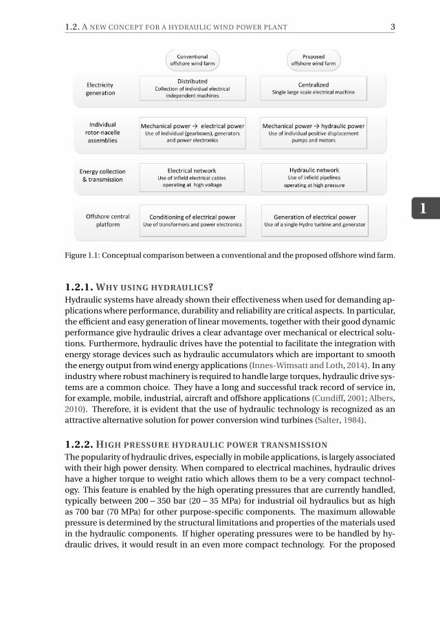
The main aspects of a hydraulic wind power plant are discussed in the following sub-
sections. A conceptual comparison between a conventional and the proposed offshore
wind farm is shown in Figure 1.1.
1.2. A NEW CONCEPT FOR A HYDRAULIC WIND POWER PLANT
1
3
Figure 1.1: Conceptual comparison between a conventional and the proposed offshore wind farm.
1.2.1. WHY USING HYDRAULICS?Hydraulic systems have already shown their effectiveness when used for demanding ap-
plications where performance, durability and reliability are critical aspects. In particular,
the efficient and easy generation of linear movements, together with their good dynamic
performance give hydraulic drives a clear advantage over mechanical or electrical solu-
tions. Furthermore, hydraulic drives have the potential to facilitate the integration with
energy storage devices such as hydraulic accumulators which are important to smooth
the energy output from wind energy applications (Innes-Wimsatt and Loth, 2014). In any
industry where robust machinery is required to handle large torques, hydraulic drive sys-
tems are a common choice. They have a long and successful track record of service in,
for example, mobile, industrial, aircraft and offshore applications (Cundiff, 2001; Albers,
2010). Therefore, it is evident that the use of hydraulic technology is recognized as an
attractive alternative solution for power conversion wind turbines (Salter, 1984).
1.2.2. HIGH PRESSURE HYDRAULIC POWER TRANSMISSION
The popularity of hydraulic drives, especially in mobile applications, is largely associated
with their high power density. When compared to electrical machines, hydraulic drives
have a higher torque to weight ratio which allows them to be a very compact technol-
ogy. This feature is enabled by the high operating pressures that are currently handled,
typically between 200− 350 bar (20− 35 MPa) for industrial oil hydraulics but as high
as 700 bar (70 MPa) for other purpose-specific components. The maximum allowable
pressure is determined by the structural limitations and properties of the materials used
in the hydraulic components. If higher operating pressures were to be handled by hy-
draulic drives, it would result in an even more compact technology. For the proposed
1
4 1. INTRODUCTION
concept, using high pressure makes it possible to reduce the top mass of the individual
rotor-nacelle assemblies. For this reason, a high potential exists to reduce the amount
of structural steel needed in the support structures as well; for a 5 MW turbine in 30 m
water depth, 1.9 ton of structural steel of the monopile can be saved for every ton of top
mass reduction (Segeren and Diepeveen, 2014). Using high pressures makes the use of
fluid power an attractive means to transmit the captured energy from the rotor-nacelle
assemblies to a central platform.
1.2.3. WATER AS HYDRAULIC FLUID
A very important aspect to be considered in fluid power technology is the selection of
the hydraulic fluid. Mineral oil still remains the leading choice as hydraulic fluid in most
industrial applications due to its physical properties over the whole range of operating
temperatures and pressures. However, the pressure on the offshore industry to become
more environmentally friendly is pushing the case for developments in water hydraulics.
Furthermore, in terms of safety, water hydraulics might be preferred due to potential fire
hazards or risk of leakage (Trostmann, 1995; Lim et al., 2003). Seawater is a vast resource
available offshore and might also be used as hydraulic fluid. It is important to consider
that seawater contains a high concentration of minerals, which give it a high degree of
hardness. It also contains dissolved gases such as oxygen and chlorine which cause cor-
rosion. Despite its corrosive nature, the use of seawater hydraulics has already been used
in some industrial applications; an example in the offshore industry includes the seawa-
ter hydraulic system for deep sea pile driving incorporating high pressure water pumps
(Schaap, 2012). The use of seawater requires the use of special filters which have to be
cleaned more frequently.
Despite the high operating pressures, large volumetric flows of either oil or water, are
required for the transmission of dozens or hundreds of MWs. Therefore, from an avail-
ability and environmental perspective, the use of water as hydraulic fluid is the preferred
choice for centralizing electricity generation in an offshore wind power plant. In combi-
nation with one or more large capacity hydro turbines, the pressurized flow of water is
used in this concept to generate electrical power in a central offshore platform.
1.2.4. HYDRO TURBINES TO CENTRALIZE ELECTRICITY GENERATION
Hydraulic turbines are the prime movers that transform the energy content of the water
into mechanical energy and whose primary function is to drive electric generators. From
the existing hydraulic turbines used in hydroelectric power plants, the Pelton turbine is
the most suitable to handle high pressures (Dixon and Hall, 2014). Pelton turbines have
been built up to a capacity of 423 MW for a single machine (Angehm, 2000) and with
operational efficiencies above 90% (Keck et al., 2000). High rotational speed, combined
with high torque, enables a compact design. Hence, a wind farm dedicated to pressurize
a water flow in a central platform requires only one or a few Pelton turbines to produce
electricity using similar technology to what is used in existing hydro-power plants. The
same principle has been envisaged in other ocean energy technologies like wave energy
farms, where flapping wave energy devices are dedicated to pressurize water into an on-
shore power plant where electricity is produced via a Pelton turbine (Whittaker et al.,
2007).
1.2. A NEW CONCEPT FOR A HYDRAULIC WIND POWER PLANT
1
5
An important characteristic of a Pelton turbine is that the nozzle, used to create the wa-
ter jet, and the runner of the turbine are not physically connected; therefore, it allows to
have a physically decoupled system between the individual wind turbines and the hy-
draulic network at the energy capture side, from the Pelton turbine and generator at the
grid side. This means that in case of an off-grid situation, the water jets can be deflected
from the hydraulic turbine, while the wind turbines can still operate under normal op-
erational conditions. The above mentioned characteristic has several advantages for the
individual turbines and the hydraulic network since they are not affected by electrical
disturbances. Electrical disturbances do impose difficulties with current wind farms, es-
pecially in complying with grid-fault ride-through requirements (Chen et al., 2009).
1.2.5. HYDRAULIC NETWORK FOR INFIELD POWER COLLECTION AND
TRANSMISSIONOne of the key aspects for having a centralized electricity generation platform is the use
of hydraulic networks to collect and transport the pressurized water from the individual
wind turbines to the generator. Similar to the electrical inter-array cable system for a
conventional offshore wind farm, the design of the hydraulic piping lay-out should con-
sider several practical and economical aspects, such as reducing the number and length
of pipelines, operational losses and installation methods. For wind farms with a large
number of turbines, it is expected that branched hydraulic networks using parallel and
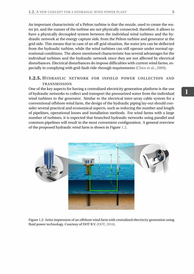
common pipelines will result in the most convenient configuration. A general overview
of the proposed hydraulic wind farm is shown in Figure 1.2.
Figure 1.2: Artist impression of an offshore wind farm with centralized electricity generation using
fluid power technology. Courtesy of DOT B.V. (DOT, 2016).
1
6 1. INTRODUCTION
1.3. REVIEW OF FLUID POWER TRANSMISSIONS IN OFFSHORE
WIND TURBINES
The use of hydraulic technology in modern wind turbines is found in different sub-
systems such as the pitch control, the drivetrain brake, the yaw system, and the filter-
cooler modules. For these applications the use of hydraulics is usually justified by their
high-power density, robust design and high controllability when compared to electro-
mechanical systems (Merritt, 1967; Murrenhoff and Linden, 1997). However, one of the
most interesting applications of hydraulic technology is its use for the power drivetrain
between the rotor and the generator. This brings yet another alternative to the existing
geared and direct-drive solutions.
The working principle behind hydraulic power transmissions is that rotating mechan-
ical power from the prime mover is converted into a fluid flow at high pressure by a
positive displacement pump; this is known as the hydrostatic principle. At the other end
of the hydraulic circuit, the fluid power is converted back to mechanical power and con-
ditioned by a hydraulic motor to a higher rotational speed with a lower torque which is
typically required by the electrical machines.
Another type of hydraulic power transmission is based on the hydrodynamic principle,
where the momentum of the fluid flow is used to transform the hydraulic power to me-
chanical power. Although the hydrodynamic transmission is widely used in ground ve-
hicles as torque converters, this particular solution it is not considered in the framework
of this thesis since the hydraulic working principle of the transmission is based on hy-
drodynamics rather than hydrostatics, the latter being the main trend for full hydraulic
transmission in wind turbines.
When compared to the commonly used geared or direct-drive transmissions, the hydro-
static transmission is particularly attractive for large offshore wind turbines for differ-
ent reasons. The first reason is its compactness, as having a more compact and light
transmission means less mass at the top of the tower. This mass reduction leads to a
significant reduction in the required amount of support structural steel (Segeren and
Diepeveen, 2014). The second reason is the possibility of having a transmission ratio
between the rotor and the generator that can be modified in a continuous manner. This
adds an extra degree of freedom from the control perspective and opens the opportunity
to explore different control strategies or physical configurations. For example, an attrac-
tive design would be allowing the use of a synchronous generator, thereby eliminating
the necessity of most power electronics.
The idea of using hydraulic transmissions in wind energy systems is not a novelty. Ex-
perimental prototypes have been developed in the 1980s, like the 6.3 kW project by the
Jacobs Energy Research Inc. (JERICO, 1981) and the 3 MW BENDIX/Shackle project (Ry-
bak, 1981). Their results reported low efficiencies and concluded that the application
of hydraulic transmission was unsuited for wind turbine applications. The main reason
was the lack of components specifically designed for the needs of efficient wind power
generation. This argument has been the main historical cause of hydraulics being dis-
regarded as a feasible option for wind turbines. Hence, the most challenging aspect of
using hydraulics has been their lower efficiency when compared to a geared and direct-
drive solution, especially when operating at conditions below rated nominal power.
1.3. REVIEW OF FLUID POWER TRANSMISSIONS IN OFFSHORE WIND TURBINES
1
7
The maturing of the fluid power industry together with modern production technolo-
gies, have resulted in an improved efficiency and reliability of hydraulic drives. Com-
mercially available pumps and motors, which could be applied in wind turbines, have
total efficiencies up to 96% for a broad range of operation (Hägglunds Drive Systems,
2014; Bosch-Rexroth, 2015). Furthermore, with the development of the digital technol-
ogy, more advanced pumps and motors have achieved efficiencies up to 98%. At the
moment, these advanced pumps and motors are in the process of being scaled close to
the power ratings of modern wind turbines (Payne et al., 2007). In parallel, efforts from
research institutes have focused on a different approach. Researchers from IFAS have
used available off-the-shelf components and different control strategies to improve the
efficiency and dynamic behaviour, reaching up to 85% efficiency at nominal conditions
in their full 1 MW test bench (Schmitz et al., 2010, 2011, 2012). An overview of the main
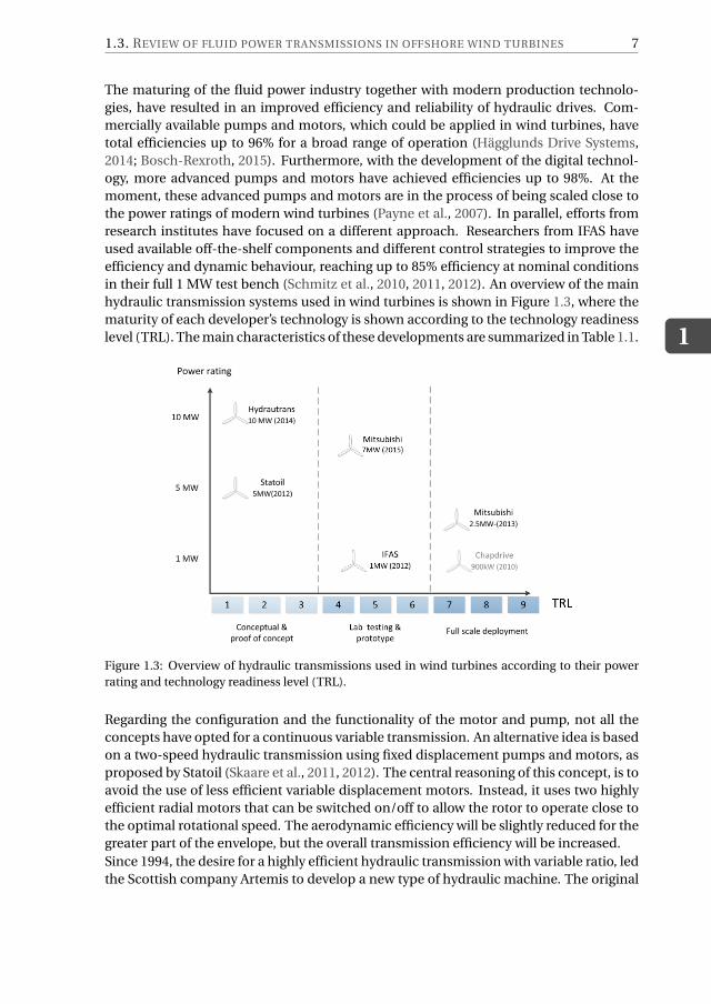
hydraulic transmission systems used in wind turbines is shown in Figure 1.3, where the
maturity of each developer’s technology is shown according to the technology readiness
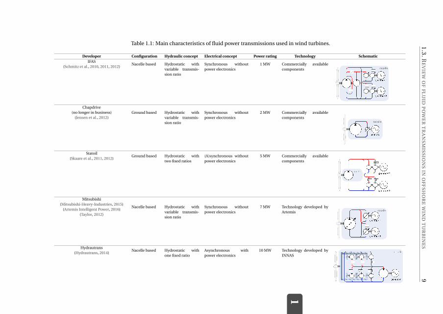
level (TRL). The main characteristics of these developments are summarized in Table 1.1.
Figure 1.3: Overview of hydraulic transmissions used in wind turbines according to their power
rating and technology readiness level (TRL).
Regarding the configuration and the functionality of the motor and pump, not all the
concepts have opted for a continuous variable transmission. An alternative idea is based
on a two-speed hydraulic transmission using fixed displacement pumps and motors, as
proposed by Statoil (Skaare et al., 2011, 2012). The central reasoning of this concept, is to
avoid the use of less efficient variable displacement motors. Instead, it uses two highly
efficient radial motors that can be switched on/off to allow the rotor to operate close to
the optimal rotational speed. The aerodynamic efficiency will be slightly reduced for the
greater part of the envelope, but the overall transmission efficiency will be increased.
Since 1994, the desire for a highly efficient hydraulic transmission with variable ratio, led
the Scottish company Artemis to develop a new type of hydraulic machine. The original

1
8 1. INTRODUCTION
idea was intended for wave and tidal energy applications, but this technology is a good
fit for wind energy developments too. Their multi-stroke radial piston pump and motor
uses computer controlled valves to engage or idle each of the individual pistons, thereby
yielding a high efficiency over the entire range of operation (Payne et al., 2007). This in-
novation was taken over by Mitsubishi Heavy Industries and implemented into a 2.5 MW
onshore wind turbine prototype in 2013. Despite their initial plans to enter the offshore
wind market with a 7 MW turbine (Mitsubishi-Heavy-Industries, 2015), it is more likely
that this drivetrain technology will only be offered as an option to the 8 MW offshore
turbine from the MHI Vestas platform.
On the other hand, other companies foresee a combination of geared and hydraulic
components in the drivetrain as a better solution. For instance, Hydrautrans proposes a
10 MW concept using a single stage gearbox with crown-gears in combination with six
hydraulic pumps of smaller size (Hydrautrans, 2014). A different ‘hybrid’ solution is the
commercial drivetrain WinDrive developed by Voith (Höhn, 2011). Their technology is
based on a hydrodynamic torque converter combined with a planetary gear. This solu-
tion also requires a two stage gearbox coupled to the main rotor.
1.3
.R
EV
IEW
OF
FL
UID
PO
WE
RT
RA
NS
MIS
SIO
NS
INO
FF
SH
OR
EW
IND
TU
RB
INE
S
1
9
Table 1.1: Main characteristics of fluid power transmissions used in wind turbines.
Developer Configuration Hydraulic concept Electrical concept Power rating Technology SchematicIFAS
(Schmitz et al., 2010, 2011, 2012)Nacelle based Hydrostatic with
variable transmis-
sion ratio
Synchronous without
power electronics
1 MW Commercially available
components
Chapdrive
(no longer in business)
(Jensen et al., 2012)
Ground based Hydrostatic with
variable transmis-
sion ratio
Synchronous without
power electronics
2 MW Commercially available
components
Statoil
(Skaare et al., 2011, 2012)Ground based Hydrostatic with
two fixed ratios
(A)synchronous without
power electronics
5 MW Commercially available
components
Mitsubishi
(Mitsubishi-Heavy-Industries, 2015)
(Artemis Intelligent Power, 2016)
(Taylor, 2012)
Nacelle based Hydrostatic with
variable transmis-
sion ratio
Synchronous without
power electronics
7 MW Technology developed by
Artemis
Hydrautrans
(Hydrautrans, 2014)Nacelle based Hydrostatic with
one fixed ratio
Asynchronous with
power electronics
10 MW Technology developed by
INNAS
1
10 1. INTRODUCTION
1.4. TECHNICAL FEASIBILITYThe technical feasibility of a hydraulic offshore wind farm using centralized electricity
generation depends on the convergence of three main aspects: the physical principles
of wind energy conversion, the available technology in the fluid-power industry and the
control strategies employed. From the conceptual to the preliminary design of the pro-
posed idea, a number of technical aspects have to be taken into account before consid-
ering the idea of centralized generation as a feasible solution. This thesis builds on with
previous research, where the use of available hydraulic technology for offshore wind en-
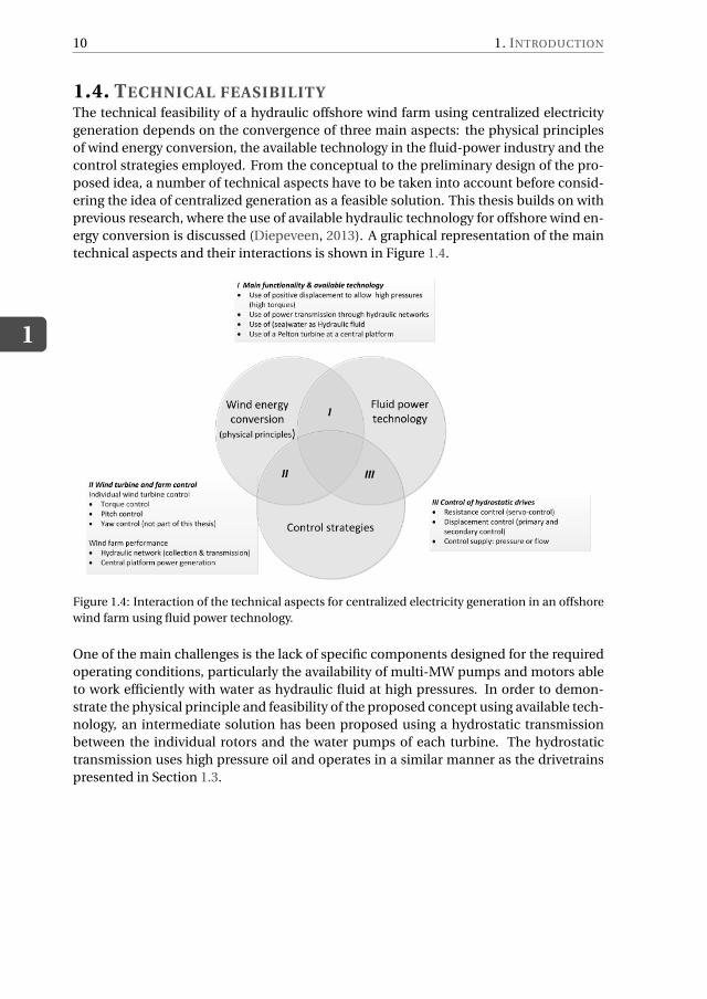
ergy conversion is discussed (Diepeveen, 2013). A graphical representation of the main
technical aspects and their interactions is shown in Figure 1.4.
Figure 1.4: Interaction of the technical aspects for centralized electricity generation in an offshore
wind farm using fluid power technology.
One of the main challenges is the lack of specific components designed for the required
operating conditions, particularly the availability of multi-MW pumps and motors able
to work efficiently with water as hydraulic fluid at high pressures. In order to demon-
strate the physical principle and feasibility of the proposed concept using available tech-
nology, an intermediate solution has been proposed using a hydrostatic transmission
between the individual rotors and the water pumps of each turbine. The hydrostatic
transmission uses high pressure oil and operates in a similar manner as the drivetrains
presented in Section 1.3.
1.4. TECHNICAL FEASIBILITY
1
11
The reasoning behind using a hydrostatic transmission as part of an intermediate solu-
tion is based on the following capabilities that this transmission offers:
• It allows to adjust the operational conditions, mainly pressures and rotational
speeds, such that commercially available components can be used.
• It gives the opportunity to explore different control strategies by using additional
degrees of freedom in the control of hydraulic drives.
• It takes advantage of the current knowledge and best practices from hydrostatic
transmissions employed in wind turbines.
On the other hand, the complexity of the concept is significantly increased by introduc-
ing extra components which has a direct impact on the reliability and efficiency of the
whole system. Nevertheless, this solution should be regarded as a step to demonstrate
the feasibility and potential advantages of the concept, before the extension to using
hydraulic power collection from a large amount of wind turbines is considered in a com-
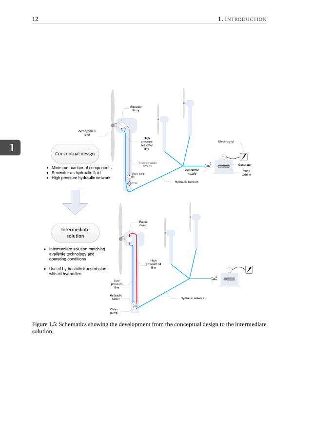
plete hydraulic wind farm. A comparison between the conceptual design and a feasible
intermediate solution, considering the available technology and operating conditions,
is shown in Figure 1.5, with the most important technical aspects is summarized in Ta-
ble 1.2.
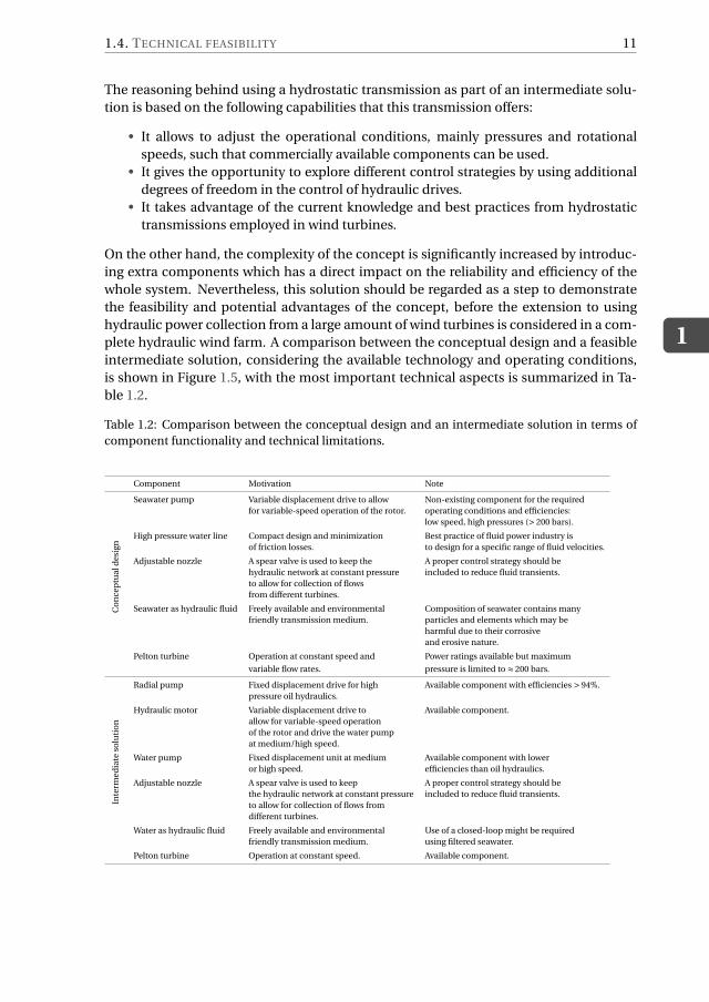
Table 1.2: Comparison between the conceptual design and an intermediate solution in terms of
component functionality and technical limitations.
Component Motivation Note
Co
nc
ep
tua
ld
esi
gn
Seawater pump Variable displacement drive to allow Non-existing component for the required
for variable-speed operation of the rotor. operating conditions and efficiencies:
low speed, high pressures (> 200 bars).
High pressure water line Compact design and minimization Best practice of fluid power industry is
of friction losses. to design for a specific range of fluid velocities.
Adjustable nozzle A spear valve is used to keep the A proper control strategy should be
hydraulic network at constant pressure included to reduce fluid transients.
to allow for collection of flows
from different turbines.
Seawater as hydraulic fluid Freely available and environmental Composition of seawater contains many
friendly transmission medium. particles and elements which may be
harmful due to their corrosive
and erosive nature.
Pelton turbine Operation at constant speed and Power ratings available but maximum
variable flow rates. pressure is limited to ≈ 200 bars.
Inte
rme
dia
teso
luti
on
Radial pump Fixed displacement drive for high Available component with efficiencies > 94%.
pressure oil hydraulics.
Hydraulic motor Variable displacement drive to Available component.
allow for variable-speed operation
of the rotor and drive the water pump
at medium/high speed.
Water pump Fixed displacement unit at medium Available component with lower
or high speed. efficiencies than oil hydraulics.
Adjustable nozzle A spear valve is used to keep A proper control strategy should be
the hydraulic network at constant pressure included to reduce fluid transients.
to allow for collection of flows from
different turbines.
Water as hydraulic fluid Freely available and environmental Use of a closed-loop might be required
friendly transmission medium. using filtered seawater.
Pelton turbine Operation at constant speed. Available component.
1
12 1. INTRODUCTION
Figure 1.5: Schematics showing the development from the conceptual design to the intermediate
solution.
1.5. THESIS OBJECTIVE AND SCOPE
1
13
1.5. THESIS OBJECTIVE AND SCOPEThis work focuses on a new concept of wind power plant, where individual wind tur-
bines are used in a hydraulic network to generate electricity in a centralized way. In Sec-
tions 1.1 and 1.2, the motivation and the main aspects of a hydraulic wind power plant
were presented. Section 1.3 gave an overview of current applications of hydraulic driv-
etrains that have been explored for its use in wind turbines. Finally Section 1.4 showed
how available technology and control strategies could be combined to achieve a feasible
technical solution of the initially proposed concept.
As with any new idea, the concept itself has raised several discussions regarding the fea-
sibility and claimed benefits and/or problems when compared to the current technol-
ogy. Before the proposed concept can be regarded or disregarded as a potential solution,
the working principle and operational behaviour of the system have to be better un-
derstood. Therefore, in order to contribute to the existing body of work, the objective
of this thesis is to understand the influence of a hydraulic network on the operational
behaviour of the individual turbines of a hydraulic wind power plant with centralized
electricity generation.
Since this concept has not been considered before, the main original contribution of
this thesis is the creation of a numerical model that is able to describe and quantify
the energy conversion process, as well as the main dynamic behaviour of a hydraulic
wind power plant, without the necessity of developing a detailed design or the need for
detailed information. In this process, the knowledge from different disciplines such as
aerodynamics, hydraulics and control will be brought together and will be used to build
a numerical model of the proposed concept. The model will be used to perform time-
domain simulations of a hypothetical wind farm under typical wind conditions. Based
on the obtained results, this thesis will provide a better basis to compare the main ad-
vantages, limitations and challenges of the proposed concept with respect to the current
solutions which generate electricity in a distributed manner.
The analysis presented for the wind turbines is being based on modifications to the
NREL 5MW baseline rotor, which is used in the field of wind energy research as a rep-
resentative utility-scale offshore turbine (Jonkman et al., 2009). With respect to the con-
trol theory, the performance and design of the controllers is limited to the framework of
linear control.
Because of the large flexibility in design and functionality that is offered by fluid power
technology, this work only discusses the results of a particular proposed concept. The
author expects that the presented work serves as an inspiration, and provides the frame-
work to analyze similar concepts or applications where both wind energy and fluid
power technology are combined.
1
14 1. INTRODUCTION
1.6. THESIS OUTLINEThe thesis is composed of seven chapters, the content of which is outlined as follows.
Chapter 2 presents a discussion of the physical modelling of the hydraulic components
comprised in a hydraulic wind farm. These components are used as building blocks in
the following chapters. Special attention is paid to the dynamics and modelling of the
flow characteristics inside the hydraulic lines. All the models are presented in terms of a
set of algebraic and ordinary differential equations (ODEs).
In Chapter 3 the main control aspects are addressed for the individual turbines. It is
shown how hydraulic technology can be used as a power drivetrain to achieve the opti-
mal aerodynamic performance of modern wind turbines. Both passive and active con-
trol strategies are proposed for a variable-speed turbine and reduced order models are
used in combination with linear control analysis tools to evaluate the performance of
the proposed controllers.
Chapter 4 describes the numerical model of two fictitious offshore wind turbines with
hydraulic transmission based on the control strategies defined in the preceding chapter.
The hydraulic transmission models are presented using the building blocks from Chap-
ter 2. Time-domain simulation are performed and the results are compared to that of a
conventional turbine for both below and above rated wind conditions.
In Chapter 5 a semi-analytical method is proposed to study the hydraulic network tran-
sients. The method is based on the impulse response of laminar flow through a hydraulic
line and includes the exact solution of a two-dimensional viscous problem in the fre-
quency domain with various interface and boundary conditions. A comparison with
existing numerical models for laminar flow dynamics is presented in three time-domain
examples.
In Chapter 6 the approach is extended from a single wind turbine towards a hydraulic
offshore wind power plant. The first part of the chapter includes a description of the
tools used to model the wind field interactions inside the offshore wind farm. Next, sim-
ulation results of a simple configuration using only two turbines are presented for dif-
ferent hydraulic networks and control options. The last part of the chapter presents the
simulation results of a small hydraulic wind power plant comprising five turbines.
Finally Chapter 7 gives the main findings and the overall conclusions of this thesis.
2PHYSICAL MODELLING OF HYDRAULIC
SYSTEMS
2.1. INTRODUCTIONThis chapter addresses the physical modelling of different hydraulic components to be
used in combination with various wind turbine subsytems. Reduced-order models are
presented in the form of algebraic and ordinary differential equations (ODEs) for their
use in time-domain simulations. The chapter is organized as follows. In Sections 2.2 and
2.3, the working principle of different hydraulic systems and their mathematical mod-
els is shown. Then, Section 2.4 describes the theory and modelling of the hydraulic line
dynamics. The line models will be used in following chapters to interconnect different
components and to form hydraulic networks. The chapter is concluded with an exam-
ple of numerical implementation and comparison of a single blocked line using modal
approximations.
2.2. HYDRAULIC DRIVES
2.2.1. POSITIVE DISPLACEMENT PUMPS/MOTORSIn fluid-power technology, the positive displacement principle refers to a fixed volume
of fluid that is trapped and forced to move into a separate confined space. In hydraulic
systems, this method has been the most efficient way of creating high pressures and
therefore the preferred option for handling large forces.
In the framework of this work, the focus is limited to rotating devices, where the phys-
ical principle is mostly based on reciprocating pistons. In this way hydraulic pumps
and motors are used to convert rotational mechanical energy into hydraulic energy and
viceversa. Positive displacement pumps and motors are characterized by a volumetric
displacement, which describes the volume of fluid obtained per rotational displacement
of the driving shaft. In the case of an ideal pump where no leakages occur, the volumetric
displacement Vp relates the volumetric flow rate Q obtained at a certain shaft rotational
velocity ωp (Merritt, 1967):
15
2
16 2. PHYSICAL MODELLING OF HYDRAULIC SYSTEMS
Q =Vp ωp (2.1)
The ideal torque τp required to obtain the pressure difference ∆p is given by the follow-
ing expression:
τp =Vp ∆p (2.2)
Hence, for an ideal hydraulic drive (no energy losses), the mechanical power given by
the product of the torque and rotational speed is equal to the hydraulic power given by
the product of the volumetric flow and the pressure difference across the machine,
τp ωp =Q ∆p (2.3)
A hydraulic pump or motor is not an ideal machine, there are energy losses that should
be considered. In practice, two different efficiencies are defined to describe the nature
of the energy losses. A volumetric efficiency is introduced in Equation 2.1 to describe
the energy losses that are associated with the volumetric flow rate such as internal or
external leakages and compressibility of the fluid. In the same manner, a mechanical ef-
ficiency is introduced in Equation 2.2 to account for the energy losses mostly associated
with friction forces. The total efficiency of a hydraulic machine is given by the product
of both the volumetric and mechanical efficiencies.
A more realistic but still simplified model of a pump is described by the following quasi-
static relations which describe the net generated volumetric flow Qp and transmitted
torque τp (Merritt, 1967).
Qp =Vp ωp −Cs ∆p (2.4)
τp =Vp ∆p +Bp ωp +C f Vp ∆p (2.5)
The internal leakage losses are described as a function of the pressure difference across
the pump through the laminar leakage coefficient Cs . For the transmitted torque, a fric-
tion torque is described with a viscous and a dry component defined with the damping
coefficient Bp and a friction coefficient C f , respectively.
For the case of a hydraulic motor the volumetric flow and transmitted torque are:
Qm =Vm ωm +Cs ∆p (2.6)
τm =Vm ∆p −Bm ωm −C f Vm ∆p (2.7)
Some of the hydraulic drives are capable of continuously modifying their volumetric dis-
placement per rotational cycle. An adjustable volumetric displacement is physically ob-
tained in different ways, where the combination of a linear actuator and a swash plate is
the most commonly used. To account for the variable displacement, Equations 2.4 and
2.5 are modified in the following manner:
Qp =Vp (e) ωp −Cs ∆p (2.8)
τp =Vp (e) ∆p +Bp ωp +C f Vp (e) ∆p (2.9)
2.2. HYDRAULIC DRIVES
2
17
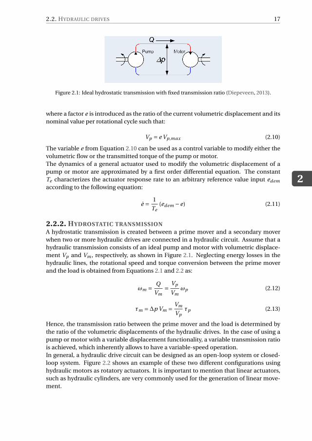
Figure 2.1: Ideal hydrostatic transmission with fixed transmission ratio (Diepeveen, 2013).
where a factor e is introduced as the ratio of the current volumetric displacement and its
nominal value per rotational cycle such that:
Vp = e Vp,max (2.10)
The variable e from Equation 2.10 can be used as a control variable to modify either the
volumetric flow or the transmitted torque of the pump or motor.
The dynamics of a general actuator used to modify the volumetric displacement of a
pump or motor are approximated by a first order differential equation. The constant
Te characterizes the actuator response rate to an arbitrary reference value input edem
according to the following equation:
e =1
Te(edem −e) (2.11)
2.2.2. HYDROSTATIC TRANSMISSIONA hydrostatic transmission is created between a prime mover and a secondary mover
when two or more hydraulic drives are connected in a hydraulic circuit. Assume that a
hydraulic transmission consists of an ideal pump and motor with volumetric displace-
ment Vp and Vm , respectively, as shown in Figure 2.1. Neglecting energy losses in the
hydraulic lines, the rotational speed and torque conversion between the prime mover
and the load is obtained from Equations 2.1 and 2.2 as:
ωm =Q
Vm=
Vp
Vmωp (2.12)
τm =∆p Vm =Vm
Vpτp (2.13)
Hence, the transmission ratio between the prime mover and the load is determined by
the ratio of the volumetric displacements of the hydraulic drives. In the case of using a
pump or motor with a variable displacement functionality, a variable transmission ratio
is achieved, which inherently allows to have a variable-speed operation.
In general, a hydraulic drive circuit can be designed as an open-loop system or closed-
loop system. Figure 2.2 shows an example of these two different configurations using
hydraulic motors as rotatory actuators. It is important to mention that linear actuators,
such as hydraulic cylinders, are very commonly used for the generation of linear move-
ment.
2
18 2. PHYSICAL MODELLING OF HYDRAULIC SYSTEMS
(a) Closed circuit (b) Open circuit
Figure 2.2: Diagrams of closed and open circuit hydraulic transmission systems (Diepeveen, 2013).
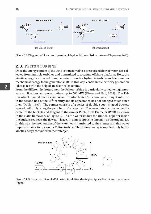
2.3. PELTON TURBINEOnce the energy content of the wind is transferred to a pressurized flow of water, it is col-
lected from multiple turbines and transmitted to a central offshore platform. Here, the
kinetic energy is extracted from the water through a hydraulic turbine and delivered as
mechanical energy to the generator shaft. In this way, centralized electricity generation
takes place with the help of an electrical machine.
From the different hydroturbines, the Pelton turbine is particularly suited to high pres-
sure applications and power ratings up to 500 MW (Dixon and Hall, 2014). The Pel-
ton wheel, named after its American inventor Lester A. Pelton, was brought into use
in the second half of the 19th century and its appearance has not changed much since
then (Doble, 1899). The runner consists of a series of double spoon shaped buckets
spaced uniformly along the periphery of a large disc. The water jets are directed to the
center of the buckets and tangent to the runner Pitch Circle Diameter (PCD) as shown
in the static framework of Figure 2.3. As the water jet hits the runner, a splitter inside
the buckets redirects the flow as it leaves in almost opposite direction as the original jet.
In this way, the momentum of the water jet is transferred to the runner and this water
impulse exerts a torque on the Pelton turbine. The driving energy is supplied only by the
kinetic energy contained in the water jet.
Figure 2.3: Schematized view of a Pelton turbine (left) and a single elliptical bucket from the runner
(right).
2.3. PELTON TURBINE
2
19
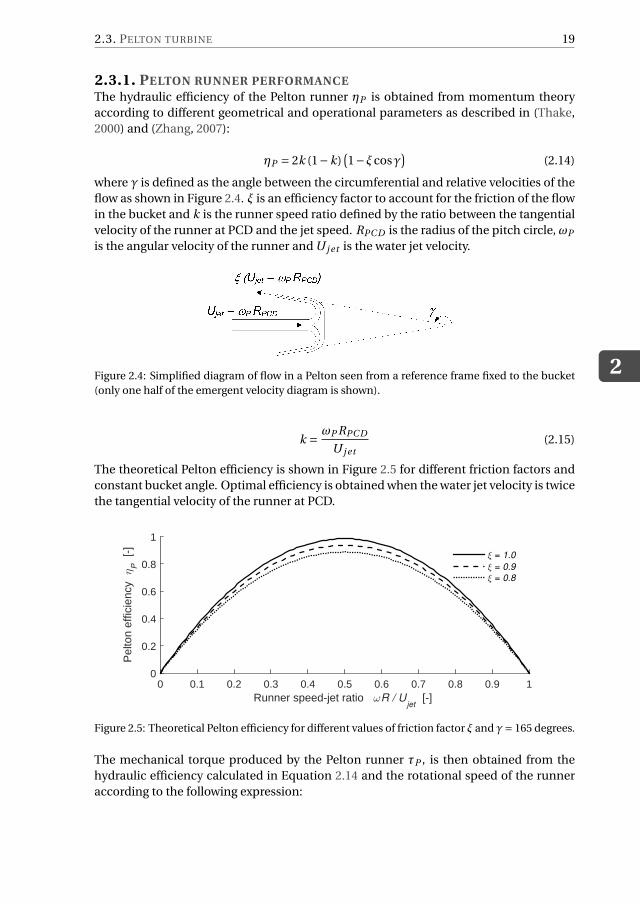
2.3.1. PELTON RUNNER PERFORMANCEThe hydraulic efficiency of the Pelton runner ηP is obtained from momentum theory
according to different geometrical and operational parameters as described in (Thake,
2000) and (Zhang, 2007):
ηP = 2k (1−k)(
1−ξcosγ)
(2.14)
where γ is defined as the angle between the circumferential and relative velocities of the
flow as shown in Figure 2.4. ξ is an efficiency factor to account for the friction of the flow
in the bucket and k is the runner speed ratio defined by the ratio between the tangential
velocity of the runner at PCD and the jet speed. RPC D is the radius of the pitch circle, ωP
is the angular velocity of the runner and U j et is the water jet velocity.
Figure 2.4: Simplified diagram of flow in a Pelton seen from a reference frame fixed to the bucket
(only one half of the emergent velocity diagram is shown).
k =ωP RPC D
U j et(2.15)
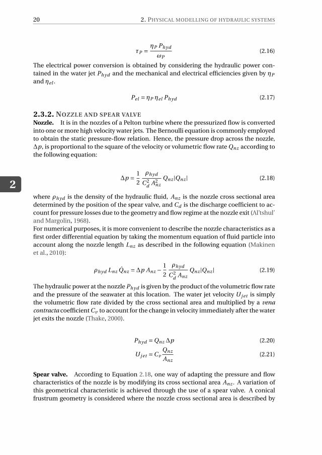
The theoretical Pelton efficiency is shown in Figure 2.5 for different friction factors and
constant bucket angle. Optimal efficiency is obtained when the water jet velocity is twice
the tangential velocity of the runner at PCD.
Runner speed-jet ratio ωR / Ujet
[-] 0 0.1 0.2 0.3 0.4 0.5 0.6 0.7 0.8 0.9 1
Pel
ton
effic
ienc
y η
P
[-]
0
0.2
0.4
0.6
0.8
1
ξ = 1.0
ξ = 0.9
ξ = 0.8
Figure 2.5: Theoretical Pelton efficiency for different values of friction factor ξ and γ= 165 degrees.
The mechanical torque produced by the Pelton runner τP , is then obtained from the
hydraulic efficiency calculated in Equation 2.14 and the rotational speed of the runner
according to the following expression:
2
20 2. PHYSICAL MODELLING OF HYDRAULIC SYSTEMS
τP =ηP Phyd
ωP(2.16)
The electrical power conversion is obtained by considering the hydraulic power con-
tained in the water jet Phyd and the mechanical and electrical efficiencies given by ηP
and ηel .
Pel = ηP ηel Phyd (2.17)
2.3.2. NOZZLE AND SPEAR VALVENozzle. It is in the nozzles of a Pelton turbine where the pressurized flow is converted
into one or more high velocity water jets. The Bernoulli equation is commonly employed
to obtain the static pressure-flow relation. Hence, the pressure drop across the nozzle,
∆p, is proportional to the square of the velocity or volumetric flow rate Qnz according to
the following equation:
∆p =1
2
ρhyd
C 2d
A2nz
Qnz |Qnz | (2.18)
where ρhyd is the density of the hydraulic fluid, Anz is the nozzle cross sectional area
determined by the position of the spear valve, and Cd is the discharge coefficient to ac-
count for pressure losses due to the geometry and flow regime at the nozzle exit (Al’tshul’
and Margolin, 1968).
For numerical purposes, it is more convenient to describe the nozzle characteristics as a
first order differential equation by taking the momentum equation of fluid particle into
account along the nozzle length Lnz as described in the following equation (Makinen
et al., 2010):
ρhyd Lnz Qnz =∆p Anz −1
2
ρhyd
C 2d
Anz
Qnz |Qnz | (2.19)
The hydraulic power at the nozzle Phyd is given by the product of the volumetric flow rate
and the pressure of the seawater at this location. The water jet velocity U j et is simply
the volumetric flow rate divided by the cross sectional area and multiplied by a vena
contracta coefficient Cv to account for the change in velocity immediately after the water
jet exits the nozzle (Thake, 2000).
Phyd =Qnz ∆p (2.20)
U j et =CvQnz
Anz(2.21)
Spear valve. According to Equation 2.18, one way of adapting the pressure and flow
characteristics of the nozzle is by modifying its cross sectional area Anz . A variation of
this geometrical characteristic is achieved through the use of a spear valve. A conical
frustrum geometry is considered where the nozzle cross sectional area is described by
2.3. PELTON TURBINE
2
21
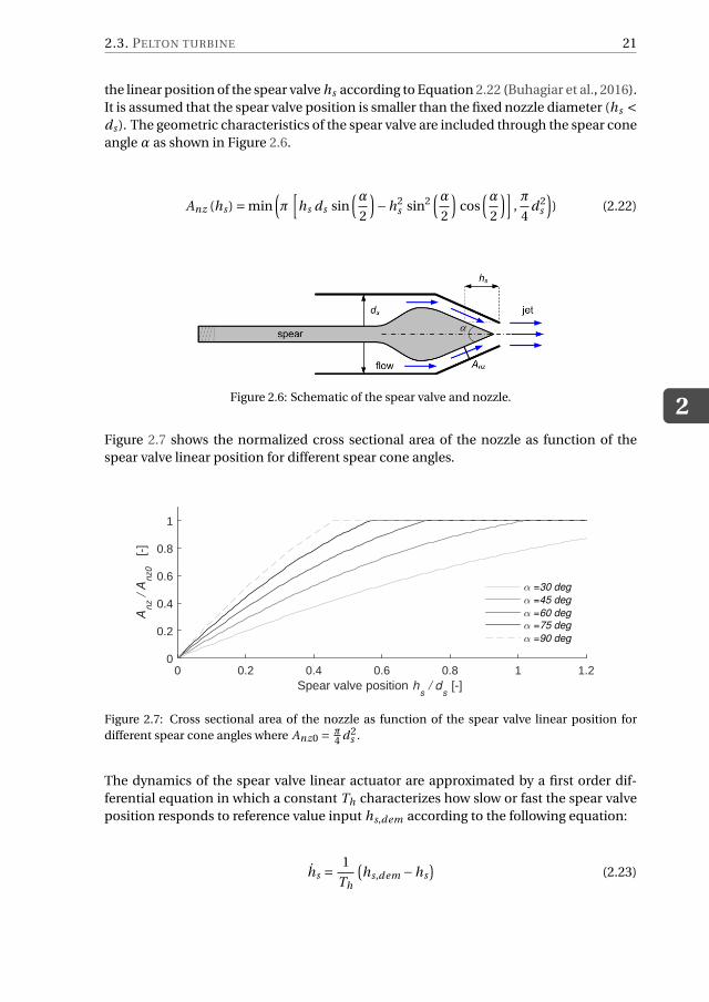
the linear position of the spear valve hs according to Equation 2.22 (Buhagiar et al., 2016).
It is assumed that the spear valve position is smaller than the fixed nozzle diameter (hs <ds ). The geometric characteristics of the spear valve are included through the spear cone
angle α as shown in Figure 2.6.
Anz (hs ) = min(
π[
hs ds sin(α
2
)
−h2s sin2
(α
2
)
cos(α
2
)]
,π
4d 2
s
)
) (2.22)
Figure 2.6: Schematic of the spear valve and nozzle.
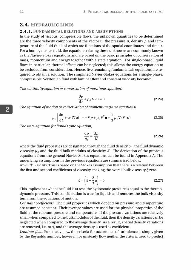
Figure 2.7 shows the normalized cross sectional area of the nozzle as function of the
spear valve linear position for different spear cone angles.
Spear valve position hs / d
s [-]
0 0.2 0.4 0.6 0.8 1 1.2
Anz /
Anz0
[-]
0
0.2
0.4
0.6
0.8
1
α =30 deg
α =45 deg
α =60 deg
α =75 deg
α =90 deg
Figure 2.7: Cross sectional area of the nozzle as function of the spear valve linear position for
different spear cone angles where Anz0 = π4 d2
s .
The dynamics of the spear valve linear actuator are approximated by a first order dif-
ferential equation in which a constant Th characterizes how slow or fast the spear valve
position responds to reference value input hs,dem according to the following equation:
hs =1
Th
(
hs,dem −hs
)
(2.23)
2
22 2. PHYSICAL MODELLING OF HYDRAULIC SYSTEMS
2.4. HYDRAULIC LINES
2.4.1. FUNDAMENTAL RELATIONS AND ASSUMPTIONSIn the study of viscous, compressible flows, the unknown quantities to be determined
are the three velocity components of the vector u, the pressure p, density ρ and tem-
perature of the fluid Θ, all of which are functions of the spatial coordinates and time t .
For a homogeneous fluid, the equations relating these unknowns are commonly known
as the Navier-Stokes equations and are based on the basic principles of conservation of
mass, momentum and energy together with a state equation. For single-phase liquid
flows in particular, thermal effects can be neglected; this allows the energy equation to
be excluded from consideration. Hence, five remaining fundamentals equations are re-
quired to obtain a solution. The simplified Navier-Stokes equations for a single-phase,
compressible Newtonian fluid with laminar flow and constant viscosity become:
The continuity equation or conservation of mass (one equation)
∂ρ
∂t+ρo ∇·u = 0 (2.24)
The equation of motion or conservation of momentum (three equations)
ρo
[
∂u
∂t+u · (∇u)
]
=−∇p +µo∇2u+1
3µo∇ (∇·u) (2.25)
The state-equation for liquids (one equation)
dρ
ρo=
dp
K(2.26)
where the fluid properties are designated through the fluid density ρo , the fluid dynamic
viscosity µo and the fluid bulk modulus of elasticity K . The derivation of the previous
equations from the general Navier-Stokes equations can be found in Appendix A. The
underlying assumptions in the previous equations are summarized below.
No bulk viscosity. This is based on the Stokes assumption that there is a relation between
the first and second coefficients of viscosity, making the overall bulk viscosity ξ zero.
ξ=(
λ+2
3µ
)
= 0 (2.27)
This implies that when the fluid is at rest, the hydrostatic pressure is equal to the thermo-
dynamic pressure. This consideration is true for liquids and removes the bulk viscosity
term from the equations of motion.
Constant coefficients. The fluid properties which depend on pressure and temperature
are assumed constant. Their average values are used for the physical properties of the
fluid at the relevant pressure and temperature. If the pressure variations are relatively
small when compared to the bulk modulus of the fluid, then the density variations can be
neglected when compared to the average density. As a result, spatial density variations
are removed, i.e. ρ(t ), and the average density is used as coefficient.
Laminar flow. For steady flow, the criteria for occurrence of turbulence is simply given
by the Reynolds number; however, for unsteady flow neither the criteria used to predict
2.4. HYDRAULIC LINES
2
23
flow instability, nor the manner in which it occurs is well understood. In the case of
an oscillating flow component which is superimposed on a mean turbulent flow, the
laminar flow solutions might be still applicable over a limited turbulent flow range. Both
physical and empirical-based corrections to the shear stress model have been proposed
for turbulent pipe transients (Vardy et al., 1993; Vardy and Brown, 1995). The correct
modelling of turbulence in transient flows is an ongoing research topic; it is not adressed
in this work.
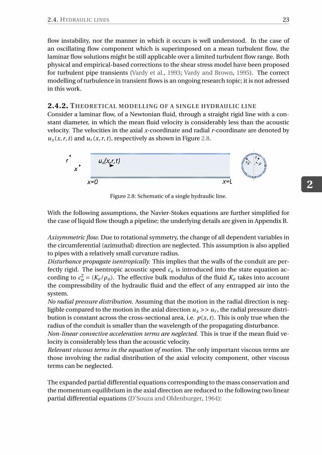
2.4.2. THEORETICAL MODELLING OF A SINGLE HYDRAULIC LINEConsider a laminar flow, of a Newtonian fluid, through a straight rigid line with a con-
stant diameter, in which the mean fluid velocity is considerably less than the acoustic
velocity. The velocities in the axial x-coordinate and radial r-coordinate are denoted by
ux (x,r, t ) and ur (x,r, t ), respectively as shown in Figure 2.8.
Figure 2.8: Schematic of a single hydraulic line.
With the following assumptions, the Navier-Stokes equations are further simplified for
the case of liquid flow though a pipeline; the underlying details are given in Appendix B.
Axisymmetric flow. Due to rotational symmetry, the change of all dependent variables in
the circumferential (azimuthal) direction are neglected. This assumption is also applied
to pipes with a relatively small curvature radius.
Disturbance propagate isentropically. This implies that the walls of the conduit are per-
fectly rigid. The isentropic acoustic speed co is introduced into the state equation ac-
cording to c2o = (Ke /ρo). The effective bulk modulus of the fluid Ke takes into account
the compressibility of the hydraulic fluid and the effect of any entrapped air into the
system.
No radial pressure distribution. Assuming that the motion in the radial direction is neg-
ligible compared to the motion in the axial direction ux >> ur , the radial pressure distri-
bution is constant across the cross-sectional area, i.e. p(x, t ). This is only true when the
radius of the conduit is smaller than the wavelength of the propagating disturbance.
Non-linear convective acceleration terms are neglected. This is true if the mean fluid ve-
locity is considerably less than the acoustic velocity.
Relevant viscous terms in the equation of motion. The only important viscous terms are
those involving the radial distribution of the axial velocity component, other viscous
terms can be neglected.
The expanded partial differential equations corresponding to the mass conservation and
the momentum equilibrium in the axial direction are reduced to the following two linear
partial differential equations (D’Souza and Oldenburger, 1964):
2
24 2. PHYSICAL MODELLING OF HYDRAULIC SYSTEMS
∂p(x, t )
∂t+ c2
oρo
[
∂ux (x,r, t )
∂x+∂ur (x,r, t )
∂r+
ur (x,r, t )
r
]
= 0 (2.28)
ρo∂ux (x,r, t )
∂t+∂p(x, t )
∂x=µo
[
∂2ux (x,r, t )
∂r 2+
1
r
∂ux (x,r, t )
∂r
]
(2.29)
The cross-sectional volumetric flow Q, is obtained through the integration of the axial
velocity across the cross-sectional area of the line with finite radius r0. The volumetric
flow is also defined as the product of the average axial velocity u(x, t ) and the cross-
sectional area:
Q(x, t ) =π r 20 u(x, t ) =
∫r0
0ux (x,r, t ) 2πr dr (2.30)
Equations 2.28 to 2.30 correspond to what is known as a two-dimensional viscous com-
pressible model or dissipative friction model (Goodson and Leonard, 1972; Stecki and
Davis, 1986).
GENERAL SOLUTION FOR A SINGLE LINE IN THE FREQUENCY DOMAIN
The solution of Equations 2.28 and 2.29 can be obtained in the frequency domain by us-
ing the Fourier transform with respect to time according to the following transformation
pair,
f (ω) =F[
f (t )]
=∫∞
−∞f (t )e −iωt dt (2.31)
f (t ) =F−1
[
f (ω)]
=1
2π
∫∞
−∞f (ω)e iωt dω (2.32)
where ω represents the frequency and i =p−1 is the imaginary unit. Let U (x,ω) =
F [u(x, t )] and P (x,ω) =F [p(x, t )]. The average velocity and the pressure are then given
in the frequency domain by the following two equations (D’Souza and Oldenburger,
1964):
U (x,ω) =[
A(ω) cosiωβ
cox +B(ω) sin
iωβ
cox
]
J0
[
i
(
iω r 20
νo
) 12
]
β2(2.33)
P (x,ω) =[
A(ω) siniωβ
cox −B(ω) cos
iωβ
cox
]
ρoco
βJ0
i
(
iω r 20
νo
) 12
(2.34)
in which A(ω) and B(ω) are the unknown integration constants to be obtained from the
applied boundary conditions, νo = µo/ρo is the kinematic viscosity of the fluid and the
constant β is expressed through the Bessel functions of the first kind J0(z) and J1(z).
2.4. HYDRAULIC LINES
2
25
β=
2
i
(
iω r 20
νo
) 12
J1
[
i
(
iω r 20
νo
) 12
]
J0
[
i
(
iω r 20
νo
) 12
]−1
− 12
(2.35)
Using the boundary conditions at the upstream section where x = 0, and at the down-
stream section with x = L, the integration constants A(ω) and B(ω) are obtained for a
single pipeline. Hence the velocity and pressure at the upstream side Uu(ω) and Pu(ω),
can be expressed in terms of the downstream velocity and pressure Ud (ω) and Pd (ω).
If the volumetric flow is used instead of the average velocity using Equation 2.30, the
following relations can be formulated in the matrix form as follows:
[
Pu(ω)
Qu(ω)
]
=
cosiωβL
co−βρo co
π r 20
siniωβL
co
π r 20
βρo cosin
iωβLco
cosiωβL
co
[
Pd (ω)
Qd (ω)
]
(2.36)
The solution for a single line can also be expressed in terms of the complex Laplace vari-
able s =σ+iω; where σ is a decay factor and ω represents the frequency. Hence, for σ= 0
Equation 2.36 is rewritten as,
[
Pu(s)
Qu(s)
]
=
cossβLco
−βρo co
π r 20
sinsβLco
π r 20
βρo cosin
sβLco
cossβLco
[
Pd (s)
Qd (s)
]
(2.37)
The previous equations are expressed more commonly in terms of hyperbolic functions
instead of trigonometric functions using the relations: sin ix = −i sinh x, and cos ix =cosh x. The hyperbolic notation is the most usual way to show the solution for a single
line as it is expressed only in terms of the line characteristic impedance Zc (s) and the
propagation operator Γ(s) (Goodson and Leonard, 1972; Stecki and Davis, 1986):
[
Pu(s)
Qu(s)
]
=[
cosh Γ(s) Zc (s) sinh Γ(s)
1Zc (s)
sinh Γ(s) cosh Γ(s)
] [
Pd (s)
Qd (s)
]
(2.38)
This general notation allows to use the solution for the different distributed parameters
models, i.e. a 1D inviscid model, or a 1D linear friction model, depending on the expres-
sion used for the terms Zc (s) and Γ(s). Using the normalized Laplace variable s = s/ωc ,
where ωc = νo/r 20 is the viscosity frequency, the line characteristic impedance Zc
(
s)
and
the propagation operator Γ(
s)
are given by Table 2.1. Two constants based on the physi-
cal properties of the fluid line are introduced, the line impedance Z0 and the dissipation
number of the line Dn which are defined respectively as:
Z0 =ρo co
πr 20
(2.39)
2
26 2. PHYSICAL MODELLING OF HYDRAULIC SYSTEMS
Dn =νoL
r 20 co
(2.40)
The value of the dissipation number is important for the transient response, as it gives
an indication of the attenuation and distortion along the line. It is given by the ratio of
the wave travel time along a line to a term indicative of the transient decay.
Table 2.1: Propagation operator Γ and line characteristic impedance Zc for different distributed
parameter models.
Γ(
s)
Zc
(
s)
Lossless modelDn s Z0(1D inviscid compressible)
Linear friction modelDn s
(
1+ 8s
)12 Z0
(
1+ 8s
)12
(1D inviscid compressible)
Dn s
1− 2
i(s)12
J1
[
i(s)12
]
J0
[
i(s)12
]
− 12
Z0
1− 2
i(s)12
J1
(
i(s)12
)
J0
(
i(s)12
)
− 12
Dissipative friction model
(2D viscous compressible)
As an example consider the case of a ‘blocked pipeline’, where the downstream flow rate
is zero, Qd (s) = 0. Hence, the downstream pressure is expressed as a function of the
upstream pressure according to
Pd (s) =1
cosh Γ(s)Pu(s) (2.41)
A comparison between the different models is shown in Figure 2.9. The frequency re-
sponse of the downstream pressure of a blocked line is shown for certain pipeline char-
acteristics.
CAUSALITY AND PHYSICAL REALIZATION
The solution presented in Equation 2.38 is a non-causal representation which gives a
good insight in the pipeline dynamics. However, for simulation purposes, it is a primary
requirement to establish the causality of the model representation according to different
boundary conditions. The physical realization of the pipeline dynamics is a combination
of two propagation effects, one in forward direction at the upstream line end boundary,
and one in backward direction at the downstream line end boundary. This means, that
in terms of the physical variables p and Q, one of them should be chosen as input vari-
able at the upstream end, and one of them should also be chosen as an input at the
downstream end.
Therefore, there are four possible input-output configurations corresponding to the four
possible sets of physically realizable boundary conditions:
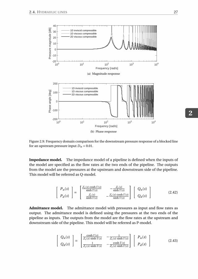
2.4. HYDRAULIC LINES
2
27
Frequency [rad/s]100 101 102 103 104
Pre
ssur
e m
agni
tude
[dB
]
-20
-10
0
10
20
30
40
1D inviscid compressible1D viscous compressible2D viscous compressible
(a) Magnitude response
Frequency [rad/s]100 101 102 103 104
Pha
se a
ngle
[deg
]
-200
-100
0
100
200
1D inviscid compressible1D viscous compressible2D viscous compressible
(b) Phase response
Figure 2.9: Frequency domain comparison for the downstream pressure response of a blocked line
for an upstream pressure input Dn = 0.01.
Impedance model. The impedance model of a pipeline is defined when the inputs of
the model are specified as the flow rates at the two ends of the pipeline. The outputs
from the model are the pressures at the upstream and downstream side of the pipeline.
This model will be referred as Q-model.
[
Pu(s)
Pd (s)
]
=
Zc (s) cosh Γ(s)sinh Γ(s)
− Zc (s)sinh Γ(s)
Zc (s)sinh Γ(s)
− Zc (s) cosh Γ(s)sinh Γ(s)
[
Qu(s)
Qd (s)
]
(2.42)
Admittance model. The admittance model with pressures as input and flow rates as
output. The admittance model is defined using the pressures at the two ends of the
pipeline as inputs. The outputs from the model are the flow rates at the upstream and
downstream side of the pipeline. This model will be referred as P-model.
[
Qu(s)
Qd (s)
]
=
cosh Γ(s)Zc (s) sinh Γ(s)
− 1Zc (s) sinh Γ(s)
1Zc (s) sinh Γ(s)
− cosh Γ(s)Zc (s) sinh Γ(s)
[
Pu(s)
Pd (s)
]
(2.43)
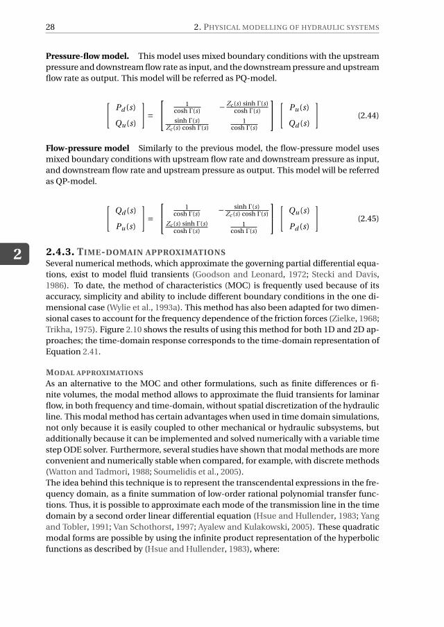
2
28 2. PHYSICAL MODELLING OF HYDRAULIC SYSTEMS
Pressure-flow model. This model uses mixed boundary conditions with the upstream
pressure and downstream flow rate as input, and the downstream pressure and upstream
flow rate as output. This model will be referred as PQ-model.
[
Pd (s)
Qu(s)
]
=
1cosh Γ(s) − Zc (s) sinh Γ(s)
cosh Γ(s)
sinh Γ(s)Zc (s) cosh Γ(s)
1cosh Γ(s)
[
Pu(s)
Qd (s)
]
(2.44)
Flow-pressure model Similarly to the previous model, the flow-pressure model uses
mixed boundary conditions with upstream flow rate and downstream pressure as input,
and downstream flow rate and upstream pressure as output. This model will be referred
as QP-model.
[
Qd (s)
Pu(s)
]
=
1cosh Γ(s) − sinh Γ(s)
Zc (s) cosh Γ(s)
Zc (s) sinh Γ(s)cosh Γ(s)
1cosh Γ(s)
[
Qu(s)
Pd (s)
]
(2.45)
2.4.3. TIME-DOMAIN APPROXIMATIONSSeveral numerical methods, which approximate the governing partial differential equa-
tions, exist to model fluid transients (Goodson and Leonard, 1972; Stecki and Davis,
1986). To date, the method of characteristics (MOC) is frequently used because of its
accuracy, simplicity and ability to include different boundary conditions in the one di-
mensional case (Wylie et al., 1993a). This method has also been adapted for two dimen-
sional cases to account for the frequency dependence of the friction forces (Zielke, 1968;
Trikha, 1975). Figure 2.10 shows the results of using this method for both 1D and 2D ap-
proaches; the time-domain response corresponds to the time-domain representation of
Equation 2.41.
MODAL APPROXIMATIONS
As an alternative to the MOC and other formulations, such as finite differences or fi-
nite volumes, the modal method allows to approximate the fluid transients for laminar
flow, in both frequency and time-domain, without spatial discretization of the hydraulic
line. This modal method has certain advantages when used in time domain simulations,
not only because it is easily coupled to other mechanical or hydraulic subsystems, but
additionally because it can be implemented and solved numerically with a variable time
step ODE solver. Furthermore, several studies have shown that modal methods are more
convenient and numerically stable when compared, for example, with discrete methods
(Watton and Tadmori, 1988; Soumelidis et al., 2005).
The idea behind this technique is to represent the transcendental expressions in the fre-
quency domain, as a finite summation of low-order rational polynomial transfer func-
tions. Thus, it is possible to approximate each mode of the transmission line in the time
domain by a second order linear differential equation (Hsue and Hullender, 1983; Yang
and Tobler, 1991; Van Schothorst, 1997; Ayalew and Kulakowski, 2005). These quadratic
modal forms are possible by using the infinite product representation of the hyperbolic
functions as described by (Hsue and Hullender, 1983), where:
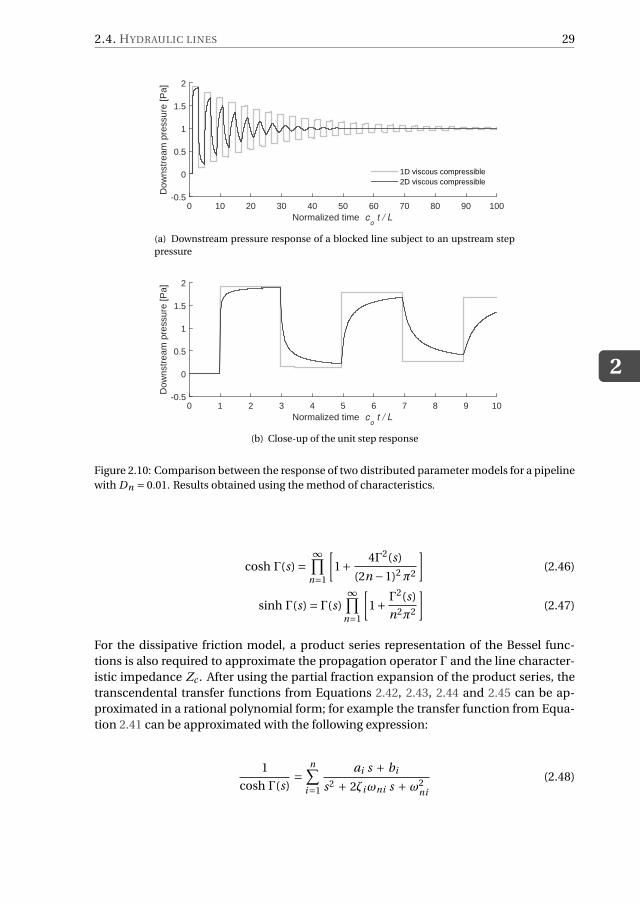
2.4. HYDRAULIC LINES
2
29
Normalized time co t / L
0 10 20 30 40 50 60 70 80 90 100
Dow
nstr
eam
pre
ssur
e [P
a]
-0.5
0
0.5
1
1.5
2
1D viscous compressible2D viscous compressible
(a) Downstream pressure response of a blocked line subject to an upstream step
pressure
Normalized time co t / L
0 1 2 3 4 5 6 7 8 9 10
Dow
nstr
eam
pre
ssur
e [P
a]
-0.5
0
0.5
1
1.5
2
(b) Close-up of the unit step response
Figure 2.10: Comparison between the response of two distributed parameter models for a pipeline
with Dn = 0.01. Results obtained using the method of characteristics.
cosh Γ(s) =∞∏
n=1
[
1+4Γ2(s)
(2n −1)2π2
]
(2.46)
sinh Γ(s) = Γ(s)∞∏
n=1
[
1+Γ
2(s)
n2π2
]
(2.47)
For the dissipative friction model, a product series representation of the Bessel func-
tions is also required to approximate the propagation operator Γ and the line character-
istic impedance Zc . After using the partial fraction expansion of the product series, the
transcendental transfer functions from Equations 2.42, 2.43, 2.44 and 2.45 can be ap-
proximated in a rational polynomial form; for example the transfer function from Equa-
tion 2.41 can be approximated with the following expression:
1
cosh Γ(s)=
n∑
i=1
ai s + bi
s2 + 2ζiωni s + ω2ni
(2.48)
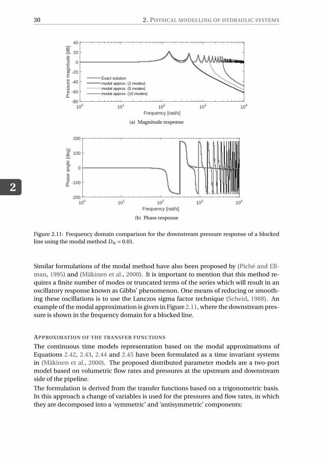
2
30 2. PHYSICAL MODELLING OF HYDRAULIC SYSTEMS
Frequency [rad/s]100 101 102 103 104
Pre
ssur
e m
agni
tude
[dB
]
-80
-60
-40
-20
0
20
40
Exact solutionmodal approx. (2 modes)modal approx. (5 modes)modal approx. (10 modes)
(a) Magnitude response
Frequency [rad/s]100 101 102 103 104
Pha
se a
ngle
[deg
]
-200
-100
0
100
200
(b) Phase response
Figure 2.11: Frequency domain comparison for the downstream pressure response of a blocked
line using the modal method Dn = 0.01.
Similar formulations of the modal method have also been proposed by (Piché and Ell-
man, 1995) and (Mäkinen et al., 2000). It is important to mention that this method re-
quires a finite number of modes or truncated terms of the series which will result in an
oscillatory response known as Gibbs’ phenomenon. One means of reducing or smooth-
ing these oscillations is to use the Lanczos sigma factor technique (Scheid, 1988). An
example of the modal approximation is given in Figure 2.11, where the downstream pres-
sure is shown in the frequency domain for a blocked line.
APPROXIMATION OF THE TRANSFER FUNCTIONS
The continuous time models representation based on the modal approximations of
Equations 2.42, 2.43, 2.44 and 2.45 have been formulated as a time invariant systems
in (Mäkinen et al., 2000). The proposed distributed parameter models are a two-port
model based on volumetric flow rates and pressures at the upstream and downstream
side of the pipeline.
The formulation is derived from the transfer functions based on a trigonometric basis.
In this approach a change of variables is used for the pressures and flow rates, in which
they are decomposed into a ‘symmetric’ and ‘antisymmetric’ components:
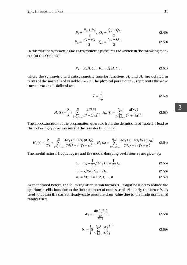
2.4. HYDRAULIC LINES
2
31
Ps =Pu +Pd
2, Qs =
Qu +Qd
2(2.49)
Pa =Pu −Pd
2, Qa =
Qu −Qd
2(2.50)
In this way the symmetric and antisymmetric pressures are written in the following man-
ner for the Q-model,
Ps = Z0HsQs , Pa = Z0HaQa (2.51)
where the symmetric and antisymmetric transfer functions Hs and Ha are defined in
terms of the normalized variable s = Ts. The physical parameter T , represents the wave
travel time and is defined as:
T =L
co(2.52)
Hs (s) =2
s+
n∑
i=2,4,...
4Γ2/s
Γ2 + (iπ)2, Ha (s) =
n−1∑
i=1,3,...
4Γ2/s
Γ2 + (iπ)2(2.53)
The approximation of the propagation operator from the definitions of Table 2.1 lead to
the following approximations of the transfer functions:
Hs (s) =2
Ts+
n∑
i=2,4,...
4σi Ts +4σi (8Dn)
T 2s2 +ǫi Ts +ω2i
, Ha (s) =n−1∑
i=1,3,...
4σi Ts +4σi bn (8Dn)
T 2s2 +ǫi Ts +ω2i
(2.54)
The modal natural frequency ωi and the modal damping coefficient ǫi are given by:
ωi =αi −1
2
√
2αi Dn +1
2Dn (2.55)
ǫi =√
2αi Dn +Dn (2.56)
αi = iπ, i = 1,2,3, . . . ,n (2.57)
As mentioned before, the following attenuation factors σi , might be used to reduce the
spurious oscillations due to the finite number of modes used. Similarly, the factor bn , is
used to obtain the correct steady-state pressure drop value due to the finite number of
modes used.
σi =sin
(
iπn+1
)
iπn+1
, (2.58)
bn =(
8n−1∑
i=1,3,...
σi
ω2i
)−1
(2.59)
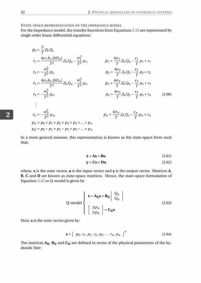
2
32 2. PHYSICAL MODELLING OF HYDRAULIC SYSTEMS
STATE-SPACE REPRESENTATION OF THE IMPEDANCE MODEL
For the impedance model, the transfer functions from Equations 2.53 are represented by
single order linear differential equations:
p0 =2
TZ0 Qs
r1 =4σ1bn (8Dn)
T 2Z0 Qa −
ω21
T 2p1, p1 =
4σ1
TZ0 Qa −
ǫ1
Tp1 + r1
r2 =−ω2
2
T 2p2, p2 =
4σ2
TZ0 Qs −
ǫ2
Tp2 + r2
r3 =4σ3bn (8Dn)
T 2Z0 Qa −
ω23
T 2p3, p3 =
4σ3
TZ0 Qa −
ǫ3
Tp3 + r3
r4 =−ω2
4
T 2p4, p4 =
4σ4
TZ0 Qs −
ǫ4
Tp4 + r4 (2.60)
...
rn =−ω2
n
T 2pn , pn =
4σn
TZ0 Qs −
ǫn
Tpn + rn
pu = p0 +p1 +p2 +p3 +p4 + ...+pn
pd = p0 −p1 +p2 −p3 +p4 − ...+pn
In a more general manner, this representation is known as the state-space form such
that:
x = Ax+Bu (2.61)
y = Cx+Du (2.62)
where, x is the state vector, u is the input vector and y is the output vector. Matrices A,
B, C and D are known as state-space matrices. Hence, the state-space formulation of
Equation 2.42 or Q-model is given by
Q-model
x = AQx+BQ
[
Qu
Qd
]
[
∆pu
∆pd
]
= CQx
(2.63)
Here, x is the state vector given by:
x =[
p0, r1, p1, r2, p2, . . . rn , pn
]T(2.64)
The matrices AQ, BQ and CQ are defined in terms of the physical parameters of the hy-
draulic line:
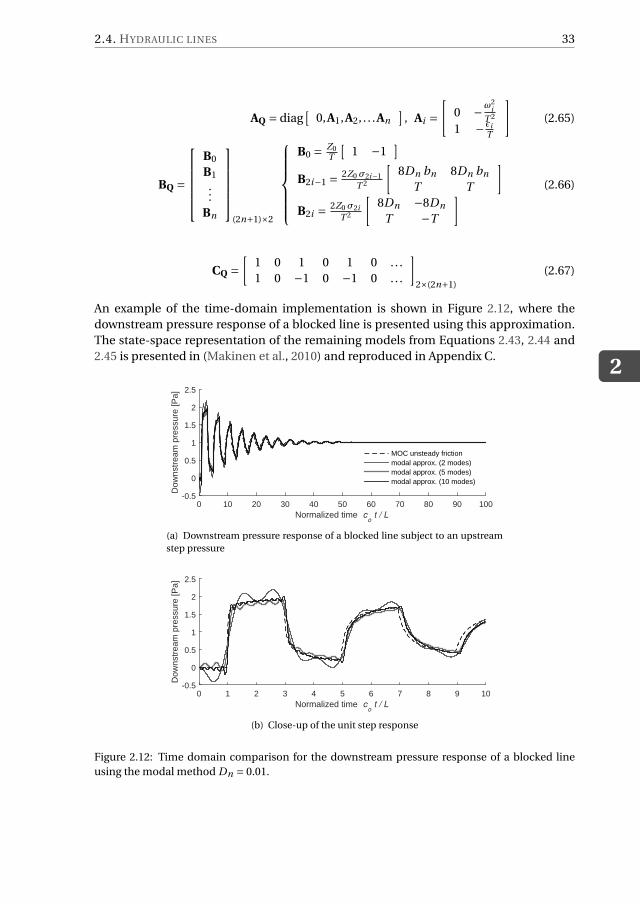
2.4. HYDRAULIC LINES
2
33
AQ = diag[
0,A1,A2, . . .An
]
, Ai =[
0 −ω2i
T 2
1 − ǫi
T
]
(2.65)
BQ =
B0
B1
...
Bn
(2n+1)×2
B0 = Z0
T
[
1 −1]
B2i−1 = 2Z0 σ2i−1
T 2
[
8Dn bn 8Dn bn
T T
]
B2i = 2Z0 σ2i
T 2
[
8Dn −8Dn
T −T
]
(2.66)
CQ =[
1 0 1 0 1 0 . . .
1 0 −1 0 −1 0 . . .
]
2×(2n+1)
(2.67)
An example of the time-domain implementation is shown in Figure 2.12, where the
downstream pressure response of a blocked line is presented using this approximation.
The state-space representation of the remaining models from Equations 2.43, 2.44 and
2.45 is presented in (Makinen et al., 2010) and reproduced in Appendix C.
Normalized time co t / L
0 10 20 30 40 50 60 70 80 90 100
Dow
nstr
eam
pre
ssur
e [P
a]
-0.5
0
0.5
1
1.5
2
2.5
MOC unsteady frictionmodal approx. (2 modes)modal approx. (5 modes)modal approx. (10 modes)
(a) Downstream pressure response of a blocked line subject to an upstream
step pressure
Normalized time co t / L
0 1 2 3 4 5 6 7 8 9 10
Dow
nstr
eam
pre
ssur
e [P
a]
-0.5
0
0.5
1
1.5
2
2.5
(b) Close-up of the unit step response
Figure 2.12: Time domain comparison for the downstream pressure response of a blocked line
using the modal method Dn = 0.01.

3CONTROL ASPECTS
3.1. INTRODUCTIONFor an offshore wind farm, it is essential that the proper operation of every single turbine
is maintained independently of the technology used for the energy transmission. To this
end, active control actions are required by every single turbine to comply with the dif-
ferent objectives such as power regulation and load mitigation among others. The term
‘active control’, refers to the general manipulation of the turbine properties or settings
during operation.
In modern wind turbines, mainly three independent control actions are used to ensure a
proper aerodynamic performance for the different operating regions. The first one is to
orient the whole rotor-nacelle assembly towards the main wind direction in such a way
that it perpendicularly faces the wind stream; this action is referred as yaw control. The
second one is to change the orientation of the blades to influence the aerodynamic loads
acting on the rotor; this action is known as pitch control. The third action is commonly
referred to as variable-speed operation and consists in adjusting the rotational velocity
of the rotor between certain limits. This last control operation can be achieved in two
different manners: by modifying the blades pitch angle, or by applying a torque to accel-
erate or decelerate the rotor through the electrical generator and power electronics; this
control action is known as generator torque control.
The so-called variable-speed operation is of particular interest in the framework of this
thesis because by removing the individual generators and power electronics from the
turbines, as stated in the motivation of this work, the hydraulic drives need to replace
the control actions to achieve the same or at least a similar variable-speed functionality.
Therefore, this chapter explores alternative solutions and limitations of the rotor-speed
control for both active and passive hydraulic configurations. Both the yaw and pitch
control strategies will remain unchanged with respect to conventional modern wind tur-
bines.
Parts of this chapter have been published in Journal of Physics: Conference Series, 555(1) (Diepeveen and Jar-
quin Laguna, 2014) and are reproduced here with permission of the co-author.
35
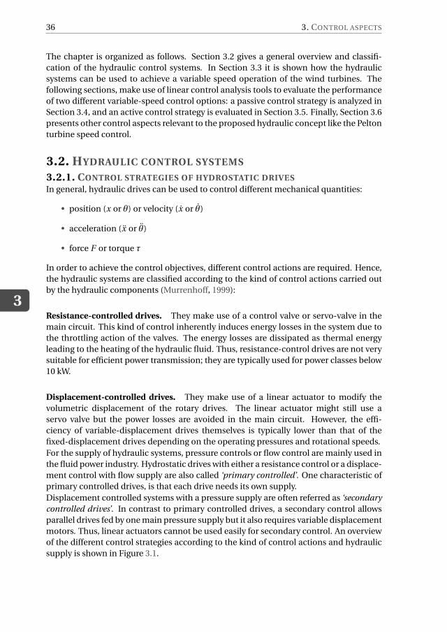
3
36 3. CONTROL ASPECTS
The chapter is organized as follows. Section 3.2 gives a general overview and classifi-
cation of the hydraulic control systems. In Section 3.3 it is shown how the hydraulic
systems can be used to achieve a variable speed operation of the wind turbines. The
following sections, make use of linear control analysis tools to evaluate the performance
of two different variable-speed control options: a passive control strategy is analyzed in
Section 3.4, and an active control strategy is evaluated in Section 3.5. Finally, Section 3.6
presents other control aspects relevant to the proposed hydraulic concept like the Pelton
turbine speed control.
3.2. HYDRAULIC CONTROL SYSTEMS
3.2.1. CONTROL STRATEGIES OF HYDROSTATIC DRIVESIn general, hydraulic drives can be used to control different mechanical quantities:
• position (x or θ) or velocity (x or θ)
• acceleration (x or θ)
• force F or torque τ
In order to achieve the control objectives, different control actions are required. Hence,
the hydraulic systems are classified according to the kind of control actions carried out
by the hydraulic components (Murrenhoff, 1999):
Resistance-controlled drives. They make use of a control valve or servo-valve in the
main circuit. This kind of control inherently induces energy losses in the system due to
the throttling action of the valves. The energy losses are dissipated as thermal energy
leading to the heating of the hydraulic fluid. Thus, resistance-control drives are not very
suitable for efficient power transmission; they are typically used for power classes below
10 kW.
Displacement-controlled drives. They make use of a linear actuator to modify the
volumetric displacement of the rotary drives. The linear actuator might still use a
servo valve but the power losses are avoided in the main circuit. However, the effi-
ciency of variable-displacement drives themselves is typically lower than that of the
fixed-displacement drives depending on the operating pressures and rotational speeds.
For the supply of hydraulic systems, pressure controls or flow control are mainly used in
the fluid power industry. Hydrostatic drives with either a resistance control or a displace-
ment control with flow supply are also called ‘primary controlled’. One characteristic of
primary controlled drives, is that each drive needs its own supply.
Displacement controlled systems with a pressure supply are often referred as ‘secondary
controlled drives’. In contrast to primary controlled drives, a secondary control allows
parallel drives fed by one main pressure supply but it also requires variable displacement
motors. Thus, linear actuators cannot be used easily for secondary control. An overview
of the different control strategies according to the kind of control actions and hydraulic
supply is shown in Figure 3.1.
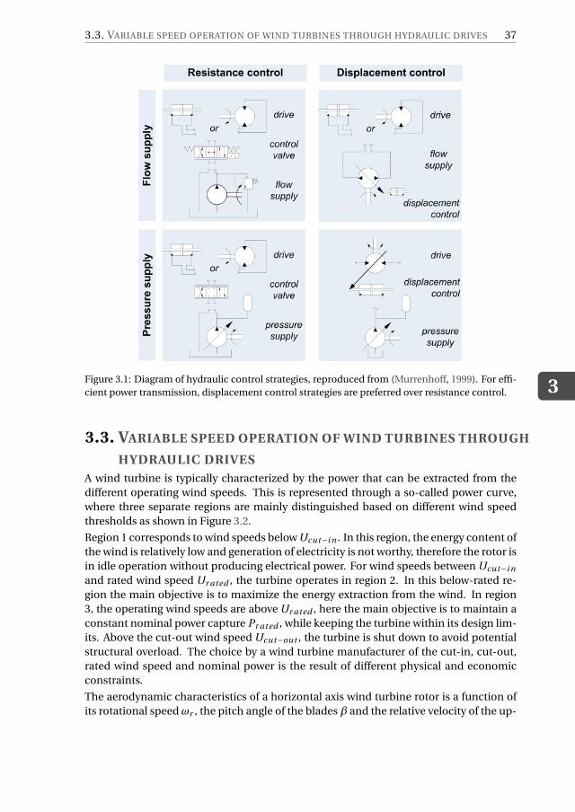
3.3. VARIABLE SPEED OPERATION OF WIND TURBINES THROUGH HYDRAULIC DRIVES
3
37
Figure 3.1: Diagram of hydraulic control strategies, reproduced from (Murrenhoff, 1999). For effi-
cient power transmission, displacement control strategies are preferred over resistance control.
3.3. VARIABLE SPEED OPERATION OF WIND TURBINES THROUGH
HYDRAULIC DRIVESA wind turbine is typically characterized by the power that can be extracted from the
different operating wind speeds. This is represented through a so-called power curve,
where three separate regions are mainly distinguished based on different wind speed
thresholds as shown in Figure 3.2.
Region 1 corresponds to wind speeds below Ucut−i n . In this region, the energy content of
the wind is relatively low and generation of electricity is not worthy, therefore the rotor is
in idle operation without producing electrical power. For wind speeds between Ucut−i n
and rated wind speed Ur ated , the turbine operates in region 2. In this below-rated re-
gion the main objective is to maximize the energy extraction from the wind. In region
3, the operating wind speeds are above Ur ated , here the main objective is to maintain a
constant nominal power capture Pr ated , while keeping the turbine within its design lim-
its. Above the cut-out wind speed Ucut−out , the turbine is shut down to avoid potential
structural overload. The choice by a wind turbine manufacturer of the cut-in, cut-out,
rated wind speed and nominal power is the result of different physical and economic
constraints.
The aerodynamic characteristics of a horizontal axis wind turbine rotor is a function of
its rotational speed ωr , the pitch angle of the blades β and the relative velocity of the up-
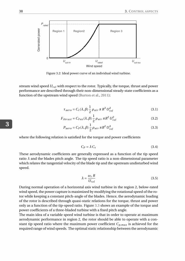
3
38 3. CONTROL ASPECTS
Wind speed
Ucut-in
Urated
Ucut-out
Ge
ne
rate
d p
ow
er
0
Prated
Region 1 Region2 Region 3
Figure 3.2: Ideal power curve of an individual wind turbine.
stream wind speed Ur el with respect to the rotor. Typically, the torque, thrust and power
performance are described through their non-dimensional steady-state coefficients as a
function of the upstream wind speed (Burton et al., 2011):
τaer o =Cτ(λ,β)1
2ρai r πR3 U 2
r el (3.1)
Fthr ust =CF ax (λ,β)1
2ρai r πR2 U 2
r el (3.2)
Paer o =CP (λ,β)1
2ρai r πR2 U 3
r el (3.3)
where the following relation is satisfied for the torque and power coefficients
CP =λCτ (3.4)
These aerodynamic coefficients are generally expressed as a function of the tip speed
ratio λ and the blades pitch angle. The tip speed ratio is a non-dimensional parameter
which relates the tangential velocity of the blade tip and the upstream undisturbed wind
speed.
λ=ωr R
Ur el(3.5)
During normal operation of a horizontal axis wind turbine in the region 2, below-rated
wind speed, the power capture is maximized by modifying the rotational speed of the ro-
tor while keeping a constant pitch-angle of the blades. Hence, the aerodynamic loading
of the rotor is described through quasi-static relations for the torque, thrust and power
only as a function of the tip-speed ratio. Figure 3.3 shows an example of the torque and
power coefficients of a three-bladed turbine with a fixed pitch angle.
The main idea of a variable speed wind turbine is that in order to operate at maximum
aerodynamic performance in region 2, the rotor should be able to operate with a con-
stant tip speed ratio where the maximum power coefficient Cp,max is achieved for the
required range of wind speeds. The optimal static relationship between the aerodynamic
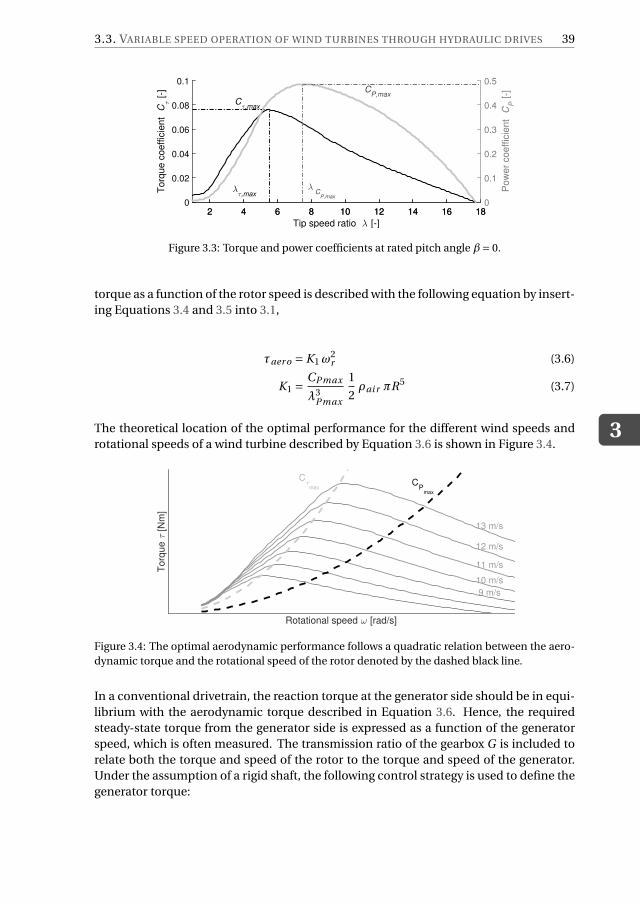
3.3. VARIABLE SPEED OPERATION OF WIND TURBINES THROUGH HYDRAULIC DRIVES
3
39
Tip speed ratio λ [-]
2 4 6 8 10 12 14 16 18
To
rqu
e c
oe
ffic
ien
t C
τ [
-]
0
0.02
0.04
0.06
0.08
0.1
Cτ,max
λτ,max
2 4 6 8 10 12 14 16 18
Po
we
r co
eff
icie
nt
CP [
-]
0
0.1
0.2
0.3
0.4
0.5 C
P,max
λ C
P,max
Figure 3.3: Torque and power coefficients at rated pitch angle β= 0.
torque as a function of the rotor speed is described with the following equation by insert-
ing Equations 3.4 and 3.5 into 3.1,
τaer o = K1 ω2r (3.6)
K1 =CPmax
λ3Pmax
1
2ρai r πR5 (3.7)
The theoretical location of the optimal performance for the different wind speeds and
rotational speeds of a wind turbine described by Equation 3.6 is shown in Figure 3.4.
Rotational speed ω [rad/s]
Torq
ue τ
[N
m]
13 m/s
12 m/s
11 m/s
10 m/s
9 m/s
Cτ
maxC
Pmax
Figure 3.4: The optimal aerodynamic performance follows a quadratic relation between the aero-
dynamic torque and the rotational speed of the rotor denoted by the dashed black line.
In a conventional drivetrain, the reaction torque at the generator side should be in equi-
librium with the aerodynamic torque described in Equation 3.6. Hence, the required
steady-state torque from the generator side is expressed as a function of the generator
speed, which is often measured. The transmission ratio of the gearbox G is included to
relate both the torque and speed of the rotor to the torque and speed of the generator.
Under the assumption of a rigid shaft, the following control strategy is used to define the
generator torque:
3
40 3. CONTROL ASPECTS
τg en = K2 ω2g en (3.8)
K2 =CPmax
G3λ3Pmax
1
2ρai r πR5 (3.9)
From above equations, it can be observed that for maximum aerodynamic performance,
the ideal steady-state relation between the torque and the rotational speed follows a
quadratic function. A simple but satisfactory way of incorporating a variable speed op-
eration, is to use this quadratic relation to set the torque demand of the generator as a
function of the measured generator speed.
The quadratic relation based on the measured generator speed is widely used because of
its simplicity, stability and smoothness. However in turbulent winds, the large rotational
inertia of the rotor prevents it from changing its speed fast enough, resulting in small
deviations from the optimal point of operation with a reduced CP . In this case, other
control strategies, such as Proportional-Integral (PI) control with an indirect estimation
of the wind speed have also been used to improve the performance of the variable-speed
rotor (Bossanyi, 2000; Bianchi et al., 1997). Furthermore, additional controllers might
be added to the reference generator-torque control to account for structural vibrations.
These vibrations are caused by the excitation of certain structural modes of the turbine.
In particular, the first tower fore-aft vibrational mode and the drivetrain torsional mode
are important as they have a direct impact on the turbine response and the available
measurements (Bossanyi and Witcher, 2009).
3.3.1. ALTERNATIVES TO REPLACE THE TORQUE CONTROLLERIn order to achieve a variable speed operation in wind turbines using hydraulic drives,
the generator torque control strategy has to be replaced. Two different modes of op-
eration have been explored in this work: a passive or compliant control, and an active
control strategy.
PASSIVE TORQUE CONTROL STRATEGY
It is possible to configure the fluid power transmission system in such a way that no form
of active control is required to adjust the rotor speed below rated wind speed conditions.
From this perspective, the passive control is an inherent property or compliant charac-
teristic of the system. The idea behind the passive control is to couple the rotor to a fixed
displacement pump and a nozzle. A high pressure line is used to conduct the pressurized
flow of hydraulic fluid into a nozzle. The flow through the nozzle induces a pressure in
the pump which determines the transmitted torque. As can be seen from Equation 2.18,
the pressure difference along the nozzle is proportional to the square of the flow rate.
The flow rate, is directly proportional to the rotational speed of the pump according to
Equation 2.1, thus:
∆p ∝Q2nz
∝ω2p (3.10)
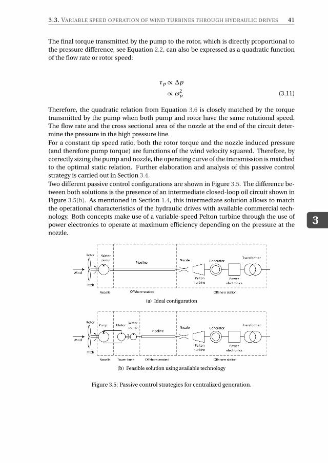
3.3. VARIABLE SPEED OPERATION OF WIND TURBINES THROUGH HYDRAULIC DRIVES
3
41
The final torque transmitted by the pump to the rotor, which is directly proportional to
the pressure difference, see Equation 2.2, can also be expressed as a quadratic function
of the flow rate or rotor speed:
τp ∝∆p
∝ω2p (3.11)
Therefore, the quadratic relation from Equation 3.6 is closely matched by the torque
transmitted by the pump when both pump and rotor have the same rotational speed.
The flow rate and the cross sectional area of the nozzle at the end of the circuit deter-
mine the pressure in the high pressure line.
For a constant tip speed ratio, both the rotor torque and the nozzle induced pressure
(and therefore pump torque) are functions of the wind velocity squared. Therefore, by
correctly sizing the pump and nozzle, the operating curve of the transmission is matched
to the optimal static relation. Further elaboration and analysis of this passive control
strategy is carried out in Section 3.4.
Two different passive control configurations are shown in Figure 3.5. The difference be-
tween both solutions is the presence of an intermediate closed-loop oil circuit shown in
Figure 3.5(b). As mentioned in Section 1.4, this intermediate solution allows to match
the operational characteristics of the hydraulic drives with available commercial tech-
nology. Both concepts make use of a variable-speed Pelton turbine through the use of
power electronics to operate at maximum efficiency depending on the pressure at the
nozzle.
(a) Ideal configuration
(b) Feasible solution using available technology
Figure 3.5: Passive control strategies for centralized generation.
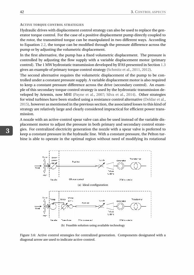
3
42 3. CONTROL ASPECTS
ACTIVE TORQUE CONTROL STRATEGIES
Hydraulic drives with displacement control strategy can also be used to replace the gen-
erator torque control. For the case of a positive displacement pump directly coupled to
the rotor, the transmitted torque can be manipulated in two different ways. According
to Equation 2.2, the torque can be modified through the pressure difference across the
pump or by adjusting the volumetric displacement.
In the first alternative, the pump has a fixed volumetric displacement. The pressure is
controlled by adjusting the flow supply with a variable displacement motor (primary
control). The 1 MW hydrostatic transmission developed by IFAS presented in Section 1.3
gives an example of primary torque control strategy (Schmitz et al., 2011, 2012).
The second alternative requires the volumetric displacement of the pump to be con-
trolled under a constant pressure supply. A variable displacement motor is also required
to keep a constant pressure difference across the drive (secondary control). An exam-
ple of this secondary torque control strategy is used by the hydrostatic transmission de-
veloped by Artemis, now MHI (Payne et al., 2007; Silva et al., 2014). Other strategies
for wind turbines have been studied using a resistance control alternative (Deldar et al.,
2015), however as mentioned in the previous section, the associated losses to this kind of
strategy are relatively large and clearly considered impractical for efficient power trans-
mission.
A nozzle with an active-control spear valve can also be used instead of the variable dis-
placement motor to adjust the pressure in both primary and secondary control strate-
gies. For centralized electricity generation the nozzle with a spear valve is preferred to
keep a constant pressure in the hydraulic line. With a constant pressure, the Pelton tur-
bine is able to operate in the optimal region without need of modifying its rotational
(a) Ideal configuration
(b) Feasible solution using available technology
Figure 3.6: Active control strategies for centralized generation. Components designated with a
diagonal arrow are used to indicate active-control.
3.4. PASSIVE SPEED CONTROL ANALYSIS
3
43
speed as opposed to the passive control strategies. A Pelton turbine operating with a
constant rotational speed considerably simplifies the integration with the electrical grid.
The constant rotational speed is realized by using a grid-connected synchronous gen-
erator, similar to most large scale hydroelectric generation plants. A schematic of these
configurations is shown in Figure 3.6.
3.4. PASSIVE SPEED CONTROL ANALYSISThis section uses linear control tools to analyse the operation below rated wind speed
of a horizontal axis variable speed wind turbine with a fluid power drivetrain. There is
particular interest to analyse stability of a passive control method using fluid power tech-
nology. In order to illustrate the passive control operation, let us consider the ideal case
where no friction, flow leakages or pressure losses occur. In this case, the final torque
transmitted by the pump to the rotor is also expressed as a quadratic function of the
rotor speed by using Equations 2.1 and 2.18 in Equation 2.2 according to:
τp = K3 ω2r (3.12)
K3 =1
2ρhyd
V 3p
C 2d
A2nz
(3.13)
By making equal the terms K1 and K3 from Equations 3.7 and 3.13 it is possible to match
both curves by proper dimensioning of the components given the aerodynamic perfor-
mance of the rotor. Hence, the nozzle is used as a hydraulic component which induces
a feedback pressure into the rotor and pump arrangement as shown in Figure 3.7.
If all the different losses in the fluid power transmission are included, the quadratic rela-
tion in Equation 2.2 is no longer valid. However, deviations from the optimal quadratic
relation are rather small if components are properly dimensioned based on the required
characteristics and ranges of operation. An experimental validation of this concept was
described in (Diepeveen and Jarquin Laguna, 2014). In general, when a design wind
speed and tip speed ratio is selected, a constant value of the nozzle area can be found
such that the resulting torque-speed curve of the power transmission closely matches
the maximal aerodynamic performance of the rotor for different wind speeds. For low
wind speeds, this will result in a slightly lower tip speed ratio and for higher wind speeds
the tip speed ratio will be slightly higher. In order to select the proper nozzle area, other
design parameters should be taken into account like maximum tip speed velocity and
rated wind speed.
3.4.1. NON LINEAR REDUCED ORDER MODELThe rotor and fluid power transmission can be modeled by including the rotational dy-
namics of the rotor, the design characteristics of the pump, the fluid flow dynamics
from the pipeline and the nozzle. A schematic showing the subsystem level modelling is
shown in Figure 3.8.
A first equation of the governing set of equations describes the rotor speed acceleration
by the balance of the aerodynamic torque and the transmitted torque of the pump. Ig-
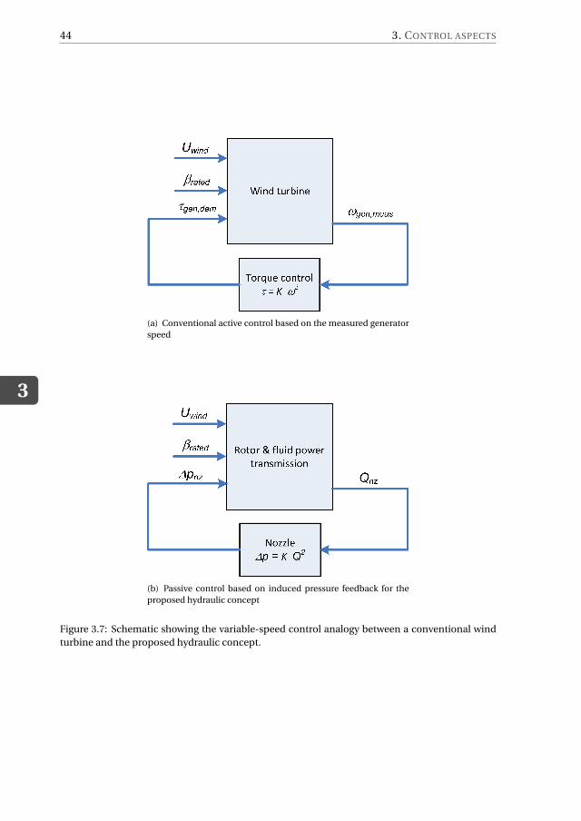
3
44 3. CONTROL ASPECTS
(a) Conventional active control based on the measured generator
speed
(b) Passive control based on induced pressure feedback for the
proposed hydraulic concept
Figure 3.7: Schematic showing the variable-speed control analogy between a conventional wind
turbine and the proposed hydraulic concept.
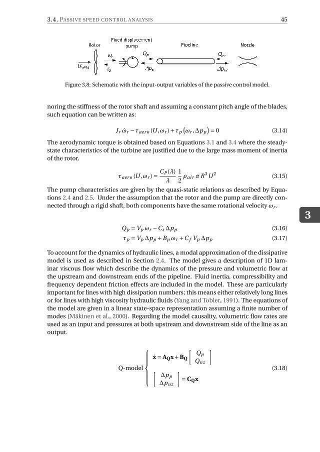
3.4. PASSIVE SPEED CONTROL ANALYSIS
3
45
Figure 3.8: Schematic with the input-output variables of the passive control model.
noring the stiffness of the rotor shaft and assuming a constant pitch angle of the blades,
such equation can be written as:
Jr ωr −τaer o (U ,ωr )+τp
(
ωr ,∆pp
)
= 0 (3.14)
The aerodynamic torque is obtained based on Equations 3.1 and 3.4 where the steady-
state characteristics of the turbine are justified due to the large mass moment of inertia
of the rotor.
τaer o (U ,ωr ) =CP (λ)
λ
1
2ρai r πR3 U 2 (3.15)
The pump characteristics are given by the quasi-static relations as described by Equa-
tions 2.4 and 2.5. Under the assumption that the rotor and the pump are directly con-
nected through a rigid shaft, both components have the same rotational velocity ωr .
Qp =Vp ωr −Cs ∆pp (3.16)
τp =Vp ∆pp +Bp ωr +C f Vp ∆pp (3.17)
To account for the dynamics of hydraulic lines, a modal approximation of the dissipative
model is used as described in Section 2.4. The model gives a description of 1D lam-
inar viscous flow which describe the dynamics of the pressure and volumetric flow at
the upstream and downstream ends of the pipeline. Fluid inertia, compressibility and
frequency dependent friction effects are included in the model. These are particularly
important for lines with high dissipation numbers; this means either relatively long lines
or for lines with high viscosity hydraulic fluids (Yang and Tobler, 1991). The equations of
the model are given in a linear state-space representation assuming a finite number of
modes (Mäkinen et al., 2000). Regarding the model causality, volumetric flow rates are
used as an input and pressures at both upstream and downstream side of the line as an
output.
Q-model
x = AQx+BQ
[
Qp
Qnz
]
[
∆pp
∆pnz
]
= CQx
(3.18)
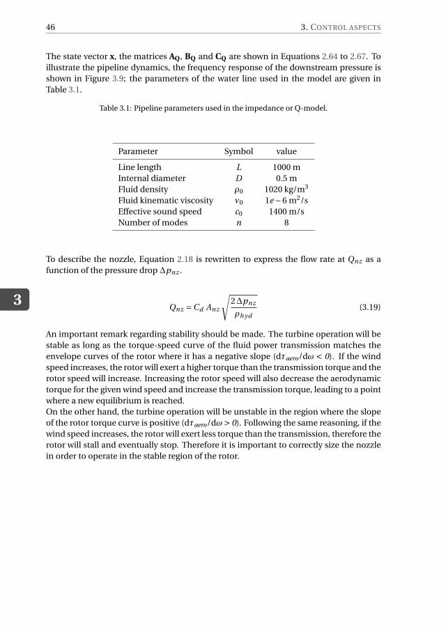
3
46 3. CONTROL ASPECTS
The state vector x, the matrices AQ, BQ and CQ are shown in Equations 2.64 to 2.67. To
illustrate the pipeline dynamics, the frequency response of the downstream pressure is
shown in Figure 3.9; the parameters of the water line used in the model are given in
Table 3.1.
Table 3.1: Pipeline parameters used in the impedance or Q-model.
Parameter Symbol value
Line length L 1000 m
Internal diameter D 0.5 m
Fluid density ρ0 1020 kg/m3
Fluid kinematic viscosity ν0 1e −6 m2/s
Effective sound speed c0 1400 m/s
Number of modes n 8
To describe the nozzle, Equation 2.18 is rewritten to express the flow rate at Qnz as a
function of the pressure drop ∆pnz .
Qnz =Cd Anz
√
2∆pnz
ρhyd(3.19)
An important remark regarding stability should be made. The turbine operation will be
stable as long as the torque-speed curve of the fluid power transmission matches the
envelope curves of the rotor where it has a negative slope (dτaero/dω < 0). If the wind
speed increases, the rotor will exert a higher torque than the transmission torque and the
rotor speed will increase. Increasing the rotor speed will also decrease the aerodynamic
torque for the given wind speed and increase the transmission torque, leading to a point
where a new equilibrium is reached.
On the other hand, the turbine operation will be unstable in the region where the slope
of the rotor torque curve is positive (dτaero/dω> 0). Following the same reasoning, if the
wind speed increases, the rotor will exert less torque than the transmission, therefore the
rotor will stall and eventually stop. Therefore it is important to correctly size the nozzle
in order to operate in the stable region of the rotor.
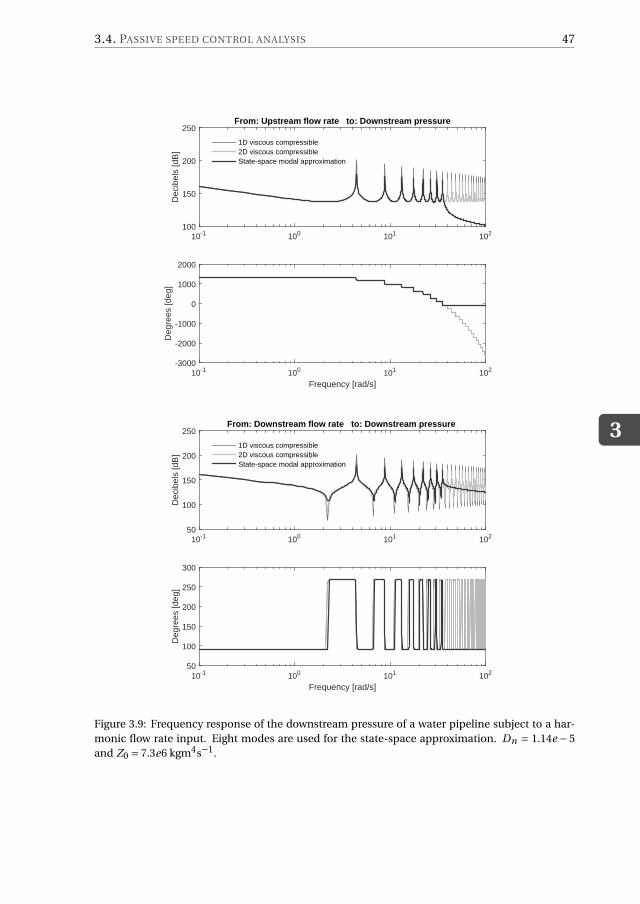
3.4. PASSIVE SPEED CONTROL ANALYSIS
3
47
10-1 100 101 102
Dec
ibel
s [d
B]
100
150
200
250From: Upstream flow rate to: Downstream pressure
1D viscous compressible2D viscous compressibleState-space modal approximation
Frequency [rad/s]10-1 100 101 102
Deg
rees
[deg
]
-3000
-2000
-1000
0
1000
2000
10-1 100 101 102
Dec
ibel
s [d
B]
50
100
150
200
250From: Downstream flow rate to: Downstream pressure
1D viscous compressible2D viscous compressibleState-space modal approximation
Frequency [rad/s]10-1 100 101 102
Deg
rees
[deg
]
50
100
150
200
250
300
Figure 3.9: Frequency response of the downstream pressure of a water pipeline subject to a har-
monic flow rate input. Eight modes are used for the state-space approximation. Dn = 1.14e − 5
and Z0 = 7.3e6 kgm4s−1.
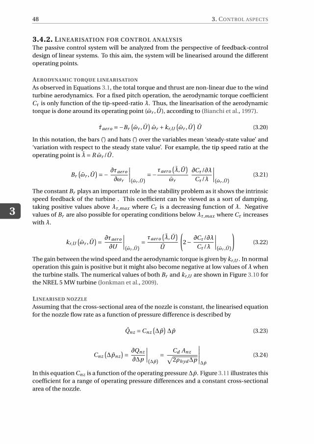
3
48 3. CONTROL ASPECTS
3.4.2. LINEARISATION FOR CONTROL ANALYSISThe passive control system will be analyzed from the perspective of feedback-control
design of linear systems. To this aim, the system will be linearised around the different
operating points.
AERODYNAMIC TORQUE LINEARISATION
As observed in Equations 3.1, the total torque and thrust are non-linear due to the wind
turbine aerodynamics. For a fixed pitch operation, the aerodynamic torque coefficient
Cτ is only function of the tip-speed-ratio λ. Thus, the linearisation of the aerodynamic
torque is done around its operating point (ωr ,U ), according to (Bianchi et al., 1997).
τaer o =−Br
(
ωr ,U)
ωr +kr,U
(
ωr ,U)
U (3.20)
In this notation, the bars ( ) and hats ( ) over the variables mean ‘steady-state value’ and
‘variation with respect to the steady state value’. For example, the tip speed ratio at the
operating point is λ= R ωr /U .
Br
(
ωr ,U)
=−∂τaer o
∂ωr
∣
∣
∣
∣
(ωr ,U)=−
τaer o
(
λ,U)
ωr
∂Cτ/∂λ
Cτ/λ
∣
∣
∣
∣
(ωr ,U)(3.21)
The constant Br plays an important role in the stability problem as it shows the intrinsic
speed feedback of the turbine . This coefficient can be viewed as a sort of damping,
taking positive values above λτ,max where Cτ is a decreasing function of λ. Negative
values of Br are also possible for operating conditions below λτ,max where Cτ increases
with λ.
kr,U
(
ωr ,U)
=∂τaer o
∂U
∣
∣
∣
∣
(ωr ,U)=
τaer o
(
λ,U)
U
(
2−∂Cτ/∂λ
Cτ/λ
∣
∣
∣
∣
(ωr ,U)
)
(3.22)
The gain between the wind speed and the aerodynamic torque is given by kr,U . In normal
operation this gain is positive but it might also become negative at low values of λ when
the turbine stalls. The numerical values of both Br and kr,U are shown in Figure 3.10 for
the NREL 5 MW turbine (Jonkman et al., 2009).
LINEARISED NOZZLE
Assuming that the cross-sectional area of the nozzle is constant, the linearised equation
for the nozzle flow rate as a function of pressure difference is described by
Qnz =Cnz
(
∆p)
∆p (3.23)
Cnz
(
∆pnz
)
=∂Qnz
∂∆p
∣
∣
∣
∣
(∆p)=
Cd Anz√
2ρhyd∆p
∣
∣
∣
∣
∣
∆p
(3.24)
In this equation Cnz is a function of the operating pressure ∆p. Figure 3.11 illustrates this
coefficient for a range of operating pressure differences and a constant cross-sectional
area of the nozzle.
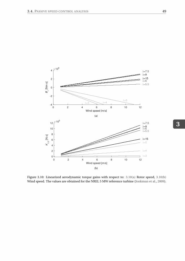
3.4. PASSIVE SPEED CONTROL ANALYSIS
3
49
Wind speed [m/s]
0 2 4 6 8 10 12
Br [
Nm
s]
×106
-4
-2
0
2
4
λ=5.5
λ=7.5
λ=15
λ=9
λ=6
λ=5λ=4λ=3
(a)
Wind speed [m/s]
0 2 4 6 8 10 12
Kr,
U [
N s
]
×105
0
2
4
6
8
10
12 λ=7.5
λ=5.5
λ=15
λ=6λ=9
λ=3
λ=4
λ=5
(b)
Figure 3.10: Linearized aerodynamic torque gains with respect to: 3.10(a) Rotor speed, 3.10(b)
Wind speed. The values are obtained for the NREL 5 MW reference turbine (Jonkman et al., 2009).
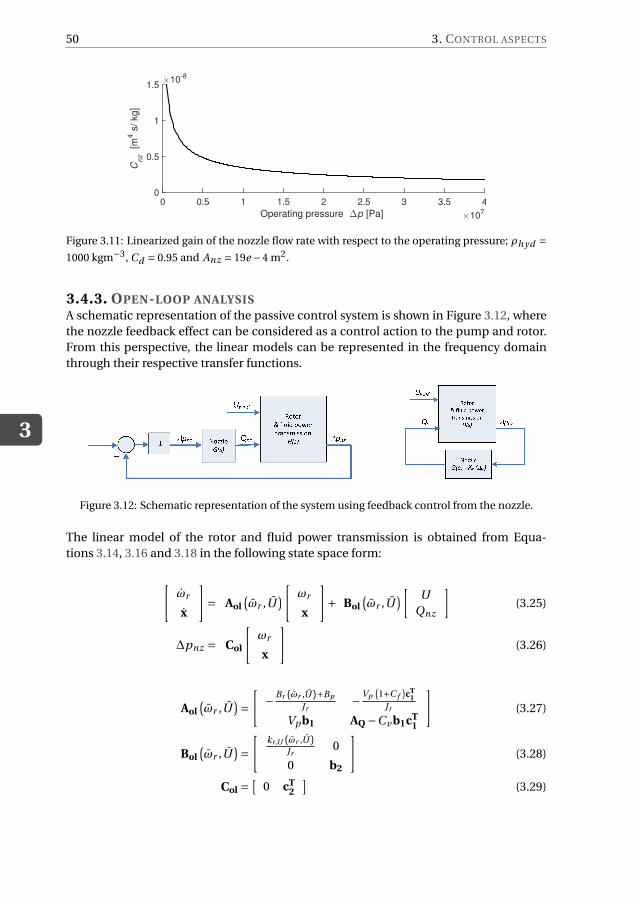
3
50 3. CONTROL ASPECTS
Operating pressure ∆p [Pa] ×107
0 0.5 1 1.5 2 2.5 3 3.5 4
Cnz
[m4 s
/ kg
]
×10-8
0
0.5
1
1.5
Figure 3.11: Linearized gain of the nozzle flow rate with respect to the operating pressure; ρhyd =1000 kgm−3, Cd = 0.95 and Anz = 19e −4 m2.
3.4.3. OPEN-LOOP ANALYSISA schematic representation of the passive control system is shown in Figure 3.12, where
the nozzle feedback effect can be considered as a control action to the pump and rotor.
From this perspective, the linear models can be represented in the frequency domain
through their respective transfer functions.
Figure 3.12: Schematic representation of the system using feedback control from the nozzle.
The linear model of the rotor and fluid power transmission is obtained from Equa-
tions 3.14, 3.16 and 3.18 in the following state space form:
[
ωr
x
]
= Aol(
ωr ,U)
[
ωr
x
]
+ Bol(
ωr ,U)
[
U
Qnz
]
(3.25)
∆pnz = Col
[
ωr
x
]
(3.26)
Aol(
ωr ,U)
=[
−Br (ωr ,U)+Bp
Jr−Vp
(
1+C f
)
cT1
Jr
Vp b1 AQ −Cv b1cT1
]
(3.27)
Bol(
ωr ,U)
=[
kr,U (ωr ,U)Jr
0
0 b2
]
(3.28)
Col =[
0 cT2
]
(3.29)
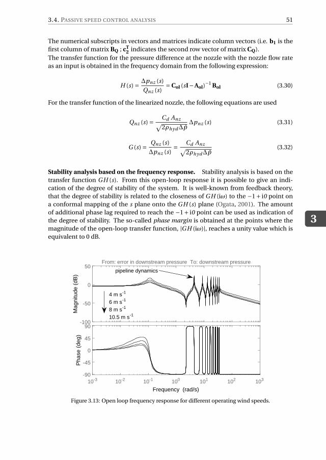
3.4. PASSIVE SPEED CONTROL ANALYSIS
3
51
The numerical subscripts in vectors and matrices indicate column vectors (i.e. b1 is the
first column of matrix BQ ; cT2 indicates the second row vector of matrix CQ).
The transfer function for the pressure difference at the nozzle with the nozzle flow rate
as an input is obtained in the frequency domain from the following expression:
H (s) =∆pnz (s)
Qnz (s)= Col (sI−Aol)
−1 Bol (3.30)
For the transfer function of the linearized nozzle, the following equations are used
Qnz (s) =Cd Anz
√
2ρhyd∆p∆pnz (s) (3.31)
G (s) =Qnz (s)
∆pnz (s)=
Cd Anz√
2ρhyd∆p(3.32)
Stability analysis based on the frequency response. Stability analysis is based on the
transfer function G H (s). From this open-loop response it is possible to give an indi-
cation of the degree of stability of the system. It is well-known from feedback theory,
that the degree of stability is related to the closeness of G H (iω) to the −1+ i0 point on
a conformal mapping of the s plane onto the G H (s) plane (Ogata, 2001). The amount
of additional phase lag required to reach the −1+ i0 point can be used as indication of
the degree of stability. The so-called phase margin is obtained at the points where the
magnitude of the open-loop transfer function, |G H (iω)|, reaches a unity value which is
equivalent to 0 dB.
Mag
nitu
de (
dB)
-100
-50
0
50From: error in downstream pressure To: downstream pressure
10-3 10-2 10-1 100 101 102 103
Pha
se (
deg)
-90
-45
0
45
90
Frequency (rad/s)
pipeline dynamics
4 m s-1
6 m s-1
8 m s-1
10.5 m s-1
Figure 3.13: Open loop frequency response for different operating wind speeds.
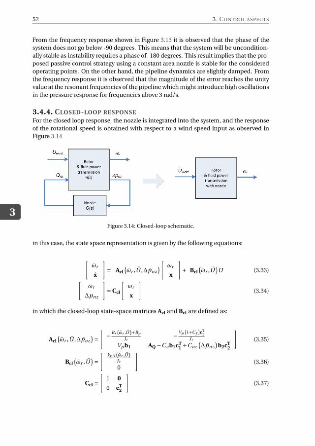
3
52 3. CONTROL ASPECTS
From the frequency response shown in Figure 3.13 it is observed that the phase of the
system does not go below -90 degrees. This means that the system will be uncondition-
ally stable as instability requires a phase of -180 degrees. This result implies that the pro-
posed passive control strategy using a constant area nozzle is stable for the considered
operating points. On the other hand, the pipeline dynamics are slightly damped. From
the frequency response it is observed that the magnitude of the error reaches the unity
value at the resonant frequencies of the pipeline which might introduce high oscillations
in the pressure response for frequencies above 3 rad/s.
3.4.4. CLOSED-LOOP RESPONSE
For the closed loop response, the nozzle is integrated into the system, and the response
of the rotational speed is obtained with respect to a wind speed input as observed in
Figure 3.14
Figure 3.14: Closed-loop schematic.
in this case, the state space representation is given by the following equations:
[
ωr
x
]
= Acl(
ωr ,U ,∆pnz
)
[
ωr
x
]
+ Bcl(
ωr ,U)
U (3.33)
[
ωr
∆pnz
]
= Ccl
[
ωr
x
]
(3.34)
in which the closed-loop state-space matrices Acl and Bcl are defined as:
Acl(
ωr ,U ,∆pnz
)
=[
−Br (ωr ,U)+Bp
Jr−Vp
(
1+C f
)
cT1
Jr
Vp b1 AQ −Cv b1cT1 +Cnz
(
∆pnz
)
b2cT2
]
(3.35)
Bcl(
ωr ,U)
=[
kr,U (ωr ,U)Jr
0
]
(3.36)
Ccl =[
1 0
0 cT2
]
(3.37)
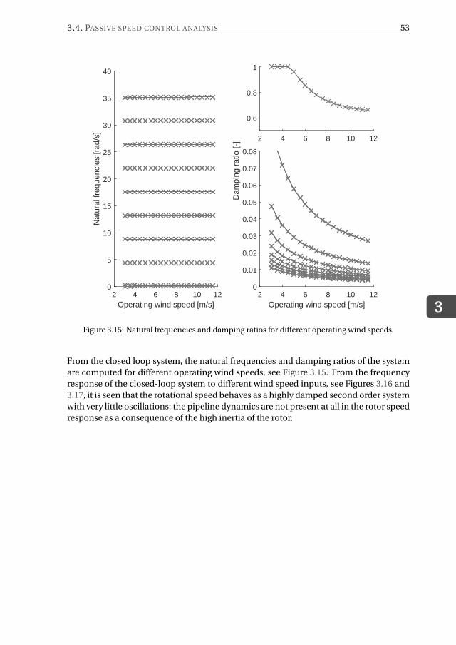
3.4. PASSIVE SPEED CONTROL ANALYSIS
3
53
Operating wind speed [m/s]2 4 6 8 10 12
Nat
ural
freq
uenc
ies
[rad
/s]
0
5
10
15
20
25
30
35
40
2 4 6 8 10 12
0.6
0.8
1
Operating wind speed [m/s]2 4 6 8 10 12
Dam
ping
rat
io [-
]
0
0.01
0.02
0.03
0.04
0.05
0.06
0.07
0.08
Figure 3.15: Natural frequencies and damping ratios for different operating wind speeds.
From the closed loop system, the natural frequencies and damping ratios of the system
are computed for different operating wind speeds, see Figure 3.15. From the frequency
response of the closed-loop system to different wind speed inputs, see Figures 3.16 and
3.17, it is seen that the rotational speed behaves as a highly damped second order system
with very little oscillations; the pipeline dynamics are not present at all in the rotor speed
response as a consequence of the high inertia of the rotor.
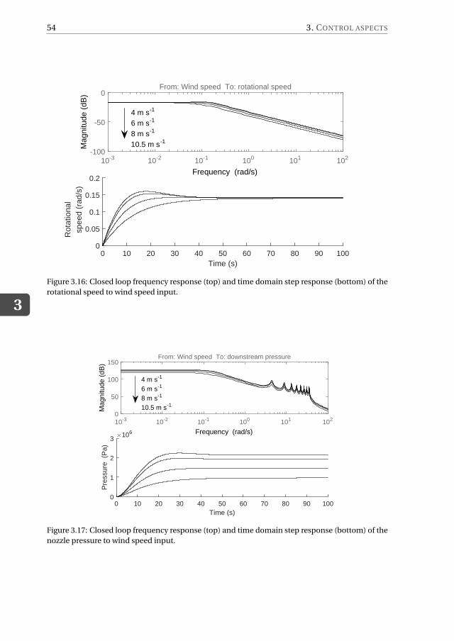
3
54 3. CONTROL ASPECTS
10-3 10-2 10-1 100 101 102
Mag
nitu
de (
dB)
-100
-50
0From: Wind speed To: rotational speed
Frequency (rad/s)
Time (s)0 10 20 30 40 50 60 70 80 90 100
Rot
atio
nal
spe
ed (
rad/
s)
0
0.05
0.1
0.15
0.2
4 m s-1
6 m s-1
8 m s-1
10.5 m s-1
Figure 3.16: Closed loop frequency response (top) and time domain step response (bottom) of the
rotational speed to wind speed input.
10-3 10-2 10-1 100 101 102
Mag
nitu
de (
dB)
0
50
100
150From: Wind speed To: downstream pressure
Frequency (rad/s)
Time (s)0 10 20 30 40 50 60 70 80 90 100
Pre
ssur
e (
Pa)
×106
0
1
2
3
4 m s-1
6 m s-1
8 m s-1
10.5 m s-1
Figure 3.17: Closed loop frequency response (top) and time domain step response (bottom) of the
nozzle pressure to wind speed input.
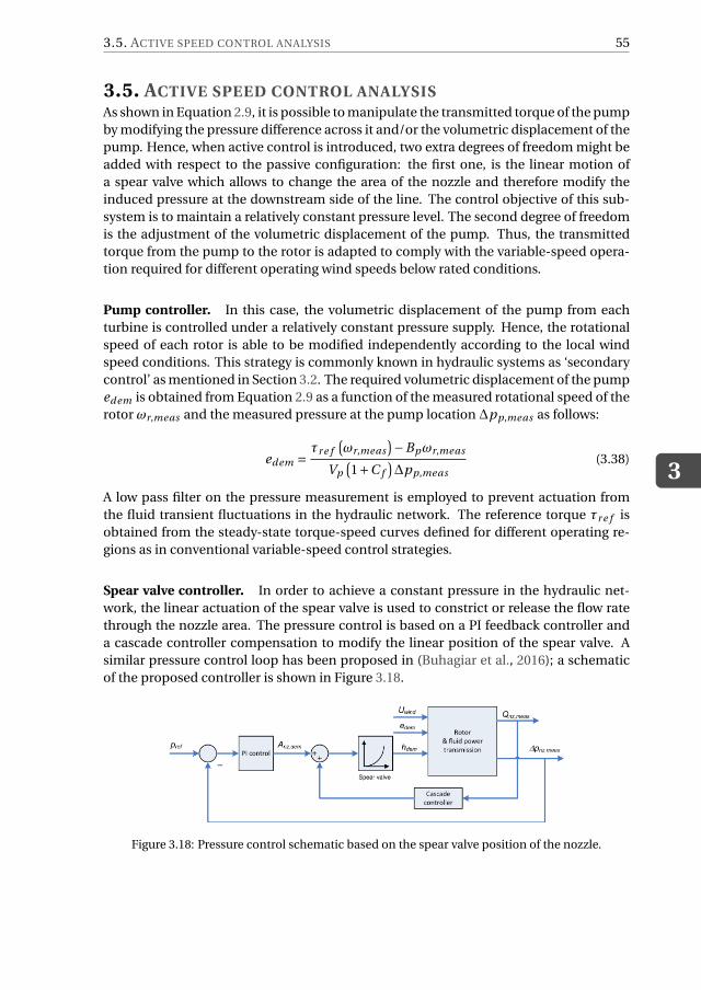
3.5. ACTIVE SPEED CONTROL ANALYSIS
3
55
3.5. ACTIVE SPEED CONTROL ANALYSISAs shown in Equation 2.9, it is possible to manipulate the transmitted torque of the pump
by modifying the pressure difference across it and/or the volumetric displacement of the
pump. Hence, when active control is introduced, two extra degrees of freedom might be
added with respect to the passive configuration: the first one, is the linear motion of
a spear valve which allows to change the area of the nozzle and therefore modify the
induced pressure at the downstream side of the line. The control objective of this sub-
system is to maintain a relatively constant pressure level. The second degree of freedom
is the adjustment of the volumetric displacement of the pump. Thus, the transmitted
torque from the pump to the rotor is adapted to comply with the variable-speed opera-
tion required for different operating wind speeds below rated conditions.
Pump controller. In this case, the volumetric displacement of the pump from each
turbine is controlled under a relatively constant pressure supply. Hence, the rotational
speed of each rotor is able to be modified independently according to the local wind
speed conditions. This strategy is commonly known in hydraulic systems as ‘secondary
control’ as mentioned in Section 3.2. The required volumetric displacement of the pump
edem is obtained from Equation 2.9 as a function of the measured rotational speed of the
rotor ωr,meas and the measured pressure at the pump location ∆pp,meas as follows:
edem =τr e f
(
ωr,meas
)
−Bpωr,meas
Vp
(
1+C f
)
∆pp,meas
(3.38)
A low pass filter on the pressure measurement is employed to prevent actuation from
the fluid transient fluctuations in the hydraulic network. The reference torque τr e f is
obtained from the steady-state torque-speed curves defined for different operating re-
gions as in conventional variable-speed control strategies.
Spear valve controller. In order to achieve a constant pressure in the hydraulic net-
work, the linear actuation of the spear valve is used to constrict or release the flow rate
through the nozzle area. The pressure control is based on a PI feedback controller and
a cascade controller compensation to modify the linear position of the spear valve. A
similar pressure control loop has been proposed in (Buhagiar et al., 2016); a schematic
of the proposed controller is shown in Figure 3.18.
Figure 3.18: Pressure control schematic based on the spear valve position of the nozzle.
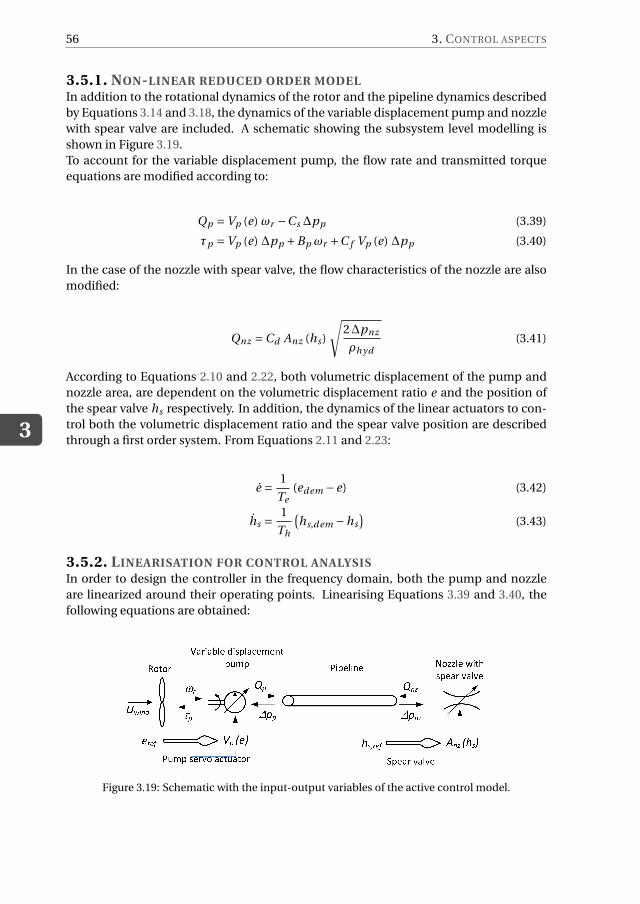
3
56 3. CONTROL ASPECTS
3.5.1. NON-LINEAR REDUCED ORDER MODELIn addition to the rotational dynamics of the rotor and the pipeline dynamics described
by Equations 3.14 and 3.18, the dynamics of the variable displacement pump and nozzle
with spear valve are included. A schematic showing the subsystem level modelling is
shown in Figure 3.19.
To account for the variable displacement pump, the flow rate and transmitted torque
equations are modified according to:
Qp =Vp (e) ωr −Cs ∆pp (3.39)
τp =Vp (e) ∆pp +Bp ωr +C f Vp (e) ∆pp (3.40)
In the case of the nozzle with spear valve, the flow characteristics of the nozzle are also
modified:
Qnz =Cd Anz (hs )
√
2∆pnz
ρhyd(3.41)
According to Equations 2.10 and 2.22, both volumetric displacement of the pump and
nozzle area, are dependent on the volumetric displacement ratio e and the position of
the spear valve hs respectively. In addition, the dynamics of the linear actuators to con-
trol both the volumetric displacement ratio and the spear valve position are described
through a first order system. From Equations 2.11 and 2.23:
e =1
Te(edem −e) (3.42)
hs =1
Th
(
hs,dem −hs
)
(3.43)
3.5.2. LINEARISATION FOR CONTROL ANALYSISIn order to design the controller in the frequency domain, both the pump and nozzle
are linearized around their operating points. Linearising Equations 3.39 and 3.40, the
following equations are obtained:
Figure 3.19: Schematic with the input-output variables of the active control model.
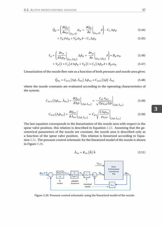
3.5. ACTIVE SPEED CONTROL ANALYSIS
3
57
Qp =(
∂Qp
∂ωp
∣
∣
∣
∣
(ωp ,e)ωp +
∂Qp
∂e
∣
∣
∣
∣
(ωp ,e)e
)
−Cs ∆pp (3.44)
=Vp e ωp +Vp ωp e −Cs ∆pp (3.45)
τp =(
∂τp
∂∆pp
∣
∣
∣
∣
(ωp ,∆pp )∆pp +
∂τp
∂e
∣
∣
∣
∣
(ωp ,∆pp )e
)
+Bp ωp (3.46)
=Vp
(
1+C f
)
e ∆pp +Vp
(
1+C f
)
∆pp e +Bp ωp (3.47)
Linearization of the nozzle flow rate as a function of both pressure and nozzle area gives:
Qnz =Cnz1
(
∆p, Anz
)
∆pnz +Cnz2
(
∆p)
Anz (3.48)
where the nozzle constants are evaluated according to the operating characteristics of
the system:
Cnz1
(
∆pnz , Anz
)
=∂Qnz
∂∆p
∣
∣
∣
∣
(∆p,Anz )=
Cd Anz√
2ρhyd∆p
∣
∣
∣
∣
∣
(∆p,Anz )
(3.49)
Cnz2
(
∆pnz
)
=∂Qnz
∂Anz
∣
∣
∣
∣
(∆p,Anz )= Cd
√
2∆pnz
ρhyd
∣
∣
∣
∣
∣
(∆p,Anz )
(3.50)
The last equation corresponds to the linearisation of the nozzle area with respect to the
spear valve position, this relation is described in Equation 2.22. Assuming that the ge-
ometrical parameters of the nozzle are constant, the nozzle area is described only as
a function of the spear valve position. This relation is linearized according to Equa-
tion 3.51. The pressure control schematic for the linearized model of the nozzle is shown
in Figure 3.20.
Anz = Knz
(
h)
h (3.51)
Figure 3.20: Pressure control schematic using the linearized model of the nozzle.
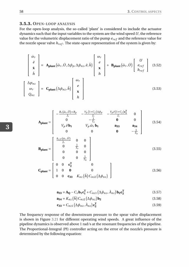
3
58 3. CONTROL ASPECTS
3.5.3. OPEN-LOOP ANALYSIS
For the open-loop analysis, the so-called ‘plant’ is considered to include the actuator
dynamics such that the input variables to the system are the wind speed U , the reference
value for the volumetric displacement ratio of the pump er e f and the reference value for
the nozzle spear valve hr e f . The state-space representation of the system is given by:
ωr
e
x
h
= Aplant(
ωr ,U ,∆pp ,∆pnz , e, h)
ωr
e
x
h
+ Bplant(
ωr ,U)
U
er e f
hr e f
(3.52)
∆pnz
ωr
Qnz
= Cplant
(
∆pnz , h)
ωr
e
x
h
(3.53)
Aplant =
−Br (ωr ,U)+Bp
Jr−Vp
(
1+C f
)
∆pp
Jr−Vp e
(
1+C f
)
cT1
Jr0
0 − 1Te
0 0
Vp e b1 Vp ωr b1 a33 a34
0 0 0 − 1Th
(3.54)
Bplant =
kr,U (ωr ,U)Jr
0 0
0 1Te
0
0 0 0
0 0 1Th
(3.55)
Cplant =
0 0 cT2 0
1 0 0 0
0 0 c33 Knz
(
h)
Cnz2
(
∆pnz
)
(3.56)
a33 = AQ −Cv b1cT1 +Cnz1
(
∆pnz , Anz
)
b2cT2 (3.57)
a34 = Knz
(
h)
Cnz2
(
∆pnz
)
b2 (3.58)
c33 =Cnz1
(
∆pnz , Anz
)
cT2 (3.59)
The frequency response of the downstream pressure to the spear valve displacement
is shown in Figure 3.21 for different operating wind speeds. A great influence of the
pipeline dynamics is observed above 1 rad/s at the resonant frequencies of the pipeline.
The Proportional-Integral (PI) controller acting on the error of the nozzle’s pressure is
determined by the following equation:
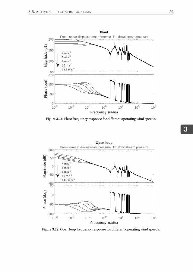
3.5. ACTIVE SPEED CONTROL ANALYSIS
3
59
Mag
nitu
de (
dB)
50
100
150
200From: spear displacement reference To: downstream pressure
10-3 10-2 10-1 100 101 102 103
Pha
se (
deg)
0
90
180
270
Plant
Frequency (rad/s)
4 m s-1
6 m s-1
8 m s-1
10 m s-1
11.5 m s-1
Figure 3.21: Plant frequency response for different operating wind speeds.
Mag
nitu
de (
dB)
-100
-50
0
50
100From: error in downstream pressure To: downstream pressure
10-3 10-2 10-1 100 101 102 103
Pha
se (
deg)
-180
-90
0
90
Open-loop
Frequency (rad/s)
4 m s-1
6 m s-1
8 m s-1
10 m s-1
11.5 m s-1
Figure 3.22: Open loop frequency response for different operating wind speeds.
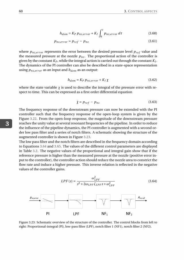
3
60 3. CONTROL ASPECTS
hdem = KP pnz,er r or +KI
∫t
0pnz,er r or d t (3.60)
pnz,er r or = pr e f − pnz (3.61)
where pnz,er r or represents the error between the desired pressure level pr e f value and
the measured pressure at the nozzle pnz . The proportional action of the controller is
given by the constant KP , while the integral action is carried out through the constant KI .
The dynamics of the PI controller can also be described in a state-space representation
using pnz,er r or as an input and hdem as an output:
hdem = KP pnz,er r or +KI χ (3.62)
where the state variable χ is used to describe the integral of the pressure error with re-
spect to time. This can be expressed as a first order differential equation
χ= pr e f − pnz (3.63)
The frequency response of the downstream pressure can now be extended with the PI
controller such that the frequency response of the open-loop system is given by the
Figure 3.22. From the open-loop response, the magnitude of the downstream pressure
reaches the unity value at several resonant frequencies of the pipeline. In order to reduce
the influence of the pipeline dynamics, the PI controller is augmented with a second or-
der low pass filter and a series of notch filters. A schematic showing the structure of the
augmented controller is shown in Figure 3.23.
The low pass filter and the notch filters are described in the frequency domain according
to Equations 3.64 and 3.65. The values of the different control parameters are displayed
in Table 3.2. The negative values of the proportional and integral gain show that if the
reference pressure is higher than the measured pressure at the nozzle (positive error in-
put to the controller), the controller action should reduce the nozzle area to constrict the
flow rate and induce a higher pressure. This inverse relation is reflected in the negative
values of the controller gains.
LPF (s) =ω2
LPF
s2 +2ωLPF ζLPF s +ω2LPF
(3.64)
Figure 3.23: Schematic overview of the structure of the controller. The control blocks from left to
right: Proportional-integral (PI), low-pass filter (LPF), notch filter 1 (NF1), notch filter 2 (NF2).
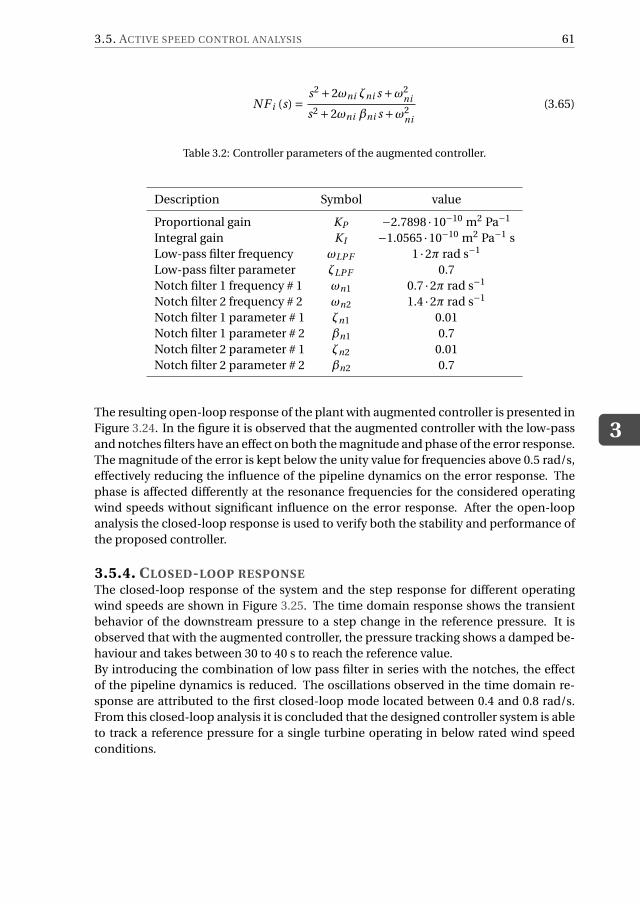
3.5. ACTIVE SPEED CONTROL ANALYSIS
3
61
N F i (s) =s2 +2ωni ζni s +ω2
ni
s2 +2ωni βni s +ω2ni
(3.65)
Table 3.2: Controller parameters of the augmented controller.
Description Symbol value
Proportional gain KP −2.7898 ·10−10 m2 Pa−1
Integral gain KI −1.0565 ·10−10 m2 Pa−1 s
Low-pass filter frequency ωLPF 1 ·2π rad s−1
Low-pass filter parameter ζLPF 0.7
Notch filter 1 frequency # 1 ωn1 0.7 ·2π rad s−1
Notch filter 2 frequency # 2 ωn2 1.4 ·2π rad s−1
Notch filter 1 parameter # 1 ζn1 0.01
Notch filter 1 parameter # 2 βn1 0.7
Notch filter 2 parameter # 1 ζn2 0.01
Notch filter 2 parameter # 2 βn2 0.7
The resulting open-loop response of the plant with augmented controller is presented in
Figure 3.24. In the figure it is observed that the augmented controller with the low-pass
and notches filters have an effect on both the magnitude and phase of the error response.
The magnitude of the error is kept below the unity value for frequencies above 0.5 rad/s,
effectively reducing the influence of the pipeline dynamics on the error response. The
phase is affected differently at the resonance frequencies for the considered operating
wind speeds without significant influence on the error response. After the open-loop
analysis the closed-loop response is used to verify both the stability and performance of
the proposed controller.
3.5.4. CLOSED-LOOP RESPONSEThe closed-loop response of the system and the step response for different operating
wind speeds are shown in Figure 3.25. The time domain response shows the transient
behavior of the downstream pressure to a step change in the reference pressure. It is
observed that with the augmented controller, the pressure tracking shows a damped be-
haviour and takes between 30 to 40 s to reach the reference value.
By introducing the combination of low pass filter in series with the notches, the effect
of the pipeline dynamics is reduced. The oscillations observed in the time domain re-
sponse are attributed to the first closed-loop mode located between 0.4 and 0.8 rad/s.
From this closed-loop analysis it is concluded that the designed controller system is able
to track a reference pressure for a single turbine operating in below rated wind speed
conditions.
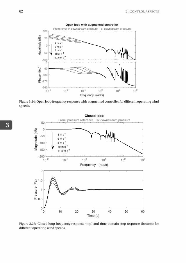
3
62 3. CONTROL ASPECTS
Mag
nitu
de (
dB)
-100
-50
0
50
100From: error in downstream pressure To: downstream pressure
10-3 10-2 10-1 100 101 102
Pha
se (
deg)
-360
-270
-180
-90
0
Open-loop with augmented controller
Frequency (rad/s)
4 m s-1
6 m s-1
8 m s-1
10 m s-1
11.5 m s-1
Figure 3.24: Open loop frequency response with augmented controller for different operating wind
speeds.
10-2 10-1 100 101 102 103
Ma
gn
itu
de
(d
B)
-200
-150
-100
-50
0
50From: pressure reference To: downstream pressure
Closed-loop
Frequency (rad/s)
Time (s)
0 10 20 30 40 50 60
Pre
ssu
re (
Pa
)
0
0.5
1
1.5
2
4 m s-1
6 m s-1
8 m s-1
10 m s-1
11.5 m s-1
Figure 3.25: Closed loop frequency response (top) and time domain step response (bottom) for
different operating wind speeds.
3.6. OTHER CONTROL ASPECTS
3
63
3.6. OTHER CONTROL ASPECTS
3.6.1. PITCH CONTROLAbove rated wind speed, the rated rotor speed is maintained by pitching collectively the
rotor blades. A conventional PI pitch controller is proposed using the rotor speed error
instead of the generator speed error. Due to the sensitivity of the aerodynamic response
of the rotor to the pitch angle, the value of the controller gains are modified as a function
of the pitch angle through a gain-scheduled approach. The gain scheduled PI controller
is shown in the next equations, where KP/I are the proportional and integral gains re-
spectively, KP/I ,0 is the gain at rated pitch angle β = 0, and βK is the blade pitch angle
at which the pitch sensitivity of aerodynamic power to rotor collective blade pitch has
doubled from its value at the rated operating point.
βdem = KP
(
β)
ωr,er r or +KI
(
β)
∫t
0ωr,er r or d t (3.66)
KP/I
(
β)
= KP/I ,0βK
βK +β(3.67)
ωr,er r or =ωr,r ated −ωr,meas (3.68)
The values of the different gains are obtained in a similar way as described in (Jonkman
et al., 2009), taking into account the drivetrain inertia relative to the low speed shaft.
Assuming a rigid shaft and a transmission ratio set to one, this drivetrain inertia is given
by the summation of the rotational mass moments of inertia of the rotor, the pump and
the low speed shaft. To get rid of high frequency excitation, a low pass filter on the rotor
speed measurement is used to prevent high frequency pitch action.
Table 3.3: Controller parameters of the pitch controller.
Description Symbol value
Proportional gain at rated pitch angle KP,0 −18.6288 s
Integral gain at rated pitch angle KI ,0 −7.9838
Blade pitch angle for gain scheduling βK 0.0082 rad
3.6.2. PELTON SPEED CONTROLIn order to keep an optimal runner speed ratio, defined by kopt , the Pelton rotational
velocity is controlled by using the generator torque. A speed control strategy based on
nozzle pressure measurement is proposed using a PI controller. From the measurement
of the pressure difference across the nozzle, a maximum power point tracking (MPPT)
is derived from static relations based on Equations 2.18 and 2.15 to determine the ref-
erence runner speed for maximum hydraulic efficiency. The optimal runner speed ratio
for maximum runner efficiency is derived from Equation 2.14 and has a theoretical value
of kopt = 0.5 (Zhang, 2007). In reality as a result of bearing friction and ’windage’ losses
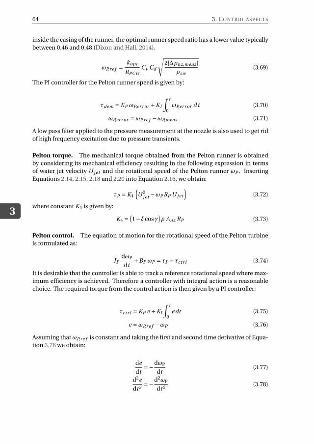
3
64 3. CONTROL ASPECTS
inside the casing of the runner, the optimal runner speed ratio has a lower value typically
between 0.46 and 0.48 (Dixon and Hall, 2014).
ωP,r e f =kopt
RPC DCv Cd
√
2|∆pnz,meas |ρsw
(3.69)
The PI controller for the Pelton runner speed is given by:
τdem = KP ωP,er r or +KI
∫t
0ωP,er r or d t (3.70)
ωP,er r or =ωP,r e f −ωP,meas (3.71)
A low pass filter applied to the pressure measurement at the nozzle is also used to get rid
of high frequency excitation due to pressure transients.
Pelton torque. The mechanical torque obtained from the Pelton runner is obtained
by considering its mechanical efficiency resulting in the following expression in terms
of water jet velocity U j et and the rotational speed of the Pelton runner ωP . Inserting
Equations 2.14, 2.15, 2.18 and 2.20 into Equation 2.16, we obtain:
τP = K4
(
U 2j et −ωP RP U j et
)
(3.72)
where constant K4 is given by:
K4 =(
1−ξcosγ)
ρ Anz RP (3.73)
Pelton control. The equation of motion for the rotational speed of the Pelton turbine
is formulated as:
JPdωP
dt+BP ωP = τP +τctr l (3.74)
It is desirable that the controller is able to track a reference rotational speed where max-
imum efficiency is achieved. Therefore a controller with integral action is a reasonable
choice. The required torque from the control action is then given by a PI controller:
τctr l = KP e +KI
∫t
0e dt (3.75)
e =ωP,r e f −ωP (3.76)
Assuming that ωP,r e f is constant and taking the first and second time derivative of Equa-
tion 3.76 we obtain:
de
dt=−
dωP
dt(3.77)
d2e
dt2=−
d2ωP
dt2(3.78)
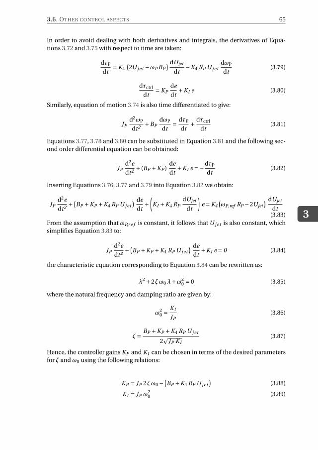
3.6. OTHER CONTROL ASPECTS
3
65
In order to avoid dealing with both derivatives and integrals, the derivatives of Equa-
tions 3.72 and 3.75 with respect to time are taken:
dτP
dt= K4
(
2U j et −ωP RP
) dUjet
dt−K4 RP U j et
dωP
dt(3.79)
dτctrl
dt= KP
de
dt+KI e (3.80)
Similarly, equation of motion 3.74 is also time differentiated to give:
JPd2ωP
dt2+BP
dωP
dt=
dτP
dt+
dτctrl
dt(3.81)
Equations 3.77, 3.78 and 3.80 can be substituted in Equation 3.81 and the following sec-
ond order differential equation can be obtained:
JPd2e
dt2+ (BP +KP )
de
dt+KI e =−
dτP
dt(3.82)
Inserting Equations 3.76, 3.77 and 3.79 into Equation 3.82 we obtain:
JPd2e
dt2+
(
BP +KP +K4 RP U j et
) de
dt+
(
KI +K4 RP
dUjet
dt
)
e = K4
(
ωP,ref RP −2Ujet
) dUjet
dt(3.83)
From the assumption that ωP,r e f is constant, it follows that U j et is also constant, which
simplifies Equation 3.83 to:
JPd2e
dt2+
(
BP +KP +K4 RP U j et
) de
dt+KI e = 0 (3.84)
the characteristic equation corresponding to Equation 3.84 can be rewritten as:
λ2 +2ζω0 λ+ω20 = 0 (3.85)
where the natural frequency and damping ratio are given by:
ω20 =
KI
JP(3.86)
ζ=BP +KP +K4 RP U j et
2p
JP KI
(3.87)
Hence, the controller gains KP and KI can be chosen in terms of the desired parameters
for ζ and ω0 using the following relations:
KP = JP 2ζω0 −(
BP +K4 RP U j et
)
(3.88)
KI = JP ω20 (3.89)
3
66 3. CONTROL ASPECTS
3.7. CONCLUDING REMARKSThis chapter showed that is possible to use hydraulic technology to replace the variable
speed functionality of wind turbines. Both a passive and active control strategies were
analyzed for a single wind turbine using feedback control tools in both the frequency
and time domain. The passive control strategy showed to be inherently stable by using
a constant area nozzle for below rated wind speed conditions. In this strategy, the size of
the diameter of the nozzle can be chosen to match the optimal tip speed ratio of the rotor
while having a variable pressure in the hydraulic network. The passive strategy is simple
and robust but is limited for a single turbine. As more turbines are to be incorporated
into the same hydraulic network, a constant pressure system would be preferred.
An active control strategy was also analyzed to obtain a variable speed rotor while keep-
ing a constant pressure in the hydraulic network. The constant pressure control was
achieved by modifying the area of the nozzle through a linear actuator. A combination
of a PI control in series with a low-pass filter and notches was used to reduce the influ-
ence of the pipeline dynamics on the pressure response. In addition a variable displace-
ment pump operating under the controlled pressure was used to modify the transmitted
torque to the rotor. Since the controllers were designed under the framework of linear-
control theory, it is expected that other control methods can lead to a more effective and
robust variable speed functionality.
4DYNAMICS AND PERFORMANCE OF A
SINGLE HYDRAULIC WIND TURBINE
4.1. INTRODUCTIONBefore evaluating the performance of a hydraulic wind farm, it is desirable to under-
stand the performance and dynamic response of a single turbine subject to a stochastic
wind. This chapter presents the modelling and analysis of two fictitious offshore wind
turbines using pressurized water as transmission medium. In order to evaluate their per-
formance, their performance is compared with that of a conventional offshore wind tur-
bine. Each of these turbines will be considered as a single operating unit of a hydraulic
wind farm at a later stage, in the simulations of Chapter 6.
The chapter is organized as follows. Section 4.2 provides the operational principle and
the main design aspects of two concepts of turbines. In Section 4.3, the hydraulic mod-
els and control strategies described in Chapter 2 and Chapter 3 are incorporated into
the model, while the operational steady-state characteristics are shown in Section 4.4.
Finally, time domain simulations are used in Section 4.5 to analyze the dynamic perfor-
mance and transient response of a single turbine under different operational conditions.
4.2. SYSTEM DESCRIPTIONTwo different concepts of offshore wind turbines will be evaluated as potential solutions
for a hydraulic wind farm. The design parameters of both hydraulic concepts were ob-
tained using as a basis the operating conditions and the same rotor as the 5 MW NREL
offshore turbine (Jonkman et al., 2009). The rotor is rigidly interconnected to the fluid
power transmission and generator platform described in the previous chapters. Despite
the lack of availability of the required multi-MW pumps or motors, it will be assumed
Parts of this chapter have been published in IET Renewable Power Generation, 8(4) and in Journal of Compu-
tational and Nonlinear Dynamics, 10(4) (Jarquin Laguna et al., 2014; Jarquin Laguna, 2015). The content is
reproduced here with permission of the publishers and the co-authors. Note that minor changes have been
introduced to make the text consistent with the other chapters of the thesis.
67
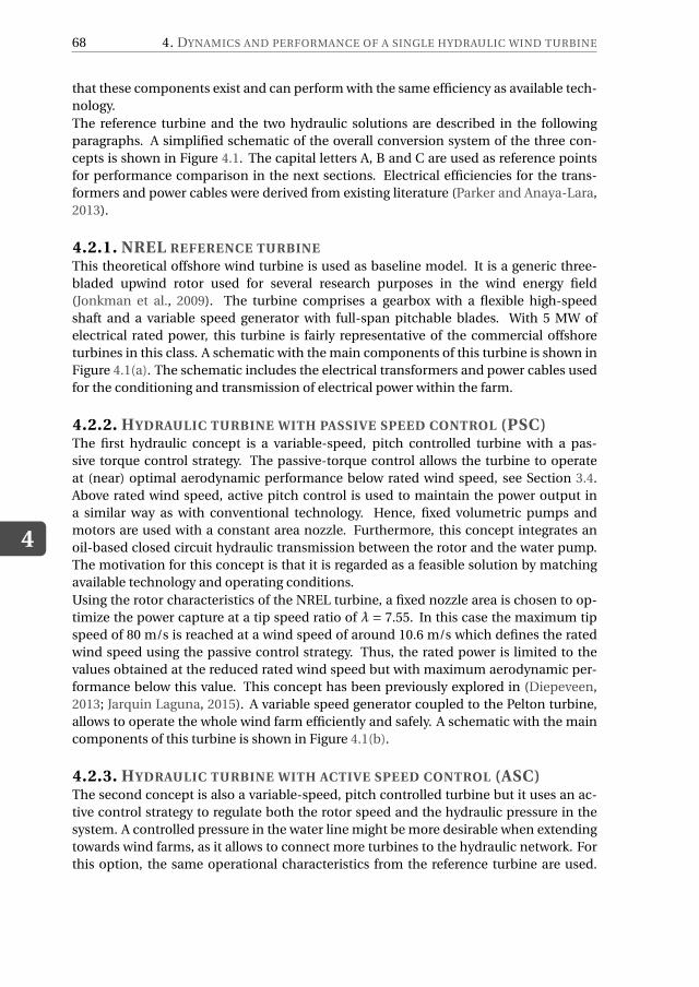
4
68 4. DYNAMICS AND PERFORMANCE OF A SINGLE HYDRAULIC WIND TURBINE
that these components exist and can perform with the same efficiency as available tech-
nology.
The reference turbine and the two hydraulic solutions are described in the following
paragraphs. A simplified schematic of the overall conversion system of the three con-
cepts is shown in Figure 4.1. The capital letters A, B and C are used as reference points
for performance comparison in the next sections. Electrical efficiencies for the trans-
formers and power cables were derived from existing literature (Parker and Anaya-Lara,
2013).
4.2.1. NREL REFERENCE TURBINEThis theoretical offshore wind turbine is used as baseline model. It is a generic three-
bladed upwind rotor used for several research purposes in the wind energy field
(Jonkman et al., 2009). The turbine comprises a gearbox with a flexible high-speed
shaft and a variable speed generator with full-span pitchable blades. With 5 MW of
electrical rated power, this turbine is fairly representative of the commercial offshore
turbines in this class. A schematic with the main components of this turbine is shown in
Figure 4.1(a). The schematic includes the electrical transformers and power cables used
for the conditioning and transmission of electrical power within the farm.
4.2.2. HYDRAULIC TURBINE WITH PASSIVE SPEED CONTROL (PSC)The first hydraulic concept is a variable-speed, pitch controlled turbine with a pas-
sive torque control strategy. The passive-torque control allows the turbine to operate
at (near) optimal aerodynamic performance below rated wind speed, see Section 3.4.
Above rated wind speed, active pitch control is used to maintain the power output in
a similar way as with conventional technology. Hence, fixed volumetric pumps and
motors are used with a constant area nozzle. Furthermore, this concept integrates an
oil-based closed circuit hydraulic transmission between the rotor and the water pump.
The motivation for this concept is that it is regarded as a feasible solution by matching
available technology and operating conditions.
Using the rotor characteristics of the NREL turbine, a fixed nozzle area is chosen to op-
timize the power capture at a tip speed ratio of λ = 7.55. In this case the maximum tip
speed of 80 m/s is reached at a wind speed of around 10.6 m/s which defines the rated
wind speed using the passive control strategy. Thus, the rated power is limited to the
values obtained at the reduced rated wind speed but with maximum aerodynamic per-
formance below this value. This concept has been previously explored in (Diepeveen,
2013; Jarquin Laguna, 2015). A variable speed generator coupled to the Pelton turbine,
allows to operate the whole wind farm efficiently and safely. A schematic with the main
components of this turbine is shown in Figure 4.1(b).
4.2.3. HYDRAULIC TURBINE WITH ACTIVE SPEED CONTROL (ASC)The second concept is also a variable-speed, pitch controlled turbine but it uses an ac-
tive control strategy to regulate both the rotor speed and the hydraulic pressure in the
system. A controlled pressure in the water line might be more desirable when extending
towards wind farms, as it allows to connect more turbines to the hydraulic network. For
this option, the same operational characteristics from the reference turbine are used.
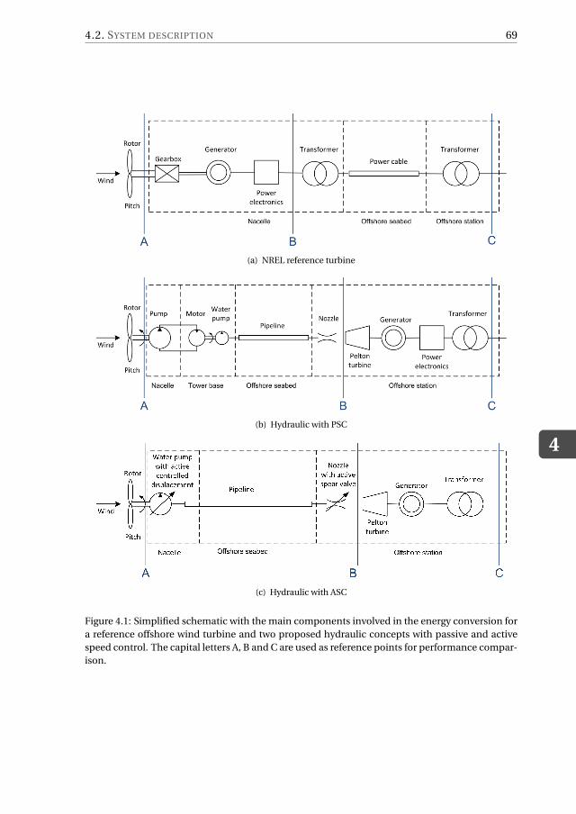
4.2. SYSTEM DESCRIPTION
4
69
(a) NREL reference turbine
(b) Hydraulic with PSC
(c) Hydraulic with ASC
Figure 4.1: Simplified schematic with the main components involved in the energy conversion for
a reference offshore wind turbine and two proposed hydraulic concepts with passive and active
speed control. The capital letters A, B and C are used as reference points for performance compar-
ison.
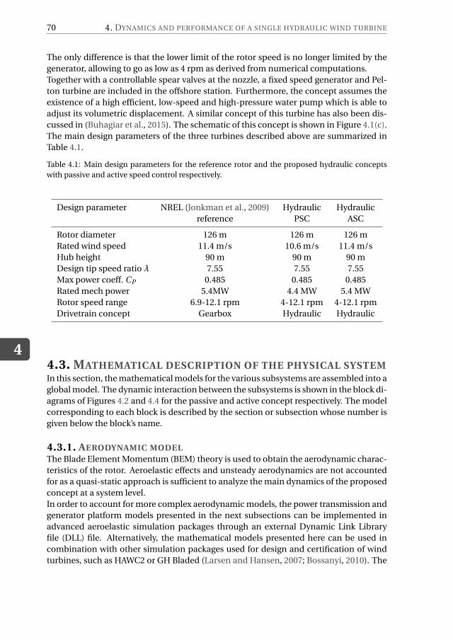
4
70 4. DYNAMICS AND PERFORMANCE OF A SINGLE HYDRAULIC WIND TURBINE
The only difference is that the lower limit of the rotor speed is no longer limited by the
generator, allowing to go as low as 4 rpm as derived from numerical computations.
Together with a controllable spear valves at the nozzle, a fixed speed generator and Pel-
ton turbine are included in the offshore station. Furthermore, the concept assumes the
existence of a high efficient, low-speed and high-pressure water pump which is able to
adjust its volumetric displacement. A similar concept of this turbine has also been dis-
cussed in (Buhagiar et al., 2015). The schematic of this concept is shown in Figure 4.1(c).
The main design parameters of the three turbines described above are summarized in
Table 4.1.
Table 4.1: Main design parameters for the reference rotor and the proposed hydraulic concepts
with passive and active speed control respectively.
Design parameter NREL (Jonkman et al., 2009) Hydraulic Hydraulic
reference PSC ASC
Rotor diameter 126 m 126 m 126 m
Rated wind speed 11.4 m/s 10.6 m/s 11.4 m/s
Hub height 90 m 90 m 90 m
Design tip speed ratio λ 7.55 7.55 7.55
Max power coeff. CP 0.485 0.485 0.485
Rated mech power 5.4MW 4.4 MW 5.4 MW
Rotor speed range 6.9-12.1 rpm 4-12.1 rpm 4-12.1 rpm
Drivetrain concept Gearbox Hydraulic Hydraulic
4.3. MATHEMATICAL DESCRIPTION OF THE PHYSICAL SYSTEMIn this section, the mathematical models for the various subsystems are assembled into a
global model. The dynamic interaction between the subsystems is shown in the block di-
agrams of Figures 4.2 and 4.4 for the passive and active concept respectively. The model
corresponding to each block is described by the section or subsection whose number is
given below the block’s name.
4.3.1. AERODYNAMIC MODELThe Blade Element Momentum (BEM) theory is used to obtain the aerodynamic charac-
teristics of the rotor. Aeroelastic effects and unsteady aerodynamics are not accounted
for as a quasi-static approach is sufficient to analyze the main dynamics of the proposed
concept at a system level.
In order to account for more complex aerodynamic models, the power transmission and
generator platform models presented in the next subsections can be implemented in
advanced aeroelastic simulation packages through an external Dynamic Link Library
file (DLL) file. Alternatively, the mathematical models presented here can be used in
combination with other simulation packages used for design and certification of wind
turbines, such as HAWC2 or GH Bladed (Larsen and Hansen, 2007; Bossanyi, 2010). The
4.3. MATHEMATICAL DESCRIPTION OF THE PHYSICAL SYSTEM
4
71
implementation of such models through an external DLL file has been previously done
for fluid power drivetrains in (Jarquin Laguna et al., 2014).
4.3.2. PITCH ACTUATOR MODELThe pitch actuator is based on a pitch-servo model described by a proportional regulator
with constant Kβ. The demanded pitch βdem was obtained from 3.6.1. The second order
model includes a time constant tβ and an input delay δ from input uβ to the pitch rate β;
the delayed input is expressed as uδβ
. The pitch actuator is implemented with pitch rate
limits of ±8◦/s.
β=1
tβ
(
uδβ− β
)
(4.1)
uβ = Kβ
(
βdem −βmeas
)
(4.2)
4.3.3. STRUCTURAL MODELThe motion of the top mass of the tower in the fore-aft direction z is described with a
second order model:
mtm z = Fthr ust −Btower z −Ktower z (4.3)
where Ktower and Btower are the support structure stiffness and damping; Fthr ust is the
thrust force exerted by the rotor on the top mass of the tower mtm , which includes the
rotor and nacelle mass.
4.3.4. HYDRAULIC DRIVETRAIN MODELThe primary function of the hydraulic drivetrain is to convert the mechanical power of
the rotor shaft into hydraulic power for electricity generation. In the proposed hydraulic
concept, the high-torque low-speed mechanical power from the rotor is converted into
a high-pressure flow-rate of water just before it enters the hydraulic turbine. The hy-
draulic drivetrains for both the passive and active control options, are constructed by
interconnecting different components like pumps, pipelines and actuators. Hence, the
overall system model is obtained by assembling together the equations of the individual
components presented in Chapter 2.
Figure 4.2: Subsystem block diagram of the hydraulic wind turbine with PSC.
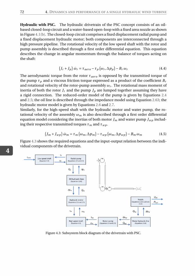
4
72 4. DYNAMICS AND PERFORMANCE OF A SINGLE HYDRAULIC WIND TURBINE
Hydraulic with PSC. The hydraulic drivetrain of the PSC concept consists of an oil-
based closed-loop circuit and a water-based open-loop with a fixed area nozzle as shown
in Figure 4.1(b). The closed-loop circuit comprises a fixed displacement radial pump and
a fixed displacement hydraulic motor; both components are interconnected through a
high pressure pipeline. The rotational velocity of the low speed shaft with the rotor and
pump assembly is described through a first order differential equation. This equation
describes the change in angular momentum through the balance of torques acting on
the shaft:
(
Jr + Jp
)
ωr = τaer o −τp
(
ωr ,∆pp
)
−Br ωr (4.4)
The aerodynamic torque from the rotor τaer o is opposed by the transmitted torque of
the pump τp and a viscous friction torque expressed as a product of the coefficient Br
and rotational velocity of the rotor-pump assembly ωr . The rotational mass moment of
inertia of both the rotor Jr and the pump Jp are lumped together assuming they have
a rigid connection. The reduced-order model of the pump is given by Equations 2.4
and 2.5; the oil line is described through the impedance model using Equation 2.63; the
hydraulic motor model is given by Equations 2.6 and 2.7.
Similarly, for the high-speed shaft with the hydraulic motor and water pump, the ro-
tational velocity of the assembly ωm is also described through a first order differential
equation model considering the inertias of both motor Jm and water pump Jw p includ-
ing their respective transmitted torques τm and τw p .
(
Jm + Jw p
)
ωm = τm
(
ωm ,∆pm
)
−τw p
(
ωm ,∆pw p
)
−Bm ωm (4.5)
Figure 4.3 shows the required equations and the input-output relation between the indi-
vidual components of the drivetrain.
Figure 4.3: Subsystem block diagram of the drivetrain with PSC.
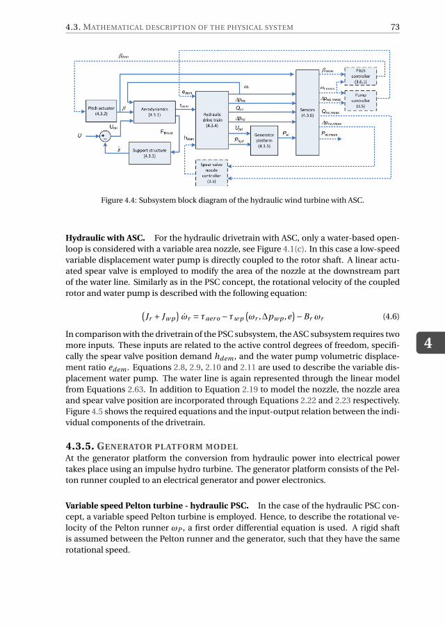
4.3. MATHEMATICAL DESCRIPTION OF THE PHYSICAL SYSTEM
4
73
Figure 4.4: Subsystem block diagram of the hydraulic wind turbine with ASC.
Hydraulic with ASC. For the hydraulic drivetrain with ASC, only a water-based open-
loop is considered with a variable area nozzle, see Figure 4.1(c). In this case a low-speed
variable displacement water pump is directly coupled to the rotor shaft. A linear actu-
ated spear valve is employed to modify the area of the nozzle at the downstream part
of the water line. Similarly as in the PSC concept, the rotational velocity of the coupled
rotor and water pump is described with the following equation:
(
Jr + Jw p
)
ωr = τaer o −τw p
(
ωr ,∆pw p ,e)
−Br ωr (4.6)
In comparison with the drivetrain of the PSC subsystem, the ASC subsystem requires two
more inputs. These inputs are related to the active control degrees of freedom, specifi-
cally the spear valve position demand hdem , and the water pump volumetric displace-
ment ratio edem . Equations 2.8, 2.9, 2.10 and 2.11 are used to describe the variable dis-
placement water pump. The water line is again represented through the linear model
from Equations 2.63. In addition to Equation 2.19 to model the nozzle, the nozzle area
and spear valve position are incorporated through Equations 2.22 and 2.23 respectively.
Figure 4.5 shows the required equations and the input-output relation between the indi-
vidual components of the drivetrain.
4.3.5. GENERATOR PLATFORM MODELAt the generator platform the conversion from hydraulic power into electrical power
takes place using an impulse hydro turbine. The generator platform consists of the Pel-
ton runner coupled to an electrical generator and power electronics.
Variable speed Pelton turbine - hydraulic PSC. In the case of the hydraulic PSC con-
cept, a variable speed Pelton turbine is employed. Hence, to describe the rotational ve-
locity of the Pelton runner ωP , a first order differential equation is used. A rigid shaft
is assumed between the Pelton runner and the generator, such that they have the same
rotational speed.
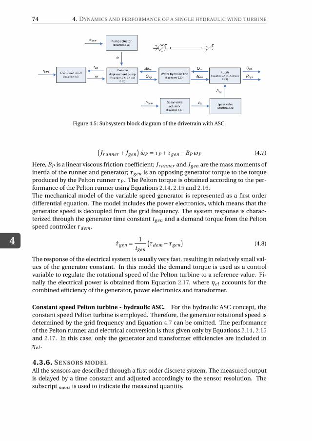
4
74 4. DYNAMICS AND PERFORMANCE OF A SINGLE HYDRAULIC WIND TURBINE
Figure 4.5: Subsystem block diagram of the drivetrain with ASC.
(
Jr unner + Jg en
)
ωP = τP +τg en −BP ωP (4.7)
Here, BP is a linear viscous friction coefficient; Jr unner and Jg en are the mass moments of
inertia of the runner and generator; τg en is an opposing generator torque to the torque
produced by the Pelton runner τP . The Pelton torque is obtained according to the per-
formance of the Pelton runner using Equations 2.14, 2.15 and 2.16.
The mechanical model of the variable speed generator is represented as a first order
differential equation. The model includes the power electronics, which means that the
generator speed is decoupled from the grid frequency. The system response is charac-
terized through the generator time constant tg en and a demand torque from the Pelton
speed controller τdem .
τg en =1
tg en
(
τdem −τg en
)
(4.8)
The response of the electrical system is usually very fast, resulting in relatively small val-
ues of the generator constant. In this model the demand torque is used as a control
variable to regulate the rotational speed of the Pelton turbine to a reference value. Fi-
nally the electrical power is obtained from Equation 2.17, where ηel accounts for the
combined efficiency of the generator, power electronics and transformer.
Constant speed Pelton turbine - hydraulic ASC. For the hydraulic ASC concept, the
constant speed Pelton turbine is employed. Therefore, the generator rotational speed is
determined by the grid frequency and Equation 4.7 can be omitted. The performance
of the Pelton runner and electrical conversion is thus given only by Equations 2.14, 2.15
and 2.17. In this case, only the generator and transformer efficiencies are included in
ηel .
4.3.6. SENSORS MODELAll the sensors are described through a first order discrete system. The measured output
is delayed by a time constant and adjusted accordingly to the sensor resolution. The
subscript meas is used to indicate the measured quantity.
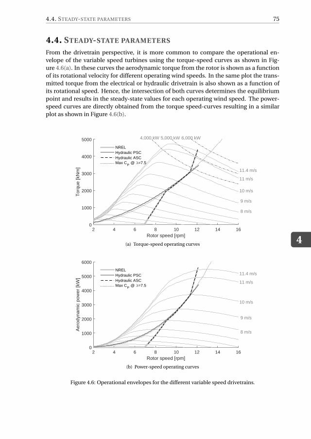
4.4. STEADY-STATE PARAMETERS
4
75
4.4. STEADY-STATE PARAMETERS
From the drivetrain perspective, it is more common to compare the operational en-
velope of the variable speed turbines using the torque-speed curves as shown in Fig-
ure 4.6(a). In these curves the aerodynamic torque from the rotor is shown as a function
of its rotational velocity for different operating wind speeds. In the same plot the trans-
mitted torque from the electrical or hydraulic drivetrain is also shown as a function of
its rotational speed. Hence, the intersection of both curves determines the equilibrium
point and results in the steady-state values for each operating wind speed. The power-
speed curves are directly obtained from the torque speed-curves resulting in a similar
plot as shown in Figure 4.6(b).
Rotor speed [rpm]2 4 6 8 10 12 14 16
Tor
que
[kN
m]
0
1000
2000
3000
4000
5000
11.4 m/s
11 m/s
10 m/s
9 m/s
8 m/s
4,000 kW 5,000 kW 6,000 kW
NRELHydraulic PSCHydraulic ASCMax C
P @ λ=7.5
(a) Torque-speed operating curves
Rotor speed [rpm]2 4 6 8 10 12 14 16
Aer
odyn
amic
pow
er [k
W]
0
1000
2000
3000
4000
5000
6000
11.4 m/s
11 m/s
10 m/s
9 m/s
8 m/s
NRELHydraulic PSCHydraulic ASCMax C
P @ λ=7.5
(b) Power-speed operating curves
Figure 4.6: Operational envelopes for the different variable speed drivetrains.
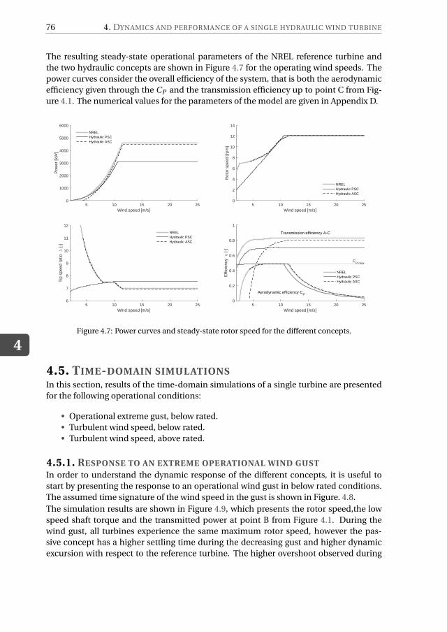
4
76 4. DYNAMICS AND PERFORMANCE OF A SINGLE HYDRAULIC WIND TURBINE
The resulting steady-state operational parameters of the NREL reference turbine and
the two hydraulic concepts are shown in Figure 4.7 for the operating wind speeds. The
power curves consider the overall efficiency of the system, that is both the aerodynamic
efficiency given through the CP and the transmission efficiency up to point C from Fig-
ure 4.1. The numerical values for the parameters of the model are given in Appendix D.
Wind speed [m/s]5 10 15 20 25
Pow
er [k
W]
0
1000
2000
3000
4000
5000
6000
NRELHydraulic PSCHydraulic ASC
Wind speed [m/s]5 10 15 20 25
Rot
or s
peed
[rpm
]
0
2
4
6
8
10
12
14
NRELHydraulic PSCHydraulic ASC
Wind speed [m/s]5 10 15 20 25
Tip
spe
ed r
atio
λ
[-]
6
7
8
9
10
11
12
NRELHydraulic PSCHydraulic ASC
Wind speed [m/s]5 10 15 20 25
Effi
cien
cy η [
-]
0
0.2
0.4
0.6
0.8
1
CP,max
Aerodynamic efficiency CP
Transmission efficiency A-C
NRELHydraulic PSCHydraulic ASC
Figure 4.7: Power curves and steady-state rotor speed for the different concepts.
4.5. TIME-DOMAIN SIMULATIONSIn this section, results of the time-domain simulations of a single turbine are presented
for the following operational conditions:
• Operational extreme gust, below rated.
• Turbulent wind speed, below rated.
• Turbulent wind speed, above rated.
4.5.1. RESPONSE TO AN EXTREME OPERATIONAL WIND GUST
In order to understand the dynamic response of the different concepts, it is useful to
start by presenting the response to an operational wind gust in below rated conditions.
The assumed time signature of the wind speed in the gust is shown in Figure. 4.8.
The simulation results are shown in Figure 4.9, which presents the rotor speed,the low
speed shaft torque and the transmitted power at point B from Figure 4.1. During the
wind gust, all turbines experience the same maximum rotor speed, however the pas-
sive concept has a higher settling time during the decreasing gust and higher dynamic
excursion with respect to the reference turbine. The higher overshoot observed during
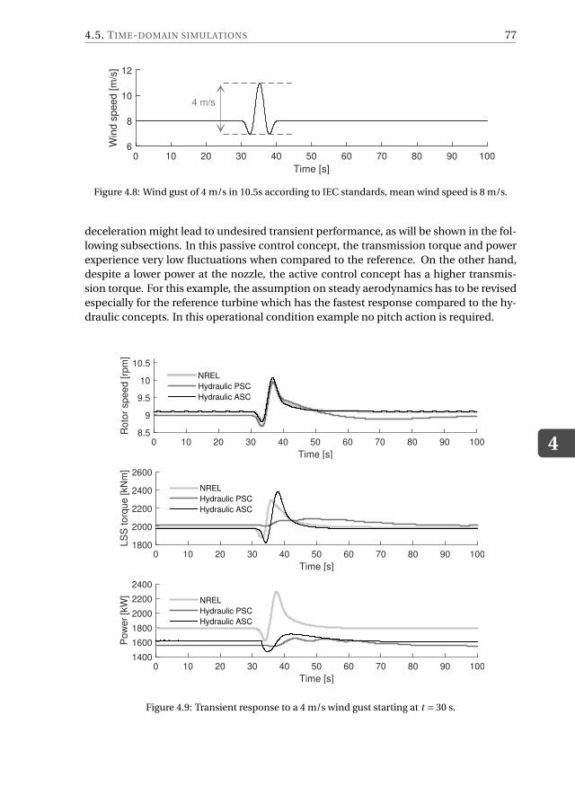
4.5. TIME-DOMAIN SIMULATIONS
4
77
Time [s]
0 10 20 30 40 50 60 70 80 90 100
Win
d s
peed [m
/s]
6
8
10
12
4 m/s
Figure 4.8: Wind gust of 4 m/s in 10.5s according to IEC standards, mean wind speed is 8 m/s.
deceleration might lead to undesired transient performance, as will be shown in the fol-
lowing subsections. In this passive control concept, the transmission torque and power
experience very low fluctuations when compared to the reference. On the other hand,
despite a lower power at the nozzle, the active control concept has a higher transmis-
sion torque. For this example, the assumption on steady aerodynamics has to be revised
especially for the reference turbine which has the fastest response compared to the hy-
draulic concepts. In this operational condition example no pitch action is required.
Time [s]
0 10 20 30 40 50 60 70 80 90 100
Ro
tor
sp
ee
d [
rpm
]
8.5
9
9.5
10
10.5
NREL
Hydraulic PSC
Hydraulic ASC
Time [s]
0 10 20 30 40 50 60 70 80 90 100
LS
S t
orq
ue
[kN
m]
1800
2000
2200
2400
2600
NREL
Hydraulic PSC
Hydraulic ASC
Time [s]
0 10 20 30 40 50 60 70 80 90 100
Po
we
r [k
W]
1400
1600
1800
2000
2200
2400
NREL
Hydraulic PSC
Hydraulic ASC
Figure 4.9: Transient response to a 4 m/s wind gust starting at t = 30 s.
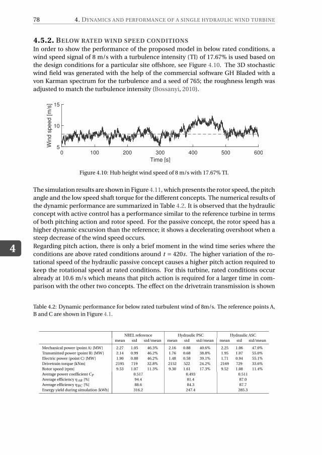
4
78 4. DYNAMICS AND PERFORMANCE OF A SINGLE HYDRAULIC WIND TURBINE
4.5.2. BELOW RATED WIND SPEED CONDITIONSIn order to show the performance of the proposed model in below rated conditions, a
wind speed signal of 8 m/s with a turbulence intensity (TI) of 17.67% is used based on
the design conditions for a particular site offshore, see Figure 4.10. The 3D stochastic
wind field was generated with the help of the commercial software GH Bladed with a
von Karman spectrum for the turbulence and a seed of 765; the roughness length was
adjusted to match the turbulence intensity (Bossanyi, 2010).
Time [s]
0 100 200 300 400 500 600
Win
d s
peed [m
/s]
5
10
15
Figure 4.10: Hub height wind speed of 8 m/s with 17.67% TI.
The simulation results are shown in Figure 4.11, which presents the rotor speed, the pitch
angle and the low speed shaft torque for the different concepts. The numerical results of
the dynamic performance are summarized in Table 4.2. It is observed that the hydraulic
concept with active control has a performance similar to the reference turbine in terms
of both pitching action and rotor speed. For the passive concept, the rotor speed has a
higher dynamic excursion than the reference; it shows a decelerating overshoot when a
steep decrease of the wind speed occurs.
Regarding pitch action, there is only a brief moment in the wind time series where the
conditions are above rated conditions around t = 420s. The higher variation of the ro-
tational speed of the hydraulic passive concept causes a higher pitch action required to
keep the rotational speed at rated conditions. For this turbine, rated conditions occur
already at 10.6 m/s which means that pitch action is required for a larger time in com-
parison with the other two concepts. The effect on the drivetrain transmission is shown
Table 4.2: Dynamic performance for below rated turbulent wind of 8m/s. The reference points A,
B and C are shown in Figure 4.1.
NREL reference Hydraulic PSC Hydraulic ASC
mean std std/mean mean std std/mean mean std std/mean
Mechanical power (point A) [MW] 2.27 1.05 46.3% 2.16 0.88 40.6% 2.25 1.06 47.0%
Transmitted power (point B) [MW] 2.14 0.99 46.2% 1.76 0.68 38.8% 1.95 1.07 55.0%
Electric power (point C) [MW] 1.90 0.88 46.2% 1.48 0.58 39.1% 1.71 0.94 55.1%
Drivetrain torque [kNm] 2195 719 32.8% 2152 522 24.2% 2169 729 33.6%
Rotor speed [rpm] 9.53 1.07 11.3% 9.30 1.61 17.3% 9.52 1.08 11.4%
Average power coefficient CP 0.517 0.493 0.511
Average efficiency ηAB [%] 94.4 81.4 87.0
Average efficiency ηBC [%] 88.6 84.3 87.7
Energy yield during simulation [kWh] 316.2 247.4 285.3
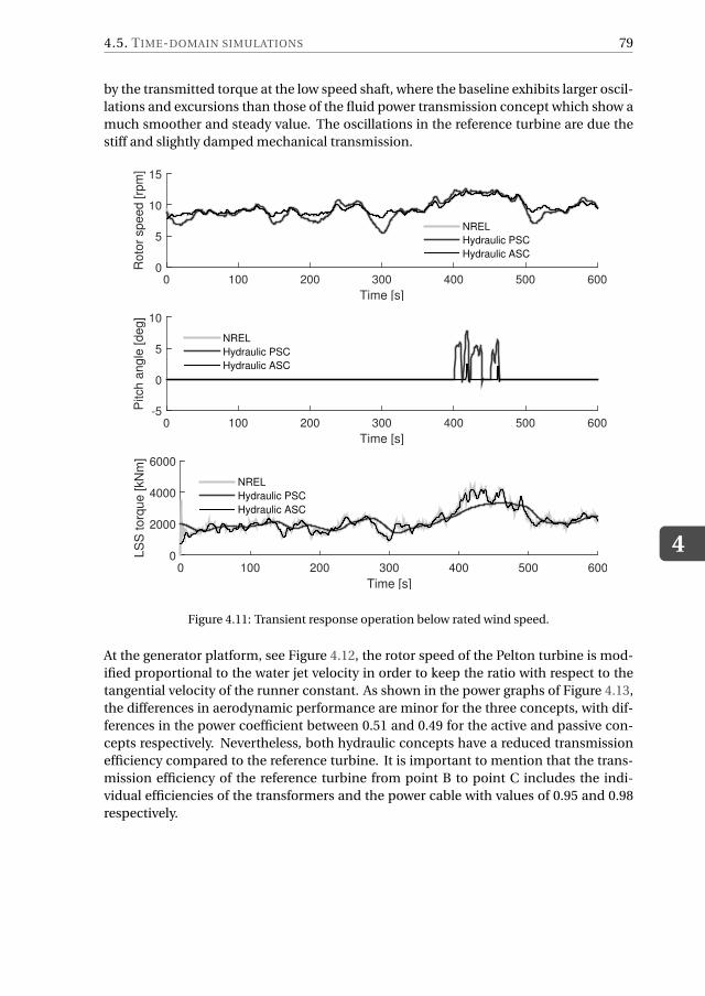
4.5. TIME-DOMAIN SIMULATIONS
4
79
by the transmitted torque at the low speed shaft, where the baseline exhibits larger oscil-
lations and excursions than those of the fluid power transmission concept which show a
much smoother and steady value. The oscillations in the reference turbine are due the
stiff and slightly damped mechanical transmission.
Time [s]
0 100 200 300 400 500 600
Roto
r speed [rp
m]
0
5
10
15
NREL
Hydraulic PSC
Hydraulic ASC
Time [s]
0 100 200 300 400 500 600
Pitch a
ngle
[deg]
-5
0
5
10
NREL
Hydraulic PSC
Hydraulic ASC
Time [s]
0 100 200 300 400 500 600
LS
S t
orq
ue
[kN
m]
0
2000
4000
6000
NREL
Hydraulic PSC
Hydraulic ASC
Figure 4.11: Transient response operation below rated wind speed.
At the generator platform, see Figure 4.12, the rotor speed of the Pelton turbine is mod-
ified proportional to the water jet velocity in order to keep the ratio with respect to the
tangential velocity of the runner constant. As shown in the power graphs of Figure 4.13,
the differences in aerodynamic performance are minor for the three concepts, with dif-
ferences in the power coefficient between 0.51 and 0.49 for the active and passive con-
cepts respectively. Nevertheless, both hydraulic concepts have a reduced transmission
efficiency compared to the reference turbine. It is important to mention that the trans-
mission efficiency of the reference turbine from point B to point C includes the indi-
vidual efficiencies of the transformers and the power cable with values of 0.95 and 0.98
respectively.
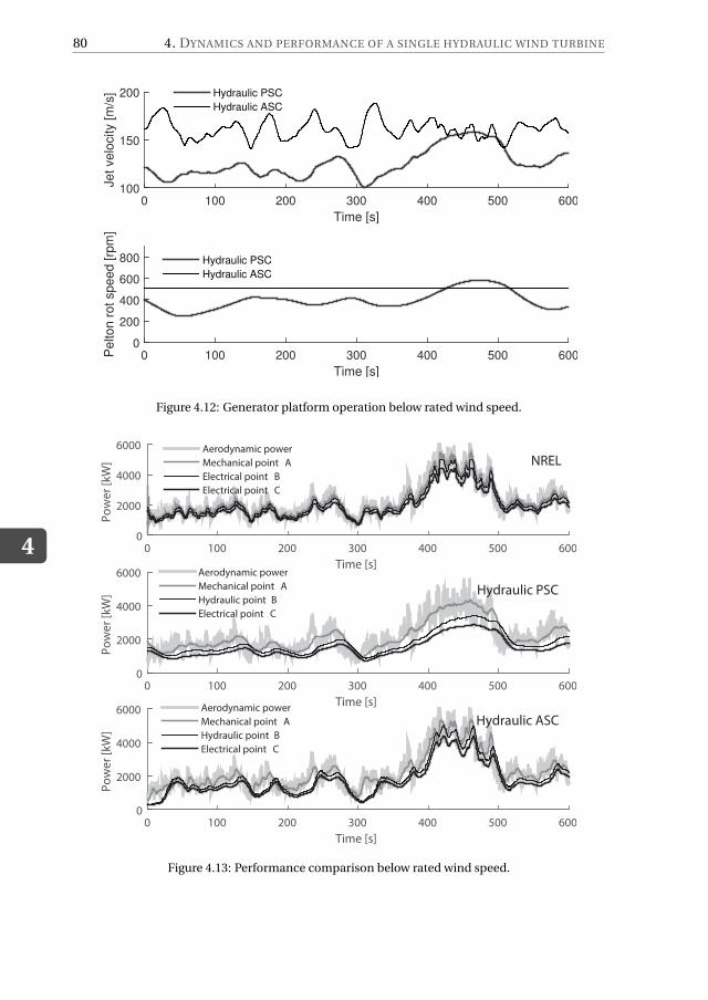
4
80 4. DYNAMICS AND PERFORMANCE OF A SINGLE HYDRAULIC WIND TURBINE
Time [s]
0 100 200 300 400 500 600
Jet velo
city [m
/s]
100
150
200 Hydraulic PSC
Hydraulic ASC
Time [s]
0 100 200 300 400 500 600Pelton r
ot speed [rp
m]
0
200
400
600
800 Hydraulic PSC
Hydraulic ASC
Figure 4.12: Generator platform operation below rated wind speed.
Time [s]
0 100 200 300 400 500 600
Po
we
r [k
W]
0
2000
4000
6000
NRELAerodynamic power
Mechanical point A
Electrical point B
Electrical point C
Time [s]
0 100 200 300 400 500 600
Po
we
r [k
W]
0
2000
4000
6000
Hydraulic PSC
Aerodynamic power
Mechanical point A
Hydraulic point B
Electrical point C
Time [s]
0 100 200 300 400 500 600
Po
we
r [k
W]
0
2000
4000
6000Hydraulic ASC
Aerodynamic power
Mechanical point A
Hydraulic point B
Electrical point C
Figure 4.13: Performance comparison below rated wind speed.
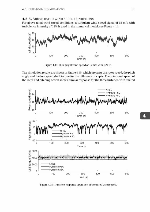
4.5. TIME-DOMAIN SIMULATIONS
4
81
4.5.3. ABOVE RATED WIND SPEED CONDITIONSFor above rated wind speed conditions, a turbulent wind speed signal of 15 m/s with
turbulence intensity of 12% is used in the numerical model, see Figure 4.14.
Time [s]
0 100 200 300 400 500 600
Win
d s
peed [m
/s]
5
10
15
20
Figure 4.14: Hub height wind speed of 15 m/s with 12% TI.
The simulation results are shown in Figure 4.15, which presents the rotor speed, the pitch
angle and the low speed shaft torque for the different concepts. The rotational speed of
the rotor and pitching action show a similar response for the three turbines, with related
Time [s]
0 100 200 300 400 500 600
Roto
r speed [rp
m]
10
12
14
NREL
Hydraulic PSC
Hydraulic ASC
Time [s]
0 100 200 300 400 500 600
Pitch a
ngle
[deg]
-10
0
10
20
NREL
Hydraulic PSC
Hydraulic ASC
Time [s]
0 100 200 300 400 500 600
LS
S t
orq
ue
[kN
m]
0
2000
4000
6000
NREL
Hydraulic PSC
Hydraulic ASC
Figure 4.15: Transient response operation above rated wind speed.
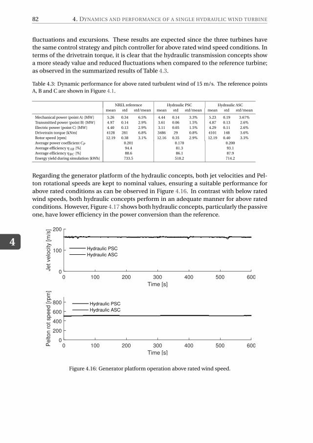
4
82 4. DYNAMICS AND PERFORMANCE OF A SINGLE HYDRAULIC WIND TURBINE
fluctuations and excursions. These results are expected since the three turbines have
the same control strategy and pitch controller for above rated wind speed conditions. In
terms of the drivetrain torque, it is clear that the hydraulic transmission concepts show
a more steady value and reduced fluctuations when compared to the reference turbine;
as observed in the summarized results of Table 4.3.
Table 4.3: Dynamic performance for above rated turbulent wind of 15 m/s. The reference points
A, B and C are shown in Figure 4.1.
NREL reference Hydraulic PSC Hydraulic ASC
mean std std/mean mean std std/mean mean std std/mean
Mechanical power (point A) [MW] 5.26 0.34 6.5% 4.44 0.14 3.3% 5.23 0.19 3.67%
Transmitted power (point B) [MW] 4.97 0.14 2.9% 3.61 0.06 1.5% 4.87 0.13 2.6%
Electric power (point C) [MW] 4.40 0.13 2.9% 3.11 0.05 1.5% 4.29 0.11 2.6%
Drivetrain torque [kNm] 4128 281 6.8% 3486 29 0.8% 4101 148 3.6%
Rotor speed [rpm] 12.19 0.38 3.1% 12.16 0.35 2.9% 12.19 0.40 3.3%
Average power coefficient CP 0.201 0.170 0.200
Average efficiency ηAB [%] 94.4 81.3 93.1
Average efficiency ηBC [%] 88.6 86.1 87.9
Energy yield during simulation [kWh] 733.5 518.2 714.2
Regarding the generator platform of the hydraulic concepts, both jet velocities and Pel-
ton rotational speeds are kept to nominal values, ensuring a suitable performance for
above rated conditions as can be observed in Figure 4.16. In contrast with below rated
wind speeds, both hydraulic concepts perform in an adequate manner for above rated
conditions. However, Figure 4.17 shows both hydraulic concepts, particularly the passive
one, have lower efficiency in the power conversion than the reference.
Time [s]
0 100 200 300 400 500 600
Jet velo
city [m
/s]
0
100
200
Hydraulic PSC
Hydraulic ASC
Time [s]
0 100 200 300 400 500 600Pelton r
ot speed [rp
m]
0
200
400
600
800 Hydraulic PSC
Hydraulic ASC
Figure 4.16: Generator platform operation above rated wind speed.
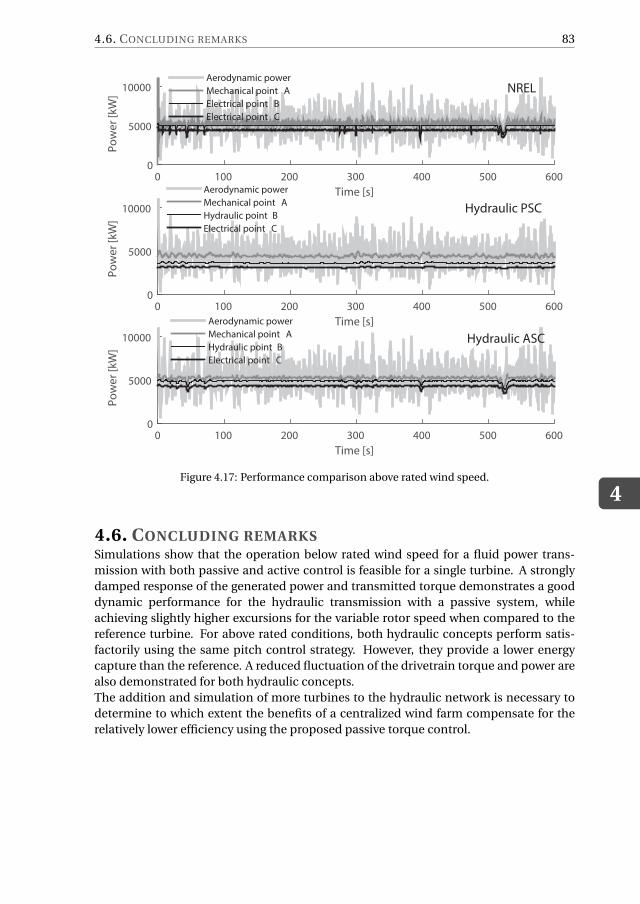
4.6. CONCLUDING REMARKS
4
83
Time [s]
0 100 200 300 400 500 600
Po
we
r [k
W]
0
5000
10000 NRELAerodynamic power
Mechanical point A
Electrical point B
Electrical point C
Time [s]
0 100 200 300 400 500 600
Po
we
r [k
W]
0
5000
10000 Hydraulic PSC
Aerodynamic power
Mechanical point A
Hydraulic point B
Electrical point C
Time [s]
0 100 200 300 400 500 600
Po
we
r [k
W]
0
5000
10000 Hydraulic ASC
Aerodynamic power
Mechanical point A
Hydraulic point B
Electrical point C
Figure 4.17: Performance comparison above rated wind speed.
4.6. CONCLUDING REMARKSSimulations show that the operation below rated wind speed for a fluid power trans-
mission with both passive and active control is feasible for a single turbine. A strongly
damped response of the generated power and transmitted torque demonstrates a good
dynamic performance for the hydraulic transmission with a passive system, while
achieving slightly higher excursions for the variable rotor speed when compared to the
reference turbine. For above rated conditions, both hydraulic concepts perform satis-
factorily using the same pitch control strategy. However, they provide a lower energy
capture than the reference. A reduced fluctuation of the drivetrain torque and power are
also demonstrated for both hydraulic concepts.
The addition and simulation of more turbines to the hydraulic network is necessary to
determine to which extent the benefits of a centralized wind farm compensate for the
relatively lower efficiency using the proposed passive torque control.


5HYDRAULIC NETWORK TRANSIENTS
5.1. INTRODUCTIONOne of the key challenges in the quest for a centralized electricity generation is the use
of hydraulic networks for collection and transport of the pressurised water from the in-
dividual wind turbines to the generator platform. This chapter presents an evaluation
of the accuracy of a numerical time-domain model of a hydraulic network developed in
the framework of this thesis. The numerical model should be able to accurately repre-
sent the transient response of the hydraulic network to enable the simulation of a more
general wind power plant model. Thus, in order to evaluate the accuracy of the model,
a semi-analytical approach is presented based on the impulse response method (IRM).
This method has been extensively used for dynamic analyses in other areas such as vi-
brations of mechanical systems (Graff, 1991), however its use in hydraulic systems has
not been completely exploited.
The chapter is organized as follows. In Section 5.2, a brief overview of the most com-
mon time-domain numerical models, to solve fluid transients in hydraulic networks, is
presented. Then, in Section 5.3 a semi-analytical method is proposed. The analytical
solution of a single line is extended to the solution of a more complex hydraulic net-
work consisting of several hydraulic lines. To illustrate the application of the analytical
method, a numerical example of a simple hydraulic network is treated in Section 5.4.
Here, the time-domain results are compared with the ones obtained by using the modal
method of analysis applied to the hydraulic network. Finally conclusions are presented
in Section 5.5.
5.2. FLUID TRANSIENTS IN HYDRAULIC NETWORKSTransient flow in hydraulic networks is a phenomenon that often occurs as a result of
either accidental or normal operation of hydraulic systems. Its importance has been
This chapter has been published in Heron, 59(1) (Jarquin Laguna and Tsouvalas, 2014) and is reproduced here
with permission of the co-author. Note that minor changes have been introduced to make the text consistent
with the other chapters of the thesis.
85
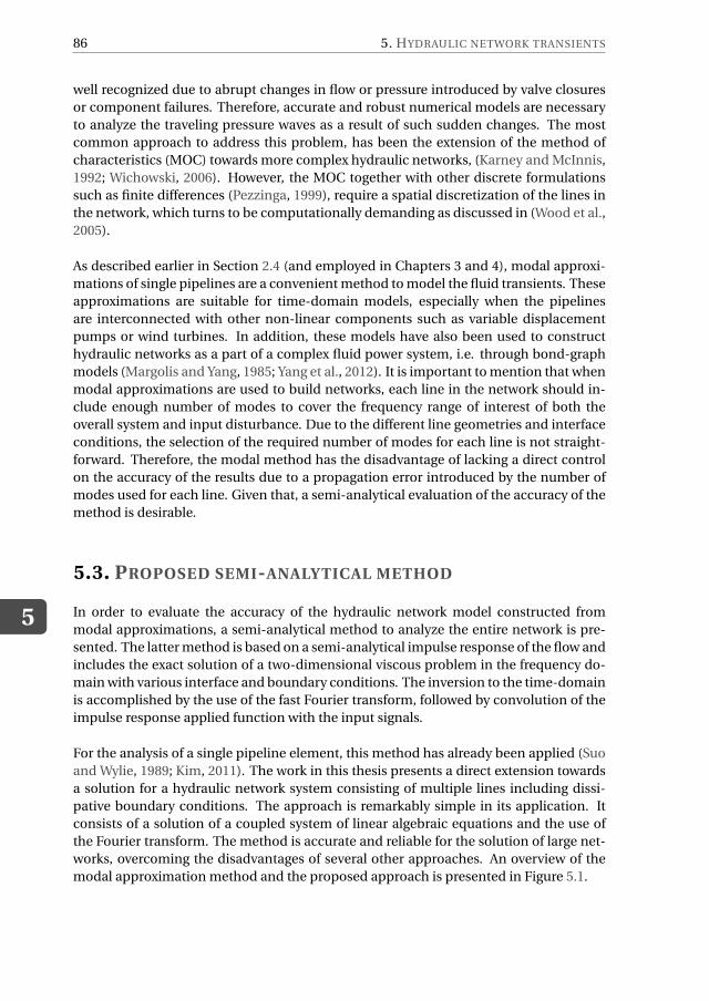
5
86 5. HYDRAULIC NETWORK TRANSIENTS
well recognized due to abrupt changes in flow or pressure introduced by valve closures
or component failures. Therefore, accurate and robust numerical models are necessary
to analyze the traveling pressure waves as a result of such sudden changes. The most
common approach to address this problem, has been the extension of the method of
characteristics (MOC) towards more complex hydraulic networks, (Karney and McInnis,
1992; Wichowski, 2006). However, the MOC together with other discrete formulations
such as finite differences (Pezzinga, 1999), require a spatial discretization of the lines in
the network, which turns to be computationally demanding as discussed in (Wood et al.,
2005).
As described earlier in Section 2.4 (and employed in Chapters 3 and 4), modal approxi-
mations of single pipelines are a convenient method to model the fluid transients. These
approximations are suitable for time-domain models, especially when the pipelines
are interconnected with other non-linear components such as variable displacement
pumps or wind turbines. In addition, these models have also been used to construct
hydraulic networks as a part of a complex fluid power system, i.e. through bond-graph
models (Margolis and Yang, 1985; Yang et al., 2012). It is important to mention that when
modal approximations are used to build networks, each line in the network should in-
clude enough number of modes to cover the frequency range of interest of both the
overall system and input disturbance. Due to the different line geometries and interface
conditions, the selection of the required number of modes for each line is not straight-
forward. Therefore, the modal method has the disadvantage of lacking a direct control
on the accuracy of the results due to a propagation error introduced by the number of
modes used for each line. Given that, a semi-analytical evaluation of the accuracy of the
method is desirable.
5.3. PROPOSED SEMI-ANALYTICAL METHOD
In order to evaluate the accuracy of the hydraulic network model constructed from
modal approximations, a semi-analytical method to analyze the entire network is pre-
sented. The latter method is based on a semi-analytical impulse response of the flow and
includes the exact solution of a two-dimensional viscous problem in the frequency do-
main with various interface and boundary conditions. The inversion to the time-domain
is accomplished by the use of the fast Fourier transform, followed by convolution of the
impulse response applied function with the input signals.
For the analysis of a single pipeline element, this method has already been applied (Suo
and Wylie, 1989; Kim, 2011). The work in this thesis presents a direct extension towards
a solution for a hydraulic network system consisting of multiple lines including dissi-
pative boundary conditions. The approach is remarkably simple in its application. It
consists of a solution of a coupled system of linear algebraic equations and the use of
the Fourier transform. The method is accurate and reliable for the solution of large net-
works, overcoming the disadvantages of several other approaches. An overview of the
modal approximation method and the proposed approach is presented in Figure 5.1.
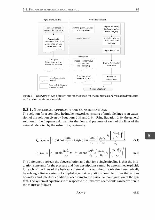
5.3. PROPOSED SEMI-ANALYTICAL METHOD
5
87
Figure 5.1: Overview of two different approaches used for the numerical analysis of hydraulic net-
works using continuous models.
5.3.1. NUMERICAL APPROACH AND CONSIDERATIONSThe solution for a complete hydraulic network consisting of multiple lines is an exten-
sion of the solution given by Equations 2.33 and 2.34. Using Equation 2.30, the general
solution in the frequency domain for the flow and pressure of each of the lines of the
network, denoted by the subscript i , is given by:
Qi (x,ω) =[
Ai (ω) cosiωβi
cox +Bi (ω) sin
iωβi
cox
]
ρoco
Z0,i
J0
[
i
(
iω r 20,i
νo
) 12
]
β2i
(5.1)
Pi (x,ω) =[
Ai (ω) siniωβi
cox −Bi (ω) cos
iωβi
cox
]
ρoco
βiJ0
i
(
iω r 20,i
νo
)
12
(5.2)
The difference between the above solution and that for a single pipeline is that the inte-
gration constants for the pressure and flow descriptions cannot be determined explicitly
for each of the lines of the hydraulic network. Instead they are obtained numerically
by solving a linear system of coupled algebraic equations compiled from the various
boundary and interface conditions according to the particular configuration of the sys-
tem. The system of equations with respect to the unknown coefficients can be written in
the matrix as follows:
A x = b (5.3)
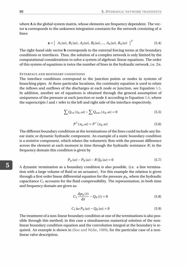
5
88 5. HYDRAULIC NETWORK TRANSIENTS
where A is the global system matrix, whose elements are frequency dependent. The vec-
tor x corresponds to the unknown integration constants for the network consisting of n
lines:
x =[
A1(ω), B1(ω), A2(ω), B2(ω), ..., An(ω), Bn(ω)]T
(5.4)
The right-hand side vector b corresponds to the external forcing terms at the boundary
conditions or interfaces. Thus, the solution of a complex network is only limited by the
computational considerations to solve a system of algebraic linear equations. The order
of this system of equations is twice the number of lines in the hydraulic network, i.e. 2n.
INTERFACE AND BOUNDARY CONDITIONS
The interface conditions correspond to the junction points or nodes in systems of
branching pipes. At these particular locations, the continuity equation is used to relate
the inflows and outflows of the discharges at each node or junction, see Equation 5.5.
In addition, another set of equations is obtained through the general assumption of
uniqueness of the pressure at each junction or node k according to Equation 5.6, where
the superscripts l and r refer to the left and right side of the interface respectively.
∑
Qi n (xk ,ω)−∑
Qout (xk ,ω) = 0 (5.5)
P l (xk ,ω) = P r (xk ,ω) (5.6)
The different boundary conditions at the terminations of the lines could include any lin-
ear static or dynamic hydraulic component. An example of a static boundary condition
is a resistive component, which relates the volumetric flow with the pressure difference
across the element at each moment in time through the hydraulic resistance R; in the
frequency domain this condition is given by
Pa (ω)−Pb (ω)−R Qb (ω) = 0 (5.7)
A dynamic termination as a boundary condition is also possible, (i.e. a line termina-
tion with a large volume of fluid or an actuator). For this example the relation is given
through a first order linear differential equation for the pressure pb , where the hydraulic
capacitance C1 accounts for the fluid compressibility. The representation, in both time
and frequency domain are given as:
C1dpb (t )
dt−Qb (t ) = 0 (5.8)
C1 iωPb (ω)−Qb (ω) = 0 (5.9)
The treatment of a non-linear boundary condition at one of the terminations is also pos-
sible through this method; in this case a simultaneous numerical solution of the non-
linear boundary condition equation and the convolution integral at the boundary is re-
quired. An example is shown in (Suo and Wylie, 1989), for the particular case of a non-
linear valve description.
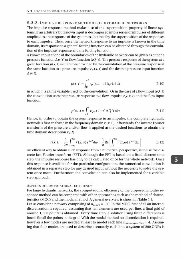
5.3. PROPOSED SEMI-ANALYTICAL METHOD
5
89
5.3.2. IMPULSE RESPONSE METHOD FOR HYDRAULIC NETWORKSThe impulse response method makes use of the superposition property of linear sys-
tems; if an arbitrary but known input is decomposed into a series of impulses of different
amplitudes, the response of the system is obtained by the superposition of the responses
to each impulse. Thus, once the network response to an impulse is known in the time
domain, its response to a general forcing function can be obtained through the convolu-
tion of the impulse response and the forcing function.
A known input at one of the boundaries of the hydraulic network can be given as either a
pressure function ∆p (t ) or flow function ∆Q (t ). The pressure response of the system at a
given location p(x, t ) is therefore provided by the convolution of the pressure response at
the same location to a pressure impulse rp (x, t ) and the desired pressure input function
∆p (t ),
p(x, t ) =∫t
0rp (x, t −τ)∆p (τ)dτ (5.10)
in which τ is a time variable used for the convolution. Or in the case of a flow input∆Q (t )
the convolution uses the pressure response to a flow impulse rQ (x, t ) and the flow input
function:
p(x, t ) =∫t
0rQ x (t −τ)∆Q (τ)dτ (5.11)
Hence, in order to obtain the system response to an impulse, the complete hydraulic
network is first analyzed in the frequency domain r (x,ω). Afterwards, the inverse Fourier
transform of the pressure and/or flow is applied at the desired locations to obtain the
time domain description rx (t ).
r (x, t ) =1
2π
∫∞
−∞r (x,ω)e iωt dω=
1
πRe
[∫∞
0r (x,ω)e iωt dω
]
(5.12)
An efficient way to obtain such response from a numerical perspective, is to use the dis-
crete fast Fourier transform (FFT). Although the FFT is based on a fixed discrete time
step, the impulse response has only to be calculated once for the whole network. Once
this response is available for the particular configuration, the numerical convolution is
obtained in a separate step for any desired input without the necessity to solve the sys-
tem once more. Furthermore the convolution can also be implemented for a variable
step approach.
ASPECTS OF COMPUTATIONAL EFFICIENCY
For large hydraulic networks, the computational efficiency of the proposed impulse re-
sponse method can be compared with other approaches such as the method of charac-
teristics (MOC) and the modal method. A general overview is shown in Table 5.1.
Let us consider a network comprising of nl i nes = 100. In the MOC, first of all an internal
discretization is required; assuming that ten elements are used per line, a final grid of
around 1,000 points is obtained. Every time step, a solution using finite differences is
found for all the points in the grid. With the modal method no discretization is required,
however a few modes are needed at least to model each line nmodesper l i ne = 4. Assum-
ing that four modes are used to describe accurately each line, a system of 800 ODEs is
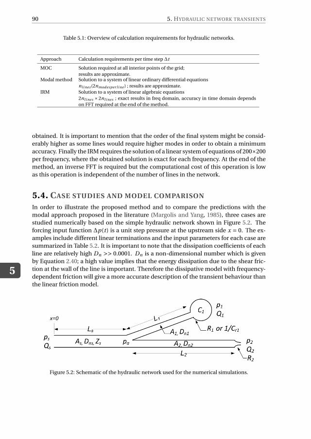
5
90 5. HYDRAULIC NETWORK TRANSIENTS
Table 5.1: Overview of calculation requirements for hydraulic networks.
Approach Calculation requirements per time step ∆t
MOC Solution required at all interior points of the grid;
results are approximate.Modal method Solution to a system of linear ordinary differential equations
nl i nes (2nmodesper l i ne ) ; results are approximate.
IRM Solution to a system of linear algebraic equations
2nl i nes ×2nl i nes ; exact results in freq domain, accuracy in time domain depends
on FFT required at the end of the method.
obtained. It is important to mention that the order of the final system might be consid-
erably higher as some lines would require higher modes in order to obtain a minimum
accuracy. Finally the IRM requires the solution of a linear system of equations of 200×200
per frequency, where the obtained solution is exact for each frequency. At the end of the
method, an inverse FFT is required but the computational cost of this operation is low
as this operation is independent of the number of lines in the network.
5.4. CASE STUDIES AND MODEL COMPARISON
In order to illustrate the proposed method and to compare the predictions with the
modal approach proposed in the literature (Margolis and Yang, 1985), three cases are
studied numerically based on the simple hydraulic network shown in Figure 5.2. The
forcing input function ∆p(t ) is a unit step pressure at the upstream side x = 0. The ex-
amples include different linear terminations and the input parameters for each case are
summarized in Table 5.2. It is important to note that the dissipation coefficients of each
line are relatively high Dn >> 0.0001. Dn is a non-dimensional number which is given
by Equation 2.40; a high value implies that the energy dissipation due to the shear fric-
tion at the wall of the line is important. Therefore the dissipative model with frequency-
dependent friction will give a more accurate description of the transient behaviour than
the linear friction model.
Figure 5.2: Schematic of the hydraulic network used for the numerical simulations.
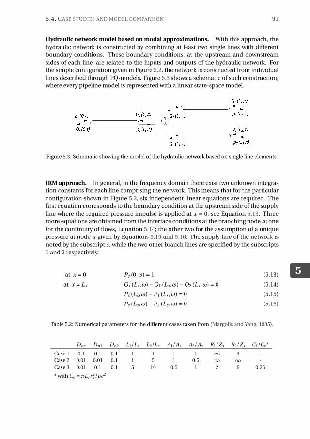
5.4. CASE STUDIES AND MODEL COMPARISON
5
91
Hydraulic network model based on modal approximations. With this approach, the
hydraulic network is constructed by combining at least two single lines with different
boundary conditions. These boundary conditions, at the upstream and downstream
sides of each line, are related to the inputs and outputs of the hydraulic network. For
the simple configuration given in Figure 5.2, the network is constructed from individual
lines described through PQ-models. Figure 5.3 shows a schematic of such construction,
where every pipeline model is represented with a linear state-space model.
Figure 5.3: Schematic showing the model of the hydraulic network based on single line elements.
IRM approach. In general, in the frequency domain there exist two unknown integra-
tion constants for each line comprising the network. This means that for the particular
configuration shown in Figure 5.2, six independent linear equations are required. The
first equation corresponds to the boundary condition at the upstream side of the supply
line where the required pressure impulse is applied at x = 0, see Equation 5.13. Three
more equations are obtained from the interface conditions at the branching node a; one
for the continuity of flows, Equation 5.14; the other two for the assumption of a unique
pressure at node a given by Equations 5.15 and 5.16. The supply line of the network is
noted by the subscript s, while the two other branch lines are specified by the subscripts
1 and 2 respectively.
at x = 0 Ps (0,ω) = 1 (5.13)
at x = Ls Qs (Ls ,ω)−Q1 (Ls ,ω)−Q2 (Ls ,ω) = 0 (5.14)
Ps (Ls ,ω)−P1 (Ls ,ω) = 0 (5.15)
Ps (Ls ,ω)−P2 (Ls ,ω) = 0 (5.16)
Table 5.2: Numerical parameters for the different cases taken from (Margolis and Yang, 1985).
Dns Dn1 Dn2 L1/Ls L2/Ls A1/As A2/As R1/Zs R2/Zs C1/Cc *
Case 1 0.1 0.1 0.1 1 1 1 1 ∞ 3 -
Case 2 0.01 0.01 0.1 1 5 1 0.5 ∞ ∞ -
Case 3 0.01 0.1 0.1 5 10 0.5 1 2 6 0.25
* with Cc =πLs r 2s /ρc2
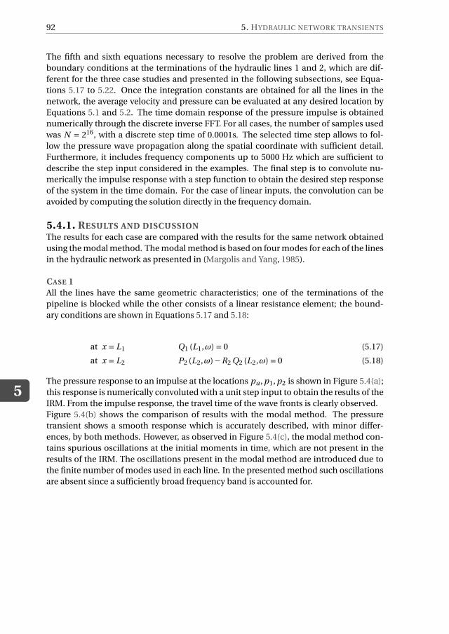
5
92 5. HYDRAULIC NETWORK TRANSIENTS
The fifth and sixth equations necessary to resolve the problem are derived from the
boundary conditions at the terminations of the hydraulic lines 1 and 2, which are dif-
ferent for the three case studies and presented in the following subsections, see Equa-
tions 5.17 to 5.22. Once the integration constants are obtained for all the lines in the
network, the average velocity and pressure can be evaluated at any desired location by
Equations 5.1 and 5.2. The time domain response of the pressure impulse is obtained
numerically through the discrete inverse FFT. For all cases, the number of samples used
was N = 216, with a discrete step time of 0.0001s. The selected time step allows to fol-
low the pressure wave propagation along the spatial coordinate with sufficient detail.
Furthermore, it includes frequency components up to 5000 Hz which are sufficient to
describe the step input considered in the examples. The final step is to convolute nu-
merically the impulse response with a step function to obtain the desired step response
of the system in the time domain. For the case of linear inputs, the convolution can be
avoided by computing the solution directly in the frequency domain.
5.4.1. RESULTS AND DISCUSSIONThe results for each case are compared with the results for the same network obtained
using the modal method. The modal method is based on four modes for each of the lines
in the hydraulic network as presented in (Margolis and Yang, 1985).
CASE 1All the lines have the same geometric characteristics; one of the terminations of the
pipeline is blocked while the other consists of a linear resistance element; the bound-
ary conditions are shown in Equations 5.17 and 5.18:
at x = L1 Q1 (L1,ω) = 0 (5.17)
at x = L2 P2 (L2,ω)−R2 Q2 (L2,ω) = 0 (5.18)
The pressure response to an impulse at the locations pa , p1, p2 is shown in Figure 5.4(a);
this response is numerically convoluted with a unit step input to obtain the results of the
IRM. From the impulse response, the travel time of the wave fronts is clearly observed.
Figure 5.4(b) shows the comparison of results with the modal method. The pressure
transient shows a smooth response which is accurately described, with minor differ-
ences, by both methods. However, as observed in Figure 5.4(c), the modal method con-
tains spurious oscillations at the initial moments in time, which are not present in the
results of the IRM. The oscillations present in the modal method are introduced due to
the finite number of modes used in each line. In the presented method such oscillations
are absent since a sufficiently broad frequency band is accounted for.
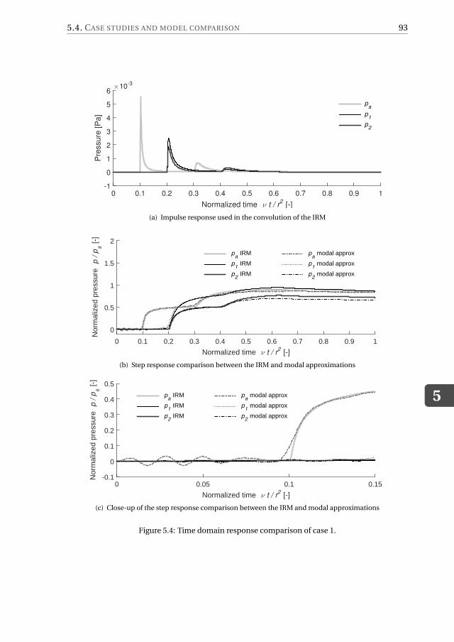
5.4. CASE STUDIES AND MODEL COMPARISON
5
93
Normalized time ν t / r2 [-]
0 0.1 0.2 0.3 0.4 0.5 0.6 0.7 0.8 0.9 1
Pre
ssure
[P
a]
×10-3
-1
0
1
2
3
4
5
6
pa
p1
p2
(a) Impulse response used in the convolution of the IRM
Normalized time ν t / r2 [-]
0 0.1 0.2 0.3 0.4 0.5 0.6 0.7 0.8 0.9 1
Nor
mal
ized
pre
ssur
e p
/ p
s [
-]
0
0.5
1
1.5
2
pa IRM
p1 IRM
p2 IRM
pa modal approx
p1 modal approx
p2 modal approx
(b) Step response comparison between the IRM and modal approximations
Normalized time ν t / r2 [-]
0 0.05 0.1 0.15
Nor
mal
ized
pre
ssur
e p
/ p
s [
-]
-0.1
0
0.1
0.2
0.3
0.4
0.5
pa IRM
p1 IRM
p2 IRM
pa modal approx
p1 modal approx
p2 modal approx
(c) Close-up of the step response comparison between the IRM and modal approximations
Figure 5.4: Time domain response comparison of case 1.
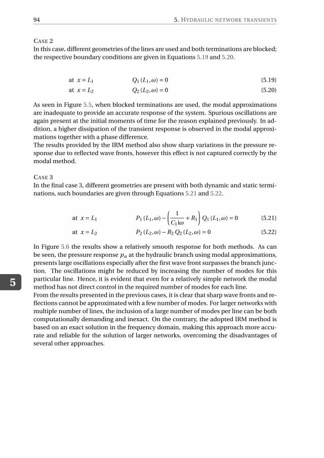
5
94 5. HYDRAULIC NETWORK TRANSIENTS
CASE 2In this case, different geometries of the lines are used and both terminations are blocked;
the respective boundary conditions are given in Equations 5.19 and 5.20.
at x = L1 Q1 (L1,ω) = 0 (5.19)
at x = L2 Q2 (L2,ω) = 0 (5.20)
As seen in Figure 5.5, when blocked terminations are used, the modal approximations
are inadequate to provide an accurate response of the system. Spurious oscillations are
again present at the initial moments of time for the reason explained previously. In ad-
dition, a higher dissipation of the transient response is observed in the modal approxi-
mations together with a phase difference.
The results provided by the IRM method also show sharp variations in the pressure re-
sponse due to reflected wave fronts, however this effect is not captured correctly by the
modal method.
CASE 3In the final case 3, different geometries are present with both dynamic and static termi-
nations, such boundaries are given through Equations 5.21 and 5.22.
at x = L1 P1 (L1,ω)−(
1
C1iω+R1
)
Q1 (L1,ω) = 0 (5.21)
at x = L2 P2 (L2,ω)−R2 Q2 (L2,ω) = 0 (5.22)
In Figure 5.6 the results show a relatively smooth response for both methods. As can
be seen, the pressure response pa at the hydraulic branch using modal approximations,
presents large oscillations especially after the first wave front surpasses the branch junc-
tion. The oscillations might be reduced by increasing the number of modes for this
particular line. Hence, it is evident that even for a relatively simple network the modal
method has not direct control in the required number of modes for each line.
From the results presented in the previous cases, it is clear that sharp wave fronts and re-
flections cannot be approximated with a few number of modes. For larger networks with
multiple number of lines, the inclusion of a large number of modes per line can be both
computationally demanding and inexact. On the contrary, the adopted IRM method is
based on an exact solution in the frequency domain, making this approach more accu-
rate and reliable for the solution of larger networks, overcoming the disadvantages of
several other approaches.
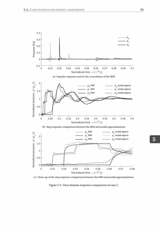
5.4. CASE STUDIES AND MODEL COMPARISON
5
95
Normalized time ν t / r2 [-]
0 0.01 0.02 0.03 0.04 0.05 0.06 0.07 0.08 0.09 0.1
Pre
ssur
e [P
a]
-0.1
0
0.1
0.2
0.3
0.4
pa
p1
p2
(a) Impulse response used in the convolution of the IRM
Normalized time ν t / r2 [-]
0 0.05 0.1 0.15 0.2 0.25 0.3 0.35 0.4 0.45 0.5
Nor
mal
ized
pre
ssur
e p
/ p
s [
-]
0
0.5
1
1.5
2 p
a IRM
p1 IRM
p2 IRM
pa modal approx
p1 modal approx
p2 modal approx
(b) Step response comparison between the IRM and modal approximations
Normalized time ν t / r2 [-]
0 0.01 0.02 0.03 0.04 0.05 0.06 0.07 0.08
Nor
mal
ized
pre
ssur
e p
/ p
s [
-]
0
0.5
1
1.5
2
pa IRM
p1 IRM
p2 IRM
pa modal approx
p1 modal approx
p2 modal approx
(c) Close-up of the step response comparison between the IRM and modal approximations
Figure 5.5: Time domain response comparison of case 2.
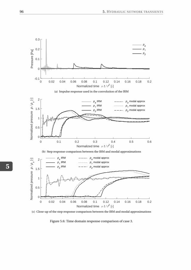
5
96 5. HYDRAULIC NETWORK TRANSIENTS
Normalized time ν t / r2 [-]
0 0.02 0.04 0.06 0.08 0.1 0.12 0.14 0.16 0.18 0.2
Pre
ssur
e [P
a]
-0.1
0
0.1
0.2
0.3
pa
p1
p2
(a) Impulse response used in the convolution of the IRM
Normalized time ν t / r2 [-]
0 0.1 0.2 0.3 0.4 0.5 0.6
Nor
mal
ized
pre
ssur
e p
/ p
s [
-]
0
0.5
1
1.5
2 p
a IRM
p1 IRM
p2 IRM
pa modal approx
p1 modal approx
p2 modal approx
(b) Step response comparison between the IRM and modal approximations
Normalized time ν t / r2 [-]
0 0.02 0.04 0.06 0.08 0.1 0.12 0.14 0.16 0.18 0.2
Nor
mal
ized
pre
ssur
e p
/ p
s [
-]
0
0.5
1
1.5
2 p
a IRM
p1 IRM
p2 IRM
pa modal approx
p1 modal approx
p2 modal approx
(c) Close-up of the step response comparison between the IRM and modal approximations
Figure 5.6: Time domain response comparison of case 3.

5.5. CONCLUDING REMARKS
5
97
5.5. CONCLUDING REMARKSAn application of a semi-analytical impulse response method to hydraulic networks
was presented for transient laminar flow using a two-dimensional viscous compressible
model. By solving analytically the complete network in the frequency domain, a unique
impulse response of pressure and/or volumetric flow is obtained in the time-domain
through the inverse FFT. A discrete numerical convolution with respect to time is then
applied separately to obtain the response of the complete network to a chosen arbitrary
input. Although the application of the method was shown for a simple hydraulic net-
work, it can be easily extended to networks with large numbers of lines with various
interface and boundary conditions.
The IRM does not require any spatial discretization and is only limited by the numeri-
cal considerations to solve a system of coupled linear algebraic equations and the fast
Fourier transform. This means that for large networks, the increase in computational
cost is only determined by the order of the global system matrix, which is linearly depen-
dent on the number of lines forming the system. In addition, the presented results show
that the adopted IRM method provides a more accurate description of the transient be-
haviour than the modal approximation of individual lines used for network modelling.
For a large network, the modal method might provide inaccurate results, as the required
number of modes for each line is not a priori known.

6DYNAMICS AND PERFORMANCE OF AN
OFFSHORE HYDRAULIC WIND POWER
PLANT
6.1. INTRODUCTIONWith the purpose to evaluate the performance of a complete hydraulic wind power plant,
the components presented in previous chapters are joined into a single time-domain nu-
merical model. The model for a single hydraulic wind turbine, introduced in Chapter 4,
is extended to include more turbines for any given farm layout. The model is capable
of accounting for the hydraulic network dynamics and wake turbine interaction. Hence,
this model makes it possible to evaluate different hydraulic pipeline configurations and
control strategies in order to achieve centralized electricity generation, while ensuring
the proper operation of the individual turbines.
This chapter is organized as follows. In Section 6.2, a description of the model for the
ambient wind field generation and aerodynamic interaction is presented. In addition,
the time-domain model of the hydraulic network is introduced. Section 6.3 presents
some intermediate results by analyzing a basic farm configuration consisting of only two
turbines. Four different cases comprising different combinations of hydraulic network
configurations and control strategies are used to assess the performance and stability.
Finally, in Section 6.4, the model is extended to include five turbines and a generator
platform. An active control strategy is used to ensure the dynamic stability of the oper-
ating turbines while producing electrical power in a centralized manner. For a particular
case with turbulent wind conditions, the time-domain results of the individual turbines
are presented and compared with those of a conventional wind farm under the same
layout and environmental conditions.
Parts of this chapter have been published in Journal of Physics: Conference Series, 524(1); Journal of Physics:
Conference Series, 753(1) (Jarquin Laguna, 2014, 2016) and under review in Wind Energy Science, 2016. Note
that minor changes have been introduced to make the text consistent with the other chapters of the thesis.
99
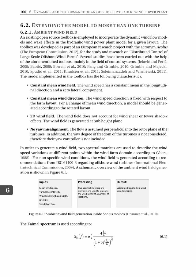
6
100 6. DYNAMICS AND PERFORMANCE OF AN OFFSHORE HYDRAULIC WIND POWER PLANT
6.2. EXTENDING THE MODEL TO MORE THAN ONE TURBINE
6.2.1. AMBIENT WIND FIELDAn existing open source toolbox is employed to incorporate the dynamic wind flow mod-
els and wake effects in the hydraulic wind power plant model for a given layout. The
toolbox was developed as part of an European research project with the acronym Aeolus
(The European Commission, 2012), for the study and research on ‘Distributed Control of
Large-Scale Offshore Wind Farms’. Several studies have been carried out with the help
of the aforementioned toolbox, mainly in the field of control systems, (Jelavic and Peric,
2009; Baotic, 2009; Borrelli et al., 2010; Pang and Grimble, 2010; Grimble and Majecki,
2010; Spudic et al., 2011; Knudsen et al., 2011; Soleimanzadeh and Wisniewski, 2011).
The model implemented in the toolbox has the following characteristics:
• Constant mean wind field. The wind speed has a constant mean in the longitudi-
nal direction and a zero lateral component.
• Constant mean wind direction. The wind speed direction is fixed with respect to
the farm layout. For a change of mean wind direction, a model should be gener-
ated according to the rotated layout.
• 2D wind field. The wind field does not account for wind shear or tower shadow
effects. The wind field is generated at hub height plane
• No yaw misalignment. The flow is assumed perpendicular to the rotor plane of the
turbines. In addition, the yaw degree of freedom of the turbines is not considered,
therefore their yaw controller is not included.
In order to generate a wind field, two spectral matrices are used to describe the wind
speed variations at different points within the wind farm domain according to (Veers,
1988). For non specific wind conditions, the wind field is generated according to rec-
ommendations from IEC 61400-3 regarding offshore wind turbines (International Elec-
trotechnical Commission, 2009). A schematic overview of the ambient wind field gener-
ation is shown in Figure 6.1.
Figure 6.1: Ambient wind field generation inside Aeolus toolbox (Grunnet et al., 2010).
The Kaimal spectrum is used according to:
Sk
(
f)
=σ2k
4Lk
U(
1+6 fLk
U
) 53
(6.1)
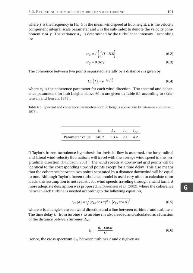
6.2. EXTENDING THE MODEL TO MORE THAN ONE TURBINE
6
101
where f is the frequency in Hz, U is the mean wind speed at hub height, L is the velocity
component integral scale parameter and k is the sub-index to denote the velocity com-
ponent x or y . The variance σk , is determined by the turbulence intensity I according
to:
σx = I
(
3
4U +5.6
)
(6.2)
σy = 0.8σx (6.3)
The coherence between two points separated laterally by a distance l is given by
Ck
(
f)
= e−ck f lU (6.4)
where ck is the coherence parameter for each wind direction. The spectral and coher-
ence parameters for hub heights above 60 m are given in Table 6.1 according to (Kris-
tensen and Jensen, 1979).
Table 6.1: Spectral and coherence parameters for hub heights above 60m (Kristensen and Jensen,
1979).
Lx Ly cxx cy y
Parameter value 340.2 113.4 7.1 4.2
If Taylor’s frozen turbulence hypothesis for inviscid flow is assumed, the longitudinal
and lateral wind velocity fluctuations will travel with the average wind speed in the lon-
gitudinal direction (Davidson, 2004). The wind speeds at downwind grid points will be
identical to the corresponding upwind points except for a time delay. This also means
that the coherence between two points separated by a distance downwind will be equal
to one. Although Taylor’s frozen turbulence model is used very often to calculate rotor
loads, this assumption is not realistic for wind speeds traveling through a wind farm. A
more adequate description was proposed in (Sørensen et al., 2002), where the coherence
between each turbine is needed according to the following equation,
cr c (α) =√
(cxx cosα)2 +(
cy y cosα)2
(6.5)
where α is an angle between wind direction and a line between turbine r and turbine c.
The time delay tr c from turbine r to turbine c is also needed and calculated as a function
of the distance between turbines dr c :
tr c =dr c cosα
U(6.6)
Hence, the cross spectrum Sr c between turbines r and c is given as:
6
102 6. DYNAMICS AND PERFORMANCE OF AN OFFSHORE HYDRAULIC WIND POWER PLANT
Sr c
(
f)
=Cr c
(
f)
√
Sr r
(
f)
Scc
(
f)
e− j 2π f tr c (6.7)
where Cr c is the coherence, and Sr r , Scc are the autospectra at turbines r and c, respec-
tively.
6.2.2. WAKE EFFECTSWhen a wind turbine is in operation, the rotor blades exert forces on the wind flow which
produce a flow structure downstream the rotor. This effect is commonly known as wind
turbine wake and its properties have been studied extensively (Crespo et al., 1999; Ver-
meer et al., 2003; Sanderse et al., 2011). The following wake effects are considered in this
work as shown in Figure 6.2:
• Wake deficit. It is a measure of the decrease in the wind speed caused by the ex-
traction of energy from the flow by the turbine.
• Wake expansion. It describes the size of the cross-sectional area affected by the
wake. As the flow decelerates under the influence of the blade forces, the stream
tube of the wake will expand as an effect of the principle of conservation of mass.
• Wake meandering. It consists of large oscillating movements of the wake cross-
sectional area in both lateral and vertical direction. The lateral position of this
wake area is defined by a wake center.
• Added turbulence intensity. It describes the increased turbulence in the wind
field. It is caused by the obstruction of the flow by the turbine and the resulting
velocity gradients in the flow.
Figure 6.2: Wake meandering of a turbine, defined by its wake center and expansion (Grunnet
et al., 2010).
Expressions for wake deficit, expansion and center are given in (Frandsen et al., 2006;
Jensen, 1983). The three characteristics at a given point p downwind from a turbine at
time t1, are defined by the wind field at the turbine and its coefficient of thrust at the
time of tracer release, t0:
6.2. EXTENDING THE MODEL TO MORE THAN ONE TURBINE
6
103
t0 = t1 −d
U(6.8)
where d is the longitudinal distance between the upwind turbine and p.
WAKE DEFICIT AND EXPANSION
The wake expansion D, is defined in terms of the wake diameter at downwind distance
d according to the following equation from (Frandsen et al., 2006):
D (d) = D0
(
βk2 +α
d
D0
) 1k
(6.9)
β=1+
p1−CT
2p
1−CT
(6.10)
where CT is the thrust coefficient, D0 is the rotor diameter and α and k are model pa-
rameters with the values of 0.5 and 2 respectively. The wake deficit c behind a single
turbine at distance d is given by the following equation from (Frandsen et al., 2006):
c =U (d)
U0≈ 1−
CT
2
D20
D2 (d)(6.11)
WAKE CENTER
A good approximation of the meandering of the wake is to consider the wake center
as a passive tracer which moves downwind with the mean wind speed (Larsen et al.,
2008). Under this assumption, the wake meandering can be modelled by applying a low
pass filter on the lateral velocity variations found at the center line of the wind turbine
rotor (Larsen et al., 2008). The wake center at time tk is a function of the center at time
tk−1 and the average lateral wind speed, over the wake area:
Wi (d , tk−1) =(
x, y)
|x = d ∧ y ∈Wy (6.12)
Wy =[
wi (d , tk−1)−1
2Di (d) ; wi (d , tk−1)+
1
2Di (d)
]
(6.13)
wi (d , tk ) = wi (d , tk−1)+ vy,i (d ,Wi (d , tk−1)) (6.14)
where wi (d , tk ) is the wake center at time k, Wi (d , tk−1) is the wake area distance d from
the turbine at time tk−1 and vy,i (d ,Wi (d , tk−1)) is the average lateral wind speed over the
wake area. For a row of turbines the deficit at turbine n +1 can be described as:
cn+1 =Un+1
U0= 1−
(
D2n
D2n+1
(1− cn)+CTn
2
D20
D2n+1
cn
)
(6.15)
where cn+1 is the deficit at turbine n +1, Dn is the wake diameter at turbine n +1, cn is
the deficit at turbine n, CTn is the thrust coefficient of turbine n and D0 is the diameter
of the rotor.
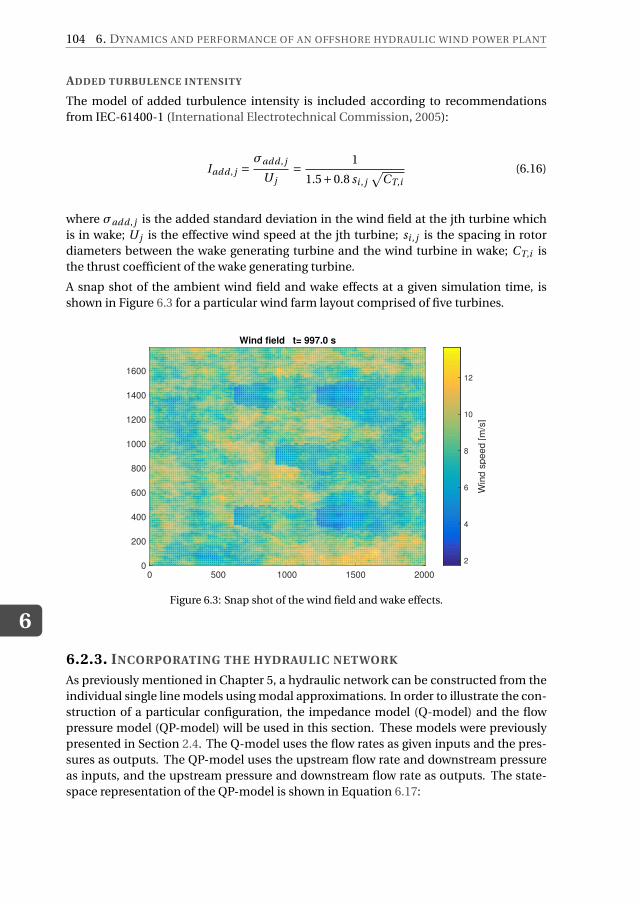
6
104 6. DYNAMICS AND PERFORMANCE OF AN OFFSHORE HYDRAULIC WIND POWER PLANT
ADDED TURBULENCE INTENSITY
The model of added turbulence intensity is included according to recommendations
from IEC-61400-1 (International Electrotechnical Commission, 2005):
Iadd , j =σadd , j
U j=
1
1.5+0.8 si , j
√
CT,i
(6.16)
where σadd , j is the added standard deviation in the wind field at the jth turbine which
is in wake; U j is the effective wind speed at the jth turbine; si , j is the spacing in rotor
diameters between the wake generating turbine and the wind turbine in wake; CT,i is
the thrust coefficient of the wake generating turbine.
A snap shot of the ambient wind field and wake effects at a given simulation time, is
shown in Figure 6.3 for a particular wind farm layout comprised of five turbines.
0 500 1000 1500 20000
200
400
600
800
1000
1200
1400
1600
Wind field t= 997.0 s
Win
d s
peed [m
/s]
2
4
6
8
10
12
Figure 6.3: Snap shot of the wind field and wake effects.
6.2.3. INCORPORATING THE HYDRAULIC NETWORK
As previously mentioned in Chapter 5, a hydraulic network can be constructed from the
individual single line models using modal approximations. In order to illustrate the con-
struction of a particular configuration, the impedance model (Q-model) and the flow
pressure model (QP-model) will be used in this section. These models were previously
presented in Section 2.4. The Q-model uses the flow rates as given inputs and the pres-
sures as outputs. The QP-model uses the upstream flow rate and downstream pressure
as inputs, and the upstream pressure and downstream flow rate as outputs. The state-
space representation of the QP-model is shown in Equation 6.17:
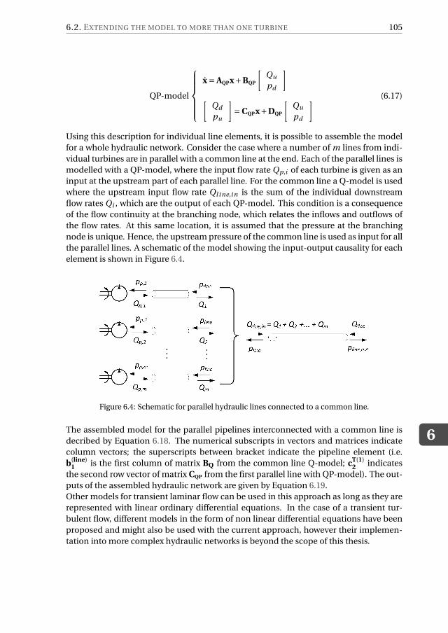
6.2. EXTENDING THE MODEL TO MORE THAN ONE TURBINE
6
105
QP-model
x = AQPx+BQP
[
Qu
pd
]
[
Qd
pu
]
= CQPx+DQP
[
Qu
pd
]
(6.17)
Using this description for individual line elements, it is possible to assemble the model
for a whole hydraulic network. Consider the case where a number of m lines from indi-
vidual turbines are in parallel with a common line at the end. Each of the parallel lines is
modelled with a QP-model, where the input flow rate Qp,i of each turbine is given as an
input at the upstream part of each parallel line. For the common line a Q-model is used
where the upstream input flow rate Ql i ne,i n is the sum of the individual downstream
flow rates Qi , which are the output of each QP-model. This condition is a consequence
of the flow continuity at the branching node, which relates the inflows and outflows of
the flow rates. At this same location, it is assumed that the pressure at the branching
node is unique. Hence, the upstream pressure of the common line is used as input for all
the parallel lines. A schematic of the model showing the input-output causality for each
element is shown in Figure 6.4.
Figure 6.4: Schematic for parallel hydraulic lines connected to a common line.
The assembled model for the parallel pipelines interconnected with a common line is
decribed by Equation 6.18. The numerical subscripts in vectors and matrices indicate
column vectors; the superscripts between bracket indicate the pipeline element (i.e.
b(line)1 is the first column of matrix BQ from the common line Q-model; cT(1)
2 indicates
the second row vector of matrix CQP from the first parallel line with QP-model). The out-
puts of the assembled hydraulic network are given by Equation 6.19.
Other models for transient laminar flow can be used in this approach as long as they are
represented with linear ordinary differential equations. In the case of a transient tur-
bulent flow, different models in the form of non linear differential equations have been
proposed and might also be used with the current approach, however their implemen-
tation into more complex hydraulic networks is beyond the scope of this thesis.
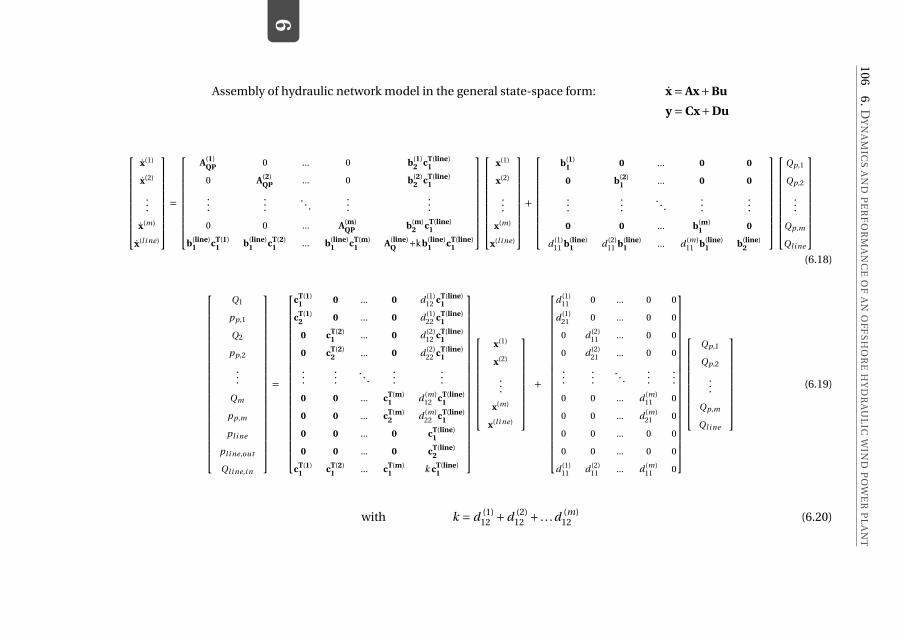
6
10
66
.D
YN
AM
ICS
AN
DP
ER
FO
RM
AN
CE
OF
AN
OF
FS
HO
RE
HY
DR
AU
LIC
WIN
DP
OW
ER
PL
AN
T
Assembly of hydraulic network model in the general state-space form: x = Ax+Bu
y = Cx+Du
x(1)
x(2)
...
x(m)
x(l i ne)
=
A(1)QP 0 ... 0 b(1)
2 cT(line)1
0 A(2)QP ... 0 b(2)
2 cT(line)1
......
. . ....
...
0 0 ... A(m)QP b(m)
2 cT(line)1
b(line)1 cT(1)
1 b(line)1 cT(2)
1 ... b(line)1 cT(m)
1 A(line)Q +k b(line)
1 cT(line)1
x(1)
x(2)
...
x(m)
x(l i ne)
+
b(1)1 0 ... 0 0
0 b(2)1 ... 0 0
......
. . ....
...
0 0 ... b(m)1 0
d (1)11 b(line)
1 d (2)11 b(line)
1 ... d (m)11 b(line)
1 b(line)2
Qp,1
Qp,2
...
Qp,m
Ql i ne
(6.18)
Q1
pp,1
Q2
pp,2
...
Qm
pp,m
pl i ne
pl i ne,out
Ql i ne,i n
=
cT(1)1 0 ... 0 d (1)
12 cT(line)1
cT(1)2 0 ... 0 d (1)
22 cT(line)1
0 cT(2)1 ... 0 d (2)
12 cT(line)1
0 cT(2)2 ... 0 d (2)
22 cT(line)1
......
. . ....
...
0 0 ... cT(m)1 d (m)
12 cT(line)1
0 0 ... cT(m)2 d (m)
22 cT(line)1
0 0 ... 0 cT(line)1
0 0 ... 0 cT(line)2
cT(1)1 cT(2)
1 ... cT(m)1 k cT(line)
1
x(1)
x(2)
...
x(m)
x(l i ne)
+
d (1)11 0 ... 0 0
d (1)21 0 ... 0 0
0 d (2)11 ... 0 0
0 d (2)21 ... 0 0
......
. . ....
...
0 0 ... d (m)11 0
0 0 ... d (m)21 0
0 0 ... 0 0
0 0 ... 0 0
d (1)11 d (2)
11 ... d (m)11 0
Qp,1
Qp,2
...
Qp,m
Ql i ne
(6.19)
with k = d (1)12 +d (2)
12 + . . .d (m)12 (6.20)
6.3. SIMULATION OF TWO TURBINES
6
107
The presented model of a hydraulic network is assembled with the rest of the algebraic
and differential equations which describe the dynamics of the individual turbines. Fol-
lowing the same approach as in (Grunnet et al., 2010), the hydraulic transmission is
incorporated instead of the mechanical gearbox; this same method was presented in
(Jarquin Laguna, 2015). The volumetric flow rate from the motor-water pump assem-
bly (high speed shaft) is used as an input to the hydraulic network, and the pressure
at the water pumps is used as feedback to the turbine models. In this manner a com-
plete model with the individual turbines coupled to the hydraulic network is obtained.
The complete wind farm model is now described through a set of coupled algebraic and
differential equations which can be solved numerically using a variable time step ODE
solver via commercial software (MATLAB-Simulink®, 2014). Simple test cases of the
overall model, using a constant wind speed input, were used to check the steady state
conditions. Time domain simulations are performed to obtain the transient response to
a stochastic wind input as described in the next sections.
6.3. SIMULATION OF TWO TURBINES
Before simulating the complete hydraulic wind power plant, some intermediate results
are presented by analyzing first the simplest farm consisting of two turbines. The tur-
bines are interconnected using two hydraulic network configurations. Time domain
simulations of the reduced wind farm are used to evaluate the performance and rotor
speed stability of both turbines under typical wind conditions. The individual turbines
have the same characteristics as the ones evaluated in Chapter 4; the main parameters
of a single turbine were given in Table 4.1.
In order to evaluate the performance and functionality of the control strategies, two tur-
bines are placed inline with the mean wind speed direction as shown in Figure 6.5. A
wind field with a mean wind speed of 9 m/s and 10% turbulence intensity is taken as the
inflow condition. Simulations of the reduced wind farm behavior are performed during
1000s with zero initial conditions. Wake effects for the downwind turbine are determined
by using the thrust coefficient CT of the upwind turbine as described in Section 6.2.2.
6.3.1. CASE STUDIES DESCRIPTION
Four different cases are simulated for the same wind field. Each case includes two iden-
tical turbines and a specific combination of the hydraulic network and control strategy.
Model 1 includes independent pipelines and nozzles for both turbines, see Figure 6.6(a).
In this configuration, the turbines are uncoupled and are controlled passively. Because
each turbine has an independent pipeline towards the offshore substation, this configu-
ration might not be the most convenient from a practical and economical point of view.
Furthermore, each central substation is limited to five or six turbines, which is the typ-
ical number of independent nozzles that a Pelton turbine is designed for. However, as
this model is a direct extension of the model presented in Chapter 4, the results will
be used as a reference. Model 2 presents a parallel configuration, in which the water
pipelines from individual turbines are connected through a common line to a single
nozzle, see Figure 6.6(b). A passive control strategy is employed in this configuration.
Hence, the two turbines have a dynamic interaction through the flow in the hydraulic
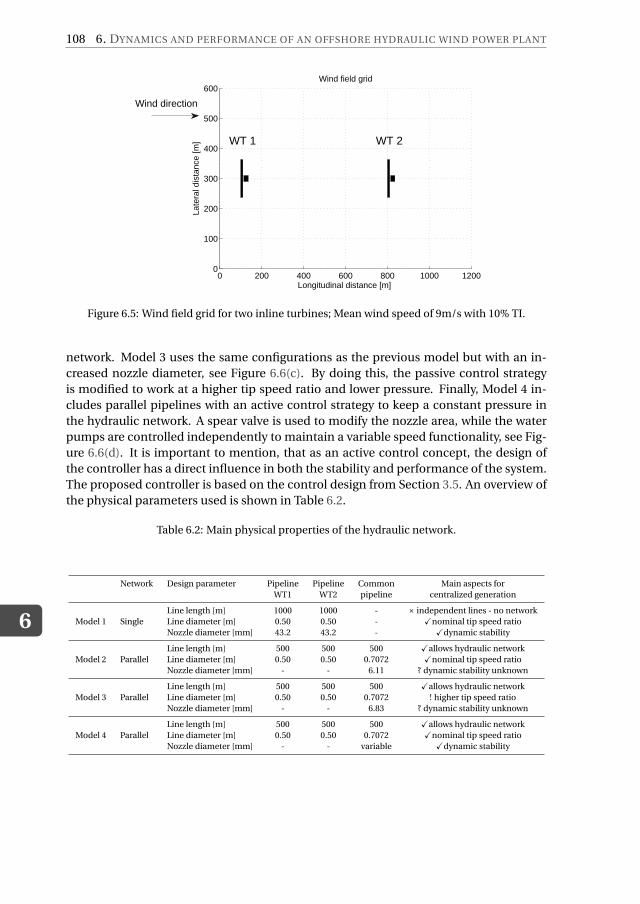
6
108 6. DYNAMICS AND PERFORMANCE OF AN OFFSHORE HYDRAULIC WIND POWER PLANT
0 200 400 600 800 1000 12000
100
200
300
400
500
600
WT 1 WT 2
Wind direction
Longitudinal distance [m]
Late
ral d
ista
nce
[m]
Wind field grid
Figure 6.5: Wind field grid for two inline turbines; Mean wind speed of 9m/s with 10% TI.
network. Model 3 uses the same configurations as the previous model but with an in-
creased nozzle diameter, see Figure 6.6(c). By doing this, the passive control strategy
is modified to work at a higher tip speed ratio and lower pressure. Finally, Model 4 in-
cludes parallel pipelines with an active control strategy to keep a constant pressure in
the hydraulic network. A spear valve is used to modify the nozzle area, while the water
pumps are controlled independently to maintain a variable speed functionality, see Fig-
ure 6.6(d). It is important to mention, that as an active control concept, the design of
the controller has a direct influence in both the stability and performance of the system.
The proposed controller is based on the control design from Section 3.5. An overview of
the physical parameters used is shown in Table 6.2.
Table 6.2: Main physical properties of the hydraulic network.
Network Design parameter Pipeline Pipeline Common Main aspects for
WT1 WT2 pipeline centralized generation
Model 1 Single
Line length [m] 1000 1000 - × independent lines - no network
Line diameter [m] 0.50 0.50 - Xnominal tip speed ratio
Nozzle diameter [mm] 43.2 43.2 - Xdynamic stability
Model 2 Parallel
Line length [m] 500 500 500 Xallows hydraulic network
Line diameter [m] 0.50 0.50 0.7072 Xnominal tip speed ratio
Nozzle diameter [mm] - - 6.11 ? dynamic stability unknown
Model 3 Parallel
Line length [m] 500 500 500 Xallows hydraulic network
Line diameter [m] 0.50 0.50 0.7072 ! higher tip speed ratio
Nozzle diameter [mm] - - 6.83 ? dynamic stability unknown
Model 4 Parallel
Line length [m] 500 500 500 Xallows hydraulic network
Line diameter [m] 0.50 0.50 0.7072 Xnominal tip speed ratio
Nozzle diameter [mm] - - variable Xdynamic stability
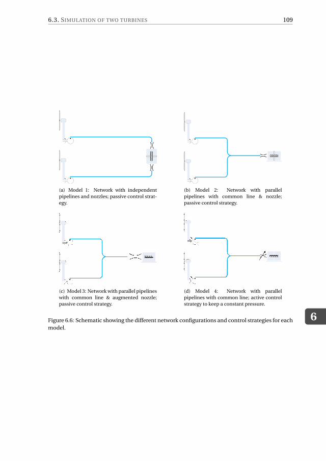
6.3. SIMULATION OF TWO TURBINES
6
109
(a) Model 1: Network with independent
pipelines and nozzles; passive control strat-
egy.
(b) Model 2: Network with parallel
pipelines with common line & nozzle;
passive control strategy.
(c) Model 3: Network with parallel pipelines
with common line & augmented nozzle;
passive control strategy.
(d) Model 4: Network with parallel
pipelines with common line; active control
strategy to keep a constant pressure.
Figure 6.6: Schematic showing the different network configurations and control strategies for each
model.
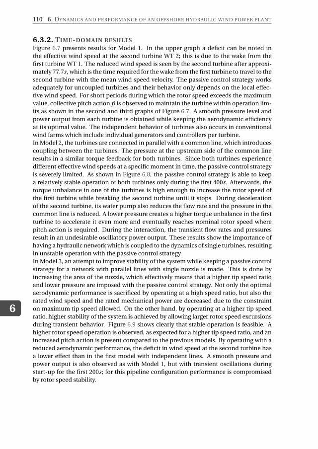
6
110 6. DYNAMICS AND PERFORMANCE OF AN OFFSHORE HYDRAULIC WIND POWER PLANT
6.3.2. TIME-DOMAIN RESULTSFigure 6.7 presents results for Model 1. In the upper graph a deficit can be noted in
the effective wind speed at the second turbine WT 2; this is due to the wake from the
first turbine WT 1. The reduced wind speed is seen by the second turbine after approxi-
mately 77.7s, which is the time required for the wake from the first turbine to travel to the
second turbine with the mean wind speed velocity. The passive control strategy works
adequately for uncoupled turbines and their behavior only depends on the local effec-
tive wind speed. For short periods during which the rotor speed exceeds the maximum
value, collective pitch action β is observed to maintain the turbine within operation lim-
its as shown in the second and third graphs of Figure 6.7. A smooth pressure level and
power output from each turbine is obtained while keeping the aerodynamic efficiency
at its optimal value. The independent behavior of turbines also occurs in conventional
wind farms which include individual generators and controllers per turbine.
In Model 2, the turbines are connected in parallel with a common line, which introduces
coupling between the turbines. The pressure at the upstream side of the common line
results in a similar torque feedback for both turbines. Since both turbines experience
different effective wind speeds at a specific moment in time, the passive control strategy
is severely limited. As shown in Figure 6.8, the passive control strategy is able to keep
a relatively stable operation of both turbines only during the first 400s. Afterwards, the
torque unbalance in one of the turbines is high enough to increase the rotor speed of
the first turbine while breaking the second turbine until it stops. During deceleration
of the second turbine, its water pump also reduces the flow rate and the pressure in the
common line is reduced. A lower pressure creates a higher torque unbalance in the first
turbine to accelerate it even more and eventually reaches nominal rotor speed where
pitch action is required. During the interaction, the transient flow rates and pressures
result in an undesirable oscillatory power output. These results show the importance of
having a hydraulic network which is coupled to the dynamics of single turbines, resulting
in unstable operation with the passive control strategy.
In Model 3, an attempt to improve stability of the system while keeping a passive control
strategy for a network with parallel lines with single nozzle is made. This is done by
increasing the area of the nozzle, which effectively means that a higher tip speed ratio
and lower pressure are imposed with the passive control strategy. Not only the optimal
aerodynamic performance is sacrificed by operating at a high speed ratio, but also the
rated wind speed and the rated mechanical power are decreased due to the constraint
on maximum tip speed allowed. On the other hand, by operating at a higher tip speed
ratio, higher stability of the system is achieved by allowing larger rotor speed excursions
during transient behavior. Figure 6.9 shows clearly that stable operation is feasible. A
higher rotor speed operation is observed, as expected for a higher tip speed ratio, and an
increased pitch action is present compared to the previous models. By operating with a
reduced aerodynamic performance, the deficit in wind speed at the second turbine has
a lower effect than in the first model with independent lines. A smooth pressure and
power output is also observed as with Model 1, but with transient oscillations during
start-up for the first 200s; for this pipeline configuration performance is compromised
by rotor speed stability.
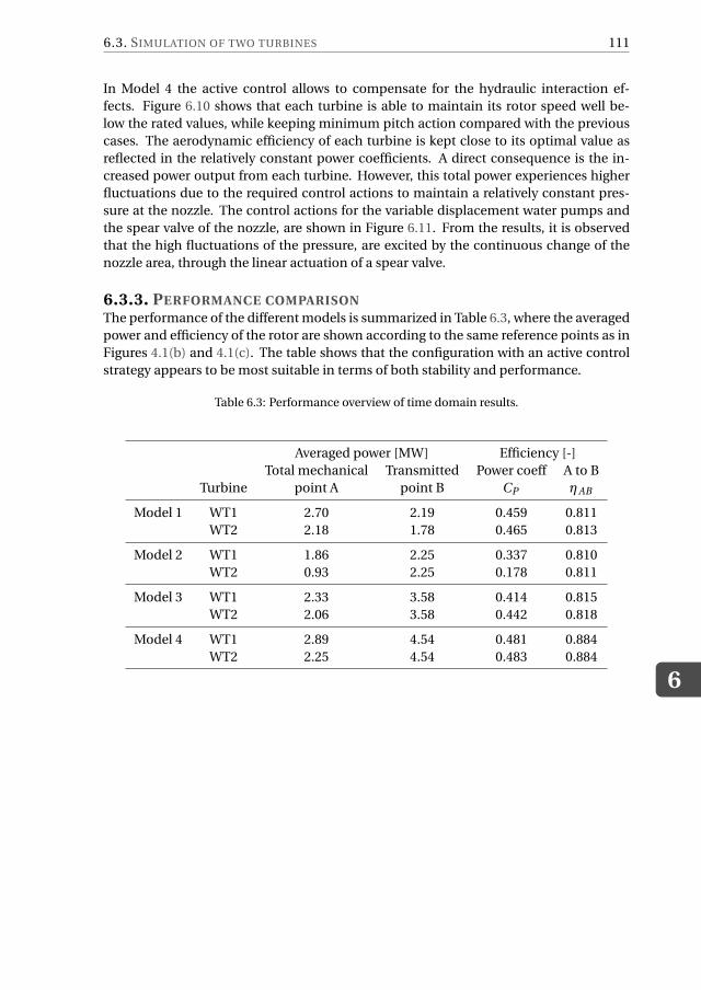
6.3. SIMULATION OF TWO TURBINES
6
111
In Model 4 the active control allows to compensate for the hydraulic interaction ef-
fects. Figure 6.10 shows that each turbine is able to maintain its rotor speed well be-
low the rated values, while keeping minimum pitch action compared with the previous
cases. The aerodynamic efficiency of each turbine is kept close to its optimal value as
reflected in the relatively constant power coefficients. A direct consequence is the in-
creased power output from each turbine. However, this total power experiences higher
fluctuations due to the required control actions to maintain a relatively constant pres-
sure at the nozzle. The control actions for the variable displacement water pumps and
the spear valve of the nozzle, are shown in Figure 6.11. From the results, it is observed
that the high fluctuations of the pressure, are excited by the continuous change of the
nozzle area, through the linear actuation of a spear valve.
6.3.3. PERFORMANCE COMPARISONThe performance of the different models is summarized in Table 6.3, where the averaged
power and efficiency of the rotor are shown according to the same reference points as in
Figures 4.1(b) and 4.1(c). The table shows that the configuration with an active control
strategy appears to be most suitable in terms of both stability and performance.
Table 6.3: Performance overview of time domain results.
Averaged power [MW] Efficiency [-]
Total mechanical Transmitted Power coeff A to B
Turbine point A point B CP ηAB
Model 1 WT1 2.70 2.19 0.459 0.811
WT2 2.18 1.78 0.465 0.813
Model 2 WT1 1.86 2.25 0.337 0.810
WT2 0.93 2.25 0.178 0.811
Model 3 WT1 2.33 3.58 0.414 0.815
WT2 2.06 3.58 0.442 0.818
Model 4 WT1 2.89 4.54 0.481 0.884
WT2 2.25 4.54 0.483 0.884
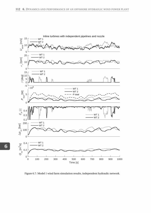
6
112 6. DYNAMICS AND PERFORMANCE OF AN OFFSHORE HYDRAULIC WIND POWER PLANT
Uw
ind [
m/s
]
5
10
15Inline turbines with independent pipelines and nozzle
WT 1WT 2
ωr [
rpm
]
0
10
20 WT 1WT 2
β [
deg]
-505
1015 WT 1
WT 2
Phyd [
W]
×106
0
5
WT 1WT 2P total
C
P [
-]
0.2
0.3
0.4
WT 1WT 2
∆p
nz [
bar]
0
100
200 WT 1WT 2
Time [s]0 100 200 300 400 500 600 700 800 900 1000
Qnz [
m3/s
]
0
0.2
0.4 WT 1WT 2
Figure 6.7: Model 1 wind farm simulation results, independent hydraulic network.
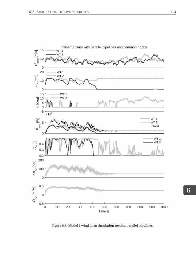
6.3. SIMULATION OF TWO TURBINES
6
113
Uw
ind [
m/s
]
5
10
15Inline turbines with parallel pipelines and common nozzle
WT 1WT 2
ωr [
rpm
]
0
10
20 WT 1WT 2
β [
deg]
-505
1015 WT 1
WT 2
Phyd [
W]
×106
0
5WT 1WT 2P total
C
P [
-]
0.2
0.3
0.4
WT 1WT 2
∆p
nz [
bar]
0
100
200
Time [s]0 100 200 300 400 500 600 700 800 900 1000
Qnz [
m3/s
]
-0.5
0
0.5
Figure 6.8: Model 2 wind farm simulation results, parallel pipelines.
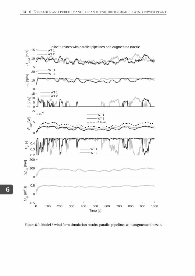
6
114 6. DYNAMICS AND PERFORMANCE OF AN OFFSHORE HYDRAULIC WIND POWER PLANT
Uw
ind [
m/s
]
5
10
15Inline turbines with parallel pipelines and augmented nozzle
WT 1WT 2
ωr [
rpm
]
0
10
20 WT 1WT 2
β [
deg]
-505
1015 WT 1
WT 2
Phyd [
W]
×106
0
5
WT 1WT 2P total
C
P [
-]
0.2
0.3
0.4
WT 1WT 2
∆p
nz [
bar]
0
100
200
Time [s]0 100 200 300 400 500 600 700 800 900 1000
Qnz [
m3/s
]
-0.5
0
0.5
Figure 6.9: Model 3 wind farm simulation results, parallel pipelines with augmented nozzle.

6.3. SIMULATION OF TWO TURBINES
6
115
Uw
ind [
m/s
]
5
10
15Inline turbines with parallel pipelines and pressure control
WT 1WT 2
ωr [
rpm
]
0
10
20 WT 1WT 2
β [
deg]
-505
1015
WT 1WT 2
Phyd [
W]
×106
0
5
WT 1WT 2P total
C
P [
-]
0.2
0.3
0.4WT 1WT 2
∆p
nz [
bar]
100
150
200
Time [s]0 100 200 300 400 500 600 700 800 900 1000
Qnz [
m3/s
]
0
0.5
1
Figure 6.10: Model 4 wind farm simulation results, parallel pipelines with pressure control.
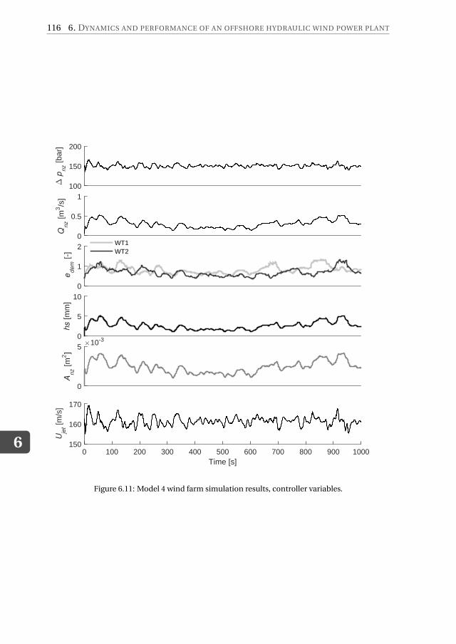
6
116 6. DYNAMICS AND PERFORMANCE OF AN OFFSHORE HYDRAULIC WIND POWER PLANT
∆ p
nz [
bar]
100
150
200
Qnz [
m3/s
]
0
0.5
1
edem
[-]
0
1
2 WT1WT2
hs [
mm
]
0
5
10
Anz [
m2]
×10-3
0
5
Time [s]0 100 200 300 400 500 600 700 800 900 1000
Uje
t [m
/s]
150
160
170
Figure 6.11: Model 4 wind farm simulation results, controller variables.
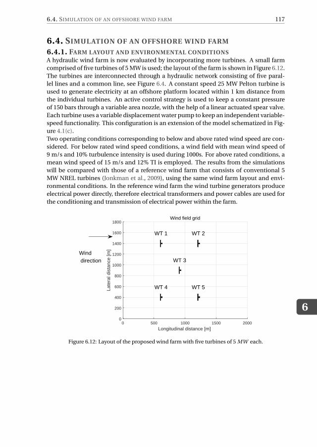
6.4. SIMULATION OF AN OFFSHORE WIND FARM
6
117
6.4. SIMULATION OF AN OFFSHORE WIND FARM
6.4.1. FARM LAYOUT AND ENVIRONMENTAL CONDITIONSA hydraulic wind farm is now evaluated by incorporating more turbines. A small farm
comprised of five turbines of 5 MW is used; the layout of the farm is shown in Figure 6.12.
The turbines are interconnected through a hydraulic network consisting of five paral-
lel lines and a common line, see Figure 6.4. A constant speed 25 MW Pelton turbine is
used to generate electricity at an offshore platform located within 1 km distance from
the individual turbines. An active control strategy is used to keep a constant pressure
of 150 bars through a variable area nozzle, with the help of a linear actuated spear valve.
Each turbine uses a variable displacement water pump to keep an independent variable-
speed functionality. This configuration is an extension of the model schematized in Fig-
ure 4.1(c).
Two operating conditions corresponding to below and above rated wind speed are con-
sidered. For below rated wind speed conditions, a wind field with mean wind speed of
9 m/s and 10% turbulence intensity is used during 1000s. For above rated conditions, a
mean wind speed of 15 m/s and 12% TI is employed. The results from the simulations
will be compared with those of a reference wind farm that consists of conventional 5
MW NREL turbines (Jonkman et al., 2009), using the same wind farm layout and envi-
ronmental conditions. In the reference wind farm the wind turbine generators produce
electrical power directly, therefore electrical transformers and power cables are used for
the conditioning and transmission of electrical power within the farm.
Longitudinal distance [m] 0 500 1000 1500 2000
Late
ral d
ista
nce
[m]
0
200
400
600
800
1000
1200
1400
1600
1800
WT 1 WT 2
WT 3
WT 4 WT 5
Wind direction
Wind field grid
Figure 6.12: Layout of the proposed wind farm with five turbines of 5 MW each.
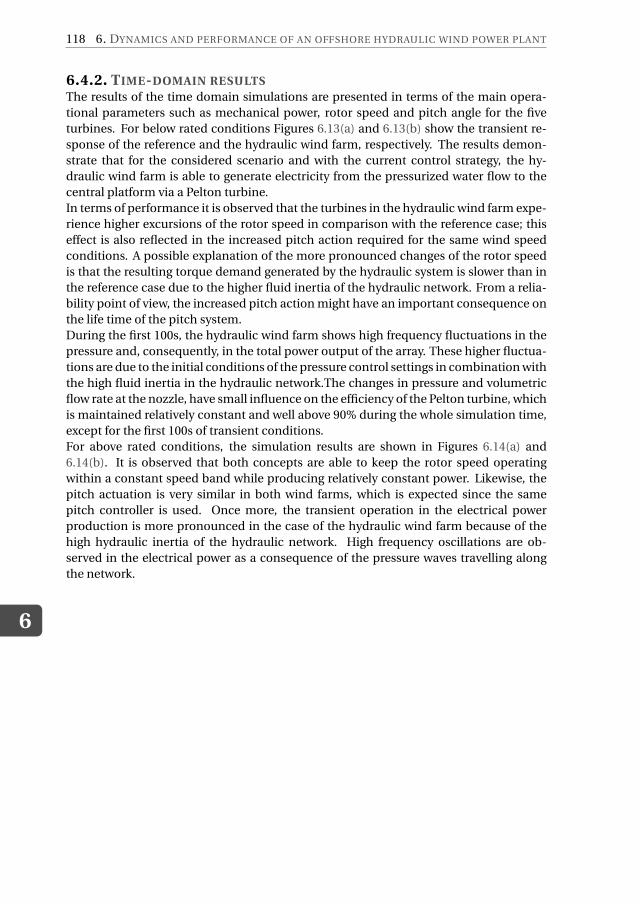
6
118 6. DYNAMICS AND PERFORMANCE OF AN OFFSHORE HYDRAULIC WIND POWER PLANT
6.4.2. TIME-DOMAIN RESULTSThe results of the time domain simulations are presented in terms of the main opera-
tional parameters such as mechanical power, rotor speed and pitch angle for the five
turbines. For below rated conditions Figures 6.13(a) and 6.13(b) show the transient re-
sponse of the reference and the hydraulic wind farm, respectively. The results demon-
strate that for the considered scenario and with the current control strategy, the hy-
draulic wind farm is able to generate electricity from the pressurized water flow to the
central platform via a Pelton turbine.
In terms of performance it is observed that the turbines in the hydraulic wind farm expe-
rience higher excursions of the rotor speed in comparison with the reference case; this
effect is also reflected in the increased pitch action required for the same wind speed
conditions. A possible explanation of the more pronounced changes of the rotor speed
is that the resulting torque demand generated by the hydraulic system is slower than in
the reference case due to the higher fluid inertia of the hydraulic network. From a relia-
bility point of view, the increased pitch action might have an important consequence on
the life time of the pitch system.
During the first 100s, the hydraulic wind farm shows high frequency fluctuations in the
pressure and, consequently, in the total power output of the array. These higher fluctua-
tions are due to the initial conditions of the pressure control settings in combination with
the high fluid inertia in the hydraulic network.The changes in pressure and volumetric
flow rate at the nozzle, have small influence on the efficiency of the Pelton turbine, which
is maintained relatively constant and well above 90% during the whole simulation time,
except for the first 100s of transient conditions.
For above rated conditions, the simulation results are shown in Figures 6.14(a) and
6.14(b). It is observed that both concepts are able to keep the rotor speed operating
within a constant speed band while producing relatively constant power. Likewise, the
pitch actuation is very similar in both wind farms, which is expected since the same
pitch controller is used. Once more, the transient operation in the electrical power
production is more pronounced in the case of the hydraulic wind farm because of the
high hydraulic inertia of the hydraulic network. High frequency oscillations are ob-
served in the electrical power as a consequence of the pressure waves travelling along
the network.
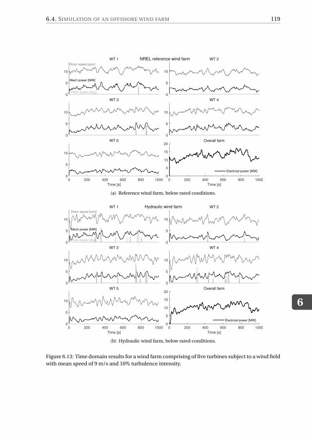
6.4. SIMULATION OF AN OFFSHORE WIND FARM
6
119
0
5
10
Mech power [MW]
Rotor speed [rpm]
Pitch angle [deg]
WT 1
0
5
10
WT 2
0
5
10
WT 3
0
5
10
WT 4
Time [s]
0 200 400 600 800 10000
5
10
WT 5
Time [s]
0 200 400 600 800 10000
5
10
15
20
NREL reference wind farm
Overall farm
Electrical power [MW]
(a) Reference wind farm, below rated conditions.
0
5
10
Mech power [MW]
Rotor speed [rpm]
Pitch angle [deg]
WT 1
0
5
10
WT 2
0
5
10
WT 3
0
5
10
WT 4
Time [s]
0 200 400 600 800 10000
5
10
WT 5
Time [s]
0 200 400 600 800 10000
5
10
15
20
Hydraulic wind farm
Overall farm
Electrical power [MW]
(b) Hydraulic wind farm, below rated conditions.
Figure 6.13: Time domain results for a wind farm comprising of five turbines subject to a wind field
with mean speed of 9 m/s and 10% turbulence intensity.
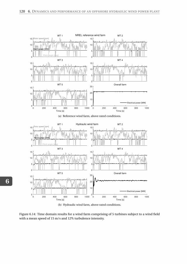
6
120 6. DYNAMICS AND PERFORMANCE OF AN OFFSHORE HYDRAULIC WIND POWER PLANT
0
5
10
15
Mech power [MW]
Rotor speed [rpm]
Pitch angle [deg]
WT 1
0
5
10
15
WT 2
0
5
10
15
WT 3
0
5
10
15
WT 4
Time [s]
0 200 400 600 800 10000
5
10
15
WT 5
Time [s]
0 200 400 600 800 10000
10
20
30
NREL reference wind farm
Overall farm
Electrical power [MW]
(a) Reference wind farm, above rated conditions.
0
5
10
15
Mech power [MW]
Rotor speed [rpm]
Pitch angle [deg]
WT 1
0
5
10
15
WT 2
0
5
10
15
WT 3
0
5
10
15
WT 4
Time [s]
0 200 400 600 800 10000
5
10
15
WT 5
Time [s]
0 200 400 600 800 10000
10
20
30
Hydraulic wind farm
Overall farm
Electrical power [MW]
(b) Hydraulic wind farm, above rated conditions.
Figure 6.14: Time domain results for a wind farm comprising of 5 turbines subject to a wind field
with a mean speed of 15 m/s and 12% turbulence intensity.
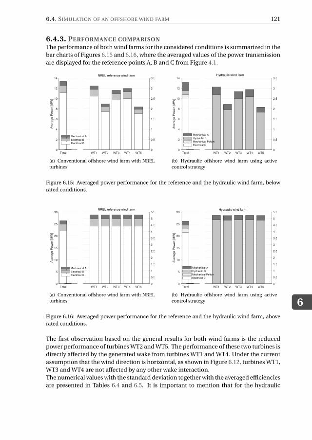
6.4. SIMULATION OF AN OFFSHORE WIND FARM
6
121
6.4.3. PERFORMANCE COMPARISONThe performance of both wind farms for the considered conditions is summarized in the
bar charts of Figures 6.15 and 6.16, where the averaged values of the power transmission
are displayed for the reference points A, B and C from Figure 4.1.
WT1 WT2 WT3 WT4 WT50
0.5
1
1.5
2
2.5
3
3.5NREL reference wind farm
Total
Ave
rag
e P
ow
er
[MW
]
0
2
4
6
8
10
12
14
Mechanical A
Electrical B
Electrical C
(a) Conventional offshore wind farm with NREL
turbines
WT1 WT2 WT3 WT4 WT50
0.5
1
1.5
2
2.5
3
3.5Hydraulic wind farm
Total
Ave
rag
e P
ow
er
[MW
]
0
2
4
6
8
10
12
14
Mechanical A
Hydraulic B
Mechanical Pelton
Electrical C
(b) Hydraulic offshore wind farm using active
control strategy
Figure 6.15: Averaged power performance for the reference and the hydraulic wind farm, below
rated conditions.
WT1 WT2 WT3 WT4 WT50
0.5
1
1.5
2
2.5
3
3.5
4
4.5
5
5.5NREL reference wind farm
Total
Ave
rag
e P
ow
er
[MW
]
0
5
10
15
20
25
30
Mechanical A
Electrical B
Electrical C
(a) Conventional offshore wind farm with NREL
turbines
WT1 WT2 WT3 WT4 WT50
0.5
1
1.5
2
2.5
3
3.5
4
4.5
5
5.5Hydraulic wind farm
Total
Ave
rag
e P
ow
er
[MW
]
0
5
10
15
20
25
30
Mechanical A
Hydraulic B
Mechanical Pelton
Electrical C
(b) Hydraulic offshore wind farm using active
control strategy
Figure 6.16: Averaged power performance for the reference and the hydraulic wind farm, above
rated conditions.
The first observation based on the general results for both wind farms is the reduced
power performance of turbines WT2 and WT5. The performance of these two turbines is
directly affected by the generated wake from turbines WT1 and WT4. Under the current
assumption that the wind direction is horizontal, as shown in Figure 6.12, turbines WT1,
WT3 and WT4 are not affected by any other wake interaction.
The numerical values with the standard deviation together with the averaged efficiencies
are presented in Tables 6.4 and 6.5. It is important to mention that for the hydraulic
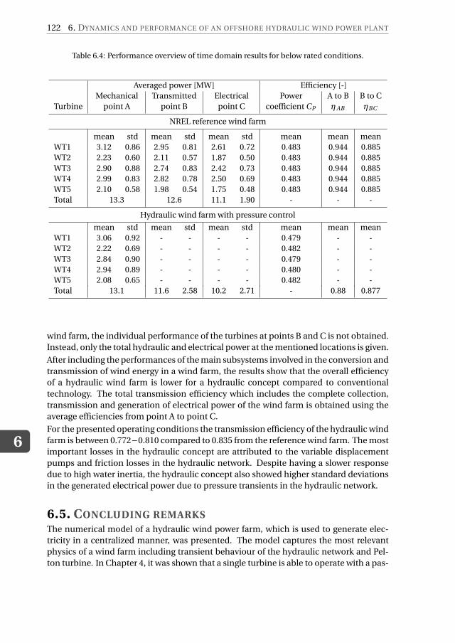
6
122 6. DYNAMICS AND PERFORMANCE OF AN OFFSHORE HYDRAULIC WIND POWER PLANT
Table 6.4: Performance overview of time domain results for below rated conditions.
Averaged power [MW] Efficiency [-]
Mechanical Transmitted Electrical Power A to B B to C
Turbine point A point B point C coefficient CP ηAB ηBC
NREL reference wind farm
mean std mean std mean std mean mean mean
WT1 3.12 0.86 2.95 0.81 2.61 0.72 0.483 0.944 0.885
WT2 2.23 0.60 2.11 0.57 1.87 0.50 0.483 0.944 0.885
WT3 2.90 0.88 2.74 0.83 2.42 0.73 0.483 0.944 0.885
WT4 2.99 0.83 2.82 0.78 2.50 0.69 0.483 0.944 0.885
WT5 2.10 0.58 1.98 0.54 1.75 0.48 0.483 0.944 0.885
Total 13.3 12.6 11.1 1.90 - - -
Hydraulic wind farm with pressure control
mean std mean std mean std mean mean mean
WT1 3.06 0.92 - - - - 0.479 - -
WT2 2.22 0.69 - - - - 0.482 - -
WT3 2.84 0.90 - - - - 0.479 - -
WT4 2.94 0.89 - - - - 0.480 - -
WT5 2.08 0.65 - - - - 0.482 - -
Total 13.1 11.6 2.58 10.2 2.71 - 0.88 0.877
wind farm, the individual performance of the turbines at points B and C is not obtained.
Instead, only the total hydraulic and electrical power at the mentioned locations is given.
After including the performances of the main subsystems involved in the conversion and
transmission of wind energy in a wind farm, the results show that the overall efficiency
of a hydraulic wind farm is lower for a hydraulic concept compared to conventional
technology. The total transmission efficiency which includes the complete collection,
transmission and generation of electrical power of the wind farm is obtained using the
average efficiencies from point A to point C.
For the presented operating conditions the transmission efficiency of the hydraulic wind
farm is between 0.772−0.810 compared to 0.835 from the reference wind farm. The most
important losses in the hydraulic concept are attributed to the variable displacement
pumps and friction losses in the hydraulic network. Despite having a slower response
due to high water inertia, the hydraulic concept also showed higher standard deviations
in the generated electrical power due to pressure transients in the hydraulic network.
6.5. CONCLUDING REMARKSThe numerical model of a hydraulic wind power farm, which is used to generate elec-
tricity in a centralized manner, was presented. The model captures the most relevant
physics of a wind farm including transient behaviour of the hydraulic network and Pel-
ton turbine. In Chapter 4, it was shown that a single turbine is able to operate with a pas-
6.5. CONCLUDING REMARKS
6
123
Table 6.5: Performance overview of time domain results for above rated conditions.
Averaged power [MW] Efficiency [-]
Mechanical Transmitted Electrical Power A to B B to C
Turbine point A point B point C coefficient CP ηAB ηBC
NREL reference wind farm
mean std mean std mean std mean mean mean
WT1 5.28 0.22 4.99 0.21 4.41 0.18 0.249 0.944 0.885
WT2 5.27 0.23 4.97 0.22 4.40 0.19 0.284 0.944 0.885
WT3 5.28 0.22 4.99 0.21 4.42 0.18 0.251 0.944 0.885
WT4 5.28 0.23 4.98 0.22 4.41 0.19 0.244 0.944 0.885
WT5 5.27 0.23 4.98 0.22 4.41 0.19 0.277 0.944 0.885
Total 26.4 24.9 22.1 0.92 - - -
Hydraulic wind farm with pressure control
mean std mean std mean std mean mean mean
WT1 5.24 0.18 - - - - 0.247 - -
WT2 5.22 0.19 - - - - 0.282 - -
WT3 5.25 0.18 - - - - 0.250 - -
WT4 5.25 0.18 - - - - 0.243 - -
WT5 5.23 0.19 - - - - 0.274 - -
Total 26.2 24.4 1.40 21.4 1.44 - 0.931 0.87
sive control strategy while keeping a stable variable-speed operation. However, when
two turbines are incorporated in a farm, the same passive control strategy has strong
limitations in terms of performance and stability when these two turbines are coupled
through a hydraulic network. An increased stability of the rotor speed for both turbines
is possible by operating at a higher tip speed ratio, but the performance of the wind farm
is then compromised. For individual turbines with independent lines and nozzles this is
not the case. However, based on the design principles for centralized electricity genera-
tion, it is preferred to have a combination of parallel and common pipelines.
From a wind farm perspective, an active control strategy is more suitable to maintain
the individual turbines performance. Based on a constant pressure control strategy, the
simulation of a hypothetical hydraulic wind farm consisting of five turbines was pre-
sented for a stochastic turbulent wind, including wake effects. For the presented case
study, the results indicate that the individual wind turbines are able to operate within
operational limits with the current active control concept. In terms of performance, the
simulations show that the hydraulic collection and transmission has a lower efficiency
when compared with a reference wind farm that employs conventional technology. The
main energy losses are associated with the variable displacement water pumps and fric-
tion losses in the hydraulic network.

7CONCLUSIONS
This dissertation addresses the idea of using pressurized water as a mean to central-
ize electricity generation in an offshore wind farm. In the proposed concept the con-
ventional geared or direct-drive power drivetrain is replaced by a positive displacement
pump. In this manner the rotor nacelle assemblies are dedicated to pressurize water into
a hydraulic network. The high pressure water flow is then collected from the wind tur-
bines of the farm and redirected into a central offshore platform where the electricity is
generated through a Pelton turbine.
In order to enable the performance evaluation of the proposed centralized generation
scheme, a numerical tool is developed and implemented for the simulation of the pro-
posed hydraulic wind farm under operating conditions. In this process, a time-domain
approach is employed to analyze the overall system in order to deal with the presence of
non-linearities in the mathematical modelling. The set of time-domain sub-models has
been presented for the main hydraulic components in Chapter 2.
With respect to the control aspects, the variable rotor speed functionality of the individ-
ual turbines, aimed to keep maximum aerodynamic performance for below rated wind
speed conditions, is realized by using hydraulic components as a replacement for the
conventional torque-controller used in modern wind turbines. Using fluid power tech-
nology, two control strategies are analyzed in Chapter 3 using feedback control tools
in both the frequency and time domain for a 5 MW turbine. The passive speed con-
trol (PSC) is based on the proper dimensioning of the hydraulic components to match
the optimal tip speed ratio of the rotor while having a variable pressure in the hydraulic
lines. For below rated wind speeds, the PSC is able to maintain the operation of the
turbine close to optimal aerodynamic performance without any measurements or ma-
nipulation of the turbine settings. In addition, the PSC shows to be inherently stable for
a single turbine by using a constant area nozzle.
A different approach is also studied, in which the variable speed functionality is realized
through active speed control (ASC). With this strategy the transmitted torque from the
drivetrain is manipulated by adjusting continuously the volumetric displacement of the
water pump. In combination with an adjustable spear valve at the nozzle side, a constant
125
7
126 7. CONCLUSIONS
pressure across the hydraulic drives is realized in what is known as ‘secondary control’
in hydraulic control systems. Special attention has to be paid to the controller design
to avoid undesired pressure waves in the hydraulic lines as a result of sudden control
actions. A combination of a PI control in series with a low-pass filter and notches is
proposed for the pressure controller to account for this effect. Since the performance
and design of the controllers is limited to the framework of linear control theory, there
are high expectations that other non-linear control methods can improve the dynamic
performance of the system.
Before looking at a complete hydraulic wind farm, the dynamics and performance of a
single hydraulic wind turbine are presented in Chapter 4. Two different wind turbines
with hydraulic transmissions are analyzed based on the PSC and ASC strategies of Chap-
ter 3 for different wind speed conditions. The design parameters of the hydraulic con-
cepts are obtained using as a basis the same rotor as the NREL 5 MW offshore wind tur-
bine reference. The simulation results indicate that the operation in below and above
rated wind speed conditions is possible for a single turbine with both PSC and ASC
strategies. Despite a lower transmission efficiency when compared to the reference tur-
bine, the hydraulic transmission with PSC has a strongly damped response of the gener-
ated electrical power and transmitted torque to the rotor.
From a design point of view, the PSC is limited in two different ways. The first one is the
choice of rated wind speed and consequently rated power. The design rated wind speed
is limited by the combination of the optimal tip speed ratio and the maximum tangential
velocity of the blades. In the considered examples of Chapter 4, the rotor of the NREL
turbine with an optimal tip speed ratio, λ = 7.55 and maximum tangential velocity of
80 m/s, resulted in a rated wind speed of 10.4 m/s with only 4.4 MW compared to the
original 5.4 MW for rated wind speed of 11.4 m/s. It is possible to design the PSC for
a lower tip speed ratio in order to reach the original rated wind speed. However a lower
tip speed ratio implies a compromise in both aerodynamic performance and rotor speed
stability. A dedicated design of the rotor which includes the PSC into consideration could
result in an alternative solution that has yet to be evaluated. Furthermore, the reliability
of the system is not compromised due to the passive nature of the control strategy.
The following step towards a wind farm with centralized electricity generation is to in-
clude more than one turbine in the energy conversion process. To this end, the use of a
hydraulic network consisting of hydraulic lines from each turbine into a central offshore
platform is required. The development and implementation of the flow dynamics in the
hydraulic network through a continuous time-domain model is presented in Chapter 5.
The hydraulic network model is assembled from individual models of single hydraulic
lines with different boundary conditions. For each line, an approximation of the solu-
tion in the frequency domain of a two-dimensional viscous compressible laminar flow
is employed. These ‘modal approximations’ replace the transcendental transfer func-
tions with a finite summation of low-order rational polynomials, which can be directly
translated into the time domain as a set of linear ordinary differential equations. For
different boundary conditions, a linear time-invariant system is formulated in the state-
space form. The main disadvantage of using the method of modal approximations is the
lack of direct control of the accuracy of the results due to a propagation error introduced
7
127
by a limited number of modes used for each line. In general, these approximations are
not able to capture the sharp or steep pressure variations in the wave fronts. In order to
asses the suitability of the hydraulic network model, a semi-analytical approach based
on the impulse response method is proposed to study accurately the entire hydraulic
network with linear boundary conditions. The proposed method is only limited by the
numerical considerations to solve a system of coupled linear algebraic equations and
the fast Fourier transform.
The assumption in the hydraulic models of laminar flow through the pipelines is cer-
tainly not realistic. Friction losses due to turbulent flow have a direct impact on the per-
formance of the system and need to be taken into account. While accurate modelling
of transient turbulent flow is currently an on going research topic, it is expected that
the turbulent flows will result in higher energy dissipation which is translated as higher
damping in the fluid pressure oscillations. From this perspective, the models for laminar
flow give a more conservative response in terms of fluid transients.
Finally, the turbines, the hydraulic network and the central offshore platform are inte-
grated into a wind farm model in Chapter 6. The ambient wind field conditions and wake
interaction are considered from existing models used in the field of distributed control
for large-scale offshore wind farms. For the modelling of each rotor-nacelle assembly,
the aerodynamic loading is simplified to an axial thrust force acting at the top of the
support structure and an aerodynamic torque acting on the hydraulic drivetrain. In the
simulations both loads are obtained through the steady-state performance coefficients,
while aeroelastic and unsteady effects are not accounted for. Although this assumption
is not realistic, in terms of quantifying the energy conversion at a wind farm level the
accuracy is not significantly compromised by these simplified models. Furthermore, the
computational cost is greatly reduced, especially when several turbines need to be in-
cluded in the farm model. Since the modelling of the turbulent wind field is limited to
a 2D approach where wind shear and tower shadow effects are not included, the overall
wind farm models are consistent in the level of simplification. It is possible to further de-
velop the current model to include a more realistic aerodynamic description with more
complex simulation codes.
The simulation results indicate that by incorporating more than one turbine into the hy-
draulic network, the PSC strategy is limited by the use of independent lines and nozzles
for each turbine. From a centralized generation point of view, it is more suitable to use
a combination of parallel and common pipelines rather than independent pipelines in
the hydraulic network. Under this scheme, at the central platform, a Pelton turbine is
limited to cope with a finite number of wind turbines, which is determined by the max-
imum number of nozzles allowed by the conventional Pelton runner designs. A more
appropriate solution is possible with the ASC strategy in which a constant pressure sys-
tem allows to incorporate more than one turbine to the hydraulic network. Hence, a
relatively small hydraulic wind power plant with ASC and constant pressure is simulated
for five turbines coupled to the same hydraulic network. It is important to mention that
as more turbines are incorporated in the hydraulic network, the overall hydraulic inertia
of the system is increased. Thus, the hydraulic wind farm has a slower response when
compared to the reference wind farm with conventional technology.
7
128 7. CONCLUSIONS
The wind farm numerical model demonstrates that, on the basis of physical principles
it is possible to generate electricity in a centralized manner by dedicating the individ-
ual turbines inside a wind farm to pressurize water into a hydraulic network and then
use the pressurized flow in a Pelton turbine. The performance of the hydraulic wind
farm is obtained from time-domain simulations, which indicate that both PSC and ASC
concepts have overall energy conversion efficiencies between 68−70% and 77−81%, re-
spectively. The numerical model accounts for the different stages related to the energy
conversion process, namely the aerodynamic performance, hydraulic collection, trans-
mission and generation of electricity. The obtained performance is lower than that of a
conventional wind farm with electrical power conditioning, with an overall conversion
efficiency between 82−84%.
Future prospects of the hydraulic concept include the development and integration of an
energy storage system using hydraulic accumulators. It is expected that these hydraulic
devices will minimize the electrical power fluctuations despite the turbulent wind con-
ditions. Further development of the proposed hydraulic concept requires validation of
the numerical model and comparison between simulation results and experiments. The
integration of wind energy and fluid power technology can also contribute to existing ap-
plications in which the production of electrical power is not the primary goal. Some ex-
amples of such applications include seawater desalination, pumped hydro-storage and
thermal energy production for both heating and cooling.
BIBLIOGRAPHY
Albers, P. Motion control in offshore and dredging. Springer Science, 2010.
Al’tshul’, A. and Margolin, M. S. Effect of vortices on the discharge coefficient for flow of
a liquid through an orifice. Hydrotechnical Construction, 2(6):507–510, 1968.
Angehm, R. Safety Engineering for the 423MW-Pelton runners at Bieudron. In 20th IAHR
Symposium. VATECH HYDRO, August 2000.
Artemis Intelligent Power. www.artemisip.com, accessed: December 2016.
Ayalew, B. and Kulakowski, B. T. Modal approximation of distributed dynamics for a
hydraulic transmission line with pressure input-flow rate output causality. J. Dyn. Syst.
Meas. Control, vol. 127:p.503–507, 2005.
Baotic, M. Polytopic computations in constrained optimal control. Automatika: Journal
for Control, Measurement, Electronics, Computing & Communications, 50(3-4):p.119–
134, 2009.
Bianchi, F., Battista, H., and Mantz, R. Article title. In Editor, A., editor, Wind Turbine
Control Systems: Principles, Modelling and Gain Scheduling Design, volume 1 of Ad-
vances in Industrial Control, Chapter 1, pages 1–3. Springer London, 1str s edition, May
1997.
Borrelli, F., Baotic, M., Pekar, J., and Stewart, G. On the computation of linear model
predictive control laws. Automatica, 46(6):p.1035–1041, 2010.
Bosch-Rexroth. Hydraulic Control Technology for Wind Turbine Generators.
www.boschrexroth.com/ics Bosch-Rexroth brochure, accessed: January 2015.
Bossanyi, E. The design of closed loop controllers for wind turbines. Wind Energy, 3(3):
p.149–163, 2000.
Bossanyi, E. and Witcher, D. Controller for 5 MW reference turbine. Technical report
11593/BR/04, Integrated Wind Turbine Design - UpWind, Bristol, England, July 2009.
Bossanyi, E. Bladed User Manual. Technical report, Garrad Hassan and Partners Ltd,
Bristol, England, 2010.
Brown, F. The transient response of fluid lines. J. Basic Eng, vol. 84:p.547–553, 1962.
Buhagiar, D., Sant, T., and Bugeja, M. K. Control of an open-loop hydraulic offshore wind
turbine using a variable-area orifice. In Proceedings of the International Conference on
Offshore Mechanics and Arctic Engineering - OMAE, volume 9, 2015.
129
7
130 7. CONCLUSIONS
Buhagiar, D., Sant, T., and Bugeja, M. A comparison of two pressure control concepts
for hydraulic offshore wind turbines. Journal of Dynamic Systems, Measurement, and
Control, 2016.
Burton, T., Jenkins, N., Sharpe, D., and Bossanyi, E. Wind Energy Handbook, Second Edi-
tion, chapter 8. The controller. Wind Energy Handbook, Second Edition. John Wiley &
Sons, Ltd., 2011.
Chen, Z., Guerrero, J., and Blaabjerg, F. A review of the state of the art of power electron-
ics for wind turbines. IEEE Transactions on Power Electronics, 24(8):pp. 1859–1875,
August 2009.
Crespo, A., Hernandez, J., and Frandsen, S. Survey of modelling methods for wind tur-
bine wakes and wind farms. Wind Energy, 2(1):p.1–24, 1999.
Cundiff, J. S. Fluid power circuits and controls: fundamentals and applications, vol-
ume 21. CRC Press, 2001.
Davidson, P. A. Turbulence. Oxford University Press, 2004.
Deldar, M., Izadian, A., Vaezi, M., and Anwar, S. Modeling of a hydraulic wind power
transfer utilizing a proportional valve. IEEE Transactions on Industry Applications, 51
(2):p.1837–1844, 2015.
Det Norske Veritas and Germanischer Lloyd. Offshore Wind: A Manifesto for Cost Re-
duction. DNV GL manifesto for offshore wind cost reduction, 2015.
Diepeveen, N. On the Application of Fluid Power Transmission in Offshore Wind Tur-
bines. PhD thesis, Technical University of Delft, August 2013.
Diepeveen, N. and Jarquin Laguna, A. Wind tunnel experiments to prove a hydraulic
passive torque control concept for variable speed wind turbines. In Journal of Physics:
Conference Series, volume 555(1), page 012028. the European Academy of Wind En-
ergy, IOP Publishing, 2014. The Science of Making Torque from Wind 2012.
Dixon, S. and Hall, C. Fluid mechanics and thermodynamics of turbomachinery.
Butterworth-Heinemann, 7th edition, 2014.
Doble, W. A. The tangential water-wheel. Transactions of the American Institute of Min-
ing Engineers, California Meeting 29, pages 852–894, 1899.
DOT. B.V. http://www.dotpower.nl/, contacted: November 2016.
D’Souza, A. and Oldenburger, R. Dynamic response of fluid lines. J. Basic Eng, vol. 86:
p.589–598, 1964.
Fleming, P., Ning, A., Gebraad, P. M. O., and Dykes, K. Wind plant system engineering
through optimization of layout and yaw control. Wind Energy, 19(2):p.29–344, 2016.
7
131
Frandsen, S., Barthelmie, R., Pryor, S., Rathmann, O., Larsen, S., and Højstrup, J. Ana-
lytical modelling of wind speed deficit in large offshore wind farms. Wind Energy, 9:
p.39–53, 2006.
Ghidaoui, M. S., Zhao, M., McInnis, D. A., and Axworthy, D. H. A review of water hammer
theory and practice. Applied Mechanics Reviews, 58(1-6):p. 49–75, 2005.
Goodson, R. and Leonard, R. A survey of modeling techniques for fluid line transients. J.
Basic Eng, vol. 94:p.474–482, 1972.
Graff, F. Wave motion in elastic solids. Dover, 1991.
Grimble, M. and Majecki, P. Polynomial approach to non-linear predictive generalised
minimum variance control. IET control theory & applications, 4(3):p.411–424, 2010.
Grunnet, J., Soltani, M., Knudsen, T., Kragelund, M., and Bak, T. Aeolus toolbox for dy-
namics wind farm model, simulation and control. In The European Wind Energy Con-
ference & Exhibition, EWEC 2010, 2010.
Hägglunds Drive Systems. www.hagglunds.com, accessed: January 2014.
Höhn, B. Future Transmissions for Wind Turbines. Applied Mechanics and Materials,
vol. 86:p.18–25, 2011.
Hsue, C. and Hullender, D. Modal approximations for the fluid dynamics of hydraulic
and pneumatic transmission lines. In Transmission Line Dynamics, ASME Special Pub-
lication, pages p.51–77, 1983.
Hydrautrans. www.hydrautrans.com, accessed: September 2014.
Innes-Wimsatt, C., E. Qin and Loth, E. Economic benefits of hydraulic-electric hybrid
wind turbines. International Journal of Environmental Studies, 71(6):p.812–827, 2014.
International Electrotechnical Commission. Wind turbines-part 1: Design require-
ments. IEC 61400, 1, 2005.
International Electrotechnical Commission. Wind turbines-part 3: Design requirements
for offshore wind turbines. IEC 61400, 3, 2009.
Jarquin Laguna, A. Fluid power network for centralized electricity generation in offshore
wind farms. In Journal of Physics: Conference Series, volume 524(1), page 012075. the
European Academy of Wind Energy, IOP Publishing, 2014. The Science of Making
Torque from Wind 2014.
Jarquin Laguna, A. Modeling and analysis of an offshore wind turbine with fluid power
transmission for centralized electricity generation. Journal of Computational and
Nonlinear Dynamics: Special issue wind turbine modelling, 10(4):pp.11–24, 2015.
Jarquin Laguna, A. Simulation of an offshore wind farm using fluid power for centralized
electricity generation. In Journal of Physics: Conference Series, volume 753(10), page
102004. the European Academy of Wind Energy, IOP Publishing, 2016. The Science of
Making Torque from Wind 2016.
7
132 7. CONCLUSIONS
Jarquin Laguna, A. and Tsouvalas, A. Transient laminar flow in hydraulic networks based
on a semi-analytical impulse response method. HERON: Special issue dynamics of
structures, 59(1):pp.37–55, 2014.
Jarquin Laguna, A., Diepeveen, N., and Van Wingerden, J. Analysis of dynamics of fluid
power drive-trains for variable speed wind turbines: Parameter study. IET Renewable
Power Generation, 8(4):pp.398–410, 2014.
Jelavic, M. and Peric, N. Wind turbine control for highly turbulent winds. Automatika:
Journal for Control, Measurement, Electronics, Computing & Communications, 50,
2009.
Jensen, J., Furuseth, A., Chang, P., and Thomsen, K. Technological Advances in Hydraulic
Drive Trains for Wind Turbines. In Proceedings of the European Wind Energy Associa-
tion. EWEA, April 2012.
Jensen, N. A note on wind generator interaction. Technical report, Risø National Labo-
ratory, 1983.
JERICO. Hydraulic Wind Energy Conversion. Technical report, Jacobs Energy Research,
July 1981.
Jonkman, J., Butterfield, S., Musial, W., and Scott, G. Definition of a 5MW Reference Wind
Turbine for Offshore System Development. Technical report NREL/TP-500-38060, Na-
tional Renewable Energy Laboratory, Golden, Colorado, February 2009.
Karney, B. W. and McInnis, D. Efficient calculation of transient flow in simple pipe net-
works. J. Hyd. Eng., vol. 118(7):p.1014–1030, 1992.
Keck, H., Vullioud, G., and Joye, P. Commissioning and Operation Experience with the
Worlds Largest Pelton Turbines Bieudron. Technical report, VATECH hydro, 2000.
Kim, S. Holistic unsteady-friction model for laminar transient flow in pipeline systems.
J. Hyd. Eng., vol. 137(12):p.1649–1658, 2011.
Knudsen, T., Bak, T., and Soltani, M. Prediction models for wind speed at turbine loca-
tions in a wind farm. Wind Energy, 14(7):p.877–894, 2011.
Kristensen, L. and Jensen, N. O. Lateral coherence in isotropic turbulence and in the
natural wind. Boundary-Layer Meteorology, 17:p.353–373, 1979.
Larsen, G. C., Madsen, H. A., Thomsen, K., and Larsen, T. J. Wake meandering: A prag-
matic approach. Wind Energy, 11:p.377–395, 2008.
Larsen, T. and Hansen, A. How to HAWC2, the users manual. Technical Report Riso-
R-1597(en), Risoe National Laboratory, Technical University of Denmark, Denmark,
2007.
Lim, G., Chua, P., and He, Y. Modern water hydraulics—the new energy-transmission
technology in fluid power. Applied Energy, 76(1):p. 239–246, 2003.
7
133
Liserre, M., Cardenas, R., Molinas, M., and Rodriguez, J. Overview of multi-mw wind
turbines and wind parks. IEEE Transactions on Industrial Electronics, 4(58):p.1081–
1095, 2011.
Mäkinen, J., Piche, R., and Ellman, A. Fluid transmission line modeling using a variable
method. J. Dyn. Syst. Meas. Control, vol. 122:p.153–162, 2000.
Makinen, J., Pertola, P., and Marjamaki, H. Modeling Coupled Hydraulic-Driven Multi-
body Systems using Finite Element Method. In The 1st Joint International Conference
on Multibody System Dynamics. Lappeenranta University of Technology, May 2010.
Margolis, D. and Yang, W. Bond graph models for fluid networks using modal approxi-
mation. J. Dyn. Syst. Meas. Control, vol. 107:p.169–175, 1985.
MATLAB-Simulink®. version 8.4.0 (R2014b). The MathWorks Inc., Natick, Mas-
sachusetts, 2014.
Merritt, H. Hydraulic control systems. John Wiley & Sons, 1967.
Mitsubishi-Heavy-Industries. Sea Angel, the future of offshore wind.
www.mhips.com/products/seaangel, accessed: December 2015.
Murrenhoff, H. Systematic approach to the control of hydrostatic drives. Proceedings
of the Institution of Mechanical Engineers.Part I: Journal of Systems and Control Engi-
neering, 213(5):333–347, 1999.
Murrenhoff, H. and Linden, D. Umdruck zur Vorlesung Grundlagen der Fluidtechnik.
Shaker, 1997.
Ogata, K. Modern control engineering. Prentice Hall PTR, 2001.
Pang, Y. and Grimble, M. J. Ngmv control of delayed piecewise affine systems. IEEE
Transactions on Automatic Control, 55(12):p.2817–2821, 2010.
Parker, M. and Anaya-Lara, O. Cost and losses associated with offshore wind farm collec-
tion networks which centralise the turbine power electronic converters. IET Renew-
able Power Generation, 7(4):p.390–400, July 2013.
Payne, G., Kiprakis, A., Ehsan, M., Rampen, W., Chick, J., and Wallace, A. Efficiency and
dynamic performance of digital displacement™ hydraulic transmission in tidal cur-
rent energy converters. Proceedings of the Institution of Mechanical Engineers, Part A:
Journal of Power and Energy, vol. 221(2):p.207–218, 2007.
Pezzinga, G. Quasi-2d model for unsteady flow in pipe networks. J. Hyd. Eng., vol. 125
(7):p.676–685, 1999.
Piché, R. and Ellman, A. A fluid transmission line model for use with ode simulators. In
The Eighth Bath International Fluid Power Workshop, 1995.
7
134 7. CONCLUSIONS
Rybak, S. Description of the 3MW SWT-3 Wind Turbine at San Gorgonio Pass, Califor-
nia. Technical report, The Bendix Corporation Energy, Environment and Technology
Office, 1981.
Salter, S. Hydraulics for wind. In European Wind Energy Conference, pages p.534–541.
EWEC, October 1984.
Sanderse, B., van der Pijl, S., and Koren, B. Review of computational fluid dynamics for
wind turbine wake aerodynamics. Wind Energy, 14(7):p.799–819, 2011.
Schaap, M. Seawater Driven Piling Hammer. In Proceedings of the Dutch Fluid Power
Conference in Ede, September 2012.
Scheid, F. Schaum’s outline of theory and problems of numerical analysis. McGraw-Hill,
1988.
Schmitz, J., Vatheuer, N., and Murrenhoff, H. Development of a Hydrostatic Transmis-
sion for Wind Turbines. Proceedings of the International Fluid Power Conference 2010,
vol. 3:p.479–488, 2010.
Schmitz, J., Vatheuer, N., and Murrenhoff, H. Hydrostatic drive train in Wind Energy
Plants. In Proceedings of the European Wind Energy Association. EWEA, 2011.
Schmitz, J., Diepeveen, N., Vatheuer, N., and Murrenhoff, H. Dynamic transmission re-
sponse of a hydrostatic transmission measured on a test bench. In Proceedings of the
European Wind Energy Association. EWEA, 2012.
Segeren, M. and Diepeveen, N. Influence of the rotor nacelle assembly mass on the
design of monopile foundations. Heron, vol. 59(1):p.17–36, 2014.
Silva, P., Giuffrida, A., Fergnani, N., Macchi, E., Cantù, M., Suffredini, M., R.and Schi-
avetti, and Gigliucci, G. Performance prediction of a multi-mw wind turbine adopting
an advanced hydrostatic transmission. Energy, 64:p. 450–461, 2014.
Skaare, B., Hörnsten, B., and Nielsen, F. Energy Considerations for Wind Turbines with
Hydraulic Transmission Systems. In Proceedings of EWEA Offshore Conference , Ams-
terdam, Netherlands. EWEA, December 2011.
Skaare, B., Hörnsten, B., and Nielsen, F. Modeling, Simulation and Control of a Wind
Turbine with a Hydraulic Transmission Systems. Wind Energy, October 2012.
Soleimanzadeh, M. and Wisniewski, R. Controller design for a wind farm, considering
both power and load aspects. Mechatronics, 21(4):p.720–727, 2011.
Soumelidis, M., Johnston, D., K.A., E., and Tilley, D. A comparative study of modelling
techniques for laminar flow transients in hydraulic pipelines. In Proceedings JFPS con-
ference, 2005.
Spudic, V., Jelavic, M., and Baotic, M. Wind turbine power references in coordinated con-
trol of wind farms. Automatika–Journal for Control, Measurement, Electronics, Com-
puting and Communications, 52(2), 2011.
7
135
Sørensen, P., Hansen, A. D., André, P., and Rosas, C. Wind models for simulation of power
fluctuations from wind farms. Journal of Wind Engineering and Industrial Aerody-
namics, 90:p.1381–1402, 2002.
Stecki, J. and Davis, D. Fluid transmission lines-distributed parameter models, part 1: A
review of the state of the art. Proc. Inst. Mech. Eng., Part A, vol. 200:p.215–228, 1986.
Suo, L. and Wylie, E. Impulse response method for frequency-dependent pipeline tran-
sients. ASME Trans. J. Fluids Eng., vol. 111:p.478–483, 1989.
Taylor, J. The Artemis Digital Displacement Transmission; a Lightweight, Network-
Supporting Power-Train for Sea-Angel. EWEA Annual Event Conference Proceedings,
April 2012.
Thake, J. The Micro-hydro Pelton Turbine Manual. Practical Action Publishing, 2000.
The European Commission. Aeolus, distributed control of large scale offshore wind
farms. http://www.ict-aeolus.eu/, January 2012. European research project under
the IST framework programme 7.
Tijsseling, A. Fluid-structure interaction in liquid-filled pipe systems: A review. J. Fluids
Struct., vol. 10:p.109–146, 1995.
Trikha, A. An efficient method for simulating frequency-dependent friction in transient
liquid flow. ASME Trans. J. Fluids Eng., vol. 97:p.97–105, 1975.
Trostmann, E. Water hydraulics control technology. CRC Press, 1995.
van Kuik, G. A. M., Peinke, J., Nijssen, R., Lekou, D., Mann, J., Sørensen, J. N., Ferreira,
C., van Wingerden, J. W., Schlipf, D., Gebraad, P., Polinder, H., Abrahamsen, A., van
Bussel, G. J. W., Sørensen, J. D., Tavner, P., Bottasso, C. L., Muskulus, M., Matha, D.,
Lindeboom, H. J., Degraer, S., Kramer, O., Lehnhoff, S., Sonnenschein, M., Sørensen,
P. E., Künneke, R. W., Morthorst, P. E., and Skytte, K. Long-term research challenges
in wind energy – a research agenda by the european academy of wind energy. Wind
Energy Science, 1(1):p.1–39, 2016.
Van Schothorst, G. Modeling of Long-Stroke Hydraulic Servo-Systems for Flight Simulator
Motion Control and System Design. PhD thesis, Technical University of Delft, Septem-
ber 1997.
van Zuijlen, E., Zaaijer, M., and Meijer, B. TKI Wind op Zee - Roadmap 2015 - 2020.
http://www.tki-windopzee.nl/page/tki-wind-op-zee, 2014.
Vardy, A. and Brown, J. Transient, turbulent, smooth pipe friction. J. Hydraul. Res., vol.
33:p.435–456, 1995.
Vardy, A., Hwang, K., and Brown, J. A weighting model of transient turbulent pipe fric-
tion. J. Hydraul. Res., vol. 31:p.533–548, 1993.
Veers, P. S. Three-dimensional wind simulation. Technical Report SAND88-0152 UC-261,
Sandia National Laboratories, 1988.
7
136 7. CONCLUSIONS
Vermeer, L., J.N., S., and Crespo, A. Wind turbine wake aerodynamics. Progress in
Aerospace Sciences, 39(6-7):p.467–510, 2003.
Watton, J. and Tadmori, M. A comparison of techniques for the analysis of transmis-
sion line dynamics in electrohydraulic control systems. Appl. Math. Modelling, vol.
12:p.457–466, 1988.
Whittaker, T., Collier, D., Folley, M., Osterried, M., Henry, A., and Crowley, M. The de-
velopment of oyster—a shallow water surging wave energy converter. In Proceedings
of the 7th European Wave and Tidal Energy Conference, Porto, Portugal, pages 11–14,
2007.
Wichowski, R. Hydraulic transients analysis in pipe networks by the method of charac-
teristics (moc). Archives of Hydro-Engineering and Environmental Mechanics, vol. 53
(3):p.267–291, 2006.
WindEurope. European Wind Energy Association. The European offshore wind industry
- key trends and statistics 2016, January 2017a.
WindEurope. European Wind Energy Association. Wind in power: 2016 European statis-
tics, January 2017b.
Wood, D., Lingireddy, S., Boulos, P., Karney, B., and McPherson, D. Numerical methods
for modeling transient flow in distribution systems. Journal American Water Works
Association, vol. 97(7):p.104–115, 2005.
Wylie, E., Streeter, V., and Suo, L. Analysis of oscillatory flow in systems. In Fluid Tran-
sients in Systems. Prentice-Hall, 1993a.
Wylie, E., Streeter, V., and Suo, L. Basic differential equations for transient flow. In Fluid
Transients in Systems. Prentice-Hall, 1993b.
Yang, L., Hals, J., and Moan, T. Comparative study of bond graph models of hydraulic
transmission lines with transient flow dynamics. J. Dyn. Syst. Meas. Control, vol. 134
(3):p.031005, 2012.
Yang, W. C. and Tobler, W. E. Dissipative modal approximation of fluid transmission lines
using linear friction model. J. Dyn. Syst. Meas. Control, vol. 113:p.152–162, 1991.
Zhang, Z. Flow interactions in Pelton turbines and the hydraulic efficiency of the tur-
bine system. Proceedings of the Institution of Mechanical Engineers, Part A: Journal of
Power and Energy, 221(3):343–357, May 2007.
Zielke, W. Frequency-dependent friction in transient pipe flow. J. Basic Eng., vol. 90:
p.109–115, 1968.
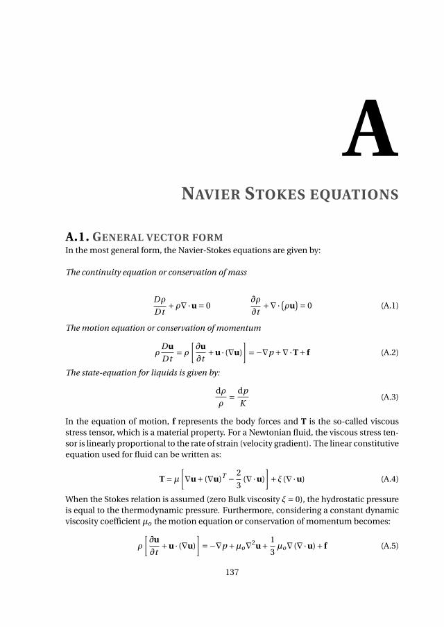
ANAVIER STOKES EQUATIONS
A.1. GENERAL VECTOR FORMIn the most general form, the Navier-Stokes equations are given by:
The continuity equation or conservation of mass
Dρ
Dt+ρ∇·u = 0
∂ρ
∂t+∇·
(
ρu)
= 0 (A.1)
The motion equation or conservation of momentum
ρDu
Dt= ρ
[
∂u
∂t+u · (∇u)
]
=−∇p +∇·T+ f (A.2)
The state-equation for liquids is given by:
dρ
ρ=
dp
K(A.3)
In the equation of motion, f represents the body forces and T is the so-called viscous
stress tensor, which is a material property. For a Newtonian fluid, the viscous stress ten-
sor is linearly proportional to the rate of strain (velocity gradient). The linear constitutive
equation used for fluid can be written as:
T =µ
[
∇u+ (∇u)T −2
3(∇·u)
]
+ξ (∇·u) (A.4)
When the Stokes relation is assumed (zero Bulk viscosity ξ= 0), the hydrostatic pressure
is equal to the thermodynamic pressure. Furthermore, considering a constant dynamic
viscosity coefficient µo the motion equation or conservation of momentum becomes:
ρ
[
∂u
∂t+u · (∇u)
]
=−∇p +µo∇2u+1
3µo∇ (∇·u)+ f (A.5)
137
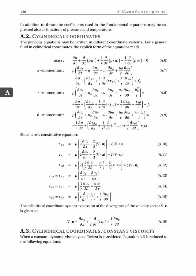
A
138 A. NAVIER STOKES EQUATIONS
In addition to these, the coefficients used in the fundamental equations may be ex-
pressed also as functions of pressure and temperature.
A.2. CYLINDRICAL COORDINATESThe previous equations may be written in different coordinate systems. For a general
fluid in cylindrical coordinates, the explicit form of the equations reads:
mass :∂ρ
∂t+
∂
∂x
(
ρux
)
+1
r
∂
∂r
(
ρr ur
)
+1
r
∂
∂θ
(
ρuθ
)
= 0 (A.6)
x−momentum : ρ
(
∂ux
∂t+ux
∂ux
∂x+ur
∂ux
∂r+
uθ
r
∂ux
∂θ
)
= (A.7)
−∂p
∂x+
(
∂τxx
∂x+
1
r
∂
∂r(rτxr )+
1
r
∂τxθ
∂θ
)
+ fx
r−momentum : ρ
(
∂ur
∂t+ux
∂ur
∂x+ur
∂ur
∂r+
uθ
r
∂ur
∂θ−
u2θ
r
)
= (A.8)
−∂p
∂r+
(
∂τr x
∂x+
1
r
∂
∂r(rτr r )+
1
r
∂τθr
∂θ−τθθ
r
)
+ fr
θ−momentum : ρ
(
∂uθ
∂t+ux
∂uθ
∂x+ur
∂uθ
∂r+
uθ
r
∂uθ
∂θ+
ur uθ
r
)
= (A.9)
−1
r
∂p
∂θ+
(
∂τθx
∂x+
1
r 2
∂
∂r(r 2τrθ)+
1
r
∂τθθ
∂θ
)
+ fθ
Shear stress constitutive equation:
τxx = µ
[
2∂ux
∂x−
2
3(∇·u)
]
+ξ (∇·u) (A.10)
τr r = µ
[
2∂ur
∂r−
2
3(∇·u)
]
+ξ (∇·u) (A.11)
τθθ = µ
[
2
(
1
r
∂uθ
∂θ+
ur
r
)
−2
3(∇·u)
]
+ξ (∇·u) (A.12)
τxr = τr x = µ
[
∂ux
∂r+∂ur
∂x
]
(A.13)
τxθ = τθx = µ
[
1
r
∂ux
∂θ+∂uθ
∂x
]
(A.14)
τrθ = τθr = µ
[
r∂
∂r
(uθ
r
)
+1
r
∂ur
∂θ
]
(A.15)
The cylindrical coordinate system expansion of the divergence of the velocity vector ∇·uis given as:
∇·u =∂ux
∂x+
1
r
∂
∂r(r ur )+
1
r
∂uθ
∂θ(A.16)
A.3. CYLINDRICAL COORDINATES, CONSTANT VISCOSITYWhen a constant dynamic viscosity coefficient is considered, Equation A.5 is reduced to
the following equations:
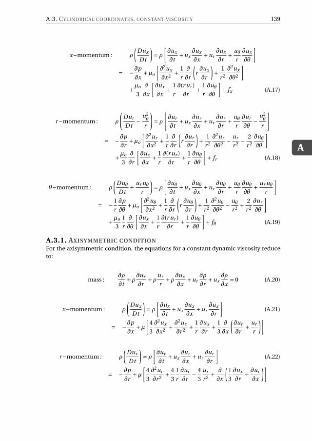
A.3. CYLINDRICAL COORDINATES, CONSTANT VISCOSITY
A
139
x−momentum : ρ
(
Dux
Dt
)
= ρ
[
∂ux
∂t+ux
∂ux
∂x+ur
∂ux
∂r+
uθ
r
∂ux
∂θ
]
= −∂p
∂x+µo
[
∂2ux
∂x2+
1
r
∂
∂r
(
r∂ux
∂r
)
+1
r 2
∂2ux
∂θ2
]
+µo
3
∂
∂x
[
∂ux
∂x+
1
r
∂(r ur )
∂r+
1
r
∂uθ
∂θ
]
+ fx (A.17)
r−momentum : ρ
(
Dur
Dt−
u2θ
r
)
= ρ
[
∂ur
∂t+ux
∂ur
∂x+ur
∂ur
∂r+
uθ
r
∂ur
∂θ−
u2θ
r
]
= −∂p
∂r+µo
[
∂2ur
∂x2+
1
r
∂
∂r
(
r∂ur
∂r
)
+1
r 2
∂2ur
∂θ2−
ur
r 2−
2
r 2
∂uθ
∂θ
]
+µo
3
∂
∂r
[
∂ux
∂x+
1
r
∂(r ur )
∂r+
1
r
∂uθ
∂θ
]
+ fr (A.18)
θ−momentum : ρ
(
Duθ
Dt+
ur uθ
r
)
= ρ
[
∂uθ
∂t+ux
∂uθ
∂x+ur
∂uθ
∂r+
uθ
r
∂uθ
∂θ+
ur uθ
r
]
= −1
r
∂p
∂θ+µo
[
∂2uθ
∂x2+
1
r
∂
∂r
(
r∂uθ
∂r
)
+1
r 2
∂2uθ
∂θ2−
uθ
r 2+
2
r 2
∂ur
∂θ
]
+µo
3
1
r
∂
∂θ
[
∂ux
∂x+
1
r
∂(r ur )
∂r+
1
r
∂uθ
∂θ
]
+ fθ (A.19)
A.3.1. AXISYMMETRIC CONDITIONFor the axisymmetric condition, the equations for a constant dynamic viscosity reduce
to:
mass :∂ρ
∂t+ρ
∂ur
∂r+ρ
ur
r+ρ
∂ux
∂x+ur
∂ρ
∂r+ux
∂ρ
∂x= 0 (A.20)
x−momentum : ρ
(
Dux
Dt
)
= ρ
[
∂ux
∂t+ux
∂ux
∂x+ur
∂ux
∂r
]
(A.21)
= −∂p
∂x+µ
[
4
3
∂2ux
∂x2+∂2ux
∂r 2+
1
r
∂ux
∂r+
1
3
∂
∂x
(
∂ur
∂r+
ur
r
)]
r−momentum : ρ
(
Dur
Dt
)
= ρ
[
∂ur
∂t+ux
∂ur
∂x+ur
∂ur
∂r
]
(A.22)
= −∂p
∂r+µ
[
4
3
∂2ur
∂r 2+
4
3
1
r
∂ur
∂r−
4
3
ur
r 2+
∂
∂x
(
1
3
∂ux
∂r+∂ur
∂x
)]

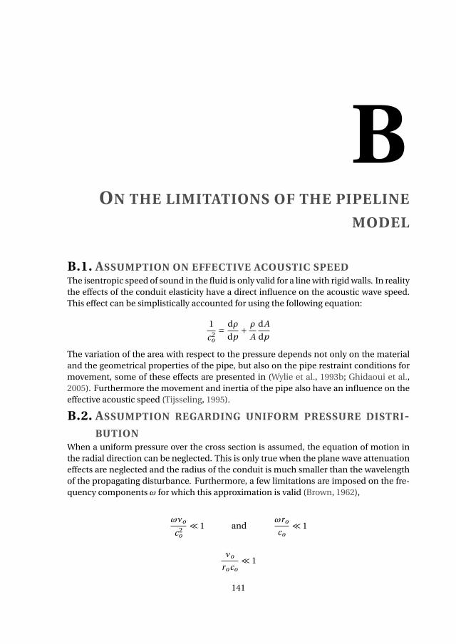
BON THE LIMITATIONS OF THE PIPELINE
MODEL
B.1. ASSUMPTION ON EFFECTIVE ACOUSTIC SPEEDThe isentropic speed of sound in the fluid is only valid for a line with rigid walls. In reality
the effects of the conduit elasticity have a direct influence on the acoustic wave speed.
This effect can be simplistically accounted for using the following equation:
1
c2o
=dρ
dp+
ρ
A
dA
dp
The variation of the area with respect to the pressure depends not only on the material
and the geometrical properties of the pipe, but also on the pipe restraint conditions for
movement, some of these effects are presented in (Wylie et al., 1993b; Ghidaoui et al.,
2005). Furthermore the movement and inertia of the pipe also have an influence on the
effective acoustic speed (Tijsseling, 1995).
B.2. ASSUMPTION REGARDING UNIFORM PRESSURE DISTRI-BUTION
When a uniform pressure over the cross section is assumed, the equation of motion in
the radial direction can be neglected. This is only true when the plane wave attenuation
effects are neglected and the radius of the conduit is much smaller than the wavelength
of the propagating disturbance. Furthermore, a few limitations are imposed on the fre-
quency components ω for which this approximation is valid (Brown, 1962),
ωνo
c2o
≪ 1 andωro
co≪ 1
νo
roco≪ 1
141

B
142 B. ON THE LIMITATIONS OF THE PIPELINE MODEL
B.3. CONDITIONS FOR NON-LINEAR CONVECTIVE TERMS TO
BE NEGLECTEDIn order to justify this assumption, the order of magnitude of the different terms involved
is considered (D’Souza and Oldenburger, 1964). Let L be the characteristic length along
the axis of the pipe, U the characteristic velocity, and co the speed of sound in the fluid.
u∂u
∂x≈
U 2
Land
∂u
∂t≈
U
L/co
Hence,
u ∂u∂x
∂u∂t
≈U 2
L
UL/co
≈U
co
This means that when U ≪ co , the term ux∂ux
∂xand similarly ur
∂ux
∂rmay be neglected
when compared with∂ux
∂t.
B.4. OTHER VISCOUS TERMS NEGLECTED
Following the same approach, the viscous term 43∂2ux
∂x2 which appears at the right hand
side of Equation A.21 may also be neglected. Let ux be of order U , x of order L and r of
order ǫL where ǫ≪ 1.
4
3
∂2ux
∂x2≈
4
3
U
L2
∂2ux
∂r 2≈
U
ǫ2L2and
1
r
∂ux
∂r≈
U
ǫ2L2
Hence,
∂2ux
∂r 2≫
4
3
∂2ux
∂x2and
1
r
∂ux
∂r≫
4
3
∂2ux
∂x2
The other viscous terms from Equation A.21, 13
∂∂x
(
∂ur
∂r+ ur
r
)
vanish as they become zero
when integrated along the cross section with respect to r , from r = 0 to r = ro .
1
3
∂
∂x
∫ro
02πr
(
∂ur
∂r+
ur
r
)
dr = 0
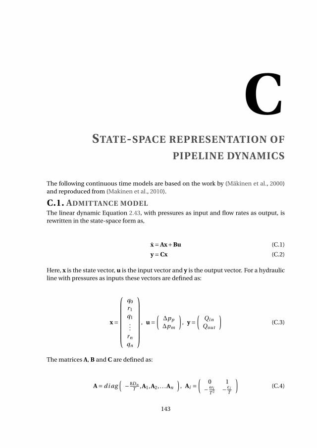
CSTATE-SPACE REPRESENTATION OF
PIPELINE DYNAMICS
The following continuous time models are based on the work by (Mäkinen et al., 2000)
and reproduced from (Makinen et al., 2010).
C.1. ADMITTANCE MODELThe linear dynamic Equation 2.43, with pressures as input and flow rates as output, is
rewritten in the state-space form as,
x = Ax+Bu (C.1)
y = Cx (C.2)
Here, x is the state vector, u is the input vector and y is the output vector. For a hydraulic
line with pressures as inputs these vectors are defined as:
x =
q0
r1
q1
...
rn
qn
, u =(
∆pp
∆pm
)
, y =(
Qi n
Qout
)
(C.3)
The matrices A, B and C are defined as:
A = di ag(
− 8Dn
T,A1,A2, . . .An
)
, Ai =(
0 1
− ωi
T 2 − ǫi
T
)
(C.4)
143
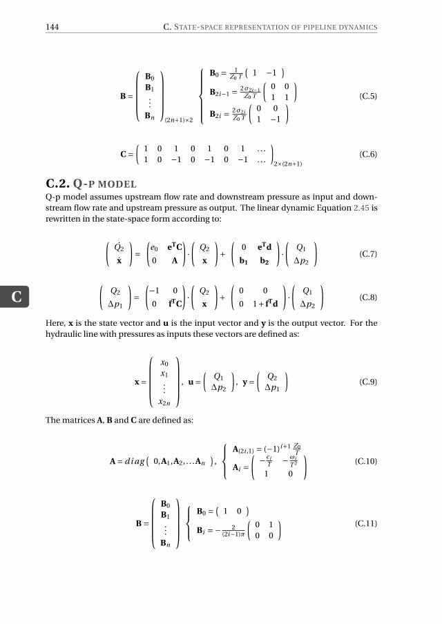
C
144 C. STATE-SPACE REPRESENTATION OF PIPELINE DYNAMICS
B =
B0
B1
...
Bn
(2n+1)×2
B0 = 1Z0 T
(
1 −1)
B2i−1 = 2σ2i−1
Z0 T
(
0 0
1 1
)
B2i = 2σ2i
Z0 T
(
0 0
1 −1
)
(C.5)
C =(
1 0 1 0 1 0 1 . . .
1 0 −1 0 −1 0 −1 . . .
)
2×(2n+1)
(C.6)
C.2. Q-P MODELQ-p model assumes upstream flow rate and downstream pressure as input and down-
stream flow rate and upstream pressure as output. The linear dynamic Equation 2.45 is
rewritten in the state-space form according to:
(
Q2
x
)
=(
e0 eTC
0 A
)
·(
Q2
x
)
+(
0 eTd
b1 b2
)
·(
Q1
∆p2
)
(C.7)
(
Q2
∆p1
)
=(
−1 0
0 fTC
)
·(
Q2
x
)
+(
0 0
0 1+ fTd
)
·(
Q1
∆p2
)
(C.8)
Here, x is the state vector and u is the input vector and y is the output vector. For the
hydraulic line with pressures as inputs these vectors are defined as:
x =
x0
x1
...
x2n
, u =(
Q1
∆p2
)
, y =(
Q2
∆p1
)
(C.9)
The matrices A, B and C are defined as:
A = di ag(
0,A1,A2, . . .An
)
,
A(2i ,1) = (−1)i+1 Z0
T
Ai =(
− ǫi
T− ωi
T 2
1 0
)
(C.10)
B =
B0
B1
...
Bn
B0 =(
1 0)
Bi =− 2(2i−1)π
(
0 1
0 0
)
(C.11)
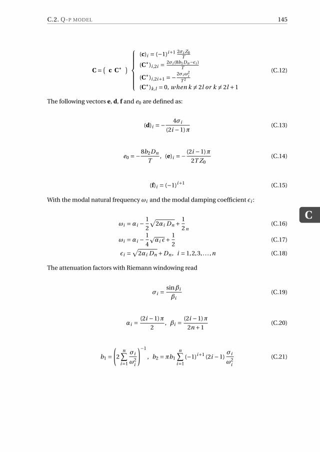
C.2. Q-P MODEL
C
145
C =(
c C∗ )
(c)i = (−1)i+1 2σi Z0
T
(C∗)i ,2i = 2σi (8b1Dn−ǫi )T
(C∗)i ,2i+1 =− 2σiω2i
T 2
(C∗)k,l = 0, when k 6= 2l or k 6= 2l +1
(C.12)
The following vectors e, d, f and e0 are defined as:
(d)i =−4σi
(2i −1)π(C.13)
e0 =−8b2Dn
T, (e)i =−
(2i −1)π
2T Z0(C.14)
(f)i = (−1)i+1 (C.15)
With the modal natural frequency ωi and the modal damping coefficient ǫi :
ωi =αi −1
2
√
2αi Dn +1
2 n(C.16)
ωi =αi −1
4
pαi ǫ+
1
2(C.17)
ǫi =√
2αi Dn +Dn , i = 1,2,3, . . . ,n (C.18)
The attenuation factors with Riemann windowing read
σi =sinβi
βi(C.19)
αi =(2i −1)π
2, βi =
(2i −1)π
2n +1(C.20)
b1 =(
2n∑
i=1
σi
ω2i
)−1
, b2 =πb1
n∑
i=1
(−1)i+1 (2i −1)σi
ω2i
(C.21)
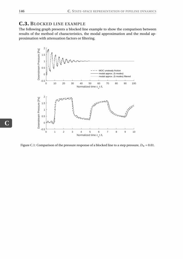
C
146 C. STATE-SPACE REPRESENTATION OF PIPELINE DYNAMICS
C.3. BLOCKED LINE EXAMPLEThe following graph presents a blocked line example to show the comparison between
results of the method of characteristics, the modal approximation and the modal ap-
proximation with attenuation factors or filtering.
Normalized time cot /L
0 10 20 30 40 50 60 70 80 90 100
Dow
nstr
eam
Pre
ssur
e [P
a]
-0.5
0
0.5
1
1.5
2
MOC unsteady frictionmodal approx. (5 modes)modal approx. (5 modes) filtered
Normalized time cot /L
0 1 2 3 4 5 6 7 8 9 10
Dow
nstr
eam
Pre
ssur
e [P
a]
-0.5
0
0.5
1
1.5
2
Figure C.1: Comparison of the pressure response of a blocked line to a step pressure, Dn = 0.01.
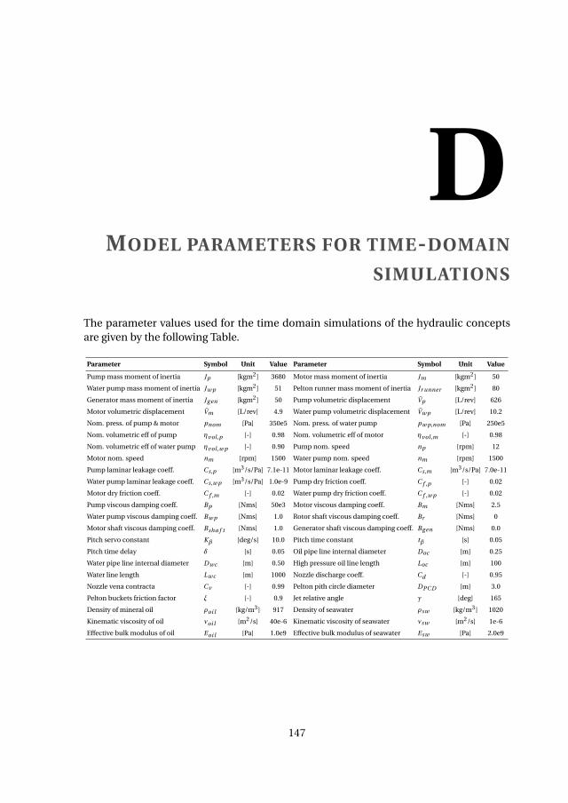
DMODEL PARAMETERS FOR TIME-DOMAIN
SIMULATIONS
The parameter values used for the time domain simulations of the hydraulic concepts
are given by the following Table.
Parameter Symbol Unit Value Parameter Symbol Unit Value
Pump mass moment of inertia Jp [kgm2] 3680 Motor mass moment of inertia Jm [kgm2] 50
Water pump mass moment of inertia Jw p [kgm2] 51 Pelton runner mass moment of inertia Jr unner [kgm2] 80
Generator mass moment of inertia Jg en [kgm2] 50 Pump volumetric displacement Vp [L/rev] 626
Motor volumetric displacement Vm [L/rev] 4.9 Water pump volumetric displacement Vw p [L/rev] 10.2
Nom. press. of pump & motor pnom [Pa] 350e5 Nom. press. of water pump pw p,nom [Pa] 250e5
Nom. volumetric eff of pump ηvol ,p [-] 0.98 Nom. volumetric eff of motor ηvol ,m [-] 0.98
Nom. volumetric eff of water pump ηvol ,w p [-] 0.90 Pump nom. speed np [rpm] 12
Motor nom. speed nm [rpm] 1500 Water pump nom. speed nm [rpm] 1500
Pump laminar leakage coeff. Cs,p [m3/s/Pa] 7.1e-11 Motor laminar leakage coeff. Cs,m [m3/s/Pa] 7.0e-11
Water pump laminar leakage coeff. Cs,w p [m3/s/Pa] 1.0e-9 Pump dry friction coeff. C f ,p [-] 0.02
Motor dry friction coeff. C f ,m [-] 0.02 Water pump dry friction coeff. C f ,w p [-] 0.02
Pump viscous damping coeff. Bp [Nms] 50e3 Motor viscous damping coeff. Bm [Nms] 2.5
Water pump viscous damping coeff. Bw p [Nms] 1.0 Rotor shaft viscous damping coeff. Br [Nms] 0
Motor shaft viscous damping coeff. Bsha f t [Nms] 1.0 Generator shaft viscous damping coeff. Bg en [Nms] 0.0
Pitch servo constant Kβ [deg/s] 10.0 Pitch time constant tβ [s] 0.05
Pitch time delay δ [s] 0.05 Oil pipe line internal diameter Doc [m] 0.25
Water pipe line internal diameter Dwc [m] 0.50 High pressure oil line length Loc [m] 100
Water line length Lwc [m] 1000 Nozzle discharge coeff. Cd [-] 0.95
Nozzle vena contracta Cv [-] 0.99 Pelton pith circle diameter DPC D [m] 3.0
Pelton buckets friction factor ξ [-] 0.9 Jet relative angle γ [deg] 165
Density of mineral oil ρoi l [kg/m3] 917 Density of seawater ρsw [kg/m3] 1020
Kinematic viscosity of oil νoi l [m2/s] 40e-6 Kinematic viscosity of seawater νsw [m2/s] 1e-6
Effective bulk modulus of oil Eoi l [Pa] 1.0e9 Effective bulk modulus of seawater Esw [Pa] 2.0e9
147

SAMENVATTING
Offshore-windenergie is een competitieve energiebron in de toekomstige Europese
energiemix aan het worden. De groei van wind op zee is duidelijk zichtbaar in de grote
windparken die worden gepland en gebouwd in de Noordzee, waarmee al vermogens
op GW-niveau worden behaald. In de huidige toepassing wordt de geproduceerde
elektriciteit per wind turbine in een windpark naar een centraal offshore-platform ge-
leid en daar geconditioneerd, voordat het door kabels over de zeebodem naar de kust
wordt getransporteerd. Zo gezien kan een offshore-windpark worden beschouwd als
één energiecentrale die elektriciteit produceert door middel van honderden multi-MW-
generatoren. De motivatie achter deze dissertatie volgt daarom het idee van elektrici-
teitsproductie op een gecentraliseerde wijze in een windpark, waarvoor slechts enkele
hoge-capaciteitsgeneratoren benodigd zijn.
Het gepresenteerde werk in deze dissertatie verkent een nieuwe manier van generatie,
bijeenbrenging en transmissie van windenergie binnen een windpark, waar geen tussen-
tijdse elektrische omzetting plaatsvindt, totdat de energie het centrale offshore-platform
heeft bereikt. Een gecentraliseerde vorm van energiegeneratie is beschouwd, waarbij ge-
bruik gemaakt wordt van watertechnologie. In het voorgestelde concept is de conventi-
onele versnellingskast of de directe aandrijving vervangen door een verdringingspomp,
waardoor vanuit de rotor-gondelassemblage water onder druk in een hydraulisch net-
werk gebracht wordt. Het water wordt onder hogedruk vanaf de wind turbines van het
windpark bijeengebracht en doorgeleid naar het centrale offshore-platform, waar ver-
volgens elektriciteit wordt gegenereerd door een Peltonturbine.
Voor het beschrijven van de energie-omzetting, alsmede het voornaamste dynamische
gedrag van de voorgestelde hydraulische windkrachtcentrale, is een numeriek model is
ontwikkeld. Het model vat de relevante fysica van de dynamische interactie tussen de
verschillende turbines, gekoppeld met een algemeen hydraulisch netwerk en een re-
gelaar. Gereduceerde-orde modellen voor de verschillende componenten worden ge-
presenteerd in de vorm van gekoppelde algebraïsche vergelijkingen en gewone diffe-
rentiaalvergelijkingen voor hun toepassing in tijdsdomeinsimulaties. Bijzondere aan-
dacht wordt gegeven aan het modeleren van hydraulische netwerken, waar een semi-
analytische aanpak wordt gepresenteerd voor transiënte laminaire stromingen, gebruik-
makend van een tweedimensionaal viskeus compressiemodel. Het model biedt de mo-
gelijkheid om sterke variaties in de voortgaande drukgolven te analyseren, welke resul-
teren van abrupte veranderingen in de stroming of druk geïntroduceerd door ventiel-
sluitingen of componentfalen. Daarnaast kan met het model de geschiktheid van an-
dere methoden, zoals modale benaderingen, gebruikt voor het representeren van kort-
durende aspecten van het hydraulische netwerk, worden beoordeeld.
Vanuit het regelsysteem gezien dient als gevolg van het verwijderen van de individuele
generatoren en de vermogenselektronica uit de turbines de hydraulische aandrijving
de regelacties te vervangen om hetzelfde of ten minste een vergelijkbare variabele-
149
150 SAMENVATTING
snelheidsfunctionaliteit van moderne windturbines te bereiken. Zowel passieve als
actieve regelstrategieën worden voorgesteld, gebruikmakend van hydraulische com-
ponenten voor een enkele variabele-snelheidswindturbine. Lineaire regelanalyse-
instrumenten worden gebruikt om de prestatie van de voorgestelde regelaars te evalu-
eren. De passieve controlestrategie toont aan inherent stabiel te zijn door gebruik te
maken van een spuitmond met een constant oppervlak voor windsnelheden lager dan
de optimale windsnelheid. De toepassing van deze strategie vergt het geschikt dimensi-
oneren van de hydraulische componenten gebruikt om de optimale snellopendheid te
bereiken, terwijl de druk in het hydraulische netwerk variabel is. De passieve strategie
is simpel en robuust, maar is beperkt tot een enkele turbine. Aangezien meerdere tur-
bines tot hetzelfde hydraulische netwerk behoren zou een constante-druksysteem de
voorkeur verdienen. Een actieve regelstrategie is ook geanalyseerd om een variabele-
snelheidsrotor te verkrijgen, terwijl de druk in het hydraulische netwerk constant
gehouden wordt. De constante-drukregelaar is bereikt door het oppervlak van de spuit-
mond aan te passen door een lineaire actuator. Een combinatie van een PI-regelaar
in serie met een laagdoorlaatfilter en inkepingen is toegepast om de invloed van de
pijplijndynamica op de drukresponsie te reduceren. Hiernaast is een pomp met variabel
debiet, werkend met een gecontroleerde druk, toegepast om het doorgegeven moment
aan de rotor aan te passen.
Twee casussen zijn beschouwd in de tijdsdomeinsimulaties voor een hypothetisch
hydraulisch windpark onderhevig aan turbulente windcondities. De prestatie- en
operationele parameters van individuele turbines zijn vergeleken met die van een refe-
rentiewindpark met conventionele-technologieturbines, gebruikmakend van dezelfde
windparklay-out en omgevingscondities. De resultaten van de gepresenteerde casus
geven aan dat de individuele windturbines kunnen werken binnen de operationele
limieten met het concept met de constante-drukregelaar. Het hydraulische windpark
is ondanks de stochastische invoer voor de turbulente wind en zogeffecten in staat om
elektriciteit te produceren met een redelijke prestatie zowel onder als boven optimale-
windcondities.
PUBLICATIONS BY THE AUTHOR
JOURNAL PUBLICATIONSJarquin Laguna, A. Modeling and analysis of an offshore wind turbine with fluid power
transmission for centralized electricity generation. Journal of Computational and
Nonlinear Dynamics: Special issue wind turbine modelling, 10(4):pp.11–24, 2015.
Jarquin Laguna, A. Simulation of an offshore wind farm using fluid power for central-
ized electricity generation. Wind Energy Science Discussions, 2016. doi: 10.5194/
wes-2016-54. URL http://www.wind-energ-sci-discuss.net/wes-2016-54/.
(under review).
Jarquin Laguna, A. and Tsouvalas, A. Transient laminar flow in hydraulic networks based
on a semi-analytical impulse response method. HERON: Special issue dynamics of
structures, 59(1):pp.37–55, 2014.
Jarquin Laguna, A., Diepeveen, N., and Van Wingerden, J. Analysis of dynamics of fluid
power drive-trains for variable speed wind turbines: Parameter study. IET Renewable
Power Generation, 8(4):pp.398–410, 2014.
CONFERENCE PUBLICATIONSDiepeveen, N. and Jarquin Laguna, A. Dynamic modeling of fluid power transmissions
for wind turbines. In Proceedings of the EWEA Offshore 2011 Conference, Amsterdam.
European Wind Energy Association, 2011.
Diepeveen, N. and Jarquin Laguna, A. Wind tunnel experiments to prove a hydraulic
passive torque control concept for variable speed wind turbines. In Journal of Physics:
Conference Series, volume 555(1), page 012028. the European Academy of Wind En-
ergy, IOP Publishing, 2014a. The Science of Making Torque from Wind 2012.
Diepeveen, N. and Jarquin Laguna, A. Preliminary design of the hydraulic drive train for
a 500kw prototype offshore wind turbine. In Proceedings of the 9th International Fluid
Power Conference, pages 133–144. RWTH Aachen, 2014b.
Jarquin Laguna, A. Fluid power network for centralized electricity generation in offshore
wind farms. In Journal of Physics: Conference Series, volume 524(1), page 012075. the
European Academy of Wind Energy, IOP Publishing, 2014. The Science of Making
Torque from Wind 2014.
Jarquin Laguna, A. Simulation of an offshore wind farm using fluid power for centralized
electricity generation. In Journal of Physics: Conference Series, volume 753(10), page
102004. the European Academy of Wind Energy, IOP Publishing, 2016. The Science of
Making Torque from Wind 2016.
151

152 SAMENVATTING
Jarquin Laguna, A. and Diepeveen, N. Performance evaluation of a hydraulic offshore
wind turbine. In Proceedings of the Renewable Energy Research Conference. Trond-
heim, Norway, 2010.
Jarquin Laguna, A. and Diepeveen, N. Dynamic analysis of fluid power drive-trains for
variable speed wind turbines: A parameter study. In Proceedings of the EWEA Offshore
2013 Conference, Vienna, Austria, 4-7 Febraury 2013. European Wind Energy Associa-
tion, 2013.
Jarquin Laguna, A. and Tsouvalas, A. A semi-analytical impulse response method for
transient laminar flow in hydraulic networks. In Proceedings of the XLIII International
Summer School Conference of Advanced Problems in Mechanics. St. Petersburg, Russia,
2015.

CURRICULUM VITÆ
Antonio JARQUÍN LAGUNA
02 June 1984 Born in Toluca, México.
EDUCATION2002–2007 Diploma in Mechanical Engineering
Universidad Nacional Autónoma de México, (México, D.F.)
National Autonomous University of Mexico
2008–2010 Master of Science in Sustainale Energy Technology
Delft University of Technology
Faculty of Applied Sciences
2011–2016 Ph.D. Research
Delft University of Technology
Faculty of Civil Engineering and Geosciences
Department of Hydraulic Engineering
Section of Offshore Engineering
2016–present Researcher at Delft University of Technology
PROFESSIONAL2007–2008 Analysis Engineer
The General Electric Company
Engine Dynamics & Structural Systems
GEIQ Aviation, Querétaro, México
2010–2012 Solution Development Engineer
Bluewater Energy Services BV
New energy group, Hoofddorp, the Netherlands
153