Embed Size (px)
Citation preview

Electronic copy available at: http://ssrn.com/abstract=1089823Electronic copy available at: http://ssrn.com/abstract=1089823Electronic copy available at: http://ssrn.com/abstract=1089823
1
Building Brand Awareness in Dynamic Oligopoly Markets
Prasad A. Naik Chancellor’s Fellow and Professor of Marketing, University of California Davis, Davis, CA 95616
Ashutosh Prasad Associate Professor, School of Management, University of Texas at Dallas, Richardson, TX 75083-0688
Suresh P. Sethi Ashbel Smith Professor of Operations Management, University of Texas at Dallas, Richardson, TX 75083-0688
Companies spend hundreds of millions of dollars annually on advertising to build and maintain awareness for their brands in competitive markets. However, awareness formation models in the marketing literature ignore the role of competition. Consequently, there is a lack of both the empirical knowledge and normative understanding of building brand awareness in dynamic oligopoly markets. To address this gap, we propose an N-brand awareness formation model, design an Extended Kalman Filter to estimate the proposed model using market data for five car brands over time, and derive the optimal closed-loop Nash equilibrium strategies for every brand. The empirical results furnish strong support for the proposed model in terms of both goodness-of-fit in the estimation sample and cross-validation in the out-of-sample data. In addition, the estimation method offers managers a systematic way to estimate ad effectiveness and forecast awareness levels for their particular brands as well as competitors’ brands. Finally, the normative analysis reveals an inverse allocation principle that suggests contrary to the proportional-to-sales or competitive parity heuristics that large (small) brands should invest in advertising proportionally less (more) than the small (large) brands. _____________________________________________________________________________________
1. Introduction
The real assets of companies are often intangible rather than physical (e.g., brand names versus
plant and machinery). For example, the Ford Motor Company recently sold physical assets and invested
over twelve billion dollars to acquire prestigious brand names: Jaguar, Aston Martin, Volvo and Land
Rover. As reported by Forbes,
“None of these marquees brought much in the way of plant and equipment but plant and equipment aren’t what the new business model is about. It’s about brands and brand building ... Ford has been selling things you can touch and buying what exists only in the consumers’ minds” (Akasie 2000).
To maintain and enhance intangible assets, managers spend hundreds of millions of dollars annually on
advertising and build brand awareness, which is a major component of brand equity (Keller 2002, p. 67)
and can be measured (e.g., Interbrand rankings of 100 global brands). But competing brands also seek to

Electronic copy available at: http://ssrn.com/abstract=1089823Electronic copy available at: http://ssrn.com/abstract=1089823Electronic copy available at: http://ssrn.com/abstract=1089823
2
increase brand awareness; hence managers must take into account the presence of multiple competitors in
determining their best course of action. However, extant awareness formation models in marketing have
ignored the role of competition (see Mahajan, Muller and Sharma 1984, Naik, Mantrala and Sawyer 1998,
Bass et al. 2005). Consequently, the literature contains sparse empirical knowledge on the effectiveness of
own and competitors’ advertising in building awareness for mature products; it also lacks normative
guidelines for the optimal strategies to pursue for enhancing brand awareness.
To address these issues, we investigate awareness formation in dynamic markets with multiple
competitors. In section 3, we propose an N-brand awareness formation model, which extends the models
of Sethi (1983) and Sorger (1989) by not only allowing competition across N > 2 brands, but also
incorporating market expansion and brand confusion effects. We empirically validate the model using
market data on awareness of five car brands over time. Because this model is a simultaneous system of
coupled nonlinear difference equations, to estimate its parameters, we apply the extended Kalman filter
(e.g., Xie, Song, Sirbu and Wang 1997). The empirical results furnish strong support for the proposed
model in terms of not only in-sample fit, but also out-of-sample forecasts. In addition, managers can use
the estimation approach to estimate ad effectiveness and forecast awareness levels for their product
markets; Section 4.2 describes the approach.
Section 5 derives the closed-loop Nash equilibrium strategies for every brand in a dynamic
oligopoly. This normative analysis reveals an inverse allocation principle, which indicates that large
(small) brands should invest in advertising proportionally less (more) than the small (large) brands. The
novelty of this principle is the proof we furnish that inverse allocation is optimal, which is contrary to the
textbook recommendations based on proportional-to-sales or competitive parity heuristics. Finally,
section 6 concludes by suggesting avenues for further research. But first, to identify the gaps in empirical
and normative understanding, we review the marketing and management science literatures.
2. Literature Review
We describe the extant findings from both awareness formation and differential game models.
2.1 Awareness Formation Models

Electronic copy available at: http://ssrn.com/abstract=1089823
3
Awareness formation models describe the growth and decay of a brand’s awareness over time in
response to advertising efforts. Mahajan, Muller and Sharma (1984) reviewed the marketing science
literature on awareness formation models. Here we present models developed by Blattberg and Golanty
(1978) and Dodson and Muller (1978), whose key features we incorporate in our formulation.
Blattberg and Golanty (1978) develop a model called TRACKER, where change in brand
awareness is driven by advertising effort that influences the unaware segment of the market. Denoting the
fraction of an aware segment by At and advertising effort by ut (operationalized by gross rating points or
GRP), the model is expressed as ∆At = At − At-1 = f(ut) (1 − At-1), where the concave response function
f(u) captures diminishing returns.
Dodson and Muller (1978) extend the TRACKER specification by incorporating word-of-mouth
and forgetting effects. They specify awareness change as ∆At = f(ut)(1 − At-1) + βAt-1(1 − At-1) − δAt-1.
Specifically, the term At-1(1 − At-1) captures the word-of-mouth effect because of the social interaction
between the aware segment At and the unaware market (1 − At-1). The last term (− δAt-1) reflects the loss
of awareness due to forgetting effects.
Overall, the common feature across these models, including the recent ones (e.g., Naik et al.
1998, Bass et al. 2005), is the absence of competitive brands and their strategic responses over time.
Because differential game models shed light on dynamic competitive strategies, we next review this
management science literature.
2.2 Differential Game Models
Differential game models facilitate the study of market dynamics via differential equations and
apply game theoretic concepts to obtain normative solutions to managers’ decisions. For surveys of this
literature, see Feichtinger, Hartl and Sethi (1994), Dockner, Jorgensen, Long and Sorger (2000), Sethi and
Thompson (2000), Erickson (2003), and Jorgensen and Zaccour (2004). Most studies in this genre
analyze duopoly markets (e.g., Erickson 1992, Chintagunta and Vilcassim 1992, Chintagunta and Jain
1995, Fruchter and Kalish 1997, Prasad and Sethi 2004), while a few notable studies on oligopoly

4
markets include Teng and Thompson (1983), Fershtman (1984), Dockner and Jorgensen (1992), Erickson
(1995), Fruchter (1999), and Naik, Raman and Winer (2005). In these oligopoly models, closed-form
solutions for optimal decisions are rarely available. In contrast, we will provide closed-form results in
oligopoly markets by extending a dynamic model in Sethi (1983).
The dynamics in Sethi (1983) can be expressed as
( ) / ( ) 1 ( ) ( )dA t dt u t A t A tρ δ= − − , A(0) = A0, (1)
where A(t) represents awareness at time t, and ρ and δ denote ad effectiveness and decay constant,
respectively. Similarities between Sethi (1983) and Dodson and Muller (1978) are as follows.
Specifically, both models consider monopoly markets; the awareness change, dA/dt, in continuous-time is
analogous to ∆At in the discrete-time version; the last term (− δA) characterizes the decay in awareness
due to forgetting effects. Furthermore, to provide an interpretation of the square-root in (1), Sorger (1989)
and Erickson (2003, p. 24) observe that ≈− A1 +− )1( A )1( AkA − , where the best-fitting value of k =
13/14 for ]1,0[∈A (as noted by an anonymous reviewer); the first term (1−A) represents the unaware
segment and the second term captures the word-of-mouth interaction effects. We next extend this
monopoly model to mature markets with multiple brands.
3. Model Development
We first review the duopoly extension and then formulate an N-brand extension. Sorger (1989)
extended the Sethi model to duopoly markets as follows:
1221111 1 mumu
dt
dmρ−−ρ= , m1(0) = m10, (2)
2112222 1 mumu
dt
dmρ−−ρ= , m2(0) = 1− m10, (3)
where for each brand i, i = 1, 2, mi(t) represents market share, ρi denotes ad effectiveness, and ui is the ad
spending level of brand i that depends on both own and competitor’s shares (i.e., ui(m1, m2)). Both the
spending levels and market shares are assumed to be strictly positive and positive fractions, respectively.

5
In addition, by summing (2) and (3), we obtain m1(t) + m2(t) = 1 for all t, which represents the logical
consistency property. Although logical consistency is a desirable property for market share data, it may
not hold for awareness levels or brand sales data. Hence we will also include the consideration of “market
expansion” effects. Finally, we note that the exogenous decay constant δ in (1) is replaced in (2) and (3)
by an endogenous loss due to the competitor’s advertising. However, in the context of awareness
formation, competitor’s advertising might increase the awareness for own brands, for example, due to
“confusion effects.” Consequently, Pauwels (2004, p. 604) urges researchers to permit both positive and
negative effects of competitor’s advertising.
To incorporate expansion effects, first, we extend Sorger (1989) formulation and allow the total
awareness ∑=
=N
ii tAtM
1
)()( to vary over time. Thus, for the N-brand oligopoly markets, we propose the
dynamic model:
∑≠=
−ξ−−ρ=N
ijj
actionscompetitorfromgainorLoss
jjij
actionowntodueGain
iiii AMuAMu
dt
dA
1'
�� ��� ���������, {1,2,.., }i I N∈ = (4)
where ui(⋅) denotes the advertising effort based on prevailing awareness for all brands in the set I = {1, 2,
..., N}. As before, the spending levels and awareness are assumed to be strictly positive. Second, to
capture potentially positive effects of competitive advertising (e.g., due to brand confusion or comparative
advertisements), we permit ξij < 0 so that own awareness Ai can increases as uj increases. Finally, if
logical consistency is necessary (e.g., when using market share data), researchers can set ξij = ρj/(N−1)
and M = 1 to ensure 1)( =∑∈Ii
i tA .
In sum, the proposed model not only allows competition across N > 2 brands, but also
incorporates market expansion and brand confusion effects. We next assess the empirical validity of this
model in describing brand awareness dynamics of competing brands.
4. Empirical Analyses
Below we present the awareness data, the estimation method and the empirical results.

6
4.1 Continuous Tracking Data
To understand the awareness dynamics, we analyze field data for compact mid-priced cars from a
continuous tracking study. Tracking studies offer the benefit that, even when brand managers do not have
access to weekly sales data for competitors’ brands, they can commission market research companies
(e.g., Millward Brown, Arbor Inc.) to conduct phone interviews and gather competitive awareness levels
every week throughout the year (i.e., “continuous” tracking). Also, as Batra, Lehmann, Burke and Pae
(1995, p. 20) note, ad agencies prefer tracking data on “purer” intermediate measures (e.g., brand
awareness, purchase intent) to assess advertising impact because non-advertising factors such as
salesforce effort or retail availability affect the final measures like brand sales or market shares.
In this tracking study, 350 phone interviews were conducted every day on a random sample of
families in Italy. The information collected “… covers all players [i.e., brands] in the market. It covers the
state of the play for that week in regard to people’s behavior, attitudes, brand awareness … This
[awareness data] is then related to other information such as media data indicating what advertising were
on during that week …” (for further details, see Sutherland 1993, Ch. 10). Specifically, we use brand
awareness of the five car brands Fiat Punto, Opel Corsa, Peugeot 206, Renault Clio, and Ford Fiesta
in response to the question: “Which of these brands of cars have you seen advertised on television
recently?” Besides the multi-brand awareness time-series, the other piece of information the media
spending patterns consists of the weekly gross rating points (GRPs), which measures the exposure of
advertisements to the target audience. GRPs are directly related to dollar-expenditure and can be related
to intermediate measures such as awareness (Rossiter and Percy 1997, p. 586). For example, Batra,
Lehmann, Burke and Pae (1995) fitted a logit model of awareness as a function of GRPs across twenty-
nine campaigns. Thus our analysis of awareness-GRPs data comports with both the company’s
information set and the extant practices (e.g., Sutherland 1993, Batra, et al. 1995, Naik et al.1998).
Thus weekly time-series of awareness and GRPs over 83 weeks for each of the five brands
comprise the dataset (see Luati and Tassinari 2005 for details). Table 1 presents the descriptive statistics.

7
To analyze this time-series data, we next describe an approach for estimation, inference and model
selection of dynamic oligopoly models.
[Insert Table 1 about here]
4.2 Extended Kalman Filter Estimation
In marketing, Xie et al. (1997) and Naik et al. (1998) pioneered the Kalman filter estimation of
dynamic models. Specifically, Xie et al (1997) studied nonlinear but univariate dynamics of the Bass
model, while Naik et al. (1998) estimated multivariate but linear dynamics of the modified Nerlove-
Arrow model. However, the dynamic model in (4) constitutes a multivariate system of nonlinear
differential equations. Hence, this paper marks the first nonlinear multivariate dynamic system estimation
in marketing.
By discretizing equation (4), we obtain a set of five equations for i = 1,⋅⋅⋅, 5 as follows:
ikkkikkkiikkikiikki AMuAMuAMuAA −ξ−−−ξ−−ρ+=+ 552221, ⋯ , (5)
where Ai is a typical element of the five-dimensional state vector αk = (A1k, ..., A5k)′ and weeks k = 1, …,
T. Equation (5) denotes a row of the matrix equation induced by the simultaneous system of nonlinear
difference equations with potential cross-equation coupling (i.e., it is not a typical regression model). The
inter-equation coupling arises, for example, due to the presence of ∑= kik AM , ; the nonlinearity comes
from the square-root formulation.
To estimate this nonlinear multivariate dynamic system, we apply the extended Kalman filter,
which consists of four steps. (For several benefits of state space modeling, see the review chapter by
Dekimpe, Franses, Hanssens and Naik 2007.) First, to compactly represent the dynamic system in a state
space form, we let αk = (A1k, ..., A5k)′ denote the state vector, and Yk = (Y1k, ..., Y5k)′ be the observed
awareness levels. Then the nonlinear multivariate state-space form is,
,)(
,
11 kkkk
kkk
G
zY
ν+α+α=αε+α=
−− (6)

8
where z is a 5 × 5 identity matrix, and G(⋅) is a vector-valued function of αk-1. The error terms εk ~ N(0,
2εσ I) and νk ~ N(0, 2
νσ I), where I denotes the 5 × 5 identity matrix. These errors can be interpreted as net
effects of myriad factors not explicitly included in the model.
Second, the standard Kalman filter is not applicable because G(⋅) is a nonlinear function of state
variables, and hence we apply the Extended Kalman Filter (EKF). The EKF recursively determines the
mean and covariance of αk, given the observed information history Ηk-1 = {Y 1, ..., Yk-1}, for each k =
1,...,T. We use the model-specific Jacobian matrix T = I + ∂G/∂α′ in the well-known EKF recursions (see
Harvey 1994, p. 161) to obtain the sequence of means and covariances of αk for k = 1, ..., T.
Third, based on the means and covariances of αk, we compute the log-likelihood of observing the
awareness sequence ΗT = (Y1, Y2, …, YT)′, which is given by
))|(();(1
1∑=
−=ΘT
kkkT HYpLnHL , (7)
where p(⋅ | ⋅) is the conditional density of Yk given the information history up to the last period, Ηk-1. The
vector Θ contains the model parameters (ρi, ξij)′ and the error variances and the initial means of α0. We
maximize (7) with respect to Θ to obtain the maximum-likelihood estimates:
)(ˆ Θ=θ LArgMax . (8)
For correctly specified models, we obtain standard errors from the square-root of the diagonal elements of
the inverse of the matrix:
θ=Θ
Θ′∂Θ∂Θ∂−=
ˆ
2 )(ˆ LJ , (9)
where the Hessian of L(Θ) is evaluated at the estimated values θ̂ . However, for misspecified models, we
seek to make inferences robust to misspecification errors. To this end, we conduct Huber-White robust
inferences (see White 1982) by computing the so-called sandwich estimator,
11 ˆˆˆ)ˆ( −−=θ JVJVar , (10)

9
where V is a K × K matrix of the gradients of the log-likelihood function; that is, GGV ′= , and G is T ×
K matrix obtained by stacking the 1 × K vector of the gradient of the log-likelihood function for each of
the T observations. In correctly specified models, J = V and so both the equations (9) and (10) yield
exactly the same standard errors (as they should); otherwise, we use the robust standard errors given by
the square-root of the diagonal elements of (10).
Finally, for model selection, we evaluate multiple information criteria (e.g., AIC, AICC and BIC),
which balance the trade-off between fidelity (enhance goodness-of-fit) and parsimony (employ few
parameters). Specifically, we compute AIC = −2L* + 2K, AICC = −2L* + T(T + K)/(T − K − 2), and BIC
= −2L* + K Ln(T), where (L*, T, K) denote the maximized log-likelihood, the sample size, and the
number of parameters, respectively. The model to be retained is associated with the smallest values of the
information criteria. By using multiple criteria, we gain convergent validity when these criteria suggest
the same model as the best one, thus enhancing confidence. However, when multiple criteria indicate
different models to be retained, researchers may apply the following guidelines: use AIC-type criteria to
select models involving many parameters and small sample sizes (i.e., large K/T ratio) because they
possess “efficiency” property; use BIC-type criteria, which possess consistency property, for settings with
few parameters and large sample sizes (i.e., small K/T ratio). For further discussion of efficiency versus
consistency, see McQuarie and Tsai (1998, p. 3) and Naik, Shi and Tsai (2007, Remark 2).
4.3 Empirical Results
4.3.1 Model Selection and Parameter Estimation
We apply the above approach to market data on five Italian car brands. We estimate the proposed
model in (5), i.e., the complete model, with five ρi parameters (one for each car brand) and twenty ξij
parameters (four for each car brand). In addition, we estimate ten versions obtained by letting ξij = ρj/λ,
where λ = 1, 2, ..., 10. To determine the best model to retain, we compute multiple information criteria
and display the results in Table 2. We find that the complete model is over-parameterized. Specifically, it
gets high scores on AIC, AICC, and BIC; further inspection reveals that several of its estimated
10
parameters are insignificant. In contrast, some of the nested versions have smaller scores on the
information criteria. Particularly the model with λ = 6 attains the minimum AIC, AICC and BIC, so we
retain the model with ξij = ρj/6. More importantly, all three criteria recommend the same model to be
retained, thus achieving convergent validity and enhancing confidence in this retained model.
[Insert Tables 2 and 3 about here]
We next test whether the assumed independence of error terms holds for this retained model. To
this end, we test the presence of serial correlation by computing Box-Ljung statistic Q (see Harvey 1994,
p. 259), which follows χ2 with one degree of freedom. For each of the five brands, we obtain Q = 0.2599,
0.2837, 0.8737, 2.0167, 0.0013 which do not exceed the critical χ2 value of 3.84 at the 95% confidence
level. Thus serial correlation is statistically negligible.
To further safeguard inference from other misspecification errors, we compute the robust
standard errors via (10) for assessing the significance of estimated parameters. Table 3 presents the
parameter estimates and robust t-ratios for the retained model. We find that all parameters have correct
signs. The observation noise is negligible, whereas the transition noise is significant. Also, ad
effectiveness of each of the five brands is statistically significant, indicating that the spending on
television GRPs does affect a brand’s awareness. Furthermore, this impact of GRP on brand awareness
differs by brand. Next we consider how well this retained model predicts out-of-sample observations.
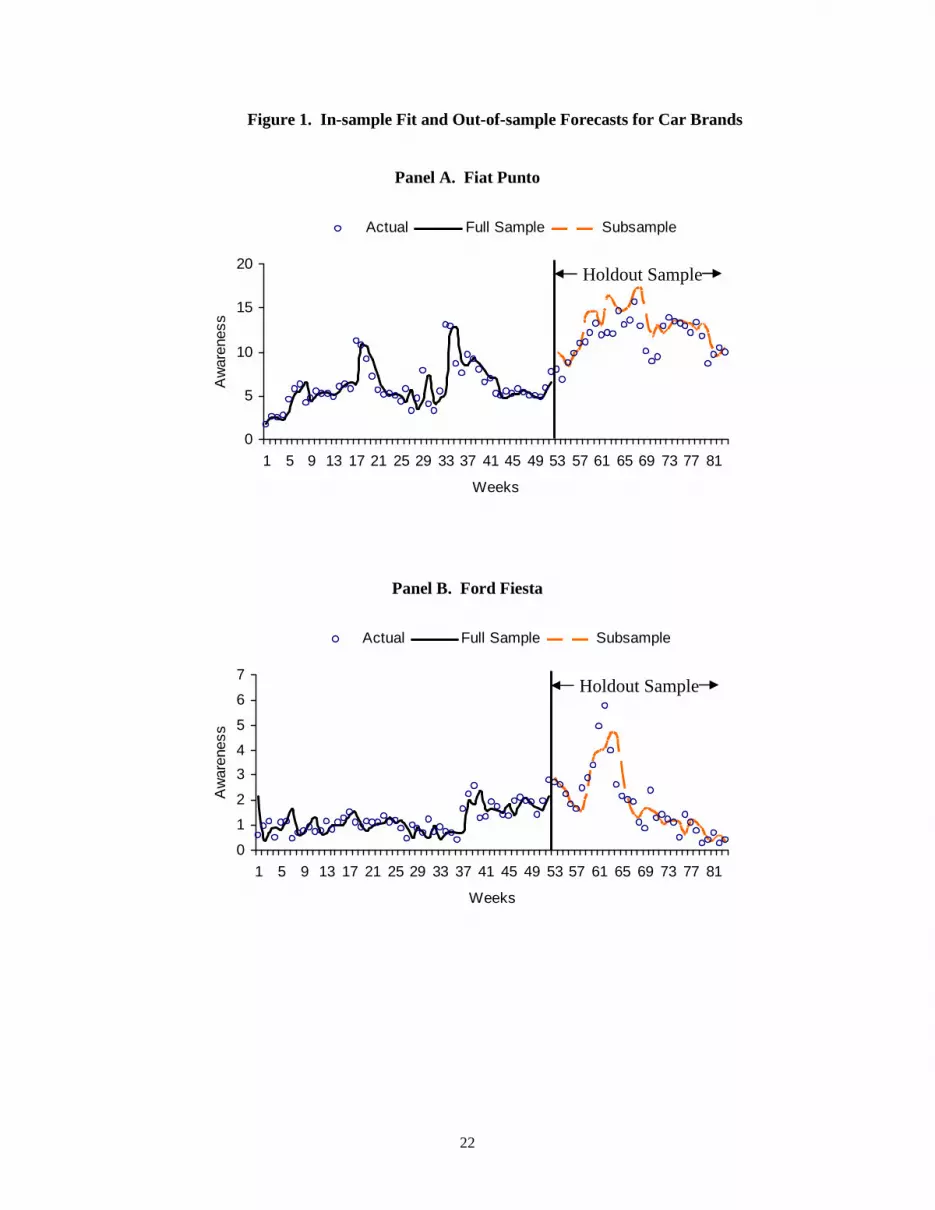
4.3.2 Out-of-sample Forecast
Using the retained model, we compute the one-step-ahead forecast of awareness levels via the
cross-validation approach. Specifically, we re-estimate the model using the sub-sample of the first 52
observations and hold 31 observations to assess its predictive validity. Figure 1 displays the cross-
validation results (see the holdout period for actuals versus forecasts). Panels A and B, respectively,
present the results for the largest and the smallest brands, namely, Fiat Punto and Ford Fiesta. (Other
graphs are essentially similar and not shown to save space.) These graphs show that the proposed model,
fitted with sub-sample data, predicts the awareness levels in the holdout period satisfactorily. Table 4

11
quantifies the quality of forecast performance. For example, correlation between actual and forecasted
awareness levels are high, ranging from 0.72 to 0.93 across five brands; similarly, forecast performance
on other metrics (e.g., percentage observations within the confidence interval, mean squared error (MSE),
mean absolute deviation (MAD)) are satisfactory. Thus the proposed model not only fits the sample data,
but also exhibits strong predictive performance.
[Insert Figure 1 and Table 4 about here]
4.3.3 Model Comparison
We close this section by comparing the retained model with an alternative model, namely, N-
brand Lanchester model whose specification is given by the following simultaneous system of coupled
differential equations (see Fruchter 1999, Naik, Raman and Winer 2005):
−
=
NNN m
m
F
F
f
f
m
m
⋮
⋯
⋮⋱⋮
⋯
⋮
ɺ
⋮
ɺ 111
0
0
, (11)
where /i i im A A= ∑ denotes the brand i’s awareness share, dtdmmi /=ɺ , iii uf β= is its marketing
force, βi and ui represent ad effectiveness and GRPs, respectively, and ∑=
=N
iifF
1
is the total marketing
force of all the brands.
To estimate the dynamic system (11), we apply the Kalman filter estimation described earlier to
the estimation sample of 52 weeks. Next, based on this estimated model and average total awareness for
the estimation sample, we predict one-step-ahead awareness levels of each of the five brands for the
subsequent 31 weeks (i.e., the holdout sample, as before). Table 5 indicates the prediction results for the
5-brand Lanchester model. Comparing the corresponding quantities in Tables 4 and 5, we observe that (i)
the proposed model performs competitively on metrics such as correlation between actuals versus
forecasts or percentage of observations within the 95% confidence interval; (ii) the proposed model
outperforms the alternative model on the formal metrics of mean squared error or mean absolute
deviation.
12
Collectively, the empirical results furnish strong support, in terms of both fit and forecast, for the
proposed N-brand model. Moreover, the estimation method based on the extended Kalman filter for
fitting nonlinear dynamic oligopoly models to market data offers managers a systematic approach to
estimate ad effectiveness and forecast awareness levels for their particular brands. Next, we derive the
optimal strategies to pursue in a dynamic oligopoly.
5. Normative Analyses
We derive the optimal strategies and elucidate their substantive implications, relegating proofs to
the Appendix (available from the authors upon request).
Starting from an initial awareness level Ai0, in response to advertising decisions to be made by all
other brands simultaneously, each brand manager decides the best course of action *iu to maximize the
brand’s total discounted present value (e.g., Fruchter and Kalish 1987, Sorger 1989),
∫∫∞
−∞
− −=−=0
2
0
0 ))()(())()(()( dttutAmedtuctReAV iiirtrt
ii , i = 1,..., N, (12)
subject to the dynamic system (4). In (12), r denotes the discount rate, R(t) and c(u) denotes the revenues
from and costs of building awareness over time. Specifically, mi represents the revenues from an
awareness point of brand i, and c(u) = u2 is the convex cost function. Note that media companies (e.g.,
NBC, ABC) sell GRPs (denoted by u) and the advertiser pays for it in dollars. In other words, GRPs and
dollar expenditure are two objects of the same exchange. As Tellis (2004, p. 45) notes, “GRPs are the
most common measure for buying media time in market today.” Equation (12) specifies a quadratic
relation between GRPs and advertising expenditures. Consequently, if we substitute v = c(u) = u2 in the
objective function and u = √v in the dynamic state equations, a formulation consistent with previous
studies (e.g., Batra, Lehmann, Burke, Pae 1995, Fruchter 1999), we learn that we have incorporated the
notion of diminishing returns (i.e., early dollar increments are more effective than the later ones). Finally,
V i(⋅) captures the total discounted present value of brand i. To maximize (12), we solve the induced N-

13
brand differential game and derive the closed-loop strategies in Nash equilibrium, which we state in the
following proposition.
Proposition 1. Maximizing (12) subject to (4), the optimal closed-loop advertising strategy of brand i is
* ( )2
i iii i i i i k
k
M Au ρ ξ φ ξ φ
∈
− = + −
∑Ι , ∀ i ∈ I (13)
and its value function
1
Ni
i j jj
V Aφ=
=∑ , ∀ j ∈ I (14)
where the coefficients ijφ are obtained from the following relations:
,
1( ) ( ) .
2i j j i ii i j j j j k j j j j k
j j i k I k
r mφ ρ ξ φ ξ φ ρ ξ φ ξ φ∈ ≠ ∈ ∈
= + + − + −
∑ ∑ ∑Ι Ι (15)
2
,
1( )
4
1( ) ( ) , .
2
i i ij i i i i k
k
s s i is s s s k s s s s k
s s j k I k
r
j i
φ ρ ξ φ ξ φ
ρ ξ φ ξ φ ρ ξ φ ξ φ
∈
∈ ≠ ∈ ∈
= − + −
+ + − + − ≠
∑
∑ ∑ ∑
ΙΙ Ι (16)
Proof. See the Appendix (available upon request from the authors).
It is remarkable that the dynamic model (4), which fits the market data well (see Table 3) and
predicts the out-of-sample observations satisfactorily (see Figure 1), also leads to simple value functions,
thus yielding closed-form optimal strategies.
More importantly, the optimal strategies reveal the inverse allocation principle: the greater the
awareness level, the smaller the spending. A large (small) brand should spend proportionally less (more)
than the small (large) brands. Why? Because each brand spends proportional to the combined awareness
of the remaining brands to compete optimally. This intuition comes from equation (13), which shows that
the optimal budget is proportional to ∝2*i )u( .
,∑
≠∈
=−ijIj
ji AAM

14
The substantive implication of this inverse allocation principle is that managers should build
dominant brands because they would face less competitive resistance and afford to advertise more
efficiently in the long run. From a life cycle perspective, small up-and-coming brands should spend more
on advertising to build awareness, whereas mature brands may “fly on automatic pilot” without
advertising heavily and relying more on brand purchase and consumption experience to maintain
awareness. Jones (1986, 1990) furnishes empirical evidence to corroborate this principle, noting that “...
For large brands, the market share normally exceeds the advertising share; for smaller brands, the
opposite is true” (Jones 1986, p. 100; emphasis in the original).
To extend this analysis to mature markets (i.e., when market expansion is negligible) or analyze
market share data, we have to incorporate an additional constraint 1)t(AIi
i =∑∈
for every instant t. To
ensure this logical consistency, we set ξij = ρj/(N−1) and M = 1 and obtain the following result:
Proposition 2. In mature markets, a brand’s optimal closed-loop advertising strategy is
φ−φ
−−ρ
= ∑=
N
j
ij
ii
iii N
N
Au
1
*
)1(2
1, ∀ i ∈ I (17)
and its value function
j
N
j
ij
ii AV ∑
=
φ+φ=1
0 , ∀ j ∈ I (18)
where the coefficients (i0φ , ijφ ) are obtained from the following (N + 1) relations:
i
N
j
ij mr =φ∑
=
)(0
, (19)
2
2
2
)1(4
φ−φ
−ρ
−=φ ∑∈Ik
ik
ii
ii
ii N
Nmr , (20)
φ−φ
φ−φ
−
ρ−=φ ∑∑
∈∈ Ik
ik
ij
Ik
jk
jj
jij NN
Nr
2
2
)1(2, ∀ j ∈ I, j ≠ i. (21)
Proof. See the Appendix (available upon request from authors).

15
Interestingly, in mature oligopoly markets, equilibrium shares need not be of the form “us/(us +
them)”, as one expects in a duopoly market. To gain this counter-intuitive insight, we derive the
equilibrium shares:
Proposition 3: For each brand in a mature market, the equilibrium share is given by
∑=
−×
−−=N
jji
i
BB
NA
1
1
11 , ∀ i ∈ I, (22)
where
φ−φ
−ρ
= ∑=
N
j
ij
ii
ii N
NB
1
2
)1(2.
Proof. See the Appendix (available upon request from authors).
Now consider a duopoly market (i = 1, 2) where the equilibrium shares are )( 21 BB
BA i
i += . In
contrast, we realize that the equilibrium shares in a triopoly are )(
21
313221
321
BBBBBBB
BBBA
ii ++
−= (i = 1, 2,
3), which differs from the expression “us divided by us plus them.” Hence, results from N-brand models
can differ from those obtained using duopoly models, highlighting the importance of studying oligopoly
generalizations. When Bi’s are equal across brands, each brand earns an equal share (=iA 1/N), as it
should.
Finally, we investigate the effects of intensifying competition in mature markets. To gain insights,
we simplify the analysis by assuming that brands are competing with “equals” and prove the result for the
symmetric brands:
Proposition 4. In mature markets, the category ad spending increases as the number of brands increases.
Proof. See the Appendix (available upon request from authors).
Although this proposition seems intuitively obvious, the result is opposite of the extant findings
in the literature. Specifically, Fershtman (1984) shows that category ad spending decreases as the number
of brands increases; however, unlike this study, his market dynamics has not been empirically validated.

16
As category ad spending increases as new brands enter, an important question arises: Is there a maximum
number of brands that a mature product category can sustain?
To address this issue, we consider the total category value
r
NmdttumeV
Iii
rt
Iii 4
)1()(4)))(((
221
2
0
2* −φ−φρ−=−= ∫ ∑∑
∞
∈
−
∈
, (23)
where (φ1−φ2) is specified by equation (D5) in the Appendix. We observe that the category value becomes
negative as N increases, indicating that an upper bound for the number of brands exists. After algebraic
manipulations, we obtain an upper bound (see the Appendix),
rmr
rN
−ρ++=
22
* 23 , (24)
which reveals that product categories will sustain three (or more) brands.
This finding the smallest upper bound is three brands closely relates to the so-called Rule of
Three. At the individual level, consumers choose brands from a small consideration set, whose size ranges
from two to eight brands across various product categories with a median of 3.0 for antacids, beers,
deodorants, gasoline, over-the-counter medicines, pain relievers, and toothpastes (see Lilien, Kotler and
Moorthy 1992, Table 2.11, p. 67). At the market level, Sheth and Sisodia (2002) suggest that only three
major brands will eventually dominate any industry. For example, McDonald’s, Burger King and
Wendy’s in fast food; General Mills, Kellogg and Post for breakfast cereals; Nike, Adidas and Reebok for
sports shoes. Because different customers may be aware of different brands, these findings are appropriate
for less heterogeneous markets. Our theoretical result that the smallest N* = 3 not only affirms these
empirical findings, but also reveals that managers can reduce the category size to three brands by
increasing ad effectiveness, but not the media weight. That is, N* decreases as ad effectiveness increases
(∂N*/∂ρ < 0), whereas it remains unchanged with an increase in media weight alone (∂N*/∂u = 0). Thus
effective advertising can serve as a strategic device to reduce competition in mature product categories.

17
6. Conclusions
Awareness building in dynamic competitive markets is an important marketing activity. For
example, in 2005, Procter & Gamble bought the Gillette Company worth $11 billion in revenues and $2
billion in earnings for $57 billion. Gillette’s intangible property, not reflected in its accounting books, is
the awareness and preferences in consumers’ minds for brand names like Sensor, Mach 3, Duracell, Oral
B, and Braun. Although existing marketing models investigate how to build brand awareness, these
models ignore the presence of competition (see Mahajan, Muller and Sharma 1984). This gap between
theory and practice motivates us to extend awareness models to mature markets by explicitly
incorporating oligopolistic competition. To bridge this gap, we proposed a dynamic oligopoly model
(section 3), developed an estimation approach (section 4.2), validated the proposed model empirically
(section 4.3), and analyzed the implied differential game (section 5). More importantly, managers can
apply the estimation approach to awareness data from their particular product markets to assess ad
effectiveness and predict awareness levels for own and competitors’ brands.
We conclude by identifying four avenues for future research. The first avenue is to extend the
model (4) to multiple media to incorporate the effects of cross-media interactions or synergies (e.g., Naik
and Raman 2003). The second is to incorporate cross-competitor interactions by specifying ξij in model
(4) to functionally depend on ui so that we can test whether a brand’s own advertising dampens the
awareness loss to competitors? Third, to compute optimal strategies and value functions empirically,
managers should estimate the value of im̂ for each brand. To this end, they can use their private
information to construct a dependent variable as “price minus variable cost multiplied by weekly sales
units” and regress it on prevailing awareness levels across weeks. Finally, future researchers may derive
normative implications when the shape of response function is not globally concave (Vakratsas, Feinberg,
Bass, Kalyanaram 2004). We believe these efforts would improve the theory and practice of marketing
communications.

18
Acknowledgments
Authors are listed in alphabetical order. We benefited from the insightful comments and valuable
suggestions of the reviewers, Area Editor, Editor, and the participants in a seminar at the Catholic
University Leuven, Belgium. The first author was supported in part by the Chancellor’s Fellowship at
University of California Davis.
References
Akasie, J. F. 2000. Ford’s Model E. Forbes July 17. Bass, F., N. Bruce, S. Majumdar, B. P. S. Murthi. 2005. A Dynamic Bayesian Model of Advertising Copy
Effectiveness in the Telecommunications Sector. Working paper, University of Texas at Dallas. Batra, R., D. Lehmann, J. Burke, J. Pae (1995), “When Does Advertising Have an Impact? A Study if
Tracking Data, Journal of Advertising Research, Sept./Oct., 19-32. Blattberg, R., J. Golanty. 1978. TRACKER: An Early Test Market Forecasting and Diagnostic Model for
New Product Planning. Journal of Marketing Research 15 (2) 192-202. Chintagunta, P. K. and Jain, D. C. 1995. Empirical Analysis of a Dynamic Duopoly Model of
Competition. Journal of Economics and Management Strategy 4 109-131. Chintagunta, P. K. and Vilcassim, N. 1992. An Empirical Investigation of Advertising Strategies in a
Dynamic Duopoly. Management Science 38 (9) 1230-1244. Dekimpe, M., P. H. Franses, M. Hanssens and P. Naik. 2007. Time Series Models in Marketing.
Handbook of Marketing Decision Models, Edited by Berend Wierenga, forthcoming. Dockner, E. J. and S. Jorgensen. 1992. New Product Advertising in Dynamic Oligopolies. Zeitschrift fur
Operations Research 36 459-473. Dockner, E. J., S. Jorgensen, N. Van Long, G. Sorger. 2000. Differential Games in Economics and
Management Science. Cambridge University Press, Cambridge, U.K. Dodson, J. A., E. Muller. 1978. Models of New Product Diffusion Through Advertising and Word of
Mouth. Management Science 24 (11) 1568-78. Erickson, G. M. 1992. Empirical Analysis of Closed-Loop Duopoly Advertising Strategies.
Management Science 38 (May) 1732-1749. Erickson, G. M. 1995. Advertising Strategies in a Dynamic Oligopoly. Journal of Marketing Research 32
(2), 233-237. Erickson, G.M. 2003. Dynamic Models of Advertising Competition, 2nd edition, Kluwer, Norwell, MA. Feichtinger, G., R. F. Hartl, S. P. Sethi. 1994. Dynamic Optimal Control Models in Advertising: Recent
Developments. Management Science 40 195-226. Fershtman, C. 1984. Goodwill and Market Shares in Oligopoly. Economica 51(August) 271-281. Fruchter, G. 1999. The Many-Player Advertising Game. Management Science 45 1609-1611. Fruchter, G., S. Kalish. 1997. Closed-Loop Advertising Strategies in a Duopoly. Management Science 43
(1) 54-63. Harvey, A. C. 1994. Forecasting, Structural Time Series Models and the Kalman Filter. Cambridge
University Press, New York, NY. Jones, J. P. 1986. What’s in a Name: Advertising and the Concept of Brands, D. C. Heath and Company,
Lexington, MA Jones, J. P. 1990. Ad Spending: Maintaining Market Share. Harvard Business Review Jan.-Feb. 38-42. Jorgensen, S. and G. Zaccour. 2004. Differential Games in Marketing. Kluwer, Norwell, MA. Keller, K. 2002. Strategic Brand Management, 2nd Edition, Prentice Hall, Upper Saddle River, NJ.

19
Lilien, G. P. Kotler, K. S. Moorthy. 1992. Marketing Models. Prentice-Hall, Inc., Englewood Cliffs, NJ. Luati, A., G. Tassinari. 2005. Intervention Analysis to Identify Significant Exposures in Pulsing
Advertising Campaigns: An Operative Procedure. Computational Management Science, 2 (4), 295-308.
Mahajan, V., E. Muller, S. Sharma. 1984. An Empirical Comparison of Awareness Forecasting Models of New Product Introduction. Marketing Science 3 (3) 179-197.
McQuarie, A. and C.-L. Tsai. 1998. Regression and Time Series Model Selection. World Scientific, Singapore.
Naik, P., K. Raman, R. Winer. 2005. Planning Marketing-Mix Strategies in the Presence of Interactions. Marketing Science 24 (1) 25-34.
Naik, P., K. Raman. 2003. Understanding the Impact of Synergy in Multimedia Communications. Journal of Marketing Research 40 (4) 375-388.
Naik, P., M. K. Mantrala, A. Sawyer. 1998. Planning Media Schedules in the Presence of Dynamic Advertising Quality. Marketing Science 17 (3) 214-235.
Naik, P., P. Shi and C.-L. Tsai. 2007. Extending the Akaike Information Criterion to Mixture Regression Models. Journal of the American Statistical Association, forthcoming.
Pauwels, K. 2004. How Dynamic Consumer Response, Competitor Response, Company Support, and Company Inertia Shape Long-Term Marketing Effectiveness. Marketing Science 23 (4), 596-610.
Prasad, A., S. P. Sethi. 2004. Advertising under Uncertainty: A Stochastic Differential Game Approach. Journal of Optimization Theory and Applications, 123(1), 163-185.
Rossiter, J. and L. Percy. 1997. Advertising Communications and Promotions Management. 2nd Edition. McGraw Hill, New York, N.Y.
Sethi, S. P. 1983. Deterministic and Stochastic Optimization of a Dynamic Advertising Model. Optimal Control Applications and Methods 4 179-184.
Sethi, S. P., G. L. Thompson. 2000. Optimal Control Theory: Applications to Management Science and Economics. Kluwer, Norwell, MA.
Sheth, J., R. Sisodia. 2002. The Rule of Three: Surviving and Thriving in Competitive Markets. The Free Press, New York, NY.
Sorger, G. 1989. Competitive Dynamic Advertising: A Modification of the Case Game. Journal of Economics Dynamics and Control 13 55-80.
Sutherland, M. 1993. Advertising and the Mind of the Consumer. Allen and Unwin Pty. Ltd., Sydney, Australia.
Tellis, G. 2004. Effective Advertising. Sage Publications, Thousand Oaks, CA. Teng, J.-T., G. L. Thompson 1983. Oligopoly Models for Optimal Advertising When Production Costs
Obey a Learning Curve. Management Science 29 1087-1101. Vakratsas, D., F. M. Feinberg, F. Bass, and G. Kalyanaram. 2004. The Shape of Advertising Response
Functions Revisited: A Model of Dynamic Probabilistic Thresholds. Marketing Science 23 (1), 109-119.
White, H. (1982). Maximum Likelihood Estimation of Misspecified Models. Econometrica, 50, 1-25. Xie, J., M. Song, M. Sirbu, Q. Wang. 1997. Kalman Filter Estimation of New Product Diffusion Models.
Journal of Marketing Research 34 (3) 378-393.

20
Table 1. Descriptive Statistics
Awareness Levels Gross Rating Points Brands Mean Std. Deviation Mean Std. Deviation
Fiat Punto 8.10 3.53 171.74 235.54 Opel Corsa 1.86 0.79 65.07 140.31 Peugeot 206 1.62 1.03 58.91 135.40 Renault Clio 3.32 1.46 93.97 159.59 Ford Fiesta 1.46 0.97 74.41 117.16
Table 2. Model Selection Using Multiple Information Criteria
Model AICC AIC BIC Complete Model 637.79 353.64 418.95 Nested Models (ξij = ρj/λ)
λ = 1 591.64 403.75 420.68 λ = 2 568.37 380.48 397.41 λ = 3 546.67 358.78 375.71 λ = 4 533.82 345.93 362.86 λ = 5 528.46 340.57 357.50 λλλλ = 6 526.91 339.02 355.95 λ = 7 526.92 339.04 355.96 λ = 8 527.53 339.64 356.57 λ = 9 528.32 340.43 357.36
λ = 10 529.14 341.14 358.18
Table 3. Extended Kalman Filter Estimates and Robust Inferences
Parameters of the Retained Model (λ = 6)
Filtered Estimates
Robust t-ratios
Ad Effectiveness Fiat Punto, ρ1
0.6998
4.34
Opel Corsa, ρ2 0.5098 6.12 Peugeot 206, ρ3 0.5098 5.58 Renault Clio, ρ4 0.9108 7.04 Ford Fiesta, ρ5 0.5349 3.55 Error Standard Deviation Observation errors, σε
0.0612
0.46
Transition errors, σν x 103 0.6748 2.44 Max. Log-likelihood -162.51

21
Table 4. Out-of-Sample Forecast Performance of the Generalized Sethi Model
Brands Correlation Between Actuals and Forecasts
Observations Within the Confidence Interval (%)
MSE MAD
Fiat Punto 0.72 61.3 4.6298 1.6966 Opel Corsa 0.80 100 0.4190 0.5005 Peugeot 206 0.72 96.8 0.3544 0.4663 Renault Clio 0.93 100 0.3071 0.4071 Ford Fiesta 0.87 96.8 0.4374 0.4672
Table 5. Out-of-Sample Forecast Performance of the Lanchester Model
Brands Correlation Between Actuals and Forecasts
Observations Within the Confidence Interval (%)
MSE MAD
Fiat Punto 0.71 64.5 17.263 3.6958 Opel Corsa 0.85 100 1.1058 0.8828 Peugeot 206 0.66 96.8 1.0791 0.8167 Renault Clio 0.80 96.8 4.5169 1.7522 Ford Fiesta 0.85 96.8 1.6102 0.8851
22
Figure 1. In-sample Fit and Out-of-sample Forecasts for Car Brands
Panel A. Fiat Punto
0
5
10
15
20
1 5 9 13 17 21 25 29 33 37 41 45 49 53 57 61 65 69 73 77 81
Weeks
Aw
aren
ess
Actual Full Sample Subsample
Panel B. Ford Fiesta
0
1
2
3
4
5
6
7
1 5 9 13 17 21 25 29 33 37 41 45 49 53 57 61 65 69 73 77 81
Weeks
Aw
aren
ess
Actual Full Sample Subsample
Holdout Sample
Holdout Sample