arX

iv:0

708.

3844

v2 [

hep-

th]

28

Aug

200

7

Bubbling the False Vacuum Away

M. Gleiser,∗ B. Rogers,† and J. Thorarinson‡

Department of Physics and Astronomy,

Dartmouth College, Hanover, NH 03755, USA

We investigate the role of nonperturbative, bubble-like inhomogeneities on the decay rate of false-vacuum states in two and three-dimensional scalar field theories. The inhomogeneities are inducedby setting up large-amplitude oscillations of the field about the false vacuum as, for example, aftera rapid quench or in certain models of cosmological inflation. We show that, for a wide range ofparameters, the presence of large-amplitude bubble-like inhomogeneities greatly accelerates the de-cay rate, changing it from the well-known exponential suppression of homogeneous nucleation to apower-law suppression. It is argued that this fast, power-law vacuum decay – known as resonant nu-cleation – is promoted by the presence of long-lived oscillons among the nonperturbative fluctuationsabout the false vacuum. A phase diagram is obtained distinguishing three possible mechanisms forvacuum decay: homogeneous nucleation, resonant nucleation, and cross-over. Possible applicationsare briefly discussed.

I. INTRODUCTION

Since the seminal results by Coleman [1], which canbe viewed as an extension of Langer’s theory of Homo-geneous Nucleation (HN) [2] in condensed matter sys-tems to relativistic field theories, there has been a largeamount of work dedicated to vacuum decay at both zeroand, inspired by Linde’s work [3], finite temperatures [4].Several textbooks and review articles describe the topicin detail [5].

In high energy physics, the interest in false vacuumdecay comes from the fact that models describing thefundamental interactions of matter fields often possessmetastable states. For instance, it is still unclear if thequark-hadron transition is or not at least weakly first or-der [6]. Within models of electroweak symmetry break-ing, several extensions of the Standard Model, supersym-metric or not, support metastable states [7]. It is hopedby many that results from the Large Hadron Collider willshed light on this issue, as they may reveal the fundamen-tal mechanism of mass generation. As we move towardthe early universe, many models of inflation, includingthe original old inflation and many others, make use ofpotentials with metastable states [8]. The same is trueof grand unified theories. It is thus of great interest toexamine under what conditions the predictions from HNtheory, which are widely used in the literature, can betrusted. In this work, we will explore the mechanismsby which a false vacuum can decay. As we hope to con-vince the reader, the effective decay rate is sensitive tothe properties of the initial state: the mechanism of falsevacuum decay reflects its previous history. Thus, hav-ing information about the decay mechanism may help us

∗Electronic address: gleiser@dartmouth.edu†Electronic address: rogers@endurance.dartmouth.edu

‡Electronic address: thorvaldur@dartmouth.edu

reconstruct the conditions prevalent at an earlier epoch,when the system under study was still in its metastablestate.

This paper is organized as follows: in the next section,we introduce our model and review basic results fromfalse vacuum decay theory. We also briefly review theproperties of oscillons, long-lived, time-dependent non-perturbative field configurations, as they play a key rolein the present work. We complete the section describ-ing the Hartree effective potential and the details of our3d lattice implementation. In section III, we explore thedifferent mechanisms of vacuum decay, emphasizing thedepartures from HN. We describe in detail how a power-law decay rate is operative for a wide range of parameterscontrolling the properties of the initial state and the fieldinteractions. We construct a phase diagram encompass-ing the three roads toward vacuum decay: HN, resonantnucleation, characterized by power-law decay, and fastcross over. We conclude in section IV, with a summaryof our results and possible applications. We include anappendix, describing how to obtain analytically the scal-ing factor controlling the dependence of the results onlattice spacing.

II. THE MODEL

We are interested in (d+1)-dimensional scalar field the-ories with conservative dynamics defined by the Hamil-tonian

H [φ] =

∫

ddx

{

1

2(∂tφ)2 +

1

2(∂iφ)2 + V (φ)

}

, (1)

where the tree-level potential energy density is writtenfor convenience as

V (φ) =m2

2φ2 − α

3φ3 +

λ

8φ4 . (2)

We use units where ~ = c = kB = 1. The parametersm, α, and λ are positive-definite and temperature inde-

2

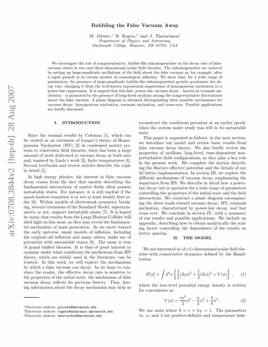
FIG. 1: The tree-level potential V (φ) for α = 0.0, 1.5, 1.6.

pendent. With the rescaling, φ′ = φ√

λ/m, x′µ = xµm,

and α′ = α/(m√

λ), the potential can be written asV (φ) = (m4/λ)V (φ′), with

V (φ′) =φ′2

2− α′ φ

′3

3+

φ′4

8, (3)

while the Hamiltonian in eq. 1 becomes, H [φ] =(m/λ)H [φ′]. Henceforth we will drop the primes. Notethat for α = 0 the model is Z2-symmetric, while forα = 3/2, V (φ) is a symmetric double-well. For α > 3/2the minimum at φ = 0 becomes the false vacuum, andthe true vacuum is at φ+ = α +

√α2 − 2. In figure 1, we

show V (φ) for several values of α.

A. False Vacuum Decay

Although our results could be extended to models atzero temperature and, thus, with false-vacuum decaycontrolled solely by quantum tunneling, we will treathere mostly finite-temperature models. We use a finite-temperature description merely for its convenience in set-ting the properties of the initial state, which we will taketo be a state of thermal equilibrium prepared in the po-tential above with α = 0. But before we describe ourprocedure, it is convenient to briefly review some rele-vant results from HN.

Consider a model with an asymmetric double-well po-tential, such as the one of eq. 3 with α > 3/2. Thefield is initially in thermal equilibrium with only small-amplitude fluctuations about the metastable minimumat φm = 0. One then computes the free energy F =−T lnZ, where Z is the partition function, given bythe path integral

∫

D[φ] exp[−F [φ]/T ]. At finite tem-perature, F [φ] is the Euclidean free-energy functional of

the configuration φ, which may contain temperature andquantum corrections to the tree-level theory defined ineq. 1. To lowest order in perturbation theory, these cor-rections are included in the effective potential. At T = 0,one should use the (d + 1)-dimensional Euclidean effec-tive action S[φ], as opposed to F [φ]/T , in the exponent[3, 4].

The calculation proceeds as follows: first, one identifiesthe stationary points of F [φ], given by the solutions tothe equations of motion. There are two for generic asym-metric double-well potentials, such as the ones in figure1: the false vacuum at φm, and the spherically-symmetricbounce or critical bubble φb(r), found by solving

∂2rφ +

(d − 1)

r∂rφ =

∂V

∂φ, (4)

where d is the number of spatial dimensions. The solu-tion must satisfy the boundary conditions, φb(0) = φ0,∂rφb(0) = 0, and limr→∞ φ(r) = φm. Second, adopt-ing the semi-classical approximation where the path in-tegral is dominated by small fluctuations about the clas-sical paths, one sums over quadratic fluctuations aboutthe stationary points of the free energy using the saddle-point approximation to the Gaussian path integral. Thecalculation is completed by summing over the contribu-tion from many bubbles, which makes use of the “dilutegas” approximation, where the nucleating bubbles are as-sumed to be far enough away from each other so as not tooverlap, being thus treated as independent events. Theend result, the probability per volume per unit time ofnucleating a bubble of “true” vacuum within the falsevacuum background for a system at temperature T is,

Γ ∼ T (d+1) exp[−F [φb]/T ] . (5)

The quotes are a reminder that the nucleating bubblesare not initially at the true vacuum, only close to it(φ0 6= φ+). The sums over bubbles and over quadraticfluctuations about the stationary points give rise to aprefactor which can be roughly approximated by T (d+1)

or, in quantum tunneling, by Md+1, where M is the rel-evant mass scale. Here, we will be mainly interested inthe exponential factor which, in most scenarios, domi-nates the false vacuum decay rate. Summarizing, thecalculation of false vacuum decay in HN relies on twokey assumptions: small (quadratic) fluctuations aboutthe false vacuum and about the critical bubble, and thedilute gas approximation.

B. Thin Wall Approximation

Although the equation describing the critical bubble,eq. 4, does not, in general, have exact solutions, an esti-mate of the energy of a critical bubble can be obtained inthe “thin wall” approximation [1, 5]. Essentially, whenthe potential V (φ) is nearly degenerate, the critical bub-ble will have a spatial extension, or “radius,” (Rb) much

3

larger than the thickness of the wall separating its interiorfrom its exterior, defined as the region where φ changesabruptly from φ0 ≃ φ+ at r = 0 to φm at r → ∞. Thereare thus two main contributions to the free energy (or Eu-clidean action) of the critical bubble: the wall (r ∼ Rb),and the interior of the bubble (r < Rb), where one writesφb(r) = φ+. The approximate expression for the bubbleenergy is,

Etw ≃ CdRd−1

{

σ − R

d|∆V |

}

, (6)

where |∆V | = |V (φ+)−V (φm)|, and Cd = 2πd/2/Γ(d/2)is related to the volume of a d-dimensional sphere of ra-

dius R by Vd = CdRd

d . Also, σ =∫

dr[

12 (φ′

b)2 + V (φb)

]

isthe surface tension. Minimizing with respect to R gives:

Rb =σ(d − 1)

|∆V | , (7)

and the nucleation energy-barrier in the thin wall approx-imation is,

Etw = Cd(d − 1)d−1

d

σd

|∆V |d−1. (8)

Within the thin-wall approximation, the bounce so-lution may be approximately parameterized by φ(r) ≃φ+

2 (1 − tanh(12 (r − Rb))). Using a scaling argument, we

can rewrite the surface tension as σ =∫

dr(∂rφb)2, which

allows us to integrate σ to obtain

σ ≃ limRb≫1

φ2+

3

e2Rb(3 + eRb )

(1 + eRb )3

=φ2

+

3. (9)

The volume contribution from the potential is only afunction of the asymmetry ∆V = 1

2 −α2 − 23α

√α2 − 2+

13 (α4 + α3

√α2 − 2). It is convenient to write α ≃

3/2 + δα, where δα ≪ 1 in the thin wall approxima-tion. Then, expanding the expressions for the energy, eq.8, and the radius, eq. 7, about δα = 0, we can obtainapproximate analytical expressions for both as follows:

Etw ≈ Cd

3

(d − 1)d−1

22d−3d

(

1

δαd−1+

d + 3

δαd−2

)

+ O(δα3−d),

(10)

Rb ≈d − 1

4

(

1

δα+ 1 − 7δα

)

. (11)

Although these expressions breakdown quite quickly asδα increases, they provide the dominant scaling of energyand radius with the coupling α.

C. Oscillons: A Brief Review

Alongside with the critical bubble or bounce, oscillonswill play a key role in the mechanism for fast vacuumdecay. In fact, the title of this work alludes to theirpresence in the metastable minimum and their effect onthe decay rate. As such, it is useful to briefly reviewtheir properties. In their simplest form, oscillons arespatially-extended, very long-lived, time-dependent so-lutions of the nonlinear Klein-Gordon equation [9], orof other PDEs with amplitude-dependent nonlinearities[10]. Their properties have been extensively studied dur-ing the past decade in two [11], three [12], and higher [13]spatial dimensions, and, more recently, in U(1) Abelian-Higgs models [14] and in SU(2)xU(1) models [15]. How-ever, it is fair to say that a more fundamental under-standing of their existence and longevity is still lacking.

In the context of relativistic scalar field models, os-cillons are characterized by large-amplitude oscillationsabout the vacuum state. Assuming spherical symmetry,it has been shown [13] that they only exist if these fluc-tuations probe beyond the inflection point [φinf ] of V (φ),although they may be more general [16]. The reader mayconsult the references cited for more details.

Scalar field oscillons have been found by two meth-ods. The first, and simpler, method makes use of aninitial condition φ(0, r) that resembles the oscillon solu-tion, for example, φ(0, r) = φ0 exp[−r2/R2], for V (φ) ofeq. 3. For values of R ≥ Rmin, and φ0 > φinf , the fieldwill evolve into the oscillon configuration, where it willremain for a lifetime that is sensitive to the values ofφ0, Rmin, and d. Rmin can be estimated analytically fordegenerate and non-degenerate polynomial potentials foran arbitrary number of spatial dimensions [13].

The second method, more general, shows that oscil-lons emerge, under very general conditions, when large-amplitude fluctuations about a given vacuum state withsufficient thermal (or quantum noise) are present. In thecontext of 2d models, Gleiser and Howell showed thatthey emerge after a quench from a single-well to a double-well potential [17]. In the model of eq. 3 this wouldcorrespond to a change from α = 0 to α = 1.5.

Inspecting figure 1, one can see qualitatively that thequench induces coherent oscillations of the field’s zeromode, φ(t) ≡ (1/V )

∫

ddxφ(x, t) about the metastableminimum at φ = 0 due to a “widening” of the potentialthere. Other mechanisms may induce large-amplitudeoscillations of the zero-mode, producing similar results.This happens, for example, in the context of reheatingin certain models of cosmological inflation [18, 19]. An-other possibility is a symmetry-breaking interaction thatchanges the shape of the potential from single to double-well, as in the case of the quench above, or one thatsimply “widens” the curvature of the potential about thevacuum. Quantitatively, the energy from these coherentoscillations is transfered to higher k modes via paramet-ric amplification and trigger the emergence of oscillons.We refer the reader to reference [17] for details. Not

4

FIG. 2: The volume-averaged field, or order parameter,〈φ(t)〉 ≡ φ(t) which corresponds to fig.3.

surprisingly, the same behavior ensues in 3d: a quenchinduces oscillations of the field’s zero mode, as can beseen in figure 2. The results were obtained in a cubiclattice of volume L3 = 643 with periodic boundary con-ditions, lattice spacing dx = 0.5, and α changed fromα = 0 to α = 1.5. The initial thermal state was preparedat T = 0.29.

In figure 3, we show snapshots of the field, display-ing the appearance of bubble-like oscillons. Shown arethe isosurfaces at φ = {0.75(blue), 1.0(red), 1.5(green)}[colors online only]. The long-lived, localized oscillationswhich emerge in synchrony are the oscillon configura-tions.

D. The Hartree Potential and Lattice

Implementation

As mentioned above, the initial state is prepared asa thermal state centered at φ = 0 in the potential ofeq. 3 with α = 0. The thermal fluctuations will inducechanges in the potential for φ, which, in leading orderin perturbation theory, may be approximated by the Ho-mogeneous Hartree Approximation (HHA). An excellentaccount of the HHA, using successive truncations withinthe hierarchy of correlation functions to obtain correctedequations of motion, can be found in ref. [20].

The HHA assumes that the fluctuations of the field andits associated momentum remain Gaussian throughoutits evolution. Thus, the approximation works well justprior and just after the quench for all temperatures, andfor low temperatures at all times. The Hartree potentialcan be derived as follows: write the field as φ = φ + δφ.Then, VH(φ) = 〈V (φ + δφ)〉, where 〈〉 means an averageover all fluctuations δφ, with 〈δφ〉 = 0 and 〈δφ2〉 ≡ β.

〈δφ2〉 is the translationally-invariant mean-square vari-ance of the field, which, in thermal equilibrium (the ini-tial state), is constant and proportional to T . We thenobtain (suppressing the bar),

VH(φ) = −αβφ +

(

1 +3

2β

)

φ2

2− α

φ3

3+

φ4

8. (12)

In thermal equilibrium, the momentum and fieldmodes in k-space satisfy

〈|π(k)|2〉 = T ; (13)

〈|φ(k)|2〉 =T

k2 + m2H

, (14)

where the Hartree mass is defined as m2H = V ′′

H(0).Due to the dependence of 〈|φ(k)|2〉 on the wave num-

ber k, a lattice implementation of the field theory willintroduce a lattice spacing (δx) dependence [21]. Wethus write, for an UV cutoff Λ, β ≡ a#dT , where theconstant a#d, which changes in different spatial dimen-sions, can be obtained numerically by comparing the lat-tice results with eq. 14. It can also be obtained ana-lytically, as shown in the Appendix. For example, forδx = 0.2, we obtain, through this method, a2d = 0.518and a3d = 1.194, in two and three spatial dimensions,respectively. These values agree very well with the nu-merical estimate. (See Appendix for details.)

In figure 4, we plot on the left the ensemble-averaged two-point correlation functions for the field(green squares, bottom) and its related momentum (bluesquares, top). The black lines are the analytical formu-las of eq. 14. On the right, we take the logarithm ofthe initial data set for the two-point correlation functionfor the field (green squares and black line), and com-pare to its value during the simulation. The red squaresare the data at every half-second for the time interval360 < t < 400, when φ(t) is well settled in the potentialminimum (check figure 2). The blue squares correspondto the same data, but after applying a thermal filter.One can clearly distinguish two populations of modes:low-k, oscillon-related modes far from equilibrium (fork <∼ 1.5), and modes that remain in thermal equilibriumfor all times (k >∼ 1.5).

Introducing β allows us to relate models with differenttemperatures and lattice spacings with a single parame-ter. From now on, we will refer to β as the effective lattice

temperature. In figure 5, we plot VH(φ) for various valuesof β and α = 1.6. The interpretation of β as an effectivetemperature should be apparent.

The initial state was prepared by thermalizing the fieldusing standard Langevin techniques [22]

φ + γφ −∇2φ = −∂V/∂φ + ζ (15)

where ζ is a Markovian noise with two-point correlationfunction obeying the fluctuation-dissipation relation,

〈ζ(x, t)ζ(x′, t′)〉 = 2γT δ(x− x′)δ(t − t′) . (16)

5

FIG. 3: Snapshots of a 3d scalar field simulation after a quench from a single to a symmetric double well potential (α = 0 → 1.5).The oscillatory bubble-like configurations which emerge in synchrony are identified as oscillons. The lattice parameters weredx = 0.5, T = 0.29 and L3 = 643. Plotted is the φ = {0.75, 1.0, 1.5} isosurfaces in blue, red and green, respectively. Theplots are snapshots at t = {45.5, 51.5, 54.5, 60.5, 62.0, 194.5}, respectively, increasing left to right and top to bottom. Notethat oscillons can be tracked over a period of oscillation as they reappear in approximately the same place about ∼ 9s later.For example, the top right corner of the first, second, fourth and fifth slices show the same oscillon. The last snapshot showsoscillons still present at late times. They eventually disappear as thermal equilibrium is restored.

The initial state is solely determined by the tempera-ture of the bath T . Note that this thermalization is sim-ply a device to set an initial distribution for the fieldmodes satisfying eq. 14 . One could have used alterna-tive T -independent methods to set up initial conditions.Ours is in tune with the more conventional statementthat vacuum decay initiates from a metastable thermalstate. This initial thermalization was verified by com-pliance with equipartition, such that the average kineticenergy of each mode was T/2.

We used a standard leapfrog algorithm [23] on cubiclattices with volume V = L3 = (256 ∗ dx)3 with periodicboundary conditions. We verified that our results do notshow any relevant dependence on L. The lattice wasevolved in time-steps of δt = 0.025. We checked that theHamiltonian evolution conserves energy to O(δt2).

III. POWER-LAW VACUUM DECAY

Within the framework of HN, the nucleation energybarrier can be calculated numerically by integrating theequation:

∂2rφ +

(d − 1)

r∂rφ = ∂φVH(φ, T ). (17)

In figure 6, we plot the energy barrier Eb(α, β) as a func-tion of asymmetry α for several values of β for d = 3. Forreference, we also included the Euclidean bounce actionfor quantum decay at T = 0. It is apparent that thedifferent curves are related by a β-dependent scaling,

Eb(α, β) ≃ Eb(α, 0)A(β), (18)

where we found that A(β) = (1 − cαβ)2, with c = 2.75giving the best fit. In order to test this approximation, infigure 7 we plot the ratio Eb(α, β)/ [Eb(α, 0)A(β)]. It is

6

FIG. 4: The radially-averaged 2-point field and momentum correlation functions. On the left, we show the results for thethermal initial conditions. The black continuous lines correspond to 〈|π(k)|2〉 = T (δx)−3 (top) and to 〈|φ(k)|2〉 = Tδx−3/{k2 +

m2

H} + c0

√k (bottom). (The small constant c0 = 0.024 used to fit the analytic prediction with the lattice results is due to the

abrupt lattice cutoff introduced by δx.) The blue and green squares are from the simulation. On the right, we plot the logarithmof the two-point correlation function for the field. The black line and green squares correspond to the thermal initial state ploton the left. The red squares are the data plotted at every half second for the time interval 360 < t < 400. The blue squaresare also the data, after applying a thermal filter. One clearly distinguishes two populations of modes: the oscillon-related, lowk modes (k <∼ 1.5), which sharply depart from the thermal spectrum, and the purely thermal modes, which remain in thermalequilibrium throughout the simulation (k >∼ 1.5). These figures were generated using the data from the same run as in fig.3.

FIG. 5: Hartree potential for α = 1.6 and several values ofβ = 0, 0.1, 0.2, 0.4, 0.75.

clear that the scaling holds to within 10% for the rangeof parameters where resonant nucleation ensues. Thescaling allows us to relate the finite-temperature bounceaction computed with the Hartree approximation of eq.12 with the tree-level bounce action computed with eq.3.

FIG. 6: The logarithmic energy of a 3d bounce or criticalbubble, ln[Eb(α, β)], for β = {0.0, 0.025, 0.05, 0.10, 0.125} asa function of α. There is a clear scaling with β that worsensas β is increased. For β = 0, the bounce “energy” is the d = 4Euclidean action.

7

FIG. 7: Testing the scaling of the bounce energy with β: weplot the ratio Eb(α, β)/ [Eb(α, 0)A(β)] versus α for variousvalues of β. The scaling holds well (dashed lines denote 10%accuracy) and worsens as β increases.

A. Computing the Exponent in Resonant

Nucleation

According to HN theory, the decay rate is given by eq.5. Is this also true after an abrupt change in the potentialV (φ) – promoted either by a quench, a new interaction,or by a coupling to another field that induces oscillationson φ(t), as in certain inflationary models [18, 19]? In ref.[24] (GH), it was found that, in 2d, changes that inducelarge-amplitude fluctuations of the field’s zero mode maydrastically alter the decay rate from an exponential toa power law for a range of asymmetries (α) and tem-peratures (T ). In GH, it was argued that the decay istriggered by the resonant nucleation of oscillons, whichmay coalesce to form a critical bubble or that simplybecome unstable and grow to become a critical bubblethemselves. This mechanism was dubbed resonant nucle-

ation (RN), and was found to lead to a power-law decayper unit area

Γ ∼ T 3 (Eb/T )−B

, (19)

with B ≃ 2.464±0.134 for the range of parameters whereRN is operative. In figure 8 we display our results for theexponent B in d = 2. The lattice spacing was δx = 0.2,and the lattice size 20482. Results were averaged over10 runs. Errors were smaller than boxes.[Note that thisvalue of B and the error bars are smaller than thosequoted in [24]. Also, we found that B is only weakly de-pendent on β. This discrepancy is due to better statisticsand to a more precise method of distinguishing betweenRN and cross-over transitions, to be explained below.]

In order to test if a power-law behavior holds in 3d,we repeated the GH procedure for different values of the

FIG. 8: The value of the decay power B as a function of β intwo dimensions.

FIG. 9: The volume-averaged field, or order parameter, φ(t)for α = 1.589 → 1.78 for β = 0.085. [Results are better seenin color.]

asymmetry α and the lattice temperature parameter β.The field is initially prepared in a thermal state in asingle well (α = 0). The potential is then changed toan asymmetric double well, by setting α > 3/2. Thesubsequent dynamics of the field is conservative, that is,we set γ = 0 in eq. 15. We then measured the volume-averaged value of the field, φ(t). Results for β = 0.085and several values of the asymmetry α are shown in figure9.

One can easily see that, for values of α close to degener-acy (towards the right of the figure), φ(t) performs manydamped oscillations about the metastable minimum of

8

VH(φ) before irreversibly transitioning to the global min-imum. For clarity, we cut off the plot before the decaycompletes. As the asymmetry is increased (towards theleft of the figure), the number of oscillations decreases un-til the transition completes by cross-over, that is, withina time-scale which is shorter than a typical oscillationperiod. [More on this soon.]

Adopting as the decay time-scale (τ) the time at whichφ(t) crosses the maximum of VH(φ), we can plot the loga-rithm of decay times as a function of the logarithm of thebounce energy (Eb/β), where Eb is computed from thesolution of eq. 17 for a given pair (α, β). The results areensemble-averaged over 50 runs, and displayed as indi-vidual points (diamonds) in the left plot of figure 10. Onthe right side, we plot the logarithm of (Eb/β3) to showthe simple scaling with β. For reference, if δx = 0.25,the value we adopted in our simulations, the tempera-ture would be in the range 0.09 ≤ T ≤ 0.14. [To getthe value of the temperature, use that T = β/a3d. An-alytically, a3d = 0.955 (see Appendix), and numericallya3d = 0.933, an error of only 2.4%.] The slopes of thestraight-line fits are the numerical values for the decaypower B.

Note that we are not including decay times smallerthan τ ≃ 22. Times shorter than this are characteristicof a cross-over transition and would not fall under reso-nant nucleation. This can be made clear by investigatinghow we extracted the slopes of the log-log plot, that is,the constant B controlling resonant nucleation. As anillustration, fixing β = 0.0954, consider the results forthe decay times displayed in figure 11. From the data, itis clear that there is a sharp departure from a straight-line fit below ln(τ) ≃ 3.2. This happens consistently forall parameters we investigated, offering a natural cutoffbelow which the transition occurs via cross-over.

In figure 12, we show our results for the power B con-trolling resonant decay. We have included two data sets:the squares are the results obtained using the Hartreeeffective potential to compute the bounce action and toread off the nucleation time-scale (which depends on thelocation of the maximum). The circles are the resultsobtained using the tree-level potential. It is clear thatfor VH(φ), B is fairly independent of β within the rangewhere resonant nucleation applies. The average value isB = 1.327 ± 0.059. The values agree well for β > 0.09.For smaller β, it is necessary to increase the value of αto probe into the resonance nucleation regime, leading tolarger errors in the tree-level estimates.

We also verified that the value of B is not very sensitiveto changes in lattice spacing. As an illustration, let uschoose δx = 1. For T = 0.55, which gives β = 0.131, werepeated the numerical experiments to obtain B ≃ 1.68.By adjusting T , this value can, for example, be comparedwith the one obtained with lattice spacing δx = 0.25 forthe same β = 0.131, which we measured to be B = 1.47.This is a change of only 13% in B for a factor 4 change inlattice spacing. As a second illustration, we compared theresults for δx = 0.35 and T = 0.175, for which β = 0.119,

with δx = 0.25, at same β. The values for the power-lawdecay were B = 1.458 and B = 1.353 respectively, a 7%difference. Within the accuracy of our simulations, weconclude that B is very weakly dependent on δx and,most importantly, on β.

B. Phase Diagram for Vacuum Decay

We summarize our results in a phase diagram display-ing the three possible mechanics for false vacuum decayas a function of the parameters controlling the asymme-try of the potential (α) and the temperature of the ini-tial metastable state (β). Homogeneous nucleation (darkblue region labeled as HN) describes vacuum decay forlow enough temperatures for all values of asymmetries.

Resonant nucleation (RN) falls within the regionbracketed by the two left to right curves (light blue re-gion labeled as RN). The diamonds and circles are theresults of the simulations. The circles, being close to thecross-over region (τ ∼ 25), were not used to compute thedecay power B. The curves bracketing RN from above(cross over, purple region) and below (HN region) wereobtained by using the average value of the field, φ(t), asa guideline: a field well-localized within the false vacuum(φ(t) ≪ φinf) will only decay via HN; a field for whichφ(t) ≫ φinf will easily cross over. RN lies in between.Noting that the amplitude of thermal fluctuations aboutφ(t) is given by |

√

〈δφ2〉| = |√

β/2|, we obtain the con-dition,

VH(φinf ±√

β/2) = 0. (20)

This condition translates into a relation between α and βthat generates the two curves bracketing the RN regionhorizontally.

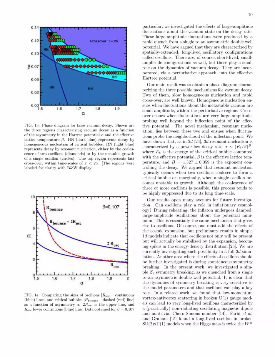
The steeper line to the left is obtained by examiningthe dynamics of resonant nucleation. As noted in ref.[24], in the region near degeneracy, where the criticalbounce is large, RN will occur due to the coalescence oftwo or more oscillons. In figure 14, we compare the ra-dius of a bounce with that of oscillons as a function of αfor β = 0.107. There are three distinct regions: For largeα >∼ 1.7, the bounce and oscillon practically match. Thisregion is typical of quick cross-overs or at most border-line RN, where a single oscillon becomes unstable, grows,and becomes critical. In the intermediate region, where1.56 <∼ α <∼ 1.7, Rbounce < 2Rosc: here, two oscillons maycoalesce to form a critical bubble. This is the region typi-cal of RN. Lastly, for α < 1.56, Rbounce > 2Rosc and morethan two oscillons are needed to produce a critical bub-ble, a process that, although not impossible, is stronglysuppressed in the allowed time scales where RN can act,that is, while oscillons are present in the system, typicallywhile ∂tφ(t) 6= 0. In this region, HN is the favored decayroute. The steeper line in the phase diagram is thus ob-tained by tracing the points where Rbounce = 2Rosc foreach β, in excellent agreement with the simulations: RN,denoted by the diamonds, ends on this line.

9

FIG. 10: Decay time-scales in 3d: we plot ln(τ ) vs. ln(Eb/β) [left], and ln(Eb/β3) [right]. From top to bottom on the leftfigure, β = {0.084, 0.095, 0.101, 0.107, 0.119, 0.131}.

FIG. 11: Extracting the decay exponent B: shown are theraw data points for the decay time ln τ vs. (ln Eb/β) withβ = 0.0954. We ran 50 experiments for each value of α (or,equivalently, of Eb). In this illustration, we used the tree-levelpotential of eq. 3 to compute Eb. The straight-line slope fitgives B = 1.473. Note the clear departure from a straight-line fit for ln τ <∼ 3.2. We characterize time-scales faster thanthose as typical of cross-over transitions.

In figure 15, we show the coalescence of oscillons lead-ing to a critical bubble that grows to complete the vac-uum decay. This figure should be contrasted with fig-ure 3 for a symmetric double-well potential. The regionsdisplayed are isosurfaces at φ = {0.9, 1.75, 1.85} whichare colored blue, red, and green, respectively. We usedα = 1.545 and β = 0.134. In figure 16 we show the cor-

FIG. 12: Results for the decay power B. Slopes as measuredindividually, as in figure 11. The circles are calculated withthe tree-level potential and the squares with the Hartree effec-tive potential. Error bars from ensemble-averaging fit withinthe sizes of the squares and circles.

responding evolution of the volume-averaged field, φ(t).The arrows denote the locations of the isocurvatures de-picted in figure 15.

IV. SUMMARY AND OUTLOOK

We have presented a detailed numerical study of thedecay of metastable vacua in scalar field theories. In

10

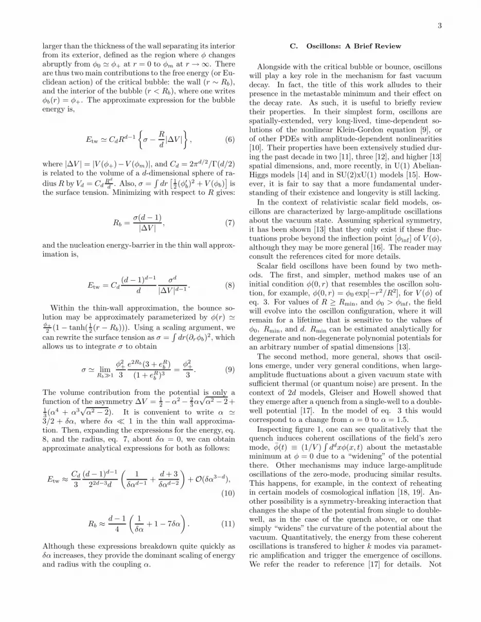
FIG. 13: Phase diagram for false vacuum decay. Shown arethe three regions characterizing vacuum decay as a functionof the asymmetry in the Hartree potential α and the effectivelattice temperature β. HN (dark blue) represents decay byhomogeneous nucleation of critical bubbles. RN (light blue)represents decay by resonant nucleation, either by the coales-cence of two oscillons (diamonds) or by the unstable growthof a single oscillon (circles). The top region represents fastcross-over, within time-scales of τ < 25. [The regions werelabeled for clarity with B&W display.

FIG. 14: Comparing the sizes of oscillons [Rosc – continuous(blue) lines] and critical bubbles [Rbounce – dashed (red) line]as a function of asymmetry α: 2Rosc is the upper line, andRosc lower continuous (blue) line. Data obtained for β = 0.107.

particular, we investigated the effects of large-amplitudefluctuations about the vacuum state on the decay rate.These large-amplitude fluctuations were produced by arapid quench from a single to an asymmetric double wellpotential. We have argued that they are characterized byspatially-extended, long-lived oscillatory configurationscalled oscillons. There are, of course, short-lived, small-amplitude configurations as well, but those play a smallrole on the dynamics of vacuum decay. They are incor-porated, via a perturbative approach, into the effectiveHartree potential.

Our main result was to obtain a phase diagram charac-terizing the three possible mechanisms for vacuum decay.Two of them, slow homogeneous nucleation and rapidcross-over, are well known. Homogeneous nucleation en-sues when fluctuations about the metastable vacuum aresmall-amplitude, within the perturbative regime. Cross-over ensues when fluctuations are very large-amplitude,probing well beyond the inflection point of the effec-tive potential. The novel mechanism, resonant nucle-ation, lies between these two and ensues when fluctua-tions probe the neighborhood of the inflection point. Wehave shown that, as in 2d [24], 3d resonant nucleation ischaracterized by a power-law decay rate, τ ∼ (Eb/β)B,where Eb is the energy of the critical bubble computedwith the effective potential, β is the effective lattice tem-perature, and B = 1.327 ± 0.059 is the exponent con-trolling the decay. We argued that resonant nucleationtypically occurs when two oscillons coalesce to form acritical bubble or, marginally, when a single oscillon be-comes unstable to growth. Although the coalescence ofthree or more oscillons is possible, this process tends tobe highly suppressed due to its long time-scale.

Our results open many avenues for future investiga-tion. Can oscillons play a role in inflationary cosmol-ogy? During reheating, the inflaton undergoes damped,large-amplitude oscillations about the potential mini-mum. This is essentially the same mechanism that givesrise to oscillons. Of course, one must add the effects ofthe cosmic expansion, but preliminary results in simple1d models indicate that oscillons not only will be presentbut will actually be stabilized by the expansion, becom-ing spikes in the energy-density distribution [25]. We arecurrently investigating such possibility in a full 3d simu-lation. Another area where the effects of oscillons shouldbe further investigated is during spontaneous symmetrybreaking. In the present work, we investigated a sim-ple Z2 symmetry breaking, as we quenched from a singleto an asymmetric double well potential. It is clear thatthe dynamics of symmetry breaking is very sensitive tothe model parameters and that oscillons can play a keyrole. In a related work, we found that low-momentumvortex-antivortex scattering in broken U(1) gauge mod-els can lead to very long-lived oscillons characterized bya (practically) non-radiating oscillating magnetic dipoleand nontrivial Chern-Simons number [14]. Farhi et al.

and Graham [15] found a long-lived oscillon in brokenSU(2)xU(1) models when the Higgs mass is twice the W±

11

FIG. 15: Snapshots of a 3d scalar field simulation after a quench from a single to an asymmetric double well potential (α = 1.545,T = 0.28, dx = 0.5, β = 0.134). The oscillons coalesce to become a critical bubble that grows to complete the vacuum decay.The slices are at times t = {27.0, 38.0, 45.5, 54.5, 71.0, 79.5}. The blue, red and green isosurfaces are at φ = {0.9, 1.75, 1.85},respectively. The average value of the field along with the respective isosurface locations are also noted on fig.16.

mass. If this turns out to be the right mass ratio, as hope-fully we will soon know from the LHC, we should expectelectroweak oscillons to exist in Nature. Alternatively,they may exist even for a wider range of values. Takentogether, these results demonstrate the rich physics oftime-dependent, spatially-extended field configurations.This richness is only beginning to be explored.

Acknowledgments

MG and JT were partially supported by a National Sci-ence Foundation grant PHY-0653341. We also would liketo thank the Discovery parallel network at Dartmouth foraccess to their facilities and the NCSA Teragrid clusterfor access under grant number PHY-070021. We wouldalso like to thank Massimo di Pierro for help getting ourparallel codes running with FERMIQCD [26].

V. APPENDIX: ANALYTICAL ESTIMATE OF

EFFECTIVE LATTICE TEMPERATURE

Consider the simple case of a quadratic potentialV0 = 1

2φ2, for which the Hartree potential is simple

VH = 12φ2 + 1

2β. Consider also the 1-loop potential withUV cutoff Λ,

V1L(φ) = V0 +T

2

∫ Λ

0

ddp

(2π)dln

(

p2 + V ′′0

)

. (21)

In d = 2 the integral gives,

V1L(φ) = V0 +T

8πV ′′

0

{

1 − ln

(

V ′′0

Λ2

)}

, (22)

while in d = 3 we obtain

V1L(φ) = V0 +T

12π2

{

3V ′′0 Λ − π(V ′′

0 )3/2}

. (23)

Focusing on the simple quadratic potential, for whichV ′′

0 = 1, we now match the cutoff-dependent term of V1L

12

FIG. 16: The volume-averaged field, or order parameter,〈φ(t)〉 ≡ φ(t) for α = 1.545 for β = 0.1385. The coloredarrows label the locations of the isosurfaces depicted in figure15.

(multiplied by d/2) with the β-dependent term of VH (eq.12) to obtain,

β =T

4π

(

1 + ln

(

π2

δx2

))

≡ a2dT, [2d] (24)

and

β =3T

4πδx≡ a3dT, [3d] (25)

where we used Λ = π/(δx) and introduced, for conve-nience, the lattice-dependent constant a#d. For example,for δx = 0.2, a2d = 0.518 and a3d = 1.194. This valueagrees very well with the numerical estimate, obtainedby comparison with eq. 14.

After comparing terms, one can write a#d most gener-ally as

a#d∼d

2

∫ Λ

0

ddp

(2πd)ln(1 + p−2) (26)

where ∼ implies take the first term of the Taylor seriesexpansion of the integral should be a#d. In the Tablebelow, we compare the numerical and analytical (eqn.26) measurements of a#d in different dimensions.

a#d analytical numerical lattice size

a1d 0.5 0.5 ± 0.001 106

a2d 0.518 0.53 ± 0.005 10242

a3d 1.194 1.19 ± 0.005 1003

a4d 3.125 3.84 ± 0.005 324

With this simple analytical method, it is possible torelate the initial state temperature T to the effective

lattice temperature β for any choice of lattice spacing.

[1] S. Coleman, Phys. Rev. D15, 2929 (1977); C. Callan andS. Coleman, Phys. Rev. D16, 1762 (1977).

[2] J. S. Langer, Ann. Phys. (NY) 41, 108 (1967); ibid. 54,258 (1969).

[3] A. Linde, Nucl. Phys. B216, 421 (1983); [Erratum:B223, 544 (1983)].

[4] Here is an incomplete list of references: M. Stone, Phys.Rev. D 14 (1976) 3568; Phys. Lett. B 67 (1977) 186; M.Alford and M. Gleiser, Phys. Rev. D 48, 2838 (1993); J.Baacke and V. Kiselev, Phys. Rev. D 48, 5648 (1993); H.Kleinert and I. Mustapic, Int. J. Mod. Phys. A11 (1996)4383, and references therein; A. Strumia and N. Tetradis,Nucl. Phys. B 554, 697 (1999); ibid. 560, 482 (2000); Sz.Borsanyi et al., Phys. Rev. D 62, 085013-1 (2000). Y.Bergner and Luis M. A. Bettencourt, Phys. Rev. D 69

(2004) 045012.[5] J. D. Gunton, M. San Miguel, and P. S. Sahni, in Phase

Transitions and Critical Phenomena, Ed. C. Domb andJ. L. Lebowitz, v. 8 (Academic Press, London, 1983); J.D. Gunton, J. Stat. Phys. 95, 903 (1999); J. S. Langer,in Solids Far from Equilibrium, Ed. C. Godreche (Cam-bridge University Press, Cambridge, 1992).

[6] See, for example, F. Karsch, hep-ph/0701210 and refer-

ences therein; M. Cheng et al. Phys. Rev. D 75, 034506(2007).

[7] See, e.g., S. Huber, T. Konstandin, T. Prokopec, and M.G. Schmidt, Nucl. Phys. B757, 172 (2006); J. Kang, P.Langacker, T. Li, and T. Liu, Phys. Rev. Lett. 94, 061801(2005); M. Gleiser and M. Trodden, Phys. Lett. B 517,7 (2001).

[8] For a recent review and references see, B. A. Bassett,S. Tsujikawa, and D. Wands, Rev. Mod. Phys. 78, 537(2006); A. H. Guth, Phys. Rev. D 23, 347 (1981); A. D.Linde, Phys. Rev. D 49, 748 (1994); M. Gleiser, Int. J.Mod. Phys. D 16, 219 (2007).

[9] M. Gleiser, Phys. Rev. D 49, 2978 (1994); I. L. Bogol-ubsky and V. G. Makhankov, JETP Lett. 24 (1976) 12[Pis’ma Zh. Eksp. Teor. Fiz. 24 (1976) 15].

[10] D. Bettison and G. Rowlands, Phys. Rev. E 55, 5427(1997); C. Crawford and H. Riecke, Phys. Rev. E 65,066307 (2002); S. Aranson, Phys. Rev. Lett. 79, 213(1997); S.-O. Jeong and H.-T. Moon, Phys. Rev. E 59,850 (1999); O. M. Umurhan, L. Tao, and E. A. Spiegel,Ann. N. Y. Acad. Sci. 867, 298 (1998).

[11] M. Gleiser and A. Sornborger, Phys. Rev. E 62, 1368(2000); A. Adib, M. Gleiser, and C. Almeida, Phys. Rev.

13

D 66, 085011 (2002); M. Hindmarsh and P. Salmi, Phys.Rev. D 74, 105005 (2006).

[12] E. J. Copeland, M. Gleiser and H.-R. Muller, Phys. Rev.D 52, 1920 (1995); E. Honda and M. Choptuik, Phys.Rev. D 68, 084037 (2002); G. Fodor, P. Forgacs, P.Grandclement, and I. Racz, Phys. Rev. D 74, 124003(2006).

[13] M. Gleiser, Phys. Lett. B 600, 126 (2004); P. M. Saffinand A. Tranberg, J. High Energy Phys. 01, 030 (2007).

[14] M. Gleiser and J. Thorarinson, Phys. Rev. D 76,041701(R) (2007).

[15] E. Farhi, N. Graham, V. Khmeani, R. Markov, and R.Rosales, Phys. Rev. D 72, 101701 (2005); N. Graham,Phys. Rev. Lett. 98, 101801 (2007), [Erratum-ibid. 98,189904 (2007)]

[16] E. Farhi, N. Graham, A. Guth, and R. Rosales, privatecommunication.

[17] M. Gleiser and R. Howell, Phys. Rev. E 68, 065203(R)(2003).

[18] A. D. Linde, Phys. Rev. D 49, 748 (1994); A. Car-doso, Phys. Rev. D 75, 027302 (2007); R. Battye, B.Garbrecht, and A. Moss, J. Cos. Astrop. Phys, 609, 7(2006); M. Kawasaki, T. Takayama, M. Yamaguchi, and

J. Yokoyama, Phys. Rev. D 74, 043525 (2006).[19] M. Gleiser, Int. J. Mod. Phys. D 16, 219 (2007).[20] G. Aarts, G. F. Bonini, and C. Wetterich, Phys. Rev.

D 63, 025012 (2000); G. Aarts, G. F. Bonini, and C.Wetterich, Nucl. Phys. B 587, 403 (2000).

[21] J. Smit, Introduction to Quantum Fields on a Lattice,(Cambridge University Press; Cambridge, UK, 2001).

[22] M. Le Bellac, Thermal field Theory, Cambridge Mono-graphs on Mathematical Physics (Cambridge UniversityPress, Cambridge, UK, 1996); R. Zwanzig, Nonequilib-

rium Statistical Mechanics (Oxford University Press, Ox-ford, UK, 2001).

[23] W. Press, S. Teukolsky, W. Vetterling, and B. Flannery,Numerical Recipes in C, (Cambridge University Press,Cambridge UK, 1992).

[24] M. Gleiser and R. Howell, Phys. Rev. Lett. 94, 151601(2005).

[25] N. Graham, N. Stamatopoulos, Phys. Lett. B 639, 541(2006).[26]

[26] M. Di Pierro et al. [FermiQCD Collaboration], Nucl.Phys. Proc. Suppl. 129, 832 (2004).