Embed Size (px)
Citation preview
birds are in our nature
Birds in the Great Western Woodlands
AUSTRALIA
ii | BIRDS IN THE GREAT WESTERN WOODLANDS
Report produced by:
BirdLife Australia Suite 2-05 60 Leicester Street Carlton VIC 3053
Phone (03) 9347 0757
Website www.birdlife.org.au
Recommended citation:
Fox, E., McNee, S., Douglas, T. (2016) Birds of the Great Western Woodlands. Report for The Nature Conservancy. BirdLife Australia, Melbourne.
Acknowledgements
The Birds in the Great Western Woodlands project is a joint project between BirdLife Australia and The Nature Conservancy, made possible through the generous support of the David Thomas Challenge and BirdLife Australia major donors: Richard Bomford, Graham Goulder, Christopher Grubb, Katie Holmes, John McRae, Ruth Pallett, Sue Robertson and Margaret Ross.
This project would not have been successful without the generous time and commitment gifted to the project by numerous volunteers.
Bird survey volunteers donated their time, knowledge, enthusiasm and resources to the project to undertake field surveys. Many thanks to: Sue Abbotts, Christine Allbury, Logan Anderson, John Baas, David Ballard, Joyce Ballard, Judy Barfett, Jeff Barnes, John Barton, Rebecca Barton, Paul Billot, Jan Binder, Simon Binder, Mark Binns, John Blyth, Judy Blyth, Lesley Brooker, Michael Brooker, Linda Brotherton, Joe Bryant, Russell Cannings, Vickie Cartledge, Tomaz Cezimbra, Roger Charles, Sue Charles, Jane Colbert, Laura Corbett, Scott Corbett, Kerry Cowie, Roger Crabtree, Judi Cullam, John Delaporte, Tony Docherty, Erik Donnachie, Andre Du Plessis, Judy Du Plessis, Ray Flanagan, Stewart Ford, David Free, Pam Free, Claire Gerrish, Simon Girando, Cheryl Gole, Martin Gole, Alison Goundrey, John Graff, Bruce Greatwich, Aina Hargans, Graeme Hargans, Ken Harris, Vivien Harris, Judith Harvey, Robina Haynes, Colin Heap, Jen Heap, Sarah Hedges, Joyce Hegney, Barry Heinrich, Mark Henryon, Andrew Hobbs, Jill Hobbs, Sally Hoedemaker, Brian Hooper, Laurel Hooper, Neil Humphris, Nigel Jackett, Darryl James, Rosemary Jasper, Virginia Jealous, Bill Johnson, Graham Johnson, Ruby Johnson, Rhys Jones, Digby Knapp, Brad Kneebone, Henny Knight, Martin Knight, Nola Kunnen, Vicki Laurie, Maris Lauva, David Lehman, Kay Lehman, Jacob Loughridge, Karen Major, Barbara Manson, Rob Mather, Sue Mather, Lesley Macauley, Cheryl McCallum, Roger McCallum, Andrew McCreery, Libby McGill, John McMullan, Wayne Merritt, Saul Montgomery, Simon Montgomery, Robert Morales, Alex Morrison, June Morrison, Jenny Moulton, Kaye Murray, Clive Napier, Wendy Napier, Greg Neill, Brenda Newbey, Wayne O’Sullivan, Alyson Paull, Ed Paull, John Peck, Peter Pittendrigh, Joe Porter, Gail Powell, Terry Powell, Jon Pridham, Mo Ramsay, John Rees, Martin Reeve, Dianne Reidy, Chris Reidy, Allan Rose, Sandy Rose, Laura Ruykys, Tim Sargent, Harriet Sawer, George Shevtsov, Barry Smith, Judi Smith, Rod Smith, Nathaniel Staniford, Alan Stewart, Eliza Stewart, Stella Stewart-Wynne, Nigel Sutherland, Rory Swiderski, Anne Taylor, Dave Taylor, Greg Taylor, Lorraine Todd, Carol Trethowen, John Tucker, Joe van Vlijmen, Jan Waterman, Ron Waterman, Alan Watson, Bryce Wells, Eric Wheatley, Herbie Whittall, Mary Whittall, Peter White, Christine Wilder, Gillian Williams and Boyd Wykes.
Many thanks to the Goldfields Naturalists’ Club, Kalgoorlie-Boulder Urban Landcare Group and BirdLife Esperance who ran bird walks in the Great Western Woodlands and submitted survey data.
Cover photo: Rufous Treecreeper by Chris Tzaros
BIRDS IN THE GREAT WESTERN WOODLANDS | iii
In particular, thanks go to Ramon Andinach, David Gleeson, Dale Johnston, Janette Kavanagh, and Kim Eckert.
An expert technical advisory group (TAG) was established at the outset of the project to provide technical advice on project methodology, analysis and interpretation of results. TAG members were: Dr Allan Burbidge, Dr Mike Craig, Dr James Fitzsimons, Cheryl Gole, Dr Carl Gosper, A.O. (Nick) Nicholls, James O’Connor and Dr Dave Watson. Their ongoing feedback and input immeasurably improved the outcomes achieved.
The BirdLife Australia Research and Conservation Committee (RACC) and Prof. Harry Recher provided input on the initial project plan. Prof. Recher also provided feedback on the interpretation of the habitat suitability modelling (Chapter 6). Dr Mike Clarke provided input and Dr Simon Watson ran the analysis on the study into the impact of fire (Chapter 8). Dr Margaret Andrew conducted the habitat suitability modelling using Maxent (Chapter 6). Dr Kerryn Herman conducted the 3 year and 37 year trend analysis (Chapter 7), in consultation with Glenn Ehmke and Dr Ross Cunningham.
TAG members reviewed and provided feedback on all data chapters in this report, with particular assistance provided by Allan Burbidge for data analysis and interpretation in Chapter 4 (Species Assemblages). James Fitzsimons, James O’Connor, Helen Bryant and Ben Carr provided invaluable feedback on the entire report.
Thanks also to those who provided additional advice and expertise to assist with background information, field knowledge, survey methodology, data entry, logistics and analysis: Margaret Andrew, Megan Barnes, Andy Chapman, Mike Clarke, Ross Cunningham, Glenn Ehmke, Veronika Gruenwald-Schwark, Judith Harvey, Kerryn Herman, Digby Knapp, Ren Millsom, Simon Nevill, Suzanne Prober, Harry Recher, Angela Sanders, Judit Szabo, Simon Watson, Leslie Westerlund and Jean Woodings.
Many volunteers provided site photographs while conducting their bird surveys to assist with vegetation analysis. Other photographs of birds, landscape settings, flora and other fauna were provided for use by the project by: Logan Anderson, Chris Baas, Mark Binns, Alan Collins, Scott Corbett,
Laura Corbett, Andre Du Plessis, Ray Flanagan, Stewart Ford, Cheryl Gole, Martin Gole, Barry Heinrich, Andrew Hobbs, Neil Humphris, Dean Ingwersen, Janette Kavanagh, Amanda Keesing, Maris Lauva, Karen Major, Barbara Manson, Sue Mather, Roger McCallum, Cheryl McCallum, Andrew McCreery, John McMullan, Robert Morales, Alex Morrison, Jenny Moulton, Kaye Murray, Clive Napier, Frank O’Connor, Wayne O’Sullivan, Ben Pearce, John Peck, Terry Powell, Joe Porter, Jon Pridham, Allan Rose, Diane Reidy, Chris Reidy, Timothy Sargent, Rod Smith, Stella Stewart-Wynne, Georgina Steytler, Nigel Sutherland, Chris Tate, Greg Taylor, Chris Thorne, Carol Trethowen, Chris Tzaros, Ron Waterman, Alan Watson, Mary Whittall and Christine Wilder.
Preparation of topographic maps for the project was provided generously by Grant Boxer.
Great Western Woodlands Committee members have brought their enthusiasm and dedicated time to the project over the last year and for future surveys: Helen Bryant, Alasdair Bulloch, Stewart Ford, Alison Goundrey, Mark Henryon, Laura Howie, Nola Kunnen, Maris Lauva, Lou Martini, Libby McGill, Scott McGregor, Wayne Monks, Erica Shedley, and John Skillen, as well as those that have been assisting the committee: Sandra Maynard and Jim Murphy.
The BirdLife WA Community Education Committee ran two trips to the Great Western Woodlands to give presentations on the birds of the Great Western Woodlands at local primary schools. Those involved included: Joyce Hegney, Annette Park, Rod Smith, Georgina Steytler and Brice Wells.
Additional bird data from the Great Western Woodlands were sourced from several mining companies and environmental consultants, with thanks to: Alacer Gold Corporation, Bamford Consulting Ecologists, Barra Resources, Biota Environmental Sciences, Cazaly Resources, Cliffs Resources, ecologia Environment, Fission Energy, Greg Harewood, Integra Mining, Keith Lindbeck & Associates, Ninox Wildlife Consulting, Outback Ecology, Polaris Metals, Portman Iron Ore, St Barbara, St Ives Gold Mine, and Western Wildlife.
The project staff would sincerely like to thank you all – this project couldn’t have happened without you.
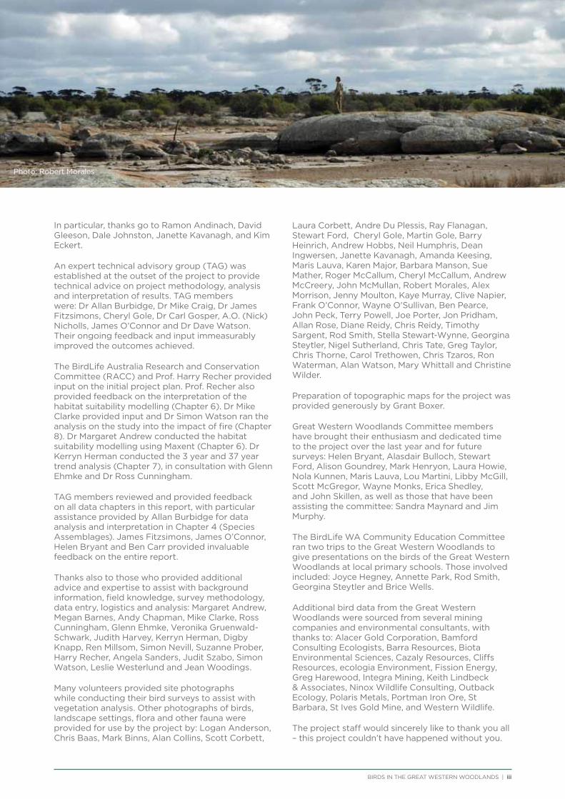
Photo: Robert Morales

iv | BIRDS IN THE GREAT WESTERN WOODLANDS
Acronyms
ANOVA Analysis of Variance
AUC Area Under the Curve
AWAP Australian Water Availability Project
CI Confidence Interval
CSIRO Commonwealth Scientific and Industrial Research Organisation
DPaW Department of Parks and Wildlife
EPBC Act Environment Protection and Biodiversity Conservation Act
GAM Generalised Additive Model
GAMM Generalised Additive Mixed Model
GLM Generalised Linear Model
GLMM Generalised Linear Mixed Model
GPP Gross Primary Productivity
IBRA Interim Biogeographic Regionalisation for Australia
KBULG Kalgoorlie-Boulder Urban Landcare Group
nMDS Non-metric Multidimensional Scaling
NVDI Normalised Difference Vegetation Index
PAR Photosynthetically Available Radiation
TNC The Nature Conservancy
UCL Unallocated Crown Land
VCF Vegetation Continuous Field
BIRDS IN THE GREAT WESTERN WOODLANDS | v
Table of Contents
1. Introduction .......................................................................................................................................................................................................1
2. Raising Awareness and Appreciation of the Great Western Woodlands ........................................................................ 5
3. General Survey Methodology and Results ...................................................................................................................................... 7
3.1. General Survey Methodology ...................................................................................................................................................... 7
3.2. General Survey Results ...................................................................................................................................................................11
4. Avian Assemblages of the Great Western Woodlands ............................................................................................................15
4.1. Methods .................................................................................................................................................................................................15
4.2. Results ....................................................................................................................................................................................................17
4.3. Discussion .............................................................................................................................................................................................19
4.4. Summary ...............................................................................................................................................................................................19
5. Description of Selected Species ..........................................................................................................................................................21
6. Distribution and Habitat Preferences of Selected Species ...................................................................................................25
6.1. Methods ................................................................................................................................................................................................25
6.2. Results ...................................................................................................................................................................................................36
6.3. Discussion .......................................................................................................................................................................................... 147
6.4. Summary ............................................................................................................................................................................................149
7. Trend Analysis of Selected Species.................................................................................................................................................. 151
7.1. Methods .............................................................................................................................................................................................. 152
7.2. Results and Discussion ................................................................................................................................................................ 153
7.3. Summary ............................................................................................................................................................................................156
8. Impact of Post-Fire Age on Bird Species ..................................................................................................................................... 157
8.1. Methods ..............................................................................................................................................................................................158
8.2. Results .................................................................................................................................................................................................159
8.3. Discussion ..........................................................................................................................................................................................163
8.4. Summary ............................................................................................................................................................................................165
9. Comparison of Great Western Woodlands and Adjacent Gondwana Link ................................................................167
9.1. Methods ..............................................................................................................................................................................................167
9.2. Results and Discussion ................................................................................................................................................................168
9.3. Summary ............................................................................................................................................................................................170
10. Prioritising Areas of High Conservation Significance ................................................................................................... 171
10.1. Spatial Connectivity ....................................................................................................................................................................... 171
10.2. Discrete Areas with High Conservation Significance................................................................................................... 174
10.3. Summary ............................................................................................................................................................................................ 178
11. Establishing a Long-term Project ..................................................................................................................................................... 179
12. Bringing it All Together – The Overall Importance of the Great Western Woodlands in an Australian Context .......................................................................................................................................................................................................... 181
vi | BIRDS IN THE GREAT WESTERN WOODLANDS
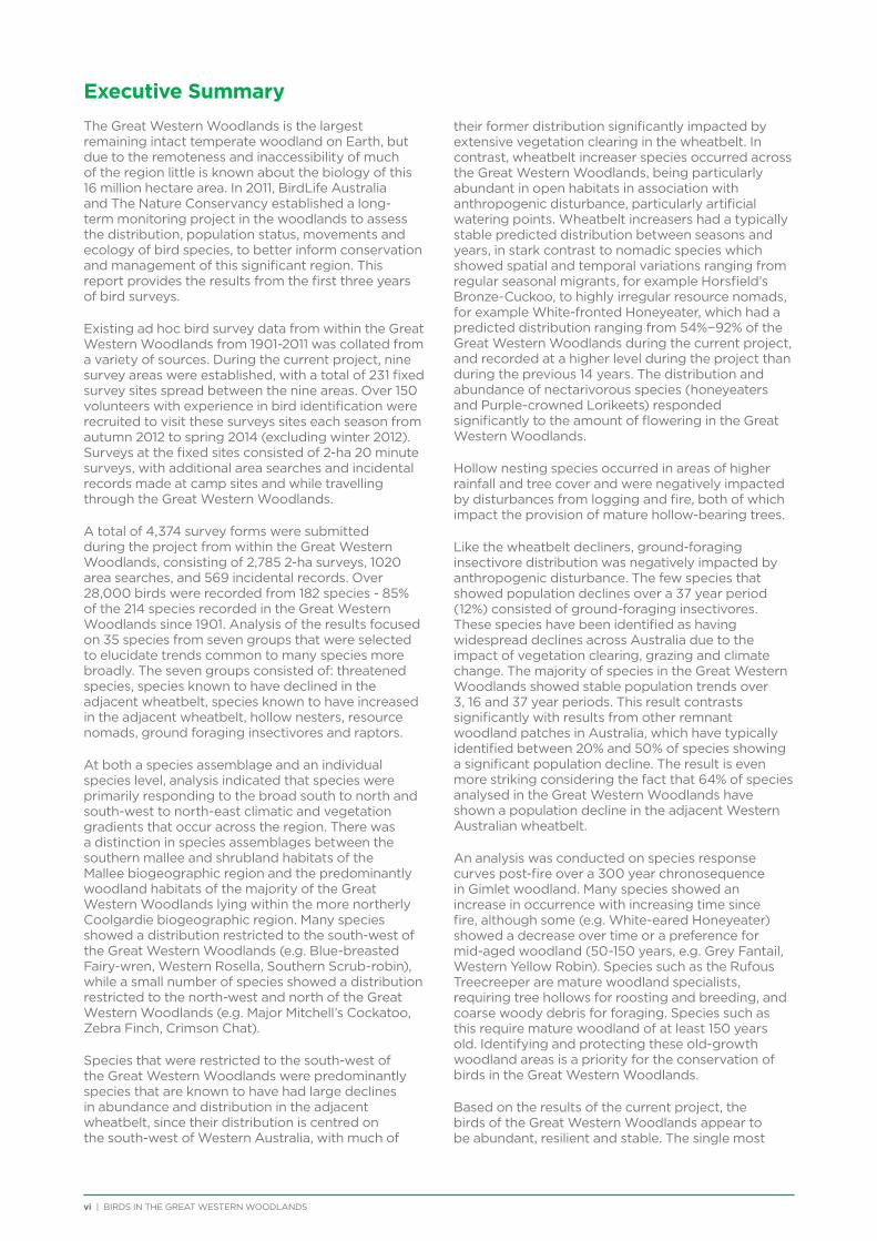
Executive Summary
The Great Western Woodlands is the largest remaining intact temperate woodland on Earth, but due to the remoteness and inaccessibility of much of the region little is known about the biology of this 16 million hectare area. In 2011, BirdLife Australia and The Nature Conservancy established a long-term monitoring project in the woodlands to assess the distribution, population status, movements and ecology of bird species, to better inform conservation and management of this significant region. This report provides the results from the first three years of bird surveys.
Existing ad hoc bird survey data from within the Great Western Woodlands from 1901-2011 was collated from a variety of sources. During the current project, nine survey areas were established, with a total of 231 fixed survey sites spread between the nine areas. Over 150 volunteers with experience in bird identification were recruited to visit these surveys sites each season from autumn 2012 to spring 2014 (excluding winter 2012). Surveys at the fixed sites consisted of 2-ha 20 minute surveys, with additional area searches and incidental records made at camp sites and while travelling through the Great Western Woodlands.
A total of 4,374 survey forms were submitted during the project from within the Great Western Woodlands, consisting of 2,785 2-ha surveys, 1020 area searches, and 569 incidental records. Over 28,000 birds were recorded from 182 species - 85% of the 214 species recorded in the Great Western Woodlands since 1901. Analysis of the results focused on 35 species from seven groups that were selected to elucidate trends common to many species more broadly. The seven groups consisted of: threatened species, species known to have declined in the adjacent wheatbelt, species known to have increased in the adjacent wheatbelt, hollow nesters, resource nomads, ground foraging insectivores and raptors.
At both a species assemblage and an individual species level, analysis indicated that species were primarily responding to the broad south to north and south-west to north-east climatic and vegetation gradients that occur across the region. There was a distinction in species assemblages between the southern mallee and shrubland habitats of the Mallee biogeographic region and the predominantly woodland habitats of the majority of the Great Western Woodlands lying within the more northerly Coolgardie biogeographic region. Many species showed a distribution restricted to the south-west of the Great Western Woodlands (e.g. Blue-breasted Fairy-wren, Western Rosella, Southern Scrub-robin), while a small number of species showed a distribution restricted to the north-west and north of the Great Western Woodlands (e.g. Major Mitchell’s Cockatoo, Zebra Finch, Crimson Chat).
Species that were restricted to the south-west of the Great Western Woodlands were predominantly species that are known to have had large declines in abundance and distribution in the adjacent wheatbelt, since their distribution is centred on the south-west of Western Australia, with much of
their former distribution significantly impacted by extensive vegetation clearing in the wheatbelt. In contrast, wheatbelt increaser species occurred across the Great Western Woodlands, being particularly abundant in open habitats in association with anthropogenic disturbance, particularly artificial watering points. Wheatbelt increasers had a typically stable predicted distribution between seasons and years, in stark contrast to nomadic species which showed spatial and temporal variations ranging from regular seasonal migrants, for example Horsfield’s Bronze-Cuckoo, to highly irregular resource nomads, for example White-fronted Honeyeater, which had a predicted distribution ranging from 54%−92% of the Great Western Woodlands during the current project, and recorded at a higher level during the project than during the previous 14 years. The distribution and abundance of nectarivorous species (honeyeaters and Purple-crowned Lorikeets) responded significantly to the amount of flowering in the Great Western Woodlands.
Hollow nesting species occurred in areas of higher rainfall and tree cover and were negatively impacted by disturbances from logging and fire, both of which impact the provision of mature hollow-bearing trees.
Like the wheatbelt decliners, ground-foraging insectivore distribution was negatively impacted by anthropogenic disturbance. The few species that showed population declines over a 37 year period (12%) consisted of ground-foraging insectivores. These species have been identified as having widespread declines across Australia due to the impact of vegetation clearing, grazing and climate change. The majority of species in the Great Western Woodlands showed stable population trends over 3, 16 and 37 year periods. This result contrasts significantly with results from other remnant woodland patches in Australia, which have typically identified between 20% and 50% of species showing a significant population decline. The result is even more striking considering the fact that 64% of species analysed in the Great Western Woodlands have shown a population decline in the adjacent Western Australian wheatbelt.
An analysis was conducted on species response curves post-fire over a 300 year chronosequence in Gimlet woodland. Many species showed an increase in occurrence with increasing time since fire, although some (e.g. White-eared Honeyeater) showed a decrease over time or a preference for mid-aged woodland (50-150 years, e.g. Grey Fantail, Western Yellow Robin). Species such as the Rufous Treecreeper are mature woodland specialists, requiring tree hollows for roosting and breeding, and coarse woody debris for foraging. Species such as this require mature woodland of at least 150 years old. Identifying and protecting these old-growth woodland areas is a priority for the conservation of birds in the Great Western Woodlands.
Based on the results of the current project, the birds of the Great Western Woodlands appear to be abundant, resilient and stable. The single most
BIRDS IN THE GREAT WESTERN WOODLANDS | vii
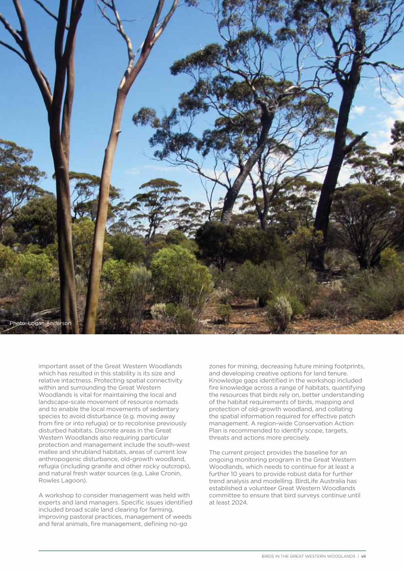
important asset of the Great Western Woodlands which has resulted in this stability is its size and relative intactness. Protecting spatial connectivity within and surrounding the Great Western Woodlands is vital for maintaining the local and landscape-scale movement of resource nomads and to enable the local movements of sedentary species to avoid disturbance (e.g. moving away from fire or into refugia) or to recolonise previously disturbed habitats. Discrete areas in the Great Western Woodlands also requiring particular protection and management include the south-west mallee and shrubland habitats, areas of current low anthropogenic disturbance, old-growth woodland, refugia (including granite and other rocky outcrops), and natural fresh water sources (e.g. Lake Cronin, Rowles Lagoon).
A workshop to consider management was held with experts and land managers. Specific issues identified included broad scale land clearing for farming, improving pastoral practices, management of weeds and feral animals, fire management, defining no-go
zones for mining, decreasing future mining footprints, and developing creative options for land tenure. Knowledge gaps identified in the workshop included fire knowledge across a range of habitats, quantifying the resources that birds rely on, better understanding of the habitat requirements of birds, mapping and protection of old-growth woodland, and collating the spatial information required for effective patch management. A region-wide Conservation Action Plan is recommended to identify scope, targets, threats and actions more precisely.
The current project provides the baseline for an ongoing monitoring program in the Great Western Woodlands, which needs to continue for at least a further 10 years to provide robust data for further trend analysis and modelling. BirdLife Australia has established a volunteer Great Western Woodlands committee to ensure that bird surveys continue until at least 2024.
Photo: Logan Anderson
1 | BIRDS IN THE GREAT WESTERN WOODLANDS
1. Introduction
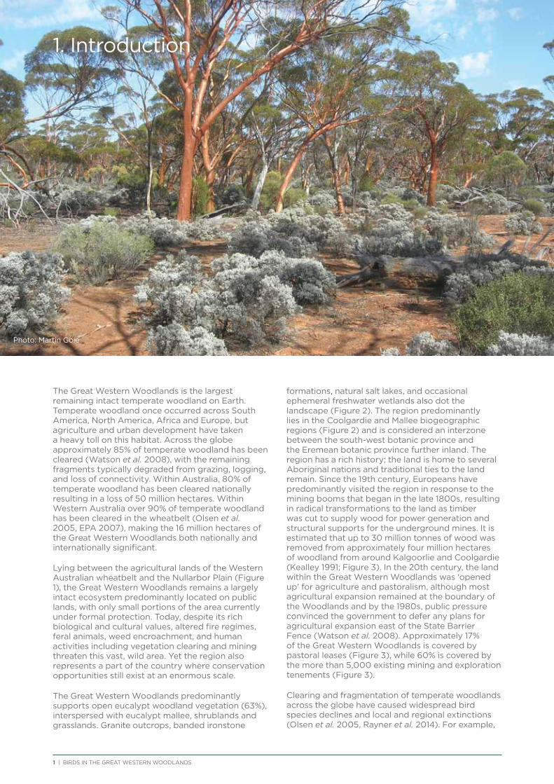
The Great Western Woodlands is the largest remaining intact temperate woodland on Earth. Temperate woodland once occurred across South America, North America, Africa and Europe, but agriculture and urban development have taken a heavy toll on this habitat. Across the globe approximately 85% of temperate woodland has been cleared (Watson et al. 2008), with the remaining fragments typically degraded from grazing, logging, and loss of connectivity. Within Australia, 80% of temperate woodland has been cleared nationally resulting in a loss of 50 million hectares. Within Western Australia over 90% of temperate woodland has been cleared in the wheatbelt (Olsen et al. 2005, EPA 2007), making the 16 million hectares of the Great Western Woodlands both nationally and internationally significant.
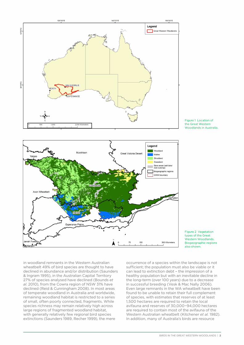
Lying between the agricultural lands of the Western Australian wheatbelt and the Nullarbor Plain (Figure 1), the Great Western Woodlands remains a largely intact ecosystem predominantly located on public lands, with only small portions of the area currently under formal protection. Today, despite its rich biological and cultural values, altered fire regimes, feral animals, weed encroachment, and human activities including vegetation clearing and mining threaten this vast, wild area. Yet the region also represents a part of the country where conservation opportunities still exist at an enormous scale.
The Great Western Woodlands predominantly supports open eucalypt woodland vegetation (63%), interspersed with eucalypt mallee, shrublands and grasslands. Granite outcrops, banded ironstone
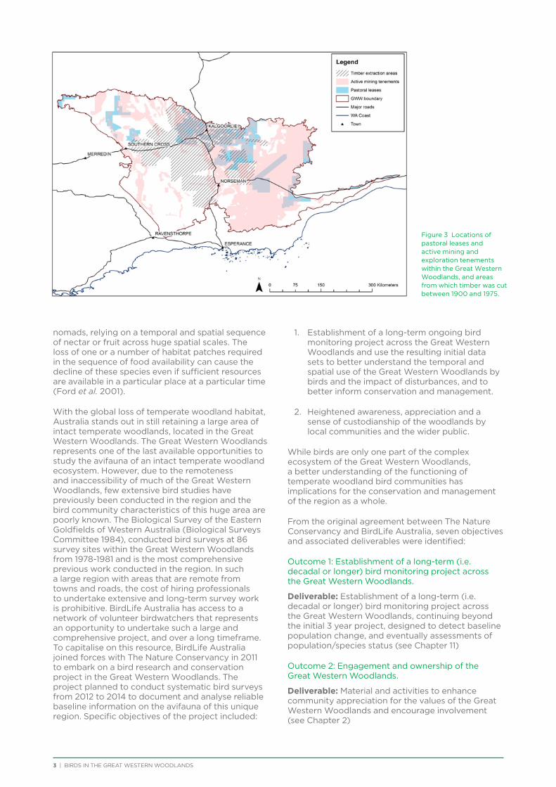
formations, natural salt lakes, and occasional ephemeral freshwater wetlands also dot the landscape (Figure 2). The region predominantly lies in the Coolgardie and Mallee biogeographic regions (Figure 2) and is considered an interzone between the south-west botanic province and the Eremean botanic province further inland. The region has a rich history; the land is home to several Aboriginal nations and traditional ties to the land remain. Since the 19th century, Europeans have predominantly visited the region in response to the mining booms that began in the late 1800s, resulting in radical transformations to the land as timber was cut to supply wood for power generation and structural supports for the underground mines. It is estimated that up to 30 million tonnes of wood was removed from approximately four million hectares of woodland from around Kalgoorlie and Coolgardie (Kealley 1991; Figure 3). In the 20th century, the land within the Great Western Woodlands was ‘opened up’ for agriculture and pastoralism, although most agricultural expansion remained at the boundary of the Woodlands and by the 1980s, public pressure convinced the government to defer any plans for agricultural expansion east of the State Barrier Fence (Watson et al. 2008). Approximately 17% of the Great Western Woodlands is covered by pastoral leases (Figure 3), while 60% is covered by the more than 5,000 existing mining and exploration tenements (Figure 3).
Clearing and fragmentation of temperate woodlands across the globe have caused widespread bird species declines and local and regional extinctions (Olsen et al. 2005, Rayner et al. 2014). For example,
Photo: Martin Gole
BIRDS IN THE GREAT WESTERN WOODLANDS | 2
in woodland remnants in the Western Australian wheatbelt 49% of bird species are thought to have declined in abundance and/or distribution (Saunders & Ingram 1995), in the Australian Capital Territory 27% of species analysed have declined (Bounds et al. 2010), from the Cowra region of NSW 31% have declined (Reid & Cunningham 2008). In most areas of temperate woodland in Australia and worldwide, remaining woodland habitat is restricted to a series of small, often poorly connected, fragments. While species richness may remain relatively high across large regions of fragmented woodland habitat, with generally relatively few regional bird species extinctions (Saunders 1989, Recher 1999), the mere
occurrence of a species within the landscape is not sufficient; the population must also be viable or it can lead to extinction debt – the impression of a healthy population but with an inevitable decline in the long-term (over 100 years) due to a decrease in successful breeding (Vesk & Mac Nally 2006). Even large remnants in the WA wheatbelt have been found to be unable to retain their full complement of species, with estimates that reserves of at least 1,500 hectares are required to retain the local avifauna and reserves of 30,000−94,000 hectares are required to contain most of the avifauna of the Western Australian wheatbelt (Kitchener et al. 1982). In addition, many of Australia’s birds are resource
Figure 1 Location of the Great Western Woodlands in Australia.
Figure 2 Vegetation types of the Great Western Woodlands. Biogeographic regions also shown.
3 | BIRDS IN THE GREAT WESTERN WOODLANDS
nomads, relying on a temporal and spatial sequence of nectar or fruit across huge spatial scales. The loss of one or a number of habitat patches required in the sequence of food availability can cause the decline of these species even if sufficient resources are available in a particular place at a particular time (Ford et al. 2001).
With the global loss of temperate woodland habitat, Australia stands out in still retaining a large area of intact temperate woodlands, located in the Great Western Woodlands. The Great Western Woodlands represents one of the last available opportunities to study the avifauna of an intact temperate woodland ecosystem. However, due to the remoteness and inaccessibility of much of the Great Western Woodlands, few extensive bird studies have previously been conducted in the region and the bird community characteristics of this huge area are poorly known. The Biological Survey of the Eastern Goldfields of Western Australia (Biological Surveys Committee 1984), conducted bird surveys at 86 survey sites within the Great Western Woodlands from 1978-1981 and is the most comprehensive previous work conducted in the region. In such a large region with areas that are remote from towns and roads, the cost of hiring professionals to undertake extensive and long-term survey work is prohibitive. BirdLife Australia has access to a network of volunteer birdwatchers that represents an opportunity to undertake such a large and comprehensive project, and over a long timeframe. To capitalise on this resource, BirdLife Australia joined forces with The Nature Conservancy in 2011 to embark on a bird research and conservation project in the Great Western Woodlands. The project planned to conduct systematic bird surveys from 2012 to 2014 to document and analyse reliable baseline information on the avifauna of this unique region. Specific objectives of the project included:
1. Establishment of a long-term ongoing bird monitoring project across the Great Western Woodlands and use the resulting initial data sets to better understand the temporal and spatial use of the Great Western Woodlands by birds and the impact of disturbances, and to better inform conservation and management.
2. Heightened awareness, appreciation and a sense of custodianship of the woodlands by local communities and the wider public.
While birds are only one part of the complex ecosystem of the Great Western Woodlands, a better understanding of the functioning of temperate woodland bird communities has implications for the conservation and management of the region as a whole.
From the original agreement between The Nature Conservancy and BirdLife Australia, seven objectives and associated deliverables were identified:
Outcome 1: Establishment of a long-term (i.e. decadal or longer) bird monitoring project across the Great Western Woodlands.
Deliverable: Establishment of a long-term (i.e. decadal or longer) bird monitoring project across the Great Western Woodlands, continuing beyond the initial 3 year project, designed to detect baseline population change, and eventually assessments of population/species status (see Chapter 11)
Outcome 2: Engagement and ownership of the Great Western Woodlands.
Deliverable: Material and activities to enhance community appreciation for the values of the Great Western Woodlands and encourage involvement (see Chapter 2)
Figure 3 Locations of pastoral leases and active mining and exploration tenements within the Great Western Woodlands, and areas from which timber was cut between 1900 and 1975.

BIRDS IN THE GREAT WESTERN WOODLANDS | 4
Outcome 3: Assessment of a wide range of bird species populations and status.
Deliverables:1. Assessments of distribution of a suite of birds
occupying the Great Western Woodlands (see Chapter 6)
2. Measures of status of a suite of birds occupying the Great Western Woodlands (see Chapter 7)
3. The importance of Great Western Woodlands for temperate woodland birds in an Australian context and the status of birds in the Great Western Woodlands (see Chapter 12)
Outcome 4: Capture of key baseline bird and ecological data geared to production of accurate habitat-specific maps for the Great Western Woodlands.
Deliverables:1. Habitat-specific maps for selected species,
providing geographic distribution (see Chapter 6)
2. Habitat-specific maps for selected species quantifying habitat requirements where feasible, and geared to appropriate fire management (see Chapter 8)
3. Habitat-specific maps for selected species quantifying habitat requirements where feasible, and geared to potential management for climate change adaptation.
Outcome 5: Comparison of bird communities within Great Western Woodlands and Gondwana Link.
Deliverables:1. Comparisons of community composition/
species richness in sites at remnants/reserves extending west from Great Western Woodlands into Gondwana Link, with sites in the Great Western Woodlands itself: including, if possible, a measure of resilience (e.g. how well do birds recolonise areas after fire in smaller patches as compared to the Great Western Woodlands) (see Chapter 9)
2. Possible community structure ‘standards’ for the reference of the adjacent eastern part of Gondwana Link: what sort of bird communities should revegetation/rehabilitation efforts in Gondwana Link areas be expected to generate?
Outcome 6: Technical recommendations for the formulation of best-practice conservation.
Deliverables:1. Recommendations on specific areas that
appear to be important for the conservation of temperate woodland birds: location, size, composition etc. (see Chapter 10)
2. Recommendations on specific areas that appear to be important for more intensive conservation management within the Great Western Woodlands: location, size, composition etc. (see Chapter 10)
Outcome 7: Management recommendations for threatened and declining bird species including for future use.
Deliverables:1. Management recommendations for threatened
and declining bird species, including management recommendations for land uses such as mining, tourism and pastoralism
2. Management recommendations for managing impacts of fire, feral predators and herbivores
During the course of the project, in consultation with the Technical Advisory Group (Appendix 1) and The Nature Conservancy, the following changes and clarifications to the initial objectives were made:
Outcome 4: Identifying impacts and management for climate change was deemed to be beyond the scope of works that could be conducted within a 3 year project timeframe and was excluded from the project.
Outcome 5: An in-depth comparison of Great Western Woodlands and adjacent Gondwana Link would require additional surveys outside of the Great Western Woodlands and was deemed to take too much focus away from the Great Western Woodlands. It was decided not to conduct any specific surveys to answer this question and instead conduct a brief comparison of species composition from the two regions with existing data (Chapter 9).
Outcome 7: It was agreed not to conduct any specific research to answer this outcome and instead hold a management workshop to identify management recommendations based on information obtained as part of this project. The workshop was held in April 2015. Minutes of the workshop were produced and provided to attendees.
This report presents all outcomes of the project and answers each deliverable above. The technical advisory group and project coordinator will produce peer-reviewed papers in the scientific literature on the basis of the results provided below and additional analysis where relevant.
5 | BIRDS IN THE GREAT WESTERN WOODLANDS
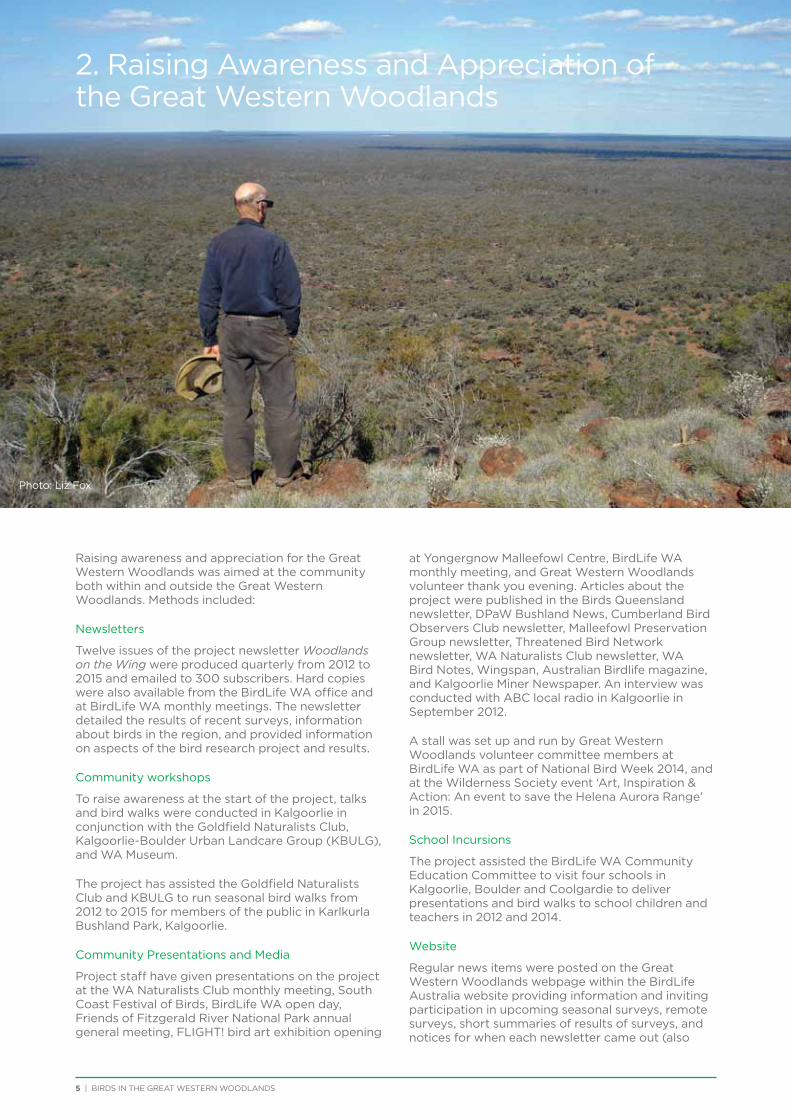
Chapter Header2. Raising Awareness and Appreciation of the Great Western Woodlands
Raising awareness and appreciation for the Great Western Woodlands was aimed at the community both within and outside the Great Western Woodlands. Methods included:
Newsletters
Twelve issues of the project newsletter Woodlands on the Wing were produced quarterly from 2012 to 2015 and emailed to 300 subscribers. Hard copies were also available from the BirdLife WA office and at BirdLife WA monthly meetings. The newsletter detailed the results of recent surveys, information about birds in the region, and provided information on aspects of the bird research project and results.
Community workshops
To raise awareness at the start of the project, talks and bird walks were conducted in Kalgoorlie in conjunction with the Goldfield Naturalists Club, Kalgoorlie-Boulder Urban Landcare Group (KBULG), and WA Museum.
The project has assisted the Goldfield Naturalists Club and KBULG to run seasonal bird walks from 2012 to 2015 for members of the public in Karlkurla Bushland Park, Kalgoorlie.
Community Presentations and Media
Project staff have given presentations on the project at the WA Naturalists Club monthly meeting, South Coast Festival of Birds, BirdLife WA open day, Friends of Fitzgerald River National Park annual general meeting, FLIGHT! bird art exhibition opening
at Yongergnow Malleefowl Centre, BirdLife WA monthly meeting, and Great Western Woodlands volunteer thank you evening. Articles about the project were published in the Birds Queensland newsletter, DPaW Bushland News, Cumberland Bird Observers Club newsletter, Malleefowl Preservation Group newsletter, Threatened Bird Network newsletter, WA Naturalists Club newsletter, WA Bird Notes, Wingspan, Australian Birdlife magazine, and Kalgoorlie Miner Newspaper. An interview was conducted with ABC local radio in Kalgoorlie in September 2012.
A stall was set up and run by Great Western Woodlands volunteer committee members at BirdLife WA as part of National Bird Week 2014, and at the Wilderness Society event ‘Art, Inspiration & Action: An event to save the Helena Aurora Range’ in 2015.
School Incursions
The project assisted the BirdLife WA Community Education Committee to visit four schools in Kalgoorlie, Boulder and Coolgardie to deliver presentations and bird walks to school children and teachers in 2012 and 2014.
Website
Regular news items were posted on the Great Western Woodlands webpage within the BirdLife Australia website providing information and inviting participation in upcoming seasonal surveys, remote surveys, short summaries of results of surveys, and notices for when each newsletter came out (also
Photo: Liz Fox
BIRDS IN THE GREAT WESTERN WOODLANDS | 6
available for download from the webpage). Posts for Latest News items coincided with when items were placed on the BirdLife enews, which is emailed to all BirdLife Australia members and supporters, as well as posts outside these times.
Coordinates and directions to the 231 fixed survey sites within the Great Western Woodlands are publicly available via the Group Sites section of the Birdata website.
Promotional Material
Promotional materials were designed and printed including banners, postcards, stickers, bookmarks, and maps. Two bird guides were produced for the Great Western Woodlands to be made available at visitor centres and other tourist attractions in the Great Western Woodlands. These guides depict common bird species in the region as well as places to go birdwatching. These materials were created in collaboration with the BirdLife WA Great Western Woodlands Committee.
A 16-page glossy brochure outlining the results of the current project was also produced in 2015 to be made available to all volunteer participants in order to provide feedback with a summary of the findings presented in this report, and to be used as promotional material on stalls and at other activities run by the Great Western Woodlands Committee beyond 2015.
Research and Conservation Workshop
The project held a workshop in 2012 with attendance by stakeholders from organisations including DPaW, CSIRO, Gondwana Link, University of WA, Department of Agriculture and Food, and Curtin University. The workshop objectives were to inform researchers and conservationists of work being done in the region (including the work of BirdLife Australia), and to facilitate networking and collaboration opportunities.
Participant questionnaire
Towards the end of 2014 a questionnaire was sent to previous participants in the bird surveys to check how effective our communication methods had been and to obtain their views on any important areas for research and conservation in the Great Western Woodlands. We also asked for feedback on whether the project had raised their awareness and appreciation of the region. 92% of participants stated that it had. Comments received in relation to this question included the following:
“Without being involved in the project I may have continued to just drive through on the highway, stopping at the usual camping spots. The project has fully immersed me in a wonderland and offered an opportunity to contribute to citizen science towards conservation that is as substantial as it gets.”
“The project has taken me to places I would never have gone to. Love the birding in that dry county.”
“Never knew it existed or its importance as an arid woodland.”
“I didn’t realise it is such a huge area and so important to conserve. The variation in terrain and vegetation is fantastic. I look forward to many more surveys in the Great Western Woodlands.”
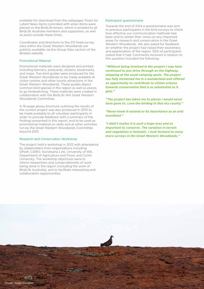
Photo: Tegan Douglas
7 | BIRDS IN THE GREAT WESTERN WOODLANDS
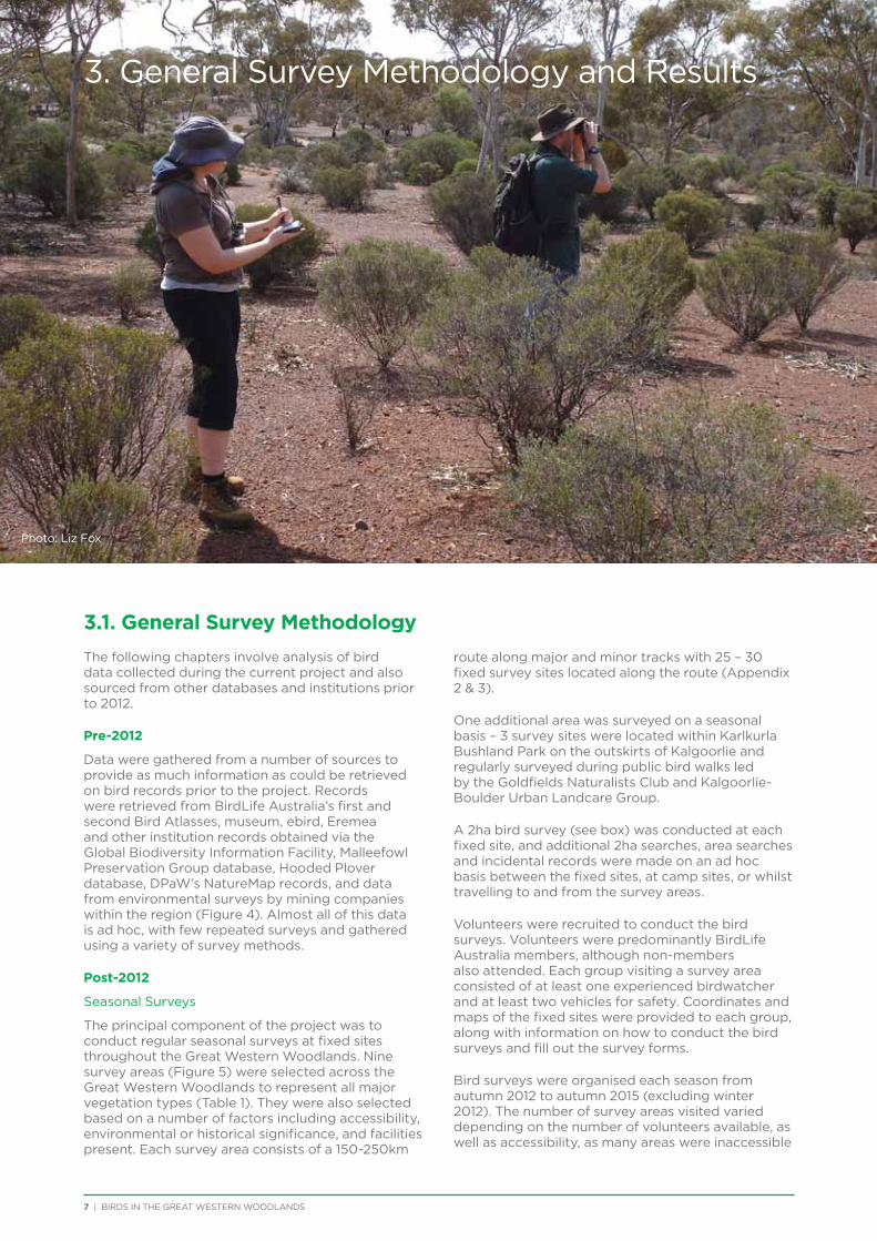
3. General Survey Methodology and Results
3.1. General Survey Methodology
The following chapters involve analysis of bird data collected during the current project and also sourced from other databases and institutions prior to 2012.
Pre-2012
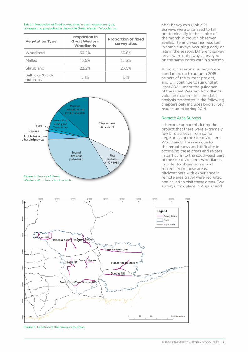
Data were gathered from a number of sources to provide as much information as could be retrieved on bird records prior to the project. Records were retrieved from BirdLife Australia’s first and second Bird Atlasses, museum, ebird, Eremea and other institution records obtained via the Global Biodiversity Information Facility, Malleefowl Preservation Group database, Hooded Plover database, DPaW’s NatureMap records, and data from environmental surveys by mining companies within the region (Figure 4). Almost all of this data is ad hoc, with few repeated surveys and gathered using a variety of survey methods.
Post-2012
Seasonal Surveys
The principal component of the project was to conduct regular seasonal surveys at fixed sites throughout the Great Western Woodlands. Nine survey areas (Figure 5) were selected across the Great Western Woodlands to represent all major vegetation types (Table 1). They were also selected based on a number of factors including accessibility, environmental or historical significance, and facilities present. Each survey area consists of a 150-250km
route along major and minor tracks with 25 – 30 fixed survey sites located along the route (Appendix 2 & 3).
One additional area was surveyed on a seasonal basis – 3 survey sites were located within Karlkurla Bushland Park on the outskirts of Kalgoorlie and regularly surveyed during public bird walks led by the Goldfields Naturalists Club and Kalgoorlie-Boulder Urban Landcare Group.
A 2ha bird survey (see box) was conducted at each fixed site, and additional 2ha searches, area searches and incidental records were made on an ad hoc basis between the fixed sites, at camp sites, or whilst travelling to and from the survey areas.
Volunteers were recruited to conduct the bird surveys. Volunteers were predominantly BirdLife Australia members, although non-members also attended. Each group visiting a survey area consisted of at least one experienced birdwatcher and at least two vehicles for safety. Coordinates and maps of the fixed sites were provided to each group, along with information on how to conduct the bird surveys and fill out the survey forms.
Bird surveys were organised each season from autumn 2012 to autumn 2015 (excluding winter 2012). The number of survey areas visited varied depending on the number of volunteers available, as well as accessibility, as many areas were inaccessible
Photo: Liz Fox
BIRDS IN THE GREAT WESTERN WOODLANDS | 8
Museumcollections and
Institutional data
Nature Map,Mining andConsultancy
SecondBird Atlas
(1998-2011)First
Bird Atlas(1977-1981)
BirdLife WA andother bird projects
eBird
Eremaea
GWW surveys(2012-2014)
Table 1 Proportion of fixed survey sites in each vegetation type, compared to proportion in the whole Great Western Woodlands.
Vegetation TypeProportion in
Great Western Woodlands
Proportion of fixed survey sites
Woodland 56.2% 53.8%
Mallee 16.5% 15.5%
Shrubland 22.2% 23.5%
Salt lake & rock outcrops 5.1% 7.1%
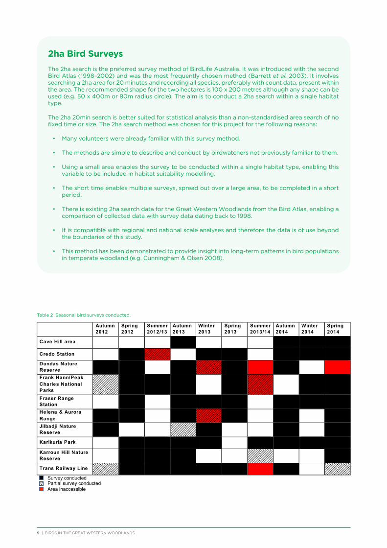
after heavy rain (Table 2). Surveys were organised to fall predominantly in the centre of the month, although observer availability and weather resulted in some surveys occurring early or late in the season. Different survey areas were not always surveyed on the same dates within a season.
Although seasonal surveys were conducted up to autumn 2015 as part of the current project, and will continue to run until at least 2024 under the guidance of the Great Western Woodlands volunteer committee, the data analysis presented in the following chapters only includes bird survey results up to spring 2014.
Remote Area Surveys
It became apparent during the project that there were extremely few bird surveys from some large areas of the Great Western Woodlands. This was due to the remoteness and difficulty in accessing these areas and relates in particular to the south-east part of the Great Western Woodlands. In order to obtain some bird records from these areas, birdwatchers with experience in remote area travel were recruited and asked to visit these areas. Two surveys took place in August and
Figure 5 Location of the nine survey areas.
Figure 4 Source of Great Western Woodlands bird records.
9 | BIRDS IN THE GREAT WESTERN WOODLANDS
2ha Bird Surveys
The 2ha search is the preferred survey method of BirdLife Australia. It was introduced with the second Bird Atlas (1998–2002) and was the most frequently chosen method (Barrett et al. 2003). It involves searching a 2ha area for 20 minutes and recording all species, preferably with count data, present within the area. The recommended shape for the two hectares is 100 x 200 metres although any shape can be used (e.g. 50 x 400m or 80m radius circle). The aim is to conduct a 2ha search within a single habitat type.
The 2ha 20min search is better suited for statistical analysis than a non-standardised area search of no fixed time or size. The 2ha search method was chosen for this project for the following reasons:
• Manyvolunteerswerealreadyfamiliarwiththissurveymethod.
• Themethodsaresimpletodescribeandconductbybirdwatchersnotpreviouslyfamiliartothem.
• Usingasmallareaenablesthesurveytobeconductedwithinasinglehabitattype,enablingthisvariable to be included in habitat suitability modelling.
• Theshorttimeenablesmultiplesurveys,spreadoutoveralargearea,tobecompletedinashortperiod.
• Thereisexisting2hasearchdatafortheGreatWesternWoodlandsfromtheBirdAtlas,enablingacomparison of collected data with survey data dating back to 1998.
• Itiscompatiblewithregionalandnationalscaleanalysesandthereforethedataisofusebeyondthe boundaries of this study.
• Thismethodhasbeendemonstratedtoprovideinsightintolong-termpatternsinbirdpopulationsin temperate woodland (e.g. Cunningham & Olsen 2008).
Autumn 2012
Spring 2012
Summer 2012/13
Autumn 2013
Winter 2013
Spring 2013
Summer 2013/14
Autumn 2014
Winter 2014
Spring 2014
Cave Hill area
Credo Station
Dundas Nature Reserve
Frank Hann/Peak Charles National Parks
Fraser Range Station
Helena & Aurora Range
Jilbadji Nature Reserve
Karlkurla Park
Karroun Hill Nature Reserve
Trans Railway Line
Survey conducted Partial survey conducted Area inaccessible
Table 2 Seasonal bird surveys conducted.
BIRDS IN THE GREAT WESTERN WOODLANDS | 10
October 2014 with 2ha searches, area searches and incidental bird surveys conducted south and east of Balladonia.
An additional remote survey was undertaken in May 2015 in order to conduct surveys south-east of Norseman, although the results from that survey are not included in this report.
Other Survey Methods
A small number of additional survey methods were employed to answer specific research questions. These methods are explained in more detail in the relevant Chapters below.
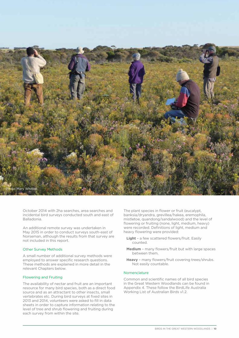
Flowering and Fruiting
The availability of nectar and fruit are an important resource for many bird species, both as a direct food source and as an attractant to other insects, small vertebrates etc. During bird surveys at fixed sites in 2013 and 2014, volunteers were asked to fill in data sheets in order to capture information relating to the level of tree and shrub flowering and fruiting during each survey from within the site.
The plant species in flower or fruit (eucalypt, banksia/dryandra, grevillea/hakea, eremophila, mistletoe, quandong/sandalwood) and the level of flowering or fruiting (none, light, medium, heavy) were recorded. Definitions of light, medium and heavy flowering were provided:
Light – a few scattered flowers/fruit. Easily counted.
Medium – many flowers/fruit but with large spaces between them.
Heavy – many flowers/fruit covering trees/shrubs. Not easily countable.
Nomenclature
Common and scientific names of all bird species in the Great Western Woodlands can be found in Appendix 4. These follow the BirdLife Australia Working List of Australian Birds v1.2.
Photo: Mary Whittall
11 | BIRDS IN THE GREAT WESTERN WOODLANDS
3.2 General Survey Results
Survey Effort
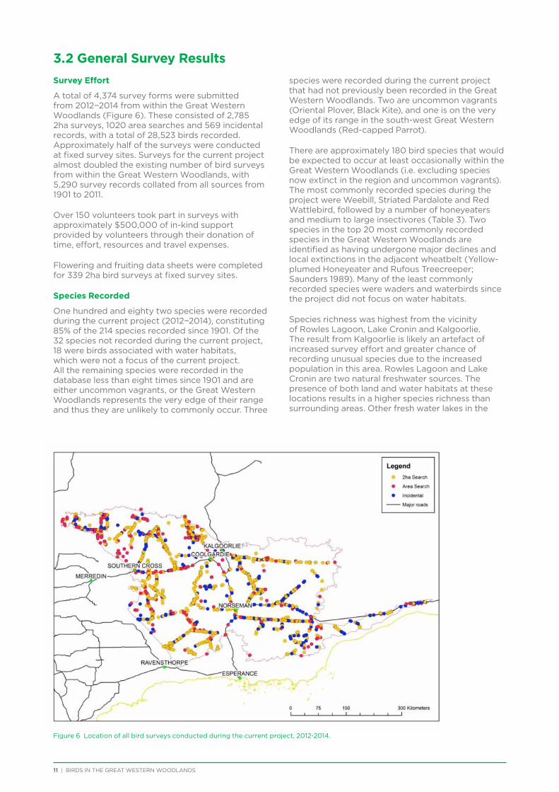
A total of 4,374 survey forms were submitted from 2012−2014 from within the Great Western Woodlands (Figure 6). These consisted of 2,785 2ha surveys, 1020 area searches and 569 incidental records, with a total of 28,523 birds recorded. Approximately half of the surveys were conducted at fixed survey sites. Surveys for the current project almost doubled the existing number of bird surveys from within the Great Western Woodlands, with 5,290 survey records collated from all sources from 1901 to 2011.
Over 150 volunteers took part in surveys with approximately $500,000 of in-kind support provided by volunteers through their donation of time, effort, resources and travel expenses.
Flowering and fruiting data sheets were completed for 339 2ha bird surveys at fixed survey sites.
Species Recorded
One hundred and eighty two species were recorded during the current project (2012−2014), constituting 85% of the 214 species recorded since 1901. Of the 32 species not recorded during the current project, 18 were birds associated with water habitats, which were not a focus of the current project. All the remaining species were recorded in the database less than eight times since 1901 and are either uncommon vagrants, or the Great Western Woodlands represents the very edge of their range and thus they are unlikely to commonly occur. Three
species were recorded during the current project that had not previously been recorded in the Great Western Woodlands. Two are uncommon vagrants (Oriental Plover, Black Kite), and one is on the very edge of its range in the south-west Great Western Woodlands (Red-capped Parrot).
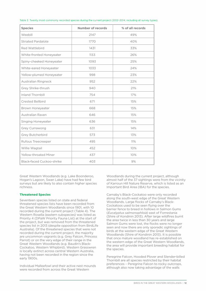
There are approximately 180 bird species that would be expected to occur at least occasionally within the Great Western Woodlands (i.e. excluding species now extinct in the region and uncommon vagrants). The most commonly recorded species during the project were Weebill, Striated Pardalote and Red Wattlebird, followed by a number of honeyeaters and medium to large insectivores (Table 3). Two species in the top 20 most commonly recorded species in the Great Western Woodlands are identified as having undergone major declines and local extinctions in the adjacent wheatbelt (Yellow-plumed Honeyeater and Rufous Treecreeper; Saunders 1989). Many of the least commonly recorded species were waders and waterbirds since the project did not focus on water habitats.
Species richness was highest from the vicinity of Rowles Lagoon, Lake Cronin and Kalgoorlie. The result from Kalgoorlie is likely an artefact of increased survey effort and greater chance of recording unusual species due to the increased population in this area. Rowles Lagoon and Lake Cronin are two natural freshwater sources. The presence of both land and water habitats at these locations results in a higher species richness than surrounding areas. Other fresh water lakes in the
Figure 6 Location of all bird surveys conducted during the current project, 2012-2014.
BIRDS IN THE GREAT WESTERN WOODLANDS | 12
Table 3 Twenty most commonly recorded species during the current project (2012−2014; including all survey types).
Species Number of records % of all records
Weebill 2147 49%
Striated Pardalote 1770 40%
Red Wattlebird 1431 33%
White-fronted Honeyeater 1133 26%
Spiny-cheeked Honeyeater 1093 25%
White-eared Honeyeater 1033 24%
Yellow-plumed Honeyeater 998 23%
Australian Ringneck 952 22%
Grey Shrike-thrush 940 21%
Inland Thornbill 754 17%
Crested Bellbird 671 15%
Brown Honeyeater 668 15%
Australian Raven 646 15%
Singing Honeyeater 636 15%
Grey Currawong 631 14%
Grey Butcherbird 573 13%
Rufous Treecreeper 495 11%
Willie Wagtail 452 10%
Yellow-throated Miner 437 10%
Black-faced Cuckoo-shrike 403 9%
Great Western Woodlands (e.g. Lake Boonderoo, Hogan’s Lagoon, Swan Lake) have had few bird surveys but are likely to also contain higher species richness.
Threatened Species
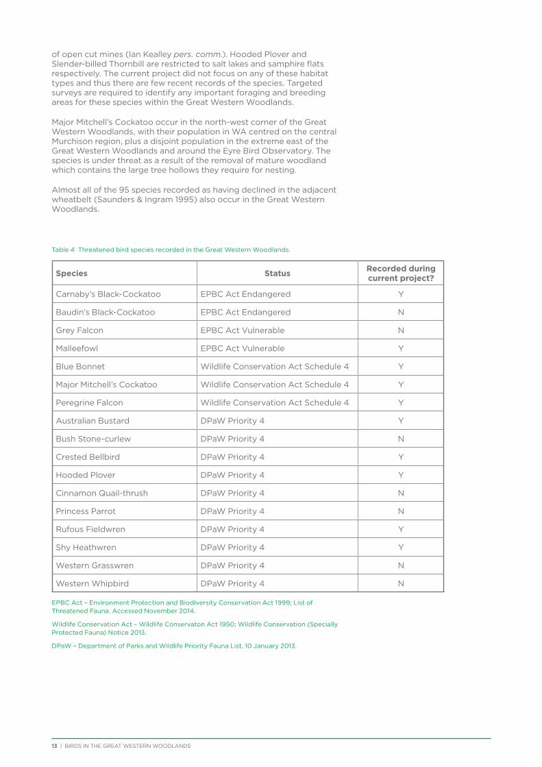
Seventeen species listed on state and federal threatened species lists have been recorded from the Great Western Woodlands since 1901, with 10 recorded during the current project (Table 4). The Western Rosella (eastern subspecies) was listed as Priority 4 (DPaW Priority Fauna List) at the start of the project, but was removed from the threatened species list in 2013 (despite opposition from BirdLife Australia). Of the threatened species that were not recorded during the current project, the majority are uncommon vagrants (e.g. Grey Falcon, Princess Parrot) or on the very edge of their range in the Great Western Woodlands (e.g. Baudin’s Black-Cockatoo, Western Whipbird). Western Grasswren is locally extinct across central Western Australia, having not been recorded in the region since the early 1900s.
Individual Malleefowl and their active nest mounds were recorded from across the Great Western
Woodlands during the current project, although almost half of the 37 sightings were from the vicinity of Karroun Hill Nature Reserve, which is listed as an Important Bird Area (IBA) for the species.
Carnaby’s Black-Cockatoo were only recorded along the south-west edge of the Great Western Woodlands. Large flocks of Carnaby’s Black-Cockatoos used to be seen flying over the barrier fence to breed in hollows in Salmon Gums (Eucalyptus salmonophloia) east of Forrestania (Shire of Kondinin 2013). After large wildfires burnt the area twice in less than 30 years and large Salmon Gums were lost, the flocks were no longer seen and now there are only sporadic sightings of birds at the western edge of the Great Western Woodlands (Shire of Kondinin 2013). It is possible that once mature woodland has re-established on the western edge of the Great Western Woodlands, the area will provide important breeding habitat for the species.
Peregrine Falcon, Hooded Plover and Slender-billed Thornbill are all species restricted by their habitat preferences – Peregrine Falcon to rocky outcrops, although also now taking advantage of the walls
of open cut mines (Ian Kealley pers. comm.). Hooded Plover and Slender-billed Thornbill are restricted to salt lakes and samphire flats respectively. The current project did not focus on any of these habitat types and thus there are few recent records of the species. Targeted surveys are required to identify any important foraging and breeding areas for these species within the Great Western Woodlands.
Major Mitchell’s Cockatoo occur in the north-west corner of the Great Western Woodlands, with their population in WA centred on the central Murchison region, plus a disjoint population in the extreme east of the Great Western Woodlands and around the Eyre Bird Observatory. The species is under threat as a result of the removal of mature woodland which contains the large tree hollows they require for nesting.
Almost all of the 95 species recorded as having declined in the adjacent wheatbelt (Saunders & Ingram 1995) also occur in the Great Western Woodlands.
Table 4 Threatened bird species recorded in the Great Western Woodlands.
Species Status Recorded during current project?
Carnaby’s Black-Cockatoo EPBC Act Endangered Y
Baudin’s Black-Cockatoo EPBC Act Endangered N
Grey Falcon EPBC Act Vulnerable N
Malleefowl EPBC Act Vulnerable Y
Blue Bonnet Wildlife Conservation Act Schedule 4 Y
Major Mitchell’s Cockatoo Wildlife Conservation Act Schedule 4 Y
Peregrine Falcon Wildlife Conservation Act Schedule 4 Y
Australian Bustard DPaW Priority 4 Y
Bush Stone-curlew DPaW Priority 4 N
Crested Bellbird DPaW Priority 4 Y
Hooded Plover DPaW Priority 4 Y
Cinnamon Quail-thrush DPaW Priority 4 N
Princess Parrot DPaW Priority 4 N
Rufous Fieldwren DPaW Priority 4 Y
Shy Heathwren DPaW Priority 4 Y
Western Grasswren DPaW Priority 4 N
Western Whipbird DPaW Priority 4 N
EPBC Act – Environment Protection and Biodiversity Conservation Act 1999; List of Threatened Fauna. Accessed November 2014.
Wildlife Conservation Act – Wildlife Conservaton Act 1950; Wildlife Conservation (Specially Protected Fauna) Notice 2013.
DPaW – Department of Parks and Wildlife Priority Fauna List, 10 January 2013.
13 | BIRDS IN THE GREAT WESTERN WOODLANDS
BIRDS IN THE GREAT WESTERN WOODLANDS | 14
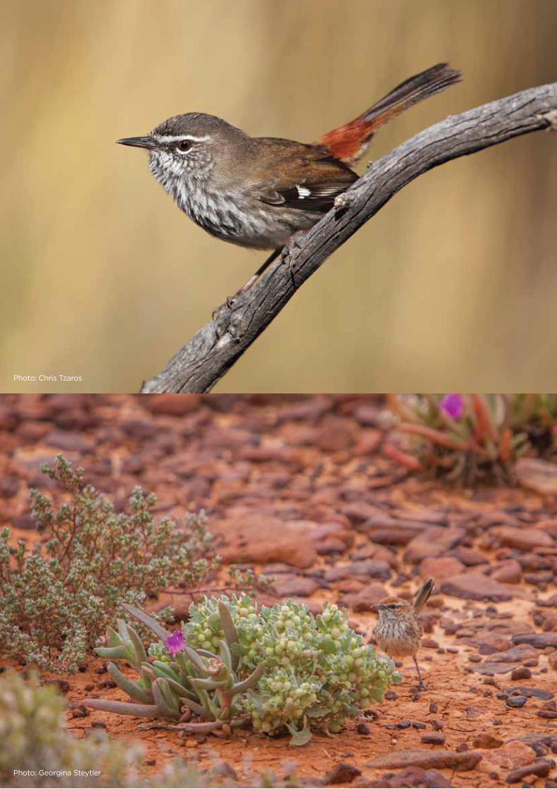
Photo: Chris Tzaros
Photo: Georgina Steytler
15 | BIRDS IN THE GREAT WESTERN WOODLANDS
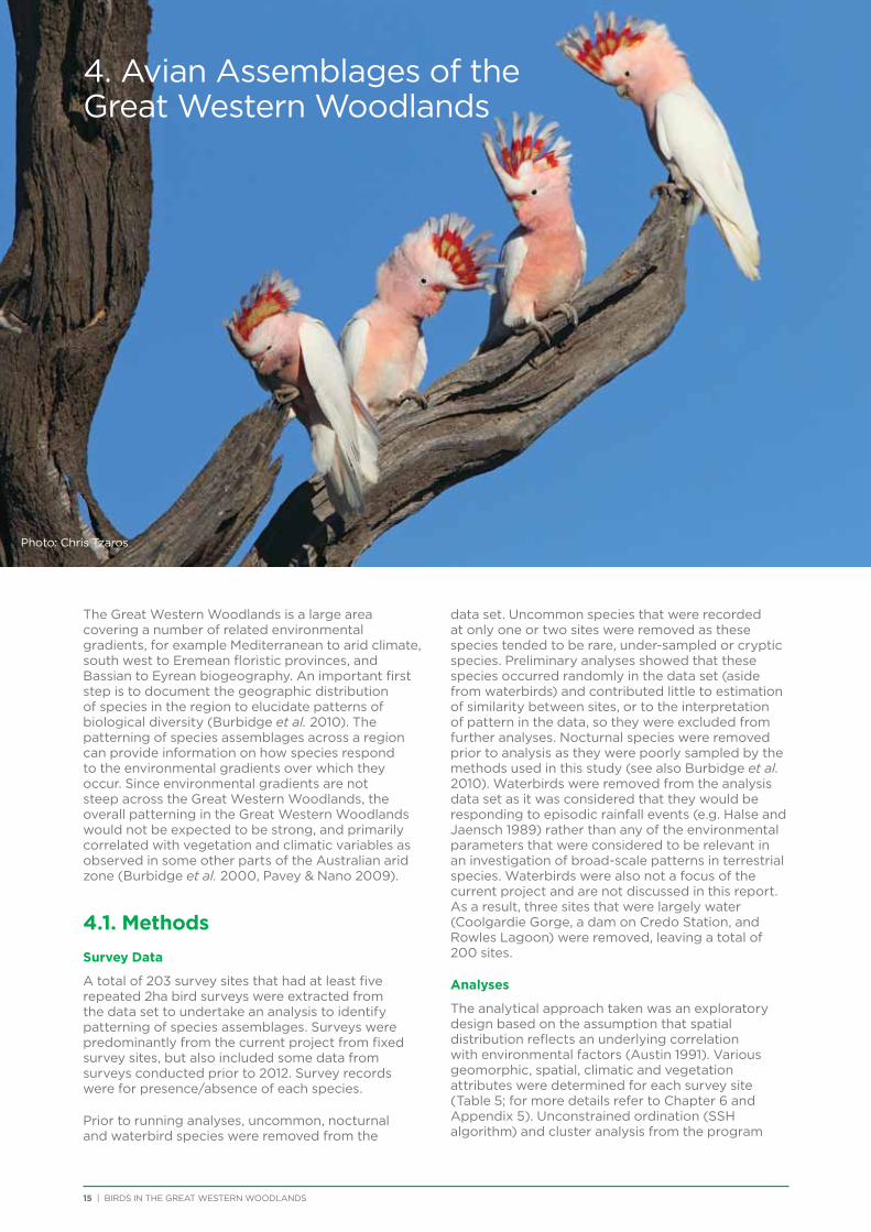
4. Avian Assemblages of the Great Western Woodlands
The Great Western Woodlands is a large area covering a number of related environmental gradients, for example Mediterranean to arid climate, south west to Eremean floristic provinces, and Bassian to Eyrean biogeography. An important first step is to document the geographic distribution of species in the region to elucidate patterns of biological diversity (Burbidge et al. 2010). The patterning of species assemblages across a region can provide information on how species respond to the environmental gradients over which they occur. Since environmental gradients are not steep across the Great Western Woodlands, the overall patterning in the Great Western Woodlands would not be expected to be strong, and primarily correlated with vegetation and climatic variables as observed in some other parts of the Australian arid zone (Burbidge et al. 2000, Pavey & Nano 2009).
4.1. Methods
Survey Data
A total of 203 survey sites that had at least five repeated 2ha bird surveys were extracted from the data set to undertake an analysis to identify patterning of species assemblages. Surveys were predominantly from the current project from fixed survey sites, but also included some data from surveys conducted prior to 2012. Survey records were for presence/absence of each species.
Prior to running analyses, uncommon, nocturnal and waterbird species were removed from the
data set. Uncommon species that were recorded at only one or two sites were removed as these species tended to be rare, under-sampled or cryptic species. Preliminary analyses showed that these species occurred randomly in the data set (aside from waterbirds) and contributed little to estimation of similarity between sites, or to the interpretation of pattern in the data, so they were excluded from further analyses. Nocturnal species were removed prior to analysis as they were poorly sampled by the methods used in this study (see also Burbidge et al. 2010). Waterbirds were removed from the analysis data set as it was considered that they would be responding to episodic rainfall events (e.g. Halse and Jaensch 1989) rather than any of the environmental parameters that were considered to be relevant in an investigation of broad-scale patterns in terrestrial species. Waterbirds were also not a focus of the current project and are not discussed in this report. As a result, three sites that were largely water (Coolgardie Gorge, a dam on Credo Station, and Rowles Lagoon) were removed, leaving a total of 200 sites.
Analyses
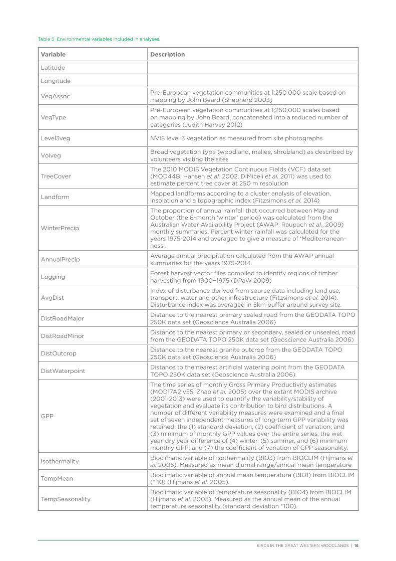
The analytical approach taken was an exploratory design based on the assumption that spatial distribution reflects an underlying correlation with environmental factors (Austin 1991). Various geomorphic, spatial, climatic and vegetation attributes were determined for each survey site (Table 5; for more details refer to Chapter 6 and Appendix 5). Unconstrained ordination (SSH algorithm) and cluster analysis from the program
Photo: Chris Tzaros
BIRDS IN THE GREAT WESTERN WOODLANDS | 16
Table 5 Environmental variables included in analyses.
Variable Description
Latitude
Longitude
VegAssocPre-European vegetation communities at 1:250,000 scale based on mapping by John Beard (Shepherd 2003)
VegTypePre-European vegetation communities at 1;250,000 scales based on mapping by John Beard, concatenated into a reduced number of categories (Judith Harvey 2012)
Level3veg NVIS level 3 vegetation as measured from site photographs
VolvegBroad vegetation type (woodland, mallee, shrubland) as described by volunteers visiting the sites
TreeCoverThe 2010 MODIS Vegetation Continuous Fields (VCF) data set (MOD44B; Hansen et al. 2002, DiMiceli et al. 2011) was used to estimate percent tree cover at 250 m resolution
Landform Mapped landforms according to a cluster analysis of elevation, insolation and a topographic index (Fitzsimons et al. 2014)
WinterPrecip
The proportion of annual rainfall that occurred between May and October (the 6-month ‘winter’ period) was calculated from the Australian Water Availability Project (AWAP; Raupach et al., 2009) monthly summaries. Percent winter rainfall was calculated for the years 1975-2014 and averaged to give a measure of ‘Mediterranean-ness’.
AnnualPrecipAverage annual precipitation calculated from the AWAP annual summaries for the years 1975-2014.
LoggingForest harvest vector files compiled to identify regions of timber harvesting from 1900−1975 (DPaW 2009)
AvgDistIndex of disturbance derived from source data including land use, transport, water and other infrastructure (Fitzsimons et al. 2014). Disturbance index was averaged in 5km buffer around survey site.
DistRoadMajorDistance to the nearest primary sealed road from the GEODATA TOPO 250K data set (Geoscience Australia 2006)
DistRoadMinorDistance to the nearest primary or secondary, sealed or unsealed, road from the GEODATA TOPO 250K data set (Geoscience Australia 2006)
DistOutcropDistance to the nearest granite outcrop from the GEODATA TOPO 250K data set (Geoscience Australia 2006)
DistWaterpointDistance to the nearest artificial watering point from the GEODATA TOPO 250K data set (Geoscience Australia 2006).
GPP
The time series of monthly Gross Primary Productivity estimates (MOD17A2 v55; Zhao et al. 2005) over the extant MODIS archive (2001-2013) were used to quantify the variability/stability of vegetation and evaluate its contribution to bird distributions. A number of different variability measures were examined and a final set of seven independent measures of long-term GPP variability was retained: the (1) standard deviation, (2) coefficient of variation, and (3) minimum of monthly GPP values over the entire series; the wet year-dry year difference of (4) winter, (5) summer, and (6) minimum monthly GPP; and (7) the coefficient of variation of GPP seasonality.
Isothermality Bioclimatic variable of isothermality (BIO3) from BIOCLIM (Hijmans et al. 2005). Measured as mean diurnal range/annual mean temperature
TempMean Bioclimatic variable of annual mean temperature (BIO1) from BIOCLIM (* 10) (Hijmans et al. 2005).
TempSeasonalityBioclimatic variable of temperature seasonality (BIO4) from BIOCLIM (Hijmans et al. 2005). Measured as the annual mean of the annual temperature seasonality (standard deviation *100).
17 | BIRDS IN THE GREAT WESTERN WOODLANDS
PATN (Belbin 1995) were used to reveal patterns of site similarity and species composition in the data matrix. Briefly, the Czekanowski (Bray-Curtis) association measure was used to compare the sites according to similarities in their species composition, and the association measure ‘two-step’ (Belbin 1980) was used to determine the quantitative relationship between each pair of species as a basis for clustering species that normally co-occurred at the same sites. For both measures of association, a modified version of ‘unweighted pair group arithmetic averaging’ hierarchical clustering strategy was used (flexible UPGMA – Sneath and Sokal 1973; Belbin 1995), with the clustering parameter (Beta) set to -0.1. This procedure is appropriate for ecological presence-absence data and is robust to variations in species abundance patterns and hence sampling efficiencies (Faith et al. 1987; Belbin 1991). The partition structure of the resulting site-dendrogram was used as a summary of compositional patterns across the study area. Site physical attributes that conformed most closely to the overall partition structure were assessed for statistical significance using Kruskal-Wallis one-way analysis of variance by ranks (the GSTA module in PATN; Belbin 1995). Partitioning of the overall dendrogram was judged visually, supplemented by expert opinion together with examination of putative groups and the two-way table, based on extrinsic properties of the component sites or species.
Species assemblages identified from the species classification were interpreted in terms of the known habitat preferences of their component species throughout their ranges elsewhere in Australia (e.g. Johnstone and Storr 1998, 2004; Barrett et al. 2003) and previous field experience in other
parts of Western Australia. The use of such extrinsic information on habitat preferences and distribution provides an indication of whether the classification is biologically meaningful.
Possible associations were explored between assemblage patterns and environmental parameters using the BIO-ENV procedure from the BEST routine in PRIMER (Clarke and Gorley 2006; Clarke et al. 2008). Because the values of some key environmental parameters were missing from 13 sites, we removed these sites before analysis. This left 187 sites and 22 continuous variables. One species was also removed (Pallid Cuckoo) as it only occurred at one site following the above reduction in sites. An examination of the environmental data for collinear variables showed that Latitude was strongly positively correlated with ‘TempMean’ and ‘TempSeasonality’ and strongly negatively correlated with ‘Isothermality’ (>0.9). Latitude was therefore taken to be a good surrogate for these three temperature variables, which were removed from the analysis. Variables were normalised before the BEST routine was run. Significance of the analysis was obtained via a permutation test with 99 random samples.
4.2. Results
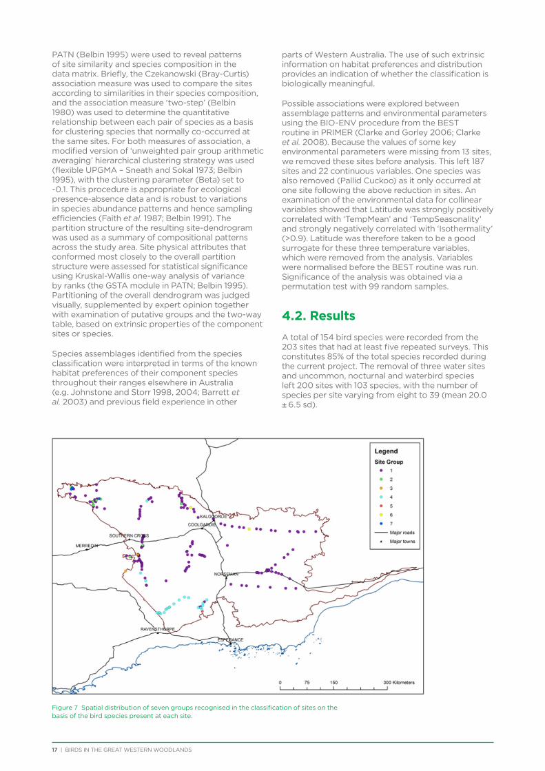
A total of 154 bird species were recorded from the 203 sites that had at least five repeated surveys. This constitutes 85% of the total species recorded during the current project. The removal of three water sites and uncommon, nocturnal and waterbird species left 200 sites with 103 species, with the number of species per site varying from eight to 39 (mean 20.0 ± 6.5 sd).
Figure 7 Spatial distribution of seven groups recognised in the classification of sites on the basis of the bird species present at each site.
BIRDS IN THE GREAT WESTERN WOODLANDS | 18
Site Classification
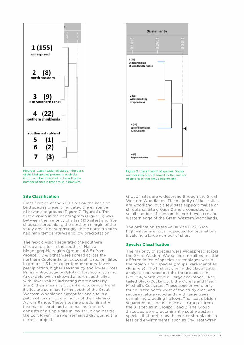
Classification of the 200 sites on the basis of bird species present indicated the existence of seven site groups (Figure 7, Figure 8). The first division in the dendrogram (Figure 8) was between the majority of sites (195 sites) and five sites scattered along the northern margin of the study area. Not surprisingly, these northern sites had high temperatures and low precipitation.
The next division separated the southern shrubland sites in the southern Mallee biogeographic region (groups 4 & 5) from groups 1, 2 & 3 that were spread across the northern Coolgardie biogeographic region. Sites in groups 1-3 had higher temperatures, lower precipitation, higher seasonality and lower Gross Primary Productivity (GPP) difference in summer (a variable which showed a north-south cline, with lower values indicating more northerly sites), than sites in groups 4 and 5. Group 4 and 5 sites are confined to the south of the Great Western Woodlands except for one site in a patch of low shrubland north of the Helena & Aurora Range. These sites are predominantly heathland, shrubland and mallee. Group 5 consists of a single site in low shrubland beside the Lort River. The river remained dry during the current project.
Group 1 sites are widespread through the Great Western Woodlands. The majority of these sites are woodland, but a few sites support mallee or shrubland. Site groups 2 and 3 consisted of a small number of sites on the north-western and western edge of the Great Western Woodlands.
The ordination stress value was 0.27. Such high values are not unexpected for ordinations involving a large number of sites.
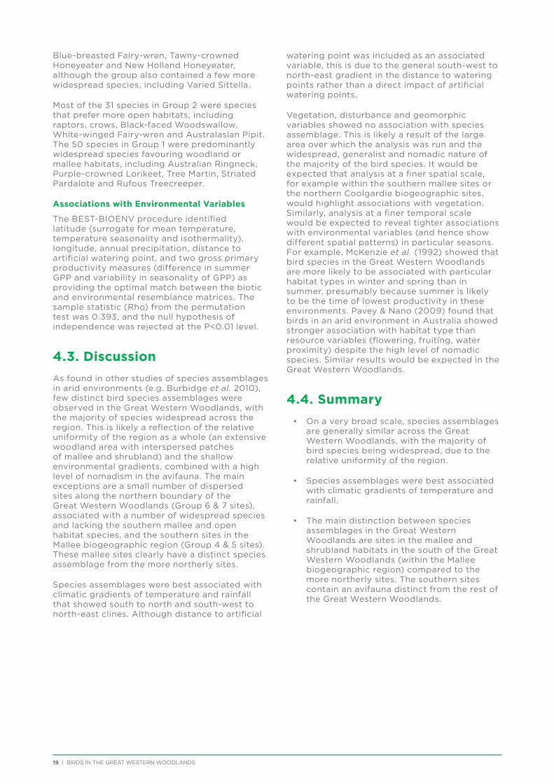
Species Classification
The majority of species were widespread across the Great Western Woodlands, resulting in little differentiation of species assemblages within the region. Four species groups were identified (Figure 9). The first division in the classification analysis separated out the three species in Group 4, which were all large cockatoos – Red-tailed Black-Cockatoo, Little Corella and Major Mitchell’s Cockatoo. These species were only found in the north-west of the study area, and require mature woodlands with large trees containing breeding hollows. The next division separated out the 19 species in Group 3 from the 81 species in Groups 1 and 2. The Group 3 species were predominantly south-western species that prefer heathlands or shrublands in less arid environments, such as Shy Heathwren,
Figure 8 Classification of sites on the basis of the bird species present at each site. Group number indicated, followed by the number of sites in that group in brackets.
Figure 9 Classification of species. Group number indicated, followed by the number of species in that group in brackets.
19 | BIRDS IN THE GREAT WESTERN WOODLANDS
Blue-breasted Fairy-wren, Tawny-crowned Honeyeater and New Holland Honeyeater, although the group also contained a few more widespread species, including Varied Sittella.
Most of the 31 species in Group 2 were species that prefer more open habitats, including raptors, crows, Black-faced Woodswallow, White-winged Fairy-wren and Australasian Pipit. The 50 species in Group 1 were predominantly widespread species favouring woodland or mallee habitats, including Australian Ringneck, Purple-crowned Lorikeet, Tree Martin, Striated Pardalote and Rufous Treecreeper.
Associations with Environmental Variables
The BEST-BIOENV procedure identified latitude (surrogate for mean temperature, temperature seasonality and isothermality), longitude, annual precipitation, distance to artificial watering point, and two gross primary productivity measures (difference in summer GPP and variability in seasonality of GPP) as providing the optimal match between the biotic and environmental resemblance matrices. The sample statistic (Rho) from the permutation test was 0.393, and the null hypothesis of independence was rejected at the P<0.01 level.
4.3. Discussion
As found in other studies of species assemblages in arid environments (e.g. Burbidge et al. 2010), few distinct bird species assemblages were observed in the Great Western Woodlands, with the majority of species widespread across the region. This is likely a reflection of the relative uniformity of the region as a whole (an extensive woodland area with interspersed patches of mallee and shrubland) and the shallow environmental gradients, combined with a high level of nomadism in the avifauna. The main exceptions are a small number of dispersed sites along the northern boundary of the Great Western Woodlands (Group 6 & 7 sites), associated with a number of widespread species and lacking the southern mallee and open habitat species, and the southern sites in the Mallee biogeographic region (Group 4 & 5 sites). These mallee sites clearly have a distinct species assemblage from the more northerly sites.
Species assemblages were best associated with climatic gradients of temperature and rainfall that showed south to north and south-west to north-east clines. Although distance to artificial
watering point was included as an associated variable, this is due to the general south-west to north-east gradient in the distance to watering points rather than a direct impact of artificial watering points.
Vegetation, disturbance and geomorphic variables showed no association with species assemblage. This is likely a result of the large area over which the analysis was run and the widespread, generalist and nomadic nature of the majority of the bird species. It would be expected that analysis at a finer spatial scale, for example within the southern mallee sites or the northern Coolgardie biogeographic sites, would highlight associations with vegetation. Similarly, analysis at a finer temporal scale would be expected to reveal tighter associations with environmental variables (and hence show different spatial patterns) in particular seasons. For example, McKenzie et al. (1992) showed that bird species in the Great Western Woodlands are more likely to be associated with particular habitat types in winter and spring than in summer, presumably because summer is likely to be the time of lowest productivity in these environments. Pavey & Nano (2009) found that birds in an arid environment in Australia showed stronger association with habitat type than resource variables (flowering, fruiting, water proximity) despite the high level of nomadic species. Similar results would be expected in the Great Western Woodlands.
4.4. Summary
• Onaverybroadscale,speciesassemblagesare generally similar across the Great Western Woodlands, with the majority of bird species being widespread, due to the relative uniformity of the region.
• Speciesassemblageswerebestassociatedwith climatic gradients of temperature and rainfall.
• Themaindistinctionbetweenspeciesassemblages in the Great Western Woodlands are sites in the mallee and shrubland habitats in the south of the Great Western Woodlands (within the Mallee biogeographic region) compared to the more northerly sites. The southern sites contain an avifauna distinct from the rest of the Great Western Woodlands.
BIRDS IN THE GREAT WESTERN WOODLANDS | 20
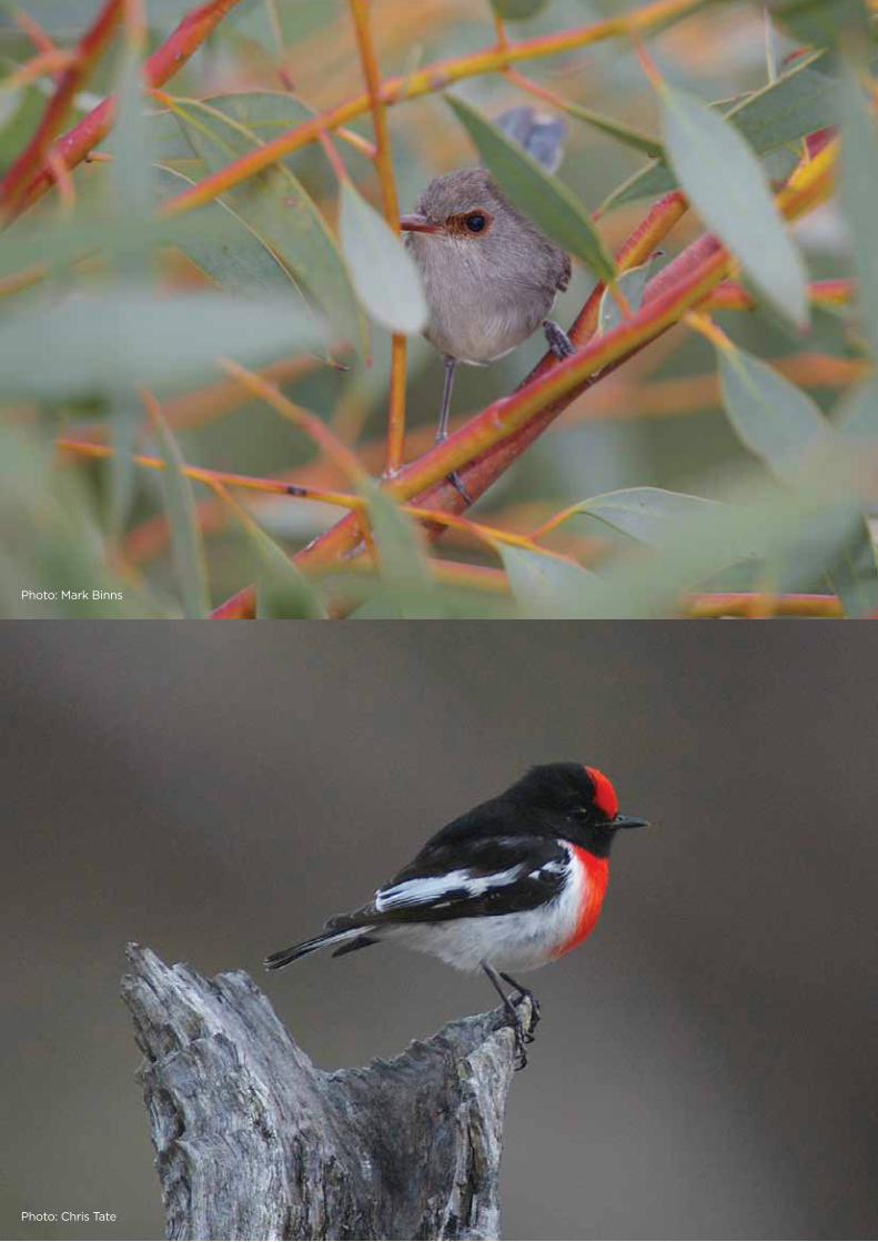
Photo: Mark Binns
Photo: Chris Tate
21 | BIRDS IN THE GREAT WESTERN WOODLANDS
5. Description of Selected Species
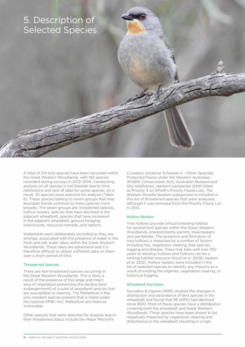
A total of 214 bird species have been recorded within the Great Western Woodlands, with 182 species recorded during surveys in 2012−2014. Conducting analysis on all species is not feasible due to time restrictions and lack of data for some species. As a result, 35 species were selected for analysis (Table 6). These species belong to seven groups that may elucidate trends common to many species more broadly. The seven groups are: threatened species, hollow nesters, species that have declined in the adjacent wheatbelt, species that have increased in the adjacent wheatbelt, ground foraging insectivores, resource nomads, and raptors.
Waterbirds were deliberately excluded as they are strongly associated with the presence of water in the fresh and salt water lakes within the Great Western Woodlands. These lakes are ephemeral and it is therefore difficult to obtain sufficient data on them over a short period of time.
Threatened Species
There are few threatened species occurring in the Great Western Woodlands. This is likely a result of the presence of this large and intact area of vegetation preventing the decline (and endangerment) of a suite of woodland species that are susceptible to clearing. The Malleefowl is the only resident species present that is listed under the national EPBC Act. Malleefowl are listed as Vulnerable.
Other species that were selected for analysis due to their threatened status include the Major Mitchell’s
Cockatoo (listed as Schedule 4 – Other Specially Protected Fauna under the Western Australian Wildlife Conservation Act), Australian Bustard and Shy Heathwren, western subspecies (both listed as Priority 4 on DPaW’s Priority Fauna List). The Western Rosella (eastern subspecies) is included in this list of threatened species that were analysed, although it was removed from the Priority Fauna List in 2013.
Hollow Nesters
Tree hollows provide critical breeding habitat for several bird species within the Great Western Woodlands, predominantly parrots, treecreepers and pardalotes. The presence and formation of tree hollows is impacted by a number of factors including fire, vegetation clearing, tree species, logging and disease. Trees may take well over 100 years to develop hollows and hollows can be a limiting habitat resource (Koch et al. 2008, Haslem et al. 2012). Hollow nesters were included in the list of selected species to identify any impacts as a result of existing fire regimes, vegetation clearing, or historical logging.
Wheatbelt Decliners
Saunders & Ingram (1995) studied the changes in distribution and abundance of bird species in the wheatbelt and found that 95 (49%) had declined since 1900. Most of these species have a distribution covering both the wheatbelt and Great Western Woodlands. These species have been shown to be negatively impacted by vegetation clearing and disturbance in the wheatbelt resulting in a high
Photo: Chris Tzaros
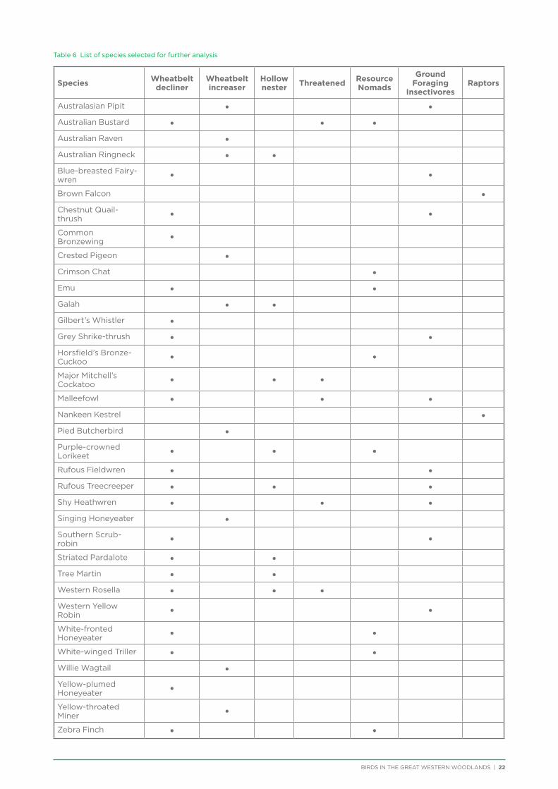
BIRDS IN THE GREAT WESTERN WOODLANDS | 22
Table 6 List of species selected for further analysis
Species Wheatbelt decliner
Wheatbelt increaser
Hollow nester Threatened Resource
Nomads
Ground Foraging
InsectivoresRaptors
Australasian Pipit • •
Australian Bustard • • •
Australian Raven •
Australian Ringneck • •
Blue-breasted Fairy-wren • •
Brown Falcon •
Chestnut Quail-thrush • •
Common Bronzewing •
Crested Pigeon •
Crimson Chat •
Emu • •
Galah • •
Gilbert’s Whistler •
Grey Shrike-thrush • •
Horsfield’s Bronze-Cuckoo • •
Major Mitchell’s Cockatoo • • •
Malleefowl • • •
Nankeen Kestrel •
Pied Butcherbird •
Purple-crowned Lorikeet • • •
Rufous Fieldwren • •
Rufous Treecreeper • • •
Shy Heathwren • • •
Singing Honeyeater •
Southern Scrub-robin • •
Striated Pardalote • •
Tree Martin • •
Western Rosella • • •
Western Yellow Robin • •
White-fronted Honeyeater • •
White-winged Triller • •
Willie Wagtail •
Yellow-plumed Honeyeater •
Yellow-throated Miner •
Zebra Finch • •
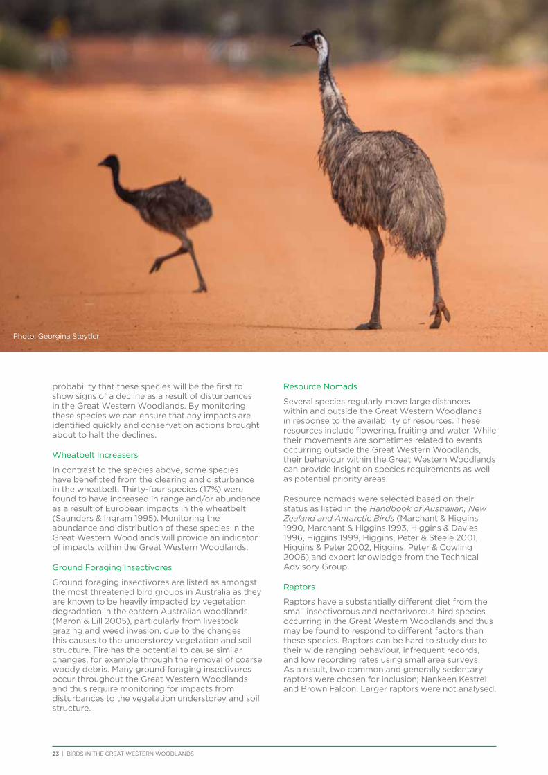
23 | BIRDS IN THE GREAT WESTERN WOODLANDS
probability that these species will be the first to show signs of a decline as a result of disturbances in the Great Western Woodlands. By monitoring these species we can ensure that any impacts are identified quickly and conservation actions brought about to halt the declines.
Wheatbelt Increasers
In contrast to the species above, some species have benefitted from the clearing and disturbance in the wheatbelt. Thirty-four species (17%) were found to have increased in range and/or abundance as a result of European impacts in the wheatbelt (Saunders & Ingram 1995). Monitoring the abundance and distribution of these species in the Great Western Woodlands will provide an indicator of impacts within the Great Western Woodlands.
Ground Foraging Insectivores
Ground foraging insectivores are listed as amongst the most threatened bird groups in Australia as they are known to be heavily impacted by vegetation degradation in the eastern Australian woodlands (Maron & Lill 2005), particularly from livestock grazing and weed invasion, due to the changes this causes to the understorey vegetation and soil structure. Fire has the potential to cause similar changes, for example through the removal of coarse woody debris. Many ground foraging insectivores occur throughout the Great Western Woodlands and thus require monitoring for impacts from disturbances to the vegetation understorey and soil structure.
Resource Nomads
Several species regularly move large distances within and outside the Great Western Woodlands in response to the availability of resources. These resources include flowering, fruiting and water. While their movements are sometimes related to events occurring outside the Great Western Woodlands, their behaviour within the Great Western Woodlands can provide insight on species requirements as well as potential priority areas.
Resource nomads were selected based on their status as listed in the Handbook of Australian, New Zealand and Antarctic Birds (Marchant & Higgins 1990, Marchant & Higgins 1993, Higgins & Davies 1996, Higgins 1999, Higgins, Peter & Steele 2001, Higgins & Peter 2002, Higgins, Peter & Cowling 2006) and expert knowledge from the Technical Advisory Group.
Raptors
Raptors have a substantially different diet from the small insectivorous and nectarivorous bird species occurring in the Great Western Woodlands and thus may be found to respond to different factors than these species. Raptors can be hard to study due to their wide ranging behaviour, infrequent records, and low recording rates using small area surveys. As a result, two common and generally sedentary raptors were chosen for inclusion; Nankeen Kestrel and Brown Falcon. Larger raptors were not analysed.
Photo: Georgina Steytler
BIRDS IN THE GREAT WESTERN WOODLANDS | 24

25 | BIRDS IN THE GREAT WESTERN WOODLANDS
6. Distribution and Habitat Preferences of Selected Species
Distribution maps are useful for identifying core habitat and area of occupancy, but in large and poorly sampled areas the interpretation of species distribution is often limited by lack of data and uneven survey coverage. Relatively few bird surveys had been conducted over much of the Great Western Woodlands prior to 2012, with the number of surveys almost doubled as a result of the current project. Prior to the current project there was only broad understanding of the distribution of species within the Great Western Woodlands and the habitat preferences driving those distributions. With the data provided by the current project it was possible to generate species distribution maps, and identify the environmental variables driving that distribution. In addition, while the current project attempted to cover as much of the Great Western Woodlands as possible, the large size and remoteness of the region resulted in some areas, particularly the north-east and south-east, having few bird surveys conducted. Therefore habitat suitability modelling was used to predict species distribution in areas that were not sampled. Identifying which environmental variables are driving distribution is also important for identifying the impacts of disturbance and climate variability, and preferred vegetation types, and can be used to model predicted distribution under varying conditions, for example different rainfall scenarios or under the impacts of future predicted climate change.
Presented in this chapter are distribution maps and habitat preferences for the 35 selected species.
6.1. Methods
Distribution mapping from raw data
Two distribution maps are shown for each selected species; a map of the raw data and a reporting rate map based on 30-minute grid cells.
Raw data map: The locations of all surveys in the Great Western Woodlands dating back to 1901 (see Chapter 3) are shown in grey, with locations where the species was recorded shown in red. All survey types (area search, 2ha, incidental, transect, etc.) are included. In the first Bird Atlas (1977−1981), records were made in either a 10 minute or 1 degree grid cell basis. Record locations were placed at the centre of each grid cell and therefore only represent the general location of where the species was seen.
Reporting Rate map: Incidental records were removed from the data set and the number of records of each species in each 30 minute grid cell was calculated using area search and 2ha survey data from 1977 to 2014. The number of records of a species was divided by the total number of surveys (excluding incidentals) recorded in that grid cell, providing a reporting rate for that species from 0 to 1. Figure 10 shows the number of surveys per grid cell that were used to calculate reporting rate. Low numbers of surveys can result in erroneous reporting rates and grid cells containing 5 or fewer surveys were removed from the analysis and reported as ‘no data’. Bird surveys from the first Bird Atlas that were reported on a one degree grid basis were also removed. A 30’ grid cell was selected as this was the
Photo: Steven Spragg

BIRDS IN THE GREAT WESTERN WOODLANDS | 26
finest scale grid that could be used whilst retaining at least 5 surveys in almost all grid cells. A finer grid would have resulted in more accurate distribution mapping, but at the expense of increased data gaps.
Habitat Suitability Modelling
Habitat suitability modelling was carried out using two different methods: Maxent modelling and generalised additive models (GAMs). Due to the structure of the data and the analysis method, not all variables were able to be included in both methods. Temporal information was included in the Maxent models, while site-specific vegetation and habitat measures could be included in the GAMs (Table 7). GAMs were also repeated on a small subset of the survey data for which survey-specific flowering information was recorded.
Maxent modelling
Habitat suitability modelling was conducted in Maxent (version 3.3.3) using a total of 2,709 2ha surveys from within the Great Western Woodlands from 2012 to 2014. Surveys were conducted at 1,195 sites, including fixed sites and ad hoc locations across the Great Western Woodlands (Figure 11).
Maximum entropy (Maxent) models were constructed of the distributions of each species (excluding Australian Bustard and Malleefowl for which there was insufficient data). Maxent is a machine learning algorithm that performs well at pattern recognition tasks such as the modelling of species distributions given the environmental conditions associated with a sample of species
presences and the background conditions in the study area (Elith et al. 2006, Phillips et al. 2006). Maxent models the probability that a species occurs under a particular combination of environmental conditions by performing optimisation routines that maximise the predicted probability at the observed training locations relative to the background environment. At the same time, it minimises the assumptions (i.e. maximises entropy) made by the model by requiring the shape of the statistical probability distribution function of the species presences along the environmental predictor variables to be as similar as possible to that of the background sample (Elith et al. 2011).
The definition of the background sample can have important influences on the Maxent models, especially when the sampled points are biased along the environmental variables (Phillips et al. 2009). In such cases, models developed using a random background will predict the distribution of the sampled points (i.e. will model the sampling biases), but not necessarily the true distribution of the species. Preliminary bird distribution models attempted to simulate the biases of the sampled points in the background set (i.e. 75% of points sampled within 5km of a road and background sample dates randomly chosen from the empirical distribution of actual survey dates). However, the influence of sampling biases was still apparent in the modelled distributions, even when omitting road and anthropogenic disturbance variables from the models. Consequently, the final set of models defined the background using the ‘target group background’ approach (Phillips et al. 2009), in which
Figure 10 Number of surveys (area searches and 2ha surveys, 1977-2014) per 30’ grid cell used to calculate reporting rate maps.
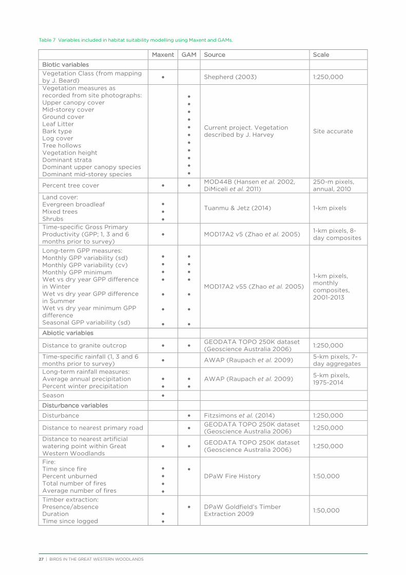
27 | BIRDS IN THE GREAT WESTERN WOODLANDS
Table 7 Variables included in habitat suitability modelling using Maxent and GAMs.
Maxent GAM Source Scale
Biotic variablesVegetation Class (from mappingby J. Beard) • Shepherd (2003) 1:250,000
Vegetation measures asrecorded from site photographs:Upper canopy coverMid-storey coverGround coverLeaf LitterBark typeLog coverTree hollowsVegetation heightDominant strataDominant upper canopy speciesDominant mid-storey species
•••••••••••
Current project. Vegetationdescribed by J. Harvey Site accurate
Percent tree cover • •MOD44B (Hansen et al. 2002, DiMiceli et al. 2011)
250-m pixels,annual, 2010
Land cover:Evergreen broadleafMixed treesShrubs
•••
Tuanmu & Jetz (2014) 1-km pixels
Time-specific Gross Primary Productivity (GPP; 1, 3 and 6 months prior to survey)
• MOD17A2 v5 (Zhao et al. 2005) 1-km pixels, 8-day composites
Long-term GPP measures:Monthly GPP variability (sd)Monthly GPP variability (cv)Monthly GPP minimumWet vs dry year GPP difference in WinterWet vs dry year GPP difference in SummerWet vs dry year minimum GPP differenceSeasonal GPP variability (sd)
••••
•
•
•
••••
•
•
•
MOD17A2 v55 (Zhao et al. 2005)
1-km pixels,monthly composites, 2001-2013
Abiotic variables
Distance to granite outcrop • •GEODATA TOPO 250K dataset (Geoscience Australia 2006) 1:250,000
Time-specific rainfall (1, 3 and 6 months prior to survey) • AWAP (Raupach et al. 2009) 5-km pixels, 7-
day aggregatesLong-term rainfall measures:Average annual precipitationPercent winter precipitation
••
••
AWAP (Raupach et al. 2009) 5-km pixels,1975-2014
Season •
Disturbance variables
Disturbance • Fitzsimons et al. (2014) 1:250,000
Distance to nearest primary road •GEODATA TOPO 250K dataset (Geoscience Australia 2006) 1:250,000
Distance to nearest artificialwatering point within GreatWestern Woodlands
• •GEODATA TOPO 250K dataset (Geoscience Australia 2006) 1:250,000
Fire:Time since firePercent unburnedTotal number of firesAverage number of fires
••••
•DPaW Fire History 1:50,000
Timber extraction:Presence/absenceDurationTime since logged
••
• DPaW Goldfield’s TimberExtraction 2009 1:50,000
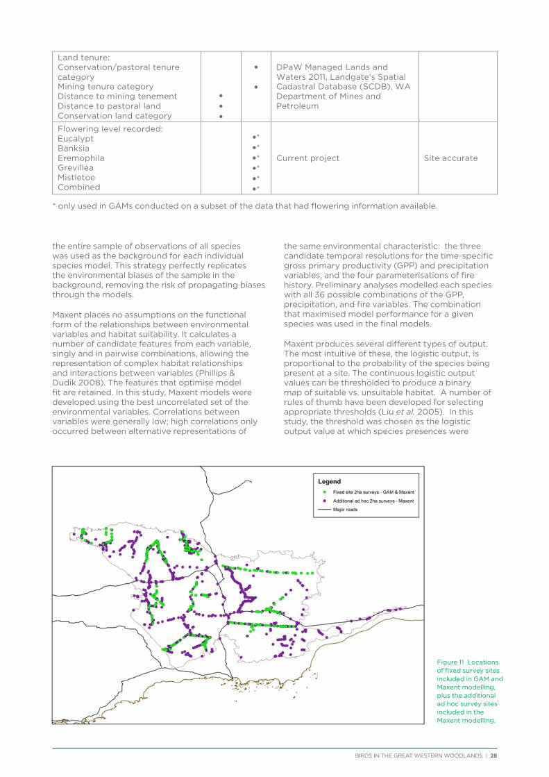
BIRDS IN THE GREAT WESTERN WOODLANDS | 28
the entire sample of observations of all species was used as the background for each individual species model. This strategy perfectly replicates the environmental biases of the sample in the background, removing the risk of propagating biases through the models.
Maxent places no assumptions on the functional form of the relationships between environmental variables and habitat suitability. It calculates a number of candidate features from each variable, singly and in pairwise combinations, allowing the representation of complex habitat relationships and interactions between variables (Phillips & Dudik 2008). The features that optimise model fit are retained. In this study, Maxent models were developed using the best uncorrelated set of the environmental variables. Correlations between variables were generally low; high correlations only occurred between alternative representations of
the same environmental characteristic: the three candidate temporal resolutions for the time-specific gross primary productivity (GPP) and precipitation variables, and the four parameterisations of fire history. Preliminary analyses modelled each species with all 36 possible combinations of the GPP, precipitation, and fire variables. The combination that maximised model performance for a given species was used in the final models.
Maxent produces several different types of output. The most intuitive of these, the logistic output, is proportional to the probability of the species being present at a site. The continuous logistic output values can be thresholded to produce a binary map of suitable vs. unsuitable habitat. A number of rules of thumb have been developed for selecting appropriate thresholds (Liu et al. 2005). In this study, the threshold was chosen as the logistic output value at which species presences were
* only used in GAMs conducted on a subset of the data that had flowering information available.
Figure 11 Locations of fixed survey sites included in GAM and Maxent modelling, plus the additional ad hoc survey sites included in the Maxent modelling.
Land tenure:Conservation/pastoral tenure categoryMining tenure categoryDistance to mining tenementDistance to pastoral landConservation land category
•••
•
•
DPaW Managed Lands and Waters 2011, Landgate's Spatial Cadastral Database (SCDB), WADepartment of Mines and Petroleum
Flowering level recorded:EucalyptBanksiaEremophilaGrevilleaMistletoeCombined
•*•*•*•*•*•*
Current project Site accurate
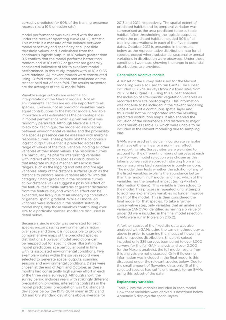
29 | BIRDS IN THE GREAT WESTERN WOODLANDS
correctly predicted for 90% of the training presence records (i.e. a 10% omission rate).
Model performance was evaluated with the area under the receiver operating curve (AUC) statistic. This metric is a measure of the balance between model sensitivity and specificity at all possible threshold values, and is calculated from the continuous logistic output. AUC values greater than 0.5 confirm that the model performs better than random and AUCs of 0.7 or greater are generally considered indicative of fair to excellent model performance. In this study, models with AUC > 0.65 were retained. All Maxent models were constructed using 10-fold cross-validation and evaluated on the test set held out of each fold. The results presented are the averages of the 10 model folds.
Variable usage outputs are essential for interpretation of the Maxent models. Not all environmental factors are equally important to all species. Likewise, not all predictor variables make equal contributions to the habitat models. Variable importance was estimated as the percentage loss in model performance when a given variable was randomly permuted. Although Maxent is a fairly ‘black box’ technique, the modelled associations between environmental variables and the probability of a species presence can be assessed with marginal response curves. These graphs plot the continuous logistic output value that is predicted across the range of values of the focal variable, holding all other variables at their mean values. The response curves are particularly helpful for interpreting variables with indirect effects on species distributions or that integrate multiple mechanisms across their ranges, such as the logging end date and fire age variables. Many of the distance surfaces (such as the distance to pastoral lease variable) also fall into this category. Sharp gradients in the response curves at low distance values suggest a possible effect of the feature itself, while patterns at greater distances from the feature, beyond which an effect can be expected, are likely due to an underlying correlation or general spatial gradient. While all modelled variables were included in the habitat suitability model maps, only those variables contributing over 10% to a particular species’ model are discussed in detail below.
Because a single model was generated for each species encompassing environmental variation over space and time, it is not possible to provide comprehensive maps of the predicted species distributions. However, model predictions can be mapped out for specific dates, illustrating the model predictions at a particular point in time with its associated environmental conditions. Five exemplary dates within the survey record were selected to generate spatial outputs, spanning seasons and environmental conditions. Dates were chosen at the end of April and October, as these months had consistently high survey effort in each of the three years surveyed. Although short, the survey period includes years with strikingly different precipitation, providing interesting contrasts in the model predictions; precipitation was 0.6 standard deviations below the 1975−2014 mean in 2012 and 0.6 and 0.9 standard deviations above average for
2013 and 2014 respectively. The spatial extent of predicted habitat and its temporal variation was summarised as the area predicted to be suitable habitat (after thresholding the logistic output at which the predicted habitat included 90% of all training observations) in each of the five mapped dates. October 2013 is presented in the results below as the representative distribution map for all species, except where substantial seasonal or annual variations in distribution were observed. Under these conditions two maps, showing the range in potential distributions, are provided.
Generalised Additive Models
A subset of the survey data used for the Maxent modelling was also used to run GAMs. The subset included 1,112 2ha surveys from 231 fixed sites from 2012−2014 (Figure 11). Using this subset enabled the inclusion of site-specific vegetation variables as recorded from site photographs. This information was not able to be included in the Maxent modelling since it was not a continuous spatial layer and thus could not be incorporated into the resulting predicted distribution maps. It also enabled the inclusion of the disturbance and distance to major roads variables (Table 7), which were unable to be included in the Maxent modelling due to sampling bias.
GAMs were used as they can incorporate variables that have either a linear or a non-linear effect on reporting rate. Survey sites were weighted to account for the different numbers of surveys at each site. Forward model selection was chosen as this takes a conservative approach, starting from a ‘null’ model assuming bird abundance is purely random. The model then tests whether the addition of any of the listed variables explains the abundance better than the random ‘null’ model, and if so, which of the variables has the greatest impact (using Akaike’s Information Criteria). This variable is then added to the model. This process is repeated, until attempts to add new explanatory variables no longer improve the fit of the model. This is then considered the final model for that species. To take a further conservative step, only variables that an analysis of variance (ANOVA) identified as having a p value of under 0.1 were included in the final model selection. GAMs were run in R (version 2.15.2).
A further subset of the fixed site data was also analysed with GAMs using the same methodology as above in order to examine the impact of flowering data on species distribution. Since this subset included only 339 surveys (compared to over 1,000 surveys for the full GAM analysis and over 2,000 for the Maxent analysis), the full model results from this analysis are not discussed. Only if flowering information was included in the final model is this discussed under the relevant species below. Due to the small amount of flowering data, only 15 of the selected species had sufficient records to run GAMs using this subset of the data.
Explanatory variables
Table 7 lists the variables included in each model. How these variables were derived is described below. Appendix 5 displays the spatial layers.
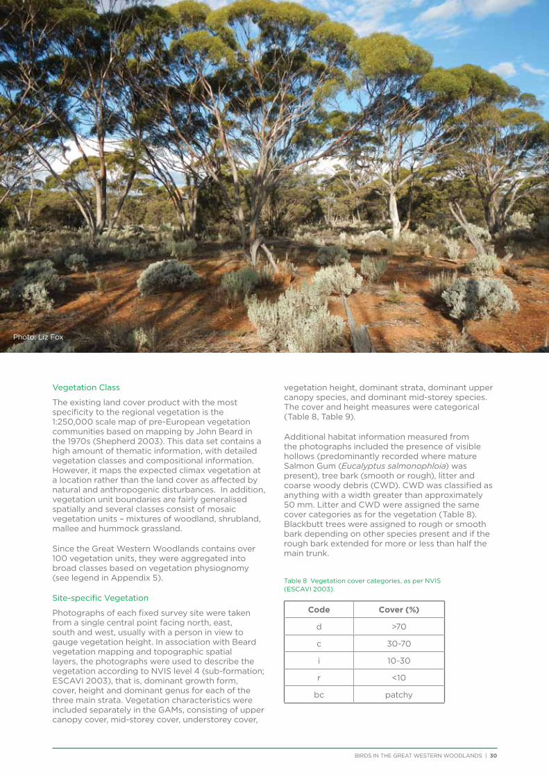
BIRDS IN THE GREAT WESTERN WOODLANDS | 30
Vegetation Class
The existing land cover product with the most specificity to the regional vegetation is the 1:250,000 scale map of pre-European vegetation communities based on mapping by John Beard in the 1970s (Shepherd 2003). This data set contains a high amount of thematic information, with detailed vegetation classes and compositional information. However, it maps the expected climax vegetation at a location rather than the land cover as affected by natural and anthropogenic disturbances. In addition, vegetation unit boundaries are fairly generalised spatially and several classes consist of mosaic vegetation units – mixtures of woodland, shrubland, mallee and hummock grassland.
Since the Great Western Woodlands contains over 100 vegetation units, they were aggregated into broad classes based on vegetation physiognomy (see legend in Appendix 5).
Site-specific Vegetation
Photographs of each fixed survey site were taken from a single central point facing north, east, south and west, usually with a person in view to gauge vegetation height. In association with Beard vegetation mapping and topographic spatial layers, the photographs were used to describe the vegetation according to NVIS level 4 (sub-formation; ESCAVI 2003), that is, dominant growth form, cover, height and dominant genus for each of the three main strata. Vegetation characteristics were included separately in the GAMs, consisting of upper canopy cover, mid-storey cover, understorey cover,
vegetation height, dominant strata, dominant upper canopy species, and dominant mid-storey species. The cover and height measures were categorical (Table 8, Table 9).
Additional habitat information measured from the photographs included the presence of visible hollows (predominantly recorded where mature Salmon Gum (Eucalyptus salmonophloia) was present), tree bark (smooth or rough), litter and coarse woody debris (CWD). CWD was classified as anything with a width greater than approximately 50 mm. Litter and CWD were assigned the same cover categories as for the vegetation (Table 8). Blackbutt trees were assigned to rough or smooth bark depending on other species present and if the rough bark extended for more or less than half the main trunk.
Table 8 Vegetation cover categories, as per NVIS (ESCAVI 2003).
Code Cover (%)
d >70
c 30-70
i 10-30
r <10
bc patchy
Photo: Liz Fox
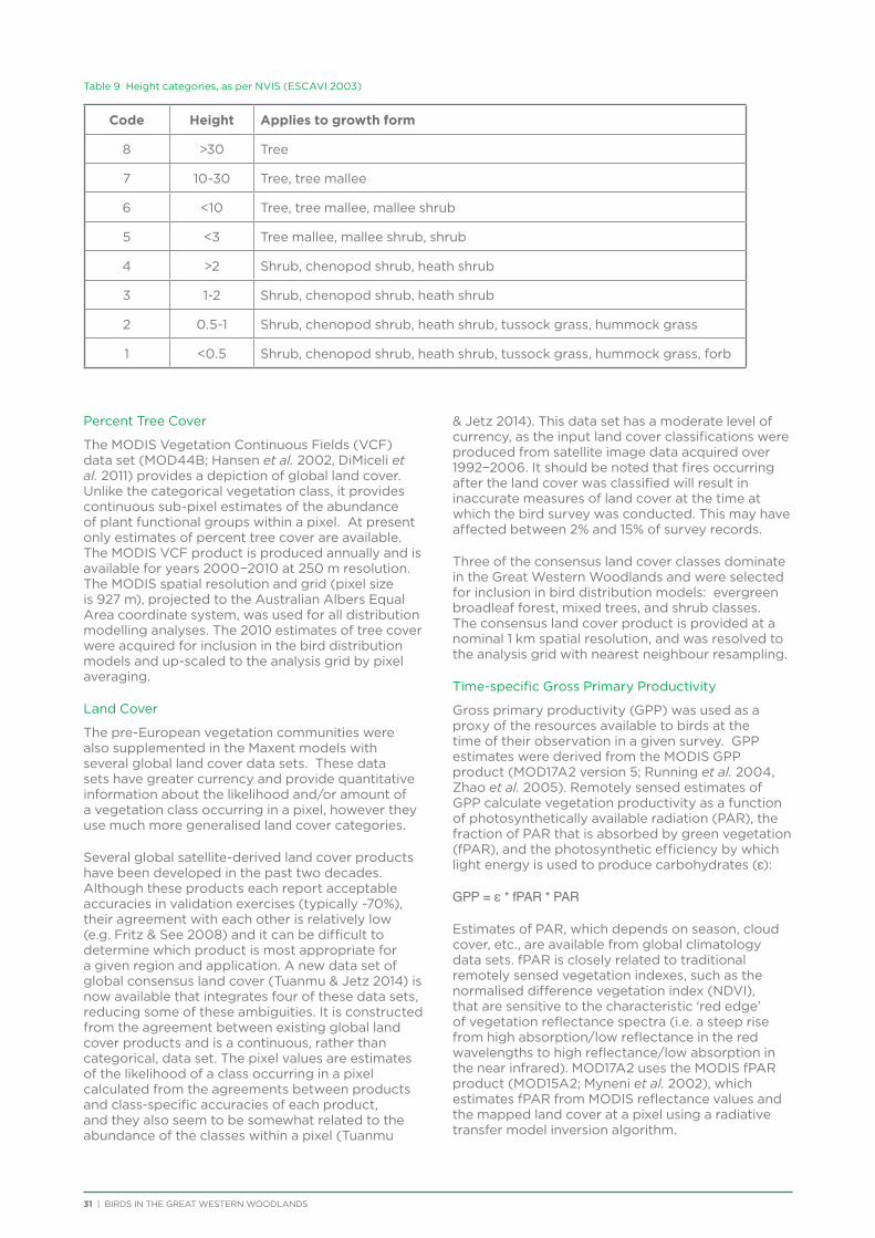
31 | BIRDS IN THE GREAT WESTERN WOODLANDS
Table 9 Height categories, as per NVIS (ESCAVI 2003)
Code Height Applies to growth form
8 >30 Tree
7 10-30 Tree, tree mallee
6 <10 Tree, tree mallee, mallee shrub
5 <3 Tree mallee, mallee shrub, shrub
4 >2 Shrub, chenopod shrub, heath shrub
3 1-2 Shrub, chenopod shrub, heath shrub
2 0.5-1 Shrub, chenopod shrub, heath shrub, tussock grass, hummock grass
1 <0.5 Shrub, chenopod shrub, heath shrub, tussock grass, hummock grass, forb
Percent Tree Cover
The MODIS Vegetation Continuous Fields (VCF) data set (MOD44B; Hansen et al. 2002, DiMiceli et al. 2011) provides a depiction of global land cover. Unlike the categorical vegetation class, it provides continuous sub-pixel estimates of the abundance of plant functional groups within a pixel. At present only estimates of percent tree cover are available. The MODIS VCF product is produced annually and is available for years 2000−2010 at 250 m resolution. The MODIS spatial resolution and grid (pixel size is 927 m), projected to the Australian Albers Equal Area coordinate system, was used for all distribution modelling analyses. The 2010 estimates of tree cover were acquired for inclusion in the bird distribution models and up-scaled to the analysis grid by pixel averaging.
Land Cover
The pre-European vegetation communities were also supplemented in the Maxent models with several global land cover data sets. These data sets have greater currency and provide quantitative information about the likelihood and/or amount of a vegetation class occurring in a pixel, however they use much more generalised land cover categories.
Several global satellite-derived land cover products have been developed in the past two decades. Although these products each report acceptable accuracies in validation exercises (typically ~70%), their agreement with each other is relatively low (e.g. Fritz & See 2008) and it can be difficult to determine which product is most appropriate for a given region and application. A new data set of global consensus land cover (Tuanmu & Jetz 2014) is now available that integrates four of these data sets, reducing some of these ambiguities. It is constructed from the agreement between existing global land cover products and is a continuous, rather than categorical, data set. The pixel values are estimates of the likelihood of a class occurring in a pixel calculated from the agreements between products and class-specific accuracies of each product, and they also seem to be somewhat related to the abundance of the classes within a pixel (Tuanmu
& Jetz 2014). This data set has a moderate level of currency, as the input land cover classifications were produced from satellite image data acquired over 1992−2006. It should be noted that fires occurring after the land cover was classified will result in inaccurate measures of land cover at the time at which the bird survey was conducted. This may have affected between 2% and 15% of survey records.
Three of the consensus land cover classes dominate in the Great Western Woodlands and were selected for inclusion in bird distribution models: evergreen broadleaf forest, mixed trees, and shrub classes. The consensus land cover product is provided at a nominal 1 km spatial resolution, and was resolved to the analysis grid with nearest neighbour resampling.
Time-specific Gross Primary Productivity
Gross primary productivity (GPP) was used as a proxy of the resources available to birds at the time of their observation in a given survey. GPP estimates were derived from the MODIS GPP product (MOD17A2 version 5; Running et al. 2004, Zhao et al. 2005). Remotely sensed estimates of GPP calculate vegetation productivity as a function of photosynthetically available radiation (PAR), the fraction of PAR that is absorbed by green vegetation (fPAR), and the photosynthetic efficiency by which light energy is used to produce carbohydrates (ε):
GPP = ε * fPAR * PAR
Estimates of PAR, which depends on season, cloud cover, etc., are available from global climatology data sets. fPAR is closely related to traditional remotely sensed vegetation indexes, such as the normalised difference vegetation index (NDVI), that are sensitive to the characteristic ‘red edge’ of vegetation reflectance spectra (i.e. a steep rise from high absorption/low reflectance in the red wavelengths to high reflectance/low absorption in the near infrared). MOD17A2 uses the MODIS fPAR product (MOD15A2; Myneni et al. 2002), which estimates fPAR from MODIS reflectance values and the mapped land cover at a pixel using a radiative transfer model inversion algorithm.
BIRDS IN THE GREAT WESTERN WOODLANDS | 32
The fPAR provides a structural estimate of the capacity of green vegetation in a pixel. However, many factors may cause green vegetation to be photosynthesising at less than full capacity or to be dormant. In order to produce a functional estimate of vegetation activity such as gross primary productivity (GPP), it is necessary to modulate fPAR with an estimate of the photosynthetic efficiency, ε, at a given time and place. Estimates of GPP may be more relevant for biodiversity research than the more traditionally used NDVI because of the incorporation of photosynthetic efficiency (Phillips et al. 2008). The MODIS GPP algorithm models ε with attenuation scalers that reduce ε under suboptimal temperatures and drought (represented by vapour pressure deficit) conditions (Running et al. 1999). Weather data were taken from global daily climatologies, and attenuation scalars were optimised for each biome using the BIOME-BGC biogeochemistry model.
MODIS GPP products are produced for a nominal 1 km grid (actual pixel size is 927 m in the study extent) and an 8 day temporal compositing period, and provided in units of kg C/m2. All 8 day MODIS GPP estimates produced for the study area over the time period of June 2011 – October 2014 were acquired and combined into a multi-temporal stack. Bird surveys were linked to the pixel in which they occurred and the compositing period with an end date closest in time to the survey date. Thus, the bird survey may have occurred in the last 4 days of the selected GPP composite, or the first 4 days of the following one. This procedure was followed, rather than simply pairing surveys with the compositing period in which they occurred, to minimise the inclusion of conditions that occurred after the bird survey in the distribution models.
GPP was estimated for nominal 1, 3, and 6 month periods preceding the survey date by calculating the average daily GPP over the 4, 12, and 24 compositing periods before the survey (including the one paired to the survey), respectively. Averages were used because the year is not evenly divided into 8 day periods. Taking the daily average instead of the cumulative GPP accounts for the slightly different length of measurement periods that span the new year.
Long-term GPP dynamics
There is currently a great deal of interest in the role of habitat refuges in arid and semi-arid ecosystems. These sites provide areas of more stable habitat in the context of environmental fluctuations at ecological time scales. Such fluctuations in the surrounding landscape are often driven by disturbances, such as fire or drought. The refuges themselves are protected from these disturbances by physical characteristics such as topographic sheltering or connection to groundwater.
The satellite archive offers the potential to detect candidate refuges (Mackey et al. 2012). Because refuges provide more stable habitat, a measure of the long-term variability (i.e. the converse of stability) of a site may describe the extent to which it can function as a refuge. Here, we used the time series of monthly GPP estimates (MOD17A2 v55; Zhao et al.
2005) over the extant MODIS archive (2001−2013) to quantify the variability/stability of vegetation and evaluate its contribution to bird distributions.
Because the most relevant estimate of temporal variability is unknown, 30 candidate measures were calculated and evaluated. These measures vary in (1) the statistical measure of variability that was calculated and (2) the specific GPP measurements included in the measure of variability. Five variability measures were considered:
i. standard deviation (sd),
ii. coefficient of variation (cv),
iii. range,
iv. minimum value (min), and
v. the difference between the GPP of the wettest and the driest years in the MODIS record (calculated as GPPwet - GPPdry). Australian Water Availability Project (AWAP) annual summaries, averaged over all pixels within the Great Western Woodlands, were used to identify the wettest (2003, with 0.402m rain) and driest (2002, with 0.197m rain) years in the time frame.
Seven different GPP summary values were investigated:
i. monthly GPP (the original data series),
ii. annual GPP (an annual series of GPP values summed over March−Feb for each year),
iii. winter GPP (an annual series of GPP values summed over Jun−Aug),
iv. summer GPP (an annual series of GPP values summed over Dec−Feb),
v. maximum monthly GPP (an annual series of the maximum GPP each year),
vi. minimum monthly GPP (an annual series of the minimum GPP each year), and
vii. the seasonality of GPP (the difference between winter and summer GPP).
These variability statistics and GPP measures were combined to produce 30 candidate metrics (not all possible combinations were assessed) for use in the bird distribution models, but many were highly inter-correlated. In particular, there tended to be strong correlations within sets containing (1) all sd and range measures, (2) all cv measures, and (3) all minimum measures. A final set of seven independent measures of long-term GPP variability was retained: the (1) sd, (2) cv, and (3) minimum of monthly GPP values over the entire series; the wet year-dry year difference of (4) winter, (5) summer, and (6) minimum monthly GPP; and (7) the cv of GPP seasonality.

33 | BIRDS IN THE GREAT WESTERN WOODLANDS
Distance to Granite Outcrop
Outcrops have high biodiversity value and often support distinct flora and fauna species and communities. In addition, they influence surrounding land cover via effects on local hydrology. Specifically, the runoff from outcrops can contribute to greater water availability, resulting in the outcrop acting as a refuge for species during drought. The location of outcrops was taken from the GEODATA TOPO 250K data set (Geoscience Australia 2006). Distance was calculated in kilometres for each pixel of the analysis grid.
Time-specific Rainfall
As with GPP, precipitation was also estimated for the periods prior to the bird surveys. The Australian Water Availability Project (AWAP; Raupach et al. 2009) data set provided gridded precipitation data at 5 km spatial resolution and 7 day temporal resolution. These surfaces are produced by spatial interpolation of weather station records (Jones et al. 2009). The 5 km data were downscaled to the MODIS GPP grid using nearest neighbour resampling. Bird surveys were paired to the 7 day period with an end date closest in time to the survey date and cumulative precipitation was calculated for the 1, 3, and 6 month periods prior to the survey. These time periods were defined as 5, 14, and 27 weeks, to match the time frames from the 8 day MODIS estimates as closely as possible. Unlike the MODIS compositing periods, which are fixed to the same dates in all years, the 7 day precipitation periods are continuous and thus avoid the necessity of an abridged period at the end of the year. As a
result, precipitation sums, instead of daily averages, were estimated for each bird survey.
Long-term Rainfall
Average annual precipitation was used as a general measure of climatic water availability. This variable was calculated from the AWAP annual summaries for the years 1975-2014. It was down-scaled to the analysis grid using nearest neighbour resampling.
The seasonality of rainfall can also be an important determinant of species distributions. The Great Western Woodlands spans a transition from the Mediterranean climate of south-west Western Australia, which receives predominantly winter rainfall, to the arid climate of the interior of the continent, with less marked winter rainfall. To capture this gradient, the proportion of annual rainfall that occurred between May and October (the 6-month “winter” period) was calculated from the AWAP monthly summaries. Percent winter rainfall was averaged for the years 1975−2014 and downscaled to the analysis grid with nearest neighbour resampling.
Season
The season in which each survey was conducted was included in the Maxent models in order to capture any seasonal patterns in distribution, such as migration.
Photo: Liz Fox

BIRDS IN THE GREAT WESTERN WOODLANDS | 34
Disturbance
An index of disturbance (Fitzsimons et al. 2014) was included in the GAM models. It was derived from GIS data for sources and types of current human disturbance. Source data were taken from GEODATA TOPO 250K Series 3 (GeoScience Australia 2006) and included land use (mine areas, built areas, homesteads, recreation areas, mine points, building points, yards), transport (airports, roads, railways, rail points, road crossing lines, railway crosslines, railway stop points), water infrastructure (bores, water holes, wind points, canals, pondage areas), and other infrastructure (fences, conveyors, pipe lines, power lines, water tanks, wind pumps). The disturbance index was the cumulative density of all these features, calculated by a moving-window analysis (circular window of 5 km radius; Fitzsimons et al. 2014). Values ranged from 0 (no mapped anthropogenic disturbance) to over 250 (numerous disturbances).
To measure the general disturbance in the area surrounding a bird survey, the disturbance index was averaged in a 5 km radius circle surrounding the survey coordinate.
The disturbance layer was unable to be included in the Maxent models because the sampling effort was biased to roadside locations.
Distance to Major Roads
Major roads were categorised as primary sealed roads, within and surrounding the Great Western Woodlands, from the GEODATA TOPO 250K data
set (Geoscience Australia 2006). Distance to the nearest road was calculated in km for each pixel of the analysis grid and included in the GAM models. It was unable to be included in the Maxent models because the sampling effort was biased to roadside locations.
Distance to Artificial Watering Points
Artificial water sources such as wells, tanks, and dams can influence wildlife distributions in arid and semi-arid areas through the provision of water, the impact on surrounding vegetation as a result of increased grazing pressure, and an increase in feral predators. This information was included in models with a distance surface to the nearest artificial watering point within the Great Western Woodlands. Point locations of water sources were extracted from the GEODATA TOPO 250K data set (Geoscience Australia 2006). Distance was calculated in km for each pixel of the analysis grid.
Fire
The time since last fire at a survey site was estimated relative to the specific date of each bird survey. Fire boundaries and dates were taken from a GIS data set maintained by the Department of Parks and Wildlife (DPaW 2014). Because of the intricate and overlapping nature of fire boundaries, the date of the most recent fire was initially rasterised at 1/100th the resolution of the analysis grid (i.e. using 92.7m pixels). These were then up-scaled to the resolution of the analyses by taking the most recent fire date that was present within each 927 m pixel of the analysis grid. The age of a fire relative to a survey
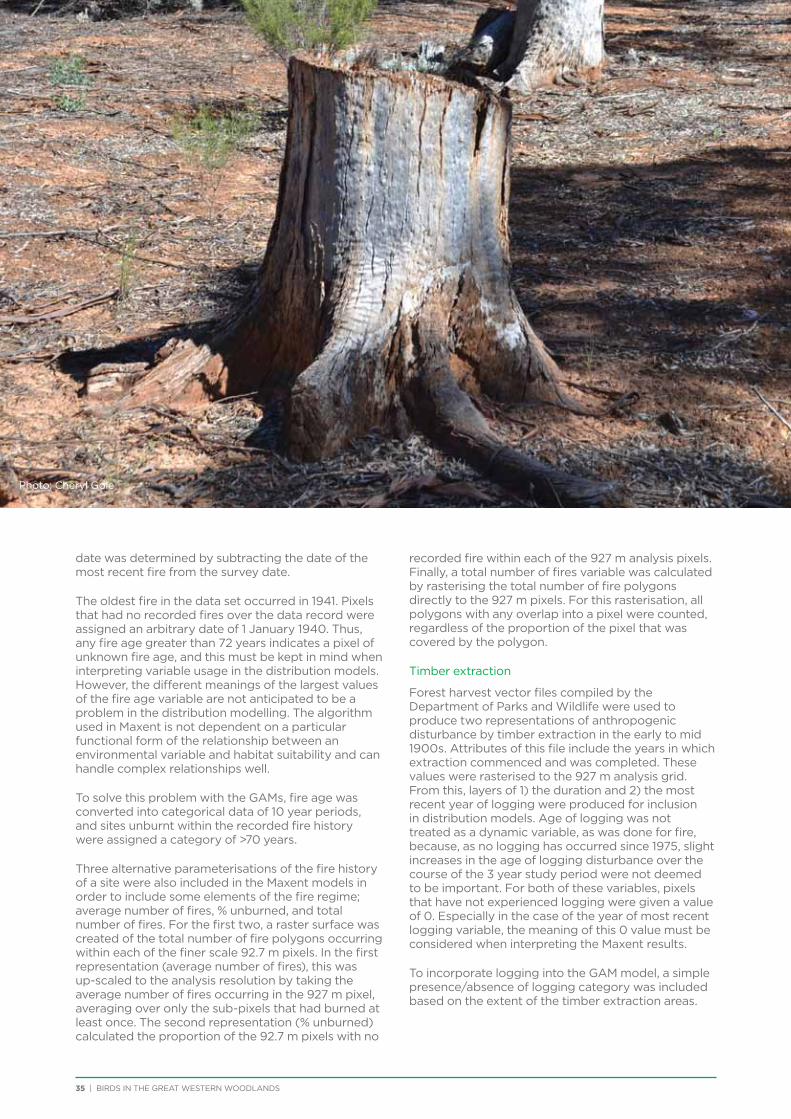
35 | BIRDS IN THE GREAT WESTERN WOODLANDS
date was determined by subtracting the date of the most recent fire from the survey date.
The oldest fire in the data set occurred in 1941. Pixels that had no recorded fires over the data record were assigned an arbitrary date of 1 January 1940. Thus, any fire age greater than 72 years indicates a pixel of unknown fire age, and this must be kept in mind when interpreting variable usage in the distribution models. However, the different meanings of the largest values of the fire age variable are not anticipated to be a problem in the distribution modelling. The algorithm used in Maxent is not dependent on a particular functional form of the relationship between an environmental variable and habitat suitability and can handle complex relationships well.
To solve this problem with the GAMs, fire age was converted into categorical data of 10 year periods, and sites unburnt within the recorded fire history were assigned a category of >70 years.
Three alternative parameterisations of the fire history of a site were also included in the Maxent models in order to include some elements of the fire regime; average number of fires, % unburned, and total number of fires. For the first two, a raster surface was created of the total number of fire polygons occurring within each of the finer scale 92.7 m pixels. In the first representation (average number of fires), this was up-scaled to the analysis resolution by taking the average number of fires occurring in the 927 m pixel, averaging over only the sub-pixels that had burned at least once. The second representation (% unburned) calculated the proportion of the 92.7 m pixels with no
recorded fire within each of the 927 m analysis pixels. Finally, a total number of fires variable was calculated by rasterising the total number of fire polygons directly to the 927 m pixels. For this rasterisation, all polygons with any overlap into a pixel were counted, regardless of the proportion of the pixel that was covered by the polygon.
Timber extraction
Forest harvest vector files compiled by the Department of Parks and Wildlife were used to produce two representations of anthropogenic disturbance by timber extraction in the early to mid 1900s. Attributes of this file include the years in which extraction commenced and was completed. These values were rasterised to the 927 m analysis grid. From this, layers of 1) the duration and 2) the most recent year of logging were produced for inclusion in distribution models. Age of logging was not treated as a dynamic variable, as was done for fire, because, as no logging has occurred since 1975, slight increases in the age of logging disturbance over the course of the 3 year study period were not deemed to be important. For both of these variables, pixels that have not experienced logging were given a value of 0. Especially in the case of the year of most recent logging variable, the meaning of this 0 value must be considered when interpreting the Maxent results.
To incorporate logging into the GAM model, a simple presence/absence of logging category was included based on the extent of the timber extraction areas.
Photo: Cheryl Gole
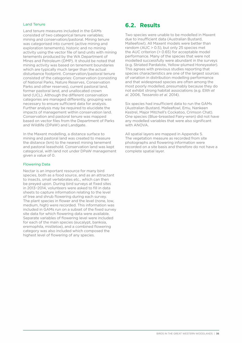
BIRDS IN THE GREAT WESTERN WOODLANDS | 36
Land Tenure
Land tenure measures included in the GAMs consisted of two categorical tenure variables; mining and conservation/pastoral. Mining tenure was categorised into current (active mining and exploration tenements), historic and no mining activity using the vector file of land units with mining tenements produced by the WA Department of Mines and Petroleum (DMP). It should be noted that mining activity was based on tenement boundaries which are typically much larger than the actual disturbance footprint. Conservation/pastoral tenure consisted of the categories: Conservation (consisting of National Parks, Nature Reserves, Conservation Parks and other reserves), current pastoral land, former pastoral land, and unallocated crown land (UCL). Although the different conservation categories are managed differently, grouping was necessary to ensure sufficient data for analysis. Further analysis may be required to elucidate the impacts of management within conservation land. Conservation and pastoral tenure was mapped based on vector files from the Department of Parks and Wildlife (DPaW) and Landgate.
In the Maxent modelling, a distance surface to mining and pastoral land was created to measure the distance (km) to the nearest mining tenement and pastoral leasehold. Conservation land was kept categorical, with land not under DPaW management given a value of 0.
Flowering Data
Nectar is an important resource for many bird species, both as a food source, and as an attractant to insects, small vertebrates etc., which can then be preyed upon. During bird surveys at fixed sites in 2013−2014, volunteers were asked to fill in data sheets to capture information relating to the level of tree and shrub flowering during each survey. The plant species in flower and the level (none, low, medium, high) were recorded. This information was included in GAMs run on a subset of the fixed survey site data for which flowering data were available. Separate variables of flowering level were included for each of the main species (eucalypt, banksia, eremophila, mistletoe), and a combined flowering category was also included which composed the highest level of flowering of any species.
6.2. Results
Two species were unable to be modelled in Maxent due to insufficient data (Australian Bustard, Malleefowl). All Maxent models were better than random (AUC > 0.5), but only 25 species met the AUC criterion (> 0.65) for acceptable model performance. Many of the species that were not modelled successfully were abundant in the surveys (e.g. Striated Pardalote, Yellow-plumed Honeyeater). This agrees with previous studies reporting that species characteristics are one of the largest sources of variation in distribution modelling performance and that widespread species are often among the most poorly modelled, presumably because they do not exhibit strong habitat associations (e.g. Elith et al. 2006, Tessarolo et al. 2014).
Six species had insufficient data to run the GAMs (Australian Bustard, Malleefowl, Emu, Nankeen Kestrel, Major Mitchell’s Cockatoo, Crimson Chat). One species (Blue-breasted Fairy-wren) did not have any modelled variables that were also significant with ANOVA.
All spatial layers are mapped in Appendix 5. The vegetation measure as recorded from site photographs and flowering information were recorded on a site basis and therefore do not have a complete spatial layer.
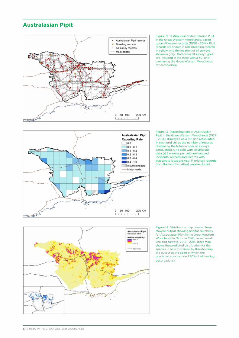
37 | BIRDS IN THE GREAT WESTERN WOODLANDS
Figure 12 Distribution of Australasian Pipit in the Great Western Woodlands, based upon all known records (1900 – 2014). Pipit records are shown in red, breeding records in yellow, and the location of all surveys shown in grey. Data from all survey types are included in the map; with a 30’ grid overlaying the Great Western Woodlands for comparison.
Figure 13 Reporting rate of Australasian Pipit in the Great Western Woodlands (1977 – 2014), displayed on a 30’ grid (calculated in each grid cell as the number of records divided by the total number of surveys conducted). Grid cells with insufficient data (≤ 5 surveys per cell) are hatched. Incidental records and records with inaccurate locations (e.g. 1° grid cell records from the first Bird Atlas) were excluded.
Figure 14 Distribution map created from Maxent output showing habitat suitability for Australasian Pipit in the Great Western Woodlands In October 2013, based on all 2ha bird surveys, 2012 – 2014. Inset map shows the predicted distribution for the species in blue (obtained by thresholding the output at the point at which the predicted area included 90% of all training observations).
Australasian Pipit
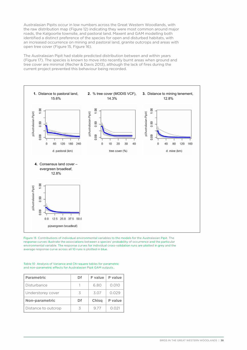
BIRDS IN THE GREAT WESTERN WOODLANDS | 38
Australasian Pipits occur in low numbers across the Great Western Woodlands, with the raw distribution map (Figure 12) indicating they were most common around major roads, the Kalgoorlie townsite, and pastoral land. Maxent and GAM modelling both identified a distinct preference of the species for open and disturbed habitats, with an increased occurrence on mining and pastoral land, granite outcrops and areas with open tree cover (Figure 15, Figure 16).
The Australasian Pipit had stable predicted distribution between and within years (Figure 17). The species is known to move into recently burnt areas when ground and tree cover are minimal (Recher & Davis 2013), although the lack of fires during the current project prevented this behaviour being recorded.
Figure 15 Contributions of individual environmental variables to the models for the Australasian Pipit. The response curves illustrate the associations between a species’ probability of occurrence and the particular environmental variable. The response curves for individual cross-validation runs are plotted in grey and the average response curve across all 10 runs is plotted in blue.
Table 10 Analysis of Variance and Chi-square tables for parametric and non-parametric effects for Australasian Pipit GAM outputs..
Parametric Df F value P value
Disturbance 1 6.80 0.010
Understorey cover 3 3.07 0.029
Non-parametric Df Chisq P value
Distance to outcrop 3 9.77 0.021
1. Distance to pastoral land, 15.6%
2. % tree cover (MODIS VCF), 14.3%
3. Distance to mining tenement, 12.8%
4. Consensus land cover – evergreen broadleaf,
12.8%
p(A
ustr
alas
ian
Pip
it)
p(A
ustr
alas
ian
Pip
it)
p(Au
stra
lasi
an P
ipit)
p(Au
stra
lasi
an P
ipit)
p(Au
stra
lasi
an P
ipit)
p(Au
stra
lasi
an P
ipit)
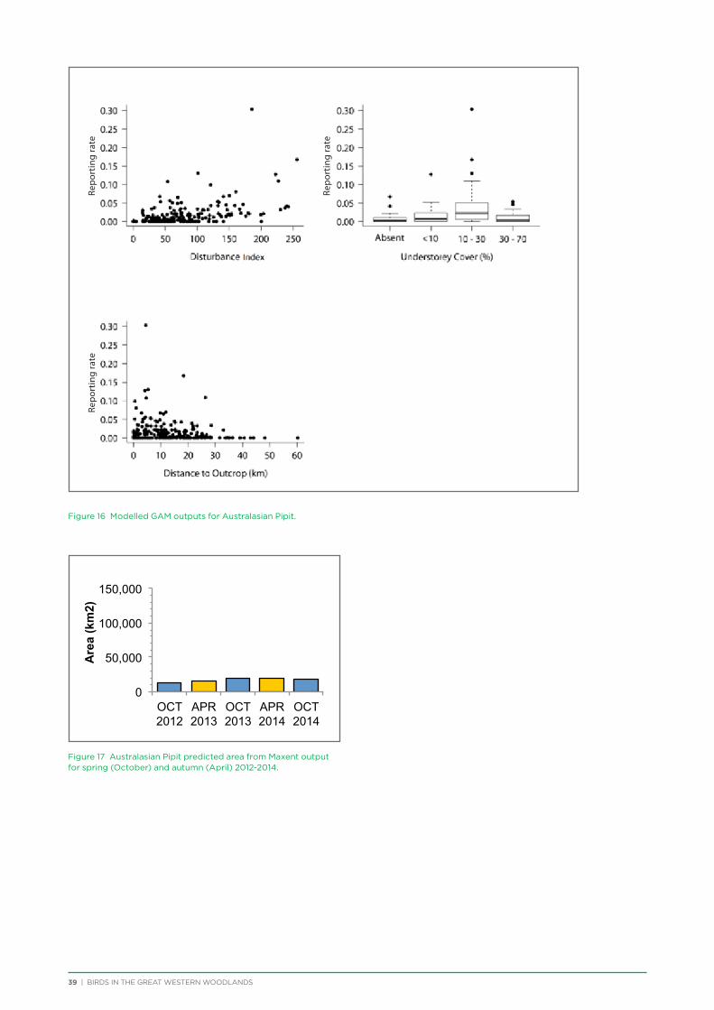
39 | BIRDS IN THE GREAT WESTERN WOODLANDS
Figure 16 Modelled GAM outputs for Australasian Pipit.
Figure 17 Australasian Pipit predicted area from Maxent output for spring (October) and autumn (April) 2012-2014.
0
50,000
100,000
150,000
OCT 2012
APR 2013
OCT 2013
APR 2014
OCT 2014
Are
a (k
m2)
Repo
rtin
g ra
teRe
port
ing
rate
Repo
rtin
g ra
te
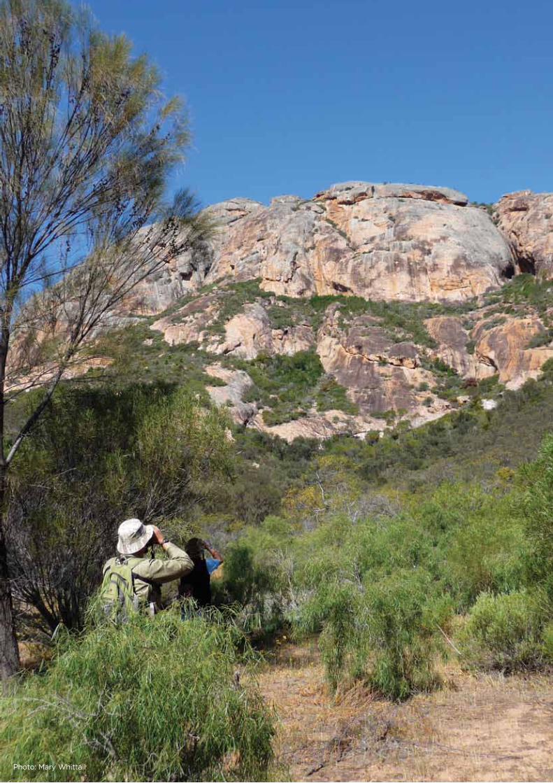
BIRDS IN THE GREAT WESTERN WOODLANDS | 40Photo: Mary Whittall
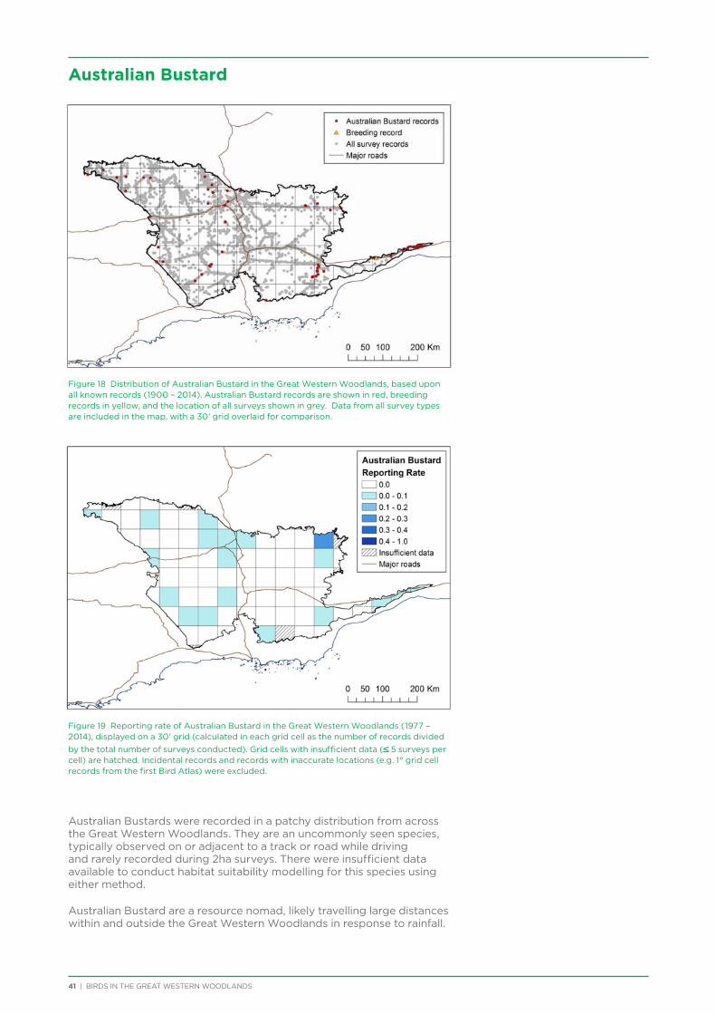
41 | BIRDS IN THE GREAT WESTERN WOODLANDS
Australian Bustard
Figure 18 Distribution of Australian Bustard in the Great Western Woodlands, based upon all known records (1900 – 2014). Australian Bustard records are shown in red, breeding records in yellow, and the location of all surveys shown in grey. Data from all survey types are included in the map, with a 30’ grid overlaid for comparison.
Figure 19 Reporting rate of Australian Bustard in the Great Western Woodlands (1977 – 2014), displayed on a 30’ grid (calculated in each grid cell as the number of records divided by the total number of surveys conducted). Grid cells with insufficient data (≤ 5 surveys per cell) are hatched. Incidental records and records with inaccurate locations (e.g. 1° grid cell records from the first Bird Atlas) were excluded.
Australian Bustards were recorded in a patchy distribution from across the Great Western Woodlands. They are an uncommonly seen species, typically observed on or adjacent to a track or road while driving and rarely recorded during 2ha surveys. There were insufficient data available to conduct habitat suitability modelling for this species using either method.
Australian Bustard are a resource nomad, likely travelling large distances within and outside the Great Western Woodlands in response to rainfall.
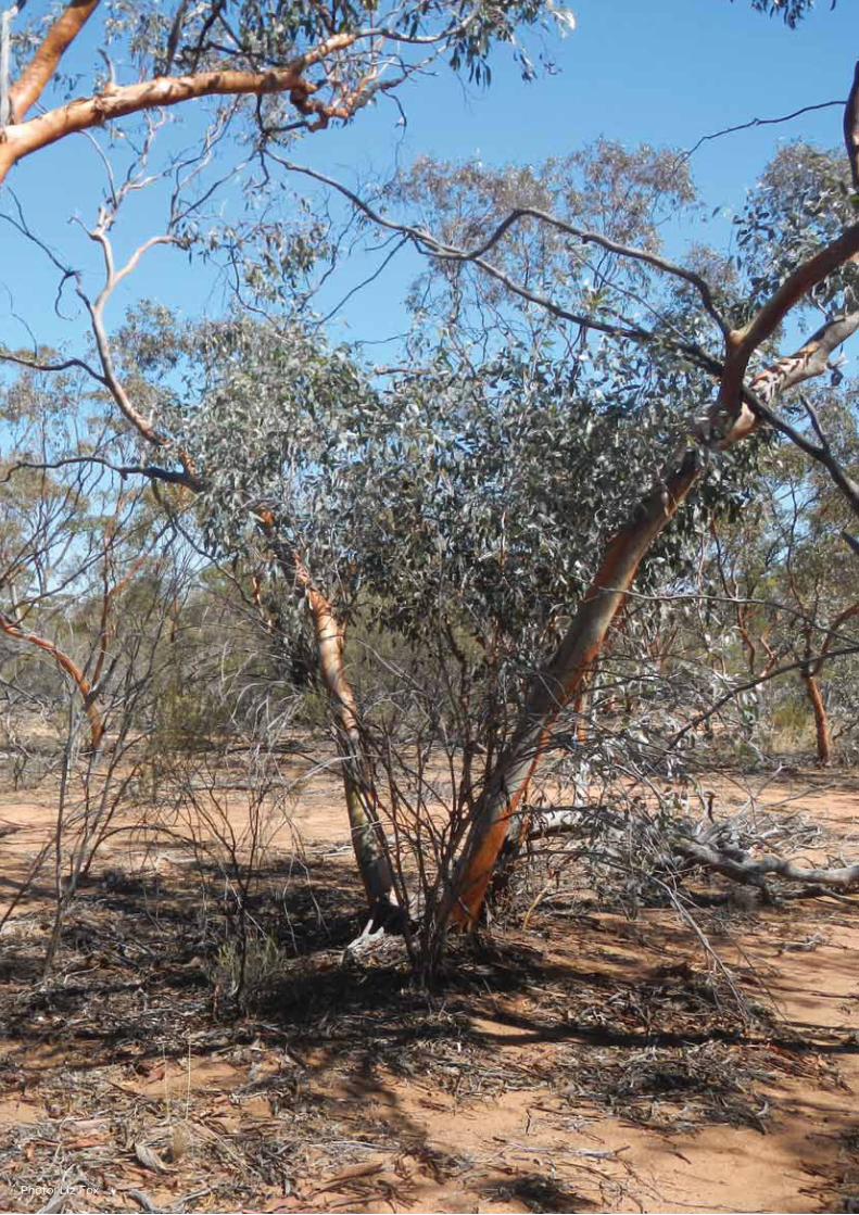
BIRDS IN THE GREAT WESTERN WOODLANDS | 42Photo: Liz Fox
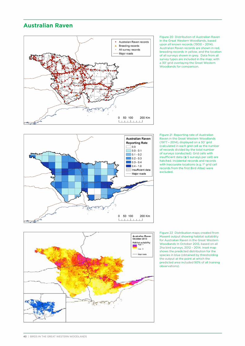
43 | BIRDS IN THE GREAT WESTERN WOODLANDS
Figure 20 Distribution of Australian Raven in the Great Western Woodlands, based upon all known records (1900 – 2014). Australian Raven records are shown in red, breeding records in yellow, and the location of all surveys shown in grey. Data from all survey types are included in the map; with a 30’ grid overlaying the Great Western Woodlands for comparison.
Figure 21 Reporting rate of Australian Raven in the Great Western Woodlands (1977 – 2014), displayed on a 30’ grid (calculated in each grid cell as the number of records divided by the total number of surveys conducted). Grid cells with insufficient data (≤ 5 surveys per cell) are hatched. Incidental records and records with inaccurate locations (e.g. 1° grid cell records from the first Bird Atlas) were excluded.
Figure 22 Distribution maps created from Maxent output showing habitat suitability for Australian Raven in the Great Western Woodlands In October 2013, based on all 2ha bird surveys, 2012 – 2014. Inset map shows the predicted distribution for the species in blue (obtained by thresholding the output at the point at which the predicted area included 90% of all training observations).
Australian Raven

BIRDS IN THE GREAT WESTERN WOODLANDS | 44
Although occurring throughout the Great Western Woodlands, Australian Raven distribution was influenced by human impacts. The reporting rate map (Figure 21) indicates a preference for major roads and towns. Since Maxent was not able to include disturbance or distance to major road as explanatory variables, these were not included in the final model, but the GAM did show a relationship with the level of disturbance (Table 11, Figure 24). Maxent identified distance to artificial watering point and pastoral land as contributing to the modelled species distribution (Figure 23) – both features that are included in the combined disturbance measure. Australian Ravens occurred in higher abundance in these more disturbed areas, and were also modelled by the GAM as occurring more commonly in mining tenements, being most common in current mining tenements, but also showing a higher occurrence even in historic tenements.
The inclusion of site vegetation characteristics in the GAM resulted in upper canopy and ground vegetation cover being important, with Australian Ravens predominantly occurring in open areas with sparse canopy cover.
Australian Ravens showed the greatest temporal constancy in predicted area of all the selected species, with fluctuations of only 3% of its predicted spatial extent between April and October 2012-2014 (Figure 25). This is likely a result of the stable provision of food and water resources from pastoral and agricultural land and towns.
Figure 23 Contributions of individual environmental variables to the models for the Australian Raven. The response curves illustrate the associations between a species’ probability of occurrence and the particular environmental variable. The response curves for individual cross-validation runs are plotted in grey and the average response curve across all 10 runs is plotted in blue.
Table 11 Analysis of Variance for parametric effects table for Australian Raven GAM outputs.
Df F value P value
Upper canopy cover 4 4.06 0.003
Disturbance 1 6.35 0.012
Understorey cover 3 2.52 0.059
Mining tenement 2 2.64 0.074
1. Distance to watering point, 22.8%
2. Distance to pastoral land, 14.7%
3. Average annual precipitation, 11.9%
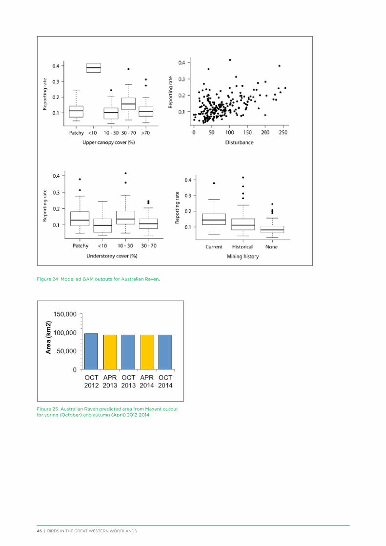
45 | BIRDS IN THE GREAT WESTERN WOODLANDS
Figure 24 Modelled GAM outputs for Australian Raven.
Figure 25 Australian Raven predicted area from Maxent output for spring (October) and autumn (April) 2012-2014.
Repo
rtin
g ra
te
Repo
rtin
g ra
te
Repo
rtin
g ra
te
Repo
rtin
g ra
te
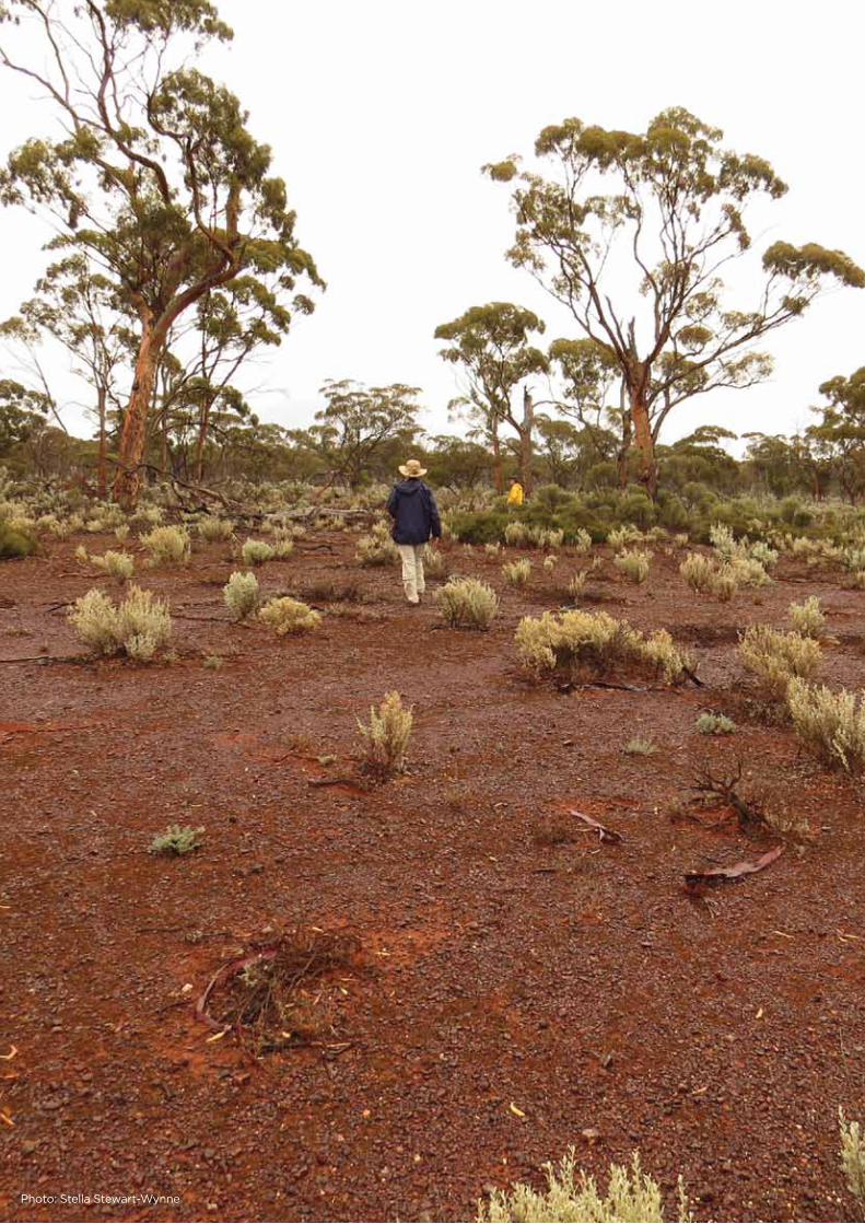
BIRDS IN THE GREAT WESTERN WOODLANDS | 46Photo: Stella Stewart-Wynne
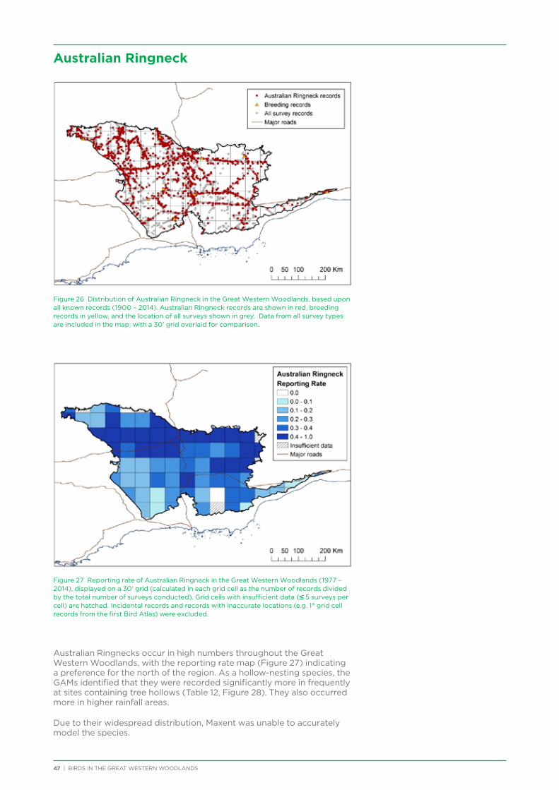
47 | BIRDS IN THE GREAT WESTERN WOODLANDS
Australian Ringneck
Figure 26 Distribution of Australian Ringneck in the Great Western Woodlands, based upon all known records (1900 – 2014). Australian Ringneck records are shown in red, breeding records in yellow, and the location of all surveys shown in grey. Data from all survey types are included in the map; with a 30’ grid overlaid for comparison.
Figure 27 Reporting rate of Australian Ringneck in the Great Western Woodlands (1977 – 2014), displayed on a 30’ grid (calculated in each grid cell as the number of records divided by the total number of surveys conducted). Grid cells with insufficient data (≤ 5 surveys per cell) are hatched. Incidental records and records with inaccurate locations (e.g. 1° grid cell records from the first Bird Atlas) were excluded.
Australian Ringnecks occur in high numbers throughout the Great Western Woodlands, with the reporting rate map (Figure 27) indicating a preference for the north of the region. As a hollow-nesting species, the GAMs identified that they were recorded significantly more in frequently at sites containing tree hollows (Table 12, Figure 28). They also occurred more in higher rainfall areas.
Due to their widespread distribution, Maxent was unable to accurately model the species.
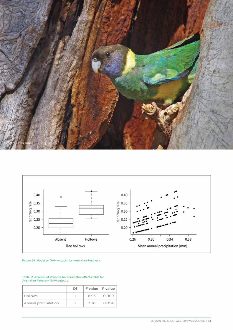
BIRDS IN THE GREAT WESTERN WOODLANDS | 48
Figure 28 Modelled GAM outputs for Australian Ringneck.
Table 12 Analysis of Variance for parametric effects table for Australian Ringneck GAM outputs.
Df F value P value
Hollows 1 6.95 0.009
Annual precipitation 1 3.76 0.054
Photo: Chris Tate
Repo
rtin
g ra
te
Repo
rtin
g ra
te
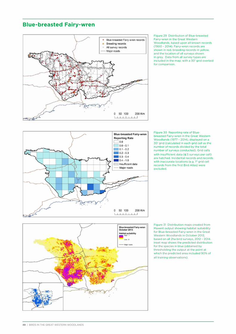
49 | BIRDS IN THE GREAT WESTERN WOODLANDS
Figure 29 Distribution of Blue-breasted Fairy-wren in the Great Western Woodlands, based upon all known records (1900 – 2014). Fairy-wren records are shown in red, breeding records in yellow, and the location of all surveys shown in grey. Data from all survey types are included in the map; with a 30’ grid overlaid for comparison.
Figure 30 Reporting rate of Blue-breasted Fairy-wren in the Great Western Woodlands (1977 – 2014), displayed on a 30’ grid (calculated in each grid cell as the number of records divided by the total number of surveys conducted). Grid cells with insufficient data (≤ 5 surveys per cell) are hatched. Incidental records and records with inaccurate locations (e.g. 1° grid cell records from the first Bird Atlas) were excluded.
Figure 31 Distribution maps created from Maxent output showing habitat suitability for Blue-breasted Fairy-wren in the Great Western Woodlands in October 2013, based on all 2ha bird surveys, 2012 – 2014. Inset map shows the predicted distribution for the species in blue (obtained by thresholding the output at the point at which the predicted area included 90% of all training observations).
Blue-breasted Fairy-wren
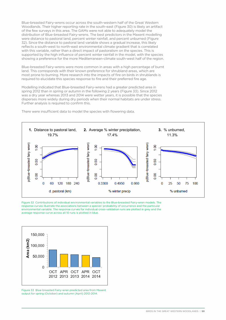
BIRDS IN THE GREAT WESTERN WOODLANDS | 50
Blue-breasted Fairy-wrens occur across the south-western half of the Great Western Woodlands. Their higher reporting rate in the south-east (Figure 30) is likely an artifact of the few surveys in this area. The GAMs were not able to adequately model the distribution of Blue-breasted Fairy-wrens. The best predictors in the Maxent modelling were distance to pastoral land, percent winter rainfall, and percent unburned (Figure 32). Since the distance to pastoral land variable shows a gradual increase, this likely reflects a south-west to north-east environmental climate gradient that is correlated with this variable, rather than a direct impact of pastoralism on the species. This is supported by the high influence of percent winter rainfall in the model, with the species showing a preference for the more Mediterranean-climate south-west half of the region.
Blue-breasted Fairy-wrens were more common in areas with a high percentage of burnt land. This corresponds with their known preference for shrubland areas, which are most prone to burning. More research into the impacts of fire on birds in shrublands is required to elucidate this species response to fire and their preferred fire age.
Modelling indicated that Blue-breasted Fairy-wrens had a greater predicted area in spring 2012 than in spring or autumn in the following 2 years (Figure 33). Since 2012 was a dry year whereas 2013 and 2014 were wetter years, it is possible that the species disperses more widely during dry periods when their normal habitats are under stress. Further analysis is required to confirm this.
There were insufficient data to model the species with flowering data.
Figure 32 Contributions of individual environmental variables to the Blue-breasted Fairy-wren models. The response curves illustrate the associations between a species’ probability of occurrence and the particular environmental variable. The response curves for individual cross-validation runs are plotted in grey and the average response curve across all 10 runs is plotted in blue.
Figure 33 Blue-breasted Fairy-wren predicted area from Maxent output for spring (October) and autumn (April) 2012-2014.
1. Distance to pastoral land, 19.7%
2. Average % winter precipitation, 17.4%
3. % unburned, 11.3%
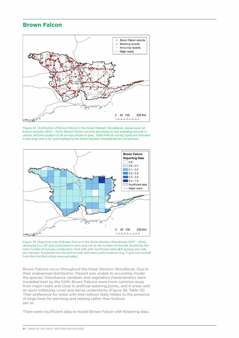
51 | BIRDS IN THE GREAT WESTERN WOODLANDS
Brown Falcon
Figure 34 Distribution of Brown Falcon in the Great Western Woodlands, based upon all known records (1900 – 2014). Brown Falcon records are shown in red, breeding records in yellow, and the location of all surveys shown in grey. Data from all survey types are included in the map; with a 30’ grid overlaying the Great Western Woodlands for comparison.
Figure 35 Reporting rate of Brown Falcon in the Great Western Woodlands (1977 – 2014), displayed on a 30’ grid (calculated in each grid cell as the number of records divided by the total number of surveys conducted). Grid cells with insufficient data (≤ 5 surveys per cell) are hatched. Incidental records and records with inaccurate locations (e.g. 1° grid cell records from the first Bird Atlas) were excluded.
Brown Falcons occur throughout the Great Western Woodlands. Due to their widespread distribution, Maxent was unable to accurately model the species. Disturbance variables and vegetation characteristics were modelled best by the GAM. Brown Falcons were more common away from major roads and close to artificial watering points, and in areas with an open midstorey cover and dense understorey (Figure 36, Table 13). Their preference for areas with tree hollows likely relates to the presence of large trees for perching and nesting rather than hollows per se.
There were insufficient data to model Brown Falcon with flowering data.
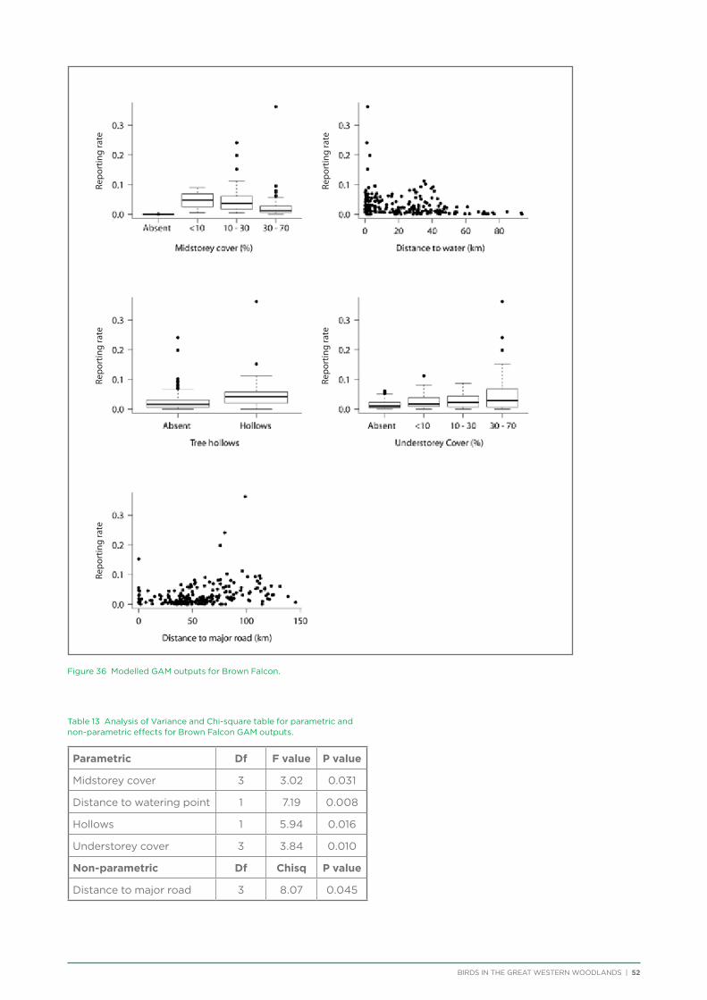
BIRDS IN THE GREAT WESTERN WOODLANDS | 52
Figure 36 Modelled GAM outputs for Brown Falcon.
Table 13 Analysis of Variance and Chi-square table for parametric and non-parametric effects for Brown Falcon GAM outputs.
Parametric Df F value P value
Midstorey cover 3 3.02 0.031
Distance to watering point 1 7.19 0.008
Hollows 1 5.94 0.016
Understorey cover 3 3.84 0.010
Non-parametric Df Chisq P value
Distance to major road 3 8.07 0.045
Repo
rtin
g ra
te
Repo
rtin
g ra
teRe
port
ing
rate
Repo
rtin
g ra
teRe
port
ing
rate
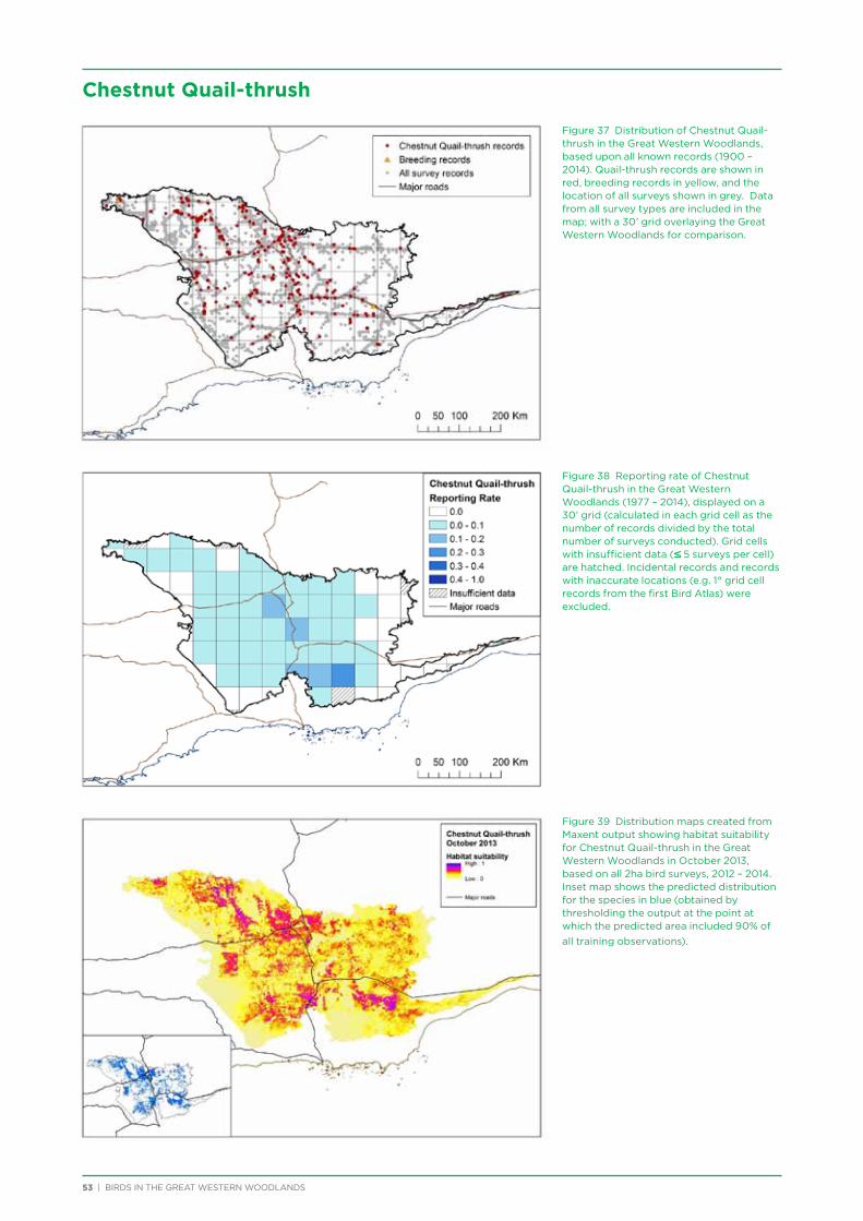
53 | BIRDS IN THE GREAT WESTERN WOODLANDS
Figure 37 Distribution of Chestnut Quail-thrush in the Great Western Woodlands, based upon all known records (1900 – 2014). Quail-thrush records are shown in red, breeding records in yellow, and the location of all surveys shown in grey. Data from all survey types are included in the map; with a 30’ grid overlaying the Great Western Woodlands for comparison.
Figure 38 Reporting rate of Chestnut Quail-thrush in the Great Western Woodlands (1977 – 2014), displayed on a 30’ grid (calculated in each grid cell as the number of records divided by the total number of surveys conducted). Grid cells with insufficient data (≤ 5 surveys per cell) are hatched. Incidental records and records with inaccurate locations (e.g. 1° grid cell records from the first Bird Atlas) were excluded.
Figure 39 Distribution maps created from Maxent output showing habitat suitability for Chestnut Quail-thrush in the Great Western Woodlands in October 2013, based on all 2ha bird surveys, 2012 – 2014. Inset map shows the predicted distribution for the species in blue (obtained by thresholding the output at the point at which the predicted area included 90% of all training observations).
Chestnut Quail-thrush

BIRDS IN THE GREAT WESTERN WOODLANDS | 54
Chestnut Quail-thrush occurred across the Great Western Woodlands, although they were absent close to the western, southern and eastern boundaries of the region (Figure 38). They were modelled as being sensitive to pastoralism, with a higher reporting away from pastoral land and the lowest reporting rate in former pastoral leaseholds compared to other conservation lands (Figure 40). They occurred in areas with a mid-range percent winter precipitation as they were less common in the south-west and east of the region (Figure 38). In the GAMs their distribution was best modelled by areas of higher tree cover and in areas of higher long-term variability in GPP (Figure 41, Table 14).
The predicted area for Chestnut Quail-thrush showed a slight seasonal variation (Figure 42), potentially a result of the lower chance of recording the species during the breeding season when birds are sitting on the nest.
There were insufficient data to model this species with flowering data.
Figure 40 Contributions of individual environmental variables to the Chestnut Quail-thrush models. The response curves illustrate the associations between a species’ probability of occurrence and the particular environmental variable. The response curves for individual. cross-validation runs are plotted in grey and the average response curve across all 10 runs is plotted in blue.
* Conservation land category: 0) Not protected 1) other reserve 4) Conservation Park 6) Former Leasehold 11) National Park 12) Nature Reserve 14) Timber reserve.
Table 14 Analysis of Variance for parametric effects table for Chestnut Quail-thrush GAM outputs.
Df F value P value
Percent tree cover 1 5.59 0.019
GPP variability (sd) 1 3.75 0.054
1. Distance to pastoral land, 16.8%
2. Average % winter precipitation, 12.8%
3. Conservation land category*, 12.7%
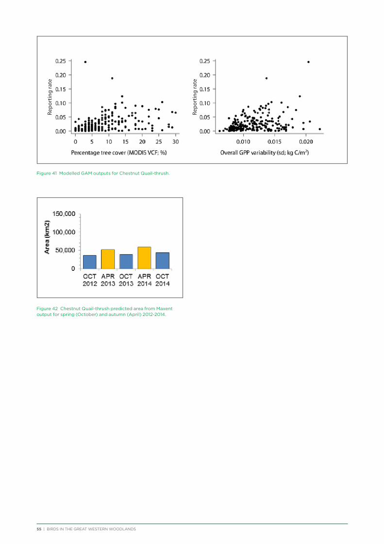
55 | BIRDS IN THE GREAT WESTERN WOODLANDS
Figure 41 Modelled GAM outputs for Chestnut Quail-thrush.
Figure 42 Chestnut Quail-thrush predicted area from Maxent output for spring (October) and autumn (April) 2012-2014.
Repo
rtin
g ra
te
Repo
rtin
g ra
te
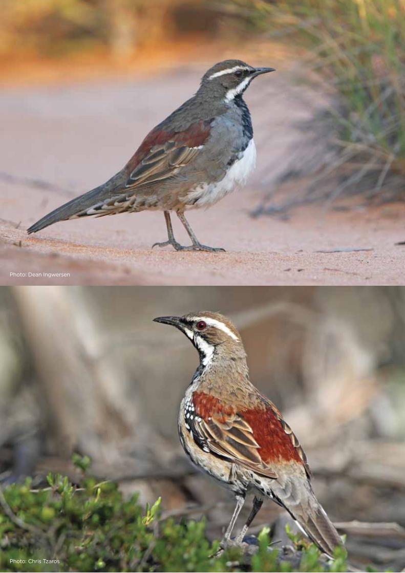
BIRDS IN THE GREAT WESTERN WOODLANDS | 56
Photo: Chris Tzaros
Photo: Dean Ingwersen
Photo: Chris Tzaros
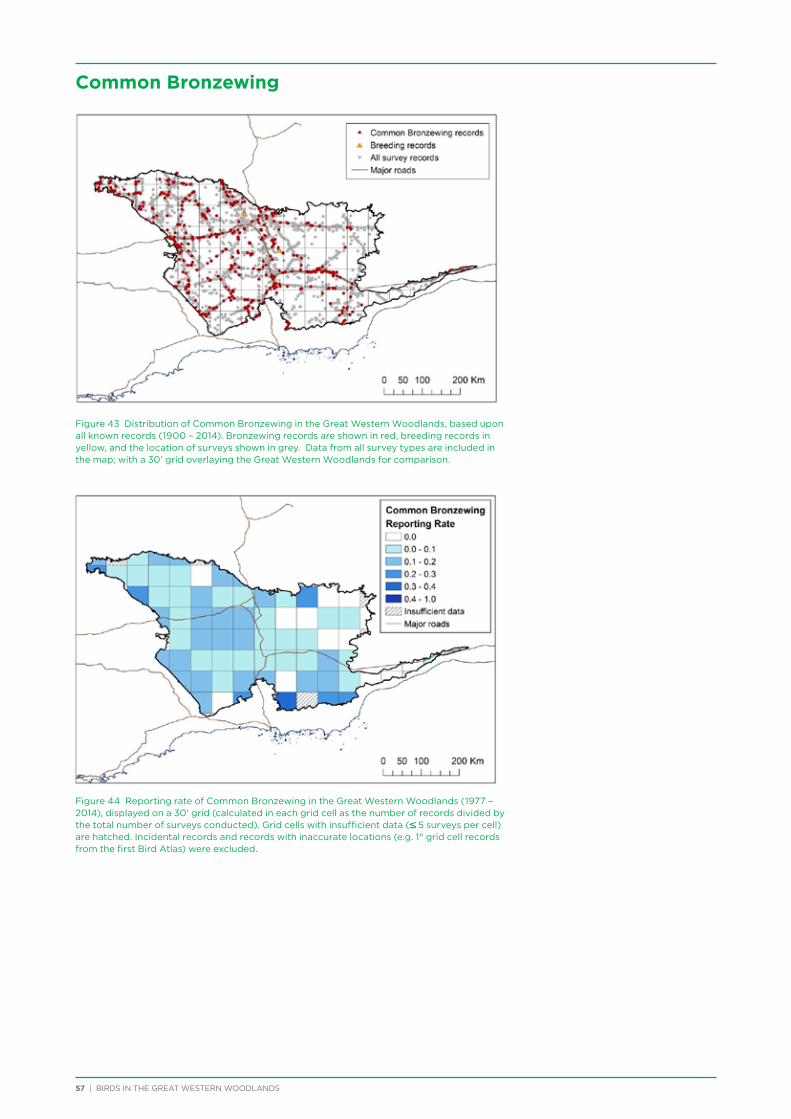
57 | BIRDS IN THE GREAT WESTERN WOODLANDS
Common Bronzewing
Figure 43 Distribution of Common Bronzewing in the Great Western Woodlands, based upon all known records (1900 – 2014). Bronzewing records are shown in red, breeding records in yellow, and the location of surveys shown in grey. Data from all survey types are included in the map; with a 30’ grid overlaying the Great Western Woodlands for comparison.
Figure 44 Reporting rate of Common Bronzewing in the Great Western Woodlands (1977 – 2014), displayed on a 30’ grid (calculated in each grid cell as the number of records divided by the total number of surveys conducted). Grid cells with insufficient data (≤ 5 surveys per cell) are hatched. Incidental records and records with inaccurate locations (e.g. 1° grid cell records from the first Bird Atlas) were excluded.
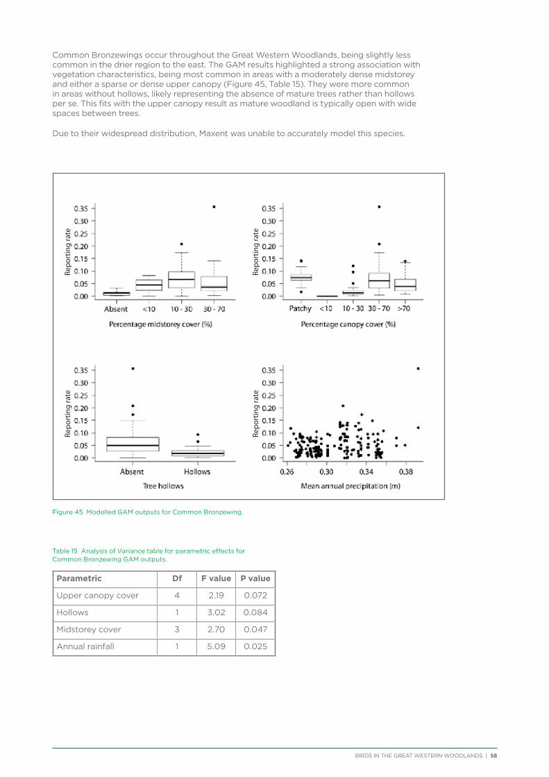
BIRDS IN THE GREAT WESTERN WOODLANDS | 58
Common Bronzewings occur throughout the Great Western Woodlands, being slightly less common in the drier region to the east. The GAM results highlighted a strong association with vegetation characteristics, being most common in areas with a moderately dense midstorey and either a sparse or dense upper canopy (Figure 45, Table 15). They were more common in areas without hollows, likely representing the absence of mature trees rather than hollows per se. This fits with the upper canopy result as mature woodland is typically open with wide spaces between trees.
Due to their widespread distribution, Maxent was unable to accurately model this species.
Figure 45 Modelled GAM outputs for Common Bronzewing.
Table 15 Analysis of Variance table for parametric effects for Common Bronzewing GAM outputs.
Parametric Df F value P value
Upper canopy cover 4 2.19 0.072
Hollows 1 3.02 0.084
Midstorey cover 3 2.70 0.047
Annual rainfall 1 5.09 0.025
Repo
rtin
g ra
teRe
port
ing
rate
Repo
rtin
g ra
teRe
port
ing
rate
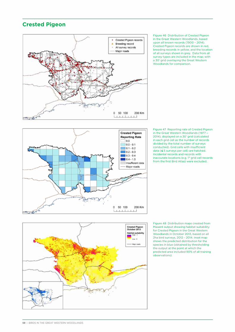
59 | BIRDS IN THE GREAT WESTERN WOODLANDS
Figure 46 Distribution of Crested Pigeon in the Great Western Woodlands, based upon all known records (1900 – 2014). Crested Pigeon records are shown in red, breeding records in yellow, and the location of all surveys shown in grey. Data from all survey types are included in the map; with a 30’ grid overlaying the Great Western Woodlands for comparison.
Figure 47 Reporting rate of Crested Pigeon in the Great Western Woodlands (1977 – 2014), displayed on a 30’ grid (calculated in each grid cell as the number of records divided by the total number of surveys conducted). Grid cells with insufficient data (≤ 5 surveys per cell) are hatched. Incidental records and records with inaccurate locations (e.g. 1° grid cell records from the first Bird Atlas) were excluded.
Figure 48 Distribution maps created from Maxent output showing habitat suitability for Crested Pigeon in the Great Western Woodlands in October 2013, based on all 2ha bird surveys, 2012 – 2014. Inset map shows the predicted distribution for the species in blue (obtained by thresholding the output at the point at which the predicted area included 90% of all training observations).
Crested Pigeon
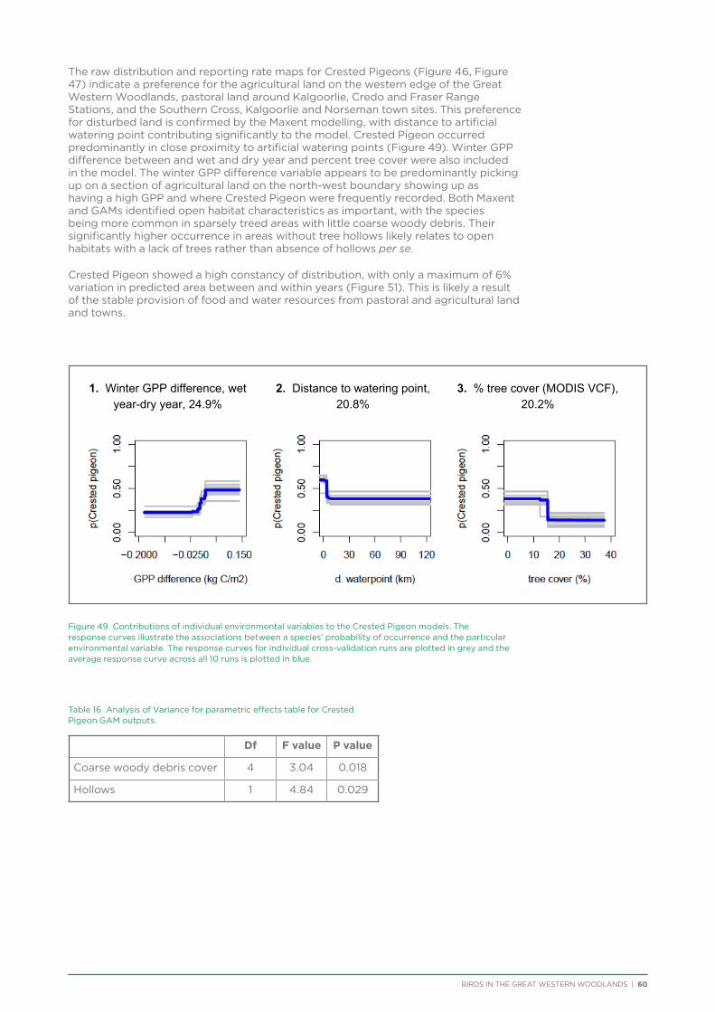
BIRDS IN THE GREAT WESTERN WOODLANDS | 60
The raw distribution and reporting rate maps for Crested Pigeons (Figure 46, Figure 47) indicate a preference for the agricultural land on the western edge of the Great Western Woodlands, pastoral land around Kalgoorlie, Credo and Fraser Range Stations, and the Southern Cross, Kalgoorlie and Norseman town sites. This preference for disturbed land is confirmed by the Maxent modelling, with distance to artificial watering point contributing significantly to the model. Crested Pigeon occurred predominantly in close proximity to artificial watering points (Figure 49). Winter GPP difference between and wet and dry year and percent tree cover were also included in the model. The winter GPP difference variable appears to be predominantly picking up on a section of agricultural land on the north-west boundary showing up as having a high GPP and where Crested Pigeon were frequently recorded. Both Maxent and GAMs identified open habitat characteristics as important, with the species being more common in sparsely treed areas with little coarse woody debris. Their significantly higher occurrence in areas without tree hollows likely relates to open habitats with a lack of trees rather than absence of hollows per se.
Crested Pigeon showed a high constancy of distribution, with only a maximum of 6% variation in predicted area between and within years (Figure 51). This is likely a result of the stable provision of food and water resources from pastoral and agricultural land and towns.
Figure 49 Contributions of individual environmental variables to the Crested Pigeon models. The response curves illustrate the associations between a species’ probability of occurrence and the particular environmental variable. The response curves for individual cross-validation runs are plotted in grey and the average response curve across all 10 runs is plotted in blue.
Table 16 Analysis of Variance for parametric effects table for Crested Pigeon GAM outputs.
Df F value P value
Coarse woody debris cover 4 3.04 0.018
Hollows 1 4.84 0.029
1. Winter GPP difference, wet year-dry year, 24.9%
2. Distance to watering point, 20.8%
3. % tree cover (MODIS VCF), 20.2%
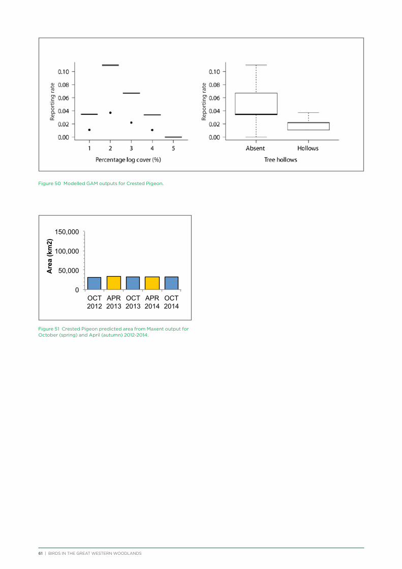
61 | BIRDS IN THE GREAT WESTERN WOODLANDS
Figure 50 Modelled GAM outputs for Crested Pigeon.
Figure 51 Crested Pigeon predicted area from Maxent output for October (spring) and April (autumn) 2012-2014.
0
50,000
100,000
150,000
OCT 2012
APR 2013
OCT 2013
APR 2014
OCT 2014
Are
a (k
m2)
Re
port
ing
rate
Repo
rtin
g ra
te
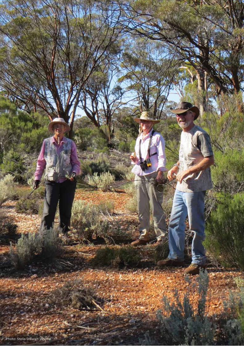
BIRDS IN THE GREAT WESTERN WOODLANDS | 62Photo: Stella Stewart-Wynne
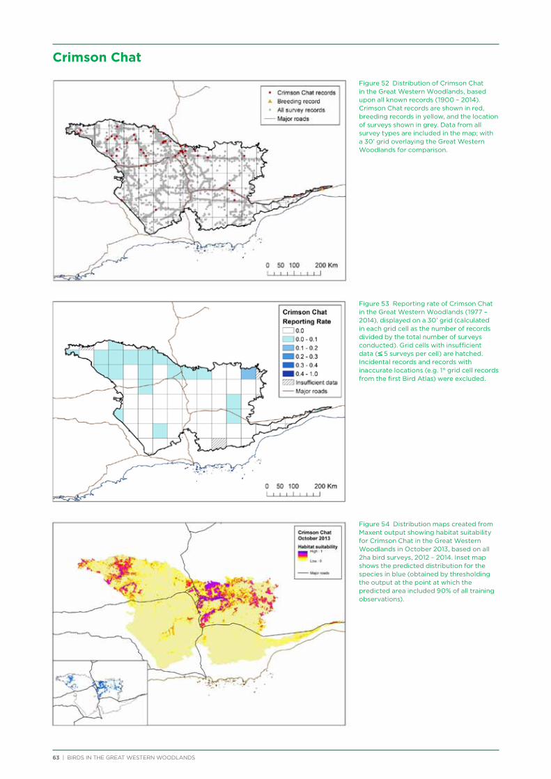
63 | BIRDS IN THE GREAT WESTERN WOODLANDS
Figure 52 Distribution of Crimson Chat in the Great Western Woodlands, based upon all known records (1900 – 2014). Crimson Chat records are shown in red, breeding records in yellow, and the location of surveys shown in grey. Data from all survey types are included in the map; with a 30’ grid overlaying the Great Western Woodlands for comparison.
Figure 53 Reporting rate of Crimson Chat in the Great Western Woodlands (1977 – 2014), displayed on a 30’ grid (calculated in each grid cell as the number of records divided by the total number of surveys conducted). Grid cells with insufficient data (≤ 5 surveys per cell) are hatched. Incidental records and records with inaccurate locations (e.g. 1° grid cell records from the first Bird Atlas) were excluded.
Figure 54 Distribution maps created from Maxent output showing habitat suitability for Crimson Chat in the Great Western Woodlands in October 2013, based on all 2ha bird surveys, 2012 – 2014. Inset map shows the predicted distribution for the species in blue (obtained by thresholding the output at the point at which the predicted area included 90% of all training observations).
Crimson Chat
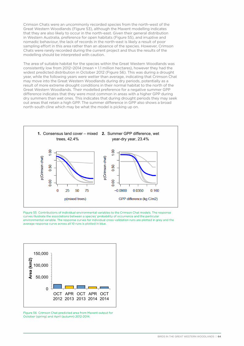
BIRDS IN THE GREAT WESTERN WOODLANDS | 64
Crimson Chats were an uncommonly recorded species from the north-west of the Great Western Woodlands (Figure 53), although the Maxent modelling indicates that they are also likely to occur in the north-east. Given their general distribution in Western Australia, preference for open habitats (Figure 55), and irruptive and nomadic behaviour, the lack of records in the north-east is likely a result of poor sampling effort in this area rather than an absence of the species. However, Crimson Chats were rarely recorded during the current project and thus the results of the modelling should be interpreted with caution.
The area of suitable habitat for the species within the Great Western Woodlands was consistently low from 2012−2014 (mean = 1.1 million hectares), however they had the widest predicted distribution in October 2012 (Figure 56). This was during a drought year, while the following years were wetter than average, indicating that Crimson Chat may move into the Great Western Woodlands during dry periods, potentially as a result of more extreme drought conditions in their normal habitat to the north of the Great Western Woodlands. Their modelled preference for a negative summer GPP difference indicates that they were most common in areas with a higher GPP during dry summers than wet ones. This indicates that during drought periods they may seek out areas that retain a high GPP. The summer difference in GPP also shows a broad north-south cline which may be what the model is picking up on.
Figure 55 Contributions of individual environmental variables to the Crimson Chat models. The response curves illustrate the associations between a species’ probability of occurrence and the particular environmental variable. The response curves for individual cross-validation runs are plotted in grey and the average response curve across all 10 runs is plotted in blue.
Figure 56 Crimson Chat predicted area from Maxent output for October (spring) and April (autumn) 2012-2014.
1. Consensus land cover – mixed trees, 42.4%
2. Summer GPP difference, wet year-dry year, 23.4%
0
50,000
100,000
150,000
OCT 2012
APR 2013
OCT 2013
APR 2014
OCT 2014
Are
a (k
m2)
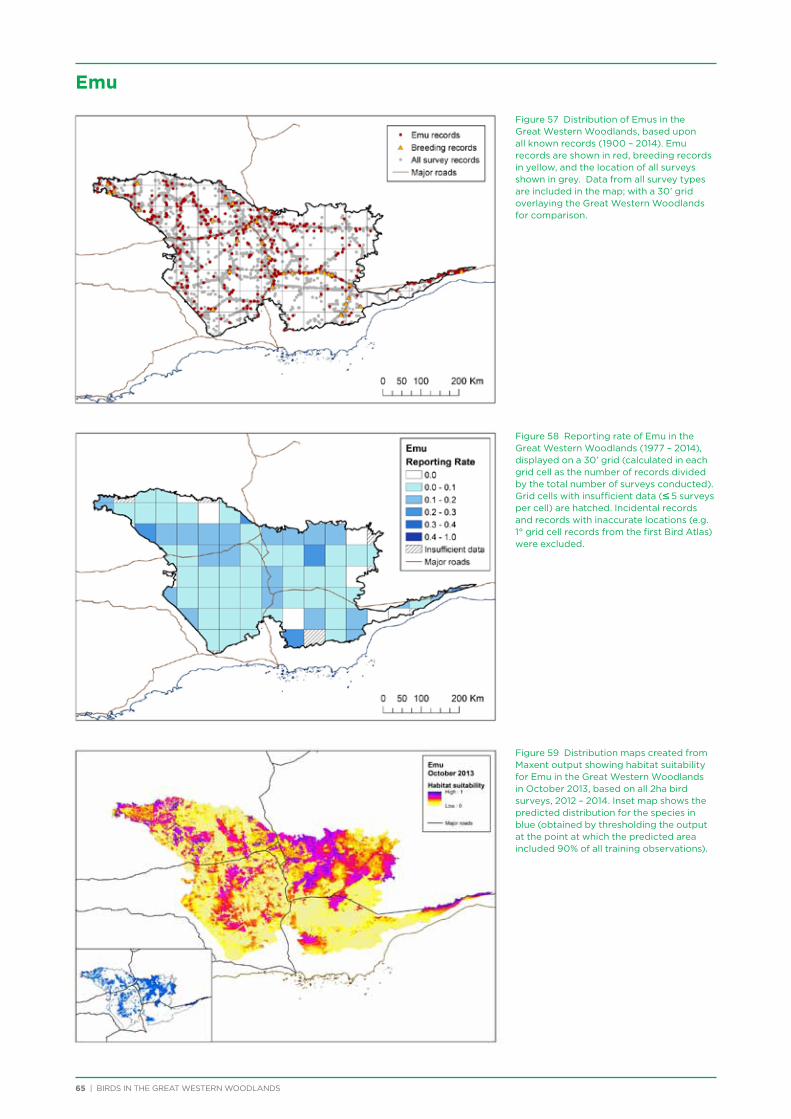
65 | BIRDS IN THE GREAT WESTERN WOODLANDS
Figure 57 Distribution of Emus in the Great Western Woodlands, based upon all known records (1900 – 2014). Emu records are shown in red, breeding records in yellow, and the location of all surveys shown in grey. Data from all survey types are included in the map; with a 30’ grid overlaying the Great Western Woodlands for comparison.
Figure 58 Reporting rate of Emu in the Great Western Woodlands (1977 – 2014), displayed on a 30’ grid (calculated in each grid cell as the number of records divided by the total number of surveys conducted). Grid cells with insufficient data (≤ 5 surveys per cell) are hatched. Incidental records and records with inaccurate locations (e.g. 1° grid cell records from the first Bird Atlas) were excluded.
Figure 59 Distribution maps created from Maxent output showing habitat suitability for Emu in the Great Western Woodlands in October 2013, based on all 2ha bird surveys, 2012 – 2014. Inset map shows the predicted distribution for the species in blue (obtained by thresholding the output at the point at which the predicted area included 90% of all training observations).
Emu
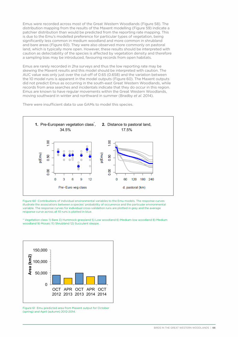
BIRDS IN THE GREAT WESTERN WOODLANDS | 66
Emus were recorded across most of the Great Western Woodlands (Figure 58). The distribution mapping from the results of the Maxent modelling (Figure 59) indicate a patchier distribution than would be predicted from the reporting rate mapping. This is due to the Emu’s modelled preference for particular types of vegetation, being significantly less common in medium woodland and more common in shrubland and bare areas (Figure 60). They were also observed more commonly on pastoral land, which is typically more open. However, these results should be interpreted with caution as detectability of the species is affected by vegetation density and therefore a sampling bias may be introduced, favouring records from open habitats.
Emus are rarely recorded in 2ha surveys and thus the low reporting rate may be skewing the Maxent results and this model should be interpreted with caution. The AUC value was only just over the cut-off of 0.65 (0.658) and the variation between the 10 model runs is apparent in the model outputs (Figure 60). The Maxent outputs did not predict Emus as occurring in the south-east Great Western Woodlands, while records from area searches and incidentals indicate that they do occur in this region. Emus are known to have regular movements within the Great Western Woodlands, moving southward in winter and northward in summer (Bradby et al. 2014).
There were insufficient data to use GAMs to model this species.
Figure 60 Contributions of individual environmental variables to the Emu models. The response curves illustrate the associations between a species’ probability of occurrence and the particular environmental variable. The response curves for individual cross-validation runs are plotted in grey and the average response curve across all 10 runs is plotted in blue.
* Vegetation class: 1) Bare 3) Hummock grassland 5) Low woodland 6) Medium-low woodland 8) Medium woodland 9) Mosaic 11) Shrubland 12) Succulent steppe.
Figure 61 Emu predicted area from Maxent output for October (spring) and April (autumn) 2012-2014.
1. Pre-European vegetation class*, 34.5%
2. Distance to pastoral land, 17.5%
0
50,000
100,000
150,000
OCT 2012
APR 2013
OCT 2013
APR 2014
OCT 2014
Are
a (k
m2)
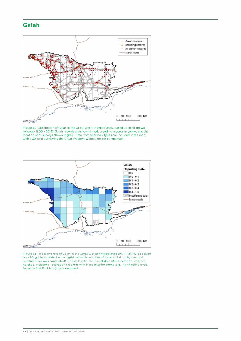
67 | BIRDS IN THE GREAT WESTERN WOODLANDS
Galah
Figure 62 Distribution of Galah in the Great Western Woodlands, based upon all known records (1900 – 2014). Galah records are shown in red, breeding records in yellow, and the location of all surveys shown in grey. Data from all survey types are included in the map; with a 30’ grid overlaying the Great Western Woodlands for comparison.
Figure 63 Reporting rate of Galah in the Great Western Woodlands (1977 – 2014), displayed on a 30’ grid (calculated in each grid cell as the number of records divided by the total number of surveys conducted). Grid cells with insufficient data (≤ 5 surveys per cell) are hatched. Incidental records and records with inaccurate locations (e.g. 1° grid cell records from the first Bird Atlas) were excluded.
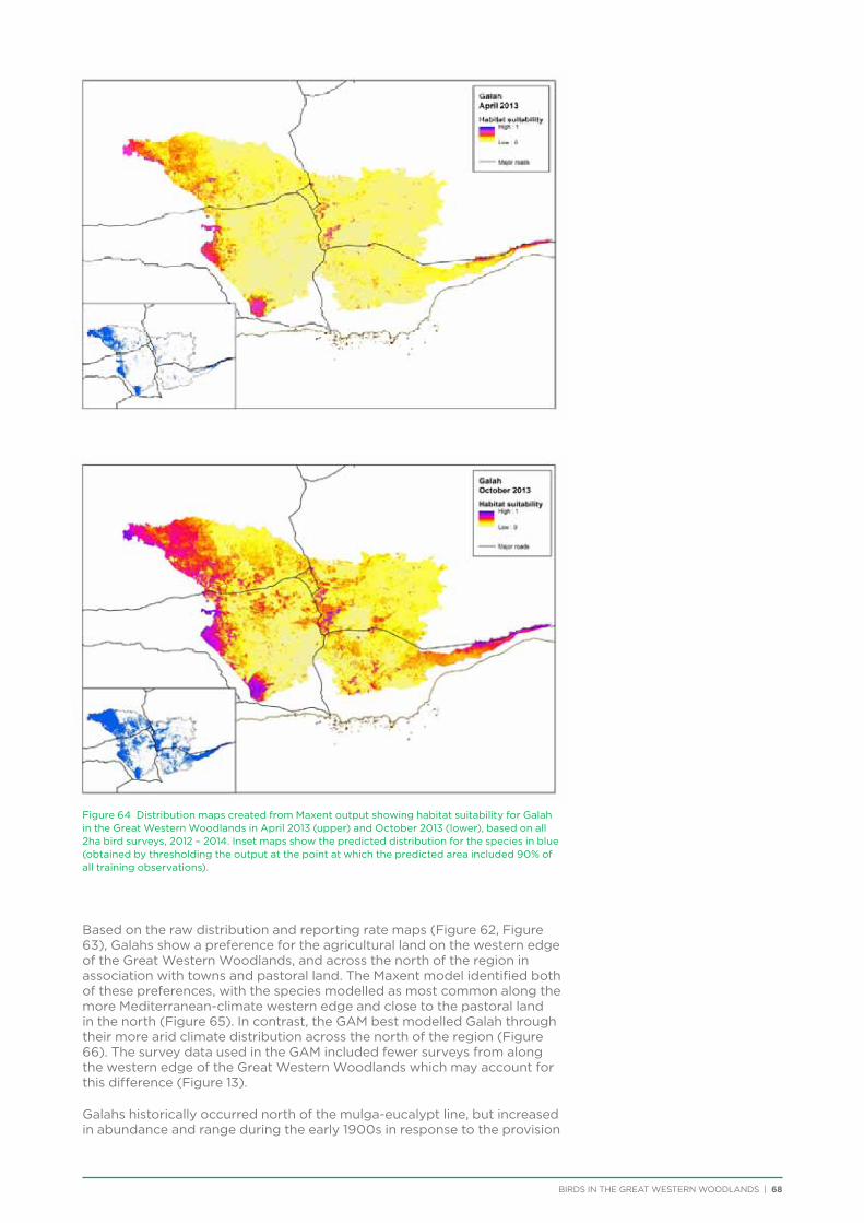
BIRDS IN THE GREAT WESTERN WOODLANDS | 68
Figure 64 Distribution maps created from Maxent output showing habitat suitability for Galah in the Great Western Woodlands in April 2013 (upper) and October 2013 (lower), based on all 2ha bird surveys, 2012 – 2014. Inset maps show the predicted distribution for the species in blue (obtained by thresholding the output at the point at which the predicted area included 90% of all training observations).
Based on the raw distribution and reporting rate maps (Figure 62, Figure 63), Galahs show a preference for the agricultural land on the western edge of the Great Western Woodlands, and across the north of the region in association with towns and pastoral land. The Maxent model identified both of these preferences, with the species modelled as most common along the more Mediterranean-climate western edge and close to the pastoral land in the north (Figure 65). In contrast, the GAM best modelled Galah through their more arid climate distribution across the north of the region (Figure 66). The survey data used in the GAM included fewer surveys from along the western edge of the Great Western Woodlands which may account for this difference (Figure 13).
Galahs historically occurred north of the mulga-eucalypt line, but increased in abundance and range during the early 1900s in response to the provision
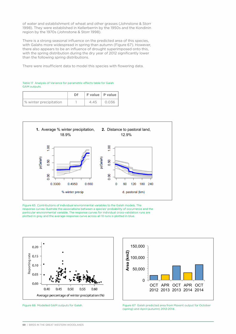
of water and establishment of wheat and other grasses (Johnstone & Storr 1998). They were established in Kellerberrin by the 1950s and the Kondinin region by the 1970s (Johnstone & Storr 1998).
There is a strong seasonal influence on the predicted area of this species, with Galahs more widespread in spring than autumn (Figure 67). However, there also appears to be an influence of drought superimposed onto this, with the spring distribution during the dry year of 2012 significantly lower than the following spring distributions.
There were insufficient data to model this species with flowering data.
Table 17 Analysis of Variance for parametric effects table for Galah GAM outputs.
Df F value P value
% winter precipitation 1 4.45 0.036
Figure 65 Contributions of individual environmental variables to the Galah models. The response curves illustrate the associations between a species’ probability of occurrence and the particular environmental variable. The response curves for individual cross-validation runs are plotted in grey and the average response curve across all 10 runs is plotted in blue.
1. Average % winter precipitation, 18.9%
2. Distance to pastoral land, 12.9%
0
50,000
100,000
150,000
OCT 2012
APR 2013
OCT 2013
APR 2014
OCT 2014
Are
a (k
m2)
Figure 66 Modelled GAM outputs for Galah. Figure 67 Galah predicted area from Maxent output for October (spring) and April (autumn) 2012-2014.
69 | BIRDS IN THE GREAT WESTERN WOODLANDS
Repo
rtin
g ra
te
BIRDS IN THE GREAT WESTERN WOODLANDS | 70Photo: Mary Whittall

71 | BIRDS IN THE GREAT WESTERN WOODLANDS
Gilbert’s Whistler
Figure 68 Distribution of Gilbert’s Whistler in the Great Western Woodlands, based upon all known records (1900 – 2014). Gilbert’s Whistler records are shown in red, breeding records in yellow, and the location of all surveys shown in grey. Data from all survey types are included in the map; with a 30’ grid overlaying the Great Western Woodlands for comparison.
Figure 69 Reporting rate of Gilbert’s Whistler in the Great Western Woodlands (1977 – 2014), displayed on a 30’ grid (calculated in each grid cell as the number of records divided by the total number of surveys conducted). Grid cells with insufficient data (≤ 5 surveys per cell) are hatched. Incidental records and records with inaccurate locations (e.g. 1° grid cell records from the first Bird Atlas) were excluded.
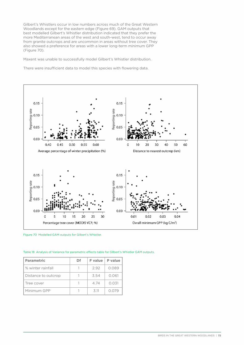
BIRDS IN THE GREAT WESTERN WOODLANDS | 72
Gilbert’s Whistlers occur in low numbers across much of the Great Western Woodlands except for the eastern edge (Figure 69). GAM outputs that best modelled Gilbert’s Whistler distribution indicated that they prefer the more Mediterranean areas of the west and south-west, tend to occur away from granite outcrops and are uncommon in areas without tree cover. They also showed a preference for areas with a lower long-term minimum GPP (Figure 70).
Maxent was unable to successfully model Gilbert’s Whistler distribution.
There were insufficient data to model this species with flowering data.
Figure 70 Modelled GAM outputs for Gilbert’s Whistler.
Table 18 Analysis of Variance for parametric effects table for Gilbert’s Whistler GAM outputs.
Parametric Df F value P value
% winter rainfall 1 2.92 0.089
Distance to outcrop 1 3.54 0.061
Tree cover 1 4.74 0.031
Minimum GPP 1 3.11 0.079
Repo
rtin
g ra
teRe
port
ing
rate
Repo
rtin
g ra
teRe
port
ing
rate
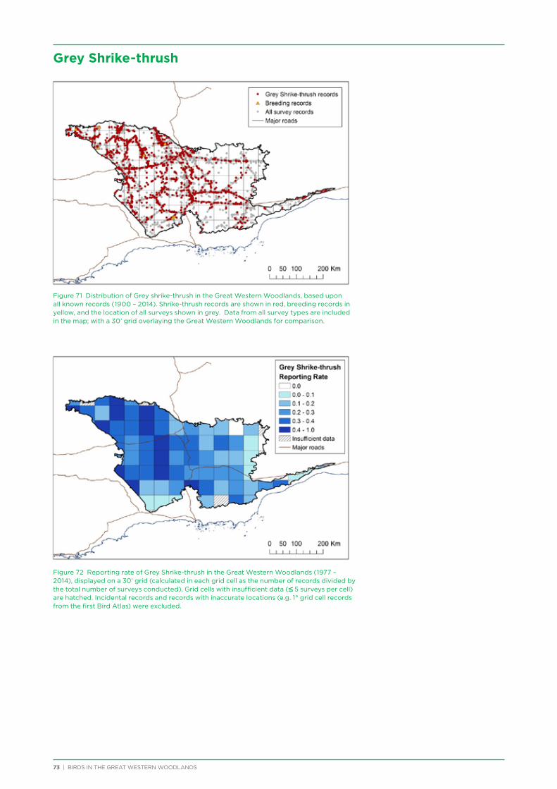
73 | BIRDS IN THE GREAT WESTERN WOODLANDS
Grey Shrike-thrush
Figure 71 Distribution of Grey shrike-thrush in the Great Western Woodlands, based upon all known records (1900 – 2014). Shrike-thrush records are shown in red, breeding records in yellow, and the location of all surveys shown in grey. Data from all survey types are included in the map; with a 30’ grid overlaying the Great Western Woodlands for comparison.
Figure 72 Reporting rate of Grey Shrike-thrush in the Great Western Woodlands (1977 – 2014), displayed on a 30’ grid (calculated in each grid cell as the number of records divided by the total number of surveys conducted). Grid cells with insufficient data (≤ 5 surveys per cell) are hatched. Incidental records and records with inaccurate locations (e.g. 1° grid cell records from the first Bird Atlas) were excluded.
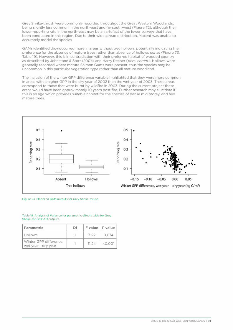
BIRDS IN THE GREAT WESTERN WOODLANDS | 74
Grey Shrike-thrush were commonly recorded throughout the Great Western Woodlands, being slightly less common in the north-east and far south-west (Figure 72), although their lower reporting rate in the north-east may be an artefact of the fewer surveys that have been conducted in this region. Due to their widespread distribution, Maxent was unable to accurately model the species.
GAMs identified they occurred more in areas without tree hollows, potentially indicating their preference for the absence of mature trees rather than absence of hollows per se (Figure 73, Table 19). However, this is in contradiction with their preferred habitat of wooded country as described by Johnstone & Storr (2004) and Harry Recher (pers. comm.). Hollows were generally recorded where mature Salmon Gums were present, thus the species may be uncommon in this particular vegetation type rather than all mature woodland.
The inclusion of the winter GPP difference variable highlighted that they were more common in areas with a higher GPP in the dry year of 2002 than the wet year of 2003. These areas correspond to those that were burnt by wildfire in 2003. During the current project these areas would have been approximately 10 years post-fire. Further research may elucidate if this is an age which provides suitable habitat for the species of dense mid-storey, and few mature trees.
Figure 73 Modelled GAM outputs for Grey Shrike-thrush.
Table 19 Analysis of Variance for parametric effects table for Grey Shrike-thrush GAM outputs.
Parametric Df F value P value
Hollows 1 3.22 0.074
Winter GPP difference, wet year - dry year 1 11.24 <0.001
Repo
rtin
g ra
te
Repo
rtin
g ra
te
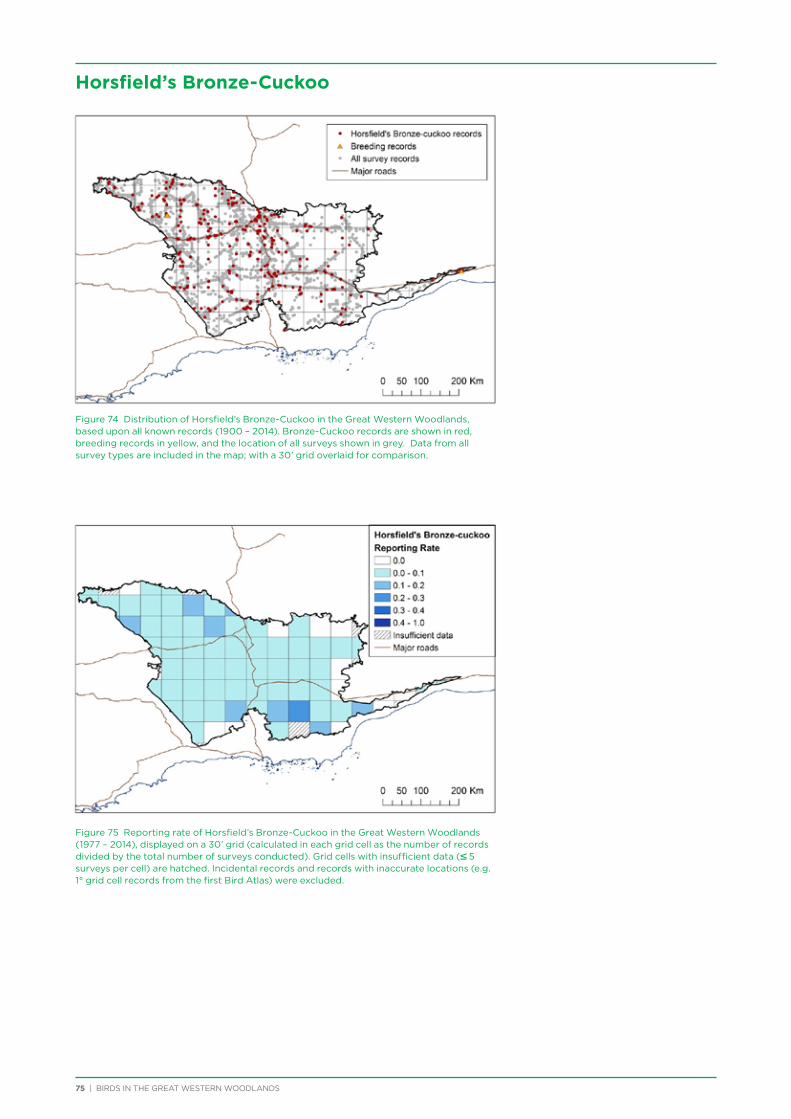
75 | BIRDS IN THE GREAT WESTERN WOODLANDS
Horsfield’s Bronze-Cuckoo
Figure 74 Distribution of Horsfield’s Bronze-Cuckoo in the Great Western Woodlands, based upon all known records (1900 – 2014). Bronze-Cuckoo records are shown in red, breeding records in yellow, and the location of all surveys shown in grey. Data from all survey types are included in the map; with a 30’ grid overlaid for comparison.
Figure 75 Reporting rate of Horsfield’s Bronze-Cuckoo in the Great Western Woodlands (1977 – 2014), displayed on a 30’ grid (calculated in each grid cell as the number of records divided by the total number of surveys conducted). Grid cells with insufficient data (≤ 5 surveys per cell) are hatched. Incidental records and records with inaccurate locations (e.g. 1° grid cell records from the first Bird Atlas) were excluded.

BIRDS IN THE GREAT WESTERN WOODLANDS | 76
Figure 76 Distribution maps created from Maxent output showing habitat suitability for Horsfield’s Bronze-Cuckoo in the Great Western Woodlands in April 2014 (upper) and October 2014 (lower), based on all 2ha bird surveys, 2012 – 2014. Inset maps show the predicted distribution for the species in blue (obtained by thresholding the output at the point at which the predicted area included 90% of all training observations).
Horsfield’s Bronze-Cuckoos are an annual migrant to the Great Western Woodlands. The raw distribution and reporting rate maps (Figure 74, Figure 75) indicate that over time they have been recorded across almost the entire Great Western Woodlands. However, Maxent modelling identified strong seasonal movements, with the species being most common in winter and spring in areas with a higher recent (1 month prior) rainfall (Figure 77). Their predicted distribution in the Great Western Woodlands between 2012 and 2014 varied from 0.3 million ha in April 2014 to 4.6 million ha in October 2014 (Figure 79). During this period the habitat was modelled as being most suitable in the eastern half of the Great Western Woodlands. However, the even spread of the longer-term reporting rate map (Figure 75) implies that in other years they may vary their distribution, dependent on conditions such as recent rainfall. Good rainfall typically precedes breeding in sedentary species and it is these species that the cuckoo parasitises. It was predicted
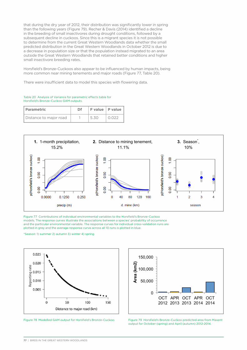
77 | BIRDS IN THE GREAT WESTERN WOODLANDS
that during the dry year of 2012, their distribution was significantly lower in spring than the following years (Figure 79). Recher & Davis (2014) identified a decline in the breeding of small insectivores during drought conditions, followed by a subsequent decline in cuckoos. Since this is a migrant species it is not possible to determine from the current Great Western Woodlands data whether the small predicted distribution in the Great Western Woodlands in October 2012 is due to a decrease in population size or that the population instead migrated to an area outside the Great Western Woodlands that retained better conditions and higher small insectivore breeding rates.
Horsfield’s Bronze-Cuckoos also appear to be influenced by human impacts, being more common near mining tenements and major roads (Figure 77, Table 20).
There were insufficient data to model this species with flowering data.
Table 20 Analysis of Variance for parametric effects table for Horsfield’s Bronze-Cuckoo GAM outputs.
Parametric Df F value P value
Distance to major road 1 5.30 0.022
Figure 77 Contributions of individual environmental variables to the Horsfield’s Bronze-Cuckoo models. The response curves illustrate the associations between a species’ probability of occurrence and the particular environmental variable. The response curves for individual cross-validation runs are plotted in grey and the average response curve across all 10 runs is plotted in blue.
*Season: 1) summer 2) autumn 3) winter 4) spring
1. 1-month precipitation, 15.2%
2. Distance to mining tenement, 11.1%
3. Season*, 10%
0
50,000
100,000
150,000
OCT 2012
APR 2013
OCT 2013
APR 2014
OCT 2014
Are
a (k
m2)
Figure 78 Modelled GAM output for Horsfield’s Bronze-Cuckoo. Figure 79 Horsfield’s Bronze-Cuckoo predicted area from Maxent output for October (spring) and April (autumn) 2012-2014.
Repo
rtin
g ra
te
BIRDS IN THE GREAT WESTERN WOODLANDS | 78Photo: Tegan Douglas
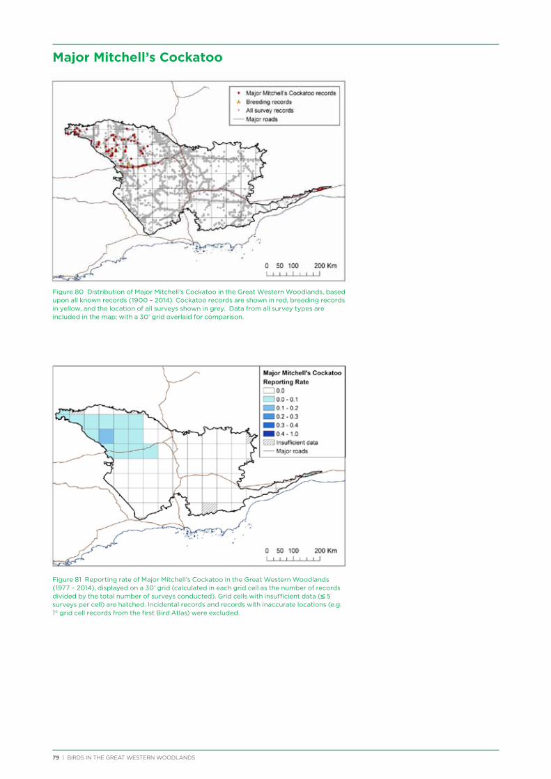
79 | BIRDS IN THE GREAT WESTERN WOODLANDS
Major Mitchell’s Cockatoo
Figure 80 Distribution of Major Mitchell’s Cockatoo in the Great Western Woodlands, based upon all known records (1900 – 2014). Cockatoo records are shown in red, breeding records in yellow, and the location of all surveys shown in grey. Data from all survey types are included in the map; with a 30’ grid overlaid for comparison.
Figure 81 Reporting rate of Major Mitchell’s Cockatoo in the Great Western Woodlands (1977 – 2014), displayed on a 30’ grid (calculated in each grid cell as the number of records divided by the total number of surveys conducted). Grid cells with insufficient data (≤ 5 surveys per cell) are hatched. Incidental records and records with inaccurate locations (e.g. 1° grid cell records from the first Bird Atlas) were excluded.
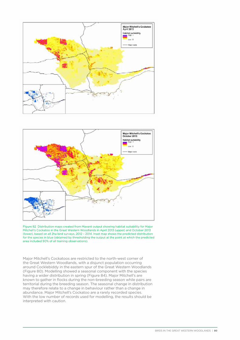
BIRDS IN THE GREAT WESTERN WOODLANDS | 80
Figure 82 Distribution maps created from Maxent output showing habitat suitability for Major Mitchell’s Cockatoo in the Great Western Woodlands in April 2013 (upper) and October 2013 (lower), based on all 2ha bird surveys, 2012 – 2014. Inset map shows the predicted distribution for the species in blue (obtained by thresholding the output at the point at which the predicted area included 90% of all training observations).
Major Mitchell’s Cockatoos are restricted to the north-west corner of the Great Western Woodlands, with a disjunct population occurring around Cocklebiddy in the eastern spur of the Great Western Woodlands (Figure 80). Modelling showed a seasonal component with the species having a wider distribution in spring (Figure 84). Major Mitchell’s are known to gather in flocks during the non-breeding season while pairs are territorial during the breeding season. The seasonal change in distribution may therefore relate to a change in behaviour rather than a change in abundance. Major Mitchell’s Cockatoo are a rarely recorded species. With the low number of records used for modelling, the results should be interpreted with caution.
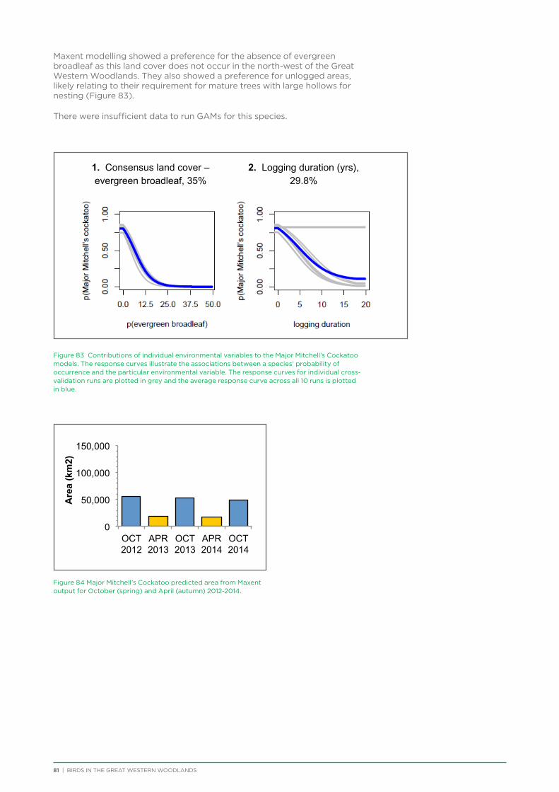
81 | BIRDS IN THE GREAT WESTERN WOODLANDS
Maxent modelling showed a preference for the absence of evergreen broadleaf as this land cover does not occur in the north-west of the Great Western Woodlands. They also showed a preference for unlogged areas, likely relating to their requirement for mature trees with large hollows for nesting (Figure 83).
There were insufficient data to run GAMs for this species.
Figure 83 Contributions of individual environmental variables to the Major Mitchell’s Cockatoo models. The response curves illustrate the associations between a species’ probability of occurrence and the particular environmental variable. The response curves for individual cross-validation runs are plotted in grey and the average response curve across all 10 runs is plotted in blue.
Figure 84 Major Mitchell’s Cockatoo predicted area from Maxent output for October (spring) and April (autumn) 2012-2014.
1. Consensus land cover – evergreen broadleaf, 35%
2. Logging duration (yrs), 29.8%
0
50,000
100,000
150,000
OCT 2012
APR 2013
OCT 2013
APR 2014
OCT 2014
Are
a (k
m2)
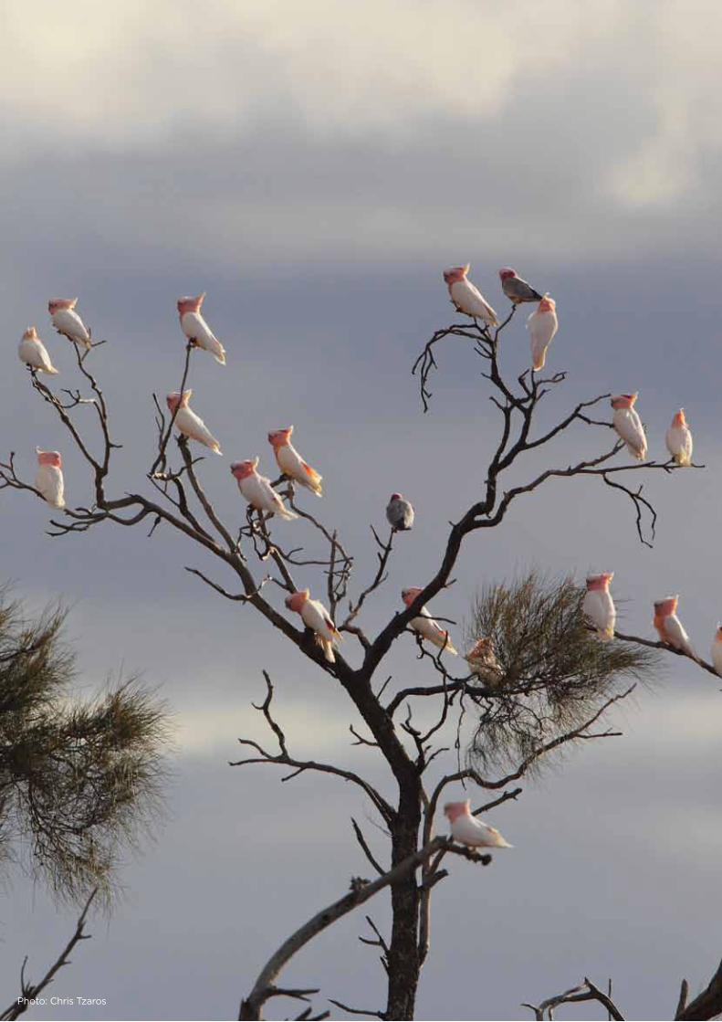
BIRDS IN THE GREAT WESTERN WOODLANDS | 82Photo: Chris Tzaros
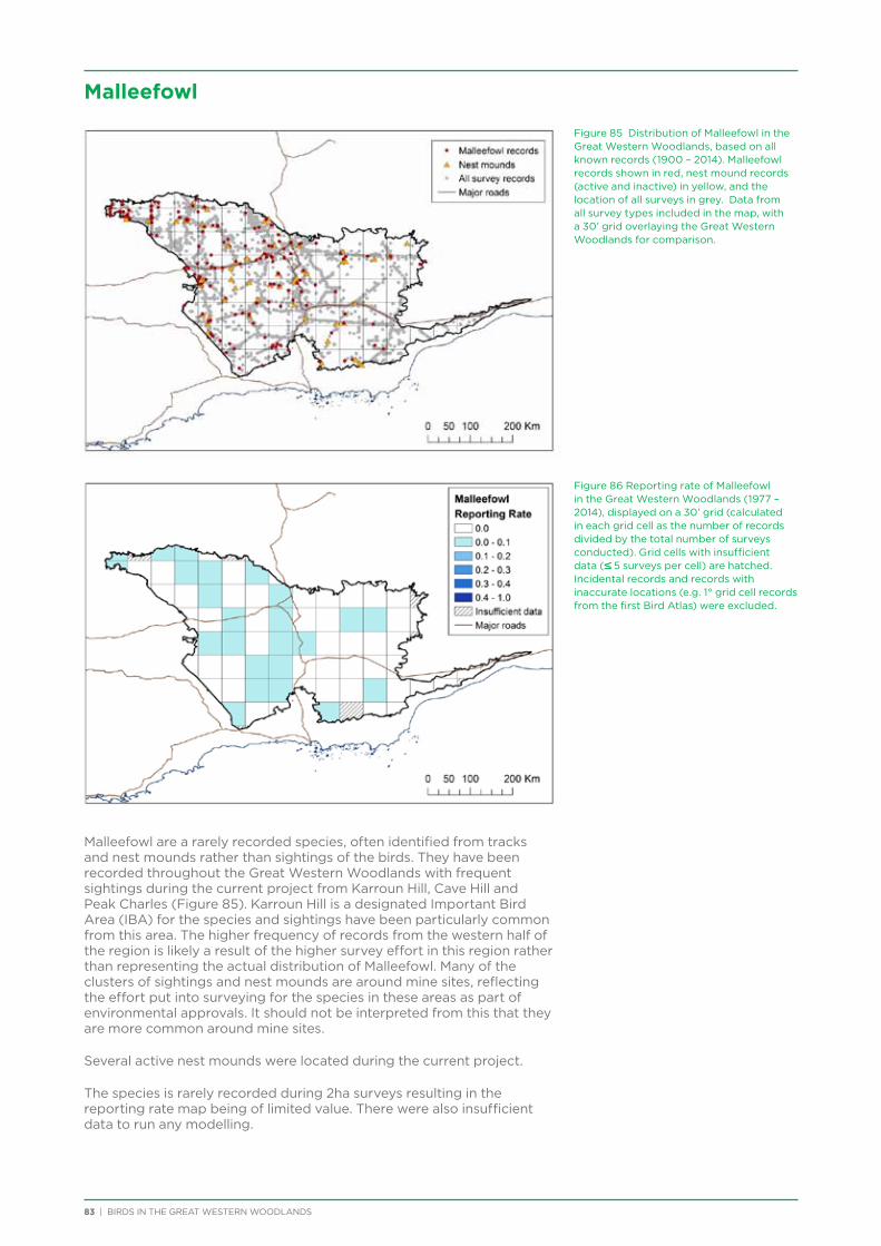
83 | BIRDS IN THE GREAT WESTERN WOODLANDS
Malleefowl
Malleefowl are a rarely recorded species, often identified from tracks and nest mounds rather than sightings of the birds. They have been recorded throughout the Great Western Woodlands with frequent sightings during the current project from Karroun Hill, Cave Hill and Peak Charles (Figure 85). Karroun Hill is a designated Important Bird Area (IBA) for the species and sightings have been particularly common from this area. The higher frequency of records from the western half of the region is likely a result of the higher survey effort in this region rather than representing the actual distribution of Malleefowl. Many of the clusters of sightings and nest mounds are around mine sites, reflecting the effort put into surveying for the species in these areas as part of environmental approvals. It should not be interpreted from this that they are more common around mine sites.
Several active nest mounds were located during the current project.
The species is rarely recorded during 2ha surveys resulting in the reporting rate map being of limited value. There were also insufficient data to run any modelling.
Figure 85 Distribution of Malleefowl in the Great Western Woodlands, based on all known records (1900 – 2014). Malleefowl records shown in red, nest mound records (active and inactive) in yellow, and the location of all surveys in grey. Data from all survey types included in the map, with a 30’ grid overlaying the Great Western Woodlands for comparison.
Figure 86 Reporting rate of Malleefowl in the Great Western Woodlands (1977 – 2014), displayed on a 30’ grid (calculated in each grid cell as the number of records divided by the total number of surveys conducted). Grid cells with insufficient data (≤ 5 surveys per cell) are hatched. Incidental records and records with inaccurate locations (e.g. 1° grid cell records from the first Bird Atlas) were excluded.
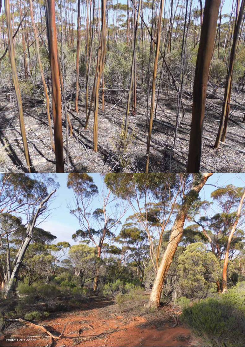
BIRDS IN THE GREAT WESTERN WOODLANDS | 84Photo: Carl Gosper
Photo: Carl Gosper
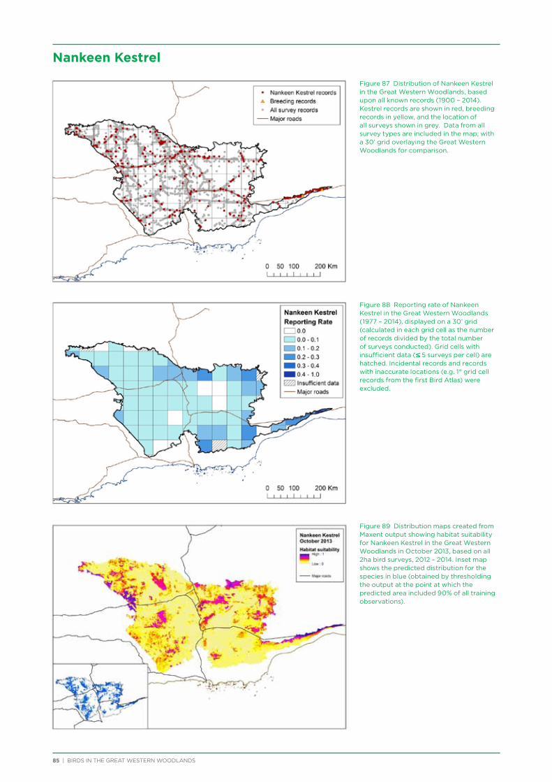
85 | BIRDS IN THE GREAT WESTERN WOODLANDS
Figure 87 Distribution of Nankeen Kestrel in the Great Western Woodlands, based upon all known records (1900 – 2014). Kestrel records are shown in red, breeding records in yellow, and the location of all surveys shown in grey. Data from all survey types are included in the map; with a 30’ grid overlaying the Great Western Woodlands for comparison.
Figure 88 Reporting rate of Nankeen Kestrel in the Great Western Woodlands (1977 – 2014), displayed on a 30’ grid (calculated in each grid cell as the number of records divided by the total number of surveys conducted). Grid cells with insufficient data (≤ 5 surveys per cell) are hatched. Incidental records and records with inaccurate locations (e.g. 1° grid cell records from the first Bird Atlas) were excluded.
Figure 89 Distribution maps created from Maxent output showing habitat suitability for Nankeen Kestrel in the Great Western Woodlands in October 2013, based on all 2ha bird surveys, 2012 – 2014. Inset map shows the predicted distribution for the species in blue (obtained by thresholding the output at the point at which the predicted area included 90% of all training observations).
Nankeen Kestrel
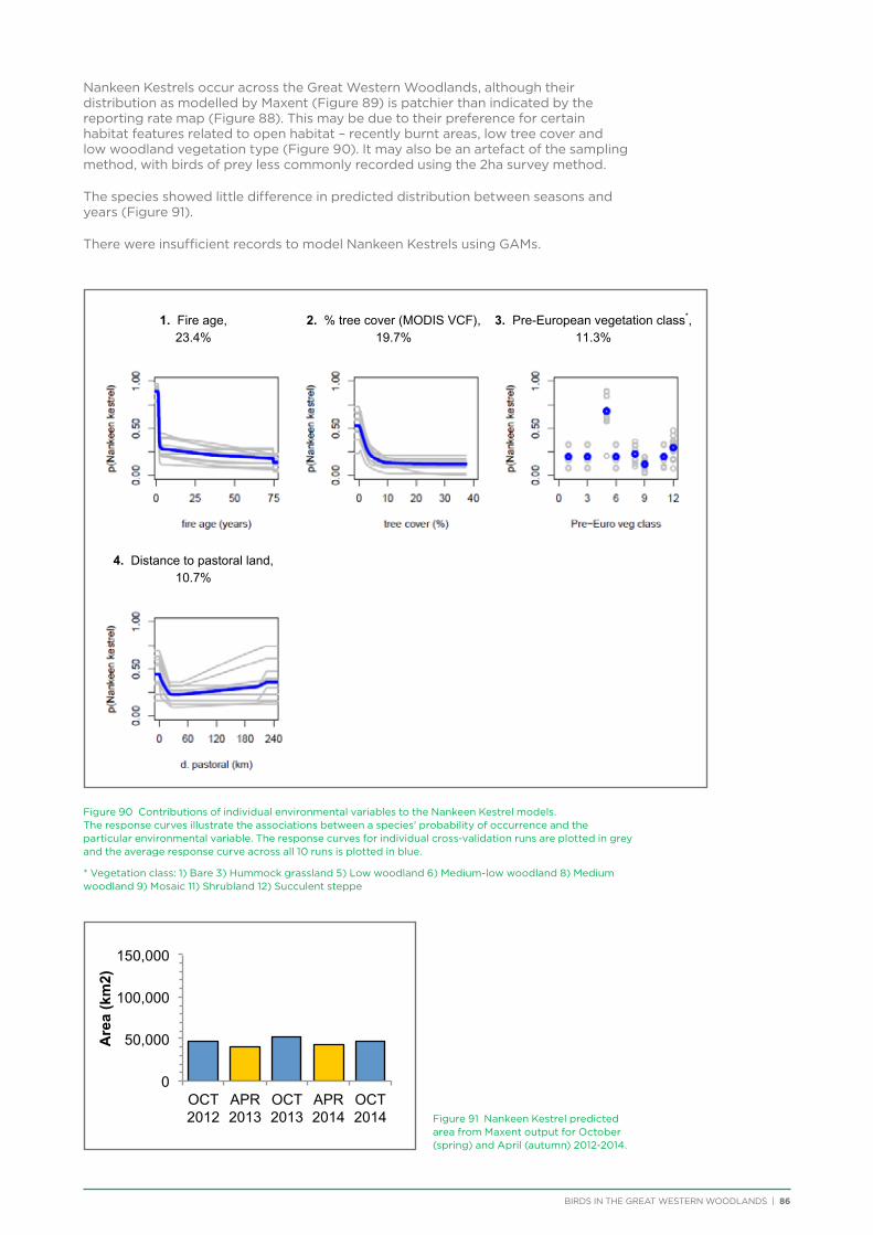
BIRDS IN THE GREAT WESTERN WOODLANDS | 86
Nankeen Kestrels occur across the Great Western Woodlands, although their distribution as modelled by Maxent (Figure 89) is patchier than indicated by the reporting rate map (Figure 88). This may be due to their preference for certain habitat features related to open habitat – recently burnt areas, low tree cover and low woodland vegetation type (Figure 90). It may also be an artefact of the sampling method, with birds of prey less commonly recorded using the 2ha survey method.
The species showed little difference in predicted distribution between seasons and years (Figure 91).
There were insufficient records to model Nankeen Kestrels using GAMs.
Figure 90 Contributions of individual environmental variables to the Nankeen Kestrel models. The response curves illustrate the associations between a species’ probability of occurrence and the particular environmental variable. The response curves for individual cross-validation runs are plotted in grey and the average response curve across all 10 runs is plotted in blue.
* Vegetation class: 1) Bare 3) Hummock grassland 5) Low woodland 6) Medium-low woodland 8) Medium woodland 9) Mosaic 11) Shrubland 12) Succulent steppe
1. Fire age, 23.4%
2. % tree cover (MODIS VCF), 19.7%
3. Pre-European vegetation class*, 11.3%
4. Distance to pastoral land, 10.7%
0
50,000
100,000
150,000
OCT 2012
APR 2013
OCT 2013
APR 2014
OCT 2014
Are
a (k
m2)
Figure 91 Nankeen Kestrel predicted area from Maxent output for October (spring) and April (autumn) 2012-2014.
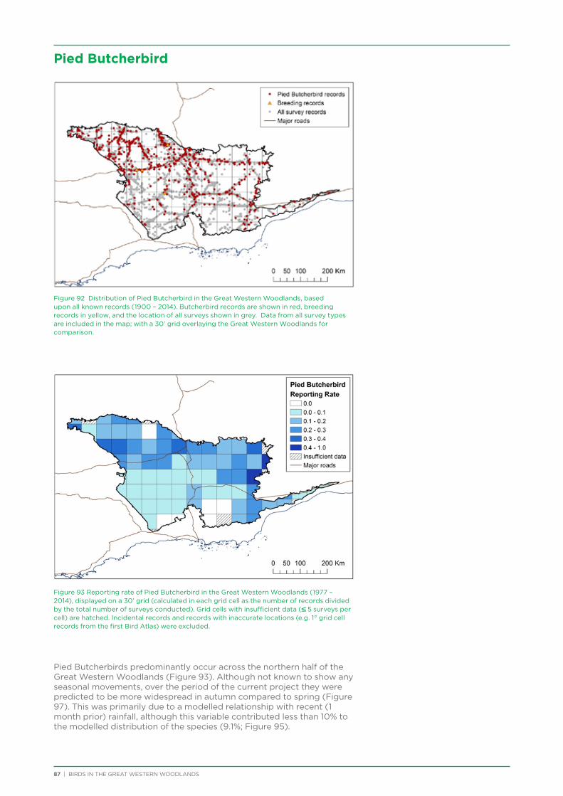
87 | BIRDS IN THE GREAT WESTERN WOODLANDS
Pied Butcherbird
Figure 92 Distribution of Pied Butcherbird in the Great Western Woodlands, based upon all known records (1900 – 2014). Butcherbird records are shown in red, breeding records in yellow, and the location of all surveys shown in grey. Data from all survey types are included in the map; with a 30’ grid overlaying the Great Western Woodlands for comparison.
Figure 93 Reporting rate of Pied Butcherbird in the Great Western Woodlands (1977 – 2014), displayed on a 30’ grid (calculated in each grid cell as the number of records divided by the total number of surveys conducted). Grid cells with insufficient data (≤ 5 surveys per cell) are hatched. Incidental records and records with inaccurate locations (e.g. 1° grid cell records from the first Bird Atlas) were excluded.
Pied Butcherbirds predominantly occur across the northern half of the Great Western Woodlands (Figure 93). Although not known to show any seasonal movements, over the period of the current project they were predicted to be more widespread in autumn compared to spring (Figure 97). This was primarily due to a modelled relationship with recent (1 month prior) rainfall, although this variable contributed less than 10% to the modelled distribution of the species (9.1%; Figure 95).
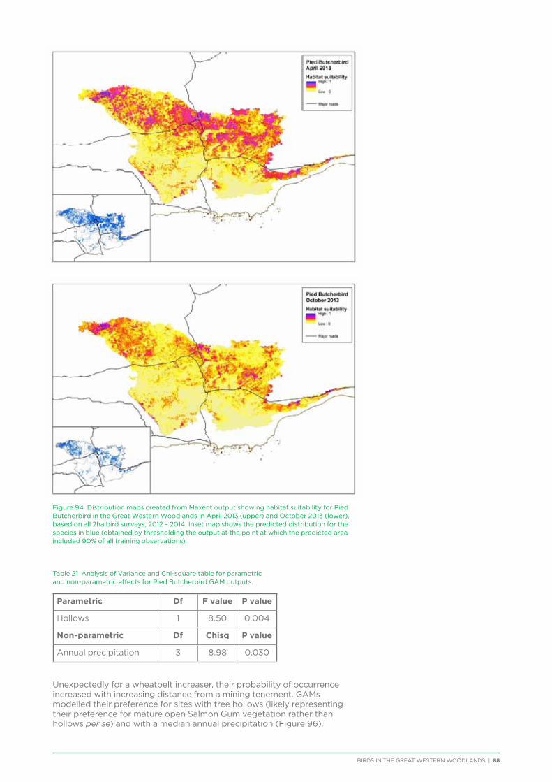
BIRDS IN THE GREAT WESTERN WOODLANDS | 88
Figure 94 Distribution maps created from Maxent output showing habitat suitability for Pied Butcherbird in the Great Western Woodlands in April 2013 (upper) and October 2013 (lower), based on all 2ha bird surveys, 2012 – 2014. Inset map shows the predicted distribution for the species in blue (obtained by thresholding the output at the point at which the predicted area included 90% of all training observations).
Table 21 Analysis of Variance and Chi-square table for parametric and non-parametric effects for Pied Butcherbird GAM outputs.
Parametric Df F value P value
Hollows 1 8.50 0.004
Non-parametric Df Chisq P value
Annual precipitation 3 8.98 0.030
Unexpectedly for a wheatbelt increaser, their probability of occurrence increased with increasing distance from a mining tenement. GAMs modelled their preference for sites with tree hollows (likely representing their preference for mature open Salmon Gum vegetation rather than hollows per se) and with a median annual precipitation (Figure 96).
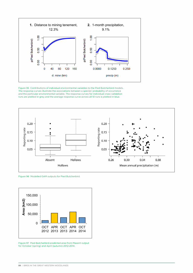
89 | BIRDS IN THE GREAT WESTERN WOODLANDS
Figure 95 Contributions of individual environmental variables to the Pied Butcherbird models. The response curves illustrate the associations between a species’ probability of occurrence and the particular environmental variable. The response curves for individual cross-validation runs are plotted in grey and the average response curve across all 10 runs is plotted in blue.
Figure 96 Modelled GAM outputs for Pied Butcherbird.
Figure 97 Pied Butcherbird predicted area from Maxent output for October (spring) and April (autumn) 2012-2014.
1. Distance to mining tenement, 12.3%
2. 1-month precipitation, 9.1%
0
50,000
100,000
150,000
OCT 2012
APR 2013
OCT 2013
APR 2014
OCT 2014
Are
a (k
m2)
Re
port
ing
rate
Repo
rtin
g ra
te
BIRDS IN THE GREAT WESTERN WOODLANDS | 90Photo: Barry Heinrich
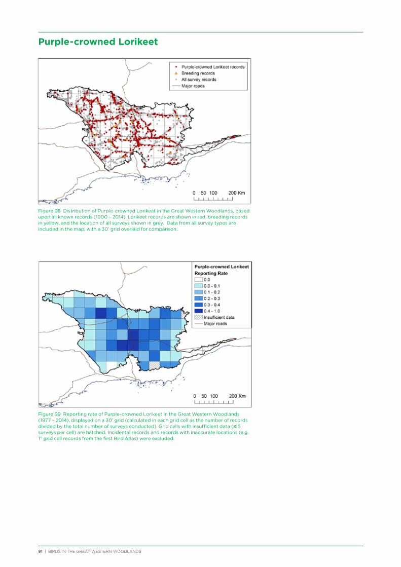
91 | BIRDS IN THE GREAT WESTERN WOODLANDS
Purple-crowned Lorikeet
Figure 98 Distribution of Purple-crowned Lorikeet in the Great Western Woodlands, based upon all known records (1900 – 2014). Lorikeet records are shown in red, breeding records in yellow, and the location of all surveys shown in grey. Data from all survey types are included in the map; with a 30’ grid overlaid for comparison.
Figure 99 Reporting rate of Purple-crowned Lorikeet in the Great Western Woodlands (1977 – 2014), displayed on a 30’ grid (calculated in each grid cell as the number of records divided by the total number of surveys conducted). Grid cells with insufficient data (≤ 5 surveys per cell) are hatched. Incidental records and records with inaccurate locations (e.g. 1° grid cell records from the first Bird Atlas) were excluded.
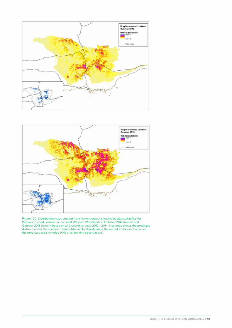
BIRDS IN THE GREAT WESTERN WOODLANDS | 92
Figure 100 Distribution maps created from Maxent output showing habitat suitability for Purple-crowned Lorikeet in the Great Western Woodlands in October 2012 (upper) and October 2013 (lower), based on all 2ha bird surveys, 2012 – 2014. Inset map shows the predicted distribution for the species in blue (obtained by thresholding the output at the point at which the predicted area included 90% of all training observations).
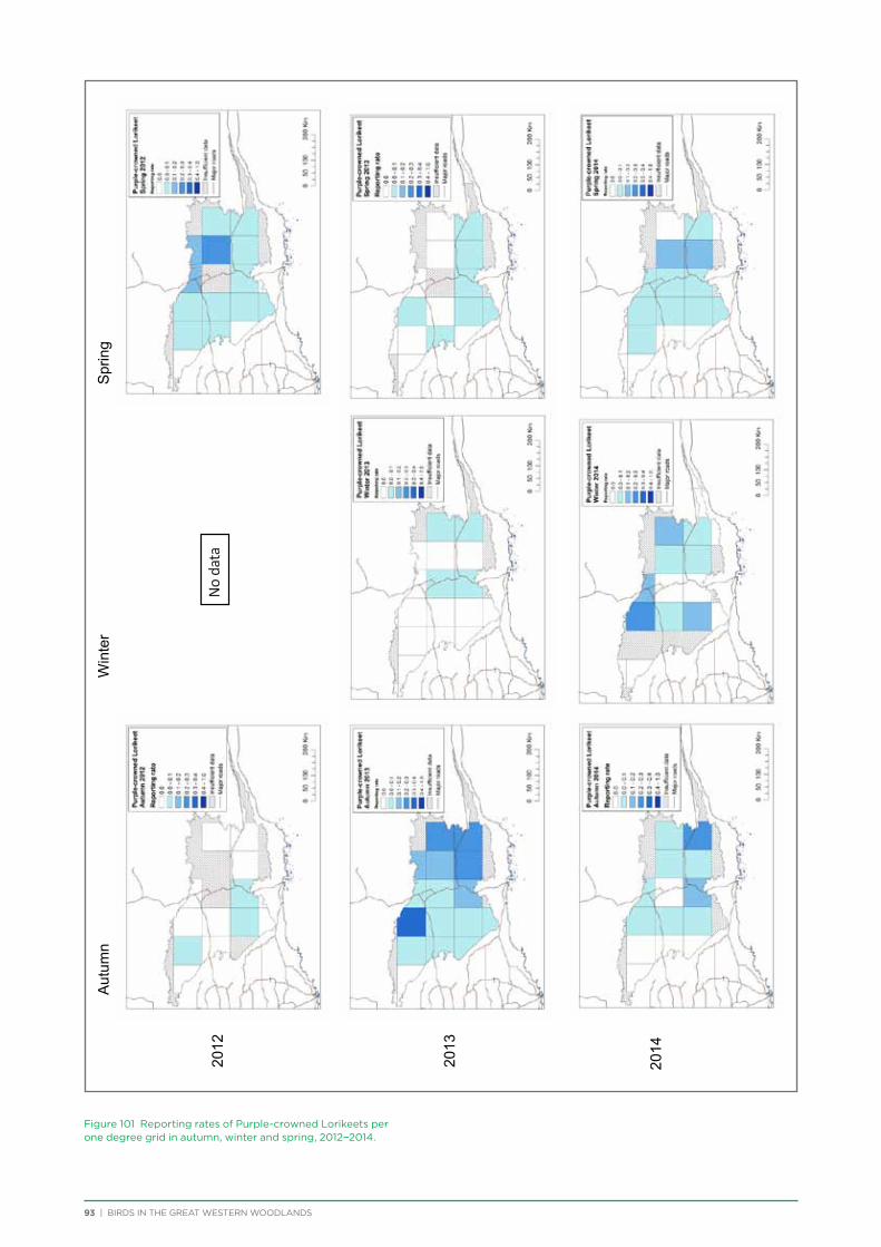
Aut
umn
W
inte
r
Spr
ing
2012
2013
2014
No
data
2014
93 | BIRDS IN THE GREAT WESTERN WOODLANDS
Figure 101 Reporting rates of Purple-crowned Lorikeets per one degree grid in autumn, winter and spring, 2012−2014.
No
data
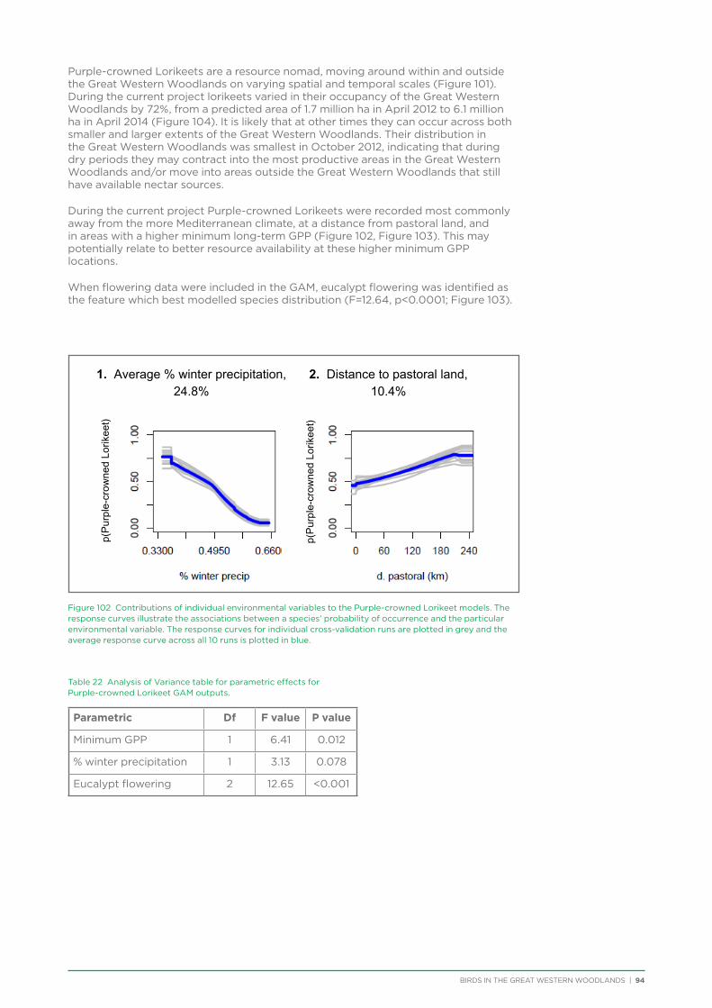
BIRDS IN THE GREAT WESTERN WOODLANDS | 94
Purple-crowned Lorikeets are a resource nomad, moving around within and outside the Great Western Woodlands on varying spatial and temporal scales (Figure 101). During the current project lorikeets varied in their occupancy of the Great Western Woodlands by 72%, from a predicted area of 1.7 million ha in April 2012 to 6.1 million ha in April 2014 (Figure 104). It is likely that at other times they can occur across both smaller and larger extents of the Great Western Woodlands. Their distribution in the Great Western Woodlands was smallest in October 2012, indicating that during dry periods they may contract into the most productive areas in the Great Western Woodlands and/or move into areas outside the Great Western Woodlands that still have available nectar sources.
During the current project Purple-crowned Lorikeets were recorded most commonly away from the more Mediterranean climate, at a distance from pastoral land, and in areas with a higher minimum long-term GPP (Figure 102, Figure 103). This may potentially relate to better resource availability at these higher minimum GPP locations.
When flowering data were included in the GAM, eucalypt flowering was identified as the feature which best modelled species distribution (F=12.64, p<0.0001; Figure 103).
Figure 102 Contributions of individual environmental variables to the Purple-crowned Lorikeet models. The response curves illustrate the associations between a species’ probability of occurrence and the particular environmental variable. The response curves for individual cross-validation runs are plotted in grey and the average response curve across all 10 runs is plotted in blue.
Table 22 Analysis of Variance table for parametric effects for Purple-crowned Lorikeet GAM outputs.
Parametric Df F value P value
Minimum GPP 1 6.41 0.012
% winter precipitation 1 3.13 0.078
Eucalypt flowering 2 12.65 <0.001
1. Average % winter precipitation, 24.8%
2. Distance to pastoral land, 10.4%
p(P
urpl
e-cr
owne
d Lo
rikee
t)
p(P
urpl
e-cr
owne
d Lo
rikee
t)
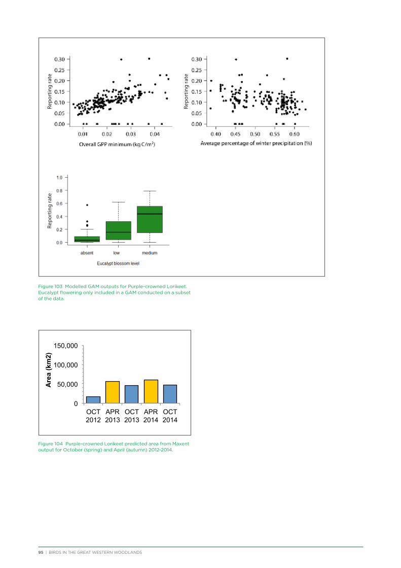
95 | BIRDS IN THE GREAT WESTERN WOODLANDS
Figure 103 Modelled GAM outputs for Purple-crowned Lorikeet. Eucalypt flowering only included in a GAM conducted on a subset of the data.
Figure 104 Purple-crowned Lorikeet predicted area from Maxent output for October (spring) and April (autumn) 2012-2014.
0
50,000
100,000
150,000
OCT 2012
APR 2013
OCT 2013
APR 2014
OCT 2014
Are
a (k
m2)
Repo
rtin
g ra
te
Repo
rtin
g ra
teRe
port
ing
rate
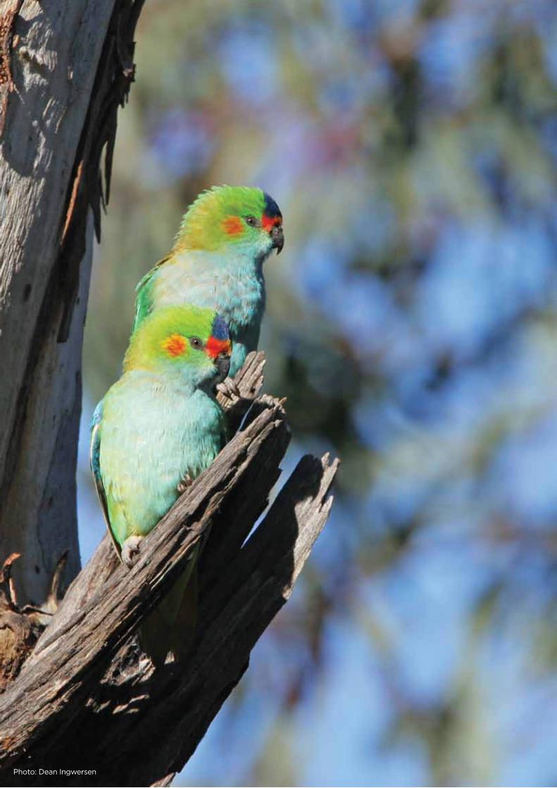
BIRDS IN THE GREAT WESTERN WOODLANDS | 96Photo: Dean Ingwersen
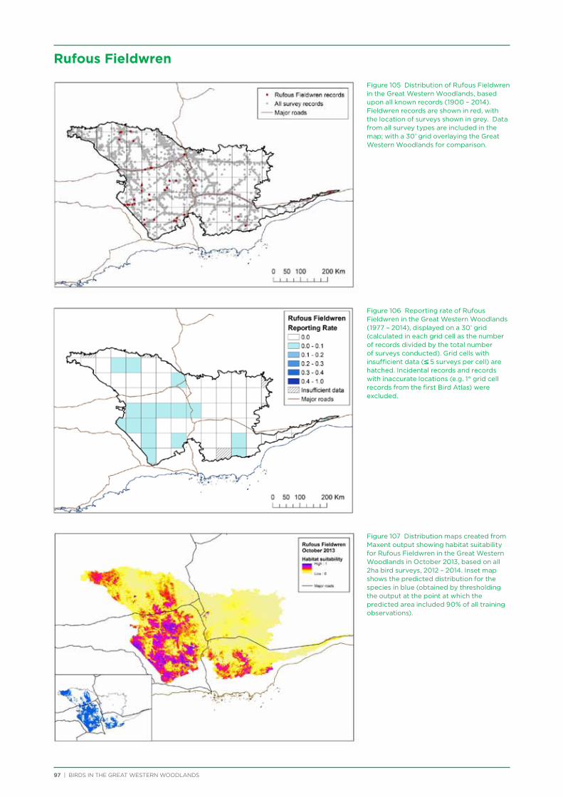
Figure 105 Distribution of Rufous Fieldwren in the Great Western Woodlands, based upon all known records (1900 – 2014). Fieldwren records are shown in red, with the location of surveys shown in grey. Data from all survey types are included in the map; with a 30’ grid overlaying the Great Western Woodlands for comparison.
Figure 106 Reporting rate of Rufous Fieldwren in the Great Western Woodlands (1977 – 2014), displayed on a 30’ grid (calculated in each grid cell as the number of records divided by the total number of surveys conducted). Grid cells with insufficient data (≤ 5 surveys per cell) are hatched. Incidental records and records with inaccurate locations (e.g. 1° grid cell records from the first Bird Atlas) were excluded.
Figure 107 Distribution maps created from Maxent output showing habitat suitability for Rufous Fieldwren in the Great Western Woodlands in October 2013, based on all 2ha bird surveys, 2012 – 2014. Inset map shows the predicted distribution for the species in blue (obtained by thresholding the output at the point at which the predicted area included 90% of all training observations).
97 | BIRDS IN THE GREAT WESTERN WOODLANDS
Rufous Fieldwren
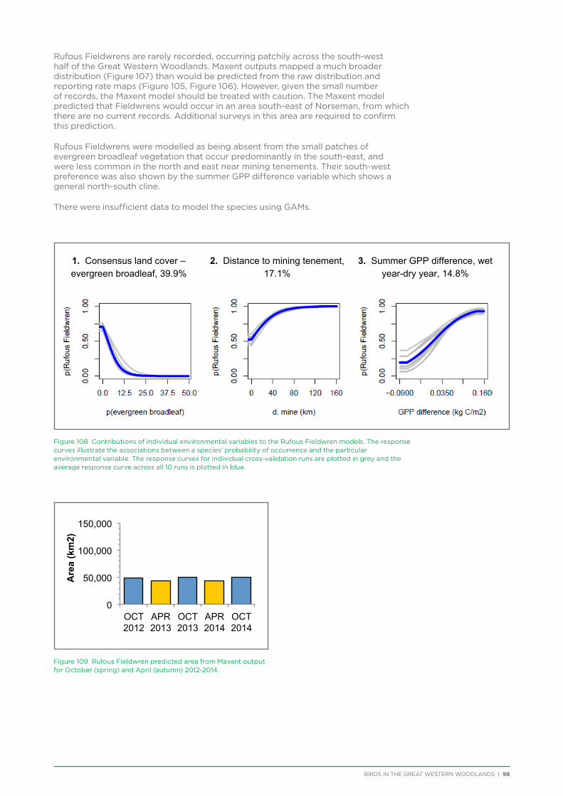
BIRDS IN THE GREAT WESTERN WOODLANDS | 98
Rufous Fieldwrens are rarely recorded, occurring patchily across the south-west half of the Great Western Woodlands. Maxent outputs mapped a much broader distribution (Figure 107) than would be predicted from the raw distribution and reporting rate maps (Figure 105, Figure 106). However, given the small number of records, the Maxent model should be treated with caution. The Maxent model predicted that Fieldwrens would occur in an area south-east of Norseman, from which there are no current records. Additional surveys in this area are required to confirm this prediction.
Rufous Fieldwrens were modelled as being absent from the small patches of evergreen broadleaf vegetation that occur predominantly in the south-east, and were less common in the north and east near mining tenements. Their south-west preference was also shown by the summer GPP difference variable which shows a general north-south cline.
There were insufficient data to model the species using GAMs.
Figure 108 Contributions of individual environmental variables to the Rufous Fieldwren models. The response curves illustrate the associations between a species’ probability of occurrence and the particular environmental variable. The response curves for individual cross-validation runs are plotted in grey and the average response curve across all 10 runs is plotted in blue.
Figure 109 Rufous Fieldwren predicted area from Maxent output for October (spring) and April (autumn) 2012-2014.
1. Consensus land cover – evergreen broadleaf, 39.9%
2. Distance to mining tenement, 17.1%
3. Summer GPP difference, wet year-dry year, 14.8%
0
50,000
100,000
150,000
OCT 2012
APR 2013
OCT 2013
APR 2014
OCT 2014
Are
a (k
m2)
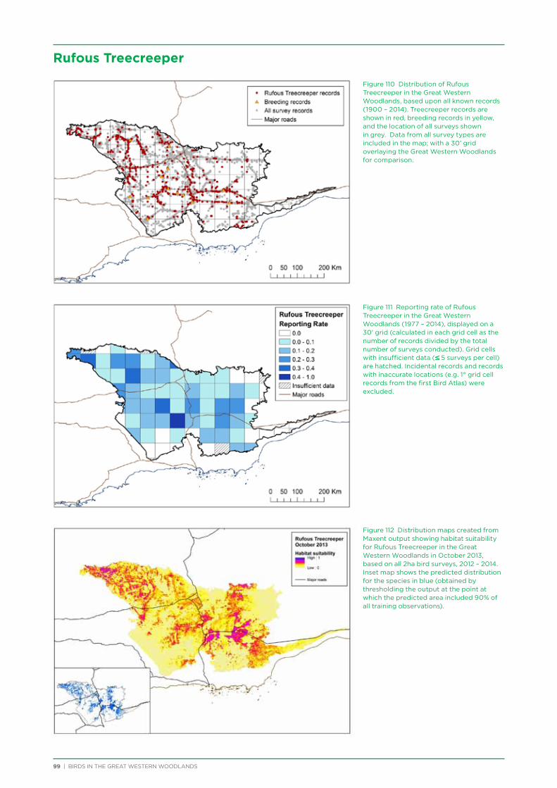
Figure 110 Distribution of Rufous Treecreeper in the Great Western Woodlands, based upon all known records (1900 – 2014). Treecreeper records are shown in red, breeding records in yellow, and the location of all surveys shown in grey. Data from all survey types are included in the map; with a 30’ grid overlaying the Great Western Woodlands for comparison.
Figure 111 Reporting rate of Rufous Treecreeper in the Great Western Woodlands (1977 – 2014), displayed on a 30’ grid (calculated in each grid cell as the number of records divided by the total number of surveys conducted). Grid cells with insufficient data (≤ 5 surveys per cell) are hatched. Incidental records and records with inaccurate locations (e.g. 1° grid cell records from the first Bird Atlas) were excluded.
Figure 112 Distribution maps created from Maxent output showing habitat suitability for Rufous Treecreeper in the Great Western Woodlands in October 2013, based on all 2ha bird surveys, 2012 – 2014. Inset map shows the predicted distribution for the species in blue (obtained by thresholding the output at the point at which the predicted area included 90% of all training observations).
99 | BIRDS IN THE GREAT WESTERN WOODLANDS
Rufous Treecreeper
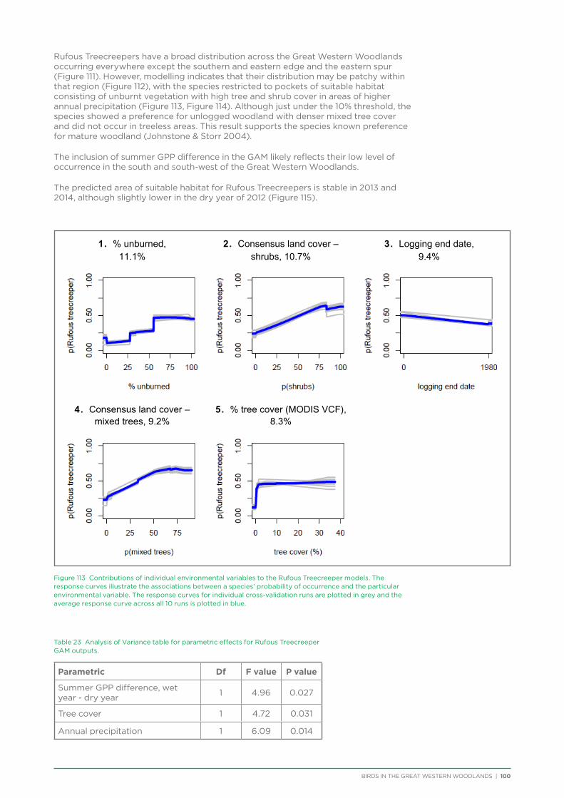
BIRDS IN THE GREAT WESTERN WOODLANDS | 100
Rufous Treecreepers have a broad distribution across the Great Western Woodlands occurring everywhere except the southern and eastern edge and the eastern spur (Figure 111). However, modelling indicates that their distribution may be patchy within that region (Figure 112), with the species restricted to pockets of suitable habitat consisting of unburnt vegetation with high tree and shrub cover in areas of higher annual precipitation (Figure 113, Figure 114). Although just under the 10% threshold, the species showed a preference for unlogged woodland with denser mixed tree cover and did not occur in treeless areas. This result supports the species known preference for mature woodland (Johnstone & Storr 2004).
The inclusion of summer GPP difference in the GAM likely reflects their low level of occurrence in the south and south-west of the Great Western Woodlands.
The predicted area of suitable habitat for Rufous Treecreepers is stable in 2013 and 2014, although slightly lower in the dry year of 2012 (Figure 115).
Figure 113 Contributions of individual environmental variables to the Rufous Treecreeper models. The response curves illustrate the associations between a species’ probability of occurrence and the particular environmental variable. The response curves for individual cross-validation runs are plotted in grey and the average response curve across all 10 runs is plotted in blue.
Table 23 Analysis of Variance table for parametric effects for Rufous Treecreeper GAM outputs.
Parametric Df F value P value
Summer GPP difference, wet year - dry year 1 4.96 0.027
Tree cover 1 4.72 0.031
Annual precipitation 1 6.09 0.014
1. % unburned, 11.1%
2. Consensus land cover – shrubs, 10.7%
3. Logging end date, 9.4%
4. Consensus land cover – mixed trees, 9.2%
5. % tree cover (MODIS VCF), 8.3%
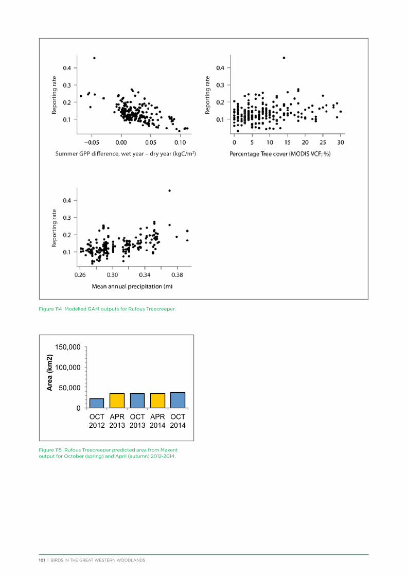
101 | BIRDS IN THE GREAT WESTERN WOODLANDS
Figure 114 Modelled GAM outputs for Rufous Treecreeper.
Figure 115 Rufous Treecreeper predicted area from Maxent output for October (spring) and April (autumn) 2012-2014.
0
50,000
100,000
150,000
OCT 2012
APR 2013
OCT 2013
APR 2014
OCT 2014
Are
a (k
m2)
Repo
rtin
g ra
teRe
port
ing
rate
Repo
rtin
g ra
te
Summer GPP difference, wet year – dry year (kgC/m2)
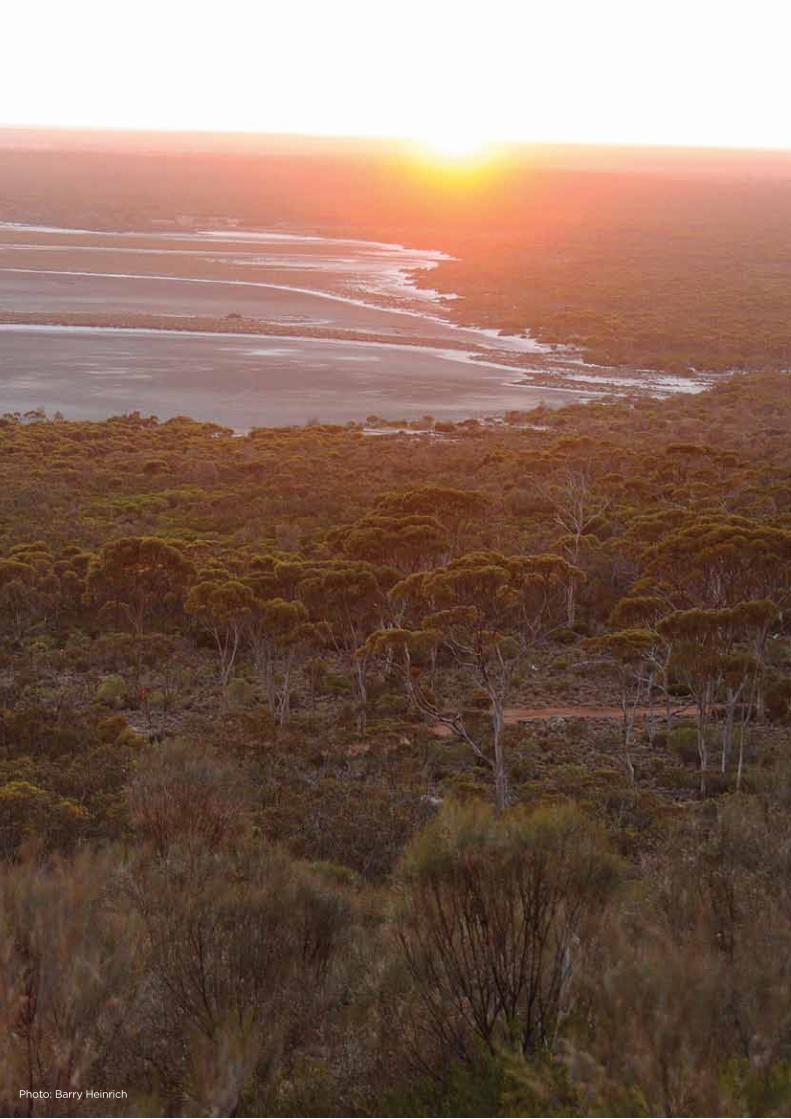
BIRDS IN THE GREAT WESTERN WOODLANDS | 102Photo: Barry Heinrich
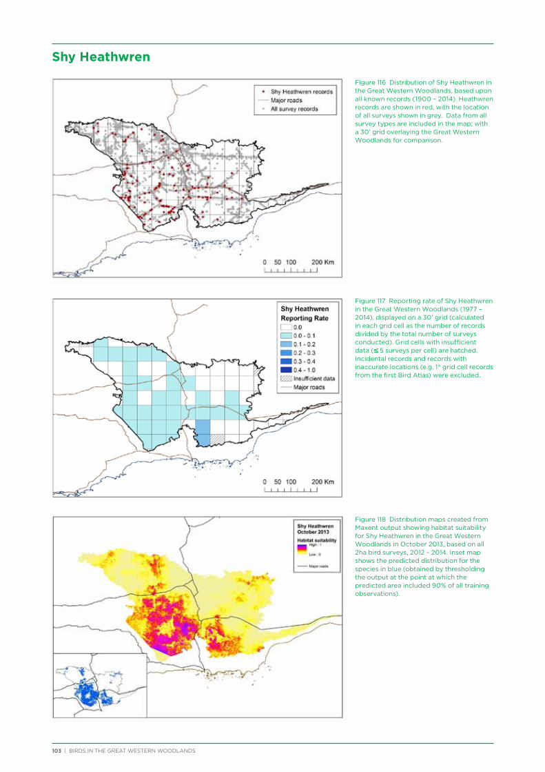
Figure 116 Distribution of Shy Heathwren in the Great Western Woodlands, based upon all known records (1900 – 2014). Heathwren records are shown in red, with the location of all surveys shown in grey. Data from all survey types are included in the map; with a 30’ grid overlaying the Great Western Woodlands for comparison.
Figure 117 Reporting rate of Shy Heathwren in the Great Western Woodlands (1977 – 2014), displayed on a 30’ grid (calculated in each grid cell as the number of records divided by the total number of surveys conducted). Grid cells with insufficient data (≤ 5 surveys per cell) are hatched. Incidental records and records with inaccurate locations (e.g. 1° grid cell records from the first Bird Atlas) were excluded.
Figure 118 Distribution maps created from Maxent output showing habitat suitability for Shy Heathwren in the Great Western Woodlands in October 2013, based on all 2ha bird surveys, 2012 – 2014. Inset map shows the predicted distribution for the species in blue (obtained by thresholding the output at the point at which the predicted area included 90% of all training observations).
103 | BIRDS IN THE GREAT WESTERN WOODLANDS
Shy Heathwren
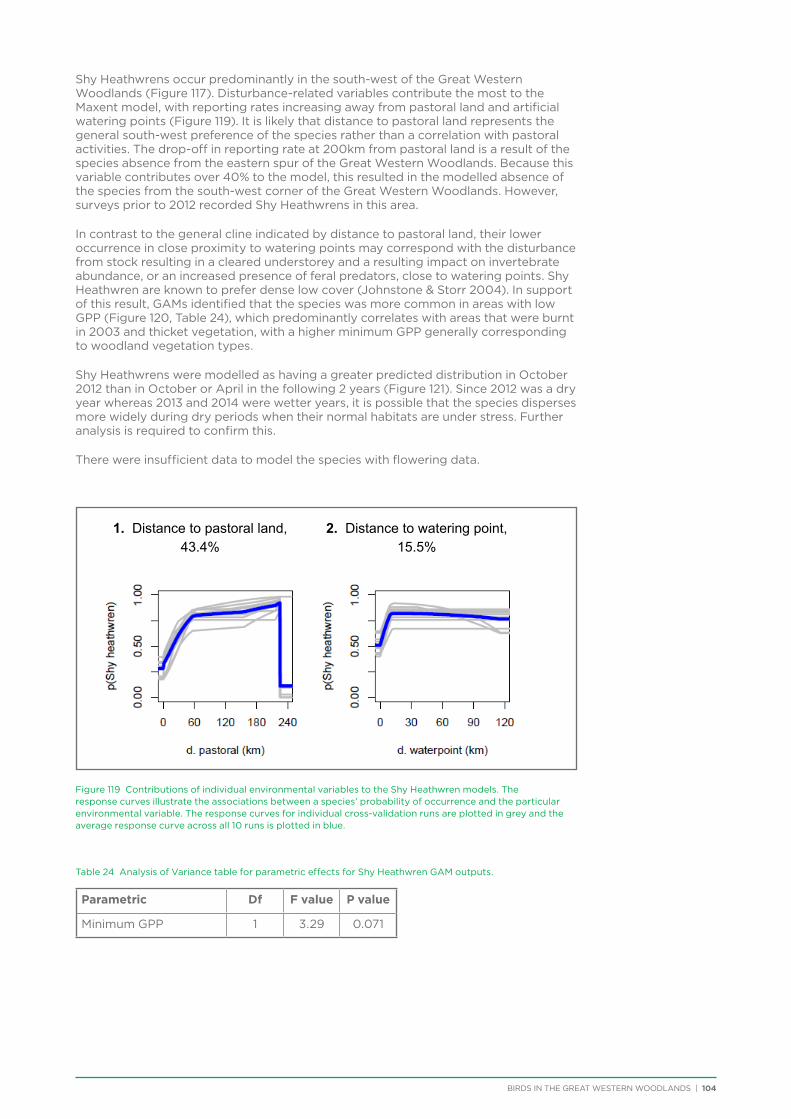
BIRDS IN THE GREAT WESTERN WOODLANDS | 104
Shy Heathwrens occur predominantly in the south-west of the Great Western Woodlands (Figure 117). Disturbance-related variables contribute the most to the Maxent model, with reporting rates increasing away from pastoral land and artificial watering points (Figure 119). It is likely that distance to pastoral land represents the general south-west preference of the species rather than a correlation with pastoral activities. The drop-off in reporting rate at 200km from pastoral land is a result of the species absence from the eastern spur of the Great Western Woodlands. Because this variable contributes over 40% to the model, this resulted in the modelled absence of the species from the south-west corner of the Great Western Woodlands. However, surveys prior to 2012 recorded Shy Heathwrens in this area.
In contrast to the general cline indicated by distance to pastoral land, their lower occurrence in close proximity to watering points may correspond with the disturbance from stock resulting in a cleared understorey and a resulting impact on invertebrate abundance, or an increased presence of feral predators, close to watering points. Shy Heathwren are known to prefer dense low cover (Johnstone & Storr 2004). In support of this result, GAMs identified that the species was more common in areas with low GPP (Figure 120, Table 24), which predominantly correlates with areas that were burnt in 2003 and thicket vegetation, with a higher minimum GPP generally corresponding to woodland vegetation types.
Shy Heathwrens were modelled as having a greater predicted distribution in October 2012 than in October or April in the following 2 years (Figure 121). Since 2012 was a dry year whereas 2013 and 2014 were wetter years, it is possible that the species disperses more widely during dry periods when their normal habitats are under stress. Further analysis is required to confirm this.
There were insufficient data to model the species with flowering data.
Figure 119 Contributions of individual environmental variables to the Shy Heathwren models. The response curves illustrate the associations between a species’ probability of occurrence and the particular environmental variable. The response curves for individual cross-validation runs are plotted in grey and the average response curve across all 10 runs is plotted in blue.
Table 24 Analysis of Variance table for parametric effects for Shy Heathwren GAM outputs.
Parametric Df F value P value
Minimum GPP 1 3.29 0.071
1. Distance to pastoral land, 43.4%
2. Distance to watering point, 15.5%
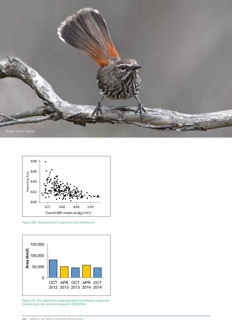
105 | BIRDS IN THE GREAT WESTERN WOODLANDS
Figure 120 Modelled GAM outputs for Shy Heathwren.
Figure 121 Shy Heathwren predicted area from Maxent output for October (spring) and April (autumn) 2012-2014.
0
50,000
100,000
150,000
OCT 2012
APR 2013
OCT 2013
APR 2014
OCT 2014
Are
a (k
m2)
Photo: Chris Tzaros
Rep
orti
ng R
ate
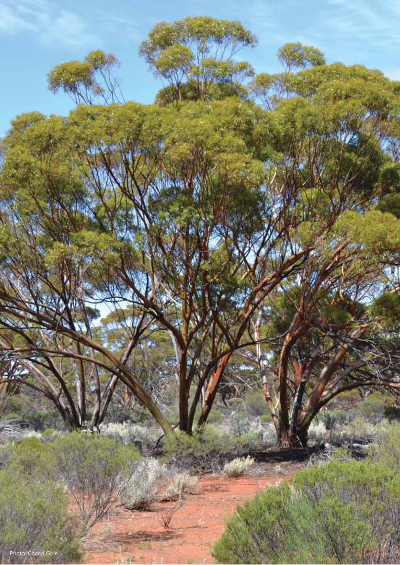
BIRDS IN THE GREAT WESTERN WOODLANDS | 106Photo: Cheryl Gole

Figure 122 Distribution of Singing Honeyeater in the Great Western Woodlands, based upon all known records (1900 – 2014). Honeyeater records are shown in red, breeding records in yellow, and the location of all surveys shown in grey. Data from all survey types are included in the map; with a 30’ grid overlaying the Great Western Woodlands for comparison.
Figure 123 Reporting rate of Singing Honeyeater in the Great Western Woodlands (1977 – 2014), displayed on a 30’ grid (calculated in each grid cell as the number of records divided by the total number of surveys conducted). Grid cells with insufficient data (≤ 5 surveys per cell) are hatched. Incidental records and records with inaccurate locations (e.g. 1° grid cell records from the first Bird Atlas) were excluded.
Figure 124 Distribution maps created from Maxent output showing habitat suitability for Singing Honeyeater in the Great Western Woodlands in October 2013, based on all 2ha bird surveys, 2012 – 2014. Inset map shows the predicted distribution for the species in blue (obtained by thresholding the output at the point at which the predicted area included 90% of all training observations).
107 | BIRDS IN THE GREAT WESTERN WOODLANDS
Singing Honeyeater
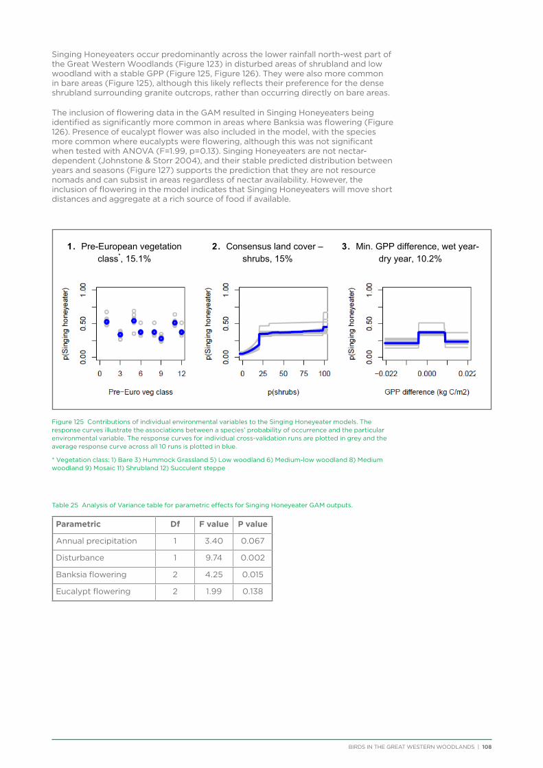
BIRDS IN THE GREAT WESTERN WOODLANDS | 108
Singing Honeyeaters occur predominantly across the lower rainfall north-west part of the Great Western Woodlands (Figure 123) in disturbed areas of shrubland and low woodland with a stable GPP (Figure 125, Figure 126). They were also more common in bare areas (Figure 125), although this likely reflects their preference for the dense shrubland surrounding granite outcrops, rather than occurring directly on bare areas.
The inclusion of flowering data in the GAM resulted in Singing Honeyeaters being identified as significantly more common in areas where Banksia was flowering (Figure 126). Presence of eucalypt flower was also included in the model, with the species more common where eucalypts were flowering, although this was not significant when tested with ANOVA (F=1.99, p=0.13). Singing Honeyeaters are not nectar-dependent (Johnstone & Storr 2004), and their stable predicted distribution between years and seasons (Figure 127) supports the prediction that they are not resource nomads and can subsist in areas regardless of nectar availability. However, the inclusion of flowering in the model indicates that Singing Honeyeaters will move short distances and aggregate at a rich source of food if available.
Figure 125 Contributions of individual environmental variables to the Singing Honeyeater models. The response curves illustrate the associations between a species’ probability of occurrence and the particular environmental variable. The response curves for individual cross-validation runs are plotted in grey and the average response curve across all 10 runs is plotted in blue.
* Vegetation class: 1) Bare 3) Hummock Grassland 5) Low woodland 6) Medium-low woodland 8) Medium woodland 9) Mosaic 11) Shrubland 12) Succulent steppe
Table 25 Analysis of Variance table for parametric effects for Singing Honeyeater GAM outputs.
Parametric Df F value P value
Annual precipitation 1 3.40 0.067
Disturbance 1 9.74 0.002
Banksia flowering 2 4.25 0.015
Eucalypt flowering 2 1.99 0.138
1. Pre-European vegetation class*, 15.1%
2. Consensus land cover – shrubs, 15%
3. Min. GPP difference, wet year-dry year, 10.2%
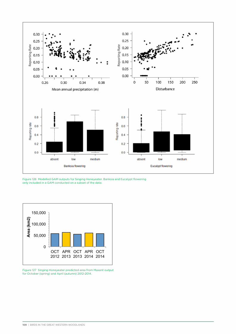
109 | BIRDS IN THE GREAT WESTERN WOODLANDS
Figure 126 Modelled GAM outputs for Singing Honeyeater. Banksia and Eucalypt flowering only included in a GAM conducted on a subset of the data.
Figure 127 Singing Honeyeater predicted area from Maxent output for October (spring) and April (autumn) 2012-2014.
0
50,000
100,000
150,000
OCT 2012
APR 2013
OCT 2013
APR 2014
OCT 2014
Are
a (k
m2)
Repo
rtin
g Ra
te
Repo
rtin
g Ra
te
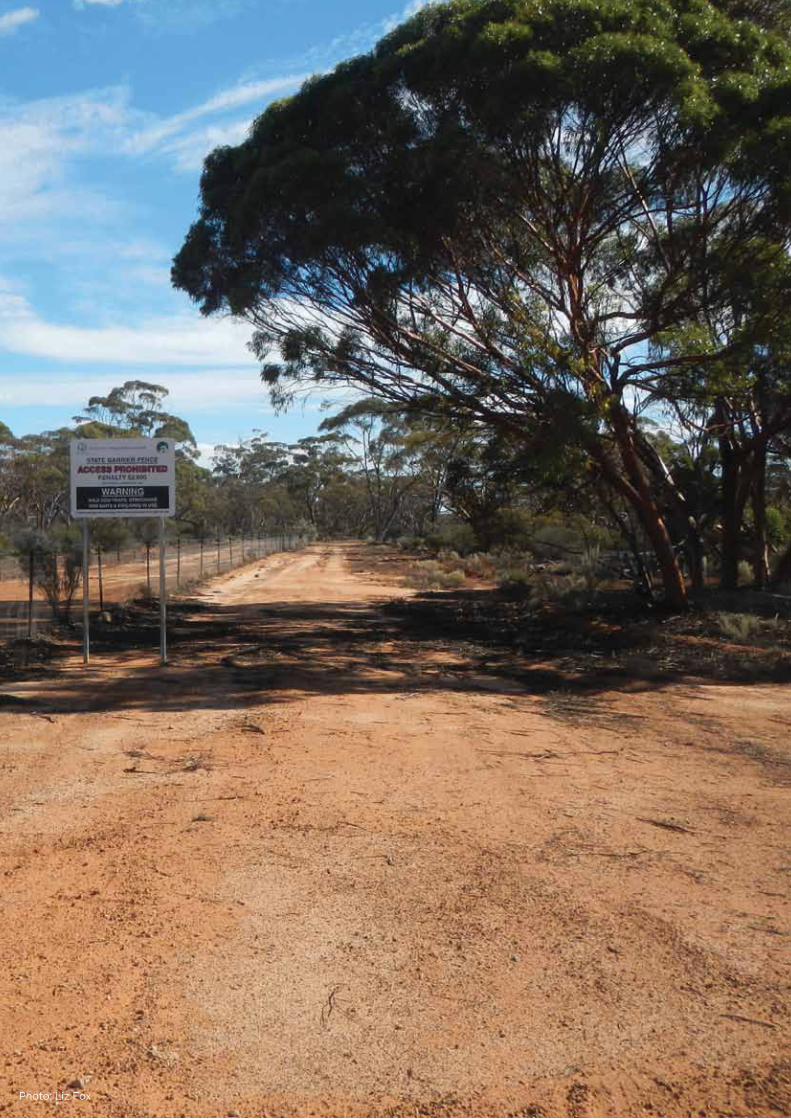
BIRDS IN THE GREAT WESTERN WOODLANDS | 110Photo: Liz Fox
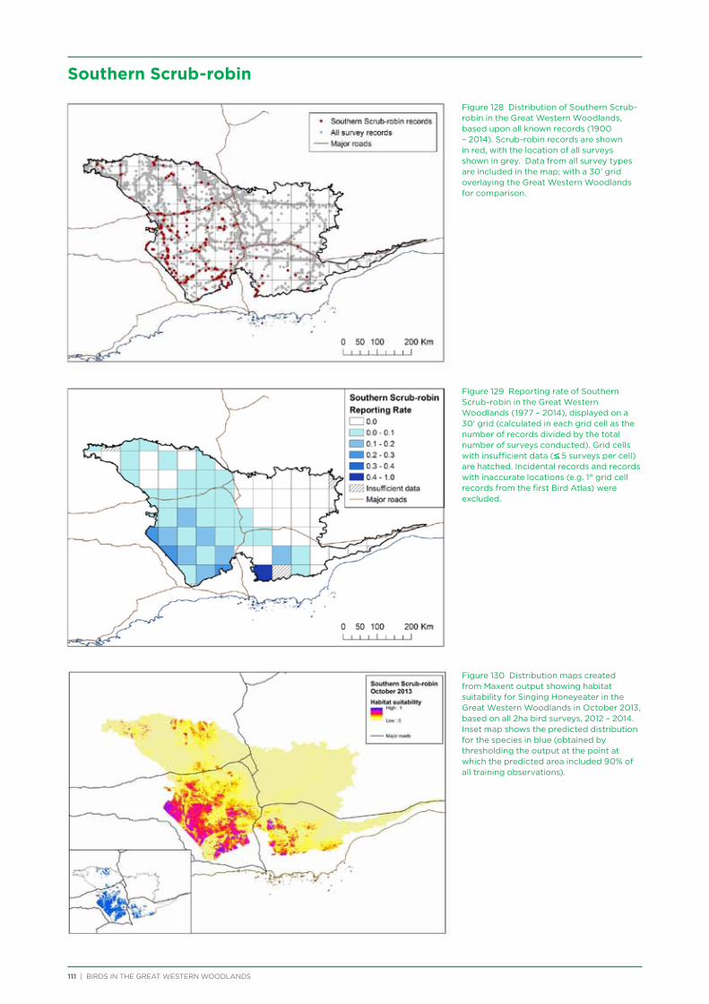
Figure 128 Distribution of Southern Scrub-robin in the Great Western Woodlands, based upon all known records (1900 – 2014). Scrub-robin records are shown in red, with the location of all surveys shown in grey. Data from all survey types are included in the map; with a 30’ grid overlaying the Great Western Woodlands for comparison.
Figure 129 Reporting rate of Southern Scrub-robin in the Great Western Woodlands (1977 – 2014), displayed on a 30’ grid (calculated in each grid cell as the number of records divided by the total number of surveys conducted). Grid cells with insufficient data (≤ 5 surveys per cell) are hatched. Incidental records and records with inaccurate locations (e.g. 1° grid cell records from the first Bird Atlas) were excluded.
Figure 130 Distribution maps created from Maxent output showing habitat suitability for Singing Honeyeater in the Great Western Woodlands in October 2013, based on all 2ha bird surveys, 2012 – 2014. Inset map shows the predicted distribution for the species in blue (obtained by thresholding the output at the point at which the predicted area included 90% of all training observations).
111 | BIRDS IN THE GREAT WESTERN WOODLANDS
Southern Scrub-robin
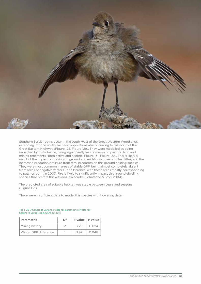
BIRDS IN THE GREAT WESTERN WOODLANDS | 112
Southern Scrub-robins occur in the south-west of the Great Western Woodlands, extending into the south-east and populations also occurring to the north of the Great Eastern Highway (Figure 128, Figure 129). They were modelled as being impacted by disturbance, being significantly less common on pastoral land and mining tenements (both active and historic; Figure 131, Figure 132). This is likely a result of the impact of grazing on ground and midstorey cover and leaf litter, and the increased predation pressure from feral predators on this ground nesting species. They were most common in areas of stable GPP, being almost completely absent from areas of negative winter GPP difference, with these areas mostly corresponding to patches burnt in 2003. Fire is likely to significantly impact this ground-dwelling species that prefers thickets and low scrubs (Johnstone & Storr 2004).
The predicted area of suitable habitat was stable between years and seasons (Figure 133).
There were insufficient data to model this species with flowering data.
Table 26 Analysis of Variance table for parametric effects for Southern Scrub-robin GAM outputs.
Parametric Df F value P value
Mining history 2 3.79 0.024
Winter GPP difference 1 3.97 0.048
Photo: Chris Tzaros
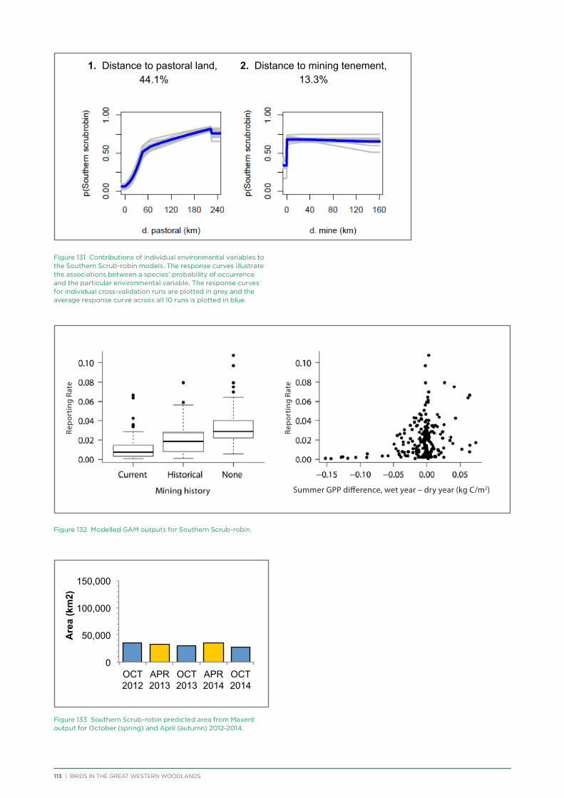
113 | BIRDS IN THE GREAT WESTERN WOODLANDS
Figure 131 Contributions of individual environmental variables to the Southern Scrub-robin models. The response curves illustrate the associations between a species’ probability of occurrence and the particular environmental variable. The response curves for individual cross-validation runs are plotted in grey and the average response curve across all 10 runs is plotted in blue.
Figure 132 Modelled GAM outputs for Southern Scrub-robin.
Figure 133 Southern Scrub-robin predicted area from Maxent output for October (spring) and April (autumn) 2012-2014.
1. Distance to pastoral land, 44.1%
2. Distance to mining tenement, 13.3%
0
50,000
100,000
150,000
OCT 2012
APR 2013
OCT 2013
APR 2014
OCT 2014
Are
a (k
m2)
Repo
rtin
g Ra
te
Repo
rtin
g Ra
te
Summer GPP difference, wet year – dry year (kg C/m2)
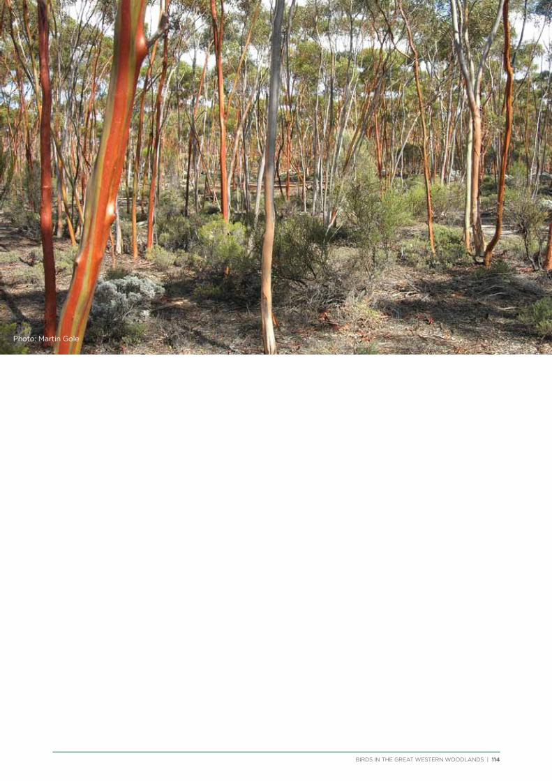
BIRDS IN THE GREAT WESTERN WOODLANDS | 114
Photo: Martin Gole
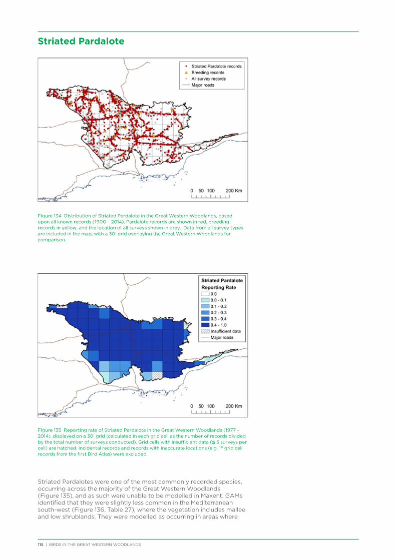
115 | BIRDS IN THE GREAT WESTERN WOODLANDS
Striated Pardalote
Figure 134 Distribution of Striated Pardalote in the Great Western Woodlands, based upon all known records (1900 – 2014). Pardalote records are shown in red, breeding records in yellow, and the location of all surveys shown in grey. Data from all survey types are included in the map; with a 30’ grid overlaying the Great Western Woodlands for comparison.
Figure 135 Reporting rate of Striated Pardalote in the Great Western Woodlands (1977 – 2014), displayed on a 30’ grid (calculated in each grid cell as the number of records divided by the total number of surveys conducted). Grid cells with insufficient data (≤ 5 surveys per cell) are hatched. Incidental records and records with inaccurate locations (e.g. 1° grid cell records from the first Bird Atlas) were excluded.
Striated Pardalotes were one of the most commonly recorded species, occurring across the majority of the Great Western Woodlands (Figure 135), and as such were unable to be modelled in Maxent. GAMs identified that they were slightly less common in the Mediterranean south-west (Figure 136, Table 27), where the vegetation includes mallee and low shrublands. They were modelled as occurring in areas where

BIRDS IN THE GREAT WESTERN WOODLANDS | 116
leaf litter is present in low densities, likely related to their increased occurrence in mature woodland (see Chapter 8) since this species requires tree hollows for nesting, although they will also forage in younger eucalypt vegetation.
Table 27 Analysis of Variance table for parametric effects for Striated Pardalote GAM outputs.
Parametric Df F value P value
Litter 4 3.60 0.007
% winter precipitation 1 3.08 0.081
Figure 136 Modelled GAM outputs for Striated Pardalote.
Photo: Ted Collinson
Repo
rtin
g Ra
te
Repo
rtin
g Ra
te
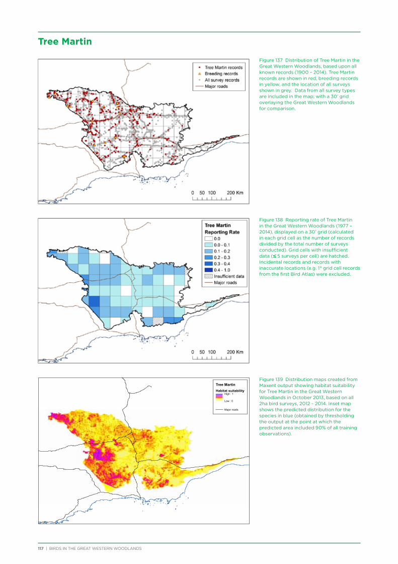
Figure 137 Distribution of Tree Martin in the Great Western Woodlands, based upon all known records (1900 – 2014). Tree Martin records are shown in red, breeding records in yellow, and the location of all surveys shown in grey. Data from all survey types are included in the map; with a 30’ grid overlaying the Great Western Woodlands for comparison.
Figure 138 Reporting rate of Tree Martin in the Great Western Woodlands (1977 – 2014), displayed on a 30’ grid (calculated in each grid cell as the number of records divided by the total number of surveys conducted). Grid cells with insufficient data (≤ 5 surveys per cell) are hatched. Incidental records and records with inaccurate locations (e.g. 1° grid cell records from the first Bird Atlas) were excluded.
Figure 139 Distribution maps created from Maxent output showing habitat suitability for Tree Martin in the Great Western Woodlands in October 2013, based on all 2ha bird surveys, 2012 – 2014. Inset map shows the predicted distribution for the species in blue (obtained by thresholding the output at the point at which the predicted area included 90% of all training observations).
117 | BIRDS IN THE GREAT WESTERN WOODLANDS
Tree Martin
Tree Martin
Habitat suitabilityHigh : 1
Low : 0
Major roads
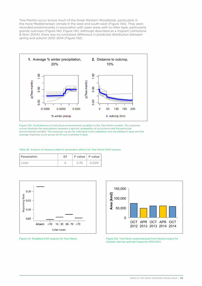
BIRDS IN THE GREAT WESTERN WOODLANDS | 118
Tree Martins occur across much of the Great Western Woodlands, particularly in the more Mediterranean climate in the west and south-west (Figure 140). They were recorded predominantly in association with open areas with no litter layer, particularly granite outcrops (Figure 140, Figure 141). Although described as a migrant (Johnstone & Storr 2004), there was no consistent difference in predicted distribution between spring and autumn 2012−2014 (Figure 142).
Figure 140 Contributions of individual environmental variables to the Tree Martin models. The response curves illustrate the associations between a species’ probability of occurrence and the particular environmental variable. The response curves for individual cross-validation runs are plotted in grey and the average response curve across all 10 runs is plotted in blue.
Table 28 Analysis of Variance table for parametric effects for Tree Martin GAM outputs.
Parametric Df F value P value
Litter 4 2.76 0.029
1. Average % winter precipitation, 20%
2. Distance to outcrop, 10%
0
50,000
100,000
150,000
OCT 2012
APR 2013
OCT 2013
APR 2014
OCT 2014
Are
a (k
m2)
Figure 141 Modelled GAM outputs for Tree Martin. Figure 142 Tree Martin predicted area from Maxent output for October (spring) and April (autumn) 2012-2014.
Repo
rtin
g Ra
te
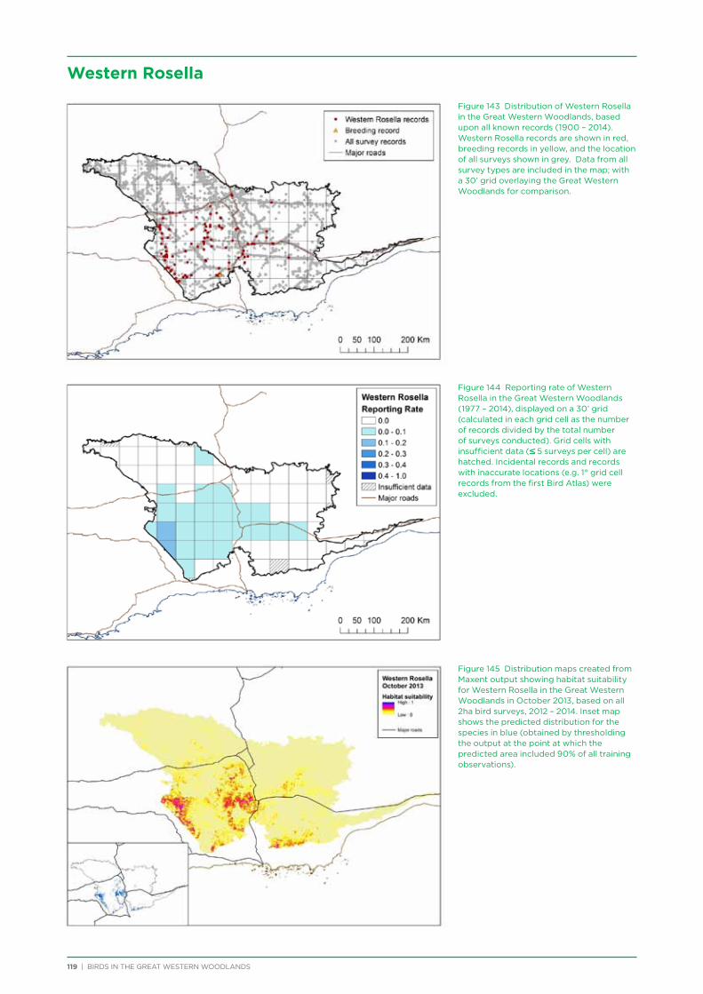
Figure 143 Distribution of Western Rosella in the Great Western Woodlands, based upon all known records (1900 – 2014). Western Rosella records are shown in red, breeding records in yellow, and the location of all surveys shown in grey. Data from all survey types are included in the map; with a 30’ grid overlaying the Great Western Woodlands for comparison.
Figure 144 Reporting rate of Western Rosella in the Great Western Woodlands (1977 – 2014), displayed on a 30’ grid (calculated in each grid cell as the number of records divided by the total number of surveys conducted). Grid cells with insufficient data (≤ 5 surveys per cell) are hatched. Incidental records and records with inaccurate locations (e.g. 1° grid cell records from the first Bird Atlas) were excluded.
Figure 145 Distribution maps created from Maxent output showing habitat suitability for Western Rosella in the Great Western Woodlands in October 2013, based on all 2ha bird surveys, 2012 – 2014. Inset map shows the predicted distribution for the species in blue (obtained by thresholding the output at the point at which the predicted area included 90% of all training observations).
119 | BIRDS IN THE GREAT WESTERN WOODLANDS
Western Rosella
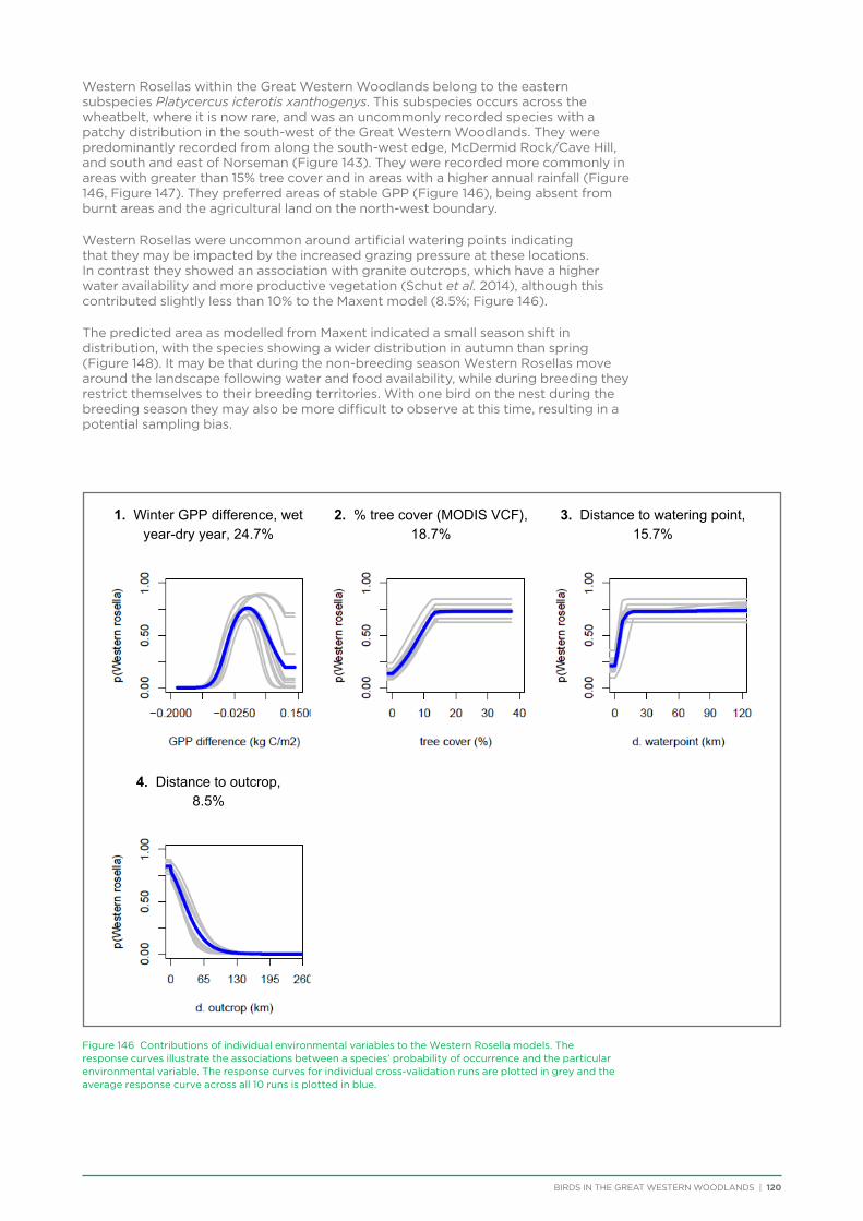
BIRDS IN THE GREAT WESTERN WOODLANDS | 120
Western Rosellas within the Great Western Woodlands belong to the eastern subspecies Platycercus icterotis xanthogenys. This subspecies occurs across the wheatbelt, where it is now rare, and was an uncommonly recorded species with a patchy distribution in the south-west of the Great Western Woodlands. They were predominantly recorded from along the south-west edge, McDermid Rock/Cave Hill, and south and east of Norseman (Figure 143). They were recorded more commonly in areas with greater than 15% tree cover and in areas with a higher annual rainfall (Figure 146, Figure 147). They preferred areas of stable GPP (Figure 146), being absent from burnt areas and the agricultural land on the north-west boundary.
Western Rosellas were uncommon around artificial watering points indicating that they may be impacted by the increased grazing pressure at these locations. In contrast they showed an association with granite outcrops, which have a higher water availability and more productive vegetation (Schut et al. 2014), although this contributed slightly less than 10% to the Maxent model (8.5%; Figure 146).
The predicted area as modelled from Maxent indicated a small season shift in distribution, with the species showing a wider distribution in autumn than spring (Figure 148). It may be that during the non-breeding season Western Rosellas move around the landscape following water and food availability, while during breeding they restrict themselves to their breeding territories. With one bird on the nest during the breeding season they may also be more difficult to observe at this time, resulting in a potential sampling bias.
Figure 146 Contributions of individual environmental variables to the Western Rosella models. The response curves illustrate the associations between a species’ probability of occurrence and the particular environmental variable. The response curves for individual cross-validation runs are plotted in grey and the average response curve across all 10 runs is plotted in blue.
1. Winter GPP difference, wet year-dry year, 24.7%
2. % tree cover (MODIS VCF), 18.7%
3. Distance to watering point, 15.7%
4. Distance to outcrop, 8.5%
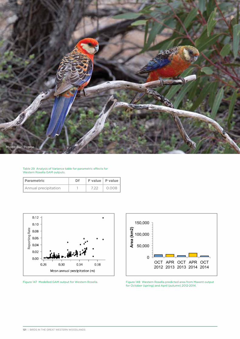
121 | BIRDS IN THE GREAT WESTERN WOODLANDS
Table 29 Analysis of Variance table for parametric effects for Western Rosella GAM outputs.
Parametric Df F value P value
Annual precipitation 1 7.22 0.008
Figure 147 Modelled GAM output for Western Rosella.
0
50,000
100,000
150,000
OCT 2012
APR 2013
OCT 2013
APR 2014
OCT 2014
Are
a (k
m2)
Figure 148 Western Rosella predicted area from Maxent output for October (spring) and April (autumn) 2012-2014.
Photo: Ben Pearce
Repo
rtin
g Ra
te
BIRDS IN THE GREAT WESTERN WOODLANDS | 122Photo: Allan Rose
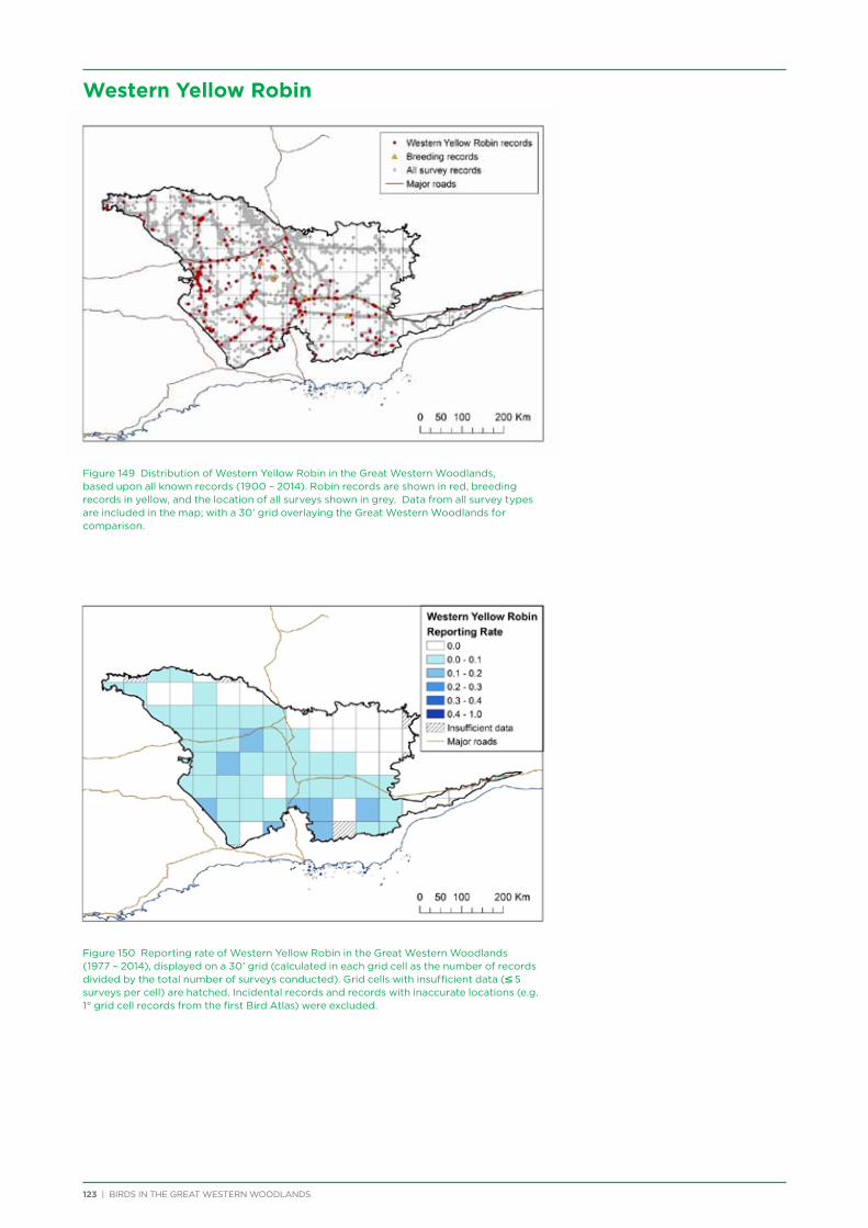
123 | BIRDS IN THE GREAT WESTERN WOODLANDS
Western Yellow Robin
Figure 149 Distribution of Western Yellow Robin in the Great Western Woodlands, based upon all known records (1900 – 2014). Robin records are shown in red, breeding records in yellow, and the location of all surveys shown in grey. Data from all survey types are included in the map; with a 30’ grid overlaying the Great Western Woodlands for comparison.
Figure 150 Reporting rate of Western Yellow Robin in the Great Western Woodlands (1977 – 2014), displayed on a 30’ grid (calculated in each grid cell as the number of records divided by the total number of surveys conducted). Grid cells with insufficient data (≤ 5 surveys per cell) are hatched. Incidental records and records with inaccurate locations (e.g. 1° grid cell records from the first Bird Atlas) were excluded.
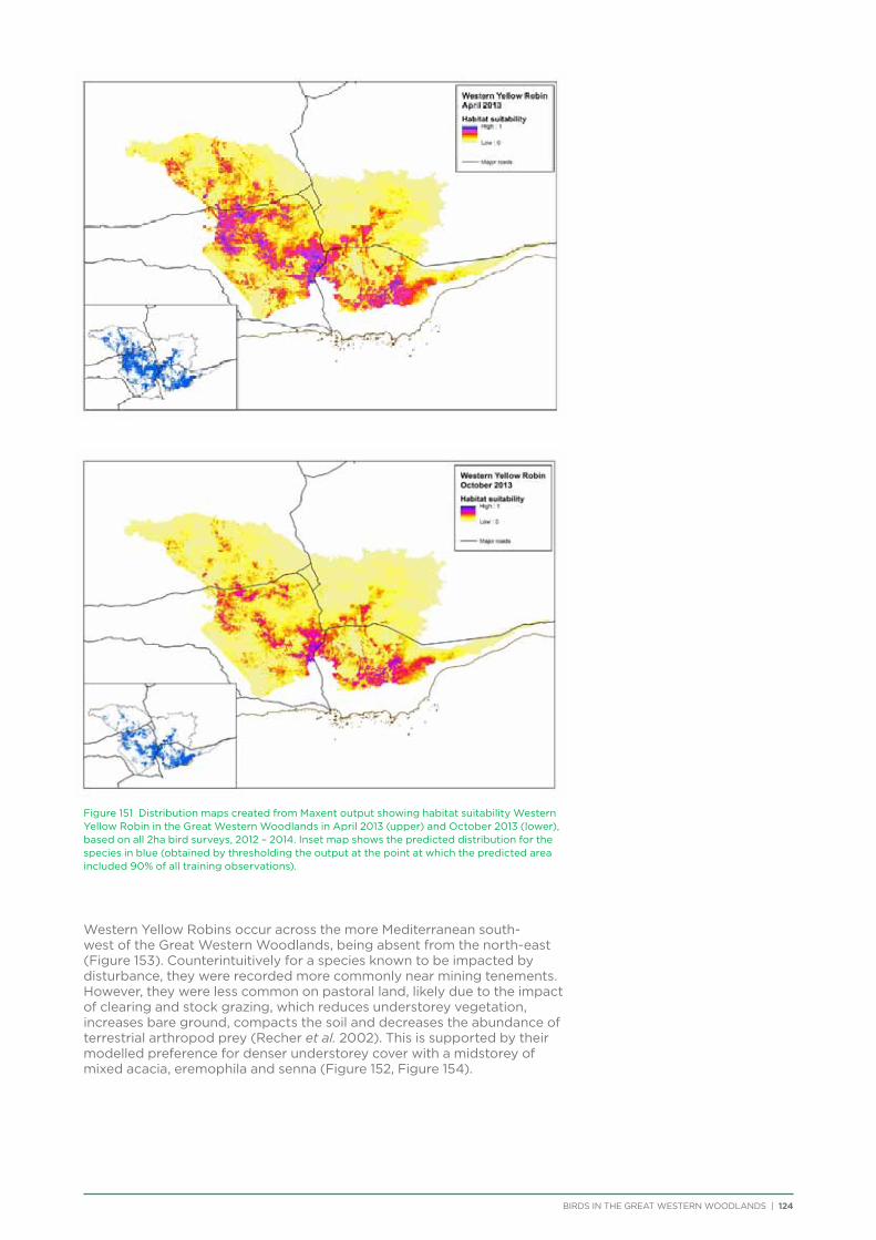
BIRDS IN THE GREAT WESTERN WOODLANDS | 124
Figure 151 Distribution maps created from Maxent output showing habitat suitability Western Yellow Robin in the Great Western Woodlands in April 2013 (upper) and October 2013 (lower), based on all 2ha bird surveys, 2012 – 2014. Inset map shows the predicted distribution for the species in blue (obtained by thresholding the output at the point at which the predicted area included 90% of all training observations).
Western Yellow Robins occur across the more Mediterranean south-west of the Great Western Woodlands, being absent from the north-east (Figure 153). Counterintuitively for a species known to be impacted by disturbance, they were recorded more commonly near mining tenements. However, they were less common on pastoral land, likely due to the impact of clearing and stock grazing, which reduces understorey vegetation, increases bare ground, compacts the soil and decreases the abundance of terrestrial arthropod prey (Recher et al. 2002). This is supported by their modelled preference for denser understorey cover with a midstorey of mixed acacia, eremophila and senna (Figure 152, Figure 154).
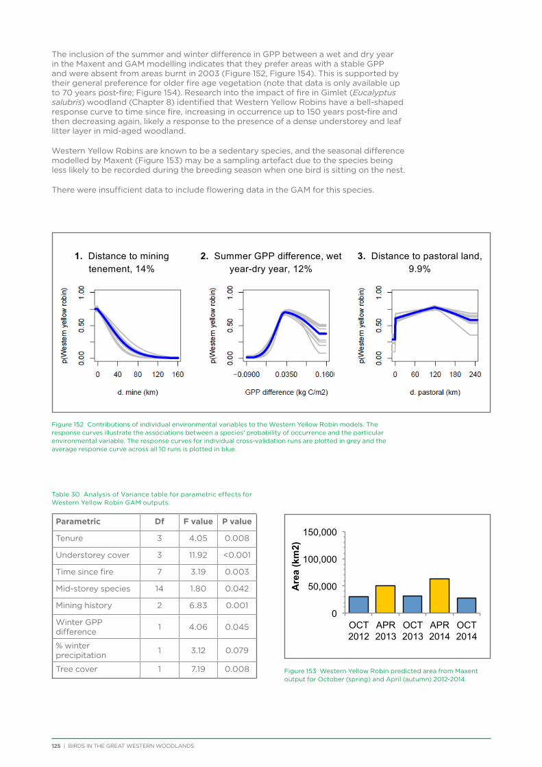
125 | BIRDS IN THE GREAT WESTERN WOODLANDS
The inclusion of the summer and winter difference in GPP between a wet and dry year in the Maxent and GAM modelling indicates that they prefer areas with a stable GPP and were absent from areas burnt in 2003 (Figure 152, Figure 154). This is supported by their general preference for older fire age vegetation (note that data is only available up to 70 years post-fire; Figure 154). Research into the impact of fire in Gimlet (Eucalyptus salubris) woodland (Chapter 8) identified that Western Yellow Robins have a bell-shaped response curve to time since fire, increasing in occurrence up to 150 years post-fire and then decreasing again, likely a response to the presence of a dense understorey and leaf litter layer in mid-aged woodland.
Western Yellow Robins are known to be a sedentary species, and the seasonal difference modelled by Maxent (Figure 153) may be a sampling artefact due to the species being less likely to be recorded during the breeding season when one bird is sitting on the nest.
There were insufficient data to include flowering data in the GAM for this species.
Figure 152 Contributions of individual environmental variables to the Western Yellow Robin models. The response curves illustrate the associations between a species’ probability of occurrence and the particular environmental variable. The response curves for individual cross-validation runs are plotted in grey and the average response curve across all 10 runs is plotted in blue.
Table 30 Analysis of Variance table for parametric effects for Western Yellow Robin GAM outputs.
Parametric Df F value P value
Tenure 3 4.05 0.008
Understorey cover 3 11.92 <0.001
Time since fire 7 3.19 0.003
Mid-storey species 14 1.80 0.042
Mining history 2 6.83 0.001
Winter GPP difference 1 4.06 0.045
% winter precipitation 1 3.12 0.079
Tree cover 1 7.19 0.008
1. Distance to mining tenement, 14%
2. Summer GPP difference, wet year-dry year, 12%
3. Distance to pastoral land, 9.9%
0
50,000
100,000
150,000
OCT 2012
APR 2013
OCT 2013
APR 2014
OCT 2014
Are
a (k
m2)
Figure 153 Western Yellow Robin predicted area from Maxent output for October (spring) and April (autumn) 2012-2014.
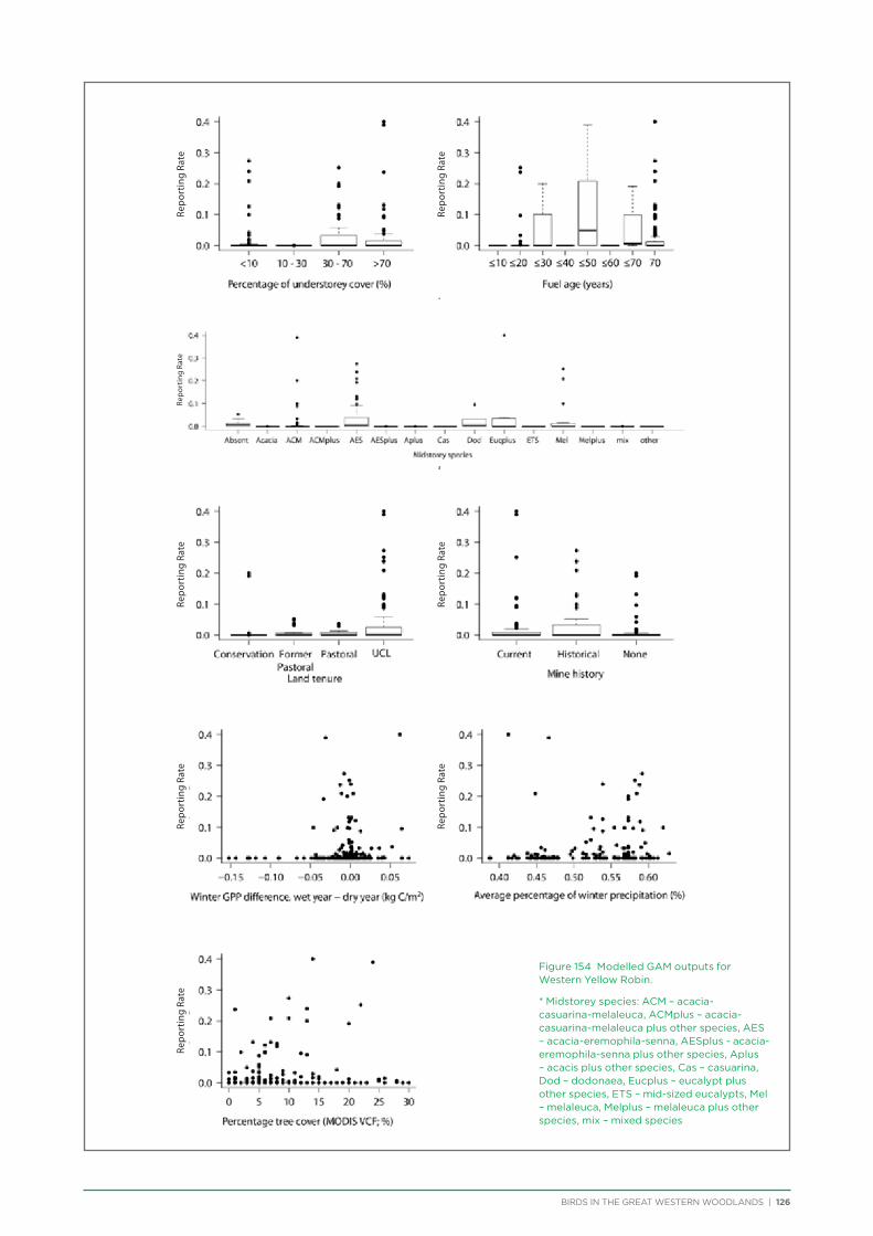
BIRDS IN THE GREAT WESTERN WOODLANDS | 126
Figure 154 Modelled GAM outputs for Western Yellow Robin.
* Midstorey species: ACM – acacia-casuarina-melaleuca, ACMplus – acacia-casuarina-melaleuca plus other species, AES – acacia-eremophila-senna, AESplus - acacia-eremophila-senna plus other species, Aplus – acacis plus other species, Cas – casuarina, Dod – dodonaea, Eucplus – eucalypt plus other species, ETS – mid-sized eucalypts, Mel – melaleuca, Melplus – melaleuca plus other species, mix – mixed species
Repo
rtin
g Ra
teRe
port
ing
Rate
Repo
rtin
g Ra
teRe
port
ing
Rate
Repo
rtin
g Ra
te
Repo
rtin
g Ra
teRe
port
ing
Rate
Repo
rtin
g Ra
te
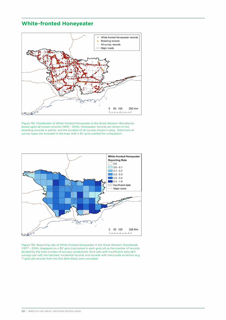
127 | BIRDS IN THE GREAT WESTERN WOODLANDS
White-fronted Honeyeater
Figure 155 Distribution of White-fronted Honeyeater in the Great Western Woodlands, based upon all known records (1900 – 2014). Honeyeater records are shown in red, breeding records in yellow, and the location of all surveys shown in grey. Data from all survey types are included in the map; with a 30’ grid overlaid for comparison.
Figure 156 Reporting rate of White-fronted Honeyeater in the Great Western Woodlands (1977 – 2014), displayed on a 30’ grid (calculated in each grid cell as the number of records divided by the total number of surveys conducted). Grid cells with insufficient data (≤ 5 surveys per cell) are hatched. Incidental records and records with inaccurate locations (e.g. 1° grid cell records from the first Bird Atlas) were excluded.
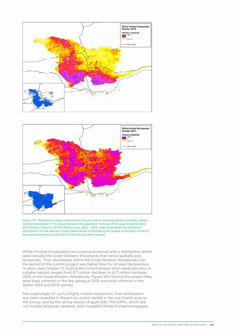
BIRDS IN THE GREAT WESTERN WOODLANDS | 128
Figure 157 Distribution maps created from Maxent output showing habitat suitability White-fronted Honeyeater in the Great Western Woodlands in October 2012 (upper) and October 2013 (lower), based on all 2ha bird surveys, 2012 – 2014. Inset maps show the predicted distribution for the species in blue (obtained by thresholding the output at the point at which the predicted area included 90% of all training observations).
White-fronted Honeyeaters are a resource nomad with a distribution within (and outside) the Great Western Woodlands that varies spatially and temporally. Their abundance within the Great Western Woodlands over the period of the current project was higher than for at least the previous 14 years (see Chapter 7). During the current project their predicted area of suitable habitat ranged from 8.7 million hectares to 14.7 million hectares (92% of the Great Western Woodlands; Figure 161). During the project they were least common in the dry spring of 2012 and most common in the wetter 2013 and 2014 springs.
Not surprisingly for such a highly mobile nectarivore, their distribution was best modelled in Maxent by recent rainfall in the one month prior to the survey, and by the spring season (Figure 159). The GAMs, which did not include temporal variables, best modelled White-fronted Honeyeater
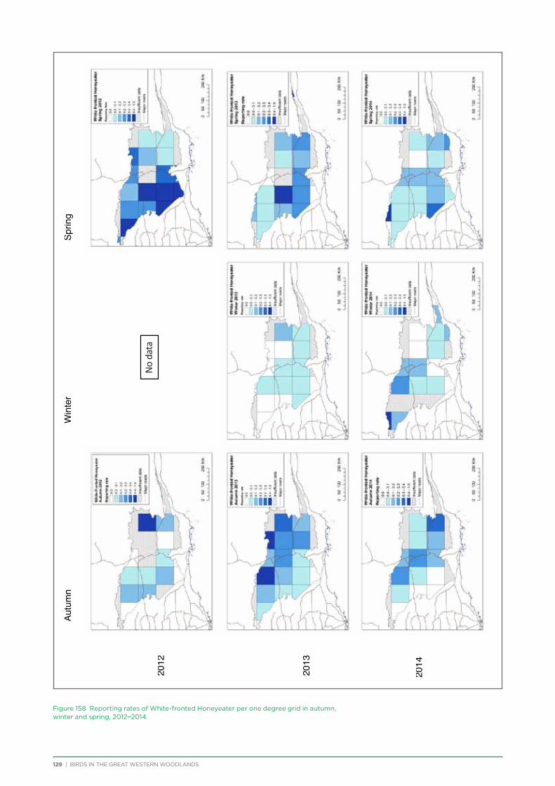
129 | BIRDS IN THE GREAT WESTERN WOODLANDS
Autu
mn
W
inte
r
Sprin
g
2012
2013
2014
No
data
Figure 158 Reporting rates of White-fronted Honeyeater per one degree grid in autumn, winter and spring, 2012−2014.
No
data
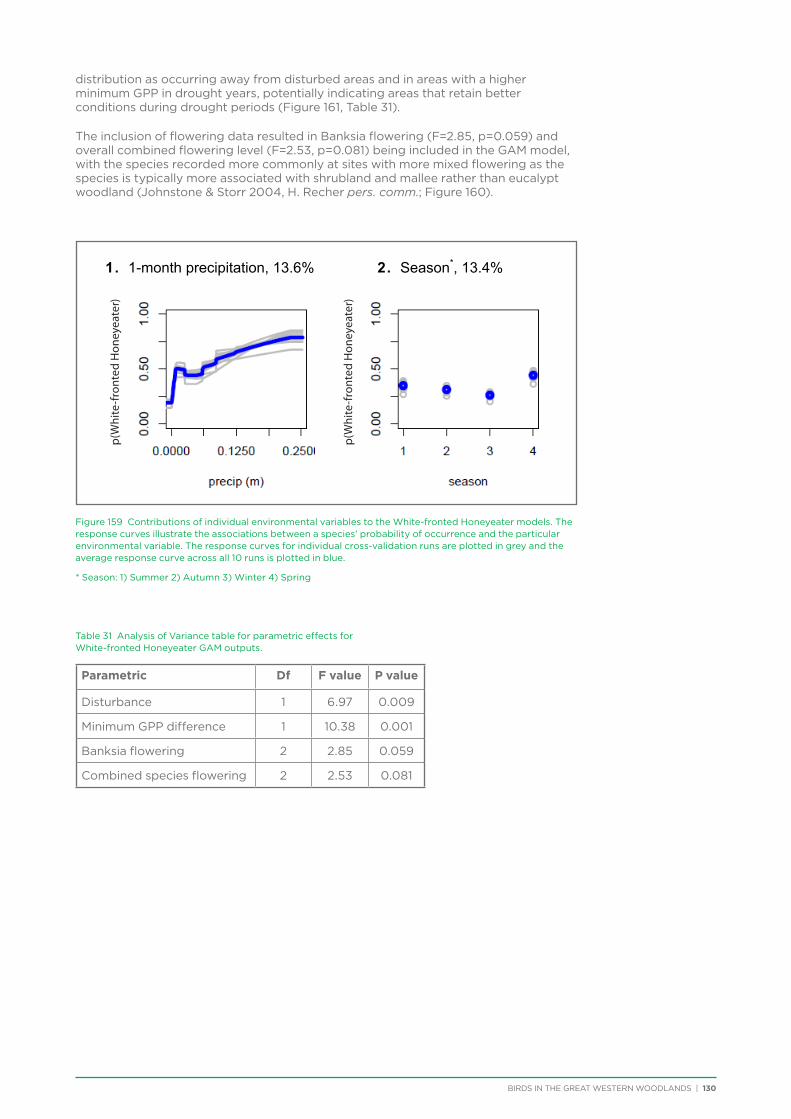
BIRDS IN THE GREAT WESTERN WOODLANDS | 130
distribution as occurring away from disturbed areas and in areas with a higher minimum GPP in drought years, potentially indicating areas that retain better conditions during drought periods (Figure 161, Table 31).
The inclusion of flowering data resulted in Banksia flowering (F=2.85, p=0.059) and overall combined flowering level (F=2.53, p=0.081) being included in the GAM model, with the species recorded more commonly at sites with more mixed flowering as the species is typically more associated with shrubland and mallee rather than eucalypt woodland (Johnstone & Storr 2004, H. Recher pers. comm.; Figure 160).
Figure 159 Contributions of individual environmental variables to the White-fronted Honeyeater models. The response curves illustrate the associations between a species’ probability of occurrence and the particular environmental variable. The response curves for individual cross-validation runs are plotted in grey and the average response curve across all 10 runs is plotted in blue.
* Season: 1) Summer 2) Autumn 3) Winter 4) Spring
Table 31 Analysis of Variance table for parametric effects for White-fronted Honeyeater GAM outputs.
Parametric Df F value P value
Disturbance 1 6.97 0.009
Minimum GPP difference 1 10.38 0.001
Banksia flowering 2 2.85 0.059
Combined species flowering 2 2.53 0.081
1. 1-month precipitation, 13.6%
2. Season*, 13.4%
p(W
hite
-fro
nted
H
oney
eate
r)
p(W
hite
-fro
nted
H
oney
eate
r)
p(W
hite
-fro
nted
Hon
eyea
ter)
p(W
hite
-fro
nted
Hon
eyea
ter)
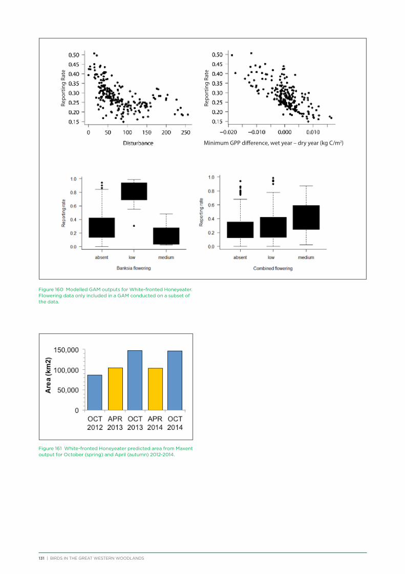
131 | BIRDS IN THE GREAT WESTERN WOODLANDS
Figure 160 Modelled GAM outputs for White-fronted Honeyeater. Flowering data only included in a GAM conducted on a subset of the data.
Figure 161 White-fronted Honeyeater predicted area from Maxent output for October (spring) and April (autumn) 2012-2014.
Repo
rtin
g Ra
te
Repo
rtin
g Ra
te
Minimum GPP difference, wet year – dry year (kg C/m2)

BIRDS IN THE GREAT WESTERN WOODLANDS | 132Photo: Cheryl Gole
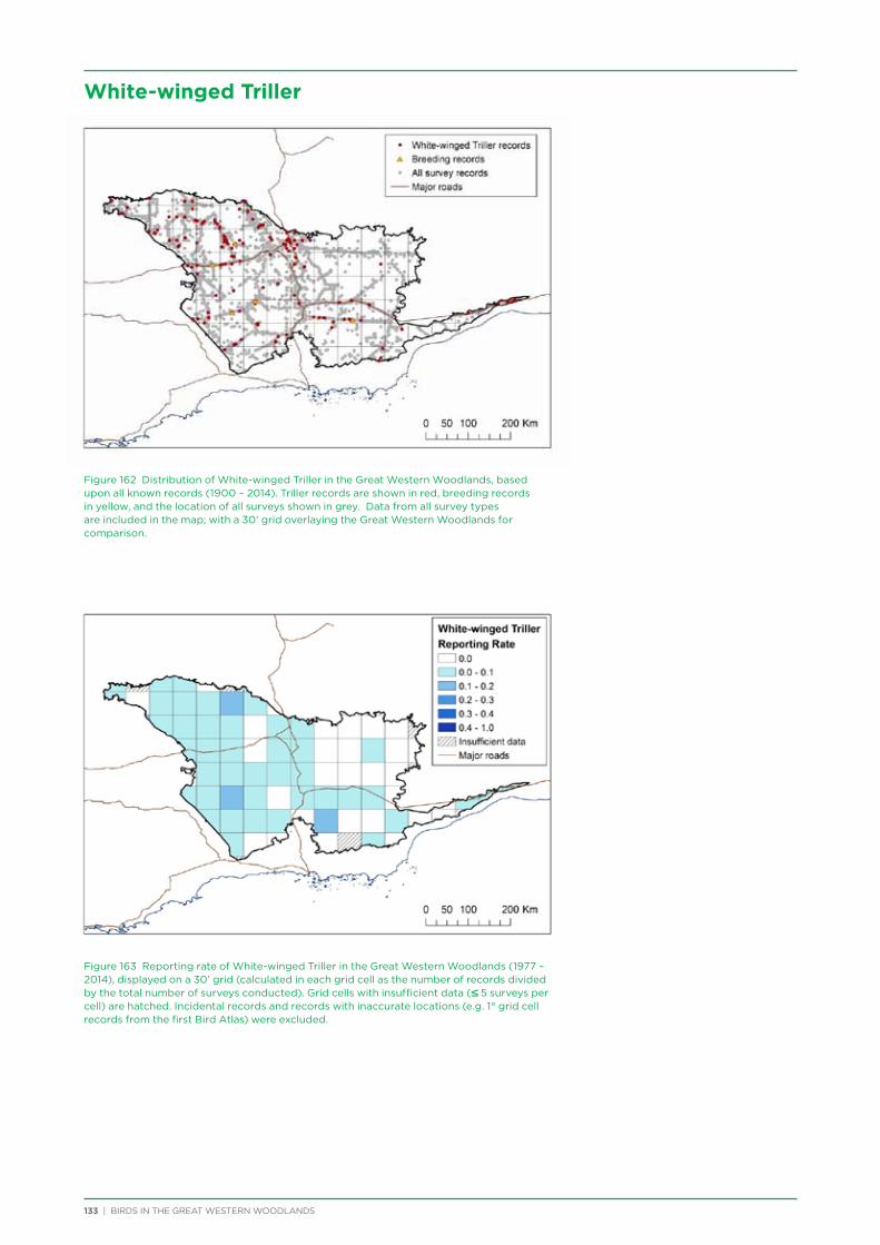
133 | BIRDS IN THE GREAT WESTERN WOODLANDS
White-winged Triller
Figure 162 Distribution of White-winged Triller in the Great Western Woodlands, based upon all known records (1900 – 2014). Triller records are shown in red, breeding records in yellow, and the location of all surveys shown in grey. Data from all survey types are included in the map; with a 30’ grid overlaying the Great Western Woodlands for comparison.
Figure 163 Reporting rate of White-winged Triller in the Great Western Woodlands (1977 – 2014), displayed on a 30’ grid (calculated in each grid cell as the number of records divided by the total number of surveys conducted). Grid cells with insufficient data (≤ 5 surveys per cell) are hatched. Incidental records and records with inaccurate locations (e.g. 1° grid cell records from the first Bird Atlas) were excluded.
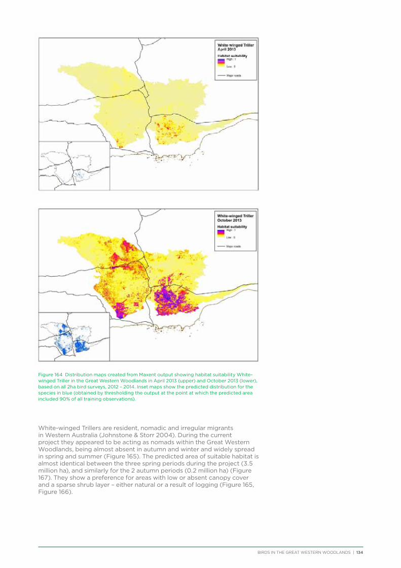
BIRDS IN THE GREAT WESTERN WOODLANDS | 134
Figure 164 Distribution maps created from Maxent output showing habitat suitability White-winged Triller in the Great Western Woodlands in April 2013 (upper) and October 2013 (lower), based on all 2ha bird surveys, 2012 – 2014. Inset maps show the predicted distribution for the species in blue (obtained by thresholding the output at the point at which the predicted area included 90% of all training observations).
White-winged Trillers are resident, nomadic and irregular migrants in Western Australia (Johnstone & Storr 2004). During the current project they appeared to be acting as nomads within the Great Western Woodlands, being almost absent in autumn and winter and widely spread in spring and summer (Figure 165). The predicted area of suitable habitat is almost identical between the three spring periods during the project (3.5 million ha), and similarly for the 2 autumn periods (0.2 million ha) (Figure 167). They show a preference for areas with low or absent canopy cover and a sparse shrub layer – either natural or a result of logging (Figure 165, Figure 166).
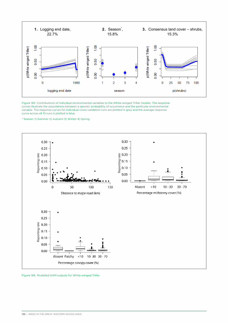
135 | BIRDS IN THE GREAT WESTERN WOODLANDS
Figure 165 Contributions of individual environmental variables to the White-winged Triller models. The response curves illustrate the associations between a species’ probability of occurrence and the particular environmental variable. The response curves for individual cross-validation runs are plotted in grey and the average response curve across all 10 runs is plotted in blue.
* Season: 1) Summer 2) Autumn 3) Winter 4) Spring
Figure 166 Modelled GAM outputs for White-winged Triller.
1. Logging end date, 22.7%
2. Season*, 15.8%
3. Consensus land cover – shrubs, 15.3%
Repo
rtin
g ra
teRe
port
ing
rate
Repo
rtin
g ra
te
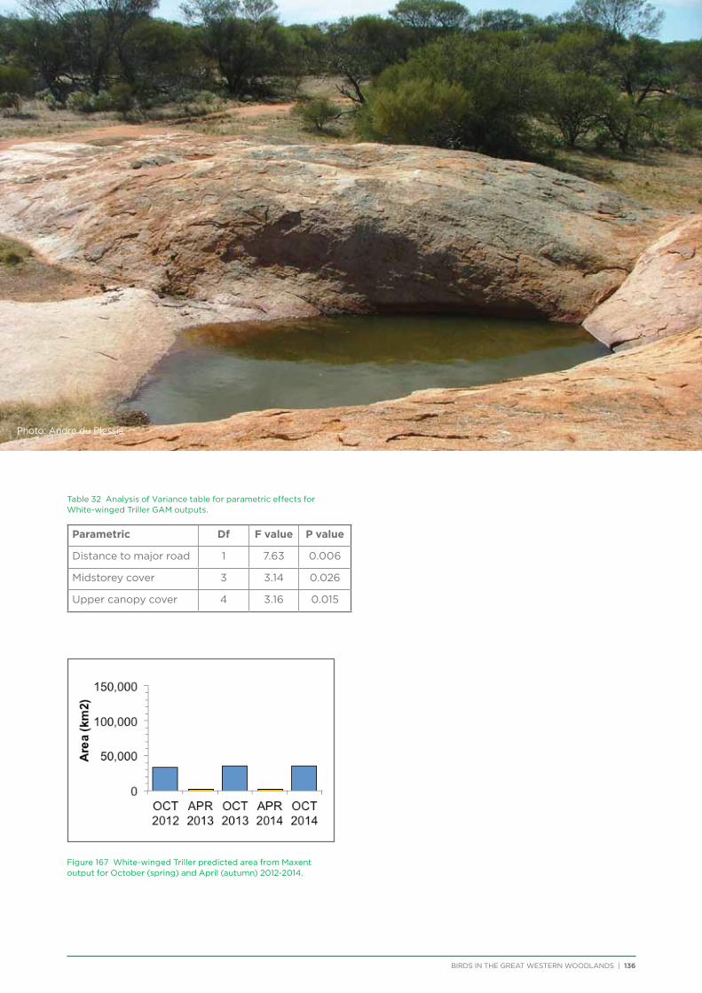
BIRDS IN THE GREAT WESTERN WOODLANDS | 136
Table 32 Analysis of Variance table for parametric effects for White-winged Triller GAM outputs.
Parametric Df F value P value
Distance to major road 1 7.63 0.006
Midstorey cover 3 3.14 0.026
Upper canopy cover 4 3.16 0.015
Figure 167 White-winged Triller predicted area from Maxent output for October (spring) and April (autumn) 2012-2014.
Photo: Andre du Plessis
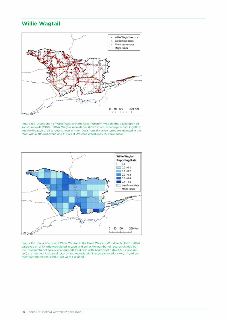
137 | BIRDS IN THE GREAT WESTERN WOODLANDS
Willie Wagtail
Figure 168 Distribution of Willie Wagtail in the Great Western Woodlands, based upon all known records (1900 – 2014). Wagtail records are shown in red, breeding records in yellow, and the location of all surveys shown in grey. Data from all survey types are included in the map; with a 30’ grid overlaying the Great Western Woodlands for comparison.
Figure 169 Reporting rate of Willie Wagtail in the Great Western Woodlands (1977 – 2014), displayed on a 30’ grid (calculated in each grid cell as the number of records divided by the total number of surveys conducted). Grid cells with insufficient data (≤ 5 surveys per cell) are hatched. Incidental records and records with inaccurate locations (e.g. 1° grid cell records from the first Bird Atlas) were excluded.
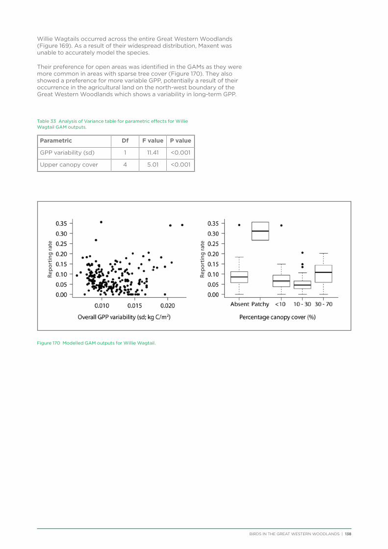
BIRDS IN THE GREAT WESTERN WOODLANDS | 138
Willie Wagtails occurred across the entire Great Western Woodlands (Figure 169). As a result of their widespread distribution, Maxent was unable to accurately model the species.
Their preference for open areas was identified in the GAMs as they were more common in areas with sparse tree cover (Figure 170). They also showed a preference for more variable GPP, potentially a result of their occurrence in the agricultural land on the north-west boundary of the Great Western Woodlands which shows a variability in long-term GPP.
Table 33 Analysis of Variance table for parametric effects for Willie Wagtail GAM outputs.
Parametric Df F value P value
GPP variability (sd) 1 11.41 <0.001
Upper canopy cover 4 5.01 <0.001
Figure 170 Modelled GAM outputs for Willie Wagtail.
Repo
rtin
g ra
te
Repo
rtin
g ra
te
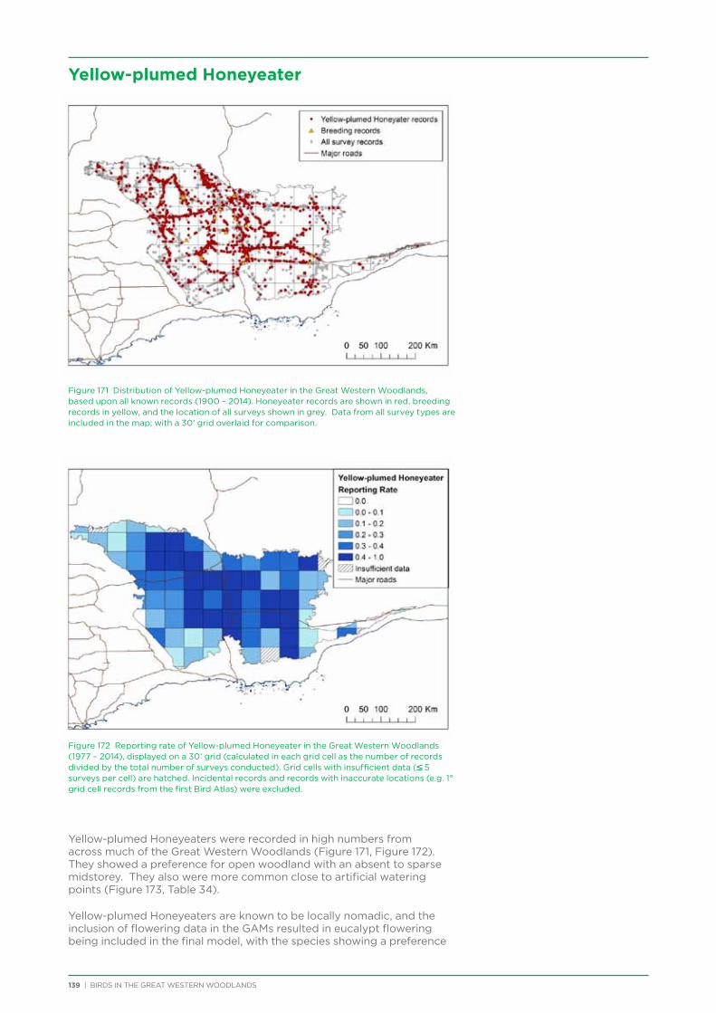
139 | BIRDS IN THE GREAT WESTERN WOODLANDS
Yellow-plumed Honeyeater
Figure 171 Distribution of Yellow-plumed Honeyeater in the Great Western Woodlands, based upon all known records (1900 – 2014). Honeyeater records are shown in red, breeding records in yellow, and the location of all surveys shown in grey. Data from all survey types are included in the map; with a 30’ grid overlaid for comparison.
Figure 172 Reporting rate of Yellow-plumed Honeyeater in the Great Western Woodlands (1977 – 2014), displayed on a 30’ grid (calculated in each grid cell as the number of records divided by the total number of surveys conducted). Grid cells with insufficient data (≤ 5 surveys per cell) are hatched. Incidental records and records with inaccurate locations (e.g. 1° grid cell records from the first Bird Atlas) were excluded.
Yellow-plumed Honeyeaters were recorded in high numbers from across much of the Great Western Woodlands (Figure 171, Figure 172). They showed a preference for open woodland with an absent to sparse midstorey. They also were more common close to artificial watering points (Figure 173, Table 34).
Yellow-plumed Honeyeaters are known to be locally nomadic, and the inclusion of flowering data in the GAMs resulted in eucalypt flowering being included in the final model, with the species showing a preference
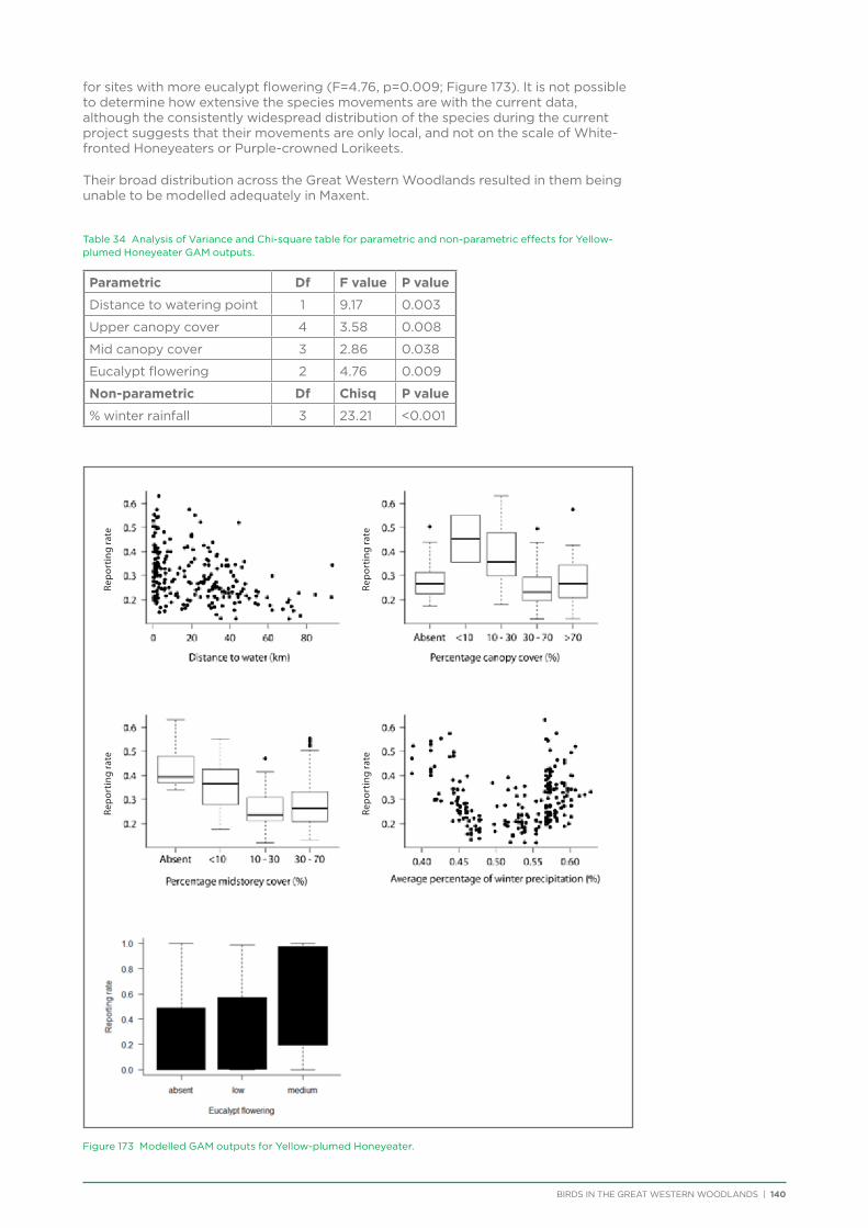
BIRDS IN THE GREAT WESTERN WOODLANDS | 140
for sites with more eucalypt flowering (F=4.76, p=0.009; Figure 173). It is not possible to determine how extensive the species movements are with the current data, although the consistently widespread distribution of the species during the current project suggests that their movements are only local, and not on the scale of White-fronted Honeyeaters or Purple-crowned Lorikeets.
Their broad distribution across the Great Western Woodlands resulted in them being unable to be modelled adequately in Maxent.
Table 34 Analysis of Variance and Chi-square table for parametric and non-parametric effects for Yellow-plumed Honeyeater GAM outputs.
Parametric Df F value P value
Distance to watering point 1 9.17 0.003
Upper canopy cover 4 3.58 0.008
Mid canopy cover 3 2.86 0.038
Eucalypt flowering 2 4.76 0.009
Non-parametric Df Chisq P value
% winter rainfall 3 23.21 <0.001
Figure 173 Modelled GAM outputs for Yellow-plumed Honeyeater.
Repo
rtin
g ra
teRe
port
ing
rate
Repo
rtin
g ra
teRe
port
ing
rate
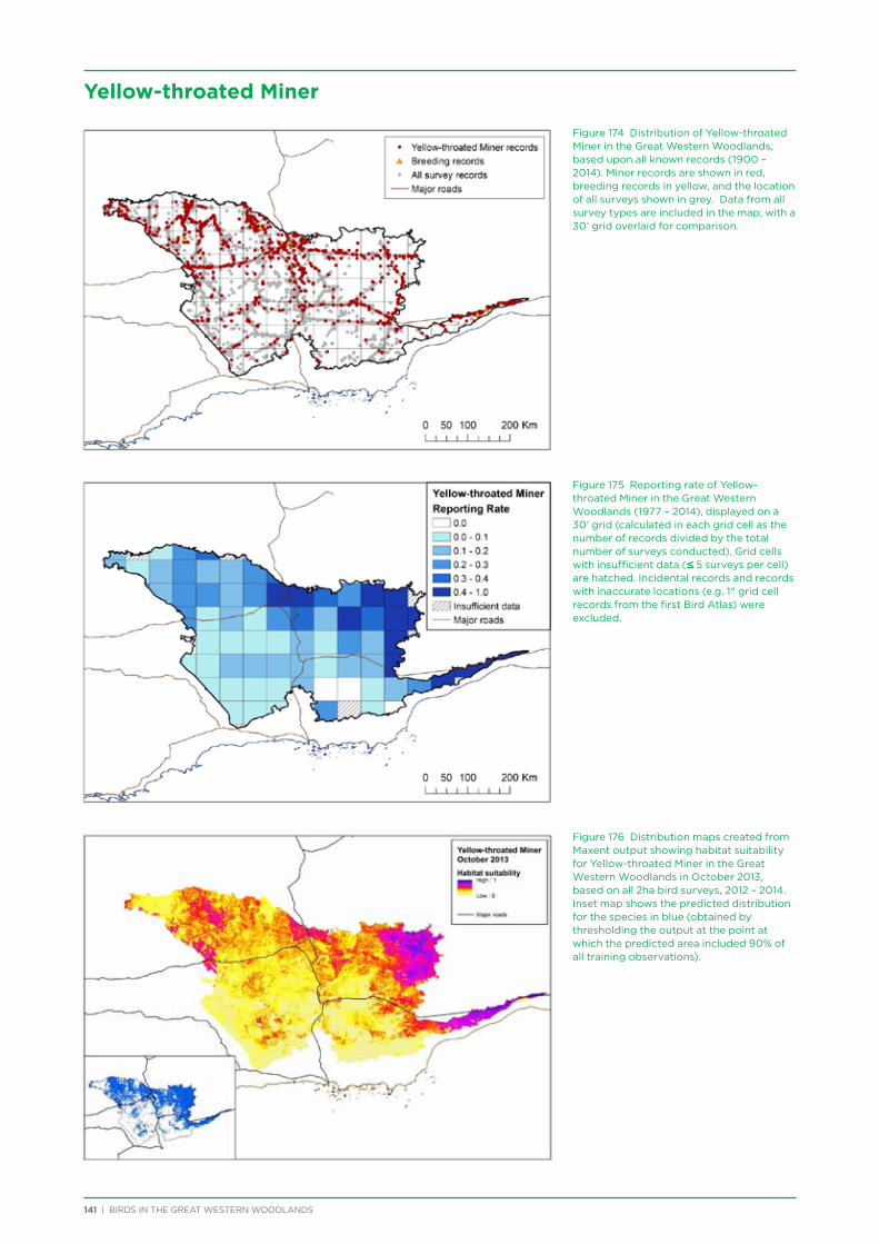
Figure 174 Distribution of Yellow-throated Miner in the Great Western Woodlands, based upon all known records (1900 – 2014). Miner records are shown in red, breeding records in yellow, and the location of all surveys shown in grey. Data from all survey types are included in the map; with a 30’ grid overlaid for comparison.
Figure 175 Reporting rate of Yellow-throated Miner in the Great Western Woodlands (1977 – 2014), displayed on a 30’ grid (calculated in each grid cell as the number of records divided by the total number of surveys conducted). Grid cells with insufficient data (≤ 5 surveys per cell) are hatched. Incidental records and records with inaccurate locations (e.g. 1° grid cell records from the first Bird Atlas) were excluded.
Figure 176 Distribution maps created from Maxent output showing habitat suitability for Yellow-throated Miner in the Great Western Woodlands in October 2013, based on all 2ha bird surveys, 2012 – 2014. Inset map shows the predicted distribution for the species in blue (obtained by thresholding the output at the point at which the predicted area included 90% of all training observations).
141 | BIRDS IN THE GREAT WESTERN WOODLANDS
Yellow-throated Miner
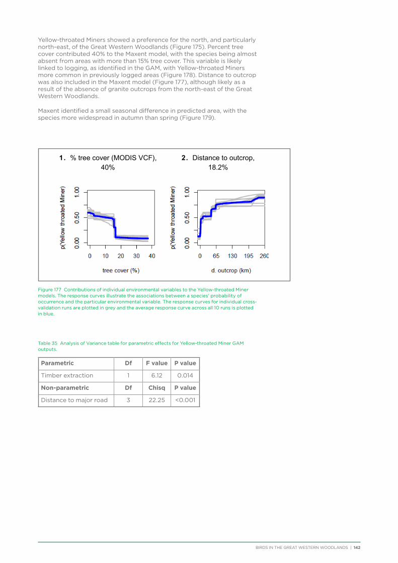
BIRDS IN THE GREAT WESTERN WOODLANDS | 142
Yellow-throated Miners showed a preference for the north, and particularly north-east, of the Great Western Woodlands (Figure 175). Percent tree cover contributed 40% to the Maxent model, with the species being almost absent from areas with more than 15% tree cover. This variable is likely linked to logging, as identified in the GAM, with Yellow-throated Miners more common in previously logged areas (Figure 178). Distance to outcrop was also included in the Maxent model (Figure 177), although likely as a result of the absence of granite outcrops from the north-east of the Great Western Woodlands.
Maxent identified a small seasonal difference in predicted area, with the species more widespread in autumn than spring (Figure 179).
Figure 177 Contributions of individual environmental variables to the Yellow-throated Miner models. The response curves illustrate the associations between a species’ probability of occurrence and the particular environmental variable. The response curves for individual cross-validation runs are plotted in grey and the average response curve across all 10 runs is plotted in blue.
Table 35 Analysis of Variance table for parametric effects for Yellow-throated Miner GAM outputs.
Parametric Df F value P value
Timber extraction 1 6.12 0.014
Non-parametric Df Chisq P value
Distance to major road 3 22.25 <0.001
1. % tree cover (MODIS VCF), 40%
2. Distance to outcrop, 18.2%
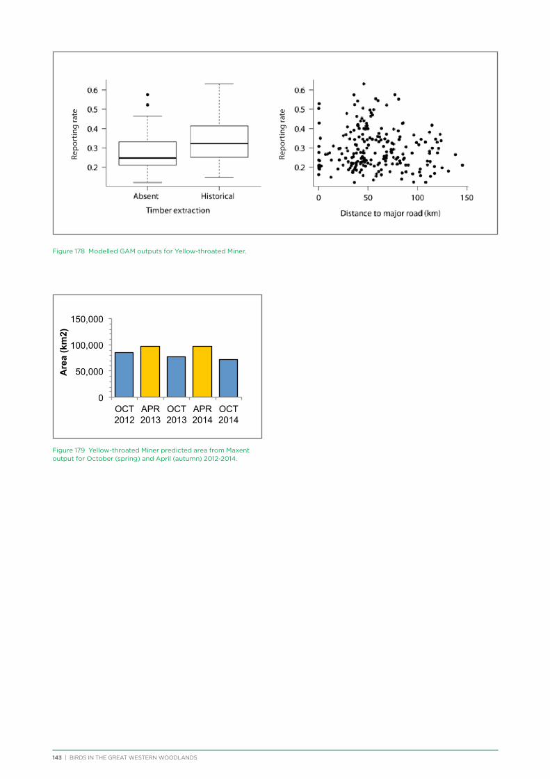
143 | BIRDS IN THE GREAT WESTERN WOODLANDS
Figure 178 Modelled GAM outputs for Yellow-throated Miner.
Figure 179 Yellow-throated Miner predicted area from Maxent output for October (spring) and April (autumn) 2012-2014.
0
50,000
100,000
150,000
OCT 2012
APR 2013
OCT 2013
APR 2014
OCT 2014
Are
a (k
m2)
Re
port
ing
rate
Repo
rtin
g ra
te
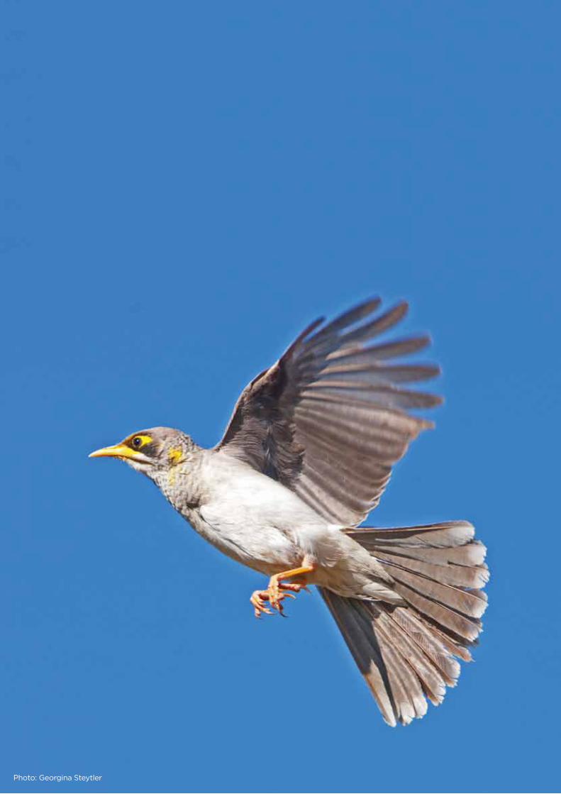
BIRDS IN THE GREAT WESTERN WOODLANDS | 144Photo: Georgina Steytler
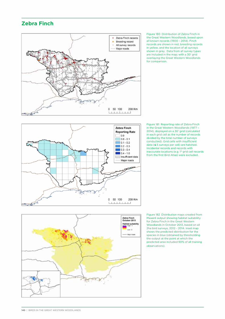
Figure 180 Distribution of Zebra Finch in the Great Western Woodlands, based upon all known records (1900 – 2014). Finch records are shown in red, breeding records in yellow, and the location of all surveys shown in grey. Data from all survey types are included in the map; with a 30’ grid overlaying the Great Western Woodlands for comparison.
Figure 181 Reporting rate of Zebra Finch in the Great Western Woodlands (1977 – 2014), displayed on a 30’ grid (calculated in each grid cell as the number of records divided by the total number of surveys conducted). Grid cells with insufficient data (≤ 5 surveys per cell) are hatched. Incidental records and records with inaccurate locations (e.g. 1° grid cell records from the first Bird Atlas) were excluded.
Figure 182 Distribution maps created from Maxent output showing habitat suitability for Zebra Finch in the Great Western Woodlands in October 2013, based on all 2ha bird surveys, 2012 – 2014. Inset map shows the predicted distribution for the species in blue (obtained by thresholding the output at the point at which the predicted area included 90% of all training observations).
145 | BIRDS IN THE GREAT WESTERN WOODLANDS
Zebra Finch
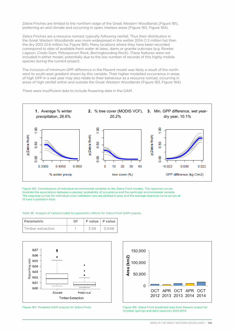
BIRDS IN THE GREAT WESTERN WOODLANDS | 146
Zebra Finches are limited to the northern edge of the Great Western Woodlands (Figure 181), preferring an arid climate and occurring in open, treeless areas (Figure 183, Figure 184).
Zebra Finches are a resource nomad, typically following rainfall. Thus their distribution in the Great Western Woodlands was more widespread in the wetter 2014 (1.5 million ha) than the dry 2012 (0.6 million ha; Figure 185). Many locations where they have been recorded correspond to sites of available fresh water at lakes, dams or granite outcrops (e.g. Rowles Lagoon, Credo Dam, Pittosporum Rock, Berringbooding Rock). These features were not included in either model, potentially due to the low number of records of this highly mobile species during the current project.
The inclusion of minimum GPP difference in the Maxent model was likely a result of the north-west to south-east gradient shown by this variable. Their higher modelled occurrence in areas of high GPP in a wet year may also relate to their behaviour as a resource nomad, occurring in areas of high rainfall within and outside the Great Western Woodlands (Figure 183, Figure 184).
There were insufficient data to include flowering data in the GAM.
Figure 183 Contributions of individual environmental variables to the Zebra Finch models. The response curves illustrate the associations between a species’ probability of occurrence and the particular environmental variable. The response curves for individual cross-validation runs are plotted in grey and the average response curve across all 10 runs is plotted in blue.
Table 36 Analysis of Variance table for parametric effects for Zebra Finch GAM outputs.
Parametric Df F value P value
Timber extraction 1 3.59 0.048
1. Average % winter precipitation, 26.6%
2. % tree cover (MODIS VCF), 20.2%
3. Min. GPP difference, wet year-dry year, 10.1%
Figure 184 Modelled GAM outputs for Zebra Finch. Figure 185 Zebra Finch predicted area from Maxent output for October (spring) and April (autumn) 2012-2014.
Repo
rtin
g ra
te

147 | BIRDS IN THE GREAT WESTERN WOODLANDS
6.3. Discussion
In general, the suitable habitat maps as predicted by the Maxent models reflected the patterns observed with the much more abundant data used in the raw distribution and reporting rate maps. However, the reporting rate maps were limited to only showing broadscale trends due to the sparseness of the data over such a large area. In contrast, Maxent was able to highlight species with a patchy distribution within a broad area, as well as those showing seasonal and annual variations in distribution. The data for the modelling only included 3 years of data. Including additional data obtained over the coming years will improve the results, particularly related to temporal patterns associated with rainfall and flowering.
The inclusion of temporal and spatial environmental variables in the Maxent models enabled the identification of temporal variation in species distribution – both short-term seasonal and longer-term drought responses. A surprising result was the unimportance of time-specific GPP to the modelled distributions. It was expected that time-specific GPP would provide a better portrayal of environmental variation than precipitation, given the fairly sparse weather station network in the Great Western Woodlands, the coarser spatial resolution of the precipitation data set, and errors associated with downscaled weather data (Daly 2006). However, the reverse was observed. Time-specific GPP was predicted to be an indicator of resource availability to birds, but it does not directly measure the actual components of the birds’ diets. Thus, one reason for its minor contribution to the Maxent models may simply be that it is a poor proxy for the floral, seed, and insect resources that are used by the species modelled, or that the abundance and availability of these resources may change more rapidly than total productivity. Another possibility is that the MODIS GPP product may not accurately represent ecosystem dynamics in the Great Western Woodlands. Although validation efforts have found that MODIS GPP generally captures relative differences in productivity over space and time (Heinsch et al. 2006, Turner et al. 2006), other studies (e.g. Leuning et al. 2005, Mu et al. 2007) have identified weaknesses in the MODIS GPP algorithm in arid and semi-arid regions. In particular, the vapour pressure deficit term used to modify photosynthetic efficiency may not be a sufficient indicator of drought stress. GPP estimates may be improved by the addition of soil moisture information. However, such soils data are not available at a global level and thus cannot be incorporated into a standard product such as MODIS GPP.
Although time-specific GPP rarely factored into species models, long-term GPP variability, especially measures contrasting the wettest and driest years of the MODIS record, were related to habitat preference in a number of species. Comparisons between specific environmental conditions (such as years with precipitation extremes) may be able to be used to identify refugia. Indeed, several species exhibited a unimodal preference for areas with little GPP difference between wet and dry years, which is consistent with the notion of refugia as
being buffered from the changes in productivity occurring in surrounding vegetation. However, the confounding effects of fire and agricultural land, and the general climatic gradients shown by these measures need to be taken into account. More research is required into the use of GPP or other methods (Keppel et al. 2012) to highlight areas of refugia in the Great Western Woodlands.
Aside from GPP measures, the most important biotic variable across species was percent tree cover, as derived from satellite imagery. The inclusion of individual site vegetation characteristics in the GAMs resulted in over half of the models including these variables in the final model. This contrasts to the broader mapped vegetation categories (Shepherd 2003) included in Maxent models which were rarely found to contribute to the species models. Although individual site vegetation characteristics were frequently included in the GAM models, the most common variables included were the presence/absence of tree hollows, and upper canopy and understorey cover. Upper canopy cover is likely directly related to percent tree cover, although it has been measured directly from site photographs at the time of survey rather than a static measure of tree cover from satellite imagery in 2010. The presence of tree hollows is likely an indirect measure of tree cover as it relates to the presence of mature woodland. The presence of trees therefore appears to be the main driver of species distribution in terms of vegetation characteristics. This is supported by the results of the species assemblage analysis (Chapter 4), which found that species assemblages were typically similar across the Great Western Woodlands, with a large number of widespread generalist species, and the main split in species assemblages being between mallee and shrubland habitats compared to woodland.
Time-specific rainfall only contributed over 10% to the Maxent models of two species; Horsfield’s Bronze-Cuckoo and White-fronted Honeyeater – both resource nomads. However, it is possible that the timeframe over which rainfall was calculated (1–6 months) was not relevant to many species. Stevens & Watson (2013) identified that the winter/spring rainfall of the previous year and the summer/autumn rainfall in the prior six years correlated with changes in the abundance of birds in forest in New South Wales. Further research is required to study the long-term impacts of rainfall on the abundance and occurrence of bird species.
Four of the 14 species, for which there were sufficient data to run a GAM including flowering data, had flowering level included in the model. Not surprisingly, these consisted of the four nectarivorous species (White-fronted Honeyeater, Singing Honeyeater, Yellow-plumed Honeyeater and Purple-crowned Lorikeet). White-fronted Honeyeater and Purple-crowned Lorikeet are resource nomads, travelling large distances within and outside the Great Western Woodlands in search of nectar sources. Along with the other nomadic species, they showed high variation in
BIRDS IN THE GREAT WESTERN WOODLANDS | 148
distribution within and between years. In general, the occurrence of nomadic species was related to temporally-specific rainfall, as well as open woodland habitat. Unlike other wheatbelt decliners, they were frequently positively associated with disturbance-related variables. In addition to within-year variations in distribution, resource nomads were typically modelled as having a much lower distribution within the Great Western Woodlands in the dry year of 2012 as compared to the following two wet years. The ability of these bird species to move large distances in search of suitable food and water resources results in these species being able to utilise the Great Western Woodlands when it provides suitable resources, and to be almost entirely absent when conditions are better elsewhere. This is a potential limitation of the current study with respect to modelling resource nomads as it focussed on explanatory variables from within the Great Western Woodlands. Some species will be responding to conditions outside the Great Western Woodlands, which would not have been picked up by the current models.
The wheatbelt increaser species tended to occur in more open habitats and were positively related to various disturbance-related variables, particularly pastoral land and their associated artificial watering points. The provision of artificial water sources is known to result in the expansion in geographic range and abundance in a number of bird species (James 1999). Prior to the provision of artificial water sources, species dependent on free water could only inhabit arid areas around permanent natural water and over larger areas following good rainfall (James 1999). Wheatbelt increaser species tended to have highly stable predicted distribution within and between years, likely a result of the stable provision of food and water resources as a result of human activity. In contrast, wheatbelt decliner species tended to be more highly variable in distribution within and between years. Except for the nomadic species, wheatbelt decliners tended to be negatively impacted by disturbance-related variables including mining, fire, logging and artificial watering points. Distance to pastoral land was a commonly included variable in the models, although this typically related to the general south-west to north-east gradient of many of these species rather than a direct impact of pastoralism. The south-west distribution of many of these species also resulted in percent winter rainfall (relating to the Mediterranean climate) being frequently positively related.
Hollow-nesting species typically occurred in areas of higher rainfall and tree cover, and tended to be negatively impacted by disturbance-related variables such as logging and fire, which impact on the presence of mature hollow-bearing trees. Several species, predominantly the parrots, showed seasonal variation in predicted distribution. This may be due to the behavioural characteristics of these species related to forming flocks during non-breeding periods and spreading out to individual territories and being less conspicuous during spring.
Not all threatened species had sufficient data to enable modelling. Of the three species that did, they were all negatively impacted by disturbance-related
variables such as watering points and logging, being significantly less common in close proximity to artificial watering points. A similar result was obtained for ground-foraging insectivores, being predominantly negatively impacted by disturbances such as fire and mining. The one ground-foraging insectivore showing the reverse result (Australasian Pipit) of being more common on mining and pastoral land is also a wheatbelt increaser, known to prefer open, disturbed habitats. In contrast, the wheatbelt decliner ground-foraging insectivores were modelled as preferring habitats consisting of denser tree and understorey cover. Their predicted area was typically stable within and between years.
Raptors are poorly sampled using the 2ha survey method and only Nankeen Kestrel was able to be modelled. They were predominantly associated with open habitats and had a stable predicted distribution during the current project.
Of interest is that the dry year of 2012 often showed a distinct difference in the predicted distribution of species compared to the following wetter years. Some species distributions may coalesce to areas of high quality habitat in periods of environmental stress, truncating the species response to environmental gradients (e.g. Rufous Treecreeper, Galah). However, the converse is also possible, with species distributions expanding to encompass marginal habitats in times of stress when preferred areas are insufficient to support populations (e.g. Shy Heathwren, Blue-breasted Fairy-wren). Conveniently, the current project covered a period of high and low rainfall years, although analysis over a longer period is required as 3 years is not sufficient to confirm behaviours in response to these long-term cycles.
A limitation of the current study is that some variables from outside the Great Western Woodlands were not included, for example distance to watering points or agricultural land outside the Great Western Woodlands may influence wheatbelt increaser species distribution such as Galah, while rainfall in the arid zone may influence the distribution and movements of nomadic arid zone species such as Zebra Finch, White-fronted Honeyeater and Crimson Chat.
Since this analysis was conducted using presence/absence data, it was not able to take into account numerical responses in abundance to time-specific environmental conditions such as drought. Species abundances are typically more sensitive to environmental changes than is presence/ absence. Studies of temporal variation in bird communities have largely identified changes in abundances, with gains or losses of entire species occurring more rarely (e.g. Mac Nally 1996, Chan 1999, Kutt et al. 2012). The volunteers conducting bird surveys were asked to record the number of individuals of each species from autumn 2013, and by the end of 2014 80% of records contained count data. Count data should be further encouraged in future surveys to enable the inclusion of species abundance in future analyses.
149 | BIRDS IN THE GREAT WESTERN WOODLANDS
6.4. Summary
• Speciesdistributionsweremappedusingraw data, reporting rate and the results of habitat suitability modelling. Habitat suitability modelling using two different methods (Maxent and Generalised Additive Models) was also used to elucidate the environmental and disturbance-related variables driving the observed species distributions.
• Twiceasmanysurveysfromamuchbroaderarea of the Great Western Woodlands were included in the Maxent modelling and therefore these results are likely to provide a better indication of variable contribution than the GAMs. However, the inclusion of site-specific vegetation variables in many GAMs indicated that vegetation characteristics are important to some species, and a more accurate vegetation map across the Great Western Woodlands would further improve the resultant maps from Maxent modelling.
• Muchofthebroaddistributionofspeciesisrelated to climate, disturbance and broadscale vegetation structural characteristics (i.e. woodland versus mallee and shrubland), rather than more detailed floristic information or temporal measures (excluding nomadic species).
• Manyspeciesshowedadistributionencompassing the south-west of the Great Western Woodlands, while a few species showed a preference for the north and north-west of the region.
• TheGAMsconductedusingasubsetofthedatathat included site-specific flowering information identified that this information is important for predicting the distribution of nectarivorous species, particularly the large-scale nomadic species such as White-fronted Honeyeater and Purple-crowned Lorikeet. Identifying satellite imagery or other remotely sensed data that can be used to approximate the presence of flowering (particularly eucalypt flowering)
would be extremely useful for mapping temporal variations in nomadic honeyeaters and Purple-crowned Lorikeet.
• AnumberofresourcenomadsrelyontheGreatWestern Woodlands to provide food resources during ‘good’ years. During drought times in the Great Western Woodlands they either contract their range in this area, or move to better quality areas outside the Great Western Woodlands. These species move widely within and outside the Great Western Woodlands, therefore it is essential that connectivity is maintained, both within the Great Western Woodlands and through links with the surrounding landscape, for example through Gondwana Link to the south-west.
• TemporalGPP,whichwasincludedtotryandprovide better information on local rainfall patterns, had very low importance in the models averaged across all species and thus was not related to any conditions relevant to species distribution. More work is required to determine correlations between long-term GPP measures and potential refugia sites.
• AlthoughtheGreatWesternWoodlandsappears generally in good condition, disturbances in the Great Western Woodlands are having an impact on the distribution of many of the species that occur here. Species that have decreased in the wheatbelt, and in particular the ground-foraging insectivores, show a negative influence of disturbance from artificial watering points on pastoral land (likely related to both impacts to vegetation and leaf litter from grazing and increased numbers of feral predators), logging, fire and mining. In contrast wheatbelt increasers show a positive influence of disturbance, particularly from the provision of water and towns. Minimising these impacts, preventing new impacts and maintaining large areas with very low levels of impacts, particularly in the south-west of the Great Western Woodlands are high priority.
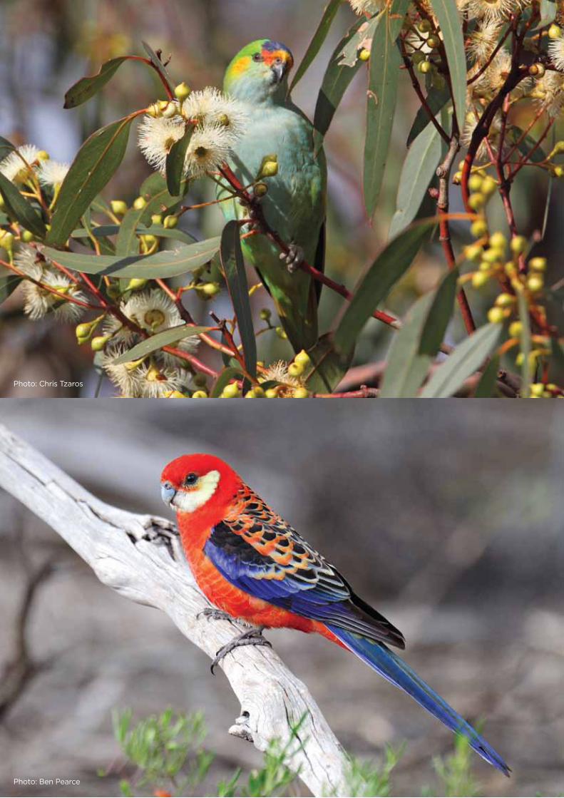
BIRDS IN THE GREAT WESTERN WOODLANDS | 150
Photo: Chris Tzaros
Photo: Ben Pearce
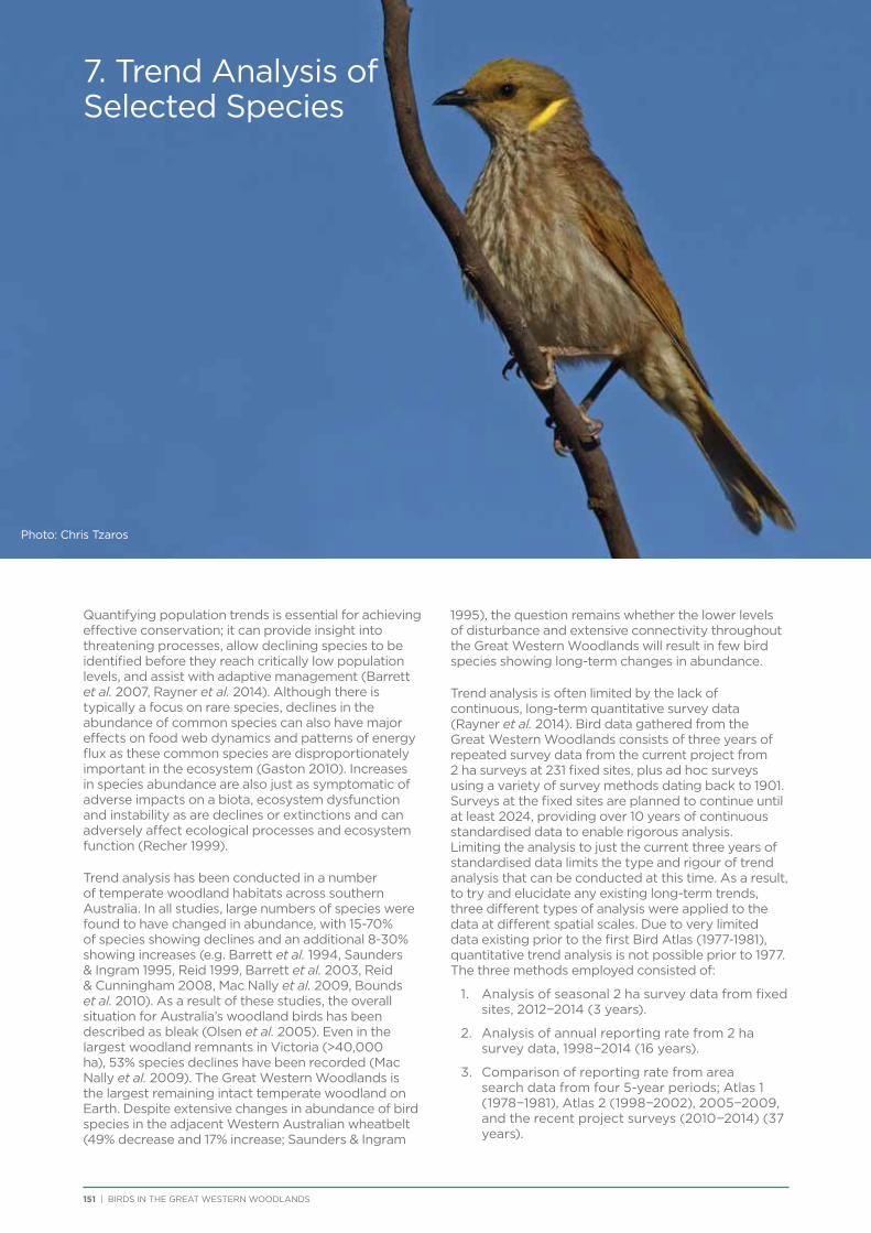
Chapter Header
151 | BIRDS IN THE GREAT WESTERN WOODLANDS
7. Trend Analysis of Selected Species
Quantifying population trends is essential for achieving effective conservation; it can provide insight into threatening processes, allow declining species to be identified before they reach critically low population levels, and assist with adaptive management (Barrett et al. 2007, Rayner et al. 2014). Although there is typically a focus on rare species, declines in the abundance of common species can also have major effects on food web dynamics and patterns of energy flux as these common species are disproportionately important in the ecosystem (Gaston 2010). Increases in species abundance are also just as symptomatic of adverse impacts on a biota, ecosystem dysfunction and instability as are declines or extinctions and can adversely affect ecological processes and ecosystem function (Recher 1999).
Trend analysis has been conducted in a number of temperate woodland habitats across southern Australia. In all studies, large numbers of species were found to have changed in abundance, with 15-70% of species showing declines and an additional 8-30% showing increases (e.g. Barrett et al. 1994, Saunders & Ingram 1995, Reid 1999, Barrett et al. 2003, Reid & Cunningham 2008, Mac Nally et al. 2009, Bounds et al. 2010). As a result of these studies, the overall situation for Australia’s woodland birds has been described as bleak (Olsen et al. 2005). Even in the largest woodland remnants in Victoria (>40,000 ha), 53% species declines have been recorded (Mac Nally et al. 2009). The Great Western Woodlands is the largest remaining intact temperate woodland on Earth. Despite extensive changes in abundance of bird species in the adjacent Western Australian wheatbelt (49% decrease and 17% increase; Saunders & Ingram
1995), the question remains whether the lower levels of disturbance and extensive connectivity throughout the Great Western Woodlands will result in few bird species showing long-term changes in abundance.
Trend analysis is often limited by the lack of continuous, long-term quantitative survey data (Rayner et al. 2014). Bird data gathered from the Great Western Woodlands consists of three years of repeated survey data from the current project from 2 ha surveys at 231 fixed sites, plus ad hoc surveys using a variety of survey methods dating back to 1901. Surveys at the fixed sites are planned to continue until at least 2024, providing over 10 years of continuous standardised data to enable rigorous analysis. Limiting the analysis to just the current three years of standardised data limits the type and rigour of trend analysis that can be conducted at this time. As a result, to try and elucidate any existing long-term trends, three different types of analysis were applied to the data at different spatial scales. Due to very limited data existing prior to the first Bird Atlas (1977-1981), quantitative trend analysis is not possible prior to 1977. The three methods employed consisted of:
1. Analysis of seasonal 2 ha survey data from fixed sites, 2012−2014 (3 years).
2. Analysis of annual reporting rate from 2 ha survey data, 1998−2014 (16 years).
3. Comparison of reporting rate from area search data from four 5-year periods; Atlas 1 (1978−1981), Atlas 2 (1998−2002), 2005−2009, and the recent project surveys (2010−2014) (37 years).
Photo: Chris Tzaros
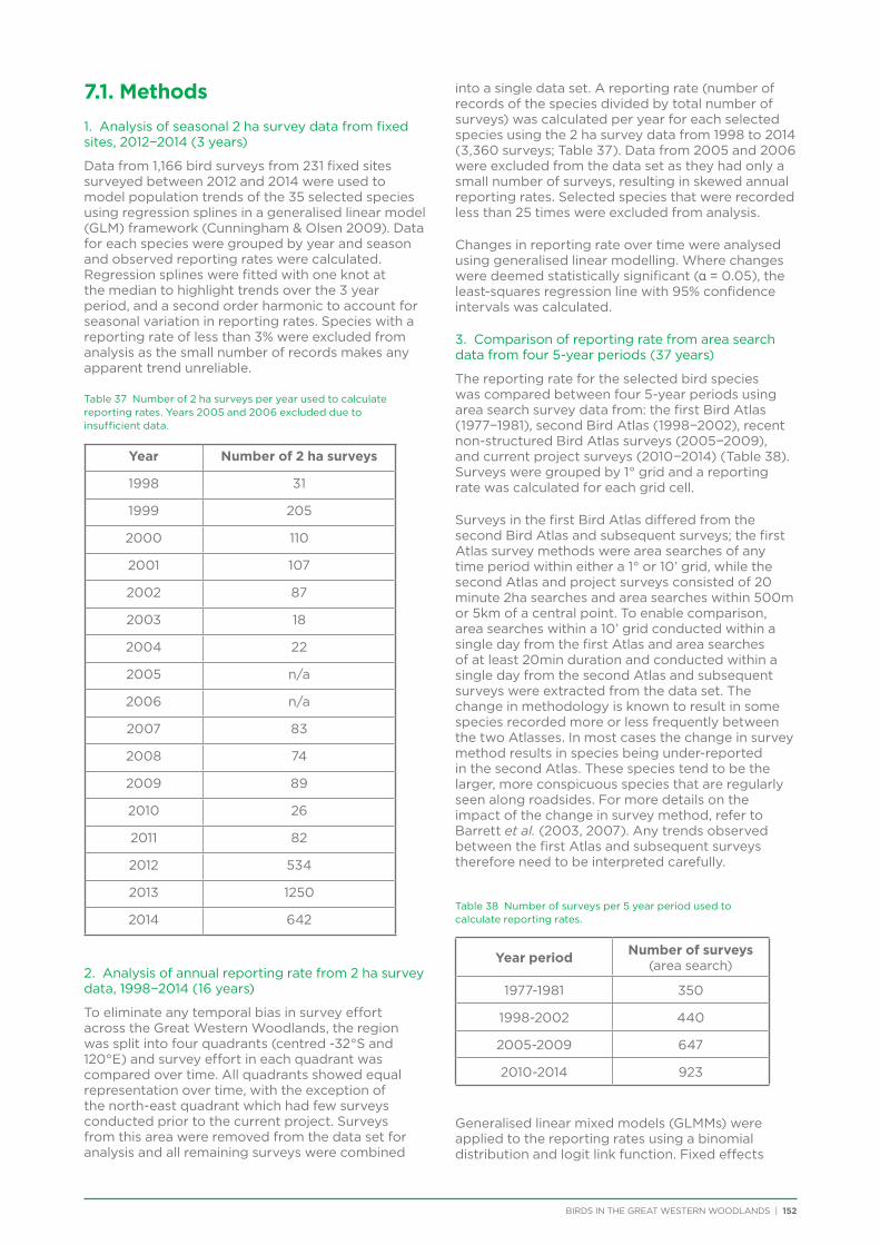
BIRDS IN THE GREAT WESTERN WOODLANDS | 152
7.1. Methods
1. Analysis of seasonal 2 ha survey data from fixed sites, 2012−2014 (3 years)
Data from 1,166 bird surveys from 231 fixed sites surveyed between 2012 and 2014 were used to model population trends of the 35 selected species using regression splines in a generalised linear model (GLM) framework (Cunningham & Olsen 2009). Data for each species were grouped by year and season and observed reporting rates were calculated. Regression splines were fitted with one knot at the median to highlight trends over the 3 year period, and a second order harmonic to account for seasonal variation in reporting rates. Species with a reporting rate of less than 3% were excluded from analysis as the small number of records makes any apparent trend unreliable.
Table 37 Number of 2 ha surveys per year used to calculate reporting rates. Years 2005 and 2006 excluded due to insufficient data.
Year Number of 2 ha surveys
1998 31
1999 205
2000 110
2001 107
2002 87
2003 18
2004 22
2005 n/a
2006 n/a
2007 83
2008 74
2009 89
2010 26
2011 82
2012 534
2013 1250
2014 642
2. Analysis of annual reporting rate from 2 ha survey data, 1998−2014 (16 years)
To eliminate any temporal bias in survey effort across the Great Western Woodlands, the region was split into four quadrants (centred -32°S and 120°E) and survey effort in each quadrant was compared over time. All quadrants showed equal representation over time, with the exception of the north-east quadrant which had few surveys conducted prior to the current project. Surveys from this area were removed from the data set for analysis and all remaining surveys were combined
into a single data set. A reporting rate (number of records of the species divided by total number of surveys) was calculated per year for each selected species using the 2 ha survey data from 1998 to 2014 (3,360 surveys; Table 37). Data from 2005 and 2006 were excluded from the data set as they had only a small number of surveys, resulting in skewed annual reporting rates. Selected species that were recorded less than 25 times were excluded from analysis.
Changes in reporting rate over time were analysed using generalised linear modelling. Where changes were deemed statistically significant (α = 0.05), the least-squares regression line with 95% confidence intervals was calculated.
3. Comparison of reporting rate from area search data from four 5-year periods (37 years)
The reporting rate for the selected bird species was compared between four 5-year periods using area search survey data from: the first Bird Atlas (1977−1981), second Bird Atlas (1998−2002), recent non-structured Bird Atlas surveys (2005−2009), and current project surveys (2010−2014) (Table 38). Surveys were grouped by 1° grid and a reporting rate was calculated for each grid cell.
Surveys in the first Bird Atlas differed from the second Bird Atlas and subsequent surveys; the first Atlas survey methods were area searches of any time period within either a 1° or 10’ grid, while the second Atlas and project surveys consisted of 20 minute 2ha searches and area searches within 500m or 5km of a central point. To enable comparison, area searches within a 10’ grid conducted within a single day from the first Atlas and area searches of at least 20min duration and conducted within a single day from the second Atlas and subsequent surveys were extracted from the data set. The change in methodology is known to result in some species recorded more or less frequently between the two Atlasses. In most cases the change in survey method results in species being under-reported in the second Atlas. These species tend to be the larger, more conspicuous species that are regularly seen along roadsides. For more details on the impact of the change in survey method, refer to Barrett et al. (2003, 2007). Any trends observed between the first Atlas and subsequent surveys therefore need to be interpreted carefully.
Table 38 Number of surveys per 5 year period used to calculate reporting rates.
Year period Number of surveys (area search)
1977-1981 350
1998-2002 440
2005-2009 647
2010-2014 923
Generalised linear mixed models (GLMMs) were applied to the reporting rates using a binomial distribution and logit link function. Fixed effects
153 | BIRDS IN THE GREAT WESTERN WOODLANDS
were included for survey period, survey effort and an interaction term of survey period and survey effort. A random effect was fitted for the 1° grid. The dispersion parameter was left unfixed. As binomial analysis determines the probability of an event (in this instance the presence of a species), survey effort needs to be taken into consideration. For the current data set there were twice as many surveys recorded for the later periods (2005-2009 and 2012-2014) than for the earlier periods. Subsequently, this variable was included in the model to determine whether differential effort introduced any bias. Analysis was conducted on all species that were recorded in at least 2 grid squares across each time period, excluding waterbirds, large raptors and night birds (a total of 76 species were analysed). Analysis was conducted in Genstat (version 17.1.0).
Declining or increasing species were defined as those with an r2 value >0.8 of the linear trend derived from the modelled probabilities.
7.2. Results and Discussion
1. Analysis of seasonal 2 ha survey data from fixed sites, 2012−2014 (3 years)
Due to the short time period, insufficient data were available for conducting the 3 year trend analysis for most of the threatened species, raptors, resource nomads and ground foraging insectivores (Table 39). The majority of species that were able to be modelled showed substantial variability in reporting rate between seasons, with Striated Pardalote the only species to show a significant linear trend over the 3 year period (Table 39, Appendix 6). Arid zone and woodland bird species can be particularly variable in their population sizes both spatially and temporally, responding strongly to events such as rainfall and flowering, either through breeding or influxes of nomadic species. It can therefore be difficult to disentangle changes in population size as a result of natural or human-induced impacts from those driven by environmental or demographic stochasticity (Rayner et al. 2014). Likewise, since many woodland-dependent species range widely, apparent trends within the study area may reflect changing conditions outside the Great Western Woodlands, rather than necessarily being driven by local factors. This variability reduces statistical power and over such a short time period it is not expected that significant trends would be observed. This analysis was predominantly carried out to confirm that the seasonal data recorded from the fixed survey sites is suitable for analysis using the regression splines methodology (Cuningham & Olsen 2009). The results should not be interpreted as indicating long-term population trends, or lack thereof. This is the method that will be used once at least 10 years of survey data are available from the fixed sites. It has been used successfully by the Canberra Ornithologists Group (Bounds et al. 2010) and Cowra Woodland Birds Program (Reid & Cunningham 2008) to identify population increases and decreases and to provide recommendations for the listing of declining species, and management activities to work towards preventing further population declines.
Rayner et al. (2014) identified that many studies reporting population trends for woodland birds had limited temporal coverage and statistical analysis (although see e.g. Reid & Cunningham 2008, Mac Nally et al. 2009, Cunningham & Olsen 2009, Bounds et al. 2010, Szabo et al. 2011). They suggested a minimum of 15 years of continuous data to reliably detect trends and thus draw conclusions about species persistence. The current project provides 3 years of data from fixed sites which can provide the basis for ongoing monitoring and further rigorous analysis of species long-term trends in the future.
2. Analysis of annual reporting rate from 2 ha survey data, 1998−2014 (16 years)
Generalised linear modelling of the annual reporting rate over a 16 year period identified four species with a detectable, long-term change in reporting rate from 1998 to 2014 (Table 39, Appendix 6); Purple-crowned Lorikeet, Pied Butcherbird, Western Rosella, Willie Wagtail. Purple-crowned Lorikeets are a nomadic species and move widely around the landscape within and outside the Great Western Woodlands in response to nectar resources (Chapter 6). For species with this behaviour pattern, long-term trends will only be able to be detected with confidence with very long-term data sets or by the inclusion of data from across the entire species distribution. Western Rosellas are an uncommonly recorded species in the Great Western Woodlands, and their recent increase in reporting rate may be associated with an increase in survey effort rather than a population increase.
Five species were unable to be analysed due to poor representation in the 2 ha survey results (Australian Bustard, Crimson Chat, Major Mitchell’s Cockatoo, Malleefowl and Rufous Fieldwren).
3. Comparison of reporting rate from area search data from four 5-year periods (37 years)
None of the selected species showing a trend over the 16 year period also showed a trend over the 37 year period (Table 39), indicating that 16 years may not be sufficient to identify significant long-term trends in birds from this region, particularly nomadic species, due to long-term environmental variation. However the limitations of the 37 year trend analysis as a result of the change in survey method between the first Atlas and subsequent surveys, and the smaller sample size from the first Atlas, should also be noted.
Of the 76 species analysed over the 37 year period, 64% are known to have declined in the adjacent Western Australian wheatbelt (Saunders & Ingram 1995). The result found here of a maximum of 12% (nine species; Appendix 6) showing a decline in the Great Western Woodlands indicates the much greater stability of the bird populations within the Great Western Woodlands. Most species known to be locally extinct within the wheatbelt, such as Gilbert’s Whistler, Yellow-plumed Honeyeater, Rufous Treecreeper, Western Rosella, Purple-crowned Lorikeet and Chestnut Quail-thrush (Saunders 1989), showed no signs of decline over the past 16 or 37 years in the Great Western Woodlands.
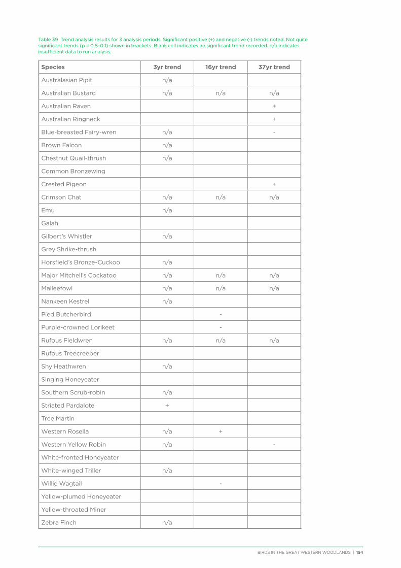
BIRDS IN THE GREAT WESTERN WOODLANDS | 154
Table 39 Trend analysis results for 3 analysis periods. Significant positive (+) and negative (-) trends noted. Not quite significant trends (p = 0.5-0.1) shown in brackets. Blank cell indicates no significant trend recorded. n/a indicates insufficient data to run analysis.
Species 3yr trend 16yr trend 37yr trend
Australasian Pipit n/a
Australian Bustard n/a n/a n/a
Australian Raven +
Australian Ringneck +
Blue-breasted Fairy-wren n/a -
Brown Falcon n/a
Chestnut Quail-thrush n/a
Common Bronzewing
Crested Pigeon +
Crimson Chat n/a n/a n/a
Emu n/a
Galah
Gilbert’s Whistler n/a
Grey Shrike-thrush
Horsfield’s Bronze-Cuckoo n/a
Major Mitchell’s Cockatoo n/a n/a n/a
Malleefowl n/a n/a n/a
Nankeen Kestrel n/a
Pied Butcherbird -
Purple-crowned Lorikeet -
Rufous Fieldwren n/a n/a n/a
Rufous Treecreeper
Shy Heathwren n/a
Singing Honeyeater
Southern Scrub-robin n/a
Striated Pardalote +
Tree Martin
Western Rosella n/a +
Western Yellow Robin n/a -
White-fronted Honeyeater
White-winged Triller n/a
Willie Wagtail -
Yellow-plumed Honeyeater
Yellow-throated Miner
Zebra Finch n/a
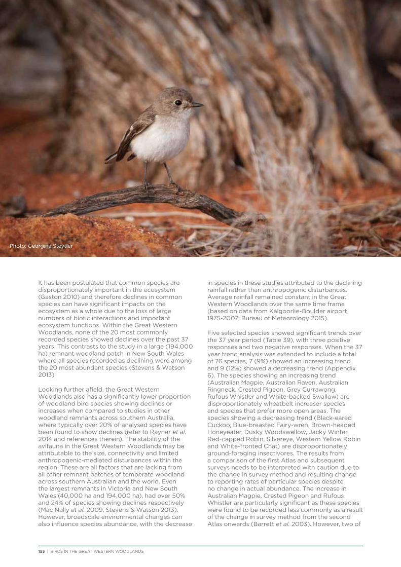
155 | BIRDS IN THE GREAT WESTERN WOODLANDS
It has been postulated that common species are disproportionately important in the ecosystem (Gaston 2010) and therefore declines in common species can have significant impacts on the ecosystem as a whole due to the loss of large numbers of biotic interactions and important ecosystem functions. Within the Great Western Woodlands, none of the 20 most commonly recorded species showed declines over the past 37 years. This contrasts to the study in a large (194,000 ha) remnant woodland patch in New South Wales where all species recorded as declining were among the 20 most abundant species (Stevens & Watson 2013).
Looking further afield, the Great Western Woodlands also has a significantly lower proportion of woodland bird species showing declines or increases when compared to studies in other woodland remnants across southern Australia, where typically over 20% of analysed species have been found to show declines (refer to Rayner et al. 2014 and references therein). The stability of the avifauna in the Great Western Woodlands may be attributable to the size, connectivity and limited anthropogenic-mediated disturbances within the region. These are all factors that are lacking from all other remnant patches of temperate woodland across southern Australian and the world. Even the largest remnants in Victoria and New South Wales (40,000 ha and 194,000 ha), had over 50% and 24% of species showing declines respectively (Mac Nally et al. 2009, Stevens & Watson 2013). However, broadscale environmental changes can also influence species abundance, with the decrease
in species in these studies attributed to the declining rainfall rather than anthropogenic disturbances. Average rainfall remained constant in the Great Western Woodlands over the same time frame (based on data from Kalgoorlie-Boulder airport, 1975-2007; Bureau of Meteorology 2015).
Five selected species showed significant trends over the 37 year period (Table 39), with three positive responses and two negative responses. When the 37 year trend analysis was extended to include a total of 76 species, 7 (9%) showed an increasing trend and 9 (12%) showed a decreasing trend (Appendix 6). The species showing an increasing trend (Australian Magpie, Australian Raven, Australian Ringneck, Crested Pigeon, Grey Currawong, Rufous Whistler and White-backed Swallow) are disproportionately wheatbelt increaser species and species that prefer more open areas. The species showing a decreasing trend (Black-eared Cuckoo, Blue-breasted Fairy-wren, Brown-headed Honeyeater, Dusky Woodswallow, Jacky Winter, Red-capped Robin, Silvereye, Western Yellow Robin and White-fronted Chat) are disproportionately ground-foraging insectivores. The results from a comparison of the first Atlas and subsequent surveys needs to be interpreted with caution due to the change in survey method and resulting change to reporting rates of particular species despite no change in actual abundance. The increase in Australian Magpie, Crested Pigeon and Rufous Whistler are particularly significant as these species were found to be recorded less commonly as a result of the change in survey method from the second Atlas onwards (Barrett et al. 2003). However, two of
Photo: Georgina Steytler
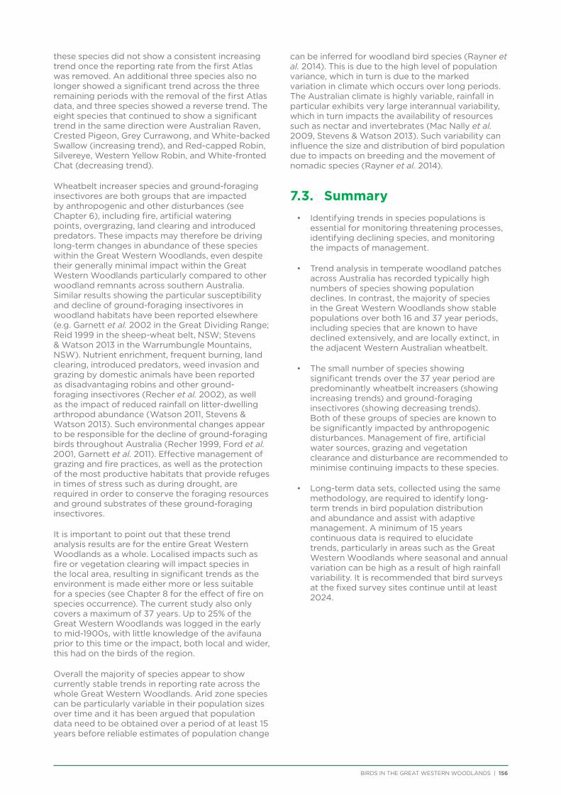
BIRDS IN THE GREAT WESTERN WOODLANDS | 156
these species did not show a consistent increasing trend once the reporting rate from the first Atlas was removed. An additional three species also no longer showed a significant trend across the three remaining periods with the removal of the first Atlas data, and three species showed a reverse trend. The eight species that continued to show a significant trend in the same direction were Australian Raven, Crested Pigeon, Grey Currawong, and White-backed Swallow (increasing trend), and Red-capped Robin, Silvereye, Western Yellow Robin, and White-fronted Chat (decreasing trend).
Wheatbelt increaser species and ground-foraging insectivores are both groups that are impacted by anthropogenic and other disturbances (see Chapter 6), including fire, artificial watering points, overgrazing, land clearing and introduced predators. These impacts may therefore be driving long-term changes in abundance of these species within the Great Western Woodlands, even despite their generally minimal impact within the Great Western Woodlands particularly compared to other woodland remnants across southern Australia. Similar results showing the particular susceptibility and decline of ground-foraging insectivores in woodland habitats have been reported elsewhere (e.g. Garnett et al. 2002 in the Great Dividing Range; Reid 1999 in the sheep-wheat belt, NSW; Stevens & Watson 2013 in the Warrumbungle Mountains, NSW). Nutrient enrichment, frequent burning, land clearing, introduced predators, weed invasion and grazing by domestic animals have been reported as disadvantaging robins and other ground-foraging insectivores (Recher et al. 2002), as well as the impact of reduced rainfall on litter-dwelling arthropod abundance (Watson 2011, Stevens & Watson 2013). Such environmental changes appear to be responsible for the decline of ground-foraging birds throughout Australia (Recher 1999, Ford et al. 2001, Garnett et al. 2011). Effective management of grazing and fire practices, as well as the protection of the most productive habitats that provide refuges in times of stress such as during drought, are required in order to conserve the foraging resources and ground substrates of these ground-foraging insectivores.
It is important to point out that these trend analysis results are for the entire Great Western Woodlands as a whole. Localised impacts such as fire or vegetation clearing will impact species in the local area, resulting in significant trends as the environment is made either more or less suitable for a species (see Chapter 8 for the effect of fire on species occurrence). The current study also only covers a maximum of 37 years. Up to 25% of the Great Western Woodlands was logged in the early to mid-1900s, with little knowledge of the avifauna prior to this time or the impact, both local and wider, this had on the birds of the region.
Overall the majority of species appear to show currently stable trends in reporting rate across the whole Great Western Woodlands. Arid zone species can be particularly variable in their population sizes over time and it has been argued that population data need to be obtained over a period of at least 15 years before reliable estimates of population change
can be inferred for woodland bird species (Rayner et al. 2014). This is due to the high level of population variance, which in turn is due to the marked variation in climate which occurs over long periods. The Australian climate is highly variable, rainfall in particular exhibits very large interannual variability, which in turn impacts the availability of resources such as nectar and invertebrates (Mac Nally et al. 2009, Stevens & Watson 2013). Such variability can influence the size and distribution of bird population due to impacts on breeding and the movement of nomadic species (Rayner et al. 2014).
7.3. Summary
• Identifyingtrendsinspeciespopulationsisessential for monitoring threatening processes, identifying declining species, and monitoring the impacts of management.
• Trendanalysisintemperatewoodlandpatchesacross Australia has recorded typically high numbers of species showing population declines. In contrast, the majority of species in the Great Western Woodlands show stable populations over both 16 and 37 year periods, including species that are known to have declined extensively, and are locally extinct, in the adjacent Western Australian wheatbelt.
• Thesmallnumberofspeciesshowingsignificant trends over the 37 year period are predominantly wheatbelt increasers (showing increasing trends) and ground-foraging insectivores (showing decreasing trends). Both of these groups of species are known to be significantly impacted by anthropogenic disturbances. Management of fire, artificial water sources, grazing and vegetation clearance and disturbance are recommended to minimise continuing impacts to these species.
• Long-termdatasets,collectedusingthesamemethodology, are required to identify long-term trends in bird population distribution and abundance and assist with adaptive management. A minimum of 15 years continuous data is required to elucidate trends, particularly in areas such as the Great Western Woodlands where seasonal and annual variation can be high as a result of high rainfall variability. It is recommended that bird surveys at the fixed survey sites continue until at least 2024.
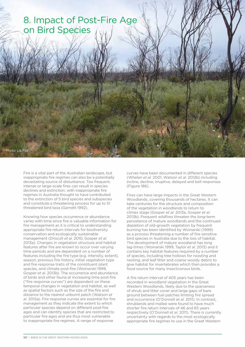
Chapter Header
157 | BIRDS IN THE GREAT WESTERN WOODLANDS
Chapter Header8. Impact of Post-Fire Age on Bird Species
Fire is a vital part of the Australian landscape, but inappropriate fire regimes can also be a potentially devastating source of disturbance. Too frequent, intense or large-scale fires can result in species declines and extinction, with inappropriate fire regimes in Australia thought to have contributed to the extinction of 5 bird species and subspecies and constitute a threatening process for up to 51 threatened bird taxa (Garnett 1992).
Knowing how species occurrence or abundance varies with time since fire is valuable information for fire management as it is critical to understanding appropriate fire return intervals for biodiversity conservation and ecologically sustainable management (Driscoll et al. 2010, Gosper et al. 2013a). Changes in vegetation structure and habitat features after fire are known to occur over varying time periods and are dependent on a number of features including the fire type (e.g. intensity, extent), season, previous fire history, initial vegetation type and fire response traits of the constituent plant species, and climate post-fire (Woinarski 1999, Gosper et al. 2013b). The occurrence and abundance of birds and other fauna at increasing time post-fire (“fire response curves”) are dependent on these temporal changes in vegetation and habitat, as well as spatial factors such as the size of the fire and distance to the nearest unburnt patch (Watson et al. 2012a). Fire response curves are essential for fire management as they indicate the extent to which particular species depend on different post-fire ages and can identify species that are restricted to particular fire ages and are thus most vulnerable to inappropriate fire regimes. A range of response
curves have been documented in different species (Whelan et al. 2001, Watson et al. 2012b) including incline, decline, irruptive, delayed and bell responses (Figure 186).
Fires can have large impacts in the Great Western Woodlands, covering thousands of hectares. It can take centuries for the structure and composition of the vegetation in woodlands to return to climax stage (Gosper et al. 2013a, Gosper et al. 2013b). Frequent wildfires threaten the long-term persistence of mature woodlands and the continued depletion of old-growth vegetation by frequent burning has been identified by Woinarski (1999) as a process threatening a number of fire sensitive bird species in Australia due to the loss of habitat. The development of mature woodland has long lag-times (Woinarski 1999, Taylor et al. 2013) and it contains key habitat features required by a number of species, including tree hollows for roosting and nesting, and leaf litter and coarse woody debris to give habitat for invertebrates which then provides a food source for many insectivorous birds.
A fire return interval of 405 years has been recorded in woodland vegetation in the Great Western Woodlands, likely due to the sparseness of shrub and litter cover and large gaps of bare ground between fuel patches limiting fire spread and occurrence (O’Donnell et al. 2011). In contrast, shrublands and mallee were found to have much shorter fire return intervals of 46 and 65 years respectively (O’Donnell et al. 2011). There is currently uncertainty with regards to the most ecologically appropriate fire regimes to use in the Great Western
Photo: Liz Fox

BIRDS IN THE GREAT WESTERN WOODLANDS | 158
Woodlands in order to deliver biodiversity outcomes (Herford et al. 2012). This could potentially lead to invalid assumptions about species habitat use post-fire and associated management responses.
A longitudinal study into the response curves of birds in response to post-fire age was undertaken in Gimlet (Eucalyptus salubris) woodland on the western edge of the Great Western Woodlands. Many chronosequence studies have artificially truncated time since fire at roughly 60 years, which equates to the period covered by contemporary sources documenting fire events such as satellite images, aerial photos or historical records (e.g. Brown et al. 2009, Parsons & Gosper 2011). In vegetation types such as eucalypt woodland in the Great Western Woodlands with a fire return interval of over 400 years (O’Donnell et al. 2011), this time scale is unsuitable for providing relevant information on species’ responses (Clarke et al. 2010, Gosper et al. 2013a). Gosper et al. (2013c) identified a method to accurately age Gimlet within the Great Western Woodlands. The same sites were used in the current study to analyse the impact of time since fire on birds in eucalypt woodland over an approximately 400 year chronosequence.
8.1. Methods
Surveys
Bird surveys were conducted at 57 sites near the western edge of the Great Western Woodlands, between Karroun Hill (30°14’S, 118°30’E) and Parker Range (31°47’S, 119°37’E) (Figure 187). All survey sites had a dominant overstorey of Gimlet (Eucalyptus salubris), sometimes in association with other Eucalyptus species. The time since fire of all survey sites had previously been identified by Gosper et al. (2013c) through a combination of
Landsat imagery analysis and estimates based on growth ring-size relationships (see Gosper et al. 2013c for details on the technique – model 2 values are used here). Time since fire at the survey sites ranged from 6 to 410 years. Information on aspects of the fire regime other than time since fire (e.g. intensity, patchiness) was not available, but the sites covered a range of different fire regimes.
Bird surveys were carried out using the 2 ha 20 minute survey method. Six surveys were conducted at each site in autumn and spring 2013 (total of 12 surveys per site) by a single experienced birdwatcher. The number of individuals of each species was recorded. The order and time of survey at each site was varied to account for variations in time of day and weather, to prevent a sampling bias from influencing the results.
Analysis
Species richness and Shannon diversity (based on average species counts for each site) were correlated with time since fire using Spearman’s correlation in R (version 2.15.2).
Non-metric multidimensional scaling (nMDS) was applied to the averaged species counts to compare the species composition of young (0-37 years), intermediate (38-120 years) and mature (>120 years) woodland. These age classes were based on Gosper et al. (2013b). A one-way non-parametric multivariate analysis of variance (permanova) was conducted to identify if the age groups were significantly different from each other. Both analyses were conducted in PAST (Hammer et al. 2001) using the Bray-Curtis similarity index.
Generalised additive mixed models (GAMMs) were used to model the effects of time since fire on the occurrence of birds. Models were generated for
Figure 186 Generalised post fire response curves, copied from Watson et al. 2012b.
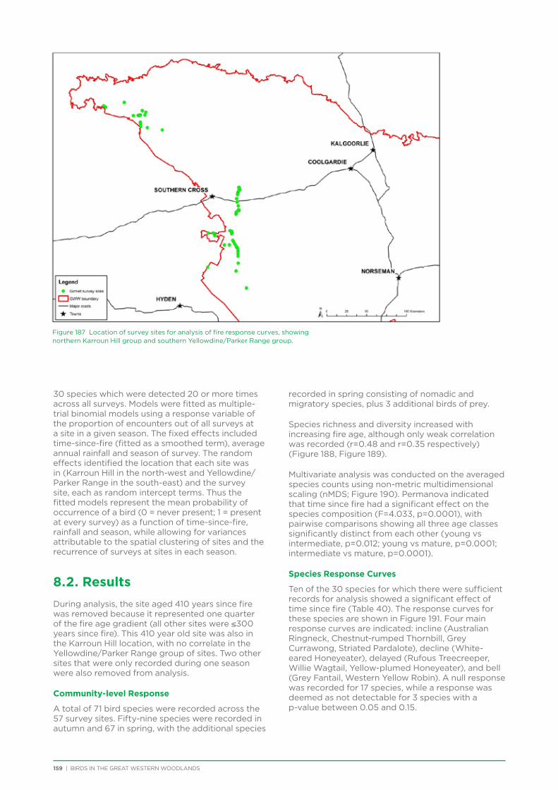
159 | BIRDS IN THE GREAT WESTERN WOODLANDS
30 species which were detected 20 or more times across all surveys. Models were fitted as multiple-trial binomial models using a response variable of the proportion of encounters out of all surveys at a site in a given season. The fixed effects included time-since-fire (fitted as a smoothed term), average annual rainfall and season of survey. The random effects identified the location that each site was in (Karroun Hill in the north-west and Yellowdine/Parker Range in the south-east) and the survey site, each as random intercept terms. Thus the fitted models represent the mean probability of occurrence of a bird (0 = never present; 1 = present at every survey) as a function of time-since-fire, rainfall and season, while allowing for variances attributable to the spatial clustering of sites and the recurrence of surveys at sites in each season.
8.2. Results
During analysis, the site aged 410 years since fire was removed because it represented one quarter of the fire age gradient (all other sites were ≤300 years since fire). This 410 year old site was also in the Karroun Hill location, with no correlate in the Yellowdine/Parker Range group of sites. Two other sites that were only recorded during one season were also removed from analysis.
Community-level Response
A total of 71 bird species were recorded across the 57 survey sites. Fifty-nine species were recorded in autumn and 67 in spring, with the additional species
recorded in spring consisting of nomadic and migratory species, plus 3 additional birds of prey.
Species richness and diversity increased with increasing fire age, although only weak correlation was recorded (r=0.48 and r=0.35 respectively) (Figure 188, Figure 189).
Multivariate analysis was conducted on the averaged species counts using non-metric multidimensional scaling (nMDS; Figure 190). Permanova indicated that time since fire had a significant effect on the species composition (F=4.033, p=0.0001), with pairwise comparisons showing all three age classes significantly distinct from each other (young vs intermediate, p=0.012; young vs mature, p=0.0001; intermediate vs mature, p=0.0001).
Species Response Curves
Ten of the 30 species for which there were sufficient records for analysis showed a significant effect of time since fire (Table 40). The response curves for these species are shown in Figure 191. Four main response curves are indicated: incline (Australian Ringneck, Chestnut-rumped Thornbill, Grey Currawong, Striated Pardalote), decline (White-eared Honeyeater), delayed (Rufous Treecreeper, Willie Wagtail, Yellow-plumed Honeyeater), and bell (Grey Fantail, Western Yellow Robin). A null response was recorded for 17 species, while a response was deemed as not detectable for 3 species with a p-value between 0.05 and 0.15.
Figure 187 Location of survey sites for analysis of fire response curves, showing northern Karroun Hill group and southern Yellowdine/Parker Range group.
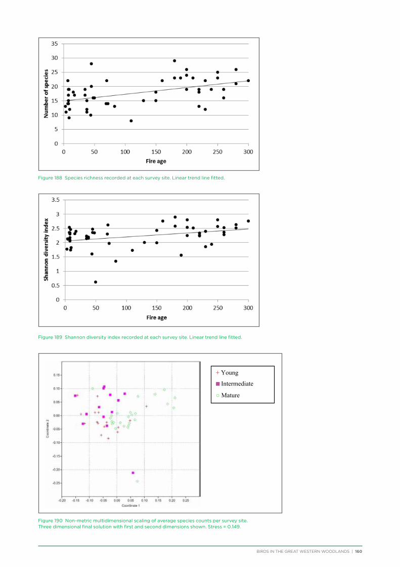
BIRDS IN THE GREAT WESTERN WOODLANDS | 160
+ Young
n Intermediate
○ Mature
Figure 188 Species richness recorded at each survey site. Linear trend line fitted.
Figure 190 Non-metric multidimensional scaling of average species counts per survey site. Three dimensional final solution with first and second dimensions shown. Stress = 0.149.
Figure 189 Shannon diversity index recorded at each survey site. Linear trend line fitted.
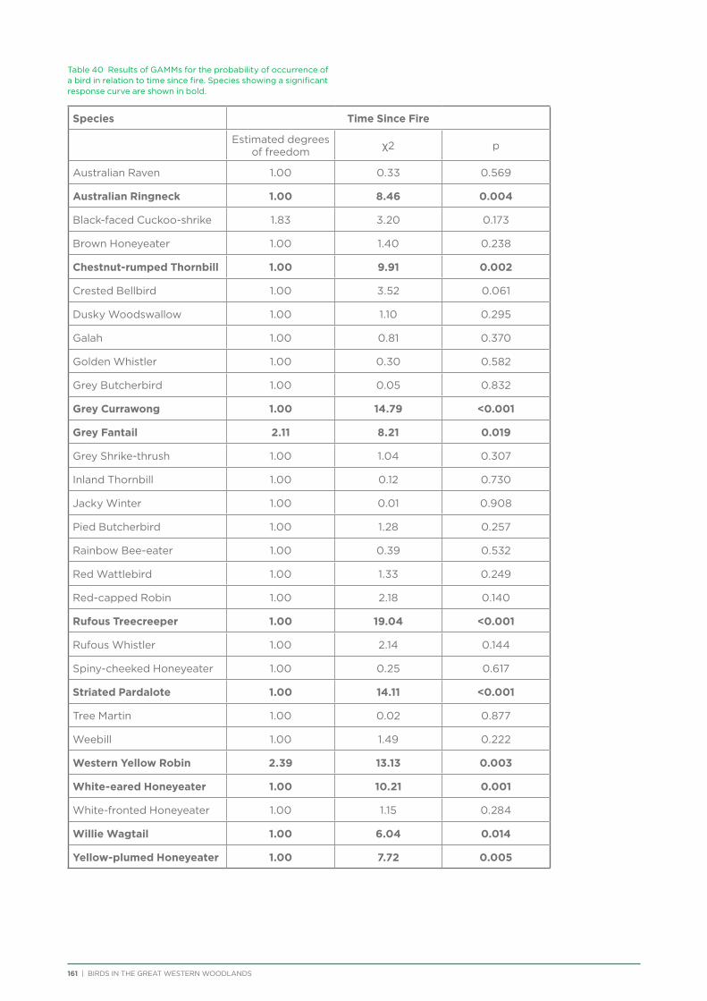
161 | BIRDS IN THE GREAT WESTERN WOODLANDS
Table 40 Results of GAMMs for the probability of occurrence of a bird in relation to time since fire. Species showing a significant response curve are shown in bold.
Species Time Since Fire
Estimated degrees of freedom χ2 p
Australian Raven 1.00 0.33 0.569
Australian Ringneck 1.00 8.46 0.004
Black-faced Cuckoo-shrike 1.83 3.20 0.173
Brown Honeyeater 1.00 1.40 0.238
Chestnut-rumped Thornbill 1.00 9.91 0.002
Crested Bellbird 1.00 3.52 0.061
Dusky Woodswallow 1.00 1.10 0.295
Galah 1.00 0.81 0.370
Golden Whistler 1.00 0.30 0.582
Grey Butcherbird 1.00 0.05 0.832
Grey Currawong 1.00 14.79 <0.001
Grey Fantail 2.11 8.21 0.019
Grey Shrike-thrush 1.00 1.04 0.307
Inland Thornbill 1.00 0.12 0.730
Jacky Winter 1.00 0.01 0.908
Pied Butcherbird 1.00 1.28 0.257
Rainbow Bee-eater 1.00 0.39 0.532
Red Wattlebird 1.00 1.33 0.249
Red-capped Robin 1.00 2.18 0.140
Rufous Treecreeper 1.00 19.04 <0.001
Rufous Whistler 1.00 2.14 0.144
Spiny-cheeked Honeyeater 1.00 0.25 0.617
Striated Pardalote 1.00 14.11 <0.001
Tree Martin 1.00 0.02 0.877
Weebill 1.00 1.49 0.222
Western Yellow Robin 2.39 13.13 0.003
White-eared Honeyeater 1.00 10.21 0.001
White-fronted Honeyeater 1.00 1.15 0.284
Willie Wagtail 1.00 6.04 0.014
Yellow-plumed Honeyeater 1.00 7.72 0.005
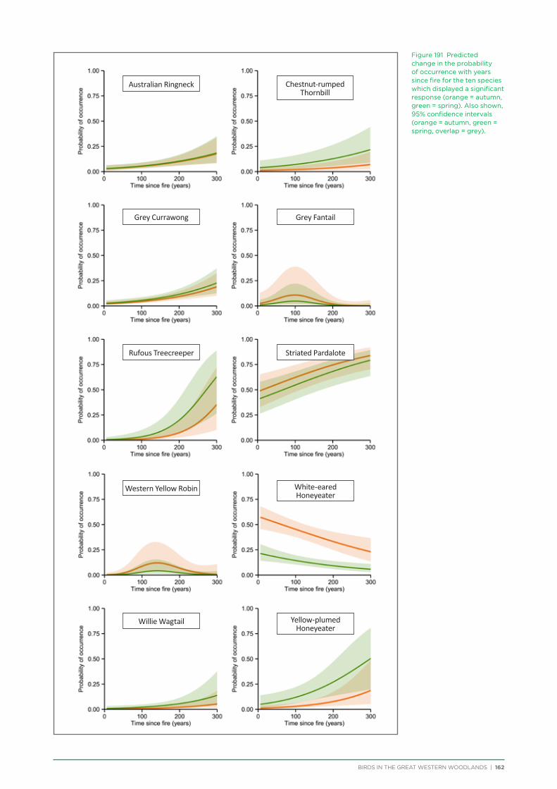
BIRDS IN THE GREAT WESTERN WOODLANDS | 162
Figure 191 Predicted change in the probability of occurrence with years since fire for the ten species which displayed a significant response (orange = autumn, green = spring). Also shown, 95% confidence intervals (orange = autumn, green = spring, overlap = grey).
Australian Ringneck
Grey Currawong
Rufous Treecreeper
Western Yellow Robin
Willie Wagtail
Grey Fantail
Striated Pardalote
White-eared Honeyeater
Yellow-plumed Honeyeater
Chestnut-rumped Thornbill
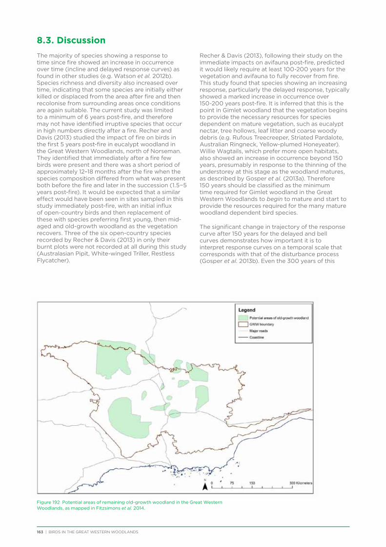
163 | BIRDS IN THE GREAT WESTERN WOODLANDS
8.3. Discussion
The majority of species showing a response to time since fire showed an increase in occurrence over time (incline and delayed response curves) as found in other studies (e.g. Watson et al. 2012b). Species richness and diversity also increased over time, indicating that some species are initially either killed or displaced from the area after fire and then recolonise from surrounding areas once conditions are again suitable. The current study was limited to a minimum of 6 years post-fire, and therefore may not have identified irruptive species that occur in high numbers directly after a fire. Recher and Davis (2013) studied the impact of fire on birds in the first 5 years post-fire in eucalypt woodland in the Great Western Woodlands, north of Norseman. They identified that immediately after a fire few birds were present and there was a short period of approximately 12–18 months after the fire when the species composition differed from what was present both before the fire and later in the succession (1.5−5 years post-fire). It would be expected that a similar effect would have been seen in sites sampled in this study immediately post-fire, with an initial influx of open-country birds and then replacement of these with species preferring first young, then mid-aged and old-growth woodland as the vegetation recovers. Three of the six open-country species recorded by Recher & Davis (2013) in only their burnt plots were not recorded at all during this study (Australasian Pipit, White-winged Triller, Restless Flycatcher).
Recher & Davis (2013), following their study on the immediate impacts on avifauna post-fire, predicted it would likely require at least 100-200 years for the vegetation and avifauna to fully recover from fire. This study found that species showing an increasing response, particularly the delayed response, typically showed a marked increase in occurrence over 150-200 years post-fire. It is inferred that this is the point in Gimlet woodland that the vegetation begins to provide the necessary resources for species dependent on mature vegetation, such as eucalypt nectar, tree hollows, leaf litter and coarse woody debris (e.g. Rufous Treecreeper, Striated Pardalote, Australian Ringneck, Yellow-plumed Honeyeater). Willie Wagtails, which prefer more open habitats, also showed an increase in occurrence beyond 150 years, presumably in response to the thinning of the understorey at this stage as the woodland matures, as described by Gosper et al. (2013a). Therefore 150 years should be classified as the minimum time required for Gimlet woodland in the Great Western Woodlands to begin to mature and start to provide the resources required for the many mature woodland dependent bird species.
The significant change in trajectory of the response curve after 150 years for the delayed and bell curves demonstrates how important it is to interpret response curves on a temporal scale that corresponds with that of the disturbance process (Gosper et al. 2013b). Even the 300 years of this
Figure 192 Potential areas of remaining old-growth woodland in the Great Western Woodlands, as mapped in Fitzsimons et al. 2014.
BIRDS IN THE GREAT WESTERN WOODLANDS | 164
study is potentially limited since woodlands in the Great Western Woodlands are known to have fire return intervals exceeding 400 years (O’Donnell et al. 2011).
The bird surveys conducted to identify the impact of time since fire on species were all conducted in Gimlet woodland in which the dominant tree is killed by fire (hence allowing ageing of the trees to identify time since fire). Epicormic resprouting is rare in eucalypts in the Great Western Woodlands, and resprouting from the lignotuber will result in similar vegetation structure changes as seen in Gimlet and other fire-sensitive eucalypt woodland. Areas where a burn is patchy, however, can result in incomplete tree death and thus alter species fire response curves. For example, while Rufous Treecreeper were predominantly found in Gimlet woodland over 150 years post-fire, they were also found at a small number of recently burnt sites due to the patchy nature of the burn, resulting in retention of some old trees. Whether this was the result of a low intensity fire or a small patch of vegetation that escaped burning requires further examination. It is the vegetation and other environmental characteristics (e.g. prey abundance) that the birds are responding to (Wooller & Calver 1988, Woinarski & Recher 1997, Leavesley et al. 2010, Barton et al. 2014) rather than time since fire per se and therefore species can show different response curves in different vegetation types (Nimmo et al. 2014), different intensities of fire, the level of patchiness of the fire, or different climatic conditions post-fire. Further analysis of the data comparing response curves to vegetation and habitat measures will help to elucidate these trends further. Other fire event effects that are likely to influence bird occurrence but were not explicitly considered in the experimental design were fire size and distance to unburnt woodland.
The delayed and bell shaped response curves identified here are the most limiting for species occurrence as species predominantly occur only at particular times since fire – in woodland over 150 years for Rufous Treecreeper, Yellow-plumed Honeyeater and Willie Wagtail and woodland aged approximately 50 – 200 years for Grey Fantail and Western Yellow Robin. Based on DPaW fire mapping (2014) up to 28% of the eucalypt woodland vegetation in the Great Western Woodlands has been burnt within the past 44 years and up to 25% was cut for timber in the late 1800s to mid-1900s (DPaW 2012). These recent fires have created much young woodland regeneration, which will become suitable habitat for bell-response species over the coming decades. Consequently, the time-since-fire related habitat requirements of these species appear reasonably secure in the medium-term. However, recent fires and timber harvesting have left only 61% of the eucalypt woodland in the Great Western Woodlands over 44 years old (identified by overlaying fuel age and timber harvesting spatial layers), with only a small percentage of this likely to be up to or older than 400 years. The amount of old-growth woodland remaining in the Great Western Woodlands is currently unknown, although potential areas have been mapped (Fitzsimons et al. 2014) and include areas around Lake Johnston & Lake Hope, north of Fraser Range and surrounding
and to the north-east of Helena & Aurora Range (Figure 192). The relative importance of old-growth woodland, and its likely limited extent in the Great Western Woodlands, indicates protection of old-growth areas may be vital to ensure habitat for old-growth dependent species. Recent work has indicated that it is the extent of older vegetation in a landscape, rather than heterogeneity, which is a major driver of diversity for birds (Taylor et al. 2012, Taylor et al. 2013, Kelly et al. 2014). More research is required in this area, as well as mapping of the vegetation age classes across the Great Western Woodlands.
Habitat connectivity is a vital aspect of the impact of fire on birds in the landscape. Surrounding unburnt habitat that is easily accessible allows for birds to escape the initial fire and subsequent loss of food and nesting resources, and to recolonise once the habitat becomes suitable. Research has found that post-fire occupancy is related to the proximity of unburnt vegetation (Watson et al. 2012a) as well as the patchiness of the burn (Woinarski 1999). In highly fragmented landscapes a single large, intense fire within a reserve has the potential to severely impact the local bird populations. This is particularly the case for already threatened species that are limited to a few small fragmented populations, for example a single wildfire in December 2004 at Mount Manypeaks is thought to have eliminated over half of the total remaining Noisy Scrub-bird population and a significant proportion of the Western Bristlebird and Western Whipbird populations (Gilfillan et al. 2009). Maintenance of broadscale habitat connectivity within the Great Western Woodlands is vital for limiting the impacts of wildfire.
The current study on the effect of time-since-fire on bird occurrence focussed on the impact of fire in eucalypt woodlands. Shrublands, mallee and thicket vegetation also occur in the Great Western Woodlands. Fire return intervals in these vegetation types are significantly shorter than in woodland (O’Donnell et al. 2011) and the species response curves would be expected to reflect the shorter time frames and variation in regeneration in these vegetation types. This is an area that requires further research.
8.4. Summary
• FireisanaturalandvitalpartoftheGreatWestern Woodlands, but inappropriate fire regimes can be detrimental to species persistence in the landscape.
• Birdsshowanumberofpost-fireresponsecurves, including incline, decline, bell and delayed. Bell and delayed curves are the most limiting, with those species predominantly occurring in only particular fire ages. The current study would not have identified irruptive species since it was limited to a minimum of 6 years post-fire.
• Sincebirdsarerespondingtovegetationstructure and floristics, and associated invertebrate abundance, rather than time-since-fire per se, different fire regimes (e.g. intensity, patchiness of burn, or climate post-fire) may result in different response curves.
• Inthisstudy,speciesshowingabell-shapedcurve preferred 50−200 year old Gimlet woodland (e.g. Grey Fantail, Western Yellow Robin), while those showing a delayed curve preferred Gimlet woodland over 150 years old (e.g. Rufous Treecreeper).
• Thereiscurrentlylimitedknowledgeontheextent of woodland over 150 years old in the Great Western Woodlands.
• Recommendationsformaintainingbirdspeciesrichness, diversity and functionality with respect to fire in the Great Western Woodlands include 1) mapping of all vegetation age classes across the Great Western Woodlands, 2) identifying, protecting and managing areas of old-growth woodland (at least 150 years old and preferably over 400 years), and 3) maintaining extensive habitat connectivity to enable species to find places of refuge from fire and enable easy recolonisation of previously burnt areas.
• Furtherresearchisrequiredontheimpactoffire on birds in shrubland, mallee and thicket habitats.
165 | BIRDS IN THE GREAT WESTERN WOODLANDS
BIRDS IN THE GREAT WESTERN WOODLANDS | 166Photo: Laura Corbett
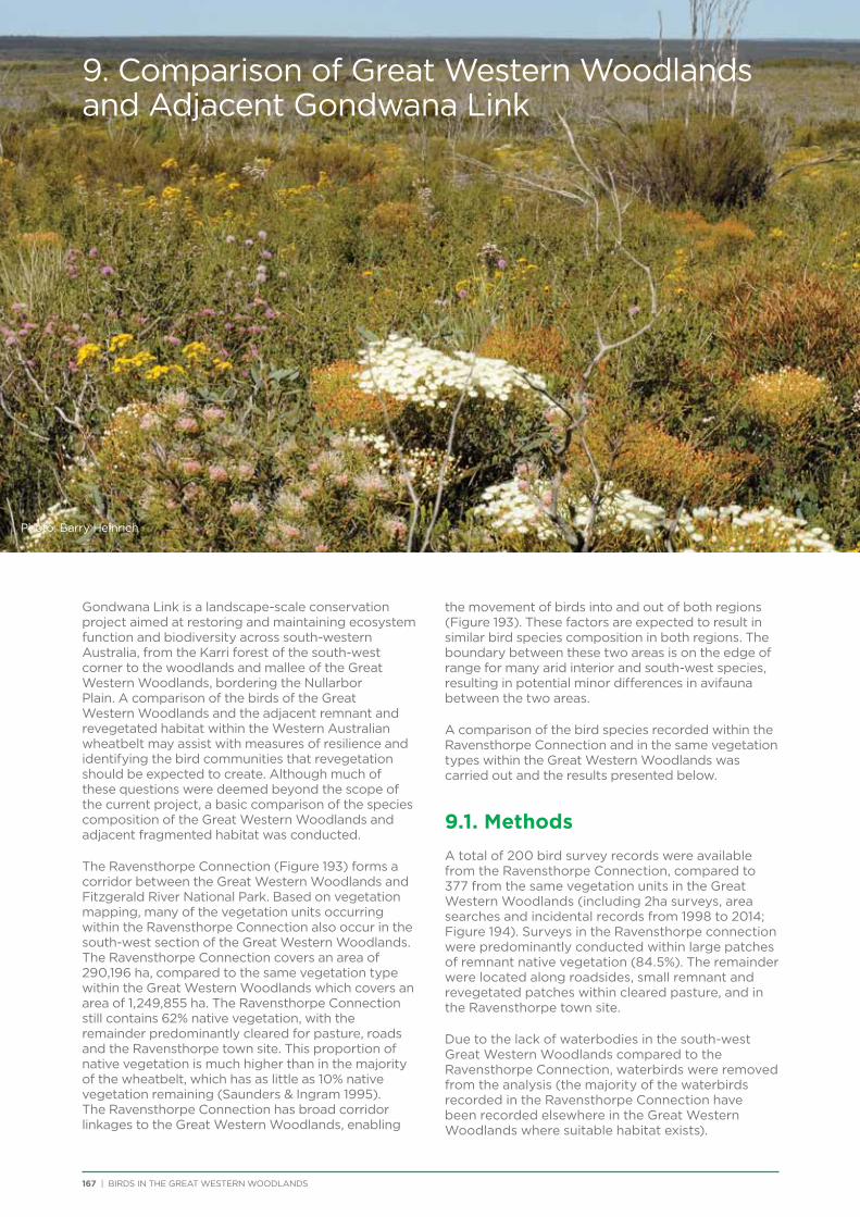
Chapter Header
167 | BIRDS IN THE GREAT WESTERN WOODLANDS
Chapter Header
Gondwana Link is a landscape-scale conservation project aimed at restoring and maintaining ecosystem function and biodiversity across south-western Australia, from the Karri forest of the south-west corner to the woodlands and mallee of the Great Western Woodlands, bordering the Nullarbor Plain. A comparison of the birds of the Great Western Woodlands and the adjacent remnant and revegetated habitat within the Western Australian wheatbelt may assist with measures of resilience and identifying the bird communities that revegetation should be expected to create. Although much of these questions were deemed beyond the scope of the current project, a basic comparison of the species composition of the Great Western Woodlands and adjacent fragmented habitat was conducted.
The Ravensthorpe Connection (Figure 193) forms a corridor between the Great Western Woodlands and Fitzgerald River National Park. Based on vegetation mapping, many of the vegetation units occurring within the Ravensthorpe Connection also occur in the south-west section of the Great Western Woodlands. The Ravensthorpe Connection covers an area of 290,196 ha, compared to the same vegetation type within the Great Western Woodlands which covers an area of 1,249,855 ha. The Ravensthorpe Connection still contains 62% native vegetation, with the remainder predominantly cleared for pasture, roads and the Ravensthorpe town site. This proportion of native vegetation is much higher than in the majority of the wheatbelt, which has as little as 10% native vegetation remaining (Saunders & Ingram 1995). The Ravensthorpe Connection has broad corridor linkages to the Great Western Woodlands, enabling
the movement of birds into and out of both regions (Figure 193). These factors are expected to result in similar bird species composition in both regions. The boundary between these two areas is on the edge of range for many arid interior and south-west species, resulting in potential minor differences in avifauna between the two areas.
A comparison of the bird species recorded within the Ravensthorpe Connection and in the same vegetation types within the Great Western Woodlands was carried out and the results presented below.
9.1. Methods
A total of 200 bird survey records were available from the Ravensthorpe Connection, compared to 377 from the same vegetation units in the Great Western Woodlands (including 2ha surveys, area searches and incidental records from 1998 to 2014; Figure 194). Surveys in the Ravensthorpe connection were predominantly conducted within large patches of remnant native vegetation (84.5%). The remainder were located along roadsides, small remnant and revegetated patches within cleared pasture, and in the Ravensthorpe town site.
Due to the lack of waterbodies in the south-west Great Western Woodlands compared to the Ravensthorpe Connection, waterbirds were removed from the analysis (the majority of the waterbirds recorded in the Ravensthorpe Connection have been recorded elsewhere in the Great Western Woodlands where suitable habitat exists).
9. Comparison of Great Western Woodlands and Adjacent Gondwana Link
Photo: Barry Heinrich
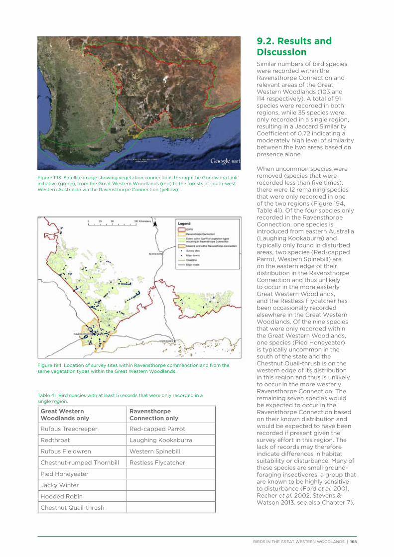
BIRDS IN THE GREAT WESTERN WOODLANDS | 168
Table 41 Bird species with at least 5 records that were only recorded in a single region.
Great Western Woodlands only
Ravensthorpe Connection only
Rufous Treecreeper Red-capped Parrot
Redthroat Laughing Kookaburra
Rufous Fieldwren Western Spinebill
Chestnut-rumped Thornbill Restless Flycatcher
Pied Honeyeater
Jacky Winter
Hooded Robin
Chestnut Quail-thrush
Figure 193 Satellite image showing vegetation connections through the Gondwana Link initiative (green), from the Great Western Woodlands (red) to the forests of south-west Western Australian via the Ravensthorpe Connection (yellow) .
Figure 194 Location of survey sites within Ravensthorpe commenction and from the same vegetation types within the Great Western Woodlands.
9.2. Results and DiscussionSimilar numbers of bird species were recorded within the Ravensthorpe Connection and relevant areas of the Great Western Woodlands (103 and 114 respectively). A total of 91 species were recorded in both regions, while 35 species were only recorded in a single region, resulting in a Jaccard Similarity Coefficient of 0.72 indicating a moderately high level of similarity between the two areas based on presence alone.
When uncommon species were removed (species that were recorded less than five times), there were 12 remaining species that were only recorded in one of the two regions (Figure 194, Table 41). Of the four species only recorded in the Ravensthorpe Connection, one species is introduced from eastern Australia (Laughing Kookaburra) and typically only found in disturbed areas, two species (Red-capped Parrot, Western Spinebill) are on the eastern edge of their distribution in the Ravensthorpe Connection and thus unlikely to occur in the more easterly Great Western Woodlands, and the Restless Flycatcher has been occasionally recorded elsewhere in the Great Western Woodlands. Of the nine species that were only recorded within the Great Western Woodlands, one species (Pied Honeyeater) is typically uncommon in the south of the state and the Chestnut Quail-thrush is on the western edge of its distribution in this region and thus is unlikely to occur in the more westerly Ravensthorpe Connection. The remaining seven species would be expected to occur in the Ravensthorpe Connection based on their known distribution and would be expected to have been recorded if present given the survey effort in this region. The lack of records may therefore indicate differences in habitat suitability or disturbance. Many of these species are small ground-foraging insectivores, a group that are known to be highly sensitive to disturbance (Ford et al. 2001, Recher et al. 2002, Stevens & Watson 2013, see also Chapter 7).
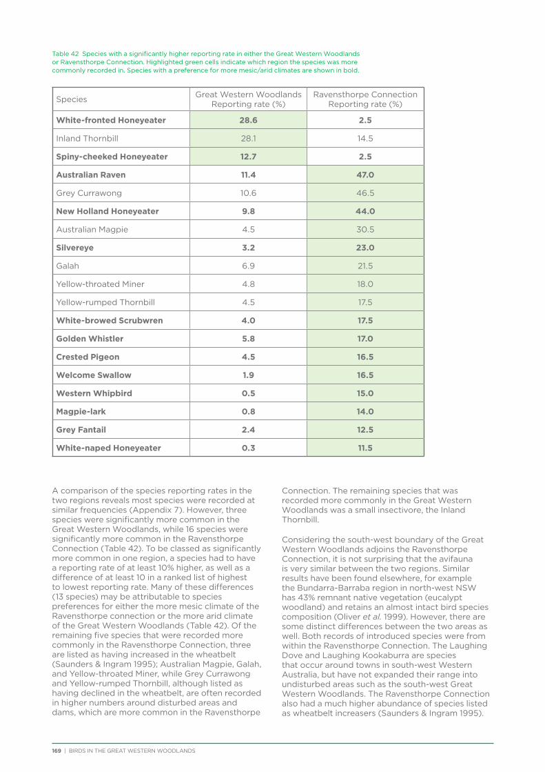
169 | BIRDS IN THE GREAT WESTERN WOODLANDS
Table 42 Species with a significantly higher reporting rate in either the Great Western Woodlands or Ravensthorpe Connection. Highlighted green cells indicate which region the species was more commonly recorded in. Species with a preference for more mesic/arid climates are shown in bold.
Species Great Western Woodlands Reporting rate (%)
Ravensthorpe Connection Reporting rate (%)
White-fronted Honeyeater 28.6 2.5
Inland Thornbill 28.1 14.5
Spiny-cheeked Honeyeater 12.7 2.5
Australian Raven 11.4 47.0
Grey Currawong 10.6 46.5
New Holland Honeyeater 9.8 44.0
Australian Magpie 4.5 30.5
Silvereye 3.2 23.0
Galah 6.9 21.5
Yellow-throated Miner 4.8 18.0
Yellow-rumped Thornbill 4.5 17.5
White-browed Scrubwren 4.0 17.5
Golden Whistler 5.8 17.0
Crested Pigeon 4.5 16.5
Welcome Swallow 1.9 16.5
Western Whipbird 0.5 15.0
Magpie-lark 0.8 14.0
Grey Fantail 2.4 12.5
White-naped Honeyeater 0.3 11.5
A comparison of the species reporting rates in the two regions reveals most species were recorded at similar frequencies (Appendix 7). However, three species were significantly more common in the Great Western Woodlands, while 16 species were significantly more common in the Ravensthorpe Connection (Table 42). To be classed as significantly more common in one region, a species had to have a reporting rate of at least 10% higher, as well as a difference of at least 10 in a ranked list of highest to lowest reporting rate. Many of these differences (13 species) may be attributable to species preferences for either the more mesic climate of the Ravensthorpe connection or the more arid climate of the Great Western Woodlands (Table 42). Of the remaining five species that were recorded more commonly in the Ravensthorpe Connection, three are listed as having increased in the wheatbelt (Saunders & Ingram 1995); Australian Magpie, Galah, and Yellow-throated Miner, while Grey Currawong and Yellow-rumped Thornbill, although listed as having declined in the wheatbelt, are often recorded in higher numbers around disturbed areas and dams, which are more common in the Ravensthorpe
Connection. The remaining species that was recorded more commonly in the Great Western Woodlands was a small insectivore, the Inland Thornbill.
Considering the south-west boundary of the Great Western Woodlands adjoins the Ravensthorpe Connection, it is not surprising that the avifauna is very similar between the two regions. Similar results have been found elsewhere, for example the Bundarra-Barraba region in north-west NSW has 43% remnant native vegetation (eucalypt woodland) and retains an almost intact bird species composition (Oliver et al. 1999). However, there are some distinct differences between the two areas as well. Both records of introduced species were from within the Ravensthorpe Connection. The Laughing Dove and Laughing Kookaburra are species that occur around towns in south-west Western Australia, but have not expanded their range into undisturbed areas such as the south-west Great Western Woodlands. The Ravensthorpe Connection also had a much higher abundance of species listed as wheatbelt increasers (Saunders & Ingram 1995).
BIRDS IN THE GREAT WESTERN WOODLANDS | 170
While most increaser species were recorded in both areas, many had significantly higher reporting rates in the Ravensthorpe Connection than the Great Western Woodlands. These species are associated with the higher food and water availability around towns and pastoral areas and/or have a preference for areas of modified or disturbed vegetation. It is surprising that there is such a difference in the abundance of wheatbelt increasers in the Ravensthorpe Connection, given that this area is still 62% native vegetation, the majority of surveys were conducted within large patches of fully connected remnant vegetation, and there are broad corridor linkages to the Great Western Woodlands. However, the impact of human disturbances on the abundance of wheatbelt increasers within the Great Western Woodlands appears to be limited to areas in close proximity to human disturbance, for example Australian Raven were typically recorded within 10 km of roads, town and watering points (Chapter 6). Therefore, protection of remnants and revegetation efforts should be focussed on establishing large areas of vegetation, free from the impacts of roads, dams, watering points, etc. The required remnant size for long-term species viability is species specific, with species such as Blue-breasted Fairy-wren able to survive in remnants of less than 144 ha (Brooker & Brooker 2001), while Crested Bellbird have been lost from even large remnants of 4,200 ha (Traill et al. 1996) and Gilbert’s Whistler are extinct from virtually all remnant vegetation in the Western Australian wheatbelt (Dell 1976, Saunders 1989, although see Gosper 2012). A study by Kitchener et al. (1982) in the wheatbelt identified that reserves of at least 1,500 ha were required to conserve the complete assemblage of local avifauna, with reserves of 30,000 – 94,000 ha required to conserve an almost complete avifauna of the wheatbelt. The maintenance of linkages and corridors between remnant and revegetated areas is also vital to enable species to move and colonise or recolonise areas as they vary in suitability over time due to natural (e.g. flowering, rainfall) or human-induced changes. As for patch size, the corridor width and composition that enables species to freely move along them varies between species. For example, a corridor width of 40−50 m is required for Western Yellow Robin, Grey Shrike-thrush and Inland Thornbill, and a well-developed understorey is vital for increasing the carrying capacity of the corridor (Lynch & Saunders 1991).
Of the threatened species recorded, the majority of differences in reporting rate between the two areas can be attributed to the preferred arid/mesic distribution of the species, except for Rufous Fieldwren, Shy Heathwren, Western Rosella, and Malleefowl. Rufous Fieldwren, Shy Heathwren and Western Rosella were all recorded more commonly in the Great Western Woodlands (1.5:0, 6.9:2, 4.3:0.5; reporting rate (%) in Great Western Woodlands:Ravensthorpe Connection respectively, Appendix 7). These species are all listed as Priority 4 (DPaW Priority Fauna List 2014) as a direct result of clearing for agriculture removing much of the habitat within their distribution in Western Australia (Garnett et al. 2011). The Great Western Woodlands supports a large proportion of the remaining populations for these species. Recommended
actions are to cease clearing vegetation, rehabilitate remnant fragments and assess food and hollow availability for the Western Rosella (Garnett et al. 2011). In contrast, Malleefowl were recorded more often in the Ravensthorpe Connection than the Great Western Woodlands (1.3:7.5; reporting rate (%) in Great Western Woodlands:Ravensthorpe Connection, Appendix 7). Since the Malleefowl is known to be impacted by vegetation clearance and fragmentation (Garnett et al. 2011), this result is likely a sampling bias due to Malleefowl being more visible on paddocks and when feeding on spilt grain beside the road, than when moving amongst dense mallee vegetation in the Great Western Woodlands. Malleefowl have been recorded breeding throughout the Great Western Woodlands.
9.3. Summary
• TheRavensthorpeConnectionadjoinsthesouth-west Great Western Woodlands and provides a corridor to the Fitzgerald River National Park and the rest of the Gondwana Link corridor to the south-west. Unlike much of the wheatbelt, the Ravensthorpe Connection still retains 62% native vegetation cover.
• Ananalysisofthespeciescompositionforthe same vegetation types within the south-west Great Western Woodlands and the Ravensthorpe Connection identified a similar species composition in both areas, although the Ravensthorpe Connection recorded two introduced bird species that were absent from the Great Western Woodlands and had a higher abundance of wheatbelt increaser species such as Australian Magpie, Galah and Yellow-throated Miner.
• Severalthreatenedspecieswererecordedinhigher abundance within the Great Western Woodlands and this region likely supports a large proportion of the remaining populations for these species.
• Tomaintainbirdspeciescompositionandecosystem function, conservation efforts within Gondwana Link should focus on increasing remnant and revegetated patch size, reducing anthropogenic disturbances within patches, and maintaining or increasing connectivity between patches.
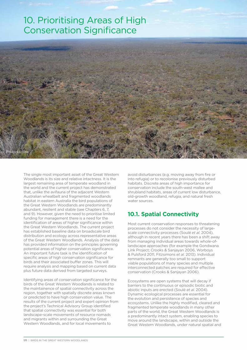
Chapter Header
171 | BIRDS IN THE GREAT WESTERN WOODLANDS
Chapter Header10. Prioritising Areas of High Conservation Significance
The single most important asset of the Great Western Woodlands is its size and relative intactness. It is the largest remaining area of temperate woodland in the world and the current project has demonstrated that, unlike the avifauna of the adjacent Western Australian wheatbelt and fragmented woodlands habitat in eastern Australia the bird populations of the Great Western Woodlands are predominantly abundant, resilient and stable (see Chapters 6, 7, and 9). However, given the need to prioritise limited funding for management there is a need for the identification of areas of higher significance within the Great Western Woodlands. The current project has established baseline data on broadscale bird distribution and ecology across representative areas of the Great Western Woodlands. Analysis of the data has provided information on the principles governing potential areas of higher conservation significance. An important future task is the identification of specific areas of high conservation significance for birds and their associated buffer zones. This will require analysis and mapping based on current data plus future data derived from targeted surveys.
Identifying areas of conservation significance for the birds of the Great Western Woodlands is related to the maintainence of spatial connectivity across the region, together with spatially discrete areas known or predicted to have high conservation value. The results of the current project and expert opinion from the project’s Technical Advisory Group identified that spatial connectivity was essential for both landscape-scale movements of resource nomads and migrants within and surrounding the Great Western Woodlands, and for local movements to
avoid disturbances (e.g. moving away from fire or into refugia) or to recolonise previously disturbed habitats. Discrete areas of high importance for conservation include the south-west mallee and shrubland habitats, areas of current low disturbance, old-growth woodland, refugia, and natural fresh water sources.
10.1. Spatial Connectivity
Most current conservation responses to threatening processes do not consider the necessity of large-scale connectivity processes (Soulé et al. 2004), although in recent years there has been a shift away from managing individual areas towards whole-of-landscape approaches (for example the Gondwana Link Project; Crooks & Sanjayan 2006, Worboys & Pulsford 2011, Fitzsimons et al. 2013). Individual remnants are generally too small to support viable populations of many species and multiple interconnected patches are required for effective conservation (Crooks & Sanjayan 2006).
Ecosystems are open systems that will decay if barriers to the continuous or episodic biotic and abiotic inputs are erected (Soulé et al. 2004). Dynamic ecological processes are essential for the evolution and persistence of species and ecosystems. Unlike the highly modified, cleared and fragmented temperate woodlands in many other parts of the world, the Great Western Woodlands is a predominantly intact system, enabling species to move around the landscape, within and outside the Great Western Woodlands, under natural spatial and
Photo: Liz Fox
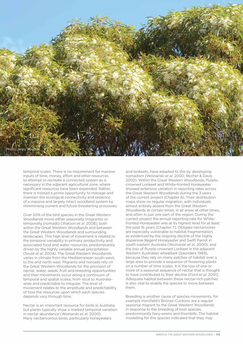
BIRDS IN THE GREAT WESTERN WOODLANDS | 172
temporal scales. There is no requirement for massive inputs of time, money, effort and other resources to attempt to recreate a connected system as is necessary in the adjacent agricultural zone, where significant resources have been expended. Rather, there is instead a prime opportunity to manage and maintain the ecological connectivity and resilence of a massive and largely intact woodland system by miniminsing current and future threatening processes.
Over 50% of the bird species in the Great Western Woodlands move either seasonally (migrants) or temporally (nomads) (Watson et al. 2008), both within the Great Western Woodlands and between the Great Western Woodlands and surrounding landscapes. This high level of movement is related to the temporal variability in primary productivity and associated food and water resources, predominantly driven by the highly variable annual precipitation (Soulé et al. 2004). The Great Western Woodlands varies in climate from the Mediterranean south-west, to the arid north-east. Migrants and nomads rely on the Great Western Woodlands for the provision of nectar, water, seeds, fruit and breeding opportunities and their movements occur along a continuum of temporal and spatial scales, from local to Australia-wide and predictable to irregular. The level of movement relates to the amplitude and predictability of how the resources upon which each species depends vary through time.
Nectar is an important resource for birds in Australia, but plants typically show a marked temporal variation in nectar abundance (Woinarski et al. 2000). Many nectarivorous birds, particularly honeyeaters
and lorikeets, have adapted to this by developing nomadism (Woinarski et al. 2000, Recher & Davis 2002). Within the Great Western Woodlands, Purple-crowned Lorikeet and White-fronted Honeyeater showed extensive variation in reporting rates across the Great Western Woodlands during the 3 years of the current project (Chapter 6). Their distribution maps show no regular migration, with individuals almost entirely absent from the Great Western Woodlands at certain times, in all areas at other times, and often in just one part of the region. During the current project the annual reporting rate for White-fronted Honeyeater was at its highest level for at least the past 16 years (Chapter 7). Obligate nectarivores are especially vulnerable to habitat fragmentation, as evidenced by the ongoing decline of the highly dispersive Regent Honeyeater and Swift Parrot in south-eastern Australia (Woinarski et al. 2000), and the loss of Purple-crowned Lorikeet in the adjacent Western Australian wheatbelt (Saunders 1989), because they rely on many patches of habitat over a large area to provide a sequence of flowering plants on a number of time scales. It is the loss of one or more of a seasonal sequence of nectar that is thought to have contributed to their decline (Ford et al. 2001). Adequate habitat between these nectar-rich patches is also vital to enable the species to move between them.
Breeding is another cause of species movements, for example Horsfield’s Bronze-Cuckoos are a regular seasonal migrant to the Great Western Woodlands in response to the breeding of host species, predominantly fairy-wrens and thornbills. The habitat modelling for this species indicated that they may
Photo: Jenny Moulton
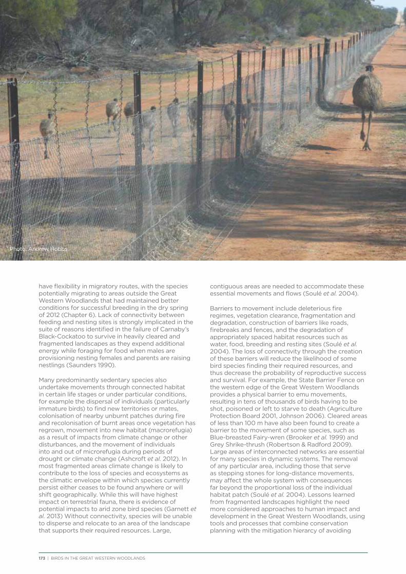
173 | BIRDS IN THE GREAT WESTERN WOODLANDS
have flexibility in migratory routes, with the species potentially migrating to areas outside the Great Western Woodlands that had maintained better conditions for successful breeding in the dry spring of 2012 (Chapter 6). Lack of connectivity between feeding and nesting sites is strongly implicated in the suite of reasons identified in the failure of Carnaby’s Black-Cockatoo to survive in heavily cleared and fragmented landscapes as they expend additional energy while foraging for food when males are provisioning nesting females and parents are raising nestlings (Saunders 1990).
Many predominantly sedentary species also undertake movements through connected habitat in certain life stages or under particular conditions, for example the dispersal of individuals (particularly immature birds) to find new territories or mates, colonisation of nearby unburnt patches during fire and recolonisation of burnt areas once vegetation has regrown, movement into new habitat (macrorefugia) as a result of impacts from climate change or other disturbances, and the movement of individuals into and out of microrefugia during periods of drought or climate change (Ashcroft et al. 2012). In most fragmented areas climate change is likely to contribute to the loss of species and ecosystems as the climatic envelope within which species currently persist either ceases to be found anywhere or will shift geographically. While this will have highest impact on terrestrial fauna, there is evidence of potential impacts to arid zone bird species (Garnett et al. 2013) Without connectivity, species will be unable to disperse and relocate to an area of the landscape that supports their required resources. Large,
contiguous areas are needed to accommodate these essential movements and flows (Soulé et al. 2004).
Barriers to movement include deleterious fire regimes, vegetation clearance, fragmentation and degradation, construction of barriers like roads, firebreaks and fences, and the degradation of appropriately spaced habitat resources such as water, food, breeding and resting sites (Soulé et al. 2004). The loss of connectivity through the creation of these barriers will reduce the likelihood of some bird species finding their required resources, and thus decrease the probability of reproductive success and survival. For example, the State Barrier Fence on the western edge of the Great Western Woodlands provides a physical barrier to emu movements, resulting in tens of thousands of birds having to be shot, poisoned or left to starve to death (Agriculture Protection Board 2001, Johnson 2006). Cleared areas of less than 100 m have also been found to create a barrier to the movement of some species, such as Blue-breasted Fairy-wren (Brooker et al. 1999) and Grey Shrike-thrush (Robertson & Radford 2009). Large areas of interconnected networks are essential for many species in dynamic systems. The removal of any particular area, including those that serve as stepping stones for long-distance movements, may affect the whole system with consequences far beyond the proportional loss of the individual habitat patch (Soulé et al. 2004). Lessons learned from fragmented landscapes highlight the need more considered approaches to human impact and development in the Great Western Woodlands, using tools and processes that combine conservation planning with the mitigation hierarcy of avoiding
Photo: Andrew Hobbs
BIRDS IN THE GREAT WESTERN WOODLANDS | 174
significant areas, minimising damage and impacts of any damage and offsetting where loss is unavoidable (e.g. Fitzsimons et al. 2014).
10.2. Discrete Areas with High Conservation Significance
The key ecological assest of the Great Western Woodlands is its large size and relative intactness. However, within the region there are discrete areas that are disproportionately important for the ongoing survival of species and thus may require ongoing management and protection. Although few specific defined areas were able to be identified from the existing data (this is a task for future research), certain types of discrete areas were able to be classified from the results of the current project and expert opinion. These include the south-west mallee and shrubland habitats, areas of current low disturbance, old-growth woodland, refugia, and natural fresh water sources, and are discussed in further detail below.
The majority of species that have declined or become locally extinct in the Western Australian wheatbelt still occur in the Great Western Woodlands. Simply put, it is the existence of the Great Western Woodlands that has resulted in few of these species being listed as threatened species. Evidence from eastern Australia shows that with widespread clearing and fragmentation of temperate woodlands, species such as Chestnut Quail-thrush, Southern Scrub-robin, Purple-crowned Lorikeet, Major Mitchell’s Cockatoo, Redthroat, Crested Bellbird and Rufous Fieldwren decline to the point where they are considered threatened (e.g. see NSW Threatened Species Conservation Act 1995, Victoria Flora and Fauna Guarantee Act 1988). Many of these species have (or had, prior to local extinction) a distribution in Western Australia centred on the lower south-west, with their distribution extending into the south-western half of the Great Western Woodlands (see for example distribution maps of Southern Scrub-robin, Rufous Fieldwren, Shy Heathwren in Chapter 6). With the loss of populations in the wheatbelt, the Great Western Woodlands is the last remaining stronghold for many of these species, for example 80% of the Shy Heathwren population is thought to now occur in the Great Western Woodlands and adjacent connected habitat (Garnett et al. 2000), and Gilbert’s Whistler is virtually extinct outside the Great Western Woodlands. The south-western half of the Great Western Woodlands is therefore of particular importance for these species, with any extensive clearing and fragmentation in this region likely to result in significant declines and potential state-wide extinctions.
Across the Great Western Woodlands, most wheatbelt decliner species showed a significant negative local impact from disturbances by grazing, artificial watering points, mining, and timber extraction (Chapter 6). In contrast, wheatbelt increasers showed the reverse trend. There are still large areas of the Great Western Woodlands with few European anthropogenic impacts (Figure 195). Maintaining these areas free of large-scale modification would enable natural ecosystem
processes to occur and provide source populations from which disturbed areas could be recolonised.
Patches of mature woodland persist in some areas of the Great Western Woodlands which have not been subject to fire, logging or vegetation disturbance. This old-growth woodland contains key habitat features, such as tree hollows, leaf litter and coarse woody debris, which are vital for a number of species including Major Mitchell’s Cockatoo, Western Rosella and Rufous Treecreeper. It takes hundreds of years for woodland to reach a mature state, and even longer for large tree hollows to form and fallen logs to accumulate to create the required resources (Wormington et al. 2003, Haslem et al. 2012). Due to the long time periods involved, these resources can be impacted by a lack of replacement (Vesk & Mac Nally 2006). Fire, disease, vegetation clearing and selective logging of large trees can all lead to the loss of old trees and the long time lag in their replacement can result in old-growth woodland being a limiting resource in disturbed landscapes.
Currently there is limited knowledge on the location of old-growth woodland in the Great Western Woodlands but in the absence of accurate mapping it is difficult to protect and effectively manage them. A map of potential old-growth woodland areas was produced in 2013 (Keisecker et al. 2013, Fitzsimons et al. 2014). Approximately 25% of the woodlands in the Great Western Woodlands were cut for timber during the early to late 1900s for use in the gold mines and as a fuel source (DPaW timber extraction mapping 2011). There have also been numerous large, high intensity wildfires in recent years that burnt approximately 28% of the woodlands (DPaW fire history mapping 2014). Figure 196 shows the location of all mapped woodland vegetation, excluding areas known to have burnt since 1970 (1940 in the Lake Johnstone area) and areas that were subject to timber cutting during the 1900s. Potential old-growth areas and other woodland areas are identified in the map. The map also includes survey locations of all Rufous Treecreeper records since 1998. To highlight areas where a lack of Treecreeper records may be a result of lack of surveys rather than an absence of the species, the locations of all surveys conducted are also mapped. Rufous Treecreepers are an old-growth woodland obligate species; they are a sedentary species with a small home range size (5-8 ha, Higgins et al. 2001), relying on tree hollows for both roosting and breeding, and foraging amongst fallen coarse woody debris and standing dead trees and hollows. The current project’s study on the impacts of fire (Chapter 8), demonstrated that Rufous Treecreepers were predominantly found in Gimlet (Eucalyptus salubris) woodland at least 150 years old in the Great Western Woodlands, with abundance increasing until at least 300 years since fire. Figure 196 shows that where surveys were conducted within the potential old-growth woodland areas, there were typically a high proportion of Rufous Treecreeper records. However, there are also some areas outside the mapped potential old-growth areas, for example in the north-west corner, where there are a high number of Rufous Treecreeper records. This may indicate the presence of old-growth woodland. Due to a lack of people resources and inaccessibility, some of the mapped potential old-growth areas
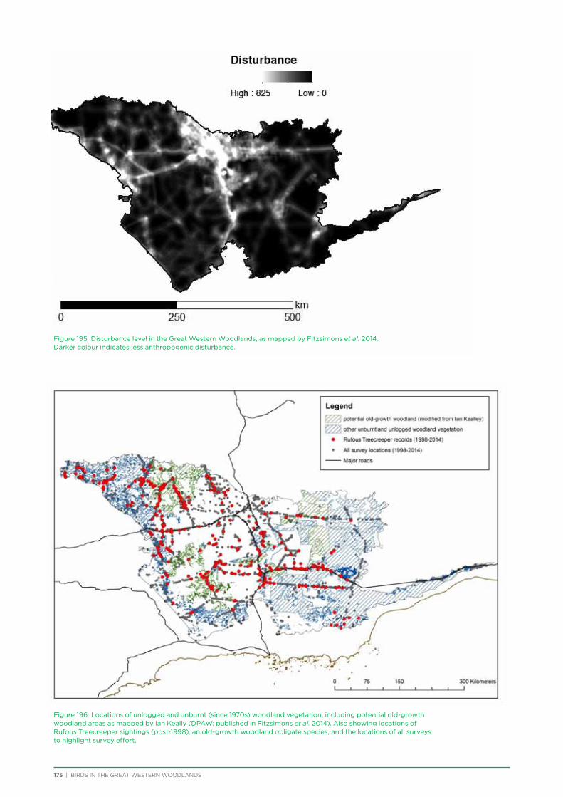
175 | BIRDS IN THE GREAT WESTERN WOODLANDS
Figure 195 Disturbance level in the Great Western Woodlands, as mapped by Fitzsimons et al. 2014. Darker colour indicates less anthropogenic disturbance.
Figure 196 Locations of unlogged and unburnt (since 1970s) woodland vegetation, including potential old-growth woodland areas as mapped by Ian Keally (DPAW; published in Fitzsimons et al. 2014). Also showing locations of Rufous Treecreeper sightings (post-1998), an old-growth woodland obligate species, and the locations of all surveys to highlight survey effort.
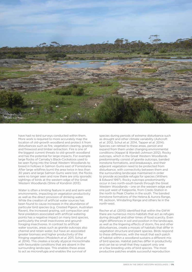
BIRDS IN THE GREAT WESTERN WOODLANDS | 176
Photo: Liz Fox
have had no bird surveys conducted within them. More work is required to more accurately map the location of old-growth woodland and protect it from disturbances such as fire, vegetation clearing, grazing and firewood and timber extraction. Fire is one of the biggest current threats to old-growth woodland and has the potential for large impacts. For example large flocks of Carnaby’s Black-Cockatoos used to be seen flying into the Great Western Woodlands to breed in hollows in Salmon Gums east of Forrestania. After large wildfires burnt the area twice in less than 30 years and large Salmon Gums were lost, the flocks were no longer seen and now there are only sporadic sightings of birds at the western edge of the Great Western Woodlands (Shire of Kondinin 2013).
Water is often a limiting feature in arid and semi-arid environments, impacting on vegetation productivity as well as the direct provision of drinking water. While the creation of artificial water sources has been found to cause increases in the abundance of particular bird species (e.g. Crested Pigeon, Australian Raven), the increased grazing, soil compaction and feral predators associated with artificial watering points has a negative impact on many bird species, particularly the small insectivores and ground-foraging insectivores. In contrast to artificial water sources, areas such as granite outcrops also channel and retain water, but have an associated greater biomass and higher productivity of the fringing vegetation (Mosblech et al. 2011, Schut et al. 2014). This creates a locally atypical microclimate with favourable conditions that are absent in the surrounding landscape. This enables these areas to act as microrefugia and enables the survival of
species during periods of extreme disturbance such as drought and other climate variability (Ashcroft et al. 2012, Schut et al. 2014, Tapper et al. 2014). Species can retreat to these areas, persist and expand from them under changing environmental conditions (Keppel & Wardell-Johnson 2012). Rocky outcrops, which in the Great Western Woodlands predominantly consist of granite outcrops, banded ironstone formations, and breakaways, and their adjacent vegetation need to be protected from disturbance, with connectivity between them and the surrounding landscape maintained in order to provide accessible refugia for species (Withers & Edward 1997). Rocky outcrops predominantly occur in two north-south bands through the Great Western Woodlands – one on the western edge and one just west of Kalgoorlie, from Credo Station in the north to Peak Charles in the south. The banded ironstone formations of the Helena & Aurora Range, Mt Jackson, Windarling Range and others lie in the north-west.
Recher et al. (2010) identified that within the GWW there are numerous micro-habitats that act as refuges during drought and other times of food scarcity. Even slight differences in soil and position in the landscape, as well as the lingering effects of storm, fire and other disturbances, create a mosaic of habitats that differ in vegetation structure and plant species. Birds respond to these differences, with the result that each patch of habitat within a woodland sustains a different mix of bird species. Habitat patches differ in productivity and can be so small that they support only one or a few breeding units of bird species. The most productive patches enable successful reproduction
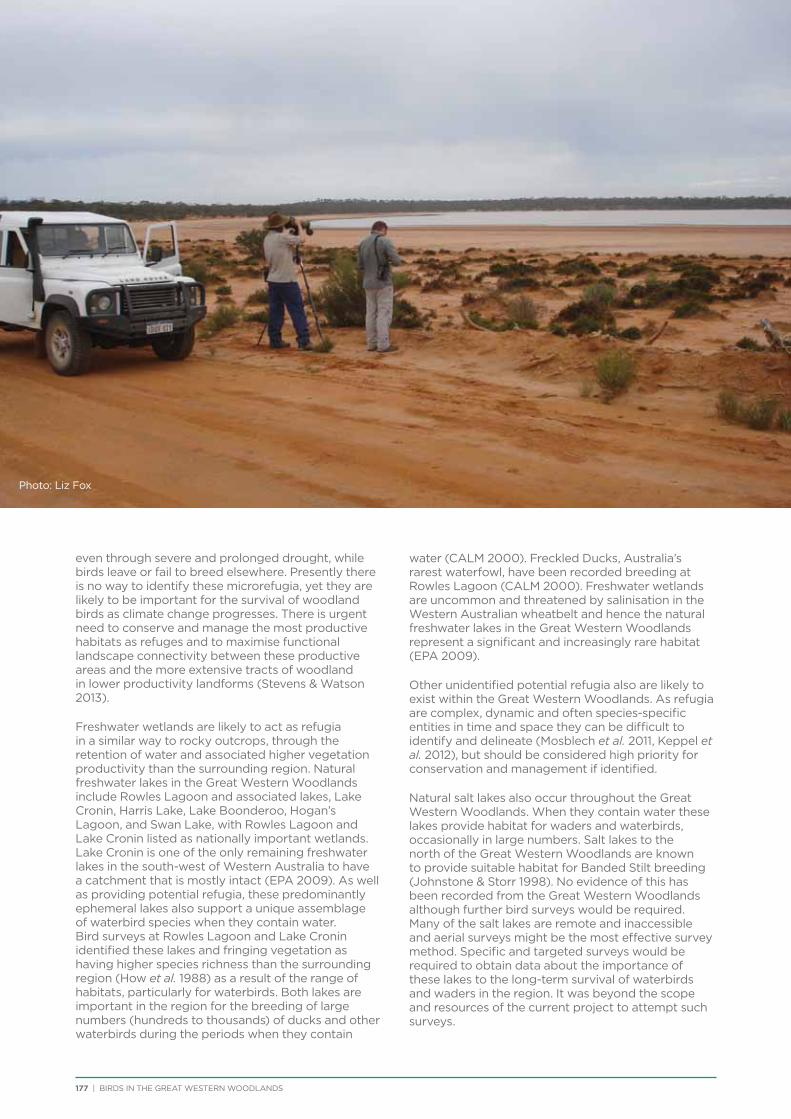
even through severe and prolonged drought, while birds leave or fail to breed elsewhere. Presently there is no way to identify these microrefugia, yet they are likely to be important for the survival of woodland birds as climate change progresses. There is urgent need to conserve and manage the most productive habitats as refuges and to maximise functional landscape connectivity between these productive areas and the more extensive tracts of woodland in lower productivity landforms (Stevens & Watson 2013).
Freshwater wetlands are likely to act as refugia in a similar way to rocky outcrops, through the retention of water and associated higher vegetation productivity than the surrounding region. Natural freshwater lakes in the Great Western Woodlands include Rowles Lagoon and associated lakes, Lake Cronin, Harris Lake, Lake Boonderoo, Hogan’s Lagoon, and Swan Lake, with Rowles Lagoon and Lake Cronin listed as nationally important wetlands. Lake Cronin is one of the only remaining freshwater lakes in the south-west of Western Australia to have a catchment that is mostly intact (EPA 2009). As well as providing potential refugia, these predominantly ephemeral lakes also support a unique assemblage of waterbird species when they contain water. Bird surveys at Rowles Lagoon and Lake Cronin identified these lakes and fringing vegetation as having higher species richness than the surrounding region (How et al. 1988) as a result of the range of habitats, particularly for waterbirds. Both lakes are important in the region for the breeding of large numbers (hundreds to thousands) of ducks and other waterbirds during the periods when they contain
water (CALM 2000). Freckled Ducks, Australia’s rarest waterfowl, have been recorded breeding at Rowles Lagoon (CALM 2000). Freshwater wetlands are uncommon and threatened by salinisation in the Western Australian wheatbelt and hence the natural freshwater lakes in the Great Western Woodlands represent a significant and increasingly rare habitat (EPA 2009).
Other unidentified potential refugia also are likely to exist within the Great Western Woodlands. As refugia are complex, dynamic and often species-specific entities in time and space they can be difficult to identify and delineate (Mosblech et al. 2011, Keppel et al. 2012), but should be considered high priority for conservation and management if identified.
Natural salt lakes also occur throughout the Great Western Woodlands. When they contain water these lakes provide habitat for waders and waterbirds, occasionally in large numbers. Salt lakes to the north of the Great Western Woodlands are known to provide suitable habitat for Banded Stilt breeding (Johnstone & Storr 1998). No evidence of this has been recorded from the Great Western Woodlands although further bird surveys would be required. Many of the salt lakes are remote and inaccessible and aerial surveys might be the most effective survey method. Specific and targeted surveys would be required to obtain data about the importance of these lakes to the long-term survival of waterbirds and waders in the region. It was beyond the scope and resources of the current project to attempt such surveys.
177 | BIRDS IN THE GREAT WESTERN WOODLANDS
Photo: Liz Fox
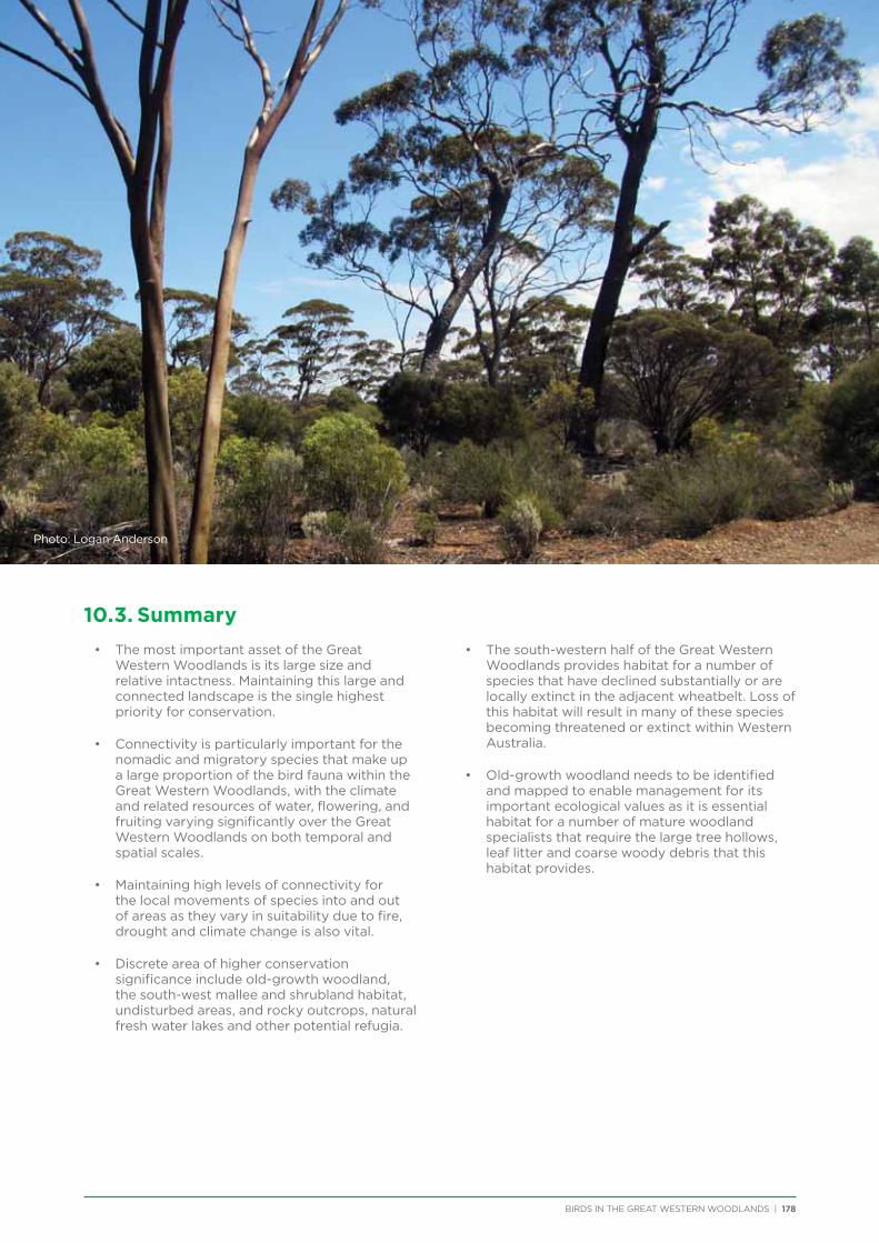
10.3. Summary
• ThemostimportantassetoftheGreatWestern Woodlands is its large size and relative intactness. Maintaining this large and connected landscape is the single highest priority for conservation.
• Connectivityisparticularlyimportantforthenomadic and migratory species that make up a large proportion of the bird fauna within the Great Western Woodlands, with the climate and related resources of water, flowering, and fruiting varying significantly over the Great Western Woodlands on both temporal and spatial scales.
• Maintaininghighlevelsofconnectivityforthe local movements of species into and out of areas as they vary in suitability due to fire, drought and climate change is also vital.
• Discreteareaofhigherconservationsignificance include old-growth woodland, the south-west mallee and shrubland habitat, undisturbed areas, and rocky outcrops, natural fresh water lakes and other potential refugia.
• Thesouth-westernhalfoftheGreatWesternWoodlands provides habitat for a number of species that have declined substantially or are locally extinct in the adjacent wheatbelt. Loss of this habitat will result in many of these species becoming threatened or extinct within Western Australia.
• Old-growthwoodlandneedstobeidentifiedand mapped to enable management for its important ecological values as it is essential habitat for a number of mature woodland specialists that require the large tree hollows, leaf litter and coarse woody debris that this habitat provides.
BIRDS IN THE GREAT WESTERN WOODLANDS | 178
Photo: Logan Anderson
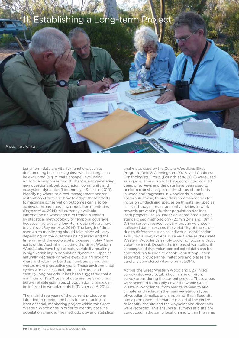
Chapter Header
179 | BIRDS IN THE GREAT WESTERN WOODLANDS
11. Establishing a Long-term Project
Long-term data are vital for functions such as documenting baselines against which change can be evaluated (e.g. climate change), evaluating ecological responses to disturbance, and generating new questions about population, community and ecosystem dynamics (Lindenmayer & Likens 2010). Identifying where to direct management and/or restoration efforts and how to adapt those efforts to maximise conservation outcomes can also be achieved through ongoing population monitoring (Rayner et al. 2014). All currently available information on woodland bird trends is limited by statistical methodology or temporal coverage because rigorous and long-term data sets are hard to achieve (Rayner et al. 2014). The length of time over which monitoring should take place will vary depending on the questions being asked and the timeframe of the ecological processes in play. Many parts of the Australia, including the Great Western Woodlands, have high climate variability resulting in high variability in population dynamics – species naturally decrease or move away during drought years and return or build up numbers during the wetter, more productive years. These environmental cycles work at seasonal, annual, decadal and century-long periods. It has been suggested that a minimum of 15-20 years of data are likely required before reliable estimates of population change can be inferred in woodland birds (Rayner et al. 2014).
The initial three years of the current project was intended to provide the basis for an ongoing, at least decadal, monitoring project within the Great Western Woodlands in order to identify baseline population change. The methodology and statistical
analysis as used by the Cowra Woodland Birds Program (Reid & Cunningham 2008) and Canberra Ornithologists Group (Bounds et al. 2010) were used as a guide. These projects have conducted over 10 years of surveys and the data have been used to perform robust analysis on the status of the birds in woodland fragments in woodlands in south-eastern Australia, to provide recommendations for inclusion of declining species on threatened species lists, and suggest management activities to work towards preventing further population declines. Both projects use volunteer-collected data, using a standardised methodology (20min 2-ha and 10min 0.8-ha surveys respectively). Although volunteer-collected data increases the variability of the results due to differences such as individual identification skills, bird surveys over such a vast area as the Great Western Woodlands simply could not occur without volunteer input. Despite the increased variability, it is recognised that volunteer-collected data can be collected in a fashion to enable robust population estimates, provided the limitations and biases are carefully considered (Rayner et al. 2014).
Across the Great Western Woodlands, 231 fixed survey sites were established in nine different survey areas during the current project. These areas were selected to broadly cover the whole Great Western Woodlands, from Mediterranean to arid climate, and including the main vegetation types of woodland, mallee and shrubland. Each fixed site had a permanent site marker placed at the centre to identify the site and the waypoint and directions were recorded. This ensures all surveys at a site are conducted in the same location and within the same
Photo: Mary Whittall
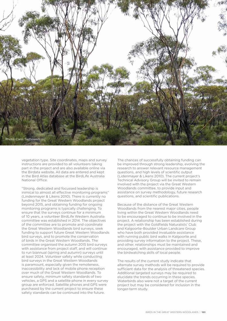
BIRDS IN THE GREAT WESTERN WOODLANDS | 180
vegetation type. Site coordinates, maps and survey instructions are provided to all volunteers taking part in the project and are also available online via the Birdata website. All data are entered and kept in the Bird Atlas database at the BirdLife Australia National Office.
“Strong, dedicated and focussed leadership is inimical to almost all effective monitoring programs” (Lindenmayer & Likens 2010). There is currently no funding for the Great Western Woodlands project beyond 2015, and obtaining funding for ongoing monitoring programs is typically challenging. To ensure that the surveys continue for a minimum of 10 years, a volunteer BirdLife Western Australia committee was established in 2014. The objectives of the committee are to promote and coordinate the Great Western Woodlands bird surveys, seek funding to support future Great Western Woodlands bird surveys, and to promote the conservation of birds in the Great Western Woodlands. The committee organised the autumn 2015 bird surveys with assistance from project staff, and will continue to run biannual (spring and autumn) surveys until at least 2024. Volunteer safety while conducting bird surveys in the Great Western Woodlands is paramount, especially given the remoteness, inaccessibility and lack of mobile phone reception over much of the Great Western Woodlands. To ensure safety, minimum safety standards of two vehicles, a GPS and a satellite phone in every survey group are enforced. Satellite phones and GPS were purchased by the current project to ensure these safety standards can be continued into the future.
The chances of successfully obtaining funding can be improved through strong leadership, evolving the research to answer relevant resource management questions, and high levels of scientific output (Lidenmayer & Likens 2010). The current project’s Technical Advisory Group will be invited to remain involved with the project via the Great Western Woodlands committee, to provide input and assistance on survey methodology, future research questions, and scientific publications.
Because of the distance of the Great Western Woodlands from the nearest major cities, people living within the Great Western Woodlands need to be encouraged to continue to be involved in the project. A relationship has been established during the project with the Goldfields Naturalists’ Club and Kalgoorlie-Boulder Urban Landcare Group who have both provided invaluable assistance with running public bird walks in Kalgoorlie and providing survey information to the project. These, and other, relationships must be maintained and encouraged, with assistance provided to improve the birdwatching skills of local people.
The results of the current study indicate that alternate survey methods will be required to provide sufficient data for the analysis of threatened species. Additional targeted surveys may be required to elucidate the trends occurring in these species. Waterbirds also were not a target of the current project but may be considered for inclusion in the longer-term study.
Photo: TBA
Photo: Carol Trethowen
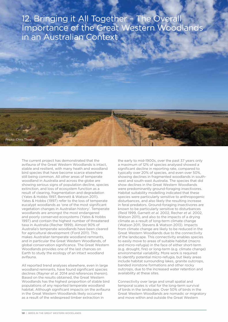
Chapter Header
181 | BIRDS IN THE GREAT WESTERN WOODLANDS
Chapter Header12. Bringing it All Together – The Overall Importance of the Great Western Woodlands in an Australian Context
The current project has demonstrated that the avifauna of the Great Western Woodlands is intact, stable and resilient, with many heath and woodland bird species that have become scarce elsewhere still being common. All other areas of temperate woodland in Australia and across the globe are showing serious signs of population decline, species extinction, and loss of ecosystem function as a result of clearing, fragmentation and degradation (Yates & Hobbs 1997, Bennett & Watson 2011). Yates & Hobbs (1997) refer to the loss of temperate eucalypt woodlands as ‘one of the most significant vegetation changes in Australian history’. Temperate woodlands are amongst the most endangered and poorly conserved ecosystems (Yates & Hobbs 1997) and contain the highest number of threatened taxa in Australia (Recher 1999). Almost 90% of Australia’s temperate woodlands have been cleared for agricultural development (Ford 2011). This makes Australian temperate woodland remnants, and in particular the Great Western Woodlands, of global conservation significance. The Great Western Woodlands provides one of the last chances on Earth to study the ecology of an intact woodland avifauna.
All reported trend analyses elsewhere, even in large woodland remnants, have found significant species declines (Rayner et al. 2014 and references therein). Based on the results obtained, the Great Western Woodlands has the highest proportion of stable bird populations of any reported temperate woodland habitat. Although significant impacts on the avifauna in the Great Western Woodlands likely occurred as a result of the widespread timber extraction in
the early to mid-1900s, over the past 37 years only a maximum of 12% of species analysed showed a significant decline in reporting rate, compared to typically over 20% of species, and even over 50%, showing declines in fragmented woodlands in south-west and south-east Australia. The species that did show declines in the Great Western Woodlands were predominantly ground-foraging insectivores. Habitat suitability modelling indicated that these species were particularly sensitive to anthropogenic disturbances, and also likely the resulting increase in feral predators. Ground-foraging insectivores are known to be particularly sensitive to disturbances (Reid 1999, Garnett et al. 2002, Recher et al. 2002, Watson 2011), and also to the impacts of a drying climate as a result of long-term climate change (Watson 2011, Stevens & Watson 2013). Impacts from climate change are likely to be reduced in the Great Western Woodlands due to the connectivity of the landscape. This connectivity enables species to easily move to areas of suitable habitat (macro and micro-refugia) in the face of either short-term (e.g. drought, fire) or long-term (e.g. climate change) environmental variability. More work is required to identify potential micro-refugia, but likely areas include habitat surrounding lakes, granite outcrops, banded ironstone formations and other rocky outcrops, due to the increased water retention and availability at these sites.
Connectivity over large and small spatial and temporal scales is vital for the long-term survival of birds in the landscape. Over 50% of birds in the Great Western Woodlands are nomadic or migratory and move within and outside the Great Western
Photo: Chris Thorne
BIRDS IN THE GREAT WESTERN WOODLANDS | 182
Woodlands in response to resource availability. Species such as the Purple-crowned Lorikeet, an obligate nectar-feeder, require a spatial and temporal sequence of eucalypt flowering across vast areas. The remnant vegetation within the Western Australian wheatbelt no longer provides sufficient resources for this species, with the species seldom recorded from areas where they used to be common (Saunders & Ingram 1995). Loss of woodland connectivity in south-east Australia has contributed to the severe decline of obligate nectar-feeders such as Regent Honeyeaters and Swift Parrots, with both species now listed as endangered. Purple-crowned Lorikeets and other nomadic honeyeaters were recorded as common and stable within the Great Western Woodlands.
The Great Western Woodlands is vital for the continued survival of many species that have declined or are locally extinct in the adjacent Western Australian wheatbelt. Only one species has become locally extinct within the GWW – Western Grasswren occurred east of Kalgoorlie and was lost from across the Western Australian interior in the early 1900s as a result of overgrazing by introduced animals. This compares favourably to the wheatbelt where numerous species are locally extinct throughout much of the southern and central wheatbelt (for example Western Rosella, Gilbert’s Whistler, Yellow-plumed Honeyeater; Saunders 1989). Ninety-five species have declined in the wheatbelt (Saunders & Ingram 1995), but those that occur within the Great Western Woodlands are predominantly all still abundant to moderately common within the Great Western Woodlands, particularly the south-west half of the region due to the natural distribution of these species which is typically focussed on the more Mediterranean-climate habitat. Extensive clearing and fragmentation within the Great Western Woodlands would undoubtedly result in widespread declines in these species with many becoming threatened with extinction.
Inappropriate fire regimes are the biggest threat facing the Great Western Woodlands. Maintaining habitat connectivity helps to reduce the impact to species by enabling individuals to escape the direct impacts of a fire and also to recolonise the area once the vegetation has recovered to a suitable level for the species. However, the potential loss of old-growth woodland within the Great Western Woodlands is a significant current threat. Many species are more abundant in old-growth woodland, but some species are disproportionately reliant on the tree hollows, leaf litter and coarse woody debris that this habitat type provides. Species such as Rufous Treecreepers and Major Mitchell’s Cockatoos rely on woodland where eucalypts over 150 years old occur since it can take at least 100-200 years for eucalypts to reach maturity and then form the large tree hollows required for breeding and to drop branches to create the coarse woody debris on the ground that attracts invertebrates. Once lost through fire or vegetation clearing, old-growth woodland takes the longest of any habitat type to replace.
Other potential threats include mining, exploration and associated disturbances (e.g. infrastructure such as haul roads, dewatering, pit lakes); invasive flora and fauna; increased access and tourism and the associated potential for track proliferation, increased fire risk and spread of organisms; climate change; vegetation degradation and clearing; and grazing and the provision of water. It is recommended that a region-wide Conservation Action Plan (CAP) be undertaken to identify scope, targets, threats and actions more precisely and to work towards a consensus of stakeholders.
The Great Western Woodlands is important as the largest remaining area of intact temperate woodland in the world. It provides the rare chance to conserve an already intact ecosystem rather than trying to rebuild a fractured landscape which inevitably requires an exhaustive input of time, money and resources. It also provides the opportunity to anticipate and act on changes while we still have time to succeed, rather than trying to concentrate conservation efforts on already threatened species and areas, where it can be difficult to achieve a positive outcome (Recher 1999). We need to protect our Great Western Woodlands and the birds it supports so that it remains great now and into the future.
183 | BIRDS IN THE GREAT WESTERN WOODLANDS
References
Agriculture Protection Board (2001). The State Barrier Fence of Western Australia 1901– 2001. Department of Agriculture, Perth
Ashcroft, M. B., Gollan, J. R., Warton, D. I., & Ramp, D. (2012). A novel approach to quantify and locate potential microrefugia using topoclimate, climate stability, and isolation from the matrix. Global Change Biology 18(6): 1866-1879
Austin, M. P. (1991). Vegetation theory in relation to cost-efficient survey. In Nature Conservation: Cost Effective Biological Surveys and Data Analysis (eds C. R. Margules and M. P. Austin.) pp. 17–22. CSIRO Division of Wildlife and Ecology: Canberra
Barrett, G.W., Ford, H.A., Recher, H.F. (1994). Conservation of woodland birds in a fragmented rural landscape. Pacific Conservation Biology 1: 245–256.
Barrett, G., Silcocks, A., Barry, S., Cunningham, R., and Poulter, R. (2003). The New Atlas of Australian Birds. Royal Australasian Ornithologists’ Union: Melbourne
Barrett, G.W., Silcocks, A.F., Cunningham, R., Oliver, D.L., Weston, M.A., Baker, J. (2007). Comparison of atlas data to determine the conservation status of bird species in New South Wales, with an emphasis on woodland-dependent species. Australian Zoologist 34: 37–77
Barton, P. S., Ikin, K., Smith, A. L., MacGregor, C., & Lindenmayer, D. B. (2014). Vegetation structure moderates the effect of fire on bird assemblages in a heterogeneous landscape. Landscape Ecology 29(4): 703-714
Belbin, L. (1980). TWOSTP: a program incorporating asymmetric comparisons that uses two steps to produce a dissimilarity matrix. CSIRO Division of Water and Land Resources Technical Memorandum 80/9, Canberra
Belbin, L. (1991). The analysis of pattern in bio-survey data. In Nature Conservation: Cost Effective Biological Surveys and Data Analysis (eds C. R. Margules and M. P. Austin.) pp. 176–190. CSIRO: Melbourne
Belbin, L. (1995). PATN Technical Reference. CSIRO Division of Wildlife and Ecology: Canberra
Biological Survey Committee. (1984). The biological survey of the Eastern Goldfields of Western Australia. Part 1. Introduction and methods. Records of the Western Australia Museum Supplement 18: 1-19
BirdLife Australia (2014). The BirdLife Australia Working List of Australian Birds, Version 1.2.
Blakers, M., Davies, S.J.J.F., and Reilly, P.N. (1984). ‘The Atlas of Australian Birds.’ (Melbourne University Press: Melbourne.)
Bounds, J., Taws, N., Cunningham, R., (2010). A statistical analysis of trends in occupancy rates of woodland birds in the ACT, December 1998 to December 2008: the ten year data analysis. Canberra Bird Notes 35: 158–192.
Bradby, K., Fitzsimons, J.A., Del Marco, A., Driscoll, D.A., Ritchie, E.G., Lau, J., Bradshaw, C.J.A. & Hobbs, R.J. (2014). Ecological connectivity or Barrier Fence? Critical choices on the agricultural margins of Western Australia. Ecological Management and Restoration 15: 180-190.
Brooker, M., & Brooker, L. (2001). Breeding biology, reproductive success and survival of blue-breasted fairy-wrens in fragmented habitat in the Western Australian wheatbelt. Wildlife Research 28(2): 205-214.
Brooker, L., M. Brooker, and P. Cale. 1999. Animal dispersal in fragmented habitat: measuring habitat connectivity, corridor use, and dispersal mortality. Conservation Ecology 3(1): 4.
Brown, S., Clarke, M., & Clarke, R. (2009). Fire is a key element in the landscape-scale habitat requirements and global population status of a threatened bird: The Mallee Emu-wren (Stipiturus mallee). Biological Conservation 142(2): 432-445.
Burbidge, A. A., Casperson, K. D., and Fuller, P. J. (1987). Birds. In ‘A Biological Survey of the Nullarbor Region’. (Eds N. L. McKenzie and A. Robinson.) pp. 153–178. (SADEP, WA Dept of CALM and ANPWS, Adelaide.)
Burbidge, A. H., Johnstone, R. E., Fuller, P. J., and Stone, P. (2000). Terrestrial birds of the southern Carnarvon Basin, Western Australia: contemporary patterns of occurrence. Records of the Western Australian Museum Supplement No. 61: 449–464.
Burbidge, A. H., Johnstone, R. E., & Pearson, D. J. (2010). Birds in a vast arid upland: avian biogeographical patterns in the Pilbara region of Western Australia. Records of the Western Australian Museum, Supplement 78: 247–270.
CALM (2000). Rowles Lagoon Conservation Park and Clear and Muddy Lakes Nature Reserve: Management Plan 2000-2010. Report for the National parks and Nature Conservation Authority.
BIRDS IN THE GREAT WESTERN WOODLANDS | 184
Clarke, K. R., and Gorley, R. N. (2006). PRIMER v6: User Manual/Tutorial. PRIMER-E Ltd: Plymouth
Clarke, K. R., Somerfield, P. J., and Gorley, R. N. (2008). Testing of null hypotheses in exploratory community analyses: similarity profiles and biota-environment linkage. Journal of Experimental Marine Biology and Ecology 366: 56–69.
Clarke, M. F., Avitabile, S. C., Brown, L., Callister, K. E., Haslem, A., Holland, G. J., et al. (2010). Ageing mallee eucalypt vegetation after fire: insights for successional trajectories in semi-arid mallee ecosystems. Australian Journal of Botany 58(5): 363-372.
Crooks, K. R., & Sanjayan, M. (2006). Connectivity Conservation (Vol. 14). Cambridge University Press.
Cunningham, R., and Olsen, P. (2009). A statistical methodology for tracking long-term change in reporting rates of birds from volunteer-collected presence-absence data. Biodiversity Conservation 18(5): 1305-1327.
Daly, C. (2006). Guidelines for assessing the suitability of spatial climate data sets. International Journal of Climatology 26:707-721.
Dell, J. (1976). Birds of Lake Magenta Wildlife Sanctuary, Western Australia. Records of the Western Australian Museum 4(2): 117-132.
Dell, J., and How, R. A. (1988). Vertebrate fauna. In The Biological Survey of the Eastern Goldfields of Western Australia. Part 5. Edjudina-Menzies study area. Records of the Western Australian Museum Supplement No. 31: 38–66.
Department of Environment and Conservation (2010) A biodiversity and cultural conservation strategy for the Great Western Woodlands. Department of Environment and Conservation: Perth
Department of Environment and Conservation (2013) Great Western Woodlands draft strategic weed and feral animal management plan. Department of Environment and Conservation: Perth
DiMiceli, C. M., M. L. Carroll, R. A. Sohlberg, C. Huang, M. C. Hansen, and J. R. G. Townshend. 2011. Annual Global Automated MODIS Vegetation Continuous Fields (MOD44B) at 250 m Spatial Resolution for Data Years Beginning Day 65, 2000 - 2010, Collection 5 Percent Tree Cover. University of Maryland: College Park.
Driscoll, D. A., Lindenmayer, D. B., Bennett, A. F., Bode, M., Bradstock, R. A., Cary, G. J., et al. (2010). Fire management for biodiversity conservation: Key research questions and our capacity to answer them. Biological Conservation 143(9): 1928-1939
Dufrêne, M. and P. Legendre, P. (1997). Species assemblages and indicator species: the need for a flexible asymmetrical approach. Ecological Monographs 67, 345-366.
Elith, J., C. H. Graham, R. P. Anderson, M. Dudik, S. Ferrier, A. Guisan, R. J. Hijmans, F. Huettmann, J. R. Leathwick, A. Lehmann, J. Li, L. G. Lohmann, B. A. Loiselle, G. Manion, C. Moritz, M. Nakamura, Y. Nakazawa, J. M. Overton, A. T. Peterson, S. J. Phillips, K. Richardson, R. Scachetti-Pereira, R. E. Schapire, J. Soberon, S. Williams, M. S. Wisz, & N. E. Zimmermann. (2006). Novel methods improve prediction of species’ distributions from occurrence data. Ecography 29:129-151.
Elith, J., S. J. Phillips, T. Hastie, M. Dudik, Y. E. Chee, & C. J. Yates. (2011). A statistical explanation of maxent for ecologists. Diversity and Distributions 17:43-57.
Environmental Protection Authority (2007). State of the Environment Report. Department of Environment and Conservation: Perth
Environmental Protection Authority (2009). Advice on Conservation Values and Review of Nature Reserve Proposals in the Lake Cronin Region. Report 1329
Executive Steering committee for Australian Vegetation Information (ESCAVI) (2003) Australian Vegetation Attribute Manual: National Vegetation Information System, Version 6.0. Department of Environment and Heritage: Canberra
Faith, D. P., Minchin, P. R., & Belbin, L. (1987). Compositional dissimilarity as a robust measure of ecological distance. Vegetatio 69: 57–68
Fitzsimons, J., Pulsford, I. & Wescott, G. (eds) (2013). Linking Australia’s Landscapes: Lessons and Opportunities from Large-scale Conservation Networks. CSIRO Publishing: Collingwood
Fitzsimons, J., Heiner, M., McKenney, B., Sochi, K., & Kiesecker, J. (2014) Development by Design in Western Australia: Overcoming offset obstacles. Land 3: 167-187
Ford, H. A. (2011). The causes of decline of birds of eucalypt woodlands: advances in our knowledge over the last 10 years. Emu 111(1): 1-9
185 | BIRDS IN THE GREAT WESTERN WOODLANDS
Ford, H.A., Barrett, G.W., Saunders, D.A., Recher, H.F. (2001) Why have birds in the woodlands of Southern Australia declined? Biological Conservation 97: 71-88
Fritz, S., & L. See. (2008). Identifying and quantifying uncertainty and spatial disagreement in the comparison of global land cover for different applications. Global Change Biology 14:1057-1075
Garnett (1992). Threatened and extinct birds of Australia. RAOU Report 82. Royal Australasian Ornithologists Union and Australian National parks and Wildlife Service: Moonee Ponds
Garnett, S., Crowley, G., & Barrett, G. (2002). Patterns and Trends in Australian Bird Distributions and Abundance: Preliminary Analysis of Data from the New Atlas of Australian Birds. Report to the National Land & Water Resources Audit, Canberra.
Garnett, S.T., Franklin, D.C., Ehmke, G., VanDerWal, J.J., Hodgson, L., Pavey, C., Reside, A.E., Welbergen, J.A., Butchart, S.H.M., Perkins, G.C. & Williams, S.E. (2013) Climate change adaptation strategies for Australian birds. National Climate Change Adaptation Research Facility: Gold Coast.
Garnett, S., Szabo, J., & Dutson, G. (2011). Action Plan for Australian Birds 2010. Environment Australia, Canberra
Gaston, K.J. (2010) Valuing common species. Science 327: 154-155
Geoscience Australia 2006. GEODATA TOPO 250K Series 3 User Guide. Geoscience Australia, Canberra, Australia.
Gilfillan, S., Comer, S., Burbidge, A., Blyth, J., Danks, A., Newell, J. (2009) South coast threatened birds recovery plan 2009-2018. Western Australian Wildlife Management Program No. 44. Report for the South Coast Threatened Birds Recovery Team.
Gosper, C. R. (2012). Birds of two important bird areas of Western Australia-lake magenta and dunn rock and lake king. Australian Field Ornithology 29(1)
Gosper, C.R., Prober, S.M., Yates, C.J. (2013a). Multi-century changes in vegetation structure and fuel availability in fire-sensitive eucalypt woodlands. Forest Ecology and Management 310: 102-109
Gosper, C. R., Yates, C. J., & Prober, S. M. (2013b). Floristic diversity in fire-sensitive eucalypt woodlands shows a ‘U’-shaped relationship with time since fire. Journal of Applied Ecology 50(5): 1187-1196.
Gosper, C. R., Prober, S. M., Yates, C. J., & Wiehl, G. (2013c). Estimating the time since fire of long-unburnt Eucalyptus salubris (Myrtaceae) stands in the Great Western Woodlands. Australian Journal of Botany 61(1): 11-21.
Halse, S. A., & Jaensch, R. P. (1989). Breeding seasons of waterbirds in south-western Australia - the importance of rainfall. Emu 89: 232–249.
Hammer, Ø., Harper, D.A.T., and P. D. Ryan, 2001. PAST: Paleontological Statistics Software Package for Education and Data Analysis. Palaeontologia Electronica 4(1)
Hansen, M. C., R. S. DeFries, J. R. G. Townshend, R. Sohlberg, C. Dimiceli, & M. Carroll. (2002). Towards an operational MODIS continuous field of percent tree cover algorithm: examples using AVHRR and MODIS data. Remote Sensing of Environment 83: 303-319.
Haslem, A., Avitabile, S. C., Taylor, R. S., Kelly, L. T., Watson, S. J., Nimmo, D. G., Kenny, S.A., Callister, K.E., Spence-Bailey, L.M., Bennet, A.F., Clarke, M.F. (2012). Time-since-fire and inter-fire interval influence hollow availability for fauna in a fire-prone system. Biological Conservation 152: 212-221.
Heinsch, F. A., M. Zhao, S. W. Running, J. S. Kimball, R. R. Nemani, K. J. Davis, P. V. Bolstad, B. D. Cook, A. R. Desai, D. M. Ricciuto, B. E. Law, W. C. Oechel, H. Kwon, H. Luo, S. C. Wofsy, A. L. Dunn, J. W. Munger, D. D. Baldocchi, L. Xu, D. Y. Hollinger, A. D. Richardson, P. C. Stoy, M. B. S. Siqueira, R. K. Monson, S. P. Burns, and L. B. Flanagan. (2006). Evaluation of remote sensing based terrestrial productivity from MODIS using regional tower eddy flux network observations. IEEE Transactions on Geoscience and Remote Sensing 44:1908-1925.
Herford, I., Armstrong, R., & Daniel, G. (2012) Fire management plan for the conservation of biodiversity and cultural heritage values in the Great Western Woodlands. Department of Environment and Conservation
Higgins, P.J., Peter, J.M., Steele, W.K., 2001. Handbook of Australian, New Zealand and Antarctic Birds. Tyrant-flycatchers to Chats, Vol. 5. Oxford University Press: Melbourne
Hijmans, R. J., Cameron, S. E., Parra, J. L., Jones, P. G., & Jarvis, A. (2005). Very high resolution interpolated climate surfaces for global land areas. International journal of climatology 25(15): 1965-1978
James, C. D., Landsberg, J., & Morton, S. R. (1999). Provision of watering points in the Australian arid zone: a review of effects on biota. Journal of arid environments 41(1): 87-121
BIRDS IN THE GREAT WESTERN WOODLANDS | 186
Johnson M. (2006) ‘Feathered foes’: Soldier settlers and Western Australia’s ‘Emu War’ of 1932. Journal of Australian Studies 30(88): 147–157
Johnstone , R.E., & Storr, G.M. (1998) Handbook of Western Australian Birds. Volume I – Non-passerines (Emu to Dollarbird). Western Australian Museum: Perth
Johnstone , R.E., & Storr, G.M. (2004) Handbook of Western Australian Birds. Volume II – Passerines (Blue-winged Pitta to Goldfinch). Western Australian Museum: Perth
Jones, D. A., W. Wang, & R. Fawcett. (2009). High-quality spatial climate data-sets for Australia. Australian Meteorological and Oceanographic Journal 58:233-248
Kealley, I. (1991). Management of inland arid and semi-arid woodland forest of Western Australia. In Forest Management in Australia (eds F. H. McKinnell, E. R. Hopkins & J. E. D. Fox), pp. 286-295). Surrey Beatty & Sons: Chipping Norton
Kelly, L.T., Bennett, A.F., Clarke, M.F., & McCarthy, M.A. (2014) Optimal fire histories for biodiversity conservation. Conservation Biology 29(2): 473-481
Keppel, G., & Wardell-Johnson, G. W. (2012). Refugia: keys to climate change management. Global Change Biology 18(8): 2389-2391
Keppel, G., Van Niel, K. P., Wardell-Johnson, G. W., Yates, C. J., Byrne, M., Mucina, L., Schut, G.T., Hopper, S.D., & Franklin, S. E. (2012). Refugia: identifying and understanding safe havens for biodiversity under climate change. Global Ecology and Biogeography 21(4): 393-404
Kiesecker, J., Heiner, M., Sochi, K., McKenney, B., and Fitzsimons, J. (2013). Development by Design: Cooperative mitigation planning for Barrick Gold’s Kanowna Belle operations in Western Australia. The Nature Conservancy: Arlington, VA
Kitchener, D. J., Dell, J., Muir, B. G., & Palmer, M. (1982). Birds in Western Australian wheatbelt reserves—implications for conservation. Biological Conservation 22(2): 127-163
Koch, A.J., Munks, S.A., Driscoll, D., Kirkpatrick, J.B., 2008. Does hollow occurrence vary with forest type? A case study in wet and dry Eucalyptus obliqua forest. Forest Ecology and Management 255: 3938–3951
Leavesley, A. J., Cary, G. J., Edwards, G. P., & Gill, A. M. (2010). The effect of fire on birds of mulga woodland in arid central Australia. International Journal of Wildland Fire 19(7): 949-960
Leuning, R., H. A. Cleugh, S. J. Zegelin, and D. Hughes. (2005). Carbon and water fluxes over a temperate Eucalyptus forest and a tropical wet/dry savanna in Australia: measurements and comparison with MODIS remote sensing estimates. Agricultural and Forest Meteorology 129:151-173.
Lindenmayer, D.B., Likens, G.E., 2010. The science and application of ecological monitoring. Biological Conservation 143: 1317–1328.
Liu, C., P. M. Berry, T. P. Dawson, & R. G. Pearson. (2005). Selecting thresholds of occurrence in the prediction of species distributions. Ecography 28:385-393.
Lynch, J. F., & Saunders, D. A. (1991). Responses of bird species to habitat fragmentation in the wheatbelt of Western Australia: interiors, edges and corridors. In Nature conservation 2: The role of corridors (eds D. Saunders & R. Hobbs), pp. 143-158. Surrey Beatty & Sons: Chipping Norton
Mac Nally, R., Bennett, A.F., Thomson, J.R., Radford, J.Q., Unmack, G., Horrocks, G., Vesk, P.A. (2009). Collapse of an avifauna: climate change appears to exacerbate habitat loss and degradation. Diversity and Distribution 15: 720–730.
Mackey, B., S. Berry, S. Hugh, S. Ferrier, T. D. Harwood, & K. J. Williams. (2012). Ecosystem greenspots: identifying potential drought, fire, and climate-change micro-refuges. Ecological Applications 22:1852-1864.
Marchant, S., & Higgins, P. J. (eds) (1990). Handbook of Australian, New Zealand and Antarctic birds. Volume 1: Ratities to Ducks. Oxford University Press: Melbourne
Marchant, S., & P.J. Higgins (eds) (1993). Handbook of Australian, New Zealand and Antarctic Birds. Volume 2: Raptors to Lapwings. Oxford University Press: Melbourne
Higgins, P.J. & S.J.J.F. Davies (eds) (1996). Handbook of Australian, New Zealand and Antarctic Birds. Volume 3: Snipe to Pigeons. Oxford University Press: Melbourne
Higgins, P.J. (ed) (1999). Handbook of Australian, New Zealand and Antarctic Birds. Volume 4: Parrots to Dollarbird. Oxford University Press: Melbourne
187 | BIRDS IN THE GREAT WESTERN WOODLANDS
Higgins, P.J., J.M. Peter & W.K. Steele (eds) (2001). Handbook of Australian, New Zealand and Antarctic Birds. Volume 5: Tyrant-flycatchers to Chats. Oxford University Press: Melbourne
Higgins, P.J. & J.M. Peter (eds) (2002). Handbook of Australian, New Zealand and Antarctic Birds. Volume 6: Pardalotes to Shrike-thrushes. Oxford University Press: Melbourne
Higgins, P.J., J.M. Peter & S.J. Cowling (eds) (2006). Handbook of Australian, New Zealand and Antarctic Birds. Volume 7: Boatbill to Starlings. Oxford University Press: Melbourne
Maron, M., & Lill, A. (2005). The influence of livestock grazing and weed invasion on habitat use by birds in grassy woodland remnants. Biological Conservation 124(4): 439-450.
McCune, B. and Mefford, M. J. (2011). PC-ORD. Multivariate Analysis of Ecological Data. Version 6.0. (MjM Software: Gleneden Beach, Oregon, U.S.A.)
McKenzie, N. L., Rolfe, J. K., & Youngson, W. K. (1992). Vertebrate fauna. In The Biological Survey of the Eastern Goldfields of Western Australia. Part 8. The Kurnalpi-Kalgoorlie study area (eds N. L. McKenzie & N. J. Hall.) Records of the Western Australian Museum Supplement No. 41: 37–64.
McKenzie, N. L., and Rolfe, J. K. (1995). Vertebrate fauna. In ‘The Biological Survey of the Eastern Goldfields of Western Australia. Part 11. Boorabbin-Southern Cross study area’. (Eds G. J. Keighery, N. L. McKenzie, and N. J. Hall.) pp. 31–65 (Records of the Western Australian Museum Supplement No. 49)
Mosblech, N. A., Bush, M. B., & van Woesik, R. (2011). On metapopulations and microrefugia: palaeoecological insights. Journal of Biogeography 38(3): 419-429.
Mu, Q., M. Zhao, F. A. Heinsch, M. Liu, H. Tian, and S. W. Running. (2007). Evaluating water stress controls on primary production in biogeochemical and remote sensing based models. Journal of Geophysical Research-Biogeosciences 112: G01012.
Myneni, R. B., S. Hoffman, Y. Knyazikhin, J. L. Privette, J. Glassy, Y. Tian, Y. Wang, X. Song, Y. Zhang, G. R. Smith, A. Lotsch, M. Friedl, J. T. Morisette, P. Votava, R. R. Nemani, & S. W. Running. (2002). Global products of vegetation leaf area and fraction absorbed PAR from year one of MODIS data. Remote Sensing of Environment 83:214-231.
Nimmo, D.G., Kelly, L.T., Farnsworth, L.M., Watson, S.J. & Bennett, A.F. (2014) Why do some species have geographically varying responses to fire history? Ecography, 37: 805-813
O’Donnell, A. J., Boer, M. M., McCaw, W. L., & Grierson, P. F. (2011). Climatic anomalies drive wildfire occurrence and extent in semi-arid shrublands and woodlands of southwest Australia. Ecosphere 2(11): art127.
Oliver, D. L., Ley, A. J., Ford, H. A., & Williams, B. (1999). Habitat of the Regent Honeyeater Xanthomyza phrygia and the value of the Bundarra-Barraba region for the conservation of avifauna. Pacific Conservation Biology 5(3): 224.
Olsen, P., Weston, M., Tzaros, C., & Silcocks, A. (2005). The State of Australia’s Birds 2005: Woodlands and Birds. Birds Australia: Melbourne
Parsons, B. C., & Gosper, C. R. (2011). Contemporary fire regimes in a fragmented and an unfragmented landscape: implications for vegetation structure and persistence of the fire-sensitive malleefowl. International Journal of Wildland Fire 20(2): 184-194.
Pavey, C. R., and Nano, C. E. M. (2009). Bird assemblages of arid Australia: vegetation patterns have a greater effect than disturbance and resource pulses. Journal of Arid Environments 73: 634–642.
Phillips, S. J., & M. Dudik. (2008). Modeling of species distributions with maxent: new extensions and a comprehensive evaluation. Ecography 31:161-175.
Phillips, S. J., R. P. Anderson, & R. E. Schapire. (2006). Maximum entropy modelling of species geographic distributions. Ecological Modelling 190:231-259.
Phillips, L. B., A. J. Hansen, & C. H. Flather. (2008). Evaluating the species energy relationship with the newest measures of ecosystem energy: NDVI versus MODIS primary production. Remote Sensing of Environment 112:3538-3549.
Phillips, S. J., M. Dudik, J. Elith, C. H. Graham, A. Lehmann, J. Leathwick, & S. Ferrier. (2009). Sample selection bias and presence-only distribution models: implications for background and pseudo-absence data. Ecological Applications 19:181-197.
Raupach, M. R., P. R. Briggs, V. Haverd, E. A. King, M. Paget, and C. M. Trudinger. 2009. Australian Water Availability Project (AWAP): CSIRO Marine and Atmospheric Research component: Final report for Phase 3. CAWCR Technical Report No. 013.
BIRDS IN THE GREAT WESTERN WOODLANDS | 188
Rayner, L., Lindenmayer, D., Gibbons, P., Manning, A. (2014) Evaluating empirical evidence for decline in temperate woodland birds: A nationally threatened assemblage of species. Biological Conservation 171: 145-155
Recher, H. F. (1999). The state of Australia’s avifauna: a personal opinion and prediction for the new millennium. Australian Zoologist 31: 11-29
Recher, H. F., & Davis, W. E. (2002). Foraging profile of a Salmon Gum woodland avifauna in Western Australia. Journal of the Royal Society of Western Australia 85: 103–111.
Recher, H. F., & Davis, W. E. (2013). Response of birds to a wildfire in the Great Western Woodlands, Western Australia. Pacific Conservation Biology 19(3/4): 188.
Recher, H. F., & Davis, W. E. (2014). Response of birds to episodic summer rainfall in the Great Western Woodlands, Western Australia. Australian Zoologist 37(2): 206-224.
Recher, H. F., Davis, W. E., & Calver, M. C. (2002). Comparative foraging ecology of five species of ground-pouncing birds in western Australian woodlands with comments on species decline. Ornithological Science 1(1): 29-40.
Recher, H.F., Majer, J.D., Davis, W.E. (2010) The eucalypt woodlands of Western Australia: lessons from the birds. In Temperate woodland conservation and management (eds D. Lindenmayer, A. Bennett, and R. Hobbs), pp. 63-72. CSIRO Publishing: Collingwood
Reid, J.R.W. (1999). Threatened and declining birds in the New South Wales Sheep-Wheat Belt: I. Diagnosis, characteristics and management. Consultancy report to NSW National Parks and Wildlife Service. CSIRO Sustainable Ecosystems: Canberra
Reid, J. & Cunningham, R. (2008). Statistical analysis of the Cowra woodland birds program’s bird database. A report prepared for the Lachlan Catchment Management Authority and Birds Australia Southern New South Wales and ACT.
Robertson, O. J., & Radford, J. Q. (2009). Gap-crossing decisions of forest birds in a fragmented landscape. Austral Ecology 34(4): 435-446.
Running, S. W., R. Nemani, J. M. Glassy, & P. E. Thornton. (1999). MODIS daily photosynthesis (PSN) and annual net primary productivity (NPP) product (MOD17). Algorithm Theoretical Basis Document.
Running, S. W., R. R. Nemani, F. A. Heinsch, M. S. Zhao, M. Reeves, & H. Hashimoto. (2004). A continuous satellite-derived measure of global terrestrial primary production. Bioscience 54:547-560.
Saunders, D.A. (1989). Changes in the avifauna of a region, district and remnant as a result of fragmentation of native vegetation: the wheatbelt of Western Australia. A case study. Biological Conservation 50: 99-135.
Saunders, D. A. (1990). Problems of survival in an extensively cultivated landscape: the case of Carnaby’s cockatoo Calyptorhynchus funereus latirostris. Biological Conservation 54: 277-90.
Saunders, D., Ingram, J. (1995) Birds of Southwestern Australia: An atlas of changes in the distribution and abundance of the wheatbelt avifauna. Surrey Beatty and Sons, Chipping Norton
Schut A.G.T., Wardell-Johnson G.W., Yates C.J., Keppel G., Baran I., Franklin, S.E., Hopper, S.D., Van Niel, K.P., Mucina, L., Byrne, M. (2014) Rapid Characterisation of Vegetation Structure to Predict Refugia and Climate Change Impacts across a Global Biodiversity Hotspot. PLoS ONE 9(1): e82778
Shepherd, D. P. 2003. Implementation of the National Vegetation Information System model in Western Australia. Milestone 6 Report. Final report on the implementation of the National Vegetation Information System model in Western Australia. Bureau of Rural Services: Canberra.
Shire of Kondinin, Shire of Dundas, Western Areas Ltd, Norilsk Nickel & Gondwana Link Ltd (2013) Granite and Woodlands: The conservation action plan for the Kondinin and Dundas parts of the Great Western Woodlands
Sneath, P. H. A., & Sokal, R. R. (1973). Numerical Taxonomy: The Principles and Practice of Numerical Classification. Freeman: San Francisco
Soulé, M. E., Mackey, B. G., Recher, H. F., Williams, J. E., Woinarski, J. C. Z., Driscoll, D., et al. (2004). The role of connectivity in Australian conservation. Pacific Conservation Biology 10: 266-275.
Stevens, H. C., & Watson, D. M. (2013). Reduced rainfall explains avian declines in an unfragmented landscape: incremental steps toward an empty forest? Emu 113(2): 112-121.
Szabo, J.K., Vesk, P.A., Baxter, P.W.J., Possingham, H.P. (2011). Paying the extinction debt: woodland birds in the Mount Lofty Ranges, South Australia. Emu 111: 59–70.
189 | BIRDS IN THE GREAT WESTERN WOODLANDS
Tapper, S. L., Byrne, M., Yates, C. J., Keppel, G., Hopper, S. D., Van Niel, K., Schut, A.G.T., Mucina, L., & Wardell-Johnson, G.W. (2014). Prolonged isolation and persistence of a common endemic on granite outcrops in both mesic and semi-arid environments in south-western Australia. Journal of Biogeography 41(11): 2032-2044.
Taylor, R. S., Watson, S. J., Nimmo, D. G., Kelly, L. T., Bennett, A. F., & Clarke, M. F. (2012). Landscape-scale effects of fire on bird assemblages: does pyrodiversity beget biodiversity? Diversity and distributions 18(5): 519-529.
Taylor, R.S., Watson, S.J., Bennett, A.F., & Clarke, M.F. (2013) Which fire management strategies benefit biodiversity? A landscape-perspective case study using birds in mallee ecosystems of south-eastern Australia, Biological Conservation 159: 248-256
Tessarolo, G., T. F. Rangel, M. B. Araujo, & J. Hortal. (2014). Uncertainty associated with survey design in species distribution models. Diversity and Distributions 20:1258-1269.
Traill, B. J., Collins, E., Peake, P., & Jessup, S. (1996). Current and past status of the birds of Chiltern–a box-ironbark forest in north-eastern Victoria. Australian Bird Watcher 16: 309-326.
Tuanmu, M.-N., & W. Jetz. (2014). A global 1-km consensus land-cover product for biodiversity and ecosystem modelling. Global Ecology and Biogeography 23:1031-1045.
Turner, D. P., W. D. Ritts, W. B. Cohen, S. T. Gower, S. W. Running, M. S. Zhao, M. H. Costa, A. A. Kirschbaum, J. M. Ham, S. R. Saleska, and D. E. Ahl. (2006). Evaluation of MODIS NPP and GPP products across multiple biomes. Remote Sensing of Environment 102:282-292.
Vesk, P.A., Mac Nally, R. (2006) The clock is ticking – revegetation and habitat for birds and arboreal mammals in rural landscapes of southern Australia. Agriculture, Ecosystems and Environment 112: 356-366
Watson, D.M. (2011) A productivity-based explanation for woodland bird declines: poorer soils yield less food. Emu 111: 10-18
Watson, A., Judd, S., Watson, J., Lam, A., & Mackenzie, D. (2008). The extraordinary nature of the Great Western Woodlands. Wilderness Society of WA
Watson, S. J., Taylor, R. S., Nimmo, D. G., Kelly, L. T., Clarke, M. F., & Bennett, A. F. (2012a). The influence of unburnt patches and distance from refuges on post-fire bird communities. Animal Conservation 15(5): 499-507.
Watson, S. J., Taylor, R. S., Nimmo, D. G., Kelly, L. T., Haslem, A., Clarke, M. F., et al. (2012b). Effects of time since fire on birds: How informative are generalized fire response curves for conservation management? Ecological Applications 22(2): 685-696.
Whelan, R. J., L. Rodgerson, C. R. Dickman, and E. F. Sutherland. (2001). Critical life cycles of plants and animals: developing a process-based understanding of population changes in fire prone landscapes. In Flammable Australia: the fire regimes and biodiversity of a continent (eds R. Bradstock, J. E. Williams, and A. M. Gill), pp. 94–124. Cambridge University Press: Cambridge.
Withers, P. C., & Edward, D. H. (1997). Terrestrial fauna of granite outcrops in Western Australia. Journal of the Royal Society of Western Australia 80: 159-166.
Woinarski, J. C. Z. (1999). Fire and Australian birds: a review. Australia’s Biodiversity-Responses to Fire 55-180.
Woinarski, J., & Recher, H. F. (1997). Impact and response: a review of the effects of fire on the Australian avifauna. Pacific Conservation Biology 3(3): 183.
Wooller, R. D., & Calver, M. C. (1988). Changes in an assemblage of small birds in the understorey of dry sclerophyll forest in southwestern Australia after fire. Wildlife Research 15(3): 331-338.
Woinarski, J. C., Connors, G., & Franklin, D. C. (2000). Thinking honeyeater: nectar maps for the Northern Territory, Australia. Pacific Conservation Biology 6(1): 61-80.
Worboys, G. L., & Pulsford, I. (2011). Connectivity conservation in Australian landscapes. Report prepared for the Australian Government Department of Sustainability, Environment, Water, Population and Communities on behalf of the State of the Environment.
Wormington, K. R., Lamb, D., McCallum, H. I., & Moloney, D. J. (2003). The characteristics of six species of living hollow-bearing trees and their importance for arboreal marsupials in the dry sclerophyll forests of southeast Queensland, Australia. Forest ecology and management 182(1): 75-92.
Yates, C. J., & Hobbs, R. J. (1997). Temperate eucalypt woodlands: a review of their status, processes threatening their persistence and techniques for restoration. Australian Journal of Botany 45(6): 949-973.
Zhao, M. S., F. A. Heinsch, R. R. Nemani, and S. W. Running. 2005. Improvements of the MODIS terrestrial gross and net primary production global data set. Remote Sensing of Environment 95: 164-176.
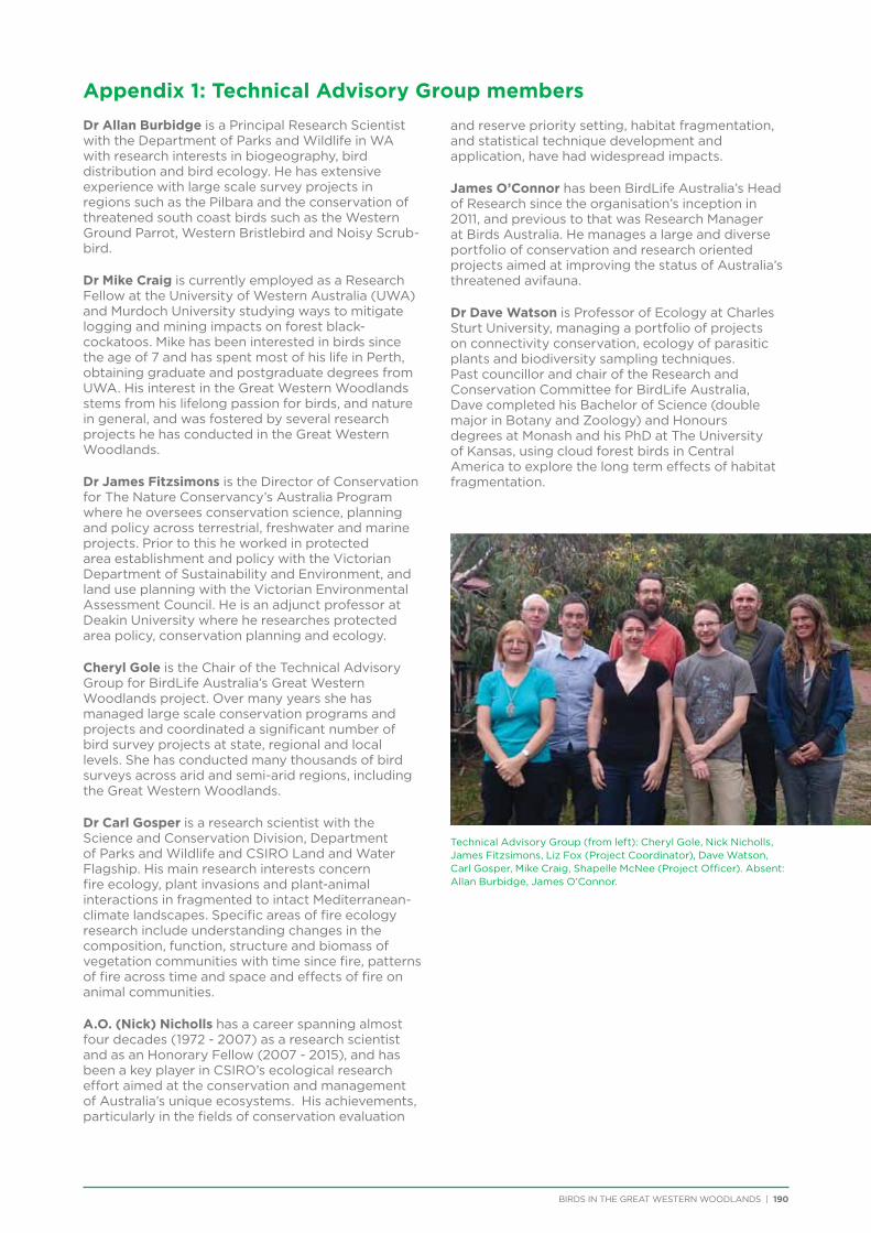
BIRDS IN THE GREAT WESTERN WOODLANDS | 190
Appendix 1: Technical Advisory Group members
Dr Allan Burbidge is a Principal Research Scientist with the Department of Parks and Wildlife in WA with research interests in biogeography, bird distribution and bird ecology. He has extensive experience with large scale survey projects in regions such as the Pilbara and the conservation of threatened south coast birds such as the Western Ground Parrot, Western Bristlebird and Noisy Scrub-bird.
Dr Mike Craig is currently employed as a Research Fellow at the University of Western Australia (UWA) and Murdoch University studying ways to mitigate logging and mining impacts on forest black-cockatoos. Mike has been interested in birds since the age of 7 and has spent most of his life in Perth, obtaining graduate and postgraduate degrees from UWA. His interest in the Great Western Woodlands stems from his lifelong passion for birds, and nature in general, and was fostered by several research projects he has conducted in the Great Western Woodlands.
Dr James Fitzsimons is the Director of Conservation for The Nature Conservancy’s Australia Program where he oversees conservation science, planning and policy across terrestrial, freshwater and marine projects. Prior to this he worked in protected area establishment and policy with the Victorian Department of Sustainability and Environment, and land use planning with the Victorian Environmental Assessment Council. He is an adjunct professor at Deakin University where he researches protected area policy, conservation planning and ecology.
Cheryl Gole is the Chair of the Technical Advisory Group for BirdLife Australia’s Great Western Woodlands project. Over many years she has managed large scale conservation programs and projects and coordinated a significant number of bird survey projects at state, regional and local levels. She has conducted many thousands of bird surveys across arid and semi-arid regions, including the Great Western Woodlands.
Dr Carl Gosper is a research scientist with the Science and Conservation Division, Department of Parks and Wildlife and CSIRO Land and Water Flagship. His main research interests concern fire ecology, plant invasions and plant-animal interactions in fragmented to intact Mediterranean-climate landscapes. Specific areas of fire ecology research include understanding changes in the composition, function, structure and biomass of vegetation communities with time since fire, patterns of fire across time and space and effects of fire on animal communities.
A.O. (Nick) Nicholls has a career spanning almost four decades (1972 - 2007) as a research scientist and as an Honorary Fellow (2007 - 2015), and has been a key player in CSIRO’s ecological research effort aimed at the conservation and management of Australia’s unique ecosystems. His achievements, particularly in the fields of conservation evaluation
and reserve priority setting, habitat fragmentation, and statistical technique development and application, have had widespread impacts.
James O’Connor has been BirdLife Australia’s Head of Research since the organisation’s inception in 2011, and previous to that was Research Manager at Birds Australia. He manages a large and diverse portfolio of conservation and research oriented projects aimed at improving the status of Australia’s threatened avifauna.
Dr Dave Watson is Professor of Ecology at Charles Sturt University, managing a portfolio of projects on connectivity conservation, ecology of parasitic plants and biodiversity sampling techniques. Past councillor and chair of the Research and Conservation Committee for BirdLife Australia, Dave completed his Bachelor of Science (double major in Botany and Zoology) and Honours degrees at Monash and his PhD at The University of Kansas, using cloud forest birds in Central America to explore the long term effects of habitat fragmentation.
Technical Advisory Group (from left): Cheryl Gole, Nick Nicholls, James Fitzsimons, Liz Fox (Project Coordinator), Dave Watson, Carl Gosper, Mike Craig, Shapelle McNee (Project Officer). Absent: Allan Burbidge, James O’Connor.
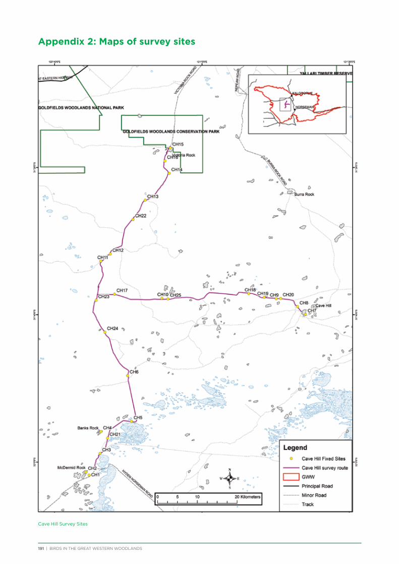
191 | BIRDS IN THE GREAT WESTERN WOODLANDS
Cave Hill Survey Sites
Appendix 2: Maps of survey sites
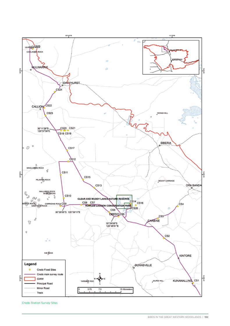
BIRDS IN THE GREAT WESTERN WOODLANDS | 192
Credo Station Survey Sites
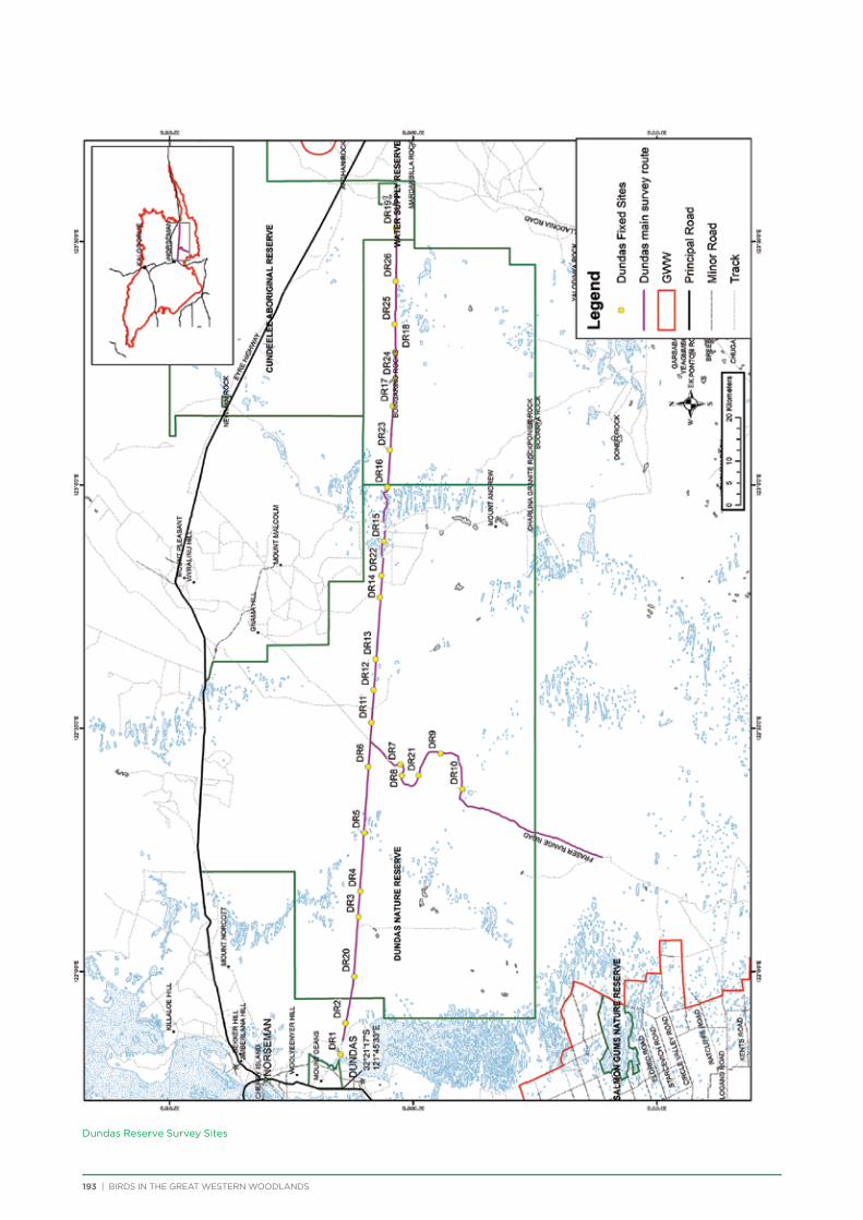
193 | BIRDS IN THE GREAT WESTERN WOODLANDS
Dundas Reserve Survey Sites
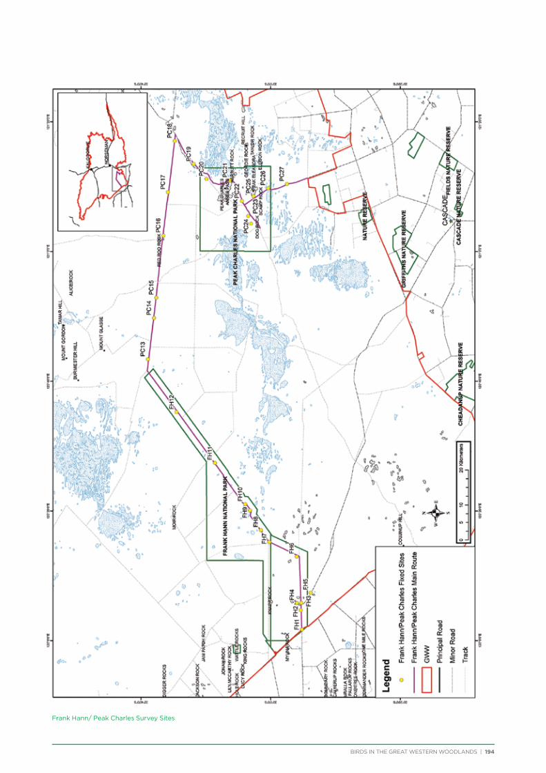
BIRDS IN THE GREAT WESTERN WOODLANDS | 194
Frank Hann/ Peak Charles Survey Sites

195 | BIRDS IN THE GREAT WESTERN WOODLANDS
Fraser Range Survey Sites
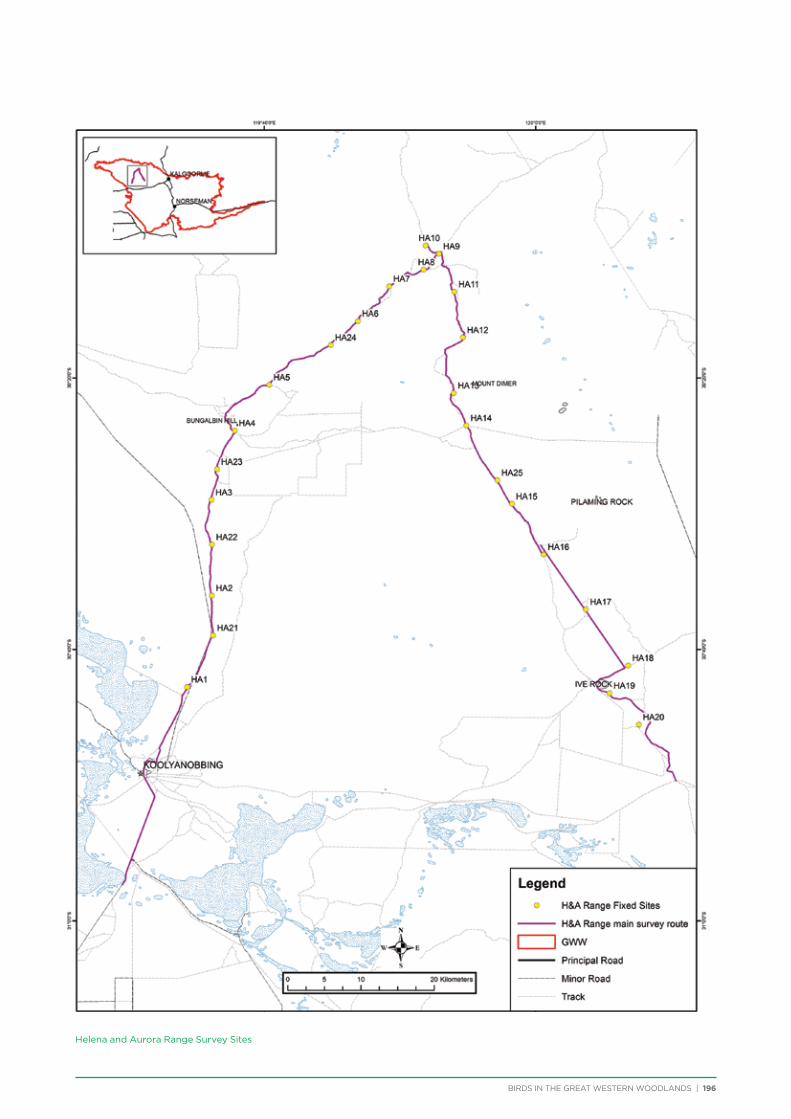
BIRDS IN THE GREAT WESTERN WOODLANDS | 196
Helena and Aurora Range Survey Sites
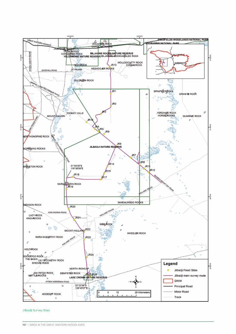
197 | BIRDS IN THE GREAT WESTERN WOODLANDS
Jilbadji Survey Sites
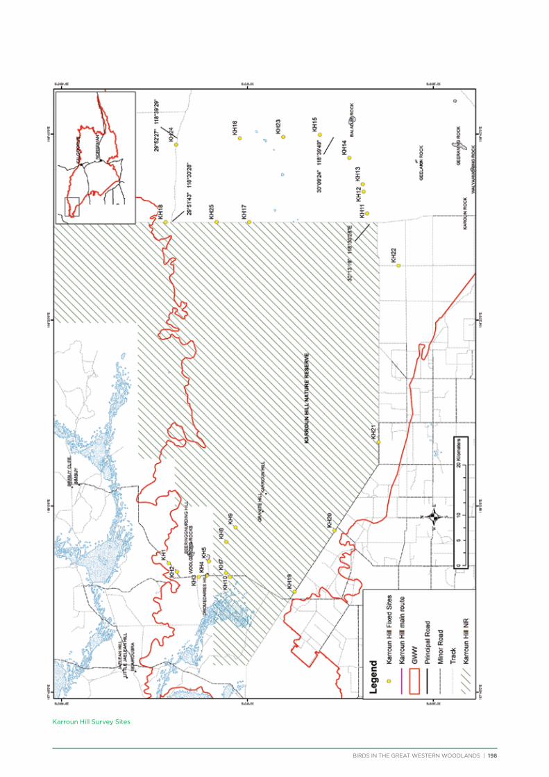
BIRDS IN THE GREAT WESTERN WOODLANDS | 198
Karroun Hill Survey Sites
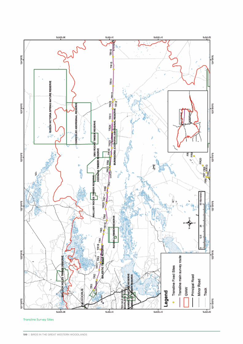
199 | BIRDS IN THE GREAT WESTERN WOODLANDS
Transline Survey Sites
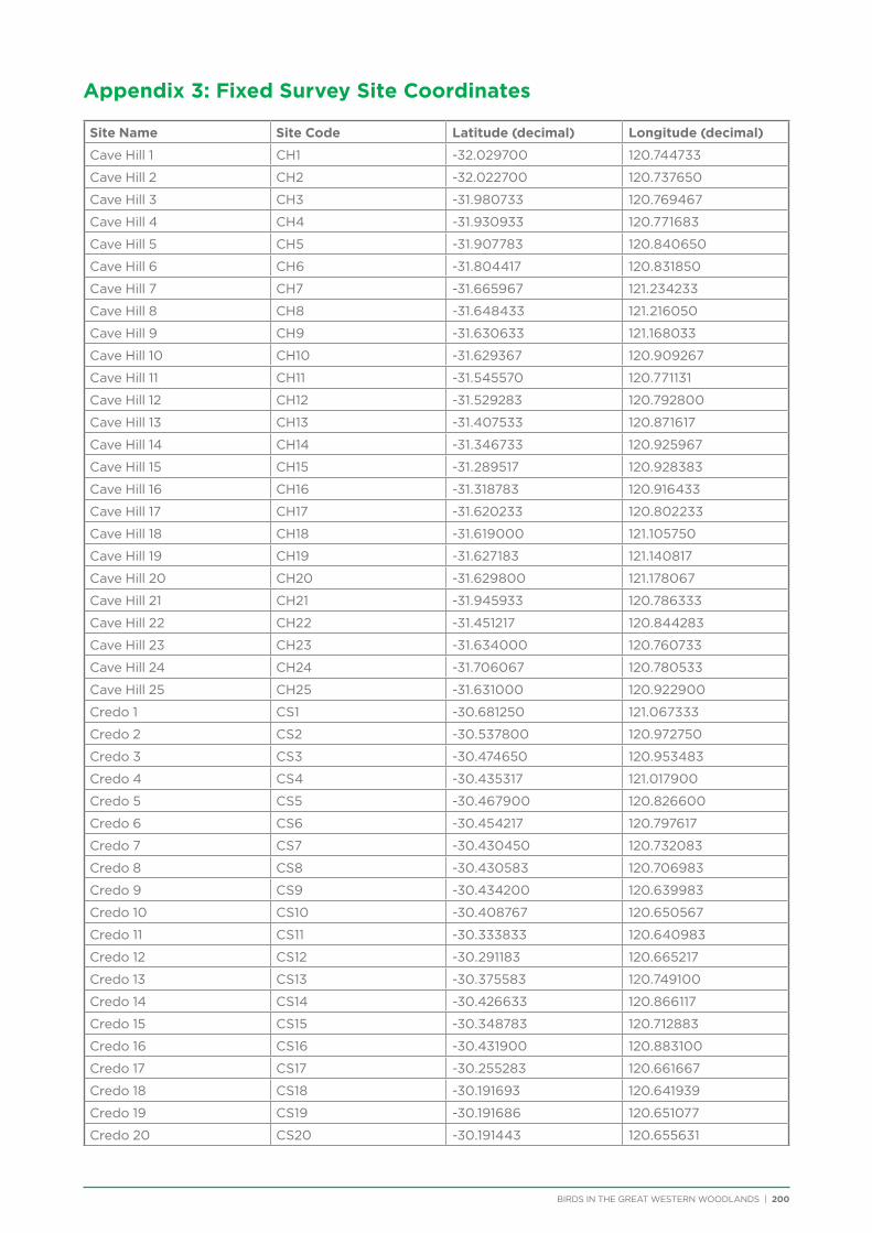
BIRDS IN THE GREAT WESTERN WOODLANDS | 200
Appendix 3: Fixed Survey Site Coordinates
Site Name Site Code Latitude (decimal) Longitude (decimal)
Cave Hill 1 CH1 -32.029700 120.744733
Cave Hill 2 CH2 -32.022700 120.737650
Cave Hill 3 CH3 -31.980733 120.769467
Cave Hill 4 CH4 -31.930933 120.771683
Cave Hill 5 CH5 -31.907783 120.840650
Cave Hill 6 CH6 -31.804417 120.831850
Cave Hill 7 CH7 -31.665967 121.234233
Cave Hill 8 CH8 -31.648433 121.216050
Cave Hill 9 CH9 -31.630633 121.168033
Cave Hill 10 CH10 -31.629367 120.909267
Cave Hill 11 CH11 -31.545570 120.771131
Cave Hill 12 CH12 -31.529283 120.792800
Cave Hill 13 CH13 -31.407533 120.871617
Cave Hill 14 CH14 -31.346733 120.925967
Cave Hill 15 CH15 -31.289517 120.928383
Cave Hill 16 CH16 -31.318783 120.916433
Cave Hill 17 CH17 -31.620233 120.802233
Cave Hill 18 CH18 -31.619000 121.105750
Cave Hill 19 CH19 -31.627183 121.140817
Cave Hill 20 CH20 -31.629800 121.178067
Cave Hill 21 CH21 -31.945933 120.786333
Cave Hill 22 CH22 -31.451217 120.844283
Cave Hill 23 CH23 -31.634000 120.760733
Cave Hill 24 CH24 -31.706067 120.780533
Cave Hill 25 CH25 -31.631000 120.922900
Credo 1 CS1 -30.681250 121.067333
Credo 2 CS2 -30.537800 120.972750
Credo 3 CS3 -30.474650 120.953483
Credo 4 CS4 -30.435317 121.017900
Credo 5 CS5 -30.467900 120.826600
Credo 6 CS6 -30.454217 120.797617
Credo 7 CS7 -30.430450 120.732083
Credo 8 CS8 -30.430583 120.706983
Credo 9 CS9 -30.434200 120.639983
Credo 10 CS10 -30.408767 120.650567
Credo 11 CS11 -30.333833 120.640983
Credo 12 CS12 -30.291183 120.665217
Credo 13 CS13 -30.375583 120.749100
Credo 14 CS14 -30.426633 120.866117
Credo 15 CS15 -30.348783 120.712883
Credo 16 CS16 -30.431900 120.883100
Credo 17 CS17 -30.255283 120.661667
Credo 18 CS18 -30.191693 120.641939
Credo 19 CS19 -30.191686 120.651077
Credo 20 CS20 -30.191443 120.655631
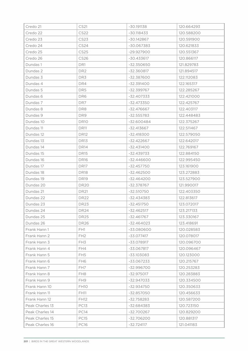
201 | BIRDS IN THE GREAT WESTERN WOODLANDS
Credo 21 CS21 -30.191138 120.664293
Credo 22 CS22 -30.118433 120.588200
Credo 23 CS23 -30.142867 120.591900
Credo 24 CS24 -30.067383 120.621833
Credo 25 CS25 -29.927900 120.551367
Credo 26 CS26 -30.433617 120.866117
Dundas 1 DR1 -32.350650 121.829783
Dundas 2 DR2 -32.360817 121.894517
Dundas 3 DR3 -32.387600 122.112083
Dundas 4 DR4 -32.391400 122.165317
Dundas 5 DR5 -32.399767 122.285267
Dundas 6 DR6 -32.407333 122.421000
Dundas 7 DR7 -32.473350 122.425767
Dundas 8 DR8 -32.476667 122.403117
Dundas 9 DR9 -32.555783 122.448483
Dundas 10 DR10 -32.600484 122.375267
Dundas 11 DR11 -32.413667 122.511467
Dundas 12 DR12 -32.418300 122.579050
Dundas 13 DR13 -32.422667 122.642017
Dundas 14 DR14 -32.431400 122.769167
Dundas 15 DR15 -32.439733 122.884150
Dundas 16 DR16 -32.446600 122.995450
Dundas 17 DR17 -32.457750 123.161900
Dundas 18 DR18 -32.462500 123.272883
Dundas 19 DR19 -32.464200 123.527900
Dundas 20 DR20 -32.378767 121.990017
Dundas 21 DR21 -32.510750 122.403350
Dundas 22 DR22 -32.434383 122.813617
Dundas 23 DR23 -32.451750 123.072017
Dundas 24 DR24 -32.462517 123.217133
Dundas 25 DR25 -32.461767 123.330167
Dundas 26 DR26 -32.464023 123.418691
Frank Hann 1 FH1 -33.080600 120.028583
Frank Hann 2 FH2 -33.077417 120.078017
Frank Hann 3 FH3 -33.078917 120.096700
Frank Hann 4 FH4 -33.067817 120.096467
Frank Hann 5 FH5 -33.103083 120.123000
Frank Hann 6 FH6 -33.067233 120.215767
Frank Hann 7 FH7 -32.996700 120.253283
Frank Hann 8 FH8 -32.975017 120.283883
Frank Hann 9 FH9 -32.947033 120.334500
Frank Hann 10 FH10 -32.934750 120.350633
Frank Hann 11 FH11 -32.857050 120.456633
Frank Hann 12 FH12 -32.758283 120.587200
Peak Charles 13 PC13 -32.684383 120.723150
Peak Charles 14 PC14 -32.700267 120.829200
Peak Charles 15 PC15 -32.706200 120.881317
Peak Charles 16 PC16 -32.724117 121.041183
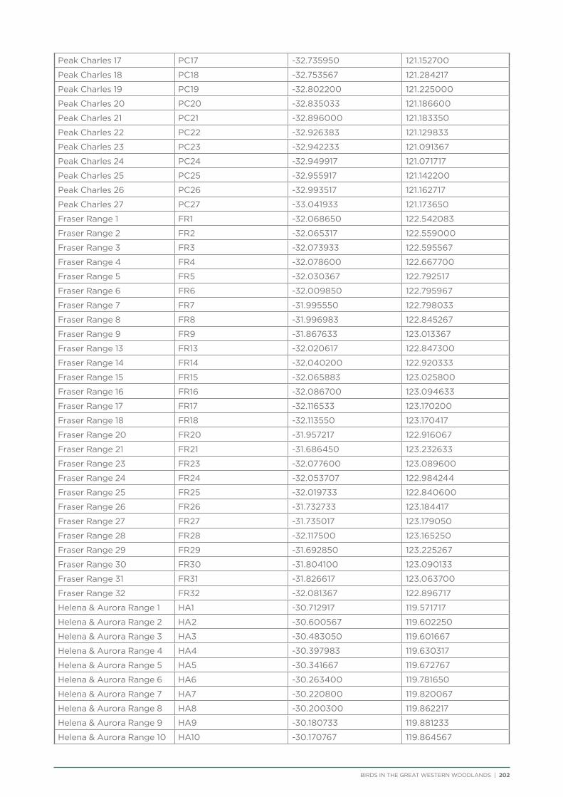
BIRDS IN THE GREAT WESTERN WOODLANDS | 202
Peak Charles 17 PC17 -32.735950 121.152700
Peak Charles 18 PC18 -32.753567 121.284217
Peak Charles 19 PC19 -32.802200 121.225000
Peak Charles 20 PC20 -32.835033 121.186600
Peak Charles 21 PC21 -32.896000 121.183350
Peak Charles 22 PC22 -32.926383 121.129833
Peak Charles 23 PC23 -32.942233 121.091367
Peak Charles 24 PC24 -32.949917 121.071717
Peak Charles 25 PC25 -32.955917 121.142200
Peak Charles 26 PC26 -32.993517 121.162717
Peak Charles 27 PC27 -33.041933 121.173650
Fraser Range 1 FR1 -32.068650 122.542083
Fraser Range 2 FR2 -32.065317 122.559000
Fraser Range 3 FR3 -32.073933 122.595567
Fraser Range 4 FR4 -32.078600 122.667700
Fraser Range 5 FR5 -32.030367 122.792517
Fraser Range 6 FR6 -32.009850 122.795967
Fraser Range 7 FR7 -31.995550 122.798033
Fraser Range 8 FR8 -31.996983 122.845267
Fraser Range 9 FR9 -31.867633 123.013367
Fraser Range 13 FR13 -32.020617 122.847300
Fraser Range 14 FR14 -32.040200 122.920333
Fraser Range 15 FR15 -32.065883 123.025800
Fraser Range 16 FR16 -32.086700 123.094633
Fraser Range 17 FR17 -32.116533 123.170200
Fraser Range 18 FR18 -32.113550 123.170417
Fraser Range 20 FR20 -31.957217 122.916067
Fraser Range 21 FR21 -31.686450 123.232633
Fraser Range 23 FR23 -32.077600 123.089600
Fraser Range 24 FR24 -32.053707 122.984244
Fraser Range 25 FR25 -32.019733 122.840600
Fraser Range 26 FR26 -31.732733 123.184417
Fraser Range 27 FR27 -31.735017 123.179050
Fraser Range 28 FR28 -32.117500 123.165250
Fraser Range 29 FR29 -31.692850 123.225267
Fraser Range 30 FR30 -31.804100 123.090133
Fraser Range 31 FR31 -31.826617 123.063700
Fraser Range 32 FR32 -32.081367 122.896717
Helena & Aurora Range 1 HA1 -30.712917 119.571717
Helena & Aurora Range 2 HA2 -30.600567 119.602250
Helena & Aurora Range 3 HA3 -30.483050 119.601667
Helena & Aurora Range 4 HA4 -30.397983 119.630317
Helena & Aurora Range 5 HA5 -30.341667 119.672767
Helena & Aurora Range 6 HA6 -30.263400 119.781650
Helena & Aurora Range 7 HA7 -30.220800 119.820067
Helena & Aurora Range 8 HA8 -30.200300 119.862217
Helena & Aurora Range 9 HA9 -30.180733 119.881233
Helena & Aurora Range 10 HA10 -30.170767 119.864567
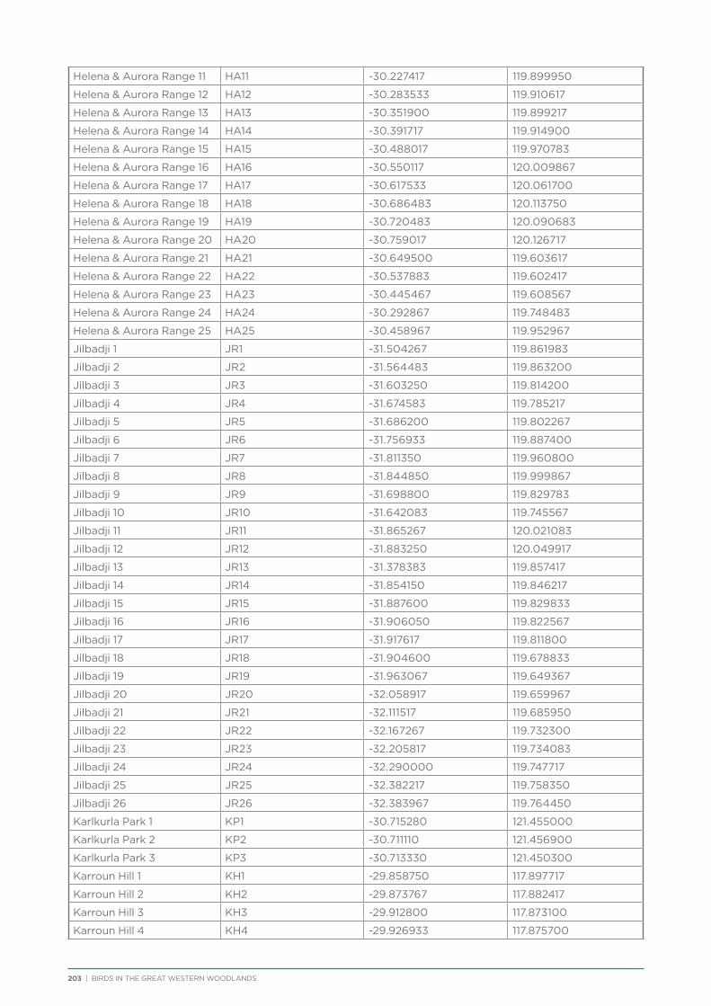
203 | BIRDS IN THE GREAT WESTERN WOODLANDS
Helena & Aurora Range 11 HA11 -30.227417 119.899950
Helena & Aurora Range 12 HA12 -30.283533 119.910617
Helena & Aurora Range 13 HA13 -30.351900 119.899217
Helena & Aurora Range 14 HA14 -30.391717 119.914900
Helena & Aurora Range 15 HA15 -30.488017 119.970783
Helena & Aurora Range 16 HA16 -30.550117 120.009867
Helena & Aurora Range 17 HA17 -30.617533 120.061700
Helena & Aurora Range 18 HA18 -30.686483 120.113750
Helena & Aurora Range 19 HA19 -30.720483 120.090683
Helena & Aurora Range 20 HA20 -30.759017 120.126717
Helena & Aurora Range 21 HA21 -30.649500 119.603617
Helena & Aurora Range 22 HA22 -30.537883 119.602417
Helena & Aurora Range 23 HA23 -30.445467 119.608567
Helena & Aurora Range 24 HA24 -30.292867 119.748483
Helena & Aurora Range 25 HA25 -30.458967 119.952967
Jilbadji 1 JR1 -31.504267 119.861983
Jilbadji 2 JR2 -31.564483 119.863200
Jilbadji 3 JR3 -31.603250 119.814200
Jilbadji 4 JR4 -31.674583 119.785217
Jilbadji 5 JR5 -31.686200 119.802267
Jilbadji 6 JR6 -31.756933 119.887400
Jilbadji 7 JR7 -31.811350 119.960800
Jilbadji 8 JR8 -31.844850 119.999867
Jilbadji 9 JR9 -31.698800 119.829783
Jilbadji 10 JR10 -31.642083 119.745567
Jilbadji 11 JR11 -31.865267 120.021083
Jilbadji 12 JR12 -31.883250 120.049917
Jilbadji 13 JR13 -31.378383 119.857417
Jilbadji 14 JR14 -31.854150 119.846217
Jilbadji 15 JR15 -31.887600 119.829833
Jilbadji 16 JR16 -31.906050 119.822567
Jilbadji 17 JR17 -31.917617 119.811800
Jilbadji 18 JR18 -31.904600 119.678833
Jilbadji 19 JR19 -31.963067 119.649367
Jilbadji 20 JR20 -32.058917 119.659967
Jilbadji 21 JR21 -32.111517 119.685950
Jilbadji 22 JR22 -32.167267 119.732300
Jilbadji 23 JR23 -32.205817 119.734083
Jilbadji 24 JR24 -32.290000 119.747717
Jilbadji 25 JR25 -32.382217 119.758350
Jilbadji 26 JR26 -32.383967 119.764450
Karlkurla Park 1 KP1 -30.715280 121.455000
Karlkurla Park 2 KP2 -30.711110 121.456900
Karlkurla Park 3 KP3 -30.713330 121.450300
Karroun Hill 1 KH1 -29.858750 117.897717
Karroun Hill 2 KH2 -29.873767 117.882417
Karroun Hill 3 KH3 -29.912800 117.873100
Karroun Hill 4 KH4 -29.926933 117.875700
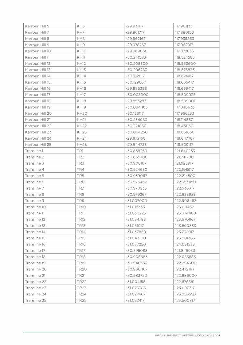
BIRDS IN THE GREAT WESTERN WOODLANDS | 204
Karroun Hill 5 KH5 -29.931117 117.901133
Karroun Hill 7 KH7 -29.961717 117.880150
Karroun Hill 8 KH8 -29.962167 117.935833
Karroun Hill 9 KH9 -29.978767 117.962017
Karroun Hill 10 KH10 -29.969050 117.872833
Karroun Hill 11 KH11 -30.214583 118.524583
Karroun Hill 12 KH12 -30.208300 118.563600
Karroun Hill 13 KH13 -30.206783 118.576833
Karroun Hill 14 KH14 -30.182617 118.624167
Karroun Hill 15 KH15 -30.129667 118.665417
Karroun Hill 16 KH16 -29.986383 118.659417
Karroun Hill 17 KH17 -30.003000 118.509033
Karroun Hill 18 KH18 -29.853283 118.509000
Karroun Hill 19 KH19 -30.084483 117.846633
Karroun Hill 20 KH20 -30.156117 117.956233
Karroun Hill 21 KH21 -30.234983 118.114867
Karroun Hill 22 KH22 -30.271050 118.431150
Karroun Hill 23 KH23 -30.064250 118.661650
Karroun Hill 24 KH24 -29.872150 118.647767
Karroun Hill 25 KH25 -29.944733 118.509117
Transline 1 TR1 -30.838250 121.640233
Transline 2 TR2 -30.869700 121.741700
Transline 3 TR3 -30.908167 121.923917
Transline 4 TR4 -30.924650 122.108917
Transline 5 TR5 -30.939067 122.214500
Transline 6 TR6 -30.973467 122.353450
Transline 7 TR7 -30.970233 122.536317
Transline 8 TR8 -30.979267 122.638933
Transline 9 TR9 -31.007000 122.906483
Transline 10 TR10 -31.018333 123.011467
Transline 11 TR11 -31.030225 123.374408
Transline 12 TR12 -31.034783 123.570867
Transline 13 TR13 -31.051917 123.590833
Transline 14 TR14 -31.037850 123.732017
Transline 15 TR15 -31.043100 123.901383
Transline 16 TR16 -31.037250 124.031533
Transline 17 TR17 -30.895083 121.845033
Transline 18 TR18 -30.906683 122.055883
Transline 19 TR19 -30.946333 122.254300
Transline 20 TR20 -30.960467 122.472167
Transline 21 TR21 -30.983750 122.686000
Transline 22 TR22 -31.004158 122.876581
Transline 23 TR23 -31.025383 123.097717
Transline 24 TR24 -31.027467 123.256550
Transline 25 TR25 -31.032417 123.500817
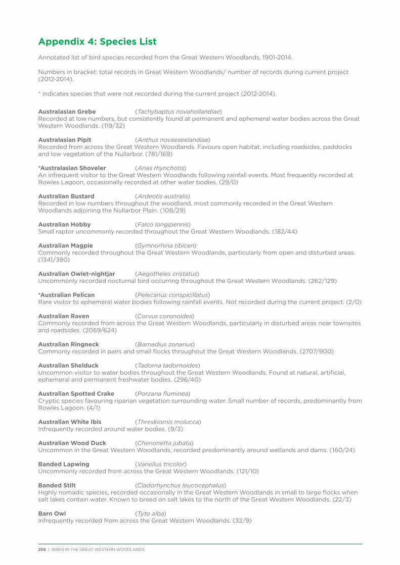
205 | BIRDS IN THE GREAT WESTERN WOODLANDS
Appendix 4: Species List
Annotated list of bird species recorded from the Great Western Woodlands, 1901-2014.
Numbers in bracket: total records in Great Western Woodlands/ number of records during current project (2012-2014).
* indicates species that were not recorded during the current project (2012-2014).
Australasian Grebe (Tachybaptus novahollandiae)Recorded at low numbers, but consistently found at permanent and ephemeral water bodies across the Great Western Woodlands. (119/32)
Australasian Pipit (Anthus novaeseelandiae)Recorded from across the Great Western Woodlands. Favours open habitat, including roadsides, paddocks and low vegetation of the Nullarbor. (781/169)
*Australasian Shoveler (Anas rhynchotis)An infrequent visitor to the Great Western Woodlands following rainfall events. Most frequently recorded at Rowles Lagoon, occasionally recorded at other water bodies. (29/0)
Australian Bustard (Ardeotis australis)Recorded in low numbers throughout the woodland, most commonly recorded in the Great Western Woodlands adjoining the Nullarbor Plain. (108/29)
Australian Hobby (Falco longipennis)Small raptor uncommonly recorded throughout the Great Western Woodlands. (182/44)
Australian Magpie (Gymnorhina tibicen)Commonly recorded throughout the Great Western Woodlands, particularly from open and disturbed areas. (1341/380)
Australian Owlet-nightjar (Aegotheles cristatus)Uncommonly recorded nocturnal bird occurring throughout the Great Western Woodlands. (262/129)
*Australian Pelican (Pelecanus conspicillatus)Rare visitor to ephemeral water bodies following rainfall events. Not recorded during the current project. (2/0)
Australian Raven (Corvus coronoides)Commonly recorded from across the Great Western Woodlands, particularly in disturbed areas near townsites and roadsides. (2069/624)
Australian Ringneck (Barnadius zonarius)Commonly recorded in pairs and small flocks throughout the Great Western Woodlands. (2707/900)
Australian Shelduck (Tadorna tadornoides)Uncommon visitor to water bodies throughout the Great Western Woodlands. Found at natural, artificial, ephemeral and permanent freshwater bodies. (296/40)
Australian Spotted Crake (Porzana fluminea)Cryptic species favouring riparian vegetation surrounding water. Small number of records, predominantly from Rowles Lagoon. (4/1)
Australian White Ibis (Threskiornis molucca)Infrequently recorded around water bodies. (9/3)
Australian Wood Duck (Chenonetta jubata)Uncommon in the Great Western Woodlands, recorded predominantly around wetlands and dams. (160/24)
Banded Lapwing (Vanellus tricolor)Uncommonly recorded from across the Great Western Woodlands. (121/10)
Banded Stilt (Cladorhynchus leucocephalus) Highly nomadic species, recorded occasionally in the Great Western Woodlands in small to large flocks when salt lakes contain water. Known to breed on salt lakes to the north of the Great Western Woodlands. (22/3)
Barn Owl (Tyto alba)Infrequently recorded from across the Great Western Woodlands. (32/9)

BIRDS IN THE GREAT WESTERN WOODLANDS | 206
*Baudin’s Black-Cockatoo (Calyptorhynchus baudinii)Small number of records from the first Bird Atlas (1978-1981) from the far south-west of the Great Western Woodlands. (8/0)
*Black Falcon (Falco subniger)Rare vagrant. Two records from the first Bird Atlas project from west and north-east of Coolgardie. (2/0)
Black Honeyeater (Certhionyx niger)A rare spring visitor to the Great Western Woodlands, often in small flocks. Records predominantly from west of Kalgoorlie. (68/42)
Black Kite (Milvus migrans)Rare visitor to the Great Western Woodlands. All records made during the current project. (4/4)
Black Swan (Cygnus atratus)Occasional visitor to natural and artificial water bodies in the Great Western Woodlands. (116/15)
Black-breasted Buzzard (Hamirostra melanosternon)Rarely recorded spring visitor to the Great Western Woodlands. (16/1)
Black-eared Cuckoo (Chrysococcyx osculans) Uncommonly recorded winter and spring migrant to the Great Western Woodlands. (201/44)
Black-faced Cuckoo-Shrike (Coracina novaehollandiae) Widespread and commonly recorded resident of the Great Western Woodlands. (1576/403)
Black-faced Woodswallow (Artamus cinereus)Widespread across the Great Western Woodlands. Recorded as individuals and in small flocks. (485/67)
Black-fronted Dotterel (Elseyornis melanops)Recorded from the edges of natural and artificial water bodies. (91/21)
Black-shouldered Kite (Elanus notatus)Uncommon small raptor in the Great Western Woodlands, most often recorded around human settlement or cleared land. (96/17)
Black-tailed Native-hen (Gallinula ventralis)Recorded from across the Great Western Woodlands at natural and artificial wetlands. Can be irruptive after rainfall. Commonly recorded in small flocks of 10-20 birds. (52/31)
Black-winged Stilt (Himantopus himantopus) Occasional visitor to the Great Western Woodlands, recorded from natural and artificial wetlands. (70/5)
Blue Bonnet (Northiella haematogaster)The Naretha subspecies of the Blue Bonnet typically occurs in the Nullarbor desert in Western Australia. There are three records from within the Great Western Woodlands; from the eastern spur around Caiguna and Cocklebiddy and along the Trans Railway Line, east of Kalgoorlie. (3/2)
Blue-billed Duck (Oxyura australis)Rare vagrant to freshwater lakes in the Great Western Woodlands. (5/1)
Blue-breasted Fairy-wren (Malurus pulcherrimus)Resident in the Great Western Woodlands, found in small family groups. Recorded across most of the Great Western Woodlands except the north-east and eastern spur. (318/109)
*Bourke’s Parrot (Neopsephotus bourkii)Bourke’s Parrot distribution is predominantly to the north of the Great Western Woodlands in Western Australia, in the Murchison region. The single record of the species is from Pigeon Rock near the north-west boundary of the Great Western Woodlands. (1/0)
Brown Falcon (Falco berigora)A common small raptor, recorded from across the Great Western Woodlands. (669/234)
Brown Goshawk (Accipter fasciatus)Widespread woodland raptor, recorded from across the Great Western Woodlands. (184/57)
Brown Honeyeater (Lichmera indistincta)Widespread and commonly recorded honeyeater. Uncommon in the north-east and eastern spur of the Great Western Woodlands. (1899/668)

207 | BIRDS IN THE GREAT WESTERN WOODLANDS
*Brown Quail (Coturnix ypsilophora)Single record from within the Great Western Woodlands in 2011, from south-east of Kambalda. (1/0)
Brown Songlark (Cincloramphus cruralis)Uncommonly recorded species occurring across the Great Western Woodlands, with the majority of records from the eastern spur. Most commonly detected in spring when the birds are singing. (155/24)
Brown-headed Honeyeater (Melithreptus brevirostris)Common, gregarious honeyeater, recorded from across the Great Western Woodlands. Uncommon in the north-east and eastern spur. Commonly recorded in small flocks of up to 50 birds. (812/261)
Brush Bronzewing (Phaps elegans)Rarely recorded in the Great Western Woodlands. Most records from the southern edge, but also occasionally from as far inland as Cave Hill. Typically recorded around granite outcrops. (40/20)
Budgerigar (Melopsittacus undulatus)Rare, irruptive, arid-zone nomad. Most commonly recorded from the northern half and eastern spur of the Great Western Woodlands. (85/12)
*Bush Stone-curlew (Burhinus maginrostris)Typical distribution of the Bush Stone-curlew is to the west of the Great Western Woodlands. There are a small number of records from the first Bird Atlas from the western edge of the Great Western Woodlands. (3/0)
Carnaby’s Black-Cockatoo (Caliptorhynchus carnabyi)Small number of records from the Forrestania area in the south-west Great Western Woodlands. Predominantly recorded in spring. (16/5)
*Cattle Egret (Ardea ibis)Rare vagrant to the Great Western Woodlands, recorded from across the region. (4/0)
Chestnut Quail-thrush (Cinclosoma castonotum)The Great Western Woodlands represents the core habitat for the Chestnut Quail-thrush. This woodland resident is found in low numbers from across the Great Western Woodlands, although absent from the far east of the region. (347/117)
*Chestnut Teal (Anas castanea) Rare visitor to wetlands in the Great Western Woodlands, particularly Lake Cronin and rivers in the far south-west corner. Not recorded during the current project. (8/0)
Chestnut-breasted Quail-thrush (Cinclosoma castaneothorax)The distribution of this species is predominantly the Murchison and Pilbara regions in Western Australia. They have been occasionally recorded close to the northern boundary of the Great Western Woodlands. (8/2)
Chestnut-rumped Thornbill (Acanthiza uropygialis)Small insectivorous passerine common across the northern half of the Great Western Woodlands. (1232/370)
*Chiming Wedgebill (Psophodes occidentalis) The typical distribution of the Chiming Wedgebill is to the north of the Great Western Woodlands. The three records of this species are all from the north-west corner of the Great Western Woodlands. The species was not recorded during the current project. (3/0)
*Cinnamon Quail-thrush (Cinclosoma cinnamomeum)The Cinnamon Quail-thrush only occurs on the Nullarbor Plain in Western Australia. There are only two records from within the Great Western Woodlands, from near the border with the Nullarbor Plain. (2/0)
Cockatiel (Nymphicus hollandicus)Arid-zone parrot, occasionally recorded in the northern Great Western Woodlands and adjacent to the Nullarbor Plain. (52/3)
Collared Sparrowhawk (Accipiter cirrhocephalus)Small raptor of the woodland country. Recorded occasionally from across the Great Western Woodlands. (95/19)
Common Bronzewing (Phaps chalcoptera) Common native pigeon recorded from across the Great Western Woodlands. Often recorded in pairs or small flocks around granite outcrops and natural and artificial water sources. (784/261)
Common Greenshank (Tringa nebularia)Transcontinental migrant and occasional spring and summer visitor to permanent and ephemeral wetlands in the Great Western Woodlands. (19/4)
BIRDS IN THE GREAT WESTERN WOODLANDS | 208
Common Sandpiper (Actitis hypoleucus)Transcontinental migrant and occasional spring and summer visitor to permanent and ephemeral wetlands in the Great Western Woodlands. (16/5)
*Common Starling (Sturnus vulgaris)Highly invasive European species occasionally recorded in southern Western Australia, having arrived from established populations in eastern Australia. Sighted individuals actively trapped and removed. There are only two records from within the Great Western Woodlands, from near Norseman and Cocklebiddy in 1980 and 1999 respectively. Not recorded during the current Great Western Woodlands project. (2/0)
Crested Bellbird (Oreoica gutturalis)Commonly recorded from across the Great Western Woodlands, particularly the north-west corner. (1777/671)
Crested Pigeon (Ocyphaps lophotes)Commonly recorded from across the Great Western Woodlands, particularly in areas of disturbance and human settlement and around natural or artificial water sources. (682/195)
Crested Shrike-tit (Falcunculus frontatus)Rarely recorded insectivore of the woodland and mallee. Conspicuous when calling, but difficult to locate otherwise. Existing records are scattered across the Great Western Woodlands. (19/2)
Crimson Chat (Epthianura tricolor)Highly mobile, nomadic bird of the arid zone. Most often recorded in the northern part of the Great Western Woodlands, likely following favourable conditions. (93/14)
*Curlew Sandpiper (Calidris ferruginea)Transcontinental migrant and rare visitor to permanent and ephemeral wetlands in the Great Western Woodlands. (4/0)
Darter (Anhinga melanogaster)Rare visitor to wetlands in the Great Western Woodlands. (3/1)
Diamond Dove (Geopelia cuneata)Small arid zone dove, rarely recorded in the Great Western Woodlands. Most existing records from the north-west edge of the Great Western Woodlands. (4/2)
Dusky Woodswallow (Artamus cyanopterus)Commonly recorded aerial insectivore, often conspicuous on exposed perches or when hawking flying insects. Often recorded in small flocks of up to 20 birds. Recorded all across the Great Western Woodlands. (693/270)
Elegant Parrot (Neophema elegans)Rarely recorded ground-foraging parrot. Records restricted to the western edge of the Great Western Woodlands. (51/14)
Emu (Dromaius novaehollandiae)Commonly recorded from all over the Great Western Woodlands. (760/132)
Eurasian Coot (Fulica atra)Recorded at natural and artificial water bodies across the Great Western Woodlands. Commonly recorded from Lake Cronin and Rowles Lagoon when they contain water. (148/17)
Fairy Martin (Hirundo ariel)Rarely recorded species in the Great Western Woodlands. Recorded in all months, although most commonly in spring. Often recorded in association with rocky outcrops, railway tunnels and water sources. (52/6)
Fan-tailed Cuckoo (Cacomantis flabelliformis)Uncommonly recorded migrant to the south-west of the Great Western Woodlands. Recorded mostly in winter and spring but also sometimes autumn, potentially after unseasonal rainfall and in response to the breeding of its brood parasite hosts. (169/62)
Fork-tailed Swift (Apus pacificus)Rare aerial migrant to the north-west of the Great Western Woodlands. All records are from early autumn. Often flies very high and therefore may be overlooked during surveys. (6/2)
Freckled Duck (Stictonetta naevosa)Rare nomadic duck, often recorded at Rowles Lagoon when it contains water. Recorded breeding at Rowles Lagoon. A single record also from Lake Cronin of 50 individuals in 1972. (15/1)

209 | BIRDS IN THE GREAT WESTERN WOODLANDS
Galah (Cacatua roseicapilla)Abundant and conspicuous large parrot, often recorded in pairs and flocks of up to 80 individuals. Commonly recorded around human disturbance and artificial water sources, particularly on the western edge of the Great Western Woodlands, adjacent to agricultural land, and on pastoral land in the north and east of the Great Western Woodlands. (1067/275)
Gilbert’s Whistler (Pachycephala inornata)Gilbert’s Whistler predominantly only occurs within the Great Western Woodlands in Western Australia and is considered largely extinct in the adjacent wheatbelt. The species is uncommonly recorded from across the Great Western Woodlands, except for the eastern edge. (340/157).
*Glossy Ibis (Plegadis falcinellus)Extremely rare vagrant to the Great Western Woodlands. Recorded from Cocklebiddy, Kalgoorlie and Rowles Lagoon. (3/0)
Golden Whistler (Pachycephala pectoralis)Uncommonly recorded species in the Great Western Woodlands. Most common in the south-west and rare in the north-east. (385/175)
Great Cormorant (Phalacrocorax carbo)Rare visitor to wetlands in the Great Western Woodlands. Recorded from Silver Lake near Kambalda during the current project. (5/1)
*Great Crested Grebe (Podiceps cristatus) Extremely rare visitor to the Great Western Woodlands. Single records from Rowles Lagoon and Lake Cronin in 1980 and 2001 respectively. (2/0)
*Great Egret (Ardea alba)Extremely rare visitor to the Great Western Woodlands. Single records from three waterbodies spread across the region. (3/0)
Grey Butcherbird (Cracticus torquatus)Commonly recorded from woodland throughout the Great Western Woodlands. (1948/573)
Grey Currawong (Strepera versicolor)Commonly recorded throughout the Great Western Woodlands. (1647/631)
*Grey Falcon (Falco hypoleucos)Widely-distributed, nomadic raptor. Single record from the Great Western Woodlands in 1979, north of Norseman. (1/0)
Grey Fantail (Rhipidura albiscapa)Uncommonly recorded in all months in the western half of the Great Western Woodlands. Both preissi and albicauda subspecies recorded. (331/101)
Grey Shrike-thrush (Colluricincla harmonica)Abundant resident, recorded from across the Great Western Woodlands. (2269/942)
Grey Teal (Anas gracilis) Recorded, occasionally in flocks of up to 500, at natural and artificial wetlands across the Great Western Woodlands. (300/52)
Grey-fronted Honeyeater (Lichenostomus plumulus)Uncommonly recorded arid zone honeyeater. Records predominantly from the north of the Great Western Woodlands. Species easily confused with the Yellow-plumed Honeyeater. (105/26)
Ground Cuckoo-Shrike (Coracina maxima) Rarely recorded nomadic species. Predominantly recorded in the northern half of the Great Western Woodlands and in the eastern spur around Cocklebiddy. (81/10)
Hardhead (Aythya australis)Rare visitor to natural and artificial wetlands in the western half of the Great Western Woodlands. (45/6)
Hoary-headed Grebe (Poliocephalus poliocephalus)Recorded at natural and artificial water bodies across the Great Western Woodlands. (172/48)
Hooded Plover (Charadruis rubricollis)Scattered records from salt lakes across the Great Western Woodlands. Recorded breeding from a number of locations including Lake Deborah, Harris Lake and salt lakes adjacent to Newman’s Rock and Emu Rock. (97/2)

BIRDS IN THE GREAT WESTERN WOODLANDS | 210
Hooded Robin (Melanodryas cucullata)Uncommonly recorded from across the Great Western Woodlands, although more common in the western half. Often recorded in association with rocky outcrops. (168/36).
Horsfield’s Bronze-Cuckoo (Chrysococcyx basalis)Winter and spring migrant to the Great Western Woodlands, following the breeding of brood hosts, mostly fairy-wrens and thornbills. (379/77)
Inland Dotterel (Charadrius australis)Rarely recorded nomadic species. Most records from the very western and southern edge of the Great Western Woodlands. (17/1)
Inland Thornbill (Acanthiza apicalis)Abundant small sedentary insectivore, recorded from across the Great Western Woodlands. (1841/756)
Jacky Winter (Microeca fascinans)Commonly recorded foraging in open woodland throughout the Great Western Woodlands, although less common in the south. (710/235)
*Laughing Kookaburra (Dacelo novaeguineae)Introduced species from the eastern states. Two records from 1980 from the western edge of the Great Western Woodlands. (2/0)
Laughing Dove (Streptopelia senegalensis)Introduced dove, recorded almost exclusively from towns in the Great Western Woodlands. (105/17)
Little Black Cormorant (Phalacrocorax sulcirostris)Rare visitor to wetlands in the Great Western Woodlands. Regularly recorded at the Coolgardie Gorge. (25/12)
Little Button-quail (Turnix velox)Rarely recorded button-quail, predominantly from the northern edge of the Great Western Woodlands and the eastern spur. (43/15)
Little Corella (Cacatua sanguinea)Rarely recorded in the Great Western Woodlands. Most records on the western edge of the region, adjacent to agricultural land, or in Kalgoorlie. (21/10)
Little Crow (Corvus bennetti)Corvid recorded from throughout the Great Western Woodlands. (433/57)
Little Eagle (Hieraaetus morphnoides)Large, widespread raptor, recorded across the Great Western Woodlands. (173/18)
*Little Grassbird (Megalurus gramineus)Extremely rare, a single record in 2000 from the Lake King – Norseman Road, in the south-west Great Western Woodlands. (1/0)
Little Pied Cormorant (Microcarbo melanoleucos)Scattered records from water bodies in the Great Western Woodlands. (39/10)
Little Woodswallow (Artamus minor)The Little Woodswallow is at the southern extent of its range in the northern Great Western Woodlands. Regularly recorded from Banded Ironstone Formations and other rocky outcrops in the north-west Great Western Woodlands. Known to breed at Helena & Aurora Range. (61/6)
Magpie-Lark (Grallina cyanoleuca)Recorded commonly from across the Great Western Woodlands, predominantly in association with towns, disturbed areas, and the open habitats of the north-east and eastern spur. (862/146)
Major Mitchell’s Cockatoo (Lophochroa leadbeateri)Two disjunct populations in the Great Western Woodlands – in the north-west and in the eastern spur near Cocklebiddy. Flocks of up to 45 birds recorded. Breeding also recorded in the Great Western Woodlands. (133/38)
Malleefowl (Leipoa ocellata)Individuals and nest mounds recorded from all across the Great Western Woodlands. During the current project, sightings particularly common around Karroun Hill Nature Reserve, also Cave Hill and Peak Charles National Park. One dead individual recorded on the Hyden-Norseman road after collision with a mining truck. (204/38)
211 | BIRDS IN THE GREAT WESTERN WOODLANDS
Masked Lapwing (Vanellus miles)Small number of records from the south-west Great Western Woodlands. (3/1).
Masked Woodswallow (Artamus personatus)Recorded uncommonly from across the Great Western Woodlands. Sometimes recorded in large flocks of hundreds of birds, flying high and hawking for aerial insects. (119/62)
Mistletoebird (Dicaeum hirundinaceum)Nomadic mistletoe specialist. Recorded uncommonly from across the Great Western Woodlands. (161/72)
Mulga Parrot (Psephotus varius)Recorded from across the Great Western Woodlands, less common in the south-west. (281/63)
Musk Duck (Biziura lobata)Recorded from waterbodies in the Great Western Woodlands, including Rowles Lagoon, Lake Cronin, Coolgardie Gorge, Hogan’s Lake and Swan Lake. (81/16)
Nankeen Kestrel (Falco cenchroides)Common small raptor. Recorded throughout the Great Western Woodlands. (687/135)
*Nankeen Night Heron (Nycticorax caledonicus)Small number of records from the Great Western Woodlands, including Lake Cronin in 2000 and 2001. (4/0)
New Holland Honeyeater (Phylidonyris novaehollandiae)Recorded from the southern half of the Great Western Woodlands. (124/50)
Orange Chat (Epthianura aurifrons)Small number of records from low, open vegetation in the north of the Great Western Woodlands and around Cocklebiddy. (10/1)
Oriental Plover (Charadrius veredus)Transcontinental migrant. Recorded at Credo Station in 2012 and 2013. No previous records from within the Great Western Woodlands. (4/4)
Pacific Black Duck (Anas superciliosa)Recorded at natural and artificial water bodies across the Great Western Woodlands. (173/25)
Painted Button-quail (Turnix varius)Small number of records from the western half of the Great Western Woodlands. (7/3)
Pallid Cuckoo (Cacomantis pallidus)Uncommon (291/23). Spring visitor to the Great Western Woodlands. Brood parasite, arrival timed to match breeding of host species. Records from throughout Great Western Woodlands.
Peregrine Falcon (Falco peregrinus)Widely-dispersed small raptor. Commonly associated with banded ironstone formations, breakaways and granite outcrops. (94/14)
Pied Butcherbird (Cracticus nigrogularis)Commonly recorded throughout the Great Western Woodlands, although more common in the northern half. (1146/317)
*Pied Cormorant (Phalacrocorax varius)Rare visitor to the Great Western Woodlands. One record in 1978 from the far south-west corner of the Great Western Woodlands and one record in 2008 from near Cocklebiddy. (2/0)
Pied Honeyeater (Certhionyx variegatus)Nomadic arid zone honeyeater. Scattered records from across the western half of the Great Western Woodlands. Predominantly recorded in spring. (63/24)
Pink-eared Duck (Malacorhynchus membra)Recorded at natural and artificial water bodies across the Great Western Woodlands, including Lake Cronin, Rowles Lagoon, and lakes around Coolgardie and Kalgoorlie. (58/10)
Purple-crowned Lorikeet (Glossopsitta porphyrocephala)Wide-ranging resource nomad common throughout woodland and mallee in the Great Western Woodlands, although can be scarce to abundant in any particular area or time. Often recorded in small to large flocks. Recorded breeding in the Great Western Woodlands. (1343/349)
BIRDS IN THE GREAT WESTERN WOODLANDS | 212
Purple-gaped Honeyeater (Lichenostomus cratitius)Recorded from mallee and shrubland in the south-western half of the Great Western Woodlands. (250/130)
Rainbow Bee-eater (Merops ornatus)Common summer migrant recorded from across the Great Western Woodlands. (576/208)
Red Wattlebird (Anthochaera carunculata)Abundant large honeyeater recorded from across the Great Western Woodlands. (3640/1431)
Red-backed Kingfisher (Todiramphus pyrrhopygia)Uncommonly recorded from across the Great Western Woodlands except for the southern edge. Predominantly recorded in spring and summer. (157/28)
Red-capped Parrot (Purpureicephalus spurius)Single record of this south-west Western Australian endemic from the Lake King – Norseman Road in October 2013. (1/1)
Red-capped Plover (Charadrius ruficapillus)Recorded from natural and artificial waterbodies across the Great Western Woodlands when they contain water. Breeding records from Lake Dundas. (58/10)
Red-capped Robin (Petroica goodenovii)Common small insectivore recorded from woodland habitat across the Great Western Woodlands. (1089/329)
Red-kneed Dotterel (Erythrogonys cinctus)Small number of records from fresh and saltwater lakes across the Great Western Woodlands. (23/8)
Red-necked Avocet (Recurvirostra novaeholla)Recorded from fresh and saltwater lakes across the Great Western Woodlands, with most records from Rowles Lagoon and salt lakes around Kalgoorlie. (37/3)
Red-necked Stint (Calidris ruficollis)Transcontinental migrant. Small number of records scattered across the Great Western Woodlands from spring and autumn. (5/1)
Red-tailed Black-Cockatoo (Calyptorhynchus banksia)Recorded in small to medium flocks of up to 70 birds in the north-west corner of the Great Western Woodlands. (131/46)
Redthroat (Pyrrholaemus brunneus)Common small insectivore, recorded throughout the Great Western Woodlands. (997/377)
Regent Parrot (Polytelis anthopeplus)Uncommonly recorded large parrot, seen in pairs and small flocks. Predominantly recorded in the western half of the Great Western Woodlands. (266/55)
Restless Flycatcher (Myiagra inquieta)Rarely recorded in the Great Western Woodlands, predominantly recorded at Lake Cronin and in the central and southern regions. (79/18)
Rock Dove (Columba livia)Introduced cosmopolitan species, associated with towns and human settlements. Recorded almost exclusively around townsites in the Great Western Woodlands. (80/2)
Rufous Fieldwren (Calamanthus campestris)Small number of scattered records across the south-west half of the Great Western Woodlands. (54/15)
Rufous Songlark (Cincloramphus mathewsi) Uncommonly recorded from across the Great Western Woodlands. (115/40)
Rufous Treecreeper (Climacteris rufa)Commonly recorded in pairs or small family groups from woodland habitat across the Great Western Woodlands. Absent from the eastern spur. Abundant and conspicuous in suitable habitat. (1032/495)
Rufous Whistler (Pachycephala rufiventris)Commonly recorded in the north-west of the Great Western Woodlands. Uncommon in the eastern half and not recorded in the eastern spur. (844/321)
213 | BIRDS IN THE GREAT WESTERN WOODLANDS
Sacred Kingfisher (Todiramphus sanctus)Rarely recorded species, predominantly in the southern half of the Great Western Woodlands. Mostly recorded in spring. (86/20)
Scarlet-chested Parrot (Neophema splendida)Central desert species, irruptive and nomadic. Scattered records, predominantly made in spring, from across northern and central Great Western Woodlands. Majority of records of this species were from 2012 and 2013, during the current project. Both adult and immature birds recorded. (19/12)
Sharp-tailed Sandpiper (Calidris acuminate)Occasionally recorded from lakes across the Great Western Woodlands. (21/1)
Shining Bronze-Cuckoo (Chrysococcyx lucidus)Late winter and spring migrant to the south-west Great Western Woodlands. Brood parasite of small sedentary insectivores. (45/18)
Shy Heathwren (Hylacola cauta)Small sedentary insectivore, recorded at low reporting rates from much of the Great Western Woodlands except the north-east and eastern spur. (202/95)
*Silver Gull (Larus novaehollandiae)Small number of records scattered across lakes in the Great Western Woodlands. Not recorded during the current project. (6/0).
Silvereye (Zosterops lateralis)Recorded uncommonly across the southern Great Western Woodlands. (286/64)
Singing Honeyeater (Lichenostomus virescens)Abundant honeyeater, recorded most commonly in the north. (1758/636)
Slaty-backed Thornbill (Acanthiza robustirostris)Rare (34/15). Arid-zone insectivore typically distributed to the north of the Great Western Woodlands. Occasionally recorded in the north-west within the Great Western Woodlands. Can be confused with other thornbill species.
*Slender-billed Thornbill (Acanthiza iredalei)Small number of records of this arid zone insectivore scattered across suitable saltbush and samphire habitat in the Great Western Woodlands. (7/0)
Southern Boobook (Ninox novaeseelandiae)Recorded throughout the Great Western Woodlands. Likely under-reported due to its nocturnal habit. (315/92)
Southern Emu-wren (Stipiturus malachurus)Small insectivore of the heathland in southern Western Australia. At least one disjunct population occurs in the Great Western Woodlands, east of Hyden. (2/1)
Southern Scrub-robin (Drymodes brunneopygia)Uncommon (265/112). Ground-foraging insectivore, most commonly recorded in the south-west Great Western Woodlands. Absent from the north-east and eastern spur.
Southern Whiteface (Aphelocephala leucopsis)Small arid-zone insectivore, most commonly recorded in the north-west Great Western Woodlands. (197/34)
Spiny-cheeked Honeyeater (Acanthagenys rufogularis)Abundant honeyeater recorded from across the Great Western Woodlands, predominantly in the north-west. (2491/1093)
Splendid Fairy-wren (Malurus splendens)Sedentary, group-living insectivore, typically recorded in groups of up to eight birds. Recorded in the north-west and south-west of the Great Western Woodlands. Absent from the eastern and central west regions. (335/126)
*Spotless Crake (Porzana tabuensis)Single record from the Oldfield River in 2001 in the far south-west of the Great Western Woodlands. (1/0)
Spotted Harrier (Circus assimilis)Medium-sized raptor, favours foraging over low vegetation. Scattered records from throughout the Great Western Woodlands. (57/12)

BIRDS IN THE GREAT WESTERN WOODLANDS | 214
Spotted Nightjar (Eurostopodus argus)Often inconspicuous nocturnal hunter, unless flushed up from road at night. Recorded throughout the Great Western Woodlands. Likely under-reported due to its nocturnal habit. (87/23)
Spotted Pardalote (Pardalotus punctatus)Tiny but vocal canopy dweller. Favours eucalypt, both mallee and woodland. Predominantly recorded in the southern Great Western Woodlands. (252/152)
*Spotted Dove (Streptopelia chinensis)Introduced dove that favours human settlements. Single record from Kalgoorlie in 1977 from the first Bird Atlas. (1/0)
Square-tailed Kite (Lophoictinia isura)Medium-sized raptor, recorded uncommonly from across the Great Western Woodlands. Mostly recorded in late winter and spring. (112/19)
Straw-necked Ibis (Threskiornis spinicollis)Rare visitor to waterbodies of the Great Western Woodlands. Predominantly recorded from Lake Cronin, Rowles Lagoon, Coolgardie Gorge and around Cocklebiddy. (33/3)
Striated Pardalote (Pardalotus striatus)One of the most commonly recorded species in the Great Western Woodlands. Recorded in high numbers throughout the region. (3672/1722)
Stubble Quail (Coturnix pectoralis)Small number of records scattered across the Great Western Woodlands. (36/7)
*Swamp Harrier (Circus approximans)Single record from Credo station in 2008. (1/0)
Tawny Frogmouth (Podargus strigoides)Well-camouflaged nocturnal species, recorded from across the Great Western Woodlands. Likely under-reported due to its cryptic and nocturnal habit. (153/53)
Tawny-crowned Honeyeater (Phylidonyris melanops)Common honeyeater in the south-west corner of the Great Western Woodlands, but not recorded further to the north or east of the region. (288/145)
Torresian Crow (Corvus orru)Records from across the Great Western Woodlands, although less common in the southern half and not recorded from the eastern spur. (86/26)
Tree Martin (Hirundo nigricans)Small to medium sized flocks of up to 80 birds commonly recorded from throughout the Great Western Woodlands. Often associated with water and rocky outcrops. (861/311)
Varied Sittella (Daphoenositta chrysoptera)Small flocks of up to 12 birds uncommonly recorded from woodland and mallee habitat across the Great Western Woodlands. (241/53)
Wedge-tailed Eagle (Aquila audax)Large, widespread raptor commonly recorded from throughout the Great Western Woodlands. (746/166)
Weebill (Smicrornis brevirostris)Most commonly recorded species, occurring in all habitat types throughout the Great Western Woodlands. (4396/2149)
Welcome Swallow (Hirundo neoxena)Species occurs throughout the Great Western Woodlands, but is most common around human habitation; roosting and nesting around buildings. (651/157)
Western Bowerbird (Chlamydera guttata)Typical distribution for this species is to the north of the Great Western Woodlands. Small number of records from the north-west edge of the Great Western Woodlands. (15/2) Western Corella (Cacatua pastinator)Typical distribution for this species is to the west of the Great Western Woodlands. Small number of records from the north-west corner of the Great Western Woodlands around Karroun Hill Nature Reserve and Remlap station. (9/3)
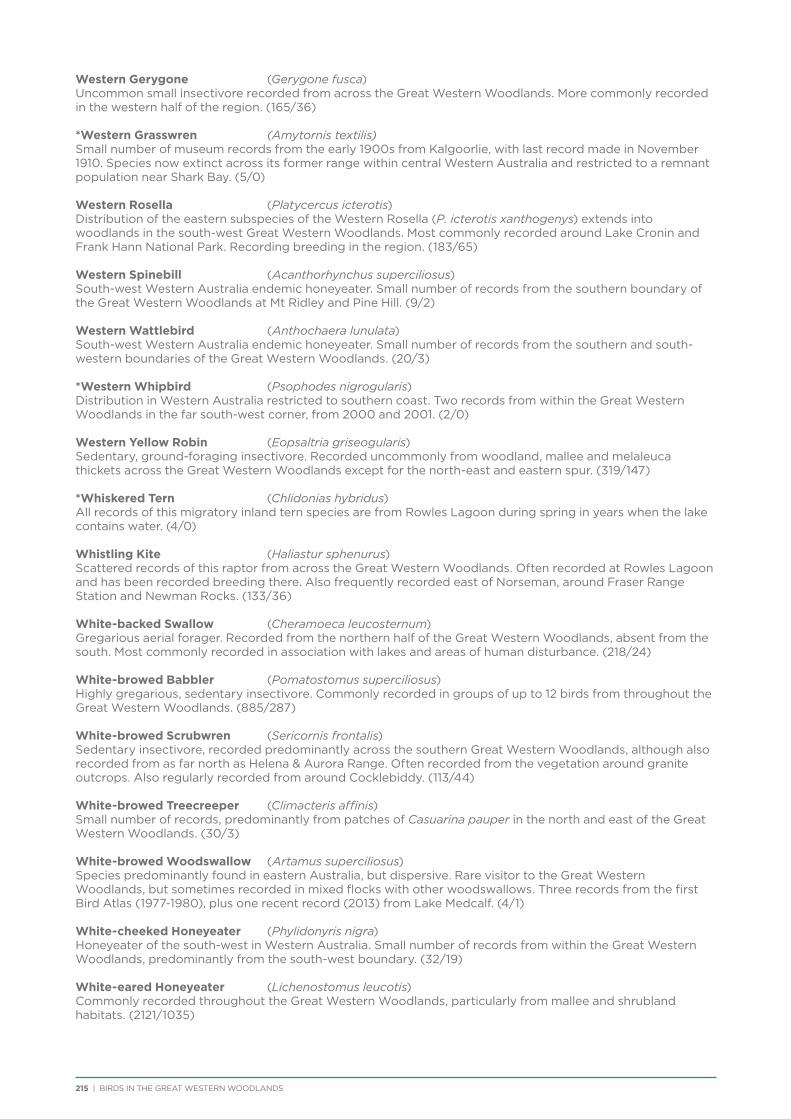
215 | BIRDS IN THE GREAT WESTERN WOODLANDS
Western Gerygone (Gerygone fusca)Uncommon small insectivore recorded from across the Great Western Woodlands. More commonly recorded in the western half of the region. (165/36)
*Western Grasswren (Amytornis textilis)Small number of museum records from the early 1900s from Kalgoorlie, with last record made in November 1910. Species now extinct across its former range within central Western Australia and restricted to a remnant population near Shark Bay. (5/0)
Western Rosella (Platycercus icterotis)Distribution of the eastern subspecies of the Western Rosella (P. icterotis xanthogenys) extends into woodlands in the south-west Great Western Woodlands. Most commonly recorded around Lake Cronin and Frank Hann National Park. Recording breeding in the region. (183/65)
Western Spinebill (Acanthorhynchus superciliosus)South-west Western Australia endemic honeyeater. Small number of records from the southern boundary of the Great Western Woodlands at Mt Ridley and Pine Hill. (9/2)
Western Wattlebird (Anthochaera lunulata)South-west Western Australia endemic honeyeater. Small number of records from the southern and south-western boundaries of the Great Western Woodlands. (20/3) *Western Whipbird (Psophodes nigrogularis)Distribution in Western Australia restricted to southern coast. Two records from within the Great Western Woodlands in the far south-west corner, from 2000 and 2001. (2/0)
Western Yellow Robin (Eopsaltria griseogularis)Sedentary, ground-foraging insectivore. Recorded uncommonly from woodland, mallee and melaleuca thickets across the Great Western Woodlands except for the north-east and eastern spur. (319/147)
*Whiskered Tern (Chlidonias hybridus)All records of this migratory inland tern species are from Rowles Lagoon during spring in years when the lake contains water. (4/0)
Whistling Kite (Haliastur sphenurus)Scattered records of this raptor from across the Great Western Woodlands. Often recorded at Rowles Lagoon and has been recorded breeding there. Also frequently recorded east of Norseman, around Fraser Range Station and Newman Rocks. (133/36)
White-backed Swallow (Cheramoeca leucosternum)Gregarious aerial forager. Recorded from the northern half of the Great Western Woodlands, absent from the south. Most commonly recorded in association with lakes and areas of human disturbance. (218/24)
White-browed Babbler (Pomatostomus superciliosus)Highly gregarious, sedentary insectivore. Commonly recorded in groups of up to 12 birds from throughout the Great Western Woodlands. (885/287)
White-browed Scrubwren (Sericornis frontalis)Sedentary insectivore, recorded predominantly across the southern Great Western Woodlands, although also recorded from as far north as Helena & Aurora Range. Often recorded from the vegetation around granite outcrops. Also regularly recorded from around Cocklebiddy. (113/44)
White-browed Treecreeper (Climacteris affinis)Small number of records, predominantly from patches of Casuarina pauper in the north and east of the Great Western Woodlands. (30/3)
White-browed Woodswallow (Artamus superciliosus)Species predominantly found in eastern Australia, but dispersive. Rare visitor to the Great Western Woodlands, but sometimes recorded in mixed flocks with other woodswallows. Three records from the first Bird Atlas (1977-1980), plus one recent record (2013) from Lake Medcalf. (4/1)
White-cheeked Honeyeater (Phylidonyris nigra)Honeyeater of the south-west in Western Australia. Small number of records from within the Great Western Woodlands, predominantly from the south-west boundary. (32/19)
White-eared Honeyeater (Lichenostomus leucotis)Commonly recorded throughout the Great Western Woodlands, particularly from mallee and shrubland habitats. (2121/1035)

BIRDS IN THE GREAT WESTERN WOODLANDS | 216
White-faced Heron (Egretta novaehollandiae)Widespread waterbird, recorded at natural and artificial waterbodies throughout the Great Western Woodlands. (129/20)
White-fronted Chat (Ephthianura albifrons)Recorded throughout the Great Western Woodlands, typically in chenopod habitat surrounding waterbodies. (217/34)
White-fronted Honeyeater (Phylidonyris albifrons)Highly nomadic, dispersive honeyeater, following available nectar across landscape. Commonly recorded from across the Great Western Woodlands, although can be scarce to abundant in any particular area or time. Showed a particularly high reporting rate during the current project (2012-2014) compared to the prior 14 years. (1919/1133)
*White-naped Honeyeater (Melithreptus lunatus)Species typical distribution is the south-west corner of Western Australia. There are two records from within the Great Western Woodlands, in the far south-west near Coijinup Creek and Pyramid Lake. (2/0)
White-necked Heron (Ardea pacifica)Widespread, dispersive waterbird. Recorded from natural and artificial waterbodies from throughout the Great Western Woodlands. (50/20)
White-plumed Honeyeater (Lichenostomus penicillatus)Common throughout the Pilbara and Murchison, with a small number of records from the northern edge of the Great Western Woodlands. (4/2)
White-winged Fairy-wren (Malurus leucopterus)Sedentary, group-living insectivore. Mostly recorded in the northern half of the Great Western Woodlands. Often recorded in chenopod or other low shrubland. (242/75)
White-winged Triller (Lalage sueurii)Spring and summer migrant to the Great Western Woodlands. Recorded throughout the region although less common in north-east. (240/93)
Willie Wagtail (Rhipidura leucophrys)Abundant, conspicuous ground-foraging insectivore. Common throughout the woodland. (1635/452)
*Wood Sandpiper (Tringa glareola)Transcontinental migrant and occasional spring and summer visitor to permanent and ephemeral wetlands in the Great Western Woodlands. (7/0)
*Yellow Bittern (Ixobrychus sinensis)Resident of Indonesia and south Asia. The single specimen recorded in the Great Western Woodlands from 1967 was the first record of the species in Australia. (1/0)
Yellow-billed Spoonbill (Platelea flavipes)Rare visitor to the Great Western Woodlands. Recorded predominantly from Rowles Lagoon and Coolgardie Gorge. (13/4)
Yellow-plumed Honeyeater (Lichenostomus ornatus)Abundant, noisy, pugnacious bird, often recorded in small flocks of up to 30 birds. One of the most commonly recorded birds, found throughout the Great Western Woodlands. (2544/998)
Yellow-rumped Thornbill (Acanthiza chrysorrhoa)Common, gregarious ground-foraging insectivore. Recorded in small flocks of up to 20 birds from across the Great Western Woodlands. (921/215)
Yellow-throated Miner (Manorina flavigula)Common throughout the Great Western Woodlands, although most abundant in the north-east of the Great Western Woodlands. Typically recorded in open habitat and around human disturbance and settlements. (1778/437)
Zebra Finch (Taeniopygia guttata)Nomadic granivore of the arid zone, predominantly recorded from open habitats and around fresh-water sources in the northern Great Western Woodlands. Typically recorded in small flocks of up to 30 birds. (145/60)
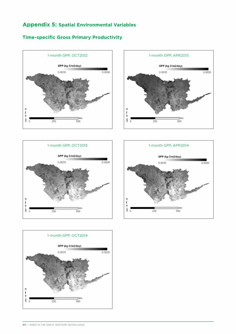
217 | BIRDS IN THE GREAT WESTERN WOODLANDS
Appendix 5: Spatial Environmental Variables
Time-specific Gross Primary Productivity
1-month GPP, OCT2012
1-month GPP, OCT2013
1-month GPP, OCT2014
1-month GPP, APR2013
1-month GPP, APR2014

BIRDS IN THE GREAT WESTERN WOODLANDS | 218
Time-specific Gross Primary Productivity
3-month GPP, OCT2012
3-month GPP, OCT2013
3-month GPP, OCT2014
3-month GPP, APR2013
3-month GPP, APR2014
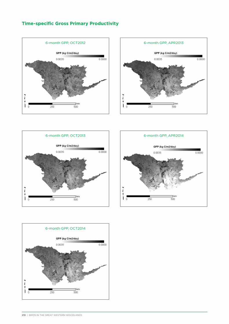
Time-specific Gross Primary Productivity
219 | BIRDS IN THE GREAT WESTERN WOODLANDS
6-month GPP, OCT2012
6-month GPP, OCT2013
6-month GPP, OCT2014
6-month GPP, APR2013
6-month GPP, APR2014
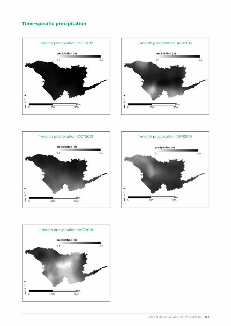
Time-specific precipitation
BIRDS IN THE GREAT WESTERN WOODLANDS | 220
1-month precipitation, OCT2012
1-month precipitation, OCT2013
1-month precipitation, OCT2014
1-month precipitation, APR2013
1-month precipitation, APR2014
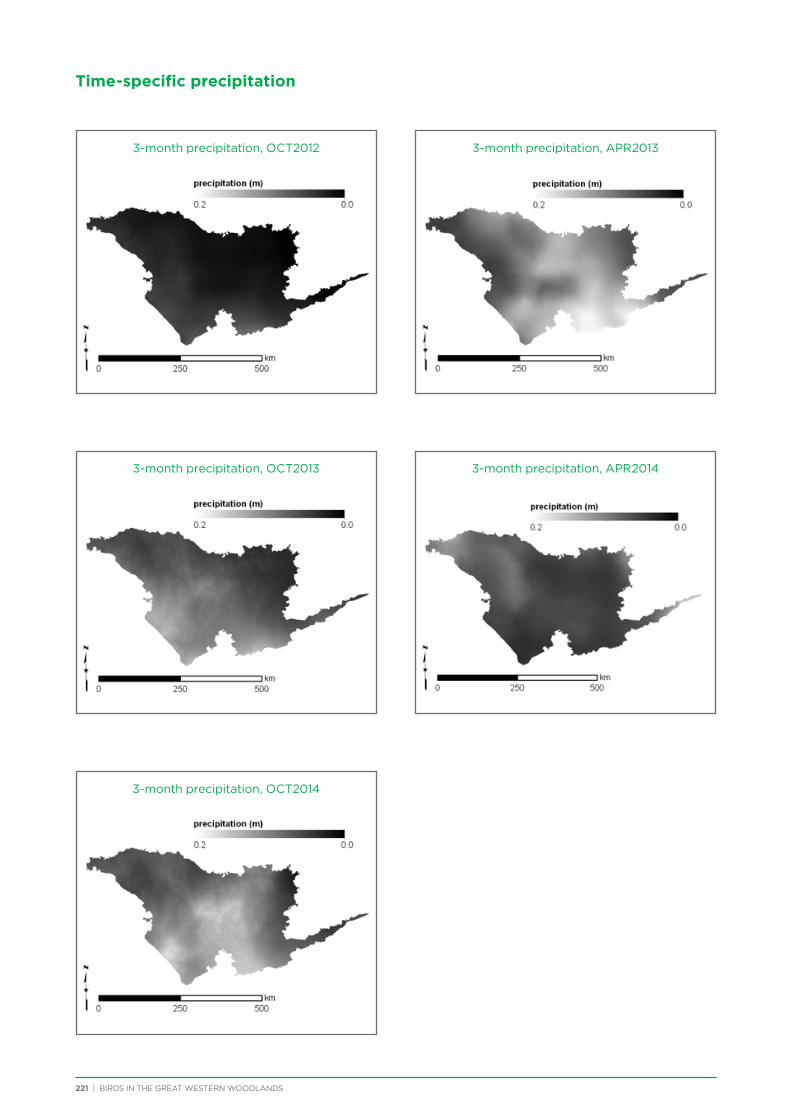
Time-specific precipitation
221 | BIRDS IN THE GREAT WESTERN WOODLANDS
3-month precipitation, OCT2012
3-month precipitation, OCT2013
3-month precipitation, OCT2014
3-month precipitation, APR2013
3-month precipitation, APR2014

Time-specific precipitation
BIRDS IN THE GREAT WESTERN WOODLANDS | 222
6-month precipitation, OCT2012
6-month precipitation, OCT2013
6-month precipitation, OCT2014
6-month precipitation, APR2013
6-month precipitation, APR2014

Land cover
223 | BIRDS IN THE GREAT WESTERN WOODLANDS
Pre-European vegetation class*
Consensus land cover – mixed trees
MODIS VCF % tree cover
*Vegetation class legend (not all classes are present in the study area): 1. Bare; 2. Grasslands; 3. Hummock grasslands; 4. Low forest; 5. Low woodland; 6. Medium-low woodland; 7. Medium forest; 8. Medium woodland; 9. Mosaic; 10. Sedgeland; 11. Shrublands; 12. Succulent steppe
Distance to outcrop (km)
Consensus land cover – evergreen broadleaf
Consensus land cover – shrubs
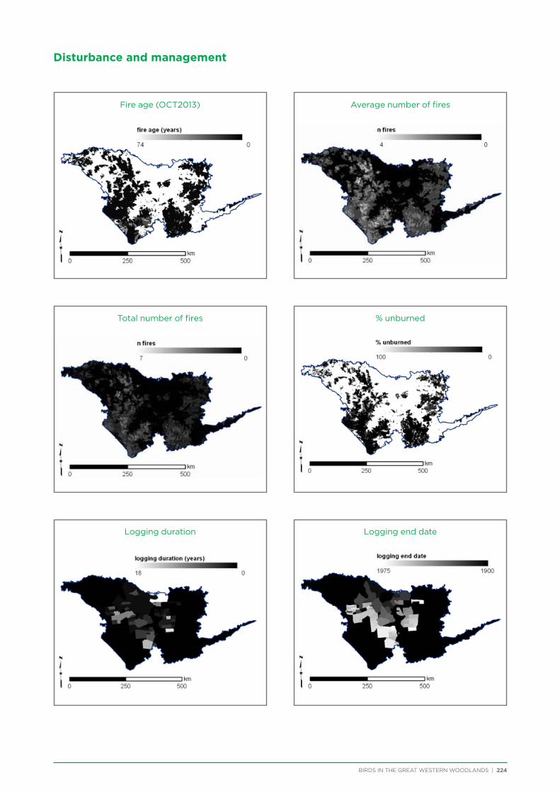
Disturbance and management
BIRDS IN THE GREAT WESTERN WOODLANDS | 224
Fire age (OCT2013)
Total number of fires
Logging duration Logging end date
Average number of fires
% unburned
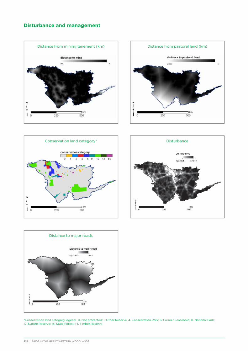
225 | BIRDS IN THE GREAT WESTERN WOODLANDS
Disturbance and management
Distance from mining tenement (km)
Conservation land category*
Distance to major roads
*Conservation land category legend: 0. Not protected; 1. Other Reserve; 4. Conservation Park; 6. Former Leasehold; 11. National Park; 12. Nature Reserve; 13. State Forest; 14. Timber Reserve
Distance from pastoral land (km)
Disturbance
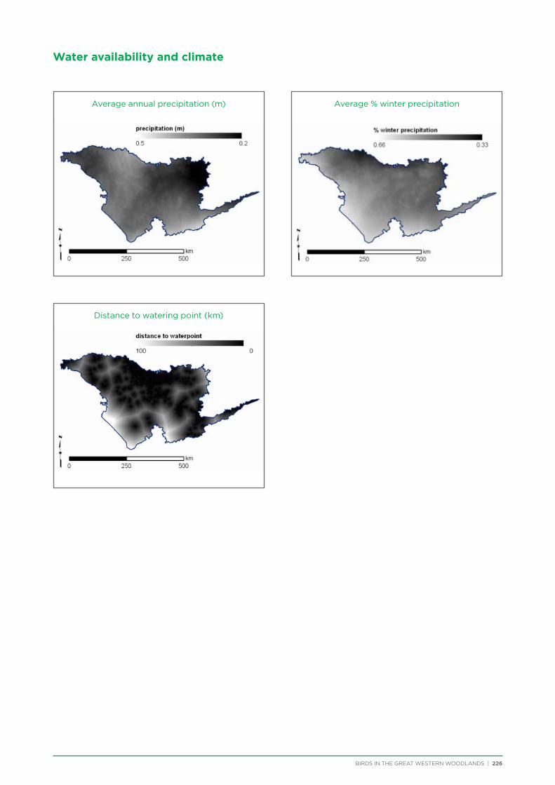
Water availability and climate
BIRDS IN THE GREAT WESTERN WOODLANDS | 226
Average annual precipitation (m)
Distance to watering point (km)
Average % winter precipitation
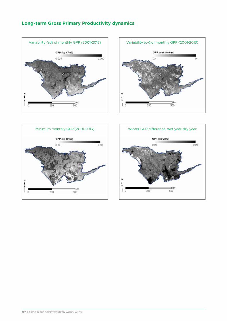
Long-term Gross Primary Productivity dynamics
227 | BIRDS IN THE GREAT WESTERN WOODLANDS
Variability (sd) of monthly GPP (2001-2013)
Minimum monthly GPP (2001-2013)
Variability (cv) of monthly GPP (2001-2013)
Winter GPP difference, wet year-dry year
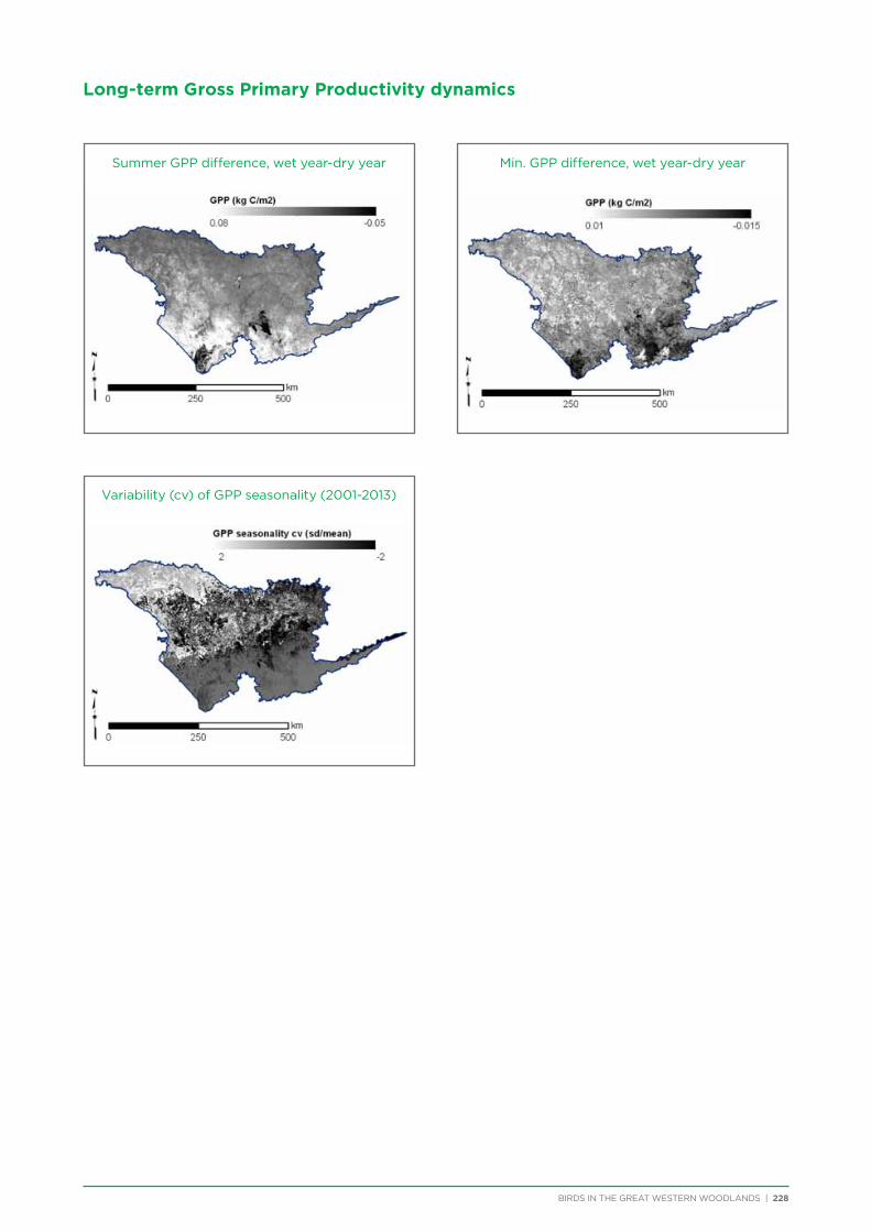
Long-term Gross Primary Productivity dynamics
BIRDS IN THE GREAT WESTERN WOODLANDS | 228
Variability (cv) of GPP seasonality (2001-2013)
Summer GPP difference, wet year-dry year Min. GPP difference, wet year-dry year
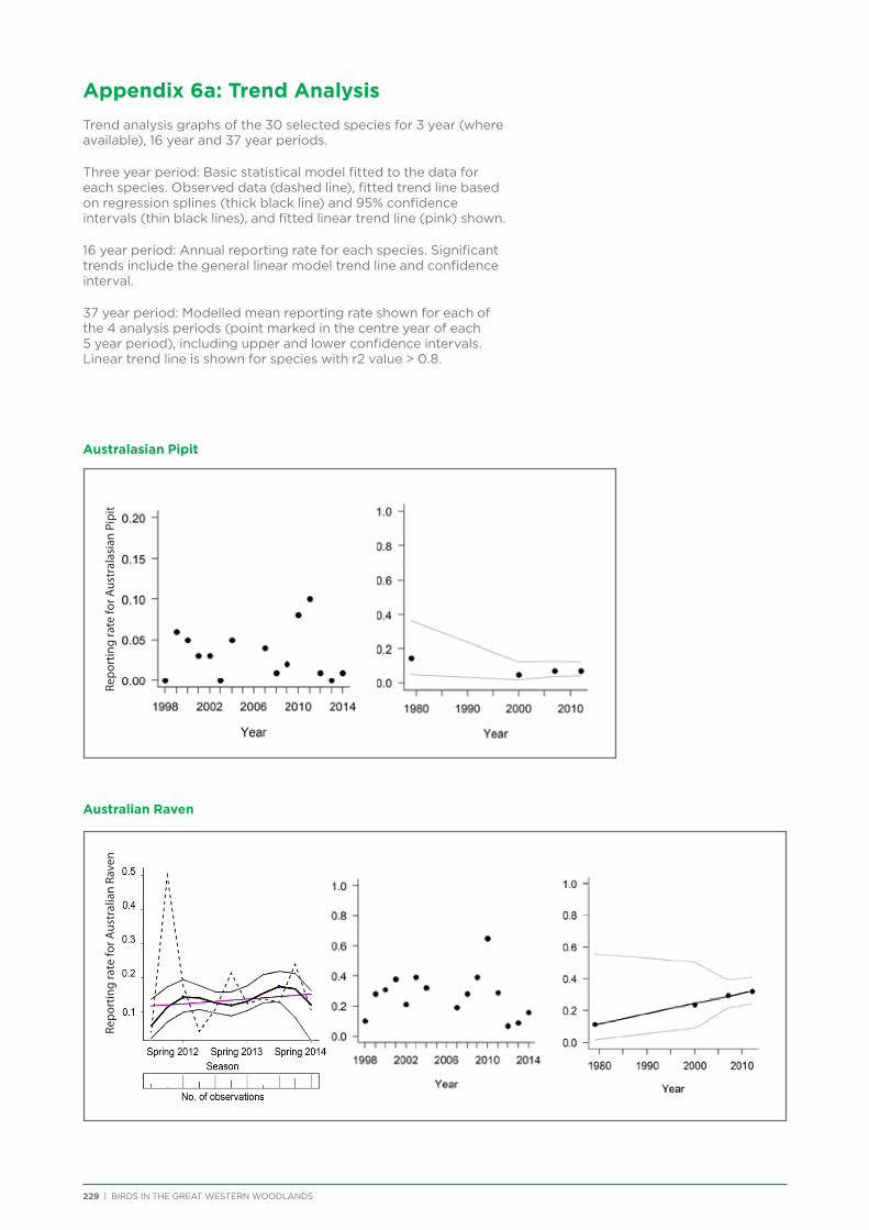
Appendix 6a: Trend Analysis
Trend analysis graphs of the 30 selected species for 3 year (where available), 16 year and 37 year periods.
Three year period: Basic statistical model fitted to the data for each species. Observed data (dashed line), fitted trend line based on regression splines (thick black line) and 95% confidence intervals (thin black lines), and fitted linear trend line (pink) shown.
16 year period: Annual reporting rate for each species. Significant trends include the general linear model trend line and confidence interval.
37 year period: Modelled mean reporting rate shown for each of the 4 analysis periods (point marked in the centre year of each 5 year period), including upper and lower confidence intervals. Linear trend line is shown for species with r2 value > 0.8.
Australasian Pipit
Australian Raven
229 | BIRDS IN THE GREAT WESTERN WOODLANDS
Repo
rtin
g ra
te fo
r Aus
tral
asia
n Pi
pit
Repo
rtin
g ra
te fo
r Aus
tral
ian
Rave
n
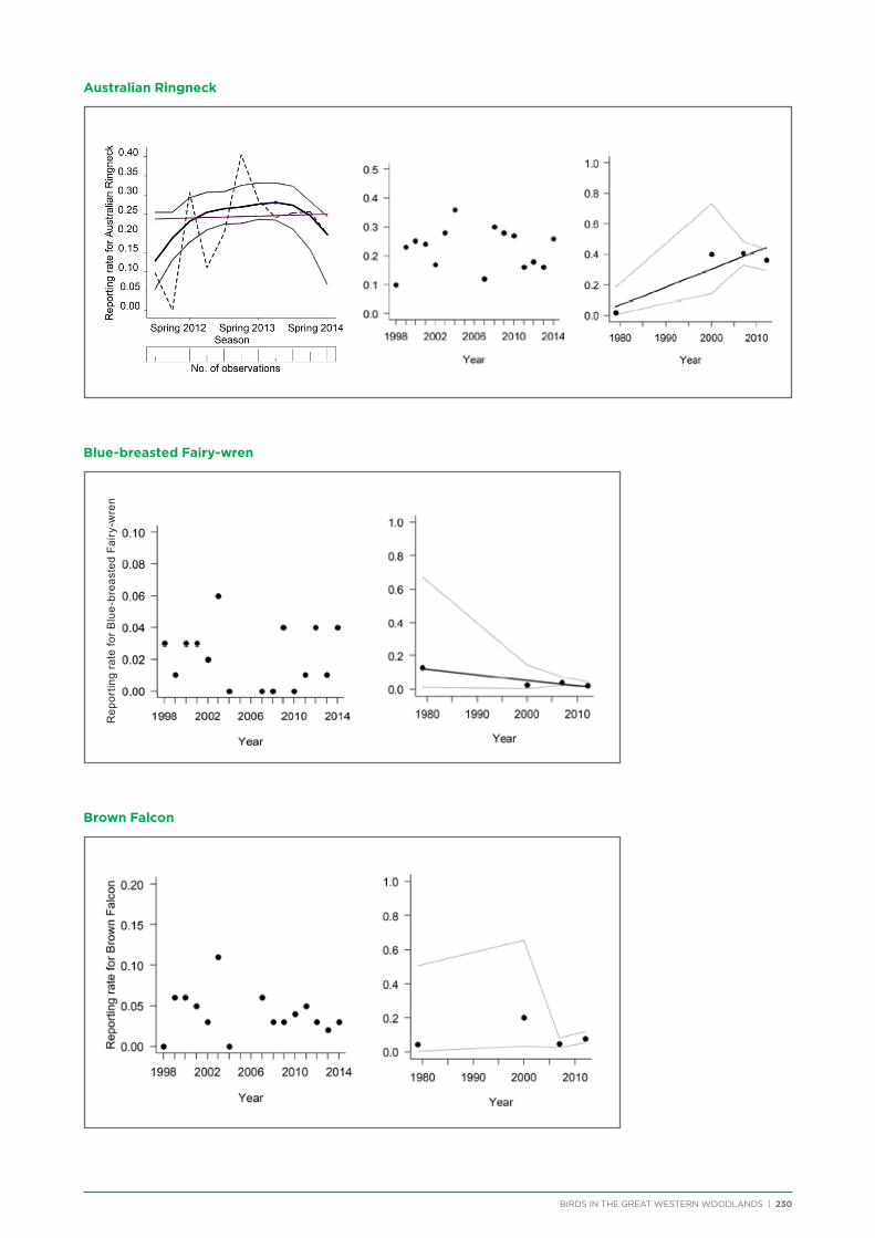
BIRDS IN THE GREAT WESTERN WOODLANDS | 230
Australian Ringneck
Blue-breasted Fairy-wren
Brown Falcon
Re
po
rtin
g r
ate
fo
r B
lue
-bre
ast
ed
Fa
iry-
wre
n
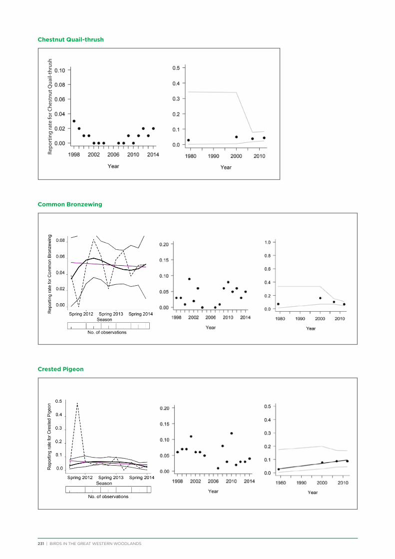
231 | BIRDS IN THE GREAT WESTERN WOODLANDS
Chestnut Quail-thrush
Common Bronzewing
Crested Pigeon
Repo
rtin
g ra
te fo
r Che
stnu
t Qua
il-th
rush
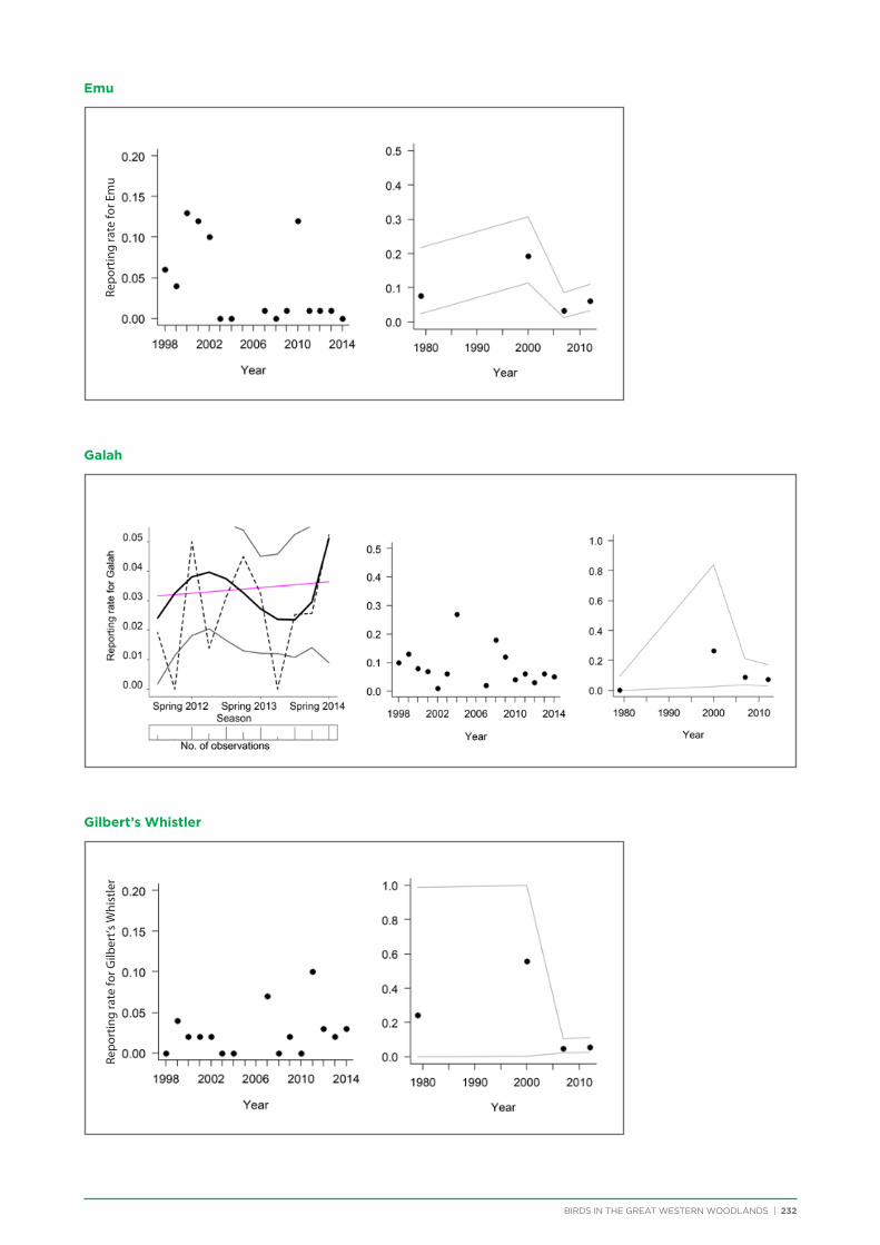
BIRDS IN THE GREAT WESTERN WOODLANDS | 232
Emu
Galah
Gilbert’s Whistler
Repo
rtin
g ra
te fo
r Em
uRe
port
ing
rate
for G
ilber
t’s W
hist
ler
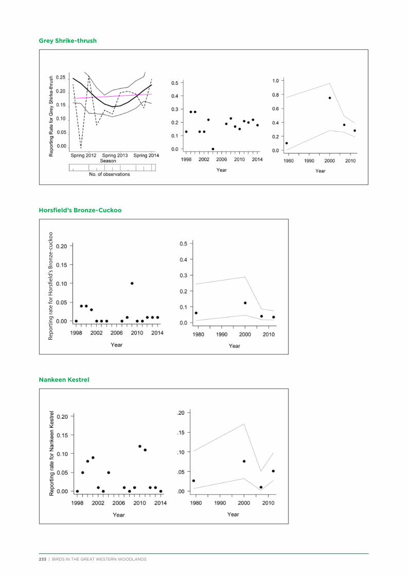
233 | BIRDS IN THE GREAT WESTERN WOODLANDS
Grey Shrike-thrush
Horsfield’s Bronze-Cuckoo
Nankeen Kestrel
Repo
rtin
g ra
te fo
r Hor
sfiel
d’s
Bron
ze-c
ucko
o
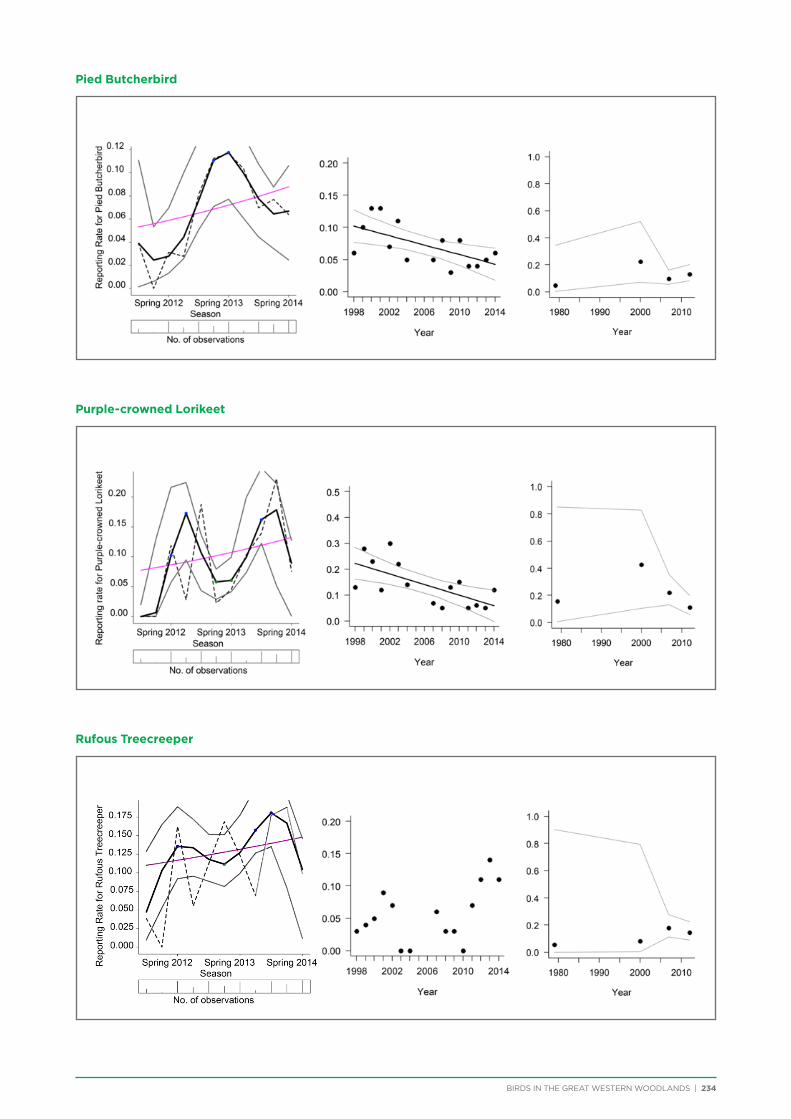
BIRDS IN THE GREAT WESTERN WOODLANDS | 234
Pied Butcherbird
Purple-crowned Lorikeet
Rufous Treecreeper

235 | BIRDS IN THE GREAT WESTERN WOODLANDS
Shy Heathwren
Singing Honeyeater
Southern Scrub-robin
Repo
rtin
g ra
te fo
r Shy
Hea
thw
ren
Repo
rtin
g ra
te fo
r Sou
ther
n Sc
rub
-rob
in
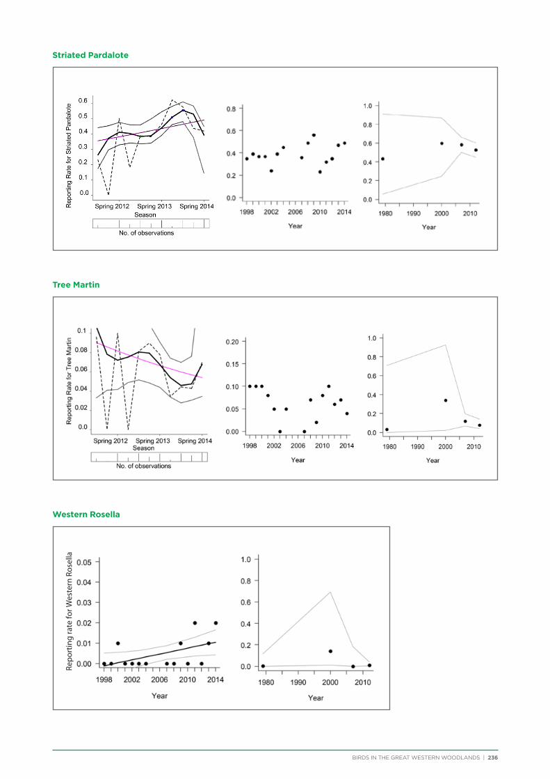
BIRDS IN THE GREAT WESTERN WOODLANDS | 236
Striated Pardalote
Tree Martin
Western Rosella
Repo
rtin
g ra
te fo
r Wes
tern
Ros
ella
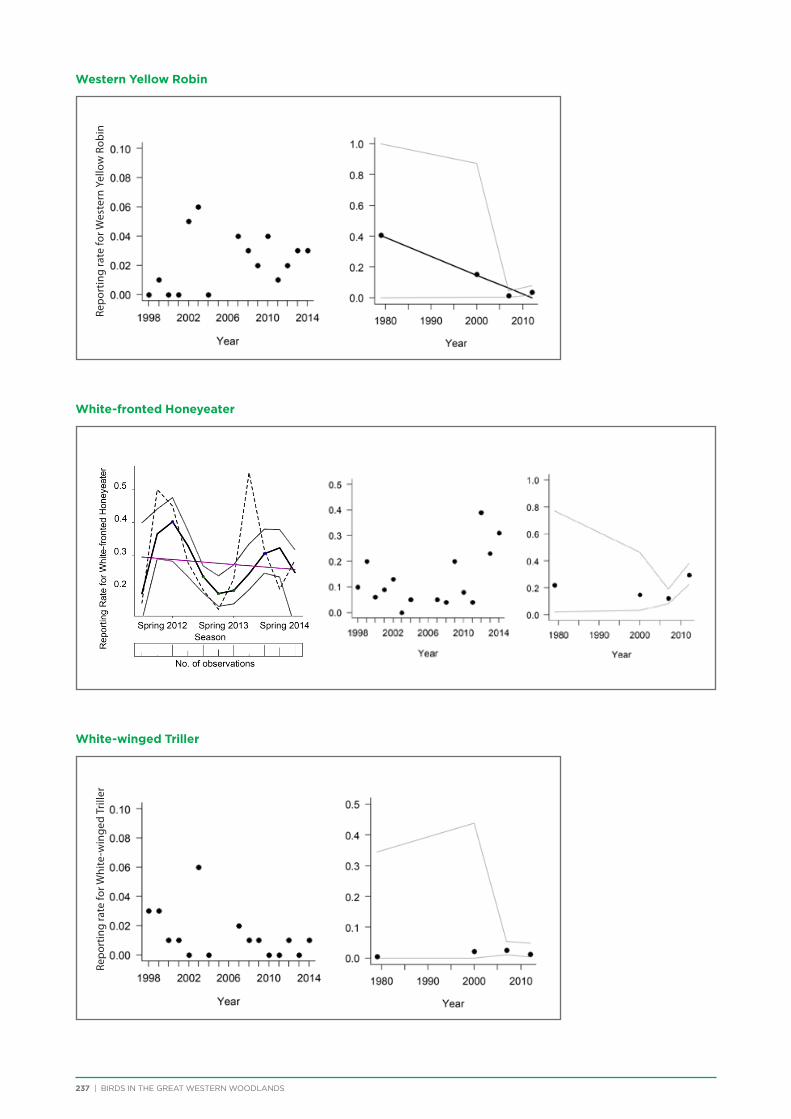
237 | BIRDS IN THE GREAT WESTERN WOODLANDS
Western Yellow Robin
White-fronted Honeyeater
White-winged Triller
Repo
rtin
g ra
te fo
r Wes
tern
Yel
low
Rob
inRe
port
ing
rate
for W
hite
-win
ged
Trill
er
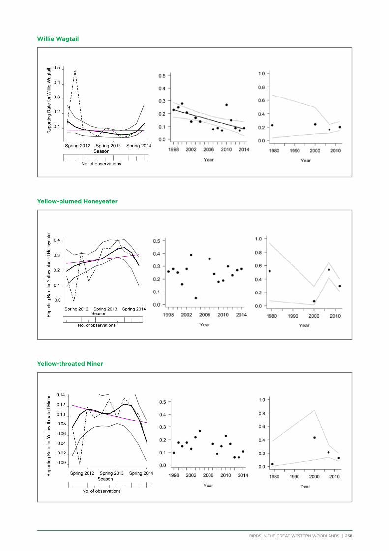
BIRDS IN THE GREAT WESTERN WOODLANDS | 238
Willie Wagtail
Yellow-plumed Honeyeater
Yellow-throated Miner
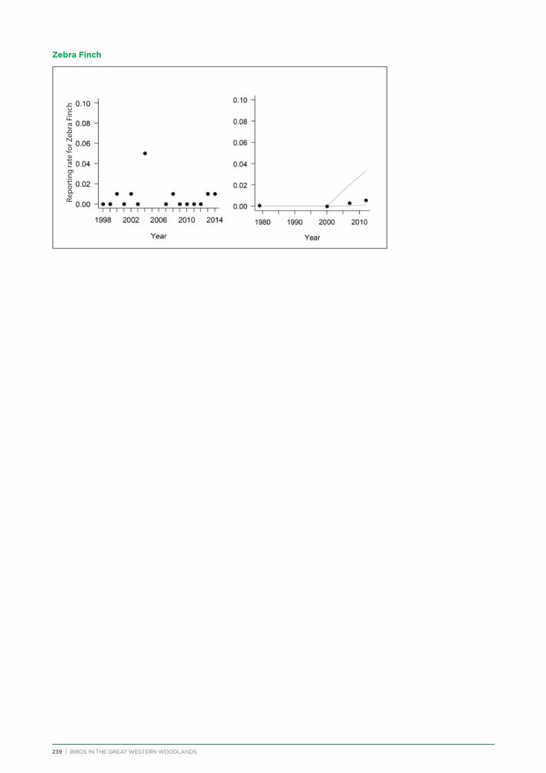
239 | BIRDS IN THE GREAT WESTERN WOODLANDS
Zebra Finch
Repo
rtin
g ra
te fo
r Zeb
ra F
inch
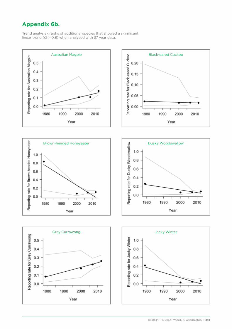
Appendix 6b.
Trend analysis graphs of additional species that showed a significant linear trend (r2 > 0.8) when analysed with 37 year data.
BIRDS IN THE GREAT WESTERN WOODLANDS | 240
Australian Magpie
Brown-headed Honeyeater
Grey Currawong
Black-eared Cuckoo
Dusky Woodswallow
Jacky Winter
Repo
rtin
g ra
te fo
r Bla
ck-e
ared
Cuc
koo

241 | BIRDS IN THE GREAT WESTERN WOODLANDS
Red-capped Robin
Silvereye
White-fronted Chat
Rufous Whistler
White-backed Swallow
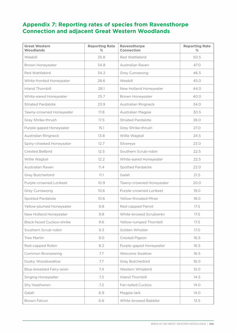
Appendix 7: Reporting rates of species from Ravensthorpe Connection and adjacent Great Western Woodlands Great Western Woodlands
Reporting Rate %
Ravensthorpe Connection
Reporting Rate %
Weebill 35.8 Red Wattlebird 50.5
Brown Honeyeater 34.8 Australian Raven 47.0
Red Wattlebird 34.2 Grey Currawong 46.5
White-fronted Honeyeater 28.6 Weebill 45.0
Inland Thornbill 28.1 New Holland Honeyeater 44.0
White-eared Honeyeater 25.7 Brown Honeyeater 40.0
Striated Pardalote 23.9 Australian Ringneck 34.0
Tawny-crowned Honeyeater 17.8 Australian Magpie 30.5
Grey Shrike-thrush 17.5 Striated Pardalote 28.0
Purple-gaped Honeyeater 15.1 Grey Shrike-thrush 27.0
Australian Ringneck 13.8 Willie Wagtail 24.5
Spiny-cheeked Honeyeater 12.7 Silvereye 23.0
Crested Bellbird 12.5 Southern Scrub-robin 22.5
Willie Wagtail 12.2 White-eared Honeyeater 22.5
Australian Raven 11.4 Spotted Pardalote 22.0
Grey Butcherbird 11.1 Galah 21.5
Purple-crowned Lorikeet 10.9 Tawny-crowned Honeyeater 20.0
Grey Currawong 10.6 Purple-crowned Lorikeet 19.0
Spotted Pardalote 10.6 Yellow-throated Miner 18.0
Yellow-plumed Honeyeater 9.8 Red-capped Parrot 17.5
New Holland Honeyeater 9.8 White-browed Scrubwren 17.5
Black-faced Cuckoo-shrike 9.6 Yellow-rumped Thornbill 17.5
Southern Scrub-robin 9.3 Golden Whistler 17.0
Tree Martin 9.0 Crested Pigeon 16.5
Red-capped Robin 8.2 Purple-gaped Honeyeater 16.5
Common Bronzewing 7.7 Welcome Swallow 16.5
Dusky Woodswallow 7.7 Grey Butcherbird 16.0
Blue-breasted Fairy-wren 7.4 Western Whipbird 15.0
Singing Honeyeater 7.2 Inland Thornbill 14.5
Shy Heathwren 7.2 Fan-tailed Cuckoo 14.0
Galah 6.9 Magpie-lark 14.0
Brown Falcon 6.6 White-browed Babbler 13.5
BIRDS IN THE GREAT WESTERN WOODLANDS | 242
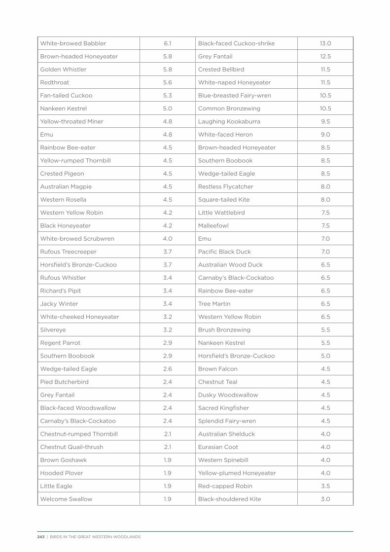
White-browed Babbler 6.1 Black-faced Cuckoo-shrike 13.0
Brown-headed Honeyeater 5.8 Grey Fantail 12.5
Golden Whistler 5.8 Crested Bellbird 11.5
Redthroat 5.6 White-naped Honeyeater 11.5
Fan-tailed Cuckoo 5.3 Blue-breasted Fairy-wren 10.5
Nankeen Kestrel 5.0 Common Bronzewing 10.5
Yellow-throated Miner 4.8 Laughing Kookaburra 9.5
Emu 4.8 White-faced Heron 9.0
Rainbow Bee-eater 4.5 Brown-headed Honeyeater 8.5
Yellow-rumped Thornbill 4.5 Southern Boobook 8.5
Crested Pigeon 4.5 Wedge-tailed Eagle 8.5
Australian Magpie 4.5 Restless Flycatcher 8.0
Western Rosella 4.5 Square-tailed Kite 8.0
Western Yellow Robin 4.2 Little Wattlebird 7.5
Black Honeyeater 4.2 Malleefowl 7.5
White-browed Scrubwren 4.0 Emu 7.0
Rufous Treecreeper 3.7 Pacific Black Duck 7.0
Horsfield’s Bronze-Cuckoo 3.7 Australian Wood Duck 6.5
Rufous Whistler 3.4 Carnaby’s Black-Cockatoo 6.5
Richard’s Pipit 3.4 Rainbow Bee-eater 6.5
Jacky Winter 3.4 Tree Martin 6.5
White-cheeked Honeyeater 3.2 Western Yellow Robin 6.5
Silvereye 3.2 Brush Bronzewing 5.5
Regent Parrot 2.9 Nankeen Kestrel 5.5
Southern Boobook 2.9 Horsfield’s Bronze-Cuckoo 5.0
Wedge-tailed Eagle 2.6 Brown Falcon 4.5
Pied Butcherbird 2.4 Chestnut Teal 4.5
Grey Fantail 2.4 Dusky Woodswallow 4.5
Black-faced Woodswallow 2.4 Sacred Kingfisher 4.5
Carnaby’s Black-Cockatoo 2.4 Splendid Fairy-wren 4.5
Chestnut-rumped Thornbill 2.1 Australian Shelduck 4.0
Chestnut Quail-thrush 2.1 Eurasian Coot 4.0
Brown Goshawk 1.9 Western Spinebill 4.0
Hooded Plover 1.9 Yellow-plumed Honeyeater 4.0
Little Eagle 1.9 Red-capped Robin 3.5
Welcome Swallow 1.9 Black-shouldered Kite 3.0
243 | BIRDS IN THE GREAT WESTERN WOODLANDS

BIRDS IN THE GREAT WESTERN WOODLANDS | 244
Australian Owlet-nightjar 1.6 Elegant Parrot 3.0
White-winged Triller 1.6 Richard’s Pipit 3.0
Brush Bronzewing 1.6 Varied Sittella 3.0
Hooded Robin 1.6 White-cheeked Honeyeater 3.0
Little Crow 1.6 Australasian Grebe 2.5
Little Wattlebird 1.6 Australian Owlet-nightjar 2.5
Rufous Fieldwren 1.6 Black-fronted Dotterel 2.5
Pied Honeyeater 1.6 Shining Bronze-Cuckoo 2.5
Square-tailed Kite 1.6 Singing Honeyeater 2.5
White-backed Swallow 1.1 Southern Emu-wren 2.5
Mistletoebird 1.1 Spiny-cheeked Honeyeater 2.5
Sacred Kingfisher 1.1 Spotted Nightjar 2.5
Spotted Nightjar 1.1 Tawny Frogmouth 2.5
Varied Sittella 1.1 White-fronted Honeyeater 2.5
White-faced Heron 1.1 White-winged Triller 2.5
Splendid Fairy-wren 0.8 Barn Owl 2.0
Australian Hobby 0.8 Grey Teal 2.0
Black-eared Cuckoo 0.8 Hoary-headed Grebe 2.0
Gilbert’s Whistler 0.8 Peregrine Falcon 2.0
Magpie-lark 0.8 Pied Butcherbird 2.0
Malleefowl 0.8 Red-eared Firetail 2.0
Red-backed Kingfisher 0.8 Shy Heathwren 2.0
Barn Owl 0.8 Black-eared Cuckoo 1.5
Shining Bronze-Cuckoo 0.8 Brown Goshawk 1.5
Elegant Parrot 0.8 Hardhead 1.5
Peregrine Falcon 0.8 Rufous Whistler 1.5
Tawny Frogmouth 0.5 Australian Hobby 1.0
Collared Sparrowhawk 0.5 Australian Pelican 1.0
Budgerigar 0.5 Black-faced Woodswallow 1.0
Mulga Parrot 0.5 Little Black Cormorant 1.0
Masked Woodswallow 0.5 Little Eagle 1.0
Red-capped Plover 0.5 Little Pied Cormorant 1.0
Red-tailed Black-Cockatoo 0.5 Painted Button-quail 1.0
Southern Emu-wren 0.5 Rufous Songlark 1.0
Spotted Harrier 0.5 Western Gerygone 1.0
Western Whipbird 0.5 Banded Lapwing 0.5
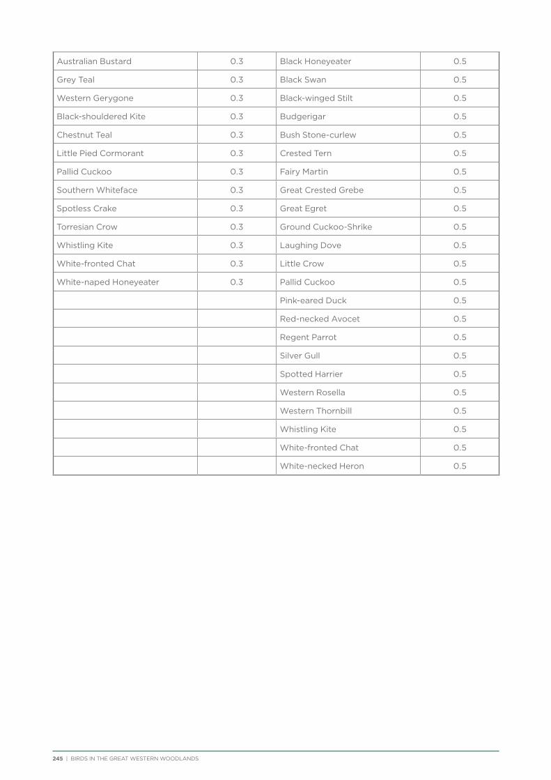
245 | BIRDS IN THE GREAT WESTERN WOODLANDS
Australian Bustard 0.3 Black Honeyeater 0.5
Grey Teal 0.3 Black Swan 0.5
Western Gerygone 0.3 Black-winged Stilt 0.5
Black-shouldered Kite 0.3 Budgerigar 0.5
Chestnut Teal 0.3 Bush Stone-curlew 0.5
Little Pied Cormorant 0.3 Crested Tern 0.5
Pallid Cuckoo 0.3 Fairy Martin 0.5
Southern Whiteface 0.3 Great Crested Grebe 0.5
Spotless Crake 0.3 Great Egret 0.5
Torresian Crow 0.3 Ground Cuckoo-Shrike 0.5
Whistling Kite 0.3 Laughing Dove 0.5
White-fronted Chat 0.3 Little Crow 0.5
White-naped Honeyeater 0.3 Pallid Cuckoo 0.5
Pink-eared Duck 0.5
Red-necked Avocet 0.5
Regent Parrot 0.5
Silver Gull 0.5
Spotted Harrier 0.5
Western Rosella 0.5
Western Thornbill 0.5
Whistling Kite 0.5
White-fronted Chat 0.5
White-necked Heron 0.5


