1

Biophysical temperature measurements and thermal modelling

11080671 1100052

1 1104199

1 1102446

1 1106948

1 1104654

1

1 Department of Physics and Astronomy, University of Glasgow, Glasgow G12 8QQ,

UK

Abstract. A method of measuring biophysical temperatures taken from the forearm region

has been used in parallel with theoretical modelling of thermal and microwave behaviour

to compare the heat flux from internal muscle tissue with the external heat loss from the

skin to the environment. The heat loss coefficient can be extracted from the

relationship between the internal change in temperature with tissue depth and the external

difference in temperature between the skin surface and the surroundings. The dependency

of the internal temperature gradient on the geometrical nature of the thermal model was

investigated through modelling the forearm, first as a cuboidal slab and then as a cylinder.

Comparison of experimental planar and cylindrical heat loss coefficients with theoretical

model predictions, determined the cylindrical model fitted better than the slab model for

majority of subjects. The large error associated with calculated values arose due to a

number of factors associated with the data recording.

1. Introduction

Thermography is the study of using thermal data to analyse the heat distribution of a given structure or

region. This investigation focuses on using this principle to model the heat loss of a person’s forearm.

In order to achieve this we will look to create a system for collecting accurate data, and to formulate a

refined model. Our ultimate aim is to compare our heat models for internal and external heat loss.

The natural processes in the forearm components and the interaction between them can be described

using a selection of appropriate formulae, simply by analysing the properties and special

characteristics of each component involved. The main aim was to compare the heat flux from the

internal muscle tissue with the heat loss from the skin estimated from external modelling in the

following formula

( ) ( )

where is the heat transfer coefficient, is the temperature at the surface of the skin measured with

the infrared thermometer, is the ambient temperature measured by a thermocouple thermometer,

is the tissue thermal conductivity and

is the gradient of the temperature profile, T(z). This

temperature gradient is partially dependent on the geometrical thermal model used and finding this

2

allows the heat loss coefficient, , for an internal model which can then be compared to an externally

model ho value.

2. Background

The heat transfer coefficient is the sum of the external heat loss processes such as radiation,

convection and evaporation and is calculated using the following formulae:

( )(

) ( )

For both slab and cylindrical model, where = Stefan Boltzmann constant and e = skin emissivity,

( ) ( )

W (4)

Evaporative heat loss for both models per °C,

( )

assuming is a small value.

The temperature profile, T(z), in each case was obtained considering the solutions of the steady-state

Pennes bioheat equation:

( ) ( )

The thermal diffusion factor, , is first encountered with formulae,

√

(

) ( )

where is the arterial blood perfusion, is the blood density and is the blood specific heat. The

second formula of (7) allows beta values to be experimentally found through measured microwave,

surface and arterial temperatures ( , ), and is the power attenuation factor.

In one dimension using equation (7) to solve the bioheat equation, a temperature profile through the

slab then takes the form,

( ) ( ( ))

( )( ) ( )

where is the oral temperature , D is the depth of the arterial source of heat and z is the depth

measured from the surface towards the centre of the arm.

By considering the boundary conditions for a semi-infinite slab, D , z as ( ) , the

temperature profile used takes the form,

3

( ) ( ) ( )

In order to provide a more accurate representation of its true geometric shape, we shifted to a model

that represented a forearm as a solid cylinder with no variations along or around its central axis. This

can be achieved by using the same measurements as in the slab model but with an alternative

cylindrical coordinate system and altered boundary conditions, which in turn offers a different solution

to the Pennes Bioheat equation. When changed to cylindrical co-ordinates, the Pennes equation

becomes:

(

( )

)

( ( )) ( )

With boundary conditions of a temperature, Ts at the surface of radius R,

( )

( )

In cylindrical coordinates with no variation along and around the principal axis, solving the Pennes

equation with the specific boundary conditions gave the following estimation of Bessel temperature,

( ) ( )

( )( ) ( )

for a surface at radius R at a temperature , and ( ) is the zero order modified Bessel function of

the first kind.

The attenuation factor was expressed in terms of relative permittivity

and relative loss

factor

, with the vacuum permittivity ( ) as follows

√(

)(√ (

)

)

√ ( )

where is the measurement free space wavelength ( 9.23 ).

3. Method

3.1 Equipment

The equipment used for our data collection is shown below:

4

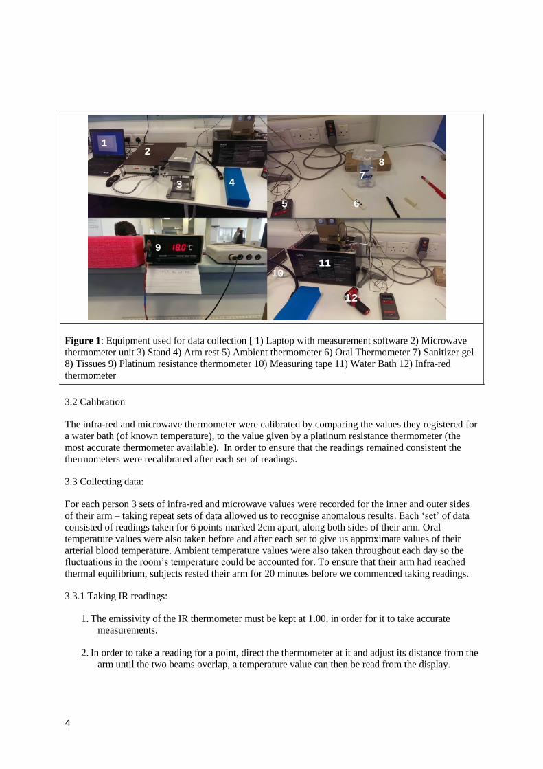
Figure 1: Equipment used for data collection [ 1) Laptop with measurement software 2) Microwave

thermometer unit 3) Stand 4) Arm rest 5) Ambient thermometer 6) Oral Thermometer 7) Sanitizer gel

8) Tissues 9) Platinum resistance thermometer 10) Measuring tape 11) Water Bath 12) Infra-red

thermometer

3.2 Calibration

The infra-red and microwave thermometer were calibrated by comparing the values they registered for

a water bath (of known temperature), to the value given by a platinum resistance thermometer (the

most accurate thermometer available). In order to ensure that the readings remained consistent the

thermometers were recalibrated after each set of readings.

3.3 Collecting data:

For each person 3 sets of infra-red and microwave values were recorded for the inner and outer sides

of their arm – taking repeat sets of data allowed us to recognise anomalous results. Each ‘set’ of data

consisted of readings taken for 6 points marked 2cm apart, along both sides of their arm. Oral

temperature values were also taken before and after each set to give us approximate values of their

arterial blood temperature. Ambient temperature values were also taken throughout each day so the

fluctuations in the room’s temperature could be accounted for. To ensure that their arm had reached

thermal equilibrium, subjects rested their arm for 20 minutes before we commenced taking readings.

3.3.1 Taking IR readings:

1. The emissivity of the IR thermometer must be kept at 1.00, in order for it to take accurate

measurements.

2. In order to take a reading for a point, direct the thermometer at it and adjust its distance from the

arm until the two beams overlap, a temperature value can then be read from the display.

6

8

12

7

1 2

3

5

9

10

4

11

5

z=0 z=D z=2D

𝑇(𝑧) 𝑇𝑠

𝑑𝑇

𝑑𝑧 𝑇(𝑧) 𝑇𝑎𝑟𝑡

𝑇(𝑧) 𝑇𝑠

0 D 2D

3. Take readings for all six points, on both sides of the arm, working along from the person’s

elbow.

3.4.2 Taking MW readings:

1. Start by placing the detector head before the first point on the arm and wait until the software is

registering a reasonable temperature (similar to your IR readings +2°C).

2. Slide the detector on to the first point and set the software to average the readings over a 3

second period. Record the average.

3. Slide the detector along and repeat the process for the other points and then the other side of the

arm.

4. Pilot Study

The aim of the Pilot Study was to familiarise ourselves with the apparatus. The microwave and surface

temperatures of four subjects were measured and compared in order to outline key issues in data

gathering and to aid in refining the method.

The majority of our data recording issues arose from the microwave detector. This drew the following

conclusions: Before starting the calibration, the thermometer must be left in the water bath for enough

time for it to reach thermal equilibrium with the water. For this reason, the thermometer must also be

held to a subject’s arm for a while before starting, on a non-data point. Once the detector has reached

equilibrium with the arm it must be held against the skin for the duration of the 6 readings, sliding

from point to point, otherwise it will cause the temperature to spike. It was also noted that the

microwave detector had a tendency to heat up when held in sustained contact with the skin or the

water bath, causing the temperature to rise to unreasonably high temperatures. This issue was later

rectified by leaving the detector head to sit for a while in cold water to cool. Finally, it was found that

a nearby radiator was affecting the measured ambient temperature. Once the data gathering had been

moved to another set of apparatus on the other side of the room, the ambient temperature became less

temperamental.

5. Modeling

5.1 2D Slab Model

In the first section of the experiment the arm was modelled as a slab of thickness 2D.

Figure 2: 2D slab diagram

The arm itself is modelled as a cuboid slab with boundary conditions,

6

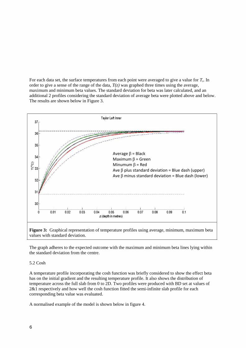
For each data set, the surface temperatures from each point were averaged to give a value for Ts. In

order to give a sense of the range of the data, T(z) was graphed three times using the average,

maximum and minimum beta values. The standard deviation for beta was later calculated, and an

additional 2 profiles considering the standard deviation of average beta were plotted above and below.

The results are shown below in Figure 3.

Figure 3: Graphical representation of temperature profiles using average, minimum, maximum beta

values with standard deviation.

The graph adheres to the expected outcome with the maximum and minimum beta lines lying within

the standard deviation from the centre.

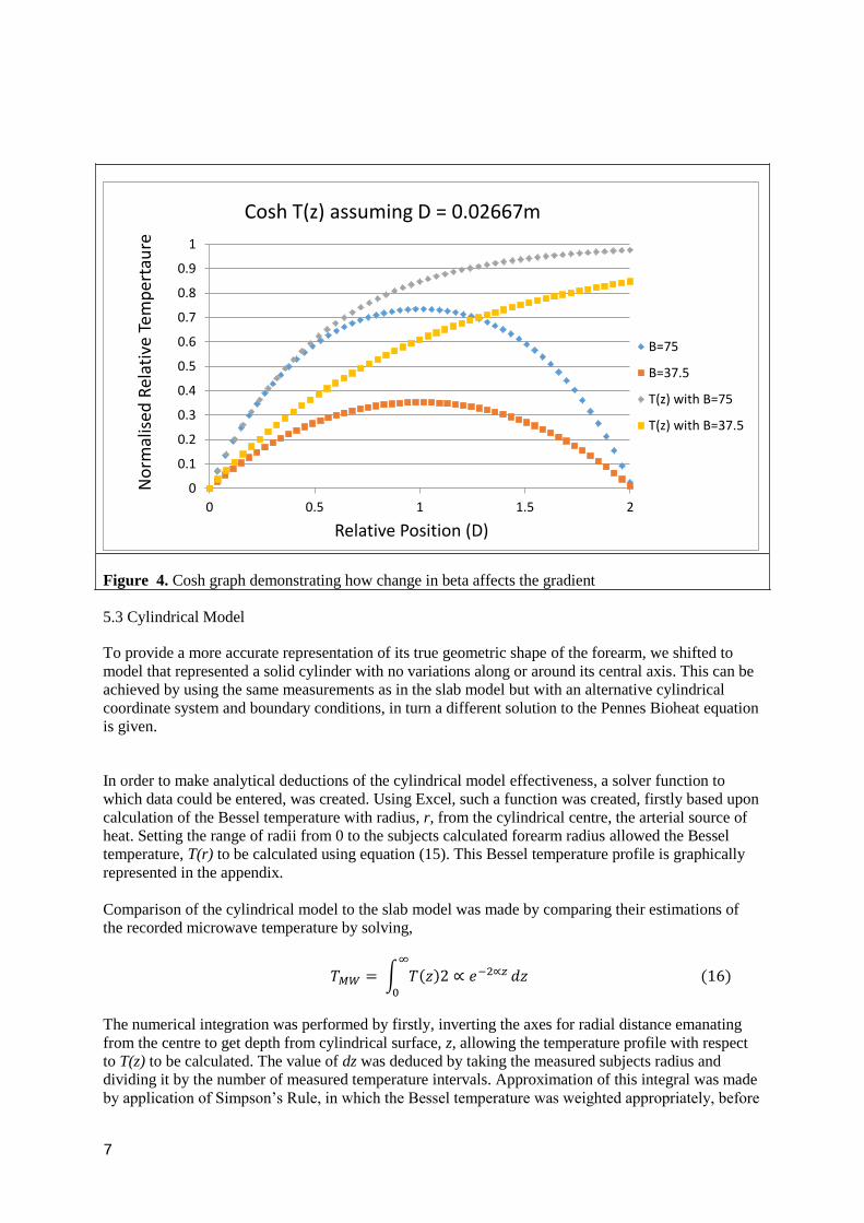
5.2 Cosh

A temperature profile incorporating the cosh function was briefly considered to show the effect beta

has on the initial gradient and the resulting temperature profile. It also shows the distribution of

temperature across the full slab from 0 to 2D. Two profiles were produced with BD set at values of

2&1 respectively and how well the cosh function fitted the semi-infinite slab profile for each

corresponding beta value was evaluated.

A normalised example of the model is shown below in figure 4.

Average β = Black Maximum β = Green Minumum β = Red Ave β plus standard deviation = Blue dash (upper) Ave β minus standard deviation = Blue dash (lower)

7

Figure 4. Cosh graph demonstrating how change in beta affects the gradient

5.3 Cylindrical Model

To provide a more accurate representation of its true geometric shape of the forearm, we shifted to

model that represented a solid cylinder with no variations along or around its central axis. This can be

achieved by using the same measurements as in the slab model but with an alternative cylindrical

coordinate system and boundary conditions, in turn a different solution to the Pennes Bioheat equation

is given.

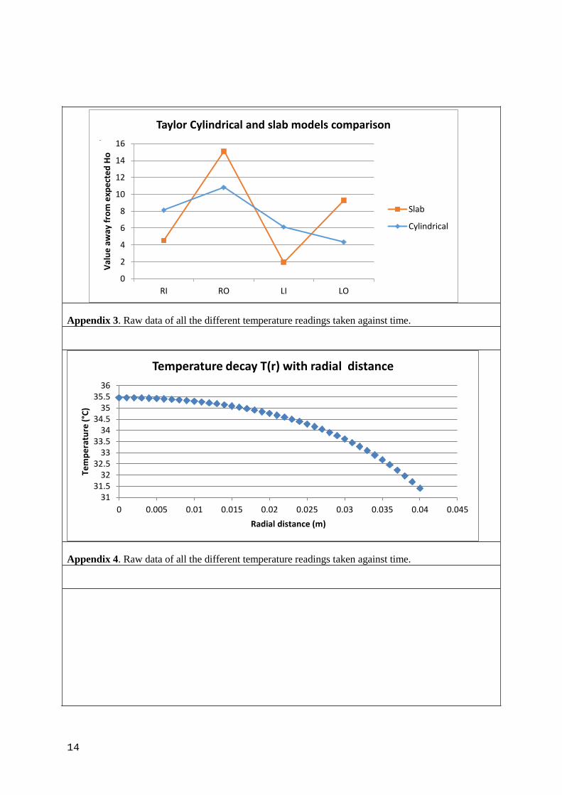
In order to make analytical deductions of the cylindrical model effectiveness, a solver function to

which data could be entered, was created. Using Excel, such a function was created, firstly based upon

calculation of the Bessel temperature with radius, r, from the cylindrical centre, the arterial source of

heat. Setting the range of radii from 0 to the subjects calculated forearm radius allowed the Bessel

temperature, T(r) to be calculated using equation (15). This Bessel temperature profile is graphically

represented in the appendix.

Comparison of the cylindrical model to the slab model was made by comparing their estimations of

the recorded microwave temperature by solving,

∫ ( )

( )

The numerical integration was performed by firstly, inverting the axes for radial distance emanating

from the centre to get depth from cylindrical surface, z, allowing the temperature profile with respect

to T(z) to be calculated. The value of dz was deduced by taking the measured subjects radius and

dividing it by the number of measured temperature intervals. Approximation of this integral was made

by application of Simpson’s Rule, in which the Bessel temperature was weighted appropriately, before

0

0.1

0.2

0.3

0.4

0.5

0.6

0.7

0.8

0.9

1

0 0.5 1 1.5 2

No

rmal

ised

Rel

ativ

e Te

mp

ert

aure

Relative Position (D)

Cosh T(z) assuming D = 0.02667m

B=75

B=37.5

T(z) with B=75

T(z) with B=37.5

8

a summation of the weighted temperatures was made. The predicted microwave temperature could be

compared with the experimental value and the models could then be related by evaluating how closely

they resembled the microwave predictions. The enhanced microwave model was adopted in attempt

to delve deeper into the true nature of the microwave signal generation. The previous microwave

model makes a plane-wave field propagation assumption and the model can be enhanced by

incorporating the contributing effects of the near-field regions, d1 and the attenuation increase in

propagation, d2. Combining the effects of near field power generation and dissipation and increased

attenuation, a better estimation of the signal generation takes the form,

( )( ) ∫ ( ) ( )

( )

where d1≈0.18 and d2≈0.1 for an antenna consisting of a cylindrical waveguide in contact with a

material of high water content. However, assuming the medium being analysed is the brachioradialis

muscle consisting of 75% water, these constants were adjusted to 75% of their above values.

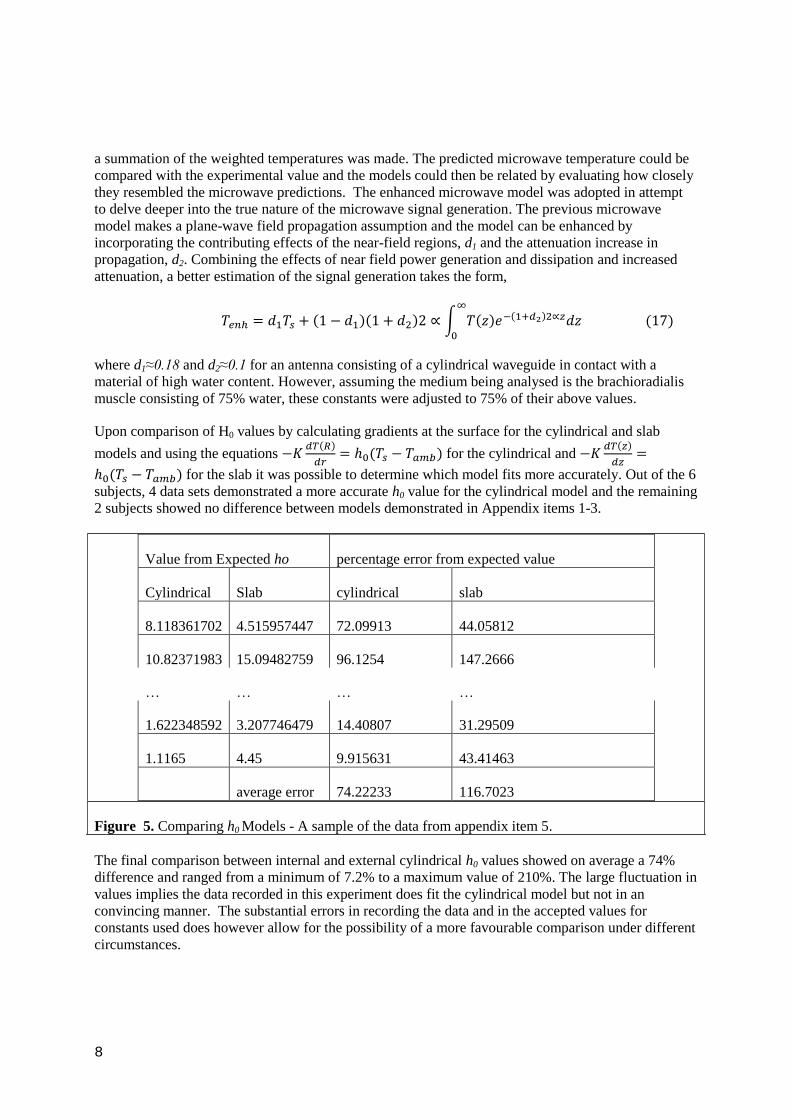
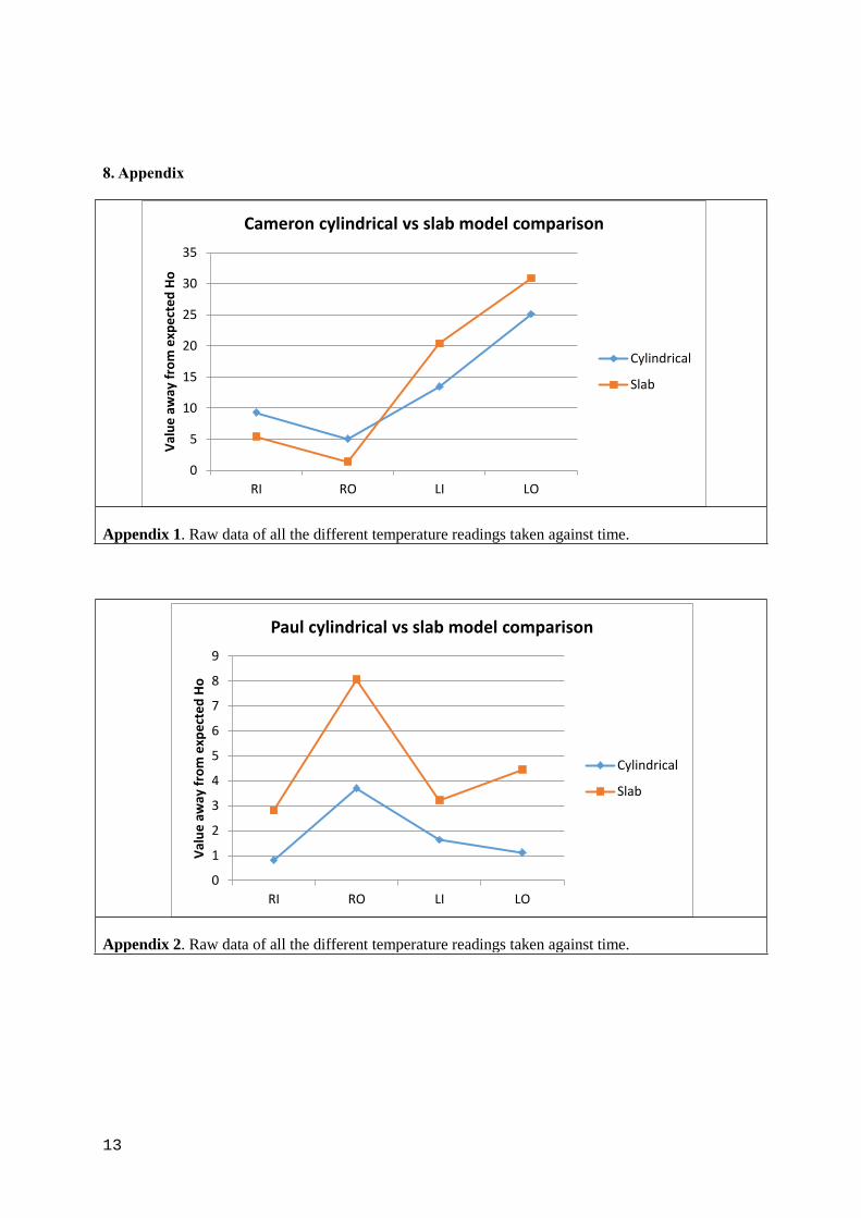
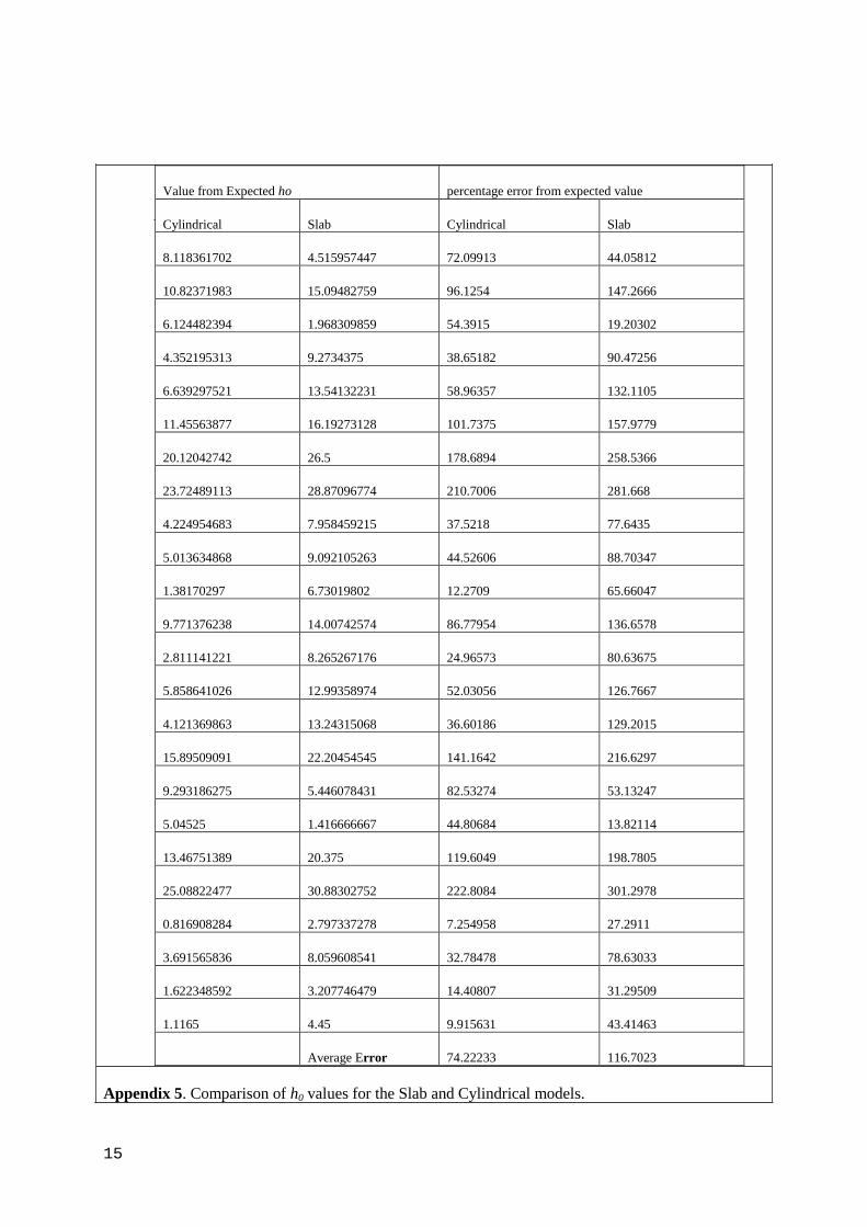
Upon comparison of H0 values by calculating gradients at the surface for the cylindrical and slab

models and using the equations ( )

( ) for the cylindrical and

( )

( ) for the slab it was possible to determine which model fits more accurately. Out of the 6

subjects, 4 data sets demonstrated a more accurate h0 value for the cylindrical model and the remaining

2 subjects showed no difference between models demonstrated in Appendix items 1-3.

Value from Expected ho percentage error from expected value

Cylindrical Slab cylindrical slab

8.118361702 4.515957447 72.09913 44.05812

10.82371983 15.09482759 96.1254 147.2666

… … … …

1.622348592 3.207746479 14.40807 31.29509

1.1165 4.45 9.915631 43.41463

average error 74.22233 116.7023

Figure 5. Comparing h0 Models - A sample of the data from appendix item 5.

The final comparison between internal and external cylindrical h0 values showed on average a 74%

difference and ranged from a minimum of 7.2% to a maximum value of 210%. The large fluctuation in

values implies the data recorded in this experiment does fit the cylindrical model but not in an

convincing manner. The substantial errors in recording the data and in the accepted values for

constants used does however allow for the possibility of a more favourable comparison under different

circumstances.

9

y = -0.0412x + 31.3

y = -0.0005x + 32.457

y = 0.0006x + 33.044

y = 0.0024x + 36.448

y = 0.0194x + 21.218

15.00

20.00

25.00

30.00

35.00

40.00

0.00 5.00 10.00 15.00 20.00 25.00 30.00 35.00

Tem

pe

ratu

re (

oC

)

Time (mins)

Temperature Fluctuations

Irt

Mw

Prt

Oral

Ambient

6. Errors

6.1 Temperature Fluctuation Experiment

6.1.1 Method

In order to check the accuracy of our array of thermometers over time, a small experiment was

devised. Over the course of 30 minutes a single point on a person’s arm was measured, using the IRT

and MWT, at 3 minute intervals (having rested the arm for 20 minutes first). Ambient readings as well

as PRT readings of the water bath were also taken. The person’s oral temperature was also taken every

6 minutes (as it takes longer for the oral thermometer to register a reading).

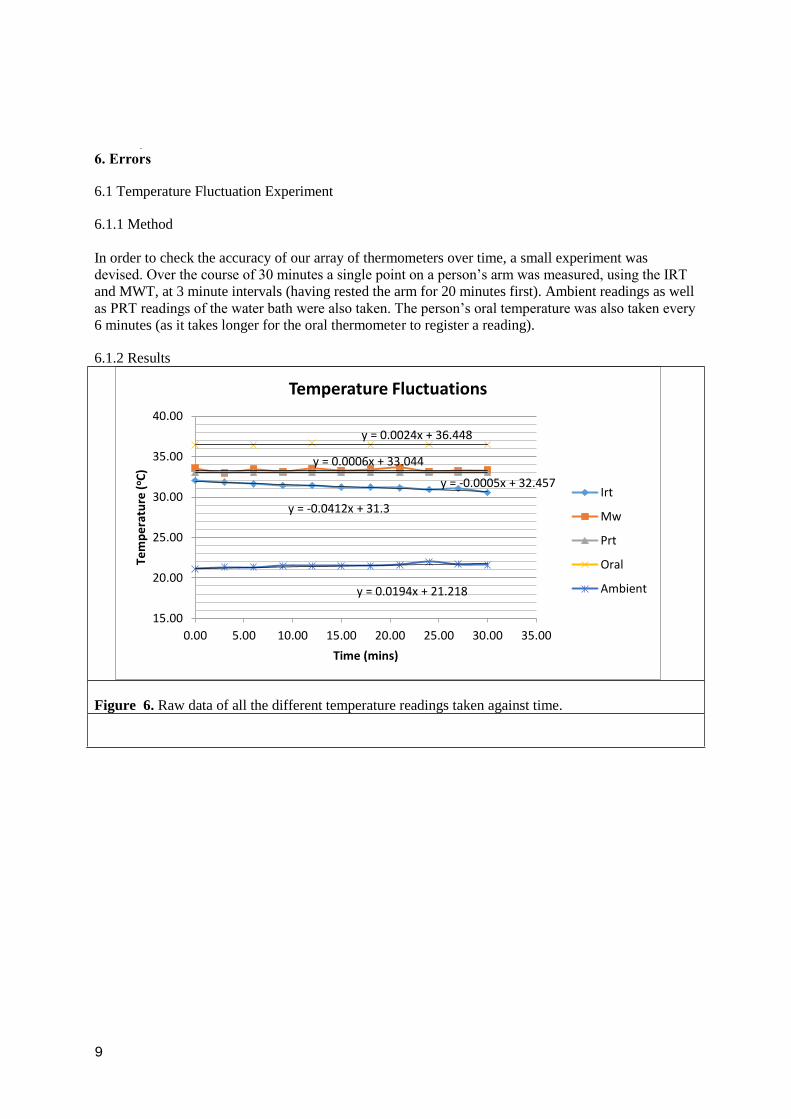
6.1.2 Results

Figure 6. Raw data of all the different temperature readings taken against time.

10

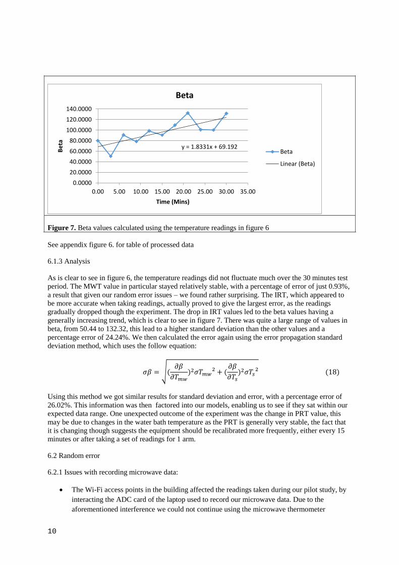
Figure 7. Beta values calculated using the temperature readings in figure 6

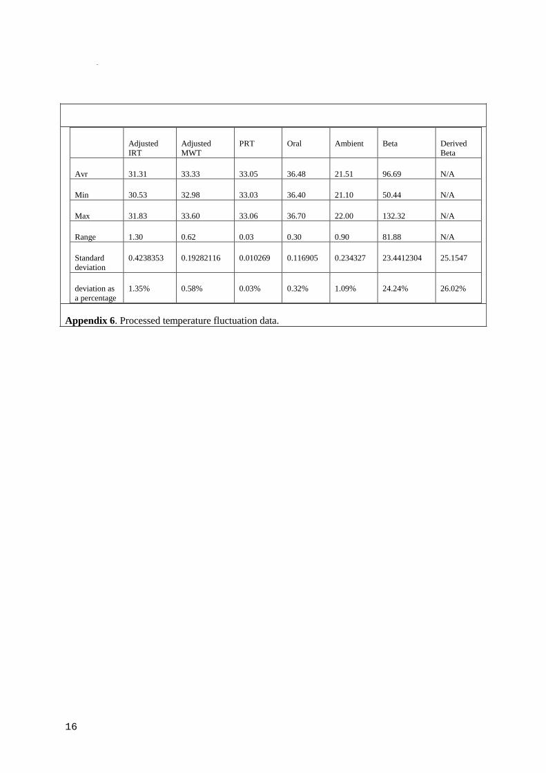
See appendix figure 6. for table of processed data

6.1.3 Analysis

As is clear to see in figure 6, the temperature readings did not fluctuate much over the 30 minutes test

period. The MWT value in particular stayed relatively stable, with a percentage of error of just 0.93%,

a result that given our random error issues – we found rather surprising. The IRT, which appeared to

be more accurate when taking readings, actually proved to give the largest error, as the readings

gradually dropped though the experiment. The drop in IRT values led to the beta values having a

generally increasing trend, which is clear to see in figure 7. There was quite a large range of values in

beta, from 50.44 to 132.32, this lead to a higher standard deviation than the other values and a

percentage error of 24.24%. We then calculated the error again using the error propagation standard

deviation method, which uses the follow equation:

√(

)

(

)

( )

Using this method we got similar results for standard deviation and error, with a percentage error of

26.02%. This information was then factored into our models, enabling us to see if they sat within our

expected data range. One unexpected outcome of the experiment was the change in PRT value, this

may be due to changes in the water bath temperature as the PRT is generally very stable, the fact that

it is changing though suggests the equipment should be recalibrated more frequently, either every 15

minutes or after taking a set of readings for 1 arm.

6.2 Random error

6.2.1 Issues with recording microwave data:

The Wi-Fi access points in the building affected the readings taken during our pilot study, by

interacting the ADC card of the laptop used to record our microwave data. Due to the

aforementioned interference we could not continue using the microwave thermometer

y = 1.8331x + 69.192

0.0000

20.0000

40.0000

60.0000

80.0000

100.0000

120.0000

140.0000

0.00 5.00 10.00 15.00 20.00 25.00 30.00 35.00

Be

ta

Time (Mins)

Beta

Beta

Linear (Beta)

11

equipment set up in our assigned region of the lab. The microwave thermometer array was

tested in several places around the building however we eventually determined that the

building was entirely saturated. In order to remove the interference of the Wi-Fi we would

have to disable the repeaters in our lab as well as on the floors above and below – this was

deemed unfeasible. We later discovered that a majority of the fluctuation could be put down to

the fact that there are a large number of computers in the lab.

We found that over time the microwave thermometer’s detector head had a tendency to heat

up with prolonged use. This caused it to falsely register readings as being up to 10oC higher.

We found that the best way to counteract the heat build-up was to turn off the microwave

thermometer and hold the detector head in cold water, for a few minutes.

We also found that if the detector loses contact with the skin the read out spikes and can take

several seconds to settle down.

Fortunately the other group’s microwave array set up across the lab appeared to be affected to

a lesser degree by the Wi-Fi. For our final results we time shared the working equipment with

the other group.

6.2.2 Slide Variation Experiment

6.2.2.1 Method

To check the variation in MWT for each point over a short period of time, we did another quick

experiment, this time taking readings over 6 points then immediately going back to the 1st point and

taking readings again. The aim of this was to take the repeat readings before significant amounts of

heat were lost from the arm, with the points ideally coming out the same each time. We repeated this

process 6 times and took oral temperatures before and after.

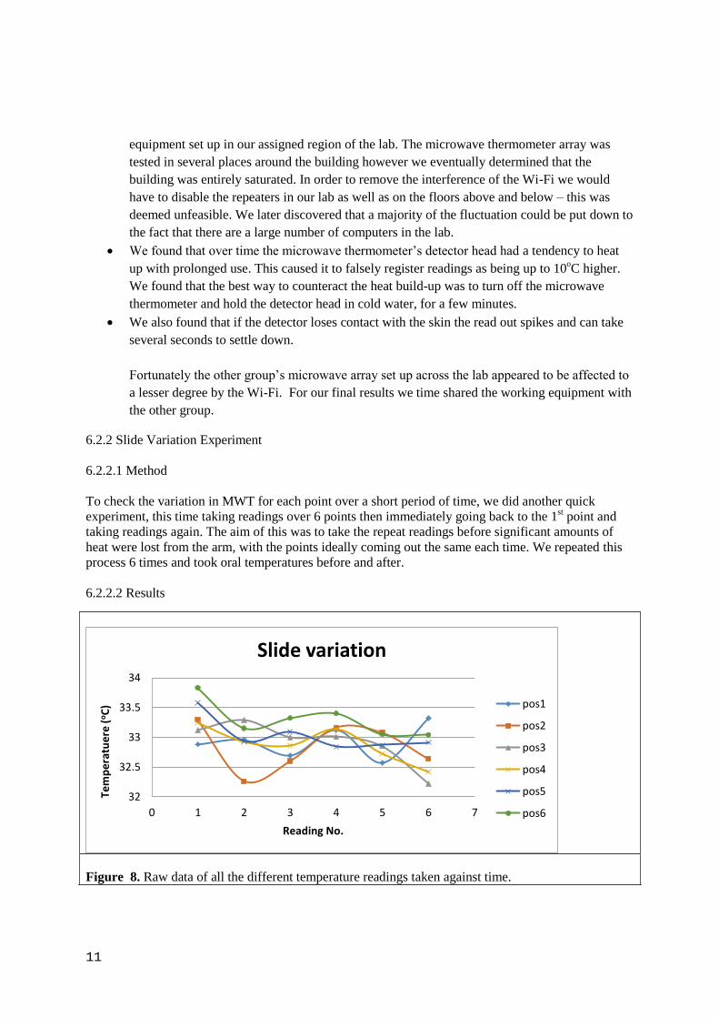
6.2.2.2 Results

Figure 8. Raw data of all the different temperature readings taken against time.

32

32.5

33

33.5

34

0 1 2 3 4 5 6 7

Tem

pe

ratu

ere

(oC

)

Reading No.

Slide variation

pos1

pos2

pos3

pos4

pos5

pos6

12

6.2.2.3 Analysis

From the results it’s clear to see that even in a short period of time, the temperature clearly fluctuated

for each point with no clear trend. This shows how important it is to take repeat readings as the

temperature isn’t likely to stay the same. It’s also important to maintain the same time for the readings

to average on the MW software to keep the readings consistent, as if the averaging time is too long the

temperature can fluctuate too much, giving a large range of values of the time and therefore a less

accurate average value. As mentioned in 6.2.1 we had issues with the MW equipment throughout the

experiment so it’s important to regularly calibrate to check that the temperature fluctuations are

genuine and not caused by equipment errors.

6.2.3 Other causes of interference:

RF impedance from power lines set on the wall may have caused some background noise,

which could have affected some of the readings. The lines produce low level interference as

the long cables used to distribute power around the lab lack proper shielding.

Our initial array was positioned in close proximity to one of the room’s radiators which

affected our pilot study ambient temperature readings.

7. Conclusion

The comparison between the internal and external modelling of the arm demonstrated the large range

of factors that need to be taken into account when carrying out any experimental thermal work. In the

external modelling process, which is considerably less complex than the interior model, there were a

number of aspects which required attention, mainly the three ways heat can be transported away from

the skin surface. As for the internal measurements, initially modelling the forearm as a slab of

thickness 2D gave a basic understanding of the way heat flows from the central arteries to the skin

surface in a linear fashion whilst not being lost laterally. The temperature profiles produced for such a

model were a useful tool in showing the way heat was lost exponentially between the central arteries

and the surface.

The progression from the slab model to the cylindrical was the next logical step, giving a better

representation of both the arm’s actual shape and also of the way heat is transferred from the core. The

key issues in this model arose due to fluctuation in MWT values due to interference from external

sources, along with fluctuation in IRT values as the arm continued to cool during measurements. The

drop in temperature was most likely caused by a decrease in blood flow whilst the muscle experienced

inactivity.

When ho values were compared for the slab and cylindrical models there was clear evidence in support

of the cylindrical model being more efficient and accurate. This appeared not to be the case for two of

the subjects however this is likely due to their increased vascularity near the skin as well as their

increased arm radii due to enhanced muscle mass. The final comparison between ho values showed on

average a 74% difference between the externally calculated values and the value obtained from the

internal models experimental data. Whilst this is rather inaccurate, the sheer number of sources of

error in the experiment allows for the possibility for ho to fall within a large range and thus it is

possible that both models could be comparable with different data.

13

0

5

10

15

20

25

30

35

RI RO LI LO

Val

ue

aw

ay f

rom

exp

ect

ed

Ho

Cameron cylindrical vs slab model comparison

Cylindrical

Slab

0

1

2

3

4

5

6

7

8

9

RI RO LI LO

Val

ue

aw

ay f

rom

exp

ect

ed

Ho

Paul cylindrical vs slab model comparison

Cylindrical

Slab

8. Appendix

Appendix 1. Raw data of all the different temperature readings taken against time.

Appendix 2. Raw data of all the different temperature readings taken against time.

14

0

2

4

6

8

10

12

14

16

RI RO LI LO

Val

ue

aw

ay f

rom

exp

ect

ed

Ho

Taylor Cylindrical and slab models comparison

Slab

Cylindrical

3131.5

3232.5

3333.5

3434.5

3535.5

36

0 0.005 0.01 0.015 0.02 0.025 0.03 0.035 0.04 0.045

Tem

pe

ratu

re (°C

)

Radial distance (m)

Temperature decay T(r) with radial distance

Appendix 3. Raw data of all the different temperature readings taken against time.

Appendix 4. Raw data of all the different temperature readings taken against time.

15

Value from Expected ho percentage error from expected value

Cylindrical Slab Cylindrical Slab

8.118361702 4.515957447 72.09913 44.05812

10.82371983 15.09482759 96.1254 147.2666

6.124482394 1.968309859 54.3915 19.20302

4.352195313 9.2734375 38.65182 90.47256

6.639297521 13.54132231 58.96357 132.1105

11.45563877 16.19273128 101.7375 157.9779

20.12042742 26.5 178.6894 258.5366

23.72489113 28.87096774 210.7006 281.668

4.224954683 7.958459215 37.5218 77.6435

5.013634868 9.092105263 44.52606 88.70347

1.38170297 6.73019802 12.2709 65.66047

9.771376238 14.00742574 86.77954 136.6578

2.811141221 8.265267176 24.96573 80.63675

5.858641026 12.99358974 52.03056 126.7667

4.121369863 13.24315068 36.60186 129.2015

15.89509091 22.20454545 141.1642 216.6297

9.293186275 5.446078431 82.53274 53.13247

5.04525 1.416666667 44.80684 13.82114

13.46751389 20.375 119.6049 198.7805

25.08822477 30.88302752 222.8084 301.2978

0.816908284 2.797337278 7.254958 27.2911

3.691565836 8.059608541 32.78478 78.63033

1.622348592 3.207746479 14.40807 31.29509

1.1165 4.45 9.915631 43.41463

Average Error 74.22233 116.7023

Appendix 5. Comparison of h0 values for the Slab and Cylindrical models.

16

Adjusted

IRT

Adjusted

MWT

PRT Oral Ambient Beta Derived

Beta

Avr 31.31 33.33 33.05 36.48 21.51 96.69 N/A

Min 30.53 32.98 33.03 36.40 21.10 50.44 N/A

Max 31.83 33.60 33.06 36.70 22.00 132.32 N/A

Range 1.30 0.62 0.03 0.30 0.90 81.88 N/A

Standard

deviation

0.4238353 0.19282116 0.010269 0.116905 0.234327 23.4412304 25.1547

deviation as

a percentage

1.35% 0.58% 0.03% 0.32% 1.09% 24.24% 26.02%

Appendix 6. Processed temperature fluctuation data.

17

References

[1] Land, D. V., (187) A clinical microwave thermography system. Roc. IEE 134A: 193-200.

[2] Stańczk, M., Telega, J. J., (2002) Modelling of heat transfer in biomechanics – a review Part I. Soft

tissues. Acta of Bioengineering and Biomechanics 4(1): 31-61

[3] Burden, R. L., Faires, J. D., (2011) Numerical Differentiation & Integration. [Online]. [Accessed

10 March 2014]. Available from:

http://www.personal.psu.edu/jjb23/web/html/sl455SP12/ch4/CH04_4AS.pdf

[4] Nyborg, W. L., (1988) Solutions of the bio-heat transfer equation. Phys. Med. Biol. 33(7): 785-792

[5] Wissler, E. H., (1998) Pennes’ 1948 paper revisited. Journal of Applied Physiology 85(1): 35-41

[6] Draper, J. W. and Boag, J. W., (1971) The calculation of skin temperature distributions in

thermography. Phys. Med. Biol. 16: 201-211

[7] Levick, A., Land, D. & Hand, J., (2011) Validation of microwave radiometry for measuring the

internal temperature profile of human tissue. Measurement Science and Technology 22:

stacks.iop.org/MST/22/065801

[8] Kai Yu, Xinxin Fhang and Fan Yu, (2004) Analytic solution of One-dimensional Stady-state

Pennes’ Bioheat Transfer Equation in Cylindrical Coordinates, J. Thermal Science 13(3); 255-258

[9] Seketee, J., (1973) Spectral emissivity of skin and pericardium. Phys. Med. Biol. 18: 686.

[10] McIntosh, R. L. & Anderson, V., (2010) A comprehensive tissue properties database provided for

the thermal assessment of a human at rest. Biophysical Review and Letters 5(3): 129-151