Embed Size (px)
Citation preview

Bioinspiration and Robotics: Walking and Climbing Robots

Bioinspiration and Robotics: Walking and Climbing Robots
Edited by Maki K. Habib
I-Tech
IV
Published by Advanced Robotic Systems International and I-Tech
I-Tech Education and Publishing Vienna Austria
Abstracting and non-profit use of the material is permitted with credit to the source. Statements and opinions expressed in the chapters are these of the individual contributors and not necessarily those of the editors or publisher. No responsibility is accepted for the accuracy of information contained in the published articles. Publisher assumes no responsibility liability for any damage or injury to persons or property arising out of the use of any materials, instructions, methods or ideas contained inside. After this work has been published by the I-Tech Education and Publishing, authors have the right to repub-lish it, in whole or part, in any publication of which they are an author or editor, and the make other personal use of the work.
© 2007 I-Tech Education and Publishing www.ars-journal.com Additional copies can be obtained from: [email protected]
First published September 2007 Printed in Croatia
A catalogue record for this book is available from the Austrian Library. Bioinspiration and Robotics: Walking and Climbing Robots, Edited by Maki K. Habib
p. cm. ISBN 978-3-902613-15-8 1. Walking Robots. 2. Climbing Robots. I. Maki K. Habib
V
Preface
A large number of robots have been developed, and researchers continue to design new robots with greater capabilities to perform more challenging and comprehen-sive tasks. Between the 60s and end of 80s, most robot applications were related to industries and manufacturing, such as assembly, welding, painting, material han-dling, packaging, etc. However, the state-of-the-art in micro-technology, micro-processors, sensor technology, smart materials, signal processing and computing technologies, information and communication technologies, navigation technol-ogy, and the biological inspiration in developing learning and decision-making paradigms, MEMs, etc. have raised the demand for innovative solutions targeting new areas of potential applications. This led to breakthrough in the invention of a new generation of robots called service robots. The new types of robots aim to achieve high level of intelligence, functionality, modularity, flexibility, adaptabil-ity, mobility, intractability, and efficiency to perform wide range of tasks in com-plex and hazardous environment, and to provide and perform services of various kinds to human users and society. Service robots are manipulative and dexterous, and have the capability to interact with human, perform tasks autonomously, semi-autonomously (multi modes operation), and they are portable. Crucial pre-requisites for performing services are safety, mobility, and autonomy supported by strong sensory perception. Wide range of applications can be covered by service robots, such as in agriculture & harvesting, healthcare/rehabilitation, cleaning (house, public, industry), construction, humanitarian demining, entertainment, fire fighting, hobby/leisure, hotel/restaurant, marketing, food industry, medical, min-ing, surveillance, inspection and maintenance, search & rescue, guides & office, nuclear power plant, transport, refilling & refuelling, hazardous environments, military, sporting, space, underwater, etc.
Different locomotion mechanisms have been developed to enable an intelligent ro-bot to move flexibly and reliably across a variety of ground surfaces, such as wheels, crawlers, legs, etc. to support crawling, rolling, walking, climbing, jump-ing, etc. types of movement. The application fields of such locomotion mechanisms are naturally restricted, depending on the condition of the ground. In order to have good mobility over uneven and rough terrain a legged robot seems to be a good solution because legged locomotion is mechanically superior to wheeled or tracked locomotion over a variety of soil conditions and certainly superior for crossing ob-stacles. In addition, the potential is enormous for wall and pipe climbing robots that can work in extremely hazardous environments, such as atomic energy, chemical compounds, high-rise buildings and large ships. The focus on developing such robots has intensified while novel and bio-inspired solutions for complex and very diverse applications have been anticipated by means of significant progress in
VI
this area of robotics and the supporting technologies such as, bio-inspired actua-tors, light and strong composite smart materials, reliable adhesion mechanisms, modular and reconfigurable structures, intelligent sensors, etc. Some wall climbing robots are in use in industry today to clean high-rise buildings, and to perform in-spections in dangerous environments such as storage tanks for petroleum indus-tries and nuclear power plants. The design of a wall-climbing robot is determined to a large extent by its intended application, operating environment and the ability to withstand different conditions.
However, creating and controlling an intelligent legged machine that is powerful enough, but still light enough is very difficult. Legged robots are usually slower and have a lower load/power ratio with respect to wheeled robot. Researchers in the filed have recognized that it is very difficult to realize mechanical design that can keep superior energy efficiency with high number of actuators (degrees of freedom). Beside dynamic stability and safety, autonomous walking and climbing robots have distinct control issues that must be addressed carefully. The main problem facing current walking and climbing robots is their demand for high power and energy consumption, which limits mainly their autonomy. In addition, these systems require high precision in their motions, high frequency response and to be capable to generate in real-time gait mechanism based on natural dynamics. In addition, navigating and avoiding obstacles in real-time and in real environment is a challenging problem for mobile robots in general, and for legged robots in spe-cific.
Nature has always been a source of inspiration and ideas for the robotics commu-nity. New solutions and technologies are required and hence this book is coming out to address and deal with the main challenges facing walking and climbing ro-bots, and contributes with innovative solutions, designs, technologies and tech-niques. This book reports on the state of the art research and development findings and results. The content of the book has been structured into 5 technical research sections with total of 30 chapters written by well recognized researchers world-wide.
Finally, I hope the readers of this book will enjoy its reading and find it useful to enhance their understanding about walking and climbing robots and the support-ing technologies, and helps them to initiate new research in the field.
Editor Maki K. Habib
Saga University, Japan [email protected]


IX
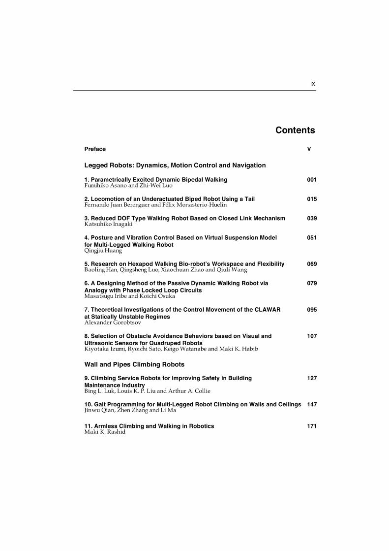
Contents
Preface V
Legged Robots: Dynamics, Motion Control and Navigation
1. Parametrically Excited Dynamic Bipedal Walking 001 Fumihiko Asano and Zhi-Wei Luo
2. Locomotion of an Underactuated Biped Robot Using a Tail 015 Fernando Juan Berenguer and Félix Monasterio-Huelin
3. Reduced DOF Type Walking Robot Based on Closed Link Mechanism 039 Katsuhiko Inagaki
4. Posture and Vibration Control Based on Virtual Suspension Model for Multi-Legged Walking Robot
051
Qingjiu Huang
5. Research on Hexapod Walking Bio-robot s Workspace and Flexibility 069 Baoling Han, Qingsheng Luo, Xiaochuan Zhao and Qiuli Wang
6. A Designing Method of the Passive Dynamic Walking Robot via Analogy with Phase Locked Loop Circuits
079
Masatsugu Iribe and Koichi Osuka
7. Theoretical Investigations of the Control Movement of the CLAWAR at Statically Unstable Regimes
095
Alexander Gorobtsov
8. Selection of Obstacle Avoidance Behaviors based on Visual and Ultrasonic Sensors for Quadruped Robots
107
Kiyotaka Izumi, Ryoichi Sato, Keigo Watanabe and Maki K. Habib
Wall and Pipes Climbing Robots
9. Climbing Service Robots for Improving Safety in Building Maintenance Industry
127
Bing L. Luk, Louis K. P. Liu and Arthur A. Collie
10. Gait Programming for Multi-Legged Robot Climbing on Walls and Ceilings 147 Jinwu Qian, Zhen Zhang and Li Ma
11. Armless Climbing and Walking in Robotics 171 Maki K. Rashid
X
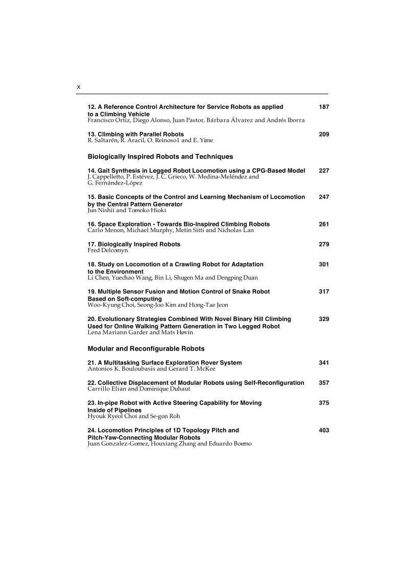
12. A Reference Control Architecture for Service Robots as applied to a Climbing Vehicle
187
Francisco Ortiz, Diego Alonso, Juan Pastor, Bárbara Álvarez and Andrés Iborra
13. Climbing with Parallel Robots 209 R. Saltarén, R. Aracil, O. Reinoso1 and E. Yime
Biologically Inspired Robots and Techniques
14. Gait Synthesis in Legged Robot Locomotion using a CPG-Based Model 227 J. Cappelletto, P. Estévez, J. C. Grieco, W. Medina-Meléndez and G. Fernández-López
15. Basic Concepts of the Control and Learning Mechanism of Locomotion by the Central Pattern Generator
247
Jun Nishii and Tomoko Hioki
16. Space Exploration - Towards Bio-Inspired Climbing Robots 261 Carlo Menon, Michael Murphy, Metin Sitti and Nicholas Lan
17. Biologically Inspired Robots 279 Fred Delcomyn
18. Study on Locomotion of a Crawling Robot for Adaptation to the Environment
301
Li Chen, Yuechao Wang, Bin Li, Shugen Ma and Dengping Duan
19. Multiple Sensor Fusion and Motion Control of Snake Robot Based on Soft-computing
317
Woo-Kyung Choi, Seong-Joo Kim and Hong-Tae Jeon
20. Evolutionary Strategies Combined With Novel Binary Hill Climbing Used for Online Walking Pattern Generation in Two Legged Robot
329
Lena Mariann Garder and Mats Høvin
Modular and Reconfigurable Robots
21. A Multitasking Surface Exploration Rover System 341 Antonios K. Bouloubasis and Gerard T. McKee
22. Collective Displacement of Modular Robots using Self-Reconfiguration 357 Carrillo Elian and Dominique Duhaut
23. In-pipe Robot with Active Steering Capability for Moving Inside of Pipelines
375
Hyouk Ryeol Choi and Se-gon Roh
24. Locomotion Principles of 1D Topology Pitch and Pitch-Yaw-Connecting Modular Robots
403
Juan Gonzalez-Gomez, Houxiang Zhang and Eduardo Boemo
XI
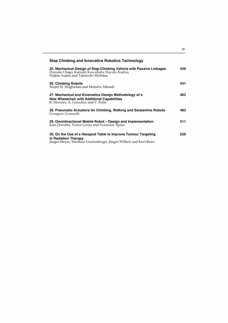
Step Climbing and Innovative Robotics Technology
25. Mechanical Design of Step-Climbing Vehicle with Passive Linkages 429 Daisuke Chugo, Kuniaki Kawabata, Hayato Kaetsu, Hajime Asama and Taketoshi Mishima
26. Climbing Robots 441 Majid M. Moghadam and Mojtaba Ahmadi
27. Mechanical and Kinematics Design Methodology of a New Wheelchair with Additional Capabilities
463
R. Morales, A. González and V. Feliu
28. Pneumatic Actuators for Climbing, Walking and Serpentine Robots 483 Grzegorz Granosik
29. Omnidirectional Mobile Robot – Design and Implementation 511 Ioan Doroftei, Victor Grosu and Veaceslav Spinu
30. On the Use of a Hexapod Table to Improve Tumour Targeting in Radiation Therapy
529
Jürgen Meyer, Matthias Guckenberger, Jürgen Wilbert and Kurt Baier

1
Parametrically Excited Dynamic Bipedal Walking
Fumihiko Asano1 and Zhi-Wei Luo1,2
1Bio-Mimetic Control Research Center, Riken, 2Kobe University Japan
1. Introduction
Human biped locomotion is an ultimate style of biological movement that is a highly evolved function. Biped locomotion by robots is a dream to be attained by the most highly evolved or integrated technology, and research on this has a history of over 30 years. Many methods of generating gaits have been proposed. There has been a tendency to reduce the complicated dynamics of a walking robot to a simple inverted pendulum (Hemami et al., 1973), and to control its motion according to pre-designed time-dependent trajectories while guaranteeing zero moment point (ZMP) conditions (Vukobratovi & Stepanenko, 1972). Although such approaches have successfully been applied to practical applications and nowadays successful biped-himanoids are developed by them, problems on gait performances still remain. Several advanced approaches on the other hand have taken the robot's dynamics into account for generating gaits based on natural dynamics. Miura and Shimoyama studied dynamic bipedal walking without ankle-joint actuation (Miura & Shimoyama, 1984) and they developed robots on stilts whose foot contact occurred at a point. Sano and Furusho accomplished natural dynamic biped walking based on angular momentum using ankle-joint actuation (Sano & Furusho, 1990). Kajita proposed a method of control based on a linear inverted pendulum model with a potential-energy-conserving orbit (Kajita et al., 1992). These approaches utilized the robot’s own dynamics effectively but did not investigate the energy-efficiency by introducing performance indices. It was unclear whether or not efficient gaits were generated. McGeer's passive dynamic walking (PDW) (McGeer, 1990) has provided clues to solve these problems. Passive-dynamic walkers can walk without any actuation on a gentle slope, and they provide an optimal solution to the problem of generating a natural and energy-efficient gait. The objective most expected to be met by PDW is to attain natural, high-speed energy-efficient dynamic bipedal walking on level ground like humans do. However, we need to supply power-input to the robot by driving its joint-actuators to continue stable walking on level ground, and certain methods of supplying power must be introduced. Ankle-joint torque is mathematically very important for effectively propelling the robot's center of mass (CoM) in the walking direction, and it is thus required relatively more often than other joint torques. However, to exert ankle-joint torque on a passive-dynamic walker, we need to add feet and this creates the ZMP constraint problem. We clarified that there is a trade-off between optimal gait and ZMP conditions through parametric studies, and
Bioinspiration and Robotics: Walking and Climbing Robots 2
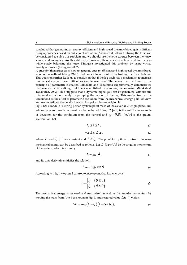
concluded that generating an energy-efficient and high-speed dynamic biped gait is difficult using approaches based on ankle-joint actuation (Asano et al., 2004). Utilizing the torso can be considered to solve this problem and we should use the joint torques between the torso, stance, and swing-leg. Another difficulty, however, then arises as to how to drive the legs while stably balancing the torso. Kinugasa investigated this problem by using virtual gravity approach (Kinugasa, 2002). A question then arises as to how to generate energy-efficient and high-speed dynamic biped locomotion without taking ZMP conditions into account or controlling the torso balance. This question further leads us to conclusion that if the leg itself has a mechanism to increase mechanical energy, these difficulties can be overcome. The answer can be found in the principle of parametric excitation. Minakata and Tadakuma experimentally demonstrated that level dynamic walking could be accomplished by pumping the leg mass (Minakata & Tadakuma, 2002). This suggests that a dynamic biped gait can be generated without any rotational actuation, merely by pumping the motion of the leg. This mechanism can be understood as the effect of parametric excitation from the mechanical energy point of view, and we investigate the detailed mechanical principles underlying it. Fig. 1 has a model of a swing-person system; point mass m has a variable-length pendulum
whose mass and inertia moment can be neglected. Here, θ [rad] is the anticlockwise angle
of deviation for the pendulum from the vertical and 9.81g = [m/s2] is the gravity
acceleration. Let
0 1l l l≤ ≤ , (1)
π θ π− ≤ ≤ , (2)
where 0l and 1l [m] are constant and 1 0l l≥ . The proof for optimal control to increase
mechanical energy can be described as follows. Let L [kg·m2/s] be the angular momentum of the system, which is given by
2L ml θ= , (3)
and its time derivative satisfies the relation
sinL mgl θ= − . (4)
According to this, the optimal control to increase mechanical energy is
( )( )
1
0
0
0
ll
lθθ
≤=
>. (5)
The mechanical energy is restored and maximized as well as the angular momentum by
moving the mass from A to E as shown in Fig. 1, and restored value EΔ [J] yields
( )( )1 0 01 cosE mg l l θΔ = − − , (6)
Parametrically Excited Dynamic Bipedal Walking 3
where 0θ [rad] is the deviation angle when 0θ = (at D and E positions). Lavrovskii and
Formalskii provide further details (Lavrovskii & Formalskii, 1993). In the following, we discuss how we applied this pumping mechanism to controlling the swing-leg of a planar telescopic-legged biped robot.
Figure 1. Swing-person system and optimal control to increase mechanical energy
2. Modelling Planar Telescopic-legged Biped
This section describes the mathematical model for the simplest planar biped robot with telescopic legs.
2.1 Dynamic equation
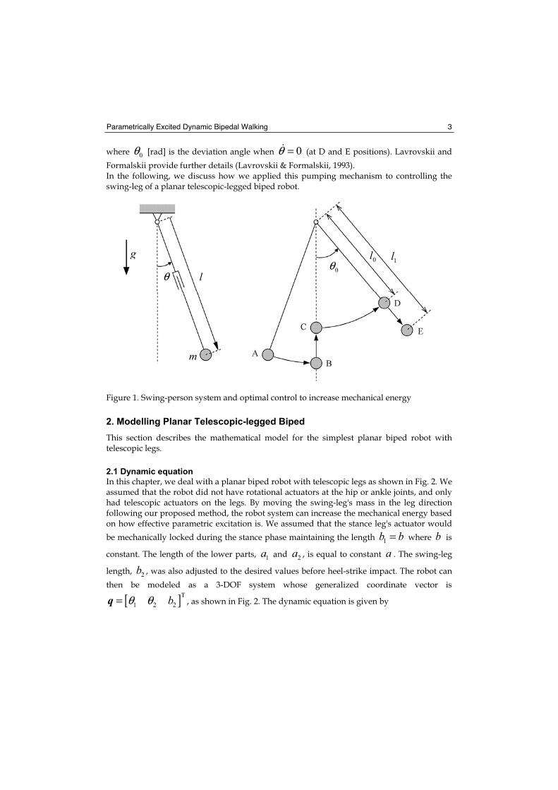
In this chapter, we deal with a planar biped robot with telescopic legs as shown in Fig. 2. We assumed that the robot did not have rotational actuators at the hip or ankle joints, and only had telescopic actuators on the legs. By moving the swing-leg's mass in the leg direction following our proposed method, the robot system can increase the mechanical energy based on how effective parametric excitation is. We assumed that the stance leg's actuator would
be mechanically locked during the stance phase maintaining the length 1b b= where b is
constant. The length of the lower parts, 1a and 2a , is equal to constant a . The swing-leg
length, 2b , was also adjusted to the desired values before heel-strike impact. The robot can
then be modeled as a 3-DOF system whose generalized coordinate vector is
[ ]T
1 2 2bθ θ=q , as shown in Fig. 2. The dynamic equation is given by
g
l
m
θ0θ 1l0l
Bioinspiration and Robotics: Walking and Climbing Robots 4
( ) ( , )+ =M q q h q q Su = u1
0
0. (7)
where ( ) 33×∈ RqM is the inertia matrix and ( ) 3Rqq,h ∈ is the vector for Coriolis,
centrifugal, and gravity forces. The u is the control input for the telescopic actuator on the
swing leg.
Figure 2. Model of planar telescopic legged biped with semicircular feet
Several past researchers have been considered the telescopic-leg mechanism in PDW. Although van der Linde introduced it as a compliance mechanism (van der Linde, 1998) and Osuka and Saruta adopted it to avoid foot-scuffing during the stance phase (Osuka & Saruta, 2000), its dynamics and effect on restoring mechanical energy have thus far not been investigated.
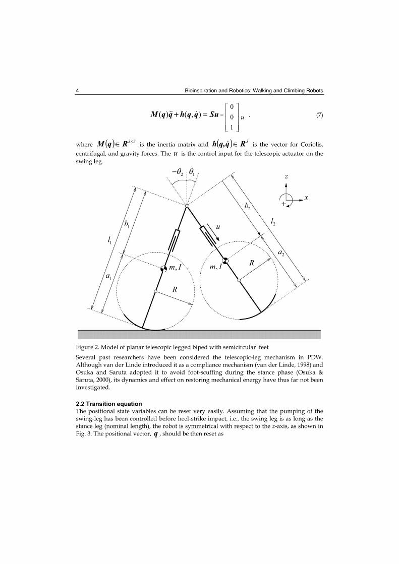
2.2 Transition equation
The positional state variables can be reset very easily. Assuming that the pumping of the swing-leg has been controlled before heel-strike impact, i.e., the swing leg is as long as the stance leg (nominal length), the robot is symmetrical with respect to the z-axis, as shown in Fig. 3. The positional vector, q , should be then reset as
1l
1b
1a
R
,m I ,m I R
2l
2b
2a
u
1θ2θ−
x
z
+
Parametrically Excited Dynamic Bipedal Walking 5
0 1 0
1 0 0
0 0 1
+ −=q q . (8)
The velocities, on the other hand, are reset according to the following algorithms by
introducing the extended generalized coordinate vector, 6Rq ∈ . The heel-strike collision
model can be modeled as
T( ) ( ) ( )I I+ −= −M q q M q q J q , (9)
4 1( )I+
×= 0J q q , (10)
where ( ) 64×∈ RqJ I is the Jacobian matrix derived following the geometric condition at
impact, 4RI ∈λ is Lagrange's undetermined multiplier vector within the context of
impulsive force, and Eq. (10) represents the post-impact velocity constraint conditions. The generalized coordinate vector in this case is defined as
T
1
T
2
,
i
i i
i
xzθ
= =q
q qq
. (11)
The inertia matrix, ( ) 66×∈ RqM , is derived according to q , and detailed as
1 1 3 3
3 3 2 2
( )( )
( )
×
×
=0
0
M qM q
M q, (12)
where the matrix, ( ) 33×∈ RqM ii , is the inertia matrix for leg i . Note + −= =q q q in
Eq. (9), and impulsive force vector I in Eq. (9) can be derived as
1 1 T, .I I I I I I− − −= =X J q X J M J (13)
By substituting Eq. (13) into (9), we obtain
( )1 T 1
6 I I I− − −= −+q I M J X J q . (14)
Semicircular feet have shock absorbing effect; they decrease mechanical energy dissipation caused by the impact of heel-strike. The authors theoretically investigated the detailed mechanism and clarified that there is a condition to decrease mechanical energy dissipation to zero when the foot radius is equal to the leg length (Asano & Luo, 2007). By utilizing this
Bioinspiration and Robotics: Walking and Climbing Robots 6
effect, the robot can effectively promote parametric excitation and increase the walking speed effectively.
2.3 Mechanical energy
The total mechanical energy, E [J], is defined by the sum of kinetic and potential energy as
T1( , ) ( ) ( )
2E P= +q q q M q q q , (15)
and its time derivative satisfies the relation
T
2E u b u= =q S . (16)
It remains constant with zero-input, or passive dynamic walking on a gentle slope. It should be steadily increased during the stance phase on level ground to restore the lost energy by every heel-strike collisions.
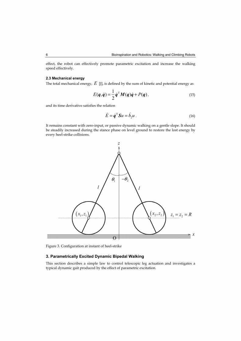
Figure 3. Configuration at instant of heel-strike
3. Parametrically Excited Dynamic Bipedal Walking
This section describes a simple law to control telescopic leg actuation and investigates a typical dynamic gait produced by the effect of parametric excitation.
l1θ 2θ−
x
z
l
1 2z z R= =( )1 1,x z ( )2 2,x z
O
Parametrically Excited Dynamic Bipedal Walking 7
3.1 Control law
A level gait can be generated by simply controlling pumping to the swing-leg. We propose output following control in this chapter to reproduce the parametric excitation mechanism in Fig. 1 by expanding and contracting the swing-leg length. We chose the telescopic length
of the swing-leg, T
2b = S q , as the system's output, and its second order derivative yields
T 1 T 1
2 ( ) ( ) ( , )b u− −= −S M q S S M q h q q . (17)
Let 2d ( )b t be the time-dependent trajectory for 2b , and the control input that exactly
achieves 2 2d ( )b b t≡ can be determined as
( ) ( )1T 1 T 1
2d( ) ( ) ( , )u b−− −= S M q S + S M q h q q . (18)
We give the control input in Eq. (18) as a continuous-time signal to enable the exact gait to be evaluated. Considering smooth pumping motion, we intuitively introduced a time-
dependent trajectory, 2d ( )b t , to enable telescopic leg motion:
( )
( )
3
set
set2d
set
sin ,( )
,
b A t t TTb t
b t T
π− ≤=
> (19)
where setT [s] is the desired settling-time, and where we assumed that setT would occur
before heel-strike collisions. In other words, let T [s] be the steady-step period, condition
setT T≥ should always hold. We called this the settling-time condition. Since ( )2d setb T is
not differentiable but continuous here, the control input, u , also becomes continuous.
3.2 Numerical simulations
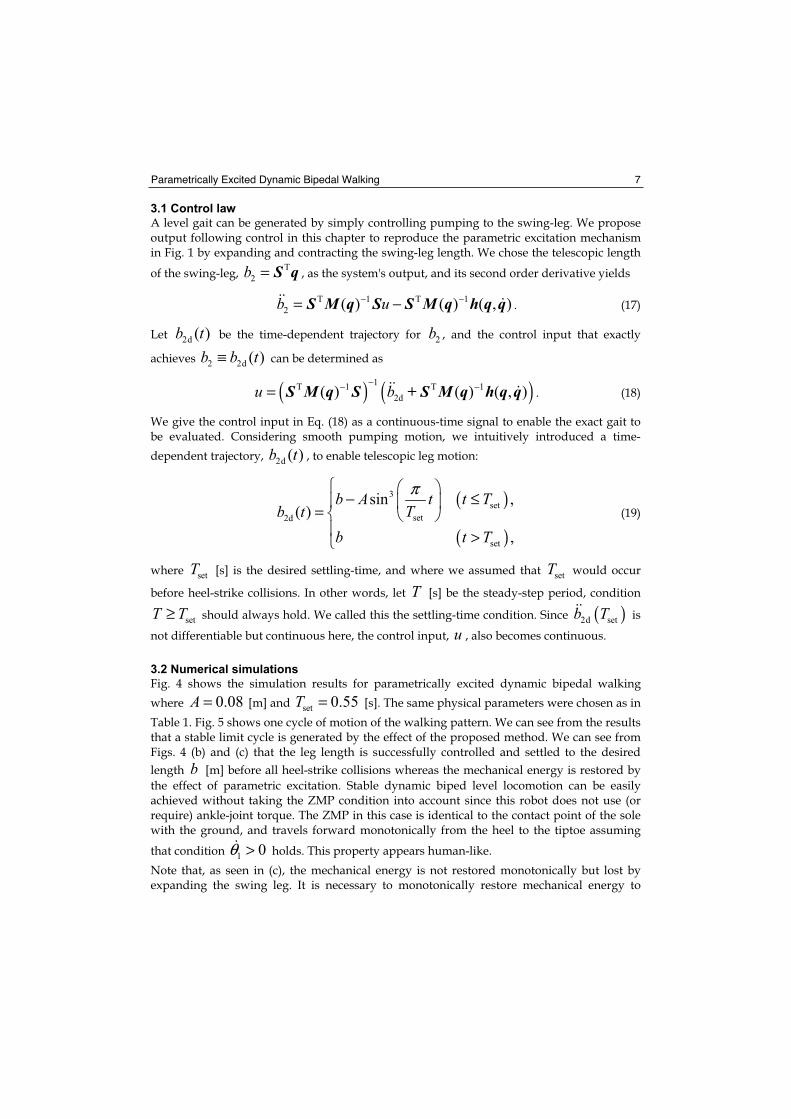
Fig. 4 shows the simulation results for parametrically excited dynamic bipedal walking
where 0.08A = [m] and set 0.55T = [s]. The same physical parameters were chosen as in
Table 1. Fig. 5 shows one cycle of motion of the walking pattern. We can see from the results that a stable limit cycle is generated by the effect of the proposed method. We can see from Figs. 4 (b) and (c) that the leg length is successfully controlled and settled to the desired
length b [m] before all heel-strike collisions whereas the mechanical energy is restored by
the effect of parametric excitation. Stable dynamic biped level locomotion can be easily achieved without taking the ZMP condition into account since this robot does not use (or require) ankle-joint torque. The ZMP in this case is identical to the contact point of the sole with the ground, and travels forward monotonically from the heel to the tiptoe assuming
that condition 1 0θ > holds. This property appears human-like.
Note that, as seen in (c), the mechanical energy is not restored monotonically but lost by expanding the swing leg. It is necessary to monotonically restore mechanical energy to
Bioinspiration and Robotics: Walking and Climbing Robots 8
obtain maximum efficiency (Asano et al., 2005), and how to improve this will be investigated in the next section.
Figure 4. Simulation results for parametrically excited dynamic bipedal walking where
0.08A = [m] and set 0.55T = [s]
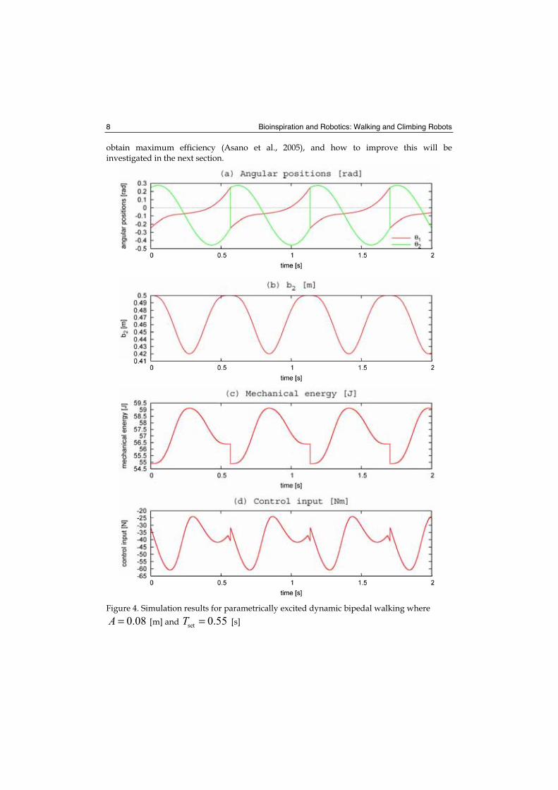
Parametrically Excited Dynamic Bipedal Walking 9
Figure 5. One cycle of motion for parametrically excited dynamic bipedal walking in Fig. 4
m 5.0 kg
I 0.1 2kg m⋅l a b= + 1.0 ma 0.5 mb 0.5 m
R 0.5 m
Table 1. Physical parameters of telescopic-legged biped robot in Fig. 2
4. Improvements in Energy-efficiency Using Elastic Element
Since the pumping motion of swing leg causes energy loss, as mentioned in Section 3, it leads to inefficient walking. This section therefore investigates improved energy-efficiency achieved by using an elastic element and adjusting its mechanical impedances.
4.1 Model with elastic elements
Telescopic leg actuation requires very large torque to raise the entire leg mass and this causes inefficient dynamic walking. The utilization of elastic elements should be considered to solve this problem. This section introduces a model with elastic elements and we analyze its effectiveness through numerical simulations.
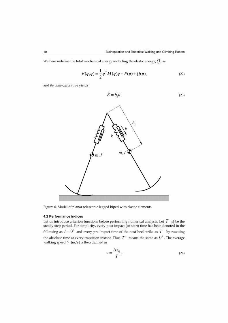
Fig. 6 outlines a biped model with elastic elements where 0k > is the elastic coefficient
and 0b is the nominal length. Its dynamic equation during the swing phase is given by
T( ) ( , )
Qu ∂+ = −∂
M q q h q q Sq
, (20)
where Q is the elastic energy defined as
( )2
2 0
1
2Q k b b= − . (21)
The other terms except for the elastic effect are the same as those in Eq. (7).
Bioinspiration and Robotics: Walking and Climbing Robots 10
We here redefine the total mechanical energy including the elastic energy, Q , as
T1( , ) ( ) ( ) ( )
2E P Q= + +q q q M q q q q , (22)
and its time-derivative yields
2E b u= . (23)
Figure 6. Model of planar telescopic legged biped with elastic elements
4.2 Performance indices
Let us introduce criterion functions before performing numerical analysis. Let T [s] be the steady step period. For simplicity, every post-impact (or start) time has been denoted in the
following as 0t += and every pre-impact time of the next heel-strike as T − by resetting
the absolute time at every transition instant. Thus T + means the same as 0+
. The average
walking speed v [m/s] is then defined as
GxvT
Δ= , (24)
,m I
u
,m I
2b
k
Parametrically Excited Dynamic Bipedal Walking 11
where Gx [m] is the x-position at the robot’s center of mass and
( ) ( )G G G 0x x T x− +Δ − [m] is the change in one step. The average input power is also
defined as
20
1d
Tp b u t
T
−
+= . (25)
Energy-efficiency is then evaluated by specific resistance /p Mgv [-], which means the
expenditure of energy per unit mass and per unit length, and this is a dimension-less quantity. The main question of how to attain energy-efficient biped locomotion rests on how to increase walking speed v while keeping p small.
4.3 Efficiency analysis
The control input, u , to exactly achieve 2 2db b≡ in this case is determined to cancel out
the elastic effect in Eq. (20) as
( ) 1T 1 T 1
2d T( ) ( ) ( , )
Qu b−− − ∂= +
∂S M q S + S M q h q q
q. (26)
This does not change walking motion regardless of the elastic element's mechanical impedances. Only the actuator's burden is adjusted. The maximum energy-efficiency
condition is then found in the combination of k and 0b that minimize the average input
power, p . The following relation holds for the definite integral of the absolute function to
calculate p ,
20 0
1 1d d
T T Ep b u t E tT T T
− −
+ +
Δ≥ = = , (27)
where ( ) ( )0E E T E− +Δ − [J] is the restored mechanical energy in one cycle, and it
should be positive if a stable gait is generated. Therefore, following Eqs. (24) and (27), we can obtain the relation
G
p EMgv Mg x
Δ≥Δ
. (28)
Where M 2m [kg] is the robot’s total mass. Here note that the equality holds in Eq. (27) if
and only if 2 0E b u= ≥ . This means that the monotonic restoration of mechanical energy
by control input is the necessary condition for maximum efficiency (Asano et al., 2005).
=Δ=
Δ=
Bioinspiration and Robotics: Walking and Climbing Robots 12
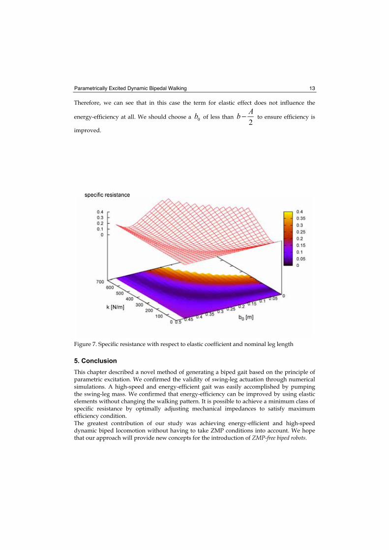
Fig. 7 shows the specific resistance with respect to k and 0b with its contours. There is an
optimal combination of k and 0b in the valley of the 3-D plot, and the specific resistance is
kept quite small at less than 0.04, which is much smaller than that of previous results (Gregorio et al., 1997). The gait obtained with optimal mechanical impedances is much faster than that with virtual passive dynamic walking at the same value for specific resistance. As previously mentioned, elastic effect increases the energy-efficiency without destroying the generated high-speed parametrically-excited gait. In such cases, total mechanical energy including elastic energy defined by Eq. (22) almost monotonically increases during a cycle, i.e., maximum efficiency condition is achieved. The optimal mechanical impedances, however, must be found by conducting numerical simulations.
The edges of the 3-D plot in Fig. 7 are lines where 0k = and 0 0.46b = with the same
value. The specific resistance where 0k = is of course kept constant regardless of 0b , i.e.,
the value without any power assist. On the other hand, 0 0.46b = [m] yields the same
efficiency as in the case of 0k = regardless of k . This can be explained as follows. Eq. (26)
can be expressed as
( )0 2 0u u k b b= + − , (29)
where 0u is the same as u in Eq. (18). The sign of u is always negative when
02
Ab b= − , thus that of 2E b u= is equivalent to that of 2b− . The input power integral
can then be divided as follows.
( )( ) ( )( )
set set
set
set set
set
/ 2
2 2 20 0 / 2
/ 2
2 0 2 0 2 0 2 00 / 2
d d d
d d .
T T T
T
T T
T
b u t b u t b u t
b u k b b t b u k b b t
−
+ +
+
= −
= + − − + − (30)
Here the following relations hold.
( ) ( )
( ) ( )
2 0set
2 0
2 0set
set2 0
2/ 2 2
2 2 0 2 00
2
22
2 2 0 2 0/ 2
2
1d 0
2
1d 0
2
Ab bT
Ab b
Ab bT
T Ab b
b k b b t k b b
b k b b t k b b
+
= −
= +
= +
= −
− = − =
− = − =
(31)
Parametrically Excited Dynamic Bipedal Walking 13
Therefore, we can see that in this case the term for elastic effect does not influence the
energy-efficiency at all. We should choose a 0b of less than 2
Ab − to ensure efficiency is
improved.
Figure 7. Specific resistance with respect to elastic coefficient and nominal leg length
5. Conclusion
This chapter described a novel method of generating a biped gait based on the principle of parametric excitation. We confirmed the validity of swing-leg actuation through numerical simulations. A high-speed and energy-efficient gait was easily accomplished by pumping the swing-leg mass. We confirmed that energy-efficiency can be improved by using elastic elements without changing the walking pattern. It is possible to achieve a minimum class of specific resistance by optimally adjusting mechanical impedances to satisfy maximum efficiency condition. The greatest contribution of our study was achieving energy-efficient and high-speed dynamic biped locomotion without having to take ZMP conditions into account. We hope that our approach will provide new concepts for the introduction of ZMP-free biped robots.
Bioinspiration and Robotics: Walking and Climbing Robots 14
6. References
Asano, F., Luo, Z.W. & Yamakita, M. (2005). Biped gait generation and control based on a unified property of passive dynamic walking, IEEE Transactions on Robotics, Vol.21, No.4, pp.754--762, Aug. 2005.
Asano, F., Luo, Z.W. & Yamakita, M. (2004). Unification of dynamic gait generation methods via variable virtual gravity and its control performance analysis, Proc. of the IEEE/RSJ Int. Conf. on Intelligent Robots and Systems (IROS), pp.3865--3870, Oct. 2004.
Asano, F & Luo, Z.W. (2007). The effect of semicircular feet on energy dissipation by heel-strike in dynamic biped locomotion, Proc. of the IEEE Int. Conf. on Robotics and Automation (ICRA), pp. 3976--3981, Apr. 2007.
Gregorio, P., Ahmadi, M. & Buehler, M. (1997). Design, control, and energetics of an electrically actuated legged robot, IEEE Trans. on Systems, Man and Cybernetics--Part B: Cybernetics, Vol.27, No.4, pp.626--634, Aug. 1997.
Hemami, H., Weimer, F.C. & Koozekanani, S.H. (1973). Some aspects of the inverted pendulum problem for modeling of locomotion systems, IEEE Trans. on Automatic Control, Vol.18, No.6, pp.658--661, Dec. 1973.
Kajita, S., Kobayashi, A. & Yamaura, T. (1992). Dynamic walking control of a biped robot along a potential energy conserving orbit, IEEE Trans. on Robotics and Automation,Vol.8, No.4, pp.431--438, Aug. 1992.
Kinugasa, T. (2002). Biped walking of Emu based on passive dynamic walking mechanism, Proc. of the ICASE/SICE Workshop –Intelligent Control and Systems, pp.304--309, Oct. 2002.
McGeer, T. (1990). Passive dynamic walking, Int. J. of Robotics Research, Vol.9, No.2, pp.62--82, Apr. 1990.
Miura, H. & Shimoyama, I. (1984). Dynamic walk of a biped, Int. J. of Robotics Research, Vol.3, No.2, pp.60--74, Apr. 1984.
Lavrovskii E.K. & Formalskii, A.M. (1993). Optimal control of the pumping and damping of a swing, J. of Applied Mathematics and Mechanics, Vol.57, No.2, pp.311--320, 1993.
van der Linde, R.Q. (1998). Active leg compliance for passive walking, Proc. of the IEEE Int. Conf. on Robotics and Automation (ICRA), Vol.3, pp.2339--2345, May 1998.
Minakata, H. & Tadakuma, S. (2002). An experimental study of passive dynamic walking with non-rotate knee joint biped, Proc. of the ICASE/SICE Workshop --Intelligent Control and Systems, pp.298--303, Oct. 2002.
Osuka K. & Saruta, Y. (2000). Development and control of new legged robot Quartet III -- From active walking to passive walking, Proc. of the IEEE/RSJ Int. Conf. on Intelligent Robots and Systems (IROS), Vol.2, pp.991--995, Oct. 2000.
Sano, A. & Furusho, J. (1990). Realization of natural dynamic walking using the angular momentum information, Proc. of the IEEE Int. Conf. on Robotics and Automation (ICRA), Vol.3, pp.1476--1481, May 1990.
2
Locomotion of an Underactuated Biped Robot Using a Tail
Fernando Juan Berenguer and Félix Monasterio-Huelin Universidad Europea de Madrid, Universidad Politécnica de Madrid
Spain
1. Introduction
At the present there exist a high number of commercial biped robots, generally humanoids, used within the area of service robotics, mainly in the field of exhibition and entertainment (Ambrose et al., 2006; Wahde & Pettersson, 2002). One of the main problems of these robots is their high power and energy consumption, which limits mainly their autonomy. It could be attributed to, for example, the high number of actuated joints (about 20), and also because the study of energy consumption is not often considered during the planning of movements. In addition, these systems require high precision in their motions and high frequency response. In order to solve these important problems there exist various solutions not used yet commercially, which are mainly based on the use of passive joints, thus reducing the number of actuated joints (Alexander, 2005; Collins et al., 2005; Kuo, 1999). The consumption of these systems is better optimized, although their control and planning require more complex schemes for the accomplishment of certain complex trajectories. The main aim of our research is the design of biped robots with passive joints that require low energy consumption. In particular our work is centred on the one hand, in studying the advantages and disadvantages of considering a tail as the main element that generates the motion, and on the other hand, in trying to reduce the energy consumption in two ways, by means of generating a smooth contact between the feet and the ground, with minimum loss of energy, and by using a spring mechanism to reduce the mechanical energy needed to obtain the oscillating motion of the tail. In addition, our present work focuses on the study of a biped mechanism of a simple design and construction, able to walk using only a single actuated joint. This is a low cost system, and its easy design and construction make it interesting for commercial and educational applications.
2. About passive bipeds and bipeds with a tail
The interaction between morphology and control is in the centre of the more recent research and debates in robotics. The main question is how to design a robot that exhibit a repertoire of behaviours. In the field of walking robots there are two main extreme approaches. Oldest focused on the intrinsic properties of the robot, leaving into the hands of control the task of achieving the desired movements. The more recent takes into account as a guiding principle, the
Bioinspiration and Robotics: Walking and Climbing Robots 16
interaction with the environment in a cooperative manner. Both approaches have at the present, open and unresolved questions and problems. The main characteristic of (biped) walkers is the abrupt kinematic change between the aerial phase and the support phase. The main problem is how to achieve a rhythmical walk. Control centred approaches must generate exact trajectories to guide the robot from one to the next support, taking into account the stability region of the aerial phase. Normally the considered region is a pressure region which has a fictitious point (the Zero Moment Point, ZMP (Vukobratovic, 1969)) on the ground plane where the torques around the axes that define this plane are equal to zero. Expanding the ZMP concept to running biped robots is the natural continuation of this approach (Kajita et al., 2007). The discovery of self-stabilizing dynamic properties of passive mechanisms by McGeer (McGeer, 1990), opens the doors to the environmental (or dynamic) approach: a simple mechanism which can walk down a slope without control nor actuation. He takes into account the terrestrial gravity as the only interaction with the world, imposing two main principles: the conservation of mechanical energy and the conservation of angular momentum in the contact instant of the leg with the ground. From the second we obtain a constraint equation that, added to the dynamical equation, gives strict initial conditions for joint positions and joint velocities to achieve a stable walk. The result is a periodic gait: a limit cycle. Numerous biped robots have been developed following this property (Collins et al., 2005), showing the noteworthy energetic efficiency in contrast to the ZMP approach (Gomes & Ruina, 2005). This approach is related with those that make an explicit use of the behaviour emergence from the interaction of body and environment, that is, those that consider the self-organizing properties of the nature. Behaviour-based robotic is an important engineering example (Pfeifer & Scheier, 1999) to understand sensory-motor coordination, or in general the perception-action relation. How to exploit the above-mentioned passive properties of biped robots with the incorporation of sensors is studied in (Iida & Pfeifer, 2006). In order to close this brief review, we need to mention biped robots with a tail. Almost none of the robots of this type make of the tail a functional element, but there are some exceptions. For example in (Takita et al., 2003) the tail and the neck are designed with the objective of stabilizing the robot walks.
3. Mechanism model and gait description
In this section the proposed model of the biped mechanism and the way it performs a gait are presented. We show the evolution of the kinematic model indicating its components and parameters, and we explain how this system is able to walk using only one actuator that moves a tail in an oscillating way.
3.1 Mechanism model
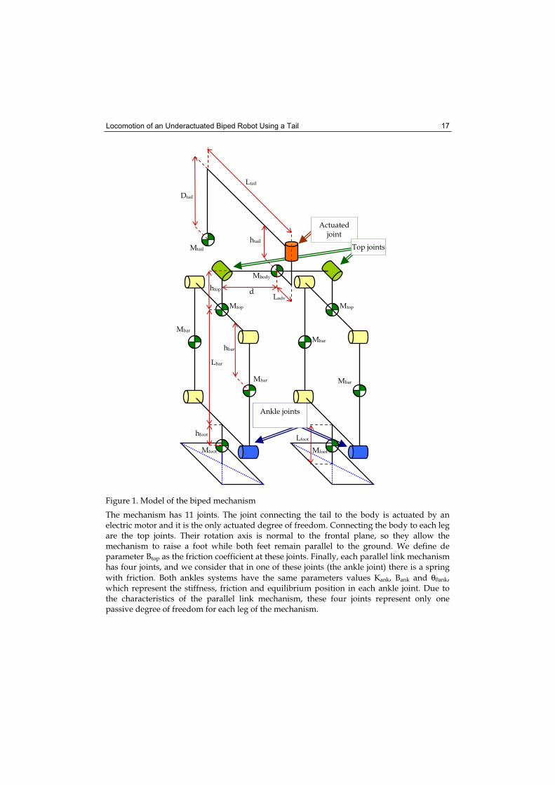
The walking mechanism consists of a light body, a tail connected to it, and two legs. Each leg is formed by a parallel link mechanism and a flat rectangular foot. The tail, with an almost horizontal displacement, works as a counterbalance and controls the movement of the biped. The kinematic model of the system is shown in Fig. 1 and it is a 3D biped model. This figure displays the masses of each independent link, and the main lengths involved in the design. We don’t consider in this work the link inertial moments for reducing the expression’s complexity and required parameters definition.
Locomotion of an Underactuated Biped Robot Using a Tail 17
Figure 1. Model of the biped mechanism
The mechanism has 11 joints. The joint connecting the tail to the body is actuated by an electric motor and it is the only actuated degree of freedom. Connecting the body to each leg are the top joints. Their rotation axis is normal to the frontal plane, so they allow the mechanism to raise a foot while both feet remain parallel to the ground. We define de parameter Btop as the friction coefficient at these joints. Finally, each parallel link mechanism has four joints, and we consider that in one of these joints (the ankle joint) there is a spring
with friction. Both ankles systems have the same parameters values Kank, Bank and θ0ank,which represent the stiffness, friction and equilibrium position in each ankle joint. Due to the characteristics of the parallel link mechanism, these four joints represent only one passive degree of freedom for each leg of the mechanism.
Mtail
Ltail
htail
Ladvd
Mbody
Mtop
Mbar
Mtop
Mbar
Mfoot Mfoot
Mbar
Mbar
htop
Lbar
hfoot
hbar
Lfoot
Actuated joint
Top joints
Ankle joints
Dtail
Bioinspiration and Robotics: Walking and Climbing Robots 18
In summary, the model has four passive degrees of freedom and one actuated degree of freedom.
3.2 Gait description
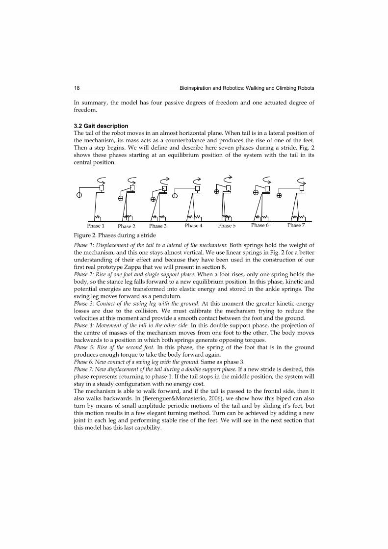
The tail of the robot moves in an almost horizontal plane. When tail is in a lateral position of the mechanism, its mass acts as a counterbalance and produces the rise of one of the feet. Then a step begins. We will define and describe here seven phases during a stride. Fig. 2 shows these phases starting at an equilibrium position of the system with the tail in its central position.
Figure 2. Phases during a stride
Phase 1: Displacement of the tail to a lateral of the mechanism: Both springs hold the weight of the mechanism, and this one stays almost vertical. We use linear springs in Fig. 2 for a better understanding of their effect and because they have been used in the construction of our first real prototype Zappa that we will present in section 8. Phase 2: Rise of one foot and single support phase. When a foot rises, only one spring holds the body, so the stance leg falls forward to a new equilibrium position. In this phase, kinetic and potential energies are transformed into elastic energy and stored in the ankle springs. The swing leg moves forward as a pendulum. Phase 3: Contact of the swing leg with the ground. At this moment the greater kinetic energy losses are due to the collision. We must calibrate the mechanism trying to reduce the velocities at this moment and provide a smooth contact between the foot and the ground. Phase 4: Movement of the tail to the other side. In this double support phase, the projection of the centre of masses of the mechanism moves from one foot to the other. The body moves backwards to a position in which both springs generate opposing torques. Phase 5: Rise of the second foot. In this phase, the spring of the foot that is in the ground produces enough torque to take the body forward again. Phase 6: New contact of a swing leg with the ground. Same as phase 3. Phase 7: New displacement of the tail during a double support phase. If a new stride is desired, this phase represents returning to phase 1. If the tail stops in the middle position, the system will stay in a steady configuration with no energy cost. The mechanism is able to walk forward, and if the tail is passed to the frontal side, then it also walks backwards. In (Berenguer&Monasterio, 2006), we show how this biped can also turn by means of small amplitude periodic motions of the tail and by sliding it’s feet, but this motion results in a few elegant turning method. Turn can be achieved by adding a new joint in each leg and performing stable rise of the feet. We will see in the next section that this model has this last capability.
Phase 1 Phase 2 Phase 3 Phase 4 Phase 5 Phase 6 Phase 7
Locomotion of an Underactuated Biped Robot Using a Tail 19
4. Necessary conditions for generating the gait
At low stride frequencies, basically the mechanism walks if it is able to rise its feet, move forward its body, and maintain its centre of gravity (CoG) into the support area. So, in this section we analyze the necessary conditions to reach these three characteristics. These conditions allow designing the tail in order to obtain a stable rise of the feet, and on the other hand, they establish the procedure for selecting the ankle parameters of the system to obtain the advance of the robot. The displacement of the system’s CoG will be also introduced in this section because it determines the necessary support area during walking and therefore the required minimum size of the feet. We will consider static and quasi-static cases, we mean, we will not consider the velocities effects or overshoots in oscillating motions, so the conclusions are valid at low velocities and for over-damped spring systems.
4.1 Design of the tail for a stable rise of the foot
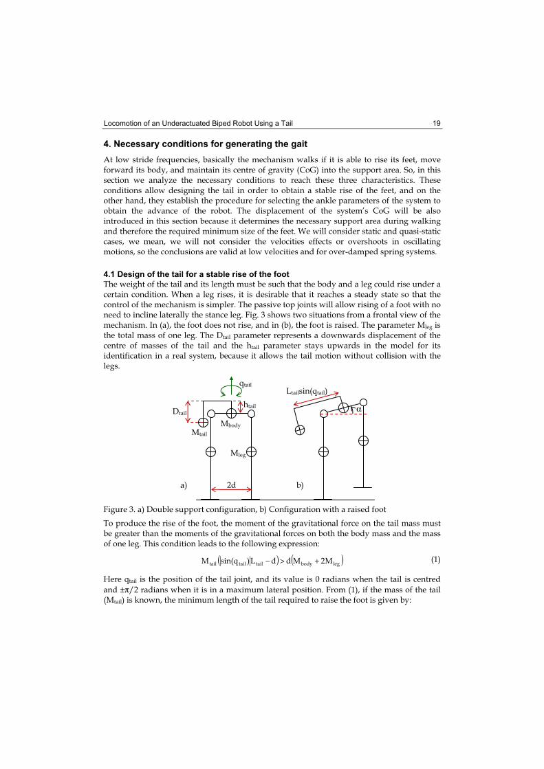
The weight of the tail and its length must be such that the body and a leg could rise under a certain condition. When a leg rises, it is desirable that it reaches a steady state so that the control of the mechanism is simpler. The passive top joints will allow rising of a foot with no need to incline laterally the stance leg. Fig. 3 shows two situations from a frontal view of the mechanism. In (a), the foot does not rise, and in (b), the foot is raised. The parameter Mleg is the total mass of one leg. The Dtail parameter represents a downwards displacement of the centre of masses of the tail and the htail parameter stays upwards in the model for its identification in a real system, because it allows the tail motion without collision with the legs.
Figure 3. a) Double support configuration, b) Configuration with a raised foot
To produce the rise of the foot, the moment of the gravitational force on the tail mass must be greater than the moments of the gravitational forces on both the body mass and the mass of one leg. This condition leads to the following expression:
( ) ( )legbodytailtailtail M2MddL)qsin(M +>− (1)
Here qtail is the position of the tail joint, and its value is 0 radians when the tail is centred
and ±π/2 radians when it is in a maximum lateral position. From (1), if the mass of the tail (Mtail) is known, the minimum length of the tail required to raise the foot is given by:
Mbody
Mleg
Mtail
qtail
2d
Ltailsin(qtail)
αhtailDtail
a) b)
Bioinspiration and Robotics: Walking and Climbing Robots 20
++=
tail
legbody
tailM
M2M1dL (2)
When condition (1) is satisfied, if the body has an inclination angle α, and the joint of the tail is in a fixed position (qtail), the moments at the top joint due to the tail and the body&leg set are respectively:
( )( )( ) )cos(gdM2MMt
)cos()dL)qsin(()sin(DhgMMt
legbodyleg&body
tailtailtailtailtailtail
α+=α−+α−= (3)
Using (1), we deduce that if htail>Dtail, then Mttail>Mtbody&leg for any inclination α, and therefore the system is in an unstable configuration. We analysed this case in (Berenguer&Monasterio, 2006), and it was necessary to use an adjustable friction coefficient Btop in the top joints for controlling the biped movements.
If htail<Dtail, then there exists an inclination α0, so that Mttail=Mtbody&leg, and if there is friction
in the top joints, α0 represents a stable equilibrium inclination angle of the body.
From (3) the Dtail value needed for a desired α0, when the tail is fixed in a position qtail, is given by:
( ))(tgM
L)qsin(MdMM2MhD
0tail
tailtailtailtaillegbody
tailtail α−++
−= (4)
Some of the important advantages that using a stable inclination angle provides are the following ones:
• We can consider the top joints as passive joints with negligible friction. In the theoretical model and simulations, a parameter in the design disappears, since now we consider the friction in the top joints negligible (Btop 0).
• The inclination of the body depends now on the position of the tail and goes through successive stable states.
• The length of a single support phase is not limited in time. It allows the system to remain with a foot raised during an indefinite time.
• The yaw turn of the mechanism can be reached during a single support phase by adding new joints in the feet or the hip of the mechanism.
• It is possible to vary the speed of advance in a stable form by changing the oscillation frequency of the tail, with no need to consider the length of the single support phase.
4.2 Design of the springs and friction at the ankle joints
If the ankles equilibrium position (θ0ank) is zero and stable, then, when the mechanism rise a foot due to slow tail oscillation, the body and the legs don’t move in the forward direction and the mechanism doesn’t advance. It is necessary that the ankle equilibrium position will be different from zero in this case. Afterwards, in section 5, we will see that at higher tail oscillation frequencies, the tail produces a force in the X direction over the body that
generates the body oscillation and allows the system to walk even with θ0ank equals to zero. We present now a theoretical approach for the selection of the parameters that define the springs and friction at the ankle joints of the mechanism. For this purpose we analyze the configuration of the system at the moment of contact between the foot in the air and the
Locomotion of an Underactuated Biped Robot Using a Tail 21
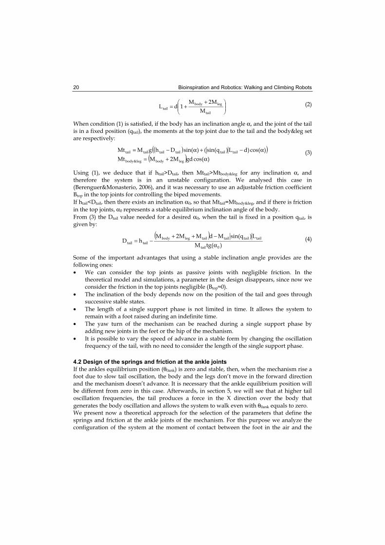
ground, that is, phases 3 and 6 shown in Figure 2. If this configuration is an equilibrium state for both legs, and is reached without overshoot at the moment at which the inclination velocity of the body is null, then the kinetic energy losses in the collision will be minimum. In order to obtain simple expressions for the design, we consider the system decoupled into two parts: The swing leg as a pendulum with parallel links (Figure 4.a), and the stance leg as a parallel link system fixed to the ground (Figure 4.b).
Figure 4. (a) Pendulum model, (b) parallel link system model
The angles θa and θb in Figure 4 are the generalized coordinates that represent the degree of freedom of each system. We suppose that the joint where the angle is showed in both systems, is the ankle joint of each leg, and a spring with friction exists which generates a
torque τ following a classic linear model, given by expression (5). In this expression θ is the
position of the joint, θ0ank is the equilibrium position of the spring, Kank is the spring constant, and Bank is the friction coefficient.
θ−θ−θ−=τ ankank0ank B)(K (5)
The equations of motion that we obtain for these two systems, and the values that we assign
to angles θa and θb, based on the desired step length, will allow us to select the spring parameters.We use the Euler-Lagrange method to derive the equations of motion. For the system in Figure 4.a, Kinetic energy Ta and potential energy Va (with respect to the position of the foot
when θa=0rad) are given by:
2aa
2aa,bar
22bar
21foota J
2
1JvMvM
2
1T θ=θ++= (6)
( ) ( ))cos(GC
h)cos(LhgM2L)cos(1gMV
aaa
barabarfootbarbarafoota
θ−==θ−++θ−= (7)
In (6), v1 and v2 are the magnitude of vectors v1 and v2 shown in the Figure 4.a. Jbar,a is the moment of inertia of each vertical parallel bar, with respect to the rotation axis of a lower joint. We have defined for greater clarity the constants Ja, Ga and Ca, and their values are:
M1
Mbar
θb
Mbar
v2
h1
Mfoot
Lbarθa
hfoot
hbar
v1
v1
a) b)
Bioinspiration and Robotics: Walking and Climbing Robots 22
)Lh(gM2gLMC
ghM2gLMG
J2hM2LMJ
barfootbarbarfoota
barbarbarfoota
a,bar2barbar
2barfoota
++=+=
++= (8)
In the same way, the energies for the system in Figure 4.b are:
2bb
2bb,bar
2b
2barbarbar
2b
2bar1b J
2
1J)hL(MLM
2
1T θ=θ+θ−+θ= (9)
( ))cos(GC
)cos()hL(gM2)cos(LhgMV
bbb
bbarbarbarbbar11b
θ+==θ−+θ+=
(10)
Where,
11b
barbarbarbar1b
b,bar2
barbarbar2bar1b
legtopbodytail1
ghMC
)hL(gM2gLMG
J2)hL(M2LMJ
MMMMM
=−+=
+−+=
+++=
(11)
The parameter h1 is the height of the mass M1 relative to the upper joints, and since it does not affect the behaviour of the system, we do not calculate its value here. Now, Jbar,b is the moment of inertia of each parallel bar, with respect to the rotation axis of an upper joint. Applying the Euler-Lagrange equation to the lagrangian (L = T - V) in each case, and using (5), we obtain the equations of motion for these systems:
aankank0aankaaaa B)(K)sin(GJ θ−θ−θ−=θ+θ (12)
bankank0bankbbbb B)(K)sin(GJ θ−θ−θ−=θ−θ (13)
If both systems are in an equilibrium configuration, the two following equations will be fulfilled together:
0)sin(G)(K aaank0aank =θ+θ−θ (14)
0)sin(G)(K bbank0bank =θ−θ−θ (15)
Once fixed the values of θa and θb, we calculate the values of Kank and θ0ank for the springs with the next equations:
ab
bbaaank
)sin(G)sin(GK
θ−θθ+θ= (16)
)sin(K
Gb
ank
bbank0 θ−θ=θ (17)
For obtaining a θ0ank value different from zero, θa must be a small negative angle different
from zero, -0.01rad for example. Once selected θa, the relation between the step length (Lstep)
and the necessary angle θb is given by:
Locomotion of an Underactuated Biped Robot Using a Tail 23
θ−−=θ )sin(L
Larcsin a
bar
step
b (18)
Finally, if we linearize equation (13), and compare the result with a second order system equation, we find that the necessary value of Bank to obtain critical damping is:
bbankank J)GK(2B −= (19)
When the contact takes place, the top joints of the legs will be at different height and the
body will have an inclination α (defined in Figure 3.b). The minimum inclination module
|αmin| that the body must reach for obtaining a desired configuration at contact instant is given by Equation (20).
( )θ−θ=αd2
)cos()cos(Larcsin babar
min (20)
4.3 Approximation of the Center of Gravity projection trajectory
In this quasi-static study, we can obtain an estimation of the necessary support area during walking, and the minimum required feet size, by means of approximating the Centre of Gravity (CoG) projection trajectory instead of the Zero Moment Point (ZMP) trajectory. For this approximation we will assume that the tail moves side to side only when the body is in a central position between both feet, during a double support phase (Phase 4 in figure
2), and the tail stands in a lateral position (qtail=±π/2) the rest of time, during the double and single support phases (Phases 5 and 6 in figure 2). For additional simplicity, we assume that legs and feet are massless, and the body center of masses is located at the tail-joint axis. In the first case, because only the tail mass moves, the CoG describes a circumference arc with radius R1 given by:
tailtotal
tail1 L
M
MR = (21)
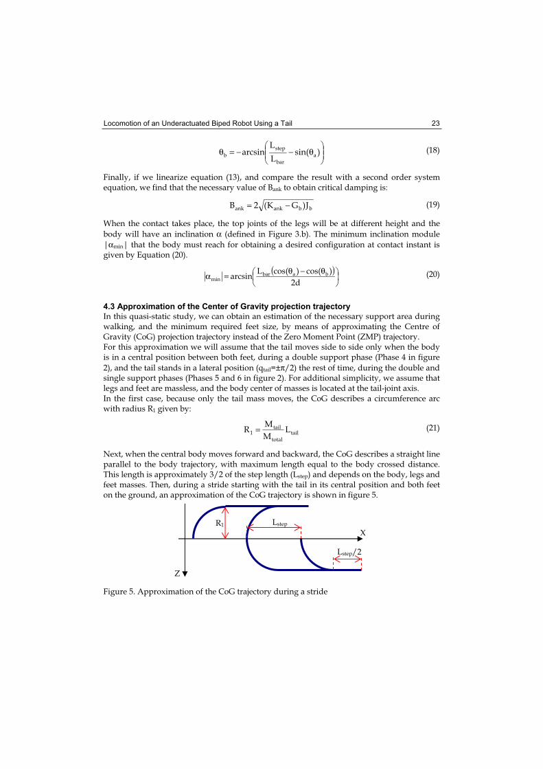
Next, when the central body moves forward and backward, the CoG describes a straight line parallel to the body trajectory, with maximum length equal to the body crossed distance. This length is approximately 3/2 of the step length (Lstep) and depends on the body, legs and feet masses. Then, during a stride starting with the tail in its central position and both feet on the ground, an approximation of the CoG trajectory is shown in figure 5.
Figure 5. Approximation of the CoG trajectory during a stride
X
Z
R1 Lstep
Lstep/2
Bioinspiration and Robotics: Walking and Climbing Robots 24
The required length of the feet in the X direction is given by R1+3/2Lstep and the distance between the outside of the feet must be at least 2R1. We can establish that this biped mechanism needs a relatively large support area and feet length that depends mainly on the tail length and mass, and on the desired step length.
5. Study of the system behaviour with oscillation frequency variation
This section focuses on studying the effect of increasing the oscillation frequency that allows the mechanism to increase its speed. We will see how the conditions of the previous section are modified by means of analyzing a simpler system, a horizontal pendulum with rotational actuated joint.
5.1 ZMP trajectory and generated forces at the tail joint axis
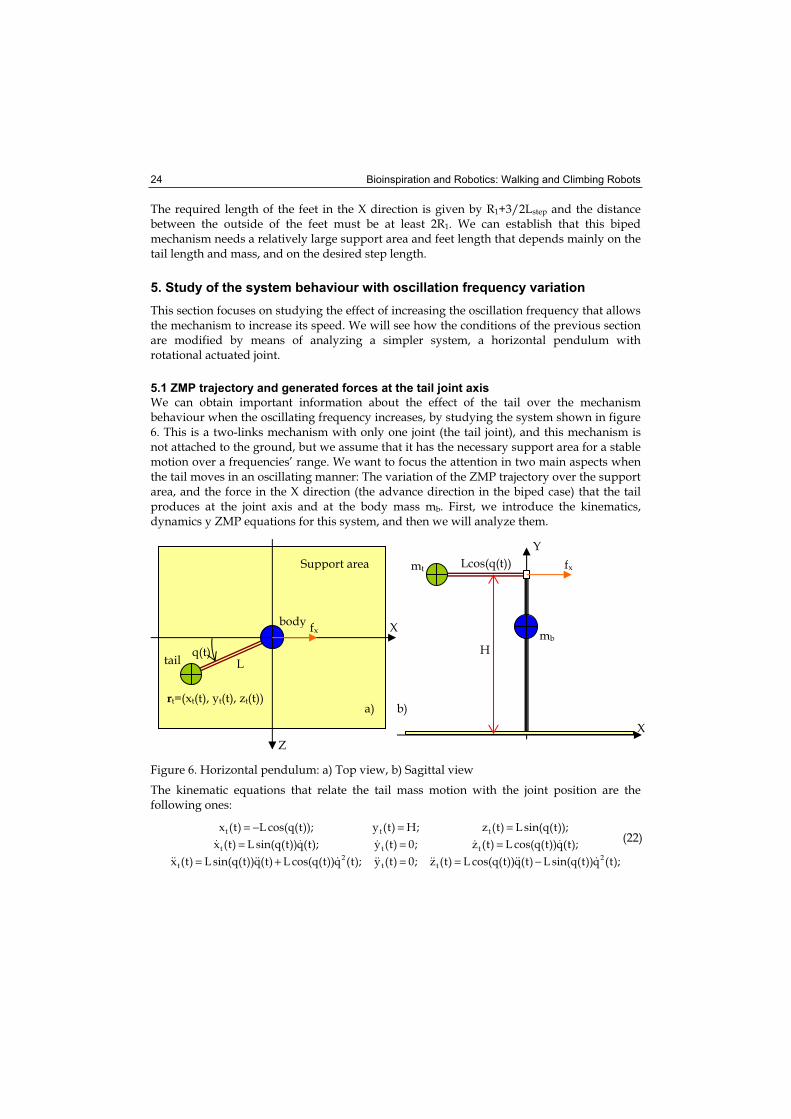
We can obtain important information about the effect of the tail over the mechanism behaviour when the oscillating frequency increases, by studying the system shown in figure 6. This is a two-links mechanism with only one joint (the tail joint), and this mechanism is not attached to the ground, but we assume that it has the necessary support area for a stable motion over a frequencies’ range. We want to focus the attention in two main aspects when the tail moves in an oscillating manner: The variation of the ZMP trajectory over the support area, and the force in the X direction (the advance direction in the biped case) that the tail produces at the joint axis and at the body mass mb. First, we introduce the kinematics, dynamics y ZMP equations for this system, and then we will analyze them.
Figure 6. Horizontal pendulum: a) Top view, b) Sagittal view
The kinematic equations that relate the tail mass motion with the joint position are the following ones:
);t(q))t(qsin(L)t(q))t(qcos(L)t(z;0)t(y);t(q))t(qcos(L)t(q))t(qsin(L)t(x
);t(q))t(qcos(L)t(z;0)t(y);t(q))t(qsin(L)t(x
));t(qsin(L)t(z;H)t(y));t(qcos(L)t(x
2tt
2t
ttt
ttt
−==+====
==−=(22)
X
Z
q(t)
rt=(xt(t), yt(t), zt(t))
body
tail
Support area
L
fx
X
mb
mt
Y
Lcos(q(t)) fx
H
a) b)
Locomotion of an Underactuated Biped Robot Using a Tail 25
We obtain the dynamic equation by means of Newton-Euler Method. These equations provide the force f(t) that the tail exerts over the joint axis and body mass, and on the other
hand, the needed joint torque τ(t) to produce a desired trajectory q(t).
[ ]
[ ]−
+−=−==
)t(q))t(qsin()t(q))t(qcos(L
g
)t(q))t(qcos()t(q))t(qsin(L
m
)t(z
g
)t(x
m
)t(f
)t(f
)t(f
)t(2
2
t
t
t
t
z
y
x
f (23)
)t(q)LmI())t(z)t(x)t(x)t(z(m)t(qIm)t(qI 2ttyttttttytttty +=−+=×+=τ rr (24)
Parameters mt and Ity are the tail mass and Y-component of the inertial moment respectively. The total mass of this system is M=mt+mb, and the CoG is given by:
[ ]Tt ))t(qsin(0))t(qcos(M
Lm −=cog (25)
The general expression for the ZMP for an n-link system is (Vukobratovic et al., 1990):
( )( )( )
( )( )( )
=
=
=
=
+
ω−−+=
+
ω−−+=
n
1i ii
n
1i ixixiiiii
zn
1i ii
n
1i iziziiiii
xgym
Izygyzmzmp;
gym
Ixygyxmzmp (26)
In the case of our simple pendulum, the ZMP vector is reduced to the expression 27, and we can see that it depends on three terms: a gravitational term, a centripetal term and an inertial term.
−−
+=−
−=
))t(qcos(
0
))t(qsin(
)t(qH
))t(qsin(
0
))t(qcos(
))t(qg(Mg
Lm
zygz
0
xygx
Mg
m 2tt
ttt
ttt
tzmp (27)
We analyze now these magnitudes when the mass mt moves from one side of X axis to the
other one. We consider that q(t) oscillates between the values of –π/2 and π/2, given this trajectory by a periodic function (a sinusoidal or triangular function, as an example). If this trajectory is symmetric, then at q(t)=0 radians, the joint velocity modulus will be maximum
and the acceleration will be zero. At the trajectory limits q(t) =±π/2, when the joint changes its motion direction, the velocity will be zero, and the acceleration modulus will reach a maximum. Using (23), we can see that when q(t) is within one of these limits, the force f is in the positive X direction, proportional to the acceleration, and tries to push the mb mass in this positive direction. When the joint passes through the centre position q(t)=0, this force is in the negative X direction, proportional to the square of the joint velocity, and pushes the mass mb in this negative direction. The magnitude of the fx component thus varies in a periodic fashion with and oscillation frequency being twice the joint frequency. Using now (25) and (27), the CoG always describes a circumference arc, while the ZMP will describe a trajectory depending on the joint trajectory selected. In the least case we can observe that the maximum and minimum values of the component zmpx, which define the
Bioinspiration and Robotics: Walking and Climbing Robots 26
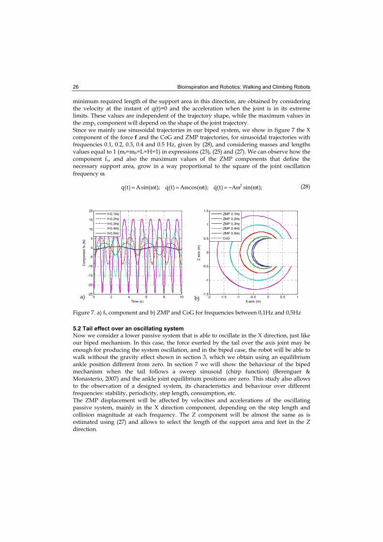
minimum required length of the support area in this direction, are obtained by considering the velocity at the instant of q(t)=0 and the acceleration when the joint is in its extreme limits. These values are independent of the trajectory shape, while the maximum values in the zmpz component will depend on the shape of the joint trajectory. Since we mainly use sinusoidal trajectories in our biped system, we show in figure 7 the X component of the force f and the CoG and ZMP trajectories, for sinusoidal trajectories with frequencies 0.1, 0.2, 0.3, 0.4 and 0.5 Hz, given by (28), and considering masses and lengths values equal to 1 (mt=mb=L=H=1) in expressions (23), (25) and (27). We can observe how the component fx, and also the maximum values of the ZMP components that define the necessary support area, grow in a way proportional to the square of the joint oscillation
frequency ω.
);tsin(A)t(q);tcos(A)t(q);tsin(A)t(q 2 ωω−=ωω=ω= (28)
0 2 4 6 8 10-25
-20
-15
-10
-5
0
5
10
15
20
Time (s)
Com
ponent
fx (
N)
f=0.1Hz
f=0.2Hz
f=0.3Hz
f=0.4Hz
f=0.5Hz
-2 -1.5 -1 -0.5 0 0.5 1-1.5
-1
-0.5
0
0.5
1
1.5
X axis (m)
Z a
xis
(m
)
ZMP 0.1Hz
ZMP 0.2Hz
ZMP 0.3Hz
ZMP 0.4Hz
ZMP 0.5Hz
CoG
Figure 7. a) fx component and b) ZMP and CoG for frequencies between 0,1Hz and 0,5Hz
5.2 Tail effect over an oscillating system
Now we consider a lower passive system that is able to oscillate in the X direction, just like our biped mechanism. In this case, the force exerted by the tail over the axis joint may be enough for producing the system oscillation, and in the biped case, the robot will be able to walk without the gravity effect shown in section 3, which we obtain using an equilibrium ankle position different from zero. In section 7 we will show the behaviour of the biped mechanism when the tail follows a sweep sinusoid (chirp function) (Berenguer & Monasterio, 2007) and the ankle joint equilibrium positions are zero. This study also allows to the observation of a designed system, its characteristics and behaviour over different frequencies: stability, periodicity, step length, consumption, etc. The ZMP displacement will be affected by velocities and accelerations of the oscillating passive system, mainly in the X direction component, depending on the step length and collision magnitude at each frequency. The Z component will be almost the same as is estimated using (27) and allows to select the length of the support area and feet in the Z direction.
a) b)
Locomotion of an Underactuated Biped Robot Using a Tail 27
6. Power and energy consumption study
In this section we present solutions to reduce the power consumption of the system. On the one hand, we try to obtain a smooth contact between the feet and the ground in order to reduce the kinetic energy losses at the collisions. On the other hand, we will consider the design of a spring system at the tail joint to allow the robot to produce the tail oscillation with low power consumption. Let us remember that one of our main objectives is to obtain a periodic gait that can be maintained with minimum energy cost.
6.1 Smooth contact between the feet and the ground
In order to reach this objective we adjust the system parameters trying to reduce the foot velocity of the swing leg near zero at the contact instant. This velocity reduction involves less kinetic energy losses, and is obtained by means of reducing velocities of both ankle joints and the inclination velocity of the body at the same instant. Ankle joint velocity will be zero if the joint is in a stable equilibrium state or if the joint oscillation is in a maximum position. The first situation is obtained easily for the swing leg by means of adjusting the friction coefficient Bank. In the case of the stance leg, this first situation requires high friction, and we search the second option by adjusting the Kank and
θ0ank spring parameters. In addition, this second option produces a longer step, compared to the first one, and less energy dissipation due to joint friction.
On the other hand, the inclination velocity of the body will be zero if the inclination angle αis reached at stable or a maximum position. That depends on the tail joint oscillation frequency and trajectory shape, and also on the top joint friction. Because we assumed this friction to be negligible, we try to adjust the trajectory amplitude so that the velocity is near zero when the angle reaches its maximum. In the case of a real robot, it is important to mention that although the ankle parameters are mechanical parameters whose adjustment is not made by software, mechanisms like MACCEPA (Van Ham et al., 2006) allow for adjustment of the equilibrium position and the spring constant of this type of joints in real time. The parameter Bank should be adjustable once for different gaits.
6.2 Adding a spring to the tail joint
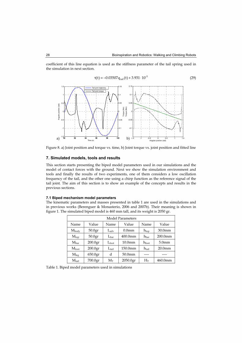
The oscillatory motion of the tail requires high energy consumption if only one electric motor is used, since this motion involves successive accelerations and decelerations. In (Berenguer & Monasterio, 2006) we proposed adding a torsional spring to the tail joint that collaborates in performing this motion. The spring constant was selected by trial and error. In this work we propose to use the relation between torque and position of the tail without spring for selecting the stiffness using the slope of the line that fits this curve. As an example, figure 8 shows the torque and position relation in the case of the last result presented in (Berenguer & Monasterio, 2007b), that will be our comparative experiment in the simulation results presented in section 7. Figure 8.a presents both magnitudes versus time and we can see how the torque is quite different with respect to an unperturbed linear spring (sinusoidal torque). Figure 8.b shows torque versus joint position during eight strides and we can observe the nonlinearity of this relation and the phase shift between both signals (remember Lissajous curves). This figure also shows the line that fits the closed curve which expression is given by (29). The first
Bioinspiration and Robotics: Walking and Climbing Robots 28
coefficient of this line equation is used as the stiffness parameter of the tail spring used in the simulation in next section.
-5tail 103.931)t(q0.03507)t( ⋅+−=τ (29)
90 92 94 96 98 100-1.5
-1
-0.5
0
0.5
1
1.5
Angula
r positio
n (
rad)
90 92 94 96 98 100
-0.1
-0.05
0
0.05
0.1
0.15
Time (s)
Torq
ue (
Nm
)
Tail joint torque
Tail joint trajectory
-1.5 -1 -0.5 0 0.5 1 1.5
-0.1
-0.05
0
0.05
0.1
0.15
Angular postion (rad)
Torq
ue (
Nm
)
Figure 8. a) Joint position and torque vs. time, b) Joint torque vs. joint position and fitted line
7. Simulated models, tools and results
This section starts presenting the biped model parameters used in our simulations and the model of contact forces with the ground. Next we show the simulation environment and tools and finally the results of two experiments, one of them considers a low oscillation frequency of the tail, and the other one using a chirp function as the reference signal of the tail joint. The aim of this section is to show an example of the concepts and results in the previous sections.
7.1 Biped mechanism model parameters
The kinematic parameters and masses presented in table 1 are used in the simulations and in previous works (Berenguer & Monasterio, 2006 and 2007b). Their meaning is shown in figure 1. The simulated biped model is 460 mm tall, and its weight is 2050 gr.
Model Parameters
Name Value Name Value Name Value
Mbody 50.0gr Ladv 0.0mm htop 30.0mm
Mtop 50.0gr Lbar 400.0mm hbar 200.0mm
Mbar 200.0gr Lfoot 10.0mm hfoot 5.0mm
Mfoot 200.0gr Ltail 150.0mm htail 20.0mm
Mleg 650.0gr d 50.0mm ---- ----
Mtail 700.0gr MT 2050.0gr HT 460.0mm
Table 1. Biped model parameters used in simulations
a) b)
Locomotion of an Underactuated Biped Robot Using a Tail 29
7.2 Estimation of the Ground Reaction Force and ZMP
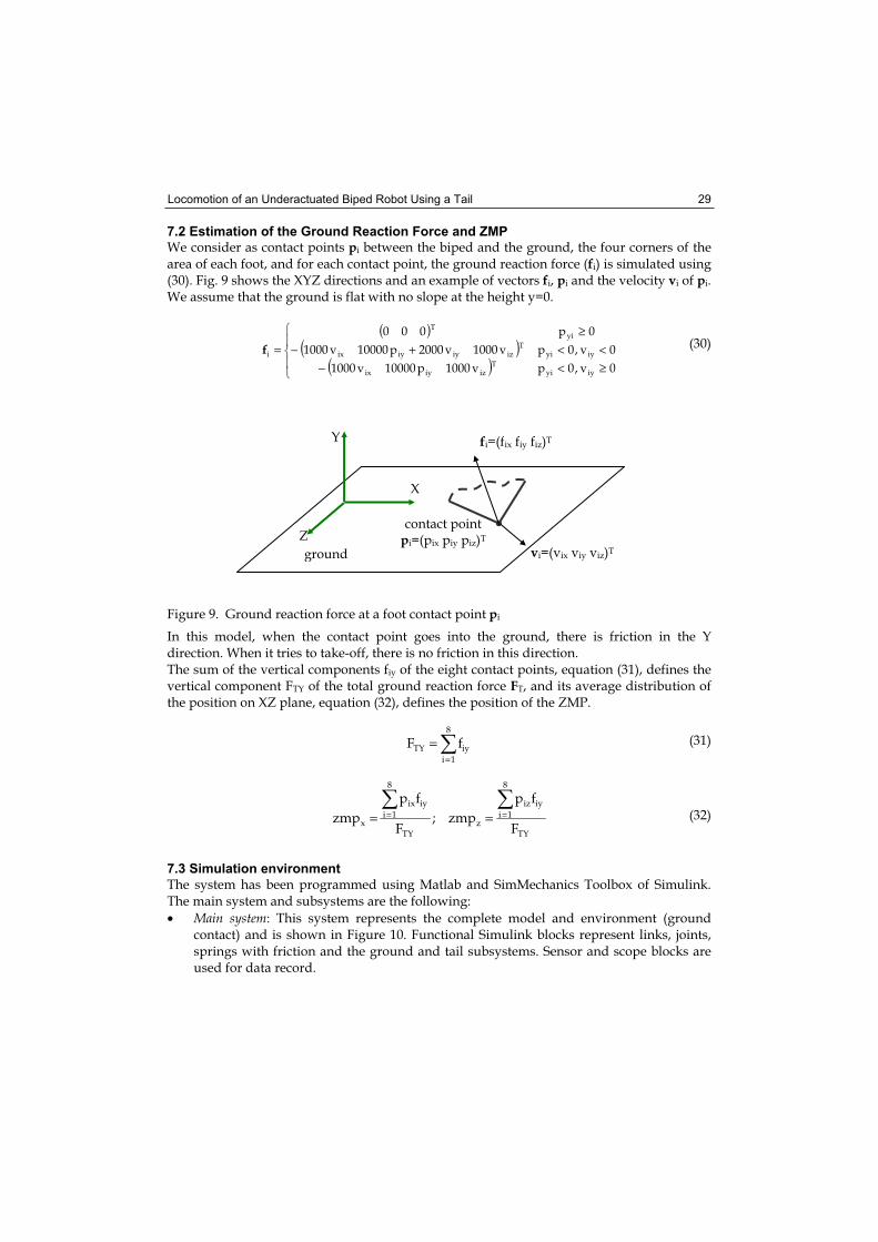
We consider as contact points pi between the biped and the ground, the four corners of the area of each foot, and for each contact point, the ground reaction force (fi) is simulated using (30). Fig. 9 shows the XYZ directions and an example of vectors fi, pi and the velocity vi of pi.We assume that the ground is flat with no slope at the height y=0.
( )( )
( ) ≥<−<<+−
≥=
0v,0pv1000p10000v1000
0v,0pv1000v2000p10000v1000
0p000
iyyiT
iziyix
iyyiT
iziyiyix
yiT
if (30)
Figure 9. Ground reaction force at a foot contact point pi
In this model, when the contact point goes into the ground, there is friction in the Y direction. When it tries to take-off, there is no friction in this direction. The sum of the vertical components fiy of the eight contact points, equation (31), defines the vertical component FTY of the total ground reaction force FT, and its average distribution of the position on XZ plane, equation (32), defines the position of the ZMP.
=
=8
1i
iyTY fF (31)
TY
8
1i
iyiz
zTY
8
1i
iyix
xF
fp
zmp;F
fp
zmp == == (32)
7.3 Simulation environment
The system has been programmed using Matlab and SimMechanics Toolbox of Simulink. The main system and subsystems are the following:
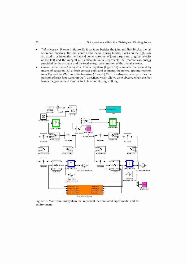
• Main system: This system represents the complete model and environment (ground contact) and is shown in Figure 10. Functional Simulink blocks represent links, joints, springs with friction and the ground and tail subsystems. Sensor and scope blocks are used for data record.
Y
X
Z
ground
fi=(fix fiy fiz)T
vi=(vix viy viz)T
contact point pi=(pix piy piz)T
Bioinspiration and Robotics: Walking and Climbing Robots 30
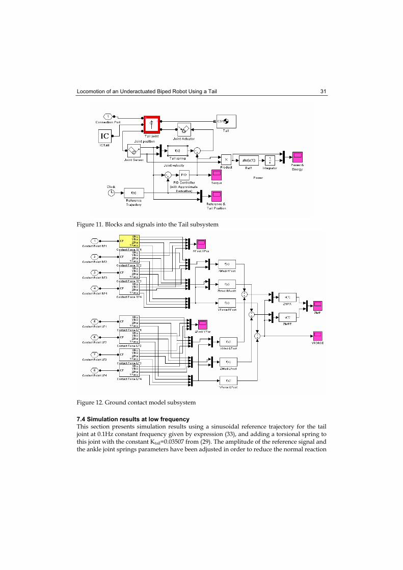
• Tail subsystem: Shown in figure 11, it contains besides the joint and link blocks, the tail reference trajectory, the joint control and the tail spring blocks. Blocks on the right side are used to estimate the mechanical power (product of joint torque and angular velocity of the tail) and the integral of its absolute value, represents the (mechanical) energy provided by the actuator and the total energy consumption of the overall system.
• Ground model contact subsystem: This subsystem (Figure 12) simulates the ground by means of equation (30) at each contact point and estimates the normal ground reaction force FTY and the ZMP coordinates using (31) and (32). This subsystem also provides the position of each foot corner in the Y direction, which allows us to observe when the foot leaves the ground and also the foot elevation during walking.
Figure 10. Main Simulink system that represent the simulated biped model and its environment
Locomotion of an Underactuated Biped Robot Using a Tail 31
Figure 11. Blocks and signals into the Tail subsystem
Figure 12. Ground contact model subsystem
7.4 Simulation results at low frequency
This section presents simulation results using a sinusoidal reference trajectory for the tail joint at 0.1Hz constant frequency given by expression (33), and adding a torsional spring to this joint with the constant Ktail=0.03507 from (29). The amplitude of the reference signal and the ankle joint springs parameters have been adjusted in order to reduce the normal reaction
Bioinspiration and Robotics: Walking and Climbing Robots 32
force of the ground at contact instant. The values of these parameters are presented in Table 2.
( )( )( )( )( )
≤
<≤−ω+
<≤−ω
<≤ω−
=
ts1050
s105ts5.102)5.102t(2cos12
As5.102ts5.2)5.2t(cosA
s5.2ts0t2cos12
A
)t(q
stail
stail
stail
ref (33)
ωs
(rad/s)
Atail
(rad)Ktail
(Nm/rad)Kank
(Nm/rad)Bank
(Nms/rad)θ0ank
(rad)
Foot size (mm2)
0.2π 1.49 0.03507 8.4 0.4 -0.038 200x85
Table 2. Parameters in the first experiment at 0,1Hz stride frequency
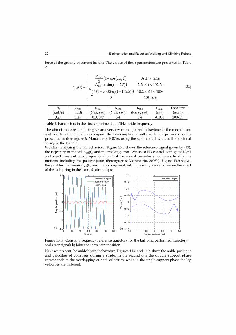
The aim of these results is to give an overview of the general behaviour of the mechanism, and on the other hand, to compare the consumption results with our previous results presented in (Berenguer & Monasterio, 2007b), using the same model without the torsional spring at the tail joint. We start analyzing the tail behaviour. Figure 13.a shows the reference signal given by (33), the trajectory of the tail qtail(t), and the tracking error. We use a PD control with gains KP=1and KD=0.5 instead of a proportional control, because it provides smoothness to all joints motions, including the passive joints (Berenguer & Monasterio, 2007b). Figure 13.b shows the joint torque versus qtail(t), and if we compare it with figure 8.b, we can observe the effect of the tail spring in the exerted joint torque.
0 20 40 60 80 100 120-1.5
-1
-0.5
0
0.5
1
1.5
Time (s)
Angula
r positio
n (
rad)
-1.5 -1 -0.5 0 0.5 1 1.5-0.2
-0.15
-0.1
-0.05
0
0.05
0.1
0.15
0.2
Angular position (rad)
Torq
ue (
Nm
)
Reference signal
Joint trajectory
Error signal
Tail joint torque
Figure 13. a) Constant frequency reference trajectory for the tail joint, performed trajectory and error signal; b) Joint toque vs. joint position
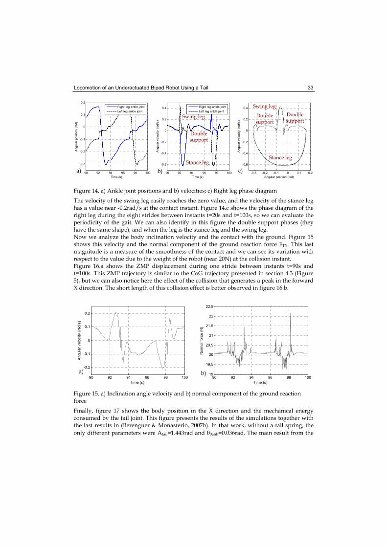
Next we present the ankle’s joint behaviour. Figures 14.a and 14.b show the ankle positions and velocities of both legs during a stride. In the second one the double support phase corresponds to the overlapping of both velocities, while in the single support phase the leg velocities are different.
a) b)
Locomotion of an Underactuated Biped Robot Using a Tail 33
90 92 94 96 98 100
-0.3
-0.2
-0.1
0
0.1
0.2
Time (s)
Angula
r positio
n (
rad)
Right leg ankle joint
Left leg ankle joint
90 92 94 96 98 100
-0.6
-0.4
-0.2
0
0.2
0.4
Time (s)
Angula
r velo
city (
rad/s
)
Right leg ankle joint
Left leg ankle joint
-0.3 -0.2 -0.1 0 0.1 0.2
-0.6
-0.4
-0.2
0
0.2
0.4
Angular position (rad)
Angula
r velo
city (
rad/s
)
Figure 14. a) Ankle joint positions and b) velocities; c) Right leg phase diagram
The velocity of the swing leg easily reaches the zero value, and the velocity of the stance leg has a value near -0.2rad/s at the contact instant. Figure 14.c shows the phase diagram of the right leg during the eight strides between instants t=20s and t=100s, so we can evaluate the periodicity of the gait. We can also identify in this figure the double support phases (they have the same shape), and when the leg is the stance leg and the swing leg. Now we analyze the body inclination velocity and the contact with the ground. Figure 15 shows this velocity and the normal component of the ground reaction force FTY. This last magnitude is a measure of the smoothness of the contact and we can see its variation with respect to the value due to the weight of the robot (near 20N) at the collision instant. Figure 16.a shows the ZMP displacement during one stride between instants t=90s and t=100s. This ZMP trajectory is similar to the CoG trajectory presented in section 4.3 (Figure 5), but we can also notice here the effect of the collision that generates a peak in the forward X direction. The short length of this collision effect is better observed in figure 16.b.
90 92 94 96 98 100
-0.2
-0.1
0
0.1
0.2
Time (s)
Angula
r velo
city (
rad/s
)
90 92 94 96 98 10019
19.5
20
20.5
21
21.5
22
22.5
Time (s)
Norm
al fo
rce (
N)
Figure 15. a) Inclination angle velocity and b) normal component of the ground reaction force
Finally, figure 17 shows the body position in the X direction and the mechanical energy consumed by the tail joint. This figure presents the results of the simulations together with the last results in (Berenguer & Monasterio, 2007b). In that work, without a tail spring, the
only different parameters were Atail=1.443rad and θ0ank=0.036rad. The main result from the
Stance leg
Swing leg
Doublesupport
Doublesupport
Doublesupport
Stance leg
Swing leg
a) b)
a) b) c)
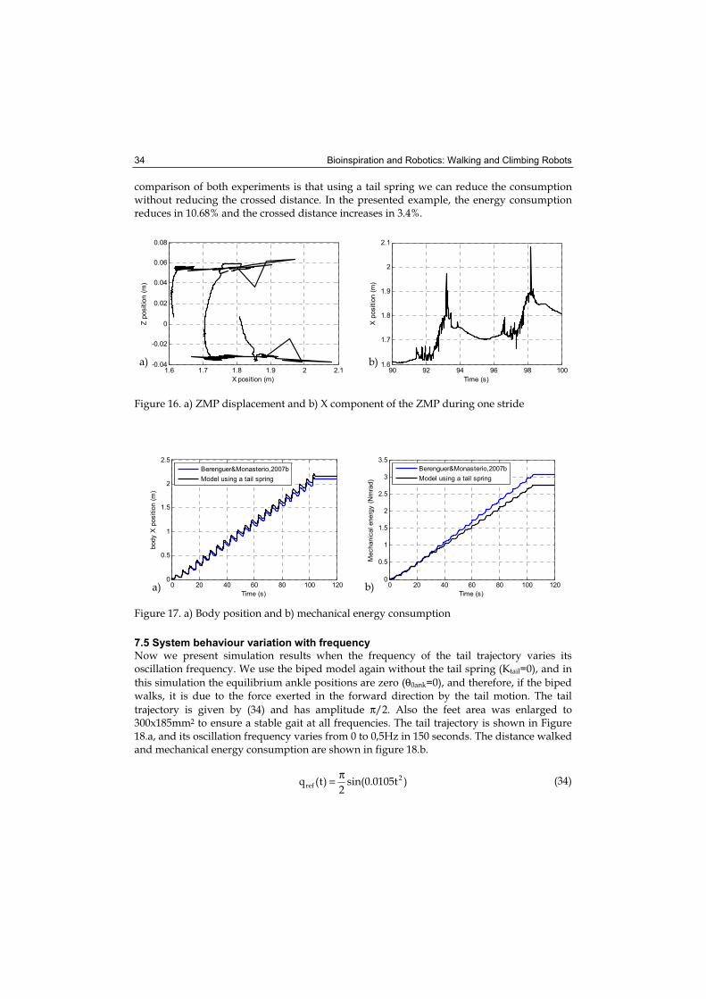
Bioinspiration and Robotics: Walking and Climbing Robots 34
comparison of both experiments is that using a tail spring we can reduce the consumption without reducing the crossed distance. In the presented example, the energy consumption reduces in 10.68% and the crossed distance increases in 3.4%.
1.6 1.7 1.8 1.9 2 2.1-0.04
-0.02
0
0.02
0.04
0.06
0.08
X position (m)
Z p
ositio
n (
m)
90 92 94 96 98 1001.6
1.7
1.8
1.9
2
2.1
Time (s)X
positio
n (
m)
Figure 16. a) ZMP displacement and b) X component of the ZMP during one stride
0 20 40 60 80 100 1200
0.5
1
1.5
2
2.5
Time (s)
body X
positio
n (
m)
0 20 40 60 80 100 1200
0.5
1
1.5
2
2.5
3
3.5
Time (s)
Mechanic
al energ
y (
Nm
rad)
Berenguer&Monasterio,2007b
Model using a tail spring
Berenguer&Monasterio,2007b
Model using a tail spring
Figure 17. a) Body position and b) mechanical energy consumption
7.5 System behaviour variation with frequency
Now we present simulation results when the frequency of the tail trajectory varies its oscillation frequency. We use the biped model again without the tail spring (Ktail=0), and in
this simulation the equilibrium ankle positions are zero (θ0ank=0), and therefore, if the biped walks, it is due to the force exerted in the forward direction by the tail motion. The tail
trajectory is given by (34) and has amplitude π/2. Also the feet area was enlarged to 300x185mm2 to ensure a stable gait at all frequencies. The tail trajectory is shown in Figure 18.a, and its oscillation frequency varies from 0 to 0,5Hz in 150 seconds. The distance walked and mechanical energy consumption are shown in figure 18.b.
)t0105.0sin(2
)t(q 2ref
π= (34)
a) b)
a) b)
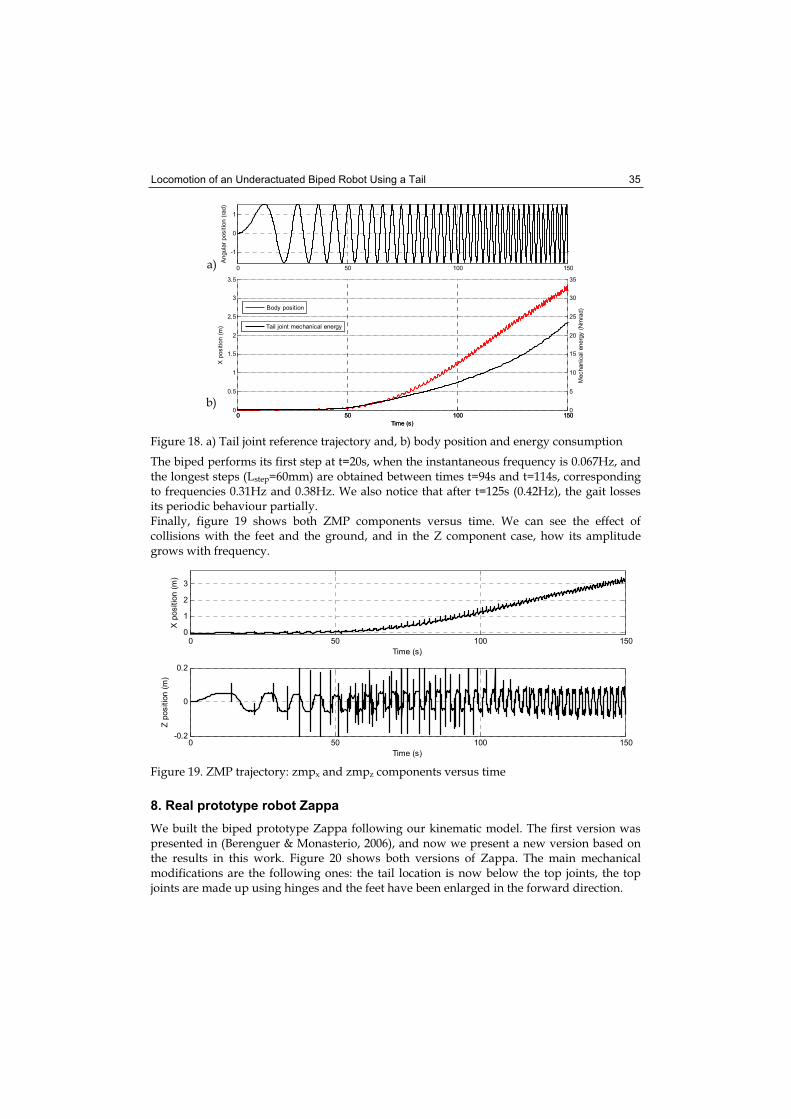
Locomotion of an Underactuated Biped Robot Using a Tail 35
0 50 100 150
-1
0
1
Angula
r positio
n (
rad)
0 50 100 1500
0.5
1
1.5
2
2.5
3
3.5
Time (s)
X p
ositio
n (
m)
0 50 100 1500
5
10
15
20
25
30
35
Time (s)
Mechanic
al energ
y (
Nm
rad)Body position
Tail joint mechanical energy
Figure 18. a) Tail joint reference trajectory and, b) body position and energy consumption
The biped performs its first step at t=20s, when the instantaneous frequency is 0.067Hz, and the longest steps (Lstep=60mm) are obtained between times t=94s and t=114s, corresponding to frequencies 0.31Hz and 0.38Hz. We also notice that after t=125s (0.42Hz), the gait losses its periodic behaviour partially. Finally, figure 19 shows both ZMP components versus time. We can see the effect of collisions with the feet and the ground, and in the Z component case, how its amplitude grows with frequency.
0 50 100 1500
1
2
3
Time (s)
X p
ositio
n (
m)
0 50 100 150-0.2
0
0.2
Time (s)
Z p
ositio
n (
m)
Figure 19. ZMP trajectory: zmpx and zmpz components versus time
8. Real prototype robot Zappa
We built the biped prototype Zappa following our kinematic model. The first version was presented in (Berenguer & Monasterio, 2006), and now we present a new version based on the results in this work. Figure 20 shows both versions of Zappa. The main mechanical modifications are the following ones: the tail location is now below the top joints, the top joints are made up using hinges and the feet have been enlarged in the forward direction.
a)
b)
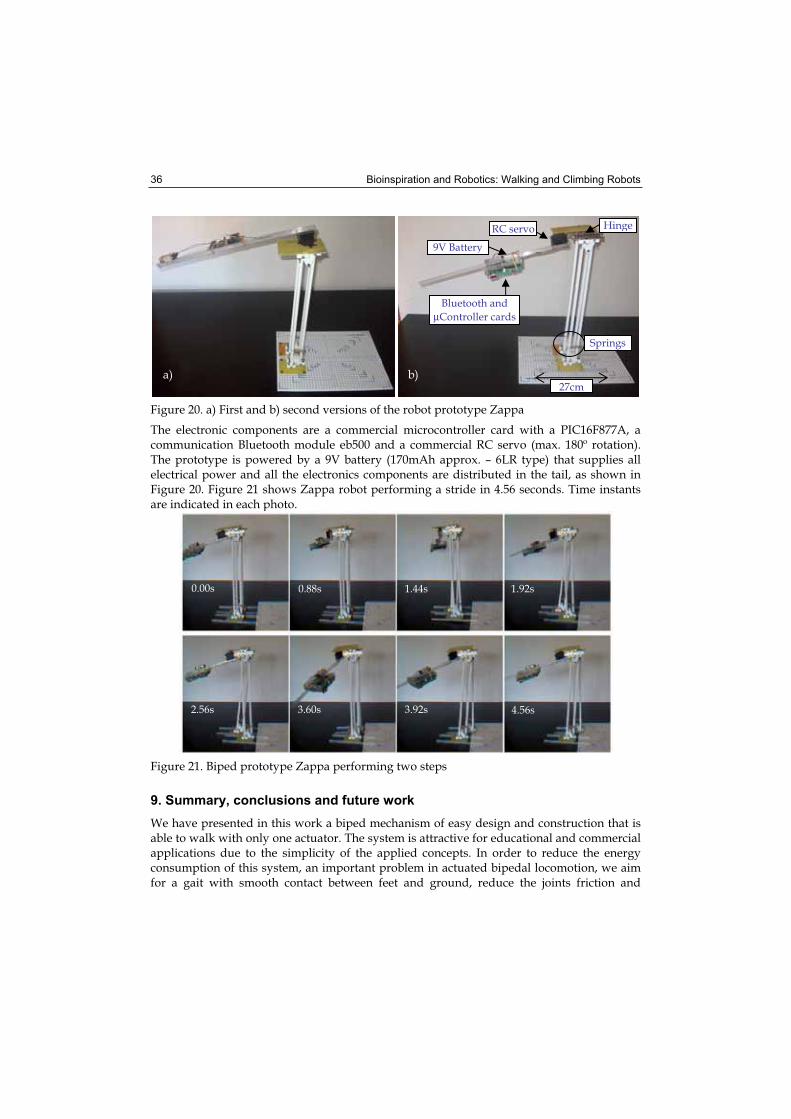
Bioinspiration and Robotics: Walking and Climbing Robots 36
Figure 20. a) First and b) second versions of the robot prototype Zappa
The electronic components are a commercial microcontroller card with a PIC16F877A, a communication Bluetooth module eb500 and a commercial RC servo (max. 180º rotation). The prototype is powered by a 9V battery (170mAh approx. – 6LR type) that supplies all electrical power and all the electronics components are distributed in the tail, as shown in Figure 20. Figure 21 shows Zappa robot performing a stride in 4.56 seconds. Time instants are indicated in each photo.
Figure 21. Biped prototype Zappa performing two steps
9. Summary, conclusions and future work
We have presented in this work a biped mechanism of easy design and construction that is able to walk with only one actuator. The system is attractive for educational and commercial applications due to the simplicity of the applied concepts. In order to reduce the energy consumption of this system, an important problem in actuated bipedal locomotion, we aim for a gait with smooth contact between feet and ground, reduce the joints friction and
Bluetooth and
μController cards
9V Battery
RC servo
Springs
Hinge
27cm a) b)
0.00s 0.88s 1.44s 1.92s
2.56s 3.60s 3.92s 4.56s
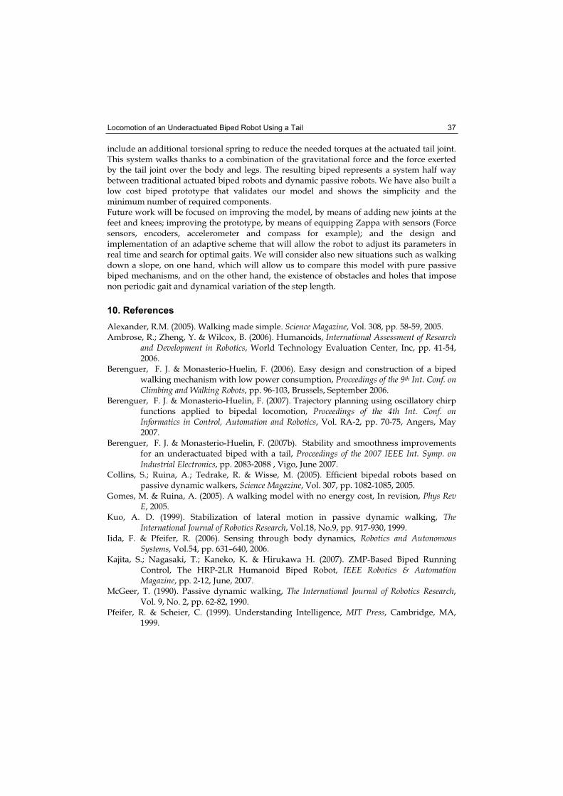
Locomotion of an Underactuated Biped Robot Using a Tail 37
include an additional torsional spring to reduce the needed torques at the actuated tail joint. This system walks thanks to a combination of the gravitational force and the force exerted by the tail joint over the body and legs. The resulting biped represents a system half way between traditional actuated biped robots and dynamic passive robots. We have also built a low cost biped prototype that validates our model and shows the simplicity and the minimum number of required components. Future work will be focused on improving the model, by means of adding new joints at the feet and knees; improving the prototype, by means of equipping Zappa with sensors (Force sensors, encoders, accelerometer and compass for example); and the design and implementation of an adaptive scheme that will allow the robot to adjust its parameters in real time and search for optimal gaits. We will consider also new situations such as walking down a slope, on one hand, which will allow us to compare this model with pure passive biped mechanisms, and on the other hand, the existence of obstacles and holes that impose non periodic gait and dynamical variation of the step length.
10. References
Alexander, R.M. (2005). Walking made simple. Science Magazine, Vol. 308, pp. 58-59, 2005. Ambrose, R.; Zheng, Y. & Wilcox, B. (2006). Humanoids, International Assessment of Research
and Development in Robotics, World Technology Evaluation Center, Inc, pp. 41-54, 2006.
Berenguer, F. J. & Monasterio-Huelin, F. (2006). Easy design and construction of a biped walking mechanism with low power consumption, Proceedings of the 9th Int. Conf. on Climbing and Walking Robots, pp. 96-103, Brussels, September 2006.
Berenguer, F. J. & Monasterio-Huelin, F. (2007). Trajectory planning using oscillatory chirp functions applied to bipedal locomotion, Proceedings of the 4th Int. Conf. on Informatics in Control, Automation and Robotics, Vol. RA-2, pp. 70-75, Angers, May 2007.
Berenguer, F. J. & Monasterio-Huelin, F. (2007b). Stability and smoothness improvements for an underactuated biped with a tail, Proceedings of the 2007 IEEE Int. Symp. on Industrial Electronics, pp. 2083-2088 , Vigo, June 2007.
Collins, S.; Ruina, A.; Tedrake, R. & Wisse, M. (2005). Efficient bipedal robots based on passive dynamic walkers, Science Magazine, Vol. 307, pp. 1082-1085, 2005.
Gomes, M. & Ruina, A. (2005). A walking model with no energy cost, In revision, Phys Rev E, 2005.
Kuo, A. D. (1999). Stabilization of lateral motion in passive dynamic walking, TheInternational Journal of Robotics Research, Vol.18, No.9, pp. 917-930, 1999.
Iida, F. & Pfeifer, R. (2006). Sensing through body dynamics, Robotics and Autonomous Systems, Vol.54, pp. 631–640, 2006.
Kajita, S.; Nagasaki, T.; Kaneko, K. & Hirukawa H. (2007). ZMP-Based Biped Running Control, The HRP-2LR Humanoid Biped Robot, IEEE Robotics & Automation Magazine, pp. 2-12, June, 2007.
McGeer, T. (1990). Passive dynamic walking, The International Journal of Robotics Research,Vol. 9, No. 2, pp. 62-82, 1990.
Pfeifer, R. & Scheier, C. (1999). Understanding Intelligence, MIT Press, Cambridge, MA, 1999.
Bioinspiration and Robotics: Walking and Climbing Robots 38
Takita, K.; Katayama, T. & Hirose, S. (2003). Development of Dinosaur-like Robot TITRUS -The Efficacy of the Neck and Tail of Miniature Dinosaur-like Robot TITRUS III, Proceedings of the 2003 IEEE Int. Conf. on Robotics & Automation, pp. 2466-2471, Taipei, Taiwan, September, 2003.
Van Ham, R.; Van Damme, M.; Vanderborght, B.; Verrelst, B. & Lefeber, D. (2006). MACCEPA: The mechanically adjustable compliance and controllable equilibrium position actuator, Proceedings of the 9th Int. Conf. on Climbing and Walking Robots,Brussels, pp. 196-203, September 2006.
Vukobratovic, M. & Juricie, D. (1969). Contribution to the synthesis of biped gait, IEEE Transactions on Bio-Medical Engineering, Vol.16, No.1, pp. 1-6, 1969.
Vukobratovic, M.; Borovac, B.; Surla, D. & Stokic, D. (1990). Biped locomotion: Dynamics, stability, control and application, Springer-Verlag, 1990.
Wahde, M. & Pettersson, J. (2002). A brief review of bipedal robotics research, Proceedings of the 8th UK Mechatronics Forum International Conference (Mechatronics 2002), pp. 480-488, 2002.
3
Reduced DOF Type Walking Robot Based on Closed Link Mechanism
Katsuhiko Inagaki Department of Applied Computer Engineering, TOKAI University
Japan
1. Introduction
The types of mobile robot can be roughly divided into three categories, wheeled type, crawler type and legged type. In these types, walking machine (legged type robot) has some of noteworthy strong points that other types of mobile robot don't have. Especially, high adaptability to the terrain is one of the most important strong points of walking machine. The fact that general type of walking machine has many numbers of DOF is essential reason of the above mentioned strong point. However, this fact causes a serious problem that it is very difficult to build up a walking machine that can be into practical use. The following matters are the main reason that disturbs to make walking machine into practical use. 1. Automatic control is required for each DOF (Degrees Of Freedom) 2. Energy cost of walking machine is fully worse than that of other kinds of mobile
machines It goes without saying that automobile that is typical type of wheeled machines has been already made into practical use. In case of automobile, its essential DOF is only two. Therefore, it is able to put the DOF of them under human control. On the contrary, in case of walking machine, number of DOF is too many to put them under human control. Thus, technique of automatic control including complex calculation of kinematics is absolutely required for walking machine. The second matter is more serious. The fact that walking machine requires many DOF means that many actuators corresponding to the number of DOF are required. Although increasing of number of actuators does not always influenced to efficiency of energy cost, it is very difficult to realize mechanical design that can keep superior energy efficiency. As a result of it, energy costs of walking machine is often made be so bad. Some design technique is required to solve this problem. To overcome the problem, a new notion that is called reduced DOF design has been proposed. Generally, conventional walking robot requires three DOF for each leg. Therefore, 12 DOF and 18 DOF are required for general type of quadruped machine and that of hexapod machine for each. However, these numbers are not always minimum required number for walking machine. On this point of view, to improve energy efficiency of walking machine by reducing number of DOF is main purpose of the notion of reduced DOF. Based of this notion, some types of walking robot has been developed (Yoneda et al. 2001), (Ota et al. 2001), (Iida 2003) and (Behzadipour 2004).
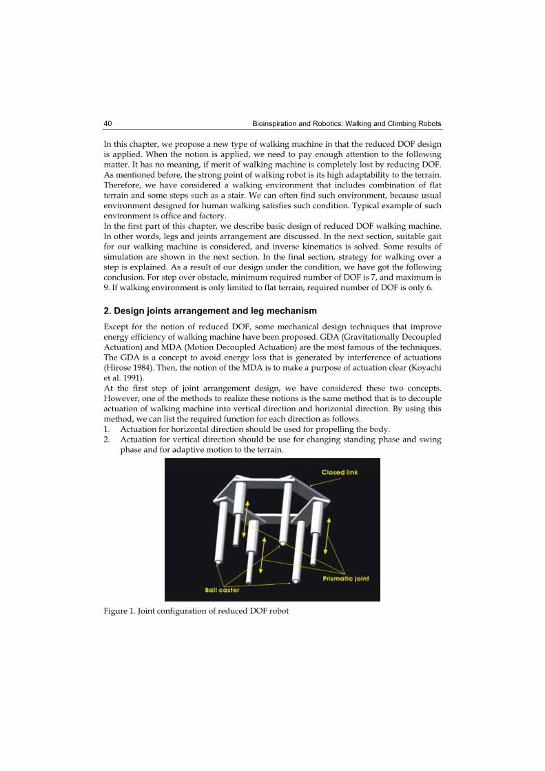
Bioinspiration and Robotics: Walking and Climbing Robots 40
In this chapter, we propose a new type of walking machine in that the reduced DOF design is applied. When the notion is applied, we need to pay enough attention to the following matter. It has no meaning, if merit of walking machine is completely lost by reducing DOF. As mentioned before, the strong point of walking robot is its high adaptability to the terrain. Therefore, we have considered a walking environment that includes combination of flat terrain and some steps such as a stair. We can often find such environment, because usual environment designed for human walking satisfies such condition. Typical example of such environment is office and factory. In the first part of this chapter, we describe basic design of reduced DOF walking machine. In other words, legs and joints arrangement are discussed. In the next section, suitable gait for our walking machine is considered, and inverse kinematics is solved. Some results of simulation are shown in the next section. In the final section, strategy for walking over a step is explained. As a result of our design under the condition, we have got the following conclusion. For step over obstacle, minimum required number of DOF is 7, and maximum is 9. If walking environment is only limited to flat terrain, required number of DOF is only 6.
2. Design joints arrangement and leg mechanism
Except for the notion of reduced DOF, some mechanical design techniques that improve energy efficiency of walking machine have been proposed. GDA (Gravitationally Decoupled Actuation) and MDA (Motion Decoupled Actuation) are the most famous of the techniques. The GDA is a concept to avoid energy loss that is generated by interference of actuations (Hirose 1984). Then, the notion of the MDA is to make a purpose of actuation clear (Koyachi et al. 1991). At the first step of joint arrangement design, we have considered these two concepts. However, one of the methods to realize these notions is the same method that is to decouple actuation of walking machine into vertical direction and horizontal direction. By using this method, we can list the required function for each direction as follows. 1. Actuation for horizontal direction should be used for propelling the body. 2. Actuation for vertical direction should be use for changing standing phase and swing
phase and for adaptive motion to the terrain.
Figure 1. Joint configuration of reduced DOF robot
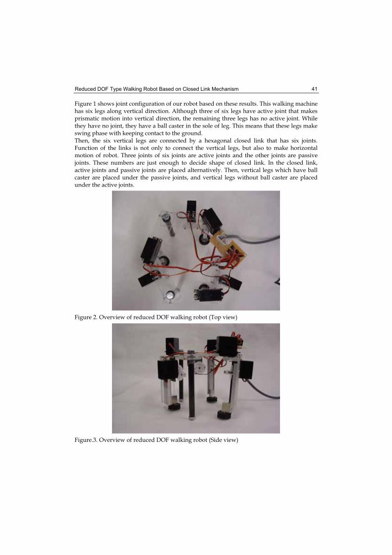
Reduced DOF Type Walking Robot Based on Closed Link Mechanism 41
Figure 1 shows joint configuration of our robot based on these results. This walking machine has six legs along vertical direction. Although three of six legs have active joint that makes prismatic motion into vertical direction, the remaining three legs has no active joint. While they have no joint, they have a ball caster in the sole of leg. This means that these legs make swing phase with keeping contact to the ground. Then, the six vertical legs are connected by a hexagonal closed link that has six joints. Function of the links is not only to connect the vertical legs, but also to make horizontal motion of robot. Three joints of six joints are active joints and the other joints are passive joints. These numbers are just enough to decide shape of closed link. In the closed link, active joints and passive joints are placed alternatively. Then, vertical legs which have ball caster are placed under the passive joints, and vertical legs without ball caster are placed under the active joints.
Figure 2. Overview of reduced DOF walking robot (Top view)
Figure.3. Overview of reduced DOF walking robot (Side view)
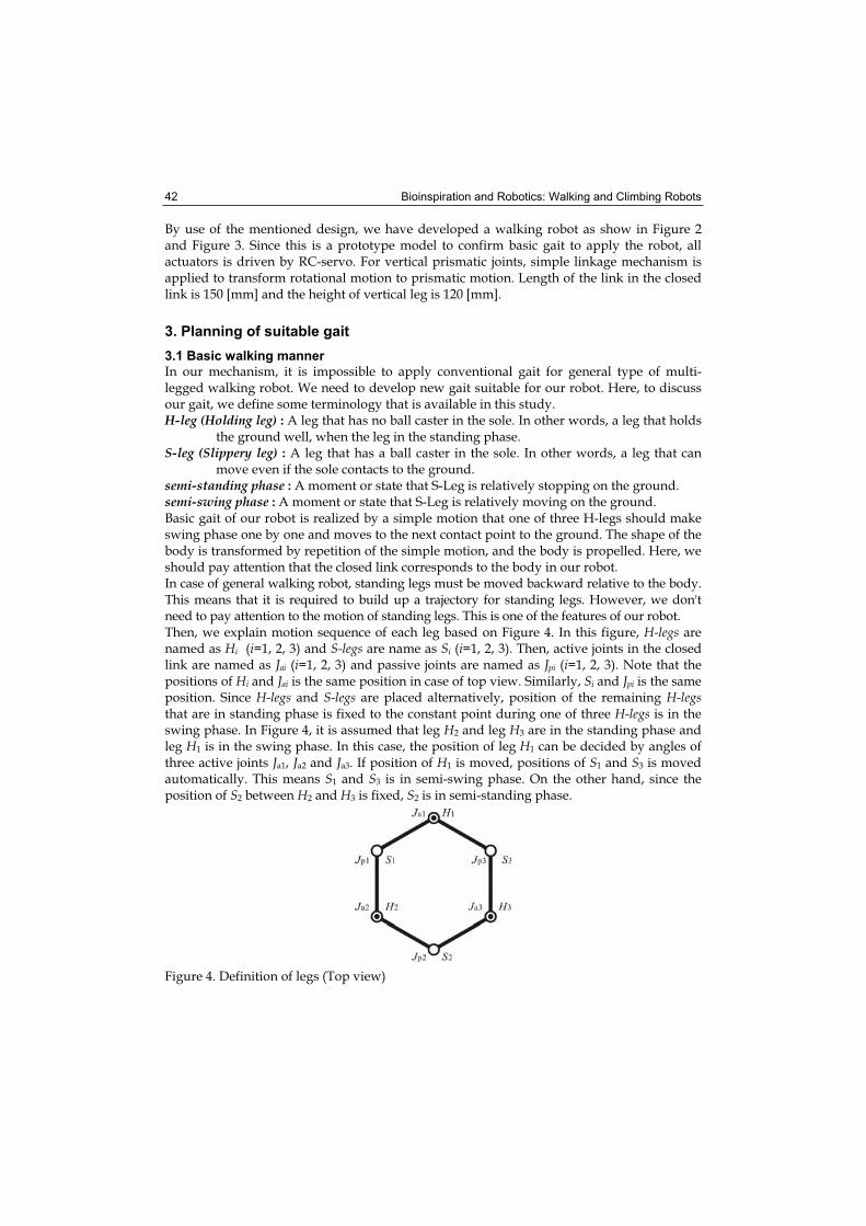
Bioinspiration and Robotics: Walking and Climbing Robots 42
By use of the mentioned design, we have developed a walking robot as show in Figure 2 and Figure 3. Since this is a prototype model to confirm basic gait to apply the robot, all actuators is driven by RC-servo. For vertical prismatic joints, simple linkage mechanism is applied to transform rotational motion to prismatic motion. Length of the link in the closed link is 150 [mm] and the height of vertical leg is 120 [mm].
3. Planning of suitable gait
3.1 Basic walking manner
In our mechanism, it is impossible to apply conventional gait for general type of multi-legged walking robot. We need to develop new gait suitable for our robot. Here, to discuss our gait, we define some terminology that is available in this study. H-leg (Holding leg) : A leg that has no ball caster in the sole. In other words, a leg that holds
the ground well, when the leg in the standing phase. S-leg (Slippery leg) : A leg that has a ball caster in the sole. In other words, a leg that can
move even if the sole contacts to the ground. semi-standing phase : A moment or state that S-Leg is relatively stopping on the ground. semi-swing phase : A moment or state that S-Leg is relatively moving on the ground. Basic gait of our robot is realized by a simple motion that one of three H-legs should make swing phase one by one and moves to the next contact point to the ground. The shape of the body is transformed by repetition of the simple motion, and the body is propelled. Here, we should pay attention that the closed link corresponds to the body in our robot. In case of general walking robot, standing legs must be moved backward relative to the body. This means that it is required to build up a trajectory for standing legs. However, we don't need to pay attention to the motion of standing legs. This is one of the features of our robot. Then, we explain motion sequence of each leg based on Figure 4. In this figure, H-legs are named as Hi (i=1, 2, 3) and S-legs are name as Si (i=1, 2, 3). Then, active joints in the closed link are named as Jai (i=1, 2, 3) and passive joints are named as Jpi (i=1, 2, 3). Note that the positions of Hi and Jai is the same position in case of top view. Similarly, Si and Jpi is the same position. Since H-legs and S-legs are placed alternatively, position of the remaining H-legsthat are in standing phase is fixed to the constant point during one of three H-legs is in the swing phase. In Figure 4, it is assumed that leg H2 and leg H3 are in the standing phase and leg H1 is in the swing phase. In this case, the position of leg H1 can be decided by angles of three active joints Ja1, Ja2 and Ja3. If position of H1 is moved, positions of S1 and S3 is moved automatically. This means S1 and S3 is in semi-swing phase. On the other hand, since the position of S2 between H2 and H3 is fixed, S2 is in semi-standing phase.
Figure 4. Definition of legs (Top view)
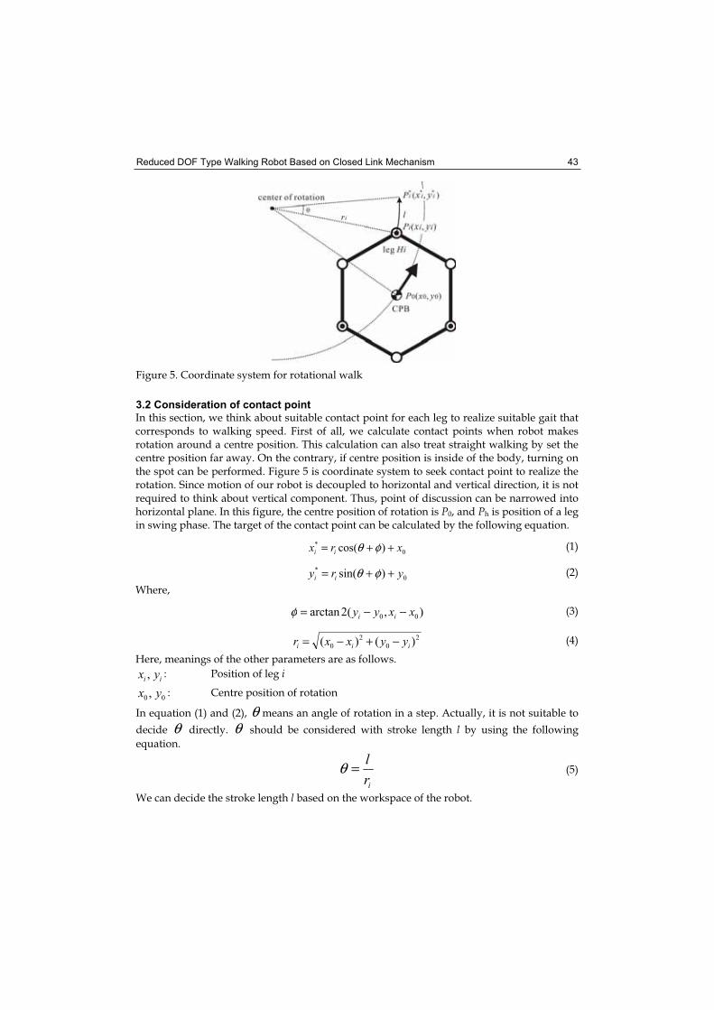
Reduced DOF Type Walking Robot Based on Closed Link Mechanism 43
Figure 5. Coordinate system for rotational walk
3.2 Consideration of contact point
In this section, we think about suitable contact point for each leg to realize suitable gait that corresponds to walking speed. First of all, we calculate contact points when robot makes rotation around a centre position. This calculation can also treat straight walking by set the centre position far away. On the contrary, if centre position is inside of the body, turning on the spot can be performed. Figure 5 is coordinate system to seek contact point to realize the rotation. Since motion of our robot is decoupled to horizontal and vertical direction, it is not required to think about vertical component. Thus, point of discussion can be narrowed into horizontal plane. In this figure, the centre position of rotation is P0, and Ph is position of a leg in swing phase. The target of the contact point can be calculated by the following equation.
0
* )cos( xrx ii ++= φθ (1)
0
* )sin( yry ii ++= φθ (2)
Where,
),(2arctan 00 xxyy ii −−=φ (3)
2
0
2
0 )()( iii yyxxr −+−= (4)
Here, meanings of the other parameters are as follows.
ii yx , : Position of leg i
00 , yx : Centre position of rotation
In equation (1) and (2), θ means an angle of rotation in a step. Actually, it is not suitable to
decide θ directly. θ should be considered with stroke length l by using the following
equation.
irl=θ (5)
We can decide the stroke length l based on the workspace of the robot.
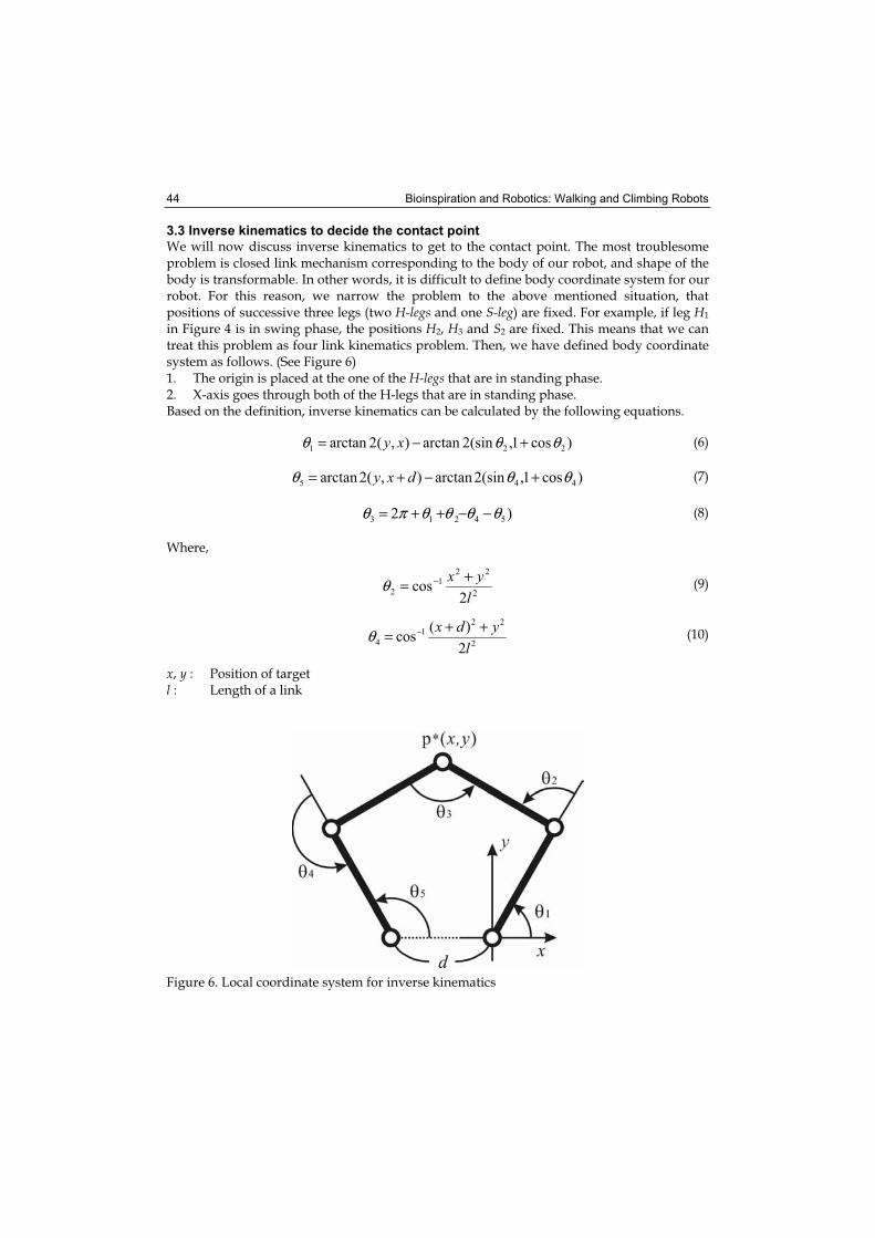
Bioinspiration and Robotics: Walking and Climbing Robots 44
3.3 Inverse kinematics to decide the contact point
We will now discuss inverse kinematics to get to the contact point. The most troublesome problem is closed link mechanism corresponding to the body of our robot, and shape of the body is transformable. In other words, it is difficult to define body coordinate system for our robot. For this reason, we narrow the problem to the above mentioned situation, that positions of successive three legs (two H-legs and one S-leg) are fixed. For example, if leg H1
in Figure 4 is in swing phase, the positions H2, H3 and S2 are fixed. This means that we can treat this problem as four link kinematics problem. Then, we have defined body coordinate system as follows. (See Figure 6) 1. The origin is placed at the one of the H-legs that are in standing phase. 2. X-axis goes through both of the H-legs that are in standing phase. Based on the definition, inverse kinematics can be calculated by the following equations.
)cos1,(sin2arctan),(2arctan 221 θθθ +−= xy (6)
)cos1,(sin2arctan),(2arctan 445 θθθ +−+= dxy (7)
)2 54213 θθθθπθ −−++= (8)
Where,
2
221
22
cosl
yx += −θ (9)
2
221
42
)(cos
lydx ++= −θ (10)
x, y : Position of target l : Length of a link
Figure 6. Local coordinate system for inverse kinematics
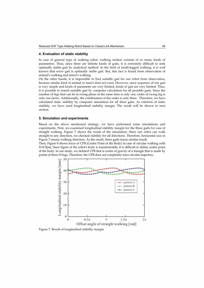
Reduced DOF Type Walking Robot Based on Closed Link Mechanism 45
4. Evaluation of static stability
In case of general type of walking robot, walking motion consists of so many kinds of parameters. Thus, since there are infinite kinds of gaits, it is extremely difficult to seek optimally stable gait by analytical method. In the field of multi-legged walking, it is well known that wave gait is optimally stable gait. But, this fact is found from observation of animal's walking and insect's walking. On the other hands, it is impossible to find suitable gait for our robot from observation, because similar kind of animal or insect does not exist. However, since sequence of our gait is very simple and kinds of parameter are very limited, kinds of gait are very limited. Thus, it is possible to search suitable gait by computer calculation for all possible gaits. Since the number of legs that can be in swing phase at the same time is only one, order of swing leg is only one factor. Additionally, the combination of the order is only three. Therefore, we have calculated static stability by computer simulation for all three gaits. As criterion of static stability, we have used longitudinal stability margin. The result will be shown in next section.
5. Simulation and experiments
Based on the above mentioned strategy, we have performed some simulations and experiments. First, we examined longitudinal stability margin for the three gaits for case of straight walking. Figure 7 shows the result of the simulation. Since our robot can walk straight to any direction, we checked stability for all directions. Therefore, horizontal axis in Figure 7 means walking direction. As the result, three gaits traces similar result. Then, Figure 8 shows locus of CPB (Centre Point of the Body) in case of circular walking with R=0.5[m]. Since figure of the robot's body is transformable, it is difficult to define centre point of the body. In our study, we defined CPB that is centre of gravity of a triangle that is made by points of three H-legs. Therefore, the CPB does not completely trace circular trajectory.
Figure 7. Result of longitudinal stability margin
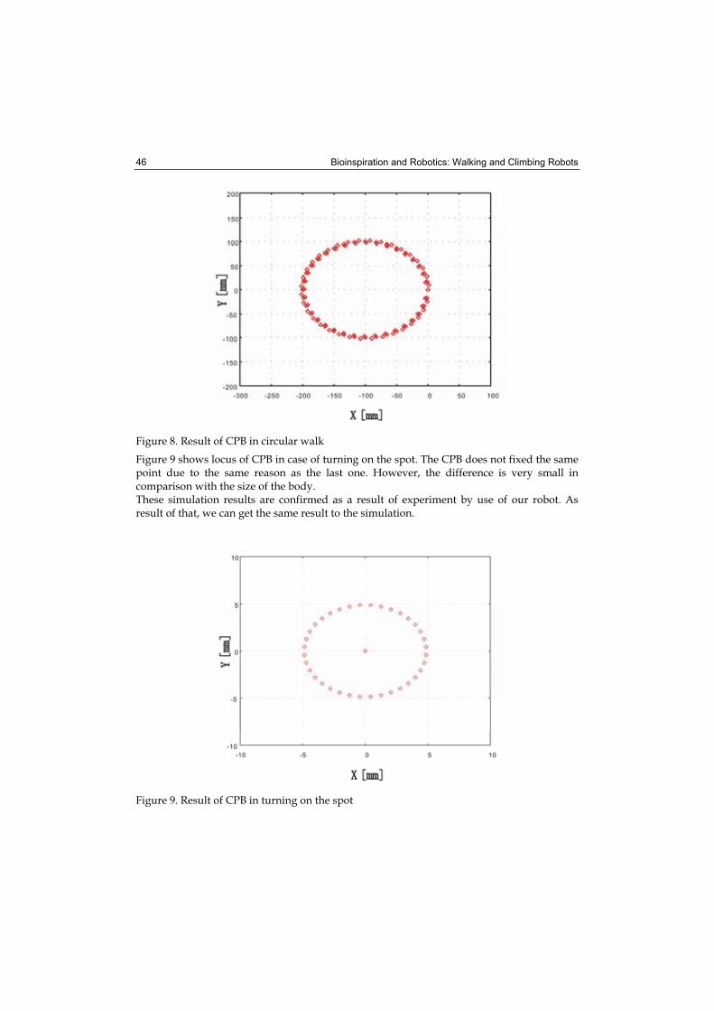
Bioinspiration and Robotics: Walking and Climbing Robots 46
Figure 8. Result of CPB in circular walk
Figure 9 shows locus of CPB in case of turning on the spot. The CPB does not fixed the same point due to the same reason as the last one. However, the difference is very small in comparison with the size of the body. These simulation results are confirmed as a result of experiment by use of our robot. As result of that, we can get the same result to the simulation.
Figure 9. Result of CPB in turning on the spot
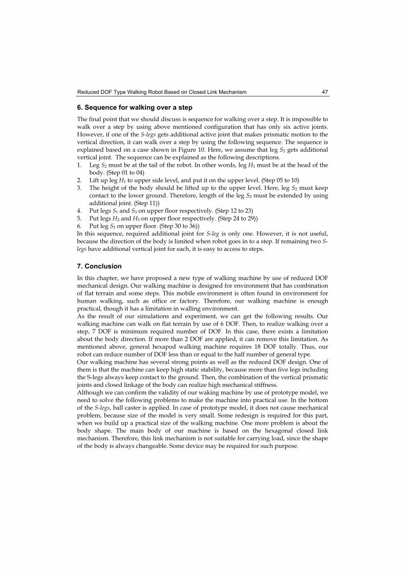
Reduced DOF Type Walking Robot Based on Closed Link Mechanism 47
6. Sequence for walking over a step
The final point that we should discuss is sequence for walking over a step. It is impossible to walk over a step by using above mentioned configuration that has only six active joints. However, if one of the S-legs gets additional active joint that makes prismatic motion to the vertical direction, it can walk over a step by using the following sequence. The sequence is explained based on a case shown in Figure 10. Here, we assume that leg S2 gets additional vertical joint. The sequence can be explained as the following descriptions. 1. Leg S2 must be at the tail of the robot. In other words, leg H1 must be at the head of the
body. (Step 01 to 04) 2. Lift up leg H1 to upper side level, and put it on the upper level. (Step 05 to 10) 3. The height of the body should be lifted up to the upper level. Here, leg S2 must keep
contact to the lower ground. Therefore, length of the leg S2 must be extended by using additional joint. (Step 11))
4. Put legs S1 and S3 on upper floor respectively. (Step 12 to 23) 5. Put legs H2 and H3 on upper floor respectively. (Step 24 to 29)) 6. Put leg S1 on upper floor. (Step 30 to 36)) In this sequence, required additional joint for S-leg is only one. However, it is not useful, because the direction of the body is limited when robot goes in to a step. If remaining two S-legs have additional vertical joint for each, it is easy to access to steps.
7. Conclusion
In this chapter, we have proposed a new type of walking machine by use of reduced DOF mechanical design. Our walking machine is designed for environment that has combination of flat terrain and some steps. This mobile environment is often found in environment for human walking, such as office or factory. Therefore, our walking machine is enough practical, though it has a limitation in walling environment. As the result of our simulations and experiment, we can get the following results. Our walking machine can walk on flat terrain by use of 6 DOF. Then, to realize walking over a step, 7 DOF is minimum required number of DOF. In this case, there exists a limitation about the body direction. If more than 2 DOF are applied, it can remove this limitation. As mentioned above, general hexapod walking machine requires 18 DOF totally. Thus, our robot can reduce number of DOF less than or equal to the half number of general type. Our walking machine has several strong points as well as the reduced DOF design. One of them is that the machine can keep high static stability, because more than five legs including the S-legs always keep contact to the ground. Then, the combination of the vertical prismatic joints and closed linkage of the body can realize high mechanical stiffness. Although we can confirm the validity of our waking machine by use of prototype model, we need to solve the following problems to make the machine into practical use. In the bottom of the S-legs, ball caster is applied. In case of prototype model, it does not cause mechanical problem, because size of the model is very small. Some redesign is required for this part, when we build up a practical size of the walking machine. One more problem is about the body shape. The main body of our machine is based on the hexagonal closed link mechanism. Therefore, this link mechanism is not suitable for carrying load, since the shape of the body is always changeable. Some device may be required for such purpose.
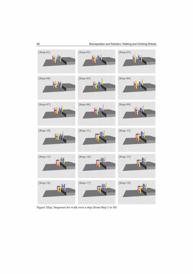
Bioinspiration and Robotics: Walking and Climbing Robots 48
Figure 10(a). Sequence for walk over a step (from Step 1 to 18)
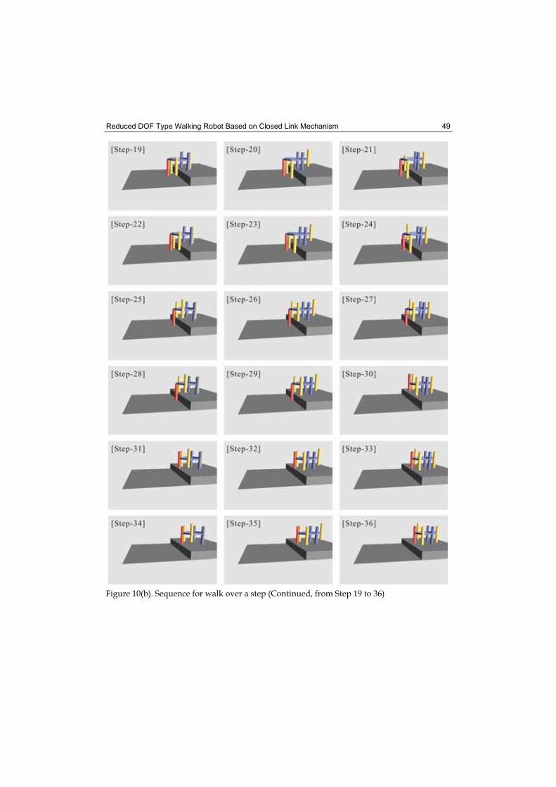
Reduced DOF Type Walking Robot Based on Closed Link Mechanism 49
Figure 10(b). Sequence for walk over a step (Continued, from Step 19 to 36)
Bioinspiration and Robotics: Walking and Climbing Robots 50
8. References
Behzadipour, S. & Khajepou, A. (2004). Design of reduced DOF raprallell cable-based robots Mechanism and Machine Theory, Vol.39, No.10, (October 2004) pp.1051-1065
Hirose, S. (1984). A Study of Design and control of a quadruped waking machine, International Journal of Robotics Research, Vol.3, No.2 (1984) pp.37-48
Iida, K. Nakata, Y. Hira, T. Kamano, T. & Suzuki, T. (2003). Moving performance of reduced D.O.F’s quadruped robot, Proceedings of SICE Annual Conference in Fukui, pp.328-333, Fukui University, August 2003, SICE, Fukui
Koyachi, N. & Adachi, H. (1991) Development of Stair-climbable Self-contained Hexapod with Semi-fixed Gait, Proceedings of International Conference on Advanced Robotics (ICAR'91), pp.747-752, June 1991, Pisa
Ota, Y. Yoneda, K. Muramatsu, Y. & Hirose, S. (2001). Development of walking and task performing robot with bipedal configuration, Proceedings of IEEE/RSJ International Conference on Intelligent Robots and Systems (IROS 2001), pp.247-252, October 2001, Hawaii
Yoneda, K. Ota,Y. Hirano, K. & Hirose, S. (2001). Development of a Light-Weight Wall Climbing Quadruped with Reduced Degrees of Freedom, Proceedings of 4th
International Conference on Climbing and Walking Robots (CLAWAR2001), pp.907-912, September 2001, Karlsruhe
4
Posture and Vibration Control Based on Virtual Suspension Model for Multi-Legged Walking Robot
Qingjiu Huang Tokyo Institute of Technoligy
Japan
1. Introduction
Until now, studies on suspension control by using frequency response analysis that have been reported are almost for motorcar, but not for multi-legged walking robot. However, because of the disturbances, such as the various frequency properties of terrain, the collision and the slip between foot of robot and ground, the dynamic changes of the supported weight by each leg and the centre of gravity of robot with the change of the walking pattern, tiny vibration of robot's body occur when robot walks, especially on rough terrain. This tiny vibration can become unstable big vibration when the above disturbances to the posture of robot exist, which will influence normal walk and work of robot. Recently there are some studies about the posture control of multi-legged walking robot (Shin-Min Song & Keneth J.Waldron, 1989); (Kan Yoneda, et al, 1994); (Qingjiu Huang, et al, 2000); (Qingjiu Huang & Kenzo Nonami, 2002); (Qingjiu Huang, et al, 2003), but no any study on the tiny vibration control of robot's body. Moreover, only posture control can not effectively decrease the tiny vibration of body when robot walks, especially on rough terrain. Therefore, it is necessary to study suspension and its control algorithm to decrease the tiny vibration of body for multi-legged walking robot. In this chapter, we treat a six-legged walking robot as a study example of the multi-legged walking robot, and introduce the newest study on a control for the posture and vibration of the robot using suspension mechanism to realize the better stability and the better adaptability of its walking for unknown rough terrain. On the other hand, until now most reported studies on suspension control are performed on the basis of real suspension model with spring and damper (Nurkan Yagiz, et al, 2000); (Makoto Yokoyama, et al, 2001). However, for large scale multi-DOF system, such as multi-legged walking robots, it is difficult to equip lots of springs and dampers to the robot. Therefore, in this chapter, we introduce a new control method for the posture and vibration of the six-legged walking robot (Qingjiu Huang, et al, 2007), which is based on not a real suspension model but a virtual suspension model consisting of virtual spring and damper. And then considering the nonlinear disturbances and trade-off problem in the design of suspension, a robust control using sliding mode control based on the constructed virtual suspension model for the posture and vibration of the six-legged walking robot is proposed and introduced.
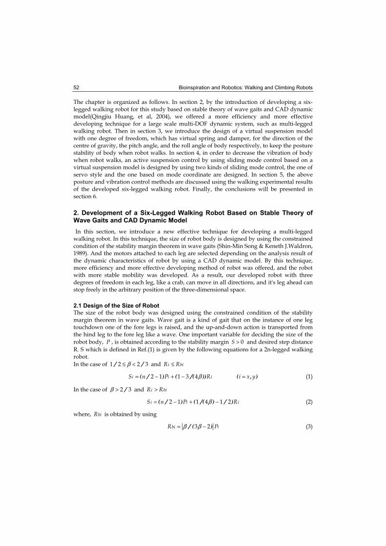
Bioinspiration and Robotics: Walking and Climbing Robots 52
The chapter is organized as follows. In section 2, by the introduction of developing a six-legged walking robot for this study based on stable theory of wave gaits and CAD dynamic model(Qingjiu Huang, et al, 2004), we offered a more efficiency and more effective developing technique for a large scale multi-DOF dynamic system, such as multi-legged walking robot. Then in section 3, we introduce the design of a virtual suspension model with one degree of freedom, which has virtual spring and damper, for the direction of the centre of gravity, the pitch angle, and the roll angle of body respectively, to keep the posture stability of body when robot walks. In section 4, in order to decrease the vibration of body when robot walks, an active suspension control by using sliding mode control based on a virtual suspension model is designed by using two kinds of sliding mode control, the one of servo style and the one based on mode coordinate are designed. In section 5, the above posture and vibration control methods are discussed using the walking experimental results of the developed six-legged walking robot. Finally, the conclusions will be presented in section 6.
2. Development of a Six-Legged Walking Robot Based on Stable Theory of Wave Gaits and CAD Dynamic Model
In this section, we introduce a new effective technique for developing a multi-legged walking robot. In this technique, the size of robot body is designed by using the constrained condition of the stability margin theorem in wave gaits (Shin-Min Song & Keneth J.Waldron, 1989). And the motors attached to each leg are selected depending on the analysis result of the dynamic characteristics of robot by using a CAD dynamic model. By this technique, more efficiency and more effective developing method of robot was offered, and the robot with more stable mobility was developed. As a result, our developed robot with three degrees of freedom in each leg, like a crab, can move in all directions, and it's leg ahead can stop freely in the arbitrary position of the three-dimensional space.
2.1 Design of the Size of Robot
The size of the robot body was designed using the constrained condition of the stability margin theorem in wave gaits. Wave gait is a kind of gait that on the instance of one leg touchdown one of the fore legs is raised, and the up-and-down action is transported from the hind leg to the fore leg like a wave. One important variable for deciding the size of the
robot body, P , is obtained according to the stability margin S > 0 and desired step distance
R. S which is defined in Ref.(1) is given by the following equations for a 2n-legged walking robot.
In the case of / /β≤ <1 2 2 3 and i biR R≤
( / ) ( /( ))i i iS n P Rβ= − + −2 1 1 3 4 ( , )i x y= (1)
In the case of /β > 2 3 and i biR R>
( / ) ( /( ) / )i i iS n P Rβ= − + −2 1 1 4 1 2 (2)
where, biR is obtained by using
/ ( )bi iR Pβ β= −3 2 (3)
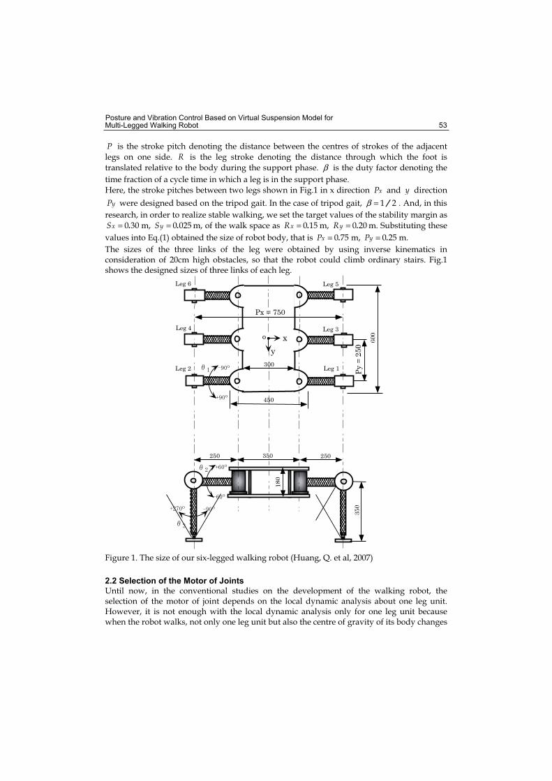
Posture and Vibration Control Based on Virtual Suspension Model for Multi-Legged Walking Robot 53
P is the stroke pitch denoting the distance between the centres of strokes of the adjacent
legs on one side. R is the leg stroke denoting the distance through which the foot is
translated relative to the body during the support phase. β is the duty factor denoting the
time fraction of a cycle time in which a leg is in the support phase.
Here, the stroke pitches between two legs shown in Fig.1 in x direction xP and y direction
yP were designed based on the tripod gait. In the case of tripod gait, /β = 1 2 . And, in this
research, in order to realize stable walking, we set the target values of the stability margin as
.xS = 0 30 m, .yS = 0 025 m, of the walk space as .xR = 0 15 m, .yR = 0 20 m. Substituting these
values into Eq.(1) obtained the size of robot body, that is .xP = 0 75 m, .yP = 0 25 m.
The sizes of the three links of the leg were obtained by using inverse kinematics in consideration of 20cm high obstacles, so that the robot could climb ordinary stairs. Fig.1 shows the designed sizes of three links of each leg.
350250 250
300
450
Leg 1Leg 2
Leg 3Leg 4
Leg 5Leg 6
Px = 750
xo
y
Figure 1. The size of our six-legged walking robot (Huang, Q. et al, 2007)
2.2 Selection of the Motor of Joints
Until now, in the conventional studies on the development of the walking robot, the selection of the motor of joint depends on the local dynamic analysis about one leg unit. However, it is not enough with the local dynamic analysis only for one leg unit because when the robot walks, not only one leg unit but also the centre of gravity of its body changes
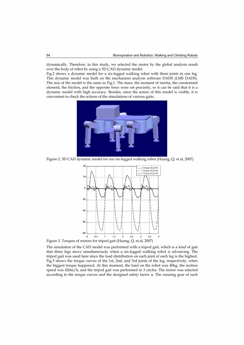
Bioinspiration and Robotics: Walking and Climbing Robots 54
dynamically. Therefore, in this study, we selected the motor by the global analysis result over the body of robot by using a 3D CAD dynamic model. Fig.2 shows a dynamic model for a six-legged walking robot with three joints in one leg. This dynamic model was built on the mechanism analysis software DADS (LMS DADS). The size of the model is the same as Fig.1. The mass, the moment of inertia, the constrained element, the friction, and the opposite force were set precisely, so it can be said that it is a dynamic model with high accuracy. Besides, since the action of this model is visible, it is convenient to check the actions of the simulations of various gaits.
Figure 2. 3D CAD dynamic model for our six-legged walking robot (Huang, Q. et al, 2007)
Figure 3. Torques of motors for tripod gait (Huang, Q. et al, 2007)
The simulation of the CAD model was performed with a tripod gait, which is a kind of gait that three legs move simultaneously when a six-legged walking robot is advancing. The tripod gait was used here since the load distribution on each joint of each leg is the highest. Fig.3 shows the torque curves of the 1st, 2nd, and 3rd joints of the leg, respectively, when the biggest torque happened. At this moment, the load on the robot was 40kg, the motion speed was 420m/h, and the tripod gait was performed in 3 circles. The motor was selected according to the torque curves and the designed safety factor . The running gear of each
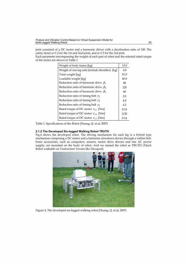
Posture and Vibration Control Based on Virtual Suspension Model for Multi-Legged Walking Robot 55
joint consisted of a DC motor and a harmonic driver with a deceleration ratio of 100. The safety factor =1.2 for the 1st and 2nd joints, and =1.5 for the 3rd joint. Each parameter encompassing the weight of each part of robot and the selected rated torque of the motor are shown in Table 1.
Weight of body frame [kg] 15.0
Weight of one leg unit (include shoulder) [kg] 6.0
Total weight [kg] 51.0
Loadable weight [kg] 40.0
Reduction ratio of harmonic drive β 1 80
Reduction ratio of harmonic drive β 2 120
Reduction ratio of harmonic drive β 3 80
Reduction ratio of timing belt γ 1 2.0
Reduction ratio of timing belt γ 1 4.0
Reduction ratio of timing belt γ 1 4.2
Rated torque of DC motor rτ 1 [Nm] 0.14
Rated torque of DC motor rτ 2 [Nm] 0.20
Rated torque of DC motor rτ 3 [Nm] 0.14
Table 1. Specifications of the Robot (Huang, Q. et al, 2007)
2.1.2 The Developed Six-legged Walking Robot TRUTH
Fig.4 shows the developed robot. The driving mechanism for each leg is a hybrid type mechanism composing a DC motor and a harmonic slowdown device through a rubber belt. Some accessories, such as computers, sensors, motor drive drivers and one AC power supply, are mounted on the body of robot. And we named the robot as TRUTH (Titech Robot walkable on Unstructure Terrain like Hexapod).
Figure 4. The developed six-legged walking robot (Huang, Q. et al, 2007)
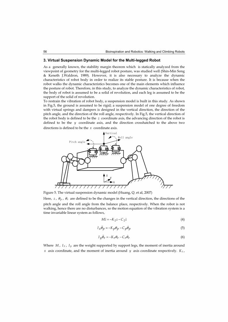
Bioinspiration and Robotics: Walking and Climbing Robots 56
3. Virtual Suspension Dynamic Model for the Multi-legged Robot
As a generally known, the stability margin theorem which is statically analyzed from the viewpoint of geometry for the multi-legged robot posture, was studied well (Shin-Min Song & Keneth J.Waldron, 1989). However, it is also necessary to analyze the dynamic characteristics of robot body in order to realize its stable posture. It is because when the robot walks the dynamic characteristics becomes one of the main elements which influence the posture of robot. Therefore, in this study, to analyze the dynamic characteristics of robot, the body of robot is assumed to be a solid of revolution, and each leg is assumed to be the support of the solid of revolution. To restrain the vibration of robot body, a suspension model is built in this study. As shown in Fig.5, the ground is assumed to be rigid; a suspension model of one degree of freedom with virtual springs and dampers is designed in the vertical direction, the direction of the pitch angle, and the direction of the roll angle, respectively. In Fig.5, the vertical direction of the robot body is defined to be the z coordinate axis, the advancing direction of the robot is
defined to be the y coordinate axis, and the direction crosshatched to the above two
directions is defined to be the x coordinate axis.
Figure 5. The virtual suspension dynamic model (Huang, Q. et al, 2007)
Here, z , pθ , rθ are defined to be the changes in the vertical direction, the directions of the
pitch angle and the roll angle from the balance place, respectively. When the robot is not walking, hence there are no disturbances, so the motion equation of the vibration system is a time invariable linear system as follows,
Mz K z C zz z= − − (4)
I K Cx p p p p pθ θ θ= − − (5)
I K Cy r r r r rθ θ θ= − − (6)
Where M , xI , yI are the weight supported by support legs, the moment of inertia around
x axis coordinate, and the moment of inertia around y axis coordinate respectively. zK ,
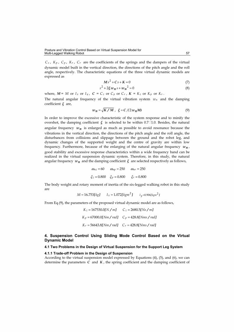
Posture and Vibration Control Based on Virtual Suspension Model for Multi-Legged Walking Robot 57
zC , pK , pC , rK , rC are the coefficients of the springs and the dampers of the virtual
dynamic model built in the vertical direction, the directions of the pitch angle and the roll angle, respectively. The characteristic equations of the three virtual dynamic models are expressed as
M C Ks s+ + =2 0 (7)
w wn ns s+ + =2 22 0 (8)
where, M = M or xI or yI , C = zC or pC or rC , K = zK or pK or rK .
The natural angular frequency of the virtual vibration system nw and the damping
coefficient are,
w K / Mn = , C w M)n/(= 2 (9)
In order to improve the excessive characteristic of the system response and to minify the
overshot, the damping coefficient is selected to be within 0.7�1.0. Besides, the natural
angular frequency wn is enlarged as much as possible to avoid resonance because the
vibrations in the vertical direction, the directions of the pitch angle and the roll angle, the disturbances from collisions and slippage between the ground and the robot leg, and dynamic changes of the supported weight and the centre of gravity are within low
frequency. Furthermore, because of the enlarging of the natural angular frequency wn ,
good stability and excessive response characteristics within a wide frequency band can be realized in the virtual suspension dynamic system. Therefore, in this study, the natural
angular frequency wn and the damping coefficient are selected respectively as follows,
nzω = 60 npω = 250 nrω = 250
.zξ = 0 800 .pξ = 0 800 .rξ = 0 800
The body weight and rotary moment of inertia of the six-legged walking robot in this study are
. [ ]M kg= 16 753 . [ ]xI kgm= 21 072 . [ ]I kgmy = 20 906
From Eq.(9), the parameters of the proposed virtual dynamic model are as follows,
. [ / ]zK N m= 167530 0 . [ / ]zC Ns m= 2680 5
. [ / ]pK Nm rad= 67000 0 . [ / ]pC Nms rad= 428 8
. [ / ]rK Nm rad= 56643 8 . [ / ]rC Nms rad= 428 8
4. Suspension Control Using Sliding Mode Control Based on the Virtual Dynamic Model
4.1 Two Problems in the Design of Virtual Suspension for the Support Leg System
4.1.1 Trade-off Problem in the Design of Suspension
According to the virtual suspension model expressed by Equations (4), (5), and (6), we can
determine the parameters C and K , the spring coefficient and the damping coefficient of
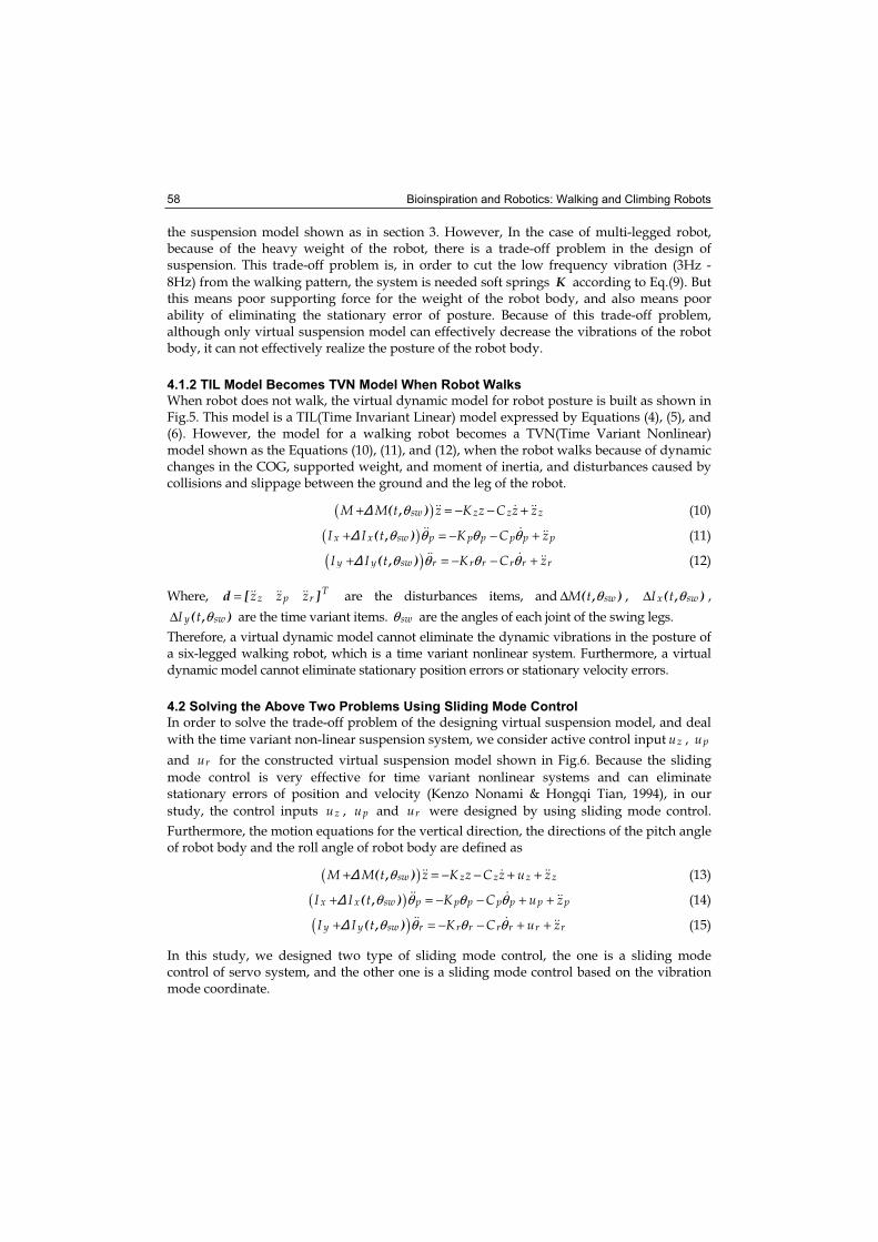
Bioinspiration and Robotics: Walking and Climbing Robots 58
the suspension model shown as in section 3. However, In the case of multi-legged robot, because of the heavy weight of the robot, there is a trade-off problem in the design of suspension. This trade-off problem is, in order to cut the low frequency vibration (3Hz -
8Hz) from the walking pattern, the system is needed soft springs K according to Eq.(9). But this means poor supporting force for the weight of the robot body, and also means poor ability of eliminating the stationary error of posture. Because of this trade-off problem, although only virtual suspension model can effectively decrease the vibrations of the robot body, it can not effectively realize the posture of the robot body.
4.1.2 TIL Model Becomes TVN Model When Robot Walks
When robot does not walk, the virtual dynamic model for robot posture is built as shown in Fig.5. This model is a TIL(Time Invariant Linear) model expressed by Equations (4), (5), and (6). However, the model for a walking robot becomes a TVN(Time Variant Nonlinear) model shown as the Equations (10), (11), and (12), when the robot walks because of dynamic changes in the COG, supported weight, and moment of inertia, and disturbances caused by collisions and slippage between the ground and the leg of the robot.
( )( , )sw z z zM M t z K z C z zθ+ = − − + (10)
( )( , )x x sw p p p p p pI I t K C zθ θ θ θ+ = − − + (11)
( )( , )y y sw r r r r r rI I t K C zθ θ θ θ+ = − − + (12)
Where, d [ ] Tz p rz z z= are the disturbances items, and ( , )swM t θΔ , ( , )x swI t θΔ ,
( , )y swI t θΔ are the time variant items. swθ are the angles of each joint of the swing legs.
Therefore, a virtual dynamic model cannot eliminate the dynamic vibrations in the posture of a six-legged walking robot, which is a time variant nonlinear system. Furthermore, a virtual dynamic model cannot eliminate stationary position errors or stationary velocity errors.
4.2 Solving the Above Two Problems Using Sliding Mode Control
In order to solve the trade-off problem of the designing virtual suspension model, and deal
with the time variant non-linear suspension system, we consider active control input zu , puand ru for the constructed virtual suspension model shown in Fig.6. Because the sliding
mode control is very effective for time variant nonlinear systems and can eliminate stationary errors of position and velocity (Kenzo Nonami & Hongqi Tian, 1994), in our
study, the control inputs zu , pu and ru were designed by using sliding mode control.
Furthermore, the motion equations for the vertical direction, the directions of the pitch angle of robot body and the roll angle of robot body are defined as
( )( , )sw z z z zM M t z K z C z u zθ+ = − − + + (13)
( )( , )x x sw p p p p p p pI I t K C u zθ θ θ θ+ = − − + + (14)
( )( , )y y sw r r r r r r rI I t K C u zθ θ θ θ+ = − − + + (15)
In this study, we designed two type of sliding mode control, the one is a sliding mode control of servo system, and the other one is a sliding mode control based on the vibration mode coordinate.
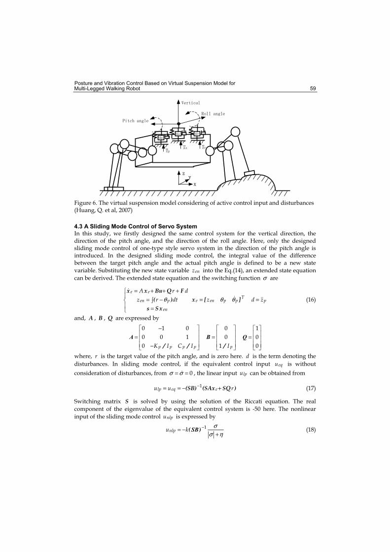
Posture and Vibration Control Based on Virtual Suspension Model for Multi-Legged Walking Robot 59
.... ..
Figure 6. The virtual suspension model considering of active control input and disturbances (Huang, Q. et al, 2007)
4.3 A Sliding Mode Control of Servo System
In this study, we firstly designed the same control system for the vertical direction, the direction of the pitch angle, and the direction of the roll angle. Here, only the designed sliding mode control of one-type style servo system in the direction of the pitch angle is introduced. In the designed sliding mode control, the integral value of the difference between the target pitch angle and the actual pitch angle is defined to be a new state
variable. Substituting the new state variable enz into the Eq.(14), an extended state equation
can be derived. The extended state equation and the switching function σ are
x x Bu Q F( )
s S x
e e
en p
en
A r dz r dtθ
= + + += −
=x [ ] T
e en p pz θ θ= pd z= (16)
and, A , B , Q are expressed by
/ /p p p pK I C I
−=
−
0 1 0
0 0 1
0
A
/ pI=
0
0
1
B =1
0
0
Q
where, r is the target value of the pitch angle, and is zero here. d is the term denoting the
disturbances. In sliding mode control, if the equivalent control input equ is without
consideration of disturbances, from σ σ= = 0 , the linear input lpu can be obtained from
(SB) (SAx SQ )lp eq eu u r−= = − +1 (17)
Switching matrix S is solved by using the solution of the Riccati equation. The real
component of the eigenvalue of the equivalent control system is -50 here. The nonlinear
input of the sliding mode control nlpu is expressed by
( )nlpu k σσ η
−= −+
1SB (18)
Bioinspiration and Robotics: Walking and Climbing Robots 60
Nonlinear input nlpu compensates for the uncertainty of the system, as the control input to
constrain the system state variables within the switching plane. Here, the coefficient to
repress the disturbances k = 8600 , and the coefficient to avoid the chattering .η = 0 1 .
Therefore, the input of the sliding mode control pu for the direction of pitch angle, which is
composed of the linear control input lpu and the nonlinear control input nlpu is expressed
as follows.
( ) (SAx SQ ) ( )p lp nlp eu u u r k σσ η
− −= + = − + −+
1 1SB SB (19)
The input of sliding mode control in the z direction zu and the direction of roll angle ruwere calculated in the same way by using Eqs.(16)-(19). Substituting the obtained zu , pu ,
and ru into Eqs.(13)-(15), the forces in z direction of the tips of support legs were
calculated according to (Kan Yoneda, et al, 1994). Then, by using position/force hybrid control introduced in (Qingjiu Huang & Kenzo Nonami, 2002), the calculated forces of the tips of support legs were transformed into the motor torques to driving the motors attached on the support legs. On the other hand, the motor torques of the swing legs were calculated by PD control for following the desired trajectories of the swing legs.
4.4 A Sliding Mode Control Based on the Vibration Mode Coordinate
Also we designed a sliding mode control based on the vibration mode coordinate to control the posture and restrain the vibration of the robot body. Although the state variable is impossible to be controlled in the general state equation, by departing the mode, the state matrix in the state equation becomes a diagonal canonical matrix. Correspondingly, the state variable becomes controlled, and the system becomes easy to be stabilized. here, the
state equation without the extended state variable enz is shown in Eq.(20).
x A x Bu F d= + + (20)
The vibration mode is transformed by following Eq.(21).
x Tz= (21)
The state equation with departed mode is expressed in Eq.(22).
z Az FBu d= + + (22)
Where, A , B is defined as follows:
λλ
=1
2
0
0A
/( )/( )
p
p
II
λ λλ λ
− −=
−2 1
2 1B
,/ ( / ) /p p p p p pC I C I K I
λ− ± −
=2
1 24
2
The control input pu of the sliding mode control is the same with the one of the sliding
mode control of servo system. It is also composed of linear input and nonlinear input. pu is
expressed by
Posture and Vibration Control Based on Virtual Suspension Model for Multi-Legged Walking Robot 61
(SB) (SAz S(SB)p lp nlpu u u ) σσ η
− −= + = − −+
1 1 (23)
The inputs in the z direction zu and the direction of roll angle ru were calculated in the
same way with the calculation procedure of pu . And, the transforms from the virtual
suspension model with the active inputs zu , pu , and ru to the motor torques of the
support legs and the swing legs were performed as stated in section 4.3.
4.5 About How to Deal with the Suspension and Posture Control
In the above two type sliding mode control based on the virtual suspension model, we can design the virtual suspension to cut the low frequency vibration (3Hz - 8Hz) from the
walking pattern. And because the nonlinear input nlu of sliding mode control can supply
the strong force to support the heavy weight of the robot, the trade-off problem in the design of suspension can be solved, and then the good suspension effect can be realized. On the other hand, because the design of sliding mode control is satisfied the matching condition, although the dynamic changes and the disturbances exist, the stationary errors of
position and velocity can be eliminated. If we change the state variable x [ ] Te en p pz θ θ=
in Eq.(16) to x [ ]Te en p pref p pz θ θ θ θ= − − , and change the state variable x [ ]T
p pθ θ=
in Eq.(20) to x [ ] Tp pref p prefθ θ θ θ= − − , we can realize the posture control for the pitch
angle. Here, prefθ is the reference for the pitch angle. And with the same method, we can
realize the posture control for the roll angle and vertical direction.
5. Experiment and Discussion
Both of the sliding mode control of one-type servo system and the sliding mode control based on the vibration mode coordinate were applied to the developed robot.
5.1 Preparations for the Experiment
Because the purpose of this study is to restrain the vibration in the z direction and the directions of the pitch angle and the roll angle of the robot body when the robot walks, it is necessary to obtain the outputs in these three directions. As to the output angles in the directions of the pitch angle and the roll angle, they were measured by a slant sensor. In the vertical direction, the output can be calculated from the size of the robot body and the forces in the vertical direction of each leg. Here, in order to save the cost, we don't use the force sensor to observe the forces of each leg, rather then use the motor pseudo-torque.
5.1.1 The Observation by Using the Motor Pseudo-Torque
The motor torque is obtained by multiplying a torque coefficient to the motor electric current. However, because the vibration caused by noise is too big, instead of the motor torque, a pseudo-torque is used as the input torque. The pseudo-torque is the calculated torque of one sampling time before. In the servo electric circuit, the calculated pseudo-torque approximates to the actual consumed torque. Therefore, using the pseudo-torque, there is no the influence by the noise. Of course, a delay of one sampling time arises
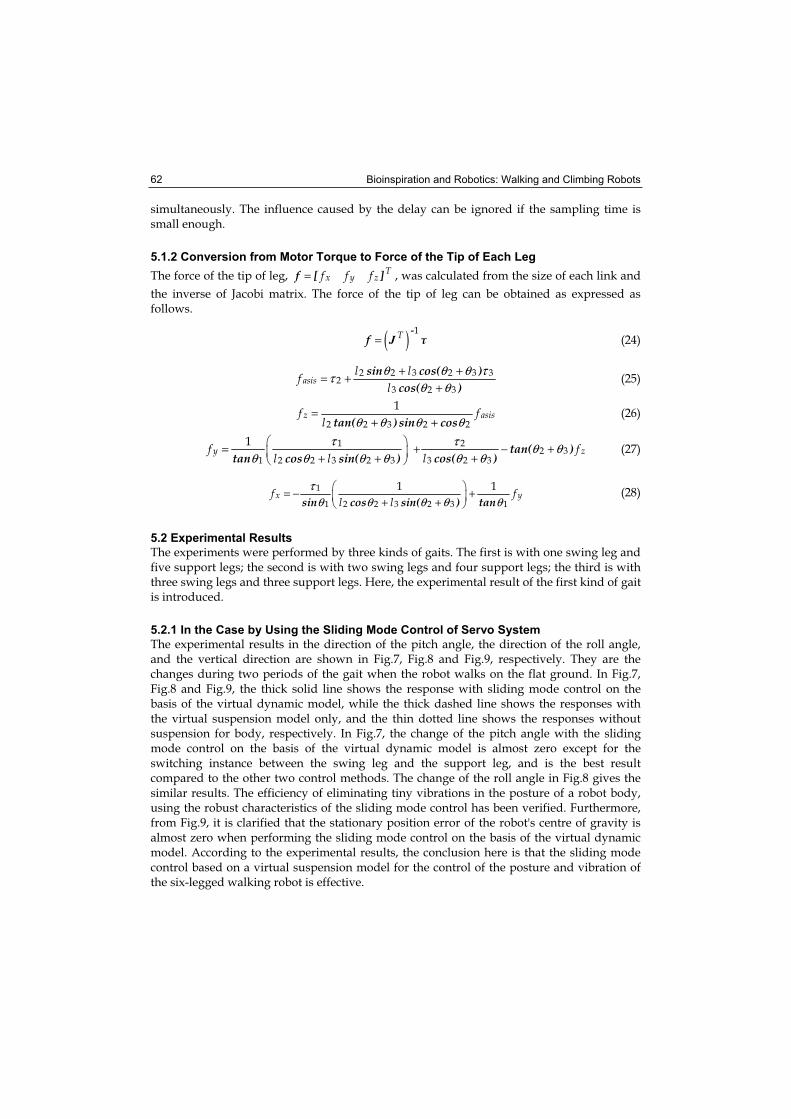
Bioinspiration and Robotics: Walking and Climbing Robots 62
simultaneously. The influence caused by the delay can be ignored if the sampling time is small enough.
5.1.2 Conversion from Motor Torque to Force of the Tip of Each Leg
The force of the tip of leg, f [ ] Tx y zf f f= , was calculated from the size of each link and
the inverse of Jacobi matrix. The force of the tip of leg can be obtained as expressed as follows.
( ) -f T=
1J (24)
sin cos( )cos( )
asisl lf
lθ θ θ ττ
θ θ+ += +
+2 2 3 2 3 3
23 2 3
(25)
tan( )sin cosz asisf f
l θ θ θ θ=
+ +2 2 3 2 2
1 (26)
tan cos sin( )yf
l lτ
θ θ θ θ=
+ +1
1 2 2 3 2 3
1 tan( )cos( )
zfl
τ θ θθ θ
+ − ++
22 3
3 2 3 (27)
sin cos sin( ) tanx yf f
l lτ
θ θ θ θ θ= − +
+ +1
1 2 2 3 2 3 1
1 1 (28)
5.2 Experimental Results
The experiments were performed by three kinds of gaits. The first is with one swing leg and five support legs; the second is with two swing legs and four support legs; the third is with three swing legs and three support legs. Here, the experimental result of the first kind of gait is introduced.
5.2.1 In the Case by Using the Sliding Mode Control of Servo System
The experimental results in the direction of the pitch angle, the direction of the roll angle, and the vertical direction are shown in Fig.7, Fig.8 and Fig.9, respectively. They are the changes during two periods of the gait when the robot walks on the flat ground. In Fig.7, Fig.8 and Fig.9, the thick solid line shows the response with sliding mode control on the basis of the virtual dynamic model, while the thick dashed line shows the responses with the virtual suspension model only, and the thin dotted line shows the responses without suspension for body, respectively. In Fig.7, the change of the pitch angle with the sliding mode control on the basis of the virtual dynamic model is almost zero except for the switching instance between the swing leg and the support leg, and is the best result compared to the other two control methods. The change of the roll angle in Fig.8 gives the similar results. The efficiency of eliminating tiny vibrations in the posture of a robot body, using the robust characteristics of the sliding mode control has been verified. Furthermore, from Fig.9, it is clarified that the stationary position error of the robot's centre of gravity is almost zero when performing the sliding mode control on the basis of the virtual dynamic model. According to the experimental results, the conclusion here is that the sliding mode control based on a virtual suspension model for the control of the posture and vibration of the six-legged walking robot is effective.
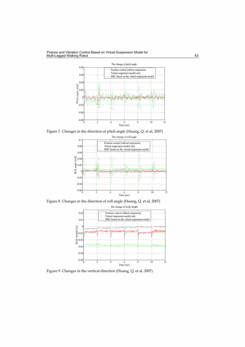
Posture and Vibration Control Based on Virtual Suspension Model for Multi-Legged Walking Robot 63
0 2 4 6 8 10 12-0.06
-0.04
-0.02
0
0.02
0.04
0.06
0.08The change of pitch angle
Time [sec]
Pit
ch a
ng
le [
rad
]
Position control without suspension Virtual suspension model only SMC based on the virtual suspension model
Figure 7. Changes in the direction of pitch angle (Huang, Q. et al, 2007)
0 2 4 6 8 10 12-0.06
-0.04
-0.02
0
0.02
0.04
0.06
0.08
0.1The change of roll angle
Time [sec]
Ro
ll a
ng
le [
rad
]
Position control without suspension Virtual suspension model only SMC based on the virtual suspension model
Figure 8. Changes in the direction of roll angle (Huang, Q. et al, 2007)
0 2 4 6 8 10 12-0.05
-0.04
-0.03
-0.02
-0.01
0
0.01
0.02
The change of body height
Time [sec]
Bo
dy
hei
gh
t [m
]
Position control without suspension Virtual suspension model only SMC based on the virtual suspension model
Figure 9. Changes in the vertical direction (Huang, Q. et al, 2007)
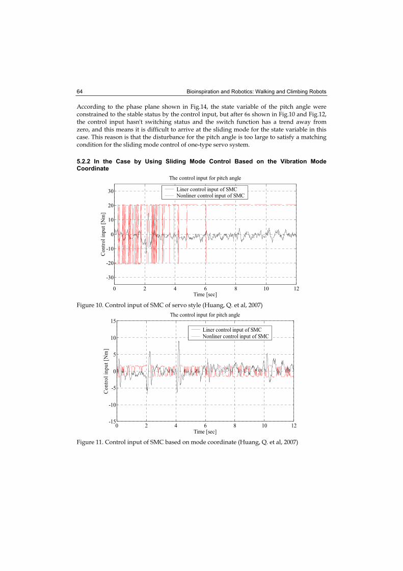
Bioinspiration and Robotics: Walking and Climbing Robots 64
According to the phase plane shown in Fig.14, the state variable of the pitch angle were constrained to the stable status by the control input, but after 6s shown in Fig.10 and Fig.12, the control input hasn't switching status and the switch function has a trend away from zero, and this means it is difficult to arrive at the sliding mode for the state variable in this case. This reason is that the disturbance for the pitch angle is too large to satisfy a matching condition for the sliding mode control of one-type servo system.
5.2.2 In the Case by Using Sliding Mode Control Based on the Vibration Mode Coordinate
0 2 4 6 8 10 12
-30
-20
-10
0
10
20
30
The control input for pitch angle
Time [sec]
Con
trol
input
[Nm
]
Liner control input of SMC Nonliner control input of SMC
Figure 10. Control input of SMC of servo style (Huang, Q. et al, 2007)
0 2 4 6 8 10 12-15
-10
-5
0
5
10
15The control input for pitch angle
Time [sec]
Co
ntr
ol
inp
ut
[Nm
]
Liner control input of SMC Nonliner control input of SMC
Figure 11. Control input of SMC based on mode coordinate (Huang, Q. et al, 2007)
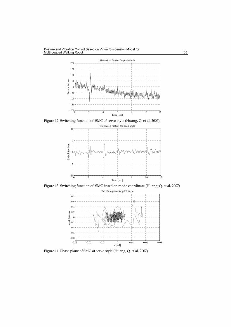
Posture and Vibration Control Based on Virtual Suspension Model for Multi-Legged Walking Robot 65
0 2 4 6 8 10 12-200
-150
-100
-50
0
50
100
150
200The switch fuction for pitch angle
Time [sec]
Sw
itch
fu
ctio
n
Figure 12. Switching function of SMC of servo style (Huang, Q. et al, 2007)
0 2 4 6 8 10 12-10
-5
0
5
10The switch fuction for pitch angle
Time [sec]
Sw
itch
fu
ctio
n
Figure 13. Switching function of SMC based on mode coordinate (Huang, Q. et al, 2007)
-0.03 -0.02 -0.01 0 0.01 0.02 0.03
-0.8
-0.6
-0.4
-0.2
0
0.2
0.4
0.6
0.8
The phase plane for pitch angle
x [rad]
dx/d
t [r
ad/s
ec]
Figure 14. Phase plane of SMC of servo style (Huang, Q. et al, 2007)
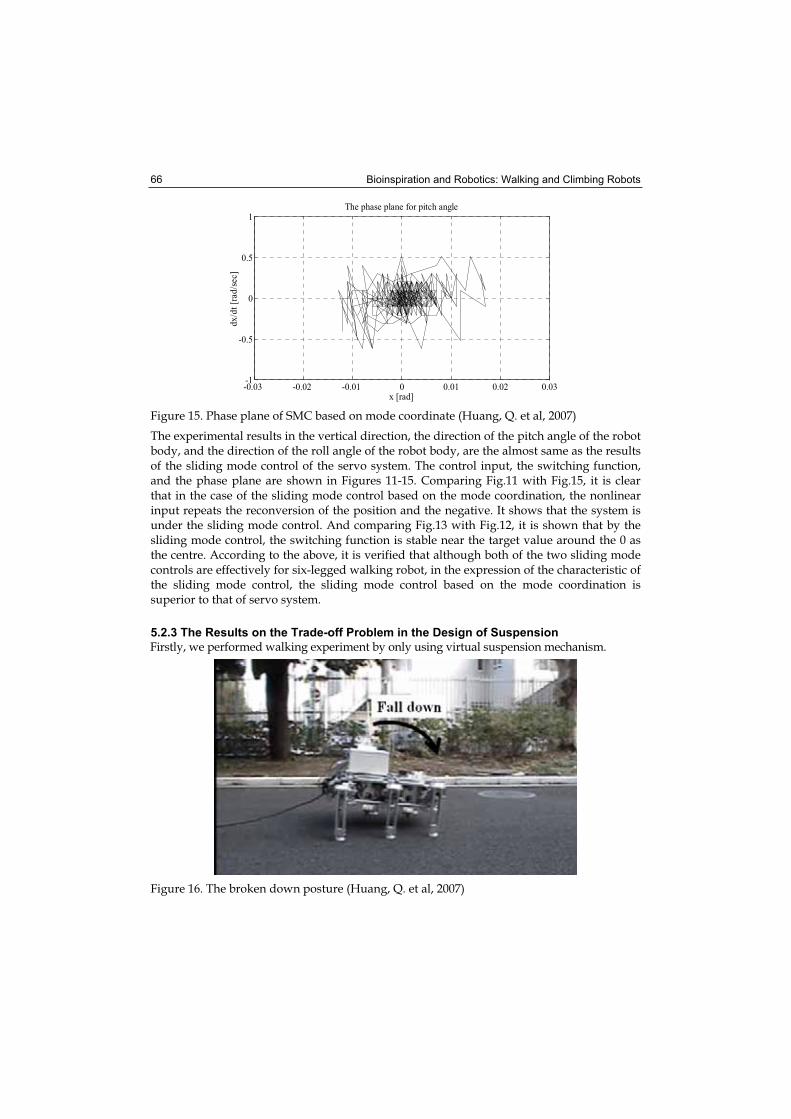
Bioinspiration and Robotics: Walking and Climbing Robots 66
-0.03 -0.02 -0.01 0 0.01 0.02 0.03-1
-0.5
0
0.5
1The phase plane for pitch angle
x [rad]
dx
/dt
[rad
/sec
]
Figure 15. Phase plane of SMC based on mode coordinate (Huang, Q. et al, 2007)
The experimental results in the vertical direction, the direction of the pitch angle of the robot body, and the direction of the roll angle of the robot body, are the almost same as the results of the sliding mode control of the servo system. The control input, the switching function, and the phase plane are shown in Figures 11-15. Comparing Fig.11 with Fig.15, it is clear that in the case of the sliding mode control based on the mode coordination, the nonlinear input repeats the reconversion of the position and the negative. It shows that the system is under the sliding mode control. And comparing Fig.13 with Fig.12, it is shown that by the sliding mode control, the switching function is stable near the target value around the 0 as the centre. According to the above, it is verified that although both of the two sliding mode controls are effectively for six-legged walking robot, in the expression of the characteristic of the sliding mode control, the sliding mode control based on the mode coordination is superior to that of servo system.
5.2.3 The Results on the Trade-off Problem in the Design of Suspension
Firstly, we performed walking experiment by only using virtual suspension mechanism.
Figure 16. The broken down posture (Huang, Q. et al, 2007)
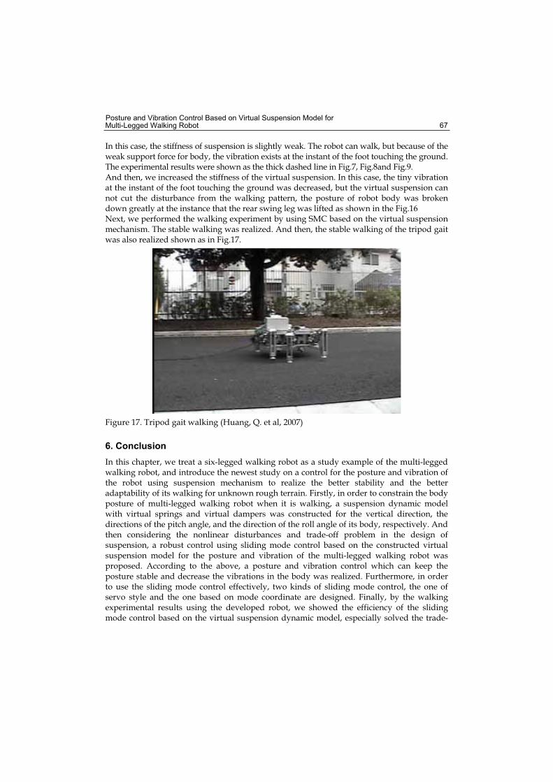
Posture and Vibration Control Based on Virtual Suspension Model for Multi-Legged Walking Robot 67
In this case, the stiffness of suspension is slightly weak. The robot can walk, but because of the weak support force for body, the vibration exists at the instant of the foot touching the ground. The experimental results were shown as the thick dashed line in Fig.7, Fig.8and Fig.9. And then, we increased the stiffness of the virtual suspension. In this case, the tiny vibration at the instant of the foot touching the ground was decreased, but the virtual suspension can not cut the disturbance from the walking pattern, the posture of robot body was broken down greatly at the instance that the rear swing leg was lifted as shown in the Fig.16 Next, we performed the walking experiment by using SMC based on the virtual suspension mechanism. The stable walking was realized. And then, the stable walking of the tripod gait was also realized shown as in Fig.17.
Figure 17. Tripod gait walking (Huang, Q. et al, 2007)
6. Conclusion
In this chapter, we treat a six-legged walking robot as a study example of the multi-legged walking robot, and introduce the newest study on a control for the posture and vibration of the robot using suspension mechanism to realize the better stability and the better adaptability of its walking for unknown rough terrain. Firstly, in order to constrain the body posture of multi-legged walking robot when it is walking, a suspension dynamic model with virtual springs and virtual dampers was constructed for the vertical direction, the directions of the pitch angle, and the direction of the roll angle of its body, respectively. And then considering the nonlinear disturbances and trade-off problem in the design of suspension, a robust control using sliding mode control based on the constructed virtual suspension model for the posture and vibration of the multi-legged walking robot was proposed. According to the above, a posture and vibration control which can keep the posture stable and decrease the vibrations in the body was realized. Furthermore, in order to use the sliding mode control effectively, two kinds of sliding mode control, the one of servo style and the one based on mode coordinate are designed. Finally, by the walking experimental results using the developed robot, we showed the efficiency of the sliding mode control based on the virtual suspension dynamic model, especially solved the trade-
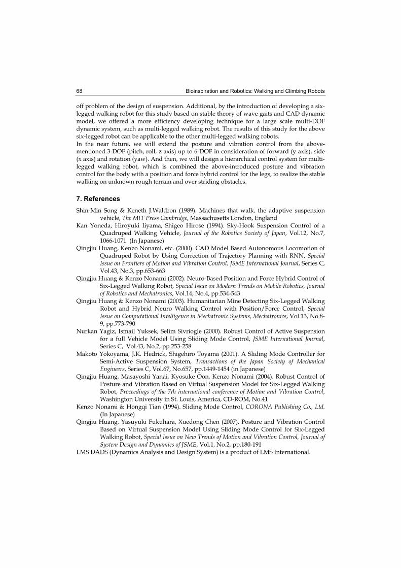
Bioinspiration and Robotics: Walking and Climbing Robots 68
off problem of the design of suspension. Additional, by the introduction of developing a six-legged walking robot for this study based on stable theory of wave gaits and CAD dynamic model, we offered a more efficiency developing technique for a large scale multi-DOF dynamic system, such as multi-legged walking robot. The results of this study for the above six-legged robot can be applicable to the other multi-legged walking robots. In the near future, we will extend the posture and vibration control from the above-mentioned 3-DOF (pitch, roll, z axis) up to 6-DOF in consideration of forward (y axis), side (x axis) and rotation (yaw). And then, we will design a hierarchical control system for multi-legged walking robot, which is combined the above-introduced posture and vibration control for the body with a position and force hybrid control for the legs, to realize the stable walking on unknown rough terrain and over striding obstacles.
7. References
Shin-Min Song & Keneth J.Waldron (1989). Machines that walk, the adaptive suspension vehicle, The MIT Press Cambridge, Massachusetts London, England
Kan Yoneda, Hiroyuki Iiyama, Shigeo Hirose (1994). Sky-Hook Suspension Control of a Quadruped Walking Vehicle, Journal of the Robotics Society of Japan, Vol.12, No.7, 1066-1071 (In Japanese)
Qingjiu Huang, Kenzo Nonami, etc. (2000). CAD Model Based Autonomous Locomotion of Quadruped Robot by Using Correction of Trajectory Planning with RNN, Special Issue on Frontiers of Motion and Vibration Control, JSME International Journal, Series C, Vol.43, No.3, pp.653-663
Qingjiu Huang & Kenzo Nonami (2002). Neuro-Based Position and Force Hybrid Control of Six-Legged Walking Robot, Special Issue on Modern Trends on Mobile Robotics, Journal of Robotics and Mechatronics, Vol.14, No.4, pp.534-543
Qingjiu Huang & Kenzo Nonami (2003). Humanitarian Mine Detecting Six-Legged Walking Robot and Hybrid Neuro Walking Control with Position/Force Control, Special Issue on Computational Intelligence in Mechatronic Systems, Mechatronics, Vol.13, No.8-9, pp.773-790
Nurkan Yagiz, Ismail Yuksek, Selim Sivriogle (2000). Robust Control of Active Suspension for a full Vehicle Model Using Sliding Mode Control, JSME International Journal,Series C, Vol.43, No.2, pp.253-258
Makoto Yokoyama, J.K. Hedrick, Shigehiro Toyama (2001). A Sliding Mode Controller for Semi-Active Suspension System, Transactions of the Japan Society of Mechanical Engineers, Series C, Vol.67, No.657, pp.1449-1454 (in Japanese)
Qingjiu Huang, Masayoshi Yanai, Kyosuke Oon, Kenzo Nonami (2004). Robust Control of Posture and Vibration Based on Virtual Suspension Model for Six-Legged Walking Robot, Proceedings of the 7th international conference of Motion and Vibration Control,Washington University in St. Louis, America, CD-ROM, No.41
Kenzo Nonami & Hongqi Tian (1994). Sliding Mode Control, CORONA Publishing Co., Ltd.(In Japanese)
Qingjiu Huang, Yasuyuki Fukuhara, Xuedong Chen (2007). Posture and Vibration Control Based on Virtual Suspension Model Using Sliding Mode Control for Six-Legged Walking Robot, Special Issue on New Trends of Motion and Vibration Control, Journal of System Design and Dynamics of JSME, Vol.1, No.2, pp.180-191
LMS DADS (Dynamics Analysis and Design System) is a product of LMS International.
5
Research on Hexapod Walking Bio-robot’s Workspace and Flexibility
Baoling Han, Qingsheng Luo, Xiaochuan Zhao and Qiuli Wang Beijing Institute of Technology
China
0. Introduction
Because of the natural selection and the long period evolution of various animals in the nature, the animals generates the strong adaptability to the surroundings on energy conversion, locomotion control, gesture adjustment, information processing and discerning direction. The animals’ structure and function is better than the man-made mechanical equipment’s. Therefore animals are becoming references of human’s advanced technology equipment .AT the 2004 IEEE Robotics and Bionics International Academic Conference, the experts pointed out :“The bio-robots imitating the animal body structure and function, will take the place of the traditional industry robots and become the trend in robot study field.” The definition of the bio-walking robot is a foot framework moving device which imitates the body structure and walking styles of multi-leg animals in the nature controlled by the computer [1]. According to the investigation, nearly half of the ground on the earth can not be reached by traditional wheel or pedrail vehicles, while many multi-leg animals can walk on it freely. Inspired by this phenomenon, many experts from different countries begin to study the technologies concerning to the walking bio-robots. Compared to others, the locomotion of the walking bio-robot has some unique capabilities which are not owned by other driving styles. For example, the walking bio-robot has many DOFs(degree of freedom), walking deftly like animals, therefore they have stronger adaptability to the complex changeable ground. Compared to the pedrail robot, the falling feet spots are discrete, so their feet tips can adjust the walking gesture within the reachable areas and choose the proper supporting pots, which makes the robot has the ability to avoid and overcome the obstacles[2]. Furthermore, the vibration can be isolated by the walking bio-robot’s locomotion system independently, that is to say, it allows body moving track and feet moving track relieve coupling. Although the ground is uneven, the robot can walk smoothly.Among all kinds of the walking bio-robots, because of the hexapod walking bio- robot’s advantages on structure and locomotion, people pay more attention on the hexapod walking bio-robot, which is becoming the key and hot point in robot study field. Figure 1 shows the new style hexapod walking bio-robot designed by the authors using the software UG. Due to its large number joints and the complex structure, how to make its body structure and legs ,realize the optimum design to extend its feet reachable area, improve its body agility, and fulfil the whole body’s optimum design becomes the key point. Because
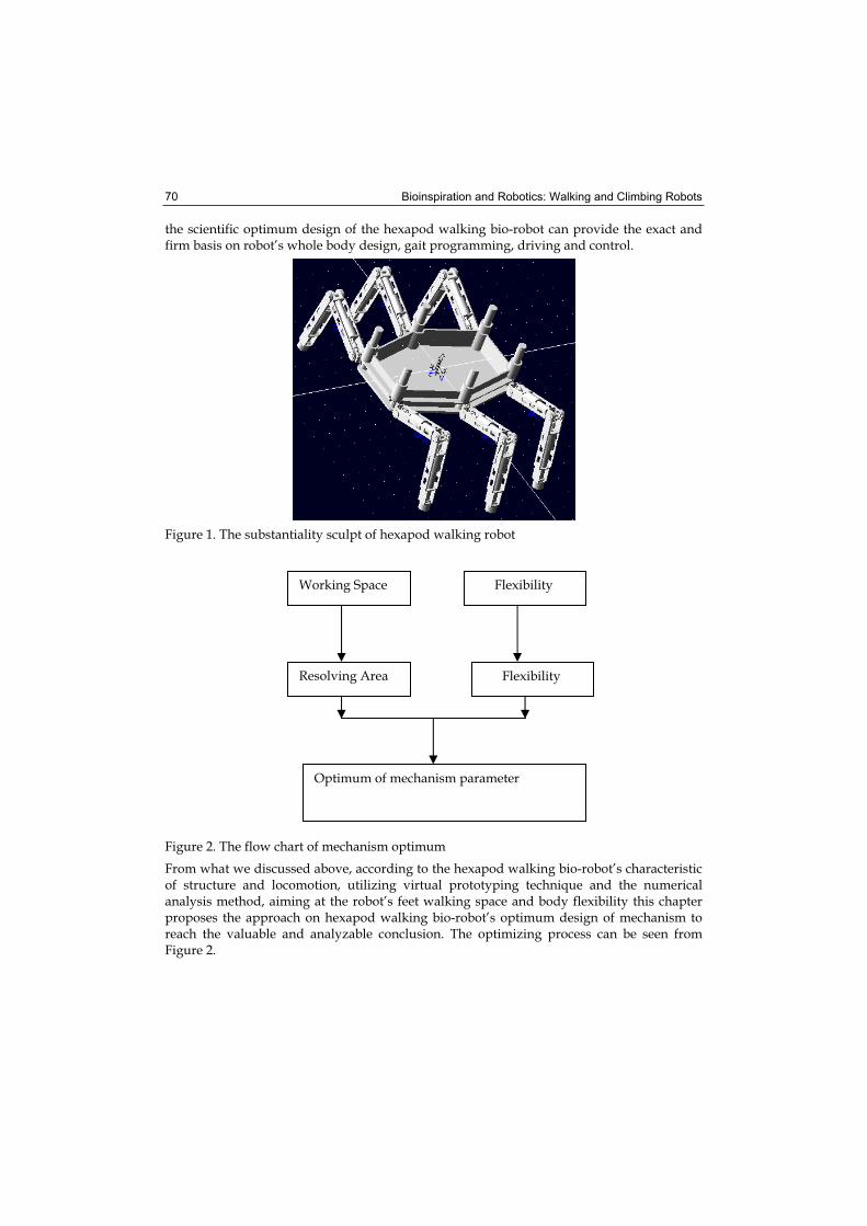
Bioinspiration and Robotics: Walking and Climbing Robots 70
the scientific optimum design of the hexapod walking bio-robot can provide the exact and firm basis on robot’s whole body design, gait programming, driving and control.
Figure 1. The substantiality sculpt of hexapod walking robot
Figure 2. The flow chart of mechanism optimum
From what we discussed above, according to the hexapod walking bio-robot’s characteristic of structure and locomotion, utilizing virtual prototyping technique and the numerical analysis method, aiming at the robot’s feet walking space and body flexibility this chapter proposes the approach on hexapod walking bio-robot’s optimum design of mechanism to reach the valuable and analyzable conclusion. The optimizing process can be seen from Figure 2.
Working Space Flexibility
Resolving Area Flexibility
Optimum of mechanism parameter
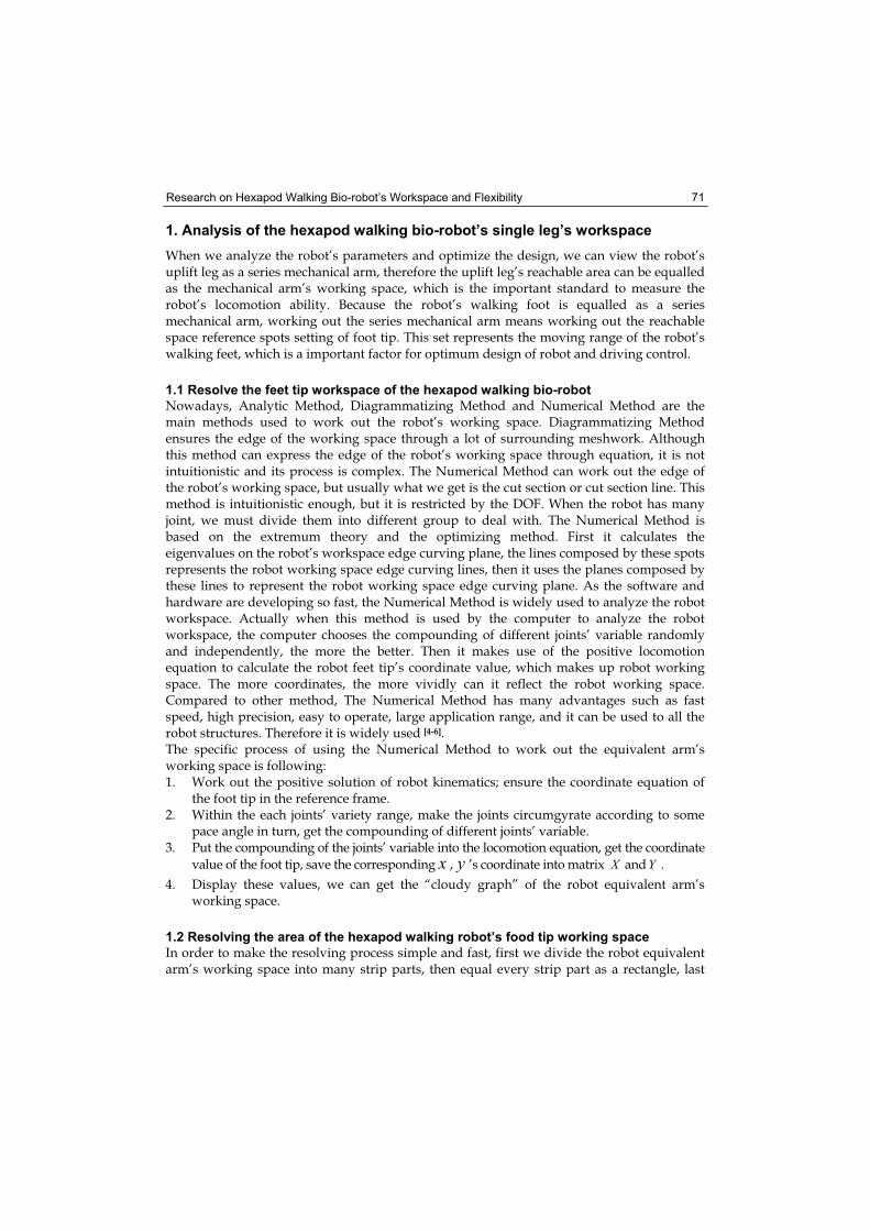
Research on Hexapod Walking Bio-robot’s Workspace and Flexibility 71
1. Analysis of the hexapod walking bio-robot’s single leg’s workspace
When we analyze the robot’s parameters and optimize the design, we can view the robot’s uplift leg as a series mechanical arm, therefore the uplift leg’s reachable area can be equalled as the mechanical arm’s working space, which is the important standard to measure the robot’s locomotion ability. Because the robot’s walking foot is equalled as a series mechanical arm, working out the series mechanical arm means working out the reachable space reference spots setting of foot tip. This set represents the moving range of the robot’s walking feet, which is a important factor for optimum design of robot and driving control.
1.1 Resolve the feet tip workspace of the hexapod walking bio-robot
Nowadays, Analytic Method, Diagrammatizing Method and Numerical Method are the main methods used to work out the robot’s working space. Diagrammatizing Method ensures the edge of the working space through a lot of surrounding meshwork. Although this method can express the edge of the robot’s working space through equation, it is not intuitionistic and its process is complex. The Numerical Method can work out the edge of the robot’s working space, but usually what we get is the cut section or cut section line. This method is intuitionistic enough, but it is restricted by the DOF. When the robot has many joint, we must divide them into different group to deal with. The Numerical Method is based on the extremum theory and the optimizing method. First it calculates the eigenvalues on the robot’s workspace edge curving plane, the lines composed by these spots represents the robot working space edge curving lines, then it uses the planes composed by these lines to represent the robot working space edge curving plane. As the software and hardware are developing so fast, the Numerical Method is widely used to analyze the robot workspace. Actually when this method is used by the computer to analyze the robot workspace, the computer chooses the compounding of different joints’ variable randomly and independently, the more the better. Then it makes use of the positive locomotion equation to calculate the robot feet tip’s coordinate value, which makes up robot working space. The more coordinates, the more vividly can it reflect the robot working space. Compared to other method, The Numerical Method has many advantages such as fast speed, high precision, easy to operate, large application range, and it can be used to all the robot structures. Therefore it is widely used [4-6].The specific process of using the Numerical Method to work out the equivalent arm’s working space is following: 1. Work out the positive solution of robot kinematics; ensure the coordinate equation of
the foot tip in the reference frame. 2. Within the each joints’ variety range, make the joints circumgyrate according to some
pace angle in turn, get the compounding of different joints’ variable. 3. Put the compounding of the joints’ variable into the locomotion equation, get the coordinate
value of the foot tip, save the corresponding x , y ’s coordinate into matrix X andY .
4. Display these values, we can get the “cloudy graph” of the robot equivalent arm’s working space.
1.2 Resolving the area of the hexapod walking robot’s food tip working space
In order to make the resolving process simple and fast, first we divide the robot equivalent arm’s working space into many strip parts, then equal every strip part as a rectangle, last
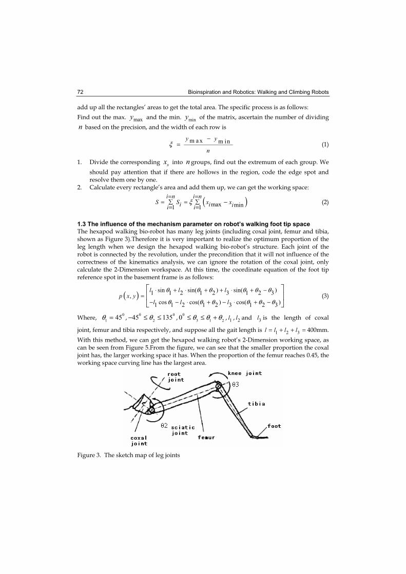
Bioinspiration and Robotics: Walking and Climbing Robots 72
add up all the rectangles’ areas to get the total area. The specific process is as follows:
Find out the max. maxy and the min. miny of the matrix, ascertain the number of dividing
n based on the precision, and the width of each row is
m a x m iny y
nξ
−= (1)
1. Divide the corresponding sx into n groups, find out the extremum of each group. We
should pay attention that if there are hollows in the region, code the edge spot and resolve them one by one.
2. Calculate every rectangle’s area and add them up, we can get the working space:
( )max min1 1
i n i nS S x xi i ii i
ξ= =
= = −= =
(2)
1.3 The influence of the mechanism parameter on robot’s walking foot tip space
The hexapod walking bio-robot has many leg joints (including coxal joint, femur and tibia, shown as Figure 3).Therefore it is very important to realize the optimum proportion of the leg length when we design the hexapod walking bio-robot’s structure. Each joint of the robot is connected by the revolution, under the precondition that it will not influence of the correctness of the kinematics analysis, we can ignore the rotation of the coxal joint, only calculate the 2-Dimension workspace. At this time, the coordinate equation of the foot tip reference spot in the basement frame is as follows:
( ) sin sin( ) sin( )1 1 2 1 2 3 1 2 3,
cos cos( ) cos( )1 1 2 1 2 3 1 2 3
l l lp x y
l l l
θ θ θ θ θ θ
θ θ θ θ θ θ
⋅ + ⋅ + + ⋅ + −=
− − ⋅ + − ⋅ + − (3)
Where,0
145θ = ,
0 0
245 135θ− ≤ ≤ ,
0
3 1 20 θ θ θ≤ ≤ + , 1l , 2l and 3l is the length of coxal
joint, femur and tibia respectively, and suppose all the gait length is 1 2 3l l l l= + + = 400mm.
With this method, we can get the hexapod walking robot’s 2-Dimension working space, as can be seen from Figure 5.From the figure, we can see that the smaller proportion the coxal joint has, the larger working space it has. When the proportion of the femur reaches 0.45, the working space curving line has the largest area.
Figure 3. The sketch map of leg joints
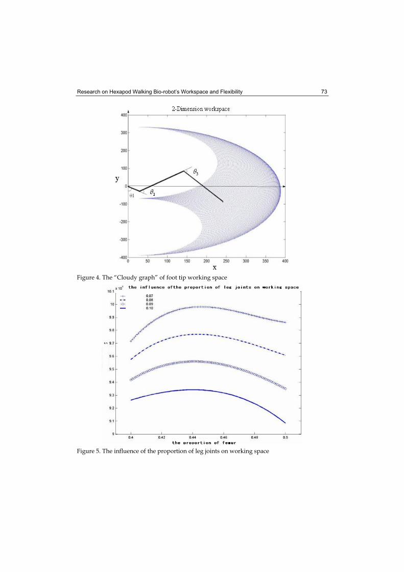
Research on Hexapod Walking Bio-robot’s Workspace and Flexibility 73
Figure 4. The “Cloudy graph” of foot tip working space
Figure 5. The influence of the proportion of leg joints on working space
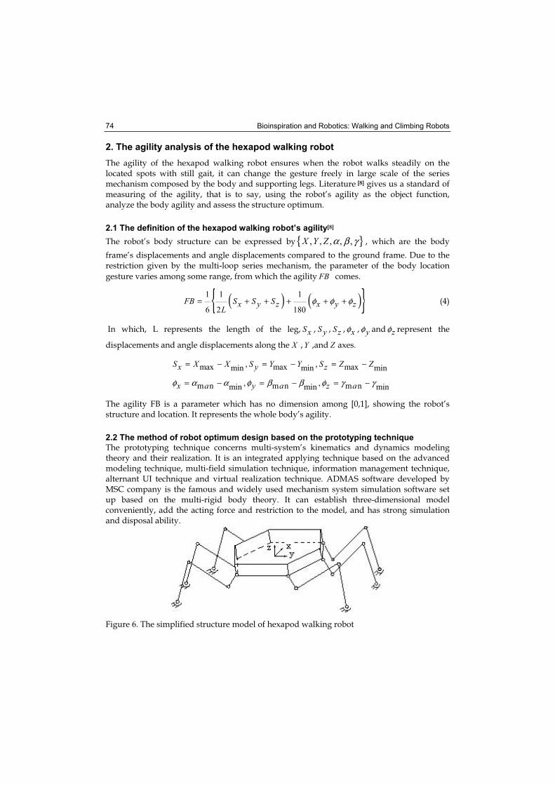
Bioinspiration and Robotics: Walking and Climbing Robots 74
2. The agility analysis of the hexapod walking robot
The agility of the hexapod walking robot ensures when the robot walks steadily on the located spots with still gait, it can change the gesture freely in large scale of the series mechanism composed by the body and supporting legs. Literature [8] gives us a standard of measuring of the agility, that is to say, using the robot’s agility as the object function, analyze the body agility and assess the structure optimum.
2.1 The definition of the hexapod walking robot’s agility[8]
The robot’s body structure can be expressed by{ }, , , , ,X Y Z α β γ , which are the body
frame’s displacements and angle displacements compared to the ground frame. Due to the restriction given by the multi-loop series mechanism, the parameter of the body location
gesture varies among some range, from which the agility FB comes.
( ) ( ){ }1 1 1
6 2 180FB S S Sx y z x y z
Lφ φ φ= + + + + + (4)
In which, L represents the length of the leg, Sx , S y , Sz , xφ , yφ and zφ represent the
displacements and angle displacements along the X , Y ,and Z axes.
, ,max max maxmin min min
, ,m n m n m nmin min min
S X X S Y Y S Z Zx y z
x a y a z aφ α α φ β β φ γ γ
= − = − = −
= − = − = −
The agility FB is a parameter which has no dimension among [0,1], showing the robot’s structure and location. It represents the whole body’s agility.
2.2 The method of robot optimum design based on the prototyping technique
The prototyping technique concerns multi-system’s kinematics and dynamics modeling theory and their realization. It is an integrated applying technique based on the advanced modeling technique, multi-field simulation technique, information management technique, alternant UI technique and virtual realization technique. ADMAS software developed by MSC company is the famous and widely used mechanism system simulation software set up based on the multi-rigid body theory. It can establish three-dimensional model conveniently, add the acting force and restriction to the model, and has strong simulation and disposal ability.
Figure 6. The simplified structure model of hexapod walking robot
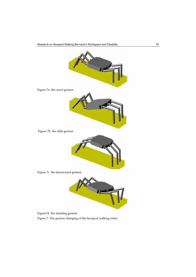
Research on Hexapod Walking Bio-robot’s Workspace and Flexibility 75
Figure 7a the crawl gesture
Figure 7b the sidle gesture
Figure 7c the turnaround gesture
Figure7d the standing gesture
Figure 7. The gesture changing of the hexapod walking robot
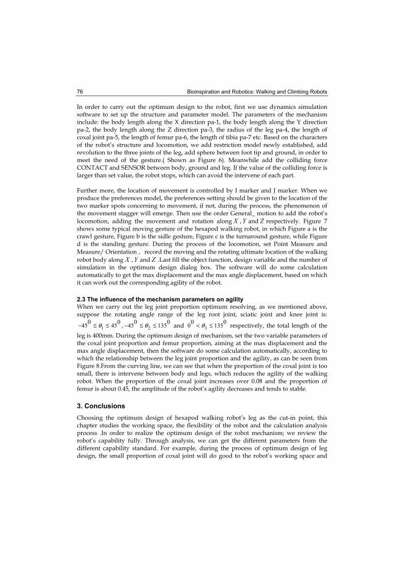
Bioinspiration and Robotics: Walking and Climbing Robots 76
In order to carry out the optimum design to the robot, first we use dynamics simulation software to set up the structure and parameter model. The parameters of the mechanism include: the body length along the X direction pa-1, the body length along the Y direction pa-2, the body length along the Z direction pa-3, the radius of the leg pa-4, the length of coxal joint pa-5, the length of femur pa-6, the length of tibia pa-7 etc. Based on the characters of the robot’s structure and locomotion, we add restriction model newly established, add revolution to the three joints of the leg, add sphere between foot tip and ground, in order to meet the need of the gesture.( Shown as Figure 6). Meanwhile add the colliding force CONTACT and SENSOR between body, ground and leg. If the value of the colliding force is larger than set value, the robot stops, which can avoid the intervene of each part.
Further more, the location of movement is controlled by I marker and J marker. When we produce the preferences model, the preferences setting should be given to the location of the two marker spots concerning to movement, if not, during the process, the phenomenon of the movement stagger will emerge. Then use the order General_ motion to add the robot’s
locomotion, adding the movement and rotation along X ,Y and Z respectively. Figure 7 shows some typical moving gesture of the hexapod walking robot, in which Figure a is the crawl gesture, Figure b is the sidle gesture, Figure c is the turnaround gesture, while Figure d is the standing gesture. During the process of the locomotion, set Point Measure and
Measure/ Orientation record the moving and the rotating ultimate location of the walking
robot body along X ,Y and Z .Last fill the object function, design variable and the number of simulation in the optimum design dialog box. The software will do some calculation automatically to get the max displacement and the max angle displacement, based on which it can work out the corresponding agility of the robot.
2.3 The influence of the mechanism parameters on agility
When we carry out the leg joint proportion optimum resolving, as we mentioned above, suppose the rotating angle range of the leg root joint, sciatic joint and knee joint is:
1
0 045 45θ− ≤ ≤ , 2
0 045 135θ− ≤ ≤ and 3
0 00 135θ< ≤ respectively, the total length of the
leg is 400mm. During the optimum design of mechanism, set the two variable parameters of the coxal joint proportion and femur proportion, aiming at the max displacement and the max angle displacement, then the software do some calculation automatically, according to which the relationship between the leg joint proportion and the agility, as can be seen from Figure 8.From the curving line, we can see that when the proportion of the coxal joint is too small, there is intervene between body and legs, which reduces the agility of the walking robot. When the proportion of the coxal joint increases over 0.08 and the proportion of femur is about 0.45, the amplitude of the robot’s agility decreases and tends to stable.
3. Conclusions
Choosing the optimum design of hexapod walking robot’s leg as the cut-in point, this chapter studies the working space, the flexibility of the robot and the calculation analysis process .In order to realize the optimum design of the robot mechanism; we review the robot’s capability fully. Through analysis, we can get the different parameters from the different capability standard. For example, during the process of optimum design of leg design, the small proportion of coxal joint will do good to the robot’s working space and
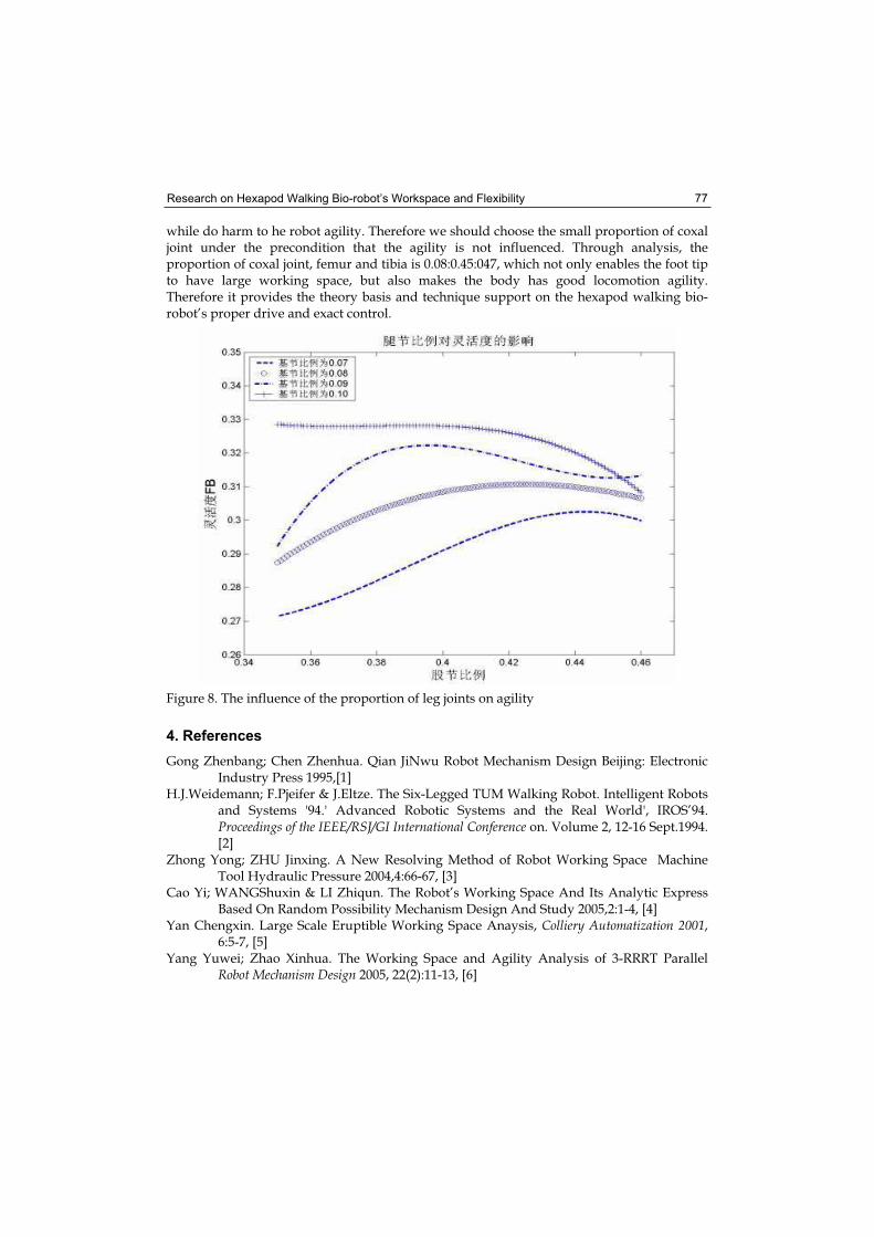
Research on Hexapod Walking Bio-robot’s Workspace and Flexibility 77
while do harm to he robot agility. Therefore we should choose the small proportion of coxal joint under the precondition that the agility is not influenced. Through analysis, the proportion of coxal joint, femur and tibia is 0.08:0.45:047, which not only enables the foot tip to have large working space, but also makes the body has good locomotion agility. Therefore it provides the theory basis and technique support on the hexapod walking bio-robot’s proper drive and exact control.
Figure 8. The influence of the proportion of leg joints on agility
4. References
Gong Zhenbang; Chen Zhenhua. Qian JiNwu Robot Mechanism Design Beijing: Electronic Industry Press 1995,[1]
H.J.Weidemann; F.Pjeifer & J.Eltze. The Six-Legged TUM Walking Robot. Intelligent Robots and Systems '94.' Advanced Robotic Systems and the Real World', IROS’94. Proceedings of the IEEE/RSJ/GI International Conference on. Volume 2, 12-16 Sept.1994. [2]
Zhong Yong; ZHU Jinxing. A New Resolving Method of Robot Working Space Machine Tool Hydraulic Pressure 2004,4:66-67, [3]
Cao Yi; WANGShuxin & LI Zhiqun. The Robot’s Working Space And Its Analytic Express Based On Random Possibility Mechanism Design And Study 2005,2:1-4, [4]
Yan Chengxin. Large Scale Eruptible Working Space Anaysis, Colliery Automatization 2001,6:5-7, [5]
Yang Yuwei; Zhao Xinhua. The Working Space and Agility Analysis of 3-RRRT Parallel Robot Mechanism Design 2005, 22(2):11-13, [6]
Bioinspiration and Robotics: Walking and Climbing Robots 78
Cao Yi ; Wang Shuxin & Li Zhiqun The Robot’s Working Space And Its Area Resolving Based On Random Possibility Manufacturing Automatization 2005,27(2): 24-29, [7]
Zhao Tieshi; Zhao Yongsheng & Huang Zhen. Crab-Like Walking Mechanism Modeling And Agility Analysis China Mechanism Engineering 1998,9(3):52-54, [8]
Wang Monan; Yang Yuchun. Crab-Like Bio-robot Modeling And Optimum HIT Transaction 2003,8(6):1-3, [9]
Zhong Jianrong. Adams Virtual Prototyping Introduction and Improvement Beijing: Mechanism Industry Press 2002, [10]
HAN Baoling, female, the Han nationality, from Anhui, Hefei Province, born in 1957, doctor, professor. Majoring in MEMS, Computer Graphics , Mechanical and Electronic Integration Design. Published more than 80 papers and three literatures
6
A designing method of the passive dynamic walking robot via analogy
with Phase locked loop circuits
Masatsugu Iribe1 and Koichi Osuka2
1Information Technologies Labs., Sony Corp., Tokyo 2Mechanical Engineering Dept. Kobe University, Hyogo
Japan
1. Introduction
Recently many biped walking robots are developed, and almost all the researches about those robots adopt mass-link models to control and referring zero moment point not to fall over while walking. Here we position these conventional control methods as “model-based control”. Features of the method are that the robot moves accurate and rigid at low efficiency. So it is also important to remember that these researches also adopt other ideas to decrease their energy consumption, to absorb the impact shock of the contact, or to control the joint stiffness …etc. For example, Honda robot “ASIMO” adopts soft material soles (Takenaka, 2001), Sony robot “SDR-4X” and Waseda university's robot controls its joint stiffness (Iribe et al, 2007) (Yamaguchi & Takanishi, 1997), and so on. So it seems important and valuable for the model-based control method to import the ideas based on the dynamics of the robots for their performance gain.On the other hand, we focus the passive dynamic walking robot which walks only by the dynamics caused by the gravity (McGeer, 1990) (Goswani et al, 1996) (Garcia et al, 1998) (Sugimoto & Osuka, 2005). Here we also position this control method which is operated by the dynamics as “dynamics-based control” method. Features of the method are that the robot moves soft and smooth at high efficiency. If the principle of the dynamics-based control is analyzed and elucidated, we will be able to apply the essence of this system to the conventional walking robot control, and also able to contribute the performance gain of walking robot control (Iribe & Osuka, 2006-2). Therefore we think that well-designed walking robots have both two above-mentioned ideas as shown in Fig.1. However, the dynamics-based control method doesn’t seems to be studied enough and does not show practical designing methods of the robot system in contrast to the model-based control method. Therefore it is important to develop robotic designing methods which are based on the ideas of the dynamics-based control. In this paper, firstly we analyze the behavior of the passive dynamic walking robot via analogy with Phase locked loop circuit which shows similar behaviors to the robot system, and ascertain the robot's gaits bifurcation and shows the chaotic behavior on the same condition which causes chaotic behaviors of Phase locked loop circuit. Secondly we ascertain that we can get initial conditions and set-up parameters which cause the desired
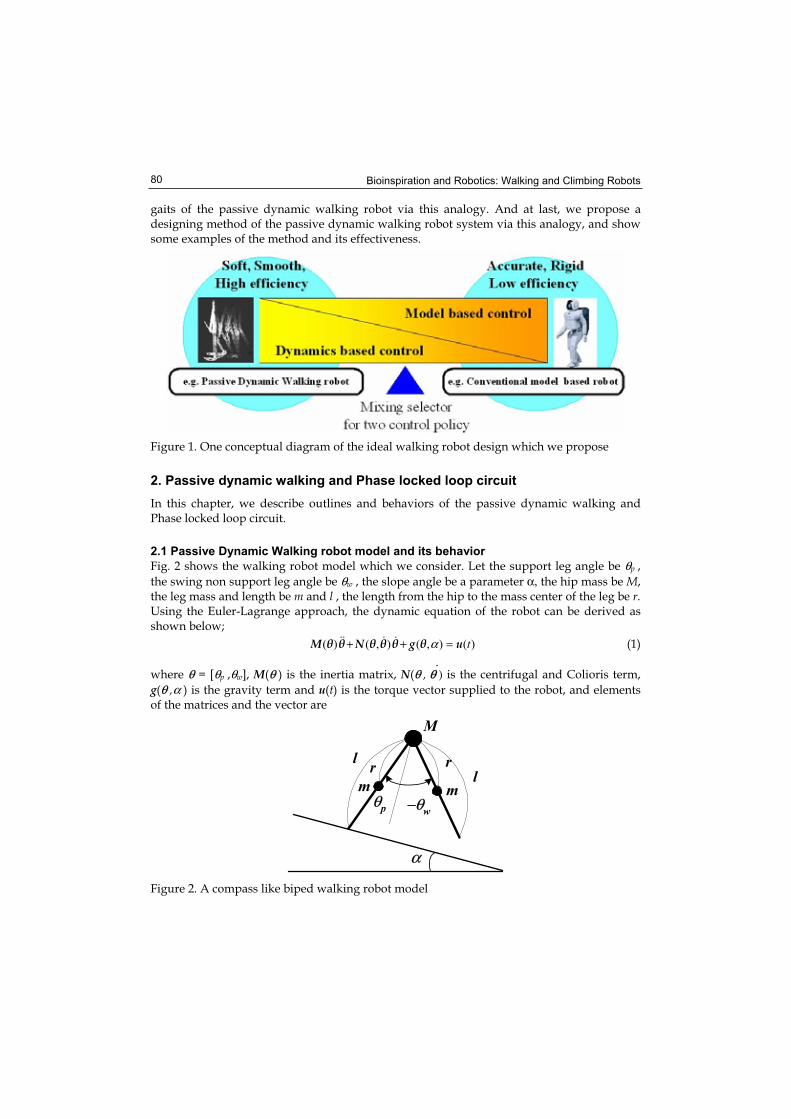
Bioinspiration and Robotics: Walking and Climbing Robots 80
gaits of the passive dynamic walking robot via this analogy. And at last, we propose a designing method of the passive dynamic walking robot system via this analogy, and show some examples of the method and its effectiveness.
Figure 1. One conceptual diagram of the ideal walking robot design which we propose
2. Passive dynamic walking and Phase locked loop circuit
In this chapter, we describe outlines and behaviors of the passive dynamic walking and Phase locked loop circuit.
2.1 Passive Dynamic Walking robot model and its behavior
Fig. 2 shows the walking robot model which we consider. Let the support leg angle be θp ,
the swing non support leg angle be θw , the slope angle be a parameter α, the hip mass be M,the leg mass and length be m and l , the length from the hip to the mass center of the leg be r.Using the Euler-Lagrange approach, the dynamic equation of the robot can be derived as shown below;
( ) ( , ) ( , ) ( )tα+ + =M N g u (1)
where θ = [θp ,θw], M(θ ) is the inertia matrix, N(θ , θθ ) is the centrifugal and Colioris term,
g(θ ,α ) is the gravity term and u(t) is the torque vector supplied to the robot, and elements of the matrices and the vector are
θp −θw
M
α
m
l rrm l
Figure 2. A compass like biped walking robot model
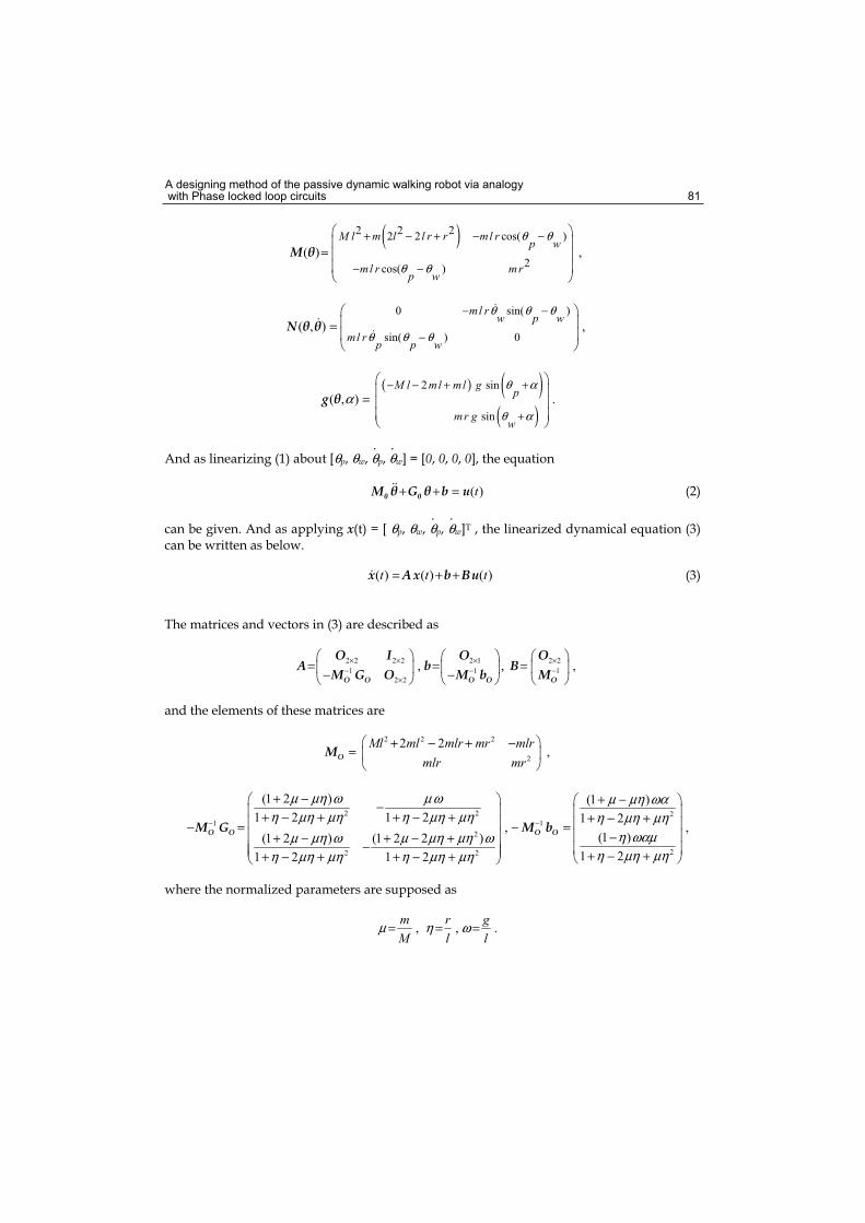
A designing method of the passive dynamic walking robot via analogy with Phase locked loop circuits 81
( )2 2 22 2 cos( )
2cos( )
( ) ,
M l m l l r r ml r p w
ml r m rp w
θ θ
θ θ
+ − + − −
− −=M
0 sin( )
sin( ) 0( , ) ,
ml r w p wml r p p w
θ θ θ
θ θ θ
− −
−=N
( ) ( )( )
2 sin
sin
( , ) .M l ml ml g p
m r g w
θ α
θ αα
− − + +
+=g
And as linearizing (1) about [θp, θw, θp, θw] = [0, 0, 0, 0], the equation
( )t+ + =0 0M G b u (2)
can be given. And as applying x(t) = [ θp, θw, θp, θw]T , the linearized dynamical equation (3) can be written as below.
( ) ( ) ( )t t t= + +x Ax b Bu (3)
The matrices and vectors in (3) are described as
2 2 2 2 2 1 2 2
1 1 1
2 2
, , ,× × × ×
− − −×
= = =− −O O O O O
O I O OA b B
M G O M b M
and the elements of these matrices are
2 2 2
2
2 2,
Ml ml mlr mr mlrmlr mr
+ − + −=OM
2 2 2
1 1
2
22 2
(1 2 ) (1 )
1 2 1 2 1 2, ,
(1 )(1 2 ) (1 2 2 )
1 21 2 1 2
μ μη ω μω μ μη ωαη μη μη η μη μη η μη μη
η ωαμμ μη ω μ μη μη ωη μη μηη μη μη η μη μη
− −
+ − + −−+ − + + − + + − +
− = − =−+ − + − +−
+ − ++ − + + − +
O O O OM G M b
where the normalized parameters are supposed as
, , .m r gM l l
μ η ω= = =
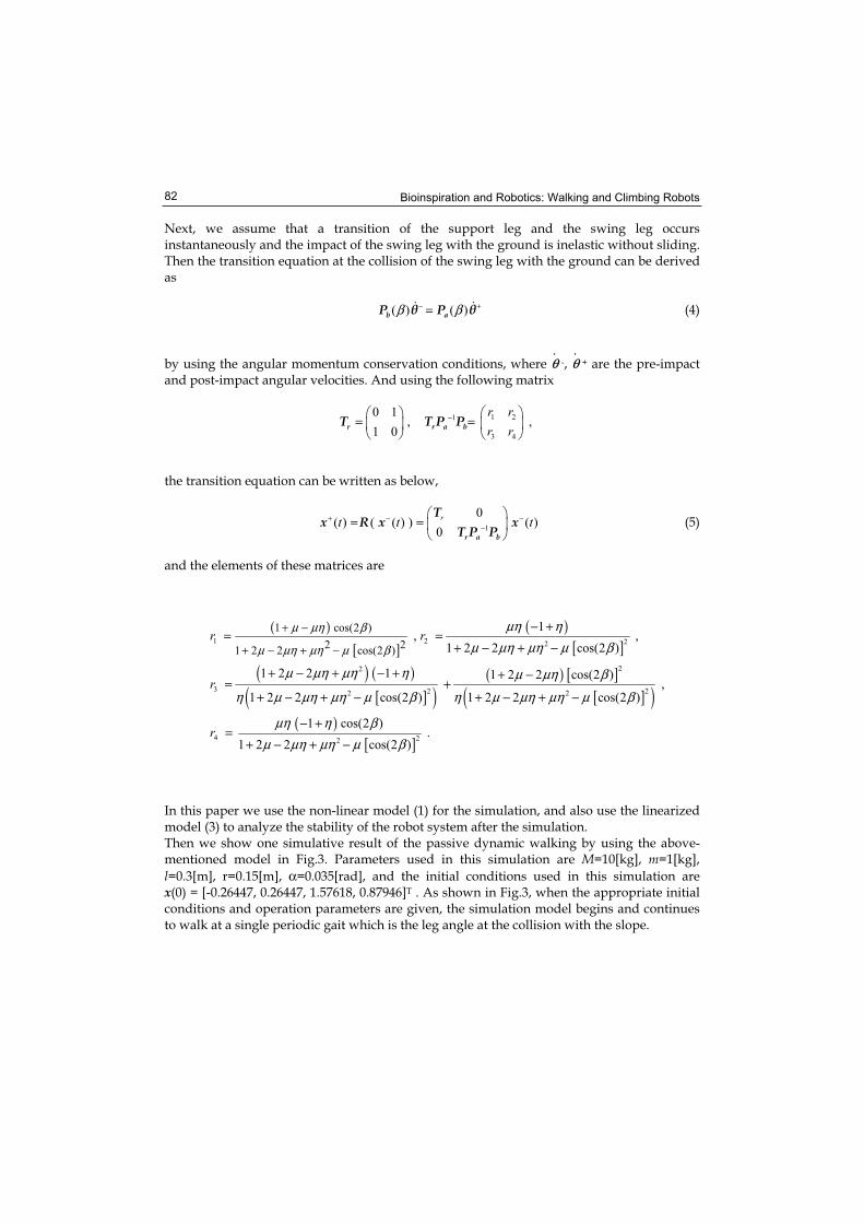
Bioinspiration and Robotics: Walking and Climbing Robots 82
Next, we assume that a transition of the support leg and the swing leg occurs instantaneously and the impact of the swing leg with the ground is inelastic without sliding. Then the transition equation at the collision of the swing leg with the ground can be derived as
( ) ( )β β− +=b aP P (4)
by using the angular momentum conservation conditions, where θ -, θ + are the pre-impact and post-impact angular velocities. And using the following matrix
1 21
3 4
0 1, ,
1 0
r rr r
−= =r r a bT T P P
the transition equation can be written as below,
1
0( ) ( ( ) ) ( )
0
rt t t+ − −−= =
r a b
Tx R x x
T P P (5)
and the elements of these matrices are
( )[ ]
( )[ ]
( ) ( )[ ]( )
( ) [ ][ ]( )
( )[ ]
1 2 22
22
3 2 22 2
4 22
1 cos(2 )
2 21 2 2 cos(2 )
1, ,
1 2 2 cos(2 )
1 2 2 1 1 2 2 cos(2 ),
1 2 2 cos(2 ) 1 2 2 cos(2 )
1 cos(2 ).
1 2 2 cos(2 )
r r
r
r
μ μη β
μ μη μη μ β
μη ημ μη μη μ β
μ μη μη η μ μη β
η μ μη μη μ β η μ μη μη μ β
μη η βμ μη μη μ β
+ −
+ − + −
− += =
+ − + −
+ − + − + + −= +
+ − + − + − + −
− +=
+ − + −
In this paper we use the non-linear model (1) for the simulation, and also use the linearized model (3) to analyze the stability of the robot system after the simulation. Then we show one simulative result of the passive dynamic walking by using the above-mentioned model in Fig.3. Parameters used in this simulation are M=10[kg], m=1[kg],
l=0.3[m], r=0.15[m], α=0.035[rad], and the initial conditions used in this simulation are x(0) = [-0.26447, 0.26447, 1.57618, 0.87946]T . As shown in Fig.3, when the appropriate initial conditions and operation parameters are given, the simulation model begins and continues to walk at a single periodic gait which is the leg angle at the collision with the slope.
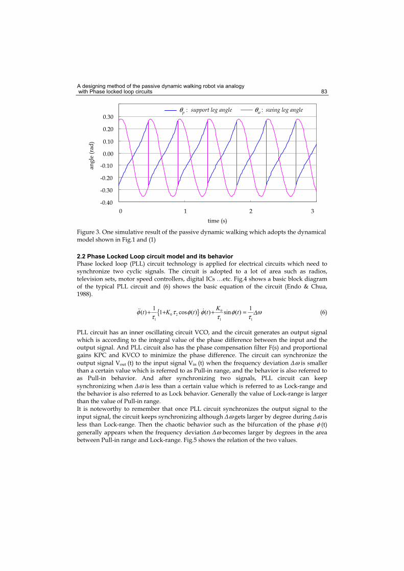
A designing method of the passive dynamic walking robot via analogy with Phase locked loop circuits 83
-0.40
-0.30
-0.20
-0.10
0.00
0.10
0.20
0.30
0 1 2 3
time (s)
ang
le (
rad
)
θw : swing leg angleθp : support leg angle
Figure 3. One simulative result of the passive dynamic walking which adopts the dynamical model shown in Fig.1 and (1)
2.2 Phase Locked Loop circuit model and its behavior
Phase locked loop (PLL) circuit technology is applied for electrical circuits which need to synchronize two cyclic signals. The circuit is adopted to a lot of area such as radios, television sets, motor speed controllers, digital ICs …etc. Fig.4 shows a basic block diagram of the typical PLL circuit and (6) shows the basic equation of the circuit (Endo & Chua, 1988).
{ } 00 2
1 1 1
1 1( ) 1 cos ( ) ( ) sin ( )
Kt K t t tφ τ φ φ φ ωτ τ τ
+ + + = (6)
PLL circuit has an inner oscillating circuit VCO, and the circuit generates an output signal which is according to the integral value of the phase difference between the input and the output signal. And PLL circuit also has the phase compensation filter F(s) and proportional gains KPC and KVCO to minimize the phase difference. The circuit can synchronize the
output signal Vout (t) to the input signal Vin (t) when the frequency deviation ω is smaller than a certain value which is referred to as Pull-in range, and the behavior is also referred to as Pull-in behavior. And after synchronizing two signals, PLL circuit can keep
synchronizing when ω is less than a certain value which is referred to as Lock-range and the behavior is also referred to as Lock behavior. Generally the value of Lock-range is larger than the value of Pull-in range. It is noteworthy to remember that once PLL circuit synchronizes the output signal to the
input signal, the circuit keeps synchronizing although ω gets larger by degree during ω is
less than Lock-range. Then the chaotic behavior such as the bifurcation of the phase φ (t)generally appears when the frequency deviation ω becomes larger by degrees in the area between Pull-in range and Lock-range. Fig.5 shows the relation of the two values.
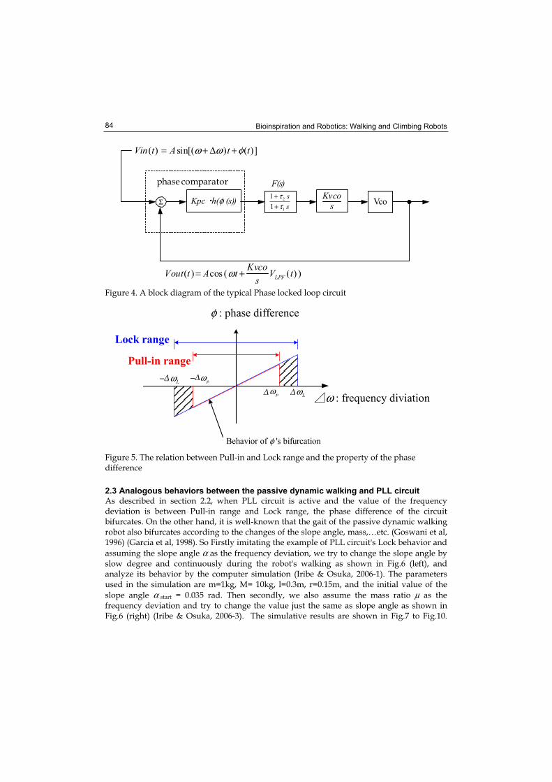
Bioinspiration and Robotics: Walking and Climbing Robots 84
( ) sin[( ) ( )]Vin t A t tω ω φ= + Δ +
Kpc h(φ (s)) KvcosΣ
phase comparator
Vco
( ) cos ( ( ) )LPFKvco
Vout t A t V ts
ω= +
F(s)2
1
1
1
ss
ττ
++
Figure 4. A block diagram of the typical Phase locked loop circuit
ω : frequency diviation
φ : phase difference
Lock range
Pull-in range
Behavior of φ 's bifurcation
pωpω−
LωLω−
Figure 5. The relation between Pull-in and Lock range and the property of the phase difference
2.3 Analogous behaviors between the passive dynamic walking and PLL circuit
As described in section 2.2, when PLL circuit is active and the value of the frequency deviation is between Pull-in range and Lock range, the phase difference of the circuit bifurcates. On the other hand, it is well-known that the gait of the passive dynamic walking robot also bifurcates according to the changes of the slope angle, mass,…etc. (Goswani et al, 1996) (Garcia et al, 1998). So Firstly imitating the example of PLL circuit's Lock behavior and
assuming the slope angle α as the frequency deviation, we try to change the slope angle by slow degree and continuously during the robot's walking as shown in Fig.6 (left), and analyze its behavior by the computer simulation (Iribe & Osuka, 2006-1). The parameters used in the simulation are m=1kg, M= 10kg, l=0.3m, r=0.15m, and the initial value of the
slope angle α start = 0.035 rad. Then secondly, we also assume the mass ratio μ as the frequency deviation and try to change the value just the same as slope angle as shown in Fig.6 (right) (Iribe & Osuka, 2006-3). The simulative results are shown in Fig.7 to Fig.10.
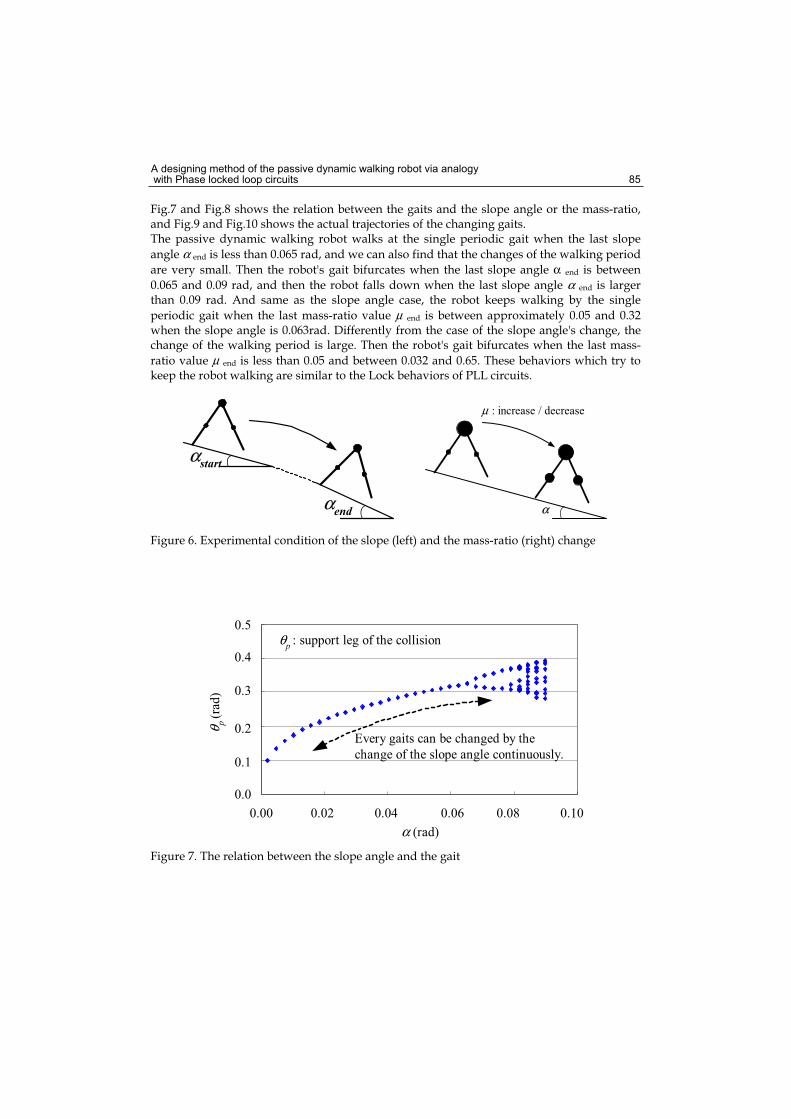
A designing method of the passive dynamic walking robot via analogy with Phase locked loop circuits 85
Fig.7 and Fig.8 shows the relation between the gaits and the slope angle or the mass-ratio, and Fig.9 and Fig.10 shows the actual trajectories of the changing gaits. The passive dynamic walking robot walks at the single periodic gait when the last slope
angle α end is less than 0.065 rad, and we can also find that the changes of the walking period
are very small. Then the robot's gait bifurcates when the last slope angle α end is between
0.065 and 0.09 rad, and then the robot falls down when the last slope angle α end is larger than 0.09 rad. And same as the slope angle case, the robot keeps walking by the single
periodic gait when the last mass-ratio value μ end is between approximately 0.05 and 0.32 when the slope angle is 0.063rad. Differently from the case of the slope angle's change, the change of the walking period is large. Then the robot's gait bifurcates when the last mass-
ratio value μ end is less than 0.05 and between 0.032 and 0.65. These behaviors which try to keep the robot walking are similar to the Lock behaviors of PLL circuits.
αend
αstart
α
μ : increase / decrease
Figure 6. Experimental condition of the slope (left) and the mass-ratio (right) change
0.0
0.1
0.2
0.3
0.4
0.5
0.00 0.02 0.04 0.06 0.08 0.10
α (rad)
θ p(r
ad)
θp : support leg of the collision
Every gaits can be changed by the
change of the slope angle continuously.
Figure 7. The relation between the slope angle and the gait
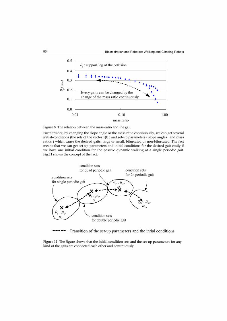
Bioinspiration and Robotics: Walking and Climbing Robots 86
0.0
0.1
0.2
0.3
0.4
0.5
0.01 0.10 1.00
mass ratio
θ p(r
ad)
θp : support leg of the collision
Every gaits can be changed by the
change of the mass ratio continuously.
Figure 8. The relation between the mass-ratio and the gait
Furthermore, by changing the slope angle or the mass ratio continuously, we can get several initial-conditions (the sets of the vector x(t) ) and set-up parameters ( slope angles and mass ratios ) which cause the desired gaits, large or small, bifurcated or non-bifurcated. The fact means that we can get set-up parameters and initial conditions for the desired gait easily if we have one initial condition for the passive dynamic walking at a single periodic gait. Fig.11 shows the concept of the fact.
θ1 , μ1,α1
θ2 , μ2,α2
θ4 , μ4 ,α4
θ2n , μ2n,α2n
: Transition of the set-up parameters and the intial conditions
condition sets
for single periodic gait
condition sets
for double periodic gait
condition sets
for quad periodic gait condition sets
for 2n periodic gait
Figure 11. The figure shows that the initial condition sets and the set-up parameters for any kind of the gaits are connected each other and continuously
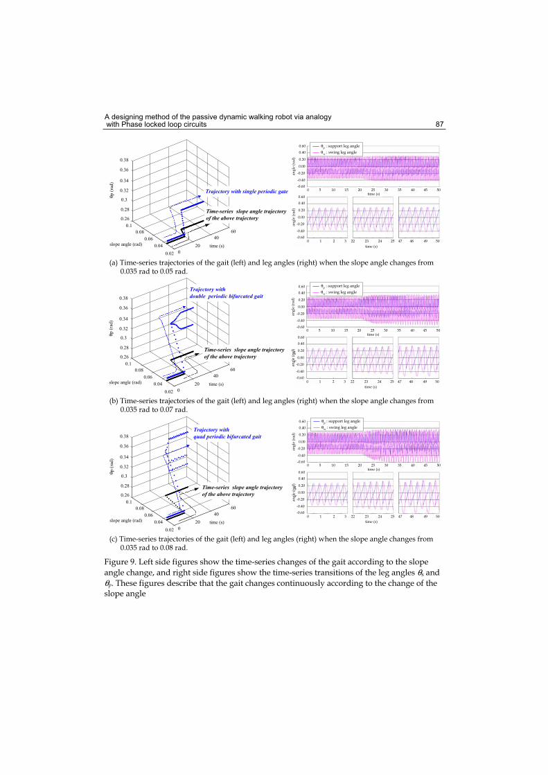
A designing method of the passive dynamic walking robot via analogy with Phase locked loop circuits 87
0
20
40
60
0.02
0.04
0.06
0.08
0.1
0.26
0.28
0.3
0.32
0.34
0.36
0.38
θp (
rad)
time (s)slope angle (rad)
Time-series slope angle trajectoryof the above trajectory
Trajectory with single periodic gate
0
20
40
60
0.02
0.04
0.06
0.08
0.1
0.26
0.28
0.3
0.32
0.34
0.36
0.38
θp (
rad)
time (s)slope angle (rad)
Trajectory withdouble periodic bifurcated gait
Time-series slope angle trajectoryof the above trajectory
Trajectory withquad periodic bifurcated gait
Time-series slope angle trajectoryof the above trajectory
0
20
40
60
0.02
0.04
0.06
0.08
0.1
0.26
0.28
0.3
0.32
0.34
0.36
0.38
θp (
rad)
time (s)slope angle (rad)
(a) Time-series trajectories of the gait (left) and leg angles (right) when the slope angle changes from 0.035 rad to 0.05 rad.
-0.60
-0.40
-0.20
0.00
0.20
0.40
0.60
ang
le (
rad
)
-0.60
-0.40
-0.20
0.00
0.20
0.40
0.60
an
gle
(ra
d)
0 5 10 15 20 30 35 40 45 50time (s)
25
time (s)
0 1 2 3 22 23 24 25 47 48 49 50
-0.60
-0.40
-0.20
0.00
0.20
0.40
0.60
an
gle
(ra
d)
-0.60
-0.40
-0.20
0.00
0.20
0.40
0.60
ang
le (
rad
)
0 5 10 15 20 30 35 40 45 50time (s)
25
time (s)
0 1 2 3 22 23 24 25 47 48 49 50
-0.60
-0.40
-0.20
0.00
0.20
0.40
0.60
an
gle
(ra
d)
-0.60
-0.40
-0.20
0.00
0.20
0.40
0.60
an
gle
(ra
d)
0 5 10 15 20 30 35 40 45 50time (s)
25
time (s)
0 1 2 3 22 23 24 25 47 48 49 50
(b) Time-series trajectories of the gait (left) and leg angles (right) when the slope angle changes from 0.035 rad to 0.07 rad.
(c) Time-series trajectories of the gait (left) and leg angles (right) when the slope angle changes from 0.035 rad to 0.08 rad.
θp : support leg angle
θw
: swing leg angle
θp : support leg angle
θw
: swing leg angle
θp : support leg angle
θw
: swing leg angle
Figure 9. Left side figures show the time-series changes of the gait according to the slope
angle change, and right side figures show the time-series transitions of the leg angles θs and
θp. These figures describe that the gait changes continuously according to the change of the slope angle
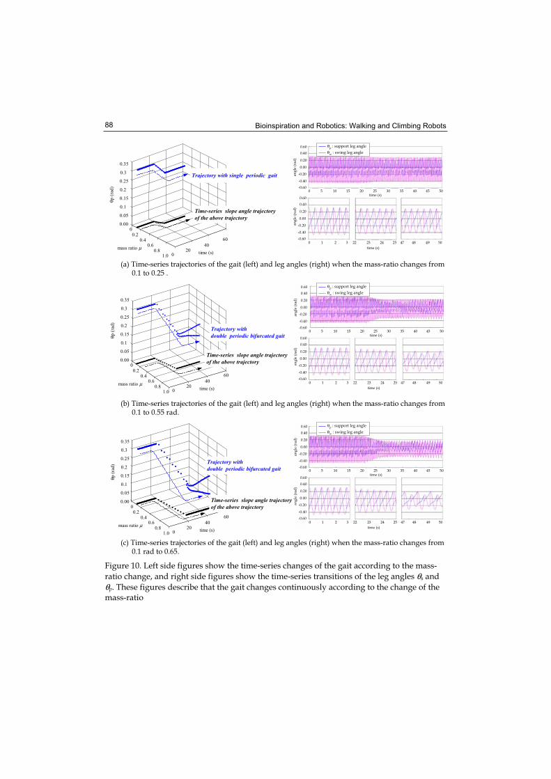
Bioinspiration and Robotics: Walking and Climbing Robots 88
(a) Time-series trajectories of the gait (left) and leg angles (right) when the mass-ratio changes from 0.1 to 0.25 .
(b) Time-series trajectories of the gait (left) and leg angles (right) when the mass-ratio changes from 0.1 to 0.55 rad.
(c) Time-series trajectories of the gait (left) and leg angles (right) when the mass-ratio changes from 0.1 rad to 0.65.
00.2
0.40.6
0.81.0 0
2040
60
0.00
0.05
0.1
0.15
0.2
0.25
0.3
0.35
θp (
rad)
time (s)mass ratio μ
Trajectory with single periodic gait
Time-series slope angle trajectoryof the above trajectory
Trajectory withdouble periodic bifurcated gait
Time-series slope angle trajectoryof the above trajectory
00.2
0.40.6
0.81.0 0
2040
60
0.00
0.05
0.1
0.15
0.2
0.25
0.3
0.35
θp (
rad)
time (s)mass ratio μ
00.2
0.40.6
0.81.0 0
2040
60
0.00
0.05
0.1
0.15
0.2
0.25
0.3
0.35
θp (
rad)
time (s)mass ratio μ
Trajectory withdouble periodic bifurcated gait
Time-series slope angle trajectoryof the above trajectory
-0.60
-0.40
-0.20
0.00
0.20
0.40
0.60
an
gle
(ra
d)
0 5 10 15 20 30 35 40 45 50time (s)
25
time (s)
0 1 2 3 22 23 24 25 47 48 49 50-0.60
-0.40
0.00
0.20
0.40
0.60
an
gle
(ra
d)
-0.20
-0.60
-0.40
-0.20
0.00
0.20
0.40
0.60
ang
le (
rad
)
0 5 10 15 20 30 35 40 45 50time (s)
25
time (s)
0 1 2 3 22 23 24 25 47 48 49 50-0.60
-0.40
0.00
0.20
0.40
0.60
an
gle
(ra
d)
-0.20
-0.60
-0.40
-0.20
0.00
0.20
0.40
0.60
ang
le (
rad
)
0 5 10 15 20 30 35 40 45 50time (s)
25
time (s)
0 1 2 3 22 23 24 25 47 48 49 50-0.60
-0.40
0.00
0.20
0.40
0.60
an
gle
(ra
d)
-0.20
θp : support leg angle
θw
: swing leg angle
θp : support leg angle
θw
: swing leg angle
θp : support leg angle
θw : swing leg angle
Figure 10. Left side figures show the time-series changes of the gait according to the mass-
ratio change, and right side figures show the time-series transitions of the leg angles θs and
θp. These figures describe that the gait changes continuously according to the change of the mass-ratio
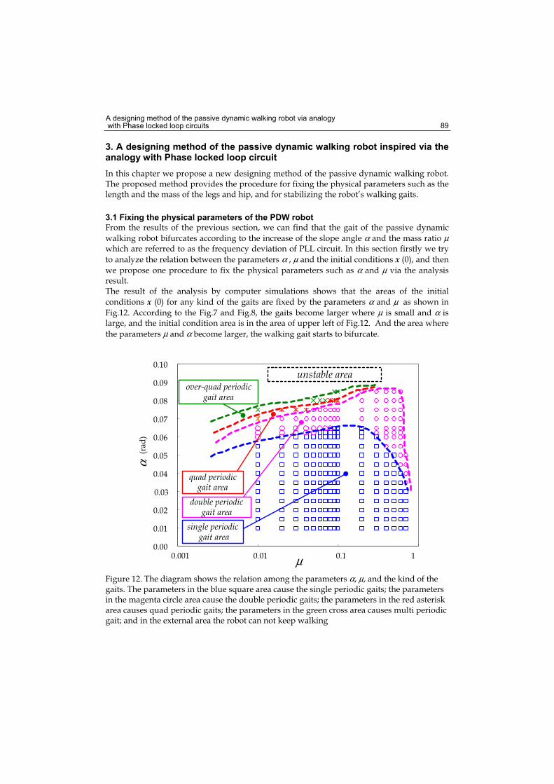
A designing method of the passive dynamic walking robot via analogy with Phase locked loop circuits 89
3. A designing method of the passive dynamic walking robot inspired via the analogy with Phase locked loop circuit
In this chapter we propose a new designing method of the passive dynamic walking robot. The proposed method provides the procedure for fixing the physical parameters such as the length and the mass of the legs and hip, and for stabilizing the robot’s walking gaits.
3.1 Fixing the physical parameters of the PDW robot
From the results of the previous section, we can find that the gait of the passive dynamic
walking robot bifurcates according to the increase of the slope angle α and the mass ratio μwhich are referred to as the frequency deviation of PLL circuit. In this section firstly we try
to analyze the relation between the parameters α , μ and the initial conditions x (0), and then
we propose one procedure to fix the physical parameters such as α and μ via the analysis result.The result of the analysis by computer simulations shows that the areas of the initial
conditions x (0) for any kind of the gaits are fixed by the parameters α and μ as shown in
Fig.12. According to the Fig.7 and Fig.8, the gaits become larger where μ is small and α is large, and the initial condition area is in the area of upper left of Fig.12. And the area where
the parameters μ and α become larger, the walking gait starts to bifurcate.
0.00
0.01
0.02
0.03
0.04
0.05
0.06
0.07
0.08
0.09
0.10
0.001 0.01 0.1 1μ
α(r
ad)
single periodic gait area
double periodicgait area
quad periodicgait area
over-quad periodicgait area
unstable area
Figure 12. The diagram shows the relation among the parameters α, μ, and the kind of the gaits. The parameters in the blue square area cause the single periodic gaits; the parameters in the magenta circle area cause the double periodic gaits; the parameters in the red asterisk area causes quad periodic gaits; the parameters in the green cross area causes multi periodic gait; and in the external area the robot can not keep walking
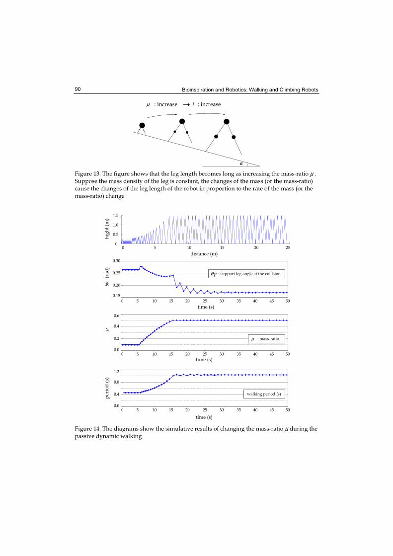
Bioinspiration and Robotics: Walking and Climbing Robots 90
α
μ : increase l : increase
Figure 13. The figure shows that the leg length becomes long as increasing the mass-ratio μ .Suppose the mass density of the leg is constant, the changes of the mass (or the mass-ratio) cause the changes of the leg length of the robot in proportion to the rate of the mass (or the mass-ratio) change
0.0
0.4
0.8
1.2
0 5 10 15 20 25 30 35 40 45 50
per
iod
(s)
time (s)
0.0
0.2
0.4
0.6
0 5 10 15 20 25 30 35 40 45 50
μ
time (s)
0.15
0.20
0.25
0.30
0 5 10 15 20 25 30 35 40 45 50
time (s)
θp(r
ad)
μ : mass-ratio
θ p : support leg angle at the collision
walking period (s)
0 5 10 15 20 250
0.5
1.0
1.5
distance (m)
hig
ht
(m)
Figure 14. The diagrams show the simulative results of changing the mass-ratio μ during the passive dynamic walking
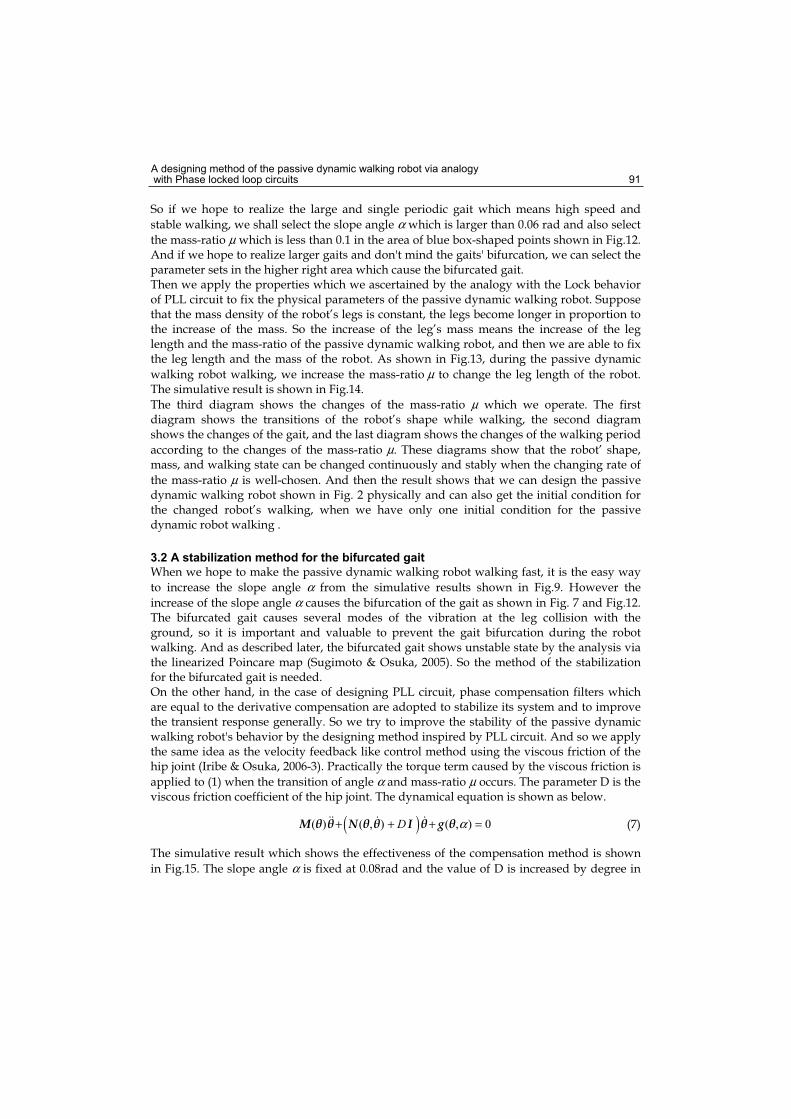
A designing method of the passive dynamic walking robot via analogy with Phase locked loop circuits 91
So if we hope to realize the large and single periodic gait which means high speed and
stable walking, we shall select the slope angle α which is larger than 0.06 rad and also select
the mass-ratio μ which is less than 0.1 in the area of blue box-shaped points shown in Fig.12. And if we hope to realize larger gaits and don't mind the gaits' bifurcation, we can select the parameter sets in the higher right area which cause the bifurcated gait. Then we apply the properties which we ascertained by the analogy with the Lock behavior of PLL circuit to fix the physical parameters of the passive dynamic walking robot. Suppose that the mass density of the robot’s legs is constant, the legs become longer in proportion to the increase of the mass. So the increase of the leg’s mass means the increase of the leg length and the mass-ratio of the passive dynamic walking robot, and then we are able to fix the leg length and the mass of the robot. As shown in Fig.13, during the passive dynamic
walking robot walking, we increase the mass-ratio μ to change the leg length of the robot. The simulative result is shown in Fig.14.
The third diagram shows the changes of the mass-ratio μ which we operate. The first diagram shows the transitions of the robot’s shape while walking, the second diagram shows the changes of the gait, and the last diagram shows the changes of the walking period
according to the changes of the mass-ratio μ. These diagrams show that the robot’ shape, mass, and walking state can be changed continuously and stably when the changing rate of
the mass-ratio μ is well-chosen. And then the result shows that we can design the passive dynamic walking robot shown in Fig. 2 physically and can also get the initial condition for the changed robot’s walking, when we have only one initial condition for the passive dynamic robot walking .
3.2 A stabilization method for the bifurcated gait
When we hope to make the passive dynamic walking robot walking fast, it is the easy way
to increase the slope angle α from the simulative results shown in Fig.9. However the
increase of the slope angle α causes the bifurcation of the gait as shown in Fig. 7 and Fig.12. The bifurcated gait causes several modes of the vibration at the leg collision with the ground, so it is important and valuable to prevent the gait bifurcation during the robot walking. And as described later, the bifurcated gait shows unstable state by the analysis via the linearized Poincare map (Sugimoto & Osuka, 2005). So the method of the stabilization for the bifurcated gait is needed. On the other hand, in the case of designing PLL circuit, phase compensation filters which are equal to the derivative compensation are adopted to stabilize its system and to improve the transient response generally. So we try to improve the stability of the passive dynamic walking robot's behavior by the designing method inspired by PLL circuit. And so we apply the same idea as the velocity feedback like control method using the viscous friction of the hip joint (Iribe & Osuka, 2006-3). Practically the torque term caused by the viscous friction is
applied to (1) when the transition of angle α and mass-ratio μ occurs. The parameter D is the viscous friction coefficient of the hip joint. The dynamical equation is shown as below.
( )( ) ( , ) ( , ) 0D α+ + + =M N I g (7)
The simulative result which shows the effectiveness of the compensation method is shown
in Fig.15. The slope angle α is fixed at 0.08rad and the value of D is increased by degree in
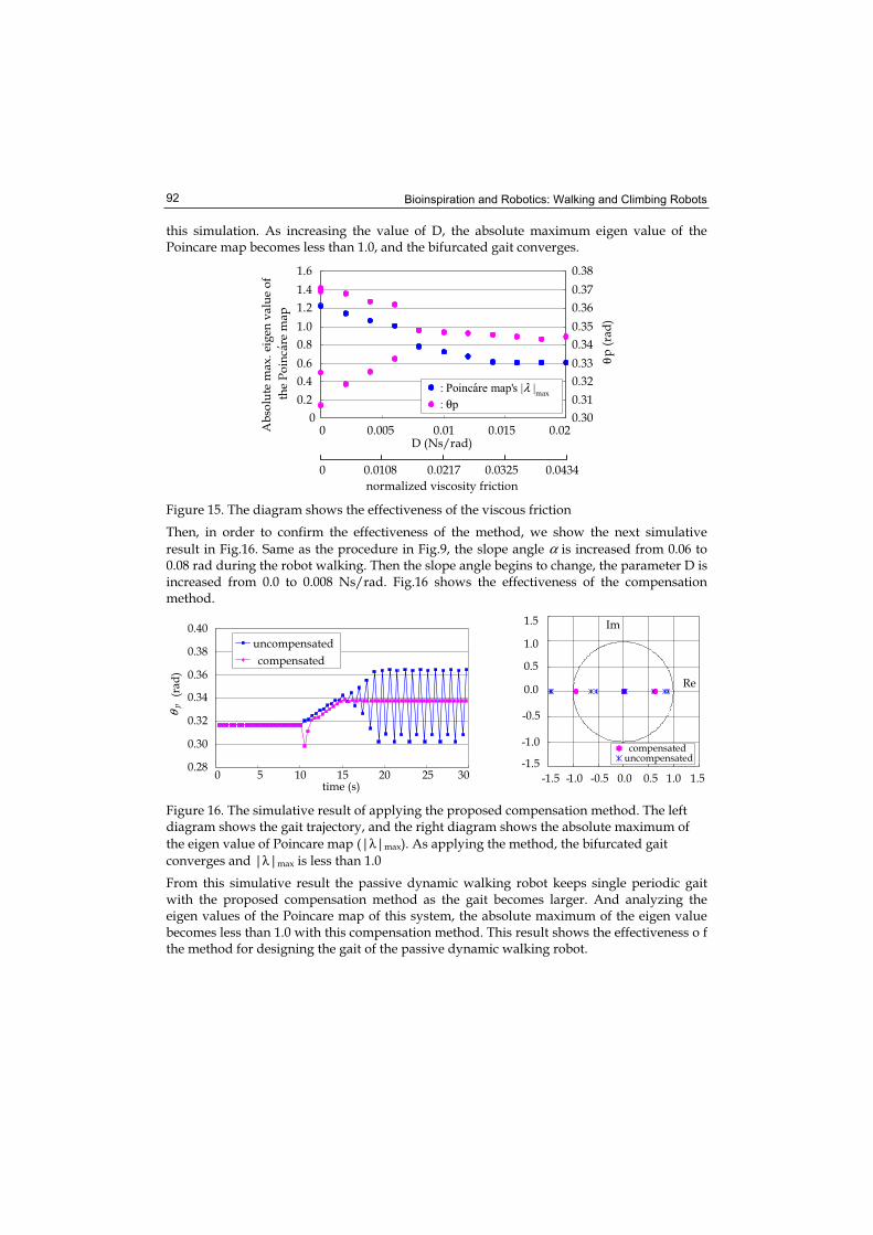
Bioinspiration and Robotics: Walking and Climbing Robots 92
this simulation. As increasing the value of D, the absolute maximum eigen value of the Poincare map becomes less than 1.0, and the bifurcated gait converges.
0
0.2
0.4
0.6
0.8
1.0
1.2
1.4
1.6
0 0.005 0.01 0.015 0.02D (Ns/rad)
Ab
solu
te m
ax.
eig
en v
alu
e o
f
the
Po
inca
re m
ap
0.30
0.31
0.32
0.33
0.34
0.35
0.36
0.37
0.38
θp (
rad
)
: Poincare map's |λ |max
: θp
0 0.0108 0.0217 0.0325 0.0434
normalized viscosity friction
,
,
Figure 15. The diagram shows the effectiveness of the viscous friction
Then, in order to confirm the effectiveness of the method, we show the next simulative
result in Fig.16. Same as the procedure in Fig.9, the slope angle α is increased from 0.06 to 0.08 rad during the robot walking. Then the slope angle begins to change, the parameter D is increased from 0.0 to 0.008 Ns/rad. Fig.16 shows the effectiveness of the compensation method.
0.28
0.30
0.32
0.34
0.36
0.38
0.40
0 5 10 15 20 25 30time (s)
uncompensated
compensated
θp
(ra
d)
-1.5
-1.0
-0.5
0.0
0.5
1.0
1.5
-1.5 -0.5 0.5 1.5-1.0 0.0 1.0
compensateduncompensated
Re
Im
Figure 16. The simulative result of applying the proposed compensation method. The left diagram shows the gait trajectory, and the right diagram shows the absolute maximum of
the eigen value of Poincare map (|λ|max). As applying the method, the bifurcated gait
converges and |λ|max is less than 1.0
From this simulative result the passive dynamic walking robot keeps single periodic gait with the proposed compensation method as the gait becomes larger. And analyzing the eigen values of the Poincare map of this system, the absolute maximum of the eigen value becomes less than 1.0 with this compensation method. This result shows the effectiveness o f the method for designing the gait of the passive dynamic walking robot.
A designing method of the passive dynamic walking robot via analogy with Phase locked loop circuits 93
This method seems to be a kind of the Delayed Feedback Control (DFC) reported in (Pyragas, 1992), (Sugimoto & Osuka, 2004) which is the effective control method for the non-linear system which shows the chaotic behavior. And in addition, here, we describe the linearized Poincare map which we use for analyzing the behavior of the passive dynamic walking. The linearized Poincare map Pk around the x*-
is given by the following equation (Sugimoto & Osuka, 2005) :
*
k e τ= AdP S R (8)
where
* **
( ), , d x x
xAx
−−=
∂= + = − =∂
*
*
v C Rv x b S I RC v
(9)
and the details in (8) and (9) are as follows :
• xk : perturbation value given by xk = xk- - x*-
• C : geometric condition (jump condition) as C = [1, 1, 0, 0]
• S : state constraint at the collision
• eAτ * : state transition from last collision to the next collision
• Rd : state transition at the collision The matrix A and vector v* are described in (3). And as applying this equation we can analyze the gait’s stability of the passive dynamic walking robot.
4. Conclusion
In this paper we ascertained the analogous behavior between Phase locked loop circuit and the passive dynamic walking robot, and showed the effective property to get set-up parameters and initial conditions. Then we proposed one method to fix the physical parameters and conditions which cause the desired walking gaits, and at last we showed the compensation method which is effective to stabilize the bifurcated gait of the robot. The proposed method which is inspired by the analogy with Phase locked loop circuit is probably valuable for designing the passive dynamic walking robot before beginning the actual prototyping. For the future work, we try to investigate the characteristic behavior of the passive dynamic walking robot which is similar to the Lock behavior of Phase locked loop circuit in detail. The behavior seems to be a kind of property of the limit cycle, so we may describe the behavior mathematically. Then we try to increase the degree of freedom of the passive dynamic walking robot and also try to simulate if the same behavior appears or not when the degree of freedom is increased. And then, the actual experiment by means of the real prototype is needed to verify the proposed method in this paper.
Bioinspiration and Robotics: Walking and Climbing Robots 94
5. References
Endo, T., Chua, L. (1988), Chaos From Phase-Locked Loops, IEEE Transactions on Circuits and Systems, pp.987-10003, Vol.35, No.8, August, 1988.
Garcia, M., Chatterjee, A. Ruina, A., Coleman, M. (1998), The Simplest Walking Model: Stability, Complexity and Scaling, ASME Journal of Biomechanical Engineering,Vol.120, No.2, pp.281-288, 1998.
Goswani, A., Thuilot, B., Espau, B. (1996), Compass-Like Biped Robot Part I: Stability and Bifurcation of Passive Gaits, Technical Report 2996 INRIA 19996, 1996.
Iribe, M., Osuka, K. (2006), Analogy between Passive walking robot and Phase Locked Loop circuit, Proceedings of SICE-ICASE International Joint Conference 2006, Busan, Korea, Oct.2006.
Iribe, M., Osuka, K. (2006), Analysis and stabilization of the passive walking robot via analogy with the Phase Locked Loop circuits, Proceedings of IEEE-RAS International Conference on Humanoid Robots (HUMANOIDS '06), pp.548-553, Genova, Italy, Dec.2006.
Iribe, M., Osuka, K. (2006) , A designing method of the passive dynamic walking robot viaanalogy with the Phase Locked Loop circuits, Proceedings of the 2006 IEEE International Conference on Robotics and Biomimetics (ROBIO2006), pp.636-641, Kunming, China, Dec., 2006.
Iribe, M., Moridaira, T., Fukushima, T., Kuroki, Y. (2007), Safety design for small biped walking home entertainment robot SDR-4XII, In: Mechatronics for Safety, Security and Dependability in a New Era, Arai., E. and Arai., T.(Ed.), pp.189-194, ELSEVIER, 0-08-044963-8, UK.
McGeer, T. (1990), Passive Dynamic Walking, The International Journal of Robotic Research,Vol.9, No.2, pp.62-82, 1990.
Pyragas, K. (1992) , Continuous control of chaos by selfcontrolling feedback, Phys. Lett. A,Vol.170, pp.421-428, 1992.
Sugimoto, Y., Osuka, K. (2004), Walking Control of Quasi Passive Dynamic Walking Robot "Quartet III" base on Continuous Delayed Feedback Control, Proceedings of IEEE International Conference on Robotics and Biomimetics, Shenyang, China, Aug. 2004.
Sugimoto, Y., Osuka, K. (2005), Stability Analysis of Passive Dynamic Walking focusing on the Inner Structure of Poincare Map, Proceedings of The 12th International Conference on Advanced Robotics, pp.236-241, 2005.
Takenaka, T. (2001). Honda humanoid robot ‘ASIMO‘, Report of Honda foundation, No.99, September, 2001 ( In Japanese ).
Yamaguchi, J., Takanishi, A. (1997), Development of a Biped Walking Robot Having Antagonistic Driven Joints Using Nonlinear Spring Mechanism, Proceedings of the 1997 IEEE International Conference on Robotics and Automation, pp.185-192, April. 1997.
7
Theoretical Investigations of the Control Movement of the CLAWAR at Statically Unstable
Regimes
Alexander Gorobtsov Volgograd State Technical University
Russia
1. Introduction
Dynamic control of constrained spatial mechanical systems, such as manipulators, CLAWAR, multifingered robotic hands and etc have been classic problem in robotics research. The theory of control based on fundamental idea of dynamic inverse. One of the best control schemes is hybrid position/force (Mayorga R. V., Wong A. K, . .).Ones works has been exploited the hybrid control to manipulators with open constraints. The theory of the control of robotics with closured constraints (Vukobratovic M., Kircanski M.) assumed that the rectangular matrix of the coefficients of constraints is the matrix of full rank, and not include redundant constraints. The problem of the redundant constraint raised in walking machines and systems with redundantly drive parallel mechanisms too (Jongwon K., Frank C. P. ). The mentions methods are references at two classes of mechanical systems. First it is spatial system with unmovable body and seconds is a spatial system without unmovable body. The dynamics of the systems first class is described by equations, expressed at explicit form at relative or absolute coordinates. That form of equation is permitted simple using classical method of stability analysis. The method of this type well compliance to control and stability analysis of the manipulators with end effectors constrained, parallel manipulators and multifingered robotic hands with closured constrained. Walking machines (CLAWAR) have not unmovable body. So the dynamics equations can not be expressed in generalized coordinates. At any case to equations in this form it is difficult to apply the classical methods of stability analysis. To avoid it constrain researcher used linearization equations of motion (Jong H. P.). Linearization equations made possible to provide stable analysis only at small domain of the point of linearization. To create robust CLAWAR it is necessary to accomplish stability analysis of nonlinear equation of motion at large neighborhood of current position. At present work describes the mathematical formulation of control dynamic of a class of spatial mechanical system. The proposed mathematical formulation is realized at computer software of simulation dynamic linked multibody systems. For CLAWAR applications are investigated strong instability locomotion regimes at four foots and two fingers simulation model.
Bioinspiration and Robotics: Walking and Climbing Robots 96
2. Mathematical define problem
The solutions described problem conviently to find at numerical form based on Lagrange equation 1 type or in other words Euler – Lagrange equation:
=+=−
x),xh(xD
uxxfpDxMT )(),,( tt (1)
In above equations x is the state vector dimension n , M is a inertia matrix, ),,( txxf is the
external forces vector, )(tu is a control forces vector, D is the matrix of the variable
coefficients of the constraints equations with dimension nk × , k - number of constraints
equations, ),( xxh is right side constraints equations vector, p is Lagrange multipliers
vector. Eq. (1) is the generalized equation of motion of any control mechanical system and well known at multibody dynamics. Assume that the control motion is the movement some
prescribe point of the system along program trajectories )(tw , where )(tw is vector with
dimension m . Eq. (1) can be transforming by substitute control forces )(tu on constraints
equation due program trajectories )(tw :
==
=−−
)(
),(
),,(
t
t
w
wTw
wxD
xxhxD
xxfpDpDxMT
(2)
where wD is the matrix of the variable coefficients constraints equations according program
trajectories )(tw with dimension mk × , )(tw is second derivation of a program trajectories,
wp is the Lagrange multipliers vector due )(tw . Eq. (2) are equivalent Eq. (1), but (2)
haven’t contain unknown control forces )(tu . Hence numeric integration (2), provide
kinematics parameters of the program movement )(* tx and velocities and accelerations too.
To find control forces )(tu at arbitrary time lets apply to system of Eq. (1) the constraints
according to degrees of freedom kn − . At this condition Eq. (1) become static and have zero
degree of freedoms. To summarize, we can transform Eq. (1) to:
=
=
+−=−
),(
),,(
**
****
xxhxD
)x,xh(xD
pDxMxxfpDxM
**
oo
To
To t
(3)
Where *** ,, xxx are accelerations, velocities and displacements from Eq. (2), oD is the
matrix of the variable coefficients constraints equations accord degrees of freedom system
by Eq. (1), ),( **xxho is right side vector and op is the Lagrange multipliers vector for
ones constraints equations, *p is the Lagrange multipliers vector due Eq. (2).
From Eq. (3) for current time moment it can be obtain op vector. To compare Eq. (1) and Eq.
(3) with account 0=xM at Eq. (3), we can write drives forces equations:
Theoretical Investigations of the Control Movement of the CLAWAR at Statically Unstable Regimes 97
)(toTo upD = (4)
Eq. (3) have solution in case knm −= , i.e. dimension matrix oD is nkn ×− . Additional
conditions for eq. (3) are krank =)(D , mrank w =)(D , nranko
=D
D. The krank <)(D is the
case redundant constraints, mrank w <)(D is expensive determinate program motion,
nranko
<D
D is redundant actuators. The case of expensive determinate program motion
can be simple solve by changing of the function )(tw . More complex problems are the cases
of redundant constraints and actuators. Some methods for solving ones described low.
If the 1)( krank =D and kk <1 , then the mechanical system has 1kk − redundant
constraints. For define the constrains reactions dues all k constraints proposed to cut
redundant constraints and insert into cutting some equivalent kinematical subchain. Beside
ones it can necessary change 1kk − constraints and assign to system 1kk − appended
degree of freedom, which compliant every redundant constrain. Under this transformations eq. (1) may be writing
=+=−
)x,x(hxD
uxxfpDxM
eeeee
eeeTeee tt )(),,( (5)
Where =s
ex
xx , sx is the state vector of the subchains bodies, =
se
M
MM , sM is inertia
matrix of the subchains bodies, =s
eD
DD
1 , 1D is the matrix D without 2*)( 1kk −
constraints equations, which dues to redundant links and deleted constraints, provided
appended degree of freedom, sD is the matrix of the variable coefficients constraints
equations corresponding to links of the subchains bodies, ep is the constraints reactions of
the transformed scheme. The estimate of the accuracy for Lagrange multipliers ep may be
written at form:
se MMpp /~− (6)
The matrix norm is the module of the maximal coefficient of the matrix. If 1nranko
=D
D and
nn <1 , then the mechanical system has 1nn − redundant actuators and the eq. (3) haven’t
solution. It can be possible to transform eq. (3) to form (5) in this case too. Then from ones
equations we can provide actuators forces op with accuracy estimate at form (6).
To transform equations (1) and (3) to form (5) is need find redundant constraints. Universal algorithm is the step by step including constraint equation to full system and estimate
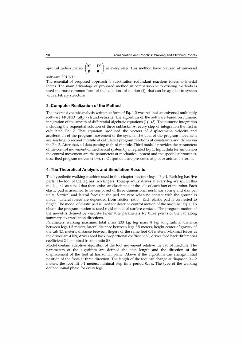
Bioinspiration and Robotics: Walking and Climbing Robots 98
spectral radius matrix −
0D
DMT
at every step. This method have realized at universal
software FRUND. The essential of proposed approach is substitution redundant reactions forces to inertial forces. The main advantage of proposed method in comparison with existing methods is used the most common form of the equations of motion (1), that can be applied to system with arbitrary structure.
3. Computer Realization of the Method
The inverse dynamic analysis written at form of Eq. 1-3 was realized at universal multibody software FRUND (http://frund.vstu.ru). The algorithm of the software based on numeric integration of the system of differential-algebraic equations (1) - (3). The numeric integration including the sequential solution of three subtasks. At every step of integration the first is calculated Eq. 2. That equation produced the vectors of displacement, velocity and acceleration of the program movement of the system. The data of the program movement are sending to second module of calculated program reactions at constraints and drives via the Eq. 3. After that, all data passing to third module. Third module provides the parameters of the control movement of mechanical system by integrated Eq. 1. Input data for simulation the control movement are the parameters of mechanical system and the special subroutines,
described program movement )(tw . Output data are presented at plot or animation forms.
4. The Theoretical Analysis and Simulation Results
The hypothetic walking machine used in this chapter has four legs – Fig.1. Each leg has five parts. The foot of the leg has two fingers. Total quantity drives at every leg are six. In this model, it is assumed that there exists an elastic pad at the sole of each foot of the robot. Each elastic pad is assumed to be composed of three dimensional nonlinear spring and damper units. Vertical and lateral forces at the pad are zero when no contact with the ground is made. Lateral forces are depended from friction ratio. Each elastic pad is connected to finger. The model of elastic pad is used for describe control motion of the machine Eq. 1. To obtain the program motion is used rigid model of surface contact. The program motion of the model is defined by describe kinematics parameters for three points of the cab along summary six translation directions. Parameters walking machine: total mass 233 kg, leg mass 8 kg, longitudinal distance between legs 1.5 meters, lateral distance between legs 2.5 meters, height center of gravity of the cab 1.1 meters, distance between fingers of the same foot 0.4 meters. Maximal forces at the drives are 4 kN, drives feed back proportional coefficient 80, drives feed back differential coefficient 2.4, nominal friction ratio 0.8. Model contain adaptive algorithm of the foot movement relative the cab of machine. The parameters of the algorithm are defined the step length and the direction of the displacement of the foot at horizontal plane. Above it the algorithm can change initial position of the foots at three direction. The length of the foot can change at diapason 0 – 2 meters, the foot lift 0.1 meters, minimal step time period 0.4 s. The type of the walking defined initial phase for every legs.
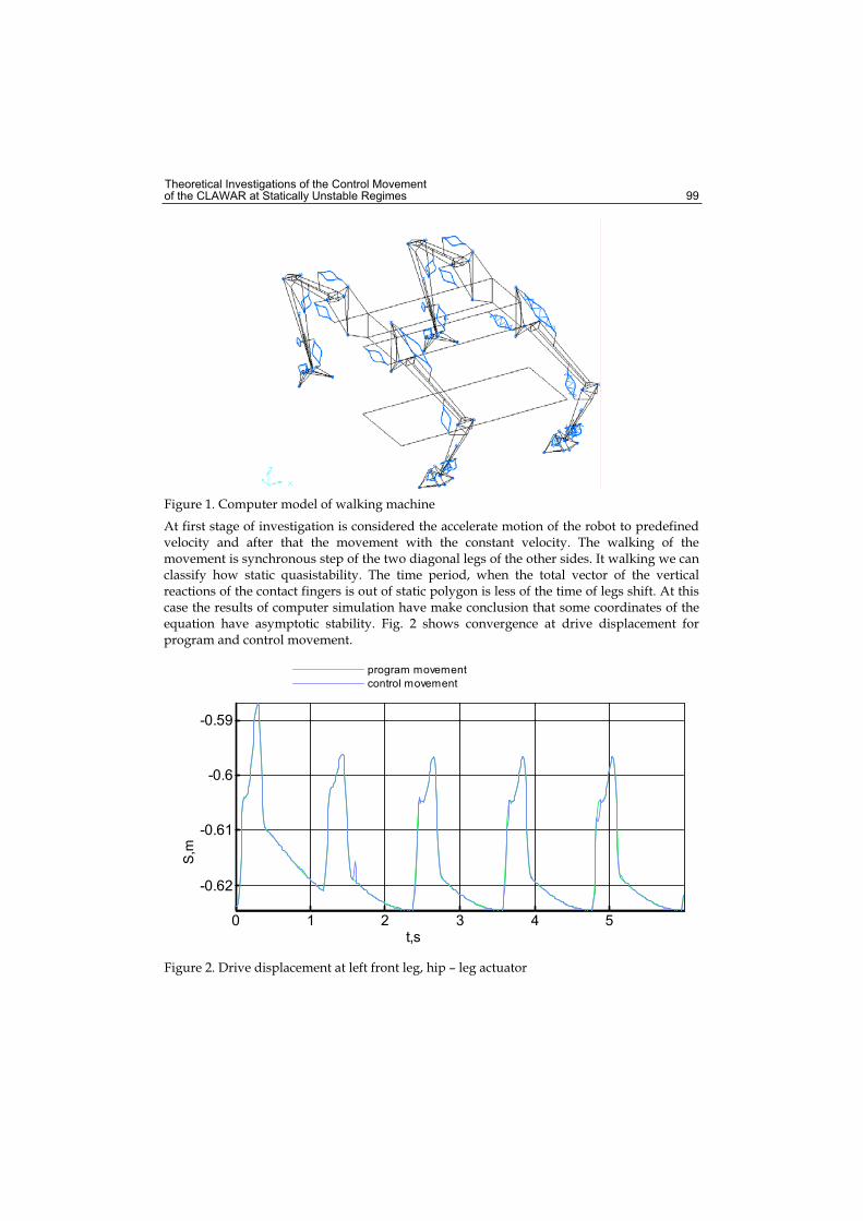
Theoretical Investigations of the Control Movement of the CLAWAR at Statically Unstable Regimes 99
Figure 1. Computer model of walking machine
At first stage of investigation is considered the accelerate motion of the robot to predefined velocity and after that the movement with the constant velocity. The walking of the movement is synchronous step of the two diagonal legs of the other sides. It walking we can classify how static quasistability. The time period, when the total vector of the vertical reactions of the contact fingers is out of static polygon is less of the time of legs shift. At this case the results of computer simulation have make conclusion that some coordinates of the equation have asymptotic stability. Fig. 2 shows convergence at drive displacement for program and control movement.
program movement
control movement
t,s 543210
S,m
-0.59
-0.6
-0.61
-0.62
Figure 2. Drive displacement at left front leg, hip – leg actuator
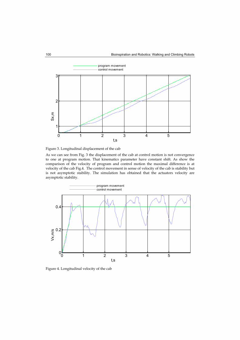
Bioinspiration and Robotics: Walking and Climbing Robots 100
program movement
control movement
t,s 543210
Sx,m
3
2
1
Figure 3. Longitudinal displacement of the cab
As we can see from Fig. 3 the displacement of the cab at control motion is not convergence to one at program motion. That kinematics parameter have constant shift. As show the comparison of the velocity of program and control motion the maximal difference is at velocity of the cab Fig.4. The control movement in sense of velocity of the cab is stability but is not asymptotic stability. The simulation has obtained that the actuators velocity are asymptotic stability.
program movement
control movement
t,s 543210
Vx,m
/s 0.4
0.2
0
Figure 4. Longitudinal velocity of the cab
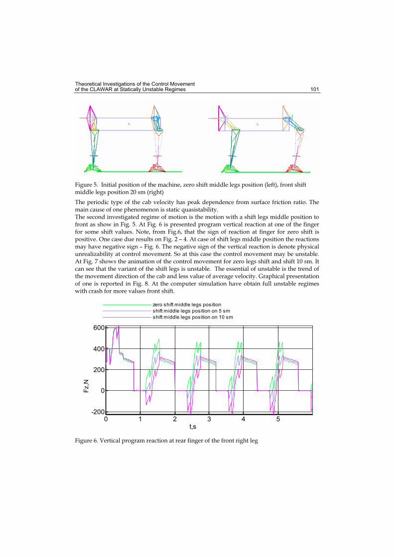
Theoretical Investigations of the Control Movement of the CLAWAR at Statically Unstable Regimes 101
Figure 5. Initial position of the machine, zero shift middle legs position (left), front shift middle legs position 20 sm (right)
The periodic type of the cab velocity has peak dependence from surface friction ratio. The main cause of one phenomenon is static quasistability. The second investigated regime of motion is the motion with a shift legs middle position to front as show in Fig. 5. At Fig. 6 is presented program vertical reaction at one of the finger for some shift values. Note, from Fig.6, that the sign of reaction at finger for zero shift is positive. One case due results on Fig. 2 – 4. At case of shift legs middle position the reactions may have negative sign – Fig. 6. The negative sign of the vertical reaction is denote physical unrealizability at control movement. So at this case the control movement may be unstable. At Fig. 7 shows the animation of the control movement for zero legs shift and shift 10 sm. It can see that the variant of the shift legs is unstable. The essential of unstable is the trend of the movement direction of the cab and less value of average velocity. Graphical presentation of one is reported in Fig. 8. At the computer simulation have obtain full unstable regimes with crash for more values front shift.
zero shift middle legs position
shift middle legs position on 5 sm
shift middle legs position on 10 sm
t,s 543210
Fz,N
600
400
200
0
-200
Figure 6. Vertical program reaction at rear finger of the front right leg
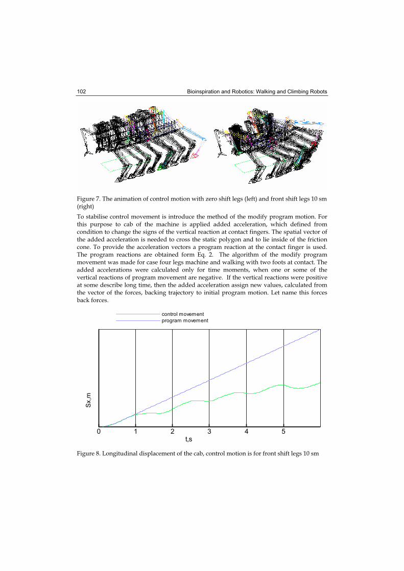
Bioinspiration and Robotics: Walking and Climbing Robots 102
Figure 7. The animation of control motion with zero shift legs (left) and front shift legs 10 sm (right)
To stabilise control movement is introduce the method of the modify program motion. For this purpose to cab of the machine is applied added acceleration, which defined from condition to change the signs of the vertical reaction at contact fingers. The spatial vector of the added acceleration is needed to cross the static polygon and to lie inside of the friction cone. To provide the acceleration vectors a program reaction at the contact finger is used. The program reactions are obtained form Eq. 2. The algorithm of the modify program movement was made for case four legs machine and walking with two foots at contact. The added accelerations were calculated only for time moments, when one or some of the vertical reactions of program movement are negative. If the vertical reactions were positive at some describe long time, then the added acceleration assign new values, calculated from the vector of the forces, backing trajectory to initial program motion. Let name this forces back forces.
control movement
program movement
t,s 543210
Sx,m
Figure 8. Longitudinal displacement of the cab, control motion is for front shift legs 10 sm
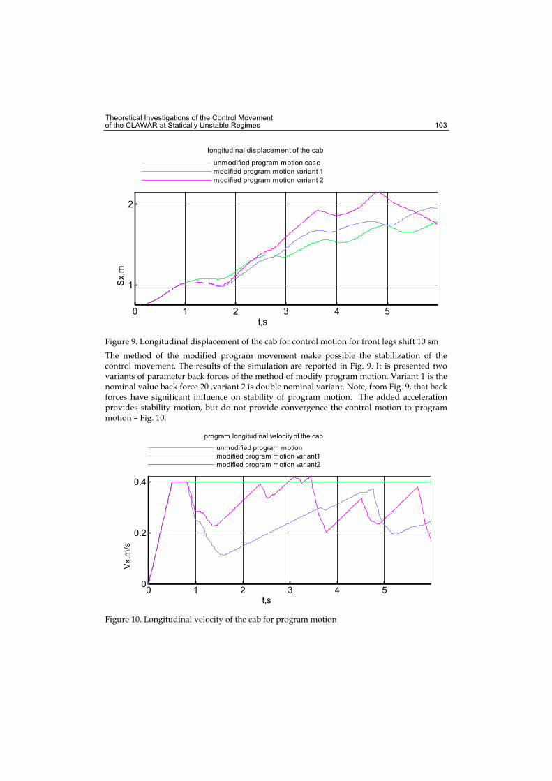
Theoretical Investigations of the Control Movement of the CLAWAR at Statically Unstable Regimes 103
longitudinal displacement of the cab
unmodified program motion case
modified program motion variant 1
modified program motion variant 2
t,s 543210
Sx,m
2
1
Figure 9. Longitudinal displacement of the cab for control motion for front legs shift 10 sm
The method of the modified program movement make possible the stabilization of the control movement. The results of the simulation are reported in Fig. 9. It is presented two variants of parameter back forces of the method of modify program motion. Variant 1 is the nominal value back force 20 ,variant 2 is double nominal variant. Note, from Fig. 9, that back forces have significant influence on stability of program motion. The added acceleration provides stability motion, but do not provide convergence the control motion to program motion – Fig. 10.
program longitudinal velocity of the cab
unmodified program motion
modified program motion variant1
modified program motion variant2
t,s 543210
Vx,m
/s
0.4
0.2
0
Figure 10. Longitudinal velocity of the cab for program motion
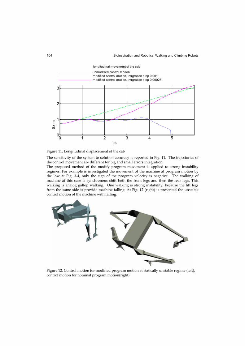
Bioinspiration and Robotics: Walking and Climbing Robots 104
longitudinal movement of the cab
unmodified control motion
modified control motion, intrgration step 0.001
modified control motion, intrgration step 0.00025
t,s 543210
Sx,m
3
2
1
0
Figure 11. Longitudinal displacement of the cab
The sensitivity of the system to solution accuracy is reported in Fig. 11. The trajectories of the control movement are different for big and small errors integration. The proposed method of the modify program movement is applied to strong instability regimes. For example is investigated the movement of the machine at program motion by the low at Fig. 3-4, only the sign of the program velocity is negative. The walking of machine at this case is synchronous shift both the front legs and then the rear legs. This walking is analog gallop walking. One walking is strong instability, because the lift legs from the same side is provide machine falling. At Fig. 12 (right) is presented the unstable control motion of the machine with falling.
Figure 12. Control motion for modified program motion at statically unstable regime (left), control motion for nominal program motion(right)
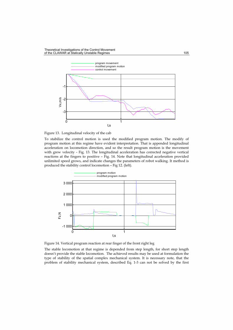
Theoretical Investigations of the Control Movement of the CLAWAR at Statically Unstable Regimes 105
program movement
modified program motion
control movement
t,s 10
Vx,m
/s -1
-2
-3
Figure 13. Longitudinal velocity of the cab
To stabilize the control motion is used the modified program motion. The modify of program motion at this regime have evident interpretation. That is appended longitudinal acceleration on locomotion direction, and so the result program motion is the movement with grew velocity - Fig. 13. The longitudinal acceleration has corrected negative vertical reactions at the fingers to positive – Fig. 14. Note that longitudinal acceleration provided unlimited speed grows, and indicate changes the parameters of robot walking. It method is produced the stability control locomotion – Fig 12. (left).
program motion
modified program motion
t,s 10
Fz,N
3 000
2 000
1 000
0
-1 000
Figure 14. Vertical program reaction at rear finger of the front right leg
The stable locomotion at that regime is depended from step length, for short step length doesn’t provide the stable locomotion. The achieved results may be used at formulation the type of stability of the spatial complex mechanical system. It is necessary note, that the problem of stability mechanical system, described Eq. 1-3 can not be solved by the first
Bioinspiration and Robotics: Walking and Climbing Robots 106
Lyapunov method, because the system is strong nonlinearity. The asymptotic stability of the part of state variable of the Eq.1-3, defined the relative displacement and velocities at the drives is provide by proportional and differential feedback gains – Fig. 2. Global stability may be formulated at the terms of second Lyapunov method. This method very difficult to apply for case of multidimensional differential-algebraic equations. The complexity of the problem is grow by the property of numerical integrations methods, needed to solve the equations. The nonlinearity of problem of the synthesis of control motion illustrated in Fig. 11, where presented two trajectories of the cab for two values of integration accuracy. Note, that both trajectories are stable at local sense. It may be conclusion that the analytical solving the problem of global stability of the system Eq. 3-1 is difficult. So it needed to develop numerical methods, based on precise nonlinear models.
5. Conclusion
A new algorithm for the control of CLAWAR at statically unstable regimes was introduced and its effectiveness investigated via numerical simulation. The essential advantages of the proposed approach may be summarized as follows. The proposal algorithm was shown to be capable of providing the control movement of the spatial machines with arbitrary structures and redundant constraints and actuators. The performance of method of modify the program movement was shown a steady state locomotion of the CLAWAR. Based on proposed method can be created the virtual prototypes of the CLAWAR with stable locomotion at any type of walking – jump, run and etc. To solve that task is need to develop more effective software, based on parallel processing, and create adaptive algorithms for procedures of program motion modification and adaptive parameters relative foots motion.
6. References
Jong H. P. (2001). Impedance Control for Biped Robot Locomotion. IEEE Transactions on Robotics and Automation, Vol 17, No. 6, December, pp. 870-882.
Jongwon K., Frank C. P. (2001), Design and Analysis of a Redundantly Actuated Parallel Mechanism for Rapid Machining. IEEE Transactions on robotics and automation, Vol. 17, No 4, pp. 423 – 434.
Mayorga R. V., Wong A. K. (1987). A singularity avoidance method for the trajectory planning of redundant and non redundant robot manipulators, Proceedings of IEEE International Conference on Robotics and Automatisation, pp. 1707-1712,IEEE Press.
Vukobratovic M., Kircanski M. (1984). A dynamic approach to nominal trajectory synthesis for redundant manipulators, IEEE Trans. Sys. Man Cybernet., SMC-14(4), pp. 580-586.
. ., . . (1976). . . , ,
6, 1976.
8
Selection of Obstacle Avoidance Behaviors Based on Visual and Ultrasonic Sensors for
Quadruped Robots
Kiyotaka Izumi, Ryoichi Sato, Keigo Watanabe and Maki K. Habib Saga University
Japan
1. Introduction
Robots are indispensable today to improve process efficiencies and labor savings in the industry and service sector. The importance of robots has also been recognized for work in critical environment, such as, space, ocean bottom, power plants, as well as, in the fields of clinical medicine, hazard prevention, etc. For this, a large number of robots have been developed, and researchers continue to design robots with greater capabilities to perform more challenging and comprehensive tasks (Hirose et al., 1986; Ooka et al., 1986; Cruse et al., 1994; Chen et al., 2002a; Habib, 2003a). There are many ways for a robot to move across a solid surface in which wheels, crawlers, and legs were common options for the available robots. The application fields of such robots are naturally restricted, depending on the condition of the ground. Wheeled mobile robots are mechanically simple, easy to construct, easy to implement a controller, dynamically stable in general, and they are ideal for operation on level and hard surfaces. When the surface is rough and has projections and depressions with dimensions that are greater than the diameter of the wheel or when the surface is soft, resistance to the movement increases drastically and their function as transport machines is almost lost, which leads to poor performance. The crawler type locomotion mechanisms have traverse ability higher than that of the wheel, but its control is hard and the dead-reckoning is difficult to realize, though it is possible to move on different terrains. In order to have good mobility over uneven and rough terrain a legged robot seems to be a good solution because legged locomotion is mechanically superior to wheeled or tracked locomotion over a variety of soil conditions and certainly superior for crossing obstacles. The path of the legged machine can be (partially) decoupled from the sequence of footholds, allowing a higher degree of mobility. This can be especially useful in narrow surroundings or terrain with discrete footholds (Raibert, 1986; Hirose, 2001). However, creating and controlling a legged machine that is powerful enough, but still light enough is very difficult. Legged robots are usually slower and have a lower load/power ratio with respect to wheeled robot. Autonomous legged robots have distinct control issues that must be addressed. These problems are amplified when the robot is small with an on-board controller that is purposely simple to accommodate weight and expense restrictions. The kinematics and dynamics of legged robots are nonlinear, while robot parameters, such as center of mass position, amount of payload, etc. are not known exactly and might also
Bioinspiration and Robotics: Walking and Climbing Robots 108
vary (Nishikawa et al., 1998). In addition, it is difficult to estimate states of the system (Pugh et al., 1990). The system might be unstable without control, and the goal of keeping balance is difficult to be decomposed into actuator commands. A legged system has a lot of degrees of freedom in which a high motion performance and ground adaptation ability on irregular terrain can be demonstrated. In order to allow a completely decoupled motion over irregular terrain, at least three degrees of freedom per leg are required. Two joints would be enough to place the foot in any desired position, and with the third joint, the robot can climb over much larger obstacles relative to its size and also can climb a slippery hill that a leg with two joints can not perform. But, this will result in using 12 actuators for a four-legged robot, which yields to increase weight and control complexity compared to six actuators for a traditional industrial manipulator (Waldron et al., 1984). Contact forces, in general, only allow pushing the feet into the surface, not pulling. This directly limits the total downwards acceleration that can be applied to a walking machine. This initiates a challenge to investigate the technical problems involved in the realization of a robot that uses legs to navigate in difficult, partially unstructured and unknown environments. Navigating and avoiding obstacles in real-time and in real environment is a challenging problem for mobile robots in general, and for legged robots in specific. There is a large body of work devoted to the navigation of wheel-based mobile robots. Some common approaches are odometry, inertial navigation [3] and landmark navigation. The navigability of an autonomous multi-legged system is a crucial element of its overall capabilities (Go et al., 2006). Biological systems have a tightly integrated action perception cycle. Hence, for walking robots, to realize their full potential, distal environment sensing must be tightly integrated with the walking cycle. Distal sensing is crucial to allow anticipatory gait adjustment to accommodate varying terrain. Close coupling of the visual and locomotor cycle can lead to rapid, adaptive adjustment of the robot (Lewis, 2002). This problem is even more difficult when the robot is unable to generate accurate global models of the obstacles in its environment. Determining an optimal navigation policy without this information can be difficult or impossible. A legged mobile robot is a free roving collection of functions primarily designed to reach a target location. Equipping robots with more sensors increases the quantity and reliability of information the robot can extract from its environment to support robot’s intelligent behavior (Ferrell, 1994). In order to facilitate flexible obstacle detection and avoidance techniques, it is necessary to acquire the 3-dimensional (3D) information about the surrounding environment. Generally, 3D information is acquired through external sensors, such as binocular cameras, ultrasonic sensors (Ohya et al., 1997), laser range finders, etc. However, a high computational cost is required to analyze 3D information because the binocular camera needs to process two frames from two cameras (Okada et al., 1999, Okada et al., 2003). In addition, although the ultrasonic sensor can accurately measure the distance to an object, there is a difficult problem in determining the azimuth. Therefore, it remains a challenging task to build a robust real-time obstacle avoidance system for a robot using vision data.
2. Quadruped Robot and Behavior based Solution for Obstacle Avoidance
In this chapter, a quadruped walking robot TITAN-VIII (Arikawa & Hirose, 1996; Hirose & Arikawa, 2000) has been used as a platform to test and demonstrate the developed behavior selection based obstacle avoidance technique (See Figure 1.(a)). TITAN VIII is a walking machine that has four modular legs. The leg mechanism is composed of a planar 2 degrees
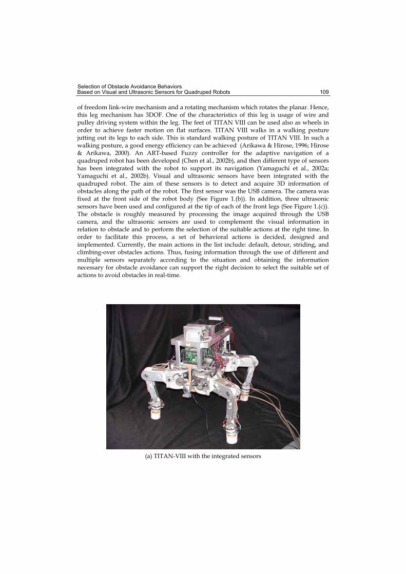
Selection of Obstacle Avoidance Behaviors Based on Visual and Ultrasonic Sensors for Quadruped Robots 109
of freedom link-wire mechanism and a rotating mechanism which rotates the planar. Hence, this leg mechanism has 3DOF. One of the characteristics of this leg is usage of wire and pulley driving system within the leg. The feet of TITAN VIII can be used also as wheels in order to achieve faster motion on flat surfaces. TITAN VIII walks in a walking posture jutting out its legs to each side. This is standard walking posture of TITAN VIII. In such a walking posture, a good energy efficiency can be achieved (Arikawa & Hirose, 1996; Hirose & Arikawa, 2000). An ART-based Fuzzy controller for the adaptive navigation of a quadruped robot has been developed (Chen et al., 2002b), and then different type of sensors has been integrated with the robot to support its navigation (Yamaguchi et al., 2002a; Yamaguchi et al., 2002b). Visual and ultrasonic sensors have been integrated with the quadruped robot. The aim of these sensors is to detect and acquire 3D information of obstacles along the path of the robot. The first sensor was the USB camera. The camera was fixed at the front side of the robot body (See Figure 1.(b)). In addition, three ultrasonic sensors have been used and configured at the tip of each of the front legs (See Figure 1.(c)). The obstacle is roughly measured by processing the image acquired through the USB camera, and the ultrasonic sensors are used to complement the visual information in relation to obstacle and to perform the selection of the suitable actions at the right time. In order to facilitate this process, a set of behavioral actions is decided, designed and implemented. Currently, the main actions in the list include: default, detour, striding, and climbing-over obstacles actions. Thus, fusing information through the use of different and multiple sensors separately according to the situation and obtaining the information necessary for obstacle avoidance can support the right decision to select the suitable set of actions to avoid obstacles in real-time.
(a) TITAN-VIII with the integrated sensors
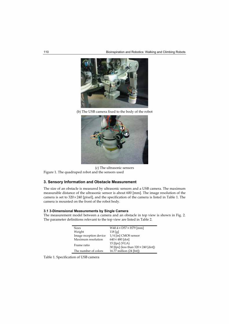
Bioinspiration and Robotics: Walking and Climbing Robots 110
(b) The USB camera fixed to the body of the robot
(c) The ultrasonic sensors Figure 1. The quadruped robot and the sensors used
3. Sensory Information and Obstacle Measurement
The size of an obstacle is measured by ultrasonic sensors and a USB camera. The maximum measurable distance of the ultrasonic sensor is about 600 [mm]. The image resolution of the camera is set to 320 × 240 [pixel], and the specification of the camera is listed in Table 1. The camera is mounted on the front of the robot body.
3.1 3-Dimensional Measurements by Single Camera
The measurement model between a camera and an obstacle in top view is shown in Fig. 2. The parameter definitions relevant to the top view are listed in Table 2.
Sizes W40.4 × D57 × H79 [mm] Weight 118 [g] Image reception device 1/4 [in] CMOS sensor Maximum resolution 640 × 480 [dot]
Frame ratio 15 [fps] (VGA) 30 [fps] (less than 320 × 240 [dot])
The number of colors 16.77 million (24 [bit])
Table 1. Specification of USB camera
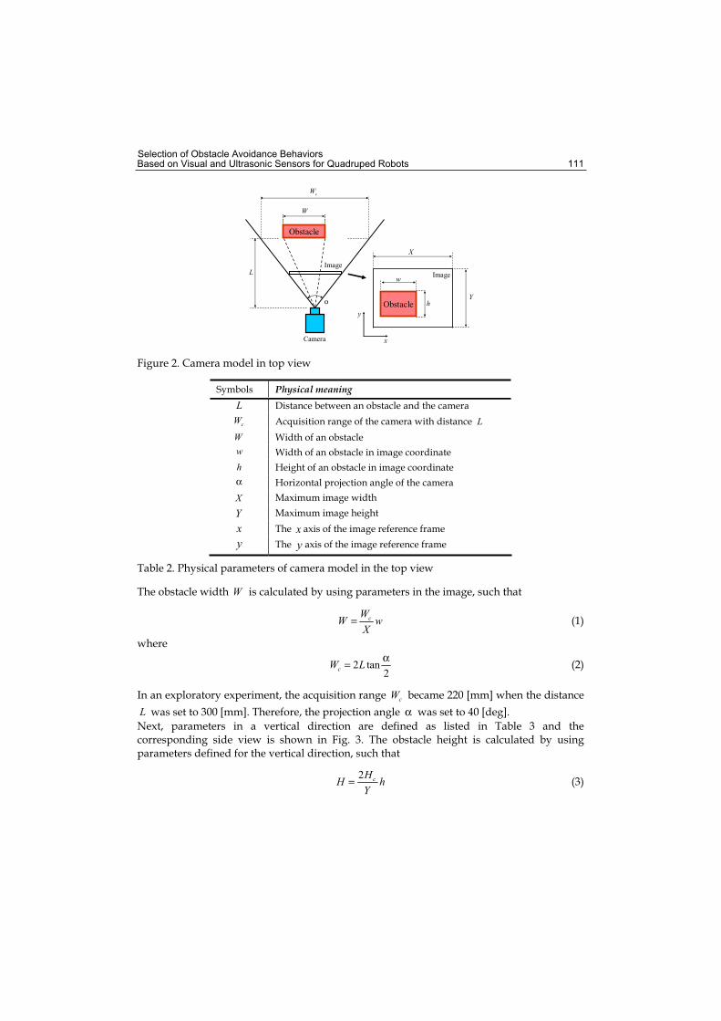
Selection of Obstacle Avoidance Behaviors Based on Visual and Ultrasonic Sensors for Quadruped Robots 111
Camera
Obstacle
Obstacle
Image
Image
h
w
Y
x
y
X
cW
W
L
α
Figure 2. Camera model in top view
Symbols Physical meaning L Distance between an obstacle and the camera
cW Acquisition range of the camera with distance LW Width of an obstacle
w Width of an obstacle in image coordinate
h Height of an obstacle in image coordinate
α Horizontal projection angle of the camera
X Maximum image width
Y Maximum image height
x The x axis of the image reference frame
y The y axis of the image reference frame
Table 2. Physical parameters of camera model in the top view
The obstacle width W is calculated by using parameters in the image, such that
wX
WW c= (1)
where
2tan2
α= LWc (2)
In an exploratory experiment, the acquisition range cW became 220 [mm] when the distance
L was set to 300 [mm]. Therefore, the projection angle α was set to 40 [deg].
Next, parameters in a vertical direction are defined as listed in Table 3 and the corresponding side view is shown in Fig. 3. The obstacle height is calculated by using parameters defined for the vertical direction, such that
hYHH c2= (3)
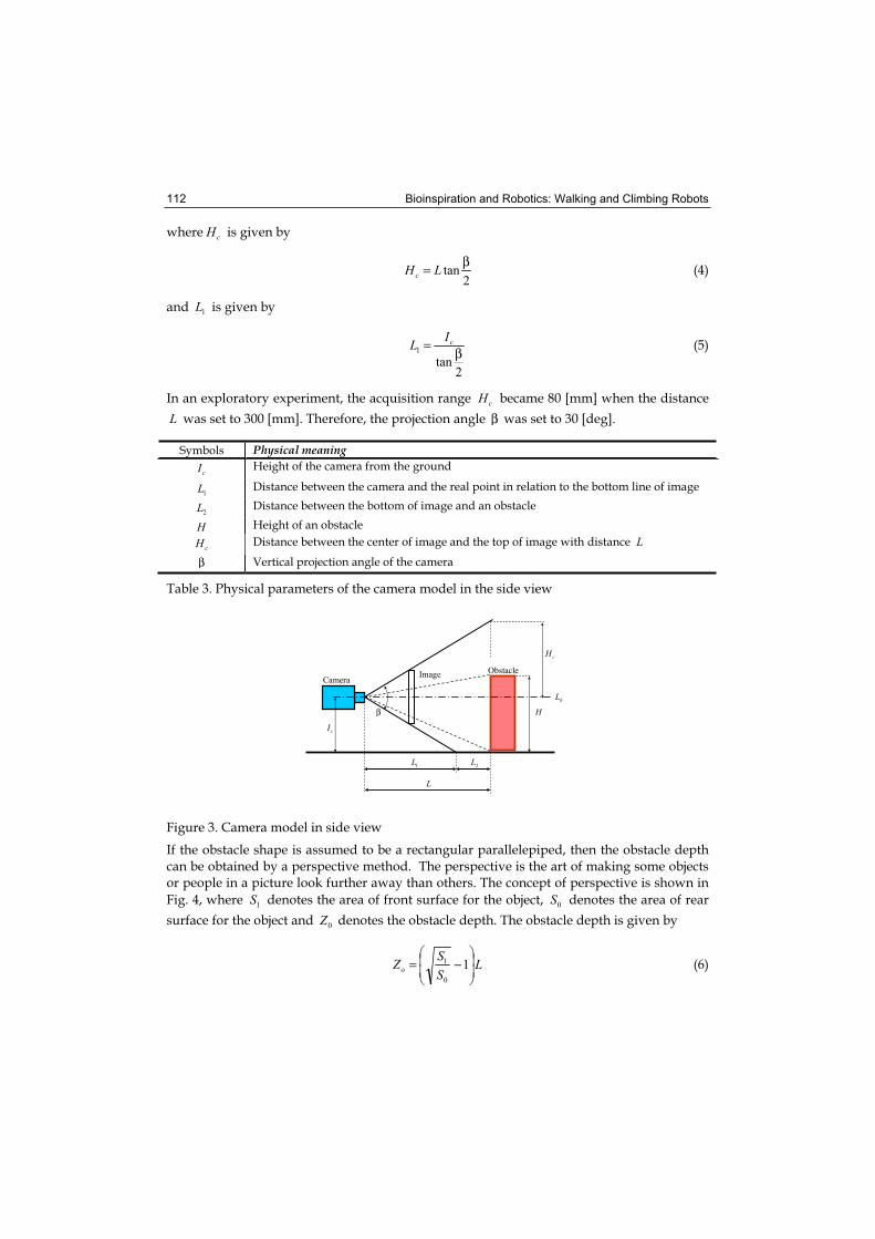
Bioinspiration and Robotics: Walking and Climbing Robots 112
where cH is given by
2tan
β= LHc (4)
and 1L is given by
2tan
1 β= cIL (5)
In an exploratory experiment, the acquisition range cH became 80 [mm] when the distance
L was set to 300 [mm]. Therefore, the projection angle β was set to 30 [deg].
Symbols Physical meaning
cI Height of the camera from the ground
1L Distance between the camera and the real point in relation to the bottom line of image
2L Distance between the bottom of image and an obstacle
H Height of an obstacle
cH Distance between the center of image and the top of image with distance L
β Vertical projection angle of the camera
Table 3. Physical parameters of the camera model in the side view
CameraImage Obstacle
β
cI
L
1L 2L
hL
H
cH
Figure 3. Camera model in side view
If the obstacle shape is assumed to be a rectangular parallelepiped, then the obstacle depth can be obtained by a perspective method. The perspective is the art of making some objects or people in a picture look further away than others. The concept of perspective is shown in
Fig. 4, where 1S denotes the area of front surface for the object, 0S denotes the area of rear
surface for the object and 0Z denotes the obstacle depth. The obstacle depth is given by
LSSZo −= 1
0
1 (6)
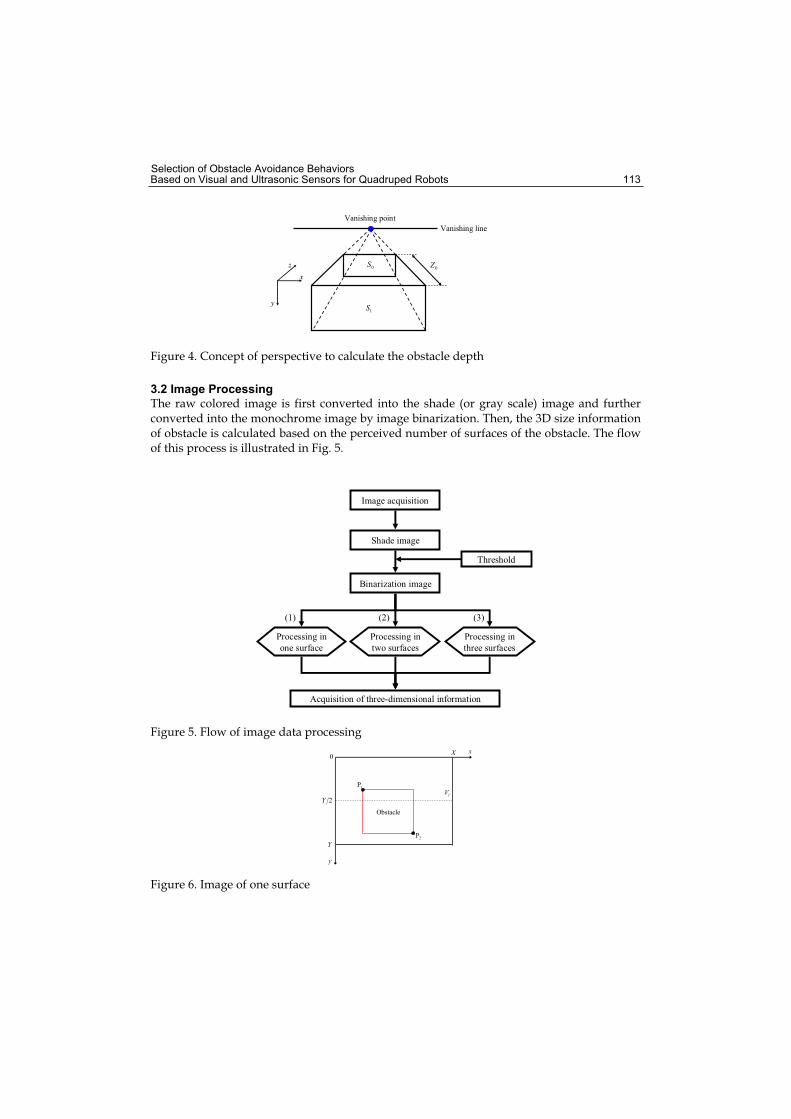
Selection of Obstacle Avoidance Behaviors Based on Visual and Ultrasonic Sensors for Quadruped Robots 113
Vanishing point
Vanishing line
0S
1S
0Zx
y
z
Figure 4. Concept of perspective to calculate the obstacle depth
3.2 Image Processing
The raw colored image is first converted into the shade (or gray scale) image and further converted into the monochrome image by image binarization. Then, the 3D size information of obstacle is calculated based on the perceived number of surfaces of the obstacle. The flow of this process is illustrated in Fig. 5.
Image acquisition
Shade image
Binarization image
Threshold
Processing in
one surface
Processing in
two surfaces
Processing in
three surfaces
Acquisition of three-dimensional information
(1) (2) (3)
Figure 5. Flow of image data processing
Obstacle
0X x
lV2Y
Y
y
1P
2P
Figure 6. Image of one surface
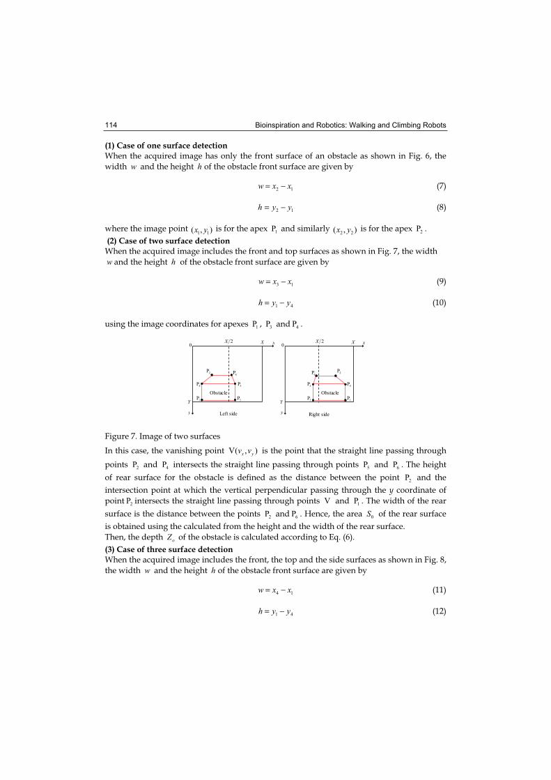
Bioinspiration and Robotics: Walking and Climbing Robots 114
(1) Case of one surface detection When the acquired image has only the front surface of an obstacle as shown in Fig. 6, the
width w and the height h of the obstacle front surface are given by
12 xxw −= (7)
12 yyh −= (8)
where the image point ),( 11 yx is for the apex 1P and similarly ),( 22 yx is for the apex 2P .
(2) Case of two surface detection When the acquired image includes the front and top surfaces as shown in Fig. 7, the width
w and the height h of the obstacle front surface are given by
13 xxw −= (9)
41 yyh −= (10)
using the image coordinates for apexes 1P , 3P and 4P .
ObstacleObstacle
Right sideLeft side
0 0x xX X2X2X
Y Y
y y
1P 1P
2P2P
3P3P
4P4P 5P5P
6P6P
Figure 7. Image of two surfaces
In this case, the vanishing point ),(V yx vv is the point that the straight line passing through
points 2P and 4P intersects the straight line passing through points 5P and 6P . The height
of rear surface for the obstacle is defined as the distance between the point 2P and the
intersection point at which the vertical perpendicular passing through the y coordinate of
point 2P intersects the straight line passing through points V and 1P . The width of the rear
surface is the distance between the points 2P and 6P . Hence, the area 0S of the rear surface
is obtained using the calculated from the height and the width of the rear surface.
Then, the depth oZ of the obstacle is calculated according to Eq. (6).
(3) Case of three surface detection When the acquired image includes the front, the top and the side surfaces as shown in Fig. 8,
the width w and the height h of the obstacle front surface are given by
14 xxw −= (11)
41 yyh −= (12)
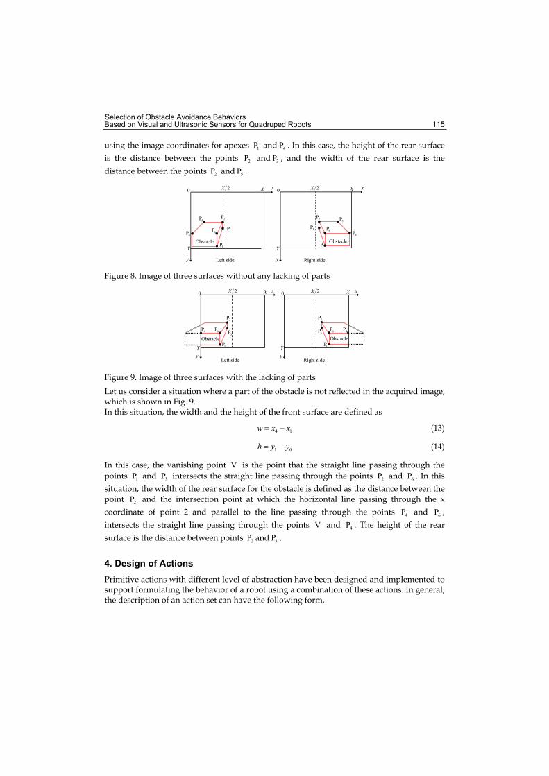
Selection of Obstacle Avoidance Behaviors Based on Visual and Ultrasonic Sensors for Quadruped Robots 115
using the image coordinates for apexes 1P and 4P . In this case, the height of the rear surface
is the distance between the points 2P and 3P , and the width of the rear surface is the
distance between the points 2P and 5P .
ObstacleObstacle
Left side Right side
0 0x xX X
Y Y
y y
2X 2X
1P 1P
2P 2P
3P 3P
4P 4P
5P5P
6P 6P
Figure 8. Image of three surfaces without any lacking of parts
ObstacleObstacle
Left side Right side
0 0x xX X2X 2X
Y Yy y
1P 1P
2P 2P
3P 3P4P 4P6P 6P
Figure 9. Image of three surfaces with the lacking of parts
Let us consider a situation where a part of the obstacle is not reflected in the acquired image, which is shown in Fig. 9. In this situation, the width and the height of the front surface are defined as
14 xxw −= (13)
61 yyh −= (14)
In this case, the vanishing point V is the point that the straight line passing through the
points 1P and 3P intersects the straight line passing through the points 2P and 6P . In this
situation, the width of the rear surface for the obstacle is defined as the distance between the
point 2P and the intersection point at which the horizontal line passing through the x
coordinate of point 2 and parallel to the line passing through the points 4P and 6P ,
intersects the straight line passing through the points V and 4P . The height of the rear
surface is the distance between points 2P and 3P .
4. Design of Actions
Primitive actions with different level of abstraction have been designed and implemented to support formulating the behavior of a robot using a combination of these actions. In general, the description of an action set can have the following form,
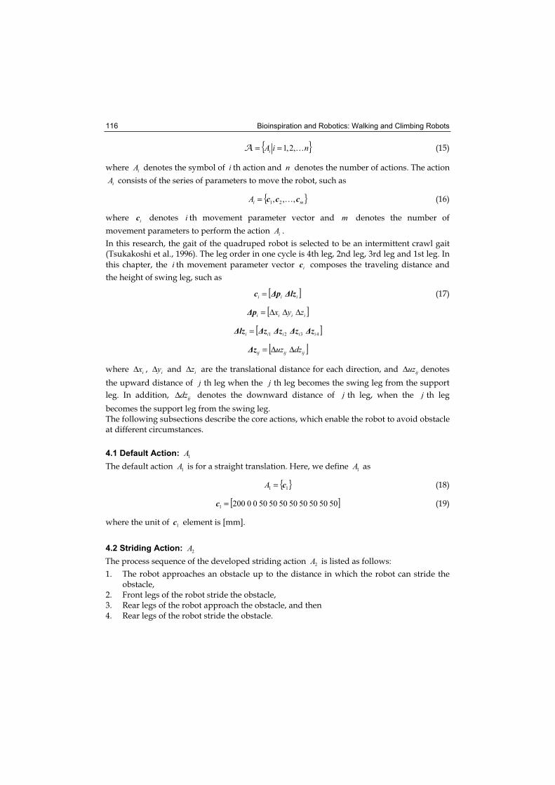
Bioinspiration and Robotics: Walking and Climbing Robots 116
{ }niAi ,2,1==A (15)
where iA denotes the symbol of i th action and n denotes the number of actions. The action
iA consists of the series of parameters to move the robot, such as
{ }miA ccc ,,, 21= (16)
where ic denotes i th movement parameter vector and m denotes the number of
movement parameters to perform the action iA .
In this research, the gait of the quadruped robot is selected to be an intermittent crawl gait (Tsukakoshi et al., 1996). The leg order in one cycle is 4th leg, 2nd leg, 3rd leg and 1st leg. In
this chapter, the i th movement parameter vector ic composes the traveling distance and
the height of swing leg, such as
[ ]iii lzpc = (17)
[ ]iiii zyx ΔΔΔ=p
[ ]4321 iiiii zzzzlz =
[ ]ijijij dzuz ΔΔ=z
where ixΔ , iyΔ and izΔ are the translational distance for each direction, and ijuzΔ denotes
the upward distance of j th leg when the j th leg becomes the swing leg from the support
leg. In addition, ijdzΔ denotes the downward distance of j th leg, when the j th leg
becomes the support leg from the swing leg. The following subsections describe the core actions, which enable the robot to avoid obstacle at different circumstances.
4.1 Default Action: 1AThe default action 1A is for a straight translation. Here, we define 1A as
{ }11 c=A (18)
[ ]5050505050505050002001 =c (19)
where the unit of 1c element is [mm].
4.2 Striding Action: 2AThe process sequence of the developed striding action 2A is listed as follows:
1. The robot approaches an obstacle up to the distance in which the robot can stride the obstacle,
2. Front legs of the robot stride the obstacle, 3. Rear legs of the robot approach the obstacle, and then 4. Rear legs of the robot stride the obstacle.
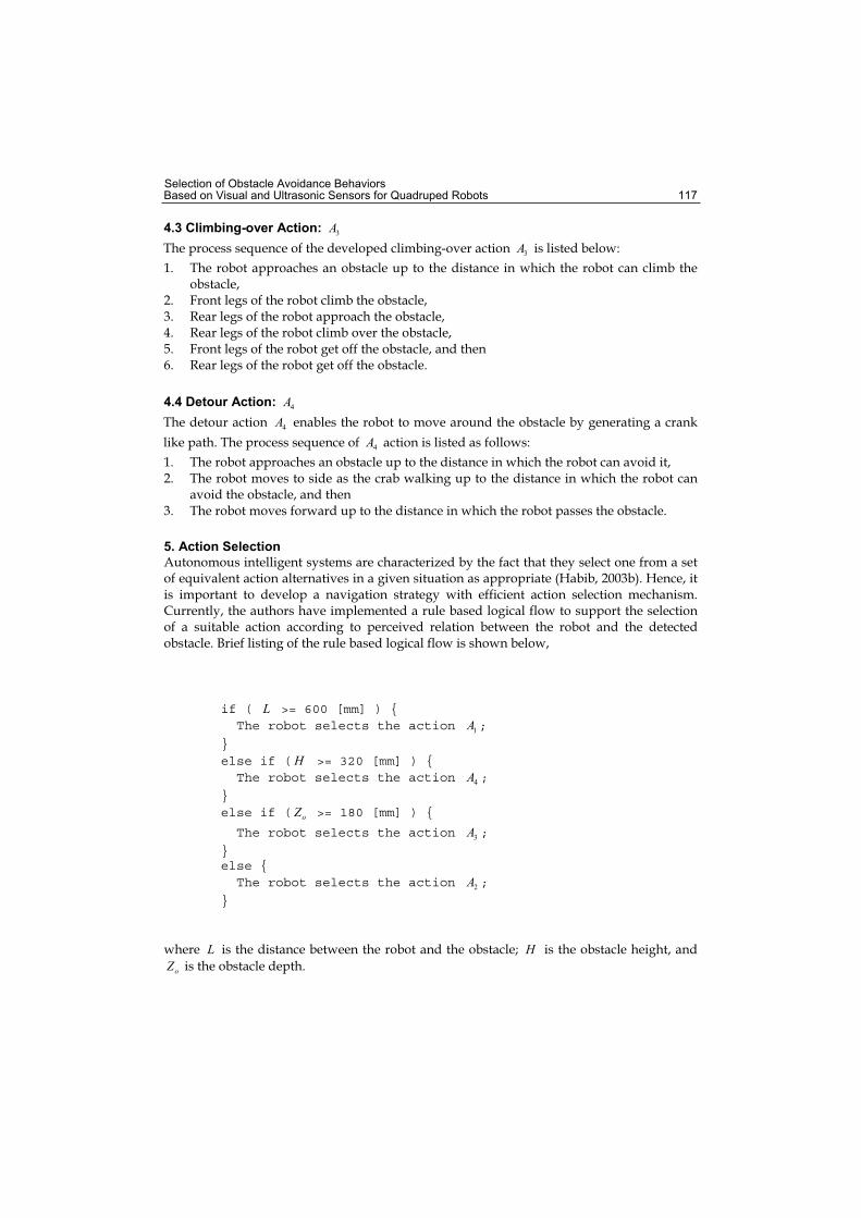
Selection of Obstacle Avoidance Behaviors Based on Visual and Ultrasonic Sensors for Quadruped Robots 117
4.3 Climbing-over Action: 3AThe process sequence of the developed climbing-over action 3A is listed below:
1. The robot approaches an obstacle up to the distance in which the robot can climb the obstacle,
2. Front legs of the robot climb the obstacle, 3. Rear legs of the robot approach the obstacle, 4. Rear legs of the robot climb over the obstacle, 5. Front legs of the robot get off the obstacle, and then 6. Rear legs of the robot get off the obstacle.
4.4 Detour Action: 4AThe detour action 4A enables the robot to move around the obstacle by generating a crank
like path. The process sequence of 4A action is listed as follows:
1. The robot approaches an obstacle up to the distance in which the robot can avoid it, 2. The robot moves to side as the crab walking up to the distance in which the robot can
avoid the obstacle, and then 3. The robot moves forward up to the distance in which the robot passes the obstacle.
5. Action Selection
Autonomous intelligent systems are characterized by the fact that they select one from a set of equivalent action alternatives in a given situation as appropriate (Habib, 2003b). Hence, it is important to develop a navigation strategy with efficient action selection mechanism. Currently, the authors have implemented a rule based logical flow to support the selection of a suitable action according to perceived relation between the robot and the detected obstacle. Brief listing of the rule based logical flow is shown below,
if ( L >= 600 [mm] ) { The robot selects the action 1A ;
} else if ( H >= 320 [mm] ) { The robot selects the action 4A ;
} else if ( oZ >= 180 [mm] ) {
The robot selects the action 3A ;
} else { The robot selects the action 2A ;
}
where L is the distance between the robot and the obstacle; H is the obstacle height, and
oZ is the obstacle depth.
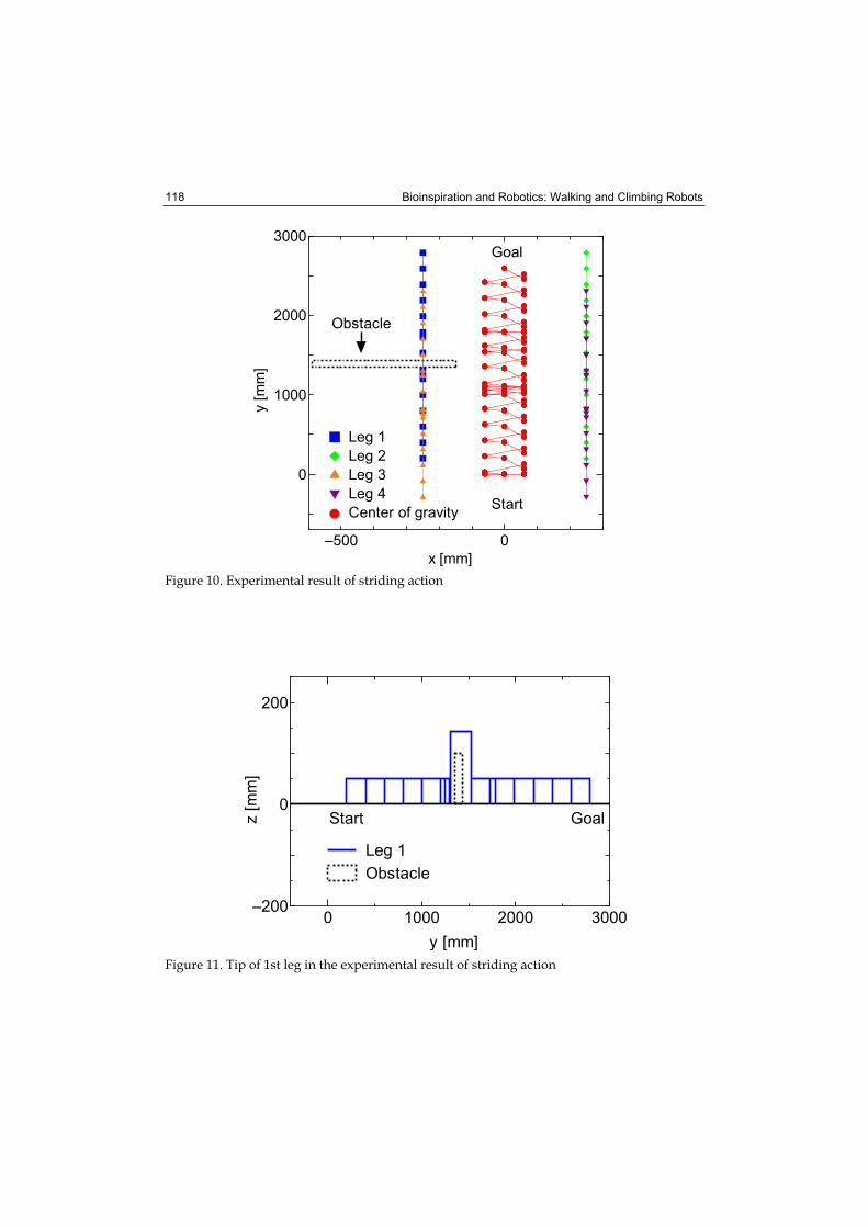
Bioinspiration and Robotics: Walking and Climbing Robots 118
–500 0
0
1000
2000
3000
Leg 1
Leg 2
Leg 3
Leg 4
Center of gravity
x [mm]
y [
mm
]
Start
Goal
Obstacle
Figure 10. Experimental result of striding action
0 1000 2000 3000–200
0
200
Start Goal
y [mm]
z [
mm
]
Leg 1
Obstacle
Figure 11. Tip of 1st leg in the experimental result of striding action
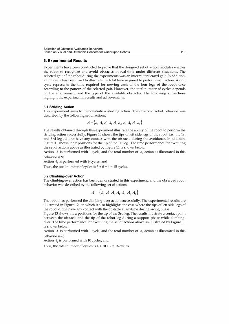
Selection of Obstacle Avoidance Behaviors Based on Visual and Ultrasonic Sensors for Quadruped Robots 119
6. Experimental Results
Experiments have been conducted to prove that the designed set of action modules enables the robot to recognize and avoid obstacles in real-time under different situations. The selected gait of the robot during the experiments was an intermittent crawl gait. In addition, a unit cycle has been used to illustrate the total time required to perform each action. A unit cycle represents the time required for moving each of the four legs of the robot once according to the pattern of the selected gait. However, the total number of cycles depends on the environment and the type of the available obstacles. The following subsections highlight the experimental results and achievements.
6.1 Striding Action
This experiment aims to demonstrate a striding action. The observed robot behavior was described by the following set of actions,
{ }1111211111 AAAAAAAAAAA =
The results obtained through this experiment illustrate the ability of the robot to perform the striding action successfully. Figure 10 shows the tips of left side legs of the robot, i.e., the 1st and 3rd legs, didn't have any contact with the obstacle during the avoidance. In addition, Figure 11 shows the z positions for the tip of the 1st leg. The time performance for executing the set of actions above as illustrated by Figure 11 is shown below,
Action 1A is performed with 1 cycle, and the total number of 1A action as illustrated in this
behavior is 9;
Action 2A is performed with 6 cycles; and
Thus, the total number of cycles is 5 + 6 + 4 = 15 cycles.
6.2 Climbing-over Action
The climbing-over action has been demonstrated in this experiment, and the observed robot behavior was described by the following set of actions,
{ }1131111 AAAAAAAA =
The robot has performed the climbing-over action successfully. The experimental results are illustrated in Figure 12, in which it also highlights the case where the tips of left side legs of the robot didn't have any contact with the obstacle at anytime during swing phase. Figure 13 shows the z positions for the tip of the 3rd leg. The results illustrate a contact point between the obstacle and the tip of the robot leg during a support phase while climbing-over. The time performance for executing the set of actions above as illustrated by Figure 13 is shown below,
Action 1A is performed with 1 cycle, and the total number of 1A action as illustrated in this
behavior is 6; Action
3A is performed with 10 cycles; and
Thus, the total number of cycles is 4 + 10 + 2 = 16 cycles.
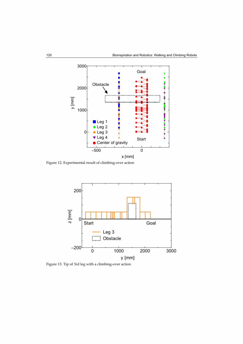
Bioinspiration and Robotics: Walking and Climbing Robots 120
–500 0
0
1000
2000
3000
Start
Goal
Leg 1
Leg 2
Leg 3
Leg 4
Center of gravity
x [mm]
y [
mm
]
Obstacle
Figure 12. Experimental result of climbing-over action
0 1000 2000 3000–200
0
200
Leg 3
Obstacle
y [mm]
z [
mm
]
Start Goal
Figure 13. Tip of 3rd leg with a climbing-over action
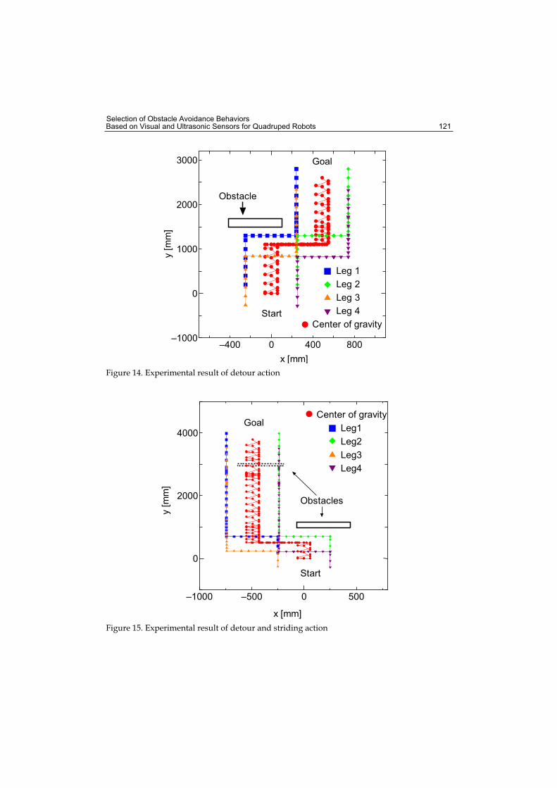
Selection of Obstacle Avoidance Behaviors Based on Visual and Ultrasonic Sensors for Quadruped Robots 121
–400 0 400 800–1000
0
1000
2000
3000
Leg 1
Leg 2
Leg 3
Leg 4
Center of gravity
x [mm]
y [
mm
]
Start
Goal
Obstacle
Figure 14. Experimental result of detour action
–1000 –500 0 500
0
2000
4000Goal
Start
Obstacles
x [mm]
y [
mm
]
Center of gravity
Leg1
Leg2
Leg3
Leg4
Figure 15. Experimental result of detour and striding action
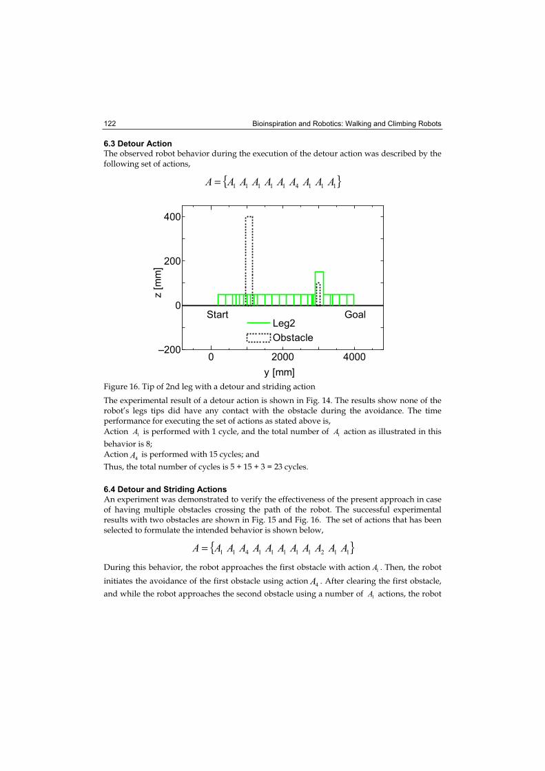
Bioinspiration and Robotics: Walking and Climbing Robots 122
6.3 Detour Action
The observed robot behavior during the execution of the detour action was described by the following set of actions,
{ }111411111 AAAAAAAAAA =
0 2000 4000–200
0
200
400
Start GoalLeg2
Obstacle
y [mm]
z [
mm
]
Figure 16. Tip of 2nd leg with a detour and striding action
The experimental result of a detour action is shown in Fig. 14. The results show none of the robot’s legs tips did have any contact with the obstacle during the avoidance. The time performance for executing the set of actions as stated above is,
Action 1A is performed with 1 cycle, and the total number of 1A action as illustrated in this
behavior is 8; Action
4A is performed with 15 cycles; and
Thus, the total number of cycles is 5 + 15 + 3 = 23 cycles.
6.4 Detour and Striding Actions
An experiment was demonstrated to verify the effectiveness of the present approach in case of having multiple obstacles crossing the path of the robot. The successful experimental results with two obstacles are shown in Fig. 15 and Fig. 16. The set of actions that has been selected to formulate the intended behavior is shown below,
{ }11211111411 AAAAAAAAAAAA =
During this behavior, the robot approaches the first obstacle with action 1A . Then, the robot
initiates the avoidance of the first obstacle using action4A . After clearing the first obstacle,
and while the robot approaches the second obstacle using a number of 1A actions, the robot
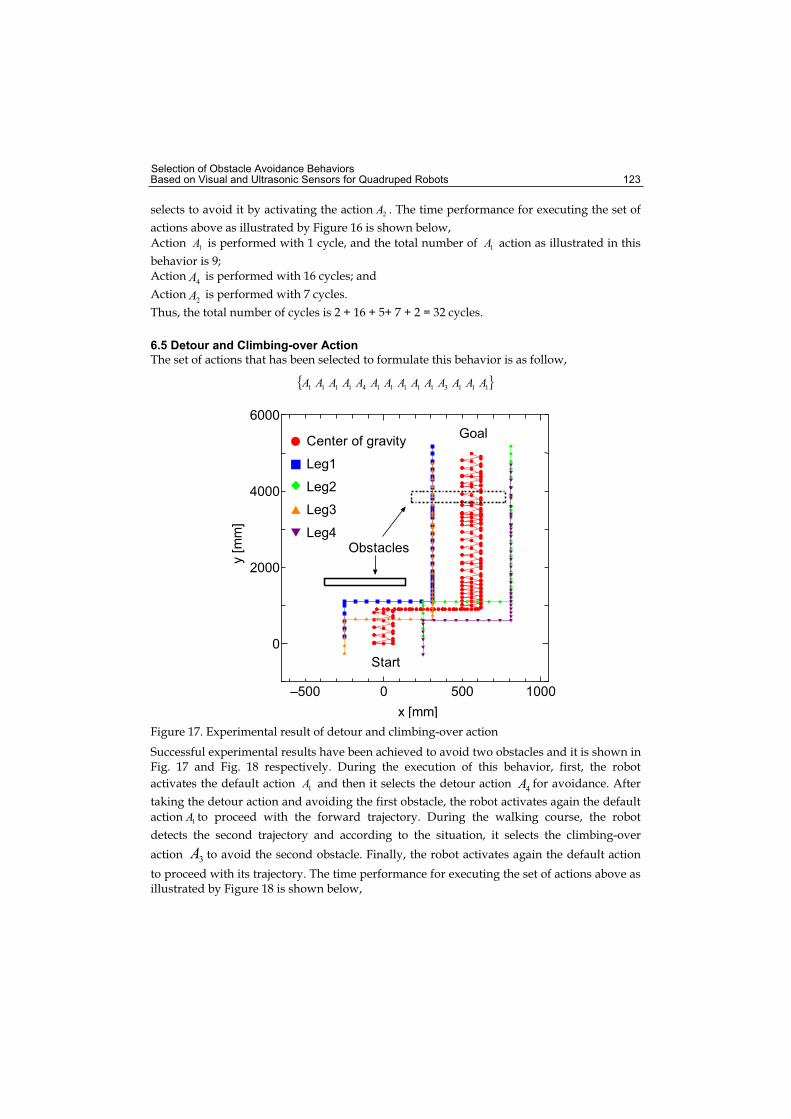
Selection of Obstacle Avoidance Behaviors Based on Visual and Ultrasonic Sensors for Quadruped Robots 123
selects to avoid it by activating the action 2A . The time performance for executing the set of
actions above as illustrated by Figure 16 is shown below,
Action 1A is performed with 1 cycle, and the total number of 1A action as illustrated in this
behavior is 9; Action
4A is performed with 16 cycles; and
Action2A is performed with 7 cycles.
Thus, the total number of cycles is 2 + 16 + 5+ 7 + 2 = 32 cycles.
6.5 Detour and Climbing-over Action
The set of actions that has been selected to formulate this behavior is as follow,
{ }11131111141111 AAAAAAAAAAAAAA
–500 0 500 1000
0
2000
4000
6000
Start
Obstacles
Goal
x [mm]
y [
mm
]
Leg1
Leg2
Leg3
Leg4
Center of gravity
Figure 17. Experimental result of detour and climbing-over action
Successful experimental results have been achieved to avoid two obstacles and it is shown in Fig. 17 and Fig. 18 respectively. During the execution of this behavior, first, the robot
activates the default action 1A and then it selects the detour action 4A for avoidance. After
taking the detour action and avoiding the first obstacle, the robot activates again the default
action 1A to proceed with the forward trajectory. During the walking course, the robot
detects the second trajectory and according to the situation, it selects the climbing-over
action 3A to avoid the second obstacle. Finally, the robot activates again the default action
to proceed with its trajectory. The time performance for executing the set of actions above as illustrated by Figure 18 is shown below,
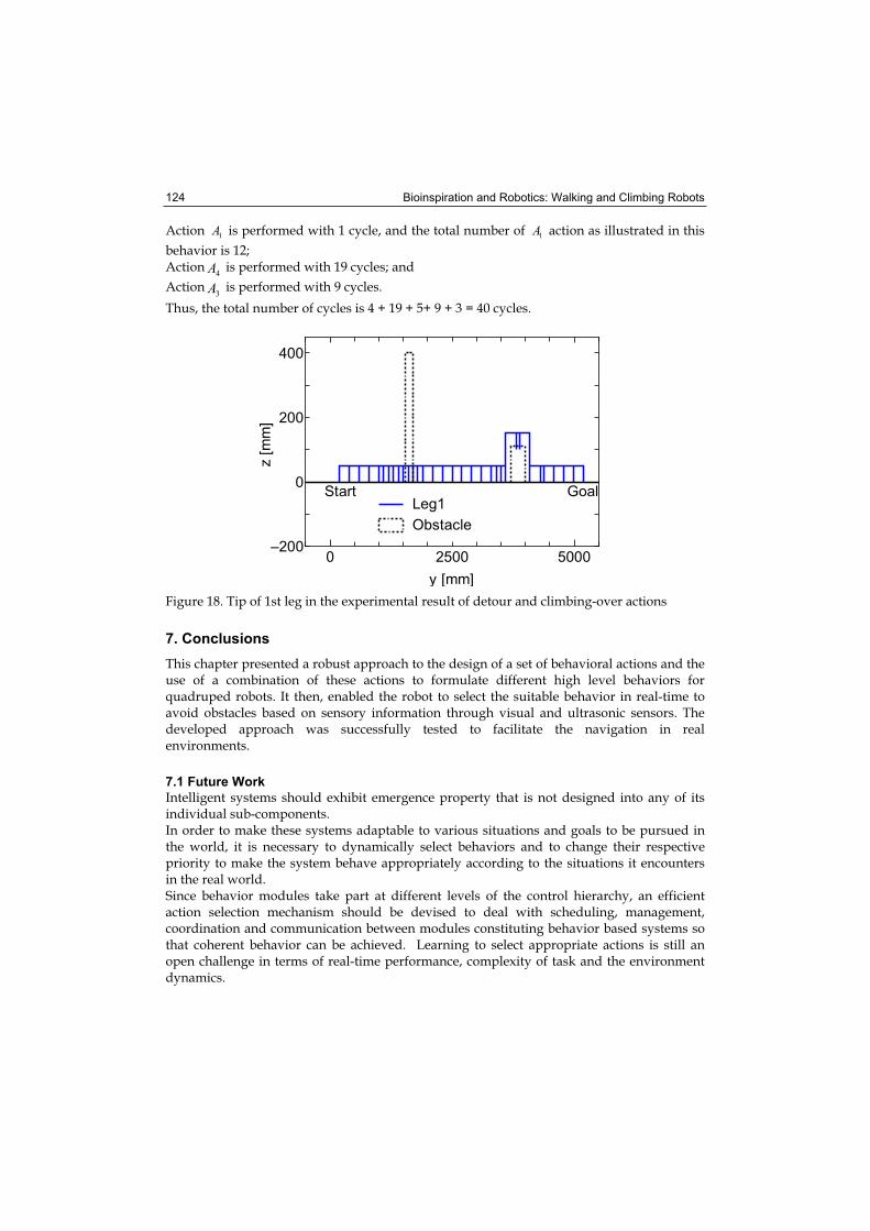
Bioinspiration and Robotics: Walking and Climbing Robots 124
Action 1A is performed with 1 cycle, and the total number of 1A action as illustrated in this
behavior is 12; Action
4A is performed with 19 cycles; and
Action3A is performed with 9 cycles.
Thus, the total number of cycles is 4 + 19 + 5+ 9 + 3 = 40 cycles.
0 2500 5000–200
0
200
400
y [mm]
z [
mm
]
Start GoalLeg1
Obstacle
Figure 18. Tip of 1st leg in the experimental result of detour and climbing-over actions
7. Conclusions
This chapter presented a robust approach to the design of a set of behavioral actions and the use of a combination of these actions to formulate different high level behaviors for quadruped robots. It then, enabled the robot to select the suitable behavior in real-time to avoid obstacles based on sensory information through visual and ultrasonic sensors. The developed approach was successfully tested to facilitate the navigation in real environments.
7.1 Future Work
Intelligent systems should exhibit emergence property that is not designed into any of its individual sub-components. In order to make these systems adaptable to various situations and goals to be pursued in the world, it is necessary to dynamically select behaviors and to change their respective priority to make the system behave appropriately according to the situations it encounters in the real world. Since behavior modules take part at different levels of the control hierarchy, an efficient action selection mechanism should be devised to deal with scheduling, management, coordination and communication between modules constituting behavior based systems so that coherent behavior can be achieved. Learning to select appropriate actions is still an open challenge in terms of real-time performance, complexity of task and the environment dynamics.
Selection of Obstacle Avoidance Behaviors Based on Visual and Ultrasonic Sensors for Quadruped Robots 125
8. References
Arikawa, K. & Hirose, S. (1996). Development of Quadruped Walking Robot TITAN-VIII, Proc. of the IEEE/RSJ International Conference on Intelligent Robots and Systems (IROS'96), Vol. 1, pp. 208-214, 1996.
Chen, X., Watanabe, K., Kiguchi, K., Izumi, K. (2002a). Path Tracking Based on Closed-Loop Control for a Quadruped Robot in a Cluttered Environment. Transactions of ASME,Vol. 24, pp. 272-280, June 2002.
Chen, X., Watanabe, K., Kiguchi, K., Izumi, K. (2002b). An ART-Based Fuzzy Controller for the Adaptive Navigation of a Quadruped Robot . IEEE/ASME Transactions on Mechatronics, Vol. 7, No. 3, pp. 318-328, Sept. 2002.
Cruse, H., Bartling, Ch., Cymbalyuk, G., Dean, J. and Dreifert, M. (1994). A neural net controller for a six Legged walking system. Proc. of International Conference from Perception to Action, pp. 55-65, 1994.
Ferrell, C. (1994). Robust and Adaptive Locomotion of an Autonomous Hexapod. Proc. of International Conference from Perception to Action, pp. 66-77, 1994.
Go, Y., Yin, X., Bowling, A. (2006). Navigability of multi-Legged Robots. IEEE/ASME Transactions on Mechatronics, Vol. 11, No. 1, pp. 1-8, 2006.
Habib, M. K. (2003a). URUK: an Autonomous Legged Mobile Robot Design and Implementation. Proc. of International Conference on Mechatronics (ICOM2003), June 2003, UK, pp 497-504.
Habib, M. K. (2003b). Behavior-Based Autonomous Robotic Systems: The Reliability of Robot’s Decision and The Challenge of Action Selection Mechanisms. Proc. of International Symposium on Artificial Life and Robotics (AROB' 2003), Jan. 2003, Oita, Japan, pp.4-9.
Hirose, S., Masui, T., Kikuchi, H., Fukuda, Y., Umetani, Y. (1986). TITAN III: A Quadruped Walking Vehicle. Proc. of International Conference on Robotics Research, pp. 325-331, 1986.
Hirose, S., Arikawa, K. (2000): Coupled and Decoupled Actuation of Robotic Mechanisms, Proc. International Conference on Advanced Robots ICRA’2000, San Francisco, pp.33-39, 2000.
Hirose, S. (2001). Super Mechano-System Project in Tokyo Institute of Technology, Proc. of 2001 Int. Workshop on Bio-Robotics and Teleoperation, pp. 7-12, 2001
Lewis, M. A. (2002). Detecting Surface Features during Locomotion using Optic Flow. Proc. of International Conference of Robotics and Automations (ICRA’2002), Washington DC, pp. 305 – 310, 2002.
Nishikawa, N., Murakami, T., Ohnishi, K. (1998). An Approach to Stable Motion Control of Biped Robot with Unknown Load by Torque Estimator. Proc. of International Workshop on Advanced Motion Control, pp. 82-87, 1998.
Ohya, A., Kosaka, A., Kak, A. (1997). Vision-Based Navigation of Mobile Robot with Obstacle Avoidance by Single Camera Vision and Ultrasonic Sensing, Proc. of the IEEE/RSJ International Conference on Intelligent Robots and Systems (IROS'97), Vol. 2, pp. 704-711, 1997
Okada, K., Kagami, S., Inaba, M., Inoue, H. (1999). Vision-based Action Control of Quadruped Legged Robot JROB-1, Proc. of 9th International Conference on Advanced Robotics (ICAR'99), pp. 451-456, 1999
Bioinspiration and Robotics: Walking and Climbing Robots 126
Okada, K., Inaba, M., Inoue, H. (2003). Integration of Real-time Binocular Stereo Vision and Whole Body Information for Dynamic Walking Navigation of Humanoid Robot, Proc. of International Conference on Multisensor Fusion and Integration for Intelligent Systems (MFI'03), pp. 131-136, 2003
Ooka, A., Ogi, K., Takemoto, Y., Okamoto, K. and Yoshida (1986). Intelligent robot system II. Proc. of International Conference on Robotics Research, pp.341-347, 1986..
Pugh, D. R., Ribble, E. A., Vohnout, V. J., Bihari, E. E., Walliser, T. M., Patterson, M. R., Waldron, K. J. (1990). Technical Description of the Adaptive Suspension Vehicle. International Journal of Robotics Research, Vol. 9, No. 2, pp. 24-42, 1990.
Raibert, M. H. (1986). Legged robots that balance. The MIT Press, 1986. Tsukakoshi, H., Hirose, S., Yoneda, K. (1996). Maneuvering Operations of the Quadruped
Walking Robot on the Slope, Proc. of the IEEE/RSJ Int. Conf. on Intelligent Robots and Systems, Vol. 2, pp. 863-869, 1996
Waldron, K. J., Vohnout, V. J., Pery, A., McGhee, R. B. (1984) . Configuration of the Adaptive Suspension Vehicle. International Journal of Robotics Research, Vol. 3, No. 2, pp. 37-48, 1984.
Yamaguchi, T., Watanabe, K., Izumi, K., Kiguchi, K. (2002a). Acquisition of An Obstacle Avoiding Path in Quadruped Robots, Proc. of Joint 1st International Conference on Soft Computing and Intelligent Systems and 4th International Symposium on Advanced Intelligent Systems(SCIS & ISIS 2002), 2002.
Yamaguchi, T. , Watanabe, K., Kiguchi, K., Izumi, K. (2002b). Obstacle Avoidance Strategy for A 4-legged Robot by Getting-over and Striding, Proc. of the 4th Asian Control Conference, pp. 1438-1443, 2002.
9
Climbing Service Robots for Improving Safety in Building Maintenance Industry
Bing L. Luk1, Louis K. P. Liu1 and Arthur A. Collie2
1Department of Manufacturing Engineering and Engineering Management, City University of Hong Kong, 2Climbing Robot Company Ltd
1Hong Kong, 2UK
1. Introduction
Tall buildings and hazardous utilities require regular inspection and maintenance to comply with the ordinance, and to ensure the integrity and safety. The traditional manual inspection and maintenance on tall building normally requires the installation of expensive scaffoldings or gondolas in which human operators need to work in mid-air and life-threatening environment. Moreover, in some hazardous industries, such as nuclear, chemical and power generation, these maintenance tasks can be harmful and hazardous to human life and health. On the other hand, the reliability of the manual inspection approach is questionable because human judgement is always subjective. Consequently, the poor inspection result will deduce either excessive or inadequate repairing work that is undesirable in term of costing and safety. Over the years, a number of climbing robots have been developed for various building inspection and cleaning applications (Tso et al., 2000; Tso et al., 2001; Zhang et al., 2001; Hillenbrand et al., 2001; Sattar et al., 2001; Bahr & Yin, 1994; Wang & Shao, 1999; Minor et al., 2000; Luk et al., 2005; Luk et al., 2006). Beside the above development, the authors have also been requested by industry to develop a number of climbing robots cater for various maintenance tasks. These tasks are usually difficult and costly to be achieved by manual approaches. As buildings in many metropolitan cities like Hong Kong are getting taller and taller, the public concern for the safety of high-rise buildings and large structures is rising. Recently, the Hong Kong Housing, Planning and Land Bureau has just finished a public consultation on mandatory building inspection and intends to pass a legislation to enforce the mandatory inspection of all tall buildings aged 30 years or above. Other cities may have similar requirement in the future. As a result, there will be more and more demands to improve the accuracy and efficiency of building inspection and maintenance processes. It is a matter of fact that application of climbing service robots is one solution to service this purpose.In this chapter, WIC, SADIE and Robug III climbing robots developed by the authors will be described. WIC is a gondola-based climbing robot developed for inspecting tile-walls of high-rise buildings in Hong Kong. SADIE is a climbing robot with seven non-articulated legs developed for carrying out ultrasonic inspection and surface preparation inside reactor cooling gas ducts at Sizewell ‘A’ Power Station. Robug III is a walking and climbing robot
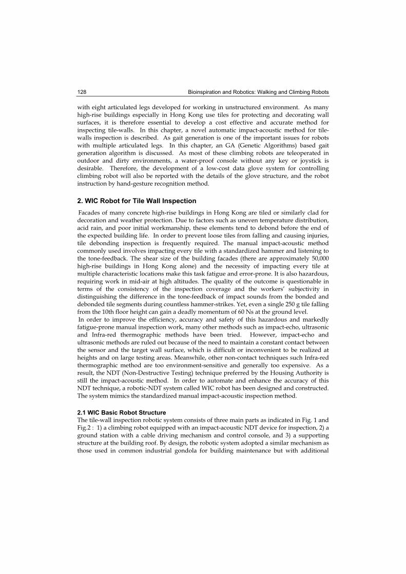
Bioinspiration and Robotics: Walking and Climbing Robots 128
with eight articulated legs developed for working in unstructured environment. As many high-rise buildings especially in Hong Kong use tiles for protecting and decorating wall surfaces, it is therefore essential to develop a cost effective and accurate method for inspecting tile-walls. In this chapter, a novel automatic impact-acoustic method for tile-walls inspection is described. As gait generation is one of the important issues for robots with multiple articulated legs. In this chapter, an GA (Genetic Algorithms) based gait generation algorithm is discussed. As most of these climbing robots are teleoperated in outdoor and dirty environments, a water-proof console without any key or joystick is desirable. Therefore, the development of a low-cost data glove system for controlling climbing robot will also be reported with the details of the glove structure, and the robot instruction by hand-gesture recognition method.
2. WIC Robot for Tile Wall Inspection
Facades of many concrete high-rise buildings in Hong Kong are tiled or similarly clad for decoration and weather protection. Due to factors such as uneven temperature distribution, acid rain, and poor initial workmanship, these elements tend to debond before the end of the expected building life. In order to prevent loose tiles from falling and causing injuries, tile debonding inspection is frequently required. The manual impact-acoustic method commonly used involves impacting every tile with a standardized hammer and listening to the tone-feedback. The shear size of the building facades (there are approximately 50,000 high-rise buildings in Hong Kong alone) and the necessity of impacting every tile at multiple characteristic locations make this task fatigue and error-prone. It is also hazardous, requiring work in mid-air at high altitudes. The quality of the outcome is questionable in terms of the consistency of the inspection coverage and the workers’ subjectivity in distinguishing the difference in the tone-feedback of impact sounds from the bonded and debonded tile segments during countless hammer-strikes. Yet, even a single 250 g tile falling from the 10th floor height can gain a deadly momentum of 60 Ns at the ground level. In order to improve the efficiency, accuracy and safety of this hazardous and markedly fatigue-prone manual inspection work, many other methods such as impact-echo, ultrasonic and Infra-red thermographic methods have been tried. However, impact-echo and ultrasonic methods are ruled out because of the need to maintain a constant contact between the sensor and the target wall surface, which is difficult or inconvenient to be realized at heights and on large testing areas. Meanwhile, other non-contact techniques such Infra-red thermographic method are too environment-sensitive and generally too expensive. As a result, the NDT (Non-Destructive Testing) technique preferred by the Housing Authority is still the impact-acoustic method. In order to automate and enhance the accuracy of this NDT technique, a robotic-NDT system called WIC robot has been designed and constructed. The system mimics the standardized manual impact-acoustic inspection method.
2.1 WIC Basic Robot Structure
The tile-wall inspection robotic system consists of three main parts as indicated in Fig. 1 and Fig.2 : 1) a climbing robot equipped with an impact-acoustic NDT device for inspection, 2) a ground station with a cable driving mechanism and control console, and 3) a supporting structure at the building roof. By design, the robotic system adopted a similar mechanism as those used in common industrial gondola for building maintenance but with additional
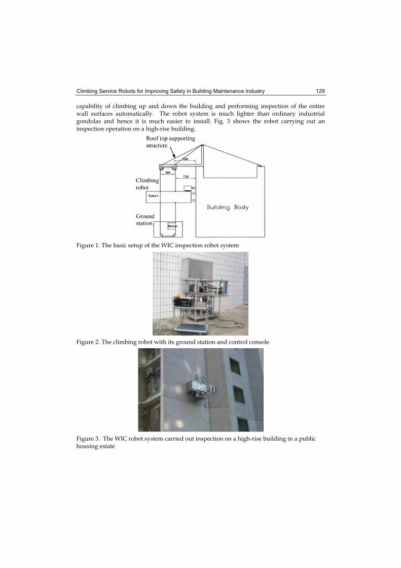
Climbing Service Robots for Improving Safety in Building Maintenance Industry 129
capability of climbing up and down the building and performing inspection of the entire wall surfaces automatically. The robot system is much lighter than ordinary industrial gondolas and hence it is much easier to install. Fig. 3 shows the robot carrying out an inspection operation on a high-rise building.
Figure 1. The basic setup of the WIC inspection robot system
Figure 2. The climbing robot with its ground station and control console
Figure 3. The WIC robot system carried out inspection on a high-rise building in a public housing estate
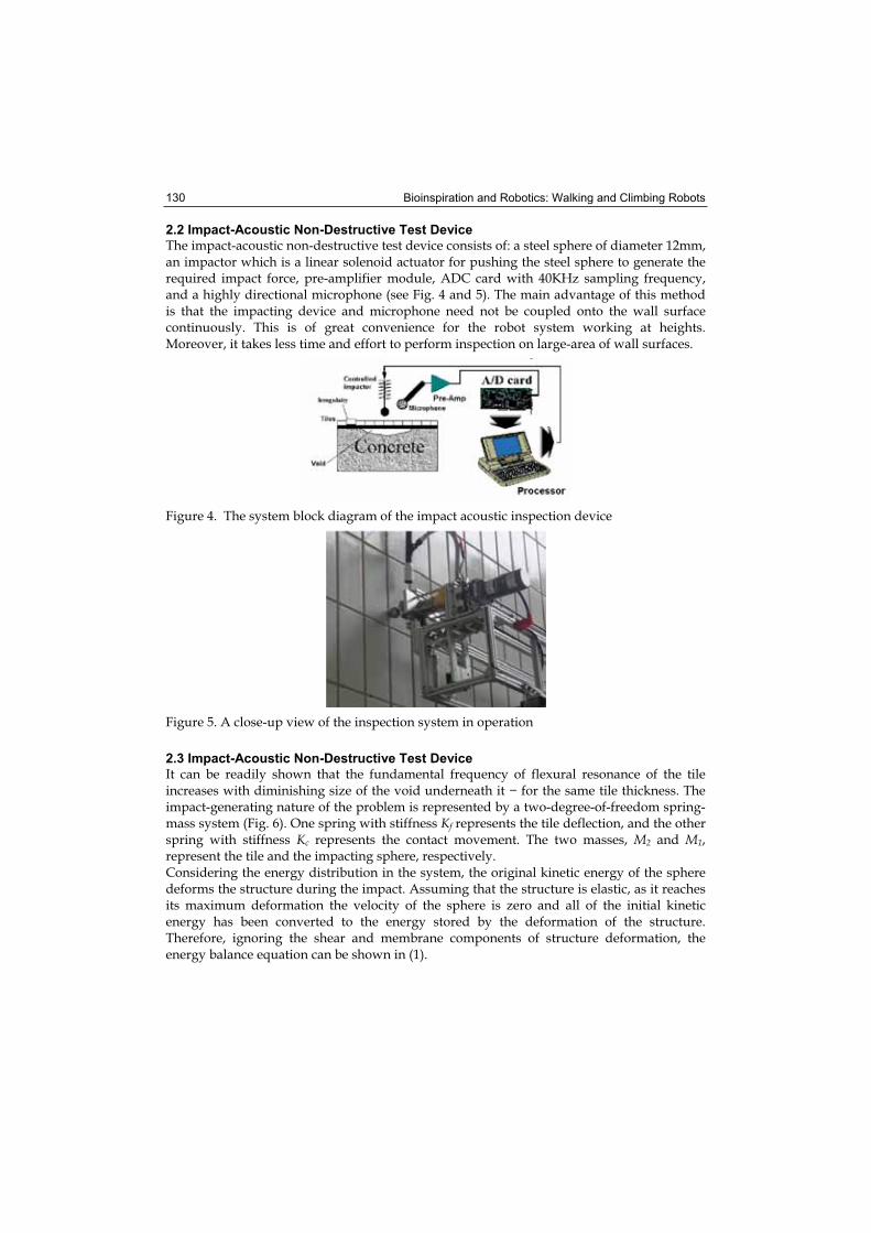
Bioinspiration and Robotics: Walking and Climbing Robots 130
2.2 Impact-Acoustic Non-Destructive Test Device
The impact-acoustic non-destructive test device consists of: a steel sphere of diameter 12mm, an impactor which is a linear solenoid actuator for pushing the steel sphere to generate the required impact force, pre-amplifier module, ADC card with 40KHz sampling frequency, and a highly directional microphone (see Fig. 4 and 5). The main advantage of this method is that the impacting device and microphone need not be coupled onto the wall surface continuously. This is of great convenience for the robot system working at heights. Moreover, it takes less time and effort to perform inspection on large-area of wall surfaces.
Figure 4. The system block diagram of the impact acoustic inspection device
Figure 5. A close-up view of the inspection system in operation
2.3 Impact-Acoustic Non-Destructive Test Device
It can be readily shown that the fundamental frequency of flexural resonance of the tile increases with diminishing size of the void underneath it for the same tile thickness. The impact-generating nature of the problem is represented by a two-degree-of-freedom spring-mass system (Fig. 6). One spring with stiffness Kf represents the tile deflection, and the other spring with stiffness Kc represents the contact movement. The two masses, M2 and M1,represent the tile and the impacting sphere, respectively. Considering the energy distribution in the system, the original kinetic energy of the sphere deforms the structure during the impact. Assuming that the structure is elastic, as it reaches its maximum deformation the velocity of the sphere is zero and all of the initial kinetic energy has been converted to the energy stored by the deformation of the structure. Therefore, ignoring the shear and membrane components of structure deformation, the energy balance equation can be shown in (1).
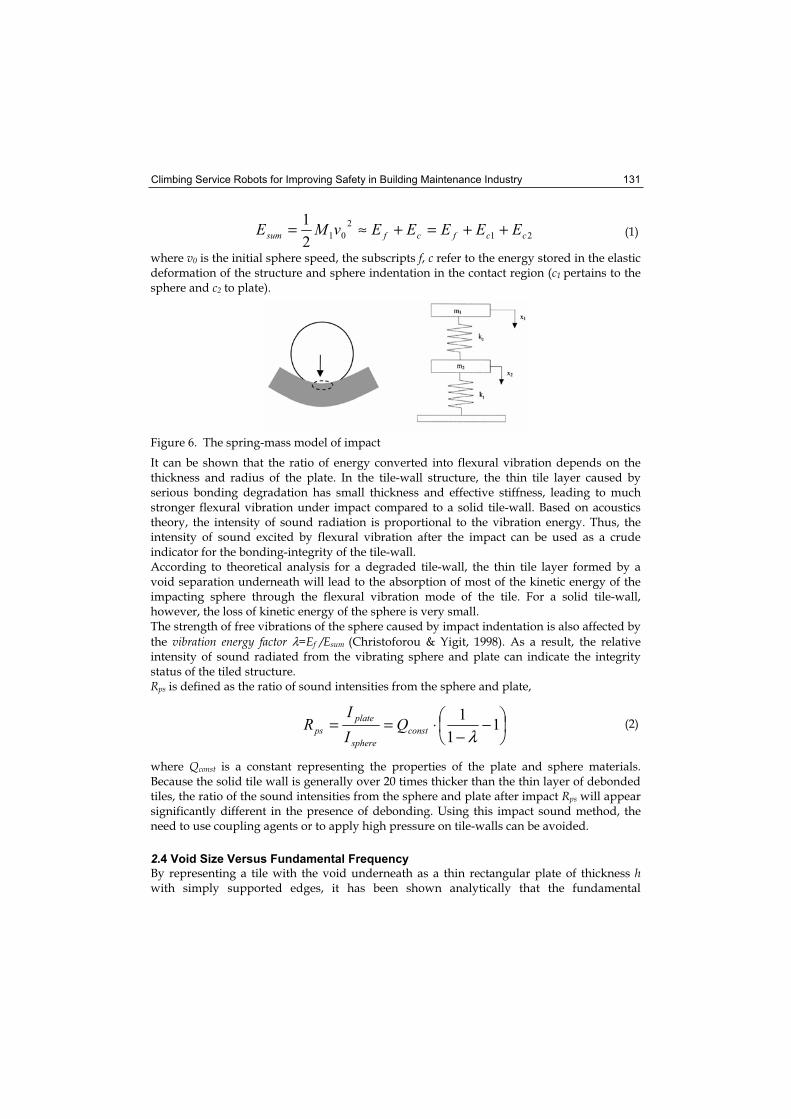
Climbing Service Robots for Improving Safety in Building Maintenance Industry 131
where v0 is the initial sphere speed, the subscripts f, c refer to the energy stored in the elastic deformation of the structure and sphere indentation in the contact region (c1 pertains to the sphere and c2 to plate).
Figure 6. The spring-mass model of impact
It can be shown that the ratio of energy converted into flexural vibration depends on the thickness and radius of the plate. In the tile-wall structure, the thin tile layer caused by serious bonding degradation has small thickness and effective stiffness, leading to much stronger flexural vibration under impact compared to a solid tile-wall. Based on acoustics theory, the intensity of sound radiation is proportional to the vibration energy. Thus, the intensity of sound excited by flexural vibration after the impact can be used as a crude indicator for the bonding-integrity of the tile-wall. According to theoretical analysis for a degraded tile-wall, the thin tile layer formed by a void separation underneath will lead to the absorption of most of the kinetic energy of the impacting sphere through the flexural vibration mode of the tile. For a solid tile-wall, however, the loss of kinetic energy of the sphere is very small. The strength of free vibrations of the sphere caused by impact indentation is also affected by
the vibration energy factor λ=Ef /Esum (Christoforou & Yigit, 1998). As a result, the relative intensity of sound radiated from the vibrating sphere and plate can indicate the integrity status of the tiled structure. Rps is defined as the ratio of sound intensities from the sphere and plate,
where Qconst is a constant representing the properties of the plate and sphere materials. Because the solid tile wall is generally over 20 times thicker than the thin layer of debonded tiles, the ratio of the sound intensities from the sphere and plate after impact Rps will appear significantly different in the presence of debonding. Using this impact sound method, the need to use coupling agents or to apply high pressure on tile-walls can be avoided.
2.4 Void Size Versus Fundamental Frequency
By representing a tile with the void underneath as a thin rectangular plate of thickness hwith simply supported edges, it has been shown analytically that the fundamental
−−
⋅== 11
1
λconstsphere
plateps Q
II
R (2)
21
2
012
1ccfcfsum EEEEEvME ++=+≈= (1)
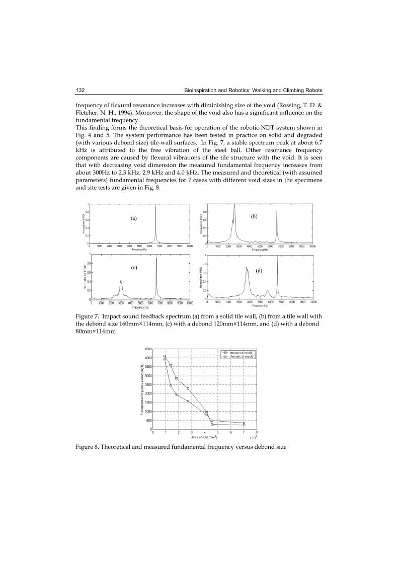
Bioinspiration and Robotics: Walking and Climbing Robots 132
frequency of flexural resonance increases with diminishing size of the void (Rossing, T. D. & Fletcher, N. H., 1994). Moreover, the shape of the void also has a significant influence on the fundamental frequency.This finding forms the theoretical basis for operation of the robotic-NDT system shown in Fig. 4 and 5. The system performance has been tested in practice on solid and degraded (with various debond size) tile-wall surfaces. In Fig. 7, a stable spectrum peak at about 6.7 kHz is attributed to the free vibration of the steel ball. Other resonance frequency components are caused by flexural vibrations of the tile structure with the void. It is seen that with decreasing void dimension the measured fundamental frequency increases from about 300Hz to 2.3 kHz, 2.9 kHz and 4.0 kHz. The measured and theoretical (with assumed parameters) fundamental frequencies for 7 cases with different void sizes in the specimens and site tests are given in Fig. 8.
Figure 7. Impact sound feedback spectrum (a) from a solid tile wall, (b) from a tile wall with the debond size 160mm×114mm, (c) with a debond 120mm×114mm, and (d) with a debond 80mm×114mm
Figure 8. Theoretical and measured fundamental frequency versus debond size
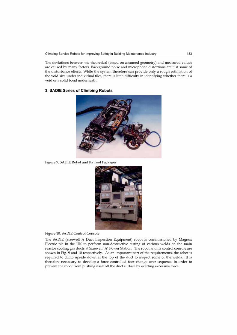
Climbing Service Robots for Improving Safety in Building Maintenance Industry 133
The deviations between the theoretical (based on assumed geometry) and measured values are caused by many factors. Background noise and microphone distortions are just some of the disturbance effects. While the system therefore can provide only a rough estimation of the void size under individual tiles, there is little difficulty in identifying whether there is a void or a solid bond underneath.
3. SADIE Series of Climbing Robots
Figure 9. SADIE Robot and Its Tool Packages
Figure 10. SADIE Control Console
The SADIE (Sizewell A Duct Inspection Equipment) robot is commissioned by Magnox Electric plc in the UK to perform non-destructive testing of various welds on the main reactor cooling gas ducts at Sizewell ‘A’ Power Station. The robot and its control console are shown in Fig. 9 and 10 respectively. As an important part of the requirements, the robot is required to climb upside down at the top of the duct to inspect some of the welds. It is therefore necessary to develop a force controlled foot change over sequence in order to prevent the robot from pushing itself off the duct surface by exerting excessive force.
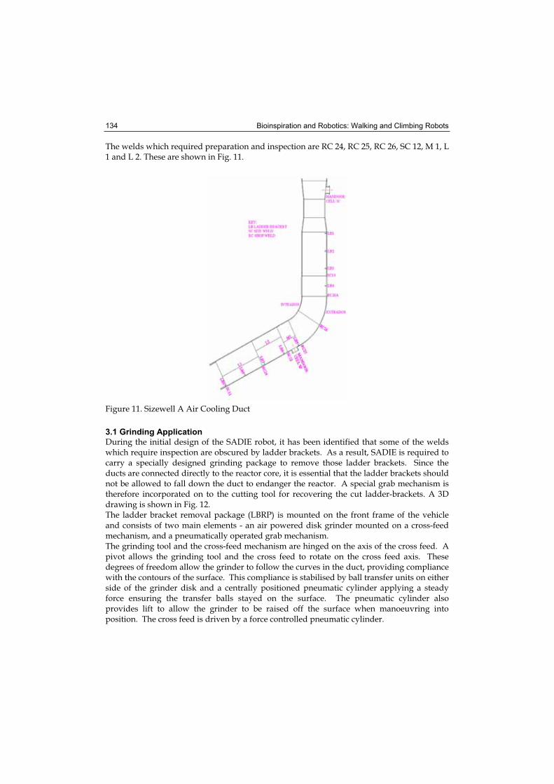
Bioinspiration and Robotics: Walking and Climbing Robots 134
The welds which required preparation and inspection are RC 24, RC 25, RC 26, SC 12, M 1, L 1 and L 2. These are shown in Fig. 11.
Figure 11. Sizewell A Air Cooling Duct
3.1 Grinding Application
During the initial design of the SADIE robot, it has been identified that some of the welds which require inspection are obscured by ladder brackets. As a result, SADIE is required to carry a specially designed grinding package to remove those ladder brackets. Since the ducts are connected directly to the reactor core, it is essential that the ladder brackets should not be allowed to fall down the duct to endanger the reactor. A special grab mechanism is therefore incorporated on to the cutting tool for recovering the cut ladder-brackets. A 3D drawing is shown in Fig. 12. The ladder bracket removal package (LBRP) is mounted on the front frame of the vehicle and consists of two main elements - an air powered disk grinder mounted on a cross-feed mechanism, and a pneumatically operated grab mechanism.The grinding tool and the cross-feed mechanism are hinged on the axis of the cross feed. A pivot allows the grinding tool and the cross feed to rotate on the cross feed axis. These degrees of freedom allow the grinder to follow the curves in the duct, providing compliance with the contours of the surface. This compliance is stabilised by ball transfer units on either side of the grinder disk and a centrally positioned pneumatic cylinder applying a steady force ensuring the transfer balls stayed on the surface. The pneumatic cylinder also provides lift to allow the grinder to be raised off the surface when manoeuvring into position. The cross feed is driven by a force controlled pneumatic cylinder.
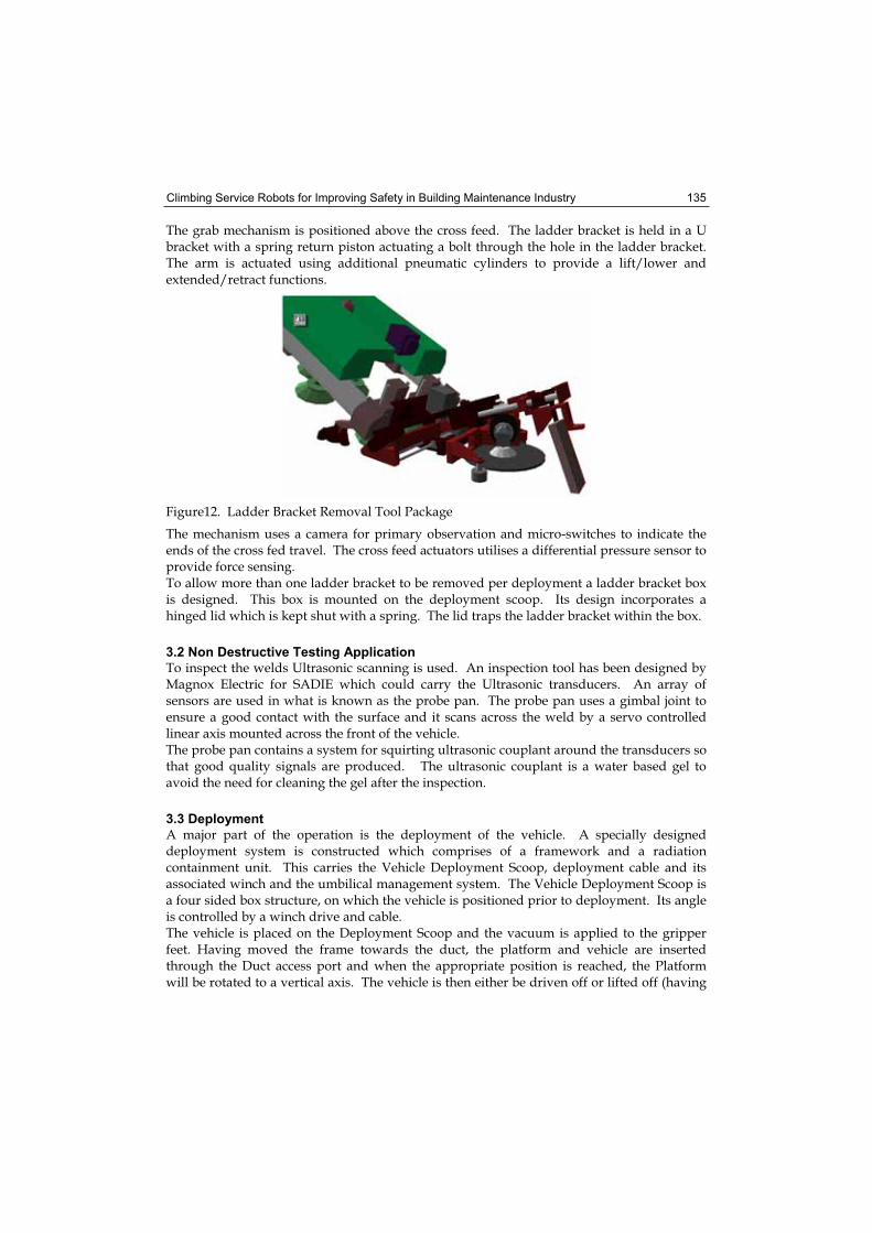
Climbing Service Robots for Improving Safety in Building Maintenance Industry 135
The grab mechanism is positioned above the cross feed. The ladder bracket is held in a U bracket with a spring return piston actuating a bolt through the hole in the ladder bracket. The arm is actuated using additional pneumatic cylinders to provide a lift/lower and extended/retract functions.
Figure12. Ladder Bracket Removal Tool Package
The mechanism uses a camera for primary observation and micro-switches to indicate the ends of the cross fed travel. The cross feed actuators utilises a differential pressure sensor to provide force sensing. To allow more than one ladder bracket to be removed per deployment a ladder bracket box is designed. This box is mounted on the deployment scoop. Its design incorporates a hinged lid which is kept shut with a spring. The lid traps the ladder bracket within the box.
3.2 Non Destructive Testing Application
To inspect the welds Ultrasonic scanning is used. An inspection tool has been designed by Magnox Electric for SADIE which could carry the Ultrasonic transducers. An array of sensors are used in what is known as the probe pan. The probe pan uses a gimbal joint to ensure a good contact with the surface and it scans across the weld by a servo controlled linear axis mounted across the front of the vehicle. The probe pan contains a system for squirting ultrasonic couplant around the transducers so that good quality signals are produced. The ultrasonic couplant is a water based gel to avoid the need for cleaning the gel after the inspection.
3.3 Deployment
A major part of the operation is the deployment of the vehicle. A specially designed deployment system is constructed which comprises of a framework and a radiation containment unit. This carries the Vehicle Deployment Scoop, deployment cable and its associated winch and the umbilical management system. The Vehicle Deployment Scoop is a four sided box structure, on which the vehicle is positioned prior to deployment. Its angle is controlled by a winch drive and cable. The vehicle is placed on the Deployment Scoop and the vacuum is applied to the gripper feet. Having moved the frame towards the duct, the platform and vehicle are inserted through the Duct access port and when the appropriate position is reached, the Platform will be rotated to a vertical axis. The vehicle is then either be driven off or lifted off (having
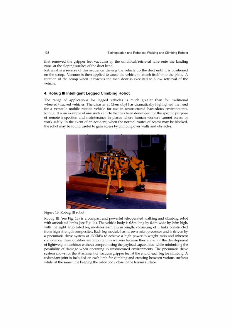
Bioinspiration and Robotics: Walking and Climbing Robots 136
first removed the gripper feet vacuum) by the umbilical/retrieval wire onto the landing zone, at the sloping surface of the duct bend. Retrieval is a reverse of this sequence, driving the vehicle up the duct until it is positioned on the scoop. Vacuum is then applied to cause the vehicle to attach itself onto the plate. A rotation of the scoop when it reaches the man door is executed to allow retrieval of the vehicle.
4. Robug III Intelligent Legged Climbing Robot
The range of applications for legged vehicles is much greater than for traditional wheeled/tracked vehicles. The disaster at Chernobyl has dramatically highlighted the need for a versatile mobile robotic vehicle for use in unstructured hazardous environments. Robug III is an example of one such vehicle that has been developed for the specific purpose of remote inspection and maintenance in places where human workers cannot access or work safely. In the event of an accident, when the normal routes of access may be blocked, the robot may be found useful to gain access by climbing over walls and obstacles.
Figure 13. Robug III robot
Robug III (see Fig. 13) is a compact and powerful teleoperated walking and climbing robot with articulated limbs (see Fig. 14). The vehicle body is 0.8m long by 0.6m wide by 0.6m high, with the eight articulated leg modules each 1m in length, consisting of 3 links constructed from high strength composites. Each leg module has its own microprocessor and is driven by a pneumatic drive system at 1300kPa to achieve a high power-to-weight ratio and inherent compliance; these qualities are important in walkers because they allow for the development of lightweight machines without compromising the payload capabilities, while minimising the possibility of damage when operating in unstructured environments. The pneumatic drive system allows for the attachment of vacuum gripper feet at the end of each leg for climbing. A redundant joint is included on each limb for climbing and crossing between various surfaces whilst at the same time keeping the robot body close to the terrain surface.
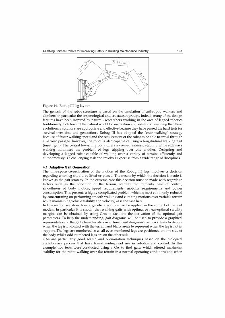
Climbing Service Robots for Improving Safety in Building Maintenance Industry 137
Figure 14. Robug III leg layout
The genesis of the robot structure is based on the emulation of arthropod walkers and climbers; in particular the entomological and crustacean groups. Indeed, many of the design features have been inspired by nature - researchers working in the area of legged robotics traditionally look toward the natural world for inspiration and solutions, reasoning that these evolutionary solutions are appropriate and effective because they have passed the hard tests for survival over time and generations. Robug III has adopted the “crab walking” strategy because of faster walking speed and the requirement of the robot to be able to crawl through a narrow passage, however, the robot is also capable of using a longitudinal walking gait (insect gait). The central low-slung body offers increased intrinsic stability while sideways walking minimises the problem of legs tripping over one another. Designing and developing a legged robot capable of walking over a variety of terrains efficiently and autonomously is a challenging task and involves expertise from a wide range of disciplines.
4.1 Adaptive Gait Generation
The time-space co-ordination of the motion of the Robug III legs involves a decision regarding what leg should be lifted or placed. The means by which the decision is made is known as the gait strategy. In the extreme case this decision must be made with regards to factors such as the condition of the terrain, stability requirements, ease of control, smoothness of body motion, speed requirements, mobility requirements and power consumption. This presents a highly complicated problem which is most commonly reduced by concentrating on performing smooth walking and climbing motions over variable terrain while maintaining vehicle stability and velocity, as is the case here. In this section we show how a genetic algorithm can be applied in the context of the gait models, in particular it is shown that walking gaits with optimal or near-optimal stability margins can be obtained by using GAs to facilitate the derivation of the optimal gait parameters. To help the understanding, gait diagrams will be used to provide a graphical representation of the gait characteristics over time. Gait diagrams use black lines to denote when the leg is in contact with the terrain and blank areas to represent when the leg is not in support. The legs are numbered so as all even-numbered legs are positioned on one side of the body whilst odd-numbered legs are on the other side. GAs are particularly good search and optimisation techniques based on the biological evolutionary process that have found widespread use in robotics and control. In this example two tests were conducted using a GA to find gaits which offered maximum stability for the robot walking over flat terrain in a normal operating conditions and when
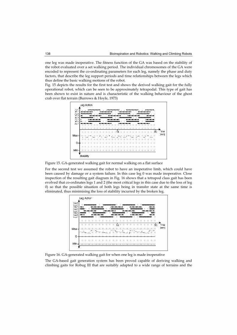
Bioinspiration and Robotics: Walking and Climbing Robots 138
one leg was made inoperative. The fitness function of the GA was based on the stability of the robot evaluated over a set walking period. The individual chromosomes of the GA were encoded to represent the co-ordinating parameters for each leg, namely the phase and duty factors, that describe the leg support periods and time relationships between the legs which thus define the basic walking motions of the robot. Fig. 15 depicts the results for the first test and shows the derived walking gait for the fully operational robot, which can be seen to be approximately tetrapodal. This type of gait has been shown to exist in nature and is characteristic of the walking behaviour of the ghost crab over flat terrain (Burrows & Hoyle, 1973)
Figure 15. GA-generated walking gait for normal walking on a flat surface
For the second test we assumed the robot to have an inoperative limb, which could have been caused by damage or a system failure. In this case leg 0 was made inoperative. Close inspection of the resulting gait diagram in Fig. 16 shows that a tetrapod class gait has been evolved that co-ordinates legs 1 and 2 (the most critical legs in this case due to the loss of leg 0) so that the possible situation of both legs being in transfer state at the same time is eliminated, thus minimising the loss of stability incurred by the broken leg.
Figure 16. GA-generated walking gait for when one leg is made inoperative
The GA-based gait generation system has been proved capable of deriving walking and climbing gaits for Robug III that are suitably adapted to a wide range of terrains and the
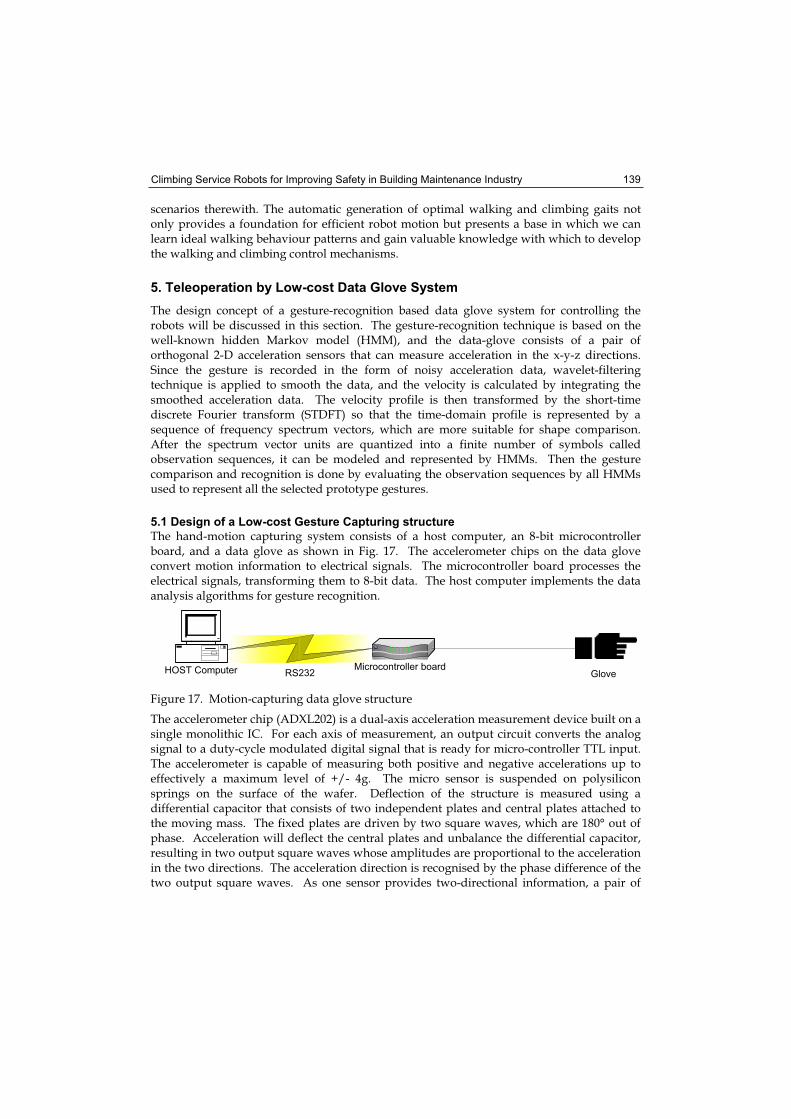
Climbing Service Robots for Improving Safety in Building Maintenance Industry 139
scenarios therewith. The automatic generation of optimal walking and climbing gaits not only provides a foundation for efficient robot motion but presents a base in which we can learn ideal walking behaviour patterns and gain valuable knowledge with which to develop the walking and climbing control mechanisms.
5. Teleoperation by Low-cost Data Glove System
The design concept of a gesture-recognition based data glove system for controlling the robots will be discussed in this section. The gesture-recognition technique is based on the well-known hidden Markov model (HMM), and the data-glove consists of a pair of orthogonal 2-D acceleration sensors that can measure acceleration in the x-y-z directions. Since the gesture is recorded in the form of noisy acceleration data, wavelet-filtering technique is applied to smooth the data, and the velocity is calculated by integrating the smoothed acceleration data. The velocity profile is then transformed by the short-time discrete Fourier transform (STDFT) so that the time-domain profile is represented by a sequence of frequency spectrum vectors, which are more suitable for shape comparison. After the spectrum vector units are quantized into a finite number of symbols called observation sequences, it can be modeled and represented by HMMs. Then the gesture comparison and recognition is done by evaluating the observation sequences by all HMMs used to represent all the selected prototype gestures.
5.1 Design of a Low-cost Gesture Capturing structure
The hand-motion capturing system consists of a host computer, an 8-bit microcontroller board, and a data glove as shown in Fig. 17. The accelerometer chips on the data glove convert motion information to electrical signals. The microcontroller board processes the electrical signals, transforming them to 8-bit data. The host computer implements the data analysis algorithms for gesture recognition.
RS232HOST Computer Microcontroller boardGlove
Figure 17. Motion-capturing data glove structure
The accelerometer chip (ADXL202) is a dual-axis acceleration measurement device built on a single monolithic IC. For each axis of measurement, an output circuit converts the analog signal to a duty-cycle modulated digital signal that is ready for micro-controller TTL input. The accelerometer is capable of measuring both positive and negative accelerations up to effectively a maximum level of +/- 4g. The micro sensor is suspended on polysilicon springs on the surface of the wafer. Deflection of the structure is measured using a differential capacitor that consists of two independent plates and central plates attached to the moving mass. The fixed plates are driven by two square waves, which are 180° out of phase. Acceleration will deflect the central plates and unbalance the differential capacitor, resulting in two output square waves whose amplitudes are proportional to the acceleration in the two directions. The acceleration direction is recognised by the phase difference of the two output square waves. As one sensor provides two-directional information, a pair of
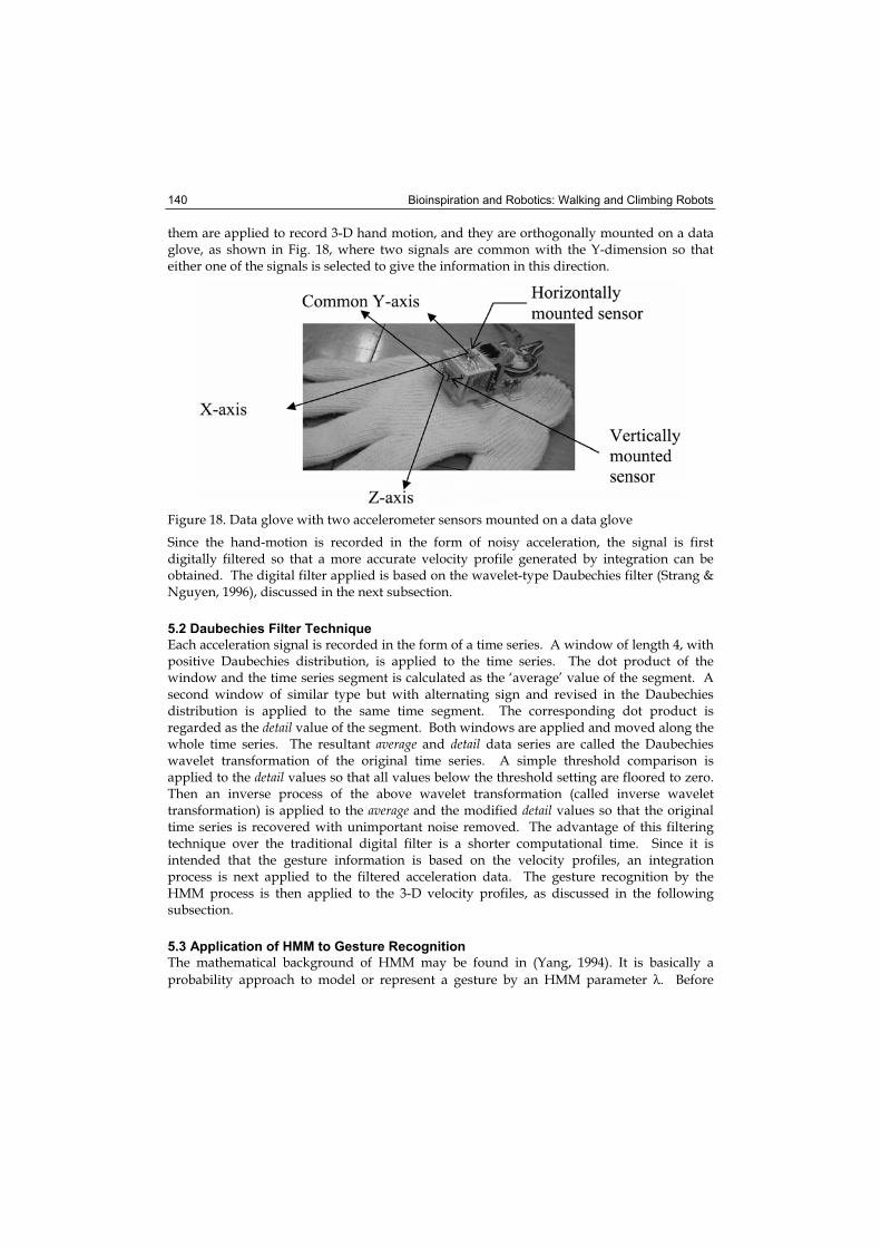
Bioinspiration and Robotics: Walking and Climbing Robots 140
them are applied to record 3-D hand motion, and they are orthogonally mounted on a data glove, as shown in Fig. 18, where two signals are common with the Y-dimension so that either one of the signals is selected to give the information in this direction.
Figure 18. Data glove with two accelerometer sensors mounted on a data glove
Since the hand-motion is recorded in the form of noisy acceleration, the signal is first digitally filtered so that a more accurate velocity profile generated by integration can be obtained. The digital filter applied is based on the wavelet-type Daubechies filter (Strang & Nguyen, 1996), discussed in the next subsection.
5.2 Daubechies Filter Technique
Each acceleration signal is recorded in the form of a time series. A window of length 4, with positive Daubechies distribution, is applied to the time series. The dot product of the window and the time series segment is calculated as the ‘average’ value of the segment. A second window of similar type but with alternating sign and revised in the Daubechies distribution is applied to the same time segment. The corresponding dot product is regarded as the detail value of the segment. Both windows are applied and moved along the whole time series. The resultant average and detail data series are called the Daubechies wavelet transformation of the original time series. A simple threshold comparison is applied to the detail values so that all values below the threshold setting are floored to zero. Then an inverse process of the above wavelet transformation (called inverse wavelet transformation) is applied to the average and the modified detail values so that the original time series is recovered with unimportant noise removed. The advantage of this filtering technique over the traditional digital filter is a shorter computational time. Since it is intended that the gesture information is based on the velocity profiles, an integration process is next applied to the filtered acceleration data. The gesture recognition by the HMM process is then applied to the 3-D velocity profiles, as discussed in the following subsection.
5.3 Application of HMM to Gesture Recognition
The mathematical background of HMM may be found in (Yang, 1994). It is basically a
probability approach to model or represent a gesture by an HMM parameter λ. Before
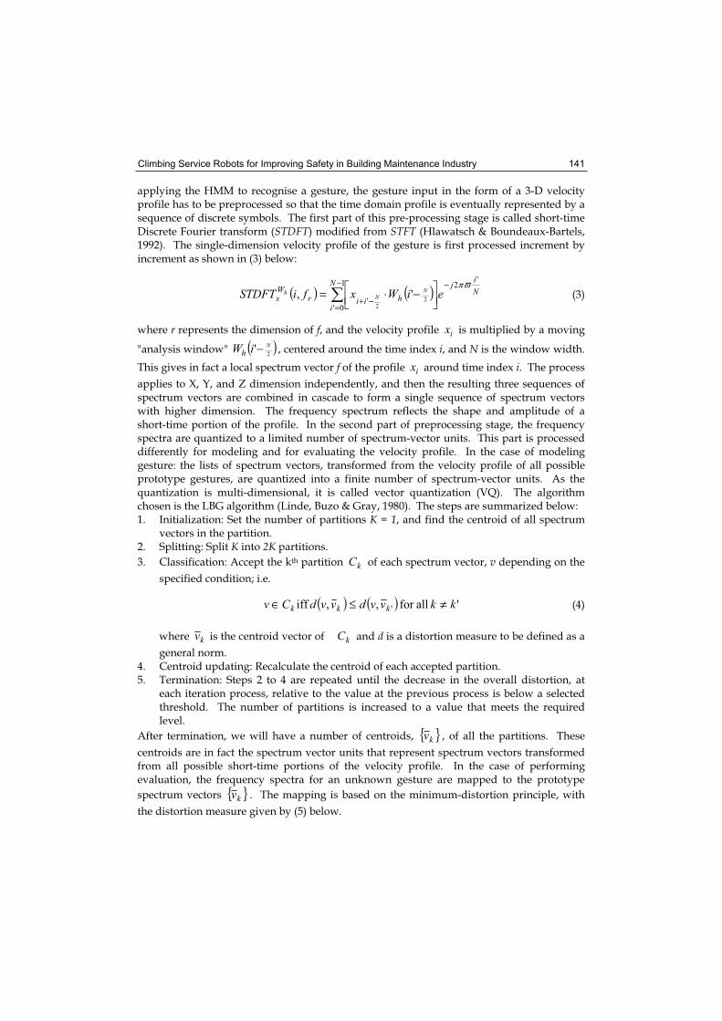
Climbing Service Robots for Improving Safety in Building Maintenance Industry 141
applying the HMM to recognise a gesture, the gesture input in the form of a 3-D velocity profile has to be preprocessed so that the time domain profile is eventually represented by a sequence of discrete symbols. The first part of this pre-processing stage is called short-time Discrete Fourier transform (STDFT) modified from STFT (Hlawatsch & Boundeaux-Bartels, 1992). The single-dimension velocity profile of the gesture is first processed increment by increment as shown in (3) below:
( ) ( )−
=
−
−+−⋅=
1
0'
'2
' 22
',N
i
Nij
hiirWx eiWxfiSTDFT N
Nh
ϖπ (3)
where r represents the dimension of f, and the velocity profile ix is multiplied by a moving
"analysis window" ( )2
' NiWh − , centered around the time index i, and N is the window width.
This gives in fact a local spectrum vector f of the profile ix around time index i. The process
applies to X, Y, and Z dimension independently, and then the resulting three sequences of spectrum vectors are combined in cascade to form a single sequence of spectrum vectors with higher dimension. The frequency spectrum reflects the shape and amplitude of a short-time portion of the profile. In the second part of preprocessing stage, the frequency spectra are quantized to a limited number of spectrum-vector units. This part is processed differently for modeling and for evaluating the velocity profile. In the case of modeling gesture: the lists of spectrum vectors, transformed from the velocity profile of all possible prototype gestures, are quantized into a finite number of spectrum-vector units. As the quantization is multi-dimensional, it is called vector quantization (VQ). The algorithm chosen is the LBG algorithm (Linde, Buzo & Gray, 1980). The steps are summarized below: 1. Initialization: Set the number of partitions K = 1, and find the centroid of all spectrum
vectors in the partition. 2. Splitting: Split K into 2K partitions.
3. Classification: Accept the kth partition Ck of each spectrum vector, v depending on the
specified condition; i.e.
( ) ( ) 'allfor,,iff ' kkvvdvvdCv kkk ≠≤∈ (4)
where kv is the centroid vector of kC and d is a distortion measure to be defined as a
general norm. 4. Centroid updating: Recalculate the centroid of each accepted partition. 5. Termination: Steps 2 to 4 are repeated until the decrease in the overall distortion, at
each iteration process, relative to the value at the previous process is below a selected threshold. The number of partitions is increased to a value that meets the required level.
After termination, we will have a number of centroids, { }kv , of all the partitions. These
centroids are in fact the spectrum vector units that represent spectrum vectors transformed from all possible short-time portions of the velocity profile. In the case of performing evaluation, the frequency spectra for an unknown gesture are mapped to the prototype
spectrum vectors { }kv . The mapping is based on the minimum-distortion principle, with
the distortion measure given by (5) below.
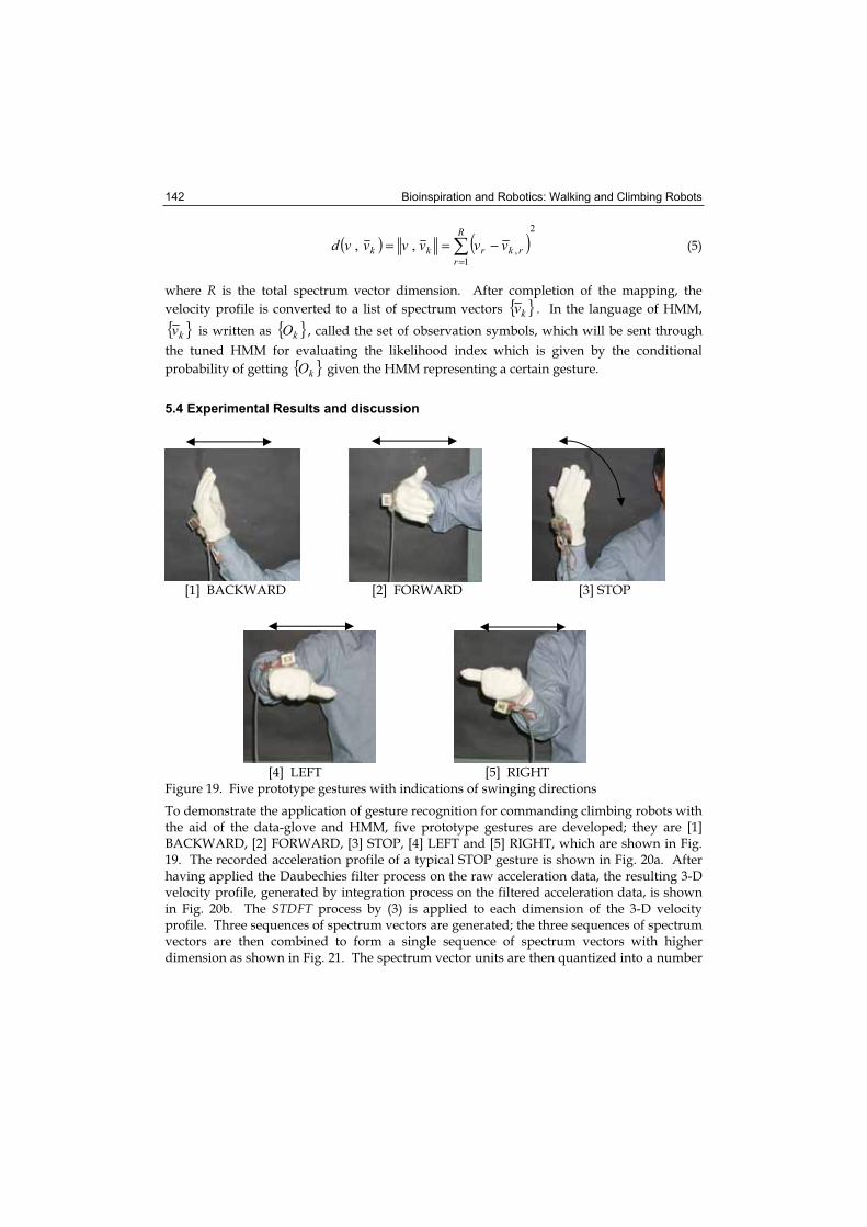
Bioinspiration and Robotics: Walking and Climbing Robots 142
( ) ( )2
1,,,
=−==
R
rrkrkk vvvvvvd (5)
where R is the total spectrum vector dimension. After completion of the mapping, the
velocity profile is converted to a list of spectrum vectors { }kv . In the language of HMM,
{ }kv is written as { }kO , called the set of observation symbols, which will be sent through
the tuned HMM for evaluating the likelihood index which is given by the conditional
probability of getting { }kO given the HMM representing a certain gesture.
5.4 Experimental Results and discussion
[1] BACKWARD [2] FORWARD [3] STOP
[4] LEFT [5] RIGHT Figure 19. Five prototype gestures with indications of swinging directions
To demonstrate the application of gesture recognition for commanding climbing robots with the aid of the data-glove and HMM, five prototype gestures are developed; they are [1] BACKWARD, [2] FORWARD, [3] STOP, [4] LEFT and [5] RIGHT, which are shown in Fig. 19. The recorded acceleration profile of a typical STOP gesture is shown in Fig. 20a. After having applied the Daubechies filter process on the raw acceleration data, the resulting 3-D velocity profile, generated by integration process on the filtered acceleration data, is shown in Fig. 20b. The STDFT process by (3) is applied to each dimension of the 3-D velocity profile. Three sequences of spectrum vectors are generated; the three sequences of spectrum vectors are then combined to form a single sequence of spectrum vectors with higher dimension as shown in Fig. 21. The spectrum vector units are then quantized into a number
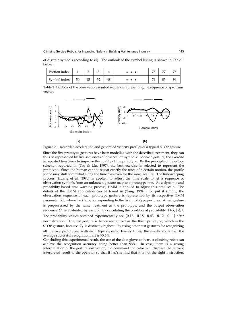
Climbing Service Robots for Improving Safety in Building Maintenance Industry 143
of discrete symbols according to (5). The outlook of the symbol listing is shown in Table 1 below.
Portion index 1 2 3 4 • • • 76 77 78
Symbol index 50 45 52 48 • • • 79 83 96
Table 1 Outlook of the observation symbol sequence representing the sequence of spectrum vectors
-4
-2
0
2
4
1 21 41 61 81 101 121
Sam ple index
Acce
lera
tio
n (
g)
X Y Z
(a) (b) Figure 20. Recorded acceleration and generated velocity profiles of a typical STOP gesture
Since the five prototype gestures have been modelled with the described treatment, they can thus be represented by five sequences of observation symbols. For each gesture, the exercise is repeated five times to improve the quality of the prototype. By the principle of trajectory selection reported in (Tso & Liu, 1997), the best exercise is selected to represent the prototype. Since the human cannot repeat exactly the trace of a certain motion, the profile shape may shift somewhat along the time axis even for the same gesture. The time-warping process (Huang et al., 1990) is applied to adjust the time scale to let a sequence of observation symbols from an unknown gesture map to a prototype one. As a dynamic and probability-based time-warping process, HMM is applied to adjust this time scale. The details of the HMM application can be found in (Yang, 1994). To put it simply, the observation sequence of each prototype gesture is represented by its respective HMM
parameter iλ , where i = 1 to 5, corresponding to the five prototype gestures. A test gesture
is preprocessed by the same treatment as the prototype, and the output observation
sequence tO is evaluated by each iλ by calculating the conditional probability ( )itOP λ| .
The probability values obtained experimentally are ( )11.012.043.018.016.0 after
normalization. The test gesture is hence recognized as the third prototype, which is the
STOP gesture, because 3λ is distinctly highest. By using other test gestures for recognizing
all the five prototypes, with each type repeated twenty times, the results show that the average successful recognition rate is 95.6%. Concluding this experimental result, the use of the data glove to instruct climbing robot can achieve the recognition accuracy being better than 95%. In case, there is a wrong interpretation of the gesture instruction, the command indicator will displace the current interpreted result to the operator so that if he/she find that it is not the right instruction,
-40
-20
0
20
1 21 41 61 81 101 121
Sample index
Ve
locity (
m/s
)
X Y Z
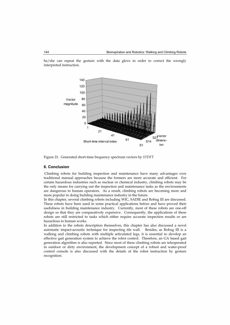
Bioinspiration and Robotics: Walking and Climbing Robots 144
he/she can repeat the gesture with the data glove in order to correct the wrongly interpreted instruction.
1
21
41
61
S1
S14
S27
0
20
40
60
80
100
120
140
Vector
magnitude
Short-time interval index
Vector
dimens-
ion
Figure 21. Generated short-time frequency spectrum vectors by STDFT
6. Conclusion
Climbing robots for building inspection and maintenance have many advantages over traditional manual approaches because the formers are more accurate and efficient. For certain hazardous industries such as nuclear or chemical industry, climbing robots may be the only means for carrying out the inspection and maintenance tasks as the environments are dangerous to human operators. As a result, climbing robots are becoming more and more popular in doing building maintenance industry in the future. In this chapter, several climbing robots including WIC, SADIE and Robug III are discussed. These robots have been used in some practical applications before and have proved their usefulness in building maintenance industry. Currently, most of these robots are one-off design so that they are comparatively expensive. Consequently, the applications of these robots are still restricted to tasks which either require accurate inspection results or are hazardous to human works. In addition to the robots description themselves, this chapter has also discussed a novel automatic impact-acoustic technique for inspecting tile wall. Besides, as Robug III is a walking and climbing robots with multiple articulated legs, it is essential to develop an effective gait generation system to achieve the robot control. Therefore, an GA based gait generation algorithm is also reported. Since most of these climbing robots are teleoperated in outdoor or dirty environment, the development concept of a robust and water-proof control console is also discussed with the details of the robot instruction by gesture recognition.
Climbing Service Robots for Improving Safety in Building Maintenance Industry 145
7. Acknowledgments
The authors would like to express their sincere gratitude to Prof. S.K. Tso, Dr. S. Galt, Dr. D. S. Cooke, Mr. T. White, Mr. N. Hewer, Dr. Y. H. Fung, Dr. L. Han, Dr. F. Tong, Mr. Ben Yeung, Mr. A. Choy and Mr. D. Lam for their help and contribution to the works described in this chapter.
8. References
Bahr, B. & Yin, Y. (1994). Wall climbing robots for aircraft, ship, nuclear power plants, sky scrapers, etc, Proceedings of 5th International Symposium on Robotics and Manufacturing, Hawaii, USA, August 1994.
Burrows, M. & Hoyle, G. (1973). The mechanism of rapid running in the ghost crab, ocypode cerathophthalma, Journal of Experimental Biology, Vol.58, pp 327-349.
Christoforou, A.P. & Yigit, A.S. (1998). Effect of flexibility on low velocity impact response, Journal of sound and vibration, Vol 217, 1998, pp563-578.
Hillenbrand, C.; Berns, K.; Weise F. & Koehnen J. (2001). Development of a climbing robot system for non-destructive testing of bridges, Proceedings of the 8th IEEE Conference on Mechatrinics and Machine Vision in Practice, 27-29 August 2001, Hong Kong, pp399-403.
Hlawatsch, F. & Boundeaux-Bartels, G.F. (1992). Linear and Quadratic Time-frequency Signal Representations, IEEE SP Magazine, Vol. 9, No. 2, pp21-67.
Huang, X.D.; Ariki, Y. & Jack, M.A. (1990). Hidden Markov Models for Speech Recognition,Edinburgh University Press.
Minor, M.; Dulimarta, H.; Danghi, G.; Mukherjee, R.; Lal Tummala, R. & Aslam, D. (2000). Design, implementation, and evaluation of an under-actuated miniature biped climbing robot, Proceedings of the IEEE/RSJ International Conference on Intelligent Robots and Systems, 31 October - 5 November 2000, Vol.3, pp.1999 – 2005
Linde, Y.; Buzo, A. & Gray, R.M. (1980). An Algorithm for Vector Quantizer Design, IEEE Trans. on Communication, Vol. COM-28, pp84-95.
Luk, B. L. ; Cooke, D. S.; Galt, S.; Collie, A. A. & Chen, S. (2005). Intelligent Legged Climbing Service Robot For Remote Maintenance Applications In Hazardous Environments, Journal of Robotics and Autonomous Systems, Vol 53/2, pp 142 - 152, ISSN 0921-8890.
Luk, B. L.; Liu, K. P.; Collie, A. A.; Cooke, D. S. & Chen, S. (2006). Tele-operated Climbing and Mobile Service robots for Remote Inspection and Maintenance in Nuclear Industry, Industrial Robot, Vol 33, No 3, pp194 – 204, ISBN 0143-991X.
Rossing, T. D. & Fletcher, N. H. (1994). Principles of vibration and sound, Springer-Verlag, New York, 1994.
Sattar,T. P.; Alaoui,M.; S. Chen & B. Bridge (2001). A magnetically adhering wall climbing robot to perform continuous welding of long seams and non-destructively test the welds on the hull of a container ship, Proceedings of the 8th IEEE Conference on Mechatrinics and Machine Vision in Practice, 27-29 August 2001, Hong Kong, pp408-414
Strang, G. & Nguyen, T. (1996). Wavelets and Filter Banks, Wellesley-Cambridge Press, MA.
Bioinspiration and Robotics: Walking and Climbing Robots 146
Tso, S. K. & Liu, K. P. (1997). Demonstrated Trajectory Selection by Hidden Markov Model,Proc. IEEE Int. Conf. on Robotics and Automation, Albuquerque, New Mexico, USA, pp2713-2718.
Tso,S.K.; Fung, Y.H.; Chow,W.L.; Zong, G.H. & Liu, R. (2000). Design and implementation of a glass-wall cleaning robot for high-rise buildings, Proceedings of the World Automation Congress Eighth International Symposium on Robotics with Applications,Maui, Hawaii, June 11-16, 2000, paper ID: ISORA123.
Tso,S.K.; Zhu, J. & B.L.Luk (2001). Prototype design of a light-weight climbing robot capable of continuous motion, Proceedings of the 8th IEEE Conference on Mechatronics and Machine Vision in Practice, 27-29 August 2001, Hong Kong, pp235-238
Wang, Y. & Shao, H. (1999). Wall climbing robot for cleaning and painting, Proceedings of the 2nd International Conference on Climbing and Walking Robots, Portsmouth, UK, September 1999.
Yang, J. (1994). Hidden Markov Model for Human Performance Modeling, PhD Dissertation,the University of Akron, August 1994.
Zhang, Q.X.; Ren, Z.G. & Zhao, Z.W (2001). Development of a 3W window-cleaning robot for high-rise buildings, Proceedings of the 8th IEEE Conference on Mechatronics and Machine Vision in Practice, 27-29 August 2001, Hong Kong, pp257-260
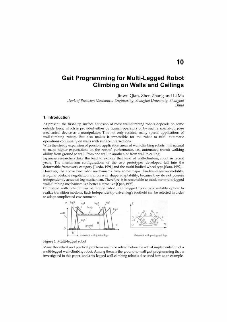
10
Gait Programming for Multi-Legged Robot Climbing on Walls and Ceilings
Jinwu Qian, Zhen Zhang and Li Ma Dept. of Precision Mechanical Engineering, Shanghai University, Shanghai
China
1. Introduction
At present, the first-step surface adhesion of most wall-climbing robots depends on some outside force, which is provided either by human operators or by such a special-purpose mechanical device as a manipulator. This not only restricts many special applications of wall-climbing robots. But also makes it impossible for the robot to fulfil automatic operations continually on walls with surface intersections. With the steady expansion of possible application areas of wall-climbing robots, it is natural to make higher expectations on the robots’ performance, i.e., automated transit walking ability from ground to wall, from one wall to another, or from wall to ceiling. Japanese researchers take the lead to explore that kind of wall-climbing robot in recent years. The mechanism configurations of the two prototypes developed fall into the deformable framework category [Ikeda, 1991] and the multi-bodied wheel type [Sato, 1992]. However, the above two robot mechanisms have some major disadvantages on mobility, irregular obstacle negotiation and on wall shape adaptability, because they do not possess independently actuated leg mechanism. Therefore, it is reasonable to think that multi-legged wall-climbing mechanism is a better alternative [Qian,1993]. Compared with other forms of mobile robot, multi-legged robot is a suitable option to realize transition motions. Each independently-driven leg’s foothold can be selected in order to adapt complicated environment.
Figure 1 Multi-legged robot
Many theoretical and practical problems are to be solved before the actual implementation of a multi-legged wall-climbing robot. Among them is the ground-to-wall gait programming that is investigated in this paper, and a six-legged wall-climbing robot is discussed here as an example.
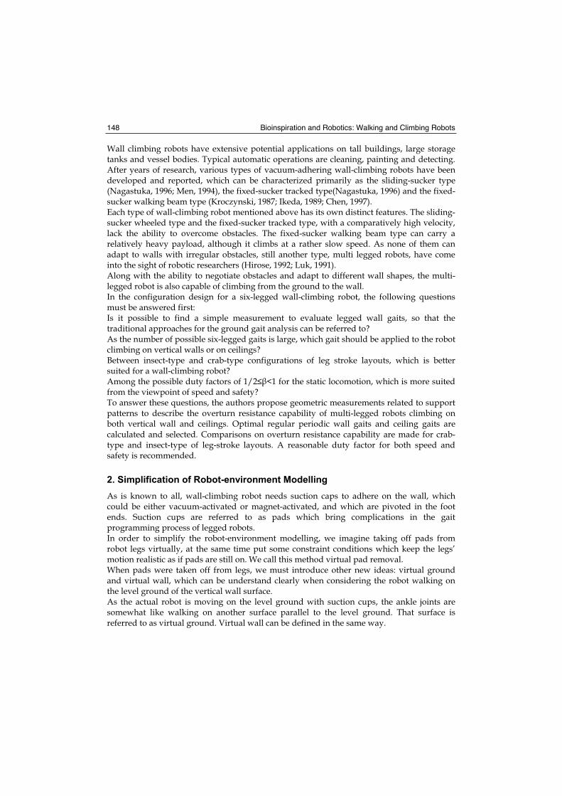
Bioinspiration and Robotics: Walking and Climbing Robots 148
Wall climbing robots have extensive potential applications on tall buildings, large storage tanks and vessel bodies. Typical automatic operations are cleaning, painting and detecting. After years of research, various types of vacuum-adhering wall-climbing robots have been developed and reported, which can be characterized primarily as the sliding-sucker type (Nagastuka, 1996; Men, 1994), the fixed-sucker tracked type(Nagastuka, 1996) and the fixed-sucker walking beam type (Kroczynski, 1987; Ikeda, 1989; Chen, 1997). Each type of wall-climbing robot mentioned above has its own distinct features. The sliding-sucker wheeled type and the fixed-sucker tracked type, with a comparatively high velocity, lack the ability to overcome obstacles. The fixed-sucker walking beam type can carry a relatively heavy payload, although it climbs at a rather slow speed. As none of them can adapt to walls with irregular obstacles, still another type, multi legged robots, have come into the sight of robotic researchers (Hirose, 1992; Luk, 1991). Along with the ability to negotiate obstacles and adapt to different wall shapes, the multi-legged robot is also capable of climbing from the ground to the wall. In the configuration design for a six-legged wall-climbing robot, the following questions must be answered first: Is it possible to find a simple measurement to evaluate legged wall gaits, so that the traditional approaches for the ground gait analysis can be referred to? As the number of possible six-legged gaits is large, which gait should be applied to the robot climbing on vertical walls or on ceilings? Between insect-type and crab-type configurations of leg stroke layouts, which is better suited for a wall-climbing robot? Among the possible duty factors of 1/2 <1 for the static locomotion, which is more suited from the viewpoint of speed and safety? To answer these questions, the authors propose geometric measurements related to support patterns to describe the overturn resistance capability of multi-legged robots climbing on both vertical wall and ceilings. Optimal regular periodic wall gaits and ceiling gaits are calculated and selected. Comparisons on overturn resistance capability are made for crab-type and insect-type of leg-stroke layouts. A reasonable duty factor for both speed and safety is recommended.
2. Simplification of Robot-environment Modelling
As is known to all, wall-climbing robot needs suction caps to adhere on the wall, which could be either vacuum-activated or magnet-activated, and which are pivoted in the foot ends. Suction cups are referred to as pads which bring complications in the gait programming process of legged robots. In order to simplify the robot-environment modelling, we imagine taking off pads from robot legs virtually, at the same time put some constraint conditions which keep the legs’ motion realistic as if pads are still on. We call this method virtual pad removal. When pads were taken off from legs, we must introduce other new ideas: virtual ground and virtual wall, which can be understand clearly when considering the robot walking on the level ground of the vertical wall surface. As the actual robot is moving on the level ground with suction cups, the ankle joints are somewhat like walking on another surface parallel to the level ground. That surface is referred to as virtual ground. Virtual wall can be defined in the same way.
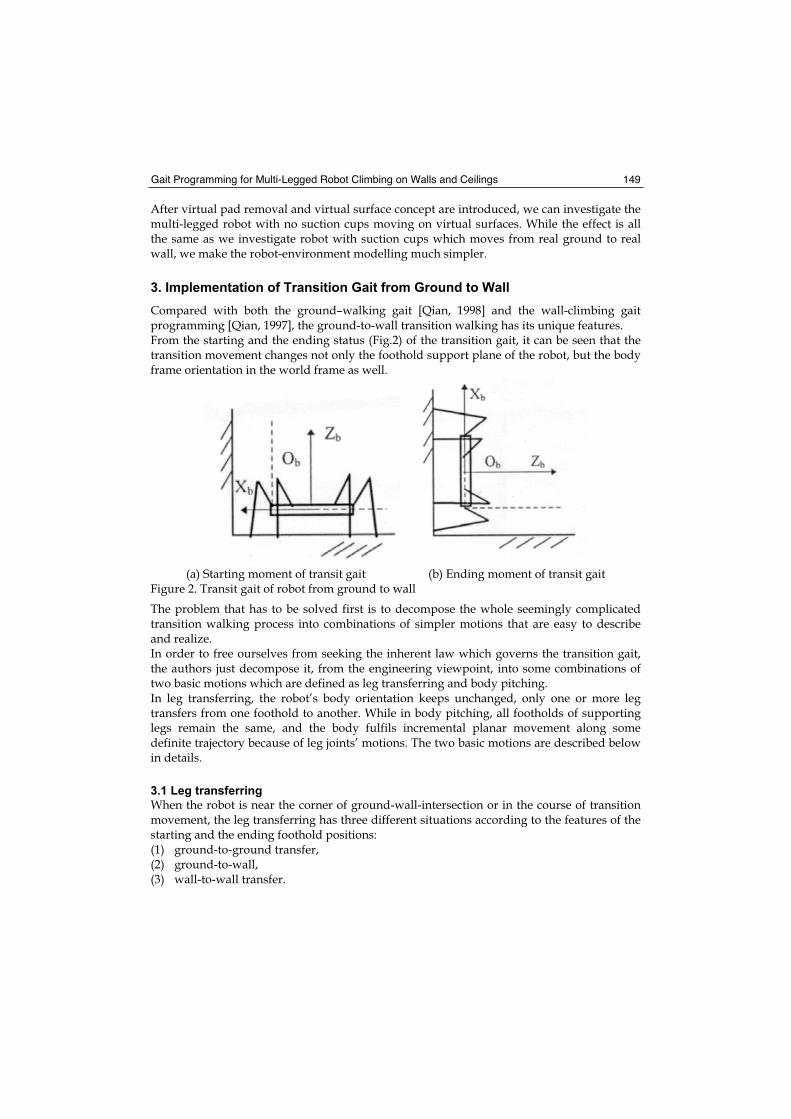
Gait Programming for Multi-Legged Robot Climbing on Walls and Ceilings 149
After virtual pad removal and virtual surface concept are introduced, we can investigate the multi-legged robot with no suction cups moving on virtual surfaces. While the effect is all the same as we investigate robot with suction cups which moves from real ground to real wall, we make the robot-environment modelling much simpler.
3. Implementation of Transition Gait from Ground to Wall
Compared with both the ground–walking gait [Qian, 1998] and the wall-climbing gait programming [Qian, 1997], the ground-to-wall transition walking has its unique features. From the starting and the ending status (Fig.2) of the transition gait, it can be seen that the transition movement changes not only the foothold support plane of the robot, but the body frame orientation in the world frame as well.
(a) Starting moment of transit gait (b) Ending moment of transit gait Figure 2. Transit gait of robot from ground to wall
The problem that has to be solved first is to decompose the whole seemingly complicated transition walking process into combinations of simpler motions that are easy to describe and realize. In order to free ourselves from seeking the inherent law which governs the transition gait, the authors just decompose it, from the engineering viewpoint, into some combinations of two basic motions which are defined as leg transferring and body pitching. In leg transferring, the robot’s body orientation keeps unchanged, only one or more leg transfers from one foothold to another. While in body pitching, all footholds of supporting legs remain the same, and the body fulfils incremental planar movement along some definite trajectory because of leg joints’ motions. The two basic motions are described below in details.
3.1 Leg transferring
When the robot is near the corner of ground-wall-intersection or in the course of transition movement, the leg transferring has three different situations according to the features of the starting and the ending foothold positions: (1) ground-to-ground transfer, (2) ground-to-wall, (3) wall-to-wall transfer.
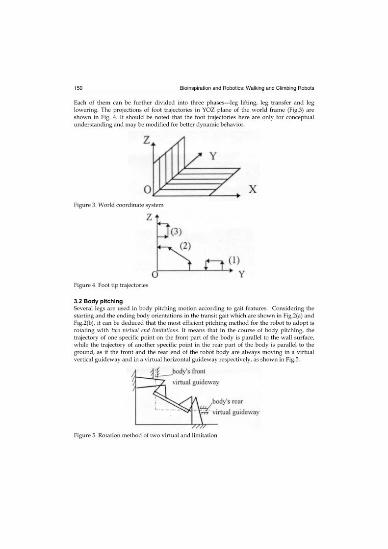
Bioinspiration and Robotics: Walking and Climbing Robots 150
Each of them can be further divided into three phases---leg lifting, leg transfer and leg lowering. The projections of foot trajectories in YOZ plane of the world frame (Fig.3) are shown in Fig. 4. It should be noted that the foot trajectories here are only for conceptual understanding and may be modified for better dynamic behavior.
Figure 3. World coordinate system
Figure 4. Foot tip trajectories
3.2 Body pitching
Several legs are used in body pitching motion according to gait features. Considering the starting and the ending body orientations in the transit gait which are shown in Fig.2(a) and Fig.2(b), it can be deduced that the most efficient pitching method for the robot to adopt is rotating with two virtual end limitations. It means that in the course of body pitching, the trajectory of one specific point on the front part of the body is parallel to the wall surface, while the trajectory of another specific point in the rear part of the body is parallel to the ground, as if the front and the rear end of the robot body are always moving in a virtual vertical guideway and in a virtual horizontal guideway respectively, as shown in Fig.5.
Figure 5. Rotation method of two virtual and limitation
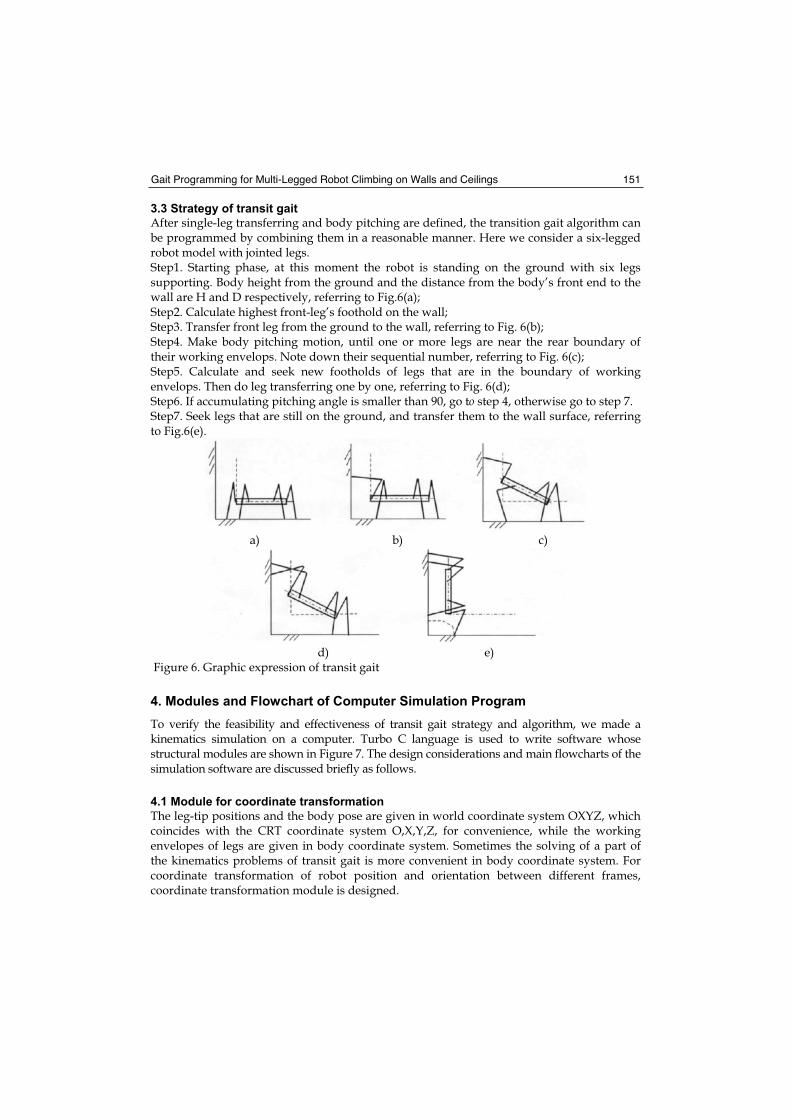
Gait Programming for Multi-Legged Robot Climbing on Walls and Ceilings 151
3.3 Strategy of transit gait
After single-leg transferring and body pitching are defined, the transition gait algorithm can be programmed by combining them in a reasonable manner. Here we consider a six-legged robot model with jointed legs. Step1. Starting phase, at this moment the robot is standing on the ground with six legs supporting. Body height from the ground and the distance from the body’s front end to the wall are H and D respectively, referring to Fig.6(a); Step2. Calculate highest front-leg’s foothold on the wall; Step3. Transfer front leg from the ground to the wall, referring to Fig. 6(b); Step4. Make body pitching motion, until one or more legs are near the rear boundary of their working envelops. Note down their sequential number, referring to Fig. 6(c); Step5. Calculate and seek new footholds of legs that are in the boundary of working envelops. Then do leg transferring one by one, referring to Fig. 6(d); Step6. If accumulating pitching angle is smaller than 90, go to step 4, otherwise go to step 7. Step7. Seek legs that are still on the ground, and transfer them to the wall surface, referring to Fig.6(e).
a) b) c)
d) e) Figure 6. Graphic expression of transit gait
4. Modules and Flowchart of Computer Simulation Program
To verify the feasibility and effectiveness of transit gait strategy and algorithm, we made a kinematics simulation on a computer. Turbo C language is used to write software whose structural modules are shown in Figure 7. The design considerations and main flowcharts of the simulation software are discussed briefly as follows.
4.1 Module for coordinate transformation
The leg-tip positions and the body pose are given in world coordinate system OXYZ, which coincides with the CRT coordinate system O,X,Y,Z, for convenience, while the working envelopes of legs are given in body coordinate system. Sometimes the solving of a part of the kinematics problems of transit gait is more convenient in body coordinate system. For coordinate transformation of robot position and orientation between different frames, coordinate transformation module is designed.
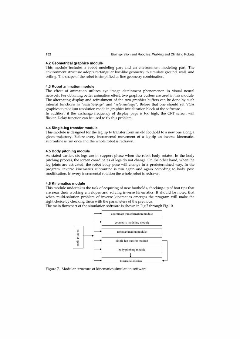
Bioinspiration and Robotics: Walking and Climbing Robots 152
4.2 Geometrical graphics module
This module includes a robot modeling part and an environment modeling part. The environment structure adopts rectangular box-like geometry to simulate ground, wall and ceiling. The shape of the robot is simplified as line geometry combination.
4.3 Robot animation module
The effect of animation utilizes eye image detainment phenomenon in visual neural network. For obtaining better animation effect, two graphics buffers are used in this module. The alternating display and refreshment of the two graphics buffers can be done by such internal functions as “setactivepage” and “setvisualpage”. Before that one should set VGA graphics to medium resolution mode in graphics initialization block of the software. In addition, if the exchange frequency of display page is too high, the CRT screen will flicker. Delay function can be used to fix this problem.
4.4 Single-leg transfer module
This module is designed for the leg tip to transfer from an old foothold to a new one along a given trajectory. Before every incremental movement of a leg-tip an inverse kinematics subroutine is run once and the whole robot is redrawn.
4.5 Body pitching module
As stated earlier, six legs are in support phase when the robot body rotates. In the body pitching process, the screen coordinates of legs do not change. On the other hand, when the leg joints are activated, the robot body pose will change in a predetermined way. In the program, inverse kinematics subroutine is run again and again according to body pose modification. In every incremental rotation the whole robot is redrawn.
4.6 Kinematics module
This module undertakes the task of acquiring of new footholds, checking-up of foot tips that are near their working envelopes and solving inverse kinematics. It should be noted that when multi-solution problem of inverse kinematics emerges the program will make the right choice by checking them with the parameters of the previous. The main flowchart of the simulation software is shown in Fig.7 through Fig.10.
coordinate transformation module
robot animation module
kinemat icsmodule
body pitching module
single-leg transfer module
geometric modeling module
mai
n p
rogra
m
Figure 7. Modular structure of kinematics simulation software
kinematics moduke
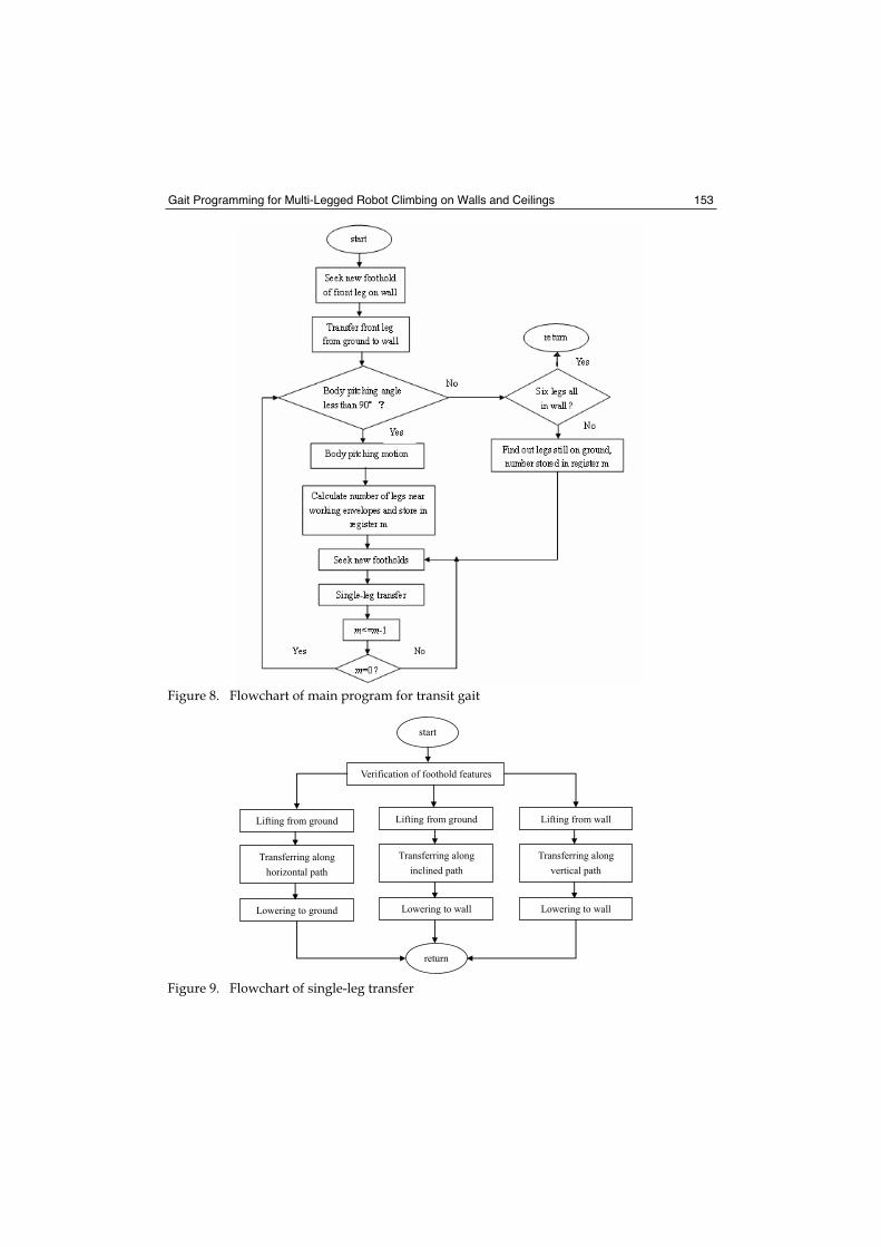
Gait Programming for Multi-Legged Robot Climbing on Walls and Ceilings 153
Figure 8. Flowchart of main program for transit gait
start
Verification of foothold features
Lifting from ground
Transferring along
horizontal path
Lowering to ground
Lifting from ground
Transferring along
inclined path
Lowering to wall
Lifting from wall
Transferring along
vertical path
Lowering to wall
return
Figure 9. Flowchart of single-leg transfer
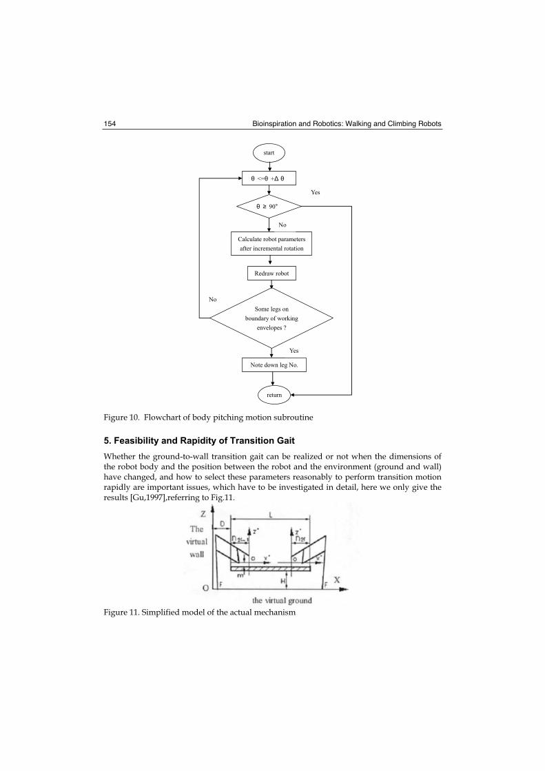
Bioinspiration and Robotics: Walking and Climbing Robots 154
start
<= +
90
Calculate robot parameters
after incremental rotation
Redraw robot
Some legs on
boundary of working
envelopes ?
Note down leg No.
return
Yes
No
Yes
No
Figure 10. Flowchart of body pitching motion subroutine
5. Feasibility and Rapidity of Transition Gait
Whether the ground-to-wall transition gait can be realized or not when the dimensions of the robot body and the position between the robot and the environment (ground and wall) have changed, and how to select these parameters reasonably to perform transition motion rapidly are important issues, which have to be investigated in detail, here we only give the results [Gu,1997],referring to Fig.11.
Figure 11. Simplified model of the actual mechanism
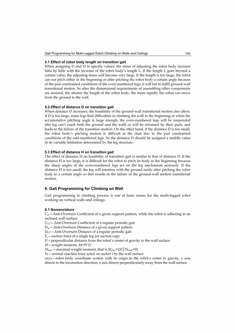
Gait Programming for Multi-Legged Robot Climbing on Walls and Ceilings 155
5.1 Effect of robot body length on transition gait
When assigning D and H to specific values, the times of adjusting the robot body increase little by little with the increase of the robot body’s length L. If the length L goes beyond a certain value, the adjusting times will become very large. If the length is too large, the robot can not pitch either in the beginning or after pitching the robot body a certain angle because of the pad constrained conditions of the even-numbered legs, it will fail to fulfil ground-wall transitional motion. So after the dimensional requirements of assembling other components are assured, the shorter the length of the robot body, the more rapidly the robot can move from the ground to the wall.
5.2 Effect of distance D on transition gait
When distance D increases, the feasibility of the ground-wall transitional motion also alters. If D is too large, some legs find difficulties in climbing the wall in the beginning or when the accumulative pitching angle is large enough, the even-numbered legs will be suspended (the leg can’t reach both the ground and the wall) or will be refrained by their pads, and leads to the failure of the transition motion. On the other hand, if the distance D is too small, the robot body’s pitching motion is difficult at the start due to the pad constrained conditions of the odd-numbered legs. So the distance D should be assigned a middle value in its variable limitation determined by the leg structure.
5.3 Effect of distance H on transition gait
The effect of distance H on feasibility of transition gait is similar to that of distance D. If the distance H is too large, it is difficult for the robot to pitch its body in the beginning because the sharp angles of the even-numbered legs act on the leg mechanism seriously. If the distance H is too small, the leg will interfere with the ground easily after pitching the robot body to a certain angle so that results in the failure of the ground-wall motion transitional motion.
6. Gait Programming for Climbing on Wall
Gait programming in climbing process is one of basic issues for the multi-legged robot working on vertical walls and ceilings.
6.1 Nomenclature
Csp—Anti-Overturn Coefficient of a given support pattern, while the robot is adhering in an inclined wall surface CGT—Anti-Overturn Coefficient of a regular periodic gait Dsp—Anti-Overturn Distance of a given support pattern DGT—Anti-Overturn Distance of a regular periodic gait Fs—suction force of a single leg (or suction cup) H—perpendicular distance from the robot’s center of gravity to the wall surface M—weight moment, M=W·H Mmax—maximal weight moment, that is Mmax={M Njmin=0} Ni—normal reaction force acted on sucker i by the wall surface oxyz—robot body coordinate system with its origin in the robot’s center fo gravity, x axis directs to the locomotion direction, z axis directs perpendicularly away from the wall surface
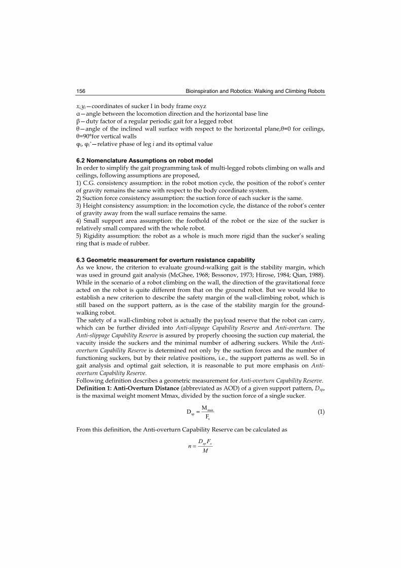
Bioinspiration and Robotics: Walking and Climbing Robots 156
xi,yi—coordinates of sucker I in body frame oxyz —angle between the locomotion direction and the horizontal base line —duty factor of a regular periodic gait for a legged robot —angle of the inclined wall surface with respect to the horizontal plane, =0 for ceilings, =90°for vertical walls
i, i*—relative phase of leg i and its optimal value
6.2 Nomenclature Assumptions on robot model
In order to simplify the gait programming task of multi-legged robots climbing on walls and ceilings, following assumptions are proposed, 1) C.G. consistency assumption: in the robot motion cycle, the position of the robot’s center of gravity remains the same with respect to the body coordinate system. 2) Suction force consistency assumption: the suction force of each sucker is the same. 3) Height consistency assumption: in the locomotion cycle, the distance of the robot’s center of gravity away from the wall surface remains the same. 4) Small support area assumption: the foothold of the robot or the size of the sucker is relatively small compared with the whole robot. 5) Rigidity assumption: the robot as a whole is much more rigid than the sucker’s sealing ring that is made of rubber.
6.3 Geometric measurement for overturn resistance capability
As we know, the criterion to evaluate ground-walking gait is the stability margin, which was used in ground gait analysis (McGhee, 1968; Bessonov, 1973; Hirose, 1984; Qian, 1988). While in the scenario of a robot climbing on the wall, the direction of the gravitational force acted on the robot is quite different from that on the ground robot. But we would like to establish a new criterion to describe the safety margin of the wall-climbing robot, which is still based on the support pattern, as is the case of the stability margin for the ground-walking robot. The safety of a wall-climbing robot is actually the payload reserve that the robot can carry, which can be further divided into Anti-slippage Capability Reserve and Anti-overturn. The Anti-slippage Capability Reserve is assured by properly choosing the suction cup material, the vacuity inside the suckers and the minimal number of adhering suckers. While the Anti-overturn Capability Reserve is determined not only by the suction forces and the number of functioning suckers, but by their relative positions, i.e., the support patterns as well. So in gait analysis and optimal gait selection, it is reasonable to put more emphasis on Anti-overturn Capability Reserve. Following definition describes a geometric measurement for Anti-overturn Capability Reserve.Definition 1: Anti-Overturn Distance (abbreviated as AOD) of a given support pattern, Dsp,is the maximal weight moment Mmax, divided by the suction force of a single sucker.
maxsp
s
MD
F= (1)
From this definition, the Anti-overturn Capability Reserve can be calculated as
MFD
n ssp=
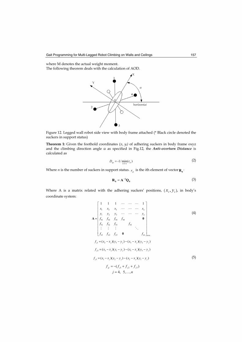
Gait Programming for Multi-Legged Robot Climbing on Walls and Ceilings 157
where M denotes the actual weight moment. The following theorem deals with the calculation of AOD.
Figure 12. Legged wall robot side view with body frame attached (* Black circle denoted the suckers in support status)
Theorem 1: Given the foothold coordinates (xi, yi) of adhering suckers in body frame oxyz and the climbing direction angle as specified in Fig.12, the Anti-overturn Distance iscalculated as
1--1/ min( )sp oii n
D r=
= (2)
Where n is the number of suckers in support status. oir is the ith element of vector
0R :
0
1
0 QAR−= (3)
Where A is a matrix related with the adhering suckers’ positions, ( ii yx , ), in body’s
coordinate system:
1 2 3
1 2 3
41 42 43 44
51 52 53 55
1 2 3
1 1 1 1
n
n
n n n nn n n
x x x xy y y yf f f ff f f f
f f f f×
=A 0
0
(4)
1 2 3 3 2( )( ) ( )( )j j j j jf x x y y x x y y= − − − − −
2 3 1 1 3( )( ) ( )( )j j j j jf x x y y x x y y= − − − − −
3 1 2 2 1( )( ) ( )( )j j j j jf x x y y x x y y= − − − − − (5)
)( 321 jjjjj ffff ++−=nj ,,5,4=
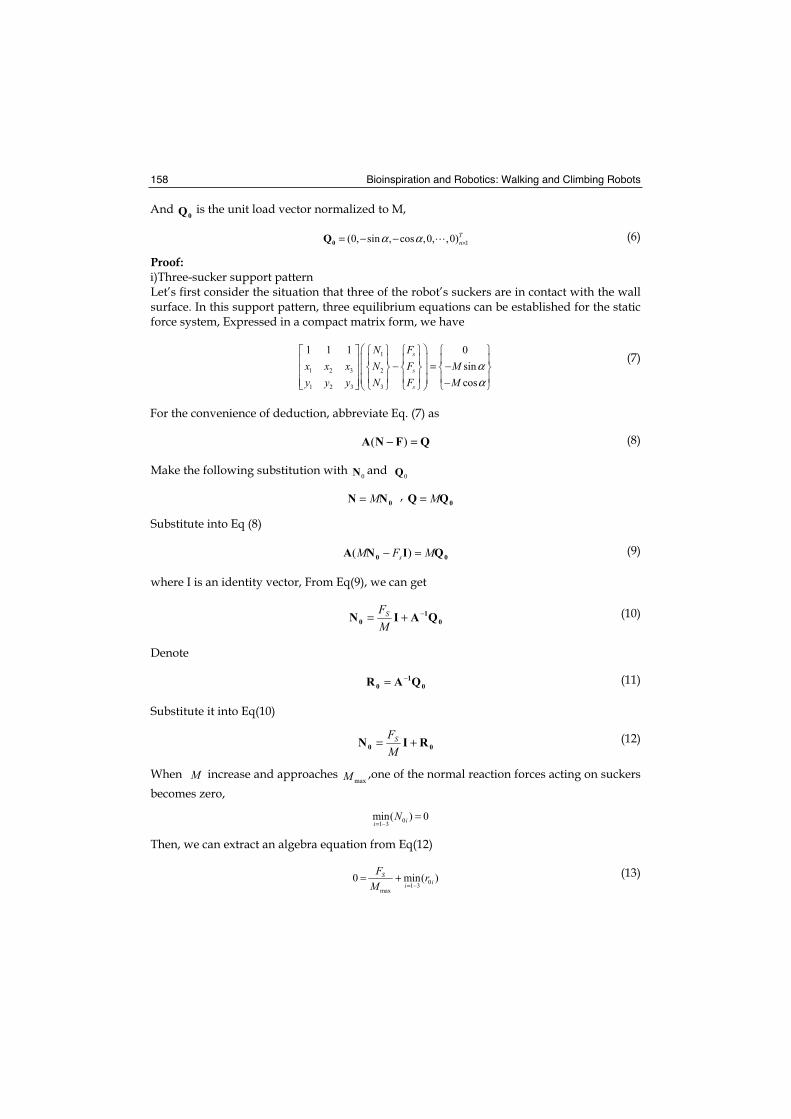
Bioinspiration and Robotics: Walking and Climbing Robots 158
And0Q is the unit load vector normalized to M,
1(0, sin , cos ,0, ,0)Tnα α ×= − −0Q (6)
Proof: i)Three-sucker support pattern Let’s first consider the situation that three of the robot’s suckers are in contact with the wall surface. In this support pattern, three equilibrium equations can be established for the static force system, Expressed in a compact matrix form, we have
1
1 2 3 2
1 2 3 3
1 1 1 0
sin
cos
s
s
s
N Fx x x N F My y y N F M
αα
− = −−
(7)
For the convenience of deduction, abbreviate Eq. (7) as
QFNA =− )( (8)
Make the following substitution with 0N and
0Q
0NN M= , 0QQ M=
Substitute into Eq (8)
00 QINA MFM s =− )( (9)
where I is an identity vector, From Eq(9), we can get
0
1
0 QAIN−+=
MFS (10)
Denote
0
1
0 QAR−= (11)
Substitute it into Eq(10)
00 RIN +=MFS (12)
When M increase and approaches maxM ,one of the normal reaction forces acting on suckers
becomes zero,
01 3
min( ) 0iiN
= −=
Then, we can extract an algebra equation from Eq(12)
01 3
max
0 min( )Sii
F rM = −
= + (13)
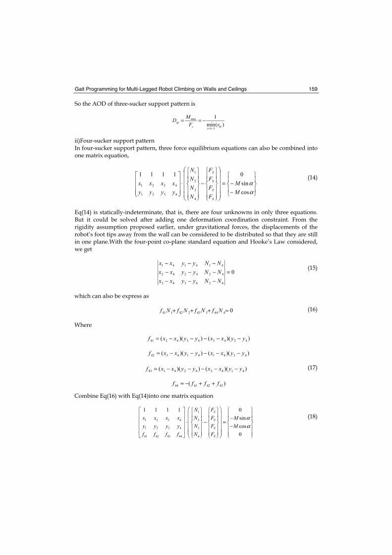
Gait Programming for Multi-Legged Robot Climbing on Walls and Ceilings 159
So the AOD of three-sucker support pattern is
max
01 3
1
min( )sp
s ii
MDF r
= −
= = −
ii)Four-sucker support pattern In four-sucker support pattern, three force equilibrium equations can also be combined into one matrix equation,
−−=−⋅
αα
cos
sin
01111
4
3
2
1
4321
4321
MM
FFFF
NNNN
yyyyxxxx
S
S
S
S
(14)
Eq(14) is statically-indeterminate, that is, there are four unknowns in only three equations. But it could be solved after adding one deformation coordination constraint. From the rigidity assumption proposed earlier, under gravitational forces, the displacements of the robot’s foot tips away from the wall can be considered to be distributed so that they are still in one plane.With the four-point co-plane standard equation and Hooke’s Law considered, we get
0
434343
424242
414141
=−−−−−−−−−
NNyyxxNNyyxxNNyyxx
(15)
which can also be express as
0444343242141 =+++ NfNfNfNf (16)
Where
))(())(( 4243434241 yyxxyyxxf −−−−−=
))(())(( 4341414342 yyxxyyxxf −−−−−=
))(())(( 4142424143 yyxxyyxxf −−−−−= (17)
)( 43424144 ffff ++−=
Combine Eq(16) with Eq(14)into one matrix equation
1
1 2 3 4 2
1 2 3 4 3
41 42 43 44 4
1 1 1 1 0
sin
cos
0
S
S
S
S
FNx x x x FN My y y y FN Mf f f f FN
αα
−⋅ − =
−
(18)
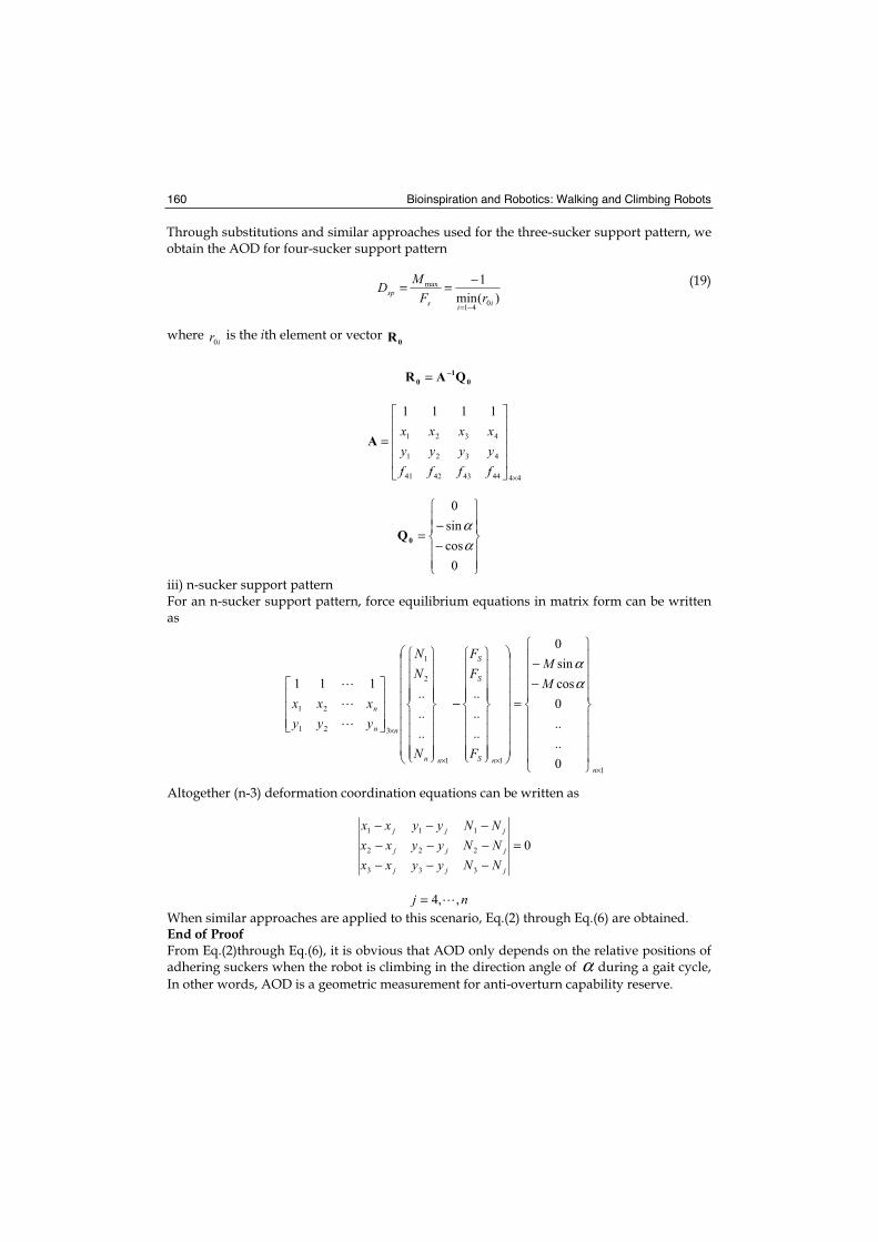
Bioinspiration and Robotics: Walking and Climbing Robots 160
Through substitutions and similar approaches used for the three-sucker support pattern, we obtain the AOD for four-sucker support pattern
)(min
1
041
max
iissp rF
MD−=
−== (19)
whereir0 is the ith element or vector
0R
0
1
0 QAR−=
4444434241
4321
4321
1111
×
=
ffffyyyyxxxx
A
−−
=
0
cos
sin
0
αα
0Q
iii) n-sucker support pattern For an n-sucker support pattern, force equilibrium equations in matrix form can be written as
1
11
2
1
321
21
0
..
..
0
cos
sin
0
..
..
..
..
..
..111
×××
×
−−
=−
nnS
S
S
nn
nn
n
MM
F
FF
N
NN
yyyxxx
αα
Altogether (n-3) deformation coordination equations can be written as
0
333
222
111
=−−−−−−−−−
jjj
jjj
jjj
NNyyxxNNyyxxNNyyxx
nj ,,4=When similar approaches are applied to this scenario, Eq.(2) through Eq.(6) are obtained. End of Proof From Eq.(2)through Eq.(6), it is obvious that AOD only depends on the relative positions of adhering suckers when the robot is climbing in the direction angle of α during a gait cycle,
In other words, AOD is a geometric measurement for anti-overturn capability reserve.
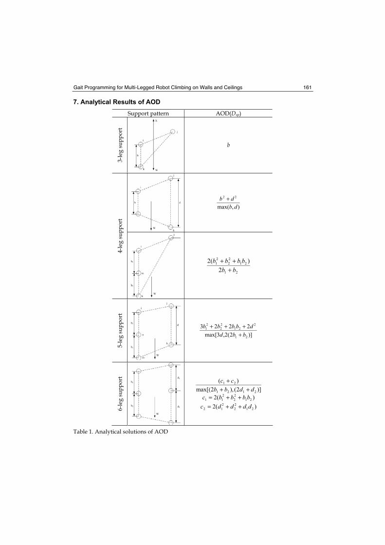
Gait Programming for Multi-Legged Robot Climbing on Walls and Ceilings 161
7. Analytical Results of AOD
Support pattern AOD(Dsp)3-
leg
su
pp
ort
b
),max(
22
dbdb +
4-le
g s
up
po
rt
21
21
2
2
2
1
2
)(2
bbbbbb
+++
5-le
g s
up
po
rt
)]2(2,3max[
2223
21
2
21
2
2
2
1
bbddbbbb
++++
6-le
g s
up
po
rt
)(2
)(2
)]2(),2max[(
)(
21
2
2
2
12
21
2
2
2
11
2121
21
ddddcbbbbc
ddbbcc
++=++=
+++
Table 1. Analytical solutions of AOD
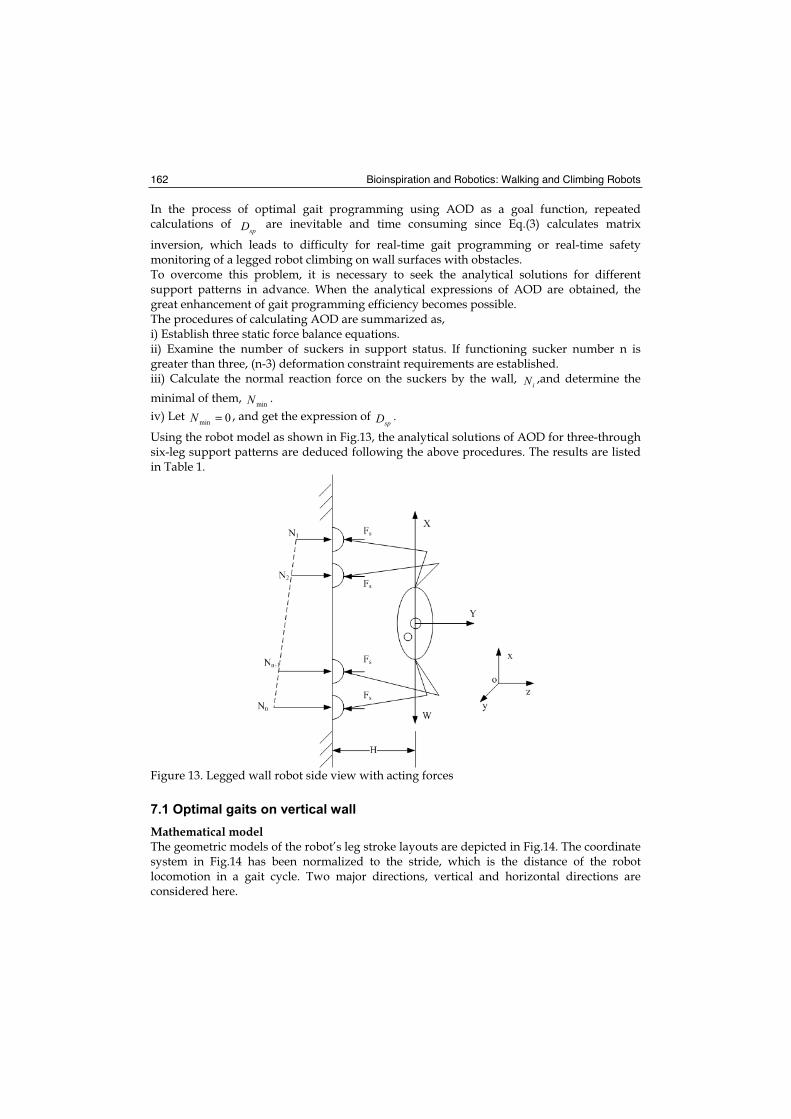
Bioinspiration and Robotics: Walking and Climbing Robots 162
In the process of optimal gait programming using AOD as a goal function, repeated calculations of
spD are inevitable and time consuming since Eq.(3) calculates matrix
inversion, which leads to difficulty for real-time gait programming or real-time safety monitoring of a legged robot climbing on wall surfaces with obstacles. To overcome this problem, it is necessary to seek the analytical solutions for different support patterns in advance. When the analytical expressions of AOD are obtained, the great enhancement of gait programming efficiency becomes possible. The procedures of calculating AOD are summarized as, i) Establish three static force balance equations. ii) Examine the number of suckers in support status. If functioning sucker number n is greater than three, (n-3) deformation constraint requirements are established. iii) Calculate the normal reaction force on the suckers by the wall,
iN ,and determine the
minimal of them, minN .
iv) Let 0min =N , and get the expression of spD .
Using the robot model as shown in Fig.13, the analytical solutions of AOD for three-through six-leg support patterns are deduced following the above procedures. The results are listed in Table 1.
Figure 13. Legged wall robot side view with acting forces
7.1 Optimal gaits on vertical wall
Mathematical model The geometric models of the robot’s leg stroke layouts are depicted in Fig.14. The coordinate system in Fig.14 has been normalized to the stride, which is the distance of the robot locomotion in a gait cycle. Two major directions, vertical and horizontal directions are considered here.
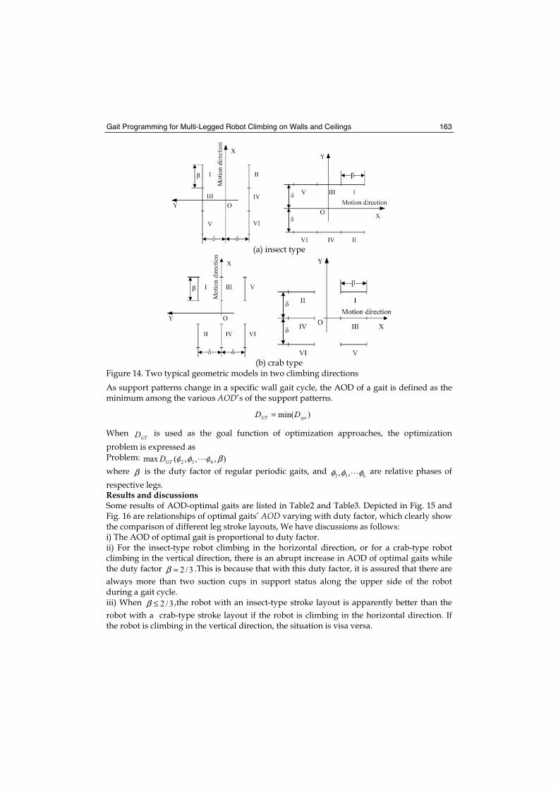
Gait Programming for Multi-Legged Robot Climbing on Walls and Ceilings 163
(a) insect type
(b) crab type
Figure 14. Two typical geometric models in two climbing directions
As support patterns change in a specific wall gait cycle, the AOD of a gait is defined as the minimum among the various AOD’s of the support patterns.
)min( spiGT DD =
WhenGTD is used as the goal function of optimization approaches, the optimization
problem is expressed as Problem: ),,,(max 632 βφφφGTDwhere β is the duty factor of regular periodic gaits, and
632 ,, φφφ are relative phases of
respective legs. Results and discussions Some results of AOD-optimal gaits are listed in Table2 and Table3. Depicted in Fig. 15 and Fig. 16 are relationships of optimal gaits’ AOD varying with duty factor, which clearly show the comparison of different leg stroke layouts, We have discussions as follows: i) The AOD of optimal gait is proportional to duty factor. ii) For the insect-type robot climbing in the horizontal direction, or for a crab-type robot climbing in the vertical direction, there is an abrupt increase in AOD of optimal gaits while the duty factor 2 / 3β = .This is because that with this duty factor, it is assured that there are
always more than two suction cups in support status along the upper side of the robot during a gait cycle. iii) When 2 / 3β ≤ ,the robot with an insect-type stroke layout is apparently better than the
robot with a crab-type stroke layout if the robot is climbing in the horizontal direction. If the robot is climbing in the vertical direction, the situation is visa versa.
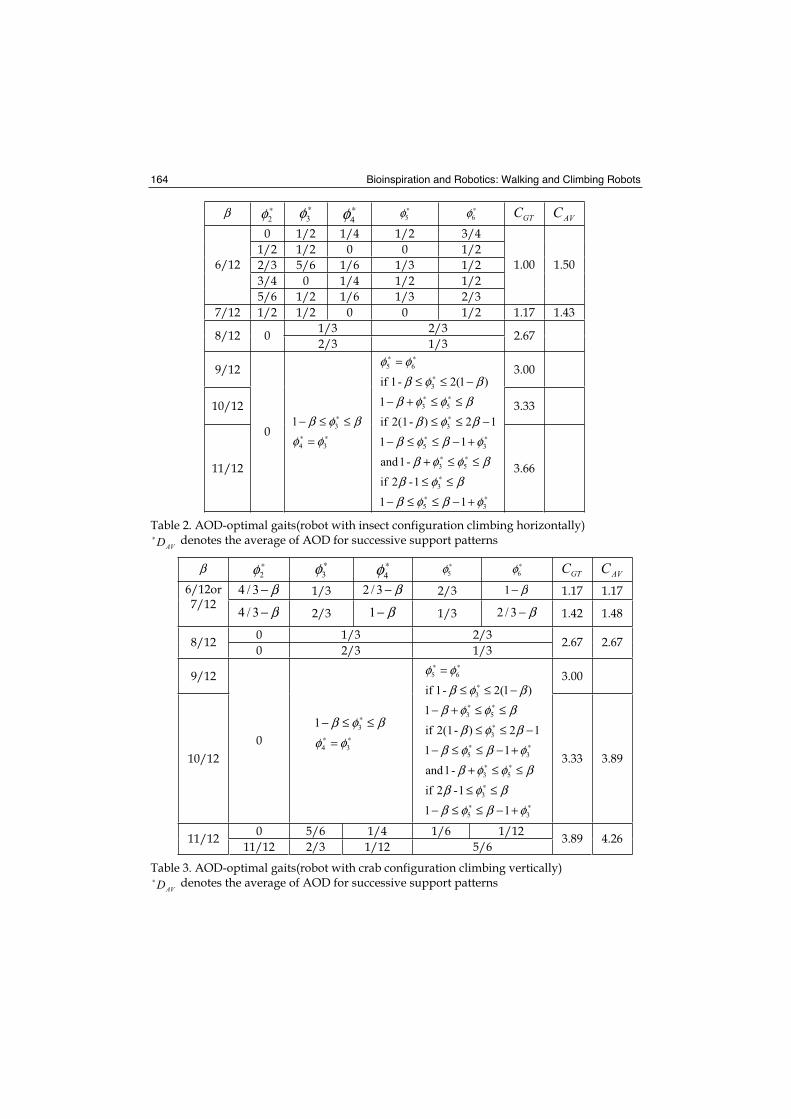
Bioinspiration and Robotics: Walking and Climbing Robots 164
β ∗2φ ∗
3φ ∗4φ 5φ∗
6φ∗GTC AVC
0 1/2 1/4 1/2 3/4
1/2 1/2 0 0 1/2
2/3 5/6 1/6 1/3 1/2
3/4 0 1/4 1/2 1/2
6/12
5/6 1/2 1/6 1/3 2/3
1.00 1.50
7/12 1/2 1/2 0 0 1/2 1.17 1.43
1/3 2/3 8/12 0
2/3 1/3 2.67
9/12 3.00
10/12 3.33
11/12
0 ∗∗
∗
=
≤≤−
34
31
φφβφβ
∗∗
∗
∗∗
∗∗
∗
∗∗
∗
∗∗
+−≤≤−
≤≤
≤≤+
+−≤≤−
−≤≤
≤≤+−
−≤≤
=
35
3
53
35
3
53
3
65
11
1-2if
-1and
11
12)-2(1if
1
)1(2-1if
φβφββφβ
βφφβφβφβ
βφββφφβ
βφβφφ
3.66
Table 2. AOD-optimal gaits(robot with insect configuration climbing horizontally)
AVD∗ denotes the average of AOD for successive support patterns
β ∗2φ ∗
3φ ∗4φ 5φ∗
6φ∗GTC AVC
β−3/4 1/3 β−3/2 2/3 β−1 1.17 1.17 6/12or7/12 β−3/4 2/3 β−1 1/3 β−3/2 1.42 1.48
0 1/3 2/3 8/12
0 2/3 1/3 2.67 2.67
9/12 3.00
10/12
0 ∗∗
∗
=
≤≤−
34
31
φφβφβ
∗∗
∗
∗∗
∗∗
∗
∗∗
∗
∗∗
+−≤≤−
≤≤
≤≤+
+−≤≤−
−≤≤
≤≤+−
−≤≤
=
35
3
53
35
3
53
3
65
11
1-2if
-1and
11
12)-2(1if
1
)1(2-1if
φβφββφβ
βφφβφβφβ
βφββφφβ
βφβφφ
3.33 3.89
0 5/6 1/4 1/6 1/12 11/12
11/12 2/3 1/12 5/6 3.89 4.26
Table 3. AOD-optimal gaits(robot with crab configuration climbing vertically)
AVD∗ denotes the average of AOD for successive support patterns
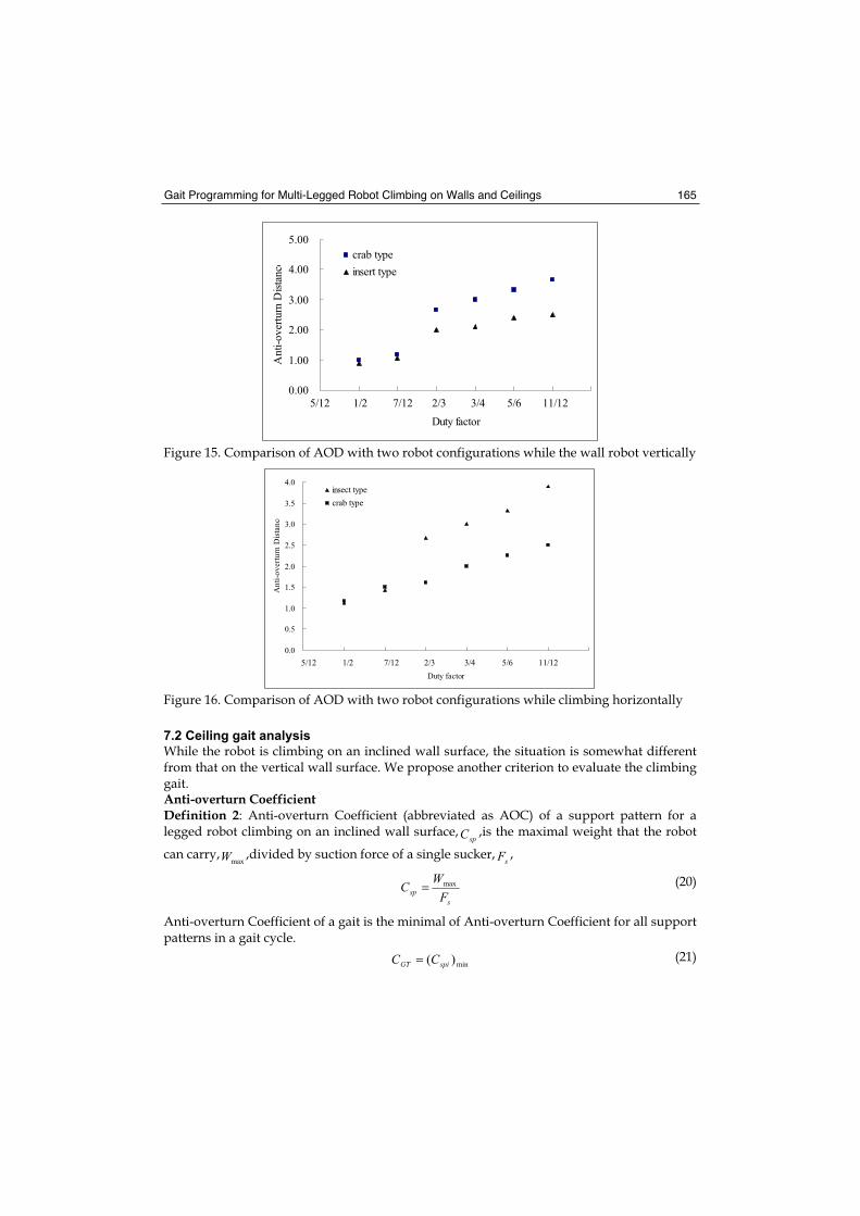
Gait Programming for Multi-Legged Robot Climbing on Walls and Ceilings 165
0.00
1.00
2.00
3.00
4.00
5.00
Duty factor
An
ti-o
ver
turn
Dis
tance
crab type
insert type
5/12 1/2 7/12 2/3 3/4 5/6 11/12
Figure 15. Comparison of AOD with two robot configurations while the wall robot vertically
0.0
0.5
1.0
1.5
2.0
2.5
3.0
3.5
4.0
Duty factor
An
ti-o
vert
urn
Dis
tan
ce
insect type
crab type
5/12 1/2 7/12 2/3 3/4 5/6 11/12
Figure 16. Comparison of AOD with two robot configurations while climbing horizontally
7.2 Ceiling gait analysis
While the robot is climbing on an inclined wall surface, the situation is somewhat different from that on the vertical wall surface. We propose another criterion to evaluate the climbing gait. Anti-overturn Coefficient Definition 2: Anti-overturn Coefficient (abbreviated as AOC) of a support pattern for a legged robot climbing on an inclined wall surface,
spC ,is the maximal weight that the robot
can carry,maxW ,divided by suction force of a single sucker,
sF ,
ssp F
WC max= (20)
Anti-overturn Coefficient of a gait is the minimal of Anti-overturn Coefficient for all support patterns in a gait cycle.
min)( spiGT CC = (21)
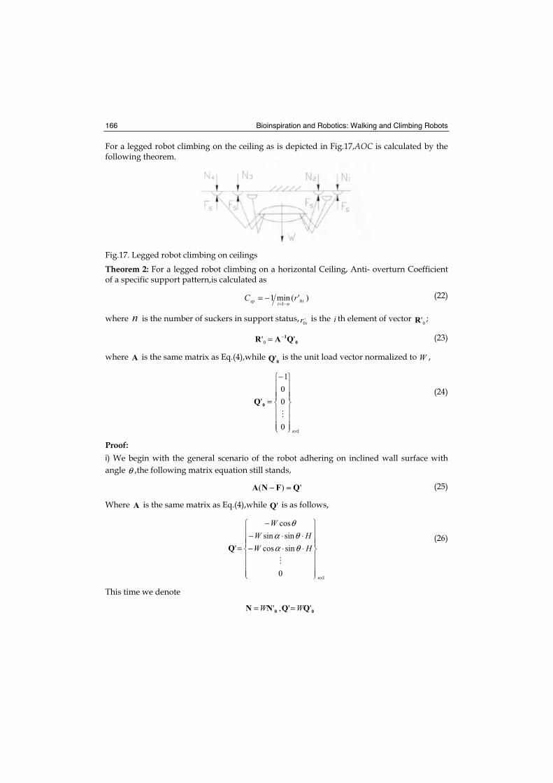
Bioinspiration and Robotics: Walking and Climbing Robots 166
For a legged robot climbing on the ceiling as is depicted in Fig.17,AOC is calculated by the following theorem.
Fig.17. Legged robot climbing on ceilings
Theorem 2: For a legged robot climbing on a horizontal Ceiling, Anti- overturn Coefficient of a specific support pattern,is calculated as
)'(min1 0~1
inisp rC=
−= (22)
where n is the number of suckers in support status, ,
0ir is the i th element of vector 0'R ;
0
1QAR ''0
−= (23)
where A is the same matrix as Eq.(4),while 0Q' is the unit load vector normalized to W ,
10
0
0
1
'
×
−
=
n
0Q
(24)
Proof: ) We begin with the general scenario of the robot adhering on inclined wall surface with
angle θ ,the following matrix equation still stands,
')( QFNA =− (25)
Where A is the same matrix as Eq.(4),while 'Q is as follows,
10
sincos
sinsin
cos
'
×
⋅⋅−⋅⋅−
−
=
n
HWHW
W
θαθα
θ
Q
(26)
This time we denote
00 QQNN '',' WW ==
Gait Programming for Multi-Legged Robot Climbing on Walls and Ceilings 167
and substitute them into Eq(25)
00 QINA ')'( WFW s =− (27)
We can get
0
1
0 QAIN '' −+=WFs (28)
Denote
0
1
0 QAR '' −= (29)
Substitute it into Eq(28)
00 RIN '' +=WFs (30)
When W increase and approaches maxW ,the minimum of the normal reaction forces acting
on suckers becomes zero,
0)'(min 0~1
== ini
N
We can extract an algebra equation from Eq(30)
)'(min0 0~1
max
ini
s rW
F=
+= (31)
and
)'(min
1
0~1
max
inissp rF
WC=
−== (32)
) For the situation of standard ceiling when 0=θ , Eq.(26) becomes
10
0
0
'
×
−
=
n
W
Q
And
10
0
0
1
''
×
−
==
n
WQ
Q 0
End of Proof It is cleat that Anti-overturn Coefficient is a measurement of overturn-resistance ability of a robot in a definite effective body height H. And it has relation with AOD,
spsp CHD ⋅=
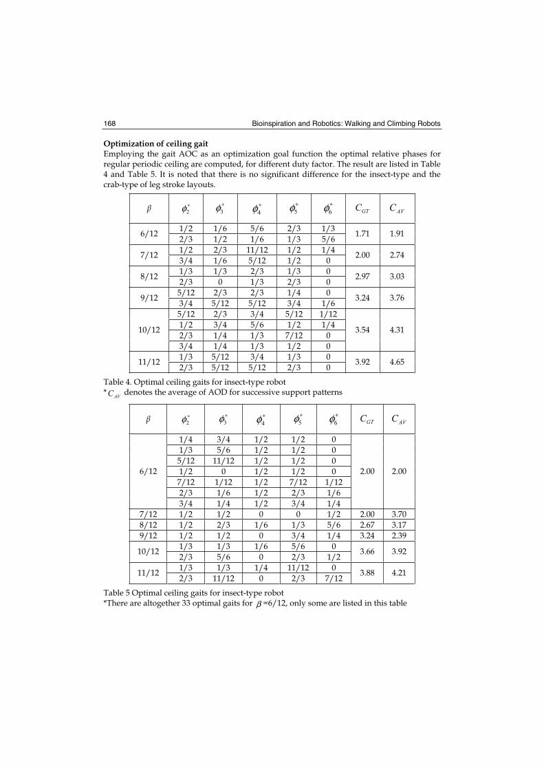
Bioinspiration and Robotics: Walking and Climbing Robots 168
Optimization of ceiling gait Employing the gait AOC as an optimization goal function the optimal relative phases for regular periodic ceiling are computed, for different duty factor. The result are listed in Table 4 and Table 5. It is noted that there is no significant difference for the insect-type and the crab-type of leg stroke layouts.
∗2φ ∗
3φ ∗4φ 5φ∗
6φ∗GTC AVC
1/2 1/6 5/6 2/3 1/3 6/12
2/3 1/2 1/6 1/3 5/6 1.71 1.91
1/2 2/3 11/12 1/2 1/4 7/12
3/4 1/6 5/12 1/2 0 2.00 2.74
1/3 1/3 2/3 1/3 0 8/12
2/3 0 1/3 2/3 0 2.97 3.03
5/12 2/3 2/3 1/4 0 9/12
3/4 5/12 5/12 3/4 1/6 3.24 3.76
5/12 2/3 3/4 5/12 1/12
1/2 3/4 5/6 1/2 1/4
2/3 1/4 1/3 7/12 0 10/12
3/4 1/4 1/3 1/2 0
3.54 4.31
1/3 5/12 3/4 1/3 0 11/12
2/3 5/12 5/12 2/3 0 3.92 4.65
Table 4. Optimal ceiling gaits for insect-type robot *
AVC denotes the average of AOD for successive support patterns
∗2φ ∗
3φ ∗4φ 5φ∗
6φ∗GTC AVC
1/4 3/4 1/2 1/2 0
1/3 5/6 1/2 1/2 0
5/12 11/12 1/2 1/2 0
1/2 0 1/2 1/2 0
7/12 1/12 1/2 7/12 1/12
2/3 1/6 1/2 2/3 1/6
6/12
3/4 1/4 1/2 3/4 1/4
2.00 2.00
7/12 1/2 1/2 0 0 1/2 2.00 3.70
8/12 1/2 2/3 1/6 1/3 5/6 2.67 3.17
9/12 1/2 1/2 0 3/4 1/4 3.24 2.39
1/3 1/3 1/6 5/6 0 10/12
2/3 5/6 0 2/3 1/2 3.66 3.92
1/3 1/3 1/4 11/12 0 11/12
2/3 11/12 0 2/3 7/12 3.88 4.21
Table 5 Optimal ceiling gaits for insect-type robot *There are altogether 33 optimal gaits for β =6/12, only some are listed in this table
Gait Programming for Multi-Legged Robot Climbing on Walls and Ceilings 169
8. Conclusion
The research on transition gait programming makes it possible for the robot to act both as a ground-walking machine and as a wall-climbing robot as well. It forms the basis of gait kinematics in developing a six-legged wall-and-ground-walking robot. It is a new attempt to investigate ground-to-wall transit gait programming of six-legged robot in the research field of walking machines. Employing kinematics geometry, the authors decompose the relatively complicated transit walking into combination of two basic motions. The method proposed is verified by kinematics simulation as correct and effective. The feasibility of the ground-wall transitional motion of the legged robot is mainly determined by the distance H and D. Too large or small values of them always lead to the failure of the motion. And the length L of the robot body is the key of the rapidity of the ground-wall transition motion, it should be assigned relative small value in the permissible limitation of the structure design. Based on the reasonable selection for various parameters, the times of adjusting the robot body can be decrease to four, which is very effective. Anti-overturn Distance (AOD) is a geometric measurement proposed to evaluate overturn-resistance capability, which is solely dependent on the support pattern of wall gaits. AOD is as important to wall gait programming as the stability margin is to ground gaits. While the robot is climbing on an inclined wall surface or ceilings, a related measurement, Anti-overturn Coefficient, is used to evaluate ceiling gaits. Optimal regular periodic wall gaits and ceiling gaits are obtained employing both Anti-overturn Distance and Anti-overturn Coefficient. In most cases, several optimal gaits exist for each given duty factor. For a six-legged robot climbing on a vertical wall, crab-type leg-stroke layout is preferred for climbing vertically; insect-type leg-stroke layout is preferred far climbing horizontally. If one robot is going to walk in bath directions, it is required that the robot can change its leg-stroke layout, which is possible if the robot is designed to have a 3-D leg configuration. While for a six-legged robot climbing on ceilings, there is no significant difference between the two leg-stroke types. Considering both the climbing safety and the climbing speed, the duty factor of wall gaits recommended is 2/3.
9. Acknowledgments
This research is partly sponsored by the Robotic Mechanism Laboratory under the National High-tech R&D Program of China.
10. References
Bessonov, A., and Umnov, N.,1973, The Analysis of Gaits in Six-legged Vehicle According Their Static Stability, Proceedings, 1st Symposium on Theory and Practice of Robots and Manipulators, pp.1-10.
Chen, Z., Gong., Z, Qian, J., et al, 1997, Research on robotic Wall-climbing Mechanism, Journal of Shanghai University, Vol. 3 No.6, pp.663-669. (in Chinese)
Hirose, S., et al., 1992, Legged Wall-climbing Robot, Journal of Japanese Robot Association, Vol. 10, No. 5, pp.575-580 (in Japanese)
Bioinspiration and Robotics: Walking and Climbing Robots 170
Hirose. S., l984, A Study of Design and Control of a Quadruped Walking Vehicle, International Journal of Robotics Research , Vol. 3 No. 2, pp.113-133
Ikeda, K., et al., 1989, Basic Study on a Wall Climbing Robot(II), Journal of Mechanical Engineering Laboratory, Vol. 43. No. 4, pp.25-33 (in Japanese)
Kroczynski P., et al., 1987, The Skywasher: a Building Washing Robot, Proceedings, Proceedings, 17th International Symposium of Industrial Robots, pp.1.11-1.19
Luk, B. L., et al., 1991, ROBUG II: an Intelligent Wall Climbing Robot, Proceedings, Proceedings, IEEE International Symposium on Robotics and Automation, pp.2342-2347
McGhee, R. B., Frank A. A., 1968, On the Stability Properties of Quadruped Creeping Gaits, Mathematical Bioscience, Vol. 3, No. 3, pp.331-351
Men, G., Zhao, and Y., Wang Y, 1994, The Control System of Wall Climbing Robot, Proceedings, 2nd Asian Conference on Robotics and Its Applications, Beijing, pp.375-377
Nagastuka, K., 1986, Vacuum Adhering Crawler System ‘VACS’, Robot, No. 53, pp.127-135 (in Japanese)
Nishi, A., et al., 1992, Development of a Wall-climbing Robot, Robot, No. 84, pp.111-l16. (in Japanese)
Qian, J., Gan, D., 1988, Stability Study of Six Legged Laterally Walking Gaits, Proceedings, ASME Design Engineering Conference, Vol.15-3 PT3, pp.17l-176
Ikeda, K., Nozaki, T., 1991, Development of a Self-contained Wall-climbing Robot, Proceedings, International Symposium on Advanced Robot Technology, pp.356-372
Sato, K. Morita, H., 1992, On-Wall Locomotion Technology for Advanced Robot Technology Research, Japan Robot Society Journal, Vol. 10, No.5, pp.581-589 (in Japanese)
Hirose, S., Nagalobo, A., 1992, Legged Wall-climbing Robot, Japan Robot Society Journal, Vol. 10, No. 5, pp.19-24 (in Japanese)
Qian, J., Gan D., 1992, Stability-optimized Gait Series for Omni-directional Hexapods While Walking Laterally, Journal of Shanghai University of Sciences and Technology, Vol. l5, No. 3, pp.60-67 (in Chinese)
Qian, J., Gong Z., et al., 1994, Anti-Overturn Distance and Its Applications in Multi-legged Wall-climbing Robots, Proceedings, 2nd.Asian Conference on Robotics and Its Application, pp.318-322
Gu, J., Qian, J., et al., 1997, Study on Feasibility and Rapidty of the Ground-wall Transitional of Legged Robot, Proceedings, 2nd China-Japan Mechatronics Symposium, Chengdu, China
Qian, J., 1993, On the Gait Kinematics of Six-legged Robot Capable of Ground and Wall Walking, Ph. D Dissertation of Beijing University of Aeronautics and Astronautics (in Chinese)
11
Armless Climbing and Walking in Robotics
Maki K. Rashid Mechanical and Industrial Engineering, Sultan Qaboos University, Muscat
Sultanate of Oman
1. Introduction
Climbing and walking robots perform tasks that are too difficult, dangerous or time consuming for the human worker. These tasks can be inspection work in hazardous or unpleasant environments (Briones et al., 1994) and, (Xu & Ma, 2002), military, maintenance (Tokioka & Sakai, 1988), overhauling (Yanzeng et al., 1999), manufacturing (Shuliang et al., 2000), and search and rescue works. With all progress in the development of climbing and walking techniques such robots still haven’t been able to penetrate the service market. There are two reasons for this slow down: First, most of today’s commercially available climbing and walking robots have insufficient payload-to weight ratio. Second, all of the most recent developments have been engineered for one very specific task. But the customer demand new approach in robot development. Mainly such robots must be competitive with other solutions by conducting the task economically. Moreover the climbing and walking robots should also be able to perform a variety of tasks so that the return of investment for the customer is improved. Armless robot without articulated hand or legs requires holding technique to working surfaces. Several types of attachment mechanisms have been studied and developed for climbing and walking robots. In the case of workspace that contains structural elements that support the use of mechanical fasteners or grippers then the contact to the surface can be established through a positive connection. This type of adhesion mechanism is the grasping technique, which requires holds, spines or grooves to grasp and pull the whole body upwards, however the climbing down process is challenging for this method (Bretl et al., 2003) and, (Autumn et al., 2000). For rough surfaces, this is a quite powerful technique but it is not suitable for armless robot. In addition if the surface is flat and smooth, this method cannot be applied. Most of today‘s robotic applications demand highly flexible solutions able to move the robot autonomously without the need of grasping a predefined elements. Therefore, the states of the art of armless robots developed an adhesive force method for climbing surfaces. Such force can be generated using different tactics. The most common type is the suction adhesion, where the robot carries an on-board pump to create vacuum inside cups which are pressed against the wall or ceiling (Pack et al., 1997) and, (Nagakubo et al., 1994). Such attachment suffers from the time delay in developing the vacuum and the special requirements for smooth surfaces and sealing design. In addition, power consumption is too high during attachment. Finally, the suction adhesion mechanism relies on ambient pressure to stick on wall, and therefore it is not useful in applications that require near zero surrounding pressure as in the case of space application.
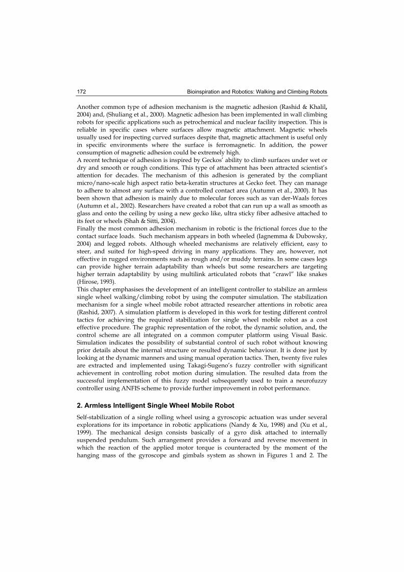
Bioinspiration and Robotics: Walking and Climbing Robots 172
Another common type of adhesion mechanism is the magnetic adhesion (Rashid & Khalil,2004) and, (Shuliang et al., 2000). Magnetic adhesion has been implemented in wall climbing robots for specific applications such as petrochemical and nuclear facility inspection. This is reliable in specific cases where surfaces allow magnetic attachment. Magnetic wheels usually used for inspecting curved surfaces despite that, magnetic attachment is useful only in specific environments where the surface is ferromagnetic. In addition, the power consumption of magnetic adhesion could be extremely high. A recent technique of adhesion is inspired by Geckos’ ability to climb surfaces under wet or dry and smooth or rough conditions. This type of attachment has been attracted scientist’s attention for decades. The mechanism of this adhesion is generated by the compliant micro/nano-scale high aspect ratio beta-keratin structures at Gecko feet. They can manage to adhere to almost any surface with a controlled contact area (Autumn et al., 2000). It has been shown that adhesion is mainly due to molecular forces such as van der-Waals forces (Autumn et al., 2002). Researchers have created a robot that can run up a wall as smooth as glass and onto the ceiling by using a new gecko like, ultra sticky fiber adhesive attached to its feet or wheels (Shah & Sitti, 2004). Finally the most common adhesion mechanism in robotic is the frictional forces due to the contact surface loads. Such mechanism appears in both wheeled (Iagnemma & Dubowsky, 2004) and legged robots. Although wheeled mechanisms are relatively efficient, easy to steer, and suited for high-speed driving in many applications. They are, however, not effective in rugged environments such as rough and/or muddy terrains. In some cases legs can provide higher terrain adaptability than wheels but some researchers are targeting higher terrain adaptability by using multilink articulated robots that “crawl” like snakes (Hirose, 1993). This chapter emphasises the development of an intelligent controller to stabilize an armless single wheel walking/climbing robot by using the computer simulation. The stabilization mechanism for a single wheel mobile robot attracted researcher attentions in robotic area (Rashid, 2007). A simulation platform is developed in this work for testing different control tactics for achieving the required stabilization for single wheel mobile robot as a cost effective procedure. The graphic representation of the robot, the dynamic solution, and, the control scheme are all integrated on a common computer platform using Visual Basic. Simulation indicates the possibility of substantial control of such robot without knowing prior details about the internal structure or resulted dynamic behaviour. It is done just by looking at the dynamic manners and using manual operation tactics. Then, twenty five rules are extracted and implemented using Takagi-Sugeno’s fuzzy controller with significant achievement in controlling robot motion during simulation. The resulted data from the successful implementation of this fuzzy model subsequently used to train a neurofuzzy controller using ANFIS scheme to provide further improvement in robot performance.
2. Armless Intelligent Single Wheel Mobile Robot
Self-stabilization of a single rolling wheel using a gyroscopic actuation was under several explorations for its importance in robotic applications (Nandy & Xu, 1998) and (Xu et al., 1999). The mechanical design consists basically of a gyro disk attached to internally suspended pendulum. Such arrangement provides a forward and reverse movement in which the reaction of the applied motor torque is counteracted by the moment of the hanging mass of the gyroscope and gimbals system as shown in Figures 1 and 2. The
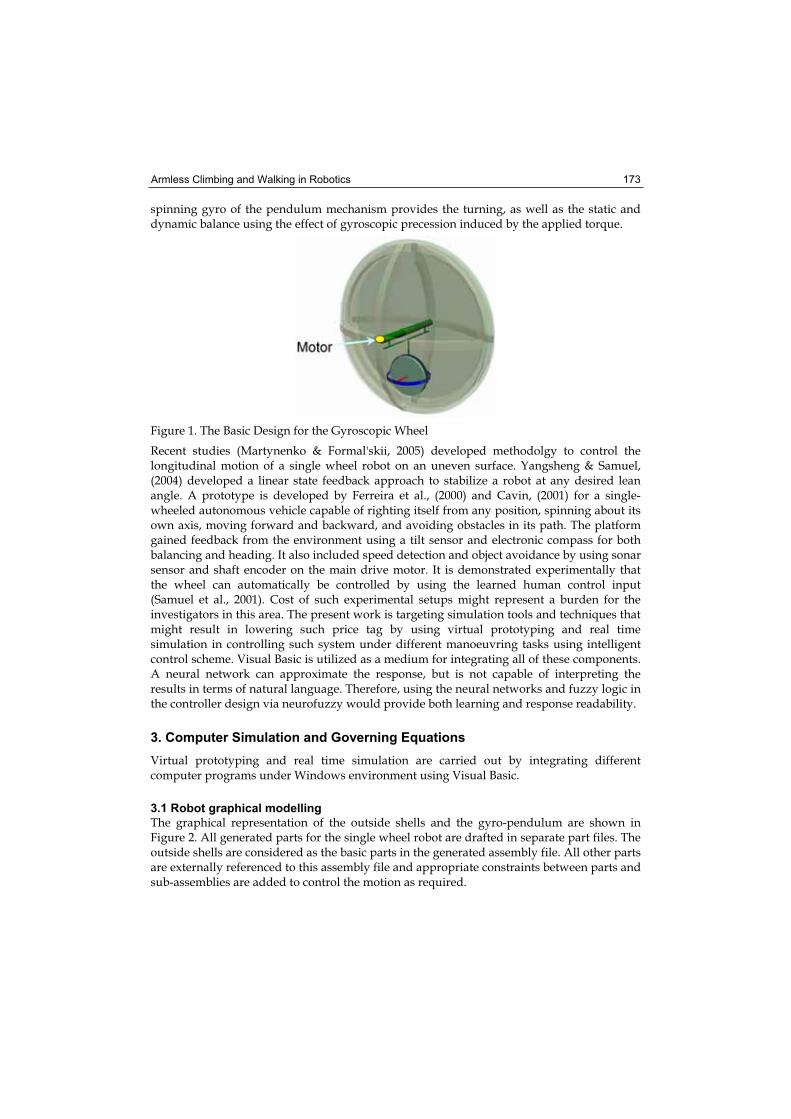
Armless Climbing and Walking in Robotics 173
spinning gyro of the pendulum mechanism provides the turning, as well as the static and dynamic balance using the effect of gyroscopic precession induced by the applied torque.
Figure 1. The Basic Design for the Gyroscopic Wheel
Recent studies (Martynenko & Formal'skii, 2005) developed methodolgy to control the longitudinal motion of a single wheel robot on an uneven surface. Yangsheng & Samuel, (2004) developed a linear state feedback approach to stabilize a robot at any desired lean angle. A prototype is developed by Ferreira et al., (2000) and Cavin, (2001) for a single-wheeled autonomous vehicle capable of righting itself from any position, spinning about its own axis, moving forward and backward, and avoiding obstacles in its path. The platform gained feedback from the environment using a tilt sensor and electronic compass for both balancing and heading. It also included speed detection and object avoidance by using sonar sensor and shaft encoder on the main drive motor. It is demonstrated experimentally that the wheel can automatically be controlled by using the learned human control input (Samuel et al., 2001). Cost of such experimental setups might represent a burden for the investigators in this area. The present work is targeting simulation tools and techniques that might result in lowering such price tag by using virtual prototyping and real time simulation in controlling such system under different manoeuvring tasks using intelligent control scheme. Visual Basic is utilized as a medium for integrating all of these components. A neural network can approximate the response, but is not capable of interpreting the results in terms of natural language. Therefore, using the neural networks and fuzzy logic in the controller design via neurofuzzy would provide both learning and response readability.
3. Computer Simulation and Governing Equations
Virtual prototyping and real time simulation are carried out by integrating different computer programs under Windows environment using Visual Basic.
3.1 Robot graphical modelling
The graphical representation of the outside shells and the gyro-pendulum are shown in Figure 2. All generated parts for the single wheel robot are drafted in separate part files. The outside shells are considered as the basic parts in the generated assembly file. All other parts are externally referenced to this assembly file and appropriate constraints between parts and sub-assemblies are added to control the motion as required.
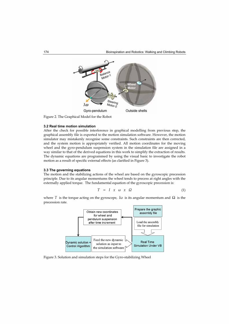
Bioinspiration and Robotics: Walking and Climbing Robots 174
Figure 2. The Graphical Model for the Robot
3.2 Real time motion simulation
After the check for possible interference in graphical modelling from previous step, the graphical assembly file is exported to the motion simulation software. However, the motion simulator may mistakenly recognise some constraints. Such constraints are then corrected, and the system motion is appropriately verified. All motion coordinates for the moving wheel and the gyro-pendulum suspension system in the simulation file are assigned in a way similar to that of the derived equations in this work to simplify the extraction of results. The dynamic equations are programmed by using the visual basic to investigate the robot motion as a result of specific external effects (as clarified in Figure 3).
3.3 The governing equations
The motion and the stabilizing actions of the wheel are based on the gyroscopic precession principle. Due to its angular momentums the wheel tends to precess at right angles with the externally applied torque. The fundamental equation of the gyroscopic precession is:
xxIT = (1)
where T is the torque acting on the gyroscope, I is its angular momentum and Ω is the
precession rate.
Figure 3. Solution and simulation steps for the Gyro-stabilizing Wheel
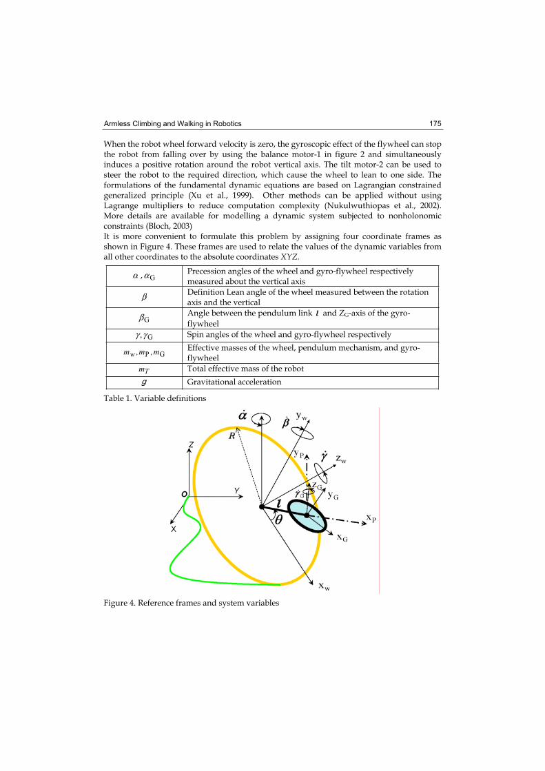
Armless Climbing and Walking in Robotics 175
When the robot wheel forward velocity is zero, the gyroscopic effect of the flywheel can stop the robot from falling over by using the balance motor-1 in figure 2 and simultaneously induces a positive rotation around the robot vertical axis. The tilt motor-2 can be used to steer the robot to the required direction, which cause the wheel to lean to one side. The formulations of the fundamental dynamic equations are based on Lagrangian constrained generalized principle (Xu et al., 1999). Other methods can be applied without using Lagrange multipliers to reduce computation complexity (Nukulwuthiopas et al., 2002). More details are available for modelling a dynamic system subjected to nonholonomic constraints (Bloch, 2003) It is more convenient to formulate this problem by assigning four coordinate frames as shown in Figure 4. These frames are used to relate the values of the dynamic variables from all other coordinates to the absolute coordinates XYZ.
α , Gα Precession angles of the wheel and gyro-flywheel respectively measured about the vertical axis
β Definition Lean angle of the wheel measured between the rotation axis and the vertical
Gβ Angle between the pendulum link ι and ZG-axis of the gyro-
flywheel
G,γγ Spin angles of the wheel and gyro-flywheel respectively
GP m,m,mwEffective masses of the wheel, pendulum mechanism, and gyro-flywheel
Tm Total effective mass of the robot
Gravitational acceleration
Table 1. Variable definitions
Figure 4. Reference frames and system variables
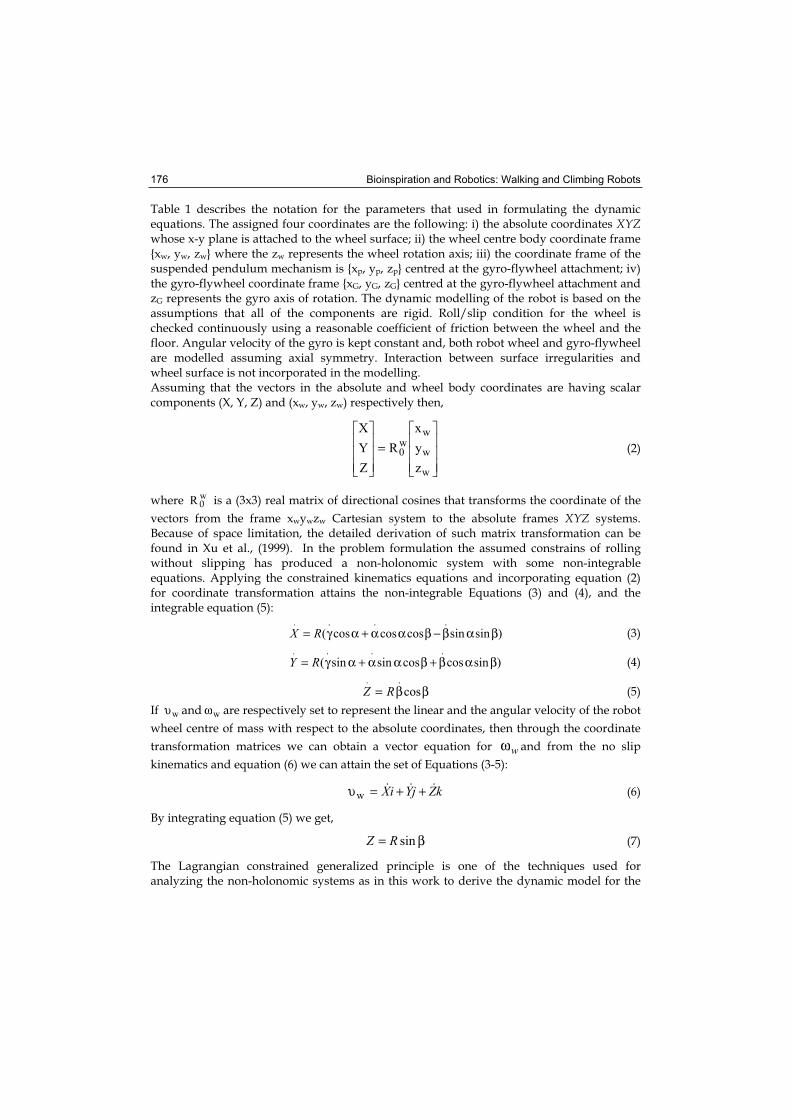
Bioinspiration and Robotics: Walking and Climbing Robots 176
Table 1 describes the notation for the parameters that used in formulating the dynamic equations. The assigned four coordinates are the following: i) the absolute coordinates XYZ whose x-y plane is attached to the wheel surface; ii) the wheel centre body coordinate frame {xw, yw, zw} where the zw represents the wheel rotation axis; iii) the coordinate frame of the suspended pendulum mechanism is {xp, yp, zp} centred at the gyro-flywheel attachment; iv) the gyro-flywheel coordinate frame {xG, yG, zG} centred at the gyro-flywheel attachment and zG represents the gyro axis of rotation. The dynamic modelling of the robot is based on the assumptions that all of the components are rigid. Roll/slip condition for the wheel is checked continuously using a reasonable coefficient of friction between the wheel and the floor. Angular velocity of the gyro is kept constant and, both robot wheel and gyro-flywheel are modelled assuming axial symmetry. Interaction between surface irregularities and wheel surface is not incorporated in the modelling. Assuming that the vectors in the absolute and wheel body coordinates are having scalar components (X, Y, Z) and (xw, yw, zw) respectively then,
=
w
w
ww0
z
y
x
R
Z
Y
X
(2)
where wR 0 is a (3x3) real matrix of directional cosines that transforms the coordinate of the
vectors from the frame xwywzw Cartesian system to the absolute frames XYZ systems. Because of space limitation, the detailed derivation of such matrix transformation can be found in Xu et al., (1999). In the problem formulation the assumed constrains of rolling without slipping has produced a non-holonomic system with some non-integrable equations. Applying the constrained kinematics equations and incorporating equation (2) for coordinate transformation attains the non-integrable Equations (3) and (4), and the integrable equation (5):
)sinsincoscoscos(...
βαβ−βαα+αγ= RX.
(3)
)sincoscossinsin(...
βαβ+βαα+αγ= RY.
(4)
ββ= cos.
RZ.
(5)
If wυ and wω are respectively set to represent the linear and the angular velocity of the robot
wheel centre of mass with respect to the absolute coordinates, then through the coordinate
transformation matrices we can obtain a vector equation for wω and from the no slip
kinematics and equation (6) we can attain the set of Equations (3-5):
kZjYiX ++=υw (6)
By integrating equation (5) we get,
β= sinRZ (7)
The Lagrangian constrained generalized principle is one of the techniques used for analyzing the non-holonomic systems as in this work to derive the dynamic model for the
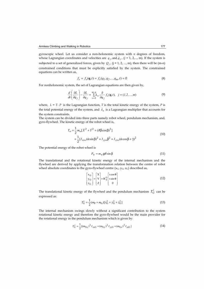
Armless Climbing and Walking in Robotics 177
gyroscopic wheel. Let us consider a non-holonomic system with n degrees of freedom,
whose Lagrangian coordinates and velocities are jj qq ,and, , (j = 1, 2,..., m). If the system is
subjected to a set of generalized forces, given by jQ , (j = 1, 2, ..., m), then there will be (m-n)
constrained conditions that must be explicitly satisfied by the system. The constrained equations can be written as,
0=== )()( t,q,...,q,qft,ff m21sss q (8)
For nonholonomic system, the set of Lagrangian equations are then given by,
)(),(. m1,2,....,jt,fqq
LqL
dtd
sj
n-m
ss
jj=
∂∂λ=
∂∂−
∂∂
=q
1
(9)
where, L = T- P is the Lagrangian function, T is the total kinetic energy of the system, P is
the total potential energy of the system, and s is a Lagrangian multiplier that accounts for
the system constraints. The system can be divided into three parts namely robot wheel, pendulum mechanism, and, gyro-flywheel. The kinetic energy of the robot wheel is,
222
222
2
1
2
1
)cos()sin([
])cos([
γ+βα+β+βα+
ββ++=
zzwyywxxw
ww
III
RYXmT (10)
The potential energy of the robot wheel is
β= sinww RmP g (11)
The translational and the rotational kinetic energy of the internal mechanism and the flywheel are derived by applying the transformation relation between the centre of robot wheel absolute coordinates to the gyro-flywheel centre (xG, yG, zG) described as,
θιθι
+=0
sin
cos
R
Z
Y
X
z
y
xOw
G
G
G
(12)
The translational kinetic energy of the flywheel and the pendulum mechanism t
GT can be
expressed as:
])[( 2G
2G
2GGP
tG zyxmmT +++=
2
1 (13)
The internal mechanism swings slowly without a significant contribution to the system rotational kinetic energy and therefore the gyro-flywheel would be the main provider for the rotational energy in the pendulum mechanism which is given by:
])()()[( zzGGzyyGGyxxGGxr
G IIIT 222
2
1 ω+ω+ω= (14)
Bioinspiration and Robotics: Walking and Climbing Robots 178
where, Gxω , Gyω and, Gzω are the components of the gyro-flywheel angular speed ( Gω )
with respect to the absolute coordinates. The potential energy of the gyro-flywheel and the pendulum mechanism is,
))(sincossin)(( GPG gβθι−β+= RmmP (15)
Finally the Lagrangian function of the system is
)()]([ Gwr
Gt
Gw PPTTTL +−++= (16)
The dynamic equations for the entire system can be derived by substituting Equations (10-15) into Eq. (16). The general dynamic equation of the system is solved numerically using the Kutta-Merson integration. The solution is based on variable time step which automatically adjusts the time increment and monitor simulation errors of various types. Because of the applied loadings, it may not be known if the robot wheel rolls without slipping or slides as it rolls. Such conditions are checked at each time increment during the
robot simulation by investigating the dynamic balance between the resulted angular and linear inertia loads and the applied external torques and forces on the robot wheel using Newton’s and Euler’s Equations. The simulation detects collisions geometrically by finding the intersections between the bodies. When bodies collide, the simulation computes the forces and/or the impulses necessary to prevent interpenetration and applies these responses at the contact points. Based on the obtained values for these responses (forces and impulses) the program calculates the new accelerations and velocities of the bodies and continues the simulation process. The solution scheme is based on using appropriately small integration steps near collisions and employs an impulse momentum collision model with proper coefficient of restitution.
4. Controller Configuration
It is difficult to acquire a controller that ensures continuous trajectory tracking under stabilized condition for single wheel mobile robot under continuous exposal to an erratic real time inputs. The use of intelligent controller is generated by the random nature of system excitations which largely depends on unpredictable parameters such as friction, and other variable dynamic forces. A neural network can model the response of such system by means of a nonlinear regression in the discrete time domain. The result is a network, with adjustable weights, that might approximate the system dynamics. Though it is a problem since the knowledge is stored in an opaque fashion and the learning results in a large set of parameter values which almost impossible to be interpreted in words. Conversely using a fuzzy rule based controller that consists of readable if-then statements which is almost a natural language, cannot learn new rules alone. The neurofuzzy controller might be preferred over the others for such application since it combines the two and it has a learning architecture (Jang et al., 1997). To construct a neurofuzzy controller with ANFIS (Adaptive Neuro Fuzzy Inference System), we need a set of input-output data. In this work, two input
signals are considered. The first input is the wheel orientation error ( βε , OrientError) which
is defined as the angle of deviation between the vertical line that passes through the ground contact point and the line that connects the wheel mass centre and wheel contact point. The second input is the deviation angle between the actual wheel path and the tangent to the
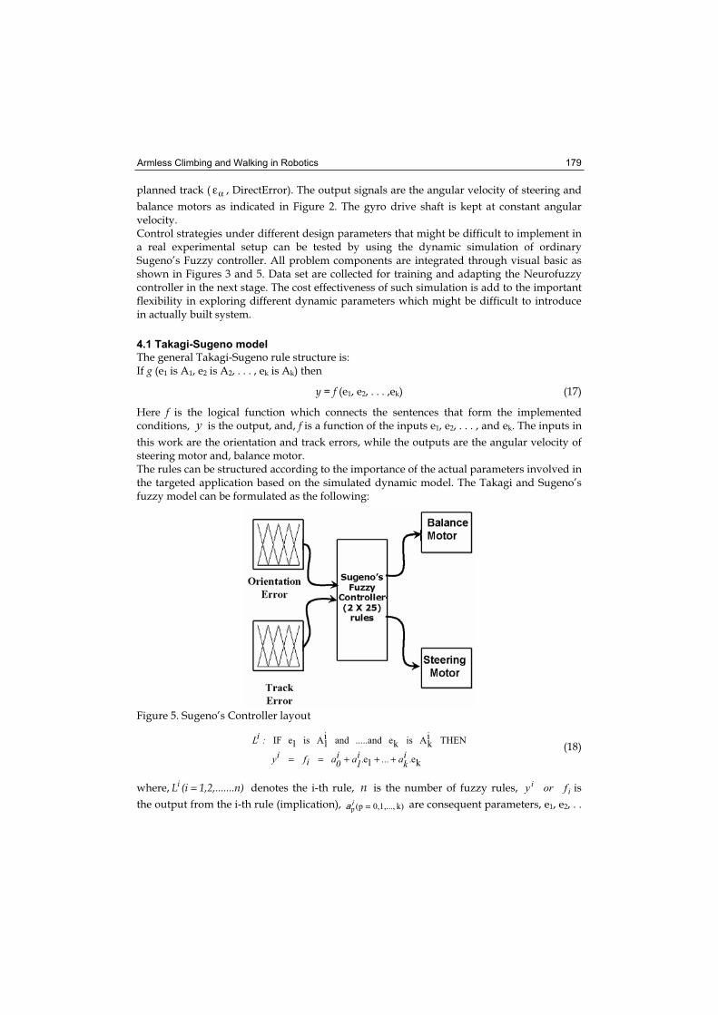
Armless Climbing and Walking in Robotics 179
planned track ( αε , DirectError). The output signals are the angular velocity of steering and
balance motors as indicated in Figure 2. The gyro drive shaft is kept at constant angular velocity. Control strategies under different design parameters that might be difficult to implement in a real experimental setup can be tested by using the dynamic simulation of ordinary Sugeno’s Fuzzy controller. All problem components are integrated through visual basic as shown in Figures 3 and 5. Data set are collected for training and adapting the Neurofuzzy controller in the next stage. The cost effectiveness of such simulation is add to the important flexibility in exploring different dynamic parameters which might be difficult to introduce in actually built system.
4.1 Takagi-Sugeno model
The general Takagi-Sugeno rule structure is: If g (e1 is A1, e2 is A2, . . . , ek is Ak) then
y = f (e1, e2, . . . ,ek) (17)
Here f is the logical function which connects the sentences that form the implemented conditions, y is the output, and, f is a function of the inputs e1, e2, . . . , and ek. The inputs in
this work are the orientation and track errors, while the outputs are the angular velocity of steering motor and, balance motor. The rules can be structured according to the importance of the actual parameters involved in the targeted application based on the simulated dynamic model. The Takagi and Sugeno’s fuzzy model can be formulated as the following:
Figure 5. Sugeno’s Controller layout
ke1e
THENikAiske.....andandi
1Ais1eIF
.ika....i
1ai0aif
iy
:iL
+++== (18)
where, .n)1,2,......(iLi = denotes the i-th rule, n is the number of fuzzy rules, ii fory is
the output from the i-th rule (implication), k)0,1,...,(pp = are consequent parameters, e1, e2, . .
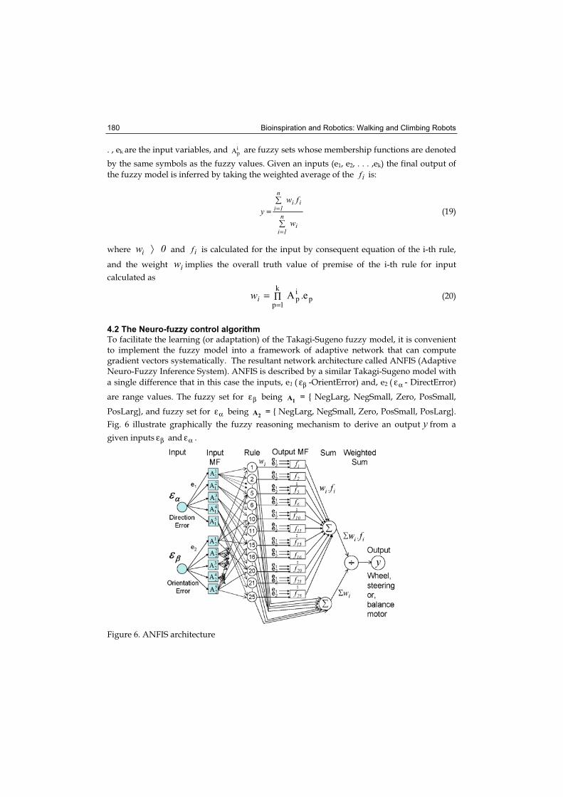
Bioinspiration and Robotics: Walking and Climbing Robots 180
. , ek are the input variables, and ipA are fuzzy sets whose membership functions are denoted
by the same symbols as the fuzzy values. Given an inputs (e1, e2, . . . ,ek) the final output of
the fuzzy model is inferred by taking the weighted average of the if is:
in
1i
iin
1i
w
fwy =
=
= (19)
where 0wi and if is calculated for the input by consequent equation of the i-th rule,
and the weight iw implies the overall truth value of premise of the i-th rule for input
calculated as
pip
k
1peA .wi ∏
== (20)
4.2 The Neuro-fuzzy control algorithm
To facilitate the learning (or adaptation) of the Takagi-Sugeno fuzzy model, it is convenient to implement the fuzzy model into a framework of adaptive network that can compute gradient vectors systematically. The resultant network architecture called ANFIS (Adaptive Neuro-Fuzzy Inference System). ANFIS is described by a similar Takagi-Sugeno model with
a single difference that in this case the inputs, e1 ( βε -OrientError) and, e2 ( αε - DirectError)
are range values. The fuzzy set for βε being 1A = { NegLarg, NegSmall, Zero, PosSmall,
PosLarg}, and fuzzy set for αε being 2A = { NegLarg, NegSmall, Zero, PosSmall, PosLarg}.
Fig. 6 illustrate graphically the fuzzy reasoning mechanism to derive an output y from a
given inputs βε and αε .
Figure 6. ANFIS architecture
Armless Climbing and Walking in Robotics 181
ANFIS can have only one output y ; therefore three neurofuzzy controllers are implemented
in order to obtain the required control command for the output motors. Output if is one of
the motors angular speed for i-th rule where the size of the rule base is 25. The dynamic simulation is conducted with several types and sizes of membership functions
for the fuzzy sets 1
A and,2A . Using triangular membership functions and a size of five for
each of the two fuzzy sets were found the simplest and best suited for this case. The square elements in Fig. 6 represent the adaptive nodes depending on the parameter set of the adaptive network. The circles represent fixed nodes, which are independent of the parameter set. The first layer is composed of adaptive nodes representing the triangular membership functions (Jang et al., 1997) associated with each linguistic value. The second layer implements the fuzzy rules. Each node in this layer calculates the firing strength of a rule by means of multiplication between the membership degrees of the two inputs. The third layer consists of adaptive nodes which include the output membership. The other two layers consist of fixed nodes that implement the weighted average procedure to obtain one of the motors output y as shown in Fig. 6. As the size of the rule base of the Sugeno fuzzy inference system (SFIS) is 25, we will have to identify 75 consequent
parameters { 10a , …., 25
0a , 11a , …., 25
1a , 12a , …., 25
2a } as indicated in Jang et al., (1997). This
can be obtained from the neural network (NN) using training set { βε , αε , y } which are
collected from the dynamic simulation results by using the Sugeno fuzzy inference system. A back-propagation learning algorithm is used to identify these parameters in two steps. In the forward pass, the input membership functions are fixed and consequent parameters associated with the output are calculated by applying the least square estimation method. Using these parameters, the NN generates an estimate of the motor output. The difference between this estimate and the motor’s value from the training set is then back-propagated in a second pass when the premise parameters associated with the input membership functions are calculated.
5. Simulation Results
In our simulation, we investigated the robot control tactics when passing a platform of three segments namely I, II, and, III as shown in Fig. 7. Segment-I in Fig. 7 (a) is used to investigate the robot capability in climbing an uphill ground or passing obstacle with adjustable tilt angle ψ both friction and restitution coefficients between the wheel and the
uphill ground can be investigated. The uphill ground represented by the segment-I is kept with zero angular twist around the pathway centreline during results extractions. Segment-II represents the middle section of the platform with adjustable level relative to segment-I to investigate the jumping behaviour of the robot. Finally segment-III is the last section of the
platform and twisted with an angle λ around the pathway centreline and used to examine
manoeuvrability of the robot when it is confronted with sudden slop change of ground. Throughout our simulation the following physical, geometrical and mass parameters are used as given in Table 1
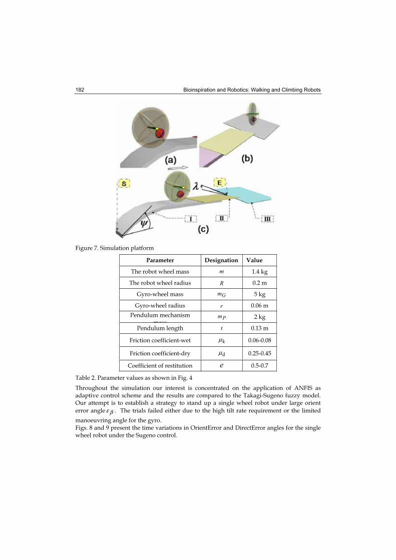
Bioinspiration and Robotics: Walking and Climbing Robots 182
Figure 7. Simulation platform
Parameter Designation Value
The robot wheel mass m 1.4 kg
The robot wheel radius R 0.2 m
Gyro-wheel mass Gm 5 kg
Gyro-wheel radius r 0.06 m
Pendulum mechanism mass
Pm 2 kg
Pendulum length ι 0.13 m
Friction coefficient-wet kμ 0.06-0.08
Friction coefficient-dry dμ 0.25-0.45
Coefficient of restitution e 0.5-0.7
Table 2. Parameter values as shown in Fig. 4
Throughout the simulation our interest is concentrated on the application of ANFIS as adaptive control scheme and the results are compared to the Takagi-Sugeno fuzzy model. Our attempt is to establish a strategy to stand up a single wheel robot under large orient
error angle βε . The trials failed either due to the high tilt rate requirement or the limited
manoeuvring angle for the gyro. Figs. 8 and 9 present the time variations in OrientError and DirectError angles for the single wheel robot under the Sugeno control.
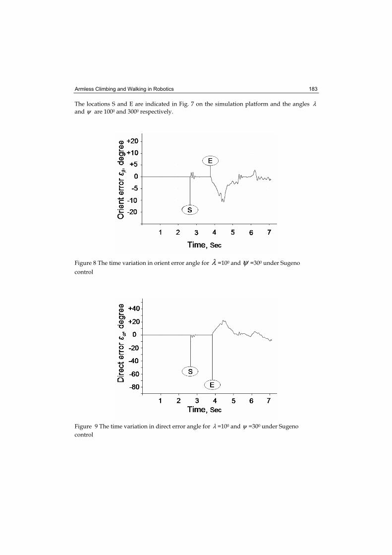
Armless Climbing and Walking in Robotics 183
The locations S and E are indicated in Fig. 7 on the simulation platform and the angles λand ψ are 1000 and 3000 respectively.
Figure 8 The time variation in orient error angle for λ =100 and ψ =300 under Sugeno
control
Figure 9 The time variation in direct error angle for λ =100 and ψ =300 under Sugeno
control
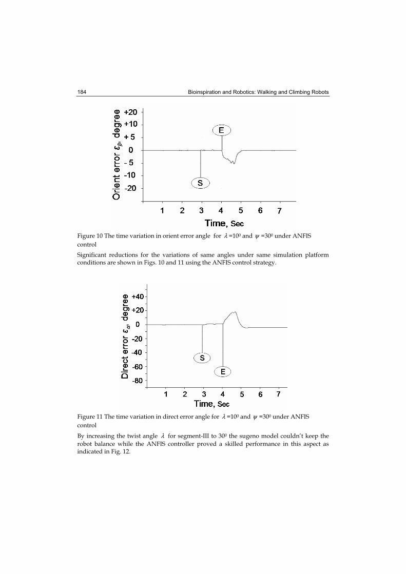
Bioinspiration and Robotics: Walking and Climbing Robots 184
Figure 10 The time variation in orient error angle for λ =100 and ψ =300 under ANFIS
control
Significant reductions for the variations of same angles under same simulation platform conditions are shown in Figs. 10 and 11 using the ANFIS control strategy.
Figure 11 The time variation in direct error angle for λ =100 and ψ =300 under ANFIS
control
By increasing the twist angle λ for segment-III to 300 the sugeno model couldn’t keep the
robot balance while the ANFIS controller proved a skilled performance in this aspect as indicated in Fig. 12.
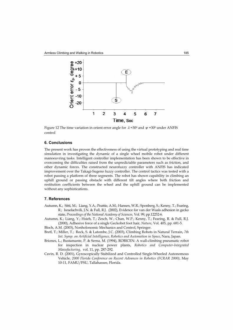
Armless Climbing and Walking in Robotics 185
Figure 12 The time variation in orient error angle for λ =300 and ψ =300 under ANFIS
control
6. Conclusions
The present work has proven the effectiveness of using the virtual prototyping and real time simulation in investigating the dynamic of a single wheel mobile robot under different manoeuvring tasks. Intelligent controller implementation has been shown to be effective in overcoming the difficulties raised from the unpredictable parameters such as friction, and other dynamic forces. The constructed neurofuzzy controller with ANFIS has indicated improvement over the Takagi-Sugeno fuzzy controller. The control tactics was tested with a robot passing a platform of three segments. The robot has shown capability in climbing an uphill ground or passing obstacle with different tilt angles where both friction and restitution coefficients between the wheel and the uphill ground can be implemented without any sophistications.
7. References
Autumn, K.; Sitti, M.; Liang, Y.A.; Peattie, A.M.; Hansen, W.R.; Sponberg, S.; Kenny, T.; Fearing, R.; Israelachvili, J.N. & Full, R.J. (2002), Evidence for van der Waals adhesion in gecko state, Proceedings of the National Academy of Sciences, Vol. 99, pp.12252-6.
Autumn, K.; Liang, Y.; Hsieh, T.; Zesch, W.; Chan, W.P.; Kenny, T.; Fearing, R. & Full, R.J. (2000), Adhesive force of a single Geckobot foot hair, Nature, Vol. 405, pp. 681-5.
Bloch, A.M. (2003), Nonholonomic Mechanics and Control, Springer. Bretl, T.; Miller, T.; Rock, S. & Latombe, J.C. (2003), Climbing Robots in Natural Terrain, 7th
Int. Symp. on Artificial Intelligence, Robotics and Automation in Space, Nara, Japan. Briones, L.; Bustamante, P. & Serna, M. (1994), ROBICEN: A wall-climbing pneumatic robot
for inspection in nuclear power plants, Robotics and Computer-Integrated Manufacturing, vol. 11, pp. 287-292.
Cavin, R. D. (2001), Gyroscopically Stabilized and Controlled Single-Wheeled Autonomous Vehicle, 2000 Florida Conference on Recent Advances in Robotics (FCRAR 2000), May 10-11, FAMU/FSU, Tallahassee, Florida.
Bioinspiration and Robotics: Walking and Climbing Robots 186
Ferreira, E.; Tsai, S.; Paredis, C.; & Brown, H. (2000), Control of the Gyrover: a single-wheel gyroscopically stabilized robot, Advanced Robotics, Vol. 14, No. 6, pp. 459 - 475.
Hirose, s. (1993), Biologically Inspired Robots: Snake-Like Locomotors and Manipulators, New York, NY, Oxford University Press.
Iagnemma, K. & Dubowsky, S. (2004), Traction Control of Wheeled Robotic Vehicles with Application to Planetary Rovers, Intl Journal of Robotics Research, Vol. 23, no. 10, pp. 1029-1040.
Jang, J.-S. R.; Sun, C.-T. & Mizutani, E. (1997), Neuro-Fuzzy and Soft Computing, Prentice Hall, ISBN 0-13-261066-3
Martynenko, Yu. G. & Formal'skii, A. M. (2005), A Control of the Longitudinal Motion of a Single-Wheel Robot on an Uneven Surface, Journal of Computer and Systems Sciences International, Vol. 44, No. 4, pp. 662-670
Nagakubo, A. & Hirose, S. (1994), Walking and running of the quadruped wall-climbing robot, Proceedings of the IEEE International Conference on Robotics and Automation, pp. 1005-1012.
Nandy, G. C. & Xu, Y. (1998), Dynamic model of a gyroscopic wheel, Proc. IEEE Int. Conf. on Robotics and Automation, pp. 2683-88, Leuven, Belgium.
Nukulwuthiopas, W.; Laowattana, D. & Maneewarn, T. (2002), Dynamic Modeling of a One-Wheel Robot By Using Kane's Method, IEEE International Conference on Industrial Technology (IEEE ICIT '02), pp. 524-529, December 11-14, Bangkok, Thailand.
Pack, R.T.; Christopher, J.L. & Kawamura, K. (1997), A Rubbertuator-Based Structure-Climbing Inspection Robot, Proceedings of the IEEE International Conference on Robotics and Automation, pp. 1869-1874.
Rashid, M. K. & Khalil, Z. A. (2004), Configuration Design and Intelligent Stepping of a Spherical Motor in Robotic Joint, Journal of Intelligent and Robotic Systems, Volume 40, Issue 2, Pages 165 – 181..
Rashid, M. K. (2007), Simulation of Intelligent Single Wheel Mobile Robot, International Journal of Advanced Robotic Systems, ARS Publication, Vol. 4 No. 1 ISSN 1729-8806, pp.73-80.
Samuel, K. W. Au; Yangsheng, Xu & Wilson, W. K. Yu. (2001), Control of tilt-up motion of a single wheel robot via model-based and human-based controllers, Mechatronics,Vol. 11, pp. 451-473
Shah, G. & Sitti, M. (2004), Modeling and Design of Biomimetic Adhesives Inspired by Gecko Foot-Hairs, Proc. of the IEEE Conf. on Robotics and Biomimetics, Shenyang, China.
Shuliang, L.; Yanzheng, Z.; Xueshan, G.; Dianguo, X. & Yan, W. (2000), A wall-climbing robot with magnetic crawlers for sand-blasting, Spray- Painting and Measurement High Technology Letters, Vol. 10, 86-8.
Tokioka, S. & Sakai, S. (1988), Painting robot for wall surface, Robot, Vol. 65, 88-96. Xu, Y.; Brown, H. B. &, Au, K. W. (1999), Dynamic Mobility with Single-Wheel Configuration,
The International Journal of Robotics Research, Vol. 18, No. 7, pp. 728-738 Xu, Z. & Ma, P., (2002)A wall-climbing robot for labeling scale of oil tank’s volume, Robotica,
Vol. 20, 209-212. Yangsheng Xu & Samuel, K. W. Ou (2004), Stabilization and path following of a single
wheel robot, IEEE/ASME Transactions on Mechatronics, Vol. 9, No. 2, pp. 407-419. Yanzeng, Z.; S. Hao, & Yan, W. (1999), Wall-climbing robot with negative pressure sucker
used for cleaning work, High Technology Letters, Vol. 5, 85-88.
12
A Reference Control Architecture for Service Robots as applied to a Climbing Vehicle
Francisco Ortiz, Diego Alonso, Juan Pastor, Bárbara Álvarez and Andrés Iborra
Division of Electronics Engineering & Systems - Universidad Politécnica de Cartagena Spain
1. Introduction
Recent progress in mechatronics, perception and computing is opening up a number of new application domains for robotics, improving the way in which robots perform actions that release the human from dangerous or risky tasks. Nowadays, the field of service robotics is in continuous development, covering more and more application domains, from home to industry, and offering more and more capabilities in a reliable and user-friendly way. One of the new environments where robots are starting to appear is in the shipyard. Developing robots for working in shipyards is very challenging because of both the difficulty of the missions that robots should perform as well as the lack of robotic culture in this kind of industrial facility. The authors’ research group, the DSIE (Division of Electronics Engineering & Systems) at the Technical University of Cartagena, has a considerable experience in the development of software applications for teleoperated service robots, mainly for nuclear power plants (Iborra et al., 2003) and in shipyards industry (Fernández et al., 2004). The work presented in this chapter has been carried out in the context of the EFTCoR project (Environmental Friendly and Cost-Effective Technology for Coating Removal) (EFTCoR, 2005). The EFTCoR project sought to develop a solution for ships’ hulls cleaning and for the retrieval and confinement of the oxide, paint and sea adherences resulting from the cleaning operations. For this purpose, several robots were designed, one of which being a climbing vehicle capable of positioning a grit-blasting tool onto ships’ hulls. This chapter describes our experience in the development of the climbing robot and the software architecture designed for its control unit, ACROSET (Control Architecture for Service Teleoperated Robots). Software architecture is one of the key elements of any robotic system. As technology evolves, it is possible to build systems that are capable of carrying out more complex tasks in more complex environments. But the new robot capabilities demand a great variety of components, both hardware and software, that must interact in diverse ways. Such components must be structured in a way that (1) the robot achieves its global functionality and (2) the system could be easily maintained and updated. The way in which components are organised is described by the architecture of the system. The importance of considering system architecture to handle the inherent complexity of robotic systems is well known (Coste-Manière & Simmons, 2000): overall system complexity can be reduced by dividing it
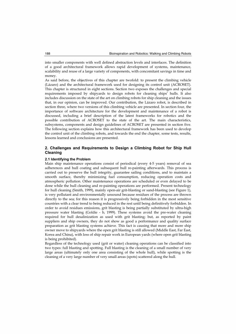
Bioinspiration and Robotics: Walking and Climbing Robots 188
into smaller components with well defined abstraction levels and interfaces. The definition of a good architectural framework allows rapid development of systems, maintenance, scalability and reuse of a large variety of components, with concomitant savings in time and money. As said before, the objectives of this chapter are twofold: to present the climbing vehicle (Lázaro) and the architectural framework used for designing its control unit (ACROSET). This chapter is structured in eight sections. Section two exposes the challenges and special requirements imposed by shipyards to design robots for cleaning ships’ hulls. It also includes discussion on the state of the art on climbing robots for ship cleaning and the issues that, in our opinion, can be improved. Our contribution, the Lázaro robot, is described in section three, where two versions of this climbing vehicle are presented. In section four, the importance of software architecture for the development and maintenance of a robot is discussed, including a brief description of the latest frameworks for robotics and the possible contribution of ACROSET to the state of the art. The main characteristics, subsystems, components and design guidelines of ACROSET are presented in section five. The following section explains how this architectural framework has been used to develop the control unit of the climbing robots, and towards the end the chapter, some tests, results, lessons learned and conclusions are presented.
2. Challenges and Requirements to Design a Climbing Robot for Ship Hull Cleaning
2.1 Identifying the Problem
Main ship maintenance operations consist of periodical (every 4-5 years) removal of sea adherences and hull coating and subsequent hull re-painting afterwards. This process is carried out to preserve the hull integrity, guarantee sailing conditions, and to maintain a smooth surface, thereby minimizing fuel consumption, reducing operation costs and atmospheric pollution. Other maintenance operations are scheduled or even delayed to be done while the hull cleaning and re-painting operations are performed. Present technology for hull cleaning (Smith, 1999), mainly open-air grit-blasting or sand-blasting (see Figure 1), is very pollutant and environmentally unsound because residues of the process are thrown directly to the sea; for this reason it is progressively being forbidden in the most sensitive countries with a clear trend to being reduced in the rest until being definitively forbidden. In order to avoid residues emissions, grit blasting is being partially substituted by ultra-high pressure water blasting (Goldie - b, 1999). These systems avoid the pre-water cleaning required for hull desalinization as used with grit blasting; but, as reported by paint suppliers and ship owners, they do not show as good a performance and quality surface preparation as grit blasting systems achieve. This fact is causing that more and more ship owner move to shipyards where the open grit blasting is still allowed (Middle East, Far East, Korea and China), with loss of ship repair work in European yards (where open grit blasting is being prohibited). Regardless of the technology used (grit or water) cleaning operations can be classified into two types: full blasting and spotting. Full blasting is the cleaning of a small number of very large areas (ultimately only one area consisting of the whole hull), while spotting is the cleaning of a very large number of very small areas (spots) scattered along the hull.
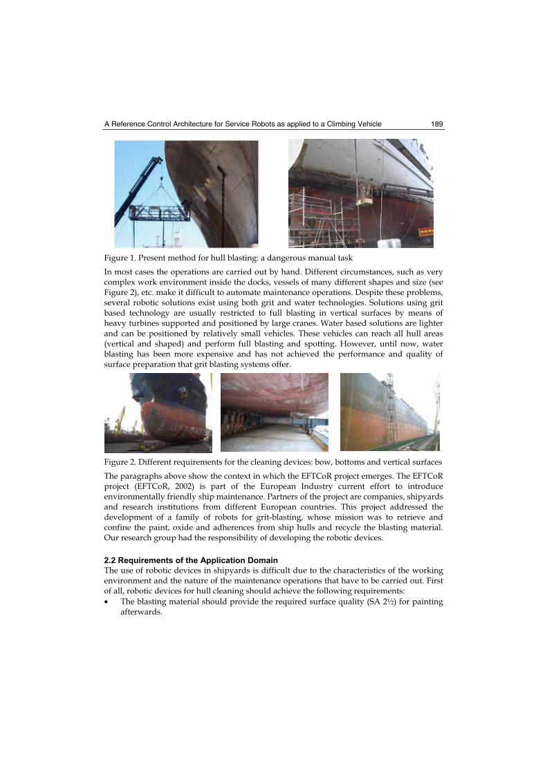
A Reference Control Architecture for Service Robots as applied to a Climbing Vehicle 189
Figure 1. Present method for hull blasting: a dangerous manual task
In most cases the operations are carried out by hand. Different circumstances, such as very complex work environment inside the docks, vessels of many different shapes and size (see Figure 2), etc. make it difficult to automate maintenance operations. Despite these problems, several robotic solutions exist using both grit and water technologies. Solutions using grit based technology are usually restricted to full blasting in vertical surfaces by means of heavy turbines supported and positioned by large cranes. Water based solutions are lighter and can be positioned by relatively small vehicles. These vehicles can reach all hull areas (vertical and shaped) and perform full blasting and spotting. However, until now, water blasting has been more expensive and has not achieved the performance and quality of surface preparation that grit blasting systems offer.
Figure 2. Different requirements for the cleaning devices: bow, bottoms and vertical surfaces
The paragraphs above show the context in which the EFTCoR project emerges. The EFTCoR project (EFTCoR, 2002) is part of the European Industry current effort to introduce environmentally friendly ship maintenance. Partners of the project are companies, shipyards and research institutions from different European countries. This project addressed the development of a family of robots for grit-blasting, whose mission was to retrieve and confine the paint, oxide and adherences from ship hulls and recycle the blasting material. Our research group had the responsibility of developing the robotic devices.
2.2 Requirements of the Application Domain
The use of robotic devices in shipyards is difficult due to the characteristics of the working environment and the nature of the maintenance operations that have to be carried out. First of all, robotic devices for hull cleaning should achieve the following requirements:
• The blasting material should provide the required surface quality (SA 2½) for painting afterwards.
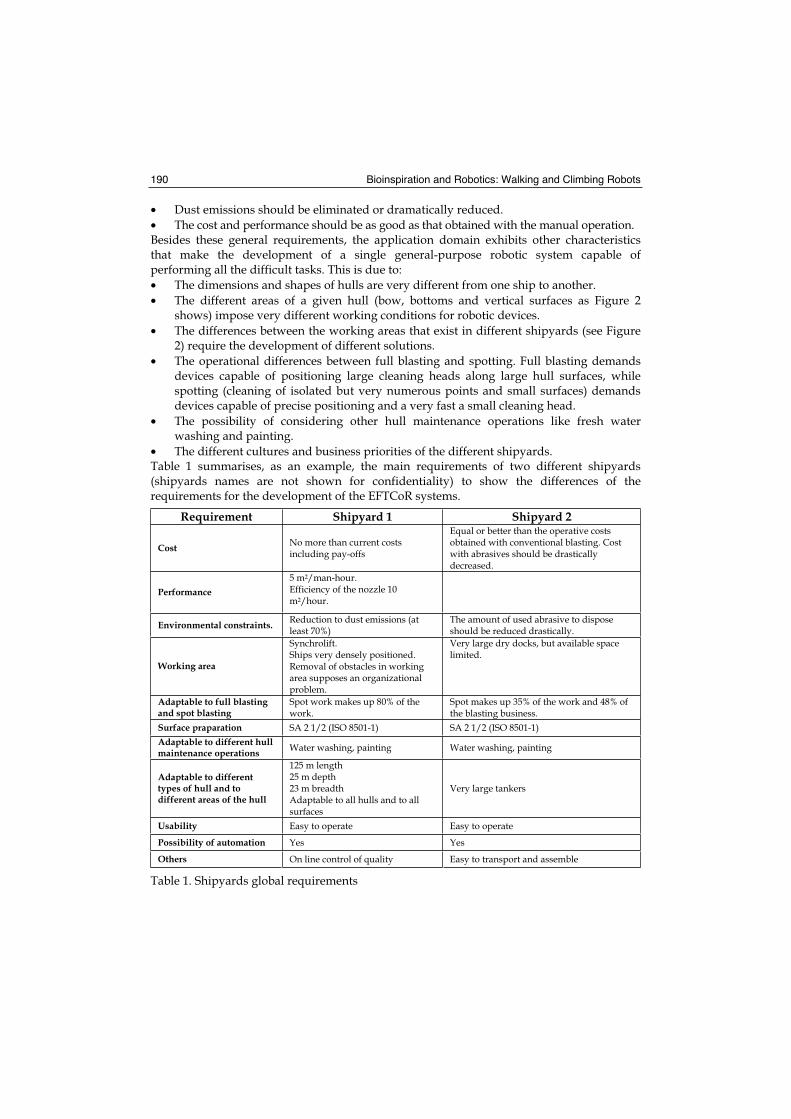
Bioinspiration and Robotics: Walking and Climbing Robots 190
• Dust emissions should be eliminated or dramatically reduced.
• The cost and performance should be as good as that obtained with the manual operation. Besides these general requirements, the application domain exhibits other characteristics that make the development of a single general-purpose robotic system capable of performing all the difficult tasks. This is due to:
• The dimensions and shapes of hulls are very different from one ship to another.
• The different areas of a given hull (bow, bottoms and vertical surfaces as Figure 2 shows) impose very different working conditions for robotic devices.
• The differences between the working areas that exist in different shipyards (see Figure 2) require the development of different solutions.
• The operational differences between full blasting and spotting. Full blasting demands devices capable of positioning large cleaning heads along large hull surfaces, while spotting (cleaning of isolated but very numerous points and small surfaces) demands devices capable of precise positioning and a very fast a small cleaning head.
• The possibility of considering other hull maintenance operations like fresh water washing and painting.
• The different cultures and business priorities of the different shipyards.Table 1 summarises, as an example, the main requirements of two different shipyards (shipyards names are not shown for confidentiality) to show the differences of the requirements for the development of the EFTCoR systems.
Requirement Shipyard 1 Shipyard 2
Cost No more than current costs including pay-offs
Equal or better than the operative costs obtained with conventional blasting. Cost with abrasives should be drastically decreased.
Performance 5 m2/man-hour. Efficiency of the nozzle 10 m2/hour.
Environmental constraints. Reduction to dust emissions (at least 70%)
The amount of used abrasive to dispose should be reduced drastically.
Working area
Synchrolift.Ships very densely positioned. Removal of obstacles in working area supposes an organizational problem.
Very large dry docks, but available space limited.
Adaptable to full blasting and spot blasting
Spot work makes up 80% of the work.
Spot makes up 35% of the work and 48% of the blasting business.
Surface praparation SA 2 1/2 (ISO 8501-1) SA 2 1/2 (ISO 8501-1)
Adaptable to different hull maintenance operations Water washing, painting Water washing, painting
Adaptable to different types of hull and to different areas of the hull
125 m length 25 m depth 23 m breadth Adaptable to all hulls and to all surfaces
Very large tankers
Usability Easy to operate Easy to operate
Possibility of automation Yes Yes
Others On line control of quality Easy to transport and assemble
Table 1. Shipyards global requirements
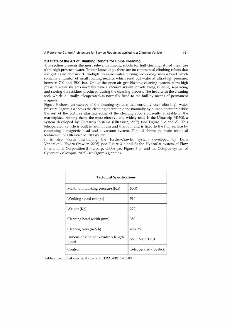
A Reference Control Architecture for Service Robots as applied to a Climbing Vehicle 191
2.3 State of the Art of Climbing Robots for Ships Cleaning
This section presents the most relevant climbing robots for hull cleaning. All of them use ultra-high pressure water. To our knowledge, there are no commercial climbing robots that use grit as an abrasive. Ultra-high pressure water blasting technology uses a head which contains a number of small rotating nozzles which send out water at ultra-high pressure, between 700 and 2500 bar. Unlike the open-air grit blasting cleaning system, ultra-high pressure water systems normally have a vacuum system for retrieving, filtering, separating and storing the residues produced during the cleaning process. The head with the cleaning tool, which is usually teleoperated, is normally fixed to the hull by means of permanent magnets.Figure 3 shows an excerpt of the cleaning systems that currently uses ultra-high water pressure. Figure 3-a shows the cleaning operation done manually by human operators while the rest of the pictures illustrate some of the cleaning robots currently available in the marketplace. Among them, the most effective and widely used is the Ultrastrip M3500, asystem developed by Ultrastrip Systems (Ultrastrip, 2007) (see Figure 3 c and d). This teleoperated vehicle is built in aluminium and titanium and is fixed to the hull surface by combining a magnetic head and a vacuum system. Table 2 shows the main technical features of the Ultrastrip M3500 system. It is also worth mentioning the Hydro-Crawler system developed by Dans Vandteknik (Hydro-Crawler, 2006) (see Figure 3 e and f); the HydroCat system of Flow
International Corporation (Flowcorp, 2005) (see Figure 3-b); and the Octopus system of
Cybernetix (Octopus, 2005) (see Figure 3 g and h).
Technical Specifications
Maximum working pressure (bar) 3000
Working speed (mm/s) 510
Weight (Kg) 222
Cleaning head width (mm) 380
Clearing ratio (m2/h) 46 a 268
Dimensions: height x width x length (mm)
560 x 690 x 1710
Control Teleoperated/Joystick
Table 2. Technical specifications of ULTRASTRIP M3500
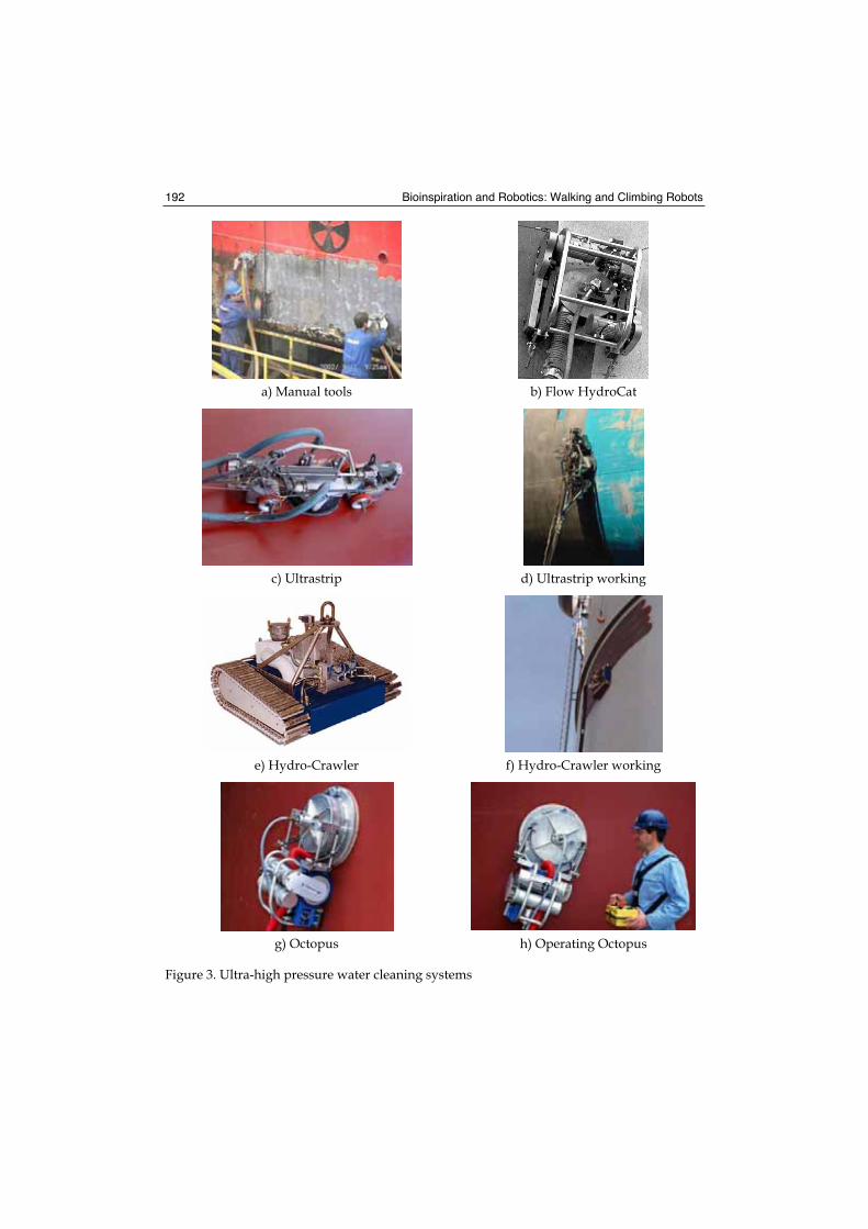
Bioinspiration and Robotics: Walking and Climbing Robots 192
a) Manual tools b) Flow HydroCat
c) Ultrastrip d) Ultrastrip working
e) Hydro-Crawler f) Hydro-Crawler working
g) Octopus h) Operating Octopus
Figure 3. Ultra-high pressure water cleaning systems
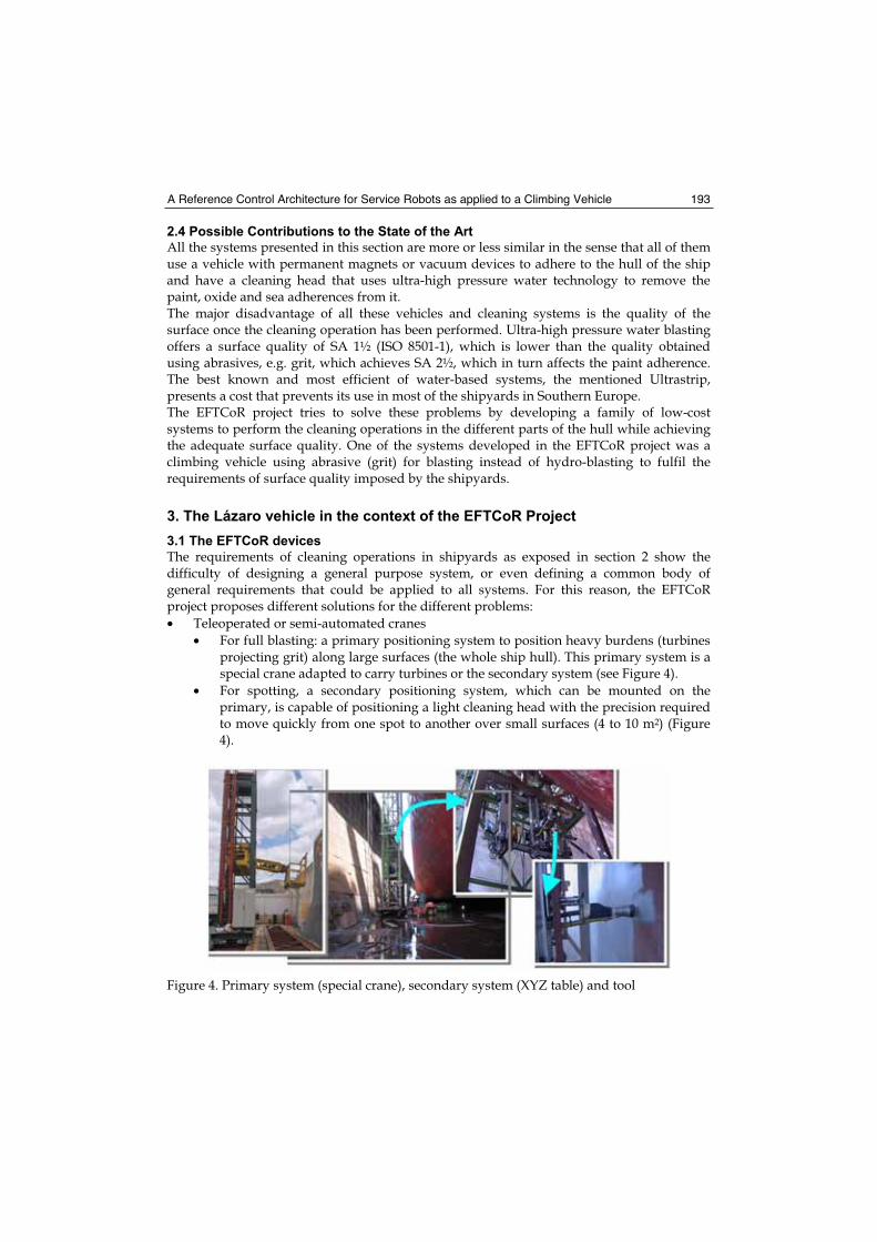
A Reference Control Architecture for Service Robots as applied to a Climbing Vehicle 193
2.4 Possible Contributions to the State of the Art
All the systems presented in this section are more or less similar in the sense that all of them use a vehicle with permanent magnets or vacuum devices to adhere to the hull of the ship and have a cleaning head that uses ultra-high pressure water technology to remove the paint, oxide and sea adherences from it. The major disadvantage of all these vehicles and cleaning systems is the quality of the surface once the cleaning operation has been performed. Ultra-high pressure water blasting offers a surface quality of SA 1½ (ISO 8501-1), which is lower than the quality obtained using abrasives, e.g. grit, which achieves SA 2½, which in turn affects the paint adherence. The best known and most efficient of water-based systems, the mentioned Ultrastrip, presents a cost that prevents its use in most of the shipyards in Southern Europe.The EFTCoR project tries to solve these problems by developing a family of low-cost systems to perform the cleaning operations in the different parts of the hull while achieving the adequate surface quality. One of the systems developed in the EFTCoR project was a climbing vehicle using abrasive (grit) for blasting instead of hydro-blasting to fulfil the requirements of surface quality imposed by the shipyards.
3. The Lázaro vehicle in the context of the EFTCoR Project
3.1 The EFTCoR devices
The requirements of cleaning operations in shipyards as exposed in section 2 show the difficulty of designing a general purpose system, or even defining a common body of general requirements that could be applied to all systems. For this reason, the EFTCoR project proposes different solutions for the different problems:
• Teleoperated or semi-automated cranes
• For full blasting: a primary positioning system to position heavy burdens (turbines projecting grit) along large surfaces (the whole ship hull). This primary system is a special crane adapted to carry turbines or the secondary system (see Figure 4).
• For spotting, a secondary positioning system, which can be mounted on the primary, is capable of positioning a light cleaning head with the precision required to move quickly from one spot to another over small surfaces (4 to 10 m2) (Figure 4).
Figure 4. Primary system (special crane), secondary system (XYZ table) and tool
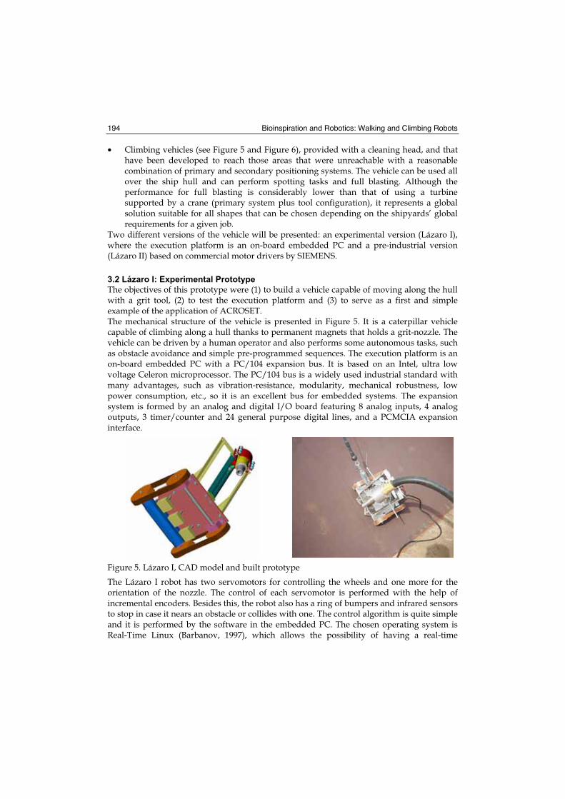
Bioinspiration and Robotics: Walking and Climbing Robots 194
• Climbing vehicles (see Figure 5 and Figure 6), provided with a cleaning head, and that have been developed to reach those areas that were unreachable with a reasonable combination of primary and secondary positioning systems. The vehicle can be used all over the ship hull and can perform spotting tasks and full blasting. Although the performance for full blasting is considerably lower than that of using a turbine supported by a crane (primary system plus tool configuration), it represents a global solution suitable for all shapes that can be chosen depending on the shipyards’ global requirements for a given job.
Two different versions of the vehicle will be presented: an experimental version (Lázaro I), where the execution platform is an on-board embedded PC and a pre-industrial version (Lázaro II) based on commercial motor drivers by SIEMENS.
3.2 Lázaro I: Experimental Prototype
The objectives of this prototype were (1) to build a vehicle capable of moving along the hull with a grit tool, (2) to test the execution platform and (3) to serve as a first and simple example of the application of ACROSET. The mechanical structure of the vehicle is presented in Figure 5. It is a caterpillar vehicle capable of climbing along a hull thanks to permanent magnets that holds a grit-nozzle. The vehicle can be driven by a human operator and also performs some autonomous tasks, such as obstacle avoidance and simple pre-programmed sequences. The execution platform is an on-board embedded PC with a PC/104 expansion bus. It is based on an Intel, ultra low voltage Celeron microprocessor. The PC/104 bus is a widely used industrial standard with many advantages, such as vibration-resistance, modularity, mechanical robustness, low power consumption, etc., so it is an excellent bus for embedded systems. The expansion system is formed by an analog and digital I/O board featuring 8 analog inputs, 4 analog outputs, 3 timer/counter and 24 general purpose digital lines, and a PCMCIA expansion interface.
Figure 5. Lázaro I, CAD model and built prototype
The Lázaro I robot has two servomotors for controlling the wheels and one more for the orientation of the nozzle. The control of each servomotor is performed with the help of incremental encoders. Besides this, the robot also has a ring of bumpers and infrared sensors to stop in case it nears an obstacle or collides with one. The control algorithm is quite simple and it is performed by the software in the embedded PC. The chosen operating system is Real-Time Linux (Barbanov, 1997), which allows the possibility of having a real-time
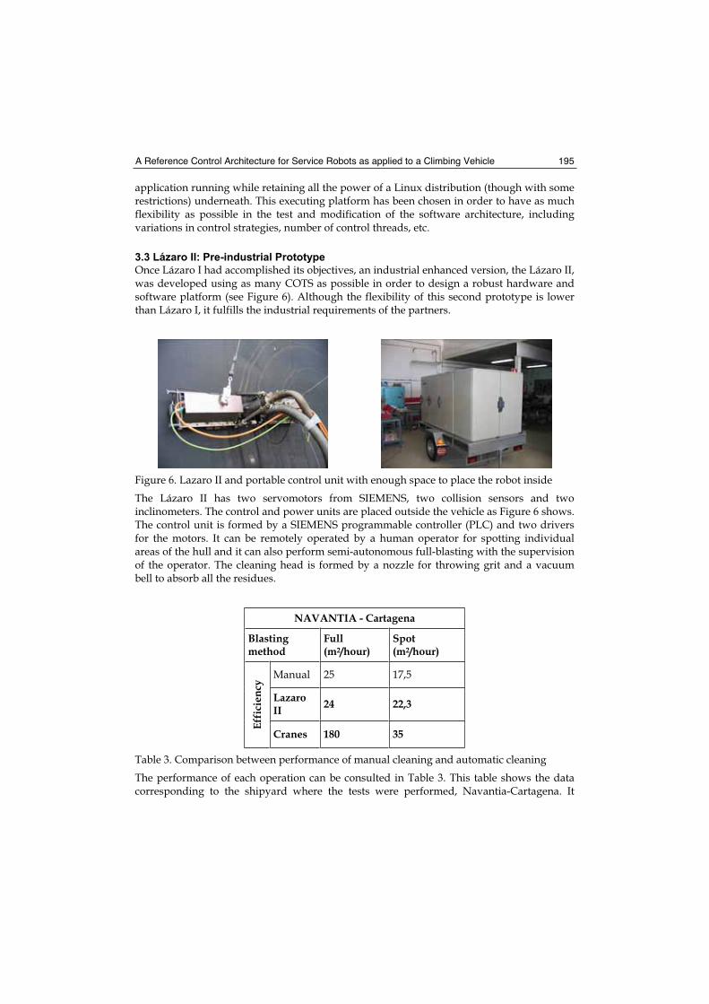
A Reference Control Architecture for Service Robots as applied to a Climbing Vehicle 195
application running while retaining all the power of a Linux distribution (though with some restrictions) underneath. This executing platform has been chosen in order to have as much flexibility as possible in the test and modification of the software architecture, including variations in control strategies, number of control threads, etc.
3.3 Lázaro II: Pre-industrial Prototype
Once Lázaro I had accomplished its objectives, an industrial enhanced version, the Lázaro II, was developed using as many COTS as possible in order to design a robust hardware and software platform (see Figure 6). Although the flexibility of this second prototype is lower than Lázaro I, it fulfills the industrial requirements of the partners.
Figure 6. Lazaro II and portable control unit with enough space to place the robot inside
The Lázaro II has two servomotors from SIEMENS, two collision sensors and two inclinometers. The control and power units are placed outside the vehicle as Figure 6 shows. The control unit is formed by a SIEMENS programmable controller (PLC) and two drivers for the motors. It can be remotely operated by a human operator for spotting individual areas of the hull and it can also perform semi-autonomous full-blasting with the supervision of the operator. The cleaning head is formed by a nozzle for throwing grit and a vacuum bell to absorb all the residues.
NAVANTIA - Cartagena
Blastingmethod
Full(m2/hour)
Spot (m2/hour)
Manual 25 17,5
LazaroII 24 22,3
Effi
cien
cy
Cranes 180 35
Table 3. Comparison between performance of manual cleaning and automatic cleaning
The performance of each operation can be consulted in Table 3. This table shows the data corresponding to the shipyard where the tests were performed, Navantia-Cartagena. It
Bioinspiration and Robotics: Walking and Climbing Robots 196
compares the data available in the shipyard with measurements made by the development team in several tests. In our opinion these results could be extrapolated and applied to most shipyards. Table 3 compares the efficiency corresponding to full and spot blasting operations performed manually, with those where the Lazaro II and the EFTCoR cranes were used. In the worst cases, efficiency has been maintained and in some cases it has been increased. Even in the cases when efficiency or total execution is similar to the manual operation, the advantage of having a residues retrieving and recycling system supposes a strategic advance due to the clear trend of European regulations forbidding environmentally costly practices.
4. Architectural Frameworks for Robotic Systems Development
As mentioned before, robotic systems comprise hardware and software elements that interact in complex and diverse ways. Architecture handles the inherent complexity of robotic systems by dividing it into smaller components with well defined abstraction levels and interfaces. When trying to define the software architecture for the EFTCoR devices, some requirements must be kept in mind:
• High variability of functionality and physical characteristics.
• Different combinations of vehicles, manipulators and tools.
• A large variety of execution infrastructures, including different kinds of processors, communication links and human machine interfaces.
• A large variety of sensors and actuators.
• Different kinds of control algorithms, from very simple reactive actions to extremely complex navigation strategies.
• Different degrees of autonomy, from operator-driven systems to semi-autonomous robots.
These requirements are common in the service robotics domain as they cover a broad range of mechanisms that carry out different activities in hostile environments. Usually, these systems perform a small number of highly specialized tasks. Considering all the sources of variability mentioned above, it is very difficult to design a single architecture flexible enough to deal with such heterogeneity. However, despite all these differences, such robotic systems have many common requirements in their definition and many common components, both logical and physical, in their implementation. Therefore, it should be possible to simplify the development of service robots by defining a flexible and extensible architectural framework to design systems with different requirements but sharing some characteristics. For the purposes of the EFTCoR project we considered that such an architectural framework should be devised according the following design goals:
• The framework should not impose a concrete architecture, but allow defining different architectures (different interactions and constraints) depending on the concrete application requirements.
• It should be possible to reuse components in systems with different architectures. This implies that a clear distinction should exist between the components and their interaction patterns.
• The implementation of components may be software or hardware; it is highly advisable that such components are COTS components.
A Reference Control Architecture for Service Robots as applied to a Climbing Vehicle 197
• It should be possible to integrate “intelligence,” or to interoperate with “intelligent systems”.
Other robotic-framework developers, such as (Brooks et al, 2005), offer a more complete list of requirements, but for our purposes those listed above are enough.
4.1 State of the Art of Robotic Component Frameworks
There have been numerous efforts to provide developers with component frameworks to ease the development of robotic systems. Among these frameworks it is possible to highlight the following: OROCOS (Bruyninckx et al., 2002), CLARAty (Volpe et al., 2001), MCA (Scholl et al., 2001), ORCA (Brooks et al., 2005), CARMEN (Montemerlo et al., 2003) and PLAYER (Vaughan et al., 2003). All of them make very valuable contributions that simplify the development of these systems. CLARAty (Coupled Layer Architecture for Robotic Autonomy) gives a very valuable global solution that considers low and high level issues (from architectural design to implementation), in a way that intelligent elements can be integrated where required. To our knowledge, the main drawback of CLARAty is that it is limited to the use of object-oriented technology. Object assembly depends upon the object implementation, not merely upon the object interface, significantly restricting the way in which object can be used as components, as it is explained in the following section. The frameworks OROCOS, MCA and ORCA are component-oriented although their components rely on object-oriented technologies. As such, designers manage components as design units instead of objects. In addition, OROCOS proposes architecture-neutral components, similar to a library of components to build motion controllers, and MCA proposes a common software platform with different modules that can be organized and compiled to generate the robot control unit. However, OROCOS and MCA overly depend on a given infrastructure (specifically Linux and C++ language). In general, the component approach involves choosing both a given component model and a certain execution infrastructure linked to such a model. This implies that components are not exchangeable from one framework to another. ORCA relies on a middleware to broaden the number of execution platforms and programming languages. In the field of mobile robots, CARMEN and Player provide repositories of components and an infrastructure where such components can be deployed. They have recently been linked to the C++ language and Linux operating system.
4.2 Object technology versus components
When it comes to implementing a software architecture neither the object-oriented paradigm nor the modularity achieved by packaging functionality are usually enough to successfully achieve the objectives listed above. An object cannot be seen as a real component because the required services are not part of the specification of the object, rather they are scattered through the object implementation (Luckham, 1995). Component-Based Software Engineering (CBD) (Szyperski, 2002) aims at shifting the emphasis in system development from programming to composing, building software systems from a mixture of off-the-shelf and custom-built components. A component-oriented approach must assume:
• The system is built by composing and linking components using connectors.
Bioinspiration and Robotics: Walking and Climbing Robots 198
• A component is defined in terms of its interfaces, which include both the required and provided services. These interfaces are the only way in which components can communicate with each other.
• Components should be interchangeable and can also be distributed among different computation units. Connectors mediate between components while at the same time hiding the communications that components make between themselves, for our purposes this leads us to consider connectors as a special type of component.
Most CBD approaches consider that components should be binaries units of deployment. However, we prefer to consider that they could be binaries units, but also design units, provided that they (1) encapsulate behaviour and data; (2) provide and require functionalities by means of ports; and (3) are subject to composition. Perhaps the main contribution of a component based paradigm is that it effectively allows the reuse of the same components across different architectures, even if they interact in different ways (using different connectors).
4.3 Possible contributions to the state of the art
Current component frameworks for robotic applications generally impose a concrete programming language and execution platform. The use of a middleware layer allows some of these frameworks to broaden the number of potential execution platforms, but again, in some situations, the middleware itself may not be compatible with the application requirements. In fact, this was one of the problems we faced when developing the EFTCoR family of robots. It would be preferable to be able to define components that are independent of both system architecture and execution platform, but that can simultaneously be (1) used to define different architectures and (2) be translated into concrete components executable in a given platform. This is the idea behind the architectural framework that we defined and implemented for the specification and development of the control software of EFTCoR devices, ACROSET (Control Architecture for Teleoperated Service Robots). ACROSET relies on the abstract concepts of component, port and connector, offering a way to reuse the same components in very different systems by separating the components from their interaction patterns. ACROSET provides a common framework of abstract components which can be implemented in different ways (integrating software and hardware components, and even COTS), and running in different execution platforms, in order to develop teleoperated robots with very diverse behaviours. The abstract components could be instantiated to concrete components, implementing them as a combination of C++ objects, PLC function blocks, Ada packages or interfaces to COTS components (hardware or software), without having to be linked to a given infrastructure. In that sense, ACROSET can be defined as an abstract component framework which is platform independent. However, although the capacity offered by ACROSET for describing the robotic systems architecture is valuable, the manual translation of the ACROSET abstract components into concrete, platform specific components is a difficult and error prone task. So, ACROSET will only show its full potential if we are able to find a way to automatically translate abstract components into concrete components. The adoption of the MDE (Model Driven Engineering) (Kent, 2002) approach is a key step to achieving this goal. This approach is in concordance with the current trends in software development, e.g. the OMG’s (Object Management Group, www.omg.org) initiative MDA (Model Driven Approach) is a very
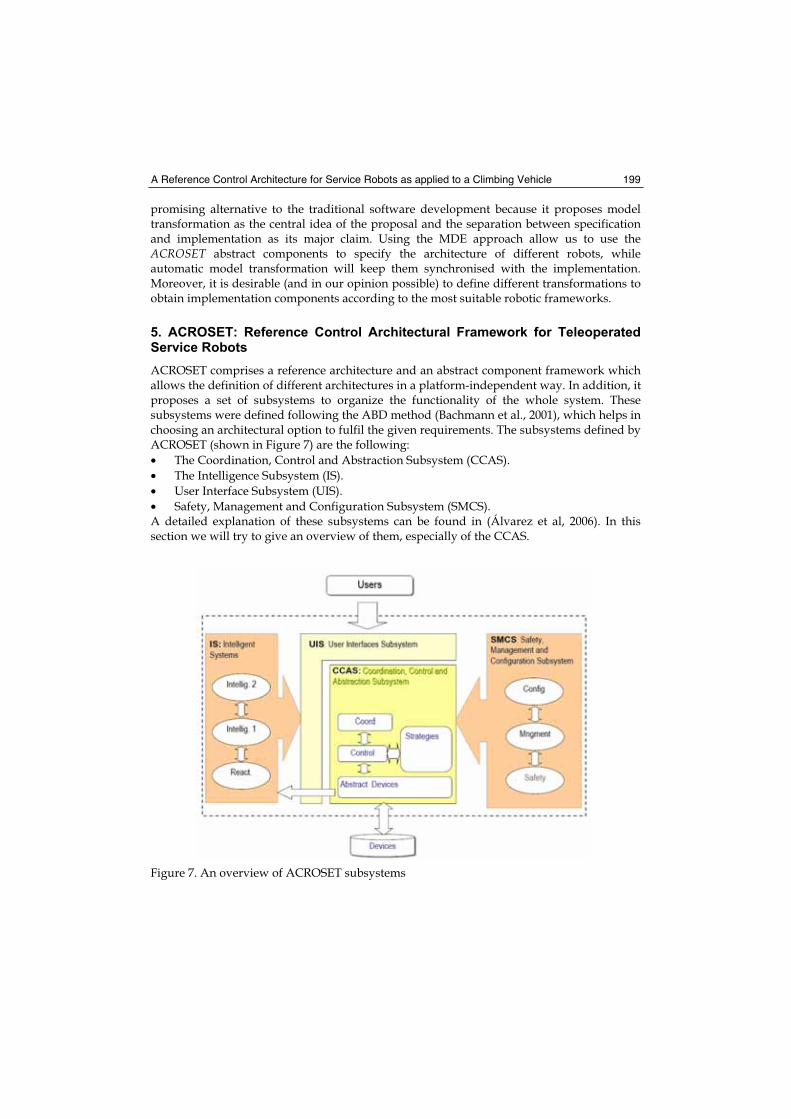
A Reference Control Architecture for Service Robots as applied to a Climbing Vehicle 199
promising alternative to the traditional software development because it proposes model transformation as the central idea of the proposal and the separation between specification and implementation as its major claim. Using the MDE approach allow us to use the ACROSET abstract components to specify the architecture of different robots, while automatic model transformation will keep them synchronised with the implementation. Moreover, it is desirable (and in our opinion possible) to define different transformations to obtain implementation components according to the most suitable robotic frameworks.
5. ACROSET: Reference Control Architectural Framework for Teleoperated Service Robots
ACROSET comprises a reference architecture and an abstract component framework which allows the definition of different architectures in a platform-independent way. In addition, it proposes a set of subsystems to organize the functionality of the whole system. These subsystems were defined following the ABD method (Bachmann et al., 2001), which helps in choosing an architectural option to fulfil the given requirements. The subsystems defined by ACROSET (shown in Figure 7) are the following:
• The Coordination, Control and Abstraction Subsystem (CCAS).
• The Intelligence Subsystem (IS).
• User Interface Subsystem (UIS).
• Safety, Management and Configuration Subsystem (SMCS). A detailed explanation of these subsystems can be found in (Álvarez et al, 2006). In this section we will try to give an overview of them, especially of the CCAS.
Figure 7. An overview of ACROSET subsystems

Bioinspiration and Robotics: Walking and Climbing Robots 200
The CCAS subsystem abstracts and encapsulates the functionality of the system’s physical devices. This subsystem breaks down into a hierarchy of control components that model the different control loops inside a robot. The (abstract) components can be finally implemented in either software or hardware, but all the components of the CCAS and their relationships are independent of the final implementation. Thus, as section 6 will show, the same (abstract) architecture can be reused in different platforms. The Intelligence Subsystem (IS) allows the integration of components that perform (semi-) autonomous operations and act as another user of the CCAS functionality. The CCAS is well suited for operator-driven systems and systems where the reactive or autonomous behaviour responds to simple rules that can be added to CCAS. However, there are systems where the autonomous behaviour is anything but simple. In such cases, the intelligent component needs to integrate more information than that which is embedded in a given component. The approach adopted in ACROSET is to superimpose “intelligent” autonomous behaviour and operator-driven behaviour, and to provide the means to integrate both and resolve the potential conflicts by means of “arbitration” components (which can also be considered complex connectors). This separation between intelligence and functionality enhances the modifiability and adaptability of the system to new missions and behaviours, but compel us to define a subsystem that mediates between the intelligence subsystems and functionality provided by CCAS, the UIS. The User Interface Subsystem (UIS) is intended to interpret, combine and arbitrate between orders that may come simultaneously from different users of the CCAS. These users can be human operators or the “intelligent subsystems” of the IS. The CCAS does not concern itself with the source of the order. In the simplest systems, the UIS simply separates the control logic from the user interfaces facilitating the addition and the change of man-machine interfaces. In the most complex cases the UIS includes special components, that we call arbitrators, which merge commands coming from several sources following different strategies (to select the right source depending on the control mode, merge behaviours, etc.) and provide a unique command to the CCAS components that remain unchanged. The Safety, Management and Configuration Subsystem (SMCS) manages and configures the application and separates the functionality per se from the monitoring of such functionality. The SMCS is connected directly to CCAS without the mediation of the UIS.
5.1 Components of the CCAS
The Coordination, Control and Abstraction Subsystem (CCAS) comprises a set of components that encapsulate the functionality of the control unit of a robot. They are defined in four levels of granularity:
• Hardware Abstraction Layer.
• SCs: Simple Controllers.
• MCs: Mechanisms Controllers.
• RCs: Robot Controllers. A very simple CCAS is shown in Fig. 8. The notation used makes explicit the components, ports and connectors and it is inspired by the 4 views of Hofmeister (Hofmeister et al., 2000) and ROOM (Selic et al., 1994). The simplest components modelled by ACROSET are sensors and actuators, which are encapsulated in the Hardware Abstraction Layer. This layer abstracts the main
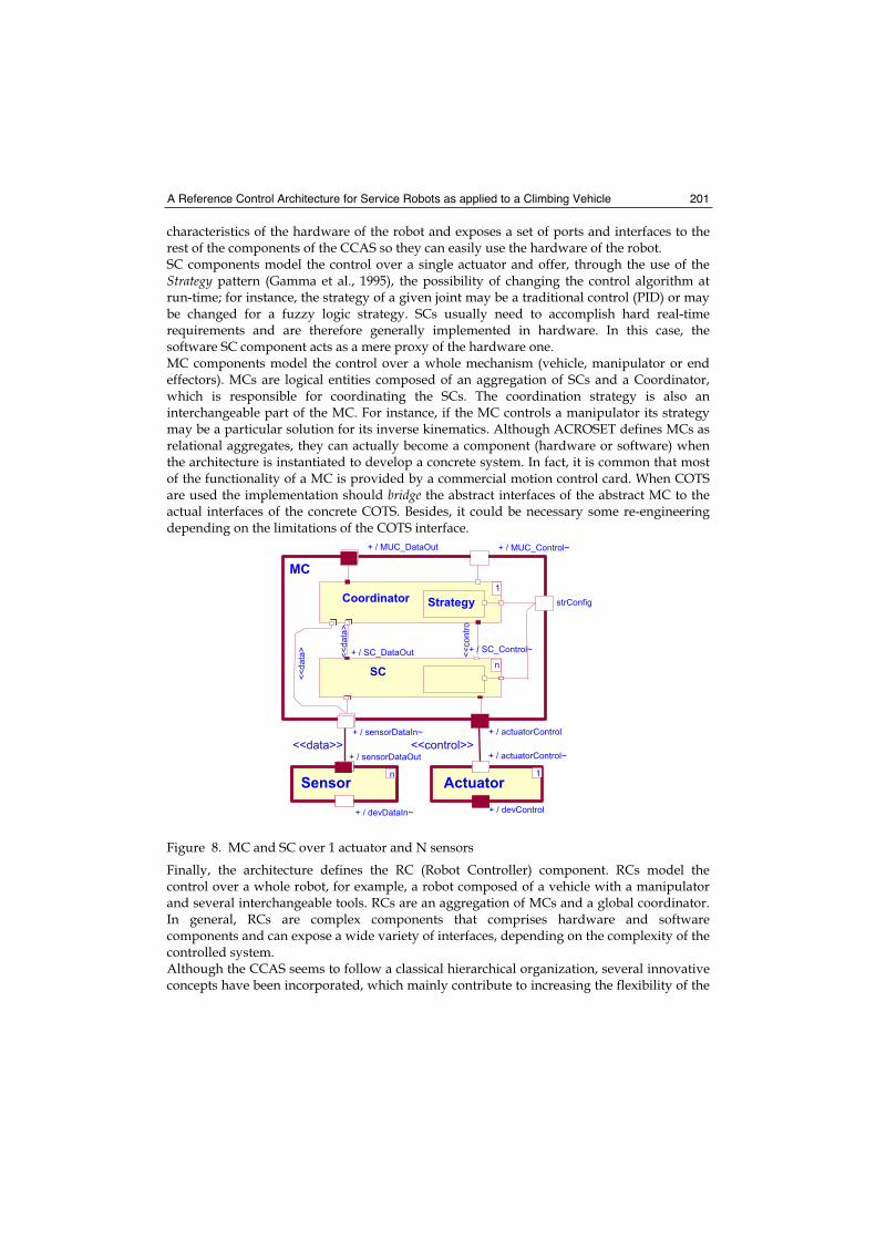
A Reference Control Architecture for Service Robots as applied to a Climbing Vehicle 201
characteristics of the hardware of the robot and exposes a set of ports and interfaces to the rest of the components of the CCAS so they can easily use the hardware of the robot. SC components model the control over a single actuator and offer, through the use of the Strategy pattern (Gamma et al., 1995), the possibility of changing the control algorithm at run-time; for instance, the strategy of a given joint may be a traditional control (PID) or may be changed for a fuzzy logic strategy. SCs usually need to accomplish hard real-time requirements and are therefore generally implemented in hardware. In this case, the software SC component acts as a mere proxy of the hardware one. MC components model the control over a whole mechanism (vehicle, manipulator or end effectors). MCs are logical entities composed of an aggregation of SCs and a Coordinator, which is responsible for coordinating the SCs. The coordination strategy is also an interchangeable part of the MC. For instance, if the MC controls a manipulator its strategy may be a particular solution for its inverse kinematics. Although ACROSET defines MCs as relational aggregates, they can actually become a component (hardware or software) when the architecture is instantiated to develop a concrete system. In fact, it is common that most of the functionality of a MC is provided by a commercial motion control card. When COTS are used the implementation should bridge the abstract interfaces of the abstract MC to the actual interfaces of the concrete COTS. Besides, it could be necessary some re-engineering depending on the limitations of the COTS interface.
Figure 8. MC and SC over 1 actuator and N sensors
Finally, the architecture defines the RC (Robot Controller) component. RCs model the control over a whole robot, for example, a robot composed of a vehicle with a manipulator and several interchangeable tools. RCs are an aggregation of MCs and a global coordinator. In general, RCs are complex components that comprises hardware and software components and can expose a wide variety of interfaces, depending on the complexity of the controlled system. Although the CCAS seems to follow a classical hierarchical organization, several innovative concepts have been incorporated, which mainly contribute to increasing the flexibility of the
strConfig
+ / MUC_Control~
Coordinator
+ / MUC_DataOut
MC
+ / SC_Control~+ / SC_DataOut
<<
da
ta>
<<
da
ta>
<<
co
ntr
o
l
+ / sensorDataIn~ + / actuatorControl
+ / devDataIn~
+ / sensorDataOut + / actuatorControl~
+ / devControl
<<data>> <<control>>
ActuatorSensorn 1
Strategy
1
SCn
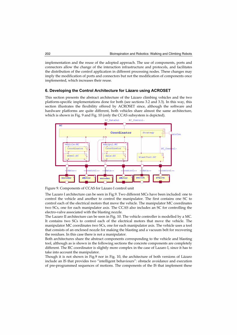
Bioinspiration and Robotics: Walking and Climbing Robots 202
implementation and the reuse of the adopted approach. The use of components, ports and connectors allow the change of the interaction infrastructure and protocols, and facilitates the distribution of the control application in different processing nodes. These changes may imply the modification of ports and connectors but not the modification of components once implemented, which increases their reuse.
6. Developing the Control Architecture for Lázaro using ACROSET
This section presents the abstract architecture of the Lázaro climbing vehicles and the two platform-specific implementations done for both (see sections 3.2 and 3.3). In this way, this section illustrates the flexibility offered by ACROSET since, although the software and hardware platforms are quite different, both vehicles share almost the same architecture, which is shown in Fig. 9 and Fig. 10 (only the CCAS subsystem is depicted).
Figure 9. Components of CCAS for Lázaro I control unit
The Lazaro I architecture can be seen in Fig.9. Two different MCs have been included: one to control the vehicle and another to control the manipulator. The first contains one SC to control each of the electrical motors that move the vehicle. The manipulator MC coordinates two SCs, one for each manipulator axis. The CCAS also includes an SC for controlling the electro-valve associated with the blasting nozzle. The Lazaro II architecture can be seen in Fig. 10. The vehicle controller is modelled by a MC. It contains two SCs to control each of the electrical motors that move the vehicle. The manipulator MC coordinates two SCs, one for each manipulator axis. The vehicle uses a tool that consists of an enclosed nozzle for making the blasting and a vacuum belt for recovering the residues. In this case there is not a manipulator. Both architectures share the abstract components corresponding to the vehicle and blasting tool, although as is shown in the following sections the concrete components are completely different. The RC coordinator is slightly more complex in the case of Lazaro I, since it has to take into account the manipulator. Though it is not shown in Fig.9 nor in Fig. 10, the architecture of both versions of Lázaro include an IS that provides two “intelligent behaviours”: obstacle avoidance and execution of pre-programmed sequences of motions. The components of the IS that implement these
<<control>>
eValve 1
RC_Control~
Coordinator
RC_DataOut
SC_Control~
strCon Strategy
<<data>>
switch 1
manipul:MC
1
1
blastTool:SC1
<<data>>
2encoder
Axis:SC 2
Coordinator 1
vehicle:MC 1
wheel:SC 2
Coordinator 1
<<data>> <<control>>
eMotor encoder 2 2
<<control>>
eMotor 2
RC
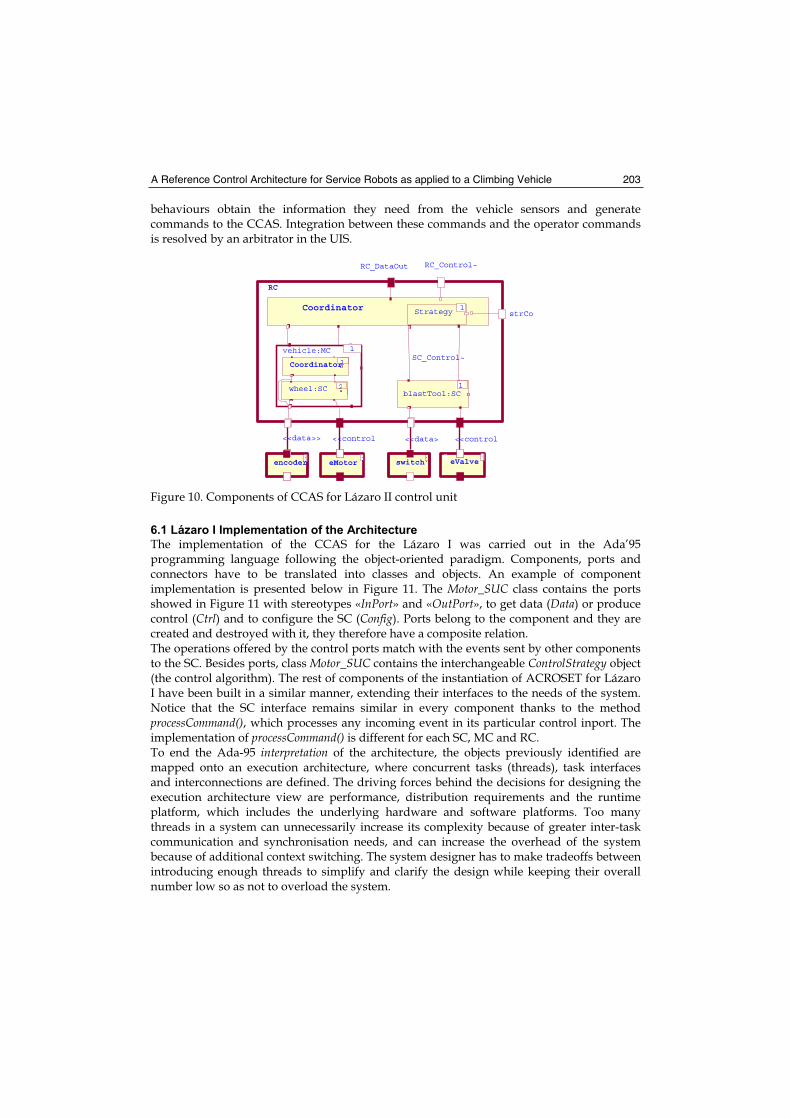
A Reference Control Architecture for Service Robots as applied to a Climbing Vehicle 203
behaviours obtain the information they need from the vehicle sensors and generate commands to the CCAS. Integration between these commands and the operator commands is resolved by an arbitrator in the UIS.
Figure 10. Components of CCAS for Lázaro II control unit
6.1 Lázaro I Implementation of the Architecture
The implementation of the CCAS for the Lázaro I was carried out in the Ada’95 programming language following the object-oriented paradigm. Components, ports and connectors have to be translated into classes and objects. An example of component implementation is presented below in Figure 11. The Motor_SUC class contains the ports showed in Figure 11 with stereotypes «InPort» and «OutPort», to get data (Data) or produce control (Ctrl) and to configure the SC (Config). Ports belong to the component and they are created and destroyed with it, they therefore have a composite relation. The operations offered by the control ports match with the events sent by other components to the SC. Besides ports, class Motor_SUC contains the interchangeable ControlStrategy object (the control algorithm). The rest of components of the instantiation of ACROSET for Lázaro I have been built in a similar manner, extending their interfaces to the needs of the system. Notice that the SC interface remains similar in every component thanks to the method processCommand(), which processes any incoming event in its particular control inport. The implementation of processCommand() is different for each SC, MC and RC. To end the Ada-95 interpretation of the architecture, the objects previously identified are mapped onto an execution architecture, where concurrent tasks (threads), task interfaces and interconnections are defined. The driving forces behind the decisions for designing the execution architecture view are performance, distribution requirements and the runtime platform, which includes the underlying hardware and software platforms. Too many threads in a system can unnecessarily increase its complexity because of greater inter-task communication and synchronisation needs, and can increase the overhead of the system because of additional context switching. The system designer has to make tradeoffs between introducing enough threads to simplify and clarify the design while keeping their overall number low so as not to overload the system.
RC_Control~
Coordinator
RC_DataOut
SC_Control~
strCo
vehicle:MC 1
wheel:SC 2
Coordinator1
<<data>> <<control
eMotorencoder2 2
<<control
1
Strategy
<<data>>
switch1
1
blastTool:SC1
RC
eValve
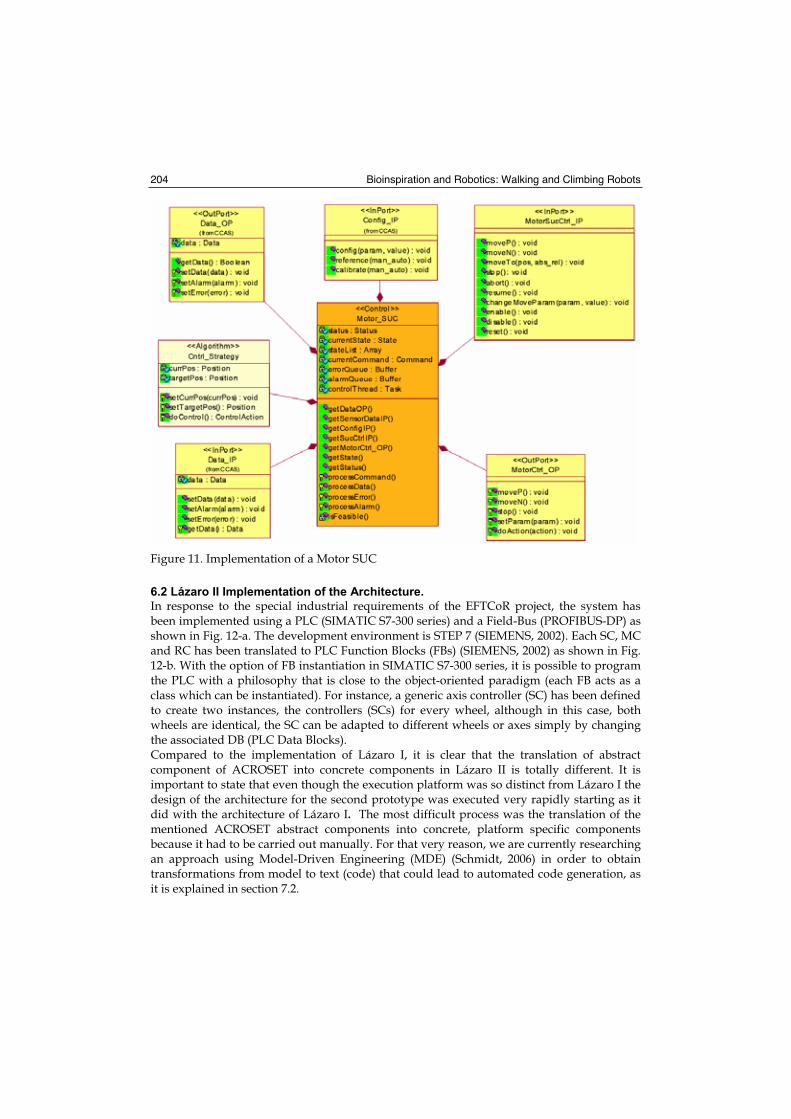
Bioinspiration and Robotics: Walking and Climbing Robots 204
Figure 11. Implementation of a Motor SUC
6.2 Lázaro II Implementation of the Architecture.
In response to the special industrial requirements of the EFTCoR project, the system has been implemented using a PLC (SIMATIC S7-300 series) and a Field-Bus (PROFIBUS-DP) as shown in Fig. 12-a. The development environment is STEP 7 (SIEMENS, 2002). Each SC, MC and RC has been translated to PLC Function Blocks (FBs) (SIEMENS, 2002) as shown in Fig. 12-b. With the option of FB instantiation in SIMATIC S7-300 series, it is possible to program the PLC with a philosophy that is close to the object-oriented paradigm (each FB acts as a class which can be instantiated). For instance, a generic axis controller (SC) has been defined to create two instances, the controllers (SCs) for every wheel, although in this case, both wheels are identical, the SC can be adapted to different wheels or axes simply by changing the associated DB (PLC Data Blocks). Compared to the implementation of Lázaro I, it is clear that the translation of abstract component of ACROSET into concrete components in Lázaro II is totally different. It is important to state that even though the execution platform was so distinct from Lázaro I the design of the architecture for the second prototype was executed very rapidly starting as it did with the architecture of Lázaro I. The most difficult process was the translation of the mentioned ACROSET abstract components into concrete, platform specific components because it had to be carried out manually. For that very reason, we are currently researching an approach using Model-Driven Engineering (MDE) (Schmidt, 2006) in order to obtain transformations from model to text (code) that could lead to automated code generation, as it is explained in section 7.2.
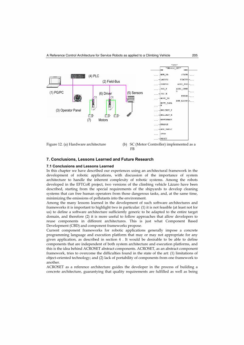
A Reference Control Architecture for Service Robots as applied to a Climbing Vehicle 205
Figure 12. (a) Hardware architecture (b) SC (Motor Controller) implemented as a FB
7. Conclusions, Lessons Learned and Future Research
7.1 Conclusions and Lessons Learned
In this chapter we have described our experiences using an architectural framework in the development of robotic applications, with discussion of the importance of system architecture to handle the inherent complexity of robotic systems. Among the robots developed in the EFTCoR project, two versions of the climbing vehicle Lázaro have been described, starting from the special requirements of the shipyards to develop cleaning systems that can free human operators from those dangerous tasks, and, at the same time, minimizing the emissions of pollutants into the environment. Among the many lessons learned in the development of such software architectures and frameworks it is important to highlight two in particular: (1) it is not feasible (at least not for us) to define a software architecture sufficiently generic to be adapted to the entire target domain, and therefore (2) it is more useful to follow approaches that allow developers to reuse components in different architectures. This is just what Component Based Development (CBD) and component frameworks propose. Current component frameworks for robotic applications generally impose a concrete programming language and execution platform that may or may not appropriate for any given application, as described in section 4 . It would be desirable to be able to define components that are independent of both system architecture and execution platforms, and this is the idea behind ACROSET abstract components. ACROSET, as an abstract component framework, tries to overcome the difficulties found in the state of the art: (1) limitations of object-oriented technology; and (2) lack of portability of components from one framework to another.ACROSET as a reference architecture guides the developer in the process of building a concrete architecture, guarantying that quality requirements are fulfilled as well as being
(1) PG/PC
(2) Field-Bus
(3) Operator Panel
(4) PLC
(5) Sensors (6) Driver
(7) Motors
Bioinspiration and Robotics: Walking and Climbing Robots 206
flexible enough to combine different components inside these subsystems. In addition it does not restrict the level of granularity that must be reached in every implementation. With regard to the implementation of the architecture into different execution platform, section six demonstrated the way in which a similar definition of abstract components for two prototypes can be translated into very different implementations. ACROSET components are defined at a high enough level of abstraction to allow different implementations on different execution platforms, programming languages or hardware/software partitions (software objects, PLC function blocks, hardware components, COTS, etc). It is even relatively easy to distribute some software components to different processing nodes keeping the same conceptual model of the architecture, by simply changing the connectors between such components.
7.2 Future Research
Although the capacity offered by ACROSET for describing the robotic systems architecture has been very valuable, the translation of the ACROSET abstract components into concrete, platform specific components has been a difficult and error prone task. Therefore, after this experience, we believe that an approach like ACROSET will only show its full potential if a way of automatically translating abstract components into concrete components is found. The adoption of the Model-Driven Engineering (MDE) (Schmidt, 2006) approach is a key step to achieve this goal. Currently, a MDE approach to developing the software architecture of robotic systems based on the abstract components proposed by ACROSET is being adopted. The tools and standards developed by the OMG allow us to design the architecture of a robot at a high level of abstraction and in a platform-independent way, and to successively transform these models until we obtain a textual representation (code generation), ready for compilation. By designing different transformations it will also be possible to map the ACROSET components to different robotic frameworks when needed. Although this work is still at an early stage, the results we have already obtained are more than promising.
8. References
Álvarez B.; Sánchez P.; Pastor J.A.; & Ortiz F. (2006). An Architectural Framework for Modeling Teleoperated Service Robots, ROBOTICA - International Journal of Information, Education and Research in Robotics and Artificial Intelligence ISSN 0263-5747, Cambridge University Press. Vol. 24, No. 04, pp. 411-418. July 2006.
Barbanov, M. (1997). A Linux-based Real-Time Operating System. PhD thesis, New Mexico Institute of Mining and Technology, June 1997.
Bézivin, J. (2005). On the Unification Power of Models. Journal of Software and Systems Modeling, Vol. 4, No. 2, pp. 171–188. doi: 10.1007/s10270-005-0079-0.
Brooks, A.; Kaupp, T.; Makarenko, A., Williams, S. & Oreback, A. (2005). Towards Component-Based Robotics. IEEE/RSJ International Conference on Intelligent Robots and Systems., pp 163- 168, Aug. 2005.
Bruyninckx, H.; Konincks, B. & Soetens, P. (2002). A Software Framework for Advanced Motion Control, Dpt. of Mechanical Engineering, K.U. Leuven. OROCOS project inside EURON. Belgium.
A Reference Control Architecture for Service Robots as applied to a Climbing Vehicle 207
Coste-Manière, E. & Simmons, R. (2000). Architecture, the Backbone of Robotic System, Proceedings of the 2000 IEEE International Conference on Robotics & Automation, pp. 505-513, April 2000, San Francisco, USA.
EFTCoR (2002) Environmentally Friendly and Cost-Effective Technology for Coating Removal (EFTCOR). Fifth Framework Programme, European Community, Subprogram Growth ref. GRD2-2001-50004, (Oct 2002).
EFTCoR (2005) EFTCoR Offcial Site. http://www.eftcor.com Iborra, A.; Pastor, J.A.; Álvarez, B.; Fernández, C. & Fernández-Meroño, J.M. (2003). Robots
in Radioactive Environments. IEEE Robotics & Automation Magazine. Vol 10, No. 4, pp.12-22. Dec. 2003.
Fernández, C.; Iborra, A.; Álvarez, B.; Pastor, J.A.; Sánchez, P.; Fernández-Meroño, J.M. & Ortega, N. (2005). Co-operative Robots for Hull Blasting in European Shiprepair Industry. IEEE Robotics & Automation Magazine, Nov. 2004. ISSN: 1070-9932
Flowcorp (2006) http://www.flowcorp.com Gamma, E. and Helm, R. and Johnson, R. and Vlissides, J. (1995). Design patterns : elements of
reusable object-oriented software. Ed. Addison-Wesley Proffesional, 1995. ISBN: 0-201-63361-2
Goldie, B. (a) (1999) A comparative look at dry blast units for vertical surfaces, PCE, Jul 1999. Goldie, B. (b) (1999) Comparing robotic units made to clean vertical surfaces with UHP
waterjetting, PCE, Sep 1999. Hofmeister, C.; Nord, R. & Soni, D. (2000). Applied software architecture. Ed. Addison-Wesley,
2000. ISBN: 0-201-32571-3. Hydro-Crawler (2006) http://www.dansk-vandteknik.dk/e_hydro-crawler.htmLuckham, D.; Vera, J. & Meldal, S. (1995). Three Concepts of System Architecture. Technical
Report: CSL-TR-95-674. Stanford University, CA, USA. Montemerlo, N.; Roy, N. & Thrun, S. (2003). Perspectives on standardization in mobile robot
programming: The Carnegie Mellon Navigation (CARMEN) toolkit. In IEEE/RSJ Intl. Workshop on Intelligent Robots and Systems, 2003.
Octopus (2005) http:// www.cybernetix.fr OMG (2007), Object Management Group, Unified Modeling Language (UML)
Superstructure Specification v2.1.1, formal/2007-02-05, 2007. Schmidt, D. (2006): Model-Driven Engineering. IEEE Computer, Vol. 39, No. 2, IEEE
Computer Society. ISSN 0018-9162. doi: 10.1109/MC.2006.58. Scholl, K.U. Albiez, J. & Gassmann, B. (2001) MCA: An Expandable Modular Controller
Architecture, Karlsruhe University, 3rd Real-Time Linux Workshop, Milano, Italy Sendall, S. & Kozaczynski, W. (2003). Model Transformation: The Heart and Soul of Model-
Driven Software Development. IEEE Software, Vol. 20, No. 5, pp. 42-45, IEEE Computer Society. ISSN 0740-7459. doi: 10.1109/MS.2003.1231150.
Shaw, M. & Garlan B. (1996). Software Architecture : Perspective on a emerging discipline. Ed. Prentice Hall, 1996. ISBN 0-131-82957-2.
SIEMENS (2002). SIMATIC - Working with STEP 7 5.2. ref. 6ES7810-4CA06-8BA0. www.siemens.com.
Szyperski, C. (2002). Component Software: Beyond Object-Oriented Programming. Addison-Wesley Professional, 2002. ISBN 0-201-17888-5.
Ultrastrip (2007) http://www.ecospheretech.com/htm/e_rov.htm
Bioinspiration and Robotics: Walking and Climbing Robots 208
Vaughan, R.; Gerkey, B. & Howard, A. (2003). On device abstractions for portable, reusable robot code. In Proc. of the IEEE/RSJ Intl. Conf. On Intelligent Robots and Systems (IROS), 2003.
Volpe, R.; Nesnas, I.; Estlin, T.; Mutz, D.; Petras, R.; & Das, H. (2001). The CLARAty architecture for robotic autonomy. In IEEE Proceedings of the 2001 Aerospace Conference, Vol. 1, pp 121-132, 2001 Montana, USA.
13
Climbing with parallel robots
R. Saltarén, R. Aracil, O. Reinoso1 and E. Yime DISAM Universidad Politécnica de Madrid,
1Departamento de Ingeniería de Sistemas Industriales, Universidad Miguel Hernández Spain
1. Introduction
Inherently, parallel robots present many advantages to climb in comparison with robots that use serial legs. The availability of a great number of redundant degrees of freedom on the climbing robots with legs does not necessarily increase the ability of those types of machine to progress in a complex workspace. The serial legs mechanisms have a sequential configuration that imposes high torques on the actuators placed on the base. Therefore, the architecture of serial legs of some climbing robots implies a limit on load capability. In contrast with the limitations of the climbing robots with legs, the use of a Gough–Stewart platform as a climbing robot (Stewart, 1965), solves many of these limitations and opens a new field of applications for this type of mechanism. In order to emphasize the great performance of the G–S parallel robot as a climbing robot, it is pertinent to remember that this type of parallel robot is based on a simple mechanical concept that consists of two rings (platforms) linked with six linear actuators joined through universal and spherical joints (this type of structure is also referenced as a 6-UPS parallel robot). These characteristics allow obtaining a mechanical structure of light weight and with high stiffness, which is able to reach high velocities and develop big forces with a very important advantage: the low cost of manufacturing (Lazard, 1992)). The forward kinematic of the G–S platform has been previously analyzed for many authors (Husty, 1994) (Dasgupta, 1994). This paper has been developed in based to references (Almonacid, 2003) (Aracil, 2003) (Aracil, 2006) and (Saltaren 2005) and reflects the state of the art of the researchers made by the authors during the last years. The morphology proposed for the parallel G–S platform as climbing robot is shown in Fig. 1(a). The G–S platform is formed by two rings joined with 6 linear actuators as UPS kinematics chains (where the U degrees of freedom belong to a universal joint, P is a prismatic degree of freedom that belongs to the linear actuator and S is the spherical joint) (Saltaren, 2000). The robot assembly around the tubular structure is carried out through a system of hinges. The holding systems are based on a series of grip devices built in each ring. Those grip devices hold the reference ring firmly attached to the tubular structure while the free ring is displaced by the control system. In Fig. 1(b), we show the climbing robot to work on the outside wall of pipes. In this case the platform of Fig. 1(a) is modified by adding two legs on each one of the external rings of the robot. These legs allow fastening one ring to the pipe while the other ring moves along the structure. The external rings can rotate increasing the working space of the robot.
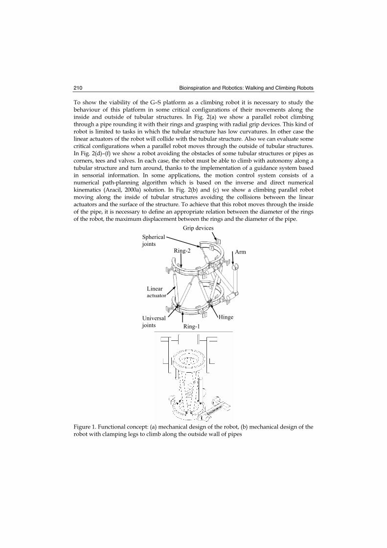
Bioinspiration and Robotics: Walking and Climbing Robots 210
To show the viability of the G–S platform as a climbing robot it is necessary to study the behaviour of this platform in some critical configurations of their movements along the inside and outside of tubular structures. In Fig. 2(a) we show a parallel robot climbing through a pipe rounding it with their rings and grasping with radial grip devices. This kind of robot is limited to tasks in which the tubular structure has low curvatures. In other case the linear actuators of the robot will collide with the tubular structure. Also we can evaluate some critical configurations when a parallel robot moves through the outside of tubular structures. In Fig. 2(d)–(f) we show a robot avoiding the obstacles of some tubular structures or pipes as corners, tees and valves. In each case, the robot must be able to climb with autonomy along a tubular structure and turn around, thanks to the implementation of a guidance system based in sensorial information. In some applications, the motion control system consists of a numerical path-planning algorithm which is based on the inverse and direct numerical kinematics (Aracil, 2000a) solution. In Fig. 2(b) and (c) we show a climbing parallel robot moving along the inside of tubular structures avoiding the collisions between the linear actuators and the surface of the structure. To achieve that this robot moves through the inside of the pipe, it is necessary to define an appropriate relation between the diameter of the rings of the robot, the maximum displacement between the rings and the diameter of the pipe.
Ring-1
Grip devices
Hinge
ArmRing-2
Linear actuator
Universal joints
Sphericaljoints
Figure 1. Functional concept: (a) mechanical design of the robot, (b) mechanical design of the robot with clamping legs to climb along the outside wall of pipes
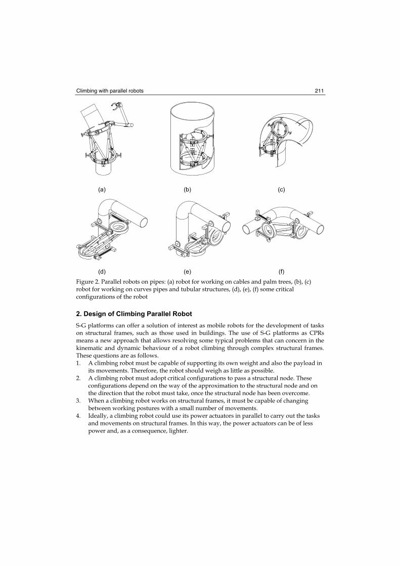
Climbing with parallel robots 211
Figure 2. Parallel robots on pipes: (a) robot for working on cables and palm trees, (b), (c) robot for working on curves pipes and tubular structures, (d), (e), (f) some critical configurations of the robot
2. Design of Climbing Parallel Robot
S-G platforms can offer a solution of interest as mobile robots for the development of tasks on structural frames, such as those used in buildings. The use of S-G platforms as CPRs means a new approach that allows resolving some typical problems that can concern in the kinematic and dynamic behaviour of a robot climbing through complex structural frames. These questions are as follows. 1. A climbing robot must be capable of supporting its own weight and also the payload in
its movements. Therefore, the robot should weigh as little as possible. 2. A climbing robot must adopt critical configurations to pass a structural node. These
configurations depend on the way of the approximation to the structural node and on the direction that the robot must take, once the structural node has been overcome.
3. When a climbing robot works on structural frames, it must be capable of changing between working postures with a small number of movements.
4. Ideally, a climbing robot could use its power actuators in parallel to carry out the tasks and movements on structural frames. In this way, the power actuators can be of less power and, as a consequence, lighter.
Bioinspiration and Robotics: Walking and Climbing Robots 212
3.1 Conceptual Design of the CPR
The morphology proposed for the CPR is based on a parallel platform of six degrees of freedom (DOFs). The main structure of the robot is similar to the classic structure of the parallel robot based on the S-G platform (Stewart, 1965) (Merlet, 1997). This platform consists of two parallel rings linked by six linear actuators as universal–prismatic– spherical (UPS) kinematic chains (where the U DOFs belong to an universal joint, P is a prismatic DOF that belongs to the linear actuator, and S is the spherical joint) (see Fig. 3). In the development of the CPR, it is necessary to carry out some modifications on this platform with the purpose of facilitating the movements of the robot on structural frames. The conceptual design of the robot used to climb along metallic structures is shown in Fig. 1. The robot is constituted by two cylindrical bases: a base or lower ring (Ring-1), and a base or upper ring (Ring-2). These two rings are linked by six linear actuators that allow the displacement between both bases. Over each one of the rings of the robot, an additional exterior rotating ring has been added, allowing turns off. In this way, the robot can orient its legs to facilitate the hold of the robot on the metallic structure. Previous prototypes of this robot have been developed to carry out tasks on pipes and tubular structures (Almonacid, 2003) (Aracil 2003). However, some changes have been added to previous platforms, due to the inherent features of the structural frames in which the robots must work. In contrast to the climbing robot presented in (Saltaren, 2000b) with an interior clamping device to hold and climb by palm trunks and pipes, the clamping devices of the robot to work on structural frames should fold and extend at least in two predetermined positions. The possibility of folding or extending the clamping legs allows reducing possible collisions between the movement ring and the environment. Moreover, in some sequences of displacement, it is necessary to orient the legs of each one of the rings of the robot to predetermined positions (-90º, 0º, +90º), because the rotation of the exterior ring with its clamping device may reduce the rotation requirements of both rings around its axes. In this way, it is possible to avoid singular configurations of the parallel robot, reported by Fichter (Fichter, 2003). For the same reason, it is possible to avoid the collisions between the linear actuators originated when they cross themselves in the displacement of each one of the two rings of the robot.
3.2 Spherical and Universal Joints Adaptations
The robot needs to orient its rings at 90º to accomplish displacements through structural frames. So, with the purpose of allowing configurations of 90º between the rings that constitute the basis of the robot, the spherical and universal joints have been adapted with a new design (Fig. 4 (a), (b)). As we can observe in Fig. 4(b), the new suggestion of the universal joint consists of redesigning in cantilever the junction of the two parts of the classical universal joint. The modified spherical joint is achieved, adding a rotation in the junction of the linear actuator with the universal joint. In Fig. 4(c), a detail of the new modified joints added to the robot is illustrated. With these new joints, the robot can achieve all the necessary postures to carry out the required displacements detailed in the following section. The image shows that the robot can reach configurations of 90º between its rings with the new modified joints.
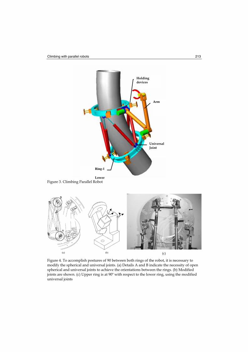
Climbing with parallel robots 213
Figure 3. Climbing Parallel Robot
(c)
Figure 4. To accomplish postures of 90 between both rings of the robot, it is necessary to modify the spherical and universal joints. (a) Details A and B indicate the necessity of open spherical and universal joints to achieve the orientations between the rings. (b) Modified joints are shown. (c) Upper ring is at 90º with respect to the lower ring, using the modified universal joints
Ring-1
Lower
Holdingdevices
Universal Joint
Arm
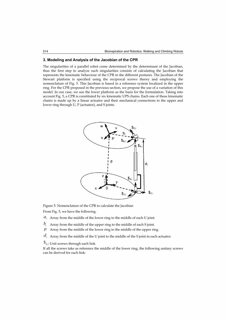
Bioinspiration and Robotics: Walking and Climbing Robots 214
3. Modeling and Analysis of the Jacobian of the CPR
The singularities of a parallel robot come determined by the determinant of the Jacobian, thus the first step to analyze such singularities consists of calculating the Jacobian that represents the kinematic behaviour of the CPR in the different postures. The Jacobian of the Stewart platform is specified using the reciprocal screws theory and employing the nomenclature of Fig. 5. This Jacobian is based in a reference system localized in the upper ring. For the CPR proposed in the previous section, we propose the use of a variation of this model. In our case, we use the lower platform as the basis for the formulation. Taking into account Fig. 5, a CPR is constituted by six kinematic UPS chains. Each one of these kinematic chains is made up by a linear actuator and their mechanical connections to the upper and lower ring through U, P (actuator), and S joints.
Figure 5. Nomenclature of the CPR to calculate the Jacobian
From Fig. 5, we have the following.
ia Array from the middle of the lower ring to the middle of each U joint.
ib Array from the middle of the upper ring to the middle of each S joint.
p Array from the middle of the lower ring to the middle of the upper ring.
id Array from the middle of the U joint to the middle of the S joint in each actuator.
,$n i Unit screws through each link.
If all the screws take as reference the middle of the lower ring, the following unitary screws can be derived for each link:
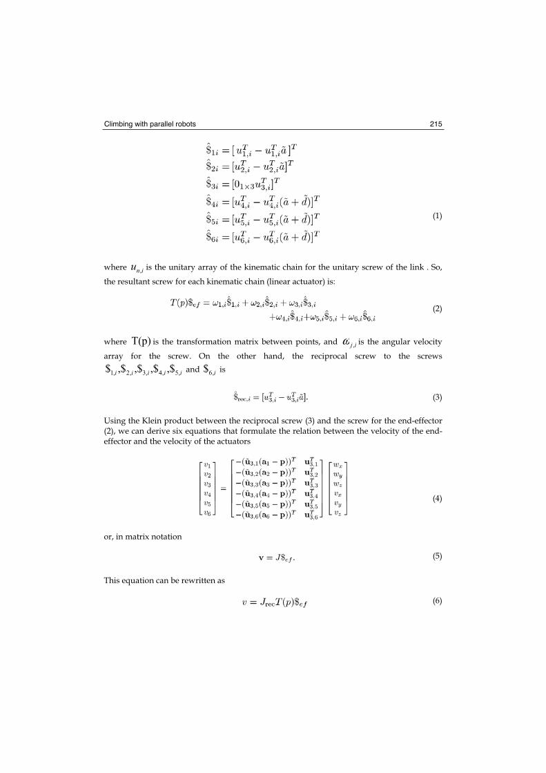
Climbing with parallel robots 215
(1)
where inu , is the unitary array of the kinematic chain for the unitary screw of the link . So,
the resultant screw for each kinematic chain (linear actuator) is:
(2)
where T(p) is the transformation matrix between points, and ij ,ω is the angular velocity
array for the screw. On the other hand, the reciprocal screw to the screws
iiiii ,5,4,3,2,1 ,$,$,$,$$ and i,6$ is
(3)
Using the Klein product between the reciprocal screw (3) and the screw for the end-effector (2), we can derive six equations that formulate the relation between the velocity of the end-effector and the velocity of the actuators
(4)
or, in matrix notation
(5)
This equation can be rewritten as
(6)
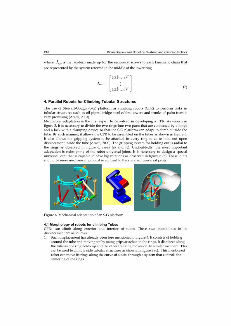
Bioinspiration and Robotics: Walking and Climbing Robots 216
where recJ is the Jacobian made up for the reciprocal screws to each kinematic chain that
are represented by the system referred to the middle of the lower ring
(7)
4. Parallel Robots for Climbing Tubular Structures
The use of Stewart-Gough (S-G) platform as climbing robots (CPR) to perform tasks in tubular structures such as oil pipes, bridge steel cables, towers and trunks of palm trees is very promising (Aracil, 2003). Mechanical adaptation is the first aspect to be solved in developing a CPR. As shown in figure 3, it is necessary to divide the two rings into two parts that are connected by a hinge and a lock with a clamping device so that the S-G platform can adapt to climb outside the tube. By such manner, it allows the CPR to be assembled on the tubes as shown in figure 6. It also allows the gripping system to be attached in every ring so as to hold out upon displacement inside the tube (Aracil, 2000). The gripping system for holding out is radial to the rings as observed in figure 6, cases (a) and (c). Undoubtedly, the most important adaptation is redesigning of the robot universal joints. It is necessary to design a special universal joint that is capable to have big rotations as observed in figure 6 (b). These joints should be more mechanically robust in contrast to the standard universal joints.
Figure 6. Mechanical adaptation of an S-G platform
4.1 Morphology of robots for climbing Tubes
CPRs can climb along exterior and interior of tubes. These two possibilities in its displacement are as follows: 1. Such displacement has already been fore mentioned in figure 3. It consists of holding
around the tube and moving up by using grips attached to the rings. It displaces along the tube as one ring holds up and the other free ring moves on. In similar manner, CPRs can be used to climb inside tubular structures as shown in figure 2 (c). This mentioned robot can move its rings along the curve of a tube through a system that controls the centering of the rings.
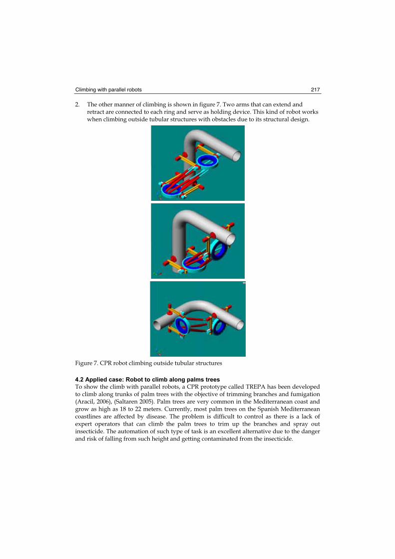
Climbing with parallel robots 217
2. The other manner of climbing is shown in figure 7. Two arms that can extend and retract are connected to each ring and serve as holding device. This kind of robot works when climbing outside tubular structures with obstacles due to its structural design.
Figure 7. CPR robot climbing outside tubular structures
4.2 Applied case: Robot to climb along palms trees
To show the climb with parallel robots, a CPR prototype called TREPA has been developed to climb along trunks of palm trees with the objective of trimming branches and fumigation (Aracil, 2006), (Saltaren 2005). Palm trees are very common in the Mediterranean coast and grow as high as 18 to 22 meters. Currently, most palm trees on the Spanish Mediterranean coastlines are affected by disease. The problem is difficult to control as there is a lack of expert operators that can climb the palm trees to trim up the branches and spray out insecticide. The automation of such type of task is an excellent alternative due to the danger and risk of falling from such height and getting contaminated from the insecticide.
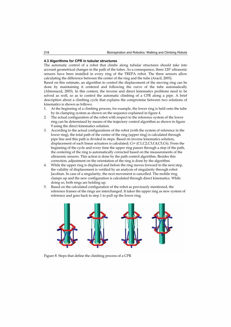
Bioinspiration and Robotics: Walking and Climbing Robots 218
4.3 Algorithms for CPR in tubular structures
The automatic control of a robot that climbs along tubular structures should take into account geometrical changes in the path of the tubes. As a consequence, three 120º ultrasonic sensors have been installed in every ring of the TREPA robot. The three sensors allow calculating the difference between the center of the ring and the tube (Aracil, 2003). Based on this estimate, an algorithm to control the displacement of the moving ring can be done by maintaining it centered and following the curve of the tube automatically (Almonacid, 2003). In this context, the inverse and direct kinematics problems need to be solved as well, so as to control the automatic climbing of a CPR along a pipe. A brief description about a climbing cycle that explains the compromise between two solutions of kinematics is shown as follows. 1. At the beginning of a climbing process, for example, the lower ring is held onto the tube
by its clamping system as shown on the sequence explained in figure 4. 2. The actual configuration of the robot with respect to the reference system of the lower
ring can be determined by means of the trajectory control algorithm as shown in figure 9 using the direct kinematics solution.
3. According to the actual configurations of the robot (with the system of reference in the lower ring), the total path of the center of the ring (upper ring) is calculated through pipe line and this path is divided in steps. Based on inverse kinematics solution, displacement of each linear actuators is calculated; Ci= (C1,C2,C3,C4,C5,C6). From the beginning of the cycle and every time the upper ring passes through a step of the path, the centering of the ring is automatically corrected based on the measurements of the ultrasonic sensors. This action is done by the path control algorithm. Besides this correction, adjustment on the orientation of the ring is done by the algorithm.
4. While the upper ring is displaced and before the ring moves forward to the next step, the validity of displacement is verified by an analysis of singularity through robot Jacobian. In case of a singularity, the next movement is cancelled. The mobile ring clamps up and the new configuration is calculated through direct kinematics. While doing so, both rings are holding up.
5. Based on the calculated configuration of the robot as previously mentioned, the reference frames of the rings are interchanged. It takes the upper ring as new system of reference and goes back to step 1 to pull up the lower ring.
Figure 8. Steps that define the climbing process of a CPR
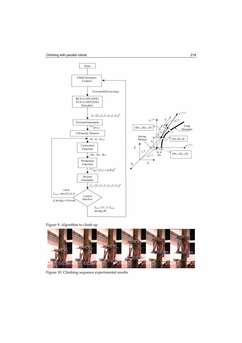
Climbing with parallel robots 219
Li=[L1,L2,L3,L4,L5,L6]T
Start
BCS to ON/(OFF) TCS to OFF/(ON)
Encoders
baseqe49x1
(d1, d2, d3)ef
baseqef =[x,y,z,α,β,γ]T
(Δxi, Δyi, Δ)ef
Correction
Function
Cij=[C1,C2,C3,C4,C5,C6]T
Inverse kinematic
Prediction Function
Control Interface
Ultrasonic Sensors
Lmin ≤ Ci ≤ Lmax
det(φq)≠0
while Lmax- max(Cj)≤ Δ
if det(φq)=0,break
Forward kinematic
Extended(Retracting)
Climb Secuence Control
z’1(i)
Δ
Long Structure
Moving Platform
z’1(i-1)
y’1(i-1)
Δ
Δ
Δyi
(Δxi,Δyi,Δ)
(Δxi+1,Δyi+1,Δ)
(Δxi-1,Δyi-1,Δ)
z’1(i+1)
r1(i)
r1(i-1)
Y
Z
X
ai
Figure 9. Algorithm to climb up
Figure 10. Climbing sequence experimental results
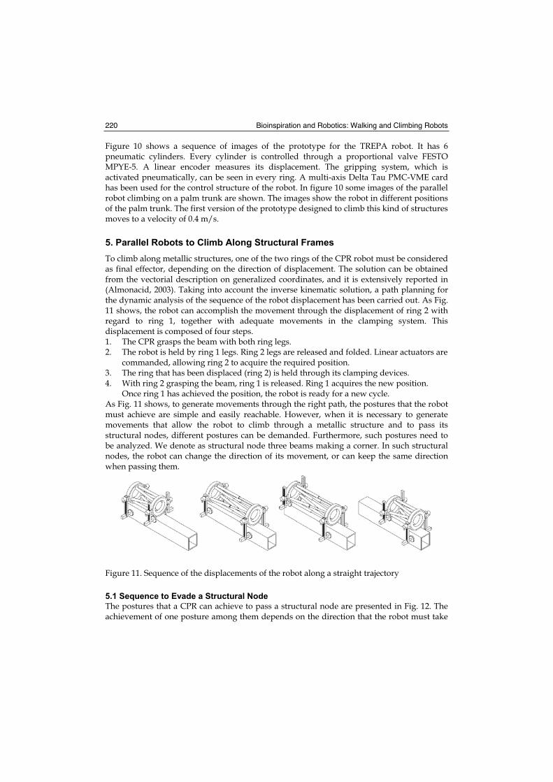
Bioinspiration and Robotics: Walking and Climbing Robots 220
Figure 10 shows a sequence of images of the prototype for the TREPA robot. It has 6 pneumatic cylinders. Every cylinder is controlled through a proportional valve FESTO MPYE-5. A linear encoder measures its displacement. The gripping system, which is activated pneumatically, can be seen in every ring. A multi-axis Delta Tau PMC-VME card has been used for the control structure of the robot. In figure 10 some images of the parallel robot climbing on a palm trunk are shown. The images show the robot in different positions of the palm trunk. The first version of the prototype designed to climb this kind of structures moves to a velocity of 0.4 m/s.
5. Parallel Robots to Climb Along Structural Frames
To climb along metallic structures, one of the two rings of the CPR robot must be considered as final effector, depending on the direction of displacement. The solution can be obtained from the vectorial description on generalized coordinates, and it is extensively reported in (Almonacid, 2003). Taking into account the inverse kinematic solution, a path planning for the dynamic analysis of the sequence of the robot displacement has been carried out. As Fig. 11 shows, the robot can accomplish the movement through the displacement of ring 2 with regard to ring 1, together with adequate movements in the clamping system. This displacement is composed of four steps. 1. The CPR grasps the beam with both ring legs. 2. The robot is held by ring 1 legs. Ring 2 legs are released and folded. Linear actuators are
commanded, allowing ring 2 to acquire the required position. 3. The ring that has been displaced (ring 2) is held through its clamping devices. 4. With ring 2 grasping the beam, ring 1 is released. Ring 1 acquires the new position.
Once ring 1 has achieved the position, the robot is ready for a new cycle. As Fig. 11 shows, to generate movements through the right path, the postures that the robot must achieve are simple and easily reachable. However, when it is necessary to generate movements that allow the robot to climb through a metallic structure and to pass its structural nodes, different postures can be demanded. Furthermore, such postures need to be analyzed. We denote as structural node three beams making a corner. In such structural nodes, the robot can change the direction of its movement, or can keep the same direction when passing them.
Figure 11. Sequence of the displacements of the robot along a straight trajectory
5.1 Sequence to Evade a Structural Node
The postures that a CPR can achieve to pass a structural node are presented in Fig. 12. The achievement of one posture among them depends on the direction that the robot must take
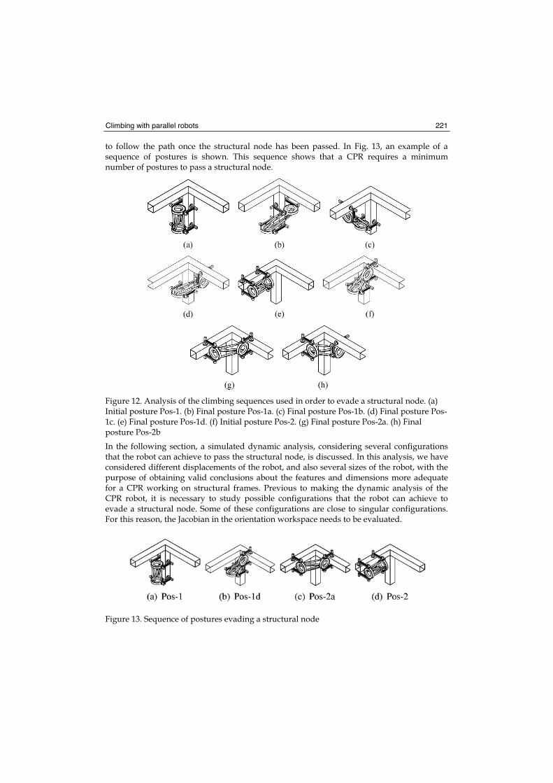
Climbing with parallel robots 221
to follow the path once the structural node has been passed. In Fig. 13, an example of a sequence of postures is shown. This sequence shows that a CPR requires a minimum number of postures to pass a structural node.
Figure 12. Analysis of the climbing sequences used in order to evade a structural node. (a) Initial posture Pos-1. (b) Final posture Pos-1a. (c) Final posture Pos-1b. (d) Final posture Pos-1c. (e) Final posture Pos-1d. (f) Initial posture Pos-2. (g) Final posture Pos-2a. (h) Final posture Pos-2b
In the following section, a simulated dynamic analysis, considering several configurations that the robot can achieve to pass the structural node, is discussed. In this analysis, we have considered different displacements of the robot, and also several sizes of the robot, with the purpose of obtaining valid conclusions about the features and dimensions more adequate for a CPR working on structural frames. Previous to making the dynamic analysis of the CPR robot, it is necessary to study possible configurations that the robot can achieve to evade a structural node. Some of these configurations are close to singular configurations. For this reason, the Jacobian in the orientation workspace needs to be evaluated.
Figure 13. Sequence of postures evading a structural node
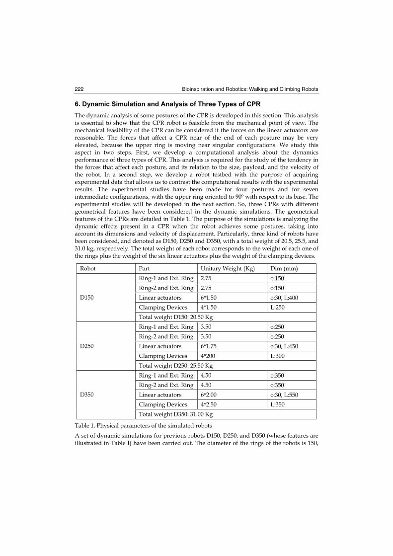
Bioinspiration and Robotics: Walking and Climbing Robots 222
6. Dynamic Simulation and Analysis of Three Types of CPR
The dynamic analysis of some postures of the CPR is developed in this section. This analysis is essential to show that the CPR robot is feasible from the mechanical point of view. The mechanical feasibility of the CPR can be considered if the forces on the linear actuators are reasonable. The forces that affect a CPR near of the end of each posture may be very elevated, because the upper ring is moving near singular configurations. We study this aspect in two steps. First, we develop a computational analysis about the dynamics performance of three types of CPR. This analysis is required for the study of the tendency in the forces that affect each posture, and its relation to the size, payload, and the velocity of the robot. In a second step, we develop a robot testbed with the purpose of acquiring experimental data that allows us to contrast the computational results with the experimental results. The experimental studies have been made for four postures and for seven intermediate configurations, with the upper ring oriented to 90º with respect to its base. The experimental studies will be developed in the next section. So, three CPRs with different geometrical features have been considered in the dynamic simulations. The geometrical features of the CPRs are detailed in Table 1. The purpose of the simulations is analyzing the dynamic effects present in a CPR when the robot achieves some postures, taking into account its dimensions and velocity of displacement. Particularly, three kind of robots have been considered, and denoted as D150, D250 and D350, with a total weight of 20.5, 25.5, and 31.0 kg, respectively. The total weight of each robot corresponds to the weight of each one of the rings plus the weight of the six linear actuators plus the weight of the clamping devices.
Robot Part Unitary Weight (Kg) Dim (mm)
Ring-1 and Ext. Ring 2.75 φ:150
Ring-2 and Ext. Ring 2.75 φ:150
Linear actuators 6*1.50 φ:30, L:400
Clamping Devices 4*1.50 L:250
D150
Total weight D150: 20.50 Kg
Ring-1 and Ext. Ring 3.50 φ:250
Ring-2 and Ext. Ring 3.50 φ:250
Linear actuators 6*1.75 φ:30, L:450
Clamping Devices 4*200 L:300
D250
Total weight D250: 25.50 Kg
Ring-1 and Ext. Ring 4.50 φ:350
Ring-2 and Ext. Ring 4.50 φ:350
Linear actuators 6*2.00 φ:30, L:550
Clamping Devices 4*2.50 L:350
D350
Total weight D350: 31.00 Kg
Table 1. Physical parameters of the simulated robots
A set of dynamic simulations for previous robots D150, D250, and D350 (whose features are illustrated in Table I) have been carried out. The diameter of the rings of the robots is 150,
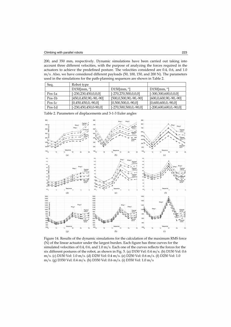
Climbing with parallel robots 223
200, and 350 mm, respectively. Dynamic simulations have been carried out taking into account three different velocities, with the purpose of analyzing the forces required in the actuators to achieve the predefined posture. The velocities considered are 0.4, 0.6, and 1.0 m/s. Also, we have considered different payloads (50, 100, 150, and 200 N). The parameters used in the simulations for the path-planning sequences are shown in Table 2.
Seq. Robot type
D150[mm, º] D150[mm, º] D150[mm, º]
Pos-1a [-230,230,450,0,0,0] [-270,270,500,0,0,0] [-300,300,600,0,0,0]
Pos-1b [450,0,450,90,-90,-90] [500,0,500,90,-90,-90] [600,0,600,90,-90,-90]
Pos-1c [0,450,450,0,-90,0] [0,500,500,0,-90,0] [0,600,600,0,-90,0]
Pos-1d [-230,450,450,0-90,0] [-270,500,500,0,-90,0] [-200,600,600,0,-90,0]
Table 2. Parameters of displacements and 3-1-3 Euler angles
Figure 14. Results of the dynamic simulations for the calculation of the maximum RMS force (N) of the linear actuator under the largest burden. Each figure has three curves for the simulated velocities of 0.4, 0.6, and 1.0 m/s. Each one of the curves reflects the forces for the six different postures of the robot, as shown in Fig. 5. (a) D150 Vel: 0.4 m/s. (b) D150 Vel: 0.6 m/s. (c) D150 Vel: 1.0 m/s. (d) D250 Vel: 0.4 m/s. (e) D250 Vel: 0.6 m/s. (f) D250 Vel: 1.0 m/s. (g) D350 Vel: 0.4 m/s. (h) D350 Vel: 0.6 m/s. (i) D350 Vel: 1.0 m/s
Bioinspiration and Robotics: Walking and Climbing Robots 224
Results of the simulations are shown in Fig. 14. Each one of the graphics in this figure can be explained as follows. 1. The horizontal axis on each graphic corresponds to the postures Pos-1a, Pos-1b, Pos-1c,
Pos-1d, Pos-2a, and Pos-2b. The vertical axis corresponds to the force required in the actuator (in Newtons).
2. Each graphic has three pairs of curves that correspond to the payloads of the robot. Each payload comprises
3. two curves: one for the displacement of the upper ring, and the other one for the displacement of the lower ring. The weight of the rings is not the same, because we have considered the weight of the servos of the linear actuators that are assembled at the end of the linear actuator.
4. The curves have been created evaluating for each posture the maximum root mean square (RMS) force of the more requested linear actuator. For example, for the case of the D150 robot and for a velocity of 0.4 m/s and a payload of 150 N, the maximum RMS force is requested in posture Pos-1d (500 N), considering ring 1 fixed and displacing ring 2.
6.1 Discussion of the simulation results
In this section, the results of simulations made to study the dynamic behavior of the robot in its displacement from an initial position to reach each posture in Fig. 12 are presented. These simulations have been carried out with ADAMS (Adams). Numerous simulations have been carried out with the aim of studying the dynamic performance of the CPR. From Fig. 14, we can observe that for a 0.6 m/s velocity (b,e,h), and for a 1.0 m/s velocity (c,f,i), the displacement of sequence 1d in Fig. 12 requires larger forces in linear actuators. Using the results from Fig. 13, it can be observed that the dynamic results that give rise to the most uniform forces among the six different postures evaluated correspond to the velocity of 0.4 m/s. It is clear that the dynamic performance of the CPR is affected by the magnitude of its displacement sequence and payload, but more strongly by the velocity.
Posture D150 D250 D350 Velocity (m/sec)
Pos-2b 740 800 860 0.4
Pos-1d 750 1100 1100 0.6
Pos-1d 800 1120 1600 1.0
Table 3. Example of maximum forces (in Newton) required by the most requested actuator
From Fig. 12, it can be deduced that for D250 and D350 robots and for 0.6 and 1.0 m/s velocities, sequence 1d is the one that originates higher forces on the linear actuators. Some results of the RMS power, calculated following the data obtained for the higher RMS forces on each one of the cases in Fig. 14, are presented in Table 3. For example, taking into account the values of such graphics, we can deduce the posture Pos-1d as most critical, from a dynamic point of view, when the payload is 200 N. It would be approximately necessary to have a maximum force of 1120N by actuator. Other values of maximum forces required to reach the analyzed postures can be deduced from data presented in Fig. 14, taking into account the payload and the velocity of the robot. However, it can be concluded that posture Pos-1d requires maximum forces in the actuators.
Climbing with parallel robots 225
7. Conclusion
The S-G platform with proper mechanical adaptation could be used for a CPR robot. A CPR has great advantages compared to a serial robot with legs. Advantages, such as high weight payload capacity, are obtainable since the final effectors of the robot are directly connected in parallel to the base through the linear actuators. Consequently, a heavy weight load capacity is essential for a climbing robot, as it must consider carrying its deadweight as well. Weight restriction slows down advancement in the development of climbing robots. The results obtained are quite promising in many ways. 1. First, a parallel robot mechanism is simple and robust. Its deadweight is less than that
of a serial robot designed to perform similar tasks. 2. The simplicity of the parallel robot’s mechanical design is excellent; as it has two rings
connected by six linear actuators though universal and spherical joints. The CPR has overcome two main difficulties. The first is related to the task of climbing along tubes or trees. The development of the experimental prototype and the results show that the parallel robot is able to climb along tubes and stems. This capability is highly regarded when the parallel robot is able to adapt to the structural changes and get around performing its task. The second difficulty is related to climbing structures. The design of climbing robots for structures has 6 DOF; it allows one of the two rings to orient and displace conveniently and hold onto the rails of the metallic structure. To overcome the structural node, the robot must complete some postures that are relatively simple compared to other types of climbing devices. Some problems of singularity in certain orientations inside the working space of the robot can arise. But, on the whole, the climbing sequences and four postures previously mentioned are attainable. In conclusion, CPRs have great advantages that make them more promising than other climbing robots. Some research work in the teleoperation for these devices is being done, along with development of algorithms that will operate the robots semiautomatically in their trajectory when they displace along the tubular or metallic structure.
8. References
ADAMS-10.0. Software simulationa reality, MDI Almonacid, M. ; Saltaren, R. ; Aracil, R. & Reinoso, O. (2003). Motion planning of a climbing
parallel robot, IEEE Transactions on Robotics and Autonomous Systems, Vol. 19, No. 3, pp. 485-489
Aracil, R. ; Saltaren R. ; Almoncacid, M. ; Sabater, J.M. & Azorin, J.M. (2000). Kinematic control for navigation of mobile parallel robots applied to large structures, International Symposium on Automation and Robotics in Construction
Aracil, R. ; Saltaren, R. & Reinoso O. (2003). Parallel robots for autonomous climbing along tubular structures, Robotics and Autonomous Systems, Vol. 42, No. 2, pp. 125-134
Aracil, R. ; Saltaren, R. & Reinoso, O. (2006). A Climbing Parallel Robot: A robot to climb along tubular and metallic structures, IEEE Robotics & Automation Magazine, Vol. 13, No. 1, pp. 16-22
Dasgupta, B. ; Mruthyunjaya, T.S. (1994). A canonical formulation of the direct position kinematics for a general 6-6 Stewart platform, Mechanism and Machine Theory, Vol. 29, No. 6, pp. 819-827
Bioinspiration and Robotics: Walking and Climbing Robots 226
Fichter, E.F. (2003). A Stewart platform-based manipulator: General theory and practical consideration, The International Journal of Robotics Research, Vol. 5, No. 2, pp. 125-134
Hysty, M. L., (1994). An algorithm for solving the direct kinematic of Gough-Stewart type platforms, Rapport de Recherce TR-CIM-94-7, Univ. McGill, Montreal
Merlet, J. (1997). Les robots paralleles, Ed. Hermes Lazard, D. (1992). Stewart Platform and Grobner basis, In ARK Ferrae, pp. 136-142 Saltaren, R. ; Aracil, R. ; Reinoso, O. ; Sabater, J.M. & Almonacid M. (2000a). Parallel climbing
robot for construction, inspection and maintenance, International Symposium on Automation and Robotics in Construction, Madrid, pp. 359-364
Saltaren, R. ; Sabater, J.M. ; Azorin, J.M. ; Reinoso, O. & Aracil, R. (2000b). Research and development of a pneumatic control for a parallel climbing robot, CLAWAR’2000Climbing and Walking Robots, Madrid, Spain, pp. 461-475
Saltaren, R. ; Aracil, R. ; Reinoso, O. & Scarano, M.A. (2005). Parallel Robot: A computational and experimental study of its performance around structural nodes, IEEE Transactions on Robotics, Vol. 21, No. 6, pp. 1056-1066
Stewart, D. (1965). A platform with six degrees of freedom, Proc. Instn Mech. Engrs (Part I), pp. 371-38
14
Gait Synthesis in Legged Robot Locomotion using a CPG-Based Model
J. Cappelletto, P. Estévez, J. C. Grieco, W. Medina-Meléndez and G. Fernández-López
Mechatronics Research Group,Universidad Simón Bolívar Venezuela
1. Introduction
Biology has always been a source of inspiration and ideas for the robotics community. Legged locomotion problem is not an exception, and many experiences have taken ideas from animals, both for morphological and behavioral issues. The first ideas for gait generation came from animal observation, but they were mainly focused on mimicking legs movements. It was not until the nineties that the first relevant works appeared trying to identify the principles behind the generation of those movements in animals. The proposed models were based on neurophysiologic principles, and most of them tried to include characteristics of animal locomotion by the addition of neural networks, dynamic oscillators, or using a set of “movement rules”. Although many models have been suggested, most of them share some common aspects: 1. Motion signals generation and processing are very slow and highly distributed
processes. 2. The brain tends to perform high level feed-forward movement control and prediction. 3. The locomotion system has local feedback, from pressure sensors, force sensors,
intramuscular sensors, etc. In some processes these characteristics are obvious, like in the heart beating or breathing. In these processes there is no need for the intervention of a complex processing unit like the brain, since most of the coordinated oscillatory behavior of the muscles is carried out locally and distributed. The oscillatory nature of locomotion patterns has attracted studies about the existence of a similar structure in charge of this problem. The biologic and electrochemical bases of the system in animals are fairly well explained in the works on neural networks by Hodgkin-Huxley (Hodgkin, 1952). Another important characteristic of animal systems is that biological neural networks can perform timing tasks through oscillatory networks, and also can modulate neuromuscular excitatory signals, thus giving the ability to shape neural network output. Compared to robot legged locomotion, it is possible to identify some common issues like inter-leg coordination that can be thought as a timing system, and the intra-leg actuators coordination that can be addressed as a spatial system. In legged animal locomotion the periodical excitation of the flexor and extensor muscles is needed in order to produce effective walking movements. To model this process, two
Bioinspiration and Robotics: Walking and Climbing Robots 228
different approaches have been developed. The first one, usually called “reflex chain”, lies on the idea of a complex network of joint sensors connected directly to the actuators, so that the muscles were able to detect the right moment to act in order to produce the desired motion. Based on this, it is possible to model many movement processes by using local feedback control networks. The second approach suggest the idea of an oscillating system located at the low level nervous system, that generates timing signals needed to activate the repetitive actions (Marder, 2001; Marder, 2005), which is called central pattern generator.Nowadays, it is widely accepted that motion generation and control processes are performed in the spinal chord by the Central Pattern Generator (CPG). Combining high level brain signals with low level sensory feedback, this system is able to coordinate the neuromuscular excitation in order to achieve desired leg movements. The CPG can be described as a circuit able to produce rhythmic motor patterns in the absence of any external stimuli. This means that a CPG is present when the existence of a rhythmic behavior does not depend of the peripheral or central nervous system signals, although those signals can alter the motor patterns generated by the CPG. There are several works that study the effect of sensory feedback in the modulating action (Conradt, 2003; Kimura, 2002; Kuo, 2002; Ijspeert, 1999). Some authors have proposed to model the CPG using continuous time recurrent neural networks (CTRNN) (Gallagher, 1999; Ghallager, 1999); and it has been proved to be a good choice thanks to the CTRNN ability to model dynamic systems and generating rhythmic responses. Other works are based on neural networks built on leaky integrators which using local feedback of joint angles were able to synthesize different walking modes for simple legged robot models (Billard, 2000). There are some models that generate a CPG through coupled oscillators described by a set of differential equations as the Amplitude Controlled Phase Oscillator (ACPO) concept developed in the BIRG group of EPFL (Buchli, 2004). The modeling of the walking system with CPG has also been employed in non-legged robots, like snake-like robots (Conradt, 2003). It was possible to control a robot with a high number of DOF actuated through servomotors, whose angle references were generated using a distributed CPG synthesized with coupled oscillators. It also must be mentioned the work developed by R. M. Ghigliazza (Ghigliazza, 2004) based on biomechanical locomotion model on insects like cockroaches. They were able to control the support factor and frequency on leg movement by using a reduced model of recurrent networks implemented through coupled oscillators. Many solutions have been proposed for robots with simple leg models, but several key functionalities remain unsolved in a clear way, like coordination of articulations movements for legged robots with medium-high complexity in the kinematical structure and marginally stable platforms like 3 DOF quadrupeds and hexapods. It is also necessary to provide models were temporal reference generation and spatial coordination can be controlled in a separate way mimicking the biological model, and thus giving the ability to apply specific control actions that does not require major modifications on the system architecture when migrating through different legged platforms. This chapter describes a technique for gait synthesis on legged robots by using the Central Pattern Generator (CPG) concept. The work here described bases on separating the walking problem in a temporal coordination and a spatial representations problem. By the addition of a nonlinear space transformation subsystem, it is possible to convert reference vector from the temporal coordination subsystem, into spatial references in the legs workspace, with the capability to manage all the spatial corrections (obstacles, stability problems, direct or inverse kinematics). Sensor feedback can be employed in both subsystems in order to
Gait Synthesis in Legged Robot Locomotion using a CPG-Based Model 229
control actions. The chapter will be organized as follows: an introduction of the state-of-the-art review in robot locomotion models based on CPG; section two will describe the basic system architecture, following the principle of separation into temporal coordination and spatial reference generation subsystems; section 3 describes a first approach for the CPG model using simple time references and FFNN, including experimental setups and results. Sections 4 and 5 introduce two improved models to solve drawbacks observed in the previous model; they are based on coupled oscillators and employing FFNN and parametric trajectory description for the spatial subsystem. Conclusion and future works are shown in section 6, and finally references will be at section 7.
1.1 Review on Legged Robot Locomotion using Central Pattern Generator (CPG).
As described in the previous section, CPG models can be separated on those based on a recurrent neural networks architecture, including leaky integrators, which are models derived of simple Amari-Hopfield oscillator model and CTRNN, and those that relay in coupled differential equations, like ACPO. The model proposed by Chiel, Beer, and Gallagher (Gallagher, 1999) is based con CTRNN, built on neuron nodes which transfer function is given by Equation 1.1.
( )1
, 1,...,M
i i i ji i i ij
y y y I i Mτ ω σ θ=
= − + + + = (1.1)
In the Eq. 1.1 the variable y is the output vector state for the ith neuron. The time constant
associated with the cellular membrane permittivity is represented by τ, while the synaptic
connections weights are represented by ωij. The variable θ is the node bias point. The kernel of the transfer function of each neuron is the standard logistic sigmoid, given by the following Equation:
( ) 1
1 xxe
σ −=+
(1.2)
There are several important characteristics in this particular model of neural networks. The Eq. 1.1 can be interpreted as describing the temporal evolution for the state variable y where it can converge to a single attractor point, multiple attractor point, or a closed attractor cycle. The most used interconnection architecture for this kind of systems is fully bidirectional interconnected networks. The number of neurons N in each network used to be between 3 and 5. Although bigger networks could be implemented to achieve richer dynamics, their analysis complexities make them impractical. The use of Genetic Algorithms (GAs) for the synthesis of parameters for the CPG based on CTRNN was mentioned in Gallagher et al. work. As fitness function, it was used the robot body speed obtained by evaluating the resulting network as a torque reference generator for the leg actuators. The kinematical model employed by Gallagher (Gallagher, 1999) consists in a 2 DOF leg, with two neurons controlling swing (FS and BS), and other neuron controlling the vertical positioning of the foot (FT). Figure 1.1 shows this CPG architecture based on CTRNN. This model provides a direct link between the neural oscillator and the actuator references, and can be modified to other leg kinematics. Satisfactory results have been reported using
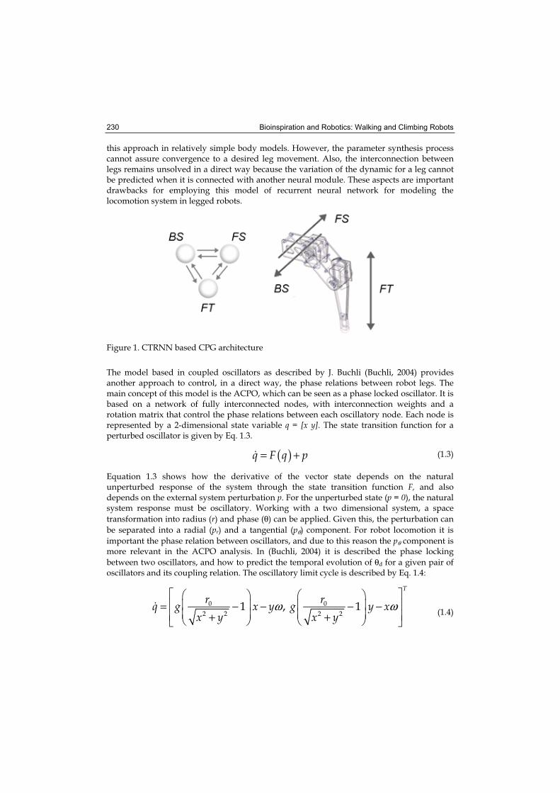
Bioinspiration and Robotics: Walking and Climbing Robots 230
this approach in relatively simple body models. However, the parameter synthesis process cannot assure convergence to a desired leg movement. Also, the interconnection between legs remains unsolved in a direct way because the variation of the dynamic for a leg cannot be predicted when it is connected with another neural module. These aspects are important drawbacks for employing this model of recurrent neural network for modeling the locomotion system in legged robots.
Figure 1. CTRNN based CPG architecture
The model based in coupled oscillators as described by J. Buchli (Buchli, 2004) provides another approach to control, in a direct way, the phase relations between robot legs. The main concept of this model is the ACPO, which can be seen as a phase locked oscillator. It is based on a network of fully interconnected nodes, with interconnection weights and a rotation matrix that control the phase relations between each oscillatory node. Each node is represented by a 2-dimensional state variable q = [x y]. The state transition function for a perturbed oscillator is given by Eq. 1.3.
( )q F q p= + (1.3)
Equation 1.3 shows how the derivative of the vector state depends on the natural unperturbed response of the system through the state transition function F, and also depends on the external system perturbation p. For the unperturbed state (p = 0), the natural system response must be oscillatory. Working with a two dimensional system, a space
transformation into radius (r) and phase (θ) can be applied. Given this, the perturbation can
be separated into a radial (pr) and a tangential (pθ) component. For robot locomotion it is
important the phase relation between oscillators, and due to this reason the pθ component is more relevant in the ACPO analysis. In (Buchli, 2004) it is described the phase locking
between two oscillators, and how to predict the temporal evolution of θd for a given pair of oscillators and its coupling relation. The oscillatory limit cycle is described by Eq. 1.4:
0 0
2 2 2 21 , 1
T
r rq g x y g y xx y x y
ω ω= − − − −+ + (1.4)
Gait Synthesis in Legged Robot Locomotion using a CPG-Based Model 231
For this equation the state vector q converges to a circle of radius ro, with a natural
frequency of ω. The variable g denotes the convergence gain to the limit cycle. Being FACPO(q)the limit cycle described by Eq. 1.4, and modeling the interconnection between nodes like perturbations, the full CPG for a quadruped robot can be described as:
( ) ( ) ( ) ( )( ) ( ) ( ) ( )( ) ( ) ( ) ( )( ) ( ) ( ) ( )
1 1 2 3 4
2 2 3 4 1
3 3 4 1 2
4 4 1 2 3
ACPO c c c
ACPO c c c
ACPO c c c
ACPO c c c
q F q p q p q p qq F q p q p q p qq F q p q p q p qq F q p q p q p q
= + + += + + += + + += + + +
(1.5)
where pc(qi) is the perturbation vector produced by the coupling among each node, and it is obtained by rotating each qi vector according to the desired phase relations between oscillators. It can be observed that this model provides a direct control of oscillatory frequency, and phase relations between legs, however the system outputs are mainly sinusoidal signals that cannot drive joints actuators directly. It is necessary the inclusion of a nonlinear space transformation that converts these phase locked temporal references into useful motor references according to the leg kinematical structure.
2. Proposed Legged Robot Locomotion Models Based on CPG
This section describes different implementations for a CPG based model, with a system architecture that follows the philosophy of separating the walking problem into two different, but not unrelated, spatial and temporal subsystems. This approach is derived from observations of biological systems, where locomotion is associated with rhythmic behavior of neuromuscular activity giving the timing reference, and local modulation is done as consequence of the sensory feedback. Such situation has its analogy with robot locomotion where it is required a control of phase relations between legs, and specific spatial control to cope with leg kinematics and any perturbation due to interaction with the environment. It is important to point out that the spatiotemporal separation allows the implementation of better control schemes because issues like stability, gait modes, weight distribution and others, and can be addressed by applying control actions well developed for standard approaches in robot locomotion. The design process of the locomotion system starts by pointing the desired characteristics for the gait synthesis model, which can be identified as: 1. Reference trajectories for legs: The movement of each leg must describe a continuous
closed shape. Such trajectory consists on a transfer phase and a support phase, which provides the effective propulsion for the robot platform. The spatial references are associated with the leg kinematics and are desirable to be in the actuators space, as joint angles, for example. By controlling this stage it is possible to deal with uneven and irregular terrains.
2. Inter-leg movements coordination: The specific robot gait is given in a direct way by the phase relation between the leg movements. It is desirable that the model provides a way to make soft transitions between different walking modes.
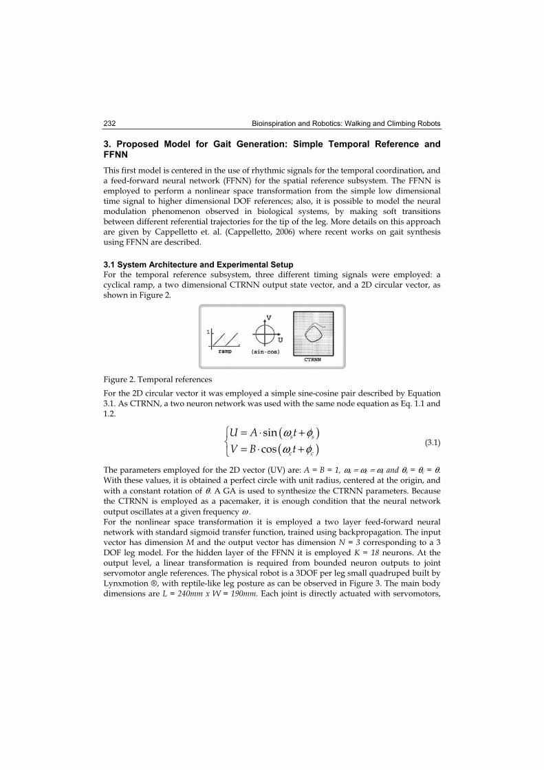
Bioinspiration and Robotics: Walking and Climbing Robots 232
3. Proposed Model for Gait Generation: Simple Temporal Reference and FFNN
This first model is centered in the use of rhythmic signals for the temporal coordination, and a feed-forward neural network (FFNN) for the spatial reference subsystem. The FFNN is employed to perform a nonlinear space transformation from the simple low dimensional time signal to higher dimensional DOF references; also, it is possible to model the neural modulation phenomenon observed in biological systems, by making soft transitions between different referential trajectories for the tip of the leg. More details on this approach are given by Cappelletto et. al. (Cappelletto, 2006) where recent works on gait synthesis using FFNN are described.
3.1 System Architecture and Experimental Setup
For the temporal reference subsystem, three different timing signals were employed: a cyclical ramp, a two dimensional CTRNN output state vector, and a 2D circular vector, as shown in Figure 2.
Figure 2. Temporal references
For the 2D circular vector it was employed a simple sine-cosine pair described by Equation 3.1. As CTRNN, a two neuron network was used with the same node equation as Eq. 1.1 and 1.2.
( )( )
sin
coss s
c c
U A tV B t
ω φω φ
= ⋅ += ⋅ +
(3.1)
The parameters employed for the 2D vector (UV) are: A = B = 1, ωs = ωc = ω, and θs = θc = θ.With these values, it is obtained a perfect circle with unit radius, centered at the origin, and
with a constant rotation of θ. A GA is used to synthesize the CTRNN parameters. Because the CTRNN is employed as a pacemaker, it is enough condition that the neural network
output oscillates at a given frequency ω .For the nonlinear space transformation it is employed a two layer feed-forward neural network with standard sigmoid transfer function, trained using backpropagation. The input vector has dimension M and the output vector has dimension N = 3 corresponding to a 3 DOF leg model. For the hidden layer of the FFNN it is employed K = 18 neurons. At the output level, a linear transformation is required from bounded neuron outputs to joint servomotor angle references. The physical robot is a 3DOF per leg small quadruped built by Lynxmotion ®, with reptile-like leg posture as can be observed in Figure 3. The main body dimensions are L = 240mm x W = 190mm. Each joint is directly actuated with servomotors,
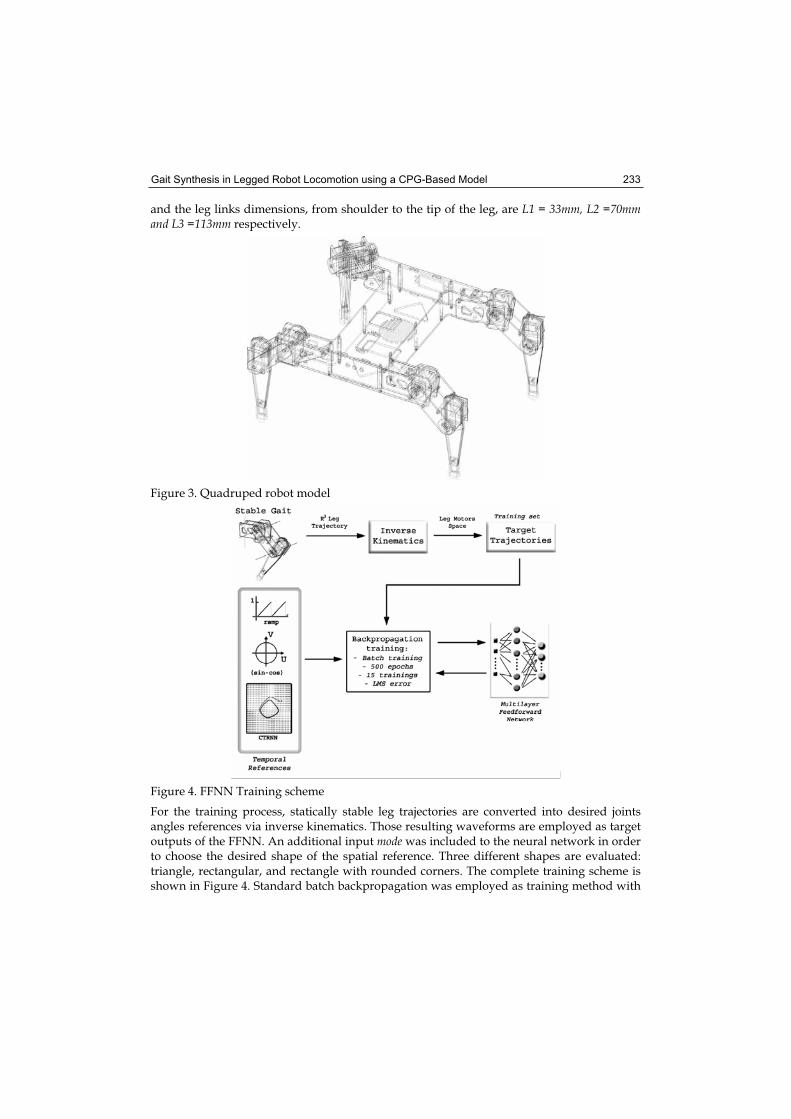
Gait Synthesis in Legged Robot Locomotion using a CPG-Based Model 233
and the leg links dimensions, from shoulder to the tip of the leg, are L1 = 33mm, L2 =70mm and L3 =113mm respectively.
Figure 3. Quadruped robot model
Figure 4. FFNN Training scheme
For the training process, statically stable leg trajectories are converted into desired joints angles references via inverse kinematics. Those resulting waveforms are employed as target outputs of the FFNN. An additional input mode was included to the neural network in order to choose the desired shape of the spatial reference. Three different shapes are evaluated: triangle, rectangular, and rectangle with rounded corners. The complete training scheme is shown in Figure 4. Standard batch backpropagation was employed as training method with
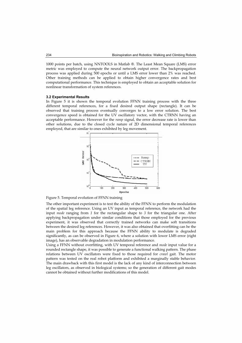
Bioinspiration and Robotics: Walking and Climbing Robots 234
1000 points per batch, using NNTOOLS in Matlab ®. The Least Mean Square (LMS) error metric was employed to compute the neural network output error. The backpropagation process was applied during 500 epochs or until a LMS error lower than 2% was reached. Other training methods can be applied to obtain higher convergence rates and best computational performance. This technique is employed to obtain an acceptable solution for nonlinear transformation of system references.
3.2 Experimental Results
In Figure 5 it is shown the temporal evolution FFNN training process with the three different temporal references, for a fixed desired output shape (rectangle). It can be observed that training process eventually converges to a low error solution. The best convergence speed is obtained for the UV oscillatory vector, with the CTRNN having an acceptable performance. However for the ramp signal, the error decrease rate is lower than other solutions, due to the closed cycle nature of 2D dimensional temporal references employed, that are similar to ones exhibited by leg movement.
Figure 5. Temporal evolution of FFNN training
The other important experiment is to test the ability of the FFNN to perform the modulation of the spatial leg reference. Using an UV input as temporal reference, the network had the input mode ranging from 1 for the rectangular shape to 3 for the triangular one. After applying backpropagation under similar conditions that those employed for the previous experiment, it was observed that correctly trained networks can make soft transitions between the desired leg references. However, it was also obtained that overfitting can be the main problem for this approach because the FFNN ability to modulate is degraded significantly, as can be observed in Figure 6, where a solution with lower LMS error (right image), has an observable degradation in modulation performance. Using a FFNN without overfitting, with UV temporal reference and mode input value for a rounded rectangle shape, it was possible to generate a functional walking pattern. The phase relations between UV oscillators were fixed to those required for crawl gait. The motor pattern was tested on the real robot platform and exhibited a marginally stable behavior. The main drawback with this first model is the lack of any kind of interconnection between leg oscillators, as observed in biological systems; so the generation of different gait modes cannot be obtained without further modifications of this model.
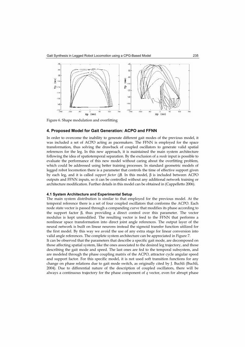
Gait Synthesis in Legged Robot Locomotion using a CPG-Based Model 235
Figure 6. Shape modulation and overfitting
4. Proposed Model for Gait Generation: ACPO and FFNN
In order to overcome the inability to generate different gait modes of the previous model, it was included a set of ACPO acting as pacemakers. The FFNN is employed for the space transformation, thus solving the drawback of coupled oscillators to generate valid spatial references for the leg. In this new approach, it is maintained the main system architecture following the idea of spatiotemporal separation. By the exclusion of a mode input is possible to evaluate the performance of this new model without caring about the overfitting problem, which could be addressed using better training processes. In standard geometric models of legged robot locomotion there is a parameter that controls the time of effective support given
by each leg, and it is called support factor (β). In this model, β is included between ACPO outputs and FFNN inputs, so it can be controlled without any additional network training or architecture modification. Further details in this model can be obtained in (Cappelletto 2006).
4.1 System Architecture and Experimental Setup
The main system distribution is similar to that employed for the previous model. At the temporal reference there is a set of four coupled oscillators that conforms the ACPO. Each node state vector is passed through a companding curve that modifies its phase according to
the support factor β, thus providing a direct control over this parameter. The vector modulus is kept unmodified. The resulting vector is feed to the FFNN that performs a nonlinear space transformation into direct joint angle references. The output layer of the neural network is built on linear neurons instead the sigmoid transfer function utilized for the first model. By this way we avoid the use of any extra stage for linear conversion into valid angle references. The complete system architecture can be appreciated in Figure 7. It can be observed that the parameters that describe a specific gait mode, are decomposed on those affecting spatial system, like the ones associated to the desired leg trajectory, and those describing the gait mode and speed. The last ones are fed to the temporal subsystem, and are modeled through the phase coupling matrix of the ACPO, attractor cycle angular speed and support factor. For this specific model, it is not used soft transition functions for any change on phase relations due to gait mode switch, as originally cited by J. Buchli (Buchli, 2004). Due to differential nature of the description of coupled oscillators, there will be always a continuous trajectory for the phase component of q vector, even for abrupt phase
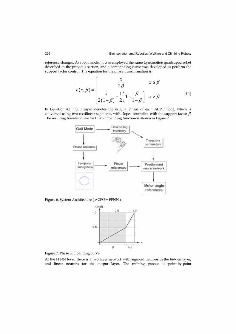
Bioinspiration and Robotics: Walking and Climbing Robots 236
reference changes. As robot model, it was employed the same Lynxmotion quadruped robot described in the previous section, and a companding curve was developed to perform the support factor control. The equation for the phase transformation is:
( )
( )
2,
11
2 1 2 1
x xc x
x x
ββ
ββ β
β β
≤
=+ − >
− −(4.1)
In Equation 4.1, the x input denotes the original phase of each ACPO node, which is
converted using two rectilinear segments, with slopes controlled with the support factor β.The resulting transfer curve for this companding function is shown in Figure 7.
Figure 6. System Architecture ( ACPO + FFNN )
Figure 7. Phase companding curve
At the FFNN level, there is a two layer network with sigmoid neurons in the hidden layer, and linear neurons for the output layer. The training process is point-by-point
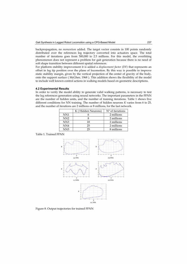
Gait Synthesis in Legged Robot Locomotion using a CPG-Based Model 237
backpropagation, no momentum added. The target vector consists in 100 points randomly distributed over the references leg trajectory converted into actuators space. The total number of iterations goes from 500,000 to 2.5 millions. For this model, the overfitting phenomenon does not represent a problem for gait generation because there is no need of soft shape transition between different spatial references. For platform stability improvement it is added a displacement factor (DF) that represents an offset in leg tip position over the plane of locomotion. By this way is possible to improve static stability margin, given by the vertical projection of the center of gravity of the body, onto the support surface ( McGhee, 1968 ). This addition shows the flexibility of the model to include well known control actions in walking models based on geometric descriptions.
4.2 Experimental Results
In order to verify the model ability to generate valid walking patterns, is necessary to test the leg references generation using neural networks. The important parameters in the FFNN are the number of hidden units, and the number of training iterations. Table 1 shows five different conditions for NN training. The number of hidden neurons K varies from 6 to 25, and the number of iterations are 2 millions or 8 millions, for the last network.
K ( Hidden Neurons) Nº of iterations
NN1 6 2 millions
NN2 8 2 millions
NN3 18 2 millions
NN4 25 2 millions
NN5 25 8 millions
Table 1. Trained FFNN
Figure 8. Output trajectories for trained FFNN
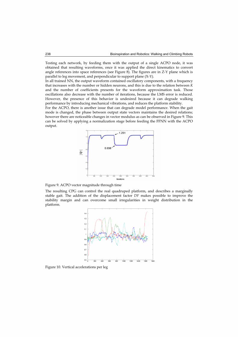
Bioinspiration and Robotics: Walking and Climbing Robots 238
Testing each network, by feeding them with the output of a single ACPO node, it was obtained that resulting waveforms, once it was applied the direct kinematics to convert angle references into space references (see Figure 8). The figures are in Z-Y plane which is parallel to leg movement, and perpendicular to support plane (X-Y). In all trained NN, the output waveform contained oscillatory components, with a frequency that increases with the number or hidden neurons, and this is due to the relation between Kand the number of coefficients presents for the waveform approximation task. Those oscillations also decrease with the number of iterations, because the LMS error is reduced. However, the presence of this behavior is undesired because it can degrade walking performance by introducing mechanical vibrations, and reduces the platform stability. For the ACPO, there is another issue that can degrade model performance. When the gait mode is changed, the phase between output state vectors maintains the desired relations; however there are noticeable changes in vector modulus as can be observed in Figure 9. This can be solved by applying a normalization stage before feeding the FFNN with the ACPO output.
Figure 9. ACPO vector magnitude through time
The resulting CPG can control the real quadruped platform, and describes a marginally stable gait. The addition of the displacement factor DF makes possible to improve the stability margin and can overcome small irregularities in weight distribution in the platform.
Figure 10. Vertical accelerations per leg
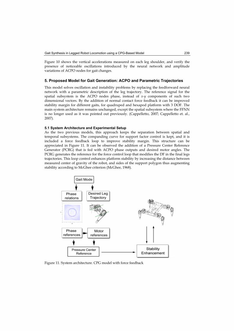
Gait Synthesis in Legged Robot Locomotion using a CPG-Based Model 239
Figure 10 shows the vertical accelerations measured on each leg shoulder, and verify the presence of noticeable oscillations introduced by the neural network and amplitude variations of ACPO nodes for gait changes.
5. Proposed Model for Gait Generation: ACPO and Parametric Trajectories
This model solves oscillation and instability problems by replacing the feedforward neural network with a parametric description of the leg trajectory. The reference signal for the spatial subsystem is the ACPO nodes phase, instead of x-y components of such two dimensional vectors. By the addition of normal contact force feedback it can be improved stability margin for different gaits, for quadruped and hexapod platform with 3 DOF. The main system architecture remains unchanged, except the spatial subsystem where the FFNN is no longer used as it was pointed out previously. (Cappelletto, 2007; Cappelletto et. al., 2007).
5.1 System Architecture and Experimental Setup
As the two previous models, this approach keeps the separation between spatial and temporal subsystems. The companding curve for support factor control is kept, and it is included a force feedback loop to improve stability margin. This structure can be appreciated in Figure 11. It can be observed the addition of a Pressure Center Reference Generator (PCRG) that is fed with ACPO phase outputs and desired motor angles. The PCRG generates the reference for the force control loop that modifies the DF in the final legs trajectories. This loop control enhances platform stability by increasing the distance between measured center of gravity of the robot, and sides of the support polygon thus augmenting stability according to McGhee criterion (McGhee, 1968).
Figure 11. System architecture. CPG model with force feedback
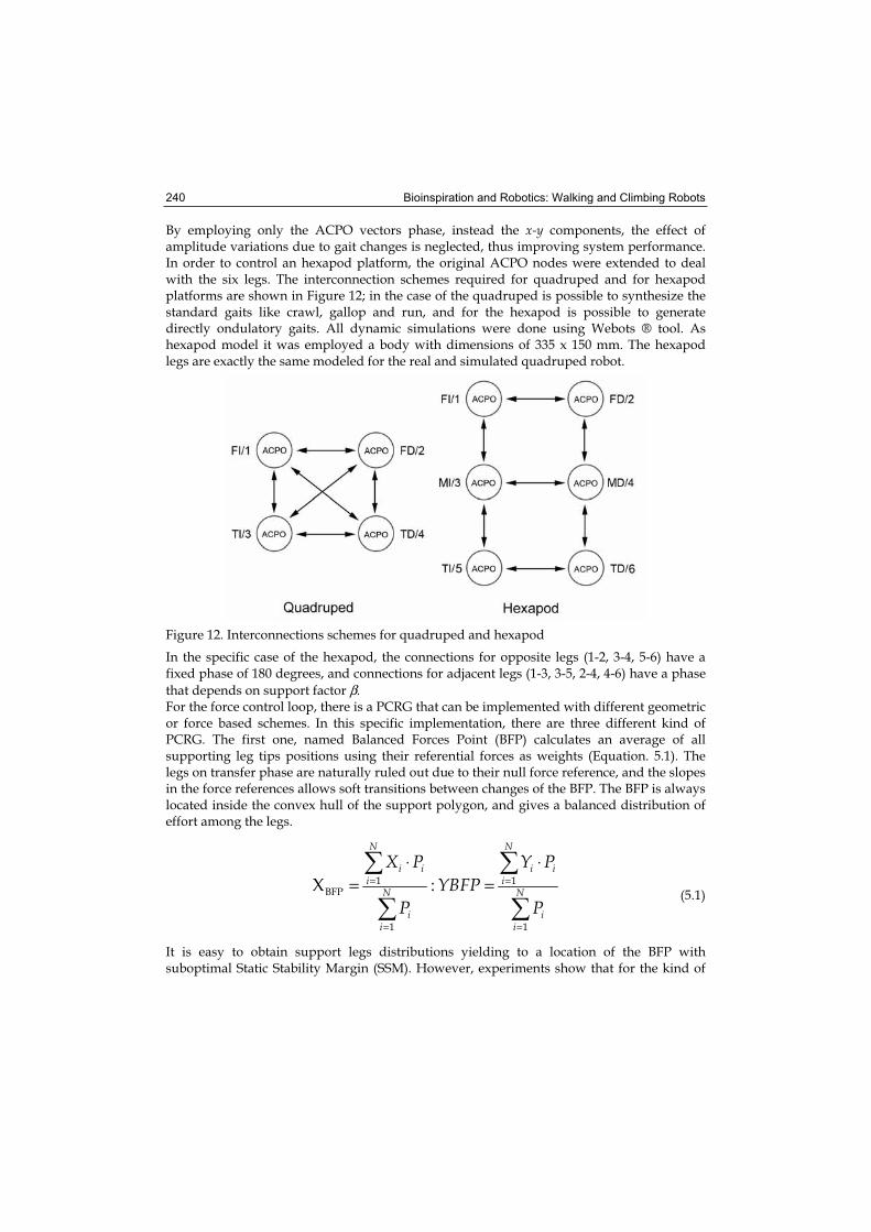
Bioinspiration and Robotics: Walking and Climbing Robots 240
By employing only the ACPO vectors phase, instead the x-y components, the effect of amplitude variations due to gait changes is neglected, thus improving system performance. In order to control an hexapod platform, the original ACPO nodes were extended to deal with the six legs. The interconnection schemes required for quadruped and for hexapod platforms are shown in Figure 12; in the case of the quadruped is possible to synthesize the standard gaits like crawl, gallop and run, and for the hexapod is possible to generate directly ondulatory gaits. All dynamic simulations were done using Webots ® tool. As hexapod model it was employed a body with dimensions of 335 x 150 mm. The hexapod legs are exactly the same modeled for the real and simulated quadruped robot.
Figure 12. Interconnections schemes for quadruped and hexapod
In the specific case of the hexapod, the connections for opposite legs (1-2, 3-4, 5-6) have a fixed phase of 180 degrees, and connections for adjacent legs (1-3, 3-5, 2-4, 4-6) have a phase
that depends on support factor β. For the force control loop, there is a PCRG that can be implemented with different geometric or force based schemes. In this specific implementation, there are three different kind of PCRG. The first one, named Balanced Forces Point (BFP) calculates an average of all supporting leg tips positions using their referential forces as weights (Equation. 5.1). The legs on transfer phase are naturally ruled out due to their null force reference, and the slopes in the force references allows soft transitions between changes of the BFP. The BFP is always located inside the convex hull of the support polygon, and gives a balanced distribution of effort among the legs.
1 1BFP
1 1
X :
N N
i i i ii i
N N
i ii i
X P Y PYBFP
P P= =
= =
⋅ ⋅= =
(5.1)
It is easy to obtain support legs distributions yielding to a location of the BFP with suboptimal Static Stability Margin (SSM). However, experiments show that for the kind of
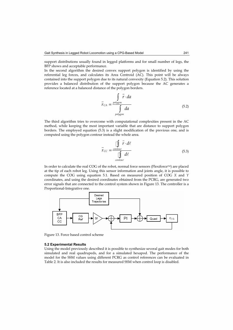
Gait Synthesis in Legged Robot Locomotion using a CPG-Based Model 241
support distributions usually found in legged platforms and for small number of legs, the BFP shows and acceptable performance. In the second algorithm the desired convex support polygon is identified by using the referential leg forces, and calculates its Area Centroid (AC). This point will be always contained into the support polygon due to its natural convexity (Equation 5.2). This solution provides a balanced distribution of the support polygon because the AC generates a reference located at a balanced distance of the polygon borders.
polygonCA
polygon
r dar
da
⋅= (5.2)
The third algorithm tries to overcome with computational complexities present in the AC method, while keeping the most important variable that are distance to support polygon borders. The employed equation (5.3) is a slight modification of the previous one, and is computed using the polygon contour instead the whole area.
contourCC
contour
r dr
d
⋅= (5.3)
In order to calculate the real COG of the robot, normal force sensors (FlexiforceTM) are placed at the tip of each robot leg. Using this sensor information and joints angle, it is possible to compute the COG using equation 5.1. Based on measured position of COG X and Ycoordinates, and using the desired coordinates obtained from the PCRG, are generated two error signals that are connected to the control system shown in Figure 13. The controller is a Proportional-Integrative one.
Figure 13. Force based control scheme
5.2 Experimental Results
Using the model previously described it is possible to synthesize several gait modes for both simulated and real quadrupeds, and for a simulated hexapod. The performance of the model for the SSM values using different PCRG as control references can be evaluated in Table 2. It is also included the results for measured SSM when control loop is disabled.
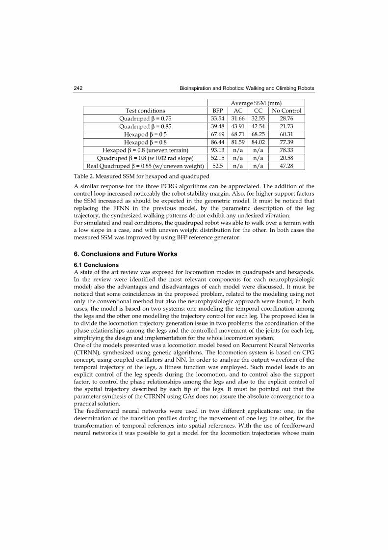
Bioinspiration and Robotics: Walking and Climbing Robots 242
Average SSM (mm)
Test conditions BFP AC CC No Control
Quadruped β = 0.75 33.54 31.66 32.55 28.76
Quadruped β = 0.85 39.48 43.91 42.54 21.73
Hexapod β = 0.5 67.69 68.71 68.25 60.31
Hexapod β = 0.8 86.44 81.59 84.02 77.39
Hexapod β = 0.8 (uneven terrain) 93.13 n/a n/a 78.33
Quadruped β = 0.8 (w 0.02 rad slope) 52.15 n/a n/a 20.58
Real Quadruped β = 0.85 (w/uneven weight) 52.5 n/a n/a 47.28
Table 2. Measured SSM for hexapod and quadruped
A similar response for the three PCRG algorithms can be appreciated. The addition of the control loop increased noticeably the robot stability margin. Also, for higher support factors the SSM increased as should be expected in the geometric model. It must be noticed that replacing the FFNN in the previous model, by the parametric description of the leg trajectory, the synthesized walking patterns do not exhibit any undesired vibration. For simulated and real conditions, the quadruped robot was able to walk over a terrain with a low slope in a case, and with uneven weight distribution for the other. In both cases the measured SSM was improved by using BFP reference generator.
6. Conclusions and Future Works
6.1 Conclusions
A state of the art review was exposed for locomotion modes in quadrupeds and hexapods. In the review were identified the most relevant components for each neurophysiologic model; also the advantages and disadvantages of each model were discussed. It must be noticed that some coincidences in the proposed problem, related to the modeling using not only the conventional method but also the neurophysiologic approach were found; in both cases, the model is based on two systems: one modeling the temporal coordination among the legs and the other one modelling the trajectory control for each leg. The proposed idea is to divide the locomotion trajectory generation issue in two problems: the coordination of the phase relationships among the legs and the controlled movement of the joints for each leg, simplifying the design and implementation for the whole locomotion system. One of the models presented was a locomotion model based on Recurrent Neural Networks (CTRNN), synthesized using genetic algorithms. The locomotion system is based on CPG concept, using coupled oscillators and NN. In order to analyze the output waveform of the temporal trajectory of the legs, a fitness function was employed. Such model leads to an explicit control of the leg speeds during the locomotion, and to control also the support factor, to control the phase relationships among the legs and also to the explicit control of the spatial trajectory described by each tip of the legs. It must be pointed out that the parameter synthesis of the CTRNN using GAs does not assure the absolute convergence to a practical solution. The feedforward neural networks were used in two different applications: one, in the determination of the transition profiles during the movement of one leg; the other, for the transformation of temporal references into spatial references. With the use of feedforward neural networks it was possible to get a model for the locomotion trajectories whose main
Gait Synthesis in Legged Robot Locomotion using a CPG-Based Model 243
structure is independent of the kinematics model of the robot leg. The use of the model directed to get soft transitions among different spatial trajectories of the walking profiles for the 3 DOF legs of a quadruped robot. It has been shown that it is possible to synthesize the desired trajectories for 3DOF quadruped legs using simple feedforward neural networks. It is reasonably expected that this method could be extended to other kind of walking machines after doing the proper modifications of the method. The problem of the modeling of the locomotion system using ACPO was solved using a feedforward neural network connected to the output of the vector states of the coupled oscillators. It must be noticed that the problem of coordination of the movement of one leg using ACPO had not been solved to the present. Coupled oscillators issue with magnitude changes due to gait mode variations was solved by employing only the phase information of the output vector. The problem of margin stability arises for the platform control. To improve the SSM, platform accelerations and ground contact measurements were taken during online operation of robotic platform. It was observed the effects of overfitting in the training of the neural network. Such overfitting produced low amplitude oscillations during walking phase. This is closely related to the number of neuron units in the hidden layer. Special care in this issue is recommended to avoid stability problems in higher speed walking modes. Also it was pointed out the effect that can have neural network on support factor, reducing it due to waveform approximation task. It is suggested to study other neuron function kernels in order to reduce this problem. This parameter, the support factor, is employed in the conventional locomotive geometric model. The parameter is represented here through a companding curve of the phase for the temporal reference of each leg, being completely independent of leg kinematics and specific implementation of temporal subsystem. By including additional control inputs to the network, it could be possible to achieve a higher level control for robot platform variables, like body inclination and weight distribution by the use of accelerometers and ground contact sensors.
6.2 Future works
It is mandatory to review different training methods for the RNN employed to model the locomotion system. Using genetic algorithms it was shown that convergence is not assured. The training methods must use as training samples the spatial trajectories of the joints of each leg of the quadruped. Also, it must be emphasized the feasibility to control the phase relationships among the networks that control each leg of the robot. The problem observed of overfitting in the training stage of the NN must be studied in dependence with the neuron number and the structure of the hidden layer and its influence on stability, vibrations and support factor of the platform. It must be studied the viability to implement the generation of spatial trajectories through coupled differential equations like the ones employed in ACPO. Such implementation must be oriented to generate an attractor space where the state vectors converge to the desired spatial trajectory in order to control each leg. It is relevant to be capable to control the final trajectory of the system with dependence of the parameters employed in the geometric locomotion model. It is needed to study the impact of the variations of magnitude in state vectors of the ACPO during the walking modes transition. Normalization of such vectors or the control of its magnitude during the companding phase must be granted. In this way it could be reduced
Bioinspiration and Robotics: Walking and Climbing Robots 244
the time that the trajectory remains in space points that do not belong to the trajectory training examples of the NN. A variant of the generator proposed based on ACPO, could be studied the performance of the model employing the information provided by the magnitude and angle of the state vectors of the oscillators instead of its {x, y} components. In the near future some different approaches are going to be tested, as combination of gait synthesis using the FFNN with strategies of position-force control on the quadruped leg. With this approach it should be possible to overcome more significant terrain irregularities and other external perturbations.
7. References and Bibliography
Amari S. (1972). Characteristic of the random nets of analog neuron-like elements. IEEE Transaction on System, Man and Cybernetics, SMC-2:643–657.
Ames J. (2003). Design methods for pattern generation circuits. Master´s thesis, Case Western Reserve University.
Arsenio A. M. (200). Tuning of neural oscillators for the design of rhythmic motions. InICRA, pp 1888–1893.
Bares J. E., Whittaker W. L. (1993). Configuration of autonomous walkers for extreme terrain. The International Journal of Robotics Research, 12(6):621–649.
Billard A., Ijspeert A. J. (2000). Biologically inspired neural controllers for motor control in a IEEE-INNS-ENNS International Joint Conference on Neural Networks. Volume VI, pages 637–641. IEEE Computer Society.
Buchli J., Ijspeert A. J. (2004). Distributed central pattern generator model for robotics application based on phase sensitivity analysis. First International Workshop, BioADIT 2004, volume 3141 of Lecture Notes in Computer Science, pp 333–349.
Buchli J., Righetti L., Ijspeert A. J. (2005). A dynamical systems approach to learning: a frequency-adaptive hopper robot. In Proceedings of the VIIIth European Conference on Artificial Life ECAL 2005, LNAI, pp 210–220. Springer Verlag.
Cappelletto J., Estévez P., Medina W., Fermín L., Bogado J. M., Grieco J. C., Fernández G. (2006). Gait synthesis and modulation for quadruped robot locomotion using a simple feed-forward network. In Lecture Notes in Computer Science - 4029, pp 731–739. Springer Berlin / Heidelberg.
Cappelletto J., Estevez P., Grieco J. C., Fernandez-Lopez G., Armada M. (2006). A CPG based model for gait synthesis in legged robot locomotion. In Proceedings CLAWAR 2006,pp 59–64, Brussels, Belgium.
Cappelletto J. (2007). Gait generator for a quadruped robot using neurophysiologic principles. Master´s thesis. University Simón Bolivar. Caracas, Venezuela.
Cappelletto J., Estévez P., Fernandez-Lopez G., Grieco J. C. (2007) A CPG with force feedback for a statically stable quadruped gait. To be published in CLAWAR 2007
Conradt J., Varshavskaya P. (2003). Distributed central pattern generator control. Technical report, ETH / University Zurich.
Di Paolo E. (2002). Evolving robust robots using homeostatic oscillators. Technical report,University of Sussex.
Franceschi H. (2005). Análisis, Diseño y Evaluación de Estrategias de Control de Fuerza en Robots Caminantes. PhD Thesis, Universidad Complutense de Madrid. Spain.
Gait Synthesis in Legged Robot Locomotion using a CPG-Based Model 245
Funahashi K. I. (1989). On the approximate realization of continuous mapping by neural networks. Neural Networks, 2:978–982.
Funahashi K., Nakamura Y. (1993). Approximation of dynamical systems by continuous time recurrent neural networks. Neural Networks, 6:801–806.
Gallagher J. C., Chiel H., Beer R. D. (1999). Evolution and analysis of model cpgs for walking: I. dynamical modules. Journal of Computational Neuroscience, pp 99–118.
Gallagher J. C., Chiel H., Beer R. D. (1999). Evolution and analysis of model cpgs for walking: II. general principles and individual variability. Journal of Computational Neuroscience, pp 119–147.
Garcia E., Gonzalez de Santos P. (2003). Adaptive periodic straight forward/ backward gait of a quadruped. In 13th International Symposium on Measurement and Control in Robotics, Madrid, Spain..
Gerstner W., Kistler W. M. (2002). Spiking Neuron Models. Single Neurons, Populations, Plasticity. Cambridge University Press.
Ghigliazza R. M., Holmes P. (2004). A minimal model of a central pattern generator and motoneurons for insect locomotion. In Press.
Ghigliazza R. M., Holmes P. (2004). A minimal model of bursting neurons: The effects of multiple currents and timescales. SIAM J. on Applied Dynamical Systems, 3(4):636– 670.
Grieco J. C. (1997). Robots escaladores. Consideraciones acerca del diseño, estabilidad y estrategias de control. PhD disertation, Universidad de Valladolid.
Hodgkin A. L., Huxley A. F. (1952). A quantitative description of ion currents and its applications to conduction and excitation in nerve membranes. Journal of Physiology, 117:500–544.
Ijspeert A. J., Kodjabachian J. (1999). Evolution and development of a central pattern generator for the swimming of a lamprey. Artificial Life, 5(3):247–269.
Kimura H., Fukuoka Y., Hada Y., Takase K. (2002). Three-dimensional adaptive dynamic walking of a quadruped - rolling motion feedback to cpgs controlling pitching motion. IEEE International Conference on Robotics and Automation, ICRA 2002., pp. 2228–2233, 2002.
Kimura H., Fukuoka Y., Cohen A. (2003). Adaptive dynamic walking of a quadruped robot on irregular terrain based on biological concepts. International Journal of Robotics Research, 22(3-4):187–202.
Kuo A.1 D. (2002). The relative roles of feedforward and feedback in the control of rhythmic movements. Motor Control, 6:129–145, 2002.
Lewis M. A. (2002). Perception driven robot locomotion. Journal Robot Society of Japan, pp 51–56.
Marder E. (2001). Moving rythms. Nature, 410:755.Marder E., Bucher D., Schulz D., Taylor A. (2005). Invertebrate central pattern generator
moves along. Current Biology, 15:685–699 (R). McGhee R. B., Frank A. A. (1968). On the stability properties of quadruped creeping gaits.
Mathematical Bioscience, Vol 3. pp 331- 351. Molter C. (2004). Chaos in small recurrent neural networks : theoretical and practical
studies. Technical report, Univ. Libre de Bruxelles.
Bioinspiration and Robotics: Walking and Climbing Robots 246
Nepomnyashchikh V. A., Podgornyj K. A. (2003). Emergence of adaptive searching rules from the dynamics of a simple nonlinear system. Adaptive Behaviour, 11(4):245–265.
Paine R. W., Tani J. (2004). Evolved motor primitives and sequences in a hierarchical recurrent neural network. In GECCO (1), pp 603–614.
Schmitz J. (2001). Biologically inspired controller for hexapod walking: Simple solutions by exploiting physical properties. Biol. Bulletin, pp 195–200.
Simó L. S., Lewis M. A. (1999). Elegant stepping: A model of visually triggered gait adaptation. Connection Science.
Solidum A., Lewis M. A., Fagg A. (1992). Genetic programming approach to the construction of a neural network for control of a walking robot. IROS’92, pp 2618–2623.
Susuki R., Nishii J. (1994). Oscillatory network model which learns a rhytmic pattern of an external signal. In IFAC Symposium, pp 501–502.
Talebi S., Poulakakis I., Papadopoulos E., Buehler M. (2000). Quadruped robot running with a bounding gait. In ISER, pp 281–289..
Todd D. J. (1985). Walking Machines. An Introduction To Legged Robotics. Kogan Page Ltd., Pentonville Road, London N1 9JN.
Tsung F. S. (1994). Modeling Dynamical Systems with Recurrent Neural Networks. PhDThesis, Univ. of California, San Diego.
Wettergreen D., Pangels H., Bares J. (1995). Behavior-based gait execution for the dante ii walking robot. IEEE International Conference on Intelligent Robots and Systems (IROS).
White H., Hornik K., Stinchcombe M. (1989). Multilayer feedforward networks are universal function approximators. Neural Networks, 2:359–366.
15
Basic Concepts of the Control and Learning Mechanism of Locomotion by the Central
Pattern Generator
Jun Nishii and Tomoko Hioki Yamaguchi University
Japan
1. Introduction
Basic locomotor patterns of living bodies, such as walking and swimming, are produced by a central nervous system that is referred to as the CPG (central pattern generator). In vertebrates, the CPG is located in the spinal cord and a burst signal from the brainstem induces a periodic activity in the CPG. The firing pattern of the CPG is strongly affected by sensory feedback signals from the musculoskeletal system; with the help of these feedback signals, the CPG synchronizes with body movement and accordingly send motor commands to motor neurons at an appropriate time in a movement cycle. Although it has been known that higher centers are also involved in the control of locomotion, particularly in higher vertebrates such as cats (Takakusaki et al., 2004), some experiments on spinal animals have revealed that only the CPG in the spinal cord can generate a basic motor command (Kandel et al., 2000). Although the neural circuit of the CPG would be genetically determined at a significant level, some studies such as those on spinal cats suggest the existence of a learning mechanism in the CPG (Rossignol & Bouyer, 2004). How does the CPG learn and generate proper motor signals for locomotor patterns? Considering the answer for this question would not only help the understanding of learning control system of living bodies but also bring a hint to make legged robots. In fact, some studies using computer simulation and legged robots have indicated the robustness of locomotion by using the concept of the CPG (Taga et al., 1991; Fukuoka et al., 2003). In this chapter, we introduce basic concepts of the control and learning mechanism of locomotor patterns produced by the CPG.
2. CPG and physical system
The CPG generates a periodic activity on receiving a burst signal from the brainstem. Therefore, the CPG is often modeled as an oscillatory network that translates the spatio-pattern from higher centers (supraspinal centers) to a periodic pattern. Let us begin modeling the CPG from the most simple mathematical form: a phase oscillator model,
θ ω= , (1)
Bioinspiration and Robotics: Walking and Climbing Robots 248
where θ and ω are the phase and intrinsic frequency of the oscillator, respectively. A
locomotor pattern is generated as a result of interaction between the CPG and a physical system. In the case of walking, a leg has its intrinsic frequency and exhibits a periodic movement. Therefore, the physical system can also be regarded as an oscillator based on which the dynamics of the CPG and the physical system can be modeled as
( )
( )f
R
F
θ ω ε θ θ
θ ε θ θ
= + ,
= Ω + , , (2)
where θ and Ω denote the phase and intrinsic frequency of the physical system,
respectively. θ θ,( )R indicates the effect of sensory signals on the phase dynamics of the
CPG, θ θ,( )F signifies the effect of the control signal from the CPG on the physical system,
and <<f,εε 1 indicate the coupling strength. When the dynamics of the CPG can be
transformed to the Poincare’s normal form for Hopf bifurcation and the attraction to the limit cycle is strong, the above phase dynamics of the oscillator can be approximated as follows:
( ) ( )P Qθ ω ε θ θ= + , (3)
where θ θ φ≈ +( ) sin( )P a ( φ,a : constants) indicates the effect of an input signal on the
phase dynamics of the oscillator, and θ( )Q is a sensory feedback signal from the physical
system to the oscillator (Nishii & Suzuki, 1994).
3. Control parameters of the CPG
Which parameters of the CPG must be coordinated in order to realize a target motion? First, the intrinsic frequency of the CPG must be tuned in order to synchronize the firing pattern of the CPG with the physical system. This is because it is difficult to synchronize the CPG and the physical system if there is a considerable difference between their intrinsic frequencies; consequently a significant amount of energy is required to control the physical system. Second, the phase difference between the CPG and the physical system should be coordinated in order that the CPG fires and sends signals to motor neurons at a proper time within a period of the movement. Then, how can the phase difference be adjusted? In living bodies, feedback signals from the musculoskeletal system have large effects on the central nervous system, and a variety of feedback signals exist, e.g., information of muscle length and tension. Therefore, the phase difference between the CPG and the physical system can be coordinated by a combination of these feedback signals. The dynamics of the CPG with such feedback signals can be modeled by
( ) ( )i ii
w P Qθ ω θ θ= + , (4)
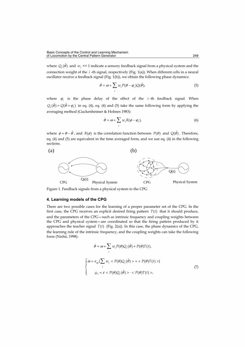
Basic Concepts of the Control and Learning Mechanism of Locomotion by the Central Pattern Generator 249
where ( )iQ θ and iw << 1 indicate a sensory feedback signal from a physical system and the
connection weight of the i -th signal, respectively (Fig. 1(a)). When different cells in a neural
oscillator receive a feedback signal (Fig. 1(b)), we obtain the following phase dynamics:
( ) ( )i ii
w P Qθ ω θ ϕ θ= + − , (5)
where iϕ is the phase delay of the effect of the i -th feedback signal. When
( )iQ θ ( )iQ θ ϕ= + in eq. (4), eq. (4) and (5) take the same following form by applying the
averaging method (Guckenheimer & Holmes 1983):
( )i ii
w Rθ ω φ ϕ= + − , (6)
where φ θ θ= − , and φ( )R is the correlation function between θ( )P and θ( )Q . Therefore,
eq. (4) and (5) are equivalent in the time averaged form, and we use eq. (4) in the following sections.
(a) (b)
CPG Physical System
Q(t)
CPG Physical SystemQi(t)
Figure 1. Feedback signals from a physical system to the CPG
4. Learning models of the CPG
There are two possible cases for the learning of a proper parameter set of the CPG. In the
first case, the CPG receives an explicit desired firing pattern ( )T t that it should produce,
and the parameters of the CPG—such as intrinsic frequency and coupling weights between the CPG and physical system—are coordinated so that the firing pattern produced by it
approaches the teacher signal ( )T t (Fig. 2(a)). In this case, the phase dynamics of the CPG,
the learning rule of the intrinsic frequency, and the coupling weights can take the following form (Nishii, 1998):
( ) ( ) ( ) ( )i ii
w P Q P T tθ ω θ θ θ= + + ,
{ ( ) ( ) ( ) ( ) }
( ) ( ) ( ) ( )
i ii
i i
w P Q P T t
P Q P T tw
ωω ε θ θ θ
ε θ θ θ
= < > + < >
= < > ⋅ < >, (7)
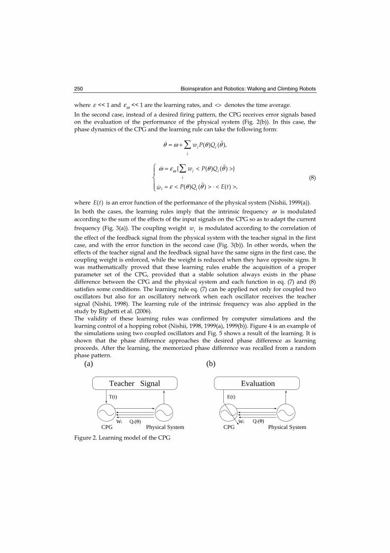
Bioinspiration and Robotics: Walking and Climbing Robots 250
where ε << 1 and ωε << 1 are the learning rates, and <> denotes the time average.
In the second case, instead of a desired firing pattern, the CPG receives error signals based on the evaluation of the performance of the physical system (Fig. 2(b)). In this case, the phase dynamics of the CPG and the learning rule can take the following form:
( ) ( )i ii
w P Qθ ω θ θ= + ,
{ ( ) ( ) }
( ) ( ) ( )
i ii
i i
w P Q
P Q E tw
ωω ε θ θ
ε θ θ
= < >
= < > ⋅ < >, (8)
where ( )E t is an error function of the performance of the physical system (Nishii, 1999(a)).
In both the cases, the learning rules imply that the intrinsic frequency ω is modulated
according to the sum of the effects of the input signals on the CPG so as to adapt the current
frequency (Fig. 3(a)). The coupling weight iw is modulated according to the correlation of
the effect of the feedback signal from the physical system with the teacher signal in the first case, and with the error function in the second case (Fig. 3(b)). In other words, when the effects of the teacher signal and the feedback signal have the same signs in the first case, the coupling weight is enforced, while the weight is reduced when they have opposite signs. It was mathematically proved that these learning rules enable the acquisition of a proper parameter set of the CPG, provided that a stable solution always exists in the phase difference between the CPG and the physical system and each function in eq. (7) and (8) satisfies some conditions. The learning rule eq. (7) can be applied not only for coupled two oscillators but also for an oscillatory network when each oscillator receives the teacher signal (Nishii, 1998). The learning rule of the intrinsic frequency was also applied in the study by Righetti et al. (2006). The validity of these learning rules was confirmed by computer simulations and the learning control of a hopping robot (Nishii, 1998, 1999(a), 1999(b)). Figure 4 is an example of the simulations using two coupled oscillators and Fig. 5 shows a result of the learning. It is shown that the phase difference approaches the desired phase difference as learning proceeds. After the learning, the memorized phase difference was recalled from a random phase pattern.
Qi(θ) CPG Physical System
Teacher Signal
T(t)
Wi
(a)
Evaluation
E(t)
(b)
CPG Physical SystemWi Qi(θ)
Figure 2. Learning model of the CPG
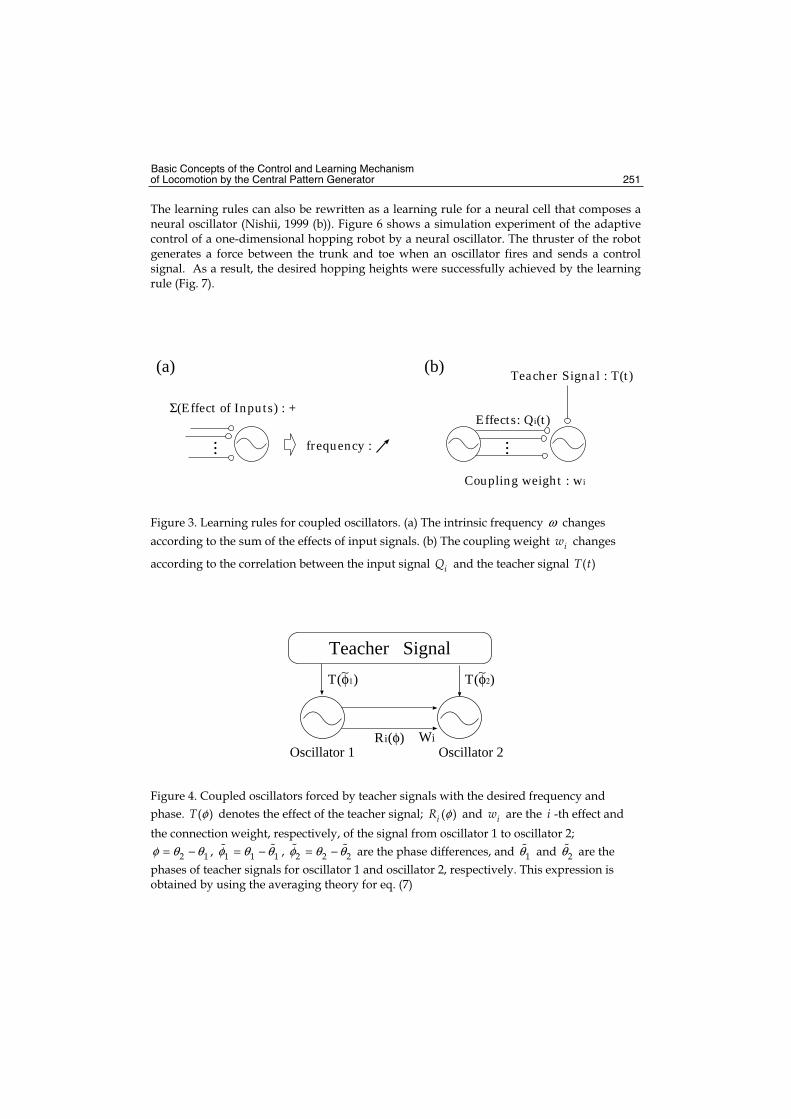
Basic Concepts of the Control and Learning Mechanism of Locomotion by the Central Pattern Generator 251
The learning rules can also be rewritten as a learning rule for a neural cell that composes a neural oscillator (Nishii, 1999 (b)). Figure 6 shows a simulation experiment of the adaptive control of a one-dimensional hopping robot by a neural oscillator. The thruster of the robot generates a force between the trunk and toe when an oscillator fires and sends a control signal. As a result, the desired hopping heights were successfully achieved by the learning rule (Fig. 7).
Σ(Effect of Inputs) : +
...
(b)
frequency :
Effects: Qi(t)
Teacher Signal : T(t)
Coupling weight : wi
...
(a)
Figure 3. Learning rules for coupled oscillators. (a) The intrinsic frequency ω changes
according to the sum of the effects of input signals. (b) The coupling weight iw changes
according to the correlation between the input signal iQ and the teacher signal ( )T t
Ri(φ) Oscillator 1
Teacher Signal
Wi Oscillator 2
T(φ1) T(φ2)∼ ∼
Figure 4. Coupled oscillators forced by teacher signals with the desired frequency and
phase. φ( )T denotes the effect of the teacher signal; ( )iR φ and iw are the i -th effect and
the connection weight, respectively, of the signal from oscillator 1 to oscillator 2;
2 1φ θ θ= − , 1 1 1φ θ θ= − , 2 2 2φ θ θ= − are the phase differences, and 1θ and 2θ are the
phases of teacher signals for oscillator 1 and oscillator 2, respectively. This expression is obtained by using the averaging theory for eq. (7)
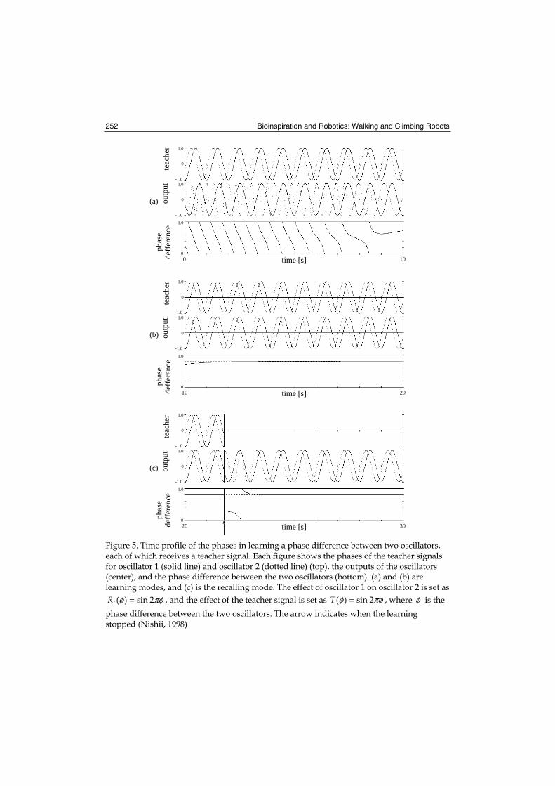
Bioinspiration and Robotics: Walking and Climbing Robots 252
0 10time [s]
1.0
0
1.0
0
-1.01.0
0
-1.0
10 20time [s]
1.0
0
1.0
0
-1.01.0
0
-1.0
(a)
(b)
(c)
teac
her
p
hase
deff
eren
ceou
tput
20 30time [s]
1.0
0
1.0
0
-1.01.0
0
-1.0
teac
her
p
hase
deff
eren
ceou
tput
teac
her
p
hase
deff
eren
ceou
tput
Figure 5. Time profile of the phases in learning a phase difference between two oscillators, each of which receives a teacher signal. Each figure shows the phases of the teacher signals for oscillator 1 (solid line) and oscillator 2 (dotted line) (top), the outputs of the oscillators (center), and the phase difference between the two oscillators (bottom). (a) and (b) are learning modes, and (c) is the recalling mode. The effect of oscillator 1 on oscillator 2 is set as
( ) sin 2iR φ πφ= , and the effect of the teacher signal is set as φ πφ=( ) sin 2T , where φ is the
phase difference between the two oscillators. The arrow indicates when the learning stopped (Nishii, 1998)
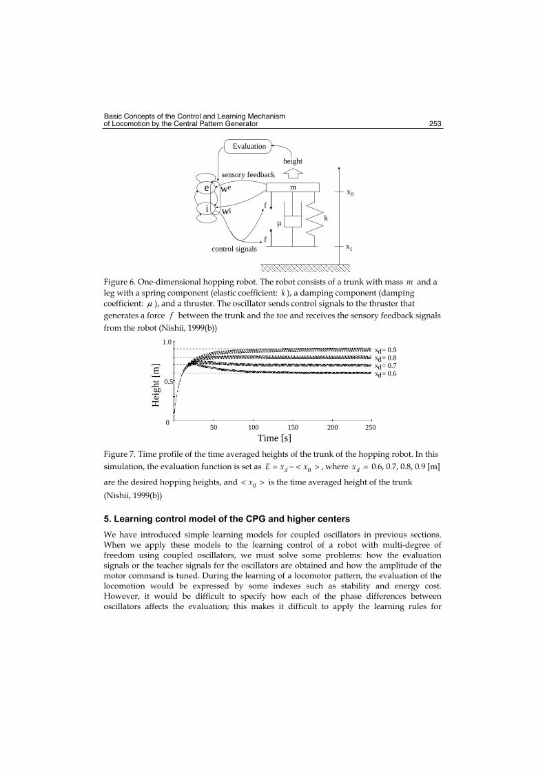
Basic Concepts of the Control and Learning Mechanism of Locomotion by the Central Pattern Generator 253
f
f
k
m
μ
height
sensory feedback
control signals x1
x0
Evaluation
e
i wi
we
Figure 6. One-dimensional hopping robot. The robot consists of a trunk with mass m and a
leg with a spring component (elastic coefficient: k ), a damping component (damping
coefficient: μ ), and a thruster. The oscillator sends control signals to the thruster that
generates a force f between the trunk and the toe and receives the sensory feedback signals
from the robot (Nishii, 1999(b))
1.0
Hei
ght [
m]
0
Time [s] 250100
x = 0.9x = 0.8
x = 0.6x = 0.7
0.5
50 150 200
dddd
Figure 7. Time profile of the time averaged heights of the trunk of the hopping robot. In this
simulation, the evaluation function is set as 0dE x x= − < > , where dx = 0.6, 0.7, 0.8, 0.9 [m]
are the desired hopping heights, and 0x< > is the time averaged height of the trunk
(Nishii, 1999(b))
5. Learning control model of the CPG and higher centers
We have introduced simple learning models for coupled oscillators in previous sections. When we apply these models to the learning control of a robot with multi-degree of freedom using coupled oscillators, we must solve some problems: how the evaluation signals or the teacher signals for the oscillators are obtained and how the amplitude of the motor command is tuned. During the learning of a locomotor pattern, the evaluation of the locomotion would be expressed by some indexes such as stability and energy cost. However, it would be difficult to specify how each of the phase differences between oscillators affects the evaluation; this makes it difficult to apply the learning rules for
Bioinspiration and Robotics: Walking and Climbing Robots 254
oscillators. Then, how do living bodies acquire adequate parameters of the CPG? In this section, we introduce a hierarchical learning model that is a model of the mechanism to acquire the teacher signal for the CPG.
5.1 Hierarchical learning model of the CPG and higher centers
It has been known that the legged locomotion of animals is controlled by not only the CPG in the spinal cord but also higher centers such as the cerebellum and motor cortex (Kandel et al., 2000). It appears that these higher centers play important roles in the realization of locomotion, e.g., monitoring and controlling the activity of the CPG, particularly for reacting to perturbation and avoiding obstacles. If we assume that the higher centers evaluate the performance of locomotion and learn control signals for the component oscillators of the CPG by some learning mechanisms such as reinforcement learning, the control signal can serve not only for tuning the activity of the oscillators but also as a teacher signal for the learning of the CPG. Some experimental studies have also reported the existence of some projections from higher centers, such as motor cortex, to the spinal cord, which affect the activity of motor neurons (Takakusaki et al. 2004). Although it would be difficult to independently modulate the period, phase relation, and amplitude of the firing pattern of coupled neural oscillators by tuning the parameters within the oscillators, the modulation would become easier if higher centers control the amplitude. The above considerations led to the concept of the hierarchical learning model proposed by Miyazaki et al. (2007) (Fig. 8). This model consists of a physical system, a higher center, the CPG, and motor neurons. In this model, the higher center monitors the activity of the CPG and the result of locomotion through sensory feedback signals. It also learns the control signals to the CPG, such as a reset signal that induces an immediate firing of component oscillators of the CPG and a suspend signal that delays the firing, according to the states of the physical system and the CPG. The CPG coordinates its intrinsic frequency and the weights of connections from sensory feedback signals so as to decrease the effect of control signals from the higher center by eq. (7); thus, the CPG can itself produce the desired signal without the control signal after learning. The higher center also learns and controls the amplitude of motor command. This model was again applied to the learning control of a one-dimensional hopping robot (Fig. 6). In this application, an actor-critic architecture of reinforcement learning was used for the learning of the higher center. As learning progressed, the robot was able to hop at the target heights. Figure 9 shows the activity of the higher center and the amplitude of the force both during and after learning. Shortly after the beginning of learning, many control signals were sent to the CPG and the amplitude of the force continued to change, since the higher center explored the control signals for the desired hopping. After learning, the robot hopped at the target height, and the higher center sent no signal to the CPG, and the force amplitude attained a constant value. Figure 10 shows the time profile of the height of the trunk of the robot, the control signals from the higher center, and the amplitude of the force when a mechanical perturbation was applied to the robot after learning. It is shown that the higher center sent control signals and tuned the amplitude of the force in response to the perturbation. When the hopping of the robot was perturbed, the hopping was sometimes stopped. The recovery obtained by using the multiple controls from both the CPG and the higher center exhibited a higher success rate and a shorter average time than that obtained by using only the control from the CPG.
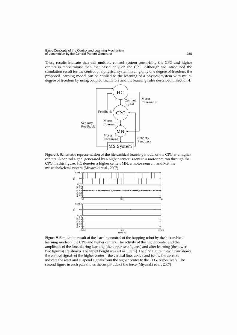
Basic Concepts of the Control and Learning Mechanism of Locomotion by the Central Pattern Generator 255
These results indicate that this multiple control system comprising the CPG and higher centers is more robust than that based only on the CPG. Although we introduced the simulation result for the control of a physical system having only one degree of freedom, the proposed learning model can be applied to the learning of a physical-system with multi-degree of freedom by using coupled oscillators and the learning rules described in section 4.
HC
CPG
MN
MS System
MotorCommand
MotorCommand
MotorCommand
ControlSignal
Feedback
SensoryFeedback
SensoryFeedback
Figure 8. Schematic representation of the hierarchical learning model of the CPG and higher centers. A control signal generated by a higher center is sent to a motor neuron through the CPG. In this figure, HC denotes a higher center; MN, a motor neuron; and MS, the musculoskeletal system (Miyazaki et al., 2007) tal system (Miyazaki et al., 2007)
SUPP
NO
RESET
HC
SUPP
NO
RESET
HC
120000 120050 120100TIME [s]
00.10.20.30.40.5
FOR
CE
[N
]
50 100 1500
0.10.20.30.40.5
FOR
CE
[N
]
Figure 9. Simulation result of the learning control of the hopping robot by the hierarchical learning model of the CPG and higher centers. The activity of the higher center and the amplitude of the force during learning (the upper two figures) and after learning (the lower two figures) are shown. The target height was set as 1.0 [m]. The first figure in each pair shows the control signals of the higher center—the vertical lines above and below the abscissa indicate the reset and suspend signals from the higher center to the CPG, respectively. The second figure in each pair shows the amplitude of the force (Miyazaki et al., 2007)
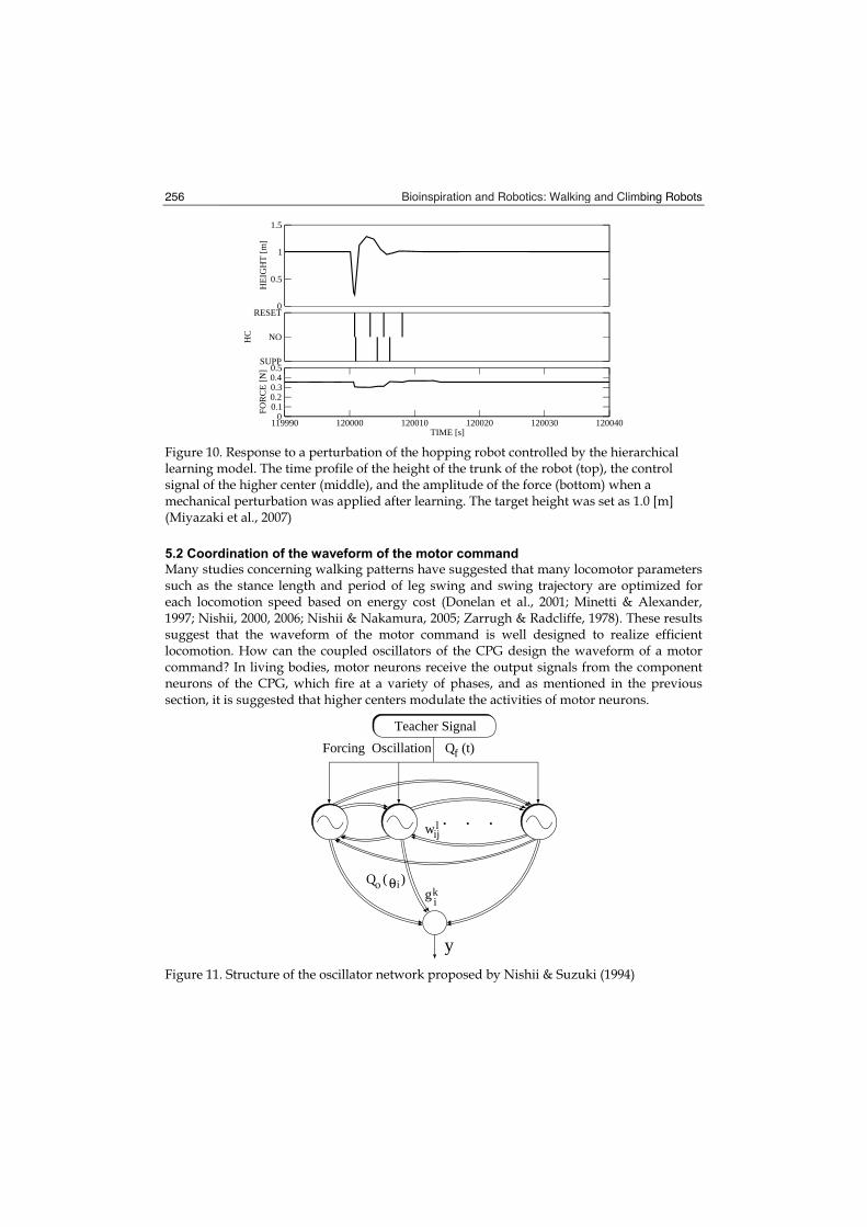
Bioinspiration and Robotics: Walking and Climbing Robots 256 Bioinspiration and Robotics: Walking and Clim
0
0.5
1
1.5
HE
IGH
T [
m]
SUPP
NO
RESET
HC
119990 120000 120010 120020 120030 120040TIME [s]
00.10.20.30.40.5
FOR
CE
[N
]
Figure 10. Response to a perturbation of the hopping robot controlled by the hierarchical learning model. The time profile of the height of the trunk of the robot (top), the control signal of the higher center (middle), and the amplitude of the force (bottom) when a mechanical perturbation was applied after learning. The target height was set as 1.0 [m] (Miyazaki et al., 2007)
5.2 Coordination of the waveform of the motor command
Many studies concerning walking patterns have suggested that many locomotor parameters such as the stance length and period of leg swing and swing trajectory are optimized for each locomotion speed based on energy cost (Donelan et al., 2001; Minetti & Alexander, 1997; Nishii, 2000, 2006; Nishii & Nakamura, 2005; Zarrugh & Radcliffe, 1978). These results suggest that the waveform of the motor command is well designed to realize efficient locomotion. How can the coupled oscillators of the CPG design the waveform of a motor command? In living bodies, motor neurons receive the output signals from the component neurons of the CPG, which fire at a variety of phases, and as mentioned in the previous section, it is suggested that higher centers modulate the activities of motor neurons.
. . .
Teacher Signal
y
Q ( )θο ig
ik
Forcing Oscillation Q (t)f
wijl
Figure 11. Structure of the oscillator network proposed by Nishii & Suzuki (1994)
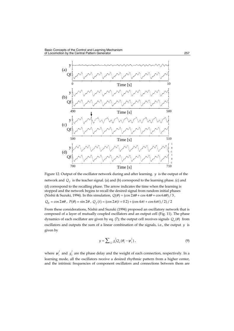
Basic Concepts of the Control and Learning Mechanism of Locomotion by the Central Pattern Generator 257
y
Qf
Time [s]0 10
(a)
y
Qf
Time [s]490 500
(b)
y
Qf
Time [s]500 510
(c)
y
Qf
Time [s]700 710
(d)
0
1
-1
0
1
-1
Figure 12. Output of the oscillator network during and after learning. y is the output of the
network and fQ is the teacher signal. (a) and (b) correspond to the learning phase. (c) and
(d) correspond to the recalling phase. The arrow indicates the time when the learning is stopped and the network begins to recall the desired signal from random initial phases
(Nishii & Suzuki, 1994). In this simulation, θ πθ πθ πθ= + +( ) (cos 2 cos 4 cos 6 ) / 3Q ,
0 cos 2Q πθ= , θ θ=( ) sin 2P , ( ) (cos 2 ( 0.2) (cos 4 cos 6 ) / 2) / 2fQ t t t tπ π π= + + +
From these considerations, Nishii and Suzuki (1994) proposed an oscillatory network that is composed of a layer of mutually coupled oscillators and an output cell (Fig. 11). The phase
dynamics of each oscillator are given by eq. (7); the output cell receives signals ( )oQ θ from
oscillators and outputs the sum of a linear combination of the signals, i.e., the output y is
given by
( )l li o i ii ly g Q θ ψ
,= − , (9)
whereliψ and
lig are the phase delay and the weight of each connection, respectively. In a
learning mode, all the oscillators receive a desired rhythmic pattern from a higher center, and the intrinsic frequencies of component oscillators and connections between them are
Bioinspiration and Robotics: Walking and Climbing Robots 258
changed according to the learning rule eq. (7). The connections from each oscillator to the
output cell are modulated in order to minimize the square error E between the output of
the network y and the teacher signal fQ , i.e.,
21( )
2fE y Q= − ,
0( ) ( )k ki f i ik
i
Eg y Q Q
gε ε θ ψ
∂= − = − − −
∂, (10)
where ε is the learning rate. Figure 12 shows the simulation result. The output of the
network converges to the desired signal in the learning phase, and the desired signal is recalled after learning from random initial phases of oscillators. In this model, each intrinsic frequency of the component oscillators of the CPG converges to a component frequency of the teacher signal. Although there is no evidence that the desired waveform of a motor pattern in living bodies is decomposed into component frequencies, a desired waveform of motor command would be obtained by the linear sum of the outputs from the component neurons of the CPG which fire with a variety of phases and duration, and the proposed learning rule in this section could be applied.
6. Conclusion
In this chapter, we introduced the basic concepts of the control and learning mechanism to realize a desired locomotion by the CPG. As introduced in section 5.1, the control system of locomotion in living bodies assumes a hierarchical structure in which the CPG synchronizes with a physical system and generates motor signals to motor neurons, and higher centers learn a desired motor signal from the performance of locomotion and control the CPG. The control signal from higher centers can also function as a teacher signal for the CPG to acquire neural parameters in the CPG. The concept that the higher centers acquire a motor command appears to be a natural assumption because higher centers such as the motor cortex sends motor commands in order to respond to sensory stimulus, e.g., avoiding obstacles. Such hierarchical and multiple control system by higher centers and the CPG also contribute to acquire robust control, as shown in the simulation result in section 5.1. The concept of this model with learning rules for coupled oscillators that send signals to each actuator can be applied to a robot with multi-degree of freedom. However, in order to consider the learning system for locomotion, we should consider the learning mechanism not only for the CPG but also for higher centers. For instance, it appears that higher centers play an important role in shaping the motor command that is generated by the CPG, as mentioned in section 5.2. Another important problem is the explosion of the search space of a motor command, e.g., as the number of actuators increases, that is, as the degree of freedom of a robot increases, the search space for the desired motor command becomes vast. Therefore, it is important to consider an efficient learning mechanism for higher centers to find a desired motor command for each actuator from the performance of locomotion. It has been suggested that locomotor patterns of living bodies are well optimized on energy cost; as mentioned in section 5.2; therefore, the minimization of energy cost would be a constraint
Basic Concepts of the Control and Learning Mechanism of Locomotion by the Central Pattern Generator 259
to design a locomotor pattern. Such a constraint would contribute to narrow the search space for the desired motor command. Recent studies have also revealed that human walking is generated by some base set of muscle activities (Ivanenko et al., 2004), which suggests the existence of a good base of motor commands for locomotion. The understanding of an efficient system in living bodies to find a desired motor command or a base set for a motor command under some criterion would be a challenging problem for revealing the intelligence of living bodies.
7. Reference
Donelan, J.; Kram, R. and Kuo, A. (2001). Mechanical and metabolic determinants of the preferred step width in human walking, Proceeding of the Royal Society of London B,Vol. 268, pp. 1985-1992.
Fukuoka, Y.; Kimura, H. and Cohen, H. (2003). Adaptive dynamic walking of a quadruped robot on irregular terrain based on biological concepts, International Journal of Robotic Research, Vol. 22, No. 3-4, pp. 187-202.
Ivanenko, Y.; Poppele, R. and Lacquaniti, F. (2004). Five basic muscle activation patterns account for muscle activity during human locomotion, Journal of Physiology, Vol. 556, No. 1, pp.267-282.
Guckenheimer, J. and Holmes, P. (1983). Nonlinear oscillations, dynamical systems, and bifurcations of vector fields, New York: Springer-Verlag, ISBN 0387908196.
Kandel, E.; Schwartz, J. and Jessell, T. (2000). Locomotion, In: Principles of neural science Fourth Edition, pp. 737-755, McGraw-Hill Companies, ISBN 0838577016.
Minetti, A. and Alexander, R. (1997). A theory of metabolic costs for bipedal gaits, Journal of Theoretical Biology, Vol. 186, pp.467-476.
Miyazaki, Y.; Maeda, H.; Hioki, T. and Nishii, J. (2007). A hierarchical learning control model of locomotor patterns of legged animals, Proceeding of 2nd International Symposium on Mobiligence, pp. 295-298.
Nishii, J. and Suzuki, R. (1994). Oscillatory network model which learns a rhythmic pattern of an external signal, Proceeding of IFAC symposium, pp. 501-502.
Nishii, J. (1998). A learning model for oscillatory networks, Neural Networks, Vol. 11, pp. 249-257.
Nishii, J. (1999). (a) . A learning model of a periodic locomotor pattern by the central pattern generator, Adaptive Behavior, Vol. 7, No. 2, pp. 137-149.
Nishii, J. (1999). (b) . Learning model for coupled neural oscillators, Network: Computation in Neural Systems, Vol. 10, pp. 213-226.
Nishii, J. (2000). Legged insects select the optimal locomotor pattern based on energetic cost, Biological Cybernetics, Vol. 83, No. 5, pp. 435-442.
Nishii, J. and Nakamura, M. (2005). A determinant of the leg swing trajectory during walking, Proceeding of 3rd international symposium on adaptive motion in animals and machines, CD-ROM.
Nishii, J. (2006). An analytical estimation of the energy cost for legged locomotion, Journal of Theoretical Biology, Vol. 238, pp. 636-645.
Righetti, L.; Buchli, J. and Ijspeert, A. (2006). Dynamic Hebbian learning in adaptive frequency oscillators, Physica D, Vol. 216, No. 2, pp. 269-281.
Rossignol, S. and Bouyer, L. (2004). Adaptive mechanism of spinal locomotion in cats, Integrative and Comparative Biology, Vol. 44, No. 1, pp. 71-79.
Bioinspiration and Robotics: Walking and Climbing Robots 260
Taga, G.; Yamaguchi, Y. and Shimizu, H. (1991). Self-organized control of bipedal locomotion by neural oscillators in unpredictable environment, Biological Cybernetics, Vol. 65, pp. 147-159.
Takakusaki, K.; Saitoh, K.; Harada, H. and Kashiwayanagi, M. (2004). Role of basal ganglia-brainstem pathways in the control of motor behaviors, Neuroscience Research, Vol. 50, pp. 137-151.
Zarrugh, M. and Radcliffe, C. (1978). Predicting metabolic cost of level walking, European Journal of Applied Physiology, Vol. 38, No. 3, pp. 215-223.
16
Space exploration - towards bio-inspired climbing robots
Carlo Menon1, Michael Murphy2, Metin Sitti2 and Nicholas Lan3
1School of Engineering Science, Simon Fraser University, 2Department of Mechanical Engineering, Carnegie Mellon University
3Ursa Minor Space and Navigation B.V. 1Canada, 2U.S.A, 3The Netherlands
1. Introduction
Robotic systems continue to be an important tool in space exploration, and as robotic systems continue to gain capability, the particular challenges of the space environment and the tasks required in space will benefit from such systems finding new roles in space. This chapter focuses on the design of climbing robots suitable for use in space. These mimic the climbing ability of geckos, using micro-structured hairs to provide dry adhesion, and exploit gait to exhibit rapid and robust motion over vertical surfaces on earth. Mobility of robotic systems allows many different roles for systems in space, including exploration on extraterrestrial surfaces and navigating vehicle surfaces in orbit. Climbing robots in space may provide extra capability in the ability to negotiate a broader range of terrains. The range of surfaces that might be required to be negotiated in space can be matched by the range of different possible climbing strategies. In particular, dry adhesive techniques inspired by the gecko are highlighted, with different robot designs intended to take advantage of such dry adhesives described in detail. Examples of other strategies for climbing robots are presented and discussed, particularly in the context of usefulness for future implementation in space. With this section introducing the subject and composition of this chapter, section 2 gives a brief overview of the main challenges facing robotic systems in space. Section 3 is devoted to the introduction of different strategies for climbing robots, including examples designed for use in space. Examples of robotic systems employing different approaches are given. In section 4, the subject of biologically inspired synthetic dry adhesion is introduced. Section 5 forms the major part of this chapter, describing the design and breadboarding of three climbing robots, intended to form the basis for future robots using such dry adhesives. Future work is discussed in section 6 and conclusions are given in section 7.
2. Issues for Space Robotics
Robotic systems used in space are subject to a range of challenging environments from launch to deployment and operation, which must all be mitigated with great robustness given the impossibility of repair of most space-borne systems.
Bioinspiration and Robotics: Walking and Climbing Robots 262
The launch phase presents mechanical challenges to the system in terms of both static and dynamic loads. Mechanical interface of the robot to the connected part of the space vehicle must be considered in addition to the robotic system itself. These include high steady state acceleration, and significant low frequency longitudinal and lateral vibrations. Random vibrations caused by the engine, and thin layer noise are also present. Furthermore, in multi-stage launchers shocks are undergone when stage separations occur. Thermal conditions must be accounted for in the phases before launch, where the system must be prepared and integrated and then transferred to the launch site, as well as thermal conditions during launch. Mechanisms must also adhere to cleanliness requirements for launch, not only to avoid contaminants that may detriment systems on the robot or launcher, but in some cases also to avoid contamination of extraterrestrial environments that may interfere with scientific payload. On orbit, the robotic system must mitigate the vacuum environment if not used inside a pressured spacecraft. Outgassing from materials in the robotic system must then be taken into account. In the case of earth orbit, the radiation environment will impact robotic design, for instance requiring the use of radiation hardened electronic components. Atomic oxygen, particularly abundant in low earth orbit, causes material dependent corrosion of surfaces. Since abundance of atomic oxygen in orbit is also dependent on solar flux, both solar activity and the eclipse cycling of the orbiting system will impact on this effect. Plasma effects are also orbit dependent, where at low altitude (100 – 1000 km) it is relatively cool, dense and regular, while at geosychronous altitude (35000 km) it is hot, irregular and highly variable. Collective effects dominate at low altitudes, where surface charging by plasma can cause, for instance, higher impedance in antennas. At geosychronous altitude, where effects of individual highly energetic plasma particles dominate, build-up of charge in components and subsequent discharging can cause critical failures in spacecraft. Space debris is an increasing problem around the earth. Smaller particles (10-3 – 10-9 g) cause erosion of surfaces, while mitigation of larger particles may require use of appropriate shielding materials. Finally, solar flux combined with periods of eclipse, mean that orbiting systems experience large changes in thermal environment. For subsystems, this is highly dependent on the system’s orientation to the sun and the thermal design of the system. In general, thermal environment will also be highly dependent on orbit, with low altitude entailing a higher rate of thermal cycling due to a higher rate of eclipse cycles. Extraterrestrial surface environments are varied, but may in addition to the above include factors such as large amounts of dust, extreme temperatures and pressures, and strong winds. Furthermore, deployment on a surface may entail more demanding mechanical loads dependent on landing characteristics. In addition to the demands placed on robotic systems materials and structure, the remote nature of space environments demands robust operation in situations far from the reach or control of humans. Not only must the physical design of robotic space systems be in accordance with these demands, but various degrees of autonomy and intelligence is required from such systems. Furthermore, space systems are generally required to be energy efficient, and low in volume and mass. Robotic systems continue to be of use in space in complementing human presence in space. While human agents in space provide adaptability in function presently unavailable to robots, the greatly reduced cost and risk involved in the use of robotic space systems means that they will continue to find uses in space for the foreseeable future. Indeed, as the
Space exploration - towards bio-inspired climbing robots 263
capability of robotic systems increases, as does their potential for miniaturisation, new opportunities arise in enabling novel uses for robots in space.
3. Strategies for Climbing Robots
3.1 Negative pressure
Various robotic climbing systems have been based on suction adhesion. Generally, in comparison to other clinging mechanisms, generation of suction requires high power, and gaps in the seals in suction cups will negate the suction effect although some systems using dynamic suction have also been designed. In any case, since suction adhesion is reliant on ambient pressure, such systems are unsuitable for use in orbit. Two robots, termed Flipper and Crawler, are examples of climbing robots that employ suction adhesion (Tummala et. al., 2004). Intended for use as remote sensors in hostile terrestrial environments, they are capable of traversing both horizontal and inclined surfaces, as well as transiting between some surfaces with differing gradients. Their designs emphasise low power consumption, small size, and low weight. While prototypes of these designs performed satisfactorily, speed was limited by the time taken to establish adhesion and release with the suction mechanism. Additionally, the systems were limited in the range of surfaces they could climb. Another example, named Gecko (Cepolina et. al., 2003), employs a novel suspension system to assure modulated pressure in its suction mechanisms. This is just one example of many robotic systems that have been designed for the cleaning of vertical terrestrial surfaces. Dynamic suction has been implemented in commercially available robots, able to be used with a variety of payloads (Illingworth & Reinfeld, 2001). These systems are able to transition easily from horizontal to vertical surfaces using a ‘tornado in a cup’ vortex to generate suction. However, for adhesion to walls the dynamic vortex must be active even when stationary, requiring significant power expenditure.
3.2 Mechanical Grip
Like the dry adhesion employed by animals such as the gecko, many examples may be found in nature of species that employ mechanical grip in climbing. However, the use of mechanical grip for climbing is dependent on suitable surfaces, where for instance the climbing of a smooth inverted surface on earth using only mechanical grip would be unfeasible. LEMUR IIb is a multi-limbed robot capable of free climbing near vertical surfaces (Bretl et. al., 2004). Irregularities in an otherwise smooth surface are used to provide reaction force to the climbing limbs. Eurobot is a robot designed for use in space that, in addition, utilises anthropomorphic manipulators at the ends of its limbs (Visentin, 2005; Joudrier et. al., 2005). Under normal gravity conditions, such manipulators would allow extra grip when climbing inclined surfaces and enable robotic designs to cling to inverted surfaces, where handholds are available. Since Eurobot is primarily designed for use in microgravity, manipulators are required to remain attached to the spacecraft and can also be employed to perform tasks that would otherwise require and EVA astronaut. Micro-spine clinging is another bioinspired climbing system, used in nature by various insects, arthropods and some species of gecko. Micro-scale spines take advantage of asperities (bumps or pits) on surfaces and provide reaction force to enable climbing of
Bioinspiration and Robotics: Walking and Climbing Robots 264
vertical surfaces. Such systems allow clinging to porous or dusty surfaces and are not as susceptible to degrading from dust unlike currently manufactured, smaller scale gecko-inspired adhesive fibre arrays. However, the micro-spine method is still surface dependent, although the technique is scalable to surfaces of differing roughness Such systems have been implemented on the Spinybot II and RiSE robots (Kim et. al., 2005; Haynes & Rizzi, 2006).
3.3 Magnetic
Magnetic systems for climbing have also been designed, though clearly in this case a ferromagnetic surface is required to allow adhesion. In addition, for some space applications large magnetic forces might interfere with payload or other mission systems. The hexapod REST robot (Grieco et. al., 1998), uses a combination of permanent magnets and electromagnets to carry payloads of up to 100 kg while clinging to vertical or inverted surfaces. Safety is enhanced through the use of permanent magnets that retain adhesion in the case of a loss of power. Electromagnets reinforce grip during locomotion. Clearly this system is only suitable for climbing where ferromagnetic surfaces are available, and is therefore aimed at use only in terrestrial industrial environments. As neither planetary and satellite surfaces are usually ferromagnetic, this technique is not the most appropriate for space applications.
3.4 Dry Adhesive
In comparison to magnetic and suction approaches to adhesion, dry adhesion is passive and might therefore be thought of as having potential for the design of energy efficient systems, a compelling advantage in space applications. While it has been found that capillary forces may play a significant role in gecko-type adhesion, it has also been found that adhesion is still possible even in the absence of water, and that adhesion can still be produced in vacuum. Potentially, this type of adhesion would therefore be suitable for use in extraterrestrial environments as well as microgravity and vacuum environments. Using Scotch® tape as an adhesive the Mini-Whegs™ robot uses wheel-legs for locomotion (Daltorio et. al., 2005a). Each wheel foot consists of a rotating hub, with several compliant adhesive feet attached around its circumference. In this configuration, the robot was able to traverse vertical surfaces with relative ease and had some success in locomotion across inverted surfaces. The robot was found to be suitable for transitioning between surfaces of different inclination. The system has also been tested with microstructured polymer adhesives, achieving somewhat lower performance (Daltorio et. al., 2005b). Tri-Leg Waalbot, named after the Van der Waal’s Forces it uses for adhesion, also uses wheel-legs for climbing smooth surfaces (Murphy et. al., 2007). Its two legs hold six adhesive footpads which allow the robot to climb, transition, and turn in small corridors. Recent progress includes inverted walking and turning and integration of microstructured polymer adhesives into the footpads. Extracting further attributes from gecko adhesion strategy, the Stickybot robot employs hierarchical compliance to increase contact area with the surface (Kim et. al., 2007). The robot’s construction implements compliance at micrometer, millimetre and centimetre scales to allow adhesion over a great portion of the robot surface, to surfaces that are uneven over these scales. Furthermore, directional adhesives and distributed force control are employed to increase performance. Polyurethane or Sorbothane® adhesives were used on early versions.
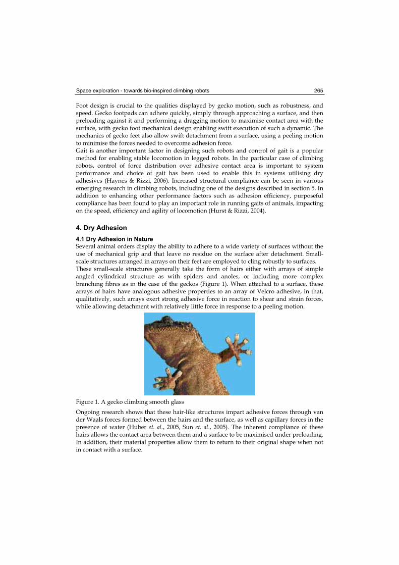
Space exploration - towards bio-inspired climbing robots 265
Foot design is crucial to the qualities displayed by gecko motion, such as robustness, and speed. Gecko footpads can adhere quickly, simply through approaching a surface, and then preloading against it and performing a dragging motion to maximise contact area with the surface, with gecko foot mechanical design enabling swift execution of such a dynamic. The mechanics of gecko feet also allow swift detachment from a surface, using a peeling motion to minimise the forces needed to overcome adhesion force. Gait is another important factor in designing such robots and control of gait is a popular method for enabling stable locomotion in legged robots. In the particular case of climbing robots, control of force distribution over adhesive contact area is important to system performance and choice of gait has been used to enable this in systems utilising dry adhesives (Haynes & Rizzi, 2006). Increased structural compliance can be seen in various emerging research in climbing robots, including one of the designs described in section 5. In addition to enhancing other performance factors such as adhesion efficiency, purposeful compliance has been found to play an important role in running gaits of animals, impacting on the speed, efficiency and agility of locomotion (Hurst & Rizzi, 2004).
4. Dry Adhesion
4.1 Dry Adhesion in Nature
Several animal orders display the ability to adhere to a wide variety of surfaces without the use of mechanical grip and that leave no residue on the surface after detachment. Small-scale structures arranged in arrays on their feet are employed to cling robustly to surfaces. These small-scale structures generally take the form of hairs either with arrays of simple angled cylindrical structure as with spiders and anoles, or including more complex branching fibres as in the case of the geckos (Figure 1). When attached to a surface, these arrays of hairs have analogous adhesive properties to an array of Velcro adhesive, in that, qualitatively, such arrays exert strong adhesive force in reaction to shear and strain forces, while allowing detachment with relatively little force in response to a peeling motion.
Figure 1. A gecko climbing smooth glass
Ongoing research shows that these hair-like structures impart adhesive forces through van der Waals forces formed between the hairs and the surface, as well as capillary forces in the presence of water (Huber et. al., 2005, Sun et. al., 2005). The inherent compliance of these hairs allows the contact area between them and a surface to be maximised under preloading. In addition, their material properties allow them to return to their original shape when not in contact with a surface.
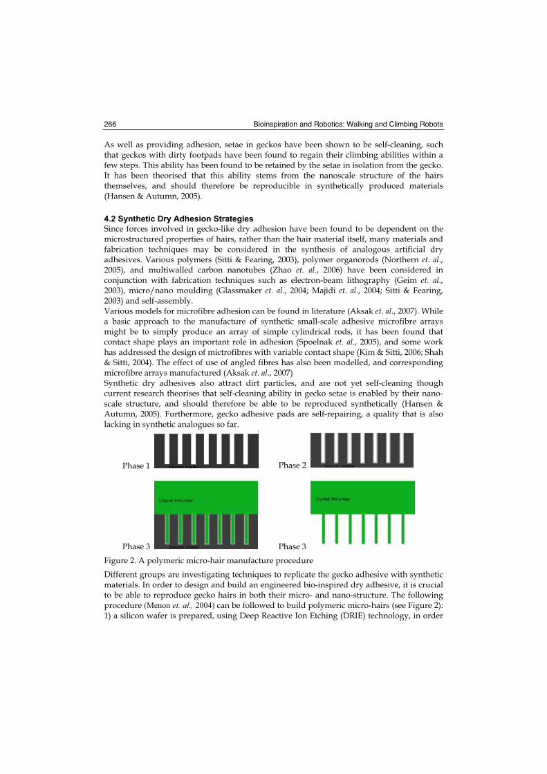
Bioinspiration and Robotics: Walking and Climbing Robots 266
As well as providing adhesion, setae in geckos have been shown to be self-cleaning, such that geckos with dirty footpads have been found to regain their climbing abilities within a few steps. This ability has been found to be retained by the setae in isolation from the gecko. It has been theorised that this ability stems from the nanoscale structure of the hairs themselves, and should therefore be reproducible in synthetically produced materials (Hansen & Autumn, 2005).
4.2 Synthetic Dry Adhesion Strategies
Since forces involved in gecko-like dry adhesion have been found to be dependent on the microstructured properties of hairs, rather than the hair material itself, many materials and fabrication techniques may be considered in the synthesis of analogous artificial dry adhesives. Various polymers (Sitti & Fearing, 2003), polymer organorods (Northern et. al., 2005), and multiwalled carbon nanotubes (Zhao et. al., 2006) have been considered in conjunction with fabrication techniques such as electron-beam lithography (Geim et. al.,2003), micro/nano moulding (Glassmaker et. al., 2004; Majidi et. al., 2004; Sitti & Fearing, 2003) and self-assembly. Various models for microfibre adhesion can be found in literature (Aksak et. al., 2007). While a basic approach to the manufacture of synthetic small-scale adhesive microfibre arrays might be to simply produce an array of simple cylindrical rods, it has been found that contact shape plays an important role in adhesion (Spoelnak et. al., 2005), and some work has addressed the design of mictrofibres with variable contact shape (Kim & Sitti, 2006; Shah & Sitti, 2004). The effect of use of angled fibres has also been modelled, and corresponding microfibre arrays manufactured (Aksak et. al., 2007) Synthetic dry adhesives also attract dirt particles, and are not yet self-cleaning though current research theorises that self-cleaning ability in gecko setae is enabled by their nano-scale structure, and should therefore be able to be reproduced synthetically (Hansen & Autumn, 2005). Furthermore, gecko adhesive pads are self-repairing, a quality that is also lacking in synthetic analogues so far.
Phase 1 Phase 2
Phase 3 Phase 3
Figure 2. A polymeric micro-hair manufacture procedure
Different groups are investigating techniques to replicate the gecko adhesive with synthetic materials. In order to design and build an engineered bio-inspired dry adhesive, it is crucial to be able to reproduce gecko hairs in both their micro- and nano-structure. The following procedure (Menon et. al., 2004) can be followed to build polymeric micro-hairs (see Figure 2): 1) a silicon wafer is prepared, using Deep Reactive Ion Etching (DRIE) technology, in order
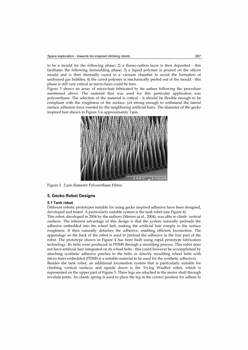
Space exploration - towards bio-inspired climbing robots 267
to be a mould for the following phase; 2) a fluoro-carbon layer is then deposited - this facilitates the following demoulding phase; 3) a liquid polymer is poured on the silicon mould and is then thermally cured in a vacuum chamber to avoid the formation of undesired gas bubbles; 4) the cured polymer is mechanically peeled out of the mould - this phase is still very critical as micro-hairs could be torn. Figure 3 shows an array of micro-hair fabricated by the authors following the procedure mentioned above. The material that was used for this particular application was polyurethane. The selection of the material is critical - it should be flexible enough to be compliant with the roughness of the surface, yet strong enough to withstand the lateral surface adhesion force exerted by the neighboring artificial hairs. The diameter of the gecko
inspired hair shown in Figure 3 is approximately 2 μm.
Figure 3. 2 μm diameter Polyurethane Fibres
5. Gecko Robot Designs
5.1 Tank robot
Different robotic prototypes suitable for using gecko inspired adhesive have been designed, developed and tested. A particularly suitable system is the tank robot (see Figure 4). This robot, developed in 2004 by the authors (Menon at al., 2004), was able to climb vertical surfaces. The inherent advantage of this design is that the system naturally preloads the adhesive embedded into the wheel belt, making the artificial hair comply to the surface roughness. It then naturally detaches the adhesive, enabling efficient locomotion. The appendage on the back of the robot is used to preload the adhesive in the fore part of the robot. The prototype shown in Figure 4 has been built using rapid prototype fabrication technology. Its belts were produced in PDMS through a moulding process. This robot does not have artificial hair integrated on its wheel belts - this could however be accomplished by attaching synthetic adhesive patches to the belts or directly moulding wheel belts with micro-hairs embedded (PDMS is a suitable material to be used for the synthetic adhesive). Besides the tank robot, an additional locomotion system that is particularly suitable for climbing vertical surfaces and upside down is the Tri-leg Waalbot robot, which is represented on the upper part of Figure 5. Three legs are attached to the motor shaft through revolute joints. An elastic spring is used to place the leg in the correct position for adhere to
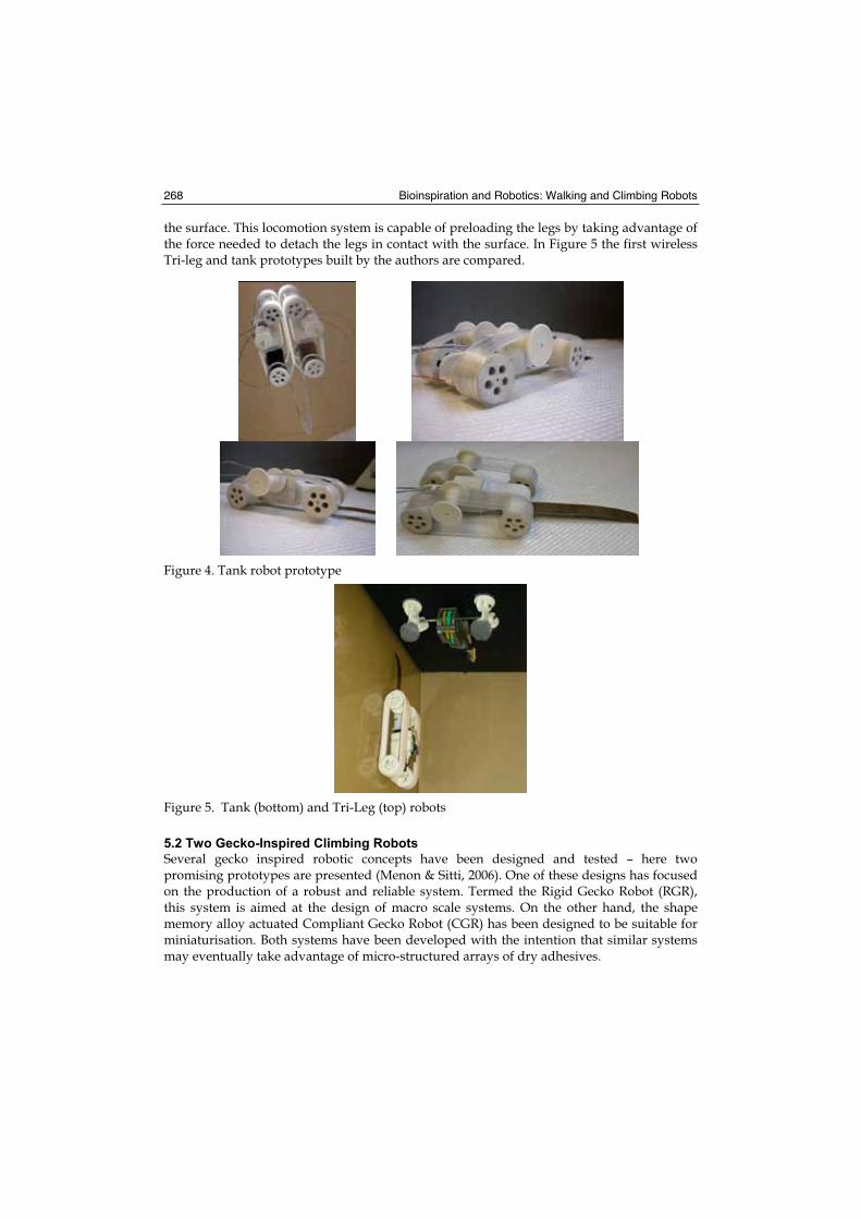
Bioinspiration and Robotics: Walking and Climbing Robots 268
the surface. This locomotion system is capable of preloading the legs by taking advantage of the force needed to detach the legs in contact with the surface. In Figure 5 the first wireless Tri-leg and tank prototypes built by the authors are compared.
Figure 4. Tank robot prototype
Figure 5. Tank (bottom) and Tri-Leg (top) robots
5.2 Two Gecko-Inspired Climbing Robots
Several gecko inspired robotic concepts have been designed and tested – here two promising prototypes are presented (Menon & Sitti, 2006). One of these designs has focused on the production of a robust and reliable system. Termed the Rigid Gecko Robot (RGR), this system is aimed at the design of macro scale systems. On the other hand, the shape memory alloy actuated Compliant Gecko Robot (CGR) has been designed to be suitable for miniaturisation. Both systems have been developed with the intention that similar systems may eventually take advantage of micro-structured arrays of dry adhesives.
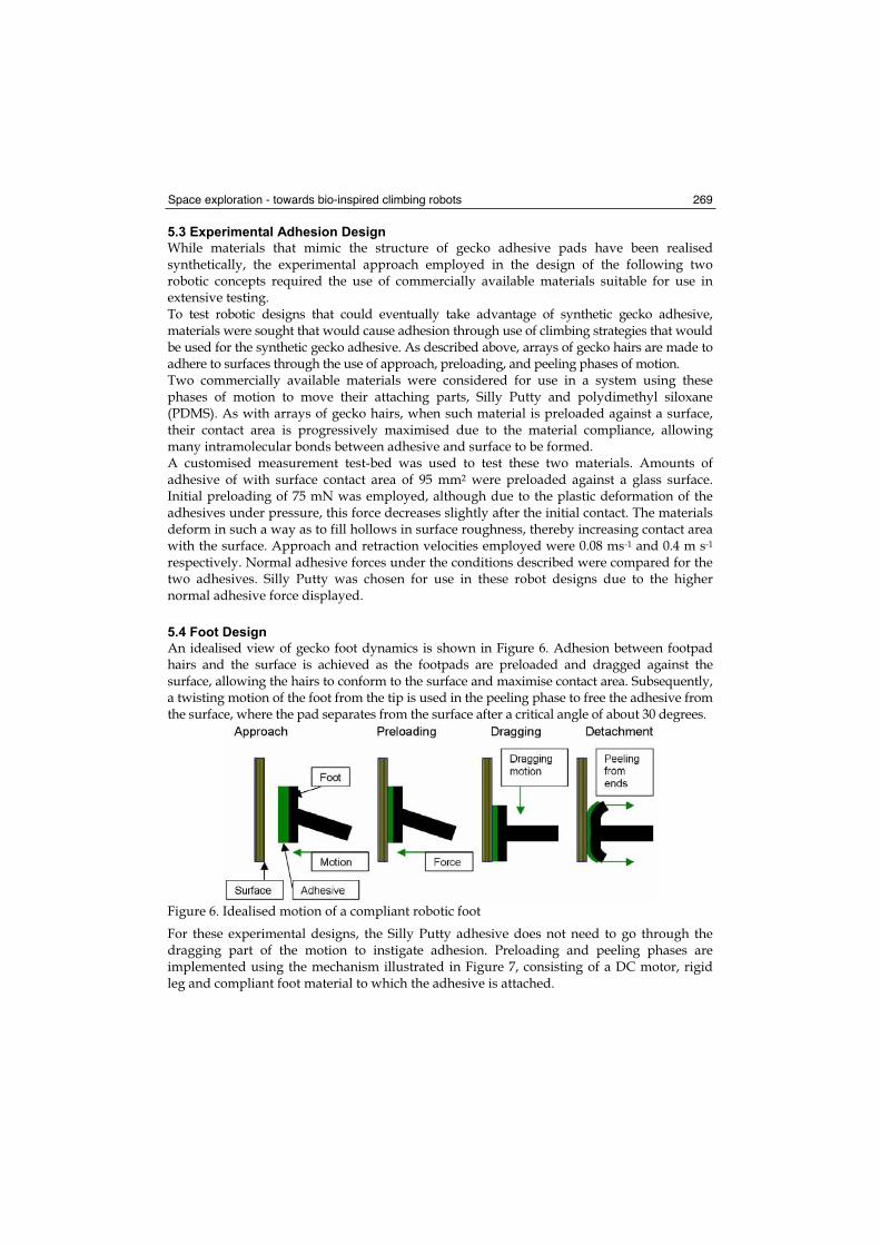
Space exploration - towards bio-inspired climbing robots 269
5.3 Experimental Adhesion Design
While materials that mimic the structure of gecko adhesive pads have been realised synthetically, the experimental approach employed in the design of the following two robotic concepts required the use of commercially available materials suitable for use in extensive testing. To test robotic designs that could eventually take advantage of synthetic gecko adhesive, materials were sought that would cause adhesion through use of climbing strategies that would be used for the synthetic gecko adhesive. As described above, arrays of gecko hairs are made to adhere to surfaces through the use of approach, preloading, and peeling phases of motion. Two commercially available materials were considered for use in a system using these phases of motion to move their attaching parts, Silly Putty and polydimethyl siloxane (PDMS). As with arrays of gecko hairs, when such material is preloaded against a surface, their contact area is progressively maximised due to the material compliance, allowing many intramolecular bonds between adhesive and surface to be formed. A customised measurement test-bed was used to test these two materials. Amounts of adhesive of with surface contact area of 95 mm2 were preloaded against a glass surface. Initial preloading of 75 mN was employed, although due to the plastic deformation of the adhesives under pressure, this force decreases slightly after the initial contact. The materials deform in such a way as to fill hollows in surface roughness, thereby increasing contact area with the surface. Approach and retraction velocities employed were 0.08 ms-1 and 0.4 m s-1
respectively. Normal adhesive forces under the conditions described were compared for the two adhesives. Silly Putty was chosen for use in these robot designs due to the higher normal adhesive force displayed.
5.4 Foot Design
An idealised view of gecko foot dynamics is shown in Figure 6. Adhesion between footpad hairs and the surface is achieved as the footpads are preloaded and dragged against the surface, allowing the hairs to conform to the surface and maximise contact area. Subsequently, a twisting motion of the foot from the tip is used in the peeling phase to free the adhesive from the surface, where the pad separates from the surface after a critical angle of about 30 degrees.
Figure 6. Idealised motion of a compliant robotic foot
For these experimental designs, the Silly Putty adhesive does not need to go through the dragging part of the motion to instigate adhesion. Preloading and peeling phases are implemented using the mechanism illustrated in Figure 7, consisting of a DC motor, rigid leg and compliant foot material to which the adhesive is attached.
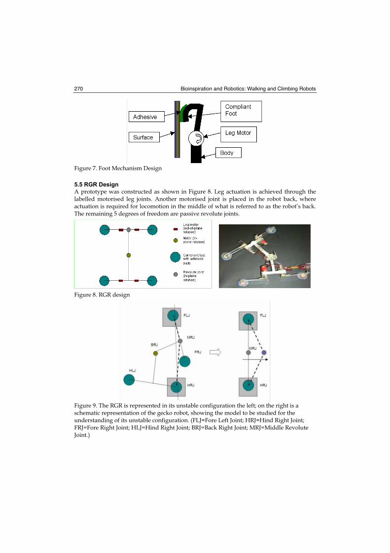
Bioinspiration and Robotics: Walking and Climbing Robots 270
Figure 7. Foot Mechanism Design
5.5 RGR Design
A prototype was constructed as shown in Figure 8. Leg actuation is achieved through the labelled motorised leg joints. Another motorised joint is placed in the robot back, where actuation is required for locomotion in the middle of what is referred to as the robot’s back. The remaining 5 degrees of freedom are passive revolute joints.
Figure 8. RGR design
Figure 9. The RGR is represented in its unstable configuration the left; on the right is a schematic representation of the gecko robot, showing the model to be studied for the understanding of its unstable configuration. (FLJ=Fore Left Joint; HRJ=Hind Right Joint; FRJ=Fore Right Joint; HLJ=Hind Right Joint; BRJ=Back Right Joint; MRJ=Middle Revolute Joint.)
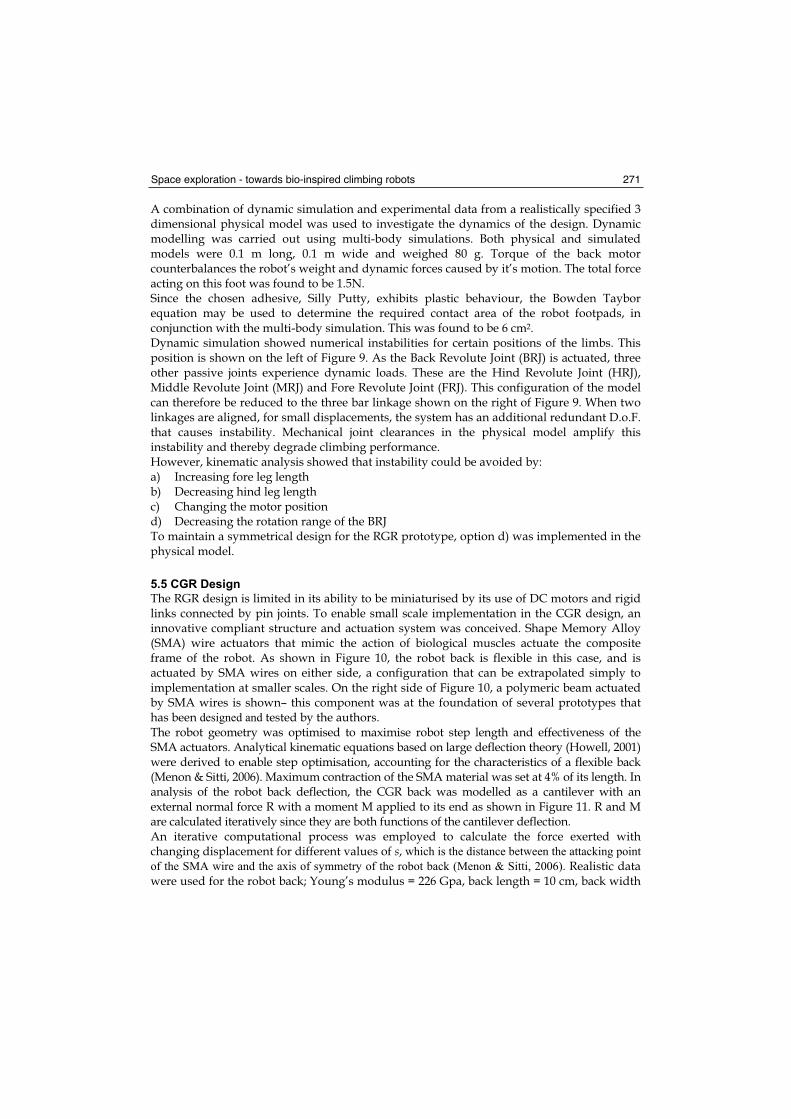
Space exploration - towards bio-inspired climbing robots 271
A combination of dynamic simulation and experimental data from a realistically specified 3 dimensional physical model was used to investigate the dynamics of the design. Dynamic modelling was carried out using multi-body simulations. Both physical and simulated models were 0.1 m long, 0.1 m wide and weighed 80 g. Torque of the back motor counterbalances the robot’s weight and dynamic forces caused by it’s motion. The total force acting on this foot was found to be 1.5N. Since the chosen adhesive, Silly Putty, exhibits plastic behaviour, the Bowden Taybor equation may be used to determine the required contact area of the robot footpads, in conjunction with the multi-body simulation. This was found to be 6 cm2.Dynamic simulation showed numerical instabilities for certain positions of the limbs. This position is shown on the left of Figure 9. As the Back Revolute Joint (BRJ) is actuated, three other passive joints experience dynamic loads. These are the Hind Revolute Joint (HRJ), Middle Revolute Joint (MRJ) and Fore Revolute Joint (FRJ). This configuration of the model can therefore be reduced to the three bar linkage shown on the right of Figure 9. When two linkages are aligned, for small displacements, the system has an additional redundant D.o.F. that causes instability. Mechanical joint clearances in the physical model amplify this instability and thereby degrade climbing performance. However, kinematic analysis showed that instability could be avoided by: a) Increasing fore leg length b) Decreasing hind leg length c) Changing the motor position d) Decreasing the rotation range of the BRJ To maintain a symmetrical design for the RGR prototype, option d) was implemented in the physical model.
5.5 CGR Design
The RGR design is limited in its ability to be miniaturised by its use of DC motors and rigid links connected by pin joints. To enable small scale implementation in the CGR design, an innovative compliant structure and actuation system was conceived. Shape Memory Alloy (SMA) wire actuators that mimic the action of biological muscles actuate the composite frame of the robot. As shown in Figure 10, the robot back is flexible in this case, and is actuated by SMA wires on either side, a configuration that can be extrapolated simply to implementation at smaller scales. On the right side of Figure 10, a polymeric beam actuated by SMA wires is shown– this component was at the foundation of several prototypes that has been designed and tested by the authors. The robot geometry was optimised to maximise robot step length and effectiveness of the SMA actuators. Analytical kinematic equations based on large deflection theory (Howell, 2001) were derived to enable step optimisation, accounting for the characteristics of a flexible back (Menon & Sitti, 2006). Maximum contraction of the SMA material was set at 4% of its length. In analysis of the robot back deflection, the CGR back was modelled as a cantilever with an external normal force R with a moment M applied to its end as shown in Figure 11. R and M are calculated iteratively since they are both functions of the cantilever deflection. An iterative computational process was employed to calculate the force exerted with changing displacement for different values of s, which is the distance between the attacking point
of the SMA wire and the axis of symmetry of the robot back (Menon & Sitti, 2006). Realistic data were used for the robot back; Young’s modulus = 226 Gpa, back length = 10 cm, back width
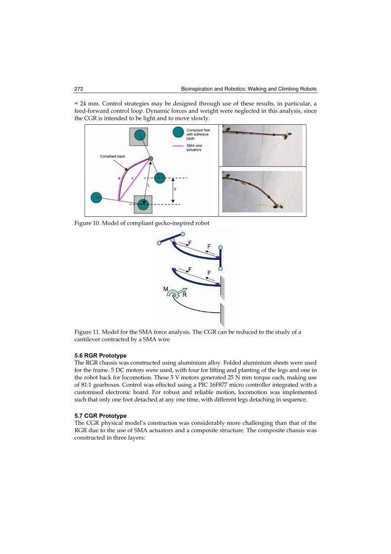
Bioinspiration and Robotics: Walking and Climbing Robots 272
= 24 mm. Control strategies may be designed through use of these results, in particular, a feed-forward control loop. Dynamic forces and weight were neglected in this analysis, since the CGR is intended to be light and to move slowly.
Figure 10. Model of compliant gecko-inspired robot
Figure 11. Model for the SMA force analysis. The CGR can be reduced to the study of a cantilever contracted by a SMA wire
5.6 RGR Prototype
The RGR chassis was constructed using aluminium alloy. Folded aluminium sheets were used for the frame. 5 DC motors were used, with four for lifting and planting of the legs and one in the robot back for locomotion. These 5 V motors generated 25 N mm torque each, making use of 81:1 gearboxes. Control was effected using a PIC 16F877 micro controller integrated with a customised electronic board. For robust and reliable motion, locomotion was implemented such that only one foot detached at any one time, with different legs detaching in sequence.
5.7 CGR Prototype
The CGR physical model’s construction was considerably more challenging than that of the RGR due to the use of SMA actuators and a composite structure. The composite chassis was constructed in three layers:
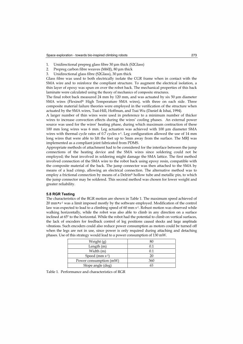
Space exploration - towards bio-inspired climbing robots 273
1. Unidirectional prepreg glass fibre 30 μm thick (S2Glass)
2. Prepreg carbon fibre weaves (M60J), 80 μm thick
3. Unidirectional glass fibre (S2Glass), 30 μm thick Glass fibre was used to both electrically isolate the CGR frame when in contact with the SMA wire and to reinforce the compliant structure. To augment the electrical isolation, a thin layer of epoxy was spun on over the robot back. The mechanical properties of this back laminate were calculated using the theory of mechanics of composite structures.
The final robot back measured 24 mm by 120 mm, and was actuated by six 50 μm diameter SMA wires (Flexinol® High Temperature SMA wires), with three on each side. Three composite material failure theories were employed in the verification of the structure when actuated by the SMA wires, Tsai-Hill, Hoffman, and Tsai Wu (Daniel & Ishai, 1994). A larger number of thin wires were used in preference to a minimum number of thicker wires to increase convection effects during the wires’ cooling phases. An external power source was used for the wires’ heating phase, during which maximum contraction of these
100 mm long wires was 6 mm. Leg actuation was achieved with 100 μm diameter SMA wires with thermal cycle rates of 0.7 cycles s-1. Leg configuration allowed the use of 14 mm long wires that were able to lift the feet up to 5mm away from the surface. The MRJ was implemented as a compliant joint fabricated from PDMS. Appropriate methods of attachment had to be considered for the interface between the jump connections of the heating device and the SMA wires since soldering could not be employed; the heat involved in soldering might damage the SMA lattice. The first method involved connection of the SMA wire to the robot back using epoxy resin, compatible with the composite material of the back. The jump connector was then attached to the SMA by means of a lead crimp, allowing an electrical connection. The alternative method was to employ a frictional connection by means of a Delrin® hollow tube and metallic pin, to which the jump connector may be soldered. This second method was chosen for lower weight and greater reliability.
5.8 RGR Testing
The characteristics of the RGR motion are shown in Table 1. The maximum speed achieved of 20 mm•s-1 was a limit imposed mostly by the software employed. Modification of the control law was expected to lead to a climbing speed of 60 mm s-1. Robust motion was observed while walking horizontally, while the robot was also able to climb in any direction on a surface inclined at 65º to the horizontal. While the robot had the potential to climb on vertical surfaces, the lack of encoders for feedback control of leg positions caused shocks and large amplitude
vibrations. Such encoders could also reduce power consumption as motors could be turned off when the legs are not in use, since power is only required during attaching and detaching phases. Use of this strategy would lead to a power consumption of 130 mW.
Weight (g) 80
Length (m) 0.1
Width (m) 0.1
Speed (mm s-1) 20
Power consumption (mW) 360
Slope angle (deg) 65
Table 1. Performance and characteristics of RGR
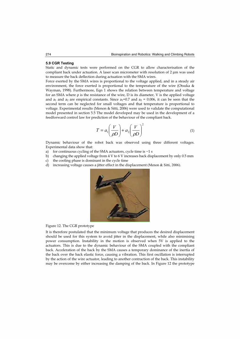
Bioinspiration and Robotics: Walking and Climbing Robots 274
5.9 CGR Testing
Static and dynamic tests were performed on the CGR to allow characterisation of the
compliant back under actuation. A laser scan micrometer with resolution of 2 μm was used to measure the back deflection during actuation with the SMA wires. Force exerted by the SMA wires is proportional to the voltage applied, and in a steady air environment, the force exerted is proportional to the temperature of the wire (Otsuka & Wayman, 1998). Furthermore, Eqn 1 shows the relation between temperature and voltage
for an SMA where ρ is the resistance of the wire, D is its diameter, V is the applied voltage and a1 and a2 are empirical constants. Since a1=0.7 and a2 = 0.006, it can be seen that the second term can be neglected for small voltages and that temperature is proportional to voltage. Experimental results (Menon & Sitti, 2006) were used to validate the computational model presented in section 5.5 The model developed may be used in the development of a feedforward control law for prediction of the behaviour of the compliant back.
2
21 +=D
VaD
VaTρρ
(1)
Dynamic behaviour of the robot back was observed using three different voltages. Experimental data show that: a) for continuous cycling of the SMA actuators, cycle time is ~1 s b) changing the applied voltage from 4 V to 6 V increases back displacement by only 0.5 mm c) the cooling phase is dominant in the cycle time d) increasing voltage causes a jitter effect in the displacement (Menon & Sitti, 2006).
Figure 12. The CGR prototype
It is therefore postulated that the minimum voltage that produces the desired displacement should be used for this system to avoid jitter in the displacement, while also minimising power consumption. Instability in the motion is observed when 5V is applied to the actuators. This is due to the dynamic behaviour of the SMA coupled with the compliant back. Acceleration of the back by the SMA causes a temporary dominance of the inertia of the back over the back elastic force, causing a vibration. This first oscillation is interrupted by the action of the wire actuator, leading to another contraction of the back. This instability may be overcome by either increasing the damping of the back. In Figure 12 the prototype
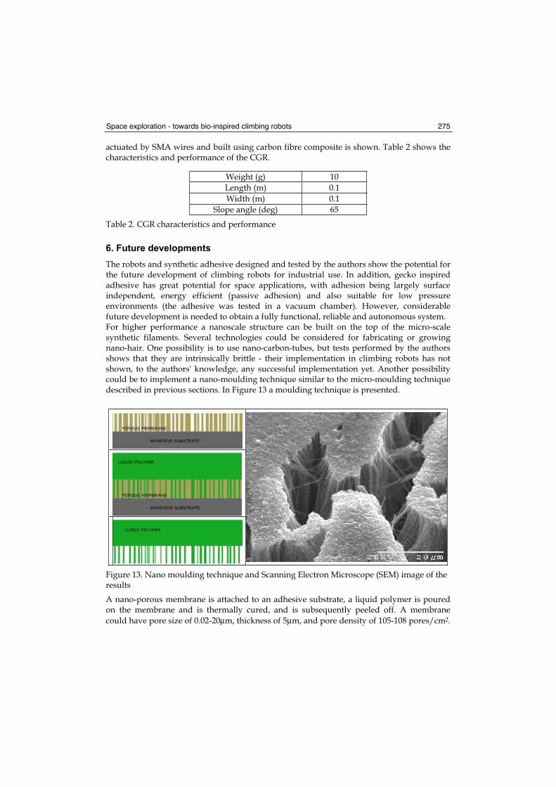
Space exploration - towards bio-inspired climbing robots 275
actuated by SMA wires and built using carbon fibre composite is shown. Table 2 shows the characteristics and performance of the CGR.
Weight (g) 10
Length (m) 0.1
Width (m) 0.1
Slope angle (deg) 65
Table 2. CGR characteristics and performance
6. Future developments
The robots and synthetic adhesive designed and tested by the authors show the potential for the future development of climbing robots for industrial use. In addition, gecko inspired adhesive has great potential for space applications, with adhesion being largely surface independent, energy efficient (passive adhesion) and also suitable for low pressure environments (the adhesive was tested in a vacuum chamber). However, considerable future development is needed to obtain a fully functional, reliable and autonomous system. For higher performance a nanoscale structure can be built on the top of the micro-scale synthetic filaments. Several technologies could be considered for fabricating or growing nano-hair. One possibility is to use nano-carbon-tubes, but tests performed by the authors shows that they are intrinsically brittle - their implementation in climbing robots has not shown, to the authors' knowledge, any successful implementation yet. Another possibility could be to implement a nano-moulding technique similar to the micro-moulding technique described in previous sections. In Figure 13 a moulding technique is presented.
Figure 13. Nano moulding technique and Scanning Electron Microscope (SEM) image of the results
A nano-porous membrane is attached to an adhesive substrate, a liquid polymer is poured on the membrane and is thermally cured, and is subsequently peeled off. A membrane
could have pore size of 0.02-20μm, thickness of 5μm, and pore density of 105-108 pores/cm2.
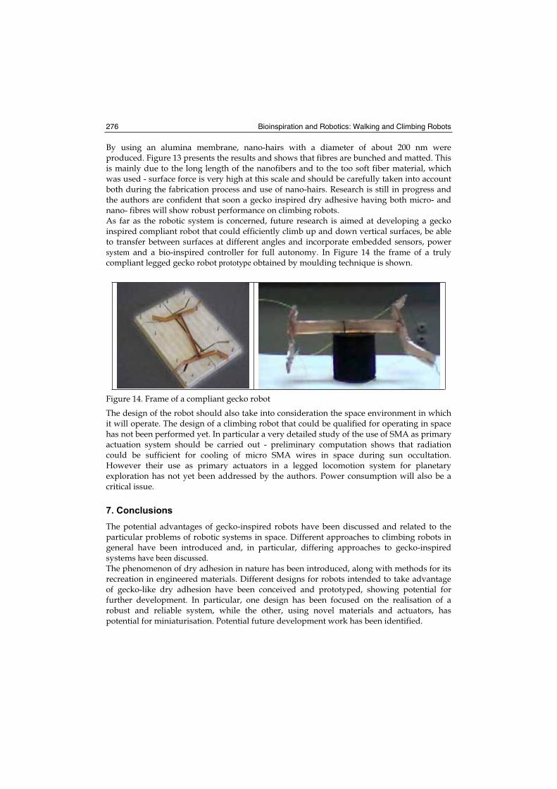
Bioinspiration and Robotics: Walking and Climbing Robots 276
By using an alumina membrane, nano-hairs with a diameter of about 200 nm were produced. Figure 13 presents the results and shows that fibres are bunched and matted. This is mainly due to the long length of the nanofibers and to the too soft fiber material, which was used - surface force is very high at this scale and should be carefully taken into account both during the fabrication process and use of nano-hairs. Research is still in progress and the authors are confident that soon a gecko inspired dry adhesive having both micro- and nano- fibres will show robust performance on climbing robots. As far as the robotic system is concerned, future research is aimed at developing a gecko inspired compliant robot that could efficiently climb up and down vertical surfaces, be able to transfer between surfaces at different angles and incorporate embedded sensors, power system and a bio-inspired controller for full autonomy. In Figure 14 the frame of a truly compliant legged gecko robot prototype obtained by moulding technique is shown.
Figure 14. Frame of a compliant gecko robot
The design of the robot should also take into consideration the space environment in which it will operate. The design of a climbing robot that could be qualified for operating in space has not been performed yet. In particular a very detailed study of the use of SMA as primary actuation system should be carried out - preliminary computation shows that radiation could be sufficient for cooling of micro SMA wires in space during sun occultation. However their use as primary actuators in a legged locomotion system for planetary exploration has not yet been addressed by the authors. Power consumption will also be a critical issue.
7. Conclusions
The potential advantages of gecko-inspired robots have been discussed and related to the particular problems of robotic systems in space. Different approaches to climbing robots in general have been introduced and, in particular, differing approaches to gecko-inspired systems have been discussed.The phenomenon of dry adhesion in nature has been introduced, along with methods for its recreation in engineered materials. Different designs for robots intended to take advantage of gecko-like dry adhesion have been conceived and prototyped, showing potential for further development. In particular, one design has been focused on the realisation of a robust and reliable system, while the other, using novel materials and actuators, has potential for miniaturisation. Potential future development work has been identified.
Space exploration - towards bio-inspired climbing robots 277
8. References
Aksak, B., Murphy, M., Sitti, M. (2007). 'Adhesion of Biologically Inspired Vertical and Angled Polymer Microfiber Arrays,' Langmuir, 2007, 23, 3322-3332.
Bretl, T., Rock, S., Latombe, J.C., Kennedy, B., Aghazarian, H. (2004). Free-Climbing with a multi-Use Robot (2004). International Symposium on Experimental Robotics (ISER),Singapore.
Cepolina, F., Michelini, R.C., Molfino, R.M., Razzoli, R.P. (2003). Gecko, a climbing robot for walls cleaning, ASER03, 1st International Workshop on Advances in Service Robotics,13-15 March 2003, Bardolino, Italy, ISBN 3-8167-6268-9
Daltorio K. A., Horchler A. D., Gorb S., Ritzmann R. E. and Quinn R. (2005a). A Small Wall-Walking Robot with Compliant, Adhesive Feet, Int. Conf. on Intelligent Robots and Systems (IROS ‘05), Edmonton, Canada.
Daltorio, K.A., Gorb, S., Peressadko, A., Horchler, A.D., Ritzmann, R.E., Quinn, R.D. (2000b) A robot that climbs walls using micro-structured polymer feet. Proc. Int. Conf. Climbing and Walking Robots (CLAWAR), London, UK. 13-15. September 2005
Daniel I. M. & Ishai 0. (1994). Engineering Mechanics of Composite Materials. Oxford University Press, Oxford, 1994.
Hansen, W. & Autumn, K. (2005). Evidence for self-cleaning in gecko setae. Proc. Natl. Acad. Sci. U.S.A. 2005, 102, 385-389.
Geim, A. K., Dubonos, S. V., Grigorieva, I. V., Novoselov, K. S., Zhukov, A. A., Shapoval, S. Y. (2003) Microfabricated adhesive mimicking gecko foot-hair. Nat. Mater. 2003, 2,461-463.
Glassmaker, N. J., Jagota, A., Hui, C. Y., Kim, J. (2004). Design of biomimetics fibrillar interfaces: 1. making contact. J. R. Soc. Interface 2004, 1 (1), 23-33
Grieco J, Armada M, Gonzalez de Santos P, Prieto M. (1998). A six-legged climbing robot for high payloads. Proceedings of the 1998 IEEE International Conference on Control AppEicarions, Trieste, Italy, 1998, 1, 446450.
Haynes, G. & Rizzi, A. (2006). Gait Regulation and Feedback on a Robotic Climbing Hexapod, Proceedings of Robotics: Science and Systems, August, 2006.
Howell, L.L. (2001). Compliant Mechanisms, Wiley-Interactive, New York, 2001 Huber, G., Mantz, H., Spolenak, R., Mecke, K., Jacobs, K., Gorb, S. N., Arzt, E. (2005)
Evidence for capillarity contributions to gecko adhesion from single spatula nanomechanical measurements. Proc. Natl. Acad. Sci. U.S.A. 2005, 102, 16293-16296.
J.W. Hurst & Rizzi, A. (2004). Physically Variable Compliance in Running, CLAWAR,Springer-Verlag, www.springeronline.com, September, 2004.
Illingworth, L. and Reinfeld, D. (2001) The Vortex Attractor: US Patents #6565321 and #6497553, Vortex Holding Company, United States Patent and Trademark Office, USA.
Joudrier, L., Didot, F., Kapellos, K., (2005). EUROBOT: USE OF THE MUROCO FORMAL APPROACH FOR ACTIVITY ANALYSIS, PROGRAMMING AND CONTROL Proc. of 'The 8th International Symposium on Artifical Intelligence, Robotics and Automation in Space - iSAIRAS’, Munich, Germany.5-8 September 2005, (ESA SP-603, August 2005)
Kim, S., Asbeck, A., Provancher, W., and Cutkosky, M.R. (2005). SpinybotII: Climbing Hard Walls with Compliant Microspines, IEEE ICAR, Seattle, WA, July, 18-20, 2005.
Bioinspiration and Robotics: Walking and Climbing Robots 278
S. Kim and M. Sitti, (2006) “Biologically Inspired Polymer Microfibers with Spatulate Tips as Repeatable Fibrillar Adhesives,” Applied Physics Letters, vol. 89, no. 26, pp. 26911-13, 27 Dec. 2006.
Kim, S., Spenko, M., Trujillo, S., Heyneman, B., Mattoli, V., Cutkosky, M.R. (2007). Whole body adhesion: hierarchical, directional and distributed control of adhesive forces for a climbing robot, IEEE ICRA07, April 2007.
Majidi, C., Groff, R., Fearing, R. (2004). Clumping and packing of hair arrays manufactured by nanocasting. Proc. ASME Int. Mech. Eng. Congress Exposition 2004, 579-584.
Menon, C. & Sitti, M. (2006). A Biomimetic Climbing Robot Based on the Gecko, Journal of Bionic Engineering, Vol. 3, No. 3 (September 2006), pp 115-125), 1672-6529
Menon, C., Murphy, M., Angrilli, F., Sitti, M., (2004), WaalBots for Space applications, 55th IAC Conference, Vancouver, Canada.
Murphy, M., Sitti, M., (2007), Waalbot: An Agile Small-Scale Wall Climbing Robot Utilizing Dry Elastomer Adhesives, IEEE/ASME Trans. on Mechatronics, 2007, 12, 330-338.
Northen, M. T. & Turner, K. L. (2005). A batch fabricated biomimetic dry adhesive, Nanotechnology, 16, 1159-1166.
Otsuka K, Wayman C M. Shape Memory Materials. Cambridge University Press, Cambridge, UK, 1998
Sitti, M. & Fearing, R. (2003) Synthetic gecko foot-hair micro/nanostructures as dry adhesives. J. Adhes. Sci. Technol., 17 (5), 1055-74.
Shah, G., Sitti, M., (2004). Modeling and Design of Biomimetic Adhesives Inspired by Gecko Foot-Hairs, IEEE International Conference on Robotics and Biomimetics (ROBIO),Shenyang, China, Aug 2004.
Spolenak, R., Gorb, S., Gao, H., Arzt, E. (2005). Effects of contact shape on the scaling of biological attachments. Proc. R. Soc. London, Ser. A, 2005, 461, 305-319.
Sun, W., Neuzil, P., Kustandi, T., Oh, S., Samper, V. D. (2005) The nature of the gecko lizard adhesive force. Biophys. J. Biophys. Lett. 2005, L14-L17.
Tummala, R., Mukherjee, R., Aslam, D., Xi, N., Mahadevan, S., Weng, J. (1999) Reconfigurable Adaptable Micro-Robot, Proceedings of the IEEE Conference on Systems, Man, and Cybernetics (SMC), Tokyo, Japan, Oct. 12-15, 1999.
Unver, O. Uneri, A. Aydemir, A. Sitti, M. Geckobot: a gecko inspired climbing robot using elastomer adhesives, Proceedings 2006 IEEE International Conference on Robotics and Automation, 2006 (May 2006), pp 2329-2335, 1050-4729
Visentin, G. (2005). Robotic Programmes and Applications at ESA: Present and Perspectives, 'i-SAIRAS 2005' - The 8th International Symposium on Artificial Intelligence, Robotics and Automation in Space. Edited by B. Battrick. ESA SP-603. European Space Agency, 2005. Published on CDROM., p.1.1 Publication Date: 08/2005
Zhao, Y., Tong, T., Delzeit, L., Kashani, A., Meyyappan, M., Majumdar, A. (2006). Interfacial energy and strength of multiwalled-carbon-nanotube-based dry adhesive. J. Vac. Sci. Technol., B: Microelectron. Nanometer Struct.sProcess., Meas., Phenom. 2006, 24, 331-335.
17
Biologically Inspired Robots
Fred Delcomyn University of Illinois
U. S. A.
1. Introduction
The idea of building machines that emulate features of animals that we see around us has a long history. Leonardo da Vinci’s drawings of machines that fly like birds are one familiar example. It was not until the middle of the 19th century, however, that scientific knowledge had advanced enough for realistic and realizable plans for such machines to be made (Raibert, 1986) and truly successful attempts to make walking or crawling robots proliferated only in the last few decades of the 20th century (e.g., Raibert, 1990). In the sense that any machine that swims, flies, or walks can be said to be inspired by fish, birds, or legged animals, every mobile robot that employs one of these means of locomotion can be said to be biologically inspired. However, the term biologically inspired and the current concept of biologically inspired robotics originated in the last few decades of the 20th
century. The first use of the phrase in the title of a journal article appears to have been by Beer et al. (1997). In this article, Beer and his colleagues make a distinction between merely emulating some general feature of an animal like legs or wings and a more considered approach in which specific structural or functional elements of particular animals is emulated in hardware or software. Because animals are both structurally and functionally complex, it is obvious that a complete reproduction of any animal in hardware and software is not possible. Hence, there is some debate among bioroboticists about where to draw the line. Some researchers take the approach of Ritzmann and colleagues (Ritzmann et al., 2000), who suggested that as many features of an animal should be incorporated into a robot as possible, even if the functional advantage of any particular feature is not clear (e.g., Cham et al., 2004; Dillmann et al., 2007). In recent years, this approach has sometimes been called biomimetic robotics (e.g., Ayres & Witting, 2007). The argument is that many of these features actually do confer useful attributes to the robot even if that usefulness is not immediately apparent. Other researchers take a more conservative approach, even arguing that including too many animal-like features into a robot can impair performance (e.g., Yoneda & Ota, 2003). Biorobotics has a second element as well. In addition to arguing that using biological principles as a source of inspiration for the construction of robots, some researchers have argued that studying robots can advance biologists’ knowledge and understanding of those same biological principles (Beer et al., 1998; Ritzmann et al., 2000; Webb, 2006). The idea is that any attempt to implement in hardware and software specific features of a real animal can only improve our understanding of those features because such an attempt will immediately expose any part of our understanding that is incomplete or that when
Bioinspiration and Robotics: Walking and Climbing Robots 280
implemented does not lead to a level of performance that is expected. The discussion paper by Webb (2001a) and the resulting commentaries (see discussion of them by Webb, 2001b) is probably the best single source for an introduction to this approach and the response of the biological and engineering communities to it. Whether approached from an engineering or a biological perspective, there is no doubt that by whatever term one chooses to characterize it, bioinspired engineering, biorobotics, biological inspiration, or biomimetics, the fusion of biology and engineering is emerging as a discipline in its own right. The appearance of semi-popular works (e.g., Paulson, 2004) and papers appearing in non-traditional journals (e.g., Delcomyn, 2004) also attests to the growing awareness of the field. This does not even include the more than 1.5 million hits one obtains by conducting a Google search on the phrase “walking robot” or the roughly 61,400 hits for pages with images of robots with legs as of June, 2007. Considering only the research literature, a search of the ISI Web of Knowledge database reveals that from 2000 to 2004, there were an average of 9.2 papers per year on mobile robotic machines that listed biological inspiration or variants thereof as a key phrase. In 2005, the number jumped to 16, an increase of over 70%, and in 2006, there were 30, an additional increment of more than 85%. Though not large, this is nevertheless a field worth paying attention to.
2. Bioinspiration as a Means of Improving Robotic Performance
2.1 Animal locomotion and its performance features
Two words encapsulate what engineers find attractive about the walking and running of animals – speed and agility. Running speed among mammals ranges from about 8 miles per hour (mph; 12 km/hr or 3.6 meters per second) for a mouse to a top speed of about 70 mph (113 km/hr, 31 m/s) for a cheetah. Small animals like insects, of course, move much more slowly, only a few miles per hour at best. The land speed record for an insect appears to be a tiger beetle at 5.5 mph (8.8 km/hr, 2.5 m/s) (Kamoun & Hogenhout, 1996). Some cockroaches are also relatively fast, some having been clocked at about 3 mph (5.5 km/hr, 1.5 m/s; Full & Tu, 1991). More relevant to small animals, however, is body-lengths per second, since this measure scales the speed of locomotion to the size of the animal. Cheetahs check in at about 20-29 body lengths per second. Cockroaches and mice run at about 50 to 71 body lengths per second, while the swift tiger beetle apparently tops the scale at 245 body lengths per second. Agility is much more difficult to measure since there is no single measurement one can make that will represent it. Clearly, many animals are extraordinarily agile – think of monkeys scrambling about in the treetops or a snow leopard chasing a goat nearly full speed down a steep mountain slope. A few studies have been done on agility among insects, though measuring agility was not the purpose of the study. Frantsevich & Cruse (2005) showed that a small bug (approximately 1 cm long) is able to walk along a stick about 1 mm in diameter and when it reaches the end, smoothly turn around and walk back without falling off. A stick insect has also been shown to be able to cross a gap that is about as wide as the length of its body (Bläsing, 2006). Cockroaches are adept at climbing over obstacles that are at least as high as they are (Watson et al., 2002). Some can run over rugged surfaces containing obstacles about twice the insect’s height (Full et al., 1998).
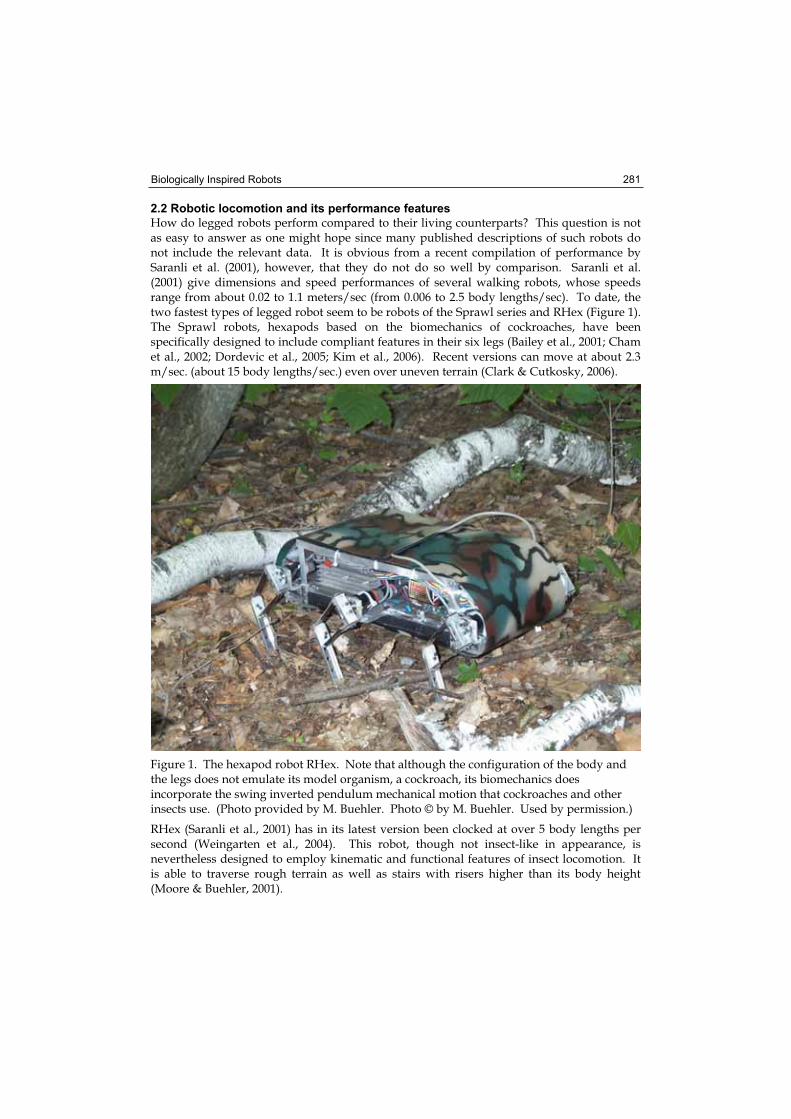
Biologically Inspired Robots 281
2.2 Robotic locomotion and its performance features
How do legged robots perform compared to their living counterparts? This question is not as easy to answer as one might hope since many published descriptions of such robots do not include the relevant data. It is obvious from a recent compilation of performance by Saranli et al. (2001), however, that they do not do so well by comparison. Saranli et al. (2001) give dimensions and speed performances of several walking robots, whose speeds range from about 0.02 to 1.1 meters/sec (from 0.006 to 2.5 body lengths/sec). To date, the two fastest types of legged robot seem to be robots of the Sprawl series and RHex (Figure 1). The Sprawl robots, hexapods based on the biomechanics of cockroaches, have been specifically designed to include compliant features in their six legs (Bailey et al., 2001; Cham et al., 2002; Dordevic et al., 2005; Kim et al., 2006). Recent versions can move at about 2.3 m/sec. (about 15 body lengths/sec.) even over uneven terrain (Clark & Cutkosky, 2006).
Figure 1. The hexapod robot RHex. Note that although the configuration of the body and the legs does not emulate its model organism, a cockroach, its biomechanics does incorporate the swing inverted pendulum mechanical motion that cockroaches and other insects use. (Photo provided by M. Buehler. Photo © by M. Buehler. Used by permission.)
RHex (Saranli et al., 2001) has in its latest version been clocked at over 5 body lengths per second (Weingarten et al., 2004). This robot, though not insect-like in appearance, is nevertheless designed to employ kinematic and functional features of insect locomotion. It is able to traverse rough terrain as well as stairs with risers higher than its body height (Moore & Buehler, 2001).
Bioinspiration and Robotics: Walking and Climbing Robots 282
Although recent reports do a better job of giving specific details of a robot’s physical parameters and its speed of walking, it is clear that there is still no set of tests to which engineers routinely subject their constructions in order to test performance. Not just speed of walking over a level surface, but also such parameters as minimum turning radius, steepest incline navigable, height of obstacle (relative to body height) that can be climbed over, etc., should be assessed and reported. As Delcomyn (2004) has pointed out, using such a set of tests for all walking robots would greatly advance the discipline of biorobotics.
3. Crawling Robots
3.1 Applications
Although certainly some robots are designed and built with the prime objective being research on the physical features of the robot or on the mechanisms that control it, most are conceived and built with one or more specific applications in mind. This seems to be particularly true for crawling robots. Furthermore, the great diversity of applications for which such robots are built is reflected in the great diversity of their physical structure. This structure ranges from legged robots that drag their bodies along the substrate (e.g., Voyles & Larson, 2005) to worm- or snake-like robots (Menciassi & Dario, 2003, Menciassi et al., 2006; Chernousko, 2005; Crespi et al., 2005). Actual or suggested applications for crawling robots are as diverse as body types and include inspection and maintenance of pipelines (Bolotnik et al., 2002; Chatzakos et al., 2006; Gu et al., 2005), construction of a space array (Kaya et al., 2005), open heart surgury (Riviere et al., 2004), surveillance (Voyles & Larson, 2005), search and rescue (Wang & Appleton, 2003), and off-world exploration (Voyles & Larson, 2005). Pipeline or tunnel inspection and maintenance is probably the most common use for crawling robots. Some robots in this category are intended simply to crawl along the exterior (Chatzakos et al., 2006) or the interior (Bolotnik et al., 2002) of a pipeline. Others are more complex, being able to alter their shapes (Wang & Appleton, 2003) in order to squeeze through broken areas or to detect the profile of a pipe in order to identify collapsed tunnels or pipes (Gu et al., 2005). Some crawling robots have no legs and are more exotic, such as a small remotely controlled robot that adheres by suction to a heart or other tissue during surgury (Riviere et al., 2004).
3.2 Features
Crawling robots slither or pull/push themselves along the surface on which they are moving and therefore need not be concerned with maintaining balance. (Although robots that move along pipes or tubes are typically referred to as crawling, some may actually support their body weight on their legs (e.g., Bolotnik et al., 2002).) Hence it is probably fair to say that there is a greater variety of means of locomotion among crawling than among walking robots. Except for the presence of legs, there is no indication that pipe-crawling robots have been designed with any biological principles or features in mind. Most are conventional, in the sense that they typically have 6-8 legs, but a few have unusual features. Voyles & Larson (2005) have designed a small two-legged robot that can crawl by dragging its body along. Its small size will enable it to search through the rubble of collapsed buildings for survivors or to explore the rugged terrain of other planets. Not having to support its body weight on
Biologically Inspired Robots 283
its legs means that the two “arms” can be used to manipulate objects in the environment if necessary. Wang & Appleton (2003) offer a shape-shifting robot to make it possible for the robot to squeeze through small spaces. Most crawling robots have no legs, though some do (Matsuno et al., 2002; Voyles & Larson, 2005). Legless robots come in a variety of forms and use a variety of locomotor schemes. Some are modeled after snakes both structurally and functionally and progress by a snake-like slithering locomotion (e.g., Chernousko, 2005). Others are designed to progress more like earthworms, using peristaltic movement, a repetitive, concertena-like compression and elongation of the body, to move forward (Menciassi et al., 2006). A third type progresses like an inchworm, having sucker-like appendages at the front and back and moving forward by attaching to the substrate at the front end, pulling the body forward, then attaching at the rear, releasing the front sucker and advancing the body, and repeating the cycle (Riviere et al., 2004).
3.3 Performance and advantages
As pointed out by Saga & Nakamura (2004), snake-like or worm-like locomotion generally requires less space than does locomotion with legs because the body is elongated and does not have any projections. Hence, robots built to emulate snakes or worms have an inherent advantage over robots with legs when they must operate in close quarters. This advantage, however, is offset by rather slow forward progression. Multilink snake-like robots, for example, can travel at less than 20 cm/sec (Chernousko, 2005). Given their size (more than a meter long), this translates into less than 0.01 body lengths/sec. Some snakes, like some other animals, are amphibious. Certainly an amphibious robot can be designed with legs or without, but an advantage of an amphibious snake-like robot is that a similar control system can be used to regulate motion in water and on land. Legged animals generally use their legs differently on land than in the water, hence adding an extra layer of complexity to any legged amphibious robot (Ijspeert et al., 2005). By using a snake model, Crespi and colleagues (Crespi et al., 2005) are able to use a single control mechanism, since the locomotion they are emulating is essentially the same on land as it is in the water. Robots designed to emulate the peristaltic locomotion of worms can move forward using even less space than snake-like robots require (Saga & Nakamura, 2004) because there is no side-to-side motion of the body at all. The challenge for robots modelled after worms is finding an appropriate type of actuator that will impart the necessary motion to the body. Saga & Nakamura (2004) have implemented a novel approach, using a magnetic fluid whose viscosity changes with a fluctuating magnetic field inside a micro-robot. Hence, the robot can be controlled in a restricted environment from outside the robot itself. Furthermore, even though the robot requires no wires or external connection, its movements can nevertheless be precisely controlled by application of an external magnet that supplies the necessary magnetic field. An important advantage of biomimetically designed worm-like crawling robots is their potential use in medicine. In addition to their modular nature, a feature that simplifies construction and control, the main advantage of such robots is the possibility of their use inside the human intestine or in blood vessels. For example, Menciassi and collaborators (Menciassi & Dario, 2003; Menciassi et al., 2006) have developed a robot that could in principle be used in microendoscopy, a procedure for examining for abnormalities the human intestinal tract or small tubes or ducts. The main feature of the robot is a system of
Bioinspiration and Robotics: Walking and Climbing Robots 284
microhooks on its surface, enabling it to gain traction against the smooth inner surface of any biological tube or duct. Progression is achieved through control of shape memory alloy in the robot that is deformed and then regains its original form, moving the robot forward. An advantage of robots based on peristaltic locomotion is that they can press against the walls of the tube within which they are moving. If the robot is to be used on the exterior surface of an object, this obviously cannot be done. In these circumstances, an inchworm-like robot may be a better choice and such robots have been designed for these circumstances. For example, Rincon & Castro (2003) discuss their inchworm-like robot and its structural advantages. (It should be noted, however, that they describe as “inchwormlike” the peristaltic locomotion of an earthworm, which is not a correct usage of the term.) Riviere and colleagues (Riviere et al., 2004; Patronik et al., 2004) have used the inchworm model for their small robot that can work on the epicardium of a beating heart. The robot adheres by suction and navigates by crawling like an inchworm under control or an operating surgeon.
4. Walking Robots
4.1 Applications
Many of the applications suggested for crawling robots, such as surveillance, search and rescue, and off-world exploration, have been suggested for walking robots as well. Even endoscopic surgery, to which crawling robots might seem better suited, has been proposed as an application for a robot with legs (Urban et al., 1999). Underwater walking applications have been implemented successfully as well (Ayres, 2004). The presence of legs does in principle add a functional capacity not generally available to crawling, legless, robots – the ability to walk up vertical surfaces. (Some snakes can actually climb trees, but climbing is not a feature of snake-like robots.) A way to grip a surface with enough force that the robot will not slip and fall is, however, not easy to devise. Most animals that can climb are either quite small (like insects) and therefore do not have much weight to support, or have claws or other special adaptations on their feet that enable them to form a firm grip on surfaces. One animal used as a model for studies of wall-climbing is the gecko. These reptiles have special pads on the soles of their feet that allow them to adhere to virtually any surface; this feature has made them attractive subjects for research on how to incorporate tight grip into a robot (Dai & Sun, 2007). A second active area of research that is unique to robots with legs is the study of humanoid robots (e.g., Witte et al., 2004). Part of the attraction of these robots is the challenge of designing one that can walk and balance well on two legs. Although a task like ascending or descending stairs can be carried out by humans without any thought at all, it is not so easy to design a robot to do the same thing since the balance issues are significant. Another attraction is simply the challenge of building a robot that looks like a human being, and that can interact with humans. The Honda Corporation has been particularly active in this field, having designed and built a fully independent, walking humanoid robot. (Simple technical details are available at the Honda web site: http://asimo.honda.com/EducationMaterials.aspx.) An important driving force in this burgeoning field of research is the goal of building humanoid robots that can serve along with humans in ordinary workspaces or in homes. The challenges are well described in a recent review by Kemp et al. (2007). Engineers in the field generally do not use the term biomimetic in reference to their work, but any attempt to emulate the physical structure of a living organism in a robot obviously does fall into this category.
Biologically Inspired Robots 285
4.2 Features
A search of the ISI Web of Science database in June, 2007 using the search terms robot and walking together yielded more than 660 publications. Clearly, this is an active area of research and any brief overview of the field like this one cannot hope to be comprehensive. Here I will concentrate on features of some representative biomimetic robots that seem particularly important. Walking or hopping robots have been made with leg numbers ranging from one to 10. Animal models for these robots include humans (Witte et al., 2004), rats (Chavarriaga et al., 2005), salamanders (Ijspeert et al., 2005), a variety of insects (ants: Goulet & Gosselin, 2005, cockroaches: Delcomyn & Nelson, 2000; Saranli et al., 2001; Nelson et al., 1999; stick insects: Dean et al., 1999), scorpions (Klaassen et al., 2002), and lobsters (Ayres & Witting, 2007). Raibert & Hodgins (1993) have developed a single-legged robot that “walks” by hopping. Some robots are designed to reproduce the physical structure of the animal after which they are modeled (e.g., Delcomyn & Nelson, 2000; Nelson et al, 1999; Ayres & Witting, 2007; see Figure 2) but scaled up appropriately in size. The rationale for this attention to detail is that the physical structure of the animal (the differences in size, structure, and articulation with the body in the legs of cockroaches, for example) confers to it certain locomotor capabilities and that by emulating the animal's physical structure some of those capabilities will be conferred to the robot (Ritzmann et al., 2004). Other robots are built along more conventional engineering lines with legs being similar to one another and simply articulated (Dillmann et al., 2007). One hexapod robot, RHex, while not built to resemble its model organism physically, nevertheless was designed to emulate the kinamatics and dynamics of its walking (Altendorfer et al., 2001). And while most robots are built with a rigid body, some have been designed with the ability to flex or bend the body just as animals can. This feature has been shown to aid significantly in the robot's ability to climb over obstacles (Quin et al., 2003). An important element in any walking robot is the type of actuator used to power the movements of the limbs. In early robots, the actuator of choice was generally an electrical motor (e.g., Beer et al., 1997). Later robots have used pneumatics (Nelson & Delcomyn, 2000, Quinn et al., 2001) to drive the legs or artificial muscles such as McKibbon actuators. (Klute et al., 2002), electroactive polymers (Bar-Cohen, 2003), Nitinol wire with shape memory (Safak & Adams, 2002), and other devices. The common feature of these artificial muscle devices is that they incorporate essential features of living muscle such as compliance and favorable force-velocity relationships while at the same time not consuming too much power. No robot is of any use if it cannot walk effectively, so an appropriate method of controlling leg movements is obviously essential. Here again, a comparison of the control mechanisms used in early robots with those that are generally used today shows the influence and effectiveness of biorobotics. Even early biomimetic robots tended to be controlled in a rather rigid fashion, such that hexapod walking machines, for example, were programmed to use the typical insect tripod gait (front and rear legs on one side of the body moving together with the middle leg on the other side, and these three legs alternating their movements with the other three) at all times. More recent robots use a more flexible control system that allows independent movement of the legs of the robot when this is desirable (e.g., Arena et al., 2002, 2004), leading to a flexible determination of the appropriate gait to use in a given circumstance.
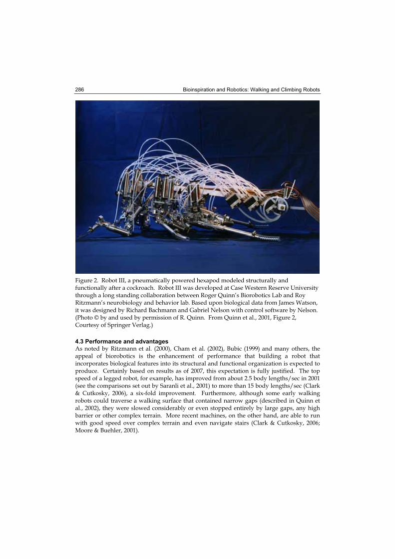
Bioinspiration and Robotics: Walking and Climbing Robots 286
Figure 2. Robot III, a pneumatically powered hexapod modeled structurally and functionally after a cockroach. Robot III was developed at Case Western Reserve University through a long standing collaboration between Roger Quinn’s Biorobotics Lab and Roy Ritzmann’s neurobiology and behavior lab. Based upon biological data from James Watson, it was designed by Richard Bachmann and Gabriel Nelson with control software by Nelson. (Photo © by and used by permission of R. Quinn. From Quinn et al., 2001, Figure 2, Courtesy of Springer Verlag.)
4.3 Performance and advantages
As noted by Ritzmann et al. (2000), Cham et al. (2002), Bubic (1999) and many others, the appeal of biorobotics is the enhancement of performance that building a robot that incorporates biological features into its structural and functional organization is expected to produce. Certainly based on results as of 2007, this expectation is fully justified. The top speed of a legged robot, for example, has improved from about 2.5 body lengths/sec in 2001 (see the comparisons set out by Saranli et al., 2001) to more than 15 body lengths/sec (Clark & Cutkosky, 2006), a six-fold improvement. Furthermore, although some early walking robots could traverse a walking surface that contained narrow gaps (described in Quinn et al., 2002), they were slowed considerably or even stopped entirely by large gaps, any high barrier or other complex terrain. More recent machines, on the other hand, are able to run with good speed over complex terrain and even navigate stairs (Clark & Cutkosky, 2006; Moore & Buehler, 2001).
Biologically Inspired Robots 287
Significant improvements in performance are often described in papers or at conferences by comparing the performance of a new robot with its predecessors. This is certainly useful. However, another welcome trend in recent research is to compare the performance of a walking robot directly with its animal counterpart (e.g., Bailey et al., 2001; Quinn et al., 2003), something that was not usually done except in the most casual way by early workers. This can be particularly useful because it is clear from zoology that animals themselves have widely disparate abilities to move fast or to traverse rugged terrain. Hence, it can be helpful to evaluate any robot not against some absolute standard but against its animal model, suitably scaled. After all, comparing the speed of a robot to that of a cheetah is hardly useful if the objective is to make a mechanical rat. Improvements in robotic performance have come from several different avenues of research. One of these is investigations in biomechanics. This topic has until recently been rather neglected even among biologists. Not until the seminal article by Chiel & Beer (1997), in which they pointed out the importance of kinematics and skeletomuscular mechanics to locomotion (and indeed, any behavior), did biologists who study locomotion begin to take much notice of biomechanics. In the following decade, the topic began to yield new insights into how walking is controlled in animals and the contribution of biomechanics to walking. In brief, research has shown that the skeletomuscular system of an animal acts as a kind of natural resonant system that stabilizes the body during fast locomotion. This is true for all legged animals. (See Delcomyn, 2004, for a review of the relevant insect literature, and Dickinson, et al., 2000 and Full & Farley, 2000 for a more general discussion of biomechanics and animal locomotion.) The new appreciation for biomechanics has spilled into the field of biorobotics. Much of this biomechanical robotics work has been done using insect models. The robot RHex, in particular, has been built specifically to incorporate the spring-loaded inverted pendulum leg movements of cockroaches and other insects into its walking (Altendorfer et al., 2001; Koditschek et al., 2004). Clark & Cutkosky (2006) have shown the importance of the different sizes and shapes of the legs of insects like cockroaches, which impact the mechanics of the insect’s walking. Other animals have been used as models as well, as shown by the recent work of Geng et al. (2006) on biped walking, in which they demonstrated that a stable biped walk can be mastered by a robot in part by taking the biomechanics of bipeds into account in the design of the machine. A second important area of research that has led to better robotic performance is in the area of control. Traditional approaches to control of movement, coming as they did from the necessity to control the movements of industrial robots to a high degree of precision, involve precise calculation of intended movements (Spong & Vidyasagar, 1989). Although this approach has been applied to walking robots with some success, the method imposes a high computational load on the controller and severely limits the flexibility of the walking gaits that can be used (e.g., Pratihar et al., 2000). An alternative approach is the use of a biomimetically designed controller based on the principles of locomotor control used by animals (see Delcomyn, 1999 for an overview of the topic). A number of investigators have used the biological concept of a central pattern generator (CPG) for generation of walking patterns (e.g., Arena et al., 2002, 2004; Ayres & Witting, 2007; Collins & Richmond, 1994; Fukuoka et al., 2003). Investigators have also employed the concept of distributed control, that is, that gait is generated by an interaction of CPGs controlling different legs or even different joints of single legs, and the feedback from sensors in the legs (e.g., Beer et al., 1992;
Bioinspiration and Robotics: Walking and Climbing Robots 288
Chiel et al., 1992; Dean et al., 1999; Kindermann, 2001). Underappreciated work by Ferrell (1995) compared the performance of various models of locomotor control. Complementing work on biomechanics and controllers is research on actuators. Early robots used electrical motors to power movement of the legs (e.g., Quinn & Espenschied, 1993), but it was apparent from the beginning that such motors could not generate the power and speed of action that would allow robots to emulate animal walking. The problem for engineers is that muscle is compliant and has the ability to develop and release tension extremely rapidly. Both attributes feature prominently in the ability of muscle to power leg movements during walking. Early attempts to actuate robot legs by muscle-like actuators took advantage of the principles of pneumatics. Compressed air introduced into cylinders to impart movement to pistons has compliance, an important feature of muscle. Furthermore, when pulsed, power can be controlled in ways quite similar to the ways in which muscle is controlled by the nervous system (Cocatre-Zilgien et al., 1996; Delcomyn & Nelson, 2000). In some cases, pneumatic control is used in flexible devices known as a McKibben actuators (Klute et al., 2002; Quinn et al., 2001). A significant problem with pneumatics, however, is that a robot so powered must either generate its own compressed air or be tethered via tubes to a supply, thus eliminating the possibility that the robot can be autonomous. A number of research efforts in recent years have attempted to make alternative artificial muscles. The types of such artificial muscles include those composed of Nitinol wire (Safak & Adams, 2002), electroactive polymers (Bar-Cohen, 2003), electroactive elastomers (electroelastomers; Pei et al., 2003), and ionic polymeric-conductor composites (IPCCs) (Shahinpoor, 2003). Kim & Shahinpoor (2007) have edited a recent review volume of papers on artificial muscle that readers should consult for further information. To date, the performances of these artificial muscles still do not approach that of the biological model, but new and innovative approaches along with refinements of current approaches will undoubtedly yield actuators with more strength, speed, and versatility than the devices presently available. An element of performance that has too often been neglected is what has been termed fault tolerance. Animals in nature must be able to deal with injuries of one sort or another. Insects, for example, may lose one or more legs as they attempt to escape from a predator. A truly biomimetic robot ought to be able to continue to perform in spite of such drastic injury. Fault tolerance was considered theoretically by Ferrell (1995) and implemented in a distributed controller on a robot by Chiel et al. (1992). The topic has received more attention in recent years, with studies of faults ranging from simple joint malfunction to loss of one or more legs. For example, Yang has developed theoretical algorithms that will allow both quadraped robots (Yang, 2006) and hexapod robots (Yang, 2005) to continue to walk effectively even after a joint in one leg freezes. Inagaki (1999) and Chu & Pang (2002) have conducted a similar analysis, as has Parker (2005), who has also tested his control algorithm on a physical robot.
5. Bioinspired Robots as Test-beds for Investigating Biological Questions
5.1 The effects of biomechanical structure
Although there has been some discussion in the biological literature of the benefits that studying a robot may have for advancing understanding of biological processes (Beer et al., 1998; Ritzmann et al., 2000; Webb, 2001a), only a few robotics studies that have had an
Biologically Inspired Robots 289
impact on the biology of locomotion have actually been conducted. The most prominent of these is study of the biomechanics of locomotion. Until the work of Chiel & Beer (1997) and of Full and colleagues (e.g., Full & Tu, 1990), too little attention had been paid to the role of mechanics and the physical structure of an animal’s body in its locomotor performance. The work of Full and his colleagues on walking in cockroaches (Full & Tu, 1991) and its expansion to a more general consideration of insect (Full et al., 1991) and then any legged walking (Full & Kodischek, 1999) made it clear that the structure of an insect’s body played a major role in allowing it to walk rapidly and with agility. What was not clear simply from studying the biology was the contribution that specific morphological features played in this. Research on biomimetic robots helped answer this question by allowing researchers to assess the walking performance of robots that incorporated specific structural features from the animal model into the robot. By using such an approach, Quinn & Ritzmann (1998) were able to show that for cockroaches, at least, the distinct structures of the front, middle, and rear pairs of legs as well as the ability of the insect to flex its body during climbing, were important in allowing it to walk rapidly over irregular terrain. Recent progress and prospects for the future of this field have been reviewed by Koditschek et al. (2004). Nearly all biomechanical work on walking and walking robots has been done using hexapods as models. However, some work has also been done on humanoid robots, where the problems of balance are severe. Witte et al. (2004) articulate several “principles” of humanoid walking that they arrived at from an analysis of biped walking in bipedal robots. These include, 1) human walking depends on elasticity as much as neuromuscular control, and hence rigid biomechanics cannot describe human walking sufficiently; 2) the trunk is an important component in walking; and 3) the ability of humans to twist the spine around the waist must be taken into consideration in an analysis of human walking. From an energetics point of view, Sellers et al. (2003) have used simulations of bipedal walking robots to test hypotheses about the evolution of bipedalism in early hominids, a project that would have been impossible without the robotics component.
5.2 The evolution of control architecture
The other research arena in which robotics has been used to study biological problems is in the area of locomotor control. Webb (2000, 2001a, b) lays out and discusses the central issues in the context of the study of animal behavior generally. In particular, she correctly points out that in spite of criticisms of the approach on the grounds that no mechanical construct can begin to approach the complexity of any biological model organism being studied for its walking, a serious attempt to build a robotic version of a walking animal has two potential benefits. First, in forces researchers to deal with every aspect of the problem under consideration. For example, until it was pointed out by Chiel & Beer (1997) that the physical structure of a walking animal was an integral component of the neurobiological control system by which walking is coordinated, neurobiologists had completely ignored the role that the biomechanics of the body might play in locomotion control. Hence, issues such as the role of compliance or the specifics of leg structure were not considered when hypotheses about the neural control of walking were posed. However, building a robot without compliant legs and actuators or with improperly structured legs quickly forces researchers to reassess these matters because the robot will not perform well. Second, it can, as Webb (2000) puts it, provide “insight into the true nature of the problem” by forcing
Bioinspiration and Robotics: Walking and Climbing Robots 290
researchers to come to grips with a problem if a robot that they believe ought to operate well does not do so. It is one thing to realize that a rigidly designed robot does not perform well, but it is quite another to recognize that lack of compliance may be the underlying problem. Using salamanders as model organisms, Ijspeert and his colleagues have applied robotics to the biological problem of the evolution of vertebrate walking,. Salamanders swim like fish by undulating the body laterally when in water, but walk using a typical tetrapod gait when they are on land. Ijspeert et al. (2005) developed a multi-segmented, legged robot to study this multimodal behavior and developed a controller for both modes of locomotion based on chained, coupled oscillators (CPGs). They placed one set of CPG controllers in each of the body segments to control body movements during swimming, and four separate controllers in the body segments that contained the legs to control them. Simulation studies and implementation of the controllers in the robot suggested that a simple differential response to stronger activating signals to the CPGs would cause a transition from the slower walking to the faster swimming movements (Ijspeert et al., 2007). Study of the circumstances of transition from one mode of locomotion to the other in the simulated controller and in the robot led the researchers to the prediction that certain lesions in the central nervous system will knock out walking without impeding swimming. These predictions would not have been developed without the robotic and simulation studies; they can now be tested in animal experiments and may lead to new insights into the organization of the vertebrate pattern generator for locomotion.
6. Control of Locomotion – the Common Ground Between Biology and Engineering
6.1 Building a robot and testing controllers
Whether a researcher is a biologist interested in using robotic platforms to test hypotheses about animal movement or an engineer interested in incorporating biological principles into a robot, it is clear that a collaborative research effort will be required. At the early stages of such a collaborative effort, it will be helpful for biologists and engineers to have some common ground for discussion. The topic of how locomotion is controlled can serve as such common ground. Any device that walks on legs, be it organic or mechanical, faces the same problems of coordination and balance (Delcomyn, 2004; Quinn & Ritzmann, 1998). The challenge for a biologist trying to understand the walking of an animal is identical to the problem of an engineer trying to design a control scheme for a walking robot that will allow the robot to move with agility over surfaces – in both cases, researchers must be able to explain how an adaptive pattern of leg movements is generated. Hence, this fundamental issue can serve as a focal point of discussions among members of the collaborative team. A considerable amount of work has been done on controllers for walking as well as on the biology of locomotion control. From biological studies, we know that locomotion control in insects is modular (distributed) and hierarchical (Delcomyn, 1999). This means that higher neural centers (the brain) control the overall execution of the locomotion (speed, direction) and that local centers associated with each leg control the individual movements of that leg. Feedback from sensory structures in the legs interact with the local centers to help adapt movements to conditions. Vertebrates have a similar organization in spite of the significant differences in neural structure (Grillner, 1985; Grillner & Wallen, 2002). The local networks
Biologically Inspired Robots 291
of neurons that control the movements of individual legs are known as central pattern generators (Delcomyn, 1999). Many of the controllers developed for robots have been patterned on this organization. This includes controllers for insects (Arena et al., 2004; Beer et al., 1992; Dean et al., 1999), other arthropods (Ayers & Witting, 2007), and vertebrates (Fukuota et al., 2003; Ijspeert et al., 2005). Ferrell evaluated several different designs of controllers (Ferrell, 1995). The popularity of the approach is a reflection of its success in being able to control the complexity of legged locomotion.
6.2 Study of controllers in a simulation environment
The ultimate objective of developing a controller is, of course, to have that controller direct the walking of a physical robot. In many studies, however, controllers are developed and evaluated in simulation. It is obviously much easier to test a control structure in a simulation environment than it is simply to put it into a robot and hope that it does not fail and cause damage to the machine. The work of the Cruse laboratory (Kindermann, 2001; Schmitz et al., 2001) is a good example of this approach, though certainly others have used it as well (e.g., Klaassen et al., 2002). An important innovation in the development of controllers in simulation is what is called the evolutionary approach (also called the genetic algorithm [GA] approach) for generating a useful controller. In very general terms, the method involves setting up a simulation in which the program is allowed to modify itself based on the degree to which a particular simulation run improves on the performance achieved by a previous run, according to a set of criteria set by the programmers. Hence, to evolve a control algorithm for a particular movement, researchers will set up a neural net with arbitrary connections between the inputs and outputs of the program and allow the program to run. As the simulation progresses, the connections are adjusted by the program itself as it evaluates its success in achieving its goal. In the end, the program will likely have generated a set of connections that will achieve the desired result given some appropriate input. See Kodjabachian & Meyer (1995) for an overview. The method has been used in several specific applications. In some research, it has been used mainly to optimize the connections between independent CPGs (Kamimura et al., 2005). In other work, it has been used to evolve appropriate gaits (Mazzapioda & Nolfi, 2006; Parker, 2005). Since controlling six legs with multiple degrees of freedom can be a challenge, some researchers have also applied fuzzy logic to the problem (e.g., Pratihar et al., 2002), meaning that rather than striving for precise solutions, the algorithm is allowed to develop approximations. Still other researchers have used the genetic algorithm approach to evolve controllers that can handle obstacle avoidance (e.g., Filliat et al., 1999; Kodjabachian & Meyer, 1998). In the end, whether researchers reach this point or not, the objective is to place the evolved controller into a physical robot and allow it to control the robot. This transfer has been done successfully in some cases (e.g., Gallagher et al., 1996).
7. Conclusions
7.1 Where we are
It should be apparent from this review of biologically inspired robotics, as incomplete as it is, that the field is active, vibrant, and growing. Even robotics research on problems such as
Bioinspiration and Robotics: Walking and Climbing Robots 292
pathfinding and navigation in an open environment (Latombe, 1999; Pratihar et al., 2002; Go et al., 2006), which have usually seen a traditional engineering approach, have in recent years begun to incorporate biomimetic approaches and concepts into the field (Franz & Mallot, 2000; Meyer et al., 2005). There is also no question that engineers wishing to improve speed or agility of their walking robots now make at least some effort to incorporate biological concepts into their designs, as detailed in previous sections. It is only to be expected that future developments will incorporate even more biological principles and that future walking robots will begin to resemble their animal models more and more closely in their levels of performance. The purported advantages of building mimics of biological systems in hardware and software have been articulated by several researchers in recent years, especially by members of the groups represented by Dean et al. (1999) and Quinn et al. (2003). It is no accident that these proponents of the approach are those who have most thoroughly integrated biologists and engineers into a viable working group. Although proof of the value of the biomimetic approach is in the successful design of walking robots with superior performance, it is worthwhile to summarize here the general areas of the robotics of walking robots to which biological principles have made the greatest contribution – actuators, dynamics, sensory feedback, and locomotor control. It has been obvious over the last decade or so that traditional actuators cannot begin to provide the speed and force relative to weight and power consumption that animal muscle can. Hence one significant contribution to robotics of biomimetic work is the stimulation of research into various non-conventional ways to move parts of the body (Kim & Shahinpoor, 2007). Work is already in progress on a variety of novel actuators, such as electroelastomers (Pei et al., 2003) and ionic polymeric-conductor composites (Shahinpoor, 2003) and it seems likely that even more will be developed in the near future. A second contribution of biologically inspired robotics is the articulation of the concept that dynamic mechanics plays a significant role in animals in allowing them to run with speed and agility. Incorporation of biomechanical principles into robots has certainly contributed to the better performance of these robots (Altendorfer et al., 2001). A third area of contribution is the recognition that sensory feedback is critical to a fully functional, agile walking robot (Schmitz, et al., 2001). This is perhaps the area in which robotics has lagged the farthest from incorporation of biological principles, in part because it is difficult to make artificial sensors that are effective yet small and light enough to be used in robots. This too, is an area of research that is active and likely to produce significant findings in the near term. And finally, many engineers are incorporating the overriding principle of animal locomotion into their robots – that locomotor control is distributed. In most early robots, control was thought to require a centrally located system that took care of everything, from planning a gait to dealing with unexpected perturbances. However, it has been clearly established that all animals use a system of distributed and hierarchical control in which individual legs, even individual segments of legs, each have their own controller that is responsible for generating a basic back and forth movement (see Delcomyn, 1999 for discussion of this organization in insects). These controllers interact with one another and with sensory feedback to generate a suitable gait on the fly, with no central control being responsible for every detail of foot placement and gait generation. Higher centers are responsible for overseeing matters such as the speed and direction of locomotion. There is
Biologically Inspired Robots 293
no question that robots incorporating this principle perform better over rugged terrain than would conventionally controlled robots.
7.2 Where we can be
What can be done to advance the field? First, and obviously, additional research will help, not just in the application of biological knowledge to engineering problems, but on the biological systems themselves. It is all very well to say that incorporating more biological knowledge into the design of a walking robot will improve the performance of that robot, but the fact of the matter is that biologists still do not have a complete understanding of how walking in any animal is generated, controlled, and regulated. Hence, biorobotics will benefit from additional biological research as well as engineering work. Second, and perhaps not so obviously, the field would benefit greatly from development of a set of standard tests that can be used to evaluate the performance of individual robots. Perhaps the single most striking difference between biological and engineering work is that the latter often has as its outcome a physical object. As noted by Delcomyn (2004), this object is often described in the literature mainly as a proof of concept. If the objective of biorobotics is to improve the performance of robots in the real world, then it is essential that robots be subjected to real tests of performance. Clearly, the kind of tests to which a robot might be subjected will vary from robot to robot and be different for robots that have different performance objectives. It is also clear that researchers will tend to use tests that show the particular virtues of their own creations. Nevertheless, certain performance results, such as speed of progression, minimum turning radius, ability to back up, ability to right itself, or ability to travel over obstacles, can reasonably be expected for any walking robot. As results begin to appear in the literature, they will serve as a powerful impetus to researchers to improve the performances of their robots. It is gratifying (and in many ways a reflection of the maturation of the field) that there is indeed an increasing attention to performance. Saranli et al (2001) gives the specifications and speeds of several biomimetic robots, hence providing a useful comparison of the status of robot performance at the beginning of the 21st century. Clark & Cutkosky (2006) give performance information about the recent Sprawl robot. Moore & Buehler (2001) and Weingarten et al. (2004) give some performance features of the RHex robot. It would be helpful, however, if performance over some standard course or test were to become a required component of any publication that describes a fully functional robot. If nothing else, it will allow researchers who have designed the top performers to demonstrate to those who have provided research support that the funds have been well spent. A third suggestion (Delcomyn, 2004) is to take a page from biological science and apply the experimental method and hypothesis testing more explicitly to robotics projects. Certainly, any successful robot that is built is inevitably the result of a long, informal process of trial and error, which in a sense can be seen as a series of tests of various hypotheses as to what will work for a specific purpose. However, this can be made much more explicit by articulating specific and testable hypotheses about the efficacy of some particular control method or physical structure. Certainly it can be time consuming and expensive to implement various competing ideas about how a robot ought to be constructed, but thinking in terms of explicit hypothesis testing can sharply focus the mind on elements that are really important, and hence speed progress in the long run.
Bioinspiration and Robotics: Walking and Climbing Robots 294
Biologically inspired robotics has emerged in the last decade as a strong and vibrant field of research. There is little doubt that this fusion of biological insights with more traditional engineering approaches will continue to have an invigorating effect on robotics research. In another decade, it seems likely that researchers will hardly recognize the field.
8. References
Altendorfer, R.; Moore, N.; Komsuolu, H.; Buehler, M.; Brown, H. B.; Mcmordie, D.; Saranli, U.; Full, R. & Koditschek, D. E. (2001). RHex: a biologically inspired hexapod runner. Autonomous Robots 11, 207-213.
Arena, P.; Fortuna, L. & Frasca, M. (2002). Multi-template approach to realize central pattern generators for artificial locomotion control. International Journal of Circuit Theory and Applications 30, 441-458.
Arena, P.; Fortuna, L.; Frasca, M. & Sicurella, G. (2004). An adaptive, self-organizing dynamical system for hierarchical control of bio-inspired locomotion. IEEETransactions on Systems Man and Cybernetics Part B-Cybernetics 34, 1823-1837.
Ayers, J. (2004). Underwater walking. Arthropod Structure & Development 33, 347-360. Ayers, J. & Witting, J. (2007). Biomimetic approaches to the control of underwater walking
machines. Philosophical Transactions of the Royal Society A-Mathematical Physical and Engineering Sciences 365, 273-295.
Bailey, S. A.; Cham, J. G.; Cutkosky, M. R. & Full, R. J. (2001). Comparing the locomotion dynamics of the cockroach and a shape deposition manufactured biomimetic hexapod. Lecture Notes in Control and Information Sciences: Experimental Robotics VII271, 239-248.
Bar-Cohen, Y. (2003). Actuation of biologically inspired intelligent robotics using artificial muscles. Industrial Robot-an International Journal 30, 331-337.
Beer, R. D.; Chiel, H. J.; Quinn, R. D.; Espenschied, K. S. & Larsson, P. (1992). A distributed neural network architecture for hexapod robot locomotion. Neural Computation 4, 356-365.
Beer, R. D.; Chiel, H. J.; Quinn, R. D. & Ritzmann, R. E. (1998). Biorobotic approaches to the study of motor systems. Current Opinion in Neurobiology 8, 777-782.
Beer, R.D.; Quinn, R.D.; Chiel, H.J. & Ritzmann, R. (1997). Biologically inspired approaches to robotics. Communications of the ACM 40, 31-38.
Bläsing, B. (2006). Crossing large gaps: a simulation study of stick insect behavior. AdaptiveBehavior 14, 265-285.
Bolotnik, N. N.; Chernousko, F. L.; Kostin, G. V. & Pfeiffer, F. (2002). Regular motion of a tube-crawling robot in a curved tube. Mechanics of Structures and Machines 30, 431-462.
Bubic, F. R. (1999). Fundamental biorobotics of inherently lifelike machines. Transactions of the Canadian Society for Mechanical Engineering 23, 1-18.
Cham, J. G.; Bailey, S. A.; Clark, J. E.; Full, R. J. & Cutkosky, M. R. (2002). Fast and robust: hexapedal robots via shape deposition manufacturing. International Journal of Robotics Research 21, 869-882.
Cham, J. G.; Karpick, J. K. & Cutkosky, M. R. (2004). Stride period adaptation of a biomimetic running hexapod. International Journal of Robotics Research 23, 141-153.
Biologically Inspired Robots 295
Chatzakos, P.; Markopoulos, Y. P.; Hrissagis, K. & Khalid, A. (2006). On the development of a modular external-pipe crawling omni-directional mobile robot. Industrial Robot-an International Journal 33, 291-297.
Chavarriaga, R.; Strosslin, T.; Sheynikhovich, D. & Gerstner, W. (2005). A computational model of parallel navigation systems in rodents. Neuroinformatics 3, 223-241.
Chernousko, F. L. (2005). Modelling of snake-like locomotion. Applied Mathematics and Computation 164, 415-434.
Chiel, H. J. & Beer, R. D. (1997). The brain has a body: adaptive behavior emerges from interactions of nervous system, body and environment. Trends in Neurosciences 20, 553-557.
Chiel, H. J.; Beer, R. D.; Quinn, R. D. & Espenschied, K. S. (1992). Robustness of a distributed neural network controller for locomotion in a hexapod robot. IEEE Transactions on Robotics and Automation 8, 293-303.
Chu, S. K. K. & Pang, G. K. H. (2002). Comparison between different model of hexapod robot in fault-tolerant gait. IEEE Transactions on Systems Man and Cybernetics Part A-Systems and Humans 32, 752-756.
Clark, J. E. & Cutkosky, M. R. (2006). The effect of leg specialization in a biomimetic hexapedal running robot. Journal of Dynamic Systems Measurement and Control-Transactions of the ASME 128, 26-35.
Cocatre-Zilgien, J. H.; Delcomyn, F. & Hart, J. M. (1996). Performance of a muscle-like "leaky" pneumatic actuator powered by modulated air pulses. Journal of Robotic Systems 13, 379-390.
Collins, J. J. & Richmond, S. A. (1994). Hard-wired central pattern generators for quadrupedal locomotion. Biological Cybernetics 71, 375-385.
Crespi, A.; Badertscher, A.; Guignard, A. & Ijspeert, A. J. (2005). Amphibot I. An amphibious snake-like robot. Robotics and Autonomous Systems 50, 163-175.
Dai, Z. D. & Sun, J. R. (2007). Research progress in gecko locomotion and biomimetic gecko-robots. Progress in Natural Science 17, 1-5.
Dean, J.; Kindermann, T.; Schmitz, J.; Schumm, M. & Cruse, H. (1999). Control of walking in the stick insect: from behavior and physiology to modeling. Autonomous Robots 7, 271-288.
Delcomyn, F. (1999). Walking robots and the central and peripheral control of locomotion in insects. Autonomous Robots 7, 259-270.
Delcomyn, F. (2004). Insect walking and robotics. Annual Review of Entomology 49, 51-70. Delcomyn, F. & Nelson, M. E. (2000). Architectures for a biomimetic hexapod robot.
Robotics and Autonomous Systems 30, 5-15. Dickinson, M.H.; Farley, C.T.; Full, R.J.; Koehl, M.A.R.; Kram R. & Lehman, S. (2000). How
animals move: An integrative view. Science 288, 100-106. Dillmann, R.; Albiez, J.; Gassmann, B.; Kerscher, T. & Zoellner, M. (2007). Biologically
inspired walking machines: design, control and perception. Philosophical Transactions of the Royal Society A-Mathematical Physical and Engineering Sciences 365, 133-151.
Dordevic, G. S.; Rasic, M. & Shadmehr, R. (2005). Parametric models for motion planning and control in biomimetic robotics. IEEE Transactions on Robotics 21, 80-92.
Ferrell, C. (1995). A comparison of three insect-inspired locomotion controllers. Robotics and Autonomous Systems 16, 135-159.
Bioinspiration and Robotics: Walking and Climbing Robots 296
Filliat, D.; Kodjabachian, J. & Meyer, J. A. (1999). Evolution of neural controllers for locomotion and obstacle avoidance in a six-legged robot. Connection Science 11, 225-242.
Frantsevich, L. I. & Cruse, H. (2005). Leg coordination during turning on an extremely narrow substrate in a bug, Mesocerus marginatus (Heteroptera, Coreidae). Journal of Insect Physiology 51, 1092-1104.
Franz, M. O. & Mallot, H. A. (2000). Biomimetic robot navigation. Robotics and Autonomous Systems 30, 133-153.
Fukuoka, Y.; Kimura, H. & Cohen, A. H. (2003). Adaptive dynamic walking of a quadruped robot on irregular terrain based on biological concepts. International Journal of Robotics Research 22, 187-202.
Full, R. J.; Autumn, K.; Chung, J. I.; & Ahn, A. (1998). Rapid negotiation of rough terrain by the death-head cockroach. American Zoologist 38, 81A.
Full, R. J.; Blickhan, R. & Ting, L. H. (1991). Leg design in hexapedal runners. Journal of Experimental Biology 158, 369-390.
Full, R. J. & Farley, C. T. (2000). Musculoskeletal dynamics in rhythmic systems: a comparative approach to legged locomotion, Biomechanics and Neural Control of Posture and Movement, Winters, J.M. & Crago, P.E. (Eds) pp. 192-203, Springer-Verlag, ISBN 0387949747, New York, NY.
Full, R. J. & Kodischek, D. E. (1999). Templates and anchors: neuromechanical hypotheses of legged locomotion on land. Journal of Experimental Biology 202, 3325-3332.
Full, R. J. & Tu, M. S. (1990). Mechanics of 6-legged runners. Journal of Experimental Biology148, 129-146.
Full, R. J. & Tu, M. S. (1991). Mechanics of a rapid running insect: two-, four- and six-legged locomotion. Journal of Experimental Biology 156, 215-231.
Gallagher, J. C.; Beer, R. D.; Espenschied, K. S. & Quinn, R. D. (1996). Application of evolved locomotion controllers to a hexapod robot. Robotics and Autonomous Systems 19, 95-103.
Geng, T.; Porr, B. & Worgotter, F. (2006). A reflexive neural network for dynamic biped walking control. Neural Computation 18, 1156-1196.
Go, Y. T.; Yin, X. L. & Bowling, A. (2006). Navigability of multi-legged robots. IEEE-ASME Transactions on Mechatronics 11, 1-8.
Goulet, M. & Gosselin, C. (2005). Hexapode: a walking robot. Transactions of the Canadian Society for Mechanical Engineering 29, 553-568.
Grillner, S. (1985). Neurobiological bases of rhythmic motor acts in vertebrates. Science 228, 143–149.
Grillner, S. & Wallen, P. (2002). Cellular bases of a vertebrate locomotor system - steering, intersegmental and segmental co-ordination and sensory control. Brain Research Reviews 40, 92-106.
Gu, H.; Wang, Z. L.; Wang, H. W. & Wang, M. (2005). Design Study of a pipe profile detector. Dynamics of Continuous Discrete and Impulsive Systems-Series B-Applications & Algorithms 1, 57-61.
Ijspeert, A. J.; Crespi, A. & Cabelguen, J. M. (2005). Simulation and robotics studies of salamander locomotion - applying neurobiological principles to the control of locomotion in robots. Neuroinformatics 3, 171-195.
Biologically Inspired Robots 297
Ijspeert, A. J.; Crespi, A.; Ryczko, D. & Cabelguen, J. M. (2007). From swimming to walking with a salamander robot driven by a spinal cord model. Science 315, 1416-1420.
Inagaki, K. A. (1999). Gait study for a one-leg-disabled hexapod robot. Advanced Robotics 12, 593-604.
Kamimura, A.; Kurokawa, H.; Yoshida, E.; Murata, S.; Tomita, K. & Kokaji, S. (2005). Automatic locomotion design and experiments for a modular robotic system. IEEE-ASME Transactions on Mechatronics 10, 314-325.
Kamoun, S. & Hogenhout, S. A. (1996). Flightlessness and rapid terrestrial locomotion in tiger beetles of the Cicindela L-subgenus Rivacindela van Nidek from saline habitats of Australia (Coleoptera: Cicindelidae). Coleopterists Bulletin 50, 221-230.
Kaya, N.; Iwashita, M.; Nakasuka, S.; Summerer, L. & Mankins, J. (2005). Crawling robots on large web in rocket experiment on furoshiki deployment. Journal of the British Interplanetary Society 58, 403-406.
Kemp, C. C.; Edsinger, A. & Torres-Jara E. (2007). Manipulation in human environments.IEEE Robotics & Automation Magazine 14, 20-29.
Kim, S.; Clark, J. E. & Cutkosky, M. R. (2006). Isprawl: design and tuning for high-speed autonomous open-loop running. International Journal of Robotics Research 25, 903-912.
Kim, K. J. & Shahinpoor, M.; editors (2007). Special Issue. Biomimetics, artificial muscles, and nano-bio 2004. Journal of Intelligent Material Systems and Structures 18, 101-186.
Kindermann, T. (2001). Behavior and adaptability of a six-legged walking system with highly distributed control. Adaptive Behavior 9, 16-41.
Klaassen, B.; Linnemann, R.; Spenneberg, D. & Kirchner, F. (2002). Biomimetic walking robot scorpion: control and modeling. Robotics and Autonomous Systems 41, 69-76.
Klute, G. K.; Czerniecki, J. M. & Hannaford, B. (2002). Artificial muscles: actuators for biorobotic systems. International Journal of Robotics Research 21, 295-309.
Koditschek, D. E.; Full, R. J. & Buehler, M. (2004). Mechanical aspects of legged locomotion control. Arthropod Structure & Development 33, 251-272.
Kodjabachian, J. & Meyer, J. A. (1995). Evolution and development of control architectures in animats. Robotics and Autonomous Systems 16, 161-182.
Kodjabachian, J. & Meyer, J. A. (1998). Evolution and development of neural controllers for locomotion, gradient-following, and obstacle-avoidance in artificial insects. IEEE Transactions on Neural Networks 9, 796-812.
Latombe, J. C. (1999). Motion planning: a journey of robots, molecules, digital actors, and other artifacts. International Journal of Robotics Research 18, 1119-1128.
Matsuno, F.; Ito, K. & Takahashi, R. (2002). Realization of crawling motion by an underactuated robot with changing constraints. Advanced Robotics 16, 161-173.
Mazzapioda, M. & Nolfi, S. (2006). Synchronization and gait adaptation in evolving hexapod robots. From Animals to Animats 9. 9th International Conference on Simulation of Adaptive Behavior, Proceedings, Vol. 4095, pp. 113-125, Rome, Italy, September, 2006, Rome.
Menciassi, A.; Accoto, D.; Gorini, S. & Dario, P. (2006). Development of a biomimetic miniature robotic crawler. Autonomous Robots 21, 155-163.
Menciassi, A. & Dario, P. (2003). Bio-inspired solutions for locomotion in the gastrointestinal tract: background and perspectives. Philosophical Transactions of the Royal Society a-Mathematical Physical and Engineering Sciences 361, 2287-2298.
Bioinspiration and Robotics: Walking and Climbing Robots 298
Meyer, J. A.; Guillot, A.; Girard, B.; Khamassi, M.; Pirim, P. & Berthoz, A. (2005). The Psikharpax project: towards building an artificial rat. Robotics and Autonomous Systems 50, 211-223.
Moore, E.Z. & Buehler, M. (2001). Stable stair climbing in a simple hexapod. In 4th
International Conference on Climbing and Walking Robots, pp. 603-610. Nelson, G. M.; Quinn, R. D.; Bachmann, R. J.; Flannigan, W. C.; Ritzmann, R. E. & Watson, J.
T. (1999). Design and simulation of a cockroach-like hexapod robot, in Proc. IEEE International Conference on Robotics and Automation, Albuquerque, NM, April 1997, pp. 1106–1111.
Parker, G. B. (2005). Evolving gaits for hexapod robots using cyclic genetic algorithms. International Journal of General Systems 34, 301-315.
Patronik, N. A.; Zenati, M. A. & Riviere, C. N. (2004). Crawling on the heart: a mobile robotic device for minimally invasive cardiac interventions. Medical Image Computing and Computer-Assisted Intervention -- MICCAI 2004 3217, 9-16.
Paulson, L. D. (2004). Biomimetic robots. Computer 37, 48-53. Pei, Q.; Pelrine, R.; Stanford, S.; Kornbluh, R. & Rosenthal, M. (2003). Electroelastomer rolls
and their application for biomimetic walking robots. Synthetic Metals 135, 129-131. Pratihar, D. K.; Deb, K. & Ghosh, A. (2000). Optimal turning gait of a six-legged robot using
a GA-fuzzy approach. AI EDAM-Artificial Intelligence for Engineering Design Analysis and Manufacturing 14, 207-219.
Pratihar, D. K.; Deb, K. & Ghosh, A. (2002). Optimal path and gait generations simultaneously of a six-legged robot using a GA-fuzzy approach. Robotics and Autonomous Systems 41, 1-20.
Quinn, R. D. & Espenschied, K. S.. (1993). Control of a hexapod robot using a biologically inspired neural network, Biological Neural Networks in Invertebrate Neuroethology and Robotics, Beer, R. D.; Ritzmann, R. E. & McKenna, T. (Eds.) pp. 365-381, Academic Press, ISBN 0-12-084728-0, San Diego, California.
Quinn, R. D.; Nelson, G. M.; Bachmann, R. J.; Kingsley, D. A.; Offi, J. T.; Allen, T. J. & Ritzmann, R. E. (2003). Parallel complementary strategies for implementing biological principles into mobile robots. International Journal of Robotics Research 22, 169-186.
Quinn, R. D.; Nelson, G. M.; Bachmann, R. J. & Ritzmann, R. E. (2001). Toward mission capable legged robots through biological inspiration. Autonomous Robots 11, 215-220.
Quinn, R. D.; Nelson, G. M. & Ritzmann, R. E. (2002). Toward the development of agile and mission-capable legged robots, Neurotechnology for Biomimetic Robots, Ayers, J.; Davis, J. L. & Rudolph, A. (Eds.) pp. 401-.417, MIT Press, ISBN 0-262-01193-X, Cambridge, Massachusetts.
Quinn, R. D. & Ritzmann, R. E. (1998). Construction of a hexapod robot with cockroach kinematics benefits both robotics and biology. Connection Science 10, 239-254.
Raibert, M. A. (1986). Legged robots. Communications of the ACM 29, 499-514. Raibert, M. A. (1990). Special Issue on Legged Locomotion - Foreword. International Journal
of Robotics Research 9, 2-3. Raibert, M. A. & Hodgins, J. K. (1993). Legged robots, Neurotechnology for Biomimetic Robots,
Ayers, J.; Davis, J. L. & Rudolph, A. (Eds.) pp. 319-354, MIT Press, ISBN 0-262-01193-X, Cambridge, Massachusetts.
Biologically Inspired Robots 299
Rincon, D. M. & Castro, J. M. S. (2003). Dynamic and experimental analysis for inchwormlike biomimetic robots. IEEE Robotics & Automation Magazine 10, 53-57.
Ritzmann, R. E.; Quinn, R. D. & Fischer, M. S. (2004). Convergent evolution and locomotion through complex terrain by insects, vertebrates and robots. Arthropod Structure & Development 33, 361-379.
Ritzmann, R. E.; Quinn, R. D.; Watson, J. T. & Zill, S. N. (2000). Insect walking and biorobotics: a relationship with mutual benefits. Bioscience 50, 23-33.
Riviere, C. N.; Patronik, N. A. & Zenati, M. A. (2004). Prototype epicardial crawling device for intrapericardial intervention on the beating heart. Heart Surgery Forum 7, E639-E643.
Safak, K. K. & Adams, G. G. (2002). Modeling and simulation of an artificial muscle and its application to biomimetic robot posture control. Robotics and Autonomous Systems41, 225-243.
Saga, N. & Nakamura, T. (2004). Development of a peristaltic crawling robot using magnetic fluid on the basis of the locomotion mechanism of the earthworm. Smart Materials & Structures 13, 566-569.
Saranli, U.; Buehler, M. & Koditschek, D. E. (2001). RHex: a simple and highly mobile hexapod robot. International Journal of Robotics Research 20, 616-631.
Schmitz, J.; Dean, J.; Kindermann, T.; Schumm, M. & Cruse, H. (2001). A biologically inspired controller for hexapod walking: simple solutions by exploiting physical properties. Biological Bulletin 200, 195-200.
Sellers, W. I.; Dennis, L. A. & Crompton, R. H. (2003). Predicting the metabolic energy costs of bipedalism using evolutionary robotics. Journal of Experimental Biology 206, 1127-1136.
Shahinpoor, M. (2003). Ionic polymer-conductor composites as biomimetic sensors, robotic actuators and artificial muscles - a review. Electrochimica Acta 48, 2343-2353.
Spong, M. W. & Vidyasagar, M. (1989). Robot Dynamics and Control. John Wiley & Sons, ISBN 0-471-61243-X, New York, NY.
Urban, V.; Wapler, M.; Weisener, T. & Schonmayr, R. (1999). A tactile feedback hexapod operating robot for endoscopic procedures. Neurological Research 21, 28-30.
Voyles, R. M. & Larson, A. C. (2005). Terminatorbot: a novel robot with dual-use mechanism for locomotion and manipulation. IEEE-ASME Transactions on Mechatronics 10, 17-25.
Wang, Z. L. & Appleton, E. (2003). The concept and research of a pipe crawling rescue robot. Advanced Robotics 17, 339-358.
Watson, J. T.; Ritzmann, R. E.; Zill, S. N. & Pollack, A. J. (2002). Control of obstacle climbing in the cockroach, Blaberus discoidalis. I. Kinematics. Journal of Comparative Physiology A-Neuroethology Sensory Neural and Behavioral Physiology 188, 39-53.
Webb, B. (2000). What does robotics offer animal behaviour? Animal Behaviour 60, 545-558. Webb, B. (2001a). Can Robots Make Good Models of Biological Behaviour? Behavioral and
Brain Sciences 24, 1033-1050. Webb, B. (2001b). Robots Can Be (Good) Models – Response. Behavioral and Brain Sciences
24, 1081-1094. Webb, B. (2006). Validating Biorobotic Models. Journal of Neural Engineering 3, R25-R35.
Bioinspiration and Robotics: Walking and Climbing Robots 300
Weingarten, J. D. , Groff, R. E. & Koditschek, D. E. (2004). Automated gait generation and optimization for legged robots, in Proc. IEEE Int. Conf. Robotics and Automation 3, 2153–2158.
Witte, H.; Hoffmann, H.; Hackert, R.; Schilling, C.; Fischer, M. S. & Preuschoft, H. (2004). Biomimetic robotics should be based on functional morphology. Journal of Anatomy204, 331-342.
Yang, J. M. (2005). Gait synthesis for hexapod robots with a locked joint failure. Robotica 23, 701-708.
Yang, J.-M. (2006). Kinematic constraints on fault-tolerant gaits for a locked joint failure. Journal of Intelligent and Robotic Systems 45, 323–342.
Yoneda, K. & Ota, Y. (2003). Non-bio-mimetic walkers. International Journal of Robotics Research 22, 241-249.
18
Study on Locomotion of a Crawling Robot for Adaptation to the Environment
Li Chen1, Yuechao Wang2 ,Bin Li 2 , Shugen Ma 2, 3 and Dengping Duan1
1Institute of Aerospace Science and Technology, Shanghai Jiaotong University, 2 Key Robotics Laboratory, Shen Yang Institute of Automations,
3 Organization for Promotion of the COE Program, Ritsumeikan University 1,2 P.R. China, 3 Japan
1. Introduction
With the marriage of biomimetics and robotics, there has been a new revolution in structure design and selection of gaits of robot, and thus the field of robotic application was broadly enlarged. Crawling robot as one type of biological inspired robot has been studied in the last forty years (Hirose, 1993). The main characteristics of the crawling robot is that it has low gravity center, narrow body section and many degrees of freedom, thus it has many types of locomotion for a higher adaptability to the environment. However, in spite of a wealth of research work on the realization of their locomotion of the crawling robots (Togawa et al., 2000; Yim et al., 2000; Burdick et al., 1993), there are very few concerning the improvement of the adaptation to the environment. Therefore, two main categories of work should be stressed on: one is improvement the adaptability of an existing type of locomotion for as many different environments as possible, and the other is to lay out a new efficient type of locomotion for a specially given environment. In our former researches (Chen et al., 2003; Chen et al., 2004) it is found that traveling wave locomotion is a widely used type of locomotion and getting over a vertical obstacle is a rigorous environment for a crawling robot. So in order to increase the environmental adaptability of a crawling robot, in this paper some studies are introduced and arranged as follows: Firstly, a new reconfigurable modular crawling robot has been developed, which can achieve some locomotion not only on a plane but also in a 3-dimensional space by different reconfiguration. Secondly, according to traveling wave locomotion, a good theoretical comprehension of this locomotion is represented based on its kinematics and dynamics analysis with the environment constrains. And some experiments are carried out to validate its high ability of environmental adaptation and improve motion efficiency. Thirdly, a new type of locomotion, namely rolling locomotion, is proposed to get over an obstacle. It is interesting that three kinds of lateral rolling locomotion are realized, through which a crawling robot can achieve net lateral translation, alternation of the contact subspace and crossing over some obstacles only with a few models .
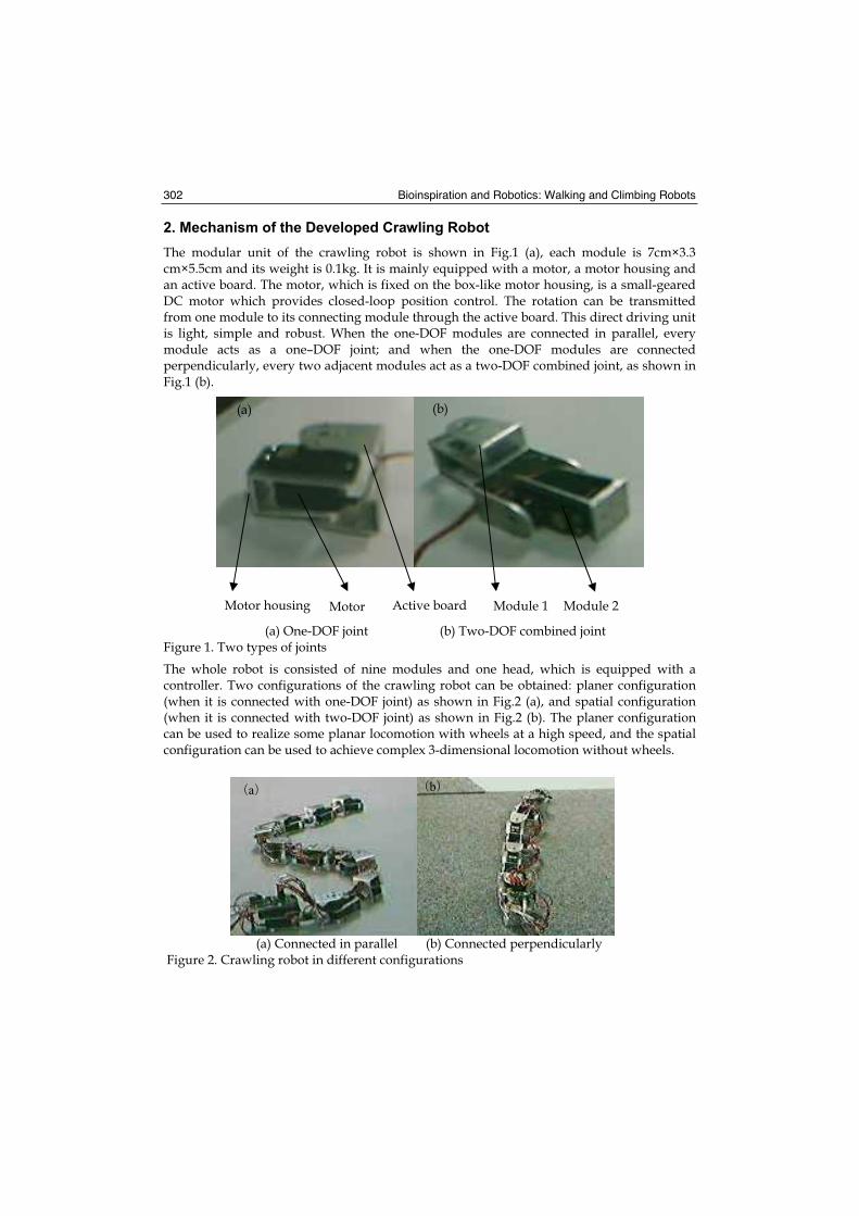
Bioinspiration and Robotics: Walking and Climbing Robots 302
2. Mechanism of the Developed Crawling Robot
The modular unit of the crawling robot is shown in Fig.1 (a), each module is 7cm×3.3 cm×5.5cm and its weight is 0.1kg. It is mainly equipped with a motor, a motor housing and an active board. The motor, which is fixed on the box-like motor housing, is a small-geared DC motor which provides closed-loop position control. The rotation can be transmitted from one module to its connecting module through the active board. This direct driving unit is light, simple and robust. When the one-DOF modules are connected in parallel, every module acts as a one–DOF joint; and when the one-DOF modules are connected perpendicularly, every two adjacent modules act as a two-DOF combined joint, as shown in Fig.1 (b).
(a) One-DOF joint (b) Two-DOF combined joint Figure 1. Two types of joints
The whole robot is consisted of nine modules and one head, which is equipped with a controller. Two configurations of the crawling robot can be obtained: planer configuration (when it is connected with one-DOF joint) as shown in Fig.2 (a), and spatial configuration (when it is connected with two-DOF joint) as shown in Fig.2 (b). The planer configuration can be used to realize some planar locomotion with wheels at a high speed, and the spatial configuration can be used to achieve complex 3-dimensional locomotion without wheels.
(a) Connected in parallel (b) Connected perpendicularly Figure 2. Crawling robot in different configurations
Module 1Motor housing Active board Motor Module 2
(a) (b)
a b
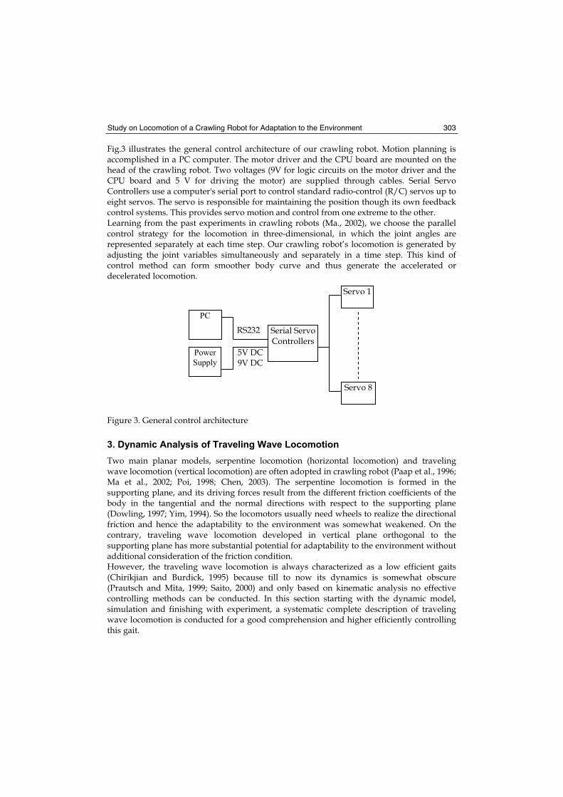
Study on Locomotion of a Crawling Robot for Adaptation to the Environment 303
Fig.3 illustrates the general control architecture of our crawling robot. Motion planning is accomplished in a PC computer. The motor driver and the CPU board are mounted on the head of the crawling robot. Two voltages (9V for logic circuits on the motor driver and the CPU board and 5 V for driving the motor) are supplied through cables. Serial Servo Controllers use a computer's serial port to control standard radio-control (R/C) servos up to eight servos. The servo is responsible for maintaining the position though its own feedback control systems. This provides servo motion and control from one extreme to the other. Learning from the past experiments in crawling robots (Ma., 2002), we choose the parallel control strategy for the locomotion in three-dimensional, in which the joint angles are represented separately at each time step. Our crawling robot’s locomotion is generated by adjusting the joint variables simultaneously and separately in a time step. This kind of control method can form smoother body curve and thus generate the accelerated or decelerated locomotion.
Figure 3. General control architecture
3. Dynamic Analysis of Traveling Wave Locomotion
Two main planar models, serpentine locomotion (horizontal locomotion) and traveling wave locomotion (vertical locomotion) are often adopted in crawling robot (Paap et al., 1996; Ma et al., 2002; Poi, 1998; Chen, 2003). The serpentine locomotion is formed in the supporting plane, and its driving forces result from the different friction coefficients of the body in the tangential and the normal directions with respect to the supporting plane (Dowling, 1997; Yim, 1994). So the locomotors usually need wheels to realize the directional friction and hence the adaptability to the environment was somewhat weakened. On the contrary, traveling wave locomotion developed in vertical plane orthogonal to the supporting plane has more substantial potential for adaptability to the environment without additional consideration of the friction condition. However, the traveling wave locomotion is always characterized as a low efficient gaits (Chirikjian and Burdick, 1995) because till to now its dynamics is somewhat obscure (Prautsch and Mita, 1999; Saito, 2000) and only based on kinematic analysis no effective controlling methods can be conducted. In this section starting with the dynamic model, simulation and finishing with experiment, a systematic complete description of traveling wave locomotion is conducted for a good comprehension and higher efficiently controlling this gait.
RS232
5V DC9V DC
Power Supply
Serial Servo Controllers
Servo 1
Servo 8
PC
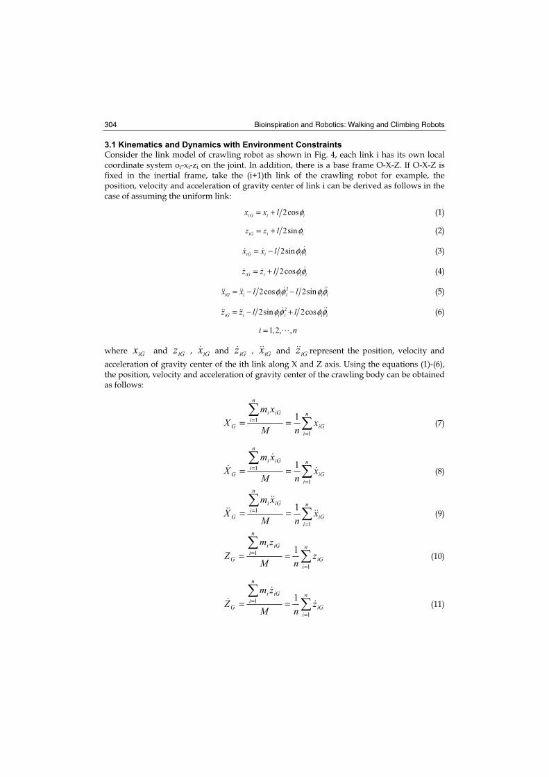
Bioinspiration and Robotics: Walking and Climbing Robots 304
3.1 Kinematics and Dynamics with Environment Constraints
Consider the link model of crawling robot as shown in Fig. 4, each link i has its own local coordinate system oi-xi-zi on the joint. In addition, there is a base frame O-X-Z. If O-X-Z is fixed in the inertial frame, take the (i+1)th link of the crawling robot for example, the position, velocity and acceleration of gravity center of link i can be derived as follows in the case of assuming the uniform link:
2cosiG i ix x l φ= + (1)
2siniG i iz z l φ= + (2)
2siniG i i ix x l φφ= − (3)
2cosiG i i iz z l φφ= + (4)
22cos 2siniG i i i i ix x l lφφ φφ= − − (5)
22sin 2cosiG i i i i iz z l lφφ φφ= − + (6)
1,2, ,i n=
where iGx and iGz , iGx and iGz , iGx and iGz represent the position, velocity and
acceleration of gravity center of the ith link along X and Z axis. Using the equations (1)-(6), the position, velocity and acceleration of gravity center of the crawling body can be obtained as follows:
=
= ==n
iiG
n
iiGi
G xnM
xmX
1
1 1 (7)
=
= ==n
iiG
n
iiGi
G xnM
xmX
1
1 1 (8)
=
= ==n
iiG
n
iiGi
G xnM
xmX
1
1 1 (9)
=
= ==n
iiG
n
iiGi
G znM
zmZ
1
1 1 (10)
=
= ==n
iiG
n
iiGi
G znM
zmZ
1
1 1 (11)
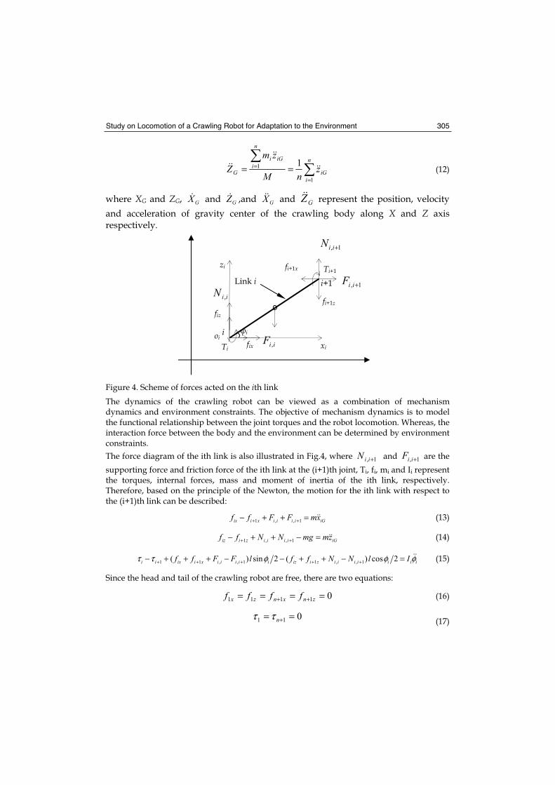
Study on Locomotion of a Crawling Robot for Adaptation to the Environment 305
=
= ==n
iiG
n
iiGi
G znM
zmZ
1
1 1 (12)
where XG and ZG, GX and GZ ,and GX and GZ represent the position, velocity
and acceleration of gravity center of the crawling body along X and Z axisrespectively.
Figure 4. Scheme of forces acted on the ith link
The dynamics of the crawling robot can be viewed as a combination of mechanism dynamics and environment constraints. The objective of mechanism dynamics is to model the functional relationship between the joint torques and the robot locomotion. Whereas, the interaction force between the body and the environment can be determined by environment constraints.
The force diagram of the ith link is also illustrated in Fig.4, where 1, +iiN and 1, +iiF are the
supporting force and friction force of the ith link at the (i+1)th joint, Ti, fi, mi and Ii represent the torques, internal forces, mass and moment of inertia of the ith link, respectively. Therefore, based on the principle of the Newton, the motion for the ith link with respect to the (i+1)th link can be described:
1 , , 1ix i x i i i i iGf f F F mx+ +− + + = (13)
1 , , 1iz i z i i i i iGf f N N mg mz+ +− + + − = (14)
1 1 , , 1 1 , , 1( ) sin 2 ( ) cos 2i i ix i x i i i i i iz i z i i i i i i if f F F l f f N N l Iτ τ φ φ φ+ + + + +− + + + − − + + − = (15)
Since the head and tail of the crawling robot are free, there are two equations:
01111 ==== ++ znxnzx ffff (16)
011 == +nττ (17)
oi
zi
xi
1, +iiFiiN ,
iiF ,
i
Ti
i
fix
fiz
1, +iiN
Ti+1
fi+1z
fi+1x
Link i i+1
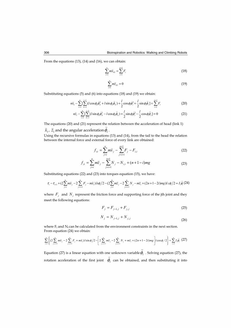
Bioinspiration and Robotics: Walking and Climbing Robots 306
From the equations (13), (14) and (16), we can obtain:
1
1 1
n n
iG ii i
mx F+
= =
= (18)
1
0n
iGi
mz=
= (19)
Substituting equations (5) and (6) into equations (18) and (19) we obtain:
1 12 2
1
1 1 1
[ ( cos sin ) cos sin ]2 2
n i n
k k k k i i i i ii k i
l lnx l l Fφ φ φ φ φ φ φ φ− +
= = =
− + + + = (20)
12 2
1
1 1
[ ( sin cos ) sin cos ] 02 2
n i
k k k k i i i ii k
l lnz l lφ φ φ φ φφ φ φ−
= =
− − + − = (21)
The equations (20) and (21) represent the relation between the acceleration of head (link 1)
1x , 1z and the angular acceleration 1φ .
Using the recursive formulas in equations (13) and (14), from the tail to the head the relation between the internal force and external force of every link are obtained:
ii
n
ijj
n
ijjxi FFxmf ,
1
1
−−=+
+== (22)
mginNNzmf ii
n
ijj
n
ijjzi )1(,
1
1
−++−−=+
+==(23)
Substituting equations (22) and (23) into torques equation (15), we have:
1
1 1
(2 2 ) 2 (2 2 (2 1 2 ) ) 2n n n n
i i j j i i j j i i i ij i j i j i j i
mx F mx ls mz N mz n i mg l c Iτ τ φ φ φ+= = + = = +
− + − − − − − + + − = (24)
where jF and jN represent the friction force and supporting force of the jth joint and they
meet the following equations:
jjjjj FFF ,,1 += − (25)
jjjjj NNN ,,1 += − (26)
where Fi and Ni can be calculated from the environment constraints in the next section. From equation (24) we obtain:
1 1 1 1 1 1
(2 2 ) sin 2 2 2 (2 1 2 ) cos / 2n n n n n n
j j i i j j i i i ii j i j i j i j i i
mx F mx l mz N mz n i mg l Iφ φ φ= = + = + = + = + =
− + − − + + + − = (27)
Equation (27) is a linear equation with one unknown variable 1φ . Solving equation (27), the
rotation acceleration of the first joint 1φ can be obtained, and then substituting it into
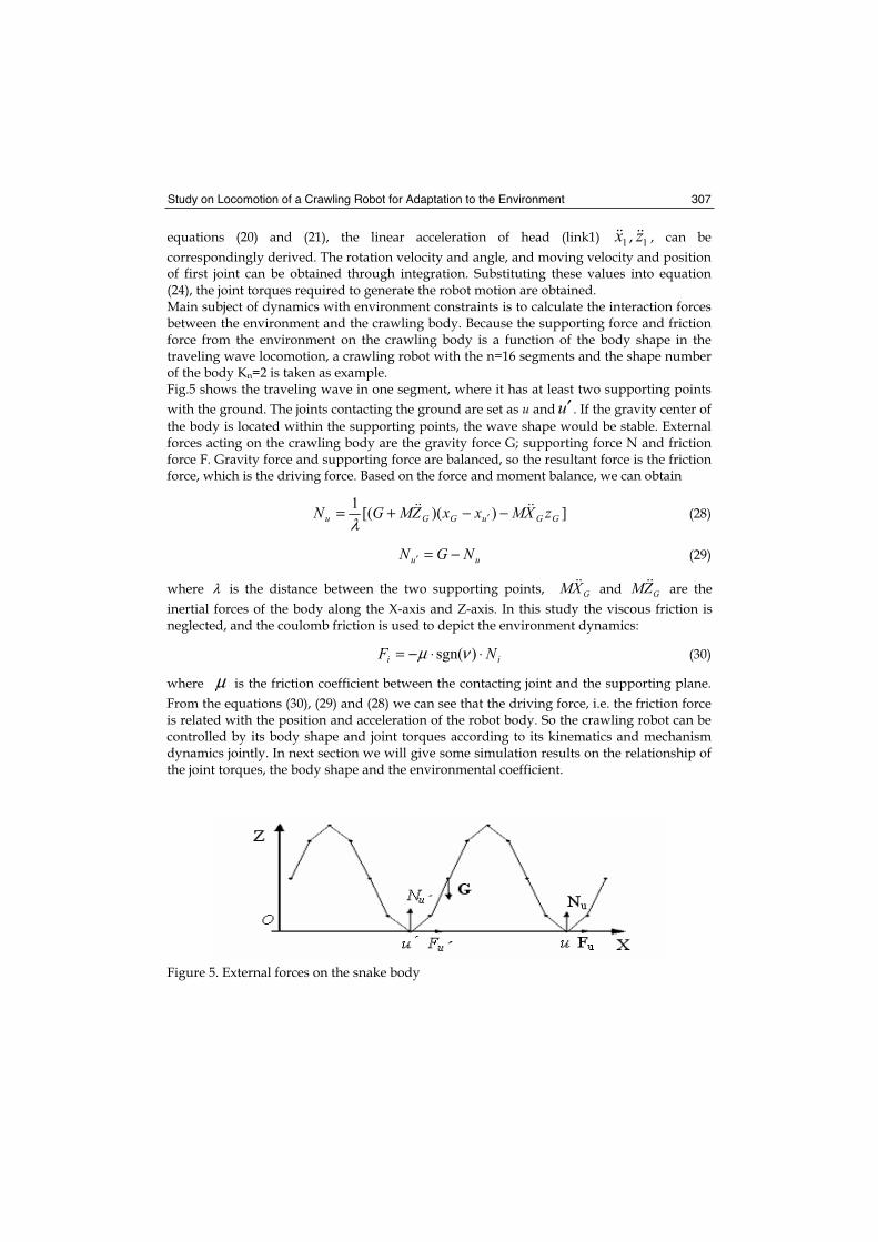
Study on Locomotion of a Crawling Robot for Adaptation to the Environment 307
equations (20) and (21), the linear acceleration of head (link1) 1x , 1z , can be
correspondingly derived. The rotation velocity and angle, and moving velocity and position of first joint can be obtained through integration. Substituting these values into equation (24), the joint torques required to generate the robot motion are obtained. Main subject of dynamics with environment constraints is to calculate the interaction forces between the environment and the crawling body. Because the supporting force and friction force from the environment on the crawling body is a function of the body shape in the traveling wave locomotion, a crawling robot with the n=16 segments and the shape number of the body Kn=2 is taken as example. Fig.5 shows the traveling wave in one segment, where it has at least two supporting points
with the ground. The joints contacting the ground are set as u and u′ . If the gravity center of
the body is located within the supporting points, the wave shape would be stable. External forces acting on the crawling body are the gravity force G; supporting force N and friction force F. Gravity force and supporting force are balanced, so the resultant force is the friction force, which is the driving force. Based on the force and moment balance, we can obtain
]))([(1
GGuGGu zXMxxZMGN −−+= ′λ (28)
uu NGN −=′ (29)
where λ is the distance between the two supporting points, GMX and GMZ are the
inertial forces of the body along the X-axis and Z-axis. In this study the viscous friction is neglected, and the coulomb friction is used to depict the environment dynamics:
ii NF ⋅⋅−= )sgn(νμ (30)
where μ is the friction coefficient between the contacting joint and the supporting plane.
From the equations (30), (29) and (28) we can see that the driving force, i.e. the friction force is related with the position and acceleration of the robot body. So the crawling robot can be controlled by its body shape and joint torques according to its kinematics and mechanism dynamics jointly. In next section we will give some simulation results on the relationship of the joint torques, the body shape and the environmental coefficient.
Figure 5. External forces on the snake body
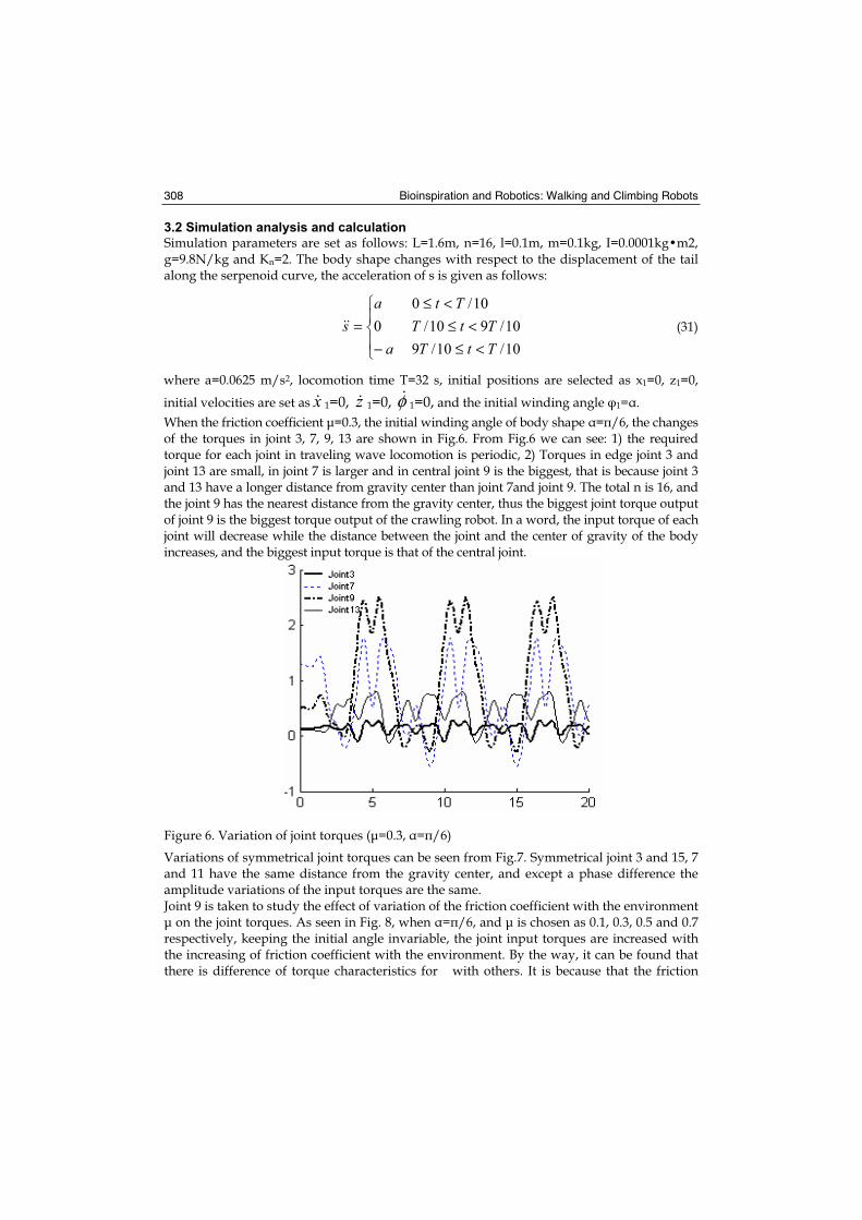
Bioinspiration and Robotics: Walking and Climbing Robots 308
3.2 Simulation analysis and calculation
Simulation parameters are set as follows: L=1.6m, n=16, l=0.1m, m=0.1kg, I=0.0001kg•m2, g=9.8N/kg and Kn=2. The body shape changes with respect to the displacement of the tail along the serpenoid curve, the acceleration of s is given as follows:
−=
a
as 0
10/10/9
10/910/
10/0
TtTTtT
Tt
<≤<≤
<≤ (31)
where a=0.0625 m/s2, locomotion time T=32 s, initial positions are selected as x1=0, z1=0,
initial velocities are set as x 1=0, z 1=0, φ 1=0, and the initial winding angle 1= .
When the friction coefficient μ=0.3, the initial winding angle of body shape = /6, the changes of the torques in joint 3, 7, 9, 13 are shown in Fig.6. From Fig.6 we can see: 1) the required torque for each joint in traveling wave locomotion is periodic, 2) Torques in edge joint 3 and joint 13 are small, in joint 7 is larger and in central joint 9 is the biggest, that is because joint 3 and 13 have a longer distance from gravity center than joint 7and joint 9. The total n is 16, and the joint 9 has the nearest distance from the gravity center, thus the biggest joint torque output of joint 9 is the biggest torque output of the crawling robot. In a word, the input torque of each joint will decrease while the distance between the joint and the center of gravity of the body increases, and the biggest input torque is that of the central joint.
Figure 6. Variation of joint torques (μ=0.3, = /6)
Variations of symmetrical joint torques can be seen from Fig.7. Symmetrical joint 3 and 15, 7 and 11 have the same distance from the gravity center, and except a phase difference the amplitude variations of the input torques are the same. Joint 9 is taken to study the effect of variation of the friction coefficient with the environment μ on the joint torques. As seen in Fig. 8, when = /6, and μ is chosen as 0.1, 0.3, 0.5 and 0.7 respectively, keeping the initial angle invariable, the joint input torques are increased with the increasing of friction coefficient with the environment. By the way, it can be found that there is difference of torque characteristics for with others. It is because that the friction
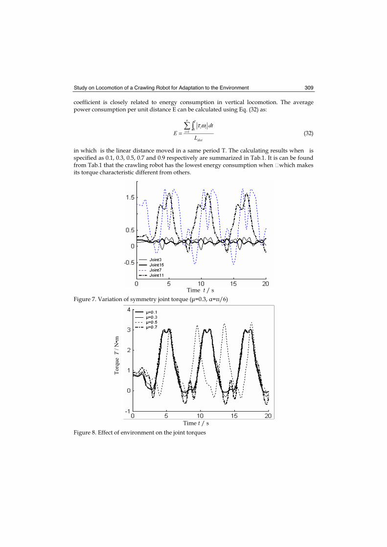
Study on Locomotion of a Crawling Robot for Adaptation to the Environment 309
coefficient is closely related to energy consumption in vertical locomotion. The average power consumption per unit distance E can be calculated using Eq. (32) as:
01
n T
i ii
dist
dtE
L
τ ω== (32)
in which is the linear distance moved in a same period T. The calculating results when is specified as 0.1, 0.3, 0.5, 0.7 and 0.9 respectively are summarized in Tab.1. It is can be found from Tab.1 that the crawling robot has the lowest energy consumption when �which makes its torque characteristic different from others.
Figure 7. Variation of symmetry joint torque (μ=0.3, = /6)
Figure 8. Effect of environment on the joint torques
Time t / s
Time t / s
To
rqu
eT
/ N
•m
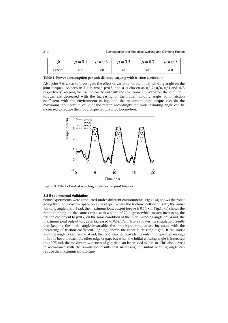
Bioinspiration and Robotics: Walking and Climbing Robots 310
μ 0.1μ = 0.3μ = 0.5μ = 0.7μ = 0.9μ =
E(N·m) 430 380 320 500 700
Table 1. Power consumption per unit distance varying with friction coefficient
Also joint 9 is taken to investigate the effect of variation of the initial winding angle on the joint torques. As seen in Fig 9, when μ=0.5, and is chosen as /12, /6, /4 and /3 respectively, keeping the friction coefficient with the environment invariable, the joint input torques are decreased with the increasing of the initial winding angle. So if friction coefficient with the environment is big, and the maximum joint torque exceeds the maximum input torque value of the motor, accordingly the initial winding angle can be increased to reduce the input torque required for locomotion.
Figure 9. Effect of initial winding angle on the joint torques
3.3 Experimental Validation
Some experiments were conducted under different environments. Fig.10 (a) shows the robot going through a narrow space on a flat carpet, where the friction coefficient is 0.3, the initial winding angle is 0.4 rad, the maximum joint output torque is 0.5N•m. Fig.10 (b) shows the robot climbing on the same carpet with a slope of 20 degree, which means increasing the friction coefficient to μ=0.7, on the same condition of the initial winding angle =0.4 rad, the maximum joint output torque is increased to 0.82N/m. This validates the simulation results that keeping the initial angle invariable, the joint input torques are increased with the increasing of friction coefficient. Fig.10(c) shows the robot is crossing a gap. If the initial winding angle is kept as =0.4 rad, the robot can not provide the output torque high enough to lift its head to reach the other edge of gap, but when the initial winding angle is increased to =0.75 rad, the maximum wideness of gap that can be crossed is 0.14 m. This also is well in accordance with the simulation results that increasing the initial winding angle can reduce the maximum joint torque.
Time t / s
To
rqu
eT/
Nm
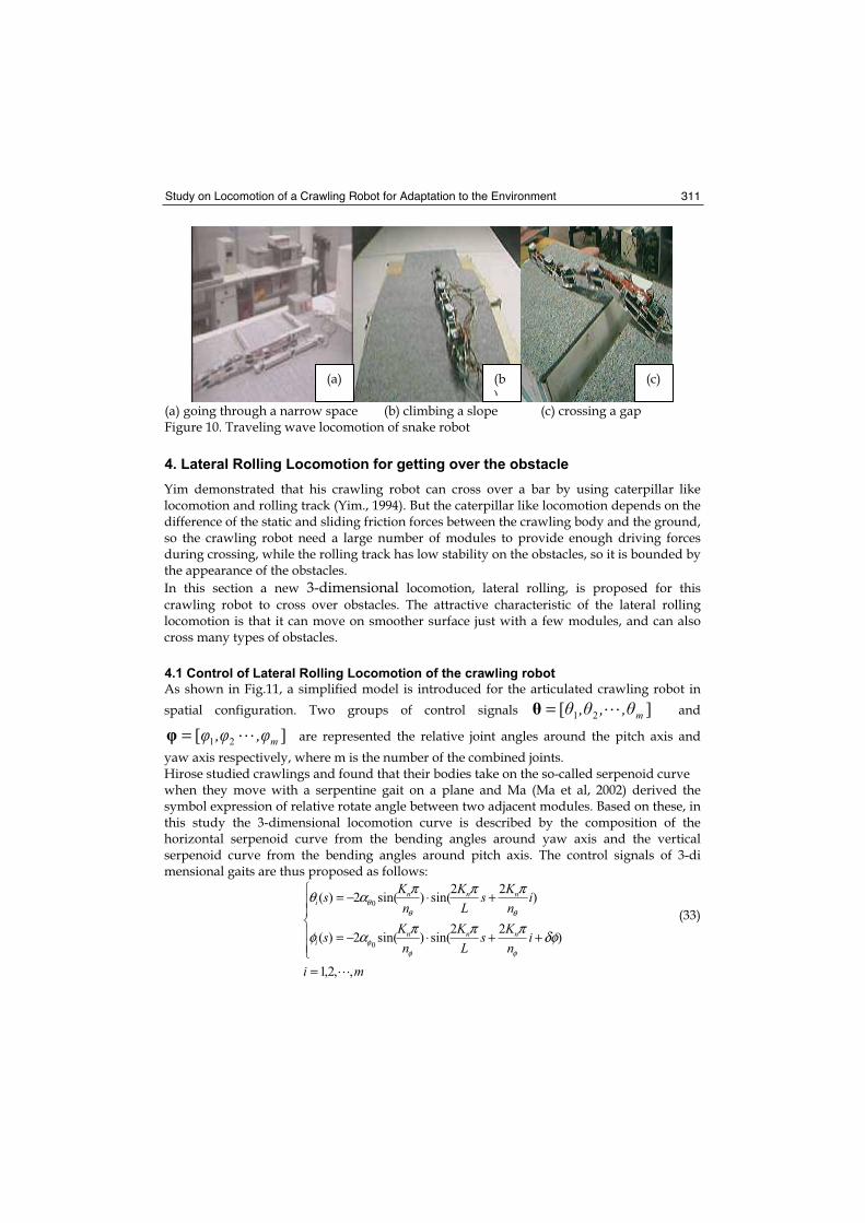
Study on Locomotion of a Crawling Robot for Adaptation to the Environment 311
(a) going through a narrow space (b) climbing a slope (c) crossing a gap Figure 10. Traveling wave locomotion of snake robot
4. Lateral Rolling Locomotion for getting over the obstacle
Yim demonstrated that his crawling robot can cross over a bar by using caterpillar like locomotion and rolling track (Yim., 1994). But the caterpillar like locomotion depends on the difference of the static and sliding friction forces between the crawling body and the ground, so the crawling robot need a large number of modules to provide enough driving forces during crossing, while the rolling track has low stability on the obstacles, so it is bounded by the appearance of the obstacles.
In this section a new 3-dimensional locomotion, lateral rolling, is proposed for this
crawling robot to cross over obstacles. The attractive characteristic of the lateral rolling locomotion is that it can move on smoother surface just with a few modules, and can also cross many types of obstacles.
4.1 Control of Lateral Rolling Locomotion of the crawling robot
As shown in Fig.11, a simplified model is introduced for the articulated crawling robot in
spatial configuration. Two groups of control signals ][ 21 m,,,= and
][ 21 m,,= are represented the relative joint angles around the pitch axis and
yaw axis respectively, where m is the number of the combined joints. Hirose studied crawlings and found that their bodies take on the so-called serpenoid curve when they move with a serpentine gait on a plane and Ma (Ma et al, 2002) derived the symbol expression of relative rotate angle between two adjacent modules. Based on these, in this study the 3-dimensional locomotion curve is described by the composition of the horizontal serpenoid curve from the bending angles around yaw axis and the vertical serpenoid curve from the bending angles around pitch axis. The control signals of 3-di mensional gaits are thus proposed as follows:
mi
inKs
LK
nKs
inKs
LK
nKs
nnni
nnni
,,2,1
)22
sin()sin(2)(
)22
sin()sin(2)(
0
0
=
++⋅−=
+⋅−=
δφπππαφ
πππαθ
φφφ
θθθ
(33)
(a) (c)(b)
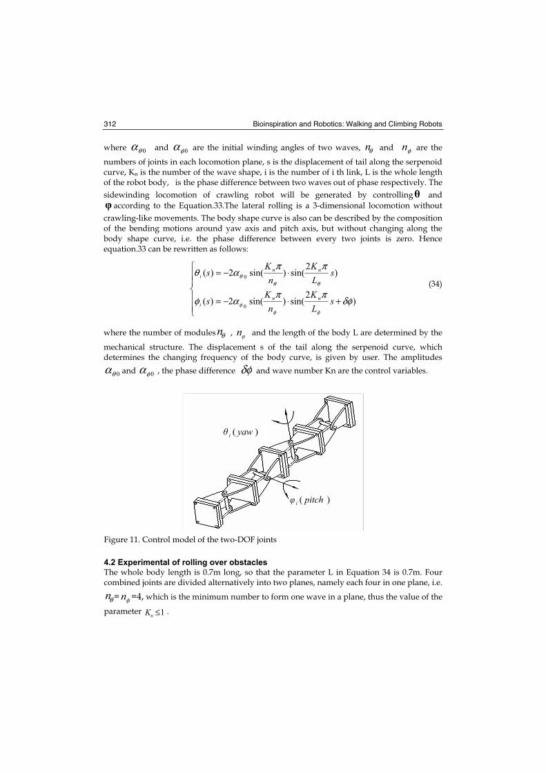
Bioinspiration and Robotics: Walking and Climbing Robots 312
where 0θα and 0φα are the initial winding angles of two waves, θn and φn are the
numbers of joints in each locomotion plane, s is the displacement of tail along the serpenoid curve, Kn is the number of the wave shape, i is the number of i th link, L is the whole length of the robot body, is the phase difference between two waves out of phase respectively. The
sidewinding locomotion of crawling robot will be generated by controlling and
according to the Equation.33.The lateral rolling is a 3-dimensional locomotion without
crawling-like movements. The body shape curve is also can be described by the composition of the bending motions around yaw axis and pitch axis, but without changing along the body shape curve, i.e. the phase difference between every two joints is zero. Hence equation.33 can be rewritten as follows:
+⋅−=
⋅−=
)2
sin()sin(2)(
)2
sin()sin(2)(
0
0
δφππ
αφ
ππαθ
φφφ
θθθ
sLK
nK
s
sLK
nK
s
nni
nni
(34)
where the number of modules θn , n and the length of the body L are determined by the
mechanical structure. The displacement s of the tail along the serpenoid curve, which determines the changing frequency of the body curve, is given by user. The amplitudes
0θα and 0φα , the phase difference δφ and wave number Kn are the control variables.
Figure 11. Control model of the two-DOF joints
4.2 Experimental of rolling over obstacles
The whole body length is 0.7m long, so that the parameter L in Equation 34 is 0.7m. Four combined joints are divided alternatively into two planes, namely each four in one plane, i.e.
θn = φn =4, which is the minimum number to form one wave in a plane, thus the value of the
parameter 1≤nK .
)( pitchi
)( yawi
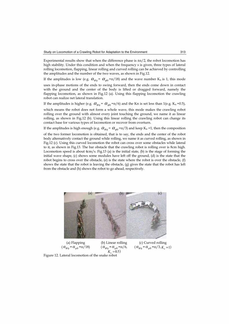
Study on Locomotion of a Crawling Robot for Adaptation to the Environment 313
Experimental results show that when the difference phase is ± /2, the robot locomotion has high stability. Under this condition and when the frequency s is given, three types of lateral rolling locomotion, flapping, linear rolling and curved rolling can be achieved by controlling the amplitudes and the number of the two waves, as shown in Fig.12.
If the amplitudes is low (e.g. 0θα = 0φα = /18) and the wave number Kn is 1, this mode
uses in-phase motions of the ends to swing forward, then the ends come down in contact with the ground and the center of the body is lifted or dragged forward, namely the flapping locomotion, as shown in Fig.12 (a). Using this flapping locomotion the crawling robot can realize net lateral translation.
If the amplitudes is higher (e.g. 0θα = 0φα = /6) and the Kn is set less than 1(e.g. Kn =0.5),
which means the robot does not form a whole wave, this mode makes the crawling robot rolling over the ground with almost every joint touching the ground, we name it as linear rolling, as shown in Fig.12 (b). Using this linear rolling the crawling robot can change its contact base for various types of locomotion or recover from overturn.
If the amplitudes is high enough (e.g. 0θα = 0φα = /3) and keep Kn =1, then the composition
of the two former locomotion is obtained, that is to say, the ends and the center of the robot body alternatively contact the ground while rolling, we name it as curved rolling, as shown in Fig.12 (c). Using this curved locomotion the robot can cross over some obstacles while lateral to it, as shown in Fig.13. The bar obstacle that the crawling robot is rolling over is 8cm high. Locomotion speed is about 4cm/s. Fig.13 (a) is the initial state, (b) is the stage of forming the initial wave shape, (c) shows some modules have left off the ground, (d) is the state that the robot begins to cross over the obstacle, (e) is the state where the robot is over the obstacle, (f) shows the state that the robot is leaving the obstacle, (g) gives the state that the robot has left from the obstacle and (h) shows the robot to go ahead, respectively.
(a) Flapping (
0θ = 0 = /18)(b) Linear rolling (
0θ = 0 = /6,
5.0=nK )
(c) Curved rolling (
0θ = 0 = /3, 1=nK )
Figure 12. Lateral locomotion of the snake robot
(c)(b)(a)
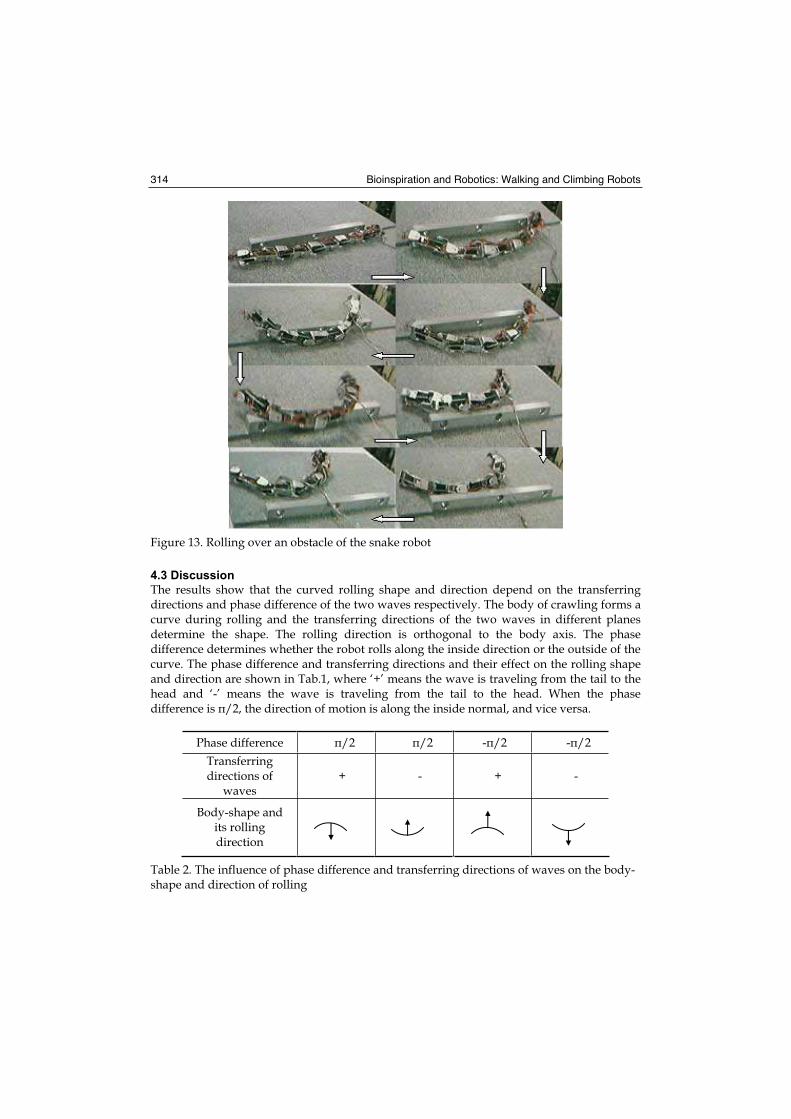
Bioinspiration and Robotics: Walking and Climbing Robots 314
Figure 13. Rolling over an obstacle of the snake robot
4.3 Discussion
The results show that the curved rolling shape and direction depend on the transferring directions and phase difference of the two waves respectively. The body of crawling forms a curve during rolling and the transferring directions of the two waves in different planes determine the shape. The rolling direction is orthogonal to the body axis. The phase difference determines whether the robot rolls along the inside direction or the outside of the curve. The phase difference and transferring directions and their effect on the rolling shape and direction are shown in Tab.1, where ‘+’ means the wave is traveling from the tail to the head and ‘-’ means the wave is traveling from the tail to the head. When the phase difference is /2, the direction of motion is along the inside normal, and vice versa.
Phase difference /2 /2 - /2 - /2
Transferringdirections of
waves+ - + -
Body-shape and its rolling direction
Table 2. The influence of phase difference and transferring directions of waves on the body-shape and direction of rolling
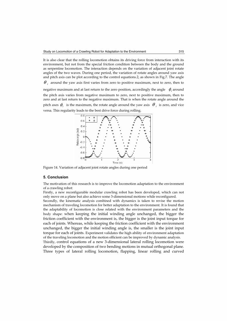
Study on Locomotion of a Crawling Robot for Adaptation to the Environment 315
It is also clear that the rolling locomotion obtains its driving force from interaction with its environment, but not from the special friction condition between the body and the ground as serpentine locomotion. The interaction depends on the variation of adjacent joint rotate angles of the two waves. During one period, the variation of rotate angles around yaw axis and pitch axis can be plot according to the control equations.2, as shown in Fig.7. The angle
iθ around the yaw axis first varies from zero to positive maximum, next to zero, then to
negative maximum and at last return to the zero position, accordingly the angle iφ around
the pitch axis varies from negative maximum to zero, next to positive maximum, then to zero and at last return to the negative maximum. That is when the rotate angle around the
pitch axes iφ is the maximum, the rotate angle around the yaw axis iθ is zero, and vice
versa. This regularity leads to the best drive force during rolling.
Figure 14. Variation of adjacent joint rotate angles during one period
5. Conclusion
The motivation of this research is to improve the locomotion adaptation to the environment of a crawling robot: Firstly, a new reconfigurable modular crawling robot has been developed, which can not only move on a plane but also achieve some 3-dimensional motions while reconfigured. Secondly, the kinematic analysis combined with dynamics is taken to revise the motion mechanism of traveling locomotion for better adaptation to the environment. It is found that the adaptability of locomotion is close related with the environment parameters and the
body shape: when keeping the initial winding angle unchanged, the bigger the friction coefficient with the environment is, the bigger is the joint input torque for each of joints. Whereas, while keeping the friction coefficient with the environment unchanged, the bigger the initial winding angle is, the smaller is the joint input torque for each of joints. Experiment validates the high ability of environment adaptation
of the traveling locomotion and the motion efficient can be improved by dynamic analysis.
Thirdly, control equations of a new 3-dimensional lateral rolling locomotion were developed by the composition of two bending motions in mutual orthogonal plane. Three types of lateral rolling locomotion, flapping, linear rolling and curved
Bioinspiration and Robotics: Walking and Climbing Robots 316
rolling, were achieved by controlling the amplitudes and the number of two waves in the two bending motions. The lateral rolling locomotion obtains its driving force through the interaction with the environment, and the rolling shape and its direction depend on the transferring direction and phase difference of the two waves respectively. Using these types of locomotion the snake robot can realize net lateral translation, alternation of the contact base and cross over some obstacleswith a few models.This paper can give some hints for efficiently control the locomotion of crawling robot for improvement its environmental adaptability.
8. References
Burdick J, Radford J. and Chirikjian G. S., (1993). A Sidewinding Locomotion Gait for Hyper-Redundant Robots, Advanced Robotics, Vol.9, No, 3, pp.195-216
Chen L., Wang Y.C., Ma S.G. and Li B., (2003). Analysis of the traveling wave locomotion of crawling robot, in Proc. IEEE Int. Conf .on Robotics, Intelligent Systems and Signal processing, pp, 365-369
Chen L., Wang Y.C., Ma S.G., (2004). Studies on Lateral Rolling Locomotion of a Crawling Robot, in Proc. IEEE Int. Conf .on Robotics and Automation, pp, 5070-5074
Chirikjian and Burdick ,(1995), The Kinematics of Hyper-Redundant Robot Locomotion, IEEE Trans. on Robotics and Automation, Vol. 11, No. 6, pp, 781-793
Dowling K., 1997 . Limbless Locomotion: Learning to Crawl with a Crawling Robot, Doctoral dissertation, tech. report CMU-RI-TR-97-48, Robotics Institute, Carnegie Mellon University
Gray J., (1946), The mechanism of locomotion in crawlings, Journal of experimental biologyHirose S., (1993). Biologically Inspired Robots (Crawling-like Locomotor and Manipulator),
Oxford University Press, ISBN 0198562616, New York, United States Ma S., Araya H. and Li L., (2002). Development of a creeping locomotion of crawling-like
robot, Int. J. of Robotics and Automation, vol.17, No.4, pp.146-153 Mori M. and Hirose S., ( 2001). Development of Active Cord Mechanism ACM-R3 with
Agile 3D Mobility, in Proc. IEEE Int. Conf .on Intelligent Robots and SystemsPaap K. L., Dehlwisch M. and Klaassen B., (1996). GMD-Crawling: A Semi-Autonomous
Crawling-like Robot, Distributed Autonomous Robotic Systems 2, Springer-Verlag, Tokyo
Poi G., Scarabeo C. and Allotta B., (1998).Traveling wave locomotion hyper-redundant mobile robot, in Proc. IEEE Int. Conf.on Robotics and Automation
Prautsch P. and Mita T., (1999).Control and Analysis of the Gait of Crawling robots, in Proc. IEEE Int. Conf.on Control applications, pp, 502-507
Saito M., Fukaya M., and Iwasaki T., (2000). Serpentine locomotion with robotics crawlings, IEEE control systems magazine,Vol.20, No, 2, pp, 64-81
Togawa K., Mori M. and Hirose S., (2000). Study on 3-dimensional Active Cord Mechanism: Development of ACM-R2, in Proc. IEEE Int. Conf .on Intelligent Robots and Systems
Yim. M., (1994). New Locomotion Gains, in Proc. IEEE Int. Conf .on Robotics and Automation,pp, 310–316
Yim M., Duff D.G. and Roufas K.D., ( 2000). Polybot: a Modular Reconfigurable Robot, in Proc. IEEE Int. Conf .on Robotics and Automation
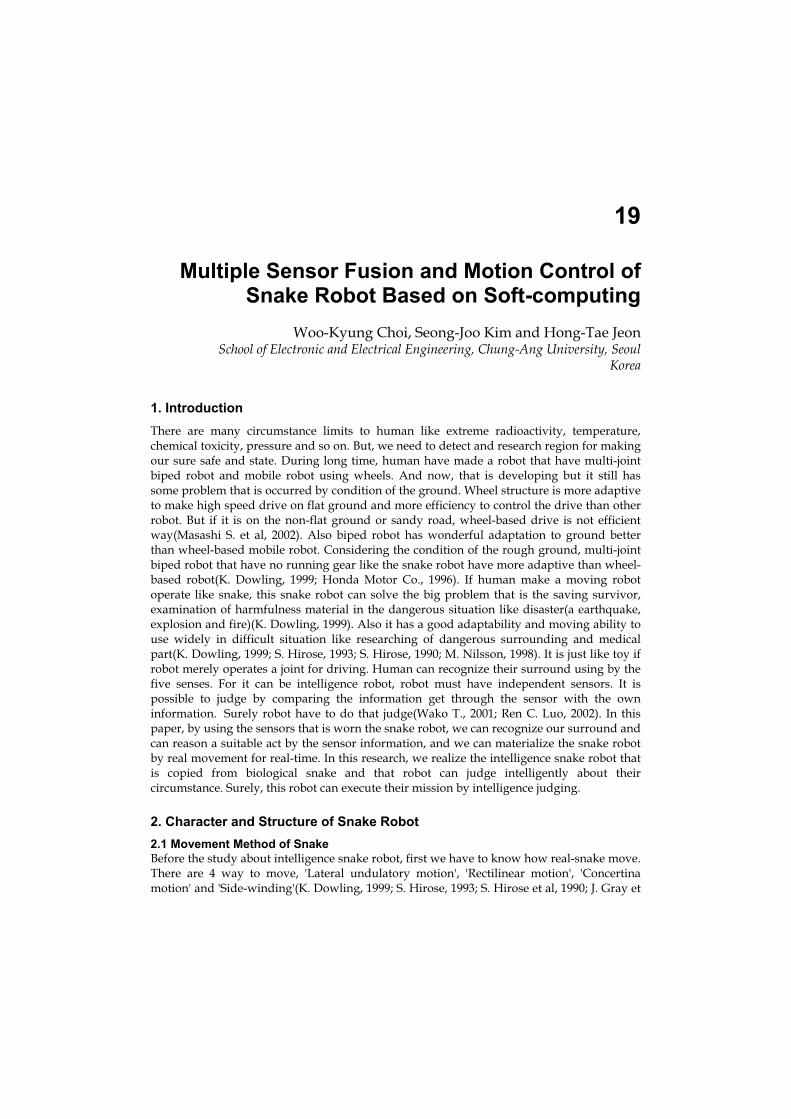
19
Multiple Sensor Fusion and Motion Control of Snake Robot Based on Soft-computing
Woo-Kyung Choi, Seong-Joo Kim and Hong-Tae Jeon School of Electronic and Electrical Engineering, Chung-Ang University, Seoul
Korea
1. Introduction
There are many circumstance limits to human like extreme radioactivity, temperature, chemical toxicity, pressure and so on. But, we need to detect and research region for making our sure safe and state. During long time, human have made a robot that have multi-joint biped robot and mobile robot using wheels. And now, that is developing but it still has some problem that is occurred by condition of the ground. Wheel structure is more adaptive to make high speed drive on flat ground and more efficiency to control the drive than other robot. But if it is on the non-flat ground or sandy road, wheel-based drive is not efficient way(Masashi S. et al, 2002). Also biped robot has wonderful adaptation to ground better than wheel-based mobile robot. Considering the condition of the rough ground, multi-joint biped robot that have no running gear like the snake robot have more adaptive than wheel-based robot(K. Dowling, 1999; Honda Motor Co., 1996). If human make a moving robot operate like snake, this snake robot can solve the big problem that is the saving survivor, examination of harmfulness material in the dangerous situation like disaster(a earthquake, explosion and fire)(K. Dowling, 1999). Also it has a good adaptability and moving ability to use widely in difficult situation like researching of dangerous surrounding and medical part(K. Dowling, 1999; S. Hirose, 1993; S. Hirose, 1990; M. Nilsson, 1998). It is just like toy if robot merely operates a joint for driving. Human can recognize their surround using by the five senses. For it can be intelligence robot, robot must have independent sensors. It is possible to judge by comparing the information get through the sensor with the own information. Surely robot have to do that judge(Wako T., 2001; Ren C. Luo, 2002). In this paper, by using the sensors that is worn the snake robot, we can recognize our surround and can reason a suitable act by the sensor information, and we can materialize the snake robot by real movement for real-time. In this research, we realize the intelligence snake robot that is copied from biological snake and that robot can judge intelligently about their circumstance. Surely, this robot can execute their mission by intelligence judging.
2. Character and Structure of Snake Robot
2.1 Movement Method of Snake
Before the study about intelligence snake robot, first we have to know how real-snake move. There are 4 way to move, 'Lateral undulatory motion', 'Rectilinear motion', 'Concertina motion' and 'Side-winding'(K. Dowling, 1999; S. Hirose, 1993; S. Hirose et al, 1990; J. Gray et
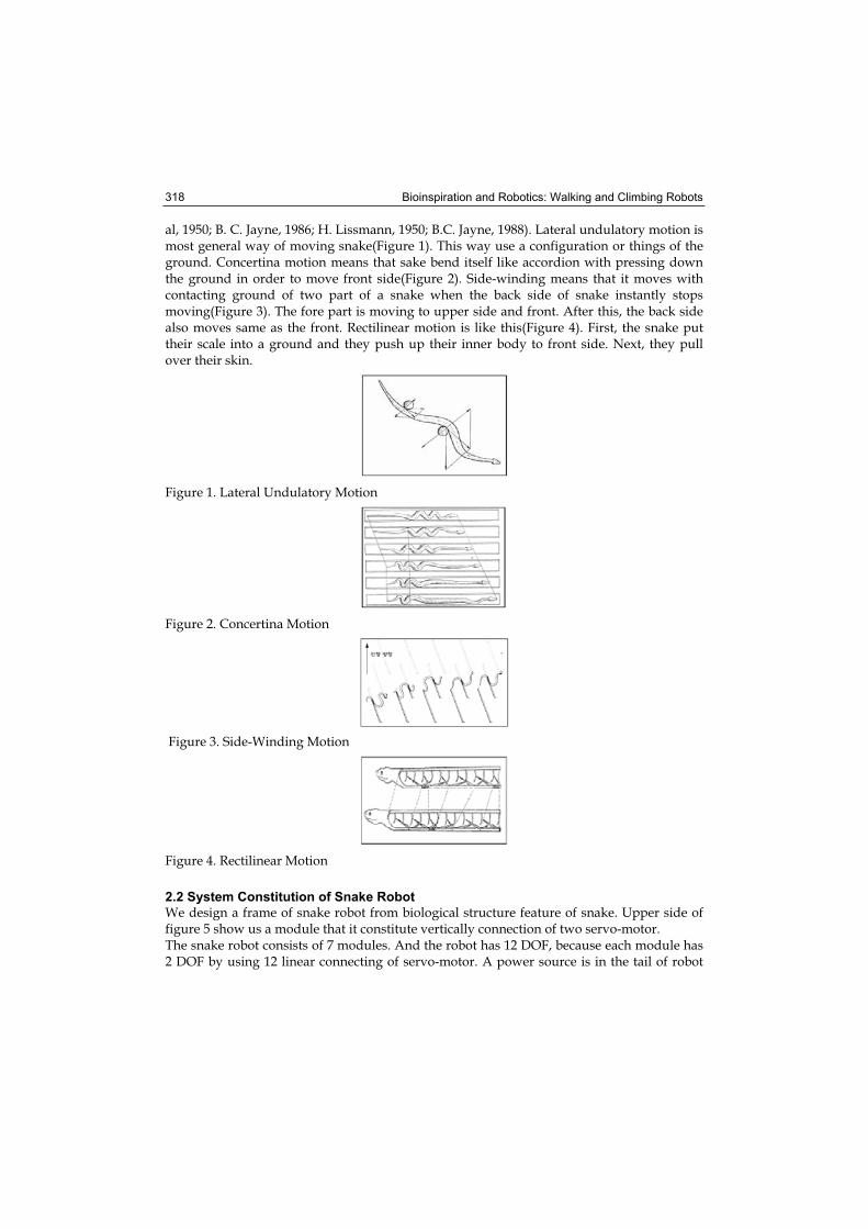
Bioinspiration and Robotics: Walking and Climbing Robots 318
al, 1950; B. C. Jayne, 1986; H. Lissmann, 1950; B.C. Jayne, 1988). Lateral undulatory motion is most general way of moving snake(Figure 1). This way use a configuration or things of the ground. Concertina motion means that sake bend itself like accordion with pressing down the ground in order to move front side(Figure 2). Side-winding means that it moves with contacting ground of two part of a snake when the back side of snake instantly stops moving(Figure 3). The fore part is moving to upper side and front. After this, the back side also moves same as the front. Rectilinear motion is like this(Figure 4). First, the snake put their scale into a ground and they push up their inner body to front side. Next, they pull over their skin.
Figure 1. Lateral Undulatory Motion
Figure 2. Concertina Motion
Figure 3. Side-Winding Motion
Figure 4. Rectilinear Motion
2.2 System Constitution of Snake Robot
We design a frame of snake robot from biological structure feature of snake. Upper side of figure 5 show us a module that it constitute vertically connection of two servo-motor. The snake robot consists of 7 modules. And the robot has 12 DOF, because each module has 2 DOF by using 12 linear connecting of servo-motor. A power source is in the tail of robot
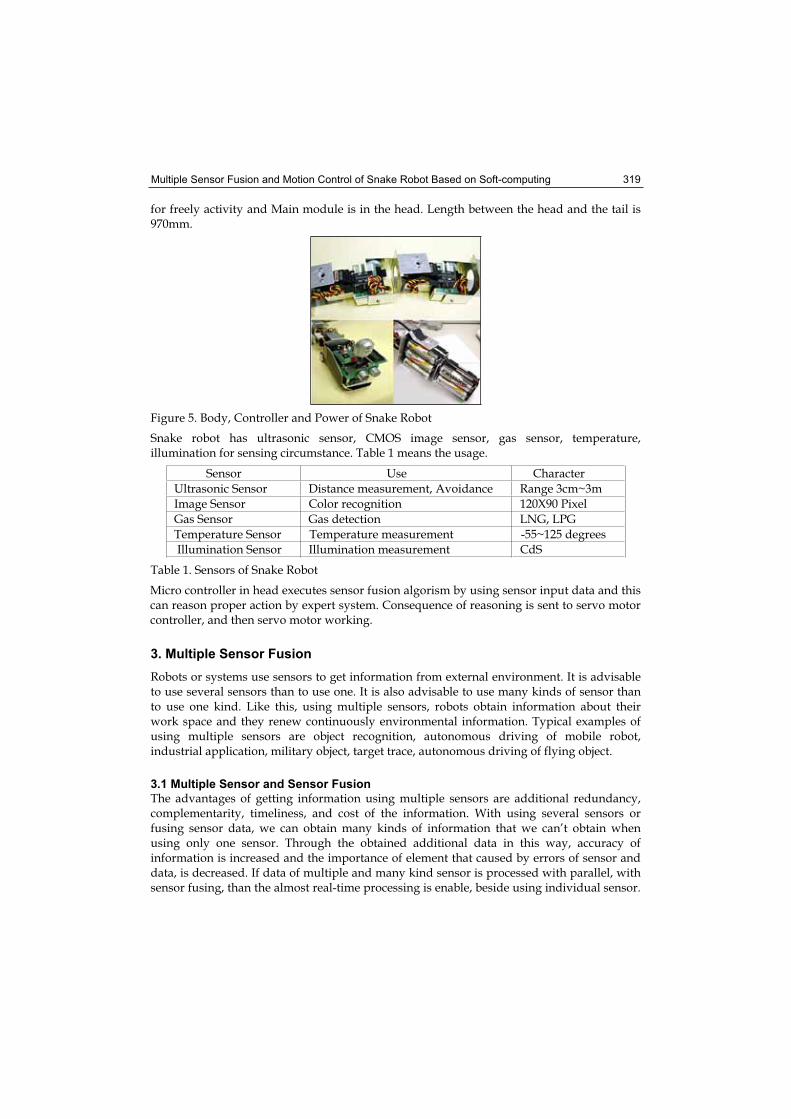
Multiple Sensor Fusion and Motion Control of Snake Robot Based on Soft-computing 319
for freely activity and Main module is in the head. Length between the head and the tail is 970mm.
Figure 5. Body, Controller and Power of Snake Robot
Snake robot has ultrasonic sensor, CMOS image sensor, gas sensor, temperature, illumination for sensing circumstance. Table 1 means the usage.
Sensor Use Character
Ultrasonic Sensor Distance measurement, Avoidance Range 3cm~3m
Image Sensor Color recognition 120X90 Pixel
Gas Sensor Gas detection LNG, LPG
Temperature Sensor Temperature measurement -55~125 degrees
Illumination Sensor Illumination measurement CdS
Table 1. Sensors of Snake Robot
Micro controller in head executes sensor fusion algorism by using sensor input data and this can reason proper action by expert system. Consequence of reasoning is sent to servo motor controller, and then servo motor working.
3. Multiple Sensor Fusion
Robots or systems use sensors to get information from external environment. It is advisable to use several sensors than to use one. It is also advisable to use many kinds of sensor than to use one kind. Like this, using multiple sensors, robots obtain information about their work space and they renew continuously environmental information. Typical examples of using multiple sensors are object recognition, autonomous driving of mobile robot, industrial application, military object, target trace, autonomous driving of flying object.
3.1 Multiple Sensor and Sensor Fusion
The advantages of getting information using multiple sensors are additional redundancy, complementarity, timeliness, and cost of the information. With using several sensors or fusing sensor data, we can obtain many kinds of information that we can’t obtain when using only one sensor. Through the obtained additional data in this way, accuracy of information is increased and the importance of element that caused by errors of sensor and data, is decreased. If data of multiple and many kind sensor is processed with parallel, with sensor fusing, than the almost real-time processing is enable, beside using individual sensor.
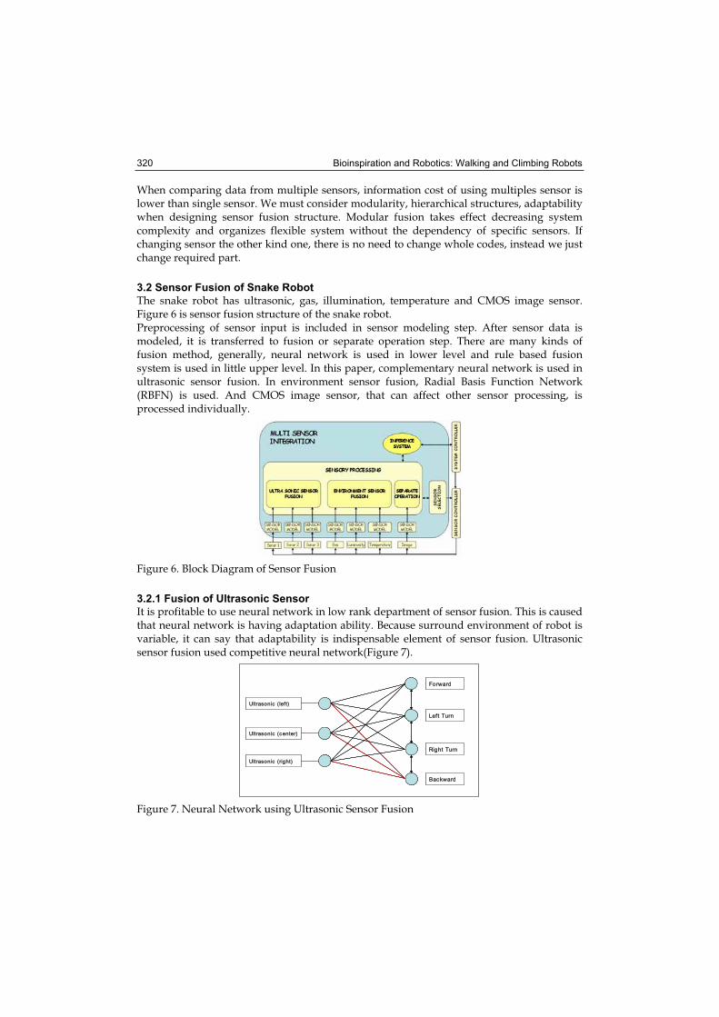
Bioinspiration and Robotics: Walking and Climbing Robots 320
When comparing data from multiple sensors, information cost of using multiples sensor is lower than single sensor. We must consider modularity, hierarchical structures, adaptability when designing sensor fusion structure. Modular fusion takes effect decreasing system complexity and organizes flexible system without the dependency of specific sensors. If changing sensor the other kind one, there is no need to change whole codes, instead we just change required part.
3.2 Sensor Fusion of Snake Robot
The snake robot has ultrasonic, gas, illumination, temperature and CMOS image sensor. Figure 6 is sensor fusion structure of the snake robot. Preprocessing of sensor input is included in sensor modeling step. After sensor data is modeled, it is transferred to fusion or separate operation step. There are many kinds of fusion method, generally, neural network is used in lower level and rule based fusion system is used in little upper level. In this paper, complementary neural network is used in ultrasonic sensor fusion. In environment sensor fusion, Radial Basis Function Network (RBFN) is used. And CMOS image sensor, that can affect other sensor processing, is processed individually.
Figure 6. Block Diagram of Sensor Fusion
3.2.1 Fusion of Ultrasonic Sensor
It is profitable to use neural network in low rank department of sensor fusion. This is caused that neural network is having adaptation ability. Because surround environment of robot is variable, it can say that adaptability is indispensable element of sensor fusion. Ultrasonic sensor fusion used competitive neural network(Figure 7).
Figure 7. Neural Network using Ultrasonic Sensor Fusion
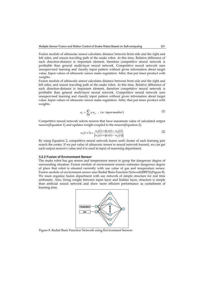
Multiple Sensor Fusion and Motion Control of Snake Robot Based on Soft-computing 321
Fusion module of ultrasonic sensor calculates distance between front side and the right and left sides, and reason traveling path of the snake robot. At this time, Relative difference of each direction-distance is important element, therefore competitive neural network is profitable than general multi-layer neural network. Competitive neural network uses unsupervised learning and classify input pattern without given information about target value. Input values of ultrasonic sensor make regulation. After, that put inner product with weights.Fusion module of ultrasonic sensor calculates distance between front side and the right and left sides, and reason traveling path of the snake robot. At this time, Relative difference of each direction-distance is important element, therefore competitive neural network is profitable than general multi-layer neural network. Competitive neural network uses unsupervised learning and classify input pattern without given information about target value. Input values of ultrasonic sensor make regulation. After, that put inner product with weights.
):(,1
munberinputnwxan
iijij
=
= (1)
Competitive neural network selects neuron that have maximum value of calculated output neuron(Equation 1) and updates weight coupled to the neuron(Equation 2).
))()(()(
))()(()()1(
twtxtwtwtxtwtw
kk
kkk −+
−+=+ηη (2)
By using Equation 2, competitive neural network learns until cluster of each learning pair search the center. If we put value of ultrasonic sensor to neural network learned, we can get each output neuron's value and it is used in input of reasoning department.
3.2.2 Fusion of Environment Sensor
The snake robot has gas sensor and temperature sensor to grasp the dangerous degree of surrounding situation. Fusion module of environment sensors estimates dangerous degree of place that robot is situated currently with use value of gas and temperature sensor. Fusion module of environment sensor uses Radial Basis Function Network(RBFN)(Figure 8). We must organize fusion department with use network of simple structure for real time arithmetic. Also, fixing weight between input layer and hidden layer, structure is simple than artificial neural network and show more efficient performance as curtailment of learning time.
Figure 8. Radial Basis Function Network using Environment Sensors
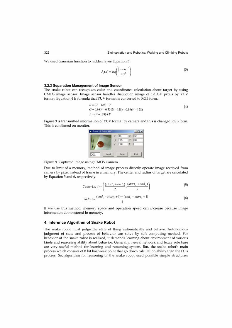
Bioinspiration and Robotics: Walking and Climbing Robots 322
We used Gaussian function to hidden layer(Equation 3).
−=
2
2
2exp)(
i
ii
uxxR
σ (3)
3.2.3 Separation Management of Image Sensor
The snake robot can recognizes color and coordinates calculation about target by using CMOS image sensor. Image sensor handles distinction image of 120X90 pixels by YUV format. Equation 4 is formula that YUV format is converted to RGB form.
YVBVUYG
YUR
+−=−−−−=
+−=
)128(
)128(19.0)128(53.098.0
)128( (4)
Figure 9 is transmitted information of YUV format by camera and this is changed RGB form. This is confirmed on monitor.
Figure 9. Captured Image using CMOS Camera
Due to limit of a memory, method of image process directly operate image received from camera by pixel instead of frame in a memory. The center and radius of target are calculated by Equation 5 and 6, respectively.
++=2
)(,
2
)(),(
yyxx endstartendstartyxCenter (5)
4
)1()1( +−++−= yyxx startendstartend
radius (6)
If we use this method, memory space and operation speed can increase because image information do not stored in memory.
4. Inference Algorithm of Snake Robot
The snake robot must judge the state of thing automatically and behave. Autonomous judgment of state and process of behavior can solve by soft computing method. For behavior of the snake robot is realized, it demands learning about environment of various kinds and reasoning ability about behavior. Generally, neural network and fuzzy rule base are very useful method for learning and reasoning system. But, the snake robot's main process which consists of 8 bit has weak point that go down calculation ability than the PC's process. So, algorithm for reasoning of the snake robot used possible simple structure's
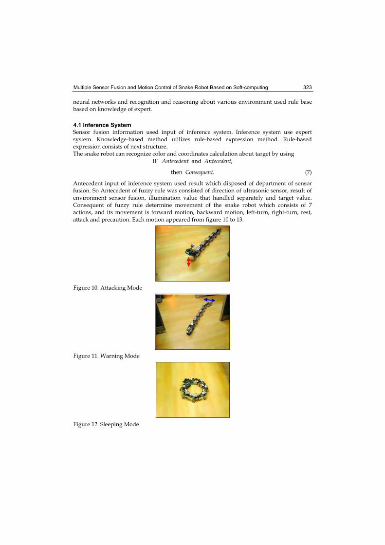
Multiple Sensor Fusion and Motion Control of Snake Robot Based on Soft-computing 323
neural networks and recognition and reasoning about various environment used rule base based on knowledge of expert.
4.1 Inference System
Sensor fusion information used input of inference system. Inference system use expert system. Knowledge-based method utilizes rule-based expression method. Rule-based expression consists of next structure. The snake robot can recognize color and coordinates calculation about target by using
IF Antecedent and Antecedent,
then Consequent. (7)
Antecedent input of inference system used result which disposed of department of sensor fusion. So Antecedent of fuzzy rule was consisted of direction of ultrasonic sensor, result of environment sensor fusion, illumination value that handled separately and target value. Consequent of fuzzy rule determine movement of the snake robot which consists of 7 actions, and its movement is forward motion, backward motion, left-turn, right-turn, rest, attack and precaution. Each motion appeared from figure 10 to 13.
Figure 10. Attacking Mode
Figure 11. Warning Mode
Figure 12. Sleeping Mode
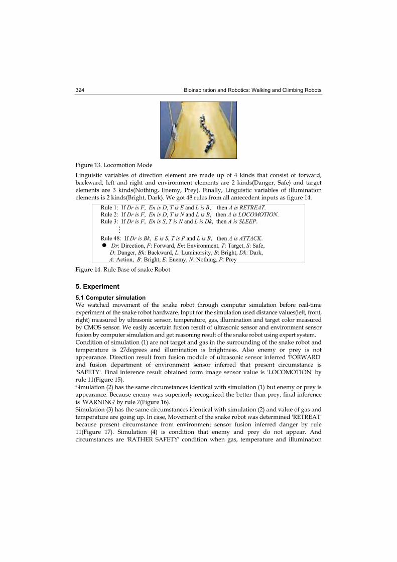
Bioinspiration and Robotics: Walking and Climbing Robots 324
Figure 13. Locomotion Mode
Linguistic variables of direction element are made up of 4 kinds that consist of forward, backward, left and right and environment elements are 2 kinds(Danger, Safe) and target elements are 3 kinds(Nothing, Enemy, Prey). Finally, Linguistic variables of illumination elements is 2 kinds(Bright, Dark). We got 48 rules from all antecedent inputs as figure 14.
Rule 1: If Dr is F, En is D, T is E and L is B, then A is RETREAT.Rule 2: If Dr is F, En is D, T is N and L is B, then A is LOCOMOTION.Rule 3: If Dr is F, En is S, T is N and L is Dk, then A is SLEEP.
Rule 48: If Dr is Bk, E is S, T is P and L is B, then A is ATTACK.
Dr: Direction, F: Forward, En: Environment, T: Target, S: Safe, D: Danger, Bk: Backward, L: Luminorsity, B: Bright, Dk: Dark, A: Action, B: Bright, E: Enemy, N: Nothing, P: Prey
Figure 14. Rule Base of snake Robot
5. Experiment
5.1 Computer simulation
We watched movement of the snake robot through computer simulation before real-time experiment of the snake robot hardware. Input for the simulation used distance values(left, front, right) measured by ultrasonic sensor, temperature, gas, illumination and target color measured by CMOS sensor. We easily ascertain fusion result of ultrasonic sensor and environment sensor fusion by computer simulation and get reasoning result of the snake robot using expert system. Condition of simulation (1) are not target and gas in the surrounding of the snake robot and temperature is 27degrees and illumination is brightness. Also enemy or prey is not appearance. Direction result from fusion module of ultrasonic sensor inferred 'FORWARD' and fusion department of environment sensor inferred that present circumstance is 'SAFETY'. Final inference result obtained form image sensor value is 'LOCOMOTION' by rule 11(Figure 15).Simulation (2) has the same circumstances identical with simulation (1) but enemy or prey is appearance. Because enemy was superiorly recognized the better than prey, final inference is 'WARNING' by rule 7(Figure 16). Simulation (3) has the same circumstances identical with simulation (2) and value of gas and temperature are going up. In case, Movement of the snake robot was determined 'RETREAT' because present circumstance from environment sensor fusion inferred danger by rule 11(Figure 17). Simulation (4) is condition that enemy and prey do not appear. And circumstances are 'RATHER SAFETY' condition when gas, temperature and illumination
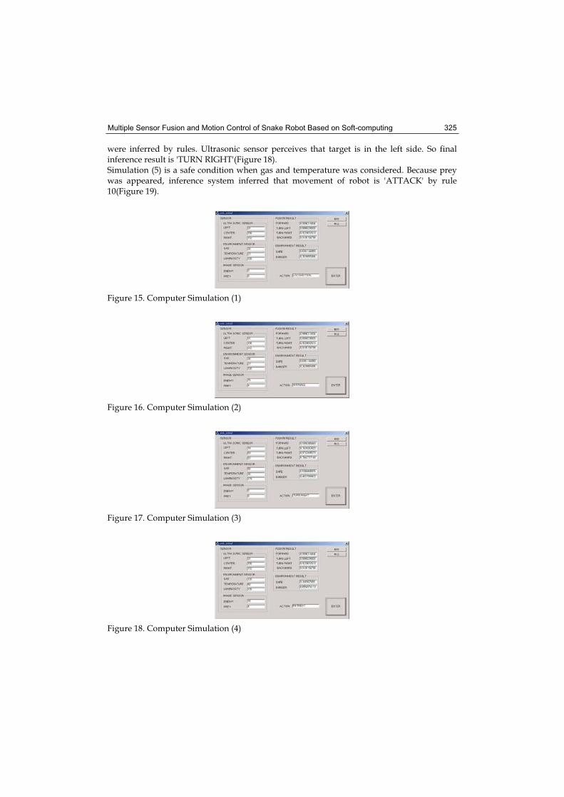
Multiple Sensor Fusion and Motion Control of Snake Robot Based on Soft-computing 325
were inferred by rules. Ultrasonic sensor perceives that target is in the left side. So final inference result is 'TURN RIGHT'(Figure 18). Simulation (5) is a safe condition when gas and temperature was considered. Because prey was appeared, inference system inferred that movement of robot is 'ATTACK' by rule 10(Figure 19).
Figure 15. Computer Simulation (1)
Figure 16. Computer Simulation (2)
Figure 17. Computer Simulation (3)
Figure 18. Computer Simulation (4)
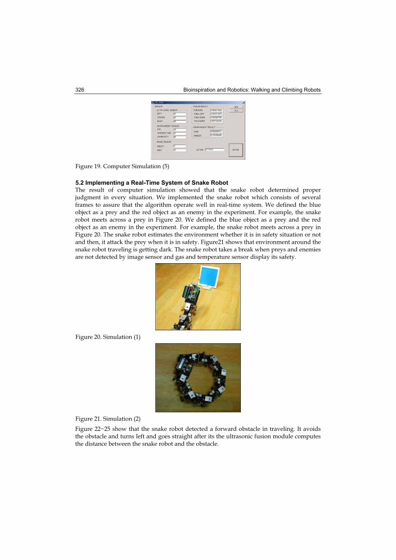
Bioinspiration and Robotics: Walking and Climbing Robots 326
Figure 19. Computer Simulation (5)
5.2 Implementing a Real-Time System of Snake Robot
The result of computer simulation showed that the snake robot determined proper judgment in every situation. We implemented the snake robot which consists of several frames to assure that the algorithm operate well in real-time system. We defined the blue object as a prey and the red object as an enemy in the experiment. For example, the snake robot meets across a prey in Figure 20. We defined the blue object as a prey and the red object as an enemy in the experiment. For example, the snake robot meets across a prey in Figure 20. The snake robot estimates the environment whether it is in safety situation or not and then, it attack the prey when it is in safety. Figure21 shows that environment around the snake robot traveling is getting dark. The snake robot takes a break when preys and enemies are not detected by image sensor and gas and temperature sensor display its safety.
Figure 20. Simulation (1)
Figure 21. Simulation (2)
Figure 22~25 show that the snake robot detected a forward obstacle in traveling. It avoids the obstacle and turns left and goes straight after its the ultrasonic fusion module computes the distance between the snake robot and the obstacle.
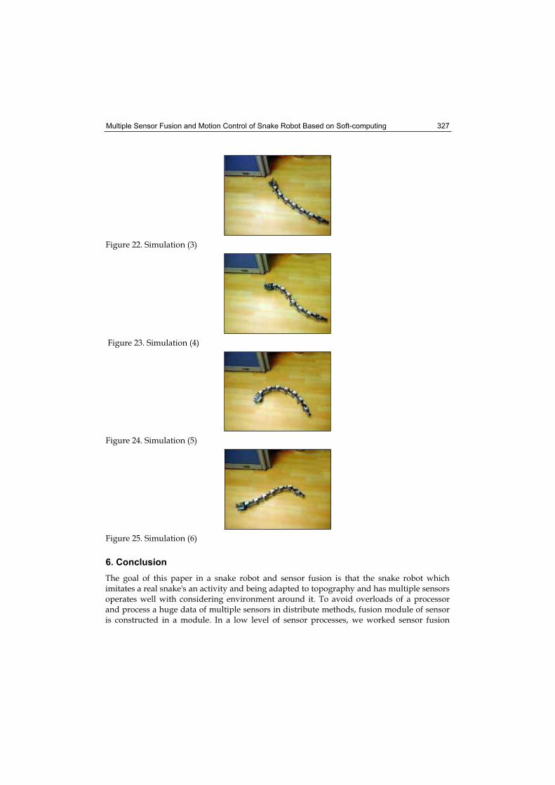
Multiple Sensor Fusion and Motion Control of Snake Robot Based on Soft-computing 327
Figure 22. Simulation (3)
Figure 23. Simulation (4)
Figure 24. Simulation (5)
Figure 25. Simulation (6)
6. Conclusion
The goal of this paper in a snake robot and sensor fusion is that the snake robot which imitates a real snake's an activity and being adapted to topography and has multiple sensors operates well with considering environment around it. To avoid overloads of a processor and process a huge data of multiple sensors in distribute methods, fusion module of sensor is constructed in a module. In a low level of sensor processes, we worked sensor fusion
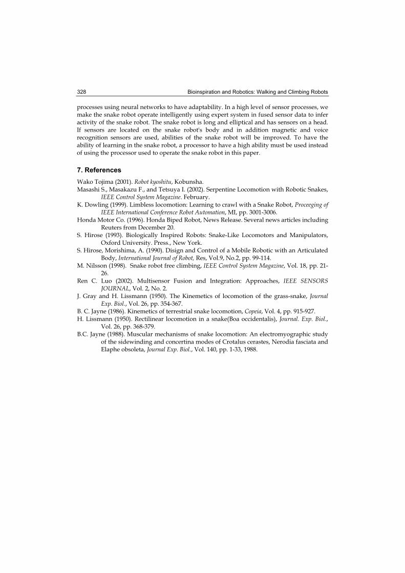
Bioinspiration and Robotics: Walking and Climbing Robots 328
processes using neural networks to have adaptability. In a high level of sensor processes, we make the snake robot operate intelligently using expert system in fused sensor data to infer activity of the snake robot. The snake robot is long and elliptical and has sensors on a head. If sensors are located on the snake robot's body and in addition magnetic and voice recognition sensors are used, abilities of the snake robot will be improved. To have the ability of learning in the snake robot, a processor to have a high ability must be used instead of using the processor used to operate the snake robot in this paper.
7. References
Wako Tojima (2001). Robot kyoshitu, Kobunsha. Masashi S., Masakazu F., and Tetsuya I. (2002). Serpentine Locomotion with Robotic Snakes,
IEEE Control System Magazine. February. K. Dowling (1999). Limbless locomotion: Learning to crawl with a Snake Robot, Proceeging of
IEEE International Conference Robot Automation, MI, pp. 3001-3006. Honda Motor Co. (1996). Honda Biped Robot, News Release. Several news articles including
Reuters from December 20. S. Hirose (1993). Biologically Inspired Robots: Snake-Like Locomotors and Manipulators,
Oxford University. Press., New York. S. Hirose, Morishima, A. (1990). Disign and Control of a Mobile Robotic with an Articulated
Body, International Journal of Robot, Res, Vol.9, No.2, pp. 99-114. M. Nilsson (1998). Snake robot free climbing, IEEE Control System Magazine, Vol. 18, pp. 21-
26.Ren C. Luo (2002). Multisensor Fusion and Integration: Approaches, IEEE SENSORS
JOURNAL, Vol. 2, No. 2. J. Gray and H. Lissmann (1950). The Kinemetics of locomotion of the grass-snake, Journal
Exp. Biol., Vol. 26, pp. 354-367. B. C. Jayne (1986). Kinemetics of terrestrial snake locomotion, Copeia, Vol. 4, pp. 915-927. H. Lissmann (1950). Rectilinear locomotion in a snake(Boa occidentalis), Journal. Exp. Biol.,
Vol. 26, pp. 368-379. B.C. Jayne (1988). Muscular mechanisms of snake locomotion: An electromyographic study
of the sidewinding and concertina modes of Crotalus cerastes, Nerodia fasciata and Elaphe obsoleta, Journal Exp. Biol., Vol. 140, pp. 1-33, 1988.
20
Evolutionary Strategies Combined With Novel Binary Hill Climbing Used for Online Walking
Pattern Generation in Two Legged Robot
Lena Mariann Garder and Mats Høvin University of Oslo
Norway
1. Introduction
Evolutionary algorithms (EA) has often been proposed as a method for designing systems for real-world applications (Higuchi et al., 1999). Developing effective gaits for bipedal robots is a difficult task that requires optimization of many parameters in a highly irregular, multidimensional space. In recent years biologically inspired computation methods have been employed by several authors. For instance, Hornby et al. used genetic algorithms (GA) to generate robust gaits on the Aibo quadruped robot (Hornby et al., 2000). GA applied to bipedal locomotion was also proposed by Arakawa and Fukuda (Arakawa & Fukuda, 1996) who made a GA based on energy optimization in order to generate a natural, human-like bipedal gait. One of the main objections to applying EA’s in the search for gaits is the time consuming characteristic of these techniques due to the large fitness search space that is normally present. For this reason most approaches have been based on offline and simulator based searches. To reduce the time spent searching large search spaces with EA, various techniques for speeding up the algorithms have been presented. With the increased complexity evolution schema introduced by Torresen (Torresen, 1998), Torresen has shown how to increase the search speed by using a divide and conquer approach, by dividing the problem into subtasks in a character recognition system. Haddow and Tufte have also done experiments with reducing the genotype representation (Haddow & Tufte, 2000). Kalganova (Kalaganova, 2000) has shown how to increase the search speed by evolving incremental and bidirectional to achieve an overall complex behavior both for the complex system to the sub-system, and from the sub-system to the complex system. For an exhaustive description of other approaches readers may refer to Cantú-Paz (Cantú-Paz, 1998). The robot presented in this paper is a two-legged biped with binary operated pneumatic cylinders. The search space in our experiments was set up to describe the forward speed of the robot given the different gaits, and the goal was to find the most efficient gait with respect to speed. To enable efficient gaits the search space needed to be quite large as the accuracy of the pause lengths between the different leg positions is outmost critical, especially for gaits dominated by jumping movements. The focus has not been on evolving a balancing system as there have been no other sensory feedback than the forward position of the robot. The main goal for our work was to find a search algorithm fast enough to enable real-time gait generation/adaptation where the fitness is provided by the mechanical robot
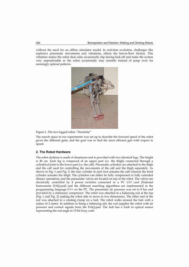
Bioinspiration and Robotics: Walking and Climbing Robots 330
without the need for an offline simulator model. In real-time evolution, challenges like explosive pneumatic movements and vibrations, effects the feet-to-floor friction. This vibration makes the robot shoe soles occasionally slip during kick-off and make the system very unpredictable as the robot occasionally may stumble instead of jump even for seemingly optimal patterns.
Figure 1. The two legged robot, “Henriette“
The search space in our experiments was set up to describe the forward speed of the robot given the different gaits, and the goal was to find the most efficient gait with respect to speed.
2. The Robot Hardware
The robot skeleton is made of aluminum and is provided with two identical legs. The height is 40 cm. Each leg is composed of an upper part (i.e. the thigh) connected through a cylindrical joint to the lower part (i.e. the calf). Pneumatic cylinders are attached to the thigh and the calf used for controlling the movements of the calf and the thigh separately. As shown in Fig. 1 and Fig. 3, the rear cylinder in each foot actuates the calf whereas the front cylinder actuates the thigh. The cylinders can either be fully compressed or fully extended (binary operation), and the pneumatic valves are located on top of the robot. The valves are electrically controlled by 4 power switches connected to a PC I/O card (National Instruments DAQ-pad) and the different searching algorithms are implemented in the programming language C++ on the PC. The pneumatic air pressure was set to 8 bar and provided by a stationary compressor. The robot was attached to a balancing rod at the top (Fig. 1 and Fig. 2) making the robot able to move in two dimensions. The other end of the rod was attached to a rotating clamp on a hub. The robot walks around the hub with a radius of 2 meter. In addition to being a balancing aid, the rod supplies the robot with air pressure and control signals from the DAQ-pad. The hub has a built in optical sensor representing the rod angle in 13 bit Gray code.
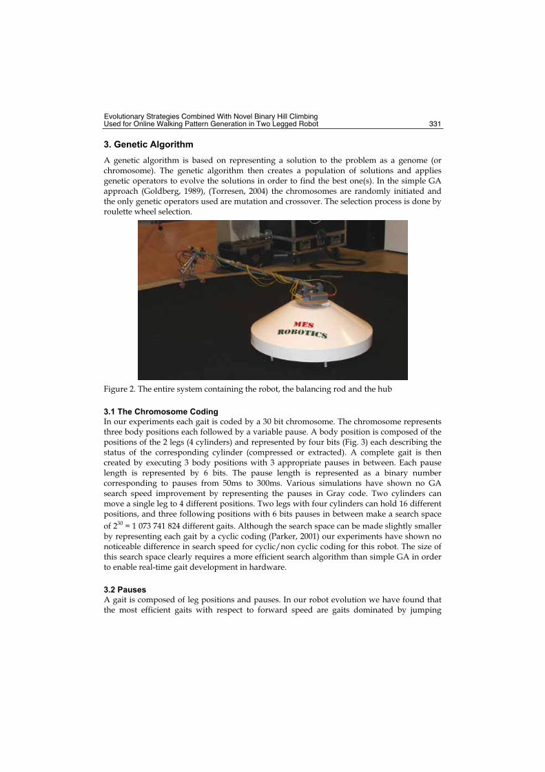
Evolutionary Strategies Combined With Novel Binary Hill Climbing Used for Online Walking Pattern Generation in Two Legged Robot 331
3. Genetic Algorithm
A genetic algorithm is based on representing a solution to the problem as a genome (or chromosome). The genetic algorithm then creates a population of solutions and applies genetic operators to evolve the solutions in order to find the best one(s). In the simple GA approach (Goldberg, 1989), (Torresen, 2004) the chromosomes are randomly initiated and the only genetic operators used are mutation and crossover. The selection process is done by roulette wheel selection.
Figure 2. The entire system containing the robot, the balancing rod and the hub
3.1 The Chromosome Coding
In our experiments each gait is coded by a 30 bit chromosome. The chromosome represents three body positions each followed by a variable pause. A body position is composed of the positions of the 2 legs (4 cylinders) and represented by four bits (Fig. 3) each describing the status of the corresponding cylinder (compressed or extracted). A complete gait is then created by executing 3 body positions with 3 appropriate pauses in between. Each pause length is represented by 6 bits. The pause length is represented as a binary number corresponding to pauses from 50ms to 300ms. Various simulations have shown no GA search speed improvement by representing the pauses in Gray code. Two cylinders can move a single leg to 4 different positions. Two legs with four cylinders can hold 16 different positions, and three following positions with 6 bits pauses in between make a search space
of 230 = 1 073 741 824 different gaits. Although the search space can be made slightly smaller by representing each gait by a cyclic coding (Parker, 2001) our experiments have shown no noticeable difference in search speed for cyclic/non cyclic coding for this robot. The size of this search space clearly requires a more efficient search algorithm than simple GA in order to enable real-time gait development in hardware.
3.2 Pauses
A gait is composed of leg positions and pauses. In our robot evolution we have found that the most efficient gaits with respect to forward speed are gaits dominated by jumping
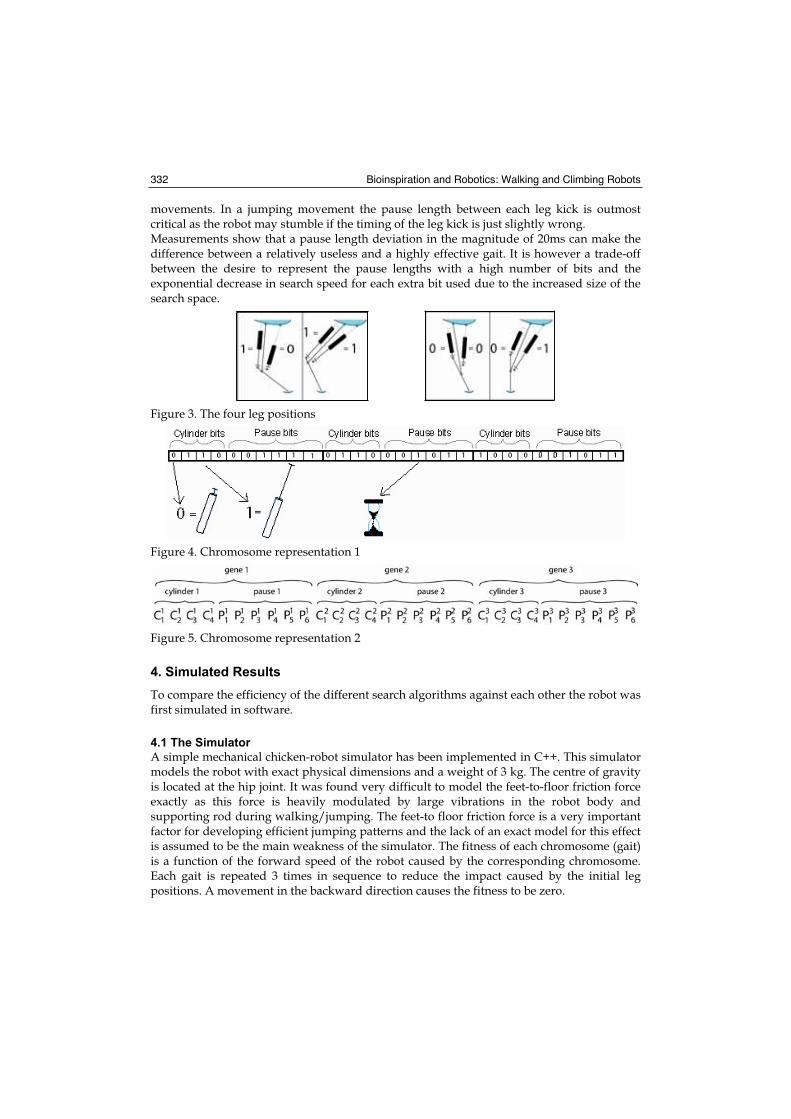
Bioinspiration and Robotics: Walking and Climbing Robots 332
movements. In a jumping movement the pause length between each leg kick is outmost critical as the robot may stumble if the timing of the leg kick is just slightly wrong. Measurements show that a pause length deviation in the magnitude of 20ms can make the difference between a relatively useless and a highly effective gait. It is however a trade-off between the desire to represent the pause lengths with a high number of bits and the exponential decrease in search speed for each extra bit used due to the increased size of the search space.
Figure 3. The four leg positions
Figure 4. Chromosome representation 1
Figure 5. Chromosome representation 2
4. Simulated Results
To compare the efficiency of the different search algorithms against each other the robot was first simulated in software.
4.1 The Simulator
A simple mechanical chicken-robot simulator has been implemented in C++. This simulator models the robot with exact physical dimensions and a weight of 3 kg. The centre of gravity is located at the hip joint. It was found very difficult to model the feet-to-floor friction force exactly as this force is heavily modulated by large vibrations in the robot body and supporting rod during walking/jumping. The feet-to floor friction force is a very important factor for developing efficient jumping patterns and the lack of an exact model for this effect is assumed to be the main weakness of the simulator. The fitness of each chromosome (gait) is a function of the forward speed of the robot caused by the corresponding chromosome. Each gait is repeated 3 times in sequence to reduce the impact caused by the initial leg positions. A movement in the backward direction causes the fitness to be zero.
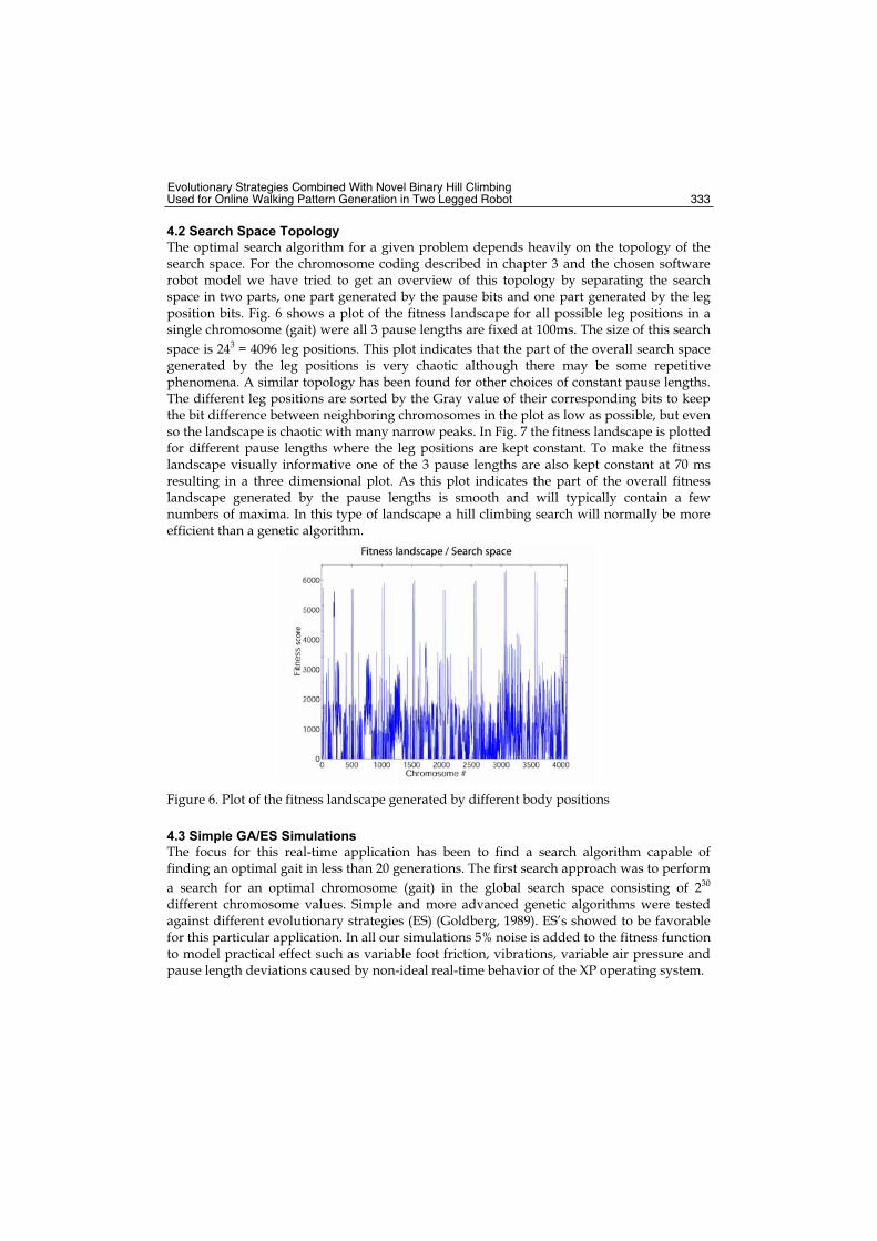
Evolutionary Strategies Combined With Novel Binary Hill Climbing Used for Online Walking Pattern Generation in Two Legged Robot 333
4.2 Search Space Topology
The optimal search algorithm for a given problem depends heavily on the topology of the search space. For the chromosome coding described in chapter 3 and the chosen software robot model we have tried to get an overview of this topology by separating the search space in two parts, one part generated by the pause bits and one part generated by the leg position bits. Fig. 6 shows a plot of the fitness landscape for all possible leg positions in a single chromosome (gait) were all 3 pause lengths are fixed at 100ms. The size of this search
space is 243 = 4096 leg positions. This plot indicates that the part of the overall search space generated by the leg positions is very chaotic although there may be some repetitive phenomena. A similar topology has been found for other choices of constant pause lengths. The different leg positions are sorted by the Gray value of their corresponding bits to keep the bit difference between neighboring chromosomes in the plot as low as possible, but even so the landscape is chaotic with many narrow peaks. In Fig. 7 the fitness landscape is plotted for different pause lengths where the leg positions are kept constant. To make the fitness landscape visually informative one of the 3 pause lengths are also kept constant at 70 ms resulting in a three dimensional plot. As this plot indicates the part of the overall fitness landscape generated by the pause lengths is smooth and will typically contain a few numbers of maxima. In this type of landscape a hill climbing search will normally be more efficient than a genetic algorithm.
Figure 6. Plot of the fitness landscape generated by different body positions
4.3 Simple GA/ES Simulations
The focus for this real-time application has been to find a search algorithm capable of finding an optimal gait in less than 20 generations. The first search approach was to perform
a search for an optimal chromosome (gait) in the global search space consisting of 230
different chromosome values. Simple and more advanced genetic algorithms were tested against different evolutionary strategies (ES) (Goldberg, 1989). ES’s showed to be favorable for this particular application. In all our simulations 5% noise is added to the fitness function to model practical effect such as variable foot friction, vibrations, variable air pressure and pause length deviations caused by non-ideal real-time behavior of the XP operating system.
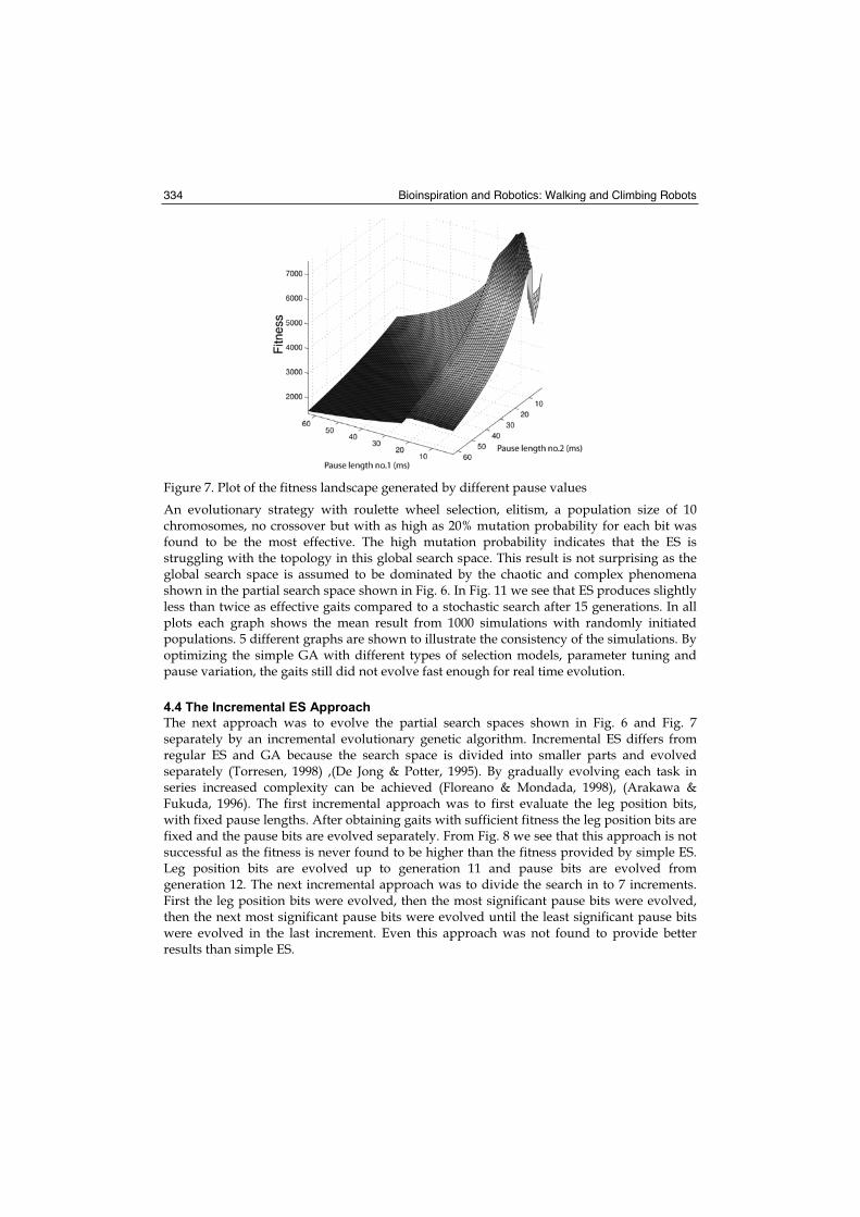
Bioinspiration and Robotics: Walking and Climbing Robots 334
Figure 7. Plot of the fitness landscape generated by different pause values
An evolutionary strategy with roulette wheel selection, elitism, a population size of 10 chromosomes, no crossover but with as high as 20% mutation probability for each bit was found to be the most effective. The high mutation probability indicates that the ES is struggling with the topology in this global search space. This result is not surprising as the global search space is assumed to be dominated by the chaotic and complex phenomena shown in the partial search space shown in Fig. 6. In Fig. 11 we see that ES produces slightly less than twice as effective gaits compared to a stochastic search after 15 generations. In all plots each graph shows the mean result from 1000 simulations with randomly initiated populations. 5 different graphs are shown to illustrate the consistency of the simulations. Byoptimizing the simple GA with different types of selection models, parameter tuning and pause variation, the gaits still did not evolve fast enough for real time evolution.
4.4 The Incremental ES Approach
The next approach was to evolve the partial search spaces shown in Fig. 6 and Fig. 7 separately by an incremental evolutionary genetic algorithm. Incremental ES differs from regular ES and GA because the search space is divided into smaller parts and evolved separately (Torresen, 1998) ,(De Jong & Potter, 1995). By gradually evolving each task in series increased complexity can be achieved (Floreano & Mondada, 1998), (Arakawa & Fukuda, 1996). The first incremental approach was to first evaluate the leg position bits, with fixed pause lengths. After obtaining gaits with sufficient fitness the leg position bits are fixed and the pause bits are evolved separately. From Fig. 8 we see that this approach is not successful as the fitness is never found to be higher than the fitness provided by simple ES. Leg position bits are evolved up to generation 11 and pause bits are evolved from generation 12. The next incremental approach was to divide the search in to 7 increments. First the leg position bits were evolved, then the most significant pause bits were evolved, then the next most significant pause bits were evolved until the least significant pause bits were evolved in the last increment. Even this approach was not found to provide better results than simple ES.
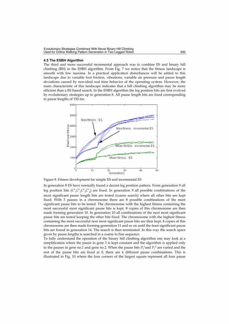
Evolutionary Strategies Combined With Novel Binary Hill Climbing Used for Online Walking Pattern Generation in Two Legged Robot 335
4.5 The ESBH Algorithm
The third and more successful incremental approach was to combine ES and binary hill climbing (BH) in the ESBH algorithm. From Fig. 7 we notice that the fitness landscape is smooth with few maxima. In a practical application disturbances will be added to this landscape due to variable foot friction, vibrations, variable air pressure and pause length deviations caused by non-ideal real time behavior of the operating system. However, the main characteristic of this landscape indicates that a hill climbing algorithm may be more efficient than a ES based search. In the ESBH algorithm the leg position bits are first evolved by evolutionary strategies up to generation 8. All pause length bits are fixed corresponding to pause lengths of 150 ms.
Figure 8. Fitness development for simple ES and incremental ES
In generation 8 ES have normally found a decent leg position pattern. From generation 9 all
leg position bits (Cx1C
x2C
x3C
x4) are fixed. In generation 9 all possible combinations of the
most significant pause length bits are tested (coarse search) where all other bits are kept fixed. With 3 pauses in a chromosome there are 8 possible combinations of the most significant pause bits to be tested. The chromosome with the highest fitness containing the most successful most significant pause bits is kept. 8 copies of this chromosome are then made forming generation 10. In generation 10 all combinations of the next most significant pause bits are tested keeping the other bits fixed. The chromosome with the highest fitness containing the most successful next most significant pause bits are then kept. 8 copies of this chromosome are then made forming generation 11 and so on until the least significant pause bits are found in generation 14. The search is then terminated. In this way the search space given by pause lengths is searched in a coarse to fine sequence. To fully understand the operation of the binary hill climbing algorithm one may look at a simplification where the pause in gene 3 is kept constant and the algorithm is applied only
to the pauses in gene no.1 and gene no.2. When the pause bits P11and P1
2 are varied and the
rest of the pause bits are fixed at 0, there are 4 different pause combinations. This is illustrated in Fig. 10 where the four corners of the largest square represent all four pause
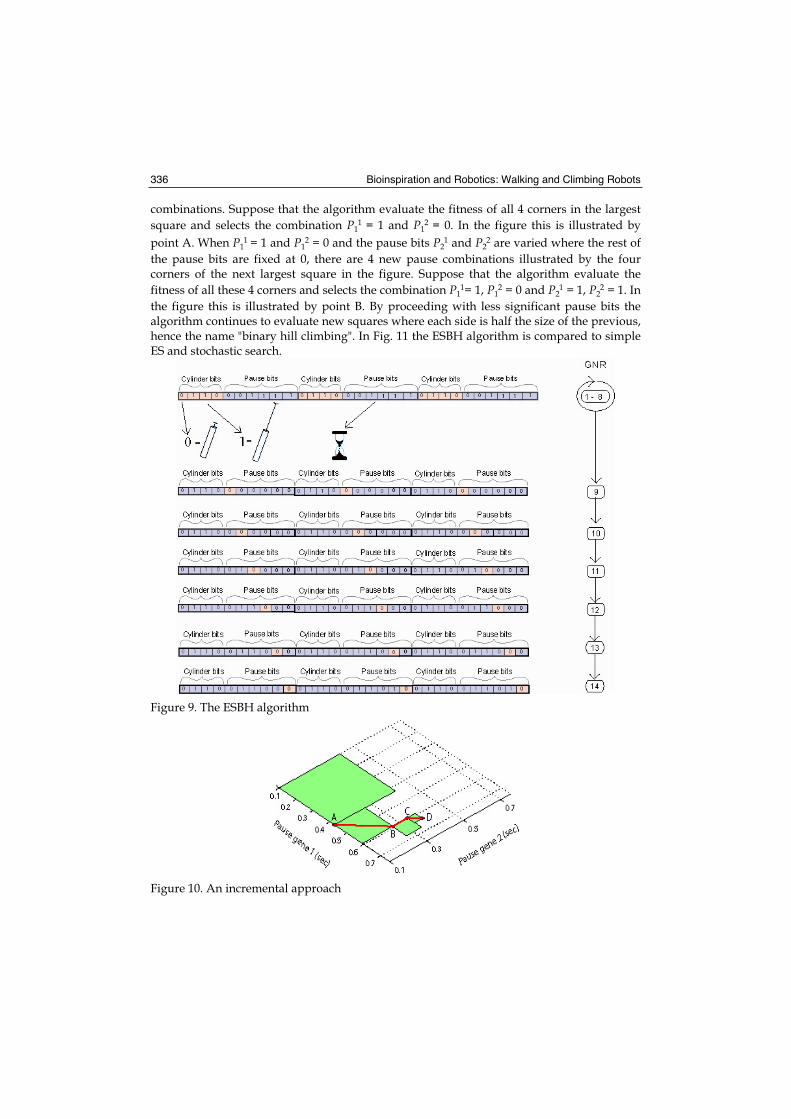
Bioinspiration and Robotics: Walking and Climbing Robots 336
combinations. Suppose that the algorithm evaluate the fitness of all 4 corners in the largest
square and selects the combination P11 = 1 and P1
2 = 0. In the figure this is illustrated by
point A. When P11 = 1 and P1
2 = 0 and the pause bits P21 and P2
2 are varied where the rest of
the pause bits are fixed at 0, there are 4 new pause combinations illustrated by the four corners of the next largest square in the figure. Suppose that the algorithm evaluate the
fitness of all these 4 corners and selects the combination P11= 1, P1
2 = 0 and P21 = 1, P2
2 = 1. In
the figure this is illustrated by point B. By proceeding with less significant pause bits the algorithm continues to evaluate new squares where each side is half the size of the previous, hence the name "binary hill climbing". In Fig. 11 the ESBH algorithm is compared to simple ES and stochastic search.
Figure 9. The ESBH algorithm
Figure 10. An incremental approach
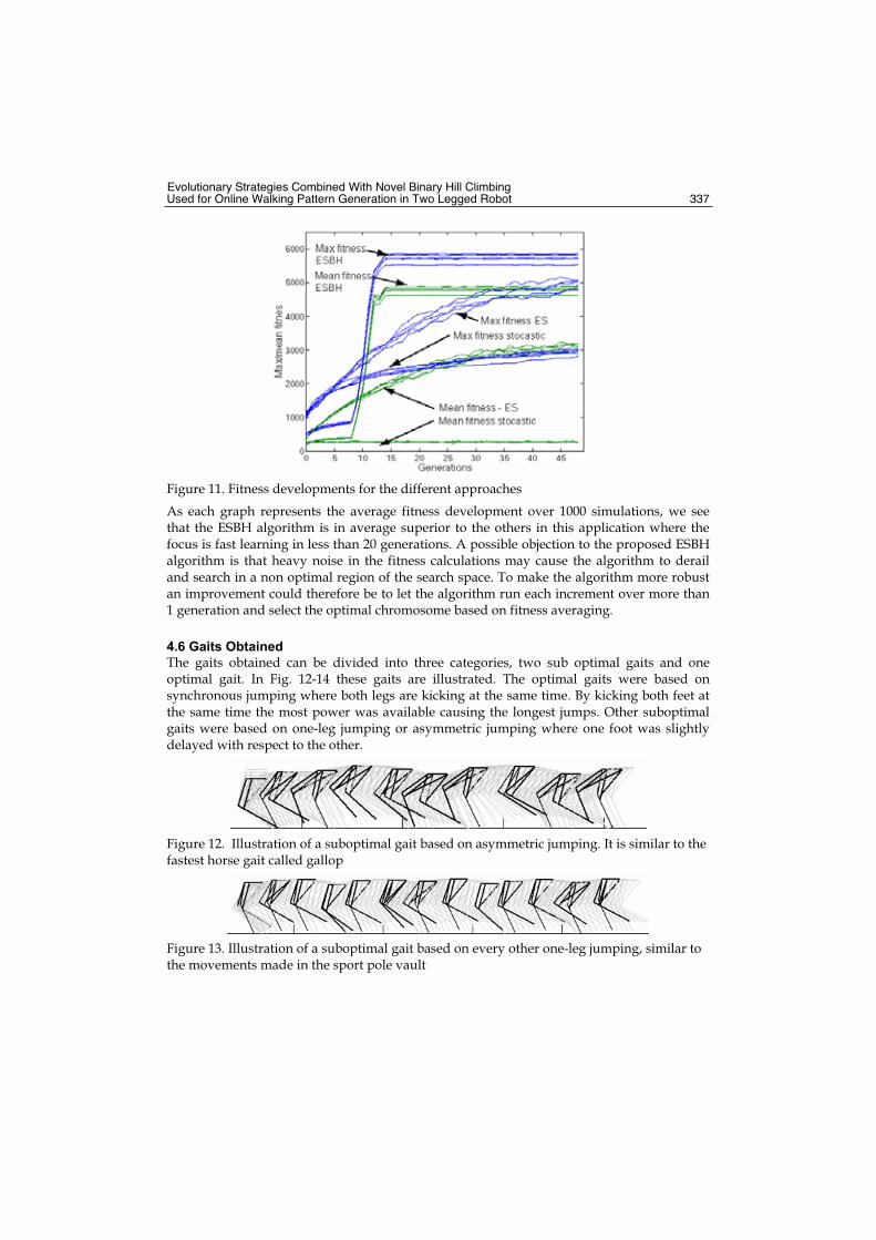
Evolutionary Strategies Combined With Novel Binary Hill Climbing Used for Online Walking Pattern Generation in Two Legged Robot 337
Figure 11. Fitness developments for the different approaches
As each graph represents the average fitness development over 1000 simulations, we see that the ESBH algorithm is in average superior to the others in this application where the focus is fast learning in less than 20 generations. A possible objection to the proposed ESBH algorithm is that heavy noise in the fitness calculations may cause the algorithm to derail and search in a non optimal region of the search space. To make the algorithm more robust an improvement could therefore be to let the algorithm run each increment over more than 1 generation and select the optimal chromosome based on fitness averaging.
4.6 Gaits Obtained
The gaits obtained can be divided into three categories, two sub optimal gaits and one optimal gait. In Fig. 12-14 these gaits are illustrated. The optimal gaits were based on synchronous jumping where both legs are kicking at the same time. By kicking both feet at the same time the most power was available causing the longest jumps. Other suboptimal gaits were based on one-leg jumping or asymmetric jumping where one foot was slightly delayed with respect to the other.
Figure 12. Illustration of a suboptimal gait based on asymmetric jumping. It is similar to the fastest horse gait called gallop
Figure 13. Illustration of a suboptimal gait based on every other one-leg jumping, similar to the movements made in the sport pole vault
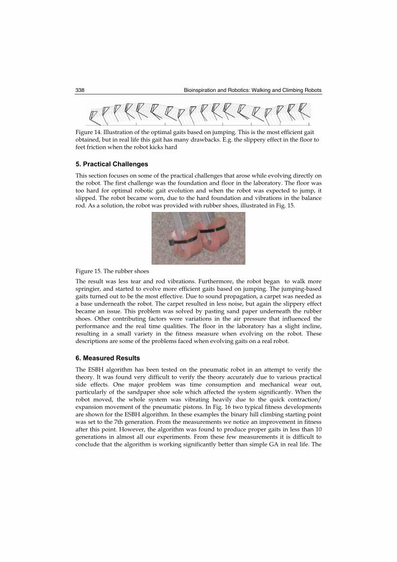
Bioinspiration and Robotics: Walking and Climbing Robots 338
Figure 14. Illustration of the optimal gaits based on jumping. This is the most efficient gait obtained, but in real life this gait has many drawbacks. E.g. the slippery effect in the floor to feet friction when the robot kicks hard
5. Practical Challenges
This section focuses on some of the practical challenges that arose while evolving directly on the robot. The first challenge was the foundation and floor in the laboratory. The floor was too hard for optimal robotic gait evolution and when the robot was expected to jump, it slipped. The robot became worn, due to the hard foundation and vibrations in the balance rod. As a solution, the robot was provided with rubber shoes, illustrated in Fig. 15.
Figure 15. The rubber shoes
The result was less tear and rod vibrations. Furthermore, the robot began to walk more springier, and started to evolve more efficient gaits based on jumping. The jumping-based gaits turned out to be the most effective. Due to sound propagation, a carpet was needed as a base underneath the robot. The carpet resulted in less noise, but again the slippery effect became an issue. This problem was solved by pasting sand paper underneath the rubber shoes. Other contributing factors were variations in the air pressure that influenced the performance and the real time qualities. The floor in the laboratory has a slight incline, resulting in a small variety in the fitness measure when evolving on the robot. These descriptions are some of the problems faced when evolving gaits on a real robot.
6. Measured Results
The ESBH algorithm has been tested on the pneumatic robot in an attempt to verify the theory. It was found very difficult to verify the theory accurately due to various practical side effects. One major problem was time consumption and mechanical wear out, particularly of the sandpaper shoe sole which affected the system significantly. When the robot moved, the whole system was vibrating heavily due to the quick contraction/ expansion movement of the pneumatic pistons. In Fig. 16 two typical fitness developments are shown for the ESBH algorithm. In these examples the binary hill climbing starting point was set to the 7th generation. From the measurements we notice an improvement in fitness after this point. However, the algorithm was found to produce proper gaits in less than 10 generations in almost all our experiments. From these few measurements it is difficult to conclude that the algorithm is working significantly better than simple GA in real life. The
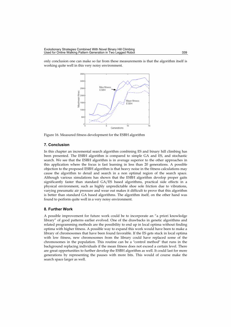
Evolutionary Strategies Combined With Novel Binary Hill Climbing Used for Online Walking Pattern Generation in Two Legged Robot 339
only conclusion one can make so far from these measurements is that the algorithm itself is working quite well in this very noisy environment.
Figure 16. Measured fitness development for the ESBH algorithm
7. Conclusion
In this chapter an incremental search algorithm combining ES and binary hill climbing has been presented. The ESBH algorithm is compared to simple GA and ES, and stochastic search. We see that the ESBH algorithm is in average superior to the other approaches in this application where the focus is fast learning in less than 20 generations. A possible objection to the proposed ESBH algorithm is that heavy noise in the fitness calculations may cause the algorithm to derail and search in a non optimal region of the search space. Although various simulations has shown that the ESBH algorithm develop proper gaits significantly faster than standard GA/ES based algorithms, practical side effects in a physical environment, such as highly unpredictable shoe sole friction due to vibrations, varying pneumatic air pressure and wear out makes it difficult to prove that this algorithm is better than standard GA based algorithms. The algorithm itself, on the other hand was found to perform quite well in a very noisy environment.
8. Further Work
A possible improvement for future work could be to incorporate an “a priori knowledge library” of good patterns earlier evolved. One of the drawbacks in genetic algorithms and related programming methods are the possibility to end up in local optima without finding optima with higher fitness. A possible way to expand this work would have been to make a library of chromosomes that have been found favorable. If the ES gets stuck in local optima with low fitness, new chromosomes from the library could have replaced some of the chromosomes in the population. This routine can be a "control method" that runs in the background replacing individuals if the mean fitness does not exceed a certain level. There are great opportunities to further develop the ESBH algorithm as well. It could last for more generations by representing the pauses with more bits. This would of course make the search space larger as well.
Bioinspiration and Robotics: Walking and Climbing Robots 340
9. References
Arakawa, T. & Fukuda, T. (1996) Natural motion trajectory generation of biped locomotion robot using genetic algorithm through energy optimization, In: Proceedings of the 1996 IEEE International Conference on Systems, Man and Cybernetics, vol. 2, pp. 1495–1500
Cant´u-Paz, E. (1998) A survey of parallel genetic algorithms. In: Calculateurs Paralleles, Reseaux et Systems Repartis, pp. 141–171, Paris
Floreano, D. & Mondada, F. (1998) Hardware solutions for evolutionary robotics. In: Proceedings of the First European Workshop on Evolutionary Robotics, pp. 137–151, Springer-Verlag, London
Goldberg, D. E. (1989) Genetic Algorithms in Search, Optimization and Machine Learning.Addison-Wesley Longman Publishing Co., Boston
Haddow, P. C. & Tufte, G. (2000) An evolvable hardware FPGA for adaptive hardware. In: Proceedings of the2000 Congress on Evolutionary Computation, pp. 553–560, IEEE Press, California
Higuchi, T.; Iwata, M.; Keymeulen, D.; Sakanashi, H.; Murakawa, M.; Kajitani, I.; Takahashi, E.; Toda, K.; Salami, N.; Kajihara, N. & Otsu, N. (1999) Real-world applications of analog and digital evolvable hardware, In: IEEE Transactions on EvolutionaryComputation, pp. 220–235
Hornby, G.; Takamura, S.; Yokono, J.; Hanagata, O.; Yamamoto, T., & Fujita. M. (2000) Evolving robust gaits with Aibo, In: IEEE International Conference on Robotics and Automation, pp. 3040–3045
De Jong, K. & Potter, M. A. (1995) Evolving complex structures via cooperative coevolution, In: Proceedings on the Fourth Annual Conference on Evolutionary Programming, pp. 307–317, MIT Press, Cambridge
Kalganova, T. (2000) Bidirectional incremental evolution in extrinsic evolvable hardware, In:Proceedings of the 2nd NASA/DoD workshop on Evolvable Hardware, pp. 65–74, IEEE Computer Society , Washington DC
Parker, G. B. (2001) Evolving cyclic control for a hexapod robot performing area coverage, In: Proceedings of the 2001 IEEE Computational Intelligence in Robotics and Automation,pp. 555–560, Canada
Torresen, J. (1998) A divide-and-conquer approach to evolvable hardware, In: Proceedings of the Second International Conference on Evolvable Systems, pp. 57–65, Springer-Verlag, London
Torresen, J. (2004) An evolvable hardware tutorial, In: Proceedings of the 14th International Conference on Field Programmable Logic and Applications, pp. 821–830, Belgium
21
A MultitaskingSurface Exploration Rover System
Antonios K. Bouloubasis and Gerard T. McKee School of Systems Engineering, University of Reading, Reading
United Kingdom
1. Introduction
Exploration of the unknown and survival have always been generic instincts of the human nature. According to our knowledge about the universe and the available technology, exploration progressed from a quest for land across the horizon, to a search for planetary bodies in our galaxial neighbourhood, which given the appropriate infrastructure, could sustain artificial ecosystems. The best candidates for exploration within our Solar System are the Moon and Mars. The Earth’s moon is the nearest celestial body and therefore most easily accessible. It has been excessively studied throughout the centuries but it wasn’t before the 70’s that the Luna [Harvey, 2005] and Apollo programs successfully delivered both tele-operated, semi-autonomous and remotely-operated [Muirhead, 2004] [Young, 2006] rover vehicles onto its surface. Many scenarios for lunar stations have been and continue to be considered [Smith, 2005]. These involve the deployment of similar in nature, but more advanced surface mobility systems for infrastructure development. Mars has also been visited using wheeled robotic explorers. The Sojourner deployed in 1997 [Matijevic, 1997] and more recently the two Mars Exploration Rovers (MER) [Erickson, 2006], all returned valuable information about the Martian environment. Mars Science Laboratory (MSL) [Naderi, 2006] is a highly instrumented rover that will be deployed on the Red Planet sometime in October 2010 and used to perform more detailed remote-field geology. NASA’s scenarios for a planetary outpost [Drake, 1998] include the deployment of 3 un-pressurized rover vehicles. ESA’s Exomars mission, planned for 2012, will deliver the Pasteur rover whose equipment includes an on-board drill system [Jorge, 2006]. The Multi-Tasking Rover (MTR) presented here and depicted in Fig. 1, is an experimental robotic platform, which incorporates advanced mobility features. In order to account for local terrain irregularities, the rover employs one passive and two active suspension systems. It can shift its centre of mass accordingly, to obtain stability enhancing traversability when so required. The MTR incorporates a novel suspension system to promote significant advantages over traditional rover designs. Its real strength however, lies in providing a multitasking robotic platform rather than a dedicated system that can only be engaged in specific, pre-defined scenarios. To do so the rover operates in conjunction with Tool and Science Packs (TP/SP).
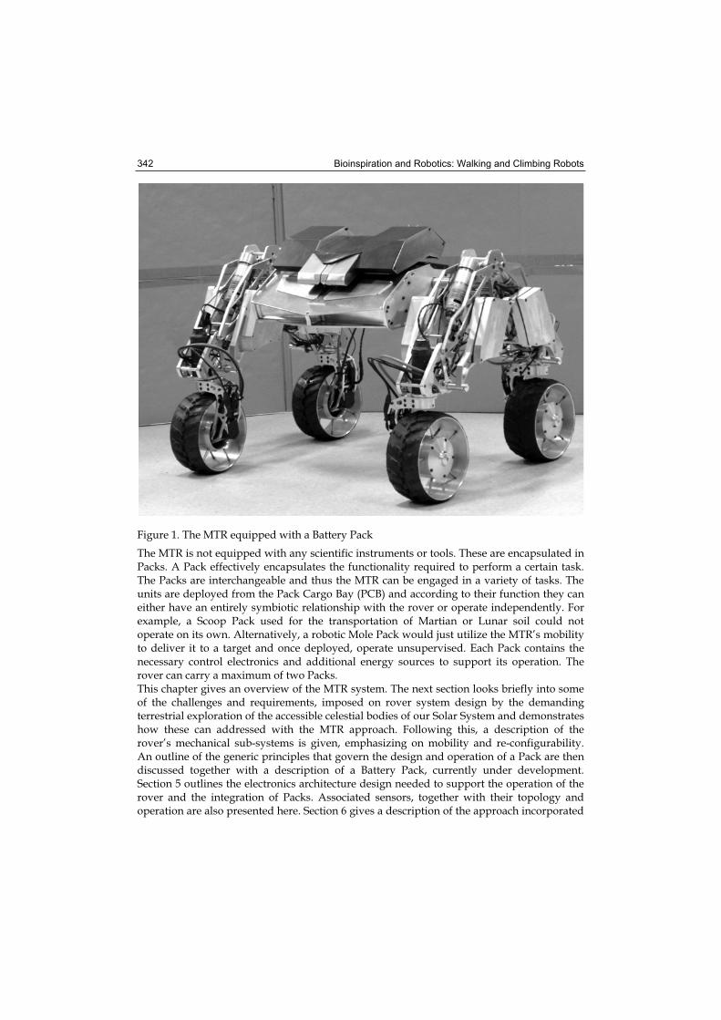
Bioinspiration and Robotics: Walking and Climbing Robots 342
Figure 1. The MTR equipped with a Battery Pack
The MTR is not equipped with any scientific instruments or tools. These are encapsulated in Packs. A Pack effectively encapsulates the functionality required to perform a certain task. The Packs are interchangeable and thus the MTR can be engaged in a variety of tasks. The units are deployed from the Pack Cargo Bay (PCB) and according to their function they can either have an entirely symbiotic relationship with the rover or operate independently. For example, a Scoop Pack used for the transportation of Martian or Lunar soil could not operate on its own. Alternatively, a robotic Mole Pack would just utilize the MTR’s mobility to deliver it to a target and once deployed, operate unsupervised. Each Pack contains the necessary control electronics and additional energy sources to support its operation. The rover can carry a maximum of two Packs. This chapter gives an overview of the MTR system. The next section looks briefly into some of the challenges and requirements, imposed on rover system design by the demanding terrestrial exploration of the accessible celestial bodies of our Solar System and demonstrates how these can addressed with the MTR approach. Following this, a description of the rover’s mechanical sub-systems is given, emphasizing on mobility and re-configurability. An outline of the generic principles that govern the design and operation of a Pack are then discussed together with a description of a Battery Pack, currently under development. Section 5 outlines the electronics architecture design needed to support the operation of the rover and the integration of Packs. Associated sensors, together with their topology and operation are also presented here. Section 6 gives a description of the approach incorporated
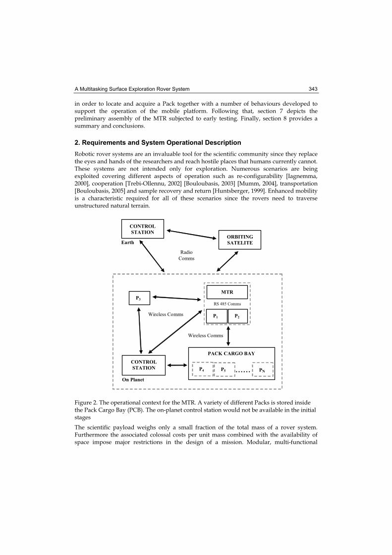
A Multitasking Surface Exploration Rover System 343
in order to locate and acquire a Pack together with a number of behaviours developed to support the operation of the mobile platform. Following that, section 7 depicts the preliminary assembly of the MTR subjected to early testing. Finally, section 8 provides a summary and conclusions.
2. Requirements and System Operational Description
Robotic rover systems are an invaluable tool for the scientific community since they replace the eyes and hands of the researchers and reach hostile places that humans currently cannot. These systems are not intended only for exploration. Numerous scenarios are being exploited covering different aspects of operation such as re-configurability [Iagnemma, 2000], cooperation [Trebi-Ollennu, 2002] [Bouloubasis, 2003] [Mumm, 2004], transportation [Bouloubasis, 2005] and sample recovery and return [Huntsberger, 1999]. Enhanced mobility is a characteristic required for all of these scenarios since the rovers need to traverse unstructured natural terrain.
CONTROL
STATION
MTR
P1 P2
RS 485 Comms
PACK CARGO BAY
P4 ......
Wireless Comms
Wireless Comms
P5 PN
P3
ORBITING
SATELITE
CONTROL
STATION
Earth
On Planet
Radio
Comms
Figure 2. The operational context for the MTR. A variety of different Packs is stored inside the Pack Cargo Bay (PCB). The on-planet control station would not be available in the initial stages
The scientific payload weighs only a small fraction of the total mass of a rover system. Furthermore the associated colossal costs per unit mass combined with the availability of space impose major restrictions in the design of a mission. Modular, multi-functional
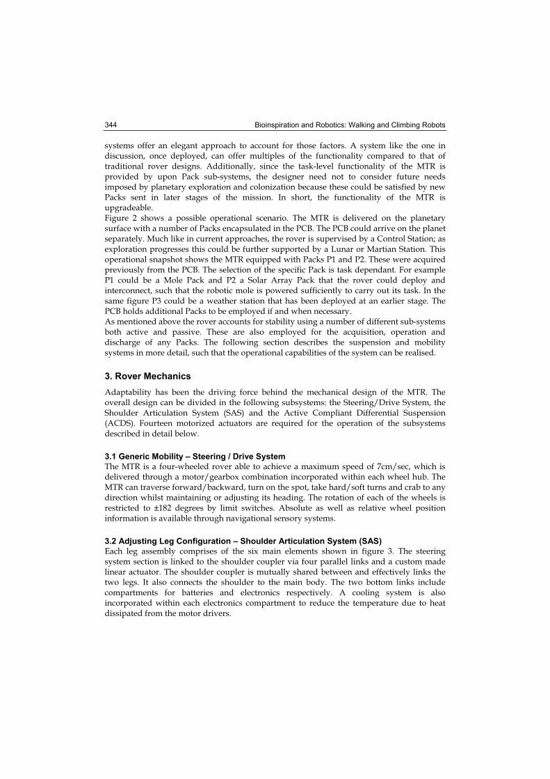
Bioinspiration and Robotics: Walking and Climbing Robots 344
systems offer an elegant approach to account for those factors. A system like the one in discussion, once deployed, can offer multiples of the functionality compared to that of traditional rover designs. Additionally, since the task-level functionality of the MTR is provided by upon Pack sub-systems, the designer need not to consider future needs imposed by planetary exploration and colonization because these could be satisfied by new Packs sent in later stages of the mission. In short, the functionality of the MTR is upgradeable.Figure 2 shows a possible operational scenario. The MTR is delivered on the planetary surface with a number of Packs encapsulated in the PCB. The PCB could arrive on the planet separately. Much like in current approaches, the rover is supervised by a Control Station; as exploration progresses this could be further supported by a Lunar or Martian Station. This operational snapshot shows the MTR equipped with Packs P1 and P2. These were acquired previously from the PCB. The selection of the specific Pack is task dependant. For example P1 could be a Mole Pack and P2 a Solar Array Pack that the rover could deploy and interconnect, such that the robotic mole is powered sufficiently to carry out its task. In the same figure P3 could be a weather station that has been deployed at an earlier stage. The PCB holds additional Packs to be employed if and when necessary. As mentioned above the rover accounts for stability using a number of different sub-systems both active and passive. These are also employed for the acquisition, operation and discharge of any Packs. The following section describes the suspension and mobility systems in more detail, such that the operational capabilities of the system can be realised.
3. Rover Mechanics
Adaptability has been the driving force behind the mechanical design of the MTR. The overall design can be divided in the following subsystems: the Steering/Drive System, the Shoulder Articulation System (SAS) and the Active Compliant Differential Suspension (ACDS). Fourteen motorized actuators are required for the operation of the subsystems described in detail below.
3.1 Generic Mobility – Steering / Drive System
The MTR is a four-wheeled rover able to achieve a maximum speed of 7cm/sec, which is delivered through a motor/gearbox combination incorporated within each wheel hub. The MTR can traverse forward/backward, turn on the spot, take hard/soft turns and crab to any direction whilst maintaining or adjusting its heading. The rotation of each of the wheels is restricted to ±182 degrees by limit switches. Absolute as well as relative wheel position information is available through navigational sensory systems.
3.2 Adjusting Leg Configuration – Shoulder Articulation System (SAS)
Each leg assembly comprises of the six main elements shown in figure 3. The steering system section is linked to the shoulder coupler via four parallel links and a custom made linear actuator. The shoulder coupler is mutually shared between and effectively links the two legs. It also connects the shoulder to the main body. The two bottom links include compartments for batteries and electronics respectively. A cooling system is also incorporated within each electronics compartment to reduce the temperature due to heat dissipated from the motor drivers.
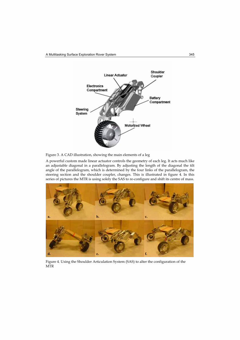
A Multitasking Surface Exploration Rover System 345
Figure 3. A CAD illustration, showing the main elements of a leg
A powerful custom made linear actuator controls the geometry of each leg. It acts much like an adjustable diagonal in a parallelogram. By adjusting the length of the diagonal the tilt angle of the parallelogram, which is determined by the four links of the parallelogram, the steering section and the shoulder coupler, changes. This is illustrated in figure 4. In this series of pictures the MTR is using solely the SAS to re-configure and shift its centre of mass.
a. b. c.
d. e. f.
Figure 4. Using the Shoulder Articulation System (SAS) to alter the configuration of the MTR
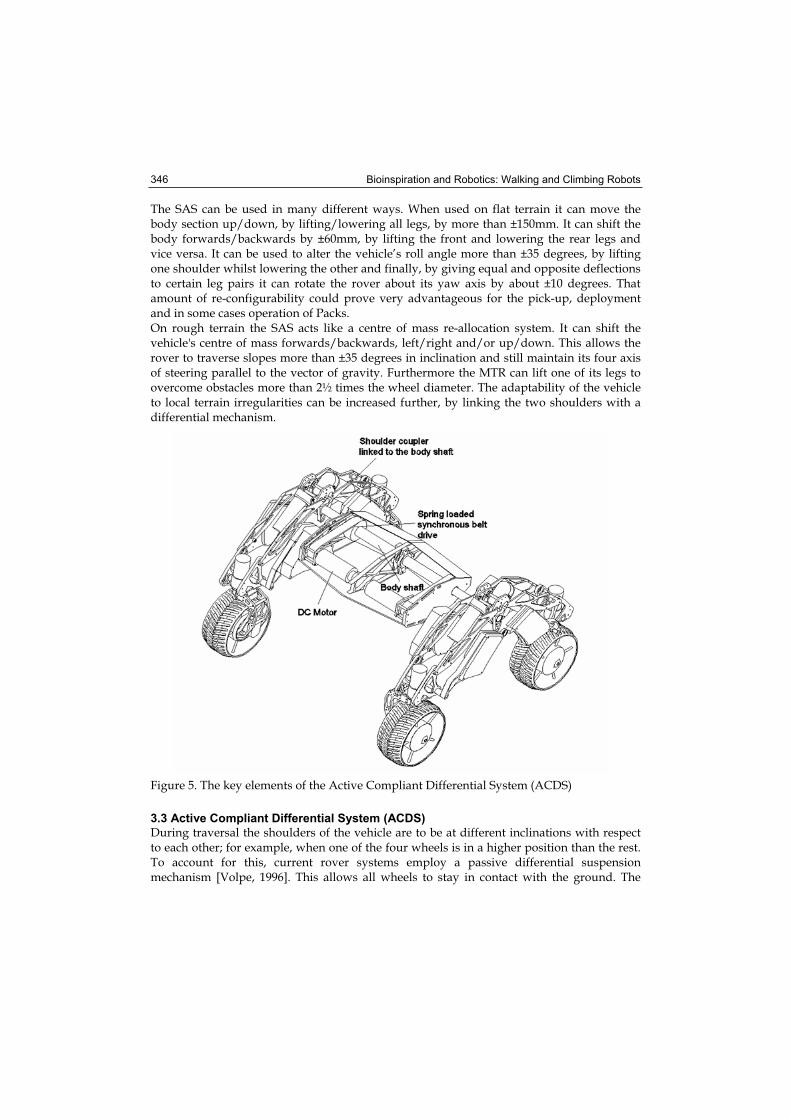
Bioinspiration and Robotics: Walking and Climbing Robots 346
The SAS can be used in many different ways. When used on flat terrain it can move the body section up/down, by lifting/lowering all legs, by more than ±150mm. It can shift the body forwards/backwards by ±60mm, by lifting the front and lowering the rear legs and vice versa. It can be used to alter the vehicle’s roll angle more than ±35 degrees, by lifting one shoulder whilst lowering the other and finally, by giving equal and opposite deflections to certain leg pairs it can rotate the rover about its yaw axis by about ±10 degrees. That amount of re-configurability could prove very advantageous for the pick-up, deployment and in some cases operation of Packs. On rough terrain the SAS acts like a centre of mass re-allocation system. It can shift the vehicle's centre of mass forwards/backwards, left/right and/or up/down. This allows the rover to traverse slopes more than ±35 degrees in inclination and still maintain its four axis of steering parallel to the vector of gravity. Furthermore the MTR can lift one of its legs to overcome obstacles more than 2½ times the wheel diameter. The adaptability of the vehicle to local terrain irregularities can be increased further, by linking the two shoulders with a differential mechanism.
Figure 5. The key elements of the Active Compliant Differential System (ACDS)
3.3 Active Compliant Differential System (ACDS)
During traversal the shoulders of the vehicle are to be at different inclinations with respect to each other; for example, when one of the four wheels is in a higher position than the rest. To account for this, current rover systems employ a passive differential suspension mechanism [Volpe, 1996]. This allows all wheels to stay in contact with the ground. The
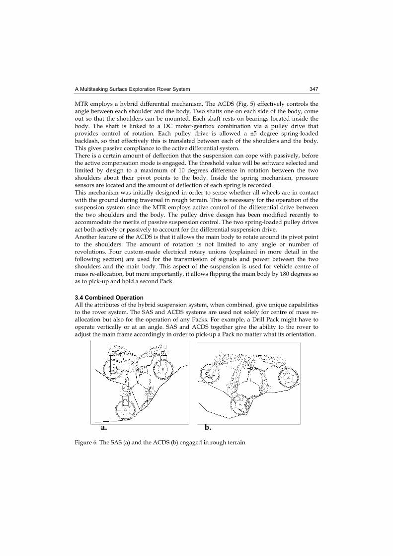
A Multitasking Surface Exploration Rover System 347
MTR employs a hybrid differential mechanism. The ACDS (Fig. 5) effectively controls the angle between each shoulder and the body. Two shafts one on each side of the body, come out so that the shoulders can be mounted. Each shaft rests on bearings located inside the body. The shaft is linked to a DC motor-gearbox combination via a pulley drive that provides control of rotation. Each pulley drive is allowed a ±5 degree spring-loaded backlash, so that effectively this is translated between each of the shoulders and the body. This gives passive compliance to the active differential system. There is a certain amount of deflection that the suspension can cope with passively, before the active compensation mode is engaged. The threshold value will be software selected and limited by design to a maximum of 10 degrees difference in rotation between the two shoulders about their pivot points to the body. Inside the spring mechanism, pressure sensors are located and the amount of deflection of each spring is recorded. This mechanism was initially designed in order to sense whether all wheels are in contact with the ground during traversal in rough terrain. This is necessary for the operation of the suspension system since the MTR employs active control of the differential drive between the two shoulders and the body. The pulley drive design has been modified recently to accommodate the merits of passive suspension control. The two spring-loaded pulley drives act both actively or passively to account for the differential suspension drive. Another feature of the ACDS is that it allows the main body to rotate around its pivot point to the shoulders. The amount of rotation is not limited to any angle or number of revolutions. Four custom-made electrical rotary unions (explained in more detail in the following section) are used for the transmission of signals and power between the two shoulders and the main body. This aspect of the suspension is used for vehicle centre of mass re-allocation, but more importantly, it allows flipping the main body by 180 degrees so as to pick-up and hold a second Pack.
3.4 Combined Operation
All the attributes of the hybrid suspension system, when combined, give unique capabilities to the rover system. The SAS and ACDS systems are used not solely for centre of mass re-allocation but also for the operation of any Packs. For example, a Drill Pack might have to operate vertically or at an angle. SAS and ACDS together give the ability to the rover to adjust the main frame accordingly in order to pick-up a Pack no matter what its orientation.
a. b.
Figure 6. The SAS (a) and the ACDS (b) engaged in rough terrain
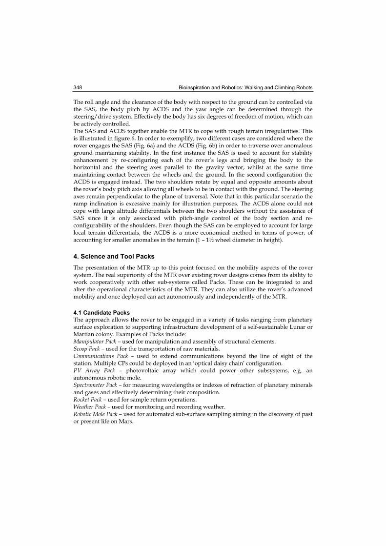
Bioinspiration and Robotics: Walking and Climbing Robots 348
The roll angle and the clearance of the body with respect to the ground can be controlled via the SAS, the body pitch by ACDS and the yaw angle can be determined through the steering/drive system. Effectively the body has six degrees of freedom of motion, which can be actively controlled. The SAS and ACDS together enable the MTR to cope with rough terrain irregularities. This is illustrated in figure 6. In order to exemplify, two different cases are considered where the rover engages the SAS (Fig. 6a) and the ACDS (Fig. 6b) in order to traverse over anomalous ground maintaining stability. In the first instance the SAS is used to account for stability enhancement by re-configuring each of the rover’s legs and bringing the body to the horizontal and the steering axes parallel to the gravity vector, whilst at the same time maintaining contact between the wheels and the ground. In the second configuration the ACDS is engaged instead. The two shoulders rotate by equal and opposite amounts about the rover’s body pitch axis allowing all wheels to be in contact with the ground. The steering axes remain perpendicular to the plane of traversal. Note that in this particular scenario the ramp inclination is excessive mainly for illustration purposes. The ACDS alone could not cope with large altitude differentials between the two shoulders without the assistance of SAS since it is only associated with pitch-angle control of the body section and re-configurability of the shoulders. Even though the SAS can be employed to account for large local terrain differentials, the ACDS is a more economical method in terms of power, of accounting for smaller anomalies in the terrain (1 – 1½ wheel diameter in height).
4. Science and Tool Packs
The presentation of the MTR up to this point focused on the mobility aspects of the rover system. The real superiority of the MTR over existing rover designs comes from its ability to work cooperatively with other sub-systems called Packs. These can be integrated to and alter the operational characteristics of the MTR. They can also utilize the rover’s advanced mobility and once deployed can act autonomously and independently of the MTR.
4.1 Candidate Packs
The approach allows the rover to be engaged in a variety of tasks ranging from planetary surface exploration to supporting infrastructure development of a self-sustainable Lunar or Martian colony. Examples of Packs include: Manipulator Pack – used for manipulation and assembly of structural elements. Scoop Pack – used for the transportation of raw materials. Communications Pack – used to extend communications beyond the line of sight of the station. Multiple CPs could be deployed in an ‘optical daisy chain’ configuration. PV Array Pack – photovoltaic array which could power other subsystems, e.g. an autonomous robotic mole. Spectrometer Pack – for measuring wavelengths or indexes of refraction of planetary minerals and gases and effectively determining their composition. Rocket Pack – used for sample return operations. Weather Pack – used for monitoring and recording weather. Robotic Mole Pack – used for automated sub-surface sampling aiming in the discovery of past or present life on Mars.
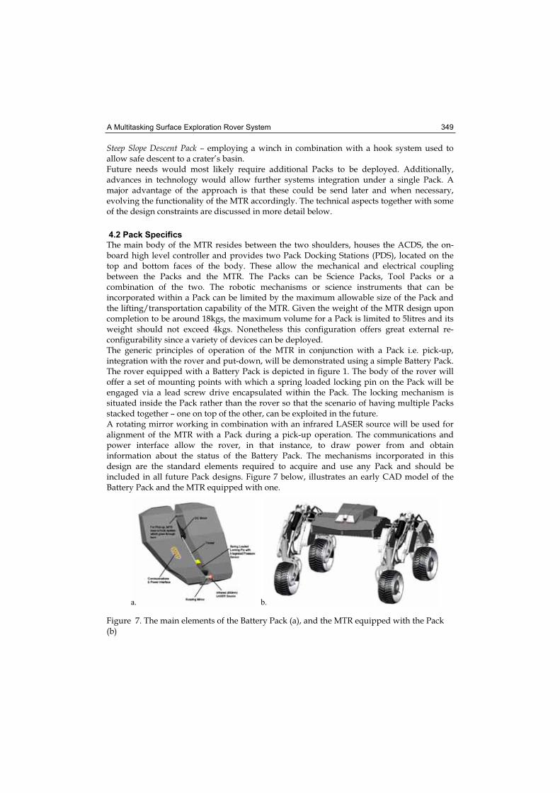
A Multitasking Surface Exploration Rover System 349
Steep Slope Descent Pack – employing a winch in combination with a hook system used to allow safe descent to a crater’s basin. Future needs would most likely require additional Packs to be deployed. Additionally, advances in technology would allow further systems integration under a single Pack. A major advantage of the approach is that these could be send later and when necessary, evolving the functionality of the MTR accordingly. The technical aspects together with some of the design constraints are discussed in more detail below.
4.2 Pack Specifics
The main body of the MTR resides between the two shoulders, houses the ACDS, the on-board high level controller and provides two Pack Docking Stations (PDS), located on the top and bottom faces of the body. These allow the mechanical and electrical coupling between the Packs and the MTR. The Packs can be Science Packs, Tool Packs or a combination of the two. The robotic mechanisms or science instruments that can be incorporated within a Pack can be limited by the maximum allowable size of the Pack and the lifting/transportation capability of the MTR. Given the weight of the MTR design upon completion to be around 18kgs, the maximum volume for a Pack is limited to 5litres and its weight should not exceed 4kgs. Nonetheless this configuration offers great external re-configurability since a variety of devices can be deployed. The generic principles of operation of the MTR in conjunction with a Pack i.e. pick-up, integration with the rover and put-down, will be demonstrated using a simple Battery Pack. The rover equipped with a Battery Pack is depicted in figure 1. The body of the rover will offer a set of mounting points with which a spring loaded locking pin on the Pack will be engaged via a lead screw drive encapsulated within the Pack. The locking mechanism is situated inside the Pack rather than the rover so that the scenario of having multiple Packs stacked together – one on top of the other, can be exploited in the future. A rotating mirror working in combination with an infrared LASER source will be used for alignment of the MTR with a Pack during a pick-up operation. The communications and power interface allow the rover, in that instance, to draw power from and obtain information about the status of the Battery Pack. The mechanisms incorporated in this design are the standard elements required to acquire and use any Pack and should be included in all future Pack designs. Figure 7 below, illustrates an early CAD model of the Battery Pack and the MTR equipped with one.
a. b.
Figure 7. The main elements of the Battery Pack (a), and the MTR equipped with the Pack (b)
Bioinspiration and Robotics: Walking and Climbing Robots 350
5. Electrics/Electronics and Sensing
5.1 Rover System – Low-level Controller
The electronics system for the MTR comprises two subsystems (fig. 8.). The first, the low-level controller, is built around the Microchip PIC controller and a number of different peripherals. It has the responsibility of motor PID-servo control, as well as obtaining the sensors’ feedback to be utilized by local, low-level behavioural loops, or the higher-level controller (the second subsystem) when necessary. Modularity is a key design goal. The low-level controller is divided into five smaller subsystems. Each leg will comprise a small network of four PICs, three motion controllers and one additional general-purpose controller. Each leg has a number of sensors associated with it. Apart from optical encoders, limit switches and potentiometers, which are employed for the control of the motors, infrared range finders and motion detectors, are mounted on the steering brackets of each wheel. Another range finder is positioned at the side of the leg together with a pair of infrared detectors. The latter are used during the Pack Pick-Up Sequence so that the presence of a Pack is detected; as explained below, the Pack emits an infrared beam, which the rover uses in order to align with it. Other low-level functions may be required and therefore both I2C and RS-485 communication buses are utilised so that additional controllers/sensors can be added in a plug-and-play fashion. The fifth low-level subsystem is located inside the body of the MTR and will be in charge of the actuators that govern the operation of the ACDS. It is also used to obtain sensor information and report back to the high-level controller. Sensors located on the body include: a 3-axis accelerometer; a GPS receiver; a digital compass; two stereo-camera systems (front and rear); ultrasonic sensors located at the front and rear faces of the body; infrared distance sensors at the top and bottom faces of the body; force sensors, encoders and potentiometers for the operation of the ACDS; a series of infrared detectors located at the top and bottom faces of the body for detecting the infrared LASER beam emitted by a source on the Pack and aligning with it; opto-reflectors to verify positioning of the Pack with respect to the body; and finally motion detectors situated at the front and rear faces of the body, to aid the navigation of the MTR in dynamic environments. Note that many of the sensory devices mentioned above cannot operate in a space environment. Nonetheless alternatives exist that do. Usage of cheaper systems allows the principles of operation of the MTR system to be demonstrated.
5.2 High-level Controller
The second subsystem, an on-board high-level controller, will be connected with all the modules through an RS485 bus allowing a sufficiently large number of devices to be part of the loop. The Gumstix/Verdex has been selected as the most appropriate platform. It uses an Intel XScale PXA-270, running at 400MHz, with 64MB of RAM and 16MB of flash. It provides many peripherals on a single board – Bluetooth, access to a 32-Bit External bus, CompactFlash/PCMCIA interfaces, a CMOS/CCD image sensor input, MSL (up to 416 Mbps), I2C, SPI, SD Card and Memory Stick , USB Host/Device. The unit measures 80 x 20 mm and consumes as little as 650 mW. Many expansion boards also exist. The high-level controller, which is located within the body, needs to exchange information via a full-duplex RS-485 communications bus, with the low-level controller, which is distributed over both shoulders and the body. Furthermore 8 Lithium-Polymer battery cells are distributed over both shoulders and the body of the rover. If uniform discharge is
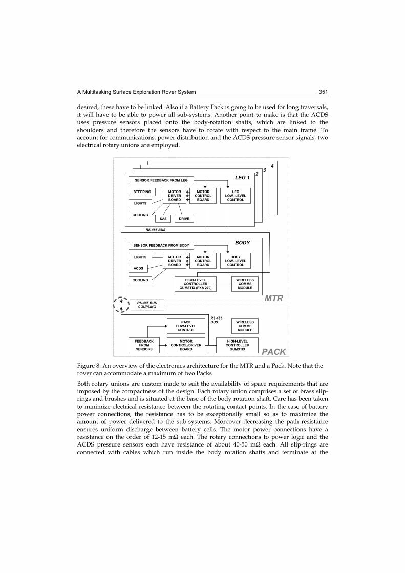
A Multitasking Surface Exploration Rover System 351
desired, these have to be linked. Also if a Battery Pack is going to be used for long traversals, it will have to be able to power all sub-systems. Another point to make is that the ACDS uses pressure sensors placed onto the body-rotation shafts, which are linked to the shoulders and therefore the sensors have to rotate with respect to the main frame. To account for communications, power distribution and the ACDS pressure sensor signals, two electrical rotary unions are employed.
4 3
2 LEG 1
SENSOR FEEDBACK FROM LEG
STEERING
DRIVE SAS COOLING
LIGHTS
MOTOR DRIVER
BOARD
MOTOR CONTROL
BOARD
LEG LOW- LEVEL
CONTROL
BODY
MOTOR DRIVER
BOARD
MOTOR CONTROL
BOARD
BODY LOW- LEVEL
CONTROL ACDS
LIGHTS
COOLING
SENSOR FEEDBACK FROM BODY
HIGH-LEVEL CONTROLLER
GUMSTIX (PXA 270)
WIRELESS COMMS
MODULE
RS-485 BUS
WIRELESS COMMS
MODULE
HIGH-LEVEL CONTROLLER
GUMSTIX
MOTOR CONTROL/DRIVER
BOARD
PACKLOW-LEVEL
CONTROL
FEEDBACK FROM
SENSORS
RS-485 BUS COUPLING
PACK
MTR
RS-485BUS
Figure 8. An overview of the electronics architecture for the MTR and a Pack. Note that the rover can accommodate a maximum of two Packs
Both rotary unions are custom made to suit the availability of space requirements that are imposed by the compactness of the design. Each rotary union comprises a set of brass slip-rings and brushes and is situated at the base of the body rotation shaft. Care has been taken to minimize electrical resistance between the rotating contact points. In the case of battery power connections, the resistance has to be exceptionally small so as to maximize the amount of power delivered to the sub-systems. Moreover decreasing the path resistance ensures uniform discharge between battery cells. The motor power connections have a resistance on the order of 12-15 m each. The rotary connections to power logic and the ACDS pressure sensors each have resistance of about 40-50 m each. All slip-rings are connected with cables which run inside the body rotation shafts and terminate at the
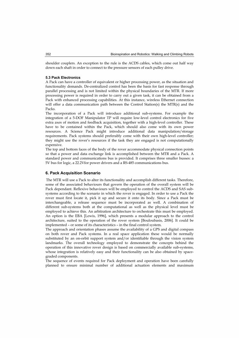
Bioinspiration and Robotics: Walking and Climbing Robots 352
shoulder couplers. An exception to the rule is the ACDS cables, which come out half way down each shaft in order to connect to the pressure sensors of each pulley drive.
5.3 Pack Electronics
A Pack can have a controller of equivalent or higher processing power, as the situation and functionality demands. De-centralized control has been the basis for fast response through parallel processing and is not limited within the physical boundaries of the MTR. If more processing power is required in order to carry out a given task, it can be obtained from a Pack with enhanced processing capabilities. At this instance, wireless Ethernet connection will offer a data communication path between the Control Station(s) the MTR(s) and the Packs. The incorporation of a Pack will introduce additional sub-systems. For example the integration of a 5-DOF Manipulator TP will require low-level control electronics for five extra axes of motion and feedback acquisition, together with a high-level controller. These have to be contained within the Pack, which should also come with its own power resources. A Science Pack might introduce additional data manipulation/storage requirements. Pack systems should preferably come with their own high-level controller; they might use the rover’s resources if the task they are engaged is not computationally expensive.The top and bottom faces of the body of the rover accommodate physical connection points so that a power and data exchange link is accomplished between the MTR and a Pack. A standard power and communications bus is provided. It comprises three smaller busses: a 5V bus for logic, a 22.2Vfor power drivers and a RS-485 communications bus.
6. Pack Acquisition Scenario
The MTR will use a Pack to alter its functionality and accomplish different tasks. Therefore, some of the associated behaviours that govern the operation of the overall system will be Pack dependant. Reflexive behaviours will be employed to control the ACDS and SAS sub-systems according to the scenario in which the rover is engaged. In order to use a Pack the rover must first locate it, pick it up and secure it onto its body. Since a Pack must be interchangeable, a release sequence must be incorporated as well. A combination of different sub-systems both at the computational as well as the physical level must be employed to achieve this. An arbitration architecture to orchestrate this must be employed. An option is the EBA [Lewis, 1996], which presents a modular approach to the control architecture, suited to the operation of the rover system [Bouloubasis, 2006]. It could be implemented – or some of its characteristics – in the final control system. The approach and orientation phases assume the availability of a GPS and digital compass on both rover and Pack systems. In a real space application these would be normally substituted by an on-orbit support system and/or identifiable through the vision system landmarks. The overall technology employed to demonstrate the concepts behind the operation of this innovative rover design is based on commercially available sub-systems, whose integration is relatively easy and their functionality can be also obtained by space-graded components. The sequence of events required for Pack deployment and operation have been carefully planned to ensure minimal number of additional actuation elements and maximum
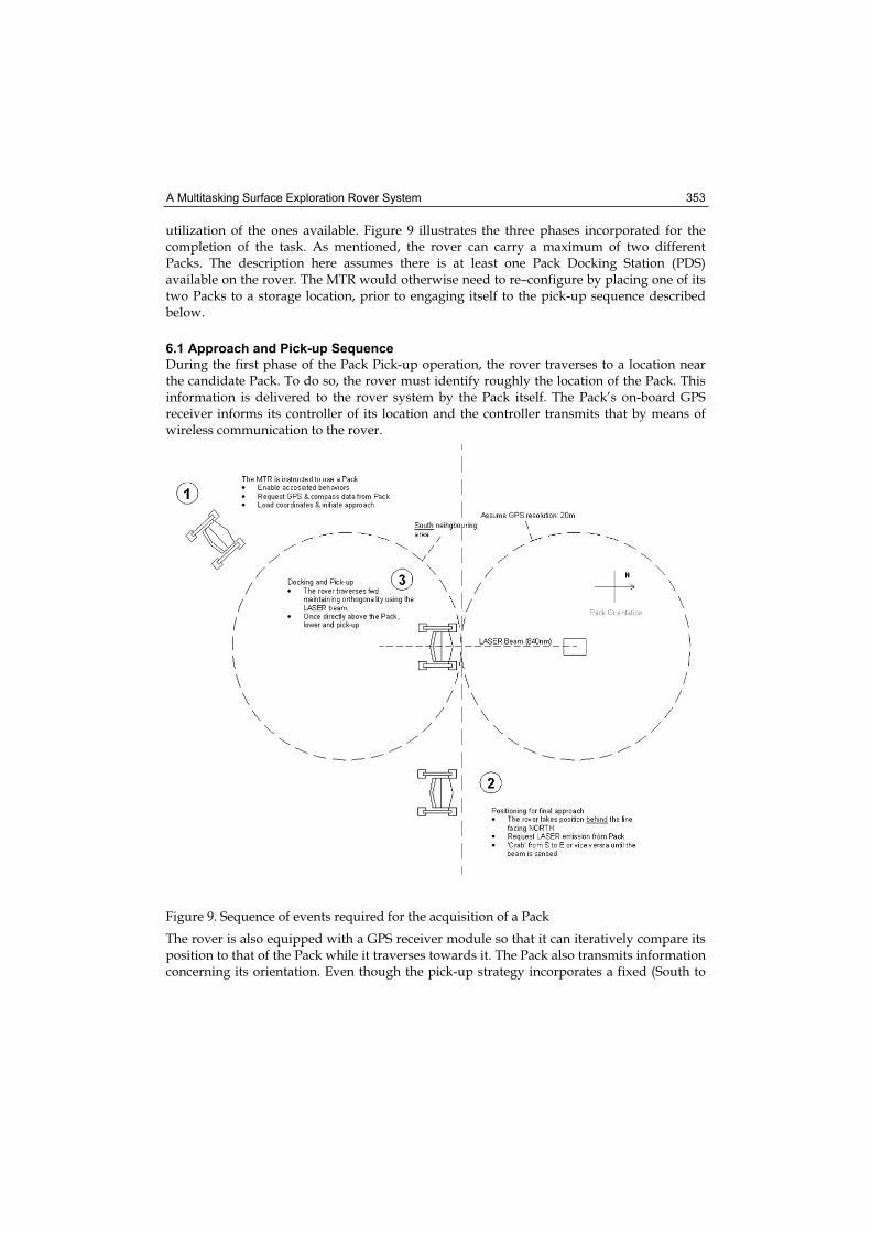
A Multitasking Surface Exploration Rover System 353
utilization of the ones available. Figure 9 illustrates the three phases incorporated for the completion of the task. As mentioned, the rover can carry a maximum of two different Packs. The description here assumes there is at least one Pack Docking Station (PDS) available on the rover. The MTR would otherwise need to re–configure by placing one of its two Packs to a storage location, prior to engaging itself to the pick-up sequence described below.
6.1 Approach and Pick-up Sequence
During the first phase of the Pack Pick-up operation, the rover traverses to a location near the candidate Pack. To do so, the rover must identify roughly the location of the Pack. This information is delivered to the rover system by the Pack itself. The Pack’s on-board GPS receiver informs its controller of its location and the controller transmits that by means of wireless communication to the rover.
Figure 9. Sequence of events required for the acquisition of a Pack
The rover is also equipped with a GPS receiver module so that it can iteratively compare its position to that of the Pack while it traverses towards it. The Pack also transmits information concerning its orientation. Even though the pick-up strategy incorporates a fixed (South to
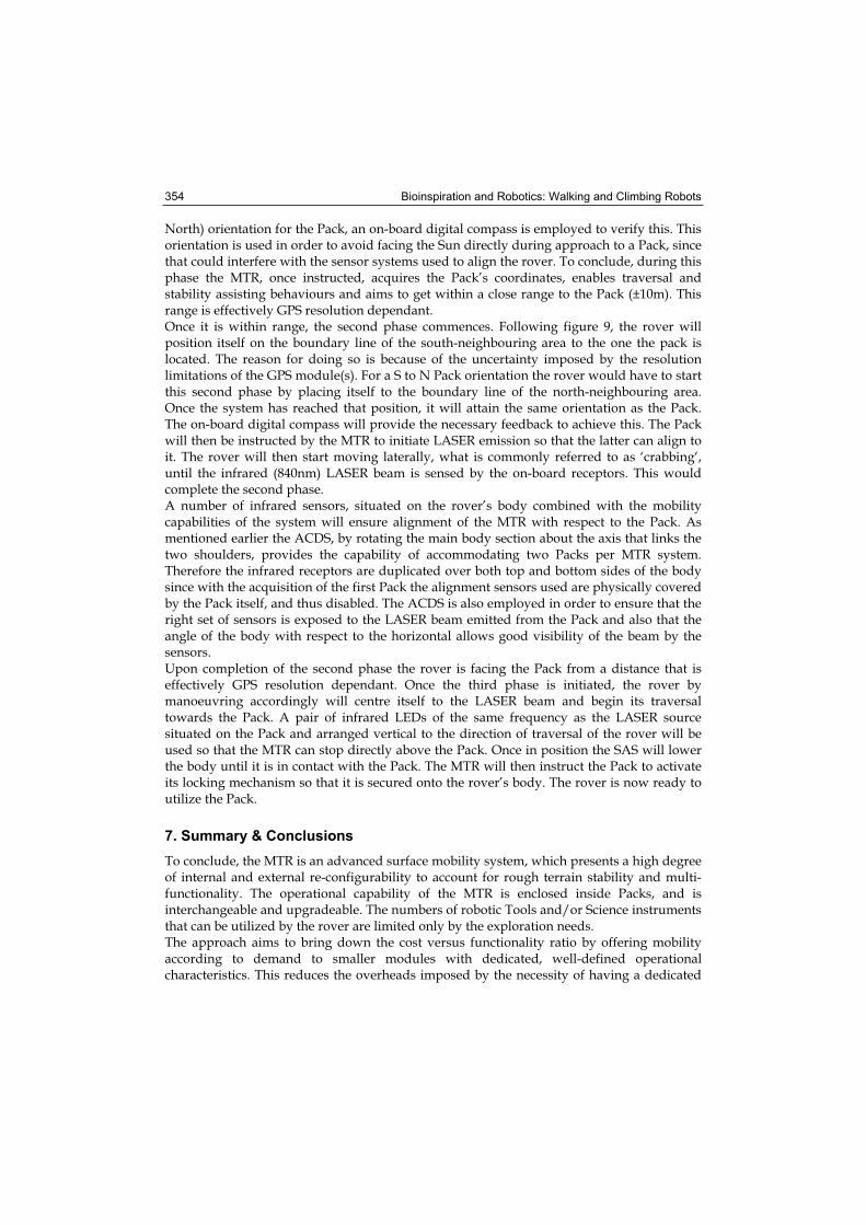
Bioinspiration and Robotics: Walking and Climbing Robots 354
North) orientation for the Pack, an on-board digital compass is employed to verify this. This orientation is used in order to avoid facing the Sun directly during approach to a Pack, since that could interfere with the sensor systems used to align the rover. To conclude, during this phase the MTR, once instructed, acquires the Pack’s coordinates, enables traversal and stability assisting behaviours and aims to get within a close range to the Pack (±10m). This range is effectively GPS resolution dependant. Once it is within range, the second phase commences. Following figure 9, the rover will position itself on the boundary line of the south-neighbouring area to the one the pack is located. The reason for doing so is because of the uncertainty imposed by the resolution limitations of the GPS module(s). For a S to N Pack orientation the rover would have to start this second phase by placing itself to the boundary line of the north-neighbouring area. Once the system has reached that position, it will attain the same orientation as the Pack. The on-board digital compass will provide the necessary feedback to achieve this. The Pack will then be instructed by the MTR to initiate LASER emission so that the latter can align to it. The rover will then start moving laterally, what is commonly referred to as ‘crabbing‘, until the infrared (840nm) LASER beam is sensed by the on-board receptors. This would complete the second phase. A number of infrared sensors, situated on the rover’s body combined with the mobility capabilities of the system will ensure alignment of the MTR with respect to the Pack. As mentioned earlier the ACDS, by rotating the main body section about the axis that links the two shoulders, provides the capability of accommodating two Packs per MTR system. Therefore the infrared receptors are duplicated over both top and bottom sides of the body since with the acquisition of the first Pack the alignment sensors used are physically covered by the Pack itself, and thus disabled. The ACDS is also employed in order to ensure that the right set of sensors is exposed to the LASER beam emitted from the Pack and also that the angle of the body with respect to the horizontal allows good visibility of the beam by the sensors. Upon completion of the second phase the rover is facing the Pack from a distance that is effectively GPS resolution dependant. Once the third phase is initiated, the rover by manoeuvring accordingly will centre itself to the LASER beam and begin its traversal towards the Pack. A pair of infrared LEDs of the same frequency as the LASER source situated on the Pack and arranged vertical to the direction of traversal of the rover will be used so that the MTR can stop directly above the Pack. Once in position the SAS will lower the body until it is in contact with the Pack. The MTR will then instruct the Pack to activate its locking mechanism so that it is secured onto the rover’s body. The rover is now ready to utilize the Pack.
7. Summary & Conclusions
To conclude, the MTR is an advanced surface mobility system, which presents a high degree of internal and external re-configurability to account for rough terrain stability and multi-functionality. The operational capability of the MTR is enclosed inside Packs, and is interchangeable and upgradeable. The numbers of robotic Tools and/or Science instruments that can be utilized by the rover are limited only by the exploration needs. The approach aims to bring down the cost versus functionality ratio by offering mobility according to demand to smaller modules with dedicated, well-defined operational characteristics. This reduces the overheads imposed by the necessity of having a dedicated
A Multitasking Surface Exploration Rover System 355
mobility for each of the functions that may be required for each of the different exploration phases. Instead of sending a large number of rovers to perform a variety of tasks, a small team of MTR units could be deployed with a large number of Packs, offering multiples of the functionality at a fraction of the payload. Apart from mission costs, this also decreases the probability of mission failure, since if a rover malfunctions, its operations could be performed by any of its fellow robotic-workers. By offering mobility according to demand, to dedicated tools, the productivity of a robotic colony could be maximized, reducing running and maintenance costs. Furthermore the capabilities of an MTR robotic team would be upgradeable since new Packs could be send that would enclose any additional science instruments and/or tools that may be required for the completion of the next part of the mission. Once on the surface of the Moon or Mars, the MTR could stay and serve mankind for many generations.
8. References
Bouloubasis, A. K.; McKee, G. T. & Schenker, S. P. (2003) A Behavior-Based Manipulator for Multi-Robot Transport Tasks, Proceedings of the IEEE International Conference on Robotics and Automation (ICRA’03), pp. 2287-2292, Taipei, Taiwan, May 2003.
Bouloubasis, A. K. & McKee, G. T. (2005). Cooperative Transport of Extended Payloads, Proceedings of the ICAR 2005, pp. 882-887, Seattle, USA, July 2005.
Bouloubasis, A. K. & McKee, G. T. (2006). MTR: The Multi-tasking Rover - A New Concept In Rover Design, Proceedings of the INSTICC International Conference in Control, Automation and Robotics, pp. 176-181, Setubal, Portugal, August 2006.
Drake, B. G. (1998), Reference Mission Version 3.0-Addendum to the Human Exploration of Mars: The Reference Mission of the NASA Exploration Study Team, NASA/SP-6107-ADD, Lyndon B. Johnson Space Center, June 1998.
Erickson, J. K. (2006). Living the Dream: An Overview of the Mars Exploration Project, IEEE Robotics & Automation Magazine, Vol. 13, No. 2, pp. 12-18, June 2006.
Harvey, B. & Shayler, D. J. (2005), Soviet and Russian Lunar Exploration: Comparisons of the Soviet and American Quest, November 2005.
Heiken, G. & Jones, E. (2007), On the Moon: The Apollo Journals, Springer-Praxis Books. Hayati, S.; Volpe, R.; Backes, P.; Balaram, J.; Welsh, R.; Ivlev, R.; Tharp, G.; Peters, S.; Ohm,
T.; Petras P. & Laubach, S. (1997), The Rocky 7 Rover: A Mars Sciencecraft Prototype, Proceedings of ICRA 1997, pp. 2458-2464, Albuquerique, NM, April 1997.
Huntsberger, T. L.; Baumgartner, E. T.; Aghazarian, H.; Cheng, Y.; Schenker, P. S.; Leger, P. C.; Iagnemma K. D. & Dubowsky S. (1999). Sensor Fused autonomous guidance of a mobile robot and applications to Mars sample return operations, Proceedings of Sensor Fusion and Decentralised Control in Robotic Systems II, SPIE Vol. 3839, Boston, MA, September 1999.
Iagnemma, K.; Rzepniewski, A.; Dubowsky, S.; Pirjanian, P.; Huntsberger T. & Schenker, P. (2000). Mobile robot kinematic reconfigurability for rough terrain, Proceedings of Sensor Fusion and Decentralised Control in Robotics Systems III, SPIE Vol. 4196, Boston, MA, November 2000.
Lewis, M. G. & Sharkey P. M. (1996). Assisted remote viewing of a teleoperation workcell, Proceedings Intl Sump. Telemanipulator and telepresence Technologies III, pp. 69-80, Boston, USA, November 1996.
Bioinspiration and Robotics: Walking and Climbing Robots 356
Matijevic J. (1997). Mars Pathfinder Microrover - Implementing a Low Cost Planetary Mission Experiment, Proceeding of the Second IAA International Conference on Low-Cost Planetary Missions, John Hopkins Applied Physics Laboratory, Maryland, USA, April 16-19, 1997, paper # IAA-L-0510.
Muirhead, K. B. (2004). Mars rovers, Past and Future, Proceedings of IEEE Aerospace Conference, pp. 128-134, Blue Sky, Montana, USA, March 2004.
Mumm, E.; Farritor, S.; Pirjanian, P.; Leger, C. & Schenker, P. (2004). Planetary Cliff Descent Using Cooperative Robots, Autonomous Robots 16 (3), pp. 259-272, May 2004.
Naderi, F.; McCleese, D. J. & Jordan, J. F. Jr. (2006). Mars Exploration: What have we learned? What lies Ahead? IEEE Robotics & Automation Magazine, pp. 72-82, ISSN 1070-9932.
Smith, M. S. (2005). Space Exploration: Issues Concerning the Vision for Space Exploration, CRS Report for Congress, November 2005.
Schenker, P. S.; Huntsberger, T. L.; Pirjanian, P.; Baumgartner, E.; Aghazarian, H.; Trebi-Ollennu, A.; Leger, P. C.; Cheng, Y.; Backes, P. G.; Tunstel, E. W.; Jet Propulsion Laboratory; Dubowsky, S.; Iagnemma, K.; Massachusetts Institute of Technology; G. T. McKee, University of Reading (UK). (2001). Robotic automation for space: planetary surface exploration, terrain-adaptive mobility, and multi-robot cooperative tasks, Proceedings SPIE Vol. 4572, Intelligent Robots and Computer Vision XX, Newton, MA, October, 2001.
Trebi-Ollennu, A.; Das Nayer, H.; Aghazarian, H.; Ganino, A.; Pirjanian, P.; Kennedy, B.; Huntsberger T. & Schenker P. (2002). Mars Rover Pair Cooperatively Transporting a Long Payload Proceedings of the 2002 IEEE International Conference on Robotics and Automation, pp. 3136-3141, Washington DC, USA, May 2002.
Vago, J. (2006). Pasteur Instrument Payload for the ExoMars Mission, Progress Letter 5, October 2006.
Young, A. (2006). Lunar and Planetary Rovers: The Wheels of Apollo and the Quest for Mars,Springer-Praxis, November 2006.
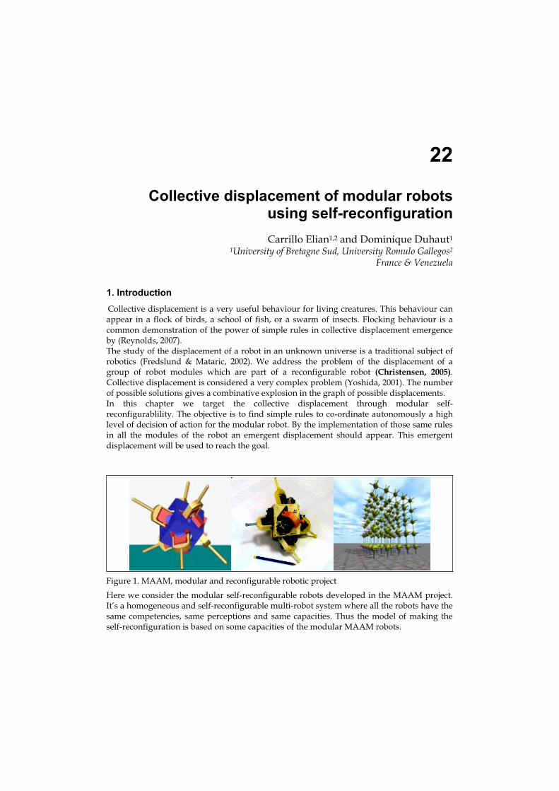
22
Collective displacement of modular robots using self-reconfiguration
Carrillo Elian1,2 and Dominique Duhaut1
1University of Bretagne Sud, University Romulo Gallegos2
France & Venezuela
1. Introduction
Collective displacement is a very useful behaviour for living creatures. This behaviour can appear in a flock of birds, a school of fish, or a swarm of insects. Flocking behaviour is a common demonstration of the power of simple rules in collective displacement emergence by (Reynolds, 2007). The study of the displacement of a robot in an unknown universe is a traditional subject of robotics (Fredslund & Mataric, 2002). We address the problem of the displacement of a group of robot modules which are part of a reconfigurable robot (Christensen, 2005).Collective displacement is considered a very complex problem (Yoshida, 2001). The number of possible solutions gives a combinative explosion in the graph of possible displacements. In this chapter we target the collective displacement through modular self-reconfigurablility. The objective is to find simple rules to co-ordinate autonomously a high level of decision of action for the modular robot. By the implementation of those same rules in all the modules of the robot an emergent displacement should appear. This emergent displacement will be used to reach the goal.
Figure 1. MAAM, modular and reconfigurable robotic project
Here we consider the modular self-reconfigurable robots developed in the MAAM project. It’s a homogeneous and self-reconfigurable multi-robot system where all the robots have the same competencies, same perceptions and same capacities. Thus the model of making the self-reconfiguration is based on some capacities of the modular MAAM robots.
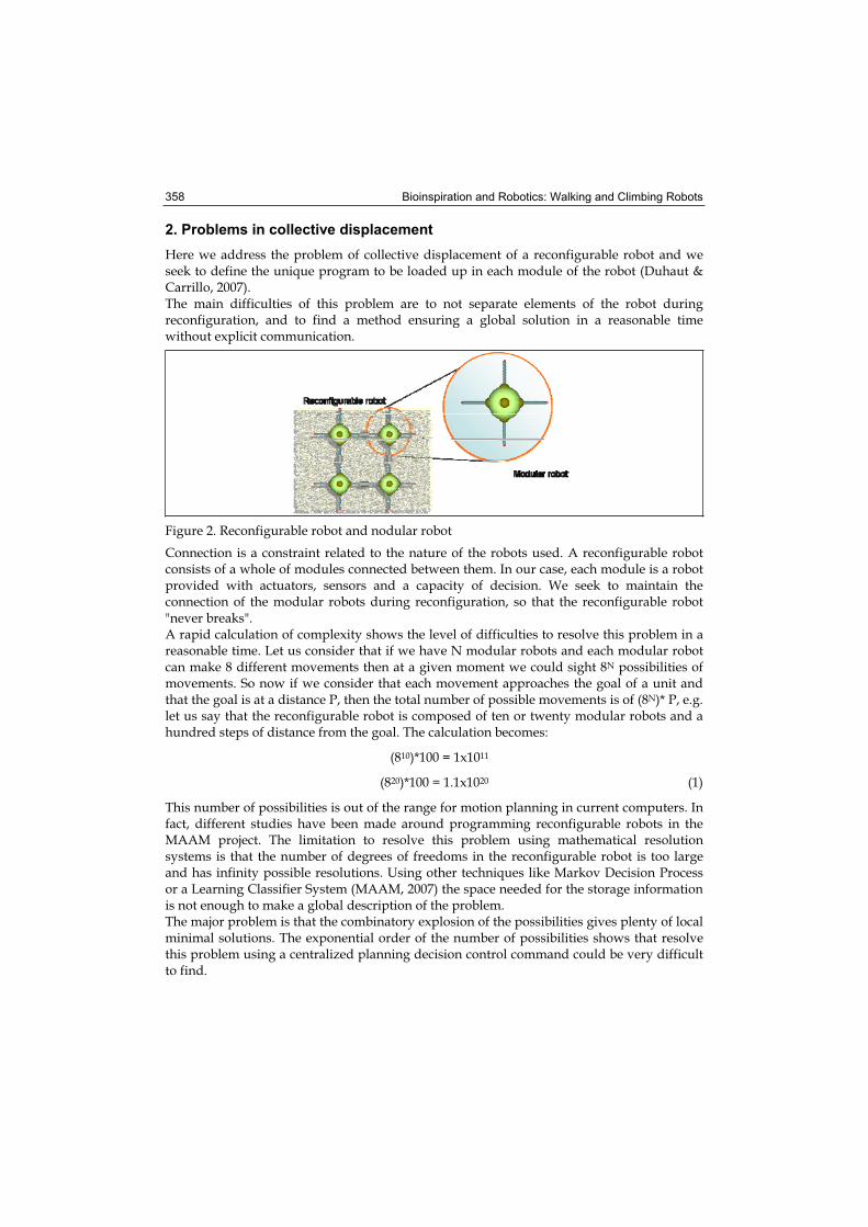
Bioinspiration and Robotics: Walking and Climbing Robots 358
2. Problems in collective displacement
Here we address the problem of collective displacement of a reconfigurable robot and we seek to define the unique program to be loaded up in each module of the robot (Duhaut & Carrillo, 2007).The main difficulties of this problem are to not separate elements of the robot during reconfiguration, and to find a method ensuring a global solution in a reasonable time without explicit communication.
Figure 2. Reconfigurable robot and nodular robot
Connection is a constraint related to the nature of the robots used. A reconfigurable robot consists of a whole of modules connected between them. In our case, each module is a robot provided with actuators, sensors and a capacity of decision. We seek to maintain the connection of the modular robots during reconfiguration, so that the reconfigurable robot "never breaks". A rapid calculation of complexity shows the level of difficulties to resolve this problem in a reasonable time. Let us consider that if we have N modular robots and each modular robot can make 8 different movements then at a given moment we could sight 8N possibilities of movements. So now if we consider that each movement approaches the goal of a unit and that the goal is at a distance P, then the total number of possible movements is of (8N)* P, e.g. let us say that the reconfigurable robot is composed of ten or twenty modular robots and a hundred steps of distance from the goal. The calculation becomes:
(810)*100 = 1x10¹¹
(820)*100 = 1.1x10²⁰ (1)
This number of possibilities is out of the range for motion planning in current computers. In fact, different studies have been made around programming reconfigurable robots in the MAAM project. The limitation to resolve this problem using mathematical resolution systems is that the number of degrees of freedoms in the reconfigurable robot is too large and has infinity possible resolutions. Using other techniques like Markov Decision Process or a Learning Classifier System (MAAM, 2007) the space needed for the storage information is not enough to make a global description of the problem. The major problem is that the combinatory explosion of the possibilities gives plenty of local minimal solutions. The exponential order of the number of possibilities shows that resolve this problem using a centralized planning decision control command could be very difficult to find.
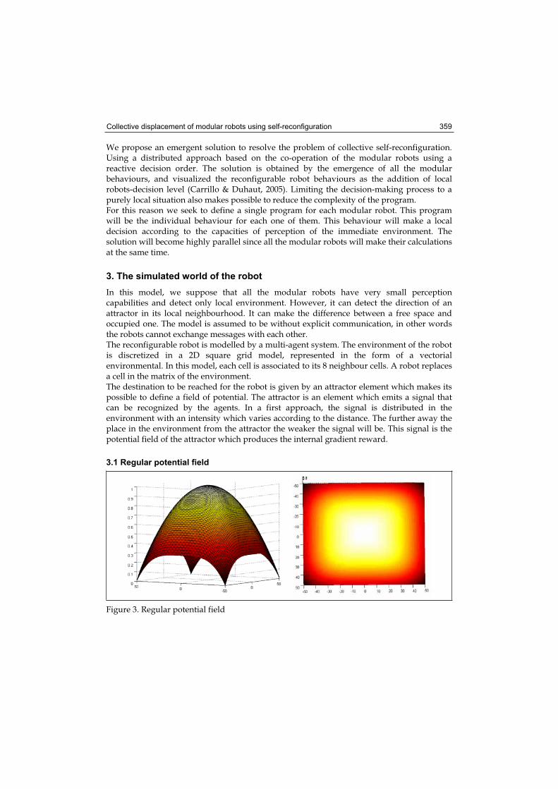
Collective displacement of modular robots using self-reconfiguration 359
We propose an emergent solution to resolve the problem of collective self-reconfiguration. Using a distributed approach based on the co-operation of the modular robots using a reactive decision order. The solution is obtained by the emergence of all the modular behaviours, and visualized the reconfigurable robot behaviours as the addition of local robots-decision level (Carrillo & Duhaut, 2005). Limiting the decision-making process to a purely local situation also makes possible to reduce the complexity of the program. For this reason we seek to define a single program for each modular robot. This program will be the individual behaviour for each one of them. This behaviour will make a local decision according to the capacities of perception of the immediate environment. The solution will become highly parallel since all the modular robots will make their calculations at the same time.
3. The simulated world of the robot
In this model, we suppose that all the modular robots have very small perception capabilities and detect only local environment. However, it can detect the direction of an attractor in its local neighbourhood. It can make the difference between a free space and occupied one. The model is assumed to be without explicit communication, in other words the robots cannot exchange messages with each other. The reconfigurable robot is modelled by a multi-agent system. The environment of the robot is discretized in a 2D square grid model, represented in the form of a vectorial environmental. In this model, each cell is associated to its 8 neighbour cells. A robot replaces a cell in the matrix of the environment. The destination to be reached for the robot is given by an attractor element which makes its possible to define a field of potential. The attractor is an element which emits a signal that can be recognized by the agents. In a first approach, the signal is distributed in the environment with an intensity which varies according to the distance. The further away the place in the environment from the attractor the weaker the signal will be. This signal is the potential field of the attractor which produces the internal gradient reward.
3.1 Regular potential field
Figure 3. Regular potential field
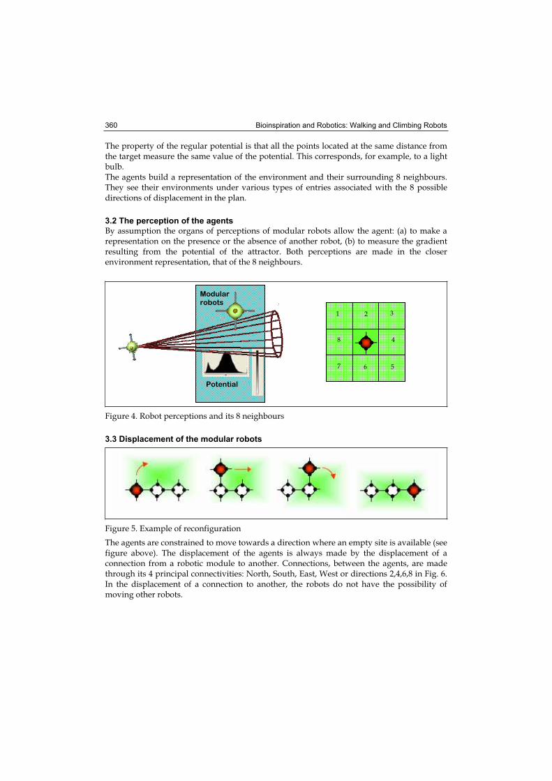
Bioinspiration and Robotics: Walking and Climbing Robots 360
The property of the regular potential is that all the points located at the same distance from the target measure the same value of the potential. This corresponds, for example, to a light bulb.The agents build a representation of the environment and their surrounding 8 neighbours. They see their environments under various types of entries associated with the 8 possible directions of displacement in the plan.
3.2 The perception of the agents
By assumption the organs of perceptions of modular robots allow the agent: (a) to make a representation on the presence or the absence of another robot, (b) to measure the gradient resulting from the potential of the attractor. Both perceptions are made in the closer environment representation, that of the 8 neighbours.
Figure 4. Robot perceptions and its 8 neighbours
3.3 Displacement of the modular robots
Figure 5. Example of reconfiguration
The agents are constrained to move towards a direction where an empty site is available (see figure above). The displacement of the agents is always made by the displacement of a connection from a robotic module to another. Connections, between the agents, are made through its 4 principal connectivities: North, South, East, West or directions 2,4,6,8 in Fig. 6. In the displacement of a connection to another, the robots do not have the possibility of moving other robots.
Potential
Modular robots
1
8
2 3
4
567
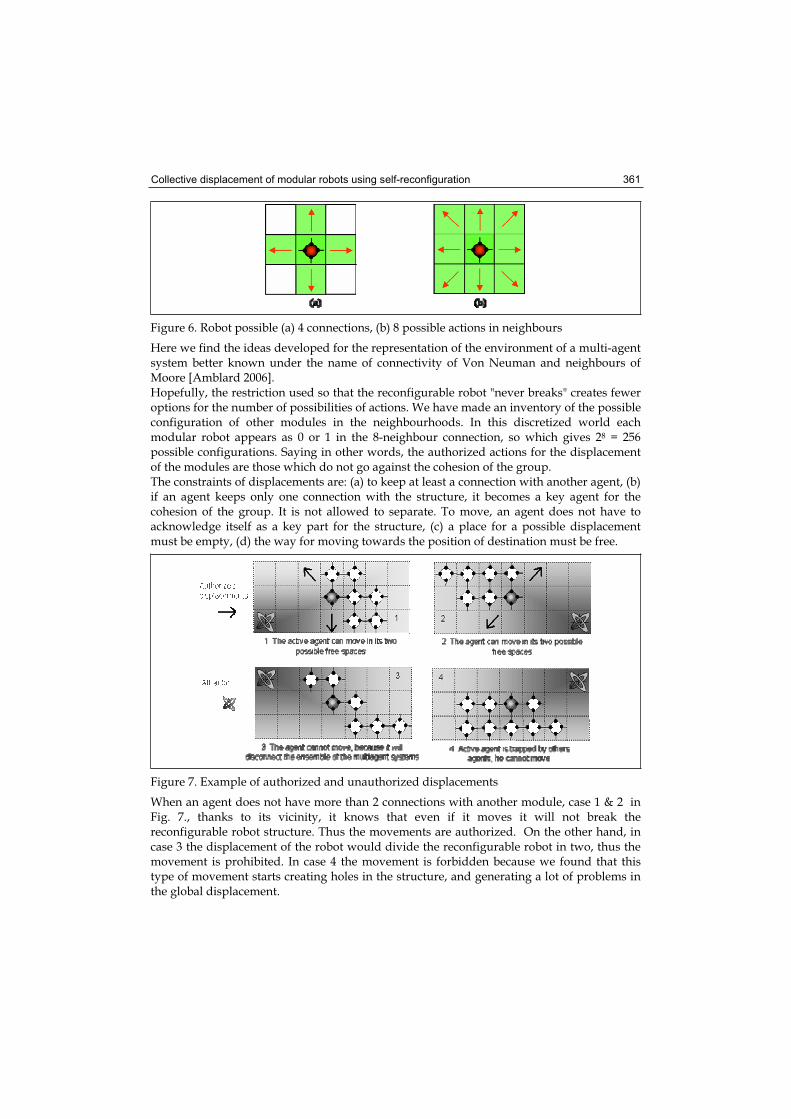
Collective displacement of modular robots using self-reconfiguration 361
Figure 6. Robot possible (a) 4 connections, (b) 8 possible actions in neighbours
Here we find the ideas developed for the representation of the environment of a multi-agent system better known under the name of connectivity of Von Neuman and neighbours of Moore [Amblard 2006]. Hopefully, the restriction used so that the reconfigurable robot "never breaks" creates fewer options for the number of possibilities of actions. We have made an inventory of the possible configuration of other modules in the neighbourhoods. In this discretized world each modular robot appears as 0 or 1 in the 8-neighbour connection, so which gives 28 = 256 possible configurations. Saying in other words, the authorized actions for the displacement of the modules are those which do not go against the cohesion of the group. The constraints of displacements are: (a) to keep at least a connection with another agent, (b) if an agent keeps only one connection with the structure, it becomes a key agent for the cohesion of the group. It is not allowed to separate. To move, an agent does not have to acknowledge itself as a key part for the structure, (c) a place for a possible displacement must be empty, (d) the way for moving towards the position of destination must be free.
Figure 7. Example of authorized and unauthorized displacements
When an agent does not have more than 2 connections with another module, case 1 & 2 in Fig. 7., thanks to its vicinity, it knows that even if it moves it will not break the reconfigurable robot structure. Thus the movements are authorized. On the other hand, in case 3 the displacement of the robot would divide the reconfigurable robot in two, thus the movement is prohibited. In case 4 the movement is forbidden because we found that this type of movement starts creating holes in the structure, and generating a lot of problems in the global displacement.
Bioinspiration and Robotics: Walking and Climbing Robots 362
3.4 The scheduling of calculations in the robots
The scheduling of calculations corresponds to the order in which the programs are performed in the modules of the reconfigurable robot. Of course, the ideal model is absolute parallelism: all calculations are done at the same time in each module. However, a reconfigurable robot is sequential by nature. Displacement cannot be carried out in parallel when two robots are close, because of the risks involved. It is supposed that the order of execution of movements of the robots is regulated at the mechanical level. A robot will move if it is guaranteed that the other modules do not move. This constraint shows that on the level of the program, calculation is not the same if one makes the movement of a modular robot after or before another. To account for this problem we will suppose in the simulations that there are two types of possible software scheduling. (a) Sequential Scheduling: In this case the modular robots receive a quota of time (presumably sufficient to make a complete iteration of the behaviour) one robot after another according to a fixed list. (b) Random Scheduling: In this case the modular robots receive their time quotas in a random way. This makes it possible to take into account the possible differences in the processing times of calculations in modular robots. Due to it being the most "chaotic" of scheduling, it forces us to develop sure methods of construction of the emergent algorithms.
4. Reactive programming
The objective of reactive programming is to reach a global displacement of the robot by the set of reconfiguration of all the modules. The constraint is that the robot must not lose any module during the global movement. We seek to define the program which must be charged in each robot module that makes robots move in an autonomous way towards a goal maintaining the cohesion of the group of modules. This program will be the individual behaviour of each robot. This reactive behaviour will make a local decision according to the perception of the immediate environment. The interactions of all its modules in an autonomous way make the emergent displacement.
4.1 Forward algorithms
The principle of the reactive algorithm is to decrease the distance which separates the robot from the source of the attractor following a potential field (Arkin, 1998). Modular robots must take the decision of the place to go making a minimization of the distance with the information of the potential. The algorithm decides the action to take according to two factors: the gradient of attractor and configuration of the modular robot in its neighbourhoods. Displacement is carried out towards a direction where the potential is augmented, respecting the cohesion of the reconfigurable robot structure.In the simulations of section 5, we consider two different algorithms: (a) "total forward": In this case the module will make a continuation of displacement along the molecule until reaching a position which will be a minimum for the potential, (b) "one step forward": In this case the module will make only one displacement along the molecule then will stop and await its next quota of time. During this time all the other modules can move.
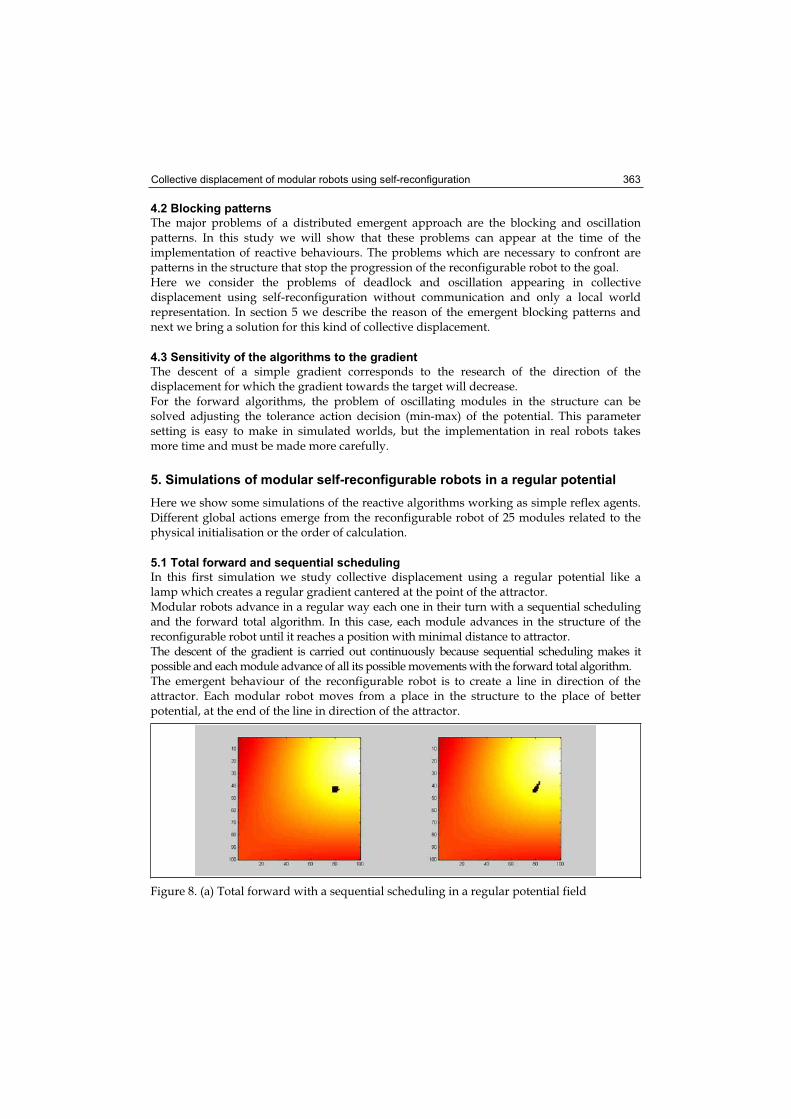
Collective displacement of modular robots using self-reconfiguration 363
4.2 Blocking patterns
The major problems of a distributed emergent approach are the blocking and oscillation patterns. In this study we will show that these problems can appear at the time of the implementation of reactive behaviours. The problems which are necessary to confront are patterns in the structure that stop the progression of the reconfigurable robot to the goal. Here we consider the problems of deadlock and oscillation appearing in collective displacement using self-reconfiguration without communication and only a local world representation. In section 5 we describe the reason of the emergent blocking patterns and next we bring a solution for this kind of collective displacement.
4.3 Sensitivity of the algorithms to the gradient
The descent of a simple gradient corresponds to the research of the direction of the displacement for which the gradient towards the target will decrease. For the forward algorithms, the problem of oscillating modules in the structure can be solved adjusting the tolerance action decision (min-max) of the potential. This parameter setting is easy to make in simulated worlds, but the implementation in real robots takes more time and must be made more carefully.
5. Simulations of modular self-reconfigurable robots in a regular potential
Here we show some simulations of the reactive algorithms working as simple reflex agents. Different global actions emerge from the reconfigurable robot of 25 modules related to the physical initialisation or the order of calculation.
5.1 Total forward and sequential scheduling
In this first simulation we study collective displacement using a regular potential like a lamp which creates a regular gradient cantered at the point of the attractor. Modular robots advance in a regular way each one in their turn with a sequential scheduling and the forward total algorithm. In this case, each module advances in the structure of the reconfigurable robot until it reaches a position with minimal distance to attractor. The descent of the gradient is carried out continuously because sequential scheduling makes it possible and each module advance of all its possible movements with the forward total algorithm. The emergent behaviour of the reconfigurable robot is to create a line in direction of the attractor. Each modular robot moves from a place in the structure to the place of better potential, at the end of the line in direction of the attractor.
Figure 8. (a) Total forward with a sequential scheduling in a regular potential field
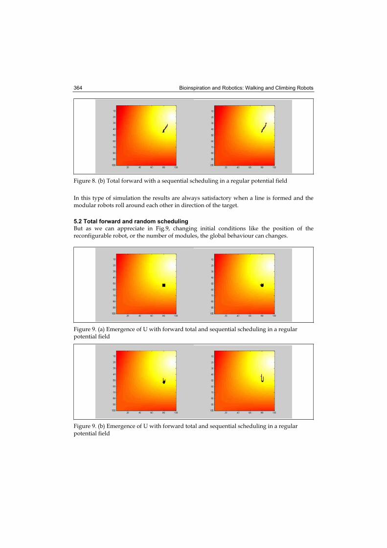
Bioinspiration and Robotics: Walking and Climbing Robots 364
Figure 8. (b) Total forward with a sequential scheduling in a regular potential field
In this type of simulation the results are always satisfactory when a line is formed and the modular robots roll around each other in direction of the target.
5.2 Total forward and random scheduling
But as we can appreciate in Fig.9, changing initial conditions like the position of the reconfigurable robot, or the number of modules, the global behaviour can changes.
Figure 9. (a) Emergence of U with forward total and sequential scheduling in a regular potential field
Figure 9. (b) Emergence of U with forward total and sequential scheduling in a regular potential field
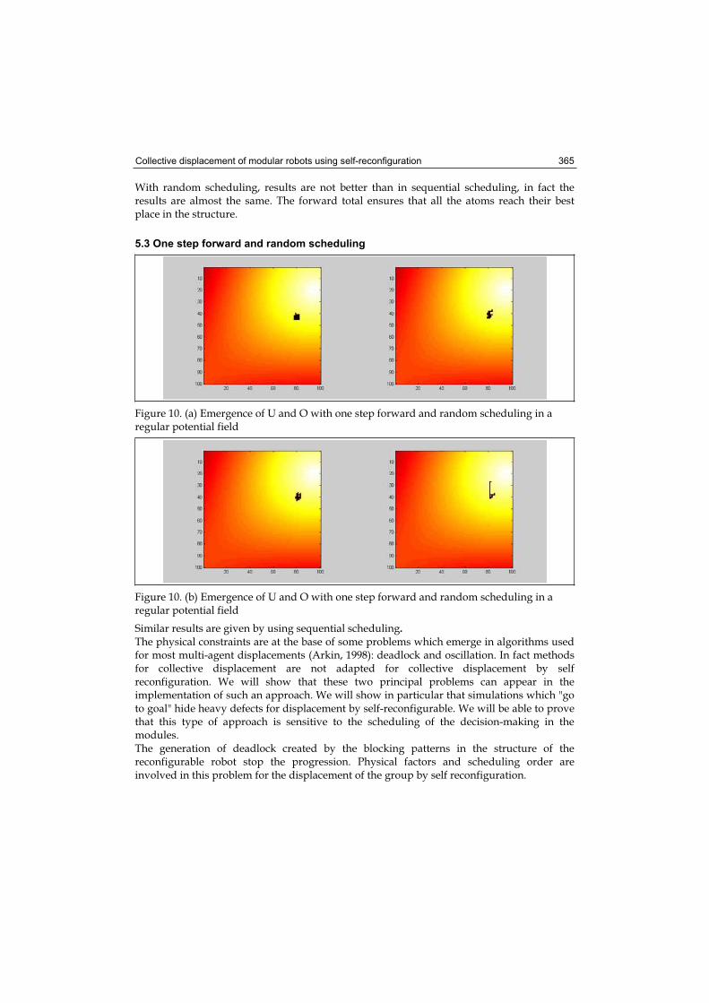
Collective displacement of modular robots using self-reconfiguration 365
With random scheduling, results are not better than in sequential scheduling, in fact the results are almost the same. The forward total ensures that all the atoms reach their best place in the structure.
5.3 One step forward and random scheduling
Figure 10. (a) Emergence of U and O with one step forward and random scheduling in a regular potential field
Figure 10. (b) Emergence of U and O with one step forward and random scheduling in a regular potential field
Similar results are given by using sequential scheduling.The physical constraints are at the base of some problems which emerge in algorithms used for most multi-agent displacements (Arkin, 1998): deadlock and oscillation. In fact methods for collective displacement are not adapted for collective displacement by self reconfiguration. We will show that these two principal problems can appear in the implementation of such an approach. We will show in particular that simulations which "go to goal" hide heavy defects for displacement by self-reconfigurable. We will be able to prove that this type of approach is sensitive to the scheduling of the decision-making in the modules. The generation of deadlock created by the blocking patterns in the structure of the reconfigurable robot stop the progression. Physical factors and scheduling order are involved in this problem for the displacement of the group by self reconfiguration.
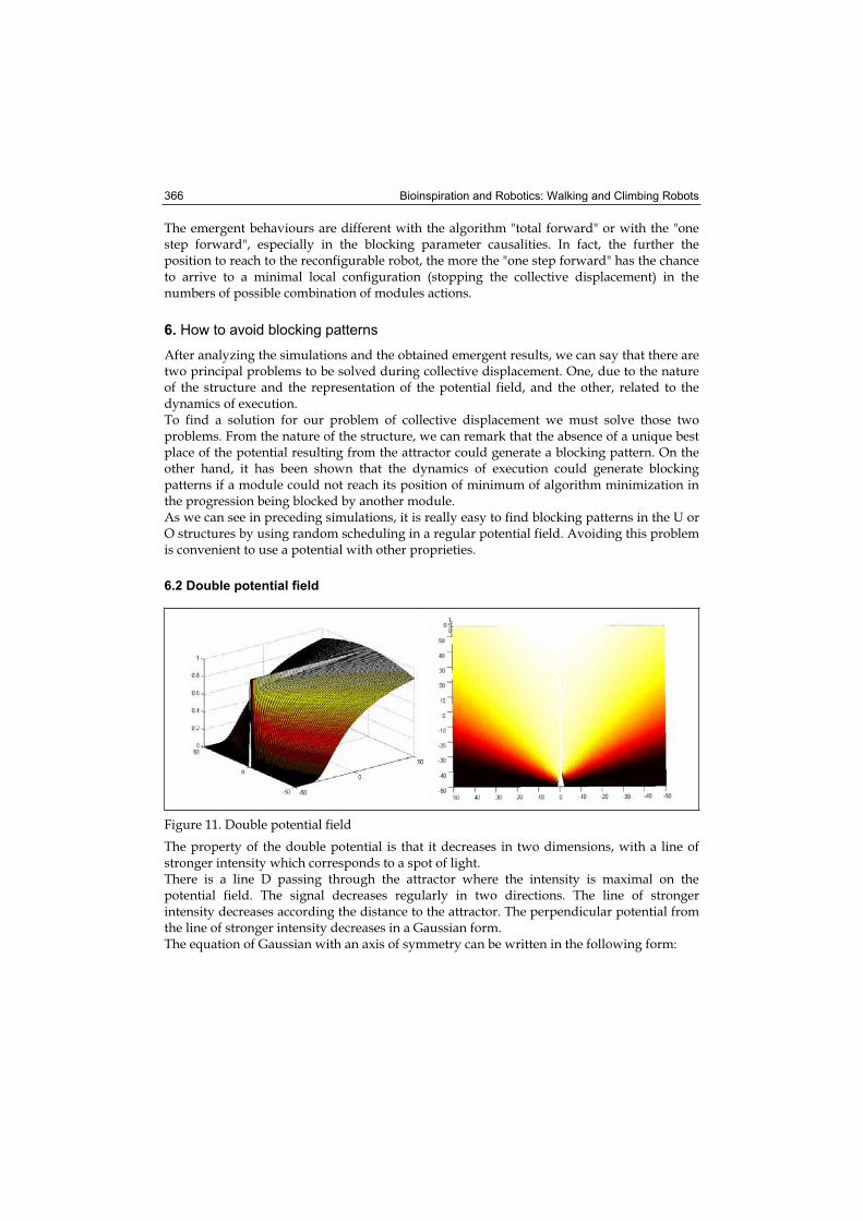
Bioinspiration and Robotics: Walking and Climbing Robots 366
The emergent behaviours are different with the algorithm "total forward" or with the "one step forward", especially in the blocking parameter causalities. In fact, the further the position to reach to the reconfigurable robot, the more the "one step forward" has the chance to arrive to a minimal local configuration (stopping the collective displacement) in the numbers of possible combination of modules actions.
6. How to avoid blocking patterns
After analyzing the simulations and the obtained emergent results, we can say that there are two principal problems to be solved during collective displacement. One, due to the nature of the structure and the representation of the potential field, and the other, related to the dynamics of execution. To find a solution for our problem of collective displacement we must solve those two problems. From the nature of the structure, we can remark that the absence of a unique best place of the potential resulting from the attractor could generate a blocking pattern. On the other hand, it has been shown that the dynamics of execution could generate blocking patterns if a module could not reach its position of minimum of algorithm minimization in the progression being blocked by another module. As we can see in preceding simulations, it is really easy to find blocking patterns in the U or O structures by using random scheduling in a regular potential field. Avoiding this problem is convenient to use a potential with other proprieties.
6.2 Double potential field
Figure 11. Double potential field
The property of the double potential is that it decreases in two dimensions, with a line of stronger intensity which corresponds to a spot of light. There is a line D passing through the attractor where the intensity is maximal on the potential field. The signal decreases regularly in two directions. The line of stronger intensity decreases according the distance to the attractor. The perpendicular potential from the line of stronger intensity decreases in a Gaussian form. The equation of Gaussian with an axis of symmetry can be written in the following form:
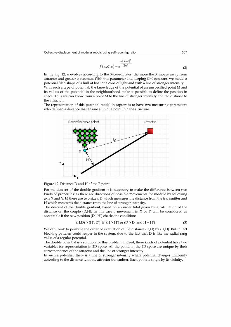
Collective displacement of modular robots using self-reconfiguration 367
(2)
In the Fig. 12, evolves according to the X-coordinates: the more the X moves away from attractor and greater becomes. With this parameter and keeping C=0 constant, we model a potential filed shape of a hull of boat or a cone of light and with a line of stronger intensity. With such a type of potential, the knowledge of the potential of an unspecified point M and its values of the potential in the neighbourhood make it possible to define the position in space. Thus we can know from a point M to the line of stronger intensity and the distance to the attractor.The representation of this potential model in captors is to have two measuring parameters who defined a distance that ensure a unique point P in the structure.
Figure 12. Distance D and H of the P point
For the descent of the double gradient it is necessary to make the difference between two kinds of properties: a) there are directions of possible movements for module by following axis X and Y, b) there are two sizes, D which measures the distance from the transmitter and H which measures the distance from the line of stronger intensity. The descent of the double gradient, based on an order total given by a calculation of the distance on the couple (D,H). In this case a movement in X or Y will be considered as acceptable if the new position (D’, H’) checks the condition:
(H,D) > (H’, D’) if (H > H’) or (D > D’ and H = H’) (3)
We can think to permute the order of evaluation of the distance (D,H) by (H,D). But in fact blocking patterns could reaper in the system, due to the fact that D is like the radial rang value of a regular potential. The double potential is a solution for this problem. Indeed, these kinds of potential have two variables for representation in 2D space. All the points in the 2D space are unique by their correspondence of the attractor and the line of stronger intensity In such a potential, there is a line of stronger intensity where potential changes uniformly according to the distance with the attractor transmitter. Each point is single by its vicinity.
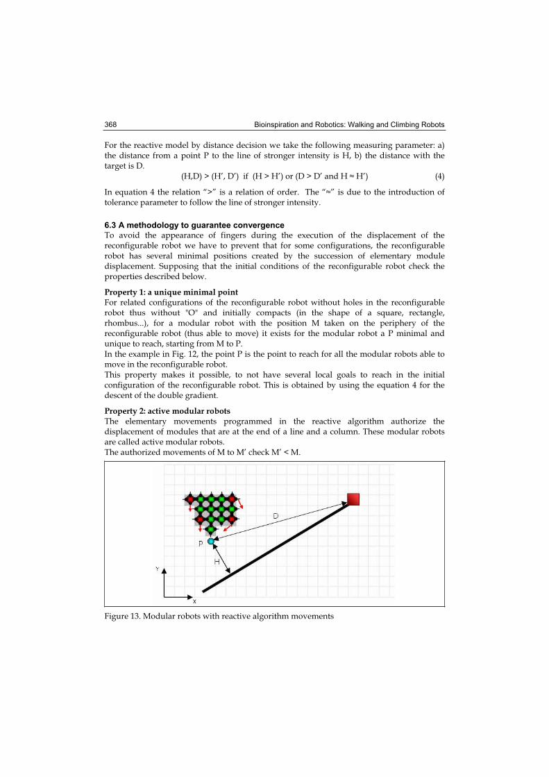
Bioinspiration and Robotics: Walking and Climbing Robots 368
For the reactive model by distance decision we take the following measuring parameter: a) the distance from a point P to the line of stronger intensity is H, b) the distance with the target is D.
(H,D) > (H’, D’) if (H > H’) or (D > D’ and H H’) (4)
In equation 4 the relation “>” is a relation of order. The “ ” is due to the introduction of tolerance parameter to follow the line of stronger intensity.
6.3 A methodology to guarantee convergence
To avoid the appearance of fingers during the execution of the displacement of the reconfigurable robot we have to prevent that for some configurations, the reconfigurable robot has several minimal positions created by the succession of elementary module displacement. Supposing that the initial conditions of the reconfigurable robot check the properties described below.
Property 1: a unique minimal point For related configurations of the reconfigurable robot without holes in the reconfigurable robot thus without "O" and initially compacts (in the shape of a square, rectangle, rhombus...), for a modular robot with the position M taken on the periphery of the reconfigurable robot (thus able to move) it exists for the modular robot a P minimal and unique to reach, starting from M to P. In the example in Fig. 12, the point P is the point to reach for all the modular robots able to move in the reconfigurable robot. This property makes it possible, to not have several local goals to reach in the initial configuration of the reconfigurable robot. This is obtained by using the equation 4 for the descent of the double gradient.
Property 2: active modular robots The elementary movements programmed in the reactive algorithm authorize the displacement of modules that are at the end of a line and a column. These modular robots are called active modular robots. The authorized movements of M to M’ check M’ < M.
Figure 13. Modular robots with reactive algorithm movements
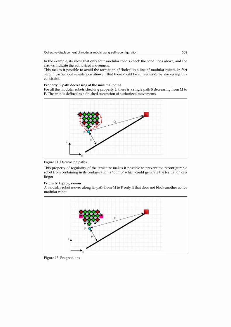
Collective displacement of modular robots using self-reconfiguration 369
In the example, its show that only four modular robots check the conditions above, and the arrows indicate the authorized movement. This makes it possible to avoid the formation of "holes" in a line of modular robots. In fact certain carried-out simulations showed that there could be convergence by slackening this constraint.
Property 3: path decreasing at the minimal point For all the modular robots checking property 2, there is a single path S decreasing from M to P. The path is defined as a finished succession of authorized movements.
Figure 14. Decreasing paths
This property of regularity of the structure makes it possible to prevent the reconfigurable robot from containing in its configuration a "bump" which could generate the formation of a finger
Property 4: progression A modular robot moves along its path from M to P only it that does not block another active modular robot.
Figure 15. Progressions

Bioinspiration and Robotics: Walking and Climbing Robots 370
This property must be checked at the initialization of the program, we will show that it remains maintained during the execution of the program. The programming of elementary displacements allows the active modular robots which are ahead (within the meaning of the order on the environment) to block the advance of those which are behind. In the example above the two modular robots at the top in red will not be able to exceed the pink places, because, if they overtake the other robots in red they could block the progression of the reconfigurable robot by the creation of a blocking patterns. This property forces the scheduling of the movements of the modular robots. It implies that an unspecified modular robot is able to determine if the modular robots with which it progresses have or not a path with the partial target P or not.
Lemma 1If an active modular robot reaches P then the new minimal point P' is unique. Proof: As the point P is minimal then the P' point is close to P because of the regularity of the order. This point exists since the environment uniformly decreases (except on the target where the program stops).The P' point less than P is thus unique since P is unique and minimal by property 1 and that there are not two identical points in the environment. QED
Lemma 2 The new P' point is accessible by all the active modular robots from the reconfigurable robot. Proof:By property 2 all active modular robots have the possibility of reaching P by a path uniformly decreasing. As P' is close to P, the access to the P' point thus obliges to replace the last movement towards P by a succession of two movements, the first to reach P, the second to reach P'. It is supposed here that the elementary movements programmed in the modular robots make it possible to solve all these configurations of displacement from P to P'. The decrease of the path is obvious since P' is minimal by lemma 1. QED
TheoremIf the four preceding properties are then checked the reconfigurable robot will converge towards its goal whatever the order in which calculations will be carried out. Proof:This proof consists in show that for each intermediate goal P: 1. there is an active modular robot M which will reach P. 2. all the other active modular robots will be able to reach the intermediate goal following
P'.3. the new active modular robots which will be created following the displacement of M
will have properties 3 & 4 and will be able to reach P' if such is the case then as there is a path C decreasing of P initial until the attractor by construction of the potential, there will always be a modular robot to reach the intermediate points of C without blocking since property 4 is checked at every moment. 1. there is an active modular robot M which will reach P: The position P will be necessarily reached by an active modular robot. Because of the property 4 only those which have a free path to P will be able to reach it. If there are 2 modular robots in 2D space, one coming with P from the left and the other from the right. It
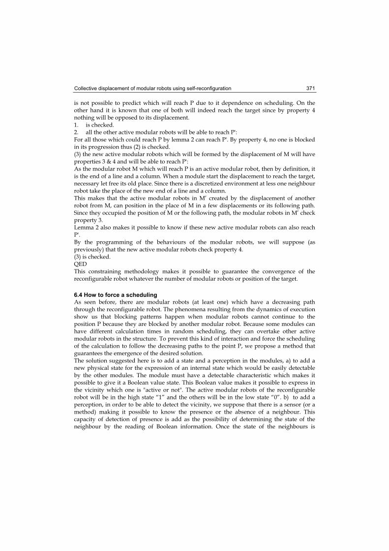
Collective displacement of modular robots using self-reconfiguration 371
is not possible to predict which will reach P due to it dependence on scheduling. On the other hand it is known that one of both will indeed reach the target since by property 4 nothing will be opposed to its displacement. 1. is checked. 2. all the other active modular robots will be able to reach P': For all those which could reach P by lemma 2 can reach P'. By property 4, no one is blocked in its progression thus (2) is checked. (3) the new active modular robots which will be formed by the displacement of M will have properties 3 & 4 and will be able to reach P': As the modular robot M which will reach P is an active modular robot, then by definition, it is the end of a line and a column. When a module start the displacement to reach the target, necessary let free its old place. Since there is a discretized environment at less one neighbour robot take the place of the new end of a line and a column. This makes that the active modular robots in M’ created by the displacement of another robot from M, can position in the place of M in a few displacements or its following path. Since they occupied the position of M or the following path, the modular robots in M’ check property 3. Lemma 2 also makes it possible to know if these new active modular robots can also reach P'. By the programming of the behaviours of the modular robots, we will suppose (as previously) that the new active modular robots check property 4. (3) is checked. QEDThis constraining methodology makes it possible to guarantee the convergence of the reconfigurable robot whatever the number of modular robots or position of the target.
6.4 How to force a scheduling
As seen before, there are modular robots (at least one) which have a decreasing path through the reconfigurable robot. The phenomena resulting from the dynamics of execution show us that blocking patterns happen when modular robots cannot continue to the position P because they are blocked by another modular robot. Because some modules can have different calculation times in random scheduling, they can overtake other active modular robots in the structure. To prevent this kind of interaction and force the scheduling of the calculation to follow the decreasing paths to the point P, we propose a method that guarantees the emergence of the desired solution. The solution suggested here is to add a state and a perception in the modules, a) to add a new physical state for the expression of an internal state which would be easily detectable by the other modules. The module must have a detectable characteristic which makes it possible to give it a Boolean value state. This Boolean value makes it possible to express in the vicinity which one is "active or not". The active modular robots of the reconfigurable robot will be in the high state “1” and the others will be in the low state “0”. b) to add a perception, in order to be able to detect the vicinity, we suppose that there is a sensor (or a method) making it possible to know the presence or the absence of a neighbour. This capacity of detection of presence is add as the possibility of determining the state of the neighbour by the reading of Boolean information. Once the state of the neighbours is
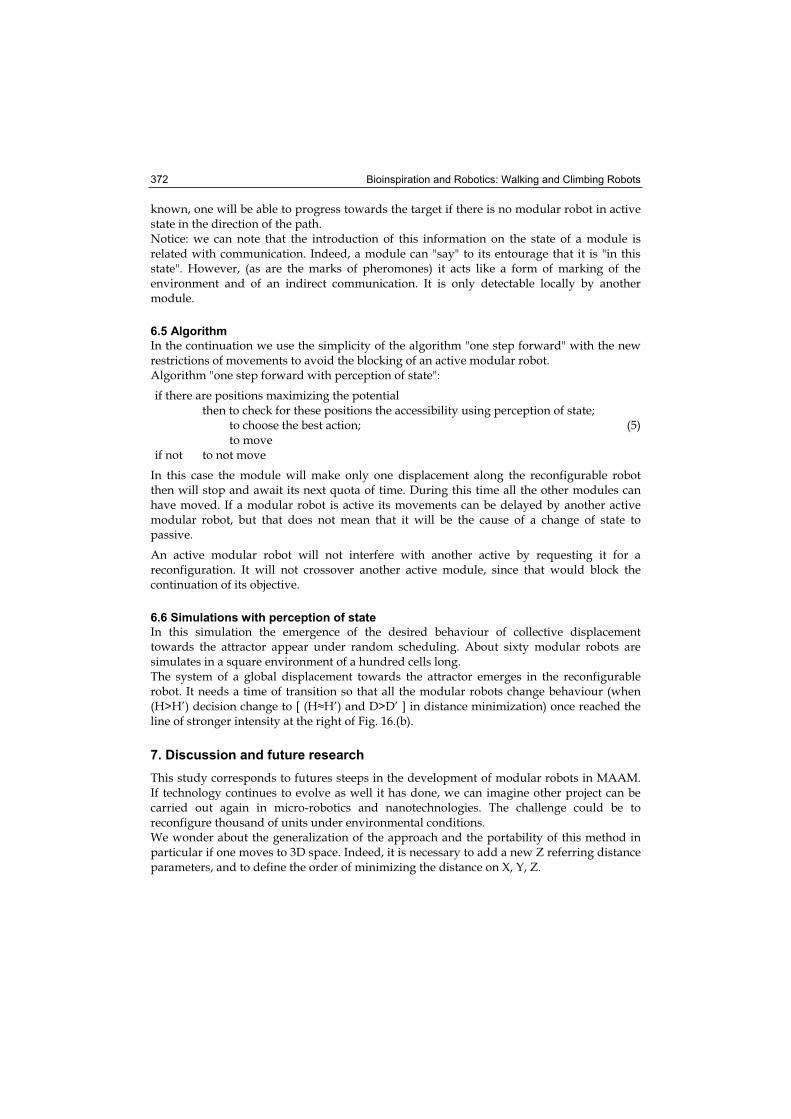
Bioinspiration and Robotics: Walking and Climbing Robots 372
known, one will be able to progress towards the target if there is no modular robot in active state in the direction of the path. Notice: we can note that the introduction of this information on the state of a module is related with communication. Indeed, a module can "say" to its entourage that it is "in this state". However, (as are the marks of pheromones) it acts like a form of marking of the environment and of an indirect communication. It is only detectable locally by another module.
6.5 Algorithm
In the continuation we use the simplicity of the algorithm "one step forward" with the new restrictions of movements to avoid the blocking of an active modular robot. Algorithm "one step forward with perception of state":
if there are positions maximizing the potential then to check for these positions the accessibility using perception of state;
to choose the best action; to move if not to not move
(5)
In this case the module will make only one displacement along the reconfigurable robot then will stop and await its next quota of time. During this time all the other modules can have moved. If a modular robot is active its movements can be delayed by another active modular robot, but that does not mean that it will be the cause of a change of state to passive.
An active modular robot will not interfere with another active by requesting it for a reconfiguration. It will not crossover another active module, since that would block the continuation of its objective.
6.6 Simulations with perception of state
In this simulation the emergence of the desired behaviour of collective displacement towards the attractor appear under random scheduling. About sixty modular robots are simulates in a square environment of a hundred cells long. The system of a global displacement towards the attractor emerges in the reconfigurable robot. It needs a time of transition so that all the modular robots change behaviour (when (H>H’) decision change to [ (H H’) and D>D’ ] in distance minimization) once reached the line of stronger intensity at the right of Fig. 16.(b).
7. Discussion and future research
This study corresponds to futures steeps in the development of modular robots in MAAM. If technology continues to evolve as well it has done, we can imagine other project can be carried out again in micro-robotics and nanotechnologies. The challenge could be to reconfigure thousand of units under environmental conditions. We wonder about the generalization of the approach and the portability of this method in particular if one moves to 3D space. Indeed, it is necessary to add a new Z referring distance parameters, and to define the order of minimizing the distance on X, Y, Z.
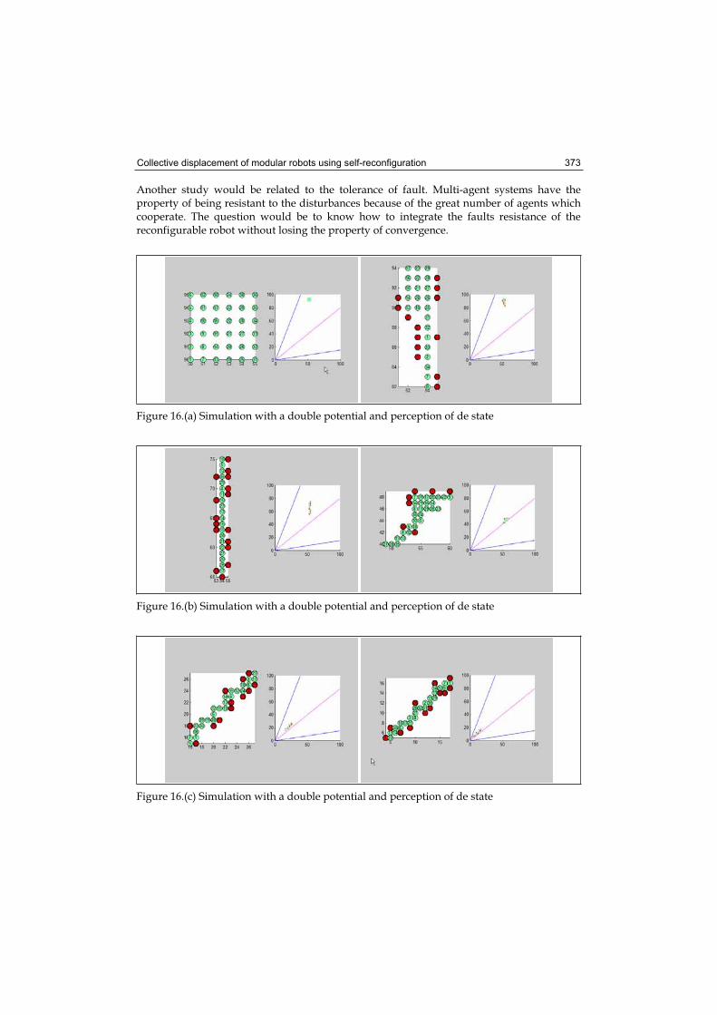
Collective displacement of modular robots using self-reconfiguration 373
Another study would be related to the tolerance of fault. Multi-agent systems have the property of being resistant to the disturbances because of the great number of agents which cooperate. The question would be to know how to integrate the faults resistance of the reconfigurable robot without losing the property of convergence.
Figure 16.(a) Simulation with a double potential and perception of de state
Figure 16.(b) Simulation with a double potential and perception of de state
Figure 16.(c) Simulation with a double potential and perception of de state
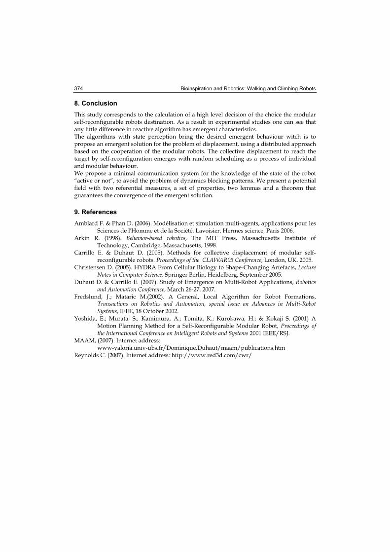
Bioinspiration and Robotics: Walking and Climbing Robots 374
8. Conclusion
This study corresponds to the calculation of a high level decision of the choice the modular self-reconfigurable robots destination. As a result in experimental studies one can see that any little difference in reactive algorithm has emergent characteristics. The algorithms with state perception bring the desired emergent behaviour witch is to propose an emergent solution for the problem of displacement, using a distributed approach based on the cooperation of the modular robots. The collective displacement to reach the target by self-reconfiguration emerges with random scheduling as a process of individual and modular behaviour. We propose a minimal communication system for the knowledge of the state of the robot “active or not”, to avoid the problem of dynamics blocking patterns. We present a potential field with two referential measures, a set of properties, two lemmas and a theorem that guarantees the convergence of the emergent solution.
9. References
Amblard F. & Phan D. (2006). Modélisation et simulation multi-agents, applications pour les Sciences de l'Homme et de la Société. Lavoisier, Hermes science, Paris 2006.
Arkin R. (1998). Behavior-based robotics, The MIT Press, Massachusetts Institute of Technology, Cambridge, Massachusetts, 1998.
Carrillo E. & Duhaut D. (2005). Methods for collective displacement of modular self-reconfigurable robots. Proceedings of the CLAWAR05 Conference, London, UK. 2005.
Christensen D. (2005). HYDRA From Cellular Biology to Shape-Changing Artefacts, Lecture Notes in Computer Science. Springer Berlin, Heidelberg, September 2005.
Duhaut D. & Carrillo E. (2007). Study of Emergence on Multi-Robot Applications, Roboticsand Automation Conference, March 26-27. 2007.
Fredslund, J.; Mataric M.(2002). A General, Local Algorithm for Robot Formations, Transactions on Robotics and Automation, special issue on Advances in Multi-Robot Systems, IEEE, 18 October 2002.
Yoshida, E.; Murata, S.; Kamimura, A.; Tomita, K.; Kurokawa, H.; & Kokaji S. (2001) A Motion Planning Method for a Self-Reconfigurable Modular Robot, Proceedings of the International Conference on Intelligent Robots and Systems 2001 IEEE/RSJ.
MAAM, (2007). Internet address: www-valoria.univ-ubs.fr/Dominique.Duhaut/maam/publications.htm
Reynolds C. (2007). Internet address: http://www.red3d.com/cwr/
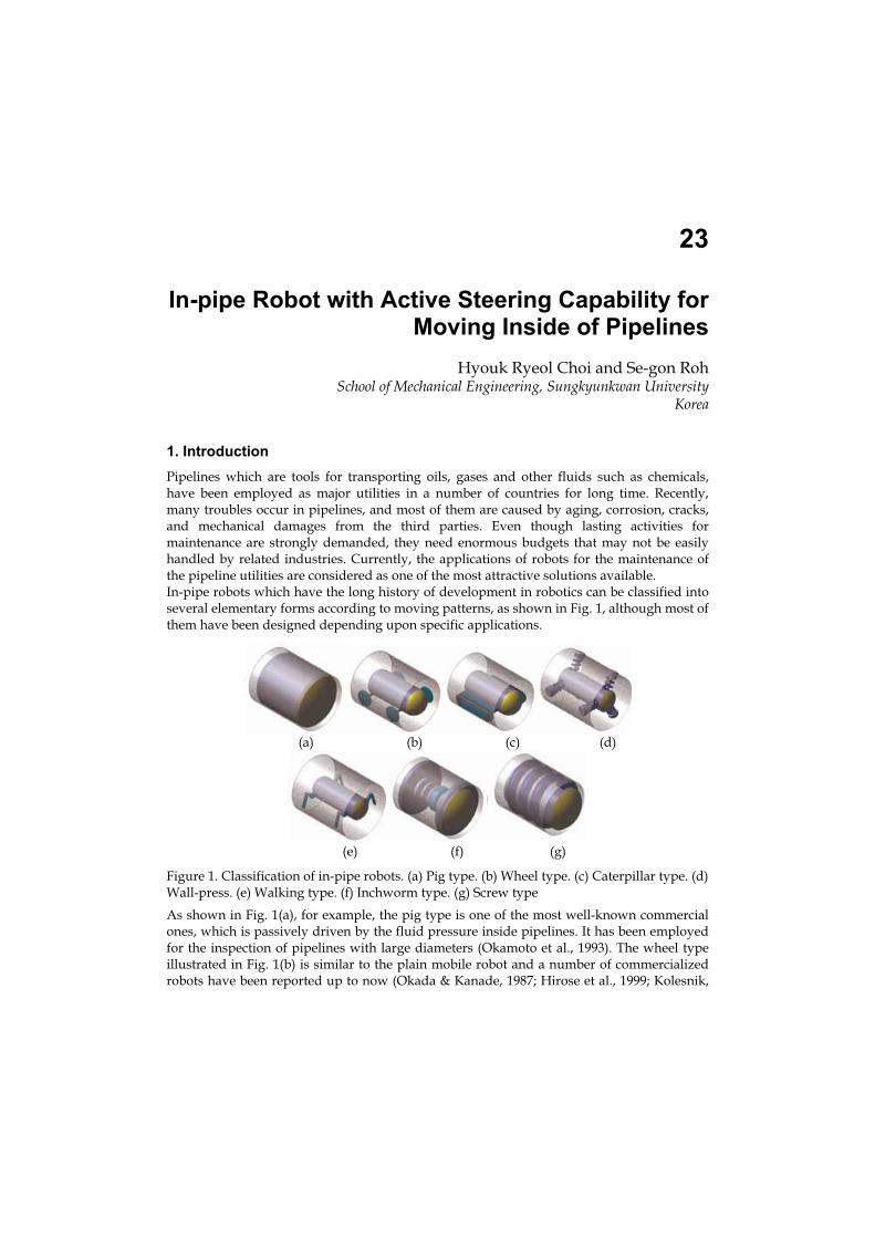
23
In-pipe Robot with Active Steering Capability for Moving Inside of Pipelines
Hyouk Ryeol Choi and Se-gon Roh School of Mechanical Engineering, Sungkyunkwan University
Korea
1. Introduction
Pipelines which are tools for transporting oils, gases and other fluids such as chemicals, have been employed as major utilities in a number of countries for long time. Recently, many troubles occur in pipelines, and most of them are caused by aging, corrosion, cracks, and mechanical damages from the third parties. Even though lasting activities for maintenance are strongly demanded, they need enormous budgets that may not be easily handled by related industries. Currently, the applications of robots for the maintenance of the pipeline utilities are considered as one of the most attractive solutions available. In-pipe robots which have the long history of development in robotics can be classified into several elementary forms according to moving patterns, as shown in Fig. 1, although most of them have been designed depending upon specific applications.
(a) (b) (c) (d)
(e) (f) (g)
Figure 1. Classification of in-pipe robots. (a) Pig type. (b) Wheel type. (c) Caterpillar type. (d) Wall-press. (e) Walking type. (f) Inchworm type. (g) Screw type
As shown in Fig. 1(a), for example, the pig type is one of the most well-known commercial ones, which is passively driven by the fluid pressure inside pipelines. It has been employed for the inspection of pipelines with large diameters (Okamoto et al., 1993). The wheel type illustrated in Fig. 1(b) is similar to the plain mobile robot and a number of commercialized robots have been reported up to now (Okada & Kanade, 1987; Hirose et al., 1999; Kolesnik,
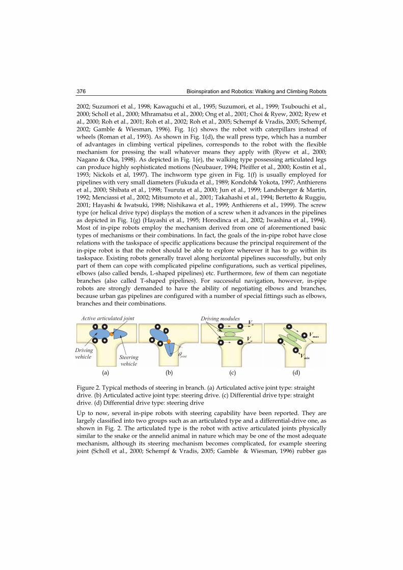
Bioinspiration and Robotics: Walking and Climbing Robots 376
2002; Suzumori et al., 1998; Kawaguchi et al., 1995; Suzumori, et al., 1999; Tsubouchi et al., 2000; Scholl et al., 2000; Mhramatsu et al., 2000; Ong et al., 2001; Choi & Ryew, 2002; Ryew et al., 2000; Roh et al., 2001; Roh et al., 2002; Roh et al., 2005; Schempf & Vradis, 2005; Schempf, 2002; Gamble & Wiesman, 1996). Fig. 1(c) shows the robot with caterpillars instead of wheels (Roman et al., 1993). As shown in Fig. 1(d), the wall press type, which has a number of advantages in climbing vertical pipelines, corresponds to the robot with the flexible mechanism for pressing the wall whatever means they apply with (Ryew et al., 2000; Nagano & Oka, 1998). As depicted in Fig. 1(e), the walking type possessing articulated legs can produce highly sophisticated motions (Neubauer, 1994; Pfeiffer et al., 2000; Kostin et al., 1993; Nickols et al, 1997). The inchworm type given in Fig. 1(f) is usually employed for pipelines with very small diameters (Fukuda et al., 1989; Kondoh& Yokota, 1997; Anthierens et al., 2000; Shibata et al., 1998; Tsuruta et al., 2000; Jun et al., 1999; Landsberger & Martin, 1992; Menciassi et al., 2002; Mitsumoto et al., 2001; Takahashi et al., 1994; Bertetto & Ruggiu, 2001; Hayashi & Iwatsuki, 1998; Nishikawa et al., 1999; Anthierens et al., 1999). The screw type (or helical drive type) displays the motion of a screw when it advances in the pipelines as depicted in Fig. 1(g) (Hayashi et al., 1995; Horodinca et al., 2002; Iwashina et al., 1994). Most of in-pipe robots employ the mechanism derived from one of aforementioned basic types of mechanisms or their combinations. In fact, the goals of the in-pipe robot have close relations with the taskspace of specific applications because the principal requirement of the in-pipe robot is that the robot should be able to explore wherever it has to go within its taskspace. Existing robots generally travel along horizontal pipelines successfully, but only part of them can cope with complicated pipeline configurations, such as vertical pipelines, elbows (also called bends, L-shaped pipelines) etc. Furthermore, few of them can negotiate branches (also called T-shaped pipelines). For successful navigation, however, in-pipe robots are strongly demanded to have the ability of negotiating elbows and branches, because urban gas pipelines are configured with a number of special fittings such as elbows, branches and their combinations.
� � � � � � � � � � � � � � � � � � � �
� � � � � � �
� � � � � � � �
� � � � � � �
� � � � � � ��� � � � �
��
��
� � � � � � � � � � � � �
�� � �
�� � �
(a) (b) (c) (d)
Figure 2. Typical methods of steering in branch. (a) Articulated active joint type: straight drive. (b) Articulated active joint type: steering drive. (c) Differential drive type: straight drive. (d) Differential drive type: steering drive
Up to now, several in-pipe robots with steering capability have been reported. They are largely classified into two groups such as an articulated type and a differential-drive one, as shown in Fig. 2. The articulated type is the robot with active articulated joints physically similar to the snake or the annelid animal in nature which may be one of the most adequate mechanism, although its steering mechanism becomes complicated, for example steering joint (Scholl et al., 2000; Schempf & Vradis, 2005; Gamble & Wiesman, 1996) rubber gas
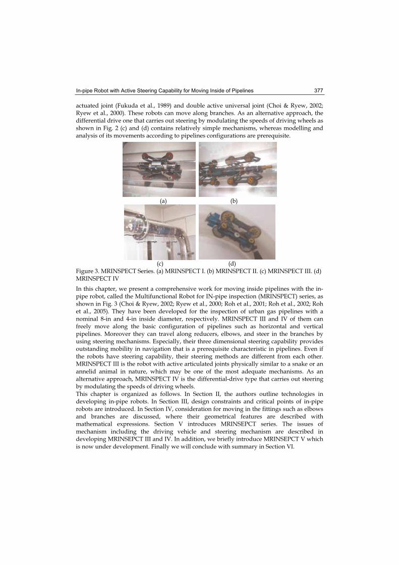
In-pipe Robot with Active Steering Capability for Moving Inside of Pipelines 377
actuated joint (Fukuda et al., 1989) and double active universal joint (Choi & Ryew, 2002; Ryew et al., 2000). These robots can move along branches. As an alternative approach, the differential drive one that carries out steering by modulating the speeds of driving wheels as shown in Fig. 2 (c) and (d) contains relatively simple mechanisms, whereas modelling and analysis of its movements according to pipelines configurations are prerequisite.
(a) (b)
(c) (d) Figure 3. MRINSPECT Series. (a) MRINSPECT I. (b) MRINSPECT II. (c) MRINSPECT III. (d) MRINSPECT IV
In this chapter, we present a comprehensive work for moving inside pipelines with the in-pipe robot, called the Multifunctional Robot for IN-pipe inspection (MRINSPECT) series, as shown in Fig. 3 (Choi & Ryew, 2002; Ryew et al., 2000; Roh et al., 2001; Roh et al., 2002; Roh et al., 2005). They have been developed for the inspection of urban gas pipelines with a nominal 8-in and 4-in inside diameter, respectively. MRINSPECT III and IV of them can freely move along the basic configuration of pipelines such as horizontal and vertical pipelines. Moreover they can travel along reducers, elbows, and steer in the branches by using steering mechanisms. Especially, their three dimensional steering capability provides outstanding mobility in navigation that is a prerequisite characteristic in pipelines. Even if the robots have steering capability, their steering methods are different from each other. MRINSPECT III is the robot with active articulated joints physically similar to a snake or an annelid animal in nature, which may be one of the most adequate mechanisms. As an alternative approach, MRINSPECT IV is the differential-drive type that carries out steering by modulating the speeds of driving wheels. This chapter is organized as follows. In Section II, the authors outline technologies in developing in-pipe robots. In Section III, design constraints and critical points of in-pipe robots are introduced. In Section IV, consideration for moving in the fittings such as elbows and branches are discussed, where their geometrical features are described with mathematical expressions. Section V introduces MRINSEPCT series. The issues of mechanism including the driving vehicle and steering mechanism are described in developing MRINSEPCT III and IV. In addition, we briefly introduce MRINSEPCT V which is now under development. Finally we will conclude with summary in Section VI.
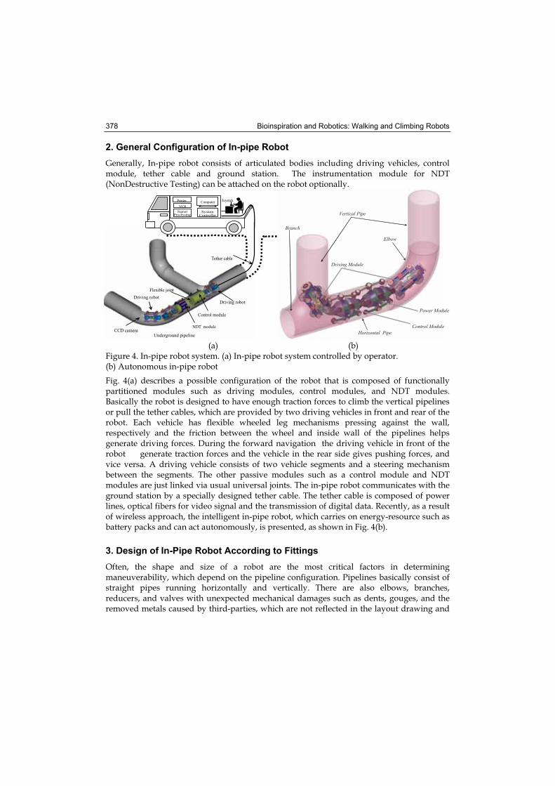
Bioinspiration and Robotics: Walking and Climbing Robots 378
2. General Configuration of In-pipe Robot
Generally, In-pipe robot consists of articulated bodies including driving vehicles, control module, tether cable and ground station. The instrumentation module for NDT (NonDestructive Testing) can be attached on the robot optionally.
���������
��� ������ ��
����������� ��� ��
���
�������������
������
�����������
��������������
� ���������� ��
��
� ��� ������� !���� �"
� # �������� # �������
� � � � �
� � � �
� � � � � � � � � � �
� � � � � � � � � � � �
� � � � � � � � � �
� � � � � � � � � � � �
� � ! � � � � � � � � � �
(a) (b) Figure 4. In-pipe robot system. (a) In-pipe robot system controlled by operator. (b) Autonomous in-pipe robot
Fig. 4(a) describes a possible configuration of the robot that is composed of functionally partitioned modules such as driving modules, control modules, and NDT modules. Basically the robot is designed to have enough traction forces to climb the vertical pipelines or pull the tether cables, which are provided by two driving vehicles in front and rear of the robot. Each vehicle has flexible wheeled leg mechanisms pressing against the wall, respectively and the friction between the wheel and inside wall of the pipelines helps generate driving forces. During the forward navigation the driving vehicle in front of the robot generate traction forces and the vehicle in the rear side gives pushing forces, and vice versa. A driving vehicle consists of two vehicle segments and a steering mechanism between the segments. The other passive modules such as a control module and NDT modules are just linked via usual universal joints. The in-pipe robot communicates with the ground station by a specially designed tether cable. The tether cable is composed of power lines, optical fibers for video signal and the transmission of digital data. Recently, as a result of wireless approach, the intelligent in-pipe robot, which carries on energy-resource such as battery packs and can act autonomously, is presented, as shown in Fig. 4(b).
3. Design of In-Pipe Robot According to Fittings
Often, the shape and size of a robot are the most critical factors in determining maneuverability, which depend on the pipeline configuration. Pipelines basically consist of straight pipes running horizontally and vertically. There are also elbows, branches, reducers, and valves with unexpected mechanical damages such as dents, gouges, and the removed metals caused by third-parties, which are not reflected in the layout drawing and
In-pipe Robot with Active Steering Capability for Moving Inside of Pipelines 379
demands the highly flexible design of robots. Based on the considerations of the pipeline configuration, the requirements of design can be derived as follows: 1. active steering capability in branches 2. surmounting right angle elbow
3. driving through pipelines with a various diameter ( ± 20 %) 4. sufficient traction forces (vertical load excluding self-weight) Items from 1) to 3) provide the fundamental requirements for the mobility that the robot should have and prerequisite to negotiate through wide range of configurations of pipelines. Also, 4) describes the supplementary capabilities, which is necessary to carry out and perform useful tasks by using appropriate inspection tools such as CCD cameras and NDT units. Major design issues of the robotic system correspond to how to enhance mobility inside pipelines. The design of the system mainly depends on the present state of the art in technology as well as the requirements of the system. The configuration of pipelines restricts the whole size of the robot and the current technology determines the possibility of implementation because actuator, drive electronics, embedded controller, power supply, sensor, and communication tools would have to be placed in an extremely small space. From the present technological point of view, therefore, only a very large robot in size is possible. One reasonable solution to this problem is the use of articulated structure such as snakelike or multi--joint robots though the control of the robot gets more difficult.
3.1. Wheel Leg Mechanism
One of the most important issues in the design of a driving vehicle is how to obtain the traction force enough to pull instrumentation as well as the vehicle itself. Especially in vertical pipelines, it is desirable to keep adequate wall pressing forces in order to ensure sufficient traction forces. Excessive forces may dissipate power and be in danger of damaging the robot. On the contrary insufficient forces may cause the robot to fall down. On the condition that the wheel does not slip on the pipeline surfaces, the traction force is proportional to the friction coefficient and the pressing force between the wheel and the pipeline surface, and the friction coefficient depends on the material of wheel and the surface condition of pipelines. In addition, the link mechanism of the vehicle should minimize the variation of traction force caused by variation of pipeline diameters. Therefore, a leg mechanism has to meet the following three requirements. At first, it should be possible to push against the pipeline wall with adequate pressing forces. In the second, the pressing force should not show significant change during navigation in order to provide stable traction force and flexible locomotion. At last, the mechanism should be simple and small in size to occupy minimal space inside the pipelines. For example, the driving vehicle of MRINSPECT III has three wheeled legs circumferentially spaced 120 degree apart on the main shaft of the vehicle. Fig. 5 illustrates the kinematic diagram of the wheeled leg mechanism of MRINSPECT III. The mechanism employs a pantograph mechanism with a sliding base that permits the natural folding and unfolding of the leg. Here, l is the length of link, θ means the folding
angle of the link measured by the rotary potentiometer, K denotes the spring constant, hrepresents the distance of the center of the wheel from the base. wF denotes the wall
pressing force, xA and yA are the forces acting on the link by the spring, x is the
displacement of the sliding base. In the proposed mechanism when the wheels are pressed
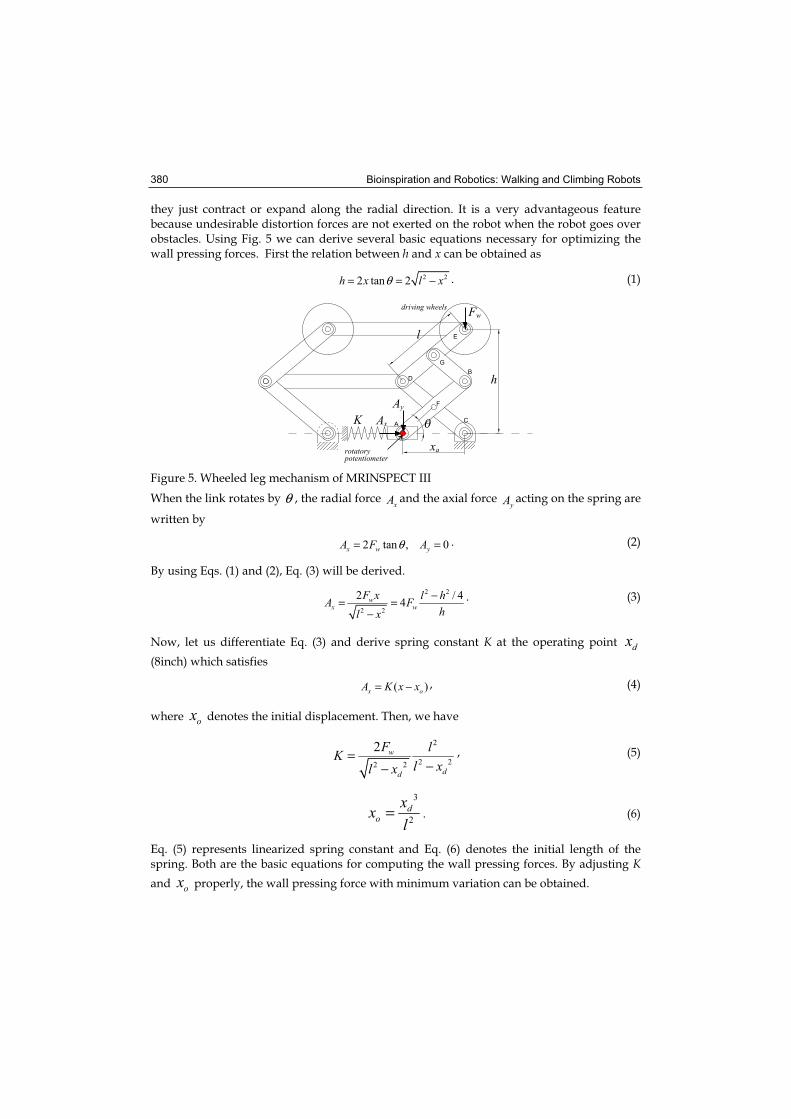
Bioinspiration and Robotics: Walking and Climbing Robots 380
they just contract or expand along the radial direction. It is a very advantageous feature because undesirable distortion forces are not exerted on the robot when the robot goes over obstacles. Using Fig. 5 we can derive several basic equations necessary for optimizing the wall pressing forces. First the relation between h and x can be obtained as
2 22 tan 2h x l xθ= = − . (1)
��
�
�
��
�
�� �
��
���
�
�
�
�
�
��
�� � ��� �������
�������������� ������
Figure 5. Wheeled leg mechanism of MRINSPECT III
When the link rotates by θ , the radial force xA and the axial force
yA acting on the spring are
written by
2 tan , 0x w yA F Aθ= = . (2)
By using Eqs. (1) and (2), Eq. (3) will be derived.
2 2
2 2
2 / 44w
x wF x l hA F
hl x−= =
−. (3)
Now, let us differentiate Eq. (3) and derive spring constant K at the operating point dx(8inch) which satisfies
( )x oA K x x= − , (4)
where ox denotes the initial displacement. Then, we have
2
2 22 2
2 w
dd
F lKl xl x
=−−
, (5)
3
2
do
xxl
= . (6)
Eq. (5) represents linearized spring constant and Eq. (6) denotes the initial length of the spring. Both are the basic equations for computing the wall pressing forces. By adjusting Kand ox properly, the wall pressing force with minimum variation can be obtained.
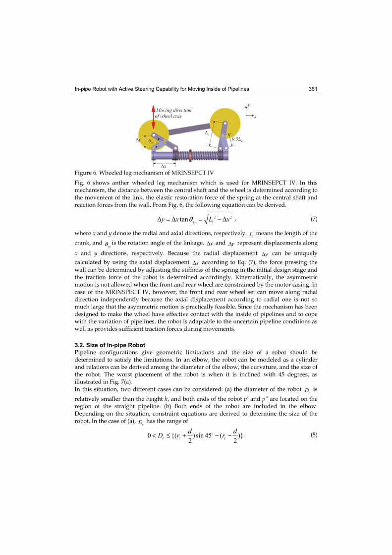
In-pipe Robot with Active Steering Capability for Moving Inside of Pipelines 381
�
�
�
� "
� #
$%
& ' ( $%
� � � � � � � � � � � � � � � �
� ) � � � � � � � " � �
�
�" #
"
#
Figure 6. Wheeled leg mechanism of MRINSEPCT IV
Fig. 6 shows anther wheeled leg mechanism which is used for MRINSEPCT IV. In this mechanism, the distance between the central shaft and the wheel is determined according to the movement of the link, the elastic restoration force of the spring at the central shaft and reaction forces from the wall. From Fig. 6, the following equation can be derived.
2 2
1tan xyy x L xθΔ = Δ = − Δ , (7)
where x and y denote the radial and axial directions, respectively. 1L means the length of the
crank, and xyθ is the rotation angle of the linkage. xΔ and yΔ represent displacements along
x and y directions, respectively. Because the radial displacement yΔ can be uniquely
calculated by using the axial displacement xΔ according to Eq. (7), the force pressing the
wall can be determined by adjusting the stiffness of the spring in the initial design stage and the traction force of the robot is determined accordingly. Kinematically, the asymmetric motion is not allowed when the front and rear wheel are constrained by the motor casing. In case of the MRINSPECT IV, however, the front and rear wheel set can move along radial direction independently because the axial displacement according to radial one is not so much large that the asymmetric motion is practically feasible. Since the mechanism has been designed to make the wheel have effective contact with the inside of pipelines and to cope with the variation of pipelines, the robot is adaptable to the uncertain pipeline conditions as well as provides sufficient traction forces during movements.
3.2. Size of In-pipe Robot
Pipeline configurations give geometric limitations and the size of a robot should be determined to satisfy the limitations. In an elbow, the robot can be modeled as a cylinder and relations can be derived among the diameter of the elbow, the curvature, and the size of the robot. The worst placement of the robot is when it is inclined with 45 degrees, as illustrated in Fig. 7(a). In this situation, two different cases can be considered: (a) the diameter of the robot
rD is
relatively smaller than the height h, and both ends of the robot p’ and p” are located on the region of the straight pipeline. (b) Both ends of the robot are included in the elbow. Depending on the situation, constraint equations are derived to determine the size of the robot. In the case of (a),
rD has the range of
0 {( )sin 45 ( )}2 2
r c cd dD r r< ≤ + − − . (8)
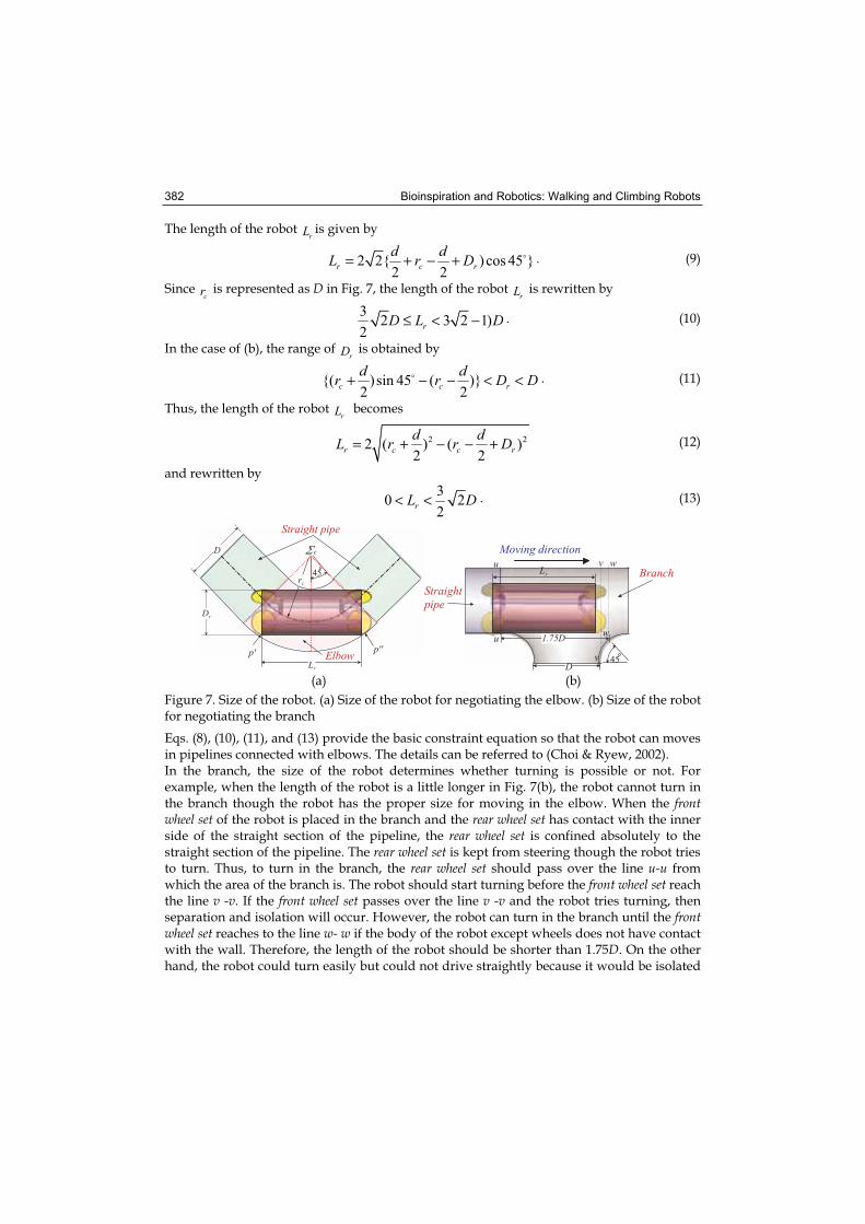
Bioinspiration and Robotics: Walking and Climbing Robots 382
The length of the robot rL is given by
2 2{ )cos 45 }2 2
r c rd dL r D= + − + . (9)
Sincecr is represented as D in Fig. 7, the length of the robot
rL is rewritten by
32 3 2 1)
2rD L D≤ < − . (10)
In the case of (b), the range of rD is obtained by
{( )sin 45 ( )}2 2
c c rd dr r D D+ − − < < . (11)
Thus, the length of the robot rL becomes
2 22 ( ) ( )2 2
r c c rd dL r r D= + − − + (12)
and rewritten by
30 2
2rL D< < . (13)
�
� �
$
�
�
� � � � � � � � � � �
� � � � �
� � �
� *� * *
$
% ' + ( �
� � � �
� � � � � �
� � � �
� �
�
�
�
� � �
� � � � � � � � � � � � � �
�
(a) (b)
Figure 7. Size of the robot. (a) Size of the robot for negotiating the elbow. (b) Size of the robot for negotiating the branch
Eqs. (8), (10), (11), and (13) provide the basic constraint equation so that the robot can moves in pipelines connected with elbows. The details can be referred to (Choi & Ryew, 2002). In the branch, the size of the robot determines whether turning is possible or not. For example, when the length of the robot is a little longer in Fig. 7(b), the robot cannot turn in the branch though the robot has the proper size for moving in the elbow. When the front wheel set of the robot is placed in the branch and the rear wheel set has contact with the inner side of the straight section of the pipeline, the rear wheel set is confined absolutely to the straight section of the pipeline. The rear wheel set is kept from steering though the robot tries to turn. Thus, to turn in the branch, the rear wheel set should pass over the line u-u fromwhich the area of the branch is. The robot should start turning before the front wheel set reach the line v -v. If the front wheel set passes over the line v -v and the robot tries turning, then separation and isolation will occur. However, the robot can turn in the branch until the front wheel set reaches to the line w- w if the body of the robot except wheels does not have contact with the wall. Therefore, the length of the robot should be shorter than 1.75D. On the other hand, the robot could turn easily but could not drive straightly because it would be isolated
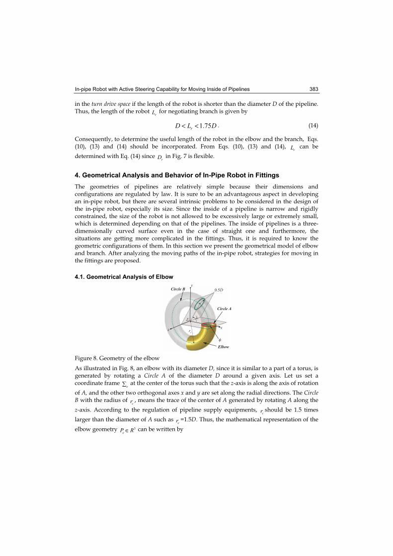
In-pipe Robot with Active Steering Capability for Moving Inside of Pipelines 383
in the turn drive space if the length of the robot is shorter than the diameter D of the pipeline. Thus, the length of the robot
rL for negotiating branch is given by
1.75rD L D< < . (14)
Consequently, to determine the useful length of the robot in the elbow and the branch, Eqs. (10), (13) and (14) should be incorporated. From Eqs. (10), (13) and (14),
rL can be
determined with Eq. (14) since rD in Fig. 7 is flexible.
4. Geometrical Analysis and Behavior of In-Pipe Robot in Fittings
The geometries of pipelines are relatively simple because their dimensions and configurations are regulated by law. It is sure to be an advantageous aspect in developing an in-pipe robot, but there are several intrinsic problems to be considered in the design of the in-pipe robot, especially its size. Since the inside of a pipeline is narrow and rigidly constrained, the size of the robot is not allowed to be excessively large or extremely small, which is determined depending on that of the pipelines. The inside of pipelines is a three-dimensionally curved surface even in the case of straight one and furthermore, the situations are getting more complicated in the fittings. Thus, it is required to know the geometric configurations of them. In this section we present the geometrical model of elbow and branch. After analyzing the moving paths of the in-pipe robot, strategies for moving in the fittings are proposed.
4.1. Geometrical Analysis of Elbow
"
#
!
� � �
�
�
� � � � � �
� � � � � �
�
� � � �
� � �
Figure 8. Geometry of the elbow
As illustrated in Fig. 8, an elbow with its diameter D, since it is similar to a part of a torus, is generated by rotating a Circle A of the diameter D around a given axis. Let us set a coordinate frame
e at the center of the torus such that the z-axis is along the axis of rotation
of A, and the other two orthogonal axes x and y are set along the radial directions. The CircleB with the radius of
cr , means the trace of the center of A generated by rotating A along the
z-axis. According to the regulation of pipeline supply equipments, cr should be 1.5 times
larger than the diameter of A such as cr =1.5D. Thus, the mathematical representation of the
elbow geometry 3
eP R∈ can be written by
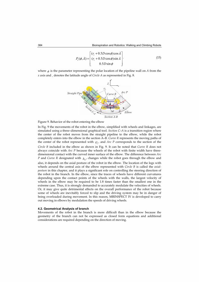
Bioinspiration and Robotics: Walking and Climbing Robots 384
( 0.5 cos )cos
( , ) ( 0.5 cos )sin
0.5 sin
c
e c
r DP r D
D
φ λφ λ φ λ
φ
+= + . (15)
where φ is the parameter representing the polar location of the pipeline wall on A from the
x axis and ¸ denotes the latitude angle of Circle A as represented in Fig. 8.
� � � � �
� � � � � � � � � � �
� � � � � � � � � , �
�
�
�
�
�
�
���� � ��� �, �
� � � � � -
� � � �
�
�
�
.
� ��
Figure 9. Behavior of the robot entering the elbow
In Fig. 9 the movements of the robot in the elbow, simplified with wheels and linkages, are simulated using a three–dimensional graphical tool. Section C–A is a transition region where the center of the robot moves from the straight pipeline to the elbow, while the robot completely enters into the elbow in the section A–B. Curve R represents the moving paths of the center of the robot represented with
rO , and Arc P corresponds to the section of the
Circle B included in the elbow as shown in Fig. 9. It can be noted that Curve R does not always coincide with Arc P because the wheels of the robot with finite width have three-dimensional contact with the curved inner surface of the elbow. The difference between Arc P and Curve R designated with
dΔ , changes while the robot goes through the elbow and
also, it depends on the axial posture of the robot in the elbow. The location of the legs with wheels around the central axis of the elbow represented with Circle B is called the axial-posture in this chapter, and it plays a significant role on controlling the steering direction of the robot in the branch. In the elbow, since the traces of wheels have different curvatures depending upon the contact points of the wheels with the walls, the largest velocity of wheels in the elbow may be required to be 1.8 times faster than the smallest one in the extreme case. Thus, it is strongly demanded to accurately modulate the velocities of wheels. Or, it may give quite detrimental effects on the overall performance of the robot because some of wheels are inevitably forced to slip and the driving system may be in danger of being overloaded during movement. In this reason, MRINSPECT IV is developed to carry out moving in elbows by modulation the speeds of driving wheels.
4.2. Geometrical Analysis of branch
Movements of the robot in the branch is more difficult than in the elbow because the geometry of the branch can not be expressed as closed form equations and additional considerations are required depending on the direction of moving.
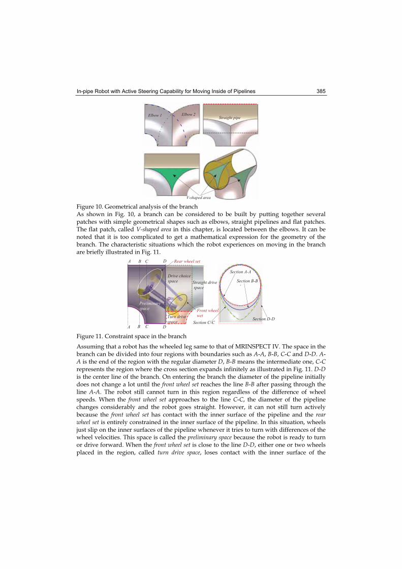
In-pipe Robot with Active Steering Capability for Moving Inside of Pipelines 385
� , � � � � � �
� � � � � � %� � � � � � /
� � � � � � � � � � �
Figure 10. Geometrical analysis of the branch As shown in Fig. 10, a branch can be considered to be built by putting together several patches with simple geometrical shapes such as elbows, straight pipelines and flat patches. The flat patch, called V-shaped area in this chapter, is located between the elbows. It can be noted that it is too complicated to get a mathematical expression for the geometry of the branch. The characteristic situations which the robot experiences on moving in the branch are briefly illustrated in Fig. 11.
� � � � � � � � � , �
� � � � � � � � � , �
� � � � � � � � � , �
� � � � � � � � � , �
0 � � � � � � �
� � � �
� � � � � � � � � �
� � � � �
� � � � � � � � � � � �
� � � � �
� � � � � � � � # �
� � � � �1 � � � � � � � � �
� � �
- � � � � � � � � � � ��
�
�
�
�
� �
�
Figure 11. Constraint space in the branch
Assuming that a robot has the wheeled leg same to that of MRINSPECT IV. The space in the branch can be divided into four regions with boundaries such as A-A, B-B, C-C and D-D. A-A is the end of the region with the regular diameter D, B-B means the intermediate one, C-Crepresents the region where the cross section expands infinitely as illustrated in Fig. 11. D-Dis the center line of the branch. On entering the branch the diameter of the pipeline initially does not change a lot until the front wheel set reaches the line B-B after passing through the line A-A. The robot still cannot turn in this region regardless of the difference of wheel speeds. When the front wheel set approaches to the line C-C, the diameter of the pipeline changes considerably and the robot goes straight. However, it can not still turn actively because the front wheel set has contact with the inner surface of the pipeline and the rear wheel set is entirely constrained in the inner surface of the pipeline. In this situation, wheels just slip on the inner surfaces of the pipeline whenever it tries to turn with differences of the wheel velocities. This space is called the preliminary space because the robot is ready to turn or drive forward. When the front wheel set is close to the line D-D, either one or two wheels placed in the region, called turn drive space, loses contact with the inner surface of the
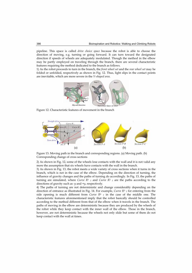
Bioinspiration and Robotics: Walking and Climbing Robots 386
pipeline. This space is called drive choice space because the robot is able to choose the direction of moving, e.g. turning or going forward. It can turn toward the designated direction if speeds of wheels are adequately modulated. Though the method in the elbow may be partly employed on traveling through the branch, there are several characteristic features requiring the method dedicated to the branch as follows. 1) As the robot proceeds to turn in the branch, the front wheel set and the rear wheel set may be folded or unfolded, respectively as shown in Fig. 12. Thus, light slips in the contact points are inevitable, which are more severe in the V-shaped area.
� � � � � � � � � �
� � � � � � �
� � � � � � � � �
� � � � �
� � � � � � � � � � � � � � � � � � � � � � � � � � � � � � � � � � ! � � � � � � �
� � � � � � � � � � � � � � �
Figure 12. Characteristic features of movement in the branch
�
�
� � � � � � � � � �
0 � � � � � �
�
�
� � � � � � � � � � � � -%
0 �� � � � � � � � � � � � � � �
�
� � � � � � � � � � � � -/
� �� � � � � � � � � � � � � � �� � � � � -
/
0 ��
� � � � � � � � � � � � � , � � � � � � � � � � � , � �� � � � � � � � � , � �
(a) (b)
Figure 13. Moving path in the branch and corresponding regions. (a) Moving path. (b) Corresponding change of cross sections
2) As shown in Fig. 12, some of the wheels lose contacts with the wall and it is not valid any more the assumption that six wheels have contacts with the wall in the branch. 3) As shown in Fig. 13, the robot meets a wide variety of cross sections when it turns in the branch, which is not in the case of the elbow. Depending on the direction of turning, the influence of gravity changes and the paths of turning do accordingly. In Fig. 13, the paths of turning are simulated, where Curve R1 T and Curve R2 T are the paths according to the directions of gravity such as -y and +y, respectively. 4) The paths of turning are not deterministic and change considerably depending on the direction of entrance as illustrated in Fig. 14. For example, Curve R3 T for entering from the side opening is much different from Curve R4 T in the case of the middle one. The characteristic features aforementioned imply that the robot basically should be controlled according to the method different from that of the elbow when it travels in the branch. The paths of moving in the elbow are deterministic because they are produced by the wheels of the robot while they keep contact with the inner wall of the elbow. Those in the branch, however, are not deterministic because the wheels not only slide but some of them do not keep contact with the wall at times.
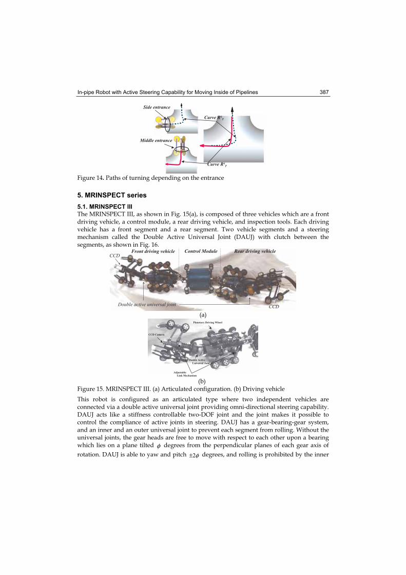
In-pipe Robot with Active Steering Capability for Moving Inside of Pipelines 387
� � " � � #$
% ��
� � " � � #&
% ��
� � � � � � � � � � � � �
' � � � � � � � � � � � � �
Figure 14. Paths of turning depending on the entrance
5. MRINSPECT series
5.1. MRINSPECT III
The MRINSPECT III, as shown in Fig. 15(a), is composed of three vehicles which are a front driving vehicle, a control module, a rear driving vehicle, and inspection tools. Each driving vehicle has a front segment and a rear segment. Two vehicle segments and a steering mechanism called the Double Active Universal Joint (DAUJ) with clutch between the segments, as shown in Fig. 16.
( � � � � � � � � " � � ) � " � � � � # � � � � � � � " � � ) � " � � � �
� � � � � � � � � � � � � � � � � � � � � � � � � �
� � � � � � ' � � � �
� � �
� � �
(a)
� � � � � � � � � � �
� � � � � � � � � � � � � � � � � � �
� � � � � � � � � �
� � � � � � � � � � � � � � � � � � � � � �
� � � � � � � � � �
� � � � � � � � � � � � � � � � � �
(b) Figure 15. MRINSPECT III. (a) Articulated configuration. (b) Driving vehicle
This robot is configured as an articulated type where two independent vehicles are connected via a double active universal joint providing omni-directional steering capability. DAUJ acts like a stiffness controllable two-DOF joint and the joint makes it possible to control the compliance of active joints in steering. DAUJ has a gear-bearing-gear system, and an inner and an outer universal joint to prevent each segment from rolling. Without the universal joints, the gear heads are free to move with respect to each other upon a bearing which lies on a plane tilted φ degrees from the perpendicular planes of each gear axis of
rotation. DAUJ is able to yaw and pitch 2φ± degrees, and rolling is prohibited by the inner
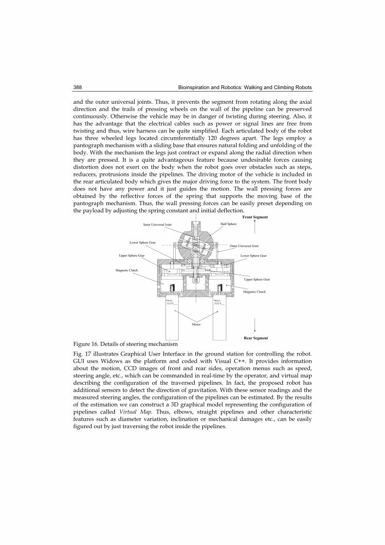
Bioinspiration and Robotics: Walking and Climbing Robots 388
and the outer universal joints. Thus, it prevents the segment from rotating along the axial direction and the trails of pressing wheels on the wall of the pipeline can be preserved continuously. Otherwise the vehicle may be in danger of twisting during steering. Also, it has the advantage that the electrical cables such as power or signal lines are free from twisting and thus, wire harness can be quite simplified. Each articulated body of the robot has three wheeled legs located circumferentially 120 degrees apart. The legs employ a pantograph mechanism with a sliding base that ensures natural folding and unfolding of the body. With the mechanism the legs just contract or expand along the radial direction when they are pressed. It is a quite advantageous feature because undesirable forces causing distortion does not exert on the body when the robot goes over obstacles such as steps, reducers, protrusions inside the pipelines. The driving motor of the vehicle is included in the rear articulated body which gives the major driving force to the system. The front body does not have any power and it just guides the motion. The wall pressing forces are obtained by the reflective forces of the spring that supports the moving base of the pantograph mechanism. Thus, the wall pressing forces can be easily preset depending on the payload by adjusting the spring constant and initial deflection.
�������������� ���� �����������
������������������������������� ����
�����������������
�����������������
�����������������
���������������
���������������
�����
����������
�� �������
Figure 16. Details of steering mechanism
Fig. 17 illustrates Graphical User Interface in the ground station for controlling the robot. GUI uses Widows as the platform and coded with Visual C++. It provides information about the motion, CCD images of front and rear sides, operation menus such as speed, steering angle, etc., which can be commanded in real-time by the operator, and virtual map describing the configuration of the traversed pipelines. In fact, the proposed robot has additional sensors to detect the direction of gravitation. With these sensor readings and the measured steering angles, the configuration of the pipelines can be estimated. By the results of the estimation we can construct a 3D graphical model representing the configuration of pipelines called Virtual Map. Thus, elbows, straight pipelines and other characteristic features such as diameter variation, inclination or mechanical damages etc., can be easily figured out by just traversing the robot inside the pipelines.
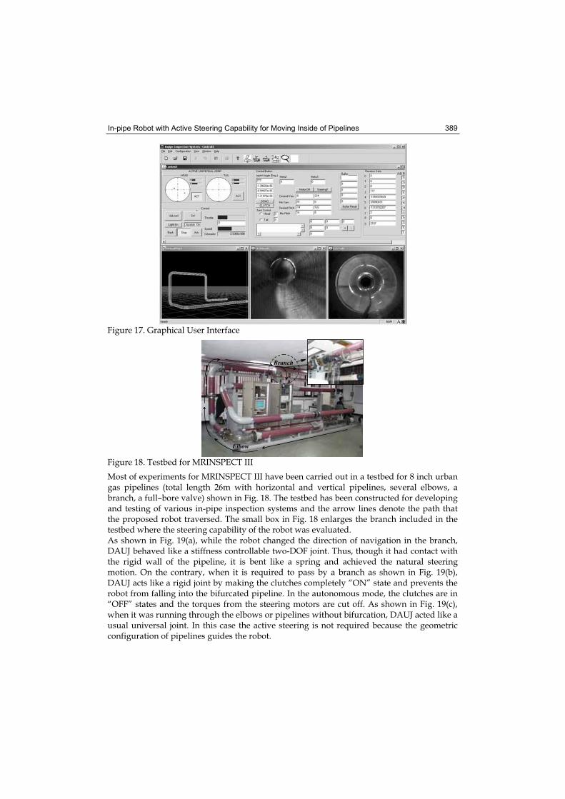
In-pipe Robot with Active Steering Capability for Moving Inside of Pipelines 389
Figure 17. Graphical User Interface
������
��� ��
Figure 18. Testbed for MRINSPECT III
Most of experiments for MRINSPECT III have been carried out in a testbed for 8 inch urban gas pipelines (total length 26m with horizontal and vertical pipelines, several elbows, a branch, a full–bore valve) shown in Fig. 18. The testbed has been constructed for developing and testing of various in-pipe inspection systems and the arrow lines denote the path that the proposed robot traversed. The small box in Fig. 18 enlarges the branch included in the testbed where the steering capability of the robot was evaluated. As shown in Fig. 19(a), while the robot changed the direction of navigation in the branch, DAUJ behaved like a stiffness controllable two-DOF joint. Thus, though it had contact with the rigid wall of the pipeline, it is bent like a spring and achieved the natural steering motion. On the contrary, when it is required to pass by a branch as shown in Fig. 19(b), DAUJ acts like a rigid joint by making the clutches completely “ON” state and prevents the robot from falling into the bifurcated pipeline. In the autonomous mode, the clutches are in “OFF” states and the torques from the steering motors are cut off. As shown in Fig. 19(c), when it was running through the elbows or pipelines without bifurcation, DAUJ acted like a usual universal joint. In this case the active steering is not required because the geometric configuration of pipelines guides the robot.
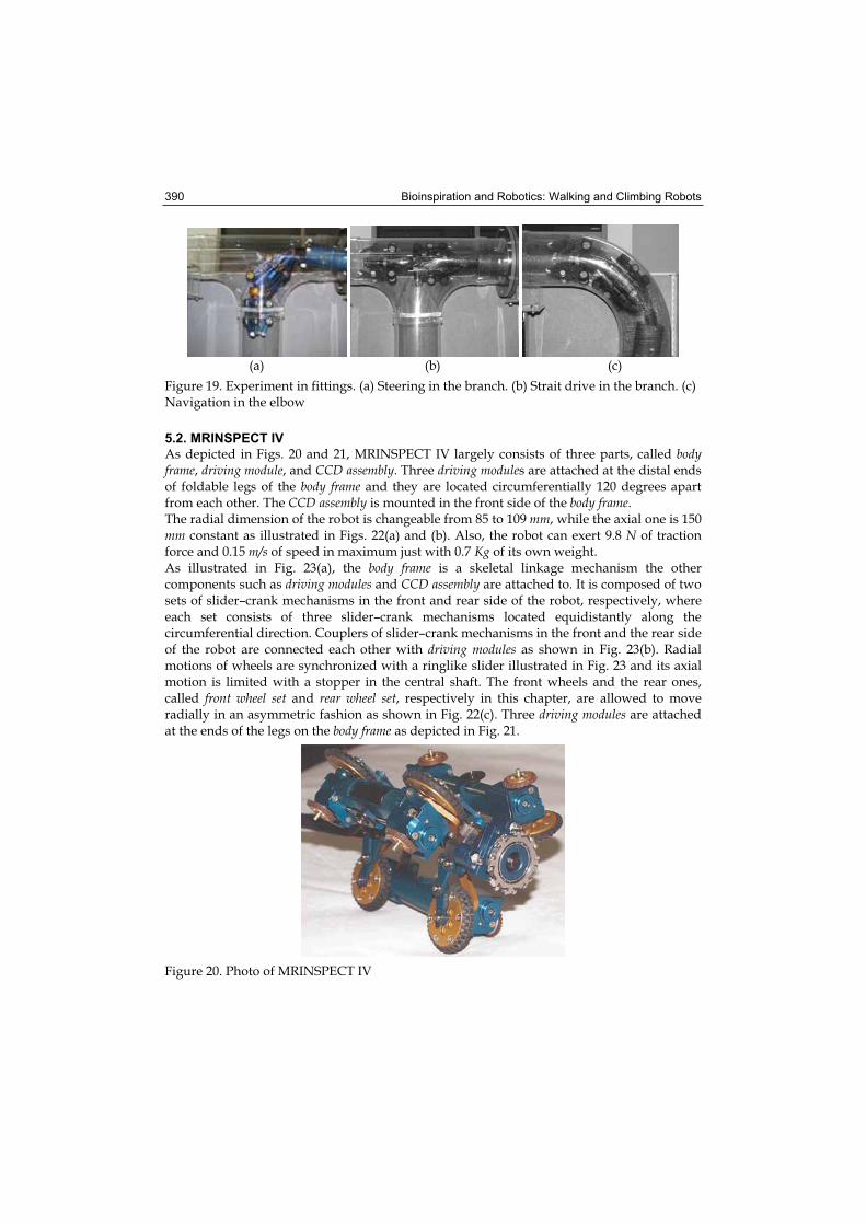
Bioinspiration and Robotics: Walking and Climbing Robots 390
(a) (b) (c)
Figure 19. Experiment in fittings. (a) Steering in the branch. (b) Strait drive in the branch. (c) Navigation in the elbow
5.2. MRINSPECT IV
As depicted in Figs. 20 and 21, MRINSPECT IV largely consists of three parts, called body frame, driving module, and CCD assembly. Three driving modules are attached at the distal ends of foldable legs of the body frame and they are located circumferentially 120 degrees apart from each other. The CCD assembly is mounted in the front side of the body frame.The radial dimension of the robot is changeable from 85 to 109 mm, while the axial one is 150 mm constant as illustrated in Figs. 22(a) and (b). Also, the robot can exert 9.8 N of traction force and 0.15 m/s of speed in maximum just with 0.7 Kg of its own weight. As illustrated in Fig. 23(a), the body frame is a skeletal linkage mechanism the other components such as driving modules and CCD assembly are attached to. It is composed of two sets of slider–crank mechanisms in the front and rear side of the robot, respectively, where each set consists of three slider–crank mechanisms located equidistantly along the circumferential direction. Couplers of slider–crank mechanisms in the front and the rear side of the robot are connected each other with driving modules as shown in Fig. 23(b). Radial motions of wheels are synchronized with a ringlike slider illustrated in Fig. 23 and its axial motion is limited with a stopper in the central shaft. The front wheels and the rear ones, called front wheel set and rear wheel set, respectively in this chapter, are allowed to move radially in an asymmetric fashion as shown in Fig. 22(c). Three driving modules are attached at the ends of the legs on the body frame as depicted in Fig. 21.
Figure 20. Photo of MRINSPECT IV
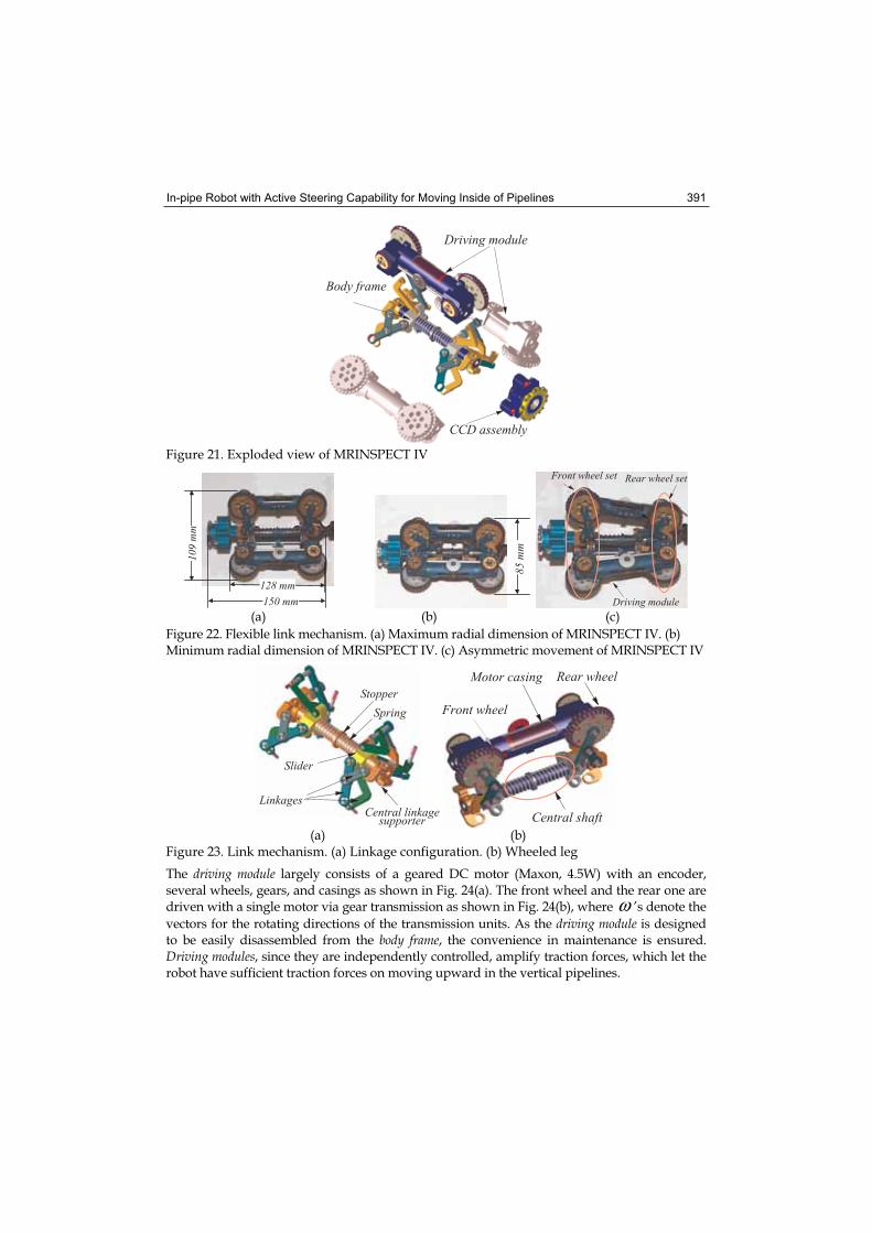
In-pipe Robot with Active Steering Capability for Moving Inside of Pipelines 391
� � # � ) � �
� � � � � � � � � � � �
� � � � � � � � � � #
Figure 21. Exploded view of MRINSPECT IV
% ( & � � �
%&2���
% / 3 � � �
3(����
1 � � � � � � � � � � � � �- � � � � � � � � � � �
� � � � � � � � � � � �
(a) (b) (c)
Figure 22. Flexible link mechanism. (a) Maximum radial dimension of MRINSPECT IV. (b) Minimum radial dimension of MRINSPECT IV. (c) Asymmetric movement of MRINSPECT IV
� � � � � �
� � � �
� � � � � �
$ � � 4 � � �
� � � � � � � � � 4 � � �
� � � � � � �
� � � � � � � � � � �
�
1 � � � � � � � � �
- � � � � � � �
�
� � � � � � � � � ) �
(a) (b) Figure 23. Link mechanism. (a) Linkage configuration. (b) Wheeled leg
The driving module largely consists of a geared DC motor (Maxon, 4.5W) with an encoder, several wheels, gears, and casings as shown in Fig. 24(a). The front wheel and the rear one are driven with a single motor via gear transmission as shown in Fig. 24(b), where ω ’s denote the
vectors for the rotating directions of the transmission units. As the driving module is designed to be easily disassembled from the body frame, the convenience in maintenance is ensured. Driving modules, since they are independently controlled, amplify traction forces, which let the robot have sufficient traction forces on moving upward in the vertical pipelines.
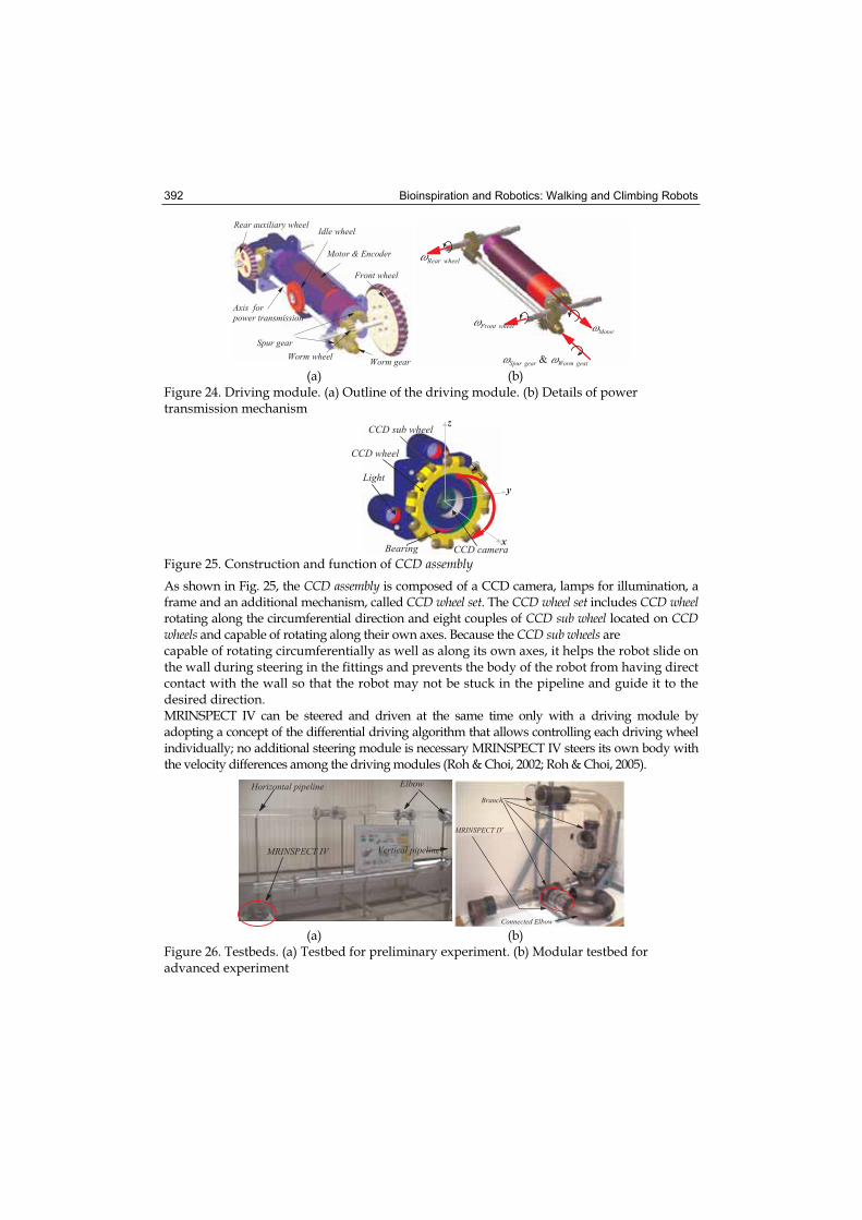
Bioinspiration and Robotics: Walking and Climbing Robots 392
� 1 � � � � � � � � � �
5 � � � � � � � �
6 � � � � �
6 � � � � � � � �
� � � � � �
� � � � � 7 � � � � � �
� " � � � � ) � �
� � � � � � � � � � � � � � �
- � � � " � � � # � � � � � � �
�� � � � � �
� �6 � � � � � �
�� � � �
�- � � � � � � �
� � � � � �1 � � � � � � � � �
(a) (b) Figure 24. Driving module. (a) Outline of the driving module. (b) Details of power transmission mechanism
�
� � � � � � � � � � � � � �
*
�
� � � � �
� � � � � � � � � �
� � � � � � �
$ � � � �
Figure 25. Construction and function of CCD assembly
As shown in Fig. 25, the CCD assembly is composed of a CCD camera, lamps for illumination, a frame and an additional mechanism, called CCD wheel set. The CCD wheel set includes CCD wheel rotating along the circumferential direction and eight couples of CCD sub wheel located on CCD wheels and capable of rotating along their own axes. Because the CCD sub wheels are capable of rotating circumferentially as well as along its own axes, it helps the robot slide on the wall during steering in the fittings and prevents the body of the robot from having direct contact with the wall so that the robot may not be stuck in the pipeline and guide it to the desired direction. MRINSPECT IV can be steered and driven at the same time only with a driving module by adopting a concept of the differential driving algorithm that allows controlling each driving wheel individually; no additional steering module is necessary MRINSPECT IV steers its own body with the velocity differences among the driving modules (Roh & Choi, 2002; Roh & Choi, 2005).
� � � � �
� � � � � � � � � � � � � � �
� � ! � � � � � � � � � � � � �
� - 5 8 � � � � 0 � 5 �
� � � �
� - 5 8 � � � � 0 � 5 �
� � � � � � � � � � � � � �
(a) (b) Figure 26. Testbeds. (a) Testbed for preliminary experiment. (b) Modular testbed for advanced experiment
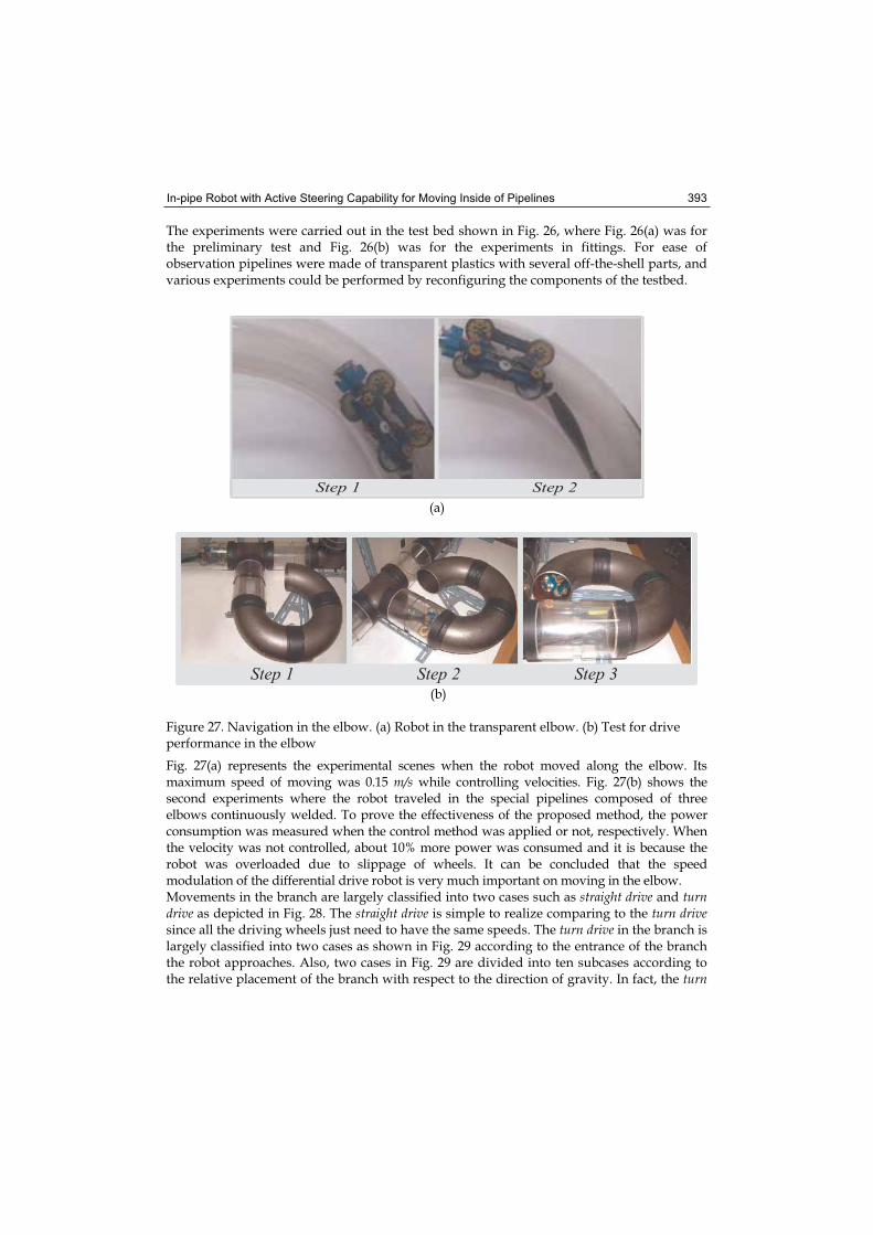
In-pipe Robot with Active Steering Capability for Moving Inside of Pipelines 393
The experiments were carried out in the test bed shown in Fig. 26, where Fig. 26(a) was for the preliminary test and Fig. 26(b) was for the experiments in fittings. For ease of observation pipelines were made of transparent plastics with several off-the-shell parts, and various experiments could be performed by reconfiguring the components of the testbed.
� � � � � � � � � � � � � � � � � � � � � � � � % � � � � � � � � � � � � � � � � � � � � � � � � � � � � � � � � � � � � � � � � � � � / � � � � � � � � � � � � � �
(a)
� � � � � � � � � � � � � � � � � � � � � � % � � � � � � � � � � � � � � � � � � � � � � � � � � � � � � � � � / � � � � � � � � � � � � � � � � � � � � � � � � � � � � � � � 9 � � � � � � � � � � � � � � � � �
(b)
Figure 27. Navigation in the elbow. (a) Robot in the transparent elbow. (b) Test for drive performance in the elbow
Fig. 27(a) represents the experimental scenes when the robot moved along the elbow. Its maximum speed of moving was 0.15 m/s while controlling velocities. Fig. 27(b) shows the second experiments where the robot traveled in the special pipelines composed of three elbows continuously welded. To prove the effectiveness of the proposed method, the power consumption was measured when the control method was applied or not, respectively. When the velocity was not controlled, about 10% more power was consumed and it is because the robot was overloaded due to slippage of wheels. It can be concluded that the speed modulation of the differential drive robot is very much important on moving in the elbow. Movements in the branch are largely classified into two cases such as straight drive and turn drive as depicted in Fig. 28. The straight drive is simple to realize comparing to the turn drive since all the driving wheels just need to have the same speeds. The turn drive in the branch is largely classified into two cases as shown in Fig. 29 according to the entrance of the branch the robot approaches. Also, two cases in Fig. 29 are divided into ten subcases according to the relative placement of the branch with respect to the direction of gravity. In fact, the turn
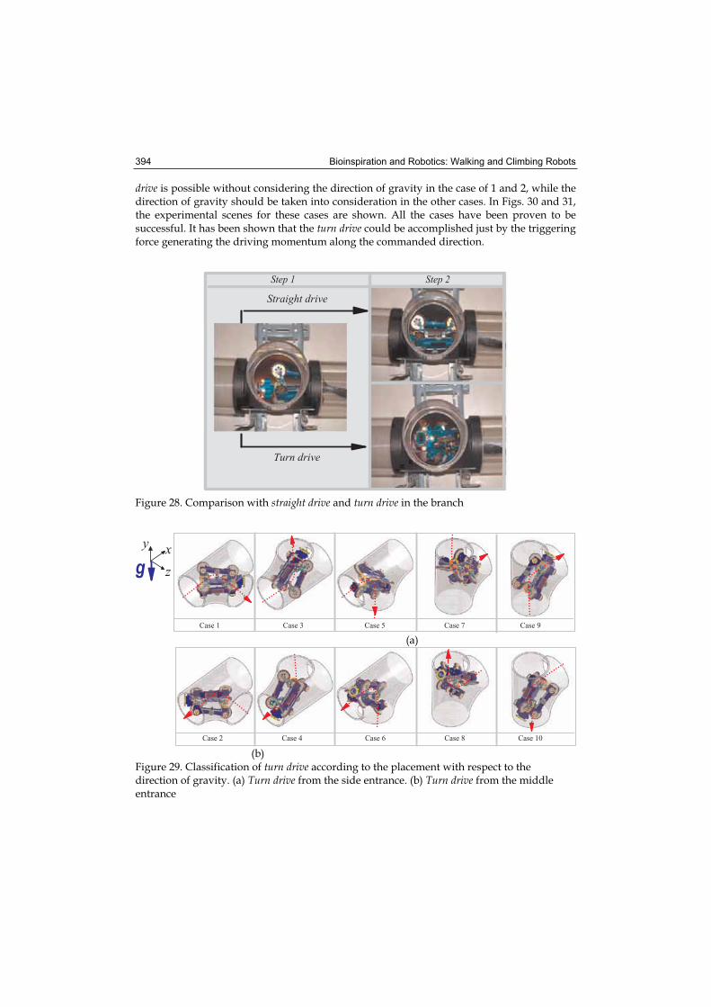
Bioinspiration and Robotics: Walking and Climbing Robots 394
drive is possible without considering the direction of gravity in the case of 1 and 2, while the direction of gravity should be taken into consideration in the other cases. In Figs. 30 and 31, the experimental scenes for these cases are shown. All the cases have been proven to be successful. It has been shown that the turn drive could be accomplished just by the triggering force generating the driving momentum along the commanded direction.
� � � � � � � � � � � � � � � � � � � � � � � � � � � � � � � % � � � � � � � � � � � � � � � � � � � � � � � � � � � � � � � � � � � � � � � � � � � � � � � � � � � � � � � � � � / � � � � � � � � � � � � � � � � � � � � � �
� � � � � � � � � �
0 � � � � � �
Figure 28. Comparison with straight drive and turn drive in the branch
"#
!�
� � � � � � � � � � � � � � �
(a)
� � � � � � � � � � � � � � � �
(b)Figure 29. Classification of turn drive according to the placement with respect to the direction of gravity. (a) Turn drive from the side entrance. (b) Turn drive from the middle entrance
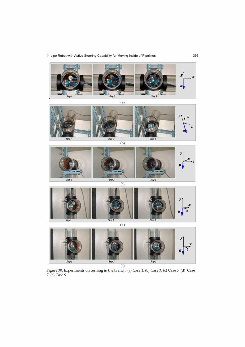
In-pipe Robot with Active Steering Capability for Moving Inside of Pipelines 395
.(a)
(b)
(c)
(d)
(e)Figure 30. Experiments on turning in the branch. (a) Case 1. (b) Case 3. (c) Case 5. (d) Case 7. (e) Case 9
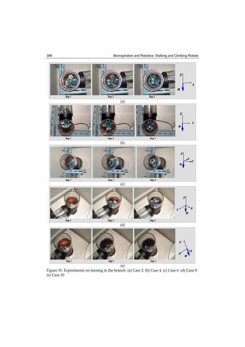
Bioinspiration and Robotics: Walking and Climbing Robots 396
(a)
(b)
(c)
(d)
(e)Figure 31. Experiments on turning in the branch. (a) Case 2. (b) Case 4. (c) Case 6. (d) Case 8. (e) Case 10
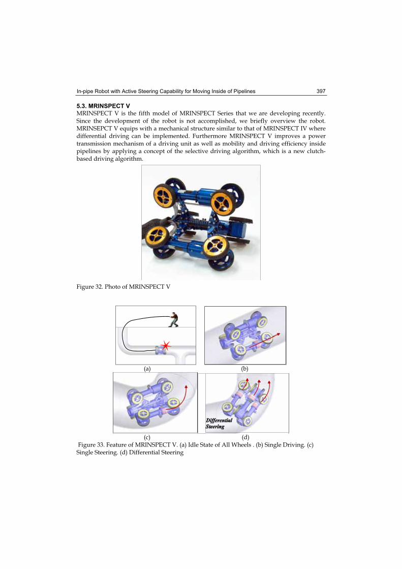
In-pipe Robot with Active Steering Capability for Moving Inside of Pipelines 397
5.3. MRINSPECT V
MRINSPECT V is the fifth model of MRINSPECT Series that we are developing recently. Since the development of the robot is not accomplished, we briefly overview the robot. MRINSEPCT V equips with a mechanical structure similar to that of MRINSPECT IV where differential driving can be implemented. Furthermore MRINSPECT V improves a power transmission mechanism of a driving unit as well as mobility and driving efficiency inside pipelines by applying a concept of the selective driving algorithm, which is a new clutch-based driving algorithm.
Figure 32. Photo of MRINSPECT V
(a) (b)
(c) (d) Figure 33. Feature of MRINSPECT V. (a) Idle State of All Wheels . (b) Single Driving. (c) Single Steering. (d) Differential Steering
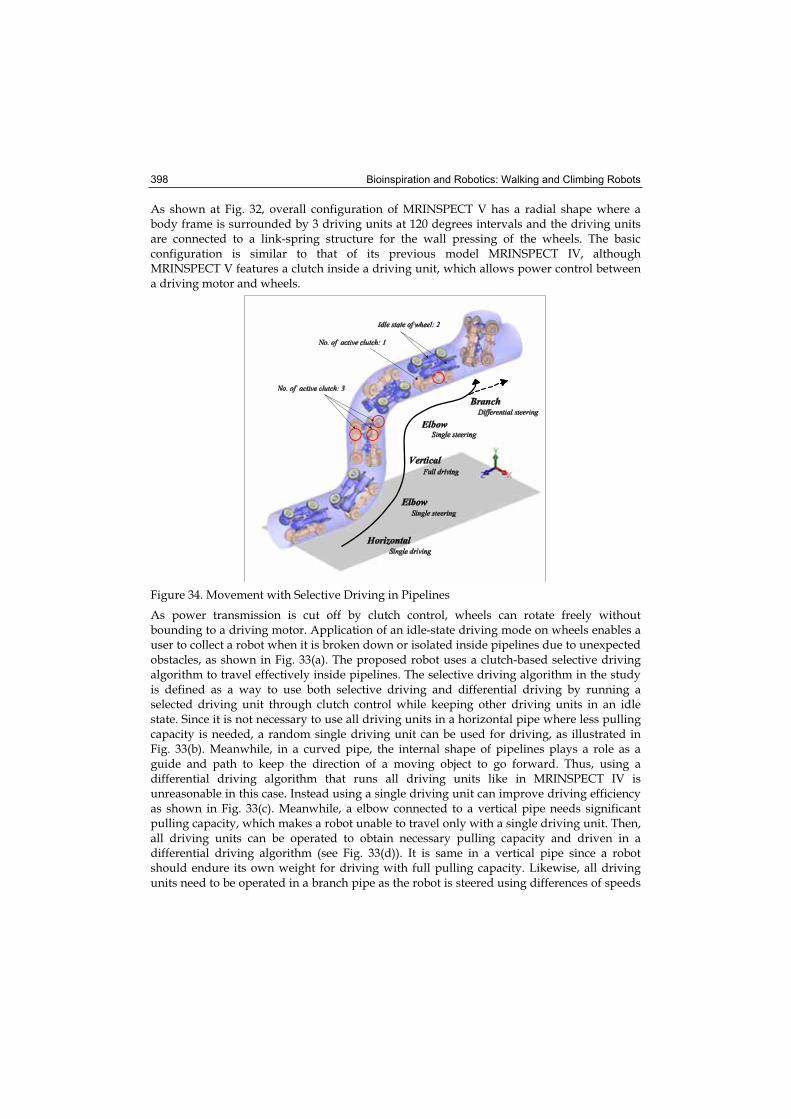
Bioinspiration and Robotics: Walking and Climbing Robots 398
As shown at Fig. 32, overall configuration of MRINSPECT V has a radial shape where a body frame is surrounded by 3 driving units at 120 degrees intervals and the driving units are connected to a link-spring structure for the wall pressing of the wheels. The basic configuration is similar to that of its previous model MRINSPECT IV, although MRINSPECT V features a clutch inside a driving unit, which allows power control between a driving motor and wheels.
Figure 34. Movement with Selective Driving in Pipelines
As power transmission is cut off by clutch control, wheels can rotate freely without bounding to a driving motor. Application of an idle-state driving mode on wheels enables a user to collect a robot when it is broken down or isolated inside pipelines due to unexpected obstacles, as shown in Fig. 33(a). The proposed robot uses a clutch-based selective driving algorithm to travel effectively inside pipelines. The selective driving algorithm in the study is defined as a way to use both selective driving and differential driving by running a selected driving unit through clutch control while keeping other driving units in an idle state. Since it is not necessary to use all driving units in a horizontal pipe where less pulling capacity is needed, a random single driving unit can be used for driving, as illustrated in Fig. 33(b). Meanwhile, in a curved pipe, the internal shape of pipelines plays a role as a guide and path to keep the direction of a moving object to go forward. Thus, using a differential driving algorithm that runs all driving units like in MRINSPECT IV is unreasonable in this case. Instead using a single driving unit can improve driving efficiency as shown in Fig. 33(c). Meanwhile, a elbow connected to a vertical pipe needs significant pulling capacity, which makes a robot unable to travel only with a single driving unit. Then, all driving units can be operated to obtain necessary pulling capacity and driven in a differential driving algorithm (see Fig. 33(d)). It is same in a vertical pipe since a robot should endure its own weight for driving with full pulling capacity. Likewise, all driving units need to be operated in a branch pipe as the robot is steered using differences of speeds
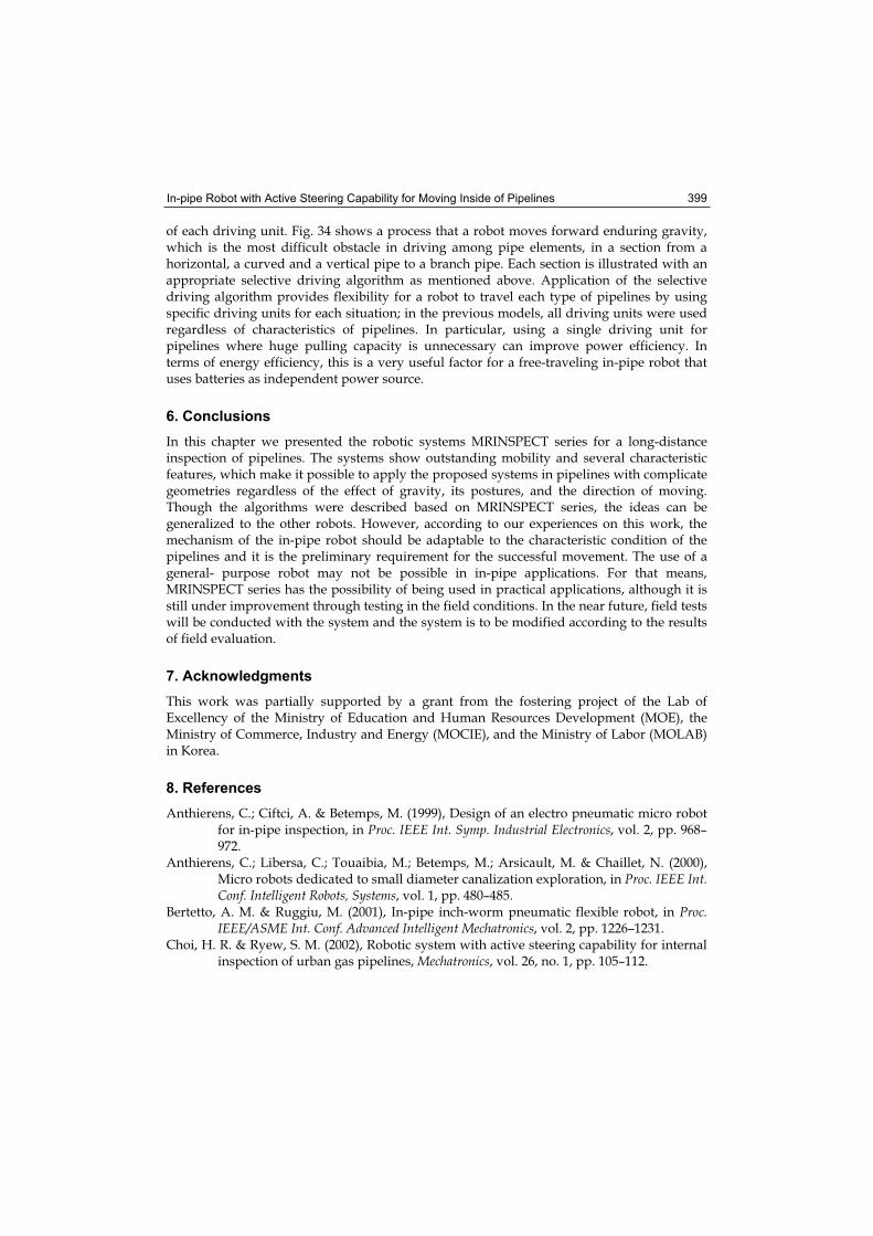
In-pipe Robot with Active Steering Capability for Moving Inside of Pipelines 399
of each driving unit. Fig. 34 shows a process that a robot moves forward enduring gravity, which is the most difficult obstacle in driving among pipe elements, in a section from a horizontal, a curved and a vertical pipe to a branch pipe. Each section is illustrated with an appropriate selective driving algorithm as mentioned above. Application of the selective driving algorithm provides flexibility for a robot to travel each type of pipelines by using specific driving units for each situation; in the previous models, all driving units were used regardless of characteristics of pipelines. In particular, using a single driving unit for pipelines where huge pulling capacity is unnecessary can improve power efficiency. In terms of energy efficiency, this is a very useful factor for a free-traveling in-pipe robot that uses batteries as independent power source.
6. Conclusions
In this chapter we presented the robotic systems MRINSPECT series for a long-distance inspection of pipelines. The systems show outstanding mobility and several characteristic features, which make it possible to apply the proposed systems in pipelines with complicate geometries regardless of the effect of gravity, its postures, and the direction of moving. Though the algorithms were described based on MRINSPECT series, the ideas can be generalized to the other robots. However, according to our experiences on this work, the mechanism of the in-pipe robot should be adaptable to the characteristic condition of the pipelines and it is the preliminary requirement for the successful movement. The use of a general- purpose robot may not be possible in in-pipe applications. For that means, MRINSPECT series has the possibility of being used in practical applications, although it is still under improvement through testing in the field conditions. In the near future, field tests will be conducted with the system and the system is to be modified according to the results of field evaluation.
7. Acknowledgments
This work was partially supported by a grant from the fostering project of the Lab of Excellency of the Ministry of Education and Human Resources Development (MOE), the Ministry of Commerce, Industry and Energy (MOCIE), and the Ministry of Labor (MOLAB) in Korea.
8. References
Anthierens, C.; Ciftci, A. & Betemps, M. (1999), Design of an electro pneumatic micro robot for in-pipe inspection, in Proc. IEEE Int. Symp. Industrial Electronics, vol. 2, pp. 968–972.
Anthierens, C.; Libersa, C.; Touaibia, M.; Betemps, M.; Arsicault, M. & Chaillet, N. (2000), Micro robots dedicated to small diameter canalization exploration, in Proc. IEEE Int. Conf. Intelligent Robots, Systems, vol. 1, pp. 480–485.
Bertetto, A. M. & Ruggiu, M. (2001), In-pipe inch-worm pneumatic flexible robot, in Proc. IEEE/ASME Int. Conf. Advanced Intelligent Mechatronics, vol. 2, pp. 1226–1231.
Choi, H. R. & Ryew, S. M. (2002), Robotic system with active steering capability for internal inspection of urban gas pipelines, Mechatronics, vol. 26, no. 1, pp. 105–112.
Bioinspiration and Robotics: Walking and Climbing Robots 400
Fukuda, T.; Hosokai, H. & Uemura, M. (1989), Rubber gas actuator driven by hydrogen storage alloy for in-pipe inspection mobile robot with flexible structure, in Proc. IEEE Int. Conf. Robotics, Automation, vol. 3, pp. 1847–1852.
Gamble, B. B. & Wiesman, R. M. (1996), Tethered Mouse System for Inspection of Gas Distribution Mains, Gas Res. Inst., Doc. GRI-96/0209.
Hayashi, I.; Iwatsuki, N. & Iwashina, S. (1995), The running characteristics of a screw-principle microrobot in a small bent pipe, in Proc. Int. Symp. Micro Machines, Human Science, pp. 225–228.
Hayashi, I. & Iwatsuki, N. (1998), Micro moving robotics, in Proc. IEEE Int. Conf. Intelligent Robots, Systems, pp. 41–50.
Hirose, S.; Ohno, H.; Mitsui, T. & Suyama, K. (1999), Design of in-pipe inspection vehicles
for φ 25, φ 50, φ 150 pipes, in Proc. IEEE Int. Conf. Robotics, Automation, pp. 2309–
2314.Horodinca, M.; Dorftei, I.; Mignon, E. & Preumont, A. (2002), A simple architecture for in-
pipe inspection robots, in Proc. Int. Colloq. Mobile, Autonomous Systems, pp. 61–64. Iwashina, S.; Hayashi, I.; Iwatsuki, N. & Nakamura, K. (1994), Development of in-pipe
operation micro robots, in Proc. Int. Symp. Micro Machines Human Science, pp. 41–45. Jun, L.; Sun, P.; Lian, L.; Qin, X. & Gong, Z. (1999), Improvement of characteristics of in-pipe
micro robot, in Proc. Int. Symp. Micromechatronics, Human Science, pp. 153–156. Kawaguchi, Y.; Yoshida, I.; Kurumatani, H.; Kikuta, T. & Yamada, Y. (1995), Internal pipe
inspection robot, in Proc. IEEE Int. Conf. Robotics, Automation, pp. 857–862. Kolesnik, M. (2002), Visual orientation in the sewer—Adaptation to the environment, in
Proc. Int. Conf. Pattern Recognit., pp. 11–15. Kondoh, Y. & Yokota, S. (1997), Micro in-pipe mobile machines by making use of an electro-
rheological fluid, in Proc. IEEE Int. Conf. Intelligent Robots, Systems, vol. 3, pp. 1672–1677.
Kostin, G. V.; Chernousko, F. L. & Bolotnik, N. N. (1993), Regular motions of a tube-crawling robot: Simulation and optimization, in Proc. Workshop Robot Motion, Control, pp. 45–50.
Landsberger, S. E. & Martin, B. F. (1992), The design of a pipe crawling robot for control of zebra mussel infestations, in Proc. Mastering the Oceans Through Technology, vol. 2, pp. 819–824.
Menciassi, A.; Park, J. H.; Lee, S.; Gorinil, S.; Dario, P. & Park, J.-O. (2002), Robotic solutions and mechanisms for a semi-autonomous endoscope, in Proc. IEEE/RSJ Int. Conf. Intelligent Robots, Systems, pp. 1379–1384.
Mhramatsu, M.; Namiki, N.; Koyama, U. & Suga, Y. (2000), Autonomous mobile robot in pipe for piping operations, in Proc. IEEE/RSJ Int. Conf. Intelligent Robots, Systems,vol. 3, pp. 2366–2171.
Mitsumoto, N.; Tsuruta, K.; Shibata, T. & Kawahara, N. (2001), Wireless link system for communication and energy transmission of microrobot, in Proc. Int. Symp. Micromechatronics, Human Science, pp. 107–112.
Nagano, S. & Oka, Y. (1998), Application of in-pipe visual inspection robot to piping internal surface lining, in Proc. 5th Int. Symp. Robotics in Construction, pp. 897–906.
Neubauer, W. (1994), A spider-like robot that climbs vertically in ducts or pipes, in Proc. IEEE/RSJ Int. Conf. Intelligent Robots, Systems, pp. 1178–1185.
In-pipe Robot with Active Steering Capability for Moving Inside of Pipelines 401
Nickols, F.; Ho, D.; Harrold, S. O.; Bradbeer, R. T. & Yeung, L. (1997), An ultrasonically controlled robot submarine for pipe inspection, in Proc. 4th Annu. Conf. Mechatronics, Machine Vision in Practice, pp. 142–147.
Nishikawa, H.; Sasaya, T.; Shibata, T. & Kaneko, T. (1999), In-pipe wireless micro locomotive system, in Proc. Int. Symp. Micromechatronics, Human Science, pp. 141–147.
Ong, J. K.; Kerr, D. & Bouazza-Marouf, K. (2001), In-pipe multi-robot system: Modular configurable co-operative semi-autonomous robotic units, in Proc. Int. Gas Research Conf., Paper Do07.
Okada T. & Kanade T. (1987), A three-wheeled self-adjusting vehicle in a pipe, FERRET-1, Int. J. Robot. Res., vol. 6, no. 4, pp. 60–75, 1987.
Okamoto, J.; Adamowski, Jr. J. C.; Tsuzuki, M. S. G.; Buiochi, F. & Camerini, C. S. (1999), Autonomous system for oil pipelines inspection, Mechatronics, vol. 9, pp. 731–743
Pfeiffer, F.; Robmann, T. & Loffer, K. (2000), Control of a tube crawling machine, in Proc. Int. Conf. Control of Oscillations and Chaos, vol. 3, pp. 586–591.
Roman, H. T.; Pellegrino, B. A. & Sigrist, W. R. (1993), Pipe crawling inspection robots: An overview, IEEE Trans. Energy Convers., vol. 8, pp. 576–583, Sept.
Roh, S. G.; Ryew, S. M.; Yang, J. H. & Choi, H. R. (2001), Actively steerable inpipe inspection robots for underground urban gas pipelines, in Proc. IEEE Int. Conf. Robotics, Automation, pp. 761–766.
Roh, S. G. & Choi, H. R (2002) Strategy for Navigation Inside Pipelines with Differential-drive Inpipe Robot, In Proc. IEEE Int. Conf. Robotics, Automation, pp. 2575-2580.
Roh, S. G. & Choi, H. R. (2005), Differential-Drive In-Pipe Robot for Moving Inside Urban Gas Pipelines, IEEE Trans. Robotics, Vol. 21, No.1, pp.1-17.
Ryew, S. M.; Baik, S. H.; Ryu, S. W.; Jung, K. M.; Roh, S. G. & Choi, H. R. (2000), Inpipe inspection robot system with active steering mechanism, in Proc. IEEE Int. Conf. Intelligent Robots, Systems, pp. 1652–1657.
Schempf, H. (2002), GRISLEE: Gas Main Repair and Inspection System for Live-Entry Environments, Gas Res. Inst., Doc. GRI-02/0132.
Schempf, H. & Vradis, G. (2005), Explorer: Long-range untethered real-time live gas main inspection system. presented at Proc. Conf. GTI. [Online]. Available: http://www.rec.ri.cmu.edu/projects/explorer
Scholl, K.-U.; Kepplin, V.; Berns, K. & Dillmann, R. (2000), Controlling a multijoint robot for autonomous sewer inspection, in Proc. IEEE Int. Conf. Robotics, Automation, vol. 2, pp. 24–28.
Shibata, T.; Sasaya, T. & Kawahara, N. (1998), Microwave energy supply system for in-pipe micromachine, in Proc. Int. Symp. Micromechatronics, Human Science, pp. 237–242.
Suzumori, K.; Hori, K. & Miyagawa, T. (1998), A direct-drive pneumatic stepping motor for robots: Designs for pipe-inspection microrobots and for human-care robots, in Proc. IEEE. Int. Conf. Robotics, Automation, vol. 4, pp. 3047–3052.
Suzumori, K.; Miyagawa, T.; Kimura, M. & Hasegawa, Y. (1999) Micro inspection robot for 1-in pipes, IEEE/ASME Trans. Mechatronics, vol. 4, pp. 286–292, Sep.
Takahashi, M.; Hayashi, I.; Iwatsuki, N.; Suzumori, K. & Ohki, N. (1994), The development of an in-pipe microrobot applying the motion of an earthworm, in Proc. Int. Symp. Micro Machines, Human Science, pp. 35–40.
Bioinspiration and Robotics: Walking and Climbing Robots 402
Tsubouchi, T.; Takaki, S.; Kawaguchi, Y. & Yuta, S. (2000), A straight pipe observation from the inside by laser spot array and a TV camera, in Proc. IEEE/RSJ Int. Conf. Intelligent Robots, Systems, vol. 1, pp. 82–87.
Tsuruta, K.; Sasaya, T.; Shibata, T. & Kawahara, N. (2000), Control circuit in an in-pipe wireless micro inspection robot, in Proc. Int. Symp. Micromechatronics, Human Science, pp. 59–64.
24
Locomotion Principles of 1D Topology Pitch and Pitch-Yaw-Connecting Modular Robots
Juan Gonzalez-Gomez1, Houxiang Zhang2 and Eduardo Boemo1
1Universidad Autonoma de Madrid, 2University of Hamburg 1Spain, 2Germany
1. Introduction
The last few years have witnessed an increasing interest in modular reconfigurable robotics. The applications include industrial inspection (Granosik, 2005), urban search and rescue (Zhang, 2006a), space applications (Yim, 2003) and military reconnaissance (Zong, 2006). They are also very interesting for research purposes. Modular robots are composed of some identical or similar units which can attach to and detach from each other and are capable of changing the configurations. Some modular prototypes are quite famous, such as Polybot from Mark Yim (Yim, 2000), CONRO (Castano, 2000), SuperBot (Chen, 2006) from the Information Sciences Institute and Computer Science and M-TRAN robot from Japan (Kurokawa, 2003). These prototypes have two things in common. Normally this kind of robots consists of many modules which are able to change the way they are connected. In addition the modular approach enables robots the reconfiguration capability which is very essential in such tasks which are difficult for a fixed-shape robot. It also endows the mobile robotic system the characteristics of versatility, robustness, low-cost and fast-prototyping so that new configurations of different robots can be built fast and easily, for the exploration, testing and analysis of new ideas. The more exciting advantage is that the robots have the capability of adopting different kinds of locomotion to match various tasks and suit complex environments. Modular robots can be classified according to both the connection between the modules and the topology of their structure. One important group are the Snake robots, whose configurations consist of one chain of modules (1D Topology). Locomotion is performed by means of body motions. Depending on the type of connection between the modules, there are pitch, yaw and pitch-yaw connecting snake robots. The locomotion capabilities of the yaw family have been thoroughly studied (Hirose, 1993). There is also research work on the locomotion capabilities of some specific pitch-yaw modular robots. In (Chen, 2004) the rolling gaits are comprehensively studied and (Mori, 2002) implemented different gaits in the ACM robot. However, the locomotion principles for the whole pitch-yaw family have not been fully studied. In this chapter we propose a model for the locomotion of pitch-yaw snake robots that allows them to perform five different gaits: forward and backward, side-winding, rotating, rolling and turning. The rotating gait is a new one that, to the best of our knowledge has not been previously achieved by other researchers. Each joint is controlled by means of a sinusoidal
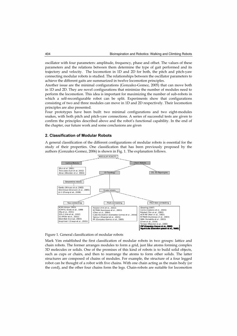
Bioinspiration and Robotics: Walking and Climbing Robots 404
oscillator with four parameters: amplitude, frequency, phase and offset. The values of these parameters and the relations between them determine the type of gait performed and its trajectory and velocity. The locomotion in 1D and 2D for both, the pitch and pitch-yaw connecting modular robots is studied. The relationships between the oscillator parameters to achieve the different gaits are summarized in twelve locomotion principles. Another issue are the minimal configurations (Gonzalez-Gomez, 2005) that can move both in 1D and 2D. They are novel configurations that minimize the number of modules need to perform the locomotion. This idea is important for maximizing the number of sub-robots in which a self-reconfigurable robot can be split. Experiments show that configurations consisting of two and three modules can move in 1D and 2D respectively. Their locomotion principles are also presented. Four prototypes have been built: two minimal configurations and two eight-modules snakes, with both pitch and pitch-yaw connections. A series of successful tests are given to confirm the principles described above and the robot’s functional capability. In the end of the chapter, our future work and some conclusions are given
2. Classification of Modular Robots
A general classification of the different configurations of modular robots is essential for the study of their properties. One classification that has been previously proposed by the authors (Gonzalez-Gomez, 2006) is shown in Fig. 1. The explanation follows.
Figure 1. General classification of modular robots
Mark Yim established the first classification of modular robots in two groups: lattice and chain robots. The former arranges modules to form a grid, just like atoms forming complex 3D molecules or solids. One of the promises of this kind of robots is to build solid objects, such as cups or chairs, and then to rearrange the atoms to form other solids. The latter structures are composed of chains of modules. For example, the structure of a four legged robot can be thought of a robot with five chains. With one chain acting as the main body (or the cord), and the other four chains form the legs. Chain-robots are suitable for locomotion
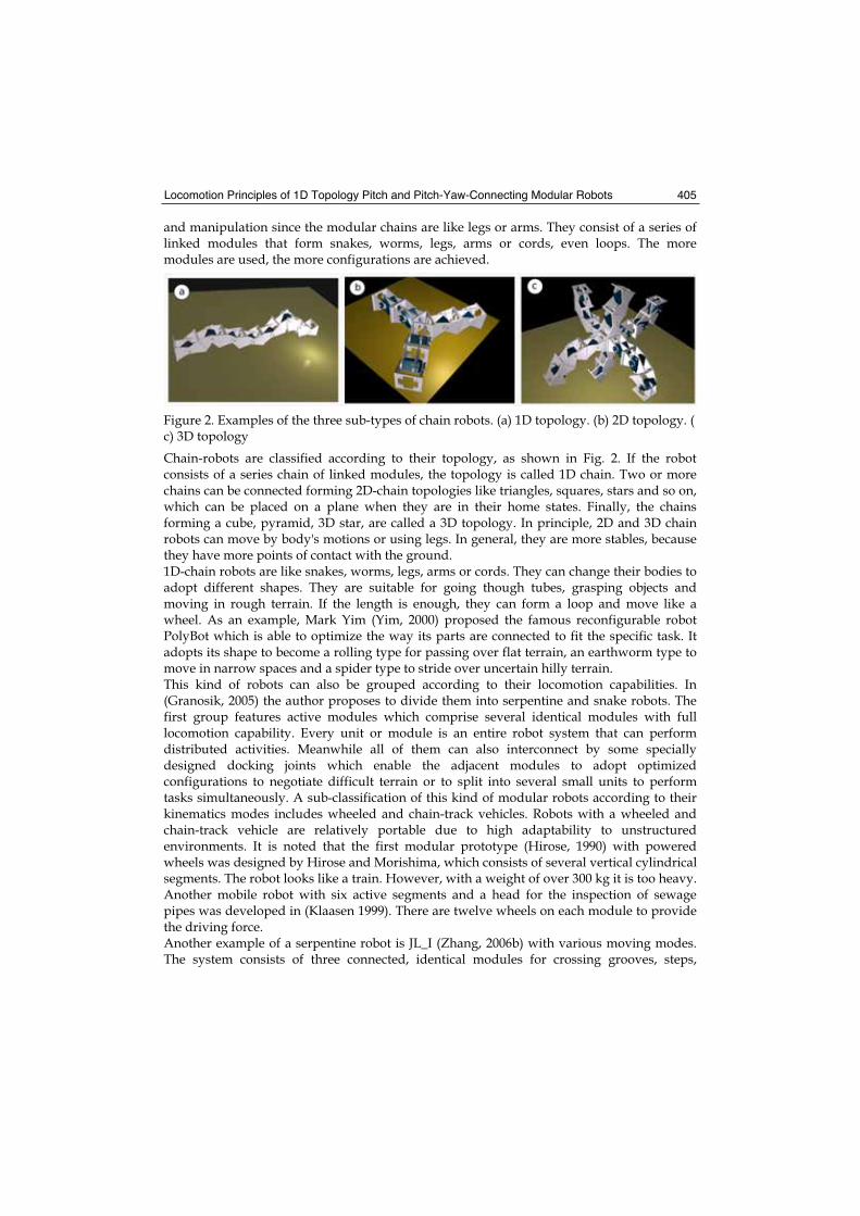
Locomotion Principles of 1D Topology Pitch and Pitch-Yaw-Connecting Modular Robots 405
and manipulation since the modular chains are like legs or arms. They consist of a series of linked modules that form snakes, worms, legs, arms or cords, even loops. The more modules are used, the more configurations are achieved.
Figure 2. Examples of the three sub-types of chain robots. (a) 1D topology. (b) 2D topology. ( c) 3D topology
Chain-robots are classified according to their topology, as shown in Fig. 2. If the robot consists of a series chain of linked modules, the topology is called 1D chain. Two or more chains can be connected forming 2D-chain topologies like triangles, squares, stars and so on, which can be placed on a plane when they are in their home states. Finally, the chains forming a cube, pyramid, 3D star, are called a 3D topology. In principle, 2D and 3D chain robots can move by body's motions or using legs. In general, they are more stables, because they have more points of contact with the ground. 1D-chain robots are like snakes, worms, legs, arms or cords. They can change their bodies to adopt different shapes. They are suitable for going though tubes, grasping objects and moving in rough terrain. If the length is enough, they can form a loop and move like a wheel. As an example, Mark Yim (Yim, 2000) proposed the famous reconfigurable robot PolyBot which is able to optimize the way its parts are connected to fit the specific task. It adopts its shape to become a rolling type for passing over flat terrain, an earthworm type to move in narrow spaces and a spider type to stride over uncertain hilly terrain. This kind of robots can also be grouped according to their locomotion capabilities. In (Granosik, 2005) the author proposes to divide them into serpentine and snake robots. The first group features active modules which comprise several identical modules with full locomotion capability. Every unit or module is an entire robot system that can perform distributed activities. Meanwhile all of them can also interconnect by some specially designed docking joints which enable the adjacent modules to adopt optimized configurations to negotiate difficult terrain or to split into several small units to perform tasks simultaneously. A sub-classification of this kind of modular robots according to their kinematics modes includes wheeled and chain-track vehicles. Robots with a wheeled and chain-track vehicle are relatively portable due to high adaptability to unstructured environments. It is noted that the first modular prototype (Hirose, 1990) with powered wheels was designed by Hirose and Morishima, which consists of several vertical cylindrical segments. The robot looks like a train. However, with a weight of over 300 kg it is too heavy. Another mobile robot with six active segments and a head for the inspection of sewage pipes was developed in (Klaasen 1999). There are twelve wheels on each module to provide the driving force. Another example of a serpentine robot is JL_I (Zhang, 2006b) with various moving modes. The system consists of three connected, identical modules for crossing grooves, steps,
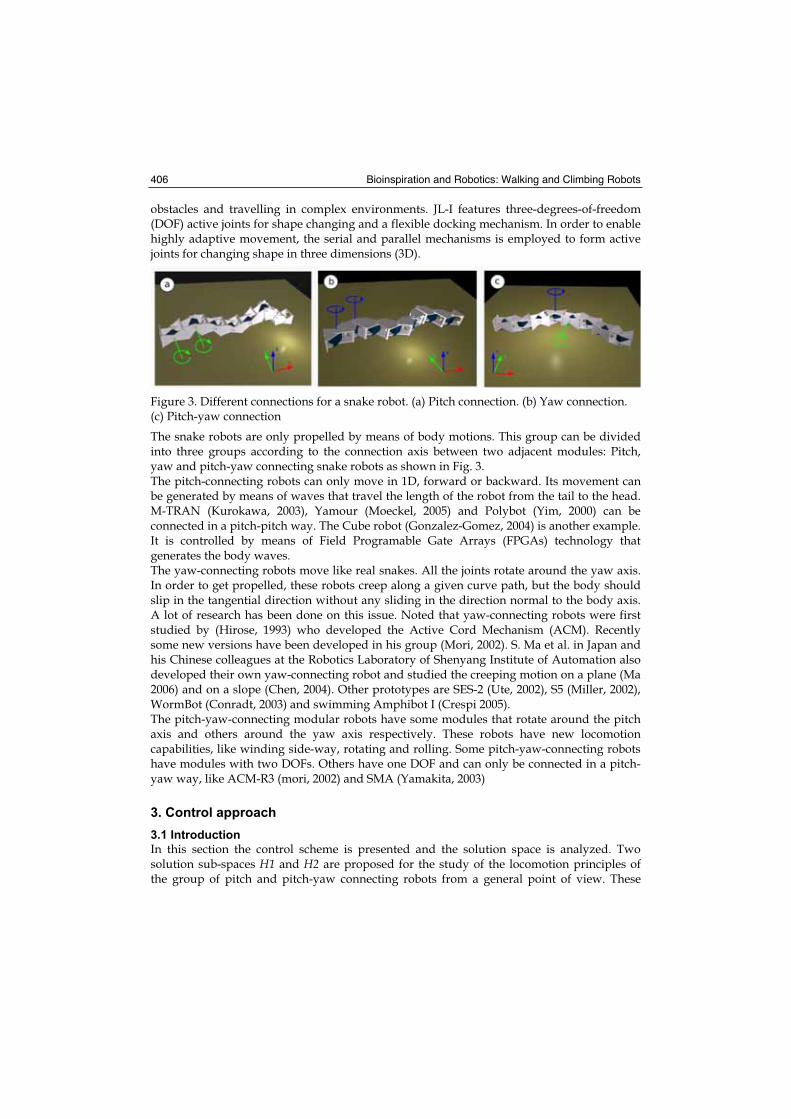
Bioinspiration and Robotics: Walking and Climbing Robots 406
obstacles and travelling in complex environments. JL-I features three-degrees-of-freedom (DOF) active joints for shape changing and a flexible docking mechanism. In order to enable highly adaptive movement, the serial and parallel mechanisms is employed to form active joints for changing shape in three dimensions (3D).
Figure 3. Different connections for a snake robot. (a) Pitch connection. (b) Yaw connection. (c) Pitch-yaw connection
The snake robots are only propelled by means of body motions. This group can be divided into three groups according to the connection axis between two adjacent modules: Pitch, yaw and pitch-yaw connecting snake robots as shown in Fig. 3. The pitch-connecting robots can only move in 1D, forward or backward. Its movement can be generated by means of waves that travel the length of the robot from the tail to the head. M-TRAN (Kurokawa, 2003), Yamour (Moeckel, 2005) and Polybot (Yim, 2000) can be connected in a pitch-pitch way. The Cube robot (Gonzalez-Gomez, 2004) is another example. It is controlled by means of Field Programable Gate Arrays (FPGAs) technology that generates the body waves. The yaw-connecting robots move like real snakes. All the joints rotate around the yaw axis. In order to get propelled, these robots creep along a given curve path, but the body should slip in the tangential direction without any sliding in the direction normal to the body axis. A lot of research has been done on this issue. Noted that yaw-connecting robots were first studied by (Hirose, 1993) who developed the Active Cord Mechanism (ACM). Recently some new versions have been developed in his group (Mori, 2002). S. Ma et al. in Japan and his Chinese colleagues at the Robotics Laboratory of Shenyang Institute of Automation also developed their own yaw-connecting robot and studied the creeping motion on a plane (Ma 2006) and on a slope (Chen, 2004). Other prototypes are SES-2 (Ute, 2002), S5 (Miller, 2002), WormBot (Conradt, 2003) and swimming Amphibot I (Crespi 2005). The pitch-yaw-connecting modular robots have some modules that rotate around the pitch axis and others around the yaw axis respectively. These robots have new locomotion capabilities, like winding side-way, rotating and rolling. Some pitch-yaw-connecting robots have modules with two DOFs. Others have one DOF and can only be connected in a pitch-yaw way, like ACM-R3 (mori, 2002) and SMA (Yamakita, 2003)
3. Control approach
3.1 Introduction
In this section the control scheme is presented and the solution space is analyzed. Two solution sub-spaces H1 and H2 are proposed for the study of the locomotion principles of the group of pitch and pitch-yaw connecting robots from a general point of view. These
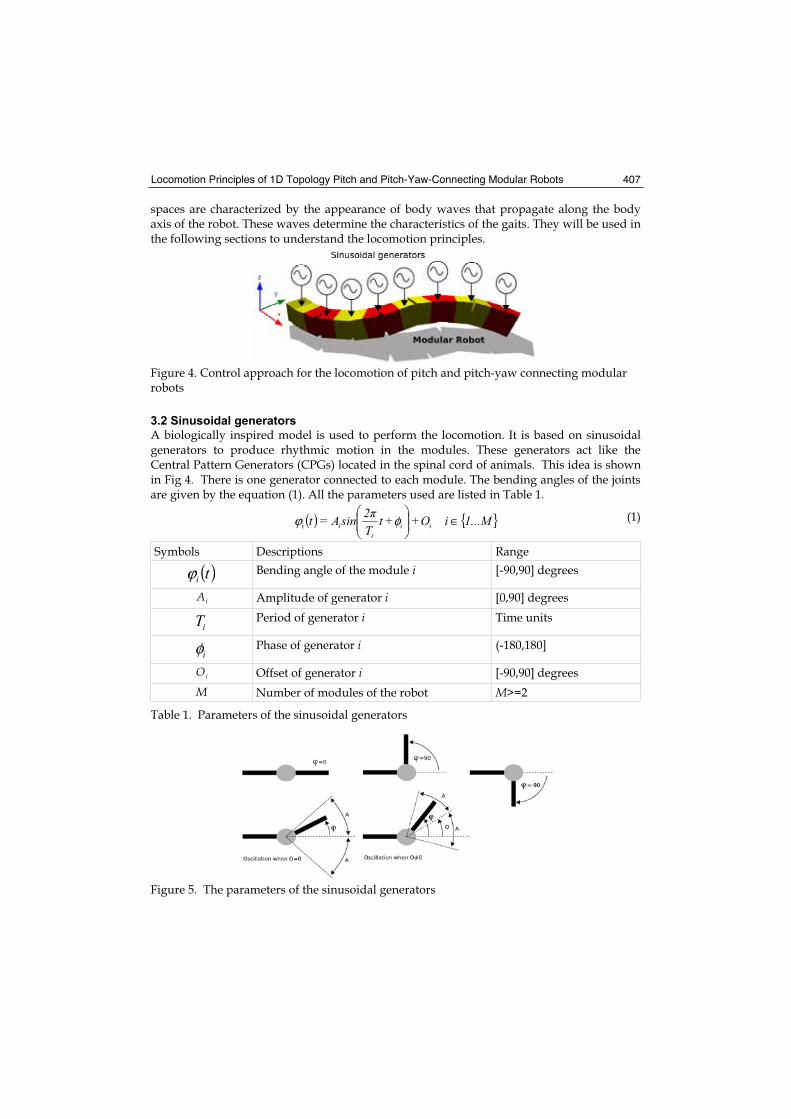
Locomotion Principles of 1D Topology Pitch and Pitch-Yaw-Connecting Modular Robots 407
spaces are characterized by the appearance of body waves that propagate along the body axis of the robot. These waves determine the characteristics of the gaits. They will be used in the following sections to understand the locomotion principles.
Figure 4. Control approach for the locomotion of pitch and pitch-yaw connecting modular robots
3.2 Sinusoidal generators
A biologically inspired model is used to perform the locomotion. It is based on sinusoidal generators to produce rhythmic motion in the modules. These generators act like the Central Pattern Generators (CPGs) located in the spinal cord of animals. This idea is shown in Fig 4. There is one generator connected to each module. The bending angles of the joints are given by the equation (1). All the parameters used are listed in Table 1.
( ) { }1...MiO+tT2sinAt ii
ii ∈+=i φϕ (1)
Symbols Descriptions Range
( )tiϕ Bending angle of the module i [-90,90] degrees
Ai Amplitude of generator i [0,90] degrees
iT Period of generator i Time units
iφ Phase of generator i (-180,180]
Oi Offset of generator i [-90,90] degrees
M Number of modules of the robot M>=2
Table 1. Parameters of the sinusoidal generators
Figure 5. The parameters of the sinusoidal generators
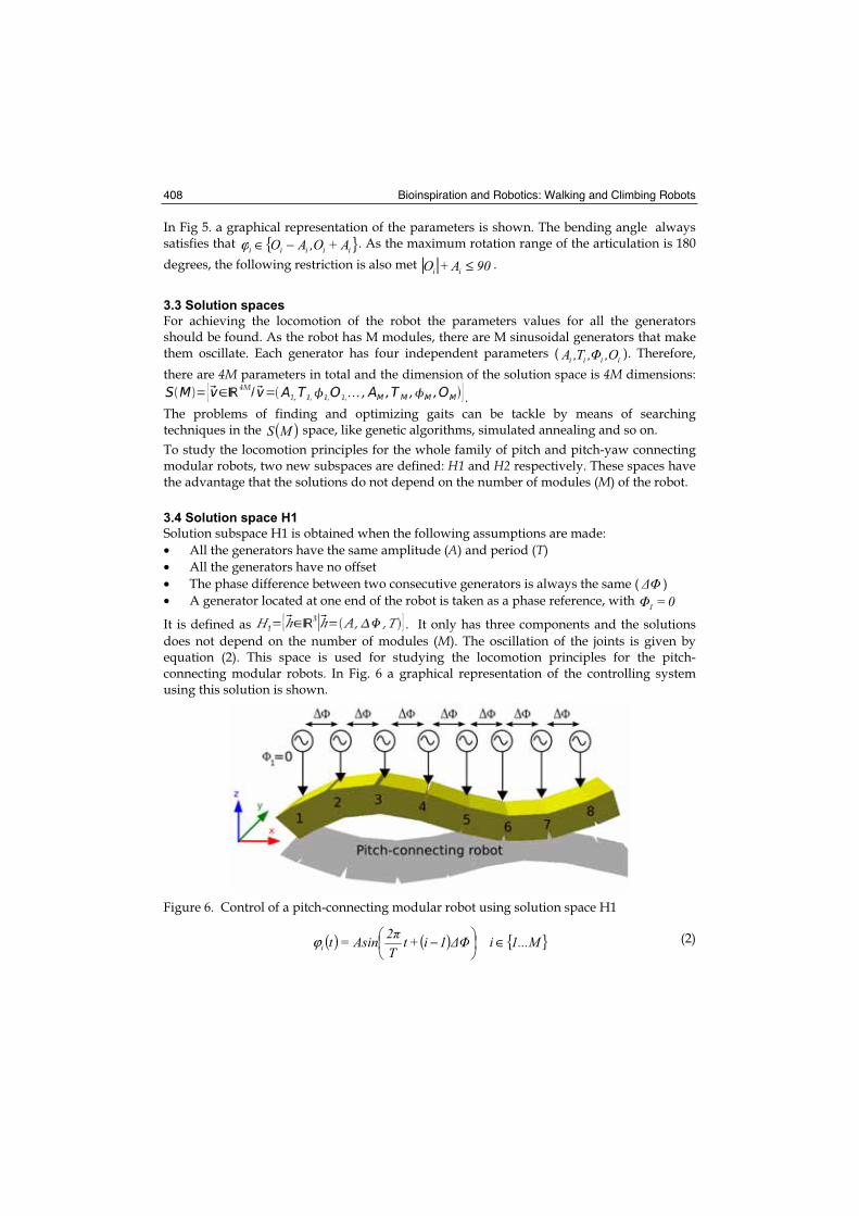
Bioinspiration and Robotics: Walking and Climbing Robots 408
In Fig 5. a graphical representation of the parameters is shown. The bending angle always satisfies that { }iiiii A+O,AO −∈ϕ . As the maximum rotation range of the articulation is 180
degrees, the following restriction is also met | | 90A+O ii ≤ .
3.3 Solution spaces
For achieving the locomotion of the robot the parameters values for all the generators should be found. As the robot has M modules, there are M sinusoidal generators that make them oscillate. Each generator has four independent parameters ( iiii O,,T,A ). Therefore,
there are 4M parameters in total and the dimension of the solution space is 4M dimensions:
.The problems of finding and optimizing gaits can be tackle by means of searching techniques in the ( )MS space, like genetic algorithms, simulated annealing and so on.
To study the locomotion principles for the whole family of pitch and pitch-yaw connecting modular robots, two new subspaces are defined: H1 and H2 respectively. These spaces have the advantage that the solutions do not depend on the number of modules (M) of the robot.
3.4 Solution space H1
Solution subspace H1 is obtained when the following assumptions are made:
• All the generators have the same amplitude (A) and period (T)
• All the generators have no offset
• The phase difference between two consecutive generators is always the same ( )
• A generator located at one end of the robot is taken as a phase reference, with 01 =
It is defined as . It only has three components and the solutions
does not depend on the number of modules (M). The oscillation of the joints is given by equation (2). This space is used for studying the locomotion principles for the pitch-connecting modular robots. In Fig. 6 a graphical representation of the controlling system using this solution is shown.
Figure 6. Control of a pitch-connecting modular robot using solution space H1
( ) ( ) { }1...Mi1i+tT2Asinti ∈−=ϕ (2)
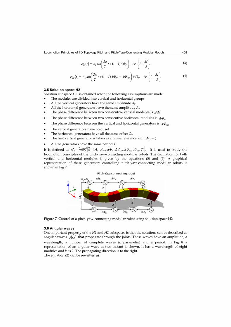
Locomotion Principles of 1D Topology Pitch and Pitch-Yaw-Connecting Modular Robots 409
( ) ( ) ∈−2M1...i1i+t
T2sinA=t VVViϕ (3)
( ) ( ) ∈−2M1...iO++1i+t
T2sinA=t HVHHHHiϕ (4)
3.5 Solution space H2
Solution subspace H2 is obtained when the following assumptions are made:
• The modules are divided into vertical and horizontal groups
• All the vertical generators have the same amplitude Av
• All the horizontal generators have the same amplitude Ah
• The phase difference between two consecutive vertical modules is v
• The phase difference between two consecutive horizontal modules is H
• The phase difference between the vertical and horizontal generators is VH
• The vertical generators have no offset
• The horizontal generators have all the same offset Oh
• The first vertical generator is taken as a phase reference with 0=v1
• All the generators have the same period TIt is defined as . It is used to study the
locomotion principles of the pitch-yaw-connecting modular robots. The oscillation for both vertical and horizontal modules is given by the equations (3) and (4). A graphical representation of these generators controlling pitch-yaw-connecting modular robots is shown in Fig 7.
Figure 7. Control of a pitch-yaw-connecting modular robot using solution space H2
3.6 Angular waves
One important property of the H1 and H2 subspaces is that the solutions can be described as angular waves ( )it,ϕ that propagate through the joints. These waves have an amplitude, a
wavelength, a number of complete waves (k parameter) and a period. In Fig 8 a representation of an angular wave at two instant is shown. It has a wavelength of eight modules and k is 2. The propagating direction is to the right. The equation (2) can be rewritten as:
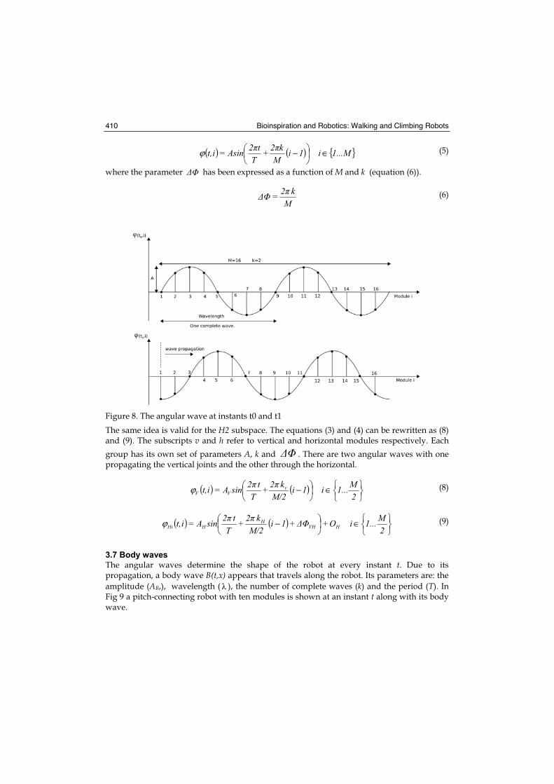
Bioinspiration and Robotics: Walking and Climbing Robots 410
( ) ( ) { }1...Mi1iM
k2+T
t2Asin=it, ∈−ϕ (5)
where the parameter has been expressed as a function of M and k (equation (6)).
Mk2= (6)
Figure 8. The angular wave at instants t0 and t1
The same idea is valid for the H2 subspace. The equations (3) and (4) can be rewritten as (8) and (9). The subscripts v and h refer to vertical and horizontal modules respectively. Each
group has its own set of parameters A, k and . There are two angular waves with one propagating the vertical joints and the other through the horizontal.
( ) ( ) ∈−2M1...i1i
M/2k2+
Tt2sinA=it, v
VVϕ (8)
( ) ( ) ∈−2M1...iO++1i
M/2k2+
Tt2sinA=it, HVH
HHHiϕ (9)
3.7 Body waves
The angular waves determine the shape of the robot at every instant t. Due to its propagation, a body wave B(t,x) appears that travels along the robot. Its parameters are: the
amplitude (AB,), wavelength ( ), the number of complete waves (k) and the period (T). In Fig 9 a pitch-connecting robot with ten modules is shown at an instant t along with its body wave.
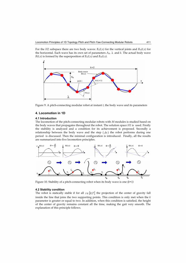
Locomotion Principles of 1D Topology Pitch and Pitch-Yaw-Connecting Modular Robots 411
For the H2 subspace there are two body waves: Bv(t,x) for the vertical joints and BH(t,x) for
the horizontal. Each wave has its own set of parameters AB, and k. The actual body wave B(t,x) is formed by the superposition of Bv(t,x) and BH(t,x).
Figure 9. A pitch-connecting modular robot at instant t, the body wave and its parameters
4. Locomotion in 1D
4.1 Introduction
The locomotion of the pitch-connecting modular robots with M modules is studied based on the body waves that propagates throughout the robot. The solution space H1 is used. Firstly the stability is analyzed and a condition for its achievement is proposed. Secondly a
relationship between the body wave and the step ( x ) the robot performs during one
period is discussed. Then the minimal configuration is introduced. Finally, all the results are summarized into five locomotion principles.
Figure 10. Stability of a pitch-connecting robot when its body wave is one (k=1)
4.2 Stability condition
The robot is statically stable if for all [ ]T0,t ∈ the projection of the center of gravity fall
inside the line that joins the two supporting points. This condition is only met when the kparameter is greater or equal to two. In addition, when this condition is satisfied, the height of the center of gravity remains constant all the time, making the gait very smooth. The explanation of this principle follows.
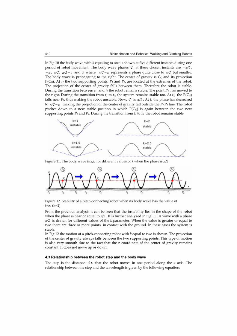
Bioinspiration and Robotics: Walking and Climbing Robots 412
In Fig 10 the body wave with k equaling to one is shown at five different instants during one
period of robot movement. The body wave phases at these chosen instants are /2− ,− , /2 , /2 − and 0, where /2 − represents a phase quite close to /2 but smaller.
The body wave is propagating to the right. The center of gravity is CG and its projection P(CG). At t1 the two supporting points, P1 and P2, are located at the extremes of the robot. The projection of the center of gravity falls between them. Therefore the robot is stable. During the transition between t1 and t2 the robot remains stable. The point P1 has moved to the right. During the transition from t2 to t3, the system remains stable too. At t3, the P(CG)
falls near P1, thus making the robot unstable. Now, is /2 . At t4 the phase has decreased
to /2 − making the projection of the center of gravity fall outside the P1 P2 line. The robot
pitches down to a new stable position in which P(CG) is again between the two new supporting points P3 and P4. During the transition from t4 to t5 the robot remains stable.
Figure 11. The body wave B(x,t) for different values of k when the phase is /2
Figure 12. Stability of a pitch-connecting robot when its body wave has the value of two (k=2)
From the previous analysis it can be seen that the instability lies in the shape of the robot when the phase is near or equal to /2 . It is further analyzed in Fig. 11. A wave with a phase
/2 is drawn for different values of the k parameter. When the value is greater or equal to two there are three or more points in contact with the ground. In these cases the system is stable. In Fig 12 the motion of a pitch-connecting robot with k equal to two is shown. The projection of the center of gravity always falls between the two supporting points. This type of motion is also very smooth due to the fact that the z coordinate of the center of gravity remains constant. It does not move up or down.
4.3 Relationship between the robot step and the body wave
The step is the distance x that the robot moves in one period along the x axis. The
relationship between the step and the wavelength is given by the following equation:
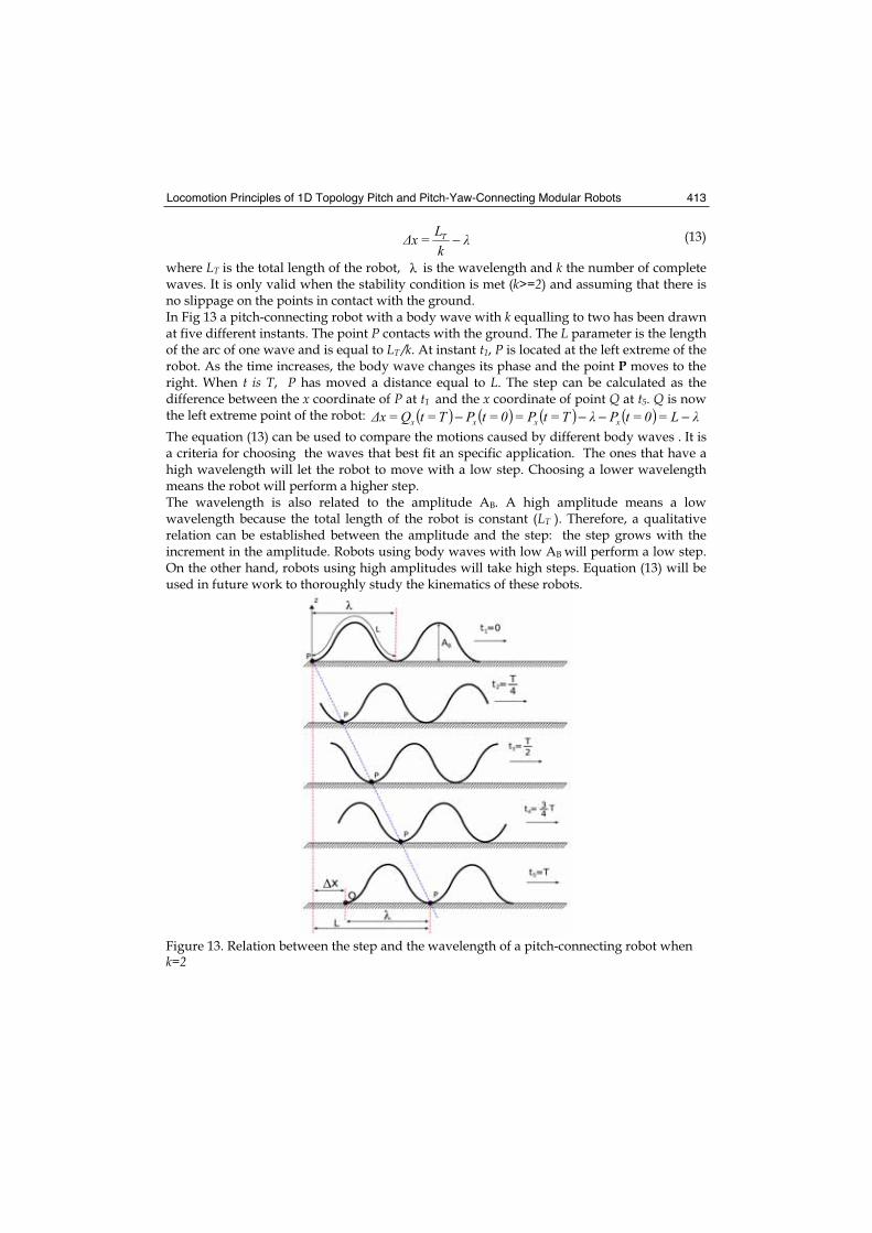
Locomotion Principles of 1D Topology Pitch and Pitch-Yaw-Connecting Modular Robots 413
kL=x T − (13)
where LT is the total length of the robot, is the wavelength and k the number of complete waves. It is only valid when the stability condition is met (k>=2) and assuming that there is no slippage on the points in contact with the ground. In Fig 13 a pitch-connecting robot with a body wave with k equalling to two has been drawn at five different instants. The point P contacts with the ground. The L parameter is the length of the arc of one wave and is equal to LT /k. At instant t1, P is located at the left extreme of the robot. As the time increases, the body wave changes its phase and the point P moves to the right. When t is T, P has moved a distance equal to L. The step can be calculated as the difference between the x coordinate of P at t1 and the x coordinate of point Q at t5. Q is now the left extreme point of the robot: ( ) ( ) ( ) ( ) L=0=tPT=tP=0=tPT=tQ=x xxxx −−−−The equation (13) can be used to compare the motions caused by different body waves . It is a criteria for choosing the waves that best fit an specific application. The ones that have a high wavelength will let the robot to move with a low step. Choosing a lower wavelength means the robot will perform a higher step. The wavelength is also related to the amplitude AB. A high amplitude means a low wavelength because the total length of the robot is constant (LT ). Therefore, a qualitative relation can be established between the amplitude and the step: the step grows with the increment in the amplitude. Robots using body waves with low AB will perform a low step. On the other hand, robots using high amplitudes will take high steps. Equation (13) will be used in future work to thoroughly study the kinematics of these robots.
Figure 13. Relation between the step and the wavelength of a pitch-connecting robot when k=2
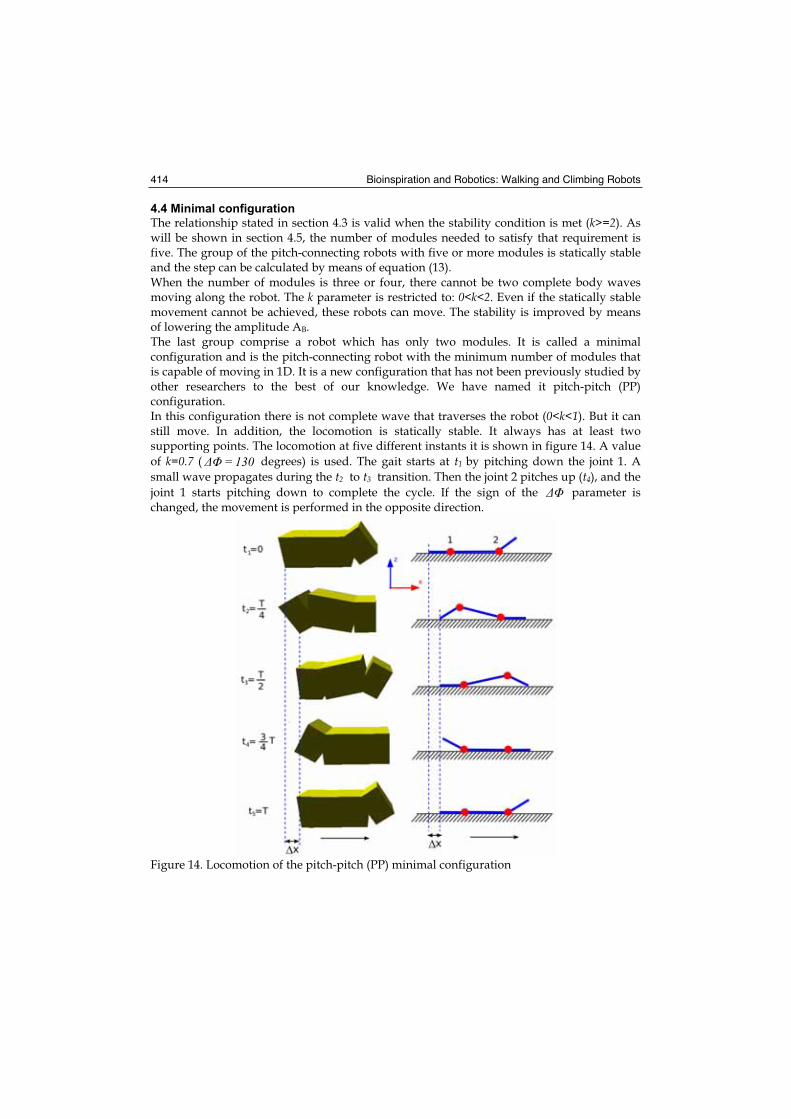
Bioinspiration and Robotics: Walking and Climbing Robots 414
4.4 Minimal configuration
The relationship stated in section 4.3 is valid when the stability condition is met (k>=2). As will be shown in section 4.5, the number of modules needed to satisfy that requirement is five. The group of the pitch-connecting robots with five or more modules is statically stable and the step can be calculated by means of equation (13). When the number of modules is three or four, there cannot be two complete body waves moving along the robot. The k parameter is restricted to: 0<k<2. Even if the statically stable movement cannot be achieved, these robots can move. The stability is improved by means of lowering the amplitude AB.The last group comprise a robot which has only two modules. It is called a minimal configuration and is the pitch-connecting robot with the minimum number of modules that is capable of moving in 1D. It is a new configuration that has not been previously studied by other researchers to the best of our knowledge. We have named it pitch-pitch (PP) configuration. In this configuration there is not complete wave that traverses the robot (0<k<1). But it can still move. In addition, the locomotion is statically stable. It always has at least two supporting points. The locomotion at five different instants it is shown in figure 14. A value
of k=0.7 ( 130= degrees) is used. The gait starts at t1 by pitching down the joint 1. A
small wave propagates during the t2 to t3 transition. Then the joint 2 pitches up (t4), and the
joint 1 starts pitching down to complete the cycle. If the sign of the parameter is changed, the movement is performed in the opposite direction.
Figure 14. Locomotion of the pitch-pitch (PP) minimal configuration
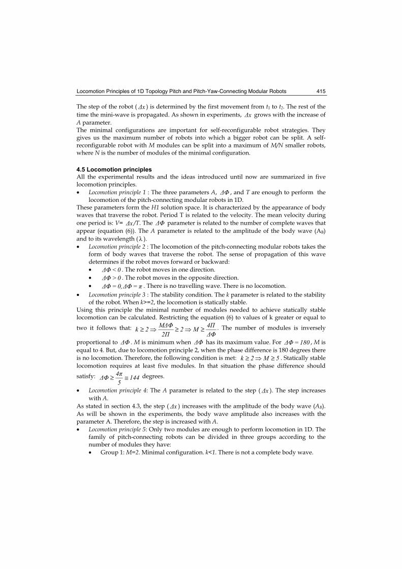
Locomotion Principles of 1D Topology Pitch and Pitch-Yaw-Connecting Modular Robots 415
The step of the robot ( x ) is determined by the first movement from t1 to t2. The rest of the
time the mini-wave is propagated. As shown in experiments, x grows with the increase of
A parameter. The minimal configurations are important for self-reconfigurable robot strategies. They gives us the maximum number of robots into which a bigger robot can be split. A self-reconfigurable robot with M modules can be split into a maximum of M/N smaller robots, where N is the number of modules of the minimal configuration.
4.5 Locomotion principles
All the experimental results and the ideas introduced until now are summarized in five locomotion principles.
• Locomotion principle 1 : The three parameters A, , and T are enough to perform the locomotion of the pitch-connecting modular robots in 1D.
These parameters form the H1 solution space. It is characterized by the appearance of body waves that traverse the robot. Period T is related to the velocity. The mean velocity during
one period is: V= x /T. The parameter is related to the number of complete waves that
appear (equation (6)). The A parameter is related to the amplitude of the body wave (AB)
and to its wavelength ( ).
• Locomotion principle 2 : The locomotion of the pitch-connecting modular robots takes the form of body waves that traverse the robot. The sense of propagation of this wave determines if the robot moves forward or backward:
• 0< . The robot moves in one direction.
• 0> . The robot moves in the opposite direction.
• =0,= . There is no travelling wave. There is no locomotion.
• Locomotion principle 3 : The stability condition. The k parameter is related to the stability of the robot. When k>=2, the locomotion is statically stable.
Using this principle the minimal number of modules needed to achieve statically stable locomotion can be calculated. Restricting the equation (6) to values of k greater or equal to
two it follows that: 4M22
M2k ≥≥≥ . The number of modules is inversely
proportional to . M is minimum when has its maximum value. For 180= , M is
equal to 4. But, due to locomotion principle 2, when the phase difference is 180 degrees there
is no locomotion. Therefore, the following condition is met: 5M2k ≥≥ . Statically stable
locomotion requires at least five modules. In that situation the phase difference should
satisfy: 1445
4 ≅≥ degrees.
• Locomotion principle 4: The A parameter is related to the step ( x ). The step increases
with A. As stated in section 4.3, the step ( x ) increases with the amplitude of the body wave (AB).
As will be shown in the experiments, the body wave amplitude also increases with the parameter A. Therefore, the step is increased with A.
• Locomotion principle 5: Only two modules are enough to perform locomotion in 1D. The family of pitch-connecting robots can be divided in three groups according to the number of modules they have:
• Group 1: M=2. Minimal configuration. k<1. There is not a complete body wave.
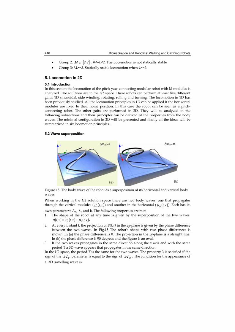
Bioinspiration and Robotics: Walking and Climbing Robots 416
• Group 2: [ ]3,4M ∈ . 0<=k<2. The Locomotion is not statically stable
• Group 3: M>=5. Statically stable locomotion when k>=2.
5. Locomotion in 2D
5.1 Introduction
In this section the locomotion of the pitch-yaw-connecting modular robot with M modules is analyzed. The solutions are in the H2 space. These robots can perform at least five different gaits: 1D sinusoidal, side winding, rotating, rolling and turning. The locomotion in 1D has been previously studied. All the locomotion principles in 1D can be applied if the horizontal modules are fixed to their home position. In this case the robot can be seen as a pitch-connecting robot. The other gaits are performed in 2D. They will be analyzed in the following subsections and their principles can be derived of the properties from the body waves. The minimal configuration in 2D will be presented and finally all the ideas will be summarized in six locomotion principles.
5.2 Wave superposition
Figure 15. The body wave of the robot as a superposition of its horizontal and vertical body waves
When working in the H2 solution space there are two body waves: one that propagates through the vertical modules ( ( )xt,Bv ) and another in the horizontal ( ( )xt,BH ). Each has its
own parameters: AB, , and k. The following properties are met: 1. The shape of the robot at any time is given by the superposition of the two waves:
( ) ( ) ( )xt,B+xt,B=xt,B hv .
2. At every instant t, the projection of B(t,x) in the zy-plane is given by the phase difference between the two waves. In Fig.15 The robot's shape with two phase differences is shown. In (a) the phase difference is 0. The projection in the zy-plane is a straight line. In (b) the phase difference is 90 degrees and the figure is an oval.
3. If the two waves propagates in the same direction along the x axis and with the same period T a 3D wave appears that propagates in the same direction.
In the H2 space, the period T is the same for the two waves. The property 3 is satisfied if the sign of the V parameter is equal to the sign of H . The condition for the appearance of
a 3D travelling wave is:
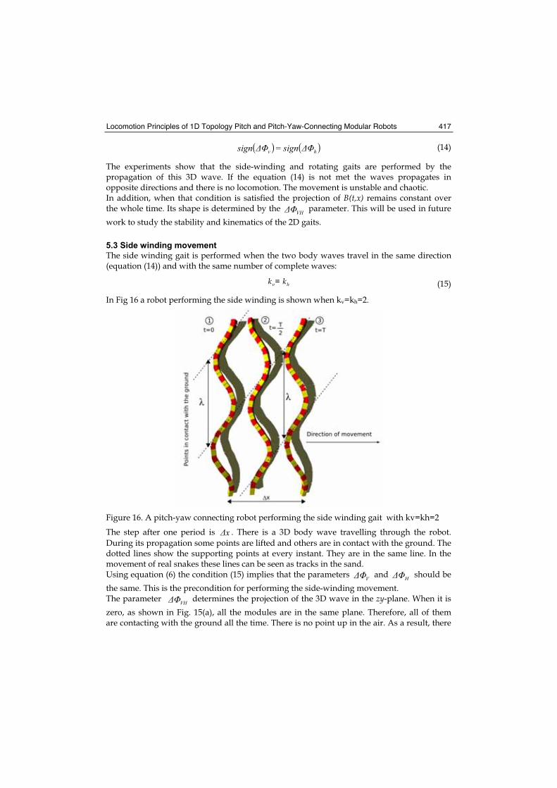
Locomotion Principles of 1D Topology Pitch and Pitch-Yaw-Connecting Modular Robots 417
( ) ( )hv sign=sign (14)
The experiments show that the side-winding and rotating gaits are performed by the propagation of this 3D wave. If the equation (14) is not met the waves propagates in opposite directions and there is no locomotion. The movement is unstable and chaotic. In addition, when that condition is satisfied the projection of B(t,x) remains constant over the whole time. Its shape is determined by the VH parameter. This will be used in future
work to study the stability and kinematics of the 2D gaits.
5.3 Side winding movement
The side winding gait is performed when the two body waves travel in the same direction (equation (14)) and with the same number of complete waves:
kv= kh (15)
In Fig 16 a robot performing the side winding is shown when kv=kh=2.
Figure 16. A pitch-yaw connecting robot performing the side winding gait with kv=kh=2
The step after one period is x . There is a 3D body wave travelling through the robot.
During its propagation some points are lifted and others are in contact with the ground. The dotted lines show the supporting points at every instant. They are in the same line. In the movement of real snakes these lines can be seen as tracks in the sand. Using equation (6) the condition (15) implies that the parameters V and H should be
the same. This is the precondition for performing the side-winding movement. The parameter VH determines the projection of the 3D wave in the zy-plane. When it is
zero, as shown in Fig. 15(a), all the modules are in the same plane. Therefore, all of them are contacting with the ground all the time. There is no point up in the air. As a result, there
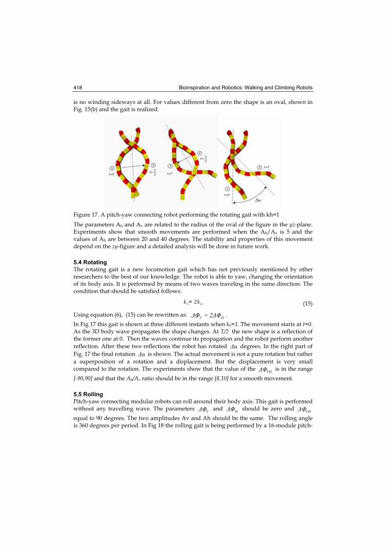
Bioinspiration and Robotics: Walking and Climbing Robots 418
is no winding sideways at all. For values different from zero the shape is an oval, shown in Fig. 15(b) and the gait is realized.
Figure 17. A pitch-yaw connecting robot performing the rotating gait with kh=1
The parameters Ah and Av are related to the radius of the oval of the figure in the yz-plane. Experiments show that smooth movements are performed when the Ah/Av is 5 and the values of Ah are between 20 and 40 degrees. The stability and properties of this movement depend on the zy-figure and a detailed analysis will be done in future work.
5.4 Rotating
The rotating gait is a new locomotion gait which has not previously mentioned by other researchers to the best of our knowledge. The robot is able to yaw, changing the orientation of its body axis. It is performed by means of two waves traveling in the same direction. The condition that should be satisfied follows:
kv= 2k h (15)
Using equation (6), (15) can be rewritten as: HV 2= .
In Fig 17 this gait is shown at three different instants when kh=1. The movement starts at t=0.As the 3D body wave propagates the shape changes. At T/2 the new shape is a reflection of the former one at 0. Then the waves continue its propagation and the robot perform another
reflection. After these two reflections the robot has rotated degrees. In the right part of
Fig. 17 the final rotation is shown. The actual movement is not a pure rotation but rather
a superposition of a rotation and a displacement. But the displacement is very small compared to the rotation. The experiments show that the value of the VH is in the range
[-90,90] and that the Ah/Av ratio should be in the range [8,10] for a smooth movement.
5.5 Rolling
Pitch-yaw connecting modular robots can roll around their body axis. This gait is performed without any travelling wave. The parameters V and H should be zero and VH
equal to 90 degrees. The two amplitudes Av and Ah should be the same. The rolling angle is 360 degrees per period. In Fig 18 the rolling gait is being performed by a 16-module pitch-
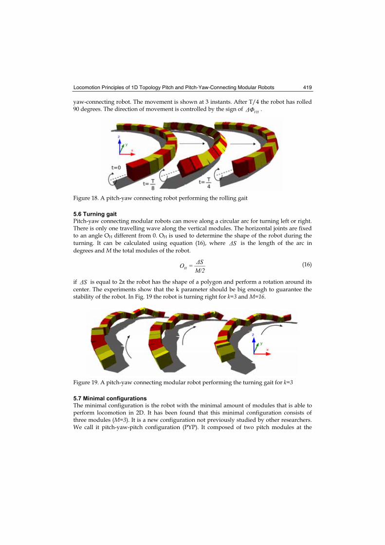
Locomotion Principles of 1D Topology Pitch and Pitch-Yaw-Connecting Modular Robots 419
yaw-connecting robot. The movement is shown at 3 instants. After T/4 the robot has rolled 90 degrees. The direction of movement is controlled by the sign of VH .
Figure 18. A pitch-yaw connecting robot performing the rolling gait
5.6 Turning gait
Pitch-yaw connecting modular robots can move along a circular arc for turning left or right. There is only one travelling wave along the vertical modules. The horizontal joints are fixed to an angle OH different from 0. OH is used to determine the shape of the robot during the
turning. It can be calculated using equation (16), where S is the length of the arc in
degrees and M the total modules of the robot.
M/2S=OH
(16)
if S is equal to 2 the robot has the shape of a polygon and perform a rotation around its
center. The experiments show that the k parameter should be big enough to guarantee the stability of the robot. In Fig. 19 the robot is turning right for k=3 and M=16.
Figure 19. A pitch-yaw connecting modular robot performing the turning gait for k=3
5.7 Minimal configurations
The minimal configuration is the robot with the minimal amount of modules that is able to perform locomotion in 2D. It has been found that this minimal configuration consists of three modules (M=3). It is a new configuration not previously studied by other researchers. We call it pitch-yaw-pitch configuration (PYP). It composed of two pitch modules at the
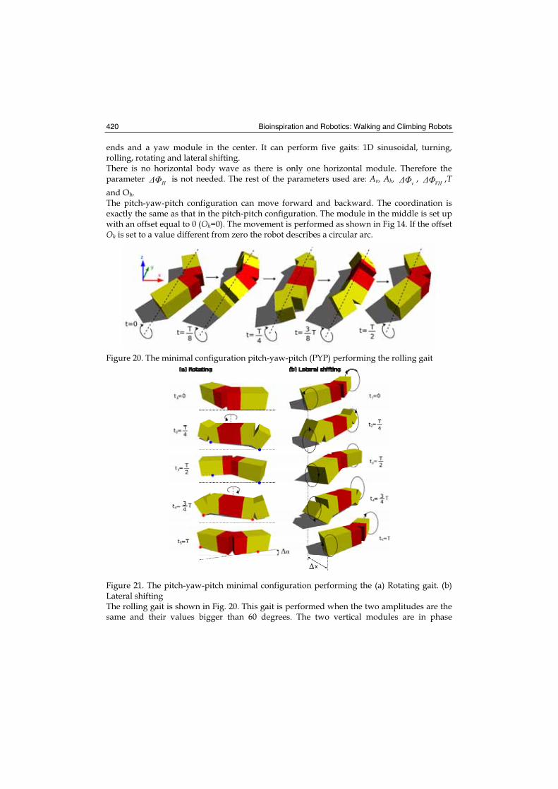
Bioinspiration and Robotics: Walking and Climbing Robots 420
ends and a yaw module in the center. It can perform five gaits: 1D sinusoidal, turning, rolling, rotating and lateral shifting. There is no horizontal body wave as there is only one horizontal module. Therefore the parameter H is not needed. The rest of the parameters used are: Av, Ah, v , VH ,Tand Oh.The pitch-yaw-pitch configuration can move forward and backward. The coordination is exactly the same as that in the pitch-pitch configuration. The module in the middle is set up with an offset equal to 0 (Oh=0). The movement is performed as shown in Fig 14. If the offset Oh is set to a value different from zero the robot describes a circular arc.
Figure 20. The minimal configuration pitch-yaw-pitch (PYP) performing the rolling gait
Figure 21. The pitch-yaw-pitch minimal configuration performing the (a) Rotating gait. (b) Lateral shifting The rolling gait is shown in Fig. 20. This gait is performed when the two amplitudes are the same and their values bigger than 60 degrees. The two vertical modules are in phase
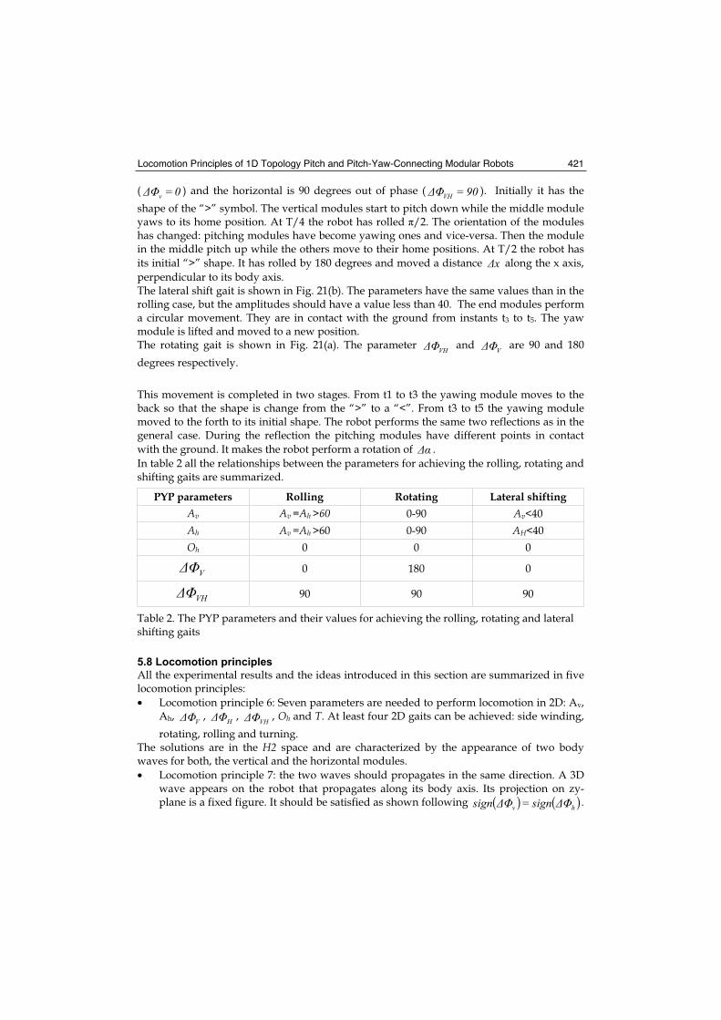
Locomotion Principles of 1D Topology Pitch and Pitch-Yaw-Connecting Modular Robots 421
( 0=v ) and the horizontal is 90 degrees out of phase ( 90=VH ). Initially it has the
shape of the “>” symbol. The vertical modules start to pitch down while the middle module yaws to its home position. At T/4 the robot has rolled /2. The orientation of the modules has changed: pitching modules have become yawing ones and vice-versa. Then the module in the middle pitch up while the others move to their home positions. At T/2 the robot has
its initial “>” shape. It has rolled by 180 degrees and moved a distance x along the x axis,
perpendicular to its body axis. The lateral shift gait is shown in Fig. 21(b). The parameters have the same values than in the rolling case, but the amplitudes should have a value less than 40. The end modules perform a circular movement. They are in contact with the ground from instants t3 to t5. The yaw module is lifted and moved to a new position. The rotating gait is shown in Fig. 21(a). The parameter VH and V are 90 and 180
degrees respectively.
This movement is completed in two stages. From t1 to t3 the yawing module moves to the back so that the shape is change from the “>” to a “<”. From t3 to t5 the yawing module moved to the forth to its initial shape. The robot performs the same two reflections as in the general case. During the reflection the pitching modules have different points in contact
with the ground. It makes the robot perform a rotation of .
In table 2 all the relationships between the parameters for achieving the rolling, rotating and shifting gaits are summarized.
PYP parameters Rolling Rotating Lateral shifting Av Av =Ah >60 0-90 Av<40
Ah Av =Ah >60 0-90 AH<40
Oh 0 0 0
V 0 180 0
VH 90 90 90
Table 2. The PYP parameters and their values for achieving the rolling, rotating and lateral shifting gaits
5.8 Locomotion principles
All the experimental results and the ideas introduced in this section are summarized in five locomotion principles:
• Locomotion principle 6: Seven parameters are needed to perform locomotion in 2D: Av,Ah, V , H , VH , Oh and T. At least four 2D gaits can be achieved: side winding,
rotating, rolling and turning. The solutions are in the H2 space and are characterized by the appearance of two body waves for both, the vertical and the horizontal modules.
• Locomotion principle 7: the two waves should propagates in the same direction. A 3D wave appears on the robot that propagates along its body axis. Its projection on zy-plane is a fixed figure. It should be satisfied as shown following ( ) ( )hv sign=sign .
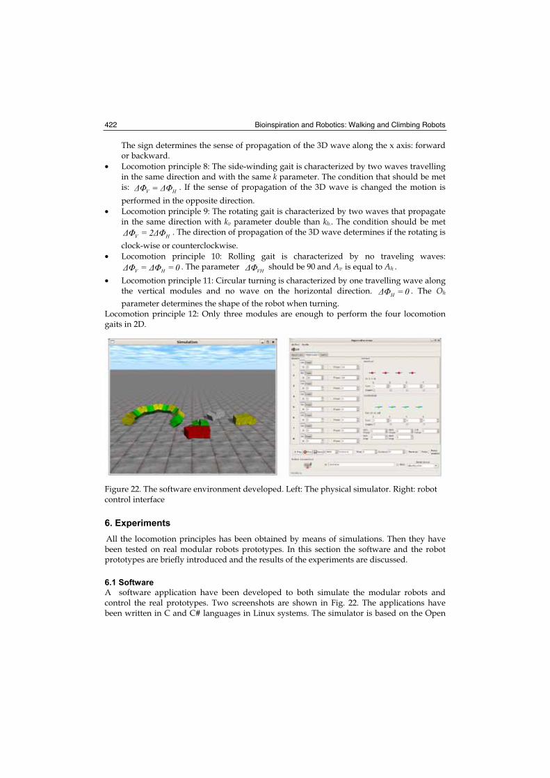
Bioinspiration and Robotics: Walking and Climbing Robots 422
The sign determines the sense of propagation of the 3D wave along the x axis: forward or backward.
• Locomotion principle 8: The side-winding gait is characterized by two waves travelling in the same direction and with the same k parameter. The condition that should be met is: HV = . If the sense of propagation of the 3D wave is changed the motion is
performed in the opposite direction.
• Locomotion principle 9: The rotating gait is characterized by two waves that propagate in the same direction with kv parameter double than kh.. The condition should be met
HV 2= . The direction of propagation of the 3D wave determines if the rotating is
clock-wise or counterclockwise.
• Locomotion principle 10: Rolling gait is characterized by no traveling waves:
0== HV . The parameter VH should be 90 and Av is equal to Ah .
• Locomotion principle 11: Circular turning is characterized by one travelling wave along the vertical modules and no wave on the horizontal direction. 0=H . The Oh
parameter determines the shape of the robot when turning. Locomotion principle 12: Only three modules are enough to perform the four locomotion gaits in 2D.
Figure 22. The software environment developed. Left: The physical simulator. Right: robot control interface
6. Experiments
All the locomotion principles has been obtained by means of simulations. Then they have been tested on real modular robots prototypes. In this section the software and the robot prototypes are briefly introduced and the results of the experiments are discussed.
6.1 Software
A software application have been developed to both simulate the modular robots and control the real prototypes. Two screenshots are shown in Fig. 22. The applications have been written in C and C# languages in Linux systems. The simulator is based on the Open
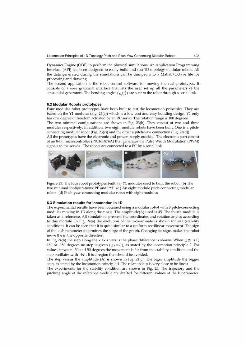
Locomotion Principles of 1D Topology Pitch and Pitch-Yaw-Connecting Modular Robots 423
Dynamics Engine (ODE) to perform the physical simulations. An Application Programming Interface (API) has been designed to easily build and test 1D topology modular robots. All the data generated during the simulations can be dumped into a Matlab/Octave file for processing and drawing.The second application is the robot control software for moving the real prototypes. It consists of a user graphical interface that lets the user set up all the parameters of the sinusoidal generators. The bending angles ( ( )tiϕ ) are sent to the robot through a serial link.
6.2 Modular Robots prototypes
Four modular robot prototypes have been built to test the locomotion principles. They are based on the Y1 modules (Fig. 23(a)) which is a low cost and easy building design. Y1 only has one degree of freedom actuated by an RC servo. The rotation range is 180 degrees. The two minimal configurations are shown in Fig. 23(b). They consist of two and three modules respectively. In addition, two eight module robots have been built. One is a pitch-connecting modular robot (Fig. 23(c)) and the other a pitch-yaw connection (Fig. 23(d)). All the prototypes have the electronic and power supply outside. The electronic part consist of an 8-bit microcontroller (PIC16F876A) that generates the Pulse Width Modulation (PWM) signals to the servos. The robots are connected to a PC by a serial link.
Figure 23. The four robot prototypes built. (a) Y1 modules used to built the robot. (b) The two minimal configurations: PP and PYP. (c ) An eight module pitch-connecting modular robot . (d) Pitch-yaw-connecting modular robot with eight modules
6.3 Simulation results for locomotion in 1D
The experimental results have been obtained using a modular robot with 8 pitch-connecting modules moving in 1D along the x axis. The amplitude(A) used is 45. The fourth module is taken as a reference. All simulations presents the coordinates and rotation angles according to this module. In Fig. 24(a) the evolution of the x-coordinate is shown for k=2 (stability condition). It can be seen that it is quite similar to a uniform rectilinear movement. The sign
of the parameter determines the slope of the graph. Changing its signs makes the robot move the in the opposite direction.
In Fig 24(b) the step along the x axis versus the phase difference is shown. When is 0,
180 or -180 degrees no step is given ( 0=x ), as stated by the locomotion principle 2. For
values between -50 and 50 degrees the movement is far from the stability condition and the
step oscillates with . It is a region that should be avoided. The step versus the amplitude (A) is shown in Fig. 24(c). The biger amplitude the bigger step, as stated by the locomotion principle 4. The relationship is very close to be linear. The experiments for the stability condition are shown in Fig. 25. The trajectory and the pitching angle of the reference module are drafted for different values of the k parameter.
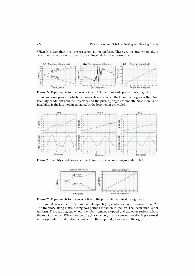
Bioinspiration and Robotics: Walking and Climbing Robots 424
When k is less than two, the trajectory is not uniform. There are instants where the x coordinate decreases with time. The pitching angle is not uniform either.
Figure 24. Experiments for the Locomotion in 1D of an 8 module pitch-connecting robot
There are some peaks in which it changes abruptly. When the k is equal or greater than two (stability condition) both the trajectory and the pitching angle are smooth. Now there is no instability in the locomotion, as stated by the locomotion principle 3.
Figure 25. Stability condition experiments for the pitch-connecting modular robot
Figure 26. Experiments for the locomotion of the pitch-pitch minimal configuration
The simulation results for the minimal pitch-pitch (PP) configuration are shown in Fig. 26. The trajectory along x axis during two periods is shown in the left. The locomotion is not uniform. There are regions where the robot remains stopped and the other regions where
the robot can move. When the sign of is changed, the movement direction is performed in the opposite. The step also increases with the amplitude, as shown in the right.
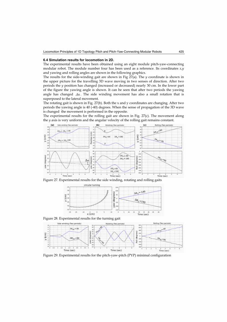
Locomotion Principles of 1D Topology Pitch and Pitch-Yaw-Connecting Modular Robots 425
6.4 Simulation results for locomotion in 2D.
The experimental results have been obtained using an eight module pitch-yaw-connecting modular robot. The module number four has been used as a reference. Its coordinates x,yand yawing and rolling angles are shown in the following graphics. The results for the side-winding gait are shown in Fig 27(a). The y coordinate is shown in the upper picture for the travelling 3D wave moving in two senses of direction. After two periods the y position has changed (increased or decreased) nearly 30 cm. In the lower part of the figure the yawing angle is shown. It can be seen that after two periods the yawing
angle has changed . The side winding movement has also a small rotation that is
superposed to the lateral movement. The rotating gait is shown in Fig. 27(b). Both the x and y coordinates are changing. After two periods the yawing angle is 40 (-40) degrees. When the sense of propagation of the 3D wave is changed the movement is performed in the opposite. The experimental results for the rolling gait are shown in Fig. 27(c). The movement along the y axis is very uniform and the angular velocity of the rolling gait remains constant.
Figure 27. Experimental results for the side winding, rotating and rolling gaits
Figure 28. Experimental results for the turning gait
Figure 29. Experimental results for the pitch-yaw-pitch (PYP) minimal configuration
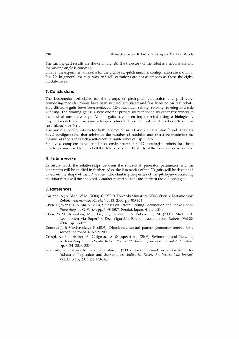
Bioinspiration and Robotics: Walking and Climbing Robots 426
The turning-gait results are shown in Fig. 28. The trajectory of the robot is a circular arc and the yawing angle is constant. Finally, the experimental results for the pitch-yaw-pitch minimal configuration are shown in Fig. 29. In general, the x, y, yaw and roll variations are not as smooth as those the eight-module cases.
7. Conclusions
The Locomotion principles for the groups of pitch-pitch connection and pitch-yaw-connecting modular robots have been studied, simulated and finally tested on real robots. Five different gaits have been achieved: 1D sinusoidal, rolling, rotating, turning and side winding. The rotating gait is a new one not previously mentioned by other researchers to the best of our knowledge. All the gaits have been implemented using a biologically inspired model based on sinusoidal generators that can be implemented efficiently on low cost microcontrollers. The minimal configurations for both locomotion in 1D and 2D have been found. They are novel configurations that minimize the number of modules and therefore maximize the number of robots in which a self-reconfigurable robot can split into. Finally a complete new simulation environment for 1D topologies robots has been developed and used to collect all the data needed for the study of the locomotion principles.
8. Future works
In future work the relationships between the sinusoidal generator parameters and the kinematics will be studied in further. Also, the kinematics of the 2D gaits will be developed based on the shape of the 3D waves. The climbing properties of the pitch-yaw-connecting modular robot will the analyzed. Another research line is the study of the 2D topologies.
9. References
Castano, A.; & Shen, W.M. (2000). CONRO: Towards Miniature Self-Sufficient Metamorphic Robots, Autonomous Robots, Vol.13, 2000, pp.309-324.
Chen, L.; Wang, Y. & Ma, S. (2004) Studies on Lateral Rolling Locomotion of a Snake Robot, Proceeding of IROS2004, pp. 5070-5074, Sendai, Japan, Sept., 2004.
Chen, W.M.; Krivokon, M.; Chiu, H.; Everist, J. & Rubenstein, M. (2006). Multimode Locomotion via SuperBot Reconfigurable Robots. Autonomous Robots, Vol.20, 2006, pp165-177
Conradt J. & Varshavskaya P (2003), Distributed central pattern generator control for a serpentine robot. ICANN 2003.
Crespi, A.; Badertscher, A.; Guignard, A. & Ijspeert A.J. (2005). Swimming and Crawling with an Amphibious Snake Robot. Proc. IEEE. Int. Conf. on Robotics and Automation,pp. 3024- 3028, 2005.
Granosik, G.; Hansen, M. G. & Borenstein, J. (2005). The Omnitread Serpentine Robot for Industrial Inspection and Surveillance, Industrial Robot: An Internationa Journal,Vol.32, No.2, 2005, pp.139-148.
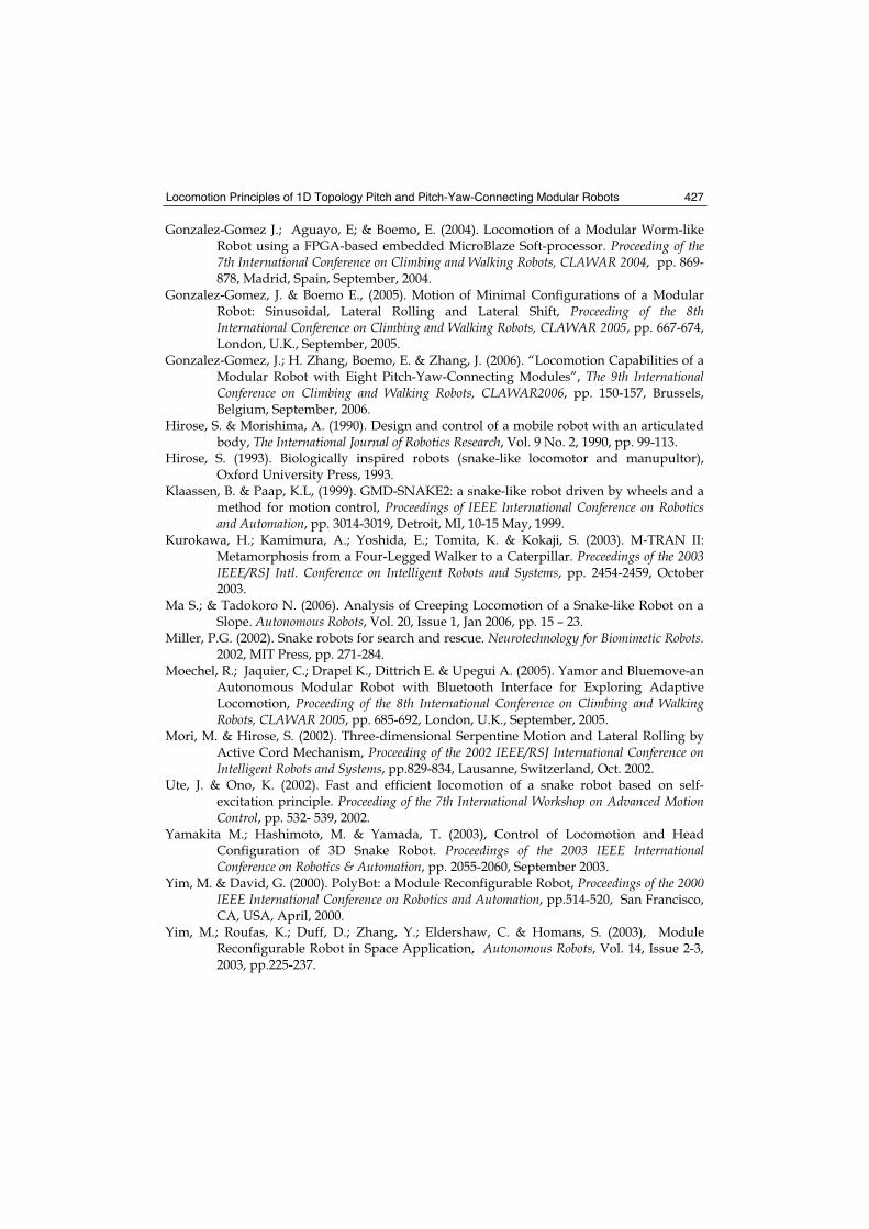
Locomotion Principles of 1D Topology Pitch and Pitch-Yaw-Connecting Modular Robots 427
Gonzalez-Gomez J.; Aguayo, E; & Boemo, E. (2004). Locomotion of a Modular Worm-like Robot using a FPGA-based embedded MicroBlaze Soft-processor. Proceeding of the 7th International Conference on Climbing and Walking Robots, CLAWAR 2004, pp. 869-878, Madrid, Spain, September, 2004.
Gonzalez-Gomez, J. & Boemo E., (2005). Motion of Minimal Configurations of a Modular Robot: Sinusoidal, Lateral Rolling and Lateral Shift, Proceeding of the 8th International Conference on Climbing and Walking Robots, CLAWAR 2005, pp. 667-674, London, U.K., September, 2005.
Gonzalez-Gomez, J.; H. Zhang, Boemo, E. & Zhang, J. (2006). “Locomotion Capabilities of a Modular Robot with Eight Pitch-Yaw-Connecting Modules”, The 9th International Conference on Climbing and Walking Robots, CLAWAR2006, pp. 150-157, Brussels, Belgium, September, 2006.
Hirose, S. & Morishima, A. (1990). Design and control of a mobile robot with an articulated body, The International Journal of Robotics Research, Vol. 9 No. 2, 1990, pp. 99-113.
Hirose, S. (1993). Biologically inspired robots (snake-like locomotor and manupultor), Oxford University Press, 1993.
Klaassen, B. & Paap, K.L, (1999). GMD-SNAKE2: a snake-like robot driven by wheels and a method for motion control, Proceedings of IEEE International Conference on Robotics and Automation, pp. 3014-3019, Detroit, MI, 10-15 May, 1999.
Kurokawa, H.; Kamimura, A.; Yoshida, E.; Tomita, K. & Kokaji, S. (2003). M-TRAN II: Metamorphosis from a Four-Legged Walker to a Caterpillar. Preceedings of the 2003 IEEE/RSJ Intl. Conference on Intelligent Robots and Systems, pp. 2454-2459, October 2003.
Ma S.; & Tadokoro N. (2006). Analysis of Creeping Locomotion of a Snake-like Robot on a Slope. Autonomous Robots, Vol. 20, Issue 1, Jan 2006, pp. 15 – 23.
Miller, P.G. (2002). Snake robots for search and rescue. Neurotechnology for Biomimetic Robots.2002, MIT Press, pp. 271-284.
Moechel, R.; Jaquier, C.; Drapel K., Dittrich E. & Upegui A. (2005). Yamor and Bluemove-an Autonomous Modular Robot with Bluetooth Interface for Exploring Adaptive Locomotion, Proceeding of the 8th International Conference on Climbing and Walking Robots, CLAWAR 2005, pp. 685-692, London, U.K., September, 2005.
Mori, M. & Hirose, S. (2002). Three-dimensional Serpentine Motion and Lateral Rolling by Active Cord Mechanism, Proceeding of the 2002 IEEE/RSJ International Conference on Intelligent Robots and Systems, pp.829-834, Lausanne, Switzerland, Oct. 2002.
Ute, J. & Ono, K. (2002). Fast and efficient locomotion of a snake robot based on self-excitation principle. Proceeding of the 7th International Workshop on Advanced Motion Control, pp. 532- 539, 2002.
Yamakita M.; Hashimoto, M. & Yamada, T. (2003), Control of Locomotion and Head Configuration of 3D Snake Robot. Proceedings of the 2003 IEEE International Conference on Robotics & Automation, pp. 2055-2060, September 2003.
Yim, M. & David, G. (2000). PolyBot: a Module Reconfigurable Robot, Proceedings of the 2000 IEEE International Conference on Robotics and Automation, pp.514-520, San Francisco, CA, USA, April, 2000.
Yim, M.; Roufas, K.; Duff, D.; Zhang, Y.; Eldershaw, C. & Homans, S. (2003), Module Reconfigurable Robot in Space Application, Autonomous Robots, Vol. 14, Issue 2-3, 2003, pp.225-237.
Bioinspiration and Robotics: Walking and Climbing Robots 428
Zhang, H.; Wang W.; Deng, Z. & Zong, G. (2006a): A Novel Reconfigurable Robot for Urban Search and Rescue, International Journal of Advanced Robotic Systems, Vol.3 No.4, 2006, pp.359-366.
Zhang, H.; Deng, Z.; Wang, W.; Zhang, J. & Zong, G. (2006b). Locomotion Capabilities of a Novel Reconfigurable Robot with 3 DOF Active Joints for Rugged Terrain, Proceedings of the 2006 IEEE/RSJ International Conference on Intelligent Robots and Systems, IROS 2006, pp.5588-5593, Beijing, China, October, 2006
Zong, G.; Deng, Z.; & Wang, W. (2006) Realization of a Modular Reconfigurable Robot for Rough Terrain, Proceedings of the 2006 IEEE International Conference on Mechatronics and Automation, pp. 289-294, Luoyang, Henan, China, June,2006.
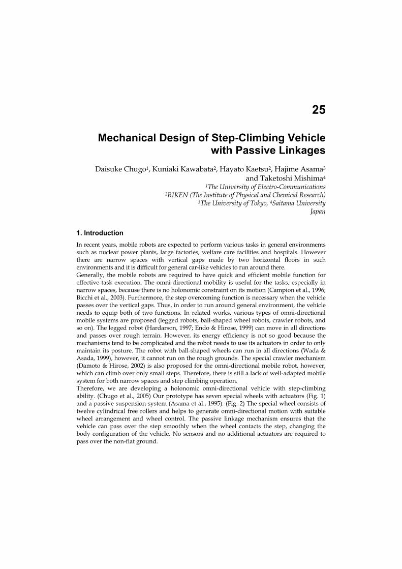
25
Mechanical Design of Step-Climbing Vehicle with Passive Linkages
Daisuke Chugo1, Kuniaki Kawabata2, Hayato Kaetsu2, Hajime Asama3
and Taketoshi Mishima4
1The University of Electro-Communications 2RIKEN (The Institute of Physical and Chemical Research)
3The University of Tokyo, 4Saitama University Japan
1. Introduction
In recent years, mobile robots are expected to perform various tasks in general environments such as nuclear power plants, large factories, welfare care facilities and hospitals. However there are narrow spaces with vertical gaps made by two horizontal floors in such environments and it is difficult for general car-like vehicles to run around there. Generally, the mobile robots are required to have quick and efficient mobile function for effective task execution. The omni-directional mobility is useful for the tasks, especially in narrow spaces, because there is no holonomic constraint on its motion (Campion et al., 1996; Bicchi et al., 2003). Furthermore, the step overcoming function is necessary when the vehicle passes over the vertical gaps. Thus, in order to run around general environment, the vehicle needs to equip both of two functions. In related works, various types of omni-directional mobile systems are proposed (legged robots, ball-shaped wheel robots, crawler robots, and so on). The legged robot (Hardarson, 1997; Endo & Hirose, 1999) can move in all directions and passes over rough terrain. However, its energy efficiency is not so good because the mechanisms tend to be complicated and the robot needs to use its actuators in order to only maintain its posture. The robot with ball-shaped wheels can run in all directions (Wada & Asada, 1999), however, it cannot run on the rough grounds. The special crawler mechanism (Damoto & Hirose, 2002) is also proposed for the omni-directional mobile robot, however, which can climb over only small steps. Therefore, there is still a lack of well-adapted mobile system for both narrow spaces and step climbing operation. Therefore, we are developing a holonomic omni-directional vehicle with step-climbing ability. (Chugo et al., 2005) Our prototype has seven special wheels with actuators (Fig. 1) and a passive suspension system (Asama et al., 1995). (Fig. 2) The special wheel consists of twelve cylindrical free rollers and helps to generate omni-directional motion with suitable wheel arrangement and wheel control. The passive linkage mechanism ensures that the vehicle can pass over the step smoothly when the wheel contacts the step, changing the body configuration of the vehicle. No sensors and no additional actuators are required to pass over the non-flat ground.
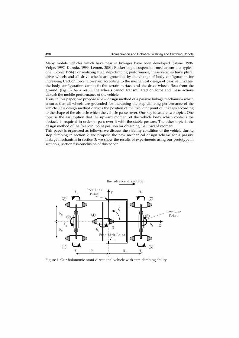
Bioinspiration and Robotics: Walking and Climbing Robots 430
Many mobile vehicles which have passive linkages have been developed. (Stone, 1996; Volpe, 1997; Kuroda, 1999; Lemon, 2004) Rocker-bogie suspension mechanism is a typical one. (Stone, 1996) For realizing high step-climbing performance, these vehicles have plural drive wheels and all drive wheels are grounded by the change of body configuration for increasing traction force. However, according to the mechanical design of passive linkages, the body configuration cannot fit the terrain surface and the drive wheels float from the ground. (Fig. 3) As a result, the wheels cannot transmit traction force and these actions disturb the mobile performance of the vehicle. Thus, in this paper, we propose a new design method of a passive linkage mechanism which ensures that all wheels are grounded for increasing the step-climbing performance of the vehicle. Our design method derives the position of the free joint point of linkages according to the shape of the obstacle which the vehicle passes over. Our key ideas are two topics. One topic is the assumption that the upward moment of the vehicle body which contacts the obstacle is required in order to pass over it with the stable posture. The other topic is the design method of the free joint point position for obtaining the upward moment. This paper is organized as follows: we discuss the stability condition of the vehicle during step climbing in section 2; we propose the new mechanical design scheme for a passive linkage mechanism in section 3; we show the results of experiments using our prototype in section 4; section 5 is conclusion of this paper.
Figure 1. Our holonomic omni-directional vehicle with step-climbing ability
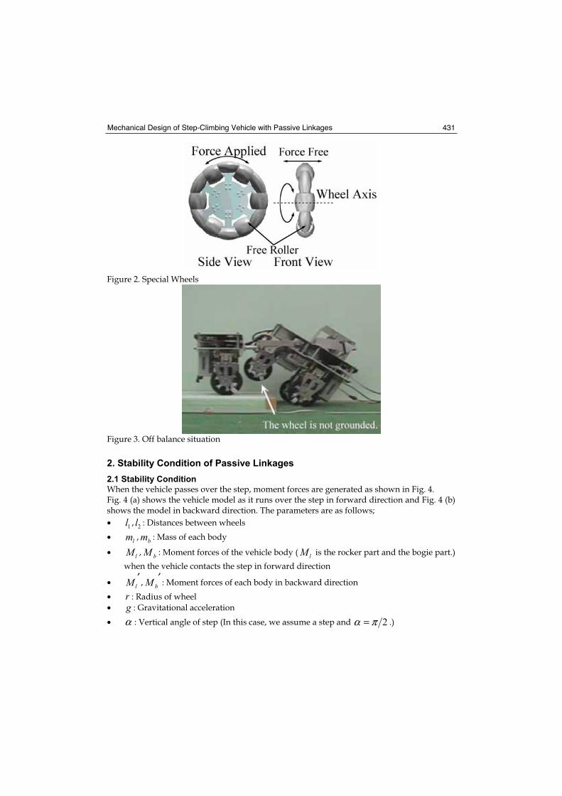
Mechanical Design of Step-Climbing Vehicle with Passive Linkages 431
Figure 2. Special Wheels
Figure 3. Off balance situation
2. Stability Condition of Passive Linkages
2.1 Stability Condition
When the vehicle passes over the step, moment forces are generated as shown in Fig. 4. Fig. 4 (a) shows the vehicle model as it runs over the step in forward direction and Fig. 4 (b) shows the model in backward direction. The parameters are as follows;
•1l ,
2l : Distances between wheels
• lm , bm : Mass of each body
• lM , bM : Moment forces of the vehicle body ( lM is the rocker part and the bogie part.)
when the vehicle contacts the step in forward direction
• ′lM ,
′bM : Moment forces of each body in backward direction
• r : Radius of wheel
• g : Gravitational acceleration
• α : Vertical angle of step (In this case, we assume a step and 2πα = .)
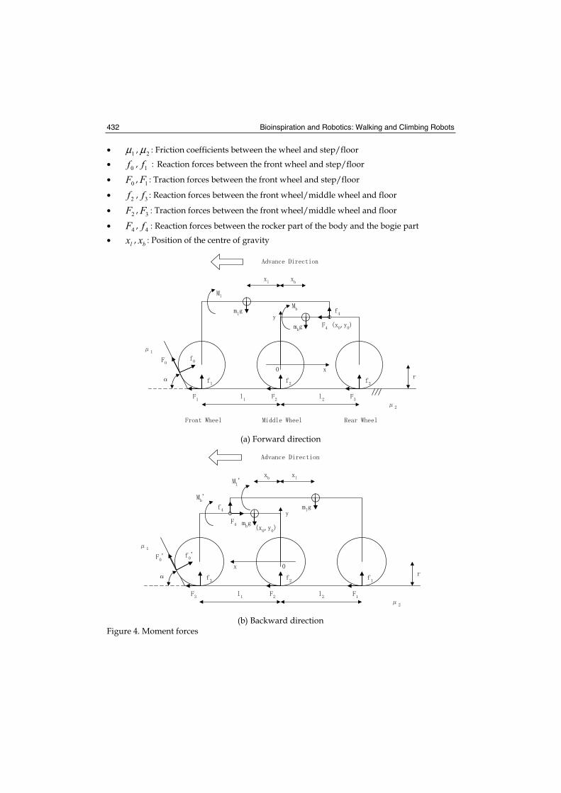
Bioinspiration and Robotics: Walking and Climbing Robots 432
•1μ ,
2μ : Friction coefficients between the wheel and step/floor
•0f ,
1f Reaction forces between the front wheel and step/floor
•0F ,
1F : Traction forces between the front wheel and step/floor
•2f ,
3f : Reaction forces between the front wheel/middle wheel and floor
•2F ,
3F : Traction forces between the front wheel/middle wheel and floor
•4F ,
4f : Reaction forces between the rocker part of the body and the bogie part
• lx , bx : Position of the centre of gravity
(a) Forward direction
(b) Backward direction Figure 4. Moment forces
Mechanical Design of Step-Climbing Vehicle with Passive Linkages 433
For realizing high step-climbing performance, the following two conditions are required.
• The traction force is enough for step climbing comparing with the mass of the body.
• When the vehicle climbs the step, the moment force of the vehicle body is positive. If the vehicle does not have enough traction output for step climbing, the vehicle cannot pass over it. Therefore, the first condition is indispensability. The second condition is required for that the body configuration can change according to the terrain surface and all wheels can be grounded. If all wheels with actuator are not grounded, the vehicle cannot transmit the traction force. In this study, we assume that the vehicle has driving actuators with enough traction output and we discuss the second condition. Furthermore, for quick and efficient mobility performance, the vehicle should pass over the step in forward and backward direction. Therefore, we discuss the moment forces of both directions.
2.2 Derivation of Moment Forces
Now, we derive these moment forces. We set the position of free joint point as ( )00 , yx on
the coordination in Fig. 4. When the vehicle contacts the α -degree step in forward
direction, these equations are derived from the balance of forces.
( ) 0cossin 4100 =−−− FFFf αα (1)
( ) gmfFf l=++ 400 sincos αα (2)
0324 =−− FFF (3)
0432 =−−+ fgmff b (4)
From the balance of moment forces on its body, equation (5) is derived.
( ) ( ) ( ) 004024222 =++−−−−= yrFxlfxlgmlfM bbb (5)
When the vehicle climbs the step, the vehicle should have enough traction force to lift its own body. Therefore, the reaction force between the front wheel and ground is zero.
011 == Ff (6)
We assume that the wheel transmits maximum power to the ground within the range of friction between the wheel and ground.
010 fF μ= ,222 fF μ= ,
323 fF μ= (7)
The moment force of rocker part of the body ( lM ) is derived as equation (8).
( )( ) ( )( )( )010
00100
coscossin
sincossin
yrfxxgmxlrfFM lll
+−−+−+++=
ααμαααα
(8)
From equation (1) to (8), we can derive the equation (9) and (10).
Bioinspiration and Robotics: Walking and Climbing Robots 434
( )( ) ( )( )( )010
00110
coscossin
sinsincos
yrfxxgmxlrfM lll
+−−+−+++=
ααμαααμα
(9)
( )( ) ( )αμαμαμα
μsincoscossin 121
20 ++−
+= gmmf bl (10)
From equation (9) and (10), the moment force when the vehicle passes over the step
( 2πα = ) in forward direction are expressed as equation (11). From this equation, the
moment force lM is function of free joint point position ( )00 , yx .
( ){ } ( )( )( ) ( ){ } gxmlrmm
ymmxmmm
M llbl
bllbl
l21
21121
02021
1
1
2
μμμμμμ
μμμ
+−−+++
+−−+
= (11)
Similarly, when the vehicle passes over the step in backward direction, the moment force
′bM is derived as equation (12). The moment force
′bM is derived from the position of free
joint point ( )00 , yx as lM .
( ){ } ( )( )( ) ( ){ } gxmlrmm
ymmxmmm
M bbbl
blbbl
b21
21221
02021
1
1
2
μμμμμμ
μμμ
+−−+++
+−−+−
=′ (12)
From these equations, it is required to design the position of free joint point ( )00 , yx for
increasing the step-climbing performance of the vehicle.
3. Design of Passive Linkages
3.1 Free Joint Position
In this section, we design the proposed passive linkage mechanism. For increasing mobile performance on the step, the moment force which applies to the vehicle body should be positive. From equation (11) and (12), the moment force when the vehicle passes over the step is led by only the position of free joint point. Thus, we design the free joint point position so that the moment force is positive when the vehicle climbs the step. Fig. 5 shows the moment force when the vehicle contacts the step. In Fig. 5, (a) shows the
moment force based on 0x as a variable and (b) is based on
0y . lM is the moment force
which is applied on the vehicle body when the vehicle passes over the step in forward
direction. On the other hand, ′
bM is the moment force when the vehicle passes over it in
backward direction. The parameters of the vehicle are chosen from the prototype vehicle model as shown in Table 1. The friction coefficients between the wheel and the floor are set
as1μ =
2μ =0.3 or 1μ =
2μ =0.5. The former assumes a linoleum floor and the latter assumes
a skidding on the floor.
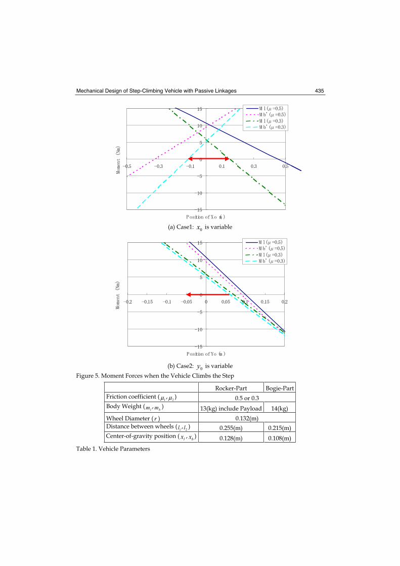
Mechanical Design of Step-Climbing Vehicle with Passive Linkages 435
(a) Case1: 0x is variable
(b) Case2: 0y is variable
Figure 5. Moment Forces when the Vehicle Climbs the Step
Rocker-Part Bogie-Part
Friction coefficient (1μ ,
2μ ) 0.5 or 0.3
Body Weight (lm ,
bm ) 13(kg) include Payload 14(kg)
Wheel Diameter ( r ) 0.132(m)
Distance between wheels (1l ,
2l ) 0.255(m) 0.215(m)
Center-of-gravity position ( lx , bx ) 0.128(m) 0.108(m)
Table 1. Vehicle Parameters
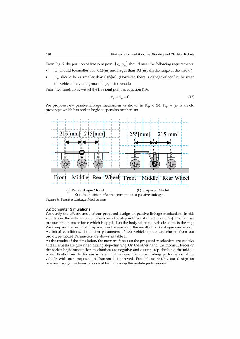
Bioinspiration and Robotics: Walking and Climbing Robots 436
From Fig. 5, the position of free joint point ( )00 , yx should meet the following requirements.
•0x should be smaller than 0.15[m] and larger than -0.1[m]. (In the range of the arrow.)
•0y should be as smaller than 0.05[m]. (However, there is danger of conflict between
the vehicle body and ground if 0y is too small.)
From two conditions, we set the free joint point as equation (13).
000 == yx (13)
We propose new passive linkage mechanism as shown in Fig. 6 (b). Fig. 6 (a) is an old prototype which has rocker-bogie suspension mechanism.
(a) Rocker-bogie Model (b) Proposed Model O is the position of a free joint point of passive linkages.
Figure 6. Passive Linkage Mechanism
3.2 Computer Simulations
We verify the effectiveness of our proposed design on passive linkage mechanism. In this simulation, the vehicle model passes over the step in forward direction at 0.25[m/s] and we measure the moment force which is applied on the body when the vehicle contacts the step. We compare the result of proposed mechanism with the result of rocker-bogie mechanism. As initial conditions, simulation parameters of test vehicle model are chosen from our prototype model. Parameters are shown in table 1. As the results of the simulation, the moment forces on the proposed mechanism are positive and all wheels are grounded during step-climbing. On the other hand, the moment forces on the rocker-bogie suspension mechanism are negative and during step-climbing, the middle wheel floats from the terrain surface. Furthermore, the step-climbing performance of the vehicle with our proposed mechanism is improved. From these results, our design for passive linkage mechanism is useful for increasing the mobile performance.
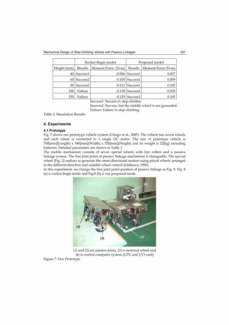
Mechanical Design of Step-Climbing Vehicle with Passive Linkages 437
Rocker-Bogie model Proposed model
Height (mm) Results Moment Force (N-m) Results Moment Force (N-m)
40 Success1 -0.006 Success1 0.037
60 Success2 -0.105 Success1 0.059
80 Success2 -0.111 Success1 0.105
100 Failure -0.129 Success1 0.105
150 Failure -0.129 Success1 0.105
Success1: Success in step-climbin; Success2: Success, but the middle wheel is not grounded. Failure: Failure in step-climbing
Table 2. Simulation Results
4. Experiments
4.1 Prototype
Fig. 7 shows our prototype vehicle system (Chugo et al., 2005). The vehicle has seven wheels and each wheel is connected to a single DC motor. The size of prototype vehicle is 750[mm](Length) x 540[mm](Width) x 520[mm](Height) and its weight is 22[kg] including batteries. Detailed parameters are shown in Table 1. The mobile mechanism consists of seven special wheels with free rollers and a passive linkage system. The free joint point of passive linkage mechanism is changeable. The special wheel (Fig. 2) realizes to generate the omni-directional motion using plural wheels arranged in the different direction and suitable wheel control (Ichikawa, 1995). In this experiment, we change the free joint point position of passive linkage as Fig. 8. Fig. 8 (a) is rocker-bogie mode and Fig.8 (b) is our proposed mode.
(1) and (2) are passive joints, (3) is motored wheel and (4) is control computer system (CPU and I/O card).
Figure 7. Our Prototype
(1)
(2)
(3)
(4)
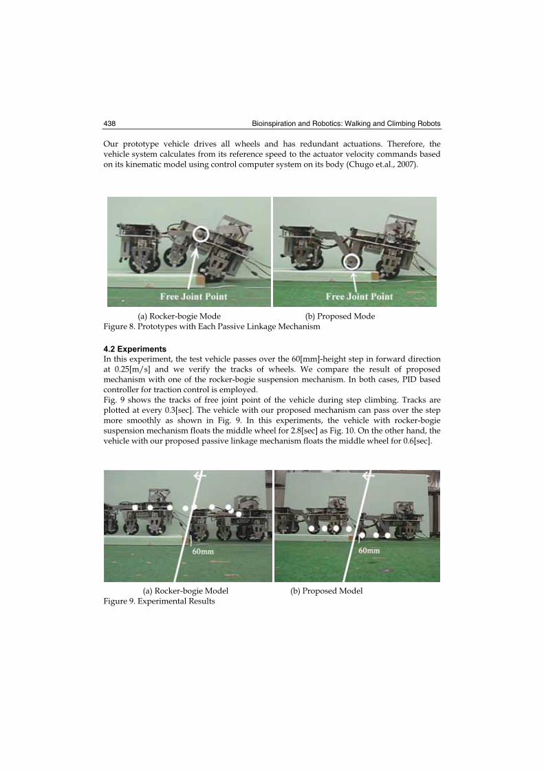
Bioinspiration and Robotics: Walking and Climbing Robots 438
Our prototype vehicle drives all wheels and has redundant actuations. Therefore, the vehicle system calculates from its reference speed to the actuator velocity commands based on its kinematic model using control computer system on its body (Chugo et.al., 2007).
(a) Rocker-bogie Mode (b) Proposed Mode Figure 8. Prototypes with Each Passive Linkage Mechanism
4.2 Experiments
In this experiment, the test vehicle passes over the 60[mm]-height step in forward direction at 0.25[m/s] and we verify the tracks of wheels. We compare the result of proposed mechanism with one of the rocker-bogie suspension mechanism. In both cases, PID based controller for traction control is employed. Fig. 9 shows the tracks of free joint point of the vehicle during step climbing. Tracks are plotted at every 0.3[sec]. The vehicle with our proposed mechanism can pass over the step more smoothly as shown in Fig. 9. In this experiments, the vehicle with rocker-bogie suspension mechanism floats the middle wheel for 2.8[sec] as Fig. 10. On the other hand, the vehicle with our proposed passive linkage mechanism floats the middle wheel for 0.6[sec].
(a) Rocker-bogie Model (b) Proposed Model Figure 9. Experimental Results
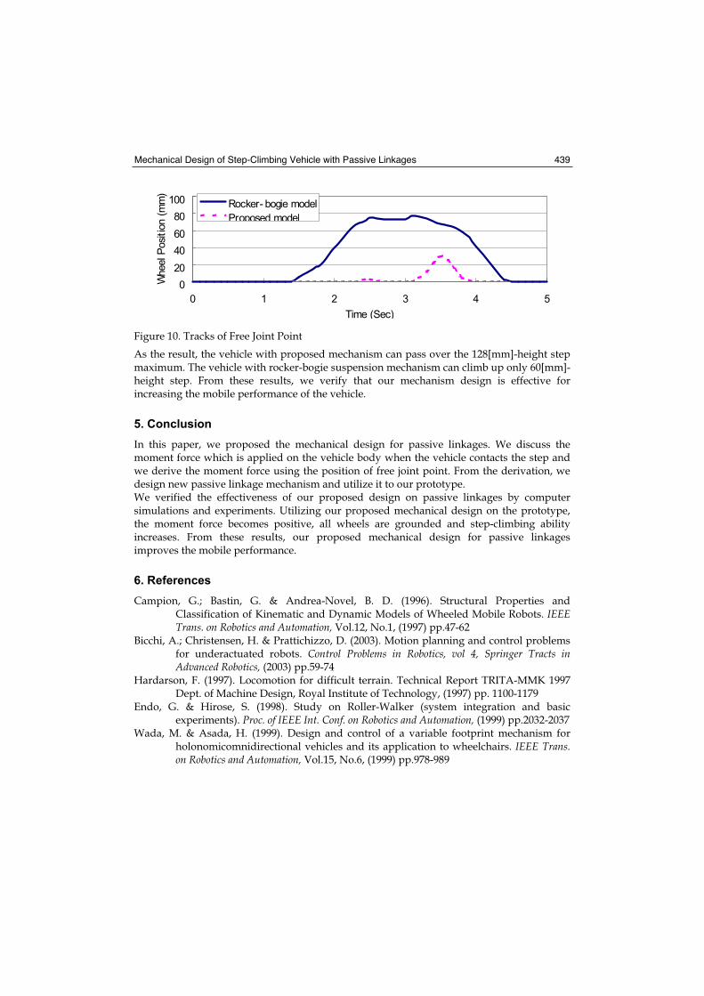
Mechanical Design of Step-Climbing Vehicle with Passive Linkages 439
Figure 10. Tracks of Free Joint Point
As the result, the vehicle with proposed mechanism can pass over the 128[mm]-height step maximum. The vehicle with rocker-bogie suspension mechanism can climb up only 60[mm]-height step. From these results, we verify that our mechanism design is effective for increasing the mobile performance of the vehicle.
5. Conclusion
In this paper, we proposed the mechanical design for passive linkages. We discuss the moment force which is applied on the vehicle body when the vehicle contacts the step and we derive the moment force using the position of free joint point. From the derivation, we design new passive linkage mechanism and utilize it to our prototype. We verified the effectiveness of our proposed design on passive linkages by computer simulations and experiments. Utilizing our proposed mechanical design on the prototype, the moment force becomes positive, all wheels are grounded and step-climbing ability increases. From these results, our proposed mechanical design for passive linkages improves the mobile performance.
6. References
Campion, G.; Bastin, G. & Andrea-Novel, B. D. (1996). Structural Properties and Classification of Kinematic and Dynamic Models of Wheeled Mobile Robots. IEEETrans. on Robotics and Automation, Vol.12, No.1, (1997) pp.47-62
Bicchi, A.; Christensen, H. & Prattichizzo, D. (2003). Motion planning and control problems for underactuated robots. Control Problems in Robotics, vol 4, Springer Tracts in Advanced Robotics, (2003) pp.59-74
Hardarson, F. (1997). Locomotion for difficult terrain. Technical Report TRITA-MMK 1997 Dept. of Machine Design, Royal Institute of Technology, (1997) pp. 1100-1179
Endo, G. & Hirose, S. (1998). Study on Roller-Walker (system integration and basic experiments). Proc. of IEEE Int. Conf. on Robotics and Automation, (1999) pp.2032-2037
Wada, M. & Asada, H. (1999). Design and control of a variable footprint mechanism for holonomicomnidirectional vehicles and its application to wheelchairs. IEEE Trans. on Robotics and Automation, Vol.15, No.6, (1999) pp.978-989
Bioinspiration and Robotics: Walking and Climbing Robots 440
Damoto, R. & Hirose, S. (2002). Development of Holonomic Omnidirectional Vehicle "Vuton-II" with Omni-Discs. J. of Robotics and Mechatronics, Vol.14, No.2, (2002) pp.186-192
Chugo, D. ; Kawabata, K.; Kaetsu, H.; Asama, H. & Mishima, T. (2005). Development of a Control System for an Omni directional Vehicle with Step-Climbing Ability. Advanced Robotics, Vol.19, No.1, (2005) pp.51-71
Chugo, D. ; Kawabata, K.; Kaetsu, H.; Asama, H. & Mishima, T. (2007). Configuration-Based Wheel Control for Step-Climbing Vehicle. J. of Robotics and Mechatoronics, Vol.19, No.1, (2007) pp.52-59
Asama, H.; Sato, M.; Bogoni, L.; Kaetsu, H.; Mitsumoto, A. & Endo, I. (1995). Development of an omni-directional mobile robot with 3 DOF decoupling drive mechanism. Proc. of IEEE Int. Conf. on Robotics and Automation, (1995) pp.1925-1930
Stone, H. W. (1996). Mars Pathfinder Microrover: A Low-Cost, Low-Power Spacecraft. Proc. of 1996 AIAA Forum on Advanced Developments in Space Robotics, (1996)
Volpe, R.; Balaram, J.; Ohm, T, & Ivlev, R. (1997). Rocky-7: a next generation Mars rover prototype. Advanced Robotics, Vol.11, No.4, (1997) pp.341-358
Kuroda Y.; Kondo, K.; Nakamura, K.; Kunii, Y. & Kubota, T. (1999). Low Power Mobility System for Micro Planetary Rover Micro5. Proc. of 5th Int. Symp. on Artificial Intelligence, Robotics and Automation in Space, (1999) pp.77-82
Lamon, P.; Krebs, A.; Lauria, M.; Shooter, S. & Siegwart, R. (2004). Wheel torque control for a rough terrain rover. Proc. of IEEE Int. Conf. on Robotics and Automation, (1995) pp.4682-4687
Ichikawa, M. (1995). Wheel arrangements for Wheeled Vehicle. J. of the Robotics Society of Japan, Vol.13, No.1, (1995) pp.107-112
26
Climbing Robots
Majid M. Moghadam1 and Mojtaba Ahmadi2
1Tarbiat Modares University, 2Carleton University 1Iran, 2Canada
1. Introduction
Today, due to technological advances of robotic applications in human life, it is necessary to overcome natural and virtual obstacles such as stairs which are the most known obstacles to the motion of such robots. Several research have been conducted toward the design of stair climbing and obstacle traversing robots during the past decade. A number of robots have robots have been built for climbing stairs and traversing obstacles, such as quadruped and hexapod robots. Although these robots can climb stairs and traverse obstacles, they do not have smooth motion on flat surfaces, which is due to the motion of their legs. Buehler built a hexapod robot (RHex) that could ascend and descend stairs dynamically. He has also built a quadruped robot (SCOUT) which could climb just one stair (M. Buehler, (2002), U. Saranli, (2001), Martin Buehler , (2002) C. Steeves1,(2002)). Furthermore, a few wheeled and leg-wheel robots have been proposed that either can climb only one stair or can not climb stairs individually and need to be supported by a person; Therefore, they are not good enough to be practical. Koyanagi proposed a six wheeled robot that could climb a stair (Eiji KOYANAGI). Kumar offered a wheelchair with legs for people with disabilities which could climb a stair (Parris Wellman, (1995) , Venkat Krovi, (1995)) . Halme offered a robot with movement by simultaneous wheel and leg propulsion (Aarne Halme (2001)). Quinn built Leg-Wheel (quadruped and hexapod) robots (Mini-Whegs) that could ascend, descend and jump stairs (Roland Siegwart, (1998), Nakayama R (1998)). Kmen invented a wheelchair with wheels (iBOT 3000) that could climb stairs by human support (A. Crespi) . Also NASA designed Urban Robot which was a Tracked robot. It could climb stairs and curbs using a tracked design instead of wheels. The Urban Robot (Urbie) led to the PackBot platform of iRobot. Besides, Dalvand designed a wheeled mobile robot that has the capability of climbing stairs, traversing obstacles, and is adaptable to uphill, downhill and slope surfaces (Dalvand and Moghaddam (2003)).Parallel platforms present many advantages that make them especially suitable to be used as climbing robots, in contrast with other types of climbing robots with legs. The availability of a great number of redundant degrees of freedom of the climbing robots with legs does not necessarily increase the ability of the machine to progress in a complex workspace. Climbing robots with legs use their legs to hold and move the robot body (H.R. Choi, (2000)). The legs mechanisms have a sequential configuration that originates a limitation in the robot movement and great torques in the actuators placed on the legs base. Architecture of serial legs also implies a limit on load capability. This is a typical effect on serial articulated mechanisms influenced by force and torque effects present on joints (J.P. Merlet, (1992)).
Bioinspiration and Robotics: Walking and Climbing Robots 442
Due to the preceding, it is also well known that weight/power relation on climbing robots is high while both the useful load capacity and the velocity of serial mechanisms are limited. In contrast with the limitations of the robot legs to climb, the use of a Gough–Stewart platform as a climbing robot (Buehler M., (2002)), solves many of these limitations and opens a new field of application for this type of mechanism. In order to emphasize the great performance of the G–S parallel robot as a climbing robot, it is pertinent to remember that this type of parallel robot is based on a simple mechanical concept that consists of two rings (platforms) linked with six linear actuators joined through universal and spherical joints (this type of structure is also reffered as a 6-UPS parallel robot). These characteristics allow to obtain a mechanical structure of low weight and high stiffness, which is able to reach high velocities and develop large forces with a very important advantage: the low cost of manufacturing (D. Lazard, (1992)).
2. Leg-Wheel Robots
There is an enormous variety of walking robots in the world today. Most of them have six legs to maintain good static stability, many have 8 legs for greater speed and higher load capacity and there are some that implement clever balancing algorithms which allow them to walk on two legs to move over sloping ground and to climb up and down stairs, like humans do (eg. Such as Honda's Asimo robots). In general, the main motive behind the creation of most of these walking machines is to enjoy experiencing about the physics of motion by applying “state of the art” technologies to control the movement of articulated limbs and joint actuators. After all, it is not an easy task to recreate the efficient yet very complex movements of biological insects and mammals which effortlessly execute various types of periodic gait patterns and adaptive gaits and very high speeds. (Visit the CLAWAR web site to view most of the modern walking robots that have been built in recent years). Unfortunately, due to the very complex and multi-disciplinary nature of this field of research, very few walking robots and multi-legged vehicles have been proven to be the “best and most economical solution” for solving problems in domestic, industrial, construction, military or space applications. It seems as though most of today’s small walking robots are only the result of human's fascination with the application and useful for entertainment only. In addition, the majority of large scale ‘high-powered’ walking robots are still in their “experimental” stages and are not commercially available for bulk purchasing. Most large scale walking robots lack sufficiently intelligent software for solving “real world” problems automatically and in the most cost effective manner possible. With the added flexibility of being able to control the foundation points of the vehicle while traversing over almost any type of irregular surface, comes the increased complexity of foot and joint control to maintain stability and coordinated movements for gait movements. Another major problem is the inherent slowness of legged and walking locomotion, compared to wheeled transport. It would be beneficial for a mobile robot to possess the advantages of extreme rough terrain negotiating flexibility, which multi-degree-of-freedom (MDOF) legs can offer, with the high-speed and simplicity afforded by wheels.Such a multi-legged and wheeled robot would be able to find practical use in solving difficult transportation type problems in virtually any type of outdoor application where high speed is essential. Some examples of useful applications for reliable, high speed, and high load carrying capacity walking vehicles include:
Climbing Robots 443
• A walking vehicle for paraplegic people or the elderly who cannot walk easily • Deep sea or planet surveying and exploration on the moon or on Mars
• Automated or tele-remote controlled (semi-automated) construction
• Underground mining
• Automated agriculture (planting and harvesting) eg. Plustech foresting robot
• “Battlebots” to take the place of human soldiers on a battlefield
• Security or police robots that can patrol a defined area and identify or
• apprehend trespassers
• Firefighting robots that can climb over rough terrain and large obstacles to
• reach the heart of a fire with a fire extinguisher or water hose.
• Skeletal animatronic machines to take the place of “fake looking” 3D
• computer generated dinosaurs in monster films and science fiction movies. The Curtin University “Hydrobug” project involves the design, construction and testing of a 6-legged “insect-like” hybrid walking vehicle which will be able to carry three adult passengers over rough terrain or very broken ground with gaps, pot holes or obstacles which are too large for wheels to traverse. This vehicle is also designed to continue
moving from level ground onto steep inclinations up to 45° to the horizontal. The Hydrobug is designed with the necessary degrees of freedom to walk over extremely rugged terrain using 6 three-degree-of-freedom articulated-limb legs. It will also be able to convert to 4-wheel-drive mode for high speed travel, while it’s legs are fully raised and its feet are kept high off the ground. This type of robot will be able to travel at high speeds on smooth roads.
3. Rough Terrain Climber Robots
Rough-terrain robot navigation has received a significant amount of attention recently, most prominently showcased to the broader public by the success of current Mars rover missions. In the future, increased autonomous capabilities will be required to accomplish ambitious planetary missions as well as a whole variety of Earth-bound tasks. This demand has led to the development of numerous approaches to solving the rough-terrain robot motion planning task. The common factor with all such research lies in the underlying characteristics of the rough terrain itself. By the very nature of the task, binary obstacle definitions cannot be exclusively applied to rough-terrain motion planning. Each configuration of the robot operating on the terrain has a characteristic difficulty associated with its attainment. Depending on the properties of the problem being studied, different aspects of the robot/terrain interaction assume high relevance. These factors are consequently included in the terrain abstraction while other aspects are typically chosen to be omitted. Nevertheless, independently of the terrain model used, there remains the specific difficulty associated with reaching a particular configuration. Further, in near future, robots will take the place of human labor in many areas. They will perform various hazardous duties like fire fighting, rescuing people, demining, suppressing terrorist outrage, and scouting enemy territory. To make use of robots in these various circumstances, robots should have the ability of passing through rough terrain such as steps. There are three types of moving mechanisms for this kind of robots in general : wheel type, track type and walking type mechanism. Robots with wheel mechanism are inferior to robots with track when they are to move on rough terrain. Walking robots have complex
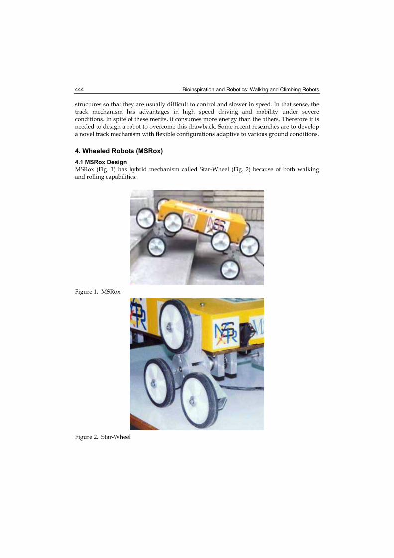
Bioinspiration and Robotics: Walking and Climbing Robots 444
structures so that they are usually difficult to control and slower in speed. In that sense, the track mechanism has advantages in high speed driving and mobility under severe conditions. In spite of these merits, it consumes more energy than the others. Therefore it is needed to design a robot to overcome this drawback. Some recent researches are to develop a novel track mechanism with flexible configurations adaptive to various ground conditions.
4. Wheeled Robots (MSRox)
4.1 MSRox Design
MSRox (Fig. 1) has hybrid mechanism called Star-Wheel (Fig. 2) because of both walking and rolling capabilities.
Figure 1. MSRox
Figure 2. Star-Wheel
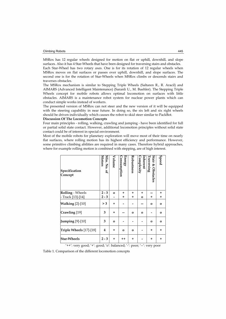
Climbing Robots 445
MSRox has 12 regular wheels designed for motion on flat or uphill, downhill, and slope surfaces. Also it has 4 Star-Wheels that have been designed for traversing stairs and obstacles. Each Star-Wheel has two rotary axes. One is for its rotation of 12 regular wheels when MSRox moves on flat surfaces or passes over uphill, downhill, and slope surfaces. The second one is for the rotation of Star-Wheels when MSRox climbs or descends stairs and traverses obstacles. The MSRox mechanism is similar to Stepping Triple Wheels (Saltaren R., R. Aracil) and AIMARS (Advanced Intelligent Maintenance) (Saranli U., M. Buehler). The Stepping Triple Wheels concept for mobile robots allows optimal locomotion on surfaces with little obstacles. AIMARS is a maintenance robot system for nuclear power plants which can conduct simple works instead of workers. The presented version of MSRox can not steer and the new version of it will be equipped with the steering capability in near future. In doing so, the six left and six right wheels should be driven individually which causes the robot to skid steer similar to PackBot. Discussion Of The Locomotion Concepts Four main principles - rolling, walking, crawling and jumping - have been identified for full or partial solid state contact. However, additional locomotion principles without solid state contact could be of interest in special environment. Most of the mobile robots for planetary exploration will move most of their time on nearly flat surfaces, where rolling motion has its highest efficiency and performance. However, some primitive climbing abilities are required in many cases. Therefore hybrid approaches, where for example rolling motion is combined with stepping, are of high interest.
Specification Concept
Min. N
o. of M
otors
Volum
e
Energy C
onsumption
Robustness
InherentC
omplexity
Stair & O
bstacles Traversing
Speed
Rolling - Wheels - Track [13]-[14]
2 - 32 - 3
o-
++
++
+o
--+
++
Walking [2]-[10] > 3 + - - -- o o
Crawling [19] 3 + -- o o - o
Jumping [9]-[10] 3 o - - - o o
Triple Wheels [17]-[18] 4 + o o - + +
Star-Wheels 2 - 3 + ++ + - + +
‘++’: very good; ‘+’: good; ‘o’: balanced; ‘-’: poor; ‘--’: very poor
Table 1. Comparison of the different locomotion concepts
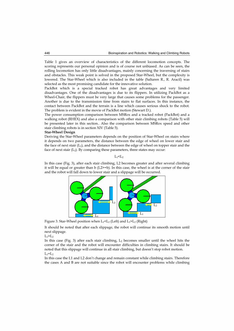
Bioinspiration and Robotics: Walking and Climbing Robots 446
Table 1 gives an overview of characteristics of the different locomotion concepts. The scoring represents our personal opinion and is of course not unbiased. As can be seen, the rolling locomotion has only little disadvantages, mainly concerning the traversing of stairs and obstacles. This weak point is solved in the proposed Star-Wheel, but the complexity is lowered. The Star-Wheel which is also included in the table (Saltaren R., R. Aracil) was selected as the most promising candidate for the innovative solution. PackBot which is a special tracked robot has great advantages and very limited disadvantages. One of the disadvantages is due to its flippers. In utilizing PackBot as a Wheel-Chair, the flippers must be very large that causes some problems for the passenger. Another is due to the transmission time from stairs to flat surfaces. In this instance, the contact between PackBot and the terrain is a line which causes serious shock to the robot. The problem is evident in the movie of PackBot motion (Stewart D.). The power consumption comparison between MSRox and a tracked robot (PackBot) and a walking robot (RHEX) and also a comparison with other stair climbing robots (Table 5) will be presented later in this section.. Also the comparison between MSRox speed and other stair climbing robots is in section XIV (Table 5). Star-Wheel Design Deriving the Star-Wheel parameters depends on the position of Star-Wheel on stairs where it depends on two parameters, the distance between the edge of wheel on lower stair and the face of next stair (L1), and the distance between the edge of wheel on topper stair and the face of next stair (L2). By comparing these parameters, three states may occur:
L1<L2
In this case (Fig. 3), after each stair climbing, L2 becomes greater and after several climbing it will be equal or greater than b (L2>=b). In this case, the wheel is at the corner of the stair and the robot will fall down to lower stair and a slippage will be occurred.
Figure 3. Star-Wheel position when L1<L2 (Left) and L1>L2 (Right)
It should be noted that after each slippage, the robot will continue its smooth motion until next slippage. L1>L2
In this case (Fig. 3) after each stair climbing, L2 becomes smaller until the wheel hits the corner of the stair and the robot will encounter difficulties in climbing stairs. It should be noted that this slippage will continue in all stair climbing, but doesn’t stop robot motion. L1=L2
In this case the L1 and L2 don’t change and remain constant while climbing stairs. Therefore the cases A and B are not suitable since the robot will encounter problems while climbing
L1
L2
L1
L2
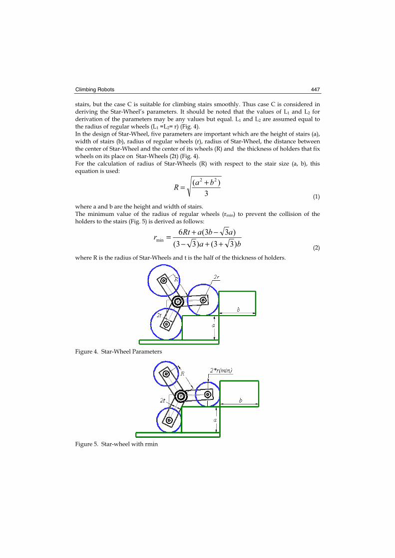
Climbing Robots 447
stairs, but the case C is suitable for climbing stairs smoothly. Thus case C is considered in deriving the Star-Wheel’s parameters. It should be noted that the values of L1 and L2 for derivation of the parameters may be any values but equal. L1 and L2 are assumed equal to the radius of regular wheels (L1 =L2= r) (Fig. 4). In the design of Star-Wheel, five parameters are important which are the height of stairs (a), width of stairs (b), radius of regular wheels (r), radius of Star-Wheel, the distance between the center of Star-Wheel and the center of its wheels (R) and the thickness of holders that fix wheels on its place on Star-Wheels (2t) (Fig. 4). For the calculation of radius of Star-Wheels (R) with respect to the stair size (a, b), this equation is used:
3
)( 22 baR += (1)
where a and b are the height and width of stairs. The minimum value of the radius of regular wheels (rmin) to prevent the collision of the holders to the stairs (Fig. 5) is derived as follows:
baabaRtr
)33()33(
)33(6min ++−
−+= (2)
where R is the radius of Star-Wheels and t is the half of the thickness of holders.
Figure 4. Star-Wheel Parameters
Figure 5. Star-wheel with rmin
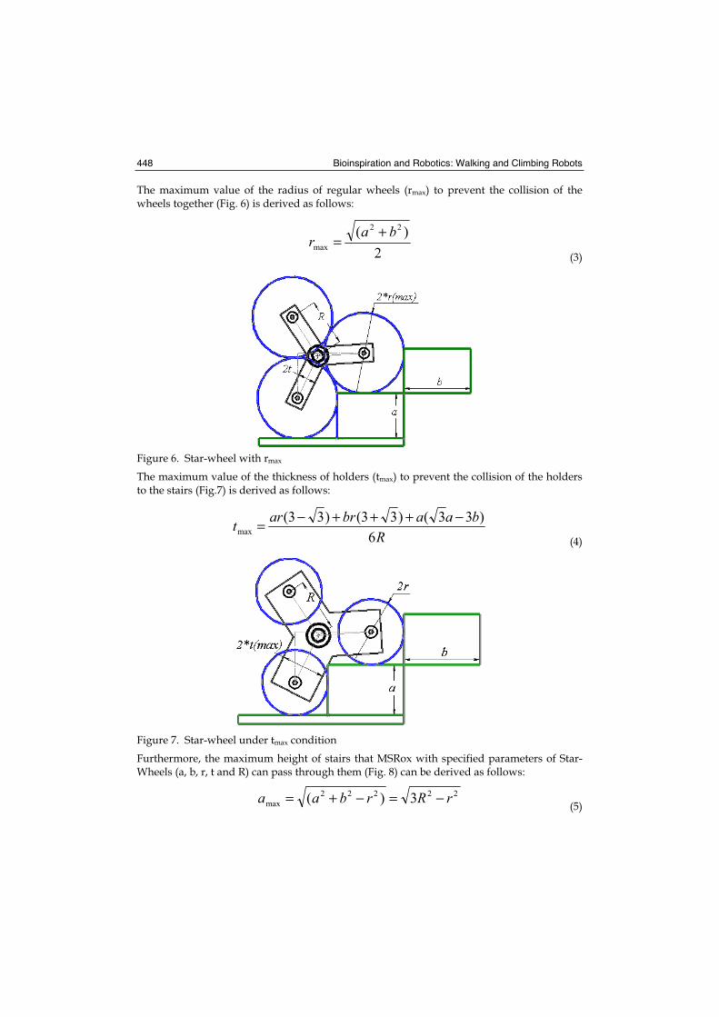
Bioinspiration and Robotics: Walking and Climbing Robots 448
The maximum value of the radius of regular wheels (rmax) to prevent the collision of the wheels together (Fig. 6) is derived as follows:
2
)( 22
max
bar
+=
(3)
Figure 6. Star-wheel with rmax
The maximum value of the thickness of holders (tmax) to prevent the collision of the holders to the stairs (Fig.7) is derived as follows:
Rbaabrart
6
)33()33()33(max
−+++−= (4)
Figure 7. Star-wheel under tmax condition
Furthermore, the maximum height of stairs that MSRox with specified parameters of Star-Wheels (a, b, r, t and R) can pass through them (Fig. 8) can be derived as follows:
22222
max 3)( rRrbaa −=−+= (5)
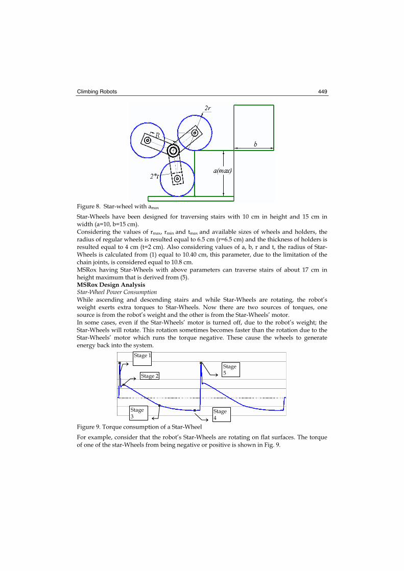
Climbing Robots 449
Figure 8. Star-wheel with amax
Star-Wheels have been designed for traversing stairs with 10 cm in height and 15 cm in width (a=10, b=15 cm). Considering the values of rmax, rmin and tmax and available sizes of wheels and holders, the radius of regular wheels is resulted equal to 6.5 cm (r=6.5 cm) and the thickness of holders is resulted equal to 4 cm (t=2 cm). Also considering values of a, b, r and t, the radius of Star-Wheels is calculated from (1) equal to 10.40 cm, this parameter, due to the limitation of the chain joints, is considered equal to 10.8 cm. MSRox having Star-Wheels with above parameters can traverse stairs of about 17 cm in height maximum that is derived from (5). MSRox Design Analysis Star-Wheel Power Consumption While ascending and descending stairs and while Star-Wheels are rotating, the robot’s weight exerts extra torques to Star-Wheels. Now there are two sources of torques, one source is from the robot’s weight and the other is from the Star-Wheels’ motor. In some cases, even if the Star-Wheels’ motor is turned off, due to the robot’s weight; the Star-Wheels will rotate. This rotation sometimes becomes faster than the rotation due to the Star-Wheels’ motor which runs the torque negative. These cause the wheels to generate energy back into the system.
Figure 9. Torque consumption of a Star-Wheel
For example, consider that the robot’s Star-Wheels are rotating on flat surfaces. The torque of one of the star-Wheels from being negative or positive is shown in Fig. 9.
Stage 1
Stage 2
Stage3
Stage4
Stage5
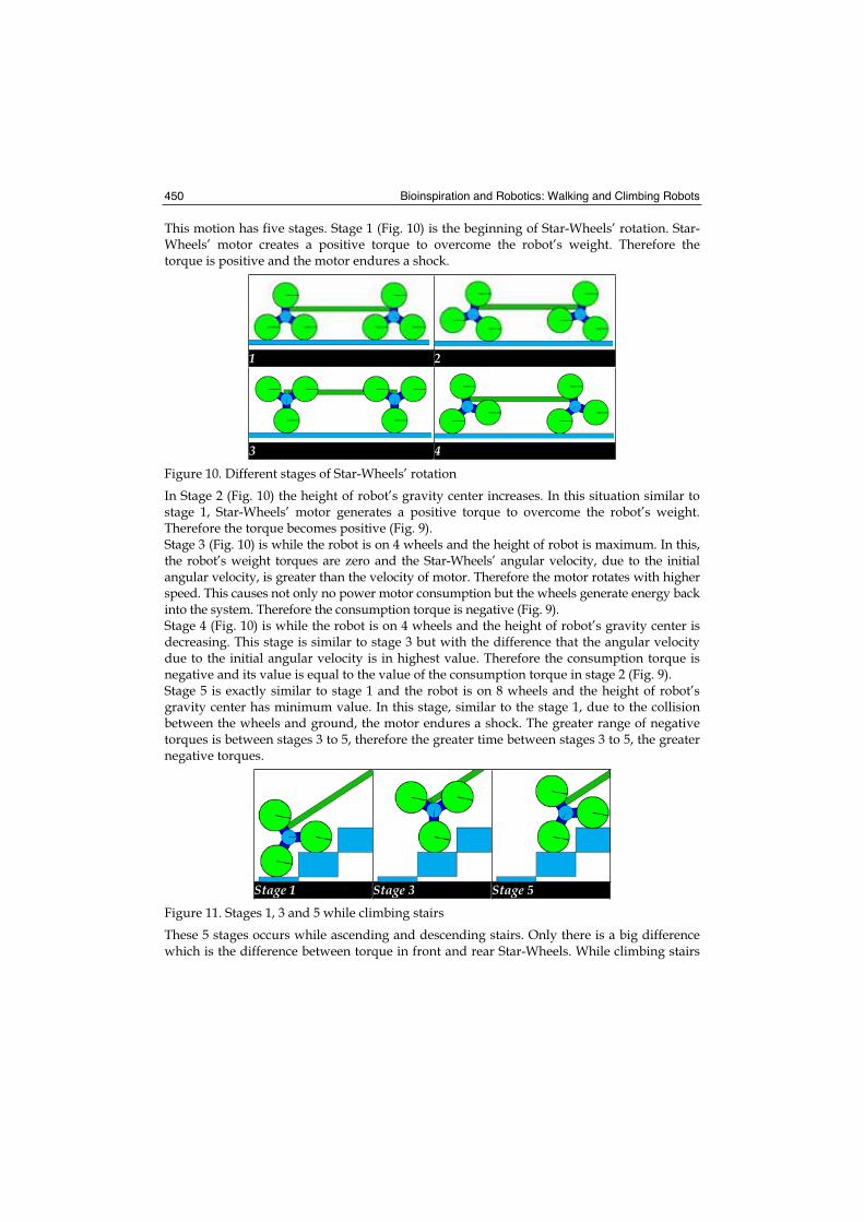
Bioinspiration and Robotics: Walking and Climbing Robots 450
This motion has five stages. Stage 1 (Fig. 10) is the beginning of Star-Wheels’ rotation. Star-Wheels’ motor creates a positive torque to overcome the robot’s weight. Therefore the torque is positive and the motor endures a shock.
1 2
3 4
Figure 10. Different stages of Star-Wheels’ rotation
In Stage 2 (Fig. 10) the height of robot’s gravity center increases. In this situation similar to stage 1, Star-Wheels’ motor generates a positive torque to overcome the robot’s weight. Therefore the torque becomes positive (Fig. 9). Stage 3 (Fig. 10) is while the robot is on 4 wheels and the height of robot is maximum. In this, the robot’s weight torques are zero and the Star-Wheels’ angular velocity, due to the initial angular velocity, is greater than the velocity of motor. Therefore the motor rotates with higher speed. This causes not only no power motor consumption but the wheels generate energy back into the system. Therefore the consumption torque is negative (Fig. 9). Stage 4 (Fig. 10) is while the robot is on 4 wheels and the height of robot’s gravity center is decreasing. This stage is similar to stage 3 but with the difference that the angular velocity due to the initial angular velocity is in highest value. Therefore the consumption torque is negative and its value is equal to the value of the consumption torque in stage 2 (Fig. 9). Stage 5 is exactly similar to stage 1 and the robot is on 8 wheels and the height of robot’s gravity center has minimum value. In this stage, similar to the stage 1, due to the collision between the wheels and ground, the motor endures a shock. The greater range of negative torques is between stages 3 to 5, therefore the greater time between stages 3 to 5, the greater negative torques.
Stage 1 Stage 3 Stage 5
Figure 11. Stages 1, 3 and 5 while climbing stairs
These 5 stages occurs while ascending and descending stairs. Only there is a big difference which is the difference between torque in front and rear Star-Wheels. While climbing stairs
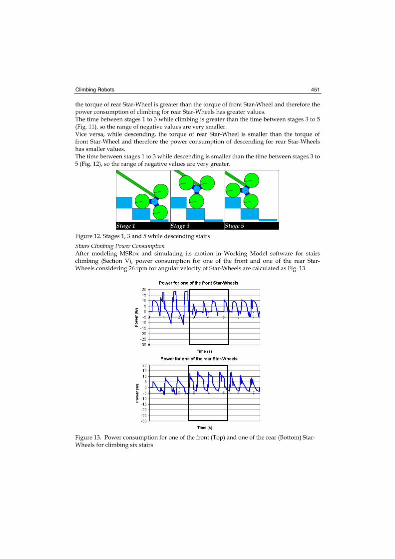
Climbing Robots 451
the torque of rear Star-Wheel is greater than the torque of front Star-Wheel and therefore the power consumption of climbing for rear Star-Wheels has greater values.The time between stages 1 to 3 while climbing is greater than the time between stages 3 to 5 (Fig. 11), so the range of negative values are very smaller. Vice versa, while descending, the torque of rear Star-Wheel is smaller than the torque of front Star-Wheel and therefore the power consumption of descending for rear Star-Wheels has smaller values. The time between stages 1 to 3 while descending is smaller than the time between stages 3 to 5 (Fig. 12), so the range of negative values are very greater.
Stage 1 Stage 3 Stage 5
Figure 12. Stages 1, 3 and 5 while descending stairs
Stairs Climbing Power Consumption After modeling MSRox and simulating its motion in Working Model software for stairs climbing (Section V), power consumption for one of the front and one of the rear Star-Wheels considering 26 rpm for angular velocity of Star-Wheels are calculated as Fig. 13.
Figure 13. Power consumption for one of the front (Top) and one of the rear (Bottom) Star-Wheels for climbing six stairs
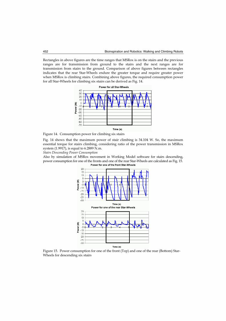
Bioinspiration and Robotics: Walking and Climbing Robots 452
Rectangles in above figures are the time ranges that MSRox is on the stairs and the previous ranges are for transmission from ground to the stairs and the next ranges are for transmission from stairs to the ground. Comparison of above figures between rectangles indicates that the rear Star-Wheels endure the greater torque and require greater power when MSRox is climbing stairs. Combining above figures, the required consumption power for all Star-Wheels for climbing six stairs can be derived as Fig. 14.
Figure 14. Consumption power for climbing six stairs
Fig. 14 shows that the maximum power of stair climbing is 34.104 W. So, the maximum essential torque for stairs climbing, considering ratio of the power transmission in MSRox system (1.9917), is equal to 6.2889 N.m. Stairs Descending Power ConsumptionAlso by simulation of MSRox movement in Working Model software for stairs descending, power consumption for one of the fronts and one of the rear Star-Wheels are calculated as Fig. 15.
Figure 15. Power consumption for one of the front (Top) and one of the rear (Bottom) Star-Wheels for descending six stairs
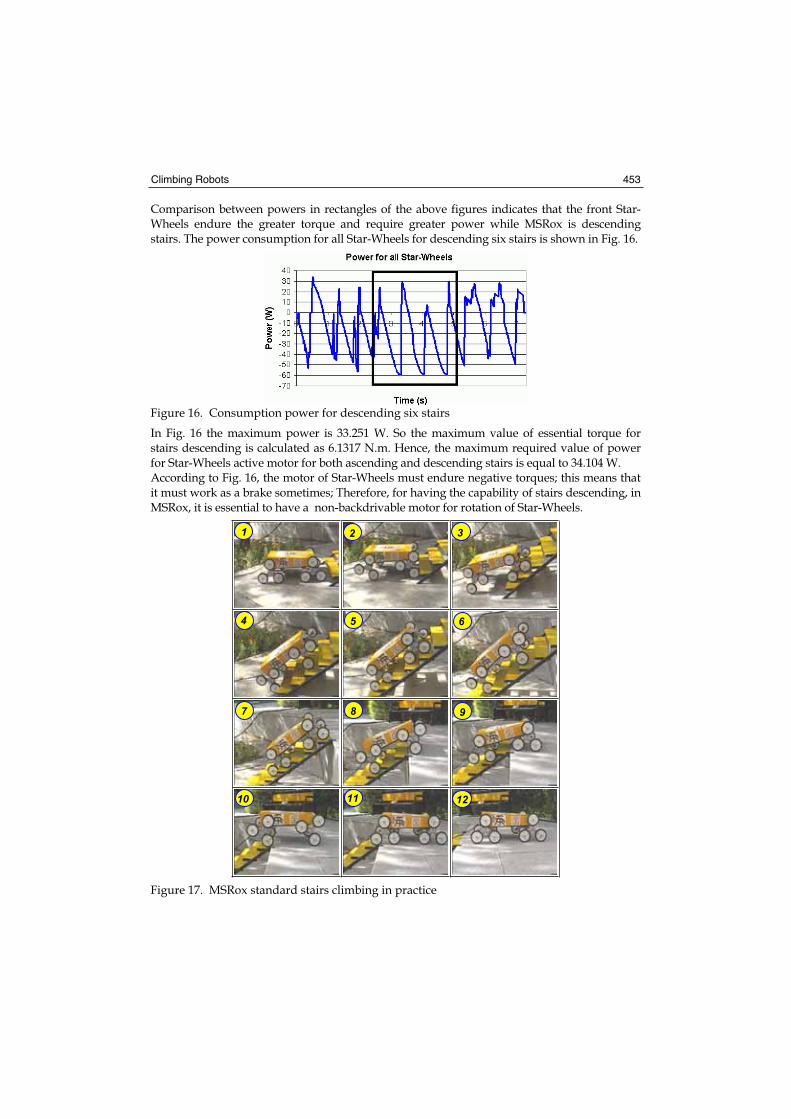
Climbing Robots 453
Comparison between powers in rectangles of the above figures indicates that the front Star-Wheels endure the greater torque and require greater power while MSRox is descending stairs. The power consumption for all Star-Wheels for descending six stairs is shown in Fig. 16.
Figure 16. Consumption power for descending six stairs
In Fig. 16 the maximum power is 33.251 W. So the maximum value of essential torque for stairs descending is calculated as 6.1317 N.m. Hence, the maximum required value of power for Star-Wheels active motor for both ascending and descending stairs is equal to 34.104 W. According to Fig. 16, the motor of Star-Wheels must endure negative torques; this means that it must work as a brake sometimes; Therefore, for having the capability of stairs descending, in MSRox, it is essential to have a non-backdrivable motor for rotation of Star-Wheels.
Figure 17. MSRox standard stairs climbing in practice
2 3
4 5 6
7 8 9
10 11 12
1
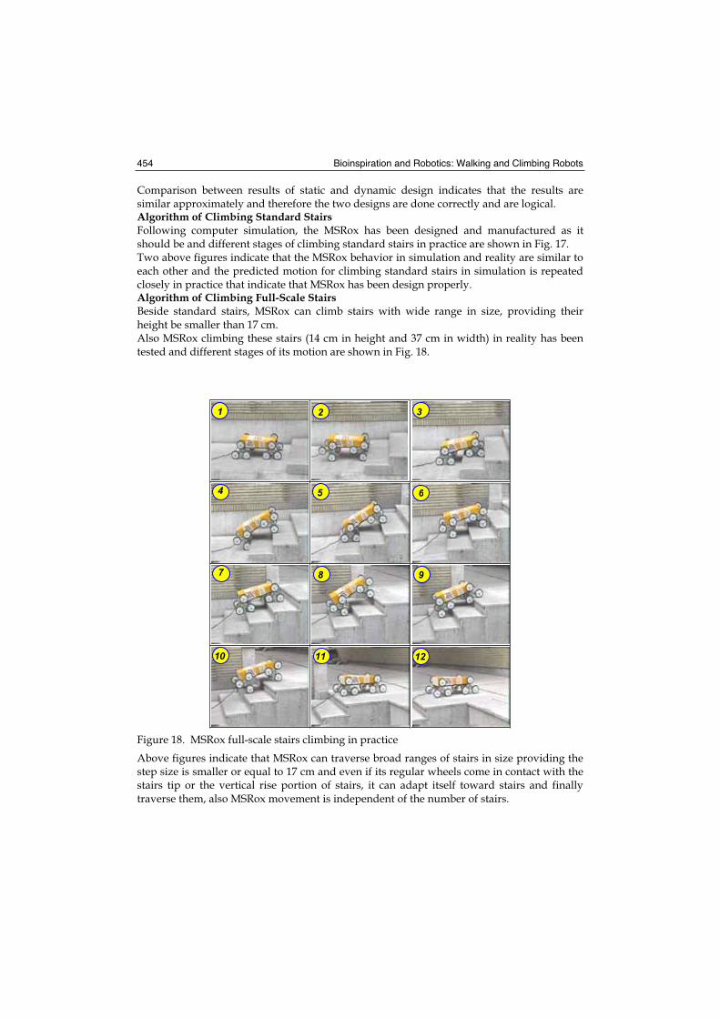
Bioinspiration and Robotics: Walking and Climbing Robots 454
Comparison between results of static and dynamic design indicates that the results are similar approximately and therefore the two designs are done correctly and are logical. Algorithm of Climbing Standard Stairs Following computer simulation, the MSRox has been designed and manufactured as it should be and different stages of climbing standard stairs in practice are shown in Fig. 17. Two above figures indicate that the MSRox behavior in simulation and reality are similar to each other and the predicted motion for climbing standard stairs in simulation is repeated closely in practice that indicate that MSRox has been design properly. Algorithm of Climbing Full-Scale Stairs Beside standard stairs, MSRox can climb stairs with wide range in size, providing their height be smaller than 17 cm. Also MSRox climbing these stairs (14 cm in height and 37 cm in width) in reality has been tested and different stages of its motion are shown in Fig. 18.
Figure 18. MSRox full-scale stairs climbing in practice
Above figures indicate that MSRox can traverse broad ranges of stairs in size providing the step size is smaller or equal to 17 cm and even if its regular wheels come in contact with the stairs tip or the vertical rise portion of stairs, it can adapt itself toward stairs and finally traverse them, also MSRox movement is independent of the number of stairs.
2 3
4 5 6
7 8 9
10 11 12
1
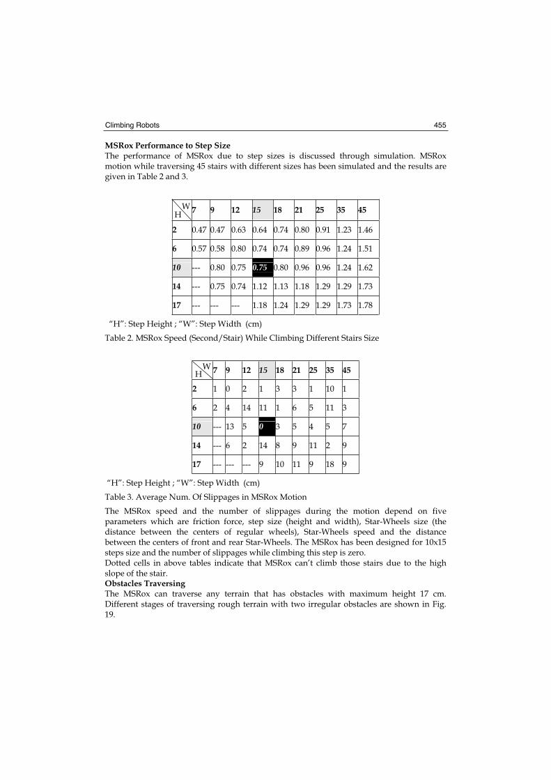
Climbing Robots 455
MSRox Performance to Step Size The performance of MSRox due to step sizes is discussed through simulation. MSRox motion while traversing 45 stairs with different sizes has been simulated and the results are given in Table 2 and 3.
7 9 12 15 18 21 25 35 45
2 0.47 0.47 0.63 0.64 0.74 0.80 0.91 1.23 1.46
6 0.57 0.58 0.80 0.74 0.74 0.89 0.96 1.24 1.51
10 --- 0.80 0.75 0.75 0.80 0.96 0.96 1.24 1.62
14 --- 0.75 0.74 1.12 1.13 1.18 1.29 1.29 1.73
17 --- --- --- 1.18 1.24 1.29 1.29 1.73 1.78
“H”: Step Height ; “W”: Step Width (cm)
Table 2. MSRox Speed (Second/Stair) While Climbing Different Stairs Size
7 9 12 15 18 21 25 35 45
2 1 0 2 1 3 3 1 10 1
6 2 4 14 11 1 6 5 11 3
10 --- 13 5 0 3 5 4 5 7
14 --- 6 2 14 8 9 11 2 9
17 --- --- --- 9 10 11 9 18 9
“H”: Step Height ; “W”: Step Width (cm)
Table 3. Average Num. Of Slippages in MSRox Motion
The MSRox speed and the number of slippages during the motion depend on five parameters which are friction force, step size (height and width), Star-Wheels size (the distance between the centers of regular wheels), Star-Wheels speed and the distance between the centers of front and rear Star-Wheels. The MSRox has been designed for 10x15 steps size and the number of slippages while climbing this step is zero. Dotted cells in above tables indicate that MSRox can’t climb those stairs due to the high slope of the stair. Obstacles Traversing The MSRox can traverse any terrain that has obstacles with maximum height 17 cm. Different stages of traversing rough terrain with two irregular obstacles are shown in Fig. 19.
WH
WH
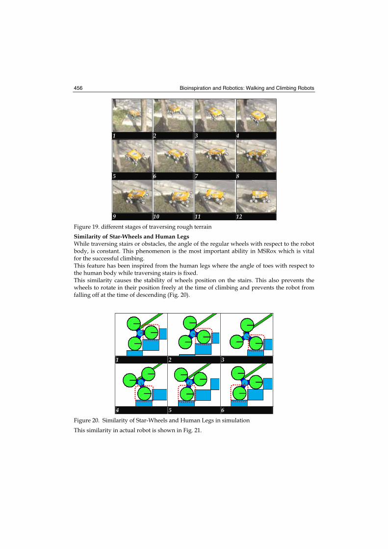
Bioinspiration and Robotics: Walking and Climbing Robots 456
1 2 3 4
5 6 7 8
9 10 11 12
Figure 19. different stages of traversing rough terrain
Similarity of Star-Wheels and Human LegsWhile traversing stairs or obstacles, the angle of the regular wheels with respect to the robot body, is constant. This phenomenon is the most important ability in MSRox which is vital for the successful climbing. This feature has been inspired from the human legs where the angle of toes with respect to the human body while traversing stairs is fixed. This similarity causes the stability of wheels position on the stairs. This also prevents the wheels to rotate in their position freely at the time of climbing and prevents the robot from falling off at the time of descending (Fig. 20).
1 2 3
4 5 6
Figure 20. Similarity of Star-Wheels and Human Legs in simulation
This similarity in actual robot is shown in Fig. 21.
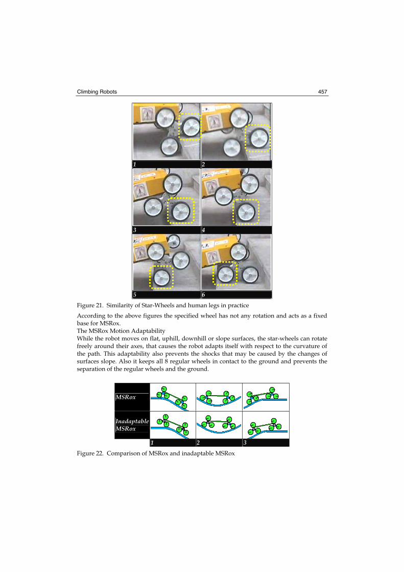
Climbing Robots 457
1 2
3 4
5 6
Figure 21. Similarity of Star-Wheels and human legs in practice
According to the above figures the specified wheel has not any rotation and acts as a fixed base for MSRox. The MSRox Motion Adaptability While the robot moves on flat, uphill, downhill or slope surfaces, the star-wheels can rotate freely around their axes, that causes the robot adapts itself with respect to the curvature of the path. This adaptability also prevents the shocks that may be caused by the changes of surfaces slope. Also it keeps all 8 regular wheels in contact to the ground and prevents the separation of the regular wheels and the ground.
MSRox
Inadaptable MSRox
1 2 3
Figure 22. Comparison of MSRox and inadaptable MSRox
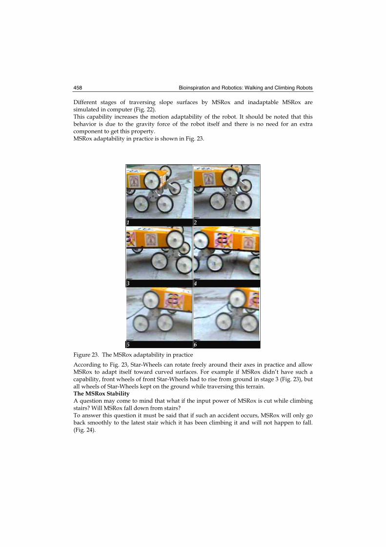
Bioinspiration and Robotics: Walking and Climbing Robots 458
Different stages of traversing slope surfaces by MSRox and inadaptable MSRox are simulated in computer (Fig. 22). This capability increases the motion adaptability of the robot. It should be noted that this behavior is due to the gravity force of the robot itself and there is no need for an extra component to get this property. MSRox adaptability in practice is shown in Fig. 23.
1 2
3 4
5 6
Figure 23. The MSRox adaptability in practice
According to Fig. 23, Star-Wheels can rotate freely around their axes in practice and allow MSRox to adapt itself toward curved surfaces. For example if MSRox didn’t have such a capability, front wheels of front Star-Wheels had to rise from ground in stage 3 (Fig. 23), but all wheels of Star-Wheels kept on the ground while traversing this terrain. The MSRox Stability A question may come to mind that what if the input power of MSRox is cut while climbing stairs? Will MSRox fall down from stairs? To answer this question it must be said that if such an accident occurs, MSRox will only go back smoothly to the latest stair which it has been climbing it and will not happen to fall. (Fig. 24).
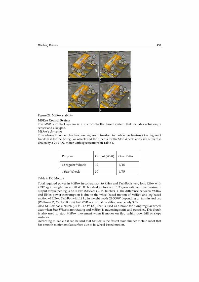
Climbing Robots 459
1 2
3 4
Figure 24. MSRox stability
MSRox Control System The MSRox control system is a microcontroller based system that includes actuators, a sensor and a keypad. MSRox's Actuators This wheeled mobile robot has two degrees of freedom in mobile mechanism. One degree of freedom is for the 12 regular wheels and the other is for the Star-Wheels and each of them is driven by a 24 V DC motor with specifications in Table 4.
Purpose Output (Watt) Gear Ratio
12 regular Wheels 12 1/16
4 Star-Wheels 30 1/75
Table 4. DC Motors
Total required power in MSRox in comparison to RHex and PackBot is very low. RHex with 7.247 kg in weight has six 20 W DC brushed motors with 1:33 gear ratio and the maximum output torque per leg is 3.614 Nm (Steeves C., M. Buehler1). The difference between MSRox and RHex power consumption is due to the wheel-based motion of MSRox and leg-based motion of RHex. PackBot with 18 kg in weight needs 24-300W depending on terrain and use (Wellman P., Venkat Krovi), but MSRox in worst condition needs only 30W. Also MSRox has a clutch (24 V - 12 W DC) that is used as a brake for fixing regular wheel axes when Star-Wheels are rotating and MSRox is traversing stairs and obstacles. This clutch is also used to stop MSRox movement when it moves on flat, uphill, downhill or slope surfaces. According to Table 5 it can be said that MSRox is the fastest stair climber mobile robot that has smooth motion on flat surface due to its wheel-based motion.
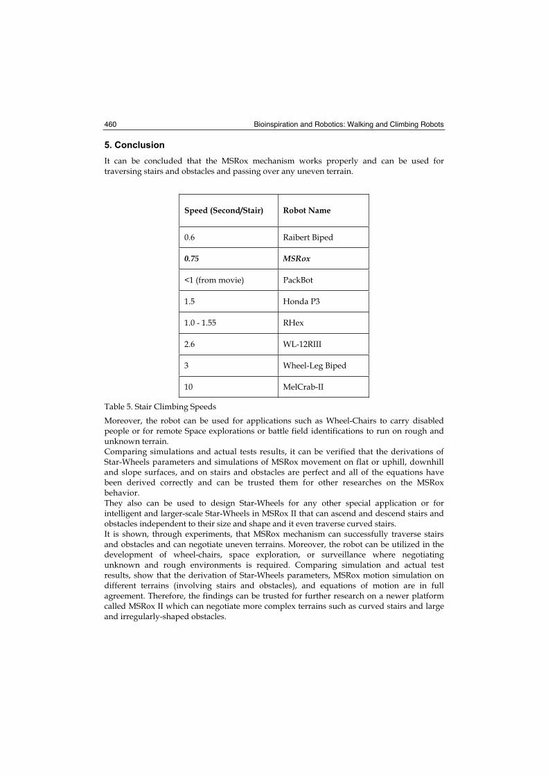
Bioinspiration and Robotics: Walking and Climbing Robots 460
5. Conclusion
It can be concluded that the MSRox mechanism works properly and can be used for traversing stairs and obstacles and passing over any uneven terrain.
Speed (Second/Stair) Robot Name
0.6 Raibert Biped
0.75 MSRox
<1 (from movie) PackBot
1.5 Honda P3
1.0 - 1.55 RHex
2.6 WL-12RIII
3 Wheel-Leg Biped
10 MelCrab-II
Table 5. Stair Climbing Speeds
Moreover, the robot can be used for applications such as Wheel-Chairs to carry disabled people or for remote Space explorations or battle field identifications to run on rough and unknown terrain. Comparing simulations and actual tests results, it can be verified that the derivations of Star-Wheels parameters and simulations of MSRox movement on flat or uphill, downhill and slope surfaces, and on stairs and obstacles are perfect and all of the equations have been derived correctly and can be trusted them for other researches on the MSRox behavior. They also can be used to design Star-Wheels for any other special application or for intelligent and larger-scale Star-Wheels in MSRox II that can ascend and descend stairs and obstacles independent to their size and shape and it even traverse curved stairs. It is shown, through experiments, that MSRox mechanism can successfully traverse stairs and obstacles and can negotiate uneven terrains. Moreover, the robot can be utilized in the development of wheel-chairs, space exploration, or surveillance where negotiating unknown and rough environments is required. Comparing simulation and actual test results, show that the derivation of Star-Wheels parameters, MSRox motion simulation on different terrains (involving stairs and obstacles), and equations of motion are in full agreement. Therefore, the findings can be trusted for further research on a newer platform called MSRox II which can negotiate more complex terrains such as curved stairs and large and irregularly-shaped obstacles.
Climbing Robots 461
6. References
Aracil R., R. Saltaren, M. Almonacid, J.M. Sabater, J.M. Azorin, (2000), Kinematic control for navigation of mobile parallel robots applied to large structures, in: Proceedings of the 17th IAARC/CIB/IEEE/IFAC/IFR International Symposium on Automation and Robotics in Construction, 2000. [1]
Buehler M., U. Saranli, D. Papadopoulos and D. Koditschek. (2002), Dynamic locomotion with four and six-legged robots, Centre for Intelligent Machines, Ambulatory Robotics Laboratory, McGill University, [2]
Buehler M., (2002) Dynamic Locomotion with One, Four and Six-Legged Robots, Ambulatory Robotics Laboratory (ARL), Centre for Intelligent Machines, McGill University , Montreal, Quebec, Canada, [3]
Choi H.R. , S.M. Ryew, T.H. Kang, J.H. Lee, H.M. Kim, A wall climbing robot with closed link mechanism, in: Proceedings of the IEEE International Conference on Intelligent Robots and Systems, San Francisco, CA, 2000, pp. 2006–2011. [4]
Crespi A., A. Badertscher, A. Guignard and A.J. Ijspeert: AmphiBot I, an amphibious snake-like robot, Robotics and Autonomous Systems, vol. 50, issue 4, pages 163-175, [5]
Dalvand M., Majid M. Moghadam, (2003) Design and modeling of a stair climber smart mobile robot, published in the 11th International Conference on Advanced Robotics(ICAR 2003), Portugal, June 30 - July3, 2003, [6]
Halme A., Ilkka Leppnen, Miso Montonen, Sami Ylnen (2001), Robot motion by simultaneously wheel and leg propulsion, Automation Technology Laboratory,Helsinki University of Technology, PL 5400, 02015 HUT, Finland, 2001, [7]
KOYANAGI J. and Shin’ich YUTA, A development of a six wheel vehicle for indoor and outdoor environment, Intelligent Robot Laboratory, Univer sity of Tsukuba Japan, [8]
Krovi V., Vijay Kumar , (1995), Modeling and Control of a Hybrid Locomotion System , ASME Journal of Mechanical Design, Vol. 121, No. 3, pp. 448-455, September 1999, [9]
Quinn R. , Gabriel M. Nelson, Richard J. Bachmann, Daniel A. Kingsley, John Offi, and Roy E. Ritzmann , (2001), Insect Designs for Improved Robot Mobility, Proc. 4th Int. Conf. On Climbing and Walking Robots, Berns and Dillmann eds., Prof. Eng. Pub., 69-76, 2001., [10]
Kamen D., R. Ambrogi, R. Heinzmann,(1991), Transportation vehicles and methods, USPatent, 5,975,225, Nov. 2, 1999, [11]
Lazard D., Stewart platform and Gröbner basis, in: ARK, Ferrare, 1992, pp. 136–142., [12] Moore Z., (2001), Design a stair climbing controller, Seminar Presentation, The Ambulatory
Robotics Lab at McGill University (ARL), 2001, [13] Merlet J.P., (1997) Les Robots Paralleles, Hermes, Paris, 1997., [14] Mohsen M. Dalvand, Majid M. Moghadam, (2003), Design and modeling of a stair climber
smart mobile robot, submitted to the Journal of Robotic System (John Wiley), May 2003, [15]
Nakayama R., et. al.,(1988), Development of a Mobile Maintenance Robot System AIMARS, ASME, Proceeding of the USA-Japan Symposium on Flexible Automation, Minniapolis, 1988, [16]
Saltaren R., R. Aracil, O. Reinoso, J.M. Sabater, M. Almonacid, (2000) Parallel climbing robot for construction, inspection and maintenance, in: Proceedings of the International Symposium on Automation and Robotics in Construction, Madrid, Spain, 2000, pp. 359–364., [17]
Bioinspiration and Robotics: Walking and Climbing Robots 462
Saranli U., M. Buehler, and D. E. Koditschek, (2001), RHex: A Simple and Highly Mobile Hexapod Robot, Int. J. Robotics Research, 20(7):616-631, July 2001., [18]
Siegwart R., Michel Lauria, Pierre-Alain Mäusli, Michel Van Winnendael, (1998), Design and Implementation of an Innovative Micro-Rover, Proceedings of Robotics 98, the 3rd Conference and Exposition on Robotics in Challenging Environments, Albuquerque, New Mexico, April 26-30, 1998, [19]
Stewart D. , Proceedings of the Institution of Mechanical Engineers (Part I) 180 (1965) 371–386., [20] Steeves C., M. Buehler1, S.G. Penzes2, (2002), Dynamic behaviors for a hybrid leg-wheel
mobile platform, McGill University, Center for Intelligent Machines, Ambulatory Robotics Lab, Montreal, QC, Canada, [21]
Wellman P., Venkat Krovi, Vijay Kumar, and William Harwin, (1995), Design of a Wheelchair with Legs for People with Motor Disabilities, IEEE transactions on rehabilitation engineering, vol. 3, no. 4, Dec. 1995, [22]
http://robotics.jpl.nasa.gov/tasks/tmr/movies/Air10FPS240x180.mov, [23] http://ai.eecs.umich.edu/RHex/RHexversions.html, [24] http://robot.spawar.navy.mil/home.asp?item=showrpasset&table=UGV&ID=30&robpa=5,[25] http://biorobots.cwru.edu/, [26] http://www.independencenow.com/nonsecure/ibot/index.html, [27] http://www.irobot.com, [28]
27
Mechanical and Kinematics Design Methodology of a New Wheelchair with
Additional Capabilities
R. Morales, A. González and V. FeliuSchool of Industrial Engineering, University of Castilla-La Mancha, Ciudad Real
Spain
1. Introduction
Since wheelchairs appeared, only minor changes have occurred with regard to their basic design. An important change was the design of the powered wheelchairs, and it is unquestionable that they greatly improve the mobility of the handicapped. Nevertheless, architectural barriers still exist in many cities and buildings, and it is expensive and time consuming, if not impossible, to eliminate all of them. A new advance in mobility assistance came with the development of wheelchairs capable of negotiating architectural barriers. The first commercial models were based on a single-section track mechanism (SUNWA Co. Ltd). A disadvantage of these tracked systems is that the entire track is forced to rotate on the edge of the first step when initiating descent. This is a difficult and dangerous operation. An evolution of this mechanism principle has been the use of low pressure tyres for ascending and descending stairs. These systems exploiting their ability to produce high grip forces on the edge of the obstacles improving the mobility and efficiency in barrier free locomotion (Uchida et al., 1999), (Hirose et al., 2001), but the basic limitations of this design still remain. Other designs based on wheels improve the efficiency in barrier free environments but needs additional mechanisms to overcome the architectural barriers. A commonly used solution is to group two, three or four wheels in a rolling cluster. The simplest models are little platforms to carry light wheelchairs (The Wheelchair Lift Company). A negative aspect of this solution is the necessity of an assistant. To operate the system without assistants, a more complex control system is required (Kamen et al., 1999). The problem can be solved by adding another cluster (Lawn & Ishimatzu, 2003). While the mechanical solution is quite simple, the systems are very sophisticated since it relies on dynamic control to maintain the upright position. The main disadvantages of these designs are the high actuating cluster torque, high number of wheels that must be driven and braked, difficulty to add a steering mechanism, and a dramatic increasing in weight, size, and cost. Solutions based on legs improve the movement of the robots in highly unstructured environments (Hirose, 1984), (Kar, 2003), (Cham et al., 2002), but their low efficiency in horizontal locomotion forces us to discard legs as a way of providing mobility for the elderly or the disabled. To enhance motion capabilities wheels are incorporated. These vehicles are referred to as high-mobility robots since they combine the efficiency in
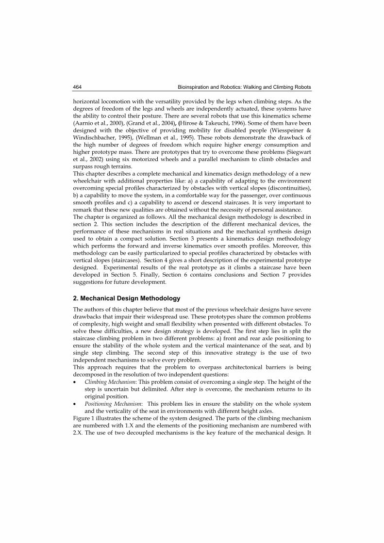
Bioinspiration and Robotics: Walking and Climbing Robots 464
horizontal locomotion with the versatility provided by the legs when climbing steps. As the degrees of freedom of the legs and wheels are independently actuated, these systems have the ability to control their posture. There are several robots that use this kinematics scheme (Aarnio et al., 2000), (Grand et al., 2004), (Hirose & Takeuchi, 1996). Some of them have been designed with the objective of providing mobility for disabled people (Wiesspeiner & Windischbacher, 1995), (Wellman et al., 1995). These robots demonstrate the drawback of the high number of degrees of freedom which require higher energy consumption and higher prototype mass. There are prototypes that try to overcome these problems (Siegwart et al., 2002) using six motorized wheels and a parallel mechanism to climb obstacles and surpass rough terrains. This chapter describes a complete mechanical and kinematics design methodology of a new wheelchair with additional properties like: a) a capability of adapting to the environment overcoming special profiles characterized by obstacles with vertical slopes (discontinuities), b) a capability to move the system, in a comfortable way for the passenger, over continuous smooth profiles and c) a capability to ascend or descend staircases. It is very important to remark that these new qualities are obtained without the necessity of personal assistance. The chapter is organized as follows. All the mechanical design methodology is described in section 2. This section includes the description of the different mechanical devices, the performance of these mechanisms in real situations and the mechanical synthesis design used to obtain a compact solution. Section 3 presents a kinematics design methodology which performs the forward and inverse kinematics over smooth profiles. Moreover, this methodology can be easily particularized to special profiles characterized by obstacles with vertical slopes (staircases). Section 4 gives a short description of the experimental prototype designed. Experimental results of the real prototype as it climbs a staircase have been developed in Section 5. Finally, Section 6 contains conclusions and Section 7 provides suggestions for future development.
2. Mechanical Design Methodology
The authors of this chapter believe that most of the previous wheelchair designs have severe drawbacks that impair their widespread use. These prototypes share the common problems of complexity, high weight and small flexibility when presented with different obstacles. To solve these difficulties, a new design strategy is developed. The first step lies in split the staircase climbing problem in two different problems: a) front and rear axle positioning to ensure the stability of the whole system and the vertical maintenance of the seat, and b) single step climbing. The second step of this innovative strategy is the use of two independent mechanisms to solve every problem. This approach requires that the problem to overpass architectonical barriers is being decomposed in the resolution of two independent questions:
• Climbing Mechanism: This problem consist of overcoming a single step. The height of the step is uncertain but delimited. After step is overcome, the mechanism returns to its original position.
• Positioning Mechanism: This problem lies in ensure the stability on the whole system and the verticality of the seat in environments with different height axles.
Figure 1 illustrates the scheme of the system designed. The parts of the climbing mechanism are numbered with 1.X and the elements of the positioning mechanism are numbered with 2.X. The use of two decoupled mechanisms is the key feature of the mechanical design. It
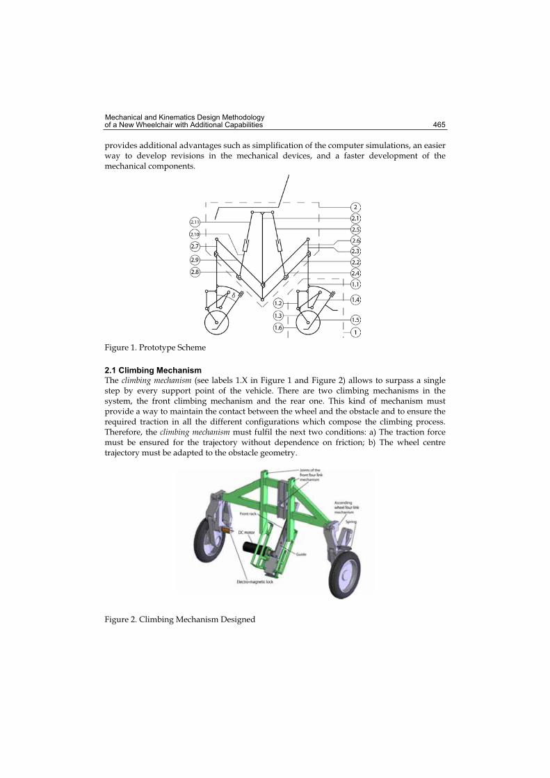
Mechanical and Kinematics Design Methodology of a New Wheelchair with Additional Capabilities 465
provides additional advantages such as simplification of the computer simulations, an easier way to develop revisions in the mechanical devices, and a faster development of the mechanical components.
Figure 1. Prototype Scheme
2.1 Climbing Mechanism
The climbing mechanism (see labels 1.X in Figure 1 and Figure 2) allows to surpass a single step by every support point of the vehicle. There are two climbing mechanisms in the system, the front climbing mechanism and the rear one. This kind of mechanism must provide a way to maintain the contact between the wheel and the obstacle and to ensure the required traction in all the different configurations which compose the climbing process. Therefore, the climbing mechanism must fulfil the next two conditions: a) The traction force must be ensured for the trajectory without dependence on friction; b) The wheel centre trajectory must be adapted to the obstacle geometry.
Figure 2. Climbing Mechanism Designed
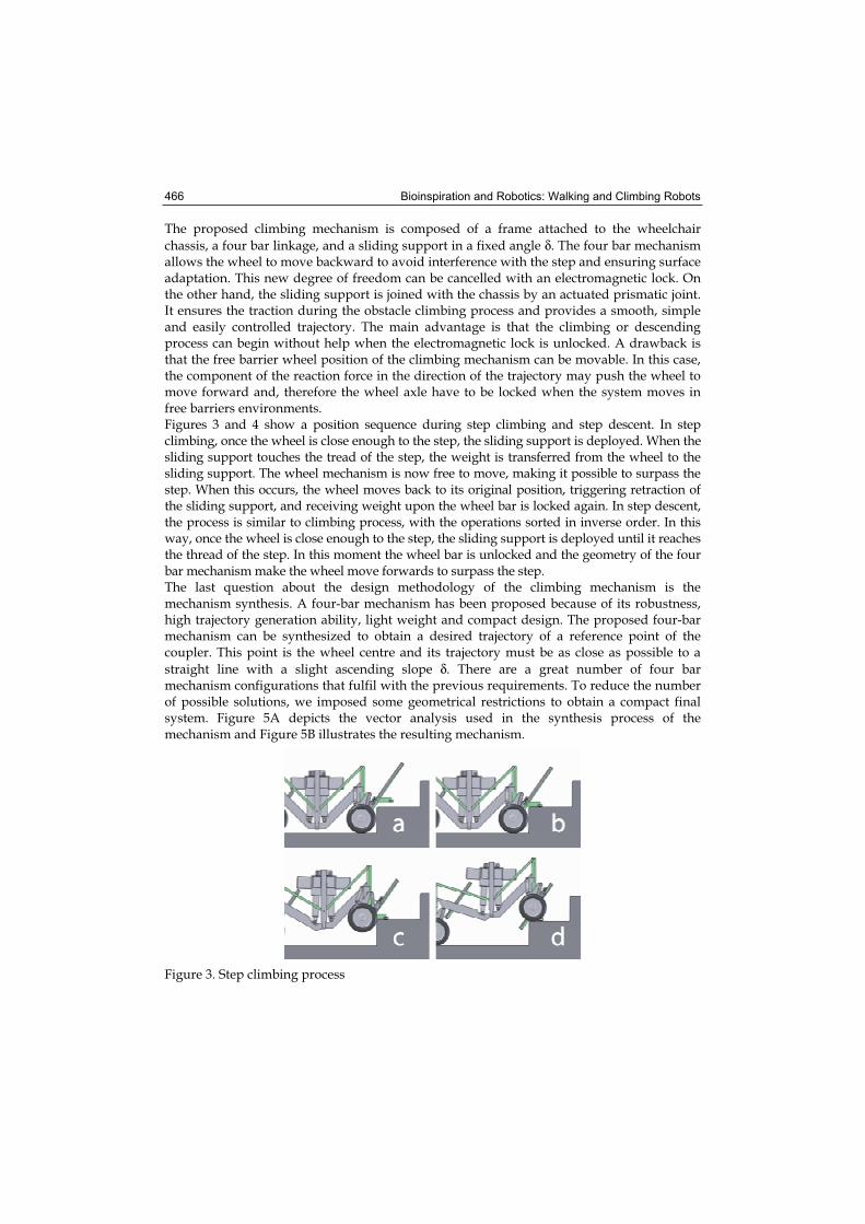
Bioinspiration and Robotics: Walking and Climbing Robots 466
The proposed climbing mechanism is composed of a frame attached to the wheelchair
chassis, a four bar linkage, and a sliding support in a fixed angle δ. The four bar mechanism allows the wheel to move backward to avoid interference with the step and ensuring surface adaptation. This new degree of freedom can be cancelled with an electromagnetic lock. On the other hand, the sliding support is joined with the chassis by an actuated prismatic joint. It ensures the traction during the obstacle climbing process and provides a smooth, simple and easily controlled trajectory. The main advantage is that the climbing or descending process can begin without help when the electromagnetic lock is unlocked. A drawback is that the free barrier wheel position of the climbing mechanism can be movable. In this case, the component of the reaction force in the direction of the trajectory may push the wheel to move forward and, therefore the wheel axle have to be locked when the system moves in free barriers environments. Figures 3 and 4 show a position sequence during step climbing and step descent. In step climbing, once the wheel is close enough to the step, the sliding support is deployed. When the sliding support touches the tread of the step, the weight is transferred from the wheel to the sliding support. The wheel mechanism is now free to move, making it possible to surpass the step. When this occurs, the wheel moves back to its original position, triggering retraction of the sliding support, and receiving weight upon the wheel bar is locked again. In step descent, the process is similar to climbing process, with the operations sorted in inverse order. In this way, once the wheel is close enough to the step, the sliding support is deployed until it reaches the thread of the step. In this moment the wheel bar is unlocked and the geometry of the four bar mechanism make the wheel move forwards to surpass the step. The last question about the design methodology of the climbing mechanism is the mechanism synthesis. A four-bar mechanism has been proposed because of its robustness, high trajectory generation ability, light weight and compact design. The proposed four-bar mechanism can be synthesized to obtain a desired trajectory of a reference point of the coupler. This point is the wheel centre and its trajectory must be as close as possible to a
straight line with a slight ascending slope δ. There are a great number of four bar mechanism configurations that fulfil with the previous requirements. To reduce the number of possible solutions, we imposed some geometrical restrictions to obtain a compact final system. Figure 5A depicts the vector analysis used in the synthesis process of the mechanism and Figure 5B illustrates the resulting mechanism.
Figure 3. Step climbing process
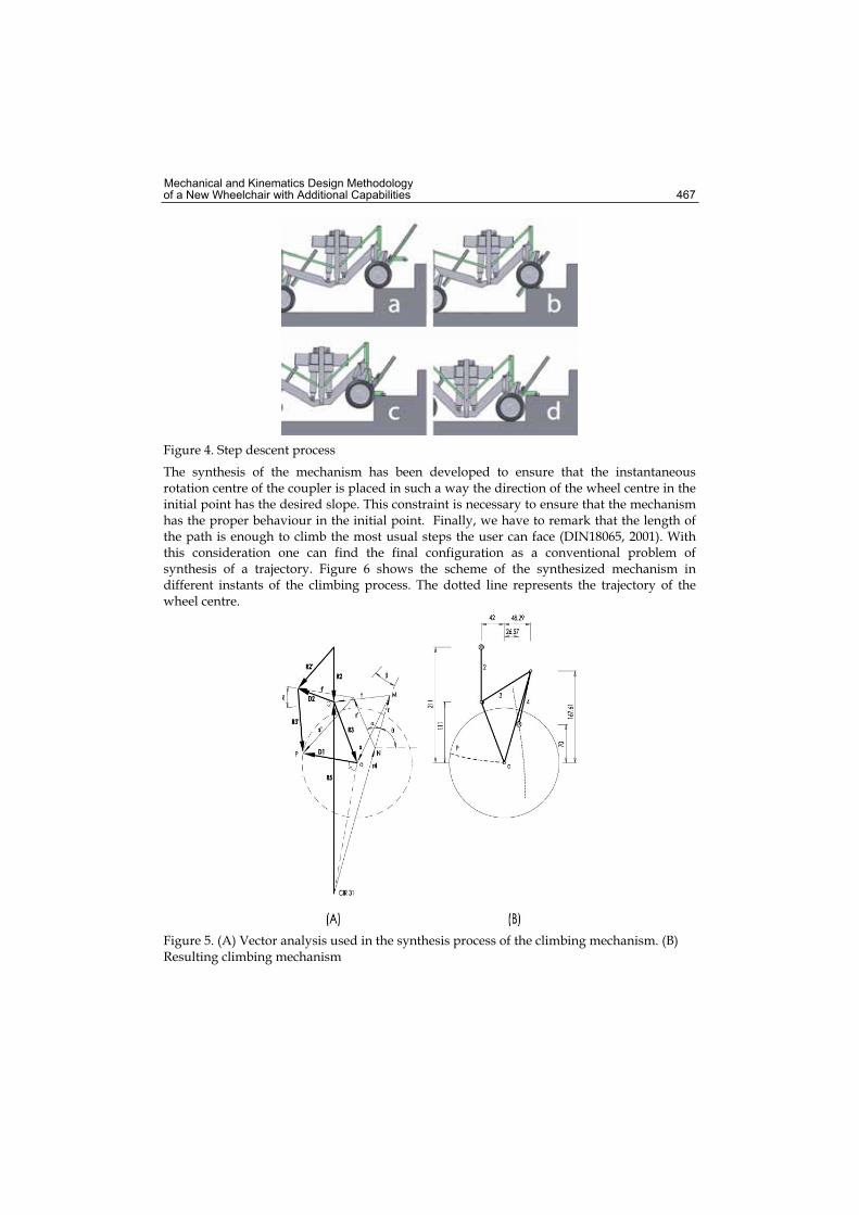
Mechanical and Kinematics Design Methodology of a New Wheelchair with Additional Capabilities 467
Figure 4. Step descent process
The synthesis of the mechanism has been developed to ensure that the instantaneous rotation centre of the coupler is placed in such a way the direction of the wheel centre in the initial point has the desired slope. This constraint is necessary to ensure that the mechanism has the proper behaviour in the initial point. Finally, we have to remark that the length of the path is enough to climb the most usual steps the user can face (DIN18065, 2001). With this consideration one can find the final configuration as a conventional problem of synthesis of a trajectory. Figure 6 shows the scheme of the synthesized mechanism in different instants of the climbing process. The dotted line represents the trajectory of the wheel centre.
Figure 5. (A) Vector analysis used in the synthesis process of the climbing mechanism. (B) Resulting climbing mechanism
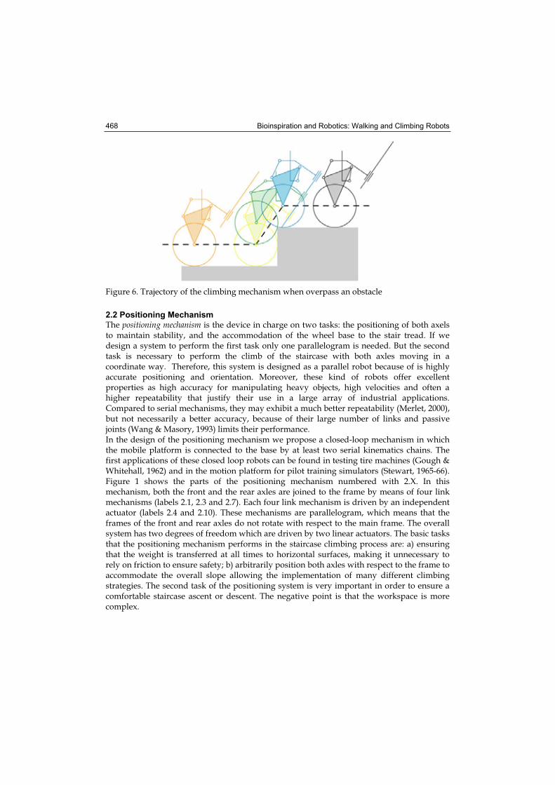
Bioinspiration and Robotics: Walking and Climbing Robots 468
Figure 6. Trajectory of the climbing mechanism when overpass an obstacle
2.2 Positioning Mechanism
The positioning mechanism is the device in charge on two tasks: the positioning of both axels to maintain stability, and the accommodation of the wheel base to the stair tread. If we design a system to perform the first task only one parallelogram is needed. But the second task is necessary to perform the climb of the staircase with both axles moving in a coordinate way. Therefore, this system is designed as a parallel robot because of is highly accurate positioning and orientation. Moreover, these kind of robots offer excellent properties as high accuracy for manipulating heavy objects, high velocities and often a higher repeatability that justify their use in a large array of industrial applications. Compared to serial mechanisms, they may exhibit a much better repeatability (Merlet, 2000), but not necessarily a better accuracy, because of their large number of links and passive joints (Wang & Masory, 1993) limits their performance. In the design of the positioning mechanism we propose a closed-loop mechanism in which the mobile platform is connected to the base by at least two serial kinematics chains. The first applications of these closed loop robots can be found in testing tire machines (Gough & Whitehall, 1962) and in the motion platform for pilot training simulators (Stewart, 1965-66). Figure 1 shows the parts of the positioning mechanism numbered with 2.X. In this mechanism, both the front and the rear axles are joined to the frame by means of four link mechanisms (labels 2.1, 2.3 and 2.7). Each four link mechanism is driven by an independent actuator (labels 2.4 and 2.10). These mechanisms are parallelogram, which means that the frames of the front and rear axles do not rotate with respect to the main frame. The overall system has two degrees of freedom which are driven by two linear actuators. The basic tasks that the positioning mechanism performs in the staircase climbing process are: a) ensuring that the weight is transferred at all times to horizontal surfaces, making it unnecessary to rely on friction to ensure safety; b) arbitrarily position both axles with respect to the frame to accommodate the overall slope allowing the implementation of many different climbing strategies. The second task of the positioning system is very important in order to ensure a comfortable staircase ascent or descent. The negative point is that the workspace is more complex.
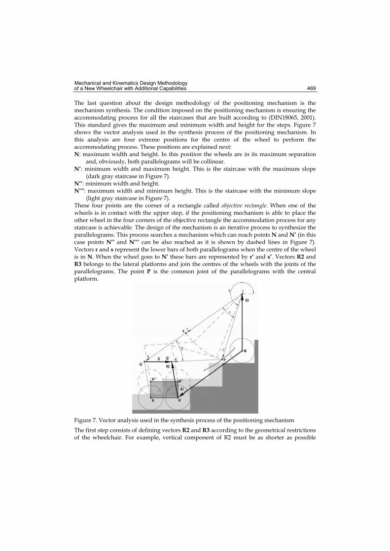
Mechanical and Kinematics Design Methodology of a New Wheelchair with Additional Capabilities 469
The last question about the design methodology of the positioning mechanism is the mechanism synthesis. The condition imposed on the positioning mechanism is ensuring the accommodating process for all the staircases that are built according to (DIN18065, 2001). This standard gives the maximum and minimum width and height for the steps. Figure 7 shows the vector analysis used in the synthesis process of the positioning mechanism. In this analysis are four extreme positions for the centre of the wheel to perform the accommodating process. These positions are explained next: N: maximum width and height. In this position the wheels are in its maximum separation
and, obviously, both parallelograms will be collinear. N’: minimum width and maximum height. This is the staircase with the maximum slope
(dark gray staircase in Figure 7). N’’: minimum width and height. N’’’: maximum width and minimum height. This is the staircase with the minimum slope
(light gray staircase in Figure 7). These four points are the corner of a rectangle called objective rectangle. When one of the wheels is in contact with the upper step, if the positioning mechanism is able to place the other wheel in the four corners of the objective rectangle the accommodation process for any staircase is achievable. The design of the mechanism is an iterative process to synthesize the parallelograms. This process searches a mechanism which can reach points N and N’ (in this case points N’’ and N’’’ can be also reached as it is shown by dashed lines in Figure 7). Vectors r and s represent the lower bars of both parallelograms when the centre of the wheel is in N. When the wheel goes to N’ these bars are represented by r’ and s’. Vectors R2 and R3 belongs to the lateral platforms and join the centres of the wheels with the joints of the parallelograms. The point P is the common joint of the parallelograms with the central platform.
Figure 7. Vector analysis used in the synthesis process of the positioning mechanism
The first step consists of defining vectors R2 and R3 according to the geometrical restrictions of the wheelchair. For example, vertical component of R2 must be as shorter as possible
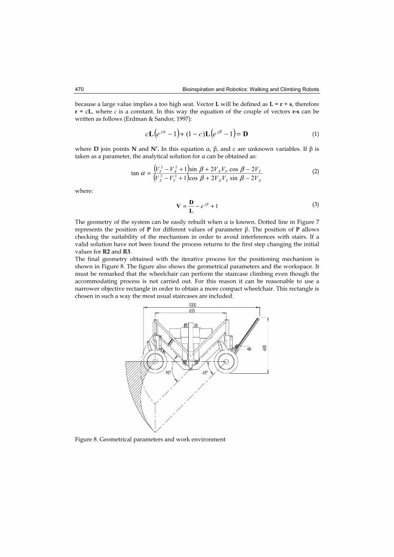
Bioinspiration and Robotics: Walking and Climbing Robots 470
because a large value implies a too high seat. Vector L will be defined as L = r + s, therefore r = cL, where c is a constant. In this way the equation of the couple of vectors r-s can be written as follows (Erdman & Sandor, 1997):
( ) ( ) DLL =−−+− 1)1(1 βα jj ecec (1)
where D join points N and N’. In this equation , , and c are unknown variables. If is taken as a parameter, the analytical solution for can be obtained as:
( )( ) XYXYX
YYXXY
VVVVVVVVVV
2sin2cos1
2cos2sin1tan
22
22
−++−−++−=
ββββα (2)
where:
1+−= βjeL
DV (3)
The geometry of the system can be easily rebuilt when is known. Dotted line in Figure 7 represents the position of P for different values of parameter . The position of P allows checking the suitability of the mechanism in order to avoid interferences with stairs. If a valid solution have not been found the process returns to the first step changing the initial values for R2 and R3.The final geometry obtained with the iterative process for the positioning mechanism is shown in Figure 8. The figure also shows the geometrical parameters and the workspace. It must be remarked that the wheelchair can perform the staircase climbing even though the accommodating process is not carried out. For this reason it can be reasonable to use a narrower objective rectangle in order to obtain a more compact wheelchair. This rectangle is chosen in such a way the most usual staircases are included.
Figure 8. Geometrical parameters and work environment
Mechanical and Kinematics Design Methodology of a New Wheelchair with Additional Capabilities 471
3. Kinematics Design Methodology
Regarding the mechanical structure, modularity was the key factor in the design methodology of the system. The wheelchair driven degrees of freedom are split into two subcategories: the fist concerns the locomotion itself (traction and ascent step) and the second concerns the posture (verticality of the chair frame). Both categories will be treated together in the kinematic model as they are coupled, but the appropriate mechanical design simplifies the control. The determination of a kinematic model becomes a critical part of the whole system because it has the responsibility of generating the real time trajectories for the actuators of the wheelchair, in such a way that this vehicle should be able to climb and desdent staircases maintaining maximum possible comfort for the passenger: smooth motions and very small deviations from the vertical. These real time trajectories are the references for the closed-loop systems (servocontrols) that control the angles of the motors (actuators) in charge of moving the several degrees of freedom of our wheelchair. This trajectory generator relies on a kinematic model that should be: (a) precise enough to describe the behavior of the mechanism; (b) simple enough for computation in real time: (c) flexible enough to include descriptions of all the tasks mentioned in the previous section, which include different chair configurations and different situations of contact with the environment (floor and staircases). Based on the modularity of the system, we proceed to develop all the kinematics methodology of the wheelchair. On the one hand, we define as forward kinematic model(FKM) the algorithm which provides the position of the center of mass (Pg) and the
inclination of the wheelchair (γ) with regard to specific values of actuator variables. On the other hand, we define as inverse kinematic model (IKM) the algorithm which gives the values (angles) of the actuator variables needed to achieve a desired centre of mass position and inclination of the wheelchair. We perform the kinematics methodology over smooth continuous profiles because is very easy to particularize on profiles composed by flat floor and staircase profiles. In these special profiles characterized by obstacles with vertical slopes (discontinuities), both forward and inverse kinematics models allow analytical solutions and iterative calculation procedures are not needed. Finally, we coment that all the kinematics design methodology presented in this section is based on complex notation: horizontal variable is the real component and vertical variable is the imaginary component (where j is the imaginary number). This notation facilitates the adquisition of the kinematic models in the prototype because we have found that expressions of rotations are simplified leading to more compact equations. Next, we will use operators Re(z) and Im(z) as the real and imaginary components respectively of the complex number z,
and ∠z and |z| will mean the phase and the complex modulus of the elements of z.
3.1 Forward kinematics design methodology of the wheelchair prototype over smooth profiles
In this section we present the kinematic methodology to obtain the forward kinematics model of the wheelchair over smooth profiles and the resulting expressions. Figure 9 illustrates the prototype scheme developed and its main parameters. We assume a smooth
generic profile ( )sf̂ . We can obtain the trajectory of the centre of the wheels ( )f from a
generic floor profile with the next equation:
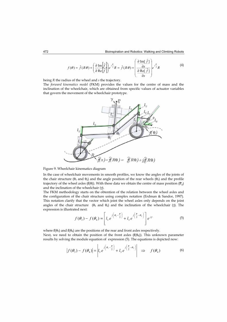
Bioinspiration and Robotics: Walking and Climbing Robots 472
[ ][ ] Re
sf
sf
RfReffRff
jj22
]ˆRe[
]ˆIm[
)(ˆˆRe
ˆIm)(ˆ)(
ππ
θθθ
∂∂
∂∂
+=∂∂+=
(4)
being R the radius of the wheel and s the trajectory. The forward kinematics model (FKM) provides the values for the centre of mass and the inclination of the wheelchair, which are obtained from specific values of actuator variables that govern the movement of the wheelchair prototype.
Figure 9. Wheelchair kinematics diagram
In the case of wheelchair movements in smooth profiles, we know the angles of the joints of
the chair structure (θ1 and θ2) and the angle position of the rear wheels (θ3) and the profile
trajectory of the wheel axles (f(θ)). With these data we obtain the centre of mass position (Pg)
and the inclination of the wheelchair (γ).The FKM methodology starts on the obtention of the relation between the wheel axles and the configuration of the chair structure using complex notation (Erdman & Sandor, 1997). This notation clarify that the vector which joint the wheel axles only depends on the joint
angles of the chair structure (θ1 and θ2) and the inclination of the wheelchair (γ). The expression is illustrated next:
γθππθ
θθ jjj
eelelff +=−−− 21
23
2343 )()( (5)
where f(θ3) and f(θ4) are the positions of the rear and front axles respectively.
Next, we need to obtain the position of the front axles (f(θ4)). This unknown parameter results by solving the module equation of expression (5). The equations is depicted now:
)()()( 42
32
343
21
θθθθππθ
felelffjj
+=−−−
(6)
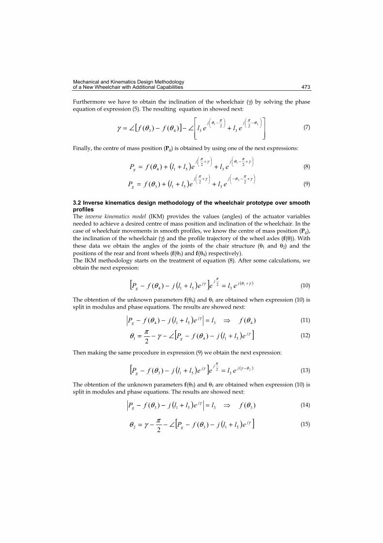
Mechanical and Kinematics Design Methodology of a New Wheelchair with Additional Capabilities 473
Furthermore we have to obtain the inclination of the wheelchair (γ) by solving the phase equation of expression (5). The resulting equation in showed next:
[ ] +∠−−∠=−− 21
23
2343 )()(
θππθθθγ
jjelelff (7)
Finally, the centre of mass position (Pg) is obtained by using one of the next expressions:
( )+−+
+++=γπθγπ
θ 23
2514
1
)(jj
g elellfP (8)
( )+−−+
+++=γπθγπ
θ 23
2513
2
)(jj
g elellfP (9)
3.2 Inverse kinematics design methodology of the wheelchair prototype over smooth profiles
The inverse kinematics model (IKM) provides the values (angles) of the actuator variables needed to achieve a desired centre of mass position and inclination of the wheelchair. In the case of wheelchair movements in smooth profiles, we know the centre of mass position (Pg),
the inclination of the wheelchair (γ) and the profile trajectory of the wheel axles (f(θ)). With
these data we obtain the angles of the joints of the chair structure (θ1 and θ2) and the
positions of the rear and front wheels (f(θ3) and f(θ4) respectively). The IKM methodology starts on the treatment of equation (8). After some calculations, we obtain the next expresion:
( )[ ] ( )γθπ
γθ +=+−− 1
32
514 )( jjjg eleelljfP (10)
The obtention of the unknown parameters f(θ4) and θ1 are obtained when expression (10) is split in modulus and phase equations. The results are showed next:
( ) )()( 43514 θθ γ flelljfP jg =+−− (11)
( )[ ]γθγπθ jg elljfP 5141 )(
2+−−∠−−= (12)
Then making the same procedure in expression (9) we obtain the next expression:
( )[ ] ( )2
32
513 )( θγπ
γθ −=+−− jjjg eleelljfP (13)
The obtention of the unknown parameters f(θ3) and θ1 are obtained when expression (10) is split in modules and phase equations. The results are showed next:
( ) )()( 33513 θθ γ flelljfP jg =+−− (14)
( )[ ]γθπγθ jg elljfP 5132 )(
2+−−∠−−= (15)
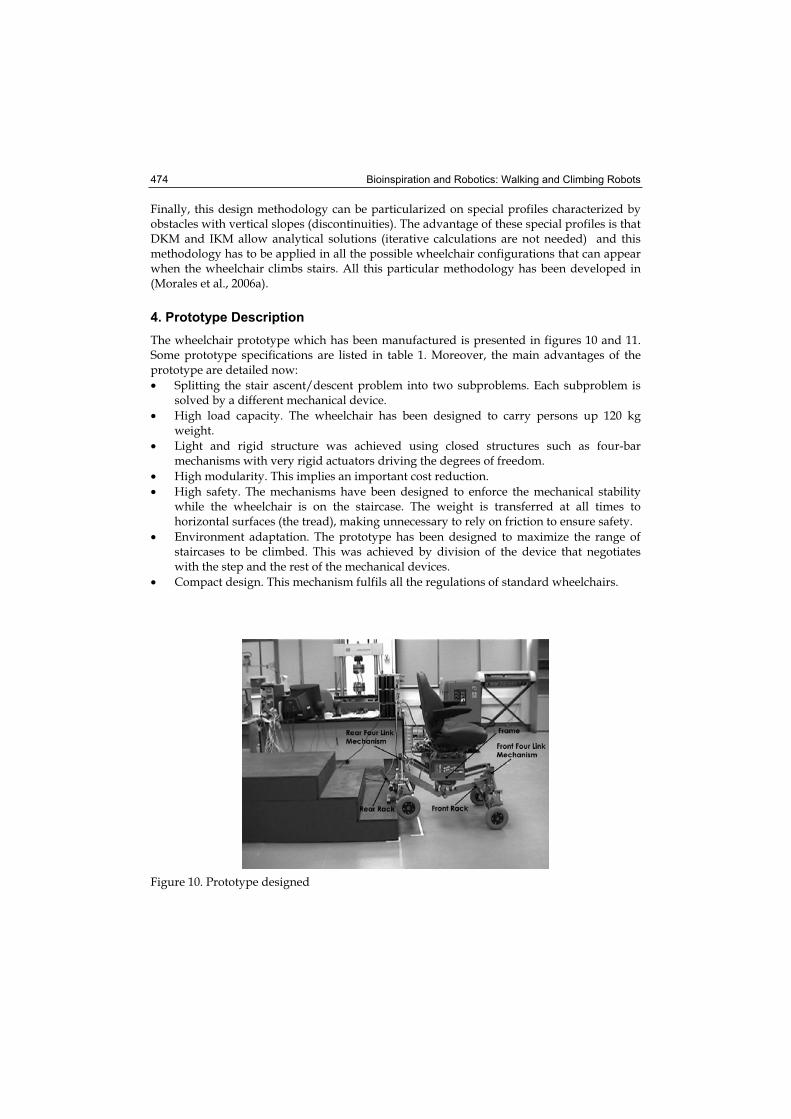
Bioinspiration and Robotics: Walking and Climbing Robots 474
Finally, this design methodology can be particularized on special profiles characterized by obstacles with vertical slopes (discontinuities). The advantage of these special profiles is that DKM and IKM allow analytical solutions (iterative calculations are not needed) and this methodology has to be applied in all the possible wheelchair configurations that can appear when the wheelchair climbs stairs. All this particular methodology has been developed in (Morales et al., 2006a).
4. Prototype Description
The wheelchair prototype which has been manufactured is presented in figures 10 and 11. Some prototype specifications are listed in table 1. Moreover, the main advantages of the prototype are detailed now:
• Splitting the stair ascent/descent problem into two subproblems. Each subproblem is solved by a different mechanical device.
• High load capacity. The wheelchair has been designed to carry persons up 120 kg weight.
• Light and rigid structure was achieved using closed structures such as four-bar mechanisms with very rigid actuators driving the degrees of freedom.
• High modularity. This implies an important cost reduction.
• High safety. The mechanisms have been designed to enforce the mechanical stability while the wheelchair is on the staircase. The weight is transferred at all times to horizontal surfaces (the tread), making unnecessary to rely on friction to ensure safety.
• Environment adaptation. The prototype has been designed to maximize the range of staircases to be climbed. This was achieved by division of the device that negotiates with the step and the rest of the mechanical devices.
• Compact design. This mechanism fulfils all the regulations of standard wheelchairs.
Figure 10. Prototype designed
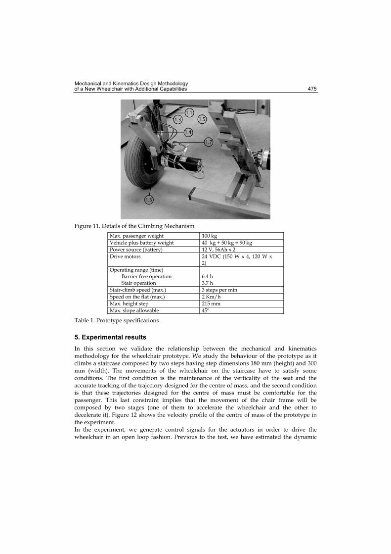
Mechanical and Kinematics Design Methodology of a New Wheelchair with Additional Capabilities 475
Figure 11. Details of the Climbing Mechanism
Max. passenger weight 100 kg
Vehicle plus battery weight 40 kg + 50 kg = 90 kg
Power source (battery) 12 V, 56Ah x 2
Drive motors 24 VDC (150 W x 4, 120 W x 2)
Operating range (time) Barrier free operation Stair operation
6.4 h 3.7 h
Stair-climb speed (max.) 3 steps per min
Speed on the flat (max.) 2 Km/h
Max. height step 215 mm
Max. slope allowable 45º
Table 1. Prototype specifications
5. Experimental results
In this section we validate the relationship between the mechanical and kinematics methodology for the wheelchair prototype. We study the behaviour of the prototype as it climbs a staircase composed by two steps having step dimensions 180 mm (height) and 300 mm (width). The movements of the wheelchair on the staircase have to satisfy some conditions. The first condition is the maintenance of the verticality of the seat and the accurate tracking of the trajectory designed for the centre of mass, and the second condition is that these trajectories designed for the centre of mass must be comfortable for the passenger. This last constraint implies that the movement of the chair frame will be composed by two stages (one of them to accelerate the wheelchair and the other to decelerate it). Figure 12 shows the velocity profile of the centre of mass of the prototype in the experiment.In the experiment, we generate control signals for the actuators in order to drive the wheelchair in an open loop fashion. Previous to the test, we have estimated the dynamic
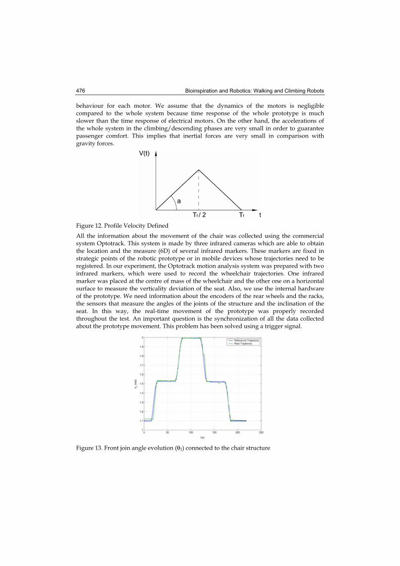
Bioinspiration and Robotics: Walking and Climbing Robots 476
behaviour for each motor. We assume that the dynamics of the motors is negligible compared to the whole system because time response of the whole prototype is much slower than the time response of electrical motors. On the other hand, the accelerations of the whole system in the climbing/descending phases are very small in order to guarantee passenger comfort. This implies that inertial forces are very small in comparison with gravity forces.
Figure 12. Profile Velocity Defined
All the information about the movement of the chair was collected using the commercial system Optotrack. This system is made by three infrared cameras which are able to obtain the location and the measure (6D) of several infrared markers. These markers are fixed in strategic points of the robotic prototype or in mobile devices whose trajectories need to be registered. In our experiment, the Optotrack motion analysis system was prepared with two infrared markers, which were used to record the wheelchair trajectories. One infrared marker was placed at the centre of mass of the wheelchair and the other one on a horizontal surface to measure the verticality deviation of the seat. Also, we use the internal hardware of the prototype. We need information about the encoders of the rear wheels and the racks, the sensors that measure the angles of the joints of the structure and the inclination of the seat. In this way, the real-time movement of the prototype was properly recorded throughout the test. An important question is the synchronization of all the data collected about the prototype movement. This problem has been solved using a trigger signal.
Figure 13. Front join angle evolution (θ1) connected to the chair structure
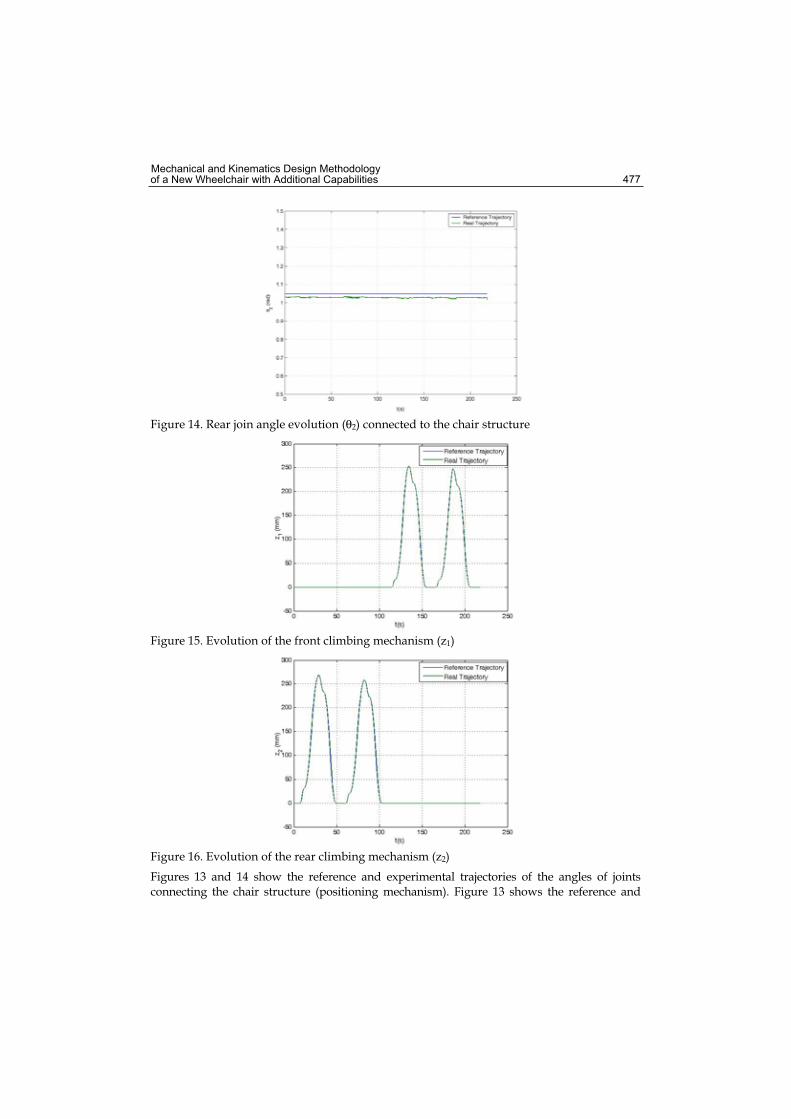
Mechanical and Kinematics Design Methodology of a New Wheelchair with Additional Capabilities 477
Figure 14. Rear join angle evolution (θ2) connected to the chair structure
Figure 15. Evolution of the front climbing mechanism (z1)
Figure 16. Evolution of the rear climbing mechanism (z2)
Figures 13 and 14 show the reference and experimental trajectories of the angles of joints connecting the chair structure (positioning mechanism). Figure 13 shows the reference and
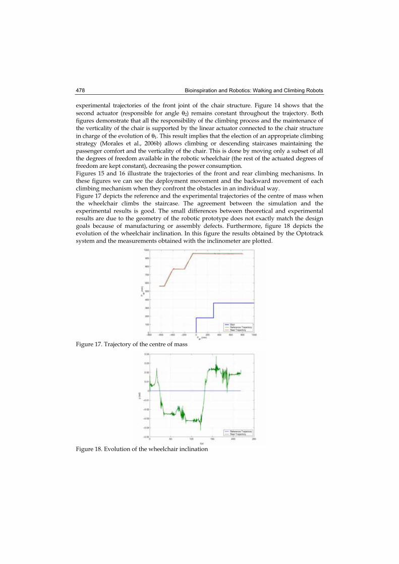
Bioinspiration and Robotics: Walking and Climbing Robots 478
experimental trajectories of the front joint of the chair structure. Figure 14 shows that the
second actuator (responsible for angle θ2) remains constant throughout the trajectory. Both figures demonstrate that all the responsibility of the climbing process and the maintenance of the verticality of the chair is supported by the linear actuator connected to the chair structure
in charge of the evolution of θ1. This result implies that the election of an appropriate climbing strategy (Morales et al., 2006b) allows climbing or descending staircases maintaining the passenger comfort and the verticality of the chair. This is done by moving only a subset of all the degrees of freedom available in the robotic wheelchair (the rest of the actuated degrees of freedom are kept constant), decreasing the power consumption.Figures 15 and 16 illustrate the trajectories of the front and rear climbing mechanisms. In these figures we can see the deployment movement and the backward movement of each climbing mechanism when they confront the obstacles in an individual way. Figure 17 depicts the reference and the experimental trajectories of the centre of mass when the wheelchair climbs the staircase. The agreement between the simulation and the experimental results is good. The small differences between theoretical and experimental results are due to the geometry of the robotic prototype does not exactly match the design goals because of manufacturing or assembly defects. Furthermore, figure 18 depicts the evolution of the wheelchair inclination. In this figure the results obtained by the Optotrack system and the measurements obtained with the inclinometer are plotted.
Figure 17. Trajectory of the centre of mass
Figure 18. Evolution of the wheelchair inclination
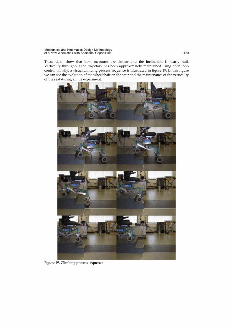
Mechanical and Kinematics Design Methodology of a New Wheelchair with Additional Capabilities 479
These data, show that both measures are similar and the inclination is nearly null. Verticality throughout the trajectory has been approximately maintained using open loop control. Finally, a visual climbing process sequence is illustrated in figure 19. In this figure we can see the evolution of the wheelchair on the stair and the maintenance of the verticality of the seat during all the experiment.
Figure 19. Climbing process sequence
Bioinspiration and Robotics: Walking and Climbing Robots 480
5. Conclusions
A new approach has been presented for designing and building a climbing-wheelchair. Its main features are: a) automatic adaptation to steps with different heights, b) easy maintenance of the verticality of the wheelchair, c) the climbing of stairs requires less effort from the actuators (only a subset of the actuated degrees of freedom is needed when the trajectory slope of the chair frame is the same as the slope of the racks or the slope of the wheels, depending on the configuration), d) weight and energy consumption are reduced and e) wheelchair stability is guaranteed during every moment because its weight is always transferred to horizontal surfaces and the support polygon is always greater than or equal to the support polygon of the conventional powered wheelchairs. The mechanical design methodology decomposes the original mechanical problem into two different subproblems which have been implemented with separate mechanical devices. On the one hand the climbing mechanism solves the problem to overcome a single step and on the other hand, the positioning mechanism ensures the stability and the verticality of the seat in environments with different height axles. Then, the synthesis process depicts the final dimensions of both mechanical devices. The final solution found has some advantages: very high payload capacity, light weight and low cost. The kinematics design methodology allows full motion of the degrees of freedom of the whole system, and it has been adapted to continuous smooth profiles and profiles composed of flat floor and staircases (this profile admits analytical solutions). The inverse kinematics model of our wheelchair prototype makes it possible to determine the real time trajectories for the articulated degrees of freedom of the wheelchair. This is important since a comfortable motion of the wheelchair requires an individual motion of the degrees of freedom in order to maintain a desired motion of the whole system. The kinematics model and the climbing strategies have been applied together to the wheelchair prototype to illustrate the good environment adaptation of our design as it moves in a staircase composed by two steps while the verticality of the seat and the trajectory of the centre of mass are maintained. All the experiments have been prepared in such a way the passenger comfort has to be guaranteed. The control trajectory is easier, as it relies basically on the motion of only one of the actuators which compose the positioning
system (responsible for angle θ1) while the second actuator (responsible for angle θ2)remains constant throughout the trajectory. Moreover, the planned trajectories are consistent and agree with the experimental results. The reported experimental results show small deviations from the verticality, and demonstrate that our mechanical design allows our chair to climb stairs with the proposed open loop control strategy, with minimum sensors requirements, and guaranteeing the stability and the comfort of the passenger.
6. Future work
The reported experimental results show small differences between simulated and real trajectories which validate the good relationship between the mechanical and kinematics methodologies proposed. These results show some small differences between simulated and experimental trajectories that will be reduced in our next future work by a) carrying out a calibration procedure of the mechanism, and b) by implementing a closed loop control system that uses feedback of the inclinometer measurements and of several ultrasound sensors that will provide with the relative positions between the steps and the wheels. This
Mechanical and Kinematics Design Methodology of a New Wheelchair with Additional Capabilities 481
will allow faster movements while maintaining the comfort and security margins for the passenger.
7. References
Aarnio, P. ; Koskinen, K., & Salmi. S. (2000). Simulation of the Hybtor Robot, Proceedings of3rt International Conference on Climbing and Walking Robots, pp. 267-274, Madrid, Spain, October, 2000.
Cham, J.G. ; Bailey, S.A. & Clark, J.E. (2002). Fast and Robust: Hexapedal Robots Via Shape Deposition Manufacturing. The International Journal of Robotics Research, Vol. 21, No. 10-11, 2002, pp. 869-882.
DIN18065 (2001). Stairs in Buildings. Terminology, Measuring Rules, Main Dimensions. Deutsches Institut Normung, 2002.
Erdman, A. G. & Sandor, G. N. (1997): Mechanism Design, Analysis and Synthesis, Third Edition, Prentice Hall, ISBN 0-13-267782-2, pp 534-570
Grand, C. ; Benamar, F; Plumet, F & Bidaud, P. (2004). Stability and Traction Optimized of a Reconfigurable Wheel-Legged Robot. The International Journal of Robotics Research, Vol. 23, No. 10-11, 2002, pp. 1041-1058.
Gough, V.E. & Whitehall, S.G. (1962). Universal Tyre Test Machine, Proceedings of the FISITA 9th International Technical Congress, pp. 117-137, 1962.
Hirose, S. (1984). A Study of Design and Control of a Quadruped Walking Vehicle. TheInternational Journal of Robotics Research, Vol. 3, No. 2, 1984, pp. 113-133.
Hirose, S. & Takeuchi, H. (1996). Study on Roller-Walk (Basic Characteristics and its Control), Proceedings of the 1996 IEEE International Conference on Robotics and Automation, pp. 3265-3270, Minneapolis, USA, April, 1996.
Hirose, S. ; Fukushima, E.F. ; Damoto, R. & Nakamoto, H. (2001). Design of Terrain Adaptative Versatile Crawler Vehicule Helios-VI, Proceedings of the 2001 IEEE/RSJ International Conference on Intelligent Robots and Systems, pp. 1540-1545, ISBN 0-7803-6612-3, Maui, Hawaii, USA, October/November 2001.
Kamen, D. ; Ambrogi, R. & Heinzman, R. (1999). Transportation Vehicles with Stability Enhancement Using CG Modification, U.S. Patent 5 975 225, November 12, 1999.
Kar, D.C. (2003). Design of Statically Stable Walking Robot: A Review. Journal of Robotics Systems, Vol. 20, No. 11, 2003, pp. 671-686.
Lawn, M. J. & Ishimatzu T. (2003). Modeling of a Stair-Climbing Wheelchair Mechanism With High Single-Step Capability. IEEE Transactions on Neural Systems and Rehabilitation Research, Vol. 11, No. 3, September, 2003, pp. 323-332, ISSN 1534-4320.
Merlet, J. P. (2000): Parallel Robots, Norwell, MA: Kluwer. Morales, R.; Feliu, V.; González. A & Pintado, P. (2006), Kinematic Model of a New Staircase
Climbing Wheelchair and Its Experimental Validation, The International Journal on Robotics Research, Vol. 25, No. 9, pp. 825-841.
Morales, R.; Feliu, V.; González. A & Pintado, P. (2006), Coordinated Motion of a New Staircase Climbing Wheelchair With Increased Passenger Comfort, Proceedings of the 2006 IEEE International Conference on Robotics and Automation, pp.3395-4001, ISBN 0-7803-9505-0, Orlando, Florida, USA, May 2006.
Siegwart, R.; Lamon, P.; Estier, T.; Lauria, M. & Piguet, R. (2002). Innovative Design for Wheeled Locomotion in Rough Terrain. Journal of Robotics and Autonomous Systems, Vol. 40, No. 2-3, pp. 151-162.
Bioinspiration and Robotics: Walking and Climbing Robots 482
Stewart, D. (1965-66). A Platform With Six Degrees of Freedom, Proceedings of the IMechE,Vol. 180, Pt. 1, No. 15, pp. 371-385, 1965-66.
Sunwa Stair-Ship TRE-52. Sunwa CO. Ltd. Sendagaya, shiuya-ku, Tokyo Japan. http://www.sunwa-jp.co.jp/en.
The Wheelchair Lift Company. http://www.thewheelchairlift.co.uk/ssas/index.html Uchida, Y.; Furuichi, K. & Hirose, S. (1999). Fundamental Performance of 6 Wheeled Off-
Road Vehicle Helios-V, Proceedings of the 1999 IEEE International Conference on Robotics and Automation, pp. 2336-2341, Detroit, Michigan, USA, May, 1999.
Wang, J. & Masory, O. (1993). On the Accuracy of a Stewart Platform-Part I: the Effect of Manufacturing Tolerances, Proceedings of the 1993 IEEE International Conference on Robotics and Automation, pp. 114-120, Atlanta, Georgia, USA, May, 1993.
Wellman, P.; Krovi, V.; Kumar, V. & Harwin, W. (1995). Design of a Wheelchair With Legs for People With Motor Disabilities. IEEE Transactions on Rehabilitation Engineering, Vol. 3, No. 4, pp. 343-353.
Wiesspeiner, G. & Windischbacher, E. (1995). Distributed Intelligence to Control a Stair-Climbing Wheelchair, Proceedings of the Engineering in Medicine and Biology Society. IEEE 17th Annual Conference, pp. 1173-1174,ISBN 0-7803-2475-7, Montreal, Que., Canada, September, 1995.
28
Pneumatic Actuators for Climbing, Walkingand Serpentine Robots1
Grzegorz Granosik Technical University of Lodz
Poland
1. Introduction
This chapter presents construction, control, advantages and disadvantages of various pneumatic actuators we have been using in several projects of climbing, walking and serpentine robots during last 13 years. We start with qualitative and quantitative analysis of different actuators. This part is mostly based on the literature review but augmented with our own experience related to these particular types of robots. We focus on pneumatic drives as very suitable for robots having permanent contact with unknown environment. Then we show a few constructions developed in our laboratory: starting from light weight manipulator for climbing robot, quadruped walker and climber, jumping and worm-like robots, see Fig. 1. We also present our contribution in development of the family of serpentine robots designed at the University of Michigan (UofM). There are some general requirements for joint actuators in mobile robots designed for regular contact with ground (obstacles). Listed here are the six most important ones: 1. Joint actuators should be capable of developing sufficient force to lift whole robot or its
parts in order to climb or overcome obstacles, or to operate with load. 2. Joint angles should be controllable proportionally. 3. Another key requirement is that mobile robots should conform to the terrain
compliantly. This assures correct propulsion and safe manipulation as well as dynamic isolation of main body (controller) from ground. Robots that don’t conform compliantly require complex sensor systems to measure contact forces and to command a momentary angle for each non-compliant joint accordingly.
4. At times it is necessary to increase the stiffness of a joint, for example to cross a gap or precisely track position trajectory. Alternatively, it may be necessary to adjust the stiffness to an intermediate level, for example to change jumping frequency. Thus, considered mobile robots and manipulators must be capable of adjusting the stiffness of every DOF individually and proportionally.
5. Joint actuators should be scalable to fit robots of different sizes. It is convenient to use the same technology in mini- and macro-scale.
1 This research was partially financed by the Ministry of Science and Higher Education under grant No
3 T11A 023 30 and 3 T11A 024 30
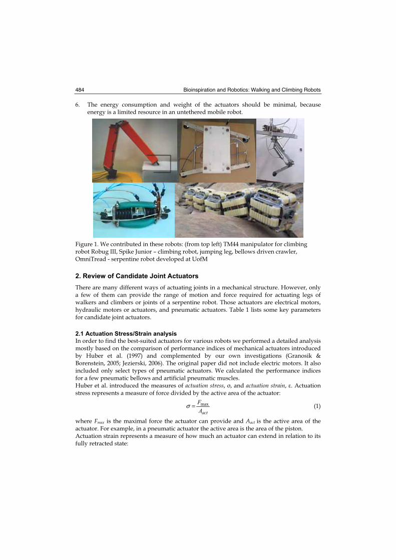
Bioinspiration and Robotics: Walking and Climbing Robots 484
6. The energy consumption and weight of the actuators should be minimal, because energy is a limited resource in an untethered mobile robot.
Figure 1. We contributed in these robots: (from top left) TM44 manipulator for climbing robot Robug III, Spike Junior – climbing robot, jumping leg, bellows driven crawler, OmniTread - serpentine robot developed at UofM
2. Review of Candidate Joint Actuators
There are many different ways of actuating joints in a mechanical structure. However, only a few of them can provide the range of motion and force required for actuating legs of walkers and climbers or joints of a serpentine robot. Those actuators are electrical motors, hydraulic motors or actuators, and pneumatic actuators. Table 1 lists some key parameters for candidate joint actuators.
2.1 Actuation Stress/Strain analysis
In order to find the best-suited actuators for various robots we performed a detailed analysis mostly based on the comparison of performance indices of mechanical actuators introduced by Huber et al. (1997) and complemented by our own investigations (Granosik & Borenstein, 2005; Jezierski, 2006). The original paper did not include electric motors. It also included only select types of pneumatic actuators. We calculated the performance indices for a few pneumatic bellows and artificial pneumatic muscles. Huber et al. introduced the measures of actuation stress, , and actuation strain, . Actuation stress represents a measure of force divided by the active area of the actuator:
actAFmax=σ (1)
where Fmax is the maximal force the actuator can provide and Aact is the active area of the actuator. For example, in a pneumatic actuator the active area is the area of the piston. Actuation strain represents a measure of how much an actuator can extend in relation to its fully retracted state:
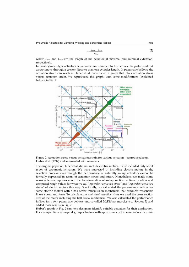
Pneumatic Actuators for Climbing, Walking and Serpentine Robots 485
min
minmax
LLL −=ε (2)
where Lmax and Lmin are the length of the actuator at maximal and minimal extension, respectively.In most cylinder-type actuators actuation strain is limited to 1.0, because the piston and rod cannot move through a greater distance than one cylinder length. In pneumatic bellows the actuation strain can reach 4. Huber et al. constructed a graph that plots actuation stress versus actuation strain. We reproduced this graph, with some modifications (explained below), in Fig. 2.
Figure 2. Actuation stress versus actuation strain for various actuators - reproduced from Huber et al. (1997) and augmented with own data
The original paper of Huber et al. did not include electric motors. It also included only select types of pneumatic actuators. We were interested in including electric motors in the selection process, even though the performance of naturally rotary actuators cannot be formally expressed in terms of actuation stress and strain. Nonetheless, we made some reasonable assumptions about the transformation of rotary motion to linear motion and computed rough values for what we call “equivalent actuation stress” and “equivalent actuation strain” of electric motors this way. Specifically, we calculated the performance indices for some electric motors with a ball screw transmission mechanism that produces reasonable linear speed and force. To calculate the equivalent actuation stress we used the cross section area of the motor including the ball screw mechanism. We also calculated the performance indices for a few pneumatic bellows and so-called McKibben muscles (see Section 3) and added those results in Fig. 2. Huber’s graph in Fig. 2 can help designers identify suitable actuators for their application. For example, lines of slope -1 group actuators with approximately the same volumetric stroke
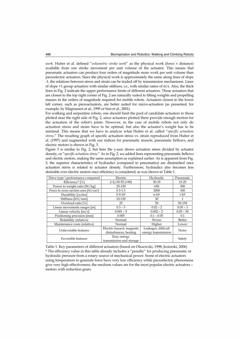
Bioinspiration and Robotics: Walking and Climbing Robots 486
work. Huber et al. defined “volumetric stroke work” as the physical work (force × distance) available from one stroke movement per unit volume of the actuator. This means that pneumatic actuators can produce four orders of magnitude more work per unit volume than piezoelectric actuators. Since the physical work is approximately the same along lines of slope -1, the relations between stress and strain can be traded off by transmission mechanisms. Lines
of slope +1 group actuators with similar stiffness, i.e., with similar ratios of σ/ε. Also, the thick lines in Fig. 2 indicate the upper performance limits of different actuators. Those actuators that are closest to the top right corner of Fig. 2 are naturally suited to lifting weights and propelling masses in the orders of magnitude required for mobile robots. Actuators closest to the lower left corner, such as piezoactuators, are better suited for micro-actuation (as presented, for example, by Magnussen et al., 1995 or Sun et al., 2001). For walking and serpentine robots, one should limit the pool of candidate actuators to those plotted near the right side of Fig. 2, since actuators plotted there provide enough motion for the actuation of the robot’s joints. However, in the case of mobile robots not only do actuation stress and strain have to be optimal, but also the actuator’s weight has to be minimal. This means that we have to analyze what Huber et al. called “specific actuation stress.” The resulting graph of specific actuation stress vs. strain reproduced from Huber et al. (1997) and augmented with our indices for pneumatic muscle, pneumatic bellows, and electric motors is shown in Fig. 3. Figure 3 is similar to Fig. 2, but here the y-axis shows actuation stress divided by actuator density, or “specific actuation stress.” As in Fig. 2, we added lines representing pneumatic bellows and electric motors, making the same assumption as explained earlier. As is apparent from Fig. 3, the superior characteristics of hydraulics (compared to pneumatics) are diminished once actuation stress is related to actuator density. Furthermore, hydraulics also becomes less desirable over electric motors once efficiency is considered, as was shown in Table 1.
Drive type \performance compared Electric Hydraulic Pneumatic
Efficiency* [%] (<1) 50-55 (>90) 30-35 15-25
Power to weight ratio [W/kg] 25-150 650 300
Force to cross section area [N/cm2] 0.3-1.5 2000 100
Durability [cycles] 5-9·105 6·106 >107
Stiffness [kN/mm] 10-120 30 1
Overload ratio [%] 25 50 50-150
Linear movements ranges [m] 0.3 – 5 0.02 – 2 0.05 – 3
Linear velocity [m/s] 0.001 – 5 0.002 – 2 0.05 – 30
Positioning precision [mm] 0.005 0.1 – 0.05 0.1
Reliability (relative) Normal Worse Better
Maintenance costs (relative) Normal Higher Lower
Unfavorable features Electric hazard, magnetic
disturbances, heating Leakages, difficult
energy transmission Noisy
Favorable features Easy energy
transmission and storage Safety
Table 1. Key parameters of different actuators (based on Olszewski, 1998; Jezierski, 2006) * The efficiency value in this table already includes a “penalty” for producing pneumatic or hydraulic pressure from a rotary source of mechanical power. Some of electric actuators using temperature to generate force have very low efficiency while piezoelectric phenomena give very high effectiveness; the medium values are for the most popular electric actuators – motors with reduction gears
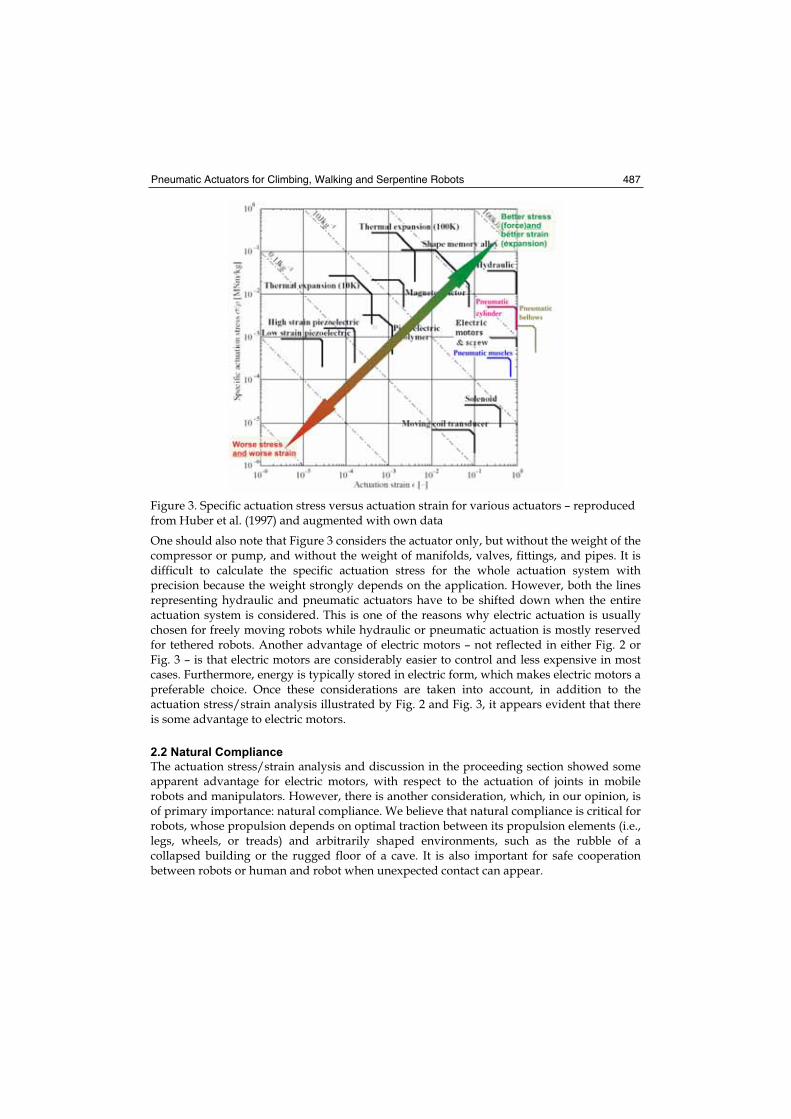
Pneumatic Actuators for Climbing, Walking and Serpentine Robots 487
Figure 3. Specific actuation stress versus actuation strain for various actuators – reproduced from Huber et al. (1997) and augmented with own data
One should also note that Figure 3 considers the actuator only, but without the weight of the compressor or pump, and without the weight of manifolds, valves, fittings, and pipes. It is difficult to calculate the specific actuation stress for the whole actuation system with precision because the weight strongly depends on the application. However, both the lines representing hydraulic and pneumatic actuators have to be shifted down when the entire actuation system is considered. This is one of the reasons why electric actuation is usually chosen for freely moving robots while hydraulic or pneumatic actuation is mostly reserved for tethered robots. Another advantage of electric motors – not reflected in either Fig. 2 or Fig. 3 – is that electric motors are considerably easier to control and less expensive in most cases. Furthermore, energy is typically stored in electric form, which makes electric motors a preferable choice. Once these considerations are taken into account, in addition to the actuation stress/strain analysis illustrated by Fig. 2 and Fig. 3, it appears evident that there is some advantage to electric motors.
2.2 Natural Compliance
The actuation stress/strain analysis and discussion in the proceeding section showed some apparent advantage for electric motors, with respect to the actuation of joints in mobile robots and manipulators. However, there is another consideration, which, in our opinion, is of primary importance: natural compliance. We believe that natural compliance is critical for robots, whose propulsion depends on optimal traction between its propulsion elements (i.e., legs, wheels, or treads) and arbitrarily shaped environments, such as the rubble of a collapsed building or the rugged floor of a cave. It is also important for safe cooperation between robots or human and robot when unexpected contact can appear.
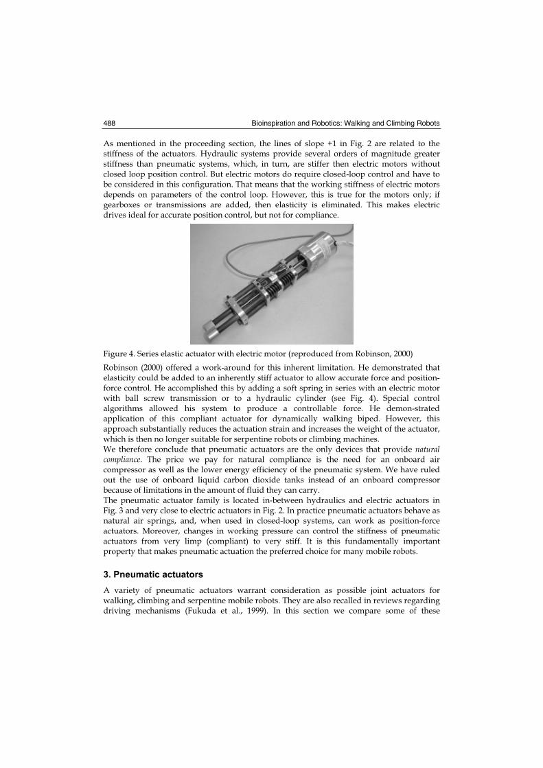
Bioinspiration and Robotics: Walking and Climbing Robots 488
As mentioned in the proceeding section, the lines of slope +1 in Fig. 2 are related to the stiffness of the actuators. Hydraulic systems provide several orders of magnitude greater stiffness than pneumatic systems, which, in turn, are stiffer then electric motors without closed loop position control. But electric motors do require closed-loop control and have to be considered in this configuration. That means that the working stiffness of electric motors depends on parameters of the control loop. However, this is true for the motors only; if gearboxes or transmissions are added, then elasticity is eliminated. This makes electric drives ideal for accurate position control, but not for compliance.
Figure 4. Series elastic actuator with electric motor (reproduced from Robinson, 2000)
Robinson (2000) offered a work-around for this inherent limitation. He demonstrated that elasticity could be added to an inherently stiff actuator to allow accurate force and position-force control. He accomplished this by adding a soft spring in series with an electric motor with ball screw transmission or to a hydraulic cylinder (see Fig. 4). Special control algorithms allowed his system to produce a controllable force. He demon-strated application of this compliant actuator for dynamically walking biped. However, this approach substantially reduces the actuation strain and increases the weight of the actuator, which is then no longer suitable for serpentine robots or climbing machines.We therefore conclude that pneumatic actuators are the only devices that provide natural compliance. The price we pay for natural compliance is the need for an onboard air compressor as well as the lower energy efficiency of the pneumatic system. We have ruled out the use of onboard liquid carbon dioxide tanks instead of an onboard compressor because of limitations in the amount of fluid they can carry. The pneumatic actuator family is located in-between hydraulics and electric actuators in Fig. 3 and very close to electric actuators in Fig. 2. In practice pneumatic actuators behave as natural air springs, and, when used in closed-loop systems, can work as position-force actuators. Moreover, changes in working pressure can control the stiffness of pneumatic actuators from very limp (compliant) to very stiff. It is this fundamentally important property that makes pneumatic actuation the preferred choice for many mobile robots.
3. Pneumatic actuators
A variety of pneumatic actuators warrant consideration as possible joint actuators for walking, climbing and serpentine mobile robots. They are also recalled in reviews regarding driving mechanisms (Fukuda et al., 1999). In this section we compare some of these
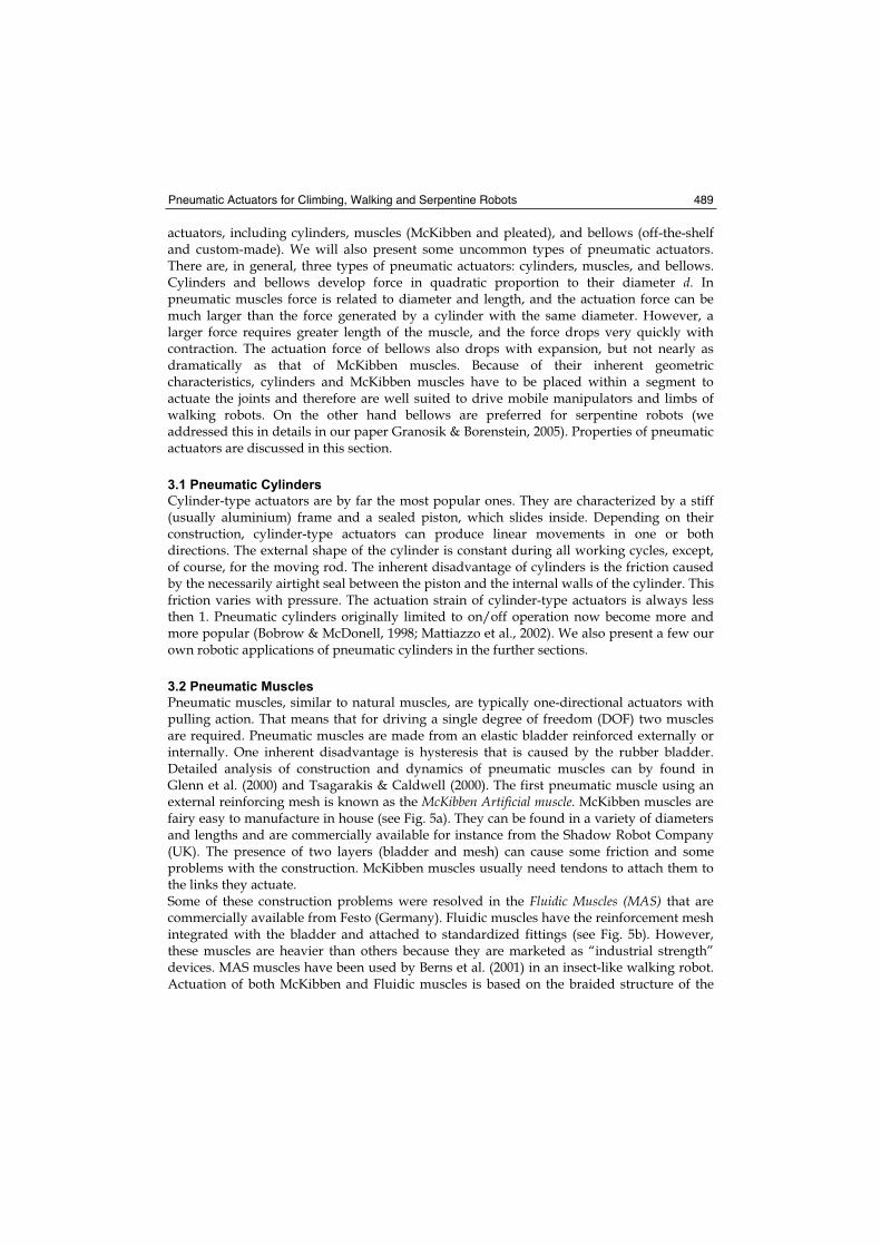
Pneumatic Actuators for Climbing, Walking and Serpentine Robots 489
actuators, including cylinders, muscles (McKibben and pleated), and bellows (off-the-shelf and custom-made). We will also present some uncommon types of pneumatic actuators. There are, in general, three types of pneumatic actuators: cylinders, muscles, and bellows. Cylinders and bellows develop force in quadratic proportion to their diameter d. In pneumatic muscles force is related to diameter and length, and the actuation force can be much larger than the force generated by a cylinder with the same diameter. However, a larger force requires greater length of the muscle, and the force drops very quickly with contraction. The actuation force of bellows also drops with expansion, but not nearly as dramatically as that of McKibben muscles. Because of their inherent geometric characteristics, cylinders and McKibben muscles have to be placed within a segment to actuate the joints and therefore are well suited to drive mobile manipulators and limbs of walking robots. On the other hand bellows are preferred for serpentine robots (we addressed this in details in our paper Granosik & Borenstein, 2005). Properties of pneumatic actuators are discussed in this section.
3.1 Pneumatic Cylinders
Cylinder-type actuators are by far the most popular ones. They are characterized by a stiff (usually aluminium) frame and a sealed piston, which slides inside. Depending on their construction, cylinder-type actuators can produce linear movements in one or both directions. The external shape of the cylinder is constant during all working cycles, except, of course, for the moving rod. The inherent disadvantage of cylinders is the friction caused by the necessarily airtight seal between the piston and the internal walls of the cylinder. This friction varies with pressure. The actuation strain of cylinder-type actuators is always less then 1. Pneumatic cylinders originally limited to on/off operation now become more and more popular (Bobrow & McDonell, 1998; Mattiazzo et al., 2002). We also present a few our own robotic applications of pneumatic cylinders in the further sections.
3.2 Pneumatic Muscles
Pneumatic muscles, similar to natural muscles, are typically one-directional actuators with pulling action. That means that for driving a single degree of freedom (DOF) two muscles are required. Pneumatic muscles are made from an elastic bladder reinforced externally or internally. One inherent disadvantage is hysteresis that is caused by the rubber bladder. Detailed analysis of construction and dynamics of pneumatic muscles can by found in Glenn et al. (2000) and Tsagarakis & Caldwell (2000). The first pneumatic muscle using an external reinforcing mesh is known as the McKibben Artificial muscle. McKibben muscles are fairy easy to manufacture in house (see Fig. 5a). They can be found in a variety of diameters and lengths and are commercially available for instance from the Shadow Robot Company (UK). The presence of two layers (bladder and mesh) can cause some friction and some problems with the construction. McKibben muscles usually need tendons to attach them to the links they actuate. Some of these construction problems were resolved in the Fluidic Muscles (MAS) that are commercially available from Festo (Germany). Fluidic muscles have the reinforcement mesh integrated with the bladder and attached to standardized fittings (see Fig. 5b). However, these muscles are heavier than others because they are marketed as “industrial strength” devices. MAS muscles have been used by Berns et al. (2001) in an insect-like walking robot. Actuation of both McKibben and Fluidic muscles is based on the braided structure of the
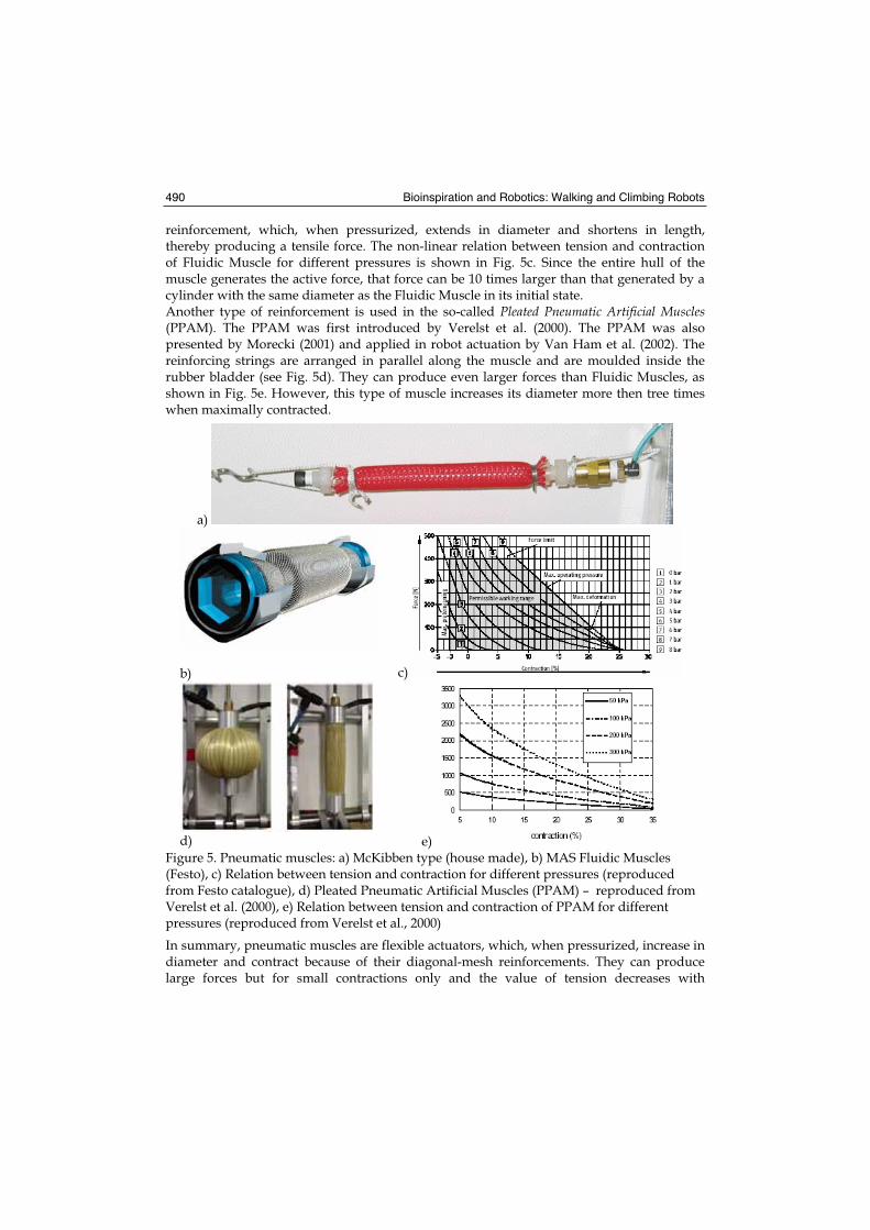
Bioinspiration and Robotics: Walking and Climbing Robots 490
reinforcement, which, when pressurized, extends in diameter and shortens in length, thereby producing a tensile force. The non-linear relation between tension and contraction of Fluidic Muscle for different pressures is shown in Fig. 5c. Since the entire hull of the muscle generates the active force, that force can be 10 times larger than that generated by a cylinder with the same diameter as the Fluidic Muscle in its initial state. Another type of reinforcement is used in the so-called Pleated Pneumatic Artificial Muscles (PPAM). The PPAM was first introduced by Verelst et al. (2000). The PPAM was also presented by Morecki (2001) and applied in robot actuation by Van Ham et al. (2002). The reinforcing strings are arranged in parallel along the muscle and are moulded inside the rubber bladder (see Fig. 5d). They can produce even larger forces than Fluidic Muscles, as shown in Fig. 5e. However, this type of muscle increases its diameter more then tree times when maximally contracted.
a)
b) c)
d) e)Figure 5. Pneumatic muscles: a) McKibben type (house made), b) MAS Fluidic Muscles (Festo), c) Relation between tension and contraction for different pressures (reproduced from Festo catalogue), d) Pleated Pneumatic Artificial Muscles (PPAM) – reproduced from Verelst et al. (2000), e) Relation between tension and contraction of PPAM for different pressures (reproduced from Verelst et al., 2000)
In summary, pneumatic muscles are flexible actuators, which, when pressurized, increase in diameter and contract because of their diagonal-mesh reinforcements. They can produce large forces but for small contractions only and the value of tension decreases with
Pneumatic Actuators for Climbing, Walking and Serpentine Robots 491
increasing contraction. The useful actuation strain is between 5-30% of the initial length. Pneumatic muscles are elastic and therefore can conform easily to skeleton of manipulator or walking robot, they can also drive joints having more than one degree of freedom (DOF) – so called multi DOF – usually found in the kinematic structure of biologically inspired robots (Feja, 2006).
3.3 Pneumatic Bellows
a) b)
c) d)
Figure 6. Pneumatic bellows: a) pneumatic group actuator (reproduced from Hirai et al., 2002), b) flexible pneumatic microactuator (reproduced from Suzomori et al., 1997), c) thin-sleeve rubber bellows (reproduced from McMaster-Carr catalogue), d) static characteristics of thin sleeve bellow (reproduced from McMaster-Carr)
The third type of pneumatic actuators is the bellows. Bellows are elastic structures performing one-directional (pushing) action. They are either made out of a very thick-walled rubber tube or they require external reinforcement to appropriately direct force in longitudinal direction. This type of actuation is used only rarely for robotic actuation. Shimizu et al. (1995) proposed a hexahedron actuator to drive rotational joints and Hirai et
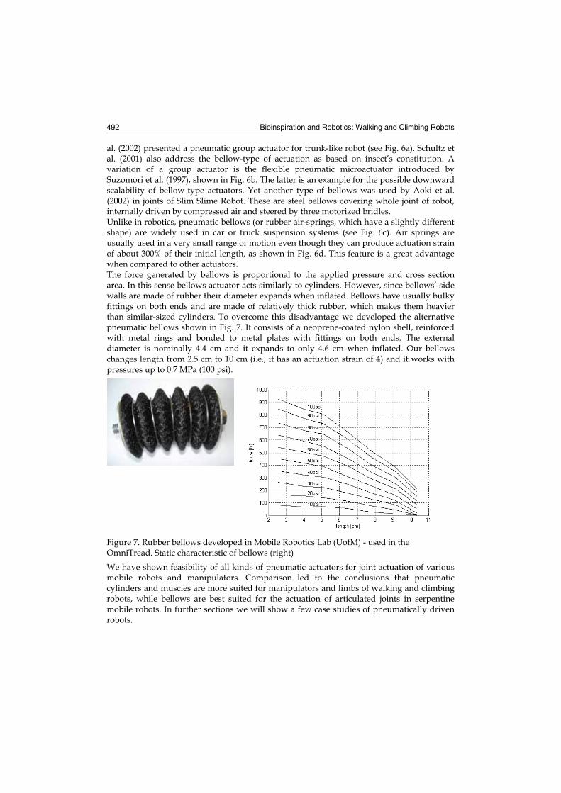
Bioinspiration and Robotics: Walking and Climbing Robots 492
al. (2002) presented a pneumatic group actuator for trunk-like robot (see Fig. 6a). Schultz et al. (2001) also address the bellow-type of actuation as based on insect’s constitution. A variation of a group actuator is the flexible pneumatic microactuator introduced by Suzomori et al. (1997), shown in Fig. 6b. The latter is an example for the possible downward scalability of bellow-type actuators. Yet another type of bellows was used by Aoki et al. (2002) in joints of Slim Slime Robot. These are steel bellows covering whole joint of robot, internally driven by compressed air and steered by three motorized bridles. Unlike in robotics, pneumatic bellows (or rubber air-springs, which have a slightly different shape) are widely used in car or truck suspension systems (see Fig. 6c). Air springs are usually used in a very small range of motion even though they can produce actuation strain of about 300% of their initial length, as shown in Fig. 6d. This feature is a great advantage when compared to other actuators. The force generated by bellows is proportional to the applied pressure and cross section area. In this sense bellows actuator acts similarly to cylinders. However, since bellows’ side walls are made of rubber their diameter expands when inflated. Bellows have usually bulky fittings on both ends and are made of relatively thick rubber, which makes them heavier than similar-sized cylinders. To overcome this disadvantage we developed the alternative pneumatic bellows shown in Fig. 7. It consists of a neoprene-coated nylon shell, reinforced with metal rings and bonded to metal plates with fittings on both ends. The external diameter is nominally 4.4 cm and it expands to only 4.6 cm when inflated. Our bellows changes length from 2.5 cm to 10 cm (i.e., it has an actuation strain of 4) and it works with pressures up to 0.7 MPa (100 psi).
Figure 7. Rubber bellows developed in Mobile Robotics Lab (UofM) - used in the OmniTread. Static characteristic of bellows (right)
We have shown feasibility of all kinds of pneumatic actuators for joint actuation of various mobile robots and manipulators. Comparison led to the conclusions that pneumatic cylinders and muscles are more suited for manipulators and limbs of walking and climbing robots, while bellows are best suited for the actuation of articulated joints in serpentine mobile robots. In further sections we will show a few case studies of pneumatically driven robots.
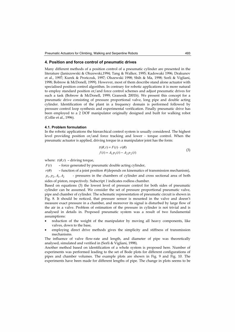
Pneumatic Actuators for Climbing, Walking and Serpentine Robots 493
4. Position and force control of pneumatic drives
Many different methods of a position control of a pneumatic cylinder are presented in the literature (Janiszowski & Olszewski,1994; Tang & Walker, 1995; Kadowaki 1996; Drakunov et al., 1997; Kurek & Pro czuk, 1997; Olszewski 1998; Shih & Ma, 1998; Sorli & Vigliani, 1998; Bobrow & McDonell, 1999). However, most of them describe stand alone actuator with specialised position control algorithm. In contrary for robotic applications it is more natural to employ standard position or/and force control schemes and adjust pneumatic drives for such a task (Bobrow & McDonell, 1999; Granosik 2001b). We present this concept for a pneumatic drive consisting of pressure proportional valve, long pipe and double acting cylinder. Identification of the plant in a frequency domain is performed followed by pressure control loop synthesis and experimental verification. Finally pneumatic drive has been employed to a 2 DOF manipulator originally designed and built for walking robot (Collie et al., 1996).
4.1. Problem formulation
In the robotic applications the hierarchical control system is usually considered. The highest level providing position or/and force tracking and lower - torque control. When the pneumatic actuator is applied, driving torque in a manipulator joint has the form:
)()()(
)()(),(
2211 tpAtpAtfrtFt−=
⋅= θθτ (3)
where: ),( tθτ – driving torque,
)(tF – force generated by pneumatic double acting cylinder,
)(θr – function of a joint position θ (depends on kinematics of transmission mechanism),
2121 ,,, AApp - pressures in the chambers of cylinder and cross sectional area of both
sides of piston, respectively. Subscript 1 indicates rodless chamber. Based on equations (3) the lowest level of pressure control for both sides of pneumatic cylinder can be assumed. We consider the set of pressure proportional pneumatic valve, pipe and chamber of cylinder. The schematic representation of pneumatic circuit is shown in Fig. 8. It should be noticed, that pressure sensor is mounted in the valve and doesn’t measure exact pressure in a chamber, and moreover its signal is disturbed by large flow of the air in a valve. Problem of estimation of the pressure in cylinder is not trivial and is analysed in details in. Proposed pneumatic system was a result of two fundamental assumptions:
• reduction of the weight of the manipulator by moving all heavy components, like valves, down to the base,
• employing direct drive methods gives the simplicity and stiffness of transmission mechanisms.
The influence of valve flow-rate and length, and diameter of pipe was theoretically analysed, simulated and verified in (Sorli & Vigliani, 1998). Another method based on identification of a whole system is proposed here. Number of experiments was performed leading to the set of Bode plots for different configurations of pipes and chamber volumes. The example plots are shown in Fig. 9 and Fig. 10. The experiments have been made for different lengths of pipe. The change in plots seems to be
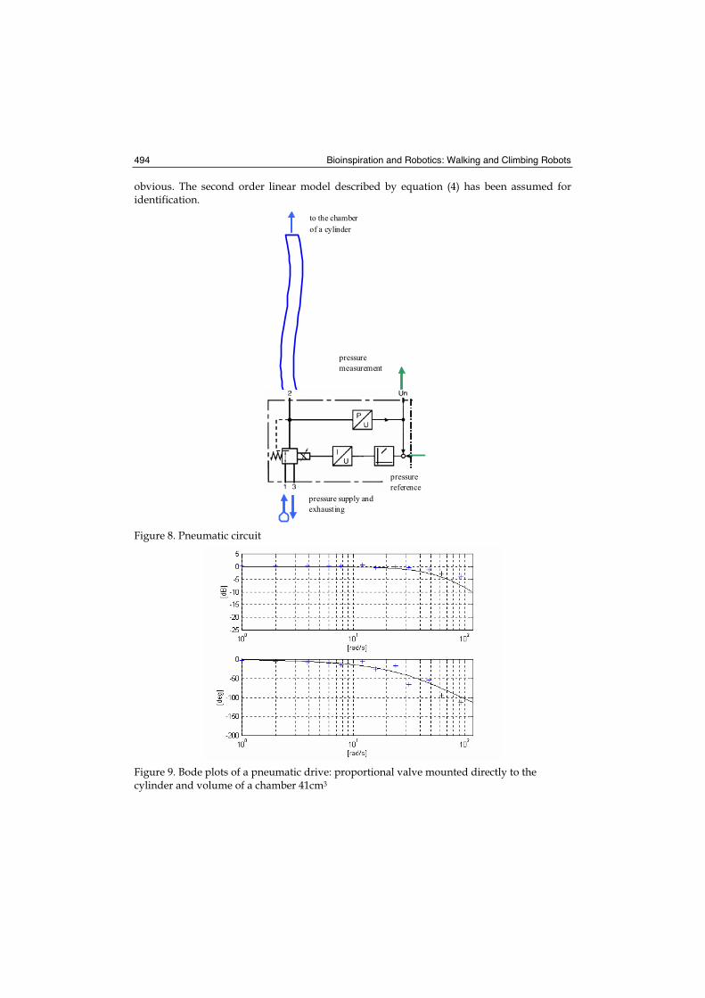
Bioinspiration and Robotics: Walking and Climbing Robots 494
obvious. The second order linear model described by equation (4) has been assumed for identification.
to the chamber
of a cylinder
pressure
measurement
pressure
reference
pressure supply and
exhausting
Figure 8. Pneumatic circuit
Figure 9. Bode plots of a pneumatic drive: proportional valve mounted directly to the cylinder and volume of a chamber 41cm3
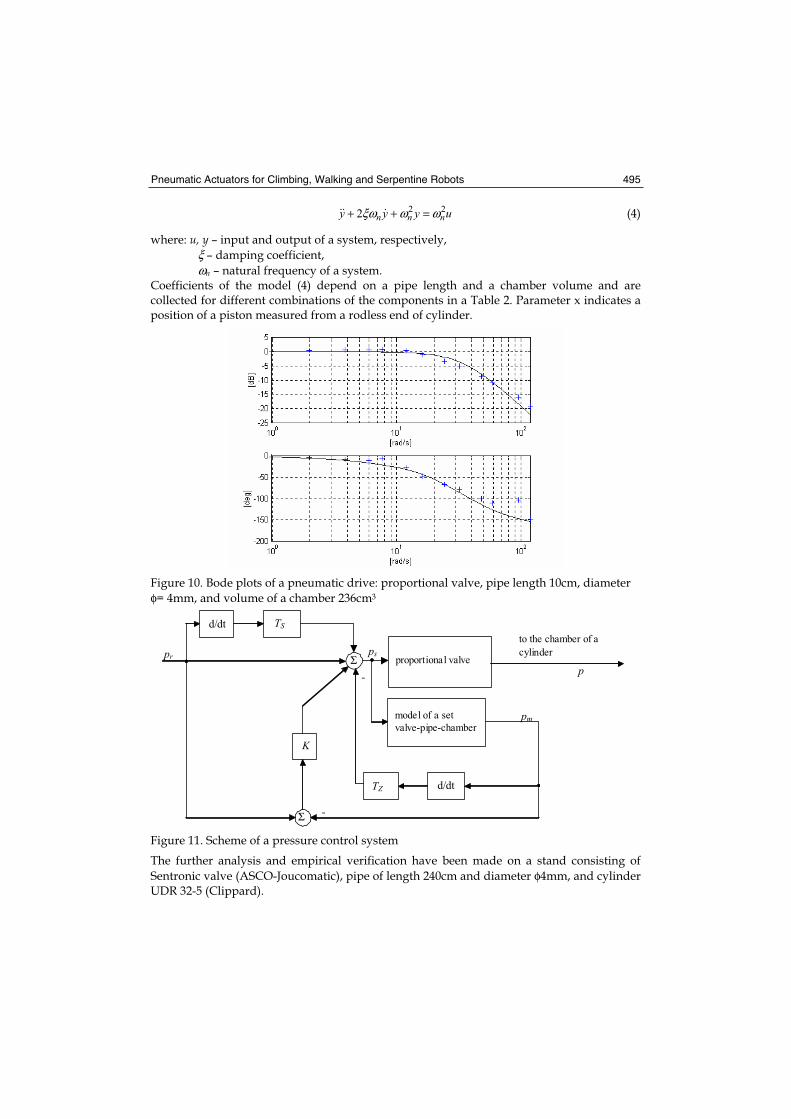
Pneumatic Actuators for Climbing, Walking and Serpentine Robots 495
uyyy nnn222 ωωξω =++ (4)
where: u, y – input and output of a system, respectively,
ξ – damping coefficient,
ωn – natural frequency of a system. Coefficients of the model (4) depend on a pipe length and a chamber volume and are collected for different combinations of the components in a Table 2. Parameter x indicates a position of a piston measured from a rodless end of cylinder.
Figure 10. Bode plots of a pneumatic drive: proportional valve, pipe length 10cm, diameter
φ= 4mm, and volume of a chamber 236cm3
Σ
Σ proportional valve
model of a set
valve-pipe-chamber
pr
TSd/dt
K
d/dtTZ
to the chamber of a
cylinder
-
-
pm
p
ps
Figure 11. Scheme of a pressure control system
The further analysis and empirical verification have been made on a stand consisting of
Sentronic valve (ASCO-Joucomatic), pipe of length 240cm and diameter φ4mm, and cylinder UDR 32-5 (Clippard).
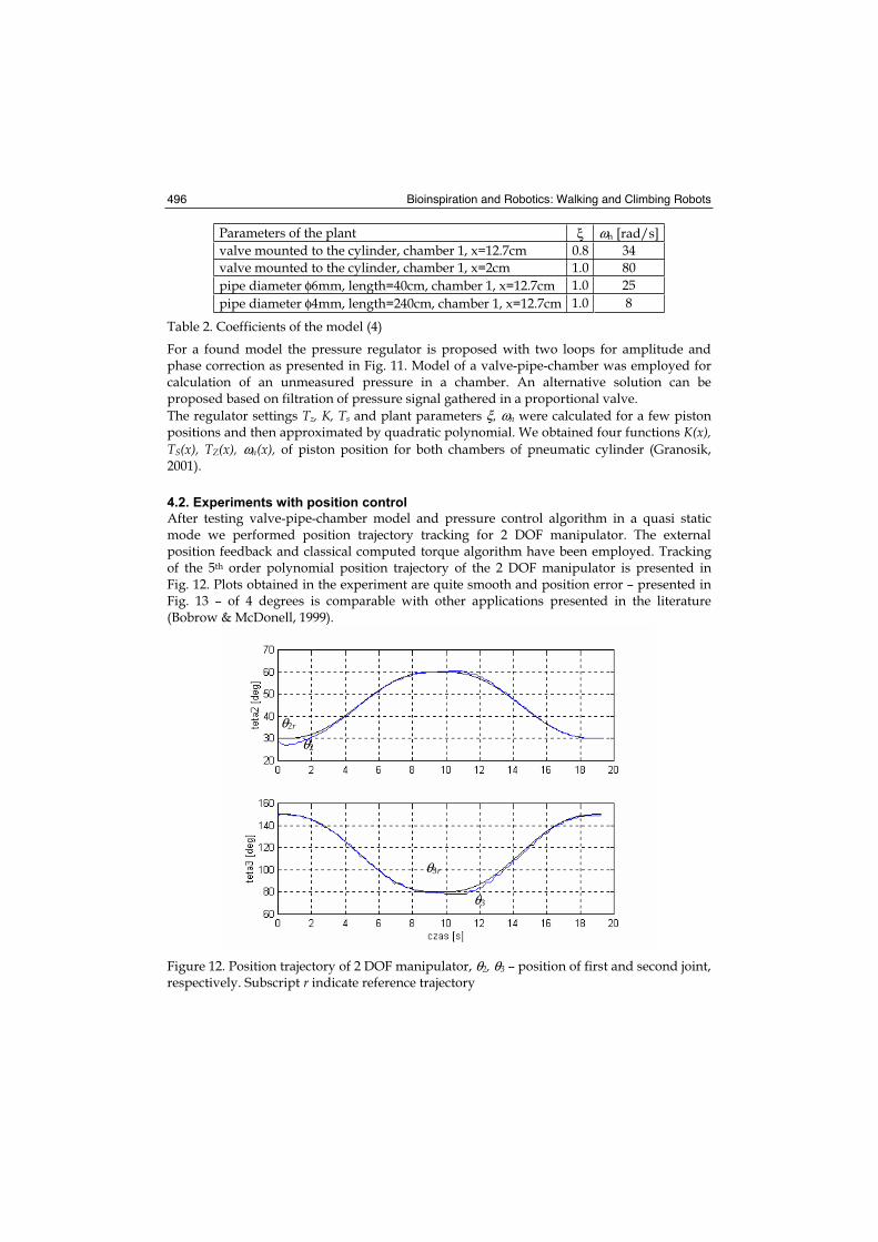
Bioinspiration and Robotics: Walking and Climbing Robots 496
Parameters of the plant ξ ωn [rad/s]
valve mounted to the cylinder, chamber 1, x=12.7cm 0.8 34
valve mounted to the cylinder, chamber 1, x=2cm 1.0 80
pipe diameter φ6mm, length=40cm, chamber 1, x=12.7cm 1.0 25
pipe diameter φ4mm, length=240cm, chamber 1, x=12.7cm 1.0 8
Table 2. Coefficients of the model (4)
For a found model the pressure regulator is proposed with two loops for amplitude and phase correction as presented in Fig. 11. Model of a valve-pipe-chamber was employed for calculation of an unmeasured pressure in a chamber. An alternative solution can be proposed based on filtration of pressure signal gathered in a proportional valve.
The regulator settings Tz, K, Ts and plant parameters ξ, ωn were calculated for a few piston positions and then approximated by quadratic polynomial. We obtained four functions K(x),TS(x), TZ(x), ωn(x), of piston position for both chambers of pneumatic cylinder (Granosik, 2001).
4.2. Experiments with position control
After testing valve-pipe-chamber model and pressure control algorithm in a quasi static mode we performed position trajectory tracking for 2 DOF manipulator. The external position feedback and classical computed torque algorithm have been employed. Tracking of the 5th order polynomial position trajectory of the 2 DOF manipulator is presented in Fig. 12. Plots obtained in the experiment are quite smooth and position error – presented in Fig. 13 – of 4 degrees is comparable with other applications presented in the literature (Bobrow & McDonell, 1999).
Figure 12. Position trajectory of 2 DOF manipulator, θ2, θ3 – position of first and second joint, respectively. Subscript r indicate reference trajectory
θ2r θ2
θ3
θ3r
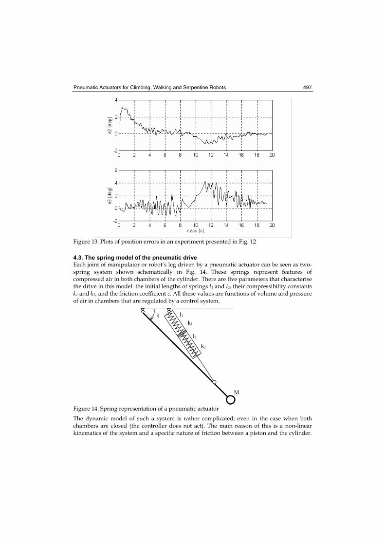
Pneumatic Actuators for Climbing, Walking and Serpentine Robots 497
Figure 13. Plots of position errors in an experiment presented in Fig. 12
4.3. The spring model of the pneumatic drive
Each joint of manipulator or robot’s leg driven by a pneumatic actuator can be seen as two-spring system shown schematically in Fig. 14. These springs represent features of compressed air in both chambers of the cylinder. There are five parameters that characterise the drive in this model: the initial lengths of springs l1 and l2, their compressibility constants k1 and k2, and the friction coefficient c. All these values are functions of volume and pressure of air in chambers that are regulated by a control system.
k1
M
l2
l1
k2
q
Figure 14. Spring representation of a pneumatic actuator
The dynamic model of such a system is rather complicated; even in the case when both chambers are closed (the controller does not act). The main reason of this is a non-linear kinematics of the system and a specific nature of friction between a piston and the cylinder.
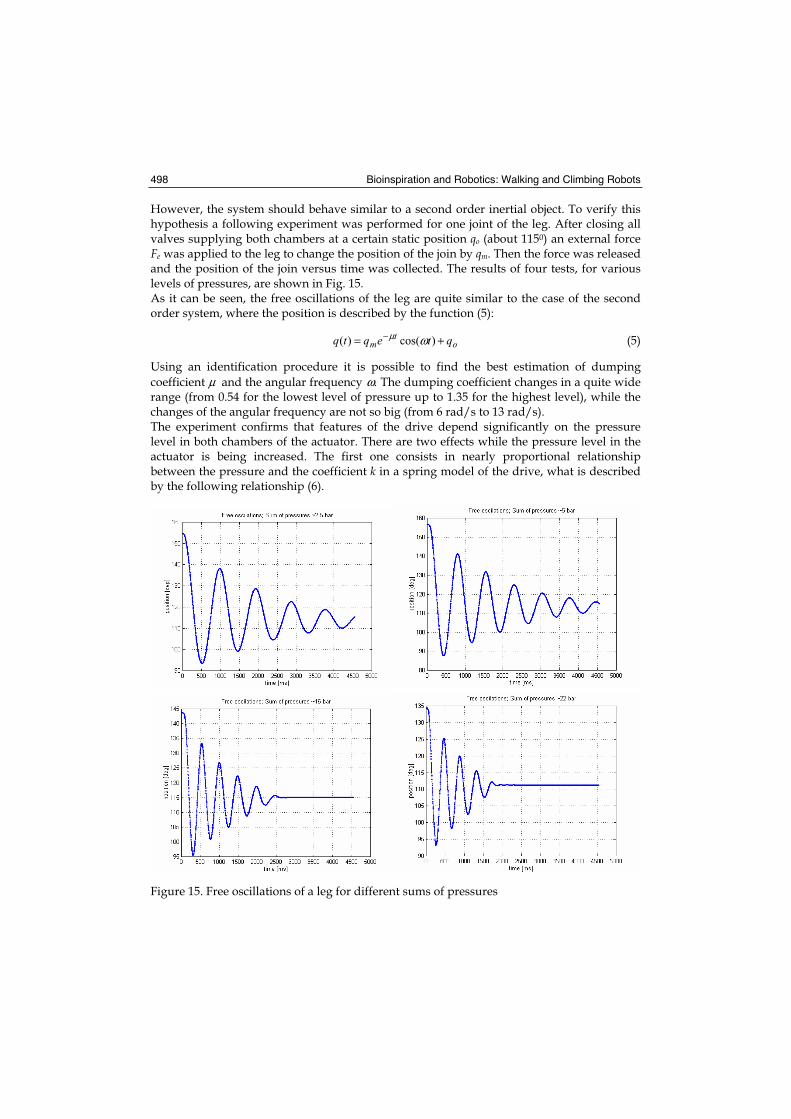
Bioinspiration and Robotics: Walking and Climbing Robots 498
However, the system should behave similar to a second order inertial object. To verify this hypothesis a following experiment was performed for one joint of the leg. After closing all valves supplying both chambers at a certain static position qo (about 1150) an external force Fe was applied to the leg to change the position of the join by qm. Then the force was released and the position of the join versus time was collected. The results of four tests, for various levels of pressures, are shown in Fig. 15. As it can be seen, the free oscillations of the leg are quite similar to the case of the second order system, where the position is described by the function (5):
ot
m qteqtq += − )cos()( ωμ (5)
Using an identification procedure it is possible to find the best estimation of dumping
coefficient μ and the angular frequency ω. The dumping coefficient changes in a quite wide range (from 0.54 for the lowest level of pressure up to 1.35 for the highest level), while the changes of the angular frequency are not so big (from 6 rad/s to 13 rad/s). The experiment confirms that features of the drive depend significantly on the pressure level in both chambers of the actuator. There are two effects while the pressure level in the actuator is being increased. The first one consists in nearly proportional relationship between the pressure and the coefficient k in a spring model of the drive, what is described by the following relationship (6).
Figure 15. Free oscillations of a leg for different sums of pressures
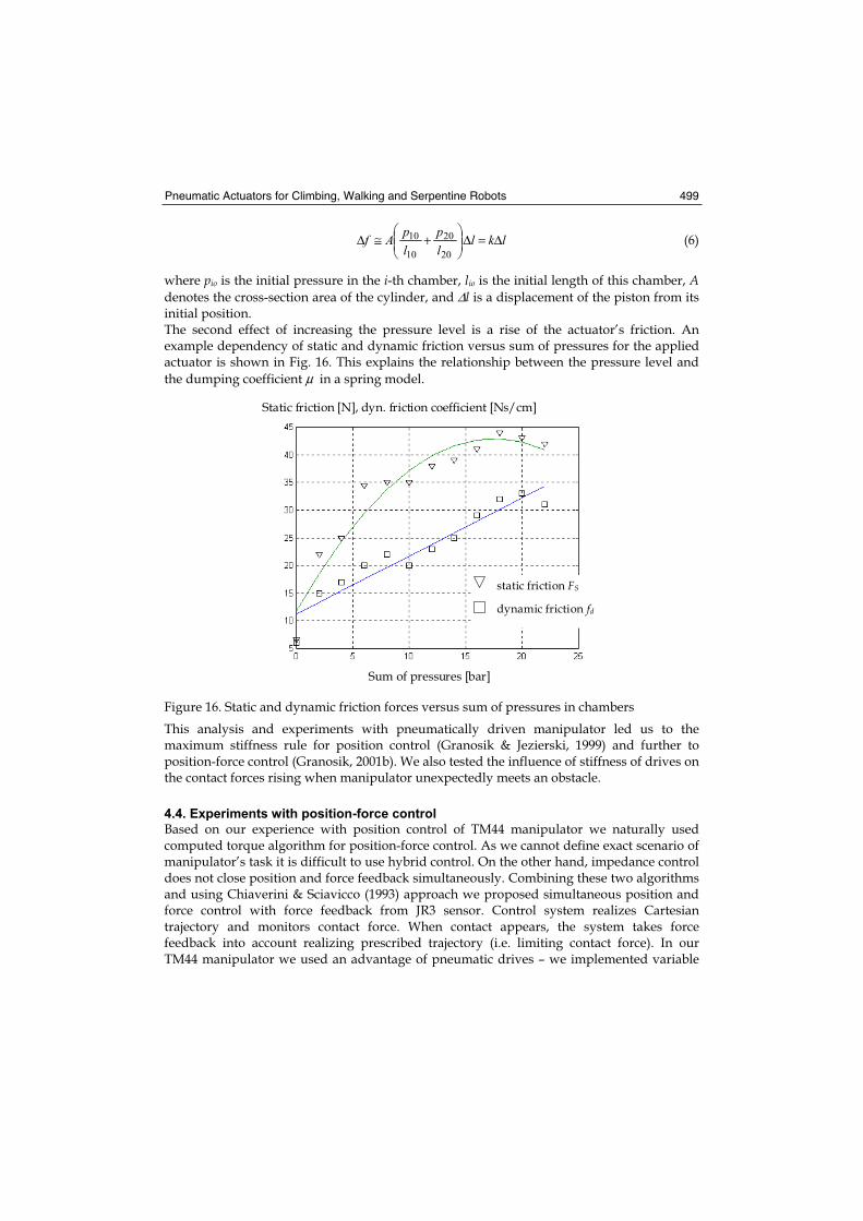
Pneumatic Actuators for Climbing, Walking and Serpentine Robots 499
lkllp
lpAf Δ=Δ+≅Δ
20
20
10
10 (6)
where pio is the initial pressure in the i-th chamber, lio is the initial length of this chamber, Adenotes the cross-section area of the cylinder, and Δl is a displacement of the piston from its initial position. The second effect of increasing the pressure level is a rise of the actuator’s friction. An example dependency of static and dynamic friction versus sum of pressures for the applied actuator is shown in Fig. 16. This explains the relationship between the pressure level and
the dumping coefficient μ in a spring model.
static friction FS
dynamic friction fd
Sum of pressures [bar]
Static friction [N], dyn. friction coefficient [Ns/cm]
Figure 16. Static and dynamic friction forces versus sum of pressures in chambers
This analysis and experiments with pneumatically driven manipulator led us to the maximum stiffness rule for position control (Granosik & Jezierski, 1999) and further to position-force control (Granosik, 2001b). We also tested the influence of stiffness of drives on the contact forces rising when manipulator unexpectedly meets an obstacle.
4.4. Experiments with position-force control
Based on our experience with position control of TM44 manipulator we naturally used computed torque algorithm for position-force control. As we cannot define exact scenario of manipulator’s task it is difficult to use hybrid control. On the other hand, impedance control does not close position and force feedback simultaneously. Combining these two algorithms and using Chiaverini & Sciavicco (1993) approach we proposed simultaneous position and force control with force feedback from JR3 sensor. Control system realizes Cartesian trajectory and monitors contact force. When contact appears, the system takes force feedback into account realizing prescribed trajectory (i.e. limiting contact force). In our TM44 manipulator we used an advantage of pneumatic drives – we implemented variable
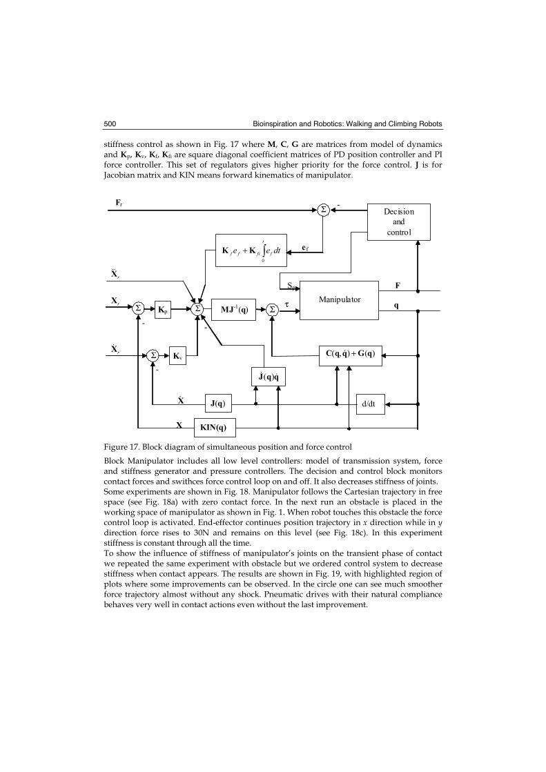
Bioinspiration and Robotics: Walking and Climbing Robots 500
stiffness control as shown in Fig. 17 where M, C, G are matrices from model of dynamics and Kp, Kv, Kf, Kfi are square diagonal coefficient matrices of PD position controller and PI force controller. This set of regulators gives higher priority for the force control. J is for Jacobian matrix and KIN means forward kinematics of manipulator.
Σ
ΣManipulator
)(),( qGqqC +
rX
Kv
d/dt
-
-
qτ ΣMJ-1(q)Σ
rX
rX
Kp
J(q)
KIN(q)X
X
qqJ )(
-
Σ -
+t
ffiff dtee0
KK
Fr
F
ef
Decision
and
control
Sp
Figure 17. Block diagram of simultaneous position and force control
Block Manipulator includes all low level controllers: model of transmission system, force and stiffness generator and pressure controllers. The decision and control block monitors contact forces and swithces force control loop on and off. It also decreases stiffness of joints. Some experiments are shown in Fig. 18. Manipulator follows the Cartesian trajectory in free space (see Fig. 18a) with zero contact force. In the next run an obstacle is placed in the working space of manipulator as shown in Fig. 1. When robot touches this obstacle the force control loop is activated. End-effector continues position trajectory in x direction while in ydirection force rises to 30N and remains on this level (see Fig. 18c). In this experiment stiffness is constant through all the time. To show the influence of stiffness of manipulator’s joints on the transient phase of contact we repeated the same experiment with obstacle but we ordered control system to decrease stiffness when contact appears. The results are shown in Fig. 19, with highlighted region of plots where some improvements can be observed. In the circle one can see much smoother force trajectory almost without any shock. Pneumatic drives with their natural compliance behaves very well in contact actions even without the last improvement.
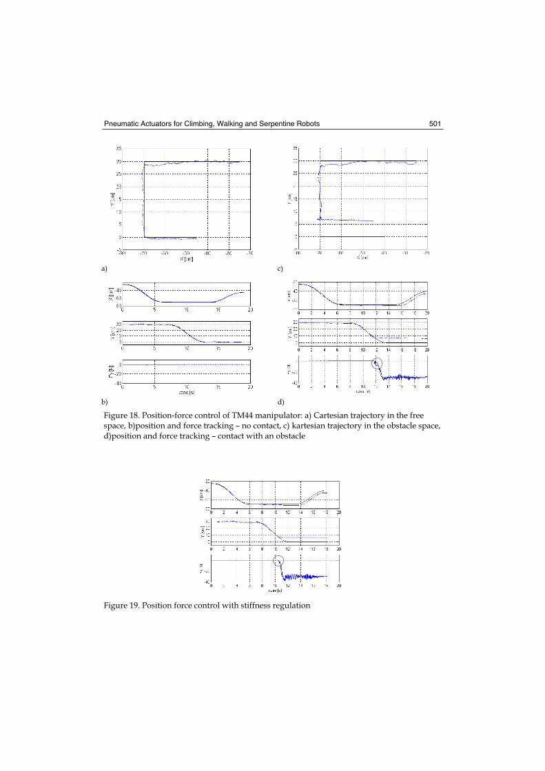
Pneumatic Actuators for Climbing, Walking and Serpentine Robots 501
a) c)
b) d)
Figure 18. Position-force control of TM44 manipulator: a) Cartesian trajectory in the free space, b)position and force tracking – no contact, c) kartesian trajectory in the obstacle space, d)position and force tracking – contact with an obstacle
Figure 19. Position force control with stiffness regulation
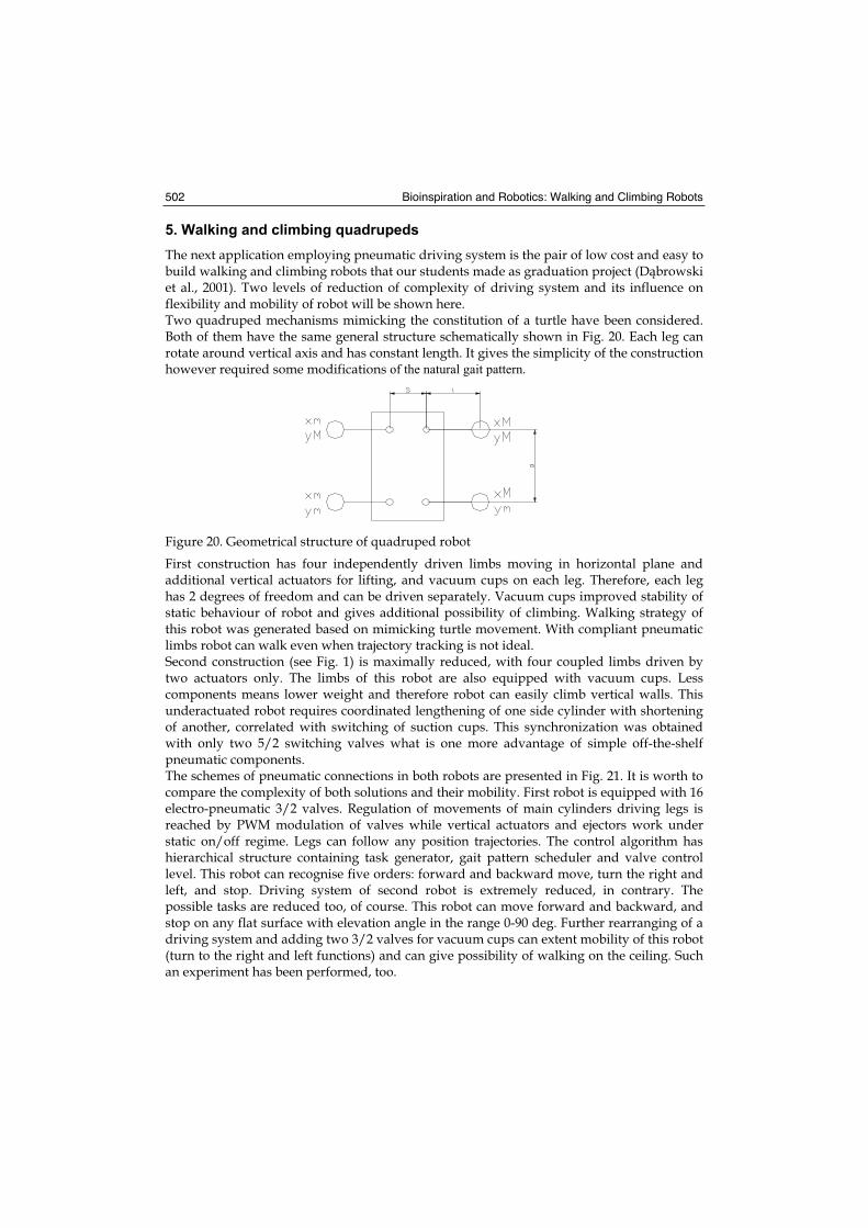
Bioinspiration and Robotics: Walking and Climbing Robots 502
5. Walking and climbing quadrupeds
The next application employing pneumatic driving system is the pair of low cost and easy to build walking and climbing robots that our students made as graduation project (D browskiet al., 2001). Two levels of reduction of complexity of driving system and its influence on flexibility and mobility of robot will be shown here. Two quadruped mechanisms mimicking the constitution of a turtle have been considered. Both of them have the same general structure schematically shown in Fig. 20. Each leg can rotate around vertical axis and has constant length. It gives the simplicity of the construction however required some modifications of the natural gait pattern.
Figure 20. Geometrical structure of quadruped robot
First construction has four independently driven limbs moving in horizontal plane and additional vertical actuators for lifting, and vacuum cups on each leg. Therefore, each leg has 2 degrees of freedom and can be driven separately. Vacuum cups improved stability of static behaviour of robot and gives additional possibility of climbing. Walking strategy of this robot was generated based on mimicking turtle movement. With compliant pneumatic limbs robot can walk even when trajectory tracking is not ideal. Second construction (see Fig. 1) is maximally reduced, with four coupled limbs driven by two actuators only. The limbs of this robot are also equipped with vacuum cups. Less components means lower weight and therefore robot can easily climb vertical walls. This underactuated robot requires coordinated lengthening of one side cylinder with shortening of another, correlated with switching of suction cups. This synchronization was obtained with only two 5/2 switching valves what is one more advantage of simple off-the-shelf pneumatic components. The schemes of pneumatic connections in both robots are presented in Fig. 21. It is worth to compare the complexity of both solutions and their mobility. First robot is equipped with 16 electro-pneumatic 3/2 valves. Regulation of movements of main cylinders driving legs is reached by PWM modulation of valves while vertical actuators and ejectors work under static on/off regime. Legs can follow any position trajectories. The control algorithm has hierarchical structure containing task generator, gait pattern scheduler and valve control level. This robot can recognise five orders: forward and backward move, turn the right and left, and stop. Driving system of second robot is extremely reduced, in contrary. The possible tasks are reduced too, of course. This robot can move forward and backward, and stop on any flat surface with elevation angle in the range 0-90 deg. Further rearranging of a driving system and adding two 3/2 valves for vacuum cups can extent mobility of this robot (turn to the right and left functions) and can give possibility of walking on the ceiling. Such an experiment has been performed, too.
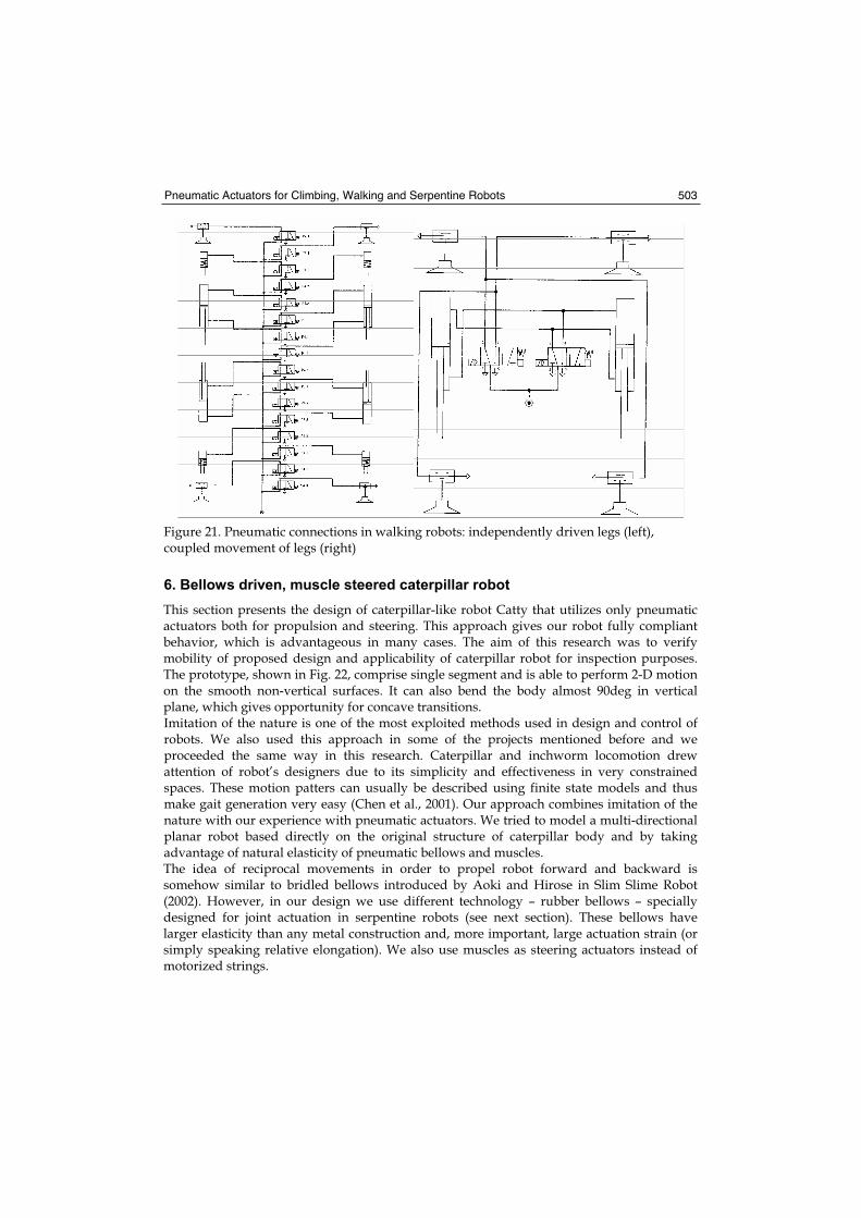
Pneumatic Actuators for Climbing, Walking and Serpentine Robots 503
Figure 21. Pneumatic connections in walking robots: independently driven legs (left), coupled movement of legs (right)
6. Bellows driven, muscle steered caterpillar robot
This section presents the design of caterpillar-like robot Catty that utilizes only pneumatic actuators both for propulsion and steering. This approach gives our robot fully compliant behavior, which is advantageous in many cases. The aim of this research was to verify mobility of proposed design and applicability of caterpillar robot for inspection purposes. The prototype, shown in Fig. 22, comprise single segment and is able to perform 2-D motion on the smooth non-vertical surfaces. It can also bend the body almost 90deg in vertical plane, which gives opportunity for concave transitions. Imitation of the nature is one of the most exploited methods used in design and control of robots. We also used this approach in some of the projects mentioned before and we proceeded the same way in this research. Caterpillar and inchworm locomotion drew attention of robot’s designers due to its simplicity and effectiveness in very constrained spaces. These motion patters can usually be described using finite state models and thus make gait generation very easy (Chen et al., 2001). Our approach combines imitation of the nature with our experience with pneumatic actuators. We tried to model a multi-directional planar robot based directly on the original structure of caterpillar body and by taking advantage of natural elasticity of pneumatic bellows and muscles. The idea of reciprocal movements in order to propel robot forward and backward is somehow similar to bridled bellows introduced by Aoki and Hirose in Slim Slime Robot (2002). However, in our design we use different technology – rubber bellows – specially designed for joint actuation in serpentine robots (see next section). These bellows have larger elasticity than any metal construction and, more important, large actuation strain (or simply speaking relative elongation). We also use muscles as steering actuators instead of motorized strings.
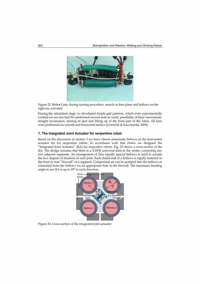
Bioinspiration and Robotics: Walking and Climbing Robots 504
Figure 22. Robot Catty during turning procedure, muscle in first plane and bellows on the right are activated
During the simulation stage we developed simple gait patterns, which were experimentally verified on our test bed.We performed several tests to verify possibility of basic movements: straight locomotion, turning in spot and lifting up of the front part of the robot. All tests were performed on smooth and horizontal surface (Granosik & Kaczmarski, 2005).
7. The Integrated Joint Actuator for serpentine robot
Based on the discussion in section 3 we have chosen pneumatic bellows as the best-suited actuator for for serpentine robots. In accordance with that choice we designed the “Integrated Joint Actuator” (IJA) for serpentine robots. Fig. 23 shows a cross-section of the IJA. The design assumes that there is a 2-DOF universal joint in the center, connecting any two adjacent segments. An arrangement of four equally spaced bellows is used to actuate the two degrees of freedom of each joint. Each closed end of a bellows is rigidly fastened to the front or rear “firewall” of a segment. Compressed air can be pumped into the bellows or exhausted from the bellows via an appropriate hole in the firewall. The maximum bending angle in our IJA is up to 25° in each direction.
Ad
D
Bellow arrangement 4Disclosure.cdr
Drivetracks
Bellows 1 Bellows 2
Bellows 3
Bellows 4
Segment firewall
Universal joint
Figure 23. Cross-section of the integrated joint actuator
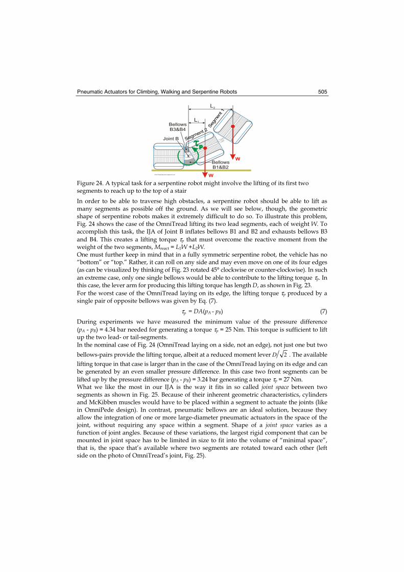
Pneumatic Actuators for Climbing, Walking and Serpentine Robots 505
Seg
men
t 1
Segment 2
L1
L2
W
W
Joint B
Bellows B3&B4
BellowsB1&B2
OmniTread Moment 4 paper103.cdr
Figure 24. A typical task for a serpentine robot might involve the lifting of its first two segments to reach up to the top of a stair
In order to be able to traverse high obstacles, a serpentine robot should be able to lift as many segments as possible off the ground. As we will see below, though, the geometric shape of serpentine robots makes it extremely difficult to do so. To illustrate this problem, Fig. 24 shows the case of the OmniTread lifting its two lead segments, each of weight W. To accomplish this task, the IJA of Joint B inflates bellows B1 and B2 and exhausts bellows B3
and B4. This creates a lifting torque τp that must overcome the reactive moment from the weight of the two segments, Mreact = L1W +L2W.One must further keep in mind that in a fully symmetric serpentine robot, the vehicle has no “bottom” or “top.” Rather, it can roll on any side and may even move on one of its four edges (as can be visualized by thinking of Fig. 23 rotated 45° clockwise or counter-clockwise). In such
an extreme case, only one single bellows would be able to contribute to the lifting torque τp. In this case, the lever arm for producing this lifting torque has length D, as shown in Fig. 23.
For the worst case of the OmniTread laying on its edge, the lifting torque τp produced by a single pair of opposite bellows was given by Eq. (7).
τp = DA(pA - pB) (7)
During experiments we have measured the minimum value of the pressure difference
(pA - pB) = 4.34 bar needed for generating a torque τp = 25 Nm. This torque is sufficient to lift up the two lead- or tail-segments. In the nominal case of Fig. 24 (OmniTread laying on a side, not an edge), not just one but two
bellows-pairs provide the lifting torque, albeit at a reduced moment lever 2D . The available
lifting torque in that case is larger than in the case of the OmniTread laying on its edge and can be generated by an even smaller pressure difference. In this case two front segments can be
lifted up by the pressure difference (pA - pB) = 3.24 bar generating a torque τp = 27 Nm. What we like the most in our IJA is the way it fits in so called joint space between two segments as shown in Fig. 25. Because of their inherent geometric characteristics, cylinders and McKibben muscles would have to be placed within a segment to actuate the joints (like in OmniPede design). In contrast, pneumatic bellows are an ideal solution, because they allow the integration of one or more large-diameter pneumatic actuators in the space of the joint, without requiring any space within a segment. Shape of a joint space varies as a function of joint angles. Because of these variations, the largest rigid component that can be mounted in joint space has to be limited in size to fit into the volume of “minimal space”, that is, the space that’s available where two segments are rotated toward each other (left side on the photo of OmniTread’s joint, Fig. 25).
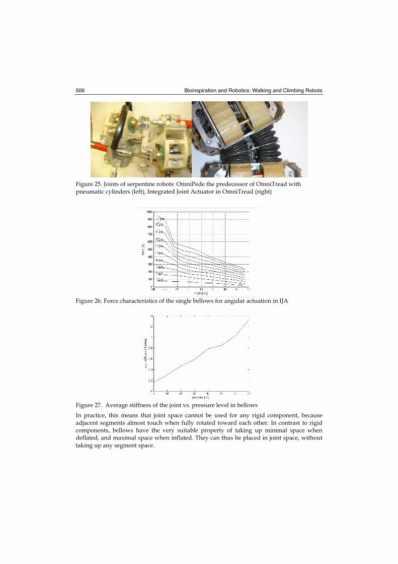
Bioinspiration and Robotics: Walking and Climbing Robots 506
Figure 25. Joints of serpentine robots: OmniPede the predecessor of OmniTread with pneumatic cylinders (left), Integrated Joint Actuator in OmniTread (right)
Figure 26. Force characteristics of the single bellows for angular actuation in IJA
Figure 27. Average stiffness of the joint vs. pressure level in bellows
In practice, this means that joint space cannot be used for any rigid component, because adjacent segments almost touch when fully rotated toward each other. In contrast to rigid components, bellows have the very suitable property of taking up minimal space when deflated, and maximal space when inflated. They can thus be placed in joint space, without taking up any segment space.
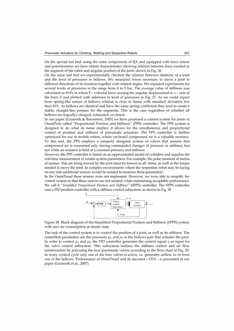
Pneumatic Actuators for Climbing, Walking and Serpentine Robots 507
On the special test bed, using the same components of IJA and equipped with force sensor and potentiometer we have obtain characteristics showing relation between force exerted to the segment of the robot and angular position of the joint, shown in Fig. 26. On the same test bed we experimentally checked the relation between elasticity of a joint and the level of pressures in bellows. We measured forces necessary to move a joint in different directions of its freedom together with related angles. We repeated experiments for several levels of pressures in the range from 0 to 5 bar. The average value of stiffness was
calculated as S=Fr/α where F – external force causing the angular displacement α, r – arm of the force F and plotted with reference to level of pressures in Fig. 27. As we could expect from spring-like nature of bellows relation is close to linear with standard deviation less then 10%. As bellows are identical and have the same spring coefficient they tend to create a stable, straight-line posture for the segments. This is the case regardless of whether all bellows are (equally) charged, exhausted, or closed. In our paper (Granosik & Borenstein, 2005) we have proposed a control system for joints of OmniPede called “Proportional Position and Stiffness” (PPS) controller. The PPE system is designed to do what its name implies: it allows for the simultaneous and proportional control of position and stiffness of pneumatic actuators. The PPS controller is further optimized for use in mobile robots, where on-board compressed air is a valuable resource. To this end, the PPS employs a uniquely designed system of valves that assures that compressed air is consumed only during commanded changes of pressure or stiffness, but not while an actuator is held at a constant pressure and stiffness. However, the PPS controller is based on an approximated model of cylinders and requires the real-time measurement of certain system parameters. For example, the polar moment of inertia of masses that are being moved by the joint must be known at all times, as well as the torque needed to move the joint. In complex environments where the serpentine robot may be laying on any side additional sensors would be needed to measure these parameters. In the OmniTread these sensors were not implement. However, we were able to simplify the control system so that these sensors are not needed, while maintaining acceptable performance. We call it “Simplified Proportional Position and Stiffness” (SPPS) controller. The SPPS controller uses a PID position controller with a stiffness control subsystem, as shown in Fig. 28.
Σ Joint
actuator
rq
-
qValves control subsystem
PID
pA,pB
t1..t4
S
u
Figure 28. Block diagram of the Simplified Proportional Position and Stiffness (SPPS) system with zero air consumption at steady state
The task of the control system is to control the position of a joint, as well as its stiffness. The controlled parameters are the pressures pA and pB in the bellows-pair that actuates the joint. In order to control pA and pB, the PID controller generates the control signal u as input for the valve control subsystem. This subsystem realizes the stiffness control and air flow minimization by activating the four pneumatic valves according to the flow chart in Fig. 29. In every control cycle only one of the four valves is active, i.e. generates airflow to or from one of the bellows. Performance of OmniTread and its ancestor – OT4 – is presented in our paper (Granosik et al., 2007).
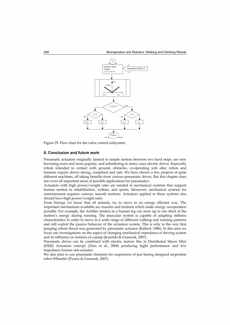
Bioinspiration and Robotics: Walking and Climbing Robots 508
u
Demanded stiffness S
u<0
t2=t
Initialize pulse lengths
t1=t2=t3=t4=0
u
100%
pA+pB<S yes
t/tp
-umax umax
t1=t
yesu<0
t3=t t4=t
yes
Valves
Figure 29. Flow chart for the valve control subsystem
8. Conclusion and future work
Pneumatic actuators originally limited to simple motion between two hard stops, are now becoming more and more popular, and substituting in many cases electric drives. Especially robots intended to contact with ground, obstacles, co-operating with other robots and humans require drives strong, compliant and safe. We have shown a few projects of quite different machines, all taking benefits from various pneumatic drives. But this chapter does not cover all important areas of possible applications for pneumatics. Actuators with high power/weight ratio are needed in mechanical systems that support human motion in rehabilitation, welfare, and sports. Moreover, mechanical systems for entertainment requires various, smooth motions. Actuators applied to these systems also should have high power/weight ratio. From biology we know that all animals, try to move in an energy efficient way. The important mechanisms available are muscles and tendons which make energy recuperation possible. For example, the Achilles tendon in a human leg can store up to one third of the motion’s energy during running. The muscular system is capable of adapting stiffness characteristics in order to move in a wide range of different walking and running patterns and still exploit the passive behavior of the actuation system. This is why in the very first jumping robots thrust was generated by pneumatic actuator (Raibert, 1986). In this area we focus our investigations on the aspect of changing mechanical impedance of driving system and its influence on features of a jump (Jezierski & Granosik, 2007). Pneumatic drives can be combined with electric motors like in Distributed Macro Mini (DM2) Actuation concept (Zinn et al., 2004) producing hight performance and low impedance human safe actuator. We also plan to use pneumatic elements for suspension of just beeing designed serpentine robot Wheeeler (Pytasz & Granosik, 2007).
Pneumatic Actuators for Climbing, Walking and Serpentine Robots 509
9. References
Aoki T., Ohno H., Hirose S. (2002). Design of Slim Slime Robot II (SSR-II) with Bridle Bellows, Proc. IEEE/RSJ Int. Conf.on Intelligent Robots and System, vol.1, pp. 835-840.
Berns K., Albiez J., Kepplin V., Hillenbrand C. (2001). Airbug - insect-like machine actuated by fluidic muscle, 4th Int. Conference on Climbing and Walking Robots CLAWAR, pp. 237–244, Karlsruhe, 24-26 Sept. 2001
Bobrow J.E., McDonell B.W. (1998). Modeling, identification, and control of a pneumatically actuated, force controllable robot, IEEE Trans. on Robotics and Automation vol.14, pp. 732-741
Borenstein J., Granosik G. (2005). Integrated, Proportionally Controlled, and Naturally Compliant Universal Joint Actuator with Controllable Stiffness. U.S. patent #6,870,343. (Rights Assigned to the University of Michigan)
Chen I.-M., Yeo S. H., Gao Y., (2001) Locomotive Gait Generation for Inchworm-Like Robots Using Finite State Approach, Robotica, Vol. 19, No.5, pp. 535-542.
Collie A.A., Granosik G., Jezierski E., Zarychta D., Mianowski K. (1996). Light–weight and compact manipulator for hazardous environment, Proc. of 6th Int. Symposium on Measurement and Control in Robotics, pp. 304-308, Brussels 1996
D browski T., Feja K., Granosik G. (2001). Biologically inspired control strategy of a pneumatically driven walking robot, Proc. Of the 4th Int. Conference on Climbing and Walking Robots CLAWAR 2001, pp 687-694, Karlsruhe 2001
Feja K. (2006). Kinematics of selected manipulators with multi DOF joints. (in polish) Post py robotyki. Sterowanie percepcja i komunikacja. Red. K. Tcho . pp. 37-46, WK Warszawa, ISBN: 83-206-1628-X
Festo AG & Co, Catalogue of Fluidic Muscle MAS, www.festo.com. Fukuda T., Kurashige K., Arai F. (1999). Recent topics on robotic actuation technologies,
Proc. of 2nd Int. Conference on Climbing and Walking Robots, pp. 3-15, Portsmouth, 1999 Glenn K. K. (2000). Accounting for Elastic Energy Storage in McKibben Artificial Muscle
Actuators. Transactions of the ASME. Journal of Dynamic Systems, Measurement, and Control, Vol. 122, pp. 386-388
Granosik G. (2001). Modelling of a pneumatic drive and correction of its dynamics for robotic application, Proc. of 7th IEEE Int. Conf. on Methods and Models in Automation and Robotics MMAR 2001, vol. II, pp 755-760, Mi dzyzdroje 2001
Granosik G. (2001b). Position/force control of a pneumatically driven robot arm, (in polish). Proc. of VII National Robotics Conference, Nr 103, t.2, pp 313-322, L dek-Zdrój 2001
Granosik G., Borenstein J. (2005). Integrated joint actuator for serpentine robots. IEEE/ASME Transactions on Mechatronics, Vol. 10, pp. 473-481
Granosik G., Borenstein J. and Hansen M.G. (2007). Serpentine Robots for Industrial Inspection and Surveillance, in Industrial Robotics. Programming, Simulation and Applications, Edited by Low Kin Huat, pp. 633-662, Published by the plV pro literatur Verlag, Germany, February 2007, ISBN 3-86611-286-6
Granosik G., Jezierski E. (1999). Application of a maximum stiffness rule for pneumatically driven legs of walking robot, Proc. of 2nd Int. Conference on Climbing and Walking Robots, pp 213-218, Portsmouth 1999
Granosik G., Kaczmarski M. (2005). Bellows driven, muscle steered caterpillar robot, Proc. of 8th Int. Conf. on Climbing and Walking Robots and the Support Technologies for Mobile Machines CLAWAR 2005, pp. 743-750, London, UK, September 12-15, 2005.
Bioinspiration and Robotics: Walking and Climbing Robots 510
Hirai S., Masui T., Kawamura S. (2002). Prototyping pneumatic group actuators composed of multiple single-motion elastic tubes, Proc. of Journal of Robotic Society of Japan, vol. 20, no 3, pp. 77-84, 2002
Huber J. E., Fleck N. A. and Ashby M.F. (1997). The selection of mechanical actuators based on performance indices, Proc. of the Royal Society of London. Series A. 453, pp. 2185-2205, UK1997
Jezierski E. (2006). Robot Dynamics, (in polish), WNT, Poland, ISBN 83-204-3128-X Jezierski E., Granosik G., (2007). Modelling and Control of Jumping Robot with Pneumatic
Drive, Accepted to the IEEE MMAR Conference 2007.Knight R., Nehmzow U. (2002). Walking robots – a survey and a research proposal, Technical
report CSM-375 Department of Computer Science University of Essex, UK 2002 Magnussen B., Fatikow S., Rembold, U. (1995). Actuation in microsystems: problem field
overview and practical example of the piezoelectric robot for handling of microobjects. Proc. INRIA/IEEE Symp. on Emerging Technologies and Factory Automation, Vol. 3 pp. 21-27, 10-13 Oct.
Mattiazzo G., Mauro S., Raparelli T., Velardocchia M. (2002). Control of a Six-Axis Pneumatic Robot. Journal of Robotic Systems 19(8), 363–378
McMaster-Carr Supply Company, online catalogue: www.mcmaster.com Morecki A. (2001). Polish artificial pneumatic muscle – design problems, 4th Int. Conference on
Climbing and Walking Robots CLAWAR, pp. 215-222, Karlsruhe. Olszewski M. (1998). Position control of pneumatic drive, (in polish) Pomiary Automatyka
Robotyka, nr 10, pp. 10-14 and 42-43, Poland Pytasz M., Granosik G. (2007). Modeling and control of Wheeeler the hyper mobile robot,
Accepted to the IEEE MMAR Conference 2007Raibert M.H. (1986). Legged robots that balance, The MIT Press, 1986. Robinson D.W. (2000). Design and analysis of series elasticity in closed-loop actuator force
control, PhD thesis, Massachusetts Institute of Technology 2000. Schultz S., Pylatiuk C., Bretthauer G. (2001). Walking machine with compliant joints, 4th Int.
Conference on Climbing and Walking Robots CLAWAR, pp. 231-236, Karlsruhe. Shadow Robot Company, Air Muscles, www.shadow.org.uk Shimizu T., Hayakawa Y., Kawamura S. (1995). Development of hexahedron rubber
actuator, Proc. IEEE Int. Conf. on Robotics and Automation, pp. 2619-2624, Nagoya. Sun L., Sun P., Luo Y., Zhang Y., Gong Z. (2001). Micro in-pipe robots with PZT actuator, 4th
Int. Conf. on Climbing and Walking Robots CLAWAR, pp. 539-546, Karlsruhe. Suzomori K., Maeda T., Watanabe H., Hisada T. (1997). Fiberless flexible microactuator designed
by finite-element method, IEEE Trans. on Mechatronics, Vol. 2, No. 4, Dec.1997 Tsagarakis N., Caldwell D.G. (2000). Improved Modelling and Assesment of pneumatic
Muscle Actuators. Proc. of IEEE Int. Conf. on Robotics and Automation, pp. 3641-3646, San Francisco, USA
Van Ham R.R., Daerden F., Verrelst B., Lefeber D., Vandenhoudt J. (2002). Control of pneumatic artificial muscles with enhanced speed up circuitry, 5th Int. Conference on Climbing and Walking Robots CLAWAR, pp. 195-202, Paris, 25-27 Sept. 2002
Verrelst B., Daerden F., Lefaber D., Van Ham R., Fabri T. (2000). Introducing pleated pneumatic artificial muscles for the actuation of legged robots: a one-dimensional set-up, Proc. of 3rd Int. Conf. on Climbing and Walking Robots, Madrid, 2-4 Oct.2000
Zinn M., Khatib O., Roth B., Salisbury J.K. (2004). Playing it safe [human-friendly robots]. IEEE Robotics & Automation Magazine, Vol. 11, Issue 2, pp. 12-21
29
Omnidirectional Mobile Robot – Design and Implementation
Ioan Doroftei, Victor Grosu and Veaceslav Spinu “Gh. Asachi” Technical University of Iasi
Romania
1. Introduction
Industrial and technical applications of mobile robots are continuously gaining in importance. They are already widely used for surveillance, inspection and transportation tasks. A further emerging market is that of mobile entertainment robots. One of the main requirements of an autonomous mobile robot is its ability to move through the operational space, avoiding obstacles and finding its way to the next location, in order to perform its task, capabilities known as localization and navigation. In order to know where to go, the robot must have accurate knowledge of its current location. It means, it should use a great variety of sensors, external references and algorithms. In order to move in tight areas and to avoid obstacles mobile robots should have good mobility and maneuverability. These capabilities mainly depend on the wheels design. Research is continuously going on in this field, to improve the autonomous navigation capability of mobile robotic systems. This chapter introduces an omnidirectional mobile robot for educational purposes. The robot has full omnidirectional motion capabilities, thanks to its special Mecanum wheels. The present chapter provides some information about conventional and special wheels designs, mechanical design aspects of the Mecanum wheel and also of the robot, kinematic models, as well as electronics and control strategies: remote control, line follow, autonomous strategy. Thanks to its motion capabilities and to its different control possibilities, the robot discussed in this chapter could be used as an interesting educational platform. This report is the result of a research conducted at the Robotics Laboratory of the Mechanical Engineering Faculty, “Gh. Asachi” Technical University of Iasi, Romania.
2. Previous work
There are two types of omnidirectional wheeled platforms: one type is using special wheels, and the other type includes conventional wheels. Special wheels, which have been mostly studied for the omnidirectional mobile platforms, have an active tracking direction and a passive moving direction. Conventional wheels can be broken into two types, caster wheels and steering wheels. The Mecanum wheel was invented in 1973 by a Swedish engineer (Mecanum Company), named Ilon (Ilon, 1975). This is why it is called Mecanum or Swedish wheel. Using four of these wheels provides omni-directional movement for a vehicle without needing a
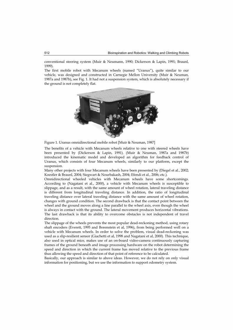
Bioinspiration and Robotics: Walking and Climbing Robots 512
conventional steering system (Muir & Neumann, 1990; Dickerson & Lapin, 1991; Braunl, 1999).The first mobile robot with Mecanum wheels (named “Uranus”), quite similar to our vehicle, was designed and constructed in Carnegie Mellon University (Muir & Neuman, 1987a and 1987b), see Fig. 1. It had not a suspension system, which is absolutely necessary if the ground is not completely flat.
Figure 1. Uranus omnidirectional mobile robot [Muir & Neuman, 1987]
The benefits of a vehicle with Mecanum wheels relative to one with steered wheels have been presented by (Dickerson & Lapin, 1991). (Muir & Neuman, 1987a and 1987b) introduced the kinematic model and developed an algorithm for feedback control of Uranus, which consists of four Mecanum wheels, similarly to our platform, except the suspension. Many other projects with four Mecanum wheels have been presented by (Diegel et al., 2002; Koestler & Braunl, 2004; Siegwart & Nourbakash, 2004; Efendi et al., 2006; etc.). Omnidirectional wheeled vehicles with Mecanum wheels have some shortcomings. According to (Nagatani et al., 2000), a vehicle with Mecanum wheels is susceptible to slippage, and as a result, with the same amount of wheel rotation, lateral traveling distance is different from longitudinal traveling distance. In addition, the ratio of longitudinal traveling distance over lateral traveling distance with the same amount of wheel rotation, changes with ground condition. The second drawback is that the contact point between the wheel and the ground moves along a line parallel to the wheel axis, even though the wheel is always in contact with the ground. The lateral movement produces horizontal vibrations. The last drawback is that its ability to overcome obstacles is not independent of travel direction. The slippage of the wheels prevents the most popular dead-reckoning method, using rotary shaft encoders (Everett, 1995 and Borenstein et al, 1996), from being performed well on a vehicle with Mecanum wheels. In order to solve the problem, visual dead-reckoning was used as a slip-resilient sensor (Giachetti et al, 1998 and Nagatani et al, 2000). This technique, also used in optical mice, makes use of an on-board video-camera continuously capturing frames of the ground beneath and image processing hardware on the robot determining the speed and direction in which the current frame has moved relative to the previous frame thus allowing the speed and direction of that point of reference to be calculated. Basically, our approach is similar to above ideas. However, we do not rely on only visual information for positioning, but we use the information to support odometry system.
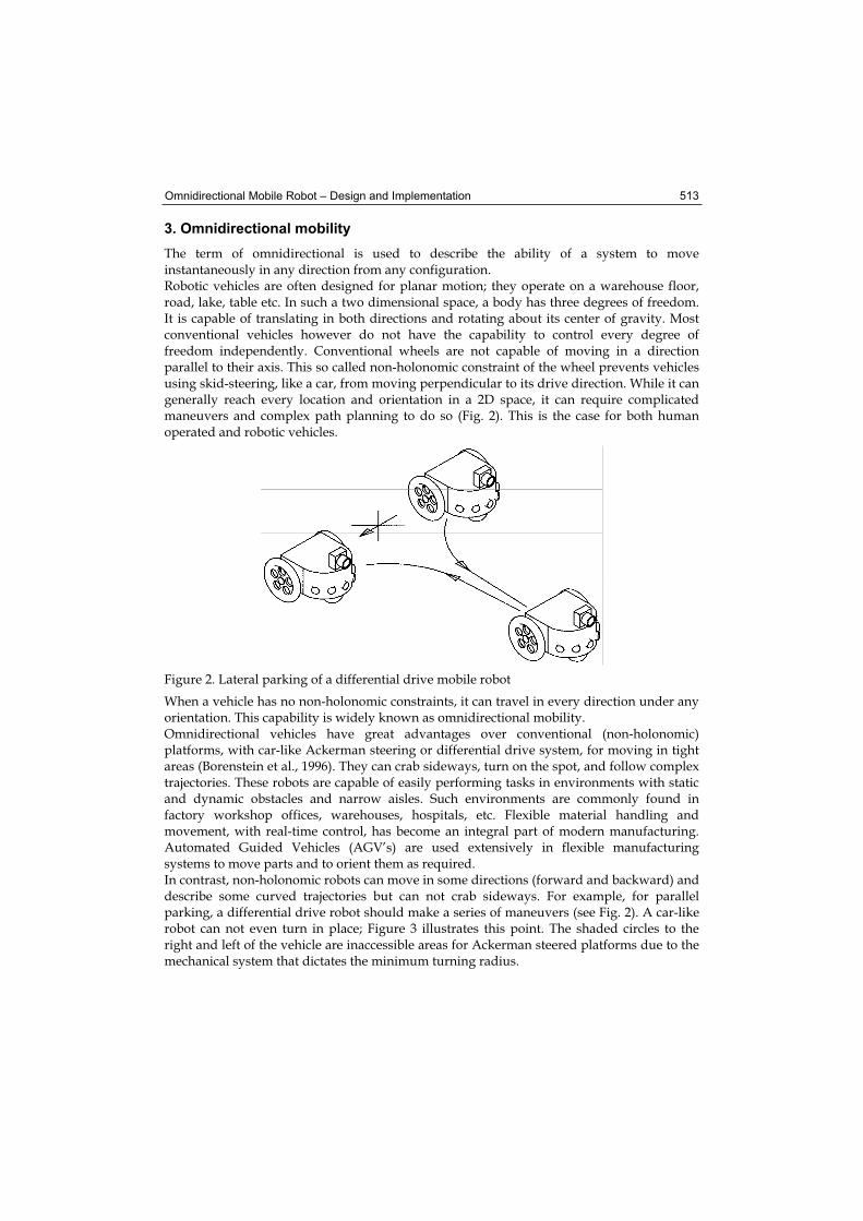
Omnidirectional Mobile Robot – Design and Implementation 513
3. Omnidirectional mobility
The term of omnidirectional is used to describe the ability of a system to move instantaneously in any direction from any configuration. Robotic vehicles are often designed for planar motion; they operate on a warehouse floor, road, lake, table etc. In such a two dimensional space, a body has three degrees of freedom. It is capable of translating in both directions and rotating about its center of gravity. Most conventional vehicles however do not have the capability to control every degree of freedom independently. Conventional wheels are not capable of moving in a direction parallel to their axis. This so called non-holonomic constraint of the wheel prevents vehicles using skid-steering, like a car, from moving perpendicular to its drive direction. While it can generally reach every location and orientation in a 2D space, it can require complicated maneuvers and complex path planning to do so (Fig. 2). This is the case for both human operated and robotic vehicles.
Figure 2. Lateral parking of a differential drive mobile robot
When a vehicle has no non-holonomic constraints, it can travel in every direction under any orientation. This capability is widely known as omnidirectional mobility. Omnidirectional vehicles have great advantages over conventional (non-holonomic) platforms, with car-like Ackerman steering or differential drive system, for moving in tight areas (Borenstein et al., 1996). They can crab sideways, turn on the spot, and follow complex trajectories. These robots are capable of easily performing tasks in environments with static and dynamic obstacles and narrow aisles. Such environments are commonly found in factory workshop offices, warehouses, hospitals, etc. Flexible material handling and movement, with real-time control, has become an integral part of modern manufacturing. Automated Guided Vehicles (AGV’s) are used extensively in flexible manufacturing systems to move parts and to orient them as required. In contrast, non-holonomic robots can move in some directions (forward and backward) and describe some curved trajectories but can not crab sideways. For example, for parallel parking, a differential drive robot should make a series of maneuvers (see Fig. 2). A car-like robot can not even turn in place; Figure 3 illustrates this point. The shaded circles to the right and left of the vehicle are inaccessible areas for Ackerman steered platforms due to the mechanical system that dictates the minimum turning radius.
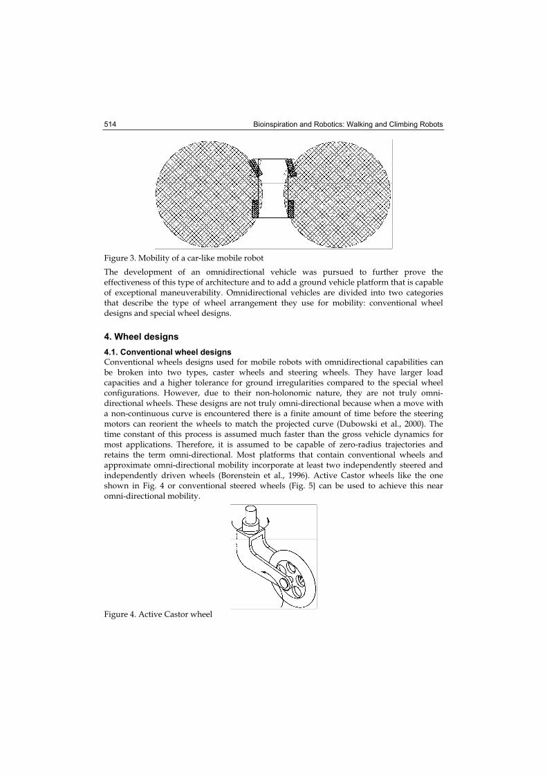
Bioinspiration and Robotics: Walking and Climbing Robots 514
Figure 3. Mobility of a car-like mobile robot
The development of an omnidirectional vehicle was pursued to further prove the effectiveness of this type of architecture and to add a ground vehicle platform that is capable of exceptional maneuverability. Omnidirectional vehicles are divided into two categories that describe the type of wheel arrangement they use for mobility: conventional wheel designs and special wheel designs.
4. Wheel designs
4.1. Conventional wheel designs
Conventional wheels designs used for mobile robots with omnidirectional capabilities can be broken into two types, caster wheels and steering wheels. They have larger load capacities and a higher tolerance for ground irregularities compared to the special wheel configurations. However, due to their non-holonomic nature, they are not truly omni-directional wheels. These designs are not truly omni-directional because when a move with a non-continuous curve is encountered there is a finite amount of time before the steering motors can reorient the wheels to match the projected curve (Dubowski et al., 2000). The time constant of this process is assumed much faster than the gross vehicle dynamics for most applications. Therefore, it is assumed to be capable of zero-radius trajectories and retains the term omni-directional. Most platforms that contain conventional wheels and approximate omni-directional mobility incorporate at least two independently steered and independently driven wheels (Borenstein et al., 1996). Active Castor wheels like the one shown in Fig. 4 or conventional steered wheels (Fig. 5} can be used to achieve this near omni-directional mobility.
Figure 4. Active Castor wheel
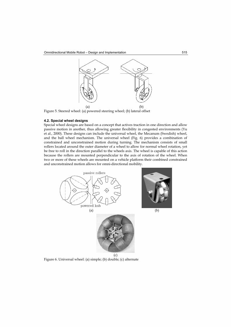
Omnidirectional Mobile Robot – Design and Implementation 515
(a) (b) Figure 5. Steered wheel: (a) powered steering wheel; (b) lateral offset
4.2. Special wheel designs
Special wheel designs are based on a concept that actives traction in one direction and allow passive motion in another, thus allowing greater flexibility in congested environments (Yu et al., 2000). These designs can include the universal wheel, the Mecanum (Swedish) wheel, and the ball wheel mechanism. The universal wheel (Fig. 6) provides a combination of constrained and unconstrained motion during turning. The mechanism consists of small rollers located around the outer diameter of a wheel to allow for normal wheel rotation, yet be free to roll in the direction parallel to the wheels axis. The wheel is capable of this action because the rollers are mounted perpendicular to the axis of rotation of the wheel. When two or more of these wheels are mounted on a vehicle platform their combined constrained and unconstrained motion allows for omni-directional mobility.
(a) (b)
(c)Figure 6. Universal wheel: (a) simple; (b) double; (c) alternate
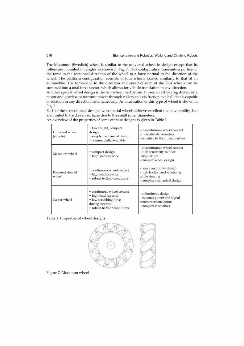
Bioinspiration and Robotics: Walking and Climbing Robots 516
The Mecanum (Swedish) wheel is similar to the universal wheel in design except that its rollers are mounted on angles as shown in Fig. 7. This configuration transmits a portion of the force in the rotational direction of the wheel to a force normal to the direction of the wheel. The platform configuration consists of four wheels located similarly to that of an automobile. The forces due to the direction and speed of each of the four wheels can be summed into a total force vector, which allows for vehicle translation in any direction. Another special wheel design is the ball wheel mechanism. It uses an active ring driven by a motor and gearbox to transmit power through rollers and via friction to a ball that is capable of rotation in any direction instantaneously. An illustration of this type of wheel is shown in Fig. 8. Each of these mentioned designs with special wheels achieve excellent maneuverability, but are limited to hard even surfaces due to the small roller diameters. An overview of the properties of some of these designs is given in Table 1.
Universal wheel (simple)
+ low weight, compact design+ simple mechanical design + commercially available
- discontinuous wheel contact or variable drive-radius - sensitive to floor irregularities
Mecanum wheel + compact design + high load capacity
- discontinuous wheel contact - high sensitivity to floor irregularities - complex wheel design
Powered steered wheel
+ continuous wheel contact + high load capacity + robust to floor conditions
- heavy and bulky design - high friction and scrubbing while steering - complex mechanical design
Castor wheel
+ continuous wheel contact + high load capacity + low scrubbing force during steering + robust to floor conditions
- voluminous design - transmit power and signal across rotational joints - complex mechanics
Table 1. Properties of wheel designs
Figure 7. Mecanum wheel
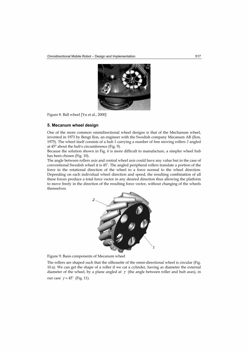
Omnidirectional Mobile Robot – Design and Implementation 517
Figure 8. Ball wheel [Yu et al., 2000]
5. Mecanum wheel design
One of the more common omnidirectional wheel designs is that of the Mechanum wheel, invented in 1973 by Bengt Ilon, an engineer with the Swedish company Mecanum AB (Ilon, 1975). The wheel itself consists of a hub 1 carrying a number of free moving rollers 2 angledat 45° about the hub's circumference (Fig. 9). Because the solution shown in Fig. 6 is more difficult to manufacture, a simpler wheel hub has been chosen (Fig. 10). The angle between rollers axis and central wheel axis could have any value but in the case of conventional Swedish wheel it is 45˚. The angled peripheral rollers translate a portion of the force in the rotational direction of the wheel to a force normal to the wheel direction. Depending on each individual wheel direction and speed, the resulting combination of all these forces produce a total force vector in any desired direction thus allowing the platform to move freely in the direction of the resulting force vector, without changing of the wheels themselves.
Figure 9. Basis components of Mecanum wheel
The rollers are shaped such that the silhouette of the omni-directional wheel is circular (Fig. 10.a). We can get the shape of a roller if we cat a cylinder, having as diameter the external diameter of the wheel, by a plane angled at γ (the angle between roller and hub axes), in
our case γ = 45 (Fig. 11).
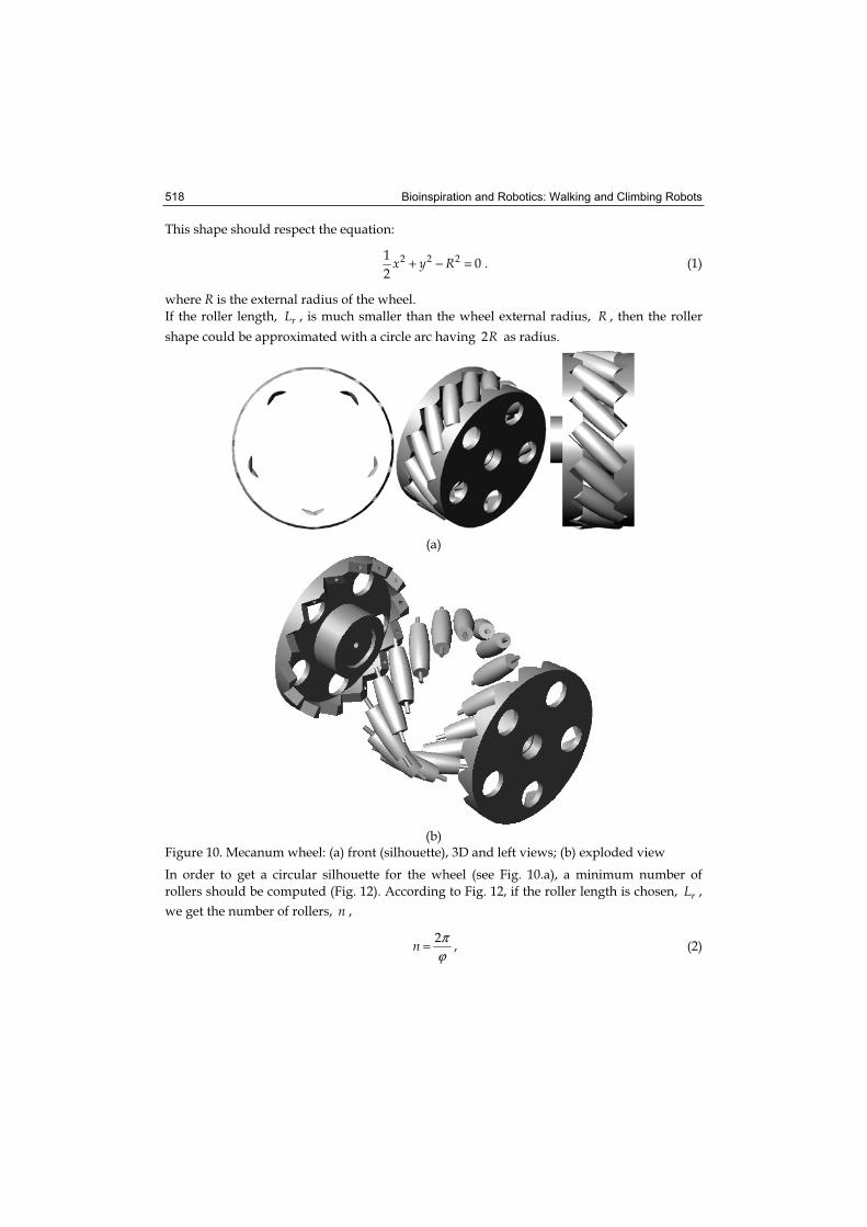
Bioinspiration and Robotics: Walking and Climbing Robots 518
This shape should respect the equation:
+ − =2 2 210
2x y R . (1)
where R is the external radius of the wheel.
If the roller length, rL , is much smaller than the wheel external radius, R , then the roller
shape could be approximated with a circle arc having 2R as radius.
(a)
(b)Figure 10. Mecanum wheel: (a) front (silhouette), 3D and left views; (b) exploded view
In order to get a circular silhouette for the wheel (see Fig. 10.a), a minimum number of
rollers should be computed (Fig. 12). According to Fig. 12, if the roller length is chosen, rL ,
we get the number of rollers, n ,
πϕ
= 2n , (2)
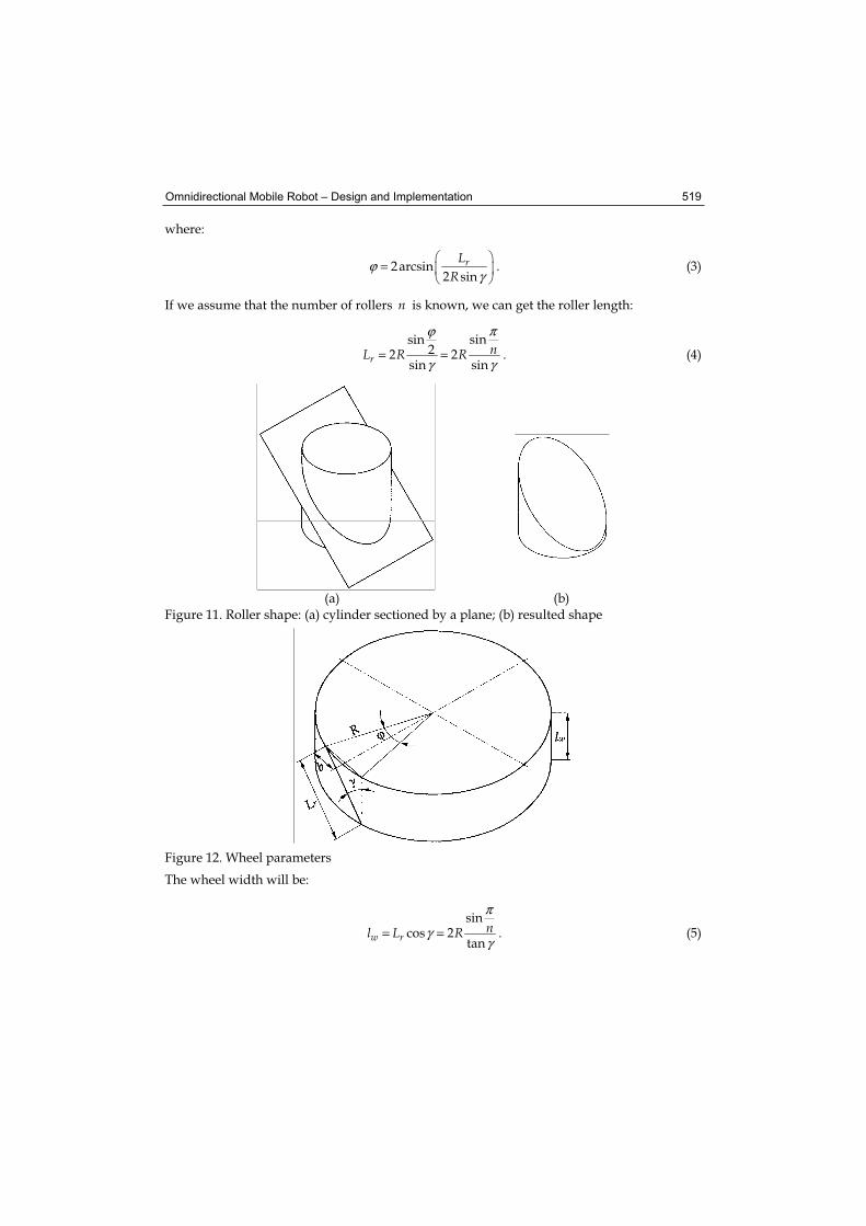
Omnidirectional Mobile Robot – Design and Implementation 519
where:
ϕγ
= 2arcsin2 sin
rLR
. (3)
If we assume that the number of rollers n is known, we can get the roller length:
πϕ
γ γ= =
sinsin22 2
sin sinr
nL R R . (4)
(a) (b) Figure 11. Roller shape: (a) cylinder sectioned by a plane; (b) resulted shape
Figure 12. Wheel parameters
The wheel width will be:
π
γγ
= =sin
cos 2tan
w rnl L R . (5)
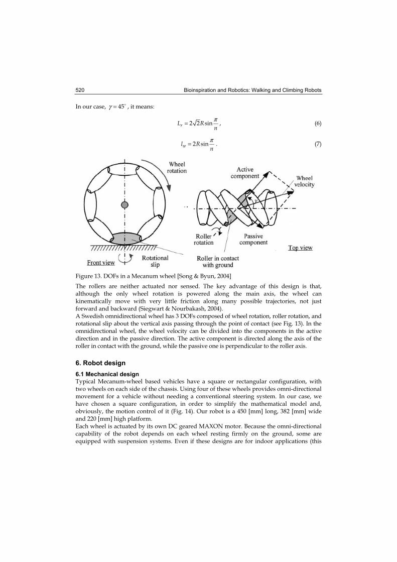
Bioinspiration and Robotics: Walking and Climbing Robots 520
In our case, γ = 45 , it means:
π= 2 2 sinrL Rn
, (6)
π= 2 sinwl Rn
. (7)
Figure 13. DOFs in a Mecanum wheel [Song & Byun, 2004]
The rollers are neither actuated nor sensed. The key advantage of this design is that, although the only wheel rotation is powered along the main axis, the wheel can kinematically move with very little friction along many possible trajectories, not just forward and backward (Siegwart & Nourbakash, 2004). A Swedish omnidirectional wheel has 3 DOFs composed of wheel rotation, roller rotation, and rotational slip about the vertical axis passing through the point of contact (see Fig. 13). In the omnidirectional wheel, the wheel velocity can be divided into the components in the active direction and in the passive direction. The active component is directed along the axis of the roller in contact with the ground, while the passive one is perpendicular to the roller axis.
6. Robot design
6.1 Mechanical design
Typical Mecanum-wheel based vehicles have a square or rectangular configuration, with two wheels on each side of the chassis. Using four of these wheels provides omni-directional movement for a vehicle without needing a conventional steering system. In our case, we have chosen a square configuration, in order to simplify the mathematical model and, obviously, the motion control of it (Fig. 14). Our robot is a 450 [mm] long, 382 [mm] wide and 220 [mm] high platform. Each wheel is actuated by its own DC geared MAXON motor. Because the omni-directional capability of the robot depends on each wheel resting firmly on the ground, some are equipped with suspension systems. Even if these designs are for indoor applications (this
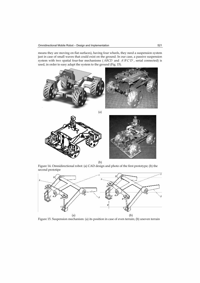
Omnidirectional Mobile Robot – Design and Implementation 521
means they are moving on flat surfaces), having four wheels, they need a suspension system just in case of small waves that could exist on the ground. In our case, a passive suspension
system with two spatial four-bar mechanisms ( ABCD and ' ' ' 'A B C D , serial connected) is
used, in order to easy adapt the system to the ground (Fig. 15).
(a)
(b)Figure 14. Omnidirectional robot: (a) CAD design and photo of the first prototype; (b) the second prototipe
(a) (b) Figure 15. Suspension mechanism: (a) its position in case of even terrain; (b) uneven terrain
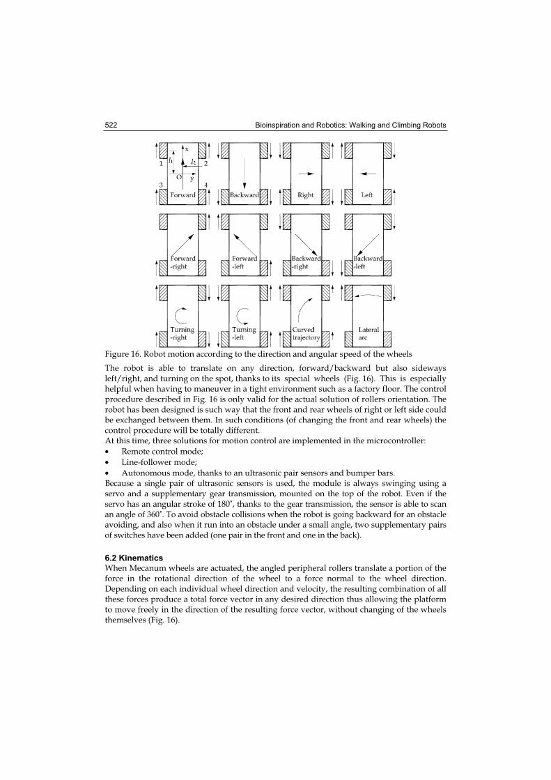
Bioinspiration and Robotics: Walking and Climbing Robots 522
Figure 16. Robot motion according to the direction and angular speed of the wheels
The robot is able to translate on any direction, forward/backward but also sideways left/right, and turning on the spot, thanks to its special wheels (Fig. 16). This is especially helpful when having to maneuver in a tight environment such as a factory floor. The control procedure described in Fig. 16 is only valid for the actual solution of rollers orientation. The robot has been designed is such way that the front and rear wheels of right or left side could be exchanged between them. In such conditions (of changing the front and rear wheels) the control procedure will be totally different. At this time, three solutions for motion control are implemented in the microcontroller:
• Remote control mode;
• Line-follower mode;
• Autonomous mode, thanks to an ultrasonic pair sensors and bumper bars. Because a single pair of ultrasonic sensors is used, the module is always swinging using a servo and a supplementary gear transmission, mounted on the top of the robot. Even if the servo has an angular stroke of 180˚, thanks to the gear transmission, the sensor is able to scan an angle of 360˚. To avoid obstacle collisions when the robot is going backward for an obstacle avoiding, and also when it run into an obstacle under a small angle, two supplementary pairs of switches have been added (one pair in the front and one in the back).
6.2 Kinematics
When Mecanum wheels are actuated, the angled peripheral rollers translate a portion of the force in the rotational direction of the wheel to a force normal to the wheel direction. Depending on each individual wheel direction and velocity, the resulting combination of all these forces produce a total force vector in any desired direction thus allowing the platform to move freely in the direction of the resulting force vector, without changing of the wheels themselves (Fig. 16).
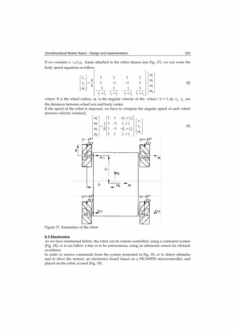
Omnidirectional Mobile Robot – Design and Implementation 523
If we consider a S S Sx O y frame attached to the robot chassis (see Fig. 17), we can write the
body speed equations as follow:
ωωω
ωω
= − − ⋅
− −+ + + +
1
2
3
41 2 1 2 1 2 1 2
1 1 1 1
1 1 1 14
1 1 1 1
x
y
z
vRv
l l l l l l l l
(8)
where: R is the wheel radius; ωi is the angular velocity of the wheel i (i = 1..4); 1l , 2l are
the distances between wheel axis and body center. If the speed of the robot is imposed, we have to compute the angular speed of each wheel (inverse velocity solution):
ωωω
ωω
− +− +
= ⋅− − +
+
1 1 2
2 1 2
3 1 2
4 1 2
1 1 ( )
1 11
1 1 ( )
1 1
x
y
z
l lv
l lv
l lRl l
(9)
Figure 17. Kinematics of the robot
6.3 Electronics
As we have mentioned before, the robot can be remote controlled, using a command system (Fig. 18), or it can follow a line or to be autonomous, using an ultrasonic sensor for obstacle avoidance. In order to receive commands from the system presented in Fig. 18, or to detect obstacles and to drive the motors, an electronics board based on a PIC16F876 microcontroller, and placed on the robot, is used (Fig. 19).
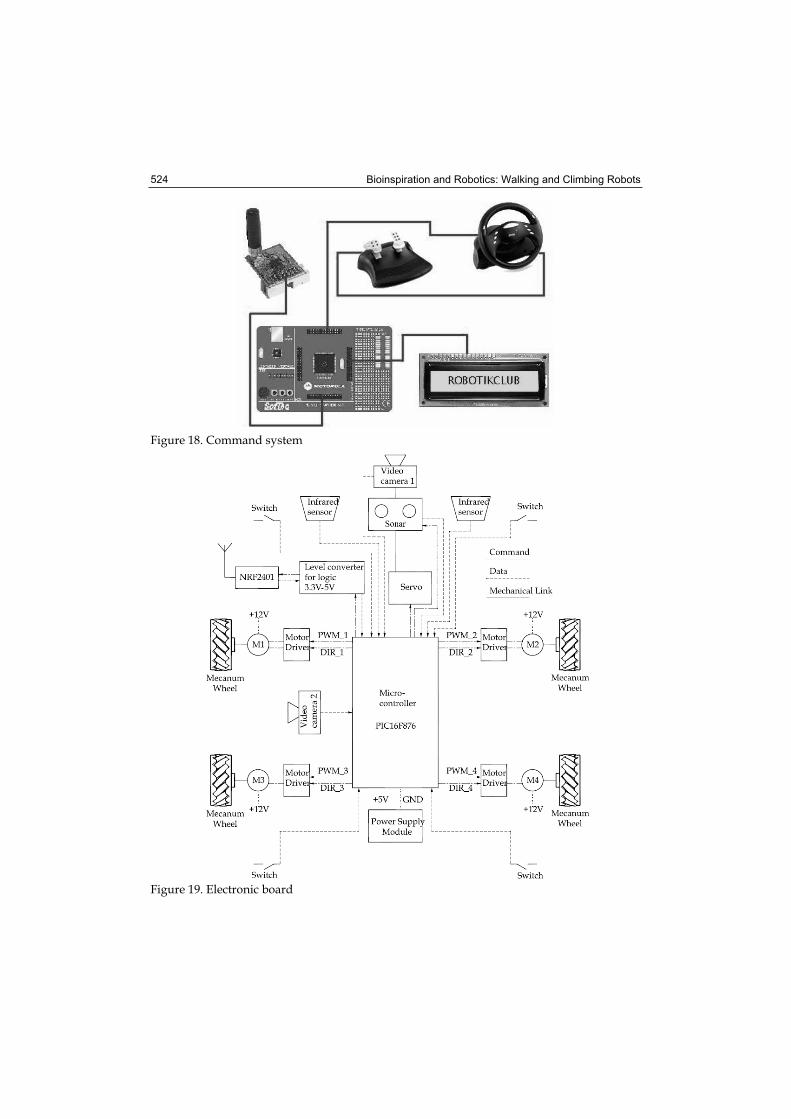
Bioinspiration and Robotics: Walking and Climbing Robots 524
Figure 18. Command system
Figure 19. Electronic board
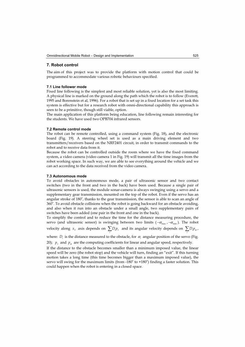
Omnidirectional Mobile Robot – Design and Implementation 525
7. Robot control
The aim of this project was to provide the platform with motion control that could be programmed to accommodate various robotic behaviours specified.
7.1 Line follower mode
Fixed line following is the simplest and most reliable solution, yet is also the most limiting. A physical line is marked on the ground along the path which the robot is to follow (Everett, 1995 and Borenstein et al, 1996). For a robot that is set up in a fixed location for a set task this system is effective but for a research robot with omni-directional capability this approach is seen to be a primitive, though still viable, option. The main application of this platform being education, line following remain interesting for the students. We have used two OPB704 infrared sensors.
7.2 Remote control mode
The robot can be remote controlled, using a command system (Fig. 18), and the electronic board (Fig. 19). A steering wheel set is used as a main driving element and two transmitters/receivers based on the NRF2401 circuit, in order to transmit commands to the robot and to receive data from it. Because the robot can be controlled outside the room where we have the fixed command system, a video camera (video camera 1 in Fig. 19) will transmit all the time images from the robot working space. In such way, we are able to see everything around the vehicle and we can act according to the data received from the video camera.
7.3 Autonomous mode
To avoid obstacles in autonomous mode, a pair of ultrasonic sensor and two contact switches (two in the front and two in the back) have been used. Because a single pair of ultrasonic sensors is used, the module sonar-camera is always swinging using a servo and a supplementary gear transmission, mounted on the top of the robot. Even if the servo has an angular stroke of 180˚, thanks to the gear transmission, the sensor is able to scan an angle of 360˚. To avoid obstacle collisions when the robot is going backward for an obstacle avoiding, and also when it run into an obstacle under a small angle, two supplementary pairs of switches have been added (one pair in the front and one in the back). To simplify the control and to reduce the time for the distance measuring procedure, the
servo (and ultrasonic sensor) is swinging between two limits ( α− max , α− min ). The robot
velocity along Sx axis depends on i vi
D p and its angular velocity depends on ωii
D p ,
where: iD is the distance measured to the obstacle, for α i angular position of the servo (Fig.
20); vp and ωp are the computing coefficients for linear and angular speed, respectively.
If the distance to the obstacle becomes smaller than a minimum imposed value, the linear speed will be zero (the robot stop) and the vehicle will turn, finding an “exit”. If this turning motion takes a long time (this time becomes bigger than a maximum imposed value), the servo will swing for the maximum limits (from -180˚ to +180˚) finding a faster solution. This could happen when the robot is entering in a closed space.
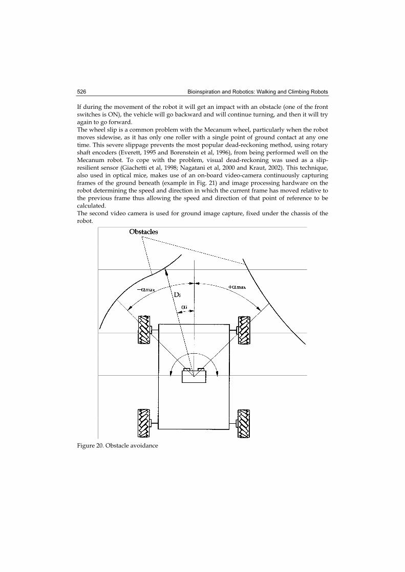
Bioinspiration and Robotics: Walking and Climbing Robots 526
If during the movement of the robot it will get an impact with an obstacle (one of the front switches is ON), the vehicle will go backward and will continue turning, and then it will try again to go forward. The wheel slip is a common problem with the Mecanum wheel, particularly when the robot moves sidewise, as it has only one roller with a single point of ground contact at any one time. This severe slippage prevents the most popular dead-reckoning method, using rotary shaft encoders (Everett, 1995 and Borenstein et al, 1996), from being performed well on the Mecanum robot. To cope with the problem, visual dead-reckoning was used as a slip-resilient sensor (Giachetti et al, 1998; Nagatani et al, 2000 and Kraut, 2002). This technique, also used in optical mice, makes use of an on-board video-camera continuously capturing frames of the ground beneath (example in Fig. 21) and image processing hardware on the robot determining the speed and direction in which the current frame has moved relative to the previous frame thus allowing the speed and direction of that point of reference to be calculated. The second video camera is used for ground image capture, fixed under the chassis of the robot.
Figure 20. Obstacle avoidance
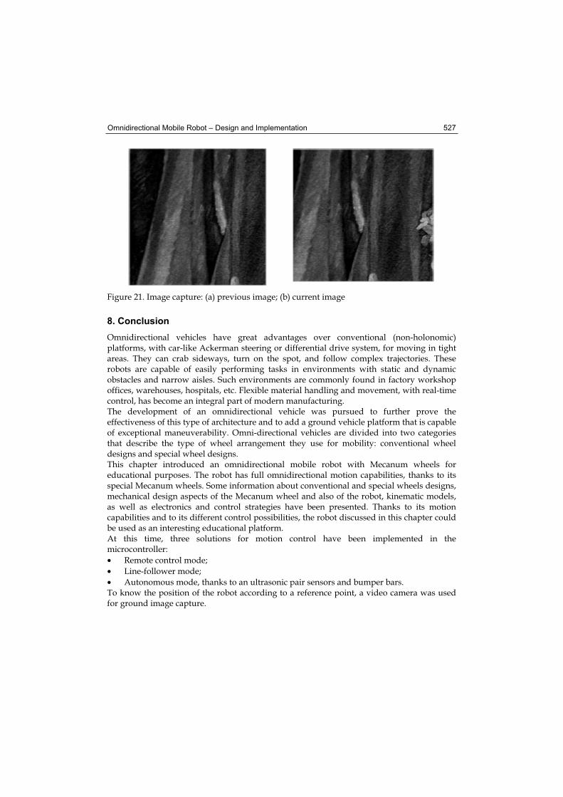
Omnidirectional Mobile Robot – Design and Implementation 527
Figure 21. Image capture: (a) previous image; (b) current image
8. Conclusion
Omnidirectional vehicles have great advantages over conventional (non-holonomic) platforms, with car-like Ackerman steering or differential drive system, for moving in tight areas. They can crab sideways, turn on the spot, and follow complex trajectories. These robots are capable of easily performing tasks in environments with static and dynamic obstacles and narrow aisles. Such environments are commonly found in factory workshop offices, warehouses, hospitals, etc. Flexible material handling and movement, with real-time control, has become an integral part of modern manufacturing. The development of an omnidirectional vehicle was pursued to further prove the effectiveness of this type of architecture and to add a ground vehicle platform that is capable of exceptional maneuverability. Omni-directional vehicles are divided into two categories that describe the type of wheel arrangement they use for mobility: conventional wheel designs and special wheel designs. This chapter introduced an omnidirectional mobile robot with Mecanum wheels for educational purposes. The robot has full omnidirectional motion capabilities, thanks to its special Mecanum wheels. Some information about conventional and special wheels designs, mechanical design aspects of the Mecanum wheel and also of the robot, kinematic models, as well as electronics and control strategies have been presented. Thanks to its motion capabilities and to its different control possibilities, the robot discussed in this chapter could be used as an interesting educational platform. At this time, three solutions for motion control have been implemented in the microcontroller:
• Remote control mode;
• Line-follower mode;
• Autonomous mode, thanks to an ultrasonic pair sensors and bumper bars. To know the position of the robot according to a reference point, a video camera was used for ground image capture.
Bioinspiration and Robotics: Walking and Climbing Robots 528
9. References
Borenstein, J.; Everett, H.R. & Feng, L. (1996). Navigating Mobile Robots: Sensors and Techniques. A K Peters, Ltd, MA, USA.
Bräunl, T. (1999). Eye-Bot: a family of autonomous mobile robots. In: Proceedings of 6thInternational Conference on Neural Information Processing, pp. 645-649, November, 1999, Perth, Australia.
Dickerson, S.L. & Lapin, B.D. (1991). Control of an omni-directional robotic vehicle with Mecanum wheels. In: National Telesystems Conference Proceedings, pp.323-328, March 26-27, 1991, Atlanta, USA.
Diegel, O.; Badve, A.; Bright, G.; Potgieter, J. & Tlatle, S. (2002). Improved Mecanum Wheel Design for Omni-directional Robots, Proc. 2002 Australian Conference on Robotics and Automation, Auckland, 27-29 Nov. 2002, pp. 117-121.
Dubowsky, S.; Genot, F.; Godding, S.; Kozono, H.; Skwersky, A.; Yu, H. & Yu, L. (2000). PAMM – A Robotic Aid to the Eldery for Mobility Assistance and Monitoring: A Helping-Hand for the Elderly, IEEE International Conference on Robotics and Automation, 2000.
Everett, H.R. (1995). Sensors for Mobile Robots: Theory and Application. A K Peters, Ltd, MA, USA.
Giachetti, A.; Campani, M. & Torre, V. (1998). The use of optical flow for road navigation. IEEE Transactions on Robotics and Automation. Vol.,14, No.,1, pp.34-48.
Ilon, B. E. (1975). Wheels for a Course Stable Selfpropelling Vehicle Movable in any Desired Direction on the Ground or Some Other Base. U.S. Patent. U.S.A.
Koestler, A. & Bräunl, Th. (2004). Mobile Robot Simulation with Realistic Error Models, 2nd International Conference on Autonomous Robots and Agents, December 13-15, 2004 Palmerston North, New Zealand, pp. 46-51.
Muir, P. F. & C. P. Neuman (1987). Kinematic Modeling for Feedback Control of an Omnidirection Wheeled Mobile Robot. IEEE Intenational Conference on Robotics and Automation.
Muir, P. F. & C. P. Neuman (1987). Kinematic Modeling of Wheeled Mobile Robots. Journal of Robotic Systems, No. 4(2), pp. 281-340.
Muir, P.F. & Neumann, C.P. (1990). Kinematic modeling for feedback control of an omnidirectional wheeled mobile robot. In: Autonomous Robot Vehicles, Editors I.J. Coxy and G.T. Wilfong, pp.25-31, Springer-Verlag, Berlin.
Nagatani, K.; Tachibana, S.; Sofne, M. & Tanaka, Y. (2000). Improvement of odometry for omnidirectional vehicle using optical flow information. IEEE/RSJ International Conference on Intelligent Robots and Systems.
Salih, J.E.M.; Rizon, M.; Yaacob, S.; Adom, A.H. & Mamat, M.R. (2006). Designing Omni-Directional Mobile Robot with Mecanum Wheel, American Journal of Applied Sciences3 (5): 1831-1835, 2006 ISSN 1546-9239.
Siegwart, R. & Nourbakash, I.R. (2004). Intro to Autonomous Mobile Systems, MIT Press 2004. Song, J.B. & Byun, K.S.. (2004). Design and Control of a Four-Wheeled Omnidirectional
Mobile Robot with Steerable Omnidirectional Wheels, Journal of Robotic Systems,21(4), 2004, pp. 193-208.
Yu, H.; Dubowsky, S. & Skwersky, A. (2000). Omni-directional Mobility Using Active Split Offset Castors, Proceedings ASME Design Engineering Technical Conferences,Baltimore, September 2000.
30
On the use of a hexapod table to improve tumour targeting in radiation therapy
Jürgen Meyer1,2, Matthias Guckenberger2, Jürgen Wilbert2 and Kurt Baier2
1University of Canterbury, 2University of Würzburg 1New Zealand, 2Germany
1. Introduction
Following the discovery of x-rays by Röntgen at the end of the 19th century it did not take long before ionising radiation was used to treat cancer (Del Regato, 2000). Early treatments were not very accurate in terms of targeting the tumour and sparing surrounding healthy tissue. Geometrical accuracy was in the range of centimetres rather than millimetres. Since those pioneering days considerable improvements facilitated by several technological advances and treatment strategies have been made (Abrams, 1992; Schlegel et al., 2006; Webb, 2001). Today treatment with high energy ionising radiation is one of the three traditional forms of medical treatment used to treat cancer and for palliation of symptoms. It may be used alone or in conjunction with surgery or chemotherapy. It is unrivalled as a treatment in cases where surgical removal of the cancer is impossible or might debilitate the patient, e.g. tumours that are infiltrative or located close to a critical organ such as the spinal cord. The more precisely the tumour can be localised the better it can be targeted. Improvements over the last decades in both anatomical and functional imaging as well as detector technology have made it possible for tumours to be more accurately located (Apisarnthanarax & Chao, 2005; Grosu et al., 2005; Jaffray & Siewerdsen, 2000; Ling et al., 2000). Improved localization has the potential to reduce safety margins around the tumour volume leading to more patient-specific but also more complex shaped target volumes reflecting the demarcation of the tumour in the medical images. Delivering the radiation dose to these irregular target volumes requires a great deal of technological but also human effort. It is against this background that radiotherapy has become a discipline with a quest for precision and sub-millimetre accuracy (Guckenberger et al., 2006a; Meyer et al., 2007; Murphy, 1997; Solberg et al., 2004; Yu et al., 2004). Considering the diversity and elasticity of a human body, its temporal biological variations and various sources of organ motion this is a challenging pursuit requiring sophisticated technology. The use of robots in radiotherapy is beginning to play an increasingly important role in achieving this goal. The challenge is to integrate and utilize robotic technology in a judicious and safe way. The aim is to be able to perform treatments, which were previously unattainable, less accurate and/or reliable or dependent on the skills and experience of the medical team performing the treatment. For a detailed description and review of the fundamentals of radiotherapy the reader is referred to other sources (Khan, 2003; Podgorsak, 2005). However, a brief introduction is
Bioinspiration and Robotics: Walking and Climbing Robots 530
given here to introduce some of the basics and in doing so the reader should become familiar with the principles of radiotherapy. Radiotherapy can be subdivided into two main categories, namely brachytherapy (Greek: brachy = short) and teletherapy (Greek: tele = long). Brachytherapy refers to therapeutic use of encapsulated (sealed) radionuclides within or close to a tumour. To achieve this, the radiation source has to be placed inside the patient where it gives a high dose of radiation to the cancerous tissue in close proximity. Due to the rapid fall-off of the intensity of the radiation, healthy tissues further away from the source receive considerably less dose. Teletherapy, on the other hand, also referred to as external beam radiotherapy (EBRT), is a more common technique for treating cancer patients. In teletherapy, high-energy photon (or electron) beams are typically applied to treat deep-seated tumours. These beams, which reach megavoltage (MV) energies, are produced on medical linear accelerators (Greene & Williams, 1997), denoted linacs. The beams are directed from the outside of the patient towards the tumour thereby depositing energy in the tissue as they penetrate through the body. By applying multiple isocentric fields from a number of different directions, the dose to the tumour can be controlled and the dose to the surrounding healthy tissues minimised. Typically, the isocentre is located in the centre of the tumour and is the pivot point of the linac to which the radiation beams are directed. The challenge with both techniques is to deliver a prescribed dose as conformal as possible to the tumour volume and at the same time keep the dose to surrounding tissues as low as one reasonably can. The treatment planning parameters, such as beam energy, beam shape, relative beam weight and beam orientation, are crucial and are optimized at the treatment planning stage. In order for the treatment to be executed adequately, the radiation has to be delivered exactly as specified in the treatment plan. In practice this is often difficult to achieve due to the flexibility and day-to-day variations in the patient’s anatomy (e.g. different rectal filling, movement due to breathing, weight loss) but, with regards to teletherapy, also due to the difficulty of repositioning and aligning the patient in exactly the same position every day (Gildersleve et al., 1995; Noel et al., 1995). Inaccurate alignment of the radiation beam with the patient can lead to two things. Critical organs may receive an unwanted high dose leading to normal tissue complications and/or the tumour may receive a reduced dose leading to a loss in tumour control. Tumour control is achieved if all clonogenic tumour cells, cells that have the potential to proliferate indefinitely and give rise to a colony of cells, are inactivated. Normal tissue complications and tumour control have an impact on both the patient’s quality-of-life and survival, respectively, and at all cost should be minimised and maximised, respectively. The relationship between the benefit of radiotherapy and harm due to toxicity of the healthy tissues is called therapeutic ratio. Maximizing the therapeutic ratio is one of the main goals of current research. This clearly highlights the importance of spatial accuracy in the delivery of radiotherapy. Amongst other approaches, robots have been utilized to improve accuracy and reproducibility in radiotherapy.In the following section, an overview of the literature regarding the use of robotic systems in radiotherapy will be given. Note that these robots do not necessarily fall into the category of walking or climbing robots. This will be followed in sections 3 and 4, respectively, by a more detailed description of the two main applications studied by the authors. They are: 1) the use of a robotic hexapod treatment table for accurate patient positioning in six degrees of freedom (DOF) and 2) the utilization of an industrial robot to develop a system to operate the robotic hexapod table dynamically with the aim to compensate for breathing induced
On the use of a hexapod table to improve tumour targeting in radiation therapy 531
tumour motion in real-time during radiotherapy treatment. The former approach has been successfully implemented into clinical routine and the clinical benefits but also the potential risks associated with this new technology will be addressed. The use of an additional robot to simulate dynamic compensation of tumour motion in real-time is an active area of research and the experimental set-up as well as encouraging preliminary results will be presented.
2. Literature on robots in radiotherapy
Depending on the definition of the term “robot” several computer controlled electro-mechanical systems conveying some sense of intelligence or agency could be referred to as robots. For brevity, only the most relevant ones guided by imaging technology are mentioned here. To improve the geometrical targeting for both teletherapy and brachytherapy the radiation source needs to be positioned accurately with respect to the identified tumour volume. Based on imaging information (or any other signal that provides relevant information) this can be done by either adjusting the radiation source relative to the patient or the patient relative to a fixed radiation source. In brachytherapy, the radioactive sources are guided into or near the tumour through needles. A number of groups are currently working on prototypes and have demonstrated the feasibility of using robots as a moveable needle guide (Dimaio et al., 2007; Wei et al., 2004) leaving the actual insertion of the needle into the target organ to the physician. Other groups are working on placing radioactive seeds directly into the lesion, e.g. the lung (Trejos et al., 2007) or the prostate (Fichtinger et al., 2006). For all of these procedures image-guided feedback was provided by either trans-rectal ultrasound (TRUS) or by means of magnetic resonance imaging (MRI). The favourable positioning accuracy of the robotically assisted procedures was demonstrated in phantom studies. Another advantage of robotic approaches is that some of the limitations of traditional brachytherapy, such as merely parallel insertion of the needles through a template into the prostate, can be overcome. With robots, it is possible to position the needles and radioactive seeds accurately at any angle thereby making it possible to place sources into positions that were previously not attainable due to the anatomy of the patient. An example for this is pubic arch interference with the path of the needle. For parallel insertion of the needle through a template, some parts of the prostate are impossible to be targeted, whereas with a robot this is not a restraint.Probably the most exciting development in radiotherapy with regards to robots was the development of the cyberknife by Adler at the Department of Neurosurgery at Stanford University Medical Centre (Adler et al., 1997; Chang et al., 1998). The cyberknife is a 6 MV linear accelerator mounted to a robotic manipulator. It was originally designed for treatment of cranial lesions but has been modified to treat extra-cranial tumours (Murphy et al., 2000). Guided by stereo x-ray imaging the cyberknife can deliver non-isocentric pencil beams with a high degree of accuracy from arbitrary points in space. One of the main advantages of robotic linacs in general is the fact that non-spherical target volumes can be irradiated with a higher degree of conformity than with isocentric systems (Webb, 1999; 2000). In addition, traditional frame based systems require the patient to be fixed to the treatment table for targeting and immobilisation reasons. This can be done by invasive or non-invasive means depending on the accuracy required. With the cyberknife, the patient can be on the treatment table without restraints of any kind. Movement of the patient or the tumour is
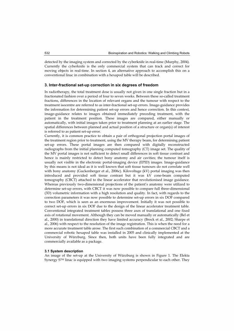
Bioinspiration and Robotics: Walking and Climbing Robots 532
detected by the imaging system and corrected by the cyberknife in real-time (Murphy, 2004). Currently the cyberknife is the only commercial system that can track and correct for moving objects in real-time. In section 4, an alternative approach to accomplish this on a conventional linac in combination with a hexapod table will be described.
3. Inter-fractional set-up correction in six degrees of freedom
In radiotherapy, the total treatment dose is usually not given in one single fraction but in a fractionated fashion over a period of four to seven weeks. Between these so-called treatment fractions, differences in the location of relevant organs and the tumour with respect to the treatment isocentre are referred to as inter-fractional set-up errors. Image-guidance provides the information for determining patient set-up errors and hence correction. In this context, image-guidance relates to images obtained immediately preceding treatment, with the patient in the treatment position. These images are compared, either manually or automatically, with initial images taken prior to treatment planning at an earlier stage. The spatial differences between planned and actual position of a structure or organ(s) of interest is referred to as patient set-up error. Currently, it is common practice to obtain a pair of orthogonal projection portal images of the treatment region prior to treatment, using the MV therapy beam, for determining patient set-up errors. These portal images are then compared with digitally reconstructed radiographs from the initial planning computed tomography (CT) image set. The quality of the MV portal images is not sufficient to detect small differences in soft tissue contrast and hence is mainly restricted to detect bony anatomy and air cavities; the tumour itself is usually not visible in the electronic portal-imaging device (EPID) images. Image-guidance by this means is not ideal as it is well known that soft tissue tumours do not correlate well with bony anatomy (Guckenberger et al., 2006c). Kilovoltage (kV) portal imaging was then introduced and provided soft tissue contrast but it was kV cone-beam computed tomography (CBCT) attached to the linear accelerator that revolutionised image guidance. Whereas previously two-dimensional projections of the patient’s anatomy were utilized to determine set-up errors, with CBCT it was now possible to compare full three-dimensional (3D) volumetric information with a high resolution and quality. In fact, with regards to the correction parameters it was now possible to determine set-up errors in six DOF compared to two DOF, which is seen as an enormous improvement. Initially it was not possible to correct set-up errors in six DOF due to the design of the linear accelerator treatment table. Conventional integrated treatment tables possess three axes of translational and one fixed axis of rotational movement. Although they can be moved manually or automatically (Bel et al., 2000) in translational direction they have limited accuracy (Brock et al., 2002; Sharpe et al., 2006) with respect to the resolution of the image registration. This is when the need for a more accurate treatment table arose. The first such combination of a commercial CBCT and a commercial robotic hexapod table was installed in 2005 and clinically implemented at the University of Würzburg. Since then, both units have been fully integrated and are commercially available as a package.
3.1 System description
An image of the set-up at the University of Würzburg is shown in Figure 1. The Elekta Synergy STM linac is equipped with two imaging systems perpendicular to each other. They
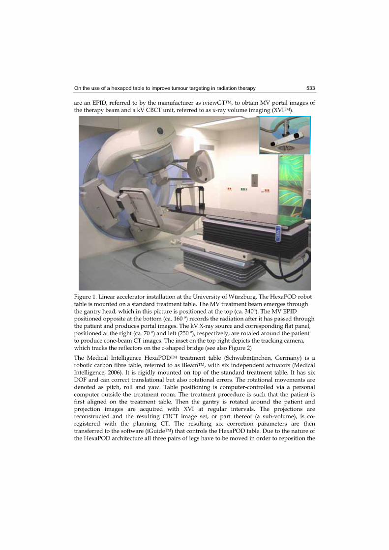
On the use of a hexapod table to improve tumour targeting in radiation therapy 533
are an EPID, referred to by the manufacturer as iviewGTTM, to obtain MV portal images of the therapy beam and a kV CBCT unit, referred to as x-ray volume imaging (XVITM).
Figure 1. Linear accelerator installation at the University of Würzburg. The HexaPOD robot table is mounted on a standard treatment table. The MV treatment beam emerges through the gantry head, which in this picture is positioned at the top (ca. 340º). The MV EPID positioned opposite at the bottom (ca. 160 º) records the radiation after it has passed through the patient and produces portal images. The kV X-ray source and corresponding flat panel, positioned at the right (ca. 70 º) and left (250 º), respectively, are rotated around the patient to produce cone-beam CT images. The inset on the top right depicts the tracking camera, which tracks the reflectors on the c-shaped bridge (see also Figure 2)
The Medical Intelligence HexaPODTM treatment table (Schwabmünchen, Germany) is a robotic carbon fibre table, referred to as iBeamTM, with six independent actuators (Medical Intelligence, 2006). It is rigidly mounted on top of the standard treatment table. It has six DOF and can correct translational but also rotational errors. The rotational movements are denoted as pitch, roll and yaw. Table positioning is computer-controlled via a personal computer outside the treatment room. The treatment procedure is such that the patient is first aligned on the treatment table. Then the gantry is rotated around the patient and projection images are acquired with XVI at regular intervals. The projections are reconstructed and the resulting CBCT image set, or part thereof (a sub-volume), is co-registered with the planning CT. The resulting six correction parameters are then transferred to the software (iGuideTM) that controls the HexaPOD table. Due to the nature of the HexaPOD architecture all three pairs of legs have to be moved in order to reposition the
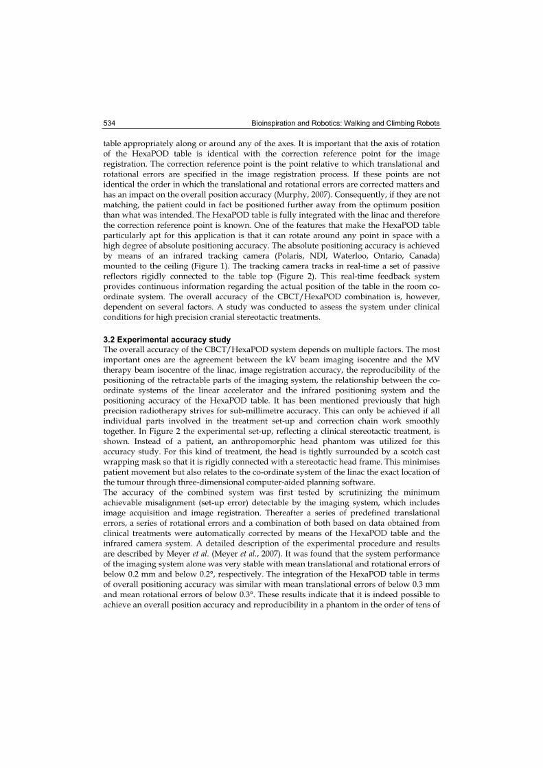
Bioinspiration and Robotics: Walking and Climbing Robots 534
table appropriately along or around any of the axes. It is important that the axis of rotation of the HexaPOD table is identical with the correction reference point for the image registration. The correction reference point is the point relative to which translational and rotational errors are specified in the image registration process. If these points are not identical the order in which the translational and rotational errors are corrected matters and has an impact on the overall position accuracy (Murphy, 2007). Consequently, if they are not matching, the patient could in fact be positioned further away from the optimum position than what was intended. The HexaPOD table is fully integrated with the linac and therefore the correction reference point is known. One of the features that make the HexaPOD table particularly apt for this application is that it can rotate around any point in space with a high degree of absolute positioning accuracy. The absolute positioning accuracy is achieved by means of an infrared tracking camera (Polaris, NDI, Waterloo, Ontario, Canada) mounted to the ceiling (Figure 1). The tracking camera tracks in real-time a set of passive reflectors rigidly connected to the table top (Figure 2). This real-time feedback system provides continuous information regarding the actual position of the table in the room co-ordinate system. The overall accuracy of the CBCT/HexaPOD combination is, however, dependent on several factors. A study was conducted to assess the system under clinical conditions for high precision cranial stereotactic treatments.
3.2 Experimental accuracy study
The overall accuracy of the CBCT/HexaPOD system depends on multiple factors. The most important ones are the agreement between the kV beam imaging isocentre and the MV therapy beam isocentre of the linac, image registration accuracy, the reproducibility of the positioning of the retractable parts of the imaging system, the relationship between the co-ordinate systems of the linear accelerator and the infrared positioning system and the positioning accuracy of the HexaPOD table. It has been mentioned previously that high precision radiotherapy strives for sub-millimetre accuracy. This can only be achieved if all individual parts involved in the treatment set-up and correction chain work smoothly together. In Figure 2 the experimental set-up, reflecting a clinical stereotactic treatment, is shown. Instead of a patient, an anthropomorphic head phantom was utilized for this accuracy study. For this kind of treatment, the head is tightly surrounded by a scotch cast wrapping mask so that it is rigidly connected with a stereotactic head frame. This minimises patient movement but also relates to the co-ordinate system of the linac the exact location of the tumour through three-dimensional computer-aided planning software. The accuracy of the combined system was first tested by scrutinizing the minimum achievable misalignment (set-up error) detectable by the imaging system, which includes image acquisition and image registration. Thereafter a series of predefined translational errors, a series of rotational errors and a combination of both based on data obtained from clinical treatments were automatically corrected by means of the HexaPOD table and the infrared camera system. A detailed description of the experimental procedure and results are described by Meyer et al. (Meyer et al., 2007). It was found that the system performance of the imaging system alone was very stable with mean translational and rotational errors of below 0.2 mm and below 0.2°, respectively. The integration of the HexaPOD table in terms of overall positioning accuracy was similar with mean translational errors of below 0.3 mm and mean rotational errors of below 0.3°. These results indicate that it is indeed possible to achieve an overall position accuracy and reproducibility in a phantom in the order of tens of
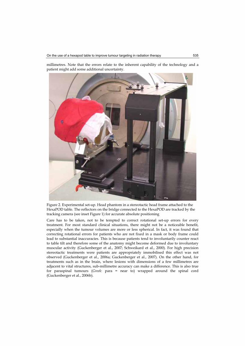
On the use of a hexapod table to improve tumour targeting in radiation therapy 535
millimetres. Note that the errors relate to the inherent capability of the technology and a patient might add some additional uncertainty.
Figure 2. Experimental set-up. Head phantom in a stereotactic head frame attached to the HexaPOD table. The reflectors on the bridge connected to the HexaPOD are tracked by the tracking camera (see inset Figure 1) for accurate absolute positioning
Care has to be taken, not to be tempted to correct rotational set-up errors for every treatment. For most standard clinical situations, there might not be a noticeable benefit, especially when the tumour volumes are more or less spherical. In fact, it was found that correcting rotational errors for patients who are not fixed in a mask or body frame could lead to substantial inaccuracies. This is because patients tend to involuntarily counter react to table tilt and therefore some of the anatomy might become deformed due to involuntary muscular activity (Guckenberger et al., 2007; Schweikard et al., 2000). For high precision stereotactic treatments were patients are appropriately immobilised this effect was not observed (Guckenberger et al., 2006a; Guckenberger et al., 2007). On the other hand, for treatments such as in the brain, where lesions with dimensions of a few millimetres are adjacent to vital structures, sub-millimetre accuracy can make a difference. This is also true for paraspinal tumours (Greek: para = near to) wrapped around the spinal cord (Guckenberger et al., 2006b).
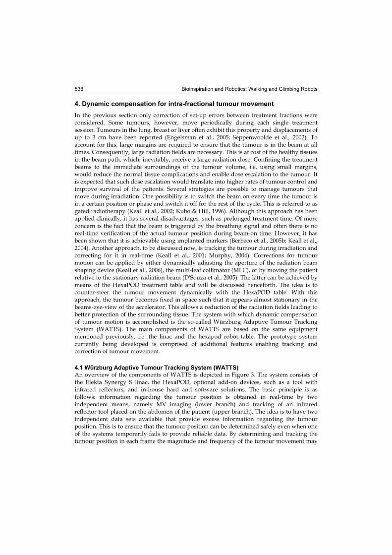
Bioinspiration and Robotics: Walking and Climbing Robots 536
4. Dynamic compensation for intra-fractional tumour movement
In the previous section only correction of set-up errors between treatment fractions were considered. Some tumours, however, move periodically during each single treatment session. Tumours in the lung, breast or liver often exhibit this property and displacements of up to 3 cm have been reported (Engelsman et al., 2005; Seppenwoolde et al., 2002). To account for this, large margins are required to ensure that the tumour is in the beam at all times. Consequently, large radiation fields are necessary. This is at cost of the healthy tissues in the beam path, which, inevitably, receive a large radiation dose. Confining the treatment beams to the immediate surroundings of the tumour volume, i.e. using small margins, would reduce the normal tissue complications and enable dose escalation to the tumour. It is expected that such dose escalation would translate into higher rates of tumour control and improve survival of the patients. Several strategies are possible to manage tumours that move during irradiation. One possibility is to switch the beam on every time the tumour is in a certain position or phase and switch it off for the rest of the cycle. This is referred to as gated radiotherapy (Keall et al., 2002; Kubo & Hill, 1996). Although this approach has been applied clinically, it has several disadvantages, such as prolonged treatment time. Of more concern is the fact that the beam is triggered by the breathing signal and often there is no real-time verification of the actual tumour position during beam-on time. However, it has been shown that it is achievable using implanted markers (Berbeco et al., 2005b; Keall et al., 2004). Another approach, to be discussed now, is tracking the tumour during irradiation and correcting for it in real-time (Keall et al., 2001; Murphy, 2004). Corrections for tumour motion can be applied by either dynamically adjusting the aperture of the radiation beam shaping device (Keall et al., 2006), the multi-leaf collimator (MLC), or by moving the patient relative to the stationary radiation beam (D'Souza et al., 2005). The latter can be achieved by means of the HexaPOD treatment table and will be discussed henceforth. The idea is to counter-steer the tumour movement dynamically with the HexaPOD table. With this approach, the tumour becomes fixed in space such that it appears almost stationary in the beams-eye-view of the accelerator. This allows a reduction of the radiation fields leading to better protection of the surrounding tissue. The system with which dynamic compensation of tumour motion is accomplished is the so-called Würzburg Adaptive Tumour Tracking System (WATTS). The main components of WATTS are based on the same equipment mentioned previously, i.e. the linac and the hexapod robot table. The prototype system currently being developed is comprised of additional features enabling tracking and correction of tumour movement.
4.1 Würzburg Adaptive Tumour Tracking System (WATTS)
An overview of the components of WATTS is depicted in Figure 3. The system consists of the Elekta Synergy S linac, the HexaPOD, optional add-on devices, such as a tool with infrared reflectors, and in-house hard and software solutions. The basic principle is as follows: information regarding the tumour position is obtained in real-time by two independent means, namely MV imaging (lower branch) and tracking of an infrared reflector tool placed on the abdomen of the patient (upper branch). The idea is to have two independent data sets available that provide excess information regarding the tumour position. This is to ensure that the tumour position can be determined safely even when one of the systems temporarily fails to provide reliable data. By determining and tracking the tumour position in each frame the magnitude and frequency of the tumour movement may
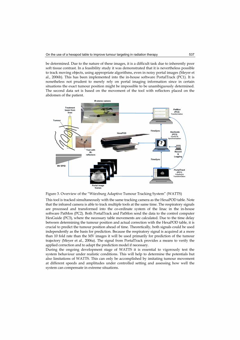
On the use of a hexapod table to improve tumour targeting in radiation therapy 537
be determined. Due to the nature of these images, it is a difficult task due to inherently poor soft tissue contrast. In a feasibility study it was demonstrated that it is nevertheless possible to track moving objects, using appropriate algorithms, even in noisy portal images (Meyer et al., 2006b). This has been implemented into the in-house software PortalTrack (PC1). It is nonetheless not prudent to merely rely on portal imaging information since in certain situations the exact tumour position might be impossible to be unambiguously determined. The second data set is based on the movement of the tool with reflectors placed on the abdomen of the patient.
MV EPID
Tumour
Treatment
beam from
linac
Tool with
IR-
reflectors
IR-stereo camera
Portal image
frames
HexaPOD
PortalTrack(PC1)
Tracking &
Transformation
PatMon (PC2)
Transformation
HexGuide (PC3)
Control &
Synchronization
Record
&
Logging
TimeSync
TimeSync
Figure 3. Overview of the “Würzburg Adaptive Tumour Tracking System” (WATTS)
This tool is tracked simultaneously with the same tracking camera as the HexaPOD table. Note that the infrared camera is able to track multiple tools at the same time. The respiratory signals are processed and transformed into the co-ordinate system of the linac in the in-house software PatMon (PC2). Both PortalTrack and PatMon send the data to the control computer HexGuide (PC3), where the necessary table movements are calculated. Due to the time delay between determining the tumour position and actual correction with the HexaPOD table, it is crucial to predict the tumour position ahead of time. Theoretically, both signals could be used independently as the basis for prediction. Because the respiratory signal is acquired at a more than 10 fold rate than the MV images it will be used primarily for prediction of the tumour trajectory (Meyer et al., 2006a). The signal from PortalTrack provides a means to verify the applied correction and to adapt the prediction model if necessary. During the ongoing development stage of WATTS it is essential to vigorously test the system behaviour under realistic conditions. This will help to determine the potentials but also limitations of WATTS. This can only be accomplished by imitating tumour movement at different speeds and amplitudes under controlled setting and assessing how well the system can compensate in extreme situations.
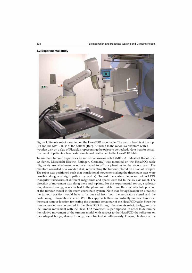
Bioinspiration and Robotics: Walking and Climbing Robots 538
4.2 Experimental study
Figure 4. Six-axis robot mounted on the HexaPOD robot table. The gantry head is at the top (0º) and the MV EPID is at the bottom (180º). Attached to the robot is a phantom with a wooden disk on a slab of Plexiglas representing the object to be tracked. Note that for actual treatment of patients a head extension board is attached to the HexaPOD table
To simulate tumour trajectories an industrial six-axis robot (MELFA Industrial Robot, RV-1A Series, Mitsubishi Electric, Ratingen, Germany) was mounted on the HexaPOD table (Figure 4). An attachment was constructed to affix a phantom to the robotic arm. The phantom consisted of a wooden disk, representing the tumour, placed on a slab of Perspex. The robot was positioned such that translational movements along the three main axes were possible along a straight path (x, y and z). To test the system behaviour of WATTS, triangular trajectories of different magnitude and speed were fed to the six-axis robot. The direction of movement was along the x and y-plane. For this experimental set-up, a reflector tool, denoted toolTum, was attached to the phantom to determine the exact absolute position of the tumour model in the room coordinate system. Note that for application on a patient the tumour position would have to be devised from both the respiratory signal and the portal image information instead. With this approach, there are virtually no uncertainties in the exact tumour location for testing the dynamic behaviour of the HexaPOD table. Since the tumour model was connected to the HexaPOD through the six-axis robot, toolTum records the tumour movement with the HexaPOD movement superimposed. In order to determine the relative movement of the tumour model with respect to the HexaPOD the reflectors on the c-shaped bridge, denoted toolHex, were tracked simultaneously. During playback of the
X
Y
Z
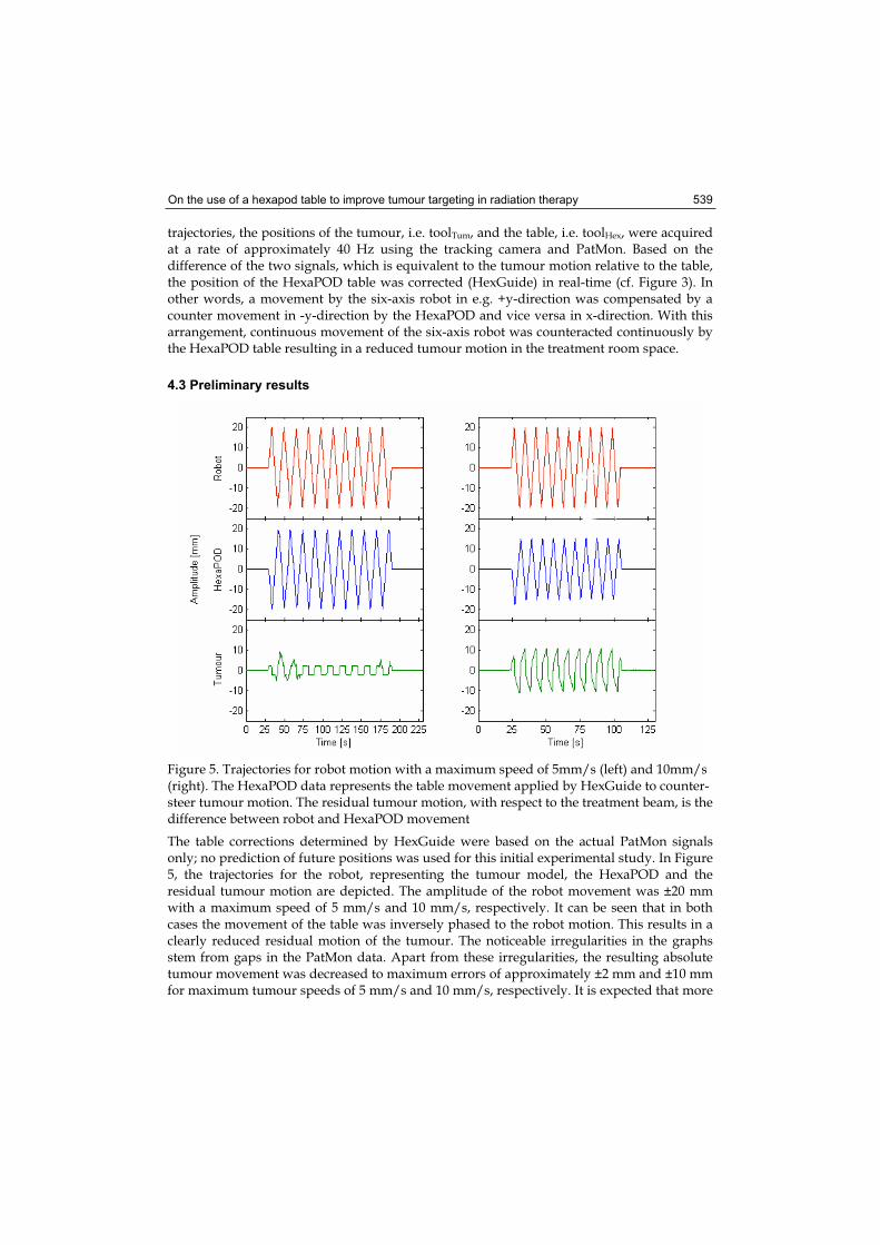
On the use of a hexapod table to improve tumour targeting in radiation therapy 539
trajectories, the positions of the tumour, i.e. toolTum, and the table, i.e. toolHex, were acquired at a rate of approximately 40 Hz using the tracking camera and PatMon. Based on the difference of the two signals, which is equivalent to the tumour motion relative to the table, the position of the HexaPOD table was corrected (HexGuide) in real-time (cf. Figure 3). In other words, a movement by the six-axis robot in e.g. +y-direction was compensated by a counter movement in -y-direction by the HexaPOD and vice versa in x-direction. With this arrangement, continuous movement of the six-axis robot was counteracted continuously by the HexaPOD table resulting in a reduced tumour motion in the treatment room space.
4.3 Preliminary results
Figure 5. Trajectories for robot motion with a maximum speed of 5mm/s (left) and 10mm/s (right). The HexaPOD data represents the table movement applied by HexGuide to counter-steer tumour motion. The residual tumour motion, with respect to the treatment beam, is the difference between robot and HexaPOD movement
The table corrections determined by HexGuide were based on the actual PatMon signals only; no prediction of future positions was used for this initial experimental study. In Figure 5, the trajectories for the robot, representing the tumour model, the HexaPOD and the residual tumour motion are depicted. The amplitude of the robot movement was ±20 mm with a maximum speed of 5 mm/s and 10 mm/s, respectively. It can be seen that in both cases the movement of the table was inversely phased to the robot motion. This results in a clearly reduced residual motion of the tumour. The noticeable irregularities in the graphs stem from gaps in the PatMon data. Apart from these irregularities, the resulting absolute tumour movement was decreased to maximum errors of approximately ±2 mm and ±10 mm for maximum tumour speeds of 5 mm/s and 10 mm/s, respectively. It is expected that more
X
Y
Z
Bioinspiration and Robotics: Walking and Climbing Robots 540
realistic sinusoidal tumour trajectories would result in even smaller overall errors. The sudden changes in the triangular tumour trajectories require the HexaPOD to accelerate and decelerate rapidly. As can be seen in Figure 5, this constitutes the main source of error for the residual tumour motion. Furthermore, given the fact that no efforts were made to compensate for delay in the control system this is a promising result. The next step will be to implement predictive models to determine tumour positions ahead of time with the overall aim to decrease absolute tumour movement to 1-2 mm for tumour speeds of up to 2-3 cm/s. If attainable, this would pave the way for smaller radiation fields resulting in less irradiation of healthy tissue.
5. Discussion & Conclusion
High precision image-guided radiotherapy demands a high degree of spatial accuracy for treatment delivery. Recent advances in imaging technology for radiotherapy have been shown to yield information with respect to the tumour position with sub-millimetre accuracy. Differences between planned and actual tumour position at treatment can be calculated in six DOF. With standard equipment, it is not possible to correct for these set-up errors with the same accuracy as they were detected. Furthermore, it is not possible to correct for all rotational errors. These limitations can be overcome with the robotic HexaPOD table. With the combination of 3D volume imaging on the linac and the HexaPOD table, an overall mean positioning accuracy of 0.3 mm and 0.3º was obtained in an experimental accuracy study. With this combination, it is possible to deliver treatment with a high degree of accuracy guided by imaging technology. This, in turn, has the potential to reduce safety margins around the tumours and hence to improve treatment outcomes. At the University of Würzburg, 6D patient set-up correction is routinely carried out for high-precision radiotherapy. Patients who most benefit from such high accuracy are those with tumours in very close proximity to critical structures, such as lesions in the brain or paraspinal lesions. The latter are frequently wrapped around the spinal cord. Due to the elongated dimensions of paraspinal tumours surrounding a critical structure, this constellation is very sensitive to rotational set-up errors, which can be corrected adequately with the HexaPOD table. It was found that although rotational errors can be corrected it is essential to ensure that the patient is appropriately immobilized. Clinical application of 6D position correction has revealed that several non-immobilized patients who received standard treatment in the pelvic region moved after rotational errors had been corrected. This was most likely to counter act table rotations around the patient axis. Some patients ended up with set-up errors larger than before correction. This fact highlights the fine line between the benefits and detrimental effects with this new technology. A critical evaluation is indispensable to determine the exact circumstances under which a treatment can actually be improved. At the University of Würzburg, a reasonable number of studies have been carried out to integrate image-guided radiotherapy and corrections with the HexaPOD table seamlessly into clinical routine. Today, for high-precision radiotherapy at the University of Würzburg, the HexaPOD table is an integral part of the treatment. An active area of research is dynamic real-time compensation of tumour movement by means of WATTS. The approach described is a feasibility study. So far, its achievability has been demonstrated under non-clinical settings in a clinical environment. Although the preliminary results are very encouraging, it is still a long way from clinical implementation. Hitherto, both tracking the tumour in real-time using MV portal imaging and recording the
On the use of a hexapod table to improve tumour targeting in radiation therapy 541
breathing motion by means of the tracking camera have been applied passively to a few dozens patients. This was done without altering the actual treatment. It is envisaged that one of the first applications of WATTS will not be to compensate for tumour movement dynamically but rather to detect any drift in the tumour mean position, so-called base-line drifts, during standard lung treatments. Thus, rather then adapting the treatment WATTS may initially be used for verification purposes. This is in-line with other researchers who are working on imaging approaches to verify gated radiotherapy non-invasively (Berbeco et al., 2005a; Korreman et al., 2006). After enough confidence has been gained, one could introduce single table corrections for drifts over a certain threshold value of the mean tumour position. For gated treatments, this correction could be applied when the beam is switched off. Over time, the threshold value could be reduced so that more corrections are performed with the HexaPOD table. Finally, before treatment margins are to be reduced, the data have to be critically evaluated. Only if a benefit can be demonstrated one should consider dynamic correction of tumour motion. It is essential that the final goal of all technology in medical practice is to improve treatment results. The technology itself does not justify its use, only a benefit to the patient does.
6. Acknowledgements
This work was supported in part by the Bayerische Forschungsstiftung (BFS), Munich, Germany and by Elekta Oncology Systems, Crawley, UK. WATTS is a collaborative project between the Department of Radiotherapy and the Department of Computer Science VII, University of Würzburg, Germany, and Medical Intelligence GmbH, Schwabmünchen, Germany.
7. References
Abrams, R.A. (1992). Recent developments in radiotherapy. Curr Opin Oncol; Vol. 4, No. 6, pp. 1099-1107.
Adler, J.R., Jr., Chang, S.D., Murphy, M.J., Doty, J., Geis, P., et al. (1997). The Cyberknife: a frameless robotic system for radiosurgery. Stereotact Funct Neurosurg; Vol. 69, No. 1-4 Pt 2, pp. 124-128.
Apisarnthanarax, S. & Chao, K.S. (2005). Current imaging paradigms in radiation oncology. Radiat Res; Vol. 163, No. 1, pp. 1-25.
Bel, A., Petrascu, O., Van de Vondel, I., Coppens, L., Linthout, N., et al. (2000). A computerized remote table control for fast on-line patient repositioning: implementation and clinical feasibility. Med Phys; Vol. 27, No. 2, pp. 354-358.
Berbeco, R.I., Mostafavi, H., Sharp, G.C. & Jiang, S.B. (2005a). Towards fluoroscopic respiratory gating for lung tumours without radiopaque markers. Phys Med Biol;Vol. 50, No. 19, pp. 4481-4490.
Berbeco, R.I., Neicu, T., Rietzel, E., Chen, G.T. & Jiang, S.B. (2005b). A technique for respiratory-gated radiotherapy treatment verification with an EPID in cine mode. Phys Med Biol; Vol. 50, No. 16, pp. 3669-3679.
Brock, K.K., McShan, D.L. & Balter, J.M. (2002). A comparison of computer-controlled versus manual on-line patient setup adjustment. J Appl Clin Med Phys; Vol. 3, No. 3, pp. 241-247.
Bioinspiration and Robotics: Walking and Climbing Robots 542
Chang, S.D., Murphy, M., Geis, P., Martin, D.P., Hancock, S.L., et al. (1998). Clinical experience with image-guided robotic radiosurgery (the Cyberknife) in the treatment of brain and spinal cord tumors. Neurol Med Chir; Vol. 38, No. 11, pp. 780-783.
D'Souza, W.D., Naqvi, S.A. & Yu, C.X. (2005). Real-time intra-fraction-motion tracking using the treatment couch: a feasibility study. Phys Med Biol; Vol. 50, No. 17, pp. 4021-4033.
Del Regato, J.A. (2000). One hundred years of radiation oncology, In: J. S. Tobias and P. R. M. Thomas (Ed.), Chapter 1, Oxford University Press, ISBN: 978-0-340-61387-0, New York.
Dimaio, S.P., Pieper, S., Chinzei, K., Hata, N., Haker, S.J., et al. (2007). Robot-assisted needle placement in open MRI: System architecture, integration and validation. ComputAided Surg; Vol. 12, No. 1, pp. 15-24.
Engelsman, M., Sharp, G.C., Bortfeld, T., Onimaru, R. & Shirato, H. (2005). How much margin reduction is possible through gating or breath hold? Phys Med Biol; Vol. 50, No. 3, pp. 477-490.
Fichtinger, G., Burdette, E.C., Tanacs, A., Patriciu, A., Mazilu, D., et al. (2006). Robotically assisted prostate brachytherapy with transrectal ultrasound guidance--Phantom experiments. Brachytherapy; Vol. 5, No. 1, pp. 14-26.
Gildersleve, J., Dearnaley, D.P., Evans, P.M. & Swindell, W. (1995). Reproducibility of patient positioning during routine radiotherapy, as assessed by an integrated megavoltage imaging system. Radiother Oncol; Vol. 35, No. 2, pp. 151-160.
Greene, D. & Williams, P.C. (1997). Linear Accelerators for Radiation Therapy, Taylor & Francis Group, ISBN: 0750304022, New York.
Grosu, A.L., Piert, M., Weber, W.A., Jeremic, B., Picchio, M., et al. (2005). Positron emission tomography for radiation treatment planning. Strahlenther Onkol; Vol. 181, No. 8, pp. 483-499.
Guckenberger, M., Meyer, J., Vordermark, D., Baier, K., Wilbert, J., et al. (2006a). Magnitude and clinical relevance of translational and rotational patient setup errors: a cone-beam CT study. Int J Radiat Oncol Biol Phys; Vol. 65, No. 3, pp. 934-942.
Guckenberger, M., Meyer, J., Wilbert, J., Baier, K. & Flentje, M. (2006b). Dose escalation in treatment of (para-) spinal tumors: a novel image-guided radiation therapy (IGRT) protocol. Proceedings of 27. Deutscher Krebskongress, Berlin, Germany
Guckenberger, M., Meyer, J., Wilbert, J., Baier, K., Mueller, G., et al. (2006c). Cone-beam CT based image-guidance for extracranial stereotactic radiotherapy of intrapulmonary tumors. Acta Oncol; Vol. 45, No. 7, pp. 897-906.
Guckenberger, M., Meyer, J., Wilbert, J., Baier, K., Sauer, O., et al. (2007). Precision of Image-Guided Radiotherapy (IGRT) in Six Degrees of Freedom and Limitations in Clinical Practice. Strahlenther Onkol; Vol. 183, No. 6, pp. 307-313.
Jaffray, D.A. & Siewerdsen, J.H. (2000). Cone-beam computed tomography with a flat-panel imager: initial performance characterization. Med Phys; Vol. 27, No. 6, pp. 1311-1323.
Keall, P.J., Cattell, H., Pokhrel, D., Dieterich, S., Wong, K.H., et al. (2006). Geometric accuracy of a real-time target tracking system with dynamic multileaf collimator tracking system. Int J Radiat Oncol Biol Phys; Vol. 65, No. 5, pp. 1579-1584.
On the use of a hexapod table to improve tumour targeting in radiation therapy 543
Keall, P.J., Kini, V.R., Vedam, S.S. & Mohan, R. (2001). Motion adaptive x-ray therapy: a feasibility study. Phys Med Biol; Vol. 46, No. 1, pp. 1-10.
Keall, P.J., Kini, V.R., Vedam, S.S. & Mohan, R. (2002). Potential radiotherapy improvements with respiratory gating. Australas Phys Eng Sci Med; Vol. 25, No. 1, pp. 1-6.
Keall, P.J., Todor, A.D., Vedam, S.S., Bartee, C.L., Siebers, J.V., et al. (2004). On the use of EPID-based implanted marker tracking for 4D radiotherapy. Med Phys; Vol. 31, No. 12, pp. 3492-3499.
Khan, F.M. (2003). The Physics of Radiation Therapy, Lippincott Williams & Wilkins, ISBN: 0781730651,
Korreman, S., Mostafavi, H., Le, Q.T. & Boyer, A. (2006). Comparison of respiratory surrogates for gated lung radiotherapy without internal fiducials. Acta Oncol; Vol. 45, No. 7, pp. 935-942.
Kubo, H.D. & Hill, B.C. (1996). Respiration gated radiotherapy treatment: a technical study. Phys Med Biol; Vol. 41, No. 1, pp. 83-91.
Ling, C.C., Humm, J., Larson, S., Amols, H., Fuks, Z., et al. (2000). Towards multidimensional radiotherapy (MD-CRT): biological imaging and biological conformality. Int J Radiat Oncol Biol Phys; Vol. 47, No. 3, pp. 551-560.
Medical Intelligence. HexaPOD RT System, (2006), http://www.medint.de, (06.06.2007) Meyer, J., Baier, K., Wilbert, J., Guckenberger, M., Richter, A., et al. (2006a). Three-
dimensional spatial modelling of the correlation between abdominal motion and lung tumour motion with breathing. Acta Oncol; Vol. 45, No. 7, pp. 923-934.
Meyer, J., Richter, A., Baier, K., Wilbert, J., Guckenberger, M., et al. (2006b). Tracking moving objects with megavoltage portal imaging: a feasibility study. Med Phys; Vol. 33, No. 5, pp. 1275-1280.
Meyer, J., Wilbert, J., Baier, K., Guckenberger, M., Richter, A., et al. (2007). Positioning accuracy of cone-beam computed tomography in combination with a HexaPOD robot treatment table. Int J Radiat Oncol Biol Phys; Vol. 67, No. 4, pp. 1220-1228.
Murphy, M.J. (1997). An automatic six-degree-of-freedom image registration algorithm for image-guided frameless stereotaxic radiosurgery. Med Phys; Vol. 24, No. 6, pp. 857-866.
Murphy, M.J. (2004). Tracking moving organs in real time. Semin Radiat Oncol; Vol. 14, No. 1, pp. 91-100.
Murphy, M.J. (2007). Image-guided patient positioning: If one cannot correct for rotational offsets in external-beam radiotherapy setup, how should rotational offsets be managed? Med Phys; Vol. 34, No. 6, pp. 1880-1883.
Murphy, M.J., Adler, J.R., Jr., Bodduluri, M., Dooley, J., Forster, K., et al. (2000). Image-guided radiosurgery for the spine and pancreas. Comput Aided Surg; Vol. 5, No. 4, pp. 278-288.
Noel, A., Aletti, P., Bey, P. & Malissard, L. (1995). Detection of errors in individual patients in radiotherapy by systematic in vivo dosimetry. Radiother Oncol; Vol. 34, No. 2, pp. 144-151.
Podgorsak, E.B. (2005). Radiation Oncology Physics: A handbook for teachers and students,International Atomic Energy Agency, ISBN: 92-0-107304-6, Vienna.
Schlegel, W., Bortfeld, T. & Grosu, A.L. (2006). New Technologies in Radiation Oncology,Springer, ISBN: 3540003215, Berlin, Heidelberg, New York.
Bioinspiration and Robotics: Walking and Climbing Robots 544
Schweikard, A., Glosser, G., Bodduluri, M., Murphy, M.J. & Adler, J.R. (2000). Robotic motion compensation for respiratory movement during radiosurgery. Comput Aided Surg; Vol. 5, No. 4, pp. 263-277.
Seppenwoolde, Y., Shirato, H., Kitamura, K., Shimizu, S., van Herk, M., et al. (2002). Precise and real-time measurement of 3D tumor motion in lung due to breathing and heartbeat, measured during radiotherapy. Int J Radiat Oncol Biol Phys; Vol. 53, No. 4, pp. 822-834.
Sharpe, M.B., Moseley, D.J., Purdie, T.G., Islam, M., Siewerdsen, J.H., et al. (2006). The stability of mechanical calibration for a kV cone beam computed tomography system integrated with linear accelerator. Med Phys; Vol. 33, No. 1, pp. 136-144.
Solberg, T.D., Goetsch, S.J., Selch, M.T., Melega, W., Lacan, G., et al. (2004). Functional stereotactic radiosurgery involving a dedicated linear accelerator and gamma unit: a comparison study. J Neurosurg; Vol. 101 Suppl 3, No. pp. 373-380.
Trejos, A.L., Lin, A.W., Pytel, M.P., Patel, R.V. & Malthaner, R.A. (2007). Robot-assisted minimally invasive lung brachytherapy. Int J Med Robot; Vol. 3, No. pp. 41-51.
Webb, S. (1999). Conformal intensity-modulated radiotherapy (IMRT) delivered by robotic linac--testing IMRT to the limit? Phys Med Biol; Vol. 44, No. 7, pp. 1639-1654.
Webb, S. (2000). Conformal intensity-modulated radiotherapy (IMRT) delivered by robotic linac--conformality versus efficiency of dose delivery. Phys Med Biol; Vol. 45, No. 7, pp. 1715-1730.
Webb, S. (2001). Intensity-Modulated Radiation Therapy, Taylor & Francis, ISBN: 0750306998, London.
Wei, Z., Wan, G., Gardi, L., Mills, G., Downey, D., et al. (2004). Robot-assisted 3D-TRUS guided prostate brachytherapy: system integration and validation. Med Phys; Vol. 31, No. 3, pp. 539-548.
Yu, C., Main, W., Taylor, D., Kuduvalli, G., Apuzzo, M.L., et al. (2004). An anthropomorphic phantom study of the accuracy of Cyberknife spinal radiosurgery. Neurosurgery;Vol. 55, No. 5, pp. 1138-1149.


