Handbook of best practice and standards for 3D imaging of Natural History specimens

Authors

Jonathan Brecko

Aurore Mathys

Didier VandenSpiegel

Patrick Semal

etc.

Synthesys 3 (2013-2017) (http://www.synthesys.info/)

NA 2 (SYNTHESYS 3) – Improving collections management and enhancing accessibility

Objective 1: Managing new (virtual and physical) collections - Task 1.2

date: 08-2016

NA 2 – Improving collections management and enhancing accessibility.

The tools, standards and training provided by SYNTHESYS 1&2 NAs have proved successful in

improving collections management of traditional European NH collections (e.g.

alcohol-preserved specimens, desiccated plants and insects, bones and minerals). There is a

demand from both NH institutions and the User community to move the focus from

improving collections management of traditional collections to developing that for their

growing virtual and new physical collections.

NA2 will meet the demand by developing collection management policies and strategic

priorities for open and flexible access to virtual and new physical collections.

Objective 1: Managing new (virtual and physical) collections

Task 1.2 Produce handbook of best practice and standards for 3D imaging of NH specimens

To get an overview of all relevant 3D techniques, software and equipment, a handbook of

best practice for 3D imaging will be produced. The handbook will use JRA obj. 2 results and

include recommendations concerning which techniques should be used for different types

of object, and which technical standards exist for creating a 3D image and for visualisation

of the images.

International groups working on 3D imaging will be invited to a workshop to discuss the

handbook content and to horizon scan the domain. Chapters will be written by working

groups constituted at the workshop (including others deemed relevant). The results will be

used by JRA obj. 4.

I. Introduction

Scope of the Handbook

The scope of this handbook is to present the different digitization techniques currently in

use in European institutions. By presenting these techniques we aim to provide a guideline

for other starting digitization initiatives by showing, which techniques can be used for a

certain collection or specimen. In this handbook of best practice one will find, besides the

general information of a certain technique, a thorough workflow, an equipment list and a

test case per institution on how to create a good digital replica of a specimen.

Background of Digitization

To preserve, to study and to present collections are three important principles of any

museum. The technological developments as well as the evolution of the public interest,

step by step transformed the possibilities and the answers to the various challenges which

museum institutions are facing.

Technological development means that there are more requests for destructive sampling

for analysis which require a "backup" of the collection specimen before its destruction. This

evolution of practice also means that new material often doesn’t make it into the physical

collections of scientific institutions. Also, the collections and the way of collecting objects

have completely changed since the last 50 years. It is not always possible to export the

objects from their country of origin to study them. We also have to consider that precious

artifacts can be destroyed in human and natural catastrophes and thus need to be

preserved. Finally, the expectations of the public have increased and there is a large

demand for more information and new and innovative media.

High Resolution digitization can solve these problems by allowing:

● to create a virtual object with the highest possible resolution in order to preserve the

original data of the specimen;

● to increase the collections in terms of quantity and scientific value;

● to continue to have access to the repatriated specimens for scientific studies;

● to create physical reproductions for display in the Museums.

II. 2D+ Digitization

1. 2D+ Focus Stacking (Macro/Micro) DSLR

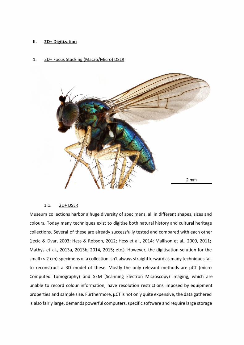
1.1. 2D+ DSLR

Museum collections harbor a huge diversity of specimens, all in different shapes, sizes and

colours. Today many techniques exist to digitise both natural history and cultural heritage

collections. Several of these are already successfully tested and compared with each other

(Jecic & Dvar, 2003; Hess & Robson, 2012; Hess et al., 2014; Mallison et al., 2009, 2011;

Mathys et al., 2013a, 2013b, 2014, 2015; etc.). However, the digitisation solution for the

small (< 2 cm) specimens of a collection isn't always straightforward as many techniques fail

to reconstruct a 3D model of these. Mostly the only relevant methods are µCT (micro

Computed Tomography) and SEM (Scanning Electron Microscopy) imaging, which are

unable to record colour information, have resolution restrictions imposed by equipment

properties and sample size. Furthermore, µCT is not only quite expensive, the data gathered

is also fairly large, demands powerful computers, specific software and require large storage

capacities with specific infrastructure for online sharing. Often the inside of the object isn't

of importance, or even a complete 3D isn't entirely necessary. While SEM imaging is time

consuming as the specimen often needs to be dried and gold covered, which is not possible

for type specimen. The best solution for the digitisation of these small objects might be

taking 2D+ pictures by means of focus stacking. We recently described the level of detail of

our inexpensive focus stacking set-up compared to high end solutions (Brecko et al., 2014),

but in this short paper we will discuss the versatility of this focus stacking set-up and what

we use it for on a daily basis at our institutes in the framework of the DIGIT-03 Belgian

federal collections digitisation program.

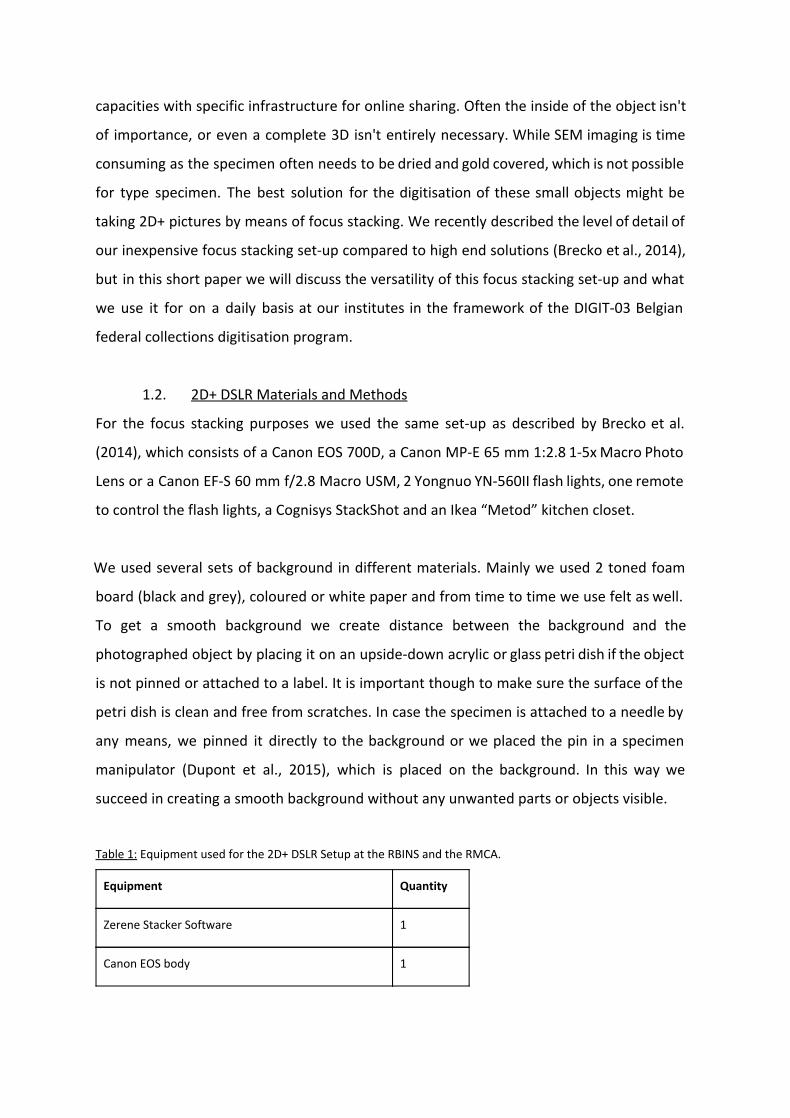
1.2. 2D+ DSLR Materials and Methods

For the focus stacking purposes we used the same set-up as described by Brecko et al.

(2014), which consists of a Canon EOS 700D, a Canon MP-E 65 mm 1:2.8 1-5x Macro Photo

Lens or a Canon EF-S 60 mm f/2.8 Macro USM, 2 Yongnuo YN-560II flash lights, one remote

to control the flash lights, a Cognisys StackShot and an Ikea “Metod” kitchen closet.

We used several sets of background in different materials. Mainly we used 2 toned foam

board (black and grey), coloured or white paper and from time to time we use felt as well.

To get a smooth background we create distance between the background and the

photographed object by placing it on an upside-down acrylic or glass petri dish if the object

is not pinned or attached to a label. It is important though to make sure the surface of the

petri dish is clean and free from scratches. In case the specimen is attached to a needle by

any means, we pinned it directly to the background or we placed the pin in a specimen

manipulator (Dupont et al., 2015), which is placed on the background. In this way we

succeed in creating a smooth background without any unwanted parts or objects visible.

Table 1: Equipment used for the 2D+ DSLR Setup at the RBINS and the RMCA.

Equipment Quantity

Zerene Stacker Software 1

Canon EOS body 1

Canon 65 mm MP-E f/2.8 1-5x Super Macro 1

Canon 60 mm f/2.8 EF Macro 1

Cognisys StackShot 1

Shutter Speed Cable 1

Yongnuo Digital Speedlight YN560-II 2

Remote control for Speedlight 1

Extra Battery 1

Rechargeable batteries AA/AAA 16/8

Ikea closet or similar 1

Figure 1: Focus Stacking setup used at the RBINS and the RMCA. 1A: View of the complete set-up; 1B: Detailed

view of the camera mounted to stackshot and to the closet using a metal corner, to mount the camera vertically.

Software

We use the Canon EOS Utility software to control the camera. Zerene Stacker is used for

stacking the individual pictures into one ‘stacked image’ as described in Brecko et al. 2014.

Once the pictures are processed a scale bar is added, which is calculated according to

following formula:

(A/B)*C

A= Magnification

B= Sensor size (mm)

C= Image width (pixels)

In this way you get the amount of pixels for 1 mm and you can compute any scale bar and

create it by a photo processing software like GIMP. For a magnification of 5x using a Canon

EOS 700D (sensor size 22,3 mm) and an image width of 5184 pixels, 1 mm is represented in

the picture by 1162,3 pixels, allowing a submicron resolution. In case you don’t want to

make every calculation yourself, an excellent spreadsheet is provided by Charles Krebs

(2006).

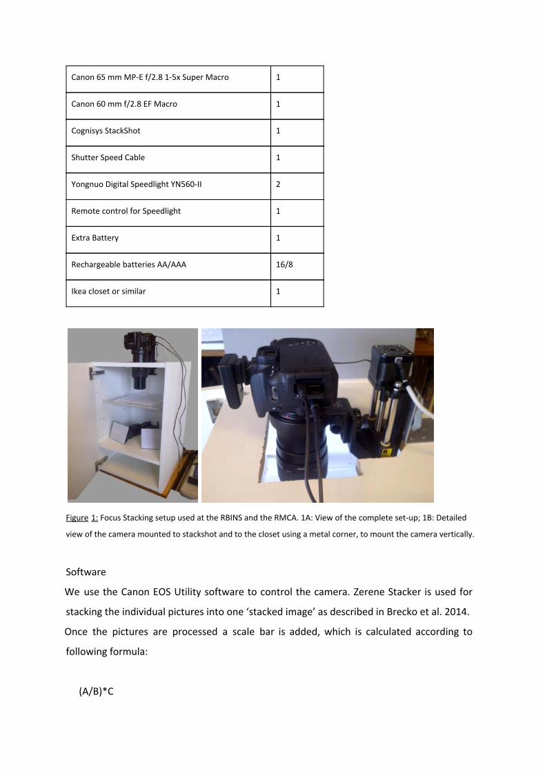
We use the Canon EOS 700D because tests and calculations show that at 50.6 megapixel on

a 36mm sensor (full frame), the amount of µm per pixel is almost equal when using the

same magnification on a 22.3mm sensor (Table 2). The quality of the pictures is nearly the

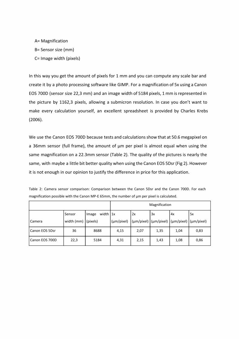
same, with maybe a little bit better quality when using the Canon EOS 5Dsr (Fig 2). However

it is not enough in our opinion to justify the difference in price for this application.

Table 2: Camera sensor comparison: Comparison between the Canon 5Dsr and the Canon 700D. For each

magnification possible with the Canon MP-E 65mm, the number of µm per pixel is calculated.

Magnification

Camera

Sensor

width (mm)

Image width

(pixels)

1x

(µm/pixel)

2x

(µm/pixel)

3x

(µm/pixel)

4x

(µm/pixel)

5x

(µm/pixel)

Canon EOS 5Dsr 36 8688 4,15 2,07 1,35 1,04 0,83

Canon EOS 700D 22,3 5184 4,31 2,15 1,43 1,08 0,86

Figure 2: Visual camera sensor comparison: A Hormius sp. specimen pictured at 4x magnification with a Canon

EOS 5Dsr (left) and a Canon EOS 700D (right).

1.3. 2D+ DSLR Collections

The main goal of using the focus stacking set-up within the DIGIT-03 project is to provide

highly detailed pictures of type specimens which are too small to digitize in 3D without the

use of a µCT scanner.

In essence the specimens together with their challenges can be divided according to their

way of storage: wet or dry. The wet collection mainly houses specimens preserved in

ethanol, while the dry collection are non-attached or attached specimens (pinned, glued, on

a microscope plate).

Aside from the storage medium, within each group various other difficulties might occur

which are related to the specimens appearance: hairy, shiny, translucent, etc.

Specimens, wet (within liquid) or dry, from 2 mm up to 20 cm. All collections are suitable

(Geology, Antropology, Palaeontology, Entomology, Vertebrates, Recent Invertebrates,

Plants, …).

1.4. 2D+ DSLR Test specimens

Dry collection

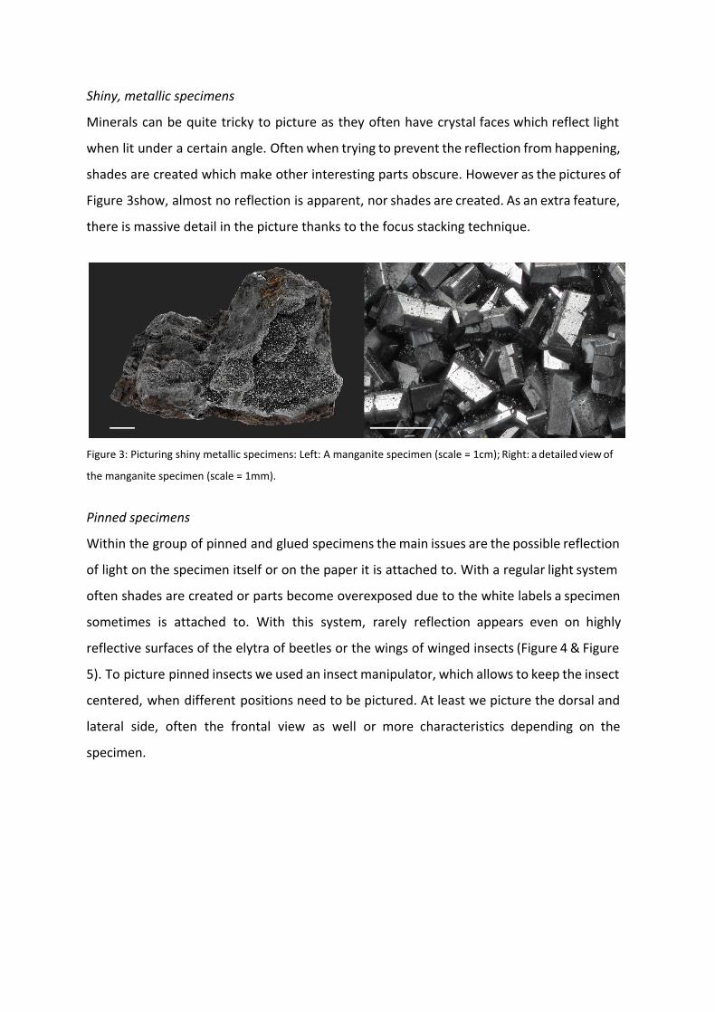
Shiny, metallic specimens

Minerals can be quite tricky to picture as they often have crystal faces which reflect light

when lit under a certain angle. Often when trying to prevent the reflection from happening,

shades are created which make other interesting parts obscure. However as the pictures of

Figure 3show, almost no reflection is apparent, nor shades are created. As an extra feature,

there is massive detail in the picture thanks to the focus stacking technique.

Figure 3: Picturing shiny metallic specimens: Left: A manganite specimen (scale = 1cm); Right: a detailed view of

the manganite specimen (scale = 1mm).

Pinned specimens

Within the group of pinned and glued specimens the main issues are the possible reflection

of light on the specimen itself or on the paper it is attached to. With a regular light system

often shades are created or parts become overexposed due to the white labels a specimen

sometimes is attached to. With this system, rarely reflection appears even on highly

reflective surfaces of the elytra of beetles or the wings of winged insects (Figure 4 & Figure

5). To picture pinned insects we used an insect manipulator, which allows to keep the insect

centered, when different positions need to be pictured. At least we picture the dorsal and

lateral side, often the frontal view as well or more characteristics depending on the

specimen.

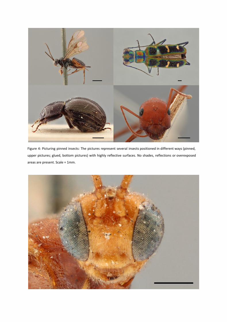
Figure 4: Picturing pinned insects: The pictures represent several insects positioned in different ways (pinned,

upper pictures; glued, bottom pictures) with highly reflective surfaces. No shades, reflections or overexposed

areas are present. Scale = 1mm.

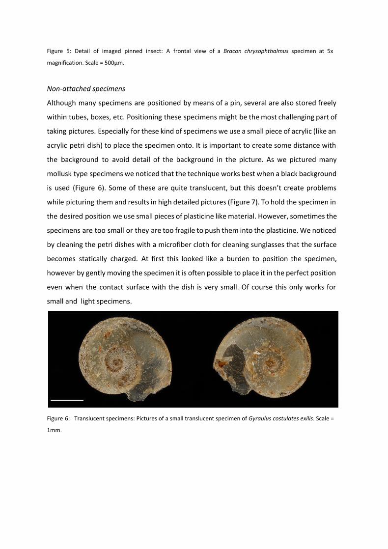
Figure 5: Detail of imaged pinned insect: A frontal view of a Bracon chrysophthalmus specimen at 5x

magnification. Scale = 500µm.

Non-attached specimens

Although many specimens are positioned by means of a pin, several are also stored freely

within tubes, boxes, etc. Positioning these specimens might be the most challenging part of

taking pictures. Especially for these kind of specimens we use a small piece of acrylic (like an

acrylic petri dish) to place the specimen onto. It is important to create some distance with

the background to avoid detail of the background in the picture. As we pictured many

mollusk type specimens we noticed that the technique works best when a black background

is used (Figure 6). Some of these are quite translucent, but this doesn’t create problems

while picturing them and results in high detailed pictures (Figure 7). To hold the specimen in

the desired position we use small pieces of plasticine like material. However, sometimes the

specimens are too small or they are too fragile to push them into the plasticine. We noticed

by cleaning the petri dishes with a microfiber cloth for cleaning sunglasses that the surface

becomes statically charged. At first this looked like a burden to position the specimen,

however by gently moving the specimen it is often possible to place it in the perfect position

even when the contact surface with the dish is very small. Of course this only works for

small and light specimens.

Figure 6: Translucent specimens: Pictures of a small translucent specimen of Gyraulus costulates exilis . Scale =

1mm.

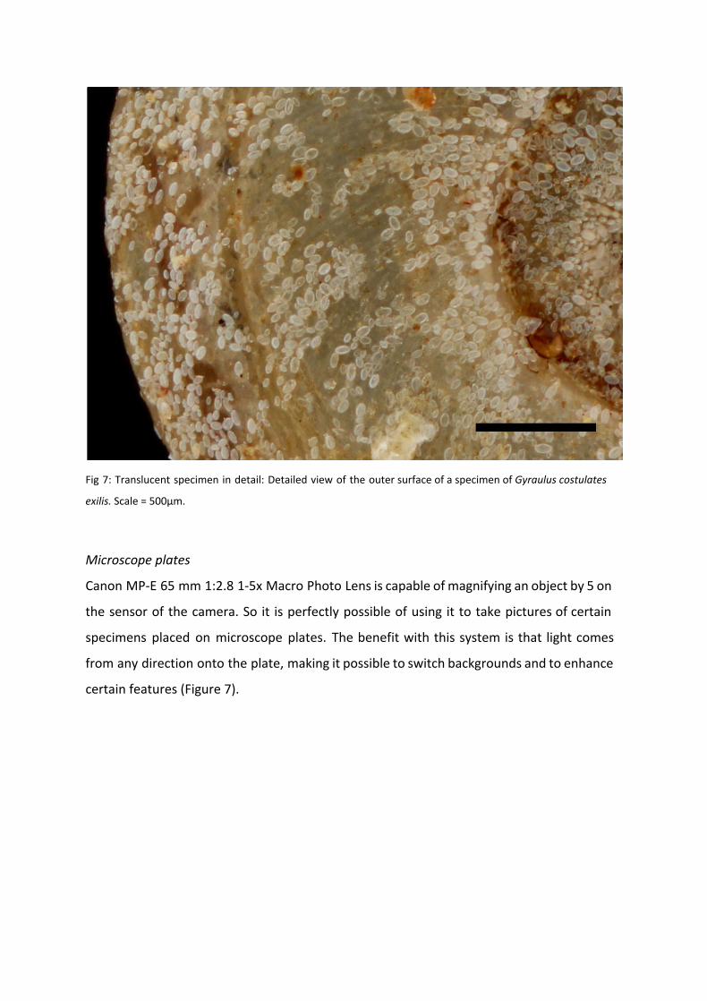
Fig 7: Translucent specimen in detail: Detailed view of the outer surface of a specimen of Gyraulus costulates

exilis. Scale = 500µm.

Microscope plates

Canon MP-E 65 mm 1:2.8 1-5x Macro Photo Lens is capable of magnifying an object by 5 on

the sensor of the camera. So it is perfectly possible of using it to take pictures of certain

specimens placed on microscope plates. The benefit with this system is that light comes

from any direction onto the plate, making it possible to switch backgrounds and to enhance

certain features (Figure 7).

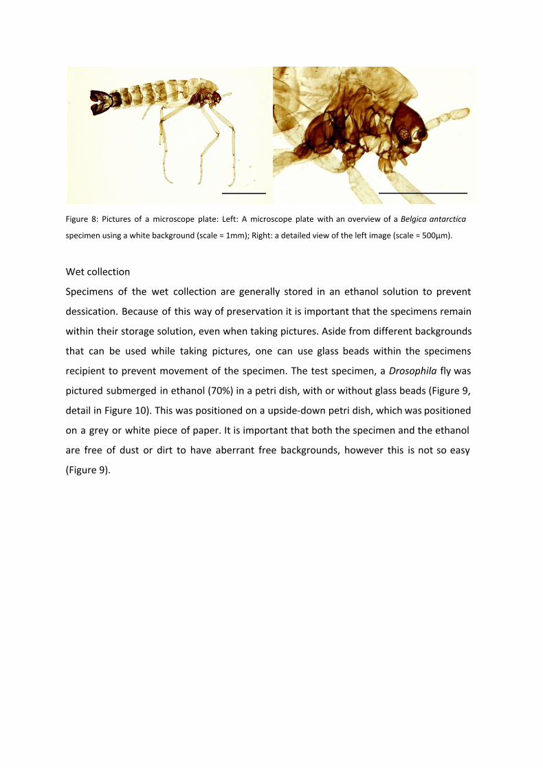
Figure 8: Pictures of a microscope plate: Left: A microscope plate with an overview of a Belgica antarctica

specimen using a white background (scale = 1mm); Right: a detailed view of the left image (scale = 500µm).

Wet collection

Specimens of the wet collection are generally stored in an ethanol solution to prevent

dessication. Because of this way of preservation it is important that the specimens remain

within their storage solution, even when taking pictures. Aside from different backgrounds

that can be used while taking pictures, one can use glass beads within the specimens

recipient to prevent movement of the specimen. The test specimen, a Drosophila fly was

pictured submerged in ethanol (70%) in a petri dish, with or without glass beads (Figure 9,

detail in Figure 10). This was positioned on a upside-down petri dish, which was positioned

on a grey or white piece of paper. It is important that both the specimen and the ethanol

are free of dust or dirt to have aberrant free backgrounds, however this is not so easy

(Figure 9).

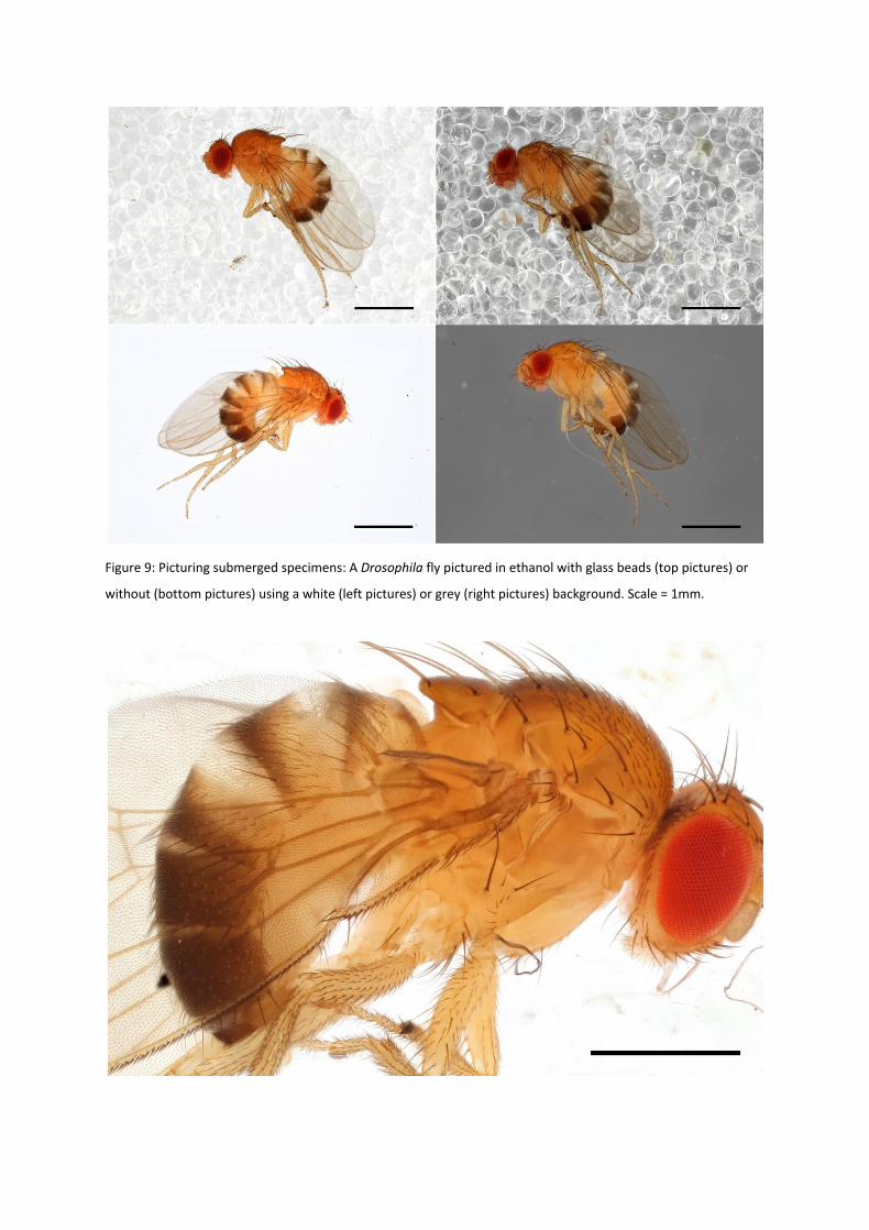
Figure 9: Picturing submerged specimens: A Drosophila fly pictured in ethanol with glass beads (top pictures) or

without (bottom pictures) using a white (left pictures) or grey (right pictures) background. Scale = 1mm.

Figure 10: Detail of a specimen stored in ethanol: A detailed lateral view of a Drosophila sp. Specimen submerged

in a 70% ethanol solution. Scale = 500µm.

Aside from specimens emerged in ethanol or formaldehyde solutions, some specimens are

kept in other media. Glycerin is such a media that is used to store specimens that are

cleared and stained, a technique to make bone and cartilage visible for morphological

studies. These specimens are very fragile after this particular treatment, but it is necessary

to take them out of their container to study them closely, unless good pictures are provided

as show in Figure 11. This was shot in an old acrylic holder so the scratches are visible on the

background of the pictures.

Figure 11: Specimen stored within glycerin: Cleared and Stained specimen of Haplochromis sp. pictured in

glycerin. The right part of the picture is photographed with a magnification of 5x. Scale = 500µm.

The versatility of the white closet with the mounted StackShot and the flash lights

positioned below the specimen to be pictured is huge. Previous research (Brecko et al.,

2014) showed, that this set-up is able to compete with high-end stacking solutions and

delivers better and more detailed pictures at certain magnifications. A lot of the small

specimens inside a museum collection can be pictured with ease, as the light system creates

an evenly lit specimen even within media like ethanol or glycerin. This is very interesting as

specimens stored within fluids are mostly not covered within digitization programs.

There appears to be no issues with imaging translucent, transparent or reflective specimens,

regardless of the size they have. An extra benefit, especially when picturing microscope

plates, is the possibility to change the background to create different contrasts to enhance

details of the specimen.

Besides the use in the framework of the digitization project, DIGIT-03, the set-up is used by

scientists at our institutes to picture newly described species or to take detailed pictures of

certain morphological features when needed for publication. Pictures, in full resolution,

made of type specimens in the framework of DIGIT-03 for Royal Belgian Institute of Natural

Sciences can be studied at the virtual collections web page

(http://virtualcollections.naturalsciences.be/) and the Digit03 webpage of the Royal

Museum for Central Africa (http://digit03.africamuseum.be)

1.5. References

Dupont S, Price B, Blagoderov V (2015) Imp: The customizable LEGO Pinned Insect Manipulator. Zookeys 481:

131-138. doi: 10.3897/zookeys.481.8788

Brecko J, Mathys A, Dekoninck W, Leponce M, VandenSpiegel D, Semal P (2014) Focus stacking: Comparing

commercial top-end set-ups with a semi-automatic low budget approach. A possible solution for mass digitization

of type specimens”. Zookeys 464: 1-23. doi: 10.3897/zookeys.464.8615

Hess M, Robson S (2013) Re-engineering Watt: A case study and best practice recommendations for 3D colour

laser scans and 3D printing in museum artefact documentation. In: Saunders D, Strlic M, Kronen C, Birholzerberg

K, Luxford N (eds.) Lasers in the Conservation of Artworks IX, London, 154-162.

Hess M, Robson S, Hosseininaveh Ahmadabadian A (2014) A contest of sensors in close range 3D imaging:

Performance evaluation with a new metric test object. The International Archives of the Photogrammetry,

Remote Sensing and Spatial Information Sciences 5: 277-284.

Jecic S, Dvar N (2003) The assessment of structures light and laser scanning methods in 3Dshape measurements.

4th International Congress of Croatian Society of Mechanics, 237-244.

Krebs C. “A spreadsheet for scale-bar calculation”, 2006, www.krebsmicro.com/scale_bars.xls

Mallison H, Hohloch A, Pfretzschner H-U (2009) Mechanical digitizing for paleontology – new and improved

techniques. Palaeontologia Electronica. 12(2): 4T.

Mallison H (2011) Digitizing methods for paleontology – applications, benefits and limitations. In: Elewa AMT (Ed)

Computational Paleontology. Springer, Berlin, 7-44.

Mathys A, Brecko J, Semal P (2013) Comparing 3D digitizing technologies: what are the differences? In: Addison

AC, De Luca L, Guidi G, Pescarin S (Ed) Digital Heritage International Congress, vol. 1. Marseille: CNRS, 201-204.

Mathys A, Brecko J, Di Modica K, Abrams G, Bonjean D, Semal P (2013) Low cost 3D imaging: a first look for field

archaeology. Notae Praehistoricae 33: 33-42.

Mathys A, Brecko J, Semal P (2014) Cost evaluation of 3D Digitisation Techniques. In: Ioannides M,

Magnenat-Thalmann N, Fink E, Zarnic R, Yen A, Quak E (Ed) EUROMED 2014 Proceedings, 17-25.

Mathys A, Brecko J, Vandenspiegel D, Semal P (2015) 3D and challenging Materials: Guidelines for different 3D

digitisation methods for museum collections with varying material optical properties. In: Proceedings of the 2nd

International Congress on Digital Heritage.

Slizewski A, Freiss M Semal P (2010) Surface scanning of anthropological specimens: nominal-actual comparison

with low cost laser scanning and high end fringe light projection surface scanning systems. Quartär 57: 179-187.

2. 2D+ Focus Stacking (Macro/Micro) Microscope

Many specimens are small and/or parts of them are mounted on a microscope plate. In case

the mounted part or specimen is larger, it is perfectly possible to picture them using the

focus stacking setup described previously (above). However, in case the specimens are small

or a quick GigaPan image is necessary, than a microscope with mounted digital camera is

how to proceed. Many different brands exist, all with their own software, but usually all of

them work more or less the same.

2.1. Equipment

‘Information in Images’ and Olympus BX51 Bright---field and reflected light Trinocular

Optical Microscope with a motorized stage, motorized focus adapter and a QiCam colour

camera of 1392 x 1040 pixels, 1/2” Sensor with 4.65 x 4.65 micron pixels, 12--Bit colour

output.

The microscope is able to make both focus stacks and Gigapan images, as with a SatScan

system, but with the precision and magnification of a microscope. In this way it is possible to

zoom substantially on a microscopic image.

http://www.informationinimages.com/#!automated-microscopes/crwd

Add pictures of the equipment

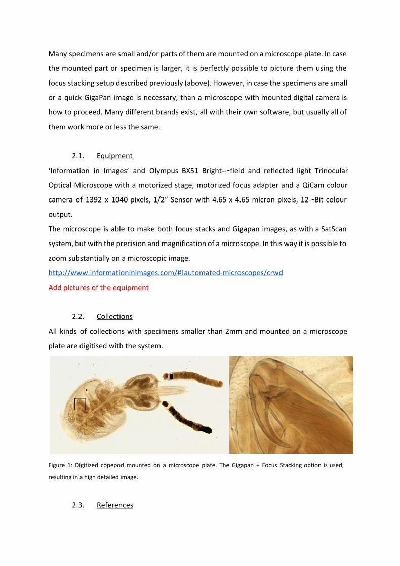
2.2. Collections

All kinds of collections with specimens smaller than 2mm and mounted on a microscope

plate are digitised with the system.

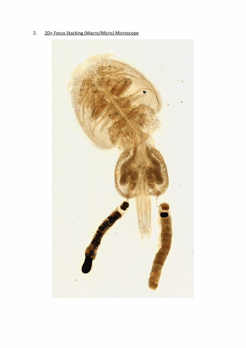
Figure 1: Digitized copepod mounted on a microscope plate. The Gigapan + Focus Stacking option is used,

resulting in a high detailed image.

2.3. References

Anonymous. Microscope Slide Scanner Manual. 2014. Field Museum of Natural history.

3. Zoosphere

From http://Zoosphere.net:

Amongst the major targets of the ZooSphere project are:

● An international repository and web hub for high resolution image sequences of

biological specimen

● Delivering content to various end user devices, such as dekstop computers, mobile

devices and web browsers in general

● Create a tool for scientists, especially taxonomists, to speed up and improve their

research

● Prevent physical object transfer via regular mail

● Reduce travel costs and efforts related to local object inspection

● Digital preservation of biological collection objects, which are subject to natural

decay

● Increasing the visibility and accesibility of biological collection objects

● Making objects available to both: general public and scientists

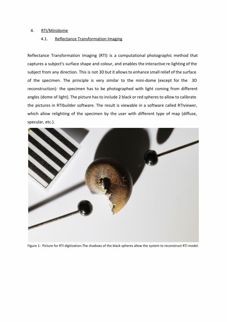
4. RTI/Minidome

4.1. Reflectance Transformation Imaging

Reflectance Transformation Imaging (RTI) is a computational photographic method that

captures a subject's surface shape and colour, and enables the interactive re-lighting of the

subject from any direction. This is not 3D but it allows to enhance small relief of the surface

of the specimen. The principle is very similar to the mini-dome (except for the 3D

reconstruction): the specimen has to be photographed with light coming from different

angles (dome of light). The picture has to include 2 black or red spheres to allow to calibrate

the pictures in RTIbuilder software. The result is viewable in a software called RTIviewer,

which allow relighting of the specimen by the user with different type of map (diffuse,

specular, etc.).

Figure 1: Picture for RTI digitization.The shadows of the black spheres allow the system to reconstruct RTI model.

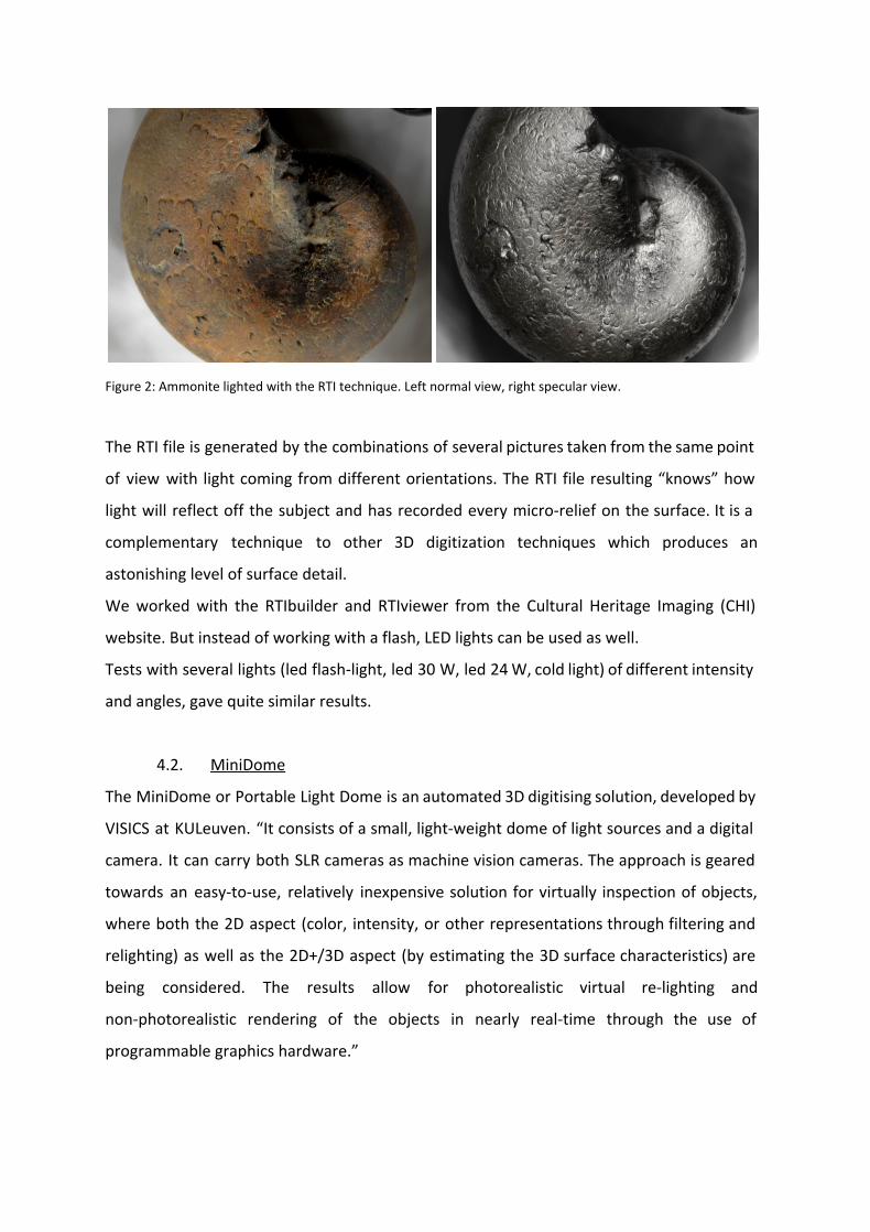
Figure 2: Ammonite lighted with the RTI technique. Left normal view, right specular view.

The RTI file is generated by the combinations of several pictures taken from the same point

of view with light coming from different orientations. The RTI file resulting “knows” how

light will reflect off the subject and has recorded every micro-relief on the surface. It is a

complementary technique to other 3D digitization techniques which produces an

astonishing level of surface detail.

We worked with the RTIbuilder and RTIviewer from the Cultural Heritage Imaging (CHI)

website. But instead of working with a flash, LED lights can be used as well.

Tests with several lights (led flash-light, led 30 W, led 24 W, cold light) of different intensity

and angles, gave quite similar results.

4.2. MiniDome

The MiniDome or Portable Light Dome is an automated 3D digitising solution, developed by

VISICS at KULeuven. “It consists of a small, light-weight dome of light sources and a digital

camera. It can carry both SLR cameras as machine vision cameras. The approach is geared

towards an easy-to-use, relatively inexpensive solution for virtually inspection of objects,

where both the 2D aspect (color, intensity, or other representations through filtering and

relighting) as well as the 2D+/3D aspect (by estimating the 3D surface characteristics) are

being considered. The results allow for photorealistic virtual re-lighting and

non-photorealistic rendering of the objects in nearly real-time through the use of

programmable graphics hardware.”

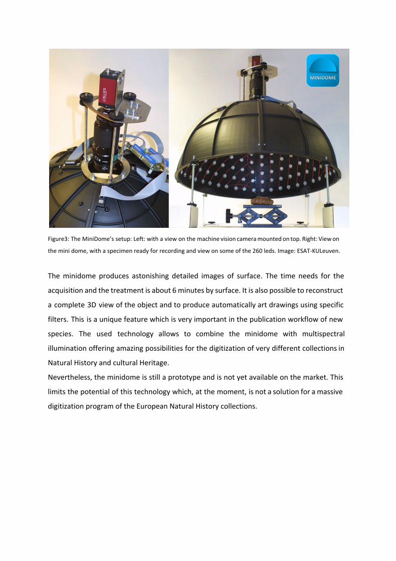
Figure3: The MiniDome’s setup: Left: with a view on the machine vision camera mounted on top. Right: View on

the mini dome, with a specimen ready for recording and view on some of the 260 leds. Image: ESAT-KULeuven.

The minidome produces astonishing detailed images of surface. The time needs for the

acquisition and the treatment is about 6 minutes by surface. It is also possible to reconstruct

a complete 3D view of the object and to produce automatically art drawings using specific

filters. This is a unique feature which is very important in the publication workflow of new

species. The used technology allows to combine the minidome with multispectral

illumination offering amazing possibilities for the digitization of very different collections in

Natural History and cultural Heritage.

Nevertheless, the minidome is still a prototype and is not yet available on the market. This

limits the potential of this technology which, at the moment, is not a solution for a massive

digitization program of the European Natural History collections.

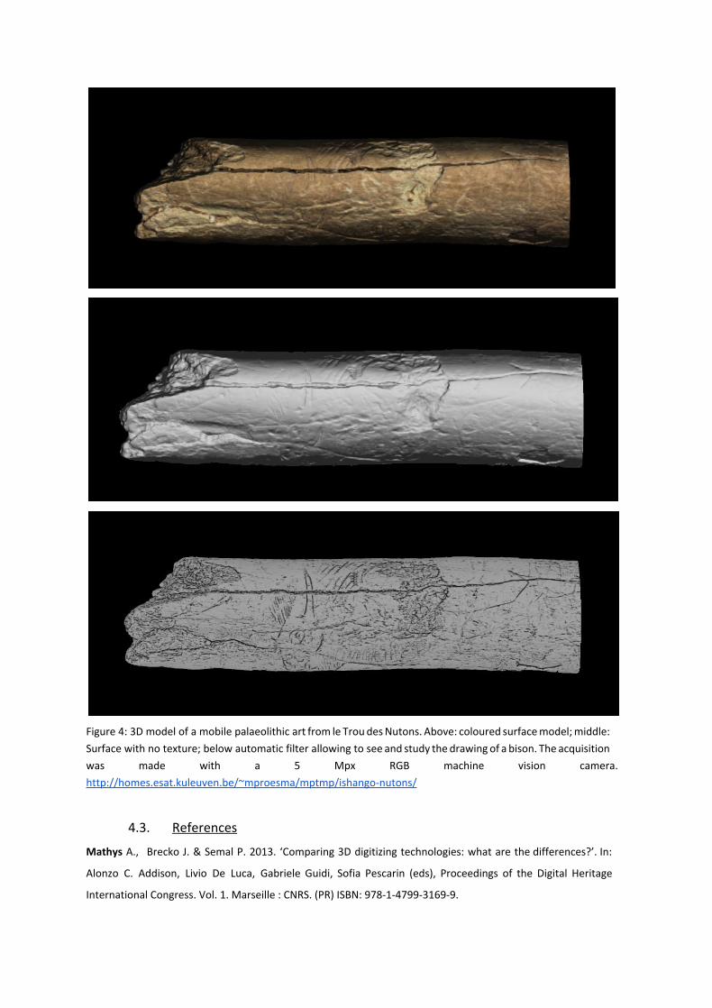
Figure 4: 3D model of a mobile palaeolithic art from le Trou des Nutons. Above: coloured surface model; middle:

Surface with no texture; below automatic filter allowing to see and study the drawing of a bison. The acquisition

was made with a 5 Mpx RGB machine vision camera.

http://homes.esat.kuleuven.be/~mproesma/mptmp/ishango-nutons/

4.3. References

Mathys A., Brecko J. & Semal P. 2013. ‘Comparing 3D digitizing technologies: what are the differences?’. In:

Alonzo C. Addison, Livio De Luca, Gabriele Guidi, Sofia Pescarin (eds), Proceedings of the Digital Heritage

International Congress. Vol. 1. Marseille : CNRS. (PR) ISBN: 978-1-4799-3169-9.

III. 3D Digitization

1. Photogrammetry

Photogrammetry is a technique which enables to compute 3D models of an object based on

pictures taken of it from different angles and positions.

1.1. Photogrammetry of large specimens (> 2cm)

1.1.1. Equipment

Automatic turntable + RBINS Control System

Canon EOS 600D camera (in case of using the automated turntable) or other DSLR

Tripod to mount the camera

Agisoft Photoscan (Professional)

Light setup or Light tent

Different materials as background

Supports or plasticine to hold the specimen in position

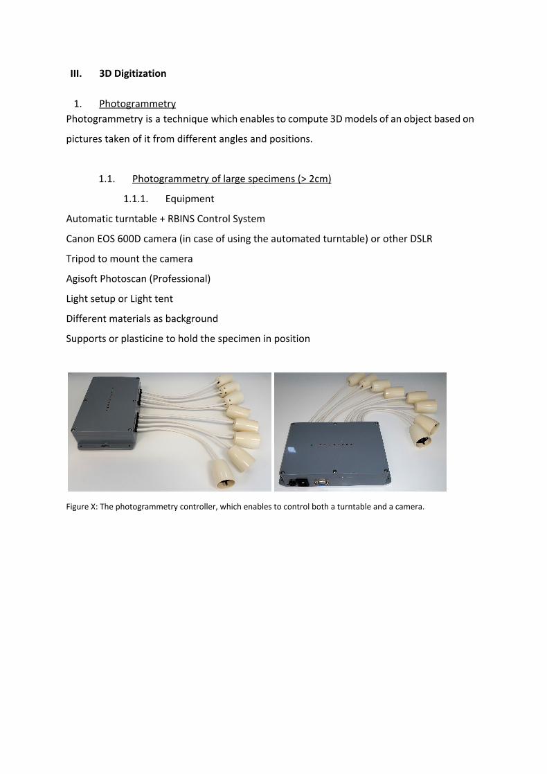
Figure X: The photogrammetry controller, which enables to control both a turntable and a camera.

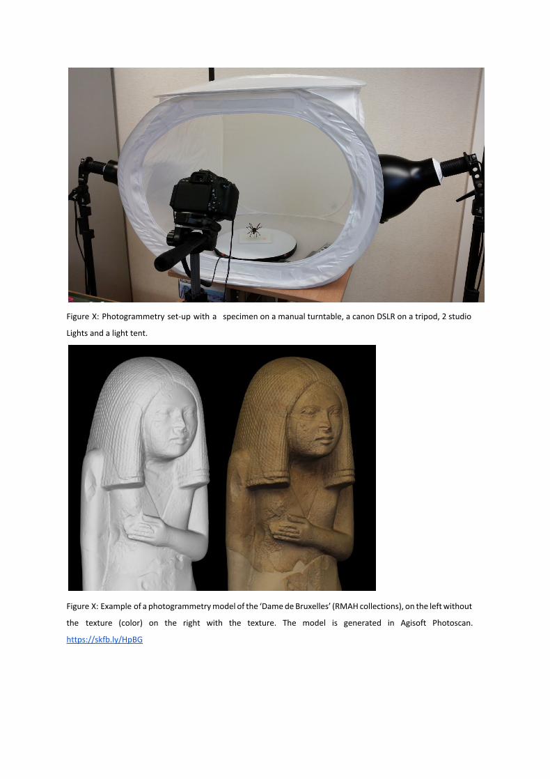
Figure X: Photogrammetry set-up with a specimen on a manual turntable, a canon DSLR on a tripod, 2 studio

Lights and a light tent.

Figure X: Example of a photogrammetry model of the ‘Dame de Bruxelles’ (RMAH collections), on the left without

the texture (color) on the right with the texture. The model is generated in Agisoft Photoscan.

https://skfb.ly/HpBG

Figure X: Photogrammetry model of a Costa Rican Sacrificing warrior (800-1300 AD) in Basalt (RMAH collections).

Thanks to the possibility of viewing the model without the texture, the markings of the belt are better visible.

https://skfb.ly/MXnY

https://sketchfab.com/africamuseum

https://sketchfab.com/naturalsciences

1.2. Photogrammetry of small specimens (<2 cm)

Very small objects too can be digitised in a satisfying way. However when the specimen is <

2 cm, most of the 3D techniques, except for µCT, do not produce detailed or accurate 3D

models. In taxonomic research, when dealing with the morphology of a small specimen,

highly detailed information is necessary. Often for drawings based upon microscopic views,

recordings made with a Scanning Electron Microscope (SEM) or µCT are used

(Vandenspiegel et al ., 2015; Samoh et al. , 2015; Jocqué & Henrard, 2015; etc.). But,

sometimes a 2D+ (focus stacked) picture will do just fine (Brecko et al. , 2014).

Unfortunately, these are still 2D recordings or in case of µCT colourless 3D recordings. For

some research however, colour information is necessary, preferably in 3D. On the other

hand, sometimes the information on the inside of the animal is not of interest, for instance

in case only the outside morphology is studied. Therefore the huge data storage and large

time effort and cost of µCt isn’t justified.

Often budgets or projects are too small to acquire expensive equipment. The logical next

step would be the combination of photogrammetry and focus stacking to tackle the lack of

colour in the 3D model and hopefully provide details visible in the high resolution pictures

for small specimens (<2 cm). Previous research (Nguyen et al. , 2014) proved not to be

detailed enough for taxonomic nor biomechanical research, solely for educational purposes,

but software evolves.

To find out whether it is justified to take a tenfold of pictures when focus stacking every

single camera orientation, we took pictures using a larger F-stop (f/14). This increases the

depth of field, but also augments the loss of sharp detail. Further tests consist of taking

several pictures with different focus distances per single view, imported in Agisoft

Photoscan as stacked images per view and without stacking.

1.2.1. Macro-pictures large f-stop

Five rotations with a total of 76 views were used to generate the 3D model of a Gabbiella

humerosa edwardi specimen using a large f-stop when taking the pictures. After loading the

pictures to Agisoft Photoscan, a masking from background method was used prior to

aligning the pictures. Both the alignment and the dense point cloud were calculated on high

accuracy. The mesh was calculated at high precision, which is the single highest precision

possible. The produced texture was exported and adjusted for brightness and imported

again. Both the mesh and the texture provide low detail (Figure x & x). Even the general

morphology isn’t visible on the 3D mesh (https://skfb.ly/FQKr).

Fig.x: 3D model with texture of a Gabbiella humerosa edwardi mollusk generated in Agisoft Photoscan based on single images (f/14).

Fig.x: 3D model, mesh only, of a Gabbiella humerosa edwardi mollusk generated in Agisoft Photoscan based on single images (f/14).

1.2.2.a Multiple low f-stop pictures, non-stacked

Five rotations with a total of 66 views, accounting for 854 individual pictures, were taken

and inserted into Agisoft Photoscan. Because of the amount of pictures, we used a powerful

desktop computer with 256GB of RAM memory. However, even after dividing the different

rotations into chunks and using a masking from background method to ease the aligning

process, Agisoft Photoscan failed to align the pictures. So no model was produced using this

approach.

1.2.2.b Multiple low f-stop pictures, focus stacked

Five rotations with a total of 66 views, accounting for 854 individual pictures, were used to

generate the 3D model of a Gabbiella humerosa edwardi specimen (https://skfb.ly/FQJZ).

Before the pictures were inserted into Agisoft Photoscan, the pictures of each view were

stacked in Zerene Stacker. We used the PMax option to stack as this produced the best

results for this particular specimen. After loading the pictures to Agisoft Photoscan, a

masking from background method was used prior to aligning the pictures. Both the

alignment and the dense point cloud were calculated on high accuracy. The mesh was

calculated at high precision.The produced texture was exported and adjusted for brightness

and imported again. The texture is accurate in colour and is sharp (Figure 8). The mesh is

very detailed, every morphological part is visible and even fine indentations, spots where

parts of the outer layer of the shell are missing, are visible (Figure 9).

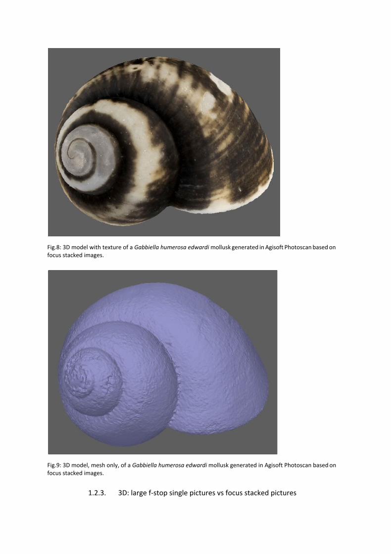
Fig.8: 3D model with texture of a Gabbiella humerosa edwardi mollusk generated in Agisoft Photoscan based on focus stacked images.

Fig.9: 3D model, mesh only, of a Gabbiella humerosa edwardi mollusk generated in Agisoft Photoscan based on focus stacked images.

1.2.3. 3D: large f-stop single pictures vs focus stacked pictures

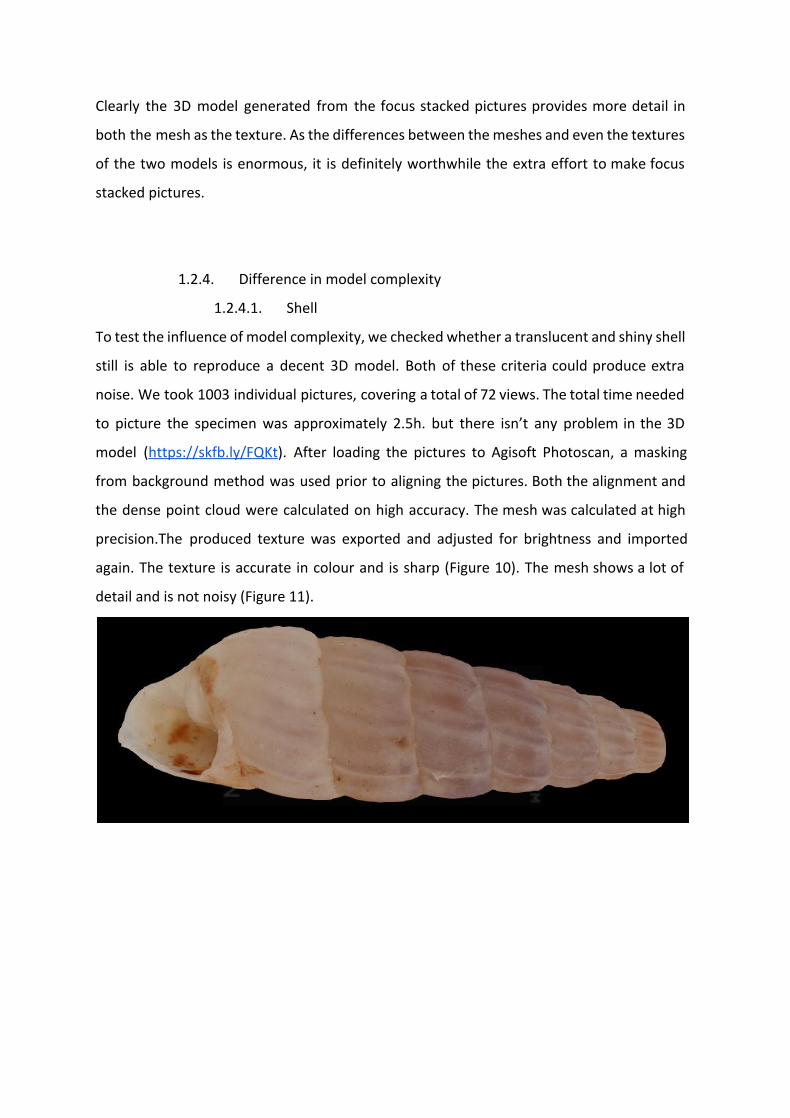
Clearly the 3D model generated from the focus stacked pictures provides more detail in

both the mesh as the texture. As the differences between the meshes and even the textures

of the two models is enormous, it is definitely worthwhile the extra effort to make focus

stacked pictures.

1.2.4. Difference in model complexity

1.2.4.1. Shell

To test the influence of model complexity, we checked whether a translucent and shiny shell

still is able to reproduce a decent 3D model. Both of these criteria could produce extra

noise. We took 1003 individual pictures, covering a total of 72 views. The total time needed

to picture the specimen was approximately 2.5h. but there isn’t any problem in the 3D

model (https://skfb.ly/FQKt). After loading the pictures to Agisoft Photoscan, a masking

from background method was used prior to aligning the pictures. Both the alignment and

the dense point cloud were calculated on high accuracy. The mesh was calculated at high

precision.The produced texture was exported and adjusted for brightness and imported

again. The texture is accurate in colour and is sharp (Figure 10). The mesh shows a lot of

detail and is not noisy (Figure 11).

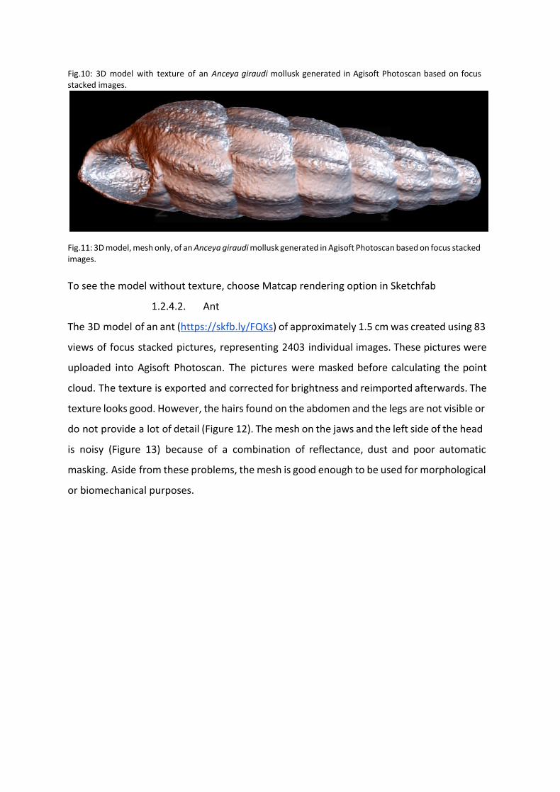
Fig.10: 3D model with texture of an Anceya giraudi mollusk generated in Agisoft Photoscan based on focus stacked images.

Fig.11: 3D model, mesh only, of an Anceya giraudi mollusk generated in Agisoft Photoscan based on focus stacked images.

To see the model without texture, choose Matcap rendering option in Sketchfab

1.2.4.2. Ant

The 3D model of an ant (https://skfb.ly/FQKs) of approximately 1.5 cm was created using 83

views of focus stacked pictures, representing 2403 individual images. These pictures were

uploaded into Agisoft Photoscan. The pictures were masked before calculating the point

cloud. The texture is exported and corrected for brightness and reimported afterwards. The

texture looks good. However, the hairs found on the abdomen and the legs are not visible or

do not provide a lot of detail (Figure 12). The mesh on the jaws and the left side of the head

is noisy (Figure 13) because of a combination of reflectance, dust and poor automatic

masking. Aside from these problems, the mesh is good enough to be used for morphological

or biomechanical purposes.

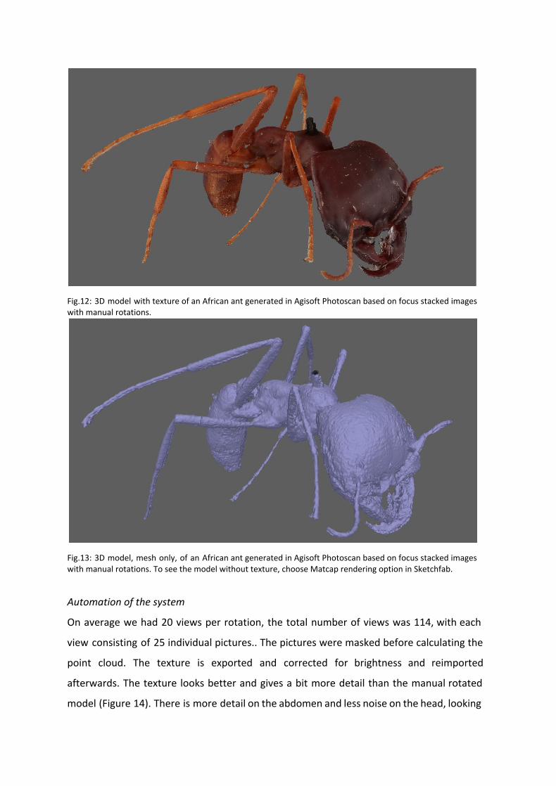
Fig.12: 3D model with texture of an African ant generated in Agisoft Photoscan based on focus stacked images with manual rotations.

Fig.13: 3D model, mesh only, of an African ant generated in Agisoft Photoscan based on focus stacked images with manual rotations. To see the model without texture, choose Matcap rendering option in Sketchfab.

Automation of the system

On average we had 20 views per rotation, the total number of views was 114, with each

view consisting of 25 individual pictures.. The pictures were masked before calculating the

point cloud. The texture is exported and corrected for brightness and reimported

afterwards. The texture looks better and gives a bit more detail than the manual rotated

model (Figure 14). There is more detail on the abdomen and less noise on the head, looking

at the mesh (Figure 15). Although the model is definitely better than the one with manual

rotations. It might perhaps not be sufficient at this time for taxonomic research, but is

perfectly suited for biomechanical research (https://skfb.ly/FQSu). Of course it can also be

used to add annotations regarding anatomy to create virtual educational models. There still

is some noise available on the legs and the head, but this can be resolved by proper masking

and using a different background while taking the pictures. The huge benefit using the

automated method, is the time gain while taking the pictures. Once the specimen is

properly positioned and the parameters are set, it runs on its own. It is important however

to use fully charged batteries for the flashes as they need to flash quite often. A good

investment might be the use of external battery packs (Yongnuo SF-18 battery pack) for the

flashes.

Fig.14: Textured 3D model of an ant generated from focus stacked pictures produced by the Cognisys 3X system.

Fig.15: 3D model (mesh only) of an ant generated from focus stacked pictures produced by the Cognisys 3X system. To see the model without texture, choose Matcap rendering option in Sketchfab.

1.2.5. Equipment

Same equipment used as for focus stacking, added with the following

Cognisys rotary tables (2x)

New Cognisys Controller to control both the stacking rail as the two turntables

Figure X: Part of the Cognisys StackShot 3X Deluxe Kit, reassambled for the photogrammetry purpose. The 2

rotary tables are mounted perpendicular to each other, with rotary table A, moving a steel angle which has rotary

table B fixed at the end.

1.2.6. Price of the System

The complete price for the Stackshot set-up, the Cognisys 3X system, the Agisoft Photoscan

license and a license for Zerene Stacker is approximately 5500 euro. We included the price

of Agisoft Photoscan Professional educational license and for Zerene Stacker the

Professional edition as well. We did not include the price for a computer as this depends a

lot on the configuration you want, but normally for around 1000 euro to 1500 euro you

have a really decent machine to compute 3D models in Agisoft Photoscan. In table 1, we

included as price per week of the staff/operator, the cost to operate the machine. We know

this is different in every country/institution and depends on whether a scientist or

technician operates the set-up. But it gives a good idea as this will be the running cost after

purchasing the equipment. With the set-up it is possible to digitize 10 more or less complex

specimens (like an ant) a week as this requires 5 rotations minimum to cover the entire

specimen. If you would digitize simple forms like a shell 3 rotations might be enough and

you can do 20 specimens a week. Because it takes approximately twenty minutes before a

rotation is finished, it is possible to start a second machine to perform focus stacking of

another specimen. Therefore we included a part in the table that considers the price of two

entire set-ups (software included) and we doubled the amount of specimens that can be

done a week. Furthermore we show the price evolution for each model depending on the

amount models you need to make and also the time it takes to digitize that amount of

models. It is quite clear that if your collection is less than 100 specimens, there is no need to

double the set-ups as this won’t change a lot in price per digitized specimen, only the time

to do it is half of it. A collection of 500 specimens or more is the point where you might

consider adding a second set-up as this doesn’t only divides your time digitizing in 2, the

cost per specimen is also considerably lower.

Table 1: Overview of the digitization costs for one or two running set-ups, with respectively 10 and 20 or 20 and

40 digitized specimens per week given per collection size.

Digitization with one setup

10/week 20 specimens 100 specimens 500 specimens 1K specimens 10K specimens

# weeks 2 10 50 100 1.000

Running cost/week 1000 1000 1000 1000 1000

Price Setup 5500 5500 5500 5500 5500

Total Price 7500 15500 55500 105500 1005500

Price/Specimen 375 155 111 105,5 100,55

20/week 20 specimens 100 specimens 500 specimens 1K specimens 10K specimens

# weeks 1 5 25 50 500

Running cost/week 1000 1000 1000 1000 1000

Price Setup 5500 5500 5500 5500 5500

Total Price 6500 10500 30500 55500 505500

Price/Specimen 325 105 61 55,5 50,55

Digitization with two setups

20/week 20 specimens 100 specimens 500 specimens 1K specimens 10K specimens

# weeks 1 5 25 50 500

Running cost/week 1000 1000 1000 1000 1000

Price Setup 11000 11000 11000 11000 11000

Total Price 12000 16000 36000 61000 511000

Price/Specimen 600 160 72 61 51,1

40/week 20 specimens 100 specimens 500 specimens 1K specimens 10K specimens

# weeks 0,5 2,5 12,5 25 250

Running cost/week 1000 1000 1000 1000 1000

Price Setup 11000 11000 11000 11000 11000

Total Price 11500 13500 23500 36000 261000

Price/Specimen 575 135 47 36 26,1

1.2.7. Discussion

The single picture approach using a high F-Stop did not result in a decent 3D model. We

could expect this to happen, since the effective f-number equals the nominal f-number

multiplied by the magnification plus one. For an f-number of 14 at a magnification of 2x, this

results in an effective f-number of 42, which is well above the optimum of f/16 to f/22.

effective f-number = n*(m+1)

n = nominal f-number

m = magnification

14*3 = 42

The difference with the focus stacked approach was huge as the model of the Gabbiella

humerosa edwardii showed more colour information and a detailed mesh. Even though

using focus stacking as an approach to create the single views is more time consuming it is

worth the effort, considering the end result, especially with the Gastropoda tested. The

model of the ant, shows great detail as well, as all the legs and many small morphologies are

visible. However the real micro details, like hairs on the legs and abdomen, which you do get

in a µCT recording are missing. Therefore it makes this technique for the moment less useful

for taxonomic research of specimens as fine details like hairs are often important in this

context. But for all the other groups with similar detail to the Gastropoda, like minerals,

archaeological remains, fossils, etc it is a great added value to research. The models can be

scaled in Agisoft Photoscan, making online measurements possible.

The only downside, like with µCT scanning, is time. It takes approximately two to three

hours to finish taking pictures of all the different views. When going for the complete low

budget approach and using a manual turntable, a person is occupied the entire day to

produce pictures of 2 to 4 specimens. Fortunately it is possible to let the computer calculate

the focus stacked pictures of a rotation while taking pictures of another one. Of course you

can also calculate models while photographing a specimen, depending on the workstation

you are using. Calculating photogrammetry models can be a quite automated process,

however sometimes a human interaction is necessary in case an alignment, the masking

process or something else doesn’t work out. Therefore it is highly beneficial if the process of

taking pictures (all the individual images of each view of the different rotations) is done

automatically. With the 3X system of Cognisys it is possible to add one or two rotary tables

to the StackShot. If you use only one, you need to place the specimen in another orientation

after each rotation, thus the human interaction and working time is a little bit more than

when using the two rotary table approach. To save precious time it is obviously possible to

let the computer calculate models or stacked pictures during the night in batch.

The technique presented comes at half the cost per specimen as for µCT recordings. of

course if you need the inside information, photogrammetry isn’t going to provide you this.

But if you need 3D models of tiny objects in a digitization program, a research project, for

education or to print (Figure 16) them afterwards, this technique is easy to use and comes

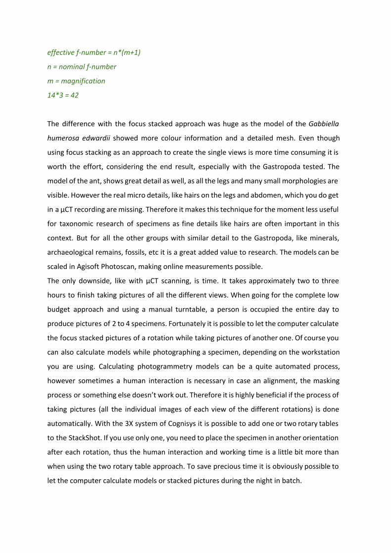
at a small starting cost.

Fig 16: Printed 3D model of a Gabbiella humerosa edwardi shell, magnified up to a size of 10 cm.

The individual pictures that are produced with the set-up could be used in a similar viewer

like the Zoosphere project of the Museum fur Naturkunde in Berlin (www.zoosphere.net) to

get a 3D impression. In the end the models produced by our set-up will be visible at our

virtual collections page (virtualcollections.naturalsciences.be and digit03.africamuseum.be),

with the 3D models hosted through our sketchfab accounts (sketchfab.com/naturalsciences

or sketchfab.com/africamuseum).

1.2.8. References

Mallison, H., Hohloch, A. and H-U Pfretzschner. (2009). Mechanical digitizing for paleontology – new and improved techniques. Palaeontologia Electronica 12.2.4T

Mallison, H. (2011). Digitizing methods for paleontology – applications, benefits and limitations. Pp. 7-44 in Elewa, A.M.T. (ed.): Computational Paleontology. Springer.

Mathys, A., Lemaitre, S., Brecko, J. and P. Semal. 2013a. “Agora 3D: Evaluating 3D Imaging Technology for the

Research, Conservation and Display of Museum Collections.” Antiquity 87 (336).

http://antiquity.ac.uk/projgall/mathys336/.

Mathys, A., J. Brecko, K. Di Modica, G. Abrams, D. Bonjean & P. Semal. 2013b. Agora 3D. Low cost 3D imaging: a

first look for field archaeology. Notae Praehistoricae, 33/2013 : 33-42.

Mathys, A., Brecko, J. & Semal, P. 2014. ‘Cost Evaluation of 3D Digitisation Techniques’. In: Marinos Ioannides,

Nadia Magnenat-Thalmann, Eleanor Fink, Roko Zarnic, Alex-Yianing Yen and Ewald Quak (eds), EUROMED

2014 Proceedings . Essex : MultiScience Ltd, pp. 556. (PR) ISBN: 978 1 907132 47 6.

Mathys, A., Brecko, J., Vandenspiegel, D. & Semal, P. 2015. 3D and challenging Materials: Guidelines for different

3D digitisation methods for museum collections with varying material optical properties. Proceedings of the

2nd International Congress on Digital Heritage 2015.

Nguyen, CV, Lovell DR, Adcock M, and J La Salle. 2014. “Capturing Natural-Colour 3D Models of Insects for Species Discovery and Diagnostics.” PloS One 9 (4): e94346.

2. Infrared Sensors

The infra-red sensor family (Kinect based) was originally a motion sensor device used for the

Microsoft Xbox video games. There are currently several different brands of sensors which

are used for 3D scanning. These sensors are very fast (several millions of points per second)

and transfer data by means of a USB 2.0 connection to a laptop. The need for a power

supply on the site depends on the battery lifetime of the computer. The accuracy is

approximately one millimetre and is adapted to record large structures.

2.1. Equipment

“Infra Red sensors technology” or “Kinect technology” is the expression we choose to

designate motion-sensing captors like Kinect, Xtion and Carmine. Originally used for game

on Xbox 360 console, the device was hacked allowing it to be used as a 3D scanner. The

technology is quite recent and promising for large objects or for field recording.

The device features an RGB camera and an infrared laser projector for depth sensing.

Several software exist for motion sensing, among them: Scenect, Skanect, ReconstructMe,

Kscan3d, and Gotcha.

● Kscan3D v1.0.4.51 is the software developed by 3d3 solutions. Texture capture and

static acquisition that have to be manually realigned. The mesh resulting from the

capture is correct for that kind of sensor, but it has a very low resolution texture and

is time consuming. The ratio between time and quality was poor.

● ReconstructMe 1.2 was an Open Source software. It captures point cloud but doesn't

capture texture.

● Scenect 5.1 is an Open Source software developed by FARO. This system is still very

basic and under development.

● Skanect from Mantcl capture colour and quite accurate point cloud but we had to

process the data out of Skanect since in version 1.2 it was very time consuming. In

the 1.3 version the meshing is quite faster but the scan is less accurate, the software

records less points. The texture is meeting our requirements better.

● Gotcha is a sensor sold by Mephisto (4dd). It uses a Carmine 1.09 and has his own

software. This software allow continuous acquisition similar to as Skanect, but allow

as well to realign single records. It also capture texture. The Carmine allows a more

precise acquisition than the Asus Xtion Live Pro and the software of the Gotcha is the

more complete. Among the downside, the black background of the software

interface is might pose problems when recording and re-aligning scans of dark

objects.

● Artec Studio is one of the most evolved software used with kinect type sensor as it is

the same software used by the Artec spider and Artec Eva scanners. The software

can realign based on shape and on texture.

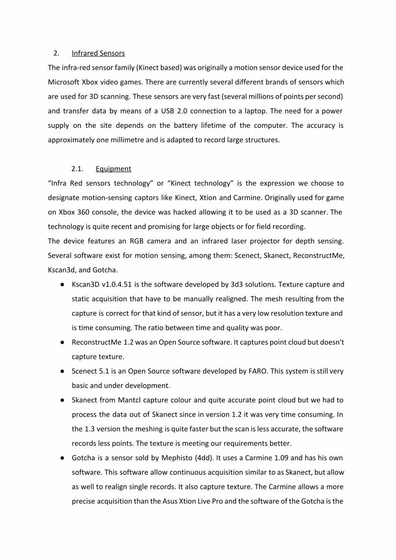
In the RBINS and RMCA we used the Gotcha 3D Scanner, wich is a Carmine 1.09 Infrared

sensor and with it comes the Mephisto 3D scanning software.

Figure X: Kinect based infrared scanner.

The problem is still the accuracy of those devices, since the sensor is not calibrated, only

one out of ten could be precise, the sensor can move inside size causing differences and this

added up to change of temperature or light make it really difficult to realign a great number

of scan for large object like needed with the Gotcha.

Regarding the Gotcha software, after numerous test and numerous contact with the

Mephisto firm, we realised that although it seems to work nicely to begin with, the software

was actually quite limited and bugged. We have faced repeated crashes. The firm couldn't

explain us the different setting of processing.

2.2. Collections

This technology can be used to scan large specimens like a mammoth (RBINS 1 week), a

Moai (RMAH, 1 hour), an elephant (RMCA, 2h30) or an excavation site. The moai was

scanned with both the gotcha and the xtion-skanect package. The moai being massive it

works really well, while with the mammoth skeleton it is a bit more challenging for the thin

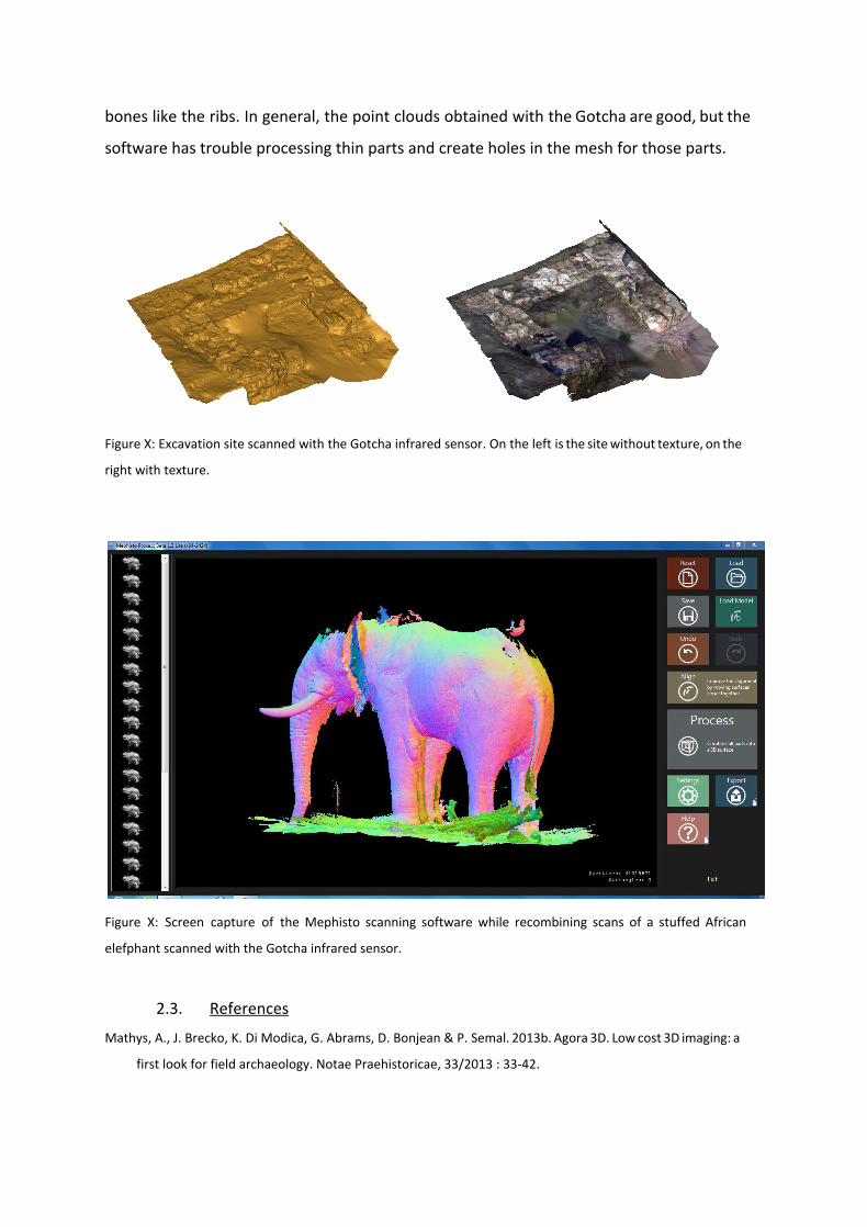
bones like the ribs. In general, the point clouds obtained with the Gotcha are good, but the

software has trouble processing thin parts and create holes in the mesh for those parts.

Figure X: Excavation site scanned with the Gotcha infrared sensor. On the left is the site without texture, on the

right with texture.

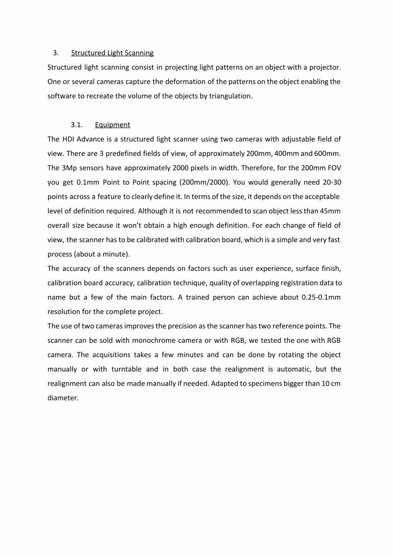
Figure X: Screen capture of the Mephisto scanning software while recombining scans of a stuffed African

elefphant scanned with the Gotcha infrared sensor.

2.3. References

Mathys, A., J. Brecko, K. Di Modica, G. Abrams, D. Bonjean & P. Semal. 2013b. Agora 3D. Low cost 3D imaging: a

first look for field archaeology. Notae Praehistoricae, 33/2013 : 33-42.

3. Structured Light Scanning

Structured light scanning consist in projecting light patterns on an object with a projector.

One or several cameras capture the deformation of the patterns on the object enabling the

software to recreate the volume of the objects by triangulation.

3.1. Equipment

The HDI Advance is a structured light scanner using two cameras with adjustable field of

view. There are 3 predefined fields of view, of approximately 200mm, 400mm and 600mm.

The 3Mp sensors have approximately 2000 pixels in width. Therefore, for the 200mm FOV

you get 0.1mm Point to Point spacing (200mm/2000). You would generally need 20-30

points across a feature to clearly define it. In terms of the size, it depends on the acceptable

level of definition required. Although it is not recommended to scan object less than 45mm

overall size because it won’t obtain a high enough definition. For each change of field of

view, the scanner has to be calibrated with calibration board, which is a simple and very fast

process (about a minute).

The accuracy of the scanners depends on factors such as user experience, surface finish,

calibration board accuracy, calibration technique, quality of overlapping registration data to

name but a few of the main factors. A trained person can achieve about 0.25-0.1mm

resolution for the complete project.

The use of two cameras improves the precision as the scanner has two reference points. The

scanner can be sold with monochrome camera or with RGB, we tested the one with RGB

camera. The acquisitions takes a few minutes and can be done by rotating the object

manually or with turntable and in both case the realignment is automatic, but the

realignment can also be made manually if needed. Adapted to specimens bigger than 10 cm

diameter.

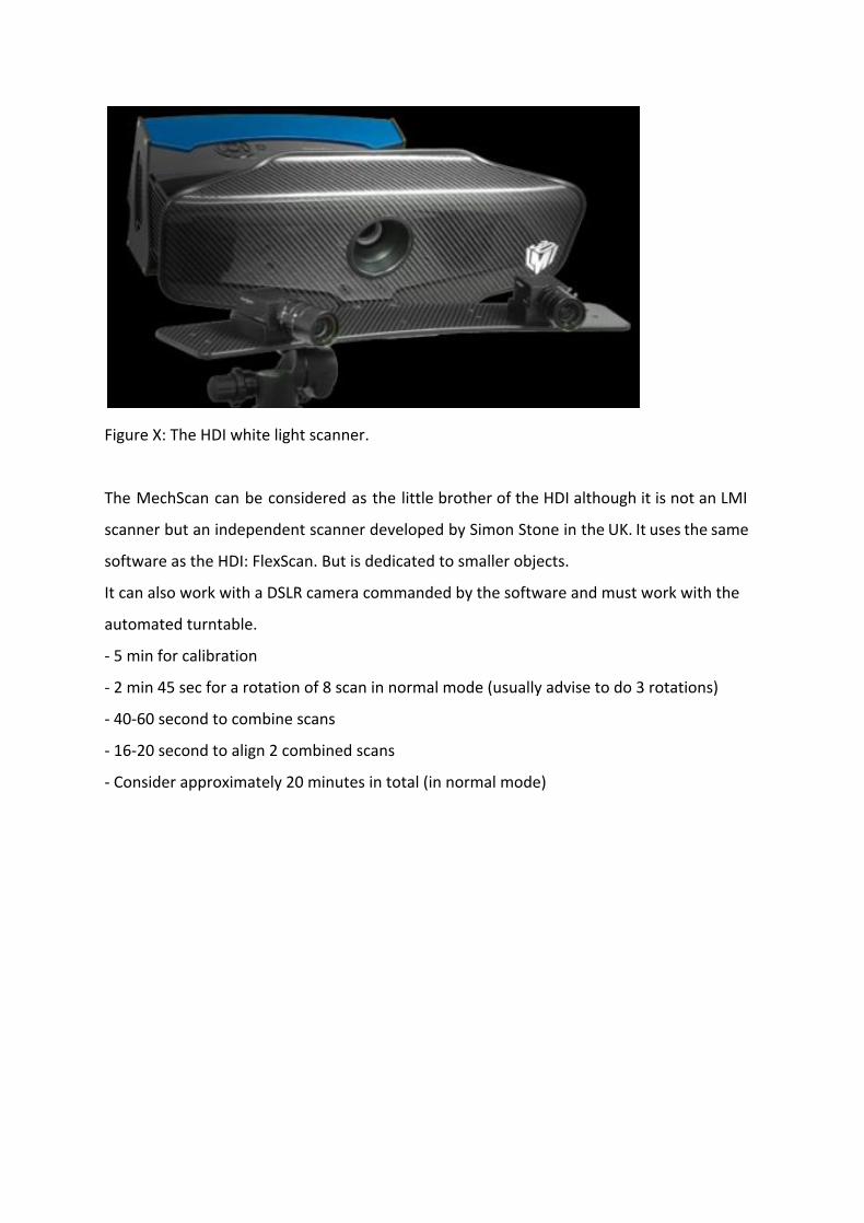
Figure X: The HDI white light scanner.

The MechScan can be considered as the little brother of the HDI although it is not an LMI

scanner but an independent scanner developed by Simon Stone in the UK. It uses the same

software as the HDI: FlexScan. But is dedicated to smaller objects.

It can also work with a DSLR camera commanded by the software and must work with the

automated turntable.

- 5 min for calibration

- 2 min 45 sec for a rotation of 8 scan in normal mode (usually advise to do 3 rotations)

- 40-60 second to combine scans

- 16-20 second to align 2 combined scans

- Consider approximately 20 minutes in total (in normal mode)

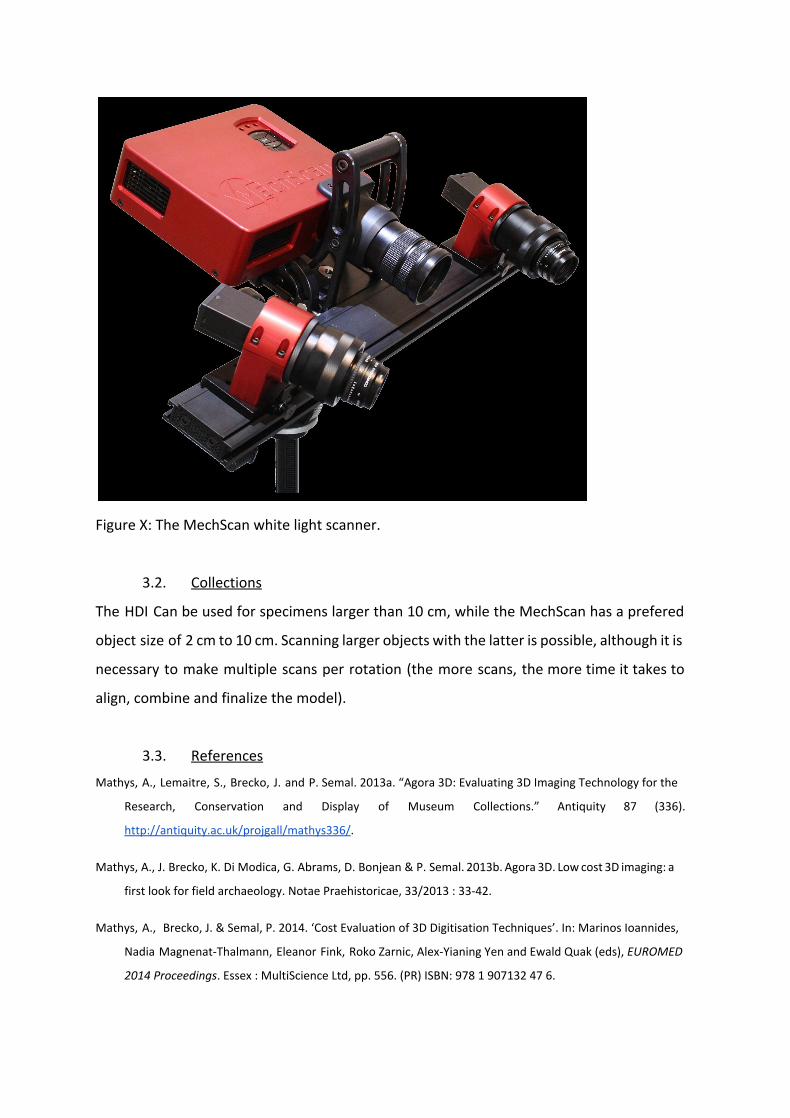
Figure X: The MechScan white light scanner.

3.2. Collections

The HDI Can be used for specimens larger than 10 cm, while the MechScan has a prefered

object size of 2 cm to 10 cm. Scanning larger objects with the latter is possible, although it is

necessary to make multiple scans per rotation (the more scans, the more time it takes to

align, combine and finalize the model).

3.3. References

Mathys, A., Lemaitre, S., Brecko, J. and P. Semal. 2013a. “Agora 3D: Evaluating 3D Imaging Technology for the

Research, Conservation and Display of Museum Collections.” Antiquity 87 (336).

http://antiquity.ac.uk/projgall/mathys336/.

Mathys, A., J. Brecko, K. Di Modica, G. Abrams, D. Bonjean & P. Semal. 2013b. Agora 3D. Low cost 3D imaging: a

first look for field archaeology. Notae Praehistoricae, 33/2013 : 33-42.

Mathys, A., Brecko, J. & Semal, P. 2014. ‘Cost Evaluation of 3D Digitisation Techniques’. In: Marinos Ioannides,

Nadia Magnenat-Thalmann, Eleanor Fink, Roko Zarnic, Alex-Yianing Yen and Ewald Quak (eds), EUROMED

2014 Proceedings . Essex : MultiScience Ltd, pp. 556. (PR) ISBN: 978 1 907132 47 6.

Mathys, A., Brecko, J., Vandenspiegel, D. & Semal, P. 2015. 3D and challenging Materials: Guidelines for different

3D digitisation methods for museum collections with varying material optical properties. Proceedings of the

2nd International Congress on Digital Heritage 2015.

Mathys, A., Brecko, J. & Semal, P. 2013. ‘Comparing 3D digitizing technologies: what are the differences?’. In:

Alonzo C. Addison, Livio De Luca, Gabriele Guidi, Sofia Pescarin (eds), Proceedings of the Digital Heritage

International Congress. Vol. 1. Marseille : CNRS. (PR) ISBN: 978-1-4799-3169-9

4. Laser Scanning

4.1. General Information

4.2. Equipment

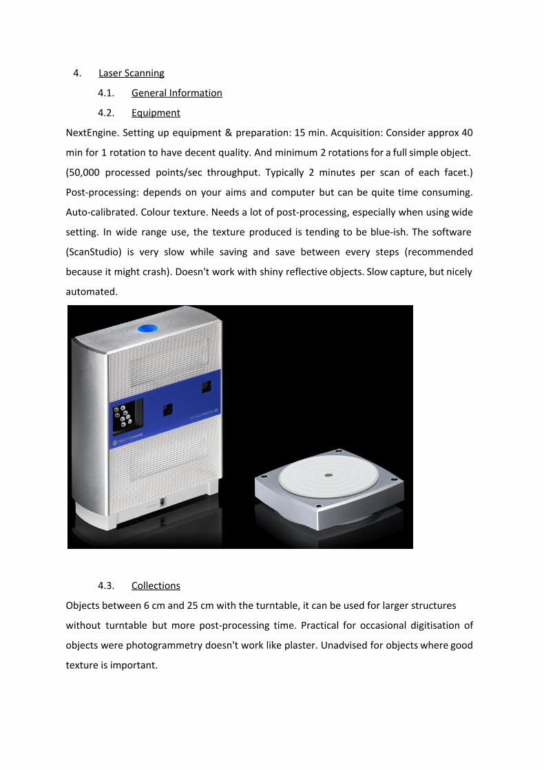
NextEngine. Setting up equipment & preparation: 15 min. Acquisition: Consider approx 40

min for 1 rotation to have decent quality. And minimum 2 rotations for a full simple object.

(50,000 processed points/sec throughput. Typically 2 minutes per scan of each facet.)

Post-processing: depends on your aims and computer but can be quite time consuming.

Auto-calibrated. Colour texture. Needs a lot of post-processing, especially when using wide

setting. In wide range use, the texture produced is tending to be blue-ish. The software

(ScanStudio) is very slow while saving and save between every steps (recommended

because it might crash). Doesn't work with shiny reflective objects. Slow capture, but nicely

automated.

4.3. Collections

Objects between 6 cm and 25 cm with the turntable, it can be used for larger structures

without turntable but more post-processing time. Practical for occasional digitisation of

objects were photogrammetry doesn't work like plaster. Unadvised for objects where good

texture is important.

4.4. References

Mathys, A., Brecko, J. & Semal, P. 2014. ‘Cost Evaluation of 3D Digitisation Techniques’. In: Marinos Ioannides,

Nadia Magnenat-Thalmann, Eleanor Fink, Roko Zarnic, Alex-Yianing Yen and Ewald Quak (eds), EUROMED

2014 Proceedings . Essex : MultiScience Ltd, pp. 556. (PR) ISBN: 978 1 907132 47 6.

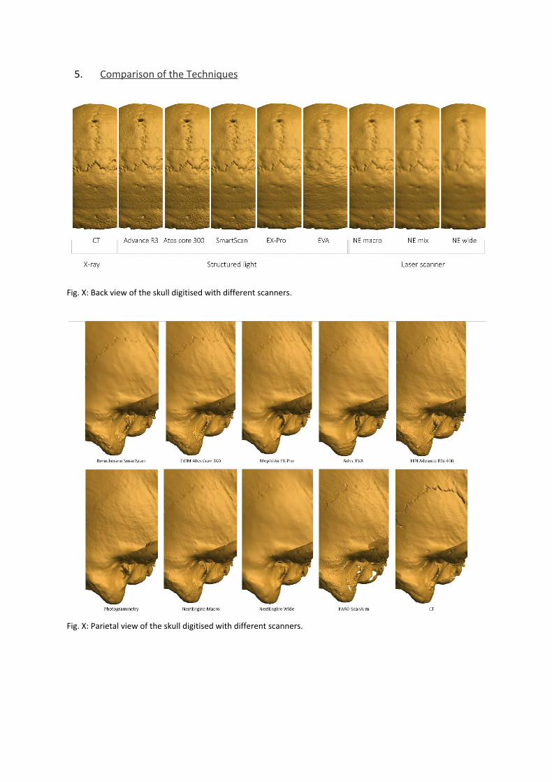
5. Comparison of the Techniques

Fig. X: Back view of the skull digitised with different scanners.

Fig. X: Parietal view of the skull digitised with different scanners.

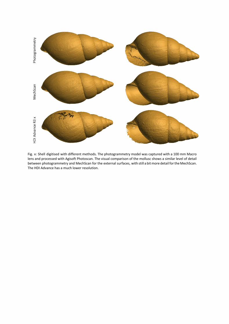
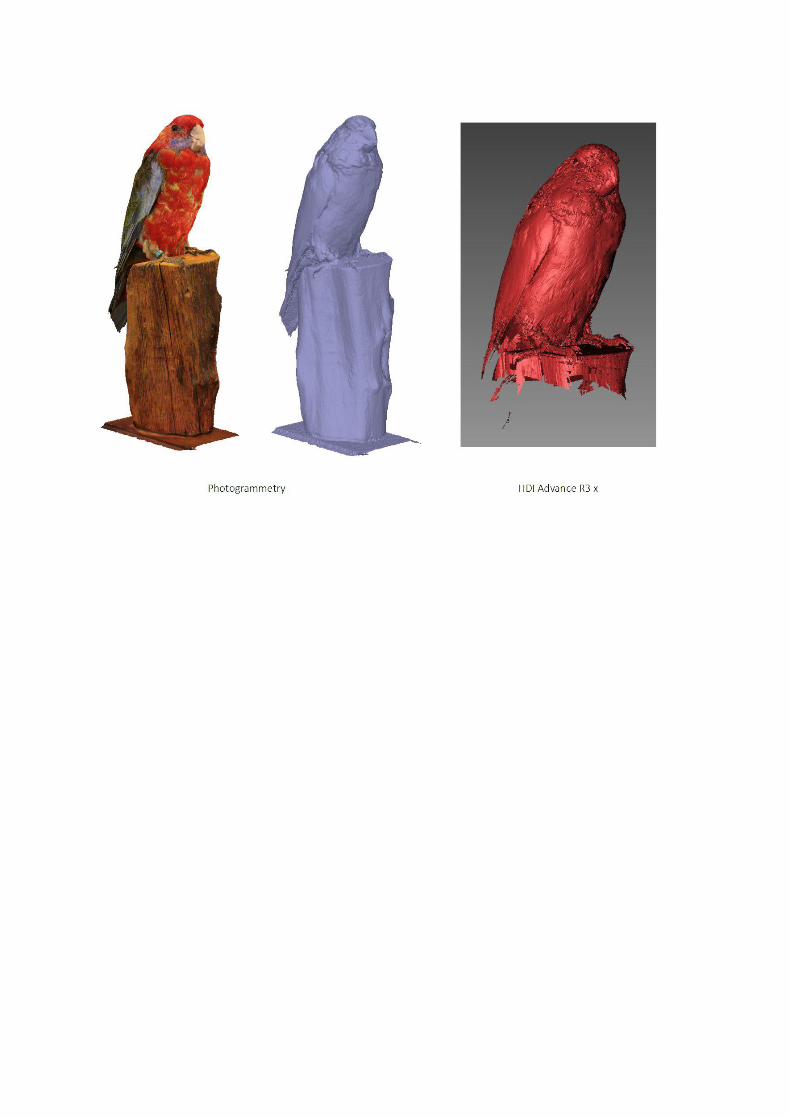
Fig. x: Shell digitised with different methods. The photogrammetry model was captured with a 100 mm Macro lens and processed with Agisoft Photoscan. The visual comparison of the mollusc shows a similar level of detail between photogrammetry and MechScan for the external surfaces, with still a bit more detail for the MechScan. The HDI Advance has a much lower resolution.

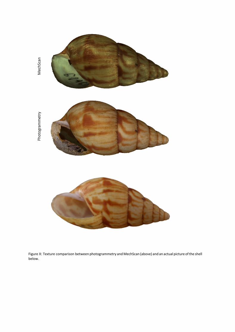
Figure X: Texture comparison between photogrammetry and MechScan (above) and an actual picture of the shell below.

IV. Challenging Materials As mentioned above, museum’s collections can be very different in size and material and

there is no unique digitisation technique which is applicable to an entire collection [5], [6],

and furthermore each technique has both advantages and drawbacks. We tested a large

range of different materials with different optical properties, both from natural history and

cultural heritage collections (stones, metals, feathers, beetles, fabric, etc.) with different 3D

digitisation techniques in order to evaluate what techniques correspond best to which

materials and how best to treat the surface of certain objects. Different materials do not

react in the same way to different technologies. Anti-reflection coating can be sprayed onto

objects to make them easier to scan but this is often not possible with museum objects.

The examples illustrated in this paper only represent a small sample of the analyzed

materials.

TABLE I. Tested sensors

Technology Sensors/software tested

CT/µCT Siemens VolumeZoom Sensation 64

SkyScan (Bruker)

ASTRX (MNHN, Paris)

Structured light Breuckmann SmartScan

GOM Atos Core

HDI Advance R3x

MechScan

Mephisto EX-Pro & Mephisto EOSScan

Artec Spider & Artec EVA

Laser scanner NextEngine

Faro ScanArm

Motion sensor Primesense Carmine 1.02 + Gotcha/skanect

Xtion Live Pro + skanect

Photogrammetry/SfM Agisoft Photoscan

The diverse shapes of the objects allowed us to exclude shape related issues.

We choose to organize different materials in categories based on their optical properties as

material properties differ depending on how the object is treated and can be matt, glossy,

or translucent to several degrees.

Objects found in museum collections are often composed of a variety of materials or

composed of materials with different properties.

We defined the following categories based on major optical properties which can be found

on the same material (fig. 1):

A. Opaque to transparent was classified with the following categories:

1. Opaque: visible light does not penetrate the surface of the material

2. semi-translucent: light penetrates the surface but you cannot distinguish

anything through the material

3. translucent: light penetrates and you can distinguish some features through

the material

4. transparent/highly translucent: light penetrates and you can see a lot of

features through the material

Additional parameters are were also considered:

B. Tones: light versus dark

C. Colour: visible spectrum

D. Homogeneity: homogeneous surface to contrasted surface with detail(s)

E. Light reflection:

1. Matt: does not reflect light

2. Slightly glossy: reflects light moderately

3. Glossy: reflects light. Diffuse reflection (on rough surfaces)

4. Highly glossy: reflects a lot of light, specular reflection (mirror type, on

smooth surfaces)

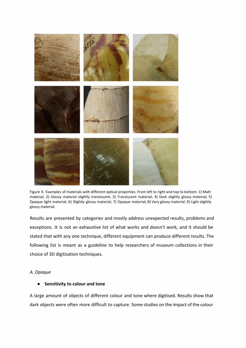
Figure X. Examples of materials with different optical properties. From left to right and top to bottom: 1) Matt material; 2) Glossy material slightly translucent; 3) Translucent material; 4) Dark slightly glossy material; 5) Opaque light material; 6) Slightly glossy material; 7) Opaque material; 8) Very glossy material; 9) Light slightly glossy material.

Results are presented by categories and mostly address unexpected results, problems and

exceptions. It is not an exhaustive list of what works and doesn't work, and it should be

stated that with any one technique, different equipment can produce different results. The

following list is meant as a guideline to help researchers of museum collections in their

choice of 3D digitisation techniques.

A. Opaque

● Sensitivity to colour and tone A large amount of objects of different colour and tone where digitised. Results show that

dark objects were often more difficult to capture. Some studies on the impact of the colour

of the object have already been made for laser scanners. The results demonstrated that

colour has an influence with black and green giving the poorest results [7]. Indeed, for black

surfaces only a small amount of laser light is reflected by the object [8] making it difficult to

capture dark objects.

Structured light is also influenced by colour: depending on the colour of the light projected

by the projector of the scanner, the system is able to capture better some colours than

others [9].

We focused on a white light structured light scanner because these are usually able to

capture texture. White light structured light scanners can work with dark objects but

parameters have to be adjusted depending on the tone of the object and it is sensitive to

large differences of colour within an object as this would require different times of

exposure/intensity of the light projected. Very dark objects can also be responsible for

noise1 on the model [10]. If the object is under or overexposed it won’t be possible to

generate a mesh.

Some scanners have HDR capture mode enabling different exposures for one view to

overcome large tonal differences. Another issue is that many museum objects are marked

with black Indian ink. Black Indian ink is dark but also glossy and both laser scanners and

structured light scanners have difficulty capturing it.

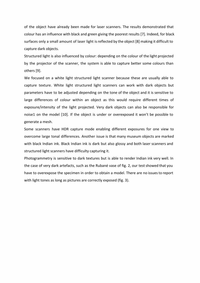
Photogrammetry is sensitive to dark textures but is able to render Indian ink very well. In

the case of very dark artefacts, such as the Rubané vase of fig. 2, our test showed that you

have to overexpose the specimen in order to obtain a model. There are no issues to report

with light tones as long as pictures are correctly exposed (fig. 3).

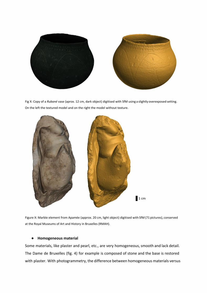
Fig X: Copy of a Rubané vase (aprox. 12 cm, dark object) digitised with SfM using a slightly overexposed setting.

On the left the textured model and on the right the model without texture.

Figure X: Marble element from Apamée (approx. 20 cm, light object) digitised with SfM (71 pictures), conserved

at the Royal Museums of Art and History in Bruxelles (RMAH).

● Homogeneous material

Some materials, like plaster and pearl, etc., are very homogeneous, smooth and lack detail.

The Dame de Bruxelles (fig. 4) for example is composed of stone and the base is restored

with plaster. With photogrammetry, the difference between homogeneous materials versus

detailed material is considerable. The parts in stone are rendered very detailed, while the

plaster parts have a very small amount of points. When computed, this might be displayed

as noise on the final model.

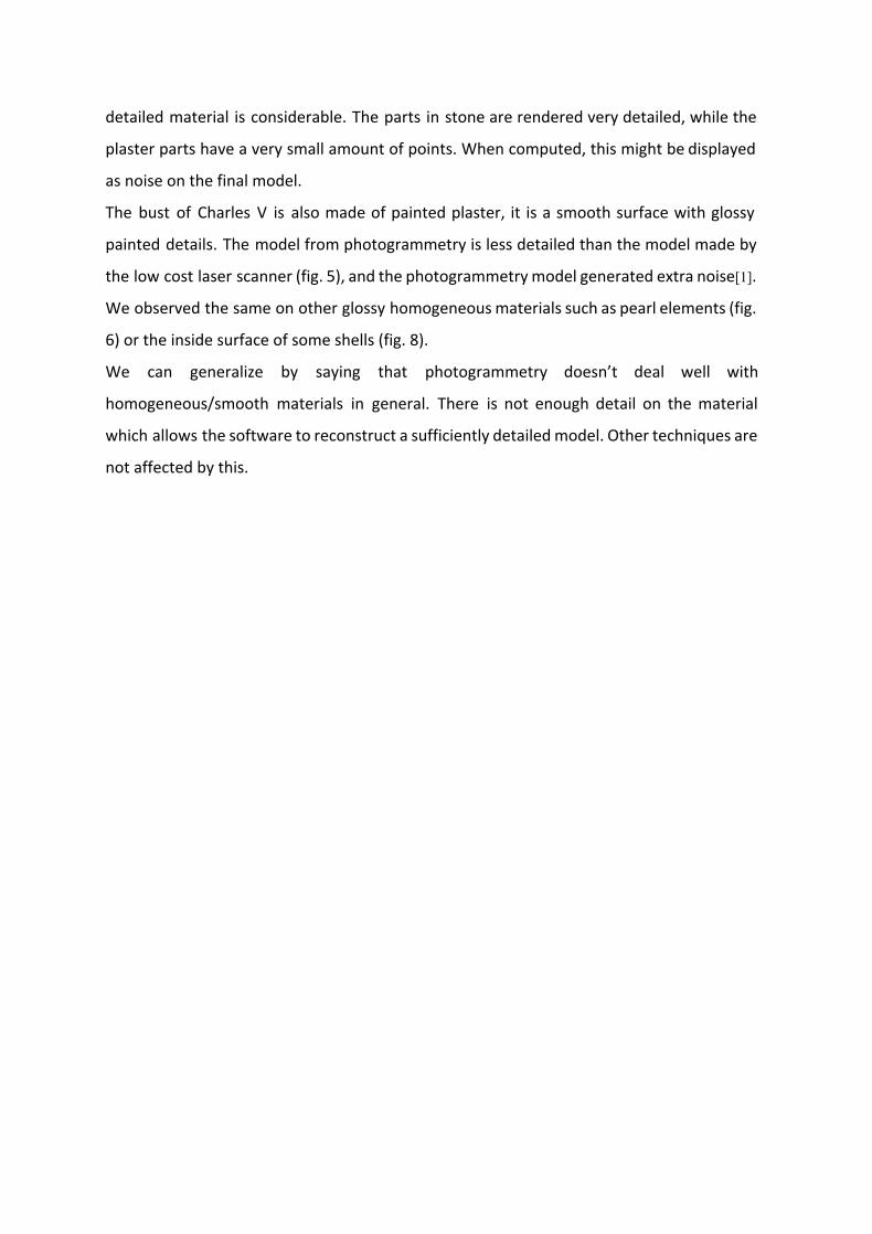
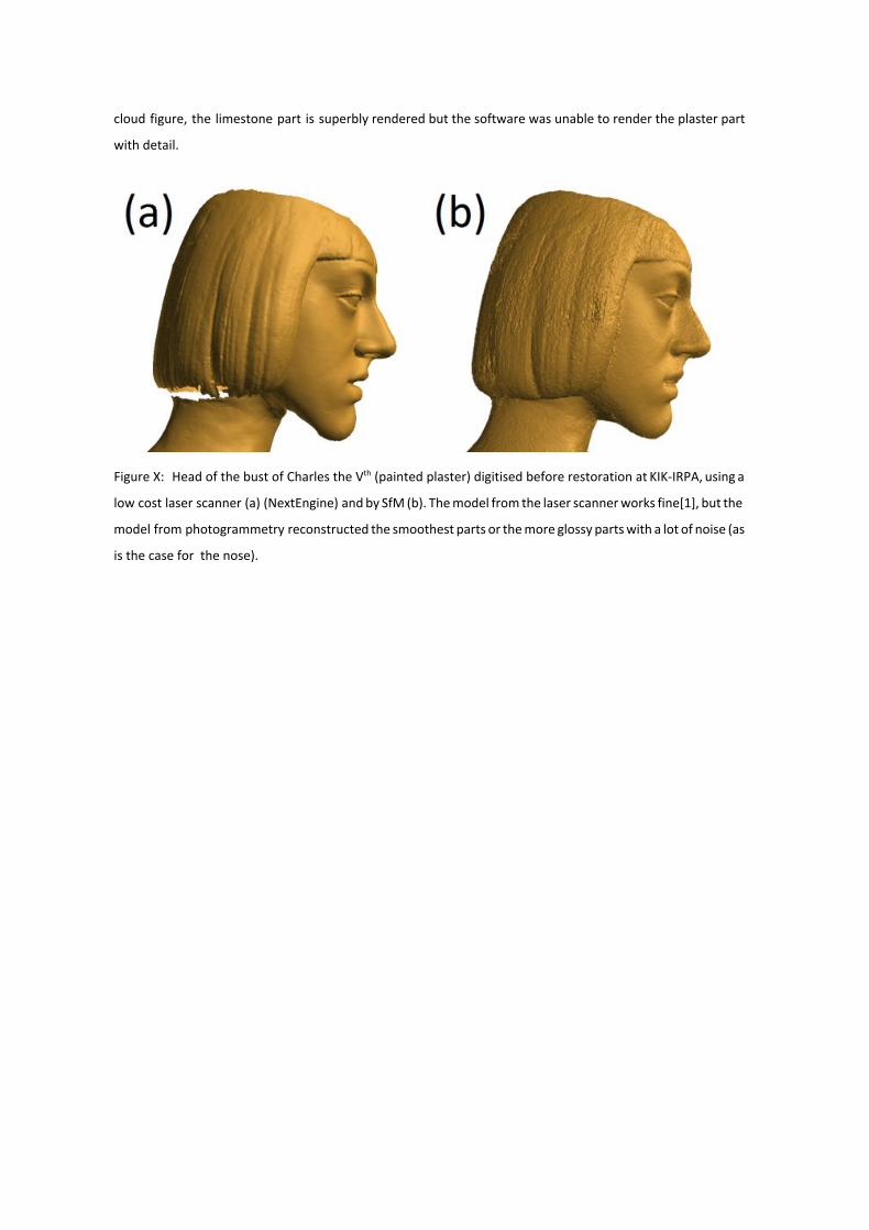
The bust of Charles V is also made of painted plaster, it is a smooth surface with glossy

painted details. The model from photogrammetry is less detailed than the model made by

the low cost laser scanner (fig. 5), and the photogrammetry model generated extra noise[1].

We observed the same on other glossy homogeneous materials such as pearl elements (fig.

6) or the inside surface of some shells (fig. 8).

We can generalize by saying that photogrammetry doesn’t deal well with

homogeneous/smooth materials in general. There is not enough detail on the material

which allows the software to reconstruct a sufficiently detailed model. Other techniques are

not affected by this.

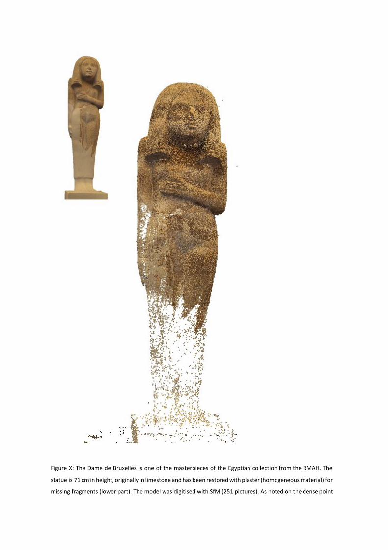
Figure X: The Dame de Bruxelles is one of the masterpieces of the Egyptian collection from the RMAH. The

statue is 71 cm in height, originally in limestone and has been restored with plaster (homogeneous material) for

missing fragments (lower part). The model was digitised with SfM (251 pictures). As noted on the dense point

cloud figure, the limestone part is superbly rendered but the software was unable to render the plaster part

with detail.

Figure X: Head of the bust of Charles the Vth (painted plaster) digitised before restoration at KIK-IRPA, using a

low cost laser scanner (a) (NextEngine) and by SfM (b). The model from the laser scanner works fine[1], but the

model from photogrammetry reconstructed the smoothest parts or the more glossy parts with a lot of noise (as

is the case for the nose).

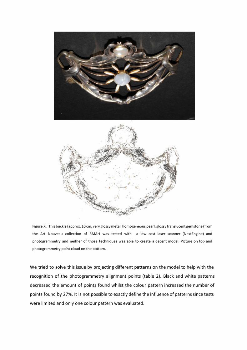
Figure X: This buckle (approx. 10 cm, very glossy metal, homogeneous pearl, glossy translucent gemstone) from

the Art Nouveau collection of RMAH was tested with a low cost laser scanner (NextEngine) and

photogrammetry and neither of those techniques was able to create a decent model. Picture on top and

photogrammetry point cloud on the bottom.

We tried to solve this issue by projecting different patterns on the model to help with the

recognition of the photogrammetry alignment points (table 2). Black and white patterns

decreased the amount of points found whilst the colour pattern increased the number of

points found by 27%. It is not possible to exactly define the influence of patterns since tests

were limited and only one colour pattern was evaluated.

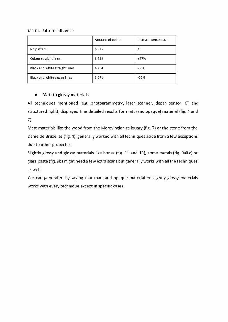
TABLE I. Pattern influence

Amount of points Increase percentage

No pattern 6 825 /

Colour straight lines 8 692 +27%

Black and white straight lines 4 454 -33%

Black and white zigzag lines 3 071 -55%

● Matt to glossy materials

All techniques mentioned (e.g. photogrammetry, laser scanner, depth sensor, CT and

structured light), displayed fine detailed results for matt (and opaque) material (fig. 4 and

7).

Matt materials like the wood from the Merovingian reliquary (fig. 7) or the stone from the

Dame de Bruxelles (fig. 4), generally worked with all techniques aside from a few exceptions

due to other properties.

Slightly glossy and glossy materials like bones (fig. 11 and 13), some metals (fig. 9a&c) or

glass paste (fig. 9b) might need a few extra scans but generally works with all the techniques

as well.

We can generalize by saying that matt and opaque material or slightly glossy materials

works with every technique except in specific cases.

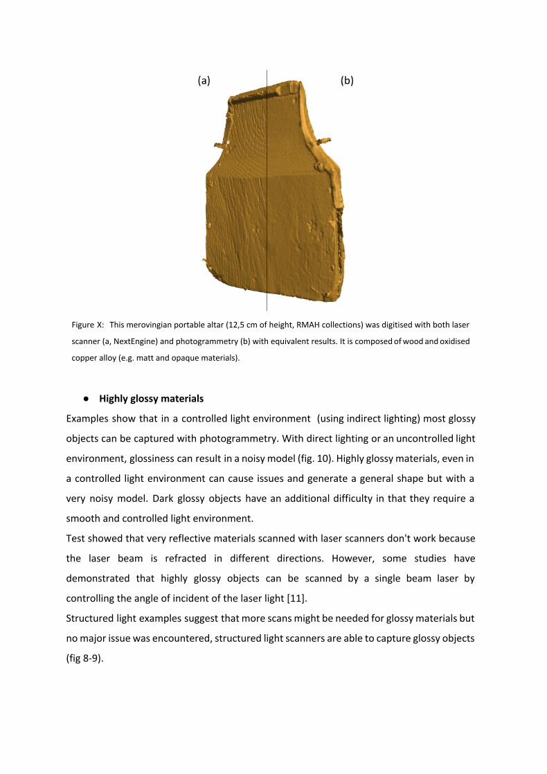
Figure X: This merovingian portable altar (12,5 cm of height, RMAH collections) was digitised with both laser

scanner (a, NextEngine) and photogrammetry (b) with equivalent results. It is composed of wood and oxidised

copper alloy (e.g. matt and opaque materials).

● Highly glossy materials

Examples show that in a controlled light environment (using indirect lighting) most glossy

objects can be captured with photogrammetry. With direct lighting or an uncontrolled light

environment, glossiness can result in a noisy model (fig. 10). Highly glossy materials, even in

a controlled light environment can cause issues and generate a general shape but with a

very noisy model. Dark glossy objects have an additional difficulty in that they require a

smooth and controlled light environment.

Test showed that very reflective materials scanned with laser scanners don't work because

the laser beam is refracted in different directions. However, some studies have

demonstrated that highly glossy objects can be scanned by a single beam laser by

controlling the angle of incident of the laser light [11].

Structured light examples suggest that more scans might be needed for glossy materials but

no major issue was encountered, structured light scanners are able to capture glossy objects

(fig 8-9).

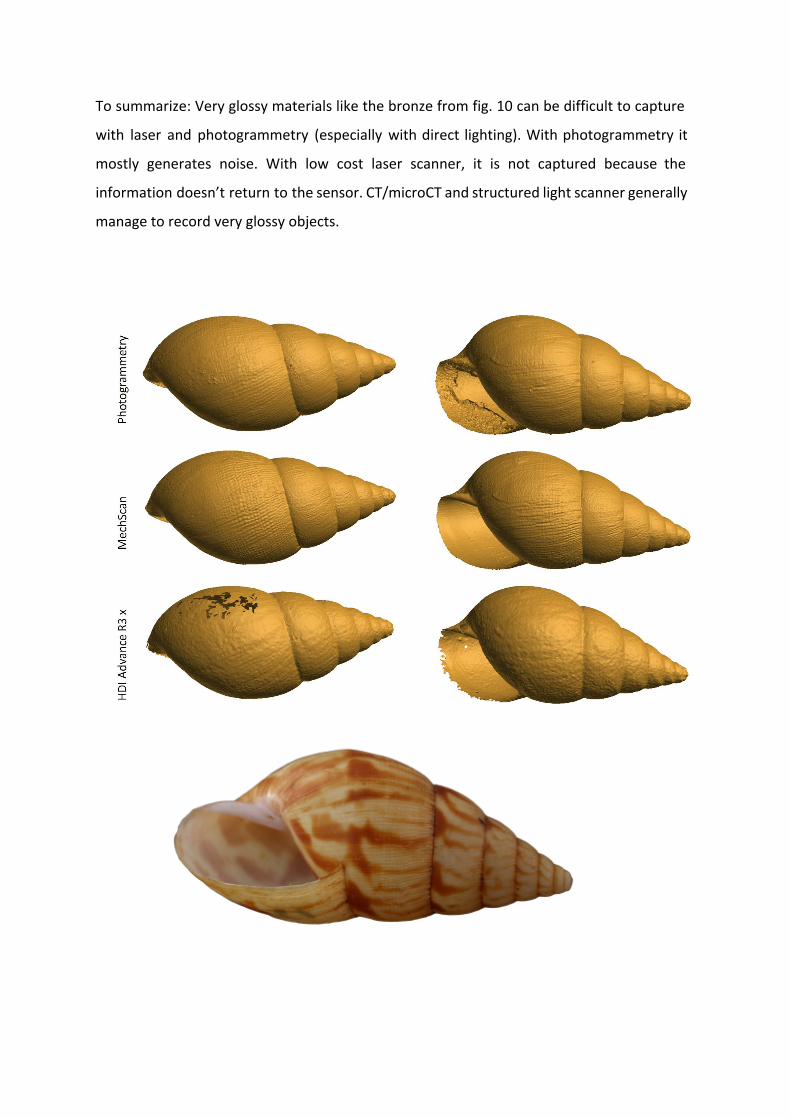
To summarize: Very glossy materials like the bronze from fig. 10 can be difficult to capture

with laser and photogrammetry (especially with direct lighting). With photogrammetry it

mostly generates noise. With low cost laser scanner, it is not captured because the

information doesn’t return to the sensor. CT/microCT and structured light scanner generally

manage to record very glossy objects.

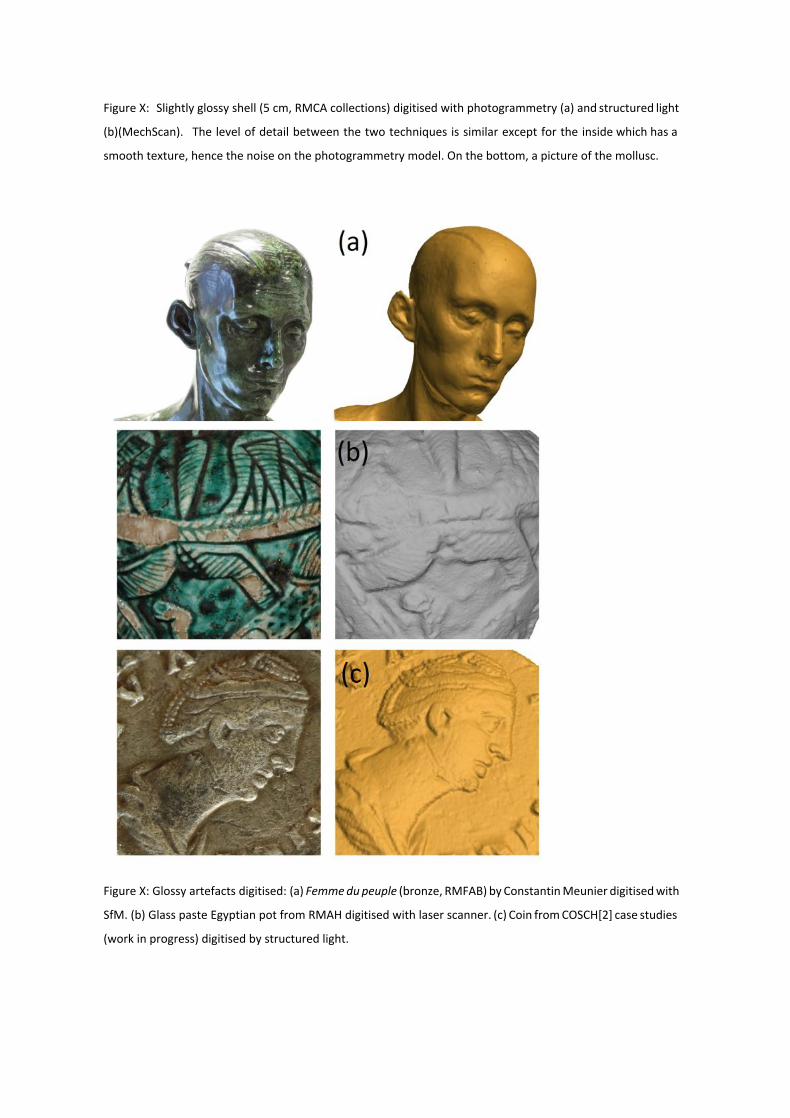
Figure X: Slightly glossy shell (5 cm, RMCA collections) digitised with photogrammetry (a) and structured light

(b)(MechScan). The level of detail between the two techniques is similar except for the inside which has a

smooth texture, hence the noise on the photogrammetry model. On the bottom, a picture of the mollusc.

Figure X: Glossy artefacts digitised: (a) Femme du peuple (bronze, RMFAB) by Constantin Meunier digitised with

SfM. (b) Glass paste Egyptian pot from RMAH digitised with laser scanner. (c) Coin from COSCH[2] case studies

(work in progress) digitised by structured light.

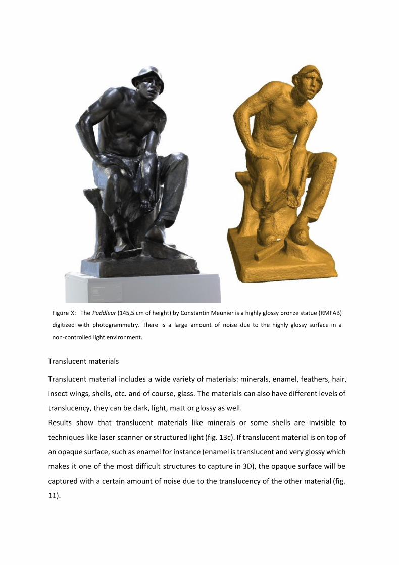
Figure X: The Puddleur (145,5 cm of height) by Constantin Meunier is a highly glossy bronze statue (RMFAB)

digitized with photogrammetry. There is a large amount of noise due to the highly glossy surface in a

non-controlled light environment.

Translucent materials

Translucent material includes a wide variety of materials: minerals, enamel, feathers, hair,

insect wings, shells, etc. and of course, glass. The materials can also have different levels of

translucency, they can be dark, light, matt or glossy as well.

Results show that translucent materials like minerals or some shells are invisible to

techniques like laser scanner or structured light (fig. 13c). If translucent material is on top of

an opaque surface, such as enamel for instance (enamel is translucent and very glossy which

makes it one of the most difficult structures to capture in 3D), the opaque surface will be

captured with a certain amount of noise due to the translucency of the other material (fig.

11).

If the translucent object is not too glossy, photogrammetry, contrary to structured light, is

able to capture a semi-translucent surface (fig.12).

Materials which are very translucent, almost transparent such as antique glass or minerals

cannot be captured by any of the surface scanning techniques. SfM also fails because whilst

the system can visualise the object it is not able to reconstruct it correctly. The generated

shape of the crystal on fig. 13a is reconstructed, but lacks detail and presents a large

amount of noise. The shape of the crystal on fig. 13b is mostly interpolated by the software.

CT and micro-CT are the only techniques at this present time which are able to cope with

this amount of translucency.

To summarise, photogrammetry can capture semi-translucent material as long as they are

not too glossy (fig. 11, 12 & 13a) (however, the result should only be used for visualisation

purposes and not for scientific studies) while surface scanners should not be used for

translucent objects (fig. 13 c).

In the case the material is translucent with an opaque background or too glossy it will

generate noise with both SfM and laser scanner (fig. 10a & 10c).

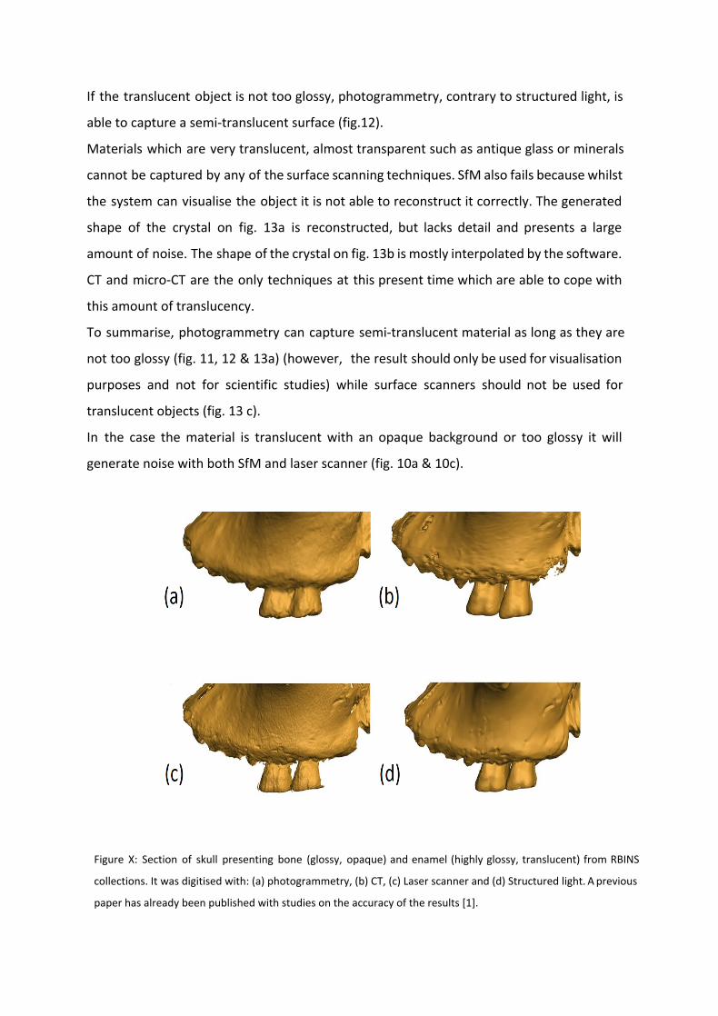
Figure X: Section of skull presenting bone (glossy, opaque) and enamel (highly glossy, translucent) from RBINS

collections. It was digitised with: (a) photogrammetry, (b) CT, (c) Laser scanner and (d) Structured light. A previous

paper has already been published with studies on the accuracy of the results [1].

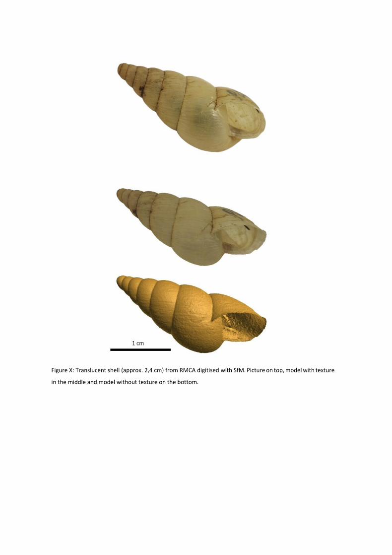
Figure X: Translucent shell (approx. 2,4 cm) from RMCA digitised with SfM. Picture on top, model with texture

in the middle and model without texture on the bottom.

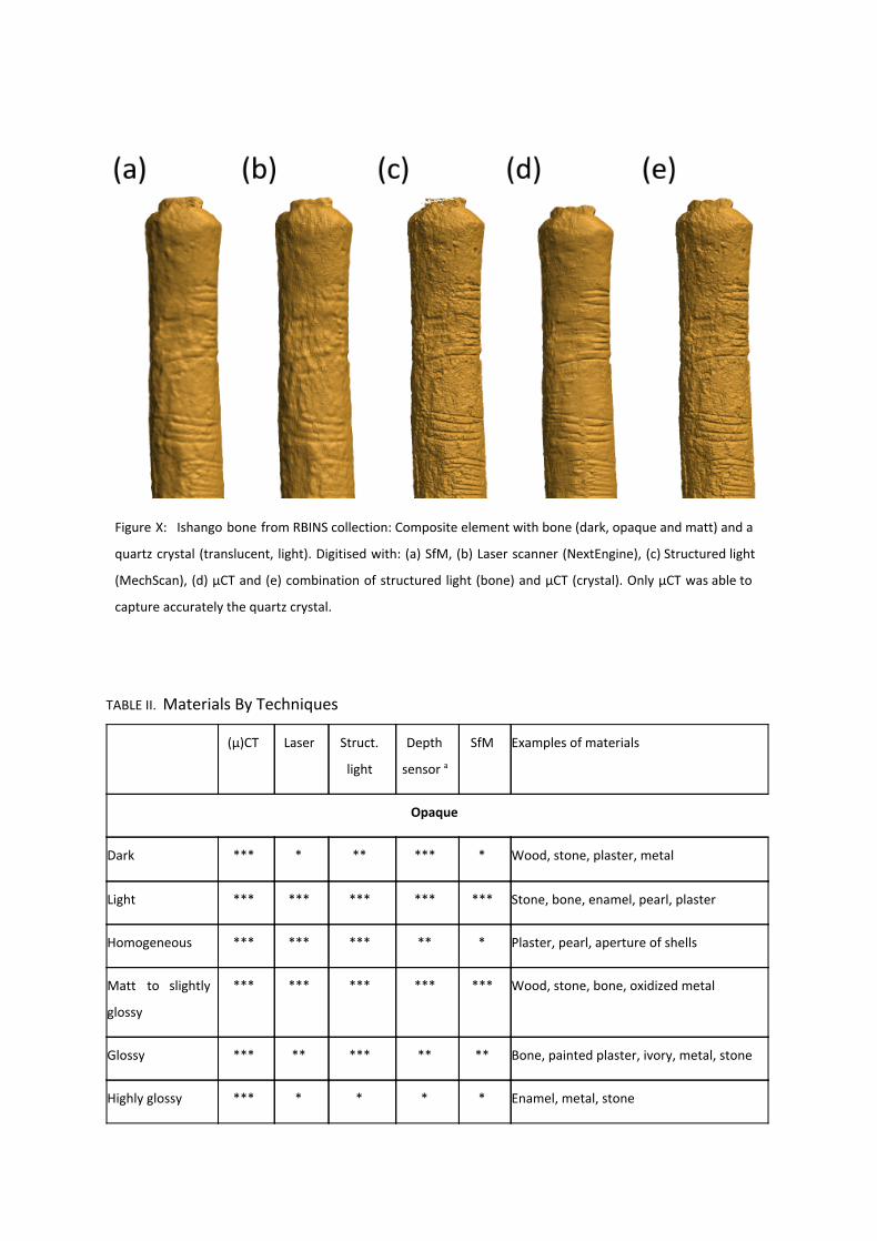
Figure X: Ishango bone from RBINS collection: Composite element with bone (dark, opaque and matt) and a

quartz crystal (translucent, light). Digitised with: (a) SfM, (b) Laser scanner (NextEngine), (c) Structured light

(MechScan), (d) µCT and (e) combination of structured light (bone) and µCT (crystal). Only µCT was able to

capture accurately the quartz crystal.

TABLE II. Materials By Techniques

(µ)CT Laser Struct.

light

Depth

sensor a

SfM Examples of materials

Opaque

Dark *** * ** *** * Wood, stone, plaster, metal

Light *** *** *** *** *** Stone, bone, enamel, pearl, plaster

Homogeneous *** *** *** ** * Plaster, pearl, aperture of shells

Matt to slightly

glossy

*** *** *** *** *** Wood, stone, bone, oxidized metal

Glossy *** ** *** ** ** Bone, painted plaster, ivory, metal, stone

Highly glossy *** * * * * Enamel, metal, stone

Translucent

Semi-Translucent *** * * x ** Enamel, shell, stone

Translucent *** x x x * Glass

a. The poor resolution of the depth sensor doesn't allow it to use this technique for small objects with details but

it can be a suitable approach for very large objects in the field.

Studying the digitisation of museum collections according to material optical properties was

quite a challenge. As previously mentioned, museum objects are very diverse in terms of

shape, size, colour, materials and many objects have mixed material (or mixed surface

texture) e.g. optical properties. The non-exhaustive analysis above, which are mainly the

case studies which demonstrated how different techniques encountered different problems

in obtaining 3D models, enabled us to make some general statements:

★ lighting conditions are a key element with laser scanner, structured light and

photogrammetry. Depth sensors are only affected by light when conditions change

during capture. In general, avoid changing light conditions during capture with all

techniques

★ dark objects need slightly overexposed or HDR pictures for photogrammetry, while

light objects require correct exposure with photogrammetry or structured light

★ matt and slightly glossy materials (if not translucent, homogeneous or with metallic

inclusions) work with all the techniques tested

★ homogeneous materials cannot produce detailed models with photogrammetry

★ metallic inclusions can generate artefacts in CT/µCT scans

★ highly translucent materials can be captured with CT and µCT only

★ matt moderately translucent materials can be digitised by photogrammetry but not

by structured light, laser or depth sensors

★ objects with high level of glossiness can be captured by structured light, depth

sensor, CT and µCT, but generate considerable amount of noise with

photogrammetry and are very difficult to capture with laser scanners

For composite objects with different optical properties it can be interesting to combine

different techniques such as for the Ishango bone in fig. 13: the µCT model presented

artifacts on the bone, but was the most accurate for the crystal, while the structured light

model was more accurate for the bone but couldn't record the crystal. Combining both

models enables us to have a more complete and accurate model.

A special note about the purpose of digitisation: in some cases the produced model can be

good enough for visualisation but not for scientific research. This is particularly the case for

Photogrammetry models, where due to their texture, they are good enough for visualisation

but lack detail in the mesh for scientific purposes.

[1] The holes in the laser model are part that weren't scan, not an issue of material.

[2] COST Action TD-1201 (http://cosch.info/case-studies/)

[1] The noise on painted plaster can also be due to the combination of homogeneous

material and glossiness of the material, this issue is addressed further on.

References

[1] A. Mathys, J. Brecko, and P. Semal, “Comparing 3D digitizing technologies: what are the differences?”,

in Digital Heritage International Congress, vol. 1, A. C. Addison, L. De Luca, G. Guidi and S. Pescarin, Eds. Marseille:

CNRS, 2013, pp. 201-204.

[2] M. Hess, S. Robson, and A. Hosseininaveh, “A contest of sensors in close range 3D imaging: performance

evaluation with a new metric test object”, in ISPRS - International Archives of the Photogrammetry, Remote

Sensing and Spatial Information Sciences, vol. XL-5, 2014, pp.277-284.

[3] A. Slizewski, M. Freiss, and P. Semal, “Surface scanning of anthropological specimens: nominal-actual

comparison with low-cost laser scanner and high end fringe light projection surface scanning systems”, in

Quartär, vol. 57, 2010, pp. 179–87.

[4] A. Mathys, J. Brecko, K. Di Modica, G. Abrams, D. Bonjean, and P. Semal, “Low cost 3D imaging: a first

look for field archaeology”, in Notae Praehistoricae, vol. 33, 2013, pp. 33-42.

[5] G. Pavlidis, A. Koutsoudis, F. Arnaoutoglou, V. Tsioukas and C. Chamzas, “Methods for 3D digitization of

Cultural Heritage”, in Journal of Cultural Heritage 8, 2007, pp. 93-98.

[6] C. Miyamae, “A dilemma of digital documentation for cultural heritage: - The possibility of one 3D

scanning system to various types of artefacts”, in Euromed 2014 proceedings, M. Ioannides et al ., Multi-Science,

2014, pp. 101-110.

[7] N. Zaimovic-Uzunovic, and S. Lemes, “Influences of Surface Parameters on Laser 3D Scanning”. in:

IMEKO Conference proceedings: International Symposium on Measurement and Quality Control 2010, Yasuhiro

Takaya, Eds. Japan, pp 408-411, September 2010.

[8] http://wiki.david-3d.com/user_manual/frequently_asked_questions, consulted on 10 march 2015.

[9] B. Mongon, J. Pfeifer, and E. Klaas, “What light colour should a white-light-scanner use?” CMSC 2012.

[10] LMI Technologies, “FlexScan3D user manual”, 2014.

[11] M. Rodrigues and M. Kormann, “3D Scanning of Highly Reflective Surfaces: Issues in Scanning the

Museums Sheffield Metalwork Collection”, in Conference on 3D Scanning and Documentation, UK: University of

Cambridge, December 2012.

V. Data management

VI. Data distribution

Digitization of museum objects and specimens for the sake of having a virtual back-up might

be one reason to do this, but another important reason is making these copies available to

other researchers and perhaps even the general public.

Considering the size of the files and the storage capacity needed not only to store, but to

make the virtual objects accessible, sketchfab for now is the best solution to host your

institutional 3D files. Sketchfab offers free pro accounts to institutions and research facilities

and are very keen on developing new tools which can aid the research on the models.

Important to note is that in a pro-account, it is possible to place models in private folders.

And maybe the most important thing is that the one uploading the files, keeps the copyright

of them.

VII. Workflows

Workflow 2D+ Focus Stacking DSLR @ RBINS & RMCA

1. Before switching on the StackShot Controller by connecting it to the Electrical network,

make sure the following steps are ok:

a. The camera is connected to the Stackshot controller (Shutter cable)

b. The StackShot controller is connected to the StackShot Rail

c. The camera is connected to the PC

All ok? Plug in the StackShot Controller

2. Switch on the camera

a. Open 'EOS Utility'

b. Select 'Camera settings/Remote Shooting'

c. Now the window appears to select your camera settings etc. Follow further

instructions

3. Switch on the light inside the closet

4. Switch on 'Live View Shoot' (Bottom left in the EOS Utility window)

5. Set the Shutter speed on 'BULB' (click on the shutter speed and press ↓)

6. Set the power of the speed lights: if you use a Grey Background

a. ½ or ¼ for 3x to 5x magnification

b. 1/8 to 1/16 for 1x to 3x magnification

c. 1/32 or 1/64 for regular macro lenses

d. test if the flash lights work by pressing the remote

7. Place the specimen in the closet in the centre of the lens

8. If you use the MP-E 65 mm Macro Photo, set the approx. desired magnification

Magnification Sensor filling size

1x 22.5 mm

2x 11.3 mm

3x 7.5 mm

4x 5.6 mm

5x 4.5 mm

9. Make sure that 'Mode: Auto-Dist' is selected on the StackShot controller, if not press

'up' or 'down' on the controller till it appears.

10. Move the camera up or down by pressing 'Fwd' or 'Back' till the specimen is in-focus

(Confirm through Live View in EOS Utility).

11. Set the distance the camera needs to travel between each picture by pressing 'select'

once and 'up' or 'down' to increase or decrease the 'Dist/Step'. Guidelines for the Step

Size:

Magnification Step Size

60mm 1:1 – 1:10 400 µm to 2 mm

1x 150 µm to 300 µm

2x 120 µm to 200 µm

3x 75 µm to 150 µm

4x 50 µm to 80 µm

5x 30 µm to 60 µm

Write down the magnification you used, as this is needed to add a scale after stacking the

images.

Normally you'll end up with a stack of 15 to 40 pictures for the mean values.

12. Set the appropriate f-stop and speed light power

a. 1:1 to 1:5: f/5.6 to f/7.1, flash 1/16 to 1/64

b. 3x to 5x magnification f/4.0 or f/4.5, flash ½ nd or ¼ th

c. 1x to 3x magnification f/4.5 to f/5.6 flash 1/8 th till 1/16 th

d. Press test shooting in the Live view window, a new window appears

e. close the Live View window, otherwise the speed lights won't flash

f. press the white square button upper right

g. alter the f-stop and/or flash power if needed

13. Select the upper most part of the specimen by travelling upwards

a. press 'Back' on the controller till the entire specimen is out of focus

b. press 'Fwd' till a part (the upper most part), is in focus

c. press 'up' or 'down'

d. 'Select End Pos' appears

14. Select the most distant part

a. Press 'Fwd' on the controller till the entire specimen is out of focus

b. Press 'Back' till a part (the most distant) is in focus

c. Press 'up' or 'down'

15. Close Live View window and check again if the speed lights work (press the button of

the transmitter on the camera)

16. Select the folder to save the pictures and make sure you take both RAW and Large

pictures if desired.

17. Press the 'Up' or 'Down' button to start the process of taking pictures

Zerene Stacker Workflow

18. Open Zerene Stacker (not the safe mode)

19. Press 'ok' on the welcome screen

20. Click 'add files' in the 'File' menu or skip to 23 on if you have multiple folders (views) to

stack.

a. Select all the images in the selected folder

b. press 'add'

21. In the 'Stack' menu select one of the following parameters:

a. Align and Stack PMax

b. Align and Stack DMap

c. Align and stack both

d. it is possible to stack without aligning by selecting the images in the 'input'

window and select 'Stack selected (PMax)' or 'Stack selected (DMap)' in the

Stack menu

22. After the stacking process is done, select all the out files and press 'Save output images'

in the 'File' menu.

23. Click on ‘Show batch dialog’ in the Batch menu tab (a new window appears).

24. In the Batch Queue window the left part is to select folders and to choose what to do

with project files. The right part is to decide how to stack and safe the stacked images.

25. LEFT: Click on ‘Add Projects and Folders’ and select the folders to be stacked (important

each folder is one view). Decide to Save the project folders in case of type material.

26. RIGHT: Click on ‘Add’ and Select ‘PMax’ and ‘DMap’ (Align and Stack) and press OK

27. Select ‘Save in Source Folders’ and Press ‘Run all Batches’. You can close the Batch

Queue Window.

28. If you want that automatically the name of the folder is saved as name for the stacked

image, do as follows:

Open the ‘Preference’ submenu in the ‘Options’ menu and choose ‘Image saving’. Below

you find ‘Output Image Names’ and write the following in the space below:

{sourcefolder} ZS {method}

Press on ‘Apply’ and OK

Troubleshooting

1. The stacking process (picturing) is started, but there aren't any pictures taken by the

camera.

a. Check if the shutter cable is well connected to the camera and the stackshot

controller

b. Check if the light of the Stackshot is blinking when a picture should be taken

c. Check if the 'Live Shoot' from the EOS Utility window is closed

2. The pictures taken fluctuate in light intensity, some are well exposed, others are too

dark.

a. The batteries of the flash, working in 'Slave-mode', are low in power. Change

batteries, preferably of both flashes.

b. In case you do not have spare batteries, make the time in between 2 pictures

longer (config) to give more time to recharge the batteries. To do so press

‘config’ on the stackshot controller and press select once to change the

settling time (Tsettle) or twice to change the time in between picturing and

movement of the rail (Toff).

3. Some pictures are black, others a well lit.

a. Check the batteries of the flash with the receiver on it. It is possible the

batteries are without power, so recharge them.

b. It is possible the batteries of the receiver are low on power.

c. It is possible that only the transmitter is low on energy, change the batteries

of the transmitter or receiver if changing the batteries of the speedlites didn't

work.

4. During stacking with Zerene stacker, there is a warning that the selected file doesn't

contain any pictures.

a. Check previous folders for the pictures, it is possible that you saved your

pictures in another folder.

The setup can be used by persons with only low knowledge of photography, after a small

training course of half a day. However it is important to judge the skills of handling small,

fragile and unique specimens. Best is to let them start with groups of solid, difficult to

damage specimens, before switching to the other.

Positioning specimens in alcohol can be challenging from time to time, but key is to add just

enough alcohol in the holder (petri dish, glass beaker, ...) to submerge the specimen.

Something that is important as well it to tell the photographer what characters have to be

visualized in the picture. In this way all the pictures taken show the information needed.

Workflow Microscope (Information in Imaging) @ RBINS & RMCA

● Switch on the microscope, the light, the camera (switch on top), the glitch (switch

under the glitch) and open Surveyor. Surveyor will initiate the stage so make sure

that the lenses are positioned high enough.

● Place the microscope slide on the glitch and first use the 5x magnification to find the

specimens. You can focus the microscope either manually or with the joystick on

screen. The joystick on screen also allow you to move the glitch on x,y to find the

specimen on the slide.

● Change the magnification if requiered, make sur you change it on the software as

well (joystick window).

● Calibrate for exposure, light balance using a part of the slide were the specimen is

not visible, calibrate shadding correction without the slide in front of the lens

(choose hole next to the slide).

● Create a grid selecting the part you want to aquire. Select turboscan scanning

stepped for a gigapan image.

●

● Gigapan + stacking: check the depth of the specimens, and place your focus in the

middle of the depth of the specimen. Enter the total thickness of the specimens and

the step size on the Zstack window. Create a grid of the part you want to digitize and

select zstack. then you can choose to save the different layer and stack them in

Zerene stacking or use the stacked image from the software (first option advised).

●

WorkFlow RTI/Minidome @ RBINS

1) Acquisition:

● Select the lens with the right magnification and mount t on the minidome.

● Make sure everything is pluged and start PLDAquisition version 4. Close it and start

PLD Acquisition version 5.

● Create a new project and press save.

● Turn on the background light.

● Put the specimens in the center of the dome at the equator level of the dome.

● Focus the camera.

● Remove the specimen and place the calibration sheet instead. Make sur it is well

centered.

● Choose 500 ms exposure time and press calibrate.

● Replace the calibration sheet by a white balance card and calibrate white balance.

● Replace the white balance card by the specimens, in the center. Choose the right

exposure and aperture, choose the side of the record if several view of the same

object will be made and start new record.

2) Processing:

● Open the project file in PLDDigitize

● Choose the last Bayer filter on the list and start processing.

3) Viewing:

● Once the file is processed you can open a new record in PLDViewer

● Save the record file as a .cun file, this way you can move the result without having to

keep it with the record file.

● You can also export a 3D model.

Warning:

● Minidome recordings are not compatible with other RTI viewer and doesn’t enable

to view RTI files processed with other softwares.

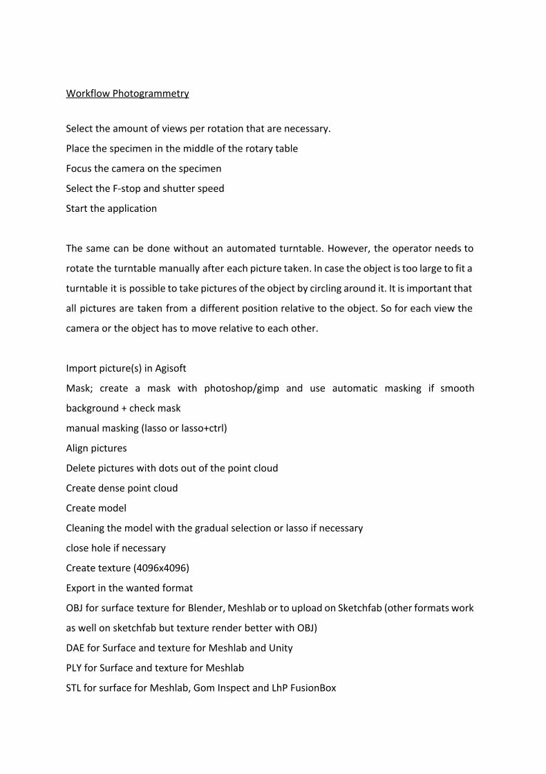
Workflow Photogrammetry

Select the amount of views per rotation that are necessary.

Place the specimen in the middle of the rotary table

Focus the camera on the specimen

Select the F-stop and shutter speed

Start the application

The same can be done without an automated turntable. However, the operator needs to

rotate the turntable manually after each picture taken. In case the object is too large to fit a

turntable it is possible to take pictures of the object by circling around it. It is important that

all pictures are taken from a different position relative to the object. So for each view the

camera or the object has to move relative to each other.

Import picture(s) in Agisoft

Mask; create a mask with photoshop/gimp and use automatic masking if smooth

background + check mask

manual masking (lasso or lasso+ctrl)

Align pictures

Delete pictures with dots out of the point cloud

Create dense point cloud

Create model

Cleaning the model with the gradual selection or lasso if necessary

close hole if necessary

Create texture (4096x4096)

Export in the wanted format

OBJ for surface texture for Blender, Meshlab or to upload on Sketchfab (other formats work

as well on sketchfab but texture render better with OBJ)

DAE for Surface and texture for Meshlab and Unity

PLY for Surface and texture for Meshlab

STL for surface for Meshlab, Gom Inspect and LhP FusionBox

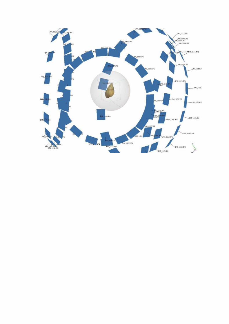
Workflow Infrared sensors @ RMCA & RBINS

Make different scans with overlap of the different sides of the object. These scans need to

be merged afterwards. In case of uniform looking objects it is best to stick easy removeable

landmarks on the object to help identify similar points on different scans.

The technique is sensitive to differences in light. Best is to do it in controlled light

environments, by placing tents around the object or use studio lights to evenly expose the

object.

After merging the scans it is possible to export the pointcloud and mesh it in third party

software like GOM inspect, if the meshing of the original software is not good enough.

To make it easier merging all the different scanned fragments together, it really helps to

give them a good name, which makes it clear what part is scanned.

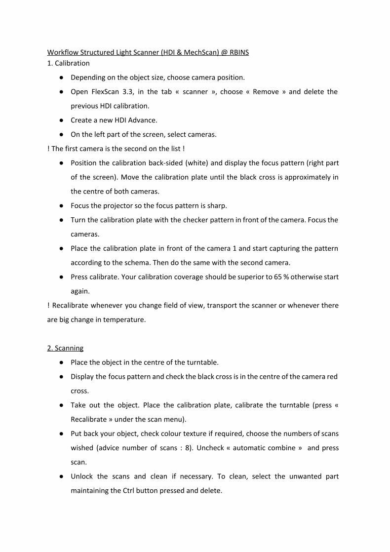
Workflow Structured Light Scanner (HDI & MechScan) @ RBINS

1. Calibration

● Depending on the object size, choose camera position.

● Open FlexScan 3.3, in the tab « scanner », choose « Remove » and delete the

previous HDI calibration.

● Create a new HDI Advance.

● On the left part of the screen, select cameras.

! The first camera is the second on the list !

● Position the calibration back-sided (white) and display the focus pattern (right part

of the screen). Move the calibration plate until the black cross is approximately in

the centre of both cameras.

● Focus the projector so the focus pattern is sharp.

● Turn the calibration plate with the checker pattern in front of the camera. Focus the

cameras.

● Place the calibration plate in front of the camera 1 and start capturing the pattern

according to the schema. Then do the same with the second camera.

● Press calibrate. Your calibration coverage should be superior to 65 % otherwise start

again.

! Recalibrate whenever you change field of view, transport the scanner or whenever there

are big change in temperature.

2. Scanning

● Place the object in the centre of the turntable.

● Display the focus pattern and check the black cross is in the centre of the camera red

cross.

● Take out the object. Place the calibration plate, calibrate the turntable (press «

Recalibrate » under the scan menu).

● Put back your object, check colour texture if required, choose the numbers of scans

wished (advice number of scans : 8). Uncheck « automatic combine » and press

scan.

● Unlock the scans and clean if necessary. To clean, select the unwanted part

maintaining the Ctrl button pressed and delete.

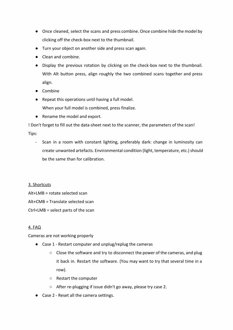
● Once cleaned, select the scans and press combine. Once combine hide the model by

clicking off the check-box next to the thumbnail.

● Turn your object on another side and press scan again.

● Clean and combine.

● Display the previous rotation by clicking on the check-box next to the thumbnail.

With Alt button press, align roughly the two combined scans together and press

align.

● Combine

● Repeat this operations until having a full model.

When your full model is combined, press finalize.

● Rename the model and export.

! Don't forget to fill out the data-sheet next to the scanner, the parameters of the scan!

Tips:

- Scan in a room with constant lighting, preferably dark: change in luminosity can

create unwanted artefacts. Environmental condition (light, temperature, etc.) should

be the same than for calibration.

3. Shortcuts

Alt+LMB = rotate selected scan

Alt+CMB = Translate selected scan

Ctrl+LMB = select parts of the scan

4. FAQ

Cameras are not working properly

● Case 1 - Restart computer and unplug/replug the cameras

○ Close the software and try to disconnect the power of the cameras, and plug

it back in. Restart the software. (You may want to try that several time in a

row).

○ Restart the computer

○ After re-plugging if issue didn't go away, please try case 2.

● Case 2 - Reset all the camera settings.

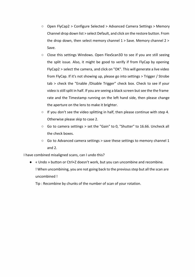
○ Open FlyCap2 > Configure Selected > Advanced Camera Settings > Memory

Channel drop down list > select Default, and click on the restore button. From

the drop down, then select memory channel 1 > Save. Memory channel 2 >

Save.

○ Close this settings Windows. Open FlexScan3D to see if you are still seeing

the split issue. Also, it might be good to verify if from FlyCap by opening

FlyCap2 > select the camera, and click on "OK". This will generate a live video

from FlyCap. If it's not showing up, please go into settings > Trigger / Strobe

tab > check the "Enable /Disable Trigger" check box. Check to see if your

video is still split in half. If you are seeing a black screen but see the the frame

rate and the Timestamp running on the left hand side, then please change

the aperture on the lens to make it brighter.

○ If you don't see the video splitting in half, then please continue with step 4.

Otherwise please skip to case 2.

○ Go to camera settings > set the "Gain" to 0, "Shutter" to 16.66. Uncheck all

the check boxes.

○ Go to Advanced camera settings > save these settings to memory channel 1

and 2.

I have combined misaligned scans, can I undo this?

● « Undo » button or Ctrl+Z doesn't work, but you can uncombine and recombine.

! When uncombining, you are not going back to the previous step but all the scan are

uncombined !

Tip : Recombine by chunks of the number of scan of your rotation.

Workflow Laser Scanning @ RBINS

1. Calibration

The NextEngine is a self-calibrated scanner, therefore no calibration is required.

2. Scanning

● Open StudioScan/StudioScanHD and press on the Scan button. This doesn’t initiate a

scan but open the scan window in order to parameter the scan

● Positioning: 360°

● Division: number of scan in one rotation, choose according to the complexity of your

object, but usually between 8 and 12 should be enough.

● Precision: if you are scanning a small object or want a higher precision choose

“macro”, otherwise choose “wide”

● If you choosed macro, your object should be placed at 16.5 cm (! distance to the

surface of the object to be scanned, not to the center of the object). If you choosed

wide, your object should be placed at 43 cm.

● On the preview window check that the object is well centered (you can use the turn

arrows on top to check that it is well centered and will stay in the view when

rotated). You can also draw a selection window on the preview if you want to scan

only a small part of the view (faster scan and less cleaning required afterwhile).

● Start scanning.

3. Processing

● Alignment

● Cleaning