Average distance and routing algorithms in the star-connected cycles interconnection network

Average Distance and Routing Algorithms in theStar-Connected Cycles Interconnection Network

Marcelo M. de Azevedo, Nader Bagherzadeh, and Martin DowdDepartment of Electrical and Computer Engineering

University of California, Irvine – Irvine, CA 92717-2625

Shahram LatifiDepartment of Electrical and Computer Engineering

University of Nevada, Las Vegas – Las Vegas, NV 89154-4026

April 1996 - Technical Report ECE 96-04-01

Average Distance and Routing Algorithms in theStar-Connected Cycles Interconnection Network

Marcelo Moraes de Azevedo�, Nader Bagherzadeh, and Martin Dowd

Dept. of Electrical and Computer Engineering – Univ. of California – Irvine, CA 92717-2625�mazevedo, nader, martin � @ece.uci.edu Phone: (714) 824-8720 FAX: (714) 824-2321

Shahram Latifi

Dept. of Electrical and Computer Engineering – Univ. of Nevada – Las Vegas, NV 89154

[email protected] Phone: (702) 895-4016 FAX: (702) 895-4075

Abstract — The star-connected cycles (SCC) graph was recently proposed as an attractive inter-connection network for parallel processing, using a star graph to connect cycles of nodes. Thispaper presents an analytical solution for the problem of the average distance of the SCC graph.We divide the cost of a route in the SCC graph into three components, and show that one of suchcomponents is affected by the routing algorithm being used. Three routing algorithms for the SCCgraph are presented, which respectively employ random, greedy and optimal routing rules. Thecomputational complexities of the algorithms, and the average costs of the paths they produce,are compared. Finally, we discuss how source-based and distributed versions of the algorithmspresented in this paper can be used in association with wormhole routing.

Key words — Star-connected cycles graph, average distance, routing, interconnection networks,parallel processing.

1 Introduction

An interconnection network is characterized by four distinct aspects: topology, routing, flow control,and switching [13]. The topology of a network defines how the nodes are interconnected by links,and is usually modelled by a graph. Routing determines the path selected by a packet to reach itsdestination, and is usually specified by means of a routing algorithm. Flow control deals with theallocation of links and buffers to a packet as it is routed through the network. Switching determinesthe mechanism by which data is moved from an incoming link to an outgoing link of a node (e.g.,store-and-forward, circuit switching, virtual cut-through, and wormhole routing are examples ofswitching techniques found in parallel architectures).

In this paper, we continue the study of topological and routing aspects of the star-connectedcycles (SCC) interconnection network [12], which was recently proposed as an attractive extensionof the star graph [2, 3]. An SCC graph is related to a star graph in the same way a cube-connected

�This research was supported in part by Conselho Nacional de Desenvolvimento Cientıfico e Tecnologico (CNPq -

Brazil), under the grant No. 200392/92-1.

1

cycles graph [14] is related to a hypercube [15]. Namely, an SCC graph is formed from a stargraph by replacing the nodes of the latter with cycles or rings of nodes. The SCC graph constitutesan efficient architecture for execution of parallel algorithms, which include broadcasting [4] andFFT [16]. Mesh algorithms are also supported in SCC graphs via embeddings [5]. The SCC graphinherits many of the interesting properties of the star graph [3], while employing at most three I/Oports per node. This last aspect categorizes the SCC graph as a bounded-degree network (otherexamples are in [14, 17]). Networks with bounded degree favor area-efficient VLSI layouts, andscale more easily than variable-degree networks.

Previously known topological aspects of SCC graphs include degree, symmetry, diameter, andfault-diameter, and were derived in [6, 12]. Here, we continue the study of these by investigating theaverage distance (or average diameter) of SCC graphs. Our interest in this property is twofold: 1)to obtain a metric for comparing the performance of routing algorithms, and 2) to provide continuedcharacterization of the graph theoretical aspects of SCC networks.

In the absence of other network traffic, modern switching techniques (e.g., wormhole routing [8])achieve a communication latency which is virtually independent of the selected path length [13]. Inthis ideal environment, the two factors which contribute to the communication latency experiencedby a packet are the start-up latency and the network latency [13]. In a realistic environment inwhich congestion occurs, however, a third factor known as blocking time also contributes to thecommunication latency.

Regardless of the flow control and switching mechanisms being used in the network, congestioncan usually be minimized if fewer links are used when routing a packet [7]. For communication-intensive parallel applications, the blocking time (and, consequently, the communication latency)is expected to grow with path length [7]. In such cases, a routing algorithm should ideally computepaths whose average cost matches the average distance of the network.

In this paper, we show that routes in an SCC graph may contain up to three classes of links,which we refer to as lateral links,

��local links, and

��local links (see Section 3 for definitions).

Exact expressions for the average number of lateral links and��

local links between two nodes inan SCC graph, and an upper bound on the average number of

��local links, are derived. When

combined, these expressions produce a tight upper bound on the average distance of the SCC graph.We show that the number of

��local links is affected by the routing algorithm being used, and

propose three different algorithms for the SCC graph: random, greedy, and optimal routing. Theproposed routing algorithms are compared according to criteria such as computational complexity(which affects their implementation in hardware) and average routing cost, for which figures wereobtained by means of simulation programs. The results obtained with the optimal routing algorithmprovide exact numeric solutions for the average distance of SCC graphs. Our simulations indicatethat the greedy routing algorithm performs close to the optimal routing algorithm, while requiringa smaller complexity. We show that the random routing algorithm presents the smallest complexityamong the three algorithms described in this paper, and provide average and worst-case routing costmetrics for it. Finally, we discuss how the three algorithms can be implemented in combinationwith wormhole routing [8].

2

2 Background

2.1 The star graph

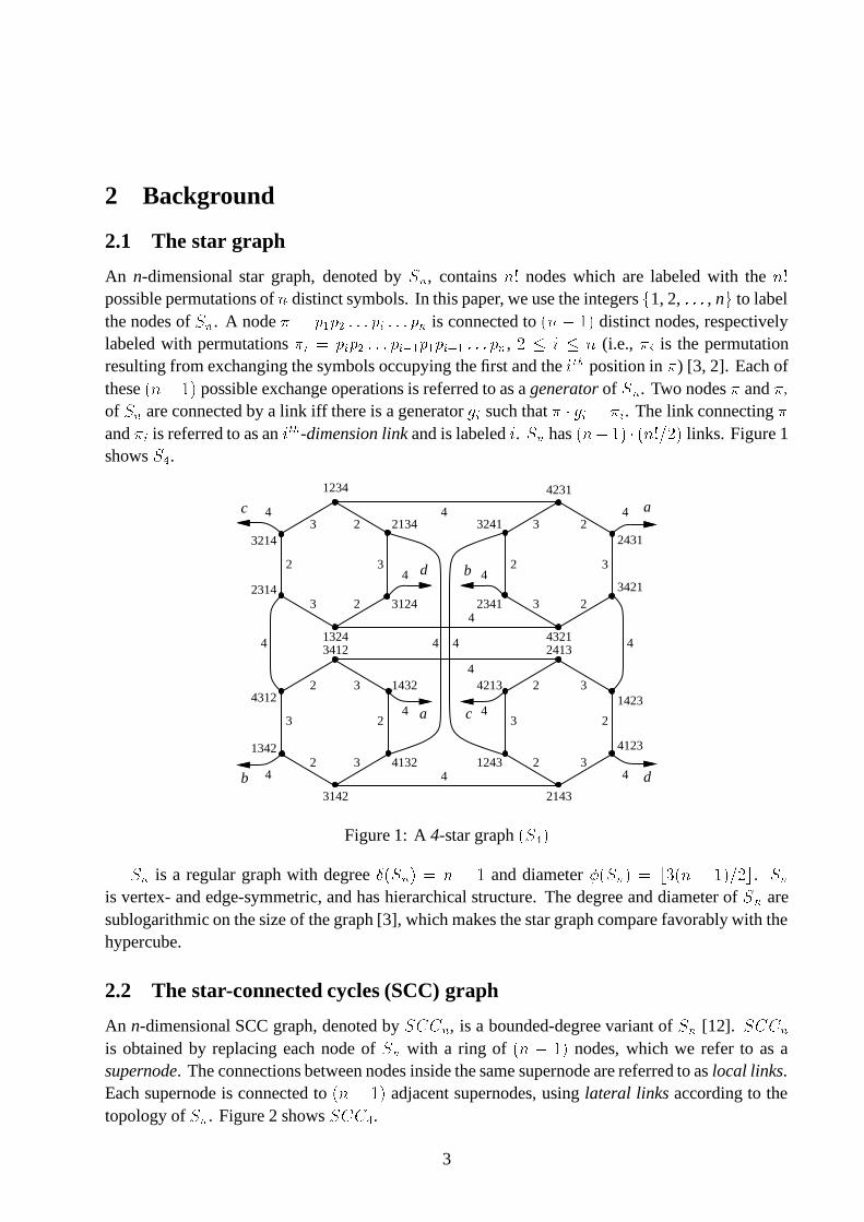
An n-dimensional star graph, denoted by��

, contains �� nodes which are labeled with the ��possible permutations of � distinct symbols. In this paper, we use the integers � 1, 2, �� , n to labelthe nodes of

��. A node � �� is connected to ��! distinct nodes, respectively

labeled with permutations �"�#�$��%��'&��(��*)�� , +-,/.0,/� (i.e., �1� is the permutationresulting from exchanging the symbols occupying the first and the .(2'3 position in � ) [3, 2]. Each ofthese ��4�5�! possible exchange operations is referred to as a generator of

��. Two nodes � and �1�

of�"�

are connected by a link iff there is a generator 67� such that �98:6;��<�� . The link connecting �and �� is referred to as an . 2'3 -dimension link and is labeled . . �=� has ��0�-�! "8��*>!+7 links. Figure 1shows

�"?.

c

d

a

b

a

b

c

d

3214

1234 4231

2134 32412431

3421

43212413

1423

4123

2143

1243

42131432

2341

13243412

2314

4312

1342

3142

4132

4

4

2 3

3 2

23

2 3

3 2

23

2 3

2

32

3 3

2 3

2

32

3124

4 4 44

4

4

4 4

44

44

4 4

Figure 1: A 4-star graph � �? �"�

is a regular graph with degree @�� =� 0�A�B�C� and diameter D�� 0�FEHG��B�I�! J>!+LK . �"�is vertex- and edge-symmetric, and has hierarchical structure. The degree and diameter of

��are

sublogarithmic on the size of the graph [3], which makes the star graph compare favorably with thehypercube.

2.2 The star-connected cycles (SCC) graph

An n-dimensional SCC graph, denoted by�NM0MO�

, is a bounded-degree variant of�=�

[12].�NM0MN�

is obtained by replacing each node of��

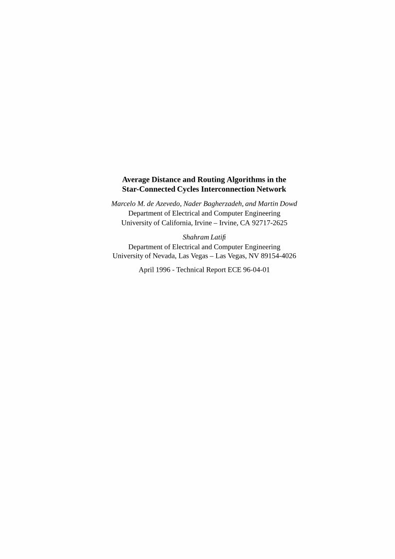
with a ring of �� C�! nodes, which we refer to as asupernode. The connections between nodes inside the same supernode are referred to as local links.Each supernode is connected to ��<�! adjacent supernodes, using lateral links according to thetopology of

��. Figure 2 shows

�NM0MP?.

3

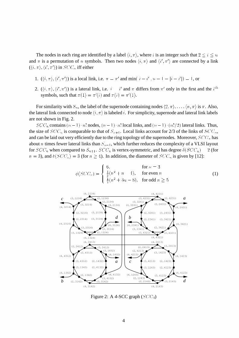
The nodes in each ring are identified by a label� .�� , where . is an integer such that + ,�.N,��

and � is a permutation of � symbols. Then two nodes� .�� and

� .�� are connected by a link(� .�� .�� ) in

�NM0MN�iff either

1. (� .�� .�� ) is a local link, i.e. � �<�� and min �� .=�5.�� 9��#�� .=�5.�� C� , or

2. (� .�� .�� ) is a lateral link, i.e. .#� .�� and � differs from �� only in the first and the .�2'3

symbols, such that � �J�! �<��'��. and � ��. ��'�J�! .For similarity with

��, the label of the supernode containing nodes

� +�� is � . Also,the lateral link connected to node

� .�� is labeled . . For simplicity, supernode and lateral link labelsare not shown in Fig. 2.�NM0MN�

contains �� B�! �8 �� nodes, �� B�! �8 �� local links, and �� B�! �8 ��*>!+7 lateral links. Thus,the size of

�NM0MP�is comparable to that of

�=� )�� . Local links account for 2/3 of the links of�NM0MO�

,and can be laid out very efficiently due to the ring topology of the supernodes. Moreover,

�NM0M �has

about � times fewer lateral links than�=� )�� , which further reduces the complexity of a VLSI layout

for�NM0MN�

when compared to�� )�� . �NM0MN� is vertex-symmetric, and has degree @�� NM0M � �<+ (for

� �<G ), and @�� NM0MN� N�<G (for �� ). In addition, the diameter of�NM0M �

is given by [12]:

D�� NM0MN� N�� for � �<G�� 9�!�� for even �� G;�9�#"7 � for odd ��%$ (1)

(4,3214)

(4,2314)

(4,1234)

(3,3214)

(3,1234) (2,1234)

(3,3124)

(2,3214)

(2,2314)

(2,2134)

(3,2314)

(2,1324)(3,1324)

(4,1324)

(4,2134)

(3,2134)

(2,3124)

(4,3124)

c

d

(4,4231)

(2,4231)(3,4231)

(2,2431)(4,2431)

(3,2431)

(3,3421)

(4,3421)(2,3421)

(2,4321)

(4,4321)

(3,4321)

(3,2341)

(4,2341)

(2,2341)

(2,3241)

(4,3241)

(4,4312)(2,4312)

(2,3412)

(4,3412)

(3,3412)(3,1432)

(4,1432)

(2,1432)

(2,4132)

(4,4132)

(3,4132)(3,3142)

(4,3142)

(2,3142)

(2,1342)(4,1342)

(3,1342)

(3,4312)

(4,2413)

(4,1423)

(3,1423)

(3,2413)

(2,1423)

(2,4123)

(4,4123)(3,4123)

(3,2143)

(4,2143)

(2,2143)(2,1243)

(4,1243)

(3,1243)

(3,4213)

(4,4213)

(2,4213)

(2,2413)

a

b

a

b

c

d

(3,3241)

Figure 2: A 4-SCC graph (�NM0MP?

)

4

3 Average distance of the SCC graph

3.1 Preliminaries

Let the cost of a route�

between node� .�� and the identity node

� .�� N� � +��+ �� in�NM0MN�

be denoted by �4�� , where �� and �� respectively denote the number of lateral links andthe number of local links in

�. Because

�NM0MO�is vertex-symmetric, its average distance can be

computed by finding minimal cost routes to the identity from every node in the graph, and averagingthose over ��9� �! 8!�� .

Before we can derive the average distance of�NM0MO�

, some definitions related to lateral linksare needed. We may organize the symbols of permutation � as a set of r-cycles � – i.e. cyclicallyordered sets of symbols with the property that each symbol’s desired position is that occupied bythe next symbol in the set. We assume in this paper that all r-cycles are written in canonical form[10], i.e. the smallest symbol appears first in each r-cycle. A permutation � �C+ � $ �7G�� labeling asupernode of

�NM0M��, for example, can be written in cyclic format as (1 2 6)(3 5)(4). Note that any

symbol already in its correct position appears as a 1-cycle.Let

M �#� ��.��#.�� #.�� be an r-cycle included in permutation � ( +B,��B, � ). Let �B8�� bethe permutation produced from � by moving the symbols in

M � (i.e., ��.�� .��N.�� ) to their correctpositions. The execution of an r-cycle

M � is, by definition, a minimal sequence of lateral links � � � ,leading from supernode � to supernode �98 � � . � � can be expressed by [9, 11]:

� �� .�� .�� .�� if .�� C��.�� .�� .��J&�� .�� .�� if .��C� (2)

In the case .��C� , M � can actually be executed with � different sequences of lateral links [9, 11]:

� ��C��.�� .�� .��J&�� .�� .�� F��.�� .�� .�� .�� .�� F8�8�8��F��.�� .�� .��J&�� .��J&�� .�� (3)

As shown in [3], the minimum number of lateral links in a route from supernode � to �� is:

��N�� if the first symbol in � is 1� �� -+�� if the first symbol in � is not 1,

(4)

where � is the number of r-cycles of length at least 2 in � and � is the total number of symbolsin these r-cycles. It is shown in [3, 9] that �� does not depend on the order chosen to execute ther-cycles in � .

Routes in�NM0MP�

often consist of sequences of lateral links interleaved with local links. In whatfollows, we give some definitions that relate to local links.

Recall that �� denotes the contribution of the local links to the total cost of a route�

from� .�� to� .�� . �� can be further divided into two components, which we denote by

�� and�� , and define as follows:�

r-cycles provide a convenient means to represent permutations [10] and should not be confused with physicalcycles or rings, which constitute the supernodes of �!"!$# .%

Note that local links are not an issue here.

5

� �� – the number of move-in (MI) local links existing in the route from� .�� to

� .�� .By definition, these are local links that must be traversed between two lateral links belongingto the execution sequence of an r-cycle in � .

� �� – the number of move-between (MB) local links existing in the route from� .�� to� .�� . By definition,

��local links are: 1) local links that must be traversed between the

executions of two consecutive r-cycles in � , 2) local links that must be traversed in supernode� , and are required to move from

� .�� to the lateral link that initiates the execution of thefirst r-cycle of � , and 3) local links that must be traversed in supernode �� , and are requiredto move from the lateral link that finishes the execution of the last r-cycle of � to

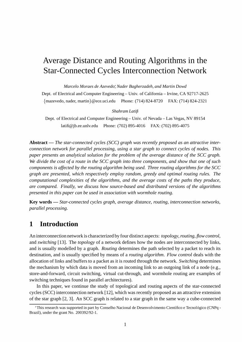
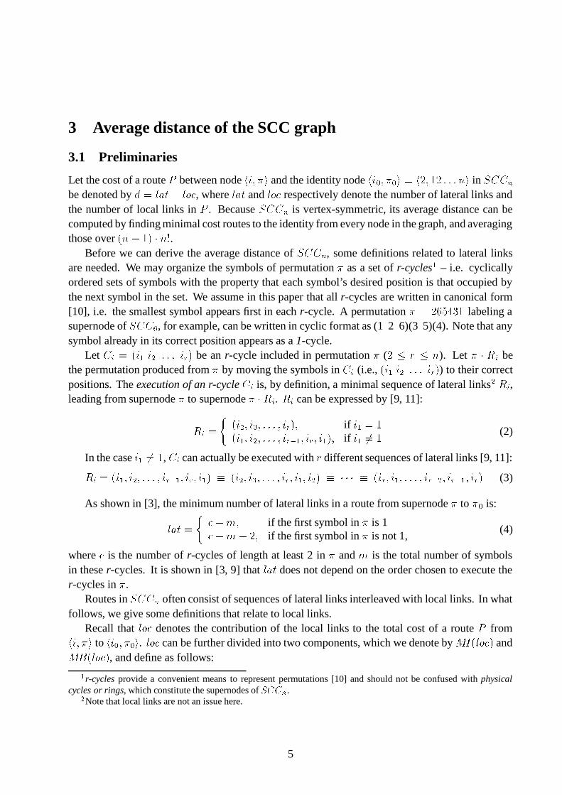
� . �� .Thus, � � �� B� �� . As an example, consider routing from� G�� G ��+ $ � to

� +��+;G � $ � in�NM0M��

. The cyclic representation of permutation 34125 is (1 3)(2 4)(5).One possible route uses the sequences of lateral links ��+�� +7 and ��G7 . Figure 3 shows the

��local

links and the��

local links in such a route.

4 3

25

4 3

25

4 3

25

4 3

25

4 3

25

Legend:

Lateral link MI local link MB local link

2

4

2

3

34125 43125 23145 32145 12345

Source node Destination node

Supernode labels

Figure 3:��

and��

local links in a route in�NM0M��

Note that from the topological viewpoint there is no distinction between��

and��

locallinks. A particular local link existing in the route between two nodes of

�NM0M �is considered to be

either an��

or an��

local link, depending on the conditions stated above. Therefore, the samelocal link can be classified as an

��local link for some routes, and as an

��local link for others.

The cost components �� , �� , and�� exist in the route between any node in

�NM0M �and the identity node (although in some short routes one or more of these components may benull). Therefore, one can derive the average distance of

�NM0M#�by computing the average numbers

of lateral links,��

local links, and��

local links in a route from� .�� to

� .�� . We denotesuch average numbers by �� , �� , and

�� , respectively. The average distance of�NM0M �

,denoted by D�� NM0MP� , can then be expressed by:

D�� NM0MN� � �� (5)

Finally, the average number of local links existing in a route from� .�� to

� . �� in�NM0MN�

is,by definition, �� .

6

3.2 Average number of lateral links

The number of lateral links in the route between any node of�NM0M#�

and the identity node is exactlyequal to the cost of the corresponding route in the underlying n-star graph [12]. Therefore, �� isexactly equal to the average distance of

��, which is given by [2, 3]:

�� <� � � � � +� �!� � where

� � ��

�� is the nth Harmonic number [10]. (6)

3.3 Average number of �� local links

The number of��

local links in the route between two nodes in�NM0M#�

can be calculated as follows.Consider routing from

� .�� to the identity node� . � � �� , and let the number of r-cycles of length

at least 2 in � be � . LetM � �A��.��#.��B��#.�� be one of these r-cycles, and let � � be an execution

sequence forM � (Eq. 2). Moving between two consecutive lateral links .� , .� in � � requires ��.� � .�

��local links, where [12]:

��.� � .� �� .�N�5.�� 9� � �� .�N�5.�� (7)

The total number of��

local links that must be traversed during the execution ofM � , denoted

by�� M �H , is therefore the sum of the distances ��.� � .� between all pairs of consecutive lateral

links ��.� � .�� in � � :�� M �H N�

�� . � &�� . � � ��.�� .�� if .�� I�� . � &�� . � � if .��#�I�

(8)

Lemma 1 The number of��

local links that must be traversed in the route between any two nodesof�NM0MN�

is independent of the order chosen to execute the r-cycles existing between those nodes.

Proof : Without loss of generality, let the two nodes be� .�� and

� .�� . LetM �� .��N.�� N.��

be an r-cycle of � , +�,��9, � . We first show that�� M �H does not depend on the sequence

of lateral links � � chosen to executeM � . If .�� , there is only one such sequence (Eq. 2). If

.�� C� , there are � different possible sequences (Eq. 3). However, due to the cyclic nature of thesesequences, they all have the same cost

�� M � (Eq. 8). By extension, the total number of��

local links in the route,�� , must also be an invariant. �

An immediate consequence of Lemma 1 is that the number of��

local links between two nodesof�NM0MN�

can be derived without further considerations about routing. (Assuming, of course, thatrouting is accomplished in adherence to Eqs. 2 and 3, as is the case with all routing algorithmspresented in this paper.) As an example, consider an r-cycle

M ��C��+ � �� , and let � �� . Such an r-cycle can be executed with a sequence of lateral links � ��I��+�� +7 . The number of

��local links

required in the execution of this sequence is�� M �' N� ��+�� +7 ��+ � + � +4� �

.

7

Theorem 1 The average number of��

local links that must be traversed in the route between apair of nodes in

�NM0MP�is:

�� 9��! � � �� &�� (9)

Proof : The average number of local links that must be traversed between two adjacent lateral linksis:

�� N�� .�� +7 �9�5+ �

� �� &��9�5+ (10)

The average number of local links that must be traversed in the execution of an r-cycleM � �

��.�� .��9�� .�� is:

�� M � �� 87� � �5+7 � if .�� C�� 8 � � if .��C� (11)

Over all �� possible permutations of � symbols and for each integer value � , +9,�� ,C� , thereis a total of ��<�! � r-cycles that include symbol 1 ( .(� � � ) and ��*> � ��<�! � r-cycles that donot include symbol 1 ( . � ��/� ). The average number of

��local links over all �� permutations is

therefore:

�� 9��! �78 �� 87� � �5+7 �

�� ! � �08 �� 8 �

��

� �� 87��9��! ��9�5+7 � � ��9��! � � � � � � &��

� �

3.4 Average number of �� local links

Recall that��

local links are needed to move between execution sequences of adjacent r-cycles( +�,��, � ), to move into the first lateral link, and to move out of the last lateral link in a routebetween a pair of nodes in

�NM0M �.

Theorem 2 The average number of��

local links that must be traversed in the route between apair of nodes in

�NM0MP�, under a random ordering of r-cycles, is:

�� N� � +�� 9��+ ��

� � �5+��-+

� +�9�� (12)

Proof : Over all �� possible permutations of � symbols and for each integer value � , + , ��, � ,there is a total of ��*> � r-cycles. The total number of r-cycles of length at least 2 in the �� possiblepermutations of � symbols is, therefore, � �#�� *> �; N�<��78;� � � ��! .

The average number of r-cycles, + , � , � , in a permutation of � symbols is �9�� >!�� . The average number of��

local links that must be traversed between these r-cycles is:

8

�� . �� C� � ��! �8 �� &�� 5+7

�9�5+ (13)

Assuming that the source node is� .�� and that the first lateral link in the route to the destination

node is . � , + ,<. � ,�� , the average number of local links that must be traversed between� .�� and� . � � �� is:

��.�� N�� .�� +7 �9��

� �� &�� (14)

Note that ��.�� differs from �� (Eq. 10), since to compute ��.�� we must consider the case.N�<. � . Similarly, the average number of local links that must be traversed between the last laterallink in the route and the destination node is �� 0� ��.�� . Then, the average number of

��

local links that must be traversed in the route between a pair of nodes in the SCC graph, assuminga random ordering of r-cycles in the route, is

�� #� ��.�� . �� .The theorem follows. �

As described in Section 4, a properly designed routing algorithm can optimize the ordering ofthe r-cycles and reduce the average number of

��local links further below the value provided by

a random ordering of r-cycles (Eq. 12). The average number of��

local links, considering thatthe shortest route between any two nodes of an SCC graph is determined by an optimal routingalgorithm, is therefore bounded by:

�� N, �� (15)

3.5 Average distance in the SCC graph

Theorem 3 The average distance of�NM0M �

is bounded by:

D�� NM0MN� ,<� � � � � +� �!� � � +�� + �� #� �

�� 5+

�9�5+� +�� (16)

Proof : The theorem immediately follows from Eqs. 5, 6, 9, 12 and 15. �

4 Routing algorithms in the SCC graph

4.1 Ordering of r-cycles

Routing between two nodes� .�� and

� .�� in�NM0MN�

is equivalent to routing from� .�� to� .�� , where �� I� &�� 8!�� , �� C��+;G �� , and � &�� is the inverse or reciprocal of permutation

�� [2, 12].Let

� � � �� denote a route from from� .�� to

� .�� in�NM0MN�

, along a sequence of lateral links �0� � �� C� � �� . The total cost of

� � � �� is given with:

9

� � � �� ;� � ��.�� &��

� � � � � )�� .�� (17)

Depending on the order chosen to execute the r-cycles in � �� , different routes� � � �� from� .�� to

� .�� are produced. As explained in Section 3, a common feature to any of these routesis that they all have the same number of lateral links ( �� ) and

��local links (

�� ).Finding the shortest route from

� .�� to� .�� is therefore a matter of choosing an r-cycle

ordering which minimizes the number of��

local links (�� ). A routing algorithm which

achieves this goal is given in Subsection 4.4. Non-optimal (but simpler) routing algorithms arepresented in Subsections 4.2 and 4.3.

To illustrate the different cost components in a route, and how they are affected by the orderchosen to execute the r-cycles, assume routing from node

� G�� G ��+ $ � to node� +��+;G � $ � in

�NM0M �.

A route along the sequence �0��+ � G7 N�C��+�� +�� G7 contains four lateral links, four��

local links,and three

��local links (i.e., � ��+ � G7 � 7� � � � � G0�C�;� ). However, if the sequence of lateral

links �0��G � +7 #�/��G�� +�� +7 is used, a route with four lateral links, four��

local links, and one��

local link results (i.e., � ��G � +7 � 7� � � � � � � �).

In some cases, the number of��

local links in a route from� . �� to

� .�� can be furtherreduced by interleaving (rather than executing separately) the r-cycles in � �� . For example, somepossible sequences of lateral links from supernode � �� +;G��$ �I� �J�9+ G7 ��$7 to supernode�� +;G � $ in

�NM0M��are (2, 3, 4, 5, 4), (2, 3, 5, 4, 5), (4, 5, 4, 2, 3), (5, 4, 5, 2, 3), (2, 4, 5, 4, 3)

and (2, 5, 4, 5, 3). The last two of these sequences interleave r-cycles �J�#+ G7 and �� $7 . All of therouting algorithms presented in this paper account for the possibility of interleaving r-cycles.

4.2 Random routing algorithm

A simple routing algorithm for�NM0M �

consists of choosing a random order to execute the r-cyclesin �� . Particularly, a possible algorithm that can be used for this purpose is the routing algorithmof the star graph [9]:

Algorithm 1 (Non-deterministic routing in the star graph):

Repeat until � ��N�� :1. If the first symbol in � �� is 1, then exchange it with any symbol not in its correct position.

2. If the first symbol in � �� is � �� , then either exchange it with the symbol at position � ,or exchange it with any symbol in an r-cycle of length at least two, other than the r-cyclecontaining � .

The above algorithm requires at most � � � steps of complexity �0�J�! each, and therefore itscomplexity is �0� � �� , or �0�� , since � , � , EH��>!+LK and � , � ,<� .

10

4.3 Greedy routing algorithm

A simple approach to minimize the number of��

local links in the route between nodes� . �� and� .�� consists of using a greedy algorithm. Such an algorithm uses the following data structures

and variables:

� ��– the set of r-cycles of length at least 2 in � �� .

� � � – a subset of the symbols of � �� , such that:

– If �J�#.��.�� .�� is an r-cycle of��

, then .�� and � � .�� .�� .– If ��.��".��0��=.�� is an r-cycle of

��that does not include symbol 1, then .(�� .�� .�� .

� . � – an integer variable initialized to . � �<.�� .

Algorithm 2 (Greedy routing in the SCC graph):

1. If ��N�� , then route inside the supernode and exit.

2. Identify the r-cycles of length at least 2 that exist in � �� , and initialize��

,� � , and . � .

3. Choose a symbol .�� such that ��. � � .�7 is minimal. LetM be the r-cycle that contains

symbol .� . Once .� is chosen, make . � �<.� .4. If

M has the form �J�4.�� .�� 0.�� (i.e.,M includes symbol 1), then make

� � � �� J�4.� .�� 0.�� # � � �J�4.�� 0.�� # and

� �B� � � �C�!.�� !.�� . Otherwise, make�� -� M � and� � � � ��-�� 7� M , where �� 7� M denotes a function that

returns the set of symbols in r-cycleM .

5. Repeat Steps 3 and 4 until� � �� .

The greedy approach used by Algorithm 2 consists of choosing the r-cycle that has the minimumdistance from . � as the next one to be executed. If the selected r-cycle

M includes symbol 1, thenonly the first lateral link of

M is taken, which allows for an interleaved execution of that r-cycle.IfM does not include symbol 1, then

M is executed completely. The complexity of the greedyrouting algorithm is �0� � � , or �0�� since � , ��, EH��>!+LK and � , � ,/� . The ordering ofr-cycles chosen by this algorithm, however, may not be optimal.

4.4 Optimal routing algorithm

We now present an optimal routing algorithm which provides the shortest route between a pair ofnodes

� .�� and� .�� in

�NM0MN�. The goal of the algorithm is to find a sequence of lateral links�0� � � � �� , such that � � � � � �� is minimal (Eq. 17). We note that an earlier version of our

optimal routing algorithm appeared in [12]. The algorithm we present here improves that of [12] in

11

two ways: 1) it employs more selective heuristics to further constrain the search space generated bythe algorithm, and 2) it accounts for the possibility of interleaving r-cycles, which is not possiblewith the algorithm in [12].

The algorithm performs a depth-first search on a weighted tree structure. The tree is builtby expanding at each step only those r-cycle orderings that seem to result in a minimal numberof local links. Although the search tree can virtually examine all possible r-cycle orderings,including interleaved r-cycles, its size is significantly constrained in our algorithm. To guaranteethat an optimal route is always found, backtracking is used to enable expansion of previous r-cycleorderings that seem to be better than the most recently expanded orderings.

In the following discussion, we use the term vertex to refer to an element of the search tree.In addition, we use the term edge to refer to the logical connection between vertices in the searchtree, which is usually implemented with pointers or some form of indexing. The following datastructures are stored within each vertex � � of the search tree and are used by our routing algorithm:

� � � � � �� – the label of the node reached so far by the routing algorithm.

� � � – a subset of the symbols of �"� , such that:

– If �J�#.��.�� .�� is an r-cycle of �1� , + , �0,<� , then .�� and � � .�� .�� .– If ��.��0.��0.�� is an r-cycle of �1� , +<, ��, � , such that .�� .�� .�� , then.�� .�� .�� .

The symbols in� � represent all possible lateral links that can be selected by the routing

algorithm while expanding the search tree from a given vertex � � . For convenience, we definea function to generate

� � from �� . Let this function be referred to as bsymbols, such that� �� 7��' .

�� – a subset of the symbols of �"� , such that:

– If �J�#.��.�� .�� is an r-cycle of �1� , + , �0,<� , then . �� and � � .�� .��J&�� .– If ��.��0.��0.�� is an r-cycle of �1� , +<, ��, � , such that .�� .�� .�� , then.�� .�� .�� .

The symbols in � � represent all lateral links that can be possibly selected by the routingalgorithm to enter supernode � � (i.e., all possible r-cycle orderings that can be selected bythe routing algorithm from a given vertex � � necessarily end with a lateral link

� � � � ). Forconvenience, we define a function to generate � � from �� . Let this function be referred to asfsymbols, such that � �� 7��H .

�� – the number of local links used so far by the routing algorithm in the route from� . ��

to� � � � �� .

12

� � � – an estimate of the minimum number of local links that may be needed by the routingalgorithm to reach node

� .�� from node� .�� , using the route already constructed by

the algorithm up to the intermediate node� � � � �� . For convenience, we use a function dubbed

as minloc to compute� � from � �� , �� , .�� . Such a function is defined as:

� �� .�� !� � �� .�� N� � � � min � �� J �� M � � min � �� !� � .�� J �

(18)

where � �� , � �� 7��' , and !�� , � �=� �� 7��H .Note that minloc is computed under the optimistic assumption that the route from

� � � � �� to� .�� selects the best possible lateral links in the sets� � and � � . In addition, the summation

term used to compute the number of local links that are required to execute all r-cyclesM ��B��

(see Eq. 8) assumes that an optimal r-cycle ordering requiring no local links to move fromone r-cycle to the next can be found by the routing algorithm.

�� – an enable/disable bit which indicates whether the tree should continue to be expandedfrom vertex � � or not.

In addition, the tree structure generated by the optimal routing algorithm has the followingcharacteristics:

� The number of levels in the search tree is at most �� + , with �� being given by Eq. 4. Wenumber these levels from 0 to �� , starting from the root level.

� Let � � be the parent of a vertex � �� in the search tree. We refer to the data stored in � � and � �� as� � � � � �� and � � � �� , respectively. The weight of theedge connecting � � to � �� corresponds to the number of local links that are required to routefrom

� � � � �� to� � �� in

�NM0MN�and is given by �� min �� "� � �� 9�<� �� =� � �� .

Hence, � �� .Note that routing from

� � � � �� to� � �� also requires one lateral link if �"��/�� , and zero

lateral links otherwise. Since the total number of lateral links that must be traversed in theroute from

� .�� to� .�� can be computed in advance (Eq. 4), the routing algorithm

focuses on accounting for the local links only.

� The root vertex is initialized with� � � � �� .�� , � �I� � �� 7�� , � �<�

�� 7�� , � �� ,� �� .�� !� �� .�� .�� and � �� ON. All vertices located at level�� in the tree have� � � � ��N� � .�� , � �� =�� and

� �� .�� !� � �� .�� .�� =� � � .All vertices located at level �� in the tree have

� � � � ��N� � �� (with��

being the lateral linkused to enter supernode � � ), � �� , and

� �� .�� !� � �� .�� N� � � � �� .�� .� The backtracking mechanism is triggered by comparing the estimated minimum number of

local links (� � ) stored in the most recently generated child vertices with a global variable

referred to as

. This variable is updated whenever a backtracking procedure occurs, meaning

13

that the minimum number of local links that is required in the route from� . �� to

� .�� is actually greater than the previous value of

. As expected, the search for an optimal route

becomes more selective as

increases, which not only limits the width of the search tree butalso makes the backtracking mechanism less likely to be triggered again.

Given the definitions above, the optimal routing algorithm for the SCC graph follows :

Algorithm 3 (Optimal routing in the SCC graph):

1. If ��N�� , then route inside the supernode and exit.

2. Create a root vertex with� � � � �� .�� , � � � � �� 7�� , � � � �� 7�� ,

� � � � ,� � � � .�� !� �� .�� .�� and � � � ON. Also, initialize

with the value

�� .�� !� �� .�� .�� .3. Generate child vertices for all enabled vertices, such that the label

� �� for each child correspondsto exactly one of the symbols stored in the set

� � of each parent vertex. Set � � � OFF ateach recently expanded parent vertex. Also, obtain permutation � �� for each child vertexby swapping the 1st and the

� �� th symbols of the corresponding permutation stored in theparent vertex ( �1� ), and make

� �� 7�� , � �� 7�� , � �� ,� �� .�� !� � �� .�� . Enabled vertices located at level �� of the search tree must beexpanded similarly. However, they generate a single child with

� �� /.�� , �� /�� , � �� ,� �� , � �� .�� , � �� . In any case, a child vertex is enabled with � �� ON if� �� ,

. Otherwise, we set � �� OFF.

4. If one of the child vertices has� � �� .�� and � �� ON, then an optimal route has been

found. The optimal sequence of lateral links �0� � �� can be obtained in reverse order bybacking up towards the root of the tree and listing the value of the symbol

� � stored in eachvertex located between the ��J2'3 and the 1st levels. Once �0� � �� has been obtained, exitthe algorithm.

5. If none of the enabled child vertices has� � �� N� � .�� , go to Step 3.

6. If there are no enabled child vertices, do a backtracking search in the tree. Among all existingchild vertices, select those with the smallest value of

� � and set

to this value. Also, enablethe selected nodes and go to Step 4.

The height of the search tree is �0�� , since its maximum value is D�� + �AEHG �� ! J>!+LK � + .A worst-case analysis of the width of the search tree can be done under the following pessimisticassumption: considering that all possible orderings of r-cycles in permutation � �� are examined bythe optimal routing algorithm, the lowest level in the search tree would have at most � � vertices.This is justified by the fact that there are at most � � possible ways to move the � misplacedsymbols in � �� to their correct positions, using the minimum number of lateral links given by Eq. 4.In practice, the constraints placed on the number of expanded vertices by the heuristics of the

14

l = 5 = (153) (24) (6)

B = {2,4,5} F = {2,3,4}

L = 0 M = 6 e = OFF

π

l = 2 = (14253) (6)

B = {4} F = {3}

L = 2 M = 10 e = OFF

i i

i i

i i i

i i

i i

i i i

π l = 4 = (12453) (6)

B = {2} F = {3}

L = 1 M = 8 e = OFF

i i

i i

i i i

i i

i

i i i

i

π π

l = 2 = (1423) (5) (6)

B = {4} F = {3}

L = 2 M = 7 e = OFF

l = 3 = (1) (24) (3) (5) (6)

B = {2,4} F = {2,4}

L = 2 M = 8 e = OFF

l = 4 = (1243) (5) (6)

B = {2} F = {3}

L = 1 M = 6 e = OFF

i i

i

i i i

i

πi i

i

i i i

i

πi i

i

i i i

i

π

l = 2 = (143) (2) (5) (6)

B = {4} F = {3}

L = 3 M = 6 e = OFF

i i

i

i i i

i

π

2 1 0

2 2 1

2

l = 4 = (13) (2) (4) (5) (6)

B = {3} F = {3}

L = 5 M = 6 e = OFF

i i

i

i i i

i

π

2

l = 3 = (1) (2) (3) (4) (5) (6)

B = { } F = { }

L = 6 M = 6 e = ON

i i

i

i i i

i

π

1

l = 5 = (13) (24) (5) (6)

B = {2,3,4} F = {2,3,4}

L = 0 M = 5 e = OFF

Backtracking threshold used: T = 6

Source node: < 5, (153) (24) (6) >

Optimal sequence of lateral links found: (5,4,2,4,3)

Number of lateral links in the optimal path: 5

Number of local links in the optimal path: 6

Total length of the optimal path: 11 links

Destination node: < 3, (1) (2) (3) (4) (5) (6) >

Dimensionality of the SCC graph: n = 6

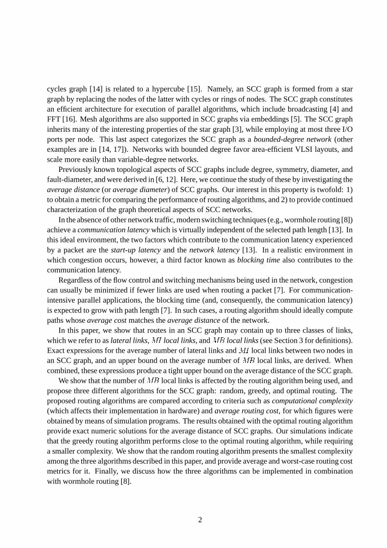
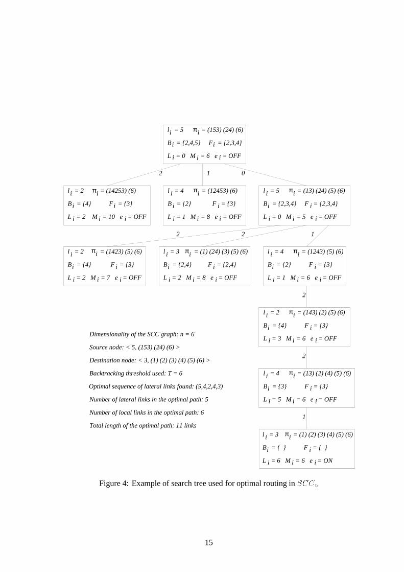
Figure 4: Example of search tree used for optimal routing in�NM0M#�

15

algorithm (i.e., the estimated minimum number of local links� � ) limit the width of the search tree

considerably. Simulations carried out for �9,<� , �revealed that a very small number of vertices

is enabled at each step, which makes the maximum width of the tree virtually proportional to � .Figure 4 illustrates an example of the search tree constructed by the algorithm.

The main computations that must be performed upon creation of a vertex of the search tree referto� �� , � �� and

� �� . Fortunately, each of these computations can be accomplished in �0�J�! time byusing the corresponding values

� � , � � and� � that are stored in the parent vertex, and taking into

account the differences in the r-cycle structures of permutations �=� and �� .The reasoning above results in a worst-case complexity of �0� � � �� . As explained above, such

computational requirements were not observed during simulations of the optimal algorithm. Thepotential need for backtracking searches in the tree, added to fact that the maximum width of thetree is in practice proportional to � , results in a complexity of �0� � � � , on the average (or �0�� ,since � , � ,<� ).

5 Simulation results

The performance of routing algorithms for the�NM0MO�

graph was evaluated with simulation programsthat compute the route of all ��<�! �� nodes of the graph to the identity. The routing algorithmsthat were tested are: 1) a random routing algorithm that generates all possible routes to the identitywith equal probability, which is based on Algorithm 1, 2) Algorithm 2, and 3) Algorithm 3. Thesimulations were carried out for G�, �5, �

. A log of worst-case routes that may result from therandom routing algorithm was also made.

� 3 4 5 6 7 8 9

Graph size �J��9��! �8!��* 12 72 480 3,600 30,240 282,240 2,903,040

Graph diam. � D�� NM0MP� J 6 8 16 19 31 34 50

Average number of 1.500 2.583 3.683 4.783 5.879 6.968 8.051lateral links � ��J

Average number of��

0.667 1.500 3.200 5.000 7.714 10.500 14.222local links � ��

Average number of��

0.833 1.222 1.925 2.337 2.924 3.334 3.873local links � ��

Average number of 1.500 2.722 5.125 7.337 10.638 13.834 18.096local links � �� !

Average dist. � D�� NM0MP� J 3.000 5.306 8.808 12.121 16.517 20.802 26.147

Table 1: Average distance of SCC graphs under optimal routing

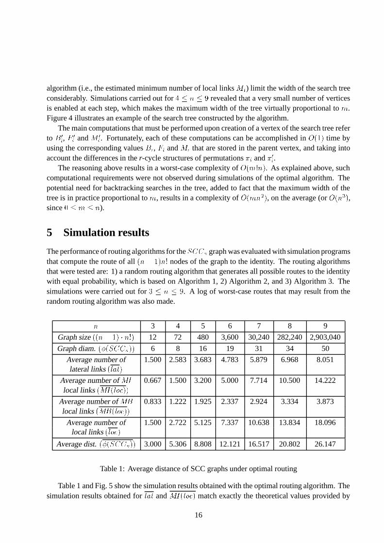
Table 1 and Fig. 5 show the simulation results obtained with the optimal routing algorithm. Thesimulation results obtained for �� and

�� match exactly the theoretical values provided by

16

Eqs. 6 and 9. Also, the simulation results obtained for�� under an optimal routing algorithm

are closely bounded by Eq. 12.

3.0 5.0 7.0 9.0n

0.0

10.0

20.0

30.0

Dis

tanc

es

Average distanceAverage number of local linksAverage number of MI local linksAverage number of lateral linksAverage number of MB local links

Figure 5: Average distances on the SCC graph under optimal routing

3.0 5.0 7.0 9.0n

0.0

2.0

4.0

6.0

8.0

Ave

rage

num

ber

of M

B lo

cal l

inks

Random routing (worst-case)Random routing (average, simulation)Random routing (average, theoretical)Greedy routingOptimal routing

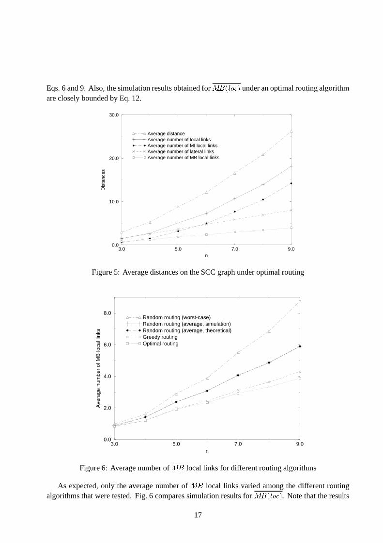
Figure 6: Average number of��

local links for different routing algorithms

As expected, only the average number of��

local links varied among the different routingalgorithms that were tested. Fig. 6 compares simulation results for

�� . Note that the results

17

for the random routing algorithm are very close to the theoretical values provided by Eq. 12.The model used to derive that equation seems to result in an error proportional to �!>!�� , which isnegligible considering that Eq. 12 is still a close upper bound for

�� . As expected, both thegreedy and the optimal routing algorithm outperform the random routing algorithm, as far as theaverage number of

��local links is concerned. Also observe that, for G ,/�<, � , the greedy

routing algorithm performs as well as the optimal routing algorithm. Besides, our results indicatethat the performance of these algorithms is quite similar for $5, �I, �

, which makes the lesscomplex greedy routing algorithm particularly attractive.

� 3 4 5 6 7 8 9

Optimal routing 3.000 5.306 8.808 12.121 16.517 20.802 26.147

Greedy routing 3.000 5.305 8.812 12.215 16.707 21.109 26.570

Random routing (theoretical) 3.000 5.500 9.261 12.858 17.660 22.332 28.168

Random routing (simulation) 3.084 5.514 9.264 12.858 17.660 22.332 28.168

Random routing (worst-case) 3.167 5.694 9.775 13.662 19.100 24.324 31.043

Table 2: Average costs for different routing algorithms

Average costs of paths produced by the three routing algorithms are summarized in Table 2. Therandom routing algorithm has a complexity of �0�� and performs reasonably well on the average.Utilization of such an algorithm may, however, result in variations in the average cost of routes upto the worst-case values shown in Table 2.

0.0 20.0 40.0 60.0Distance to the identity

0.0

100000.0

200000.0

300000.0

Optimal routingGreedy routingRandom routing (average)Random routing (worst case)

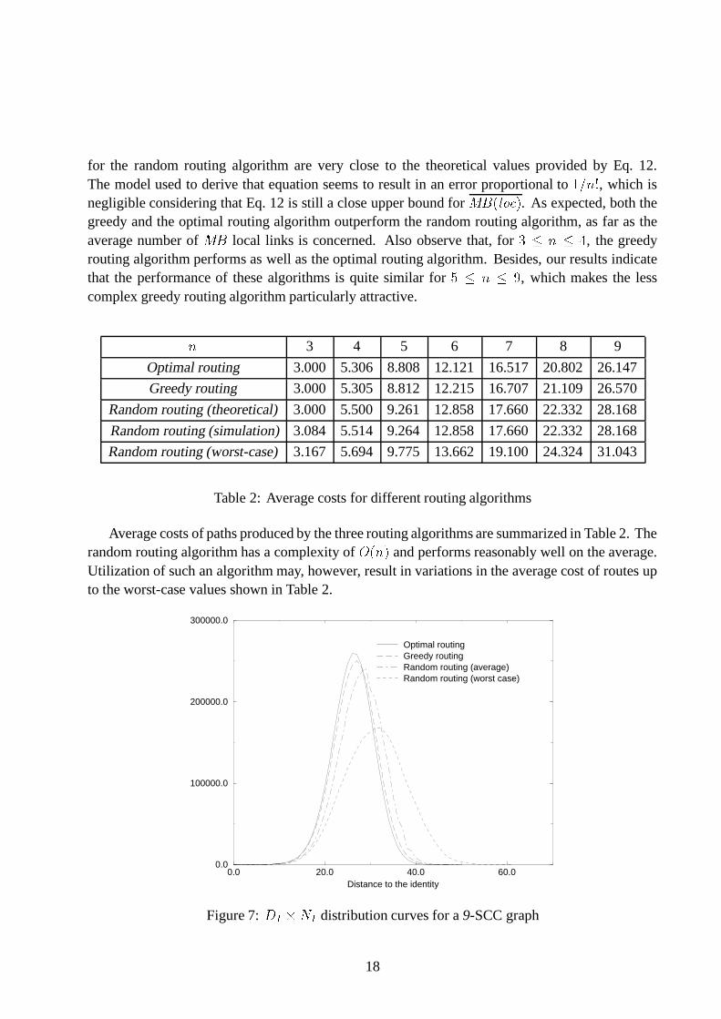
Figure 7:�� distribution curves for a 9-SCC graph

18

Figure 7 shows distribution curves comparing the three routing algorithms in the case of an�NM0M� graph. A point � �� in one of these curves indicates that the corresponding routing

algorithm will compute a route of cost� �

to the identity for � � nodes in the SCC graph. Theaverage distribution for the random routing algorithm is shown, but the results for that algorithmmay actually vary from the optimal to the worst-case distribution curves due to the non-deterministicnature of the algorithm. It is also interesting to observe that the greedy routing algorithm providesa distribution curve which is close to that of the optimal routing algorithm, presenting however asmaller complexity.

6 Considerations on wormhole routing

In this section, we briefly describe how the algorithms presented in the paper can be combined withwormhole routing [8], which is a popular switching technique used in parallel computers.

All three algorithms can be used with wormhole routing, when implemented as source-basedrouting algorithms [13]. In source-based routing, the source node selects the entire path beforesending the packet. Because the processing delay for the routing algorithm is incurred only at thesource node, it adds only once to the communication latency, and can be viewed as part of thestart-up latency. Source-based routing, however, has two disadvantages: 1) each packet must carrycomplete information about its path in the header, which increases the packet length, and 2) thepath cannot be changed while the packet is being routed, which precludes incorporating adaptivityinto the routing algorithm.

Distributed routing eliminates the disadvantages of source-based routing by invoking the routingalgorithm in each node to which the packet is forwarded [13]. Thus, the decision on whether apacket should be delivered to the local processor or forwarded on an outgoing link is done locallyby the routing circuit of a node. Because the routing algorithm is invoked multiple times while apacket is being routed, the routing decision must be taken as fast as possible. From this viewpoint,it is important that the routing algorithm can be easily and efficiently rendered in hardware, whichfavors the random routing algorithm over the greedy and optimal routing algorithms.

Besides being the most complex algorithm discussed in this paper, the optimal routing algorithmincludes a feature which precludes its distributed implementation in association with wormholerouting, namely its backtracking mechanism. Distributed versions of the random and greedyalgorithms, however, can be used in combination with wormhole routing. A sub-optimal distributedrouting algorithm which supports wormhole routing can be obtained by removing the backtrackingmechanism from Algorithm 3. Such a sub-optimal algorithm is likely to have computationalcomplexity and average cost that lie between those of the greedy and the optimal routing algorithm.

Due to its non-deterministic nature, the random routing algorithm also seems to be a goodcandidate for SCC networks employing distributed adaptive routing [13]. Adaptivity is desirable,for example, if the routing algorithm must dynamically respond to network conditions such ascongestion and faults. Some degree of adaptivity is also possible in the greedy and optimal routingalgorithms, which in some cases can decide between paths of equal cost.

19

7 Conclusion

This paper compared the average cost and the complexity of three different routing algorithms for theSCC graph. We divided the route between a pair of nodes in the graph into three components (laterallinks,

��local links and

��local links) and showed that only the number of

��local links may

be affected by the routing algorithm being considered. Exact expressions for the average numberof lateral links and the average number of

��local links were presented. Also, an upper bound for

the average number of��

local links was derived, considering a random routing algorithm. As aresult, a tight upper bound on the average distance of the SCC graph was obtained.

Simulation results for a random, a greedy and an optimal routing algorithm were presented andcompared with theoretical values. The complexity of the proposed algorithms is respectively �0�� ,

�0�� , and �0�� , where � is the dimensionality of the�NM0M �

graph. The results under optimalrouting produce exact numerical values for the average distance of

�NM0M �, for G ,<�B, �

.Our results indicate that the greedy algorithm performs as well as the optimal algorithm for

G�, � , � . The greedy algorithm also performs close to optimality for $�, � , �, and is

an interesting choice due to its �0�� complexity. The random routing algorithm has an �0�� complexity and performs fairly well on the average, but may introduce additional

��local links

in the route under worst-case conditions.Finally, we discussed how the routing algorithms presented in this paper can be used in asso-

ciation with the wormhole routing switching technique. Directions for future research in this areainclude an evaluation of requirements for deadlock avoidance (e.g., number of virtual channels).

References

[1] S. B. Akers and B. Krishnamurthy, “Group Graphs as Interconnection Networks,” Proc. 14th Int’l Conf.on Fault-Tolerant Computing, 1984, pp. 422-427.

[2] S. B. Akers and B. Krishnamurthy, “A Group-Theoretic Model for Symmetric Interconnection Net-works,” Proc. Int’l Conf. on Parallel Processing, 1986, pp. 216-223.

[3] S. B. Akers, D. Harel and B. Krishnamurthy, “The Star Graph: An Attractive Alternative to the � -Cube,”Proc. Int’l Conf. on Parallel Processing, 1987, pp. 393-400.

[4] M. M. Azevedo, N. Bagherzadeh and S. Latifi, “Broadcasting Algorithms for the Star-Connected CyclesInterconnection Network,” J. Par. Dist. Comp., 25, 209-222 (1995).

[5] M. M. Azevedo, N. Bagherzadeh, and S. Latifi, “Embedding Meshes in the Star-Connected CyclesInterconnection Network,” to appear in Math. Modelling and Scientific Computing.

[6] M. M. Azevedo, N. Bagherzadeh, and S. Latifi, “Fault-Diameter of the Star-Connected Cycles Inter-connection Network,” Proc. 28th Annual Hawaii Int’l Conf. on System Sciences, Vol. II, Maui, Hawaii,January 3-6, 1995, pp. 469-478.

[7] W.-K. Chen, M. F. M. Stallmann, and E. F. Gehringer, “Hypercube Embedding Heuristics: an Evalua-tion," Int’l Journal of Parallel Programming, Vol. 18, No. 6, 1989, pp. 505-549.

20

[8] W. J. Dally and C. I. Seitz, “The Torus Routing Chip,” Distributed Computing, Vol. 1, No. 4, 1986, pp.187-196.

[9] K. Day and A. Tripathi, “A Comparative Study of Topological Properties of Hypercubes and StarGraphs,” IEEE Trans. Par. Dist. Systems, Vol. 5, No. 1, January 1994, pp. 31-38.

[10] D. E. Knuth, The Art of Computer Programming, Vol. 1, Addison-Wesley, 1968, pp. 73, pp. 176-177.

[11] S. Latifi, “Parallel Dimension Permutations on Star Graph,” IFIP Transactions A: Computer Scienceand Technology, 1993, A23, pp. 191-201.

[12] S. Latifi, M. M. Azevedo and N. Bagherzadeh, “The Star-Connected Cycles: a Fixed-Degree Inter-connection Network for Parallel Processing,” Proc. Int’l Conf. Parallel Processing, 1993, Vol. 1, pp.91-95.

[13] L. M. Ni and P. K. McKinley, “A Survey of Wormhole Routing Techniques in Direct Routing Tech-niques,” Computer, February 1993, pp. 62-76.

[14] F. P. Preparata and J. Vuillemin, “The Cube-Connected Cycles: A Versatile Network for ParallelComputation,” Comm. of the ACM, Vol. 24, No. 5, May 1981, pp. 300-309.

[15] Y. Saad and M. H. Schultz, “Topological Properties of Hypercubes,” IEEE Trans. Comp., Vol. 37, No.7, July 1988, pp. 867-872.

[16] S. Shoari and N. Bagherzadeh, “Computation of the Fast Fourier Transform on the Star-ConnectedCycle Network,” to appear in Computers & Electrical Engineering, 1996.

[17] P. Vadapalli and P. K. Srimani, “Two Different Families of Fixed Degree Regular Cayley Networks,”Proc. Int’l Phoenix Conf. on Computers and Communications, Scottsdale, AZ, March 28-31, 1995, pp.263-269.

21

Documents

Average distance and routing algorithms in the star-connected cycles interconnection network