Portuguese Average Cost of Capital

1

Faculdade de Economia da UNL

Portuguese Average Cost of Capital – July 2009

Universidade Nova de Lisboa

PORTUGUESE AVERAGE COST OF CAPITAL

J. C. Costa, Mª Eugénia Mata, D. Justino1

July 2009

1 We thank the facilities we received from FEUNL, in particular from L. Catela Nunes in some technical areas and calcu-

lations, and from John Huffstot for correcting our English. Of course, all errors are our own.

2



Abstract

The oldest Portuguese share index still being calculated is the BVL/PSI-General, one which

started the daily series on 5/Jan/1988 with a base value of 1000 points. Everyday a single value is

computed based on the closing prices of all the shares included in the sample. Also, all corporate

events affecting the price of any share beyond market sentiment are taken into account through

proper adjustments, either in the numerator or the denominator of the formula.

However, for dates before January 1988, there is nothing comparable to this index since the two

different series known either never disclosed the methodology adopted to calculate the index or

followed solutions not compatible with the above index. The present paper explains the solutions

adopted to replicate as closely as possible the methodology of the BVL-General index to the main

market of the Lisbon Exchange for the period 1978 – 1987.

This is the first estimate of the historical Equity Risk Premium in Portugal above short-term risk-

free rate from the re-opening of the market following the Carnation Revolution (and the accompa-

nying nationalizations), to the present. In showing a value of the same order of magnitude found

in other countries, the paper invites further studies on the effects of political decisions such as pri-

vatizations and joining the European Union.

3



1. ECONOMIC RELEVANCE OF A GOOD ESTIMATE FOR THE COST OF CAPITAL

There are today four important areas in which a country needs to know its domestic cost of capital:

a) Capital Budgeting: ranking and selecting alternative projects requires discounting to the cur-rent date the future cash flows forecast for such projects, in order to check whether there is a

positive NPV added to the value of the company and, if so, which of those projects adds more

value within the constraints of the available cash budget;

b) Asset Allocation: to divide a portfolio of assets between shares, bonds, and others one needs to have estimates of the relative risks and rewards provided by each of those different competing

classes of assets;

c) Pension Funds: the goal is to determine how much to save today for a certain periodic pension

to be received (or to be paid) sometime in the future to some beneficiary. Whether the pension

plan is of the defined contribution or the defined benefit type, the side that bears the uncer-

tainty of the future returns is the only thing that changes;

d) Reward of Utilities Investments: when imposing administratively the selling prices of the ser-

vices provided by a monopolistic utility company, regulators must allow that firm to recover

fair but sufficient profits from the large investments made in the necessary infrastructures.

Unfortunately this discount rate is not known with certainty in any market. However, this does not

mean that one cannot make an estimate by observing the history of his own capital markets. That is

the purpose of this paper in relation to the particular case of the Portuguese domestic economy.

2. THE INTERNATIONAL EXPERIENCE

In recent decades, especially following the end of the Breton-Woods regime in the beginning of the

1970s, scholars have produced significant macroeconomic and financial studies that allow us today to

work with sophisticated mathematical models that help us to make difficult financial decisions, par-

ticularly in the investment selection process.

Some of these models require the input of an average cost of capital, the search for which has trig-

gered a number of other studies in many countries, especially in the UK and the USA, due to their

cultural environment and the availability of recorded historical data. But the success of the American

economy in the Twentieth Century may suggest higher than normal annual rates and that may be mis-

leading when extrapolated to other national economies. Therefore, some years ago three professors of

the London Business School – Dimson, Marsh and Staunton (DMS) – published a large study, involv-

ing 16 countries (including Spain), that covers the whole Twentieth Century2.

This study provided, for the first time, a long-run perspective for the cost of capital in the world, but it

also showed the diverse financial behavior of the sampled countries, as some of them had signifi-

cantly smaller capital costs in comparison with the historical values for the USA or for the UK.

2 “The Triumph of the Optimists: 101 Years of Global Investment Returns”, 2002.

4



This same study became such an important source of information, both for scholars and for practitio-

ners, that it has been updated annually ever since – and expanded later to a 17th country – thanks to a

co-operative agreement established between those three authors and the Dutch ABN-Amro Bank.

Unfortunately, Portugal was not included in that study, a limitation that might lead some our long-

term decisions to be taken based on the extrapolation of the cost of capital from countries considered

to be similar. The only study that includes Portugal was conducted by Jorion & Goetzmann3 but only

reports the period from 1931 to 1996 and it suffers from three limitations:

i) the authors had to make use of indirect sources of information for Portugal – especially the

“International Financial Statistics” published by the IMF;

ii) dividends are not included in the equity returns estimates, and this may undervalue the esti-

mate;

iii) the risk premium is measured as the capital returns in excess of inflation, not the risk-free rate.

The purpose of our paper is precisely to close that gap via an historical analysis identical to the one

conducted by DMF. Therefore, this is an investigation into the past of the Portuguese Exchange share

market to uncover any potential average return that, if stationary, may be extrapolated into the future.

It is not a forecasting exercise as performed by a number of scholars including, for example, recent

works from Goyal and Welch (2008) or Ferreira and Santa-Clara (2009), where some past eco-

nomic/financial variables are used to estimate the near future value of a stock return. Two reasons dic-

tated our option:

• an intention to make simply an historical survey;

• we are convinced that one of the main characteristics of any efficient market is that any method

accurate enough to deserve the attention of investors is immediately destroyed by the subsequent

decisions of those very investors. As Ferreira and Santa-Clara wrote “…to the extent that what we

are capturing is excessive predictability rather than risk premiums, the very success of our analy-

sis will eventually destroy its usefulness.” That is, unless a new and accurate methodology of fore-

casting is used only by its author – and for a limited period of time – any volatile future is impos-

sible to forecast with certainty. So, only stable values unveiled from the past can be taken into the

future without much risk.

3. LITERATURE REVIEW

3.a. Why CAPM Model

There is now a consensus that variability of share returns requires them, on average, to pay more to an

investor than debt instruments with similar maturity as a compensation for that uncertainty. That posi-

tive spread depends on the particular issuer under consideration, but for the whole share market of a

country there is an average difference that is called the domestic Equity Risk Premium (ERP).

There are different models that connect the individual spread of a particular share to the general mood

of the whole market underlying that particular issuer and/or to other macroeconomic variables of the

country, such as the annual GDP growth rate, some factors of the industrial sector involved, etc.

3 “A Century of Global Stock Markets”, NBER, February 2000.

5



However, any multivariable model requires the computation of a large number of parameters propor-

tional to the number of explanatory variables used by the model. In this respect, the particular case of

the CAPM model is very attractive because it uses only one explanatory variable – the market average

return – although this still requires the estimation of the three following parameters:

i) the cost of risk-free debt (Ri);

ii) the particular level of risk of the issuer (ββββi) ( )freemarketifreei RRRR −+= .β ;

iii) the average risk premium ( )marketR .

Therefore, the selection of the CAPM model is a simplification measure justified on the grounds of

the level of accuracy that it is still available, and also by the widespread adoption of similar ap-

proaches by other scholars.

3.b. Historical versus Future Returns

All four of the long-term decisions mentioned above are forward-looking computations and require

the use of a discount rate that shall be valid for the future, not a Cost of Capital that was in place in

the past. However, this single value is not observable in the market and there is as yet no known

model that quantifies such a value for any time-frame ahead. There are many studies that develop

methodologies for predicting the equity premium predictors4 but their results do not hold for the

1990s.5

Mehra and Prescott (1985) used an 1889-1978 data base for GDP and Consumption in the USA and

concluded that Arrow-Debreu asset-pricing models could not explain the high (American) equity risk

premium at the same time as the small average risk-free return that was historically observed. Rietz

(1988) re-specified that model for a frictionless pure-exchange economy and solved the puzzle in cap-

turing the effects of (possible) market crashes by abandoning the hypothesis that consumption growth

rates are symmetric about their mean (and fall above their mean as often as they fall below). Reason-

able degrees of time-preference and risk aversion were found, provided that plausible severe crashes

are not too improbable in the long-term analysis. Although crises are unlikely phenomena, they oc-

curred historically.

Barro and Ursúa (2008) went into full annual data on Consumption for 22 countries (including Portu-

gal) to detect crises, as this is the variable “that enters into usual asset-price equations”. To enlarge

the sample they also used GDP for 35 countries (including Portugal). For samples that start as early as

1870 (as is the case for Portuguese GDP estimations) a peak-to-trough method was used for each

country to isolate economic crises (defined as cumulative declines in Consumption or GDP by at least

10%) and 87 crises for consumption and 148 for GDP were discovered, leading to the conclusion that

3.5 years was the average duration for disasters, having a mean of 21-22% declines, under a coinci-

dent timing both in Consumption and GDP. The conclusion is that their model accords with “the ob-

served average equity premium of around 7% levered equity”, after assuming that 3.5 is the coeffi-

cient of relative risk aversion.

4 Fama and Schwert (1977), (1981); Rozeff (1984); Keim and Stambaugh (1986); Campbell and Schiller (1988 a, b); Fa-

ma and French (1988, 1989). 5 Lettau and Ludvigson (2001) and Schwert (2002).

6



It is little wonder that people began to look again into the past in order to estimate that historical cost,

hoping that the future would not be much different from that observed past6. That raises a number of

problems, however, in particular:

i) nothing guaranties a smooth replication of the past into the future;

ii) most countries did not accumulate enough information about their past – especially the distant

past – to produce reliable estimates of such realized cost.

These reasons led the whole financial industry to base their estimates for the Cost of Capital on the

single historical analysis that has been conducted by Ibbotson Associates for the US market, since this

country recorded a time series that runs uninterrupted from the beginning of 1926. Alternatively, the

industry turned to the UK market, where Barclays Capital and Credit Suisse First Boston both pro-

duced historical estimates for the British Cost of Capital from a series that starts in 1919. The similar-

ity of all three final results led most capital budgeting, fund management practice, and regulators’ de-

cisions to be made traditionally from that much known American ERP of (around) 8.5% p.a.7

Unfortunately, and more recently, this single “anglo-saxon” value became suspicious after the argu-

ments coming from two different grounds:

i) both DMS (2002) and Goetzmann (1999) conducted historical estimates for some countries (in-

cluding the US market) using data covering the entire Twentieth Century and obtained not a

single common historical rate, but a wide range of different domestic average share returns,

some of them significantly far from the US value, even after considering the impact of the vari-

ous currencies involved. On top of that, Schwert (1998) noted that, extending the US data base

backward to the beginning of the Nineteenth Century (a time series ca. 200-years long), the

American average Cost of Capital becomes much less than the traditional Ibbotson result, a fact

that may indicate that the risk premium may be non-stationary, and, if so, the future may be dif-

ferent from the observed past;

ii) an ERP of 8.5% is too large to be compatible with both the rate of long-term economic annual

growth of any economy (estimated to be around 2%) and the level of risk aversion normally ac-

cepted for an average investor (exponent γγγγ between 1 and 2).

In relation to the first criticism, such a time variability of the Cost of Capital within one single country

or among different countries makes sense, since markets inevitably comprise human beings and it is

known that their mood does change in response to the economic and social conditions surrounding

that market. That is, human reasons may determine, now and then, an adjustment of the equity spread

demanded by investors to take the risk of price volatility in tandem with those same environment

changes.

But why are the Ibbotson and DMS estimates for the US market (8.5%) so much larger than the

Schwert estimate (4% p.a.) for the same country? The answer comes from what is now called8 “sur-

vival bias”: investors demand an ERP not only to cope with the variability of stock returns, but also to

compensate them for the potential total loss due to rare but catastrophic crises that are always possi-

ble, as recorded in the history of any country. That is, although people only require an extra payment

6 Campbell and Thompson (2005), Hillebrand, Lee and Medeiros (2009). 7 This is the value indicated on the most recommended book, “Corporate Finance” by Richard Brealey and Stuart Myers in

its successive editions. 8 Brown, Goetzmann, and Ross (1995).

7



to invest in volatile shares, because shares also suffer from a kind of “credit risk”, the total premium

must be large enough to pay for both sources of risk9.

Indeed, during the entire Twentieth Century the USA was lucky enough to avoid the great turmoils

that affected, for example, Russia – two revolutions – or Germany and Japan – collapse of their

economies after the loss of world wars and/or of invasion by foreign armies. On the contrary, the US

economy developed throughout the same years in a rather smooth manner, in spite of some “minor”

crises that were observed here and there, such as the Great Depression of 1929 and the two oil shocks

of the 1970s and 1980s In any case, the American financial market never closed for extended periods,

there was no major nationalization affecting large sectors of that economy, and there were no signifi-

cant social events affecting the nation. On the contrary, in the previous century there were the 1812-

15 War with the British empire and the major Civil War (1861 to 1865), which brought vast devasta-

tion to some important regions of that country, and these may explain that, extending the time series

to include these last 100 years, the average equity return becomes closer to the observed values of

those other more unstable countries.

Under this interpretation, the high ERP observed during the Twentieth Century in the US market

would be the result of a pessimistic view of the average American investor during those recent 100

years that required them to demand a compensation to cover the expected volatility of returns plus the

risk of a potential total loss. But, in the Nineteenth Century, the realized ERP already incorporates the

actual losses of those catastrophic years, and this could explain the much lower premium found ex-

post.

As to the second criticism, there are two economic models that suggest that the 8.5% ERP estimated

for the US market must be too large a figure:

i) Gordon´s constant growth model10 for corporations allows us to estimate the ERP from

1

0

real real

DERP g r

P= + −

where g is the constant growth rate of the company, and D/P is the percent return obtained from

the amount D1 of (next year) dividends received from a share currently priced at P0, and r is the

cost of debt. For annual dividends on the order of 3% to 4% of P and a real return of long-term

debt of around 2%, an annual ERP of 8.5% requires a growth rate larger than 6% p.a.,11 which

can only exist while a company is still in its infant stages of development12. But even that

model is over-optimistic since it assumes a constant rate g forever. For a more realistic model

with rates of growth decreasing from an initial high value, as the company matures, the dis-

count rates of future dividends must be less, meaning a smaller ERP than under the constant g

model;

9 As Jorion & Goetzmann (2000) stated: “To the extent that the event causing the break was anticipated, the market seems

to have been able to gauge the gravity of the unfolding events. Price declines before breaks is consistent with increasing

demand for risk compensation for a catastrophic event”, page 14 . 10 Gordon, Myron J. (1959). "Dividends, Earnings and Stock Prices". Review of Economics and Statistics 41: 99–105. 11 See Annex II 12 Otherwise – if unabated – that company would, sooner or later, become larger than its surrounding economy. Note that

the consensus is for a long-term growth rate of any economy of about 2% p.a.

8



ii) Consumption-based asset pricing seeks to estimate the ERP from economic theory, as that pre-

mium ought to be the expression of the risk aversion of investors, since the securities’ extra re-

turns are the price of deviating consumption from today into the future. The appropriate meas-

ure of the risk of investing in volatile assets is to assess the impact of that investment on the

riskiness of future consumption. This leads us to the recognition that the key to investment risk

is the correlation between asset returns and consumption variation: the higher that correlation

the more risky are those assets because they pay off more precisely when consumption is al-

ready high, and vice-versa

RC σσργ ... ∆=Asset an for Premium Risk

Here γγγγ is the average investors´ risk aversion and ρρρρ is the correlation between the percentage change in consumption ∆∆∆∆C and the asset return R. Once again, for normal values of these four

parameters13, the equity risk premium obtained would be about 100 times lower than the em-

pirical findings. Any accommodation based on accepting values of γγγγ much larger than the

classical range14 is not possible because that would require extremely large real interest rates,

which were never found in any market for a prolonged period of time.

It has been suggested that this consumption model might be either too conservative or too rational. As

to the conservative side, Campbell and Cochrane (1997) proposed a change in the utility functions

such that “as consumption drops toward the accustomed standard of living X, people become more

risk averse because they are less willing to accept further declines in consumption”. That is, γγγγ is not constant and can become much larger than in classical models, especially when consumption falls and

approaches that habit level.

On the psychological front, the development of Prospect Theory by Tversky and Kaheman (1992)

allowed bringing some irrationality to the explanation of market behavior. This is what Benartzi and

Thaler (1995) did:

a) investors care more about the returns obtained than about the value of their portfolios;

b) since losses are particularly painful, some investors do not evaluate returns everyday, but only

at large intervals of time, avoiding the useless pains due to temporary losses;

c) so, those investors evaluating their portfolios everyday require a large risk premium to hold

shares instead of bonds, but those taking large time intervals between evaluations have smaller

probabilities of losses and require smaller risk premia;

d) therefore, there many different risk premia in the market and such values may change over

time according to the average time horizon of evaluation of investments.

In summary: since the known theoretical models are not yet able to supply reliable figures for future

values of the ERP, we are left with the classic approach of estimating the future from the recorded

past. However, the Ibbotson figure sounds exaggerated, not only for the US market, but also for other

countries, suggesting that the best each country can do is to develop its own data base of stock returns

and extend it backward as far as possible to improve the quality of the estimate.

13 Normal orders of magnitude: γγγγ = 1 or 2, σσσσ∆∆∆∆C is around 1% p.a., σσσσR around 20% p.a. and %20≤ρ .

14 Even if we are slightly more generous and accept γγγγ around 10 and ρρρρ around 40%, we find a risk premium of about 0.8%

p.a.

9



However, this avenue raises some problems:

i) is the historical sample large enough to produce estimates falling within narrow confidence in-

tervals?

ii) what if the ERP is itself variable?

This question of non-stationarity is crucial for historical estimates because the most simple analysis

has implicit the assumption of stationarity. But there are reasons for suspecting that the true ERP may

be changing over time, a fact that is in agreement with some tests that reveal statistically significant

changes in market variability. So, unless we have a model of how the ERP varies over time, we may

be misled by historical data and/or we obtain extremely large confidence intervals even from century-

long time series.

Fortunately, there are also arguments in favor of giving some value to the results linearly extrapolated

from those historical series:

a) as mentioned above, one of the most comprehensive analyses was conducted by DMS (2002)

for the entire Twentieth Century and covers 16 countries that represent more than 95% of the

free-float market capitalization of all world equities at the start-2002; although the historical

average of Risk Premium15 varies among those countries, that premium is always positive and

covers a range (arithmetic averages) between 3.2% and 10.6% p.a.;

b) this large range of values is compatible with the different histories followed by the various

countries in the sample, especially catastrophic events such as revolutions, nationalizations,

etc. that plagued them;

c) the average volatility of returns shown currently by most indices – around 15% p.a. – suggests

that 100 years of history is not enough to reduce the uncertainty of the estimated average eq-

uity returns; that is, the confidence interval anticipated for those averages is still too large16;

but is also compatible with the above range of values;

d) even if the return demanded from shares does vary over time, it is difficult to accept that it

took some fixed value in the past but, from now on, has definitely changed; most likely, it has

changed a number of times in the past – following the business cycle – without any up or

down trend, and will do the same in the future; therefore, the average past of each country may

not be very different from its future, and we can approach that historical average provided our

data base covers a number of different business cycles;

e) although there is a minimum rationality in price formation, recent studies have revealed the

degree of irrationality present in this particular area of human behavior; so, it is possible that

the high values of risk premium found in the past series are a simple reflection of some of

those irrationalities and, unless we assume that mankind will change in the future and be fully

rational from now on, we cannot reject those high ERPs.

All in all, it seems that our low level of knowledge of these matters still recommends the use of the

past as the “least worst” predictor of the future.

15 Relative to T-Bills, not to T-Bonds. 16 Bradford Cornell: “…72 years´ worth of data is not enough to measure the risk premium with sufficient precision to

satisfy most investors … even if it is assumed that the future is like the past, the estimates are so imprecise that it is not

clear what the risk premium has truly been in the past”, page 44.

10



3.c. Main Sources of Practical International Data

Every year the Ibbotson Group publishes a number of studies updating the statistical information from

a number of countries: Ibbotson Associates - Stocks, Bonds, Bills, and Inflation Yearbook.

Since the publication of “The Triumph of the Optimists” in 2002, which covered 101 years of 16

countries, the London Business School and the ABN-Amro Bank have partnered to update those his-

torical results every year and to extend that type of analysis to a 17th new country.

Prof Damodaran also maintains a page on his website – http://pages.stern.nyu.edu/~adamodar/ –

where some statistical data are also accessible, in particular the historical cost of capital.

4. CONSTRAINTS OF THE PORTUGUESE CAPITAL MARKET

4.a. Liquidity Constraints in the Stock Exchange

Most share markets in small countries show low levels of liquidity, due mostly to that reduced eco-

nomic dimension that translates into a small number of large domestic corporations that are listed, in

parallel with insignificant foreign investors´ interest in all domestic companies. However, the situa-

tion in Portugal during the 30 years under analysis shows some additional constraints stemming from

the following:

a) by tradition, the largest source of funding of our domestic businesses is bank credit, not share-

holders’ capital; the banking segment has always overshadowed the capital market in this

country;

b) during 1975 (following the Carnation Revolution in 1974), a large slice of the economy was

nationalized – implying that the number of listed companies dropped significantly in one fell

swoop – and all overseas companies listed on the Lisbon Exchange ceased their operations fol-

lowing the political independencies (under leftist governments) granted to those overseas terri-

tories in that same year.

Adding to these limitations, the operations of our two domestic Exchanges were suspended on the 25

of April 1974, only reopening for share trading in March 197717. All in all, these factors determined

that, when trading in shares restarted, the number of listed companies was extremely reduced, none of

them were large entities, and investors were very risk averse due to the traumas brought recently to

them by the political and economic events following the Revolution.

Fortunately, in a few years it was possible to overcome most of these fears and to re-establish a “nor-

mal” capital market that was open to foreign investors and mature enough to accommodate the large

privatization program the country executed during the 1990s. That “miracle” was “bright” enough to

call the attention of some other European Exchanges, a fact that led in February 2002 to the merger of

our two domestic organized markets with the Euronext Group18.

17 Although the order from the government was dated from the 4th of March, 1977, only on the 7th March was trading re-

sumed. Meanwhile, the Porto Exchange remained closed until 1981. 18 Later, in April 2007 this pure European Euronext Group merged with the NYSE Group to form the current transatlantic

NYSE Euronext Group.

11



4.b. Share Indices in Portugal

To the best of our knowledge, only very late in the Twentieth Century did Portugal start to compute

share indices according to the standards of any other developed capital market. In fact, it was only in

February 199119 that the Lisbon Stock Exchange launched a capitalization-weighted share index –

then called the BVL-General Index20 – with a time series dating back to the first trading day of 1988.

This index is still being calculated once a day and released after the close of the trading session. There

is only one single value per session because it is based on the closing prices of all shares that are listed

in the main segment of our domestic Exchange market.

This initiative of the Lisbon Exchange was a response to the drawbacks arising from the two share

indices that existed at the time (beginning of 1990s):

a) the Totta & Açores Index was calculated and published everyday by the local Totta & Açores

Bank, but with a methodology for the selection of the companies to be sampled and a set of

rules for translating the corporate events in the daily index value – dividend payments, stock

splits, etc – that were never made public, thereby casting a shadow of representativeness over

the values of this index;

b) the Banco de Portugal (monthly) index was based on all the companies listed in the main mar-

ket of the Lisbon Exchange, but it weighted each share price by the corresponding traded vol-

ume, a method that overvalued those securities having more trades, not those with more capi-

tal placed in the market.

The panorama before the Carnation Revolution of 1974 was similar to that just described, although

both the Banco de Portugal and the Portuguese National Statistics Office were developing some indi-

ces to measure both the overall volume of trades and the average prices.

It is important to note that the reason for the Lisbon Stock Exchange to start that index time series

only in 1988 is connected to the liquidity problems mentioned to above:

• before 1988, a significant number of listed shares frequently showed zero transactions in a

trading session;

• when some trades took place, the number of securities transacted was very thin, raising ques-

tions about the economic representativeness of those agreed prices.

Currently the Portuguese Exchange computes some other share indices, in particular some sectorial

ones alongside a short index comprising only 20 companies. The reasons that led us to emphasize the

BVL-General index in our analysis were the following:

• it is the largest and most diversified sample, as it uses all companies with shares listed in the

main market, not only the 20 most “representative” ones as does the PSI-20 index;

• it includes large and small corporations, therefore any potential size effect is diluted in the

sample; this criterion excluded all sectoral indices from our choice;

• it corrects for dividend payouts of the sampled shares, a feature that the PSI-20 index does not

include;

19 Included in the Daily Bulletin of the Exchange, for the first time, on 25

th February, 1991.

20 This index was later renamed as PSI-General.

12



• most important, it is the longest time series available: against a base date of 5/Jan/1988 for this

index, all the sectoral indices start at the beginning of 1991, and the PSI-20 index starts on the

very last day of 1992.

4.c. Risk-free Interest Rates

Although it is understood that an Equity Risk Premium (ERP) measures the average excess return

demanded by investors to take the uncertainty of the subsequent rewards obtained from those equities,

there is no consensus about the maturity of the debt instruments that should be used as that reference

basis: a short-term or a long-term rate?

At first sight, long-term rates would be preferable as they also incorporate a premium for the long ma-

turity of the credit: it compares similar alternatives for funding new projects. However, long T-Bonds

also suffer from high volatility of returns due to the variability of the interest rates in the market –

which includes the effect of inflation variation – whereas short-lived T-Bills are much less vulnerable

to the current price of money, and inflation is always factored in when each new issue is placed in the

market.

This justifies the frequent double disclosure of ERP – excess above T-Bills and above T-Bonds –

adopted in a number of countries. This is important because, in the history of every country, there are

periods of high unanticipated inflation rates that justify long periods with negative returns from long-

term bonds if previously issued with low coupon rates. Those negative returns may mislead us when

subtracting the inflated average equity return from such negative debt returns, leading to an exces-

sively large ERP.

It is also not clear which level of credit risk imbedded in that interest rate can be accepted in a real

case: the cost of money for operations with a Central Bank (or a National Treasury) or the rates of the

Interbank Money Market, which still have some residual credit risk included.

Fortunately, the limitations of the Portuguese money market simplified our decisions in this regard:

a) because the Portuguese T-Bills were created only in 1985 and that market was closed tempo-

rarily from 1998 to 2003, we were forced to exclude this source of information;

b) during the first years of the period under analysis, the interest rates defined by our Central Bank resulted from the economic policies of the government of the day, not from any consid-

erations of monetary policy; obviously also excluded;

c) although in the time window analyzed our Interbank Money Market offered rates for a wide

range of maturities – from overnight credits to one-year operations – the clear majority of the

liquidity in that market was always concentrated in the short-term end of that spectrum.

Therefore, we excluded the T-Bills source, opted instead for the Interbank Money Market21 (IMM)

rather than Central Bank rates, and used only Overnight rates22 (O/N). Note that, in a number of coun-

21 So our “risk-free rates”, although very short-term, involve some residual credit risk.

22 But some details are in order at this moment:

i) when, after July 1993, the domestic market began to offer three Overnight rates – for the same day, for the next

day and for two days ahead – we selected the same day O/N case

ii) but during some years that shortest term segment included 24-hour to 72-hour maturities, without any distinction

between the three cases.

13



tries, the risk-free rate is “borrowed” from the issuing rate of one-month T-Bills, but we assumed that

the difference between the overnight and one-month rates was always significantly less than the esti-

mation error of the average rate of return of shares.

Finally, it must be said that due to the closing of the Portuguese IMM market at the end of 2008, we

continued our time series toward 2009 using the EONIA daily rate as the representative Portuguese

short-term interest rate.

4.d. Long-term memory of defaults

The confidence in Portuguese T-Bills as risk-free assets deserves some additional comments. Al-

though it might be thought that T-Bills are risk-free because they represent a governmental commit-

ment for the near future, historical events in Portugal during the Nineteenth Century explain why our

treasuries cannot be used as such, at least for a significant part of the 1800s and the initial part of the

Twentieth Century.

In fact, the confidence in our treasury debt instruments was very low during the second half of the

Nineteenth Century, when the total amount of public debt increased dramatically every year, thanks to

a large surplus of public expenditure over the simultaneous tax collection. The result was a low mar-

ket price for their placement in all the European capital markets. That is, the Portuguese government

of that time was forced to issue high nominal amounts of public debt but could only receive much

lower cash amounts from the few investors available.

Such negative historical experience ended with the declaration of a bankruptcy in 1892 (decree of 13

June), when our government declared that it could not fulfil all the debt contracts signed with its for-

eign lenders, following the abandonment of the gold-standard just the year before (July 1891). That

default meant that:

a) all amortizations of treasuries were suspended;

b) the country would pay only 1/3 of all interests due under those contracts.

Of course, even before this partial default, a number of public sources already raised the fear about

the Portuguese debt, as our credit rating was decreasing long before that partial bankruptcy. Special-

ized newspapers disclosed information on the prices and rewards of our bonds and bills during that

pre-bankruptcy period, and the returns demanded from those instruments increased in tandem with the

mounting fears on the risk level of Portugal. The negotiations with the creditors after 1892 lasted for

ten years, leading to an agreement only when a conversion of the loans was achieved in 1902 (law of

14 May).

The fact that capital markets do have memory means that investors always make their decisions based

on a stock of accumulated knowledge, and the reality is that, between 1870 and 1913, the coverage of

all types of news about Portugal, in the Times of London, reached an annual average of 102 reports.

The ratio of good to bad economic news that was reported was 1.12%, exceed only by Russia among

14



a sample of 16 following countries: Argentina, Brazil, Canada, Chile, China, Colombia, Costa Rica,

Greece, Egypt, Hungary, Japan, Mexico, Queensland, Sweden, Turkey, and Uruguay.23

Such a poor performance closed the doors to Portugal in all international credit markets, and only dur-

ing the First World War could a loan be obtained from the UK, in spite of the special relationship be-

tween the two countries.

In the Twentieth Century, the events in the 1960s and 1970s were also detrimental for investors’ con-

fidence in our capital market. Colonial wars began in 1961, damaging colonial exports from the zones

under military pressure in the colonies. The effort to fight the war led to a different allocation of re-

sources and to uncertainty and even adverse perspectives on the future for the colonial firms. The Car-

nation Revolution in 1974 brought about a new political model based on socialism that was conse-

crated in the 1976 constitutional text. Very soon dozens of political parties were organized, most of

them leftwing-oriented. The Communist Party performed an important role, while radical policies

were adopted. Nationalizations of banks and firms in the main economic sectors (insurance, large in-

dustries, and road transports) were carried out in 1975, while land expropriation in the large-property

districts of Alentejo and Ribatejo was also executed. Transactions in the domestic Stock Exchanges

were suspended in 1974 and the decolonization of all overseas territories left Portugal confined to her

European territory plus the tiny Atlantic archipelagos of the Azores and Madeira.

Half a million Portuguese who were living in the colonies left for Portugal in 1974-75 (representing

over 5% of the Portuguese population). Government efforts were then required to support them in

their beginning of new economic activities in the territory. On top of that, a severe economic reces-

sion in the country brought problems to our balance of payments. Export difficulties led to the cur-

rency depreciation in 1977, and the IMF help was required in this same year.

Confidence in the prosperity of Portugal under the new democratic regime was based on the project of

joining Europe, a hope that was fulfilled only in 1986. In fact, the 1972 free-trade agreement with the

then EEC was, in 1976, transformed into an association treaty to which a membership application fol-

lowed in 1977. However, the negotiations dragged on for years, and the 1980-83 recession demanded

a second intervention of technical and financial help from IMF for the period 1983 to 1985.

Portuguese membership in Europe was finally achieved in 1986, together with Spain, in a decade that

prepared Europe for further consolidation after the communist political regimes collapsed in the

1990s in Eastern Europe and Russia. The integration of the Democratic German Republic and the

Maastricht Treaty led to the European Union, while in Portugal, a social-democrat government began

a privatization program.

Only at the end of the 1990s, when it became clear that Portugal would become a member of the first

wave to enter the single European currency24, did our level of risk start to decrease, reaching the low-

est levels for more than two centuries.

23 Magee, Gary, La Trobe University, “Investors, information and the British world, 1860-1913”, paper presented at the

EBHA, Milan, 2009. http://www.hnet.org/~business/bhcweb/annmeet/abstracts09.html#magee 24 Mind that the Euro was first introduced in January 1999 simply as a virtual currency, while all legacy coin and notes

were introduced only in 2002.

15



5. THE ECONOMETRIC MODEL

5.a. Stochastic Behavior

Although it is known that the stochastic model adopted by Black and Scholes (B&S)

tdtdtSdS εσµ .... += where )1,0( Nt ≈ε

does not correctly describe the random behavior of the share prices, we have assumed it to be accurate

and simple enough to deserve our attention. Therefore, we took that model to justify the regression

that we used to estimate the historical average return provided by the Portuguese shares during the

31.5 years of our sample25. That differential equation can be transformed into

[ ] tdtdtSLnd εσσ

µ ...2

)(2

+

−=

or

( )4434421

444 3444 21 noise"" random

termtic determinis

tT tTtTSLnSLn εσσ

µ ...2

)()( 00

2

0 −+−

−+=

and that suggests that the log values of the share prices – or of the index – follow some straight line

with a slope given by

−

2

2σµ . It was this suggestion that led us to fit a line to the historical peri-

odic log values of the Portuguese share index recorded during the years January 1978 to June 2009.

5.b. Historically Realized Return or a Trend Curve

From a series of historical index values, the first impulse is to estimate the historical annual return

from the arithmetic average of the n periodic returns observed during the entire sample26

n

R

R

n

i

historic

∑= 1

25 Some scholars have studied other Stock Exchanges and found that, for some of them, a Mean Reverting model of peri-

odic returns could well describe their stochastic behavior. In our case and for the period analyzed, an adjusted autoregres-

sive model AR(1) produced an R2 of only 0.07. However, this is not a universal view and some countries have even shown

a change from such a mean reverting model to a random walk behavior. Due to that low R2, and because there is yet no

consensus in academia about this question, and since mean reverting is against the logic of market efficiency, we adopted

the B&S model. 26 We obtained an historical average of 15.9% p.a. (365 days), an annualised σ = 9.5% and an error of 4.5%.

16



However, due to the use of logarithmic periodic returns, this average coincides with

0

0 )()(

tT

SLnSLnR Trealized −

−=

But that raises an important issue: this estimate does not take into account the particular evolution of

the index between those two extreme dates. It is irrelevant whether the initial S0 and/or the final value

ST corresponds to a peak (or to a trough) of a euphoric (or pessimistic) period, because the final result

is always determined solely by those two extreme prices.

t0 T

The consequence is that the estimate obtained from a short slice of history is crucially sensible to the

starting and closing dates, particularly if either of those two prices is significantly deviated from the

“average value” of the index at each time. This drawback can be minimized only for extended time

series because:

a) based on the B&S stochastic model, the deterministic term of the difference between the final

and initial log prices grows linearly with the interval between the extreme dates, while the dis-

turbing random term grows only with the square root of that same time span;

b) therefore, even if the slope

−

2

2σµ is small, this deterministic term will sooner or later do-

minate the random component, for intervals of time long enough to compensate for that re-

duced trend.

That is, according to the B&S stochastic model and for very long time series, most of the difference

between Ln(ST) and Ln(S0) is due to the deterministic term – the slope of the line – because the ran-

dom term affects that average only marginally. In our case, we have around 30 years of data and, for a

common value σσσσ = 15% p.a. and for an average annual return of

−

2

2σµ = 10% p.a., we obtain:

“Below”

Average Below

Average

“Above”

Average

“Above”

Average

Over estimate

Under estimate

17



i) an accumulated return during the 30 years of %30030%10 =× ;

ii) and an accumulated volatility, in the same period, of %8230%15 =× .

These figures mean that we have only 5% of probability that the average annual return falls outside

the range [ ] 30/%822%300 ×± , that is, it falls between 15.5% p.a. and 4.5% p.a.

Of course, the longer that time series, the smaller will be the impact of that noise term in the size of

the confidence interval. It is this fact that only justifies the use of the realized return – the actual dif-

ference between the two extreme values – for estimates of the historical cost of capital when one has

more than one century of continuous time series.

As a second best alternative we decided to estimate that average annual return adopting the logic of

curve fitting.

5.c. Fitting an Exponential to the Historical Index Curve

Since there is a consensus that shares must provide investors with a certain expected periodic return –

although disturbed by a permanent “noise” – one can anticipate that all share indices will tend to

evolve through an “oscillating flight” around a “middle of the road” exponential line. The degree of

deviations from that ideal trend curve will depend on the level of volatility σσσσ around that average ex-pected periodic return. Of course, things can be linearized by taking the logs of all index values.

That same purpose of fitting a straight line to the series of log values of the index comes also from the

idea of estimating the parameters of the B&S model using the maximum likelihood method:

( )( )∏

−−−n

12

22

0 .2

)()(exp

i

ii tSLnSLnMaximize

σ

σµ

which leads, in essence, to the minimization of the square distances between the measured points of

the log index and the estimated best-fitted line.

There are, however, some particularities that cannot be overlooked:

a) the model assumes that the distribution of log prices around the straight line follows a Normal

function with a standard deviation that grows over time, a fact that cannot be taken as granted

because i) there are empirical findings that suggest that σσσσ is heteroscedastic, and ii) because there is frequently autocorrelation between successive returns (potentially, a residual charac-

teristic of a certain mean reverting behavior27);

b) there is a strong autocorrelation between log prices because any realized price for time ti is

almost entirely defined by the value of the same index for the previous moment ti-1.

27 For our weekly sampled series, the autocorrelation of returns is 0.267 for one week lag, 0.260 for two weeks and 0.074

for three weeks.

18



That is, the simplest form of the Ordinary Least Squares methodology for the line fitting has to be re-

placed by a more elaborated alternative that takes into account the variability of σσσσ and the intense autocorrelation along the time series of log prices.

In summary, we estimated the average historical annual return using 31.5 years of the Lisbon Stock

Exchange history and fitting a straight line to the log values of the share index covering that entire

sample, not forgetting that this time series could show strong autocorrelation and some heteroscedas-

ticity.

5.d. Measurement Errors

As mentioned above, in a significant number of days during the 10 years from 1978 to 1987, many

listed shares included in the index did not trade at all. In spite of that, when no agreed price existed,

the daily index was computed using the average value between the Bid and the Ask prices as a second

best alternative to such an equilibrium quotation. However, this decision introduced a source of error

because we knew only the range – between the two values – where any equilibrium price could have

been struck.

That is, extending the time series backward from the beginning of 1988 to January 1978 produces a

set of index values with some measurement errors. One of them is due to this Bid/Ask spread and that

can be easily estimated, but some others can only be mentioned:

a) some companies only offered either a Bid or an Ask price, and that puts a limit to the range of

potential equilibrium prices on one side only; additionally, it is not possible to make an esti-

mate of an individual error for those days and for those shares where only one side is dis-

closed;

b) even for those shares with an equilibrium price struck for the day, the very low volumes of

shares actually traded raises the question of the representativeness of that quotation.

All of this suggests that the fitted straight line is estimated in the context of an input data (Y, X)

where there are some measurement errors only in Y, not in X. But since those sampling errors do not

affect the value for the estimated slope ββββ,,,, but lead only to a confidence interval for that estimate a lit-

tle larger then the real one, this specific subject of error does not affect our estimate and can be left for

a future paper.

6. A FIRST SAMPLE OF THE PORTUGUESE MARKET

6.a. Extending the sample backward

While still collecting data to construct a full series of index prices for the entire Twentieth Century,

we were tempted to take a first glimpse of the Portuguese market by analyzing of the behavior of the

BVL-General Index published since the beginning of 1988.

19



However, that sample suffers from two important drawbacks: the base date – 5 Jan 1988 – happens to

exist exactly in the aftermath of the October 1987 speculative crisis, and, additionally, the market is

currently very depressed. Therefore:

a) one may suspect that the initial value of the index might be above the long-term trend of the

market due to the heavily “inflated” quotations observed during October 87; the market was

still returning to the “normal” levels during January 1988;

b) the current index values might be too depressed because we are near the trough of the current

financial crisis, which is far below “average”;

c) adding these two factors might produce an estimate for the average historical cost of capital

clearly below a long-term trend.

We therefore felt the necessity to tap the domestic market before January 1988 in order to minimize

the impact of that base date and also to enlarge the size of our time sample. In the end, we were able

to add 10 more years to the existing 21.5-year series by computing a share index for the years 1978 to

1987, thus fabricating an uninterrupted 31.5-year long time series. In further studies, we plan to ex-

tend that index series toward the beginning of the Twentieth Century so that we can work with a sam-

ple of the same size as those used by other authors for other countries.

6.b. Sources of Information for the period 1978-1987

Our main source of numerical data was the collection of Daily Bulletins published by the Lisbon

Stock Exchange for the period 1978 to 1987, available from the Documentation Center of the Lisbon

Exchange. Similar data from the Porto Stock Exchange were not used because this market was closed

until 1981 and also because, even after that date, it accounted only for a minor volume of the domestic

secondary market during the clear majority of the trading days.

Prices and quantities were collected only for Wednesdays in order to minimize the potential impact of

the weekend effect, if any28. In the event that Wednesday happened to be a bank holiday, the follow-

ing Thursday was taken, except if the market was also closed, in which case we took the best alterna-

tive available to represent that very same week.

For the purpose of constructing a share index, it was crucial to have information concerning all the

corporate events that affected all the firms included in the index. Three main sources were used for

this: the notices obligatorily published in the Lisbon Exchange´s Daily Bulletin by all listed compa-

nies, the Annual Report of Activities for the relevant years of the Lisbon Stock Exchange, and some

other statistical products published by the same Exchange.

Based on these sources, it was possible to adjust the weekly values of the index for all the corporate

events that were detected for each of the firms included in the sample of the index. Note that this

means in particular, that the reconstructed index measures the total return of the market - dividends

plus capital gains/losses – not only price averages.

28 Note also that, until May 3rd 1989, the Lisbon Exchange traded only four days a week. Reasons are mainly connected to

the manual workload associated with Netting and Settlement of all past trades. Also, from the reopening in 1976 until Sep-

tember 20th 1978, there were only three sessions per week, on Mondays, Wednesdays, and Fridays.

20



6.c. Tackling the Liquidity Constraints

i) Agreed Quotations versus Bid/Ask During the 10 years from 1978 to 1987, the trading mechanism in use at the Lisbon Exchange was

one single auction per trading session per security. This Roll Call trading system called every se-

curity one at a time, and an equilibrium price was then searched by the brokers in order to maxi-

mize the number of shares that could be traded29.

As mentioned above, on a number of days, buy and sell orders for a number of issues did not clear

at all, and no trades were possible on that particular day for that security. However, this did not

preclude the market having information of the best buy and best sell offers entered into the auction

crowd. Of course, these Bid and Ask prices did not represent an agreed quotation, but they were,

nevertheless, an indication of the general level of prices that the market was attributing to those

shares on those days.

Therefore, our option was to calculate the share index either with the single daily (agreed) quota-

tion found in the auction – when that information was available – or with the simple average be-

tween the corresponding Bid and Ask prices. Also, in a few cases, we used only the Ask or the

Bid if that was the sole information disclosed in the Bulletin, and this in order to avoid computing

the index with a very small pool of companies.

ii) Weeks with no price information Unfortunately, for a few days, not even those isolated Bid and Ask prices were available, either

because the security was suspended from trading (due to some corporate event), or because there

was no interest in entering orders to the market. When such interruption extended only to one week

or less, the index was calculated for that particular missing Wednesday assuming that the market

would have priced that share exactly as in the previous week. But, for longer interruptions, that

particular company was temporarily excluded from the index until its trades later resumed.

iii) Market without Quotations From February 1983 onward

30, the Exchange market was divided into two segments:

• The so called “Official Market” – the main market – where the larger and “senior” compa-

nies could list their shares;

• and the “Market without Quotations” created to trade (but not list) some junior companies

or the provisional certificates of shares (and bonds) issued by corporations already listed,

while their final paper certificates were being printed and distributed among the investors.

These differences between the two segments suggested to us to use only the firms listed in the Of-

ficial Market, but to take into account all the shares already issued by a listed corporation (if fully

liberated) when computing the capitalization weight of that particular component of the index.

iv) Selection of Companies to compute the Index Due to the restricted number of corporations that had their shares listed in the main market of the

Lisbon Exchange, we decided to use almost all of them, with the few exceptions of those so small

or so infrequently traded that their contribution to the final value of the (capitalization weighted)

index would be negligible.

29 There were additional criteria for the case of more than one price of equilibrium maximizing the volume of trades.

30 See Daily Bulletin for 13 January 1983

21



Year 1st Semester 2nd Semester

1978 14 14

1979 16 16

1980 17 17

1981 17 17

1982 16 16

1983 17 17

1984 19 19

1985 20 20

1986 27 27

1987 46 63

198831 Max = 128/Min=80 Max=154/Min=123

In the later years of the 10-year period, a growing number of companies opened their capital to

public investment and had their shares listed in our main market, most of them with so significant

a size that they deserved their inclusion in the index from the very beginning of their listing. The

above table indicates the number of companies in the index throughout the period.

The next Figure compares, per week, the number of companies in the index sample with those that

actually traded on the Wednesday representing that particular week. The panorama clearly im-

proved from 1978 to 1987, which explains why we excluded the first year (1977) after the trade

suspension imposed by the Carnation Revolution.

INDEX SAMPLE AND TRADING

0

5

10

15

20

25

30

35

40

45

50

55

60

65

04/01/78 04/01/79 04/01/80 03/01/81 03/01/82 03/01/83 03/01/84 02/01/85 02/01/86 02/01/87 02/01/88

Nº of Companies in the Index and of those that traded

Nº of Companies that traded on Wednesday

NNº of Companies in the Index

31 1988 is the first year of the already existing BVL-General Index time series

22



6.d. Heteroscedasticity and Autocorrelation

i) Autocorrelation It is frequently said that shares tend to exhibit autocorrelation in their time series, meaning that one

day price variation is not fully independent of the previous day’s performance and even from more

distant dates. However, the autocorrelation that interests us is the interdependence of the log prices

of the index over time, not the interdependence of the corresponding log returns.

Since our full time series of the index is made up of an extension of the BVL-General index series

(computed daily from the beginning of 1988) with the new weekly sampled series for the 10 previ-

ous years (1978 to 1987), any autocorrelation estimate required the construction of a new time se-

ries with only weekly prices. This loss of information was compensated by the improved quality of

the final estimate of the historical average annual return provided by the extended sample – about

50% more years.

In spite of the longer time interval between successive prices – one week rather than one day – one

can forecast a strong autocorrelation from the very model adopted from the beginning:

• Substituting, for simplicity sake, Yt for Ln(St) in the B&S model

tttt ttYY εσσ

µ ...2

2

∆+∆

−+=∆+

this means that the next expected value Yt+∆∆∆∆t tends to be close to the sum of today´s value

Yt and a small deterministic term given by t∆

− .

2

2σµ ;

• therefore, the deviation from the predicted value indicated by the linear regression line fit-

ted to the historical evolution of the index – Yt+∆∆∆∆t = a + b. Xt+∆∆∆∆t – tends to be almost equal

to the previous day’s prediction – Yt = a + b. Xt ;

• this fact translates the idea that (log) prices of the index do not distribute randomly around

the fitted line, rather they tend to stick to the previous values, that is, they show a very

strong autocorrelation.

In fact, the autocorrelogram of the 31.5-year weekly time series covering the interval January

1978 to June 2009 indicates the following values:

Time lag ρρρρ 1 week 0.998

2 weeks 0.995

3 weeks 0.992

4 weeks 0.989

5 weeks 0.985

6 weeks 0.982

7 weeks 0.978

8 weeks 0.974

9 weeks 0.971

10 weeks 0.967

23



ii) Heteroscedasticity Here we have two conflicting views:

i) on the one hand, the B&S model suggests that uncertainty about the future grows over

time as the variance of any estimate for a future price also grows with the time distance

to that future date; and that may “facilitate” large future deviations around the exponen-

tial trend line;

ii) but, in the real world, prices never move far away from such a “middle-of-the-road”

line, and empirical observations indicate that the volatility σσσσ of the periodic returns is variable and there is some autocorrelation between successive period returns (against the

random walk assumption of the B&S model).

Therefore, the fitted straight line was estimated via an OLS with potential heteroscedasticity and auto-

correlation. We include a comparison with the results from the simplest OLS approach, as well.

7. RESULTS

7.a. OLS regression of Log Prices (homoscedasticity and no correlation)

The goal of this paper is to find the slope ββββ of the fitted straight line, a coefficient that does not de-pend on any potential autocorrelation and heteroscedasticity that may exist in the time series:

Multiple R 0.902386694

R Square 0.814301745

Adjusted R Square 0.814188514

Standard Error 76.03%

Observations 1642

df SS MS F

Regression 1 4157.419 4157.419 7191.5316

Residual 1640 948.0827 0.578099

Total 1641 5105.501

Coefficients Std Error t Stat P-value Lower 95% Upper 95%

Intercept (αααα) -10.161919 0.194501 -52.24605 0 -10.54341569 -9.7804219

X Variable (ββββ) 0.04795% 5.65E-06 84.8029 0 0.04684% 0.04906%

Regression Statistics

ANOVA

Significance F

0

SUMMARY OUTPUTHomocedasticity & No Autocorrelation

From the two parameters (α, βα, βα, βα, β) of the line adjusted to the log values of the index, the corresponding parameters of the fitted exponential are:

a) Average annual return32 ..%50.17%04795.0365 apb =×=

Here, we took a 365-day year;

32 Note that this b measures, in annual terms, the continuous rate of growth of the index (the trend), but the relative annual

variation of that trend is given by exp(b) - 1 = 19.13% p.a. However, we are interested only in the first estimate, since it

represents a geometric annual average due to the use of the log values of the index to be compared to the annualized geo-

metric average risk-free rate.

24



b) Initial value of the index (on 4 Jan 1978) = 10.16192 0.0004795 4 78 33.12 index pointsJane− + × =

Here, the slope ββββ is multiplied by the initial date of the new series.

The next figure superimposes the random evolution of the index to the best-fit exponential. It seems

that, since the peak of quotations observed at the beginning of 2000 – the dot.com crash – our market

could not recover enough to cross back over the exponential curve, and also the current crisis has even

worsened the situation.

This evolution of the last (about) nine years may be a pure stochastic realization, but it may also be

interpreted as:

i) the Portuguese economy has been showing a difficulty in offering high rates of GDP growth in

that same period, a fact that may already have been recognized by the investors as a structural

change in our underlying economic model;

ii) and/or, because the country joined the single currency area in the beginning of 1999, investors may now assume that, from that moment on, no major crisis is possible in our future that

would impose a full loss of their investments; if so, our ERP may now be in much lower levels

than before;

INDEX AND BEST FIT EXPONENTIALJanuary 1978 to June 2009

0

1000

2000

3000

4000

5000

6000

4-Jan-78 4-Jan-80 3-Jan-82 3-Jan-84 2-Jan-86 2-Jan-88 1-Jan-90 1-Jan-92 31-Dec-93 31-Dec-95 30-Dec-97 30-Dec-99 29-Dec-01 29-Dec-03 28-Dec-05 28-Dec-07 27-Dec-09

Index V

alu

es (base valu

e 1000 o

n 5 Jan 88) Share Index

Best Fit Exponential

RC 7/09

iii) note that, immediately after the reopening of the Stock Exchange in 1977 and also around the

middle of the 1980s and 1990s, there was increasing confidence in the recovery of our domes-

tic economy, a fact that was confirmed by the large number of companies that joined the stock

market, and also by the tremendous success of the privatization program implemented from

1989 until 1999.

25



7.b. OLS regression of Log Prices (heteroscedasticity with autocorrelation)

The existence of autocorrelation and/or heteroscedasticity in the regression does not change the esti-

mate of the slope ββββ of the fitted line, but it does change the confidence interval of that coefficient. However, one must consider it very likely that, during these 31.5 years, the market might have experi-

enced different economic environments, that is, heteroscedasticity is most likely to exist. Also, the

stochastic model adopted from the beginning suggests a strong autocorrelation in our time series of

log values of the index. Therefore, an OLS estimate sensitive to these two characteristics was a must.

The 95% limits of confidence of the estimate are the following under the three different assumptions:

i) homoscedasticity and no autocorrelation

µ =µ =µ =µ = 17.50% SJan78 = 33.12

µ+ =µ+ =µ+ =µ+ = 17.91% (SJan78)+ = 48.50

µ− =µ− =µ− =µ− = 17.10% (SJan78)- = 22.61

95% Confidence Intervals (homoscedasticity)

ii) heteroscedasticity but no autocorrelation

There is not a great change in the accuracy of the ββββ estimate, and therefore, of the confidence

interval around the fitted curve.

µ =µ =µ =µ = 17.50% SJan78 = 33.12

µ+ =µ+ =µ+ =µ+ = 17.93% (SJan78)+ = 50.24

µ− =µ− =µ− =µ− = 17.07% (SJan78)- = 21.83

95% Confidence Intervals

iii) heteroscedasticity and autocorrelation

Autocorrelation worsens the quality of the ββββ estimate:

µ =µ =µ =µ = 17.50% SJan78 = 33.12

µ+ =µ+ =µ+ =µ+ = 18.70% (SJan78)+ = 106.89

µ− =µ− =µ− =µ− = 16.30% (SJan78)- = 10.26

95% Confidence Intervals

Under these more flexible estimates, the following graph compares the actual evolution of the index

to the fitted straight line and places that evolution within the limiting borders of one standard devia-

tion confidence interval.

26



BEST FIT EXPONENTIAL AND ONE σσσσ CONFIDENCE INTERVALJanuary 1978 to June 2009

10

100

1 000

10 000

4-Jan-78 4-Jan-80 3-Jan-82 3-Jan-84 2-Jan-86 2-Jan-88 1-Jan-90 1-Jan-92 31-Dec-93 31-Dec-95 30-Dec-97 30-Dec-99 29-Dec-01 29-Dec-03 28-Dec-05 28-Dec-07 27-Dec-09

Index Values (base value 1000 on 5 Jan 88)

Share Index

Best Fit Exponential

+1 St Deviation

-1 St Deviation

RC 7/09

It is interesting to interpret the historical development of our equity mark from this relative time evo-

lution of our general share index within the estimated “confidence strip”:

a. when the market reopened after the Carnation Revolution, the quotations were below the aver-

age, a fact that one would expect after the turmoil associated with that political, social, and

economic revolution;

b. the subsequent early recovery from the end of 1979 did not last long, due to our domestic eco-

nomic crises, which could only be tackled after a second standby agreement was signed be-

tween Portugal and the IMF;

c. the temporal coincidence of the termination of the 1983 crisis with the long-term recovery

from the 1974-75 turmoil made possible the excessive quotations that ended with the October

1987 crash;

d. the market then returned to more “normal” levels, but was again negatively influenced by the

1993 crises; but, in the beginning of 1988, the market was clearly above the average, which

explains the excessive base value of our first and longest daily share index – the BVL-General

Index – observed on 5 Jan 1988;

e. however, that world crises of 1993 was not enough to bring the index below average, probably

due to the success of the ongoing privatization program that attracted many investors to our

shares, especially the first large scale inflow from non-residents;

f. the dot.com peak at the beginning of 2000 may mark the end of this evolution around the trend

line: after that peak, our market seems to be facing difficulties in crossing back over the “aver-

age” line, a fact that may have economic interpretations beyond simple stochastic explanations

(as mentioned above);

g. in particular, the current trough of the index behavior places the market clearly away from

“average” historical values; that is, although the graph may suggest that there must now exist a

“strong force” dragging the index back toward the “middle-of-the-road” line, if our economy

and our capital market did change in 1999/2000 and the expected return has dropped to lower

values, the next world recovery may not bring our quotations back to levels close to that center

line.

27



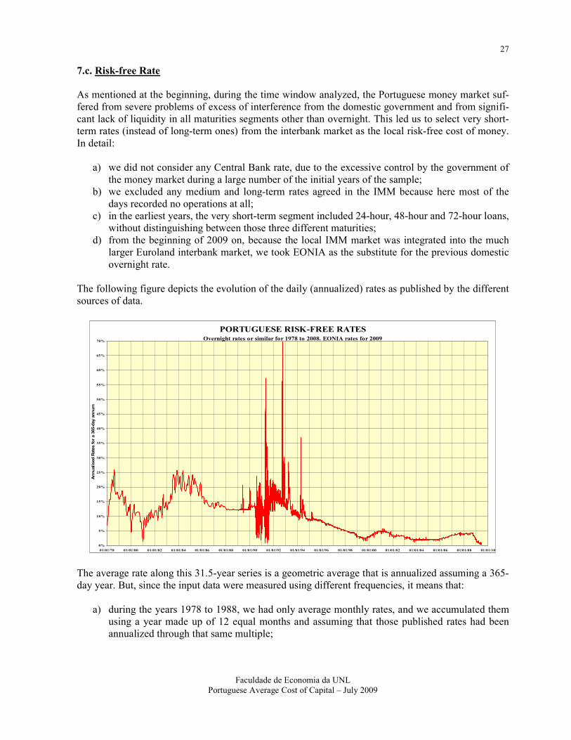
7.c. Risk-free Rate

As mentioned at the beginning, during the time window analyzed, the Portuguese money market suf-

fered from severe problems of excess of interference from the domestic government and from signifi-

cant lack of liquidity in all maturities segments other than overnight. This led us to select very short-

term rates (instead of long-term ones) from the interbank market as the local risk-free cost of money.

In detail:

a) we did not consider any Central Bank rate, due to the excessive control by the government of

the money market during a large number of the initial years of the sample;

b) we excluded any medium and long-term rates agreed in the IMM because here most of the

days recorded no operations at all;

c) in the earliest years, the very short-term segment included 24-hour, 48-hour and 72-hour loans,

without distinguishing between those three different maturities;

d) from the beginning of 2009 on, because the local IMM market was integrated into the much

larger Euroland interbank market, we took EONIA as the substitute for the previous domestic

overnight rate.

The following figure depicts the evolution of the daily (annualized) rates as published by the different

sources of data.

PORTUGUESE RISK-FREE RATESOvernight rates or similar for 1978 to 2008. EONIA rates for 2009

0%

5%

10%

15%

20%

25%

30%

35%

40%

45%

50%

55%

60%

65%

70%

01/01/78 01/01/80 01/01/82 01/01/84 01/01/86 01/01/88 01/01/90 01/01/92 01/01/94 01/01/96 01/01/98 01/01/00 01/01/02 01/01/04 01/01/06 01/01/08 01/01/10

Annualised Rates for a 365-day annum

The average rate along this 31.5-year series is a geometric average that is annualized assuming a 365-

day year. But, since the input data were measured using different frequencies, it means that:

a) during the years 1978 to 1988, we had only average monthly rates, and we accumulated them

using a year made up of 12 equal months and assuming that those published rates had been

annualized through that same multiple;

28



b) from the beginning of 1988, rates became available on a daily basis and the accumulation was

computed assuming a 360-day year, as this was the tradition in our domestic money market;

c) similarly for EONIA rates used for 2009, since these are reported on an Act/360 day count

convention;

d) however, the final geometric average for the whole 31.5-year window was annualized for a

365-day year because that risk-free rate is to be compared to an average equity return that also

assumes a 365-day year.

The final average risk-free rate obtained is

Rf = 9.47% p.a.

7.c. Equity Risk Premium above short-term rates

From the geometric equity return and subtracting the geometric risk-free rate, the average ERP rela-

tive to short-term rates is

17.50%

9.47%

8.03%

Equity Return =

Riskfree =

ERP =

8. SUMMARY AND CONCLUSIONS

Extending 10 years backward the pre-existing BVL-General share index that was initiated in the be-

ginning of 1988, we adjusted a straight line to the log values of that index assuming both autocorrela-

tion and heteroscedasticity for those prices. This is a rather detailed time series – 1652 points – since

we sampled every week (as a rule all Wednesdays) along the 31.5 years from January 1978 to June

2009.

The main result obtained was the average annual (continuous) return provided by that market during

that window of time: 17.5% p.a. (365-day year) with a 95% confidence interval between 16.3% and

18.7%. Note that this is a geometric average estimate, not an arithmetic one, as the underlying values

are the log prices of the index.

Because our Treasuries did not exist during some of the sampled years – the case of T-Bills – or were

very illiquid – the case of T-Bonds – the risk-free rate was estimated using the domestic Interbank

Money Market (in 2009 we used the European reference EONIA): the geometric annualized average

interest rate for overnight operations or similar for the same period of 31.5 years was 9.47% p.a.

(again 365-day year).

These two figures led to an estimate of the historical Equity Risk Premium in Portugal above short-

term risk-free rate of 8.03% p.a., a value on the same order of magnitude found in other countries, in

particular, the traditional Ibbotson figure estimated from a US sample starting in 1926.

29



For the future, this historical average might be excessive because it might have resulted from an extra

premium demanded by investors based on the negative experiences they had gone through recently.

And, in fact, the most recent 8 to 9 years of the index suggests a below average behavior.

The causes of this evolution may be:

a. a simple impact of the accession of Portugal to the European Union (in 1986), in particular the

sharing of the European currency since its inception in 1999: investors, both domestic and

from abroad, now demand a lower premium due to this European “seal of quality”;

b. an alternative cause may be in the low pace of GDP growth of our economy during the same

years, which is interpreted as a long-range effect upon the current value of our shares;

c. of course, simple stochastic behavior may also play a role.

This suggests additional studies in the double direction of extending even further the series toward the

beginning of the Twentieth Century, and to include the measurement of the ERP in relation to long-

term real rates – after discounting for inflation – in order to better gauge the real return obtained from

long bonds.

An important dialogue may be established between macroeconomists and finance historians in look-

ing for evidence from the large laboratory of experiences and facts that history makes available when-

ever long-term analyses are pursued. Stock Exchange variables are now a decisive topic for the global

scholarly community and for theoretical paradigms of different schools of economic thought.

9. REFERENCES

• Barclays Capital, “Equity-Gilt Study”, London 1999, Barclays Capital.

• Barro, Robert and José Ursúa, “Macroeconomic crises since 1870”, NBER Working Paper nº

13940, April (2008) available at http://www.nber.org/papers/w13940

• Benartzi, Shlomo and Richard H. Thaler, (1995) "Myopic Loss Aversion and the Equity Premium

Puzzle", The Quarterly Journal of Economics, MIT Press, vol. 110(1): 73-92, February.

• Brealey, Richard and Stuart Myers, Principles of Corporate Finance, Lisbon: McGraw-Hill, 2009

• Brown, Stephen J. and William N. Goetzmann, and Ross, Stephen “Survival Bias and the Equity

Premium Puzzle”, The Journal of Finance 50(3), 1995: 353 – 873.

• Campbell, John Y. and John H. Cochrane, (1997) “By Force of Habit: A Consumption-Based Ex-

planation of Aggregate Stock Market Behavior”; NBER working paper series, no 4995; Cam-

bridge: National Bureau of Economic Research, 1995. http://www.nber.org/papers/W4995

• Campbell and Schiller (1988 a), “The dividend-price ratio and expectations of future dividends

and discount factors”, Review of Financial Studies, 1: 195-228.

• Campbell and Schiller (1988 b) “Stock Prices, Earnings, and Expected Dividends”, Journal of

Finance, 43: 661-676.

• Campbell and Thompson (2005), “Predicting the Equity Premium Out of Sample: Can Anything

Beat the Historical Average?” NBER Working Paper No. 11468, July 2005.

• Cornell, Bradford, “The Equity Risk premium”, John Wiley & sons, 1999.

• Credit Suisse First Boston, “The CSFB Equity-Gilt Study”, London 1999, CSFB.

• Damodaran’s page in his website – http://pages.stern.nyu.edu/~adamodar

• Dimson, Elroy, Paul Marsh and Mike Staunton, “The Triumph of the Optimists, 101 Years of

Global Investment Returns”, Princeton, New Jersey, Oxford: Princeton University Press, 2002.

30



• Fama, E. and G.Schwert, (1977) “Assets returns and Inflation”, Journal of Financial Econom-

ics,5: 115-146.

• Fama E. and French (1988) “Dividend Yelds and Expected Stock Returns”, Journal of Financial Economics, 22: 3-25.

• Fama E. and French (1989) “Business Conditions and Expected Returns on Stock Bonds”, Journal of Financial Economics, 25: 23-49.

• Fama, E. and G. Schwert, (1981) “Stock Returns, Real Activity, Inflation and Money”, American

Economic Review, 71: 545-565.

• Ferreira, Miguel A., and Pedro Santa-Clara, July 2009, “Forecasting Stock Markets Returns: the

Sum of the Parts is More than the Whole”, Faculdade de Economia da Universidade Nova de Lis-

boa, in http://docentes.fe.unl.pt/~psc

• Goetzmann, William N. and Philippe Jorion, “A Century of Global stock Markets”, Working Pa-

per 5901, NBER, 2000.

• Goetzmann, William N., S. J. Brown, and R.G. Ibbotson (1999) "Offshore Hedge Funds: Sur-

vival and Performance", Journal of Business, Vol. 72, No. 1: 91-117.

• Gordon, Myron J. (1959). "Dividends, Earnings and Stock Prices". Review of Economics and

Statistics 41: 99–105.

• Goyal, Amit, and Ivo Welch, 2008, “A comprehensive look at the empirical performance of equity

risk premium prediction”, Review of Financial Studies 21: 1455-1508.

• Hillebrand, Lee and Medeiros (2009) “The Benefits of Bagging for Forecast Models of Realized

Volatility” Econometric Reviews forthcoming.

• Ibbotson Associates - Stocks, Bonds, Bills, and Inflation Yearbook, several years. • Jorion, Philippe and William Goetzmann, “A Century of Global Stock Markets”, NBER, February

2000.

• Keim and Stambaugh (1986) “Predicting Returns in the Stock and Bond Markets” Journal of Fi-

nancial Economics, 17: 357-390.

• Kaheman, Daniel and Amos Tversky, (1992) “Prospect Theory: An Analysis of Decision under

Risk” Journal of Consumer Research 19 (June 1992): 14-25.

• Lettau and Ludvigson (2001) “Consumption, Aggregate Wealth, and Expected Stock Returns” Journal of Finance, 56: 815-849.

• Mehra, Rajnish and Edward C. Prescott (1985) “The equity Premium: A Puzzle”, Journal of Monetary Economics, 15: 145-161.

• Rietz, Thomas A. (1988) “The equity Premium: A solution”, Journal of Monetary Economics

22,:117-131.

• Rozeff (1984) “Dividend Yelds Are Equity Risk Premiums”, Journal of Portfolio Management, 11:

68-75.

• Schwert, William (1998) "Stock Market Volatility: Ten Years After the Crash," NBER Working

Papers 6381, National Bureau of Economic Research, Inc.

• Schwert, William (2002) “Anomalies and Market Efficiency”, in Handbook of the Economics of

Finance, edited by M. Harris and R. Stulz, North Holland, Amsterdam.

31



ANNEX I

CAPITALIZATION-WEIGHTED SHARE INDICES

Rules of Computation for 1982 - 1987

1. The oldest Portuguese share index still being calculated is the BVL/PSI-General33, one which started the daily series on 5 Jan 1988 with a base value of 1000 points. This index includes all

shares listed in the main market of the Lisbon Stock Exchange and weights each component ac-

cording to the number of shares listed.

Everyday, a single value is computed based on the closing prices of all the shares included in the

sample. Also, all corporate events affecting the price of any share beyond market sentiment are

taken into account through proper adjustments either in the numerator or the denominator of the

formula.

However, for dates before January 1988, there is nothing compatible with this index since the dif-

ferent series known, either never disclosed the methodology adopted to calculate the index or fol-

lowed solutions not compatible to the above index.

Therefore, what the present paper does is to explain the solutions adopted to replicate as close as

possible the methodology of the BVL-General index of the Lisbon Exchange for the period 1978

– 1987. This period is very relevant for future developments in this area of indices because:

• the base date adopted for the BVL-General index – beginning of 1988 – might still be

somewhat influenced by the excessive speculation of the two previous years, which culmi-

nated in the spectacular crash of October 1987; that is, it might be “overvalued”;

• the Portuguese share market was in the 1980s still recovering from the “wounds” that fol-

lowed the economic and social events of 1974, in particular the “suspension” of the Ex-

change operations for about two years34; if the methodology of the current index can be

adapted to express the average market behavior during that 10-year time window, then it

will be extended to the earlier periods in another study.

2. The source of information used to continue the index toward earlier years is the daily bulletins

published in paper form by the Lisbon Stock Exchange and available at the Documentation Centre

of (today called) Euronext Lisbon35. However, only one day per week was used, in order to reduce

the computation burden. The selection led to the use of every Wednesday – except if it was a bank

holiday – in order to minimize potential weekend effects upon the observed prices.

33 It started as BVL-General in 1991, but was later re-baptised PSI-General, the name in use today. 34 The Exchange closed for trading on 25/April/1974 and reopened for share trading only on 7/March/1977. 35 After the Lisbon Stock Exchange joined the Euronext group of Exchanges, in February 2002, this is the legal name

adopted by this Portuguese affiliate.

32



3. Since the index covers all shares listed in the main market of the Lisbon Stock Exchange, the

sample had to be modified and the index adjusted whenever a company entered the market or left

it:

a) For the case of a new company entering the market, the index did not consider the first day of

quotation, but added its capitalization only on the second day of the time series:

( )

( )∑

∑ +

+ =n

ti

n

ti

tt

tionCapitaliza

tionCapitaliza

II

1

11

1 .

=+

=

companynew theofday second1t

companynew theofday first t

where the denominator already includes the capitalization of the new company on the first day of

trading. Of course, for the first day, the numerator excludes the capitalization of the new company

in order to reduce the index variation to simple changes in the sentiment of the market.

( )

( )∑

∑−

−

−

−=1

11

1

11. n

ti

n

ti

tt

tionCapitaliza

tionCapitaliza

II

b) When a company left the market by any reason, the denominator excludes that company for the

computation of the index on the first day already without the old company:

( )

( )∑

∑−

−

−

−=1

11

1

11. n

ti

n

ti

tt

tionCapitaliza

tionCapitaliza

II

=−

=

company oldthe ofday last1t

company oldthe tday withou firstt

4. This index measures the total return of the market including the yield due to cash dividends paid

out by some of the companies in the sample. To include this impact of the dividend, the numerator

of the formula was expanded to include the total amount of cash dividend outflow from that firm

on the first Wednesday after the payment day. But, for all other days, only the sum of capitaliza-

tions without those paid dividends were used in the formula:

( )

( )∑

∑

−

−

+=

n

ti

n

jjti

tt

tionCapitaliza

DNtionCapitaliza

II

11

11

.

.

=−

=

Wednesday previousthe 1t

out-pay dividend afterWednesday firstt

5. Unfortunately, the market did not offer trades of shares for all listed companies on every day. That

is, there was a frequent lack of quotations throughout the time window analyzed. However, the

33



daily bulletin also discloses the best Bid and the best Ask prices after each particular auction36.

Therefore, as a second-best solution, the following methodology was adopted:

• when no trades had occurred, the average between Bid and Ask was used as a proxy for

the real traded price;

• when only the Bid or the Ask was available, that single value was used as that proxy

• when none of the 3 values were present on a particular Wednesday, the value from the pre-

vious Wednesday was used;

• however, if two or more Wednesdays lacking data occurred in a row, that company was

temporarily excluded from the sample according to the rules mentioned above for new en-

trants and old companies leaving the market.

36 Note that the Stock Exchange used the Roll Call system of trading during this period, where each listed share was called

once at a time and a single equilibrium price was discovered after confrontation of all the orders carried by the brokers for

that particular asset. The prices of those orders closest to that equilibrium but already excluded from trading produced the

daily Bid and Ask prices.

34



ANNEX II

MACRO-ECONOMIC VIEW OF THE RISK PREMIUM

Gordon´s Model

The DCF formula for a constant rate of dividends leads to an annual equity return of

1

0

DR g

P= +

So, for an annual cost of debt (Treasuries) of r, the equity risk premium (ERP) is

1

0

DERP g r

P= + −

Note that this premium can be measured either in relation to T-Bills or T-Bonds, without a consensus

yet established. For an inflation rate of around ππππ and a real interest rate of debt of rreal, this implies a

nominal cost of treasuries of about rreal + ππππ, that is

( )1

0

real

DERP g r

Pπ= + − +

But the difference (g - ππππ) measures the real growth rate of the company

1

0

real real

DERP g r

P= + −

Companies cannot grow forever more than the general economy surrounding it, for which a (real)

long-run rate is estimated at a maximum of 2.5% p.a. Since the real return of long-term Treasuries is

about that same size, it implies an ERP relative to Bonds similar to the yield from Dividends. There-

fore, a bond ERP of 6% p.a. can only be compatible with a much larger greal and that is only accept-

able during limited time intervals. Of course, working with an ERP relative to bills, that figure jumps

to 8.5%, but the conclusion is the same.

The reality is even slightly worse because companies may begin with large rates of growth g but, that

pace always tends to fall as the firm matures. So for the same D1 and P0, the discount rate and the

ERP must be smaller than forecast from the standard Gordon formula. This means that the excess of

ERP suggested by the standard Gordon´s formula is even more excessive.

That is, 3% to 4% ERP over short-term Treasuries sounds excessive, much worse for an ERP of 8.5%

p.a. as advanced by Ibbotson.

Documents

Portuguese Average Cost of Capital