1

FOCUS AND SCOPE ZANCO Journal of Pure and Applied Sciences (ZJPAS) is an international, multi-disciplinary,

peer-reviewed, double-blind and open-access journal that enhances research in all fields of basic and applied sciences through the publication of high-quality articles that describe significant and novel works; and advance knowledge in a diversity of scientific fields.

ZJPAS welcomes submission of articles from all aspect of basic and applied science (Biology, Chemistry, Physics, Geology and Mathematics), environmental Science, agriculture, engineering, information technology, petroleum and biomedical sciences, also from cross-disciplinary fields.

ZJPAS is published one volume, 6 issues per year. All accepted articles are granted free online immediately after publication, which permits its users to read, download, copy, distribute, print, search, or link to the full texts of its articles, thus facilitating access to a broad readership.

MANUSCRIPT PREPARATION Language: Manuscripts should be written in clear and concise English. Contributors who are not native English speakers are strongly advised to ensure that a colleague fluent in the English language or a professional language editor has reviewed their manuscript. At proof stage, only minor changes other than corrections of printers’ errors are allowed.

Cover letter: Each manuscript should be accompanied by a cover letter containing a brief statement by the authors describing the novelty and importance of their research.

General format and length: Type the manuscript (including table legends, figure legends and references) double-spaced using 12 font size. Do not use footnotes in the text, use parentheses instead.

MANUSCRIPT STYLE Two types of manuscripts will be considered for publication, including review and original articles.

1. Review articles • The topic must be current. • The scope of the manuscript should not exceed 7500 words, excluding references, captions

and Tables. • The composition is not defined, however, the following parts are required: Title page,

Abstract (unstructured; 250 words maximum), Keywords, Introduction, Acknowledgments

ZANCO JOURNAL OF PURE AND APPLIED SCIENCES The official scientific journal of Salahaddin University-Erbil

http://zancojournals.su.edu.krd/index.php/JPAS/index

Authors Guidelines

and References (150 references maximum), Tables and Figures, if applicable, including titles and legends, and a Conflict of interest statement.

2. Original articles

Manuscripts should be double-spaced with 2-cm margins on all sides of the page, in Times New Roman font. Every page of the manuscript, including the title page, references, tables, etc., should be numbered. All copies of the manuscript should also have line numbers starting with 1 on each consecutive page. Repetitive use of long sentences and passive voice should be avoided. It is strongly recommended that the text be run through computer spelling and grammar programs.

Manuscript content

The manuscript should be divided into the following sections. Principal sections should be numbered consecutively (1. Introduction, 2. Materials and methods, etc.) and subsections should be numbered 1.1., 1.2., etc. Do not number the Acknowledgements or References sections.

The manuscript should be compiled in the following order:

1. Title page: should include the following

• Title: The title should be brief, concise, and descriptive. It should not contain any literature references or compound numbers or non-standardized abbreviations.

• Authors and affiliations: Supply given names, middle initials, and family names for complete identification. Use superscript lowercase letters to indicate different affiliations, which should be as detailed as possible and must include department, faculty/college, University, city and country.

• Corresponding author : Should be indicated with an asterisk, and contact details (Tel., and e-mail address) should be placed in a footnote.

2. Abstract

Each manuscript should contain an informative abstract of the main points (not more than 250 words). It should describe the research purposes or motivation for the manuscript; the main finding and central conclusions. On the abstract page, authors should include a list of four to six keywords.

3. Introduction

This should argue the case for your study, outlining only essential background, and should not include the findings or the conclusions. It should not be a review of the subject area, but should finish with a clear statement of the question being addressed.

4. Materials and methods

2

Explain clearly but concisely your technical and experimental procedures. Previously published papers related to the methods should be cited with appropriate references. Brand names and company locations should be supplied for all mentioned equipment, instruments, chemicals, etc.

Protection of Human Subjects and Animals in Research. When reporting experiments on human subjects, authors should indicate whether the procedures followed were in accordance with the ethical standards of the responsible committee on human experimentation (institutional and national) and with the Helsinki Declaration of 1975 (revised in 2008). When reporting experiments on animals, authors should be asked to indicate whether the institutional and national guide for the care and use of laboratory animals was followed.

5. Results

Findings must be described without comments. It must be presented in the form of text, tables and figures. The same data or information given in a Table must not be repeated in a Figure and vice versa. It is not acceptable to repeat extensively the numbers from Tables in the text or to give lengthy explanations of Tables or Figures.

6. Discussion

This should emphasize the present findings and the variations or similarities with other work done in the field by other scientists. The detailed data should not be repeated in the discussion again. Emphasize the new and important aspects of the study and the conclusions that follow from them. It must be mentioned whether the hypothesis mentioned in the manuscript is true, false or no conclusions can be derived.

7. Conclusion

The main conclusion(s) of the study should be presented in a short conclusion statement that can stand alone and be linked with the goals of the study. State new hypotheses when warranted. Include recommendations when appropriate.

• Acknowledgement

All contributors who do not meet the criteria for authorship should be covered in the acknowledgement section. It should include persons who provided technical help, writing assistance and departmental head who only provided general support. Financial and material support should also be acknowledged.

• Conflict of interest

Authors must acknowledge and declare any sources of funding and potential conflicting interest, such as receiving funds or fees. When there is no conflict of interest, the author should mention it at the end of manuscript, prior to References.

8. References

References should be prepared strictly according to the Harvard style. All references in the text must be specified by the authors’ last names and date of publication.

3

You should cite publications in the text as (Adams, 2006) using the first named author's name or (Adams and Brown, 2006) citing both names of two, or (Adams et al., 2006), when there are three or more authors except when the author is mentioned, e.g ”the study of Shena et al. (2015) was modified….”.

At the end of the paper a reference list in alphabetical order should be supplied:

For books:

Author. Year. Title, Place Published, Publisher.

e.g. Harrow, R. 2005, No Place to Hide, Simon & Schuster, New York, NY.

For book chapters

Author. Year. Title. In: Editor (ed.)^(eds.) Book Title. Edition ed. Place Published: Publisher.

e.g. Calabrese, F.A. 2005, "The early pathways: theory to practice – a continuum", in Stankosky, M. (Ed.), Creating the Discipline of Knowledge Management, Elsevier, New York, NY, pp. 15-20.

For journal articles

Author. Year. Title, Journal, Volume, Pages.

e.g. Capizzi, M.T. and Ferguson, R. 2005. Loyalty trends for the twenty-first century, Journal of Consumer Marketing, 22 (2), 72-80. For thesis

Author. Year. Title. Degree Thesis Type, University.

e.g.Zubakova, R. 2007. Analysis of the mechanisms influencing the expression of blood pressure regulating systems. Ph.D Dissertation, Heidelberg University

Endnote style for ZANCO Journal of Pure and Applied Sciences

• Tables

Submit Tables on separate pages and number them consecutively using Arabic numerals. Provide a short descriptive title, column headings, and (if necessary) footnotes to make each Table self-explanatory. In the footnote, refer to information within the Table with superscript lowercase letters, and do not use special characters or numbers. Separate units with a comma and use parentheses or square brackets for additional measures (e.g., %, range, etc.). Refer to Tables in the text as Table 1, etc. Use Table 1 (boldface), etc. in the title of the Table.

• Figures

The number of figures should be not more than 6 and appropriate for the presented data. Please make sure that artwork files are in an acceptable format (TIFF, JPEG or EPS) and of high resolution (300 dpi or more). Figures should be referred to as Figure 1, Figures. 2, 3-5 (boldface), using Arabic numerals. Each figure must be accompanied by a legend clearly

4

describing it. All aspects of the figures and legend must be fully understandable in a stand-alone format.

Note

All figure legends must be presented at the end of the manuscript, after References.

• Abbreviations and symbols

Use only standard abbreviations and avoid using them in the title. The full term for which an abbreviation stands should precede its first use in the text unless it is a standard unit of measurement.

MANUSCRIPT SUBMISSION All manuscripts must be submitted electronically via the Internet to the ZJPAS through the online system at http://zancojournals.su.edu.krd/index.php/JPAS/index. You will be guided stepwise through the creation and uploading of the various files. There are no page charges.

Manuscripts are accepted for publication on the understanding that they have not been published and are not going to be considered for publication elsewhere. Authors should certify that neither the manuscript nor its main contents have already been published or submitted for publication in another journal. After a manuscript has been submitted, it is not possible for authors to be added or removed or for the order of authors to be changed. If authors do so, their submission will be cancelled. Manuscripts may be rejected without peer review by the editor-in-chief if they do not comply with the author guidelines or if they are beyond the scope of the journal.

Plagiarism

All manuscripts received are submitted to a plagiarism checking system, which compares the content of the manuscript with a vast database of web pages and academic publications. Therefore, the use of others ideas or words in their original form or slightly changed without a proper citation is considered plagiarism and will not be tolerated. Even if a citation is given, if quotation marks are not placed around words taken directly from another author’s work, the author is still guilty of plagiarism. Reuse of the author’s own previously published words, with or without a citation, is regarded as self-plagiarism.

AFTER ACCEPTANCE • Availability of accepted article

This journal makes manuscripts available online as soon as possible after acceptance (in PDF format). A Digital Object Identifier (DOI) is allocated, thereby making it fully citable and searchable by title, author name(s) and the full text. • Proofs

One set of page proofreads (as PDF files) will be sent by e-mail to the corresponding author. Please use this proofreads only for checking the typesetting, editing, completeness and correctness of the text, tables, and figures. We will do our best to get your article published as soon as possible.

5

• Offprints The corresponding author, at no cost, will be provided with a PDF file of the article via e-

mail. The PDF file includes a cover sheet with the journal cover.

THE FINAL CHECKLIST The authors must ensure that before submitting the manuscript for publication, they have taken care of the following:

1. Title page should contain title, name of the author/co-authors, designation and institutions they are affiliated with and e-mail address for future correspondence. E-mail address, Phone number should be provided for corresponding author.

2. Provide the names of two of peer-reviewers, who could be called upon to review your manuscript.

3. Abstract in unstructured format and maximum 250 words. 4. References are mentioned as stated before and prepared via Endnote software. 5. Tables should be typed on separate pages. 6. Make sure for Headings of Tables and their numbers. 7. Figures (Photographs / illustrations) along with their captions are provided. 8. Declaring any conflict of interest. 9. Cover letter

6

ZANCO Journal of Pure and Applied Sciences

The official scientific journal of Salahaddin University-Erbil

ZJPAS (2017), 29 (2); 1-17

http://dx.doi.org/10.21271/ZJPAS.29.2.1

Cytogenetic and molecular genetic studies of number of chronic mylogenous

leukemia in Erbil province

Mustafa S. Al-Attar and Govand M. Qader University of Salahaddin-Erbil, College of science, Biology Department

A R T I C L E I N F O

A B S T R A C T

Article History:

Received: 04/05/2016

Accepted: 25/08/2016

Published:07 /06 /2017

Chronic myeloid leukemia (CML) is amyeloprolirative disorder

characterized by the Philadelphia chromosome originates from the

translocation of chromosome 9 and 22 t (9;22) (q34;q11), creating a

BCR-ABL fusion gene which results in the constitutive activation

BCR-ABL tyrosine kinase. Patients of BCR-ABL fusion gene

positive in (CML) are treated by an effective therapy called Imatinib

(Gleevec). Point mutations alter the conformation of the ATP binding

site that disturbs the binding of therapy to its target which leading to

imatinib resistance. Fifty CML patients were collected from Nanakali

Hospital in Erbil city which were diagnosed by physicians. The age

of the patients from 9 to 80 years, 62% were male and 39% were

female, median age of the patients were 38 years. The present study

deals with two different aspects; conventional cytogenetic (G-

banding) analysis to diagnose the Philadelphia chromosome as a

(CML) marker and using Allele Specific Oligonucleotide Polymerase

Chain Reaction (ASO-PCR) assay for screening the mutant allele at

the three codons 351, 311 and 315 of the BCR-ABL ATP binding

domain in Imatinib resistant CML patients. The phenotype of fifteen

CML patients were successfully analyzed, thirteen patients were in

complete cytogenetic response state (Philadelphia 0%) only two of

those patients showed the Philadelphia chromosome. Three point

mutations T1052C, T932C and C944T were identified by allele

specific oligonucleotide polymerase chain reaction (ASO-PCR). One

patient showed T1052C mutation, T932C was detected in three

patients and two patients showed the C944T ATP binding domain

mutation. In conclusion, conventional cytogenetic and molecular

genetic tests are complementary techniques to show the exact types

of abnormalities, which allow better evaluation of the genomic

aberration involved in CML patients, specifically for kinase domain

mutation that plays an important role in different diagnosis,

prognosis, therapy treatment and drug resistant management of

chronic myeloid leukemia.

Keywords:

Philadelphia Chronic

myelogenous leukemia,

chromosome, cytogenetics

mutation, ABL gene

ASO-PCR.

*Corresponding Author:

Mustafa S. Al-Attar

Email:

mustafa.mustafa@su.edu.krd

Mustafa S. and Qader /ZJPAS: 2017, 29(2): 1-17

INTRODUCTION

Chronic myeloid leukemia (CML) is a

clonal disorder of myeloid stem cells (Witte,

2001; Mark et al., 2006), accounting 15% of

adult leukemias (Kaur et al., 2012). It was first

recognized in 1845 (Rachel & Mary, 2007;

McCann, 2012). The median age of CML

patients is 45 to 55 years (Faderl et al., 1999).

It is the first malignant disorder which is found

to be associated with a chromosome aberration

called Philadelphia (Ph) chromosome (Chin et

al., 1996 ;Hamad et al., 2013).

The high exposure to ionizing radiation,

pesticide, and herbicide are factors that lead to

CML (Moloney, 1987; Kaur et al., 2012). The

typical symptoms of CML are leukocytosis,

fatigue, splenomegaly, thrombocytosis and

anemia (Faderl et al., 1999; Nestal et al.,

2012).

The induction of the genomic aberration

which lead to the formation of BCR-ABL fusion

genes are due to environmental factors, life

style, natural individual genotype difference,

exposure to radioactivity and carcinogen

substances play an important role (Iqbal, 2011;

Bhat et al., 2012). Cytogenetic analysis is the

standard tool for initial evaluation, diagnosis,

management of hematological malignancy of a

patient that suspected to cancer (Goh et al.,

2006) and used as a prognostic indicator for

monitoring therapy (Parikh and Tefferi, 2012).

Also it provides evidence of the progression of

disease at an earlier phase than hematological

marker (Alachkar et al., 2013) by detecting

various chromosomal aberrations and has a

significant role at the time of CML diagnosis

(Razelle et al., 1990; Boronova & Sotak,

2007).

The first an older therapy for CML is

Arsenic trioxide that has apro-apoptic effect

which increase apoptosis and a significant

decline BCR-ABL protein level (Cheryl, 2012;

Rachel & Mary, 2007; Melda & Guray, 2013).

Hydroxyurea is an inhibitor of the

ribonucleotide reductase as well as decrease the

tumor mass, however hydroxyurea prolonged

the duration of chronic phase as compared with

busulfan while busulfan is an alkalating agent

that used as a second line treatment after

hydroxyurea resistant or intolerance that act as

anti-tumor activity at stem cell level (

Hehlmann et al., 1993; Paci, 2013). In contrast,

interferon alpha used in response to antigenic

stimuli such as those that occur with viral

infection and malignant disease as well as it

has pleiotropic effect involving antiviral,

antiproliferative and antiangiogenic activities

(Faderl et al., 1999), however interferon alpha

prolonged survival as compared to

hydroxyurea with low risk due to expose of

significant toxicity (Eiring et al., 2011).

When a fragment of ABL gene is fused with

BCR gene thus the activation loop in BCR-ABL

fusion gene would be in the open conformation

and phosphorylation, in contrast when Imatinib

binds with an active site of the tyrosine kinase

at ATP binding site, Imatinib mesylate

switches off downstream signaling, cells stop

proliferating and apoptosis by preventing

tyrosine autophosphorylation (Guido, 2003;

Al-achkar et al., 2009; Dhara et al., 2010).

Despite response to Imatinib in the majority

of patients with chronic myeloid leukemia,

CML patients show primary or acquire

resistance (Parker et al., 2011). Generally there

are two kinds of BCR-ABL mechanism

resistant, first BCR-ABL independent

mechanism of resistance belong to decreasing

in the intracellular level of Imatinib due to

complication with drug efflus, drug influx or

drug concentration which lead to signal

activation of Ras/MEK and STAT (Hamad et

al., 2013).

While the BCR-ABL dependent

mechanism of resistance involves duplication

or over amplification of BCR-ABL oncogene

that leads to elevated ABL kinase, among them

the most frequent dependent mechanism is

Mustafa S. and Qader /ZJPAS: 2017, 29(2): 1-17

mutation in the ABL kinase domain. Mutation

can affect directly the proper binding of

Imatinib to the target molecule as well as

binding of ATP (Alimena, 2009; Hamad et al.,

2013).

The BCR-ABL domain mutation include

of four major regions P-loop ATP-binding site,

catalytic domain and activation loop, the two

major categories of mutation have been defined

as those at positions where direct contact with

imatinib occurs and those that affect the

conformation of BCR-ABL thus preventing

imatinib binding. The first category mutation

namely T315I located in the ATP-binding site

that prevents the formation of hydrogen bonds

with imatinib and F359V mutation located in

the catalytic domain. The second category

comprises mutations in the P-loop (Y253H and

E255K) and H396R/P mutation in A-loop (Tali

& Ninette, 2012; Menon, 2013).

The most frequent mutations are namely

C944T (cytosine to thymine substitution at

ABL gene in position 944 I exon3) which lead

to amino acid change of threonine to isoleusine

at position 315(Thr315Ile). T932C (thymine to

cytosine substitution at ABL gene position 932)

causing change the amino acid of

phenylalanine to leucine at position

311(Phe311Leu) and T1052C (thymine to

cytosine substitution at ABL gene position

1052) which converts the amino acid

methionine to threonine at position

351(Met351Thr) that forms apart of BCR-ABL

fusion gene and hence BCR-ABL onco-protein

(Catherine et al., 2002; Mahon, 2006).

The aims of the current study were

diagnose the Philadelphia chromosome by

cytogenetic analysis and then confirmation of

it’s by screening various mutations (T1052C,

T932C and C944T) in the BCR-ABL ATP

binding domain by allele specific

oligonucleotide polymerase chain reaction

(ASO-PCR) assay.

MATERIALS AND METHODS

Sample Collection

A total of three to five ml venous blood

samples of fifty CML patients were collected

from Nanakali Hospital in Erbil city which

were diagnosed by physicians, fifteen of the

samples were subjected to the cytogenetic

technique. Sample collection and transport was

completed at the same day on ice. The age of

the patients from 9 to 80 years, 62% were male

and 39% were female, median age of the

patients were 38 years.

A-Cytogenetic method:

Cytogenetic analysis:

Peripheral blood samples were collected in

lethium heparin tubes (Gersen & Keagle,

2005). It was performed on (24-48) hours on

peripheral blood cell culture (Joaquín et al.,

2000; Farkhondeh et al., 2001) using standard

protocol for preparation of GTG-banding

metaphase (Talwar, 2003; Boronova & Sotak,

2007) and chromosome karyotype was

described according to International System

Cytogenetic Nomenclature (ISCN) guidelines

for human Cytogenetic Nomenclature, using

cytovision system for image analysis (Qureshi,

2008). The number of metaphase were

analyzed on each sample were at least 20

metaphases (Al-achkar et al., 2007). The

prepared metaphase slides (metaphase

analyzing) had been read in laboratory of

medical genetics in Iran/Tehran.

The absence of any Ph+ metaphase cells is

indicating a complete cytogenetic response

(CyR) (Alice et al., 2007).

Preparation of Metaphase Banding Human

Chromosome:

The protocol used according to (Moorhead

et al., 1960; Fan, 2003; Gersen & eagle, 2005).

Specimens Collection and Handling:

Mustafa S. and Qader /ZJPAS: 2017, 29(2): 1-17

Three ml of venous blood was drew by a

sterile syringe and collected in a vacuum tubes

containing anticoagulant lithium heparin.

Specimens were transported on ice box and

were kept in refrigerator at 4°C till culturing.

The specimens were cultured within 24 hours

of collection for best result.

Karyotype Procedure (Culture of

leukocytes):

0.5ml of heparinized whole blood was

mixed with 4.5ml of PAA culture medium that

contain all requirements like (RPMI

1640,Phytohaemagglutinin, Fetal bovine

serum, L-glutamine and antibiotics) for cell

proliferation. The cultured cells were incubated

at 37°C for (65-70) h.

B- Molecular method:

DNA Extraction:

Genomic DNA was extracted from whole

blood by using Genomic DNA kit (Genaid,

UK), depending on manufacturer’s

instructions. The qualification and

quantitification of extracted DNA were done

by gel electrophoresis and Nano-Drop

respectively.

Allele specific Oligonucleotide Polymerase

Chain reaction (ASO-PCR)

To determine the most useful protocol in

clinical practice (Catherine et al., 2002 ) was

developed ASO-PCR assay using primer sets

detecting the three common point mutations in

BCR-ABL fusion gene ATP binding domain

known as T1052C (Met351Thr), T932C

(Phe311Leu) and C944T (Thr315Ile). ASO-

PCR assay can amplified the mutated or wild

type sequences in CML patients specifically in

the PCR reaction (Zafar, 2004; Kim, 2006;

Aamir et al., 2011).

Allele specific oligonucleotide polymerase

chain reaction technique uses three primers,

first primer wild type allele specific second

primer mutant allele specific and third common

primer. The primer wild type and mutant allele

specific usually differ by only one nucleotide

that gives them a high specifity to the

corresponding wild type or mutant allele, the

two allele specific primer are combined with

the common primer in separate reaction tubes

(Delia et al., 2008), the primers are listed in

(Table 1). The tubes were placed in the PCR

machine for amplification depending on the

PCR program file in (Table 2 and 3). Then the

PCR product was run on agarose gel

electrophoresis (2%).

PCR Mix preparation:

A 20 µl PCR reaction was performed

containing 2µl of DNA, 2X lyophilized

Accupower master mix (Bioneer, Korea) and

1.5µl was added for each of the forward and

reverse primers then the mixture was

completed by adding 15 µl of nuclease free

water.

Table 1: Identities and sequences of primers used in ASO-PCR assay for mutant allele detection in CML Gleevec resistant patients (Catherine et al., 2002).

Mustafa S. and Qader /ZJPAS: 2017, 29(2): 1-17

Mutation Primer

Type

Polarity Recognition sequence (5’—3’) Amplicon

length (bp)

T1052C

NP Forward CCA CTC AGA TCT CGT CAG

CCAT*

112 (bp) ASO Forward CCA CTC AGA TCT CGT CAG CCA

C*

Common Reverse GCC CTG AGA CCT CCT AGG CT

T932C

NP

Forward

CAC CCG GGA GCC CCC GT*

172 (bp) ASO Forward CAC CCG GGA GCC CCC GC*

Common Reverse CCC CTA CCT GTG GAT GAA GT

C944T

NP

Forward

GCC CCC GTTCTA TAT CATCAC*

158 (bp) ASO

Forward GCC CCC GTTCTA TAT CATCAT*

Common Reverse GGA TGA AGT TTT TCT TCT CCA

Table (2): Thermal cycling conditions of ASO-PCR technique for mutation C944T and T932C (Catherine et al.,

2002).

Steps Tempreture (ºC) Time Number of cycles

Initial denaturation 94 12 minutes 1

Denaturation 95 1 minute

35 Annealing 64 1 minute

Extension 72 1 minute

Final extension

72

5 minutes

1

Table (3): Reaction cycling program of ASO-PCR technique for mutation T1052C (Catherine et al., 2002).

Mustafa S. and Qader /ZJPAS: 2017, 29(2): 1-17

Steps Tempreture (ºC) Time Number of cycles

Initial denaturation 94 12 minutes 1

Denaturation 95 1 minute

35 Annealing 68 1 minute

Extension 72 1 minute

Final extension

72

5 minutes

1

Results and Discussion:

Cytogenetic studies:

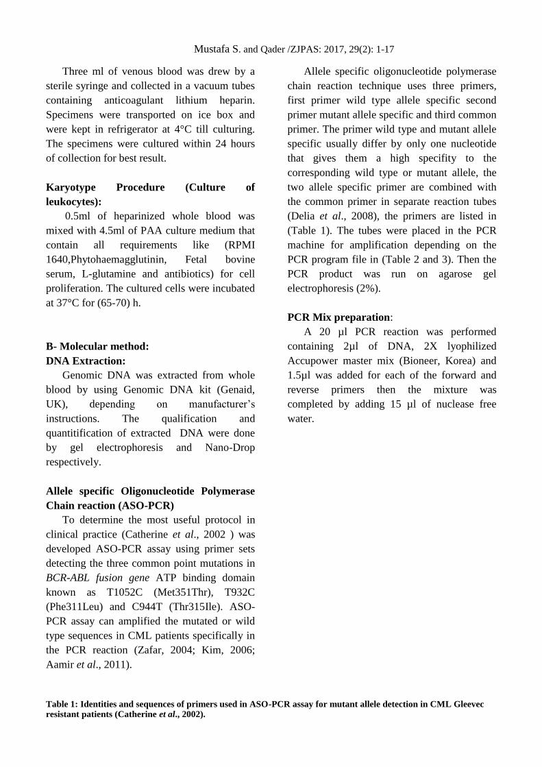
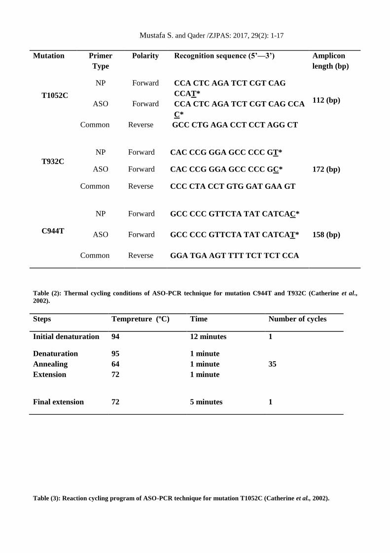
Out of the fifteen diagnosed CML patients,

two CML patients showed philadelphia

positive Figure (2) while thirteen patients’

specimen have a normal karyotype that is

philadelphia negative Figure (1). In the current

study the number of philadelphia positive was

lower than that reported by Al -Attar, (2004),

who found fourteen positive cases among

twenty six patient samples. Philadelphia

negative belong to many reasons one of them

reported by Razelle etal., (1990) that ph- can

be exists at the time of CML diagnosis patients

but this disorder are not clinically

distinguishable from those with philadelphia

positive.

On other hand Current results were

supported by the previous finding such as Goh

et al., (2006) illustrated that the analyzed

metaphase were philadelphia negative this is

due to complete cytogenetic response or

masked philadelphia chromosome (Hochhaus,

2006; Boronova & Sotak, 2007) Table (4)

shows the cytogenetic analysis of CML patient.

Figure (1): GTG-banding of human chromosome. 46,XY Normal male karyotype (negative Philadelphia

chromosome) in CML patient (1000X).

Mustafa S. and Qader /ZJPAS: 2017, 29(2): 1-17

Figure (2): GTG-banding of human chromosome. Female 46,XX,t(9;22) that revealed Philadelphia chromosome in

CML patient (1000X).

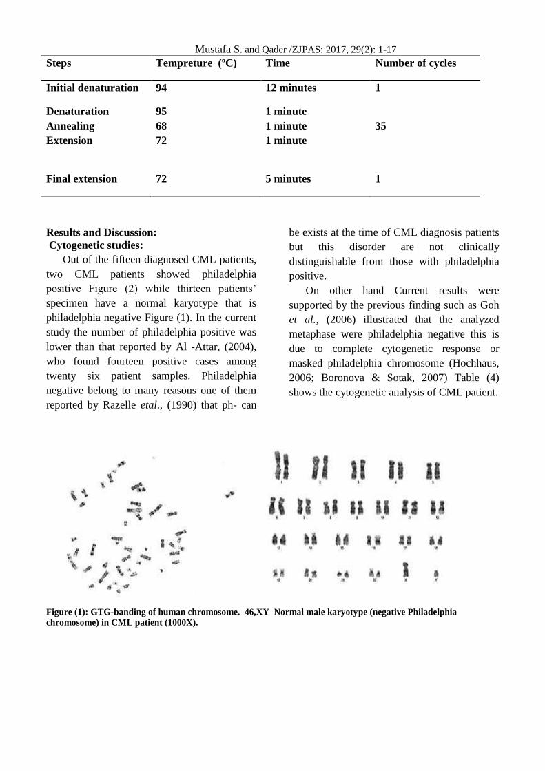
Table (4): Patient’s characteristics and results of cytogenetic analysis.

Sample Age Sex Therapy Karyotype

Case 1 70 M Nilotinib Ph-

Case 2 59 F Gleevec Ph-

Case 3 40 M Nilotinib Ph-

Case 4 58 M Nilotinib Ph-

Case 5 38 M Gleevec Ph-

Case 6 49 M Nilotinib Ph-

Case 7 13 F Gleevec Ph+

Case 8 52 M Gleevec Ph-

Case 9 40 F Gleevec Ph-

Case 10 45 M Gleevec Ph-

Case 11 55 F Gleevec Ph-

Case 12 30 M Nilotinib Ph-

Case 13 39 F Gleevec Ph-

Case 14 55 F Gleevec Ph+

Case 15 51 M Gleevec Ph-

Mustafa S. and Qader /ZJPAS: 2017, 29(2): 1-17

Molecular studies:

Molecular detection of BCR-ABL kinase

domain mutation that associated with

Imatinib resistance:

Mutation analysis was performed by using

a sensitive technique ASO-PCR for CML

cases. Out of the 50 chronic phase (CP) CML

patients examined according to the presence of

the BCR-ABL tyrosine kinase mutation, six

patients (12%) were found to harbor the mutant

allele at the three codon 351, 311 and 315 of

the BCR-ABL fusion gene Table (5). Thirty

four patients (68%) had the wild type allele of

351, 311 and 315, the remaining patients were

10 (20%) that there were no any indicator

(normal band) on the gel electrophoresis to

have wild type of the 311 and 315 alleles.

Delia et al., (2008) which supports that the

mutant specific primer was designed for high

specifity, it binds when the exact

complementary sequence for it must be present

in DNA of the CML patients otherwise

amplification is not occurred, then we

confirmed our results on the same patients by

using normal primer and also there was no any

normal bands after running PCR products on

the gel electrophoresis, in this case we were

interpreted that these CML patients (20%) have

another mutation.

Each of these mutations were detected

alone which are in concordance with results of

(Catherine et al., 2002; Aamir et al., 2011) and

there was no any double mutation in a single

patient which is disconcordance with the

results that reported by (Zafar, 2004).

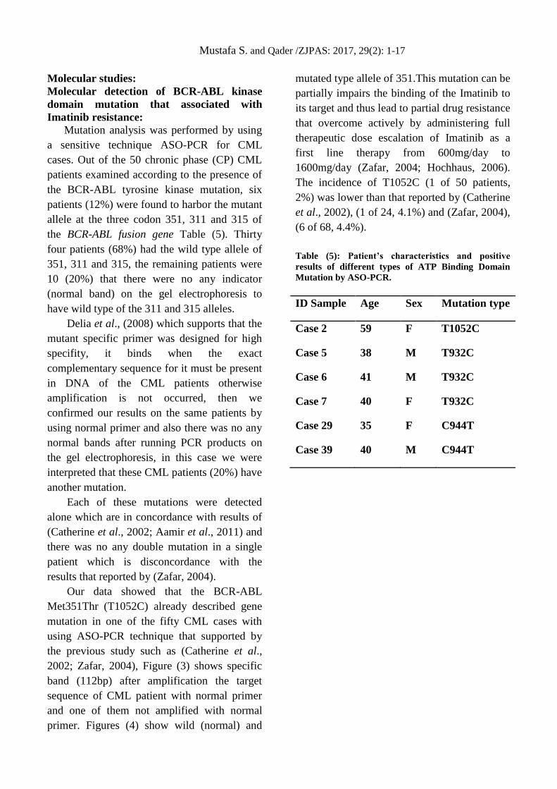
Our data showed that the BCR-ABL

Met351Thr (T1052C) already described gene

mutation in one of the fifty CML cases with

using ASO-PCR technique that supported by

the previous study such as (Catherine et al.,

2002; Zafar, 2004), Figure (3) shows specific

band (112bp) after amplification the target

sequence of CML patient with normal primer

and one of them not amplified with normal

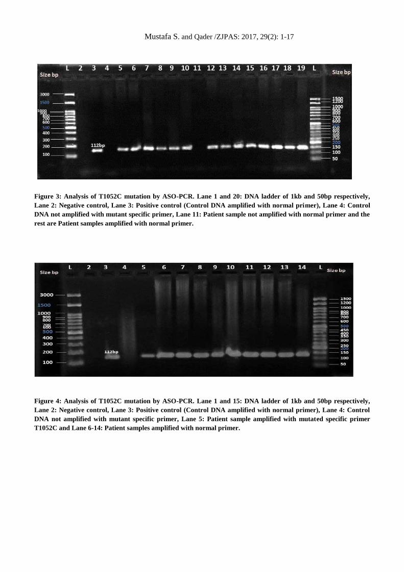
primer. Figures (4) show wild (normal) and

mutated type allele of 351.This mutation can be

partially impairs the binding of the Imatinib to

its target and thus lead to partial drug resistance

that overcome actively by administering full

therapeutic dose escalation of Imatinib as a

first line therapy from 600mg/day to

1600mg/day (Zafar, 2004; Hochhaus, 2006).

The incidence of T1052C (1 of 50 patients,

2%) was lower than that reported by (Catherine

et al., 2002), (1 of 24, 4.1%) and (Zafar, 2004),

(6 of 68, 4.4%).

Table (5): Patient’s characteristics and positive

results of different types of ATP Binding Domain

Mutation by ASO-PCR.

ID Sample Age Sex Mutation type

Case 2 59 F T1052C

Case 5 38 M T932C

Case 6 41 M T932C

Case 7 40 F T932C

Case 29 35 F C944T

Case 39 40 M C944T

Mustafa S. and Qader /ZJPAS: 2017, 29(2): 1-17

Figure 3: Analysis of T1052C mutation by ASO-PCR. Lane 1 and 20: DNA ladder of 1kb and 50bp respectively,

Lane 2: Negative control, Lane 3: Positive control (Control DNA amplified with normal primer), Lane 4: Control

DNA not amplified with mutant specific primer, Lane 11: Patient sample not amplified with normal primer and the

rest are Patient samples amplified with normal primer.

Figure 4: Analysis of T1052C mutation by ASO-PCR. Lane 1 and 15: DNA ladder of 1kb and 50bp respectively,

Lane 2: Negative control, Lane 3: Positive control (Control DNA amplified with normal primer), Lane 4: Control

DNA not amplified with mutant specific primer, Lane 5: Patient sample amplified with mutated specific primer

T1052C and Lane 6-14: Patient samples amplified with normal primer.

Mustafa S. and Qader /ZJPAS: 2017, 29(2): 1-17

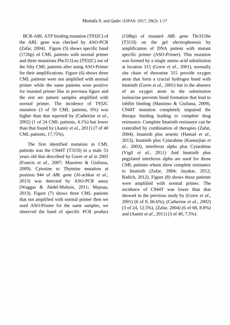
BCR-ABL ATP binding mutation (T932C) of

the ABL gene was checked by ASO-PCR

(Zafar, 2004). Figure (5) shows specific band

(172bp) of CML patients with normal primer

and three mutations Phe311Leu (T932C) out of

the fifty CML patients after using ASO-Primer

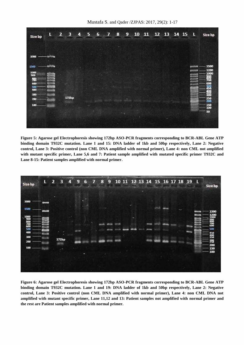
for their amplifications. Figure (6) shows three

CML patients were not amplified with normal

primer while the same patients were positive

for mutated primer like in previous figure and

the rest are patient samples amplified with

normal primer. The incidence of T932C

mutation (3 of 50 CML patients, 6%) was

higher than that reported by (Catherine et al.,

2002) (1 of 24 CML patients, 4.1%) but lower

than that found by (Aamir et al., 2011) (7 of 40

CML patients, 17.75%).

The first identified mutation in CML

patients was the C944T (T315I) in a male 53

years old that described by Gorre et al in 2001

(Francis et al., 2007; Massimo & Giuliana,

2009). Cytosine to Thymine mutation at

position 944 of ABL gene (Al-achkar et al.,

2013) was detected by ASO-PCR assay

(Waggas & Abdel-Muhsin, 2011; Maysaa,

2013). Figure (7) shows three CML patients

that not amplified with normal primer then we

used ASO-Primer for the same samples, we

observed the band of specific PCR product

(158bp) of mutated ABL gene Thr315Ile

(T315I) on the gel electrophoresis by

amplification of DNA patient with mutant

specific primer (ASO-Primer). This mutation

was formed by a single amino acid substitution

at location 315 (Gorre et al., 2001), normally

site chain of threonine 315 provide oxygen

atom that form a crucial hydrogen bond with

Imatinib (Gorre et al., 2001) but in the absence

of an oxygen atom in the substitution

isoleucine prevents bond formation that lead to

inhibit binding (Massimo & Giuliana, 2009).

C944T mutation completely impaired the

therapy binding leading to complete drug

resistance. Complete Imatinib resistance can be

controlled by combination of therapies (Zafar,

2004). Imatinib plus arsenic (Hamad et al.,

2013), Imatinib plus Cytarabine (Kantarjian et

al., 2003), interferon alpha plus Cytarabine

(Vigil et al., 2011) And Imatinib plus

pegylated interferon alpha are used for those

CML patients whom show complete resistance

to Imatinib (Zafar, 2004; Jayakar, 2012;

Radich, 2012). Figure (8) shows those patients

were amplified with normal primer. The

incidence of C944T was lower than that

showed in the previous study by (Gorre et al.,

2001) (6 of 9, 66.6%), (Catherine et al., 2002)

(3 of 24, 12.5%), (Zafar, 2004) (6 of 68, 8.8%)

and (Aamir et al., 2011) (3 of 40, 7.5%).

Mustafa S. and Qader /ZJPAS: 2017, 29(2): 1-17

Figure 5: Agarose gel Electrophoresis showing 172bp ASO-PCR fragments corresponding to BCR-ABL Gene ATP

binding domain T932C mutation. Lane 1 and 15: DNA ladder of 1kb and 50bp respectively, Lane 2: Negative

control, Lane 3: Positive control (non CML DNA amplified with normal primer), Lane 4: non CML not amplified

with mutant specific primer, Lane 5,6 and 7: Patient sample amplified with mutated specific primer T932C and

Lane 8-15: Patient samples amplified with normal primer.

Figure 6: Agarose gel Electrophoresis showing 172bp ASO-PCR fragments corresponding to BCR-ABL Gene ATP

binding domain T932C mutation. Lane 1 and 19: DNA ladder of 1kb and 50bp respectively, Lane 2: Negative

control, Lane 3: Positive control (non CML DNA amplified with normal primer), Lane 4: non CML DNA not

amplified with mutant specific primer, Lane 11,12 and 13: Patient samples not amplified with normal primer and

the rest are Patient samples amplified with normal primer.

Mustafa S. and Qader /ZJPAS: 2017, 29(2): 1-17

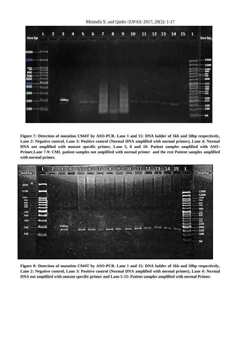
Figure 7: Detection of mutation C944T by ASO-PCR. Lane 1 and 15: DNA ladder of 1kb and 50bp respectively,

Lane 2: Negative control, Lane 3: Positive control (Normal DNA amplified with normal primer), Lane 4: Normal

DNA not amplified with mutant specific primer, Lane 5, 6 and 10: Patient samples amplified with ASO-

Primer,Lane 7-9: CML patient samples not amplified with normal primer and the rest Patient samples amplified

with normal primer.

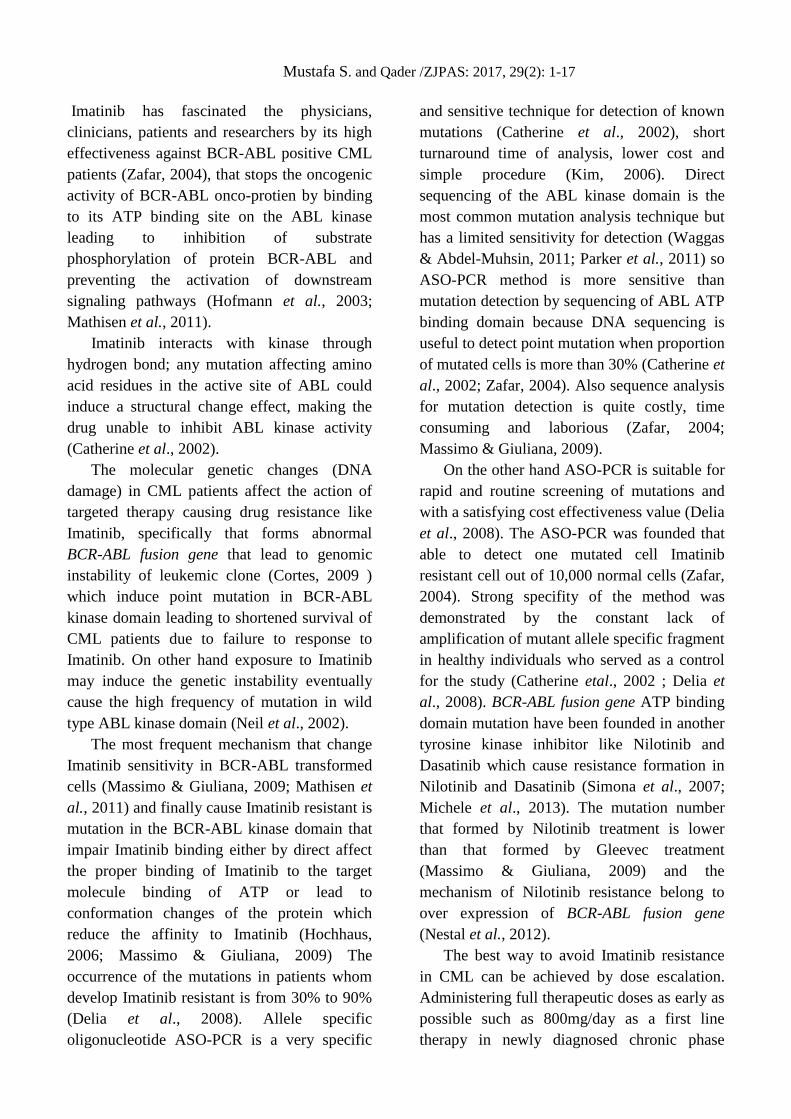
Figure 8: Detection of mutation C944T by ASO-PCR. Lane 1 and 15: DNA ladder of 1kb and 50bp respectively,

Lane 2: Negative control, Lane 3: Positive control (Normal DNA amplified with normal primer), Lane 4: Normal

DNA not amplified with mutant specific primer and Lane 5-15: Patient samples amplified with normal Primer.

Mustafa S. and Qader /ZJPAS: 2017, 29(2): 1-17

Imatinib has fascinated the physicians,

clinicians, patients and researchers by its high

effectiveness against BCR-ABL positive CML

patients (Zafar, 2004), that stops the oncogenic

activity of BCR-ABL onco-protien by binding

to its ATP binding site on the ABL kinase

leading to inhibition of substrate

phosphorylation of protein BCR-ABL and

preventing the activation of downstream

signaling pathways (Hofmann et al., 2003;

Mathisen et al., 2011).

Imatinib interacts with kinase through

hydrogen bond; any mutation affecting amino

acid residues in the active site of ABL could

induce a structural change effect, making the

drug unable to inhibit ABL kinase activity

(Catherine et al., 2002).

The molecular genetic changes (DNA

damage) in CML patients affect the action of

targeted therapy causing drug resistance like

Imatinib, specifically that forms abnormal

BCR-ABL fusion gene that lead to genomic

instability of leukemic clone (Cortes, 2009 )

which induce point mutation in BCR-ABL

kinase domain leading to shortened survival of

CML patients due to failure to response to

Imatinib. On other hand exposure to Imatinib

may induce the genetic instability eventually

cause the high frequency of mutation in wild

type ABL kinase domain (Neil et al., 2002).

The most frequent mechanism that change

Imatinib sensitivity in BCR-ABL transformed

cells (Massimo & Giuliana, 2009; Mathisen et

al., 2011) and finally cause Imatinib resistant is

mutation in the BCR-ABL kinase domain that

impair Imatinib binding either by direct affect

the proper binding of Imatinib to the target

molecule binding of ATP or lead to

conformation changes of the protein which

reduce the affinity to Imatinib (Hochhaus,

2006; Massimo & Giuliana, 2009) The

occurrence of the mutations in patients whom

develop Imatinib resistant is from 30% to 90%

(Delia et al., 2008). Allele specific

oligonucleotide ASO-PCR is a very specific

and sensitive technique for detection of known

mutations (Catherine et al., 2002), short

turnaround time of analysis, lower cost and

simple procedure (Kim, 2006). Direct

sequencing of the ABL kinase domain is the

most common mutation analysis technique but

has a limited sensitivity for detection (Waggas

& Abdel-Muhsin, 2011; Parker et al., 2011) so

ASO-PCR method is more sensitive than

mutation detection by sequencing of ABL ATP

binding domain because DNA sequencing is

useful to detect point mutation when proportion

of mutated cells is more than 30% (Catherine et

al., 2002; Zafar, 2004). Also sequence analysis

for mutation detection is quite costly, time

consuming and laborious (Zafar, 2004;

Massimo & Giuliana, 2009).

On the other hand ASO-PCR is suitable for

rapid and routine screening of mutations and

with a satisfying cost effectiveness value (Delia

et al., 2008). The ASO-PCR was founded that

able to detect one mutated cell Imatinib

resistant cell out of 10,000 normal cells (Zafar,

2004). Strong specifity of the method was

demonstrated by the constant lack of

amplification of mutant allele specific fragment

in healthy individuals who served as a control

for the study (Catherine etal., 2002 ; Delia et

al., 2008). BCR-ABL fusion gene ATP binding

domain mutation have been founded in another

tyrosine kinase inhibitor like Nilotinib and

Dasatinib which cause resistance formation in

Nilotinib and Dasatinib (Simona et al., 2007;

Michele et al., 2013). The mutation number

that formed by Nilotinib treatment is lower

than that formed by Gleevec treatment

(Massimo & Giuliana, 2009) and the

mechanism of Nilotinib resistance belong to

over expression of BCR-ABL fusion gene

(Nestal et al., 2012).

The best way to avoid Imatinib resistance

in CML can be achieved by dose escalation.

Administering full therapeutic doses as early as

possible such as 800mg/day as a first line

therapy in newly diagnosed chronic phase

Mustafa S. and Qader /ZJPAS: 2017, 29(2): 1-17

CML patients causes the maximal depletion of

leukemic cells (Jeffrey & Helen, 2003;

Hochhaus, 2006). Also higher doses (standard

dose, 800mg/day) of Imatinib reinduce

hematologic response or impair cytogenetic

response (Kantarjian et al., 2003).

BCR-ABL positive CML patients require

immediate attention not only by local

physicians and oncologists but international

community should also go many stages to work

in collaboration with local personnel for this

issue, to find out the reasons, molecular maker

of the disease and drug targets.

Conclusion

Conventional cytogenetic and molecular

genetic tests are complementary techniques to

show the exact types of abnormalities, that

allow better evaluation of the genomic

aberration involved in CML patients,

specifically for kinase domain mutation that

plays an important role in different diagnosis,

prognosis, therapy treatment and drug resistant

management of CML patients like selection the

specific tyrosine kinase inhibitor when

Imatinib mesylate treatment has been failed.

REFERENCES

Aamir, R., Sabir, H., Nazia, R., Shaukat, A., Ghulam,

M., Shahzad, B. & Ammad, A. (2011). Chronic

myeloid leukemia: Attributes of break point cluster

region-abelson (BCR-ABL). Journal of Cancer

Research and Experimental Oncology 3(6), 62-66.

Al-achkar, W.,Wafa, A. & Nwedar, M. (2007). A

complex translocation t(5;9;22) in philadelphia

cells involving the short arm of chromosome 5 in

case of chronic Myelogenous Leukemia. Journal

experimental Clinical Cancer Research 26(3), 411-

415.

Al-achkar, W., Wafa, A., Moassass, F., Klein, E. &

Liehr, T. (2013). Multiple copies of BCR-ABL

fusion gene on two isodicentric Philadelphia

chromosomes in an imatinib mesylate-resistant

chronic myeloid leukemia patient. Oncology

Letters, 5, 1579-1582.

Al-Attar, M.S. (2004). Evaluation of pesticides toxicity

on laboratory mice and human chromosomes in

Iraq-Kurdistan, Ph.D. Thesis,University of

Salahaddin/Erbil-Iraq.

Alice, F., Martin, C., Philipp, E., Tanja, L., Michelle, G.,

Oliver, F., Wolfgang, S., Rüdiger, H. & Andreas,

H. (2007). Dynamics of cytogenetic aberrations in

Philadelphia chromosome positive and negative

hematopoiesis during dasatinib therapy of chronic

myeloid leukemia patients after imatinib failure.

haematologica/the hematology journal, 92(06),

834-837.

Alimena, M. (2009). Resistance to Imatinib in Chronic

Myeloid Leukemia and Therapeutic Approaches to

Circumvent the Problem. Cardiovascular and

Haematological Disorders-Drug Targets,9(1), 21-

28.

Bhat, G., Bhat, A., Wani, A., Sadiq, N., Jeelani, S., Kaur,

R. & Ganai, B.(2012). Polymorphic Variation in

Glutathione-S-transferase Genes and Risk of

Chronic Myeloid Leukaemia in the Kashmiri

Population. Asian Pacific Journal of Cancer

Prevention, 13(1), 69-73.

Boronova, I. & Sotak, M. (2007). Detection of

Philadelphia in patients with Chronic meyeloid

leukemia from the presov region in Slovakia.

Bratisl Lek listy Journal 108, 433-436.

Catherine, R., Nathalie, G., Jean, L., Nathalie, P.,

Thierry, F., Pierre, F. & Claude, P. (2002 ). Several

types of mutations of the Abl gene can be found in

chronic myeloid leukemia patients resistant to

STI571, and they can pre-exist to the onset of

treatment. The American Society of Hematology,

100, 3, 1014-1018.

Cheryl, A. (2012). Treating Chronic Myeloid Leukemia

Improving Management Through Understanding of

the Patient Experience. Clinical Journal of

Oncology Nursing, 17(1), 13-20.

Chin, Y., Wang, L. & Zubaidah, Z. (1996). Chromosome

Aberration in philadelphia chromosome positive

Chronic Myeloid Leukemia. Genetics Society of

Malaysia Journal, 2, 258-261.

Cortes, A. (2009). Molecular biology of bcr-abl-positive

chronic myeloid leukemia. The American Society of

Hematology, 113, 1619-1630.

Delia, D., Andrei, C., Radu, P., Mariana, P. & Ljubomir,

P. (2008). Monitoring T315I mutation in chronic

myeloid leukemia by amplification refractory

mutation system PCR. Revista Română de

Medicină de Laborator, 13, 17-20.

Mustafa S. and Qader /ZJPAS: 2017, 29(2): 1-17

Dhara, P., Vipul, P. & Rajesh , S. (2010). BCR ABL

Kinase Inhibitors for Cancer Therapy. 2(2), 80-90.

Eiring, A., Khorashad, J., Morley, K., & Deininger, M.

(2011). Advances in the treatment of chronic

myeloid leukemia. Biomedical central Medicine,

9,1741-7015.

Faderl,S.; Talpaz, M.; Estrov, Z.; Brien, S.; Kurzrock, R.

& Kantarjian,H. (1999). The biology of chronic

Myeloid Leukemia. The new England of

Medicine,341(3),164-172.

Fan, Y. (2003). Molecular Cytogenetic Protocols and

Applications. Humana Press Totowa, 204, 72.

Farkhondeh, B., Ardeshir, G. &Mina, I. (2001).

Chromosomal abnormalities in leukemia in Iran.

Archives of Iranian Medicine journal, 4(4) 193-

196.

Francis, J., Dan, J., Donald, B., Hagop, K. & Steven, J.

(2007). A novel kinase inhibitor, is active in

patients with chronic myeloid leukemia or acute

lymphocytic leukemia with the T315I BCR-ABL

mutation. The American Society of Hematology,

109, 500-502.

Gersen, S., L.; Keagle, M., B. (2005). The Principle of

Clinical cytogenetics. Second Edition, Humana

Press, 63-71.

Goh, H., Hwang, J., Kim, S., Lee, Y., Kim, Y. & Kim,

D. (2006). Comprehensive analysis of BCR-ABL

transcript types in Korean CML patients using a

newly developed multiplex RT-PCR. Translational

Research, 148(5), 249-256.

Gorre, E., Katharine, M., Nicholas H., Ron, P., Nagesh,

R. M., & Charles L. (2001). Clinical Resistance to

STI-571 Cancer Therapy Caused by BCR-ABL

Gene Mutation or AmpliÞcation. science, 293, 876-

880.

Guido, M. (2003). Understanding the Molecular Basis of

Imatinib Mesylate Therapy in Chronic

Myelogenous Leukemia and the Related

Mechanisms of Resistance,9, 1248-1252.

Haferlach, C., Rieder, H., Lillington, D. M., Dastugue,

N., Hagemeijer, A., Harbott, J. & Fonatsch, C.

(2007). Proposals for standardized protocols for

cytogenetic analyses of acute leukemias, chronic

lymphocytic leukemia, chronic myeloid leukemia,

chronic myeloproliferative disorders, and

myelodysplastic syndromes. Genes Chromosomes

Cancer journal, 46(5), 494-499.

Hamad, A., Sahli, Z., Sabban, M., Mouteirik, M., &

Nasr, R. (2013). Emerging therapeutic strategies

for targeting chronic myeloid leukemia stem cells.

Stem Cells International, 2013, 1-12.

Hehlmann, H., Hasford, J., Pralle, H., Queisser, W.,

Loffler, H., Heinze, B. & Georgii A. (1993).

Randomized comparison of busulfan and

hydroxyurea in chronic myelogenous leukemia:

prolongation of survival by hydroxyurea. The

German CML Study Group. The American Society

of Hematology, 82,398-407.

Hochhaus, A. (2006). Chronic myelogenous leukemia

(CML): resistance to tyrosine kinase inhibitors.

European Society for Medical Oncology, 17, 274-

279.

Hochhaus, A., Skladny, H., Melo, JV., Sick, C., Berger,

U., Guo, JQ., Arlinghaus, RB., Hehlmann, R.,

Goldman, JM. & Cross, NC. (1996). A novel BCR-

ABL fusion gene (e6a2) in a patient with

Philadelphia chromosome-negative chronic

myelogenous leukemia. The American Society of

Hematology, 88, 2236-2240.

Hofmann, W., Komor, M., Wassmann, B., Jones, L.,

Gschaidmeier, H., Hoelzer, D. & Ottmann, O.

(2003). Presence of the BCR-ABL mutation

Glu255Lys prior to STI571 (imatinib) treatment in

patients with Ph+ acute lymphoblastic leukemia.

Blood, 102(2), 659-661.

Iqbal, Z. (2011). Frequency of Bcr-Abl Fusion Oncogene

Splice Variants Associated with Chronic Myeloid

Leukemia (CML). Journal of Cancer Therapy,

2(02), 176-180.

Jayakar, V. (2012). Chronic myeloid leukemia: In

pursuit of perfection. South Asian Journal Cancer,

1(1),16-24.

Jeffrey, A. & Helen, B. (2003). The Effect of Dose

Increase of Imatinib Mesylate in Patients with

Chronic or Accelerated Phase Chronic

Myelogenous Leukemia with Inadequate

Hematologic or Cytogenetic Response to Initial

Treatment. Clinical Cancer Research, 9, 2092-

2097.

Joaquín, S., José, R., José, M., José, N. & Antonio, T.

(2000). Cytogenetic and molecular studies of

variant Ph' translocations. Haematologica journal,

85, 435-437.

Kantarjian, H., Brien, M., Giles, S., Garcia, F., Faderl,

G., Thomas, S., Shan, D., Rios, J. & Cortes, J.

(2003). Dose escalation of imatinib mesylate can

overcome resistance to standard-dose therapy in

patients with chronic myelogenous leukemia.

Blood, 101(2), 473-475.

Mustafa S. and Qader /ZJPAS: 2017, 29(2): 1-17

Kaur, A., Kaur, S., Singh, A., & Singh, J. (2012).

Karyotypic findings in chronic myeloid leukemia

cases undergoing treatment. Indian Journal Human

Genetics, 18(1), 66-70.

Kim, H. (2006). Comparison of allele specific

oligonucleotide-polymerase chain reaction and

direct sequencing for high through put screening of

ABL kinase domain mutations in chronic myeloid

leukemia resistant to imatinib. haematologica/the

hematology journal, 91,659-662.

Mahon, M. (2006). Molecular remission in chronic

myeloid leukemia patients with sustained complete

cytogenetic remission after imatinib mesylate

treatment. Haematologica/the hematology journal,

91, 162-168.

Mark, H., Sokolic, A., & Mark,Y. (2006). Conventional

cytogenetics and FISH in the detection of BCR-

ABL fusion in chronic myeloid leukemia (CML).

Experimantal Molecular Pathology, 81(1), 1-7.

Massimo, B. & Giuliana, A. (2009). Resistance to

Imatinib in Chronic Myeloid Leukemia and

Therapeutic Approaches to Circumvent the

Problem. Cadiovascular & Hematology Disorders-

Drug targets,9,21-28.

Mathisen, M. S., Kantarjian, H. M., Cortes, J., &

Jabbour, E. (2011). Mutant BCR-ABL clones in

chronic myeloid leukemia. Haematologica, 96(3),

347-349.

Maysaa, A. (2013 ). Molecular Screening for T315I and

F317L Resistance Mutations in Iraqi Chronic

Myeloid Leukemia Non-Responders Patients to

Imatinib. Cancer and Clinical Oncology, 2, 55-61.

McCann, S. (2012). A paradigm for malignancy or just a

strange disease. Sultan Qaboos University Medical

Journal, 12(4), 422-428.

Melda, C. & Guray S. (2013). Review Article Changes

in molecular biology of chronic myeloid leukemia

in tyrosine kinase inhibitor . American Journal

Blood Research, 3, 191-200.

Menon, H. (2013). Issues in current management of

chronic myeloid leukemia: Importance of

molecular monitoring on long term outcome. South

Asian Journal Cancer, 2(1), 38-43.

Michele, B., Gianantonio, R. & Andreas, H., (2013).

European Leukemia Net recommendations for the

management of chronic myeloid leukemia.

American Society of Hematology, 122, 872-884.

Moloney, W. (1987). Radiogenic leukemia revisited.

Blood 70,905-908.

Moorhead, P.S., Nowell, P.C., Mellman,W.J., Battips ,

D.M., and Hungerford, D.A. (1960). Chromosome

preparatoin of leucocytes cultivated from human

peripheral blood. Experimental cell research, 20,

613-616.

Neil, P., Bhushan, N., Mercedes, E., Ronald, L.,John, K.,

& Charles, L. (2002). Multiple BCR-ABL kinase

domain mutations confer polyclonal resistance to

the tyrosine kinase inhibitor imatinib (STI571) in

chronic phase and blast crisis chronic myeloid

leukemia. Cancer cell, 2, 117- 125.

Nestal, M., Souza, P., Costas, F., Vasconcelos, F., Reis,

F., & Maia, R. (2012). The Interface between BCR-

ABL-Dependent and Independent Resistance

Signaling Pathways in Chronic Myeloid Leukemia.

Leukemia Research Treatment, 2012, 1-19,

ID671702.

Paci, M. (2013). Physico-Chemical Stability of Busulfan

in Injectable Solutions in Various Administration

Packages. Drugs , 13, 87–94.

Parikh, S. A., & Tefferi, A. (2012). Chronic

myelomonocytic leukemia: update on diagnosis,

risk stratification, and management. American

Journal Hematology, 87(6), 610-619.

Parker, W., Lawrence, R. M., Irwin, D., Scott, H. S.,

Hughes, T. P., & Branford, S. (2011). Sensitive

detection of BCR-ABL1 mutations in patients with

chronic myeloid leukemia after imatinib resistance

is predictive of outcome during subsequent therapy.

Journal Clinical Oncology, 29(32), 4250-4259.

Qureshi, F. (2008). Clinical and Cytogenetic Analyses in

Pakistani Leukemia Patients. Pakistan Journal

Zoology, 40(3),147-157.

Rachel, F. & Mary, F. (2007). Chronic Myeloid

Leukaemia in The 21st Century. Ulster Medical

Journal, 76, 8-17.

Radich, J. (2012). Measuring response to BCR-ABL

inhibitors in chronic myeloid leukemia. Cancer,

118(2), 300-311.

Razelle, K., Mordechai, S., Gutterman, U. & Moshe T.

(1990). Philadelphia Chromosome Negative

Chronic Myelogenous Leukemia Without

Breakpoint Cluster Region Rearrangement: A

Chronic Myeloid Leukemia with a Distinct Clinical

Course. The American Society of Hematology, 75,

445-452.

Reena, R., Salwati, S., Zubaidah, Z. & Hamidah, NH.,

(2006). Detection of BCR/ABL Gene in Chronic

Myeloid Leukaemia: Comparison of Fluorescence

Mustafa S. and Qader /ZJPAS: 2017, 29(2): 1-17

in situ Hybridisation (FISH), Conventional

Cytogenetics and Polymerase Chain Reaction

(PCR) Techniques. Medical and Health, 1,5-13.

Simona, S., Alessandra, G. & Fausto, C., (2007).

Resistance to dasatinib in Philadelphia positive

leukemia patients and the presence or the selection

of mutations at residues 315 and 317 in the BCR-

ABL kinase domain. Haematologica/the

hematology journal, 92, 401-404.

Tali, T. & Ninette, A. (2012). Laboratory Tools for

Diagnosis and Monitoring Response in Patients

with Chronic Myeloid Leukemia. IMAJ, 14,501-

507.

Talwar, K. (2003). Diagnosis and disease management in

CML patients using conventional and molecular

cytogenetics. Iranian Journal of Biotechnology,

1(1), 19-20.

Vigil, C. E., Griffiths, E. A., Wang, E. S., & Wetzler, M.

(2011). Interpretation of cytogenetic and molecular

results in patients treated for CML. National

Institute of Health,25(3), 139-146.

Waggas, A. & Abdel-Muhsin, A. (2011). Detection of

Imatinib resistance in Chronic Myeloid Leukaemia

using Allele-specific oligonucleotide polymerase

chain reaction in Sudan. Australian Journal of

Basic and Applied Sciences, 5, 80-85.

Witte, S. (2001). Modeling Philadelphia chromosome

positive leukemias. Oncogene journal, 20, 5644-

5659.

Zafar, I. (2004). Two different point mutations in ABL

gene ATP-binding domain conferring Primary

Imatinib resistance in a Chronic Myeloid Leukemia

(CML) patient: A case report. Biological

Procedures, 6, 144-148.

ZANCO Journal of Pure and Applied Sciences

The official scientific journal of Salahaddin University-Erbil

ZJPAS (2016), 29 (2); 18-23

http://dx.doi.org/10.21271/ZJPAS.29.2.2

Measurement of white blood cells count, immunoglobulins and complement

proteins in patients with scabies in Erbil- Iraq

Alaa Abdulrahman Sulaiman1, Samir Jawdat Bilal

2, Sarhang Hasan Aziz

3

1-College of Medicine, Hawler Medical Univ.

2- Dept. Fish Res. Aquatic Anim., Coll. Agriculture, Salahaddin Univ.

3- Dept. Biology, Coll. Education, Salahaddin Univ.

1. INTRODUCTION

Scabies is parasitic infection caused by a

mite, called Sarcoptes scabiei var. hominis,

(the itch mite), it is an oval, ventrally flattened

mite with dorsal spines. The fertilized female

burrows into the stratum corneum and deposits

her eggs. Scabies is characterized by pruritic

papular lesions, excoriations, and burrows.

Sites of predilection include the finger webs,

wrists, axillae, areolae, umbilicus, lower

abdomen, genitals and buttocks (James et al.;

2011).

The immune system of human interacts with

environmental, metabolic and endocrine factors

as well as with infectious agents’ bidirectional

and is arranged genetically. Scabies is one of

the most important parasitic skin diseases with

global distribution and continues to persist all

over the world at all-time despite the

A R T I C L E I N F O

A B S T R A C T

Article History:

Received: 03/05/2016

Accepted: 20/10/2016

Published: 07/06/2017

The present study was conducted from November 2014 to March

2015. Seventy four patients aged from six to forty five years old were

examined. The present study aims to determine white blood cell

counts, antibody response and some complement components levels

changes in the serum of patients with scabies. Immunological

reaction to scabies evaluated were including leucocyte count, which

was significantly increased, and Immunologic reactions mediated by

immunoglobulins including IgG, IgM, IgA and IgE. All of them were

significantly increased except IgA. Concerning complement protein

levels (C3 and C4) non-significant changes were seen in their levels.

None of these reactions have been shown to eliminate all mites from

the skin surface in patients who followed by the clinic reports, but

locally these reactions may prevent the epidemic multiplication of

scabies' organisms on the skin surface.

Keywords:

Scabies WBC

Immunoglobulins

Complements.

*Corresponding Author:

Samir J. Bilal

samir.bilal@su.edu.krd

19

availability and using of many acaricides and

therapeutic tools. Although the infestation is

not life-threatening, it is a nuisance disease that

is commonly found in health care facilities and

can result in crisis, fear and panic. Scabies

outbreaks can be difficult to control and may

easily reoccur if not properly contained and

treated (Beggs et al., 2005). Patients with

scabies react to the infestation mainly by

generating cell-mediated immune response and

humoral immunity (Şenol et al., 1997).

More than 300 million cases of scabies were

reported worldwide every year. Anybody

might be in contact with the mite being able to

catch scabies. This parasite can affect people

from all socioeconomic levels, also age, sex,

race or standards of personal hygiene not

related to the infestation (Gurevitch, 1985).

The female mite digs bore small tunnels in

epidermis for lying the eggs and elicits a very

itchy papule that is often excoriated. In some

cases ulcerated papules, nodules and vasculitis

develop as a result of other immunologic

reactions in skin. An intact immunity entails all

the forces and systems involved in recognition,

specific response and removal of foreign

objects after they again enter into the body of

the host. The cell-mediated immune reaction in

the skin and the circulating antibodies act in a

parallel manner in clearing of the mites, eggs

and debris. Studies related to humoral immune

response to scabies are limited whereas T-cell

mediated immune response to scabies is well

documented (Cabrera et al., 1993; Morsy et al.,

1993; Arlian et al., 1994; Arlian et al., 2007).

In the present study total white blood cell

count, differential counts (lymphocytes,

monocytes, neutrophils, eosinophils,

basophils), the serum levels of IgG, IgM, IgA,

IgE, C3 and C4 were evaluated in seventy four

patients with scabies with no secondary

infection or other parasitic infestations and

compared with thirty non-infested healthy

individuals as control group aimed to

determine the immunological responses in

scabies infestation.

The study aimed to clear the immune system

response against the skin parasitic infestation

with Sarcoptes scabiei and the effects of this

parasite on total and differential leukocytes

count, also, the role of complement proteins

(C3 and C4) in controlling of the infestation

were studied.

2. MATERIALS AND METHODS

2.1. Patients and Control

The study involved 74 patients attended a

private clinic in Erbil from November 2014 to

March 2015. Their ages ranged from 6- 45

years with a mean of 25.54±2.37 years. Scabies

was suspected if a patient has a suspicious skin

lesion accompanied by itching for at least one

week. Information was collected from each

case through direct interview and a

questionnaire form and the age was detected.

Concerning controls, 30 healthy persons were

selected with matched age group with the

patients.

2.2. Lab diagnosis

Confirmation of the diagnosis was done by

skin scraping which was performed by placing

a drop of microscope immersion oil over the

lesion and scraping off the epidermis over the

suspected site of scabies infestation. The

specimen was then placed on a microscope

slide and examined by light microscopy for the

demonstration of mites or eggs (Gurevitch,

1985). Thirty healthy individuals were selected

as control group; they were matched with

patients by age group.

2.3. Blood sample collection

Venous blood samples (7 ml) were collected

from patients and control group using sterile

disposable syringes. Blood samples were

20

divided into two parts, 2 ml were collected into

ethylene diamine tetra acetic acid (EDTA)

containing tubes for estimation of total white

blood cell count (WBC) and differential

leukocyte count. The other part (5 ml) were

collected into plain universal tubes and allowed

to clot, then centrifuged at 3000 rpm for 15

minutes to separate the serum which dispensed

into sterile Eppendorf tubes and stored at -20

°C to be used for immunological investigations

(Mancini et al., 1965; Nutman, 2007).

2.4. Methods

2.4.1 Determination of total and differential

leukocyte count

White blood cell and differential counts

including absolute lymphocytes, monocytes,

and granulocytes counts were measured by

coulter counter (ACT, 5 diff, USA, 2007) for

patients and control group.

2.4.2 Determination of serum

immunoglobulins (IgG, IgA, IgE and IgM)

and certain complement components (C3

and C4)

Five µl of serum were added to wells in

an agarose gel using radial immunodiffusion

plate containing monospecific antisera for IgG,

IgA, IgM, C3 and C4, the sample diffused

radially through the gel and the substance

being assayed forms a precipitation ring with

the specific antisera after 72 hours of

incubation except for IgM which was

determined after 96 hours. Ring diameter was

measured and reference values were correlated

to reach actual concentration. IgE was

evaluated by ELISA kit (Mancini et al., 1965;

Walton et al., 2010).

2.5 Statistical analysis

Data were analyzed by SPSS (statistical

package for social science) version 19. Results

were expressed as (Mean± S.E.). Statistical

differences were determined by independent

sample T- test. P-value < 0.05 was considered

statistically significant.

3. RESULTS

The mean of the total white blood cell count

for patient group in the present study was

9.1±3.71 X 103, there was a significant increase

of total WBC and differential counts in patients

when compared with that of controls 7.1±2.13

X 103 (P< 0.05).

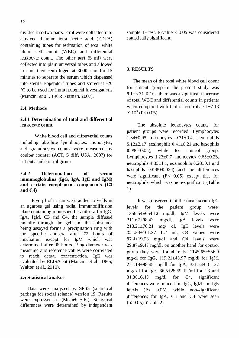
The absolute leukocytes counts for

patient groups were recorded: Lymphocytes

1.34±0.95, monocytes 0.71±0.4, neutrophils

5.12±2.17, eosinophils 0.41±0.21 and basophils

0.096±0.03), while for control group:

Lymphocytes 1.23±0.7, monocytes 0.63±0.23,

neutrophils 4.85±1.1, eosinophils 0.28±0.1 and

basophils 0.088±0.024) and the differences

were significant (P< 0.05) except that for

neutrophils which was non-significant (Table

1).

It was observed that the mean serum IgG

levels for the patient group were:

1356.54±654.12 mg/dl, IgM levels were

211.67±98.43 mg/dl, IgA levels were

213.21±76.21 mg/ dl, IgE levels were

321.54±101.37 IU/ ml, C3 values were

97.4±19.56 mg/dl and C4 levels were

29.87±9.43 mg/dl, on another hand for control

group they were found to be 1145.65±556.9

mg/dl for IgG, 119.21±48.97 mg/dl for IgM,

221.19±98.45 mg/dl for IgA, 321.54±101.37

mg/ dl for IgE, 86.5±28.59 IU/ml for C3 and

31.38±6.43 mg/dl for C4, significant

differences were noticed for IgG, IgM and IgE

levels (P< 0.05), while non-significant

differences for IgA, C3 and C4 were seen

(p>0.05) (Table 2).

21

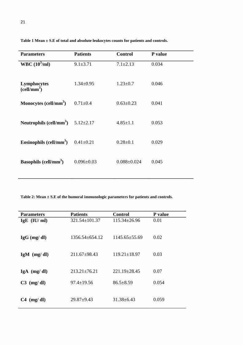
Table 1 Mean ± S.E of total and absolute leukocytes counts for patients and controls.

Table 2: Mean ± S.E of the humoral immunologic parameters for patients and controls.

Parameters Patients Control P value

WBC (103/ml) 9.1±3.71

7.1±2.13 0.034

Lymphocytes

(cell/mm3)

1.34±0.95

1.23±0.7

0.046

Monocytes (cell/mm3) 0.71±0.4

0.63±0.23

0.041

Neutrophils (cell/mm3) 5.12±2.17

4.85±1.1

0.053

Eosinophils (cell/mm3) 0.41±0.21

0.28±0.1

0.029

Basophils (cell/mm3) 0.096±0.03

0.088±0.024

0.045

Parameters Patients Control P value

IgE (IU/ ml) 321.54±101.37

115.34±26.96 0.01

IgG (mg/ dl)

1356.54±654.12

1145.65±55.69

0.02

IgM (mg/ dl)

211.67±98.43

119.21±18.97

0.03

IgA (mg/ dl)

213.21±76.21

221.19±28.45

0.07

C3 (mg/ dl) 97.4±19.56

86.5±8.59

0.054

C4 (mg/ dl)

29.87±9.43

31.38±6.43

0.059

21

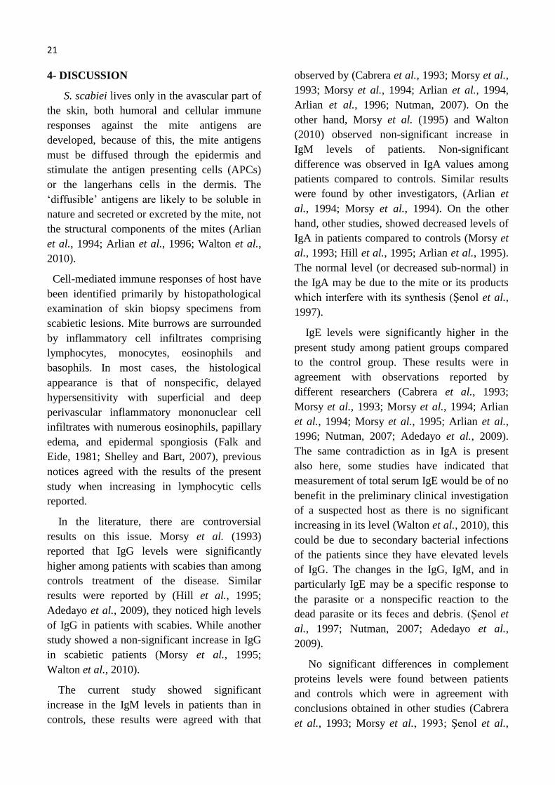
4- DISCUSSION

S. scabiei lives only in the avascular part of

the skin, both humoral and cellular immune

responses against the mite antigens are

developed, because of this, the mite antigens

must be diffused through the epidermis and

stimulate the antigen presenting cells (APCs)

or the langerhans cells in the dermis. The

‘diffusible’ antigens are likely to be soluble in

nature and secreted or excreted by the mite, not

the structural components of the mites (Arlian

et al., 1994; Arlian et al., 1996; Walton et al.,

2010).

Cell-mediated immune responses of host have

been identified primarily by histopathological

examination of skin biopsy specimens from

scabietic lesions. Mite burrows are surrounded

by inflammatory cell infiltrates comprising

lymphocytes, monocytes, eosinophils and

basophils. In most cases, the histological

appearance is that of nonspecific, delayed

hypersensitivity with superficial and deep

perivascular inflammatory mononuclear cell

infiltrates with numerous eosinophils, papillary

edema, and epidermal spongiosis (Falk and

Eide, 1981; Shelley and Bart, 2007), previous

notices agreed with the results of the present

study when increasing in lymphocytic cells

reported.

In the literature, there are controversial

results on this issue. Morsy et al. (1993)

reported that IgG levels were significantly

higher among patients with scabies than among

controls treatment of the disease. Similar

results were reported by (Hill et al., 1995;

Adedayo et al., 2009), they noticed high levels

of IgG in patients with scabies. While another

study showed a non-significant increase in IgG

in scabietic patients (Morsy et al., 1995;

Walton et al., 2010).

The current study showed significant

increase in the IgM levels in patients than in

controls, these results were agreed with that

observed by (Cabrera et al., 1993; Morsy et al.,

1993; Morsy et al., 1994; Arlian et al., 1994,

Arlian et al., 1996; Nutman, 2007). On the

other hand, Morsy et al. (1995) and Walton

(2010) observed non-significant increase in

IgM levels of patients. Non-significant

difference was observed in IgA values among

patients compared to controls. Similar results

were found by other investigators, (Arlian et

al., 1994; Morsy et al., 1994). On the other

hand, other studies, showed decreased levels of

IgA in patients compared to controls (Morsy et

al., 1993; Hill et al., 1995; Arlian et al., 1995).

The normal level (or decreased sub-normal) in

the IgA may be due to the mite or its products

which interfere with its synthesis (Şenol et al.,

1997).

IgE levels were significantly higher in the

present study among patient groups compared

to the control group. These results were in

agreement with observations reported by

different researchers (Cabrera et al., 1993;

Morsy et al., 1993; Morsy et al., 1994; Arlian

et al., 1994; Morsy et al., 1995; Arlian et al.,

1996; Nutman, 2007; Adedayo et al., 2009).

The same contradiction as in IgA is present

also here, some studies have indicated that

measurement of total serum IgE would be of no

benefit in the preliminary clinical investigation

of a suspected host as there is no significant

increasing in its level (Walton et al., 2010), this

could be due to secondary bacterial infections

of the patients since they have elevated levels

of IgG. The changes in the IgG, IgM, and in

particularly IgE may be a specific response to

the parasite or a nonspecific reaction to the

dead parasite or its feces and debris. (Şenol et

al., 1997; Nutman, 2007; Adedayo et al.,

2009).

No significant differences in complement

proteins levels were found between patients

and controls which were in agreement with

conclusions obtained in other studies (Cabrera

et al., 1993; Morsy et al., 1993; Şenol et al.,

22

1997; Mika et al., 2011) studies have indicated

similar results, whereas in other studies,

elevated levels of complement C3 were

observed (Arlin et al., 1994; Christian, 2015).

High numbers of lymphocytes, monocytes,

eosinophils and basophils in patients with

scabies were noticed by Pardo and Kerdel

(1994). Cadman and Lawrence (2010) stated

that granulocytes are innate effector cells in the

host immune defense against many

multicellular parasites. Data’s now highlights

granulocytes with immunomodulatory roles as

well, able to produce cytokines and

chemokines that can bias the immune response

in a particular direction. Eosinophils, mast cells

and basophils are reported as responsible for

the initiation and ongoing regulation of Th2

responses. They can be rapidly recruited to

sites of infection and draining lymph nodes

where they produce IL-4 and ⁄ or IL-13

(Cadman and Lawrence, 2010). Walton et al.

(2008) reported blood eosinophilia and

enhanced production of IgE, these results are in

agreements with that of the present study

where significant changes in numbers of

lymphocytes, monocytes, eosinophils and

basophils were noticed (P< 0.05).

5- CONCLUSION

The present study showed that the

immunological reactions involved in scabies

infestation includes both cellular and humoral

immune response, the most elevated leukocyte

level is eosinophils, concerning humoral

response IgE showed most elevated levels

among patients compared to controls.

However, these results are not absolute since

there are papers from literatures showed similar

results to the present study, while others

reported different ones concerning both cellular

and humoral immune responses, for this itis

recommend that studies on larger population

groups perform in future works.

Ethical consideration

An explanation of the objectives of the

study was done and an informed verbal consent

was obtained from all patients. In the case of

minors, parents or guardians were asked for the

consent. The study was approved by the

Research Ethics Committee of the College of

Medicine, Hawler Medical University, Erbil –

Iraq

REFERENCES

ADEDAYO, O.; GRELL, G. AND BELLOT, P. (2009).

Mites and HTLV-1 at the Crux of a 10-year Itch

and Plaque-Like Lesions (Human T-cell

Lymphotropic Virus 1). Infections in Medicine,

26(4): 126-130.

ARLIAN, L.G.; FALL, N. AND MORGAN, M.S.

(2007). In vivo evidence that Sarcoptes scabiei

(Acari: Sarcoptidae) is the source of molecules

that modulate splenic gene expression. Journal of

Medical Entomology, 4(6): 1054–1063.

ARLIAN, L. G.; MORGAN, M. S.; RAPP, C. M. AND

VYSZENSKI-MOHER, D. L. (1996). The

development of protective immunity in canine

scabies. Vet. Parasitol., 62: 133-142.

ARLIAN, L. G.; MORGAN, M. S.; VYSZENSKI-

MOHER, D. L. AND STEMMER, B. L. (1994).

Sarcoptes scabiei: the circulating antibody

response and induced immunity to scabies. Exp.

Parasitol., 78: 37-50.

ARLIAN, L. G.; RAPP, C. M. AND MORGAN, M. S.

(1995). Resistance and immune response in

scabies-infested hosts immunized with

Dermatophagoides mites. Am. J. Trop. Med.

Hyg., 52: 539-545.

23 CABRERA, R.; AGAR, A. AND DAHL, M. V. (1993).

The immunology of scabies. Seminaris in

Dermatology, 12(1): 15-21.

CADMAN, E. T. AND LAWRENCE, R. A. (2010).

Granulocytes: effector cells or

immunomodulators in the immune response to

helminth infection? Parasite Immunol., 32: 1–19.

CHRISTIAN, L. D. (2015).The role of endogenous

scabies mite complement inhibitors in the

development of Streptococcus pyogenes skin

infections. M.Sc. Thesis, School of Biomedical

Sciences/ Institute of Health and Biomedical

Innovation/ Faculty of Health Queensland

University of Technology & QIMR Berghofer

Medical Research Institute, 89 pp.

FALK, E. S. AND EIDE, T. J. (1981). Histologic and

clinical findings in human scabies. Int. J.

Dermatol., 20 (9):600–605.

GUREVITCH, A. W. (1985). Symposium on parasitic

infections. Scabies and Lice. Ped Clin of North

America, 32(4):987-1018.

HILL, P. B.; MORIELLO, K. A. AND DE BOER, D. J.

(1995). Concentrations of total serum IgE, IgA,

and IgG in atopic and parasitized dogs. Vet

Immunol. Immunopathol., 44: 105-113.

JAMES, W. D.; BERGER, T. G. AND ELSTON, D. M.

(2011). Parasitic Infestations, Stings, and Bites.

In: Andrews Disease of the Skin: Clinical

Dermatology, 11th edn. Philadelphia: WB

Saunders Compan; 20: 442.

BEGGS, J. C.; BEZZANT, J.; COLE, D. C.; DYKE, J.;

EHNIS, W.; ENNESS, S.; FOSTER, E.;

HOEGEMEYER, P.; JEMISON, C.;

KAUFMAN, M.; KENYON, J.; LAWHORNE,

L.; LEBBON, R.; MASTON, B.; RYE, R. A.;

SCOTT, L.; SOMSEL, P.; SPIELDENNER, S.;

STOBIERSKI, M. G.; SUNSTRUM, J.;

SZLACSKY, M.; VANVLIET, P. AND

WALKER, E. D. (2005). Scabies prevention and

control manual. Wer. 1, Michigan Department of

Community Health, 57 pp.

MANCINI, G.; CARBONARA, A. O. AND

HEREMANS, J. F. (1965). Immunochemical

quantitation of antigens by single radial

Immunodiffusion. Immunochem., 2: 235- 254.

MIKA, A.; GOH, P.; HOLT, D. C.; KEMP, D. J. AND

FISCHER, K. (2011). Scabies Mite Peritrophins

are potential targets of human host innate

immunity. PLOS Neglected Tropical Diseases,

5(9): 1-14.

MORSY, T. A.; KENAWI, M. Z.; ZOHDY, H. A.;

ABDALLA, K. F. AND EL FAKAHANY, A. F.

(1993). Serum immunoglobulin and complement

values in scabietic patients. J Egypt Soc

Parasitol, 23: 221-229.

MORSY, T. A.; EL ALFY, M. S.; ARAFA, M. A. S.;

SALAMA, M. M. AND HABIB, K. S. (1995).

Serum levels of tumour necrosis factor alpha

(TNF-alpha) versus immunoglobulins (IgG, IgM,

and IgE) in Egyptian scabietic children. J. Egypt

Soc. Parasitol., 25 (3): 773-786.

MORSY, T. A.; ZOHDI, H. W.; ABDALLA, K. F.;

NASR, M. E.; IBRAHIM, A. A.; EL SAID, A.

M. AND KHALIL, H. T. (1994).

Immunoglobulins in patients with atopic

dermatitis due to mites infestation in Qualyobia

Governorate, Egypt. J. Egypt Soc. Parasitol., 24

(3): 495-504.

ŞENOL, M.; ӦZERAL, H. I.; ӦZERAL, E.; ŞAŞMAZ,

S.; TURAN, F. AND SOYTÜRK, D. (1997).

Serum Immunoglobulin and Complement Levels

in Scabies. J. Turgut Özal Med. Cen.; 4(1): 37-

39.

NUTMAN, T. B. (2007). Evaluation and differential

diagnosis of marked, persistent eosinophilia.

Immunol Allergy Clin North Am., 27(3): 529–

549.

PARDO, J. R. AND KERDEL, F. A. (1994). Parasites,

arthropods, hazardous animals and tropical

dermatology. In: Moschella SL, Hurley HJ, eds.

Dermatol. 3rd edn. Philadelphia: WB

Saunders:1923–2004.

PODDAT, A. AND NASIRIAN, H. (2007). Prevalence

of Pediculosis and scabies in the prisoners of

Bander Abbas, Hormozgan province, Iran.

Pakistan J. Biol. Sci., 10: 3967-3969.

SHELLEY, F. W. AND BART, J. C. (2007). Problems

in diagnosing scabies, a global disease in human

and animal populations. Clinic. Microbiol. Revi.,

20 (2): 268–279.

WALTON, S. F.; BEROUKAS, D.; ROBERTS-

THOMSON, P. AND CURRIE, B. J. (2008).

New insights into disease pathogenesis in crusted

(Norwegian) scabies: the skin immune response

in crusted scabies. Br. J. Dermatol., 158: 1247–

1255.

WALTON, S. F.; PIZZUTTO, S.; SLENDER, A.;

VIBERG, L.; HOLT, D.; HALES, B. J.; KEMP,

D. J.; CURRIE, B. J.; ROLLAND, J. M. AND

HEHIR, R. O. (2010). Increased allergic immune

response to Sarcoptes scabiei antigens in crusted

versus ordinary Scabies. Clinical and Vaccine

Immunology, 17(9): 1428–1438.

ZANCO Journal of Pure and Applied Sciences The official scientific journal of Salahaddin University-Erbil

ZJPAS (2017), 29 (2); 24-31 http://dx.doi.org/10.21271/ZJPAS.29.2.3

The Economy Feasibility of Implementation WDS Project in Mala Omer Catchment Area

Dana Mawlood1 and Awaz Jalal Hussein2 1- Civil Engineering Department, college of Engineering, University of Salahaddin

2- Construction Engineering and Management, KRG Ministry of Municipalities and Tourism, Head of Zakho

Municipalities

1. INTRODUCTION

Human kind cannot survive more than few days without water. No developments and human achievements would have been achieved without water (Brooks et al., 2009). Poor water management mostly hurts poor people (Mays, 2009). The target on equitable, participatory and accountable water governance will require strong political commitment, appropriate policy and legal frameworks, effective institutional structures, efficient administrative systems and capable human resources aligned with required investments (Biswas et al., 2008).Thus, it needs to be recognized that using water

restricts the usage by others, and therefore, there is a cost involved in the action (Mays, 2009). The use of water charges to generate resources for maintenance and to reduce demand is widely advocated (Perry, 2001). A key component of pricing and institutional reform is to establish water prices that reflect the full cost of water consumption and provide incentives for efficient water-use decisions, including those relating to investment in new potable supplies, alternative sources and water savings. The purpose of consumption-based pricing is to encourage more efficient water use by aligning water bills and water consumption (National Water Commission, 2011).

A R T I C L E I N F O

A B S T R A C T

Article History: Received: 07/05/2016 Accepted: 15/11/2016 Published: 07/06/2017

The aim of the present study was to evaluate the Water Distribution System (WDS) and water distribution economy feasibility in light of Mala Omer research area that belongs to KR-I. Data have been collected regarded Mala Omer through site visits and interviews with stakeholders and it was then analyzed for information abstraction to assess the water distribution feasibility. Operation expenditures (OPEX) were estimated to 39% of the total revenue. The WDS network was not sufficient and new water paradigm was proposed working by gravity. The costs and revenue have been analyzed, the capital cost will require about five years. While the Internal Rate of Return (IRR) was 33.4%. The results of the study showed insufficient WDS with significance of the economy feasibility of the project. Family size should have significance consideration in water consumption and price rates.

Keywords: Mala Omer WDS Assessment Water price Economy Feasibility *Corresponding Author: Dana Mawlood Khmdana@gmail.com

25 Mawlood and Hussein /ZJPAS: 2017, 29(2): 24-31

The current study is conducted in Kurdistan Region of Iraq government, which represents the primary investor in water infrastructure of the research area Mala Omer. The research area is a small community belongs to Erbil province.

The main concerns of the community are improper water distribution system and continue deficit in amounts supplied. This is mainly because of irrational exploitation of the aquifer and lack of capacity in water sector. The pricing reform aims to make the economic efficiency of water use and the industry as a whole getting better. Efficient water pricing helps ensure that water-related production and consumption decisions across all sectors should be reflective of the costs they require, that way driving national economic productivity and societal welfare gains (National Water Commission, 2011) . However, the effect of pricing on water conservation and elsewhere has been effectively demonstrated like in Tucson (Beecher et al., 1994) and for agricultural water in Morocco (Lionboui et al., 2014). There should be an assessment to evaluate the cost and benefits of water supply. People pay water fees in most Kurdistan Region Government places; however, in Mala Omer, yet, the government provides water free of charge for people living there. The provided water is not enough and does not fill the people needs as there is yet a shortage in water supplying similarly as in some cities in India, for instance, Kolkata (Roy et al., 2010). It was shown previously that Water Resources and Economics is addressing the economic and financial dimensions that affect the use of water resources, across different economic sectors, including rural and urban water supply (Roy et al., 2010; Barde and Lehmann, 2014). The study in Kolkata used the artificial neural network technique for estimating cost of water. People were willing to pay for supply of

drinking water (Roy et al., 2010); no study has been undertaken in Kurdistan Region of Iraq government for determining economic feasibility of water thus far.

Therefore, this study is conducted to study the feasibility of the water economy within the research area. The approach is interested in assessing the project’s ability to generate the revenue streams so as to cover financial costs over time. “Water has an economic value in all its competing uses and should be recognized as an economic good, for example, having ensured basic human needs, allocating water to its highest value, and moving towards full cost pricing, rational use and cost recovery” [Mays, 2009; Rahaman, 2009].

2. METHODOLOGY

2.1. Location of Research Area

The selected case study is the water distribution network in Mala Omer. It is a small community of KRI, belongs to Erbil province and it is located in coordinates 36°18�0ʺ N and 44°8�3ʺ E. The topography of the research area face a huge difference in elevation changes since the lowest and highest points range are between (548 and 901 m) above S.L.

2.2. Data Collection and Analysis

There is no unique method of collecting data which is perfect in all terms, besides there being no reliable database system within Kurdistan Region Government (KRG). In the present study, questionnaires and personal interviews were used for data collection. The amount of the consumed water in the research area was difficult to be accurately estimated.

The sources of water were determined by personal interviews with Mala Omer water

26 Mawlood and Hussein /ZJPAS: 2017, 29(2): 24-31 wells operators and private owner wells. Global Positioning System (GPS) was used to determine wells location, and then, Geographical Information System (GIS) was used to determine the location, topography, distance measurement between wells, and land use map, Fig. 1. Exponential equation was used

for population growth rate forecast. Internal Rate of Return (IRR) and capital recovery payback period methods were used for economic feasibility. Microsoft Excel was used for financial calculations and sensitivity graph and analysis.

Figure 1: Wells Location Map of the Research Area and Land Use.

3. RESULTS AND DISCUSSION

3.1. Water Distribution System (WDS)

Eighty-five wells were observed to abstract water from the groundwater within the research area, but ten wells were dried and were not suitable for abstracting water. Twenty eight wells of them are used for domestic water supply within the research area and eighteen of them are operated by government and the other are personnel by public people, some of them are shared for domestic and agricultural (KRG-MM).

The water distribution systems used within the research area are mainly through direct pumping and also pumping from storage water tanks. There are about 5,000 meters of old water distribution pipes within the research area. The system misses manholes in general, especially, in case of old water distribution pipes that cause delay in identifying the leakage, and broken pipes that lay under houses and causes mixing of wastewater with drinking water beside the improper design and pipe

27 Mawlood and Hussein /ZJPAS: 2017, 29(2): 24-31 erection methods that result in traffic disruption (KRG-MM).

In fact, water is distributed from many wells in different places. In addition, the topography of Mala Omer faces huge difference in elevation. There is no equity in water distribution among served number of families provided with water, and about 1% of the served population has no water connection to their houses. Other houses are provided with at least one connection; whereas, there are families does not having enough water, because of insufficient pressure in water that make it difficult to reach them. In addition, operation and maintenance costs for water network maintenance are also insufficient and not provided on time to cover the required maintenance.

Every year, the required amount of water is increasing, but wells’ yield is decreasing (KRG-MM). Therefore, wells have become unable to provide the required water; thus, new water pipe was driven from Pirmam city to the research area passing through the main old road of research area (KRG-MM). This includes an 8 inches ductile pipe and connected to the existed main pipes that are four inches in diameter. Thus, consequently, that pipe to be connected to the existed wells and storage tanks within the research area that have a total capacity of 220 m3. Implementing with existing topography conditions and tank positions at first place, the project includes providing more manholes to the area (KRG-MM).

The amount of the consumed water in the research area is frequently difficult to be accurately estimated. This is due to the absence of any measuring meters, storage tanks with specified times and also missing records of daily amount abstracted from wells; because the main source of water is ground-water wells for supplying water for domestic purposes, agricultural and commercial purposes (Roy et al., 2010).

3.2 Evaluation of the Water Supply Network

The supplied water has been decreased due to the groundwater continuous depletion (Iglesias et al., 2009) as a result of lack integrated water planning. Therefore, it is recommended that the unifying WDS and supplying water to be reliable. This is because the old existed pipes are not reliable and they faced unplanned growth in land use changes and constructions have buried some pipes. Besides, it cannot provide the required pressure, aligned with higher costs of pumping from different areas duplicate costs aligned with more drawdown.

As mentioned earlier, the reliability of the existing aging systems is continually decreasing (Mays, 1999). In addition, the existed WDS network does not provide the desired pressures. It was concluded that, it is more effective for consistent and effective WDS to design a new one, which will be based on the design criteria for allowable pressures and velocities. In addition, it is more economical and easier for operation because it does not need pumps.

The population of Mala Omer was 3000 persons by 1997 (Sharif, 1998) and reached 11655 persons by 2013 (KRG-MM), research area is facing a big increment in population, which is estimated to be 7.98% using exponential equation (Rubin and Davidson, 2001). It is extreme when compared to Erbil population incremental rate, depending on Erbil population data (KRG-MP, 2014) using the same exponential equation estimated to equals 2.32%. This difference in the population increase is due to the location of the research area, which is close to Erbil city that made people settle to the research area.

Therefore, the government should take serious actions to balance the development in urbanization. As well as controlling the population growth by considering that all parts of the KRG area require to be planned on basis

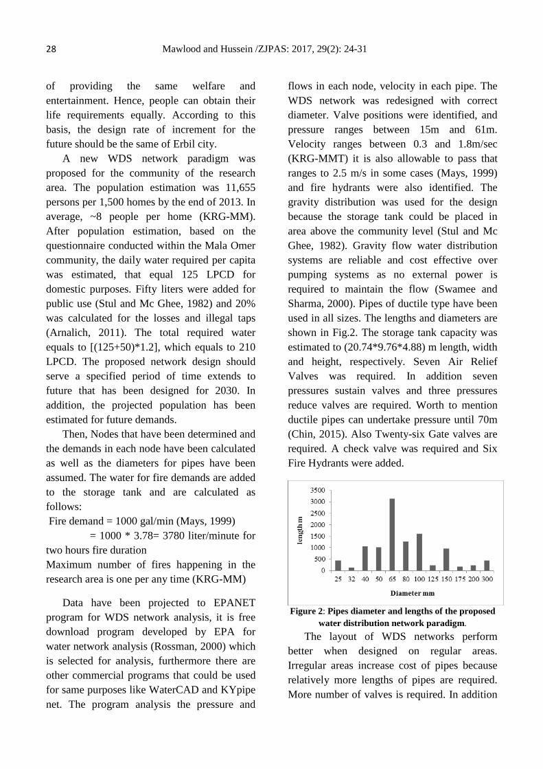
28 Mawlood and Hussein /ZJPAS: 2017, 29(2): 24-31 of providing the same welfare and entertainment. Hence, people can obtain their life requirements equally. According to this basis, the design rate of increment for the future should be the same of Erbil city.

A new WDS network paradigm was proposed for the community of the research area. The population estimation was 11,655 persons per 1,500 homes by the end of 2013. In average, ~8 people per home (KRG-MM). After population estimation, based on the questionnaire conducted within the Mala Omer community, the daily water required per capita was estimated, that equal 125 LPCD for domestic purposes. Fifty liters were added for public use (Stul and Mc Ghee, 1982) and 20% was calculated for the losses and illegal taps (Arnalich, 2011). The total required water equals to [(125+50)*1.2], which equals to 210 LPCD. The proposed network design should serve a specified period of time extends to future that has been designed for 2030. In addition, the projected population has been estimated for future demands.

Then, Nodes that have been determined and the demands in each node have been calculated as well as the diameters for pipes have been assumed. The water for fire demands are added to the storage tank and are calculated as follows: Fire demand = 1000 gal/min (Mays, 1999) = 1000 * 3.78= 3780 liter/minute for two hours fire duration Maximum number of fires happening in the research area is one per any time (KRG-MM)

Data have been projected to EPANET program for WDS network analysis, it is free download program developed by EPA for water network analysis (Rossman, 2000) which is selected for analysis, furthermore there are other commercial programs that could be used for same purposes like WaterCAD and KYpipe net. The program analysis the pressure and

flows in each node, velocity in each pipe. The WDS network was redesigned with correct diameter. Valve positions were identified, and pressure ranges between 15m and 61m. Velocity ranges between 0.3 and 1.8m/sec (KRG-MMT) it is also allowable to pass that ranges to 2.5 m/s in some cases (Mays, 1999) and fire hydrants were also identified. The gravity distribution was used for the design because the storage tank could be placed in area above the community level (Stul and Mc Ghee, 1982). Gravity flow water distribution systems are reliable and cost effective over pumping systems as no external power is required to maintain the flow (Swamee and Sharma, 2000). Pipes of ductile type have been used in all sizes. The lengths and diameters are shown in Fig.2. The storage tank capacity was estimated to (20.74*9.76*4.88) m length, width and height, respectively. Seven Air Relief Valves was required. In addition seven pressures sustain valves and three pressures reduce valves are required. Worth to mention ductile pipes can undertake pressure until 70m (Chin, 2015). Also Twenty-six Gate valves are required. A check valve was required and Six Fire Hydrants were added.

Figure 2: Pipes diameter and lengths of the proposed water distribution network paradigm.

The layout of WDS networks perform better when designed on regular areas. Irregular areas increase cost of pipes because relatively more lengths of pipes are required. More number of valves is required. In addition

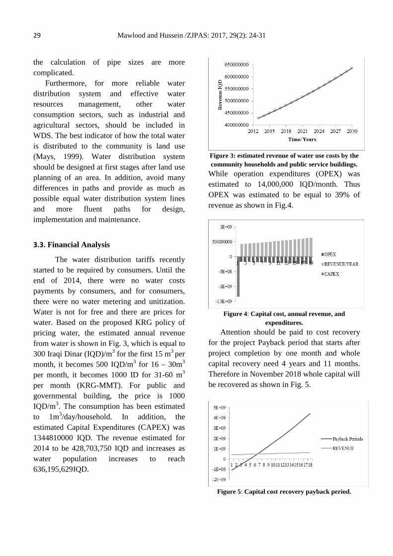
29 Mawlood and Hussein /ZJPAS: 2017, 29(2): 24-31 the calculation of pipe sizes are more complicated.

Furthermore, for more reliable water distribution system and effective water resources management, other water consumption sectors, such as industrial and agricultural sectors, should be included in WDS. The best indicator of how the total water is distributed to the community is land use (Mays, 1999). Water distribution system should be designed at first stages after land use planning of an area. In addition, avoid many differences in paths and provide as much as possible equal water distribution system lines and more fluent paths for design, implementation and maintenance.

3.3. Financial Analysis

The water distribution tariffs recently started to be required by consumers. Until the end of 2014, there were no water costs payments by consumers, and for consumers, there were no water metering and unitization. Water is not for free and there are prices for water. Based on the proposed KRG policy of pricing water, the estimated annual revenue from water is shown in Fig. 3, which is equal to 300 Iraqi Dinar (IQD)/m3 for the first 15 m3 per month, it becomes 500 IQD/m3 for 16 – 30m3 per month, it becomes 1000 ID for 31-60 m3 per month (KRG-MMT). For public and governmental building, the price is 1000 IQD/m3. The consumption has been estimated to 1m3/day/household. In addition, the estimated Capital Expenditures (CAPEX) was 1344810000 IQD. The revenue estimated for 2014 to be 428,703,750 IQD and increases as water population increases to reach 636,195,629IQD.

Figure 3: estimated revenue of water use costs by the community households and public service buildings.

While operation expenditures (OPEX) was estimated to 14,000,000 IQD/month. Thus OPEX was estimated to be equal to 39% of revenue as shown in Fig.4.

Figure 4: Capital cost, annual revenue, and

expenditures. Attention should be paid to cost recovery

for the project Payback period that starts after project completion by one month and whole capital recovery need 4 years and 11 months. Therefore in November 2018 whole capital will be recovered as shown in Fig. 5.

Figure 5: Capital cost recovery payback period.

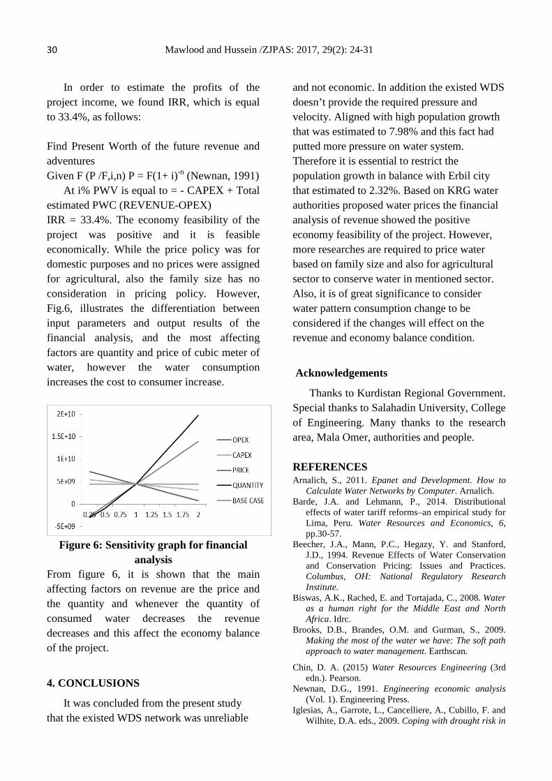
30 Mawlood and Hussein /ZJPAS: 2017, 29(2): 24-31

In order to estimate the profits of the project income, we found IRR, which is equal to 33.4%, as follows: Find Present Worth of the future revenue and adventures Given F (P /F,i,n) P = F(1+ i)-n (Newnan, 1991)

At i% PWV is equal to = - CAPEX + Total estimated PWC (REVENUE-OPEX) IRR = 33.4%. The economy feasibility of the project was positive and it is feasible economically. While the price policy was for domestic purposes and no prices were assigned for agricultural, also the family size has no consideration in pricing policy. However, Fig.6, illustrates the differentiation between input parameters and output results of the financial analysis, and the most affecting factors are quantity and price of cubic meter of water, however the water consumption increases the cost to consumer increase.

Figure 6: Sensitivity graph for financial

analysis From figure 6, it is shown that the main affecting factors on revenue are the price and the quantity and whenever the quantity of consumed water decreases the revenue decreases and this affect the economy balance of the project.

4. CONCLUSIONS

It was concluded from the present study that the existed WDS network was unreliable

and not economic. In addition the existed WDS doesn’t provide the required pressure and velocity. Aligned with high population growth that was estimated to 7.98% and this fact had putted more pressure on water system. Therefore it is essential to restrict the population growth in balance with Erbil city that estimated to 2.32%. Based on KRG water authorities proposed water prices the financial analysis of revenue showed the positive economy feasibility of the project. However, more researches are required to price water based on family size and also for agricultural sector to conserve water in mentioned sector. Also, it is of great significance to consider water pattern consumption change to be considered if the changes will effect on the revenue and economy balance condition.

Acknowledgements

Thanks to Kurdistan Regional Government. Special thanks to Salahadin University, College of Engineering. Many thanks to the research area, Mala Omer, authorities and people. REFERENCES Arnalich, S., 2011. Epanet and Development. How to

Calculate Water Networks by Computer. Arnalich. Barde, J.A. and Lehmann, P., 2014. Distributional

effects of water tariff reforms–an empirical study for Lima, Peru. Water Resources and Economics, 6, pp.30-57.

Beecher, J.A., Mann, P.C., Hegazy, Y. and Stanford, J.D., 1994. Revenue Effects of Water Conservation and Conservation Pricing: Issues and Practices. Columbus, OH: National Regulatory Research Institute.

Biswas, A.K., Rached, E. and Tortajada, C., 2008. Water as a human right for the Middle East and North Africa. Idrc.

Brooks, D.B., Brandes, O.M. and Gurman, S., 2009. Making the most of the water we have: The soft path approach to water management. Earthscan.

Chin, D. A. (2015) Water Resources Engineering (3rd edn.). Pearson.

Newnan, D.G., 1991. Engineering economic analysis (Vol. 1). Engineering Press.

Iglesias, A., Garrote, L., Cancelliere, A., Cubillo, F. and Wilhite, D.A. eds., 2009. Coping with drought risk in

31 Mawlood and Hussein /ZJPAS: 2017, 29(2): 24-31

agriculture and water supply systems: Drought management and policy development in the Mediterranean (Vol. 26). Springer Science & Business Media.

Kurdistan Region Government, Ministry of Municipality and Tourism (KRG-MMT), General Directorate of Water and Sewerage, Design Department.

Kurdistan Region Government, Ministry of Municipalities (KRG-MM), General Directorate of Erbil Municipalities, Mala Omer Municipality

Kurdistan Region Government, Ministry of Planning (KRG-MP), Kurdistan Region Statistics Office, Population Projection Report for KRI for period (2009-2020), 2014

Lionboui, H., Fadlaoui, A., Elame, F. and Benabdelouahab, T., 2014. Water pricing impact on the economic valuation of water resources. International Journal of Education and Research, 2(6), pp.147-166.

Mays, L. ed., 2009. Integrated Urban Water Management: Arid and Semi-Arid Regions: UNESCO-IHP (Vol. 3). CRC Press.

Mays, L.W., 1999. Water distribution system handbook. New York, NY, USA: McGraw-Hill Professional Publishing.

National Water Commission, 2011. Review of pricing reform in the Australian water sector.

Perry, C.J., 2001. Charging for irrigation water: The issues and options, with a case study from Iran (Vol. 52). IWMI.

Rahaman, M.M., 2009. INTEGRATED WATER RESOURCES MANAGEMENT: Constraints and opportunities with a focus on the Ganges and the Brahmaputra River Basins. Teknillinen korkeakoulu.

Rossman, L.A., 2000. EPANET 2: user’s manual. Roy, K.D., Thakur, B., Konar, T.S. and Chakrabarty,

S.N., 2010. Rapid evaluation of water supply project feasibility in Kolkata, India. Drink. Water Eng. Sci, 3(1), pp.29-42.

Rubin, E.S. and Davidson, C.I., 2001. Introduction to Engineering and the Environment. New York: McGraw-Hill.

Sharif, A. J. (1998) Study of Local Climate Comparison, Erbil Area Climate (Doctoral Thesis in Philosophy of Geography, College of Art, Sallahadin University-Hawler).

Stul, E.W. and Mc Ghee, T.J., 1982. Water supply and sewerage. McGraw-Hill International Book Company.

Swamee, P.K. and Sharma, A.K., 2000. Gravity flow water distribution system design. Journal of Water Supply: Research and Technology-Aqua, 49(4), pp.169-179.

Mawlud S. et al./ZJPAS: 2017, 29(2): 32-42

Structural characterization and Thermal Behavior of Sm3+ Ions Doped Sodium Tellurite Glasses

1,2Saman Q. Mawlud, 1Mudhafar M. Ameen, 2Md. Rahim Sahar, 1,2Kasim F. Ahmed

1Department of Physics, College of Education, University of Salahaddin, Erbil, Kurdistan Region, Iraq. 2Advanced Optical Material Research Group, Department of Physics, Faculty of Science, University of Technology Malaysia, Skudai, Johor, Malaysia.

A RT I C L E I N FO

ArticleHistory:

Received:27/08/2016 Accepted:20/11/2016 Published:07/06/2017

Keywords:

Tellurite glass, Rare Earth, Glass transition, FTIR, Raman spectra

*CorrespondingAuthor:

Saman Q. Mawlud Email: saman.mawlud@su.edu.krd

A B ST R AC T

The influence of Sm+3 ions concentration doped sodium tellurite glasses on structural characterizationand thermal parameters have been investigated. Glass samples with molar composition (80-x) TeO2-20Na2O-xSm2O3 glasses (x=0, 0.3, 0.6, 1, 1.2, 1.5) are prepared by conventionalmelt quenching technique.Crystallization temperature (Tc), melting temperature (Tm) and glass transition temperature (Tg) are measured by using differential thermal analysis (DTA),it is found that the stability factor (ΔT) of the glassincreases from (58.5to97.8) ºC with the increasingSm2O3. The amorphous phase nature of the glass samplesare observed by using X-ray diffraction (XRD), scanning electron microscopy (SEM) and energy dispersive x-ray (EDX) analysisspectrometer are applied to study the structural properties of the glass samples. Values of Thedensity (ρ), molar volume (VM), and ionic packing density (Vt) were calculated for each of the glass compositions.The effect of the Sm2O3 on the glass structure has been investigated by using Fourier transform infrared (FTIR)and Raman spectroscopies, the FTIR spectra are characterized by a band of 637 cm-1 for the telluride glass, high frequency peak at 668 cm-1 presented by Raman spectra which indicates that these glasses network arebasically consists of TeO4 and TeO3/TeO3+1structural units. The Raman spectra of shows the presence of Sm-O bond, Na-O bond, Te-O-Te bridging configurations, vibrations of Te-O-Te bonds and stretching modes of non-bonding oxygen found on the TeO3/TeO3+1 structural unit.

1. INTRODUCTION Under normal quenching conditions

tellurium dioxide (TeO2) does not possess the ability of forming a glassy network without

theaidof the secondary material component which is called a network modifier.This specific feature makes TeO2a conditional glass former (El-Mallawany, 2011;

ZANKO Journal of Pure and Applied Science The official scientific journal of Salahaddin University-Erbil

ZJPAS (2017), 29 (2); 32-42 http://dx.doi.org/10.21271/ZJPAS.29.2.4

Mawlud S. et al./ZJPAS: 2017, 29(2): 32-42

Çelikbileket al., 2011).Manystudies indicate that heavy metal oxide (HMO) glasses have been found to be more promising convenient glassy materials especially for photonic applications with acceptable low phonon energies (Sun et. al., 2006;Pan et. al., 1996),their wide advantages of tellurite glasses makes them to be represented as a more attractive structure among the HMO glasses such as low temperature of melting, good corrosion resistance, excellent chemical durability, low glass transition temperature Tg, better thermal stability, high thermal expansion coefficient, low phonon energy, wide optical transmission region (especially in the infrared region) (0.36μm–6.3μm), high refractive index and required rare earth concentration in the matrices (Xuet al., 2005).Basically, the structure of TeO2 glasses contains of three dimensional network of TeO4 trigonal bipiramids (tpb) units having two each of oxygen at two equatorial and axial sites with one other equatorial site being occupied by a lone pair of electrons, once the modifier is introduced to the structure, the three dimensional network will break down with the conversion of TeO4 units into TeO3+1 and TeO3 units (Kiefferet al., 2006; Radaet al. 2011).

In addition to the glass former conditionality and fast quenching requirements properties of tellurite glasses, they are also counted as a good host for the formation of rare earth doped glasses.The Te–O bonds are weak and canbe broken easilyby addingheavy metal and the rare earth atoms (Muraliet al., 2005). In the literature there are relatively few reports on structural of glasses doped with Sm3O ions (Bolundutet al., 2015;Yusoffet al. 2015). Accordingly the present work aims to investigate the influence of Sm3+ ion on the structural and thermal properties of TeO2-Na2O glasses. The thermal modification of the glass system were analyzed by DTA technique and the structure

of the Sm2O3 doped glasses has been studied through Raman and FTIR Spectra.

2. MATERIALS AND METHODS

TeO2-Na2O-Sm2O3glass samples possessing compositions(80-x) TeO2-20Na2O-xSm2O3 with (x=0,0.3,0.6,1,1.2,1.5)are prepared using melt quenching techniquewhich is essentially the amorphous solid can be formed by the continuous hardening (namely increase in viscosity) of the melt,, glasses code of the samples and their molar ratio of the compositions are listed in Table 1.High purity 99.9% of raw materials from Sigma Aldrichwith an appropriate amounts of chemicals for 15gm batch were weighed by using electronic balance Precisa 205A SCS model with accuracy ±0.001gm,the chemical compositions were mixed well by using a milling machine. Platinum crucible of about 30ml capacity containing the batch was used and preheated at 250ºC for about minutes for reducing the batch blanket coverage on the top of the glass and enlarges the free non coverage glass melt surface(Saharat al., 2007).Then the batch is melted at 900 ºC for 40 min by a controlled electric furnace. The melts are poured on to a stainless steel mold and annealed at 250 ºC for 3hours, then the sample cooled down tothe room temperature, sample powder of the glass prepared and used for characterizing each of Tg, Tc and Tmby Pyris Dymond TG/DTA technique at a heating rate 50°C-1000°C at 10°C/min.To analysis the amorphous state of the samples an advanced powder XRD Bruker D8 were used, the CuKα radiation specification was (1.54A°) at 40 kV, 100mA and scanning angel 2θ ranges between 10°-80°. A Perkin–Elmer FTIR double beam spectrometer over the range 400-4000 cm-1 are used for studying the transmission measurements, the spectra resolution of 4 cm-1at room temperature made by using KBr pelletswere investigated.Raman analysisis performed using a confocal Horbia

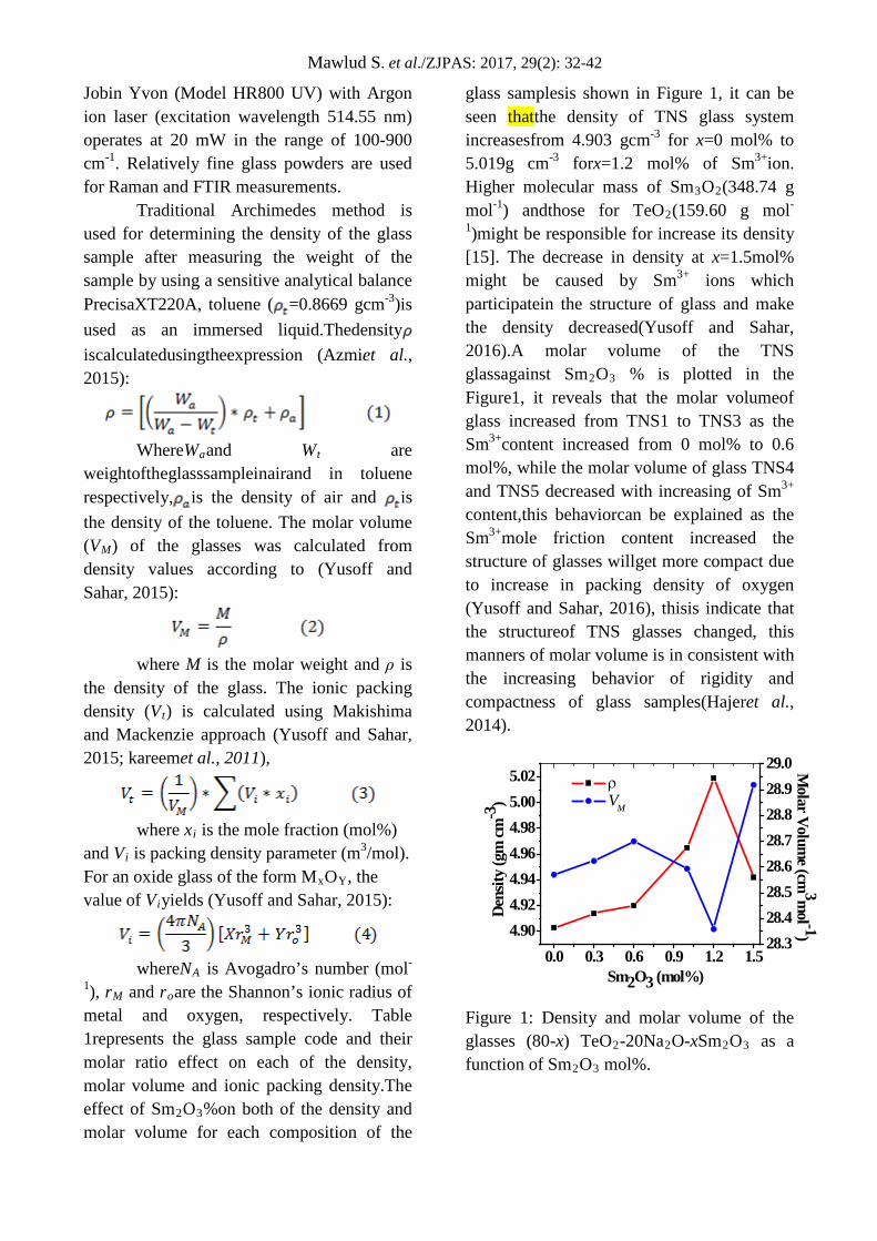
Mawlud S. et al./ZJPAS: 2017, 29(2): 32-42

Jobin Yvon (Model HR800 UV) with Argon ion laser (excitation wavelength 514.55 nm) operates at 20 mW in the range of 100-900 cm-1. Relatively fine glass powders are used for Raman and FTIR measurements.

Traditional Archimedes method is used for determining the density of the glass sample after measuring the weight of the sample by using a sensitive analytical balance PrecisaXT220A, toluene ( =0.8669 gcm-3)is used as an immersed liquid.Thedensity iscalculatedusingtheexpression (Azmiet al., 2015):

WhereWaand Wt are

weightoftheglasssampleinairand in toluene respectively, is the density of air and is the density of the toluene. The molar volume (VM) of the glasses was calculated from density values according to (Yusoff and Sahar, 2015):

where M is the molar weight and ρ is

the density of the glass. The ionic packing density (Vt) is calculated using Makishima and Mackenzie approach (Yusoff and Sahar, 2015; kareemet al., 2011),

where xi is the mole fraction (mol%)

and Vi is packing density parameter (m3/mol). For an oxide glass of the form MxOY, the value of Viyields (Yusoff and Sahar, 2015):

whereNA is Avogadro’s number (mol-

1), rM and roare the Shannon’s ionic radius of metal and oxygen, respectively. Table 1represents the glass sample code and their molar ratio effect on each of the density, molar volume and ionic packing density.The effect of Sm2O3%on both of the density and molar volume for each composition of the

glass samplesis shown in Figure 1, it can be seen thatthe density of TNS glass system increasesfrom 4.903 gcm-3 for x=0 mol% to 5.019g cm-3 forx=1.2 mol% of Sm3+ion. Higher molecular mass of Sm3O2(348.74 g mol-1) andthose for TeO2(159.60 g mol-

1)might be responsible for increase its density [15]. The decrease in density at x=1.5mol% might be caused by Sm3+ ions which participatein the structure of glass and make the density decreased(Yusoff and Sahar, 2016).A molar volume of the TNS glassagainst Sm2O3 % is plotted in the Figure1, it reveals that the molar volumeof glass increased from TNS1 to TNS3 as the Sm3+content increased from 0 mol% to 0.6 mol%, while the molar volume of glass TNS4 and TNS5 decreased with increasing of Sm3+ content,this behaviorcan be explained as the Sm3+mole friction content increased the structure of glasses willget more compact due to increase in packing density of oxygen (Yusoff and Sahar, 2016), thisis indicate that the structureof TNS glasses changed, this manners of molar volume is in consistent with the increasing behavior of rigidity and compactness of glass samples(Hajeret al., 2014).

0.0 0.3 0.6 0.9 1.2 1.54.904.924.944.964.985.005.02 ρ

VM

Sm2O3 (mol%)

Dens

ity (g

m cm

-3)

28.328.428.528.628.728.828.929.0 M

olar Volume (cm

3mol -1)

Figure 1: Density and molar volume of the glasses (80-x) TeO2-20Na2O-xSm2O3 as a function of Sm2O3 mol%.

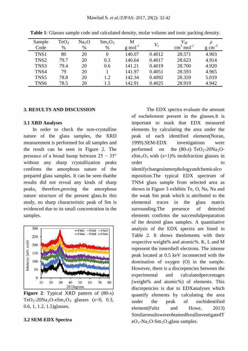
Mawlud S. et al./ZJPAS: 2017, 29(2): 32-42

3. RESULTS AND DISCUSSION 3.1 XRD Analyses In order to check the non-crystalline nature of the glass samples, the XRD measurement is performed for all samples and the result can be seen in Figure 2. The presence of a broad hump between 25 − 35° without any sharp crystallization peaks confirms the amorphous nature of the prepared glass samples. It can be seen thatthe results did not reveal any kinds of sharp peaks, therefore,proving the amorphous nature structure of the present glass.In this study, no sharp characteristic peak of Sm is evidenced due to its small concentration in the samples.

Figure 2: Typical XRD pattern of (80-x) TeO2-20Na2O-xSm2O3 glasses (x=0, 0.3, 0.6, 1, 1.2, 1.5)glasses. 3.2 SEM-EDX Spectra

The EDX spectra evaluate the amount of eachelement present in the glasses.It is important to mark that EDX measured elements by calculating the area under the peak of each identified element(Noran, 1999).SEM-EDX investigations were performed on the (80-x) TeO2-20Na2O-xSm2O3 with (x=1)% molefraction glasses in order to identifychangesinmorphologyandchemicalcomposition.The typical EDX spectrum of TNS4 glass sample from selected area as shown in Figure 3 exhibits Te, O, Na, Na and the weak Sm peak which is attributed to the elemental traces in the glass matrix surrounding.The presence of detected elements confirms the successfulpreparation of the desired glass samples. A quantitative analysis of the EDX spectra are listed in Table 2. It shows theelements with their respective weight% and atomic%. K, L and M represent the innershell electrons. The intense peak located at 0.5 keV isconnected with the domination of oxygen (O) in the sample. However, there is a discrepencies between the experimental and calculatedpercentages (weight% and atomic%) of elements. This discrepencies is due to EDXanalyses which quantify elements by calculating the area under the peak of eachidentified element(Fultz and Howe, 2013) SimilarresultswereobtainedforallinvestigatedTeO2-Na2O-Sm2O3glass samples.

Table 1: Glasses sample code and calculated density, molar volume and ionic packing density.

ρ g cm-3

VM cm3 mol-1 Vt M

g mol-1 Sm2O3

% Na2O

% TeO2

% Sample Code

4.903 28.571 0.4012 140.07 0 20 80 TNS1 4.914 28.623 0.4017 140.64 0.3 20 79.7 TNS2 4.920 28.700 0.4019 141.21 0.6 20 79.4 TNS3 4.965 28.593 0.4051 141.97 1 20 79 TNS4 5.019 28.359 0.4092 142.34 1.2 20 78.8 TNS5 4.942 28.919 0.4025 142.91 1.5 20 78.5 TNS6

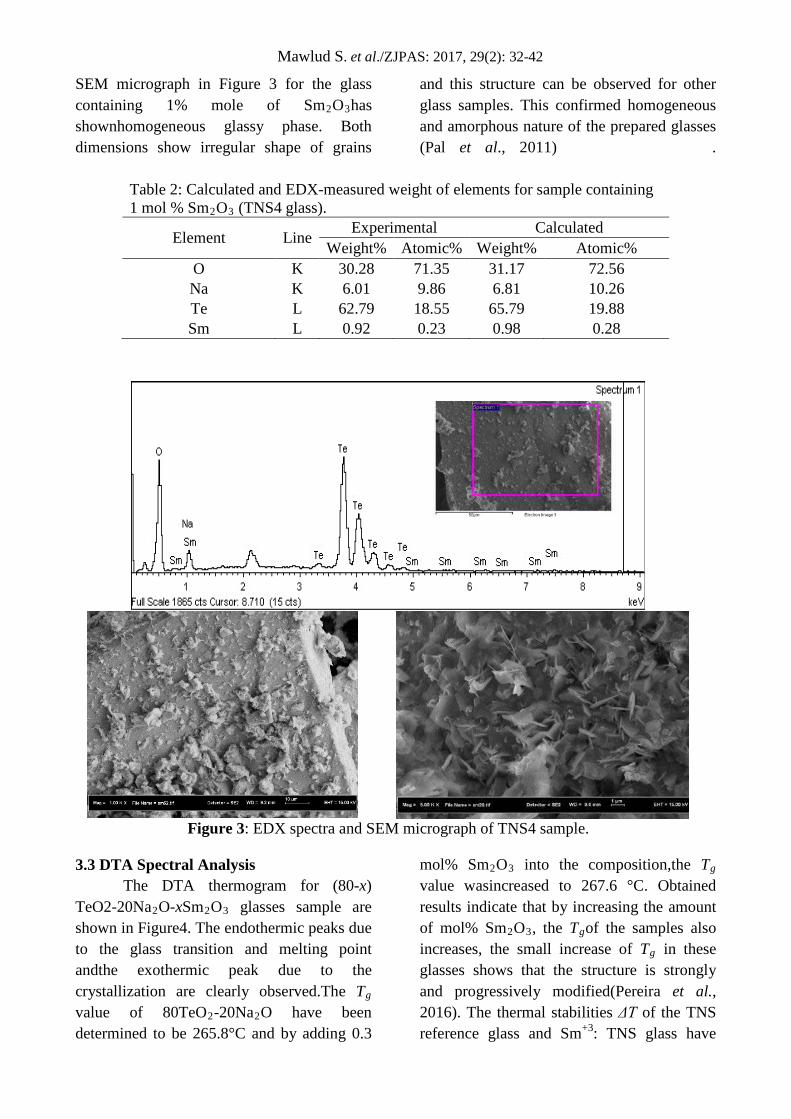
Mawlud S. et al./ZJPAS: 2017, 29(2): 32-42

SEM micrograph in Figure 3 for the glass containing 1% mole of Sm2O3has shownhomogeneous glassy phase. Both dimensions show irregular shape of grains

and this structure can be observed for other glass samples. This confirmed homogeneous and amorphous nature of the prepared glasses (Pal et al., 2011) .

Table 2: Calculated and EDX-measured weight of elements for sample containing 1 mol % Sm2O3 (TNS4 glass).

Element Line Experimental Calculated Weight% Atomic% Weight% Atomic%

O K 30.28 71.35 31.17 72.56 Na K 6.01 9.86 6.81 10.26 Te L 62.79 18.55 65.79 19.88 Sm L 0.92 0.23 0.98 0.28

Figure 3: EDX spectra and SEM micrograph of TNS4 sample.

3.3 DTA Spectral Analysis

The DTA thermogram for (80-x) TeO2-20Na2O-xSm2O3 glasses sample are shown in Figure4. The endothermic peaks due to the glass transition and melting point andthe exothermic peak due to the crystallization are clearly observed.The Tg value of 80TeO2-20Na2O have been determined to be 265.8°C and by adding 0.3

mol% Sm2O3 into the composition,the Tg value wasincreased to 267.6 °C. Obtained results indicate that by increasing the amount of mol% Sm2O3, the Tgof the samples also increases, the small increase of Tg in these glasses shows that the structure is strongly and progressively modified(Pereira et al., 2016). The thermal stabilities ΔT of the TNS reference glass and Sm+3: TNS glass have

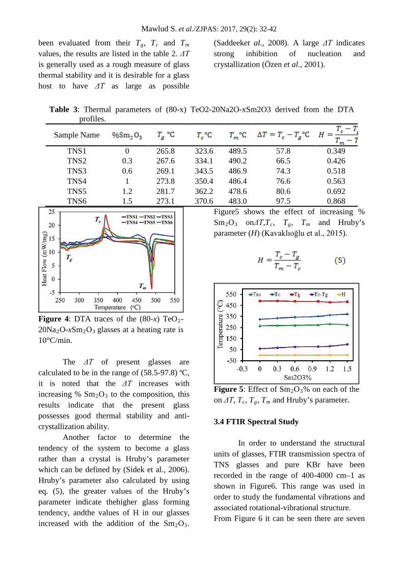
Mawlud S. et al./ZJPAS: 2017, 29(2): 32-42

been evaluated from their Tg, Tc and Tm values, the results are listed in the table 2. ΔT is generally used as a rough measure of glass thermal stability and it is desirable for a glass host to have ΔT as large as possible

(Saddeeket al., 2008). A large ΔT indicates strong inhibition of nucleation and crystallization (Özen et al., 2001).

Figure 4: DTA traces of the (80-x) TeO2-20Na2O-xSm2O3 glasses at a heating rate is 10°C/min.

The ΔT of present glasses are

calculated to be in the range of (58.5-97.8) ºC, it is noted that the ΔT increases with increasing % Sm2O3 to the composition, this results indicate that the present glass possesses good thermal stability and anti-crystallization ability.

Another factor to determine the tendency of the system to become a glass rather than a crystal is Hruby’s parameter which can be defined by (Sidek et al., 2006). Hruby’s parameter also calculated by using eq. (5), the greater values of the Hruby’s parameter indicate thehigher glass forming tendency, andthe values of H in our glasses increased with the addition of the Sm2O3.

Figure5 shows the effect of increasing % Sm2O3 onΔT,Tc, Tg, Tm and Hruby’s parameter (H) (Kavaklıoğlu et al., 2015).

Figure 5: Effect of Sm2O3% on each of the on ΔT, Tc, Tg, Tm and Hruby’s parameter. 3.4 FTIR Spectral Study

In order to understand the structural units of glasses, FTIR transmission spectra of TNS glasses and pure KBr have been recorded in the range of 400-4000 cm–1 as shown in Figure6. This range was used in order to study the fundamental vibrations and associated rotational-vibrational structure. From Figure 6 it can be seen there are seven

Table 3: Thermal parameters of (80-x) TeO2-20Na2O-xSm2O3 derived from the DTA profiles.

Sample Name

TNS1 0 265.8 323.6 489.5 57.8 0.349 TNS2 0.3 267.6 334.1 490.2 66.5 0.426 TNS3 0.6 269.1 343.5 486.9 74.3 0.518 TNS4 1 273.8 350.4 486.4 76.6 0.563 TNS5 1.2 281.7 362.2 478.6 80.6 0.692 TNS6 1.5 273.1 370.6 483.0 97.5 0.868

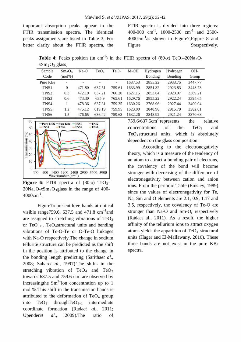
Mawlud S. et al./ZJPAS: 2017, 29(2): 32-42

important absorption peaks appear in the FTIR transmission spectra. The identical peaks assignments are listed in Table 3. For better clarity about the FTIR spectra, the

FTIR spectra is divided into three regions: 400-900 cm-1, 1000-2500 cm-1 and 2500-4000cm-1as shown in Figure7,Figure 8 and Figure 9respectively.

Table 4: Peaks position (in cm-1) in the FTIR spectra of (80-x) TeO2-20Na2O-xSm2O3 glass.

Sample Code

Sm2O3 (mol%)

Na-O TeO4 TeO3 M-OH Hydrogen Bonding

Hydrogen Bonding

OH-Group

Pure KBr - - - - 1637.53 2855.22 2933.75 3447.77 TNS1 0 471.80 637.51 759.61 1633.99 2851.32 2923.83 3443.73 TNS2 0.3 472.19 637.21 760.20 1627.15 2853.64 2923.07 3389.21 TNS3 0.6 473.30 635.9 765.61 1629.76 2855.22 2922.24 3395.65 TNS4 1 478.36 637.31 759.35 1630.26 2768.96 2927.44 3400.04 TNS5 1.2 475.12 619.19 759.95 1623.00 2848.98 2915.79 3382.01 TNS6 1.5 476.65 636.42 759.63 1632.26 2848.92 2921.24 3370.68

Figure 6: FTIR spectra of (80-x) TeO2-20Na2O-xSm2O3glass in the range of 400-4000cm-1.

Figure7representthree bands at optical visible range759.6, 637.5 and 471.8 cm–1and are assigned to stretching vibrations of TeO3 or TeO3+1, TeO4structural units and bending vibrations of Te-O-Te or O-Te-O linkages with Na-O respectively.The change in sodium tellurite structure can be predicted as the shift in the position is attributed to the change in the bonding length predicting (Sarithaet al., 2008; Saharet al., 1997).The shifts in the stretching vibration of TeO4 and TeO3 towards 637.5 and 759.6 cm-1are observed by increasingthe Sm3+ion concentration up to 1 mol %.This shift in the transmission bands is attributed to the deformation of TeO4 group into TeO3 throughTeO3+1 intermediate coordinate formation (Radaet al., 2011; Upenderet al., 2009).The ratio of

759.6/637.5cm-1represents the relative concentrations of the TeO3 and TeO4structural units, which is absolutely dependent on the glass composition.

According to the electronegativity theory, which is a measure of the tendency of an atom to attract a bonding pair of electrons, the covalency of the bond will become stronger with decreasing of the difference of electronegativity between cation and anion ions. From the periodic Table (Emsley, 1989) since the values of electronegativity for Te, Na, Sm and O elements are 2.1, 0.9, 1.17 and 3.5, respectively, the covalency of Te-O are stronger than Na-O and Sm-O, respectively (Radaet al., 2011). As a result, the higher affinity of the tellurium ions to attract oxygen atoms yields the apparition of TeO4 structural units (Hager and El-Mallawany, 2010). These three bands are not exist in the pure KBr spectra.

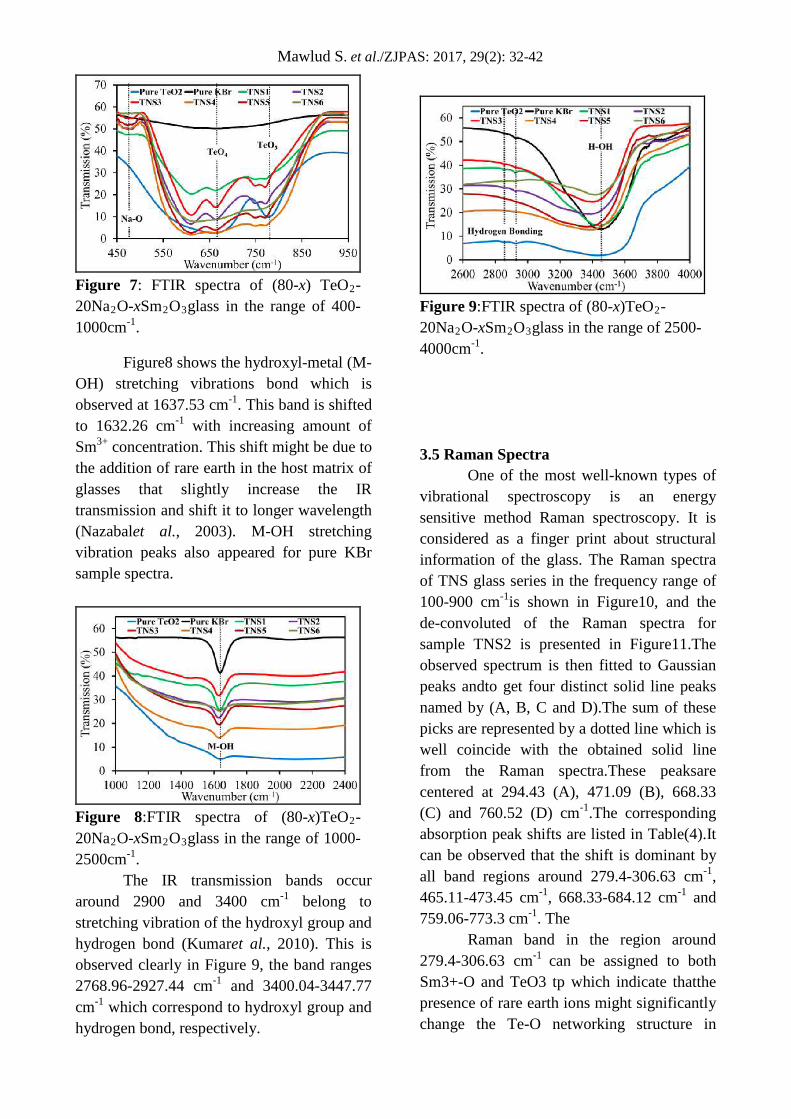
Mawlud S. et al./ZJPAS: 2017, 29(2): 32-42

Figure 7: FTIR spectra of (80-x) TeO2-20Na2O-xSm2O3glass in the range of 400-1000cm-1.

Figure8 shows the hydroxyl-metal (M-OH) stretching vibrations bond which is observed at 1637.53 cm-1. This band is shifted to 1632.26 cm-1 with increasing amount of Sm3+ concentration. This shift might be due to the addition of rare earth in the host matrix of glasses that slightly increase the IR transmission and shift it to longer wavelength (Nazabalet al., 2003). M-OH stretching vibration peaks also appeared for pure KBr sample spectra.

Figure 8:FTIR spectra of (80-x)TeO2-20Na2O-xSm2O3glass in the range of 1000-2500cm-1.

The IR transmission bands occur around 2900 and 3400 cm-1 belong to stretching vibration of the hydroxyl group and hydrogen bond (Kumaret al., 2010). This is observed clearly in Figure 9, the band ranges 2768.96-2927.44 cm-1 and 3400.04-3447.77 cm-1 which correspond to hydroxyl group and hydrogen bond, respectively.

Figure 9:FTIR spectra of (80-x)TeO2-20Na2O-xSm2O3glass in the range of 2500-4000cm-1. 3.5 Raman Spectra

One of the most well-known types of vibrational spectroscopy is an energy sensitive method Raman spectroscopy. It is considered as a finger print about structural information of the glass. The Raman spectra of TNS glass series in the frequency range of 100-900 cm-1is shown in Figure10, and the de-convoluted of the Raman spectra for sample TNS2 is presented in Figure11.The observed spectrum is then fitted to Gaussian peaks andto get four distinct solid line peaks named by (A, B, C and D).The sum of these picks are represented by a dotted line which is well coincide with the obtained solid line from the Raman spectra.These peaksare centered at 294.43 (A), 471.09 (B), 668.33 (C) and 760.52 (D) cm-1.The corresponding absorption peak shifts are listed in Table(4).It can be observed that the shift is dominant by all band regions around 279.4-306.63 cm-1, 465.11-473.45 cm-1, 668.33-684.12 cm-1 and 759.06-773.3 cm-1. The

Raman band in the region around 279.4-306.63 cm-1 can be assigned to both Sm3+-O and TeO3 tp which indicate thatthe presence of rare earth ions might significantly change the Te-O networking structure in

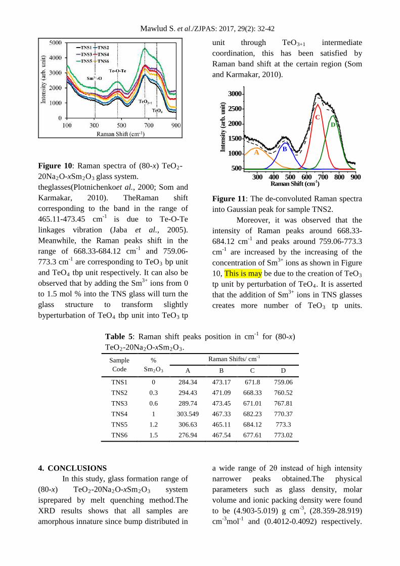
Mawlud S. et al./ZJPAS: 2017, 29(2): 32-42

theglasses(Plotnichenkoet al., 2000; Som and Karmakar, 2010). TheRaman shift corresponding to the band in the range of 465.11-473.45 cm-1 is due to Te-O-Te linkages vibration (Jaba et al., 2005). Meanwhile, the Raman peaks shift in the range of 668.33-684.12 cm-1 and 759.06-773.3 cm-1 are corresponding to TeO3 bp unit and TeO4 tbp unit respectively. It can also be observed that by adding the Sm3+ ions from 0 to 1.5 mol % into the TNS glass will turn the glass structure to transform slightly byperturbation of TeO4 tbp unit into TeO3 tp

unit through TeO3+1 intermediate coordination, this has been satisfied by Raman band shift at the certain region (Som and Karmakar, 2010).

300 400 500 600 700 800 900500

1000

1500

2000

2500

3000

CD

BInte

nsity

(arb

. uni

t)

Raman Shift (cm-1)

A

Figure 11: The de-convoluted Raman spectra into Gaussian peak for sample TNS2.

Moreover, it was observed that the intensity of Raman peaks around 668.33-684.12 cm-1 and peaks around 759.06-773.3 cm-1 are increased by the increasing of the concentration of Sm3+ ions as shown in Figure 10, This is may be due to the creation of TeO3 tp unit by perturbation of TeO4. It is asserted that the addition of Sm3+ ions in TNS glasses creates more number of TeO3 tp units.

Table 5: Raman shift peaks position in cm-1 for (80-x) TeO2-20Na2O-xSm2O3.

Sample Code

% Sm2O3

Raman Shifts/ cm-1

A B C D

TNS1 0 284.34 473.17 671.8 759.06 TNS2 0.3 294.43 471.09 668.33 760.52 TNS3 0.6 289.74 473.45 671.01 767.81 TNS4 1 303.549 467.33 682.23 770.37 TNS5 1.2 306.63 465.11 684.12 773.3 TNS6 1.5 276.94 467.54 677.61 773.02

4. CONCLUSIONS In this study, glass formation range of

(80-x) TeO2-20Na2O-xSm2O3 system isprepared by melt quenching method.The XRD results shows that all samples are amorphous innature since bump distributed in

a wide range of 2θ instead of high intensity narrower peaks obtained.The physical parameters such as glass density, molar volume and ionic packing density were found to be (4.903-5.019) g cm-3, (28.359-28.919) cm-3mol-1 and (0.4012-0.4092) respectively.

Figure 10: Raman spectra of (80-x) TeO2-20Na2O-xSm2O3 glass system.

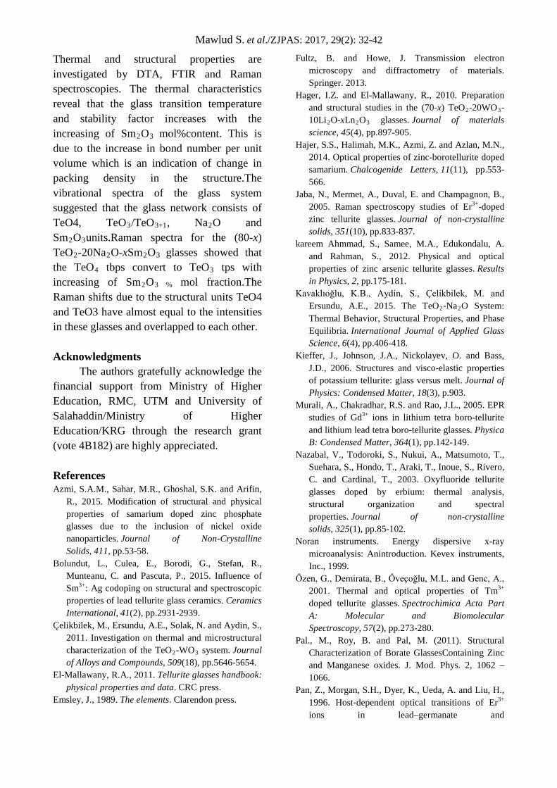
Mawlud S. et al./ZJPAS: 2017, 29(2): 32-42

Thermal and structural properties are investigated by DTA, FTIR and Raman spectroscopies. The thermal characteristics reveal that the glass transition temperature and stability factor increases with the increasing of Sm2O3 mol%content. This is due to the increase in bond number per unit volume which is an indication of change in packing density in the structure.The vibrational spectra of the glass system suggested that the glass network consists of TeO4, TeO3/TeO3+1, Na2O and Sm2O3units.Raman spectra for the (80-x) TeO2-20Na2O-xSm2O3 glasses showed that the TeO4 tbps convert to TeO3 tps with increasing of Sm2O3 % mol fraction.The Raman shifts due to the structural units TeO4 and TeO3 have almost equal to the intensities in these glasses and overlapped to each other.

Acknowledgments

The authors gratefully acknowledge the financial support from Ministry of Higher Education, RMC, UTM and University of Salahaddin/Ministry of Higher Education/KRG through the research grant (vote 4B182) are highly appreciated. References Azmi, S.A.M., Sahar, M.R., Ghoshal, S.K. and Arifin,

R., 2015. Modification of structural and physical properties of samarium doped zinc phosphate glasses due to the inclusion of nickel oxide nanoparticles. Journal of Non-Crystalline Solids, 411, pp.53-58.

Bolundut, L., Culea, E., Borodi, G., Stefan, R., Munteanu, C. and Pascuta, P., 2015. Influence of Sm3+: Ag codoping on structural and spectroscopic properties of lead tellurite glass ceramics. Ceramics International, 41(2), pp.2931-2939.

Çelikbilek, M., Ersundu, A.E., Solak, N. and Aydin, S., 2011. Investigation on thermal and microstructural characterization of the TeO2-WO3 system. Journal of Alloys and Compounds, 509(18), pp.5646-5654.

El-Mallawany, R.A., 2011. Tellurite glasses handbook: physical properties and data. CRC press.

Emsley, J., 1989. The elements. Clarendon press.

Fultz, B. and Howe, J. Transmission electron microscopy and diffractometry of materials. Springer. 2013.

Hager, I.Z. and El-Mallawany, R., 2010. Preparation and structural studies in the (70-x) TeO2-20WO3-10Li2O-xLn2O3 glasses. Journal of materials science, 45(4), pp.897-905.

Hajer, S.S., Halimah, M.K., Azmi, Z. and Azlan, M.N., 2014. Optical properties of zinc-borotellurite doped samarium. Chalcogenide Letters, 11(11), pp.553-566.

Jaba, N., Mermet, A., Duval, E. and Champagnon, B., 2005. Raman spectroscopy studies of Er3+-doped zinc tellurite glasses. Journal of non-crystalline solids, 351(10), pp.833-837.

kareem Ahmmad, S., Samee, M.A., Edukondalu, A. and Rahman, S., 2012. Physical and optical properties of zinc arsenic tellurite glasses. Results in Physics, 2, pp.175-181.

Kavaklıoğlu, K.B., Aydin, S., Çelikbilek, M. and Ersundu, A.E., 2015. The TeO2‐Na2O System: Thermal Behavior, Structural Properties, and Phase Equilibria. International Journal of Applied Glass Science, 6(4), pp.406-418.

Kieffer, J., Johnson, J.A., Nickolayev, O. and Bass, J.D., 2006. Structures and visco-elastic properties of potassium tellurite: glass versus melt. Journal of Physics: Condensed Matter, 18(3), p.903.

Murali, A., Chakradhar, R.S. and Rao, J.L., 2005. EPR studies of Gd3+ ions in lithium tetra boro-tellurite and lithium lead tetra boro-tellurite glasses. Physica B: Condensed Matter, 364(1), pp.142-149.

Nazabal, V., Todoroki, S., Nukui, A., Matsumoto, T., Suehara, S., Hondo, T., Araki, T., Inoue, S., Rivero, C. and Cardinal, T., 2003. Oxyfluoride tellurite glasses doped by erbium: thermal analysis, structural organization and spectral properties. Journal of non-crystalline solids, 325(1), pp.85-102.

Noran instruments. Energy dispersive x-ray microanalysis: Anintroduction. Kevex instruments, Inc., 1999.

Özen, G., Demirata, B., Öveçoğlu, M.L. and Genc, A., 2001. Thermal and optical properties of Tm3+ doped tellurite glasses. Spectrochimica Acta Part A: Molecular and Biomolecular Spectroscopy, 57(2), pp.273-280.

Pal., M., Roy, B. and Pal, M. (2011). Structural Characterization of Borate GlassesContaining Zinc and Manganese oxides. J. Mod. Phys. 2, 1062 – 1066.

Pan, Z., Morgan, S.H., Dyer, K., Ueda, A. and Liu, H., 1996. Host‐dependent optical transitions of Er3+ ions in lead–germanate and

Mawlud S. et al./ZJPAS: 2017, 29(2): 32-42

lead‐tellurium‐germanate glasses. Journal of applied physics, 79(12), pp.8906-8913.

Pereira, C., Barbosa, J., Cassanjes, F.C., Gonçalves, R.R., Ribeiro, S.J.L. and Poirier, G., 2016. Thermal, structural and optical properties of new TeO2. Optical Materials, 62, pp.95-103.

Plotnichenko, V.G., Sokolov, V.O., Koltashev, V.V., Dianov, E.M., Grishin, I.A. and Churbanov, M.F., 2005. Raman band intensities of tellurite glasses. Optics letters, 30(10), pp.1156-1158.

Rada, S., Culea, E. and Rada, M., 2011. The experimental and theoretical investigations on the structure of the gadolinium–lead–tellurate glasses. Materials Chemistry and Physics, 128(3), pp.464-469.

Rada, S., Pascuta, P., Rada, M. and Culea, E., 2011. Effects of samarium (III) oxide content on structural investigations of the samarium–vanadate–tellurate glasses and glass ceramics. Journal of Non-Crystalline Solids, 357(19), pp.3405-3409.

Saddeek, Y.B., Shaaban, E.R., Abdel-Rahim, F.M. and Mahmoud, K.H., 2008. Thermal analysis and infrared study of Nb2O5-TeO2 glasses. Philosophical Magazine, 88(25), pp.3059-3073.

Sahar, M.R., Jehbu, A.K. and Karim, M.M., 1997. TeO2-ZnO-ZnCl2 glasses for IR transmission. Journal of non-crystalline solids, 213, pp.164-167.

Sahar, M.R., Sulhadi, K. and Rohani, M.S., 2007. Spectroscopic studies of TeO2-ZnO-Er2O3 glass system. Journal of materials science, 42(3), pp.824-827.

Saritha, D., Markandeya, Y., Salagram, M., Vithal, M., Singh, A.K. and Bhikshamaiah, G., 2008. Effect of Bi2O3 on physical, optical and structural studies of ZnO-Bi2O3-B2O3 glasses. Journal of Non-Crystalline Solids, 354(52), pp.5573-5579.

Sidek, H.A.A., Halimah, M.K., Faizal, M.N., Daud, W.Y.W., Zaidan, A.W., Zainal, A.T. and Halim, S.A., 2006. Synthesis and elastic behaviour of borate glass doped with high tellurite

content. Journal of Applied Sciences, 6(2), pp.274-279.

Som, T. and Karmakar, B., 2010. Structure and properties of low-phonon antimony glasses and nano glass-ceramics in K2O-B2O3-Sb2O3 system. Journal of Non-Crystalline Solids, 356(20), pp.987-999.

Sun, H., Duan, Z., Zhou, G., Yu, C., Liao, M., Hu, L., Zhang, J. and Jiang, Z., 2006. Structural and up-conversion luminescence properties in Tm3+/Yb3+-codoped heavy metal oxide–halide glasses. Spectrochimica Acta Part A: Molecular and Biomolecular Spectroscopy, 63(1), pp.149-153.

Upender, G., Chandra Mouli, V. and Sathe, V.G., 2009. EPR, Raman, infrared and optical absorption studies of Cu2+ ions in 60TeO2-(40-x) WO3- xPbO glasses. Physics and Chemistry of Glasses-European Journal of Glass Science and Technology Part B, 50(6), pp.399-406.

Xu, S., Fang, D., Zhang, Z. and Jiang, Z., 2005. Unconversion Luminescence and Mechanisms of Tm3+/Yb3+ co-doped oxyhalide tellurite Glasses. J. Solid State Chem, 178, p.1817.

Yusoff, N.M. and Sahar, M.R., 2015. Effect of silver nanoparticles incorporated with samarium-doped magnesium tellurite glasses. Physica B: Condensed Matter, 456, pp.191-196.

Yusoff, N.M. and Sahar, M.R., 2016. Effect of Sm3+ Concentration on Physical Properties of Magnesium Tellurite Glasses Containing Silver Nanoparticles. In Materials Science Forum (Vol. 846, pp. 107-114). Trans Tech Publications.

Yusoff, N.M., Sahar, M.R. and Ghoshal, S.K., 2015. Sm3+: Ag NPs assisted modification in absorption features of magnesium tellurite glass. Journal of Molecular Structure, 1079, pp.167-172.

ZANCO Journal of Pure and Applied Sciences The official scientific journal of Salahaddin University-Erbil

ZJPAS (2017), 29 (2); 43-52 http://dx.doi.org/10.21271/ZJPAS.29.2.5

Assessment of natural radionuclide's in sediments of Darbandikhan Lake water resources at Kurdistan Region-Northeastern of Iraq.

Adeeb omer jafir1, Ali Hassan Ahmad1 and Wan Muhammad Saridan2

1- Department of physics, College of Science, Salahaddin University, Erbil, Kurdistan Region, Iraq.

2- Department of physic, university Technology Malaysia, Johor-Bahru, Malaysia

1. INTRODUCTION

The radioactivity of the earth includes the

primordial radionuclides which have long half-

lives and they have survived during the

creation of the earth and the cosmogentic

radionuclides which continuously produced

due to bombardment of the atmosphere by

cosmic rays [UNSCEAR, 2000 report]

The earth consists of major elements like

Ca, Fe, Cd, Pb, Mg, Mn, etc. and small

different quantity of uranium, thorium and

potassium, their distributions are dependent on

the geological and geographical conditions.

The average concentration of uranium and

thorium in the earth’s crust are about 2-3 and

8-12 ppm, respectively [IAEA, 2003].One ppm

of uranium in rocks is equivalent to 12.35

Bq/kg, one ppm of thorium is equivalent to

4.06 Bq/kg and % of potassium is 313 Bq/kg

[IAEA, 2003].

A R T I C L E I N F O

A B S T R A C T

Article History: Received: 5/09/2016 Accepted: 29/11/2016 Published: 07/06/2017

Abstract A total of 25 of sediment samples were collected from Darbandikhan Lake and

its different resources (spring, stream, and lake) during the summer season. The

activity concentration of primordial radionuclides and the concentration of major

elements were found using Energy Dispersive X-ray fluorescence (EDXRF)

techniques. The average specific activity of 40K was found to be 202.27 Bq/kg,

while the activity concentration for both uranium and thorium was beyond the

detection limits. Statistics of multivariate analysis were applied to sediment

samples, which shows that there is a strong positive correlation coefficient

between 40K and Ti, Mn and Fe and a weak negative correlation between 40K and

Mg, Si, P, Ca was observed.

Keywords: Radioactivity, Sediments, Energy Dispersive X-ray Fluorescence, Darbandikhan Lake. *Corresponding Author: Ali Hassan Ahmed ali.ahmed@su.edu.krd

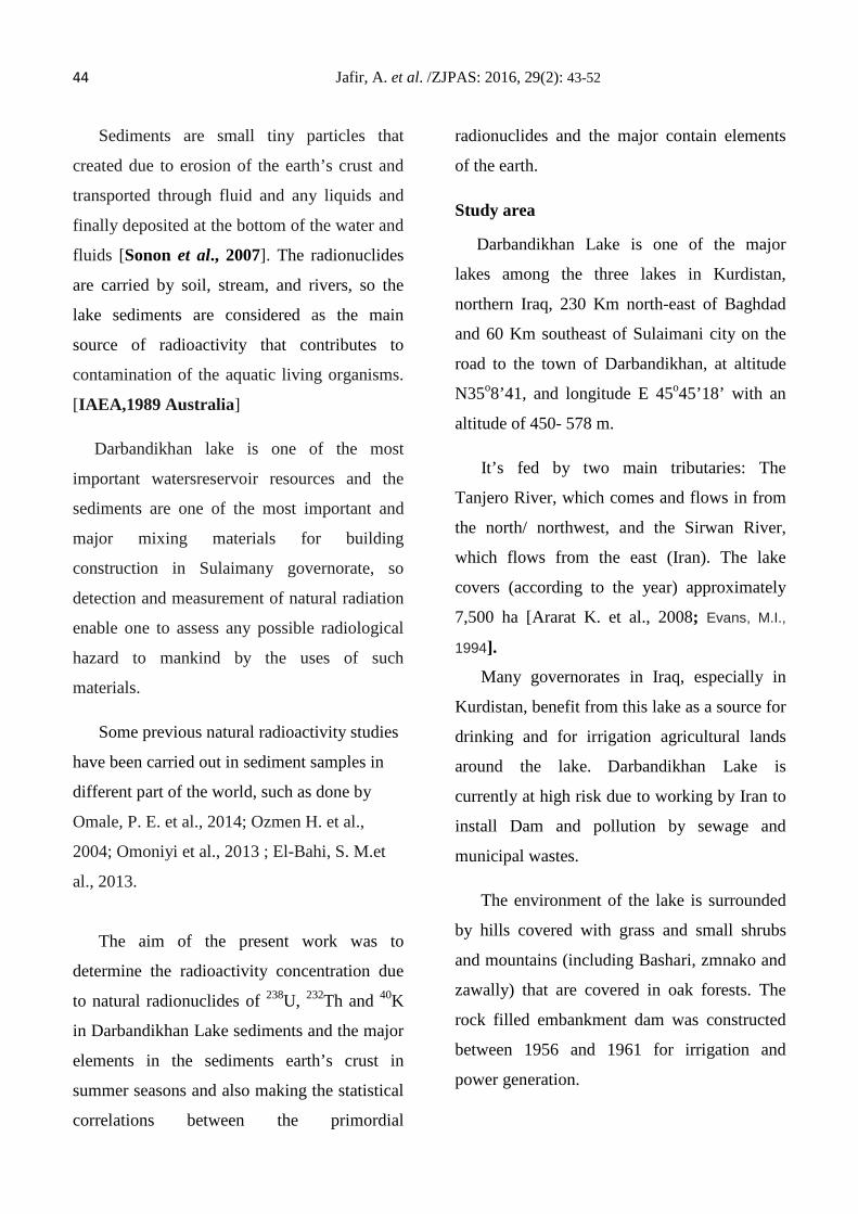
44 Jafir, A. et al. /ZJPAS: 2016, 29(2): 43-52 Sediments are small tiny particles that

created due to erosion of the earth’s crust and

transported through fluid and any liquids and

finally deposited at the bottom of the water and

fluids [Sonon et al., 2007]. The radionuclides

are carried by soil, stream, and rivers, so the

lake sediments are considered as the main

source of radioactivity that contributes to

contamination of the aquatic living organisms.

[IAEA,1989 Australia]

Darbandikhan lake is one of the most

important watersreservoir resources and the

sediments are one of the most important and

major mixing materials for building

construction in Sulaimany governorate, so

detection and measurement of natural radiation

enable one to assess any possible radiological

hazard to mankind by the uses of such

materials.

Some previous natural radioactivity studies

have been carried out in sediment samples in

different part of the world, such as done by

Omale, P. E. et al., 2014; Ozmen H. et al.,

2004; Omoniyi et al., 2013 ; El-Bahi, S. M.et

al., 2013.

The aim of the present work was to

determine the radioactivity concentration due

to natural radionuclides of 238U, 232Th and 40K

in Darbandikhan Lake sediments and the major

elements in the sediments earth’s crust in

summer seasons and also making the statistical

correlations between the primordial

radionuclides and the major contain elements

of the earth.

Study area

Darbandikhan Lake is one of the major

lakes among the three lakes in Kurdistan,

northern Iraq, 230 Km north-east of Baghdad

and 60 Km southeast of Sulaimani city on the

road to the town of Darbandikhan, at altitude

N35o8’41, and longitude E 45o45’18’ with an

altitude of 450- 578 m.

It’s fed by two main tributaries: The

Tanjero River, which comes and flows in from

the north/ northwest, and the Sirwan River,

which flows from the east (Iran). The lake

covers (according to the year) approximately

7,500 ha [Ararat K. et al., 2008; Evans, M.I.,

1994].

Many governorates in Iraq, especially in

Kurdistan, benefit from this lake as a source for

drinking and for irrigation agricultural lands

around the lake. Darbandikhan Lake is

currently at high risk due to working by Iran to

install Dam and pollution by sewage and

municipal wastes.

The environment of the lake is surrounded

by hills covered with grass and small shrubs

and mountains (including Bashari, zmnako and

zawally) that are covered in oak forests. The

rock filled embankment dam was constructed

between 1956 and 1961 for irrigation and

power generation.

45 Jafir, A. et al. /ZJPAS: 2016, 29(2): 43-52 Water levels decline in summer after the spring

due to dam release and it rises again during

winter's rain .The land is used for field,

especially wheat and barley [Evans, M.I., 1994].

The latitude, longitude and altitude recorded

from the GPS type (GPS72 GARMIN) at each

position the geological type and the height

from the sea were recorded, as shown in Table

(1). The map of Darbandikhan lake water with

their resources is shown in Figure (1).

Table (1): Location and Geological Information of the Studied Sample Sites.

sample location Geology [Jassim, S.Z., Goff. JC, 2006] code name lontitude latitude altitude(m) S1 Jomarasi N 35O27,46.4" E 045O58,35.5" 1158 Slate and alluvial deposit qulqula S2 Hassan awa N 35O29,22.0" E 045O52,19.4" 735 Gness and state of metamorphic rock S3 Kelakawa N 35O23,48.5" E 045O53,20.3" 550.9 Alluvial deposite with grains of sand and chert S4 Zallmsarchawa N 35O19,01.9" E 046O05,26.6" 878.8 Marly limestone +chert and slope deposite of mixure of soil and pebbles

S5 Ganjan(khurmal) N 35O18,14.0" E 046O02,20.0" 569.2 Recent deposit, composed of mixture of carbonate soil and sand with layers of limestone

S6 Prdizalm N 35O18,24.6" E 045O58,15.8" 510.6 Alluvial deposit, composed of clay and silt. S7 Reshensarchawa N 35O21,49.0" E 045O58,45.5" 560.7 Qalqula formation (chert) with limestone of Avroman formation S8 Rechenshallma N 35O21,36.1" E 045O58,08.2" 532.7 Alluvial deposit , with grains of limestone and chert S9 Prdiqadafari N 35O20,16.3" E 045O57,09.5" 518.9 Alluvial deposit ,with mixture of sand silt and pebbles

S10 Sarchnar N 35O35,25.3" E 045O22,59.9" 763.2 Marly limestone and slope deposit composed of mixture of clay and sand with pebbles

S11 Prditanjaro N 35O28,45.3" E 045O25,39.4" 663.6 Alluvial deposit contain clay, sand and calcareous pebbles S12 Prdiqaragoll N 35O21,22.3" E 045O37,36.3" 557 Alluvial deposit with marl and marly limestone of Tanjero formation S13 Tapikaram N 35O20,19.95" E 045O45,07.37" 532 Alluvial deposit with marl and marly limestone of Tanjero formation S41 Awamarisaru N 35O05,08.3" E 046O04,46.2" 560 Marly limestone, marl and dolomitic limestone S15 Hana zhalla N 35O06,55.8" E 045O54,03.5" 480 Alluvial deposite S16 Xulami N 35O12,11.7" E 045O51,19.1" 481 Alluvial deposite

S17 Xatitanjero N 35O16,30.31" E 045O51,05.5" 501 Slope deposit mixed with pebbles of limestone with pebbles of limestone and chert.

S18 Prdikon N 35O17,12.2" E 045O35,07.0" 485 Marly limestone, marl and some layers of sandstone of tanjero formation S19 Awalellasirwan N 35O11,42.7" E 045O50,52.2" 479 Alluvial deposite S20 Plaspi N 35O11,57.5" E 045O48,14.0" 484 Dolomitic limestone with chert nodules S21 Shanisharaka N 35O09,32.63" E 045O47,25.01" 481 Red clay stone covered by alluvial deposit S22 Kani khan N 35O09,04.35" E 045O46,06.69" 480 Alluvial deposit composed of mixure of clay and low rate of humus S23 Ban qoin N 35O08,13.55" E 045O44,53.1" 482 Layers of limestone and marl covered by top soil

S24 Darbanikhan N 35O07,18.29" E 045O43,28.49" 477 Dolomitic limestone and chaky limestone with chert nodules covered by top soil in some area.

S25 Darbanikhan N 35O06,52.37" E 045O42,18.00" 480 Dolomitic limestone and chaky limestone with chert nodules covered by top soil in some area.

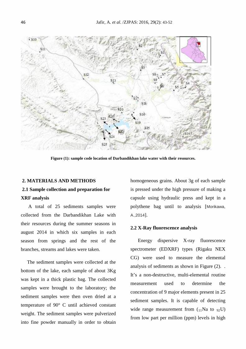
46 Jafir, A. et al. /ZJPAS: 2016, 29(2): 43-52

Figure (1): sample code location of Darbandikhan lake water with their resources.

2. MATERIALS AND METHODS

2.1 Sample collection and preparation for

XRF analysis

A total of 25 sediments samples were

collected from the Darbandikhan Lake with

their resources during the summer seasons in

august 2014 in which six samples in each

season from springs and the rest of the

branches, streams and lakes were taken.

The sediment samples were collected at the

bottom of the lake, each sample of about 3Kg

was kept in a thick plastic bag. The collected

samples were brought to the laboratory; the

sediment samples were then oven dried at a

temperature of 90° C until achieved constant

weight. The sediment samples were pulverized

into fine powder manually in order to obtain

homogeneous grains. About 3g of each sample

is pressed under the high pressure of making a

capsule using hydraulic press and kept in a

polythene bag until to analysis [Morikawa,

A.,2014].

2.2 X-Ray fluorescence analysis

Energy dispersive X-ray fluorescence

spectrometer (EDXRF) types (Rigaku NEX

CG) were used to measure the elemental

analysis of sediments as shown in Figure (2). .

It’s a non-destructive, multi-elemental routine

measurement used to determine the

concentration of 9 major elements present in 25

sediment samples. It is capable of detecting

wide range measurement from (11Na to 92U)

from low part per million (ppm) levels in high

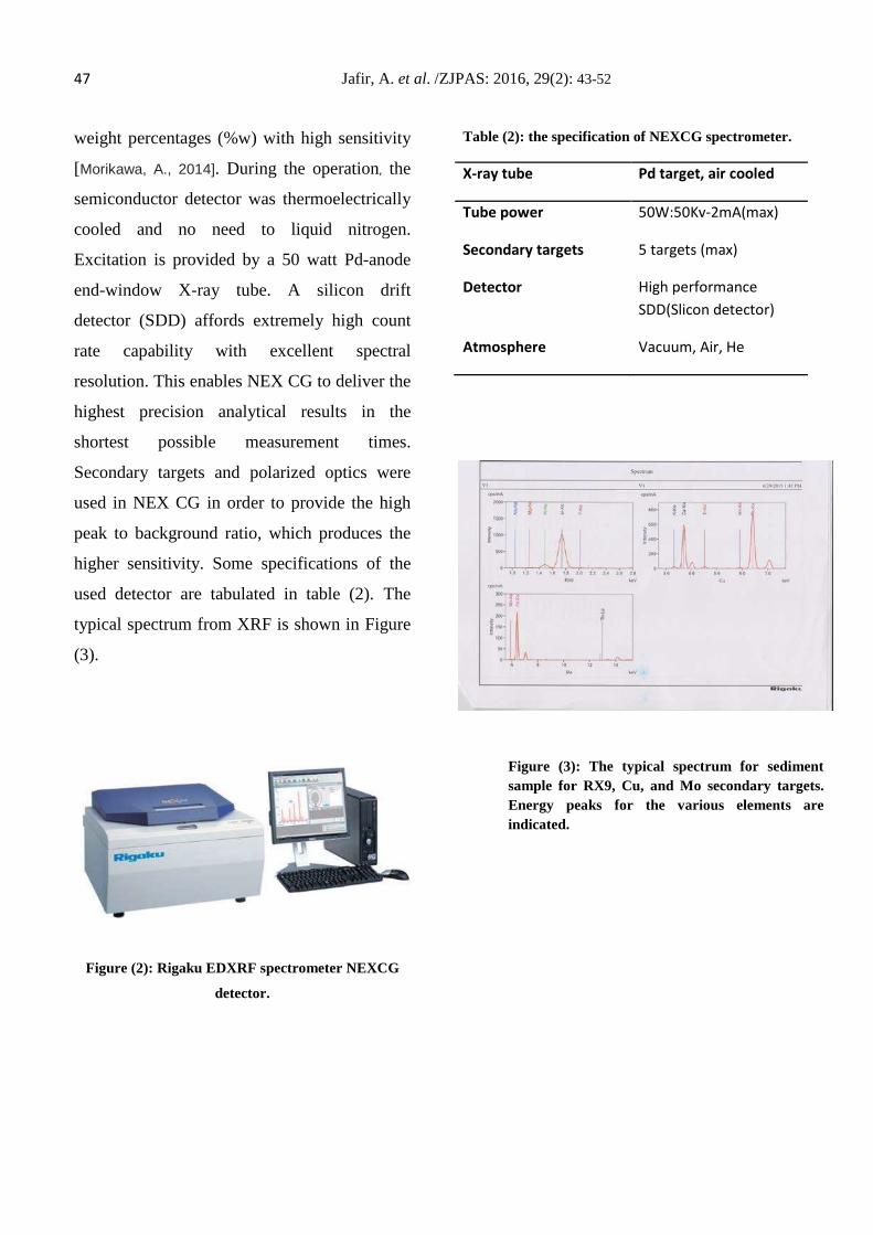
47 Jafir, A. et al. /ZJPAS: 2016, 29(2): 43-52 weight percentages (%w) with high sensitivity

[Morikawa, A., 2014]. During the operation, the

semiconductor detector was thermoelectrically

cooled and no need to liquid nitrogen.

Excitation is provided by a 50 watt Pd-anode

end-window X-ray tube. A silicon drift

detector (SDD) affords extremely high count

rate capability with excellent spectral

resolution. This enables NEX CG to deliver the

highest precision analytical results in the

shortest possible measurement times.

Secondary targets and polarized optics were

used in NEX CG in order to provide the high

peak to background ratio, which produces the

higher sensitivity. Some specifications of the

used detector are tabulated in table (2). The

typical spectrum from XRF is shown in Figure

(3).

Figure (2): Rigaku EDXRF spectrometer NEXCG

detector.

Table (2): the specification of NEXCG spectrometer.

X-ray tube Pd target, air cooled

Tube power 50W:50Kv-2mA(max)

Secondary targets 5 targets (max)

Detector High performance SDD(Slicon detector)

Atmosphere Vacuum, Air, He

Figure (3): The typical spectrum for sediment sample for RX9, Cu, and Mo secondary targets. Energy peaks for the various elements are indicated.

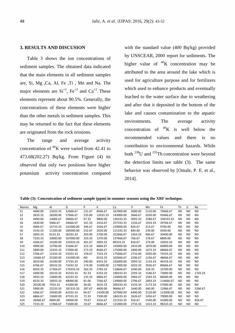
48 Jafir, A. et al. /ZJPAS: 2016, 29(2): 43-52

3. RESULTS AND DISCUSION Table 3 shows the ion concentrations of

sediment samples. The obtained data indicated

that the main elements in all sediment samples

are, Si, Mg ,Ca, Al, Fe ,Ti , Mn and Na. The

major elements are Si+2, Fe+2 and Ca+2. These

elements represent about 90.5%. Generally, the

concentrations of these elements were higher

than the other metals in sediment samples. This

may be returned to the fact that these elements

are originated from the rock erosions.

The range and average activity

concentration of 40K were varied from 42.41 to

473.68(202.27) Bq/kg. From Figure (4) its

observed that only two positions have higher

potassium activity concentration compared

with the standard value (400 Bq/kg) provided

by UNSCEAR, 2000 report for sediments. The

higher value of 40K concentration may be

attributed to the area around the lake which is

used for agriculture purpose and for fertilizers

which used to enhance products and eventually

leached to the water surface due to weathering

and after that it deposited in the bottom of the

lake and causes contamination to the aquatic

environments. The average activity

concentration of 40K is well below the

recommended values and there is no

contribution to environmental hazards. While

both 238U and 232Th concentration were beyond

the detection limits see table (3). The same

behavior was observed by [Omale, P. E. et al.,

2014].

Table (3): Concentration of sediment sample (ppm) in summer seasons using the XRF technique. Names Mg Al Si P K Ca Ti Mn Fe Th U Na S1 4400.00 15033.33 52666.67 131.67 8566.67 167000.00 3600.00 2110.00 79666.67 ND ND ND S2 3633.33 18200.00 57666.67 235.00 12033.33 143000.00 3666.67 2030.00 92666.67 ND ND ND S3 4400.00 14066.67 58666.67 97.33 9800.00 136333.33 3093.33 2586.67 104333.33 ND ND ND S4 1830.00 5066.67 34666.67 101.33 2416.67 257333.33 1256.67 1033.33 29766.67 ND ND ND S5 4966.67 14733.33 141000.00 346.67 2426.67 159000.00 826.67 313.67 9700.00 ND ND ND S6 3143.33 11200.00 185000.00 232.67 2020.00 121333.33 840.00 239.00 9200.00 ND ND ND S7 2693.33 6133.33 36333.33 203.00 2700.00 252666.67 1463.33 906.67 30400.00 ND ND ND S8 7233.33 10000.00 167000.00 333.33 1370.00 137666.67 766.67 178.67 8800.00 ND ND ND S9 4266.67 14100.00 210333.33 301.67 3003.33 89333.33 816.67 274.00 10933.33 ND ND ND S10 4900.00 12700.00 51666.67 222.33 6866.67 193000.00 2410.00 1870.00 60000.00 ND ND ND S11 5800.00 13333.33 57000.00 273.33 8566.67 175000.00 3400.00 1673.33 68666.67 ND ND ND S12 5766.67 12333.33 53333.33 159.67 7233.33 175666.67 2710.00 2050.00 74333.33 ND ND ND S13 15666.67 25200.00 131000.00 ND 6533.33 102666.67 2206.67 1236.67 48666.67 ND ND ND S14 3010.00 10100.00 37333.33 240.00 6433.33 226000.00 2693.33 1133.33 46333.33 ND ND ND S15 6766.67 20533.33 73333.33 174.00 15300.00 117000.00 5033.33 2026.67 89666.67 ND ND ND S16 6033.33 17266.67 176333.33 263.33 2783.33 118666.67 1040.00 326.33 10700.00 ND ND ND S17 4300.00 10133.33 45333.33 92.33 6333.33 190333.33 2293.33 1546.67 73000.00 ND ND 1703.33 S18 3933.33 13600.00 62333.33 133.33 9866.67 150000.00 3966.67 1593.33 86000.00 ND ND ND S19 8233.33 10933.33 48000.00 81.00 7566.67 139000.00 2706.67 2003.33 114666.67 ND ND ND S20 20100.00 7933.33 41000.00 36.00 3633.33 200333.33 1533.33 2173.33 57000.00 ND ND ND S21 5900.00 22233.33 181333.33 287.67 4600.00 96666.67 1640.00 340.00 12966.67 ND ND 3266.67 S22 6366.67 19500.00 62333.33 66.67 14200.00 107000.00 6400.00 2120.00 112000.00 ND ND ND S23 6866.67 13600.00 47333.33 72.33 7100.00 184333.33 2626.67 1456.67 70000.00 ND ND ND S24 26466.67 4800.00 34000.00 79.67 3316.67 221333.33 916.67 1540.00 41000.00 ND ND 826.67 S25 7233.33 11966.67 71000.00 19.67 8666.67 131000.00 2733.33 1413.33 98333.33 ND ND ND

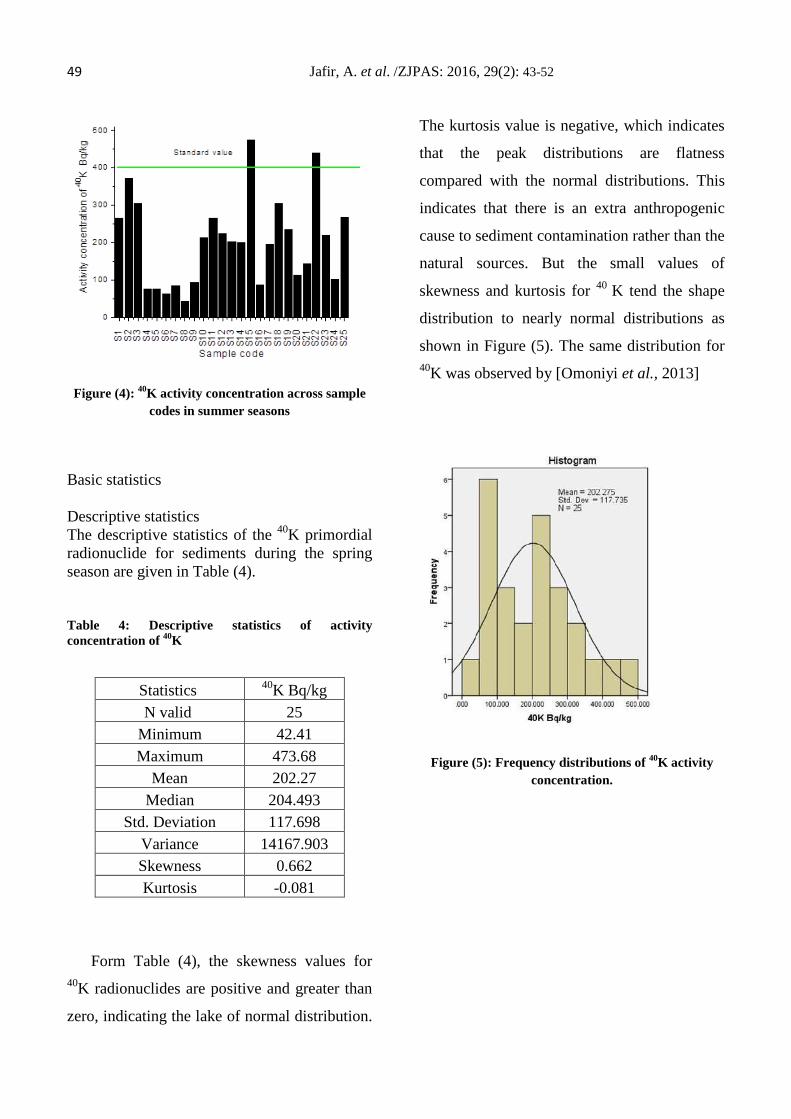
49 Jafir, A. et al. /ZJPAS: 2016, 29(2): 43-52

Figure (4): 40K activity concentration across sample codes in summer seasons

Basic statistics Descriptive statistics The descriptive statistics of the 40K primordial radionuclide for sediments during the spring season are given in Table (4). Table 4: Descriptive statistics of activity concentration of 40K

Form Table (4), the skewness values for 40K radionuclides are positive and greater than

zero, indicating the lake of normal distribution.

The kurtosis value is negative, which indicates

that the peak distributions are flatness

compared with the normal distributions. This

indicates that there is an extra anthropogenic

cause to sediment contamination rather than the

natural sources. But the small values of

skewness and kurtosis for 40 K tend the shape

distribution to nearly normal distributions as

shown in Figure (5). The same distribution for 40K was observed by [Omoniyi et al., 2013]

Figure (5): Frequency distributions of 40K activity concentration.

Statistics 40K Bq/kg N valid 25

Minimum 42.41 Maximum 473.68

Mean 202.27 Median 204.493

Std. Deviation 117.698 Variance 14167.903 Skewness 0.662 Kurtosis -0.081

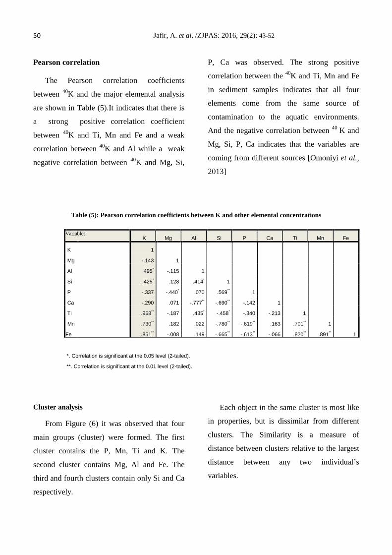
50 Jafir, A. et al. /ZJPAS: 2016, 29(2): 43-52 Pearson correlation The Pearson correlation coefficients

between 40K and the major elemental analysis

are shown in Table (5).It indicates that there is

a strong positive correlation coefficient

between 40K and Ti, Mn and Fe and a weak

correlation between 40K and Al while a weak

negative correlation between 40K and Mg, Si,

P, Ca was observed. The strong positive

correlation between the 40K and Ti, Mn and Fe

in sediment samples indicates that all four

elements come from the same source of

contamination to the aquatic environments.

And the negative correlation between 40 K and

Mg, Si, P, Ca indicates that the variables are

coming from different sources [Omoniyi et al.,

2013]

Table (5): Pearson correlation coefficients between K and other elemental concentrations Variables

K Mg Al Si P Ca Ti Mn Fe

K 1

Mg -.143 1

Al .495* -.115 1

Si -.425* -.128 .414* 1

P -.337 -.440* .070 .569** 1

Ca -.290 .071 -.777** -.690** -.142 1

Ti .958** -.187 .435* -.458* -.340 -.213 1

Mn .730** .182 .022 -.780** -.619** .163 .701** 1

Fe .851** -.008 .149 -.665** -.613** -.066 .820** .891** 1

*. Correlation is significant at the 0.05 level (2-tailed).

**. Correlation is significant at the 0.01 level (2-tailed).

Cluster analysis

From Figure (6) it was observed that four

main groups (cluster) were formed. The first

cluster contains the P, Mn, Ti and K. The

second cluster contains Mg, Al and Fe. The

third and fourth clusters contain only Si and Ca

respectively.

Each object in the same cluster is most like

in properties, but is dissimilar from different

clusters. The Similarity is a measure of

distance between clusters relative to the largest

distance between any two individual’s

variables.

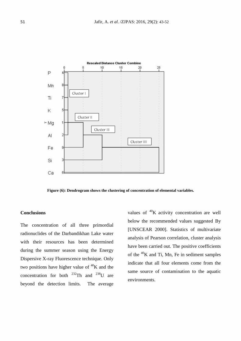
51 Jafir, A. et al. /ZJPAS: 2016, 29(2): 43-52

Figure (6): Dendrogram shows the clustering of concentration of elemental variables.

Conclusions

The concentration of all three primordial

radionuclides of the Darbandikhan Lake water

with their resources has been determined

during the summer season using the Energy

Dispersive X-ray Fluorescence technique. Only

two positions have higher value of 40K and the

concentration for both 232Th and 238U are

beyond the detection limits. The average

values of 40K activity concentration are well

below the recommended values suggested By

[UNSCEAR 2000]. Statistics of multivariate

analysis of Pearson correlation, cluster analysis

have been carried out. The positive coefficients

of the 40K and Ti, Mn, Fe in sediment samples

indicate that all four elements come from the

same source of contamination to the aquatic

environments.

52 Jafir, A. et al. /ZJPAS: 2016, 29(2): 43-52 .

REFERENCES

Ararat, K., Mehdi, R.A., Falih, H.A., Maher, A.M. and Bachmann, A., 2008. DARBANDIKHAN LAKE POISONING EVENT. Nature.

El-Bahi, S. M., Sroor, A. T., Arhoma, N. F., &Darwish, S. M. (2013).XRF Analysis of Heavy Metals for Surface Soil of Qarun Lake and Wadi El Rayan in Faiyum, Egypt.Open Journal of Metal, 3(02), 21.

Evans, M.I., 1994. Important Bird Areas in the Middle East, BirdLife International Series, No 2. Cambridge. UK, p.410.

IAEA (2003) International Atomic Energy Agency. Guidelines for radioelement mapping using gamma ray spectrometry data. IAEA-TECDOC-1363. IAEA, Vienna, Austria

Jassim, S.Z., Goff. JC, 2006. Geology of Iraq.

Morikawa, A.,(2014). Elemental analysis of PM2. 5 with energy dispersive X-ray fluorescence spectrometer NEX CG.

Omale, P. E., Okeniyi, S. O., Faruruwa, M. D., &Ngokat, A. B. (2014). DETERMINATION FOR LEVELS OF RADIONUCLIDES OF URANIUM,

THORIUM AND POTASSIUM IN WATER, SEDIMENTS AND ALGAE SAMPLES FROM SELECTED COASTAL AREAS OF LAGOS, NIGERIA; USING ENERGY DISPERSIVE X-RAY FLOURESCENCE. Global Journal of Pure and Applied Chemistry Research, 2(1), 1-24.

Omoniyi, I. M., Oludare, S. M., &Oluwaseyi, O. M. (2013). Determination of radionuclides and elemental composition of clay soils by gamma-and X-ray spectrometry. Springer Plus, 2(1), 74.

Özmen, H., Külahcı, F., Çukurovalı, A., &Doğru, M. (2004).Concentrations of heavy metal and radioactivity in surface water and sediment of Hazar Lake (Elazığ, Turkey).Chemosphere, 55(3), 401-408.

Sonon, L.S., Chappell M.A. and Evangelou V.P (2007): The history of Soil Chemistry. Journal. Science Total Environment 35, 2, 88-90.

United Nations Scientific Committee on the Effects of Atomic Radiation.(2000). UNSCEAR 2000 report.Annex C: exposure to the public from man-made sources of radiation.

ZANCO Journal of Pure and Applied Sciences The official scientific journal of Salahaddin University-Erbil

ZJPAS (2017), 29 (2); 53-73 http://dx.doi.org/10.21271/ZJPAS.29.2.6

Species chick list of Bryophyte, Pteridophyta, Lichens and of Iraq and Kurdistan Region

Farhad Hasan Aziz1 and Basheer Al-Niama2 1 Environment Department, College of Science, Salahaddin- Erbil University, Erbil, Iraq 2 Biology Department, College of Science, Mosull University

.

1. INTRODUCTION

Aziz (2010) identified 6 species of hepatopsida (liver worts) of which four species were new records to Iraqi flora these are Marchantia polymerpha in Zalm Sulaimani Concephalum conicum in Sharansh, Duhok, Pellia epiphylla and Lophocolea cuspidata in Gali Ali-Beg valley, Shex Wassan village and Nardia scalaris found near Faqyan village-Doli Ikoyan, Erbil. Metezgeria furcata near Shanadar cave and in Gali- Ali- Beg/ Erbil. Guest (1966) in his book flora of Iraq represented most species of hepatophyta. During an excursions of foreign workers to different parts of Iraq; Agnew and Vondracek

(1975) recorded 54 genera and 149 species and they referred in detail to old works on mosses collected from Mesopotamia, Iraq, Syria and other Middle East countries e.g. Lebanon, Phalstine, Persia and Afghanistan. Maulood and Rasheed (1994) recorded total number of 27 genera and 48 species in in Nineveh, Erbil and Duhok of which 4 genera and 9 species were new records to Iraqi flora. However, Al-Ni'ma (2003) identification 79 species (72 mosses and 7 liverworts), covered 5 genus among them 8 species was new records to Iraqi flora. He performed an excellent reference for bryophytes of Iraq, which has encouraged authors of bryophytes (Schaffer, 1913, Frochlich, 1959 and Rechinger and Vondracek

A R T I C L E I N F O

A B S T R A C T

Article History: Received: 03/05/2016 Accepted: 01/12/2016 Published:07 /06/2017

This is the first species check list of Iraqi lower plants and Kurdistan especially from Erbil province. It is including 658 species. Hepatophyta with 18 species in 1 class, 4 orders and, 9 families14 genus . Musci with 235 species in 1 class, 9 orders, 30 families and 80 genus. Pteridophyta with 27 species in 1 class, 3 orders, 10 families, and 27 genus lichens with 224 species in 1 class, 74 genus and Mushroom with 32 species in 1 class, 5 orders, 15 families and 19 genus

Keywords: Check list, Hepatohpyta, Iraq, Kurdistan Lichnes, Musci, Mushroom, Pteridophyta *Corresponding Author: Farhad Hasan Aziz farhad.aziz @ su.edu.krd.com

54 Aziz F and Niama B /ZJPAS: 2016, 29(2): 53-73 1965).Aziz (2011) collected mosses in different parts of Erbil, Slemani, Duhok and Even Kirkuk. He recorded a total of 67 species in 32 genus, 16 families and 9 orders, among them 17 species in 10 genus, two families Schistogaceae and Ephemeraceae and the single order Schistostegales were new to Iraqi flora. The most rare species recorded in this study was Schistostega pennato with fern-like leaves inside Shanadar cave, Pottia wissia var. Crinata at the mouth of Ba-stoon cave, Ephemerum cristatum within Gali Ali-Beg area. Al- Mashhadani and Al- Ni’ma( 2012) collected mosses in 25 different areas, they identified 75 species of which 7 species and 1 genus Orthodonium was new record to Iraqi flora. In term of lichens and based on collections made by Aziz ( 2005 ) within Erbil province from Safin mountain area and Rwandiz river path including Gali Ali-Beg, Jundian, Kawlokan, Haji-Omaran and Kawshan, up to more than 2000 m.a.s.l. A total of 89 species in 37 genera of lichens were identified at the first time in Iraq; sixty six (66) species are belong to crustose from ,19 species to foliose form , 3 species to squamilose form and 1 species to fruticose forms. Aziz (2004) recorded seventy seven (77) lichens species in 40 genera from Hasan Beg mountain area covering main road edge, Sari Bardi and it’s summit area in spring and summer season 2002. The Hasan Beg lichens community relatively has no affinities with lichens community of Oak forest and up land rock outcrops excluding 26 species have been recorded elsewhere. While,51 species encountered are new records for Iraqi flora.Lichens species was moderately of crustose form 60 species, followed by foliose form 15 species then by fruiticose form 2 species. In term of lichnes Aziz and Saeed (2006) have been recorded a total of 50 species of lichens flora in 24 genera arc reported fromm Qarajugh mountain and foothill area within

Erbil province including Gwer and Dibaga districts. Among them 24 species are new records to Iraqi lichens flora. Forty two species arc of crustose, four of foliose and two of frulicose forms. In other hand thirty four species found in rocks, while four species Collcniu spp., Diploschistes spp. Permelia, Psora and Parinotrema were rare, scattered and observed on soil. The recorded species are low due to habitat uniformity, dry conditions and the absence of old trees and forests in studied area.. Qadir and Aziz (2015) recorded a total of 58 species of epilethic lichens belong to 33 genera in 20 families, 8 orders, I phylum ( Ascomytina) and 1 class (Ascomycetes) were collected from north to extra south of Erbil governorate. Among them 30 species are new records to Iraq and Iraqi Kurdistan flora. Among various species, Caloplaca spp, Rhizocrbon spp., Lecanora spp, Physcia spp. and Verrucaria spp. are the most abundant. With respect to Mashroom and based on the collections made for mushroom between 1996-2010 in mountain areas in Slemani and Erbil provinces especially in Soran, Choman, Sedakan districts Qandil and Zalm areas up to more than 3000 m.a s.l. A total of 34 species in 23 genera, 17 families and 7 orders belong to woody and fleshy species were identified at the first time in Iraq (Aziz and Tom, 2012). I hope that the present check list could be an additional contribution to the Bryophyta, ferns Lichnes and Mushroom of Iraq.

2. METHODS

The species are arranged alphabetically and the lists were written independently started from Bryophyta ended by Mushroom passing Lichens. For the former the species list and authors and place of recorded species are not changed as wrote by Al- Ni’ma, (2001) because it is complicated. While, for the rest

55 Aziz F and Niama B /ZJPAS: 2016, 29(2): 53-73 lists and species the habitat ( place ) and authors are wrote directly as it’s.

A. Authors and their Breviation (in part from Al-Ni’ma,2001) :

Agnew ( 1973 )………………… . (Agn.) Schiffner (1897)……………S18

Agnew & Vondracek (1975 )…….( A and V) Schffiner (1913)……………S19

Long ( 1979 )……………………. ( Lon.) Handel Mazz. (1914)………Han

Al- Ni'ma ( 1994 )………………. ( Aln.) Froilic(1959)……………….Fro

Vondracek ( 1965)……………….(Vond). Vandacek(1962)……………V62

Maulood and Rasheed (1998)……M and R) Vandacek(1962)……………V62

Aziz (2004, 2005, 2006, 2010, 2012)...(Aziz)

B.Physiographic districts and their abbreviations ( from Al-Ni’ma and Alkhay’at, 2001) :

Amadiya district……………………..(MAM) Prsian Foothills district…………… (FPF)

Rwandiz district:………………… (MRO) Ghurfa-Adhairn district…………….(DGA)

Sulaimainya district………………….(MSU) Western Desert district……………. (DWD)

Jabal Singar distric………………… (MJS) Southern Desert district…………… (DSD)

Upper Jazira district………… ……... (FUJ) Eastern Alluvial plain district:………LEA)

Nineveh district…………………….. (FNI) Kirkuk district………………………(FK1)

Erbil district ;………………………. (FAR) Central Alluvial plain district………(LCA)

Lower Jazira district……………….. (DLJ) Basra Estuarine district…………….(LBA)

Southern Marsh district' …………… (LSM) Qandil mountain……………………(QAN)

These physiographic districts of Iraq were used throughout the Flora of Iraq by Guest (1966). We prefer to use it here also rather than the distribution in this check list flora of Iraq, since it depends upon administrative units. (i.e.) Liwa or province. Names and borders of these unit,. ate probably subject for changes with times as it was already took place (Al-Ni’ma,2001and Alkhay’at) with few addetions.

3. RESULTS

In this species check list of only in Kurdistan within covering 658 species. List 1 covering Hepatophyta with 18 species of in 1 class, 4 orders, 9 families, and 18 genus. List 2 covering Musci with 230 species in 1 class, 9 orders, 30 families and 80 genus. List 3 concerning Pteridophyta with 27 species in 1 class, 3 orders, 10 families, and 27 genus. List 4 deal with lichens with 224 species in 1 class, 74 genus. And List 5 related to Mushroom with 32 species in 1 class, 5 orders, 15 families, and 19 genus. These observed species were found in different part of Iraq and Iraqi Kurdistan region as follows:

List (1): Hepatophyta of Iraq and Iraqi Kurdistan region. (Al-Ni’ma, 2001 and Aziz, 2010(MRO)

56 Aziz F and Niama B /ZJPAS: 2016, 29(2): 53-73 Kingdome Plantae

Division Hepatophyta- Liver worts (12 genera and 16 species):

Subdivision Hepaticae

Class: Hepatopsida

Order: Sphyrocarpales

Family: Sphyrocarpaceae

Sphyrocarpa michelil Bellrdi (Aln: Mosul city)

Order: Marchaniales

Family: Targiolaceae

Targionia hypophylla L. ( Aziz: Rwandiz, Gali Ali- Beg- old road ) (MRO)

Reccardia penguis (L.) Gray ( Aziz: (Rwandiz, Gali Ali- Beg - old road ) (MRO)

Family: Reboullaceae

Reboullia hemisphaerica (L.) Radilic (Amadiya)

Family: Marchantiaceae

Marchantia polymorpha L. (Aziz: Slemani: Zalm)

Marchantia polymorpha var. alpestris Han( Al, Nima and Al- Khyyat)

Concephalum conicum (L.) Underw.(Aziz: Duhok, Zakho: Sharansh)[ Duhok].

Lunaria cruciata (L.) Dum (Upper Jazera, Nineva district, And Aziz: Rwandiz (MRO)

Family Ricciaceae

Riccia crytstalina (Aln. Mosul city) : Ali- Beg, Doli Malakan, Doli Ikoyan- Faqian ) (MRO)

Riccia frostii Chiffner Aziz: Rwandiz [ MRO]

R. frostrii var major Chiffner: (Western desert district)

R. sorcarpa Bisch: (Western desert district)

Order: Jungermanniales

Family: Fossommbroniceae

Fossommbronia caespitiformis De Not. Aziz from Rwandiz (MRO)

Family: Pelliaceae:

Pellia epiphylla (L.) Corda ( Aziz, Rwandiz- Faqiyan[ MRO], Dum Upper Jazera, Nineva )

P. endiviifolia (Dicks.) Dum. Aln. Dum Upper Jazera, Nineva

Riccardia pinguis (L.) Graya. Aziz from Rwandiz – Doli Ikoian/ Faqyan (MRO)

Family: Southbyaceae

Family: Southbyaceae

Southbya nigrella (De Not ) Henriques(lon: jabal Hamrin, FKi / FPF)

Order Metzgeriales

57 Aziz F and Niama B /ZJPAS: 2016, 29(2): 53-73 Family Metzgeriaceae

Metzgeria furcata (L.) Dum. Aziz: Rwandiz[ MRO - Doli Faqyan (MRO)

Lophocolea cuspidate (Nees.) Limper. (Aziz from Doli Ikoyan/ Faqyan) (MRO)

Nardia scalaris (Schard.) Gray = Nardia alicularia var. scalaris (Schard.) Corda (Aziz:

Rwandiz - Doli Faqiyan[ MRO]

List (2): Mosses (Musci) of Iraq and Kurdistan region (Al-Ni’ma, 2001and 2003; Aziz, 2011) (MRO)

Class Musci ( Bryopsida)

Order Fissidentales

Family Fissidentaceae

Fissidens arnoldi Ruthe. [For: MAM; A&V: FAR, MSU, MANI]

F. bryoides Hedw. [A&V: MSU]

F. crassipes Wils. [A&V: MAM]

F. crassipes var. submarginatus. Fleisch et Warnst. [S19: MJS; Han:; A&.MJS]

F. mnevidis amann [A&V: MRO, FAR]

F. persicus Ruthe et Milde [A&V: MJS, MSU]

F. viridulus (Web. et Mohr) [A& V: MRO, MSU]

Order Dicrinales

Family Ditrichaceae

Ditrichoideae

Ditrichum pusillum (Hedw.) Hampe.

D. heteromallum( Hedw.) E.G. Britton

Distchium capillaceum (Hedw.) B. S. G [A&V; MRO]

D.capillaceum var. compactum [Huben.)(FRO; Rementioned in A&V][FAR,ARO ]

Cheilothela chloropus (Brid.) Lind. [A&V.,MRO] Al- Ni'ma & A.H.Khay'yat

Family Dicranaceae

Sub family Dicranelloideae

Anisothecium varium (Hedw.) Mitt. [A&V;MRO]

Dicranella varia (Hedw.) Schimp

Dicranoweissia cirrata (Hedw) Mild.

Campylopus schemperi (Mild) Husn.

Family Leycobryceae

Leyucobryum glaucum (Hedw.) Angstr.

Order Pottiales

Family Eucalyptaceae

Encalypta intermedia Jur. [S19; FUJ-Han; Fro: MSU;A&VMSU,MRO,FUJ,MAM]

E. rhadocarpa Swchwaegr. [A&V;MjS]

58 Aziz F and Niama B /ZJPAS: 2016, 29(2): 53-73 E. vulgaris Hedw. [A&V} MRO,FAR,MAM ,FNI ,MSU]

Family Pottiaceae

Didymodon revolutus (Cardot) R. S.Williams

Syntrichia latifolia ( Bruch ex Hartm) Huebener

Timmiella crassinervis (Hampe) l. F. Koch

Family Trichostomceae

Sub family Trichostomodeae

Barbula acuta (Brid.) 3rd. [Han: A and V: Diyala { Jabel Hindrian & Diyuluweire,

B. fallax Hedw. [Fro; A&V:MSU]

B. Hornschuchiana Schultz [Han.; A and V :FAR,MRO,MAM,FNI]

B.Hornschuchiana var. pseudorevoluta Reim. [A and V:FPF (Jabel Hamrin)]

B. icmadophila Schimp [A&V:MRO]

Barbula revoluta Brid. [Han.; A&V:MRO,MSU]

B. rigidula (9Hedw.) Mitt. [S19: MAM, Han.; synonyme Didymodon rigidulus Hedw.

B. tophaceae (Brid.) Mitt. [Fro: FKI; A&V: LEA, FAR, MRO, MSU] the synonym

Didymodon tophaceae. Aziz Aziz. Ruwandiz[ MRO]

B. tophaceae f. Lingulata Moenkm. [A&V: LEA, MRO]

B.trifaria (Hedw.) Mitt. [V62: MRO]

B. trifiiria var. desertorum (Froehlich) S. Agnew Comb. Nov. [Fro: LEA ,FPF, LSM,

LEA/LSM;A&V:Tib DGA, LEA, FPF, DWD, MRO, FKI , FUJ, FNI, MAM].

synonym Barbula rigidula var. desertorum.

B. unguiculata Hedw. [Fro: MSU, A&V: LEA, MRO, MSU, FNI]

B. uniqulata var. caspidata (Schultz) Brid

B. vienalis Brid. [S19: MAM, MJS, FUJ; Han: A&V: FPF Jebel

Harnrin,LEA,MRO,DWD,FAR,MSU,MAM,FUJ,DLJ,MJS]

B. vienalis var. cylindrica Boul. [A&V: MRO, FNI, MAM, MSU]

Hydrogoniurn ehrenbergii (Lorentz) Jager et Sauerb. [Han: A&V: MRO, MAM,]

synonym Didymodon ehrenbergii.

Streblotrichum convolutum (Hedw.) P. Beauv. [A&V: MAM]

Hymenostylium recurvirostrum (Hedw.) Dix. [A&V: MRO]

Anoectangium aestivum (Hedw.) B. S. G. [A and V: MSU]

A. handelii Schiffn [Han.*; A&V: MAM, MSU]

Eucladium verticillatum (Brid.) B. S. G.[Fro: MSMRV62, MRO, A&V, MRO, FPF, FNI]

E. verticillatum var. angustifolium Jur. [A,&V: MRO]

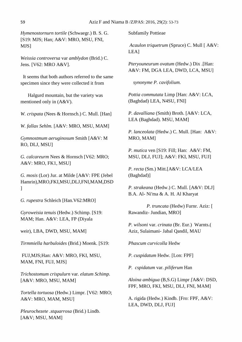
59 Aziz F and Niama B /ZJPAS: 2016, 29(2): 53-73 Hymenostornurn tortile (Schwaegr.) B. S. G. [S19: MJS; Han; A&V: MRO, MSU, FNI, MJS]

Weissia controversa var amblydon (Brid.) C. Jens. [V62: MRO A&V].

It seems that both authors referred to the same specimen since they were collected it from

Halgurd mountain, but the variety was mentioned only in (A&V).

W. crispata (Nees & Hornsch.) C. Mull. [Han]

W. fallax Sehlm. [A&V: MRO, MSU, MAM]

Gymnostmum aeruginosum Smith [A&V: M RO, DLJ, MSU]

G. calcareurm Nees & Hornsch [V62: MRO; A&V: MRO, FK1, MSU]

G. mosis (Lor) Jur. at Milde [A&V: FPE (Jebel Hamrin),MRO,FKI,MSU,DLJ,FNI,MAM,DSD]

G. rupestra Schleich [Han.V62:MRO]

Gyroweisia tenuis (Hedw.) Schimp. [S19: MAM; Han. A&V: LEA, FP (Diyala

weir), LBA, DWD, MSU, MAM]

Tirmmiella harbuloides (Brid.) Moenk. [S19:

FUJ,MJS;Han: A&V: MRO, FKI, MSU, MAM, FNI, FUJ, MJS]

Trichostomum crispulurn var. elatum Schimp. [A&V: MRO, MSU, MAM]

Tortella tortuosa (Hedw.) Limpr. [V62: MRO; A&V: MRO, MAM, MSU]

Pleurochezete .stquarrosa (Brid.) Lindb. [A&V; MSU, MAM]

Subfamily Pottieae

Acaulon triquetrum (Spruce) C. Mull [ A&V: LEA]

Pteryouneurum ovatum (Hedw.) Dix .[Han: A&V: FM, DGA LEA, DWD, LCA, MSU]

synonyme P. cavifolium.

Pottia commutata Limp [Han: A&V: LCA, (Baghdad) LEA, N4SU, FNI]

P. davalliana (Smith) Broth. [A&V: LCA, LEA (Baghdad). MSU, MAM]

P. lanceolata (Hedw.) C. Mull. [Han: A&V: MRO, MAM]

P. mutica ven [S19: Fill; Han: A&V: FM, MSU, DLJ, FUJ]; A&V: FKI, MSU, FUJ]

P. recta (Sm.) Mitt.[A&V: LCA/LEA (Baghdad)]

P. strakeana (Hedw.) C. Mull. [A&V: DLJ] B.A. Al- Ni'ma & A. H. Al Kharyat

P. truncata (Hedw) Furnr. Aziz: [ Rawandiz- Jundian, MRO]

P. wilsoni var. crinata (Br. Eur.) Warnts.( Aziz, Sulaimani- Jabal Qandil, MAU

Phascum curvicolla Hedw

P. cuspidatum Hedw. [Lon: FPF]

P. cspidatum var. piliferum Han

Aloina ambigua (B,S.G) Limpr [A&V: DSD, FPF, MRO, FKI, MSU, DLJ, FNI, MAM]

A. rigida (Hedw.) Kindb. [Fro: FPF, A&V: LEA, DWD, DLJ, FUJ]

60 Aziz F and Niama B /ZJPAS: 2016, 29(2): 53-73 A. rigida var. pilifera, B.S.G. [A&V: LCA, LEA (Baghdad), DGA, FPF, DWD, DLJ, LCA, FKI,

A. stellata Han. Aziz: [RMO]

Crossidiutn chloronotus (Brid.) Limpr. [Han: A&V: LEA] Griseum Jur [S19: MJS; Han]

C. squamigerum (Viv.) Jur. [Han: A&V: Tip river FPF/LEA/LSM, DWD, FKI]

C. squatnigerum var. pottioideum (De Not.) Moenkm. [A&V: DSD, FPF, Diyala weir, DWD,

LCA, WS, FNI, MAM,MSU]

Tortulla alpina (B.S.G.) Bruch [S19: FUJ; Han.]

T. richostomopsis aaronis (Lor.) S. Agnew & Townsend [A&V: DGA, LEA, FPF, DWD, MRO,

DLJ, MAM, FUJ, DWD]

T. Haussknechtii (Jur. Et Milde) S. Agnew & Towsend [A&V: LEA (Diyala), FM]

T. atrovlrens (Smith) Lindb. [A&V: DSD, LEA, MSU, FNI]

T. brevissitna (Schiffn.) [S19: Fuj; Han: A&V: A&V: DSD, LCA/LEA (Baghdad), LEA, FPF,

LCA, DWD, HU, FUJ, DLJ, Mosul]

T. desertorum Broth.= T. Bronmulleri Schiffn. [S19; FUJ, MJS; Han.]

Fioroo (Vent.) Roth. [S19: FUJ, MJS, Han.; Fm: Tib river FPF/LEATLSWI, FPF; A&V: Tib

river, DGA, LEA, FPF, DWD, DU, LCA, FIC1, FUJ]

T. handelii Schiffn. Han. Aziz Choman, Sedakan, Ruwandiz [MRO]

T. linermis (Brid.) Mont. [S19: FM, N. Kurdistan 250-1 100m; Han: ]

T. marginata (B.S G.) Spruce [A&V: MRO, FNI, Msu]

T.montana (Nees) Lndbg. [Han. Fro: MANI]

T. muralis Hedw. ( A&V): MSU, MAM]

T. muralis var aestiva (P. Beauv) Brid. [Han: ; A&V: MRO, MAM] synonyme Tortula aestivia

T. muralis f. brevifolia (Sehiffn.) Podp. [S19. NUS; A&V: MTh FM] the synonyrne T.aestive var.

brevifolia

T. princes De Not. [Frp: MAM]

T. rurals (Hedw.) Gaertn [Han.] (Aziz Rawandiz, Gali Ali- Beg ( MRO)

T. subulata Hedw. [Han.]

T. tortuosa (Hedow )Limp.Laubm (Aziz, Ruwandiz, Gali Ali - Beg and Kawlokan

T .vahlianas (Schultz) Mont. [Lon: FPF]

Tortulla sp. Aziz: Kawlokan [RMO]

Syntrichia alpina (. S. G.) Jur. [V62: MRO ]

S. desetorum (Broth.) Amann [A&V: FPF, DWD, MRO, FKI, FUJ, MJS]

S. hadacii Vonderacek [V65: DLJ; A&V: DLJ]

61 Aziz F and Niama B /ZJPAS: 2016, 29(2): 53-73 S. handelii (Schiffn.) Podp. [A&V: MRO, MAM, MSU]

S. inermis (Mont.) Huben [A&V: MRO, MSU, FUJ, MAM]

S. laevipila Brid [A&V: MRO, MAM, MSU]

S. montana Nees et Esneb [V62: MRO, MJS, MAM, MSU]

S. montana var. calva (Dur. Et Sag.) Amann [A&V: MSU]

S. papillosissima (Coppey) Loeske [A&V: MRO]

S. princeps (De Not.) Mitt. [A&V: MRO, MSU, MAM, FUJ, DWD]

S. pseudodesertorum Froehlich [A&V: FPF, DWD, FKI, DU, FNI]

S. pseudohandelii Froehlich [V65:MSU; A&V: MRO, FM, FNI, FUJ, DLJ, MSU]. synonym S.

handelii var. pseudodesertorum.

S. pulvinata (Jur.) Jur. [A&V: M SU]

S.ruralis Brid. [A&V: MRO, MAM, MSU] Aziz, Shaqlawa

Subfamily Cinnlidoteae

Cinclidotus fontinaloides (Hedw)p. Beauv. [A and V ; MRO, MAM, MSU]

C. nigricans (Brid.) loeske [A&V: MAM].

C. riparius Amott. [Han.]

Order: Encalyptales

Family: Encalyptaceae

Encalypta streptocarpa Hedow

Order Crimmiatales

Family Crimmiaceae

Coscindon cribrosus (Hedw.) Spruce [Han:*]

Schistidium apocarpum var. atrofuscum (Schimp.) Husnot [S19: NJS; Han.;V62: MRO.; A&V:

MRO, MSU, MJS, MAM]. The 1ST & 2nd synonym Grimmia singarensis.

Grimmia anodort B. S. G. (S19: MTh; Han. A&V: MRO, MIS, MSU]

G. apiculata Hornsch. [A&V: MR0] Aziz. Shaqlawa

G. apocarpa Hedw [Han;]

G. campstris Hook. [Han]

G. commutata Hub. (Han; Fro: MSU, V62: MRO; A&V: MRO, MSU]

G. crinita Brid. [Fro: Tib river FPF,LEA,LSM, DSD; A&V: EFT, HB.A. Al- Ni'ma & A. H. Al

Khay'yat; Aziz. Jabal Qandil

G. gibbosa S. Agnew [Agn.; FKI; Rementioned in A&V} (Tuz khurmatil bridge over Lesser zab

river and in Ain Dibbis). Note: Altone Kopri is located on lesser zab not Tuz khurmatil as the

author mentioned.

G. laevigata (Brid.) Brid. [A&V: MRO ]

G. mesopotamica Schiffn. [S19: DWD; Han.; A&V: FPF, Diala weir, DWD, LCA, FPF]

62 Aziz F and Niama B /ZJPAS: 2016, 29(2): 53-73 G. orbicularis Bruch [S19: at 400-1250 m; Fm: MAM; A&V: FPF, MRO; FKI, MAM, FNI,

FUJ, DLJ, MAM, MSU]

G. orbicularis var. persica Han. ( Aziz, Choman -Haji Omaran)]

G. ovalis var. simplex Vondracek [V65: MRO; A&V: MRO]

G. pulvinata (Hedw.) Sm. Schiffn. [S19:DWD, FUJ,MJS; [Han.; A&V: MRO, MSU, MAIM]

G. subcaespitica Schiffn. [Han.; A&V: MRO]

G. lergestina Tomm. (Han.; A&V• MRO, MJS, FNI, MSU]

G. trichophylla Grey. [Fro. MSU; A&V]

Racomitrium affine ( Wib Hedw. and Mohr.) Lindb. (Alni’ma)

Funariales

Family Funariaceae

Funaria hygomatrica

Family Ephermeraceae

Ephemerum cristatum (Hook) F. Wils.

Chistostegales

Family Chistostegaceae

Schistostega pennata (Hedw) Web and Mohr (Aziz, Amadyea MAM and Ruwandiz, RMO )

Physcomitrella patens (Hedw.) B. S. G. [V65: LSM; A&V: ,LEA (Baghdad)]

P.patens var. marginate Vondraccek [A&V: LSM]

Entosithodon.angustifithus Jur. et Milde [A&V: FKI, 'MIS]

E.handelii Schiffn. [S19: synonym Funaria andelii on calcareous rock in North East

Mesopotamia and Kurdistan 250. 1800 m; Han: .FUJ; A&V: MRO, JEW, MAM, FNI,

E. templetoni (Smith) Schwaegr. [A&V: MRO, FUJ, MAMH]

Steppomitra hadacii Vondracek [V65: 'FLU, (A&V)]

Funaria hygrometrica Hedw. [Han. ; A&V: LCA .(Baghdad), MRO, MAM, FUJ, MSU]

F. mediterranea Lindb. [Ham.; A&V: MRO, FNI, FUJ]

Family Splachnaceac

Tayloria lingulata var. acutijblia Han. Ham.; A&V: MRO, FNI, FUJ]

Order Eubryales

Bratramiacea

Family Bryaceae

Aginiobriutn albicans (Wahib.) Lmpr . [S19 MJS; Han.; A&V: LCA (Baghdad), MRO OSU)

Mniobrium delicatrulum (Hedw.) Dix (A&V: LCA, MRO, MAM, MSU, FPF, MJS]

M. latifoliutm Schiffn. [Han.; A&V: MRO] Aziz, Shaqlawa

Pahilia crudes (Hedw.) Lindb. [A&V: MRO]

63 Aziz F and Niama B /ZJPAS: 2016, 29(2): 53-73 Bryum sp. Sterile specimen [Han.]

Bryum sp. [Fm: DSD]

B. . alpinurn Brid. [Fro: MSU; A&V: MRO, MAM, MSU]

B. argentum Hedw [A and V: MRO, MSU]

B.argentum var. lanatum (P. Beauv.) B.S.G. [Fro: MSU; A&V: FKI, MSU]

B. bicolor Dicks [Lon: FPF]

B. badium Batch ex :Ruthe [Han.; A&V: FAR, MA M, MSU]

B. caespiticum Hedw. [Han.; Fro: MAM; A&V: MAM, MSU]

B capillare Hedw. [Han.; A&V: MRO, MAM, FUJ, MSU]

B. capillare f. flaccidum B.S.G. [A&V: MSU]

B.capillare var. torquescens (B.S.G.) Husn. [S18: MRO; Fro: NISU; A&V: MRO, MAM MSU]

synonyme Bryum torquescens

B. cirratum Hoppe et Hornsch. [A&V: MRO]

B. donianum Grev. [A&V: MSU]

B. funkii Schwaegr. [Han.; V62: MRO; A&V: LBA, LCA (Baghdad), DWD, FNI, MSU, LEA]

B. gemmiparum De not Upper plain and foothlls

B. pallens (Grid.) Rohl. [A&V: MRO]

B. pallescens SchIeich. [V62: MRO; A&V: MSU, NIRO, FPF, DWD, LCA]

B. pseudotriquetum (Hedw.) Schwaegr. [V62: MRO; A&V: MRO]

B. schleicheri Schwaegr. [A&V: MRO, MSU]

B. syriacum Lor. [Han.; Fro: MRO; A&V]

B. vent-rico Han.

B. rubens Mitt. (Aziz, Ruwandiz [MRO]

B. uliginosum (Grid.) Rohl.

Rhodobryum roseum ( Hedw.) Limper.

Family Mniaceae

Mnium longirostrum Brid. [V62: MRO; A and V : MRO]

Plagiominum rostratum (Schard.) kop. Aziz [RMO]

Plagiothecium denticulatum (Hedw.) Br. Eur. Aziz [MRO]

Isoptergiopsis taxiphyllum (Schimp.) Wats. Aziz [MRO]

Family Bartamiaceae

Anacolina webbii (Mont.) Schimp. [A&V: MRO]

Philonotis caespitosa Wits. [A&V: MRO, MAM]

P. calcaera (B. S. G.) Schimp. [Han.; V62:MRO; A&V: .MRO,MAM]

P. fontana (Hedw.) Brid. [Fro: MRO; A&V: MRO, MSU]

P. fontana f. laxifolia Moenk. ap. Loeske [A&V: MRO]

64 Aziz F and Niama B /ZJPAS: 2016, 29(2): 53-73 P. marchia (Hedw.) Brid. [Han.] MRO; A&V: MRO]

P, seriata (Mitt.) Lindb. [Fro: MAM and A&V]

P.tomentella Mol. [Han.; V62: MRO; A&V: MRO]

Family Orthodentaceae

Orthodontum lineare Schwagre

Order Isobryales

Family Fontinalacese

Fontinalis mesopotamica Han.

Family Orthotrichaccae

Orthotirichum affine Brid. [A&V: MRO, MAM, MSU]

O.cupulanon Brid. [Fro: MAM; A&V: MRO, MAM,MSU]

O. cupulatum var. papaillsum Gronv. [A&V:MRO, MSU]

O. cupulatum var. bistratosum Han.

O. lyellii Hook et Tayl. [A&V: MRO, MAM, MSU]

O. octoblephare [V62: MRO]

O. rupestre Schleich [Han. ; V62: MRO; A&V: MRO]

O. schimperi Hammar [A&V: MRO, MAM, MSU]

O. soeciosum Nees [A&V: MSU]

O. strumii Han

Family Leucodontaceae

Antitrichia breidleriana Schiffn.[Han.; A&V: MRO]

Order Hypnobryales

Family Fabroniaceae

Fabronia pusilla Radi [A& V: MRO, MAM]

Family Hypnaceae

Subfamily Amblystegiadeae

Cratoneuron commutatum (Hedw.) Roth. [Han; A&V: MRO, MAM]

Commutatum m var. suicatum (Lindb.) Monk. [V62: MRO]

C. decipivar. falcatum (Bride) Moenkm [Fro; MRO; V62: MRO; A&V: MRO,MSU]

C. commutatuens (De not.) Loeske Han V62: MRO; A&V: MRO]

C. decipiens var. napaeforme Han

C. filicinum ( Hedw. ) Roth . [Fro : MSU; A&V:MRO, MAM,MSU]

Plagiominum rostratum (Schard.) Kop.

Amblystegium juratzkanum Schimp. [A&V: MRO]. Smith (1978) treated this taxon as synonym of

A. serpens as it is quite impossible to separate the two taxa.

A. kurdicum [Han]

A. serpens (Hedw.) B. S. G. [A&V: MAM]

65 Aziz F and Niama B /ZJPAS: 2016, 29(2): 53-73 A. tenax (Hedw.) C. jens = Hygroamblystegium irriguum [Han} synonym Hygroamly stegium

irrguum but Smith (1978) following Nyholm (1954-69) included Hygrownbly stegium

and use the new name A. tenax.

A. varium (Hedge) Lindb. [A&V: MRO, MSU]

Amblystegiella jungermanniaides (Brid.) Giacomini [A&V: MRO]

A. spruci (Brach) Loeske [V62: MRO]

Leptodictyum riparium (Hedw.) Warnst. [A&V: MSU]

Drepanockaus aduncus (Iledw.) Moenkm. jA&V: MRO]

Acrocladium cuspidatum (Hedw.) Lindb. [AIM MRO]

Calliergon cuspidatum =Calliergonella cuspidata [V62: MRO], after Smith (1978).

Subfamily Brachytheciaceae

Homalothecium philippeanum (Spruce) B.S.G. [Han.; A&V: MRO,MAM]

H.seriaceum (Hedw.) B.S.G. [Han.; A&V: MRO, MSU]

Scorpiurum aircinnatum (Brill,) Fleisch [Han:]

Camptothecium lutescns (Hedw.) B.S.G. [Fro: MAM, MRO; A and V]

Brachythecium collinnum (Schleich.) B.S.G. [Han.; A&V: MRO, MAM, MSU]

B.olympicum Han

B.rivulare (Bruck) B.S.G. [V62: MRO; A&V: MRO, MAM, MSU]

B. rutabulum (Hedw.) Br. Eur. [Alni’ma]

B. salebtaosum Web. Et Mohr B.S.G. [A&V: MRO. MAM]

B. trachypodium Han.

B. Euryhynchium confertum (Dicks.) MiIde [A&V: MRO

Eyrhynchium paralongum var. paralongum (Hedw.) Br. Eur.

E. reipariodes (Hedw.) P.W. Richards [A&V. MRO, MAM, MSU]

E. speciosum (Bride) Milde [A&V: MA M]

Rhynchostgiella curviseta (Brid.) [A&V: MAM]

Hypnaceae

Hypnoideae

Rhytidiaelphus loreus Warnst.

List (3): Pteridophyta (Ferns) Iraq and Kurdistan region (from Guest, 1966 and Aziz,2015).

Kingdome Plantae

Pteriodphyta F. Ballard

Eequisetales

Equisetaceae F. Ballard

Equisetum arvense L. Erbil _

E.. Ramosissimum Desf, FL. Atlant, Aziz , Bastora – Hanara village

66 Aziz F and Niama B /ZJPAS: 2016, 29(2): 53-73 Filicales

Marsileaceae F.Ballard

Marsilea L. capensis A.Br.

Salviniaceae F. Ballard

Salvinia natans (L.) All. Flor. Pedum

Adiantaceae F. Ballard

Adiantum capillus- veneris L.Aziz, Gali Ali –Beq,

Anogramma leptophylla (L.) Link. Hawraman

Cheilanthes fragrans (L.) Sw. Jabal Bawaji , Gali Ali- Beg

C. margirata (L.) Mick

C. persica (Bory ) Melt ex lkuhn , Aziz, Choman - Haji Omaran

Ceratopteris Brongn

C. thalictriodes (L.) Brongn.

Aspelinaceae F. Ballard

Aspleninum trichomonas L. Aziz, Sulaimani-Ahmad Iwa

A. virid Huds.

A. husskaechii Godett Reater

A. ceterach Garsault Aziz, Erbil - Gali Ali Beg

A. officinarum DC.

Athyriaceae F. Ballard

Phyllitis scolopendruium (L.) Newm Jabal Al Khayat, Pramagron

Cystopteris . fragilis (L.) Bernh

C. regia…( Aziz, Choman- Doli Balaiyan - Wassan village)

Aspidiaceae F. Ballard

Polystichum setiferum (Forssk) Woyne Aziz, Sulaimani- Ahmad Iwa- Zalm village

Sperrnatophyta

Gymnospermae

Ephedraceae R.A. Blakelock and J.B Gillett

Ephedra alata Decne syname Gnetales alata Decne.

E. transitoria Riedl

Coniferales

Family Cupressaceae R.A Blaeklock

Janipperus polycarpos L. Koch in linnaae..............Erbil and Duhok

Cupressus L

C. arizonica Greene

C.semperrivens L.

Thuja ovientalis L.

Family Pinaceae

Pinus . halepensis L (Snobar in Kurdish Duhok, Zawita)

p. halepensis var. brutia (Ten) Henry ex Elwes and Henry

67 Aziz F and Niama B /ZJPAS: 2016, 29(2): 53-73 List(4) : Lichenes of Kurdistan mountian areas, Iraq (Aziz,2004, 2005, 2006; Kostly all of

them are widely distributed).

Class Ascomycetes (Ascolichenes).

Subclass Ascomycetidae.

Acarospora hilaris (Dufour) Hue.

A. fuscata (Schrader)Arnold

A. Htitblicata Bagl.

A. strigata (Nyl.) Jutta

Aspicilia calcarea (L.) Mudd.

A. candida (Anzi) Hue.

A. cinerea (L.) Korber

A. contorta (Hoffm.) Kremb

Aspicilia sp.

Bellemerea aplina (Somm.) Clauz. & Roux.

B. cinereorufescens (Ach.) Clauz. and Roux.

Bellemerea sp. (Aziz. 2003)

Biotora vernalis (L.) Fr.

B . disciformis (Fr.)Mudd.

B. spuria (Schaerer)Anzi.

B. stigmaea Tuck.

Caloplaca aurantia (Pers.) Hellbom

C. citrine (Hoffm.) Th. Fr.

C. bolaacina.(Tuck.) Herre

C. feracissima.H.Magn.

C. flavorubescence (Huds.)J.R. Laundon

C. holocarpa (Hoffm. ex Ach.), M.Wade

C. epithallina Lyng.

C. ignea Arup

C.ochracea (Schaer.) Flagey lieppina (Muell.Arg.) Zahlbr

C. luteominia var. bolanderi (Tuck.) Aurp.

C. pellodella. (Nyl.) Hasse

C. thallincola (Wedd.) Du Rietz

C. variabilis (Pers.) Mull. Arg.

C . velana.(A.Massal.).Du Rietz

C. verruculiferi (Vainio) Zahlbr.

Candelariella aurella.(Hoffm.)Zahlbr.

C. vitellina.(Hoffm.) Mull. and Arg.

Citrysotlirix candelaria (L.) J. R. Laundon

Coccocarpia palmicola (Sprengel) Arr.&D.J.Galloway

C. erthroxyli (Sprengel)

Collema cristatum (L.)F.H.Wigg

C. flaccidum (Ach.)Ach.

C. tenax (Sw.)Ach.

Coccotrema urceolatum (Ach.) Tuck.

Dermatacarpon miniatum (L.)W.Mann

Dermatocarpon sp.

68 Aziz F and Niama B /ZJPAS: 2016, 29(2): 53-73 Dimelaena oreina (Ach.) Norman.

Diploschistes caesioplumbeus (Nyl.) Vain.

Diploschistes ocellatus (DC.) Norman.

D. muscru. (Scop.) R.Sant

D. scruposus (Schreb.) Norman Syn.: Urcelaria

Dirina catalinarie Hasse

Endocarpon pusillum. Hedwig

Fulgensia fulgens (Sm.) Elenkin

F. subbracteata (Nyl.) Poelt.

Graphis elegans (Borrer ex Sm.) Ach.

Graphina peplophora M.Wirth & Hale

Gypsoplaca macrophylla

Haematomma ventosum (L.) A. Massal.

Heterodermia crocea R.C. Harris

H. diademata. (Taylor)D.D.Awasthi

Heteroplacedium sp

Hypotrachyna livida.(Taylor) Hale

Hypogymnia austerodes (Nyl.)Rasanen Syn.:Parmelia austerodes

Kaernefeltia merrillii (Du Rietz.) Thell.& Goward Syn. Cetraria merrillii

Lecanactis abietina (Ach) Korbe

L. cinereofiisca var. appalachensis Brodo

L. argopholis (Ach.) Ach.

L. cinereofusca var. appalachensis H. Magn.

L. circumborealis. Brodo and Vitic.

L. dispersa (L.) Sommerf.

L. garovaglii (Korber) Zahlbr.

L. muralis (Schreb.) Rabenh.

L. mutabilis (Ach.) Nyl.

L. novomexicana.H.Magn.

L. polytropa.(Hoffm.) Rabenh.

L. pruinosa Chaub.

L. hybocarpa (Tuck.)Brodo

L. cupressi Tuck.

L. xylophila Hue.

Lecanora sp. Fink H. Magn

L. wargiitata Shaerer Hartel & Rambold

Lecanora sp.

Lecanora sp. Fink H. Magn

Lecidea atrobrunnea (Ramond ex Lam.&DC.)Schaerer

L. acropora var, subplicata Zahlbr

L. cythoides (Weber) Ach.

L. fuscoatra (L.) Ach.

Lecidella picida.(Nyl.)Hertel and Leuckert

L. stigmata (Ach.)Hertel &Leuckert syn.:Lecidea micacea

Lecidella sp.

69 Aziz F and Niama B /ZJPAS: 2016, 29(2): 53-73 Lepraria incana (L.) Ach.

Leptotrema wightii (Taylor) Mull. and Arg.

Leptotrema sp.

Lobothallia praeradiosa (Nyl.) Hafellner

Eproloma vouauxii (Hue)J.R. Laundon

Megaspora verrucosa (Ach.) Hafellner &M.Wirth syn.:

Pachyospora Verrucosa

Melanelia disjucta (Frichsen) Essl.

M. panniformis (Nyl.)Essl.syn.:Parmdia punniformis

Mycoblastus affinis (Schaerer)Schauer

Neofuscelia pulla (Ach.) Essl.

Normandina pulchella (Borrer) Nyl.

Ochrolechia frigida (Sw.) Lynge

O. pallescens (L.) A. Massal

O. tartarea Gudbear

Opegrapha sp.

Orphniospora moriopsis. (A.Massal.)D.Hawksw

lacidium lacinulatum (Ach.) Breuss

Pannaria rubiginosa var. canoplea

Parmelia acetabulum (L.) Ach.

P. caperata (L.) Ach. (Ach.) Bory

P. conspersa.(Ehrh. ex Ach. )Ach.

P. saxatilis (L.)Ach.

P. tinctina (Mah.)Gill

Parmelia sp.

P. quercina (Willd.) Hal

Parmotrema chinense (Osbeck) Hale and Ahti =Parmelia (Hudson.) Ach.

P.perforatum (Jacq) A.Massal.syn.Physcia perforata (Ach

Parmotrema sp

Peltigera sp.

Peltula obscurans (Nyl.)Gyelnik

Peltula richardsii (Herre) Wetmore

Pertusaria aspergilla (Ach.) J.R. Laundon

P. flavicunda Tuck.

P. paratuverculifera Dibben

P. flavicunda Tuck.

P. subambigens Dibben

P. texana Mull. & Arg.

P. trachythallina Erichsen

P. lactea Erichsen

P. macoumii (Lamb) Dibben

P.subpertusa (L.) Tuck.

P. rubefacta Erichsen

P. velata (Furner) nyl.

Physcia aipolia (Ehrh. ex Hump.) Furnr.

P. biziana (A.Massal) Zahlbr.

70 Aziz F and Niama B /ZJPAS: 2016, 29(2): 53-73 P. caesia (Hoffm.) Furnr.

P. simpinnata (L.) Nyl.

P. pulverulenta Schreber) Furner

Physconia distorta =P.pulverulacea Schreber) Furner

P. perisidiosa (Flarke) Moberg =P. grisea Schreber) Furner

P. thamsonii Ess

P. pulverulacea Moberg.

Propidia flavocaerulescens (Hornem.)Hertel and A.J. Schwab

Psora decipiens (Hedwig) Hoffm.

Pyrenula nitida (Flarke) Mull. and Arg.

P . pseudobufonia (Rehm) R.C. Harris

Rhizocarpon calcareum (from Alvin Kershaw , 1963)

R. chioneum (Norman) Th. Er.

R. chionphilum (Norman) Th. Er.

R. disporum (Naegeli ex Hepp.) Mull. And Arg.

R. hochstetteri (Korb.) Vain.

R. georaphicum (L.) DC.

R. macrosporum Rasanen

R. obscuratuni (Ach) A. Massal

R. richardii (Nyl.) Zahlbr

R. umblicatum (Ramond) Flagey

R. marginalis (Hass.) W.A.Weber

Rhizoplaca melanophthalma (DC.)Leuckert &Poelt

R. subdiscrepans (Nyl.)R.Sant.

Rhizoplaca sp.

Rinodina atrocinerea (Hook.) Korb.

R. ascociscana Tuck.

R. bolanderi H. Magn.

R. populicola H.Magn

Rinodina sp.

Roccellina conformis Tehler

Staurothele diffractella (Nyl.) Tuck.

Squmarnia cartilagnea (With.) P. James

S. crassa (Hudson) Poelt

S. stellata -petrea Poelt

Tephromela grumosa (Pers.) Hafellner & Cl. Roux

Thelomma californicum (Tuck.) Tibell

Tonina alutacea (Anzi) Latta

T. candida (Weber)Th.Fr.=T.Alutacea

T. sedifolia (Scop.)Timdal

Tonina sp. (Aziz , 2003)

Trapelia involuta (Tylor) Hertel

T. placodioides Coppins & P. James

Trapeliopsis wallorothii

Theilidium pyrenohorum (Ach) Mudd ( Florke) Hertel& G

Trapelopsis wallorothii (Ach.) Mu

71 Aziz F and Niama B /ZJPAS: 2016, 29(2): 53-73 Umbilicaria americana (Poelt & T. Nash)

Verrucaria amphibia Clemente

V. baldensis A. Massal.

V. calsiceda DC.

V. marmorea (Scop.) Arnold

V. maura Wahlenb

V. nigrescence Pers.

Xanthoria elegans (Link) Th. Fr.

X. fallax (Hepp.)Arnold

X. fulva (Hoffm.) Poelt. and Petut

X.parietina (L.) Th. Fr.

Xanthoparmelia plittii (Gyeln.) Hall.

List (5): Classification of identified species of Mushroom (Aziz and Toma, 2012, mostly they found

in Ruwandiz, Joman, Jabal Qandil- Asha- Qulka village, Ahmad Iwa- Zalm village )

Kingdom: Fungi

Phylum : Basidiomycota

Order: Agricales

Family: Agricaceae

Agricus arvensis Sch.

A. bernardii Sch.

A. bisporus ( L.) Fr.

A. campestri ( L. ) Fr.

Macrolepiota sp

Order: Aphyllophorales

Family: Corticiaceae

Chondrostereum purpureum

Family: Stereaceae

Stereum rugosum Pers

Family: Hymenochaetaceae

Phellinus igniarius ( L.Fr.) Quel. s.l.

Family: Fomitaceae

Bjerkandera adusta

Family: Fomitopsidaceae

Fomes fomentarius ( L.Fr.) Kicky

Family: Polyporaceae

Fomitopsis pincola

Fomitopsis pincola

Trametes ochracea

T. versecolor (L.,Fr.) Pilat

Family: Paxillaceae

Paxilus corrugatus

Order: Cortinariales

Family: Cortinariaceae

Crepidotus variabilis (Pers.,Fr.) Kummer

72 Aziz F and Niama B /ZJPAS: 2016, 29(2): 53-73 Family: Inocybaceae

Inocybe godeyi (Bull,Fr,) Kummer.

Family: Strophariaceae

Hypholoma fosciculare (Huds) ex Fr. Kumme

Order: Entolomatales

Family: Entolomataceae

Entoloma rhodopolium (Fr.) Kummer

Entoloma serrulatum (Fr.) Hesler

Order: Tricholomatales

Family; Tricholomataceae

Clitocybe metachora

C. nebularis (Batch) Quel.

C. odora Bull.ex Fr.) Quel.

Cystoderma amianthinum (Scop) Konrad , Marbl.

Micronphale foetidum

Familly; Mycenaceae

Mycena arcangeliana

Russula aeruginea Fr.

Ochrolechyia tartaria (Pers.)Fries

Lactarius vellerus (Fr.) Fr

Family: Tricholomataceae

Tricholoma sejunctum

Family: Pleurataceae

Pleurotus ostreatus (Jacq Kummer

Family: Corihaceae

Panaeolus papilionaceus var. papilionaccus

(Bull) Quel.

Panaeolus semiovatus var. semiovatus

(Sowrerby) S. Lundell ,Nannf.

73 Aziz F and Niama B /ZJPAS: 2016, 29(2): 53-73

REFERENCES

Agnew S. (1973). A new Middile Eastern Grimmia j. Bryol., 7:339-342.

Agnew, S., & Townsend, C.C.( 1970). Trichostornopsis Card., A moss genus new to Asia Israel Box., 19: 254-259.

Agnew, S. & Voudracek, M. (1975). Moss Flora if Iraq. Feddes Repertorium, 86:

341489.

Al-Nima, B.A. B. 1994 New records of Liverworts from Mosul -Iraq. J. of Educe &

Sc., 20:36-44.

Al-Nima, B.A. B and Al-Khaiyat A (2001). Check list of Iraqi Bryophyta. Bull. Iraq.

Nat Hist. Mus. 3 (9) 7-18

Al- Naqshbandi M.A. and Al-Nima, B.A. B. (2012 ). New record of seven Mosses

species for Iraqi Bryflora ( un published.)

Erbil-province Iraqi

Kurdistan region, Iraq. 2- In Hassan - Beg mountain area. Zanco. The Sci. J. of Pure and

Aziz, F. H. (2005). Observation in lichens of mountainous area within Erbil-province

Iraqi Kurdistan region, Iraq. 1- In Safm, Jundian, Kawlokan and Haji Omaran areas,

mountain area. Zanco, The Sci. J. of Pure and Appl. Sci. Salahaddin Univ.-Erbil, Iraq.

16 (5): 1-19.

Aziz, F. H. (2004). Observation in lichens of mountainous area within Erbil-province

Iraqi Kurdistan region, Iraq. 2- In Hassan - Beg mountain area. Zanco. The Sci. J. of Pure

and Appl. Sci. Salahaddin Univ.-Erbil, Iraq. 17 (2): 89-117.

Aziz, F. H. and Saeed, J.F. (2006). Observation in lichens flora of mountainous area

within Erbil-province Iraqi Kurdistan region, Iraq. 3- In Karajugh mountain and foothill area.

Sci. J. of Anbar Univ. 3 (3): 32 - 54.

Aziz, F. H. (2010). Six new records of Hepatophyta (Liverworts) to Iraqi flora. Sci. J. Duhok Univ. 13 (1): 86 - 98

Aziz, F. H. (2011). Seventeen spp. New records for the mosses flora of Iraq. Phyton

International J. of Exprimental Botany. Argentina . 80: 35-46.

Aziz, F. H. and Toma Fareed H. (2012). First attempt for collection and identification of mashroom in Kurdistan Iraq. Journal advanced laboratory. 3(2):330-350

Long, D.G. (1979). Some Additions to the Bryophyte Flora of Iraq. Rev. Bryol. Lichen.,

45:103-105.

Schiffner, V. (1897). Musci Bronrnuelleriani. Osterr. Bolt Z., 47:125-132.

Schiffner, V.( 1913). Bryophyta aus Mesopotamiem und Kurdistan, Sowie, Rhodos,

Mytilini und Prinkipo. Ann. Naturhist., illus., Wien, 27:1-34.

Qadir, S. B.and Aziz F. H. (2015). Thirty new records of epelithic

lichens m within Erbil governorate, Kurdistan region M.Sc. Thesis near main

roads from north to south part of Erbil Governorate, Kurdistan Region, Iraq

Qadir, S. B. and Aziz, F. H. (2015). Lichens as a bioindecators for air pollution

assessmen College Of Science, Salahaddin Univ.- Erbil, Kurdistan, Iraq

(un published).

Vondracek, M. 1962 New Bryophyte for the Iraqi Flora. Bull. Iraq. Nat. Hist. Inst.,

2: 9-10.

Vondracek, M. 1965 Some New Mosses from Iraq. Collected by E. Hadae. Bull. Soc. Amis. Sci. Lettres Poznan, Ser. D., 6:117-122.

ZANCO Journal of Pure and Applied Sciences

The official scientific journal of Salahaddin University-Erbil

ZJPAS (2017), 29 (2); 74-77

http://dx.doi.org/10.21271/ZJPAS.29.2.7

New species of the genus, Protaetia Burmeister, 1842 from Iraq

(Coleoptera: Scarabaeidae :Cetoniinae)

Hozan Q. Hammamurad, Nabeel A. Mawlood and Banaz S. Abdulla

College of Agriculture, Salahaddin University-Erbil

1. INTRODUCTION

Protaetia is a genus of beetles of the family

Scarabaeidae and subfamily Cetoniinae of

superfamily Scarabaeoidea, the family number

exceed 30,000 species of beetles worldwide

often called Scarabs or Scarab beetles and then

genus Protaetia occurring primarily in Asia

and containing over 300 species (Mittal, 2000).

Ratcliffe (1991) study the key of genus

Protaetia in Floridae and there are five genera

in United state, Canada and Northern Mexico.

Thomas (1998) mention the 250 species of

genus Protaetia in the Oriental Australian and

Palearctic region. The adults of Cetoniinae feed

on flower and fruits, thin popularly referred to

as flower beetles, the larvae scarab beetles

white grubs caused damage to the roots of

cereal, legumes, small fruit plants, shrubs thin

caused damage to field crops and fruit trees

(Mehta et al., 2010). The classification of this

family is fairly unstable with numerous

competing theories, many of subfamilies listed

probably will not be recognized very much

linger.Some of scarab beetles are used in the

biological control of dung and dung flies

(Machatschke, 1972). Lawrence and Britton

(1991) indicated the classification of

superfamily. Arnetts (1968) mention the

hierarchical level of families and subfamilies.

In Iraq 10speciesin six genera of the family

listed by Derwesh (1965),and Al-Ali (1977)

recorded six species.

A R T I C L E I N F O

A B S T R A C T

Article History:

Received: 20/07/2016

Accepted: 01/12/2016

Published: 07/06/2017

The new species Protaetia kurdistanica sp. nov. are described

and illustrated from Iraq.The differences between the species and

closely related species is discussed. Diagnostic characters of the

new species is figured. The materials examined are deposited in

the Museum of plant protection department. College of

Agriculture ,Salahaddin University –Erbil-Iraq.

Keywords:

,Scarabaeidae . New species

,Protaetia kurdistanica sp.

nov., Erbil Kurdistan .

region- Iraq.

*Corresponding Author:

Hozan Q. Hammamurad

hozan.hamamurad@su.edu.krd

75 Hammamurad H. et al. /ZJPAS: 2017, 29(2): 74-77

2. Type material: (♂) (Holotype) Iraq-

Kurdistan region: Erbil- Rania, 360 Km N

Baghdad, 18-May.2015 from Milk thistle

Silybum marianum L., Hozan Q. Hammamurad

leg., Paratype (8 ♂♂7 ♀♀): from same locality

and date, the holotype is kept in the insect

museum of College Agricultural- Erbil,

Kurdistan region- Iraq.

3. RESULTS AND DISCUSSION

Protaetia kurdistanica sp. nov.

Body:Oval expanded, Metallic green reddish.

Length 16.1-20.5 mm, width 7.8-11.1mm.

Head:Parallel sides, elongated. Dark grassy

green completely covered with Tomentum

.Eyes black, rounded. Vertex brightly green,

flat, with low dense of fine punctures. Coronal

suture present. Frons densely punctured.

Clypeus flat, rectangular, laterally wrinkled,

middle part simply punctured. Anterior margin

of clypeus with shallow, narrow impression

along entire margin. Labrum (Fig. 1a) nearly

globular , pale yellow, sparsely pale yellow

setose, anterior margin moderately concave.

Mandible (Fig. 1b) dark brown, high

sclerotized, apical part bidenticles, inner

denticles shorter than the outer. Maxilla (Fig.

1c) dark brown, cardo triangular , sparsely

yellow setose, distal part of galea rectangular,

moderately sclerotized, apical part densely

pale brown setose, lacinia membranous , apical

part densely pale brown setose,2nd

segment of

maxillary palp square shaped 2 times as long as

1st segment, 4

th segment oval elongated, 1.5

times as long as 3rd

segment. Antenna (Fig. 1d)

lamellate, dark brown, surface yellow setose,1-

4 segment cup shaped, 5-8th

segments nearly

equal in size, 9-11 segment lamellate, 11th

segment 1.1 times as long as 8th

segment.

Thorax:Pronotum metallic grassy green,

surface randomly irregular punctures laterally ,

the middle impunctate , the anterior margin

moderately concave, posterior margin convex

at the middle, the anterior angle slightly acute ,

posterior angle rounded. Scutellum grassy

green, triangular ,apex obtusely rounded ,

surface impunctate and bare . procoxal cavity

close, prosternum dark brown, surface

randomly irregular of fine punctures , anterior

margin of prosternum strongly concave

,densely yellow setose, prosternal process

nearly globular densely yellow setose.. Elytra

metallic green, simply punctures, bare, 1/4 of

outer margin moderately concave .Epiplural

dark brown, sparsely fine punctate , yellow

setose. Hind wing brown, veins dark brown.

Forelegs dark green, outer margin of fore tibia

(Fig. 1e) triedenticate, apical part with single

long spur; tarsus five segmented, 1st- 4

th

segments cup shaped, 2nd

segment 1.3 times as

long as 1st segment, 2-4 segments same in

length, 5th

segment tubular, 1.3 times as long as

4th

segment, apical part with short process;

claws long simple moderately curved. Mid legs

resemble forelegs except the, mid tibia with

single denticle at the middle, apical part

tridenticate, with two spurs. Hind legs resemble

forelegs except, coxa plate shaped, outer

margin of hindtibia with single denticle, apical

part with two short spurs.

Abdomen: metallic grassy green, oval, with

six segments , surface sparsely yellow setose

and randomly irregular punctures, 2nd

-5th

abdominal sternites same in length.6th

abdominal sternite nearly cup shaped, anterior

margin convex, posterior margin rounded,

surface sparsely yellow setose, . 6th

tergite dark

brown, cup shaped, anterior margin nearly

straight, posterior slightly concave. Spiculum

gaster absent.

Male genitalia:Aedeagus (Fig. 1g,h) brown,

moderately curved, basal hood pale brown

.Length 0.6-0.7 mm, apical part low sclerotized

76 Hammamurad H. et al. /ZJPAS: 2017, 29(2): 74-77

nearly hook shaped. Tegmen (Fig. 1f) pale

brown, nearly Y- shaped, highly sclerotized.

Diagnosis:Protaetia kurdistanica sp. nov. this

species differs from closely related species ,

Protaetia maxwelli Jakl by the following

characters :Body length 16.-20.5 mm. Middle

parte of pronotum impunctate and bare. Elytra

bare .Fore tibia triedenticate .Aedeagus pale

brown-yellow, moderately curved, apical part

nearly hook shaped.

Acknowledgements

We sincerely thank the specialist in German

museum of technology who confirmed the

identification. We deeply express my gratitude

to Pro. Dr. Mohammed S. Abdul Rassoul in

Division of Entomology, Natural History

Research Center – University of Baghdad / Iraq

for his kind help and continuous

encouragement to this work

Figure:1 Protaetia kurdistanica sp.nov.

a. Labrum b. Mandibll c. Maxilla d. Antenna e. Foretibiaf. Tegmen g. Male genitalia lateral

view h. Male genitalia dorsal view.

77 Hammamurad H. et al. /ZJPAS: 2017, 29(2): 74-77

REFERENCES

Al-Ali, A.S.(1977). Phytophagous and

entomophagous insects and mites of Iraqi

Natural History Research center,

publishing,No. 33-142pp.

Arnetts, R.H.,J.R.(1968). The beetles of the

Unite states. Amanual for identification.

Amer. Entomo., Ann Ardor, IM., 1-112pp.

Derwesh, A.I. (1965). A preliminary list of

identified insects and arachnids of Iraq.

Direct. Gen. Agr.Res. Proj. Baghdad. Bull.,

No. 121:123pp.

Mehta, P.K.; Chandel, R.S. and Mathur,

Y.S.(2010). Status of whitegrubs in North

Western Himalaya, Jour. Inse. Sci., 23:1-

14.

Mittal, I.C.(2000). Survey of scarabaeid

(Coleoptera) fauna of Himanchal pradesh

(India). Jour. Ento., 24:133-141.

Ratcliffe, B.C.(1991). The Scarab beetles of

Nebraska. Bulletin of the Univiersity of

Nebraska State Museum, 12:1-333 pp.

Ritcher, P.O.(1958). Biology of scarabaeidae.

Ann. Rev. Ento., 3:311-334.

Thomas, M. (1998). A flower beetle, Euphoria

sepuleralis (Fabricius). In florida

(Coleoptera:

Scarabaeidae). Florida Department of

Agriculture and Consumer services,

Entomology circular, No. 386:1-2.

Lawrence, J.F. and Britton, E.B. (1991).

Coleoptera. The insects of Australia, Melbo.

Univ. Carlton, 2nd

ed., Vol., 1:543-683pp.

ZANCO Journal of Pure and Applied Sciences The official scientific journal of Salahaddin University-Erbil

ZJPAS (2017), 29 (2); 78-87 http://dx.doi.org/10.21271/ZJPAS.29.2.8

Using Proposed Nonparametric Regression Models for Clustered Data (A simulation study)

Taha H.A. Alzubaydi Department of Statistics, College of Administration and Economics, Salahaddin University, Erbil, Kurdistan Region, Iraq.

1. INTRODUCTION

Nonparametric methods try to avoid assumptions about the probability distributions in order to generate methods that can be used in settings where regular parametric assumptions do not work (Lin, X. & Carroll, R. J., 2000). Although applicable in more general circumstances, nonparametric models can lead to very complex mathematics in all but the simplest models by using seemingly unrelated kernel estimator method.

In clustered data, it is clear the data that are collected from the same subject at different times are correlated and those observations from different subjects are often independent. Therefore, it is of great interest to estimate the regression function incorporating within-

subject correlation to improve the efficiency of estimation through three correlation structures correspond to correlation ρ , (Silverman, B. W., 1984): the autoregressive case with r=0·6, the exchangeable case with r=0·6 and the

unstructured case with 8.02312 == rr and

5.013 =r correlation matrices. Clustered data arises from many applications, including ophthalmologic studies, rodent teratology experiments, dental research, family-based genetic studies, and community intervention studies, etc.

2: Methodology:

2.1: Nonparametric Regression for Clustered data:

A R T I C L E I N F O

A B S T R A C T

Article History: Received: 8/11/2016 Accepted: 2/12/2016 Published:07/06/2017

A nonparametric model is introduced to account varying impacts of factors over clusters using proposed models in comparison with some classical models. It achieves the parsimony of parameterization and allows the explorations of nonlinear interactions. The random effect in the nonparametric model also accounts within-cluster correlation. Local, linear-based estimation procedure is proposed for estimating functional coefficients, residual variance and within-cluster correlation matrix for three cases (the autoregressive, the exchangeable and the unstructured). Simulation studies are carried out to demonstrate the methodological power of the proposed methods in the finite sample, Using MATLAB language program designed for this purpose.

Keywords: Nonparametric Regression, Cluster data, Kernel method, Efficient estimation and Nonlinear model. *Corresponding Author:

Taha H.A Email: drtahaalaa1970@yahoo.com

79 Alzubaydi T./ZJPAS: 2017, 29(2): 78-87

Consider data from n clusters with im

observations in the ith cluster ( )ni ,,2,1 = .

The jth observation ( )imj ,,2,1 = in the ith

cluster consists of an outcome variable ijY and

a single covariate ijT whose values vary within

the cluster. For longitudinal data, a cluster refers to a subject and within-cluster observations refer to repeated measures over time, and ijT is a

time-varying covariate or time; for familial data, a cluster refers to a family and within-cluster observations refer to different family members and ijT is a member specific covariate. For

simplicity, we assume the number of observations per cluster takes the same value m in all clusters, although the results hold when cluster sizes vary. The outcome ijY depends on

the covariate ijT through (Xihong Lin and et al.,

2004).

( ) ( )1TY ijijij εθ +=

Where ( )ijTθ is an unknown smooth

function, and the errors ( )Tmij 111 ,, εεε = are

independent with mean zero vector and true covariance matrixΣ . We assume in our asymptotic study that the cluster size m is finite but the number of clusters n goes to infinity.

Nonparametric estimation of ( )tθ can proceed using kernel method. It is of interest to construct nonparametric estimators of ( )tθ that account for the within-cluster correlation (Wang, Y., 1998).

Define:

( )Timiii Y,,Y,YY 21 = ,

( ) ( ) ( ) ( ){ }Timiii T,,T,TT 21 θθθθ =

( )TnY,,Y,YY 21 = , and iT ,T and are

( )Tθ similarly defined.

Define: ( ) ( )hshsh /KK 1−= , where K(.) is a zero-mean kernel function and h is a bandwidth, where:

( ) ( ) ( ) ( )2m.06.1 .51 xsdh −=

Where ijx T= is ( )mn× matrix and K(.)

computed from the following (Wang, N., 2003):

{ } ( )32/exp21 /2 huK i−=π

Where ( ) hxxu isiji /−= where (s=1,2,…,m)

and ( ) ( )KdiagK =.

Let V be a working covariance matrix

(Liang, K. Y. & Zeger, S. L.,1986):

ii ssV ..ρ=

Where ( )is is the standard deviation for all clusters, and we have the three correlation structures corresponding to ρ matrix, the autoregressive case with r=0·6, the exchangeable case with r=0·6 and the

unstructured case with 8.02312 == rr and

5.013 =r correlation matrices, respectively, and they are as follows:

( )418.15.8.1

,16.16.6.1

,16.136.6.1

=

=

= ρρρ

Let Y be the dependent variable matrix by dimension (n,m) for several models (Xihong Lin and et al., 2004):

( ) ( ) ( ) ( )5sinY1 isis xxModel ==− θ

( ) ( ) ( )6)exp(Y2 isis xxModel ==− θ

80 Alzubaydi T./ZJPAS: 2017, 29(2): 78-87

( ) ( ) ( ) ( )72sinY3 isis xxModel ==− θ

( ) ( ) ( )( )8))2(*)21(2sin(

)1(*Y415/35/3 −−− ++

∗−==−

zzzsqrtxModel is

π

θ

Where ( ) 4/2+= isxz

The proposed models that have been used in this research are as follows:

( ) ( ) ( )( ) ( )92expsinY5 isis xxModel ==− θ

( ) ( ) ( ) ( )102cosY6 isis xxModel ==− θ

( ) ( ) ( )( ) ( )11sincosY7 isis xxModel πθ ==−

( ) ( ) ( )( ) ( )12cossinY8 isis xxModel ==− θ

Consider a qth-order polynomial kernel estimator (Zhang,D., Lin, X., Raz, J. & Sowers, M., 1998), we have ( )isxθ is estimated at the lth

iteration by ( ) ( )isl

K xθ , one updates ( )isxθ at the

(l+1)th iteration by ( ) ( ) 01 ˆˆ αθ =+

isl

K x , where

( )Tqαααα ,,,ˆ 10 = solves

( ) ( ) ( )( ){ } ( )130YK1 1

1 =−−∑∑= =

−n

i

m

jisjii

Tisijisijh xVxBxx µ

In which ( )isij xB is an m×(q+1) matrix of zeros

except that the jth row is

Tqisijisij xxxx ])(,,)(,1[ −− And

( ) ( )( ) ( ) ( ) ( )

( ) ( ) ( ) ( ) ( )

T

iml

Kjil

K

q

k

kisijk

jil

Kil

K

isjixxxx

xxx

−=

+=

−

∑ θθα

θθµ

ˆ,,ˆ,

,ˆ,,ˆ

1,0

1,1

The final kernel estimator at

convergence is called the seemingly unrelated

kernel estimator of ( )isxθ and is denoted

by ( )isK xθ is given by

( ) ( ) ( ){ } ( )14~~~ˆ 111 YVKVVIxKx wd

isTwhK

−−− −+=θ Where

( ) ( )

( ) ( ){ }Tisnmhish

n

i

m

j

ijisijhiswh

xxKxxK

vxxKxK

−−

−=−

= =∑∑

,,, 11

1

1 1

is an 1×nm vector,

( ) ( ){ }Tnmwhwhw xKxKK ,,11 = is an nmnm×

matrix, ( )ddd VVdiagV ,,~= and

( )1−= VdiagV d .

Let ( )xKθ be an (nm×1) vector containing the

evaluations of ( )xKθ at the vector of all the design points x, which is (Welsh, A. H., Lin, X. & Carroll, R. J., 2002):

( ) ( ) ( )( )nmKKK xxx θθθ ˆ,,ˆˆ11 =

Then

( ) ( ){ } ( )15~~~ˆ 111 YVKVVKIx wd

wK−−− −+=θ

Where I be an (nm×nm) identity matrix, for the qth-order polynomial seemingly unrelated kernel estimator, one modifies ( )xK wh in (7)

to ( )Twh xK where

( ) ( ) ( ) ( ){ }( ) ( ) ( )16~

~~~ 1

1

isdhT

is

isd

isdhT

isTT

wh

xKxx

xxVxKxxxK ∗=−

δ

Where ( )T0,,0,11 =δ , ( )isxx~ is an

nm×(q+1) matrix with {(n−1)i+j}th row given

by ( ) ( ){ }qisijisij xxxx −− ,,,1 , and

( ) ( ) ( ){ }isnmhishisdh xxKxxKdiagxK −−= ,,11 .

2.2: Measurement of Performance:

Mean squares error (MSE) is an efficient criterion used in this research and given by (Green, P. J. & Silverman, B. W., 1994):

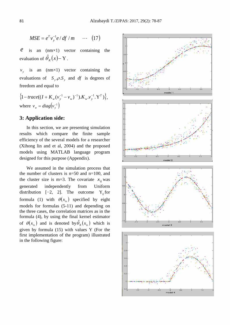
81 Alzubaydi T./ZJPAS: 2017, 29(2): 78-87

( )17//1 mdfeveMSE yT −=

e is an (nm×1) vector containing the

evaluation of ( ) Yˆ −xKθ .

yv is an (nm×1) vector containing the

evaluations of yy SS ..ρ and df is degrees of

freedom and equal to

{ })Y..).)(((1 111 Tywwyw vKvvKItrace −−− −+− ,

where ( )1−= yw vdiagv

3: Application side:

In this section, we are presenting simulation results which compare the finite sample efficiency of the several models for a researcher (Xihong lin and et al, 2004) and the proposed models using MATLAB language program designed for this purpose (Appendix).

We assumed in the simulation process that the number of clusters is n=50 and n=100, and the cluster size is m=3. The covariate ijx was generated independently from Uniform distribution [−2, 2]. The outcome ijY for formula (1) with ( )isxθ specified by eight models for formulas (5-11) and depending on the three cases, the correlation matrices as in the formula (4), by using the final kernel estimator of ( )isxθ and is denoted by ( )isK xθ which is given by formula (15) with values Y (For the first implementation of the program) illustrated in the following figure:

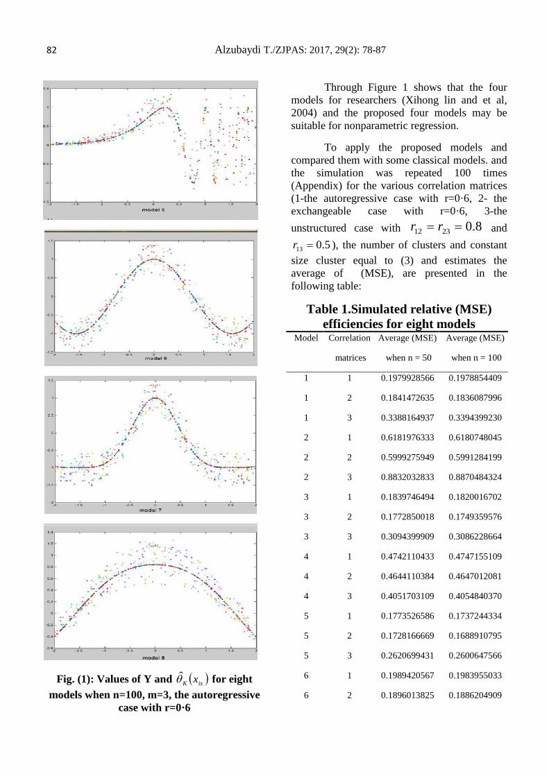
82 Alzubaydi T./ZJPAS: 2017, 29(2): 78-87

Fig. (1): Values of Y and ( )isK xθ for eight models when n=100, m=3, the autoregressive

case with r=0·6

Through Figure 1 shows that the four models for researchers (Xihong lin and et al, 2004) and the proposed four models may be suitable for nonparametric regression.

To apply the proposed models and compared them with some classical models. and the simulation was repeated 100 times (Appendix) for the various correlation matrices (1-the autoregressive case with r=0·6, 2- the exchangeable case with r=0·6, 3-the unstructured case with 8.02312 == rr and

5.013 =r ), the number of clusters and constant size cluster equal to (3) and estimates the average of (MSE), are presented in the following table:

Table 1.Simulated relative (MSE) efficiencies for eight models

Model Correlation

matrices

Average (MSE)

when n = 50

Average (MSE)

when n = 100

1 1 0.1979928566 0.1978854409

1 2 0.1841472635 0.1836087996

1 3 0.3388164937 0.3394399230

2 1 0.6181976333 0.6180748045

2 2 0.5999275949 0.5991284199

2 3 0.8832032833 0.8870484324

3 1 0.1839746494 0.1820016702

3 2 0.1772850018 0.1749359576

3 3 0.3094399909 0.3086228664

4 1 0.4742110433 0.4747155109

4 2 0.4644110384 0.4647012081

4 3 0.4051703109 0.4054840370

5 1 0.1773526586 0.1737244334

5 2 0.1728166669 0.1688910795

5 3 0.2620699431 0.2600647566

6 1 0.1989420567 0.1983955033

6 2 0.1896013825 0.1886204909

83 Alzubaydi T./ZJPAS: 2017, 29(2): 78-87

6 3 0.3503713517 0.3503368354

7 1 0.2317351071 0.2302940121

7 2 0.2211896886 0.2193551186

7 3 0.3984642780 0.3980704645

8 1 0.1497015227 0.1472124237

8 2 0.1413271547 0.1386288225

8 3 0.2412455434 0.2401688833

From table (1), we note that the best model is the eighth one of the proposed model and the matrix of the second correlation (the exchangeable case with r=0·6), because it has the least value of MSE which is equal to (0.1413271547 and 0.1386288225). The number of the clusters (n) by increasing it leads to a better model appropriate to the data for all models and cases. Correlation matrix of the second (the exchangeable case with r=0·6) is the best, followed by the first matrix (the autoregressive case with r=0·6) and finally the third matrix (the unstructured case with

8.02312 == rr and 5.013 =r ).

4: Conclusions and Recommendations:

Through this simulation study we reached to the following Conclusions and Recommendations.

4.1: Conclusions:

1. The four proposed models can be applicable in the nonparametric regression for cluster data.

2. The proposed eighth model had its preference in the appropriate cluster data with a correlation matrix (the exchangeable case with r=0·6), followed by (the autoregressive case with r=0·6).

3. Increasing the number of clusters leads to an increase in the estimation accuracy of nonparametric regression models.

4.2: Recommendations:

1. Applying the proposed models, especially the eighth model with correlation matrix (the exchangeable case with r=0·6).

2. Comparison of the proposed models between seemingly unrelated kernel estimator and spline method.

3. A comparison between the nonparametric regression and ridge regression with some transformations.

5: References: Green, P. J. & Silverman, B. W. (1994).

Nonparametric Regression and Generalized Linear Models: A Roughness Penalty Approach. London: Chapman and Hall.

Liang, K. Y. & Zeger, S. L. (1986). Longitudinal data analysis using generalized linear models. Biometrika 73, 13–22.

Lin, X. & Carroll, R. J. (2000). Nonparametric function estimation for clustered data when the predictor is measured without/with error. J. Am. Statist. Assoc. 95, 520–534.

Silverman, B. W. (1984). Spline smoothing: the equivalent variable kernel method. Ann. Statist. 12, 898–916.

Wang, N. (2003). Marginal nonparametric kernel regression ccounting for within-subject correlation. Biometrika 90, 43–52.

Wang, Y. (1998). Mixed effects smoothing spline analysis of variance. J. R. Statist. Soc. B 60, 159–174.

Welsh, A. H., Lin, X. & Carroll, R. J. (2002). Marginal longitudinal nonparametric regression: Locality and efficiency of spline and kernel methods. J. Am. Statist. Assoc. 97, 482–493.

Xihong Lin, Naisyin Wang, Alan H. Welsh and Raymond J. Carroll, (2004). Equivalent kernels of smoothing splines in nonparametric regression for clustered/longitudinal data. Biometrika 91,1, pp.177-193.

Zhang,D., Lin, X., Raz, J. & Sowers, M. (1998). Semiparametric stochastic mixed models for longitudinal data. J. Am. Statist. Assoc. 93, 710–699.

84 Alzubaydi T./ZJPAS: 2017, 29(2): 78-87

Appendix N=100

for L=1:N

n=100; model=1; cor=1; m=3; a=-2 ; b=2;ss=1;n1=n; switch cor

case 1

co=[1 .6 .6^2;.6 1 .6;.6^2 .6 1] ; case 2 co=[1 .6 .6;.6 1 .6;.6 .6 1]; case 3 co=[1 .8 .5;.8 1 .8;.5 .8 1]; end while n >= 1 x=unifrnd(a,b,1,m); sx=std(x'); h=(1.06)*m^(-.2)*sx; p=1; s=1; for i =1:m for j=1:m u(p) = (x(s,j)-x(i))/h; q(p) = (x(s,j)-x(i)); k(p)=((1/sqrt(2*pi))*exp(-u(p)^2/2))/h; p=p+1; end end k=k'; kdh=diag(k); x1=[ones(m^2,1) q' q'.^2]; switch model case 1 y=sin(x); case 2 y=exp(x); case 3 y=sin(2*x);

case 4 z=(x+2)/4; y=sqrt(z.*(1-z)).*sin(2*pi*(1+2^(-3/5))*(z+2^(-3/5)).^(-1)); case 5 y=sin(exp(2*x)); case 6 y=cos(2*x); case 7 y=cos(pi*sin(x)); case 8 y=sin(cos(x)); end sy=std(y'); v=diag(inv(sy*co*sy)); p=1; for i= 1:m for j=1:m v(p)=v(j); p=p+1; end end vw=diag(v); delta=[1 0 0]; kw=delta*(inv(x1'*kdh*vw*x1))*x1'*kdh; p=1; for i =1:m for j=1:m kw1(i,j)=kw(p); p=p+1; end end kw1; vy=sy*co*sy; vy=diag(vy); vy=diag(vy); vw1=inv(sy*co*sy); vw1=diag(vw1); vw1=diag(vw1);

85 Alzubaydi T./ZJPAS: 2017, 29(2): 78-87 theta=((eye(m)+kw1*(inv(vy)-vw1))^(-1))*kw1*inv(vy)*y'; df=1-trace(((eye(m)+kw1*(inv(vy)-vw1))^(-1))*kw1*inv(vy)); e=theta-y'; mse=e'*(inv(vy))*e/df/m; h1(ss)=mse; x11(ss,:)=x; theta=theta'; theta11(ss,:) =theta; ss=ss+1; n=n-1; end n=n1; h1; xc=x11; theta11; ss=1; while n > 1 h1; [ma no]=max(h1); h1(no)=[] ; x11(no,:)=[]; n=n-1; ss=1; for t=1:n; p=1; for i =1:m for j=1:m u(p) = (x11(t,j)-x11(t,i))/h1(t); q(p) = x11(t,j)-x11(t,i); k(p)=((1/sqrt(2*pi))*exp(-u(p)^2/2))/h1(t); p=p+1; end end k=k'; kdh=diag(k); x1=[ones(m^2,1) q' q'.^2 ]; switch model case 1 y=sin(x11(t,:)); case 2 y=exp(x11(t,:)); case 3 y=sin(2*x11(t,:)); case 4 z=(x11(t,:)+2)/4;

y=sqrt(z.*(1-z)).*sin(2*pi*(1+2^(-3/5))*(z+2^(-3/5)).^(-1)); case 5 y=sin(exp(2*x11(t,:))); case 6 y=cos(2*x11(t,:)); case 7 y=cos(pi*sin(x11(t,:))); case 8 y=sin(cos(x11(t,:))); end sy=std(y'); v=diag(inv(sy*co*sy)); p=1; for i= 1:m for j=1:m v(p)=v(j); p=p+1; end end vw=diag(v); delta=[1 0 0 ]; kw=delta*(inv(x1'*kdh*vw*x1))*x1'*kdh; p=1; for i =1:m for j=1:m kw1(i,j)=kw(p); p=p+1; end end kw1; vy=sy*co*sy; vy=diag(vy); vy=diag(vy); vw1=inv(sy*co*sy); vw1=diag(vw1); vw1=diag(vw1); theta=((eye(m)+kw1*(inv(vy)-vw1))^(-1))*kw1*inv(vy)*y';

86 Alzubaydi T./ZJPAS: 2017, 29(2): 78-87 df=1-trace(((eye(m)+kw1*(inv(vy)-vw1))^(-1))*kw1*inv(vy)); e=theta-y'; mse=e'*(inv(vy))*e/df/m; h1(ss)=mse; ss=ss+1; end end n=n1; xc; ss=1; while s <= n p=1; for i =1:m for j=1:m u(p) = (xc(s,j)-xc(s,i))/h1; q(p) = xc(s,j)-xc(s,i); k(p)=((1/sqrt(2*pi))*exp(-u(p)^2/2))/h1; p=p+1; end end k=k'; kdh=diag(k); x1=[ones(m^2,1) q' q'.^2 ]; switch model case 1 y=sin(xc(s,:)); case 2 y=exp(xc(s,:)); case 3 y=sin(2*xc(s,:)); case 4 z=(xc(s,:)+2)/4; y=sqrt(z.*(1-z)).*sin(2*pi*(1+2^(-3/5))*(z+2^(-3/5)).^(-1)); case 5

y=sin(exp(2*xc(s,:))); case 6 y=cos(2*xc(s,:)); case 7 y=cos(pi*sin(xc(s,:))); case 8 y=sin(cos(xc(s,:))); end sy=std(y'); v=diag(inv(sy*co*sy)); p=1; for i= 1:m for j=1:m v(p)=v(j); p=p+1; end end vw=diag(v); delta=[1 0 0]; kw=delta*(inv(x1'*kdh*vw*x1))*x1'*kdh; p=1; for i =1:m for j=1:m kw1(i,j)=kw(p); p=p+1; end end kw1; vy=sy*co*sy; vy=diag(vy); vy=diag(vy); vw1=inv(sy*co*sy); vw1=diag(vw1); vw1=diag(vw1); theta=((eye(m)+kw1*(inv(vy)-vw1))^(-1))*kw1*inv(vy)*y'; theta111(ss,:) =theta; ss=ss+1; s=s+1; end the=theta111*5; switch model case 1

87 Alzubaydi T./ZJPAS: 2017, 29(2): 78-87 y=sin(xc); case 2 y=exp(xc); case 3 y=sin(2*xc); case 4 z=(xc+2)/4; y=sqrt(z.*(1-z)).*sin(2*pi*(1+2^(-3/5))*(z+2^(-3/5)).^(-1)); case 5 y=sin(exp(2*xc)); case 6 y=cos(2*xc); case 7 y=cos(pi*sin(xc)); case 8 y=sin(cos(xc)); end MAE(L)=sum(sum(abs(the-y)))/(n*m); end MAE; AMAE=sum(MAE)/N plot(xc,y,'.',xc,the,'.');

ZANCO Journal of Pure and Applied Sciences The official scientific journal of Salahaddin University-Erbil

ZJPAS (2017), 29 (2); 88-95 http://dx.doi.org/10.21271/ZJPAS.29.2.9

Petroleum System Modeling of Jabal Kand Oil Field, Northern Iraq Rzger A. Abdula Department of petroleum Geosciences, Faculty of Science, Soran University, Soran, Kurdistan Region, Iraq

1. INTRODUCTION

The Jabal Kand-1 Well is located 30 km to the north of Mosul city (coordination latitude: 36º 39' 52.8'' and longitude: 43º 01' 36.8''). The ground level elevation is 398.4 m and Rotary Table Kelly Bushing (R.T.K.B.) elevation is 406 m. The well was drilled to the depth of 5848 m R.T.K.B. and penetrated Paleozoic Chia Zairi and Harur formations (North Oil Company, 1983). The Jabal Kand structure is 33 km long and 5 km wide (Jassim and Goff, 2006). This structure is a long, twisting structure with a minimum of three peaks on top of the Lower Fars (Fatha) Formation. The well is located on the middle dome (North Oil Company, 1983). The presence of structural complication features was not verified by any indicators from the Dipmeter, but a NW-SE axial trend migration of the axis to the NE direction during the Carboniferous-Upper Jurassic can be inferred. Additional structural

development and migration of the axis to the SW direction occurred during Lower Cretaceous-Miocene (North Oil Company, 1983). The well was completed in 1983 (Jassim and Goff, 2006). A petroleum system includes a mature source rock, reservoir rock, cap rock, and overburden rock. In addition, it includes the processes such as stratigraphic or structural trap formation and the generation-migration-accumulation of petroleum. In order for petroleum accumulation to be present, all required elements and processes should be within a specific time and place (Magoon and Dow, 1994). The study tries to determine the burial history, the thermal history, and the maturity history of the source rocks of the basin to reduce petroleum exploration risk. 2. MATERIALS AND METHODS The studied well was modeled using PetroMod 1-D modeling software (one of the

A R T I C L E I N F O

A B S T R A C T

Article History: Received: 06/06/2016 Accepted: 08/12/2016 Published: 07/06/2017

The petroleum system of Jabal Kand Oil Field shows that the formations such as Tertiary Kolosh, Cretaceous Shiranish, and Jurassic Sargelu are immature and have not generated any oil Ro< 0.55%. They are neglected as compared to formations below them which are also source rocks. The Kurra Chine Formation is mature with Ro> 0.55%. Other formations such as Gele Khana and other Triassic formations are with high maturity with Ro≥ 1.3% and are within wet and dry gas window while older formations are either within dry gas zone or completely generated hydrocarbon and depleted after hydrocarbon was expelled and migrated to reservoir rock of structure traps.

Keywords: PetroMode Hydrocarbon generation Jabal Kand Petroleum system Northern Iraq. *Corresponding Author: Rzger A. Abdula rzger.abdula@soran.edu.iq

89 Abdula R. /ZJPAS: 2017, 29 (2): 88-95 most famous commercial modeling software) developed by Integrated Exploration System GmbH. The 1-D burial history models are point locations, mainly wells. For chronostratigraphic divisions, the time scale of the Lexique Stratigraphique International (Bellen et al., 1959) and International Commission on Stratigraphy (2008) was used. The input data include thickness, lithology, heat flow and absolute ages for each formation and each episode. The 1-D model includes 23 formations from the base of the Lower Carboniferous Harur Formation to the Middle Miocene Lower Fars (Fatha) Formation and is based on the UTM Zone 38 (Northern Hemisphere) coordinate system using the WGS 84 datum. The stratigraphic units, their ages, and lithologies are shown in Table 1. The compositional mixtures or lithology characterized as end member rock types was assigned to the facies in each formation. The thermal conductivities and heat capacities with their thermal properties of different rock types are either user defined or software default values. The Tmax values and their mathematically determined Ro% equivalent, obtained by Rock-Eval pyrolysis, were used for calibration. 3. RESULTS AND DISCUSSIONS Basin modeling combines several geological parameters to assess the formation and evolution of sedimentary basins to help evaluation of prospective hydrocarbon reserves. The scale of the model ranges in size from a single well to a whole basin. 3.1. Burial History and Thermal Maturation Modeling Burial history, thermal maturity, and timing of petroleum generation were modeled for several key source-rock horizons at Jabal Kand-1. The formations from the oldest to youngest are the Harur, Chia Zairi, Mirga Mir,

Beduh, Gele Khana, Kurra Chine, Baluti, Butmah, Adaiyah, Mus, Alan, Sargelu, Gotnia, Garagu, Sarmord, Qamchuqa, Aqra, Shiranish, Kolosh, Khurmala, Gercus, Pila Spi, Lower Fars (Fatha) formations (Fig. 1). The results of the model indicate that peak petroleum generation from the Paleozoic Harur Formation oil- and gas-prone source rock in the deepest parts of the basin occurred and the accumulation and preservation happened from Mid Triassic (Fig. 2). The Jurassic Sargelu Formation is supposed to be more mature than it is but the absence of Upper Jurassic Najmah and Chia Gara formations and comparatively low thickness of overburden rocks (2107 m) have not contributed to increase the temperature to cook Sargelu. The Mid Sargelu Formation oil and gas-prone source rock not entered the oil window in the Miocene and it is still not within the oil window at the present time (Fig. 2). The Cretaceous source rock has no significance in the study area because of tectonic activity (obduction) and non-deposition of Oligocene-Lower Miocene and erosion of Upper Miocene-Pleistocene sediments. Also the relatively reduced thickness of the Middle Miocene sediments (some hundred meters) and the erosion or non-deposition of Lower Bakhtiary, Upper Bakhtiary, and Alluvial during Pliocene-Pleistocene time seems to be relevant for hydrocarbon maturity (Fig. 3). 3.2. Temperature and Heat Flow Analysis The goal of heat-flow analysis is temperature calculation, a prerequisite for determining geochemical reaction rates. The provided bottom hole temperature data from well logs and final geologic reports for Jabal Kand-1 Well (Fig. 4) were used to estimate the present heat flow in Mosul area.

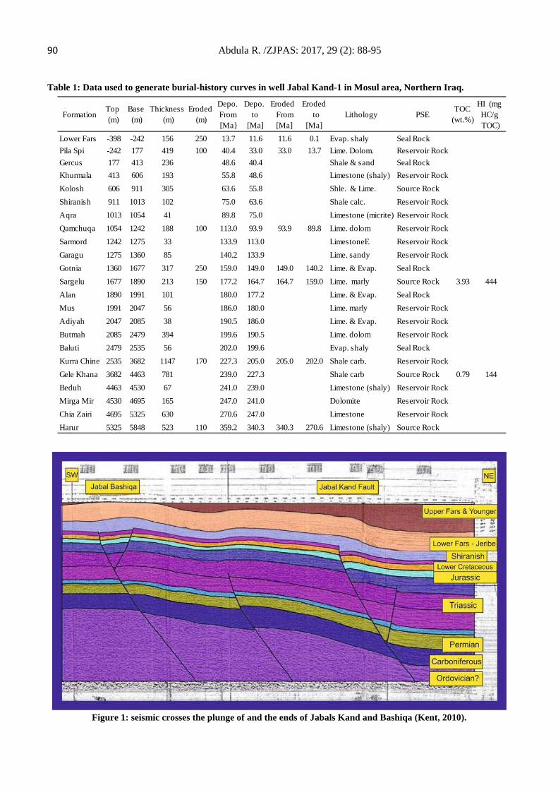
90 Abdula R. /ZJPAS: 2017, 29 (2): 88-95 Table 1: Data used to generate burial-history curves in well Jabal Kand-1 in Mosul area, Northern Iraq.

FormationTop (m)

Base (m)

Thickness (m)

Eroded (m)

Depo. From [Ma}

Depo. to

[Ma]

Eroded From [Ma]

Eroded to [Ma]

Lithology PSETOC

(wt.%)

HI (mg HC/g TOC)

Lower Fars -398 -242 156 250 13.7 11.6 11.6 0.1 Evap. shaly Seal RockPila Spi -242 177 419 100 40.4 33.0 33.0 13.7 Lime. Dolom. Reservoir RockGercus 177 413 236 48.6 40.4 Shale & sand Seal RockKhurmala 413 606 193 55.8 48.6 Limestone (shaly) Reservoir RockKolosh 606 911 305 63.6 55.8 Shle. & Lime. Source RockShiranish 911 1013 102 75.0 63.6 Shale calc. Reservoir RockAqra 1013 1054 41 89.8 75.0 Limestone (micrite) Reservoir RockQamchuqa 1054 1242 188 100 113.0 93.9 93.9 89.8 Lime. dolom Reservoir RockSarmord 1242 1275 33 133.9 113.0 LimestoneE Reservoir RockGaragu 1275 1360 85 140.2 133.9 Lime. sandy Reservoir RockGotnia 1360 1677 317 250 159.0 149.0 149.0 140.2 Lime. & Evap. Seal RockSargelu 1677 1890 213 150 177.2 164.7 164.7 159.0 Lime. marly Source Rock 3.93 444Alan 1890 1991 101 180.0 177.2 Lime. & Evap. Seal RockMus 1991 2047 56 186.0 180.0 Lime. marly Reservoir RockAdiyah 2047 2085 38 190.5 186.0 Lime. & Evap. Reservoir RockButmah 2085 2479 394 199.6 190.5 Lime. dolom Reservoir RockBaluti 2479 2535 56 202.0 199.6 Evap. shaly Seal RockKurra Chine 2535 3682 1147 170 227.3 205.0 205.0 202.0 Shale carb. Reservoir RockGele Khana 3682 4463 781 239.0 227.3 Shale carb Source Rock 0.79 144Beduh 4463 4530 67 241.0 239.0 Limestone (shaly) Reservoir RockMirga Mir 4530 4695 165 247.0 241.0 Dolomite Reservoir RockChia Zairi 4695 5325 630 270.6 247.0 Limestone Reservoir RockHarur 5325 5848 523 110 359.2 340.3 340.3 270.6 Limestone (shaly) Source Rock

Figure 1: seismic crosses the plunge of and the ends of Jabals Kand and Bashiqa (Kent, 2010).

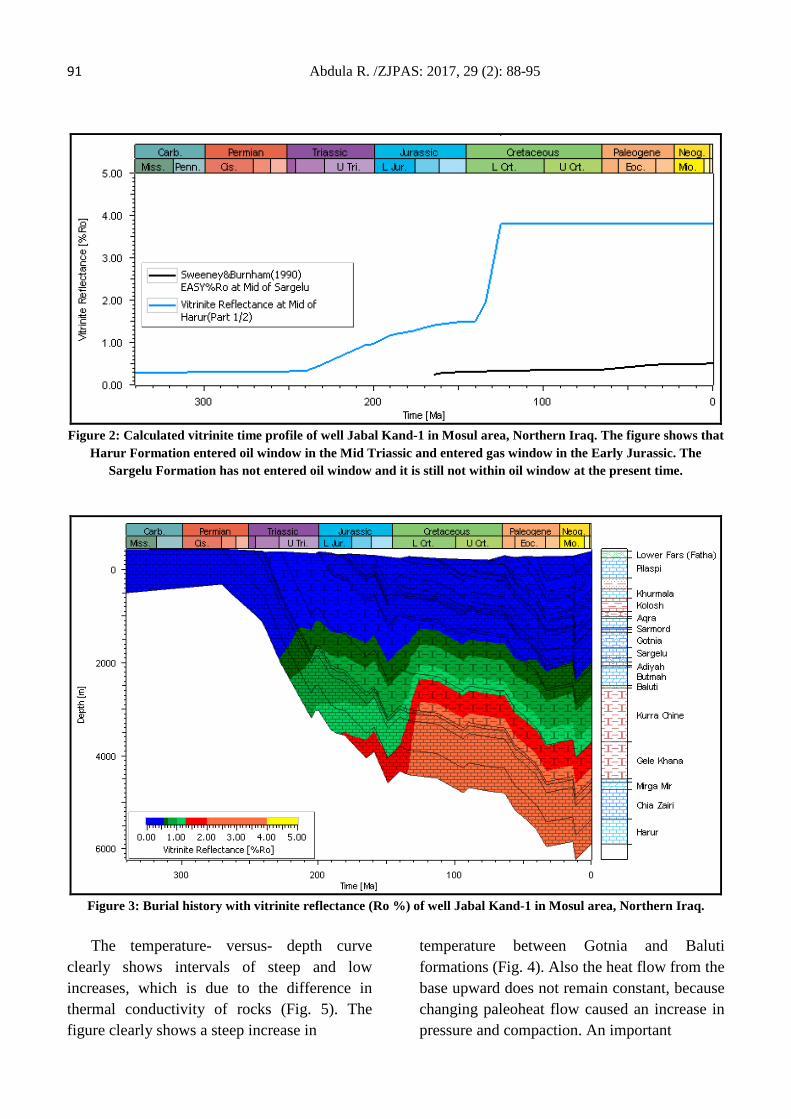
91 Abdula R. /ZJPAS: 2017, 29 (2): 88-95

Figure 2: Calculated vitrinite time profile of well Jabal Kand-1 in Mosul area, Northern Iraq. The figure shows that Harur Formation entered oil window in the Mid Triassic and entered gas window in the Early Jurassic. The

Sargelu Formation has not entered oil window and it is still not within oil window at the present time.

Figure 3: Burial history with vitrinite reflectance (Ro %) of well Jabal Kand-1 in Mosul area, Northern Iraq. The temperature- versus- depth curve clearly shows intervals of steep and low increases, which is due to the difference in thermal conductivity of rocks (Fig. 5). The figure clearly shows a steep increase in

temperature between Gotnia and Baluti formations (Fig. 4). Also the heat flow from the base upward does not remain constant, because changing paleoheat flow caused an increase in pressure and compaction. An important

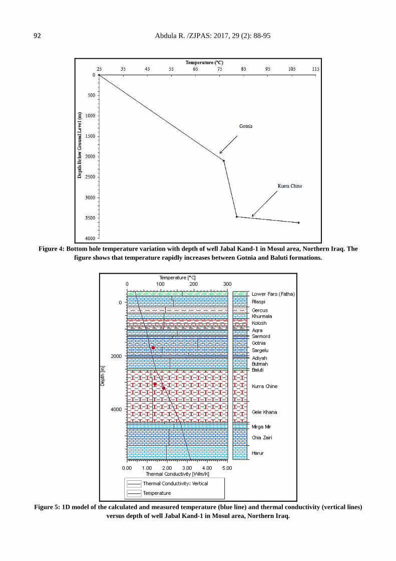
92 Abdula R. /ZJPAS: 2017, 29 (2): 88-95

Figure 4: Bottom hole temperature variation with depth of well Jabal Kand-1 in Mosul area, Northern Iraq. The figure shows that temperature rapidly increases between Gotnia and Baluti formations.

Figure 5: 1D model of the calculated and measured temperature (blue line) and thermal conductivity (vertical lines)

versus depth of well Jabal Kand-1 in Mosul area, Northern Iraq.

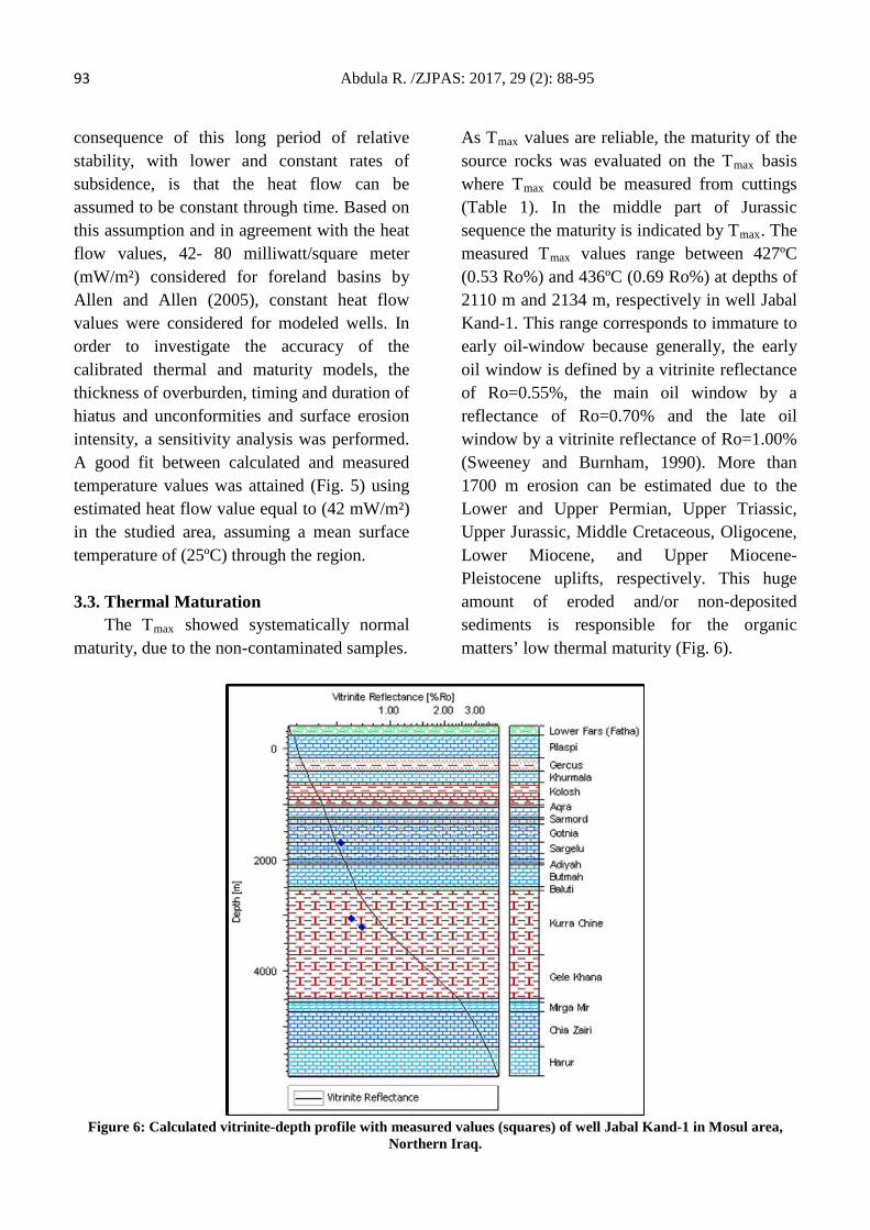
93 Abdula R. /ZJPAS: 2017, 29 (2): 88-95 consequence of this long period of relative stability, with lower and constant rates of subsidence, is that the heat flow can be assumed to be constant through time. Based on this assumption and in agreement with the heat flow values, 42- 80 milliwatt/square meter (mW/m²) considered for foreland basins by Allen and Allen (2005), constant heat flow values were considered for modeled wells. In order to investigate the accuracy of the calibrated thermal and maturity models, the thickness of overburden, timing and duration of hiatus and unconformities and surface erosion intensity, a sensitivity analysis was performed. A good fit between calculated and measured temperature values was attained (Fig. 5) using estimated heat flow value equal to (42 mW/m²) in the studied area, assuming a mean surface temperature of (25ºC) through the region. 3.3. Thermal Maturation The Tmax showed systematically normal maturity, due to the non-contaminated samples.

As Tmax values are reliable, the maturity of the source rocks was evaluated on the Tmax basis where Tmax could be measured from cuttings (Table 1). In the middle part of Jurassic sequence the maturity is indicated by Tmax. The measured Tmax values range between 427ºC (0.53 Ro%) and 436ºC (0.69 Ro%) at depths of 2110 m and 2134 m, respectively in well Jabal Kand-1. This range corresponds to immature to early oil-window because generally, the early oil window is defined by a vitrinite reflectance of Ro=0.55%, the main oil window by a reflectance of Ro=0.70% and the late oil window by a vitrinite reflectance of Ro=1.00% (Sweeney and Burnham, 1990). More than 1700 m erosion can be estimated due to the Lower and Upper Permian, Upper Triassic, Upper Jurassic, Middle Cretaceous, Oligocene, Lower Miocene, and Upper Miocene-Pleistocene uplifts, respectively. This huge amount of eroded and/or non-deposited sediments is responsible for the organic matters’ low thermal maturity (Fig. 6).

Figure 6: Calculated vitrinite-depth profile with measured values (squares) of well Jabal Kand-1 in Mosul area,

Northern Iraq.

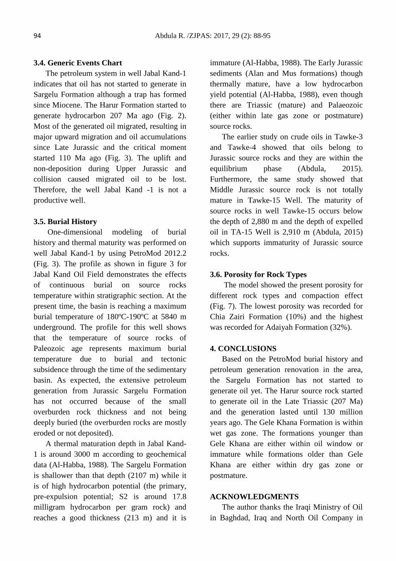
94 Abdula R. /ZJPAS: 2017, 29 (2): 88-95 3.4. Generic Events Chart The petroleum system in well Jabal Kand-1 indicates that oil has not started to generate in Sargelu Formation although a trap has formed since Miocene. The Harur Formation started to generate hydrocarbon 207 Ma ago (Fig. 2). Most of the generated oil migrated, resulting in major upward migration and oil accumulations since Late Jurassic and the critical moment started 110 Ma ago (Fig. 3). The uplift and non-deposition during Upper Jurassic and collision caused migrated oil to be lost. Therefore, the well Jabal Kand -1 is not a productive well. 3.5. Burial History One-dimensional modeling of burial history and thermal maturity was performed on well Jabal Kand-1 by using PetroMod 2012.2 (Fig. 3). The profile as shown in figure 3 for Jabal Kand Oil Field demonstrates the effects of continuous burial on source rocks temperature within stratigraphic section. At the present time, the basin is reaching a maximum burial temperature of 180ºC-190ºC at 5840 m underground. The profile for this well shows that the temperature of source rocks of Paleozoic age represents maximum burial temperature due to burial and tectonic subsidence through the time of the sedimentary basin. As expected, the extensive petroleum generation from Jurassic Sargelu Formation has not occurred because of the small overburden rock thickness and not being deeply buried (the overburden rocks are mostly eroded or not deposited). A thermal maturation depth in Jabal Kand-1 is around 3000 m according to geochemical data (Al-Habba, 1988). The Sargelu Formation is shallower than that depth (2107 m) while it is of high hydrocarbon potential (the primary, pre-expulsion potential; S2 is around 17.8 milligram hydrocarbon per gram rock) and reaches a good thickness (213 m) and it is

immature (Al-Habba, 1988). The Early Jurassic sediments (Alan and Mus formations) though thermally mature, have a low hydrocarbon yield potential (Al-Habba, 1988), even though there are Triassic (mature) and Palaeozoic (either within late gas zone or postmature) source rocks. The earlier study on crude oils in Tawke-3 and Tawke-4 showed that oils belong to Jurassic source rocks and they are within the equilibrium phase (Abdula, 2015). Furthermore, the same study showed that Middle Jurassic source rock is not totally mature in Tawke-15 Well. The maturity of source rocks in well Tawke-15 occurs below the depth of 2,880 m and the depth of expelled oil in TA-15 Well is 2,910 m (Abdula, 2015) which supports immaturity of Jurassic source rocks. 3.6. Porosity for Rock Types The model showed the present porosity for different rock types and compaction effect (Fig. 7). The lowest porosity was recorded for Chia Zairi Formation (10%) and the highest was recorded for Adaiyah Formation (32%). 4. CONCLUSIONS Based on the PetroMod burial history and petroleum generation renovation in the area, the Sargelu Formation has not started to generate oil yet. The Harur source rock started to generate oil in the Late Triassic (207 Ma) and the generation lasted until 130 million years ago. The Gele Khana Formation is within wet gas zone. The formations younger than Gele Khana are either within oil window or immature while formations older than Gele Khana are either within dry gas zone or postmature. ACKNOWLEDGMENTS The author thanks the Iraqi Ministry of Oil in Baghdad, Iraq and North Oil Company in

95 Abdula R. /ZJPAS: 2017, 29 (2): 88-95 Kirkuk, Iraq for their generous help by providing necessary information and cutting

samples.

Figure 7: Calculated porosity depth profile for different rock types of well Jabal Kand-1 in Mosul area, Northern

Iraq.

REFERENCES Abdula, R. (2015) ‘Hydrocarbon potential of Sargelu

Formation and oil-source correlation, Iraqi Kurdistan’, Arabian Journal of Geosciences, 8(8), pp. 5845–5868.

Al-Habba, Y.K. (1988) Possible petroleum source rocks in the well Kand-1. Baghdad: Oil Exploration Company Archives. Unpublished report in Arabic

Allen, P.A. and Allen, J.R. (2005) Basin analysis. second edn. Blackwell Publishing. Bellen, R.C. van, Dunnington, H.V., Wetzel, R. and

Morton, D.M. (1959) Lexique stratigraphic international. (Fascicule 10 a Vols). Paris: CNRS and Congres Geologique international, Commision de Stratigraphie.

International Commission on Stratigraphy (2008) A concise geologic timescale. Edited by J. G. Ogg, G. Ogg, and F. M. Gradstein. Cambridge University Press.

Jassim, S.Z. (2006) Geology of Iraq. Edited by J. C.

Goff. Brno: Dolin, Prague and Moravian Museum.

Kent, W.N. (2010, April). Structures of northern Iraq and Syria, and their implications for interpretation of the region’s stratigraphy. New Orleans, Louisiana. doi:Search and Discovery Article # 40623 (2010)

Magoon, L.B. and Dow, W.G. (1994) The petroleum system - From source to trap. (60 Vols). American Association of Petroleum Geologists.

North Oil Company (1983). Final well report of Jabal Kand-1. Kirkuk: Iraqi Ministry of Oil in Baghdad.

Sweeney, J.J. and Burnham, A.K. (1990) ‘Evaluation of a simple model of vitrinite reflectance based on chemical kinetics’, American Association of Petroleum Geologists, 74(10), pp. 1559–1570.

ZANCO Journal of Pure and Applied Sciences The official scientific journal of Salahaddin University-Erbil

ZJPAS (2017), 29 (2); 96-105 http://dx.doi.org/10.21271/ZJPAS.29.2.10

Theoretical, Numerical, and Experimental Analysis of Composite Double-Cracked Cantilever Beams with Various Fibers Volume Fraction and Angles

Nazhad A. Hussein1 Sardar S. Abdullah 2 1,2Department of Mechanics, College of Engineering,Salahaddin University-Erbil

INTRODUCTION

Vibration is one of the most important aspects of dynamic which is difficult and vital to analyze during designing of mechanical members and machine parts, because the stiffness and damping properties of most vibrating parts lead to behave non-linear and will change but usually vibrating parts are assumed to behave linearly. Mechanical parts may expose to some defects such as flows, cracks due to having motion during operations. As the result of these defects, the parts may lead to break down and fail. Cracks in vibrating parts can reduce natural frequencies of the vibrating system resulting in large amplitudes of vibration causing failure of the structure. K.Nikpur and A.Dimarogonas [1986] presented a paper to investigate the effect of the crack on

a vibrating beam and plate which are made of graphite-fiber reinforced polyimide. They also developed a new method to calculate the additional flexibility induced by the crack. It has been shown that when the angle of fibers is 45 degrees, the crack surfaces intercept the material principle planes. M.Krawczuk and W.M.Ostachowicz [1991] presented a paper which analyzed the effects of the cracks on the natural frequencies of a cantilever beam. They presented a method to analyze the effect of two open cracks on the vibration of the beam. They considered two types of cracks in which one of them was a double-sided crack and another was a single-sided crack. It was assumed that the cracks have occurred in the first mode of fracture. They found out that the position of the cracks in relation to each other can have a great role in changing the natural frequencies if both

A R T I C L E I N F O

A B S T R A C T

Article History: Received: 31/07/2016 Accepted: 10/12/2016 Published:07/06/2017

Crack changes the dynamic characteristics of the vibrating body such as the natural frequencies and stiffness of the system. Now a day many researchers are studying on the cracks in the structures made of composite material because are being used more than past due to their great mechanical properties such as their high strength to weight ratio. This study presents theoretical, numerical (FEM), and experimental analysis of a cantilever composite beam with double transverse crack. Carbon fiber- Epoxy has been taken as the material for this study. Several factors play grate and important rules in vibration response and natural frequencies of the cracked composite beams. This work presents dynamic responses of double-cracked composite beams at different fiber volume fraction and angles. The numerical results were found in good agreement with experimental and analytical results. The study concludes that the existence of double crack in composite structure with different fiber volume fraction and angles can be diagnosed by using vibration signatures, and it useful for monitoring the health of the composite structures.

Keywords: FEM, Dynamic Analysis, Crack, Composite Beams, Natural Frequency

*Corresponding Author: Email: nazhad6@gmail.com

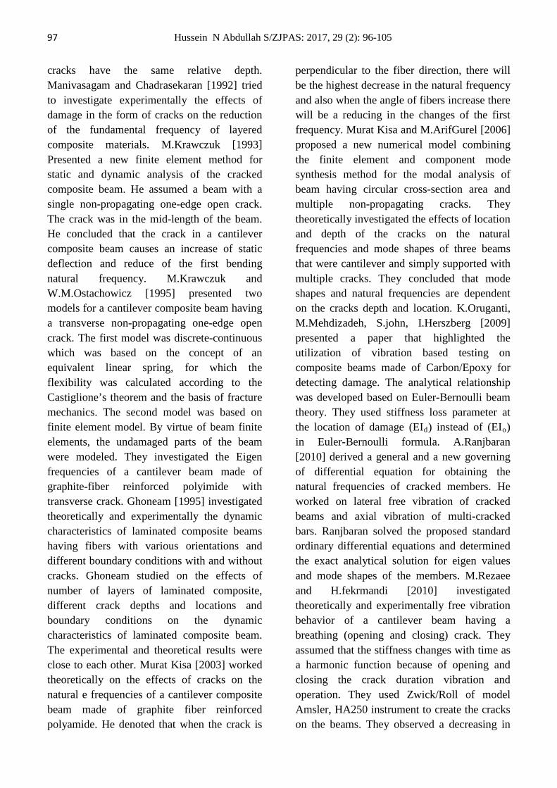
97 Hussein N Abdullah S/ZJPAS: 2017, 29 (2): 96-105

cracks have the same relative depth. Manivasagam and Chadrasekaran [1992] tried to investigate experimentally the effects of damage in the form of cracks on the reduction of the fundamental frequency of layered composite materials. M.Krawczuk [1993] Presented a new finite element method for static and dynamic analysis of the cracked composite beam. He assumed a beam with a single non-propagating one-edge open crack. The crack was in the mid-length of the beam. He concluded that the crack in a cantilever composite beam causes an increase of static deflection and reduce of the first bending natural frequency. M.Krawczuk and W.M.Ostachowicz [1995] presented two models for a cantilever composite beam having a transverse non-propagating one-edge open crack. The first model was discrete-continuous which was based on the concept of an equivalent linear spring, for which the flexibility was calculated according to the Castiglione’s theorem and the basis of fracture mechanics. The second model was based on finite element model. By virtue of beam finite elements, the undamaged parts of the beam were modeled. They investigated the Eigen frequencies of a cantilever beam made of graphite-fiber reinforced polyimide with transverse crack. Ghoneam [1995] investigated theoretically and experimentally the dynamic characteristics of laminated composite beams having fibers with various orientations and different boundary conditions with and without cracks. Ghoneam studied on the effects of number of layers of laminated composite, different crack depths and locations and boundary conditions on the dynamic characteristics of laminated composite beam. The experimental and theoretical results were close to each other. Murat Kisa [2003] worked theoretically on the effects of cracks on the natural e frequencies of a cantilever composite beam made of graphite fiber reinforced polyamide. He denoted that when the crack is

perpendicular to the fiber direction, there will be the highest decrease in the natural frequency and also when the angle of fibers increase there will be a reducing in the changes of the first frequency. Murat Kisa and M.ArifGurel [2006] proposed a new numerical model combining the finite element and component mode synthesis method for the modal analysis of beam having circular cross-section area and multiple non-propagating cracks. They theoretically investigated the effects of location and depth of the cracks on the natural frequencies and mode shapes of three beams that were cantilever and simply supported with multiple cracks. They concluded that mode shapes and natural frequencies are dependent on the cracks depth and location. K.Oruganti, M.Mehdizadeh, S.john, I.Herszberg [2009] presented a paper that highlighted the utilization of vibration based testing on composite beams made of Carbon/Epoxy for detecting damage. The analytical relationship was developed based on Euler-Bernoulli beam theory. They used stiffness loss parameter at the location of damage (EId) instead of (EIo) in Euler-Bernoulli formula. A.Ranjbaran [2010] derived a general and a new governing of differential equation for obtaining the natural frequencies of cracked members. He worked on lateral free vibration of cracked beams and axial vibration of multi-cracked bars. Ranjbaran solved the proposed standard ordinary differential equations and determined the exact analytical solution for eigen values and mode shapes of the members. M.Rezaee and H.fekrmandi [2010] investigated theoretically and experimentally free vibration behavior of a cantilever beam having a breathing (opening and closing) crack. They assumed that the stiffness changes with time as a harmonic function because of opening and closing the crack duration vibration and operation. They used Zwick/Roll of model Amsler, HA250 instrument to create the cracks on the beams. They observed a decreasing in

98 Hussein N Abdullah S/ZJPAS: 2017, 29 (2): 96-105

the natural frequencies and having larger amplitudes due to the cracks. PragyanSaraswatiBisi [2011] investigated vibration and buckling analysis of cracked composite beam. The main aim of his working was to work out a composite beam finite element with a non-propagating one-edge open crack. He wanted to analyze the effects of cracks on a cantilever composite beam and also the influence of the volume of fibers, magnitude and location of the crack and angle of fibers on the natural frequencies of the cracked composite beam. Bisi concluded that natural frequencies are not only functions of crack location and crack depths but also they are functions of fiber volume and fiber angels. Pankaj Ch.Jena, dayal R.P Goutam P. [2012] worked out fault detection in a beam consisting of a single transverse crack. Theoretical and Experimental analysis were done to identify the location and the depth of the crack in the beam with single transverse crack. A few more flexibility produced due to the presence of the crack examined by applying the strain energy

function.

VIBRATION ANALYSIS OF COMPOSITE CRACKEDBEAM

The equations are governed for vibration analysis of non-cracked composite beam. For the case of cracked beam, additional flexibility matrix is added to the flexibility of non-cracked beam to obtain the total flexibility and consequently the total stiffness matrix of the cracked composite beam.

Fourth –order differential equation

(1)

= f(x) (2)

Where b =

The natural frequencies of beams for various boundary conditions in radian/unit time are given as:

(3)

Figure (1) shows the chosen model which is a cantilever composite beam having a uniform cross-section area (A) and also having several open edge transverse cracks with different depths at different distancesfrom the fixed side. Dimensions of the beam are defined by the length (L), height (H) and width (B). The angle by which the fibers are arranged or angle between the fibers and axis of the beam is’ α ‘as shown in the figure (1).

Fig. A Cracked Beam Scheme

[N] Matrix is used to obtain the warping displacement.

[N] * (4)

Here [N] is a matrix which is called shape function matrix.

We use boundary conditions to obtain N matrix as:

(5)

(6)

99 Hussein N Abdullah S/ZJPAS: 2017, 29 (2): 96-105

(7)

(8)

(9)

(10)

Where q, and both are representing the displacements (transverse and rotational displacements).

Now the shape of above equations must be changed into a new matrix as:

= = *

(11)

Matrix) will be obtained by taking the inverse of the middle matrix.

To obtain (shape function matrix), is used and by rearranging the formulas finally it will be:

(12)

By taking the same fashion we can obtain linear corresponding strains as:

=

(13)

Where is a matrix, which is called strain nodal displacements relation matrix.

Mass matrix for both cracked and non-cracked beam is assumed to be the same so only mass matrix is derived once and is used for both cases of cracked and non-cracked because it is assumed that the crack does not change the mass of the beam.

(14)

Where (i,j=1,2,3,4,5,6)

Mass matrix elements are as following:

,

,

,

,

,

100 Hussein N Abdullah S/ZJPAS: 2017, 29 (2): 96-105

Where ρ is the density of mass of the element and Le is the length of the element.

Stiffness matrix for each element of non- cracked beam element with three nodes and two degree of freedom for each of the nodes with ∂={w,θ} is obtained by following formulas where ∂ is displacement vector.

(15)

Where (i,j=1,2,3,4,5,6)

Then, the elements of the stiffness matrix for non-cracked element will be as following:

,

,

,

,

,

,

,

,

Where Le, B, H are dimensions of the beam element and and are the stress-strain

constants and will be given in Appendix A. Crack influences on the beam and results in an additional strain energy. The best way to find cracked composite beam element stiffness matrix is to calculate the total flexibility matrix and then obtain its inverse. Due to crack, there will be two parts for the total flexibility matrix. The first part is original flexibility matrix for non-cracked composite beam, and the second part is the additional flexibility matrix created by the crack leading to energy release, additional deformation, and lower stiffness of the vibrating system or structure.

In the region close to the crack the stress field is affected by the crack. Crack causes an additional strain energy which includes flexibility coefficients expressed by stress intensity factors obtained and derived by Castiglione’s theorem. From the strain energy release rate, the compliance coefficients of the flexibility matrix can be obtained.

The strain energy of the cracked beam is obtained by following relation:

U= +

+ (16)

+ + (17)

Where =the strain energy release rate

A= Area of the crack section

are stress intensity factors for fracture modes of opening and sliding crack types and crack evaluation models, and are coefficients and can be obtained by following formulas:

) ,

,

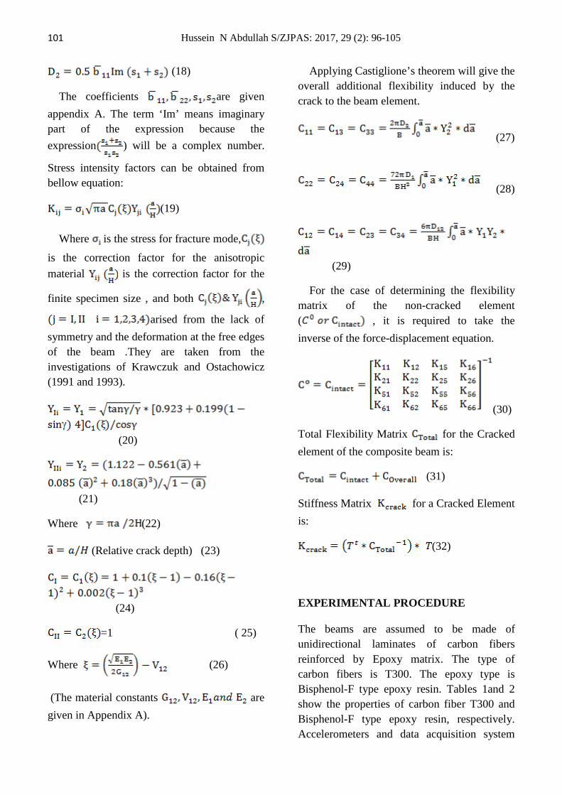
101 Hussein N Abdullah S/ZJPAS: 2017, 29 (2): 96-105

(18)

The coefficients are given appendix A. The term ‘Im’ means imaginary part of the expression because the expression ) will be a complex number.

Stress intensity factors can be obtained from bellow equation:

(19)

Where is the stress for fracture mode,

is the correction factor for the anisotropic material is the correction factor for the

finite specimen size , and both ,

arised from the lack of symmetry and the deformation at the free edges of the beam .They are taken from the investigations of Krawczuk and Ostachowicz (1991 and 1993).

(20)

(21)

Where (22)

(Relative crack depth) (23)

(24)

=1 ( 25)

Where (26)

(The material constants are given in Appendix A).

Applying Castiglione’s theorem will give the overall additional flexibility induced by the crack to the beam element.

(27)

(28)

(29)

For the case of determining the flexibility matrix of the non-cracked element ( , it is required to take the inverse of the force-displacement equation.

(30)

Total Flexibility Matrix for the Cracked element of the composite beam is:

(31)

Stiffness Matrix for a Cracked Element is:

(32)

EXPERIMENTAL PROCEDURE

The beams are assumed to be made of unidirectional laminates of carbon fibers reinforced by Epoxy matrix. The type of carbon fibers is T300. The epoxy type is Bisphenol-F type epoxy resin. Tables 1and 2 show the properties of carbon fiber T300 and Bisphenol-F type epoxy resin, respectively. Accelerometers and data acquisition system

102 Hussein N Abdullah S/ZJPAS: 2017, 29 (2): 96-105

(type B&K frame 3560) were used to record and analyze. Figure (2) will show a double cracked beam ready to test and figure (3) shows the vibration testing components.

Table1 Elastic Properties of Carbon Fiber (T300)

Properties Value

Modulus of Elasticity in longitudinal direction

Ef1 230 GPa

Modulus of Elasticity in transverse direction

Ef2 13.9 GPa

Modulus of Rigidity in longitudinal direction

Gf1 12.5 GPa

Poisson Ratio in (1-2) plane νf12 0.2

Poisson Ratio in (2-3) plane νf23 0.25

Mass Density ρf 1760 kg/m3

Table2 Elastic Properties of Matrix (Bisphenol F type)

Properties Value

Modulus of Elasticity Em 2.9 GPa

Modulus of Rigidity Gm 1.23 GPa

Poisson Ratio νm 0.43

Mass Density ρm 1160 kg/m3

Fig.2.A double cracked beam

Fig. 3. Experimental Measurement Scheme

RESULTS AND DISCUSSION

The first three natural frequencies of the composite beams with various fiber angles and volume fraction of fibers are determined and the results are presented for all specimens. Theoretical, numerical (FEM), experimental methods are used to determine the natural frequencies of the double-cracked composite beams. Finite element analysis ANSYS was used to extract the natural frequencies and results compared with experimental and analytical methods. Tables 3,4, and 5 show the results obtained from analytical method, ANSYS program, and experimental study, respectively. The results of all methods were satisfactory and showed a good agreement. The effect of fiber angles for different fraction volume are shown in the figures 4,5, and 6. As the fiber angle increased the stiffness and natural frequencies decreased while the flexibility of the beam will be increased. It is observed that the slope of the curve is more significant between 15o and 75o of fiber angles and indicating a steep fall in frequency. There is no significant effect on the natural frequency for the fiber angle lower than 15o and higher than75o. The highest natural frequency is obtained when fiber angle is zero and on the contrary the lowest natural frequency is obtained when the fibers are arranged with angle 90º. The results showed the high drop in natural frequency is when the fiber volume fraction changed from the 53% to 40% and the fiber angle was below the 75o. The beams are stronger and stiffer, if the angle between the fibers and longitudinal axis of the beam is lower. Table 3 First three natural frequencies obtained by theoretical method for Double cracked beams (a/H= 0.4 at L/8, & a/H= 0.4 at 3L/8).

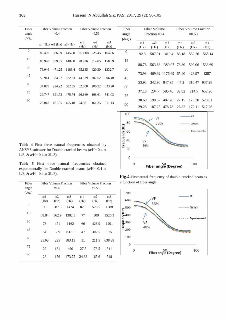
103 Hussein N Abdullah S/ZJPAS: 2017, 29 (2): 96-105

Table 4 First three natural frequencies obtained by ANSYS software for Double cracked beams (a/H= 0.4 at L/8, & a/H= 0.4 at 3L/8).

Table 5 First three natural frequencies obtained experimentally for Double cracked beams (a/H= 0.4 at L/8, & a/H= 0.4 at 3L/8).

Fig.4.Firstnatural frequency of double-cracked beam as a function of fiber angle.

Fiber Volume Fraction =0.53

Fiber Volume Fraction =0.4

Fiber angle (deg.)

ω3 (Hz)

ω2 (Hz)

ω1 (Hz)

ω3 (Hz)

ω2 (Hz)

ω1 (Hz)

1565.14 532.26 83.18 1419.4 587.91 92.3 0

1533.69

509.06

78.80

1389.07

563.68

88.76

15

1287

423.97

65.40

1176.69

469.92

73.98

30

937.28

310.47

47.2

847.95

342.90

53.93

45

652.26

214.5

32.82

595.46

234.7

37.18

60

528.61

175.20

27.15

487.26

190.57

30.60

75

517.26 172.11 26.82 478.78 187.25 29.28 90

Fiber Volume Fraction

=0.53 Fiber Volume Fraction

=0.4

Fiber angle (deg.)

ω3 (Hz)

ω2 (Hz)

ω1 (Hz) ω3 (Hz) ω2 (Hz) ω1 (Hz)

1642.6 525.45 82.3808 1452.8 586.09 89.407 0

1580.9 514.05 78.936 1402.0 559.65 85.940 15

1332.7 420.30 65.135 1188.4 471.25 73.046 30

906.40 302.52 44.579 872.83 324.27 50.941 45

633.20 206.32 32.088 582.55 224.22 34.879 60

541.03 168.61 26.160 475.74 191.73 29.747 75

511.13 161.25 24.981 455.18 181.05 28.042 90

Fiber Volume Fraction =0.53

Fiber Volume Fraction =0.4

Fiber angle (deg.)

ω3 (Hz)

ω2 (Hz)

ω1 (Hz)

ω3 (Hz)

ω2 (Hz)

ω1 (Hz)

1588 523.5 82.5 1424 587.5 90 0

1526.3 500 77 1382.5 562.9 88.84 15

1291 426.9 66 1162 471 73 30

925 302.5 47 837.5 339 54 45

638.88 211.5 31 583.13 225 35.63 60

541 173.5 27.5 490 181 29 75

518 165.6 24.88 473.75 176 28 90

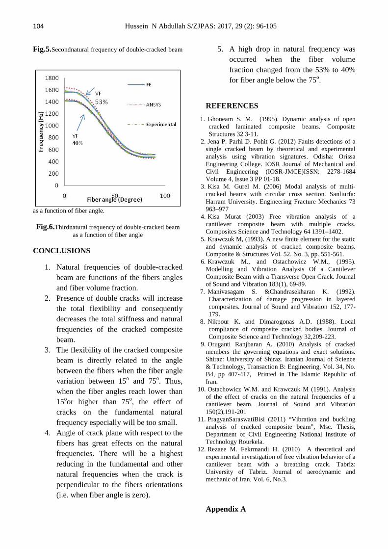
104 Hussein N Abdullah S/ZJPAS: 2017, 29 (2): 96-105

Fig.5.Secondnatural frequency of double-cracked beam

as a function of fiber angle.

Fig.6.Thirdnatural frequency of double-cracked beam as a function of fiber angle

CONCLUSIONS

1. Natural frequencies of double-cracked

beam are functions of the fibers angles and fiber volume fraction.

2. Presence of double cracks will increase the total flexibility and consequently decreases the total stiffness and natural frequencies of the cracked composite beam.

3. The flexibility of the cracked composite beam is directly related to the angle between the fibers when the fiber angle variation between 15o and 75o. Thus, when the fiber angles reach lower than 15oor higher than 75o, the effect of cracks on the fundamental natural frequency especially will be too small.

4. Angle of crack plane with respect to the fibers has great effects on the natural frequencies. There will be a highest reducing in the fundamental and other natural frequencies when the crack is perpendicular to the fibers orientations (i.e. when fiber angle is zero).

5. A high drop in natural frequency was occurred when the fiber volume fraction changed from the 53% to 40% for fiber angle below the 75o.

REFERENCES 1. Ghoneam S. M. (1995). Dynamic analysis of open

cracked laminated composite beams. Composite Structures 32 3-11.

2. Jena P. Parhi D. Pohit G. (2012) Faults detections of a single cracked beam by theoretical and experimental analysis using vibration signatures. Odisha: Orissa Engineering College. IOSR Journal of Mechanical and Civil Engineering (IOSR-JMCE)ISSN: 2278-1684 Volume 4, Issue 3 PP 01-18.

3. Kisa M. Gurel M. (2006) Modal analysis of multi-cracked beams with circular cross section. Sanliurfa: Harram University. Engineering Fracture Mechanics 73 963–977

4. Kisa Murat (2003) Free vibration analysis of a cantilever composite beam with multiple cracks. Composites Science and Technology 64 1391–1402.

5. Krawczuk M, (1993). A new finite element for the static and dynamic analysis of cracked composite beams. Composite & Structures Vol. 52. No. 3, pp. 551-561.

6. Krawczuk M., and Ostachowicz W.M., (1995). Modelling and Vibration Analysis Of a Cantilever Composite Beam with a Transverse Open Crack. Journal of Sound and Vibration 183(1), 69-89.

7. Manivasagam S. &Chandrasekharan K. (1992). Characterization of damage progression in layered composites. Journal of Sound and Vibration 152, 177-179.

8. Nikpour K. and Dimarogonas A.D. (1988). Local compliance of composite cracked bodies. Journal of Composite Science and Technology 32,209-223.

9. Oruganti Ranjbaran A. (2010) Analysis of cracked members the governing equations and exact solutions. Shiraz: University of Shiraz. Iranian Journal of Science & Technology, Transaction B: Engineering, Vol. 34, No. B4, pp 407-417, Printed in The Islamic Republic of Iran.

10. Ostachowicz W.M. and Krawczuk M (1991). Analysis of the effect of cracks on the natural frequencies of a cantilever beam. Journal of Sound and Vibration 150(2),191-201

11. PragyanSaraswatiBisi (2011) “Vibration and buckling analysis of cracked composite beam”, Msc. Thesis, Department of Civil Engineering National Institute of Technology Rourkela.

12. Rezaee M. Fekrmandi H. (2010) A theoretical and experimental investigation of free vibration behavior of a cantilever beam with a breathing crack. Tabriz: University of Tabriz. Journal of aerodynamic and mechanic of Iran, Vol. 6, No.3.

Appendix A

105 Hussein N Abdullah S/ZJPAS: 2017, 29 (2): 96-105

The following terms are the elements of the stiffness

matrix (note that ).

And consequently D

Engineering constants are calculated from transformed

compliance matrix as:

And are the roots of the following characteristic

equation:

The roots could not be real numbers and they are either

complex numbers or pure imaginary. There will be four

different roots but only those which possess positive

imaginary part are taken for the calculations.

The constants can be obtained from the following

relations:

Where and and the constant

terms of can be calculated:

ZANCO Journal of Pure and Applied Sciences The official scientific journal of Salahaddin University-Erbil

ZJPAS (2017), 29 (1); 106-116 http://dx.doi.org/10.21271/ZJPAS.29.2.11

Statistical Probability Distributions of the Noble Quran

Delshad Shaker Ismael Botani

Department of Statistics, College of Administration and Economics,SalahaddinUniversity, Erbil, Kurdistan Region, Iraq.

1. INTRODUCTION

Too many miracles of Noble Quran have been revealed from the time of revelation till now. From all over the world scientists trying to conduct researches in order to discover these miracles in different fields, such as: Biology, Chemistry, Physics, Astronomy, Psychology, Medicine, Economy, Geology, Mathematics, and so forth. But unfortunately till now there are few research studies in the field of Statistics concerning the miracles of Noble Quran.

Allah said in the chapter of Al-Hijr – verse كروإنالھلحافظون ) :9 لناالذ Verily, We, it is" (إنانحننزWe Who have sent down the Dhikr (Quran) and surely, We will guard it (from corruption)",

there should be very important things in Quran like mathematical or statistical models to save the whole Quran from corruption or distortion. Therefore, mathematicians and statisticians are trying to find these hidden models.

Al-Dargazelli (2004) had used three different schemes to classify the Quranic chapters based on verses. The first classification was grouping the number of verses per chapter into Makki and Madani and then she computed frequency distribution and some descriptive statistics with scatter plots for each group. Al-Dargazelli (2004) used sequential scheme in the second classification by placing consecutive chapters that are all either Makki or Madani together and made 25 classes. Concerning the third classification she

A R T I C L E I N F O

A B S T R A C T

Article History: Received:20/11/2016 Accepted: 22/12/2016 Published: 07/06/2017

Classification of raw data through a frequency distribution is very important to determine the nature of the data distribution (probability distribution) and their structures. This paper describes the classifications of the number of verses (Ayas), words and letters in the chapters (Sura) of the Noble Quran using frequency distributions (tables) and then drawing histograms for each of the three types in order to find their structures. The main objective of this paper is to test and compare the frequency distributions of verses, words and letters of the Noble Quran with the common theoretical probability distributions using appropriate statistical methods. The results showed that the probability distributions for the number of verses and words per Quranic chapter are Exponential and Gamma respectively. The software which had been using to obtain data was QuranCode software created by Adams, and Excel, Statgraphics Centurion XV, and EasyFit 5.5 programs used for the data analyses.

Keywords: Noble Quran Classification Chapter (Sura) Verse (Aya) Probability Distribution. *Corresponding Author: Delshad Shaker Ismael Botani delshd.botani@su.edu.krd

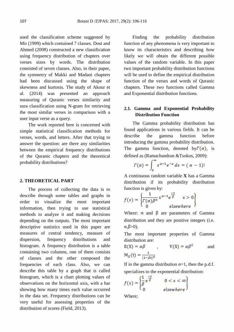
107 Botani D /ZJPAS: 2017, 29(2): 106-116 used the classification scheme suggested by Mir (1999) which contained 7 classes. Dost and Ahmed (2008) constructed a new classification using frequency distribution of chapters over verses sizes by words. The distribution consisted of seven classes. Also, in their paper, the symmetry of Makki and Madani chapters had been discussed using the shape of skewness and kurtosis. The study of Akour et al. (2014) was presented an approach measuring of Quranic verses similarity and sura classification using N-gram for retrieving the most similar verses in comparison with a user input verse as a query.

The work reported here is concerned with simple statistical classification methods for verses, words, and letters. After that trying to answer the question: are there any similarities between the empirical frequency distributions of the Quranic chapters and the theoretical probability distributions?

2. THEORETICAL PART

The process of collecting the data is to describe through some tables and graphs in order to visualize the most important information, then trying to use statistical methods to analyze it and making decisions depending on the outputs. The most important descriptive statistics used in this paper are measures of central tendency, measure of dispersion, frequency distributions and histogram. A frequency distribution is a table containing two columns, one of them consists of classes and the other composed the frequencies of each class. Also, we can describe this table by a graph that is called histogram, which is a chart plotting values of observations on the horizontal axis, with a bar showing how many times each value occurred in the data set. Frequency distributions can be very useful for assessing properties of the distribution of scores (Field, 2013).

Finding the probability distribution function of any phenomena is very important to know its characteristics and describing how likely we will obtain the different possible values of the random variable. In this paper two important probability distribution functions will be used to define the empirical distribution function of the verses and words of Quranic chapters. These two functions called Gamma and Exponential distribution functions.

2.1. Gamma and Exponential Probability Distribution Function

The Gamma probability distribution has found applications in various fields. It can be describe the gamma function before introducing the gamma probability distribution. The gamma function, denoted by , is defined as (Ramachandran &Tsokos, 2009):

A continuous random variable X has a Gamma distribution if its probability distribution function is given by:

Where: and are parameters of Gamma distribution and they are positive integers (i.e.

, >0). The most important properties of Gamma distribution are:

, and

If in the gamma distribution =1, then the p.d.f. specializes to the exponential distribution:

Where;

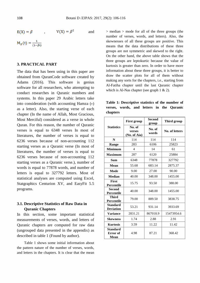
108 Botani D /ZJPAS: 2017, 29(2): 106-116

, and

3. PRACTICAL PART

The data that has been using in this paper are obtained from QuranCode software created by Adams (2016). This software is genius software for all researchers, who attempting to conduct researches in Quranic numbers and systems. In this paper 29 Arabic letters take into consideration (with accounting Hamza (ء) as a letter). Also, the starting verse of each chapter (In the name of Allah, Most Gracious, Most Merciful) considered as a verse in whole Quran. For this reason, the number of Quranic verses is equal to 6348 verses In most of literatures, the number of verses is equal to 6236 verses because of non-accounting 112 starting verses as a Quranic verse (In most of literatures, the number of verses is equal to 6236 verses because of non-accounting 112 starting verses as a Quranic verse.), number of words is equal to 77878 words, and number of letters is equal to 327792 letters. Most of statistical analyses are computed using Excel, Statgraphics Centurion XV, and EasyFit 5.5 programs.

3.1. Descriptive Statistics of Raw Data in Quranic Chapters

In this section, some important statistical measurements of verses, words, and letters of Quranic chapters are computed for raw data (ungrouped data presented in the appendix) as described in table 1 (Found by author).

Table 1 shows some initial information about the pattern nature of the number of verses, words, and letters in the chapters. It is clear that the mean

> median > mode for all of the three groups (the number of verses, words, and letters). Also, the skewnesses of all these groups are positive. This means that the data distributions of these three groups are not symmetric and skewed to the right. On the other hand, the above table shows that the three groups are leptokurtic because the value of kurtosis is greater than zero. In order to have more information about these three groups, it is better to draw the scatter plots for all of them without making any sorts for the chapters, i.e., starting from Al-Fatiha chapter until the last Quranic chapter which is Al-Nas chapter (see graph 1 & 2).

Table 1: Descriptive statistics of the number of verses, words, and letters in the Quranic chapters

Statistics

First group Second group Third group

No. of verses

(No. of Aia)

No. of words No. of letters

N 114 114 114 Range 283 6106 25823

Minimum 4 14 61

Maximum 287 6120 25884

Sum 6348 77878 327792

Mean 55.68 683.14 2875.37

Mode 9.00 27.00 90.00

Median 40.00 348.00 1455.00 First

Percentile 15.75 93.50 388.00

Second Percentile 40.00 348.00 1455.00

Third Percentile 79.00 889.50 3838.75

Standard Deviation 53.21 931.14 3933.69

Variance 2831.21 867018.9 15473954.6

Skewness 1.74 2.88 2.91

Kurtosis 3.59 11.22 11.42 Standard Error of

Mean 4.98 87.21 368.42

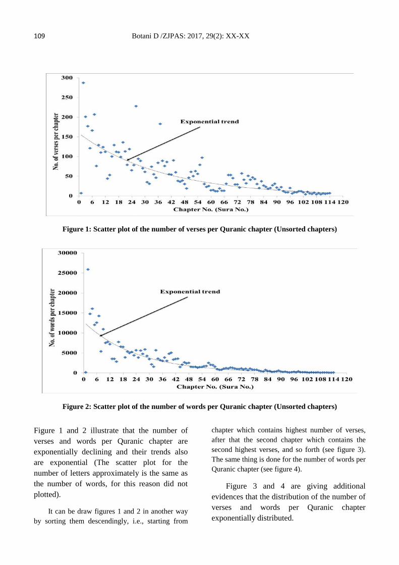
109 Botani D /ZJPAS: 2017, 29(2): XX-XX

Figure 1: Scatter plot of the number of verses per Quranic chapter (Unsorted chapters)

Figure 2: Scatter plot of the number of words per Quranic chapter (Unsorted chapters)

Figure 1 and 2 illustrate that the number of verses and words per Quranic chapter are exponentially declining and their trends also are exponential (The scatter plot for the number of letters approximately is the same as the number of words, for this reason did not plotted).

It can be draw figures 1 and 2 in another way by sorting them descendingly, i.e., starting from

chapter which contains highest number of verses, after that the second chapter which contains the second highest verses, and so forth (see figure 3). The same thing is done for the number of words per Quranic chapter (see figure 4).

Figure 3 and 4 are giving additional evidences that the distribution of the number of verses and words per Quranic chapter exponentially distributed.

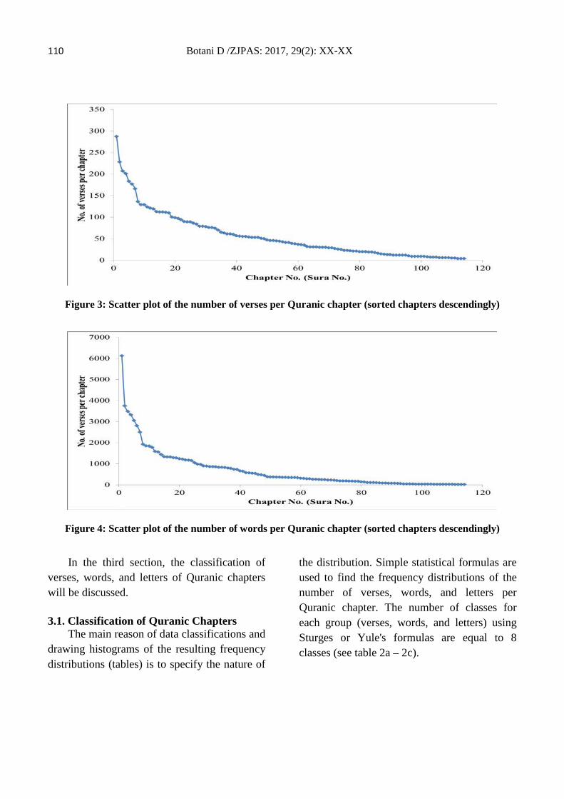
110 Botani D /ZJPAS: 2017, 29(2): XX-XX

Figure 3: Scatter plot of the number of verses per Quranic chapter (sorted chapters descendingly)

Figure 4: Scatter plot of the number of words per Quranic chapter (sorted chapters descendingly)

In the third section, the classification of verses, words, and letters of Quranic chapters will be discussed.

3.1. Classification of Quranic Chapters The main reason of data classifications and

drawing histograms of the resulting frequency distributions (tables) is to specify the nature of

the distribution. Simple statistical formulas are used to find the frequency distributions of the number of verses, words, and letters per Quranic chapter. The number of classes for each group (verses, words, and letters) using Sturges or Yule's formulas are equal to 8 classes (see table 2a – 2c).

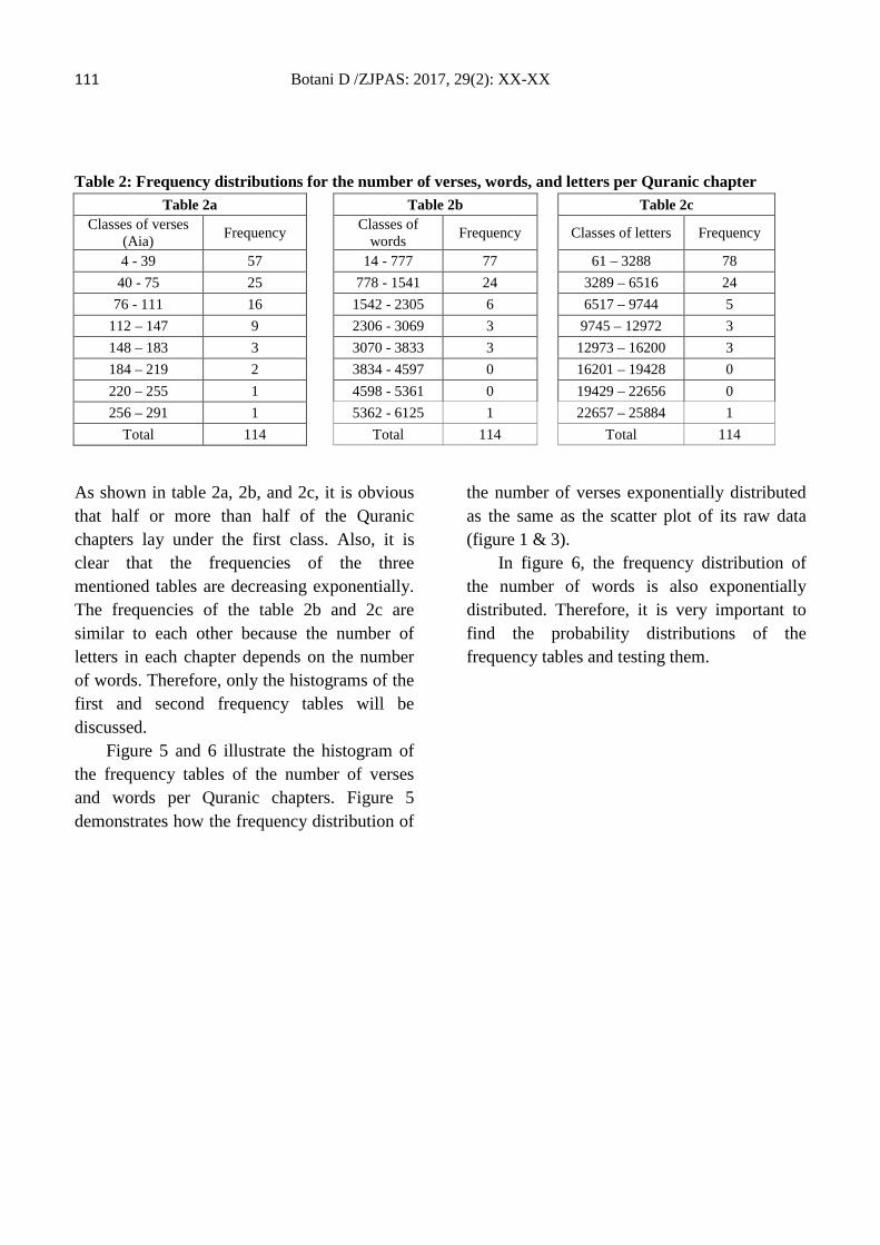
111 Botani D /ZJPAS: 2017, 29(2): XX-XX Table 2: Frequency distributions for the number of verses, words, and letters per Quranic chapter

Table 2a Table 2b Table 2c Classes of verses

(Aia) Frequency Classes of

words Frequency Classes of letters Frequency

4 - 39 57 14 - 777 77 61 – 3288 78 40 - 75 25 778 - 1541 24 3289 – 6516 24

76 - 111 16 1542 - 2305 6 6517 – 9744 5 112 – 147 9 2306 - 3069 3 9745 – 12972 3 148 – 183 3 3070 - 3833 3 12973 – 16200 3 184 – 219 2 3834 - 4597 0 16201 – 19428 0 220 – 255 1 4598 - 5361 0 19429 – 22656 0 256 – 291 1 5362 - 6125 1 22657 – 25884 1

Total 114 Total 114 Total 114

As shown in table 2a, 2b, and 2c, it is obvious that half or more than half of the Quranic chapters lay under the first class. Also, it is clear that the frequencies of the three mentioned tables are decreasing exponentially. The frequencies of the table 2b and 2c are similar to each other because the number of letters in each chapter depends on the number of words. Therefore, only the histograms of the first and second frequency tables will be discussed.

Figure 5 and 6 illustrate the histogram of the frequency tables of the number of verses and words per Quranic chapters. Figure 5 demonstrates how the frequency distribution of

the number of verses exponentially distributed as the same as the scatter plot of its raw data (figure 1 & 3).

In figure 6, the frequency distribution of the number of words is also exponentially distributed. Therefore, it is very important to find the probability distributions of the frequency tables and testing them.

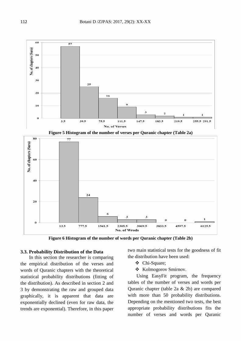
112 Botani D /ZJPAS: 2017, 29(2): XX-XX

Figure 5 Histogram of the number of verses per Quranic chapter (Table 2a)

Figure 6 Histogram of the number of words per Quranic chapter (Table 2b)

3.3. Probability Distribution of the Data In this section the researcher is comparing

the empirical distribution of the verses and words of Quranic chapters with the theoretical statistical probability distributions (fitting of the distribution). As described in section 2 and 3 by demonstrating the raw and grouped data graphically, it is apparent that data are exponentially declined (even for raw data, the trends are exponential). Therefore, in this paper

two main statistical tests for the goodness of fit the distribution have been used: Chi-Square; Kolmogorov Smirnov. Using EasyFit program, the frequency

tables of the number of verses and words per Quranic chapter (table 2a & 2b) are compared with more than 50 probability distributions. Depending on the mentioned two tests, the best appropriate probability distributions fits the number of verses and words per Quranic

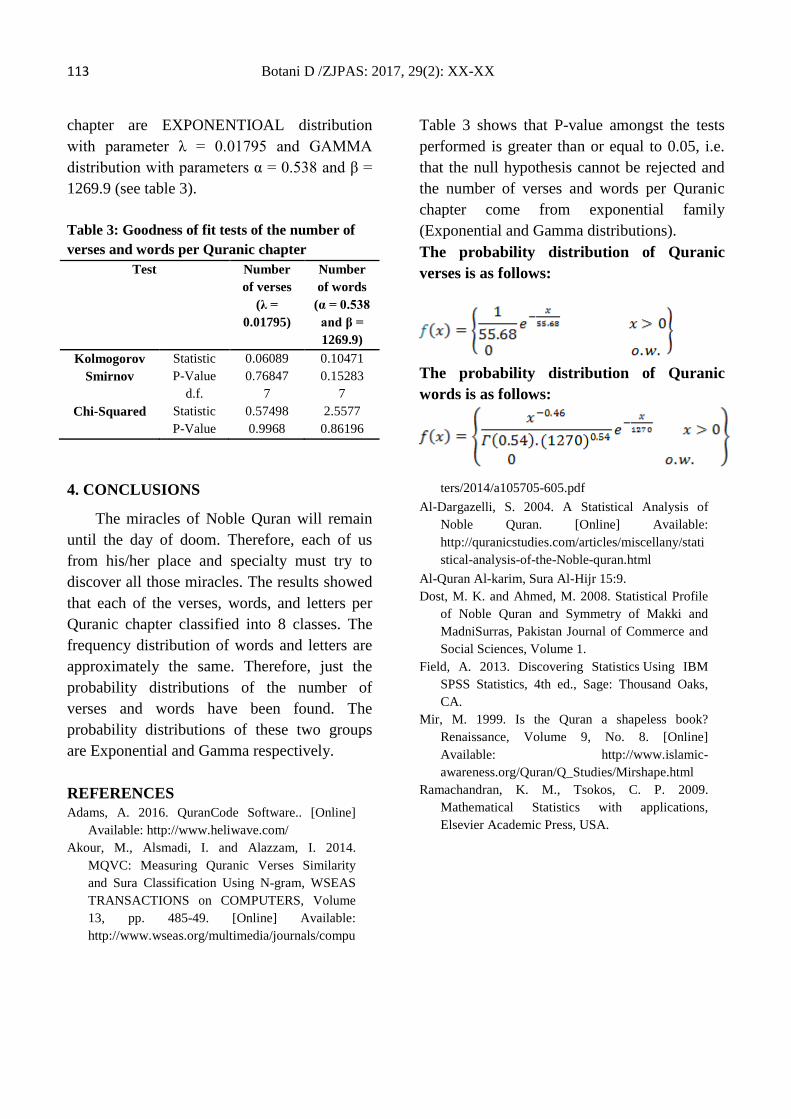
113 Botani D /ZJPAS: 2017, 29(2): XX-XX chapter are EXPONENTIOAL distribution with parameter λ = 0.01795 and GAMMA distribution with parameters α = 0.538 and β = 1269.9 (see table 3). Table 3: Goodness of fit tests of the number of verses and words per Quranic chapter

Test Number of verses

(λ = 0.01795)

Number of words

(α = 0.538 and β = 1269.9)

Kolmogorov Smirnov

Statistic P-Value

0.06089 0.76847

0.10471 0.15283

Chi-Squared

d.f. Statistic P-Value

7 0.57498 0.9968

7 2.5577

0.86196

Table 3 shows that P-value amongst the tests performed is greater than or equal to 0.05, i.e. that the null hypothesis cannot be rejected and the number of verses and words per Quranic chapter come from exponential family (Exponential and Gamma distributions). The probability distribution of Quranic verses is as follows:

The probability distribution of Quranic words is as follows:

4. CONCLUSIONS

The miracles of Noble Quran will remain until the day of doom. Therefore, each of us from his/her place and specialty must try to discover all those miracles. The results showed that each of the verses, words, and letters per Quranic chapter classified into 8 classes. The frequency distribution of words and letters are approximately the same. Therefore, just the probability distributions of the number of verses and words have been found. The probability distributions of these two groups are Exponential and Gamma respectively. REFERENCES Adams, A. 2016. QuranCode Software.. [Online]

Available: http://www.heliwave.com/ Akour, M., Alsmadi, I. and Alazzam, I. 2014.

MQVC: Measuring Quranic Verses Similarity and Sura Classification Using N-gram, WSEAS TRANSACTIONS on COMPUTERS, Volume 13, pp. 485-49. [Online] Available: http://www.wseas.org/multimedia/journals/compu

ters/2014/a105705-605.pdf Al-Dargazelli, S. 2004. A Statistical Analysis of

Noble Quran. [Online] Available: http://quranicstudies.com/articles/miscellany/statistical-analysis-of-the-Noble-quran.html

Al-Quran Al-karim, Sura Al-Hijr 15:9. Dost, M. K. and Ahmed, M. 2008. Statistical Profile

of Noble Quran and Symmetry of Makki and MadniSurras, Pakistan Journal of Commerce and Social Sciences, Volume 1.

Field, A. 2013. Discovering Statistics Using IBM SPSS Statistics, 4th ed., Sage: Thousand Oaks, CA.

Mir, M. 1999. Is the Quran a shapeless book? Renaissance, Volume 9, No. 8. [Online] Available: http://www.islamic-awareness.org/Quran/Q_Studies/Mirshape.html

Ramachandran, K. M., Tsokos, C. P. 2009. Mathematical Statistics with applications, Elsevier Academic Press, USA.

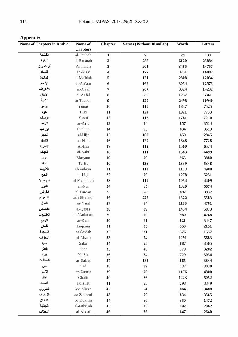
114 Botani D /ZJPAS: 2017, 29(2): XX-XX Appendix Name of Chapters in Arabic Name of

Chapters Chapter Verses (Without Bismilah) Words Letters

al-Fatihah 1 7 29 139 الفاتحة al-Baqarah 2 287 6120 25884 البقرة

Al-Imran 3 201 3485 14757 آل عمران an-Nisa' 4 177 3751 16082 النساء al-Ma'idah 5 121 2808 12034 المائدة al-An`am 6 166 3054 12573 األنعام

al-A`raf 7 207 3324 14232 األعراف al-Anfal 8 76 1237 5361 األنفال at-Taubah 9 129 2498 10940 التوبة Yunus 10 110 1837 7525 یونس Hud 11 124 1921 7733 ھود

Yusuf 12 112 1781 7210 یوسف ar-Ra`d 13 44 857 3514 الرعد Ibrahim 14 53 834 3513 ابراھیم al-Hijr 15 100 659 2845 الحجر an-Nahl 16 129 1848 7728 النحل

Al-Isra 17 112 1560 6574 اإلسراء al-Kahf 18 111 1583 6499 الكھف Maryam 19 99 965 3880 مریم Ta Ha 20 136 1339 5348 طھ

al-Anbiya' 21 113 1173 4988 ألنبیاءا al-Hajj 22 79 1278 5251 الحج

al-Mu'minun 23 119 1054 4409 المؤمنون an-Nur 24 65 1320 5674 النور

al-Furqan 25 78 897 3837 الفرقان ash-Shu`ara' 26 228 1322 5583 الشعراء an-Naml 27 94 1155 4761 النمل

al-Qasas 28 89 1434 5873 القصص al-`Ankabut 29 70 980 4268 العنكبوت

ar-Rum 30 61 821 3447 الروم Luqman 31 35 550 2151 لقمان

as-Sajdah 32 31 376 1557 السجدة al-Ahzab 33 74 1291 5683 األحزاب

Saba' 34 55 887 3565 سبإ Fatir 35 46 779 3202 فاطر Ya Sin 36 84 729 3034 یس

as-Saffat 37 183 865 3844 الصافات Sad 38 89 737 3030 ص

az-Zumar 39 76 1176 4800 الزمر Ghafir 40 86 1223 5052 غافر Fussilat 41 55 798 3349 فصلت

ash-Shura 42 54 864 3488 الشورى az-Zukhruf 43 90 834 3565 الزخرف ad-Dukhan 44 60 350 1472 الدخان al-Jathiyah 45 38 492 2062 الجاثیة al-Ahqaf 46 36 647 2640 األحقاف

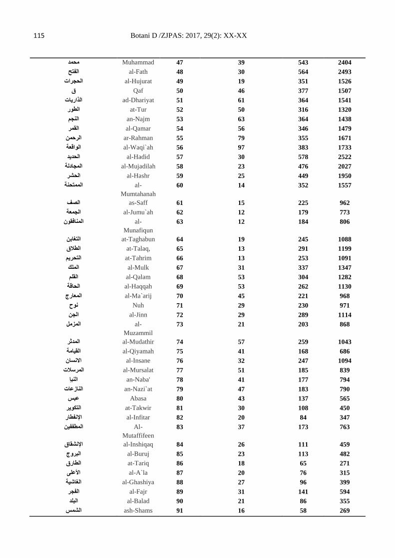
115 Botani D /ZJPAS: 2017, 29(2): XX-XX

Muhammad 47 39 543 2404 محمد al-Fath 48 30 564 2493 الفتح

al-Hujurat 49 19 351 1526 الحجرات Qaf 50 46 377 1507 ق

ad-Dhariyat 51 61 364 1541 الذاریات at-Tur 52 50 316 1320 الطور an-Najm 53 63 364 1438 النجم al-Qamar 54 56 346 1479 القمر

ar-Rahman 55 79 355 1671 الرحمن al-Waqi`ah 56 97 383 1733 الواقعة al-Hadid 57 30 578 2522 الحدید

al-Mujadilah 58 23 476 2027 المجادلة al-Hashr 59 25 449 1950 الحشر

-al الممتحنةMumtahanah

60 14 352 1557

as-Saff 61 15 225 962 الصف al-Jumu`ah 62 12 179 773 الجمعة

-al المنافقونMunafiqun

63 12 184 806

at-Taghabun 64 19 245 1088 التغابن at-Talaq, 65 13 291 1199 الطالق at-Tahrim 66 13 253 1091 التحریم al-Mulk 67 31 337 1347 الملك al-Qalam 68 53 304 1282 القلم

al-Haqqah 69 53 262 1130 الحاقة al-Ma`arij 70 45 221 968 المعارج

Nuh 71 29 230 971 نوح al-Jinn 72 29 289 1114 الجن

-al المزملMuzammil

73 21 203 868

al-Mudathir 74 57 259 1043 المدثر al-Qiyamah 75 41 168 686 القیامة al-Insane 76 32 247 1094 االنسان

al-Mursalat 77 51 185 839 المرسالت an-Naba' 78 41 177 794 النبإ

an-Nazi`at 79 47 183 790 النازعات Abasa 80 43 137 565 عبس

at-Takwir 81 30 108 450 التكویر al-Infitar 82 20 84 347 اإلنفطار-Al المطففین

Mutaffifeen 83 37 173 763

al-Inshiqaq 84 26 111 459 اإلنشقاق al-Buruj 85 23 113 482 البروج at-Tariq 86 18 65 271 الطارق al-A`la 87 20 76 315 األعلى al-Ghashiya 88 27 96 399 الغاشیة al-Fajr 89 31 141 594 الفجر al-Balad 90 21 86 355 البلد

ash-Shams 91 16 58 269 الشمس

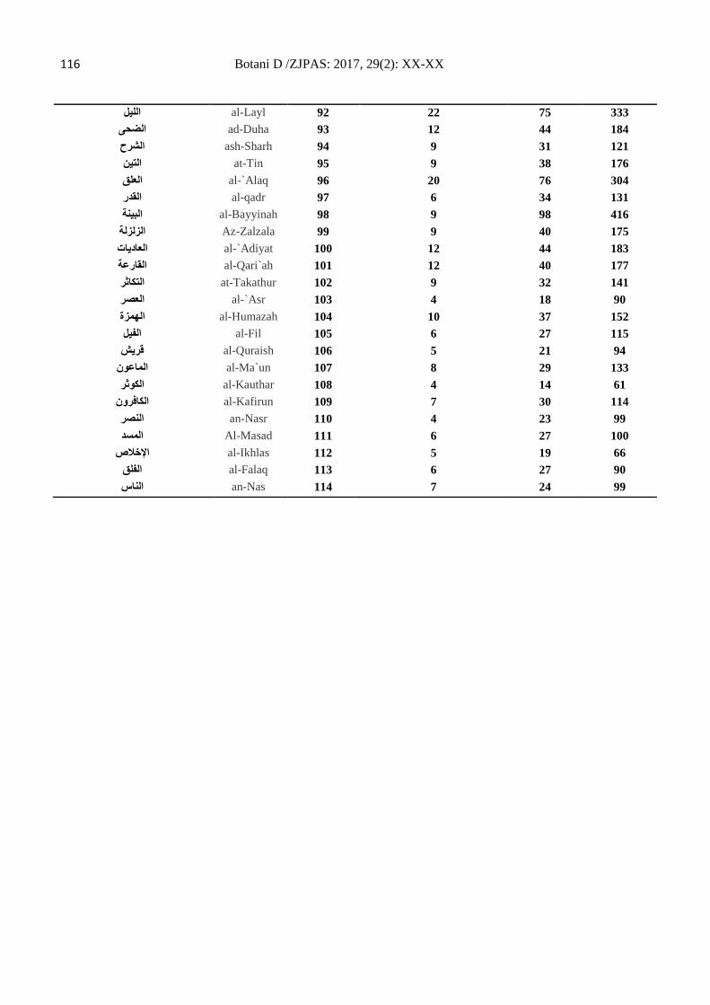
116 Botani D /ZJPAS: 2017, 29(2): XX-XX

al-Layl 92 22 75 333 اللیل ad-Duha 93 12 44 184 الضحى ash-Sharh 94 9 31 121 الشرح at-Tin 95 9 38 176 التین al-`Alaq 96 20 76 304 العلق al-qadr 97 6 34 131 القدر al-Bayyinah 98 9 98 416 البینة

Az-Zalzala 99 9 40 175 الزلزلة al-`Adiyat 100 12 44 183 العادیات al-Qari`ah 101 12 40 177 القارعة at-Takathur 102 9 32 141 التكاثر al-`Asr 103 4 18 90 العصر al-Humazah 104 10 37 152 الھمزة al-Fil 105 6 27 115 الفیل al-Quraish 106 5 21 94 قریش

al-Ma`un 107 8 29 133 الماعون al-Kauthar 108 4 14 61 الكوثر

al-Kafirun 109 7 30 114 الكافرون an-Nasr 110 4 23 99 النصر Al-Masad 111 6 27 100 المسد

al-Ikhlas 112 5 19 66 اإلخالص al-Falaq 113 6 27 90 الفلق an-Nas 114 7 24 99 الناس

ZANCO Journal of Pure and Applied Sciences The official scientific journal of Salahaddin University-Erbil

ZJPAS (2017), 29 (2); 117-125 http://dx.doi.org/10.21271/ZJPAS.29.2.12

Development of Mobile Application for Android Platform: Medical Guide

Salar Kheder Shaikhah1, Ibrahim Shamal Abdulkhalieq1, Jamal A. Hassan2

1Department of Information System Engineering, Erbil Technical Engineering College, Erbil Polytechnic University, Erbil-Iraq

2Department of Electricity, College of Engineering, Salahaddin University-Erbil, Erbil-Iraq

1. INTRODUCTION

Nowadays, huge numbers of health

organizations causes difficulty to find what you

want. Thousands of doctors, hundreds of

hospitals and pharmacies are located in

different geographical places, therefore, it takes

time and money to search for them in

traditional way like searching by car, asking

from relatives and friends don't lead to good

result, as well as websites are not efficient to

use us directory in most cases, because many

people of our society are not familiar with

using website.

Therefore; mobile applications are the best

choice to be used as health directory, because

mobile applications are user friend. Many web

sites were implemented to work as business

directory and rarely these sites focus on health

even if they have sub-parts in this field but they

do not fulfill the demand and do not have

enough information, while most peoples use

A R T I C L E I N F O

A B S T R A C T

Article History: Received: 23/05/2016 Accepted: 24/12/2016 Published: 07/06/2017

Abstract Developing smartphones leads to increase demands on verity of

applications. As the Android operating system is getting more popular, the application based on Android attracts much more attention especially Android is more flexible for designers and users than other mobile phone operating systems. This paper presents an Android mobile phone application that developed to help patients to get information about the health issues in Kurdistan Region of Iraq with Kurdish Language. The software works as a simple and efficient health directory to present what patients are needed. The application is offline and it can be connected with the online website for extra information. The user can check information via viewing the text information and finding the geographic places with an online map, besides that, the user can give rates for the parts of software. The rate that users give to the participants re-appeared for other users in order the best participant (e.g. Doctor, Pharmacy, etc…) can be chosen via rates of users. The data is classified to some groups to facilitating the search.

.

Keywords: Android Technology, System Architecture, Open Source Platform, system Implementing

*Corresponding Author: Jamal A. Hassan jamal.hassan@su.edu.krd

118 Salar K. et al. /ZJPAS: 2017, 29(2): 117-125 mobile applications due to simplicity to use

and they do not need extra device to access the

services. Recently many applications were

developed for the Kurdistan Region market,

even some of them were applications of health

field but no one focused on this field as a guide

line to direct the patients to correct target

easily.

A health system is proposed for

pregnant women in [1]. The proposed system

works based on mobile Geographic

Information System (GIS) to select closest care

Centre or hospital maternity on Google map for

the pregnant woman [1]. But due to problems

of accessibility for the General Packet Radio

Service (GPRS) or data network online

applications have weak points. Hopeful hearts

is proposed in [2]. Authers have used mobile as

a platform for a healthcare, so that people can

get factual information about their health and

can have command on their health. It will help

them to learn about their health and understand

their illness. In this paper Mobile based

healthcare application `Hopeful Hearts' has

been proposed. Application which will suggest

diet and physical activity based on six input

parameters. The input parameters are BMI

(Body Mass Index), BMR (Basal Metabolic

Rate), working hours and user current body

conditions (i.e. Body Temperature, Heart rate

and SPO2 via Sensors). Decision-Tree is being

used to make all suggestions. The application

supports continuous monitoring of user health.

The proposed system is scalable for all

Android Based Mobile Devices [2]. In Hopeful

hearts side of health issue is covered but it

doesn't consider as a guide.

An emergency mobile application

system is proposed in [3] with support of GIS,

and GPRS networks, but the problems of

network connectivity also is ignored for

emergency case.

In this paper, as a solution for many emergency

cases and to direct the patients to right target;

an offline mobile application is proposed for

the health guide under the name Medical

Guide. The application contains many efficient

features for searching, and the application is

connected with a website for getting extra

information. Each participant of the application

can has its own user and he/she can update its

information beside that the doctors can access

their accounts in the program and see their

activities with patients. The application is in

Kurdish Language and it is designed to be user

friendly

2. Android Technology

Android is a software platform and

operating system for mobile devices based on

the Linux operating system and developed by

Google and the Open Handset Alliance [4]. It

allows developers to write managed code in a

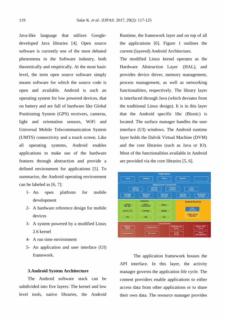
119 Salar K. et al. /ZJPAS: 2017, 29(2): 117-125 Java-like language that utilizes Google-

developed Java libraries [4]. Open source

software is currently one of the most debated

phenomena in the Software industry, both

theoretically and empirically. At the most basic

level, the term open source software simply

means software for which the source code is

open and available. Android is such an

operating system for low powered devices, that

on battery and are full of hardware like Global

Positioning System (GPS) receivers, cameras,

light and orientation sensors, WiFi and

Universal Mobile Telecommunication System

(UMTS) connectivity and a touch screen. Like

all operating systems, Android enables

applications to make use of the hardware

features through abstraction and provide a

defined environment for applications [5]. To

summarize, the Android operating environment

can be labeled as [6, 7]:

1- An open platform for mobile

development

2- A hardware reference design for mobile

devices

3- A system powered by a modified Linux

2.6 kernel

4- A run time environment

5- An application and user interface (UI)

framework.

3.Android System Architecture

The Android software stack can be

subdivided into five layers: The kernel and low

level tools, native libraries, the Android

Runtime, the framework layer and on top of all

the applications [6]. Figure 1 outlines the

current (layered) Android Architecture.

The modified Linux kernel operates as the

Hardware Abstraction Layer (HAL), and

provides device driver, memory management,

process management, as well as networking

functionalities, respectively. The library layer

is interfaced through Java (which deviates from

the traditional Linux design). It is in this layer

that the Android specific libc (Bionic) is

located. The surface manager handles the user

interface (UI) windows. The Android runtime

layer holds the Dalvik Virtual Machine (DVM)

and the core libraries (such as Java or IO).

Most of the functionalities available in Android

are provided via the core libraries [5, 6].

The application framework houses the

API interface. In this layer, the activity

manager governs the application life cycle. The

content providers enable applications to either

access data from other applications or to share

their own data. The resource manager provides

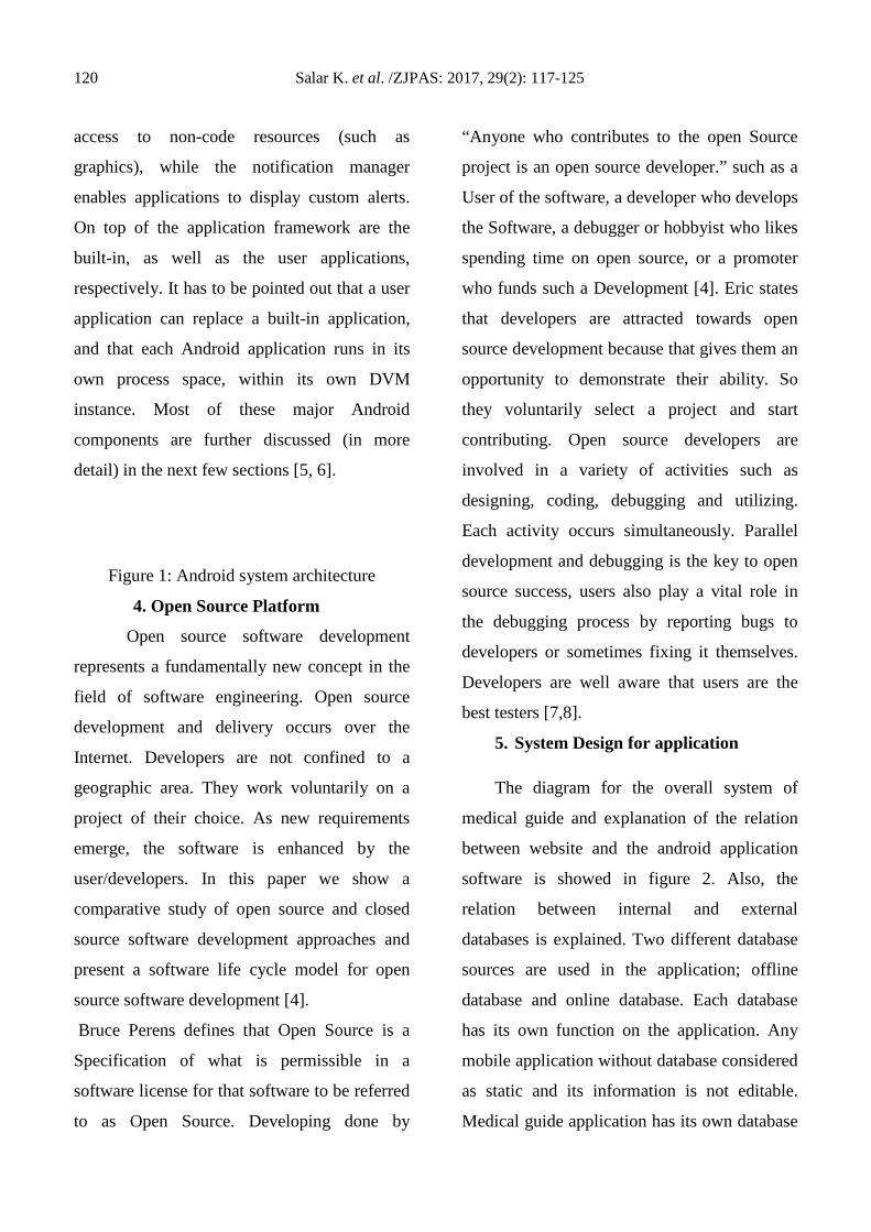
120 Salar K. et al. /ZJPAS: 2017, 29(2): 117-125 access to non-code resources (such as

graphics), while the notification manager

enables applications to display custom alerts.

On top of the application framework are the

built-in, as well as the user applications,

respectively. It has to be pointed out that a user

application can replace a built-in application,

and that each Android application runs in its

own process space, within its own DVM

instance. Most of these major Android

components are further discussed (in more

detail) in the next few sections [5, 6].

Figure 1: Android system architecture

4. Open Source Platform

Open source software development

represents a fundamentally new concept in the

field of software engineering. Open source

development and delivery occurs over the

Internet. Developers are not confined to a

geographic area. They work voluntarily on a

project of their choice. As new requirements

emerge, the software is enhanced by the

user/developers. In this paper we show a

comparative study of open source and closed

source software development approaches and

present a software life cycle model for open

source software development [4].

Bruce Perens defines that Open Source is a

Specification of what is permissible in a

software license for that software to be referred

to as Open Source. Developing done by

“Anyone who contributes to the open Source

project is an open source developer.” such as a

User of the software, a developer who develops

the Software, a debugger or hobbyist who likes

spending time on open source, or a promoter

who funds such a Development [4]. Eric states

that developers are attracted towards open

source development because that gives them an

opportunity to demonstrate their ability. So

they voluntarily select a project and start

contributing. Open source developers are

involved in a variety of activities such as

designing, coding, debugging and utilizing.

Each activity occurs simultaneously. Parallel

development and debugging is the key to open

source success, users also play a vital role in

the debugging process by reporting bugs to

developers or sometimes fixing it themselves.

Developers are well aware that users are the

best testers [7,8].

5. System Design for application

The diagram for the overall system of

medical guide and explanation of the relation

between website and the android application

software is showed in figure 2. Also, the

relation between internal and external

databases is explained. Two different database

sources are used in the application; offline

database and online database. Each database

has its own function on the application. Any

mobile application without database considered

as static and its information is not editable.

Medical guide application has its own database

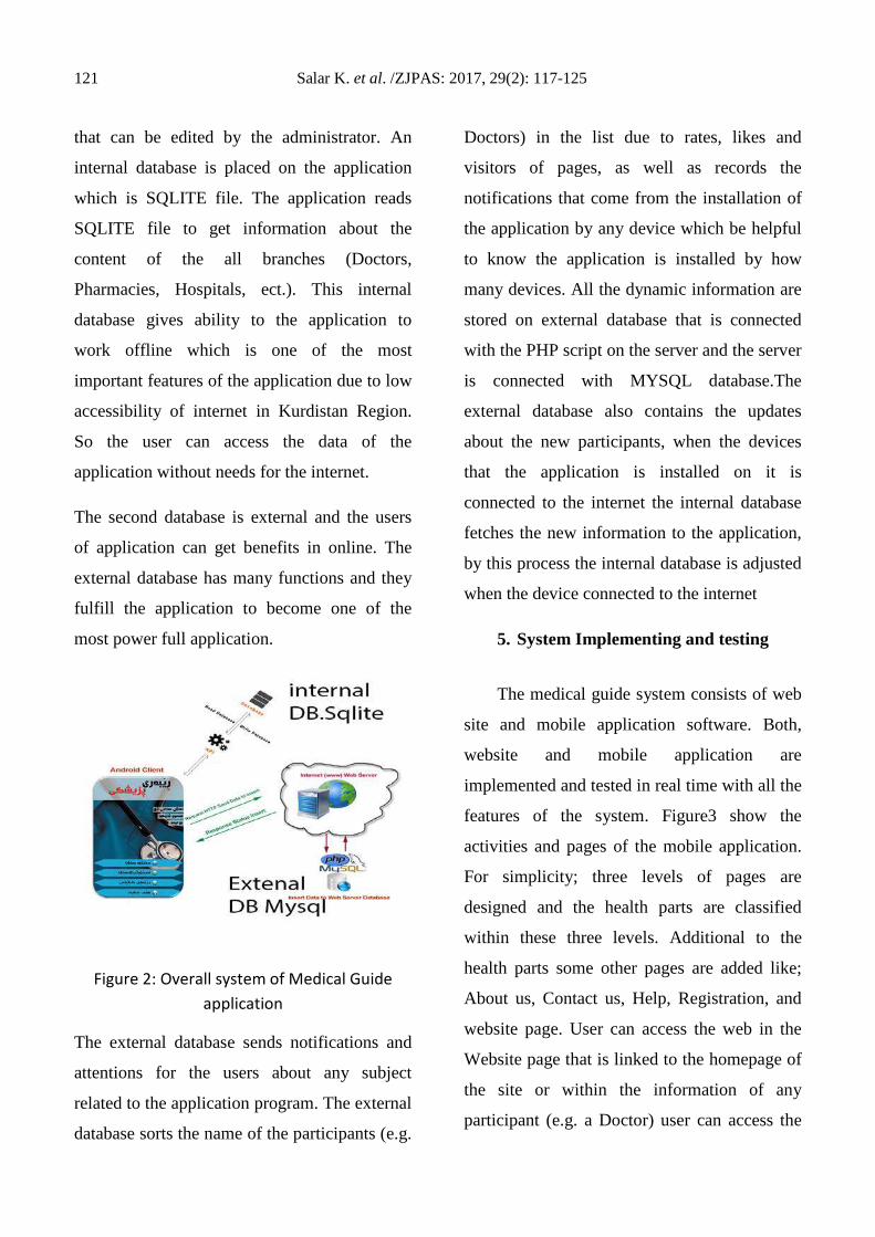
121 Salar K. et al. /ZJPAS: 2017, 29(2): 117-125 that can be edited by the administrator. An

internal database is placed on the application

which is SQLITE file. The application reads

SQLITE file to get information about the

content of the all branches (Doctors,

Pharmacies, Hospitals, ect.). This internal

database gives ability to the application to

work offline which is one of the most

important features of the application due to low

accessibility of internet in Kurdistan Region.

So the user can access the data of the

application without needs for the internet.

The second database is external and the users

of application can get benefits in online. The

external database has many functions and they

fulfill the application to become one of the

most power full application.

Figure 2: Overall system of Medical Guide application

The external database sends notifications and

attentions for the users about any subject

related to the application program. The external

database sorts the name of the participants (e.g.

Doctors) in the list due to rates, likes and

visitors of pages, as well as records the

notifications that come from the installation of

the application by any device which be helpful

to know the application is installed by how

many devices. All the dynamic information are

stored on external database that is connected

with the PHP script on the server and the server

is connected with MYSQL database.The

external database also contains the updates

about the new participants, when the devices

that the application is installed on it is

connected to the internet the internal database

fetches the new information to the application,

by this process the internal database is adjusted

when the device connected to the internet

5. System Implementing and testing

The medical guide system consists of web

site and mobile application software. Both,

website and mobile application are

implemented and tested in real time with all the

features of the system. Figure3 show the

activities and pages of the mobile application.

For simplicity; three levels of pages are

designed and the health parts are classified

within these three levels. Additional to the

health parts some other pages are added like;

About us, Contact us, Help, Registration, and

website page. User can access the web in the

Website page that is linked to the homepage of

the site or within the information of any

participant (e.g. a Doctor) user can access the

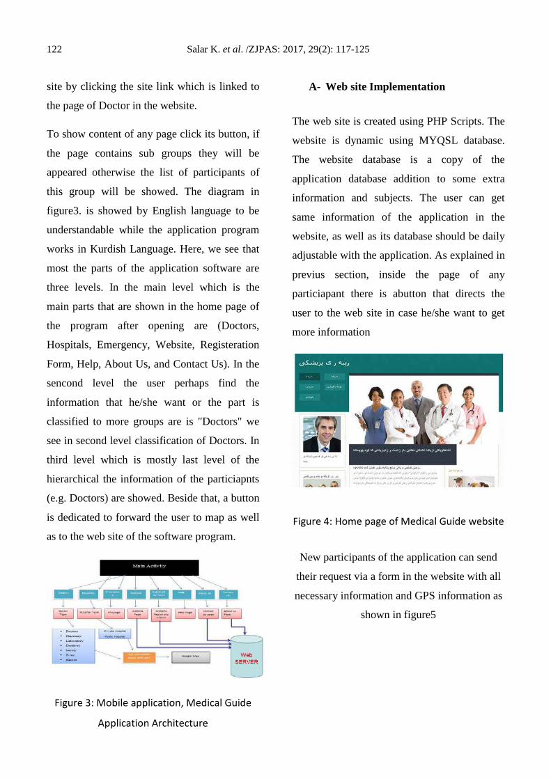
122 Salar K. et al. /ZJPAS: 2017, 29(2): 117-125 site by clicking the site link which is linked to

the page of Doctor in the website.

To show content of any page click its button, if

the page contains sub groups they will be

appeared otherwise the list of participants of

this group will be showed. The diagram in

figure3. is showed by English language to be

understandable while the application program

works in Kurdish Language. Here, we see that

most the parts of the application software are

three levels. In the main level which is the

main parts that are shown in the home page of

the program after opening are (Doctors,

Hospitals, Emergency, Website, Registeration

Form, Help, About Us, and Contact Us). In the

sencond level the user perhaps find the

information that he/she want or the part is

classified to more groups are is "Doctors" we

see in second level classification of Doctors. In

third level which is mostly last level of the

hierarchical the information of the particiapnts

(e.g. Doctors) are showed. Beside that, a button

is dedicated to forward the user to map as well

as to the web site of the software program.

Figure 3: Mobile application, Medical Guide

Application Architecture

A- Web site Implementation

The web site is created using PHP Scripts. The

website is dynamic using MYQSL database.

The website database is a copy of the

application database addition to some extra

information and subjects. The user can get

same information of the application in the

website, as well as its database should be daily

adjustable with the application. As explained in

previus section, inside the page of any

particiapant there is abutton that directs the

user to the web site in case he/she want to get

more information

Figure 4: Home page of Medical Guide website

New participants of the application can send

their request via a form in the website with all

necessary information and GPS information as

shown in figure5

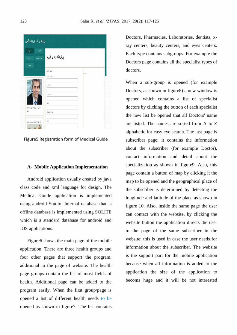
123 Salar K. et al. /ZJPAS: 2017, 29(2): 117-125

Figure5 Registration form of Medical Guide

A- Mobile Application Implementation

Android application usually created by java

class code and xml language for design. The

Medical Guide application is implemented

using android Studio. Internal database that is

offline database is implemented using SQLITE

which is a standard database for android and

IOS applications.

Figure6 shows the main page of the mobile

application. There are three health groups and

four other pages that support the program,

additional to the page of website. The health

page groups contain the list of most fields of

health. Additional page can be added to the

program easily. When the first group/page is

opened a list of different health needs to be

opened as shown in figure7. The list contains

Doctors, Pharmacies, Laboratories, dentists, x-

ray centers, beauty centers, and eyes centers.

Each type contains subgroups. For example the

Doctors page contains all the specialist types of

doctors.

When a sub-group is opened (for example

Doctors, as shown in figure8) a new window is

opened which contains a list of specialist

doctors by clicking the button of each specialist

the new list be opened that all Doctors' name

are listed. The names are sorted from A to Z

alphabetic for easy eye search. The last page is

subscriber page; it contains the information

about the subscriber (for example Doctor),

contact information and detail about the

specialization as shown in figure9. Also, this

page contain a button of map by clicking it the

map to be opened and the geographical place of

the subscriber is determined by detecting the

longitude and latitude of the place as shown in

figure 10. Also, inside the same page the user

can contact with the website, by clicking the

website button the application directs the user

to the page of the same subscriber in the

website; this is used in case the user needs for

information about the subscriber. The website

is the support part for the mobile application

because when all information is added to the

application the size of the application to

becoms huge and it will be not interested

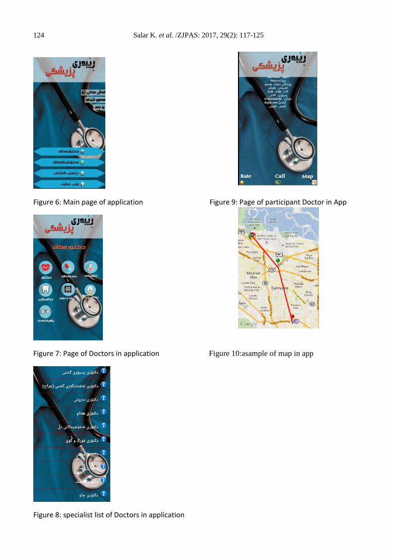
124 Salar K. et al. /ZJPAS: 2017, 29(2): 117-125

Figure 6: Main page of application Figure 9: Page of participant Doctor in App

Figure 7: Page of Doctors in application Figure 10:asample of map in app

Figure 8: specialist list of Doctors in application

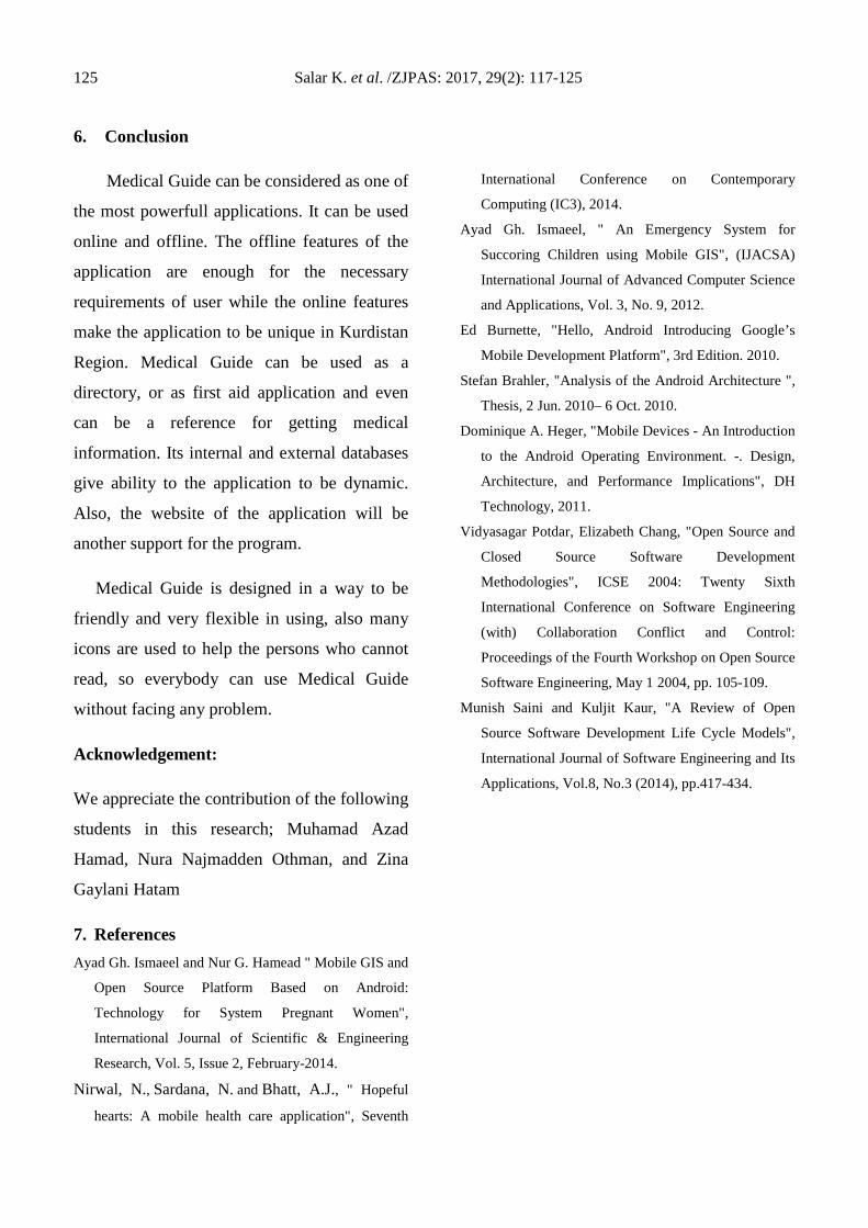
125 Salar K. et al. /ZJPAS: 2017, 29(2): 117-125 6. Conclusion

Medical Guide can be considered as one of

the most powerfull applications. It can be used

online and offline. The offline features of the

application are enough for the necessary

requirements of user while the online features

make the application to be unique in Kurdistan

Region. Medical Guide can be used as a

directory, or as first aid application and even

can be a reference for getting medical

information. Its internal and external databases

give ability to the application to be dynamic.

Also, the website of the application will be

another support for the program.

Medical Guide is designed in a way to be

friendly and very flexible in using, also many

icons are used to help the persons who cannot

read, so everybody can use Medical Guide

without facing any problem.

Acknowledgement:

We appreciate the contribution of the following

students in this research; Muhamad Azad

Hamad, Nura Najmadden Othman, and Zina

Gaylani Hatam

7. References Ayad Gh. Ismaeel and Nur G. Hamead " Mobile GIS and

Open Source Platform Based on Android:

Technology for System Pregnant Women",

International Journal of Scientific & Engineering

Research, Vol. 5, Issue 2, February-2014.

Nirwal, N., Sardana, N. and Bhatt, A.J., " Hopeful

hearts: A mobile health care application", Seventh

International Conference on Contemporary

Computing (IC3), 2014.

Ayad Gh. Ismaeel, " An Emergency System for

Succoring Children using Mobile GIS", (IJACSA)

International Journal of Advanced Computer Science

and Applications, Vol. 3, No. 9, 2012.

Ed Burnette, "Hello, Android Introducing Google’s

Mobile Development Platform", 3rd Edition. 2010.

Stefan Brahler, "Analysis of the Android Architecture ",

Thesis, 2 Jun. 2010– 6 Oct. 2010.

Dominique A. Heger, "Mobile Devices - An Introduction

to the Android Operating Environment. -. Design,

Architecture, and Performance Implications", DH

Technology, 2011.

Vidyasagar Potdar, Elizabeth Chang, "Open Source and

Closed Source Software Development

Methodologies", ICSE 2004: Twenty Sixth

International Conference on Software Engineering

(with) Collaboration Conflict and Control:

Proceedings of the Fourth Workshop on Open Source

Software Engineering, May 1 2004, pp. 105-109.

Munish Saini and Kuljit Kaur, "A Review of Open

Source Software Development Life Cycle Models",

International Journal of Software Engineering and Its

Applications, Vol.8, No.3 (2014), pp.417-434.

ZANCO Journal of Pure and Applied Sciences The official scientific journal of Salahaddin University-Erbil

ZJPAS (2016), 28 (5); 126-135 http://dx.doi.org/10.21271/ZJPAS.29.2.13

Natural Convection in a Trapezoidal Cavity Filled With Cu–Water

Nanofluid and Heated From Its Bottom Wall

1Ahmed W. Mustafa and 2Omar M. Ahmed

1Department of Mechanical Engineering, Al-Nahrain University, Baghdad 2Department of Civil and environmental Engineering, Samarra University, Salah Al-Din

1. INTRODUCTION

The low thermal conductivity of conventional fluids such as water is a primary limitation in enhancing the heat transfer. Solid has a higher thermal conductivity than liquid. For instance,

the copper (Cu) has a thermal conductivity 700 time greater than the water. Since the nanoparticles have small sizes and very large specific surface areas, nanofluids have superior properties like high thermal conductivity,

A R T I C L E I N F O

A B S T R A C T

Article History: Received: 03/10/2016 Accepted: 24/12/2016 Published: 07/06/2017

Natural convection in a trapezoidal enclosure heated from below and filled

with Cu-water nanofluid has investigated numerically. The lower wall is

maintained at constant high temperature, the side walls are maintained at

constant low temperature, and the upper wall is thermally insulated. Flow

within the enclosure is steady, two-dimensional, and laminar. The pure fluid

molecules (water) and the basic nanoparticles (Cu) are in thermal equilibrium,

and there is no sliding between them. A finite volume method with collocated

grid is used to discretize mass, momentum and energy equations. Grid

generation method is employed to generate the coordinate system. SIMPLE

algorithm is used to link the velocity and pressure fields. The range of

Rayleigh number is ) , the tilt angles of the side walls

are (θ = 0°, 30°, and 45°) and the range of solid volume fraction is (0 ≤ φ ≤

0.2).The results show that the highest average Nusselt number occurs at (θ =

0°) for both pure fluid and nanofluid, and the average Nusselt number at (θ =

30°) is almost equal to the average Nusselt number at (θ = 45°) for both pure

fluid and nanofluid.

.

.

Keywords: Natural convection; Trapezoidal enclosure; Nanofluid; Finite Volume *Corresponding Author: 1Ahmed W. Mustafa ahmedwah@eng.nahrainuniv.edu.iq

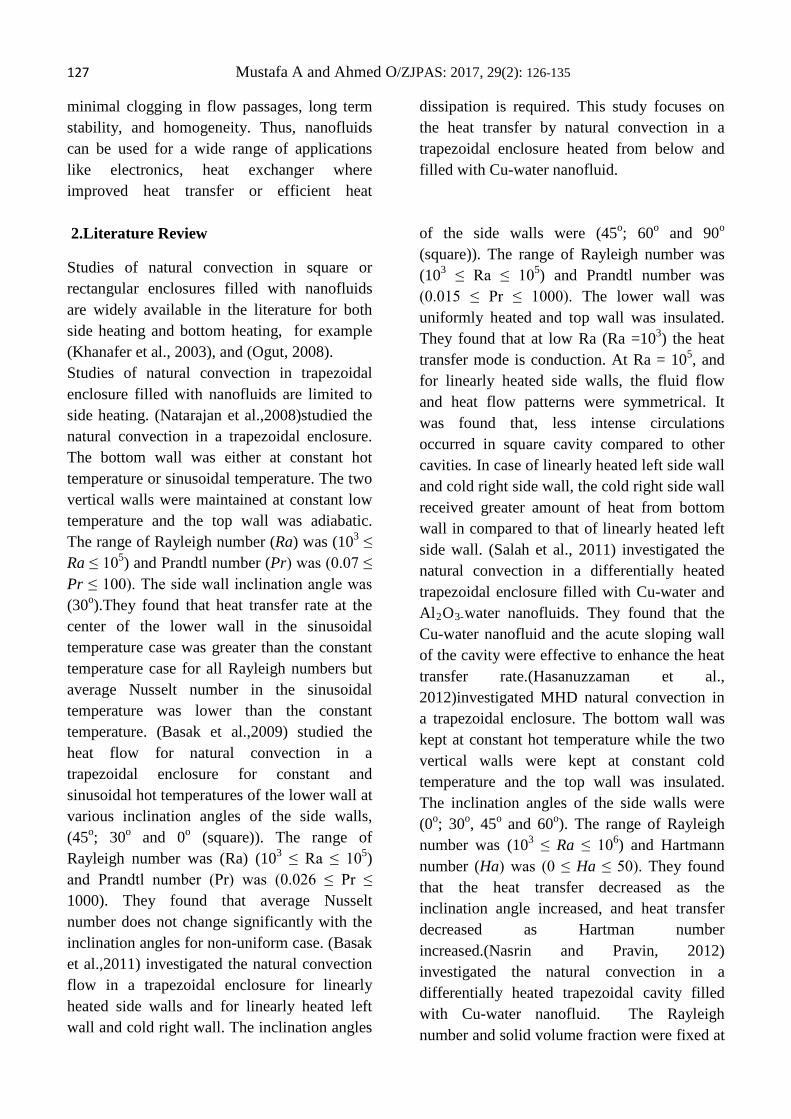
127 Mustafa A and Ahmed O/ZJPAS: 2017, 29(2): 126-135

minimal clogging in flow passages, long term stability, and homogeneity. Thus, nanofluids can be used for a wide range of applications like electronics, heat exchanger where improved heat transfer or efficient heat

dissipation is required. This study focuses on the heat transfer by natural convection in a trapezoidal enclosure heated from below and filled with Cu-water nanofluid.

2.Literature Review

Studies of natural convection in square or rectangular enclosures filled with nanofluids are widely available in the literature for both side heating and bottom heating, for example (Khanafer et al., 2003), and (Ogut, 2008). Studies of natural convection in trapezoidal enclosure filled with nanofluids are limited to side heating. (Natarajan et al.,2008)studied the natural convection in a trapezoidal enclosure. The bottom wall was either at constant hot temperature or sinusoidal temperature. The two vertical walls were maintained at constant low temperature and the top wall was adiabatic. The range of Rayleigh number (Ra) was (103 ≤ Ra ≤ 105) and Prandtl number (Pr) was (0.07 ≤ Pr ≤ 100). The side wall inclination angle was (30o).They found that heat transfer rate at the center of the lower wall in the sinusoidal temperature case was greater than the constant temperature case for all Rayleigh numbers but average Nusselt number in the sinusoidal temperature was lower than the constant temperature. (Basak et al.,2009) studied the heat flow for natural convection in a trapezoidal enclosure for constant and sinusoidal hot temperatures of the lower wall at various inclination angles of the side walls, (45o; 30o and 0o (square)). The range of Rayleigh number was (Ra) (103 ≤ Ra ≤ 105) and Prandtl number (Pr) was (0.026 ≤ Pr ≤ 1000). They found that average Nusselt number does not change significantly with the inclination angles for non-uniform case. (Basak et al.,2011) investigated the natural convection flow in a trapezoidal enclosure for linearly heated side walls and for linearly heated left wall and cold right wall. The inclination angles

of the side walls were (45o; 60o and 90o (square)). The range of Rayleigh number was (103 ≤ Ra ≤ 105) and Prandtl number was (0.015 ≤ Pr ≤ 1000). The lower wall was uniformly heated and top wall was insulated. They found that at low Ra (Ra =103) the heat transfer mode is conduction. At Ra = 105, and for linearly heated side walls, the fluid flow and heat flow patterns were symmetrical. It was found that, less intense circulations occurred in square cavity compared to other cavities. In case of linearly heated left side wall and cold right side wall, the cold right side wall received greater amount of heat from bottom wall in compared to that of linearly heated left side wall. (Salah et al., 2011) investigated the natural convection in a differentially heated trapezoidal enclosure filled with Cu-water and Al2O3-water nanofluids. They found that the Cu-water nanofluid and the acute sloping wall of the cavity were effective to enhance the heat transfer rate.(Hasanuzzaman et al., 2012)investigated MHD natural convection in a trapezoidal enclosure. The bottom wall was kept at constant hot temperature while the two vertical walls were kept at constant cold temperature and the top wall was insulated. The inclination angles of the side walls were (0o; 30o, 45o and 60o). The range of Rayleigh number was (103 ≤ Ra ≤ 106) and Hartmann number (Ha) was (0 ≤ Ha ≤ 50). They found that the heat transfer decreased as the inclination angle increased, and heat transfer decreased as Hartman number increased.(Nasrin and Pravin, 2012) investigated the natural convection in a differentially heated trapezoidal cavity filled with Cu-water nanofluid. The Rayleigh number and solid volume fraction were fixed at

128 Mustafa A and Ahmed O/ZJPAS: 2017, 29(2): 126-135

105 and 0.05 respectively. They found that both Prandtl number and aspect ratio affect the heat transfer and fluid flow in the cavity. (Ramakrishna et al., 2013)investigated the entropy generation for natural convection in differentially heated trapezoidal cavity. They found that the best shape of the trapezoidal cavity was at (θ= 60°) and (Pr = 0.015) according to lower total entropy generation and higher average Nusselt number. (Mahmoudi et al.,2013) investigated the MHD natural convection and entropy generation in a trapezoidal enclosure filled with Cu –water nanofluid. They used a two dimensional trapezoidal cavity with the left vertical wall and the inclined right wall maintained in a low constant temperature and a constant heat flux heat source placed on the lower wall of the cavity. They found that at Ra = 104 and 105 and in the presence of nanofluid the Nusselt number increased with the Hartman number, but at higher Rayleigh number, a reduction had been seen. Also the entropy generation is decreased in the presence of nanofluid but increased in the presence of magnetic field. (Esfe et al., 2016) investigated the natural convection for trapezoidal enclosure filled with carbon-nanotube-EG- water nanofluid numerically. The bottom wall of the enclosure was kept at constant hot temperature while the top wall of the enclosure was kept at constant cold temperature. The sides of the enclosure were insulated. They used the finite volume method to solve the governing equations. The range of Rayleigh number was 103-106, and the solid volume fractions were 0.0015, 0.03, and 0.045. They concluded that the average Nusselt number decreases as the inclination angle increasing at low Rayleigh number (Ra ≤ 104) for all solid volume fractions. The present study deals with the natural convection nanofluid flow within a trapezoidal enclosure, heated isothermally from below, cooled isothermally from the sides, and insulatedfrom the top.

3.Mathematical Formulation Consider a trapezoidal enclosure with base length (L) equals to the height (H). The side walls are inclined at an angel (θ) with y – axis as shown in figure 1.The enclosure is filled with (Cu – water) nanofluid. The pure fluid molecules (water) and the nanoparticles (Cu) are in thermal equilibrium, and there is no sliding between them. All thermophysical properties of the nanofluid except density are assumed to be constant. Boussinesq approximation is used in the body force term in the y-momentum equation to calculate the variation of density. The flow is assumed to be steady, laminar and two-dimensional.Under the above assumptions the governing equations can be written as:-

(1)

(2)

(3)

(4)

Whereu and v are the velocity components in the x and y directions, respectively.p is the pressure, T is the temperature, and β is the thermal expansion coefficient. By using the following dimensionless variables

(5)

The Prandtl number (Pr) and Rayleigh number (Ra) are defined as:

129 Mustafa A and Ahmed O/ZJPAS: 2017, 29(2): 126-135

(6)

The governing equations can be written in non-dimensional form as:

(7)

(8)

(9)

(10)

The thermophysical properties of the nanofluid are obtained from the following relations. (Basak and Chamkha, 2012).

The densityof the nanofluid can be calculated as

(11) The thermal conductivity of the nanofluid can be calculated as (Maxwell model)

(12)

Thermal diffusivity of the nanofluid can be calculated as:

(13)

The heat capacity of the nanofluid can be calculated as

(14)

The thermal expansion coefficient of the nanofluid can be calculated by

(15) The effective viscosity of the nanofluidcan be calculated based onBrinkman model (Brinkman, 1952) as

(16)

The thermophysical properties of the water and Cu-particle are given in Table 1. (Basak and Chamkha, 2012).

The boundary conditions for governing equations in the dimensionless form are given by

Top wall ,

Right and left walls

Bottom wall , =1

The local Nusselt number on the bottom wall can be calculated from the following relation

(17)

The average Nusselt Number on the bottom wall is calculated from

(18) The streamfunctions can be obtained from the velocity components as

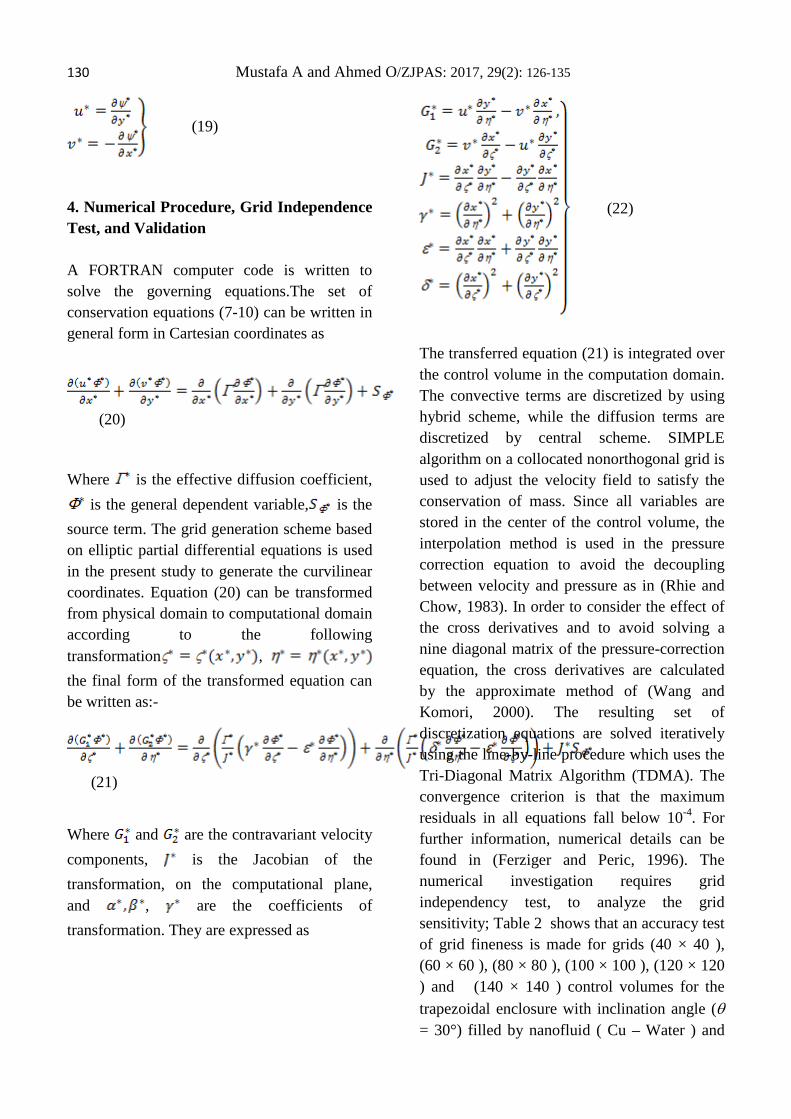
130 Mustafa A and Ahmed O/ZJPAS: 2017, 29(2): 126-135

(19)

4. Numerical Procedure, Grid Independence Test, and Validation A FORTRAN computer code is written to solve the governing equations.The set of conservation equations (7-10) can be written in general form in Cartesian coordinates as

(20) Where is the effective diffusion coefficient,

is the general dependent variable, is the source term. The grid generation scheme based on elliptic partial differential equations is used in the present study to generate the curvilinear coordinates. Equation (20) can be transformed from physical domain to computational domain according to the following transformation , the final form of the transformed equation can be written as:-

(21)

Where and are the contravariant velocity components, is the Jacobian of the transformation, on the computational plane, and , are the coefficients of transformation. They are expressed as

(22)

The transferred equation (21) is integrated over the control volume in the computation domain. The convective terms are discretized by using hybrid scheme, while the diffusion terms are discretized by central scheme. SIMPLE algorithm on a collocated nonorthogonal grid is used to adjust the velocity field to satisfy the conservation of mass. Since all variables are stored in the center of the control volume, the interpolation method is used in the pressure correction equation to avoid the decoupling between velocity and pressure as in (Rhie and Chow, 1983). In order to consider the effect of the cross derivatives and to avoid solving a nine diagonal matrix of the pressure-correction equation, the cross derivatives are calculated by the approximate method of (Wang and Komori, 2000). The resulting set of discretization equations are solved iteratively using the line-by-line procedure which uses the Tri-Diagonal Matrix Algorithm (TDMA). The convergence criterion is that the maximum residuals in all equations fall below 10-4. For further information, numerical details can be found in (Ferziger and Peric, 1996). The numerical investigation requires grid independency test, to analyze the grid sensitivity; Table 2 shows that an accuracy test of grid fineness is made for grids (40 × 40 ), (60 × 60 ), (80 × 80 ), (100 × 100 ), (120 × 120 ) and (140 × 140 ) control volumes for the trapezoidal enclosure with inclination angle (θ = 30°) filled by nanofluid ( Cu – Water ) and

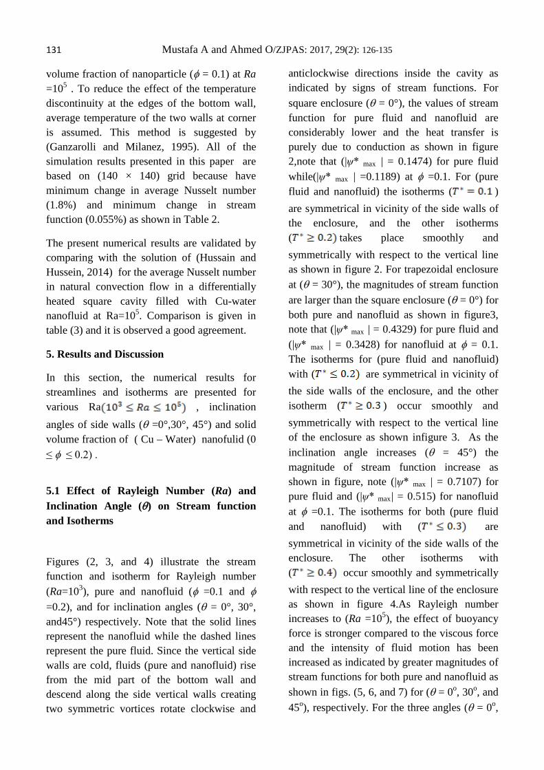
131 Mustafa A and Ahmed O/ZJPAS: 2017, 29(2): 126-135

volume fraction of nanoparticle (φ = 0.1) at Ra =105 . To reduce the effect of the temperature discontinuity at the edges of the bottom wall, average temperature of the two walls at corner is assumed. This method is suggested by (Ganzarolli and Milanez, 1995). All of the simulation results presented in this paper are based on (140 × 140) grid because have minimum change in average Nusselt number (1.8%) and minimum change in stream function (0.055%) as shown in Table 2.

The present numerical results are validated by comparing with the solution of (Hussain and Hussein, 2014) for the average Nusselt number in natural convection flow in a differentially heated square cavity filled with Cu-water nanofluid at Ra=105. Comparison is given in table (3) and it is observed a good agreement.

5. Results and Discussion

In this section, the numerical results for streamlines and isotherms are presented for various Ra , inclination angles of side walls (θ =0°,30°, 45°) and solid volume fraction of ( Cu – Water) nanofulid (0 ≤ φ ≤ 0.2) .

5.1 Effect of Rayleigh Number (Ra) and Inclination Angle (θ) on Stream function and Isotherms Figures (2, 3, and 4) illustrate the stream function and isotherm for Rayleigh number (Ra=103), pure and nanofluid (φ =0.1 and φ =0.2), and for inclination angles (θ = 0°, 30°, and45°) respectively. Note that the solid lines represent the nanofluid while the dashed lines represent the pure fluid. Since the vertical side walls are cold, fluids (pure and nanofluid) rise from the mid part of the bottom wall and descend along the side vertical walls creating two symmetric vortices rotate clockwise and

anticlockwise directions inside the cavity as indicated by signs of stream functions. For square enclosure (θ = 0°), the values of stream function for pure fluid and nanofluid are considerably lower and the heat transfer is purely due to conduction as shown in figure 2,note that (|ψ* max | = 0.1474) for pure fluid while(|ψ* max | =0.1189) at φ =0.1. For (pure fluid and nanofluid) the isotherms ( ) are symmetrical in vicinity of the side walls of the enclosure, and the other isotherms ( takes place smoothly and symmetrically with respect to the vertical line as shown in figure 2. For trapezoidal enclosure at (θ = 30°), the magnitudes of stream function are larger than the square enclosure (θ = 0°) for both pure and nanofluid as shown in figure3, note that (|ψ* max | = 0.4329) for pure fluid and (|ψ* max | = 0.3428) for nanofluid at φ = 0.1. The isotherms for (pure fluid and nanofluid) with ( are symmetrical in vicinity of the side walls of the enclosure, and the other isotherm ( ) occur smoothly and symmetrically with respect to the vertical line of the enclosure as shown infigure 3. As the inclination angle increases (θ = 45°) the magnitude of stream function increase as shown in figure, note (|ψ* max | = 0.7107) for pure fluid and (|ψ* max| = 0.515) for nanofluid at φ =0.1. The isotherms for both (pure fluid and nanofluid) with ( are symmetrical in vicinity of the side walls of the enclosure. The other isotherms with ( occur smoothly and symmetrically with respect to the vertical line of the enclosure as shown in figure 4.As Rayleigh number increases to (Ra =105), the effect of buoyancy force is stronger compared to the viscous force and the intensity of fluid motion has been increased as indicated by greater magnitudes of stream functions for both pure and nanofluid as shown in figs. (5, 6, and 7) for (θ = 0o, 30o, and 45o), respectively. For the three angles (θ = 0o,

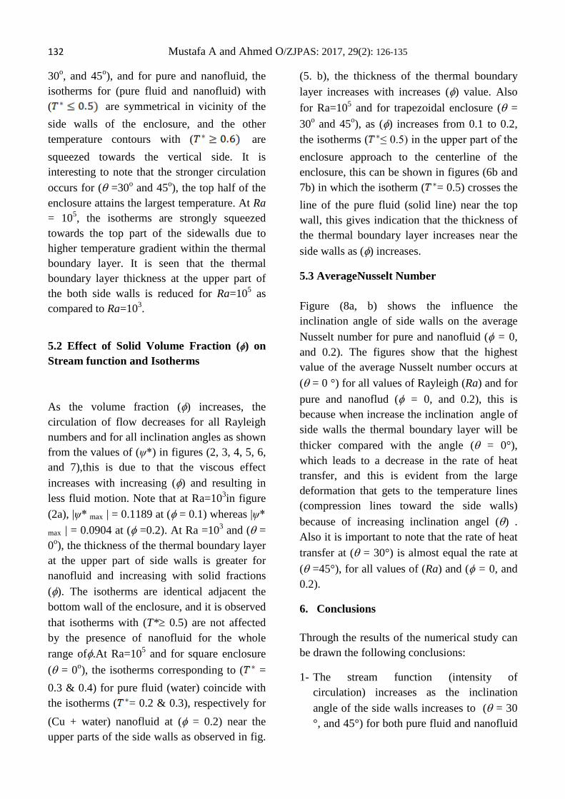
132 Mustafa A and Ahmed O/ZJPAS: 2017, 29(2): 126-135

30o, and 45o), and for pure and nanofluid, the isotherms for (pure fluid and nanofluid) with ( are symmetrical in vicinity of the side walls of the enclosure, and the other temperature contours with ( are squeezed towards the vertical side. It is interesting to note that the stronger circulation occurs for (θ =30o and 45o), the top half of the enclosure attains the largest temperature. At Ra = 105, the isotherms are strongly squeezed towards the top part of the sidewalls due to higher temperature gradient within the thermal boundary layer. It is seen that the thermal boundary layer thickness at the upper part of the both side walls is reduced for Ra=105 as compared to Ra=103.

5.2 Effect of Solid Volume Fraction (φ) on Stream function and Isotherms As the volume fraction (φ) increases, the circulation of flow decreases for all Rayleigh numbers and for all inclination angles as shown from the values of (ψ*) in figures (2, 3, 4, 5, 6, and 7),this is due to that the viscous effect increases with increasing (φ) and resulting in less fluid motion. Note that at Ra=103in figure (2a), |ψ* max | = 0.1189 at (φ = 0.1) whereas |ψ*

max | = 0.0904 at (φ =0.2). At Ra =103 and (θ = 0o), the thickness of the thermal boundary layer at the upper part of side walls is greater for nanofluid and increasing with solid fractions (φ). The isotherms are identical adjacent the bottom wall of the enclosure, and it is observed that isotherms with (T*≥ 0.5) are not affected by the presence of nanofluid for the whole range ofφ.At Ra=105 and for square enclosure (θ = 0o), the isotherms corresponding to ( = 0.3 & 0.4) for pure fluid (water) coincide with the isotherms ( = 0.2 & 0.3), respectively for (Cu + water) nanofluid at (φ = 0.2) near the upper parts of the side walls as observed in fig.

(5. b), the thickness of the thermal boundary layer increases with increases (φ) value. Also for Ra=105 and for trapezoidal enclosure (θ = 30o and 45o), as (φ) increases from 0.1 to 0.2, the isotherms ( ≤ 0.5) in the upper part of the enclosure approach to the centerline of the enclosure, this can be shown in figures (6b and 7b) in which the isotherm ( = 0.5) crosses the line of the pure fluid (solid line) near the top wall, this gives indication that the thickness of the thermal boundary layer increases near the side walls as (φ) increases.

5.3 AverageNusselt Number Figure (8a, b) shows the influence the inclination angle of side walls on the average Nusselt number for pure and nanofluid (φ = 0, and 0.2). The figures show that the highest value of the average Nusselt number occurs at (θ = 0 °) for all values of Rayleigh (Ra) and for pure and nanoflud (φ = 0, and 0.2), this is because when increase the inclination angle of side walls the thermal boundary layer will be thicker compared with the angle (θ = 0°), which leads to a decrease in the rate of heat transfer, and this is evident from the large deformation that gets to the temperature lines (compression lines toward the side walls) because of increasing inclination angel (θ) . Also it is important to note that the rate of heat transfer at (θ = 30°) is almost equal the rate at (θ =45°), for all values of (Ra) and (φ = 0, and 0.2).

6. Conclusions Through the results of the numerical study can be drawn the following conclusions:

1- The stream function (intensity of circulation) increases as the inclination angle of the side walls increases to (θ = 30 °, and 45°) for both pure fluid and nanofluid

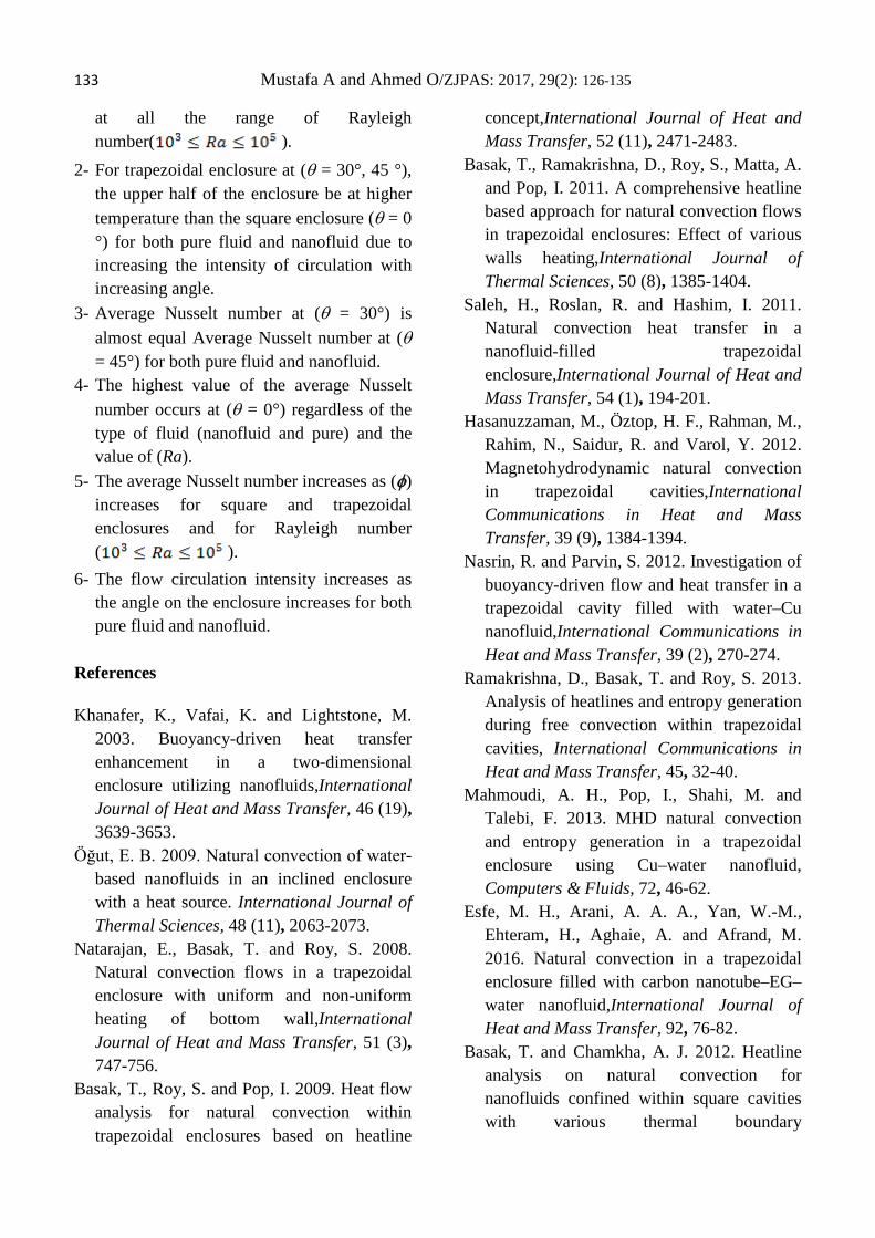
133 Mustafa A and Ahmed O/ZJPAS: 2017, 29(2): 126-135

at all the range of Rayleigh number( ).

2- For trapezoidal enclosure at (θ = 30°, 45 °), the upper half of the enclosure be at higher temperature than the square enclosure (θ = 0 °) for both pure fluid and nanofluid due to increasing the intensity of circulation with increasing angle.

3- Average Nusselt number at (θ = 30°) is almost equal Average Nusselt number at (θ = 45°) for both pure fluid and nanofluid.

4- The highest value of the average Nusselt number occurs at (θ = 0°) regardless of the type of fluid (nanofluid and pure) and the value of (Ra).

5- The average Nusselt number increases as (φ) increases for square and trapezoidal enclosures and for Rayleigh number ( ).

6- The flow circulation intensity increases as the angle on the enclosure increases for both pure fluid and nanofluid.

References Khanafer, K., Vafai, K. and Lightstone, M.

2003. Buoyancy-driven heat transfer enhancement in a two-dimensional enclosure utilizing nanofluids,International Journal of Heat and Mass Transfer, 46 (19), 3639-3653.

Öğut, E. B. 2009. Natural convection of water-based nanofluids in an inclined enclosure with a heat source. International Journal of Thermal Sciences, 48 (11), 2063-2073.

Natarajan, E., Basak, T. and Roy, S. 2008. Natural convection flows in a trapezoidal enclosure with uniform and non-uniform heating of bottom wall,International Journal of Heat and Mass Transfer, 51 (3), 747-756.

Basak, T., Roy, S. and Pop, I. 2009. Heat flow analysis for natural convection within trapezoidal enclosures based on heatline

concept,International Journal of Heat and Mass Transfer, 52 (11), 2471-2483.

Basak, T., Ramakrishna, D., Roy, S., Matta, A. and Pop, I. 2011. A comprehensive heatline based approach for natural convection flows in trapezoidal enclosures: Effect of various walls heating,International Journal of Thermal Sciences, 50 (8), 1385-1404.

Saleh, H., Roslan, R. and Hashim, I. 2011. Natural convection heat transfer in a nanofluid-filled trapezoidal enclosure,International Journal of Heat and Mass Transfer, 54 (1), 194-201.

Hasanuzzaman, M., Öztop, H. F., Rahman, M., Rahim, N., Saidur, R. and Varol, Y. 2012. Magnetohydrodynamic natural convection in trapezoidal cavities,International Communications in Heat and Mass Transfer, 39 (9), 1384-1394.

Nasrin, R. and Parvin, S. 2012. Investigation of buoyancy-driven flow and heat transfer in a trapezoidal cavity filled with water–Cu nanofluid,International Communications in Heat and Mass Transfer, 39 (2), 270-274.

Ramakrishna, D., Basak, T. and Roy, S. 2013. Analysis of heatlines and entropy generation during free convection within trapezoidal cavities, International Communications in Heat and Mass Transfer, 45, 32-40.

Mahmoudi, A. H., Pop, I., Shahi, M. and Talebi, F. 2013. MHD natural convection and entropy generation in a trapezoidal enclosure using Cu–water nanofluid, Computers & Fluids, 72, 46-62.

Esfe, M. H., Arani, A. A. A., Yan, W.-M., Ehteram, H., Aghaie, A. and Afrand, M. 2016. Natural convection in a trapezoidal enclosure filled with carbon nanotube–EG–water nanofluid,International Journal of Heat and Mass Transfer, 92, 76-82.

Basak, T. and Chamkha, A. J. 2012. Heatline analysis on natural convection for nanofluids confined within square cavities with various thermal boundary

134 Mustafa A and Ahmed O/ZJPAS: 2017, 29(2): 126-135

conditions,International Journal of Heat and Mass Transfer, 55 (21), 5526-5543.

Brinkman, H. 1952. The viscosity of concentrated suspensions and solutions. The Journal of Chemical Physics, 20 (4), 571-571.

Rhie, C. and Chow, W. 1983. Numerical study of the turbulent flow past an airfoil with trailing edge separation,AIAA journal, 21 (11), 1525-1532.

Wang, Y. and Komori, S. 2000. On the improvement of the SIMPLE-like method for flows with complex geometry,Heat and Mass Transfer, 36 (1), 71-78.

Ferziger, J. H. and Peric, M. 2012, Computational methods for fluid dynamics, Springer Science & Business Media, USA.

Ganzarolli, M. M. and Milanez, L. F. 1995. Natural convection in rectangular enclosures heated from below and symmetrically cooled from the sides,International Journal of Heat and Mass Transfer, 38 (6), 1063-1073.

Hussain, S. H. and Hussein, A. K. 2014. Natural convection heat transfer enhancement in a differentially heated parallelogrammic enclosure filled with copper-water nanofluid, Journal of Heat Transfer, 136 (8), 082502.

Nomenclature

x,y Space coordinates in Cartesian system , m

u, v Velocity components in the x and y directions , m/s

T Temperature, K

g gravitational acceleration, m/s2

H Enclosure height, m

L Enclosure width, m

k Thermal conductivity, W/m K

Cp Specific heat, J kg-1 K-1

NuNusselt number = hL/k

P Pressure, Pa PrPrandtl number, Cp μ/k Ra Rayleigh number

Greek symbols α Thermal diffusivity, m2 s-1

β Volume expansion coefficient, K-1

γ, δ, ε Transformation parameters ζ ,η Curvilinear coordinates θ Inclination angle

Dynamic viscosity, m2 s-1 Density, kg m-3

Volume fraction of nanofluid

Φ Dependent variable

ψ Stream function m2/s

Subscripts f pure fluid nfnanofluid p solid particles

h hot

c cold

av average

S Source term

Superscript

Dimensionless quantity *

Table1 The thermophysical properties of the base fluid (water) and the nanoparticles (Cu) at 300 K. (Basak and Chamkha, 2012)

Properties Water Cu Particle Cp(J.kg-1k-1) k(w.m-1k-1)

(kg.m-3)

( K-1)

4179 0.613 997.1

1.67*10-5

385 401 8933

21*10-5

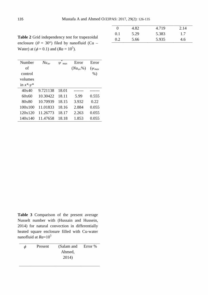
135 Mustafa A and Ahmed O/ZJPAS: 2017, 29(2): 126-135

Table 2 Grid independency test for trapezoidal enclosure (θ = 30°) filed by nanofluid (Cu – Water) at (φ = 0.1) and (Ra = 105).

Table 3 Comparison of the present average Nusselt number with (Hussain and Hussein, 2014) for natural convection in differentially heated square enclosure filled with Cu-water nanofluid at Ra=105

φ Present

(Salam and Ahmed, 2014)

Error %

0 0.1 0.2

4.82 5.29 5.66

4.719 5.383 5.935

2.14 1.7 4.6

Error (ψmax %)

Error (Nuav%)

ψ*max Nuav Number

of control

volumes in x*-y*

------- 0.555 0.22 0.055 0.055 0.055

------- 5.99 3.932 2.884 2.263 1.853

18.01 18.11 18.15 18.16 18.17 18.18

9.721138 10.30422 10.70939 11.01833 11.26773 11.47658

40x40 60x60 80x80

100x100 120x120 140x140

ZANCO Journal of Pure and Applied Sciences The official scientific journal of Salahaddin University-Erbil

ZJPAS (2017), 29 (2); 136-143 http://dx.doi.org/10.21271/ZJPAS.29.2.14

Improve differentiation of Breast mass using fuzzy segmentation method

1Heamn N. Abduljabbara*, 1 Haidar J. Ismailb and 2 Sardar Y. Perxdra

1Department of Physics, College of Education-Shaqlawa, Salahaddin University, Iraq

2Department of Physics, College of Education, Salahaddin University, Iraq.

1. INTRODUCTION

The lesions that have echogenic (solid)

and anechoic (cystic)components known as

Complex cystic masses while those contain just

echogenic fluid which imitates a solid lesion

called Complicated cysts [Cha et al, 2005]. The

first type must use percutaneous biopsy and/or

surgical ablation to get histological

verification. So, according to results it may be

benign or malignant. Histopathological

A R T I C L E I N F O

A B S T R A C T

Article History: Received: 09/08/2016 Accepted: 26/12/2016 Published: 07/06/2017

Breast cancer is one of the almost public types of cancer in women. Breast

masses generally classified to cystic and solid masses and in both, there are many

subtypes. So that understanding exact types of them is useful for better treatment

of the patient. There are clinic invasive techniques for that but image processing

usually seems helpful to get same or better results. Furthermore, an intelligent

computer-aided diagnosis system or proper algorithm can be very helpful for

radiologist in detecting and diagnosing abnormal cases earlier and faster than

typical screening methods. One of the most important image processing is Edge

detection which targets towards image understanding. This study tried to improve

the early detection of breast masses (cystic/solid) from 2D ultrasound scanning,

by running the resulted images of the abnormal cases in image enhancement, edge

detection, furthermore comparing between the resulted 2D images by 3D images,

Elastography, and then thermal detection of breast mass images. Four cases of

different abnormalities taken from 783 patients had been scanned in Harer

hospital by 2D ultrasound B- Mode Linear probe with 7.2 MHz frequency, 47 of

them diagnosed as breast mass. The images were enhanced by adaptive histogram

equalization (AHE) which usually given proper contrast enhancement. Then

appropriate conditions were chosen for Fuzzy set theory to give us proper edge

detection. The result was the obtained 2D images are much more clear for

diagnosis after running into image processing, the mass easily can be detected and

classified into the correct type without using 3D high-cost ultrasound.

.

Keywords: Breast mass, Cyst, Fibroid, Image enhancement, Fuzzy Edge detection.

. *Corresponding Author: Heamn N. Abduljabbara heamn.abduljabbar@su.edu.krd

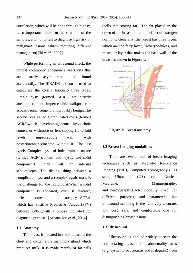
137 Heamn N. et al. /ZJPAS: 2017, 29(5): 136-143 correlation, which will be done through biopsy,

is so important toconfirm the situation of the

samples, and not to fail to diagnose high risk or

malignant lesions which requiring different

management[Zhi et al., 2007].

While performing an ultrasound check, the

utmost commonly appearance are Cysts that

are usually asymptomatic and found

accidentally. The BIRADS lexicon is used to

categorize the Cystic lesionsto three types.

Simple cysts (termed ACR2) are strictly

anechoic content, imperceptible wall,posterior

acoustic enhancement, andprobably benign.The

second type called Complicated cysts (termed

ACR3)which havehomogeneous hypoechoic

content or withmore or less sloping fluid/fluid

levels, imperceptible wall, with

posteriorenhancementor without it. The last

typeis Complex cysts of indeterminate nature

(termed ACR4)contain both cystic and solid

components, thick wall or internal

septum/septa. The distinguishing between a

complicated cyst and a complex cystic mass is

the challenge for the radiologist.When a solid

component is appeared, even if discreet,

thelesion comes into the category ACR4,

which has Positive Predictive Values (PPV)

between 2-95%,with a biopsy indicated for

diagnostic purposes [Athanasiou et al., 2014].

1.1 Anatomy

The breast is situated in the forepart of the

chest and contains the mammary gland which

produces milk. It is made mainly of fat cells

(cells that storing fat). The fat placed in the

down of the breast due to the effect of estrogen

hormone. Generally, the breast has three layers

which are the fatty layer, lactic (nodules), and

muscular layer that makes the base wall of the

breast as shown in Figure 1.

Figure 1: Breast anatomy

1.2 Breast Imaging modalities

There are severalkinds of breast imaging

techniques such as Magnetic Resonance

Imaging (MRI), Computed Tomography (CT)

scan, Ultrasound (US) scanning,Nuclear

Medicine, Mammography,

andThermography.Each modality used for

different purposes, and parameters, but

ultrasound scanning is the relatively accurate,

low cost, safe, and comfortable one for

distinguishing breast lesions.

1.3 Ultrasound

Ultrasound is applied widely to scan the

non-lactating breast to find abnormality cases

(e.g. cysts, fibroadenomas and malignant) from

138 Heamn N. et al. /ZJPAS: 2017, 29(5): 136-143 normal structures (e.g. milk ducts, lymph

nodes, glandular and adipose tissue) [Stavros et

al., 1995]. Furthermore, the capability of

ultrasound increased due to recent

technological advances to determine very small

structures for example ducts small as 0.5 mm

[Sohn et al., 1999].

1.4 Examination techniques

As for any imaging examination, all the

clinical and radiological data is important

before doing and interpreting a breast

ultrasound examination. The ultrasound

technique (B mode) should meet the following

criteria: linear probes of frequencies between

7.2 and 20 MHz (more often 12-14 MHz)

should be used. The frequency must be altered

to the breast volume and the location of lesion

in the breast (small frequency for deep lesions,

large frequency for superficial lesions); total

gain and TGC must use to get proper and

homogeneous signal from the skin to the depth

of the pectoral muscle; the focal zone must be

adjusted in depth according to the lesion; the

lesion should be examined at least in two

planes: transverse and longitudinal. The

another mode useful to characterize the lesion;

the radiologist needs to know their main

characteristics as well as their respective

advantages and disadvantages to getting an

optimize use of them.

Harmonic mode increases spatial

resolution and contrast of the lesion and

reduces artifacts (e.g. reverberation artifacts

from cyst walls) so that posterior ultrasound

variations are seen better. Compound mode

enhances the signal/noise ratio by reducing

background noise and speckle artifact

optimizes analysis of the margin of the lesion

and the internal echo structure of masses. It

also enables better finding of intralesional

calcifications [Doshi at el., 2007]. On the other

hand, posterior ultrasound modifications are

reduced [Candelaria et al., 2013]. Doppler

mode (color and/or power) ought to be

systematic. It presents hints guiding diagnosis:

perilesional hyperemia if lesions are

inflammatory (cysts, abscesses). Doppler box

size can be changed to improve sensitivity and

decrease flow artifacts. Power Doppler is more

sensitive to slow flows but is also more

sensitive to artifacts. It must be remembered

that the lake of a Doppler signal does not mean

that the solid nature of a lesion can be omitted.

Elastography can help to differentiate

complicated cysts by revealing the fluid

component (appear trilaminar or bull's eye in

static mode and signal void in shear mode).

Likewise, if the lesion is found to be very hard,

this help to improve identification of complex

masses and guide percutaneous biopsies

(improving the histological characterization of

the lesion) [Youk et al., 2013].

1.5 Ultrasound signs of complicated cysts

Complicated cysts show all the aspects of

simple cysts except for the content, which is

excellently echogenic. They can show a fluid

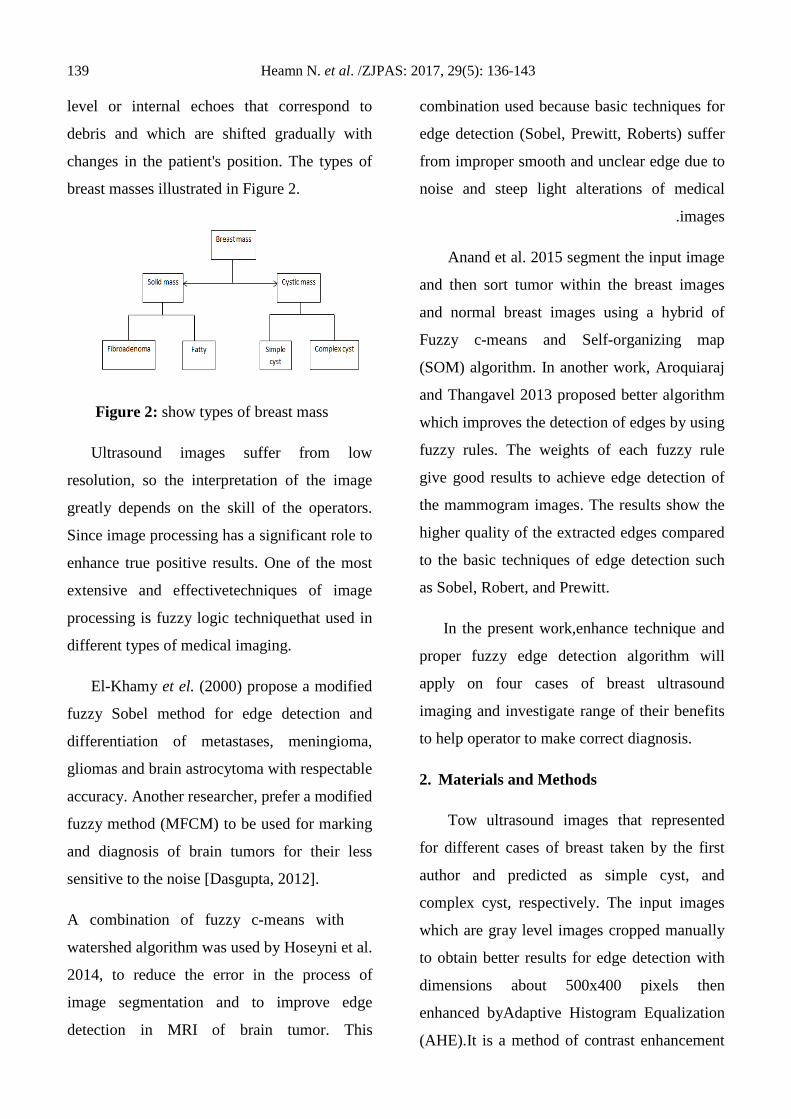
139 Heamn N. et al. /ZJPAS: 2017, 29(5): 136-143 level or internal echoes that correspond to

debris and which are shifted gradually with

changes in the patient's position. The types of

breast masses illustrated in Figure 2.

Figure 2: show types of breast mass

Ultrasound images suffer from low

resolution, so the interpretation of the image

greatly depends on the skill of the operators.

Since image processing has a significant role to

enhance true positive results. One of the most

extensive and effectivetechniques of image

processing is fuzzy logic techniquethat used in

different types of medical imaging.

El-Khamy et el. (2000) propose a modified

fuzzy Sobel method for edge detection and

differentiation of metastases, meningioma,

gliomas and brain astrocytoma with respectable

accuracy. Another researcher, prefer a modified

fuzzy method (MFCM) to be used for marking

and diagnosis of brain tumors for their less

sensitive to the noise [Dasgupta, 2012].

A combination of fuzzy c-means with

watershed algorithm was used by Hoseyni et al.

2014, to reduce the error in the process of

image segmentation and to improve edge

detection in MRI of brain tumor. This

combination used because basic techniques for

edge detection (Sobel, Prewitt, Roberts) suffer

from improper smooth and unclear edge due to

noise and steep light alterations of medical

images .

Anand et al. 2015 segment the input image

and then sort tumor within the breast images

and normal breast images using a hybrid of

Fuzzy c-means and Self-organizing map

(SOM) algorithm. In another work, Aroquiaraj

and Thangavel 2013 proposed better algorithm

which improves the detection of edges by using

fuzzy rules. The weights of each fuzzy rule

give good results to achieve edge detection of

the mammogram images. The results show the

higher quality of the extracted edges compared

to the basic techniques of edge detection such

as Sobel, Robert, and Prewitt.

In the present work,enhance technique and

proper fuzzy edge detection algorithm will

apply on four cases of breast ultrasound

imaging and investigate range of their benefits

to help operator to make correct diagnosis.

2. Materials and Methods

Tow ultrasound images that represented

for different cases of breast taken by the first

author and predicted as simple cyst, and

complex cyst, respectively. The input images

which are gray level images cropped manually

to obtain better results for edge detection with

dimensions about 500x400 pixels then

enhanced byAdaptive Histogram Equalization

(AHE).It is a method of contrast enhancement

140 Heamn N. et al. /ZJPAS: 2017, 29(5): 136-143 that is different from ordinary histogram

equalization. In adaptive method, many

histograms are computed where each histogram

corresponds to a different section of image.

Hence, AHE improves the local contrast of an

image and more details can be observed.Figure

3 shows the main steps of applying fuzzy edge

detection.

Figure 3: shows flow chart of main steps of

applying fuzzy edge detection

2.1 Fuzzy Logic edge detection

As known, the fuzzy algorithm has three

main steps. Two-dimension Gradient Gx and

Gy computed and fuzzified by two Gaussian

membership functions. The rules that modify

membership values is to be white color for both

two gradients with zero value else black color

if one of them don’t zero. Lastly, the resulted

defuzzified by triangular membership function.

Table 1 shows fuzzy sets for input and output

variables and Figure 4 illustrate the main steps

of fuzzy algorithm.

Figure 4: shows flowchart of fuzzy algorithm

Table 1: Fuzzy sets for input and output

variables

Fuzzy sets

Range MF type

P1_input [ 0.1 0] Gaussian

P2_input [ 0.1 0] Gaussian

Poutput White [0.1 1 1]

Black [0 0 0.7]

Triangular

3. Results and Discussion

3.1 Simple Breast cyst

Simple breast cyst defined in the 2D

ultrasound in the original image as shown in

Figure 5a having thin regular wall with clear

fluid filled while Figure 5b shows the same

image after using image enhancement Tanique

in image processing which improves the image

quality as or close to 3D ultrasound image.

The same image after using edge detection,

which shown in Figure 5c, by using Fuzz edge

detection technique. The cyst is clearer and can

be defined even better than infra-red IR or

thermal detection of breast mass as the image

quality is much better than IR (see Figure 5d).

3.2 Complex breast cyst

The complex breast cyst is another type of

breast cysts it can be recognized by ultrasound

scanning as it has the thick irregular outline

and acoustic shadows as shown in Figure 6a

also the fluid inside it is thick fluid, not clear

echogenicity. While Figure 6b shows the same

Input

Fuzzificat

Decisio

Defuzzifica

Fuzzy Rule

Membership Function

141 Heamn N. et al. /ZJPAS: 2017, 29(5): 136-143 cyst after running the image through image

processing software by making image

enhancement which gives us more information

about the cyst from Figure 6c, moreover we

can see the intensity of the wall thickness

clearly after using fuzzy edge detection for the

same image it helps also to detect the severity

of the cyst by defining the outline and the

acoustic shadow as shown in Figure 6d below.

It is clear that the image quality is higher and

better after using Fuzzy edge detection to

detect complex breast cyst than Elastography

as shown in Figure 12.

4. Conclusion

The importance of early accurate diagnosis

of breast masses in early stages resulted in

making this study so that four breast ultrasound

images were segmented through fuzzy edge

detection method and contrast enhanced. All

images were obtained from the correspondent

author from his privet clinic (ultrasound

scanning clinic in Erbil). The fuzzy algorithm

with our proper definitions for all main steps

capable of determining edges of all cases

precisely but it suffer from low contrast. They

were contrast enhanced as the second step.

According to our results, fuzzy edge detection

is a good choice for sonologists to have a

correct decision about suspicious cases related

to breast mass as it is a low-cost method to

increase the image quality of 2D ultrasound.

5. Acknowledgements

The authors would like to express their

acknowledgment to Salahaddin University for

supporting them with available tools. If anyone

who needs the program, please contact the

second author for any additional help.

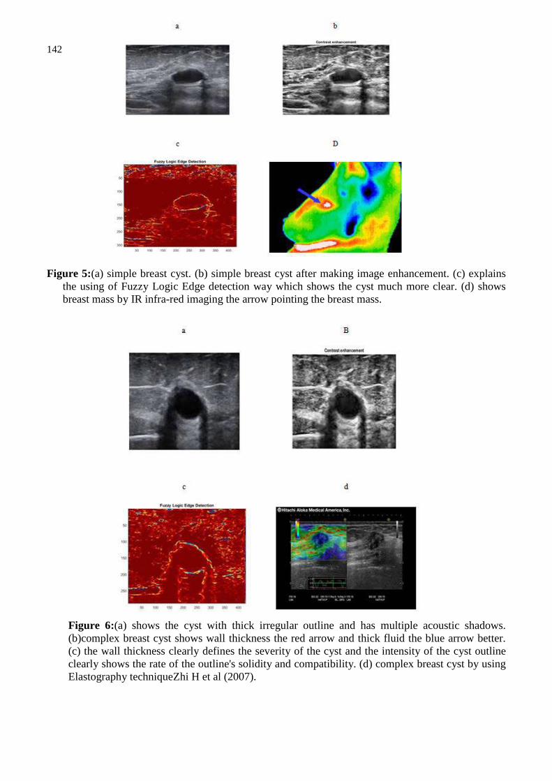
142 Heamn N. et al. /ZJPAS: 2017, 29(5): 136-143

Figure 5:(a) simple breast cyst. (b) simple breast cyst after making image enhancement. (c) explains the using of Fuzzy Logic Edge detection way which shows the cyst much more clear. (d) shows breast mass by IR infra-red imaging the arrow pointing the breast mass.

Figure 6:(a) shows the cyst with thick irregular outline and has multiple acoustic shadows. (b)complex breast cyst shows wall thickness the red arrow and thick fluid the blue arrow better. (c) the wall thickness clearly defines the severity of the cyst and the intensity of the cyst outline clearly shows the rate of the outline's solidity and compatibility. (d) complex breast cyst by using Elastography techniqueZhi H et al (2007).

143 Heamn N. et al. /ZJPAS: 2017, 29(5): 136-143 References

Anand, S., Vinod, V. and Rampure, A., 2015,

Application of Fuzzy c-means and Neural networks

to categorize tumor affected breast MR Images.

International Journal of Applied Engineering

Research, 10(64), p.274-281.

Aroquiaraj, I.L. and Thangavel, K., 2013. Mammogram

Edge Detection Using Hybrid Soft Computing

Methods. arXiv preprint arXiv:1307.4516.

Athanasiou, A., Aubert, E., Salomon, A.V. and

Tardivon, A., 2014. Complex cystic breast masses

in ultrasound examination. Diagnostic and

interventional imaging, 95(2), pp.169-179.

Candelaria, R.P., Hwang, L., Bouchard, R.R. and

Whitman, G.J., 2013, June. Breast ultrasound:

current concepts. In Seminars in Ultrasound, CT

and MRI (Vol. 34, No. 3, pp. 213-225). WB

Saunders.

Cha, J.H., Moon, W.K., Cho, N., Chung, S.Y., Park,

S.H., Park, J.M., Han, B.K., Choe, Y.H., Cho, G.

and Im, J.G., 2005. Differentiation of Benign from

Malignant Solid Breast Masses: Conventional US

versus Spatial Compound Imaging

1. Radiology, 237(3), pp.841-846.

Dasgupta, A., 2012. Demarcation of brain tumor using

modified fuzzy C-means. International Journal of

Engineering Research and Applications, 2(4),

pp.529-533.

Doshi, D.J., March, D.E., Crisi, G.M. and Coughlin,

B.F., 2007. Complex Cystic Breast Masses:

Diagnostic Approach and Imaging-Pathologic

Correlation 1. Radiographics, 27(suppl_1), pp.S53-

S64.

El-Khamy, S.E., Lotfy, M. and El-Yamany, N., 2000. A

modified fuzzy Sobel edge detector. In Radio

Science Conference, 2000. 17th NRSC'2000.

Seventeenth National (pp. C32-1). IEEE.

Hoseyni, F.A.R.N.A.Z., Haghipour, S.I.A.M.A.K. and

Sorkhabi, A., 2014. Improvement of segmentation

on MRI images using fuzzy clustering C-means and

watershed marker control algorithm. Indian J. Sci.

Res, 4(3), pp.447-451.

Sohn, C., Blohmer, J.U. and Hamper, U., 1999. Breast

ultrasound: a systematic approach to technique and

image interpretation. Thieme.

Stavros, A.T., Thickman, D., Rapp, C.L., Dennis, M.A.,

Parker, S.H. and Sisney, G.A., 1995. Solid breast

nodules: use of sonography to distinguish between

benign and malignant lesions. Radiology, 196(1),

pp.123-134.

Youk, J.H., Gweon, H.M., Son, E.J., Han, K.H. and

Kim, J.A., 2013. Diagnostic value of commercially

available shear-wave elastography for breast

cancers: integration into BI-RADS classification

with subcategories of category 4. European

radiology, 23(10), pp.2695-2704.

Zhi, H., Ou, B., Luo, B.M., Feng, X., Wen, Y.L. and

Yang, H.Y., 2007. Comparison of ultrasound

elastography, mammography, and sonography in

the diagnosis of solid breast lesions. Journal of

ultrasound in medicine, 26(6), pp.807-815.

ZANCO Journal of Pure and Applied Sciences The official scientific journal of Salahaddin University-Erbil

ZJPAS (2017), 29 (2); 144-150 http://dx.doi.org/10.21271/ZJPAS.29.2.15

Effect of pitfall trap size on the abundance and diversity of ground dwelling insects in an arable land within Erbil Province- Kurdistan region-Iraq

Khalid Qadir Khidher, Karzan Sabah D.Ahmed and Nawzad Bawakir Kadir

Department of Plant Protection, College of Agriculture, Salahaddin University–Erbil, Erbil, Iraq.

1. INTRODUCTION

Soil is known as one of the richest habitat for various kinds of terrestrial organisms, considering the habitats like vertebrate faeces, decaying wood, epiphytic soils and forest/agricultural or domestic litter (Imam et al., 2016). The community in the soil has been described as ‘poor man's tropical rainforest’ as a result of several factors such as their remarkable biodiversity and undescribed species they contain, and many research gap on their community structure and dynamics (Giller, 1996). Soil biodiversity includes various kinds of terrestrial insects including many ground dwelling insects which spend at

least one stage of their life cycle in the soil(Imam et al., 2016; Klein, 1988); influencing the diversity of plant communities, competitive interactions among plants and the yield of agricultural systems(Hunter, 2001).All of the major winged insect orders—the Coleoptera (beetles), Lepidoptera (butterflies and moths), Hymenoptera (bees, wasps and ants), and Diptera (flies)—include soil-dwelling species. The Isoptera (termites) are essentially soil insects and are saprophages. The Homoptera (aphids, cicadas), Orthoptera (grasshoppers and crickets), and minor orders such as the Dermaptera (earwigs) contain soil-dwelling species or life history stages. Indeed,

A R T I C L E I N F O

A B S T R A C T

Article History: Received: 14/08/2016 Accepted: 28/12/2016 Published: 07/06/2017

The abundance and diversity of ground dwelling insects in an arable land within Erbil Province- Kurdistan region-Iraq were investigated using four different pitfall trap sizes (10 cm, 13cm, 16cm and 19 cm diameter respectively). Five insect orders were reported with fourteen insect families. The order Diptera was the most abundant insect taxa recovered (372.9) followed by orders Hymenoptera (328.8), Coleoptera (268.4), Lepidoptera (26.7) and Hemiptera (6.4). The size of pitfall trap affected the abundance and diversity of the taxa. The highest number (450.7) of soil dwelling insects was observed in 19 cm diameter pitfall traps followed by 16cm (231.2), 13cm (198.4) and 10cm (123) respectively; suggesting that the 19cm diameter pitfall trap size may be an effective method for sampling and monitoring soil dwelling insects of arable lands in our region mainly field crops.

Keywords: Below ground Pitfall trap Soil fauna Soil insects Soil biodiversity *Corresponding Author: Khalid Qadir Khidher

khalid.khidher@su.edu.krd

145 Khidher Q. et al. /ZJPAS: 2017, 29(2): 144-150 of the 26 pterygote insect orders, all but seven contain at least some species that are involved in soil food webs in one way or another (Greenslade, 1985).Some soil insects are phytophagous and feeding on plant roots and/or soil movers; thus having economic importance as crop feeders such asthe order Homoptera, cicadas, aphids, and others (Callahamet al., 2000), Coleoptera (wireworms, wheat ground beetle etc.) (Bassett, 1978 and Milosavljevićet al., 2016), and Lepidoptera larvae (cutworms) (Lemicet al., 2016). Conversely, some others are acting as biological control agents such as many coleopteran carabid and rove beetles (Lang et al., 1999; Josephet al., 2015; Kulkarniet al., 2015and Saito, T. & Brownbridge, M. 2016). The use of pitfall trapping is known to be a very effective and useful method for sampling and monitoring soil insects (both pest and none pest species) since they are economical, eco-friendly and easy to use in the field (Schauff, 2001). They have been used for monitoring and population study of various arthropods in different ecosystems for example forest ecosystems (Bury and Corn, 1987; Majer, 1978 andOlson, 1991), grasslands and winter wheat fields (French and Elliott, 1999;Soppet al., 1987 and Standen, 2000), horticulture (Audisio, 1990 and Ester and Van Rozen, 2005) and vegetated margins of different arable fields (Thomas and Marshall, 1999).Despite their wide use in the ecological study of soil dwelling arthropods, the pitfall trap catches may be affected by several factors for example the use of baits and pheromones associated with pitfall traps are known to affect pitfall trap catches (Ester and Van Rozen, 2005; Greensladed, 1971),pitfall trap spacing (Larsen and Forsyth, 2005 and Ward et al., 2001), the shape of pitfall trap (Luff, 1975) and habitat structure (Melbourne, 1999). Despite the limited studies on the effect of pitfall trap size on certain arthropods such as spiders (Brennan

et al., 1999)however, little is known about the effect of pitfall trap size on the abundance and diversity of ground dwelling insects in arable lands and such studies are lacking in our region. This is particularly important for monitoring and integrated pest management of pest species in soils of field crops such as wheat and barley in our region. Therefore, the current study was undertaken to: 1- Detect the ground dwelling insects available at Grdarasha arable lands (pest and none pest species). 2- Determine the effect of different pitfall trap size on species biodiversity and richness at the selected study site. 2. MATERIALS AND METHODS

The survey was initiated at Grdarasha field station-Erbil from the beginning of February 2016 to the beginning of May2016 using pitfall traps. The sampling station was selected using Randomized Complete Block Design (RCBD) using four different sized pitfall traps (10cm, 13cm, 16cm and 19 cm diameter) each with three replicates (blocks) to provide an even coverage of the study area of the arable lands. In each block the four different sized pitfall traps were installed, these comprised of plastic cups set side by side with a distance of 5 meters between them over which a square of transparent plastic was supported on metal tent pegs (Figure 1) in order to prevent flooding of the traps by the irrigation system, protection from rain and predation by other animals (e.g. birds).The cups were half full of water with the addition of some alcohol (ethanol 25%) which acts as a bactericide and thus prevents decay of the catch. It is also nontoxic to mammals and thus was not a hazard to visitors. The pitfall traps were emptied every 7 days over the study period. Samples were kept in 70% ethanol (both mature and immature stages) and then transported and kept in laboratory for identification. Insects were identified to family

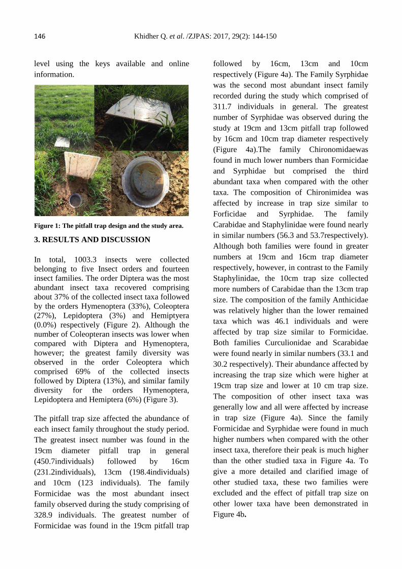
146 Khidher Q. et al. /ZJPAS: 2017, 29(2): 144-150 level using the keys available and online information.

Figure 1: The pitfall trap design and the study area.

3. RESULTS AND DISCUSSION

In total, 1003.3 insects were collected belonging to five Insect orders and fourteen insect families. The order Diptera was the most abundant insect taxa recovered comprising about 37% of the collected insect taxa followed by the orders Hymenoptera (33%), Coleoptera (27%), Lepidoptera (3%) and Hemiptyera (0.0%) respectively (Figure 2). Although the number of Coleopteran insects was lower when compared with Diptera and Hymenoptera, however; the greatest family diversity was observed in the order Coleoptera which comprised 69% of the collected insects followed by Diptera (13%), and similar family diversity for the orders Hymenoptera, Lepidoptera and Hemiptera (6%) (Figure 3).

The pitfall trap size affected the abundance of each insect family throughout the study period. The greatest insect number was found in the 19cm diameter pitfall trap in general (450.7individuals) followed by 16cm (231.2individuals), 13cm (198.4individuals) and 10cm (123 individuals). The family Formicidae was the most abundant insect family observed during the study comprising of 328.9 individuals. The greatest number of Formicidae was found in the 19cm pitfall trap

followed by 16cm, 13cm and 10cm respectively (Figure 4a). The Family Syrphidae was the second most abundant insect family recorded during the study which comprised of 311.7 individuals in general. The greatest number of Syrphidae was observed during the study at 19cm and 13cm pitfall trap followed by 16cm and 10cm trap diameter respectively (Figure 4a).The family Chironomidaewas found in much lower numbers than Formicidae and Syrphidae but comprised the third abundant taxa when compared with the other taxa. The composition of Chironimidea was affected by increase in trap size similar to Forficidae and Syrphidae. The family Carabidae and Staphylinidae were found nearly in similar numbers (56.3 and 53.7respectively). Although both families were found in greater numbers at 19cm and 16cm trap diameter respectively, however, in contrast to the Family Staphylinidae, the 10cm trap size collected more numbers of Carabidae than the 13cm trap size. The composition of the family Anthicidae was relatively higher than the lower remained taxa which was 46.1 individuals and were affected by trap size similar to Formicidae. Both families Curculionidae and Scarabidae were found nearly in similar numbers (33.1 and 30.2 respectively). Their abundance affected by increasing the trap size which were higher at 19cm trap size and lower at 10 cm trap size. The composition of other insect taxa was generally low and all were affected by increase in trap size (Figure 4a). Since the family Formicidae and Syrphidae were found in much higher numbers when compared with the other insect taxa, therefore their peak is much higher than the other studied taxa in Figure 4a. To give a more detailed and clarified image of other studied taxa, these two families were excluded and the effect of pitfall trap size on other lower taxa have been demonstrated in Figure 4b.

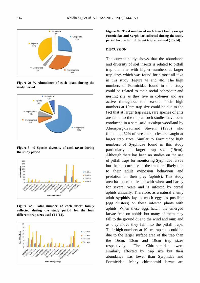
147 Khidher Q. et al. /ZJPAS: 2017, 29(2): 144-150

Figure 2: % Abundance of each taxon during the study period

Figure 3: % Species diversity of each taxon during the study period

Figure 4a: Total number of each insect family collected during the study period for the four different trap sizes used (T1-T4).

Figure 4b: Total number of each insect family except Formicidae and Syrphidae collected during the study period for the four different trap sizes used (T1-T4).

DISCUSSION:

The current study shows that the abundance and diversity of soil insects is related to pitfall trap diameter with higher numbers at larger trap sizes which was found for almost all taxa in this study (Figure 4a and 4b). The high numbers of Formicidae found in this study could be related to their social behaviour and nesting site as they live in colonies and are active throughout the season. Their high numbers at 19cm trap size could be due to the fact that at larger trap sizes, rare species of ants are fallen to the trap as such studies have been conducted in a semi-arid eucalypt woodland by Abensperg‐Traunand Steven, (1995) who found that 52% of rare ant species are caught at larger trap sizes. Similar to Formicidae high numbers of Syrphidae found in this study particularly at larger trap size (19cm). Although there has been no studies on the use of pitfall traps for monitoring Syrphidae larvae but their occurrence in the traps are likely due to their adult oviposion behaviour and predation on their prey (aphids). This study area has been cultivated with wheat and barley for several years and is infested by cereal aphids annually. Therefore, as a natural enemy adult syrphids lay as much eggs as possible (egg clusters) on these infested plants with aphids. When these eggs hatch, the emerged larvae feed on aphids but many of them may fall to the ground due to the wind and rain; and as they move they fall into the pitfall traps. Their high numbers at 19 cm trap size could be due to the larger surface area of the trap than the 16cm, 13cm and 10cm trap sizes respectively. `The Chironomidae were similarly affected by trap size but their abundance was lower than Syrphidae and Formicidae. Many chironomid larvae are

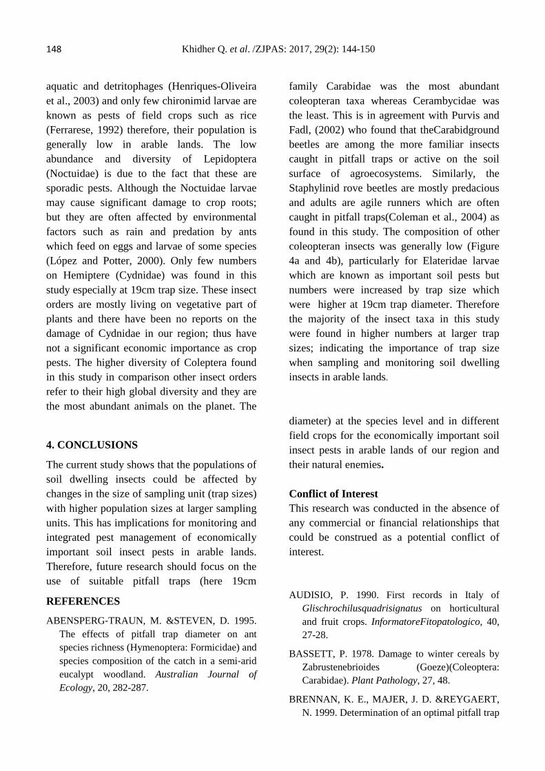
148 Khidher Q. et al. /ZJPAS: 2017, 29(2): 144-150 aquatic and detritophages (Henriques-Oliveira et al., 2003) and only few chironimid larvae are known as pests of field crops such as rice (Ferrarese, 1992) therefore, their population is generally low in arable lands. The low abundance and diversity of Lepidoptera (Noctuidae) is due to the fact that these are sporadic pests. Although the Noctuidae larvae may cause significant damage to crop roots; but they are often affected by environmental factors such as rain and predation by ants which feed on eggs and larvae of some species (López and Potter, 2000). Only few numbers on Hemiptere (Cydnidae) was found in this study especially at 19cm trap size. These insect orders are mostly living on vegetative part of plants and there have been no reports on the damage of Cydnidae in our region; thus have not a significant economic importance as crop pests. The higher diversity of Coleptera found in this study in comparison other insect orders refer to their high global diversity and they are the most abundant animals on the planet. The

family Carabidae was the most abundant coleopteran taxa whereas Cerambycidae was the least. This is in agreement with Purvis and Fadl, (2002) who found that theCarabidground beetles are among the more familiar insects caught in pitfall traps or active on the soil surface of agroecosystems. Similarly, the Staphylinid rove beetles are mostly predacious and adults are agile runners which are often caught in pitfall traps(Coleman et al., 2004) as found in this study. The composition of other coleopteran insects was generally low (Figure 4a and 4b), particularly for Elateridae larvae which are known as important soil pests but numbers were increased by trap size which were higher at 19cm trap diameter. Therefore the majority of the insect taxa in this study were found in higher numbers at larger trap sizes; indicating the importance of trap size when sampling and monitoring soil dwelling insects in arable lands.

4. CONCLUSIONS

The current study shows that the populations of soil dwelling insects could be affected by changes in the size of sampling unit (trap sizes) with higher population sizes at larger sampling units. This has implications for monitoring and integrated pest management of economically important soil insect pests in arable lands. Therefore, future research should focus on the use of suitable pitfall traps (here 19cm

diameter) at the species level and in different field crops for the economically important soil insect pests in arable lands of our region and their natural enemies. Conflict of Interest This research was conducted in the absence of any commercial or financial relationships that could be construed as a potential conflict of interest.

REFERENCES

ABENSPERG‐TRAUN, M. &STEVEN, D. 1995. The effects of pitfall trap diameter on ant species richness (Hymenoptera: Formicidae) and species composition of the catch in a semi‐arid eucalypt woodland. Australian Journal of Ecology, 20, 282-287.

AUDISIO, P. 1990. First records in Italy of Glischrochilusquadrisignatus on horticultural and fruit crops. InformatoreFitopatologico, 40, 27-28.

BASSETT, P. 1978. Damage to winter cereals by Zabrustenebrioides (Goeze)(Coleoptera: Carabidae). Plant Pathology, 27, 48.

BRENNAN, K. E., MAJER, J. D. &REYGAERT, N. 1999. Determination of an optimal pitfall trap

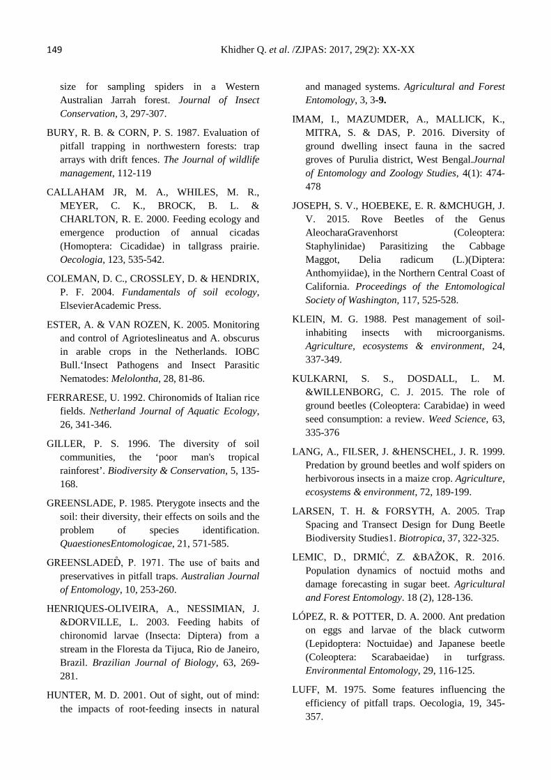
149 Khidher Q. et al. /ZJPAS: 2017, 29(2): XX-XX

size for sampling spiders in a Western Australian Jarrah forest. Journal of Insect Conservation, 3, 297-307.

BURY, R. B. & CORN, P. S. 1987. Evaluation of pitfall trapping in northwestern forests: trap arrays with drift fences. The Journal of wildlife management, 112-119

CALLAHAM JR, M. A., WHILES, M. R., MEYER, C. K., BROCK, B. L. & CHARLTON, R. E. 2000. Feeding ecology and emergence production of annual cicadas (Homoptera: Cicadidae) in tallgrass prairie. Oecologia, 123, 535-542.

COLEMAN, D. C., CROSSLEY, D. & HENDRIX, P. F. 2004. Fundamentals of soil ecology, ElsevierAcademic Press.

ESTER, A. & VAN ROZEN, K. 2005. Monitoring and control of Agrioteslineatus and A. obscurus in arable crops in the Netherlands. IOBC Bull.‘Insect Pathogens and Insect Parasitic Nematodes: Melolontha, 28, 81-86.

FERRARESE, U. 1992. Chironomids of Italian rice fields. Netherland Journal of Aquatic Ecology, 26, 341-346.

GILLER, P. S. 1996. The diversity of soil communities, the ‘poor man's tropical rainforest’. Biodiversity & Conservation, 5, 135-168.

GREENSLADE, P. 1985. Pterygote insects and the soil: their diversity, their effects on soils and the problem of species identification. QuaestionesEntomologicae, 21, 571-585.

GREENSLADED, P. 1971. The use of baits and preservatives in pitfall traps. Australian Journal of Entomology, 10, 253-260.

HENRIQUES-OLIVEIRA, A., NESSIMIAN, J. &DORVILLE, L. 2003. Feeding habits of chironomid larvae (Insecta: Diptera) from a stream in the Floresta da Tijuca, Rio de Janeiro, Brazil. Brazilian Journal of Biology, 63, 269-281.

HUNTER, M. D. 2001. Out of sight, out of mind: the impacts of root‐feeding insects in natural

and managed systems. Agricultural and Forest Entomology, 3, 3-9.

IMAM, I., MAZUMDER, A., MALLICK, K., MITRA, S. & DAS, P. 2016. Diversity of ground dwelling insect fauna in the sacred groves of Purulia district, West Bengal.Journal of Entomology and Zoology Studies, 4(1): 474-478

JOSEPH, S. V., HOEBEKE, E. R. &MCHUGH, J. V. 2015. Rove Beetles of the Genus AleocharaGravenhorst (Coleoptera: Staphylinidae) Parasitizing the Cabbage Maggot, Delia radicum (L.)(Diptera: Anthomyiidae), in the Northern Central Coast of California. Proceedings of the Entomological Society of Washington, 117, 525-528.

KLEIN, M. G. 1988. Pest management of soil-inhabiting insects with microorganisms. Agriculture, ecosystems & environment, 24, 337-349.

KULKARNI, S. S., DOSDALL, L. M. &WILLENBORG, C. J. 2015. The role of ground beetles (Coleoptera: Carabidae) in weed seed consumption: a review. Weed Science, 63, 335-376

LANG, A., FILSER, J. &HENSCHEL, J. R. 1999. Predation by ground beetles and wolf spiders on herbivorous insects in a maize crop. Agriculture, ecosystems & environment, 72, 189-199.

LARSEN, T. H. & FORSYTH, A. 2005. Trap Spacing and Transect Design for Dung Beetle Biodiversity Studies1. Biotropica, 37, 322-325.

LEMIC, D., DRMIĆ, Z. &BAŽOK, R. 2016. Population dynamics of noctuid moths and damage forecasting in sugar beet. Agricultural and Forest Entomology. 18 (2), 128-136.

LÓPEZ, R. & POTTER, D. A. 2000. Ant predation on eggs and larvae of the black cutworm (Lepidoptera: Noctuidae) and Japanese beetle (Coleoptera: Scarabaeidae) in turfgrass. Environmental Entomology, 29, 116-125.

LUFF, M. 1975. Some features influencing the efficiency of pitfall traps. Oecologia, 19, 345-357.

150 Khidher Q. et al. /ZJPAS: 2017, 29(2): XX-XX MAJER, J. 1978. An improved pitfall trap for

sampling ants and other epigaeic invertebrates. Australian Journal of Entomology, 17, 261-262.

MELBOURNE, B. A. 1999. Bias in the effect of habitat structure on pitfall traps: an experimental evaluation. Australian Journal of Ecology, 24, 228-239.

MILOSAVLJEVIĆ, I., ESSER, A. D. & CROWDER, D. W. 2016. Seasonal population dynamics of wireworms in wheat crops in the Pacific Northwestern United States. Journal of Pest Science, 1-10.

OLSON, D. M. 1991. A comparison of the efficacy of litter sifting and pitfall traps for sampling leaf litter ants (Hymenoptera, Formicidae) in a tropical wet forest, Costa Rica. Biotropica, 166-172.

PURVIS, G., AND FADEL, A. (2002). The influence of cropping rotations and soil cultivationpractice on the population ecology of carabids (Coleoptera: Carabidae) in arable land.Pedobiologia 46, 452–474.

SAITO, T. &BROWNBRIDGE, M. 2016. Compatibility of soil-dwelling predators and microbial agents and their efficacy in controlling soil-dwelling stages of western flower thripsFrankliniellaoccidentalis. Biological Control, 92, 92-100.

SCHAUFF, M. E. 2001. Collecting and preserving insects and mites: techniques & tools, Systematic Entomology Laboratory, USDA.

SOPP, P., SUNDERLAND, K. & COOMBES, D. 1987. Observations on the number of cereal aphids on the soil in relation to aphid density in winter wheat. Annals of Applied Biology, 111, 53-57.

STANDEN, V. 2000. The adequacy of collecting techniques for estimating species richness of grassland invertebrates. Journal of Applied Ecology, 37, 884-893.

THOMAS, C. & MARSHALL, E. 1999. Arthropod abundance and diversity in differently vegetated margins of arable fields. Agriculture, Ecosystems & Environment, 72, 131-144.

ZANCO Journal of Pure and Applied Sciences

The official scientific journal of Salahaddin University-Erbil

ZJPAS (2017), 29 (2); 151-156

http://dx.doi.org/10.21271/ZJPAS.29.2.16

Sero-prevalence of TORCH among pregnant and non-

pregnant women by ELISA and One step TORCH assay in

Erbil city of Kurdistan region, Iraq

Hemdad Hawez Mawlood1, Wijdan Mohammed Salih Mero

1, Ronak Ali Ismail

2 Abdallah Mohamad Isa

3

1Department of Biology, Faculty of Science, University of Zakho- Kurdistan region/Iraq

2Erbil Maternity Teaching Hospital

3Department of Biological Science, School of Life and Physical Sciences, Tennessee State University, USA

1. INTRODUCTION

TORCH group includes T. gondii, others

such as; Coxsakievirus, Syphilis, Varicella-

Zoster virus, HIV, etc. then Rubella,

Cytomegalovirus and Herpes simplex virus

type I and type II (Franca and Mugayar, 2004).

These agents gain access to the fetal blood

stream transplacentally via the chorionic villi.

Hematogenous transmission may occur at any

time during gestation or occasionally at the

time of delivery via maternal- to-Fetal

transfusion (Kumar et al., 2009).

The TORCH infection is the major cause of

Bad Obstetric history (BOD) which implies

previous unfavorable fetal outcome in terms of

two or more consecutive spontaneous

abortions, intrauterine growth retardations,

congenital anomalies and maternal infections

transmissible in utero at various stages of

gestation lead to recurrent pregnancy wastage

(Cabe and Remington, 1988). TORCH

infection usually occurs before the woman

realizes that she is pregnant or seeks medical

attention. The primary infection is likely to

have more important effect on fetus than

A R T I C L E I N F O

A B S T R A C T

Article History:

Received: 15/08/2016

Accepted: 28/12/2016

Published: 07/06/2017

The present study was conducted to detect the sero-prevalence of anti-

TORCH antibodies (Toxoplasma gondii, Rubella virus, Cytomegalovirus,

Herpes simplex virus type-II) among pregnant and non-pregnant women from

different ages (18≥48 years) in Erbil city and their relation with age and

infertility, by using ELISA (Enzyme linked immunosorbent assay) and One-

step TORCH assay. A total of 313 sera samples (150 pregnant and 90 women

were suffering from infertility and 73 fertile non-pregnant) were enrolled in the

study. In the age group 18-27 years showed the highest seropositive IgG by

ELISA test, were 21, 20, 17 and 13% for Rubella, CMV, HSV-II and

Toxoplasma gondii, respectively. The seropositive for ELISA TORCH –IgM

test/seropositive for one step TORCH- IgM test was 45/14% The comparison

of ELISA test with one-step TORCH test for detection acute TORCH infections

was significant. Hence, it could be concluded that ELISA test is more

efficacious than One-step TORCH test and There are no significant differences

among ages with the TORCH infection. Also, in infertility cases high rate of T.

gondii was observed among other TORCH groups.

Keywords:

TORCH,

Pregnancy,

Infertility

*Corresponding Author:

Hemdad H. Mawlood

Hemdadtn@gmail.com

152 Mawlood H. et al. /ZJPAS: 2017, 29 (2): 151-156

recurrent infection While each of congenital

infection possesses distinct clinical

manifestation some of these infections share

certain characteristics, therefore, it is important

to know the effect of each of them. (Maruyama

et al., 2007). In Iraq, few serological studies

have been carried out on TORCH infection. A

study in Kirkuk city showed that the rate of

TORCH infection was 71.82%. The

contribution of CMV, T. gondii, Rubella, and

HSV-II in this rate were 34.92, 26.68, 21.03,

and 16.06% respectively (Mohammad and

Salman, 2014), In Erbil city (Amin et.al.2012),

showed that T. gondii was a major parameter

among TORCH groups.

In Duhok city, a study by (Amedi,2013)

indicated that seropositivity of TORCH

infections was significantly higher in women

with BOH than normal pregnant women with

previous normal full term deliveries.

This attempt was carried out to correlate

TORCH infection during pregnancy and their

relation with age and infertility among

pregnant and non-pregnant women by using

ELISA and one step TORCH assay in Erbil

city capital of Kurdistan region /Iraq.

2. Subjects, Materials and Methods

2.1 Study subjects

This study was carried out from October 2013

to October 2014 in Erbil city/Kurdistan

region/Iraq, 313 Blood samples were collected

from women (150 pregnant, and 90 women

were suffering from infertility and 73 fertile

non-pregnant) of different ages (18 to > 48)

years. Each woman participated in this study

requested to fill out a questionnaire form

related with the age, primary and secondary

infertility.

2.2 Sample collection

Five ml of venous blood was drawn aseptically

from both groups. The sera were separated by

centrifuge at 3000 rpm for 5 minutes, and then

stored at -20Ċ until used for serological testing.

2.3 Methods

1-ELISA IgG and IgM:

All the serum samples collected were tested for

T. gondii, CMV, Rubella, and HSV-II, IgG and

IgM antibodies using commercial ELISA kits

(Bio Check, Inc., USA) which proofed by

federal drug administration and International

standards organization (ISO)

The results were calculated by ELISA reader

and they were interpreted as positive, equivocal

or negative by determining the

immunoglobulin index. IgG or IgM indexes

values <0.9, 0.9-0.99 and >1.0 were suggestive

for negative, equivocal and positive,

respectively.

2-One Step TORCH IgM:

All sero-positive IgM samples of T. gondii,

CMV, Rubella, and HSV-II were tested by

one-step TORCH Panel IgM test, (Health-

CHEM Diagnostics LLC, USA) the kit was

proofed by Federal drug administration

(FDA).and International standards organization

(ISO) The results were interpreted as

following:

Positive: Rose-pink color band in the Control

region(C) and in the test region (T)

Negative: Rose-Pink color band in Control

region only.

Invalid: No Rose-pink color band in the

Control region.

2.4 Statistical Analysis

A Chi-square (and Fisher’s exact) test was

used to analyze the differences of Torch sero-

prevalence by graph pad prism v.5.01Pakage

between the tested groups.

Results

The results presented in (Table 1 and Table

2) by ELISA regarding age group there were

no significant differences among ages with the

153 Mawlood H. et al. /ZJPAS: 2017, 29 (2): 151-156

TORCH infection for both IgG and IgM. The

highest seropositivity of TORCH IgG in age 18

to 27 years were recorded 21, 20, 17 and 13%.

For Rubella, CMV, HSV-II and T. gondii

respectively(Table.1). The highest

seropositvitly for TORCH IgM in age 28 to 37

years was recorded 5.4, 5, 3 and 2.6% for T.

gondii, CMV, HSV-2 and Rubella respectively

(Table .2).

The occurrences of TORCH IgG infection

among secondary infertility were recorded as

27, 7, 5 and 5% for T. gondii, Rubella, HSV-II

and CMV respectively. T. gondii IgG in

secondary infertility cases (27%) was higher

than T. gondii (13%) in primary infertility

cases. Also T. gondii IgM (8%) in secondary

infertility cases was higher than T. gondii IgM

(3%) in primary infertility cases.

Considering the role of immunological

techniques for detecting IgM antibodies for

TORCH infection (Table 3), the rate of ELISA

TORCH IgM (45%) was higher than One-step

TORCH IgM (14%).

4. Discussion:

The highest chronic TORCH infection

occurred among youngest aged when compared

with other ages. (Table 1 and Table 2) This

outcome due to the fact that this group was

most exposure to risk infection sources that

lead to chronic infection especially for

Toxoplasmosis (Srirup et al., 2011). This result

disagrees with the study in Duhok (Amedi,

2013) who had recorded low infection of

TORCH among young aged group.

The highest acute TORCH infection occurred

among age group 28 to 37 and the T. gondii

was highest whereas Rubella was lowest when

compared with other age groups. (Table 2)

According to T. gondii infection rate, the

current results for T. gondii IgG and IgM are in

accordance with (Hamad, 2009) in Erbil city/

Iraq

According to the distribution of TORCH

positives among 90 infertility cases in current

study The TORCH IgG and IgM positives were

high among secondary infertility cases more

than primary infertility cases also, T. gondii

IgG was the highest one among TORCH

infection in primary and secondary infertility

cases. The previous research of lab animals

recorded that infection with T. gondii could be

a cause of infertility in experimental mice

(Stahl et al., 1994; Terpsidis et al., 2009).

In current study recorded a causative relation

between chronic toxoplasmosis and infertility,

this is similar to each of (Li et al., 2011) in

China and (EL-Tantawy et al., 2014) in Egypt.

In our finding chronic toxoplasmosis and acute

toxoplasmosis in secondary infertility were

higher than primary infertility. these results can

be explained by the hypothesis that in women

during toxoplasmosis the proliferate

tachyzoites may invade female reproductive

organ specially the oviducts, subsequently

evoke tissue cysts formation in it, that may

produce tubule dysfunctions, and leads to

hormonal abnormalities which give rises into

secondary infertility sequels (Salman,2014).

Also, toxoplasmosis leads to low level of anti-

Mullerian hormone (AMH) in women, this

hormone seems to be the best endocrine marker

for growth follicles also it has a potential

ability to predict future reproductive life span

(Guyton and Hall, 2006).

In Babylon city in Iraq (Areej, 2012) stated

that CMV and Rubella were higher than T.

gondii among secondary infertility cases and

this is in disagreement with recent study.

Considering role of immunological techniques

for detecting acute TORCH infection the

ELISA efficacy higher than one step TORCH,

it could be explaining that ELISA method has

high affinity reaction occurs between TORCH

antibodies and coated antigen in the bottom of

ELISA well than the reaction between antigen

coated on immobilized antibodies in one step

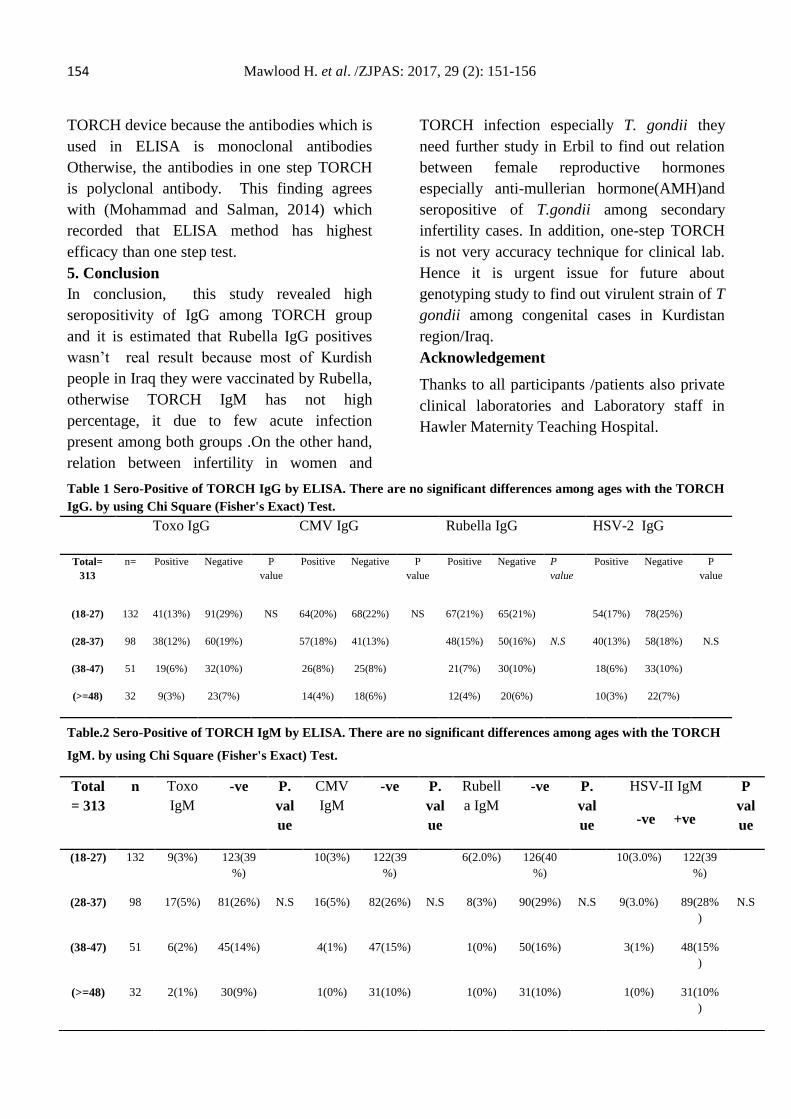
154 Mawlood H. et al. /ZJPAS: 2017, 29 (2): 151-156

TORCH device because the antibodies which is

used in ELISA is monoclonal antibodies

Otherwise, the antibodies in one step TORCH

is polyclonal antibody. This finding agrees

with (Mohammad and Salman, 2014) which

recorded that ELISA method has highest

efficacy than one step test.

5. Conclusion

In conclusion, this study revealed high

seropositivity of IgG among TORCH group

and it is estimated that Rubella IgG positives

wasn’t real result because most of Kurdish

people in Iraq they were vaccinated by Rubella,

otherwise TORCH IgM has not high

percentage, it due to few acute infection

present among both groups .On the other hand,

relation between infertility in women and

TORCH infection especially T. gondii they

need further study in Erbil to find out relation

between female reproductive hormones

especially anti-mullerian hormone(AMH)and

seropositive of T.gondii among secondary

infertility cases. In addition, one-step TORCH

is not very accuracy technique for clinical lab.

Hence it is urgent issue for future about

genotyping study to find out virulent strain of T

gondii among congenital cases in Kurdistan

region/Iraq.

Acknowledgement

Thanks to all participants /patients also private

clinical laboratories and Laboratory staff in

Hawler Maternity Teaching Hospital.

Table 1 Sero-Positive of TORCH IgG by ELISA. There are no significant differences among ages with the TORCH

IgG. by using Chi Square (Fisher's Exact) Test.

Toxo IgG CMV IgG Rubella IgG HSV-2 IgG

Total=

313

n= Positive Negative P

value

Positive Negative P

value

Positive Negative P

value

Positive Negative P

value

(18-27) 132 41(13%) 91(29%) NS 64(20%) 68(22%) NS 67(21%) 65(21%) 54(17%) 78(25%)

(28-37) 98 38(12%) 60(19%) 57(18%) 41(13%) 48(15%) 50(16%) N.S 40(13%) 58(18%) N.S

(38-47) 51 19(6%) 32(10%) 26(8%) 25(8%) 21(7%) 30(10%) 18(6%) 33(10%)

(>=48) 32 9(3%) 23(7%) 14(4%) 18(6%) 12(4%) 20(6%) 10(3%) 22(7%)

Table.2 Sero-Positive of TORCH IgM by ELISA. There are no significant differences among ages with the TORCH

IgM. by using Chi Square (Fisher's Exact) Test.

Total

= 313

n Toxo

IgM

-ve P.

val

ue

CMV

IgM

-ve P.

val

ue

Rubell

a IgM

-ve P.

val

ue

HSV-II IgM

-ve +ve

P

val

ue

(18-27) 132 9(3%) 123(39

%)

10(3%) 122(39

%)

6(2.0%) 126(40

%)

10(3.0%) 122(39

%)

(28-37) 98 17(5%) 81(26%) N.S 16(5%) 82(26%) N.S 8(3%) 90(29%) N.S 9(3.0%) 89(28%

)

N.S

(38-47) 51 6(2%) 45(14%) 4(1%) 47(15%) 1(0%) 50(16%) 3(1%) 48(15%

)

(>=48) 32 2(1%) 30(9%) 1(0%) 31(10%) 1(0%) 31(10%) 1(0%) 31(10%

)

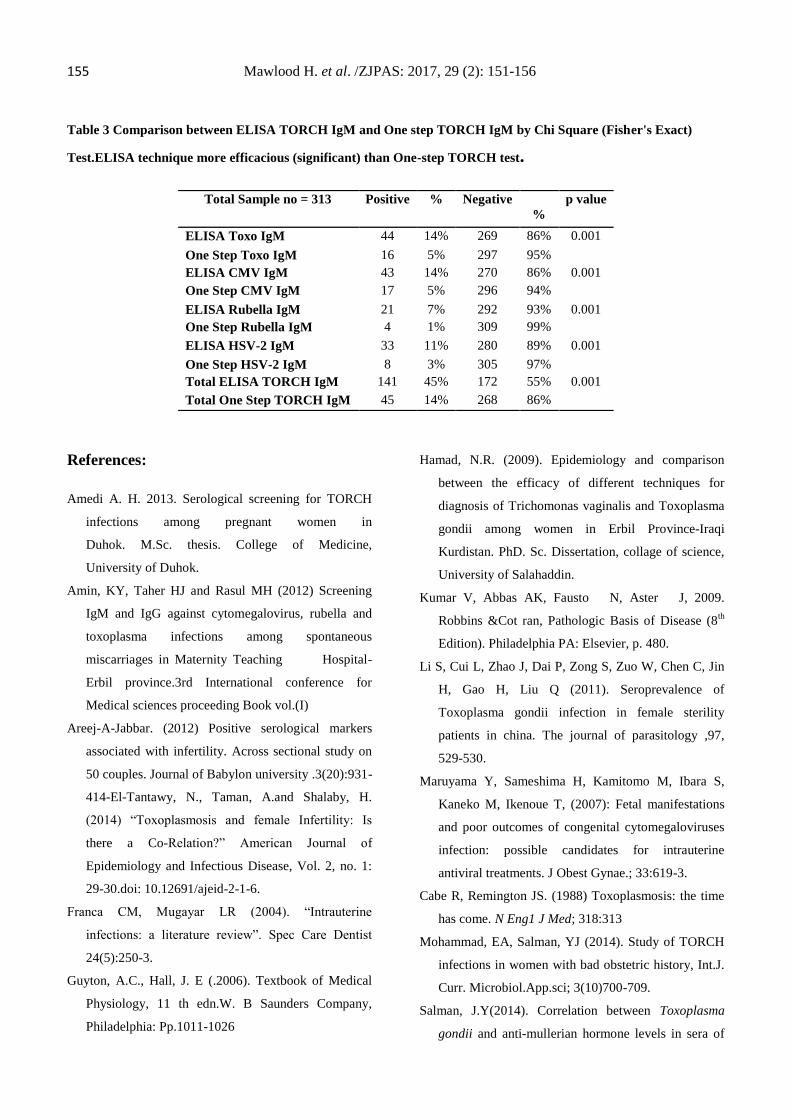
155 Mawlood H. et al. /ZJPAS: 2017, 29 (2): 151-156

Table 3 Comparison between ELISA TORCH IgM and One step TORCH IgM by Chi Square (Fisher's Exact)

Test.ELISA technique more efficacious (significant) than One-step TORCH test.

References:

Amedi A. H. 2013. Serological screening for TORCH

infections among pregnant women in

Duhok. M.Sc. thesis. College of Medicine,

University of Duhok.

Amin, KY, Taher HJ and Rasul MH (2012) Screening

IgM and IgG against cytomegalovirus, rubella and

toxoplasma infections among spontaneous

miscarriages in Maternity Teaching Hospital-

Erbil province.3rd International conference for

Medical sciences proceeding Book vol.(I)

Areej-A-Jabbar. (2012) Positive serological markers

associated with infertility. Across sectional study on

50 couples. Journal of Babylon university .3(20):931-

414-El-Tantawy, N., Taman, A.and Shalaby, H.

(2014) “Toxoplasmosis and female Infertility: Is

there a Co-Relation?” American Journal of

Epidemiology and Infectious Disease, Vol. 2, no. 1:

29-30.doi: 10.12691/ajeid-2-1-6.

Franca CM, Mugayar LR (2004). “Intrauterine

infections: a literature review”. Spec Care Dentist

24(5):250-3.

Guyton, A.C., Hall, J. E (.2006). Textbook of Medical

Physiology, 11 th edn.W. B Saunders Company,

Philadelphia: Pp.1011-1026

Hamad, N.R. (2009). Epidemiology and comparison

between the efficacy of different techniques for

diagnosis of Trichomonas vaginalis and Toxoplasma

gondii among women in Erbil Province-Iraqi

Kurdistan. PhD. Sc. Dissertation, collage of science,

University of Salahaddin.

Kumar V, Abbas AK, Fausto N, Aster J, 2009.

Robbins &Cot ran, Pathologic Basis of Disease (8th

Edition). Philadelphia PA: Elsevier, p. 480.

Li S, Cui L, Zhao J, Dai P, Zong S, Zuo W, Chen C, Jin

H, Gao H, Liu Q (2011). Seroprevalence of

Toxoplasma gondii infection in female sterility

patients in china. The journal of parasitology ,97,

529-530.

Maruyama Y, Sameshima H, Kamitomo M, Ibara S,

Kaneko M, Ikenoue T, (2007): Fetal manifestations

and poor outcomes of congenital cytomegaloviruses

infection: possible candidates for intrauterine

antiviral treatments. J Obest Gynae.; 33:619-3.

Cabe R, Remington JS. (1988) Toxoplasmosis: the time

has come. N Eng1 J Med; 318:313

Mohammad, EA, Salman, YJ (2014). Study of TORCH

infections in women with bad obstetric history, Int.J.

Curr. Microbiol.App.sci; 3(10)700-709.

Salman, J.Y(2014). Correlation between Toxoplasma

gondii and anti-mullerian hormone levels in sera of

Total Sample no = 313 Positive % Negative

%

p value

ELISA Toxo IgM 44 14% 269 86% 0.001

One Step Toxo IgM 16 5% 297 95%

ELISA CMV IgM 43 14% 270 86% 0.001

One Step CMV IgM 17 5% 296 94%

ELISA Rubella IgM 21 7% 292 93% 0.001

One Step Rubella IgM 4 1% 309 99%

ELISA HSV-2 IgM 33 11% 280 89% 0.001

One Step HSV-2 IgM 8 3% 305 97%

Total ELISA TORCH IgM 141 45% 172 55% 0.001

Total One Step TORCH IgM 45 14% 268 86%

156 Mawlood H. et al. /ZJPAS: 2017, 29 (2): 151-156

women in Kirkuk city using Elisa method. Int.J.

Curr.App. Sci 3(10)85-9

Srirup, A. Pal; Nibedita, Das and Pal, D., (2011). Sero-

Prevalence and risk factors of T. gondii in pregnant

women in Kolkata, India. Journal of recent advance

in applied science (JRAAS) V. (26): Pp.27-33

Stahl W, Kaneda Y, Noguchi T. (1994) Reproductive

failure in mice chronically infected with Toxoplasma

gondii. Parasitology research, 22-28.

Terpsidis, K.I, Papazahariadou, M.G.; Taitzoglou, I.A.;

Papaioannou, N.G.; Georgiadis, M.P. and

Theodoridis, I.Th.(2009) Toxoplasma gondii:

Reproductive parameters in experimentally infected

male rats.EXP. Parasitol., 121:238-241.

Hasan D et al./ZJPAS: 2017, 29 (2): 157-1651

Real-time data acquire from multiple Accelerometers and IMU to calculate 3-direction angles and relative orientation

1Dler Salih Hasan, 2Carl Crane III, 3Ibrahim Isamel Hamarash 1Department of Mechanical Engineering, College of Engineering, Salahaddin University-Erbil, Kurdistan, Iraq 2Department of Mechanical and Aerospace Engineering, College of Engineering, University of Florida, Florida, USA 3Department of Electrical Engineering, College of Engineering, Salahaddin Uiversity- Erbil, Kurdistan, Iraq

1. INTRODUCTION

The use of robots as intelligent providers of support for humans is not a new concept as it is widely apply in varietiessectors in industrial technology and daily life. Technological advancements have led to expansive research and development in the robotic sector in an

attempt to develop intelligent machines that can easily be integrated into the environment (Jiang & Deng, 2014). In the other way, the use of sensors has transformed robots into machines that can easily interact with humans in the real-life situation. As such, studies indicate that understanding robot operation system is a

A R T I C L E I N F O

A B S T R A C T

Article History: Received: 25/10/2016 Accepted: 28/12/2016 Published: 07/06/2017

Measuring human body kinematics using inertial measurement unit (IMU) has increased in popularity as its flexibility, cheap and ease of use, compared to alternative strategies. In this work estimation of Elbow joint angles was done in three directions based on 9-DOF IMU and three ADXL-345 accelerometers. A special wearable sensor system was designed that can be mounted on the human body to obtain information on human arm movement, the firmware was developed to capture accurate data using Arduino UNO.As the outcome data is huge a program has been developed using C# to capture the data from two links. A mathematical model was devloped and coded with Matlab software to estimate three direction angles and relative orientation based on the data collected from the sensors. The Kalman filter is applied to the IMU data and adapted to work with the circuit adequately .Also, low pass filters applied to the Accelerometers data. Three directions joint angle has been estimated and rotational matrix for the model is formulated.

Keywords: Robotics, Inertial Sensors Kalman Filter Joint Angles Rotational Matrix *Corresponding Author: Dler S. Hasan

Dler.hasan@su.edu.krd

ZANCO Journal of Pure and Applied Sciences The official scientific journal of Salahaddin University-Erbil

ZJPAS (2017), 29 (2); 157-165 http://dx.doi.org/10.21271/ZJPAS.29.2.17

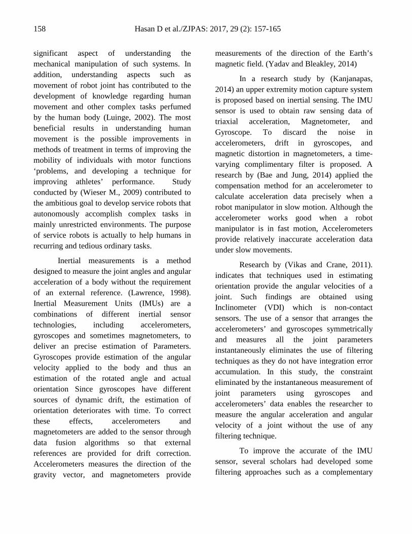
Hasan D et al./ZJPAS: 2017, 29 (2): 157-165158

significant aspect of understanding the mechanical manipulation of such systems. In addition, understanding aspects such as movement of robot joint has contributed to the development of knowledge regarding human movement and other complex tasks perfumed by the human body (Luinge, 2002). The most beneficial results in understanding human movement is the possible improvements in methods of treatment in terms of improving the mobility of individuals with motor functions ‘problems, and developing a technique for improving athletes’ performance. Study conducted by (Wieser M., 2009) contributed to the ambitious goal to develop service robots that autonomously accomplish complex tasks in mainly unrestricted environments. The purpose of service robots is actually to help humans in recurring and tedious ordinary tasks.

Inertial measurements is a method designed to measure the joint angles and angular acceleration of a body without the requirement of an external reference. (Lawrence, 1998). Inertial Measurement Units (IMUs) are a combinations of different inertial sensor technologies, including accelerometers, gyroscopes and sometimes magnetometers, to deliver an precise estimation of Parameters. Gyroscopes provide estimation of the angular velocity applied to the body and thus an estimation of the rotated angle and actual orientation Since gyroscopes have different sources of dynamic drift, the estimation of orientation deteriorates with time. To correct these effects, accelerometers and magnetometers are added to the sensor through data fusion algorithms so that external references are provided for drift correction. Accelerometers measures the direction of the gravity vector, and magnetometers provide

measurements of the direction of the Earth’s magnetic field. (Yadav and Bleakley, 2014)

In a research study by (Kanjanapas, 2014) an upper extremity motion capture system is proposed based on inertial sensing. The IMU sensor is used to obtain raw sensing data of triaxial acceleration, Magnetometer, and Gyroscope. To discard the noise in accelerometers, drift in gyroscopes, and magnetic distortion in magnetometers, a time-varying complimentary filter is proposed. A research by (Bae and Jung, 2014) applied the compensation method for an accelerometer to calculate acceleration data precisely when a robot manipulator in slow motion. Although the accelerometer works good when a robot manipulator is in fast motion, Accelerometers provide relatively inaccurate acceleration data under slow movements.

Research by (Vikas and Crane, 2011). indicates that techniques used in estimating orientation provide the angular velocities of a joint. Such findings are obtained using Inclinometer (VDI) which is non-contact sensors. The use of a sensor that arranges the accelerometers’ and gyroscopes symmetrically and measures all the joint parameters instantaneously eliminates the use of filtering techniques as they do not have integration error accumulation. In this study, the constraint eliminated by the instantaneous measurement of joint parameters using gyroscopes and accelerometers’ data enables the researcher to measure the angular acceleration and angular velocity of a joint without the use of any filtering technique.

To improve the accurate of the IMU sensor, several scholars had developed some filtering approaches such as a complementary

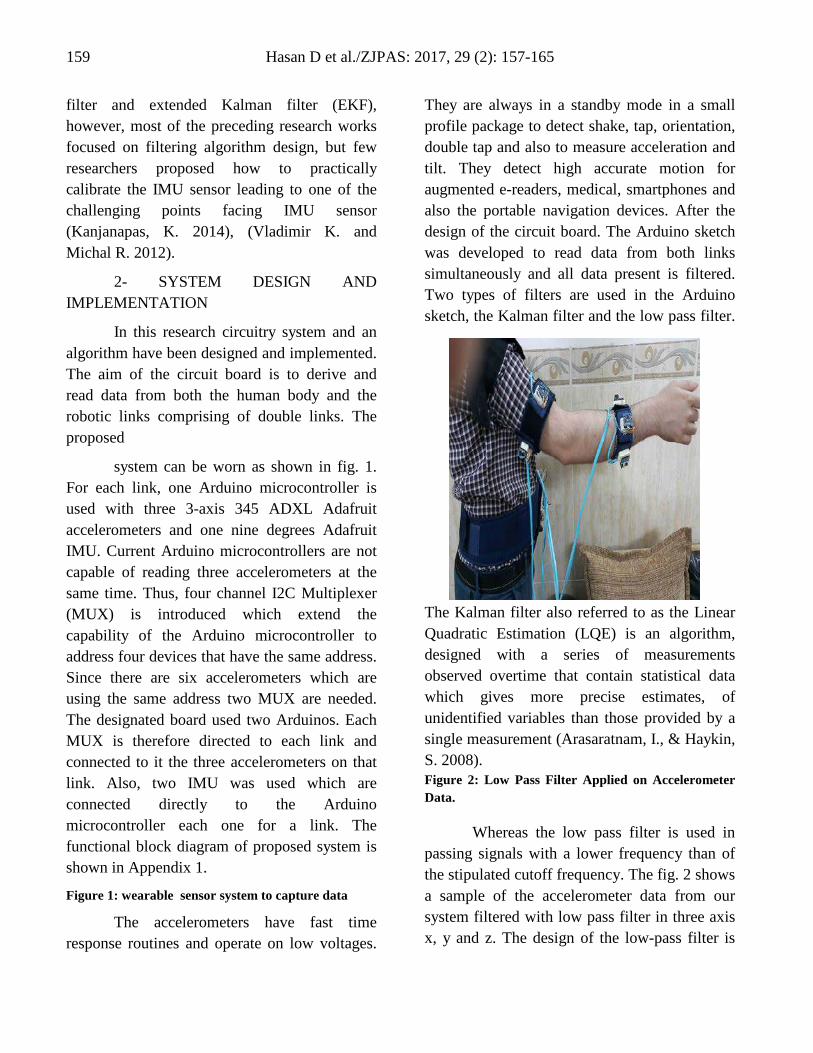
Hasan D et al./ZJPAS: 2017, 29 (2): 157-165159

filter and extended Kalman filter (EKF), however, most of the preceding research works focused on filtering algorithm design, but few researchers proposed how to practically calibrate the IMU sensor leading to one of the challenging points facing IMU sensor (Kanjanapas, K. 2014), (Vladimir K. and Michal R. 2012).

2- SYSTEM DESIGN AND IMPLEMENTATION

In this research circuitry system and an algorithm have been designed and implemented. The aim of the circuit board is to derive and read data from both the human body and the robotic links comprising of double links. The proposed

system can be worn as shown in fig. 1. For each link, one Arduino microcontroller is used with three 3-axis 345 ADXL Adafruit accelerometers and one nine degrees Adafruit IMU. Current Arduino microcontrollers are not capable of reading three accelerometers at the same time. Thus, four channel I2C Multiplexer (MUX) is introduced which extend the capability of the Arduino microcontroller to address four devices that have the same address. Since there are six accelerometers which are using the same address two MUX are needed. The designated board used two Arduinos. Each MUX is therefore directed to each link and connected to it the three accelerometers on that link. Also, two IMU was used which are connected directly to the Arduino microcontroller each one for a link. The functional block diagram of proposed system is shown in Appendix 1.

Figure 1: wearable sensor system to capture data

The accelerometers have fast time response routines and operate on low voltages.

They are always in a standby mode in a small profile package to detect shake, tap, orientation, double tap and also to measure acceleration and tilt. They detect high accurate motion for augmented e-readers, medical, smartphones and also the portable navigation devices. After the design of the circuit board. The Arduino sketch was developed to read data from both links simultaneously and all data present is filtered. Two types of filters are used in the Arduino sketch, the Kalman filter and the low pass filter.

The Kalman filter also referred to as the Linear Quadratic Estimation (LQE) is an algorithm, designed with a series of measurements observed overtime that contain statistical data which gives more precise estimates, of unidentified variables than those provided by a single measurement (Arasaratnam, I., & Haykin, S. 2008). Figure 2: Low Pass Filter Applied on Accelerometer Data.

Whereas the low pass filter is used in passing signals with a lower frequency than of the stipulated cutoff frequency. The fig. 2 shows a sample of the accelerometer data from our system filtered with low pass filter in three axis x, y and z. The design of the low-pass filter is

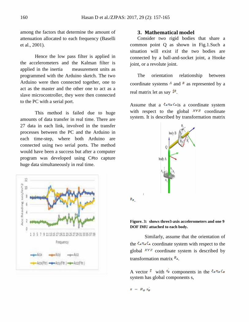
Hasan D et al./ZJPAS: 2017, 29 (2): 157-165160

among the factors that determine the amount of attenuation allocated to each frequency (Baselli et al., 2001).

Hence the low pass filter is applied in the accelerometers and the Kalman filter is applied in the inertia measurement units as programmed with the Arduino sketch. The two Arduino were then connected together, one to act as the master and the other one to act as a slave microcontroller, they were then connected to the PC with a serial port.

This method is failed due to huge amounts of data transfer in real time. There are 27 data in each link, involved in the transfer processes between the PC and the Arduino in each time-step, where both Arduino are connected using two serial ports. The method would have been a success but after a computer program was developed using C#to capture huge data simultaneously in real time.

3. Mathematical model Consider two rigid bodies that share a

common point Q as shown in Fig.1.Such a situation will exist if the two bodies are connected by a ball-and-socket joint, a Hooke joint, or a revolute joint.

The orientation relationship between

coordinate systems and as represented by a

real matrix let as say .

Assume that a is a coordinate system with respect to the global coordinate system. It is described by transformation matrix

.

Figure. 3: shows three3-axis accelerometers and one 9 DOF IMU attached to each body.

Similarly, assume that the orientation of the coordinate system with respect to the global coordinate system is described by transformation matrix .

A vector with components in the system has global components s,

Hasan D et al./ZJPAS: 2017, 29 (2): 157-165161

The global components of vector , can be transformed in terms of the coordinate system as follows:

After transformation:

Or it may be written as:

Where

The product or is the transformation

matrix from to coordinate system.

One method for determining the nine direction cosines that describe the orientation of a body-fixed coordinate system with respect to the reference coordinate is to use Joint angles.

If, then the elements of the transformation matrix can be computed, we can calculate the joint angles of both coordinate systems.

The orientation based on accelerometer and magnetometer data for the Roll, Pitch and Heading is calculated as follows:

Roll: Rotation around the X-axis

A positive roll angle is defined to be clockwise rotation about the positive X-axis.

where: , are returned value from accelerometer sensor.

Pitch: Rotation around the Y-axis

A positive pitch angle is defined to be clockwise rotation about the positive Y-axis.

Note that:

If and

then

If and

then

Heading: Rotation around the Z-axis

A positive heading angle is defined to be clockwise rotation about the positive Z-axis.

The output data from the sensors are used together with the mathematical model above, the results of the Roll, Pitch and Heading for the body A are shown in Fig.4.

The average results of the body A are

i. roll angle is 174.20 degree. ii. pitch angle is -25.44 degree. iii. heading angle is 168.42 degree.

Hasan D et al./ZJPAS: 2017, 29 (2): 157-165162

Figure 4: Joint angles for Body A.

The output data from the sensors are used together with the mathematical model above, the results of the Roll, Pitch and Heading for the body B are shown in Fig.5.

Figure 5: Joint angles for Body B

The average results of the body B are

i. roll angle is -86.01 degree. ii. pitch angle is 39.02 degree. iii. heading angle is 157.88 degree.

The Joint angles rotational matrix for Roll, Pitch and Headings are as follows:

And the Rotation Matrix is given by:

The above matrices are calculated for bodies A and B as follows:

Body A

On average rotation matrix for body A is:

Hasan D et al./ZJPAS: 2017, 29 (2): 157-165163

Body B

On average rotation matrix for body B is:

Finally, the orientation matrix from B to A coordinate system is given as:

4. CONCLUSION

The existing gap regarding the calculation of robotic parameters and understanding kinematics and dynamics in robotic motion will be filled by using a multiple instantaneous

sensors (four sensors in each link). The data fusion of these sensors contributes to increase of accuracy of the data thus the accurate estimation of the results.The real-timereading hardware model designed is wearable for both human body and robot manipulator also it is easy to use. Simultaneous results from the designed application also is very precious as it depends on the multiple accelerometers and IMU. The developed technique uses direct angles measurement and relative orientation bypassing the use ofmathematical integrations. Also, Three accelerometers and one IMU have been implemented that attached to the links. The model critically evaluates the robotic phenomenon. The model is also avoiding the use of mathematical derivatives of sensed data which reduces the effect of sensor noise on the calculations critically.

REFERENCES:

Arasaratnam, I., &Haykin, S. (2008). Square-root quadrature Kalman filtering. Signal Processing, IEEE Transactions on, 56(6), 2589-2593

Bae, Y. and Jung, S. (2014). Compensation for Position Control of a Robot Manipulator Using a Modified Disturbance Observer (DOB) based on an Accelerometer.Journal of Institute of Control, Robotics and Systems, 20(6), pp.651-656.

Dierks, T., Thumati, B. T., &Jagannathan, S. T. (2010). Fault Tolerant Control of Nonholonomic Mobile Robot Formations. In Rigatos G. (ed) Intelligent Industrial Systems: Modeling, Automation and Adaptive Behavior. Harshely, PA: IGI Global.

Ghassemi, F., Tafazoli, S., Lawrence, P., &Hashtrudi-Zaad, K., (2007). ‘Design and calibration of an integration free accelerometer-based joint-anglesensor’ .IEEE Transactionson Instrumentation and Measurement, New York, USA: IEEE press57(1), pp. 150–159.

Jiang, L., & Deng, M. (2014). Support Vector Machine Based Mobile Robot Motion Control and Obstacle Avoidance. Robotics: Concepts, Methodologies, Tools, and Applications , Hershey PA: IGI Global

Hasan D et al./ZJPAS: 2017, 29 (2): 157-165164

Kanjanapas, K. (2014). Human Mechatronics Considerations of Sensing and Actuation Systems for Rehabilitation Application. Ph.D. Berkeley, CA.

Luinge, H. (2002). Inertial Sensing Of Human Movement. PhD. Twente University.

Lawrence, A. (1998). Modern inertial technology. New York: Springer.

Vikas, V., & Crane, C. D., (2011). ‘Inclination parameter estimation for manipulator and humanoid robot links’ .In ASME International Design Engineering Technical Conference, ASME. San Diego, USA: ASME. pp. 1177-1183

Wieser, M. (2009). Hierarchical Memory Organization of Multimodal Robot Skills for Plan-based Robot Control. Ph.D. Hamburg.

Vladimir K. and Michal R.. (2012) “Complementary filtering approach to orientation estimation using inertial sensors only”. Robotics and Automation (ICRA), 2012 IEEE International Conference on. IEEE. pp.599–605.

Yadav, N. and Bleakley, C. (2014). Accurate Orientation Estimation Using AHRS under Conditions of Magnetic Distortion. Sensors, 14(11), pp.20008-20024.

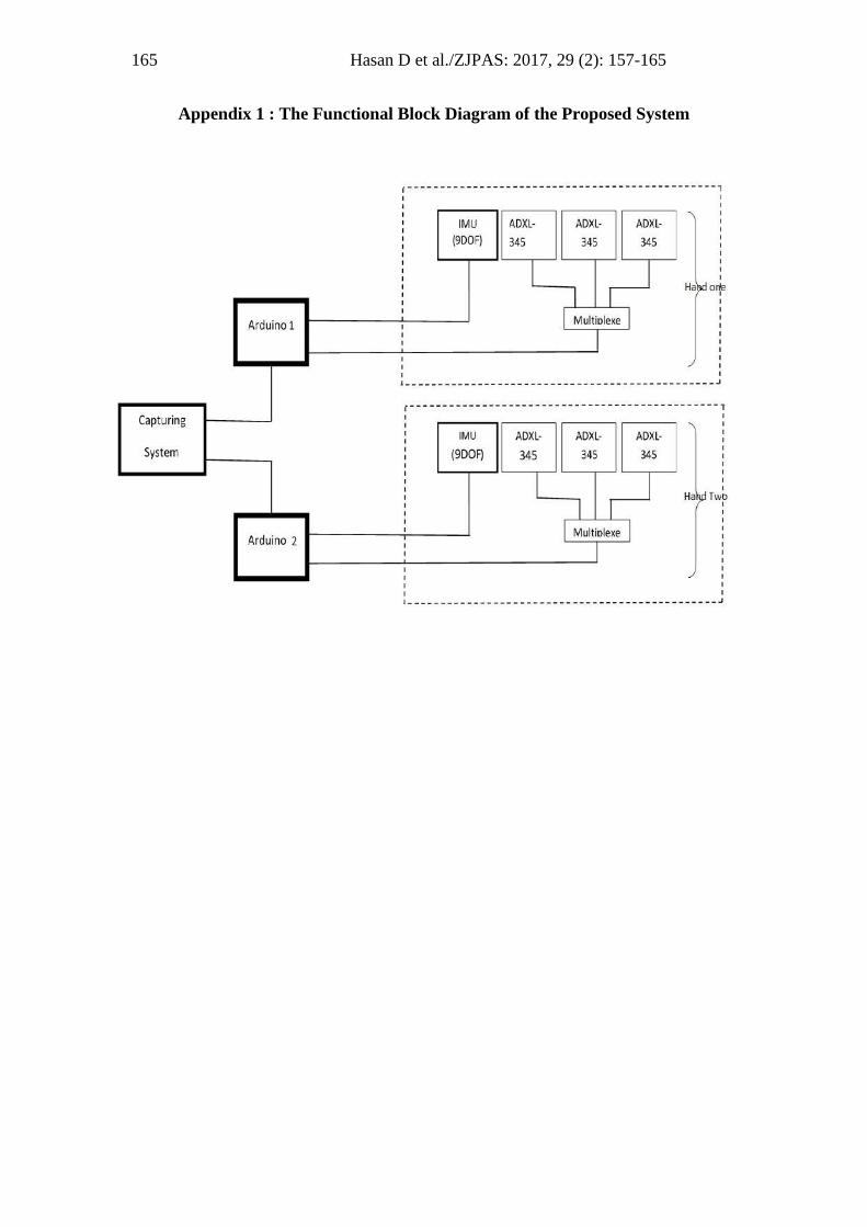
Hasan D et al./ZJPAS: 2017, 29 (2): 157-165165

Appendix 1 : The Functional Block Diagram of the Proposed System

ZANCO Journal of Pure and Applied Sciences The official scientific journal of Salahaddin University-Erbil

ZJPAS (2016), 28 (5); 166-176 http://dx.doi.org/10.21271/ZJPAS.29.2.18

Pelvic organ prolapse at Maternity Teaching Hospital in Erbil city, its prevalence

and risk factors Suzan K. Younus1 and Serwa R. Al-Dabakh2

1Department of Gynecology and Obstetrics, Maternity Teaching Hospital, Erbil-Iraq. 2Department of Gynecology and Obstetrics, College of Medicine, Hawler Medical University, Erbil-Iraq

A R T I C L E I N F O

A B S T R A C T

Article History: Received: 01/09/2016 Accepted: 02/01/2017 Published: 07/06/2017

Abstract The present study is carried out to describe the prevalence rate of pelvic

organ prolapse (POP) among women in Erbil city, to compare the prevalence

between normal vaginal delivery and cesarean section and to find out the risk

factors associated with POP. This study is a cross-sectional observational study

carried out in Maternity Teaching Hospital in Erbil city, Kurdistan region,

north of Iraq from 1st April 2015 to 1st April 2016. It includes 510 married

women aged between 15-80 years both nulliparous and multiparous, excluding

pregnant women and those in perpurium period in addition to those who

underwent previous POP surgery. The data collected by using standardized

Pelvic Organ Prolapsed - Quantitification system (POP-Q system) and the

results were analyzed using SPSS computer software version 23.0, Chi-square

test; the results were considered significant at p<0.05. The prevalence of POP

was 90.2% in general. The prevalence among those who have vaginal births

were 92.1%, while those who had caesarean sections were 77.3%. Generally

among those 90.2% of the cases, who have prolapse, nearly half of the cases

(52.9%) have both anterior and posterior vaginal wall prolapse and the 2nd stage

was found to be the most common stage (39.2%). Findings of the study

showed that POP is very common among women and is more so among those

women who delivered vaginally than those delivered by cesarean section; those

who delivered by cesarean section have a fewer degree of prolapse. The most

important risk factors were . age, a high number of vaginal deliveries,

occupation, history of an overweight baby, short birth gap space,

history of chronic diseases and low social economic state

Keywords: Pelvic organ prolapse (POP), POP-Q, Risk factors, Erbil. *Corresponding Author: Suzan K. Younus1 susan.ahmed81@yahoo.com

167 Younus S and Al-Dabakh S /ZJPAS: 2016, 28(5): 166-176

1. INTRODUCTION

Pelvic organ prolapse (POP) is a

common health problem that affects hundreds

of women in different age groups worldwide. It

affects quality of life by limiting physical,

social, psychological, and sexual functions to a

degree that living with severe types of prolapse

can be a challenge both physically and

emotionally (Monga and Dobbs, 2011;

Paudyal, 2006; Detollenaere et al., 2011; Bump

and Norton, 1998; Dietz et al., 2002).

POP is regarded as a reason for

significant gynecological operations with a

high failure rate and the reoperation incidence

is about 30% (Olsen et al., 1997). In the USA

billions of dollars are spent annually for the

treatment of this condition (Bump and Norton,

1998) and regarded as the 3rd most common

indication for hysterectomy in menopausal

women (Pearce et al., 2008; Wilcox et al.,

1994). POP defined as protrusion or descent of

one or more of female pelvic organs out of

their normal anatomical position into or out of

vagina (Thapa et al., 2013), including the

bladder, uterus, rectus, post-hysterectomy

vaginal cuff, and the small bowel, causing

urethrocele, cystocele, rectocele, enterocele and

utero vaginal prolapsed (Munir'deen et al.,

2012)

POP may occur in up to 50% of parous

women (Maher et al., 2010). However,

nulliparous women cannot be excluded from

developing this disease in which genetic

predisposition and connective tissue disorders

may play a role in it (Buchsbaum et al., 2006;

Twiss et al., 2007). Factors attributing to the

development of POP includes: multiparity,

advancing age, menopause obesity, high body-

mass index (BMI), instrumental delivery,

lifting heavy things, increasing intra-abdominal

pressure conditions like chronic constipation,

chronic cough and chronic diarrhea, in addition

to genetic predisposing factors (Buchsbaum et

al., 2006; Twiss et al., 2007; Bai et al., 2002;

Mant et al., 1997) and connective tissue

disorders (Bump and Norton, 1998; Thapa et

al., 2013; Jelovesk et al. (2007). However,

vaginal delivery and aging process are regarded

as the most common risk factors according to

Garshabi et al. (2006), and Dietz (2008).

Although the majority of POP cases were

asymptomatic, symptoms can be recorded only

by 10-20% of them (Sushma and Dudley,

2010), and even when the symptoms are

present, it has no correlation with the prolapse

stages and its severity.

In this research because of the lack of

previously published data about prevalence of

POP among women in Erbil city an attempt

was done to report the cases, finding the

associated factors and determining the stages

by using standardized POP-Q system. It is a

new system approved by International

Continence Society (ICS) (Bump and Norton,

1998). It is validated by inter-system

association and an inter-examiner agreement in

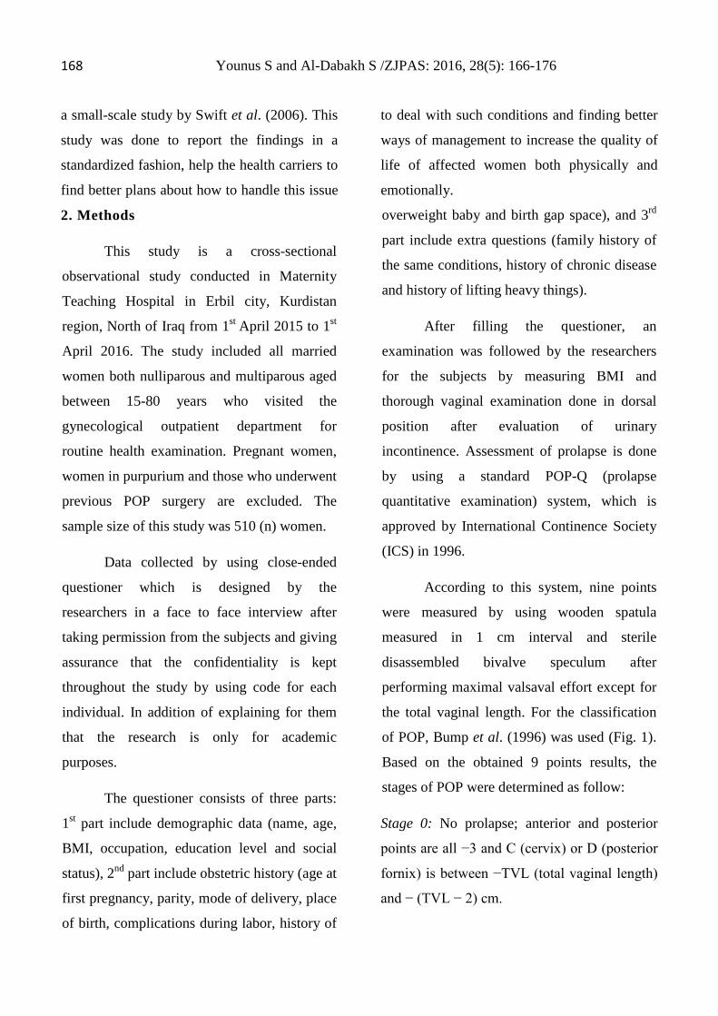
168 Younus S and Al-Dabakh S /ZJPAS: 2016, 28(5): 166-176 a small-scale study by Swift et al. (2006). This

study was done to report the findings in a

standardized fashion, help the health carriers to

find better plans about how to handle this issue

to deal with such conditions and finding better

ways of management to increase the quality of

life of affected women both physically and

emotionally.

2. Methods

This study is a cross-sectional

observational study conducted in Maternity

Teaching Hospital in Erbil city, Kurdistan

region, North of Iraq from 1st April 2015 to 1st

April 2016. The study included all married

women both nulliparous and multiparous aged

between 15-80 years who visited the

gynecological outpatient department for

routine health examination. Pregnant women,

women in purpurium and those who underwent

previous POP surgery are excluded. The

sample size of this study was 510 (n) women.

Data collected by using close-ended

questioner which is designed by the

researchers in a face to face interview after

taking permission from the subjects and giving

assurance that the confidentiality is kept

throughout the study by using code for each

individual. In addition of explaining for them

that the research is only for academic

purposes.

The questioner consists of three parts:

1st part include demographic data (name, age,

BMI, occupation, education level and social

status), 2nd part include obstetric history (age at

first pregnancy, parity, mode of delivery, place

of birth, complications during labor, history of

overweight baby and birth gap space), and 3rd

part include extra questions (family history of

the same conditions, history of chronic disease

and history of lifting heavy things).

After filling the questioner, an

examination was followed by the researchers

for the subjects by measuring BMI and

thorough vaginal examination done in dorsal

position after evaluation of urinary

incontinence. Assessment of prolapse is done

by using a standard POP-Q (prolapse

quantitative examination) system, which is

approved by International Continence Society

(ICS) in 1996.

According to this system, nine points

were measured by using wooden spatula

measured in 1 cm interval and sterile

disassembled bivalve speculum after

performing maximal valsaval effort except for

the total vaginal length. For the classification

of POP, Bump et al. (1996) was used (Fig. 1).

Based on the obtained 9 points results, the

stages of POP were determined as follow:

Stage 0: No prolapse; anterior and posterior

points are all −3 and C (cervix) or D (posterior

fornix) is between −TVL (total vaginal length)

and − (TVL − 2) cm.

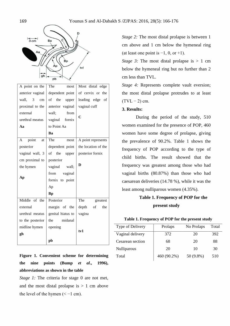
169 Younus S and Al-Dabakh S /ZJPAS: 2016, 28(5): 166-176

Figure 1. Convenient scheme for determining

the nine points (Bump et al., 1996),

abbreviations as shown in the table Stage 1: The criteria for stage 0 are not met,

and the most distal prolapse is > 1 cm above

the level of the hymen (< −1 cm).

Stage 2: The most distal prolapse is between 1

cm above and 1 cm below the hymeneal ring

(at least one point is −1, 0, or +1).

Stage 3: The most distal prolapse is > 1 cm

below the hymeneal ring but no further than 2

cm less than TVL.

Stage 4: Represents complete vault eversion;

the most distal prolapse protrudes to at least

(TVL − 2) cm.

3. Results:

During the period of the study, 510

women examined for the presence of POP, 460

women have some degree of prolapse, giving

the prevalence of 90.2%. Table 1 shows the

frequency of POP according to the type of

child births. The result showed that the

frequency was greatest among those who had

vaginal births (80.87%) than those who had

caesarean deliveries (14.78 %), while it was the

least among nulliparous women (4.35%).

Table 1. Frequency of POP for the

present study

A point on the

anterior vaginal

wall, 3 cm

proximal to the

external

urethral meatus

Aa

The most

dependent point

of the upper

anterior vaginal

wall; from

vaginal fornix

to Point Aa

Ba

Most distal edge

of cervix or the

leading edge of

vaginal cuff

C

A point at

posterior

vaginal wall, 3

cm proximal to

the hymen

Ap

The most

dependent point

of the upper

posterior

vaginal wall;

from vaginal

fornix to point

Ap

Bp

A point represents

the location of the

posterior fornix

D

Middle of the

external

urethral meatus

to the posterior

midline hymen

gh

Posterior

margin of the

genital hiatus to

the midanal

opening

pb

The greatest

depth of the

vagina

tv1

Table 1. Frequency of POP for the present study

Type of Delivery Prolaps No Prolaps Total

Vaginal delivery 372 20 392

Cesarean section 68 20 88

Nulliparous 20 10 30

Total 460 (90.2%) 50 (9.8%) 510

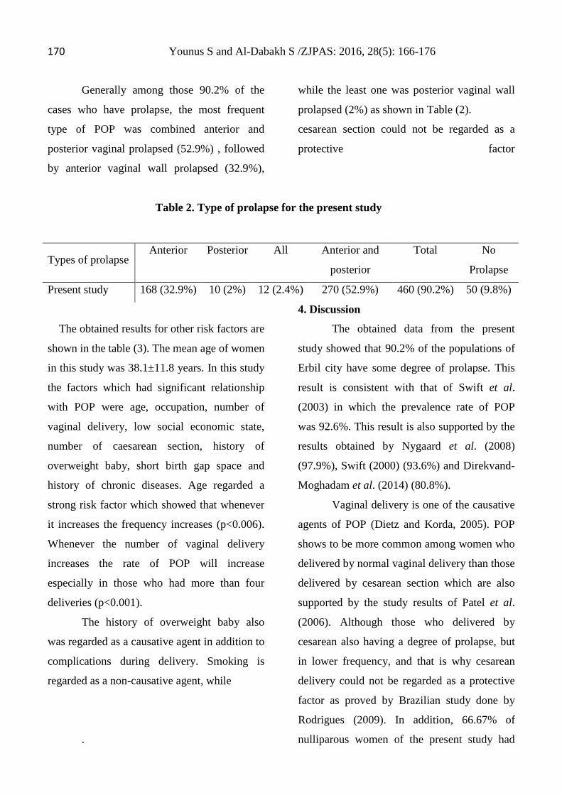
170 Younus S and Al-Dabakh S /ZJPAS: 2016, 28(5): 166-176

Generally among those 90.2% of the

cases who have prolapse, the most frequent

type of POP was combined anterior and

posterior vaginal prolapsed (52.9%) , followed

by anterior vaginal wall prolapsed (32.9%),

while the least one was posterior vaginal wall

prolapsed (2%) as shown in Table (2).

cesarean section could not be regarded as a

protective factor

Table 2. Type of prolapse for the present study

The obtained results for other risk factors are

shown in the table (3). The mean age of women

in this study was 38.1±11.8 years. In this study

the factors which had significant relationship

with POP were age, occupation, number of

vaginal delivery, low social economic state,

number of caesarean section, history of

overweight baby, short birth gap space and

history of chronic diseases. Age regarded a

strong risk factor which showed that whenever

it increases the frequency increases (p<0.006).

Whenever the number of vaginal delivery

increases the rate of POP will increase

especially in those who had more than four

deliveries (p<0.001).

The history of overweight baby also

was regarded as a causative agent in addition to

complications during delivery. Smoking is

regarded as a non-causative agent, while

.

4. Discussion

The obtained data from the present

study showed that 90.2% of the populations of

Erbil city have some degree of prolapse. This

result is consistent with that of Swift et al.

(2003) in which the prevalence rate of POP

was 92.6%. This result is also supported by the

results obtained by Nygaard et al. (2008)

(97.9%), Swift (2000) (93.6%) and Direkvand-

Moghadam et al. (2014) (80.8%).

Vaginal delivery is one of the causative

agents of POP (Dietz and Korda, 2005). POP

shows to be more common among women who

delivered by normal vaginal delivery than those

delivered by cesarean section which are also

supported by the study results of Patel et al.

(2006). Although those who delivered by

cesarean also having a degree of prolapse, but

in lower frequency, and that is why cesarean

delivery could not be regarded as a protective

factor as proved by Brazilian study done by

Rodrigues (2009). In addition, 66.67% of

nulliparous women of the present study had

Types of prolapse

Anterior Posterior All Anterior and

posterior

Total No

Prolapse

Present study 168 (32.9%) 10 (2%) 12 (2.4%) 270 (52.9%) 460 (90.2%) 50 (9.8%)

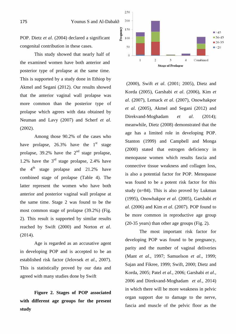
175 Younus S and Al-Dabakh S /ZJPAS: 2016, 28(5): 166-176 POP. Dietz et al. (2004) declared a significant

congenital contribution in these cases.

This study showed that nearly half of

the examined women have both anterior and

posterior type of prolapse at the same time.

This is supported by a study done in Ethiop by

Akmel and Segani (2012). Our results showed

that the anterior vaginal wall prolapse was

more common than the posterior type of

prolapse which agrees with data obtained by

Neuman and Lavy (2007) and Scherf et al.

(2002).

Among those 90.2% of the cases who

have prolapse, 26.3% have the 1st stage

prolapse, 39.2% have the 2nd stage prolapse,

1.2% have the 3rd stage prolapse, 2.4% have

the 4th stage prolapse and 21.2% have

combined stage of prolapse (Table 4). The

latter represent the women who have both

anterior and posterior vaginal wall prolapse at

the same time. Stage 2 was found to be the

most common stage of prolapse (39.2%) (Fig.

2). This result is supported by similar results

reached by Swift (2000) and Norton et al.

(2014).

Age is regarded as an accusative agent

in developing POP and is accepted to be an

established risk factor (Jelovsek et al., 2007).

This is statistically proved by our data and

agreed with many studies done by Swift

Figure 2. Stages of POP associated

with different age groups for the present

study

(2000), Swift et al. (2001; 2005), Dietz and

Korda (2005), Garshabi et al. (2006), Kim et

al. (2007), Lemack et al. (2007), Onowhakpor

et al. (2005), Akmel and Segani (2012) and

Direkvand-Moghadam et al. (2014);

meanwhile, Dietz (2008) demonstrated that the

age has a limited role in developing POP.

Stanton (1999) and Campbell and Monga

(2000) stated that estrogen deficiency in

menopause women which results fascia and

connective tissue weakness and collagen loss,

is also a potential factor for POP. Menopause

was found to be a potent risk factor for this

study (n=84). This is also proved by Lukman

(1995), Onowhakpor et al. (2005), Garshabi et

al. (2006) and Kim et al. (2007). POP found to

be more common in reproductive age group

(20-35 years) than other age groups (Fig. 2).

The most important risk factor for

developing POP was found to be pregnancy,

parity and the number of vaginal deliveries

(Mant et al., 1997; Samuelson et al., 1999;

Sajan and Fikree, 1999; Swift, 2000; Dietz and

Korda, 2005; Patel et al., 2006; Garshabi et al.,

2006 and Direkvand-Moghadam et al., 2014)

in which there will be more weakness in pelvic

organ support due to damage to the nerve,

fascia and muscle of the pelvic floor as the

176 Younus S and Al-Dabakh S /ZJPAS: 2016, 28(5): 166-176 number of vaginal deliveries increase (Allen et

al., 1990; Gurel and Gurel, 1999; Kim et al.,

2007). It appears that the women with greater

parity and more vaginal deliveries have higher

POP stage. Our data shows a strong

relationship between these factors and POP and

its ratio showed to be doubled (64.5%) in those

who had more than four deliveries comparing

to those who had <4 vaginal deliveries

(35.5%).

Occupation is one of the analyzed data

that have a positive relationship with POP.

However, most of the women in this study

were unemployed (housewives) which is in

agreement with the results of Swift et al.

(2005) and Akmel and Segani (2012). They

stated that house wives are more prone to

develop the disease and statistically it was

significant (p<0.001) due to the nature of heavy

working styles and large size family numbers

in this area. The same results also obtained by

studies done in Sweden by Samuelson et al.

(1999) and Nepal by Thapa et al. (2013).

A study done in Serbia by Mladenovic-

Segadi (2010) proposed that overweight

especially those who have BMI > 30 have

higher risk POP. The same results accepted by

Swift et al. (2003) and Iranian study done by

Garshabi et al. (2006). The current study shows

that 52.61% of those with BMI >30 have POP.

Another risk factor that also found to

have a positive relationship is the weight of the

baby. Deliveries with babies more than 4 kg

weight have a higher degree of prolapse due to

an extra extension of pelvic fascia and

weakening of supportive ligaments. This is in

consistent with the results of Gurel and Gurel

(1999), Swift (2000) and Garshabi et al.

(2006).

Statistically, the history of chronic

diseases (e.g., cough, constipation and

diarrhea) shows a significant relationship with

POP (P<0.04). This agrees with the results of

an Iranian study done by Arya et al. (2005) and

Direkvand-Moghadam et al. (2006).

A negative association was observed

between smoking and POP in the present study.

This is consistent with the results of Swift et al.

(2005). This is also proven by Bump (1993)

meanwhile; Miedel (2009) proposed that

smoking correlate positively with POP.

Studied POP found that 57.27% were

their first pregnancy under the age of 20 years,

which agrees with the results of a study done in

Nepal by Thapa et al. (2013).

Operative vaginal delivery discussed by

other studies is not practiced in this study due

unavailable data and limited use of forceps and

vacuum in our working field.

Swift et al. (2005) described the risk of

jobs involving a lot of lifting with POP. They

found that those employees who are heavy

lifters including housewives and laborers are

more likely to undergo correction operation.

Heavy working also has a positive association

as proven by Thapa et al. (2013). Heavy

working during pregnancy and perpartum

proved to be strongly associated with POP in a

177 Younus S and Al-Dabakh S /ZJPAS: 2016, 28(5): 166-176 study done by Bonder-Adler et al. (2007). He

found that 84% of women with prolapse are

heavy workers during pregnancy and 87% of

them during the postpartum period. The same

results are proven by Nigerian study done by

Onowhakpor et al. (2005). The present study

data shows that 85.65% of those lifting heavy

things have POP.

Complications during delivery (prolong

labor pain, heavy bleeding, difficulty during

placenta delivery and birth injury) showed

positive relationships with POP in this study;

the same results were obtained by Onowhakpor

et al. (2005), Akmel and Segani (2012) and

Thapa et al. (2013).

Home delivery showed by many studies

as an added factor for POP (Gurel and Gurel,

1999; Garshabi et al., 2006; Akmel and Segani,

2012). In this study the relation shows to be

significant. This is not related to the place of

delivery, but is directly related to the lack of

the hand-skilled trainer at home.

It is worth noticing that the present

work is explaining the distribution of POP in

our population depend on correlations between

physical findings with POP without

consideration of symptomatic state of the

object.

5. Conclusions and Recommendations

The POP rate for women who delivered

vaginally is nearly six times more compared to

those who delivered by caesarean section

operation and 86.7% of the subjects had stage 1

or/and 2 prolapse. These surprising results

require stronger strategies of managements to

provide a better quality of life for women and

to help clinician about how to determine

consistent frequency of POP and to define the

true pathological conditions.

This high POP rate in our community is

due to high parity, short birth space, and low

educational level as the majority of candidates

were illiterate, with few of high school or

university level education and most of them

were housewives with poor economic state and

without personal outcome. Effective plan is

needed for increasing health education leading

to decreasing the family size by using

contraceptive; which is better to be cost free for

every woman as is the case in developed

countries. In addition to that improving the

quality of life is essential through good

nutrition, regular exercise and avoiding heavy

works. It is also recommended to increase the

quality of services in delivery centers which

will help to decrease the rate of POP.

178 Younus S and Al-Dabakh S /ZJPAS: 2016, 28(5): 166-176

Table 3. Various risk factors for pelvic organic prolapsed for the present study (n=510) Risk factor Prolapse No prolapse P value Age group <20 12 (2.61%) 2 (4%) 0.006 20-35 182 (40.63%) 30 (60%) 36-45 132 (49.62%) 14 (28%) >45 134 (29.13%) 4 (8%) BMI <18.5 2 (0.43%) 0 (0%) 0.064 18.5-24.9 50 (10.87%) 10 (20%) 25-29.9 166 (36.09) 10 (20%) ≥ 30 242 (52.61%) 30 (60%) Educational level Illiterate 220 (47.83%) 16 (32%) 0.213 Read and write 66 (14.35%) 8 (16%) Primary 82 (17.83%) 10 (20%) Secondary 66 (14.35%) 12 (24%) University 26 (5.65%) 4 (8%) Occupation Employed 44 (9.57%) 12 (24%) 0.001 Unemployed 416 (90.43%) 36 (72%) Retired 0 (0%) 2 (4%) Social economic state High 2 (0.43%) 2 (4%) 0.015 Medium 120 (26.09%) 16 (32%) Low 338 (73.48%) 32 (64%) Smoking habit Smoker 52 (11.3%) 6 (12%) 0.883 Non smoker 408 (88.7%) 44 (88%) No. of viginal delivery 0 20 (5.1%) 10 (33.33%) 0.001 1 to 4 132 (33.67%) 14 (46.67%) 5 to 8 140 (35.71%) 6 (20%) >8 100 (25.51%) 0 (0%) No. of caesarean section 1 18 (26.47%) 4 (20%) 0.018 2 34 (50%) 4 (20%) 3 6 (8.82%) 4 (20%) >3 10 (14.71%) 8 (40%) Place of birth Hospital 268 (60.91%) 34 (85%) 0.003 Home 172 (39.09%) 6 (15%) Complications during delivery Yes 88 (20%) 10 (25%) 0.453 No 352 (80%) 30 (75%) Types of complications Prolong labor pain 26 (28.89%) 0 (0%) 0.068 Heavy bleeding 38 (42.22%) 8 (80%) Difficulty of placental delivery 12 (13.33%) 0 (0%) Birth injury 14 (15.56%) 2 (20%) History of overweight baby Yes 144 (32.73%) 6 (15%) 0.021 No 296 (67.27%) 34 (85%) Birth gap space < 2 years 288 (65.45%) 10 (25%) 0.001 ≥2 152 (34.55%) 30 (75%) History of lifting heavy things Yes 394 (85.65%) 40 (80%) 0.286 No 66 (14.35%) 10 (20%) History of chronic disease No disease 208 (45.22%) 22 (44%) 0.046 Cough 2 (0.43%) 2 (4%) Constipation 244 (53.04%) 26 (52%) Diarrhea 6 (1.3%) 0 (0%) Age at first pregnancy <20 252 (57.27%) 24 (60%) 0.256 20-35 186 (42.27%) 16 (40%) 36-45 2 (0.45%) 0 (0%)

179 Younus S and Al-Dabakh S /ZJPAS: 2016, 28(5): 166-176

Table 4. Stage of prolapse for the present study compared to other studies

Stage of prolapse 1st 2nd 3rd 4th Combined* No Prolapse

Present Study

(n=460)

134

(26.3%)

200

(39.2%)

6

(1.2%)

12

(2.4%)

108 (21.2%) 50

(9.8%)

Swift (2000), (n=

497)

43.3% 47.7% 2.6% 0% 6.4%

Swift et al. (2005),

(n= 1004)

38% 35% 2% 0% 24%

Garshabi et al.

(2006), (n= 3730)

23.1% 18.3% 11.6% 47%

* Those who have both anterior and posterior prolapse in stage 1 and 2.

Acknowledgments

We would like to thank the authorities

of the Maternity Teaching Hospital in Erbil

city for supporting and providing facilities for

the present work which is part of high diploma

study. Special thanks to Dr. Yawooz Kettanah

for the linguistic review and to Dr. Kamaran

for constrictive comments in statistics which

improved the manuscript.

References:

Akmel M. and Segni H., 2012. Pelvic organ prolapsed in Jimma University specialized hospital, southwest Ethiopia, Ethiopian Journal of Health Sciences, 22 (2), 85-92.

Allen R.E., Hosker G.L., Smith A.R.B. and Warrell D.E., 1990. Pelvic floor damage and childbirth: a neurophysiological study, British Journal of Obstetrics and Gynecology, 97, 770-779.

Arya L.A., Novi J.M. and Shaunik A., 2005. Pelvic organ prolapse, constipation, and dietary fiber intake in women, American Journal of Obstetrics and Gynecology, 192: 1687-1691.

Bai S.W., Choe B.H., Kim J.Y. and Park K.H., 2002. Pelvic organ prolapse and connective

tissue abnormalities in Korean women, Journal of Reproductive Medicine, 47, 231-234.

Bodner-Adler B., Shrivastava C. and Bodner K.,

2007. Risk factors for uterine prolapse in Nepal, International Urogynecology Journal, 18, 1343-1346.

Buchsbaum G.M., Duecy E.E., Kerr L.A., Huang L.S., Perevich M. and Guzick D.S., 2006. Pelvic organ prolapse in nulliparous women and their parous sisters, Obstetrics and Gynecology, 108, 1388-1393.

Bump R.C. and Norton P.A., 1998. Epidemiology and natural history of pelvic floor dysfunction, Obstetrics and Gynecology Clinics of North America, 25, 723-7462.

Bump R.C., 1993. Racial comparisons and contrasts in urinary incontinence and pelvic organ prolapse, Obstetrics and Gynecology, 81, 421-425.

Bump R.C., Mattiasson A., Bo K., Brubaker L.P., DeLancey J.O., Klarskov P., Shull B.L. and Smith A.R., 1996. The standardization of terminology of female pelvic organ prolapse and pelvic floor dysfunction. American Journal of Obstetrics and Gynecology, 175(1), 10-17.

Campbell S. and Monga A., 2000. Utero-vaginal prolapsed, In: Campbell S. and Monga A. (Eds.), Gynecology by Ten Teachers. 17th edition. ELST with Arnold, pp. 217-224.

Description for a new simplified pelvic organ prolapse classification system exam. A coordinated effort of the Standardization &

175 Younus S and Al-Dabakh S /ZJPAS: 2016, 28(5): 166-176

Terminology and research & development committees of IUGA, 2006.

Detollenaere R.J., Boon J.d., Stekelenburg J., Alhafidh A.H., Vierhout M.E. and Eijndhoven H.W., 2011. Treatment of uterine prolapse stage 2 or higher: A randomized multicenter trial comparing sacrospinous fixation with vaginal hysterectomy, Boston Medical Center Women’s Health, 11(4), DOI: 10.1186/1472-6874-11-4.

Dietz H.P. and Korda A., 2005. Which bowel symptoms are most strongly associated with a true rectocele? Australian and New Zealand Journal of Obstetrics and Gynecology, 45, 505-508.

Dietz H.P., 2008. Prolapse worsens with age, doesn’t it? Australian and New Zealand Journal of Obstetrics and Gynecology, 48, 587-591.

Dietz H.P., Eldridge A., Grace M. and Clarke B., 2004. Pelvic organ descent in young nulligravid women, American Journal of Obstetrics and Gynecology, 191(1), 95-99.

Dietz H.P., Haylen B.T. and Vancaillie T.G., 2002. Female pelvic organ prolapse and voiding function. International Urogynecology Journal and Pelvic Floor Dysfunction, 13, 284-288.

Direkvand-Moghadam A.D., Ghazanfari Z., Montazeri A., Delpisheh A. and Direkvand-Moghadam A., 2014. Risk factors of pelvic organ prolapse in Iranian women: a cross-sectional study, International Journal of Epidemiologic Research, 1(1): 29-34.

Garshasbi A., Faghih-Zadeh S. and Falah N., 2006. The status of pelvic supporting organs in a population of Iranian women 18 - 68 years of age and possible related factors, Archives of Iranian Medicine, 9(2):124-128.

Gurel H. and Gurel S.A., 1999. Pelvic relaxation and associated risk factors: the results of logistic regression analysis, Acta Obstetricia et Gynecologica Scandinavica, 78(4), 290-293.

Jelovsek J.E., Maher Ch. and Bader M.D., 2007. Pelvic organ prolapsed, Lancet. 369 (9566), 1027-1038.

Kim C.M., Jeon M.J., Chung D.J., Kim S.K., Kim J.W. and Bai S.W., 2007. Risk factors for pelvic organ prolapsed, International Journal of Gynecology and Obstetrics. 98(3), 248-251.

Lemack G.E., Xu Y., Brubaker L., Nager C., Chai T., Moalli P., Kraus S.R., Kerr L., Sirls L. and Stoddard A., 2007. Clinical and demographic factors associated with valsalva leak point pressure among women undergoing burch bladder neck suspension or autologous rectus fascial sling procedures, Neurourology and Urodynamics, 26(3), 392-396.

Lukman Y., 1995. Utero vaginal prolapse a rural disability of the young, East African Medical Journal, 72 (1), 1-9.

Maher C., Feiner B., Baessler K. and Glazener C.M.A., 2010. Surgical management of pelvic organ prolapse in women, Cochrane Database of Systematic Reviews, 4, CD004014.

Mant J., Painter R. and Vessey M., 1997. Epidemiology of genital prolapse: observations from the Oxford Family Planning Association Study, British Journal of Obstetrics and Gynecology, 104 (5), 579-585.

Miedel A., 2009. Pelvic organ prolapse: Aspects of etiology, symptomatology and outcome after surgery, Ph.D. dissertation, Stockholm South General Hospital.

Mladenovic-Segedi L. and Segedi D., 2010. Most important etiologic factors in the development of genital prolapse in Serbian, Srpski arhiv za celokupno lekarstvo, 138(5-6), 315-318.

Monga A. and Dobbs S., 2011. Gynecology by ten teachers, 19th edition. London, Hodder and Stoughton Ltd.

Munir’deen A.I. and Hadijat O.R., 2012. Treatment of pelvic organ prolapse. Urogynaecologia, 26 (e3), 8-11.

Neuman M. and Lavy Y., 2007. Conservation of the prolapsed uterus is a valid option: medium term results of a prospective comparative study with the posterior intra-vaginal slingoplasty operation, International Urogynecology Journal and Pelvic Floor Dysfunction, 18(8), 889-893.

Norton P., Brubaker L., Nager C.W., Lemack G.E., Zyczynski H.M., Sirls L., Rickey L., Stoddard A. and Varrner R.E., 2014. Pelvic organ prolapsed in a cohort of women treated for stress urinary incontinence, American Journal of Obstetrics and Gynecology, 211(5), 550.e1-5

Nygaard I., Barber M.D., Burgio K.L. Meikle S., Schaffer J., Spino C., Whitehead W.E., Wu J. and Brody D.J., 2008. Prevalence of symptomatic pelvic floor disorders in US women, Journal of the American Medical Association, 300(11), 1311-1316.

Olsen A.L., Smith V.J., Bergstrom J.O., Colling J.C. and Clark A.L., 1997. Epidemiology of surgically managed pelvic organ prolapse and urinary incontinence, Obstetrics and Gynecology, 89, 501-506.

Onowhakpor E.A., Omo-Aghoja L.O., Akani C.I. and Feyi-Waboso P., 2009. Prevalence and determinations of utero-vaginal prolapsed in southern Nigeria, Nigerian Medical Journal, 50, 29-32.

Patel P.D., Amrute K.V. and Badlani G.H., 2006.

176 Younus S and Al-Dabakh S /ZJPAS: 2016, 28(5): 166-176

Pathophysiology of pelvic organ prolaps and stress urinary incontinence, Indian Journal of Urology, 22, 310-316.

Paudyal S., 2006. Prevalence of Uterine prolapse among married women in Slum area at Thapathali, Kathmandu. Master thesis, Tribhuvan University.

Pearce M., Swift S. and Goodnight W., 2008. Pelvic organ prolapse: is there a difference in POPQ exam results based on time of day, morning or afternoon? American Journal of Obstetrics and Gynecology, 199: 200.e1-5.

Rodrigues A.M., de Oliveira L.M., Martins Kde F., Del Roy C.A., Sartori MG, Girao M.J. and Castro Rde A., 2009. Risk factors for genital prolapse in a Brazilian population, The Revista Brasileira de Ginecologia e Obstetrícia, 31(1), 17-21.

Sajan F. and Fikree F.F., 1999. Perceived gynecological morbidity among young ever-married women living in squatter settlements of Karachi-Pakistan, Journal of the Pakistan Medical Association, 49, 92-97.

Samuelsson E.C., Victor F.T.A., Tibblin G. and Svardsudd K.F., 1999. Signs of genital prolapse in a Swedish population of women 20 to 59 years of age and possible related factors, American Journal of Obstetrics and Gynecology, 180, 299-305.

Scherf C., Morison L., Fiander A., Ekpo C. and Walraven G., 2002. Epidemiology of pelvic organ prolapse in rural Gambia-West Africa, British Journal of Obstetrics and Gynecology, 109 (4), 431-436.

Stanton S. L., 1999. Vaginal prolapse. In: Edmonds D.K. (ed.), Dewhurst's Textbook of Obstetrics and Gynecology for Postgraduates, 6th edition, Blackwell Sciences, pp. 462-473.

Sushma S. and Dudley R., 2010. Urogenital Prolapse. In Luesley D.M. and Baker P.N.

(eds.), Obstetrics and Gynecology: an evidence based text for MRCOG, Britain Arnold, British, pp. 725-734.

Swift S., Woodman P., O'Boyle A., Kahn M., Valley M., Bland D., Wang W. and Schaffer J., 2005. Pelvic Organ Support Study (POSST): the distribution, clinical definition, and epidemiologic condition of pelvic organ support defects, American Journal of Obstetrics and Gynecology, 192(3): 795-806.

Swift S.E., 2000. The distribution of pelvic organ support in a population of female subjects seen for routine gynecologic health care, American Journal of Obstetrics and Gynecology, 183(2), 277-285.

Swift S.E., Pound T. and Dias J.K., 2001. Case-control study of etiologic factors in the development of severe pelvic organ prolapsed, International Urogynecology Journal and Pelvic Floor Dysfunction, 12(3), 187-92.

Swift S.E., Tate S.B. and Nicholas J., 2003. Correlation of symptoms with degree of pelvic organ support in a general population of women: what is pelvic organ prolapsed? American Journal of Obstetrics and Gynecology, 189, 372-377.

Thapa S., Angdembe M., Chauhan D. and Joshi R., 2013. Determinants of pelvic organ prolapse among the women of the western part of Nepal: A case-control study, Journal of Obstetrics and Gynecology Research, 40(2), 515-520.

Twiss C., Triaca V. and Rodriguez L.V., 2007. Familial transmission of urogenital prolapse and incontinence, Current Opinion in Obstetrics and Gynecology, 19, 464-468.

Wilcox L.A., Koonin L.M., Pokras R., Strauss L.T., Xia Z. and Peterson H.B., 1994. Hysterectomy in the United States, 1988-1990, Obstetrics and Gynecology, 83, 549-555.

ZANCO Journal of Pure and Applied Sciences The official scientific journal of Salahaddin University-Erbil

ZJPAS (2017), 29 (2); 177-195 http://dx.doi.org/10.21271/ZJPAS.29.2.19

Operation Analysis and Capacity Improvement of Signalized Intersections Using TRANSYT-7F-Case Study

Shamil A. Flamarz

Building and Construction Engineering Department, University of Garmian, Kalar, Sulaimaniya, Kurdistan Region, Iraq.

1. INTRODUCTION

Signalized intersections are critical elements of an urban road transportation system and maintaining these control systems at their optimal performance for different demand conditions has been the primary concern of the traffic engineers (Borkloe, 2013). Urban traffic networks are highly

governed by intersection capacity. The lack of surface space for roads in cities and the continuously increasing traffic demand, both are challenging traffic engineers towards all type of improvements in traffic management to make existing infrastructure more efficient (Tovar, et al., 2010).

A R T I C L E I N F O

A B S T R A C T

Article History: Received: 04/12/2016 Accepted: 19/01/2017 Published: 07/06/2017

Signalized intersection operation performance evaluation provides important and valuable knowledge about the performance of the city transportation network or system, where signalized intersections are major elements and critical points within the city transportation network. The capacity and operation performance of signalized intersections as part of the transportation network is very important and more significant because the signalized intersections often control the ability of the city streets and transportation network to accommodate the traffic volumes. The objective of the present study is operation analysis and capacity improvement of Shahid Hama Rash and Sherai Naqib signalized intersections in Kalar City by suggesting number of intersection capacity improvement scenarios, and investigates the proper scenario among the suggested scenarios to improve the traffic capacity. The required data for the study purposes like existing geometric design (using field observation) and traffic volumes (using video records through the cameras installed at both intersections) were collected. The results of this study revealed that Shahid Hama Rash and Sherai Naqib signalized intersections currently operating under congested and low performance conditions, and the suggested intersection capacity improvement scenarios provide reasonable and proper solutions to improve the capacity of the selected signalized intersections. The combination the first and second improvements has a significant impact on increasing the capacity and improving the quality of operation for both intersections, where the degree of saturation for Shahid Hama Rash reduced from 124% to 83% and the intersection level of service (LOS) changed from F to level of service (LOS) C, and the degree of saturation for Sherai Naqib intersection reduced from 126% to 66% and the intersection level of service (LOS) changed from F to level of service (LOS) D.

Keywords: Capacity improvement Optimization run Signalized intersection TRANSYT-7F *Corresponding Author: Shamil A. Flamarz

shamil.flamarz@garmian.edu.krd

178 Flamarz S./ZJPAS: 2017, 29(5): 177-195

Capacity of a road is represented by the maximum rate at which vehicles can pass through a given point in an hour under prevailing operational conditions. The number and width of lanes, grades, and lane use allocations, as well as signalization conditions ascertains the capacity of the road. The measures of effectiveness, which are commonly used to evaluate the signalized intersection operations, are Capacity and volume-to-capacity ratio, delay, and queue behavior of the vehicles. Intersection capacity or volume-to capacity ratio is one of the operational measures of effectiveness used in measuring signalized intersection LOS (Kumar, et al., 2013).

The level of service at any intersection on a highway has a significant effect on the overall operating performance of that highway. Thus, improvement of the level of service at each intersection usually results in an improvement of the overall operating performance of the highway. An analysis procedure that provides for the determination of capacity or level of service at intersections is therefore an important tool for designers, operation personnel, and policy makers. Factors that affect the level of service at intersections include the flow and distribution of traffic, the geometric characteristics, and the signalization system (Garber, et al., 2009).

The Highway Capacity Manual methodology addresses the capacity, level of service (LOS), and other performance measures for lane groups and intersection approaches and the level of service (LOS) for the intersection as a whole. Capacity is evaluated in terms of the ratio of demand flow rate to capacity (v/c ratio), whereas level of service (LOS) is evaluated on the basis of control delay vehicle (in second per vehicle). Control delay is the portion of the total delay attributed to traffic signal operation for

signalized intersection. Control delay includes initial deceleration delay, queue move-up time, stopped delay, and final acceleration delay (TRB, 2000).

2. OBJECTIVES OF THE STUDY

The objectives of this study are evaluating the traffic operation performance in the selected congested signalized intersections through the estimation of the existing level of service (LOS) using TRASYT-7F software, then propose number of improvements on the signal timing and geometric design of the selected signalized intersections and measure the influences of the improvements on its capacities by re-evaluating the traffic operation performance using TRASYT-7F software.

The objectives of the present study can be achieved through the following steps:

1- Operation analysis of two congested signalized intersections in Kalar City. This can be achieved by the estimation of the existing LOS using TRASYT-7F software for the selected signalized intersections as a case study.

2- Evaluation of the traffic operation performance in the selected congested signalized intersections.

3- Proposing number of improvements on the signal timing and geometric design of the selected signalized intersections and measure the influences of the improvements on its capacities by re-evaluating the traffic operation performance using TRASYT-7F software.

3. STUDY AREA

Kalar city is the center of Kalar District located in northeast of Iraq lies on Sirwan (Diyala) river, and it is one of Sulaimaniya Governorate Districts.

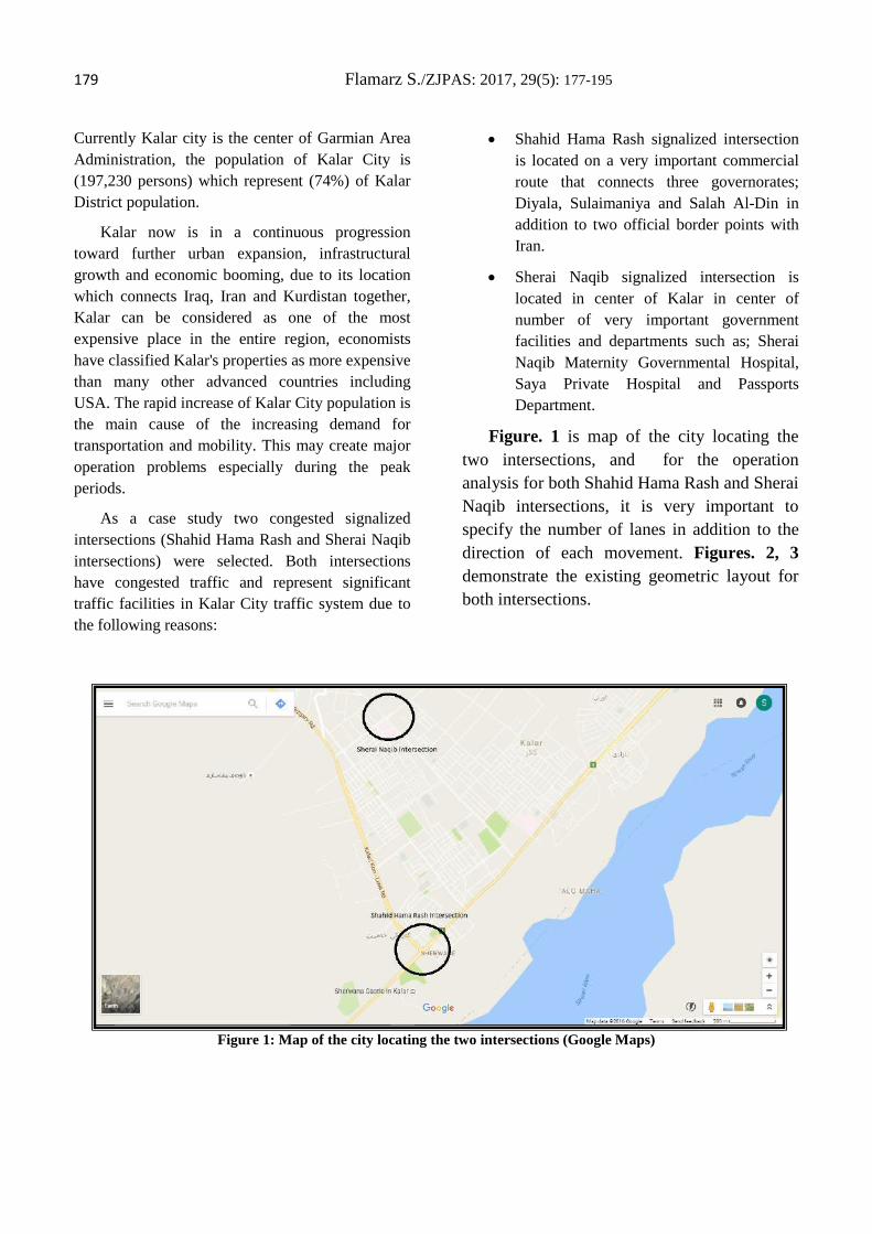
179 Flamarz S./ZJPAS: 2017, 29(5): 177-195 Currently Kalar city is the center of Garmian Area Administration, the population of Kalar City is (197,230 persons) which represent (74%) of Kalar District population.

Kalar now is in a continuous progression toward further urban expansion, infrastructural growth and economic booming, due to its location which connects Iraq, Iran and Kurdistan together, Kalar can be considered as one of the most expensive place in the entire region, economists have classified Kalar's properties as more expensive than many other advanced countries including USA. The rapid increase of Kalar City population is the main cause of the increasing demand for transportation and mobility. This may create major operation problems especially during the peak periods.

As a case study two congested signalized intersections (Shahid Hama Rash and Sherai Naqib intersections) were selected. Both intersections have congested traffic and represent significant traffic facilities in Kalar City traffic system due to the following reasons:

• Shahid Hama Rash signalized intersection is located on a very important commercial route that connects three governorates; Diyala, Sulaimaniya and Salah Al-Din in addition to two official border points with Iran.

• Sherai Naqib signalized intersection is located in center of Kalar in center of number of very important government facilities and departments such as; Sherai Naqib Maternity Governmental Hospital, Saya Private Hospital and Passports Department.

Figure. 1 is map of the city locating the two intersections, and for the operation analysis for both Shahid Hama Rash and Sherai Naqib intersections, it is very important to specify the number of lanes in addition to the direction of each movement. Figures. 2, 3 demonstrate the existing geometric layout for both intersections.

Figure 1: Map of the city locating the two intersections (Google Maps)

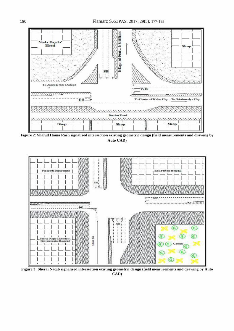
180 Flamarz S./ZJPAS: 2017, 29(5): 177-195

Figure 2: Shahid Hama Rash signalized intersection existing geometric design (field measurements and drawing by Auto CAD)

Figure 3: Sherai Naqib signalized intersection existing geometric design (field measurements and drawing by Auto CAD)

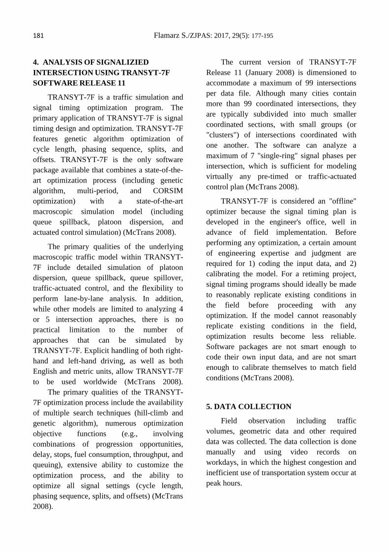
181 Flamarz S./ZJPAS: 2017, 29(5): 177-195 4. ANALYSIS OF SIGNALIZIED

INTERSECTION USING TRANSYT-7F

SOFTWARE RELEASE 11

TRANSYT-7F is a traffic simulation and signal timing optimization program. The primary application of TRANSYT-7F is signal timing design and optimization. TRANSYT-7F features genetic algorithm optimization of cycle length, phasing sequence, splits, and offsets. TRANSYT-7F is the only software package available that combines a state-of-the-art optimization process (including genetic algorithm, multi-period, and CORSIM optimization) with a state-of-the-art macroscopic simulation model (including queue spillback, platoon dispersion, and actuated control simulation) (McTrans 2008).

The primary qualities of the underlying macroscopic traffic model within TRANSYT-7F include detailed simulation of platoon dispersion, queue spillback, queue spillover, traffic-actuated control, and the flexibility to perform lane-by-lane analysis. In addition, while other models are limited to analyzing 4 or 5 intersection approaches, there is no practical limitation to the number of approaches that can be simulated by TRANSYT-7F. Explicit handling of both right-hand and left-hand driving, as well as both English and metric units, allow TRANSYT-7F to be used worldwide (McTrans 2008). The primary qualities of the TRANSYT-7F optimization process include the availability of multiple search techniques (hill-climb and genetic algorithm), numerous optimization objective functions (e.g., involving combinations of progression opportunities, delay, stops, fuel consumption, throughput, and queuing), extensive ability to customize the optimization process, and the ability to optimize all signal settings (cycle length, phasing sequence, splits, and offsets) (McTrans 2008).

The current version of TRANSYT-7F Release 11 (January 2008) is dimensioned to accommodate a maximum of 99 intersections per data file. Although many cities contain more than 99 coordinated intersections, they are typically subdivided into much smaller coordinated sections, with small groups (or "clusters") of intersections coordinated with one another. The software can analyze a maximum of 7 "single-ring" signal phases per intersection, which is sufficient for modeling virtually any pre-timed or traffic-actuated control plan (McTrans 2008).

TRANSYT-7F is considered an "offline" optimizer because the signal timing plan is developed in the engineer's office, well in advance of field implementation. Before performing any optimization, a certain amount of engineering expertise and judgment are required for 1) coding the input data, and 2) calibrating the model. For a retiming project, signal timing programs should ideally be made to reasonably replicate existing conditions in the field before proceeding with any optimization. If the model cannot reasonably replicate existing conditions in the field, optimization results become less reliable. Software packages are not smart enough to code their own input data, and are not smart enough to calibrate themselves to match field conditions (McTrans 2008).

5. DATA COLLECTION

Field observation including traffic volumes, geometric data and other required data was collected. The data collection is done manually and using video records on workdays, in which the highest congestion and inefficient use of transportation system occur at peak hours.

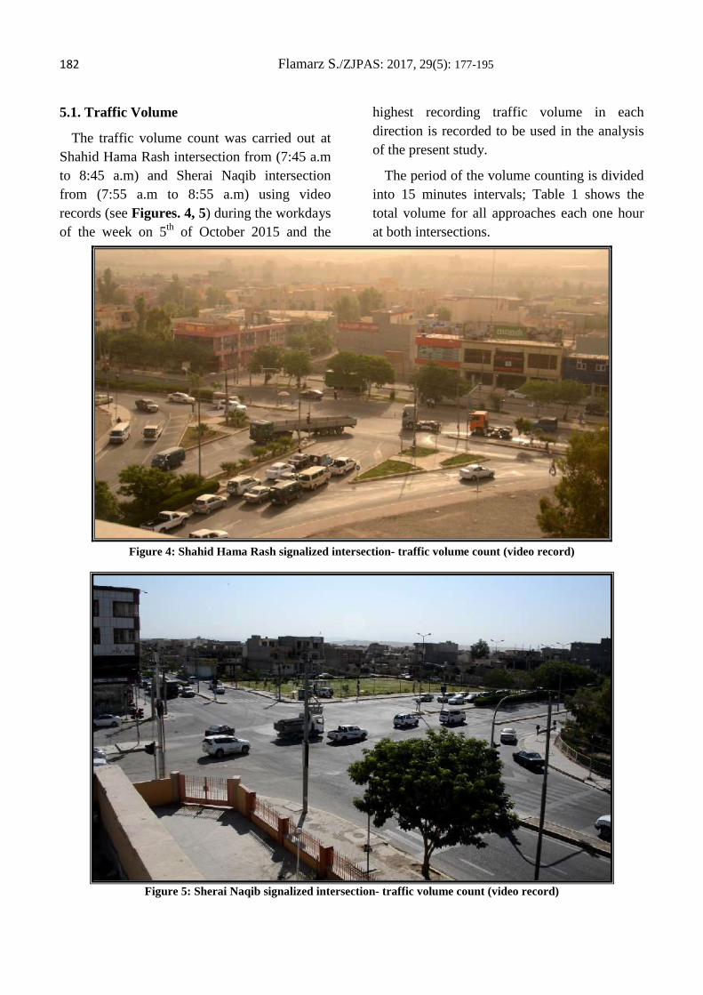
182 Flamarz S./ZJPAS: 2017, 29(5): 177-195 5.1. Traffic Volume

The traffic volume count was carried out at Shahid Hama Rash intersection from (7:45 a.m to 8:45 a.m) and Sherai Naqib intersection from (7:55 a.m to 8:55 a.m) using video records (see Figures. 4, 5) during the workdays of the week on 5th of October 2015 and the

highest recording traffic volume in each direction is recorded to be used in the analysis of the present study.

The period of the volume counting is divided into 15 minutes intervals; Table 1 shows the total volume for all approaches each one hour at both intersections.

Figure 4: Shahid Hama Rash signalized intersection- traffic volume count (video record)

Figure 5: Sherai Naqib signalized intersection- traffic volume count (video record)

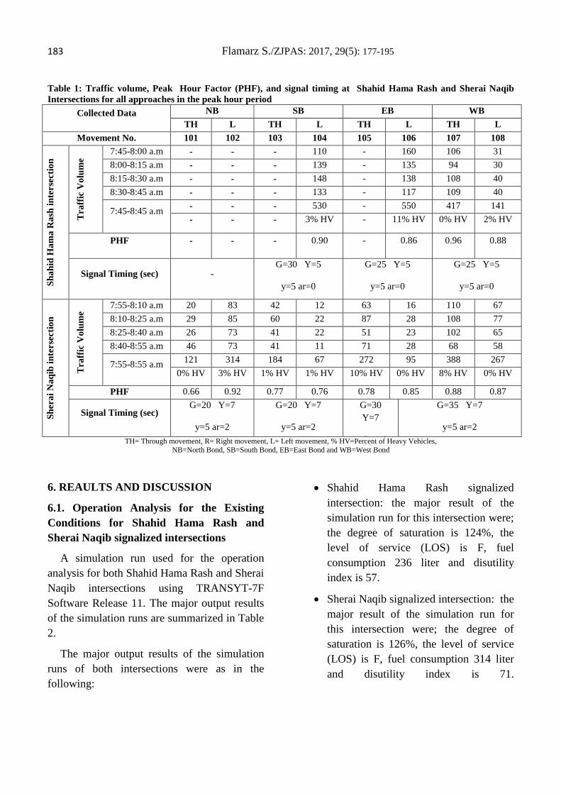
183 Flamarz S./ZJPAS: 2017, 29(5): 177-195 Table 1: Traffic volume, Peak Hour Factor (PHF), and signal timing at Shahid Hama Rash and Sherai Naqib Intersections for all approaches in the peak hour period

Collected Data NB SB EB WB TH L TH L TH L TH L

Movement No. 101 102 103 104 105 106 107 108

Shah

id H

ama

Ras

h in

ters

ectio

n

Tra

ffic

Vol

ume

7:45-8:00 a.m - - - 110 - 160 106 31 8:00-8:15 a.m - - - 139 - 135 94 30 8:15-8:30 a.m - - - 148 - 138 108 40 8:30-8:45 a.m - - - 133 - 117 109 40

7:45-8:45 a.m - - - 530 - 550 417 141 - - - 3% HV - 11% HV 0% HV 2% HV

PHF - - - 0.90 - 0.86 0.96 0.88

Signal Timing (sec) - G=30 Y=5

y=5 ar=0

G=25 Y=5

y=5 ar=0

G=25 Y=5

y=5 ar=0

Sher

ai N

aqib

inte

rsec

tion

Tra

ffic

Vol

ume

7:55-8:10 a.m 20 83 42 12 63 16 110 67 8:10-8:25 a.m 29 85 60 22 87 28 108 77 8:25-8:40 a.m 26 73 41 22 51 23 102 65 8:40-8:55 a.m 46 73 41 11 71 28 68 58

7:55-8:55 a.m 121 314 184 67 272 95 388 267 0% HV 3% HV 1% HV 1% HV 10% HV 0% HV 8% HV 0% HV

PHF 0.66 0.92 0.77 0.76 0.78 0.85 0.88 0.87

Signal Timing (sec) G=20 Y=7

y=5 ar=2

G=20 Y=7

y=5 ar=2

G=30 Y=7

5 2

G=35 Y=7

y=5 ar=2 TH= Through movement, R= Right movement, L= Left movement, % HV=Percent of Heavy Vehicles,

NB=North Bond, SB=South Bond, EB=East Bond and WB=West Bond

6. REAULTS AND DISCUSSION

6.1. Operation Analysis for the Existing Conditions for Shahid Hama Rash and Sherai Naqib signalized intersections

A simulation run used for the operation analysis for both Shahid Hama Rash and Sherai Naqib intersections using TRANSYT-7F Software Release 11. The major output results of the simulation runs are summarized in Table 2.

The major output results of the simulation runs of both intersections were as in the following:

• Shahid Hama Rash signalized intersection: the major result of the simulation run for this intersection were; the degree of saturation is 124%, the level of service (LOS) is F, fuel consumption 236 liter and disutility index is 57.

• Sherai Naqib signalized intersection: the major result of the simulation run for this intersection were; the degree of saturation is 126%, the level of service (LOS) is F, fuel consumption 314 liter and disutility index is 71.

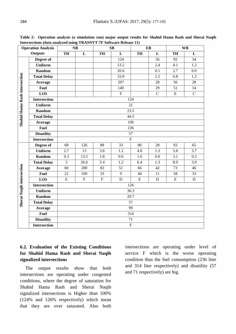
184 Flamarz S./ZJPAS: 2017, 29(5): 177-195 Table 2: Operation analysis (a simulation run) major output results for Shahid Hama Rash and Sherai Naqib Intersections (data analyzed using TRANSYT-7F Software Release 11) Operation Analysis

Outputs NB SB EB WB

TH L TH L TH L TH L

Shah

id H

ama

Ras

h in

ters

ectio

n

Degree of

124 56 92 34 Uniform

13.2 2.4 4.1 1.2

Random

20.6 0.1 2.7 0.0 Total Delay

33.9 2.5 6.8 1.2

Average

207 28 56 28 Fuel

140 29 51 14 LOS F C E C

Intersection

124 Uniform

21

Random

23.5 Total Delay

44.5

Average

106 Fuel

236 Disutility

57

Intersection

F

Sher

ai N

aqib

inte

rsec

tion

Degree of

68 126 88 33 86 28 93 65 Uniform

2.7 13 3.6 1.2 4.8 1.3 5.8 3.7

Random

0.3 13.5 1.8 0.0 1.6 0.0 3.1 0.2 Total Delay

3 26.6 5.4 1.2 6.4 1.3 8.9 3.9

Average

60 280 82 51 66 42 73 46 Fuel

22 100 33 9 44 11 58 33 LOS E F F D E D E D

Intersection

126 Uniform

36.3

Random

20.7 Total Delay

57

Average

99 Fuel

314 Disutility

71

Intersection

F

6.2. Evaluation of the Existing Conditions for Shahid Hama Rash and Sherai Naqib signalized intersections

The output results show that both intersections are operating under congested conditions, where the degree of saturation for Shahid Hama Rash and Sherai Naqib signalized intersections is Higher than 100% (124% and 126% respectively) which mean that they are over saturated. Also both

intersections are operating under level of service F which is the worse operating condition thus the fuel consumption (236 liter and 314 liter respectively) and disutility (57 and 71 respectively) are big.

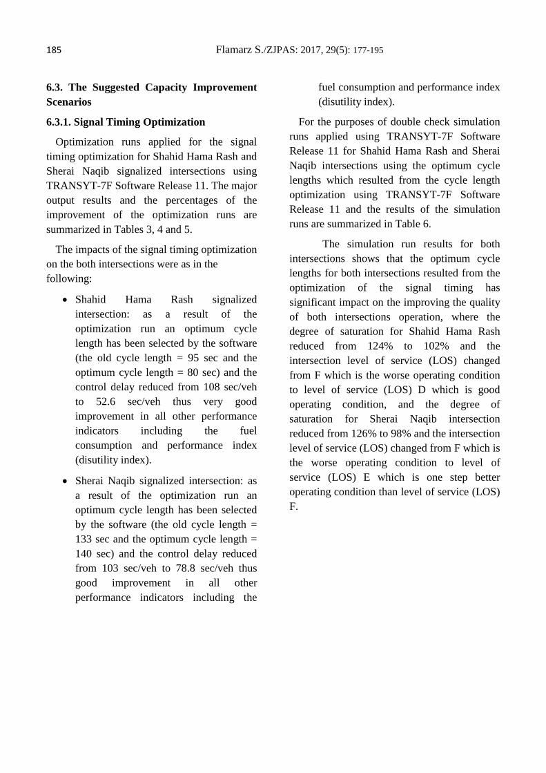
185 Flamarz S./ZJPAS: 2017, 29(5): 177-195 6.3. The Suggested Capacity Improvement Scenarios

6.3.1. Signal Timing Optimization

Optimization runs applied for the signal timing optimization for Shahid Hama Rash and Sherai Naqib signalized intersections using TRANSYT-7F Software Release 11. The major output results and the percentages of the improvement of the optimization runs are summarized in Tables 3, 4 and 5.

The impacts of the signal timing optimization on the both intersections were as in the following:

• Shahid Hama Rash signalized intersection: as a result of the optimization run an optimum cycle length has been selected by the software (the old cycle length = 95 sec and the optimum cycle length = 80 sec) and the control delay reduced from 108 sec/veh to 52.6 sec/veh thus very good improvement in all other performance indicators including the fuel consumption and performance index (disutility index).

• Sherai Naqib signalized intersection: as a result of the optimization run an optimum cycle length has been selected by the software (the old cycle length = 133 sec and the optimum cycle length = 140 sec) and the control delay reduced from 103 sec/veh to 78.8 sec/veh thus good improvement in all other performance indicators including the

fuel consumption and performance index (disutility index).

For the purposes of double check simulation runs applied using TRANSYT-7F Software Release 11 for Shahid Hama Rash and Sherai Naqib intersections using the optimum cycle lengths which resulted from the cycle length optimization using TRANSYT-7F Software Release 11 and the results of the simulation runs are summarized in Table 6.

The simulation run results for both intersections shows that the optimum cycle lengths for both intersections resulted from the optimization of the signal timing has significant impact on the improving the quality of both intersections operation, where the degree of saturation for Shahid Hama Rash reduced from 124% to 102% and the intersection level of service (LOS) changed from F which is the worse operating condition to level of service (LOS) D which is good operating condition, and the degree of saturation for Sherai Naqib intersection reduced from 126% to 98% and the intersection level of service (LOS) changed from F which is the worse operating condition to level of service (LOS) E which is one step better operating condition than level of service (LOS) F.

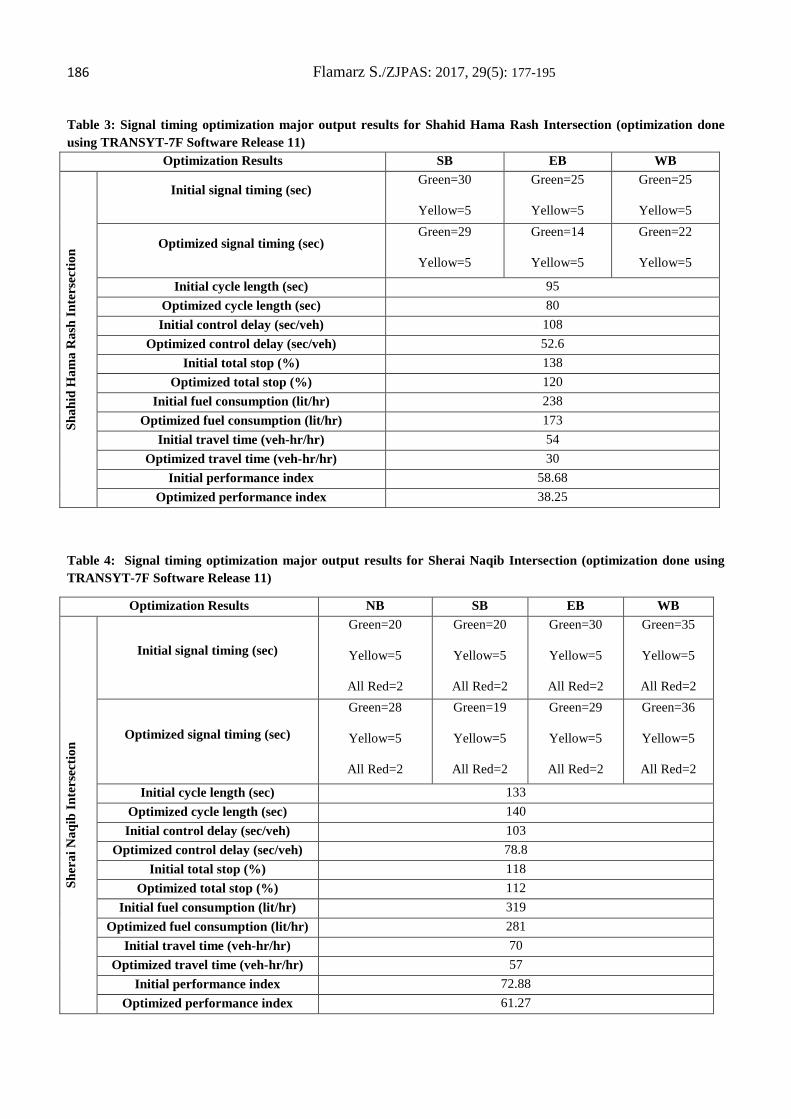
186 Flamarz S./ZJPAS: 2017, 29(5): 177-195 Table 3: Signal timing optimization major output results for Shahid Hama Rash Intersection (optimization done using TRANSYT-7F Software Release 11)

Optimization Results SB EB WB

Shah

id H

ama

Ras

h In

ters

ectio

n

Initial signal timing (sec) Green=30

Yellow=5

Green=25

Yellow=5

Green=25

Yellow=5

Optimized signal timing (sec) Green=29

Yellow=5

Green=14

Yellow=5

Green=22

Yellow=5

Initial cycle length (sec) 95 Optimized cycle length (sec) 80 Initial control delay (sec/veh) 108

Optimized control delay (sec/veh) 52.6 Initial total stop (%) 138

Optimized total stop (%) 120 Initial fuel consumption (lit/hr) 238

Optimized fuel consumption (lit/hr) 173 Initial travel time (veh-hr/hr) 54

Optimized travel time (veh-hr/hr) 30 Initial performance index 58.68

Optimized performance index 38.25

Table 4: Signal timing optimization major output results for Sherai Naqib Intersection (optimization done using TRANSYT-7F Software Release 11)

Optimization Results NB SB EB WB

Sher

ai N

aqib

Inte

rsec

tion

Initial signal timing (sec)

Green=20

Yellow=5

All Red=2

Green=20

Yellow=5

All Red=2

Green=30

Yellow=5

All Red=2

Green=35

Yellow=5

All Red=2

Optimized signal timing (sec)

Green=28

Yellow=5

All Red=2

Green=19

Yellow=5

All Red=2

Green=29

Yellow=5

All Red=2

Green=36

Yellow=5

All Red=2

Initial cycle length (sec) 133 Optimized cycle length (sec) 140 Initial control delay (sec/veh) 103

Optimized control delay (sec/veh) 78.8 Initial total stop (%) 118

Optimized total stop (%) 112 Initial fuel consumption (lit/hr) 319

Optimized fuel consumption (lit/hr) 281 Initial travel time (veh-hr/hr) 70

Optimized travel time (veh-hr/hr) 57 Initial performance index 72.88

Optimized performance index 61.27

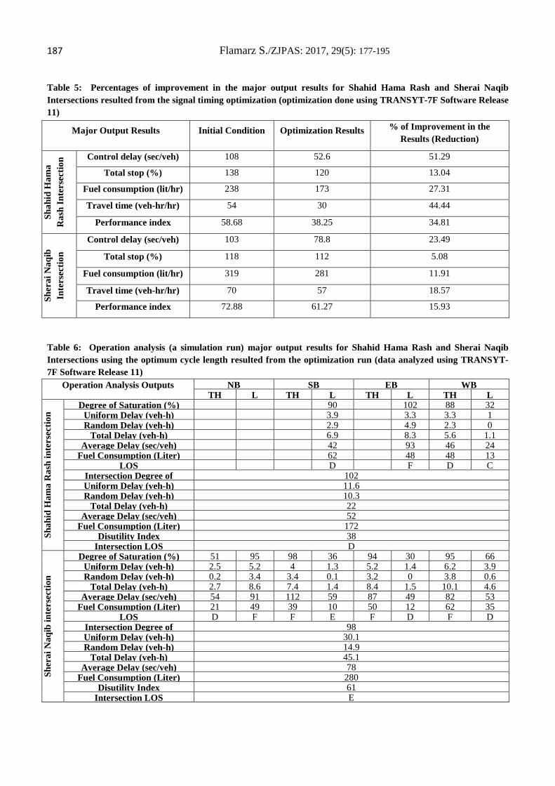
187 Flamarz S./ZJPAS: 2017, 29(5): 177-195 Table 5: Percentages of improvement in the major output results for Shahid Hama Rash and Sherai Naqib Intersections resulted from the signal timing optimization (optimization done using TRANSYT-7F Software Release 11)

Table 6: Operation analysis (a simulation run) major output results for Shahid Hama Rash and Sherai Naqib Intersections using the optimum cycle length resulted from the optimization run (data analyzed using TRANSYT-7F Software Release 11)

Operation Analysis Outputs NB SB EB WB TH L TH L TH L TH L

Shah

id H

ama

Ras

h in

ters

ectio

n

Degree of Saturation (%) 90 102 88 32 Uniform Delay (veh-h) 3.9 3.3 3.3 1 Random Delay (veh-h) 2.9 4.9 2.3 0

Total Delay (veh-h) 6.9 8.3 5.6 1.1 Average Delay (sec/veh) 42 93 46 24

Fuel Consumption (Liter) 62 48 48 13 LOS D F D C

Intersection Degree of

102 Uniform Delay (veh-h) 11.6 Random Delay (veh-h) 10.3

Total Delay (veh-h) 22 Average Delay (sec/veh) 52

Fuel Consumption (Liter) 172 Disutility Index 38

Intersection LOS D

Sher

ai N

aqib

inte

rsec

tion

Degree of Saturation (%) 51 95 98 36 94 30 95 66 Uniform Delay (veh-h) 2.5 5.2 4 1.3 5.2 1.4 6.2 3.9 Random Delay (veh-h) 0.2 3.4 3.4 0.1 3.2 0 3.8 0.6

Total Delay (veh-h) 2.7 8.6 7.4 1.4 8.4 1.5 10.1 4.6 Average Delay (sec/veh) 54 91 112 59 87 49 82 53

Fuel Consumption (Liter) 21 49 39 10 50 12 62 35 LOS D F F E F D F D

Intersection Degree of

98 Uniform Delay (veh-h) 30.1 Random Delay (veh-h) 14.9

Total Delay (veh-h) 45.1 Average Delay (sec/veh) 78

Fuel Consumption (Liter) 280 Disutility Index 61

Intersection LOS E

Major Output Results Initial Condition Optimization Results % of Improvement in the Results (Reduction)

Shah

id H

ama

Ras

h In

ters

ectio

n Control delay (sec/veh) 108 52.6 51.29

Total stop (%) 138 120 13.04

Fuel consumption (lit/hr) 238 173 27.31

Travel time (veh-hr/hr) 54 30 44.44

Performance index 58.68 38.25 34.81

Sher

ai N

aqib

In

ters

ectio

n

Control delay (sec/veh) 103 78.8 23.49

Total stop (%) 118 112 5.08

Fuel consumption (lit/hr) 319 281 11.91

Travel time (veh-hr/hr) 70 57 18.57

Performance index 72.88 61.27 15.93

187 Flamarz S./ZJPAS: 2017, 29(5): 177-195

6.3.2. Improving the Existing Geometric Design

Improving the existing geometric design of Shahid Hama Rash and Sherai Naqib intersections can be achieved by re allocating of the exiting lanes and increasing the number of the lanes (this improvement involve widening the sides of approaches and re-painting them) in the targeted approaches. It is noticed from the operation analysis (simulation run) for the existing conditions for Shahid Hama Rash and Sherai Naqib signalized intersections that most of the lane groups are operating under the level of service (LOS) E and F which are congested and poor operation condition in addition to that the level of service for both intersections Shahid Hama Rash and Sherai Naqib is F which is the worse operation condition.

Based on what mentioned above the number of lanes for the congested lane groups are increased by re allocating the existing lanes or increasing the number of lanes in the targeted approaches in both intersections Shahid Hama Rash and Sherai Naqib to reduce the delay caused by the congested lane groups and improve its operation quality and as a final result improve the overall operation quality for both intersections.

For the purposes of measuring the impact of improving the existing geometric design on the operation quality of Shahid Hama Rash and Sherai Naqib intersections a simulation run has applied using TRANSYT-7F Software Release 11 on each of the two intersections after re allocating the existing lanes or increasing the number of lanes in the targeted approaches for both intersections. The results of the simulation runs are summarized in Table 7.

The simulation run results for both intersections shows that improving the existing geometric design of both intersections has a

significant impact on increasing the capacity and improving the quality of both intersections operation, where the degree of saturation for Shahid Hama Rash reduced from 124% to 87% and the intersection level of service (LOS) changed from F which is the worse operating condition to level of service (LOS) D which is good operating condition, and the degree of saturation for Sherai Naqib intersection reduced from 126% to 76% and the intersection level of service (LOS) changed from F which is the worse operating condition to level of service (LOS) D which is good operating condition.

The impact of improving the existing geometric design on both intersection lane groups was as following:

• Shahid Hama Rash signalized intersection:

a. The impact of this improvement on the lane groups degree of saturation were; South Bond (SB) Left turn (L) the degree of saturation changed from 124% to 71%, East Bond (EB) Left Turn (L) the degree of saturation changed from 56% to 33%, West Bond (WB) Through (TH) the degree of saturation changed from 92% to 87% and West Bond (WB) Left Turn (L) the degree of saturation changed from 34% to 38%.

b. The impact of this improvement on the lane groups level of service (LOS) were; South Bond (SB) Left turn (L) the level of service (LOS) changed from F to D, East Bond (EB) Left Turn (L) the level of service (LOS) remained C, West Bond (WB) Through (TH) the level of service (LOS) changed from E to D and West Bond (WB) Left Turn (L) the level of service (LOS) remained C.

c. The impact of this improvement on the lane groups fuel consumption were; South Bond (SB) Left turn (L) the fuel

188 Flamarz S./ZJPAS: 2017, 29(5): 177-195

consumption changed from 140 liter to 59 liter, East Bond (EB) Left Turn (L) the fuel consumption changed from 29 liter to 27 liter, West Bond (WB) Through (TH) the fuel consumption changed from 51 liter to 49 liter and West Bond (WB) Left Turn (L) the fuel consumption remained 14 liter.

• Sherai Naqib signalized intersection:

a. The impact of this improvement on the lane groups degree of saturation were; North Bond (NB) Through (TH) the degree of saturation changed from 68% to 62%, Bond (NB) Left Turn (L) the degree of saturation changed from 126% to 76%, South Bond (SB) Through (TH) the degree of saturation changed from 88% to 40%, South Bond (SB) Left turn (L) the degree of saturation changed from 33% to 15%, East Bond (EB) Through (TH) the degree of saturation changed from 88% to 39%, East Bond (EB) Left Turn (L) the degree of saturation changed from 28% to 25%, West Bond (WB) Through (TH) the degree of saturation changed from 93% to 42% and West Bond (WB) Left Turn (L) the degree of saturation changed from 65% to 59%.

b. The impact of this improvement on the lane groups level of Service (LOS) were; North Bond (NB) Through (TH) the level of service (LOS) remained E, Bond

(NB) Left Turn (L) the level of service (LOS) changed from F to E, South Bond (SB) Through (TH) the level of service (LOS) changed from F to D, South Bond (SB) Left turn (L) the level of service (LOS) remained D, East Bond (EB) Through (TH) the level of service (LOS) changed from E to D, East Bond (EB) Left Turn (L) the level of service (LOS) remained D, West Bond (WB) Through (TH) the level of service (LOS) changed from E to D and West Bond (WB) Left Turn (L) the level of service (LOS) remained D.

c. The impact of this improvement on the lane groups fuel consumption were; North Bond (NB) Through (TH) the fuel consumption remained 22 liters, Bond (NB) Left Turn (L) the fuel consumption changed from 100 liters to 43 liters, South Bond (SB) Through (TH) the fuel consumption changed from 33 liters to 26 liters, South Bond (SB) Left turn (L) the fuel consumption remained 9 liters, East Bond (EB) Through (TH) the fuel consumption changed from 44 liters to 34 liters, East Bond (EB) Left Turn (L) the fuel consumption changed from 11 liters to 10 liters, West Bond (WB) Through (TH) the fuel consumption changed from 58 liters to 42 liters and West Bond (WB) Left Turn (L) the fuel consumption changed from 33 liters to 31 liters.

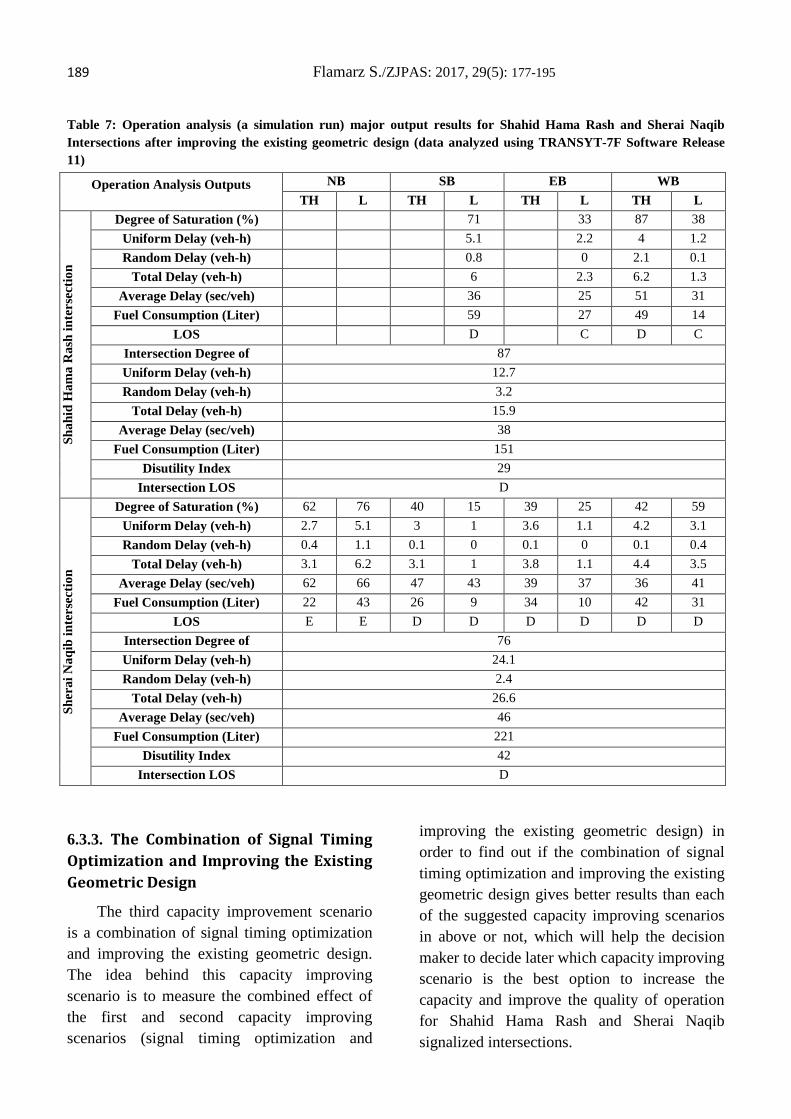
189 Flamarz S./ZJPAS: 2017, 29(5): 177-195 Table 7: Operation analysis (a simulation run) major output results for Shahid Hama Rash and Sherai Naqib Intersections after improving the existing geometric design (data analyzed using TRANSYT-7F Software Release 11)

6.3.3. The Combination of Signal Timing Optimization and Improving the Existing Geometric Design

The third capacity improvement scenario is a combination of signal timing optimization and improving the existing geometric design. The idea behind this capacity improving scenario is to measure the combined effect of the first and second capacity improving scenarios (signal timing optimization and

improving the existing geometric design) in order to find out if the combination of signal timing optimization and improving the existing geometric design gives better results than each of the suggested capacity improving scenarios in above or not, which will help the decision maker to decide later which capacity improving scenario is the best option to increase the capacity and improve the quality of operation for Shahid Hama Rash and Sherai Naqib signalized intersections.

Operation Analysis Outputs NB SB EB WB TH L TH L TH L TH L

Shah

id H

ama

Ras

h in

ters

ectio

n

Degree of Saturation (%) 71 33 87 38 Uniform Delay (veh-h) 5.1 2.2 4 1.2 Random Delay (veh-h) 0.8 0 2.1 0.1

Total Delay (veh-h) 6 2.3 6.2 1.3 Average Delay (sec/veh) 36 25 51 31

Fuel Consumption (Liter) 59 27 49 14 LOS D C D C

Intersection Degree of

87 Uniform Delay (veh-h) 12.7 Random Delay (veh-h) 3.2

Total Delay (veh-h) 15.9 Average Delay (sec/veh) 38

Fuel Consumption (Liter) 151 Disutility Index 29

Intersection LOS D

Sher

ai N

aqib

inte

rsec

tion

Degree of Saturation (%) 62 76 40 15 39 25 42 59 Uniform Delay (veh-h) 2.7 5.1 3 1 3.6 1.1 4.2 3.1 Random Delay (veh-h) 0.4 1.1 0.1 0 0.1 0 0.1 0.4

Total Delay (veh-h) 3.1 6.2 3.1 1 3.8 1.1 4.4 3.5 Average Delay (sec/veh) 62 66 47 43 39 37 36 41

Fuel Consumption (Liter) 22 43 26 9 34 10 42 31 LOS E E D D D D D D

Intersection Degree of

76 Uniform Delay (veh-h) 24.1 Random Delay (veh-h) 2.4

Total Delay (veh-h) 26.6 Average Delay (sec/veh) 46

Fuel Consumption (Liter) 221 Disutility Index 42

Intersection LOS D

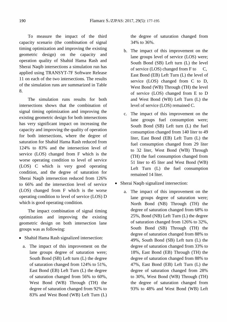
190 Flamarz S./ZJPAS: 2017, 29(5): 177-195 To measure the impact of the third capacity scenario (the combination of signal timing optimization and improving the existing geometric design) on the capacity and operation quality of Shahid Hama Rash and Sherai Naqib intersections a simulation run has applied using TRANSYT-7F Software Release 11 on each of the two intersections. The results of the simulation runs are summarized in Table 8.

The simulation runs results for both intersections shows that the combination of signal timing optimization and improving the existing geometric design for both intersections has very significant impact on increasing the capacity and improving the quality of operation for both intersections, where the degree of saturation for Shahid Hama Rash reduced from 124% to 83% and the intersection level of service (LOS) changed from F which is the worse operating condition to level of service (LOS) C which is very good operating condition, and the degree of saturation for Sherai Naqib intersection reduced from 126% to 66% and the intersection level of service (LOS) changed from F which is the worse operating condition to level of service (LOS) D which is good operating condition.

The impact combination of signal timing optimization and improving the existing geometric design on both intersection lane groups was as following:

• Shahid Hama Rash signalized intersection:

a. The impact of this improvement on the lane groups degree of saturation were; South Bond (SB) Left turn (L) the degree of saturation changed from 124% to 51%, East Bond (EB) Left Turn (L) the degree of saturation changed from 56% to 60%, West Bond (WB) Through (TH) the degree of saturation changed from 92% to 83% and West Bond (WB) Left Turn (L)

the degree of saturation changed from 34% to 36%.

b. The impact of this improvement on the lane groups level of service (LOS) were; South Bond (SB) Left turn (L) the level of service (LOS) changed from F to C, East Bond (EB) Left Turn (L) the level of service (LOS) changed from C to D, West Bond (WB) Through (TH) the level of service (LOS) changed from E to D and West Bond (WB) Left Turn (L) the level of service (LOS) remained C.

c. The impact of this improvement on the lane groups fuel consumption were; South Bond (SB) Left turn (L) the fuel consumption changed from 140 liter to 49 liter, East Bond (EB) Left Turn (L) the fuel consumption changed from 29 liter to 32 liter, West Bond (WB) Through (TH) the fuel consumption changed from 51 liter to 45 liter and West Bond (WB) Left Turn (L) the fuel consumption remained 14 liter.

• Sherai Naqib signalized intersection:

a. The impact of this improvement on the lane groups degree of saturation were; North Bond (NB) Through (TH) the degree of saturation changed from 68% to 25%, Bond (NB) Left Turn (L) the degree of saturation changed from 126% to 32%, South Bond (SB) Through (TH) the degree of saturation changed from 88% to 49%, South Bond (SB) Left turn (L) the degree of saturation changed from 33% to 18%, East Bond (EB) Through (TH) the degree of saturation changed from 88% to 47%, East Bond (EB) Left Turn (L) the degree of saturation changed from 28% to 30%, West Bond (WB) Through (TH) the degree of saturation changed from 93% to 48% and West Bond (WB) Left

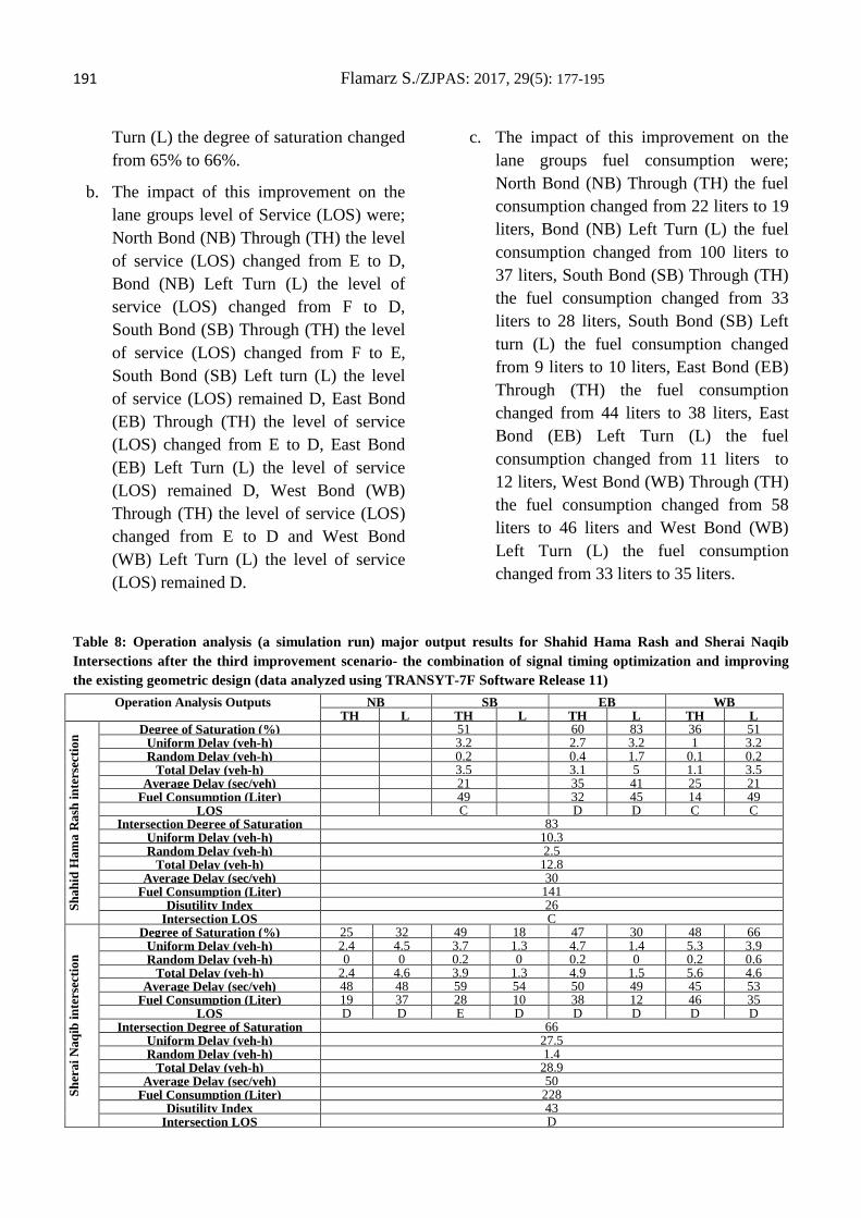
191 Flamarz S./ZJPAS: 2017, 29(5): 177-195

Turn (L) the degree of saturation changed from 65% to 66%.

b. The impact of this improvement on the lane groups level of Service (LOS) were; North Bond (NB) Through (TH) the level of service (LOS) changed from E to D, Bond (NB) Left Turn (L) the level of service (LOS) changed from F to D, South Bond (SB) Through (TH) the level of service (LOS) changed from F to E, South Bond (SB) Left turn (L) the level of service (LOS) remained D, East Bond (EB) Through (TH) the level of service (LOS) changed from E to D, East Bond (EB) Left Turn (L) the level of service (LOS) remained D, West Bond (WB) Through (TH) the level of service (LOS) changed from E to D and West Bond (WB) Left Turn (L) the level of service (LOS) remained D.

c. The impact of this improvement on the lane groups fuel consumption were; North Bond (NB) Through (TH) the fuel consumption changed from 22 liters to 19 liters, Bond (NB) Left Turn (L) the fuel consumption changed from 100 liters to 37 liters, South Bond (SB) Through (TH) the fuel consumption changed from 33 liters to 28 liters, South Bond (SB) Left turn (L) the fuel consumption changed from 9 liters to 10 liters, East Bond (EB) Through (TH) the fuel consumption changed from 44 liters to 38 liters, East Bond (EB) Left Turn (L) the fuel consumption changed from 11 liters to 12 liters, West Bond (WB) Through (TH) the fuel consumption changed from 58 liters to 46 liters and West Bond (WB) Left Turn (L) the fuel consumption changed from 33 liters to 35 liters.

Table 8: Operation analysis (a simulation run) major output results for Shahid Hama Rash and Sherai Naqib Intersections after the third improvement scenario- the combination of signal timing optimization and improving the existing geometric design (data analyzed using TRANSYT-7F Software Release 11)

Operation Analysis Outputs NB SB EB WB TH L TH L TH L TH L

Shah

id H

ama

Ras

h in

ters

ectio

n Degree of Saturation (%) 51 60 83 36 51 Uniform Delay (veh-h) 3.2 2.7 3.2 1 3.2 Random Delay (veh-h) 0.2 0.4 1.7 0.1 0.2

Total Delay (veh-h) 3.5 3.1 5 1.1 3.5 Average Delay (sec/veh) 21 35 41 25 21

Fuel Consumption (Liter) 49 32 45 14 49 LOS C D D C C

Intersection Degree of Saturation

83 Uniform Delay (veh-h) 10.3 Random Delay (veh-h) 2.5

Total Delay (veh-h) 12.8 Average Delay (sec/veh) 30

Fuel Consumption (Liter) 141 Disutility Index 26

Intersection LOS C

Sher

ai N

aqib

inte

rsec

tion

Degree of Saturation (%) 25 32 49 18 47 30 48 66 Uniform Delay (veh-h) 2.4 4.5 3.7 1.3 4.7 1.4 5.3 3.9 Random Delay (veh-h) 0 0 0.2 0 0.2 0 0.2 0.6

Total Delay (veh-h) 2.4 4.6 3.9 1.3 4.9 1.5 5.6 4.6 Average Delay (sec/veh) 48 48 59 54 50 49 45 53

Fuel Consumption (Liter) 19 37 28 10 38 12 46 35 LOS D D E D D D D D

Intersection Degree of Saturation

66 Uniform Delay (veh-h) 27.5 Random Delay (veh-h) 1.4

Total Delay (veh-h) 28.9 Average Delay (sec/veh) 50

Fuel Consumption (Liter) 228 Disutility Index 43

Intersection LOS D

192 Flamarz S./ZJPAS: 2017, 29(5): 177-195

6.4. A Comparison between the Suggested Capacity Improvement Scenarios Results

The goal of this comparison is to identify which of the three intersection capacity improvement scenarios gave the best results in term of increasing the intersection capacity and improving the quality of operation. Depending on the simulation runs for the existing conditions and the three suggested intersection capacity improvement scenarios applied to Shahid Hama Rash and Sherai Naqib signalized intersections using TRANSYT-7F Software Release 11, it can be decided which of the three capacity improvement scenarios gave the best results as it is explained in the following:

• Shahid Hama Rash Signalized Intersection: from the simulation runs major results (Intersection; degree of saturation, delay, fuel consumption, disutility index and level of service) which are summarized and explained in Table 9 for the existing conditions and the three suggested intersection capacity improvement scenarios applied on Shahid Hama Rash intersection it is easily recognized that the best capacity improvement scenario is the third intersection capacity improvement scenario (combination of signal timing optimization and improving the existing geometric design).

• Sherai Naqib Signalized Intersection: from the simulation runs major results (Intersection; degree of saturation, delay,

fuel consumption, disutility index and level of service) which are summarized and explained in Table 9 for the existing conditions and the three suggested intersection capacity improvement scenarios applied on Sherai Naqib intersection the best capacity improvement scenario is the second and third intersection capacity improvement scenarios, where in terms of intersection; delay, fuel consumption and disutility index the results of the second capacity improvement scenario (improving the existing geometric design) is better and in term of intersection degree of saturation the result of the third capacity improvement scenario (combination of signal timing optimization and improving the existing geometric design) is better. Regarding the intersection level of service (LOS), both capacity improvement scenarios resulted intersection level of service D which is good operation quality condition. But in the second intersection capacity improvement scenario the level of service for the through and left movements of the North Bond is E and it is D for all other movements (see Table 7), where in the third intersection capacity improvement scenario the level of service is E only for the through movement of the South Bond and it is D for all other movements (see Table 8).

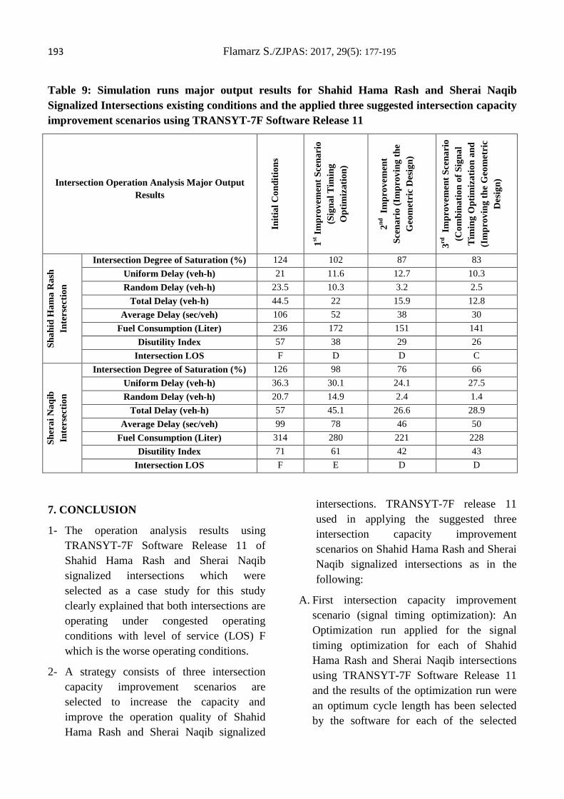
193 Flamarz S./ZJPAS: 2017, 29(5): 177-195 Table 9: Simulation runs major output results for Shahid Hama Rash and Sherai Naqib Signalized Intersections existing conditions and the applied three suggested intersection capacity improvement scenarios using TRANSYT-7F Software Release 11

7. CONCLUSION

1- The operation analysis results using TRANSYT-7F Software Release 11 of Shahid Hama Rash and Sherai Naqib signalized intersections which were selected as a case study for this study clearly explained that both intersections are operating under congested operating conditions with level of service (LOS) F which is the worse operating conditions.

2- A strategy consists of three intersection capacity improvement scenarios are selected to increase the capacity and improve the operation quality of Shahid Hama Rash and Sherai Naqib signalized

intersections. TRANSYT-7F release 11 used in applying the suggested three intersection capacity improvement scenarios on Shahid Hama Rash and Sherai Naqib signalized intersections as in the following:

A. First intersection capacity improvement scenario (signal timing optimization): An Optimization run applied for the signal timing optimization for each of Shahid Hama Rash and Sherai Naqib intersections using TRANSYT-7F Software Release 11 and the results of the optimization run were an optimum cycle length has been selected by the software for each of the selected

Intersection Operation Analysis Major Output Results

Initi

al C

ondi

tions

1st Im

prov

emen

t Sce

nari

o

(Sig

nal T

imin

g O

ptim

izat

ion)

2nd I

mpr

ovem

ent

Scen

ario

(Im

prov

ing

the

Geo

met

ric

Des

ign)

3rd I

mpr

ovem

ent S

cena

rio

(Com

bina

tion

of S

igna

l T

imin

g O

ptim

izat

ion

and

(Im

prov

ing

the

Geo

met

ric

Des

ign)

Shah

id H

ama

Ras

h In

ters

ectio

n

Intersection Degree of Saturation (%) 124 102 87 83 Uniform Delay (veh-h) 21 11.6 12.7 10.3 Random Delay (veh-h) 23.5 10.3 3.2 2.5

Total Delay (veh-h) 44.5 22 15.9 12.8 Average Delay (sec/veh) 106 52 38 30

Fuel Consumption (Liter) 236 172 151 141 Disutility Index 57 38 29 26

Intersection LOS F D D C

Sher

ai N

aqib

In

ters

ectio

n

Intersection Degree of Saturation (%) 126 98 76 66 Uniform Delay (veh-h) 36.3 30.1 24.1 27.5 Random Delay (veh-h) 20.7 14.9 2.4 1.4

Total Delay (veh-h) 57 45.1 26.6 28.9 Average Delay (sec/veh) 99 78 46 50

Fuel Consumption (Liter) 314 280 221 228 Disutility Index 71 61 42 43

Intersection LOS F E D D

194 Flamarz S./ZJPAS: 2017, 29(5): 177-195

intersection with a significant improvements in all intersection performance indicators.

B. Second intersection capacity improvement scenario (improving the existing geometric design): The simulation runs results for the selected intersections shows that improving the existing intersections geometric design have a significant impact on the increasing the capacity and improving the quality of selected intersections operation.

C. Third intersection capacity improvement scenario (the combination of signal timing optimization and improving the existing geometric design): the simulation runs results for the selected intersections shows that the combination of signal timing optimization and improving the existing geometric design has very significant impact on the increasing the capacity and improving the quality of both intersections operation.

3- Depending on the simulation runs for the existing conditions and the three suggested intersection capacity improvement scenarios applied on Shahid Hama Rash and Sherai Naqib signalized intersections using TRANSYT-7F Software Release 11, it can be decided which of the three capacity improvement scenarios gave the best results as it is explained in the following:

A. Shahid Hama Rash Signalized Intersection: from the simulation runs major results (Intersection; degree of saturation, delay, fuel consumption, disutility index and level of service) for the existing conditions and the three suggested intersection capacity

improvement scenarios applied on Shahid Hama Rash intersection it is clearly recognized that the best capacity improvement scenario is the third scenario (combination of signal timing optimization and improving the existing geometric design).

B. Sherai Naqib Signalized Intersection: from the simulation runs major results (Intersection; degree of saturation, delay, fuel consumption, disutility index and level of service) for the existing conditions and the three suggested intersection capacity improvement scenarios applied on Sherai Naqib intersection the best capacity improvement scenarios are the second and third scenarios, where in term of intersection; delay, fuel consumption and disutility index the results of the second capacity improvement scenario (improving the existing geometric design) is better and in term of intersection degree of saturation the result of the third capacity improvement scenario (combination of signal timing optimization and improving the existing geometric design) is better. Regarding the intersection level of service (LOS), both capacity improvement scenarios resulted intersection level of service D which is good operation quality condition. But in the second intersection capacity improvement scenario the level of service for the through and left movements of the North Bond is E and it is D for all other movements, where in the third intersection capacity improvement scenario the level of service is E only for the through movement of the South Bond and it is D for all other movements.

Conflict of Interest There is no conflict of interest.

195 Flamarz S./ZJPAS: 2017, 29(5): 177-195

REFERENCES

Borkloe, J. K., Nyantakyi , E. K ., Mohammed, G.A., 2013. Capacity Analysis of Selected Intersections on Mampong Road, Kumasi- Ghana Using Micro Simulation Model. International Journal of Structural and Civil Engineering Research (IJSCER), 2(3), pp.39–61.

Garber, N.J., Hoel, L.A., 2009. Traffic and Highway Engineering 4th ed., Cengage Learning.

Kumar, S., Ranjitha, J., 2013. Improvement Of Traffic Operations In Congested Signalized Intersections - A Case Study In Bangalore City. International Journal of Engineering Research and Technology (IJERT), 2(7), pp.2284–2291.

McTrans, 2008. TRANSYT-7F User’s Guide 11th ed., University of Florida.

Tovar, S. R., Alvaro, R. V., 2010. Effect of Phase Sequence in Capacity Signalized Intersections. Wolrd Conference on Transport Research (WCTR), 12(7), pp.1–17.

Transportation Research Board (TRP), 2000. Highway capacity manual, National Academy of Sciences.

ZANCO Journal of Pure and Applied Sciences

The official scientific journal of Salahaddin University-Erbil

ZJPAS (2017), 29 (2); 196-207

http://dx.doi.org/10.21271/ZJPAS.29.2.20

SYBR Green Real Time PCR Assay for Quantitative Detection of Escherichia coli

Directly from Clinical Samples

Ari Q. Nabi*

* Department of Biology, College of Science, Salahaddin University, Erbil, Kurdistan Region, Iraq.

1. INTRODUCTION

The most important limitation of blood cultures

for diagnosis of infection is the time required

from blood sampling to reporting results back

to the treating clinician. Culture based infection

diagnosis is a multistep process that can take

up to 5 days or more to rule in or rule out the

presence of a pathogen in the blood

sample(Gilbert DN et al., 2004). Some

information on whether culture bottles are

showing a detectable growth will usually be

available with 1-2 days but this is still slow

when it is taken into account that antibiotic

A R T I C L E I N F O

A B S T R A C T

Article History:

Received: 04/10/2016

Accepted: 25/02/2017

Published: 07/06/2017

Diagnosis of bloodstream bacterial infection in its early stages are key steps

for its treatment, however because of the brutal effects of sepsis and the necessity

of its immediate treatment, many physicians don’t wait for the conventional

microbiological diagnosis and start prescribing antimicrobial drugs. Therefore

designing a fast, accurate and economic quantitative real-time PCR method (qR-

PCR) to quantify the total number of Escherichia coli and to detect pathogenic

strains of the bacterium from blood and clinical samples is a crucial step for early

diagnosis and treatment of the problem. In this study, SYBR Green I used as

inexpensive indicator to reduce the costs in comparison with probe based methods

and is compatible with conventional microbiological methods. UspA gene which

encodes for the universal regulator stress protein has been selected as a target gene

which is the most suitable candidate to detect the presence of any E. coli, while eae

gene which encodes for the outer membrane protein intimin was targeted in order

to evaluate the presence of virulence strains among positive samples. The

suitability and utility of the quantitative SGR-PCR assay for detection of E. coli in

different samples sources has been evaluated by artificial inoculation of healthy

blood with type strains of E. coli used for designing a quantitative standard curve.

The protocol was then applied on blood and some clinical samples collected from

suspected patients with sepsis. Using this method and despite of a relatively low

positive data when testing the blood samples, both sets of primers showed to be

useful for the detection of E. coli and the strains that harbor virulence genes. The

developed standard curves confirmed that this method is a quantitative in a

detection range of 102 to 10

8 cells mL-1, and that the qSG R-PCR assay can be

used as a new and successful molecular tool to detect and quantify all and

pathogenic E. coli directly from clinical samples without pre-enrichment steps,

when presenting at concentrations greater than 102 cells mL-1.

Keywords:

SYBR Green I

Quantitative PCR

Blood infection.

*Corresponding Author:

Dr. Ari Q. Nabi

ari.nabi@su.edu.krd

197 Nabi A./ZJPAS: 2017, 29 (2): 196-207

therapy has to be administered very quickly to

patients who have clinical evidence of

infection. Inadequate antimicrobial treatment

has a major impact on mortality in these

patients and a recent study of patients with

severe sepsis demonstrated that each hour

delay of administration of an effective

antibiotic therapy is associated with an 8%

increase in mortality (Kumar et al., 2006,

Gilbert DN et al., 2004).

The most common bacterial pathogens

frequently isolated in association with

bloodstream infection, particularly in critical

care, are Enterobacteriaceae including E.coli,

Klebsiella species, Serratia and Proteus

species. E.coli and Proteus species are mostly

isolated with urinary tract infection but also

reported as vascular line-associated infections

(Livermore et al., 2008).Blood culture, which

is the traditional method for bacterial

identification, takes 2-3 days (Dark et al.,

2009). There has been great interest in the

development of new diagnostic methods able to

speed up the process of determining presence

of infection and identification of the pathogen.

PCR can detect and identify pathogen DNA

present in small amounts (Cursons et al.,

1999).

Quantitative real-time PCR has enhanced the

sensitivity and specificity of PCR-based assay

in the detection of pathogenic microorganisms

in food and the environment, allowing

quantitative analysis and avoiding the use of

time-consuming and cost-effective

electrophoresis (Beneduce et al., 2007).

UspA gene which encodes for the universal

stress protein has been identified and

characterized in E. coli K-12 strain W3110

(Nyström and Neidhardt, 1992), was found to

be highly specific for E. coli differentiating it

from other Gram-negative bacteria (Chen and

Griffiths, 1998, Siegele, 2005). The production

of attaching-and-effacing lesions requires the

expression of intimin, an outer-membrane

protein encoded by the eae gene that is part of

the locus of enterocyte effacement (Sharma,

2002).The popularity of using SYBR Green I

assays with R- PCRs users is due to three

factors: 1) low cost for the dye; 2) ease of assay

development, only a pair of primers is required;

and 3) the same detection mechanism can be

used for every assay (Dorak, 2007, John M.

Walker and Rapley, 2008). The most recent

advances in qR-PCR methods are focused on

the reduction of the limits of detection and

quantification, on the discrimination between

dead and live cells or the simultaneous

detection of different foodborne pathogens.

The performances of these methods were, in

some cases, successfully compared with the

official protocols or with diagnostic

commercial kits (Pasquale Russo et al., 2014,

Elizaquivel and Aznar, 2008, Dorak, 2007).

The aim of this work was development a PCR

assay that would allow a rapid and direct

detection and quantification of the pathogen in

blood samples without pre-enrichment step

before DNA extraction, to ensure an effective

treatment of patients with blood stream

bacterial infections.

2. MATERIALS AND METHODS

2.1. Samples

A total of forty-five blood samples were

collected from suspected patients for blood

infection during the period from January to

August 2016 from 2 local hospitals located in

Erbil city. During the sampling period, 2 to 6

samples were collected from each hospital

according to the case coincidences. Specimens

(blood samples) were aseptically collected into

Brain Heart Infusion Medium bottles (Oxoid,

UK), according to laboratory-defined standard

operating procedures, and then prepared for

genomic DNA extraction. Each specimen was

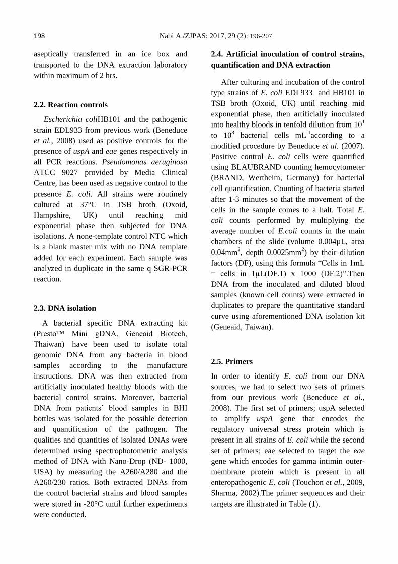
198 Nabi A./ZJPAS: 2017, 29 (2): 196-207

aseptically transferred in an ice box and

transported to the DNA extraction laboratory

within maximum of 2 hrs.

2.2. Reaction controls

Escherichia coliHB101 and the pathogenic

strain EDL933 from previous work (Beneduce

et al., 2008) used as positive controls for the

presence of uspA and eae genes respectively in

all PCR reactions. Pseudomonas aeruginosa

ATCC 9027 provided by Media Clinical

Centre, has been used as negative control to the

presence E. coli. All strains were routinely

cultured at 37°C in TSB broth (Oxoid,

Hampshire, UK) until reaching mid

exponential phase then subjected for DNA

isolations. A none-template control NTC which

is a blank master mix with no DNA template

added for each experiment. Each sample was

analyzed in duplicate in the same q SGR-PCR

reaction.

2.3. DNA isolation

A bacterial specific DNA extracting kit

(Presto™ Mini gDNA, Geneaid Biotech,

Thaiwan) have been used to isolate total

genomic DNA from any bacteria in blood

samples according to the manufacture

instructions. DNA was then extracted from

artificially inoculated healthy bloods with the

bacterial control strains. Moreover, bacterial

DNA from patients’ blood samples in BHI

bottles was isolated for the possible detection

and quantification of the pathogen. The

qualities and quantities of isolated DNAs were

determined using spectrophotometric analysis

method of DNA with Nano-Drop (ND- 1000,

USA) by measuring the A260/A280 and the

A260/230 ratios. Both extracted DNAs from

the control bacterial strains and blood samples

were stored in -20°C until further experiments

were conducted.

2.4. Artificial inoculation of control strains,

quantification and DNA extraction

After culturing and incubation of the control

type strains of E. coli EDL933 and HB101 in

TSB broth (Oxoid, UK) until reaching mid

exponential phase, then artificially inoculated

into healthy bloods in tenfold dilution from 101

to 108 bacterial cells mL

-1according to a

modified procedure by Beneduce et al. (2007).

Positive control E. coli cells were quantified

using BLAUBRAND counting hemocytometer

(BRAND, Wertheim, Germany) for bacterial

cell quantification. Counting of bacteria started

after 1-3 minutes so that the movement of the

cells in the sample comes to a halt. Total E.

coli counts performed by multiplying the

average number of E.coli counts in the main

chambers of the slide (volume 0.004µL, area

0.04mm2, depth 0.0025mm

2) by their dilution

factors (DF), using this formula “Cells in 1mL

= cells in 1µL(DF.1) x 1000 (DF.2)”.Then

DNA from the inoculated and diluted blood

samples (known cell counts) were extracted in

duplicates to prepare the quantitative standard

curve using aforementioned DNA isolation kit

(Geneaid, Taiwan).

2.5. Primers

In order to identify E. coli from our DNA

sources, we had to select two sets of primers

from our previous work (Beneduce et al.,

2008). The first set of primers; uspA selected

to amplify uspA gene that encodes the

regulatory universal stress protein which is

present in all strains of E. coli while the second

set of primers; eae selected to target the eae

gene which encodes for gamma intimin outer-

membrane protein which is present in all

enteropathogenic E. coli (Touchon et al., 2009,

Sharma, 2002).The primer sequences and their

targets are illustrated in Table (1).

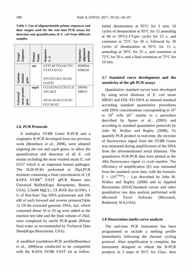
199 Nabi A./ZJPAS: 2017, 29 (2): 196-207 Table 1. List of oligonucleotide primer sequences and

their targets used for the real time PCR assays for

detection and quantification of E. coli from different

samples.

Ta

rget

Seq

uen

ce

Pri

mer

Na

me

Seq

uen

ce

5´-

3´

Seq

uen

ce

ali

gn

men

t

po

siti

on

Ga

mm

a

Inti

min

gen

e

eae GTTCACTGGACTTC

TTATTACCG

ATCGTCACCAGAG

GAATC

4598564 -

4598120

Un

iver

sal

stre

ss p

rote

in

gen

e

reg

ula

tor

uspA CCGATACGCTGCCA

ATCAGT

ACGCAGACCGTAG

GCCAGAT

299361-

298515

2.6. PCR Protocols

A multiplex SYBR Green R-PCR and a

singleplex R-PCR developed from our previous

work (Beneduce et al., 2008), were adopted

targeting the eae and uspA genes, to allow the

quantification and detection of all E. coli

strains including the most virulent strain E. coli

O157 which is an important human pathogen.

The SGR-PCRs performed in 20µLPCR

mixtures containing a final concentration of 1X

KAPA SYBR® FAST qPCR Master mix

Universal Buffer(Kapa Biosystems, Boston,

USA), 2.5mM MgCL2, 1X ROX dye (LOW), 1

U of Hot-Start Taq DNA polymerase and 200

nM of each forward and reverse primers(Table

1). Of the extracted genomic DNA, 3µL which

contained about 10 to 20 ng were added to the

reaction test tube and the final volume of 20µL

were completed by sterile PCR-grade (RNase

free) water as recommended by Technical Data

Sheet(Kapa Biosystems, USA).

A modified touchdown-PCR profile(Beneduce

et al., 2008)was conducted to be compatible

with the KAPA SYBR FAST kit as follow:

Initial denaturation at 95°C for 3 min; 10

cycles of denaturation at 95°C for 15 annealing

at 68 to 59°C(-1°Cper cycle) for 25 s, and

extension at 72°C for 50 s; followed by 30

cycles of denaturation at 95°C for 15 s,

annealing at 59°C for 25 s, and extension at

72°C for 50 s; and a final extension at 72°C for

10 min.

2.7 Standard curve development and the

sensitivity of the qR-PCR assays

Quantitative standard curves were developed

by using serial dilutions of E. coli strain

HB101 and EDL 933 DNA as internal standard

according standard quantitative procedures

with DNA concentrations corresponding to 102

to 108 cells ml

-1 similar to a procedure

described by Spano et al., (2005) and

according to standard quantitative protocols by

John M. Walker and Rapley (2008). To

quantify PCR product in real-time, the increase

of fluorescence signal from the SYBR Green

was measured during amplification of the DNA

from the aforementioned serial dilutions. The

quantitative SGR-PCR data were plotted as the

ΔRn fluorescence signal vs cycle number. The

efficiency of amplification (E) was estimated

from the standard curve data, with the formula:

E = (101/slope

) – 1,as described by John M.

Walker and Rapley (2008) and in Applied

Biosystems (2010).Standard curves and other

quantitative raw data analysis performed with

Microsoft Excel Software (Microsoft,

Redmond, WA,USA).

2.8 Dissociation (melt) curve analysis

The real-time PCR instrument has been

programmed to include a melting profile

immediately following the thermal cycling

protocol. After amplification is complete, the

instrument designed to reheat the R-PCR

products in 3 steps of 95°C for 15sec, then

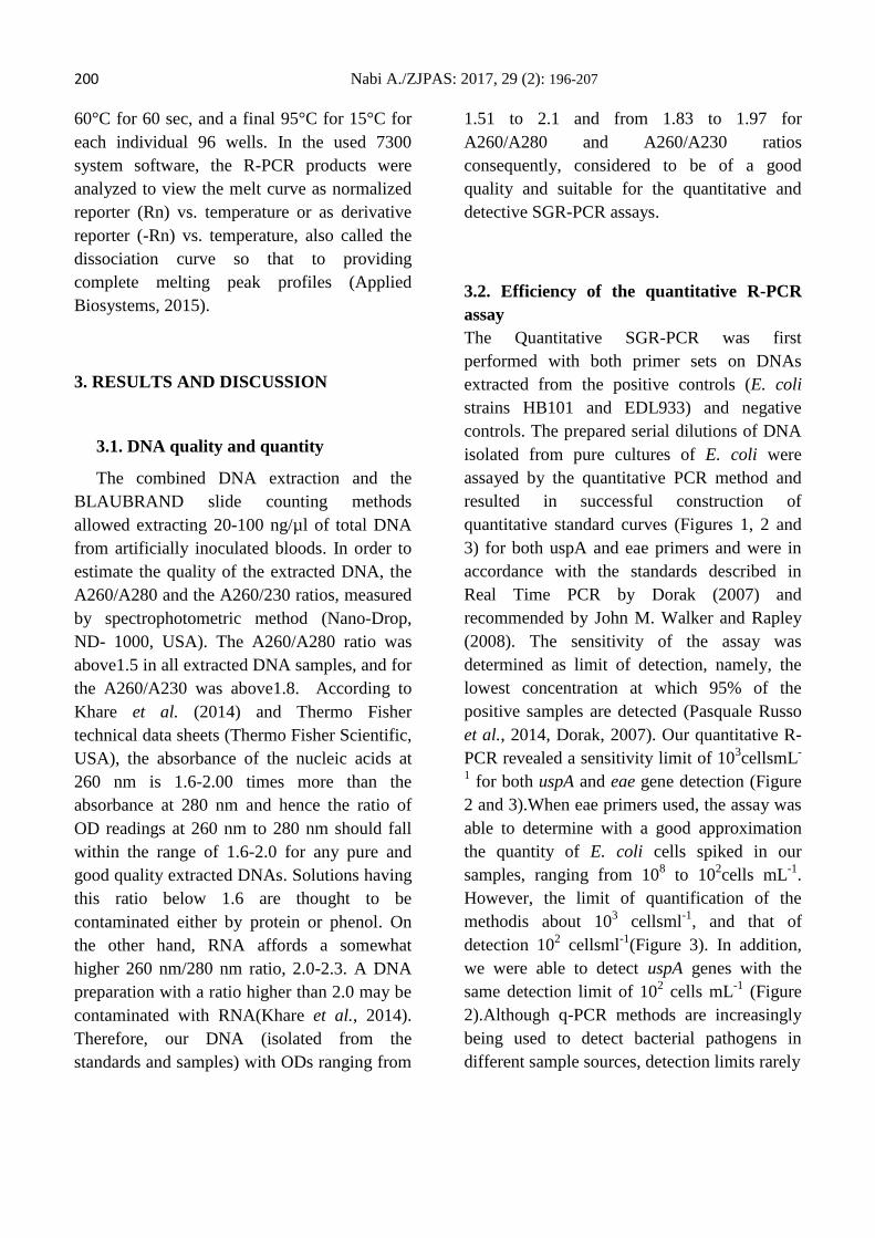
200 Nabi A./ZJPAS: 2017, 29 (2): 196-207

60°C for 60 sec, and a final 95°C for 15°C for

each individual 96 wells. In the used 7300

system software, the R-PCR products were

analyzed to view the melt curve as normalized

reporter (Rn) vs. temperature or as derivative

reporter (-Rn) vs. temperature, also called the

dissociation curve so that to providing

complete melting peak profiles (Applied

Biosystems, 2015).

3. RESULTS AND DISCUSSION

3.1. DNA quality and quantity

The combined DNA extraction and the

BLAUBRAND slide counting methods

allowed extracting 20-100 ng/µl of total DNA

from artificially inoculated bloods. In order to

estimate the quality of the extracted DNA, the

A260/A280 and the A260/230 ratios, measured

by spectrophotometric method (Nano-Drop,

ND- 1000, USA). The A260/A280 ratio was

above1.5 in all extracted DNA samples, and for

the A260/A230 was above1.8. According to

Khare et al. (2014) and Thermo Fisher

technical data sheets (Thermo Fisher Scientific,

USA), the absorbance of the nucleic acids at

260 nm is 1.6-2.00 times more than the

absorbance at 280 nm and hence the ratio of

OD readings at 260 nm to 280 nm should fall

within the range of 1.6-2.0 for any pure and

good quality extracted DNAs. Solutions having

this ratio below 1.6 are thought to be

contaminated either by protein or phenol. On

the other hand, RNA affords a somewhat

higher 260 nm/280 nm ratio, 2.0-2.3. A DNA

preparation with a ratio higher than 2.0 may be

contaminated with RNA(Khare et al., 2014).

Therefore, our DNA (isolated from the

standards and samples) with ODs ranging from

1.51 to 2.1 and from 1.83 to 1.97 for

A260/A280 and A260/A230 ratios

consequently, considered to be of a good

quality and suitable for the quantitative and

detective SGR-PCR assays.

3.2. Efficiency of the quantitative R-PCR

assay

The Quantitative SGR-PCR was first

performed with both primer sets on DNAs

extracted from the positive controls (E. coli

strains HB101 and EDL933) and negative

controls. The prepared serial dilutions of DNA

isolated from pure cultures of E. coli were

assayed by the quantitative PCR method and

resulted in successful construction of

quantitative standard curves (Figures 1, 2 and

3) for both uspA and eae primers and were in

accordance with the standards described in

Real Time PCR by Dorak (2007) and

recommended by John M. Walker and Rapley

(2008). The sensitivity of the assay was

determined as limit of detection, namely, the

lowest concentration at which 95% of the

positive samples are detected (Pasquale Russo

et al., 2014, Dorak, 2007). Our quantitative R-

PCR revealed a sensitivity limit of 103cellsmL

-

1 for both uspA and eae gene detection (Figure

2 and 3).When eae primers used, the assay was

able to determine with a good approximation

the quantity of E. coli cells spiked in our

samples, ranging from 108 to 10

2cells mL

-1.

However, the limit of quantification of the

methodis about 103 cellsml

-1, and that of

detection 102 cellsml

-1(Figure 3). In addition,

we were able to detect uspA genes with the

same detection limit of 102 cells mL

-1 (Figure

2).Although q-PCR methods are increasingly

being used to detect bacterial pathogens in

different sample sources, detection limits rarely

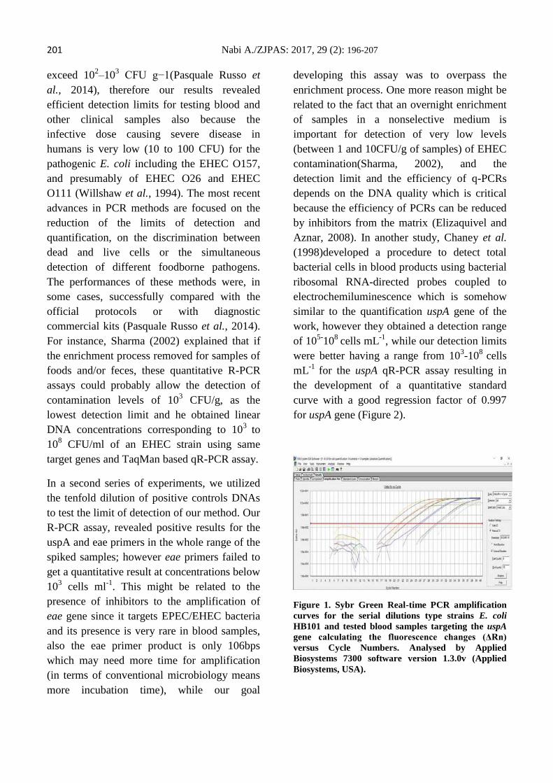
201 Nabi A./ZJPAS: 2017, 29 (2): 196-207

exceed 102–10

3 CFU g−1(Pasquale Russo et

al., 2014), therefore our results revealed

efficient detection limits for testing blood and

other clinical samples also because the

infective dose causing severe disease in

humans is very low (10 to 100 CFU) for the

pathogenic E. coli including the EHEC O157,

and presumably of EHEC O26 and EHEC

O111 (Willshaw et al., 1994). The most recent

advances in PCR methods are focused on the

reduction of the limits of detection and

quantification, on the discrimination between

dead and live cells or the simultaneous

detection of different foodborne pathogens.

The performances of these methods were, in

some cases, successfully compared with the

official protocols or with diagnostic

commercial kits (Pasquale Russo et al., 2014).

For instance, Sharma (2002) explained that if

the enrichment process removed for samples of

foods and/or feces, these quantitative R-PCR

assays could probably allow the detection of

contamination levels of 103 CFU/g, as the

lowest detection limit and he obtained linear

DNA concentrations corresponding to 103

to

108 CFU/ml of an EHEC strain using same

target genes and TaqMan based qR-PCR assay.

In a second series of experiments, we utilized

the tenfold dilution of positive controls DNAs

to test the limit of detection of our method. Our

R-PCR assay, revealed positive results for the

uspA and eae primers in the whole range of the

spiked samples; however eae primers failed to

get a quantitative result at concentrations below

103 cells ml

-1. This might be related to the

presence of inhibitors to the amplification of

eae gene since it targets EPEC/EHEC bacteria

and its presence is very rare in blood samples,

also the eae primer product is only 106bps

which may need more time for amplification

(in terms of conventional microbiology means

more incubation time), while our goal

developing this assay was to overpass the

enrichment process. One more reason might be

related to the fact that an overnight enrichment

of samples in a nonselective medium is

important for detection of very low levels

(between 1 and 10CFU/g of samples) of EHEC

contamination(Sharma, 2002), and the

detection limit and the efficiency of q-PCRs

depends on the DNA quality which is critical

because the efficiency of PCRs can be reduced

by inhibitors from the matrix (Elizaquivel and

Aznar, 2008). In another study, Chaney et al.

(1998)developed a procedure to detect total

bacterial cells in blood products using bacterial

ribosomal RNA-directed probes coupled to

electrochemiluminescence which is somehow

similar to the quantification uspA gene of the

work, however they obtained a detection range

of 105-

108

cells mL-1

, while our detection limits

were better having a range from 103-10

8 cells

mL-1

for the uspA qR-PCR assay resulting in

the development of a quantitative standard

curve with a good regression factor of 0.997

for uspA gene (Figure 2).

Figure 1. Sybr Green Real-time PCR amplification

curves for the serial dilutions type strains E. coli

HB101 and tested blood samples targeting the uspA

gene calculating the fluorescence changes (ΔRn)

versus Cycle Numbers. Analysed by Applied

Biosystems 7300 software version 1.3.0v (Applied

Biosystems, USA).

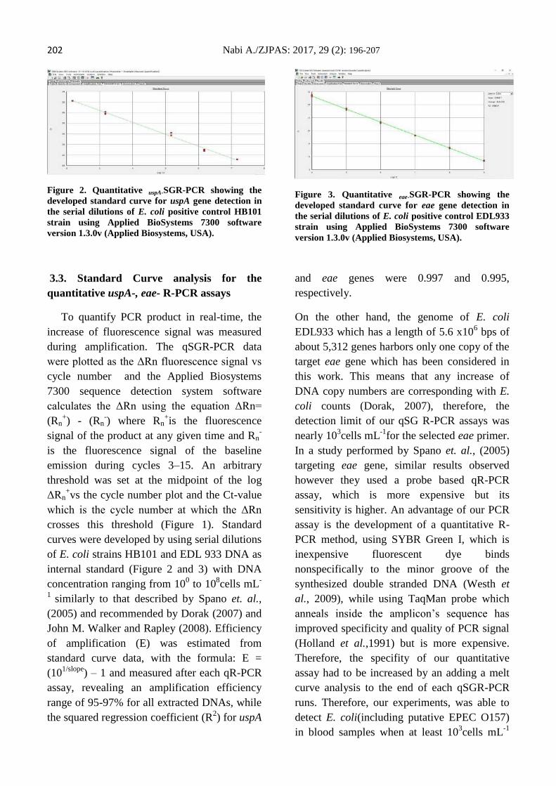
202 Nabi A./ZJPAS: 2017, 29 (2): 196-207

Figure 2. Quantitative uspA-SGR-PCR showing the

developed standard curve for uspA gene detection in

the serial dilutions of E. coli positive control HB101

strain using Applied BioSystems 7300 software

version 1.3.0v (Applied Biosystems, USA).

Figure 3. Quantitative eae-SGR-PCR showing the

developed standard curve for eae gene detection in

the serial dilutions of E. coli positive control EDL933

strain using Applied BioSystems 7300 software

version 1.3.0v (Applied Biosystems, USA).

3.3. Standard Curve analysis for the

quantitative uspA-, eae- R-PCR assays

To quantify PCR product in real-time, the

increase of fluorescence signal was measured

during amplification. The qSGR-PCR data

were plotted as the ΔRn fluorescence signal vs

cycle number and the Applied Biosystems

7300 sequence detection system software

calculates the ΔRn using the equation ΔRn=

(Rn+) - (Rn

-) where Rn

+is the fluorescence

signal of the product at any given time and Rn-

is the fluorescence signal of the baseline

emission during cycles 3–15. An arbitrary

threshold was set at the midpoint of the log

ΔRn+vs the cycle number plot and the Ct-value

which is the cycle number at which the ΔRn

crosses this threshold (Figure 1). Standard

curves were developed by using serial dilutions

of E. coli strains HB101 and EDL 933 DNA as

internal standard (Figure 2 and 3) with DNA

concentration ranging from 100 to 10

8cells mL

-

1 similarly to that described by Spano et. al.,

(2005) and recommended by Dorak (2007) and

John M. Walker and Rapley (2008). Efficiency

of amplification (E) was estimated from

standard curve data, with the formula: E =

(101/slope

) – 1 and measured after each qR-PCR

assay, revealing an amplification efficiency

range of 95-97% for all extracted DNAs, while

the squared regression coefficient (R2) for uspA

and eae genes were 0.997 and 0.995,

respectively.

On the other hand, the genome of E. coli

EDL933 which has a length of 5.6 x106 bps of

about 5,312 genes harbors only one copy of the

target eae gene which has been considered in

this work. This means that any increase of

DNA copy numbers are corresponding with E.

coli counts (Dorak, 2007), therefore, the

detection limit of our qSG R-PCR assays was

nearly 103cells mL

-1for the selected eae primer.

In a study performed by Spano et. al., (2005)

targeting eae gene, similar results observed

however they used a probe based qR-PCR

assay, which is more expensive but its

sensitivity is higher. An advantage of our PCR

assay is the development of a quantitative R-

PCR method, using SYBR Green I, which is

inexpensive fluorescent dye binds

nonspecifically to the minor groove of the

synthesized double stranded DNA (Westh et

al., 2009), while using TaqMan probe which

anneals inside the amplicon’s sequence has

improved specificity and quality of PCR signal

(Holland et al.,1991) but is more expensive.

Therefore, the specifity of our quantitative

assay had to be increased by an adding a melt

curve analysis to the end of each qSGR-PCR

runs. Therefore, our experiments, was able to

detect E. coli(including putative EPEC O157)

in blood samples when at least 103cells mL

-1

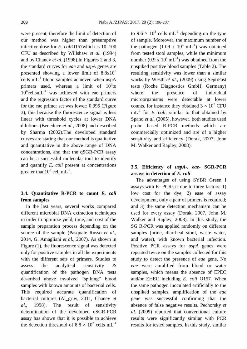
203 Nabi A./ZJPAS: 2017, 29 (2): 196-207

were present, therefore the limit of detection of

our method was higher than presumptive

infective dose for E. coliO157which is 10–100

CFU as described by Willshaw et al. (1994)

and by Chaney et al. (1998).In Figures 2 and 3,

the standard curves for eae and uspA genes are

presented showing a lower limit of 8.8x103

cells mL-1

blood samples achieved when uspA

primers used, whereas a limit of 103to

106cellsmL

-1 was achieved with eae primers

and the regression factor of the standard curve

for the eae primer set was lower; 0.995 (Figure

3), this because the fluorescence signal is less

linear with threshold cycles at lower DNA

dilutions (Beneduce et al., 2008) and described

by Sharma (2002).The developed standard

curves are stating that our method is qualitative

and quantitative in the above range of DNA

concentrations, and that the qSGR-PCR assay

can be a successful molecular tool to identify

and quantify E. coli present at concentrations

greater than103 cell mL

-1.

3.4. Quantitative R-PCR to count E. coli

from samples

In the last years, several works compared

different microbial DNA extraction techniques

in order to optimize yield, time, and cost of the

sample preparation process depending on the

source of the sample (Pasquale Russo et al.,

2014, G. Amagliani et al., 2007). As shown in

Figure (1), the fluorescence signal was detected

only for positive samples in all the experiments

with the different sets of primers. Studies to

assess the analytical sensitivity &

quantification of the pathogen DNA tests

described above involved “spiking” blood

samples with known amounts of bacterial cells.

This required accurate quantification of

bacterial cultures (Al_griw, 2011, Chaney et

al., 1998). The result of sensitivity

determination of the developed qSGR-PCR

assay has shown that it is possible to achieve

the detection threshold of 8.8 × 103 cells mL

-1

to 9.6 × 103 cells mL

-1 depending on the type

of sample. Moreover, the maximum number of

the pathogen (1.09 x 106 mL

-1) was obtained

from tested stool samples, while the minimum

number (0.9 x 101

mL-1

) was obtained from the

unspiked positive blood samples (Table 2). The

resulting sensitivity was lower than a similar

works by Westh et al., (2009) using SeptiFast

tests (Roche Diagnostics GmbH, Germany)

where the presence of individual

microorganisms were detectable at lower

counts, for instance they obtained 3 × 102 CFU

mL-1

for E. coli, similar to that obtained by

Spano et al. (2005), however, both studies used

probe based R-PCR methods which are

commercially optimized and are of a higher

sensitivity and efficiency (Dorak, 2007, John

M. Walker and Rapley, 2008).

3.5. Efficiency of uspA-, eae- SGR-PCR

assays in detection of E. coli

The advantages of using SYBR Green I

assays with R- PCRs is due to three factors: 1)

low cost for the dye; 2) ease of assay

development, only a pair of primers is required;

and 3) the same detection mechanism can be

used for every assay (Dorak, 2007, John M.

Walker and Rapley, 2008). In this study, the

SG R-PCR was applied randomly on different

samples (urine, diarrheal stool, waste water,

and water), with known bacterial infection.

Positive PCR assays for uspA genes were

repeated twice on the samples collected for this

study to detect the presence of eae gene. No

eae were amplified from blood or water

samples, which means the absence of EPEC

and/or EHEC including E. coli O157. When

the same pathogen inoculated artificially to the

unspiked samples, amplification of the eae

gene was successful confirming that the

absence of false negative results. Pechorsky et

al. (2009) reported that conventional culture

results were significantly similar with PCR

results for tested samples. In this study, similar

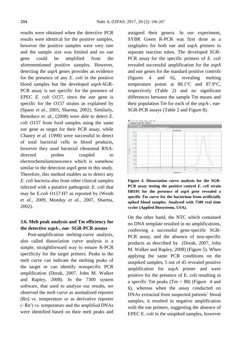
204 Nabi A./ZJPAS: 2017, 29 (2): 196-207

results were obtained when the detective PCR

results were identical for the positive samples,

however the positive samples were very rare

and the sample size was limited and no eae

gene could be amplified from the

aforementioned positive samples. However,

detecting the uspA genes provides an evidence

for the presence of any E. coli in the positive

blood samples but the developed uspA-SGR-

PCR assay is not specific for the presence of

EPEC E. coli O157, since the eae gene is

specific for the O157 strains as explained by

(Spano et al., 2005, Sharma, 2002). Similarly,

Beneduce et. al., (2008) were able to detect E.

coli O157 from food samples using the same

eae gene as target for their PCR assay, while

Chaney et al. (1998) were successful to detect

of total bacterial cells in blood products,

however they used bacterial ribosomal RNA-

directed probes coupled to

electrochemiluminescence which is somehow

similar to the detection uspA gene in this study.

Therefore, this method enables us to detect any

E. coli bacteria also from other clinical samples

infected with a putative pathogenic E. coli that

may be E.coli O157:H7 as reported by (Westh

et al., 2009, Monday et al., 2007, Sharma,

2002).

3.6. Melt peak analysis and Tm efficiency for

the detective uspA-, eae- SGR-PCR assays

Post-amplification melting-curve analysis,

also called dissociation curve analysis is a

simple, straightforward way to ensure R-PCR

specificity for the target primers. Peaks in the

melt curve can indicate the melting peaks of

the target or can identify nonspecific PCR

amplification (Dorak, 2007, John M. Walker

and Rapley, 2008). In the 7300 system

software, that used to analyze our results, we

observed the melt curve as normalized reporter

(Rn) vs. temperature or as derivative reporter

(−Rn′) vs. temperature and the amplified DNAs

were identified based on their melt peaks and

assigned their genera. In our experiment,

SYBR Green R-PCR was first done as a

singleplex for both eae and uspA primers in

separate reaction tubes. The developed SGR-

PCR assay for the specific primers of E. coli

revealed successful amplification for the uspA

and eae genes for the standard positive controls

(figures 4 and 6), revealing melting

temperature points at 88.1°C and 87.9°C,

respectively (Table 2) and no significant

differences between the sample Tm means and

their population Tm for each of the uspA-, eae-

SGR-PCR assays (Table 2 and Figure 8).

Figure 4. Dissociation curve analysis for the SGR-

PCR assay testing the positive control E. coli strain

HB101 for the presence of uspA gene revealed a

specific Tm curve for the bacterium from artificially

spiked blood samples. Analysed with 7500 real time

cycler (Applied Biosystems, USA).

On the other hand, the NTC which contained

no DNA template resulted in no amplifications,

conferring a successful gene-specific SGR-

PCR assay, and the absence of non-specific

products as described by (Dorak, 2007, John

M. Walker and Rapley, 2008) (Figure 5). When

applying the same PCR conditions on the

unspiked samples, 5 out of 45 revealed positive

amplification for uspA primer and were

positive for the presence of E. coli resulting in

a specific Tm peaks (Tm = 88) (Figure 4 and

6), whereas when the assay conducted on

DNAs extracted from suspected patients’ blood

samples, it resulted in negative amplification

with the eae primers, suggesting the absence of

EPEC E. coli in the unspiked samples, however

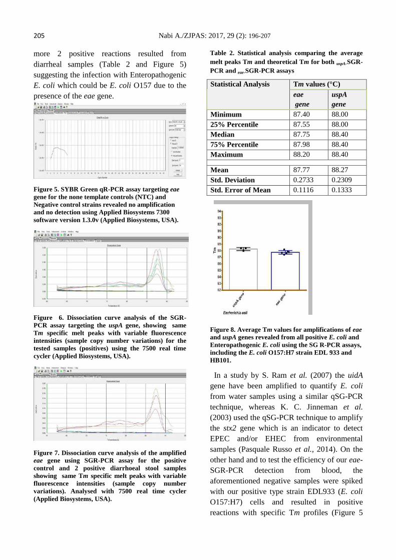
205 Nabi A./ZJPAS: 2017, 29 (2): 196-207

more 2 positive reactions resulted from

diarrheal samples (Table 2 and Figure 5)

suggesting the infection with Enteropathogenic

E. coli which could be E. coli O157 due to the

presence of the eae gene.

Figure 5. SYBR Green qR-PCR assay targeting eae

gene for the none template controls (NTC) and

Negative control strains revealed no amplification

and no detection using Applied Biosystems 7300

software version 1.3.0v (Applied Biosystems, USA).

Figure 6. Dissociation curve analysis of the SGR-

PCR assay targeting the uspA gene, showing same

Tm specific melt peaks with variable fluorescence

intensities (sample copy number variations) for the

tested samples (positives) using the 7500 real time

cycler (Applied Biosystems, USA).

Figure 7. Dissociation curve analysis of the amplified

eae gene using SGR-PCR assay for the positive

control and 2 positive diarrhoeal stool samples

showing same Tm specific melt peaks with variable

fluorescence intensities (sample copy number

variations). Analysed with 7500 real time cycler

(Applied Biosystems, USA).

Table 2. Statistical analysis comparing the average

melt peaks Tm and theoretical Tm for both uspA-SGR-

PCR and eae-SGR-PCR assays

Figure 8. Average Tm values for amplifications of eae

and uspA genes revealed from all positive E. coli and

Enteropathogenic E. coli using the SG R-PCR assays,

including the E. coli O157:H7 strain EDL 933 and

HB101.

In a study by S. Ram et al. (2007) the uidA

gene have been amplified to quantify E. coli

from water samples using a similar qSG-PCR

technique, whereas K. C. Jinneman et al.

(2003) used the qSG-PCR technique to amplify

the stx2 gene which is an indicator to detect

EPEC and/or EHEC from environmental

samples (Pasquale Russo et al., 2014). On the

other hand and to test the efficiency of our eae-

SGR-PCR detection from blood, the

aforementioned negative samples were spiked

with our positive type strain EDL933 (E. coli

O157:H7) cells and resulted in positive

reactions with specific Tm profiles (Figure 5

Statistical Analysis Tm values (°C)

eae

gene

uspA

gene

Minimum 87.40 88.00

25% Percentile 87.55 88.00

Median 87.75 88.40

75% Percentile 87.98 88.40

Maximum 88.20 88.40

Mean 87.77 88.27

Std. Deviation 0.2733 0.2309

Std. Error of Mean 0.1116 0.1333

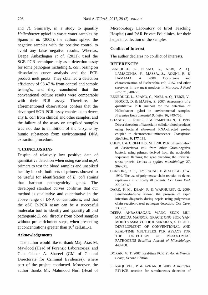
206 Nabi A./ZJPAS: 2017, 29 (2): 196-207

and 7). Similarly, in a study to quantify

Helicobacter pylori in waste water samples by

Spano et al. (2005), the authors spiked the

negative samples with the positive control to

avoid any false negative results. Whereas,

Deepa Anbazhagan et al. (2011), used the

SGR-PCR technique only as a detection assay

for some pathogens including E. coli, basing on

dissociation curve analysis and the PCR

product melt peaks. They obtained a detection

efficiency of 93.47 % from control and sample

testing’s, and they concluded that the

conventional culture results were comparable

with their PCR assay. Therefore, the

aforementioned observations confers that the

developed SGR-PCR assay enables us to detect

any E. coli from clinical and other samples, and

the failure of the assay on unspiked samples

was not due to inhibition of the enzyme by

humic substances from environmental DNA

extraction procedure.

4. CONCLUSIONS

Despite of relatively low positive data of

quantitative detection when using eae and uspA

primers to test the blood samples and unspiked

healthy bloods, both sets of primers showed to

be useful for identification of E. coli strains

that harbour pathogenicity genes. The

developed standard curves confirms that our

method is qualitative and quantitative in the

above range of DNA concentrations, and that

the qSG R-PCR assay can be a successful

molecular tool to identify and quantify all and

pathogenic E. coli directly from blood samples

without pre-enrichment steps, when presenting

at concentrations greater than 102 cell.mL-1.

Acknowledgements

The author would like to thank Maj. Aras M.

Mawlood (Head of Forensic Laboratories) and

Gen. Jabbar A. Shareef (GM of General

Directorate for Criminal Evidences), where

part of the project conducted. Moreover, the

author thanks Mr. Mahmood Nuri (Head of

Microbiology Laboratory of Erbil Teaching

Hospital) and PAR Private Policlinics, for their

helps in collection of the samples.

Conflict of Interest

The author declares no conflict of interests.

REFERENCES BENEDUCE, L., SPANO, G., NABI, A. Q.,

LAMACCHIA, F., MASSA, S., AOUNI, R. &

HAMAMA, A. 2008. Occurrence and

characterization of Escherichia coli O157 and other

serotypes in raw meat products in Morocco. J Food

Prot, 71, 2082-6.

BENEDUCE, L., SPANO, G., NABI, A. Q., TERZI, V.,

FIOCCO, D. & MASSA, S. 2007. Assessment of a

quantitative PCR method for the detection of

Helicobacter pylori in environmental samples.

Fresenius Environmental Bulletin, 16, 749-755.

CHANEY, R., RIDER, J. & PAMPHILON, D. 1998.

Direct detection of bacteria in cellular blood products

using bacterial ribosomal RNA-directed probes

coupled to electrochemiluminescence. Transfusion

Medicine, 9, 177-188.

CHEN, J. & GRIFFITHS, M. 1998. PCR differentiation

of Escherichia coli from other Gram‐negative

bacteria using primers derived from the nucleotide

sequences flanking the gene encoding the universal

stress protein. Letters in applied microbiology, 27,

369-371.

CURSONS, R. T., JEYERAJAH, E. & SLEIGH, J. W.

1999. The use of polymerase chain reaction to detect

septicemia in critically ill patients. Crit Care Med,

27, 937-40.

DARK, P. M., DEAN, P. & WARHURST, G. 2009.

Bench-to-bedside review: the promise of rapid

infection diagnosis during sepsis using polymerase

chain reaction-based pathogen detection. Crit Care,

13, 217.

DEEPA ANBAZHAGAN, WANG SEOK MUI,

MARZIDA MANSOR, GRACIE ONG SIOK YAN,

MOHD YASIM YUSOF & SEKARAN, S. D. 2011.

DEVELOPMENT OF CONVENTIONAL AND

REAL-TIME MULTIPLEX PCR ASSAYS FOR

THE DETECTION OF NOSOCOMIAL

PATHOGENS Brazilian Journal of Microbiology,

448-458.

DORAK, M. T. 2007. Real-time PCR. Taylor & Francis

Group, Second Edition.

ELIZAQUIVEL, P. & AZNAR, R. 2008. A multiplex

RTi-PCR reaction for simultaneous detection of

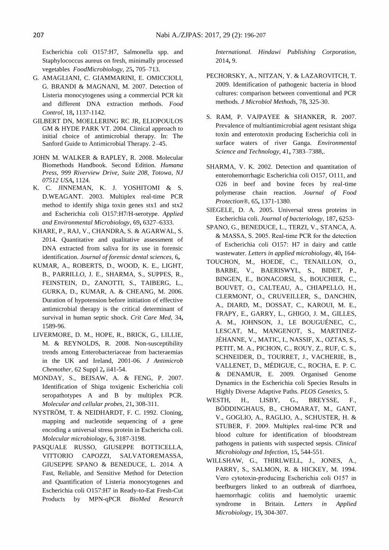
207 Nabi A./ZJPAS: 2017, 29 (2): 196-207

Escherichia coli O157:H7, Salmonella spp. and

Staphylococcus aureus on fresh, minimally processed

vegetables FoodMicrobiology, 25, 705–713.

G. AMAGLIANI, C. GIAMMARINI, E. OMICCIOLI,

G. BRANDI & MAGNANI, M. 2007. Detection of

Listeria monocytogenes using a commercial PCR kit

and different DNA extraction methods. Food

Control, 18, 1137-1142.

GILBERT DN, MOELLERING RC JR, ELIOPOULOS

GM & HYDE PARK VT. 2004. Clinical approach to

initial choice of antimicrobial therapy. In: The

Sanford Guide to Antimicrobial Therapy. 2–45.

JOHN M. WALKER & RAPLEY, R. 2008. Molecular

Biomethods Handbook. Second Edition. Humana

Press, 999 Riverview Drive, Suite 208, Totowa, NJ

07512 USA, 1124.

K. C. JINNEMAN, K. J. YOSHITOMI & S.

D.WEAGANT. 2003. Multiplex real-time PCR

method to identify shiga toxin genes stx1 and stx2

and Escherichia coli O157:H7/H-serotype. Applied

and Environmental Microbiology, 69, 6327–6333.

KHARE, P., RAJ, V., CHANDRA, S. & AGARWAL, S.

2014. Quantitative and qualitative assessment of

DNA extracted from saliva for its use in forensic

identification. Journal of forensic dental sciences, 6,

KUMAR, A., ROBERTS, D., WOOD, K. E., LIGHT,

B., PARRILLO, J. E., SHARMA, S., SUPPES, R.,

FEINSTEIN, D., ZANOTTI, S., TAIBERG, L.,

GURKA, D., KUMAR, A. & CHEANG, M. 2006.

Duration of hypotension before initiation of effective

antimicrobial therapy is the critical determinant of

survival in human septic shock. Crit Care Med, 34,

1589-96.

LIVERMORE, D. M., HOPE, R., BRICK, G., LILLIE,

M. & REYNOLDS, R. 2008. Non-susceptibility

trends among Enterobacteriaceae from bacteraemias

in the UK and Ireland, 2001-06. J Antimicrob

Chemother, 62 Suppl 2, ii41-54.

MONDAY, S., BEISAW, A. & FENG, P. 2007.

Identification of Shiga toxigenic Escherichia coli

seropathotypes A and B by multiplex PCR.

Molecular and cellular probes, 21, 308-311.

NYSTRÖM, T. & NEIDHARDT, F. C. 1992. Cloning,

mapping and nucleotide sequencing of a gene

encoding a universal stress protein in Eschericha coli.

Molecular microbiology, 6, 3187-3198.

PASQUALE RUSSO, GIUSEPPE BOTTICELLA,

VITTORIO CAPOZZI, SALVATOREMASSA,

GIUSEPPE SPANO & BENEDUCE, L. 2014. A

Fast, Reliable, and Sensitive Method for Detection

and Quantification of Listeria monocytogenes and

Escherichia coli O157:H7 in Ready-to-Eat Fresh-Cut

Products by MPN-qPCR BioMed Research

International. Hindawi Publishing Corporation,

2014, 9.

PECHORSKY, A., NITZAN, Y. & LAZAROVITCH, T.

2009. Identification of pathogenic bacteria in blood

cultures: comparison between conventional and PCR

methods. J Microbiol Methods, 78, 325-30.

S. RAM, P. VAJPAYEE & SHANKER, R. 2007.

Prevalence of multiantimicrobial agent resistant shiga

toxin and enterotoxin producing Escherichia coli in

surface waters of river Ganga. Environmental

Science and Technology, 41, 7383–7388,.

SHARMA, V. K. 2002. Detection and quantitation of

enterohemorrhagic Escherichia coli O157, O111, and

O26 in beef and bovine feces by real-time

polymerase chain reaction. Journal of Food

Protection®, 65, 1371-1380.

SIEGELE, D. A. 2005. Universal stress proteins in

Escherichia coli. Journal of bacteriology, 187, 6253-

SPANO, G., BENEDUCE, L., TERZI, V., STANCA, A.

& MASSA, S. 2005. Real‐time PCR for the detection

of Escherichia coli O157: H7 in dairy and cattle

wastewater. Letters in applied microbiology, 40, 164-

TOUCHON, M., HOEDE, C., TENAILLON, O.,

BARBE, V., BAERISWYL, S., BIDET, P.,

BINGEN, E., BONACORSI, S., BOUCHIER, C.,

BOUVET, O., CALTEAU, A., CHIAPELLO, H.,

CLERMONT, O., CRUVEILLER, S., DANCHIN,

A., DIARD, M., DOSSAT, C., KAROUI, M. E.,

FRAPY, E., GARRY, L., GHIGO, J. M., GILLES,

A. M., JOHNSON, J., LE BOUGUÉNEC, C.,

LESCAT, M., MANGENOT, S., MARTINEZ-

JÉHANNE, V., MATIC, I., NASSIF, X., OZTAS, S.,

PETIT, M. A., PICHON, C., ROUY, Z., RUF, C. S.,

SCHNEIDER, D., TOURRET, J., VACHERIE, B.,

VALLENET, D., MÉDIGUE, C., ROCHA, E. P. C.

& DENAMUR, E. 2009. Organised Genome

Dynamics in the Escherichia coli Species Results in

Highly Diverse Adaptive Paths. PLOS Genetics, 5.

WESTH, H., LISBY, G., BREYSSE, F.,

BÖDDINGHAUS, B., CHOMARAT, M., GANT,

V., GOGLIO, A., RAGLIO, A., SCHUSTER, H. &

STUBER, F. 2009. Multiplex real‐time PCR and

blood culture for identification of bloodstream

pathogens in patients with suspected sepsis. Clinical

Microbiology and Infection, 15, 544-551.

WILLSHAW, G., THIRLWELL, J., JONES, A.,

PARRY, S., SALMON, R. & HICKEY, M. 1994.

Vero cytotoxin‐producing Escherichia coli O157 in

beefburgers linked to an outbreak of diarrhoea,

haemorrhagic colitis and haemolytic uraemic

syndrome in Britain. Letters in Applied

Microbiology, 19, 304-307.