1  

 

ATMOSPHERIC CORROSION DATA OF WEATHERING STEELS. A REVIEW. 

M. Morcillo∗, B. Chico, I. Díaz, H. Cano, D. de la Fuente National Centre for Metallurgical Research (CENIM‐CSIC), Avda. Gregorio del Amo, 8, 28040‐

Madrid, Spain  

ABSTRACT Extensive information on the atmospheric corrosion of weathering steel has been published in the  scientific  literature.  The  contribution  of  the  present work  is  to  provide  a  bibliographic review of the reported information, which mostly concerns the weathering steel ASTM A‐242. This review addresses issues such as rust layer stabilisation times, steady‐state steel corrosion rates, and situations where the use of unpainted weathering steel  is feasible. It also analyses the effect of exposure conditions. Finally it approaches the important matter of predicting the long‐term behaviour of weathering steel reviewing the different prediction models published in the literature.  Keywords: A. Low alloy steel; C. Atmospheric corrosion; C. Rust  

1. Introduction 

Weathering steels (WS), also known as low‐alloy steels, are steels with a carbon content of less than 0.2 wt. %  to which mainly Cu, Cr, Ni, P, Si and Mn are added as alloying elements  to a total of no more  than 3‐5 wt. %  [1]. The enhanced corrosion  resistance of WS  in  relation  to mild steel or plain carbon steel (CS) is due to the formation in low aggressive atmospheres of a compact and well‐adhering corrosion product layer known as patina. 

This  definition,  however,  has  not  remained  unchanged  but  has  evolved  as  new  WS compositions  have  been  developed  to  achieve  improved  mechanical  properties  and/or withstand  increasingly  aggressive  atmospheric  conditions  from  the  corrosion  point  of  view, especially in marine environments. The American Society for Testing and Materials (ASTM) has standardised different alloy compositions for WS, from an  initial 1.5% total weight of alloying elements added  in  the  first standardised WS A‐242  [2],  to 5%  in  the  last standardised WS A 709‐HPS 100W [3], which is at the limit of the composition of intermediate alloy steels. Table 1 sets out the chemical composition of two commonly used WS [2, 4]. 

The patina on WS not only offers greater corrosion resistance  than on mild steel, but  is also responsible  for  its attractive appearance and  self‐healing abilities. The main applications  for WS  include  civil  structures  such  as  bridges  and  other  load‐bearing  structures,  road installations,  electricity  posts,  utility  towers,  guide  rails,  ornamental  sculptures,  façades, roofing, etc. 

The  literature  contains a great deal of  information on WS, and  there are entire  chapters  in collective  works  dedicated  to  this  issue,  e.g.  [1,  5‐6].  However,  an  in‐depth  bibliographic 

                                                            ∗ Corresponding author: Tel. +34 91 553 8900, Fax. +34 91 534 7425. e‐mail: morcillo@cenim.csic.es (M. Morcillo)  

2  

 

review  on  the  atmospheric  exposure  data  of WS  and  a  rigorous  analysis  of  the  published information are lacking. The review presented in this paper seeks to fill this gap. 

2. Brief historical development 

Albrecht and Hall [7] published a complete review on the historical development of WS. 

The birth of WS can be traced back to the development of steels containing copper, known as copper steels [8]. In 1910 Buck observed that steel sheets with 0.07% Cu manufactured by US Steel  and  exposed  in  three  environments  of  different  corrositivities  (rural,  industrial  and marine) showed a 1.5‐2% greater atmospheric corrosion resistance than CS [9]. Hence, in 1911 US  Steel  started  to market  steel  sheets with  a  certain  copper  content.  Buck  subsequently reported  that  the  improvement  achieved  with  Cu  concentrations  in  excess  of  0.25%  was insignificant, noting that 0.15% Cu provided similar results to 0.25% Cu in most cases [10]. 

Once this capacity of copper steel became known, further research led to the development of WS and thus to High Strength Low Alloy  (HSLA) steels  [7].  In the 1920's US Steel produced a new family of HSLA steels intended primarily for the railway industry. Finally, in 1933 US Steel launched  the  first  commercial WS  under  the  brand  name USS  Cor‐Ten  steel  (Early  Cor‐Ten steel or Cor‐Ten B), a name which reflects the two properties that differentiate it from CS, i.e. its corrosion resistance (Cor); and from a copper steel,  i.e.  its superior mechanical properties (tensile  strength,  Ten).  This  product  was  claimed  to  provide  a  30%  improvement  on  the mechanical  properties  of  conventional  CS,  thus  reducing  the  necessary  thickness  and accordingly  the weight of  steel  to be used  for a given  set of mechanical  requirements  [11]. Figure 1  illustrates the corrosion of these three steels  in the  industrial atmosphere of Kearny and its evolution with time [12]. Attention is drawn to the lower corrosion experienced by the Early Cor‐Ten steel. 

Early versions of USS Cor‐Ten steels were based on Fe‐Cu‐Cr‐P systems, to which Ni was later added  in order  to  improve  corrosion  resistance  in marine environments. USS Cor‐Ten  steels presented two specifications, A and B, whose main difference lay in the amount of phosphorus present  in  their  composition.  USS  Cor‐Ten  A  can  be  said  to  be  the WS  with  the  highest phosphorus content (0.07‐0.15% weight) and USS Cor‐Ten B that with the  lowest phosphorus content (≤0.04 % weight) [13]. 

Greater knowledge of the role played by the different alloying elements (Cu, Cr, Ni, P, etc.) in the atmospheric behaviour of WS was achieved thanks to two ambitious studies carried out in the United States, one began in 1941 by ASTM Committee A‐5 [14] and another began in 1942 by US Steel Co. [12]. In the first, 71 low‐alloy steels were exposed to the industrial atmosphere at Bayonne, N.J. and to the marine atmospheres at Block  Island, R.I. and at Kure Beach  (250 m), N.C. In the second study, 270 different steels were exposed in the following atmospheres: South Bend, Pa (semi‐rural), Kearny, N.J. (industrial) and Kure Beach (250 m), N.C. (marine). 

The current composition of USS Cor‐Ten steels has altered to a certain extent, especially in the case  of  specification  B,  with  the  addition  of  Ni  (≤0.40  %  Ni),  but  they  all  continue  to  be marketed  to  the  present  day  [15‐16].  In  1941  the  first  WS  was  standardised  by  ASTM specification  A‐242;  a  steel  that  is  roughly  comparable  to  USS  Cor‐Ten  A  steel.  Its  main characteristic  is  its high  resistance  to atmospheric corrosion, which  is approximately 4  times greater  than  that  of  CS  due  to  the  presence  of  copper,  a  high  phosphorus  content,  and  in 

3  

 

general  the  presence  of  nickel  (0.50‐0.65%).  However,  it  is  now  somewhat  obsolete  as  a structural  steel due  to  the  fact  that phosphorus  can  form  iron phosphide  (FeP3) during  the welding process, decreasing its weldability and causing the steel to become brittle. 

In  1968  ASTM  standard  A‐242  presented  two  specifications,  one  with  a  high  phosphorus content (<0.15% P) and the other with a lower phosphorus content (<0.04% P). The latter was ultimately replaced by ASTM standard A‐588 WS [4] (see Table 1), which is roughly comparable to USS Cor‐Ten B steel. This steel possesses less resistance to atmospheric corrosion due to its lower P content, but for this same reason it has better weldability. 

Finally,  in 1992 the US Federal Highway Administration (FHWA), the American  Iron and Steel Institute  (AISI)  and  the US Navy  started  to  develop  new  improved WS  for  bridge  building, known as High Performance Steels (HPS), and in 1997 the first bridge with HPS‐70W was built in  Nebraska  [17].  Three  basic  targets  were  set  to  improve  the  overall  quality  and manufacturability of the steels used hitherto for bridge construction in the United States [18]: (a)  improve weldability, achieved by  lowering  the carbon, phosphorus and sulphur contents; (b) improve mechanical properties, such as fracture toughness and yield strength, achieved by raising the maximum manganese  limit; and (c) maintain the formation of protective rust that characterises WS. 

3.  Requirements for the formation of protective rust layers on WS 

As has been mentioned, the enhanced corrosion resistance of WS is due to the formation of a dense and well‐adhering corrosion product layer. 

Experiments  carried  out  in  1969  by  Schmitt  and Gallagher with  low  alloy  steel  (Cor‐Ten A) indicated  that  the  texture  of  the  oxide  layer  was  dependent  upon  the  washing  action  of rainwater  and  the  drying  action  of  the  sun  [19].  Surfaces  sheltered  from  the  sun  and  rain tended to form a loose and non‐compact oxide while surfaces openly exposed to the sun and rain  produced  strongly  adherent  layers.  On  north‐facing  surfaces  the  protective  layer developed somewhat more slowly as a result of receiving less sunlight. Matsushima et al. [20] subsequently studied the role of a large number of environmental and design variables in the behaviour of WS in architectural applications, verifying the decisive influence on the formation of  the protective patina of whether or not  the metallic  surface was exposed  to  the  rain, or whether or not areas where moisture was  liable  to accumulate were drained. These effects were more  intense  in atmospheres with higher pollution  levels,  in which case  the protective patina may not fully form. 

Extensive  research work  has  thrown  light  on  the  requisites  for  the  protective  rust  layer  to form. It  is now well accepted that wet/dry cycling  is necessary to form a dense and adherent rust layer, with rainwater washing the steel surface well, accumulated moisture draining easily, and a  fast drying action  (absence of  very  long wetness  times).  Structures  should be  free of interstices,  crevices,  cavities  and  other  places where water  can  collect,  as  corrosion would progress without the formation of a protective patina. It is also not advisable to use bare WS in continuously moist exposure conditions or in marine atmospheres where the protective patina does not form [5‐6, 21]. 

Therefore,  the ability of weathering  type  steels  to  fully develop  their anticorrosive action  is dependent on  the  climate  and  exposure  conditions of  the metallic  surface.  It must  also be 

4  

 

taken  into account  that a  truly protective oxide  film may never develop on certain areas, or that their evolution will be excessively slow. 

4.  Atmospheric corrosion data of WS. Worldwide survey. 

Over the years, the first extensive field tests of WS carried out by Copson [14] and Larrabee‐Coburn [12] have been followed by further studies all over the world. 

A worldwide  literature  survey  has  been  conducted  to  obtain  data  series  on WS  corrosion versus  exposure  time  [14,  22‐55].  Table  2  lists  the  countries  and  testing  stations  where atmospheric exposure studies have been undertaken, as well as some general characteristics of the tests performed. 

A factor of uncertainty is that the atmospheres are often classified in purely qualitative terms as  rural, urban,  industrial or marine, based on subjective assessments of pollution  factors.  It can also be seen that large amounts of data are available for behaviour in the first 10 years of exposure, but there is notably less information on long‐term exposure for more than 20 years. 

The bulk of the data refers to ASTM A‐242 WS, and as such this is the steel which is particularly referred to throughout this review. 

The  abundant  literature  on  atmospheric  corrosion  of weathering  steels  can  sometimes  be confusing and  lack clear criteria regarding certain concepts that are addressed  in the present paper, namely: 

(i) How long does it take to reach a steady state (stabilisation of the rust layer) in which the corrosion rate remains practically constant? 

(ii) Effect of environmental exposure conditions 

(iii) What laws best fit the atmospheric corrosion of WS and estimation (prediction) of long‐term atmospheric corrosion? 

Each of these issues is addressed below. 

5.  Stabilisation of rust layers and steady‐state corrosion rate 

Bibliographic information on this aspect is highly erratic and variable, going from claims that a protective patina can be seen  to be  formed after as  little as 6 weeks exposure  to  reports of stabilisation times of one year, 2‐3 years, 8 years, and so forth [56]. 

Matsushima  et  al.  [20]  reported  the  time  required  for  the  corrosion  product  to  stabilise according to its location in the structure and whether the environment was industrial or urban. This time varied from 1 to 5 years, except for locations where stabilisation did not occur due to water pool formation. 

The gradual development of a protective  layer on WS takes several years before steady‐state conditions are obtained. The time taken to reach a steady state of atmospheric corrosion will obviously  depend  on  the  environmental  conditions  of  the  atmosphere  where  the  steel  is exposed. 

To determine the stabilisation times of rust layers formed on WS in the different atmospheres, reference has been made to information obtained in the aforementioned bibliographic survey (Table 2). Prior to its analysis the database has been refined by removing all data series which 

5  

 

have information for only a small number of points (e.g. 1 or 2 points on corrosion rate versus time curves), which correspond to studies that ended after short exposure times (<7 years), or in which  it was not possible  to determine  the stabilisation  time due  to rising corrosion rates with exposure time, excessively high corrosion rates, etc. 

The  procedure  established  to  determine  rust  layer  stabilisation  times  and  steady‐state corrosion rates has been as follows: 

1. The available corrosion rate, y, is plotted against the exposure time, t1, and fitted to an exponential decrease equation: 

oy  t

x‐ A y 

11

+= )(exp           (1) 

2. Once the equation (1) is obtained, it is used to determine the corrosion rate at different exposure  times  and  to  calculate  the  decrease  in  the  corrosion  rate  for  each  annual increment in exposure. 

3. A  steady  state  (stabilisation  time)  is  considered  to  have  been  reached  when  the 

decrease in the corrosion rate for a one‐year increment in exposure time is ≤ 10%. (Fig. 2). 

4. The  steady  state  corrosion  rate  is  the  rate  corresponding  to  the  year  from which  a 

decrease of ≤ 10% takes place (Fig. 2). 

With the information selected in this way, tables 3 and 4 have been prepared for non‐marine (rural, urban and industrial) and marine atmospheres respectively, listing the testing stations in order of corrosivity categories according to ISO 9223 [57], obtained from corrosion data for CS after one year of exposure. 

The  tables  contain  the  following  information:  ISO  corrosivity  category  (ISO  9223),  site  and 

country,  first‐year  CS  corrosion  (μm),  stabilisation  time  (years),  steady‐state  corrosion  rate 

(μm/y), max. exposure time (years) and type of WS according to ASTM specifications. 

Box‐whisker plots obtained  from  statistical processing of  the  stabilisation  times and  steady‐state corrosion rates for ASTM A‐242 WS shown in tables 3 and 4 are presented in figures 3 to 5. The box‐whisker  type  graph  represents  the  statistical data  as  separate boxes. The box  is determined by the 25th and 75th percentiles, and the band inside the box is the median (50th percentile). The ends of the whiskers are determined by the minimum and maximum of all of the data. The small square symbol inside the box is the mean value of the data and x symbols, the 1st and 99th percentiles. These figures reveal the following trends: 

(i) The  stabilisation  time  of  the  rust  layer  decreases  as  the  corrosivity  category  of  the atmosphere where the WS has been exposed rises (Fig. 3), going from 6‐8 years  in  less aggressive atmospheres to 4‐6 years in more corrosive atmospheres. 

The stabilisation time of the rust layers depends, among other factors, on the exposure time, the existence of wet/dry cycles, the corrosivity of the atmosphere, and in short on the  volume of  corrosion products  formed. However,  a  shorter  stabilisation  time does not  imply a greater protective capability of the rust.  In this respect, the stabilisation of the rust  layer occurs faster  in marine atmospheres due to their greater corrosivity, but 

6  

 

the  protective  value  of  this  rust  is  lower  than  that  of  rusts  formed  in  non‐marine atmospheres (rural, urban and light industrial) where the stabilisation times are longer. 

(ii) The  steady‐state  corrosion  rate  rises  in  line with  the  corrosivity of  the atmosphere  in both rural, urban and industrial atmospheres (Fig. 4) and marine atmospheres (Fig. 5). 

A matter of the greatest practical relevance  is to know when an unpainted WS can be used.  The  cost  of  painting  a  CS  bridge  usually  represents  around  12%  of  its  initial construction  cost, with  repainting  taking place every 6  to 15 years, depending on  the aggressivity of the environment to which it is exposed. WS structures normally become more  economical  than  painted  CS  structures  [58]  after  15  years  in  service  in environments of moderate aggressivity. 

The  problem  is  how  to  define  the  environmental  conditions  of  an  atmosphere  of moderate  aggressivity,  which  is  ultimately  what  determines  the  applicability  of  an unpainted WS. From a practical point of view,  the criterion  followed has been  to  limit the  steady‐state  corrosion  rate  of WS  in  the  atmosphere  to  an  acceptable  value  for material  safety, where maintenance  operations  are  not  required  [59].  Thus,  in  1960, 

after a 15‐year atmospheric corrosion test, Larrabee and Coburn [12] suggested that ≤ 5 μm/year  was  an  acceptable  corrosion  rate  for  the  use  of  unpainted  WS.  In  Japan unpainted WS can be used for bridge construction in environments where the corrosion 

loss  is ≤ 6 μm/year  for  the  first 50 years of exposure  [60], although  this criterion has subsequently  become  more  restrictive,  and  their  use  is  now  only  advised  in 

environments where the corrosion loss is ≤ 5 μm/year for the first 100 years of exposure [61].  In  the USA, Cook  [62]  reported  that  the use of unpainted WS was acceptable  in 

places with an average corrosion of up to 120 μm in the first 20 years of exposure, i.e. a 

corrosion rate of ≤ 6 μm/year. 

The  fairly widespread  criterion of ≤ 5‐6 μm/year  for  long‐term atmospheric  corrosion suggests  only  a  marginal  benefit  of  using  conventional  WS  in  preference  to  CS  in aggressive atmospheres, especially in marine atmospheres [63]. A view of figures 4 and 

5,  which  plot  a  steady‐state  corrosion  rate  of  6  μm/year,  indicates  that  unpainted 

conventional WS should not be used in atmospheres of corrosivity category ≥ C3, marine or otherwise. 

(iii) With  regard  to  the corrosion  resistance of  the  two  traditionally most widely used WS, ASTM A‐242 and ASTM A‐588, view of tables 3 and 4 reveals that ASTM A‐588 exhibits poorer corrosion  resistance  than ASTM A‐242  (its  steady‐state  corrosion  rates are 50‐100% higher than those of ASTM A‐242) and a shorter exposure time in the atmosphere before stabilisation of the rust layer. 

6. Effect of exposure conditions 

The corrosion characteristics of WS depend in a complex way on climate parameters, pollution levels, exposure conditions (open air, shelter, etc.) and the composition of the steel. 

With regard to the effect of exposure conditions on the atmospheric corrosion of WS, only a limited  amount  of  information  is  available.  In  this  respect  it  is  interesting  to  cite  the work carried  out  by  K.  Park  in  2004  [64],  which  makes  an  exhaustive  bibliographic  review 

7  

 

considering design aspects such as: angle of exposure depending on the  latitude of each site, skyward or groundward orientation, sheltered conditions, continuous moisture conditions, and heavy concentrations of pollutants from rainfall or salt spray, deicing salts, dirt, and debris  in industrial and marine environments, etc. 

In  order  for  patinas  with  optimum  protective  properties  to  develop,  the  environmental conditions must act  in  the appropriate way on  the metal surface.  In  this sense, as has been noted above,  it  is  important  that  rainwater washes  the  steel  surface well,  that accumulated moisture is well‐drained, and that drying action is fast. A key condition for the formation of a protective patina is a cyclical variation between wet and dry periods. Periodic flushing followed by drying is desirable. In rain‐sheltered areas, the typical dark patina formed on open exposure is not obtained and  instead the surface becomes coated with a  layer of  lighter‐coloured rust. Nevertheless,  the  rust  layers are more compact and adherent  than on CS and  the corrosion rate is usually so low that the absence of dark patina seems to be of only aesthetic significance [32]. An  exception  is  atmospheres with  high  chloride  contents, where  the  accumulation  of hygroscopic chlorides can give rise to very high corrosion rates [65]. 

6.1 Geometry of exposure 

The  good  performance  of  WS,  low  corrosion  rate,  good  surface  appearance,  and  early formation of protective rust  films, depend on the geometry of exposure which determines a good washing action of rainwater and easy drainage of moisture. Thus, Matsushima et al. [20] by means of periodic observations of the appearance of rust and corrosion rate measurements showed that good washing of the surface by rainwater was the most important effect for the early development of a protective rust film. 

Larrabee  [66]  and  Schikorr  [67]  noted  the  importance  of  the  orientation  and  geometrical configuration of specimens in field exposure tests, i.e. the angle with respect to the horizontal, and differences between  the upper  and  lower  sides of  the  specimens, due primarily  to  the time of wetness and amount of deposition. 

The  orientation  and  angle  of  exposure  significantly  affect  the  corrosion  rate.  To  obtain comparable  results,  ASTM  practice  G50  [68]  recommends  exposing  specimens  at  an orientation and an angle that yield the least amount of corrosion. This condition is met in the northern hemisphere when the sun  is above the equator and the specimens face south at an angle equal to the latitude of the test site. Conversely, in the southern hemisphere, specimens should  be  exposed  facing  north  at  an  angle  equal  to  the  latitude  of  the  test  site.  Most atmospheric corrosion tests in the United States have been performed at an angle of 30° facing south. However,  atmospheric  corrosion  studies  in  Europe  are  usually  done with  specimens facing south at 45° from the horizontal, owing to the higher latitudes. 

6.1.1.  Angle with respect to the horizontal 

Several  researchers  have  addressed  this  issue.  In  1951  Laque  [69]  noted  that  specimens exposed  vertically  do  not  develop  protective  rusts  as  those  exposed  at  an  angle  of  30°, especially  in  the very  severe environment  close  to  the ocean.  Laque  concluded  that vertical exposure has the disadvantage that a few degrees variation from the specified 90° will have a much greater effect on  the extent  to which  the surfaces are shaded  than a  similar variation from a specified 30° position. In 1966 Larrabee [70] also reported that the angle relative to the 

8  

 

horizontal at which specimens are exposed to the environment affected the corrosion rate of WS. 

Coburn et al. [41] presented results obtained after 16 years of exposure of ASTM A‐588 Gr.A (originally Cor‐Ten B) WS specimens in different atmospheres at two different angles, 30° and 90° (vertical), concluding that exposure at 30° led to lower corrosion rates. These results were consistent with those previously reported by Laque [69] and Larrabee [70]. Meanwhile, Coburn et al. noted that WS specimens exposed facing south showed lower corrosion rates than those facing north due to the fact that direct solar radiation from the south resulted in a shorter time of wetness [41]. 

Studies  carried out by Cosaboom et al.  [71]  confirm  the observations of Coburn et al.  [41]. While Cosaboom et al.  found  that 0°  (horizontal) specimens corroded  less than 90°  (vertical) specimens because they washed and dried within a short time after rainfall, Zoccola et al. [72], in  a  study  carried  out  in  Detroit,  noted  the  reverse  to  be  true, with  horizontal  specimens corroding more than vertical specimens. Zoccola et al. noted that the test site was subject to the accumulation of  road dirt and  salts on  the  steel  surfaces, and  the horizontal  specimens were  easily  contaminated,  promoting  prolonged  wetness  and  accelerating  steel  corrosion rates. Thus, special attention must be paid to horizontal surfaces where hygroscopic deposits, chlorides  and  sulphates, may  accumulate  and prolong  the  time during which  the  surface  is wetted. 

The  effect  of  panel  orientation  was  studied  also  by  Knotkova  et  al  [32].  Based  on  the appearance of the surfaces, the rust found on the specimens facing south, west, and east had an attractive  fine  texture and dark colour and was comparable  in all  three orientations. The horizontal  specimens  were  different  in  appearance:  the WS  had  a  light‐coloured,  coarse‐textured but adherent rust  layer while  the rust on  the CS was  flaking off  locally. Gravimetric measurements revealed that eastward exposure was the most aggressive. Moisture probably dried more  slowly  on  the  east‐facing  specimens  and  this  increased  the  time  during which active corrosion occurred. The  largest difference between WS and CS was seen on the south‐facing specimens. 

6.1.2.  Orientation 

Larrabee  [66]  and  Zoccola  [73]  showed  that  the  skyward  or  groundward  orientation  of  the specimen  can  affect  the  atmospheric  corrosion  rate  of  WS.  The  upper  surface  of  steel specimens  is generally expected  to be wet  for a  shorter  time  than  the  lower  surface, which receives no sunshine. In this respect, Oesch and Heimgartner [74] noted that rust on the lower side of a WS exposed to an atmosphere polluted with SO2 presented a higher concentration of sulphate nests, while the rust formed on the upper side was more compact with fewer flake‐offs. 

In a study of geometrical factors, Moroishi and Satake [75] assessed the upper and lower sides of CS and WS specimens using specimens with one side painted that were exposed at various angles and directions. The  lower  side  tended  to  corrode as much as 60‐70% more  than  the upper side, and the extent of corrosion  increased as the orientation approached the vertical. These observations correlated with the sulphate concentration in corrosion product layers on specimens that were only exposed on their  lower side. On the other hand, specimens whose 

9  

 

upper sides were also exposed behaved differently because of the washout caused by rainfall. These corrosion phenomena were more prominent for carbon steel than for weathering steel. 

Knotkova et al. [32] also measured the corrosion rate separately on the upper and lower sides of CS specimens during exposure  in a southerly orientation at an exposure angle of 45° from the horizontal. The 7‐year results showed a relative retardation of the corrosion process on the lower  sides  of  the  specimens,  but  this  conclusion  cannot  necessarily  be  applied  to  all exposures. In cases where large structures are exposed and ventilation conditions are different on downward‐facing surfaces, corrosion rates will be substantially different to those noted for standard panels in atmospheric exposure sites. 

6.1.3.  Other design parameters 

Important  studies  of  design  parameters  and  the  formation  of  protective  corrosion  product layers were  conducted  by  Satake  et  al.  [76]  and Matsushima  et  al.  [20]  in  1970  and  1974, respectively. These researchers constructed models with the anticipated configurations of WS structures: H‐shaped  pillars  and  beams,  ceilings, window  frames,  siding,  louvers  and  stairs. They point out that during the design and maintenance of WS, special attention must be paid to crevice areas that can retain moisture much  longer time than open surfaces and  in which more aggressive electrolytes may form. 

6.2.  Environmental conditions 

It is of interest to know the effect of climate and pollution variables on the corrosion resistance of WS. 

6.2.1.  Outdoor exposure 

The  literature contains abundant references and representations of corrosion versus time for WS exposed in atmospheres of different types: rural, urban, industrial and marine. Figure 6 is an example of  this.  Such  information, however, presents a  factor of uncertainty  in  that  the atmospheres are classified  in a purely qualitative way according to the  location of the testing station  and  its  surroundings,  based  on  a  subjective  assessment  of  climate  and  pollution factors. 

According to Knotkova et al. [32], in rural areas the corrosion rate is usually low, and the time needed  to  develop  a  protective  and  nice‐looking  patina  may  be  quite  long.  For  CS  the corrosion rate is also rather low in these conditions (Fig. 7). 

In urban environments with SO2 levels not exceeding about 90 mg SO2/m2.d, WS usually show 

stabilised  corrosion  rates  in  the  range of 2‐6 μm/year,  i.e. only  slightly higher  than  in  rural atmospheres. CS shows markedly higher corrosion rates in these conditions (Fig. 7). 

In  more  polluted  industrial  atmospheres  with  SO2  levels  exceeding  90  mg  SO2/m2.d, 

significantly higher corrosion rates are also found for WS (Fig. 7), indicating that the rust layer formed  at  very  high  SO2  pollution  is  not  altogether  protective  [32].  Although  the  surface coating may have a dark, pleasant appearance, it cannot be classified as a true patina. In these conditions  loose rust particles are also formed. However, the corrosion rate has always been found to be less than that of CS in these environments. 

In marine environments polluted with chlorides a protective patina does not develop and the corrosion  rate may  be  high,  especially  close  to  the  shore.  This  applies  especially  to  rain‐

10  

 

sheltered  surfaces, where  the  corrosion  rate may  be  very  high  due  to  the  accumulation  of chlorides which are never washed away. 

6.2.2.  Indoor exposure 

In  indoor  exposure  no  systematic  differences  have  been  observed  between  WS  and  CS corrosion rates. The  low corrosion rates observed  in all cases were due to the  low corrosivity of  the environment  and not  the  steel  composition. Thus,  in  agreement with Knotkova  [32], there is no justification for using WS in indoor conditions. 

6.2.3.  Shelter exposure 

The majority of long‐term exposure trials showing the advantages of WS have been carried out in open exposure conditions where the test specimens are freely exposed to the action of rain, wind, and sunshine. However, a large part of all steelwork is sheltered from any direct action of rain and sunshine and it is questionable whether the results from open exposure testing can be applied  to  sheltered  steelwork. Unfortunately,  little  information  is available on  corrosion rates in sheltered conditions. 

Larrabee [70], Zoccola [73], Cosaboom et al. [71] and Mckenzie [77] conducted tests with both sheltered  and  open  exposure  to  clarify  the  effect  of  sheltering  on WS  corrosion.  Sheltered racks  were  used  for  the  experiment  by  Larrabee  and  Zoccola,  whereas  Cosaboom  et  al. conducted experiments by attaching the specimens on an interior girder to achieve a sheltered effect,  and  on  a  roof  of  a  building  to  simulate  open  exposure.  Mckenzie  also  examined specimens on an interior girder, and exposed a set of specimens not on a roof but in the open, facing prevailing winds. 

Larrabee  [70]  was  the  first  researcher  to  carry  out  tests  involving  partly  and  completely sheltered  test  specimens  facing  north,  south,  east  and west. He  found  that  for  a  rural  site there  were  only  relatively  small  variations  in  weight  loss  that  could  be  attributed  to  the amount of sheltering and direction of exposure, although sheltered specimens generally had considerably higher corrosion rates than freely exposed specimens. At a marine site he found that  fully  sheltered  specimens  corroded  more  than  partly  sheltered  specimens.  This  was attributed  to  the better washing action of  rain on  the  chloride deposits on partly  sheltered specimens.  However,  in  later  tests  at  the  same  site  the  opposite  was  found,  with  fully sheltered specimens corroding less than partly sheltered specimens. 

Although the relevance of such information to the particular sheltering of a composite highway bridge  is clearly  limited, a paper analysing  the applicability of  results of  long‐term corrosion tests with WS  to  the corrosion of highway bridges concluded  that steel specimens sheltered from direct rain or sunlight would corrode more than steel fully exposed [78]. 

In  the  research carried out by Zoccola  [73], vertical  specimens were attached on an  interior girder of a bridge located on an industrial site and on the roof of a building near the bridge. WS was  two  times more  corroded  on  sheltered  interior  girders  than  in  open  exposure.  It was argued that WS exposed to traffic fumes, road salt and dirt caused the specimens to develop heavy, flaky rust and a significant accumulation of deposits. 

Cosaboom et al.  [71] mounted specimens vertically and horizontally on  interior and exterior girders of a bridge closed to traffic and on the roof of a nearby building on an  industrial site. 

11  

 

Both  the  vertical  and  horizontal  bridge‐sheltered  specimens  lost  up  to  65% more  thickness than those openly exposed on the building roof. Moreover, vertical specimens corroded more on  interior girders  than on exterior girders while horizontal  specimens  corroded almost  the same on interior and exterior girders. 

After 5 years of testing at a rural site McKenzie [77] found little indication of a reduction in the corrosion  rate  with  time  in  sheltered  conditions.  In  the  absence  of  high  chloride  levels, corrosion was lower in bridge sheltering than in open exposure. However, in sheltered marine environments the corrosion rates of WS were higher and severe pitting developed. 

6.2.4.  Continuously moist exposure 

In conditions with very  long wetness times or permanent wetness, such as exposure  in water or soil, the corrosion rate for WS is usually about the same as for CS. 

The results of experiments carried out by Larrabee [70] showed that the amount of corrosion loss on WS and CS was high in the wet tunnel where the steels remained continuously moist; especially  with  water  of  a  low  pH,  the  WS  did  not  perform  well  in  open  exposure.  The atmosphere  in  the wet  tunnel was so severely corrosive  that after one year of exposure  the thickness loss of WS was more than 11 times that of the same steel exposed on the roof. 

6.2.5.  Air‐borne pollutants 

One of the factors affecting steel corrosion  is  industrial pollution produced by the burning of fossil  fuels. Atmospheric  corrosion  increases  strongly  if  the  air  is  polluted  by  smoke  gases, particularly  sulphur  dioxide,  or  aggressive  salts,  as  in  the  vicinity  of  chimneys  and marine environments. Atmospheric corrosion  is therefore particularly strong  in  industrial and coastal areas. Corrosion is furthermore much higher if the metal surface is covered by solid particles, such as dust, dirt, and soot, because moisture and salts are then retained for a long time [79]. 

According  to  Singh  et  al.  [80],  both  SO2  and  chlorides  change  the  structure  and  protective properties of the rust layer. 

6.2.5.1  Sulphur dioxide (SO2) 

Particular mention should be made of the effect of atmospheric SO2 pollution on WS corrosion, where  the existing  literature  is rather confusing. While some authors argue  that WS are  less sensitive to SO2 than CS, especially for long exposure time, others believe that WS need access to SO2 or sulphate‐containing aerosols  to  improve  their corrosion resistance or report  that a low but  finite concentration of SO2  in  the atmosphere can actually assist  the  formation of a protective layer on WS [6]. 

ISO 9223  [57] notes  that  "in atmospheres with SO2 pollution a more protective  rust  layer  is formed". Leygraf and Graedel [6] considers that a certain amount of deposited SO2 or sulphate aerosols  is beneficial  for  the  formation of protective patinas on  the surface of WS, but  large amounts  result  in  intense  acidification  of  the  aqueous  layer,  triggering  dissolution  and hindering precipitation. 

(a) Open exposures 

Studies  into  the  effect  of  SO2  pollution  in  the  atmosphere  on WS  corrosion  are  very scarce. Perhaps one of the first studies in which this matter has been directly addressed 

12  

 

is that carried out by Satake and Moroishi [81], who exposed specimens of a  low‐alloy steel  in  a  network  of  12  stations  throughout  Japan.  These  authors  found  a  close relationship between first year corrosion losses and the SO2 concentration in the air, but this relationship was not clearly seen after five years. 

Apart from this worthy attempt by Satake and Moroishi, the fact is that few studies have been  carried  out  (supported  by  an  extensive  experimentation)  to  determine  the relationship between the atmospheric SO2 content and WS corrosion. 

Knotkova et al. [32] carried out   a field study  in different atmospheres, cited above, to determine  the effect of SO2 on  the atmospheric corrosion of an ASTM A‐242  type WS with  the  denomination  "Atmofix"  (see  Fig.  7),  and  the  following  considerations were made: 

(i) In rural and urban atmospheres with low pollution levels, i.e. SO2 levels of about 40 mg/m2.day  or  less,  the  conditions  are  suitable  for  the  formation  of  a  highly protective rust layer on low‐alloy steels leading eventually to a relatively stable low rate of  corrosion. The appearance of  the  rust  layer on WS  is  characterised by an attractive dark brown to violet colour and a compact structure. 

(ii) In more  polluted  urban  and  industrial  atmospheres,  where  the  annual  average pollution  level reaches up  to 90 mg/m2.day,  the rust  layer  formed on WS  is again dark  brown  to  violet,  but  its  structure  is  coarser  than  that  observed  in  rural atmospheres.  It  is  likely  that at certain  times of  the year  the higher SO2 content, coupled with higher humidity, causes  local cracking and spalling of  the  rust  layer, requiring the layer to reform in these areas. 

(iii) For heavily polluted industrial atmospheres where the SO2 level is high, the results indicate  a  higher  corrosion  rate  than  is  generally  seen  on WS with  a  stable  rust layer. This  indicates  that  the process of  spalling and  regrowth of  the  rust  layer  is occurring regularly and intensively. 

According to Knotkova et al. [32] the corrosion of WS must be a constant function of the SO2  content,  increasing  as  the  SO2  content  rises.  For  this  reason  it was  desirable  to specify  a  maximum  SO2  level  in  the  atmosphere  where  WS  may  be  used  without protective  coatings.  Detailed  analysis  of  the  data  set  of  long‐term  test  results, supplemented by the results of 3‐year tests in the North Bohemian network of stations with more  finely  graduated  SO2  levels, was  very helpful  to more precisely  define  the critical  SO2  level. The  results of  this  analysis  indicate  a maximum  annual  average  SO2 content of 90 mg/m2.day. A summary plot showing this analysis is given in Fig. 8. 

It  seems  that  90 mg  SO2/m2.day,  the  limit  established  by  Knotkova  et  al.  [32] may 

perhaps be excessive.  In accordance with the steady‐state corrosion rate criterion of 6 µm/year (see chapter 5(ii)), which is widely accepted to consider that unpainted WS may be used, Fig. 9 has been prepared  from data obtained  in a 8‐year study performed at numerous  locations  within  the  framework  of  the  UN/ECE  International  Cooperative Programme  on  effects  on materials,  including  historic  and  cultural monuments  [26]. 

Figure  9  shows  that  the  steady‐state  corrosion  rate  of  ≤  6  μm/year  is  obtained  for atmospheric  SO2  contents  of  less  than  20 mg  SO2/m

2.day.  Above  this  SO2  level WS 

13  

 

corrosion  is  accelerated.  These  results  seem  to  confirm  the  opinion  of  Leygraf  and Graedel  that  large  amounts  of  deposited  SO2  result  in  intense  acidification  of  the aqueous  layer  existing  on WS  during  the  corrosion  process  triggering  dissolution  and hindering precipitation [6]. 

(b) Sheltered exposures 

The results obtained by Knotkova et al. [33] for shed exposures (Stevenson screen) after 5‐year tests on WS specimens yielded the following conclusions: 

(i) The  rust  that  forms  on WS  in  shed  exposures  does  not  develop  the  protective quality found in normal exposure to the weather, and 

(ii) The  most  favourable  conditions  for  WS  application  came  from  urban  shed exposures. WS corrosion losses at the same localities were lower than those of CS, and  locations with  good  ventilation  proved  to  be  especially  favourable;  e.g.  the lower  decks  of  bridges  and  open  galleries.  Even  though  the  rust  layers  in  these cases  never  had  the  typical  appearance  of  exterior  exposures,  they were more compact  and more  adherent  on WS  than  on  CS.  The  difference  in  steady‐state corrosion rates is relatively low, so the final corrosion rates cannot be a motivation for using WS instead of CS. 

Table 5 has been prepared using data obtained in a more recent study carried out in the framework of the UN/ECE exposure programme [26], where ASTM A‐242 WS specimens were exposed  to  the open air and  inside ventilated boxes  (shelters). The  steady‐state corrosion  rate  has  been  calculated,  according  to  the  procedure mentioned  above  in chapter 5,  for different  testing  stations  in  the  two  exposure  conditions: open  air  and shelter. 

In atmospheres of  low corrosivity, where first year CS corrosion remains below 40 µm, the  steady‐state  corrosion  rate  in  sheltered  conditions  is  similar  to  or  less  than  that corresponding to open air exposure. However, when the first year CS corrosion is higher 

than 40 μm, the WS corrosion rate in sheltered exposure exceeds that found in open air exposure. In these atmospheres the SO2 content in the atmosphere is higher, promoting greater  steel  corrosion  in  sheltered  conditions  due  to  moisture  retention  and  the absence of wash‐off by rainwater. 

6.2.5.2    Sea chlorides 

If bibliographic information on the effect of SO2 on the atmospheric corrosion of WS is scarce, data analysing the effect of atmospheric salinity in marine atmospheres is even scarcer. 

The only rigorous study found in the literature was carried out in Japan on 41 bridges through long‐term exposure tests (9 years) between 1981 and 1993 by three organisations: the Public Works Research  Institute of  the Construction Ministry,  the  Japan Association of Steel Bridge Construction, and the Kozai Club [60]. Figure 10 shows the relationship between atmospheric salinity  and WS  corrosion,  differentiating  between  two  zones  according  to  the  adherent  or non‐adherent nature of the rust formed. 

14  

 

There seems to be a critical air‐borne salinity concentration of around 3 mg Cl‐/m2.day  (0.05 mg NaCl/dm2.day) below which the steady‐state corrosion rate of conventional WS is less than 

6 μm/year, the criterion already mentioned for allowing the use of unpainted WS. 

6.2.5.3    Deicing salts 

Extensive use of deicing  salts  for snow  removal, such as sodium chloride  (NaCl) and calcium chloride (CaCl2), began in the early 1960s. The common use of salt has been associated with a significant amount of damage to the environment and highway structures (Murray 1977) [82]. Albrecht and Naeemi [83] list the different ways in which salt contaminates the steel structure. 

In the literature it is possible to find results which indicate that specimens at interior and fascia girders were more corroded than roof specimens because of contamination by salt and water from the bridge deck during the winter season [71], and results obtained by Zoccola [73] which show that road spray, dirt and salts were carried by the air blast created by the heavy traffic on the  expressway  and  quickly  contaminated  horizontal  specimens.  The  prolonged wet  period caused  by  deposits,  chlorides  and  sulphates  in  close  contact  with  the  steel  tended  to accelerate poultice corrosion. 

Other  references  related with  this  point  include  Park  [64]  and  Hein  and  Sczyslo  [84].  The results of the latter study showed that more corrosion occurred in freezing weather, especially on the highway. In the turbid and freezing weather of Merklingen, ASTM A‐588 WS corrosion on  the highway showed no difference  from CS corrosion.  In contrast,  the corrosion rates  for WS and CS attached to the guardrail along the highway  in Duisburg, where  it was sunny and warm, were comparably lower than in Merklingen. 

6.2.6.  Other specific microclimates 

Results obtained by Knotkova et al. [33] in microclimates of chemical plants, agricultural areas, metallurgical  and  textile  production  plants,  as  well  as  in  automotive  and  streetcar environments,  showed  that  WS  are  generally  not  suited  for  such  applications  and  their applicability must be established by experimental results in each specific case. 

7. Long‐term atmospheric corrosion of WS 

As the use of WS in civil engineering became more common, it became necessary to estimate in‐service corrosion penetration. 

The following approaches can be used to predict the corrosion of WS: 

a) Direct reference to experimental data in the literature on the behaviour of these steels in  rural,  urban,  industrial  and  marine  environments  after  different  time  periods, considering the most similar atmospheres to the site of the planned structure. 

b) Taking  estimations  made  for  CS  and  adapting  them  to  WS,  applying  a  reduction coefficient (R) that must logically vary with exposure time and conditions. 

c) Based on empirical formulae similar to those developed for CS. 

For approach a) it will be necessary to use the broadest possible compilation of corrosion data for WS in a diversity of circumstances. Table 2 presents a compendium of information found in the  literature which may be of assistance  in  this  respect. As has been pointed out before, a factor of uncertainty  is  that atmospheres are generally classified  in purely qualitative  terms, 

15  

 

based  on  a  subjective  assessment  of  corrosion  factors. Moreover,  despite  the  profusion  of data on behaviour  in the first 10‐20 years of exposure, there  is a notable  lack of  information for exposure beyond 20 years. 

In this approach could be also of interest to predict atmospheric corrosion resistance of a WS according to its composition, i.e. the presence and proportion of each alloying element in the alloy.  This  issue  is  addressed  by  ASTM  standard  G101  [85].  For  this  purpose  the  standard establishes  two  corrosion  resistance  indices  based  on  two  sources  of  historic  atmospheric corrosion data for WS, one published by Larrabee and Coburn [12] and the other by Townsend [86].  Basically  it  consists  of  fitting  the  historic  corrosion  mass  loss  data  to  the  typical bilogarithmic equation (see Section 7.1.1), and after statistical analysis to obtain an index (for each  historic  data  source)  in  the  form  of  an  equation  in  which  alloying  elements  are independent variables. 

Both  indices are dimensionless, on a scale that goes from zero (no resistance to atmospheric corrosion) to 10 (high resistance to atmospheric corrosion).

ASTM  standard  G101  is  currently  the  only  available  guide  to  quantify  the  atmospheric corrosion resistance of WS as a function of their composition. However, its predictions need to be taken with a degree of caution due to a series of  limitations that affect the standard [87]. Thus,  for  instance,  the  atmospheric  corrosion  resistance  index obtained  from  the mass  loss data of Larrabee and Coburn [12] cannot be used as a method to predict corrosion for other WS with a different alloying composition. And on the other hand, the atmospheric corrosion resistance  index obtained  from  the historic mass  loss data  reported by Townsend  [86], who used  a wider  compositional  range  and  a  larger  number  of  alloying  elements,  presents  the disadvantage  that  atmospheric  exposure  was  carried  out  only  in  industrial  environments, although this does not necessarily prevent the behaviour prediction from being transferable to other types of atmospheres. 

With regard to approach b), the information obtained in the worldwide survey (see chapter 4) has been used to prepare Table 6, which shows the relationship (R) between corrosion rates for WS and the corresponding to CS when the rust layer stabilisation time has been reached on these  two  materials.  R  is  not  seen  to  vary  greatly  according  to  the  corrosivity  of  the atmosphere,  and  remains  in  the  0.3‐0.5  range,  indicating  a  notable  reduction  in  the atmospheric corrosion of steel when using WS. 

Finally, with  regard  to  approach  c),  it  is  first necessary  to examine what  laws  fit better  the behaviour of weathering steels. 

7.1  Models governing the evolution of atmospheric corrosion of WS with exposure time (time‐ dependent models) 

7.1.1  Power model 

As Bohnenkamp et al. noted in 1974 [35], the corrosion curves of low‐alloy steels, like those of mild and carbon steels, are reminiscent of the typical plot of parabolic laws or power functions (Fig. 6). 

Thus, most of the experimental atmospheric corrosion data has been found to adhere to the following kinetic relationship: 

16  

 

C = Atn            (2) 

where C is the corrosion after time t, and A and n are constants. 

Thus,  corrosion  penetration  data  is  usually  fitted  to  a  power model  involving  logarithmic transformation of the exposure time and corrosion penetration. 

log C = log A + n log t          (3) 

This  power  function  (also  called  the  bilogarithmic  law)  is  widely  used  to  predict  the atmospheric corrosion behaviour of metallic materials even after long exposure times, and its accuracy and reliability have been demonstrated by a great number of authors: Bohnenkamp et al.  [88],  Legault and Preban  [50], Pourbaix  [49], Feliu and Morcillo  [89], and Benarie and Lipfert [90], among others. 

If  the parabolic  law  is  fulfilled, corrosion behaviour will clearly be characterised by only  two parameters: corrosion A after the first year of exposure and the time exponent n. When A and n are known for a given steel and exposure site, the predictions may be extended to any length of time. The value of n does not affect  first year corrosion but corrosion  in successive years, and its contribution becomes increasingly important; even when the first year corrosion (A) is greater in one place than in another, it is perfectly possible for the order of importance of the corrosion process to be reversed after a number of years due to differences in the value of n. 

Pourbaix [49] also stated that the bilogarithmic law is valid for different types of atmospheres and  for  a number of materials  and  is helpful  in  extrapolating  corrosion  results up  to 20‐30 years from four‐year test results. 

The  value  of  exponent  n  can  serve  as  a  diagnostic  tool  to  indicate  the  nature  of  the relationship: linear (n = 1), parabolic (n = 0.5), cubic (n = 0.33), etc. This is usually explained in terms of deviation from parabolic behaviour as a result of changing diffusion conditions as the film grows [50].

According  to Benarie and Lipfert  [90], equation  (2)  is a mass‐balance equation  showing  that the diffusion process is rate‐determining, and this rate depends on the diffusive properties of the  layer separating the reactants. The exponential  law, equation (2), with n close to 0.5, can result from an ideal diffusion‐controlled mechanism when all the corrosion products remain on the metal surface. This situation seems to occur in slightly polluted inland atmospheres. On the other hand, n values of more than 0.5 arise due to acceleration of the diffusion process (e.g. as a  result  of  rust  detachment  by  erosion,  dissolution,  flaking,  cracking,  etc.).  This  situation  is typical of marine atmospheres, even those with low chloride contents. Conversely, n values of less  than  0.5  result  from  a  decrease  in  the  diffusion  coefficient  with  time  through recrystallisation, agglomeration, compaction, etc. of the rust layer. 

As a rule, n < 1. In the special case when n = 1, the mean corrosion rate for one‐year exposure is equal to A, the intersection of the line on the bilogarithmic plot with the abscissa t = 1 year. There  is  no  physical  sense  in  n  >  1,  as  n  =  1  is  the  limit  for  unimpeded  diffusion  (high permeable  corrosion  products  or  no  layer  at  all).  Values  of  n  >  1  occur  practically  as exceptions, due to outliers in the weight loss determinations. 

The  lower  n  is,  the more  protective  the  corrosion  product  layer  on  the metal  surface  is. Therefore, n could be used as an indicator for the physico‐chemical behaviour of the corrosion 

17  

 

layer and hence for  its  interactions with the atmospheric environment. The value of n would thus depend both on the metal concerned, the local atmosphere, and the exposure conditions. 

On the other hand, the parameter A provides a criterion for gauging short‐term atmospheric corrosion susceptibility. It provides a measure of the  inherent reactivity of a metal surface as reflected  in the tendency for that surface to produce a corrosion product  layer  in short‐term atmospheric exposure [91]. 

On  the basis of  Eq.  (2),  Townsend  and  Zoccola  [42] use  as  an  indicator of  the  atmospheric 

corrosion of different WS the time to exhibit a loss of 250 μm calculated by solving Eq. (2) for time: 

n

1

A

*C   *t )(=             (4) 

where t* is the time in years to achieve a 250 μm corrosion loss; C* is the selected corrosion 

loss (250 μm), and A and n are constants of Eq (2). 

Using the information obtained in the literature survey (chapter 4) we have represented using bilogarithmic  coordinates  the  graphs  of  the  evolution  of WS  corrosion with  exposure  time, subsequently  calculating  the  exponent  n  and  the  correlation  coefficient  (ρ).  Tables  7  and  8 show  the  results obtained  in non‐marine and marine atmospheres,  respectively.  In  the  vast majority  of  the  stations  the  data  is  well  adapted  to  straight  lines  with  high  correlation coefficients. 

By way of example, Fig. 11 displays on a bilogarithmic scale the evolution of the atmospheric corrosion of ASTM A‐242 WS in different types of atmospheres. As can be seen, the points are almost perfectly aligned and the correlation coefficients are fairly close to unity. 

The  data  series  do  not  adapt  well  to  this  rule  in  only  a  small  percentage  of  cases  with regression lines that present lower correlation coefficients (Fig. 12). 

Statistical processing of the n slopes as a function of the type of atmosphere (Fig. 13) shows the clear  tendency of marine atmospheres  to present higher average n values  (close  to 0.5) than atmospheres without a marine component, where n presents an average value of around 0.3, irrespective of the atmospheric corrosivity category of the exposure site. 

Table 9 lists the average values of n for CS and WS in different types of atmospheres. This data may be useful to help to predict  long‐term atmospheric corrosion of CS and ASTM A‐242 WS [92]. No differences are seen within the rural‐urban‐industrial group in the value of n for each of  these  types of atmospheres, nor  in  the atmospheres of a marine nature, whether or not they were close to the shoreline. The latter again confirms the high significance of the marine character of the atmosphere (which does not distinguish between the various chloride levels) in exponent n seen in a prior statistical study [93]. Attention is also drawn to the 65‐70% drop in the value of n for WS compared to CS in any atmosphere. 

A study of WS by Coburn et al. [41] which considered two different angles of exposure (30° and 90°) and orientations  (facing south and  facing north) did not show any great effect of either variable on  the exponent n value of  the Eq.  (2). The value of n only acquired  slightly higher values on the specimens exposed at a 90° slope and oriented facing north. 

18  

 

With regard to the effect of sheltering on exponent n in Eq. (2) for WS, on the basis of 8‐year data  observed  in  the  UN/ECE  exposure  programme  [26]  in  a  set  of  36  testing  stations corresponding to 14 countries, Fig. 14 points to an important effect whereby exponent n takes on  significantly  higher  values  in  sheltered  exposure  than  in  unsheltered  exposure.  In  a publication by Tidblad et al. [94] based on data obtained in this same UN/ECE programme, the authors note that n changes drastically from about 0.5 for shorter exposure times (1‐2 years) to  less  than 0.2 after 8 years of exposure  for unsheltered  samples, which practically means that  the  corrosion  products  are  almost  completely  protective.  In  sheltered  position  the exponent n changes from about 1.0 to 0.5 during the same period. 

7.1.2.  Numerical power model 

There  are  examples  in  the  literature  [40,  95] of data  that does not  fully  fit  Eq.  (2). After  a certain exposure time  in which  this  function  is  indeed  followed, the results diverge  from the predicted behaviour and are fitted by another straight  line whose slope  is shallower than the first (Fig. 15). The bi‐linear graph obtained on log‐log coordinates instead obey an equation of the following type: 

221 nn ‐ np1 t t C = C  (t ≥ tp)          (5) 

where C is the corrosion after t years, C1 is the first year corrosion, tp is the duration (in years) of the first exposure period whose slope  is n1, and n2  is the slope of the second period. One possible reason for this singular behaviour may lie in the formation with time of more compact rust layers which impede the diffusion of the reactive species that participate in the corrosion reactions. 

McCuen et al. [48] proposed to improve the power model by numerically fitting coefficients A and n with the non‐linear least‐squares method directly to the actual values of variables C and t, not  the  logarithms of  the  variables,  since  the  logarithmic  transformation  lends  too much weight to the penetration data for shorter exposure. This eliminates the overall bias, and more accurately predicts penetration for longer exposure times. They refer to this new model as the numerical power model, which has the same functional form as the bilogarithmic model. 

In order  to know what  law best predicts  the atmospheric corrosion of WS,  it  is necessary  to refer  to a greater volume of  information  that makes reference  to exposure  times of > 10‐20 years. In this respect, McCuen et al. [48] consider that penetration data for exposure times of at  least ten years  is needed to reliably estimate the penetration at the end of a 50‐100 year service life, in contrast to the opinion of Pourbaix [49], who stated that 1 to 4 years exposure data was sufficient to make long‐term forecasts (20‐30 years). 

7.1.3.  Power‐ linear model 

McCuen  et  al.  [48]  saw  that WS  corrosion penetration data  revealed behaviour differences that could not all be explained by the parabolic model and thus preferred a composite model (power‐linear model)  consisting of  a power  function  for  short exposure  times, up  to 3  to 5 years,  followed by a  linear  function  for  longer exposure  times. This model  is  similar  to  that used to develop standard ISO 9224 [96], which envisages two exposure periods with different corrosion kinetics. In the first period, covering the first ten years of exposure, the growth law is 

19  

 

parabolic (average corrosion rate, rav), while in second period, for times of more than 10 years, the behaviour is linear (steady‐state corrosion rate, rlin). 

ISO 9224 offers  information on guiding  corrosion values  for CS and WS  in each  time period according  to  the  atmospheric  corrosivity  as defined  in  ISO 9223  [57]. The  guiding  corrosion values are based on experience obtained with a  large number of exposure  sites and  service performances. 

The question of whether this law provides a better prediction of WS corrosion cannot be fully answered until a greater volume of data  is available  for analysis, with reference  to exposure times of at least 20 years. McCuen and Albrecht compared both models (the power model and the power  ‐  linear model) using  atmospheric  corrosion data  reported  for WS  in  the United States and concluded that the experimental data fitted the power‐linear model better than the power  model  and  thus  provided  more  accurate  predictions  of  long‐term  atmospheric corrosion  [48]. The  improvement  in accuracy was greatest  for plain carbon steel and copper steel data, and less for ASTM A‐588 and A‐242 steel data. 

7.1.4.  Bi‐linear model 

Some  refinement  of  the  power‐linear model  has  been  reported  for  Albrecht  and  Hall  [7], where  the authors proposed a new bi‐linear model based on  ISO 9224,  called modified  ISO 9224  (Fig.  16a),  as well  as  an  adjustment  of  this  new  bi‐linear model  that  accounts  for  a modified corrosion rate during the first year of exposure and a steady state during subsequent years.  An  application  of  this  adjustment  for  the  upper  and  lower  curves  in  the  medium corrosivity category C3 is reported in Figure 16b. 

7.2.  Damage (dose‐response) functions 

Different models have recently been developed with the aim of generalising the corrosion loss over time for different environments, reporting climate and pollutant variables as independent factors. Two of these models are presented below. 

Several  dose‐response  functions  have  been  developed within  the  International  Cooperative Programme (ICP) on “Effects on Materials,  including Historic and Cultural Monuments”  in the framework of  the UN/ECE convention on  long  range  transboundary air pollution  [97]. These functions have been formulated for WS (Table 10) and are based on both long‐term exposures and  trend  analysis  based  on  repeated  one‐year  measurements,  also  taking  into  account unsheltered or sheltered exposure. The degradation of WS over time is expressed by means of mass loss (ML) as a function of climatic parameters (Rh, T) and SO2 concentration as reported in Table 10. Further details can be found in reference [97]. 

Finally, Klinesmith et  al.  [98] mention  that  all  variation  related  to environmental  conditions appears as error variation in the time‐dependent models for models that predict corrosion loss as  a  function  of  time  only.  Furthermore,  time‐dependent  models  will  yield  inaccurate predictions when used to estimate corrosion loss in environments that are different from the environment where the model was calibrated. To overcome this problem, a model is proposed that  incorporates multiple  environmental  factors  such  as  time  of  wetness  (TOW),  sulphur dioxide (SO2), chloride content (Cl

‐) and temperature (T): 

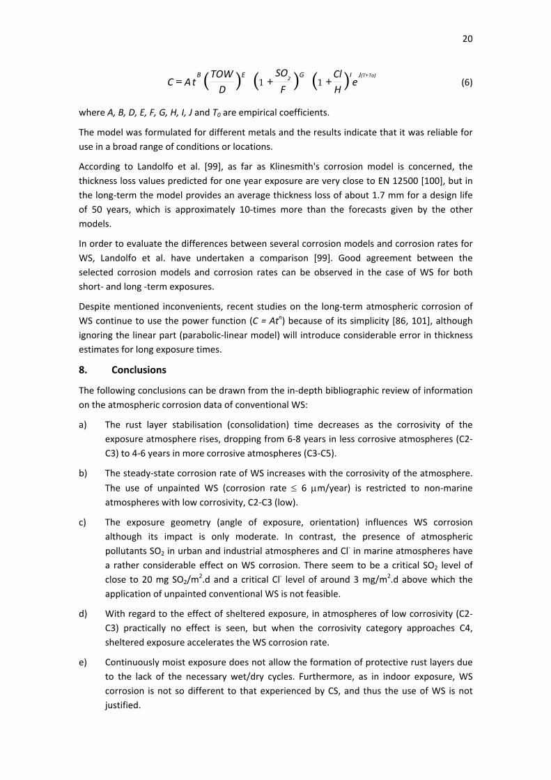
20  

 

To)(T2 JIGEBe

HCl

F

SO

DTOW

 t A  C+)()()( + += 11       (6) 

where A, B, D, E, F, G, H, I, J and T0 are empirical coefficients. 

The model was formulated for different metals and the results indicate that it was reliable for use in a broad range of conditions or locations. 

According  to  Landolfo  et  al.  [99],  as  far  as  Klinesmith's  corrosion model  is  concerned,  the thickness loss values predicted for one year exposure are very close to EN 12500 [100], but in the long‐term the model provides an average thickness loss of about 1.7 mm for a design  life of  50  years, which  is  approximately  10‐times more  than  the  forecasts  given  by  the  other models. 

In order to evaluate the differences between several corrosion models and corrosion rates for WS,  Landolfo  et  al.  have  undertaken  a  comparison  [99].  Good  agreement  between  the selected  corrosion models  and  corrosion  rates  can be observed  in  the  case of WS  for both short‐ and long ‐term exposures. 

Despite mentioned  inconvenients,  recent  studies on  the  long‐term atmospheric corrosion of WS continue to use the power function (C = Atn) because of  its simplicity [86, 101], although ignoring the  linear part (parabolic‐linear model) will  introduce considerable error  in thickness estimates for long exposure times. 

8. Conclusions 

The following conclusions can be drawn from the in‐depth bibliographic review of information on the atmospheric corrosion data of conventional WS: 

a) The  rust  layer  stabilisation  (consolidation)  time  decreases  as  the  corrosivity  of  the exposure atmosphere rises, dropping from 6‐8 years in less corrosive atmospheres (C2‐C3) to 4‐6 years in more corrosive atmospheres (C3‐C5). 

b) The steady‐state corrosion rate of WS increases with the corrosivity of the atmosphere. 

The  use  of  unpainted WS  (corrosion  rate  ≤  6  μm/year)  is  restricted  to  non‐marine atmospheres with low corrosivity, C2‐C3 (low). 

c) The  exposure  geometry  (angle  of  exposure,  orientation)  influences  WS  corrosion although  its  impact  is  only  moderate.  In  contrast,  the  presence  of  atmospheric pollutants SO2 in urban and industrial atmospheres and Cl‐ in marine atmospheres have a  rather considerable effect on WS corrosion. There  seem  to be a critical SO2  level of close  to 20 mg SO2/m

2.d and a critical Cl‐  level of around 3 mg/m2.d above which  the application of unpainted conventional WS is not feasible. 

d) With regard to the effect of sheltered exposure,  in atmospheres of  low corrosivity (C2‐C3)  practically  no  effect  is  seen,  but  when  the  corrosivity  category  approaches  C4, sheltered exposure accelerates the WS corrosion rate. 

e) Continuously moist exposure does not allow the formation of protective rust layers due to  the  lack  of  the  necessary wet/dry  cycles.  Furthermore,  as  in  indoor  exposure, WS corrosion  is not so different  to  that experienced by CS, and  thus  the use of WS  is not justified. 

21  

 

f) It  is very common  to use a power  function  (C = Atn), or  its  logarithmic  transformation (log C = log A + n log t), to predict the long‐term atmospheric corrosion of WS. n values for WS, which are in average 33% lower than for CS, are higher  in marine atmospheres (n = 0.5) than in other types of atmospheres (rural‐urban‐industrial) (n = 0.3). 

22  

 

9. References 

[1]  T. Murata, Weathering steel, in: R.W. Revie (Ed.), Uhlig's Corrosion Handbook, J. Wiley & Sons, New York, 2000. 

[2]  ASTM A‐242 / A‐242M‐04, Standard specification for high‐strength low‐alloy structural steel, American Society for Testing and Materials, Philadelphia, 2007. 

[3]  ASTM A709 /A709M, Standard specification for structural steel for bridges, American Society for Testing and Materials, Philadelphia, 2009. 

[4]  A‐588 / A‐588M, Standard specification for high‐strength low alloy structural steel with 50 ksi  [345 MPa] minimum yield point  to 4‐in.  [100 mm]  thick, American Society  for Testing and Materials, Philadelphia, 2005. 

[5]  V.  Kucera,  E.  Mattsson,  Atmospheric  corrosion,  in:  F.  Mansfeld  (Ed.),  Corrosion Mechanisms, Marcel Dekker, New York, 1987, pp. 211‐284. 

[6]  C. Leygraf, T. Graedel, Atmospheric Corrosion, Electrochemical Society Series, J. Wiley & Sons, New York, USA, 2000. 

[7]  P. Albrecht, T.T. Hall, Atmospheric corrosion  resistance of  structural  steels,  J. Mater. Civil Eng. 15 (2003) 2‐24. 

[8]  F.B. Fletcher, Corrosion of weathering  steels,  in: Vol 13B: Corrosion: Materials, ASM Handbook, 2005, pp. 28‐34. 

[9]  D.M. Buck, Copper  in  steel  ‐ The  influence on corrosion,  J.  Ind. Eng. Chem. 5  (1913) 447‐452. 

[10]  D.M. Buck, Recent progress in corrosion resistance, Iron Age (1915) 1231‐1239. 

[11]  G. Smith, Steels fit for the countryside, New Scientist (1971) 211‐213. 

[12]  C.P.  Larrabee,  S.K.  Coburn,  The  atmospheric  corrosion  of  steels  as  influenced  by changes  in chemical composition, First  International Congress on Metallic Corrosion, London, 1961, pp. 279‐285. 

[13]  W.K.  Boyd,  Corrosion  of  metals  in  the  atmosphere,  in:  Metals  and  Ceramics Information Center, Columbus, 1974, pp. 1‐18. 

[14]  H.R. Copson, Long‐time atmospheric corrosion  tests on  low‐alloy  steels, Proceedings ASTM 60, 1960, pp. 1‐16. 

[15]  Material  Specification  531,  Weathering  fine  grain  structural  steel,  COR‐TEN  A, ThyssenKrupp Steel Europe, March 2007. 

[16]  Material  Specification  532,  Weathering  fine  grain  structural  steel,  COR‐TEN  B, ThyssenKrupp Steel Europe, August 2005. 

[17]  A.  Azizinamini, High‐  Performance  Steel: New Horizon  in  Steel  Bridge  Construction, Transportation Research Board, Washington, D.C., 1998. 

[18]  A.D.  Wilson,  Properties  of  recent  production  of  A709  HPS  70W  bridge  steels,  in: International  Symposium  on  Steel  for  Fabricated  Structures,  ASM  International, Cincinnati, 1999, pp. 41‐49. 

[19]  R.J.  Schmitt,  W.P  Gallagher,  Unpainted  high  strength  low  alloy  steel,  Materials Protection 8 (1969) 70‐77. 

23  

 

[20]  I. Matsushima,  Y. Ishizu,  T. Ueno,  M. Kanasashi, K. Horikawa, Effect of structural and environmental  factors  on  the  practical  use  of  low‐alloy weathering  steel,  Corrosion Engineering 23 (1974) 177‐182. 

[21]  S. Feliu, M. Morcillo, Corrosión y Protección de los Metales en la Atmósfera, Bellaterra, Barcelona, 1982. 

[22]  A. Bragard, H. Bonnarens, Atmospheric conditions and durability of weathering steels, C.R.M. Report N. 57, December, 1980. 

[23]  A.A. Bragard, H.E. Bonnarens, Prediction at long terms of the atmospheric corrosion of structural steels from short‐term experimental data, in: S.W. Dean Jr., E.C. Rhea (Eds.), Atmospheric  Corrosion  of Metals, ASTM  STP  767, American  Society  for  Testing  and Materials, 1982, pp. 339‐358. 

[24]  R. de O. Vianna,   M.F. Cunha, A.C. Dutra, Comparative behavior of carbon  steel and weathering stels exposed for five years to different climates in Brazil, Proceedings 9th International  Congress  on  Metalic  Corrosion,  Toronto,  Vol.  3,  National  Research Council, Ed, 1984, pp. 211‐215. 

[25]  A.C. Dutra, R. de O. Vianna, Atmospheric corrosion testing in Brazil, in: W.H. Ailor (Ed.), Atmospheric Corrosion, The Electrochemical Society, John Wiley and Sons, New York, 1982, pp. 755‐774. 

[26]  UN/ECE  International  Cooperative  Programme  on  Effects  on  Materials  including Historic and Cultural Monuments, Report N. 22: Corrosion attack on weathering steel, zinc and aluminium. Evaluation after 8 years of exposure, SVUOM, Prague, May 1998. 

[27]  W. Hou, Atmospheric corrosion of steels, Proceedings 11th  International Congress on Metallic Corrosion, Firenze, 1990, pp. 2.55‐2.61. 

[28]  W.  Hou,  C.  Liang,  Eight‐year  atmospheric  corrosion  exposure  of  steels  in  China, Corrosion 55 (1999) 65‐73. 

[29]  W.T. Hou, C.F.  Liang,  Effects of  alloying on  atmospheric  corrosion of  steels,  in: H.E. Townsend  (Ed.), Outdoor Atmospheric Corrosion, ASTM  STP 1421, American  Society for Testing and Materials, West Conshohocken, 2002, pp. 368‐377. 

[30]  W. Hou, C. Liang, Atmospheric corrosion prediction of steels, Corrosion 60 (2004) 313‐322. 

[31]  D.  Knotkova,    L.  Rozlivka,  J.  Vlckova,  Corrosion  properties  of  weathering  steels, Proceedings of 8th International Congress on Metallic Corrosion, Frankfurt / Main, Vol. II, 1981, pp. 1792‐1799. 

[32]  D.  Knotkova,    J. Vlckova,  J. Honzak, Atmospheric  corrosion of weathering  steels,  in:  S.W.  Dean  Jr.,  E.C.  Rhea  (Eds.),  Atmospheric  Corrosion  of Metals,  ASTM  STP  767, American Society for Testing and Materials, 1982, pp. 7‐44. 

[33]  D. Knotkova,  K. Barton, M. Cerny, Atmospheric corrosion testing in Czechoslovakia, in: W.H. Ailor(Ed.),   Atmospheric Corrosion, The Electrochemical Society, John Wiley and Sons, New York, 1982, pp. 991‐1014. 

[34]  G.  Burgmann,  D.  Grimme,  Investigations  into  the  atmospheric  corrosion  of  plain carbon  and  low‐alloy  steels  at  various  environmnetal  conditions,  Stahl  Eisen  100 (1980) 641‐650. 

[35]  K. Bohnenkamp,  G. Burgmann, W. Schwenk, Corrosion atmospherique de l'acier doux. Exposition de l'acier aux intemperies, Galvano‐Organo 445 (1974) 587‐589. 

24  

 

[36]  T. Moroishi,  J. Satake, Effect of alloying elements on atmospheric  corrosion of high‐tensile strength steels, Transactions of the Iron and Steel Institute of Japan 13 (1973) 165‐165. 

[37]  T.  Fukushima,    N.  Satu,    Y.  Hisamatsu,    J.  Matsushima,  Y.  Aoyama,  Atmospheric corrosion  testing  in  Japan,  in:  W.H.  Ailor  (Ed.),  Atmospheric  Corrosion,  The Electrochemical Society, John Wiley and Sons, New York, 1982, pp. 841‐872. 

[38]  C.R.  Southwell,    J.D.  Bultman,  A.L.  Alexander,  Corrosion  of  metals  in  tropical environments ‐ Final report of 16‐year exposures, Mater. Performance 15 (1976) 9‐26. 

[39]  F.I. Wei, Atmospheric corrosion of carbon steels and weathering steels  in Taiwan, Br. Corros. J. 26 (1991) 209‐214. 

[40]  J.H. Wang,  F.I. Wei,  Y.S. Chang, H.C. Shih, The corrosion mechanisms of carbon steel and weathering steel in SO2 polluted atmospheres, Mater. Chem. Phys. 47 (1997) 1‐8. 

[41]  S.K. Coburn,  M.E. Komp, S.C. Lore, Atmospheric corrosion rates of weathering steels at test  sites  in  the  eastern  United  States.  Effect  of  environment  and  test  panel orientation, in: W.W. Kirk, H.H. Lawson (Eds.), Atmospheric Corrosion, ASTM STP 1239, American Society for Testing and Materials, Philadelphia, 1995, pp. 101‐113. 

[42]  H.E.  Townsend,  J.  Zoccola,  Eight‐year  atmospheric  corrosion  performance  of weathering   steel  in  industrial, rural and marine environments,  in: S.W. Dean Jr., E.C. Rhea  (Eds.), Atmospheric  Corrosion of Metals, ASTM  STP  767, American  Society  for Testing and Materials, 1982, pp. 45‐59. 

[43]  C.R.  Shastry,    J.J.  Friel,  H.E.  Townsend,  Sixteen‐year  atmospheric  corrosion performance  of weathering  steels  in marine,  rural  and  industrial  environments,  in:  S.W. Dean, T.S. Lee  (Eds.), Degradation of Metals  in the Atmosphere, ASTM STP 965, American Society of Testing and Materials, Philadelphia, 1988, pp. 5‐15. 

[44]  F.H. Haynie,  J.B. Upham,  Effects of  atmospheric pollutants on  corrosion behavior of steels, Materials Protection and Performance 10 (1971) 18‐21. 

[45]  G.B. Mannweiler,  Corrosion  test  results  of  fifteen  ferrous metals  after  seven‐years atmospheric  exposure,  in:  Metal  Corrosion  in  the  Atmosphere,  ASTM  STP  435, American Society for Testing and Materials, 1968, pp. 211‐222. 

[46]  H.R. Copson, Atmospheric corrosion of  low alloy steels, Proceedings ASTM 52  (1952) 1005‐1026. 

[47]  J.B. Horton, The composition, structure and growth of the atmospheric rust on various steels, Ph. Thesis, Lehigh University, Bethlehem, 1964. 

[48]  R.H. McCuen,   P. Albrecht, J.G. Cheng, A new approach to power‐model regression of corrosion  penetration  data,  in:  V.  Chaker  (Ed.),  Corrosion  Forms  and  Control  for Infrastructure,  ASTM  STP  1137,  American  Society  for  Testing  and  Materials, Philadelphia, 1992, pp. 46‐76. 

[49]  M. Pourbaix, The linear bilogaritmic law for atmospheric corrosion, in: W.H. Ailor (Ed.), Atmospheric Corrosion, The Electrochemical Society, John Wiley and Sons, New York, 1982, pp. 107‐121. 

[50]  R.A. Legault, A.G. Preban, Kinetics of atmospheric corrosion of  low‐alloy  steels  in an industrial environment, Corrosion (NACE) 31 (1975) 117‐122. 

[51]  Ch. Cao, Some results of long‐term atmospheric exposure tests of steels in China, 16th International  Corrosion  Congress,  Chinese  Society  for  Corrosion  and  Protection, Beijing, 2005. 

25  

 

[52]  C.  Liang, W. Hou,  Sixteen  year  atmospheric  corrosion  exposure  study of  steels, 16th International  Corrosion  Congress,  Chinese  Society  for  Corrosion  and  Protection, Beijing, 2005. 

[53]  H.E. Townsend, Atmospheric corrosion performance of quenched‐and‐tempered, high‐strength weathering steel, Corrosion (NACE) 56 (2000) 883‐886. 

[54]  L. Damian, R. Fako, Weathering structural steels corrosion  in atmospheres of various degrees of pollution in Romania, Mater. Corros. 51 (2000) 574‐578. 

[55]  A.U.  Leuenberger‐Minger,    B.  Buchmann,   M.  Faller,    P.  Richner, M.  Zobeli,  Dose‐response  functions  for weathering  steel,  copper and  zinc obtained  from a  four‐year exposure programme in Switzerland, Corros. Sci. 44 (2002) 675‐687. 

[56]  I. Díaz,  H. Cano,  B. Chico,  D. De la Fuente, M. Morcillo, Some clarifications regarding literature  on  atmospheric  corrosion  of  weathering  steels,  International  Journal  of Corrosion, ID 812192 (2012) 1‐9. 

[57]  ISO 9223, Corrosion of metals and alloys. Clasiffication of corrosivity of atmospheres, International Standard Organization, Geneve, 1991. 

[58]  D.C.  Cook,  An  active  coating  and  new  protection  technology  for  weathering  steel structures  in  chloride  containing  environments,  NACE  International,  Nashville, Tennessee (USA), 2007. 

[59]  H.  Kihira,  M.  Kimura,  Advancements  of  weathering  steel  technologies  in  Japan, Corrosion 67 (2011) 1‐13. 

[60]  Technical Report: Guideline  for designing and construction of bridges by weathering steel, Kozai Club (Ed.), Tokyo, 1993. 

[61]  Specification for highway bridges, Japan Road Association, Tokio, 2002. 

[62]  D.C. Cook, The corrosion of high performance steel  in adverse environments, ISIAME, Madrid, 2004, pp. 63‐72. 

[63]  D.C.  Cook,  Spectroscopic  identification  of  protective  and  non‐protective  corrosion coatings on steel structures in marine environments, Corros. Sci. 47 (2005) 2550‐2570. 

[64]  K. Park, Corrosion resistance of weathering steels, Ph. Thesis, Department of Civil and Environmental Engineering, University of Maryland, USA, 2004. 

[65]  J. Gullman et al., Corrosion resistance of weathering steels ‐ typical causes of damage in  building  context  and  their  prevention,  Bull.  94,  Swedish  Corrosion  Institute, Stockholm, 1985. 

[66]  C.P.  Larrabee,  The  effect  of  specimen  position  on  atmospheric  corrosion  testing  of steel, Trans. Electrochem. Soc. 85 (1944) 297‐306. 

[67]  G. Schikorr, The atmospheric oxidisation of  Iron  II, Zeitschrift  fur Elektrochemie und Angewandte Physikalische Chemie 43 (1937) 697‐704. 

[68]  ASTM G50, Conducting atmospheric  corrosion  tests on metals, American Society  for Testing and Materials, Philadelphia, 1991. 

[69]  F.L. LaQue, Corrosion testing, Proceedings ASTM 51 (1951) 495‐582. 

[70]  C.P. Larrabee, Corrosion  resistance of high‐strength  low‐alloy  steels as  influenced by composition and environment, Corrosion (NACE) 9 (1953) 259‐271. 

26  

 

[71]  B.  Cosaboom,    G. Mehalchick,  J.  Zoccola,  Bridge  construction with  unpainted  high‐trength  low‐alloy  steel:  eight‐year  progress  report,  New  Yersey  Department  of Transportation, New Yersey, 1979. 

[72]  J.  Zoccola,    A.J.  Permoda,    L.T.  Oehler,  J.B.  Horton,  Performance  of  Mayari  R weathering steel (ASTM A242) in bridges, eight‐mile road over John Lodge expressway, Detroit, Michigan, Bethlehem Steel Corporation, 1970. 

[73]  J. Zoccola, Eight year corrosion  test  report  ‐ Eight mile  road  interchange, Bethlehem Steel, Bethlehem, 1976. 

[74]  S. Oesch, P. Heimgartner, Environmental effects on metallic materials  ‐ Results of an outdoor exposure programme  running  in Switzerland, Mater. Corros. 47  (1996) 425‐438. 

[75]  T. Moroishi,  J.  Satake,  The  influence  of  the  inclination  and  direction  of  specimen surface on atmospheric corrosion of steels, Tetsu ‐ to ‐ Hagane 59 (1) (1973) 125‐130. 

[76]  J. Satake,  T. Moroishi,  Y. Nishida, S. Tanaka, Sumitomo Metals 22 (4) (1970) 516‐520. (in Japanese) 

[77]  M. McKenzie, The corrosion performance of weathering steel  in highway bridges,  in: W.H. Ailor (Ed.), Atmospheric Corrosion, The Electrochemical Society, John Wiley and Sons, New York, 1982, pp. 717‐736. 

[78]  National Academy of Sciences, An analysis of atmospheric corrosion tests in low‐alloy steels ‐ Applicability of test results to highway bridges, Highway Research Record, No. 204,  Nat. Acad. Sci., Washington DC., 1967. 

[79]  J.M. Costa,   M. Morcillo, S. Feliu, Effect of environmental parameters on atmospheric corrosion  of  metals,  in:  P.N.  Cheremisinoff  (Ed.),  Encyclopedia  of  Environmental Control  Technology: Air  Pollution Control, Gulf  Publishing Company, Houston,  1989, pp. 197‐238. 

[80]  D.D.N.  Singh,    S.  Yadav,  J.K.  Saha,  Role  of  climatic  conditions  on  corrosion characteristics of structural steels, Corros. Sci. 50 (2008) 93‐110. 

[81]  J.  Satake,  T. Moroishi,  Various  factors  affecting  atmospheric  corrosion  of  steels,  5th International Congress on Metallic Corrosion, Tokyo, Japan, 1972, pp. 744‐749. 

[82]  D.M. Murray, Economic analysis of the environmental impact of highway deicing salts, Transportation  Research  Record  647,  Transportation  Research  Board,  Washington, D.C, 1977. 

[83]  A. Naeemi,  P. Albrecht, Atmospheric  corrosion of weathering  steels,  Proceedings of 9th  International Congress of Metallic Corrosion, Toronto, Vol. 1, National Research Council, Ed, 1984, pp. 418‐427. 

[84]  W.  Hein,  S.  Sczyslo,  Corrosion  behaviour  of  weathering  steels  under  deicing  salt exposure,  Interim  Report  nº  4,  Bundesanstalt  Fuer Wasserbaw,  Federal  Republic  of Germany, 1981. 

[85]  ASTM G 101‐04, Standard guide for estimating the atmospheric corrosion resistance of low‐alloy steels, American Society for Testing and Materials, Philadelphia, 2004. 

[86]  H.E. Townsend, The effects of alloying elements on the corrosion of steel in industrial atmospheres,  Proceedings  14th  International  Corrosion  Congress,  Cape  Town, Corrosion Institute of Southern Africa, 1999. 

27  

 

[87]  H.E. Townsend, Estimating the atmospheric corrosion resistance of weathering steels, in: H.E. Townsend    (Ed), Outdoor Atmospheric Corrosion, ASTM STP 1421, American Society for Testing and Materials, PA, USA, 2002, pp. 292‐300. 

[88]  K. Bohnenkamp,   G. Burgmann, W. Schwenk,  Investigations of atmospheric corrosion of plain  carbon  and  low‐alloy  steels  in  industry,  country  and  sea  air,  Stahl  Eisen  93 (1973) 1054‐1060. 

[89]  S.  Feliu, M.  Morcillo,  Atmospheric  corrosion  testing  in  Spain,  in: W.H.  Ailor  (Ed.), Atmospheric Corrosion, J. Wiley & Sons, New York, 1982, pp. 913‐922. 

[90]  M. Benarie, F.L. Lipfert, A general corrosion function in terms of atmospheric pollutant concentrations and rain pH, Atmos. Environ. 20 (1986) 1947‐1958. 

[91]  R.A. Legault, V.P. Pearson, Atmospheric corrosion  in marine environments, Corrosion (NACE) 34 (1978) 433‐437. 

[92]  M. Morcillo,    J. Simancas, S. Feliu, Long‐term atmospheric corrosion  in Spain:  results after 13 to 16 years of exposure and comparison with worldwide data,  in: W.W. Kirk, H.H.  Lawson  (Ed.),  Atmospheric  Corrosion,  ASTM  STP  1239,  American  Society  for Testing and Materials, Philadelphia, 1995, pp. 195‐214. 

[93]  S.  Feliu,    M.  Morcillo,  S.  Feliu  Jr,  The  prediction  of  atmospheric  corrosion  from meteorological and pollution parameters.2. Long‐term forecasts, Corros. Sci. 34 (1993) 415‐422. 

[94]  J. Tidblad,  J.K. Kreislova,  D. Knotkova, V. Kucera, Exposure of weathering steel in the UN/ECE ICP Materials Programme, International Workshop on Atmospheric Corrosion and Weathering Steels, Cartagena de Indias, 2004.  

[95]  M. Morcillo,   S. Feliu,  J. Simancas, Deviation  from bilogarithmic  law  for atmospheric corrosion of steel, Br. Corros. J. 28 (1993) 50‐52. 

[96]  ISO 9224, Corrosion of metals and alloys ‐ Corrosivity of atmospheres ‐ Guiding values for the corrosivity categories, International Standards Organization, Geneve, 1992. 

[97]  V.  Kucera,  Mapping  Effects  on  Materials  in  Manual  Mapping  Critical  Load,  ICP Materials,  Coordination  Centre:  Stockholm,  2004.  Available  online:  http://icpmapping.org. 

[98]  D.E.  Klinesmith,    R.H. McCuen,  P.  Albrecht,  Effect  of  environmental  conditions  on corrosion rates, J. Mater. Civil Eng. 19 (2007) 121‐129. 

[99]  R. Landolfo,   L. Cascini, F. Portioli, Modeling of metal  structure corrosion damage: A state of the art report, Sustainability 2 (2010) 2163‐2175. 

[100]  EN 12500, Corrosion likelihood in atmospheric environment, European Committee for Standardization (CEN), Brussels, 2000. 

[101]  S.W.  Dean,    D.  Knotkova,  J.K.  Kreislova,  ISOCORRAG  International  Atmospheric Exposure  Program:  Summary  of  Results, ASTM  Series  71, ASTM  International, West Conshohocken, 2010. 

28  

 

FIGURE CAPTIONS 

Figure 1.  Atmospheric corrosion of Cor‐Ten B steel and its evolution with exposure time in the  industrial atmosphere of Kearny  [12]. Comparison with Cu‐bearing steel and plain carbon steel (CS). 

Figure 2.  Determination of rust layer stabilisation time and steady‐state corrosion rate from a  plot  of  exponential  decrease  function  obtained  with  corrosion  rate  data  at different exposure times. 

Figure 3.  Box‐whisker plots of rust layer stabilisation time of weathering steel as a function of atmospheric corrosivity category (ISO 9223 [57]). 

Figure 4.  Box‐whisker plots of weathering steel steady‐state corrosion rate as a function of atmospheric  corrosivity  category  (ISO  9223  [57]).  Non‐marine  (rural‐urban‐industrial) atmospheres. 

Figure 5.  Box‐whisker plots of weathering steel steady‐state corrosion rate as a function of atmospheric corrosivity category (ISO 9223 [57]). Marine atmospheres. 

Figure 6.  Typical plots of corrosion versus exposure time for weathering steels (ASTM A‐242 (a), due to Schmitt and Gallagher [19], and ASTM A‐588 (b), due to Townsend and Zoccola  [42]  and  Shastry,  Friel  and  Townsend  [43])  in  different  types  of atmospheres. 

Figure 7.  Corrosion  versus  exposure  time  for weathering  steel  (WS)  and  reference  plain carbon  steel  (CS)  in  atmospheres with  different  SO2  content.  Plots  have  been elaborated from graphs showed in reference [32]. 

Figure 8.  Corrosion  of  weathering  steel  in  outdoor  atmospheres  as  a  function  of  SO2 pollution level [32]. 

Figure 9.  Variation  of  atmospheric  corrosion  rate  of  conventional weathering  steel with atmospheric  SO2  content.  Constructed  from  data  corresponding  to  8‐year exposure, provided by UNECE/PIC Materials [26]. 

Figure 10.  Influence of airborne salts (atmospheric salinity) on corrosion rate of conventional weathering steel. The figure has been obtained from references [60] and [62]. 

Figure 11.  Typical  log‐log  plots  of  weathering  steel  corrosion  versus  exposure  time  at different test sites. 

Figure 12.  Log‐log plots of weathering steel corrosion versus exposure time in data series not well adapted to the power function (C = Atn), with low correlation coefficients (ρ). 

Figure 13.  Box‐whisker plots of n  values  in power  function  (C = Atn)  for different  types of atmospheres. 

Figure 14.  Box‐whisker  plots  of  n  values  in  power  function  (C  =  Atn)  for  sheltered  and unsheltered exposures. 

Figure 15.  Bi‐linear log‐log plots of weathering steel corrosion versus exposure time for data series not well adapted to the power function (C = Atn) [95]. 

29  

 

Figure 16.  Bi‐linear  plots  of  weathering  steel  corrosion  versus  exposure  time  [7]:  (a) Modified  ISO 9224 for different ISO 9223 [57] corrosivity categories; (b) Albrecht et al. adjustment and modified ISO 9224 for C3 corrosivity category. 

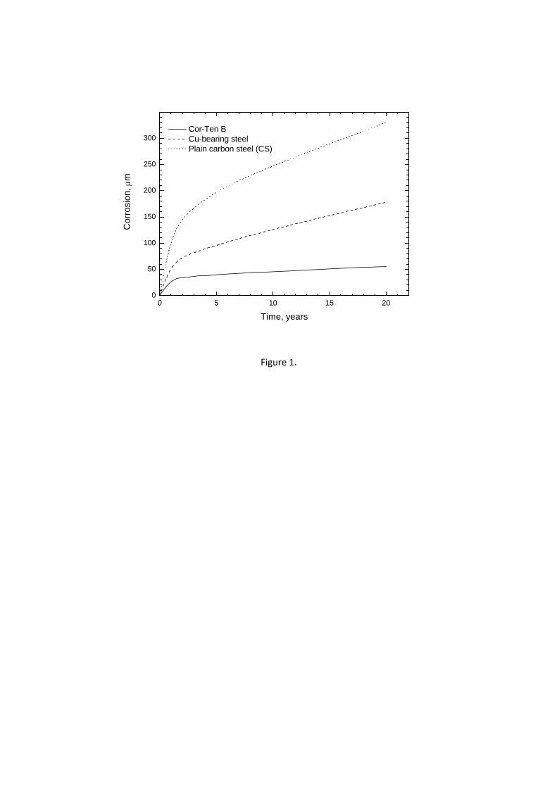
 Figure 1. 

0 5 10 15 200

50

100

150

200

250

300

Cor

rosi

on, μ

m

Time, years

Cor-Ten B Cu-bearing steel Plain carbon steel (CS)

 

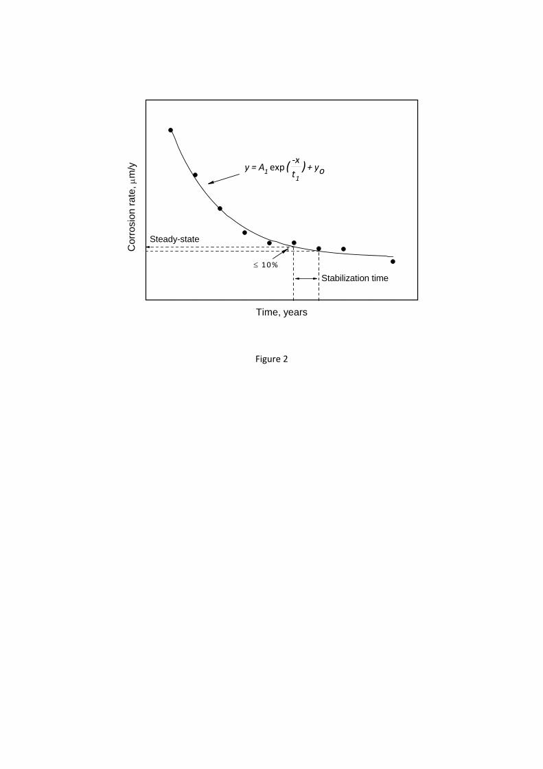
 Figure 2 

oy + t‐x

 A =y  )(1

1 exp

≤ 10%

Cor

rosi

on ra

te, μ

m/y

Time, years

Stabilization time

Steady-state

 Figure 3 

0

20

40

60

80

100

120

140

8050

25C

5C

4C

3C

2

7-8 years6-7 years

1st y

ear C

S c

orro

sion

, μm

Stabilization time, years

All types of atmospheres

4-6 years

Cor

rosi

vity

cat

egor

y (IS

O 9

223)

WS: ASTM A-242

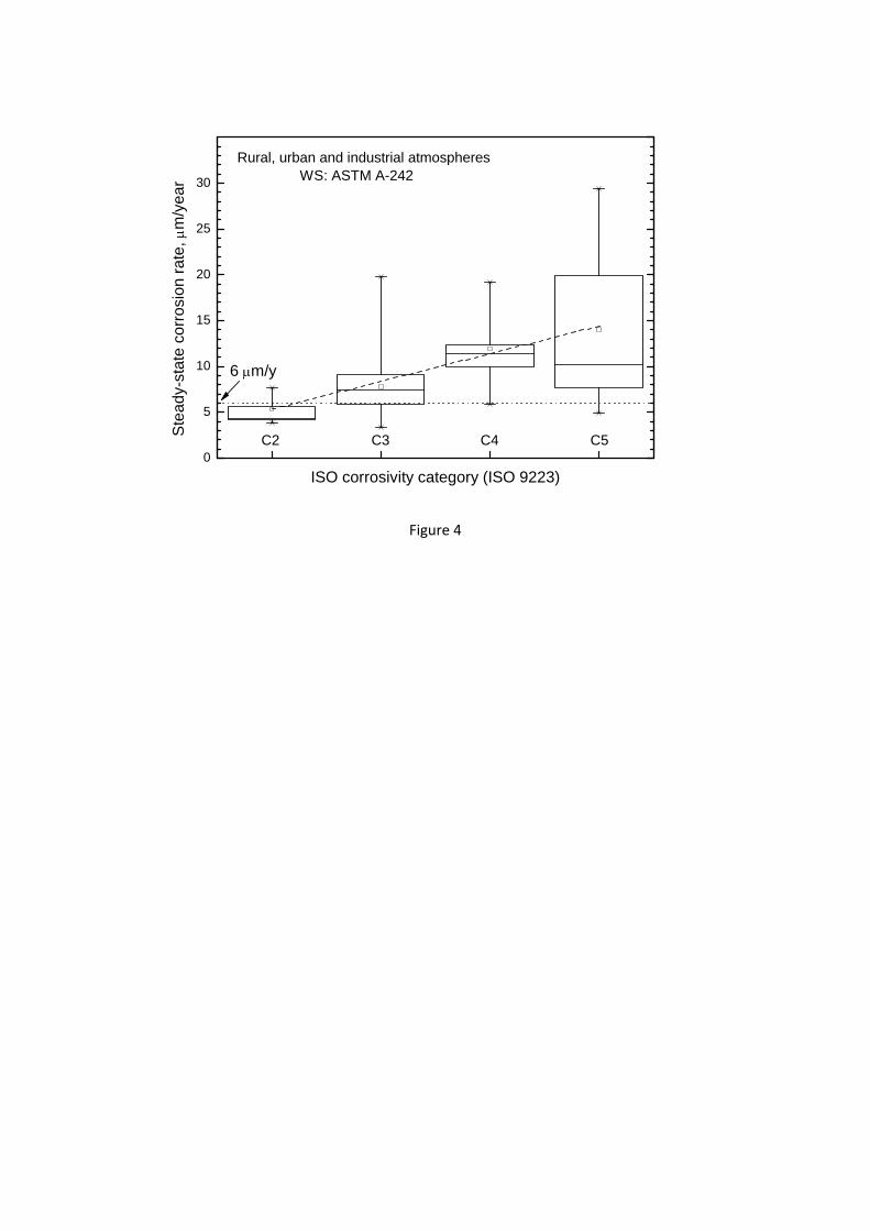
Figure 4 

0

5

10

15

20

25

30

C5C4C3Ste

ady-

stat

e co

rros

ion

rate

, μm

/yea

r

ISO corrosivity category (ISO 9223)

C2

Rural, urban and industrial atmospheresWS: ASTM A-242

6 μm/y

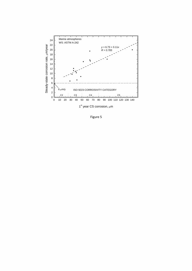
Figure 5 

0 10 20 30 40 50 60 70 80 90 100 110 120 130 1400

2

4

6

8

10

12

14

16

18

20

22

24

C2

WS: ASTM A-242

ISO 9223 CORROSIVITY CATEGORY

C5C4C3

Stea

dy-s

tate

cor

rosi

on ra

te, μ

m/y

ear

1st year CS corrosion, μm

Marine atmospheres

y = 6.73 + 0.11xR = 0.783

6 μm/y

Figure 6 

0 5 10 15 200

10

20

30

40

50

Cor

rosi

on, μ

m

Time, years

Rural (South Bend) Industrial (Kearny) Marine (Kure Beach, 250)

ASTM A-242(CORTEN A)

(a)

0 2 4 6 8 10 12 14 160

20

40

60

80

100

120

140

160

180

Cor

rosi

on, μ

m

Time, years

Rural (Saylorsburg) Heavily Travelled Expressway (Newark) Industrial (Bethlehem) Marine (Kure Beach, 250)

ASTM A-588(CORTEN B)

(b)

Figure 7 

0 1 2 3 40

20

40

60

80

100

120

140

160

180

WS

WS

CS

CS

WS

Cor

rosi

on, μ

m

Time, years

Heavily polluted atmospheres (> 90 mg SO2/m2d)

Urban and weakly polluted industrial atmospheres (40-90 mg SO2/m

2d)

Rural atmosphere (< 40 mg SO2/m2d)

CS

 

  

Figure 8 

50 100 150

1000

500

0

SO2, mg/m2.d

Corrosion, g/m

2

 Figure 9 

0 2 4 6 8 10 12 14 16 18 20 22 240.1

1

10

100

SO

2, mg/

m2 .d

Corrosion rate, μm/y

 

Figure 10 

Salinity, mg NaCl/dm2.day

Steady‐state corrosion

 rate, μ

m/y

0.001 0.1 10.052

20

200

6 μm/y

Adherent rust layer (protective)Not adherent rust layer (non protective)

0.01

.

Figure 11 

0.1 1 10

20

40

60

80

100

Cor

rosi

on, μ

m

Time, years

Quingdao, China (marine atmosphere)ρ = 0.999

Detroit, USA (urban atmosphere)ρ = 0.999

Saylorsburg, USA (rural atmosphere)ρ = 0.999

 Figure 12 

1 10200

300

400

Cor

rosi

on, g

/m2

Time, years

Kopisty (Czech Republic): ρ = 0.38 Steubenville (USA): ρ = 0.79

 Figure 13 

0.0

0.2

0.4

0.6

0.8

1.0

Exp

onen

t n in

Eq.

(2)

Type of atmosphere

Rural, urban and Marine atmospheresindustrial atmospheres

Figure 14 

-0.4

-0.2

0.0

0.2

0.4

0.6

0.8

1.0

Exp

onen

t n in

Eq.

(2)

UNSHELTERED

SHELTERED

Type of exposure

   

   

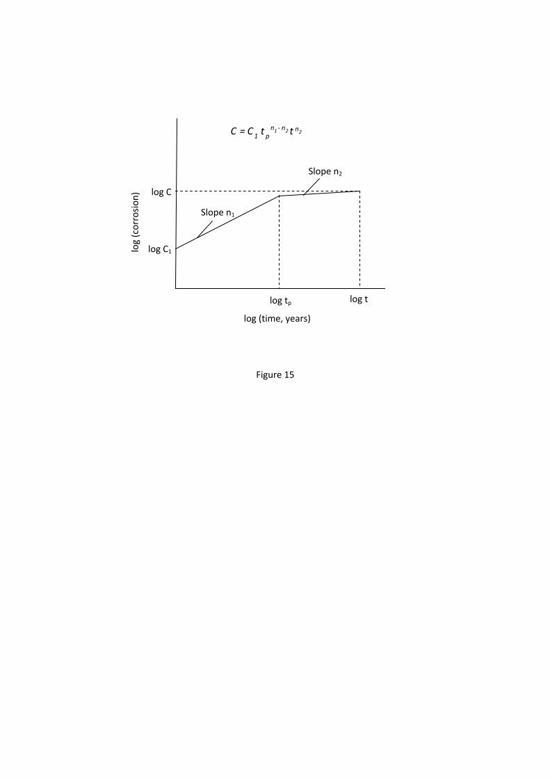
Figure 15 

tt C=C 221 nn ‐np1

log tp  log t 

log C1 

log C 

log (time, years) 

log (corrosion

)  

Slope n1 

Slope n2 

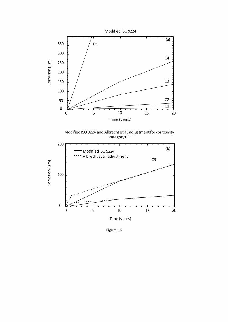
 Figure 16 

Modified ISO 9224 and Albrecht et al. adjustment for corrosivitycategory C3

C3

(b)

Time (years)

201510500

100

200

Corrosion(μm)

Modified ISO 9224Albrecht et al. adjustment

Modified ISO 9224

(a)350

Corrosion(μm)

300

250

200

150

100

50

010

C5

C4

C3

C2

C1

Time (years)

1550 20

Table 1.   Chemical compositions (weight %) of commonly used WS 

Weathering steel  C  Si  Mn  P  S  Cu  Cr  Ni  V ASTM A‐242 

(CORTEN A) [2] ≤0.15    ≤1.00  ≤0.15  < 0.05  ≥0.20       

Typical concentrations 

      ≤0.15    0.25‐0.40  0.50‐0.80  0.50‐0.65   

ASTM A‐588 Gr.A (CORTEN B) [4] 

≤0.19  0.30‐0.65  0.80‐1.25  ≤0.04  <0.05  0.25‐0.40  0.40‐0.65  ≤0.40  0.02‐0.10 

Typical concentrations 

      ≤0.04    0.30‐0.40  0.60‐1.00  0.02‐0.30   

 

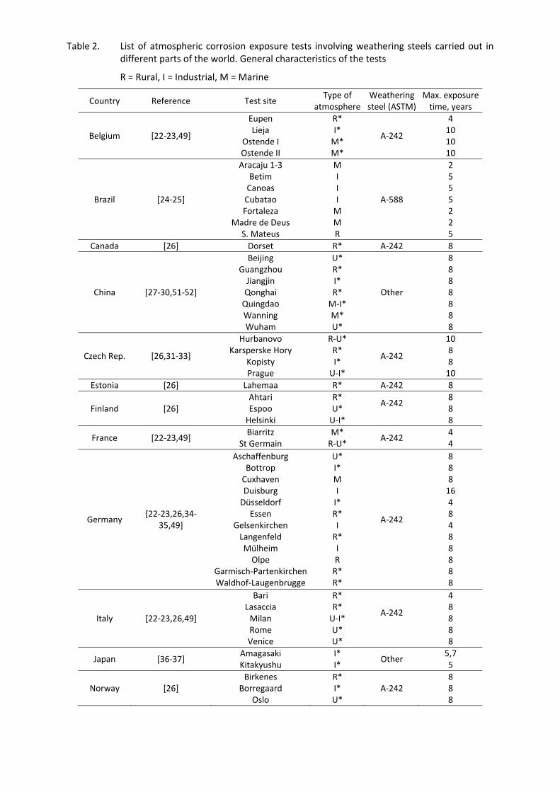
Table 2.  List of atmospheric corrosion exposure  tests  involving weathering steels carried out  in different parts of the world. General characteristics of the tests 

R = Rural, I = Industrial, M = Marine 

Country  Reference  Test site Type of 

atmosphereWeathering steel (ASTM) 

Max. exposure time, years 

Belgium  [22‐23,49] 

EupenLieja 

Ostende I Ostende II 

R*I* M* M* 

A‐242 

4 10 10 10 

Brazil  [24‐25] 

Aracaju 1‐3Betim Canoas Cubatao Fortaleza 

Madre de Deus S. Mateus 

MI I I M M R 

A‐588 

2 5 5 5 2 2 5 

Canada  [26]  Dorset R* A‐242  8 

China  [27‐30,51‐52] 

BeijingGuangzhou Jiangjin Qonghai Quingdao Wanning Wuham 

U*R* I* R* M‐I* M* U* 

Other 

8 8 8 8 8 8 8 

Czech Rep.  [26,31‐33] 

HurbanovoKarsperske Hory 

Kopisty Prague 

R‐U*R* I* U‐I* 

A‐242 

10 8 8 10 

Estonia  [26]  Lahemaa R* A‐242  8 

Finland  [26] AhtariEspoo Helsinki 

R*U* U‐I* 

A‐242  

8 8 8 

France  [22‐23,49] Biarritz

St Germain M*R‐U* 

A‐242 4 4 

Germany [22‐23,26,34‐

35,49] 

Aschaffenburg Bottrop Cuxhaven Duisburg Düsseldorf 

Essen Gelsenkirchen Langenfeld Mülheim Olpe 

Garmisch‐PartenkirchenWaldhof‐Laugenbrugge 

U* I* M I I* R* I R* I R R* R* 

A‐242 

8 8 8 16 4 8 4 8 8 8 8 8 

Italy  [22‐23,26,49] 

BariLasaccia Milan Rome Venice 

R*R* U‐I* U* U* 

A‐242  

4 8 8 8 8 

Japan  [36‐37] AmagasakiKitakyushu 

I*I* 

Other 5,7 5 

Norway  [26] Birkenes

Borregaard Oslo 

R*I* U* 

A‐242 8 8 8 

   

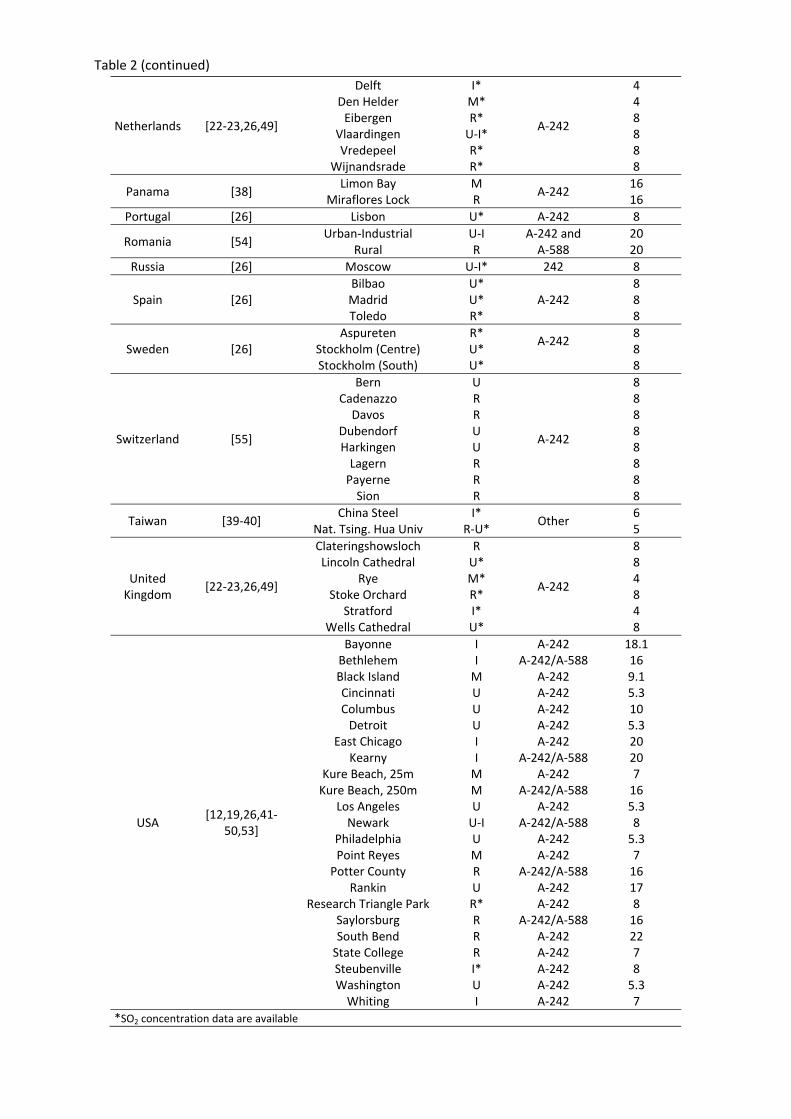
Table 2 (continued) 

Netherlands  [22‐23,26,49] 

DelftDen Helder Eibergen 

Vlaardingen Vredepeel 

Wijnandsrade 

I*M* R* U‐I* R* R* 

A‐242 

4 4 8 8 8 8 

Panama  [38] Limon Bay

Miraflores Lock MR 

A‐242 16 16 

Portugal  [26]  Lisbon U* A‐242  8 

Romania  [54] Urban‐Industrial

Rural U‐IR 

A‐242 and A‐588 

20 20 

Russia  [26]  Moscow U‐I* 242  8 

Spain  [26] BilbaoMadrid Toledo 

U*U* R* 

A‐242 8 8 8 

Sweden  [26] Aspureten

Stockholm (Centre) Stockholm (South) 

R*U* U* 

A‐242  

8 8 8 

Switzerland  [55] 

BernCadenazzo Davos 

Dubendorf Harkingen Lagern Payerne Sion 

UR R U U R R R 

A‐242 

8 8 8 8 8 8 8 8 

Taiwan  [39‐40] China Steel

Nat. Tsing. Hua Univ I*

R‐U* Other 

6 5 

United Kingdom 

[22‐23,26,49] 

ClateringshowslochLincoln Cathedral 

Rye Stoke Orchard 

Stratford Wells Cathedral 

RU* M* R* I* U* 

A‐242 

8 8 4 8 4 8 

USA [12,19,26,41‐

50,53] 

BayonneBethlehem Black Island Cincinnati Columbus Detroit 

East Chicago Kearny 

Kure Beach, 25m Kure Beach, 250m 

Los Angeles Newark 

Philadelphia Point Reyes Potter County 

Rankin Research Triangle Park 

Saylorsburg South Bend State College Steubenville Washington Whiting 

II M U U U I I M M U U‐I U M R U R* R R R I* U I 

A‐242 A‐242/A‐588 

A‐242 A‐242 A‐242 A‐242 A‐242 

A‐242/A‐588 A‐242 

A‐242/A‐588 A‐242 

A‐242/A‐588 A‐242 A‐242 

A‐242/A‐588 A‐242 A‐242 

A‐242/A‐588 A‐242 A‐242 A‐242 A‐242 A‐242 

18.1 16 9.1 5.3 10 5.3 20 20 7 16 5.3 8 5.3 7 16 17 8 16 22 7 8 5.3 7 

*SO2 concentration data are available 

 

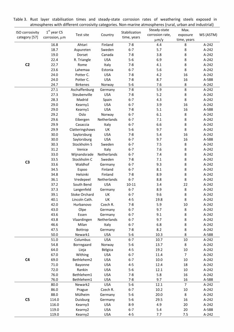
Table 3.  Rust  layer  stabilisation  times  and  steady‐state  corrosion  rates  of  weathering  steels  exposed  in atmospheres with different corrosivity categories. Non‐marine atmospheres (rural, urban and industrial) 

ISO corrosivity category [57] 

1st year CS corrosion, μm 

Test site  Country Stabilization time, years 

Steady‐state corrosion rate, 

μm/y 

Max. exposure time, years 

WS (ASTM) 

C2 

16.8  Ahtari  Finland 7‐8 4.4 8  A‐24218.7  Aspureten  Sweden 6‐7 5.7 8  A‐24219.0  Dorset  Canada 7‐8 3.8 8  A‐24222.4  R. Triangle  USA 5‐6 6.9 8  A‐24222.7  Rome  Italy 7‐8 4.1 8  A‐24223.6  Lahemaa  Estonia 6‐7 5.6 8  A‐24224.0 24.0 

Potter C. Potter C. 

USAUSA 

7‐87‐8 

4.28.7 

16 16 

A‐242A‐588 

24.7  Birkenes  Norway 5‐6 7.6 8  A‐242

C3 

27.1  Aschaffenburg  Germany 7‐8 5.9 8  A‐24227.3  Steubenville  USA 7‐8 5.2 8  A‐24228.3  Madrid  Spain 6‐7 4.3 8  A‐24229.0 29.0 

Kearny1 Kearny1 

USAUSA 

6‐77‐8 

3.95.1 

16 16 

A‐242A‐588 

29.2  Oslo  Norway 6‐7 6.1 8  A‐24229.6  Eibergen  Netherlands 6‐7 7.1 8  A‐24229.9  Casaccia  Italy 6‐7 6.6 8  A‐24229.9  Clatteringshaws  UK 5‐6 9.7 8  A‐24230.0 30.0 

Saylorsburg Saylorsburg 

USAUSA 

7‐86‐7 

5.49.7 

16 16 

A‐242A‐588 

30.3  Stockholm S  Sweden 6‐7 7.5 8  A‐24231.2  Venice  Italy 6‐7 7.6 8  A‐24233.0  Wijnandsrade  Netherlands 6‐7 7.4 8  A‐24233.5  Stockholm C  Sweden 7‐8 7.1 8  A‐24233.6  Waldhof  Germany 6‐7 9.3 8  A‐24234.5  Espoo  Finland 6‐7 8.1 8  A‐24234.8  Helsinki  Finland 7‐8 8.9 8  A‐24236.1  Vredepeel  Netherlands 6‐7 8.8 8  A‐24237.2  South Bend  USA 10‐11 3.4 22  A‐24237.3  Langenfeld  Germany 6‐7 8.9 8  A‐24239.1  Stoke Orchard  UK 6‐7 9.6 8  A‐24240.1  Lincoln Cath.  UK 4‐5 19.8 8  A‐24242.0  Hurbanovo  Czech R. 7‐8 5.9 10  A‐24243.0  Olpe  Germany 6‐7 9.7 8  A‐24243.6  Essen  Germany 6‐7 9.1 8  A‐24243.8  Vlaardingen  Netherlands 6‐7 9.7 8  A‐24246.6  Milan  Italy 6‐7 6.8 8  A‐24247.5  Bottrop  Germany 7‐8 8.2 8  A‐24250.0  Newark1  USA 5‐6 10.3 8  A‐588

C4 

51.0  Columbus  USA 6‐7 10.7 10  A‐24254.8  Borregaard  Norway 5‐6 13.7 8  A‐24264.0  Lieja  Bélgica 4‐5 19.2 10  A‐24267.0  Withing  USA 6‐7 11.4 7  A‐24269.0  Bethlehem2  USA 6‐7 10.0 10  A‐24271.0  Bayonne  USA 4‐5 12.4 18  A‐24272.0  Rankin  USA 5‐6 12.1 10  A‐24276.0 76.0 

Bethlehem1 Bethlehem1 

USAUSA 

7‐87‐8 

5.89.7 

16 16 

A‐242A‐588 

C5 

80.0  Newark2  USA 5‐6 12.1 7  A‐24286.0  Prague  Czech R. 6‐7 10.2 10  A‐24288.0  Mülheim  Germany 5‐6 20.0 8  A‐242114.0  Duisburg  Germany 5‐6 29.5 16  A‐242116.0  Kearny3  USA 8‐9 4.9 20  A‐242119.0 119.0 

Kearny2 Kearny2 

USAUSA 

6‐74‐5 

5.47.7 

20 7.5 

A‐588A‐242 

 

Table 4.  Rust layer stabilisation times and steady‐state corrosion rates of weathering steels exposed in atmospheres with different corrosivity categories. Marine atmospheres 

ISO corrosivity category [57] 

1st year CS corrosion, μm 

Test site  Country Stabilization time, years 

Steady‐state corrosion rate, 

μm/y 

Max. exposure time, years 

WS (ASTM) 

C3 

28.5  Lisbon  Portugal  6‐7  6.9  8  A‐24232.2  Wells Cathedral  UK 5‐6 9.8 8  A‐24235.0 35.0 

Miraflores Lock Miraflores Lock 

USAUSA 

6‐76‐7 

11.312.2 

16 16 

A‐242A‐242 

39.0 39.0 

Kure Beach2 Kure Beach2 

USAUSA 

5‐65‐6 

11.014.4 

16 16 

A‐242A‐588 

40.0 40.0 

Kure Beach1 Kure Beach1 

USAUSA 

5‐64‐5 

10.417.4 

16 16 

A‐242A‐588 

41.0  Bilbao  Spain 6‐7 7.3 8  A‐24247.9  Kure Beach5  USA 6‐7 8.8 8  A‐242

C4 

52.5  Kure Beach 4  USA 4‐5 15.1 16  A‐24264.0 64.0 

Limon Bay Limon Bay 

USAUSA 

6‐77‐8 

19.515.8 

16 16 

A‐242A‐242 

65.0  Cuxhaven  Germany 5‐6 15.3 8  A‐242

C5 95.0  Point Reyes  USA 6‐7 16.1 7  A‐242140.0  Kure Beach 3  USA 5‐6 20.0 7  A‐242

 

Table 5.  Rust layer stabilisation times and steady‐state corrosion rates of weathering steels exposed  in  atmospheres  with  different  corrosivity  categories  [26].  Unshelter versus shelter exposure 

ISO corrosivity 

category [57] 

1st year CS corrosion, μm 

Test site  Country SO2, μg/m3 

Unshelter Shelter

Stabilization time, years 

Steady‐state corrosion rate, μm/y 

Stabilization time, years 

Steady‐state corrosion rate, μm/y 

C2 

19.0  Dorset  Canada 2.8 7‐8 3.8  7‐8  3.722.4  R. Triangle  USA 9.8 5‐6 6.9  5‐6  6.922.7  Rome  Italy 24.5 7‐8 4.1  6‐7  3.323.6  Lahemaa  Estonia 0.6 6‐7 5.6  7‐8  4.4

C3 

27.1  Aschaffenburg  Germany 14.8 7‐8 5.9  6‐7  4.628.3  Madrid  Spain 11.7 6‐7 4.3  5‐6  4.129.6  Eibergen  Netherlands 7.7 6‐7 7.1  4‐5  6.229.9  Casaccia  Italy 6.0 6‐7 6.6  5‐6  5.430.3  Stockholm S  Sweden 8.4 6‐7 7.5  7‐8  4.231.2  Venice  Italy 15.7 6‐7 7.6  3‐4  9.033.0  Wijnandsrade  Netherlands 10.2 6‐7 7.4  4‐5  6.533.5  Stockholm C  Sweden 8.5 7‐8 7.1  7‐8  4.233.6  Waldhof  Germany 9.6 6‐7 9.3  4‐5  9.134.5  Espoo  Finland 8.8 6‐7 8.1  5‐6  6.334.8  Helsinki  Finland 11.8 7‐8 8.9  4‐5  10.136.1  Vredepeel  Netherlands 8.9 6‐7 8.8  4‐5  8.337.3  Langenfeld  Germany 19.4 6‐7 8.9  6‐7  6.639.1  Stoke Orchard  UK 14.6 6‐7 9.6  6‐7  8.740.1  Lincoln Cath.  UK 17.6 4‐5 19.8  2‐3  16.243.6  Essen  Germany 24.0 6‐7 9.1  3‐4  11.443.8  Vlaardingen  Netherlands 28.2 6‐7 9.7  2‐3  14.847.5  Bottrop  Germany 44.8 7‐8 8.2  3‐4  10.7

C4  54.8  Borregaard  Norway 34.2 5‐6 13.7  3‐4  26.8 

Table 6.  Relation  (R)  between  weathering  steel  corrosion  rate  and  plain  carbon  steel corrosion rate at the rust layer stabilisation time 

  ISO corrosivity category [57] 

1st year CS corrosion, μm 

Country  Test site R (Cws/Ccs) at the stabilization time 

RURA

L, URB

AN AND IN

DUSTRIAL ATM

OSPHER

ES 

C2  24.0  USA  Potter County  0.33 

C3 

29.0 30.0 37.0 42.0 43.0 

USA USA USA 

Czech Rep. Germany 

Kearny 1 Saylorsburg South Bend Hurbanovo 

Olpe 

0.42 0.32 0.28 0.43 0.57 

      Ave. 0.40 

C4 

51.0 64.0 67.0 69.0 71.0 72.0 76.0 

USA Belgium USA USA USA USA USA 

Columbus Lieja 

Withing Bethlehem 2 Bayonne Rankin 

Bethlehem 1 

0.49 0.39 0.58 0.38 0.38 0.34 0.35 

      Ave. 0.42 

C5 

80.0 86.0 88.0 114.0 

USA Czech Rep. Germany Germany 

Newark 2 Prague Mülheim Duisburg 

0.51 0.41 0.37 0.47 

      Ave. 0.44 

MARINE ATM

OSPHER

ES 

C3 35.0 35.0 

Panama Panama 

Miraflores Lock 1 Miraflores Lock 2 

0.52 0.56 

      Ave. 0.54 

C4 53.0 64.0 65.0 

USA USA 

Germany 

Kure Beach 4 Limon Bay Cuxhaven 

0.41 0.53 0.47 

      Ave. 0.47 

C5  140.0  USA  Kure Beach 3  0.29 

  Cws = WS (ASTM A‐242) corrosion rate Ccs = Plain carbon steel corrosion rate 

 

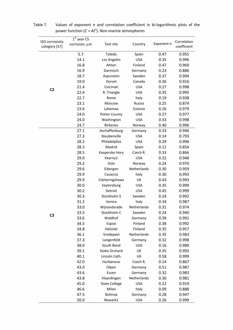
Table 7.  Values  of  exponent  n  and  correlation  coefficient  in  bi‐logarithmic  plots  of  the power function (C = Atn). Non‐marine atmospheres 

ISO corrosivity category [57] 

1st year CS corrosion, μm  Test site  Country  Exponent n  Correlation 

coefficient 

C2 

5.7  Toledo  Spain  0.47  0.955 14.1  Los Angeles  USA  0.35  0.996 16.8  Ahtari  Finland  0.47  0.969 16.9  Garmisch  Germany  0.23  0.886 18.7  Aspureten  Sweden  0.37  0.994 19.0  Dorset  Canada  0.26  0.916 21.4  Cincinati  USA  0.27  0.998 22.4  R. Triangle  USA  0.35  0.995 22.7  Rome  Italy  0.19  0.938 23.1  Moscow  Russia  0.25  0.874 23.6  Lahemaa  Estonia  0.26  0.979 24.0  Potter County  USA  0.27  0.977 24.0  Washington  USA  0.33  0.998 24.7  Birkenes  Norway  0.40  0.996 

C3 

27.1  Aschaffenburg  Germany  0.33  0.946 27.3  Steubenville  USA  0.14  0.793 28.2  Philadelphia  USA  0.29  0.996 28.3  Madrid  Spain  0.11  0.854 28.5  Kasperske Hory  Czech R.  0.33  0.866 29.0  Kearny1  USA  0.22  0.948 29.2  Oslo  Norway  0.24  0.970 29.6  Eibergen  Netherlands  0.30  0.959 29.9  Casaccia  Italy  0.30  0.993 29.9  Clatteringshaws  UK  0.43  0.993 30.0  Saylorsburg  USA  0.35  0.999 30.2  Detroit  USA  0.45  0.999 30.3  Stockholm S  Sweden  0.24  0.992 31.2  Venice  Italy  0.34  0.987 33.0  Wijnandsrade  Netherlands  0.31  0.974 33.5  Stockholm C  Sweden  0.24  0.940 33.6  Waldhof  Germany  0.39  0.991 34.5  Espoo  Finland  0.38  0.992 34.8  Helsinki  Finland  0.35  0.957 36.1  Vredepeel  Netherlands  0.35  0.983 37.3  Langenfeld  Germany  0.32  0.998 38.0  South Bend  USA  0.16  0.980 39.1  Stoke Orchard  UK  0.35  0.992 40.1  Lincoln Cath.  UK  0.58  0.999 42.0  Hurbanovo  Czech R.  0.14  0.867 43.0  Olpen  Germany  0.51  0.987 43.6  Essen  Germany  0.32  0.983 43.8  Vlaardingen  Netherlands  0.30  0.981 45.0  State College  USA  0.22  0.919 46.6  Milan  Italy  0.09  0.888 47.5  Bottrop  Germany  0.28  0.947 50.0  Newark1  USA  0.26  0.999 

Table 7 (continued) 

C4 

51.0  Columbus  USA  0.36  0.965 54.8  Borregaard  Norway  0.35  0.998 55.8  Prague  Czech R.  0.22  0.867 64.0  Lieja  Bélgica  0.64  0.998 67.0  Whiting  USA  0.17  0.947 69.0  Bethlehem2  USA  0.17  0.950 70.9  Kopisty  Czech R.  0.07  0.380 71.0  Bayonne  USA  0.31  0.996 72.0  Rankin  USA  0.32  0.978 76.0  Bethlehem1  USA  0.26  0.999 80.0  Newark2  USA  0.15  0.974 

C5 

86.0  Prague  Czech R.  0.18  0.933 88.0  Mülheim  Germany  0.50  0.998 100.0  Kopisty  Czech Rep.  0.51  0.999 114.0  Duisburg  Germany  0.61  0.996 116.0  Kearny3  USA  0.30  1.000 119.0  Kearny2  USA  0.15  0.973 

  210.0  Gelsenkirchen  Germany  0.50  0.998  

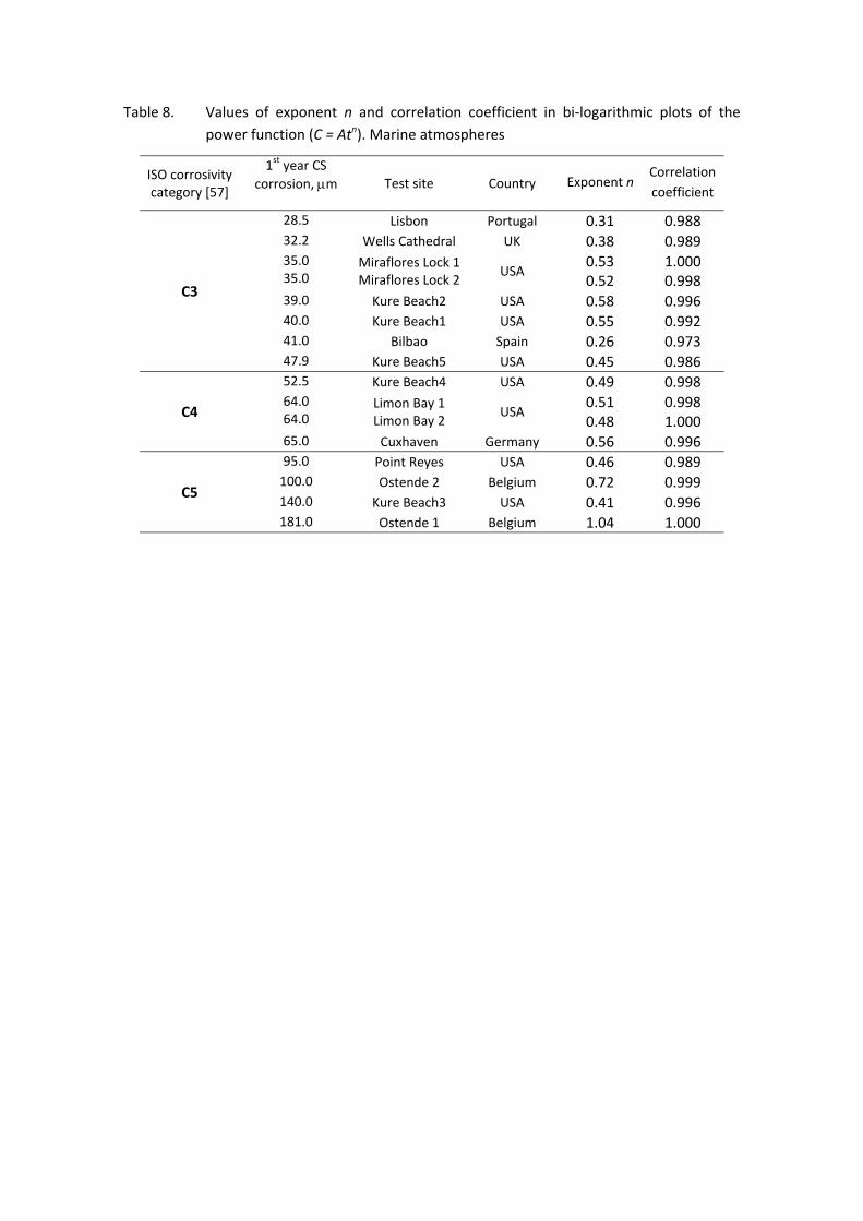
Table 8.  Values  of  exponent  n  and  correlation  coefficient  in  bi‐logarithmic  plots  of  the power function (C = Atn). Marine atmospheres 

ISO corrosivity category [57] 

1st year CS corrosion, μm  Test site  Country  Exponent n 

Correlation coefficient 

C3 

28.5  Lisbon  Portugal  0.31  0.988 32.2  Wells Cathedral  UK  0.38  0.989 35.0 35.0 

Miraflores Lock 1Miraflores Lock 2

USA 0.53 0.52 

1.000 0.998 

39.0  Kure Beach2  USA  0.58  0.996 40.0  Kure Beach1  USA  0.55  0.992 41.0  Bilbao  Spain  0.26  0.973 47.9  Kure Beach5  USA  0.45  0.986 

C4 

52.5  Kure Beach4  USA  0.49  0.998 64.0 64.0 

Limon Bay 1 Limon Bay 2 

USA 0.51 0.48 

0.998 1.000 

65.0  Cuxhaven  Germany  0.56  0.996 

C5 

95.0  Point Reyes  USA  0.46  0.989 100.0  Ostende 2  Belgium  0.72  0.999 140.0  Kure Beach3  USA  0.41  0.996 181.0  Ostende 1  Belgium  1.04  1.000 

 

Table 9.  Average values of exponent n  in bi‐logarithmic plots of  the power  function  (C = Atn)  for plain  carbon  steel  (CS) and weathering  steel  (WS)  in non‐marine  (rural‐urban‐industrial) and marine atmospheres 

Steel 

Non marine (Rural‐Urban‐Industrial) atmospheres 

Marine atmospheres 

Number of data 

n Ave. 

Range of n in Eq. (2) 

Number of data 

n Ave. 

Range of n in Eq. (2) 

CS (from ref. [92]) 

25  0.49  0.26‐0.76  13  0.73  0.37‐0.98 

WS (from tables 7‐8) 

58  0.33  0.11‐0.64  16  0.48  0.26‐0.72 

 

Table 10.  Dose‐response functions for weathering steel in unsheltered and sheltered exposures [86] 

Material  Mass loss, g/m2

Weathering steel (unsheltered)  ML = 34[SO2]0.33exp{0.020Rh + f(T)}t0.13 

Weathering steel (sheltered)  ML = 8.2[SO2]0.24exp{0.025Rh + f(T)}t0.66 

where:  t = exposure  time  (years); Rh = relative humidity  (%); T = average annual  temperature (°C); f(T) = a(T‐10) when T < 10°C, otherwise b(T‐10), with a, b being constant values depending on the specific metal; SO2 = sulfur dioxide concentration (μg/m

3)