ARE U.S. COMMERCIAL BANKS TOO BIG?

Diego A. Restrepo

Subal C. Kumbhakar Kai Sun

No. 13-14

2013

Are U.S. Commercial Banks Too Big?

Diego A. Restrepo1

Department of Economics, State University of New York at Binghamton, New York, USAEAFIT University, Medellın, Colombia.

Subal C. Kumbhakar

Department of Economics, State University of New York at Binghamton, New York, USA.

Kai Sun2

Aston Business School, Aston University, UK.

Abstract

This paper presents new nonparametric measures of scale economies and TFP growth for U.S.

banks. Unlike previous studies that use fully nonparametric models, our approach controls for

time-invariant unobserved heterogeneity among banks in estimating returns to scale, TFP growth

and its components. Using data for U.S. commercial banks from 2001 to 2010, we find evidence of

significant scale economies across the entire bank size distribution. Returns to scale are persistent

over time, decrease with bank size, and contribute significantly to TFP growth. Our results indicate

that almost all small and medium size banks and most of the largest banks have strong economic

incentives to keep growing. Thus, the consolidation of the banking industry is unlikely to retrench

in the near future.

Keywords:

Banks, TFP growth, returns to scale, scale economies, nonparametric

JEL classification: D24, G21, C14

Email addresses: drestre1@binghamton.edu (Diego A. Restrepo ), kkar@binghamton.edu. (Subal C.Kumbhakar), k.sun@aston.ac.uk (Kai Sun )

1Restrepo acknowledges financial support from the Colombian Fulbright Commission, the Colombian Adminis-trative Department of Science, Technology and Innovation (Colciencias), and EAFIT University.

2Corresponding author.

Preprint submitted to Journal of Money Credit and Banking January 2, 2013

1. Introduction

Bank size became a contentious issue after the recent U.S. financial crisis. The government

bailout of some of the biggest U.S. banks angered the public, policy makers, and academics. How-

ever, proposals to break up these banks into smaller institutions failed to materialize, in part, be-

cause there is no consensus on the desirability or feasibility of capping the size of banks (Stern and

Feldman 2009). More recently, however, the discussion has been reignited and capping the size

of banks is again at the center of the policy debate.3 In this paper, we present evidence indicating

that the behemoth size of some U.S. commercial banks seems quite normal and may still be below

optimal. Thus, without regulatory intervention further bank growth and industry consolidation are

unlikely to retrench.

Bankers, policy makers, and academics usually identify economies of scale as the main factor

behind the ever increasing size of banks in the U.S. Bigger banks seems to benefit from spreading

their investments over more output, save from consolidating operations, have access to a broader

funding mix, diversify their assets over an expanded output mix, and, probably, increase their

market power and political influence. However, the empirical evidence is inconclusive regarding

the existence of economies of scale (RTS) for the biggest banks. In particular, RTS estimates differ

substantially across studies depending on the methodology used in econometric estimation and/or

the sample period under study.

Some studies find increasing RTS for small banks and constant or slightly decreasing RTS

for large banks (e.g., Berger, Hanweck, and Humphrey 1987, Hunter and Timme 1991, Mester

1994, Clark 1996, Hughes and Mester 1998, and Wheelock and Wilson 2001). Other studies find

increasing RTS even for the biggest financial institutions (e.g., Shaffer 1994, Berger and Mester

1997, Hughes and Mester 1998, Hughes, Mester, and Moon 2001, and Feng and Serletis 2010).

In most recent works, Wheelock and Wilson (2011, 2012) present evidence indicating that all

U.S. commercial banks, bank holding companies, and credit unions operate under increasing RTS.

However, Feng and Zhang (2012) find decreasing RTS for large U.S. commercial banks. Thus, the

existence of RTS for the biggest U.S. banks is still a matter of debate.

In this paper, we present new evidence suggesting that the majority of the biggest U.S. com-

mercial banks still enjoy scale economies. Thus, they are not yet too big too exhaust the benefits

from being big to reach their optimal scale size.4 However, we also find that some of the biggest

3See Johnson (2012) and the references therein.4We find that estimates of RTS presented in some of the recent papers in the literature may be biased upward.

2

banks exhibit constant or decreasing RTS, indicating that some of them have already attained their

optimal scale size while some others are operating beyond their optimal size. In addition, we find

that RTS contribute positively and significantly to TFP growth followed by allocative efficiency

and technical change. TFP growth trends for big, medium, and small banks are similar. However,

big banks experience sharper swings in TFP growth than medium and small banks.

Like Wheelock and Wilson, we avoid the problem of specifying a priori any functional form

for the underlying cost function. However, unlike Wheelock and Wilson, our method exploits

the dynamics between total cost and its determinants over time. We start from a nonparametric

specification of the cost function of banks and then derive a growth equation for costs whose

coefficients are nonparametric functions of the arguments of the cost function, viz., outputs, input

prices, and other environmental/control variables. More specifically, we use the semiparametric

smooth coefficient (SPSC) model of Kumbhakar and Sun (2012), Li, Huang, Li, and Fu (2002),

and Li and Racine (2010) to estimate the functional coefficients. In our case the SPSC model

arises naturally from the cost function framework and is not imposed a priori. We show that the

functional coefficients of the SPSC model are nonparametric functions of the covariates of the cost

function. Furthermore, these are uniquely related to TFP growth and its components, including

RTS. Finally, to elucidate the estimates from the SPSC model, we also present results obtained

from two parametric models derived within the same framework.

We find that most U.S. commercial banks still have economic incentives to keep growing.5

Our nonparametric RTS estimates indicate presence of economically and statistically significant

scale economies for 98% of small and medium size banks, 73% of big banks, and 65% of the

biggest one hundred banks. Median nonparametric RTS estimates are around 1.375. A bank with

a RTS of 1.375, for instance, could increase outputs by 10% by increasing costs by only 7.27%

approximately (1/1.375 × 10%). Median RTS for small, medium, and big banks are 1.51, 1.31,

and 1.14, respectively. For the biggest one hundred banks, median RTS is around 1.08. Thus, a

10% increase in all outputs will raise total cost by approximately 6.6%, 7.6%, and 8.7% for small,

medium, and big banks; and by 9.2% for the biggest one hundred banks.

Our estimates show that RTS decrease monotonically across bank size deciles: small banks

exhibit higher scale economies followed by medium and big banks. The relation between mean

5 We classify big banks as those with assets above $1 billion dollars; medium banks as those with assets greaterthan $100 million and lower than $1 billion dollars; and small banks as those with assets below $100 million dollars.For each year, we also rank banks by assets an select the top 100 biggest banks. As December 31, 2010; there were479 big banks; 3,637 medium banks; and 2,290 small banks operating in the U.S. By comparison, as of December 31,2000, there were 285 big banks; 2,397 medium banks; and 5,452 small banks.

3

scale economies estimates and bank size is L-shaped across bank size deciles; indicating that after

certain threshold, increases in bank size reduce scale economies only slightly or that RTS estimates

are unrelated to bank size as measured by total assets. Thus scale economies seems to account only

partially for the economic incentives for the growth of the biggest banks.

We also find that RTS estimates are persistent over time and influence positively and signif-

icantly to TFP growth. The median estimate of TFP growth per year was 2.4% which is mostly

driven by scale and allocative components. Therefore, if banks care about achieving higher pro-

ductivity levels, the consolidation of the banking industry is likely to continue driven by scale

related gains.

The approach in this paper differs from earlier nonparametric studies (e.g., Wheelock and Wil-

son 2001, 2011, 2012) in some important ways. First, our model gives fully nonparametric esti-

mates of TFP growth and its components, including RTS, and allows for the estimation of other

important features of the underlying technology (e.g., output-cost elasticities, technical change

(TC) and input price-cost elasticities). This, in turn, allows us to check the consistency of the

results with theoretical restrictions—which is not done in others nonparametric studies. Second,

we compute RTS for each bank-year observation instead of proxies for RTS. Third, unlike all pre-

vious papers, we estimate TFP growth components, including RTS, controlling for unobserved

heterogeneity across banks—failure to do so may lead to underestimation of RTS.6

We focus on the post-deregulation period of the U.S. banking industry to isolate RTS esti-

mates from previous regulatory restrictions that may have blocked banks ability to grow to exploit

scale economies. Our sample covers 60,868 bank-year observations for 7,473 commercial banks

from 2001 to 2010. Unlike Wheelock and Wilson (2012), we exclude Bank Holding Companies

which, given their idiosyncrasies, may not be adequately comparable with most commercial banks.

Also, though quarterly data are available, we do not believe that each quarterly observation reflects

banks’ economic behavior at each point in time. Hence, we take quarterly averages to compute

yearly observations. In line with Wheelock and Wilson, our approach incorporates a large sam-

ple of banks, a nonparametric specification of the cost function, fully flexible interactions among

the explanatory variables, and includes off-balance sheet activities and equity capital as additional

control variables.

6Ignoring unobserved heterogeneity leads to the “incidental parameters problem”; which, in turn, introduces biasesand inconsistency in the estimation (See Mester 1997, Greene 2005a, Greene 2005b, Kumbhakar, Lien, Flaten, andTveterås 2008, and Wang and Ho 2010). We also control for output quality, risk, and nontraditional activities to helpcapturing heterogeneity across banks that may be confounded with differing relative costs (e.g. Mester 1996, Rogers1998) or masquerade endogenous sources of risk (e.g. Hughes and Mester 1998).

4

To check the effects of modelling unobserved heterogeneity on our results, we also estimate

RTS from a parametric model that does not control for such heterogeneity. Our findings indicate

that failing to control for unobserved heterogeneity across banks may conceal evidence of increas-

ing RTS. Using this model, we find scant evidence of scale economies: only small banks exhibit

increasing RTS and most medium and large banks show either constant or decreasing RTS.

The rest of the paper is organized as follows. In Section 2, we review the literature. In Section

3, we describe our model, the estimation strategy, and our data. In Section 4, we present our

empirical results; which we discuss in Section 5. Policy implications of our study is discussed in

Section 6. Finally Section 7 concludes.

2. Literature Review

Firms differ substantially in their productivity levels even within narrowly defined industries.7

In the banking literature, researchers investigate such differences by examining TFP growth com-

ponents, viz., efficiency and scale economies. Since surveys on bank efficiency are available else-

where (e.g., Berger and Mester 1997), we focus only on the recent literature on scale economies.

During the early stages of deregulation of the U.S. banking industry, policy makers were con-

cerned that a handful of big diversified banks could emerge and dominate the industry. Banks ap-

peared to be able to profit from being bigger, threatening the viability of smaller specialized banks

(Clark 1988). More recently, empirical evidence shows that advances in technology and changes

in regulation favor large depository institutions (Wheelock and Wilson 2011). Economists think

that economies of scale may explain such phenomena. However, the empirical evidence seems, at

best, inconclusive.

Before 1970, empirical studies showed evidence of scale economies among commercial banks

of all sizes (see Shaffer 1994 and the references therein). During the 1970’s and 1980’s, in contrast,

the bulk of empirical evidence showed scale economies for only small depository institutions.8 For

the 1990’s, the evidence was mixed: some studies find evidence of scale economies for small banks

only;9 while others present evidence of scale economies even for the largest banks.10 More recent

7 Such differences stem from supply and demand-side factors. Supply-side factors include managerial ability, tech-nological progress, scale economies, human capital, investment, R&D, industry structure, ownership, and regulation.Demand-side factors include product substitutability, transportation costs, search costs, firm-customer’s long-termrelations, among others. See Bartelsman and Doms (2000) and Syverson (2011) for reviews of the literature.

8See Clark (1988), Berger et al. (1987), and Shaffer (1994).9See Berger and Humphrey (1994), Berger et al. (1987), Hunter and Timme (1991), Mester (1994), Clark (1996),

Hughes and Mester (1998), and Wheelock and Wilson (2001).10See Shaffer (1994), Hughes, Lang, Mester, and Moon (1996, 2000), Berger and Mester (1997), Hughes and Mester

(1998), Berger, Demsetz, and Strahan (1999), and Hughes et al. (2001).

5

studies, with the exception of Feng and Zhang (2012), show evidence of scale economies across

the entire bank size distribution.11

Wheelock and Wilson (2011, 2012) investigate scale economies of U.S. credit unions, com-

mercial banks, and bank holding companies (BHC). Despite the continuous growth of these in-

stitutions since the 1980’s, Wheelock and Wilson uncovered substantial economies of scale even

for the largest institutions. Instead of using output-cost elasticities to measure economies of scale,

as it is widely done in the literature, Wheelock and Wilson infer them using ray scale economies

(RSE) and expansion-path scale economies (EPSE) indexes.12 They justify their choice arguing

that using elasticities requires estimating derivatives of nonparametric functions which are noisier

than estimates of the functions themselves. The drawback of this method is that RSE and EPSE

estimates give only an indication of RTS rather than a measure of their magnitude. Also, from the

econometric viewpoint, their estimation strategy involves a reduction of data dimensionality that

can lead to noisier estimates.

Using yearly data from 1989-2006, Wheelock and Wilson (2011) find that all U.S. credit unions

operate under increasing RTS and conclude that further consolidation of the industry and increas-

ing average size are likely. Regarding commercial banks and bank holding companies, Wheelock

and Wilson (2012) find similar results. Using quarterly data from 1984-2006, they find that RSE

measures indicate increasing RTS for all banks in each period. Further, using EPSE measures they

show that 99.7% of banks exhibit increasing RTS and the remaining banks experience constant

RTS.

Wheelock and Wilson’s results contrast with their earlier work, viz., Wheelock and Wilson

(2001), in which they find that economies of scale were exhausted when banks have between $300

and $500 million of assets. They attribute their contrasting results to the use of a larger sample

and a more realistic model of bank costs in which equity capital and off-balance sheet activities

are explicitly incorporated.

Hughes and Mester (2011) also present evidence of increasing RTS for 842 U.S. large bank

holding companies (BHC) operating during 2007. Unlike Wheelock and Wilson (2011, 2012), they

use parametric methods in their estimations. Based on Hughes et al. (1996), Hughes and Mester

(1998), Hughes et al. (2001), and Hughes and Mester (2010) , they argue that studies usually failed

11These studies include Wheelock and Wilson (2011, 2012), Hughes and Mester (2011), Feng and Serletis (2010).12 RSE are computed using the ratio of successive nonparametric local-linear estimates of the cost function along

a ray passing through the observed output vector and θy0 for θ ∈ [0.05, 0.10, . . . , 1, 2, . . . , 25]. Similarly, EPSE arecomputed from successive nonparametric estimates of the cost function as one moves along the path θ(1 − γ)y toθ(1 + γ)y for small values of γ and varying θ.

6

to uncover increasing RTS for large banks due to misspecification of the bank cost or profit model.

For example, early studies using data from the 1980’s did not consider managerial risk preferences

and the endogenous risk taking behavior of banks. Large banks may have lower marginal costs in

risk management due to diversification. This, in turn, may lead banks to take on more risk until all

the scale-related cost savings are exhausted, reducing measured scale economies.

Hughes and Mester (2011) use four different model specifications. The first model omits equity

capital as a conditioning variable and also omits the cost of equity in the cost function. Using this

model, they find slightly increasing RTS for all BHC in the sample. Using a second model, in

which equity capital enters as a conditioning variable, they find decreasing RTS for all BHC.

Results from a third model incorporating the shadow cost of equity shows slightly increasing RTS

for all BHC. However, the RTS estimates are statistically indistinguishable from those of the first

model. Finally, using a fourth model incorporating managerial preferences and conditioning on the

optimal level of equity capital, they find substantial scale economies for all BHC. In this case, RTS

range from 1.13 for the smallest BHC to 1.35 for the largest BHC. The estimated RTS, however,

increase monotonically with BHC’s size. This result is puzzling since most empirical evidence,

including Wheelock and Wilson (2011, 2012), show that RTS monotonically decrease as bank size

increases.

Feng and Serletis (2010) also present new evidence of increasing RTS for large banks. Unlike

Wheelock and Wilson (2011, 2012) and Hughes and Mester (2011) who use a cost function, Feng

and Serletis use a fully parametric output distance function which does not require data on factor

prices. They use data for U.S. banks with assets in excess of $1 billion from 2001 to 2005. The

main contribution of their paper is methodological in nature. They impose monotonicity and cur-

vature constraint on the underlying bank production technology using Bayesian techniques. They

claim that without such constraints estimates of RTS and TFP growth are distorted. They obtain

RTS estimates in the range from 1.037 to 1.056, indicating moderate increasing RTS for all banks

in the sample. Nonetheless, from their paper, it is not clear if these results are entirely driven by

their method, since they omit a comparison with the alleged misspecified model. Furthermore,

in almost all banking studies, outputs are treated as exogenous and inputs endogenous. If this is

the case, one should use an input distance function in which outputs and input ratios appearing as

regressors are exogenous (Das and Kumbhakar 2012). The use of output distance function suffers

from endogeneity problem when inputs are endogenous.

Taking together, these studies suggest that most banks operate under increasing RTS. However,

7

Feng and Zhang (2012) find that large and small banks exhibit near constant RTS. As in Feng and

Serletis, they use an output distance function to model banks’ technology, use Bayesian techniques

for estimation, and impose monotonicity and curvature conditions to the underlying technology.

They include continuously operating large banks (assets above $1 billion), large community banks

(assets below $1 billion and above $100 million), and small community banks (assets below $100

million) from 1997 to 2006. The main distinction with Feng and Serletis’s work is that Feng and

Zhang explicitly account for technical inefficiency and unobserved heterogeneity across banks in

their estimation. Their results suggest that failing to do so leads to higher RTS estimates. In partic-

ular, without accounting for unobserved heterogeneity, large banks exhibit increasing RTS ranging

from 1.022 in 1997 to 1.01 in 2006. However, when unobserved heterogeneity is incorporated

these results disappear: all large banks now exhibit constant RTS.

One important criticism that may be raised against Feng and Zhang’s results is that they do not

include any proxies for risk taking behavior as it is done in Hughes and Mester (2011) or Wheelock

and Wilson (2011, 2012) . Nonetheless, the fact that these latter studies do not account for unob-

served heterogeneity across banks also may raise questions about their reliability in line with Feng

and Zhang’s claims. Thus, the literature will benefit from a further investigation on these issues

using a methodology that may combine the insights of these three lines of research: i) controlling

for unobserved heterogeneity across banks, ii) conditioning on bank risk taking behavior, and iii)

using flexible functional specifications for the underlying technology.13 Our paper goes one step

forward in this direction.14

Another way to rationalize the observed increasing size of banks is to look at the distribution of

TFP components across different bank size categories. If TFP growth differs across the bank size

distribution, some banks will have incentives to increase their scale of operations, even though,

by itself, this strategy may have negligible or negative impact on their performance. For instance,

Hunter and Timme (1986, 1991) investigate how technical change interacts with bank size and

scale economies. Using data for U.S. bank holding companies from 1972 to 1982, they find that

technical change is associated with increases in scale economies: technological change lowers cost

by 1% per year, increases the cost-minimizing scale of operations, and affects banks’ product mix.

Early studies indicate that TFP growth in the U.S. banking during the 1980’s was modest or

13The international evidence also points toward the existence of scale economies only for small and medium-sizedbanks, Amel, Barnes, Panetta, and Salleo (2004). Allen and Liu (2007), on the other hand, report economies of scalefor the six largest Canadian banks.

14 Restrepo and Kumbhakar (2011) using data for all U.S. commercial banks from 2001 to 2010 also documentconstant RTS for most U.S. banks from 2001-2010.

8

slightly negative (Humphrey 1991, 1992, 1993, Bauer, Berger, and Humphrey 1993, Wheelock and

Wilson 1999, Stiroh 2000, Semenick Alam 2001, Berger and Mester 2003, Daniels and Tirtiroglu

1998). Tirtiroglu, Daniels, and Tirtirogu (2005) investigate how the regulatory structure of the

time might have contributed to this phenomenon. They find that deregulation had a positive impact

on banks’ long-run productivity growth, confirming the priors that the poor productivity growth

was due to regulatory restrictions. More recently, however, Mukherjee, Ray, and Miller (2001)

and Semenick Alam (2001) find positive productivity growth for large U.S. banks over roughly

the same period, indicating that larger banks may have taken better advantage of technological

progress and deregulation.

During the period 1997-2006, Feng and Zhang (2012) find positive productivity growth for

large banks, 2.04% per year on average, but poor productivity growth for small banks, 0.3% per

year on average. They also show that most productivity growth gains are due to technical change

and not to efficiency gains.15 This results echo those of Feng and Serletis (2010) who show that

technical change contributed to 70% of total productivity growth and scale economies only account

for 7%.16

3. Methodology

3.1. The Model

We use a nonparametric cost function with Q outputs, K inputs, and P environmental variables

to control for bank-specific characteristics. The cost function for bank i at time t has the following

general specification:

Cit = Ait · Bi · H(Wit,Yit, t,Zit) (1)

where Cit represents actual cost, Ait is an productivity parameter, Bi is a parameter capturing time-

invariant unobserved heterogeneity across banks (fixed-effects), H(·) is a nonparametric function of

Wit, a vector of input prices, Yit, a vector of output quantities, and Zit, a vector of control variables.

We impose homogeneity restrictions on input prices by dividing costs and input prices by the

price of input K, i.e., WK . Thus, the cost function becomes:

Cit = Ait · Bi · H(Wit,Yit, t,Zit) (2)

15The results for large banks are comparable to those in Feng and Serletis (2010)16 See Hughes et al. (2001) and Hughes and Mester (2010) on the impact of using different models on estimates of

TFP components (e.g. scale economies, efficiency, technical change, etc.).

9

where Wk = Wk/WK and Cit = C/WK . Taking logarithm to (2) and denoting ln H(·) = f (·), we can

write:

ln Cit = f (Wit,Yit, t,Zit) + ln Ait + ln Bi (3)

Dropping the subscripts and taking the total derivative of (3), we get the following growth formu-

lation:

d ln Cdt

=∂ f∂t

+

K−1∑k=1

∂ f

∂ ln Wk

·d ln Wk

dt+

Q∑q=1

∂ f∂ ln Yq

·d ln Yq

dt+

P∑p=1

∂ f∂Zp·

dZp

dt+∂ ln A∂t

(4)

We write (4) in a more compact way to get our estimating growth equation:

˙C = β0(·) +

K−1∑k=1

βk(·)˙Wk +

Q∑q=1

γq(·)Yq +

P∑p=1

ϕp(·)∇tZp + u (5)

where, in generic terms, X = d ln X/dt and ∇tX = dX/dt. We interpret u = ∂ ln A/∂t as an

error term capturing productivity shocks and establish the following mapping for the functional

coefficients:

β0(·) =∂ f∂t

; βk(·) =∂ f

∂ ln Wk

; γq(·) =∂ f

∂ ln Yq; ϕp(·) =

∂ f∂Zp

(6)

Note that the growth formulation of the cost function in (4) automatically controls for unobserved

time-invariant heterogeneity across banks by removing the fixed-effects parameters. Finally, the

functional coefficients have clear economic meaning. The estimated functional coefficients can be

used to get estimates of TFP growth and its components as shown in the next subsection.

3.2. Total Factor Productivity Change

We start with the standard definition of TFP change (see Denny, Fuss, and Waverman 1979):

˙T FP ≡Q∑

q=1

RqYq −

K∑k=1

S kXk (7)

where Rq denotes the revenue share of each output (q = 1, ...,Q) and S k the cost share of each input

(k = 1, ...,K).

10

Adding ˙T FP to both sides of (5):

˙T FP + β0(·) +

K−1∑k=1

βk(·)˙Wk +

Q∑q=1

γq(·)Yq +

P∑p=1

ϕp(·)∇tZp + u ≡ ˙C +

Q∑q=1

RqYq −

K∑k=1

S kXk (8)

Using the definitions ˙C = C − WK and C =∑K

k=1 S kWk +∑K

k=1 S kXk, the right-hand-side of (8) can

be expressed as:

˙C +

Q∑q=1

RqYq −

K∑k=1

S kXk ≡

K∑k=1

S kWk +

Q∑q=1

RqYq − WK (9)

Since∑K

k=1 S k = 1, Wk =˙Wk + WK , ∀k = 1, . . . ,K − 1, and ˙WK = 0,

K∑k=1

S kWk +

Q∑q=1

RqYq − WK ≡

K−1∑k=1

S k˙Wk +

Q∑q=1

RqYq (10)

Using this result, the relationship in (8) can be expressed as:

˙T FP ≡ −β0(·) +

Q∑q=1

(Rq − γq(·))Yq +

K−1∑k=1

(S k − βk(·))˙Wk −

P∑p=1

ϕp(·)∇tZp − u (11)

Therefore, the relationship in (11) decomposes TFP growth into five components. The first term

is the technical change component (TC = −∂ f /∂t = −β0(·)) which captures shifts of the estimated

cost function over time (percentage change in cost over time, ceteris paribus). TC < 0 indicates

technical progress (cost diminution). A positive value of TC will indicate technical regress. The

second term (S C =∑Q

q=1(Rq − γq(·))Yq) can be decomposed into two components by expressing

it as (RTS − 1)∑Q

q=1 γq(·)Yq +∑Q

q=1(Rq − γq(·)/Γ(·))Yq where Γ(·) =∑

q γq(·), and RTS = (Γ(·))−1.

The first part of it clearly depends on RTS and the second part depends on mark-up (departure

of output prices from their respective marginal costs). The third term (AL =∑K−1

k=1 (S k − βk(·))˙Wk)

corresponds to the allocative component because it captures the effects of non-optimal input alloca-

tion (deviation of input mix from the optimal). The fourth term (EX = −∑P

p=1 ϕp(·)∇tZp) captures

the effect of other factors such as output quality, risk, and other variables. Finally, the last term

(−u) is viewed as a productivity shock component which can increase/decrease TFP growth. We

assume it to be random with mean zero, and can be measured residually. Note that the TFP growth

components are nonparametric functions that can be computed after estimating (5).

11

3.3. Econometric Model

We estimate the functional coefficients in (5) using three different models. First, note that f (·)

in (5) can be thought of as an unknown smooth function of t, ln Wk, ln Yq, and Zp, then its gradients,

i.e., β0, βk, ∀k = 1, . . . ,K−1, γq, ∀q = 1, . . . ,Q, and ϕp, ∀p = 1, . . . , P, are also unknown smooth

functions of these variables as shown in (6). As a result of these, (5) can be viewed as the SPSC

model of Li et al. (2002) where the model is linear in the ˙Wk, ∀k = 1, . . . ,K−1, Yq, ∀q = 1, . . . ,Q,

and ∇tZp, ∀p = 1, . . . , P, variables. To simplify notation, we rewrite (5) (after adding the subscript

i and t for observation in the cross-section and time dimension, respectively) as

Yit = X′itΨ(Zit) + uit (12)

where Yit =˙Cit; X′it = [1, ˙W1it, . . . ,

˙WK−1 it, Y1it, . . . , YQit,∇tZ1it, . . . ,∇tZPit],

Z′it = [ln W1it, . . . , ln WK−1 it, ln Y1it, . . . , ln YQit, tit,Z1it, . . . ,ZPit];

Ψ′(·) = [β0(·), β1(·), . . . , βK−1(·), γ1(·), . . . , γQ(·), ϕ1(·), . . . , ϕP(·)]. We call this model the semipara-

metric growth model (SPG model).

Following Li et al. (2002) and Li and Racine (2007), the local-constant estimator for Ψ(z) is

expressed as:

Ψ(z) =

N∑i=1

T∑t=1

XitX′itK

(Zit − z

h

)−1 N∑i=1

T∑t=1

XitYitK

(Zit − z

h

)(13)

where N and T denotes number of banks and time periods, respectively, h is a (K + Q + P) vector

with each element a selected bandwidth for each z variable andK(·) is the product Gaussian kernel

function.17

Note that if the kernel function is eliminated, then the SPSC estimator reduces to its OLS

counterpart. The SPSC model also nests the partially linear model proposed by Robinson (1988)

as a special case, which makes only the intercept an unknown smooth function ofZ variables.

Following Li and Racine (2010), we employ the most commonly used least-squares cross-

validation (LSCV) method, which is a fully automatic data-driven approach, to select the band-

17Explicitly, the kernel function is written as:

K(·) =

K+Q+P∏l=1

1√

2πexp

−12

(Zlit − zl

hl

)2

12

width vector h, i.e.,

CVlc(h) = minh

N∑i=1

T∑t=1

[Yit − X′itΨ−it(Zit)]2M(Zit) (14)

where CVlc(h) determines the cross-validation bandwidth vector h for local constant estimator,

X′itΨ−it(Zit) = X′it[∑N

j,i∑Tτ,tX jτX

′jτK(Z jτ−zit

h )]−1 ∑N

j,i∑Tτ,tX jτY jτK(Z jτ−zit

h ) is the leave-one-out

local-constant kernel conditional mean, and 0 ≤ M(·) ≤ 1 is a weight function that serves to

avoid difficulties caused by dividing by zero. The bandwidth for the Z variables and the smooth

coefficients can be estimated using the NP package (Hayfield and Racine 2008) in R.18

Second, we estimate (5) assuming that the underlying technology can be represented by a

translog cost function. In this case, the functional coefficients in (5) are parametric functions of

[Wit,Yit, t,Zit] that can be estimated by OLS (equation (A.7) in Appendix A). We call this model

the parametric growth model (PG model).19

Third, to make our results comparable to the previous literature, we estimate the cost func-

tion (1) instead of (5) assuming that the underlying technology can be represented by a translog

cost function. However, unlike the PG model, equation (1) does not control for unobserved time-

invariant heterogeneity across banks, see Appendix A. After estimating the coefficients, we com-

pute the functional coefficients in (5). We call this model the parametric log model (PL model).

The three models described above (SPG model, PG model, and PL model) differ in terms of

their assumptions about the data generating process and the functional form of the underlying

technology. Contrary to the PL model, both the SPG and PG models control for time-invariant

unobserved heterogeneity across banks. Unlike the SPG model, the PG model assumes a paramet-

ric and common technology across banks. The functional coefficients of the SPG model are fully

nonparametric while the PG and PL models’ functional coefficients are parametric functions. In

this sense the SPG model is the most general among the three.

3.4. Data

We use data from the Report of Conditions and Income (Call Reports) from the Federal Reserve

Bank of Chicago. We include all FDIC insured commercial banks with available data between

18We use the functions npscoefbw and npscoef with their default values. To decrease the estimation computationaltime, we set the optimization options to ”nmulti=1”, ”optim.abstol = 0.000001”, and ”optim.reltol = sqrt(0.000001)”.

19Using both the SPG and PG models, we avoid the incidental parameter problem. Consistency of the functionalcoefficients follow from the standard SPSC model (Li et al. 2002) and the standard linear panel data models as thenumber of observations grow to infinity.

13

2001Q1 and 2010Q4. We exclude banks reporting negative values for assets, equity, outputs and

prices, stand alone internet banks, commercial banks conducting primarily credit card activities,

and banks chartered outside continental U.S. territory. Our data set is an unbalanced panel with

63,120 bank-year observations for 8,483 banks. We deflate all nominal quantities using the 2005

Consumer Price Index for all urban consumption published by the Bureau of Labor Statistics.

Our method is computationally demanding. To avoid extreme outliers, we use data for which

output quantities and input prices fall between 0.5% and the 99.5% of their empirical distributions.

In addition, we only consider banks with at least four years of available data from 2001 to 2010. To

get annual values, we compute the quarterly average of balance-sheet nominal (stock) values. As a

result, we have 60,868 bank-year observations for 7,473 different banks. Our growth formulation

further decreases the number of observation to 51,966 bank-year observations for 7,381 banks.

In this framework, a bank’s balance-sheet captures the essential structure of banks’ core busi-

ness: (i) liabilities, together with physical capital and labor, are inputs into the bank production

process and (ii) assets, other than physical assets, are outputs. Liabilities are composed of core

deposits and purchased funds. Assets include loans and trading securities. Therefore, banks use

labor, physical capital, and debt to produce loans, invest in financial assets, and facilitate other

financial services.

We define five output variables: household and individual loans (Y1), real estate loans (Y2),

business loans (Y3), securities (e.g., federal funds sold and securities purchased under agreements

to resell) (Y4), and other assets (Y5). These outputs are essentially the same as those used in Berger

and Mester (2003).

We define five input variables: labor (e.g., number of full-time equivalent employees at the

end of each quarter) (X1), physical capital (e.g. premises and fixed assets including capitalized

leases) (X2), purchased funds (e.g., federal funds purchased and securities sold under agreements

to repurchase, total trading liabilities, other borrowed money, and subordinated notes and deben-

tures.) (X3), interest-bearing transaction accounts (X4), and non-transaction accounts (X5). The

price of each input, W j for j = 1, ..., 5, is computed by dividing total expenses by the correspond-

ing input quantity. Total costs, C, equals the sum of expenses on each of the five inputs; total

revenues, equals the sum of revenues for each output category. Table 1 presents summary statistics

for outputs, inputs, and input prices.

Table 1 also presents information on cost, revenue, and output shares. On the revenue side,

real estate loans account for 41.6% of total banks’ revenues (R2), loan to business and other insti-

14

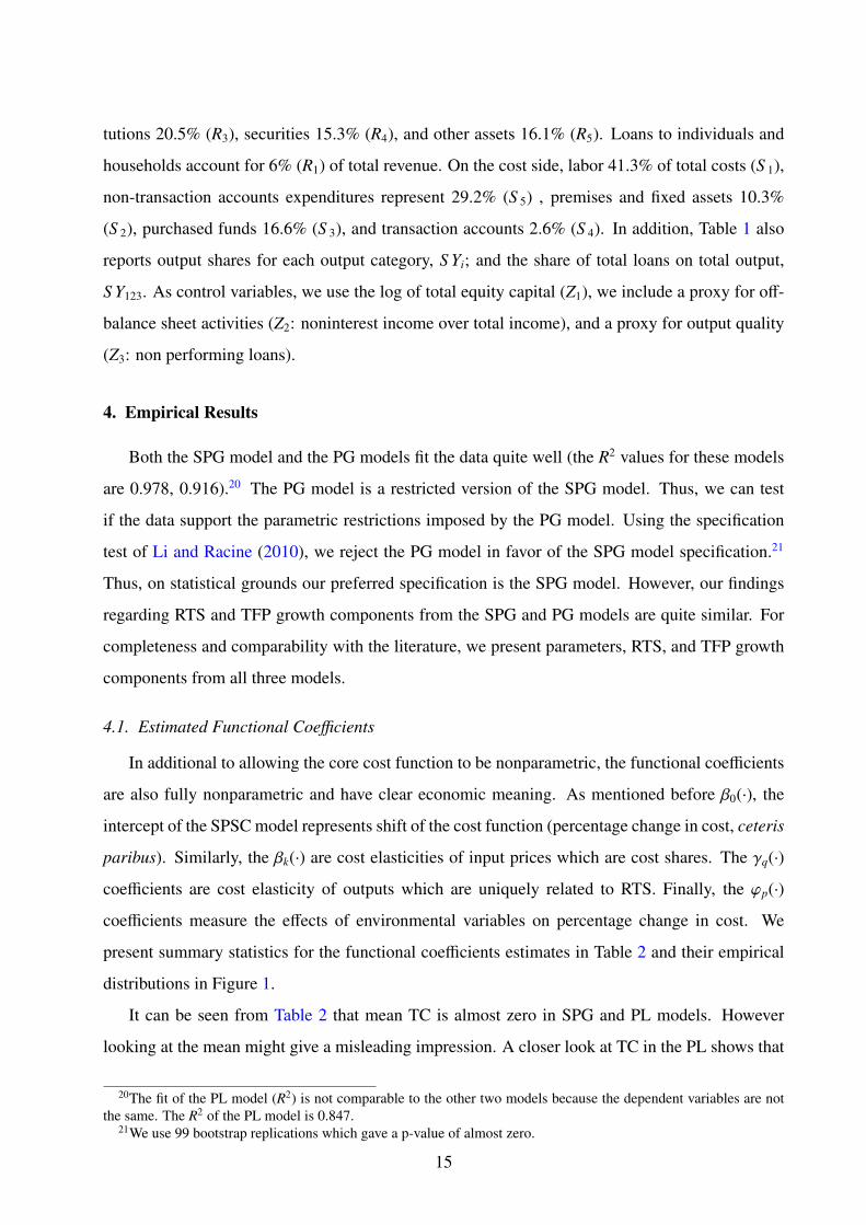
tutions 20.5% (R3), securities 15.3% (R4), and other assets 16.1% (R5). Loans to individuals and

households account for 6% (R1) of total revenue. On the cost side, labor 41.3% of total costs (S 1),

non-transaction accounts expenditures represent 29.2% (S 5) , premises and fixed assets 10.3%

(S 2), purchased funds 16.6% (S 3), and transaction accounts 2.6% (S 4). In addition, Table 1 also

reports output shares for each output category, S Yi; and the share of total loans on total output,

S Y123. As control variables, we use the log of total equity capital (Z1), we include a proxy for off-

balance sheet activities (Z2: noninterest income over total income), and a proxy for output quality

(Z3: non performing loans).

4. Empirical Results

Both the SPG model and the PG models fit the data quite well (the R2 values for these models

are 0.978, 0.916).20 The PG model is a restricted version of the SPG model. Thus, we can test

if the data support the parametric restrictions imposed by the PG model. Using the specification

test of Li and Racine (2010), we reject the PG model in favor of the SPG model specification.21

Thus, on statistical grounds our preferred specification is the SPG model. However, our findings

regarding RTS and TFP growth components from the SPG and PG models are quite similar. For

completeness and comparability with the literature, we present parameters, RTS, and TFP growth

components from all three models.

4.1. Estimated Functional Coefficients

In additional to allowing the core cost function to be nonparametric, the functional coefficients

are also fully nonparametric and have clear economic meaning. As mentioned before β0(·), the

intercept of the SPSC model represents shift of the cost function (percentage change in cost, ceteris

paribus). Similarly, the βk(·) are cost elasticities of input prices which are cost shares. The γq(·)

coefficients are cost elasticity of outputs which are uniquely related to RTS. Finally, the ϕp(·)

coefficients measure the effects of environmental variables on percentage change in cost. We

present summary statistics for the functional coefficients estimates in Table 2 and their empirical

distributions in Figure 1.

It can be seen from Table 2 that mean TC is almost zero in SPG and PL models. However

looking at the mean might give a misleading impression. A closer look at TC in the PL shows that

20The fit of the PL model (R2) is not comparable to the other two models because the dependent variables are notthe same. The R2 of the PL model is 0.847.

21We use 99 bootstrap replications which gave a p-value of almost zero.

15

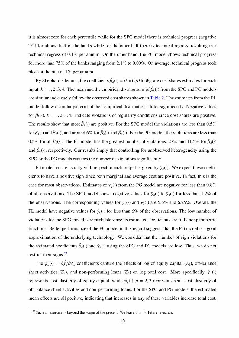
it is almost zero for each percentile while for the SPG model there is technical progress (negative

TC) for almost half of the banks while for the other half there is technical regress, resulting in a

technical regress of 0.1% per annum. On the other hand, the PG model shows technical progress

for more than 75% of the banks ranging from 2.1% to 0.00%. On average, technical progress took

place at the rate of 1% per annum.

By Shephard’s lemma, the coefficients βk(·) = ∂ ln C/∂ ln Wk, are cost shares estimates for each

input, k = 1, 2, 3, 4. The mean and the empirical distributions of βk(·) from the SPG and PG models

are similar and closely follow the observed cost shares shown in Table 2. The estimates from the PL

model follow a similar pattern but their empirical distributions differ significantly. Negative values

for βk(·), k = 1, 2, 3, 4., indicate violations of regularity conditions since cost shares are positive.

The results show that most βk(·) are positive. For the SPG model the violations are less than 0.5%

for β1(·) and β3(·), and around 6% for β2(·) and β4(·). For the PG model, the violations are less than

0.5% for all βk(·). The PL model has the greatest number of violations, 27% and 11.5% for β2(·)

and β4(·), respectively. Our results imply that controlling for unobserved heterogeneity using the

SPG or the PG models reduces the number of violations significantly.

Estimated cost elasticity with respect to each output is given by γq(·). We expect these coeffi-

cients to have a positive sign since both marginal and average cost are positive. In fact, this is the

case for most observations. Estimates of γq(·) from the PG model are negative for less than 0.8%

of all observations. The SPG model shows negative values for γ2(·) to γ4(·) for less than 1.2% of

the observations. The corresponding values for γ1(·) and γ5(·) are 5.6% and 6.25%. Overall, the

PL model have negative values for γk(·) for less than 6% of the observations. The low number of

violations for the SPG model is remarkable since its estimated coefficients are fully nonparametric

functions. Better performance of the PG model in this regard suggests that the PG model is a good

approximation of the underlying technology. We consider that the number of sign violations for

the estimated coefficients βk(·) and γk(·) using the SPG and PG models are low. Thus, we do not

restrict their signs.22

The ϕp(·) = ∂ f /∂Zp coefficients capture the effects of log of equity capital (Z1), off-balance

sheet activities (Z2), and non-performing loans (Z3) on log total cost. More specifically, ϕ1(·)

represents cost elasticity of equity capital, while ϕp(·), p = 2, 3 represents semi cost elasticity of

off-balance sheet activities and non-performing loans. For the SPG and PG models, the estimated

mean effects are all positive, indicating that increases in any of these variables increase total cost,

22Such an exercise is beyond the scope of the present. We leave this for future research.

16

ceteris paribus. In contrast, for the PL model a 1% increase in equity capital is associated with a

reduction in total cost by 4%, on average.

It is noteworthy that all the estimated functional coefficients are well behaved as shown by their

empirical distributions (Figure 1). This is particularly remarkable for the nonparametric functional

coefficients of the SPG model since they are completely unconstrained.

The functional coefficients in all three models are observation-specific. Thus, we compute their

standard errors using the wild bootstrap method of Hardle and Mammen (1993). Figure 2 shows

the observation-specific functional coefficient estimates from the SPG model along with their 95%

confidence intervals. Unreported results show a similar pattern for the PG and PL models.

To understand these figures, consider the plot for the estimated functional coefficients β0(·) in

Figure 2. We plot β0(·) against β0(·) such that all the coefficients β0(·) lie along the 45◦ line. The

points above (below) the 45◦ line represent the upper (lower) bound of each confidence interval.

Therefore, for each β0(·) on the 45◦ line we can see an observation-specific confidence interval.

If the horizontal line at zero passes inside of the confidence bounds for any given observation,

then β0(·) for this observation is statistically insignificant. Conversely, if the horizontal line at zero

passes outside of the confidence bounds, then β0(·) for this observation is statistically significant. In

addition, if the lower (upper) bound lies above (below) zero, then the coefficient for this observation

is significantly positive (negative). In general, the confidence intervals for each of the functional

coefficients are quite tight, although they become wider at the tails.

4.2. Returns to Scale

We present summary statistics for RTS estimates using the SPG, PG, and PL models in Panels

A, B, and C of Table 3. Figures 3 and 4 show their empirical distributions. We find economically

and statistically significant scale economies for most banks. For the SPG model (Panel A), mean

RTS estimates is 1.42, indicating that if outputs were to increase by 10%, total costs will increase

approximately by 7% (10% × 1/1.42). Mean RTS estimates from the PG model (Panel B) is

1.40. These results indicate presence of increasing RTS (IRTS) for most banks. The mean RTS

from the PL model (Panel C) is 1.01, indicating constant RTS (CRTS). The empirical distribution

of estimated RTS from the SPG or PG models show decreasing RTS for less than 2% of the

observations. In contrast, estimated RTS from the PL model show DRTS for about 42% of the

observations.

Estimated RTS decrease with bank size, see Table 3.23 Mean RTS for small, medium, and big

23 We classify banks by total assets as follows: Big (assets > $1 billion), medium ($100 million < assets < $1

17

banks are 1.56, 1.34, and 1.18 from the SPG model and 1.54, 1.32, and 1.10 from the PG model.

Mean RTS for the top 100 banks are also lower than for all other banks. Estimated RTS from the

SPG and PG models show that almost all medium and small banks exhibit IRTS. More than 75%

of big banks and more than 50% of the top 100 banks also exhibit IRTS. Estimates RTS from the

PL model show IRTS for about 50% of banks.24

The RTS estimates from the PG and the PL model are directly comparable in the sense that

both models controls for fixed bank-specific effects. This is, however, not the case with the PL

model. Thus the differences in RTS estimates in the PL model from the other two models might be

attributed to ignoring bank-specific effects. Estimated RTS from the PL model are both statistically

and economically smaller than those from the PG model, indicating that failure to account for time-

invariant unobserved heterogeneity conceals the evidence of substantial scale economies for most

banks.

Now we investigate the statistical significance of our RTS estimates. In Figure 5, we depict the

estimated 95% confidence intervals for RTS estimates by bank size for each model. In Table 4,

we report the percentage of observations exhibiting statistically significant increasing, decreasing,

or constant RTS. For each plot in Figure 5, points above (below) the 45◦ line represent the upper

(lower) bounds of observation-specific confidence intervals. Points on the 45◦ line are the estimated

RTS. If the horizontal line at one passes inside of the confidence bounds for any given observation,

then RTS estimate for this observation is statistically equal to one (CRTS). If the lower (upper)

bound lies above (below) one, then the RTS estimate for this observation is significantly greater

(less) than one, indicating IRTS (DRTS).

The confidence intervals in Figure 5 are consistent with the existence of IRTS for most banks

reported above. In the SPG model, 98% of the observations for medium and small banks show

presence of IRTS. The corresponding values for big and the top one hundred banks are 75% and

65%, respectively (see Table 4). Only 2% of the observations for medium and small banks show

presence of CRTS and none shows evidence of DRTS. Only 13% of the big banks and 26% of the

top one hundred banks show evidence of DRTS.

The evidence from the PG model is consistent with the results from the SPG model, except for

the top one hundred banks. The estimates from the PG model show evidence of IRTS for 100%,

74%, and 23% of medium and small banks, big banks, and the top one hundred banks, respectively.

billion), and small (assets < $100 million) banks. The top 100 banks correspond to the 100 biggest banks by assetseach year. This classification is typically used in the literature (see Feng and Serletis, 2009)

24RTS estimates from the SPG model has more extreme values than those from the PG model. This is expectedfrom a nonparametric model. That is, the distribution of RTS from the PG model is quite tight.

18

In contrast, estimates from the PL model fail to uncover evidence of IRTS for most banks.

We plot the relation between RTS estimates and bank size in Figure 6 for the SPG and PG mod-

els. RTS estimates from the SPG and PG models decrease monotonically as bank size increases.

There is a clear inverse relation between RTS and bank size — measured by size deciles. The

interquartile range of RTS estimates tend to be wider for the smallest and the biggest banks. Un-

reported results show that the empirical distribution of bank size is almost the same for the biggest

one hundred banks that exhibit either increasing or decreasing RTS. Thus, for the biggest one hun-

dred banks (as measured by total assets) RTS estimates are unrelated to bank size, suggesting that

some of these banks will continue growing irrespective of their actual size.

Based on transition probability matrices (not reported), we find that RTS estimates from the

SPG model are stable over time. The likelihood of remaining within the same RTS decile or

switching to the two adjacent RTS deciles are around 70% for the SPG model and 90% for the PG

model. For the SPG model, the probabilities of remaining in a given decile over time or switching

between adjacent deciles are lower than those for the PG model, suggesting that the RTS estimates

from the PG model are more stable over time. This may stem from the parametric assumptions

underlying the PG model. In contrast, the SPG model RTS estimates are fully nonparametric.

Nonetheless, the probabilities of switching across deciles that are farther away from each other are

small for both models, indicating that there are no large swings on the estimated RTS. Unreported

piece-wise Spearman rank correlations show that the rank correlation for adjacent years are high

for both the SPG and the PG model (above 0.75 and 0.98, respectively). These results are consistent

with the transition probabilities matrix results discussed before and may stem from the fact that the

parametric specification imposes stronger restrictions on the dynamics of RTS estimates in contrast

to the fully nonparametric RTS estimates from the SPG model.

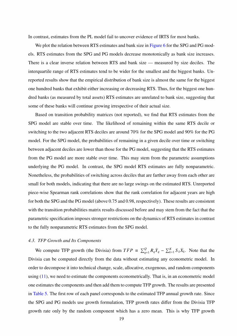
4.3. TFP Growth and Its Components

We compute TFP growth (the Divisia) from ˙T FP ≡∑Q

q=1 RqYq −∑K

k=1 S kXk. Note that the

Divisia can be computed directly from the data without estimating any econometric model. In

order to decompose it into technical change, scale, allocative, exogenous, and random components

using (11), we need to estimate the components econometrically. That is, in an econometric model

one estimates the components and then add them to compute TFP growth. The results are presented

in Table 5. The first row of each panel corresponds to the estimated TFP annual growth rate. Since

the SPG and PG models use growth formulation, TFP growth rates differ from the Divisia TFP

growth rate only by the random component which has a zero mean. This is why TFP growth

19

obtained from adding the components equals the Divisia. This is, however, not the case in the PL

model in which the error term is not the same as the last component of TFP growth in (11).25

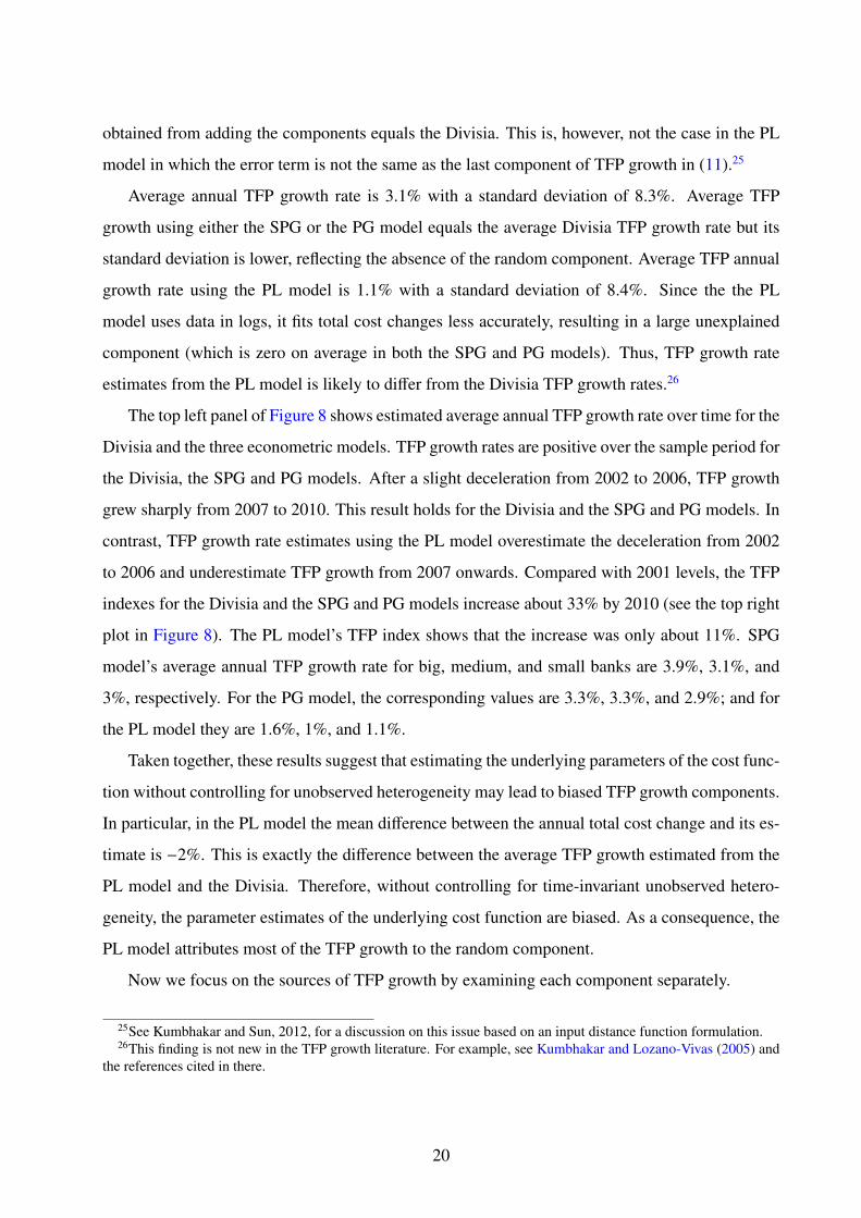
Average annual TFP growth rate is 3.1% with a standard deviation of 8.3%. Average TFP

growth using either the SPG or the PG model equals the average Divisia TFP growth rate but its

standard deviation is lower, reflecting the absence of the random component. Average TFP annual

growth rate using the PL model is 1.1% with a standard deviation of 8.4%. Since the the PL

model uses data in logs, it fits total cost changes less accurately, resulting in a large unexplained

component (which is zero on average in both the SPG and PG models). Thus, TFP growth rate

estimates from the PL model is likely to differ from the Divisia TFP growth rates.26

The top left panel of Figure 8 shows estimated average annual TFP growth rate over time for the

Divisia and the three econometric models. TFP growth rates are positive over the sample period for

the Divisia, the SPG and PG models. After a slight deceleration from 2002 to 2006, TFP growth

grew sharply from 2007 to 2010. This result holds for the Divisia and the SPG and PG models. In

contrast, TFP growth rate estimates using the PL model overestimate the deceleration from 2002

to 2006 and underestimate TFP growth from 2007 onwards. Compared with 2001 levels, the TFP

indexes for the Divisia and the SPG and PG models increase about 33% by 2010 (see the top right

plot in Figure 8). The PL model’s TFP index shows that the increase was only about 11%. SPG

model’s average annual TFP growth rate for big, medium, and small banks are 3.9%, 3.1%, and

3%, respectively. For the PG model, the corresponding values are 3.3%, 3.3%, and 2.9%; and for

the PL model they are 1.6%, 1%, and 1.1%.

Taken together, these results suggest that estimating the underlying parameters of the cost func-

tion without controlling for unobserved heterogeneity may lead to biased TFP growth components.

In particular, in the PL model the mean difference between the annual total cost change and its es-

timate is −2%. This is exactly the difference between the average TFP growth estimated from the

PL model and the Divisia. Therefore, without controlling for time-invariant unobserved hetero-

geneity, the parameter estimates of the underlying cost function are biased. As a consequence, the

PL model attributes most of the TFP growth to the random component.

Now we focus on the sources of TFP growth by examining each component separately.

25See Kumbhakar and Sun, 2012, for a discussion on this issue based on an input distance function formulation.26This finding is not new in the TFP growth literature. For example, see Kumbhakar and Lozano-Vivas (2005) and

the references cited in there.

20

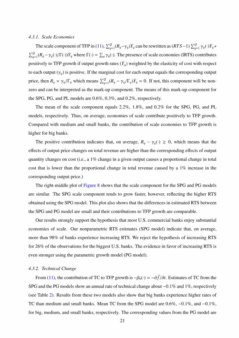
4.3.1. Scale Economies

The scale component of TFP in (11),∑Q

q=1(Rq−γq)Yq can be rewritten as (RTS−1)∑Q

q=1 γq(·)Yq+∑Qq=1(Rq−γq(·)/Γ(·))Yq where Γ(·) =

∑q γq(·). The presence of scale economies (IRTS) contributes

positively to TFP growth if output growth rates (Yq) weighted by the elasticity of cost with respect

to each output (γq) is positive. If the marginal cost for each output equals the corresponding output

price, then Rq = γq/Γq which means∑Q

q=1(Rq − γq/Γq)Yq = 0. If not, this component will be non-

zero and can be interpreted as the mark-up component. The means of this mark-up component for

the SPG, PG, and PL models are 0.6%, 0.3%, and 0.2%, respectively.

The mean of the scale component equals 2.2%, 1.8%, and 0.2% for the SPG, PG, and PL

models, respectively. Thus, on average, economies of scale contribute positively to TFP growth.

Compared with medium and small banks, the contribution of scale economies to TFP growth is

higher for big banks.

The positive contribution indicates that, on average, Rq − γq(·) ≥ 0, which means that the

effects of output price changes on total revenue are higher than the corresponding effects of output

quantity changes on cost (i.e., a 1% change in a given output causes a proportional change in total

cost that is lower than the proportional change in total revenue caused by a 1% increase in the

corresponding output price.)

The right-middle plot of Figure 8 shows that the scale component for the SPG and PG models

are similar. The SPG scale component tends to grow faster, however, reflecting the higher RTS

obtained using the SPG model. This plot also shows that the differences in estimated RTS between

the SPG and PG model are small and their contributions to TFP growth are comparable.

Our results strongly support the hypothesis that most U.S. commercial banks enjoy substantial

economies of scale. Our nonparametric RTS estimates (SPG model) indicate that, on average,

more than 98% of banks experience increasing RTS. We reject the hypothesis of increasing RTS

for 26% of the observations for the biggest U.S. banks. The evidence in favor of increasing RTS is

even stronger using the parametric growth model (PG model).

4.3.2. Technical Change

From (11), the contribution of TC to TFP growth is −β0(·) = −∂ f /∂t. Estimates of TC from the

SPG and the PG models show an annual rate of technical change about −0.1% and 1%, respectively

(see Table 2). Results from these two models also show that big banks experience higher rates of

TC than medium and small banks. Mean TC from the SPG model are 0.6%, −0.1%, and −0.1%,

for big, medium, and small banks, respectively. The corresponding values from the PG model are

21

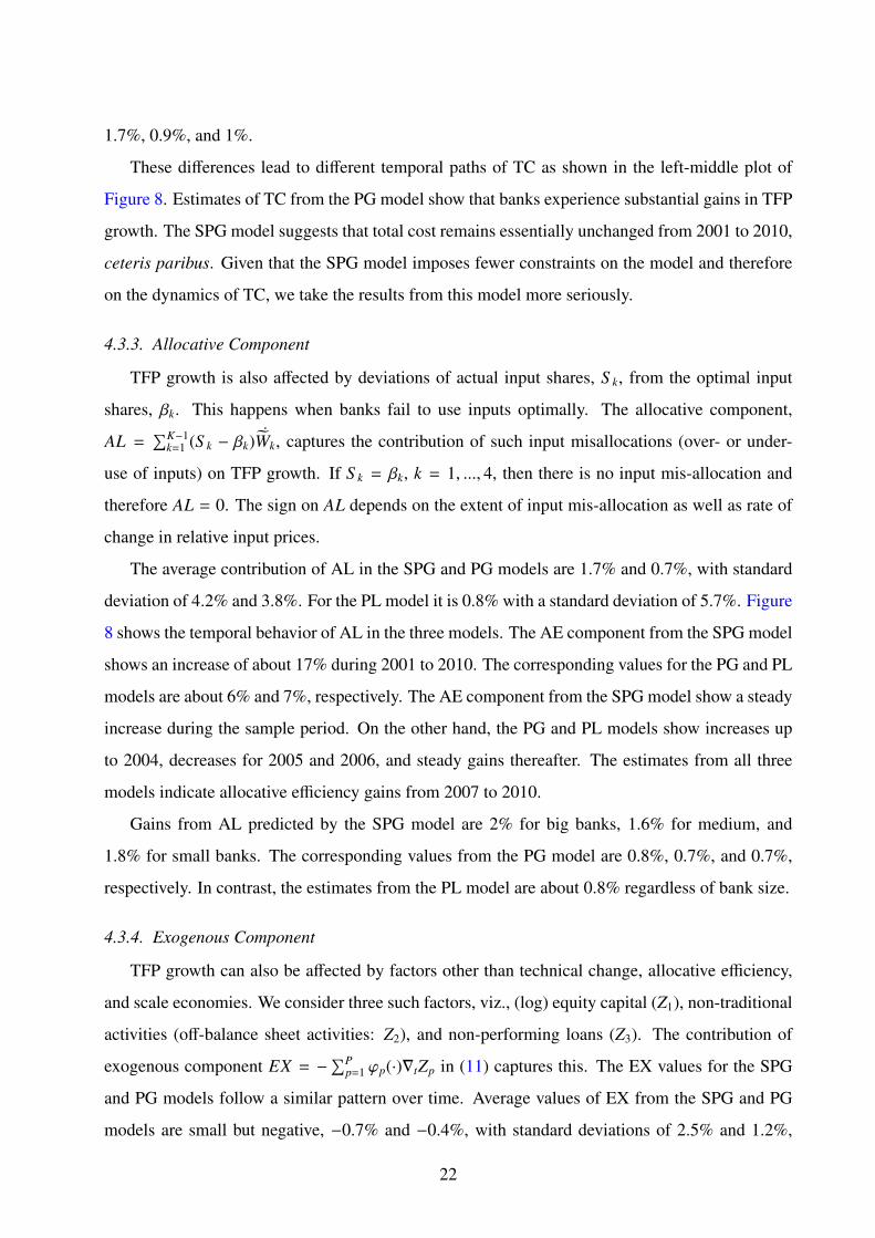
1.7%, 0.9%, and 1%.

These differences lead to different temporal paths of TC as shown in the left-middle plot of

Figure 8. Estimates of TC from the PG model show that banks experience substantial gains in TFP

growth. The SPG model suggests that total cost remains essentially unchanged from 2001 to 2010,

ceteris paribus. Given that the SPG model imposes fewer constraints on the model and therefore

on the dynamics of TC, we take the results from this model more seriously.

4.3.3. Allocative Component

TFP growth is also affected by deviations of actual input shares, S k, from the optimal input

shares, βk. This happens when banks fail to use inputs optimally. The allocative component,

AL =∑K−1

k=1 (S k − βk)˙Wk, captures the contribution of such input misallocations (over- or under-

use of inputs) on TFP growth. If S k = βk, k = 1, ..., 4, then there is no input mis-allocation and

therefore AL = 0. The sign on AL depends on the extent of input mis-allocation as well as rate of

change in relative input prices.

The average contribution of AL in the SPG and PG models are 1.7% and 0.7%, with standard

deviation of 4.2% and 3.8%. For the PL model it is 0.8% with a standard deviation of 5.7%. Figure

8 shows the temporal behavior of AL in the three models. The AE component from the SPG model

shows an increase of about 17% during 2001 to 2010. The corresponding values for the PG and PL

models are about 6% and 7%, respectively. The AE component from the SPG model show a steady

increase during the sample period. On the other hand, the PG and PL models show increases up

to 2004, decreases for 2005 and 2006, and steady gains thereafter. The estimates from all three

models indicate allocative efficiency gains from 2007 to 2010.

Gains from AL predicted by the SPG model are 2% for big banks, 1.6% for medium, and

1.8% for small banks. The corresponding values from the PG model are 0.8%, 0.7%, and 0.7%,

respectively. In contrast, the estimates from the PL model are about 0.8% regardless of bank size.

4.3.4. Exogenous Component

TFP growth can also be affected by factors other than technical change, allocative efficiency,

and scale economies. We consider three such factors, viz., (log) equity capital (Z1), non-traditional

activities (off-balance sheet activities: Z2), and non-performing loans (Z3). The contribution of

exogenous component EX = −∑P

p=1 ϕp(·)∇tZp in (11) captures this. The EX values for the SPG

and PG models follow a similar pattern over time. Average values of EX from the SPG and PG

models are small but negative, −0.7% and −0.4%, with standard deviations of 2.5% and 1.2%,

22

respectively. Thus, these exogenous factors contribute negatively to TFP growth. However, their

effects are small compared with the other components. The last plot in Figure 8 shows that the

cumulative effect of the exogenous factors for the 2001 to 2010 period based on the SPG model is

about −6% and is about −3% predicted by the PG model. On the other hand, the PL model show

that EX component contributed positively to TFP growth.

We now summarize the results of the preceding section on the importance of various compo-

nents of TFP growth. According to the SPG and the PG model, the main contributing component

to TFP growth is the scale component. The second largest component is the allocative component

for the SPG model and the technical change component for the PG model. Finally, the exogenous

component contributes little to TFP growth.

TFP grew about 33% during 2001 to 2010. According to the SPG model TC contributed

negatively by 0.5%, scale economies positively by 21.5%, allocative efficiency by 17.3% and the

exogenous factors contributed negatively by 6% due to component. For the PG model the contri-

butions are: TC 9.5%, scale economies 17.9%, allocative efficiency 7.5%, exogenous factors −4%.

According to the PL model, TFP grew only by 11.6% during 2001 to 2010. The contributions are:

TC −0.5%, scale economies 1.8%, allocative efficiency 9% , and exogenous factors 0.78%.

The trend of TFP growth for big, medium, and small banks is similar. However, big banks

experience sharper swings in TFP growth than medium and small banks. TFP grew steadily for all

banks from 2001 to 2010 with some periods of deceleration. TFP grew 44.6% , 32.2%, and 32.3%

for big, medium, and small banks. During 2008 to 2010, TFP growth for big banks was 1.5 times

faster than the medium and small banks.

5. Comparison with the recent empirical literature

Although our approach differs from previous studies but our results are broadly consistent with

most of the recent literature reviewed in Section 2. We limit our comparison of RTS results to

Wheelock and Wilson (2012) since our model is almost identical to theirs and our RTS measures

are also nonparametric functions of the determinants of banks’ total costs. Thus any differences

between our results and those in Wheelock and Wilson are likely to be driven by the use of differ-

ent estimation methods and sample periods. Our method, however, offers some advantages over

Wheelock and Wilson’s approach that make our evidence more compelling. Our theoretical frame-

work and our econometric model exploit the underlying dynamics of changes in total costs and its

determinants. Thus, our estimation strategy automatically account for cost variation over time for

23

each individual bank. Further, our RTS measures arise naturally within that theoretical framework

and correspond to the most widely accepted definition of RTS used in the literature. In contrast,

Wheelock and Wilson’s approach is theoretically static and their estimation strategy assumes that

observations for a given bank are independent over time. Unlike Wheelock and Wilson’s method,

our approach controls for time-invariant unobserved heterogeneity across banks. In addition, our

econometric model is simpler and easier to estimate than the one used by Wheelock and Wilson.

Contrary to Wheelock and Wilson (2012) who find evidence of IRTS for all banks, our results

suggest that not all U.S. commercial banks enjoy economies of scale. Although most banks exhibit

increasing RTS, some of the biggest banks, specially those among the top one hundred banks,

experience constant or slightly decreasing RTS. These differences in results may stem from the

slightly different model of bank costs that we use. Wheelock and Wilson (2012) assume that

physical capital is a quasi-fixed input. In contrast, we assume that physical capital is a variable

input. Caves, Christensen, and Swanson (1981) derive a measure of RTS to account for the quasi

fixity of inputs. They show that the correct measure of RTS have to be adjusted by the elasticity

of variable costs with respect to quasi-fixed input quantities. When this elasticity is greater (less)

than zero, the shadow price of the quasi-fixed input is greater (less) than its market price, implying

excess capacity with respect the quasi-fixed input (see Morrison 1985 and Morrison and Siegel

1999). With excess capacity, the traditional measures of RTS, which only accounts for variable

inputs, are biased upward. Since Wheelock and Wilson (2012) did not adjust their RTS estimates

to accommodate quasi fixity of physical capital, the more likely explanation is that their RTS

estimates may be biased upward.

Using the PL and PG models, we re-estimate our measure of RTS assuming that physical

capital is quasi-fixed as in Wheelock and Wilson (2012). Based on these (unreported) results,

we find that the elasticity of variable costs with respect to physical capital is positive, indicating

excess capacity with respect physical capital. Therefore, without accounting for quasi-fixity in the

computation of RTS, these estimates will be upwardly biased. We find that without adjusting for

excess capacity, the traditional measure of RTS give estimates that are about 15% higher than our

previous estimates for the PL model and 6.5% for the PG model. However, after adjusting for

the quasi fixity of physical capital, the estimates are almost identical to our previous estimates for

the PL model and about 25% lower for the PG model. Our evidence suggest that Wheelock and

Wilson (2012)’s results are upwardly biased.

Our finding that economies of scale decrease monotonically as bank size increases indicates

24

that economies of scale tend to be exhausted as banks grow. However, the process is slow and the

size level at which economies of scale cease to drive bank grow differ across the biggest banks. In

addition, since economies of scale are unrelated to total assets for the biggest one hundred banks,

total assets may be a poor measure of bank size for these banks.

The differences between our nonparametric and parametric results from the SPG and PG mod-

els indicate that using parametric functional forms for the cost function restricts the dynamics of

RTS estimates. Thus, we favor the use of nonparametric models when possible. Using the PG

model, RTS show little heterogeneity over time. In contrast, the nonparametric RTS estimates,

which are fully flexible, show substantial heterogeneity over time.

Unlike previous studies, our framework allows us to tie the functional coefficients of our models

to TFP growth components, allowing us to investigate the main forces explaining U.S. banking

industry growth. Our results show that increasing returns to scale played an important role in

explaining growth of U.S. banking industry. By comparison, the role of technical change is smaller.

Our results are consistent with the recent evidence presented by Diewert and Fox (2008) for the

U.S. manufacturing industry. In contrast, Feng and Serletis (2010) find that technical change is the

main driver of TFP growth during 2000 to 2005.

6. Policy Implications

Despite the wide range of problems recently addressed by enacted financial regulations in the

U.S., policymakers, regulators, academics, and financial market participants are still pondering the

idea of capping the size of banks, bringing the issue of existence of scale economies to the fore of

the policy debate. If big banks enjoy substantial scale economies, breaking up the biggest banks

or capping their size may impose efficiency losses for the economy. For instance, Wheelock and

Wilson (2012) estimate that the cost of breaking the four largest U.S. bank holding companies in

existence in 2010 would exceed their combined net income in each year from 2003 to 2006. On

the other hand, Boyd and Heitz (2012) estimates that the potential benefits to the society from

economies of scale of big financial institutions are unlikely to ever exceed the potential costs due

to increased risk of financial crisis.

Our results have important implications on this debate. First, contrary to Wheelock and Wilson

(2012), our findings suggest that the cost of breaking up big banks may be lower than their estimate

since not all the biggest banks enjoy economies of scale. Despite the existence of scale economies

for most banks with assets in excess of $1 billion, scale economies seem to be exhausted or may

25

be unrelated to bank size between $5 and $30 billions of assets. Therefore, the potential benefits

of scale economies for big commercial banks may be limited.

Second, our results indicate that scale economies are likely to continue to be the major driver of

growth for small, medium, and some of the biggest banks. We find that scale economies contribute

significantly to TFP growth, giving strong incentives for banks to keep growing. Thus, any attempt

to cap the size of banks will likely encounter strong opposition. Without imposing endogenous

regulatory constraints that increase the marginal cost for banks from getting bigger, the average

size of banks will continue to increase. Higher capital requirements for larger and more system-

atically important banks are likely to be more effective than capping the size of banks. As size

and complexity increase, further regulatory burden and enhanced disclosure requirements for the

biggest banks may serve as an additional deterrent to keep them from getting even bigger.

Third, consolidation of small and medium banks and further growth of some of the biggest

banks pose big challenges to regulators. Future failures will likely involve, on average, a greater

number of bigger and more interconnected banks. As overall bank size increases, the likelihood

of widespread bank failures also increases. Therefore, regulators should widen the focus of their

efforts to cover not only the top bank holding companies but also the increasing number of big

banks. In addition, larger average size of banks means stronger barriers to entry for potential

competitors which can greatly affect concentration, competition, and efficiency.

7. Conclusions

In this paper we focused on estimation of returns to scale, TFP growth and its components

(technical change, scale, exogenous factors) for U.S. commercial banks during 2001 to 2010. The

main innovation of our approach is that we start from a nonparametric cost function and control for

bank-specific fixed effects; a feature absent in previous studies for the U.S. banking industry. The

semiparametric smooth coefficient (SPSC) model we used arises naturally from the underlying

nonparametric cost function upon total differentiation with respect to time. This growth-based

approach allows us to better account for the dynamic evolution of banks’ production technologies

over time.

Another distinctive feature of our approach is that the functional coefficients of the SPSC model

are nonparametric functions of the arguments of the cost function, and are not ad hoc. In our

case, the SPSC model shares the main advantages of a fully nonparametric approach, exploits the

dynamic structure of the data, and gives us fully nonparametric estimates of RTS and TFP growth

26

components.

We also use parametric translog cost specifications with and without fixed bank-effects. This

strategy allows us to compare RTS estimates and TFP growth components across parametric and

nonparametric models.

The main conclusion we drew from the study is that more than 98% of banks still enjoy

economies of scale, and more than 73% of the biggest banks exhibit increasing RTS. We find

that RTS estimates from the semiparametric and parametric growth models decrease monotoni-

cally across bank size deciles: small banks exhibited higher scale economies than medium and

large banks. The relation between mean scale economies estimates and bank size is L-shaped

across bank size deciles; indicating that after certain threshold, increases in bank size reduce scale

economies only slightly. Thus, further increase in average bank size is likely; either through inter-

nally generated growth or through merger and acquisitions.

Our findings also show that failing to control for unobserved heterogeneity across banks is

likely to conceal evidence of increasing RTS. In contrast to the SPSC and parametric growth mod-

els, which control for unobserved heterogeneity across banks, the RTS estimates from the standard

translog model show scant evidence of scale economies. In this case, only small banks exhibit

increasing RTS and most medium and large banks show either constant or decreasing RTS.

Unlike previous studies, we find that the major drivers of TFP growth are scale and allocative

components. Technical change and other exogenous components, like changes in loan quality,

risk, and off-balance sheet activities, affect TFP growth only marginally. This reinforces our main

conclusions that banks still have incentives to continue growing: doing so contributes to TFP

growth positively and significantly.

References

Allen, J., Liu, Y., 2007. Efficiency and economies of scale of large Canadian banks. Canadian Journal of Eco-

nomics/Revue canadienne d’conomique 40 (1), 225–244.

Amel, D., Barnes, C., Panetta, F., Salleo, C., 2004. Consolidation and efficiency in the financial sector: A review of

the international evidence. Journal of Banking & Finance 28 (10), 2493 – 2519.

Bartelsman, E. J., Doms, M., 2000. Understanding Productivity: Lessons from Longitudinal Microdata. Journal of

Economic Literature 38 (3), 569.

Bauer, P., Berger, A., Humphrey, D., 1993. Efficiency and productivity growth in US banking. In: Fried, H., Lovell,

C., S., S. (Eds.), The measurement of productive efficiency: Techniques and applications. Oxford University Press,

New York, pp. 386–413.

27

Berger, A. N., Demsetz, R. S., Strahan, P. E., 1999. The consolidation of the financial services industry: Causes,

consequences, and implications for the future. Journal of Banking &amp; Finance 23 (24), 135 – 194.

Berger, A. N., Hanweck, G. A., Humphrey, D. B., 1987. Competitive viability in banking: Scale, scope, and product

mix economies. Journal of Monetary Economics 20 (3), 501 – 520.

Berger, A. N., Humphrey, D., 1994. Bank Scale Economies, Mergers, Concentration, and Efficiency: The US Experi-

ence. Center for Financial Institutions Working Papers.

Berger, A. N., Mester, L. J., 1997. Inside the Black Box: What Explains Differences in the Efficiencies of Financial

Institutions? Journal of Banking & Finance 21 (7), 895 – 947.

Berger, A. N., Mester, L. J., 2003. Explaining the Dramatic Changes in Performance of US banks: Technological

Change, Deregulation, and Dynamic Changes in Competition. Journal of Financial Intermediation 12 (1), 57 – 95.

Boyd, J., Heitz, A., 2012. The Social Costs and Benefits of Too-Big-To-Fail Banks: A “Bounding” Exercise. Tech.

rep., University of Minnesota.

Caves, D. W., Christensen, L. R., Swanson, J. A., 1981. Productivity Growth, Scale Economies, and Capacity Utiliza-

tion in U.S. Railroads, 1955-74. The American Economic Review 71 (5), pp. 994–1002.

Clark, J. A., 1988. Economies of scale and scope at depository financial institutions: A review of the literature.

Economic Review 73 (8), 17–33.

Clark, J. A., 1996. Economic Cost, Scale Efficiency, and Competitive Viability in Banking. Journal of Money, Credit

and Banking 28 (3), pp. 342–364.

Daniels, K. N., Tirtiroglu, D., 1998. Total Factor Productivity Growth in U.S. Commercial Banking for 1935–

1991: A Latent Variable Approach Using the Kalman Filter. Journal of Financial Services Research 13, 119–135,

10.1023/A:1007922103037.

Das, A., Kumbhakar, S., 2012. Productivity and Efficiency Dynamics in Indian Banking: an Input Distance Function

Approach Incorporating Quality of Inputs and Outputs. Journal of Applied Econometrics.

Denny, M., Fuss, M., Waverman, L., 1979. Productivity Measurement in Regulated industries. Academic Press, Ch.

The measurement and interpretation of total factor productivity in regulated industries, with an application to Cana-

dian telecommunications, pp. 179–212.

Diewert, W. E., Fox, K. J., 2008. On the estimation of returns to scale, technical progress and monopolistic markups.

Journal of Econometrics 145 (12), 174 – 193.

Feng, G., Serletis, A., 2009. Efficiency and productivity of the US banking industry, 1998-2005: evidence from the

Fourier cost function satisfying global regularity conditions. Journal of Applied Econometrics 24 (1), 105–138.

Feng, G., Serletis, A., 2010. Efficiency, technical change, and returns to scale in large US banks: Panel data evidence

from an output distance function satisfying theoretical regularity. Journal of Banking & Finance 34 (1), 127 – 138.

Feng, G., Zhang, X., 2012. Productivity and efficiency at large and community banks in the US: A Bayesian true

random effects stochastic distance frontier analysis. Journal of Banking & Finance Forthcoming (0).

Greene, W., 2005a. Fixed and Random Effects in Stochastic Frontier Models. Journal of Productivity Analysis 23,

7–32, 10.1007/s11123-004-8545-1.

Greene, W., 2005b. Reconsidering heterogeneity in panel data estimators of the stochastic frontier model. Journal of

Econometrics 126 (2), 269 – 303.

Hardle, W., Mammen, E., 1993. Comparing Nonparametric Versus Parametric Regression Fits. The Annals of Statis-

28

tics 21 (4), pp. 1926–1947.

Hayfield, T., Racine, J. S., 2008. Nonparametric Econometrics: The np Package. Journal of Statistical Software 27 (5).

Hughes, J., Mester, L., 1998. Bank capitalization and cost: Evidence of scale economies in risk management and

signaling. Review of Economics and Statistics 80 (2), 314–325.

Hughes, J. P., Lang, W., Mester, L. J., Moon, C.-G., 1996. Efficient Banking under Interstate Branching. Journal of

Money, Credit and Banking 28 (4), pp. 1045–1071.

Hughes, J. P., Lang, W., Mester, L. J., Moon, C.-G., 2000. Recovering Risky Technologies Using the Almost

Ideal Demand System: An Application to U.S. Banking. Journal of Financial Services Research 18, 5–27,

10.1023/A:1026554922476.

Hughes, J. P., Mester, L. J., 2010. Efficiency in Banking: Theory, Practice, and Evidence. In: Berger, A., Molyneux,

P., Wilson, J. (Eds.), The Oxford Handbook of Banking. Oxford University Press, New York, Ch. 19.

Hughes, J. P., Mester, L. J., 2011. Who said large banks don’t experience scale economies? Evidence from a risk-

return-driven cost function. Working Papers 11-27, Federal Reserve Bank of Philadelphia.

Hughes, J. P., Mester, L. J., Moon, C.-G., 2001. Are scale economies in banking elusive or illusive?: Evidence obtained

by incorporating capital structure and risk-taking into models of bank production. Journal of Banking & Finance

25 (12), 2169 – 2208.

Humphrey, D., 1992. Flow versus stock indicators of banking output: effects on productivity and scale economy

measurement. Journal of Financial Services Research 6 (2), 115–135.

Humphrey, D. B., 1991. Productivity in banking and effects from deregulation. Economic Review 1 (Mar), 16–28.

Humphrey, D. B., 1993. Cost and Technical Change: Effects from Bank Deregulation. Journal of Productivity Analysis

4 (1/2), 9 – 34.

Hunter, W. C., Timme, S. G., 1986. Technical Change, Organizational Form, and the Structure of Bank Production.

Journal of Money, Credit and Banking 18 (2), pp. 152–166.

Hunter, W. C., Timme, S. G., 1991. Technological Change in Large U.S. Commercial Banks. The Journal of Business

64 (3), pp. 339–362.

Johnson, S., December 2012. Tarullo Telegraphs Fed’s Plans to Cap Bank Size. Bloomberg News’ Column.

Kumbhakar, S., Lien, G., Flaten, O., Tveterås, R., 2008. Impacts of Norwegian Milk Quotas on Output Growth: A

Modified Distance Function Approach. Journal of Agricultural Economics 59 (2), 350–369.

Kumbhakar, S., Lozano-Vivas, A., 2005. Deregulation and productivity: The case of Spanish banks. Journal of Regu-

latory Economics 27 (3), 331–351.

Kumbhakar, S., Sun, K., 2012. Estimation of TFP growth: a semiparametric smooth coefficient approach. Empirical

Economics Forthcoming, 1–24.

Li, Q., Huang, C. J., Li, D., Fu, T.-T., 2002. Semiparametric Smooth Coefficient Models. Journal of Business &

Economic Statistics 20 (3), pp. 412–422.

Li, Q., Racine, J., 2007. Nonparametric econometrics: Theory and Practice. Princeton University Press.

Li, Q., Racine, J. S., 2010. Smooth Varying-Coefficient Estimation and Inference for Qualitative and Quantitative

Data. Econometric Theory 26 (06), 1607–1637.

Mester, L. J., 1994. How efficient are third district banks? Business Review 1994, 1–3.

Mester, L. J., 1996. A study of bank efficiency taking into account risk-preferences. Journal of Banking & Finance

29

20 (6), 1025 – 1045.

Mester, L. J., 1997. Measuring efficiency at U.S. banks: Accounting for heterogeneity is important. European Journal

of Operational Research 98 (2), 230 – 242.

Morrison, C. J., 1985. Primal and Dual Capacity Utilization: An Application to Productivity Measurement in the U.S.

Automobile Industry. Journal of Business & Economic Statistics 3 (4), pp. 312–324.

Morrison, C. J., Siegel, D. S., 1999. Scale Economies and Industry Agglomeration Externalities: A Dynamic Cost

Function Approach. The American Economic Review 89 (1), pp. 272–290.

Mukherjee, K., Ray, S. C., Miller, S. M., 2001. Productivity growth in large US commercial banks: The initial post-

deregulation experience. Journal of Banking & Finance 25 (5), 913 – 939.

Restrepo, D., Kumbhakar, S., 2011. Measuring Profit Efficiency without Estimating a Profit Function: The case of

U.S. Commercial Banks. Working Paper. Binghamton University.

Robinson, P., 1988. Root-N-consistent Semiparametric Regression. Econometrica: Journal of the Econometric Soci-

ety, 931–954.

Rogers, K., 1998. Nontraditional Activities and The Efficiency of US Commercial Banks. Journal of Banking &

Finance 22 (4), 467–482.

Semenick Alam, I. M., 2001. A Nonparametric Approach for Assessing Productivity Dynamics of Large U.S. Banks.

Journal of Money, Credit and Banking 33 (1), pp. 121–139.

Shaffer, S., 1994. A revenue-restricted cost study of 100 large banks. Applied Financial Economics 4 (3), 193–205.

Stern, G., Feldman, R., 2009. Addressing TBTF by shrinking financial institutions: An initial assessment. Federal

Reserve Bank of Minneapolis: The Region, June, 8–13.

Stiroh, K. J., 2000. How Did Bank Holding Companies Prosper in the 1990s? Journal of Banking & Finance 24 (11),

1703 – 1745.

Syverson, C., 2011. What Determines Productivity?. Journal of Economic Literature 49 (2), 326 – 365.

Tirtiroglu, D., Daniels, K. N., Tirtirogu, E., 2005. Deregulation, Intensity of Competition, Industry Evolution, and the

Productivity Growth of U.S. Commercial Banks. Journal of Money, Credit and Banking 37 (2), pp. 339–360.

Wang, H.-J., Ho, C.-W., 2010. Estimating fixed-effect panel stochastic frontier models by model transformation. Jour-

nal of Econometrics 157 (2), 286–296.

Wheelock, D. C., Wilson, P. W., 1999. Technical Progress, Inefficiency, and Productivity Change in U.S. Banking,

1984-1993. Journal of Money, Credit and Banking 31 (2), pp. 212–234.

Wheelock, D. C., Wilson, P. W., 2001. New evidence on returns to scale and product mix among U.S. commercial

banks. Journal of Monetary Economics 47 (3), 653 – 674.

Wheelock, D. C., Wilson, P. W., 2011. Are credit unions too small? Review of Economics and Statistics 93 (4),

1343–1359.

Wheelock, D. C., Wilson, P. W., 2012. Do Large Banks Have Lower Costs? New Estimates of Returns to Scale for

U.S. Banks. Journal of Money, Credit and Banking 44 (1), 171 – 199.

30

Tables and Figures

31

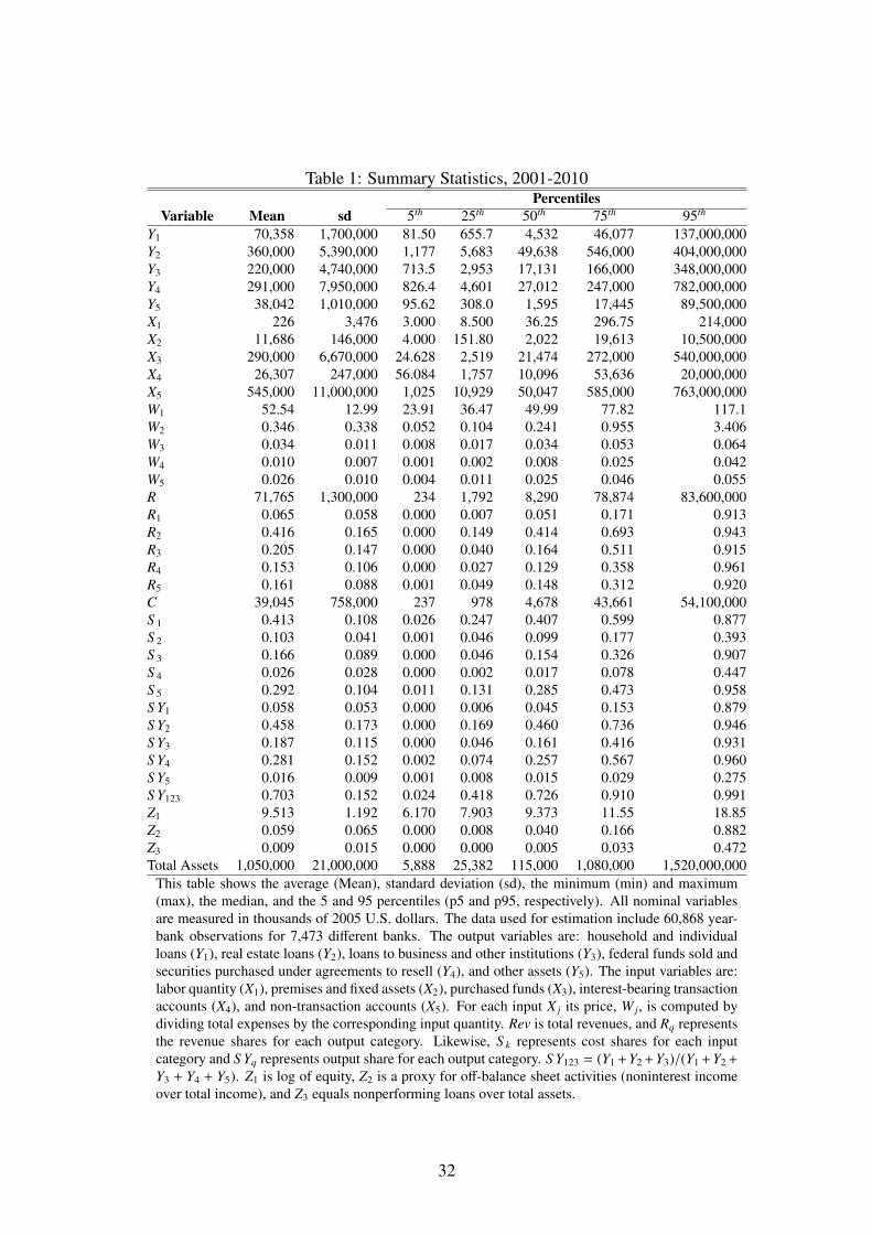
Table 1: Summary Statistics, 2001-2010Percentiles

Variable Mean sd 5th 25th 50th 75th 95th

Y1 70,358 1,700,000 81.50 655.7 4,532 46,077 137,000,000Y2 360,000 5,390,000 1,177 5,683 49,638 546,000 404,000,000Y3 220,000 4,740,000 713.5 2,953 17,131 166,000 348,000,000Y4 291,000 7,950,000 826.4 4,601 27,012 247,000 782,000,000Y5 38,042 1,010,000 95.62 308.0 1,595 17,445 89,500,000X1 226 3,476 3.000 8.500 36.25 296.75 214,000X2 11,686 146,000 4.000 151.80 2,022 19,613 10,500,000X3 290,000 6,670,000 24.628 2,519 21,474 272,000 540,000,000X4 26,307 247,000 56.084 1,757 10,096 53,636 20,000,000X5 545,000 11,000,000 1,025 10,929 50,047 585,000 763,000,000W1 52.54 12.99 23.91 36.47 49.99 77.82 117.1W2 0.346 0.338 0.052 0.104 0.241 0.955 3.406W3 0.034 0.011 0.008 0.017 0.034 0.053 0.064W4 0.010 0.007 0.001 0.002 0.008 0.025 0.042W5 0.026 0.010 0.004 0.011 0.025 0.046 0.055R 71,765 1,300,000 234 1,792 8,290 78,874 83,600,000R1 0.065 0.058 0.000 0.007 0.051 0.171 0.913R2 0.416 0.165 0.000 0.149 0.414 0.693 0.943R3 0.205 0.147 0.000 0.040 0.164 0.511 0.915R4 0.153 0.106 0.000 0.027 0.129 0.358 0.961R5 0.161 0.088 0.001 0.049 0.148 0.312 0.920C 39,045 758,000 237 978 4,678 43,661 54,100,000S 1 0.413 0.108 0.026 0.247 0.407 0.599 0.877S 2 0.103 0.041 0.001 0.046 0.099 0.177 0.393S 3 0.166 0.089 0.000 0.046 0.154 0.326 0.907S 4 0.026 0.028 0.000 0.002 0.017 0.078 0.447S 5 0.292 0.104 0.011 0.131 0.285 0.473 0.958S Y1 0.058 0.053 0.000 0.006 0.045 0.153 0.879S Y2 0.458 0.173 0.000 0.169 0.460 0.736 0.946S Y3 0.187 0.115 0.000 0.046 0.161 0.416 0.931S Y4 0.281 0.152 0.002 0.074 0.257 0.567 0.960S Y5 0.016 0.009 0.001 0.008 0.015 0.029 0.275S Y123 0.703 0.152 0.024 0.418 0.726 0.910 0.991Z1 9.513 1.192 6.170 7.903 9.373 11.55 18.85Z2 0.059 0.065 0.000 0.008 0.040 0.166 0.882Z3 0.009 0.015 0.000 0.000 0.005 0.033 0.472Total Assets 1,050,000 21,000,000 5,888 25,382 115,000 1,080,000 1,520,000,000

This table shows the average (Mean), standard deviation (sd), the minimum (min) and maximum(max), the median, and the 5 and 95 percentiles (p5 and p95, respectively). All nominal variablesare measured in thousands of 2005 U.S. dollars. The data used for estimation include 60,868 year-bank observations for 7,473 different banks. The output variables are: household and individualloans (Y1), real estate loans (Y2), loans to business and other institutions (Y3), federal funds sold andsecurities purchased under agreements to resell (Y4), and other assets (Y5). The input variables are:labor quantity (X1), premises and fixed assets (X2), purchased funds (X3), interest-bearing transactionaccounts (X4), and non-transaction accounts (X5). For each input X j its price, W j, is computed bydividing total expenses by the corresponding input quantity. Rev is total revenues, and Rq representsthe revenue shares for each output category. Likewise, S k represents cost shares for each inputcategory and S Yq represents output share for each output category. S Y123 = (Y1 +Y2 +Y3)/(Y1 +Y2 +

Y3 + Y4 + Y5). Z1 is log of equity, Z2 is a proxy for off-balance sheet activities (noninterest incomeover total income), and Z3 equals nonperforming loans over total assets.

32

Table 2: Estimated Functional CoefficientsPercentiles

Parameter Mean sd 5th 25th 50th 75th 95th

Panel A: SPG Model (R2 = .978)β0 0.001 0.018 -0.022 -0.007 0.000 0.008 0.025β1 0.456 0.087 0.343 0.402 0.449 0.504 0.594β2 0.044 0.048 -0.004 0.025 0.039 0.057 0.106β3 0.164 0.074 0.066 0.118 0.158 0.203 0.288β4 0.023 0.021 -0.002 0.015 0.023 0.032 0.050γ1 0.059 0.043 -0.003 0.039 0.060 0.080 0.114γ2 0.347 0.121 0.163 0.270 0.346 0.418 0.543γ3 0.124 0.062 0.041 0.085 0.118 0.155 0.225γ4 0.135 0.059 0.052 0.100 0.132 0.166 0.229γ5 0.047 0.040 -0.006 0.029 0.046 0.064 0.102ϕ1 0.075 0.086 -0.048 0.033 0.076 0.119 0.193ϕ2 0.202 0.256 -0.106 0.077 0.174 0.296 0.615ϕ3 0.046 1.414 -1.040 -0.226 0.071 0.351 1.155

Panel B: PG Model (R2 = .916)β0 -0.010 0.007 -0.021 -0.014 -0.009 -0.005 0.000β1 0.465 0.069 0.360 0.417 0.461 0.509 0.586β2 0.036 0.014 0.015 0.026 0.035 0.044 0.058β3 0.176 0.050 0.094 0.144 0.175 0.207 0.257β4 0.026 0.010 0.009 0.019 0.026 0.032 0.041γ1 0.053 0.015 0.027 0.045 0.054 0.063 0.076γ2 0.342 0.123 0.122 0.264 0.352 0.428 0.524γ3 0.130 0.046 0.052 0.101 0.131 0.160 0.202γ4 0.154 0.054 0.067 0.120 0.153 0.188 0.243γ5 0.044 0.011 0.026 0.037 0.044 0.051 0.061ϕ1 0.062 0.031 0.012 0.041 0.061 0.082 0.114ϕ2 0.143 0.126 -0.041 0.054 0.131 0.218 0.371ϕ3 0.057 0.147 -0.178 -0.021 0.064 0.148 0.271

Panel C: PL Model (R2 = .8474)β0 0.000 0.005 -0.007 -0.003 0.000 0.004 0.009β1 0.392 0.094 0.251 0.325 0.384 0.450 0.561β2 0.021 0.040 -0.050 -0.003 0.023 0.046 0.082β3 0.312 0.091 0.163 0.256 0.313 0.368 0.460β4 0.024 0.020 -0.010 0.012 0.025 0.038 0.056γ1 0.103 0.047 0.020 0.075 0.107 0.134 0.174γ2 0.471 0.153 0.211 0.375 0.476 0.574 0.712γ3 0.149 0.076 0.024 0.100 0.150 0.199 0.271γ4 0.228 0.106 0.058 0.162 0.227 0.296 0.401γ5 0.043 0.029 -0.002 0.024 0.042 0.060 0.089ϕ1 -0.040 0.035 -0.101 -0.061 -0.038 -0.017 0.012ϕ2 1.227 0.290 0.785 1.057 1.219 1.396 1.709ϕ3 1.430 0.666 0.400 1.005 1.445 1.910 2.415

The data used for estimation include 60,868 year-bank observations for 7,473 different banks from 2001 to 2010.SPG model, PG model, and PL model correspond to the estimation of the functional coefficients in equation (5) usingthe semiparametric smooth coefficient model (SPSCM), a parametric translog growth model, and the parametrictranslog model in levels, respectively.

33

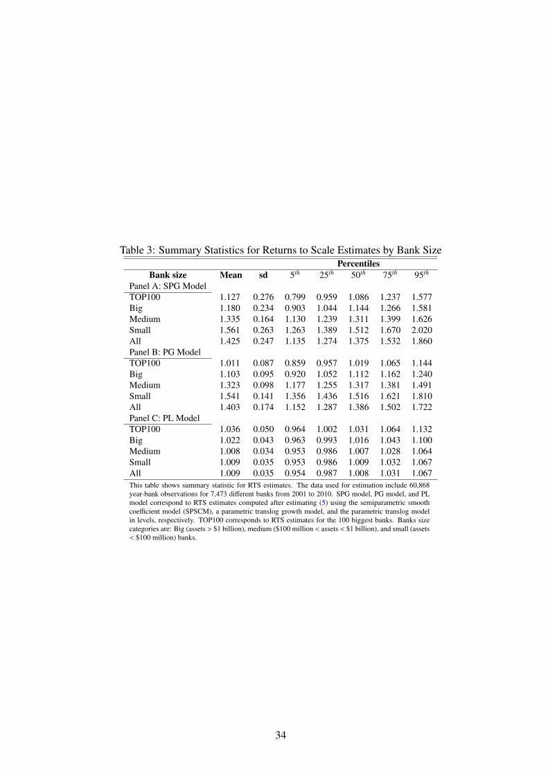
Table 3: Summary Statistics for Returns to Scale Estimates by Bank SizePercentiles

Bank size Mean sd 5th 25th 50th 75th 95th

Panel A: SPG ModelTOP100 1.127 0.276 0.799 0.959 1.086 1.237 1.577Big 1.180 0.234 0.903 1.044 1.144 1.266 1.581Medium 1.335 0.164 1.130 1.239 1.311 1.399 1.626Small 1.561 0.263 1.263 1.389 1.512 1.670 2.020All 1.425 0.247 1.135 1.274 1.375 1.532 1.860Panel B: PG ModelTOP100 1.011 0.087 0.859 0.957 1.019 1.065 1.144Big 1.103 0.095 0.920 1.052 1.112 1.162 1.240Medium 1.323 0.098 1.177 1.255 1.317 1.381 1.491Small 1.541 0.141 1.356 1.436 1.516 1.621 1.810All 1.403 0.174 1.152 1.287 1.386 1.502 1.722Panel C: PL ModelTOP100 1.036 0.050 0.964 1.002 1.031 1.064 1.132Big 1.022 0.043 0.963 0.993 1.016 1.043 1.100Medium 1.008 0.034 0.953 0.986 1.007 1.028 1.064Small 1.009 0.035 0.953 0.986 1.009 1.032 1.067All 1.009 0.035 0.954 0.987 1.008 1.031 1.067This table shows summary statistic for RTS estimates. The data used for estimation include 60,868year-bank observations for 7,473 different banks from 2001 to 2010. SPG model, PG model, and PLmodel correspond to RTS estimates computed after estimating (5) using the semiparametric smoothcoefficient model (SPSCM), a parametric translog growth model, and the parametric translog modelin levels, respectively. TOP100 corresponds to RTS estimates for the 100 biggest banks. Banks sizecategories are: Big (assets > $1 billion), medium ($100 million < assets < $1 billion), and small (assets< $100 million) banks.

34

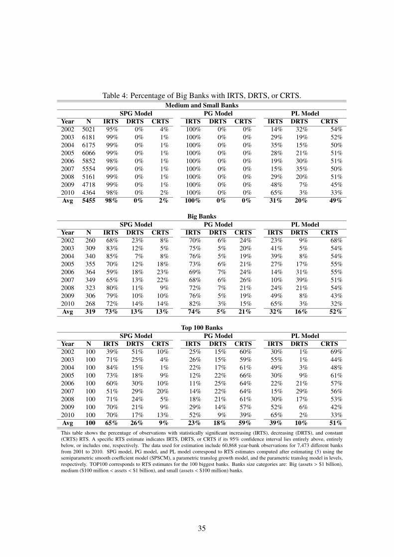
Table 4: Percentage of Big Banks with IRTS, DRTS, or CRTS.Medium and Small Banks

SPG Model PG Model PL ModelYear N IRTS DRTS CRTS IRTS DRTS CRTS IRTS DRTS CRTS2002 5021 95% 0% 4% 100% 0% 0% 14% 32% 54%2003 6181 99% 0% 1% 100% 0% 0% 29% 19% 52%2004 6175 99% 0% 1% 100% 0% 0% 35% 15% 50%2005 6066 99% 0% 1% 100% 0% 0% 28% 21% 51%2006 5852 98% 0% 1% 100% 0% 0% 19% 30% 51%2007 5554 99% 0% 1% 100% 0% 0% 15% 35% 50%2008 5161 99% 0% 1% 100% 0% 0% 29% 20% 51%2009 4718 99% 0% 1% 100% 0% 0% 48% 7% 45%2010 4364 98% 0% 2% 100% 0% 0% 65% 3% 33%Avg 5455 98% 0% 2% 100% 0% 0% 31% 20% 49%

Big BanksSPG Model PG Model PL Model

Year N IRTS DRTS CRTS IRTS DRTS CRTS IRTS DRTS CRTS2002 260 68% 23% 8% 70% 6% 24% 23% 9% 68%2003 309 83% 12% 5% 75% 5% 20% 41% 5% 54%2004 340 85% 7% 8% 76% 5% 19% 39% 8% 54%2005 355 70% 12% 18% 73% 6% 21% 27% 17% 55%2006 364 59% 18% 23% 69% 7% 24% 14% 31% 55%2007 349 65% 13% 22% 68% 6% 26% 10% 39% 51%2008 323 80% 11% 9% 72% 7% 21% 24% 21% 54%2009 306 79% 10% 10% 76% 5% 19% 49% 8% 43%2010 268 72% 14% 14% 82% 3% 15% 65% 3% 32%Avg 319 73% 13% 13% 74% 5% 21% 32% 16% 52%

Top 100 BanksSPG Model PG Model PL Model

Year N IRTS DRTS CRTS IRTS DRTS CRTS IRTS DRTS CRTS2002 100 39% 51% 10% 25% 15% 60% 30% 1% 69%2003 100 71% 25% 4% 26% 15% 59% 55% 1% 44%2004 100 84% 15% 1% 22% 17% 61% 49% 3% 48%2005 100 73% 18% 9% 12% 22% 66% 30% 9% 61%2006 100 60% 30% 10% 11% 25% 64% 22% 21% 57%2007 100 51% 29% 20% 14% 22% 64% 15% 29% 56%2008 100 71% 24% 5% 18% 21% 61% 30% 17% 53%2009 100 70% 21% 9% 29% 14% 57% 52% 6% 42%2010 100 70% 17% 13% 52% 9% 39% 65% 2% 33%Avg 100 65% 26% 9% 23% 18% 59% 39% 10% 51%This table shows the percentage of observations with statistically significant increasing (IRTS), decreasing (DRTS), and constant(CRTS) RTS. A specific RTS estimate indicates IRTS, DRTS, or CRTS if its 95% confidence interval lies entirely above, entirelybelow, or includes one, respectively. The data used for estimation include 60,868 year-bank observations for 7,473 different banksfrom 2001 to 2010. SPG model, PG model, and PL model correspond to RTS estimates computed after estimating (5) using thesemiparametric smooth coefficient model (SPSCM), a parametric translog growth model, and the parametric translog model in levels,respectively. TOP100 corresponds to RTS estimates for the 100 biggest banks. Banks size categories are: Big (assets > $1 billion),medium ($100 million < assets < $1 billion), and small (assets < $100 million) banks.

35

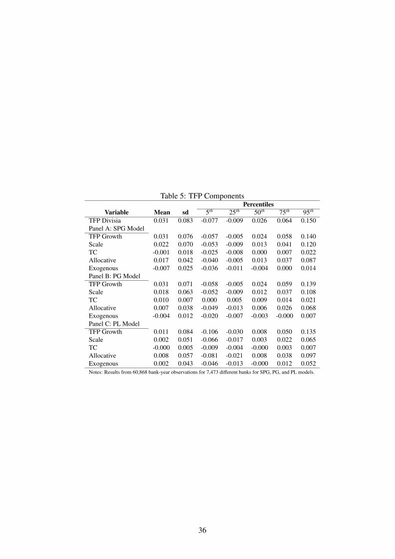
Table 5: TFP ComponentsPercentiles

Variable Mean sd 5th 25th 50th 75th 95th

TFP Divisia 0.031 0.083 -0.077 -0.009 0.026 0.064 0.150Panel A: SPG ModelTFP Growth 0.031 0.076 -0.057 -0.005 0.024 0.058 0.140Scale 0.022 0.070 -0.053 -0.009 0.013 0.041 0.120TC -0.001 0.018 -0.025 -0.008 0.000 0.007 0.022Allocative 0.017 0.042 -0.040 -0.005 0.013 0.037 0.087Exogenous -0.007 0.025 -0.036 -0.011 -0.004 0.000 0.014Panel B: PG ModelTFP Growth 0.031 0.071 -0.058 -0.005 0.024 0.059 0.139Scale 0.018 0.063 -0.052 -0.009 0.012 0.037 0.108TC 0.010 0.007 0.000 0.005 0.009 0.014 0.021Allocative 0.007 0.038 -0.049 -0.013 0.006 0.026 0.068Exogenous -0.004 0.012 -0.020 -0.007 -0.003 -0.000 0.007Panel C: PL ModelTFP Growth 0.011 0.084 -0.106 -0.030 0.008 0.050 0.135Scale 0.002 0.051 -0.066 -0.017 0.003 0.022 0.065TC -0.000 0.005 -0.009 -0.004 -0.000 0.003 0.007Allocative 0.008 0.057 -0.081 -0.021 0.008 0.038 0.097Exogenous 0.002 0.043 -0.046 -0.013 -0.000 0.012 0.052Notes: Results from 60,868 bank-year observations for 7,473 different banks for SPG, PG, and PL models.

36

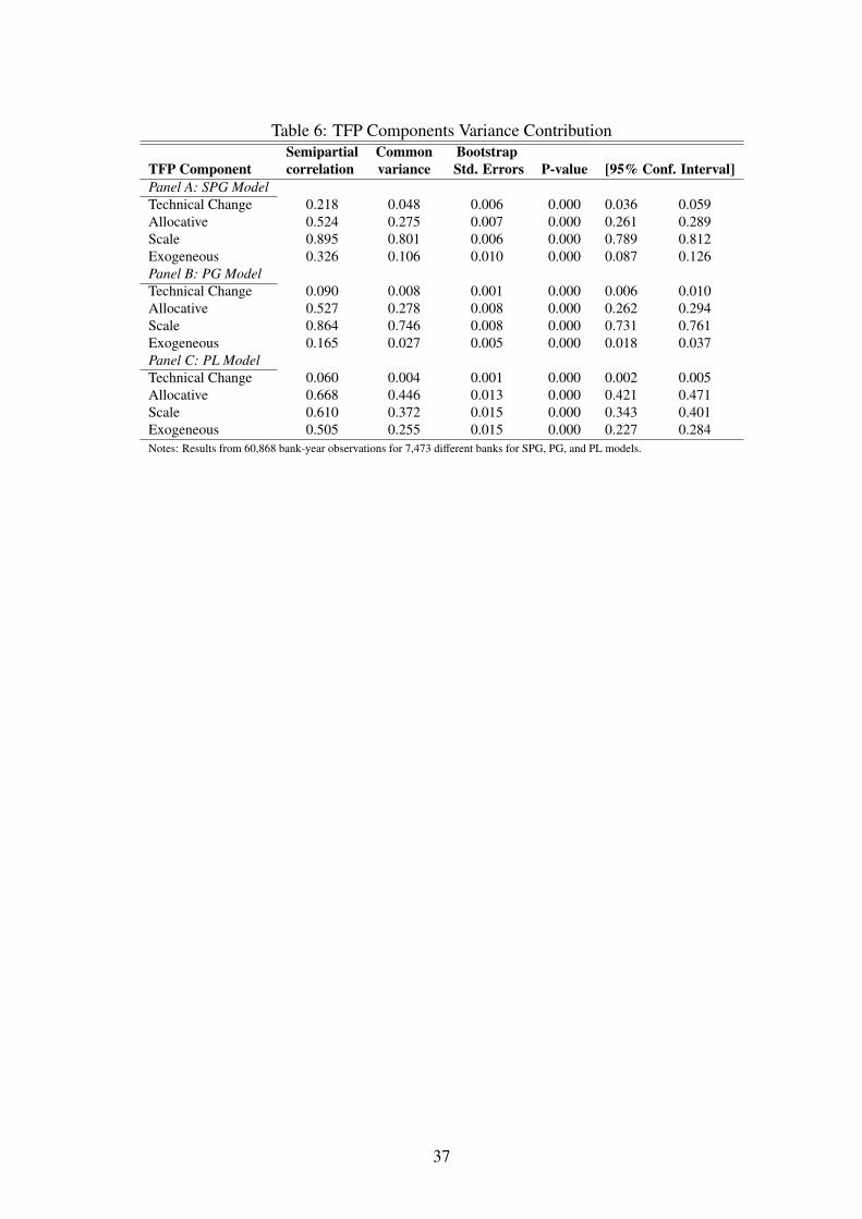
Table 6: TFP Components Variance ContributionSemipartial Common Bootstrap

TFP Component correlation variance Std. Errors P-value [95% Conf. Interval]Panel A: SPG ModelTechnical Change 0.218 0.048 0.006 0.000 0.036 0.059Allocative 0.524 0.275 0.007 0.000 0.261 0.289Scale 0.895 0.801 0.006 0.000 0.789 0.812Exogeneous 0.326 0.106 0.010 0.000 0.087 0.126Panel B: PG ModelTechnical Change 0.090 0.008 0.001 0.000 0.006 0.010Allocative 0.527 0.278 0.008 0.000 0.262 0.294Scale 0.864 0.746 0.008 0.000 0.731 0.761Exogeneous 0.165 0.027 0.005 0.000 0.018 0.037Panel C: PL ModelTechnical Change 0.060 0.004 0.001 0.000 0.002 0.005Allocative 0.668 0.446 0.013 0.000 0.421 0.471Scale 0.610 0.372 0.015 0.000 0.343 0.401Exogeneous 0.505 0.255 0.015 0.000 0.227 0.284Notes: Results from 60,868 bank-year observations for 7,473 different banks for SPG, PG, and PL models.

37

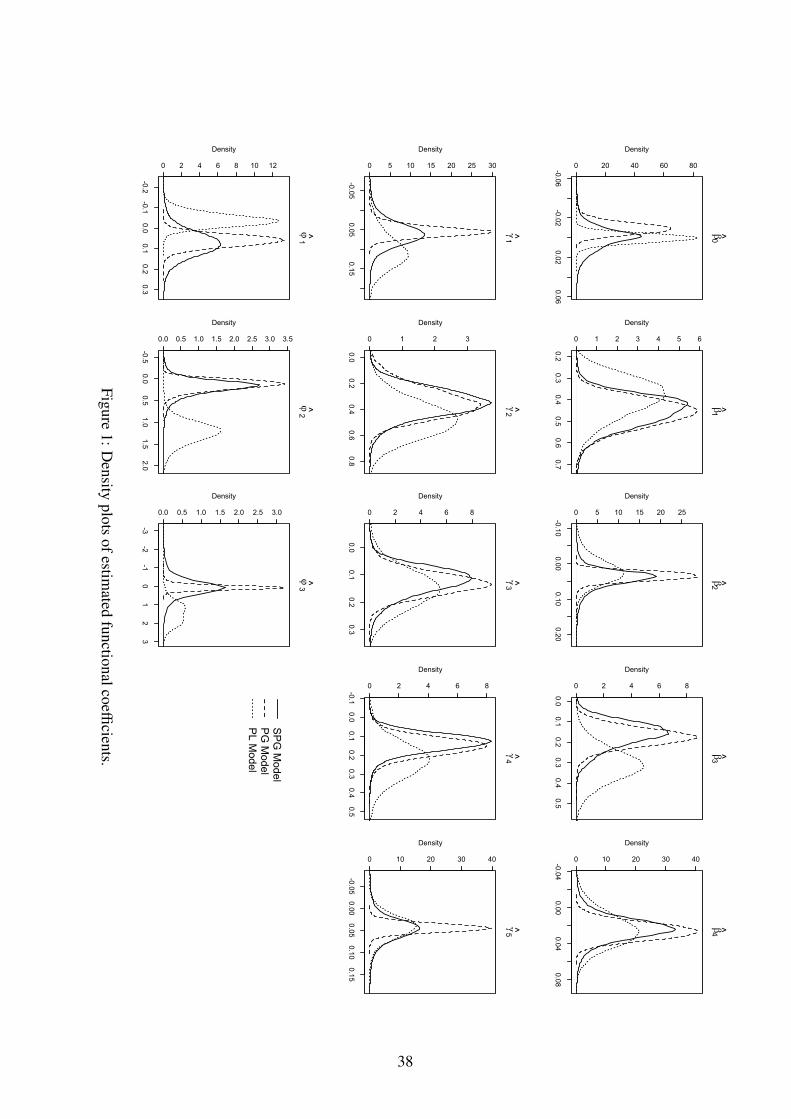
-0.06-0.02

0.020.06

0 20 40 60 80

β0

Density

0.20.3

0.40.5

0.60.7

0 1 2 3 4 5 6

β1

Density

-0.100.00

0.100.20

0 5 10 15 20 25

β2

Density

0.00.1

0.20.3

0.40.5

0 2 4 6 8

β3

Density

-0.040.00

0.040.08

0 10 20 30 40

β4

Density

-0.050.05

0.15

0 5 10 15 20 25 30

γ1

Density

0.00.2

0.40.6

0.8

0 1 2 3

γ2

Density

0.00.1

0.20.3

0 2 4 6 8

γ3

Density

-0.10.0

0.10.2

0.30.4

0.5

0 2 4 6 8

γ4

Density

-0.050.00

0.050.10

0.15

0 10 20 30 40

γ5

Density

-0.2-0.1

0.00.1

0.20.3

0 2 4 6 8 10 12

φ1

Density

-0.50.0

0.51.0

1.52.0

0.0 0.5 1.0 1.5 2.0 2.5 3.0 3.5

φ2

Density

-3-2

-10

12

3

0.0 0.5 1.0 1.5 2.0 2.5 3.0

φ3

Density

SP

G M

odelP

G M

odelP

L Model

Figure1:D

ensityplots

ofestimated

functionalcoefficients.

38

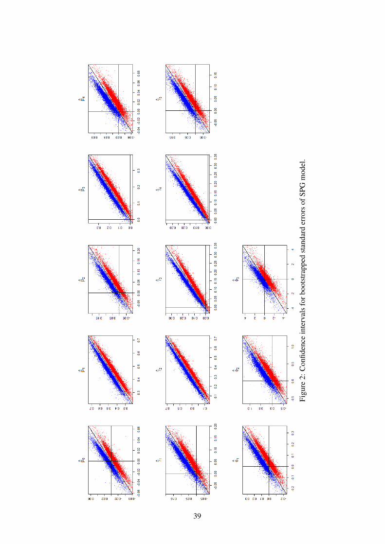
Figu

re2:

Con

fiden

cein

terv

als

forb

oots

trap

ped

stan

dard

erro

rsof

SPG

mod

el.

39

1.0 1.5 2.0 2.5

02

46

810

12

RTS

Den

sity

SPG ModelPG ModelPL Model

Figure 3: Density plots for RTS estimates for all banks.

1.0 1.5 2.0 2.5 3.0

01

23

4

2002

SPG ModelPG Model

1.0 1.5 2.0 2.5 3.0

01

23

4

2003

SPG ModelPG Model

1.0 1.5 2.0 2.5 3.0

01

23

4

2004

SPG ModelPG Model

1.0 1.5 2.0 2.5 3.0

01

23

4

2005

SPG ModelPG Model

1.0 1.5 2.0 2.5 3.0

01

23

4

2006

SPG ModelPG Model

1.0 1.5 2.0 2.5 3.0

01

23

4

2007

SPG ModelPG Model

1.0 1.5 2.0 2.5 3.0

01

23

4

2008

SPG ModelPG Model

1.0 1.5 2.0 2.5 3.0

01

23

4

2009

SPG ModelPG Model

1.0 1.5 2.0 2.5 3.0

01

23

4

2010

SPG ModelPG Model

Figure 4: RTS estimates over time.

40

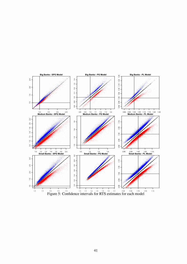
1.0 1.5 2.0 2.5

1.0

1.5

2.0

2.5

Big Banks - SPG Model

0.8 0.9 1.0 1.1 1.2 1.3 1.4

0.8

0.9

1.0

1.1

1.2

1.3

1.4

Big Banks - PG Model

0.90 0.95 1.00 1.05 1.10 1.15 1.20 1.25

0.90

0.95

1.00

1.05

1.10

1.15

1.20

1.25

Big Banks - PL Model

1.0 1.2 1.4 1.6 1.8 2.0 2.2

1.0

1.2

1.4

1.6

1.8

2.0

2.2

Medium Banks - SPG Model

1.0 1.2 1.4 1.6

1.0

1.2

1.4

1.6

Medium Banks - PG Model

0.90 0.95 1.00 1.05 1.10

0.90

0.95

1.00

1.05

1.10

Medium Banks - PL Model

1.0 1.5 2.0 2.5 3.0

1.0

1.5

2.0

2.5

3.0

Small Banks - SPG Model

1.0 1.2 1.4 1.6 1.8 2.0 2.2

1.0

1.2

1.4

1.6

1.8

2.0

2.2

Small Banks - PG Model

0.90 0.95 1.00 1.05 1.10

0.90

0.95

1.00

1.05

1.10

Small Banks - PL Model

Figure 5: Confidence intervals for RTS estimates for each model

41

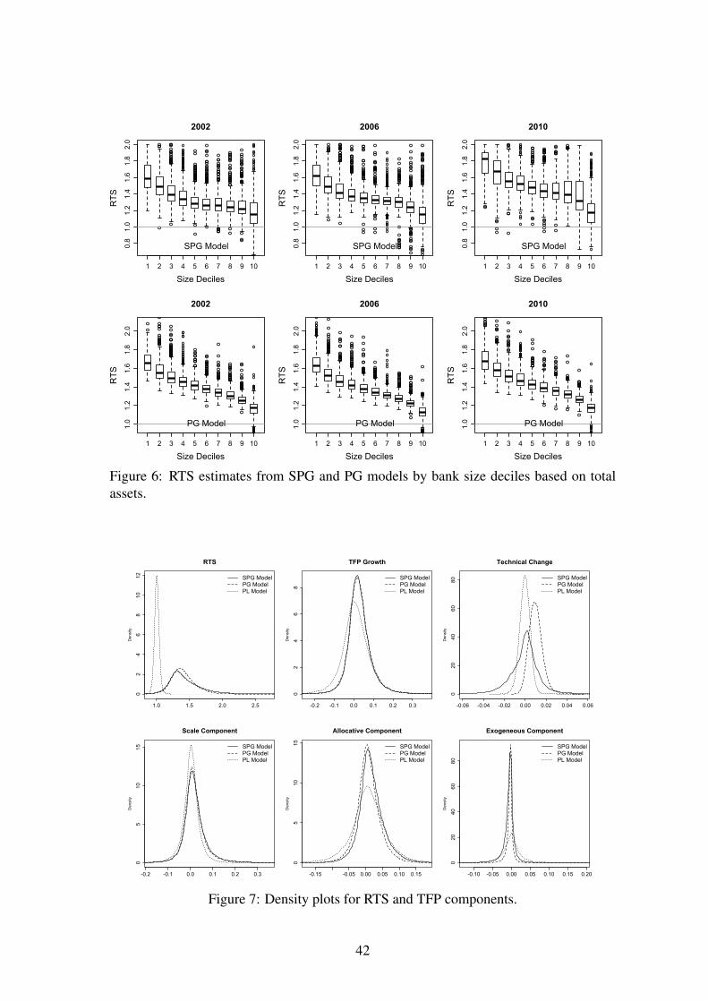
1 2 3 4 5 6 7 8 9 10

0.8

1.0

1.2

1.4

1.6

1.8

2.0

2002

Size Deciles

RT

S

SPG Model

1 2 3 4 5 6 7 8 9 10

0.8

1.0

1.2

1.4

1.6

1.8

2.0

2006

Size DecilesR

TS

SPG Model

1 2 3 4 5 6 7 8 9 10

0.8

1.0

1.2

1.4

1.6

1.8

2.0

2010

Size Deciles

RT

S

SPG Model

1 2 3 4 5 6 7 8 9 10

1.0

1.2

1.4

1.6

1.8

2.0

2002

Size Deciles

RT

S

PG Model

1 2 3 4 5 6 7 8 9 10

1.0

1.2

1.4

1.6

1.8

2.0

2006

Size Deciles

RT

S

PG Model

1 2 3 4 5 6 7 8 9 10

1.0

1.2

1.4

1.6

1.8

2.0

2010

Size DecilesR

TS

PG Model

Figure 6: RTS estimates from SPG and PG models by bank size deciles based on totalassets.

1.0 1.5 2.0 2.5

02

46

810

12

RTS

Den

sity

SPG ModelPG ModelPL Model

-0.2 -0.1 0.0 0.1 0.2 0.3

02

46

8

TFP Growth

Den

sity

SPG ModelPG ModelPL Model

-0.06 -0.04 -0.02 0.00 0.02 0.04 0.06

020

4060

80

Technical Change

Den

sity

SPG ModelPG ModelPL Model

-0.2 -0.1 0.0 0.1 0.2 0.3

05

1015

Scale Component

Den

sity

SPG ModelPG ModelPL Model

-0.15 -0.05 0.00 0.05 0.10 0.15

05

1015

Allocative Component

Den

sity

SPG ModelPG ModelPL Model

-0.10 -0.05 0.00 0.05 0.10 0.15 0.20

020

4060

80

Exogeneous Component

Den

sity

SPG ModelPG ModelPL Model

Figure 7: Density plots for RTS and TFP components.

42

2002 2004 2006 2008 2010

-0.0

50.

000.

050.

10

Year

TF

P G

row

th

Total Factor Productivity Growth

DivisiaSPG ModelPG ModelPL Model

2002 2004 2006 2008 2010

100

110

120

130

140

Year

TF

P In

dex

Total Factor Productivity Index

DivisiaSPG ModelPG ModelPL Model

2002 2004 2006 2008 2010

100

105

110

115

Year

Tec

hnic

al C

hang

e In

dex

Technical Change Index

SPG ModelPG ModelPL Model

2002 2004 2006 2008 2010

100

105

110

115

120

125

130

Year

Sca

le In

dex

Scale Index

SPG ModelPG ModelPL Model

2002 2004 2006 2008 2010

100

105

110

115

120

125

130

Year

Allo

cativ

e C

ompo

nent

Inde

x

Allocative Component Index

SPG ModelPG ModelPL Model

2002 2004 2006 2008 2010

9510

010

5

Year

Exo

geno

us C

ompo

nent

Inde

x

Exogenous Component Index

SPG ModelPG ModelPL Model

Figure 8: TFP Growth and TFP Indexes over time.

43

Appendix A. Translog Specifications

Assuming that f (·) in (3) is translog, the estimating equation for the PL model is:

f (·) =α0 +

K−1∑k=1

θk ln Wk +12

K−1∑k=1

K−1∑m=1

θkm ln Wk ln Wm +

Q∑q=1

αq ln Yq +12

Q∑q=1

Q∑o=1

αqo ln Yq ln Yo

+

Q∑q=1

K−1∑k=1

δqk ln Yq ln Wk + αt t +12αtt t2 +

Q∑q=1

λqt ln Yq t +

K−1∑k=1

δkt ln Wk t +

P∑p=1

φpZp

+12

P∑p=1

P∑l=1

φplZpZl +

P∑p=1

K−1∑k=1

ρpkZp ln Wk +

P∑p=1

Q∑q=1

τpqZp ln Yq +

P∑p=1

φptZp t + u

(A.1)

After estimating (A.1), the functional coefficients for the PL model are computed using:

∂ f

∂ ln Wk

= βk(·) =θk +

K−1∑m=1

θkm ln Wm +

Q∑q=1

δqk ln Yq + δktt +

P∑p=1

ρpkZp, ∀k = 1, . . . ,K − 1

(A.2)

∂ f∂ ln Yq

= γq(·) =αq +

Q∑o=1

αqo ln Yo +

K−1∑k=1

δqk ln Wk + λqt t +

P∑p=1

τpqZp, ∀q = 1, . . . ,Q (A.3)

∂ f∂Zp

= ϕp(·) =φp +

P∑l=1

φplZl +

K−1∑k=1

ρpk ln Wk +

Q∑q=1

τpq ln Yq + φpt t, ∀p = 1, . . . , P (A.4)

∂ f∂t

= β0(·) =αt + αttt +

Q∑q=1

λqt ln Yq +

K−1∑k=1

δkt ln Wk +

P∑p=1

φptZp (A.5)

Plugging (A.2)-(A.5) into (5) gives:

˙C =

αt + αttt +

Q∑q=1

λqt ln Yq +

K−1∑k=1

δkt ln Wk +

P∑p=1

φptZp

+

K−1∑k=1

θk +

K−1∑m=1

θkm ln Wm +

Q∑q=1

δqk ln Yq + δktt +

P∑p=1

ρpkZp

˙Wk

+

Q∑q=1

αq +

Q∑o=1

αqo ln Yo +

K−1∑k=1

δqk ln Wk + λqt t +

P∑p=1

τpqZp

Yq

+

P∑p=1

φp +

P∑l=1

φplZl +

K−1∑k=1

ρpk ln Wk +

Q∑q=1

τpq ln Yq + φpt t

∇tZp + u

(A.6)

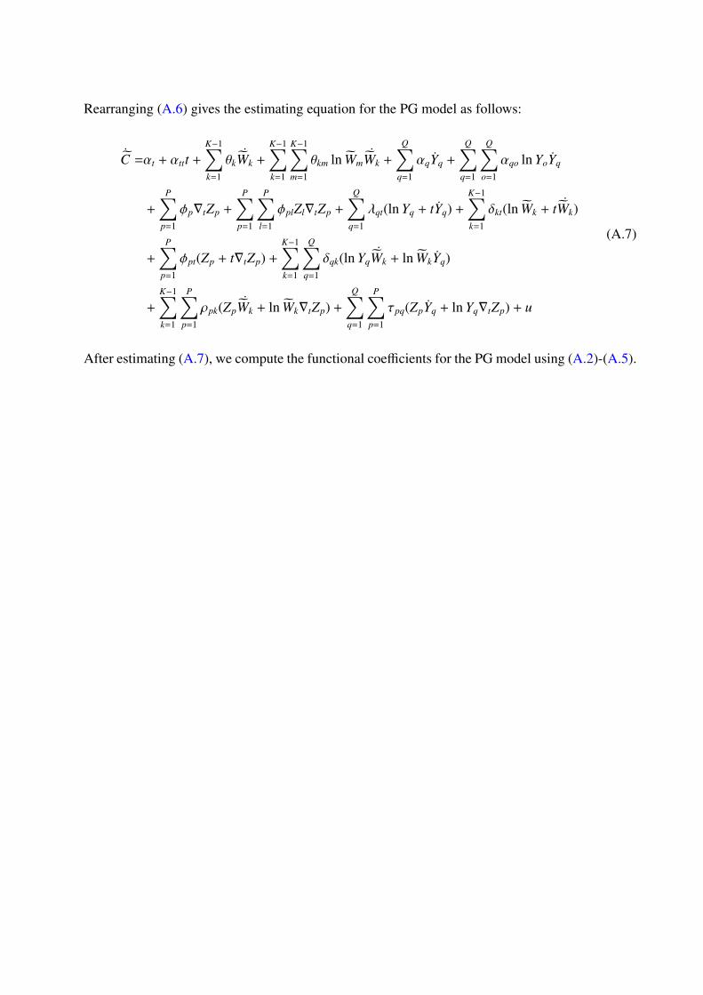
Rearranging (A.6) gives the estimating equation for the PG model as follows:

˙C =αt + αttt +

K−1∑k=1

θk˙Wk +

K−1∑k=1

K−1∑m=1

θkm ln Wm˙Wk +

Q∑q=1

αqYq +

Q∑q=1

Q∑o=1

αqo ln YoYq

+

P∑p=1

φp∇tZp +

P∑p=1

P∑l=1

φplZl∇tZp +

Q∑q=1

λqt(ln Yq + tYq) +

K−1∑k=1

δkt(ln Wk + t ˙Wk)

+

P∑p=1

φpt(Zp + t∇tZp) +

K−1∑k=1

Q∑q=1

δqk(ln Yq˙Wk + ln WkYq)

+

K−1∑k=1

P∑p=1

ρpk(Zp˙Wk + ln Wk∇tZp) +

Q∑q=1

P∑p=1

τpq(ZpYq + ln Yq∇tZp) + u

(A.7)

After estimating (A.7), we compute the functional coefficients for the PG model using (A.2)-(A.5).