Architectures and Control

Red box rules are for proof stage only. Delete before final printing.

Microgrids A

rchitectu

res and C

ontrol

MicrogridsArchitectures and ControlEditor: Nikos HatziaRgyRiou, National Technical University of Athens, Greece

Microgrids are the most innovative area in the electric power industry today. Future microgrids could exist as energy-balanced cells within existing power distribution grids or stand-alone power networks within small communities.

a definitive presentation on all aspects of microgrids, this text examines the operation of microgrids – their control concepts and advanced architectures including multi-microgrids. it takes a logical approach to overview the purpose and the technical aspects of microgrids, discussing the social, economic and environmental benefits to power system operation. the book also presents microgrid design and control issues, including protection, and explains how to implement centralized and decentralized control strategies.

Key features:

O original, state-of-the-art research material written by internationally respected contributors

O unique case studies demonstrating success stories from real-world pilot sites from Europe, the americas, Japan and China

O examines market and regulatory settings for microgrids, and provides evaluation results under standard test conditions

O a look to the future by well-known experts – technical solutions to maximize the value of distributed energy, along with the principles and criteria for developing commercial and regulatory frameworks for microgrids

O a companion website hosting full colour versions of the figures in the book

offering broad yet balanced coverage, this collaborative volume is an entry point to this very topical area of power delivery for electrical power engineers familiar with medium and low voltage distribution systems, utility operators in microgrids and power systems researchers and academics. it is also a useful reference for system planners and operators, manufacturers and network operators, government regulators and postgraduate power systems students.

EditorHatziargyriou

Editor: Nikos Hatziargyriou

MicrogridsArchitectures and Control

www.wiley.com/go/hatziargyriou_microgrids

MICROGRIDS

MICROGRIDSARCHITECTURES AND CONTROL

Edited by

Professor Nikos Hatziargyriou

National Technical University of Athens, Greece

��

This ed ition first published 2014

# 2014 John Wiley and Sons Ltd

Registered office

John Wiley & Sons Ltd, The Atrium, Southern Gate, Chichester, West Sussex, PO19 8SQ, United Kingdom

For details of our global edi torial offices, for customer service s and for informati on about how to apply for pe rmission to

reuse th e copyright material in this book please see our website at www.wiley.com.

The right of the author to be identified as the author of this work has been asserted in accordance with the Copyright,

Designs and Patents Act 1988.

All rights reserved. No part of this publication may be reproduced, stored in a retrieval system, or transmitted, in any form

or by any means, electronic, mechanical, photocopying, recording or otherwise, except as permitted by the UK Copyright,

Designs and Patents Act 1988, without the prior permission of the publisher.

Wiley also publishes its books in a variety of electronic formats. Some content that appears in print may not be available in

electronic books.

Limit of Liability/Disclaimer of Warranty: While the publisher and author have used their best efforts in preparing this

book, they make no representations or warranties with respect to the accuracy or completeness of the contents of this book

and specifically disclaim any implied warranties of merchantability or fitness for a particular purpose. It is sold on the

understanding that the publisher is not engaged in rendering professional services and neither the publisher nor the author

shall be liable for damages arising here from. If professional advice or other expert assistance is required, the services of a

competent professional should be sought.

Library of Congress Cataloging-in-Publication Data

Microgrid : architectures and control / edited by professor Nikos

Hatziargyriou.

1 online resource.

Includes bibliographical references and index.

Description based on print version record and CIP data provided by

publisher; resource not viewed.

ISBN 978-1-118-72064-6 (ePub) – ISBN 978-1-118-72065-3 – ISBN 978-1-118-72068-4 (cloth)

1. Smart power grids. 2. Small power production

facilities. I. Hatziargyriou, Nikos, editor of compilation.

TK3105

621.31–dc23

2013025351

A catalogue record for this book is available from the British Library.

ISBN: 978-1-118-72068-4

Set in 10/12 pt Times by Thomson Digital, Noida, India

http://www.wiley.com

Dedicated to the Muse of Creativity

Contents

Foreword xiii

Preface xv

List of Contributors xix

1 The Microgrids Concept 1

Christine Schwaegerl and Liang Tao

1.1 Introduction 1

1.2 The Microgrid Concept as a Means to Integrate Distributed Generation 3

1.3 Clarification of the Microgrid Concept 4

1.3.1 What is a Microgrid? 4

1.3.2 What is Not a Microgrid? 6

1.3.3 Microgrids versus Virtual Power Plants 7

1.4 Operation and Control of Microgrids 8

1.4.1 Overview of Controllable Elements in a Microgrid 8

1.4.2 Operation Strategies of Microgrids 10

1.5 Market Models for Microgrids 12

1.5.1 Introduction 12

1.5.2 Internal Markets and Business Models for Microgrids 15

1.5.3 External Market and Regulatory Settings for Microgrids 19

1.6 Status Quo and Outlook of Microgrid Applications 22

References 24

2 Microgrids Control Issues 25

Aris Dimeas, Antonis Tsikalakis, George Kariniotakis and George Korres

2.1 Introduction 25

2.2 Control Functions 25

2.3 The Role of Information and Communication Technology 27

2.4 Microgrid Control Architecture 28

2.4.1 Hierarchical Control Levels 28

2.4.2 Microgrid Operators 31

2.5 Centralized and Decentralized Control 32

2.6 Forecasting 35


2.6.2 Demand Forecasting 37

2.6.3 Wind and PV Production Forecasting 38

2.6.4 Heat Demand Forecasting 39

2.6.5 Electricity Prices Forecasting 39

2.6.6 Evaluation of Uncertainties on Predictions 40

2.7 Centralized Control 40

2.7.1 Economic Operation 41

2.7.2 Participation in Energy Markets 42

2.7.3 Mathematical Formulation 45

2.7.4 Solution Methodology 46

2.7.5 Study Case 47

2.7.6 Results 48

2.8 Decentralized Control 51

2.8.1 Multi-Agent System Theory 52

2.8.2 Agent Communication and Development 54

2.8.3 Agent Communication Language 59

2.8.4 Agent Ontology and Data Modeling 60

2.8.5 Coordination Algorithms for Microgrid Control 60

2.8.6 Game Theory and Market Based Algorithms 69

2.8.7 Scalability and Advanced Architecture 70

2.9 State Estimation 72


2.9.2 Microgrid State Estimation 73

2.9.3 Fuzzy State Estimation 74

2.10 Conclusions 76

Appendix 2.A Study Case Microgrid 76

References 78

3 Intelligent Local Controllers 81

Thomas Degner, Nikos Soultani, Alfred Engler and Asier Gil de Muro

3.1 Introduction 81

3.2 Inverter Control Issues in the Formation of Microgrids 82

3.2.1 Active Power Control 82

3.2.2 Voltage Regulation 82

3.3 Control Strategies for Multiple Inverters 82

3.3.1 Master Slave Control Scheme 82

3.3.2 Multi-Master Control Scheme 83

3.3.3 Droop Control Implementation in the VSI 85

3.3.4 Ancillary Services 89

3.3.5 Optional Secondary Control Loops 90

3.4 Implications of Line Parameters on Frequency and Voltage

Droop Concepts 92

3.4.1 Power Transmission in the LV Grid 92

3.4.2 Comparison of Droop Concepts at the LV Level 93

3.4.3 Indirect Operation of Droops 94

viii Contents

3.5 Development and Evaluation of Innovative Local Controls

to Improve Stability 98

3.5.1 Control Algorithm 98

3.5.2 Stability in Islanded Mode 100

3.5.3 Stability in Interconnected Operation 107

3.6 Conclusions 115

References 116

4 Microgrid Protection 117

Alexander Oudalov, Thomas Degner, Frank van Overbeeke

and Jose Miguel Yarza

4.1 Introduction 117

4.2 Challenges for Microgrid Protection 118

4.2.1 Distribution System Protection 118

4.2.2 Over-Current Distribution Feeder Protection 120

4.2.3 Over-Current Distribution Feeder Protection and DERs 121

4.2.4 Grid Connected Mode with External Faults (F1, F2) 121

4.2.5 Grid Connected Mode with Fault in the Microgrid (F3) 123

4.2.6 Grid Connected Mode with Fault at the

End-Consumer Site (F4) 124

4.2.7 Islanded Mode with Fault in the Microgrid (F3) 124

4.2.8 Islanded Mode and Fault at the End-Consumer Site (F4) 124

4.3 Adaptive Protection for Microgrids 125


4.3.2 Adaptive Protection Based on Pre-Calculated Settings 126

4.3.3 Microgrid with DER Switched off, in Grid-Connected Mode 129

4.3.4 Microgrid with Synchronous DERs Switched on in Grid

Connected and Islanded Modes 134

4.3.5 Adaptive Protection System Based on Real-Time

Calculated Settings 140

4.3.6 Communication Architectures and Protocols for

Adaptive Protection 144

4.4 Fault Current Source for Effective Protection in Islanded Operation 146

4.5 Fault Current Limitation in Microgrids 151

4.6 Conclusions 154

Appendices: 154

4.A.1 A Centralized Adaptive Protection System for an

MV/LV Microgrid 154

4.A.2 Description of the Prototype FCS 161

References 164

5 Operation of Multi-Microgrids 165

Jo~ao Abel PeScas Lopes, Andr�e Madureira, Nuno Gil and Fernanda Resende


5.2 Multi-Microgrid Control and Management Architecture 167

5.3 Coordinated Voltage/var Support 169

Contents ix


5.3.2 Mathematical Formulation 169

5.3.3 Proposed Approach 171

5.3.4 Microgrid Steady-State Equivalents 172

5.3.5 Development of the Tool 173

5.3.6 Main Results 174

5.4 Coordinated Frequency Control 178

5.4.1 Hierarchical Control Overview 178

5.4.2 Hierarchical Control Details 181


5.5 Emergency Functions (Black Start) 186

5.5.1 Restoration Guidelines 187

5.5.2 Sample Restoration Procedure 189

5.6 Dynamic Equivalents 192

5.6.1 Application of Dynamic Equivalence Based Approaches

to Microgrids 193

5.6.2 The Microgrid System Definition 194

5.6.3 Developing Micogrid Dynamic Equivalents 195


5.7 Conclusions 202

References 203

6 Pilot Sites: Success Stories and Learnt Lessons 206

George Kariniotakis, Aris Dimeas and Frank Van Overbeeke

(Sections 6.1, 6.2)


6.2 Overview of Microgrid Projects in Europe 206

6.2.1 Field Test in Gaidouromandra, Kythnos Microgrid

(Greece): Decentralized, Intelligent Load Control in an

Isolated System 208

6.2.2 Field Test in Mannheim (Germany): Transition from Grid

Connected to Islanded Mode 218

6.2.3 The Bronsbergen Microgrid (Netherlands): Islanded

Operation and Smart Storage 222

References 231

6.3 Overview of Microgrid Projects in the USA 231

John Romankiewicz, Chris Marnay (Section 6.3)

6.3.1 R&D Programs and Demonstration Projects 232

6.3.2 Project Summaries 236

References 248

6.4 Overview of Japanese Microgrid Projects 249

Satoshi Morozumi (Section 6.4)

6.4.1 Regional Power Grids Project 249

6.4.2 Network Systems Technology Projects 257

6.4.3 Demonstration Project in New Mexico 258

x Contents

6.5 Overview of Microgrid Projects in China 262

Meiqin Mao (Section 6.5)

6.5.1 Microgrids on Islands 262

6.5.2 Microgrids in Industrial, Commercial and Residential Areas 264

6.5.3 Microgrids in Remote Areas 268

References 269

6.6 An Off-Grid Microgrid in Chile 270

Rodrigo Palma Behnke and Guillermo Jim�enez-Est�evez (Section 6.6)

6.6.1 Project Description 270

6.6.2 Demand-Side Management 272

References 274

7 Quantification of Technical, Economic, Environmental and Social

Benefits of Microgrid Operation 275

Christine Schwaegerl and Liang Tao

7.1 Introduction and Overview of Potential Microgrid Benefits 275

7.1.1 Overview of Economic Benefits of a Microgrid 275

7.1.2 Overview of Technical Benefits of a Microgrid 277

7.1.3 Overview of Environmental and Social Benefits of a Microgrid 277

7.2 Setup of Benefit Quantification Study 278

7.2.1 Methodology for Simulation and Analysis 278

7.2.2 European Study Case Microgrids 279

7.3 Quantification of Microgrids Benefits under Standard Test Conditions 285

7.3.1 Definition of Standard Test Conditions 285

7.3.2 Balancing and Energy Results 285

7.3.3 Technical Benefits 287

7.3.4 Economic Benefits 289

7.3.5 Environmental Benefits 291

7.3.6 Reliability Improvement 293

7.3.7 Social Aspects of Microgrid Deployment 296

7.4 Impact of External Market Prices and Pricing Policies 296

7.4.1 Sensitivity Analysis 296

7.4.2 Sensitivity of Energy Balancing in Response to External

Market Prices and Price Settings 298

7.4.3 Sensitivity of Technical Benefits (Losses) in Response

to External Market Prices and Price Settings 300

7.4.4 Sensitivity of Economic Benefits in Response to External

Market Prices and Price Settings 301

7.4.5 Sensitivity of Environmental Benefits in Response to Market

Prices and Price Settings 302

7.5 Impact of Microgrid Operation Strategy 303

7.6 Extension to European Scale 307

7.7 Conclusions 310

References 313

Index 315

Contents xi

Foreword

The idea of microgrids is not new. However, as new technologies are coming into existence to

harvest renewable energy as well as more efficient electricity production methods coupled

with the flexibility of power electronics; a new industry is developing to promote these

technologies and organize them into microgrids for extracting the maximum benefits for

owners and the power grid. More than 15 years ago, the Department of Energy has sponsored

early research that laid the foundations for microgrids and explored the benefits. One key

aspect is the ability and promise to address environmental concerns that have been growing in

recent years. Today the microgrid concept has exploded to include a variety of architectures of

energy resources into a coordinated energy entity that its value is much greater than the

individual components. As a result the complexity of microgrids has increased. It is in this

environment of evolution of microgrids that the present book is very welcome. It is written in a

way that provides valuable information for specialist as well as non-specialists.

Chapter 1 provides a well thought view of the microgrid concept from the various forms of

implementation to the potential economic, environmental and technical benefits. It identifies

the role of microgrids in altering the distribution system as we know it today and at the same

time elaborates on the formation of microgrids as an organized entity interfaced to distribution

systems. In a refreshingly simple way identifies the enabling technologies for microgrids, that

is power electronics, communications, renewable resources. It discusses in simple terms the

ability of microgrids to minimize green house gases, help the power grid with load balancing

and voltage control and assist power markets. While it is recognized that participation of the

microgrids in power markets is limited by their size, it discusses possible ways that microgrids

can market their assets via aggregators and opens the field for other innovations.

The book addresses two of the great challenges of microgrids: control and protection. Four

chapters are devoted to these complex problems, three on control (Chapters 2, 3 and 5) and one

on protection (Chapter 4). Themultiplicity of control issues and their complexity is elaborated in

a clear and concise manner. Since microgrids comprise many resources that are interfaced via

power electronics, the book presents the organization of the control problems in a hierarchical

architecture that consists of local controllers that control specific resources, their operation and

their protection as well as outer loop controllers that perform load-generation management,

islanding operation aswell as the interactionwith up-stream controllers including power system

control centers. It provides a good overview of approaches as well as the role of state estimation

in controlling and operating a microgrid. In addition to conventional control methods, recent

intelligent control approaches are also discussed. The specific issues and challenges of

microgrid control are clearly elaborated. As an example, because the microgrid typically

comprises many inverters connecting various resources to the microgrid it is possible to trigger

oscillations due to inverter control interactions. Methods for solving these issues are clearly

discussed in an easy to followway. It is recognized thatmultiplemicrogrids can exist in a system

and the issue of controlling and coordinating all the microgrids is very important from the point

of view of managing the microsources as well as providing services to the power grid by

coordinating all the resources. The services can be any of the ancillary services that are typically

provided by large systems: frequency control, voltage control, power balance, capacity reserves.

The hierarchies involved in the control and operation of multi-microgrid systems is eloquently

presented as a hierarchical control problem.

Protection of microgrids is a challenging problem due to the fact that microgrid resources

provide limited fault currents. Detection of faults in microgrids is problematic at best because

the grid side fault current contribution may be very high while the contribution from

microsources is limited. Present protection schemes and functions are not reliable for

microgrids. The book describes clever methods for providing adequate protection functions

such as adaptive protection schemes, addition of components that will provide temporarily

high fault currents to enable the operation of protective relays, increasing inverter capacity

and therefore fault current contribution. While the book provides some solutions it also makes

it clear that there is much more work that needs to be done to reliably protect microgrids.

The basic approaches in designing, controlling and protecting microgrids are nicely

complimented by a long list of microgrid projects around the globe that provide a picture

of the evolution of microgrid design and lessons learned. Specific microgrid projects in

Europe, United States, Japan, China and Chile are described and discussed. These projects

provide an amazing insight into the lessons learned, challenges faced and issues resolved and

issues outstanding. The examples span small capacity microgrids as well as some very large

microgrids; grid-connected microgrids as well as stand-alone or island microgrids. The

information provided is extremely useful and enables appreciation of the challenges as well as

the rewards of these systems.

Finally, the last chapter elaborates on the technical, economic, environmental and social

benefits of microgrids. The discussion is qualitative as well as quantitative. While the

quantitative analysis is very much dependent upon specific areas and other conditions, the

qualitative discussion is applicable to microgrids anywhere in the globe. Indirectly, this

discussion makes the case for microgrids comprising mostly renewable energy resources as a

big component in solving the environmental, economic and social issues that are facing a

society that relies more and more in electric energy. The technical issues are solvable for

transforming distribution systems into a distributed microgrid. The work presented in this

book will be a fundamental reference toward the promotion and proliferation of microgrids

and the accompanied deployment of renewable resources.

This book is a must read resource for anyone interested in the design and operation of

microgrids and the integration of renewable resources into the power grid.

Sakis Meliopoulos

Georgia Power Distinguished Professor

School of Electrical and Computer Engineering

Georgia Institute of Technology

Atlanta, Georgia

xiv Foreword

Preface

The book deals with understanding, analyzing and justifying Microgrids, as novel distribution

network structures that unlock the full potential of Distributed Energy Resources (DER) and

thus form building blocks of future Smartgrids. In the context of this book, Microgrids are

defined as distribution systems with distributed energy sources, storage devices and control-

lable loads, operated connected to the main power network or islanded, in a controlled,

coordinated way. Coordination and control of DER is the key feature that distinguishes

Microgrids from simple distribution feeders with DER. In particular, effective energy

management within Microgrids is the key to achieving vital efficiency benefits by optimizing

production and consumption of energy. Nevertheless, the technical challenges associated with

the design, operation and control of Microgrids are immense. Equally important is the

economic justification of Microgrids considering current electricity market environments and

the quantified assessment of their benefits from the view of the various stakeholders involved.

Discussions about Microgrids started in the early 2000, although their benefits for island

and remote, off-grid systems were already generally appreciated. Nowadays, Microgrids are

proposed as vital solutions for critical infrastructures, campuses, remote communities,

military applications, utilities and communal networks. Bright prospects for a steady market

growth are foreseen. The book is intended to meet the needs of practicing engineers, familiar

with medium- and low-voltage distribution systems, utility operators, power systems

researchers and academics. It can also serve as a useful reference for system planners and

operators, technology providers, manufacturers and network operators, government regula-

tors, and postgraduate power systems students.

The text presents results from a 6-year joint European collaborative work conducted in the

framework of two EC-funded research projects. These are the projects “Microgrids: Large

Scale Integration of Micro-Generation to Low Voltage Grids,” funded within the 5th

Framework programme (1998–2002) and the follow-up project “More Microgrids, Advanced

Architectures and Control Concepts for More Microgrids” funded within the 6th Framework

Programme (2002–2006). The consortia involved were coordinated by the editor of this book

and comprised a number of industrial partners, power utilities and academic research teams

from 12 EU countries. Awealth of information and many practical conclusions were derived

from these two major research efforts. The book attempts to clarify the role of Microgrids

within the overall power system structure and focuses on the main findings related to primary

and secondary control and management at the Microgrid and Multi-Microgrid level. It also

provides results from quantified assessment of the Microgrids benefits from an economical,

environmental, operational and social point of view. A separate chapter beyond the EC

projects, provided by a more international authorship is devoted to an overview of real-world

Microgrids from various parts of the world, including, next to Europe, United States of

America, Japan, China and Chile.

Chapter 1, entitled “The Microgrids Concept,” co-authored by Christine Schwaegerl and

Liang Tao, clarifies the key features of Microgrids and underlines the distinguishing character-

istics from other DG dominated structures, such as Virtual Power Plants. It discusses the main

features related to their operation and control, the market models and the effect of possible

regulatory settings and provides an exemplary roadmap for Microgrid development in Europe.

Chapter 2, entitled “Microgrids Control Issues” co-authored by Aris Dimeas, Antonis

Tsikalakis, George Kariniotakis and George Korres, deals with one of the key features of

Microgrids, namely their energy management. It presents the hierarchical control levels

distinguished in Microgrids operation and discusses the principles and main functions of

centralized and decentralized control, including forecasting and state estimation. Next,

centralized control functions are analyzed and illustrated by a practical numerical example.

Finally, an overview of the basic multi-agent systems concepts and their application for

decentralized control of Microgrids is provided.

Chapter 3, entitled “Intelligent Local Controllers,” co-authored by Thomas Degner, Nikos

Soultanis, Alfred Engler and Asier Gil de Muro, presents primary control capabilities of DER

controllers. The provision of ancillary services in interconnected mode and the capabilities of

voltage and frequency control, in case of islanded operation and during transition between the

two modes are outlined. Emphasis is placed on the implications of the high resistance over

reactance ratios, typically found in LVMicrogrids. A control algorithm based on the fictitious

impedance method to overcome the related problems together with characteristic simulation

results are provided.

Chapter 4, entitled “Microgrid Protection,” co-authored by Alexander Oudalov, Thomas

Degner, Frank van Overbeeke and Jose Miguel Yarza, deals with methods for effective

protection in Microgrids. A number of challenges are caused by DER varying operating

conditions, the reduced fault contribution by power electronics interfaced DER and the

occasionally increased fault levels. Two adaptive protection techniques, based on pre-

calculated and on-line calculated settings are proposed including practical implementation

issues. Techniques to increase the amount of fault current level by a dedicated device and the

possible use of fault current limitation are also discussed.

Chapter 5, entitled “Operation of Multi-Microgrids,” co-authored by Jo~ao Abel PeScasLopes, Andr�e Madureira, Nuno Gil and Fernanda Resende examines the operation of

distribution networks with increasing penetration of several low voltage Microgrids, coor-

dinated with generators and flexible loads connected at medium voltage. An hierarchical

management architecture is proposed and functions for coordinated voltage/VAR control and

coordinated frequency control are analyzed and simulated using realistic distribution net-

works. The capability of Microgrids to provide black start services are used to provide

restoration guidelines. Finally, methods for deriving Microgrids equivalents for dynamic

studies are discussed.

Chapter 6, entitled “Pilot Sites: Success Stories and Learnt Lessons” provides an overview

of real-worldMicrogrids, already in operation as off-grid applications, pilot cases or full-scale

demonstrations. The material is organized according to geographical divisions. George

Kariniotakis, Aris Dimeas and Frank van Overbeeke describe three pilot sites in Europe

developed within the more Microgrids project; John Romankiewicz and Chris Marnay

xvi Preface

provide an overview of Microgrid Projects in the United States; Satoshi Morozumi provide an

overview of the Japanese Microgrid Projects; Meiqin Mao describes the Microgrid Projects in

China and Rodrigo Palma Behnke and Guillermo Jim�enez-Est�evez provide details of an

off-grid Microgrid in Chile. These projects are of course indicative of a continuously growing

list, they provide, however, a good impression of the on-going developments in the field.

Chapter 7, entitled “Quantification of Technical, Economic, Environmental and Social

Benefits of Microgrid Operation,” co-authored by Christine Schwaegerl and Liang Tao

attempts to quantify the Microgrids benefits using typical European distribution networks of

different types and assuming various DER penetration scenarios, market conditions, prices

and costs developments for the years 2020, 2030 and 2040. Sensitivity analysis of the

calculated benefits is performed. Although, the precision of these quantified benefits is subject

to the high uncertainties in the underlying assumptions, the positive effects of Microgrids

operation can be safely observed in all cases.

Next to the co-authors of the various chapters, there are many researchers who have

contributed to the material of this book by their knowledge, research efforts and fruitful

collaboration during the numerous technical meetings of the Microgrids projects. I am

indebted to all of them, but I feel obliged to refer to some names individually and apologize in

advance for the names I might forget. I would like to start with Profs. Nick Jenkins and Goran

Strbac from UK; I have benefited tremendously while working with them and their insights

and discussions helped clarify many concepts discussed in the book. I am indebted to Britta

Buchholz, Christian Hardt, Roland Pickhan, Mariam Khattabi, Michel Vandenbergh, Martin

Braun, Dominik Geibel and Boris Valov from Germany; Mikes Barnes, Olimpo Anaya-Lara,

Janaka Ekanayake, Pierluigi Mancarella, Danny Pudjianto and Tony Lakin from UK; Jose

Maria Oyarzabal, Joseba Jimeno and I~nigo Cobelo from Spain; Nuno Melo and Ant�onioAmorim from Portugal; Sjef Cobben from the Netherlands; John Eli Nielsen from Denmark;

Perego Omar and Michelangeli Chiara from Italy; Aleksandra Krkoleva, Natasa Markovska

and Ivan Kungulovski from FYR of Macedonia; Grzegorz Jagoda and Jerszy Zielinski from

Poland; my NTUA colleagues Stavros Papathanassiou and Evangelos Dialynas; and Stathis

Tselepis, Kostas Elmasides, Fotis Psomadellis, Iliana Papadogoula, Manolis Voumvoulakis,

Anestis Anastasiadis, Fotis Kanellos, Spyros Chadjivassiliadis and Maria Lorentzou from

Greece. I express my gratitude to my PhD students and collaborators Georgia Asimakopou-

lou, John Karakitsios, Evangelos Karfopoulos, Vassilis Kleftakis, Panos Kotsampopoulos,

Despina Koukoula, Jason Kouveliotis-Lysicatos, Alexandros Rigas, Nassos Vassilakis,

Panayiotis Moutis, Christina Papadimitriou and Dimitris Trakas, who reviewed various

chapters of the book and provided valuable comments. Finally, I wish to thank the EC

DG Research&Innovation for providing the much appreciated funding for the research

leading to this book, especially the Officers Manuel Sanchez Jimenez and Patrick Van Hove.

Nikos Hatziargyriou

Preface xvii

List of Contributors

Thomas Degner, Thomas Degner is Head of Department Network Technology and Integra-

tion at Fraunhofer IWES, Kassel, Germany. He received his Diploma in Physics and his Ph.D.

from University of Oldenburg. His particular interests include microgrids, interconnection

requirements and testing procedures for distributed generators, as well as power system

stability and control for island and interconnected power systems with a large share of

renewable generation.

Aris Dimeas, Aris L. Dimeas received the Diploma and his Ph.D. in Electrical and Computer

Engineering from the National Technical University of Athens (NTUA). He is currently senior

researcher at the Electrical and Computer Engineering School of NTUA. His research

interests include dispersed generation, artificial intelligence techniques in power systems

and computer applications in liberalized energy markets.

Alfred Engler,Alfred Engler received his Dipl.-Ing. (Master’s) from the Technical University

of Braunschweig and the degree Dr.-Ing. (Ph.D.) from the University of Kassel. He has been

head of the group Electricity Grids and of Power Electronics at ISET e.V. involved with

inverter control, island grids, microgrids, power quality and grid integration of wind power.

He is currently Manager of the Department of Advance Development at Liebherr Elektronik

GmbH.

Nuno Gil, Nuno Jos�e Gil received his electrical engineering degree from the University of

Coimbra and M.Sc. and Ph.D. from the University of Porto. He is a researcher in the Power

Systems Unit of INESC Porto and assistant professor at the Polytechnic Institute of Leiria,

Portugal. His research interests include integration of distributed generation and storage

devices in distribution grids, islanded operation and frequency control.

Guillermo Jim�enez-Est�evez, Guillermo A. Jim�enez-Est�evez received the B.Sc. degree in

Electrical Engineering from the Escuela Colombiana de Ingenier�ıa, Bogot�a, and theM.Sc. and

Ph.D. degrees from the University of Chile, Santiago. He is assistant director of the Energy

Center, FCFM, University of Chile.

George Kariniotakis,Georges Kariniotakis received his engineering andM.Sc. degrees from

the Technical University of Crete, Greece and his Ph.D. degree from Ecole desMines de Paris.

He is currently with the Centre for Processes, Renewable Energies & Energy Systems

(PERSEE) of MINES ParisTech as senior scientist and head of the Renewable Energies &

Smartgrids Group. His research interests include renewables, forecasting and smartgrids.

George Korres, George N. Korres received the Diploma and Ph.D. degrees in Electrical and

Computer Engineering from the National Technical University of Athens. He is professor with

the School of Electrical and Computer Engineering of NTUA. His research interests are in

power system state estimation, power system protection and industrial automation.

Andr�e Madureira, Andr�e G. Madureira received an Electrical Engineering degree, M.Sc.

and Ph.D. from the Faculty of Engineering of the University of Porto. He is senior researcher/

consultant in the Power Systems Unit of INESC Porto. His research interests include

integration of distributed generation and microgeneration in distribution grids, voltage and

frequency control and smartgrid deployment.

Meiqin Mao, Meiqin Mao is professor with Research Center of Photovoltaic System

Engineering, Ministry of Education, Hefei University of Technology, P.R. China. She has

been devoted to renewable energy generation research since 1993. Her research interests

include optimal operation and energy management of microgrids and power electronics

applications in renewable energy systems.

Chris Marnay, Chris Marnay has been involved in microgrid research since the 1990s. He

studies the economic and environmental optimization of microgrid equipment selection and

operation. He has chaired nine of the annual international microgrid symposiums.

Satoshi Morozumi, Satoshi Morozumi has graduated from a doctor course in Hokkaido

University. He joinedMitsubishi Research Institute, Inc. and for past 20 years, hewas engaged

in the utility’s system. He is currently director general of Smart Community Department

at NEDO, where he is in charge of management of international smart community

demonstrations.

Asier Gil de Muro, Asier Gil de Muro has received his M.Sc. in Electrical Engineering from

the School of Engineering of the University of the Basque Country in Bilbao, Spain. Since

1999 he is researcher and project manager at the Energy Unit of TECNALIA, working in

projects dealing with power electronics equipment, design and developing of grid inter-

connected power devices, microgrids and active distribution.

Alexandre Oudalov, Alexandre Oudalov received the Ph.D. in Electrical Engineering in

2003 from the Swiss Federal Institute of Technology in Lausanne (EPFL), Switzerland. He

joined ABB Switzerland Ltd., Corporate Research Center in 2004 where he is currently a

principal scientist in the Utility Solutions group. His research interests include T&D grid

automation, integration and management of DER and control and protection of microgrids

Frank van Overbeeke, Frank van Overbeeke graduated in Electrical Power Engineering at

Delft University of Technology and obtained a Ph.D. in Applied Physics from the University

of Twente. He is founder and owner of EMforce, a consultancy firm specialized in power

electronic applications for distribution networks. He has acted as the system architect for

several major utility energy storage projects in the Netherlands.

Rodrigo Palma Behnke, Rodrigo Palma Behnke received his B.Sc. and M.Sc. on Electrical

Engineering from the Pontificia Universidad Cat�olica de Chile and a Dr.-Ing. from the

University of Dortmund, Germany. He is the director of the Energy Center, FCFM, and

the Solar Energy Research Center SERC-Chile, he also is associate professor at the Electrical

Engineering Department, University of Chile.

xx List of Contributors

Jo~ao Abel PeScas Lopes, Jo~ao Abel PeScas Lopes is full professor at Faculty of Engineering ofUniversity of Porto and member of the Board of Directors of INESC Porto

Fernanda Resende, Fernanda O. Resende received an Electrical Engineering degree, from

the University of Tr�as-os-Montes e Alto Douro and M.Sc. and Ph.D. from the Faculty of

Engineering of the University of Porto. She is senior researcher in the Power Systems Unit of

INESC Porto and assistant professor at Los�ofona University of Porto. Her research interests

include integration of distributed generation, modeling and control of power systems and

small signal stability.

John Romankiewicz, John Romankiewicz is a senior research associate at Berkeley Lab,

focusing on distributed generation and energy efficiency policy. He has been working in the

energy sector in the United States and China for the past 7 years and is currently studying for

his Masters of Energy and Resources and Masters of Public Policy at UC Berkeley.

Christine Schwaegerl, Christine Schwaegerl received her Diploma in Electrical Engineering

at the University of Erlangen and her Ph.D. from Dresden Technical University, Germany. In

2000, she joined Siemens AG where she has been responsible for several national and

international research and development activities on power transmission and distribution

networks. Since 2011 she is professor at Augsburg University of Applied Science.

Nikos Soultanis, Nikos Soultanis graduated from the Electrical Engineering Department of

the National Technical University of Athens (NTUA) in 1989 and has worked on various

projects as an independent consultant. He received his M.Sc. from the University of

Manchester Institute of Science and Technology (UMIST) and his Ph.D. from NTUA. He

works currently in the dispatching center of the Greek TSO and as an associated researcher at

NTUA with interests in the area of distributed generation applications and power system

analysis.

Liang Tao, Liang Tao is a technical consultant working at Siemens PTI, Germany. His main

research interests include stochastic modeling of renewable energy sources, dimensioning and

operationmethods for storage devices, optimal power flow and optimal scheduling of multiple

types of resources in smartgrids.

Antonis Tsikalakis, Antonis G. Tsikalakis received the Diploma and Ph.D. degrees in

electrical and computer engineering from NTUA. Currently he is an adjunct lecturer in

the School of Electronics and Computer Engineering of the Technical University of Crete

(TUC) and research associate of the Technological Educational Institute of Crete. He

co-operates with the NTUA as post-doc researcher. His research interests are in distributed

generation, energy storage and autonomous power systems operation with increased RES

penetration.

Jos�eMiguel Yarza, Jos�eMiguel Yarza received anM.S. degree in Electrical Engineering and

a master degree on “Quality and Security in Electrical Energy Delivery. Power System

Protections” from the University of Basque Country and an executive MBA from ESEUNE

Business School. He is currently CTO at CG Automation. He is member of AENOR SC57

(Spanish standardization body), IEC TC57 and CIGRE.

List of Contributors xxi

1

The Microgrids Concept

Christine Schw aegerl and Liang Tao

1.1 Int roduction

Moder n societ y depend s cri tically on a secure suppl y of energy. Growing conce rns for primary

energy availabil ity and aging infras tructu re of current ele ctrical tra nsmission and distribution

networ ks are increas ingly challengin g security, relia bility and q uality of power supply. Very

significant amo unts of investment will b e require d to develop and renew these inf rastructu res,

while the most efficient way to meet soci al dem ands is to inco rporate innovative solutions,

technol ogies and grid architecture s. Acc ording to the Interna tional Energy Age ncy, globa l

investments require d in the energy sect or over the period 2003–203 0 are estimat ed at $16

trillion.

Future ele ctricity grid s have to cope with changes in tec hnology, in the values of society, in

the environm ent and in econom y [1]. Thus, system security, operation safe ty, environment al

protect ion, power quality, cost of suppl y and energy efficiency need to be examined in new

ways in respon se to changing requi rements in a liberalize d market environm ent. Technologies

should also demonst rate reliabili ty, sustai nability and cost effectiveness. The notion of smartgrids refers to the evolu tion of electricity gri ds. According to the European Technology

Platfor m of Smart Grids [2], a sma rt gri d is an ele ctricity network that can intelligent ly

integrate the actions of all user s connecte d to it – gener ators, consum ers and thos e that assume

both rol es – in order to efficientl y deliver sustai nable, economic and secure ele ctricity

supplie s. A smart grid employs innovative produc ts and services toge ther with intel ligent

monit oring, control, commun ication and sel f-healing tec hnologie s.

It is worth noting that power systems have always been “smart”, espec ially at the

transm ission level. The distribution level, h owever, is now experiencing an evolu tion that

needs mor e “smartnes s”, in order to

� facilit ate access to d istributed gener ation [3,4] on a high share, based on renewable energy

sources (RESs), either self-dispatched or dispatched by local distribution system operators

Microgrids: Architectures and Control, First Edition. Edited by Nikos Hatziargyriou.� 2014 John Wiley & Sons, Ltd. Published 2014 by John Wiley & Sons, Ltd.Companion Website: www.wiley.com/go/hatziargyriou_microgrids

http://www.wiley.com/go/hatziargyriou_microgrids

� enable local energy demand management, interacting with end-users through smart

metering systems� benefit from technologies already applied in transmission grids, such as dynamic control

techniques, so as to offer a higher overall level of power security, quality and reliability.

In summary, distribution grids are being transformed from passive to active networks, in

the sense that decision-making and control are distributed, and power flows bidirectional.

This type of network eases the integration of DG, RES, demand side integration (DSI) and

energy storage technologies, and creates opportunities for novel types of equipment and

services, all of which would need to conform to common protocols and standards. The main

function of an active distribution network is to efficiently link power generation with

consumer demands, allowing both to decide how best to operate in real-time. Power

flow assessment, voltage control and protection require cost-competitive technologies and

new communication systems with information and communication technology (ICT) playing

a key role.

The realization of active distribution networks requires the implementation of radically new

system concepts. Microgrids [5–11], also characterized as the “building blocks of smart

grids”, are perhaps the most promising, novel network structure. The organization of

microgrids is based on the control capabilities over the network operation offered by the

increasing penetration of distributed generators including microgenerators, such as micro-

turbines, fuel cells and photovoltaic (PV) arrays, together with storage devices, such as

flywheels, energy capacitors and batteries and controllable (flexible) loads (e.g. electric

vehicles [12]), at the distribution level. These control capabilities allow distribution networks,

mostly interconnected to the upstream distribution network, to also operate when isolated

from the main grid, in case of faults or other external disturbances or disasters, thus increasing

the quality of supply. Overall, the implementation of control is the key feature that

distinguishes microgrids from distribution networks with distributed generation.

From the customer’s point of view, microgrids provide both thermal and electricity

needs, and, in addition, enhance local reliability, reduce emissions, improve power quality

by supporting voltage and reducing voltage dips, and potentially lower costs of energy

supply. From the grid operator’s point of view, a microgrid can be regarded as a controlled

entity within the power system that can be operated as a single aggregated load or generator

and, given attractive remuneration, also as a small source of power or ancillary services

supporting the network. Thus, a microgrid is essentially an aggregation concept with

participation of both supply-side and demand-side resources in distribution grids. Based on

the synergy of local load and local microsource generation, a microgrid could provide a

large variety of economic, technical, environmental and social benefits to different stake-

holders. In comparison with peer microsource aggregation methods, a microgrid offers

maximum flexibility in terms of ownership constitution, allows for global optimization of

power system efficiency and appears as the best solution for motivating end-consumers via

a common interest platform.

Key economic potential for installing microgeneration at customer premises lies in the

opportunity to locally utilize the waste heat from conversion of primary fuel to electricity.

There has been significant progress in developing small, kW-scale, combined heat and power

(CHP) applications. These systems have been expected to play a very significant role in the

microgrids of colder climate countries. On the other hand, PV systems are anticipated to

2 Microgrids

become increasingly popular in countries with sunnier climates. The application of micro-

CHP and PV potentially increases the overall efficiency of utilizing primary energy sources

and consequently provides substantial environmental gains regarding carbon emissions,

which is another critically important benefit in view of the world’s efforts to combat climate

change.

From the utility point of view, application of microsources can potentially reduce the

demand for distribution and transmission facilities. Clearly, distributed generation located

close to loads can reduce power flows in transmission and distribution circuits with two

important effects: loss-reduction and the ability to potentially substitute for network assets.

Furthermore, the presence of generation close to demand could increase service quality seen

by end customers. Microgrids can provide network support in times of stress by relieving

congestion and aiding restoration after faults.

In the following sections, the microgrid concept is clarified and a clear distinction from the

virtual power plant concept is made. Then, the possible internal and external market models

and regulation settings for microgrids are discussed. A brief review of control strategies for

microgrids is given and a roadmap for microgrid development is provided.

1.2 The Microgrid Concept as a Means to Integrate DistributedGeneration

During the past decades, the deployment of distributed generation (DG) has been growing

steadily. DGs are connected typically at distribution networks, mainly at medium voltage

(MV) and high voltage (HV) level, and these have been designed under the paradigm that

consumer loads are passive and power flows only from the substations to the consumers and

not in the opposite direction. For this reason, many studies on the interconnection of DGs

within distribution networks have been carried out, ranging from control and protection to

voltage stability and power quality.

Different microgeneration technologies, such as micro-turbines (MT), photovoltaics (PV),

fuel cells (FC) and wind turbines (WT) with a rated power ranging up to 100 kW can be

directly connected to the LV networks. These units, typically located at users’ sites, have

emerged as a promising option to meet growing customer needs for electric power with an

emphasis on reliability and power quality, providing different economic, environmental and

technical benefits. Clearly, a change of interconnection philosophy is needed to achieve

optimal integration of such units.

Most importantly, it has to be recognized that with increased levels of microgeneration

penetration, the LV distribution network can no longer be considered as a passive appendage

to the transmission network. On the contrary, the impact of microsources on power balance

and grid frequency may become much more significant over the years.

Therefore, a control and management architecture is required in order to facilitate full

integration of microgeneration and active load management into the system. One promising

way to realize the emerging potential of microgeneration is to take a systematic approach that

views generation and associated loads as a subsystem or a microgrid.

In a typical microgrid setting, the control and management system is expected to bring

about a variety of potential benefits at all voltage levels of the distribution network. In order to

achieve this goal, different hierarchical control strategies need to be adopted at different

network levels.

The Microgrids Concept 3

The possibility of managing several microgrids, DG units directly connected to the MV

network and MV controllable loads introduces the concept of multi-microgrids. The

hierarchical control structure of such a system calls for an intermediate control level, which

will optimize the multi-microgrid system operation, assuming an operation under a real

market environment. The concept of multi-microgrids is further developed in Chapter 5.

The potential impact of such a system on the distribution network may lead to different

regulatory approaches and remuneration schemes, that could create incentive mechanisms for

distribution system operators (DSOs), microgeneration owners and loads to adopt the multi-

microgrid concept. This is further discussed in Chapter 7.

1.3 Clarification of the Microgrid Concept

1.3.1 What is a Microgrid?

In scope of this book, the definition from the EU research projects [7,8] is used:

Microgrids comprise LV distribution systems with distributed energy resources (DER) (micro-

turbines, fuel cells, PV, etc.) together with storage devices (flywheels, energy capacitors and

batteries) and flexible loads. Such systems can be operated in a non-autonomous way, if

interconnected to the grid, or in an autonomous way, if disconnected from the main grid. The

operation of microsources in the network can provide distinct benefits to the overall system

performance, if managed and coordinated efficiently.

There are three major messages delivered from this definition:

1. Microgrid is an integration platform for supply-side (microgeneration), storage units and

demand resources (controllable loads) located in a local distribution grid.� In the microgrid concept, there is a focus on local supply of electricity to nearby loads,

thus aggregator models that disregard physical locations of generators and loads (such as

virtual power plants with cross-regional setups) are not microgrids.� A microgrid is typically located at the LV level with total installed microgeneration

capacity below the MW range, although there can be exceptions: parts of the MV

network can belong to a microgrid for interconnection purposes.

2. A microgrid should be capable of handling both normal state (grid-connected) and

emergency state (islanded) operation.� The majority of future microgrids will be operated for most of the time under grid-

connection – except for those built on physical islands – thus, the main benefits of the

microgrid concept will arise from grid-connected (i.e. “normal”) operating states.� In order to achieve long-term islanded operation, a microgrid has to satisfy high

requirements on storage size and capacity ratings of microgenerators to continuous

supply of all loads or it has to rely on significant demand flexibility. In the latter case,

reliability benefits can be quantified from partial islanding of important loads.

3. The difference between a microgrid and a passive grid penetrated by microsources lies

mainly in terms of management and coordination of available resources.� A microgrid operator is more than an aggregator of small generators, or a network

service provider, or a load controller, or an emission regulator – it performs all these

functionalities and serves multiple economic, technical and environmental aims.

4 Microgrids

� One major advantage of the microgrid concept over other “smart” solutions lies in its

capability of handling conflicting interests of different stakeholders, so as to arrive at a

globally optimal operation decision for all players involved.

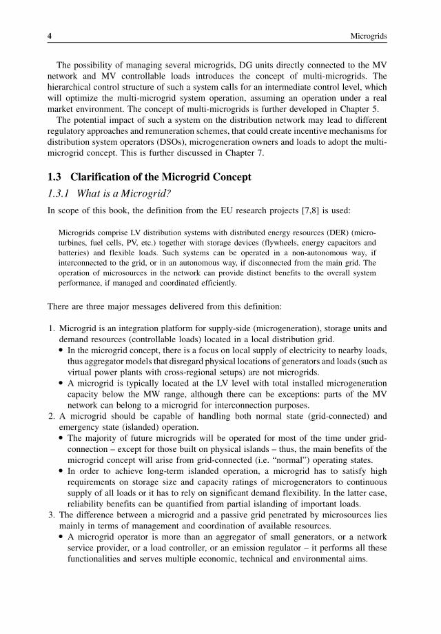
A microgrid appears at a large variety of scales: it can be defined at the level of a LV grid,

a LV feeder or a LV house – examples are given in Figure 1.1. As a microgrid grows in scale,

it will likely be equipped with more balancing capacities and feature better controllability to

reduce the intermittencies of load and RES. In general, the maximum capacity of a microgrid

(in terms of peak load demand) is limited to few MW (at least at the European scale, other

Figure 1.1 (a) Microgrid as a LV grid; (b) Microgrid as a LV feeder; (c) Microgrid as a LV house


regions may have different upper limits, see Chapter 6). At higher voltage levels, multi-

microgrid concepts are applied, implying the coordination of interconnected, but separate

microgrids in collaboration with upstream connected DGs and MV network controls. The

operation of multi-microgrids is discussed in Chapter 5.

1.3.2 What is Not a Microgrid?

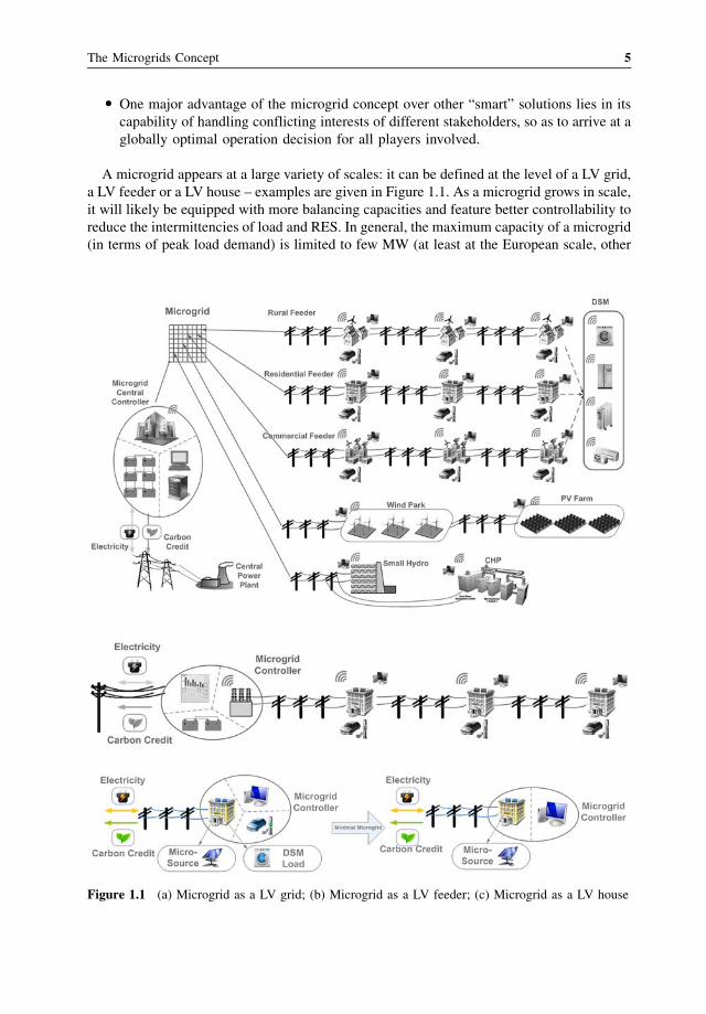
In Figure 1.2, the microgrid concept is further clarified by examples that highlight three

essential microgrid features: local load, local microsources and intelligent control. In many

countries environmental protection is promoted by the provision of carbon credits by the

use of RES and CHP technologies; this should be also added as a microgrids feature.

Absence of one or more features would be better described by DG interconnection cases or

DSI cases.

In the following section, some typical misconceptions regarding microgrids are clarified:

� Microgrids are exclusively isolated (island) systems.

) Microgrids have the capability to shift to islanded operation in emergency situations,

thus increasing customer reliability, but they are mostly operated interconnected to the

upstream distribution network. Small island systems are inherently characterized by

coordinated control of their resources, thus, depending on their size and the extent of

DER penetration and control, they can be also termed as microgrids.� Customers who own microsources build a microgrid.

) DG penetration is indeed a distinct microgrid feature, but a microgrid means more than

passive tolerance of DG (also known as “fit and forget”) and needs active supervision,

control and optimization.

Figure 1.2 What is not a microgrid? Sample cases

6 Microgrids

� Microgrids are composed of intermittent renewable energy resources, so they must be

unreliable and easily subject to failures and total black-outs.

) A microgrid can offset RES fluctuation by its own storage units (when islanded) or

external generation reserves (whengrid-connected).Moreover, themicrogrid’s capability

of transferring from grid-connected to island mode actually improves security of supply.� Microgrids are expensive to build, so the concept will be limited to field tests or only to

remote locations.

) DER penetration is increasing worldwide. Financial support schemes for RES and CHP

have already ensured the basic profitability of such distributed resources; future cost

reductions of microgeneration and storage can make microgrids commercially com-

petitive. In any case, the additional cost for transforming a distribution line with DER

into a microgrid involves only the relevant control and communication costs. These are

easily compensated by the economic advantages of coordinated DER management.� The microgrid concept is just another energy retailer advertising scheme to increase his

income.

) Even if an end-consumer chooses not to install photovoltaic panels on his rooftop or

hold a share in the community-owned CHP plant, he can still benefit from having more

choice of energy supply and of sharing carbon-reduction credits in his bill.� The microgrid controllers will force consumers to shift their demand, depending on the

availability of renewable generation, e.g. to switch on the washing machine at home only

when the sun is shining or the wind is blowing.

) Demand side integration (DSI) programs in normal commercial and household

applications should apply a “load follow generation” control philosophy only to

long-term stand-by appliances (such as refrigerators and air-conditioners) or time-

insensitive devices (such as water heaters).� A microgrid is such a totally new idea, that system operators need to rebuild their entire

network.

) Although new metering, communication and control devices would need to be

installed, conversion of a normal “passive” distribution grid to a microgrid does not

actually incur too much infrastructure costs on the network operator side – on the

contrary, a microgrid can actually defer investment costs for device replacement.� Microgrid loads will never face any supply interruptions.

) “Smooth” (i.e. no loss of load) transition to island operation is only possible with large

storage or generation redundancy within a microgrid, thus an islanded microgrid will

very probably have to shed non-critical loads according to the instantaneous amount of

available resource.

1.3.3 Microgrids versus Virtual Power Plants

A virtual power plant (VPP) is a cluster of DERs which is collectively operated by a central

control entity. A VPP can replace a conventional power plant, while providing higher

efficiency and more flexibility. Although the microgrid and the VPP appear to be similar

concepts, there are a number of distinct differences:

� Locality – In a microgrid, DERs are located within the same local distribution network and

they aim to satisfy primarily local demand. In a VPP, DERs are not necessarily located on


the same local network and they are coordinated over a wide geographical area. The VPP

aggregated production participates in traditional trading in normal energy markets.� Size – The installed capacity of microgrids is typically relatively small (from few kW to

several MW), while a VPP’s power rating can be much larger.� Consumer interest – A microgrid focuses on the satisfaction of local consumption, while a

VPP deals with consumption only as a flexible resource that participates in the aggregate

power trading via DSI remuneration.

Following on from the definition of a VPP as a commercial entity that aggregates different

generation, storage or flexible loads, regardless of their locations, the technical VPP (TVPP)

has been proposed, which also takes into account local network constraints. In any case, VPPs,

as virtual generators, tend to ignore local consumption, except for DSI, while microgrids

acknowledge local power consumption and give end consumers the choice of purchasing local

generation or generation from the upstream energy market. This leads to a better controlla-

bility of microgrids, as shown in Figure 1.3, where both supply and demand resources of a

microgrid can be simultaneously optimized, leading to better DG profitability.

1.4 Operation and Control of Microgrids

1.4.1 Overview of Controllable Elements in a Microgrid

As well as the basic demand and supply resources, a microgrid can potentially be equipped

with energy balancing facilities, such as dispatchable loads (e.g. electric vehicles) and

substation storage units (Figure 1.4), that could either contribute to minimization of power

exchange or maximization of trading profit (in case of free exchange under favorable pricing

conditions).

Figure 1.3 Microgrid benefit over commercial and technical VPP due to supply side integration

8 Microgrids

1.4.1.1 Intermittent RES Units

Controllability of intermittent RES units is limited by the physical nature of the primary

energy source. Moreover, limiting RES production is clearly undesirable due to the high

investment and low operating costs of these units and their environmental benefits over carbon

emission. Consequently, it is generally not advisable to curtail intermittent RES units, unless

they cause line overloads or overvoltage problems.

The operation strategy for intermittent RES units can therefore be described as “priority

dispatch”, that is, intermittent RES units are generally excluded from the unit commitment

schedule, as long as they do not violate system constraints. Units with independent reactive

power interfaces (decoupled from the active power output) can be included in reactive power

dispatch to improve the technical performance of the total microgrid.

1.4.1.2 Dispatchable Microsource and CHP Units

Controllability of CHP units varies according to the way they meet local heat demand –

that is, they can be heat-driven, electricity-driven or operated in a hybrid mode. Since

most microsource and CHP units are based on rotating machine technology, their reactive

power output will be constrained by both the active power output and the apparent power

rating.

Due to improved controllability of dispatchable microsource units, a microgrid with

multiple microsource units will need to solve the traditional unit commitment problem –

albeit at a much smaller scale. On the other hand, the microgrid operator needs to cope with

much higher net load variations (i.e. load minus intermittent RES output). At the same time,

optimization constraints will likely include grid operating states and emission targets, which

add much more complexities to the unit commitment task.

1.4.1.3 Storage Units

Technically, a storage unit could behave either under a load-following paradigm (i.e.

balancing applications) or under a price-following paradigm (i.e. arbitrager applications)

Figure 1.4 Microgrid stakeholders


depending on the purpose of its operation. At the same time, storage units can provide

balancing reserves ranging from short-term (milliseconds to minute-level) to long-term

(hourly to daily scale) applications. Specifically, for DC-based storage technologies

(battery, super-capacitor etc.), a properly designed power electronic interface could

contribute to the reactive power balance of the system without incurring significant

operational costs.

1.4.1.4 Demand Side Integration

Demand side integration is also referred to as demand side management (DSM) or demand

side response (DSR). It is based on the concept [13] that customers are able to choose from a

range of products that suit their preferences. The innovative products packaged by energy

suppliers will deliver – provided that end-user price regulation is removed – powerful

messages to consumers about the value of shifting their electricity consumption. Examples

of such offers include

� time-of-use (ToU): higher “on-peak” prices during daytime hours and lower “off-peak”

prices during the night and at weekends (already offered in some EU member states)� dynamic pricing (including real-time pricing): prices fluctuate to reflect changes in the

wholesale prices� critical peak prices: same rate structure as for ToU, but with much higher prices when

wholesale electricity prices are high or system reliability is compromised.

The control of customers load can either be

� manual: customers are informed about prices, for example on a display, and decide on

their own to shift their consumption, perhaps remotely through a mobile phone� automated: customers’ consumption is shifted automatically through automated appli-

ances, which can be pre-programmed and can be activated by either technical or price

signals (as agreed for instance in the supply contract).

DSI measures in a microgrid are based on forecasts of load and RES outputs and will very

probably vary from day to day. A requirement for the successful application of microgrid DSI

measures is the adoption of smart metering and smart control of household, commercial and

agricultural loads within the microgrid. Depending on the criticality of the target load, DSI

measures can generally be divided into shiftable loads and interruptible loads. The integration

of DSI measures is expected to maximize their benefits in potential “smart homes”, “smart

offices” and “smart farms” within microgrids.

1.4.2 Operation Strategies of Microgrids

Currently available DG technologies provide a wide variety of different active and reactive

power generation options. The final configuration and operation schemes of a microgrid

depend on potentially conflicting interests among different stakeholders involved in elec-

tricity supply, such as system/network operators, DG owners, DG operators, energy suppliers,

customers and regulatory bodies. Therefore, optimal operation scheduling in microgrids can

have economic, technical and environmental objectives (Figure 1.5).

10 Microgrids

Depending on the stakeholders involved in the planning or operation process, four different

microgrid operational objectives can be identified: economic option, technical option,

environmental option and combined objective option.

In the economic option, the objective function is to minimize total costs regardless of

network impact/performance. This option may be envisaged by DG owners or operators. DGs

are operated without concern for grid or emission obligations. The main limitations come

from the physical constraints of DG.

The technical option optimizes network operation (minimizing power losses, voltage

variation and device loading), without consideration of DG production costs and revenues.

This option might be preferred by system operators.

The environmental option dispatches DG units with lower specific emission levels

with higher priority, disregarding financial or technical aspects. This is preferred for

meeting environmental targets, currently mainly supported by regulatory schemes. DG

dispatch is solely determined by emission quota; only DG physical limitations are

considered.

The combined objective option solves a multi-objective DG optimal dispatch

problem, taking into account all economic, technical and environmental factors. It

converts technical and environmental criteria into economic equivalents, considering

constraints from both network and DG physical limits. This approach could be

relevant, for instance, to actors that participate not only in classical energy markets,

but also in other potential markets for provision of network services and emission

certificates.

Figure 1.5 Microgrid operation strategies


1.5 Market Models for Microgrids

1.5.1 Introduction

Microgrids are required to function within energy markets. Current energy markets operate

with various levels of complexity ranging from fully regulated to fully liberalized models. A

related issue is the interdependency between competitive (generation, retail) and regulated

activities (transmission and distribution) in market structures that range from vertically

integrated utilities to full ownership unbundling of these activities, as implemented currently

in Europe. Therefore, definition of the various actors participating in the energy market,

especially at the distribution level, are by far not generally agreed. Within this context, it is

very difficult to define a “generic” energy market model. The following discussion provides a

general overview of possible market models for microgrids.

Depending on the operational model, two major markets can be distinguished: the

wholesale market and the retail market. These two different markets can function interacting

with each other via a pool or/and via bilateral transactions. Traditionally, mandatory open

transmission access to generators and energy importers has created more competitive

wholesale power markets. At the retail level, competition has been established in many

countries, which gives customers additional choices in the supply and pricing of electricity.

Due to their relatively small sizes, microgrids cannot participate directly in the wholesale or

retail market, thus they can possibly enter as part of a portfolio of a retail supplier or an energy

service company (ESCO). Direct control of DERs by DSOs is another possible model. Fair

competition in the retail sector is expected to serve as the basis of microgrid adoption, which

assumes a suitable regulatory environment and an ICT infrastructure capable of supporting the

market operation (e.g. electronic/smart meters and a standardized interaction between retail

companies and DSOs), as further discussed in Chapter 2. These are essential conditions for the

successful implementation of microgrids.

The relevant key actors in the energy market are as follows:

� Consumer: The consumer can represent a household or a medium or small enterprise.

Typically the consumer has a contract with a retail company for his energy supply.

Furthermore, the consumers, or anyone connected to the distribution network, need to pay

fees to the distribution network owner for using the network.� DG owner/operator: Typically the owners of the DG units are also responsible for their

operation. DG owners inject their production to the network, possibly enjoying priority

dispatch and fixed feed-in tariffs, especially for RES-based DG or they might have

contracts with a retail company. They may pay distribution network charges. It is assumed

that some or all of the DG units will be equipped with at least some monitoring and

possibly control capabilities.� Prosumer: This is the special case of consumers who have installed small DG in their

premises. The local DG production can cover, wholly or partly, the consumption of the

owner, and the surplus can be exported to the main power grid. Alternatively, the total local

production can also be sold directly to the main power grid enjoying favorable feed-in

tariffs.� Customer: Consumers, DG owners/operators and prosumers are termed customers.� Market regulator: A regulatory authority for energy is an independent body responsible

for the open, fair and transparent operation of the market, ensuring open access to the

12 Microgrids

network and efficient allocation of network costs. Depending on local conditions, it also

approves the level of network usage charges and in some cases end-user prices.� Retail supplier, energy service company (ESCO): A supplier directly interacts with the

customers and has contracts with them. Its main duties are to provide electricity and

possibly other energy services to its customers. Regarding electricity retail activities, the

supplier acquires energy from different sources, such as the wholesale market or spot

market or local DG production. Unless partly or wholly regulated, the supplier determines

the energy prices of the electricity delivered to the customer, which may vary depending on

time and location. In the context of microgrids, suppliers are the actors to maximize the

value of the aggregated DER participation in local energy markets, thus maximizing the

microgrid’s value. Suppliers are also responsible for translating the complexity and

sophistication of the retail market, including the demand response market and DER

remuneration schemes, into simple forms that customers demand, by “packaging” attract-

ive products. The products offered should be easy for the customer to understand and

suppliers should effectively manage any complexity in costs (e.g. variable grid tariffs).

Depending on the regulatory framework and the market conditions, suppliers might offer,

next to the electricity supply, a broader range of energy services featuring better reliability,

appealing (green) energy production and convenience. In the future, microgrids can be part

of an ESCO commercial business portfolio, which includes a broad range of comprehen-

sive energy solutions, aiming to reduce the holistic energy cost of a group of buildings or a

building complex. Depending on the business case, the supplier/ESCO might need to

install the necessary home gateway that will be responsible for appliance management.� Distribution system operator (DSO): The distribution system operator is the actor

responsible for the operation, maintenance and development of the distribution network in

a given area. Usually the DSO (a) manages the HV, MVand LV distribution systems, (b) is

obliged to deliver electricity to consumers or absorb energy from DG/RES and (c) being a

regulated entity, it is not involved in any retail activity. In a future power system

characterized by smart grids and load flexibility, DSOs will provide the playing field

where suppliers can offer innovative products, and they will therefore play the role of

neutral market facilitators. Where applicable, the role of DSOs as metering operators is

crucial for the efficient delivery of energy services offered by suppliers on a competitive

basis. Suppliers will need timely, transparent and non-discriminatory access to commercial

data, while DSOs have access to the technical data necessary to manage their grid

effectively. Taking into account that microgrids provide considerable flexibility, DSOs

will contract both with suppliers managing microgrid customers and with individual

distributed generators to utilize their flexibility for local network balancing. Where

applicable, network tariffs should support microgrids’ commercial participation and

more generally, the development of demand response products. The direct control of

demand response or DER (e.g. storage, installed at the distribution level) without involving

suppliers is another possibility, although it would threaten the suppliers’ ability to balance

their portfolios, increasing the need for contracting reserves, and this in turn would lead to

increased costs for consumers. In the future, it is anticipated that a new set of agreements

between suppliers and DSOs will ensure that customers benefit from proper functioning of

the market, smooth processes and a secure and reliable electricity supply; suppliers will

market new products and optimize their supply and balancing portfolio, while DSOs can

guarantee local grid stability and security of supply through system services.


� Microgrid operator: The microgrid operator is responsible for the operation, mainte-

nance and development of the local (LV) distribution network forming the microgrid.

Depending on the business model, discussed in Section 1.4.2, this role can be assumed by

the local DSO or it can be a dedicated, independent DSO who acts locally on behalf of the

microgrid customers.

Microgrids’ participation in energy markets can be analyzed from the generation and the

demand side.

1.5.1.1 DG/RES Generation

As discussed in the previous section, the production of DG sources within a microgrid can be

dispatchable or intermittent for certain RES technologies, such as PVs and small wind

turbines. Today, in most countries, there is no requirement to control the production of RES

units at the distribution level. The DSO is obliged to absorb all the energy produced, except for

security reasons, and most RES technologies enjoy favorable feed-in-tariffs for their

production. This framework provides no incentives to the DG owners for active management

of their units or for actually integrating them in microgrid operation.

1.5.1.2 Demand Side

Demand side integration is an important feature of microgrid operation, as discussed in

Section 1.4.1. Demand response can be classified according to the way load changes are

induced [14]:

� Price-based demand response implementations induce changes in usage by customers in

response to time-based changes in the prices they pay. This includes real-time pricing,

critical-peak pricing and time-of-use rates.� Incentive-based demand response programs are facilitated by utilities, retail companies

or a regional DSO. These programs give customers load reduction incentives that are

separate from, or in addition to, their retail electricity rates, regardless of whether the rates

are fixed (based on average costs) or time-varying. Load reductions are coordinated as

requested by the program operator and can include direct load control, that is, a program

through which the program operator remotely shuts down or cycles a customer’s electrical

equipment (e.g. air conditioner, water heater, space heating) at short notice.

The goal of both policies is to smooth the daily load curve of the system by shifting load.

This includes peak shaving (limit consumption during hours of peak load) and valley filling

(increase consumption during the hours of low demand). Load shifting can be also used to

compensate the volatility in RES production or in the electricity prices on the spot market. In

general, flexible demand is an obvious source of “negative” power reserves, offering a great

potential that has not so far been adequately explored in practice.

1.5.1.3 Ancillary Services

“Ancillary services are all services required by the transmission or distribution system

operator to enable them to maintain the integrity and stability of the transmission or

14 Microgrids

distribution system as well as the power quality” [15]. The services include both mandatory

services and services subject to competition. The increased penetration of DER in the

distribution network combined with the objective of more reliable and cost-efficient network

operation, have opened up new opportunities for meeting system obligations and providing

grid services (reactive power, voltage support, congestion management) which are required by

DSOs at the distribution level. Ancillary services are classified according to the operation

modes of microgrids (normal operation or emergency operation/grid-connected operation or

islanded operation), as follows:

� grid-connected operation:

– frequency control support

– voltage control support

– congestion management

– reduction of grid losses

– improvement of power quality (voltage dips, flicker, compensation of harmonics)� islanded operation:

– black start

– grid-forming operation:

& frequency control

& voltage control

The participation of microgrids in local ancillary service markets can be seen as a great

opportunity, especially regarding active reserves and voltage support. DER capabilities and

detailed technical solutions for the provision of ancillary services are discussed in the

following chapters of this book, but the necessary regulatory environment needs to be

applied, and a number of critical questions need to be answered, such as:

� What is the cost of provision of ancillary services?� Who is responsible for coordinating the associated functions?

1.5.2 Internal Markets and Business Models for Microgrids

The internal market of a microgrid mainly relates to the ownership and business models

established between major stakeholders involved in the operation of a microgrid, such as local

consumers, microsources, DSO and energy supplier. A microgrid’s internal market mainly

determines the amount and direction of cash flows within the microgrid. It also defines which

entity will participate in external markets, as representative of the whole group of stake-

holders. The structure of an internal market, however, does not necessarily impact the choice

of microgrid operation strategy or its collective behavior, as seen from the external grid; thus

two microgrids with completely different ownership properties might behave very similarly to

the external energy market.

Microgrid structures can be differentiated by the level of their DER aggregation: they range

from a simple collection of independent market players to a collaboration that encompasses all

demand- and supply-side entities. Similar to the unbundling of central generation from

transmission network, the operation structure of a microgrid will be mainly decided by the

ownership of microsources, that is, by the DSO, the end consumer, the energy supplier or

directly by the microsource operator as independent power producer (IPP) (Figure 1.6).


Although theoretically there could be numerous forms of microgrids, three typical setups

can be identified, named as the DSOmonopoly, free market and prosumer consortiummodels.

These are discussed in the following subsections. In all models it is assumed that all the

required metering, monitoring and control functionalities are provided.

1.5.2.1 DSOMonopoly Model

In a DSO monopoly microgrid, the DSO is part of a vertically integrated utility, so it not only

owns and operates the distribution grid, but also fulfills the retailer function of selling

electricity to end consumers. Within this single-player context, integration and operation of

microsources is most conveniently also undertaken by the DSO, which leaves almost all

technical and financial consequences (i.e. both costs and benefits) of microgrid conversion to

DSO responsibility (Figure 1.7). In unbundled systems, DSOs might not be allowed to own

and operate a DER, but a DER used exclusively for supporting distribution system operation

might be an exception.

In a DSO monopoly microgrid, microgeneration units tend to be larger, and storage units

tend to be located at central substations.

With the business model of Figure 1.7, a versatile “extended” DSO plays the role of both

physical and financial bridge between the overlying grid and end consumers. Microsource

control decisions are basically madewithin the framework of DSO functionalities. There is no

room for a local service market except for tariff-driven DSI programs.

In general, a DSO monopoly microgrid is most likely to be built upon a technically

challenged distribution grid with aging infrastructure, maintenance and/or supply quality

problems. The investment decision in microsource units by a DSO (if allowed by the market

regulator) can be generally explained as an alternative to more expensive network solutions,

Figure 1.6 Sample micro-source ownership possibilities in a microgrid

16 Microgrids

such as upgrading overloaded lines to overcome thermal constraints. Therefore, the potential

profitability of selling microsource energy to local consumers may not be the primary

consideration.

1.5.2.2 Liberalized Market Model

In liberalized markets, microgrids (Figure 1.8) can be driven by various motives (economic,

technical, environmental etc.) from various stakeholders (suppliers, DSO, consumers etc.). As

discussed in Section 1.5.1, suppliers/ESCOs are the actors best suited to maximize the value of

the aggregated DER participation in local liberalized energy markets, that is, for the

commercial participation of microgrids. The daily operational decisions depend on real-

time negotiations (i.e. interest arbitration) of all parties involved. In this case, a microgrid

operator or central controller (MGCC) is responsible for microgrid local balance, import and

Figure 1.7 DSO monopoly model

Figure 1.8 Free market model


export control, technical performance maintenance and emission level monitoring. In a free

market microgrid, DG and storage units can vary in forms, sizes and locations.

1.5.2.3 Prosumer Consortium Model

A prosumer consortium microgrid (Figure 1.9) is most likely to be found in regions with high

retail electricity price and/or high microgeneration financial support levels. In this case, single

or multiple consumers own and operate microsources to minimize electricity bills or

maximize sales revenue from energy export to the upstream network. This type of microgrid

tends by nature to minimize the use of the distribution grid (which leads to a reduction in the

use of system revenues) and may neglect network constraints (i.e. DG hosting capacity)

during its design. DSOs can only passively influence the operation of a prosumer consortium

microgrid by imposing requirements and charges on the microsource owners, but will not be

able to benefit from the local trading process.

In a prosumer consortiummicrogrid, microgeneration tends to be smaller, and storage tends

to be small and dispersed (e.g. plug-in electric vehicles).

1.5.2.4 Costs and Revenues for a Microgrid Owner

Despite individual differences, for all three examined ownership models a common objective

function can be defined as

minimize: target value¼ self supply cost� export profit (if applicable)

� self supply cost¼ import energy costþmicrosource or local DER production cost for self

supply� export profit¼ export sales revenue�microsource or local DER production cost for back-

fed energy

This target value can be understood as the sum of opportunity costs minus opportunity

revenues obtained from optimal real-time dispatch decisions between internal (microgrid) and

Figure 1.9 Prosumer consortium model

18 Microgrids

external (market) resources. Of course, for each microgrid ownership model examined, extra

internal cost entries will arise due to the differences of corresponding interest allocationmodels.

1.5.3 External Market and Regulatory Settings for Microgrids

One critical factor of the financial and technical feasibility of microgrids is external market

operation and the associated regulatory rules. As all investment decisions are de facto based

on expected profitability, the external environment of a microgrid has a major impact over

whether or not a commercial-level microgrid will be realized. Public policy support for

microgrids in order to promote technological evolution will also prove to be critical for

creating a level playing field for both existing and new players in the market.

As briefly introduced in the previous section, there are two main types of external markets

with impact on amicrogrid: the energymarket and the ancillary services market. It is clear that

the ancillary services market can be an ideal playing field for microgrids owing to their

controllability, when properly designed. In the following part of this section focus is placed on

the three main factors of external energy market operation that have critical influence on a

microgrid:

1. satisfaction of local consumption

2. recognition of locational value

3. time of use tariffs for local energy

1.5.3.1 Satisfaction of Local Consumption

Satisfaction of local consumption implies that the power produced by microgeneration is used

to supply partly or wholly in-site consumption. In such a case, there is no requirement for

separate metering of microsource generation (also called “net-metering”). However, on-site

generation and on-site load need to be metered separately when microsource units appear as

independent generators that sell all their production directly to the network and are not

financially related to end consumers. In this case, local consumption is a market opportunity

that can be easily overlooked by all players (Figure 1.10).

There are two main advantages of promoting local consumption satisfaction within a

microgrid:

1. End consumers are provided with more choices in retail power supply.

2. Microsource operators have the possibility to obtain quasi-retail prices via selling locally

to minimize network charges.

The local retail market concept is therefore directly linked to the local consumption

mechanism, which can also be seen as a two-sided hedging tool for both demand and supply

players for reducing market risk: consumers can use the local market to hedge against high

market price, while microsources can use the local market to hedge against low market price.

1.5.3.2 Recognition of Locational Value

The microgrid operator or retail company that undertakes the microgrid market participation

is likely to trade with the external market on a daily basis, which implies both purchase and


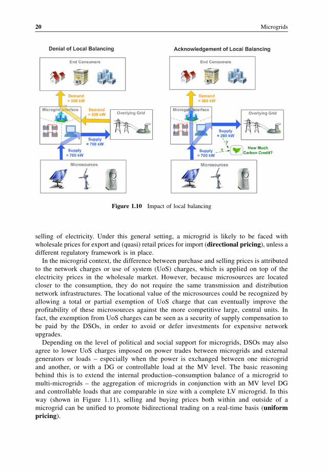
selling of electricity. Under this general setting, a microgrid is likely to be faced with

wholesale prices for export and (quasi) retail prices for import (directional pricing), unless a

different regulatory framework is in place.

In the microgrid context, the difference between purchase and selling prices is attributed

to the network charges or use of system (UoS) charges, which is applied on top of the

electricity prices in the wholesale market. However, because microsources are located

closer to the consumption, they do not require the same transmission and distribution

network infrastructures. The locational value of the microsources could be recognized by

allowing a total or partial exemption of UoS charge that can eventually improve the

profitability of these microsources against the more competitive large, central units. In

fact, the exemption from UoS charges can be seen as a security of supply compensation to

be paid by the DSOs, in order to avoid or defer investments for expensive network

upgrades.

Depending on the level of political and social support for microgrids, DSOs may also

agree to lower UoS charges imposed on power trades between microgrids and external

generators or loads – especially when the power is exchanged between one microgrid

and another, or with a DG or controllable load at the MV level. The basic reasoning

behind this is to extend the internal production–consumption balance of a microgrid to

multi-microgrids – the aggregation of microgrids in conjunction with an MV level DG

and controllable loads that are comparable in size with a complete LV microgrid. In this

way (shown in Figure 1.11), selling and buying prices both within and outside of a

microgrid can be unified to promote bidirectional trading on a real-time basis (uniform

pricing).

Figure 1.10 Impact of local balancing

20 Microgrids

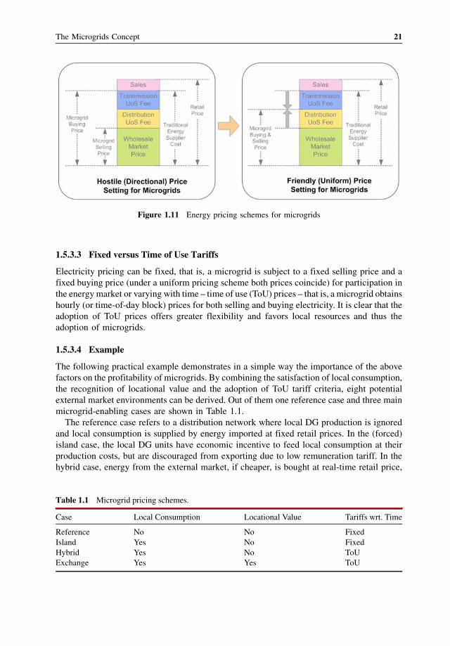
1.5.3.3 Fixed versus Time of Use Tariffs

Electricity pricing can be fixed, that is, a microgrid is subject to a fixed selling price and a

fixed buying price (under a uniform pricing scheme both prices coincide) for participation in

the energymarket or varying with time – time of use (ToU) prices – that is, a microgrid obtains

hourly (or time-of-day block) prices for both selling and buying electricity. It is clear that the

adoption of ToU prices offers greater flexibility and favors local resources and thus the

adoption of microgrids.

1.5.3.4 Example

The following practical example demonstrates in a simple way the importance of the above

factors on the profitability of microgrids. By combining the satisfaction of local consumption,

the recognition of locational value and the adoption of ToU tariff criteria, eight potential

external market environments can be derived. Out of them one reference case and three main

microgrid-enabling cases are shown in Table 1.1.

The reference case refers to a distribution network where local DG production is ignored

and local consumption is supplied by energy imported at fixed retail prices. In the (forced)

island case, the local DG units have economic incentive to feed local consumption at their

production costs, but are discouraged from exporting due to low remuneration tariff. In the

hybrid case, energy from the external market, if cheaper, is bought at real-time retail price,

Figure 1.11 Energy pricing schemes for microgrids

Table 1.1 Microgrid pricing schemes.

Case Local Consumption Locational Value Tariffs wrt. Time

Reference No No Fixed

Island Yes No Fixed

Hybrid Yes No ToU

Exchange Yes Yes ToU


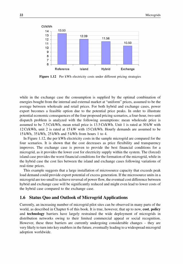
while in the exchange case the consumption is supplied by the optimal combination of

energies bought from the internal and external market at “uniform” prices, assumed to be the

average between wholesale and retail prices. For both hybrid and exchange cases, power

export becomes a feasible option due to the potential price peaks. In order to illustrate

potential economic consequences of the four proposed pricing scenarios, a four-hour, two-unit

dispatch problem is analyzed with the following assumptions: mean wholesale price is

assumed to be 7.5 Ct/kWh, mean retail price is 13.5 Ct/kWh. Unit 1 is rated at 30 kW with

12Ct/kWh, unit 2 is rated at 15 kW with 15Ct/kWh. Hourly demands are assumed to be

15 kWh, 35 kWh, 25 kWh and 5 kWh from hours 1 to 4.

In Figure 1.12, the per kWh electricity costs in the sample microgrid are compared for the

four scenarios. It is shown that the cost decreases as price flexibility and transparency

improves. The exchange case is proven to provide the best financial conditions for a

microgrid, as it provides the lower cost for electricity supply within the system. The (forced)

island case provides the worst financial conditions for the formation of the microgrid, while in

the hybrid case the cost lies between the island and exchange cases following variations of

real-time prices.

This example suggests that a large installation of microsource capacity that exceeds peak

load demand could provide export potential of excess generation. If the microsource units in a

microgrid are too small to achieve reversal of power flow, the eventual cost difference between

hybrid and exchange case will be significantly reduced and might even lead to lower costs of

the hybrid case compared to the exchange case.

1.6 Status Quo and Outlook of Microgrid Applications

Currently, an increasing number of microgrid pilot sites can be observed in many parts of the

world, as described in Chapter 6 of this book. It is true, however, that up to now, cost, policy

and technology barriers have largely restrained the wide deployment of microgrids in

distribution networks owing to their limited commercial appeal or social recognition.

However, these three barriers are currently undergoing considerable changes – they are

very likely to turn into key enablers in the future, eventually leading to a widespread microgrid

adoption worldwide.

Figure 1.12 Per kWh electricity costs under different pricing strategies

22 Microgrids

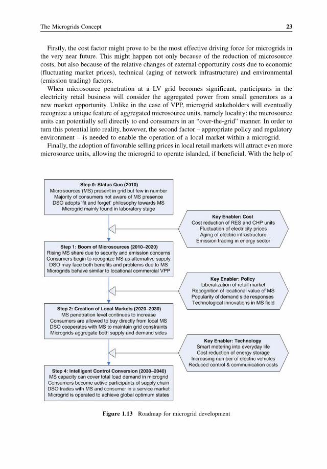
Firstly, the cost factor might prove to be the most effective driving force for microgrids in

the very near future. This might happen not only because of the reduction of microsource

costs, but also because of the relative changes of external opportunity costs due to economic

(fluctuating market prices), technical (aging of network infrastructure) and environmental

(emission trading) factors.

When microsource penetration at a LV grid becomes significant, participants in the

electricity retail business will consider the aggregated power from small generators as a

new market opportunity. Unlike in the case of VPP, microgrid stakeholders will eventually

recognize a unique feature of aggregated microsource units, namely locality: the microsource

units can potentially sell directly to end consumers in an “over-the-grid” manner. In order to

turn this potential into reality, however, the second factor – appropriate policy and regulatory

environment – is needed to enable the operation of a local market within a microgrid.

Finally, the adoption of favorable selling prices in local retail markets will attract evenmore

microsource units, allowing the microgrid to operate islanded, if beneficial. With the help of

Figure 1.13 Roadmap for microgrid development


smart metering, control and communication technologies, the microgrid operator will

eventually be able to coordinate a large consortium of intermittent and controllable micro-

source units, as well as central and distributed storage devices, to achieve multiple objectives

and, at the same time, to cater for the interests of different stakeholders. Figure 1.13 provides

an exemplary roadmap for microgrid development in Europe [8].

References

1. CIGRE (June 2011) Report on behalf of the Technical Committee. “Network of the Future”, Electricity Supply

Systems of the Future, Electra, No 256.

2. Smartgrids, European Technology Platform on Vision and Strategy for Europe’s Electricity Networks of the

Future. s.l.: EUR 22040, 2006.

3. PeScas Lopes, J.A., Hatziargyriou, N., Mutale, J. et al. (2007) Integrated distributed generation into electric power

systems: A review of drivers, challenges and opportunities. Elsevier Electr. Pow. Syst. Res., 77 (9).

4. Pepermans, G., Driesen, J., Haeseldonckx, D. et al. (2005) Distributed generation: definition, benefits and issues.

Int. J. Energy Policy, 33 (6), 787–798.

5. Lasseter, R., Akhil, A., Marnay, C. et al. (April 2002) White paper on Integration of Distributed Energy

Resources – The CERTSMicroGrid Concept. s.l.: Office of Power Technologies of the US Department of Energy,

Contract DE-AC03-76SF00098.

6. Lasseter, R.H. (2002) MicroGrids. IEEE Power Engineering Society Winter Meeting Conference Proceedings,

vol. 1., New York, NY: s.n., pp. 305–308.

7. “Microgrids: Large Scale Integration of Micro-Generation to Low Voltage Grids”, ENK5-CT-2002-00610.

2003–2005.

8. “More microgrids: Advanced Architectures and Control Concepts for More microgrids”, FP6 STREP, Proposal/

Contract no.: PL019864. 2006–2009.

9. Hatziargyriou, N. (2004) MicroGrids. 1st International Conference on the Integration of Renewable Energy

Sources and Distributed Energy Resources (IRED). Brussels: s.n., 1–3 December.

10. Hatziargyriou, N., Asano, H., Iravani, R. and Marnay, C. (July/August 2007) microgrids: An Overview of

Ongoing Research, Development and Demonstration Projects. IEEE Power and Energy, Vol. 5, Nr. 4, pp. 78–94.

11. Hatziargyriou, N. (May–June 2008,) Microgrids [guest editorial]. IEEE Power and Energy Magazine, Volume 6,

Issue 3, pp. 26–29.

12. Karfopoulos, E.L. et al. (25–28 Sept 2011) Introducing electric vehicles in the microgrids concept. 16th

International Conference on Intelligent Systems Application to Power Systems, Hersonissos, Heraklion, Greece.

13. Eurelectric Policy Paper. “Customer-Centric Retail Markets: A Future-Proof Market Design”. September 2011.

14. CIGRE WG C6.09. “Demand Side Integration”, Technical Brochure, August 2010.

15. Eurelectric, Thermal Working Group (February 2004) Ancillary Services: Unbundling Electricity Products – an

Emerging Market, Ref: 2003-150-0007.

24 Microgrids

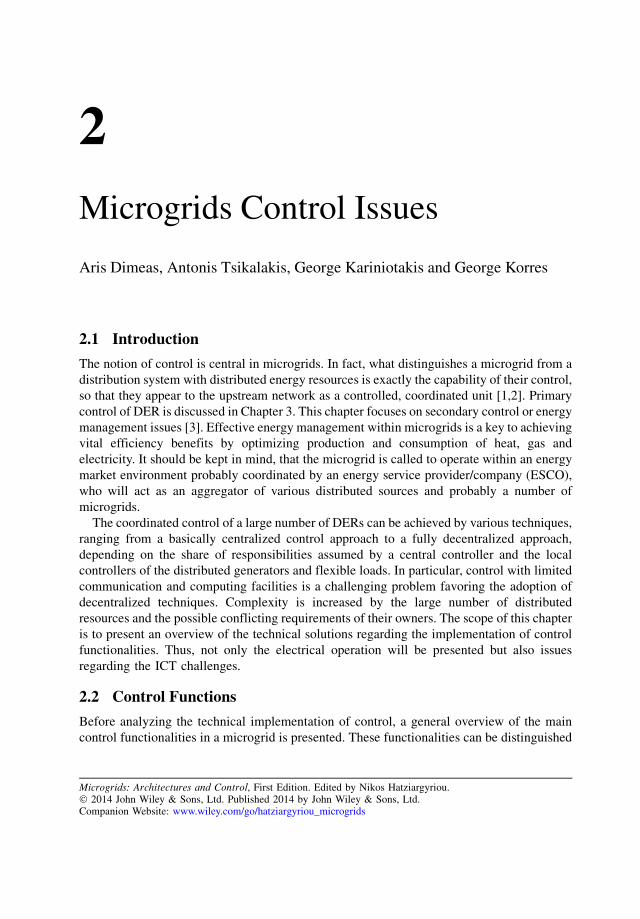
2

Microgrids Control Issues

Aris Dimeas, Antonis Tsikalakis, George Kariniotakis and George Korres

2.1 Int roduction

The notion of control is cent ral in micro grids. In fact, what disti nguishes a micro grid from a

distribution system with distributed energy resource s is exactly the capab ility of their cont rol,

so that they appea r to the upstream networ k as a control led, coord inated unit [1,2]. Primary

control of DER is discusse d in Chapte r 3. This chapter focuses on secondary control or energy

managem ent issues [3]. Effective energy man agement withi n micro grids is a key to achieving

vital efficiency benefits by optimizing production and consumpt ion of heat, gas and

elect ricity. It shoul d be kept in mind, that the micro grid is cal led to operate within an energy

market envir onment proba bly coordina ted by an energy service provider/company (ES CO),

who will act as an aggregator of vari ous distributed sourc es and proba bly a number of

micro grids.

The coord inated control of a large numb er of DERs can be achieved by various techniques,

ranging from a basically centrali zed cont rol appro ach to a fully decen tralize d approach,

depend ing on the shar e of resp onsibiliti es assumed by a central controlle r and the loca l

control lers o f the distributed generat ors and flexible loads. In particula r, control with limited

commun ication and computing facilitie s is a chal lenging problem favoring the adopt ion of

decen tralize d techniqu es. Compl exity is increased by the large numb er of distributed

resource s and the possibl e confli cting require ments of their owne rs. The scope of this chapt er

is to pres ent an overview of the technic al solu tions regarding the impleme ntation o f cont rol

functi onalitie s. Thus, not only the electrical opera tion will be p resented but also issues

regarding the IC T chal lenges.

2.2 Control Func tions

Before analyzing the technical implementation of control, a general overview of the main

control functionalities in a microgrid is presented. These functionalities can be distinguished



in three groups, as shown in Figure 2.1. The lower level is closely related to the individual

components and local control (micro sources, storage, loads and electronic interfaces), the

medium level to the overall microgrid control and the upper level to the interface to the

upstream network.

More specifically:

Upstream network interface

The core interaction with the upstream network is related to market participation, more

specifically the microgrid actions to import or export energy following the decisions of the

ESCO. Owing to the relatively small size of a microgrid, the ESCO can manage a larger

number of microgrids, in order to maximize its profit and provide ancillary services to the

upstream network. The operation of multi-microgrids is discussed in Chapter 5.

Internal microgrid control

This level includes all the functionalities within the microgrid that require the collaboration of

more than two actors. Functions within this level are:� load and RES forecast,� load shedding/management,� unit commitment/dispatch,� secondary voltage/frequency control,� secondary active/reactive power control,� security monitoring,� black start.

Local control

This level includes all the functionalities that are local and performed by a single DG, storage

or controllable load, that is:� protection functions,� primary voltage/frequency control,

Figure 2.1 Overall system functionalities

26 Microgrids

� primary active/reactive power control,� battery management.

It should be noted that these functionalities are relevant to the normal state of operation.

They might need to change in critical or emergency states, as discussed in Chapter 5.

Chapter 2 focuses on internal microgrid control (management) in the normal state of

operation. The normal state covers both islanded and interconnected mode and does not deal

with transition to island mode. The role of information and communication technology is

critical for the relevant control functions.

2.3 The Role of Information and Communication Technology

Information and communication technology (ICT) is a critical component of future power

networks. Beyond any doubt, the control and operation of the future power grids, including

microgrids, needs to be supported by sophisticated information systems (ISs) and advanced

communication networks. Currently, several technologies have been used or tested at

distribution systems and it is expected that their usage will become more extensive during

the coming years. The usual approach is to use existing solutions as a starting point, in

order to develop new applications for microgrids. The main technological areas are as

follows:

Microprocessors

Modern microprocessors are utilized extensively within microgrids providing the ability to

develop sophisticated inverters and to develop load controllers or other active components

within microgrids. An interesting characteristic of the new version of microprocessors is that

they provide adequate processing power, communication capabilities and sophisticated

software-middleware at low prices.

Communication

The past decade has been characterized by developments in communication networks and

systems. These networks provide sufficient bandwidth and can offer several services to the

users. It is obvious that active control of microgrids will be based on existing communication

infrastructures, in order to reduce the cost.

SoftwareService oriented architectures (SOA) is the modern trend in building information systems. The

core of this approach is the web service. The W3C (World Wide Web Consortium [4]) defines

a “web service” as “a software system designed to support interoperable machine-to-machine

interaction over a network”. There are many definitions of the concept of SOA. For the

purpose of this chapter an SOA is defined as a set of web services properly organized in

multiple layers, capable of solving a set of complex problems.

The internet of energy

The internet of energy is the usage of technologies, developed for the world wide web, that

allows avoiding installation and maintenance costs of dedicated devices for the control of DGs

and loads.With this approach, all the applications for household control could take the form of

a piece of software running on a device with processing capabilities: a smart TVor the internet

Microgrids Control Issues 27

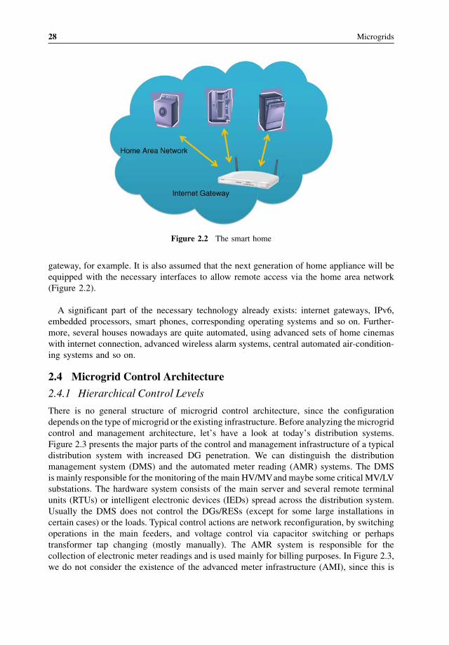
gateway, for example. It is also assumed that the next generation of home appliance will be

equipped with the necessary interfaces to allow remote access via the home area network

(Figure 2.2).

A significant part of the necessary technology already exists: internet gateways, IPv6,

embedded processors, smart phones, corresponding operating systems and so on. Further-

more, several houses nowadays are quite automated, using advanced sets of home cinemas

with internet connection, advanced wireless alarm systems, central automated air-condition-

ing systems and so on.

2.4 Microgrid Control Architecture

2.4.1 Hierarchical Control Levels

There is no general structure of microgrid control architecture, since the configuration

depends on the type of microgrid or the existing infrastructure. Before analyzing the microgrid

control and management architecture, let’s have a look at today’s distribution systems.

Figure 2.3 presents the major parts of the control and management infrastructure of a typical

distribution system with increased DG penetration. We can distinguish the distribution

management system (DMS) and the automated meter reading (AMR) systems. The DMS

is mainly responsible for the monitoring of the main HV/MVand maybe some critical MV/LV

substations. The hardware system consists of the main server and several remote terminal

units (RTUs) or intelligent electronic devices (IEDs) spread across the distribution system.

Usually the DMS does not control the DGs/RESs (except for some large installations in

certain cases) or the loads. Typical control actions are network reconfiguration, by switching

operations in the main feeders, and voltage control via capacitor switching or perhaps

transformer tap changing (mostly manually). The AMR system is responsible for the

collection of electronic meter readings and is used mainly for billing purposes. In Figure 2.3,

we do not consider the existence of the advanced meter infrastructure (AMI), since this is

Figure 2.2 The smart home

28 Microgrids

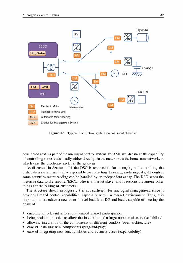
considered next, as part of the microgrid control system. By AMI, we also mean the capability

of controlling some loads locally, either directly via the meter or via the home area network, in

which case the electronic meter is the gateway.

As discussed in Section 1.5.1 the DSO is responsible for managing and controlling the

distribution system and is also responsible for collecting the energy metering data, although in

some countries meter reading can be handled by an independent entity. The DSO sends the

metering data to the supplier/ESCO, who is a market player and is responsible among other

things for the billing of customers.

The structure shown in Figure 2.3 is not sufficient for microgrid management, since it

provides limited control capabilities, especially within a market environment. Thus, it is

important to introduce a new control level locally at DG and loads, capable of meeting the

goals of

� enabling all relevant actors to advanced market participation� being scalable in order to allow the integration of a large number of users (scalability)� allowing integration of the components of different vendors (open architecture)� ease of installing new components (plug-and-play)� ease of integrating new functionalities and business cases (expandability).

Figure 2.3 Typical distribution system management structure


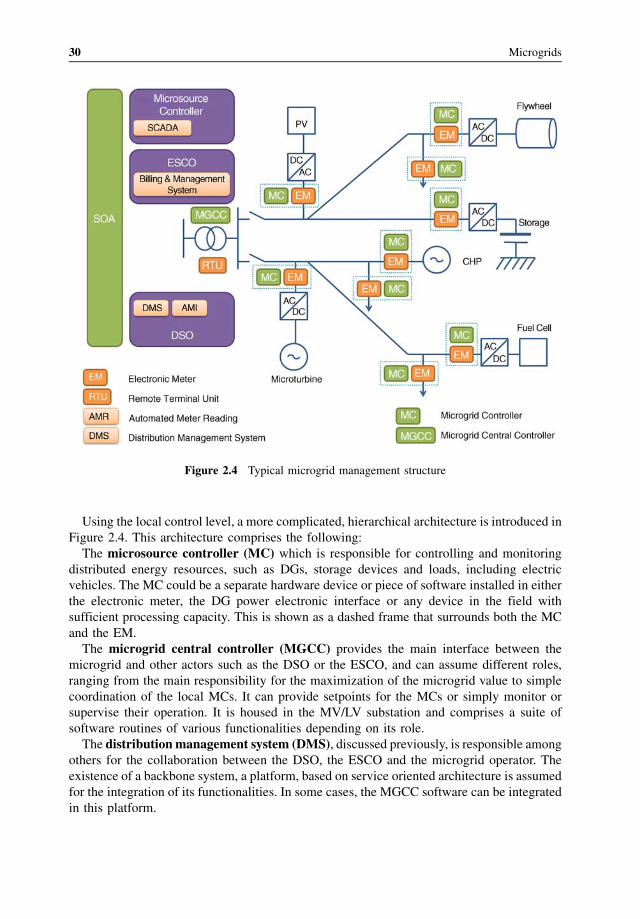
Using the local control level, a more complicated, hierarchical architecture is introduced in

Figure 2.4. This architecture comprises the following:

The microsource controller (MC) which is responsible for controlling and monitoring

distributed energy resources, such as DGs, storage devices and loads, including electric

vehicles. The MC could be a separate hardware device or piece of software installed in either

the electronic meter, the DG power electronic interface or any device in the field with

sufficient processing capacity. This is shown as a dashed frame that surrounds both the MC

and the EM.

The microgrid central controller (MGCC) provides the main interface between the

microgrid and other actors such as the DSO or the ESCO, and can assume different roles,

ranging from the main responsibility for the maximization of the microgrid value to simple

coordination of the local MCs. It can provide setpoints for the MCs or simply monitor or

supervise their operation. It is housed in the MV/LV substation and comprises a suite of

software routines of various functionalities depending on its role.

The distribution management system (DMS), discussed previously, is responsible among

others for the collaboration between the DSO, the ESCO and the microgrid operator. The

existence of a backbone system, a platform, based on service oriented architecture is assumed

for the integration of its functionalities. In some cases, the MGCC software can be integrated

in this platform.

Figure 2.4 Typical microgrid management structure

30 Microgrids

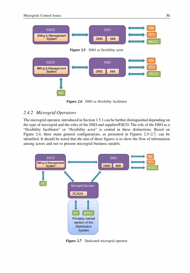
2.4.2 Microgrid Operators

The microgrid operator, introduced in Section 1.5.1 can be further distinguished depending on

the type of microgrid and the roles of the DSO and supplier/ESCO. The role of the DSO as a

“flexibility facilitator” or “flexibility actor” is central in these distinctions. Based on

Figure 2.4, three main general configurations, as presented in Figures 2.5–2.7, can be

identified. It should be noted that the aim of these figures is to show the flow of information

among actors and not to present microgrid business models.

Figure 2.5 DSO as flexibility actor

Figure 2.6 DSO as flexibility facilitator

Figure 2.7 Dedicated microgrid operator


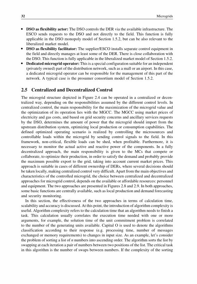
� DSO as flexibility actor: The DSO controls the DER via the available infrastructure. The

ESCO sends requests to the DSO and not directly to the field. This function is fully

applicable in the DSO monopoly model of Section 1.5.2, but can be also relevant to the

liberalized market model.� DSO as flexibility facilitator: The supplier/ESCO installs separate control equipment in

the field and directly manages at least some of the DER. There is close collaboration with

the DSO. This function is fully applicable in the liberalized market model of Section 1.5.2.� Dedicatedmicrogrid operator: This is a special configuration suitable for an independent

(privately owned) part of the distribution network, such as a mall or an airport. In this case,

a dedicated microgrid operator can be responsible for the management of this part of the

network. A typical case is the prosumer consortium model of Section 1.5.2.

2.5 Centralized and Decentralized Control

The microgrid structure depicted in Figure 2.4 can be operated in a centralized or decen-

tralized way, depending on the responsibilities assumed by the different control levels. In

centralized control, the main responsibility for the maximization of the microgrid value and

the optimization of its operation lies with the MGCC. The MGCC using market prices of

electricity and gas costs, and based on grid security concerns and ancillary services requests

by the DSO, determines the amount of power that the microgrid should import from the

upstream distribution system, optimizing local production or consumption capabilities. The

defined optimized operating scenario is realized by controlling the microsources and

controllable loads within the microgrid by sending control signals to the field. In this

framework, non-critical, flexible loads can be shed, when profitable. Furthermore, it is

necessary to monitor the actual active and reactive power of the components. In a fully

decentralized approach, the main responsibility is given to the MCs that compete or

collaborate, to optimize their production, in order to satisfy the demand and probably provide

the maximum possible export to the grid, taking into account current market prices. This

approach is suitable in cases of different ownership of DERs, where several decisions should

be taken locally, making centralized control very difficult. Apart from the main objectives and

characteristics of the controlled microgrid, the choice between centralized and decentralized

approaches for microgrid control, depends on the available or affordable resources: personnel

and equipment. The two approaches are presented in Figures 2.8 and 2.9. In both approaches,

some basic functions are centrally available, such as local production and demand forecasting

and security monitoring.

In this section, the effectiveness of the two approaches in terms of calculation time,

scalability and accuracy is discussed. At this point, the introduction of algorithm complexity is

useful. Algorithm complexity refers to the calculation time that an algorithm needs to finish a

task. This calculation usually correlates the execution time needed with one or more

arguments, for example, the solution time of the unit commitment problem is correlated

to the number of the generating units available. Capital O is used to denote the algorithms

classification according to their response (e.g. processing time, number of messages

exchanged or memory requirements) to changes in input size. As an example, let’s consider

the problem of sorting a list of n numbers into ascending order. The algorithm sorts the list by

swapping at each iteration a pair of numbers between two positions of the list. The critical task

in this algorithm is the number of swaps between numbers. If the complexity of the sorting

32 Microgrids

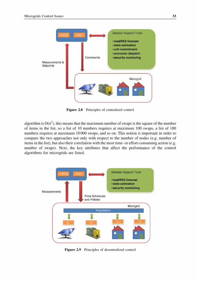
algorithm is O(n2), this means that the maximum number of swaps is the square of the number

of items in the list, so a list of 10 numbers requires at maximum 100 swaps, a list of 100

numbers requires at maximum 10 000 swaps, and so on. This notion is important in order to

compare the two approaches not only with respect to the number of nodes (e.g. number of

items in the list), but also their correlation with the most time- or effort-consuming action (e.g.

number of swaps). Next, the key attributes that affect the performance of the control

algorithms for microgrids are listed.

Figure 2.8 Principles of centralized control

Figure 2.9 Principles of decentralized control


� Number of nodes: A microgrid consists of several microsources and controllable loads.

The number of DERs affects critically the complexity of the problem and the computa-

tional time.� Number of message exchanges: DGs and loads in microgrids are usually dispersed, and

communication systems at LVusually have limited bandwidth. In several cases the number

of messages required to perform a task is of primary importance. A decentralized control

approach reduces the number of messages, since only a small part of the information is

transferred to the higher levels of control hierarchy.� Size and structure of the systemmodel: The structure and complexity of the system need

to be considered. Decisions taken by different actors might not only increase the number of

nodes, but also impose extra technical and non-technical constraints. A relevant issue is the

level of information, such as what parameter or constraint should be made available for the

decision process of the various actors. For example, the state of charge of a battery might be

important to the neighboring DGs, while the internal temperature or voltage level of a cell

and the associated technical constraints, might not be relevant.� Accuracy and optimality: An algorithm may converge to the optimal solution or near the

optimal solution. It is self-evident that the convergence and the accuracy of the solutions

depend on the accuracy of the models used and of the relevant input data. The question is

whether a suboptimal solution is acceptable and, if so, at what cost.

The choice between the centralized and decentralized approach for microgrid control,

depends on the main objectives and the special characteristics of the controlled microgrid and

the available or affordable resources: personnel and equipment.

Clearly, centralized control is more suitable if the users of the microgrid (DG and load

owners) have common goals or a common operational environment seeking cooperation, in

order to meet their goals. Such an example is an industrial microgrid, in which a single owner

might exercise full control of all its energy sources and loads, is able to continuously monitor

them and aims to operate the system in the most economical way. Considering the general

attributes listed earlier, the number of nodes is generally limited and it is relatively easy to

install a fast communication system and a set of sensors. Dedicated operating personnel for

the operation of the microgrid might be available. Furthermore, the optimization problem has

a limited set of constraints and specific objectives, such as cost minimization. Finally, the

requested solution should be as accurate as possible since a suboptimal solution may lead to

profit losses.

Microgrids operating in a market environment might require that competitive actions of the

controller of each unit have a certain degree of independence and intelligence. Furthermore,

local DER owners might have different objectives: in addition to selling power to the network,

they might have other tasks, such as producing heat for local installations, keeping the voltage

locally at a certain level or providing a backup system for local critical loads in case of main

system failure. Some microgrid customers might primarily seek their own energy cost

minimization and have diverse needs, although they all might benefit from the common

objective of lowering operating costs of their feeder. In a residential microgrid, for example,

one household might have at one particular moment increased electric energy needs, for

example for cooking, while another household might need no electricity at all, because all its

tenants are absent. Both households would like to sell the extra power produced locally to the

grid, but it is unlikely that they would accept remote control of their production. Considering

34 Microgrids

again the general attributes mentioned earlier, we should identify that in this case the number

of nodes might increase significantly. A neighborhood might have dozens of households or

installed DGs, and if we consider multi-microgrids the number is increasing further. In such

cases, it is not possible to have a dedicated communication system, but existing infrastructure

should be used. Thus, part of the system might not have sufficient bandwidth or the

communication could be expensive. An approach that limits the amount of data transfer

is essential. The availability of powerful computing facilities or dedicated operators is also

highly unlikely.

Furthermore, the optimization problem is becoming extremely complex, as a result of

specific characteristics. For example, it is extremely complicated to model the comfort

requirements in each household or to include all the special technical constraints of all

appliances in a single optimization problem. The decentralized approach suggests that this

type of constraint and sub-problem should be solved locally in each household or DG. In the

general control problem, each household could be presented as a load node that has the

ability to shed or shift some load, or a production node with DGs that can offer a certain

amount of energy without caring about the type of the engine or the technical constraints.

Finally, in this case, a suboptimal solution is probably acceptable, given the high costs of

the installation of fast communication networks or powerful processors dedicated to energy

optimization.

Another important factor is the openness of the system. The distributed computing

technology allows DG manufacturers and loads to provide plug-and-play components by

embedding control agents (following some rules) in their devices. The software should be

intelligent enough to monitor the process and follow the best policy. The availability of

dedicated personnel responsible for system installation and maintenance, likely in centralized

systems, might relax this requirement to some extent. In this case, dedicated personnel could

also be available for monitoring the process, which could intervene in an emergency.

The general conclusion is that the centralized approach is suitable for a system with one

specific goal and a decentralized one in a system with several goals.

The above considerations are summarized in the Table 2.1.

2.6 Forecasting

2.6.1 Introduction

Both centralized and decentralized control approaches require forecasts of the electricity

demand, heat demand, generation from renewable power sources and external electricity

prices, for the next few hours, as shown in Figures 2.8 and Figure 2.9. Forecasting the

evolution of these quantities allows us to face unsafe situations and to optimize production

costs and in general to maximize revenues of the production process in the marketplace. As a

consequence, forecasting options may have a direct impact on the economic viability of

microgrids, since they allow them to enhance their competitiveness compared to centralized

generation.

The aim of this section is to introduce the problem of short-term forecasting in the frame of

microgrids and to provide example methods for forecasting relevant quantities. It is recog-

nized, however, that it is still premature to propose a particular operational forecasting tool

for microgrids. First, the role of forecasting functionalities in microgrids needs to be

discussed.


2.6.1.1 Are Forecasting Functionalities Relevant for Microgrids?

Depending on the mode of operation, it is clear that in islanded operation, prediction of

demand is of primary importance, since the aim is to achieve the balance of the system. In

interconnected operation, however, the importance of demand or production forecasting may

change, depending on the focus – a system-driven or a customer-driven approach. In the first

case, forecasting functions may have less importance since we may consider that a microgrid

connected to an “infinite” source of power is able to cover any deficit at any time. However, in

a customer-driven approach, economics – and thus forecasting – gain in importance. If

microgrids is the “business case” of an energy service provider, who has to consider electricity

prices, then decisions will be based on forecasting. Forecasting functions gain in importance

when one considers multi-microgrids scenarios.

The scale of a microgrid imposes the consideration of cost-effective approaches for

forecasting. Today, forecasting technology for renewable generation is not plug-and-play.

Developing and implementing forecasting options for a power system application involves

costs for research and development, instrumentation for data collection, operational costs for

numerical weather predictions and so on. Forecasts can be provided commercially, either in

the form of a service or by software installed on-site. In any case, forecasting solutions have

a price that should be compared to the benefits they provide. Decentralizing power generation,

especially by adding renewables, adds intermittency in power generation, and retaining the

same quality of service means that accurate forecasting is a cost-effective solution to

counterbalance intermittency. Another relevant issue is the acceptability of power system

operators, who are used to manage almost deterministic processes; for example, they are able,

even without mathematical tools, to forecast the system load with an impressive accuracy of a

Table 2.1 Considerations in the applicability of centralized and decentralized control. Reproduced by

permission of the IEEE

Centralized control Decentralized control

DG ownership Single owner Multiple owners

Goals A clear, single task, e.g.

minimization of energy costs

Uncertainty over what each

owner wants at any particular

moment

Availability of operating

personnel (monitoring, low-

level management, special

switching operations, etc.)

Available Not available

Market participation Implementation of complicated

algorithms

Owners unlikely to use complex

algorithms

Installation of new equipment Requirements of specialized

personnel

Should be plug-and-play

Optimality Optimal solutions Mostly suboptimal solutions

Communication requirements High Modest

Market participation All units collaborate Some units may be competitive

Microgrid operation is attached

to a larger and more critical

operation

Possible Not possible

36 Microgrids

few percent. The capacity to accept more intermittent options is linked to the capacity to

provide tools to compensate intermittency and manage uncertainties. This is especially true, in

electricity market operation, where penalties are associated to uncertainties, and decisions

have to be taken as a function of the prices in the near future.

Considerable work in the power systems area has been devoted to forecasting demand, wind

power, heat demand and, more recently, electricity prices and PV generation. The work,

especially on demand, concerns mainly large interconnected systems. Less experience is

available on forecasting for smaller systems and with a high temporal resolution (i.e.

5–10minutes) for the next 1–4 hours. For this reason, in very small applications persistence

is usually applied. This is a simple method saying that the predicted variable will retain the

current value during the next period:

P̂ tþ kð Þ ¼ P tð Þ; k ¼ 1; 2; . . . n (2.1)

This can be the baseline model for heat, wind and price forecasting, while for load or PV

generation one could use the “diurnal persistence” which consists in using as forecast the

measured value of the process at the same hour of the previous day. Using this model for

taking decisions may reduce benefits, especially in electricity markets with highly volatile

prices. In order to quantify the value of forecasting, we need to simulate the operation of a

microgrid using persistence against perfect forecasting. The difference between the twowould

indicate the interest in investing in advanced forecasting methods. Results from such a study

would, however, be difficult to generalize, since they depend critically on the structure of the

microgrid and the characteristics of the electricity market.

2.6.2 Demand Forecasting

In interconnected or large island power systems, demand depends on weather conditions,

habits and activities of the customers and thus it is highly correlated to the time of day and the

type of the day or season of the year. Predictions are usually required for the next 24/48 hours

in hourly or 30-minute time steps. Typically, forecasting accuracy is high – in the order of

1–5% – depending on the time horizon and the type/size of the system. Uncertainty can be

estimated by classical methods, such as resampling. A large number of methods for load

forecasting can be found in the literature, for example, an extended review focusing on

artificial intelligence based techniques is given in [5,6].

Downscaling the demand prediction problem to smaller power systems, such as the systems

of islands, increases the difficulties, because the variability of the load also increases. At the

level of a microgrid, the aggregation or smoothing effect is significantly reduced, and

uncertainty increases as the size of the system gets smaller. To meet this difficulty we should

add the increase in time resolution. We enter the area of very-short-term forecasting with

reduced smoothing effects [7]. However, at the level of a feeder, the aggregation is still enough

so that time-series approaches can be applied for forecasting. When it gets down to the level of

a single client (i.e. demand of a house) there is, in general, a lack of measured data to

adequately characterize the problem. The deployment of smart meters permits the collection

of data for that purpose.

The shortest time resolution for load forecasting in microgrids could not be less than

5–10minutes, if one would like to speak about large-scale applications. The load patterns of


individual customers can be highly correlated with each other, that is, due to external

temperature dependency. First attempts to predict customer load using smart meter data

show that such data have a quite high variability, but there is still a prominent daily pattern that

makes the time series predictable. First evaluation results suggest an accuracy at the level of

30% of mean absolute percentage error. In contrast to the classical load forecasting problem, it

is also expected that the demand will be correlated to electricity prices, especially when

customer behavior is influenced by dynamic demand-side management actions. Prediction

models for demand may consider electricity prices as input (predictions) to accommodate this

correlation.

2.6.2.1 Contribution of Weather Predictions to Operation at Best Efficiency Point

The consideration of weather forecasts as a general input to the various forecasting functions

in the MGCC seems to be an option that may be exploited in multiple ways. Apart from their

use for reliable forecasting of production of renewable units and power demand, the role of

weather forecasts can be also important in predicting the operation (efficiency) of micro

turbines. This aspect is also important in larger-scale systems or multi-microgrid systems. For

light load conditions, it would be better to have fewer microturbines running, but running at

rated load, than to have several microturbines running at partial load. This is because

microturbines are more efficient when operating at rated load. The decision of how many

machines to run, and at what load, can best be made by the MGCC, because it has knowledge

of the process condition, the weather forecast and the production schedule. This requirement

is also identified in [2] for energy management systems destined for microgrids.

2.6.3 Wind and PV Production Forecasting

Although for microgrids developed in urban environments, wind energy might not be

widely adopted, small wind turbines can provide a viable option with a high potential in

several cases. Short-term forecasting is of primary importance for integrating wind

energy, especially in larger power systems, and there is very rich literature on the

subject. Research in wind power forecasting is a multidisciplinary field, since it combines

areas such as meteorology, statistics, physical modeling, computational intelligence [8].

Similar efforts exist in other areas, such as forecasting of PV, heat and hydro. An excellent

reference with a detailed state of the art on wind power forecasting is provided in [9].

In the case of very-short-term wind power prediction a review of available models is

given in [10].

In microgrids, forecasts of renewable generation can be provided in a centralized way (i.e.

in the case of an MGCC) using input from weather forecasts and past measurements. In a

decentralized management approach, where local intelligence has to be considered (i.e. at the

level of customers with PV panels and batteries), plug-and-play approaches that use basic

weather forecasts from the internet, or simply measurements, can be considered. The plug-

and-play capacity refers to the requirement for low human intervention and also to the

possibility of providing forecasts of adequate accuracy in cases with little history of measured

data available, as can be the case with new PV plant installations. Both physical methods and

statistical methods, such as fuzzy neural networks, random forests, regime switching and

kernel density estimators, can be used.

38 Microgrids

2.6.4 Heat Demand Forecasting

Forecasting heat consumption is a necessary functionality for the MGCC of a micro-CHP

based microgrid. The main factors affecting heat demand are:

� time of day effect,� weekend/weekday effect,� seasonal effects,� time varying volatility,� high negative correlation between heat demand and external temperature.

Several approaches have been developed for online prediction of heat consump-

tion in district heating systems. The time horizon is often 72 hours and the time step

hourly.

The simpler approaches are based on purely autoregressive moving average (ARMA)

models that use only heat demand data as input. Models considering seasonal differencing

have been also applied. As an extension, models are also considered with temperature as

an explanatory variable. More advanced developments assume that meteorological

forecasts are available online, although such a facility is not commonly expected in

microgrids.

The methods of prediction applied are based on adaptive estimation that allows for

adaptation to slow changes in the system. This approach is also used to track the transition

from, say, warm to cold periods. Due to different preferences of the households to which the

heat is supplied, this transition is smooth.

Alternatively, black box models such as neural networks [11,12] or fuzzy logic neural

networks can be applied. In this case, more flexibility is gained regarding the structure of the

model and the available information according to the application.

2.6.5 Electricity Prices Forecasting

Short-term forecasting of electricity prices may be important in volatile electricity markets.

Spot prices may significantly influence decisions on the use of microsources. Various

approaches have been tested for this purpose. Electricity prices vary from other commodities

because the primary good, electricity, cannot be stored, implying that inventories cannot be

created and managed to arbitrage prices over time. As an example, the process in the Leipzig

Power Exchange can be characterized by the following features [12,13]:

� strong mean reversion: deviation of the price due to random effects are corrected to a

certain degree,� time of the day effect,� calendar effects such as weekdays, weekends and holidays,� seasonal effects,� time-varying volatility and volatility clustering,� high percentage of unusual prices, mainly in periods of high demand,� inverse leverage effect: a positive price shock has a bigger impact than a negative one,� non-constant mean and variance


Models applied for short-term price forecasting include [14]:

� mean reverting processes� mean reverting processes with time-varying mean� autoregressive moving average models (ARMA)� exponential generalized autoregressive conditional heteroscedasticity models (EGARCH).

2.6.6 Evaluation of Uncertainties on Predictions

In general, statistical methods based on machine learning are among the promising

approaches that can be applied for forecasting purposes in microgrids. However, forecasting

models, especially of load or heat demand, have to be validated with measured data reflecting

the situation in real microgrids. As discussed above, due to the small size of microgrids, the

smoothing effect is reduced due to the limited aggregation of the forecasted processes.

Moreover, the need for higher time resolution results in an increase of intermittency.

Therefore, in parallel to the research on forecasting models, it is necessary to develop

research for online evaluation of the uncertainty of the predictions. Such approaches for wind

power forecasting in larger systems have been developed, and it is today possible to provide

directly probabilistic forecasts for wind or PV prediction. These provide the whole distribu-

tion for each time step and from this one can obtain various uncertainty products such as

quantiles or prediction intervals [15]. Studying the predictability and the variability of the

various processes related to microgrids is of major importance for deciding what kind of

approaches are appropriate for the management functions (i.e. deterministic or probabilistic

ones) [16]. The development of cost-effective prediction tools with plug-and-play capabilities

suitable for the limited facilities of a microgrid environment is still an open research issue.

2.7 Centralized Control

Microgrids can be centrally managed by extending and properly adapting the functionalities

of existing energy management system (EMS) functions. Regarding steady-state operation, as

shown in Figure 2.8, the basic feature of centralized control is that decisions about the

operation of the DER are taken by the microgrid operator or ESCO at the MGCC level. The

MGCC is equipped, among other things, with scheduling routines that provide optimal

setpoints to the MCs, based on the overall optimization objectives. This section describes the

scheduling functions that are required for centralized scheduling of microgrids [17].

The local distributed energy sources, acting either as individual market players or as one

coordinated market player, provide energy and ancillary services by bidding in energy and

ancillary markets, based on the prices provided by the system. Two market policies can be

distinguished: In the first case, the microgrid serves its own needs only, displacing as much

energy from the grid as economically optimal. In the second case, the microgrid participates in

the market probably through an energy service provider or aggregator. Due to its size and the

uncontrollability of the microsources, it is unlikely that the microgrid bids will concern longer

term horizons. It is conceivable, however, to have microgrid bids covering a short time ahead,

say the next 15–30minutes.

Moreover, in normal interconnected operation, individual consumers can participate in the

market operation, providing load flexibility, directly or indirectly, by suitable programmable

controllers. It is assumed that each consumer may have low and high priority loads and would

40 Microgrids

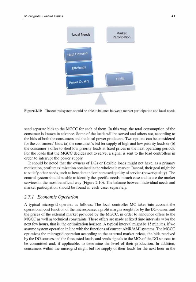
send separate bids to the MGCC for each of them. In this way, the total consumption of the

consumer is known in advance. Some of the loads will be served and others not, according to

the bids of both the consumers and the local power producers. Two options can be considered

for the consumers’ bids: (a) the consumer’s bid for supply of high and low priority loads or (b)

the consumer’s offer to shed low priority loads at fixed prices in the next operating periods.

For the loads that the MGCC decides not to serve, a signal is sent to the load controllers in

order to interrupt the power supply.

It should be noted that the owners of DGs or flexible loads might not have, as a primary

motivation, profit maximization obtained in the wholesale market. Instead, their goal might be

to satisfy other needs, such as heat demand or increased quality of service (power quality). The

control system should be able to identify the specific needs in each case and to use the market

services in the most beneficial way (Figure 2.10). The balance between individual needs and

market participation should be found in each case, separately.

2.7.1 Economic Operation

A typical microgrid operates as follows: The local controller MC takes into account the

operational cost function of the microsource, a profit margin sought for by the DG owner, and

the prices of the external market provided by the MGCC, in order to announce offers to the

MGCC as well as technical constraints. These offers are made at fixed time intervalsm for the

next few hours, that is, the optimization horizon. A typical interval might be 15minutes, if we

assume system operation in line with the functions of current AMR/AMI systems. TheMGCC

optimizes the microgrid operation according to the external market prices, the bids received

by the DG sources and the forecasted loads, and sends signals to the MCs of the DG sources to

be committed and, if applicable, to determine the level of their production. In addition,

consumers within the microgrid might bid for supply of their loads for the next hour in the

Figure 2.10 The control system should be able to balance betweenmarket participation and local needs


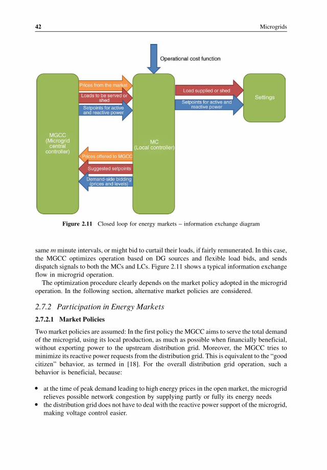
samemminute intervals, or might bid to curtail their loads, if fairly remunerated. In this case,

the MGCC optimizes operation based on DG sources and flexible load bids, and sends

dispatch signals to both the MCs and LCs. Figure 2.11 shows a typical information exchange

flow in microgrid operation.

The optimization procedure clearly depends on the market policy adopted in the microgrid

operation. In the following section, alternative market policies are considered.

2.7.2 Participation in Energy Markets

2.7.2.1 Market Policies

Two market policies are assumed: In the first policy the MGCC aims to serve the total demand

of the microgrid, using its local production, as much as possible when financially beneficial,

without exporting power to the upstream distribution grid. Moreover, the MGCC tries to

minimize its reactive power requests from the distribution grid. This is equivalent to the “good

citizen” behavior, as termed in [18]. For the overall distribution grid operation, such a

behavior is beneficial, because:

� at the time of peak demand leading to high energy prices in the open market, the microgrid

relieves possible network congestion by supplying partly or fully its energy needs� the distribution grid does not have to deal with the reactive power support of the microgrid,

making voltage control easier.

Figure 2.11 Closed loop for energy markets – information exchange diagram

42 Microgrids

From the end-users point of view, the MGCC minimizes operational cost of the microgrid,

taking into account open market prices, demand and DG bids. The end-users of the microgrid

share the benefits of reduced operational costs.

In the second of the two policies, the microgrid participates in the open market, buying and

selling active and reactive power to the grid, probably via an aggregator or energy service

provider. According to this policy, the MGCC tries to maximize the value of the microgrid,

that is, maximize the corresponding revenues of the aggregator, by exchanging power with the

grid. The end-users are charged for their active and reactive power consumption at open

market prices. From the grid’s point of view, this is equivalent to the “ideal citizen” behavior

referred to in [18]. The microgrid behaves as a single generator capable of relieving possible

network congestion not only in the microgrid itself, but also by transferring energy to nearby

feeders of the distribution network.

It should be noted that the MGCC can take into account environmental parameters such as

green house gas (GHG) emissions reductions, optimizing the microgrid operation accordingly.

2.7.2.2 Demand Side Bidding

Each consumer may have low and high priority loads allowing him to send separate bids to the

MGCC for each type of load. Without loss of generality, it is assumed that each consumer

places bids for his demand at two levels, and the prices reflect his priorities. It is preferable

that “low” priority loads are not served when the market prices are high, but can either be

satisfied at periods of lower prices (shift) or not served at all (curtailment). Two options are

considered for the consumers’ bids:

A. Shift option

Consumers place two different bids for the supply of their high and low priority loads.

B. Curtailment option

Consumers offer to shed low priority loads at fixed prices in the next operating periods

being remunerated for this service.

In both options, the MGCC

� informs consumers about the external market prices,� accepts bids from the consumers every hour, corresponding to m minute intervals, and� sends signals to the MCs, according to the outcome of the optimization routine.

The external market prices help consumers prepare their bids. According to the “good

citizen” policy, these prices correspond to the highest prices that the end-users can possibly be

charged, if security constraints are not considered. The MGCC optimizes the microgrid

operation according to the bids of both DG and loads. In the shift option, the MGCC sums up

the DG sources’ bids in ascending order, and the demand side bids in descending order, in

order to decide which DG sources will operate for the next hour and which loads will be

served. This is shown schematically in Figure 2.12. Optimal operation is achieved at the

intersection point of the producers and demand bids.

In the curtailment option, consumers bid for the part of their load that they are willing to

shed in the next time intervals, if compensated. A possible formulation of the customer bid is


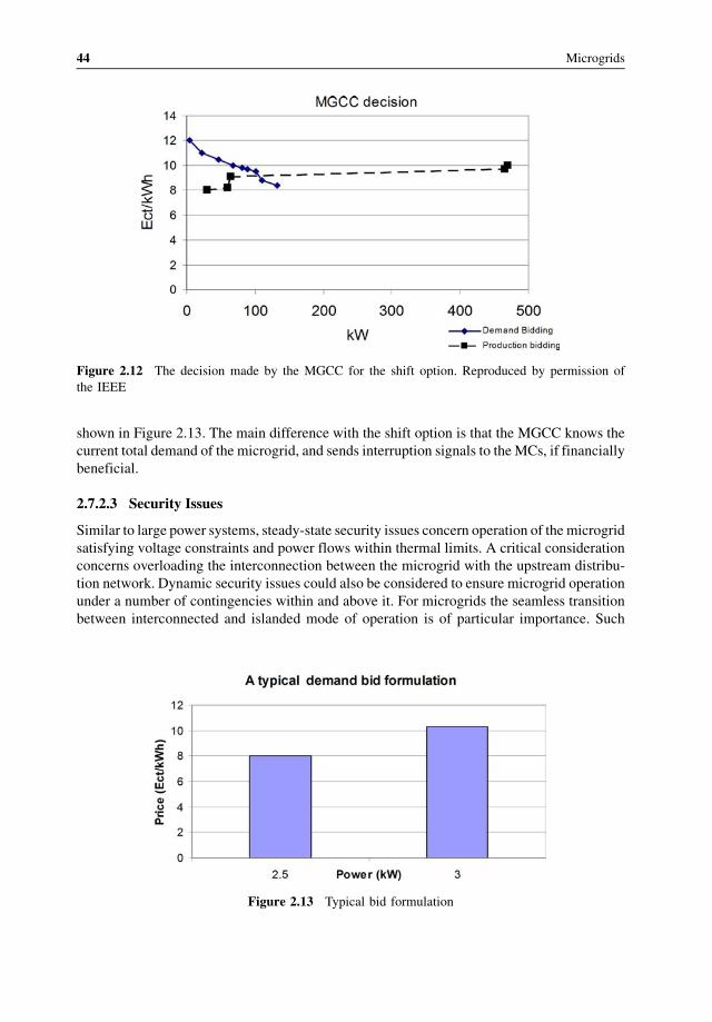
shown in Figure 2.13. The main difference with the shift option is that the MGCC knows the

current total demand of the microgrid, and sends interruption signals to the MCs, if financially

beneficial.

2.7.2.3 Security Issues

Similar to large power systems, steady-state security issues concern operation of the microgrid

satisfying voltage constraints and power flows within thermal limits. A critical consideration

concerns overloading the interconnection between the microgrid with the upstream distribu-

tion network. Dynamic security issues could also be considered to ensure microgrid operation

under a number of contingencies within and above it. For microgrids the seamless transition

between interconnected and islanded mode of operation is of particular importance. Such

Figure 2.12 The decision made by the MGCC for the shift option. Reproduced by permission of

the IEEE

Figure 2.13 Typical bid formulation

44 Microgrids

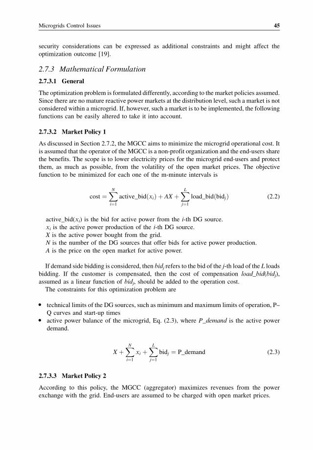
security considerations can be expressed as additional constraints and might affect the

optimization outcome [19].

2.7.3 Mathematical Formulation

2.7.3.1 General

The optimization problem is formulated differently, according to the market policies assumed.

Since there are no mature reactive power markets at the distribution level, such a market is not

considered within a microgrid. If, however, such a market is to be implemented, the following

functions can be easily altered to take it into account.

2.7.3.2 Market Policy 1

As discussed in Section 2.7.2, the MGCC aims to minimize the microgrid operational cost. It

is assumed that the operator of the MGCC is a non-profit organization and the end-users share

the benefits. The scope is to lower electricity prices for the microgrid end-users and protect

them, as much as possible, from the volatility of the open market prices. The objective

function to be minimized for each one of the m-minute intervals is

cost ¼XN

i¼1

active_bidðxiÞ þ AX þXL

j¼1

load_bidðbidjÞ (2.2)

active_bid(xi) is the bid for active power from the i-th DG source.

xi is the active power production of the i-th DG source.

X is the active power bought from the grid.

N is the number of the DG sources that offer bids for active power production.

A is the price on the open market for active power.

If demand side bidding is considered, then bidj refers to the bid of the j-th load of the L loads

bidding. If the customer is compensated, then the cost of compensation load_bid(bidj),

assumed as a linear function of bidj, should be added to the operation cost.

The constraints for this optimization problem are

� technical limits of the DG sources, such as minimum and maximum limits of operation, P–

Q curves and start-up times� active power balance of the microgrid, Eq. (2.3), where P_demand is the active power

demand.

X þXN

i¼1

xi þXL

j¼1

bidj ¼ P_demand (2.3)

2.7.3.3 Market Policy 2

According to this policy, the MGCC (aggregator) maximizes revenues from the power

exchange with the grid. End-users are assumed to be charged with open market prices.


The optimization problem is

MaximizefIncome� Expensesg ¼MaximizefRevenuesg

Income comes from selling active power to both the grid and the microgrid end-users. If the

demand is higher than the production of the DG sources, power bought from the grid is sold to

the end-users of the microgrid. If the demand is lower than the production of the DG sources,

term X in Eqs. (2.4) and (2.5) is zero.

Income ¼ AX þ A �XN

i¼1

xi (2.4)

The term Expenses includes costs for active power bought from the grid plus compensation

to DG sources. If demand side bidding is considered, relevant costs are added to Expenses.

Expenses ¼XN

i¼1

active_bidðxiÞ þ AX þXL

j¼1

load_bidðbidjÞ (2.5)

The MGCC should maximize Eq. (2.6)

Revenues ¼ A �XN

i¼1

xi �XN

i¼1

active_bidðxiÞ

�XL

j¼1

load_bidðbidjÞ(2.6)

Constraints are the technical limits of the units and that at least the demand of the microgrid

should be met, as expressed by Eq. (2.7).

X þXN

i¼1

xi þXL

j¼1

bidj � P_demand (2.7)

2.7.4 Solution Methodology

There are several methods for solving the unit commitment (UC) problem, namely to identify

which of the bids of both DGs and loads will be accepted. A simple method is the use of a

priority list. The DG bids, the load bids, if DSB options are applied, and the external market

prices are placed sequentially according to their differential cost at the highest level of

production for the specific period. This list is sorted in ascending bid values so that the total

demand is met.

DG bids are assumed to have a quadratic form:

XN

i¼1

active_bidðxiÞ ¼ aix2i þ bixi þ ci (2.8)

46 Microgrids

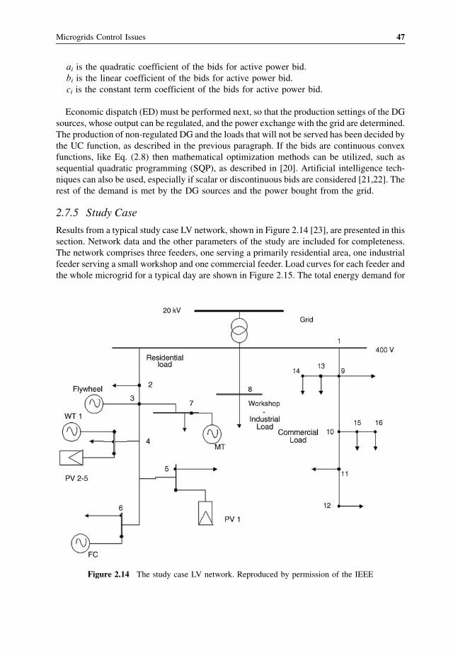
ai is the quadratic coefficient of the bids for active power bid.

bi is the linear coefficient of the bids for active power bid.

ci is the constant term coefficient of the bids for active power bid.

Economic dispatch (ED) must be performed next, so that the production settings of the DG

sources, whose output can be regulated, and the power exchange with the grid are determined.

The production of non-regulated DG and the loads that will not be served has been decided by

the UC function, as described in the previous paragraph. If the bids are continuous convex

functions, like Eq. (2.8) then mathematical optimization methods can be utilized, such as

sequential quadratic programming (SQP), as described in [20]. Artificial intelligence tech-

niques can also be used, especially if scalar or discontinuous bids are considered [21,22]. The

rest of the demand is met by the DG sources and the power bought from the grid.

2.7.5 Study Case

Results from a typical study case LV network, shown in Figure 2.14 [23], are presented in this

section. Network data and the other parameters of the study are included for completeness.

The network comprises three feeders, one serving a primarily residential area, one industrial

feeder serving a small workshop and one commercial feeder. Load curves for each feeder and

the whole microgrid for a typical day are shown in Figure 2.15. The total energy demand for

Figure 2.14 The study case LV network. Reproduced by permission of the IEEE


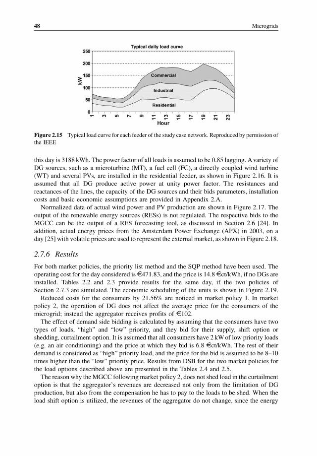
this day is 3188 kWh. The power factor of all loads is assumed to be 0.85 lagging. Avariety of

DG sources, such as a microturbine (MT), a fuel cell (FC), a directly coupled wind turbine

(WT) and several PVs, are installed in the residential feeder, as shown in Figure 2.16. It is

assumed that all DG produce active power at unity power factor. The resistances and

reactances of the lines, the capacity of the DG sources and their bids parameters, installation

costs and basic economic assumptions are provided in Appendix 2.A.

Normalized data of actual wind power and PV production are shown in Figure 2.17. The

output of the renewable energy sources (RESs) is not regulated. The respective bids to the

MGCC can be the output of a RES forecasting tool, as discussed in Section 2.6 [24]. In

addition, actual energy prices from the Amsterdam Power Exchange (APX) in 2003, on a

day [25] with volatile prices are used to represent the external market, as shown in Figure 2.18.

2.7.6 Results

For both market policies, the priority list method and the SQP method have been used. The

operating cost for the day considered is D471.83, and the price is 14.8 Dct/kWh, if no DGs are

installed. Tables 2.2 and 2.3 provide results for the same day, if the two policies of

Section 2.7.3 are simulated. The economic scheduling of the units is shown in Figure 2.19.

Reduced costs for the consumers by 21.56% are noticed in market policy 1. In market

policy 2, the operation of DG does not affect the average price for the consumers of the

microgrid; instead the aggregator receives profits of D102.The effect of demand side bidding is calculated by assuming that the consumers have two

types of loads, “high” and “low” priority, and they bid for their supply, shift option or

shedding, curtailment option. It is assumed that all consumers have 2 kWof low priority loads

(e.g. an air conditioning) and the price at which they bid is 6.8 Dct/kWh. The rest of their

demand is considered as “high” priority load, and the price for the bid is assumed to be 8–10

times higher than the “low” priority price. Results from DSB for the two market policies for

the load options described above are presented in the Tables 2.4 and 2.5.

The reason why theMGCC followingmarket policy 2, does not shed load in the curtailment

option is that the aggregator’s revenues are decreased not only from the limitation of DG

production, but also from the compensation he has to pay to the loads to be shed. When the

load shift option is utilized, the revenues of the aggregator do not change, since the energy

Figure 2.15 Typical load curve for each feeder of the study case network. Reproduced by permission of

the IEEE

48 Microgrids

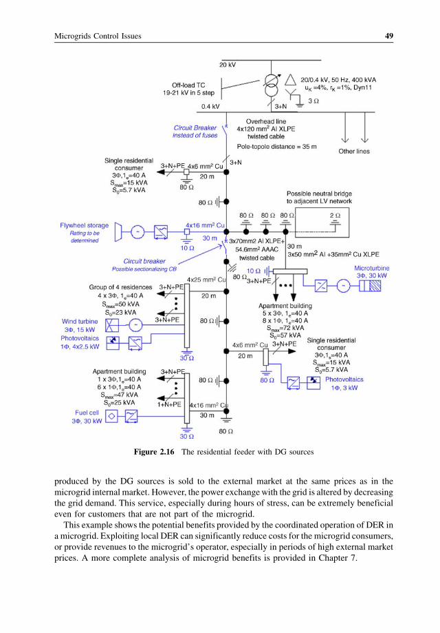
produced by the DG sources is sold to the external market at the same prices as in the

microgrid internal market. However, the power exchangewith the grid is altered by decreasing

the grid demand. This service, especially during hours of stress, can be extremely beneficial

even for customers that are not part of the microgrid.

This example shows the potential benefits provided by the coordinated operation of DER in

a microgrid. Exploiting local DER can significantly reduce costs for the microgrid consumers,

or provide revenues to the microgrid’s operator, especially in periods of high external market

prices. A more complete analysis of microgrid benefits is provided in Chapter 7.

Figure 2.16 The residential feeder with DG sources


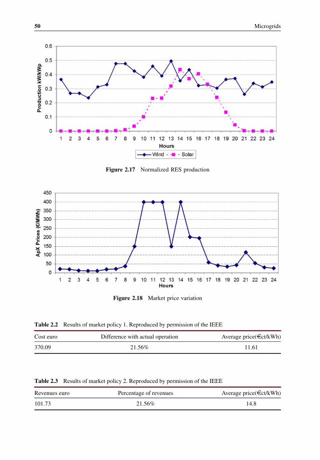
Figure 2.17 Normalized RES production

Figure 2.18 Market price variation

Table 2.2 Results of market policy 1. Reproduced by permission of the IEEE

Cost euro Difference with actual operation Average price(Dct/kWh)

370.09 21.56% 11.61

Table 2.3 Results of market policy 2. Reproduced by permission of the IEEE

Revenues euro Percentage of revenues Average price(Dct/kWh)

101.73 21.56% 14.8

50 Microgrids

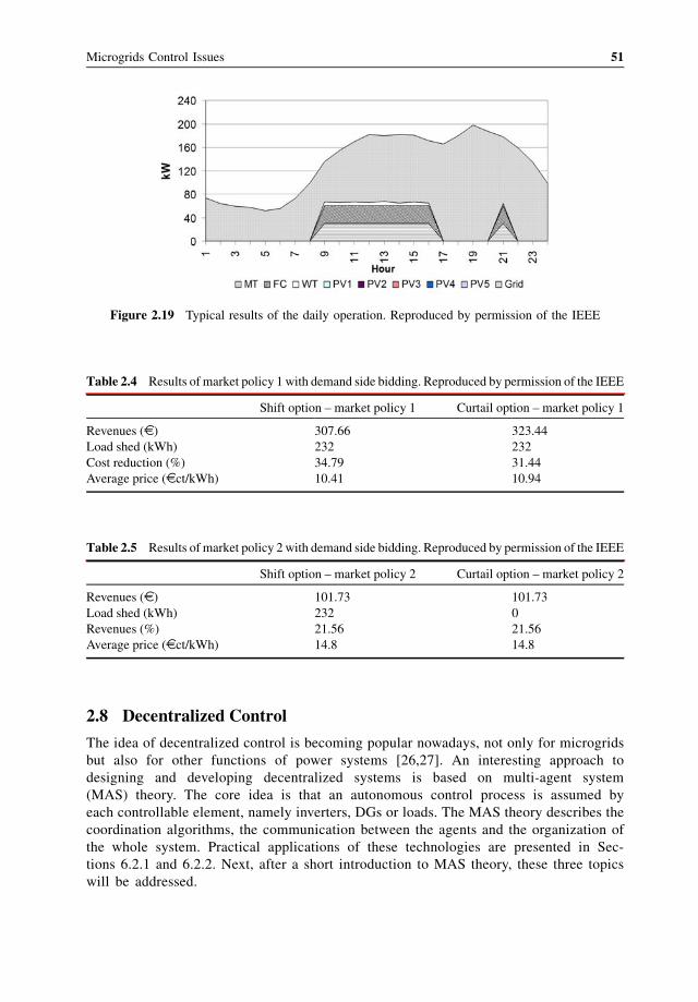
2.8 Decentralized Control

The idea of decentralized control is becoming popular nowadays, not only for microgrids

but also for other functions of power systems [26,27]. An interesting approach to

designing and developing decentralized systems is based on multi-agent system

(MAS) theory. The core idea is that an autonomous control process is assumed by

each controllable element, namely inverters, DGs or loads. The MAS theory describes the

coordination algorithms, the communication between the agents and the organization of

the whole system. Practical applications of these technologies are presented in Sec-

tions 6.2.1 and 6.2.2. Next, after a short introduction to MAS theory, these three topics

will be addressed.

Figure 2.19 Typical results of the daily operation. Reproduced by permission of the IEEE

Table 2.4 Results of market policy 1 with demand side bidding. Reproduced by permission of the IEEE

Shift option – market policy 1 Curtail option – market policy 1

Revenues (D ) 307.66 323.44

Load shed (kWh) 232 232

Cost reduction (%) 34.79 31.44

Average price (Dct/kWh) 10.41 10.94

Table 2.5 Results of market policy 2 with demand side bidding. Reproduced by permission of the IEEE

Shift option – market policy 2 Curtail option – market policy 2

Revenues (D ) 101.73 101.73

Load shed (kWh) 232 0

Revenues (%) 21.56 21.56

Average price (Dct/kWh) 14.8 14.8


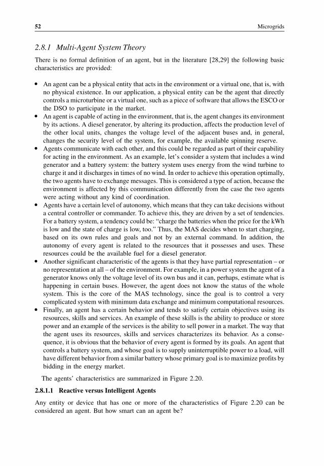
2.8.1 Multi-Agent System Theory

There is no formal definition of an agent, but in the literature [28,29] the following basic

characteristics are provided:

� An agent can be a physical entity that acts in the environment or a virtual one, that is, with

no physical existence. In our application, a physical entity can be the agent that directly

controls a microturbine or a virtual one, such as a piece of software that allows the ESCO or

the DSO to participate in the market.� An agent is capable of acting in the environment, that is, the agent changes its environment

by its actions. A diesel generator, by altering its production, affects the production level of

the other local units, changes the voltage level of the adjacent buses and, in general,

changes the security level of the system, for example, the available spinning reserve.� Agents communicate with each other, and this could be regarded as part of their capability

for acting in the environment. As an example, let’s consider a system that includes a wind

generator and a battery system: the battery system uses energy from the wind turbine to

charge it and it discharges in times of no wind. In order to achieve this operation optimally,

the two agents have to exchange messages. This is considered a type of action, because the

environment is affected by this communication differently from the case the two agents

were acting without any kind of coordination.� Agents have a certain level of autonomy, which means that they can take decisions without

a central controller or commander. To achieve this, they are driven by a set of tendencies.

For a battery system, a tendency could be: “charge the batteries when the price for the kWh

is low and the state of charge is low, too.” Thus, the MAS decides when to start charging,

based on its own rules and goals and not by an external command. In addition, the

autonomy of every agent is related to the resources that it possesses and uses. These

resources could be the available fuel for a diesel generator.� Another significant characteristic of the agents is that they have partial representation – or

no representation at all – of the environment. For example, in a power system the agent of a

generator knows only the voltage level of its own bus and it can, perhaps, estimate what is

happening in certain buses. However, the agent does not know the status of the whole

system. This is the core of the MAS technology, since the goal is to control a very

complicated system with minimum data exchange and minimum computational resources.� Finally, an agent has a certain behavior and tends to satisfy certain objectives using its

resources, skills and services. An example of these skills is the ability to produce or store

power and an example of the services is the ability to sell power in a market. The way that

the agent uses its resources, skills and services characterizes its behavior. As a conse-

quence, it is obvious that the behavior of every agent is formed by its goals. An agent that

controls a battery system, and whose goal is to supply uninterruptible power to a load, will

have different behavior from a similar battery whose primary goal is to maximize profits by

bidding in the energy market.

The agents’ characteristics are summarized in Figure 2.20.

2.8.1.1 Reactive versus Intelligent Agents

Any entity or device that has one or more of the characteristics of Figure 2.20 can be

considered an agent. But how smart can an agent be?

52 Microgrids

Let’s consider an under-voltage relay. The relay has the following characteristics:

� has partial representation of the environment (measures the voltage locally only),� possesses skills (controls a switch), and� reacts autonomously, according to its goals (opens the switch when the voltage goes

beyond certain limits).

According to the literature [28], this type of entity can be considered as a reactive agent that

just responds to stimuli from the environment.

What is a cognitive or intelligent agent? Again, there is no formal definition of what an

intelligent agent is, but some basic characteristics can be listed:

� memory to acquire and store knowledge of the environment: The memory is one

fundamental element of the intelligence and the ability to learn.� ability to perceive the environment: Having an internal modeling and representation of the

environment, detailed enough, is mandatory in order to support the decision making

process. The environment model allows the agent to understand the environment state

having local information and to predict the effect of a possible action on the environment.� ability to take decisions according to its memory and the status of the environment and not

just to react: The agent has a process (algorithm) that uses the model of the environment

and the measurements in order to define the next actions.

Figure 2.20 Agents characteristics


� ability for high level communication: The agents have the ability to exchange knowledge

and use communication as a tool to proceed with complex coordinated actions.

Figure 2.21 summarizes the differences between reactive and intelligent agents, using two

well-known societies, human society and an ant colony. In the case of ant colonies, ants do not

have significant intelligence and they simply react to stimuli; however, they manage to

achieve their main goal, to preserve the society and feed the queen. Human society is formed

of intelligent agents: humans. The human intelligence is strengthened by the capability to

exchange ideas and knowledge, that is, to communicate.

Finally, we should define the concept of the multi-agent system. An MAS is a system

comprising two or more reactive or intelligent agents. It is important to recognize that usually

there is no global coordination, simply the local goals of each individual agent are sufficient

for a system to solve a problem. Furthermore, under Wooldridge’s definitions [30], intelligent

agents must have social ability and therefore must be capable of communication with each

other.

2.8.2 Agent Communication and Development

Communication is one of the most critical elements that allow the intelligent agents to form a

society, a multi-agent system. The transmission of the messages can be done via any

traditional communication system, such as IP communications, wired or wireless channels.

This section focuses on the context and the structure of the messages. Figure 2.22 presents the

agent version of the story of the Tower of Babel, where the workers could not finish the tower

due to the lack of communication [31].

This figure presents the main characteristics of the agent communication language (ACL)

and the associate problems:

Figure 2.21 Reactive and intelligent agents

54 Microgrids

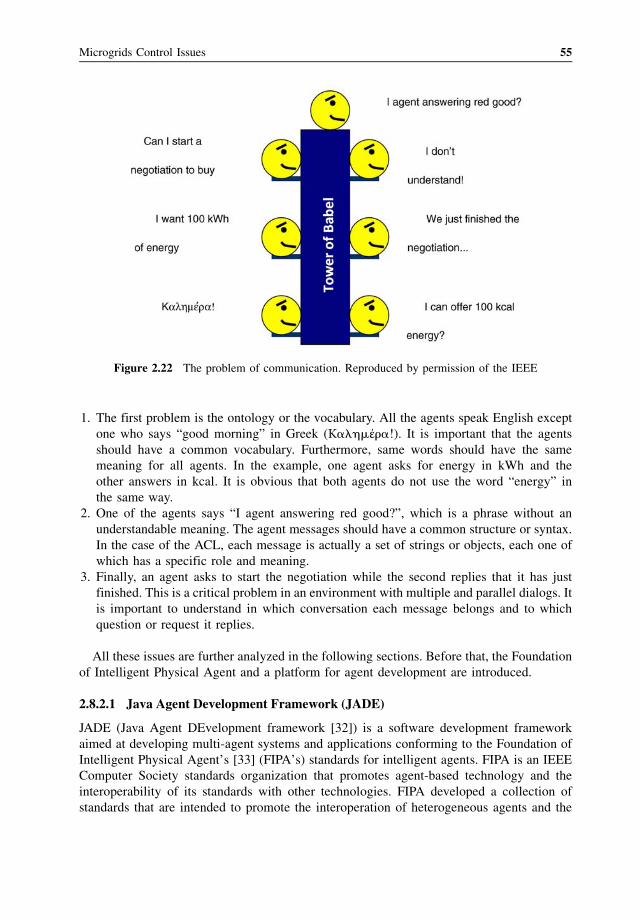
1. The first problem is the ontology or the vocabulary. All the agents speak English except

one who says “good morning” in Greek (Κalhmέra!). It is important that the agents

should have a common vocabulary. Furthermore, same words should have the same

meaning for all agents. In the example, one agent asks for energy in kWh and the

other answers in kcal. It is obvious that both agents do not use the word “energy” in

the same way.

2. One of the agents says “I agent answering red good?”, which is a phrase without an

understandable meaning. The agent messages should have a common structure or syntax.

In the case of the ACL, each message is actually a set of strings or objects, each one of

which has a specific role and meaning.

3. Finally, an agent asks to start the negotiation while the second replies that it has just

finished. This is a critical problem in an environment with multiple and parallel dialogs. It

is important to understand in which conversation each message belongs and to which

question or request it replies.

All these issues are further analyzed in the following sections. Before that, the Foundation

of Intelligent Physical Agent and a platform for agent development are introduced.

2.8.2.1 Java Agent Development Framework (JADE)

JADE (Java Agent DEvelopment framework [32]) is a software development framework

aimed at developing multi-agent systems and applications conforming to the Foundation of

Intelligent Physical Agent’s [33] (FIPA’s) standards for intelligent agents. FIPA is an IEEE

Computer Society standards organization that promotes agent-based technology and the

interoperability of its standards with other technologies. FIPA developed a collection of

standards that are intended to promote the interoperation of heterogeneous agents and the

Figure 2.22 The problem of communication. Reproduced by permission of the IEEE


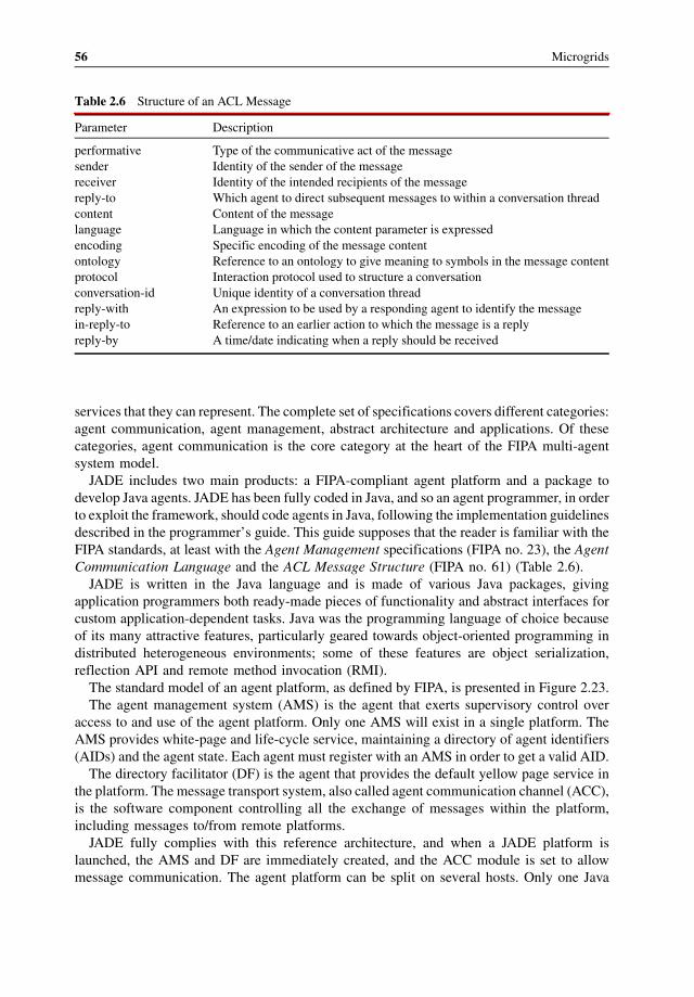
services that they can represent. The complete set of specifications covers different categories:

agent communication, agent management, abstract architecture and applications. Of these

categories, agent communication is the core category at the heart of the FIPA multi-agent

system model.

JADE includes two main products: a FIPA-compliant agent platform and a package to

develop Java agents. JADE has been fully coded in Java, and so an agent programmer, in order

to exploit the framework, should code agents in Java, following the implementation guidelines

described in the programmer’s guide. This guide supposes that the reader is familiar with the

FIPA standards, at least with the Agent Management specifications (FIPA no. 23), the Agent

Communication Language and the ACL Message Structure (FIPA no. 61) (Table 2.6).

JADE is written in the Java language and is made of various Java packages, giving

application programmers both ready-made pieces of functionality and abstract interfaces for

custom application-dependent tasks. Java was the programming language of choice because

of its many attractive features, particularly geared towards object-oriented programming in

distributed heterogeneous environments; some of these features are object serialization,

reflection API and remote method invocation (RMI).

The standard model of an agent platform, as defined by FIPA, is presented in Figure 2.23.

The agent management system (AMS) is the agent that exerts supervisory control over

access to and use of the agent platform. Only one AMS will exist in a single platform. The

AMS provides white-page and life-cycle service, maintaining a directory of agent identifiers

(AIDs) and the agent state. Each agent must register with an AMS in order to get a valid AID.

The directory facilitator (DF) is the agent that provides the default yellow page service in

the platform. The message transport system, also called agent communication channel (ACC),

is the software component controlling all the exchange of messages within the platform,

including messages to/from remote platforms.

JADE fully complies with this reference architecture, and when a JADE platform is

launched, the AMS and DF are immediately created, and the ACC module is set to allow

message communication. The agent platform can be split on several hosts. Only one Java

Table 2.6 Structure of an ACL Message

Parameter Description

performative Type of the communicative act of the message

sender Identity of the sender of the message

receiver Identity of the intended recipients of the message

reply-to Which agent to direct subsequent messages to within a conversation thread

content Content of the message

language Language in which the content parameter is expressed

encoding Specific encoding of the message content

ontology Reference to an ontology to give meaning to symbols in the message content

protocol Interaction protocol used to structure a conversation

conversation-id Unique identity of a conversation thread

reply-with An expression to be used by a responding agent to identify the message

in-reply-to Reference to an earlier action to which the message is a reply

reply-by A time/date indicating when a reply should be received

56 Microgrids

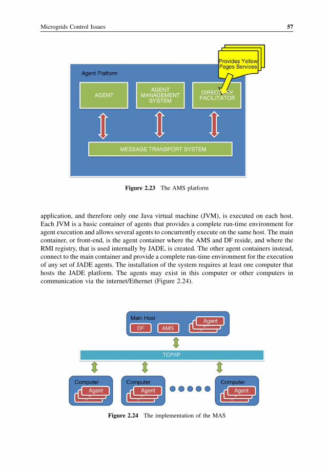
application, and therefore only one Java virtual machine (JVM), is executed on each host.

Each JVM is a basic container of agents that provides a complete run-time environment for

agent execution and allows several agents to concurrently execute on the same host. The main

container, or front-end, is the agent container where the AMS and DF reside, and where the

RMI registry, that is used internally by JADE, is created. The other agent containers instead,

connect to the main container and provide a complete run-time environment for the execution

of any set of JADE agents. The installation of the system requires at least one computer that

hosts the JADE platform. The agents may exist in this computer or other computers in

communication via the internet/Ethernet (Figure 2.24).

Figure 2.23 The AMS platform

Figure 2.24 The implementation of the MAS


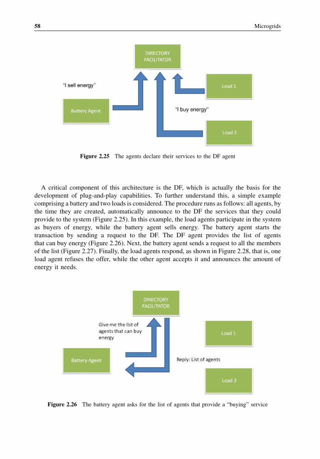
A critical component of this architecture is the DF, which is actually the basis for the

development of plug-and-play capabilities. To further understand this, a simple example

comprising a battery and two loads is considered. The procedure runs as follows: all agents, by

the time they are created, automatically announce to the DF the services that they could

provide to the system (Figure 2.25). In this example, the load agents participate in the system

as buyers of energy, while the battery agent sells energy. The battery agent starts the

transaction by sending a request to the DF. The DF agent provides the list of agents

that can buy energy (Figure 2.26). Next, the battery agent sends a request to all the members

of the list (Figure 2.27). Finally, the load agents respond, as shown in Figure 2.28, that is, one

load agent refuses the offer, while the other agent accepts it and announces the amount of

energy it needs.

Figure 2.25 The agents declare their services to the DF agent

Figure 2.26 The battery agent asks for the list of agents that provide a “buying” service

58 Microgrids

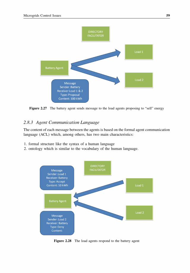
2.8.3 Agent Communication Language

The content of each message between the agents is based on the formal agent communication

language (ACL) which, among others, has two main characteristics:

1. formal structure like the syntax of a human language

2. ontology which is similar to the vocabulary of the human language.

Figure 2.27 The battery agent sends message to the load agents proposing to “sell” energy

Figure 2.28 The load agents respond to the battery agent


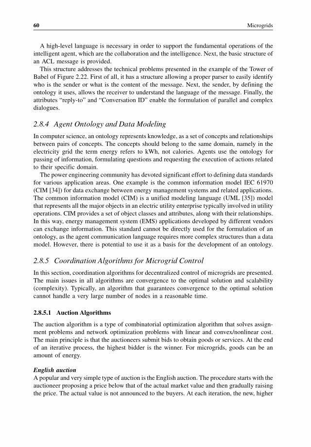
A high-level language is necessary in order to support the fundamental operations of the

intelligent agent, which are the collaboration and the intelligence. Next, the basic structure of

an ACL message is provided.

This structure addresses the technical problems presented in the example of the Tower of

Babel of Figure 2.22. First of all, it has a structure allowing a proper parser to easily identify

who is the sender or what is the content of the message. Next, the sender, by defining the

ontology it uses, allows the receiver to understand the language of the message. Finally, the

attributes “reply-to” and “Conversation ID” enable the formulation of parallel and complex

dialogues.

2.8.4 Agent Ontology and Data Modeling

In computer science, an ontology represents knowledge, as a set of concepts and relationships

between pairs of concepts. The concepts should belong to the same domain, namely in the

electricity grid the term energy refers to kWh, not calories. Agents use the ontology for

passing of information, formulating questions and requesting the execution of actions related

to their specific domain.

The power engineering community has devoted significant effort to defining data standards

for various application areas. One example is the common information model IEC 61970

(CIM [34]) for data exchange between energy management systems and related applications.

The common information model (CIM) is a unified modeling language (UML [35]) model

that represents all the major objects in an electric utility enterprise typically involved in utility

operations. CIM provides a set of object classes and attributes, along with their relationships.

In this way, energy management system (EMS) applications developed by different vendors

can exchange information. This standard cannot be directly used for the formulation of an

ontology, as the agent communication language requires more complex structures than a data

model. However, there is potential to use it as a basis for the development of an ontology.

2.8.5 Coordination Algorithms for Microgrid Control

In this section, coordination algorithms for decentralized control of microgrids are presented.

The main issues in all algorithms are convergence to the optimal solution and scalability

(complexity). Typically, an algorithm that guarantees convergence to the optimal solution

cannot handle a very large number of nodes in a reasonable time.

2.8.5.1 Auction Algorithms

The auction algorithm is a type of combinatorial optimization algorithm that solves assign-

ment problems and network optimization problems with linear and convex/nonlinear cost.

The main principle is that the auctioneers submit bids to obtain goods or services. At the end

of an iterative process, the highest bidder is the winner. For microgrids, goods can be an

amount of energy.

English auctionA popular and very simple type of auction is the English auction. The procedure starts with the

auctioneer proposing a price below that of the actual market value and then gradually raising

the price. The actual value is not announced to the buyers. At each iteration, the new, higher

60 Microgrids

price is announced and the auctioneer waits to see if any buyers arewilling to pay the proposed

price. As soon as one buyer accepts the price, the auctioneer proceeds to a new iteration with

an increased price. The auction continues until no buyers accept the new price. If the last

accepted price exceeds the actual market value, the good is sold to that buyer for the agreed

price. If the last accepted price is less than the actual value, the good is not sold.

Dutch auctionA similar approach is the Dutch auction. In this case, the procedure starts with the auctioneer

asking a price higher than the actual value, which is decreased until a buyer is willing to accept

it, or a minimum value (actual value) is reached. The winning participant pays the last

announced price.

Theoretically, both approaches are equivalent and lead to the same solution. Many

variations on these auction systems exist, for example, in some variations the bidding or

signaling from the buyers is kept secret.

Symmetric AssignmentAmore advanced auction algorithm is proposed by [36,37] to solve the symmetric assignment

problem, which is formulated as follows:

Consider n persons and n objects that should be matched. There is a benefit aij formatching person i with object j. In the presented application, the benefit for each person is

his revenues for obtaining object j, that is, an agreement for producing a certain amount of

energy. The main target is to assign the persons to objects and to maximize the total benefit,expressed as:

Xn

i¼1

aij (2.9)

The price p is an algorithmic variable that is formed by the bids of all persons and expresses

the global desire. The prices of all objects form the price vector. These prices should not be

confused with the market prices. Also, the difference between the benefit and the price is the

actual value of an object for a specific person. The actual value for a specific object is different

for two persons, since it is related to the benefit. At the beginning of the iterations, the price

vector is zero and so the actual value is equal to the benefit, although variations of the

proposed methods use initial non-zero values for faster convergence.

The auction algorithm calculates the price vector p, in order to satisfy the e-complementary

slackness condition suggested in [36,37]. The steps are as follows:

At the beginning of each iteration, the e-complementary slackness condition is checked for

all pairs (i,ji) of the assignment. The ji is the object j that person i wants to be assigned to. So

the formulation of this condition is

aiji � pji � maxj2AðiÞ

aij � pj

n o

� e (2.10)

A(i) is the set of objects that can be matched with person i. This inequality has two parts:

aij� pj is the actual value of object j for person i, as described before. The right part refers to

the object that gives maximum value to person iminus e, where e is a positive scalar, added in


the bid of each object, in order to avoid possible infinite iterations in case two or more objects

provide maximum benefit to the same person, as explained later.

If all persons are assigned to objects, the algorithm terminates. Otherwise, a non-empty

subset I of persons i that are unassigned is formed. Similarly, the non-empty subset P(j) is

formed by the available objects. The following two steps are performed only for persons that

belong to I.

The first step is the bidding phase, where each person finds an object j which provides

maximal value and this is

ji 2 maxj2AðiÞ

aij � pj

n o

(2.11)

Following this, the person computes a bidding increment

gi ¼ ui � wi þ e (2.12)

ui is the best object value

ui ¼ maxj2AðiÞ

aij � pj

n o

(2.13)

and wi the second best object value

wi ¼ maxj2AðiÞ;j 6¼ji

aij � pj

n o

(2.14)

According to these equations, the bidding increment is based on the two best objects for

every person. If there are two or more bids for an object, its price rises, and the price increment

is the larger bidding increment between the bids. It is obvious that, if the scalar e¼ 0 and the

benefits for the first and the second best object are the same, then g i¼ 0 and this leads the

algorithm to infinite iterations. The e scalar ensures that the minimum increment for the bids is

g i¼ e.The next phase is the assignment phase, where each object j selected as best object by the

non-empty subset P(j) of persons in I, determines the highest bidder

ij ¼ maxi2PðjÞ

g if g (2.15)

Object j raises its prices by the highest bidding increment maxi2PðjÞ g if g, and gets assignedto the highest bidder ij. The person that was assigned to j at the beginning of the iteration, if

any, becomes unassigned.

The algorithm iterates until all persons have an object assigned. It is proven that the

algorithm converges to the optimal solution, as long as there is one. The maximum number of

iterations is

maxði;jÞ aij��

��

e(2.16)

62 Microgrids

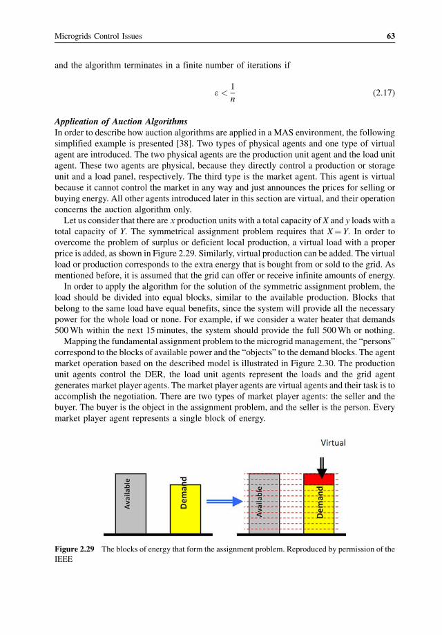
and the algorithm terminates in a finite number of iterations if

e <1

n(2.17)

Application of Auction AlgorithmsIn order to describe how auction algorithms are applied in a MAS environment, the following

simplified example is presented [38]. Two types of physical agents and one type of virtual

agent are introduced. The two physical agents are the production unit agent and the load unit

agent. These two agents are physical, because they directly control a production or storage

unit and a load panel, respectively. The third type is the market agent. This agent is virtual

because it cannot control the market in any way and just announces the prices for selling or

buying energy. All other agents introduced later in this section are virtual, and their operation

concerns the auction algorithm only.

Let us consider that there are x production units with a total capacity of X and y loads with a

total capacity of Y. The symmetrical assignment problem requires that X¼ Y. In order to

overcome the problem of surplus or deficient local production, a virtual load with a proper

price is added, as shown in Figure 2.29. Similarly, virtual production can be added. The virtual

load or production corresponds to the extra energy that is bought from or sold to the grid. As

mentioned before, it is assumed that the grid can offer or receive infinite amounts of energy.

In order to apply the algorithm for the solution of the symmetric assignment problem, the

load should be divided into equal blocks, similar to the available production. Blocks that

belong to the same load have equal benefits, since the system will provide all the necessary

power for the whole load or none. For example, if we consider a water heater that demands

500Wh within the next 15minutes, the system should provide the full 500Wh or nothing.

Mapping the fundamental assignment problem to the microgrid management, the “persons”

correspond to the blocks of available power and the “objects” to the demand blocks. The agent

market operation based on the described model is illustrated in Figure 2.30. The production

unit agents control the DER, the load unit agents represent the loads and the grid agent

generates market player agents. The market player agents are virtual agents and their task is to

accomplish the negotiation. There are two types of market player agents: the seller and the

buyer. The buyer is the object in the assignment problem, and the seller is the person. Every

market player agent represents a single block of energy.

Figure 2.29 The blocks of energy that form the assignment problem. Reproduced by permission of the

IEEE


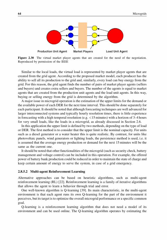
Similar to the local loads, the virtual load is represented by market player agents that are

created from the grid agent. According to the proposed market model, each producer has the

ability to sell all its production to the grid and, similarly, every load can buy energy from the

grid. For this reason, the grid agent finds the number of pairs of market player agents (sellers

and buyers) and creates extra sellers and buyers. The number of the agents is equal to market

agents that are created from the production unit agents and the load unit agents. In this way,

buying or selling energy from the grid is determined by the algorithm.

A major issue in microgrid operation is the estimation of the upper limits for the demand or

the available power of each DER for the next time interval. This should be done separately for

each participant. It should be noted that although forecasting techniques are well advanced for

larger interconnected systems and typically hourly resolution times, there is little experience

in forecasting with a high temporal resolution (e.g. <15minutes) with a horizon of 3–4 hours

for very small loads, like the loads in a microgrid, as already discussed in Section 2.6.

In this application the upper limit is defined by two methods, depending on the type of load

or DER. The first method is to consider that the upper limit is the nominal capacity. For units

such as a diesel generator or a water heater this is quite realistic. By contrast, for units like

photovoltaic panels, wind generators or lighting loads, the persistence method is used, i.e. it

is assumed that the average energy production or demand for the next 15minutes will be the

same as the current one.

It should be noted that other functionalities of the microgrid (such as security check, battery

management and voltage control) can be included in this operation. For example, the offered

power of battery bank production could be reduced in order to maintain the state of charge and

keep certain amount of energy to serve the system, in case of a grid emergency.

2.8.5.2 Multi-agent Reinforcement Learning

Alternative approaches can be based on heuristic algorithms, such as multi-agent

reinforcement learning (RL) [22]. Reinforcement learning is a family of iterative algorithms

that allows the agent to learn a behavior through trial and error.

One well-known algorithm is Q-learning [39]. Its main characteristic, in the multi-agent

environment is that each agent runs its own Q-learning for the part of the environment it

perceives, but its target is to optimize the overall microgrid performance or a specific common

goal.

Q-learning is a reinforcement learning algorithm that does not need a model of its

environment and can be used online. The Q-learning algorithm operates by estimating the

Figure 2.30 The virtual market player agents that are created for the need of the negotiation.

Reproduced by permission of the IEEE

64 Microgrids

values of state-action pairs. The value Q(s,a) is defined as the expected discounted sum of

future payoffs obtained by taking action a from state s and following an optimal policy

thereafter. Once these values have been learned, the optimal action from any state is the one

with the highest Q-value. After being initialized, Q-values are estimated on the basis of

experience, as follows:

� From the current state s, select an action a. This will bring an immediate payoff r, and

will lead to a next state s0.� Update Q(s,a) based upon this experience as follows: Qðs; aÞ ¼ ð1� kÞQðs; aÞþ

kðrþ gmaxa0 Qðs0; a0Þ) where k is the learning rate, 0 < g < 1 is the discount factor.

Alternative learning algorithms can be used, including the Nash-Q learning, which is a

general sumMAS reinforcement algorithm for a stochastic environment. The main problem is

that the execution times are prohibitive because the Nash-Q learning requires that the Q table

includes as a parameter the actions of the other agents. For systems like microgrids, the Q

table becomes huge, requesting a large number of episodes for training. Other approaches

propose forecasting the decisions of other agents, but this also cannot be easily done in

microgrid applications.

The main problem in the application of reinforcement learning is the modeling of the

environments which affects the size of the Q table and as a consequence the convergence

speed. All actions and system states are included in the Q table as

Qðs;a1;a2;a3; . . .anÞ (2.18)

a1, a2 . . . an is the selected action of agent 1, agent 2 . . . agent n.

Another concern is that the environment is stochastic, since we still cannot predict

accurately the effect on the system state after switching a load or sending a command to

change the setpoint of a DG. An approach proposed in [40,41] is to replace all actions with one

single variable called transition, which represents the final result to the environment of all

actions of all the agents.

Qðs;a1;a2;a3; . . .anÞ|fflfflfflfflfflfflfflfflfflfflfflfflfflfflfflfflffl{zfflfflfflfflfflfflfflfflfflfflfflfflfflfflfflfflffl}

Qðs;a1; trÞ (2.19)

The agent selects the action that will lead the system to the best state (transition)

considering that the other agents will follow the same policy. The selection of actions is

based on the following equation:

Selected transition ¼ arg maxtr¼1;2;3

X

maxa

ðQðs; a; trÞÞ� �

(2.20)

This means that, for each transition, each agent selects the action that maximizes the

Q value and they all add these values at each transition. The selected transition is the one with

the highest value.


Let’s consider an example of the application of the RL algorithm to microgrid black start.

After the black out, a simple procedure is followed:

1. switch off all loads

2. launch black start units

3. launch the other units

4. start the MAS according to the results of the reinforcement learning

It should be noted that the algorithm considers the steady state of the system and does not

handle transient phenomena. The algorithm focuses on how to ensure power supply to the

critical loads for a predefined period, for example 24 hours ahead. In this case, the agents have

to learn to use the available resources in the most efficient way.

Each agent executes a Q-learning procedure for the part of the environment that it

perceives. For the formulation of the problem, the variables that will be inserted in the Q

table should be defined first. It should be noted again that it is important to keep the size of the

Q table small in order to reduce the number of calculations.

The environment state variable forms a table of 24 elements, one for every hour of the

schedule. The production units are characterized by one more variable, the available fuel, with

three values: {low, medium, high}. For battery units this variable reflects the state of charge.

Finally, for the loads, there is a variable called remain with values {low, medium, high},

indicating how many hours they need to be served.

The transition variable is considered next, with three values: {up, neutral, down}. This

variable is an indication of the behavior of the other agents and the state of the system, as

explained before. The purpose of this variable is to identify the most likely next states of the

system. For example, if the transition has value {down}, the system will go to a worse state,

no matter what the action of the individual agent might be. The definition of a worse or better

state depends on the type of problem. For example, in the interconnected system operation a

worse case is when the system receives energy from the upstream networks. In non-

interconnected mode, the worse state is when the system consumes stored energy.

Accordingly, the size of the Q table for each agent is:

� storage units: Q (horizon{24}, fuel{3}, environment {3}, transition {3},action

{3})¼ 1944 elements� generation units: Q (horizon{24}, fuel{3}, environment {3}, transition {3},action

{2})¼ 1296 elements� loads: Q (horizon{24}, environment {3}, remain{3}, transition {3}, action {2})¼ 1296

elements.

The agent learns the value of its action in the various states of the system. For this case

study, the agents are able to act as in Table 2.7.

The intermediate reward for the algorithm is calculated from:

reward ¼ N � ðtransition rewardþ final state rewardþ KÞ (2.21)

N is a normalization parameter obtained by dividing the maximum production capacity

of the unit by the total production capacity of the system. This ensures a weighted

66 Microgrids

participation of all units, for example, a 100 kW unit affects more the final actions than a

1 kW unit.

� The transition reward has a value of 1/24 when the system stores energy, 0 if it remains at

the same level and �1/24 when the system consumes stored energy.� The final state reward is received in the final step and has value 1 if the system has

sufficient energy for the whole period (24 h), and �1 if not.� The K parameter is different for loads and production/storage units. For production/storage

units it indicates the remaining fuel, and for load the time (in percentage that the load

should be served).

This algorithm needs to be executed if there is a significant change in the system, such as the

installation of a new unit. This is presented in Figure 2.31. After the execution, every agent has

learnt what to do in case of an emergency. Consider for example, that the system is in zero

power exchange with the slack. The agents have to select one of three transitions {up, neutral,

down}. In order to decide which transition to follow, they announce to each other the Q values

for each transition in the current state. The selected transition is given by Eq. (2.20).

Selecting for example an “up” transition means that some agents have surplus power and

they offer it to the system having in mind that the selected path will lead to a good final

solution. The good solution is the one that ensures energy adequacy for the whole 24 hour

period.

Figure 2.31 Time schedule of the algorithm. Reproduced by permission of the IEEE

Table 2.7 Actions of the agents. Reproduced by permission of

the IEEE

Type Actions

1 load on

off

2 storage unit produce

stop

store

3 production unit stop

produce


As an example, consider a microgrid system comprising:

� diesel generator,� battery bank,� load,� renewable energy sources.

The simulation has two parts. The first part is training (exploration), in order to find

the Q values. The second part is exploitation of the algorithm in isolated operation.

Several simulations of the operation of the system were performed in order to validate

whether the agents find the solution that ensures energy adequacy. Furthermore, simple

software was developed, allowing each agent to decide absolutely independently of each

other, in order to compare the solution with the one of the reinforcement learning

algorithms.

The critical loads and the renewable energy sources participate in the simulation of the

exploitation, but there is no need to train the respective agents, since they do not control their

actions.

A learning rate k¼ 0. 95 and discount factor g ¼ 0.1 are assumed. The algorithm converges

after 20 000 iterations, which means that there are no significant changes in the values of theQ

table in more iterations. In order to ensure that this is the final solution, multiple runs have

been made with the same schedule, but with different initializations of the Q table, as well as

multiple runs with the same initial Q table. Since there is no interaction between the agents

during the learning period, every agent needs around 40 seconds in a single PC with 3GHz

processor to complete the training.

In Figure 2.32, an instant of the results of the algorithm for the battery is shown. The vertical

axis presents the Q value and the horizontal axis the time step. The agent chooses the action

with the higher Q value. The battery agent appears to learn how to handle the islanded

operation. The agent starts exhibiting a conservative behavior at the beginning, since it does

not know what will happen next, so the system tries to save energy for the next hours. This is

shown by the fact that the batteryQ values are higher for zero production in the first 8 hours, in

Figure 2.32 Results for restoration study case

68 Microgrids

comparison to the Q values for production or storing. By the time the energy adequacy

is guaranteed, the agents start to serve extra loads, like the battery, in the hours between 10 and

15. It should be noted that this is a simplified example. In a more complex application, the Q

values for the battery should be compared with the correspondingQ values of the other agents.

2.8.6 Game Theory and Market Based Algorithms

Another interesting approach is to use game theory and market based rules. The various agents

know their own benefit and cost, and they respond to price signals. This approach is using the

principles of game theory, and if the rules of the game are correct, the system will balance at

the optimal point.

Game theory is a branch [42,43] of applied mathematics that studies the interaction of

multiple players in competitive situations. Its goal is the determination of the equilibrium

state at which the optimal gain for each individual is achieved. More specifically, the theory

of non-cooperative games studies the behavior of agents in any situation where each agent’s

optimal choice may depend on its forecast of the choices of its opponents [43]. Various

categories of games exist, depending on the assumptions regarding the timing of the game,

the knowledge associated with the payoff functions and last but not least the knowledge

regarding the sequence of the previously made choices. More specifically, the games can be

categorized as:

� static/dynamic games: the players choose actions either simultaneously or consecutively.� complete/incomplete information: each player’s payoff function is common knowledge

among all the players or at least one player is uncertain about another player’s payoff

function.� perfect/imperfect information (defined only for dynamic games): at each move in the

game the player with the move knows or does not know the full history of the game

thus far [42].

A simple but realistic example is to assume a dynamic game of complete and perfect

information: the consumers and the DG units are not considered as competitive entities, but

their payoff functions are publicly available, while the history of the game at each stage is

known. The timing of such a game is as follows:

1. Player 1 chooses an action (a1) from a feasible set of actions (A1).

2. Player 2 observes this action and then chooses an action (a2) from its feasible set (A2).

3. Payoffs are u1 (a1, a2) and u2(a1, a2).

The solution of such a game is determined as the backwards-induction outcome. At the

second stage of the game, player 2 will solve the following problem, given the action a1

previously chosen by player 1:

maxa22A2

u2 a1; a2ð Þ (2.22)

It is assumed that for each a1 in A1, player 2’s optimization problem has a unique solution,

denoted by R2(a1) [42]. This is player 2’s best response to player 1’s action. Since player 1


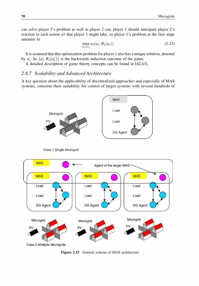
can solve player 2’s problem as well as player 2 can, player 1 should anticipate player 2’s

reaction to each action a1 that player 1 might take, so player 1’s problem at the first stage

amounts tomaxa12A1

u2 a1;R2 a1ð Þð Þ (2.23)

It is assumed that this optimization problem for player 1 also has a unique solution, denoted

by a�1. So a�1;R2 a�1� ��

is the backwards induction outcome of the game.

A detailed description of game theory concepts can be found in [42,43].

2.8.7 Scalability and Advanced Architecture

A key question about the applicability of decentralized approaches and especially of MAS

systems, concerns their suitability for control of larger systems with several hundreds of

Figure 2.33 General scheme of MAS architecture

70 Microgrids

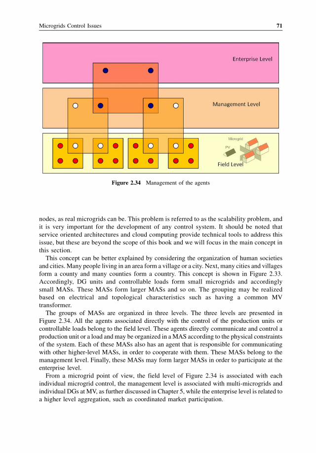
nodes, as real microgrids can be. This problem is referred to as the scalability problem, and

it is very important for the development of any control system. It should be noted that

service oriented architectures and cloud computing provide technical tools to address this

issue, but these are beyond the scope of this book and we will focus in the main concept in

this section.

This concept can be better explained by considering the organization of human societies

and cities. Many people living in an area form a village or a city. Next, many cities and villages

form a county and many counties form a country. This concept is shown in Figure 2.33.

Accordingly, DG units and controllable loads form small microgrids and accordingly

small MASs. These MASs form larger MASs and so on. The grouping may be realized

based on electrical and topological characteristics such as having a common MV

transformer.

The groups of MASs are organized in three levels. The three levels are presented in

Figure 2.34. All the agents associated directly with the control of the production units or

controllable loads belong to the field level. These agents directly communicate and control a

production unit or a load and may be organized in aMAS according to the physical constraints

of the system. Each of these MASs also has an agent that is responsible for communicating

with other higher-level MASs, in order to cooperate with them. These MASs belong to the

management level. Finally, these MASs may form larger MASs in order to participate at the

enterprise level.

From a microgrid point of view, the field level of Figure 2.34 is associated with each

individual microgrid control, the management level is associated with multi-microgrids and

individual DGs at MV, as further discussed in Chapter 5, while the enterprise level is related to

a higher level aggregation, such as coordinated market participation.

Figure 2.34 Management of the agents


2.9 State Estimation

2.9.1 Introduction

State estimation (SE) is very important for the management of active distribution networks. It

can be applied to a wider area of the distribution network including one or more microgrids

and DGs connected at the MV level, and provides to the DSO an overview of the system

operating conditions. In this way, it allows the DSO to define appropriate control strategies to

be adopted, whenever necessary.

Distribution state estimation (DSE) techniques [44–49] are different from SE in transmis-

sion systems [50,51]. The former have been developed to make up for the lack of measured

data at MV and LV levels, while the latter reduce the uncertainty of the available redundant

measurements. In distribution grids, real-time measurements are available only at the primary

substations (voltage magnitudes, power flows and circuit breaker statuses) and feeders

(current magnitudes), and so, full network observability is impossible. In order to ensure

network observability, pseudo-measurements (forecasted or near real-time load injections),

that are stochastic in nature, need to be used at all unmeasured nodes [45,52,53]. This data can

be gathered by automated meter reading devices [54] and can be stored in accessible

databases. Virtual measurements with no error (zero injections at network nodes that have

neither load nor generation, zero voltage drops at closed switching devices and zero power

flows at open switching devices) can be also utilized. The DSE will process this real-time and

forecasted data to produce the state vector consisting of nodal voltages (magnitudes and phase

angles) and transformer tap positions.

Feeders are mainly three-phase radial, but have laterals that can be single- or two-phase.

Furthermore, loads on the feeders are distributed and can be single- and two-phase (for

residential service) or three-phase (for commercial and industrial service). Therefore,

distribution systems are unbalanced by nature. Nevertheless, to avoid modeling complexities,

the network is assumed to be balanced, and the single phase equivalent network model is

considered for state estimation analysis.

The commonly used weighted least-squares (WLS) estimation method [51] can be adopted

for distribution state estimation, considering the following nonlinear measurement model:

z ¼ hðxÞ þ e (2.24)

The nodal states can be estimated by minimizing the quadratic objective function:

minx

JðxÞ ¼ z� hðxÞð ÞTR�1 z� hðxÞð Þ (2.25)

where z is the measurement vector, hðxÞ is the vector of nonlinear functions relating

measurements to states, x is the true state vector, e is the vector of normally distributed

measurement errors, with EðeÞ ¼ 0 and EðeeTÞ ¼ R ¼ diagðs2i Þ, and s2

i is the variance of the

ith measurement error. Real-time measurements will have lower variance than pseudo-

measurements. The state estimate x̂ can be obtained by iteratively solving the following

equations:

GðxkÞDxk ¼ HTðxkÞR�1Dzk (2.26)

72 Microgrids

where, k is the iteration index, Dxk ¼ xkþ1 � xk, Dzk ¼ z� hðxkÞ, H ¼ @h@x is the Jacobian

matrix and GðxkÞ ¼ HTðxkÞR�1HðxkÞ is the gain matrix.

The presence of a large number of load injection pseudo-measurements may give rise to

convergence problems [55]. In order to overcome this problem, robust SE algorithms need to

be applied [50]. One such algorithm, based on orthogonal transformations, is presented in

Section 2.9.2.

With the increasing number of nodes involved in distribution networks, the DSEmay not be

suitable for operating as a centralized algorithm. The feeders can be divided into zones or

areas, and local state estimations can be executed independently, sending their results to the

DMS, where a coordinated state estimator will calculate the system-wide state [56,57]. When

partial lack of communication occurs in some areas, the local SE processes can continue with

the remaining areas.

2.9.2 Microgrid State Estimation

The structure of a typical LV distribution network, including a microgrid system, connected to

the main MV grid, has been shown in Figure 2.4. A microgrid state estimator (MSE) will

follow the concepts of distribution state estimators, receiving a limited number of real-time

measurements from the network [47,58]. Near-real-time measurements of voltage and active

and reactive injections at DG sites can be also available at predefined time intervals. Since this

data is inadequate for state estimation, forecasted node injections obtained from historical or

near-real-time load data should be used. However, the number of loads connected to the

distribution network may be large, so it will be impractical to telemeter all those points.

Measurement time skew is a consideration when combining large area data received via a

data communication network. Due to limited communication infrastructure, near real-time

data from DG sources or loads may be sent to the DMS through different communication

channels causing additional time skew problems. In order to accommodate the effects of

randomly varying arrival of measurement data, a stochastic extended Kalman filter (EKF)

algorithm can be used to improve time skewed measurement data [59].

An important issue in state estimation modeling is the identification of network configu-

ration (topology). In transmission state estimation the statuses of switching devices are

processed by the network topology processor (NTP) to define the bus/branch network model,

by merging bus sections joined by closed switching devices into nodes. The topology is

assumed to be known and correct, but any status errors, that pass undetected by the NTP, will

result in an incorrect bus/branch model. In distribution networks including DGs, it is

frequently not possible to find and fix one topology with a very high certainty, due to

frequent topology changes (switching operations for network reconfiguration, in/out of

service load, branch or DG or microgrid system islanding). This issue is discussed further

in Chapter 4 (see, for example, Figure 4.8). In any case, one topology must be considered to

initiate the SE process, but the formulation should be flexible enough to allow changes in the

topology, if the initial one will not lead to the best solution. This means that the NTP must be

able to consider that the identification of bad data can find errors in the status of some

switching devices. This problem can be solved by augmenting the conventional state vector

with switching device statuses and other related pseudo-measurements in order to identify

topology changes and errors [51,60–62], that is, the topology will be estimated at the same

time with analog information.


In distribution systems with several microgrids, an additional problem is that the

number of islands is not known when starting the state estimation process, as a

consequence of some switching devices having an unknown or suspicious status. A

network splitting problem can be formulated as the problem of finding the state variables

in all network islands. The consideration of uncertainty affecting topology introduces the

splitting problem. When the network is split into two or more non-connected electrical

islands – owing to a set of switching devices being reported as open – the system becomes

unobservable, and the state vector cannot be computed. In order to overcome this

problem, a degree of uncertainty should be considered for the pseudo-measurements.

By including such pseudo-measurements, the network becomes observable, and the state

vector can be estimated [60].

In order to set up the measurement system, we assume that mi ¼ zi is the mean value of the

ith measurement. Then a�3si deviation around the mean covers about 99.7% of the Gaussian

curve. Hence, for a given percentage of maximum measurement error about the mean mi, the

standard deviation si is given by [44]

si ¼ mi � error%

300(2.27)

In practice, an error of 1% for voltage measurements, 3% for power flow and injection

measurements and 15% for load pseudo-measurements may be considered.

Since the load pseudo-measurements are statistical in nature, we use the state error

covariance matrix as a performance index to assess the accuracy of the state estimation

solution [50]:

Cx ¼ HTR�1H� ��1

(2.28)

The ith diagonal entry Cx i; ið Þ of Cx is the variance of the ith state.

Simulations studies [44] show that the effect of the inaccuracies of the load estimates are

more severe at the unmeasured load buses, because of the low local measurement

redundancy. As expected, there is a strong correlation between bus voltage uncertainties

and the errors in load estimates. It should be noted that, uncertainties for all buses adjacent

to the primary substation are low, because of the higher accuracy and redundancy of the

local real-time measurements. This fact enables the correct identification of topology errors

and network splitting. From state estimation runs, it can be shown that an error in a load

value on the upper feeder in network of Figure 2.4 affects mainly the node voltages of the

feeder where this load belongs to and not those of the lower feeder [44]. When applied to

real microgrids, the state estimate accuracy mostly depends on the accuracy of the load

models.

2.9.3 Fuzzy State Estimation

Usually, the SE problem is solved by using all the information available for the network,

and not just measurement values. Evidently, the quality of the solution depends critically on

the quality of the available information. In order to take this into account, a different model

using fuzzy state estimation (FSE) can be also applied [63,64], using information

characterized by uncertainty applying fuzzy set theory. Fuzzy numbers are used to model

74 Microgrids

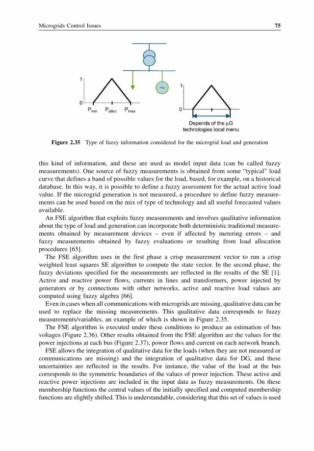
this kind of information, and these are used as model input data (can be called fuzzy

measurements). One source of fuzzy measurements is obtained from some “typical” load

curve that defines a band of possible values for the load, based, for example, on a historical

database. In this way, it is possible to define a fuzzy assessment for the actual active load

value. If the microgrid generation is not measured, a procedure to define fuzzy measure-

ments can be used based on the mix of type of technology and all useful forecasted values

available.

An FSE algorithm that exploits fuzzy measurements and involves qualitative information

about the type of load and generation can incorporate both deterministic traditional measure-

ments obtained by measurement devices – even if affected by metering errors – and

fuzzy measurements obtained by fuzzy evaluations or resulting from load allocation

procedures [65].

The FSE algorithm uses in the first phase a crisp measurement vector to run a crisp

weighted least squares SE algorithm to compute the state vector. In the second phase, the

fuzzy deviations specified for the measurements are reflected in the results of the SE [1].

Active and reactive power flows, currents in lines and transformers, power injected by

generators or by connections with other networks, active and reactive load values are

computed using fuzzy algebra [66].

Even in cases when all communications with microgrids are missing, qualitative data can be

used to replace the missing measurements. This qualitative data corresponds to fuzzy

measurements/variables, an example of which is shown in Figure 2.35.

The FSE algorithm is executed under these conditions to produce an estimation of bus

voltages (Figure 2.36). Other results obtained from the FSE algorithm are the values for the

power injections at each bus (Figure 2.37), power flows and current on each network branch.

FSE allows the integration of qualitative data for the loads (when they are not measured or

communications are missing) and the integration of qualitative data for DG, and these

uncertainties are reflected in the results. For instance, the value of the load at the bus

corresponds to the symmetric boundaries of the values of power injection. These active and

reactive power injections are included in the input data as fuzzy measurements. On these

membership functions the central values of the initially specified and computed membership

functions are slightly shifted. This is understandable, considering that this set of values is used

Figure 2.35 Type of fuzzy information considered for the microgrid load and generation


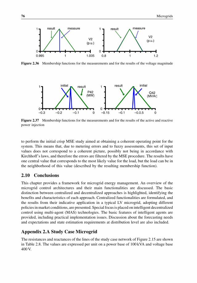
to perform the initial crisp MSE study aimed at obtaining a coherent operating point for the

system. This means that, due to metering errors and to fuzzy assessments, this set of input

values does not correspond to a coherent picture, possibly not being in accordance with

Kirchhoff’s laws, and therefore the errors are filtered by the MSE procedure. The results have

one central value that corresponds to the most likely value for the load, but the load can be in

the neighborhood of this value (described by the resulting membership function).

2.10 Conclusions

This chapter provides a framework for microgrid energy management. An overview of the

microgrid control architectures and their main functionalities are discussed. The basic

distinction between centralized and decentralized approaches is highlighted, identifying the

benefits and characteristics of each approach. Centralized functionalities are formulated, and

the results from their indicative application in a typical LV microgrid, adopting different

policies inmarket conditions, are presented. Special focus is placed on intelligent decentralized

control using multi-agent (MAS) technologies. The basic features of intelligent agents are

provided, including practical implementation issues. Discussion about the forecasting needs

and expectations and state estimation requirements at distribution level are also included.

Appendix 2.A Study Case Microgrid

The resistances and reactances of the lines of the study case network of Figure 2.15 are shown

in Table 2.8. The values are expressed per unit on a power base of 100 kVA and voltage base

400V.

Figure 2.36 Membership functions for the measurements and for the results of the voltage magnitude

Figure 2.37 Membership functions for the measurements and for the results of the active and reactive

power injection

76 Microgrids

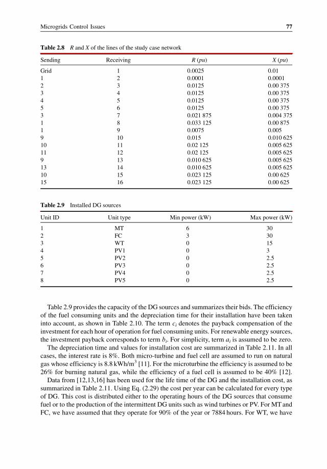
Table 2.9 provides the capacity of the DG sources and summarizes their bids. The efficiency

of the fuel consuming units and the depreciation time for their installation have been taken

into account, as shown in Table 2.10. The term ci denotes the payback compensation of the

investment for each hour of operation for fuel consuming units. For renewable energy sources,

the investment payback corresponds to term bi. For simplicity, term ai is assumed to be zero.

The depreciation time and values for installation cost are summarized in Table 2.11. In all

cases, the interest rate is 8%. Both micro-turbine and fuel cell are assumed to run on natural

gas whose efficiency is 8.8 kWh/m3 [11]. For the microturbine the efficiency is assumed to be

26% for burning natural gas, while the efficiency of a fuel cell is assumed to be 40% [12].

Data from [12,13,16] has been used for the life time of the DG and the installation cost, as

summarized in Table 2.11. Using Eq. (2.29) the cost per year can be calculated for every type

of DG. This cost is distributed either to the operating hours of the DG sources that consume

fuel or to the production of the intermittent DG units such as wind turbines or PV. For MTand

FC, we have assumed that they operate for 90% of the year or 7884 hours. For WT, we have

Table 2.8 R and X of the lines of the study case network

Sending Receiving R (pu) X (pu)

Grid 1 0.0025 0.01

1 2 0.0001 0.0001

2 3 0.0125 0.00 375

3 4 0.0125 0.00 375

4 5 0.0125 0.00 375

5 6 0.0125 0.00 375

3 7 0.021 875 0.004 375

1 8 0.033 125 0.00 875

1 9 0.0075 0.005

9 10 0.015 0.010 625

10 11 0.02 125 0.005 625

11 12 0.02 125 0.005 625

9 13 0.010 625 0.005 625

13 14 0.010 625 0.005 625

10 15 0.023 125 0.00 625

15 16 0.023 125 0.00 625

Table 2.9 Installed DG sources

Unit ID Unit type Min power (kW) Max power (kW)

1 MT 6 30

2 FC 3 30

3 WT 0 15

4 PV1 0 3

5 PV2 0 2.5

6 PV3 0 2.5

7 PV4 0 2.5

8 PV5 0 2.5


assumed 40% capacity factor which means 3504 kWh/kW and for the PVs the yearly

production is 1300 kWh/kW according to [16].

Ann_Cost ¼ ið1þ iÞnð1þ iÞn � 1

� InsCost (2.29)

i is the interest rate, n the depreciation time in years, InsCost, the installation cost and

Ann_Cost is the annual cost for depreciation.

References

1. More Microgrids. [Online] www.microgrids.eu.

2. Lasseter, R., Akhil, A., Marnay, C. et al. (2002)White Paper on Integration of Distributed Energy Resources. The

CERTS Microgrid Concept. CA: Tech. Rep. LBNL-50829, Consortium for Electric Reliability Technology

Solutions (CERTS).

3. Katiraei, F. et al. (2008) Microgrids management. IEEE Power and Energy Magazine, 6, 54–65.

4. W3C. [Online] http://www.w3.org/.

5. Charytoniuk, W. and Chan, M.S. (2000) Short-term load forecasting using Artificial Neural Networks. A review

and evaluation. IEEE T. Power Syst., 15 (1), 263–268.

6. Steinherz Hippert, H., Pedreira, C.E. and Souza, C.S. (2001) Neural Networks for short-term load forecasting, a

review and evaluation. IEEE T. Power Syst., 16 (1), 44–55.

7. Taylor, J. (2008) An evaluation of methods for very short-term electricity demand forecasting using minute-by-

minute British data. Int. J. Forecasting, 24, 645–658.

8. Anemos project. [Online] http://www.anemos-project.eu.

Table 2.10 Bids of the DG sources

Unit type ai (Dct/kWh2) bi (Dct/kWh) ci (Dct/h)

MT 0 4.37 85.06

FC 0 2.84 255.18

WT 0 10.63 0

PV1 0 54.84 0

PV2 0 54.84 0

PV3 0 54.84 0

PV4 0 54.84 0

PV5 0 54.84 0

Table 2.11 Financial data for determining the bids

MT FC WT PV

Life-time (years) 12.5 12.5 12.5 20

Costs in bibliographya (D /kW) 800–2000 3000–20 000 800–5000 4200–10 000

Installation cost (D /kW) 1500 4500 2500 7000

Depreciation time (years) 10 10 10 20

Depreciation cost (D /kW-year) 223.54 670.62 372.57 712.92

aThese costs do not necessarily reflect current costs, especially because capital costs of some

technologies have been significantly reduced.

78 Microgrids

http://www.microgrids.eu

.

http://www.w3.org/

.

http://www.anemos-project.eu

9. Giebel, G., Kariniotakis, G. and Brownsword, R., The State-of-the-art in short-term prediction of wind power. A

literature overview. Deliverable Report D1.1 of the Anemos project (ENK5-CT-2002-00665), available online at

http://anemos.cma.fr.

10. Liu,K.etal. (1996)Comparisonofveryshort-termloadforecastingtechniques. IEEET.PowerSyst.,11 (2),877–882.

11. Canu, S., Duran,M. and Ding, X. (1994) District heating forecast using artificial neural networks. Int. J. Eng., 2 (4).

12. Paravan, D., Brand, H. et al. (2002) Optimization of CHP plants in a liberalized power system. Proceedings of the

Balkan Power Conference, vol 2, pp. 219–226.

13. Nogales, F.J. et al. (2002) Forecasting next-day electricity prices by time series models. IEEE T. Power Syst., 17

(2), 342–348.

14. Garc�ıa-Martos, C., Rodr�ıguez, J. and S�anchez, M.J. (2011) Forecasting electricity prices and their volatilities

using unobserved components. Energ. Econ., 33, 1227–1239.

15. Sideratos, G. and Hatziargyriou, N. (2012) Probabilistic wind power forecasting using radial basis function neural

networks. IEEE T. Power Syst., 27, 1788–1796.

16. Pinson, P. and Kariniotakis, G. (2004) Uncertainty and Prediction Risk Assessment of Short-term Wind Power

Forecasts. Delft, The Netherlands: The Science of Making Torque from Wind.

17. Tsikalakis, A.G. and Hatziargyriou, N.D. (2008) Centralized control for optimizingmicrogrids operation. IEEE T.

Energy Conver., 23 (1), 241–248.

18. Hatziargyriou, N.D., Dimeas, A. and Tsikalakis, A. (2005) Centralised and decentralized control of microgrids.

Int. J. Distr. Energ. Resour., 1 (3), 197–212.

19. Tsikalakis, A.G. and Hatziargyriou, N.D. (2007) Environmental benefits of distributed generation with and

without emissions trading. J. Energ. Policy, 35 (6), 3395–3409.

20. Rao, S.S. (1996) Chapter 7, in Engineering Optimization,Theory and Practice, John Wiley & Sons, New York.

21. Papadogiannis, K.A., Hatziargyriou, N.D. and Saraiva, J.T. (2003) Short Term Active/Reactive Operation

Planning in Market Environment using Simulated Annealing, ISAP, Lemnos, Greece.

22. Lee, K.Y. and El-Sharkawi, M.A. (2002) Tutorial Modern Heuristic Optimization Techniques with Applications

to Power Systems, IEEE PES., Chicago.

23. Papathanassiou, S., Hatziargyriou, N. and Strunz, K. (2005) A Benchmark LV microgrid for Steady State and

Transient Analysis. Cigre Symposium “Power Systems with Dispersed Generation”, Athens,Greece..

24. Kariniotakis, G.N., Stavrakakis, G.S. and Nogaret, E.F. (1996) Wind power forecasting using advanced neural

networks models. IEEE T. Energy Conver., 11 (4), 762–767.

25. APX. Amsterdam Power Exchange. [Online] http://www.apx.nl.

26. McArthur, S.D.J. et al. (2007) Multi-agent systems for power engineering applications— Part I: concepts,

approaches, and technical challenges. IEEE T. Power Syst., 22 (4), 1743–1752.

27. McArthur, S.D.J. et al. (2007) Multi-agent systems for power engineering applications—Part II: technologies,

standards, and tools for building multi-agent systems. IEEE T. Power Syst., 22 (4), 1753–1759.

28. Ferber, J. (1999) Multi-Agent Systems. An introduction to Distributed Intelligence, Addison-Wesley.

29. Bradshaw, J.M. (1997) Software Agents, MIT Press.

30. Wooldridge, M. (2009) An Introduction to Multi-agent Systems, 2nd edn, John Wiley & Sons.

31. Dimeas, A.L., Hatzivasiliadis, S.I. and Hatziargyriou, N.D. (2009) Control agents for enabling customer-driven

microgrids. IEEE, Power & Energy Society General Meeting, PES’09, IEEE.

32. JADE website. [Online] www.jade.tilab.com.

33. FIPA website. [Online] www.fipa.org.

34. CIM. IEC 61970. [Online] http://www.iec.ch/smartgrid/standards/.

35. UML. [Online] http://www.uml.org.

36. Bertsekas, D.P. (1992) Auction algorithms for network flow problems: a tutorial introduction. Comput. Optim.

Appl., 1, 7–66.

37. Castanon, D.P. and Bertsekas, D.A. (1992) A forward/reverse auction algorithm for asymmetric assignments

problems. Comput. Optim. Appl., 1, 277–297.

38. Dimeas, A. and Hatziargyriou, N.D. (2005) Operation of a multi-agent system for microgrid control. IEEE T.

Power Syst., 20 (3), 1447–1455.

39. Dayan, P. and Watkins, C.J. (1992) Q-learning. Mach. Learn., 8, 279–292.

40. Veloso, M. and Peter, S. (1999) Opaque-Transition Reinforcement Learning. Proceedings of the Third Interna-

tional Conference on Autonomous Agents.

41. Dimeas, A.L. and Hatziargyriou, N.D. (2010) Multi-agent reinforcement learning for microgrids. IEEE, Power

and Energy Society General Meeting.


http://anemos.cma.fr

http://www.apx.nl

http://www.jade.tilab.com

http://www.fipa.org

http://www.iec.ch/smartgrid/standards/

http://www.uml.org

42. Gibbons, R. (1992) Game Theory for Applied Economists, Princeton University Press, Princeton, New Jersey.

43. Fudenberg, D. and Tirole, J. (1991) Game Theory, MIT Press, Cambridge, Massachusetts.

44. Korres, G.N., Hatziargyriou, N.D. and Katsikas, P.J. (2011) State estimation in multi-microgrids. Euro. Trans.

Electr. Power Special Issue: Microgrids and Energy Management, 21 (2), 1178–1199.

45. Ghosh, A.K., Lubkeman, D.L. and Jones, R.H. (1997) Load modeling for distribution circuit state estimation.

IEEE T. Power Deliver., 12 (2), 999–1005.

46. Kelley, A.W. and Baran, M.E. (1994) State estimation for real-time monitoring of distribution systems. IEEE T.

Power Syst., 9 (3), 1601–1609.

47. Thornley, V., Jenkins, N. and White, S. (2005) State estimation applied to active distribution networks with

minimal measurements. 15th Power Systems Computation Conference, Liege, Belgium: August 2005.

48. Ghosh, A.K., Lubkeman, D.L., Downey, M.J. and Jones, R.H. (1997) Distribution circuit state estimation using a

probabilistic approach. IEEE T. Power Syst., 12 (1), 45–51.

49. Singh, R., Pal, B.C. and Jabr, R.A. (2009) Choice of estimator for distribution system state estimation. IET Gener.

Transm. Distrib, 3 (7), 666–678.

50. Exposito, A.G. and Abur, A. (2004) Power System State Estimation: Theory and Implementation, Marcel

Dekker, New York.

51. Monticelli, A. (1999) State Estimation in Electric Power Systems: A Generalized Approach, Kluwer Academic

Publishers, Boston, US.

52. Wang, H. and Schulz, N.N. (2006) Using AMR data for load estimation for distribution system analysis. Electr.

Pow. Syst. Res., 76, 336–342.

53. Wang, H. and Schulz, N.N. (2001) A load modelling algorithm for distribution system state estimation.

Conference and Exposition in Transmission and Distribution, vol. 1 102–105.

54. Samarakoon, K., Wu, J., Ekanayake, J. and Jenkins, N. (2011) Use of Delayed Smart Meter Measurements for

Distribution State Estimation. IEEE PES General Meeting, July 2011.

55. Gu, J.W., Clements, K.A., Krumpholz, G.R. and Davis, P.W. (1983) The solution of ill-conditioned power system

state estimation problems. IEEE T. Power Ap. Syst., PAS-102, 3473–3480.

56. Korres, G.N. (2011) A distributed multiarea state estimation. IEEE T. Power Syst., 26, 73–84.

57. Gomez-Exposito, A., de laVilla Jaen, A., Gomez-Quiles, C. et al . (2011) A taxonomy of multi-area state

estimation methods. Electr. Power Syst., 81 1060–1069.

58. Cobelo, I., Shafiu, A., Jenkins, N. and Strbac, G. (2007) State estimation of networks with distributed generation.

Eur. Trans. Electr. Power, 17, 21–36.

59. Su, C.-L. and Lu, C.-N. (2001) Interconnected network state estimation using randomly delayed measurements.

IEEE T. Power Syst., 16 (4), 870–878.

60. Korres, G.N. and Manousakis, N.M. (2012) A state estimation algorithm for monitoring topology changes in

distribution systems. PES General Meeting, San Diego, CA, USA, 2012, pp. 1–7.

61. Pereira, J. (May 2009) A state estimation approach for distribution networks considering uncertainties and

switching. Porto: Faculdade de Engenharia da Universidade do Porto. PhD Thesis, July 2001 [Online] http://saca.

inescporto.pt/artigos/artigo150.pdf.

62. Katsikas, G.N. and Korres and, P.J. (2002) Identification of circuit breaker statuses in WLS state estimator. IEEE

T. Power Syst., 17 (3), 818–825.

63. Saric, A.T. and Ciric, R.M. (2003) Integrated fuzzy state estimation and load flow analysis in distribution

networks. IEEE Trans. Power Delivery, 18 (2), 571–578.

64. Konjic, T., Miranda, V. and Kapetanovic, I. (2005) Fuzzy inference systems applied to LV substation load

estimation. IEEE T. Power Syst., 20 (2), 742–749.

65. Miranda, V., Pereira, J. and Saraiva, J.T. (2000) Load allocation in DMS with a fuzzy state estimator. IEEE T.

Power Syst., 15 (2), 529–534.

66. Zadeh, L.A. (1965) Fuzzy Sets. Inform. Control, 8, 338–353.

80 Microgrids

http://saca.inescporto.pt/artigos/artigo150.pdf

http://saca.inescporto.pt/artigos/artigo150.pdf

3

Intelligent Local Controllers

Thomas Degner, Nikos Soult anis, Alfred Engler and Asier Gil de Muro

3.1 Int roduction

The develo pment and use of the intel ligent local cont rollers for micro generat ors and

control lable loads enabl es stable mi crogrid operation. These controlle rs provide efficie nt

voltage and frequency control in case of islande d operation, ancill ary service s in intercon-

nected mode, and deal efficie ntly with frequency and voltage variat ions during transitions

from interconnec ted to islande d opera tion and vice versa.

The main tasks of micro source controlle rs are to allow power shar ing b etween the different

sources at different loca tions, acting on the electroni c converters that interface them to the

networ k. As com munica tion lines, especia lly for long distanc es and cont rol purpos es are

expensive and vulne rable, at least fast com municati on should be avoided. Th is can be

achieved by using loca l cont rollers, which are based on frequency and voltage droops .

This way, the loca lly available inform ation – fre quency and voltage – is used for power

sharing. Normally, the frequ ency is linked to the active power, and voltage is linked to the

reactive power.

Standard rotating gener ator system s inherentl y suppor t thes e droops. So metime s, for

improving performanc e, additional cont rollers are appl ied. There fore it is possi ble to opera te

large numb ers of such generat ors in a single network. However, with standar d static inverters,

charact erized by fixed frequency and voltage, such an appro ach is not possib le. A cont rol

appro ach providing frequency and voltage droops is require d.

In this chapt er, intel ligent control conce pts for power electroni cs interface d micro sources

are describ ed. Control strat egies for multipl e inverter systems are developed with reference to

the self-synchr onizing mec hanism of conventional rotating gener ators. The appropri ate

control o f fre quency and voltage in each inverter facil itates the sharing of the active and

reactive power in the system . Sim ulation resu lts that dem onstrate power shar ing betwee n

distributed generators are given. In the following, the implications of line parameters, in

particular of the high resistance practically found in LV microgrids, are systematically



discussed. Finally, a control algorithm using the fictitious impedance method is analyzed and

characteristic simulation results are provided.

3.2 Inverter Control Issues in the Formation of Microgrids

3.2.1 Active Power Control

The basic principle that allows classic synchronously rotating generators to change their

power output in response to a change in the system load without an explicit communication

network is the frequency variation at the machine terminal as a function of power demand.

When two points in the network are operating at different frequencies there is an increase of

active power delivery from the location of higher frequency to the location of lower frequency.

As this happens, the two frequencies tend to drift towards a common average value until the

new steady state is reached (self-synchronizing torque). This physical relation between active

power output and frequency in the synchronous generators has to be implemented in the

control of the inverters, in the case of a system with inverter interfaced sources.

3.2.2 Voltage Regulation

Voltage control must ensure that there are no large circulating reactive currents between

sources. Without local voltage control, systems with high penetration of microsources could

experience voltage and/or reactive power oscillations. The issues are identical to those

involved in the control of large synchronous generators. However, in large power systems the

impedance between generators is usually large enough to impede circulating currents. In a

microgrid, that is typically radial, the problem of large circulating reactive currents is

immense. With small errors in voltage setpoints, the circulating current can exceed the

ratings of microsources. This situation requires a voltage vs. reactive current droop controller

so that, as the reactive current generated by the microsource becomes more capacitive, the

local voltage setpoint is reduced. Conversely, as the current becomes more inductive, the

voltage setpoint should increase.

3.3 Control Strategies for Multiple Inverters

3.3.1 Master Slave Control Scheme

The control method that has been used for paralleling inverter units in the case of UPS systems

is very difficult to adopt for a distributed generation application like the microgrid. The load

current may be measured and divided among the participating inverter units, but this requires

that the load and the microsources are separated.

In the master–slave control, one inverter regulates the voltage and the resulting current of

this unit defines the current references of the other units. The master acts as a voltage source

inverter and the rest of the units as current source inverters [1].

A system with a voltage source, as master and additional controllable current sources (grid

supporting units) is depicted in Figure 3.1. The supervisory control is responsible for power

distribution. The main features of this approach can be summarized as follows:

� a simple control algorithm at component level is required� high expenditure for buses and their cabling is needed

82 Microgrids

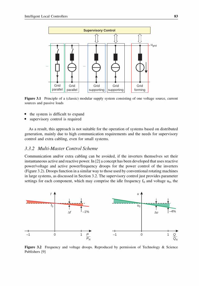
� the system is difficult to expand� supervisory control is required

As a result, this approach is not suitable for the operation of systems based on distributed

generation, mainly due to high communication requirements and the needs for supervisory

control and extra cabling, even for small systems.

3.3.2 Multi-Master Control Scheme

Communication and/or extra cabling can be avoided, if the inverters themselves set their

instantaneous active and reactive power. In [2] a concept has been developed that uses reactive

power/voltage and active power/frequency droops for the power control of the inverters

(Figure 3.2). Droops function in a similar way to those used by conventional rotating machines

in large systems, as discussed in Section 3.2. The supervisory control just provides parameter

settings for each component, which may comprise the idle frequency f0 and voltage u0, the

ugrid

Gridforming

Gridsupporting

Gridparallel

......

Supervisory Control

Gridparallel

Gridsupporting

Figure 3.1 Principle of a (classic) modular supply system consisting of one voltage source, current

sources and passive loads

u

u0

10–1 QQN

–4%

f

f0

10–1

–1%

PPN

Δf Δu

Figure 3.2 Frequency and voltage droops. Reproduced by permission of Technology & Science

Publishers [9]

Intelligent Local Controllers 83

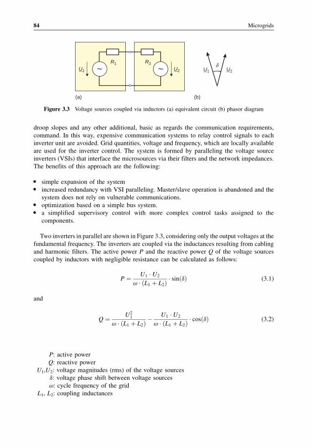
droop slopes and any other additional, basic as regards the communication requirements,

command. In this way, expensive communication systems to relay control signals to each

inverter unit are avoided. Grid quantities, voltage and frequency, which are locally available

are used for the inverter control. The system is formed by paralleling the voltage source

inverters (VSIs) that interface the microsources via their filters and the network impedances.

The benefits of this approach are the following:

� simple expansion of the system� increased redundancy with VSI paralleling. Master/slave operation is abandoned and the

system does not rely on vulnerable communications.� optimization based on a simple bus system.� a simplified supervisory control with more complex control tasks assigned to the

components.

Two inverters in parallel are shown in Figure 3.3, considering only the output voltages at the

fundamental frequency. The inverters are coupled via the inductances resulting from cabling

and harmonic filters. The active power P and the reactive power Q of the voltage sources

coupled by inductors with negligible resistance can be calculated as follows:

P ¼ U1 � U2

v � ðL1 þ L2Þ � sinðdÞ (3.1)

and

Q ¼ U21

v � ðL1 þ L2Þ �U1 � U2

v � ðL1 þ L2Þ � cosðdÞ (3.2)

P: active power

Q: reactive power

U1,U2: voltage magnitudes (rms) of the voltage sources

d: voltage phase shift between voltage sources

v: cycle frequency of the grid

L1, L2: coupling inductances

U1 U2δ

U1 U2

R1 R2

~

(a) (b)

~

Figure 3.3 Voltage sources coupled via inductors (a) equivalent circuit (b) phasor diagram

84 Microgrids

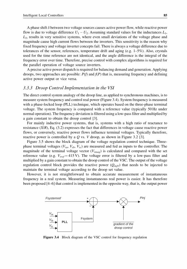
A phase shift d between two voltage sources causes active power flow, while reactive power

flow is due to voltage difference U1�U2. Assuming standard values for the inductances L1,

L2, results in very sensitive systems, where even small deviations of the voltage phase and

magnitude cause high current flows between the inverters. This sensitivity is the reason why

fixed frequency and voltage inverter concepts fail. There is always a voltage difference due to

tolerances of the sensor, references, temperature drift and aging (e.g. 1–5%). Also, crystals

used for the time reference are not identical, and the angle difference is the integral of the

frequency error over time. Therefore, precise control with complex algorithms is required for

the parallel operation of voltage source inverters.

A precise active power dispatch is required for balancing demand and generation. Applying

droops, two approaches are possible: P(f) and f(P) that is, measuring frequency and defining

active power output or vice versa.

3.3.3 Droop Control Implementation in the VSI

The direct control system analogy of the droop line, as applied to synchronous machines, is to

measure system frequency and control real power (Figure 3.4). System frequency is measured

with a phase-locked loop (PLL) technique, which operates based on the three-phase terminal

voltage. The system frequency is compared with a reference value (typically 50Hz under

normal operation). The frequency deviation is filtered using a low-pass filter and multiplied by

a gain constant to obtain the droop control [3].

For mainly inductive power systems, that is, systems with a high ratio of reactance to

resistance (X/R), Eq. (3.2) expresses the fact that differences in voltage cause reactive power

flows, or conversely, reactive power flows influence terminal voltages. Typically therefore,

reactive power is controlled by a Q vs. V droop, as shown in Figure 3.2 [3].

Figure 3.5 shows the block diagram of the voltage regulation control technique. Three-

phase terminal voltages (Vta, Vtb, Vtc) are measured and fed as inputs to the controller. The

magnitude of the terminal voltage vector (Vtmag) is calculated and compared with the set

reference value (e.g. Vtref¼ 415V). The voltage error is filtered by a low-pass filter and

multiplied by a gain constant to obtain the droop control of the VSC. The output of the voltage

regulation control block provides the reactive power (QinjV) that needs to be injected to

maintain the terminal voltage according to the droop set value.

However, it is not straightforward to obtain accurate measurement of instantaneous

frequency in a real system. Measuring instantaneous real power is easier. It has therefore

been proposed [4–6] that control is implemented in the opposite way, that is, the output power

PLL

Vta

Vtb

Vtc

Fsystemref

Fsystem

Pinj+

–

gradient of thedroop control

Figure 3.4 Block diagram of the VSC control for frequency regulation


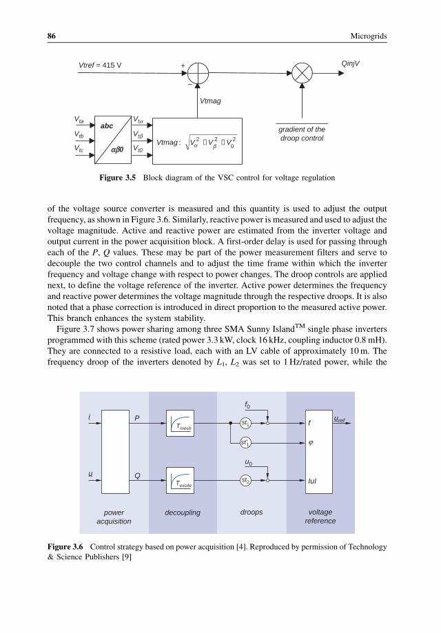
of the voltage source converter is measured and this quantity is used to adjust the output

frequency, as shown in Figure 3.6. Similarly, reactive power is measured and used to adjust the

voltage magnitude. Active and reactive power are estimated from the inverter voltage and

output current in the power acquisition block. A first-order delay is used for passing through

each of the P, Q values. These may be part of the power measurement filters and serve to

decouple the two control channels and to adjust the time frame within which the inverter

frequency and voltage change with respect to power changes. The droop controls are applied

next, to define the voltage reference of the inverter. Active power determines the frequency

and reactive power determines the voltage magnitude through the respective droops. It is also

noted that a phase correction is introduced in direct proportion to the measured active power.

This branch enhances the system stability.

Figure 3.7 shows power sharing among three SMA Sunny IslandTM single phase inverters

programmed with this scheme (rated power 3.3 kW, clock 16 kHz, coupling inductor 0.8 mH).

They are connected to a resistive load, each with an LV cable of approximately 10m. The

frequency droop of the inverters denoted by L1, L2 was set to 1Hz/rated power, while the

abc

αβ0

20

22Vtmag VVV ++: βα

Vta

Vtb

Vtc

Vtα

Vtβ

Vt0

Vtref = 415 V

Vtmag

QinjV+

–

gradient of thedroop control

Figure 3.5 Block diagram of the VSC control for voltage regulation

i

u

P

Q

Tmech

Texcite

st1

f0

st '1

st2

uref

u0

f

ϕ

IuI

poweracquisition

decoupling droops voltagereference

Figure 3.6 Control strategy based on power acquisition [4]. Reproduced by permission of Technology

& Science Publishers [9]

86 Microgrids

droop of the inverter denot ed by L3 was set to 2 Hz/ra ted power. It is evident that this method

allows the L3 inverter to suppl y half the power of the other two and that active power shar ing is

defined by the droop const ants. It is remar kable that reactive power is circulat ing – as seen

from the inverter current – as a resu lt of the phase difference cause d between inverter L3 and

L1, L2.

Next, a simulat ed case of a micro grid is present ed. The mi crogrid (Figure 3.8 ), consisting of

three inverters coupl ed via an MV distribution system (15 kV), is simul ated in ATP/EMTP

(alternat ive transient s program /electro magnetic transient s program : http://www.emtp.org/).

The inverters are represented by controllable three-phase voltage sources, and the distribution

system consists of switches, overhead lines (p-blocks), transformers and the load. The three

inverters operate in parallel via the MV distribution system and supply a resistive load with a

total power of 100 kW. The inverters are controlled with the algorithm described in Figure 3.6.

With suitable setting of the slope of the frequency droop the contribution of the inverters is

20, 30 and 50 kW, as seen in Figure 3.9. The slope of the frequency droop may be used in order

to take into account the size of the inverter. The idle frequency f0 can be used to control the

energy flow. The idle frequency of the inverters in this case is set to 50Hz. Owing to the load,

the system frequency decreases to 49Hz (Figure 3.10). The frequency could be restored to

50Hz with the use of a secondary control.

The setting of the slope of the voltage droop results in a variable virtual inductance between

the respective inverter and the distribution system. It should be chosen in order to ensure stable

operation. The idle voltage should be set in order to minimize reactive power. However,

voltage limits have to be respected.

5 5.01 5.02 5.03 5.04 5.05 5.06 5.07 5.08

–200

0

200

t/s

U/V

, Ito

tal*1

0/A

5 5.01 5.02 5.03 5.04 5.05 5.06 5.07 5.08

–5

0

5

t/s

I L1,

I L2,

I L3/

A

U

I

IL1, L2

IL3

Figure 3.7 Parallel operation of three identical inverters sharing a resistive load via their frequency vs.

power droop control. Reproduced by permission of Technology & Science Publishers [9]


http://www.emtp.org/

U U U

U

U

U

UUU

Inverter 3

Inverter 2Inverter 1

Figure 3.8 Simulation of inverter dominated system in ATP/EMTP

0.0 0.2 0.4 0.6 0.8 1.0[s]

0

10

20

30

40

50

60

*103

Figure 3.9 Load shared between the three inverters

88 Microgrids

3.3.4 Ancillary Services

While in grid-connected mode, microgrids can contribute to the overall grid control and thus

facilitate the operation of the system by providing ancillary services.

A microgrid can support voltage in the area of its connection to the upstream network, in

the event of a disturbance that causes a voltage drop. Figure 3.11 shows the simulation

results for the sudden reduction of voltage at the point of common coupling (PCC) of a

microgrid that is connected at the end of a long supply feeder with and without voltage

regulation. The microgrid with voltage regulation, in this case the VSC of an energy storage

unit, injects reactive power to maintain the rms terminal voltage (Vtrms) within acceptable

limits.

The central controller effectively sets the droop line slope of the individual VSC interfaces

to determine reactive power sharing between the units and the reactive power export/import of

the microgrid under grid-connected operation. During islanded operation the net reactive

power flow will be zero. The voltage in the microgrid will then increase (if there is excess

reactive power), forcing power electronics interfaced units to produce less Q or even absorb

reactive power, until a new steady-state voltage is reached (net zero Q flow).

Here the voltage/reactive power droops act in order to limit the reactive power flow. The

voltage control and the flow of reactive power in LV grids, which are mainly resistive, are

discussed in the following paragraphs.

0.0 0.1 0.2 0.3 0.4 0.5 0.6[s]

48.8

49.0

49.2

49.4

49.6

49.8

50.0

Figure 3.10 Frequency change in the islanded microgrid


A microgrid can absorb/inject a specified amount of aggregate power at the point of

common coupling. This is carried out by adjusting the position of the droop lines of the

individual VSCs from a central controller. A simulated case is shown in Figure 3.12. This

adjustment does not require a particularly fast control loop, since even a slow telecommu-

nications link has time constants significantly faster than most power network subsystems.

The additional active and reactive powers (Pinj, Qinj) to be injected in this case are set by the

central controller for each specific VSC. Alternatively, the droop line settings could have been

adjusted for each VSC by the central controller directly. In the system simulated, two limit

blocks are used to limit the power injection (active power limits�10 kW, reactive power limits

�20 kVAr). These limits are important during the transient period caused by a disturbance in

the system.

3.3.5 Optional Secondary Control Loops

If a microsource has to produce a specific active power during the isolated operation, a

secondary control action may be employed. The control forces the active power output of the

VSI to remain at Pref while the system frequency changes, by acting on the fref value. The

droop line is shifted vertically as shown in Figure 3.13.

The microgrid frequency will end up in steady state after every load change to a value

different from nominal that depends on the droop slope and the relation between the load and

frequency. To restore the frequency to the nominal value, a secondary control loop is needed to

cancel out the residual difference. The control action changes the Pref value so that the

Figure 3.11 Simulation results without (a) and with (b) voltage regulation control of the microgrid

connected to main supply

90 Microgrids

frequency is always brought back to the fref value. The droop line is shifted horizontally as

shown in Figure 3.14.

Likewise, secondary control action can be applied to the voltage/reactive power control.

Reactive power output of the VSI may be kept to a constant value Qref by changing the Vref

value and shifting the droop line vertically as in Figure 3.13 for active power. To keep the

output voltage of the inverter constant, Qref may be changed, shifting the droop line

horizontally as is done in Figure 3.14 for frequency.

Figure 3.12 Simulation results with the active and reactive power control set by central controller (all

other controls are deactivated and the microgrid is connected to the main supply)

fref

Pmax P

f

fref1

Pref

fref2

Figure 3.13 Control action for constant active power production at Pref


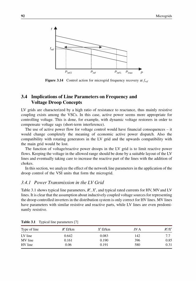
3.4 Implications of Line Parameters on Frequency andVoltage Droop Concepts

LV grids are characterized by a high ratio of resistance to reactance, thus mainly resistive

coupling exists among the VSCs. In this case, active power seems more appropriate for

controlling voltage. This is done, for example, with dynamic voltage restorers in order to

compensate voltage sags (short-term interference).

The use of active power flow for voltage control would have financial consequences – it

would change completely the meaning of economic active power dispatch. Also the

compatibility with rotating generators in the LV grid and the upwards compatibility with

the main grid would be lost.

The function of voltage/reactive power droops in the LV grid is to limit reactive power

flows. Keeping the voltage in the allowed range should be done by a suitable layout of the LV

lines and eventually taking care to increase the reactive part of the lines with the addition of

chokes.

In this section, we analyze the effect of the network line parameters in the application of the

droop control of the VSI units that form the microgrid.

3.4.1 Power Transmission in the LV Grid

Table 3.1 shows typical line parameters, R0, X0, and typical rated currents for HV, MVand LV

lines. It is clear that the assumption about inductively coupled voltage sources for representing

the droop controlled inverters in the distribution system is only correct for HV lines. MV lines

have parameters with similar resistive and reactive parts, while LV lines are even predomi-

nantly resistive.

fref

Pmax P

f

Pref Pref1Pref2

Figure 3.14 Control action for microgrid frequency recovery at fref

Table 3.1 Typical line parameters [7]

Type of line R0 V/km X0 V/km IN A R0/X0

LV line 0.642 0.083 142 7.7

MV line 0.161 0.190 396 0.85

HV line 0.06 0.191 580 0.31

92 Microgrids

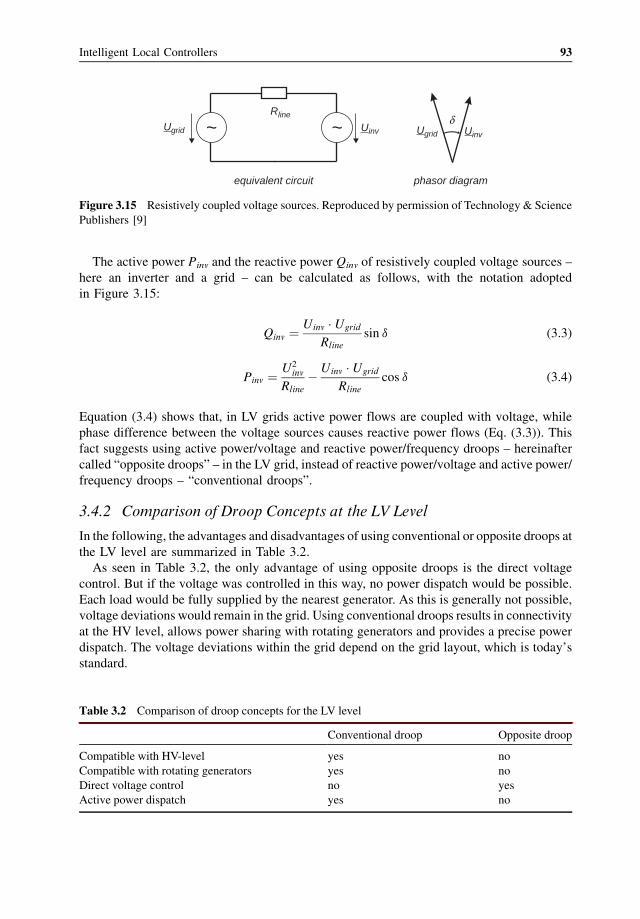
The active power Pinv and the reactive power Qinv of resistively coupled voltage sources –

here an inverter and a grid – can be calculated as follows, with the notation adopted

in Figure 3.15:

Qinv ¼Uinv � Ugrid

Rline

sin d (3.3)

Pinv ¼ U2inv

Rline

� Uinv � Ugrid

Rline

cos d (3.4)

Equation (3.4) shows that, in LV grids active power flows are coupled with voltage, while

phase difference between the voltage sources causes reactive power flows (Eq. (3.3)). This

fact suggests using active power/voltage and reactive power/frequency droops – hereinafter

called “opposite droops” – in the LV grid, instead of reactive power/voltage and active power/

frequency droops – “conventional droops”.

3.4.2 Comparison of Droop Concepts at the LV Level

In the following, the advantages and disadvantages of using conventional or opposite droops at

the LV level are summarized in Table 3.2.

As seen in Table 3.2, the only advantage of using opposite droops is the direct voltage

control. But if the voltage was controlled in this way, no power dispatch would be possible.

Each load would be fully supplied by the nearest generator. As this is generally not possible,

voltage deviations would remain in the grid. Using conventional droops results in connectivity

at the HV level, allows power sharing with rotating generators and provides a precise power

dispatch. The voltage deviations within the grid depend on the grid layout, which is today’s

standard.

equivalent circuit phasor diagram

Ugrid Uinv

Rline

~~ Ugrid Uinv

δ

Figure 3.15 Resistively coupled voltage sources. Reproduced by permission of Technology & Science

Publishers [9]

Table 3.2 Comparison of droop concepts for the LV level

Conventional droop Opposite droop

Compatible with HV-level yes no

Compatible with rotating generators yes no

Direct voltage control no yes

Active power dispatch yes no


3.4.3 Indirect Operation of Droops

Basically, the conventional droop approach can be applied in LV grids owing to the generator

voltage variation with reactive power exchange. The reactive power of each generator is tuned

in a way that the resulting voltage profile satisfies the desired active power distribution. In the

LV grid, the reactive power is a function of the phase angle, as seen in Eq. (3.3). This is

adjusted with the active power/frequency droop. Of course, the entire loop has to be

consistent. Four stable operating points depending on the slopes of the droops can be

distinguished, two of which make sense [8,9].

3.4.3.1 Stable Operating Points

In order to derive the operating points of conventional droops in LV grids, the stability of the

power transfer Eq. (3.4) is assessed in a simplified manner. Since at a reasonable operating

point, d is rather small, cos d becomes almost 1. Rearranging (3.4) with given power Pinv and

given grid voltage Ugrid, two solutions for the inverter voltage Uinv are obtained from the

quadratic equation:

Uinv1;2 ¼ Ugrid

2�

ffiffiffiffiffiffiffiffiffiffiffiffiffiffiffiffiffiffiffiffiffiffiffiffiffiffiffiffiffiffi

U2grid

4þ Pinv � R

s

(3.5)

Both solutions are considered next. Uinv1 is a voltage close to the grid voltage and Uinv2 is a

slightly negative voltage. This implies a 180� phase shift. Therefore, in (3.6) the factor k is

introduced, with k1¼ 1 for the first solution and k2¼� 1 for the negative solution. The factor

k is an approximation of the cos function in (3.4):

Pinv ¼ Uinv1;2 � Ugrid

R¼ Uinv1;2 � k1;2 (3.6)

The inverter power Pinv is adjusted by changing the inverter voltage Uinv with its reactive

power, as follows:

Uinv1;2 � Ugrid ¼ Uinv1;2 � qdroop; (3.7)

From Eq. (3.3) Qinv is a function of the angle d, for small values of which

Uinv1;2 � d � Uinv1;2 � Ugrid

R(3.8)

d is the integral over time of the generator’s frequency difference from the grid frequency:

d ¼ð

Df dt (3.9)

and

Df ¼ ðPset � PinvÞ � pdroop (3.10)

94 Microgrids

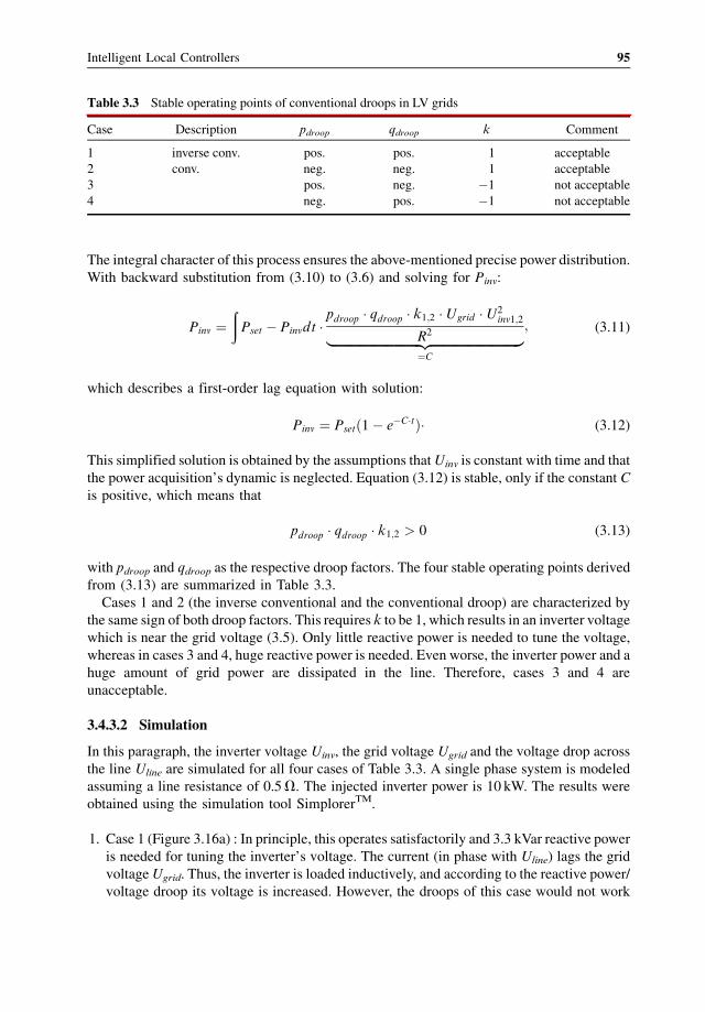
The integral character of this process ensures the above-mentioned precise power distribution.

With backward substitution from (3.10) to (3.6) and solving for Pinv:

Pinv ¼ð

Pset � Pinvdt �pdroop � qdroop � k1;2 � Ugrid � U2

inv1;2

R2|fflfflfflfflfflfflfflfflfflfflfflfflfflfflfflfflfflfflfflfflfflfflfflfflfflfflfflfflffl{zfflfflfflfflfflfflfflfflfflfflfflfflfflfflfflfflfflfflfflfflfflfflfflfflfflfflfflfflffl}

¼C

; (3.11)

which describes a first-order lag equation with solution:

Pinv ¼ Psetð1� e�C�tÞ� (3.12)

This simplified solution is obtained by the assumptions thatUinv is constant with time and that

the power acquisition’s dynamic is neglected. Equation (3.12) is stable, only if the constant C

is positive, which means that

pdroop � qdroop � k1;2 > 0 (3.13)

with pdroop and qdroop as the respective droop factors. The four stable operating points derived

from (3.13) are summarized in Table 3.3.

Cases 1 and 2 (the inverse conventional and the conventional droop) are characterized by

the same sign of both droop factors. This requires k to be 1, which results in an inverter voltage

which is near the grid voltage (3.5). Only little reactive power is needed to tune the voltage,

whereas in cases 3 and 4, huge reactive power is needed. Even worse, the inverter power and a

huge amount of grid power are dissipated in the line. Therefore, cases 3 and 4 are

unacceptable.

3.4.3.2 Simulation

In this paragraph, the inverter voltage Uinv, the grid voltage Ugrid and the voltage drop across

the line Uline are simulated for all four cases of Table 3.3. A single phase system is modeled

assuming a line resistance of 0.5V. The injected inverter power is 10 kW. The results were

obtained using the simulation tool SimplorerTM.

1. Case 1 (Figure 3.16a) : In principle, this operates satisfactorily and 3.3 kVar reactive power

is needed for tuning the inverter’s voltage. The current (in phase with Uline) lags the grid

voltageUgrid. Thus, the inverter is loaded inductively, and according to the reactive power/

voltage droop its voltage is increased. However, the droops of this case would not work

Table 3.3 Stable operating points of conventional droops in LV grids

Case Description pdroop qdroop k Comment

1 inverse conv. pos. pos. 1 acceptable

2 conv. neg. neg. 1 acceptable

3 pos. neg. �1 not acceptable

4 neg. pos. �1 not acceptable


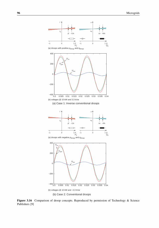
0.5 0.505 0.51 0.515 0.52 0.525 0.53 0.535 0.54−400

−200

0

200

400

Uinv

Ugrid

Uline

f

f0Δf +1%

u

Δu +4%

u0

10–1 QQN

10

(a) droops with positive pdroop and qdroop

(b) voltages @ 10 kW and 3.3 kVar

–1 PPN

(a) Case 1: Inverse conventional droops

0.5 0.505 0.51 0.515 0.52 0.525 0.53 0.535 0.54−400

−200

0

200

400Uinv

Ugrid

Uline

f

f0Δf –1%

u

Δu –4%

u0

10–1 QQN

10

(a) droops with negative pdroop and qdroop

(b) voltages @ 10 kW and –3.3 kVar

–1 PPN

(b) Case 2: Conventional droops

Figure 3.16 Comparison of droop concepts. Reproduced by permission of Technology & Science

Publishers [9]

96 Microgrids

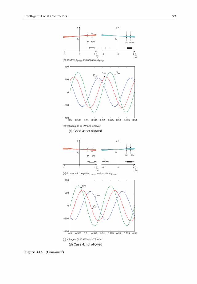
0.5 0.505 0.51 0.515 0.52 0.525 0.53 0.535 0.54−400

−200

0

200

400

UinvUgrid

Uline

f

f0Δf +1%

u

Δu –4%

u0

10–1 QQN

10

(a) positive pdroop and negative qdroop

(b) voltages @ 10 kW and 72 kVar

–1 PPN

(c) Case 3: not allowed

0.5 0.505 0.51 0.515 0.52 0.525 0.53 0.535 0.54−400

−200

0

200

400

Uline

Uinv

Ugrid

f

f0Δf –1%

10

(a) droops with negative pdroop and positive qdroop

(b) voltages @ 10 kW and –72 kVar

–1 PPN

u

Δu +4%

u0

10–1 QQN

(d) Case 4: not allowed

Figure 3.16 (Continued)


with the interconnected grid or rotating generators, as they are inverse to conventional

droops.

2. Case 2 (Figure 3.16b) demonstrates the operability of the conventional droops in the LV

grid. Here 3.3 kVar of reactive power is needed for tuning the inverter’s voltage. The

current (in phase with Uline) leads Ugrid, thus loading the inverter capacitively in order to

increase the voltage. According to the active power/frequency droop and the setting of the

idle frequency, exactly 10.0 kW is fed into the grid.

3. Case 3 (Figure 3.16c) operates at a stable but not acceptable operating point. It is

characterized by huge currents. The inverter injects exactly 10 kW, but 72 kVar of

reactive power would be needed. The corresponding currents would cause a huge

voltage drop across the line with losses larger than the injected active power of the

inverter itself.

4. Case 4 (Figure 3.16d) is almost the same as Case 3. A negative reactive power of�72 kVar

is required.

It can be concluded that the conventional droops (Case 2) can be equally applied to LV

grids. They provide a reasonable operating point and the advantages of Table 3.2.

3.5 Development and Evaluation of Innovative Local Controls toImprove Stability

For effective control of the microsources, the dependence on the line impedance has to be

overcome. To this end, a supplementary control technique that is, in effect, an elaboration of

the active power/voltage angle, reactive power/voltage magnitude discussed previously, has

been proposed; it is called the fictitious impedance method [10]. It uses the instantaneous

current feedback, thus providing additional possibilities such as control of the harmonic

frequencies. This section describes its implementation and analyzes the results by using

simulations.

A voltage drop is imposed on the inverter output formed by the inverter current across a

fictitious impedance. This impedance value is a control parameter and is defined at will,

according to the conditions of the network or the microsource/inverter stage of operation.

Therefore, it constitutes a flexible means of adjusting the inverter to the system. The

effectiveness of the control is tested under all formed line characteristics that may be

encountered, from fully inductive to mostly resistive. The aim is to decouple the P/f and

Q/V control channels, changing the behavior of the inverter, and leading to a system with

inductively coupled sources.

In the following paragraphs, results from stability analysis of distribution networks with

resistive and inductive coupling impedances are provided with the main emphasis on resistive

coupling, which is more common in LV networks and the one that provokes more stability

problems. The alternative transient program (ATP) is used for the simulations.

3.5.1 Control Algorithm

In order to simplify simulations, all sources are considered as fully controllable, three-phase

balanced voltage sources. This is an acceptable simplification, since the inverter allows the

control of the output voltage waveform.

98 Microgrids

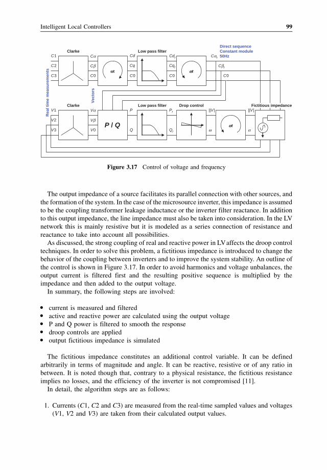
The output impedance of a source facilitates its parallel connection with other sources, and

the formation of the system. In the case of the microsource inverter, this impedance is assumed

to be the coupling transformer leakage inductance or the inverter filter reactance. In addition

to this output impedance, the line impedance must also be taken into consideration. In the LV

network this is mainly resistive but it is modeled as a series connection of resistance and

reactance to take into account all possibilities.

As discussed, the strong coupling of real and reactive power in LVaffects the droop control

techniques. In order to solve this problem, a fictitious impedance is introduced to change the

behavior of the coupling between inverters and to improve the system stability. An outline of

the control is shown in Figure 3.17. In order to avoid harmonics and voltage unbalances, the

output current is filtered first and the resulting positive sequence is multiplied by the

impedance and then added to the output voltage.

In summary, the following steps are involved:

� current is measured and filtered� active and reactive power are calculated using the output voltage� P and Q power is filtered to smooth the response� droop controls are applied� output fictitious impedance is simulated

The fictitious impedance constitutes an additional control variable. It can be defined

arbitrarily in terms of magnitude and angle. It can be reactive, resistive or of any ratio in

between. It is noted though that, contrary to a physical resistance, the fictitious resistance

implies no losses, and the efficiency of the inverter is not compromised [11].

In detail, the algorithm steps are as follows:

1. Currents (C1, C2 and C3) are measured from the real-time sampled values and voltages

(V1, V2 and V3) are taken from their calculated output values.

C1

C2

C3

Cα

Cβ

C0

Cd

Cq

C0

Cαf

Cβf

C0

V1

V2

V3

Vα

Vβ

V0P / Q

P

Q

Pf

Qf

||V |

ω

||V |

α

Cdf

Cqf

C0

Clarke

Clarke

ωt ωt

ωt

Low pass filter

Low pass filter Drop control Fictitious impedance

Rea

l tim

e m

easu

rem

ents

Vec

tors

Direct sequenceConstant module50Hz

Figure 3.17 Control of voltage and frequency


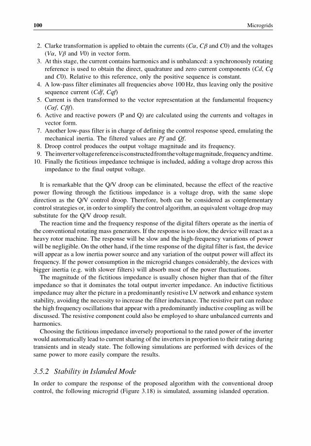
2. Clarke transformation is applied to obtain the currents (Ca, Cb and C0) and the voltages

(Va, Vb and V0) in vector form.

3. At this stage, the current contains harmonics and is unbalanced: a synchronously rotating

reference is used to obtain the direct, quadrature and zero current components (Cd, Cq

and C0). Relative to this reference, only the positive sequence is constant.

4. A low-pass filter eliminates all frequencies above 100Hz, thus leaving only the positive

sequence current (Cdf, Cqf)

5. Current is then transformed to the vector representation at the fundamental frequency

(Caf, Cbf).

6. Active and reactive powers (P and Q) are calculated using the currents and voltages in

vector form.

7. Another low-pass filter is in charge of defining the control response speed, emulating the

mechanical inertia. The filtered values are Pf and Qf.

8. Droop control produces the output voltage magnitude and its frequency.

9. Theinvertervoltagereferenceisconstructedfromthevoltagemagnitude,frequencyandtime.

10. Finally the fictitious impedance technique is included, adding a voltage drop across this

impedance to the final output voltage.

It is remarkable that the Q/V droop can be eliminated, because the effect of the reactive

power flowing through the fictitious impedance is a voltage drop, with the same slope

direction as the Q/V control droop. Therefore, both can be considered as complementary

control strategies or, in order to simplify the control algorithm, an equivalent voltage drop may

substitute for the Q/V droop result.

The reaction time and the frequency response of the digital filters operate as the inertia of

the conventional rotating mass generators. If the response is too slow, the device will react as a

heavy rotor machine. The response will be slow and the high-frequency variations of power

will be negligible. On the other hand, if the time response of the digital filter is fast, the device

will appear as a low inertia power source and any variation of the output power will affect its

frequency. If the power consumption in the microgrid changes considerably, the devices with

bigger inertia (e.g. with slower filters) will absorb most of the power fluctuations.

The magnitude of the fictitious impedance is usually chosen higher than that of the filter

impedance so that it dominates the total output inverter impedance. An inductive fictitious

impedance may alter the picture in a predominantly resistive LV network and enhance system

stability, avoiding the necessity to increase the filter inductance. The resistive part can reduce

the high frequency oscillations that appear with a predominantly inductive coupling as will be

discussed. The resistive component could also be employed to share unbalanced currents and

harmonics.

Choosing the fictitious impedance inversely proportional to the rated power of the inverter

would automatically lead to current sharing of the inverters in proportion to their rating during

transients and in steady state. The following simulations are performed with devices of the

same power to more easily compare the results.

3.5.2 Stability in Islanded Mode

In order to compare the response of the proposed algorithm with the conventional droop

control, the following microgrid (Figure 3.18) is simulated, assuming islanded operation.

100 Microgrids

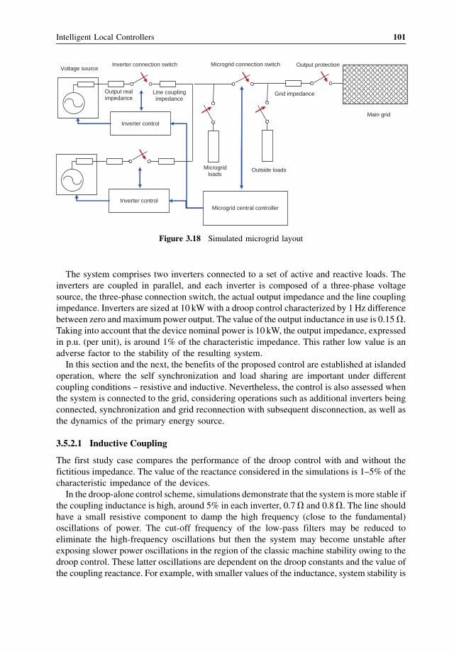
The system comprises two inverters connected to a set of active and reactive loads. The

inverters are coupled in parallel, and each inverter is composed of a three-phase voltage

source, the three-phase connection switch, the actual output impedance and the line coupling

impedance. Inverters are sized at 10 kWwith a droop control characterized by 1Hz difference

between zero and maximum power output. The value of the output inductance in use is 0.15V.

Taking into account that the device nominal power is 10 kW, the output impedance, expressed

in p.u. (per unit), is around 1% of the characteristic impedance. This rather low value is an

adverse factor to the stability of the resulting system.

In this section and the next, the benefits of the proposed control are established at islanded

operation, where the self synchronization and load sharing are important under different

coupling conditions – resistive and inductive. Nevertheless, the control is also assessed when

the system is connected to the grid, considering operations such as additional inverters being

connected, synchronization and grid reconnection with subsequent disconnection, as well as

the dynamics of the primary energy source.

3.5.2.1 Inductive Coupling

The first study case compares the performance of the droop control with and without the

fictitious impedance. The value of the reactance considered in the simulations is 1–5% of the

characteristic impedance of the devices.

In the droop-alone control scheme, simulations demonstrate that the system is more stable if

the coupling inductance is high, around 5% in each inverter, 0.7V and 0.8V. The line should

have a small resistive component to damp the high frequency (close to the fundamental)

oscillations of power. The cut-off frequency of the low-pass filters may be reduced to

eliminate the high-frequency oscillations but then the system may become unstable after

exposing slower power oscillations in the region of the classic machine stability owing to the

droop control. These latter oscillations are dependent on the droop constants and the value of

the coupling reactance. For example, with smaller values of the inductance, system stability is

Inverter control

Inverter control

Voltage source Inverter connection switch

Output realimpedance

Line couplingimpedance

Microgridloads

Outside loads

Microgrid connection switch

Grid impedance

Main grid

Output protection

Microgrid central controller

Figure 3.18 Simulated microgrid layout


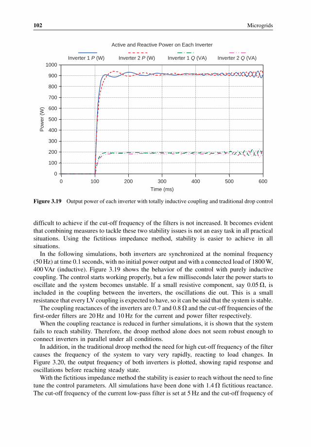
difficult to achieve if the cut-off frequency of the filters is not increased. It becomes evident

that combining measures to tackle these two stability issues is not an easy task in all practical

situations. Using the fictitious impedance method, stability is easier to achieve in all

situations.

In the following simulations, both inverters are synchronized at the nominal frequency

(50Hz) at time 0.1 seconds, with no initial power output and with a connected load of 1800W,

400VAr (inductive). Figure 3.19 shows the behavior of the control with purely inductive

coupling. The control starts working properly, but a few milliseconds later the power starts to

oscillate and the system becomes unstable. If a small resistive component, say 0.05V, is

included in the coupling between the inverters, the oscillations die out. This is a small

resistance that every LV coupling is expected to have, so it can be said that the system is stable.

The coupling reactances of the inverters are 0.7 and 0.8V and the cut-off frequencies of the

first-order filters are 20Hz and 10Hz for the current and power filter respectively.

When the coupling reactance is reduced in further simulations, it is shown that the system

fails to reach stability. Therefore, the droop method alone does not seem robust enough to

connect inverters in parallel under all conditions.

In addition, in the traditional droop method the need for high cut-off frequency of the filter

causes the frequency of the system to vary very rapidly, reacting to load changes. In

Figure 3.20, the output frequency of both inverters is plotted, showing rapid response and

oscillations before reaching steady state.

With the fictitious impedance method the stability is easier to reach without the need to fine

tune the control parameters. All simulations have been done with 1.4V fictitious reactance.

The cut-off frequency of the current low-pass filter is set at 5 Hz and the cut-off frequency of

0

100

200

300

400

500

600

700

800

900

1000

0 100 200 300 400 500 600

Active and Reactive Power on Each InverterP

ower

(W

)

Time (ms)

Inverter 1 P (W) Inverter 2 P (W) Inverter 1 Q (VA) Inverter 2 Q (VA)

Figure 3.19 Output power of each inverter with totally inductive coupling and traditional drop control

102 Microgrids

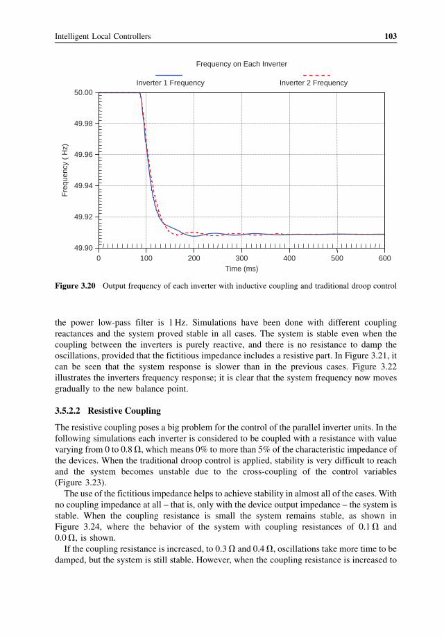
the power low-pass filter is 1Hz. Simulations have been done with different coupling

reactances and the system proved stable in all cases. The system is stable even when the

coupling between the inverters is purely reactive, and there is no resistance to damp the

oscillations, provided that the fictitious impedance includes a resistive part. In Figure 3.21, it

can be seen that the system response is slower than in the previous cases. Figure 3.22

illustrates the inverters frequency response; it is clear that the system frequency now moves

gradually to the new balance point.

3.5.2.2 Resistive Coupling

The resistive coupling poses a big problem for the control of the parallel inverter units. In the

following simulations each inverter is considered to be coupled with a resistance with value

varying from 0 to 0.8V, which means 0% to more than 5% of the characteristic impedance of

the devices. When the traditional droop control is applied, stability is very difficult to reach

and the system becomes unstable due to the cross-coupling of the control variables

(Figure 3.23).

The use of the fictitious impedance helps to achieve stability in almost all of the cases. With

no coupling impedance at all – that is, only with the device output impedance – the system is

stable. When the coupling resistance is small the system remains stable, as shown in

Figure 3.24, where the behavior of the system with coupling resistances of 0.1V and

0.0V, is shown.

If the coupling resistance is increased, to 0.3V and 0.4V, oscillations take more time to be

damped, but the system is still stable. However, when the coupling resistance is increased to

49.90

49.92

49.94

49.96

49.98

50.00

0 100 200 300 400 500 600

Frequency on Each InverterF

requ

ency

( H

z)

Time (ms)

Inverter 1 Frequency Inverter 2 Frequency

Figure 3.20 Output frequency of each inverter with inductive coupling and traditional droop control


0

100

200

300

400

500

600

700

800

900

1000

0 100 200 300 400 500 600


ower

(W

)

Time (ms)


Figure 3.21 Output power of each inverter with inductive coupling and fictitious impedance method

49.90

49.92

49.94

49.96

49.98

50.00

0 100 200 300 400 500 600

Frequency on Each Inverter

Fre

quen

cy (

Hz)

Time (ms)

Inverter 1 Frequency Inverter 2 Frequency

Figure 3.22 Output frequency of each inverter with inductive coupling and fictitious impedance

method

104 Microgrids

Figure 3.23 Output power of each inverter with resistive coupling and traditional drop control

0

100

200

300

400

500

600

700

800

900

1000

0 100 200 300 400 500 600

Active and Reactive Power on Each Inverter

Pow

er (

W)

Time (ms)


Figure 3.24 Output power of each inverter with resistive coupling and fictitious impedance method,

with small resistance


0.7 and 0.8V, the system becomes unstable (Figure 3.25). The problem can be solved by

accounting for the coupling resistance in the formation of the fictitious impedance. A

reduction of the resistance in the fictitious impedance used can lead to a stable system in

all cases. This remaining resistive portion has to be high enough to guarantee the stability in all

the inductive cases as well.

In a more systematic way, we could subtract from the fictitious impedance a resistance

value as much as the coupling resistance is expected to be, so that the system will behave

overall – including the coupling resistance – only with its fictitious resistance that is specified

in the device parameter set. In Figure 3.26, the behavior of the system is shown when the

coupling resistance (0.7 and 0.8V) is subtracted from the fictitious impedance. Both inverters

work identically, because both have the same parameters and the same output impedance. The

problem with this approach, however, is the practical difficulty of estimating the coupling

impedance of each inverter, the value of which in more complicated grid configurations may

not be clear.

3.5.2.3 Optimal Reactive Power Sharing

In this case, the optimization of the system performance is addressed by sharing the reactive

power among the sources properly. Analyzing all the possibilities, the worst system behavior

occurs when the coupling is resistive and the difference between the connection resistances is

significant. In these cases, the reactive power is generated mostly by the inverter with the

smaller coupling resistance.

0

100

200

300

400

500

600

700

800

900

1000

0 100 200 300 400 500 600


ower

(W

)

Time (ms)



with high resistance

106 Microgrids

The simulated microgrid consists of two similar inverters with a difference between

the coupling resistances equal to 0.4V. Figure 3.27 displays the behavior of the system

when the fictitious impedance is 1.4V. It can be seen that while the active power is

equally shared, the reactive power is mainly generated by the inverter with the smaller

coupling resistance. This behavior is only dependent on the connection impedance and

the fictitious impedance. The difference between the two reactive powers increases when

the fictitious impedance decreases. The reactive power productions are balanced when

the voltage drop provoked by the active power across the extra resistance is equal to the

voltage drop created by the difference of the reactive power across the fictitious

impedance. This difference can be used by a central controller to estimate the coupling

resistances of each inverter, or at least the difference between the inverter resistances.

Figure 3.28 shows the performance of the system when the coupling resistance is

compensated.

3.5.3 Stability in Interconnected Operation

In this section the progressive connection of different power sources, the synchronization

process of the microgrid with the main grid and the subsequent reconnection and dis-

connection are studied from the point of view of system stability, proposing improvements in

the control strategies.

0

100

200

300

400

500

600

700

800

900

1000

0 100 200 300 400 500 600


ower

(W

)

Time (ms)



with high resistance and compensated


–2000

0

2000

4000

6000

8000

10000

0.0 0.2 0.4 0.6 0.8 1.0 1.2 1.4 1.6 1.8 2.0


ower

(W

)

Time (s)


Figure 3.27 Output power of each inverter with unequal resistive coupling and 1.4V fictitious

impedance

–2000

0

2000

4000

6000

8000

10000

0.0 0.2 0.4 0.6 0.8 1.0 1.2 1.4 1.6 1.8 2.0

Active and Reactive Power on Each Inverter

Pow

er (

W)

Time (s)


Figure 3.28 Output power of each inverter with unequal resistive coupling and 1.4V fictitious

impedance compensated

108 Microgrids

3.5.3.1 Progressive Connection of Microsources

At time t¼ 0.1 s, a first inverter is connected to a 2 kW load. The load initially has no voltage,

so the inverter energizes the microgrid. At time t¼ 0.2 s, the load is increased to 10 kW. After

2 seconds, when the system has stabilized, a second inverter is connected to the network and

the connection of a third inverter follows one second later. All inverters are similar, but a slight

difference in their parameters is assumed, in order to study stability issues. It is assumed that

each inverter, before connecting to the existing network, has synchronized its output voltage

reference (magnitude and phase). The behavior of the system, as expressed by the output

power of the three inverters is shown in Figure 3.29 and the inverter currents in Figure 3.30.

It can be seen that when a new inverter is connected to the microgrid, currents and powers

flow from one inverter to the other, until the system reaches equilibrium. One reason for

causing fluctuations is that when a new inverter is synchronized, its voltage angle is the same

as the angle of the grid voltage, but the frequency is imposed by the power measurement

(because of the P/f droop). If the two frequencies are not the same, the inverter frequencies

fluctuate around the equilibrium point causing current oscillations. If the frequencies are

equal at the first instant, the system moves smoothly to the steady state.

Two main alternatives can be considered to reduce oscillations:

� adapt the internal values of the inverter in order to achieve the same frequency of the

inverter and the system during connection

–15000

–10000

–5000

0

5000

10000

15000

20000

25000

0 2 4 6

Power on Each InverterP

ower

(W

)

Time (s)

Inverter 1 Power (W) Inverter 2 Power (W) Inverter 3 Power (W)

Figure 3.29 Output power of the inverters during their progressive connection


� adjust the dynamic characteristics of the control system at the connection time to improve

fluctuation damping

For example, it is possible to act on the P/f droop by adding an offset value to the droop

characteristic to obtain the same frequency in the two inverters. Initially, and before

connecting the new inverter, the grid frequency is calculated and compared with the inverter

zero power frequency. The difference is added to the P/f droop curve when the new inverter

connects, resulting in 0 kW power at its output. So the system is supplied by the already

connected inverters, while the new one is synchronized with the island. The offset is gradually

reduced to zero and the system reaches balance smoothly. Figure 3.31 shows the output

powers and Figure 3.32 the currents.

The dynamic parameters of the inverters can be changed by temporarily replacing the

coupling fictitious impedances and resistances, substituting the cut-off frequencies of the

current and power filters, tuning the P/f droop slope or even modifying the digital filter

transfer function. It is worth mentioning that the only parameter set that is to be adjusted is the

one belonging to the inverter being connected.

The fictitious impedance can be employed to reduce the transients in power and current by

reducing an initial high inductance value L�Do to the final lower value L�Df with a time constant

TST according to L�D ¼ L�Df þ L�Do � L�Df� �

e�t=TST ; as shown in Figure 3.33.

3.5.3.2 Transition Between Islanded and Connected Modes

Microgrid transitions from interconnected to islanded mode of operation and vice versa are

likely to cause large mismatches between generation and loads, provoking severe frequency

and voltage variations.

Figure 3.30 Output currents of the inverters during their progressive connection

110 Microgrids

–5000

0

5000

10000

15000

0 2 4 6

Power on Each InverterP

ower

(W

)

Time (s)

Inverter 1 Power (W) Inverter 2 Power (W) Inverter 3 Power (W)

Figure 3.31 Output power of the inverters with offset technique during their progressive connection

Figure 3.32 Output currents with sudden connection of new inverters using offset technique


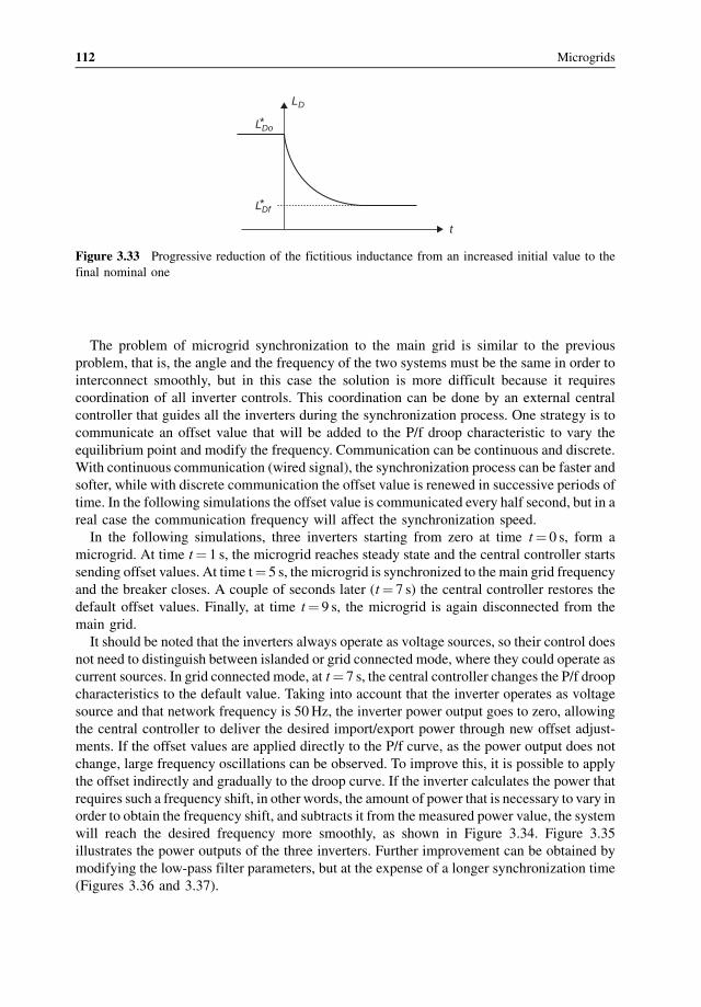
The problem of microgrid synchronization to the main grid is similar to the previous

problem, that is, the angle and the frequency of the two systems must be the same in order to

interconnect smoothly, but in this case the solution is more difficult because it requires

coordination of all inverter controls. This coordination can be done by an external central

controller that guides all the inverters during the synchronization process. One strategy is to

communicate an offset value that will be added to the P/f droop characteristic to vary the

equilibrium point and modify the frequency. Communication can be continuous and discrete.

With continuous communication (wired signal), the synchronization process can be faster and

softer, while with discrete communication the offset value is renewed in successive periods of

time. In the following simulations the offset value is communicated every half second, but in a

real case the communication frequency will affect the synchronization speed.

In the following simulations, three inverters starting from zero at time t¼ 0 s, form a

microgrid. At time t¼ 1 s, the microgrid reaches steady state and the central controller starts

sending offset values. At time t¼ 5 s, the microgrid is synchronized to the main grid frequency

and the breaker closes. A couple of seconds later (t¼ 7 s) the central controller restores the

default offset values. Finally, at time t¼ 9 s, the microgrid is again disconnected from the

main grid.

It should be noted that the inverters always operate as voltage sources, so their control does

not need to distinguish between islanded or grid connected mode, where they could operate as

current sources. In grid connected mode, at t¼ 7 s, the central controller changes the P/f droop

characteristics to the default value. Taking into account that the inverter operates as voltage

source and that network frequency is 50Hz, the inverter power output goes to zero, allowing

the central controller to deliver the desired import/export power through new offset adjust-

ments. If the offset values are applied directly to the P/f curve, as the power output does not

change, large frequency oscillations can be observed. To improve this, it is possible to apply

the offset indirectly and gradually to the droop curve. If the inverter calculates the power that

requires such a frequency shift, in other words, the amount of power that is necessary to vary in

order to obtain the frequency shift, and subtracts it from the measured power value, the system

will reach the desired frequency more smoothly, as shown in Figure 3.34. Figure 3.35

illustrates the power outputs of the three inverters. Further improvement can be obtained by

modifying the low-pass filter parameters, but at the expense of a longer synchronization time

(Figures 3.36 and 3.37).

LD

t

*LDo

*LDf

Figure 3.33 Progressive reduction of the fictitious inductance from an increased initial value to the

final nominal one

112 Microgrids

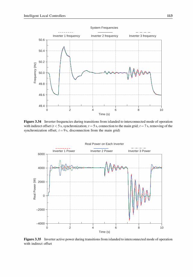
49.4

49.6

49.8

50.0

50.2

50.4

50.6

0 2 4 6 8 10

System Frequencies

Fre

quen

cy (

Hz)

Time (s)

Inverter 1 frequency Inverter 2 frequency Inverter 3 frequency

Figure 3.34 Inverter frequencies during transitions from islanded to interconnected mode of operation

with indirect offset (t< 5 s, synchronization; t¼ 5 s, connection to the main grid; t¼ 7 s, removing of the

synchronization offset; t¼ 9 s, disconnection from the main grid)

–4000

–2000

0

2000

4000

6000

0 2 4 6 8 10

Real Power on Each Inverter

Rea

l Pow

er (

W)

Time (s)

Inverter 1 Power Inverter 2 Power Inverter 3 Power

Figure 3.35 Inverter active power during transitions from islanded to interconnected mode of operation

with indirect offset


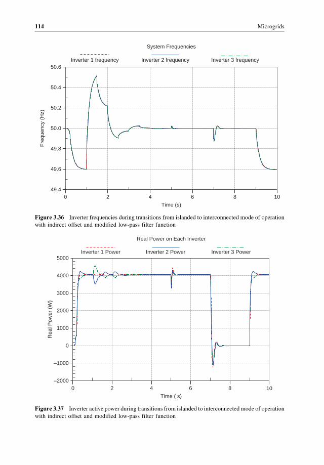
49.4

49.6

49.8

50.0

50.2

50.4

50.6

0 2 4 6 8 10

System Frequencies

Time (s)

Inverter 1 frequency Inverter 2 frequency Inverter 3 frequency

Fre

quen

cy (

Hz)

Figure 3.36 Inverter frequencies during transitions from islanded to interconnected mode of operation

with indirect offset and modified low-pass filter function

–2000

–1000

0

1000

2000

3000

4000

5000

0 2 4 6 8 10

Real Power on Each Inverter

Time ( s)


Rea

l Pow

er (

W)

Figure 3.37 Inverter active power during transitions from islanded to interconnected mode of operation

with indirect offset and modified low-pass filter function

114 Microgrids

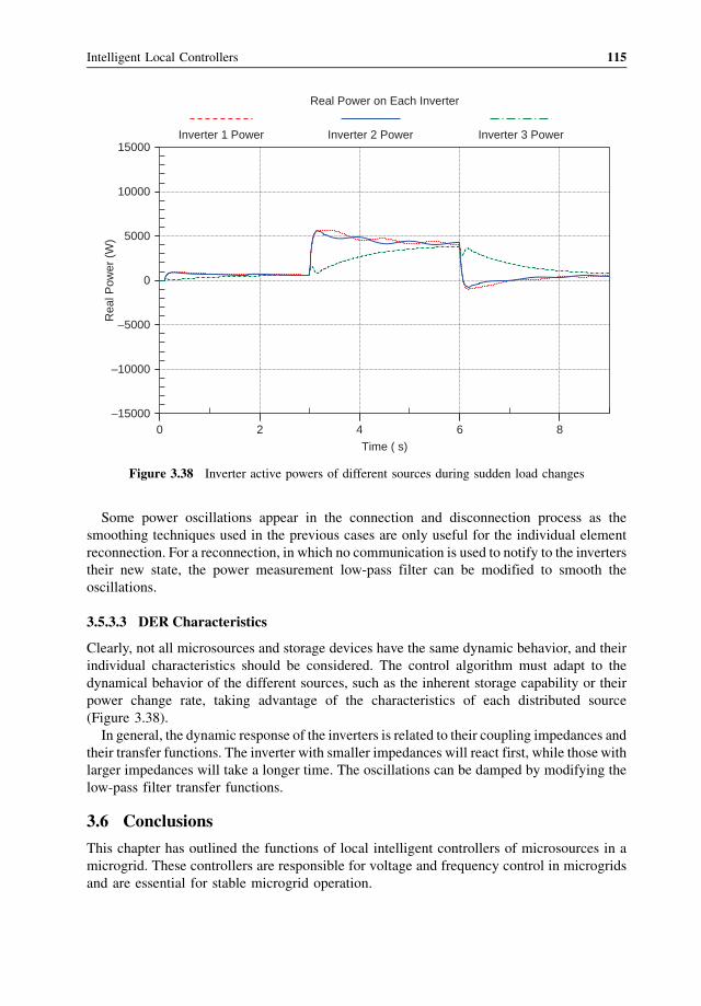
Some power oscillations appear in the connection and disconnection process as the

smoothing techniques used in the previous cases are only useful for the individual element

reconnection. For a reconnection, in which no communication is used to notify to the inverters

their new state, the power measurement low-pass filter can be modified to smooth the

oscillations.

3.5.3.3 DER Characteristics

Clearly, not all microsources and storage devices have the same dynamic behavior, and their

individual characteristics should be considered. The control algorithm must adapt to the

dynamical behavior of the different sources, such as the inherent storage capability or their

power change rate, taking advantage of the characteristics of each distributed source

(Figure 3.38).

In general, the dynamic response of the inverters is related to their coupling impedances and

their transfer functions. The inverter with smaller impedances will react first, while those with

larger impedances will take a longer time. The oscillations can be damped by modifying the

low-pass filter transfer functions.

3.6 Conclusions

This chapter has outlined the functions of local intelligent controllers of microsources in a

microgrid. These controllers are responsible for voltage and frequency control in microgrids

and are essential for stable microgrid operation.

–15000

–10000

–5000

0

5000

10000

15000

0 2 4 6 8

Real Power on Each InverterR

eal P

ower

(W

)

Time ( s)


Figure 3.38 Inverter active powers of different sources during sudden load changes


Control concepts based on frequency/active power and voltage/reactive power droops as

applied on microgrids have been discussed. They are applied to the control of the static

converters that usually couple the microgenerators to the network. The feasibility of these

concepts is shown by simulations and laboratory investigations. Power sharing in distributed

island systems has been shown. The implications of the line parameters on the choice of the

droop parameters have been systematically investigated.

Finally, inverter control using fictitious impedance has been analyzed. The fictitious

impedance method has proved to be an effective method for controlling voltage source

inverters coupled with low reactance, high resistance lines. Reactive power sharing can be

improved by compensating the line coupling impedance. Plug-and-play attributes of the

control method for different sources have been illustrated.

Overall, it has been demonstrated that microgrids powered by inverter coupled generators

can be operated in a stable way. Power sharing and voltage control between spatially

distributed generators can be effectively organized within a microgrid by applying intelligent

local generator controls which utilize droop control concepts.

References

1. Chen, J.F. and Chu, C.-L. (1995) Combination voltage-controlled and current-controlled PWM inverters for UPS

parallel operation. IEEE Trans. Power Electronics, 10 (5), 547–558.

2. Lasseter, B. (2001) “Microgrids Distributed Power Generation”, IEEE Power Engineering Society Winter

Meeting Conference Proceedings, Columbus, Ohio, vol. 1, pp. 146–149.

3. Lasseter, R.H. (2002) “Microgrids” IEEE Power Engineering Society Winter Meeting Conference Proceedings,

New York, NY, vol. 1, pp. 305–308.

4. Engler, A. Vorrichtung zum gleichberechtigten Parallelbetrieb von ein- oder drei-phasigen Spannungsquellen,

European patent: 1286444 B1 (2006) US patent: 6,693,809 B2 Feb 17, 2004 Japanese patent 2010-

1102209.

5. Engler, A., Hardt, C., Strau�, P., and Vandenbergh, M. (October 2001) “Parallel Operation of Generators for

Stand-Alone Single Phase Hybrid System”, EPVSEC Conference, Munich.

6. Engler, A. (2002) Regelung von Batteriestromrichtern in Modularen und Erweiterbaren Inselnetzen, Publisher

Verlag Dissertation.de, Berlin, ISBN: 3-89825-439-9.

7. Heuck, K. and Dettmann, K.D. Elektrische Energieversorgung, 3rd edn, Vieweg.

8. Burger, B. and Engler, A. (2000) Verfahren und Vorrichtung zur Bestimmung charakteristischer Gr€ossen aus

einem zeitlich periodischen Signal, German patent Nr. 199 49 997.7, 15.10.1999.

9. Engler, A. (2005) Applicability of droops in low voltage grids. International Journal of Distributed Energy

Resources, 1 (1) 3–15.

10. Chiang, H.C., Yen, C.Y., and Chang, K.T. (2001) A frequency-dependent droop scheme for parallel control of Ups

inverters. J. Chin. Inst. Eng., 24 (6), 699–708.

11. Guerrero, J.M., Vasquez, J.C., Matas, J. et al. (2011) Hierarchical control of Droop – Controlled AC and DC

microgrids – A general approach towards standardization. IEEE Trans. Indus. Electronics, 58 (1) 158–172.

116 Microgrids

4

Microgrid Protection

Alexander Oudalov, Thomas Degner, Frank van Overbeekeand Jose Miguel Yarza

4.1 Int roduction

One of the major t ec hnical challenges associated with a wide deploym ent of m icrogrids is

the design o f its protect ion syst em . Prot ectio n must respond both to the ut ili ty grid system

and to microgrid faults. I f the faul t i s on the ut ility grid, t he de sired r esponse is to i solate the

mi crogrid from t he main utili ty as rapidly as n ecessary to protect the m icrogrid loads. The

speed of isol ation is dependent on the specifi c customer’s loads on the microgrid, but it

p r o b a b l y r e q u i r e s t h e d evel o p m e n t a n d i n s t a l l a t i o n o f s u i t a b l e e l e c t r o n i c s t a t i c s w i t c h e s .

Electrically operated circuit breaker s in combinati on wit h directiona l ove r- c u r r e n t p r o t e c -

ti on is anot her possi bl e opti on. If the fault is wi thin the microgri d, t he protection system

isolates the s mallest possible section of the di stribu tion feeder to e li minate the f aul t [1].

A f urther segm entati on of t he mi crogrid durin g the isol ated operati on, that is, a creation

of multiple islands or sub-microgrids, must be supported by m icrosource and load

controllers.

Most conventional distribution protectio n is based on short-c ircuit current sensing. The

presence of DERs mi ght change the magnitude and direction of fault current s, and might lead

to protectio n failures. Direc tly coupled rotating- machin e-based micro sourc es will increase

short-c ircuit current s, whi le power electronic interf aced micro sources can not normally

provide any sign ificant levels of short-c ircuit current s require d. Some conventional over-

current sensing devices will not even respond to this low level of over-cur rent, and thos e that

do respon d will take many secon ds to do so, rather than the fraction of a secon d that is

required. Thus, in many operating conditions of microgrids, problems related to selectivity

(false, unnecessary tripping), sensitivity (undetected faults) and speed (delayed tripping) of

protection system may arise.



Issues related to protection of microgrids have been addressed in several publications [2–5].

The major problems can be summarized as:

� changes in the value and direction of short-circuit currents, depending on whether a

distributed generator is connected or not,� reduction of fault detection sensitivity and speed in tapped DER connections,� unnecessary tripping of utility breaker for faults in adjacent lines, due to fault contribution

of DER,� increased fault levels may exceed the capacity of the existing switchgear,� auto-reclosing and fuse-saving of the utility line breaker policies may fail,� reduced fault contribution of inverter based DER on protection system performance,

especially when isolated from the utility grid,� conflict between the feeder protection and utility requirements for fault ride through

(FRT) which is included in the grid codes of many countries with a large penetration

of DER,� effect of closed-loop and meshed distribution network topologies with DER.

This chapter presents a protection solution for microgrids that can overcome some of the

above problems. This is based on automatic adaptive protection, that is, change of protection

settings depending on the microgrid configuration based on pre-calculated or on real-time

calculated settings. The increase in the fault current level helped by a dedicated device,

especially in isolated operation of microgrids dominated by power electronics interfaced

DER, is also analyzed. Finally, the possible use of fault current limitation is discussed.

4.2 Challenges for Microgrid Protection

4.2.1 Distribution System Protection

Generally a distribution system (including a microgrid) is divided into local protective zones

which are covered either by a network (overhead lines and cables) or apparatus (buses,

transformers, generators, loads etc.) protection (Figure 4.1).

Requirements which provide a basis for design criteria of a distribution protection system

are known as “3S” which stands for:

� sensitivity – protection system should be able to identify an abnormal condition that

exceeds a nominal threshold value.� selectivity – protection system should disconnect only the faulted part (or the smallest

possible part containing the fault) of the system in order to minimize fault consequences.� speed – protective relays should respond to abnormal conditions in the least possible time

in order to avoid damage to equipment and maintain stability.

“3S” can be extended by:

� dependability – protection system must operate correctly when required to operate (detect

and disconnect all faults within the protected zone) and shall be designed to perform its

intended function while itself experiencing a credible failure.

118 Microgrids

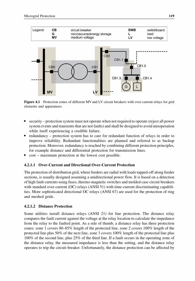
� security – protection systemmust not operate when not required to operate (reject all power

system events and transients that are not faults) and shall be designed to avoid misoperation

while itself experiencing a credible failure.� redundancy – protection system has to care for redundant function of relays in order to

improve reliability. Redundant functionalities are planned and referred to as backup

protection. Moreover, redundancy is reached by combining different protection principles,

for example distance and differential protection for transmission lines.� cost – maximum protection at the lowest cost possible.

4.2.1.1 Over-Current and Directional Over-Current Protection

The protection of distribution grid, where feeders are radial with loads tapped-off along feeder

sections, is usually designed assuming a unidirectional power flow. It is based on a detection

of high fault currents using fuses, thermo-magnetic switches and molded case circuit breakers

with standard over-current (OC) relays (ANSI 51) with time-current discriminating capabili-

ties. More sophisticated directional OC relays (ANSI 67) are used for the protection of ring

and meshed grids.

4.2.1.2 Distance Protection

Some utilities install distance relays (ANSI 21) for line protection. The distance relay

compares the fault current against the voltage at the relay location to calculate the impedance

from the relay to the faulted point. As a rule of thumb, a distance relay has three protection

zones: zone 1 covers 80–85% length of the protected line, zone 2 covers 100% length of the

protected line plus 50% of the next line, zone 3 covers 100% length of the protected line plus

100% of the second line, plus 25% of the third line. If a fault occurs in the operating zone of

the distance relay, the measured impedance is less than the setting, and the distance relay

operates to trip the circuit breaker. Unfortunately, the distance protection can be affected by

Figure 4.1 Protection zones of different MVand LV circuit breakers with over-current relays for grid

elements and apparatuses

Microgrid Protection 119

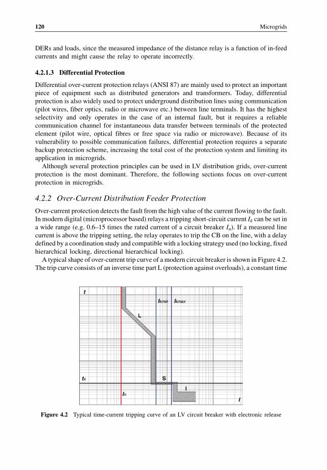
DERs and loads, since the measured impedance of the distance relay is a function of in-feed

currents and might cause the relay to operate incorrectly.

4.2.1.3 Differential Protection

Differential over-current protection relays (ANSI 87) are mainly used to protect an important

piece of equipment such as distributed generators and transformers. Today, differential

protection is also widely used to protect underground distribution lines using communication

(pilot wires, fiber optics, radio or microwave etc.) between line terminals. It has the highest

selectivity and only operates in the case of an internal fault, but it requires a reliable

communication channel for instantaneous data transfer between terminals of the protected

element (pilot wire, optical fibres or free space via radio or microwave). Because of its

vulnerability to possible communication failures, differential protection requires a separate

backup protection scheme, increasing the total cost of the protection system and limiting its

application in microgrids.

Although several protection principles can be used in LV distribution grids, over-current

protection is the most dominant. Therefore, the following sections focus on over-current

protection in microgrids.

4.2.2 Over-Current Distribution Feeder Protection

Over-current protection detects the fault from the high value of the current flowing to the fault.

In modern digital (microprocessor based) relays a tripping short-circuit current Ik can be set in

a wide range (e.g. 0.6–15 times the rated current of a circuit breaker In). If a measured line

current is above the tripping setting, the relay operates to trip the CB on the line, with a delay

defined by a coordination study and compatible with a locking strategy used (no locking, fixed

hierarchical locking, directional hierarchical locking).

A typical shape of over-current trip curve of a modern circuit breaker is shown in Figure 4.2.

The trip curve consists of an inverse time part L (protection against overloads), a constant time

Figure 4.2 Typical time-current tripping curve of an LV circuit breaker with electronic release

120 Microgrids

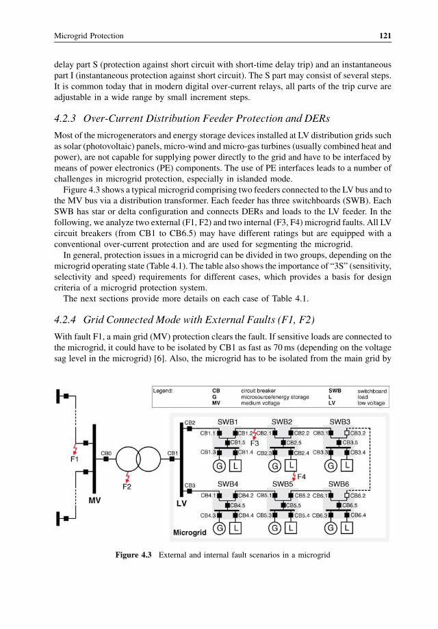
delay part S (protection against short circuit with short-time delay trip) and an instantaneous

part I (instantaneous protection against short circuit). The S part may consist of several steps.

It is common today that in modern digital over-current relays, all parts of the trip curve are

adjustable in a wide range by small increment steps.

4.2.3 Over-Current Distribution Feeder Protection and DERs

Most of the microgenerators and energy storage devices installed at LV distribution grids such

as solar (photovoltaic) panels, micro-wind and micro-gas turbines (usually combined heat and

power), are not capable for supplying power directly to the grid and have to be interfaced by

means of power electronics (PE) components. The use of PE interfaces leads to a number of

challenges in microgrid protection, especially in islanded mode.

Figure 4.3 shows a typical microgrid comprising two feeders connected to the LV bus and to

the MV bus via a distribution transformer. Each feeder has three switchboards (SWB). Each

SWB has star or delta configuration and connects DERs and loads to the LV feeder. In the

following, we analyze two external (F1, F2) and two internal (F3, F4) microgrid faults. All LV

circuit breakers (from CB1 to CB6.5) may have different ratings but are equipped with a

conventional over-current protection and are used for segmenting the microgrid.

In general, protection issues in a microgrid can be divided in two groups, depending on the

microgrid operating state (Table 4.1). The table also shows the importance of “3S” (sensitivity,

selectivity and speed) requirements for different cases, which provides a basis for design

criteria of a microgrid protection system.

The next sections provide more details on each case of Table 4.1.

4.2.4 Grid Connected Mode with External Faults (F1, F2)

With fault F1, a main grid (MV) protection clears the fault. If sensitive loads are connected to

the microgrid, it could have to be isolated by CB1 as fast as 70ms (depending on the voltage

sag level in the microgrid) [6]. Also, the microgrid has to be isolated from the main grid by

Figure 4.3 External and internal fault scenarios in a microgrid


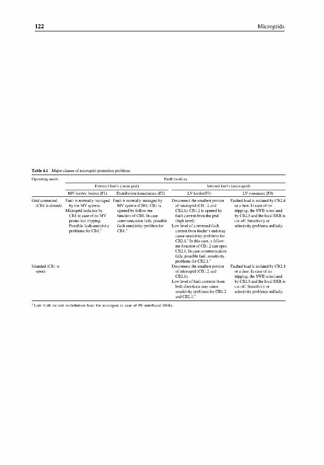
CB1, in case of MV protection tripping failure. A detection of F1 with a generic OC relay can

be problematic, in case most of the DERs in the microgrid are connected via PE interfaces

with built-in fault current limitation (i.e. there is no significant rise in current passing through

CB1). Typically, these units are capable of supplying 1.1 to 1.2�IDERrated (rated current of

microgenerator) to a fault, unless the converters are specifically designed to provide high fault

currents. This is much lower than a short-circuit current supplied by the main grid. A

directional OC relay in CB1 is the only feasible solution, if current is used for fault detection.

In order to increase relay sensitivity, the pick-up current setting is defined as the sum of fault

current contributions from the connected DER units (4.1). DERs that have to be taken into

consideration are the subset of units that contribute to the short-circuit current on the defined

direction.

Ik min ¼Xn

1

kDER � IrDER (4.1)

IrDER is the rated output current of a particular DER and kDER is its fault current

contribution coefficient, set at 1.1 for PE interfaced DER and at 5.0 for synchronous DER

units [7]. This value will vary for a large number of different types of DER. Thus, the setting

has to be continuously monitored and adapted when microgrid generation undergoes

changes (number and type of connected DER).

Alternatively, voltage sag (magnitude and duration) or/and system frequency (instanta-

neous value and rate of change) can be used as indicators for tripping CB1. It may be also

required that the energy sources of the microgrid stay connected and supply reactive power to

support the utility grid during the fault conditions. Depending on the particular grid code the

duration of support depends on the level of residual voltage and may vary from a hundred

milliseconds to several seconds.

With fault F2, the distribution transformer OC protection clears the fault by opening CB0.

CB1 is opened simultaneously by a “follow-me” function (hardware lock) of CB0. On

hardware lock failure, a possible fault sensitivity problem can arise as in the case of fault F1.

Typical solutions are similar to the F1 case: directional adaptive OC protection, under-voltage

and under-frequency protection and various islanding detection methods [8].

4.2.5 Grid Connected Mode with Fault in the Microgrid (F3)

With fault F3, microgrid protection must disconnect the smallest possible portion of the LV

feeder by CB1.2 and CB2.1. CB1.2 is opened due to a high short-circuit current supplied by

the main MV grid. If CB1.2 fails to trip, fault F3 must be cleared by CB1.1 which is a backup

protection for CB1.2. However, the sensitivity of the OC protection relay in CB1.1 can be

potentially disturbed, if a large synchronous DER (e.g. diesel generator) is installed and

switched on at SWB1 (i.e. between CB1.1 and the fault F3). In this case, the fault current

passing through CB1.1 with DER will be smaller than without DER, while the fault current at

F3 will be higher due to additional DER contribution. This effect is known as protection

blinding (the larger the synchronous DER the greater the effect – in some cases the fault

current seen by CB1.1 can be reduced by more than 30%) and may result in a delayed CB1.1

tripping, because of the fault current transition from a definite-time part to an inverse-time part

of the relay tripping characteristic (Figure 4.2). A delayed fault tripping will lead to an


unnecessary disconnection of DER at SWB1 (usually low-power diesel generators have very

low inertia and will run out of step in case of a delayed fault tripping). This issue can be solved

by proper coordination of microgrid and DER protection systems. Another option is to adapt

the protection settings with regard to current operating conditions (DER status).

If CB1.2 operates faster than CB2.1, which is very likely, it will island a part of the

microgrid which will be connected to the fault F3. If it is possible to balance generation and

load in the islanded segment of the microgrid (microsources are capable of supplying loads

directly or after load shedding), it is expedient to isolate that group of microsources and loads

from the fault F3 by opening CB2.1 and possibly closing CB3.2–6.2. However, a reversed and

low-level short-circuit current in case of PE interfaced DER will cause a sensitivity problem

for CB2.1 similar to the one described in the case of fault F1. Possible solutions include

directional adaptive OC protection and a follow-me function of CB1.2, which opens CB2.1

(in this case, a communication failure may cause sensitivity problems for CB2.1).

4.2.6 Grid Connected Mode with Fault at the End-Consumer Site (F4)

With fault F4, a high short-circuit current is supplied to the fault from the main grid, together

with a contribution from DER, which will lead to tripping of CB2.4. Frequently, there is a fuse

instead of a CB, which is rated in such a way that a shortest possible fault isolation time is

guaranteed. In case of no tripping, the SWB2 is isolated by CB2.5 and local DER is cut off. No

sensitivity or selectivity problems are foreseen in this scenario.

4.2.7 Islanded Mode with Fault in the Microgrid (F3)

The microgrid might operate in islanded mode when it is intentionally disconnected from the

mainMVgrid byCB1 (fullmicrogrid) or aCB along the LV feeder (a segment of themicrogrid).

This operatingmode is characterized by absence of the high short-circuit current supplied by the

main grid.GenericOC relays should be replacedbydirectionalOC relays, because fault currents

flow from both directions to the fault F3. If CB1.2 and CB2.1 use setting groups chosen for the

grid-connected mode, they will have a sensitivity problem with detecting and selectively

isolating the fault F3 and trippingwithin acceptable time frame for PE interfacedDER (the fault

current could shift from a definite-time part to an inverse-time part of the relay tripping

characteristic). There are two possible ways to address this problem:

� Install a source of high short-circuit current (e.g. a flywheel or a super-capacitor) to trip

CBs or blow fuses with settings or ratings for the grid-connected mode. However, a short-

circuit handling capability of PE interfaces can be increased only by increasing the

respective power rating or by having extensive cooling, which both lead to higher

investment cost [9]. This solution is discussed in Section 4.4.� Install an adaptivemicrogrid protection using online data about the microgrid topology and

status of available microsources or loads. This solution is discussed in Section 4.3.

4.2.8 Islanded Mode and Fault at the End-Consumer Site (F4)

With fault F4, a low short-circuit current is supplied to the fault from the local DERs. There is

no grid contribution to the fault current level. However, CB2.4 settings selected for the main

grid-connected mode are just slightly higher than the rated load current. This ensures that the

124 Microgrids

end-customer site will be disconnected, even if only PE-interfaced DERs are operating in the

microgrid. If there is no tripping, the SWB2 must be isolated by CB2.5 using a directional OC

relay. Similar to the grid-connected mode, there are no sensitivity or selectivity problems

foreseen in the islanded mode for a fault at the end-consumer site.

4.3 Adaptive Protection for Microgrids

4.3.1 Introduction

As discussed in Section 4.2, time over-current protection is the most common method

employed in MV and LV distribution grids, as it is quite simple to configure and is an

economically attractive option. In networks with interconnected DER, short-circuit currents

detected by over-current protection relays depend on the point of connection and the type and

size (feed-in power) of the DER units. In these networks directions and magnitudes of short

circuit currents will vary almost continuously, since the operating conditions in a microgrid

are constantly changing due to the intermittent DERs (wind and solar) and periodic load

variation. Also, the network topology can be regularly changed in order to achieve loss

minimization or other economic or operational targets. In addition, controllable islands of

different size can be formed, as a result of faults in the utility grid or inside a microgrid. In such

circumstances coordination between relays may fail and generic OC protection with a single

setting group in each relay may become inadequate, so it will not guarantee a selective

operation for all possible faults. Therefore, it is essential to ensure that protection settings

chosen for OC protection relays dynamically follow changes in grid topology and location,

type and amount of distributed energy resources. Otherwise, unwanted or uncoordinated

operation – or failure to operate when required – may occur. To solve the problems originating

from the interconnection of DERs the protection relay settings can be adapted in a flexible

way combined with the utilization of over-current protection relays with identification of

current direction. Adaptation of settings could mean a continuous adaptation of relay

characteristic settings or a switching of relay settings groups.

Adaptive protection is defined as “an online activity that modifies the preferred protective

response to a change in system conditions or requirements in a timely manner by means of

externally generated signals or control action” [10]. Technical requirements and suggestions

for a practical implementation of an adaptive microgrid protection system, as seen by the

authors, are:

� use of digital directionalOC relays, since fuses or electromechanical and standard solid state

relays (especially for selectivity holding) do not provide the flexibility for changing the

settings of tripping characteristics, and they have no current direction sensitivity feature,� digital directional over-current relays, which must provide the possibility for using

different tripping characteristics (several settings groups, e.g. modern digital OC relays

for LV applications have 2–4 settings groups) which can be parameterized locally or

remotely, automatically or manually,� use of new/existing communication infrastructure (e.g. twisted pair, power line carrier or

radio) and standard communication protocols (Modbus, IEC61850, etc.), such that

individual relays can communicate and exchange information with a central computer

or between different individual relays quickly and reliably to guarantee a required

application performance.


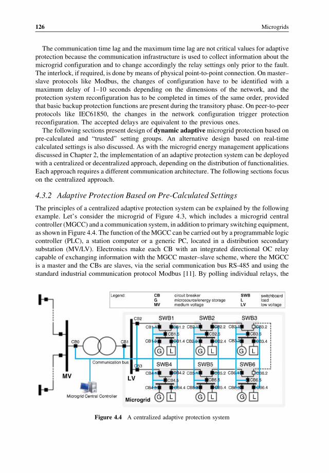
The communication time lag and the maximum time lag are not critical values for adaptive

protection because the communication infrastructure is used to collect information about the

microgrid configuration and to change accordingly the relay settings only prior to the fault.

The interlock, if required, is done by means of physical point-to-point connection. On master–

slave protocols like Modbus, the changes of configuration have to be identified with a

maximum delay of 1–10 seconds depending on the dimensions of the network, and the

protection system reconfiguration has to be completed in times of the same order, provided

that basic backup protection functions are present during the transitory phase. On peer-to-peer

protocols like IEC61850, the changes in the network configuration trigger protection

reconfiguration. The accepted delays are equivalent to the previous ones.

The following sections present design of dynamic adaptivemicrogrid protection based on

pre-calculated and “trusted” setting groups. An alternative design based on real-time

calculated settings is also discussed. As with the microgrid energy management applications

discussed in Chapter 2, the implementation of an adaptive protection system can be deployed

with a centralized or decentralized approach, depending on the distribution of functionalities.

Each approach requires a different communication architecture. The following sections focus

on the centralized approach.

4.3.2 Adaptive Protection Based on Pre-Calculated Settings

The principles of a centralized adaptive protection system can be explained by the following

example. Let’s consider the microgrid of Figure 4.3, which includes a microgrid central

controller (MGCC) and a communication system, in addition to primary switching equipment,

as shown in Figure 4.4. The function of theMGCC can be carried out by a programmable logic

controller (PLC), a station computer or a generic PC, located in a distribution secondary

substation (MV/LV). Electronics make each CB with an integrated directional OC relay

capable of exchanging information with the MGCC master–slave scheme, where the MGCC

is a master and the CBs are slaves, via the serial communication bus RS-485 and using the

standard industrial communication protocol Modbus [11]. By polling individual relays, the

Figure 4.4 A centralized adaptive protection system

126 Microgrids

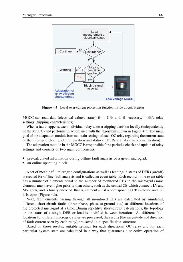
MGCC can read data (electrical values, status) from CBs and, if necessary, modify relay

settings (tripping characteristics).

When a fault happens, each individual relay takes a tripping decision locally (independently

of the MGCC) and performs in accordance with the algorithm shown in Figure 4.5. The main

goal of the adaptationmodule is tomaintain settings of eachOC relay regarding the current state

of the microgrid (both grid configuration and status of DERs are taken into consideration).

The adaptation module in the MGCC is responsible for a periodic check and update of relay

settings and consists of two main components:

� pre-calculated information during offline fault analysis of a given microgrid,� an online operating block.

A set of meaningful microgrid configurations as well as feeding-in states of DERs (on/off)

is created for offline fault analysis and is called an event table. Each record in the event table

has a number of elements equal to the number of monitored CBs in the microgrid (some

elements may have higher priority than others, such as the central CB which connects LVand

MV grids) and is binary encoded, that is, element¼ 1 if a corresponding CB is closed and 0 if

it is open (Figure 4.6).

Next, fault currents passing through all monitored CBs are calculated by simulating

different short-circuit faults (three-phase, phase-to-ground etc.) at different locations of

the protected microgrid at a time. During repetitive short-circuit calculations, the topology

or the status of a single DER or load is modified between iterations. As different fault

locations for different microgrid states are processed, the results (the magnitude and direction

of fault current seen by each relay) are saved in a specific data structure.

Based on these results, suitable settings for each directional OC relay and for each

particular system state are calculated in a way that guarantees a selective operation of

Localmeasurement ofelectrical values

Continue no

noWarning

Trippingconditionreached?

yes

yes

Disturbance?

Tripping signalto switch

Adaptation ofrelay trippingcharacteristic

Low voltage MCCB

Figure 4.5 Local over-current protection function inside circuit breaker


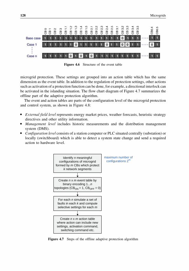
microgrid protection. These settings are grouped into an action table which has the same

dimension as the event table. In addition to the regulation of protection settings, other actions

such as activation of a protection function can be done, for example, a directional interlock can

be activated in the islanding situation. The flow chart diagram of Figure 4.7 summarizes the

offline part of the adaptive protection algorithm.

The event and action tables are parts of the configuration level of the microgrid protection

and control system, as shown in Figure 4.8:

� External field level represents energy market prices, weather forecasts, heuristic strategy

directives and other utility information.� Management level includes historic measurements and the distribution management

system (DMS).� Configuration level consists of a station computer or PLC situated centrally (substation) or

locally (switchboard) which is able to detect a system state change and send a required

action to hardware level.

Figure 4.6 Structure of the event table

Identify n meaningfulconfigurations of microgrid

formed by m CBs which protectk network segments

maximum number ofconfigurations 2m

Create n x m event table bybinary encoding 1...n

topologies (CBON = 1, CBOFF = 0)

For each n simulate a set offaults in each k and computeselective settings for each m

Create n x m action tablewhere action can include newsettings, activation command,

switching command etc.

Figure 4.7 Steps of the offline adaptive protection algorithm

128 Microgrids

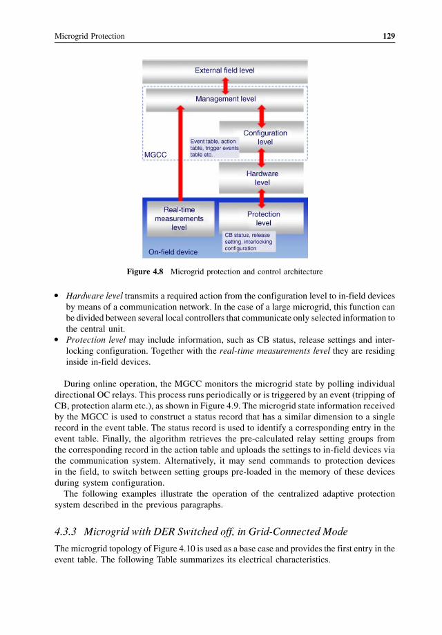
� Hardware level transmits a required action from the configuration level to in-field devices

by means of a communication network. In the case of a large microgrid, this function can

be divided between several local controllers that communicate only selected information to

the central unit.� Protection level may include information, such as CB status, release settings and inter-

locking configuration. Together with the real-time measurements level they are residing

inside in-field devices.

During online operation, the MGCC monitors the microgrid state by polling individual

directional OC relays. This process runs periodically or is triggered by an event (tripping of

CB, protection alarm etc.), as shown in Figure 4.9. The microgrid state information received

by the MGCC is used to construct a status record that has a similar dimension to a single

record in the event table. The status record is used to identify a corresponding entry in the

event table. Finally, the algorithm retrieves the pre-calculated relay setting groups from

the corresponding record in the action table and uploads the settings to in-field devices via

the communication system. Alternatively, it may send commands to protection devices

in the field, to switch between setting groups pre-loaded in the memory of these devices

during system configuration.

The following examples illustrate the operation of the centralized adaptive protection

system described in the previous paragraphs.

4.3.3 Microgrid with DER Switched off, in Grid-Connected Mode

The microgrid topology of Figure 4.10 is used as a base case and provides the first entry in the

event table. The following Table summarizes its electrical characteristics.

Figure 4.8 Microgrid protection and control architecture


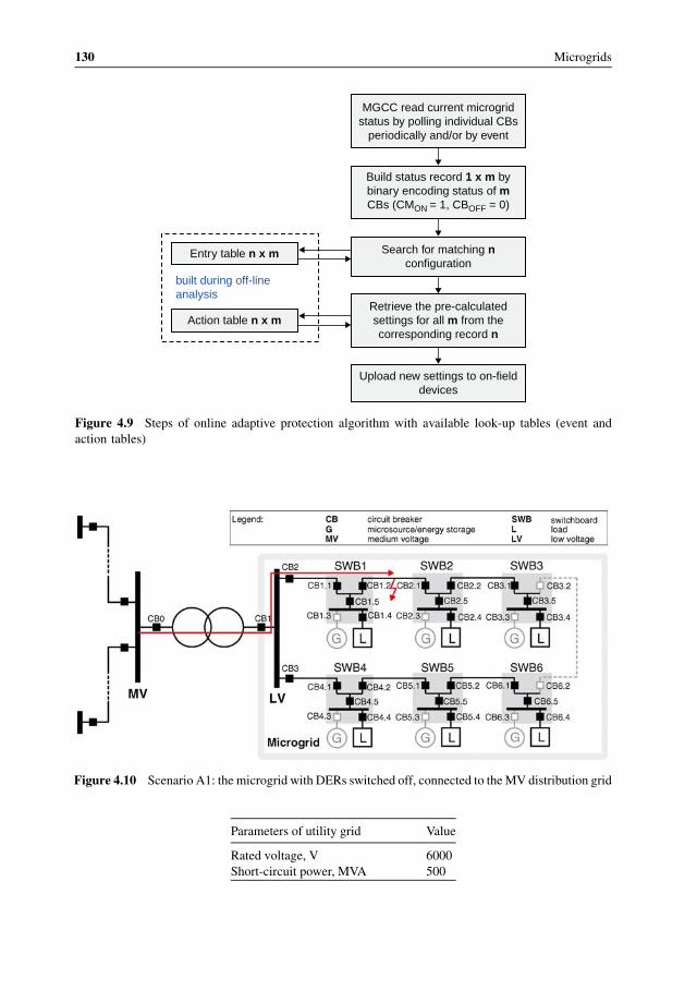
Parameters of utility grid Value

Rated voltage, V 6000

Short-circuit power, MVA 500

MGCC read current microgridstatus by polling individual CBs

periodically and/or by event

Build status record 1 x m bybinary encoding status of mCBs (CMON = 1, CBOFF = 0)

Search for matching nconfiguration

Entry table n x m

Action table n x m

built during off-lineanalysis

Retrieve the pre-calculatedsettings for all m from thecorresponding record n

Upload new settings to on-fielddevices

Figure 4.9 Steps of online adaptive protection algorithm with available look-up tables (event and

action tables)

Figure 4.10 Scenario A1: the microgrid with DERs switched off, connected to theMV distribution grid

130 Microgrids

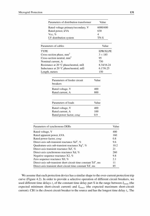
Parameters of distribution transformer Value

Rated voltage primary/secondary, V 6000/400

Rated power, kVA 630

Vcc, % 4

LV distribution system TN-S

Parameters of cables Value

TYPE EPR/XLPE

Cross-section phase, mm2 3� 185

Cross-section neutral, mm2 95

Nominal current, A 750

Resistance at 20 �C phase/neutral, mV 8.34/16.24

Inductance at 20 �C phase/neutral, mV 6.17/6.25

Length, meters 150

Parameters of feeder circuit

breakers

Value


Rated current, A 800

Parameters of loads Value


Rated current, A 100

Rated power factor, cosw 0.9

Parameters of synchronous DERs Value


Rated apparent power, kVA 160

Rated power factor, cosw 0.8

Direct-axis sub-transient reactance Xd00, % 9.6

Quadrature-axis sub-transient reactance Xq00, % 10.2

Direct-axis transient reactance Xd0, % 21

Direct-axis synchronous reactance Xd, % 260

Negative sequence reactance X2, % 9.8

Zero sequence reactance X0, % 2.1

Direct-axis sub-transient short circuit time constant Td00, ms 11

Direct-axis transient short circuit time constant Td0, ms 85

We assume that each protection device has a similar shape to the over-current protection trip

curve (Figure 4.2). In order to provide a selective operation of different circuit breakers, we

used different time delays ts of the constant time delay part S in the range between Ikmin (the

expected minimum short-circuit current) and Ikmax (the expected maximum short-circuit

current). CB1 is the closest circuit breaker to the source and has the longest time delay ts. The


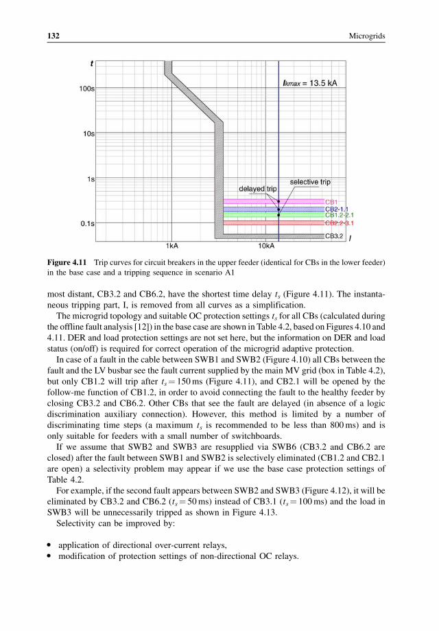
most distant, CB3.2 and CB6.2, have the shortest time delay ts (Figure 4.11). The instanta-

neous tripping part, I, is removed from all curves as a simplification.

The microgrid topology and suitable OC protection settings ts for all CBs (calculated during

the offline fault analysis [12]) in the base case are shown in Table 4.2, based on Figures 4.10 and

4.11. DER and load protection settings are not set here, but the information on DER and load

status (on/off) is required for correct operation of the microgrid adaptive protection.

In case of a fault in the cable between SWB1 and SWB2 (Figure 4.10) all CBs between the

fault and the LV busbar see the fault current supplied by the main MV grid (box in Table 4.2),

but only CB1.2 will trip after ts¼ 150ms (Figure 4.11), and CB2.1 will be opened by the

follow-me function of CB1.2, in order to avoid connecting the fault to the healthy feeder by

closing CB3.2 and CB6.2. Other CBs that see the fault are delayed (in absence of a logic

discrimination auxiliary connection). However, this method is limited by a number of

discriminating time steps (a maximum ts is recommended to be less than 800ms) and is

only suitable for feeders with a small number of switchboards.

If we assume that SWB2 and SWB3 are resupplied via SWB6 (CB3.2 and CB6.2 are

closed) after the fault between SWB1 and SWB2 is selectively eliminated (CB1.2 and CB2.1

are open) a selectivity problem may appear if we use the base case protection settings of

Table 4.2.

For example, if the second fault appears between SWB2 and SWB3 (Figure 4.12), it will be

eliminated by CB3.2 and CB6.2 (ts¼ 50ms) instead of CB3.1 (ts¼ 100ms) and the load in

SWB3 will be unnecessarily tripped as shown in Figure 4.13.

Selectivity can be improved by:

� application of directional over-current relays,� modification of protection settings of non-directional OC relays.

Figure 4.11 Trip curves for circuit breakers in the upper feeder (identical for CBs in the lower feeder)

in the base case and a tripping sequence in scenario A1

132 Microgrids

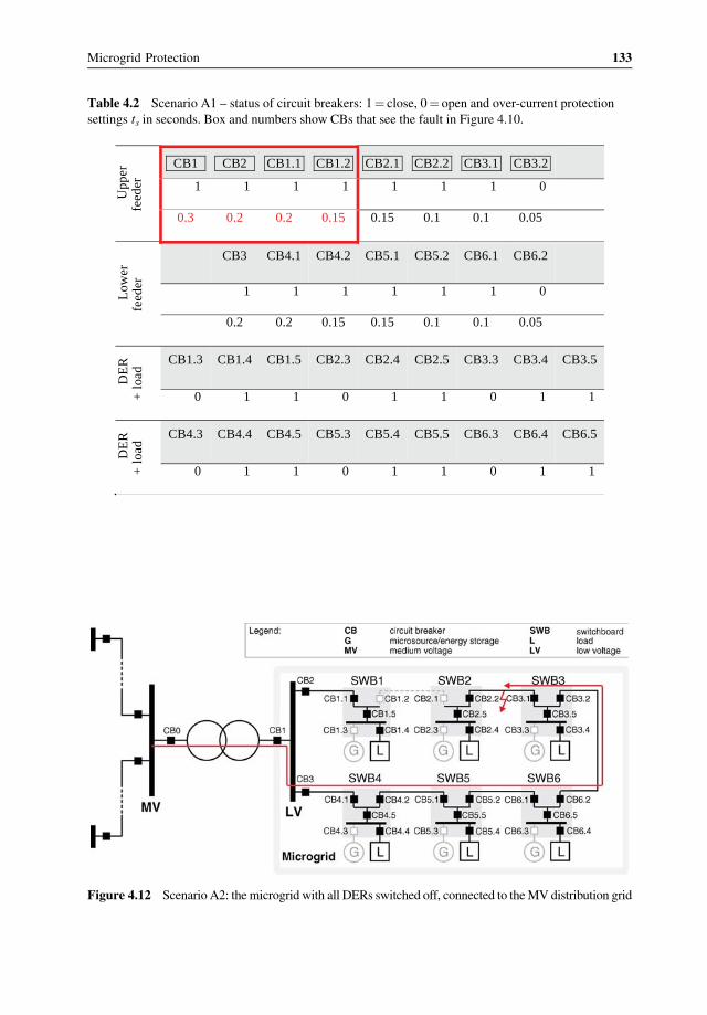
Table 4.2 Scenario A1 – status of circuit breakers: 1¼ close, 0¼ open and over-current protection

settings ts in seconds. Box and numbers show CBs that see the fault in Figure 4.10.U

pper

fe

eder

CB1 CB2 CB1.1 CB1.2 CB2.1 CB2.2 CB3.1 CB3.2

1 1 1 1 1 1 1 0

0.3 0.2 0.2 0.15 0.15 0.1 0.1 0.05

Low

er

feed

er

CB3 CB4.1 CB4.2 CB5.1 CB5.2 CB6.1 CB6.2

1 1 1 1 1 1 0

0.2 0.2 0.15 0.15 0.1 0.1 0.05

DE

R

+ lo

ad

CB1.3 CB1.4 CB1.5 CB2.3 CB2.4 CB2.5 CB3.3 CB3.4 CB3.5

0 1 1 0 1 1 0 1 1

DE

R

+ lo

ad


0 1 1 0 1 1 0 1 1

Figure 4.12 Scenario A2: themicrogrid with all DERs switched off, connected to theMV distribution grid


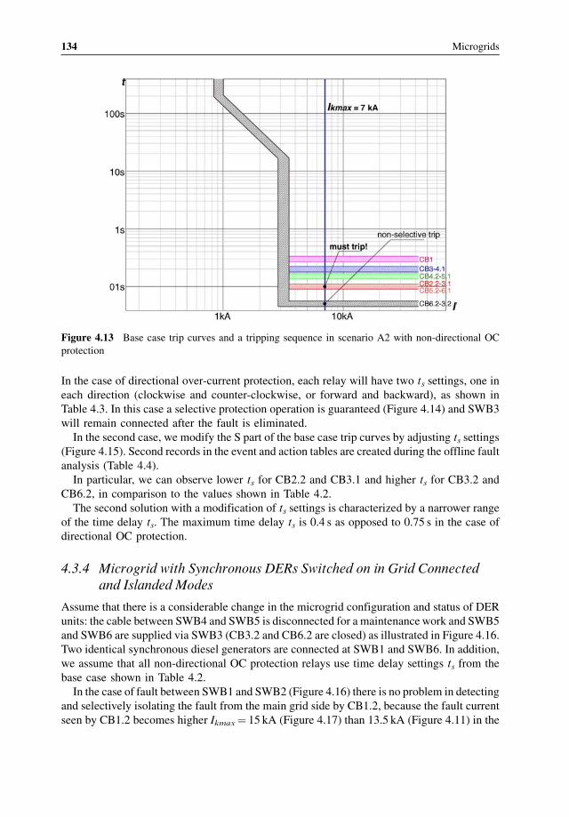
In the case of directional over-current protection, each relay will have two ts settings, one in

each direction (clockwise and counter-clockwise, or forward and backward), as shown in

Table 4.3. In this case a selective protection operation is guaranteed (Figure 4.14) and SWB3

will remain connected after the fault is eliminated.

In the second case, we modify the S part of the base case trip curves by adjusting ts settings

(Figure 4.15). Second records in the event and action tables are created during the offline fault

analysis (Table 4.4).

In particular, we can observe lower ts for CB2.2 and CB3.1 and higher ts for CB3.2 and

CB6.2, in comparison to the values shown in Table 4.2.

The second solution with a modification of ts settings is characterized by a narrower range

of the time delay ts. The maximum time delay ts is 0.4 s as opposed to 0.75 s in the case of

directional OC protection.

4.3.4 Microgrid with Synchronous DERs Switched on in Grid Connectedand Islanded Modes

Assume that there is a considerable change in the microgrid configuration and status of DER

units: the cable between SWB4 and SWB5 is disconnected for a maintenance work and SWB5

and SWB6 are supplied via SWB3 (CB3.2 and CB6.2 are closed) as illustrated in Figure 4.16.

Two identical synchronous diesel generators are connected at SWB1 and SWB6. In addition,

we assume that all non-directional OC protection relays use time delay settings ts from the

base case shown in Table 4.2.

In the case of fault between SWB1 and SWB2 (Figure 4.16) there is no problem in detecting

and selectively isolating the fault from the main grid side by CB1.2, because the fault current

seen by CB1.2 becomes higher Ikmax¼ 15 kA (Figure 4.17) than 13.5 kA (Figure 4.11) in the

Figure 4.13 Base case trip curves and a tripping sequence in scenario A2 with non-directional OC

protection

134 Microgrids

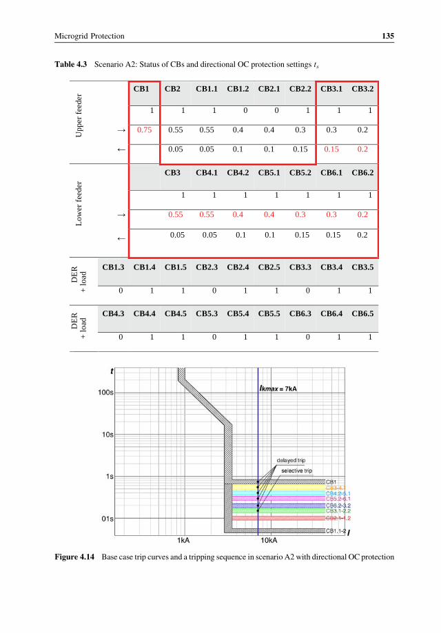
Table 4.3 Scenario A2: Status of CBs and directional OC protection settings ts

Upp

er f

eede

rCB1 CB2 CB1.1 CB1.2 CB2.1 CB2.2 CB3.1 CB3.2

1 1 1 0 0 1 1 1

0.75 0.55 0.55 0.4 0.4 0.3 0.3 0.2

0.05 0.05 0.1 0.1 0.15 0.15 0.2

Low

er f

eede

r

CB3 CB4.1 CB4.2 CB5.1 CB5.2 CB6.1 CB6.2

1 1 1 1 1 1 1

0.55 0.55 0.4 0.4 0.3 0.3 0.2

0.05 0.05 0.1 0.1 0.15 0.15 0.2

DE

R

+ lo

ad


0 1 1 0 1 1 0 1 1

DE

R

+ lo

ad


0 1 1 0 1 1 0 1 1

Figure 4.14 Base case trip curves and a tripping sequence in scenario A2 with directional OC protection


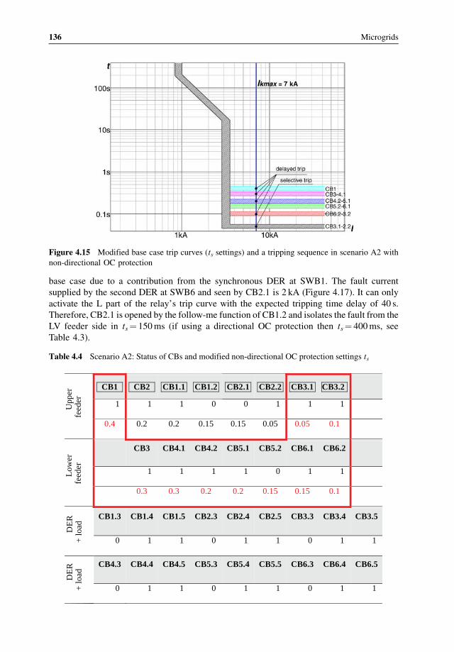
base case due to a contribution from the synchronous DER at SWB1. The fault current

supplied by the second DER at SWB6 and seen by CB2.1 is 2 kA (Figure 4.17). It can only

activate the L part of the relay’s trip curve with the expected tripping time delay of 40 s.

Therefore, CB2.1 is opened by the follow-me function of CB1.2 and isolates the fault from the

LV feeder side in ts¼ 150ms (if using a directional OC protection then ts¼ 400ms, see

Table 4.3).

Figure 4.15 Modified base case trip curves (ts settings) and a tripping sequence in scenario A2 with

non-directional OC protection

Table 4.4 Scenario A2: Status of CBs and modified non-directional OC protection settings ts

Upp

er

feed

er


1 1 1 0 0 1 1 1

0.4 0.2 0.2 0.15 0.15 0.05 0.05 0.1

Low

er

feed

er

CB3 CB4.1 CB4.2 CB5.1 CB5.2 CB6.1 CB6.2

1 1 1 1 0 1 1

0.3 0.3 0.2 0.2 0.15 0.15 0.1

DE

R

+ lo

ad


0 1 1 0 1 1 0 1 1

DE

R

+ lo

ad


0 1 1 0 1 1 0 1 1

136 Microgrids

The main concern is ts� 150ms set for the OC relay in CB1.2, which may affect the

stability of the synchronous DER with a small inertia at SWB1. A preferred solution is based

on the adaptive directional interlock. The time delay ts is set at 50ms for all OC relays in the

microgrid. Then blocking signals are sent in the correct directions, which prevents an

unnecessary disconnection of DERs and healthy parts of the microgrid.

Next we assume that, after an isolation of the first fault, the island which includes SWB2, 3,

5 and 6 is formed as shown in Figure 4.18. The synchronous DER in SWB6 is switched to a

frequency and voltage control mode, and additionally each load in the island is reduced from

100A to 50A.

Figure 4.16 Scenario B1: the microgrid with synchronous DERs connected to the MV distribution grid

Figure 4.17 Base case trip curves and a tripping sequence in scenario B1 with directional OC protection


Assume that there is a second fault inside the islandedmicrogrid between SWB2 and SWB3

and all non-directional OC relays use ts settings from the base case shown in Table 4.2. Ideally,

the fault should be cleared by CB2.2 and CB3.1. CB2.2 can not trip since there is no fault

current source at SWB2, but it can be opened by the follow-me function of CB3.1. The ts of

CB3.1 is set at 100ms for a minimum fault current level of 4�In CB¼ 3.2 kA. In case of using

directional OC protection, then ts¼ 150ms for CB3.1 (Table 4.3). However, the maximum

fault current supplied by the synchronous DER at SWB6 and seen by CB3.1 is Ikmax¼ 2.4 kA

(Figure 4.19). This will activate the L part of the relay’s trip curve with the expected tripping

Figure 4.18 Scenario B2: the islanded microgrid with the synchronous DER in SWB6

Figure 4.19 Base case and modified trip curves and a tripping sequence in scenario B2

138 Microgrids

time delay of 25 s. During this time, the DER at SWB6 will be disconnected by its out-of-step

protection.

In order to guarantee fast fault isolation in the islanded mode where the main grid does not

contribute to the fault, the trip curve must be pushed to the left dynamically, depending on the

microgrid topology and a number of connected DERs. The modified trip curves for scenario

B2 are illustrated in Figure 4.19.

Protection settings for all CBs in the island are calculated during the offline fault analysis

and shown in Table 4.5, as recorded in the event and action tables.

Another protection alternative is based on the adaptive directional interlock. The tripping time

is set at 50ms for all CBs inside the island, and the minimum short-circuit current has to be

dynamically modified (reduced) depending on the type and number of connected DER units.

A more elaborate example of multilevel microgrid and centralized adaptive protection

system is provided in the Appendix 4.A.1.

Table 4.5 Scenario B2: Status of CBs and modified OC protection settings Ikmin and ts

Upp

er f

eede

r


1 1 1 0 0 1 1 1

Ikmin 3.2 3.2 3.2 3.2 3.2 1.2 1.2 1.2

ts 0.3 0.2 0.2 0.15 0.15 0.05 0.05 0.1

Low

er f

eede

r

CB3 CB4.1 CB4.2 CB5.1 CB5.2 CB6.1 CB6.2

1 1 0 0 1 1 0

Ikmin 3.2 3.2 3.2 3.2 1.2 1.2 1.2

ts 0.2 0.2 0.15 0.15 0.05 0.05 0.1

DE

R +

lo

ad


1 1 1 0 1 1 0 1 1

DE

R +

lo

ad


0 1 1 0 1 1 1 1 1


4.3.5 Adaptive Protection System Based on Real-TimeCalculated Settings

An alternative centralized approach to the one based on predefined settings is to recalculate

protection settings in real-time operation, immediately upon changes in the microgrid

topology (network reconfiguration or DER connections). This protection scheme can be

implemented as a multifunctional intelligent digital relay (MIDR). When a fault occurs, the

routine implemented in the MIDR generates selective tripping signals, which are sent to

respective circuit breakers. The MIDR allows continuous real-time measurement and

monitoring of the analog and digital signals originating from equipment and network,

respectively. Integration of state estimation routines into a configuration of the protection

system, which monitors the DER operating state and sets up a corresponding data exchange

with the protection system is also possible [13]. Thus, new network operating conditions can

be assessed, functioning of the protection system can be analyzed and, if required, protection

settings can be adapted. Figure 4.20 illustrates the algorithm of the developed adaptive

protection relay. The scheme consists of two blocks: real-time and non-real time.

The real-time block analyzes the actual microgrid state, acquired by continuous measure-

ment of microgrid parameters, and detects disturbances due to adjusted tripping character-

istics of protection devices. When a tripping condition is detected, a tripping signal to the

respective circuit breaker is generated by the MIDR. The non-real-time block uses the

prediction data of the availability of DERs in order to review the selectivity of the tripping

characteristics for each new operating condition and to adapt them accordingly, if selectivity is

not suitably provided any longer. If the adaptation is successful and the boundary conditions

are not violated, the tripping characteristics of respective relays will be matched. If there is no

possible solution without violating the boundary conditions, a signal will be generated that

forbids the acceptance of the operation predicted by the (decentralized) energy management

system (DEMS/EMS).

The proposed adaptive protection concept for microgrids with protection settings calcu-

lated online was tested and proved in the 10/0.4 kV simulator in the laboratory of Fraunhofer

IWES (Figure 4.21). The simulator is equipped with photovoltaic systems, combined heat and

power units, diesel generators, models of wind power plants and different types of inverters.

In the test setup, the MIDR comprises the functionalities of both DEMS andMV/LV station

controller. For each of the three feeders (transformers T-1 to T-3), there is a separate database

server, realized by means of MySQL servers. In the databases, data about the interconnected

distributed energy resources (i.e. available short-circuit power provided by DER units) and the

actual microgrid configuration is stored. The actual interconnection states and short-circuit

power of DER units are stored in the respective databases and continuously communicated to

the MIDR. Communication between the MIDR and the database servers can be realized via

PLC or Ethernet. Based on the requested operational data (short-circuit power of DER in the

different grid sections) and the actual short-circuit power available from the main grid, the

MIDR calculates possible short-circuit currents and adapts the protection settings, where

required. According to the protection characteristics and the measurement signals supplied by

the current and voltage transformers, the MIDR decides whether there is a fault or not, and

sends tripping signals to respective circuit breakers, if required. In this concept, the MIDR

plays the role of the centralized protection controller which limits its application to a single

substation case. For remote circuit breakers, communication can become a bottleneck for fast

140 Microgrids

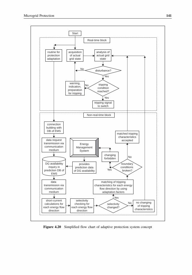
Start

routine forprotectionadaptation

acquisitionof actualgrid state

Real-time block

No

No

Yes

Yes

Yes

Yes

matching of trippingcharacteristics for each energy

flow direction by usingadaptation factors

No

No no changingof tripping

characteristics

short-currentcalculations for

each energy flowdirection

selectivitychanged?

warning,indication,preparationfor tripping

trippingconditionreached?

tripping signalto switch

disturbance?

Non-real-time block

connectionbuilding withDB of EMS

data requesttransmission viacommunication

medium

data transmission viacommunication

medium

selectivitychecking for

each energy flowdirection

EnergyManagement

System

matched trippingcharacteristics

accepted

changingforbidden

providesprediction data

of DG availability

boundaryconditions

broken?

DG availabilityinquiry in

prediction DB ofEMS

analysis ofactual grid

state

Figure 4.20 Simplified flow chart of adaptive protection system concept


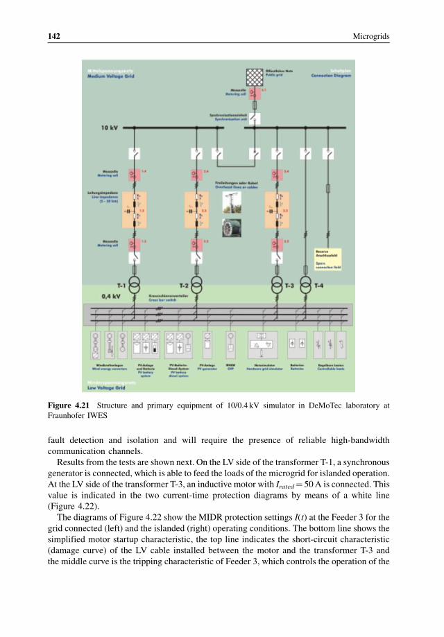
fault detection and isolation and will require the presence of reliable high-bandwidth

communication channels.

Results from the tests are shown next. On the LV side of the transformer T-1, a synchronous

generator is connected, which is able to feed the loads of the microgrid for islanded operation.

At the LV side of the transformer T-3, an inductive motor with Irated¼ 50A is connected. This

value is indicated in the two current-time protection diagrams by means of a white line

(Figure 4.22).

The diagrams of Figure 4.22 show the MIDR protection settings I(t) at the Feeder 3 for the

grid connected (left) and the islanded (right) operating conditions. The bottom line shows the

simplified motor startup characteristic, the top line indicates the short-circuit characteristic

(damage curve) of the LV cable installed between the motor and the transformer T-3 and

the middle curve is the tripping characteristic of Feeder 3, which controls the operation of the

Figure 4.21 Structure and primary equipment of 10/0.4 kV simulator in DeMoTec laboratory at

Fraunhofer IWES

142 Microgrids

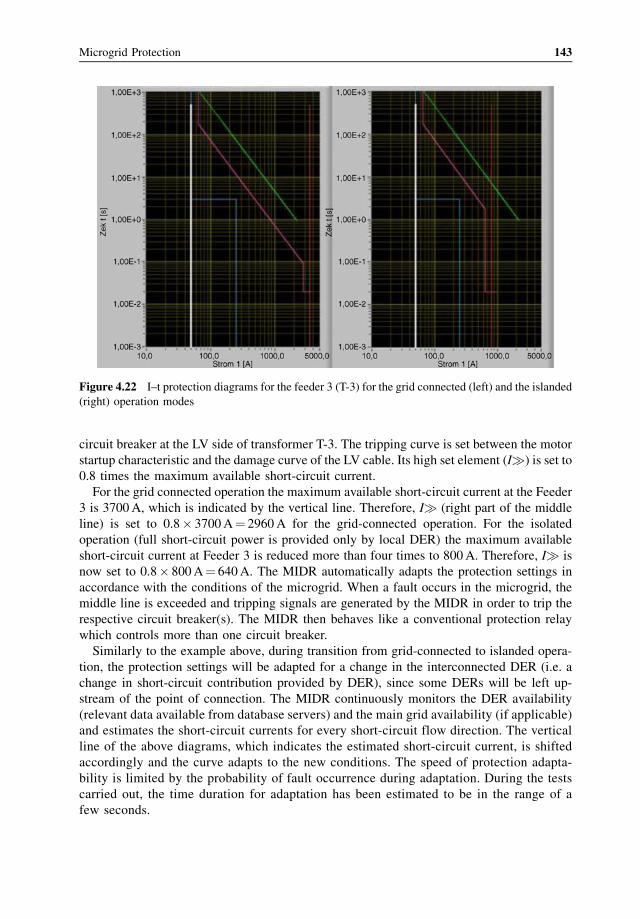
circuit breaker at the LV side of transformer T-3. The tripping curve is set between the motor

startup characteristic and the damage curve of the LV cable. Its high set element (I�) is set to

0.8 times the maximum available short-circuit current.

For the grid connected operation the maximum available short-circuit current at the Feeder

3 is 3700A, which is indicated by the vertical line. Therefore, I� (right part of the middle

line) is set to 0.8� 3700A¼ 2960A for the grid-connected operation. For the isolated

operation (full short-circuit power is provided only by local DER) the maximum available

short-circuit current at Feeder 3 is reduced more than four times to 800A. Therefore, I� is

now set to 0.8� 800A¼ 640A. The MIDR automatically adapts the protection settings in

accordance with the conditions of the microgrid. When a fault occurs in the microgrid, the

middle line is exceeded and tripping signals are generated by the MIDR in order to trip the

respective circuit breaker(s). The MIDR then behaves like a conventional protection relay

which controls more than one circuit breaker.

Similarly to the example above, during transition from grid-connected to islanded opera-

tion, the protection settings will be adapted for a change in the interconnected DER (i.e. a

change in short-circuit contribution provided by DER), since some DERs will be left up-

stream of the point of connection. The MIDR continuously monitors the DER availability

(relevant data available from database servers) and the main grid availability (if applicable)

and estimates the short-circuit currents for every short-circuit flow direction. The vertical

line of the above diagrams, which indicates the estimated short-circuit current, is shifted

accordingly and the curve adapts to the new conditions. The speed of protection adapta-

bility is limited by the probability of fault occurrence during adaptation. During the tests

carried out, the time duration for adaptation has been estimated to be in the range of a

few seconds.

Figure 4.22 I–t protection diagrams for the feeder 3 (T-3) for the grid connected (left) and the islanded

(right) operation modes


The suggested adaptive protection concept does not consider the function of automatic

reclosing, which is usually employed for temporary faults occurring on overhead lines. Of

special relevance to this concept is the data transfer between adaptive relays and EMS over

long distances. Communication via power line carrier (PLC) and LAN is a preferred option.

For a practical implementation, wireless radio communication should be considered for long

distance communication.

For the implementation of the adaptive network protection concept in distribution networks,

existing communication systems and protocols can be applied. The IEC 61850 standard allows

for real-time communication by means of periodically sent telegrams. For a sudden change of

state at the sending unit, a telegram (GOOSE message¼Generic Object Oriented Substation

Event) will be sendwith a high repetition ratewithin a fewmilliseconds after the change of state.

Thus, changes in the microgrid state can be detected rapidly. The communication link can be

established by means of common interfaces (RS-485, fiber optic etc.) and protocols. Commu-

nication architectures and protocols are discussed in Section 4.3.6.

4.3.6 Communication Architectures and Protocols forAdaptive Protection

As explained in the previous sections, the implementation of an adaptive protection system

requires that protection intelligent electronic devices (IEDs) communicate between them-

selves or with a central controller. By these communications, IEDs can provide and receive

information about the actual topology of the microgrid, about the status of generators, energy

storage devices and loads, and commands to execute an action (e.g. change of the active

setting group). The application of pre-calculated protection settings, can be deployed via a

centralized or a decentralized communications architecture:

� A centralized architecture is the most conventional and common communication scheme.

There is a central controller that takes decisions about protection IEDs which have

different settings for different operating conditions. This architecture is supported by

many communication protocols, the most common ones within the electric energy sector

being: Modbus, DNP3, IEC 60870-5-101/104 and IEC 61850. The centralized architecture

can be deployed with serial communications, bus communications, over PLC or through an

Ethernet network.� A decentralized architecture is less conventional. Within this architecture it is not

necessary to employ a central controller that coordinates protection settings, because

intelligence is distributed between IEDs themselves. Each IED, with the information

received from other IEDs, acts autonomously in order to change its active setting group.

This architecture is only feasible when the communication protocol allows it to establish a

direct communication between the IEDs, substituting direct hardwired connections

between the relays. For standard protocols, today the industry’s focus is on IEC

61850. The decentralized architecture needs to be implemented over a bus or Ethernet

network, although with a suitable bandwidth it can be implemented with future 4Gwireless

networks or over PLC.

The most significant advantage of a centralized architecture is that local protection devices

do not take decisions and therefore they are simpler. The central controller processes data and

144 Microgrids

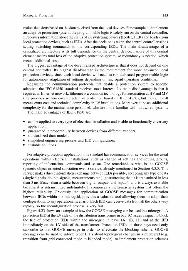
makes decisions based on the data received from the local devices. For example, to implement

an adaptive protection system, the programmable logic is solely run on the central controller.

It receives information about the status of all switching devices (feeder, DERs and loads) from

local protection devices, such as IEDs. After the decision is taken, the central controller sends

setting switching commands to the corresponding IEDs. The main disadvantage of a

centralized architecture is its full dependence on the central device. Failure of this central

element means total loss of the adaptive protection system, so redundancy is needed, which

means additional cost.

The biggest advantage of the decentralized architecture is that it does not depend on one

central controller. Its biggest disadvantage is the requirement for more advanced local

protection devices, since each local device will need to run dedicated programmable logic

for autonomous adaptation of settings depending on microgrid operating conditions.

Regarding the communication protocols that enable a protection system to become

adaptive, the IEC 61850 standard receives most interest. Its main disadvantage is that it

requires an Ethernet network. Ethernet is a common technology for automation at HVandMV

(the previous section covered adaptive protection based on IEC 61850), but today, it still

means extra cost and technical complexity in LV installations. Moreover, it poses additional

complexity for the maintenance personnel, who are more familiar with hardwired systems.

The main advantages of IEC 61850 are:

� can be applied to every type of electrical installation and is able to functionally cover any

application,� guaranteed interoperability between devices from different vendors,� standardized data models,� simplified engineering process and IED configuration,� scalable solutions.

For adaptive protection application, this standard has communication services for the usual

operations within electrical installations, such as change of settings and setting groups,

reporting of information, commands and so on. One remarkable service is the GOOSE

(generic object oriented substation event) service, already mentioned in Section 4.3.5. This

service makes direct information exchange between IEDs possible, accepting any type of data

(single signals, double signals, measurements etc.), guaranteeing that it is transmitted in less

than 3ms (faster than a cable between digital outputs and inputs), and is always available

because it is retransmitted indefinitely. It comprises a multi-master system that offers the

highest reliability. Obviously, the application of GOOSE messages for communication

between IEDs within the microgrid, provides a valuable tool allowing them to adapt their

configurations to any operational scenario. Each IED can receive data from all the others very

rapidly, so the reconfiguration process is very fast.

Figure 4.23 shows an example of how the GOOSEmessaging can be used in a microgrid. A

protection IED at the LV side of the distribution transformer in bay 1C issues a signal to block

the trip of protection IEDs within the microgrid in bays 1A, 1B, 1D and at the IED

immediately on the LV side of the transformer. Protection IEDs on those bays need only

subscribe to that GOOSE message in order to effectuate the blocking scheme. GOOSE

messages can be used to inform other IEDs about topological changes in a microgrid (e.g.

transition from grid connected mode to islanded mode), to implement protection schemes


(like the one in Figure 4.23), to execute commands (e.g. open/close circuit breakers), to

change active setting group and so on.

An adaptive protection system, such as one designed according to the IEC 61850

standard, requires higher investment than a traditional protection system for LV based

on fuses and hardwired interlock. However, microgrid operation will not be feasiblewithout

an adaptive protection system. Perhaps one of the main concerns in considering the IEC

61850 solution is the cost of the network, especially the cost of devices that were not

necessary in traditional LV networks, the “switches”. Switches enable the organizing of the

traffic within the network, taking into consideration several parameters, such as the priority

of a message, or managing VLANs in order not to mix different traffics. Switches are

necessary, but it is possible to use cheaper architectures by means of integrating these

switches inside IEDs. The implementation of an Ethernet network as a single ring of IEDs

with integrated switches is a very good option in order to reduce the cost of a high-

performance microgrid.

4.4 Fault Current Source for Effective Protection inIslanded Operation

As discussed in Section 4.1, one of the major problems in microgrid protection is the low

contribution to faults by DERs that have power electronics (PE) interfaces. This section

analyzes the installation of an independent system that supplies a fault current in the microgrid

dominated by DERs with PE interfaces, for example, PV panels. The proposed system,

Figure 4.23 The blocking scheme based on GOOSE for faults in the microgrid

146 Microgrids

designed as a fault-current source (FCS), is based on power electronics but uses a simpler and

thus less costly technology than is normal in inverters in this power range. An FCS would

consist of the following subsystems:

1. an energy storage device capable of supplying the active power for the fault current for a

specified duration – the amount of power and energy required depends on the anticipated

rating of the fault current source. The most economical way to provide a large amount of

power for a very short time (small energy) is in the form of an ultra-capacitor; these are

characterized by low standby losses and are maintenance free. They have a long life

expectancy, if used predominantly in idle mode.

2. a switch or power electronic circuit capable of releasing the power from the fault current

source into the LV network; if an ultra-capacitor is used as a storage device, a PE circuit is

needed to convert the DC voltage across the capacitor into an alternating current. For this

application, the optimum design uses much silicon and moderate cooling, which implies

using separate insulated-gate bipolar transistor (IGBT) modules on a simple heat sink. In

LV distribution networks, most faults behind the customer meter are single phase to earth/

neutral faults. Therefore the inverter must provide a neutral connection and preferably act

independently for each phase. This approach minimizes the annoyance to users of the other

two phases during a single-phase fault.

3. a detector which monitors the LV network and signals the condition of a fault, triggering

the power circuit of the switch to supply the fault current – the detection system includes

the intelligence of the fault current source. It determines when the source has to be

activated and it injects current into the microgrid. In order to be able to operate an FCS as a

plug-and-play device, this circuit should act only on locally measured information. As the

FCS is connected in parallel to the LV network, the obvious detection criterion is the

network voltage at the interconnection point of the FCS. It is assumed that the FCS is

connected to the microgrid at the point where the MV/LV step-down transformer would

normally be connected. As soon as the busbar voltage drops to a value below its statutory

minimum, the FCS can assume that something irregular has happened in the microgrid

network. This could be a fault, but it could also be insufficient generation to meet the

demand. Whatever the cause, the FCS response will not harm the microgrid operation. If

the voltage drop is caused by a transient overload – for example caused by the starting

current of a largemotor – the FCSwill reduce this overload. In any case, because the FCS is

designed to cease operating after a predetermined number of seconds, the other sources in

the microgrid will eventually supply the necessary loads again. In principle, the FCS

consists of one energy storage unit connected to three inverter phases that serve the three

network phases independently. Therefore, the triggering system will monitor each phase

independently and trigger only the inverter phase corresponding to the faulted phase. This

approach is valid for single-phase to neutral faults and for three-phase faults, because in

both situations the phase-to-neutral voltage drops to a low value. However, on a phase-to-

phase fault, the voltages of the two affected phases may simply phase-shift towards each

other. If that happens, all phase-to-neutral voltages remain more or less within specifica-

tion, but the three-phase system has a large negative-sequence component. This can be

addressed by also measuring the phase-to-phase voltages and triggering both affected

inverter phases if the voltage between the corresponding phases drops below a set

threshold.


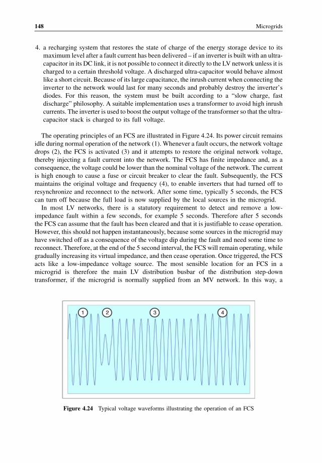
4. a recharging system that restores the state of charge of the energy storage device to its

maximum level after a fault current has been delivered – if an inverter is built with an ultra-

capacitor in its DC link, it is not possible to connect it directly to the LV network unless it is

charged to a certain threshold voltage. A discharged ultra-capacitor would behave almost

like a short circuit. Because of its large capacitance, the inrush current when connecting the

inverter to the network would last for many seconds and probably destroy the inverter’s

diodes. For this reason, the system must be built according to a “slow charge, fast

discharge” philosophy. A suitable implementation uses a transformer to avoid high inrush

currents. The inverter is used to boost the output voltage of the transformer so that the ultra-

capacitor stack is charged to its full voltage.

The operating principles of an FCS are illustrated in Figure 4.24. Its power circuit remains

idle during normal operation of the network (1). Whenever a fault occurs, the network voltage

drops (2), the FCS is activated (3) and it attempts to restore the original network voltage,

thereby injecting a fault current into the network. The FCS has finite impedance and, as a

consequence, the voltage could be lower than the nominal voltage of the network. The current

is high enough to cause a fuse or circuit breaker to clear the fault. Subsequently, the FCS

maintains the original voltage and frequency (4), to enable inverters that had turned off to

resynchronize and reconnect to the network. After some time, typically 5 seconds, the FCS

can turn off because the full load is now supplied by the local sources in the microgrid.

In most LV networks, there is a statutory requirement to detect and remove a low-

impedance fault within a few seconds, for example 5 seconds. Therefore after 5 seconds

the FCS can assume that the fault has been cleared and that it is justifiable to cease operation.

However, this should not happen instantaneously, because some sources in the microgrid may

have switched off as a consequence of the voltage dip during the fault and need some time to

reconnect. Therefore, at the end of the 5 second interval, the FCS will remain operating, while

gradually increasing its virtual impedance, and then cease operation. Once triggered, the FCS

acts like a low-impedance voltage source. The most sensible location for an FCS in a

microgrid is therefore the main LV distribution busbar of the distribution step-down

transformer, if the microgrid is normally supplied from an MV network. In this way, a

Figure 4.24 Typical voltage waveforms illustrating the operation of an FCS

148 Microgrids

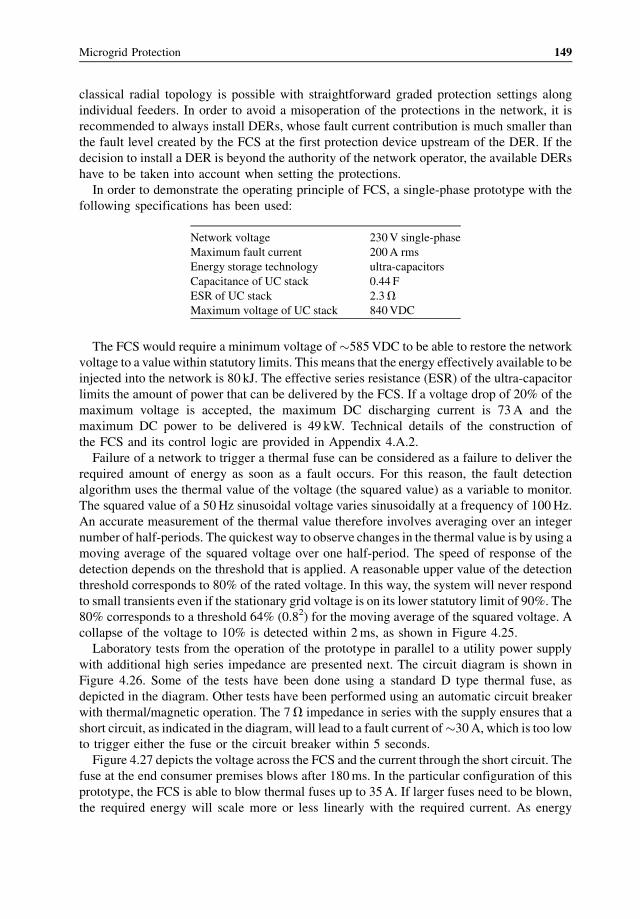
classical radial topology is possible with straightforward graded protection settings along

individual feeders. In order to avoid a misoperation of the protections in the network, it is

recommended to always install DERs, whose fault current contribution is much smaller than

the fault level created by the FCS at the first protection device upstream of the DER. If the

decision to install a DER is beyond the authority of the network operator, the available DERs

have to be taken into account when setting the protections.

In order to demonstrate the operating principle of FCS, a single-phase prototype with the

following specifications has been used:

Network voltage 230V single-phase

Maximum fault current 200A rms

Energy storage technology ultra-capacitors

Capacitance of UC stack 0.44 F

ESR of UC stack 2.3VMaximum voltage of UC stack 840VDC

The FCS would require a minimum voltage of�585VDC to be able to restore the network

voltage to a valuewithin statutory limits. This means that the energy effectively available to be

injected into the network is 80 kJ. The effective series resistance (ESR) of the ultra-capacitor

limits the amount of power that can be delivered by the FCS. If a voltage drop of 20% of the

maximum voltage is accepted, the maximum DC discharging current is 73A and the

maximum DC power to be delivered is 49 kW. Technical details of the construction of

the FCS and its control logic are provided in Appendix 4.A.2.

Failure of a network to trigger a thermal fuse can be considered as a failure to deliver the

required amount of energy as soon as a fault occurs. For this reason, the fault detection

algorithm uses the thermal value of the voltage (the squared value) as a variable to monitor.

The squared value of a 50Hz sinusoidal voltage varies sinusoidally at a frequency of 100Hz.

An accurate measurement of the thermal value therefore involves averaging over an integer

number of half-periods. The quickest way to observe changes in the thermal value is by using a

moving average of the squared voltage over one half-period. The speed of response of the

detection depends on the threshold that is applied. A reasonable upper value of the detection

threshold corresponds to 80% of the rated voltage. In this way, the system will never respond

to small transients even if the stationary grid voltage is on its lower statutory limit of 90%. The

80% corresponds to a threshold 64% (0.82) for the moving average of the squared voltage. A

collapse of the voltage to 10% is detected within 2ms, as shown in Figure 4.25.

Laboratory tests from the operation of the prototype in parallel to a utility power supply

with additional high series impedance are presented next. The circuit diagram is shown in

Figure 4.26. Some of the tests have been done using a standard D type thermal fuse, as

depicted in the diagram. Other tests have been performed using an automatic circuit breaker

with thermal/magnetic operation. The 7V impedance in series with the supply ensures that a

short circuit, as indicated in the diagram, will lead to a fault current of�30A, which is too lowto trigger either the fuse or the circuit breaker within 5 seconds.

Figure 4.27 depicts the voltage across the FCS and the current through the short circuit. The

fuse at the end consumer premises blows after 180ms. In the particular configuration of this

prototype, the FCS is able to blow thermal fuses up to 35A. If larger fuses need to be blown,

the required energy will scale more or less linearly with the required current. As energy


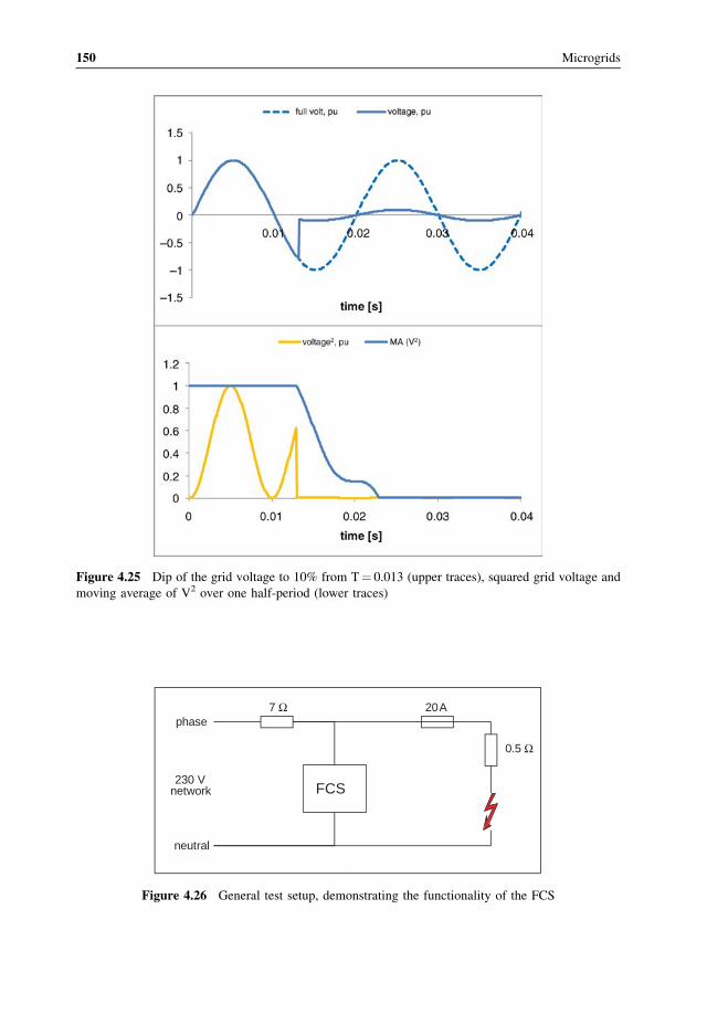
Figure 4.25 Dip of the grid voltage to 10% from T¼ 0.013 (upper traces), squared grid voltage and

moving average of V2 over one half-period (lower traces)

230 V network

phase

neutral

7 Ω

FCS

0.5 Ω

20 A

Figure 4.26 General test setup, demonstrating the functionality of the FCS

150 Microgrids

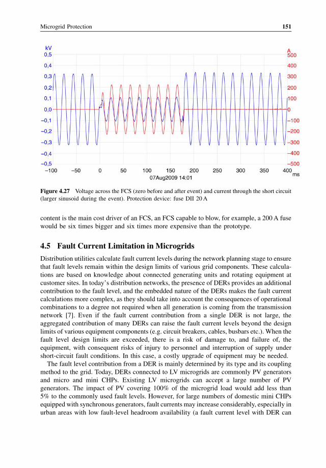
content is the main cost driver of an FCS, an FCS capable to blow, for example, a 200A fuse

would be six times bigger and six times more expensive than the prototype.

4.5 Fault Current Limitation in Microgrids

Distribution utilities calculate fault current levels during the network planning stage to ensure

that fault levels remain within the design limits of various grid components. These calcula-

tions are based on knowledge about connected generating units and rotating equipment at

customer sites. In today’s distribution networks, the presence of DERs provides an additional

contribution to the fault level, and the embedded nature of the DERs makes the fault current

calculations more complex, as they should take into account the consequences of operational

combinations to a degree not required when all generation is coming from the transmission

network [7]. Even if the fault current contribution from a single DER is not large, the

aggregated contribution of many DERs can raise the fault current levels beyond the design

limits of various equipment components (e.g. circuit breakers, cables, busbars etc.). When the

fault level design limits are exceeded, there is a risk of damage to, and failure of, the

equipment, with consequent risks of injury to personnel and interruption of supply under

short-circuit fault conditions. In this case, a costly upgrade of equipment may be needed.

The fault level contribution from a DER is mainly determined by its type and its coupling

method to the grid. Today, DERs connected to LV microgrids are commonly PV generators

and micro and mini CHPs. Existing LV microgrids can accept a large number of PV

generators. The impact of PV covering 100% of the microgrid load would add less than

5% to the commonly used fault levels. However, for large numbers of domestic mini CHPs

equipped with synchronous generators, fault currents may increase considerably, especially in

urban areas with low fault-level headroom availability (a fault current level with DER can

Figure 4.27 Voltage across the FCS (zero before and after event) and current through the short circuit

(larger sinusoid during the event). Protection device: fuse DII 20A


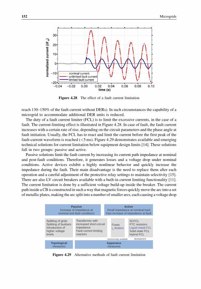
reach 130–150% of the fault current without DERs). In such circumstances the capability of a

microgrid to accommodate additional DER units is reduced.

The duty of a fault current limiter (FCL) is to limit the excessive currents, in the case of a

fault. The current-limiting effect is illustrated in Figure 4.28. In case of fault, the fault current

increases with a certain rate of rise, depending on the circuit parameters and the phase angle at

fault initiation. Usually, the FCL has to react and limit the current before the first peak of the

fault-current waveform is reached (<5ms). Figure 4.29 demonstrates available and emerging

technical solutions for current limitation below equipment design limits [14]. These solutions

fall in two groups: passive and active.

Passive solutions limit the fault current by increasing its current path impedance at nominal

and post-fault conditions. Therefore, it generates losses and a voltage drop under nominal

conditions. Active devices exhibit a highly nonlinear behavior and quickly increase the

impedance during the fault. Their main disadvantage is the need to replace them after each

operation and a careful adjustment of the protective relay settings to maintain selectivity [15].

There are also LV circuit breakers available with a built-in current limiting functionality [11].

The current limitation is done by a sufficient voltage build-up inside the breaker. The current

path inside a CB is constructed in such away thatmagnetic forces quicklymove the arc into a set

ofmetallic plates,making the arc split into a number of smaller arcs, each causing a voltage drop

Figure 4.28 The effect of a fault current limitation

Passive Active

Topological Apparatus

Increase of impedance atnominal and fault conditions

measures measures

commercialy available development

Small impedance at nominal loadFast increase of impedance at fault

Splitting of gridsSplitting of busbarsIntroduction ofhigher voltagelevels

Transformer withincreased short-circuitimpedanceFault current limitingreactors

FusesIs limiters

SCFCLPTC resistorsLiquid metal FCLSolid-state FCLHybrid FCL

Figure 4.29 Alternative methods of fault current limitation

152 Microgrids

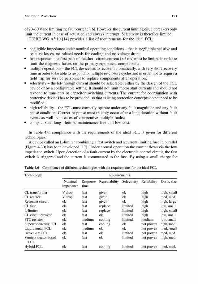
of 20–30Vand limiting the fault current [16].However, the current limiting circuit breakers only

limit the current in case of actuation and always interrupt. Selectivity is therefore limited.

CIGRE WG A3.10 [14] provides a list of requirements for the ideal FCL:

� negligible impedance under nominal operating conditions – that is, negligible resistive and

reactive losses, no related needs for cooling and no voltage drop;� fast response – the first peak of the short-circuit current (<5ms) must be limited in order to

limit the magnetic forces on the primary equipment components;� multiple operations – the FCL device has to recover automatically, with very short recovery

time in order to be able to respond to multiple re-closure cycles and in order not to require a

field trip for service personnel to replace components after operation;� selectivity – the let-through current should be selectable, either by the design of the FCL

device or by a configurable setting. It should not limit motor start currents and should not

respond to transients or capacitor switching currents. The current for coordination with

protective devices has to be provided, so that existing protection concepts do not need to be

modified;� high reliability – the FCL must correctly operate under any fault magnitude and any fault

phase condition. Correct response must reliably occur after a long duration without fault

events as well as in cases of consecutive multiple faults;� compact size, long lifetime, maintenance free and low cost.

In Table 4.6, compliance with the requirements of the ideal FCL is given for different

technologies.

A device called an Is-limiter combining a fast switch and a current limiting fuse in parallel

(Figure 4.30) has been developed [17]. Under normal operation the current flows via the low

impedance switch. Upon detection of a fault current by the electronic control circuit, the fast

switch is triggered and the current is commutated to the fuse. By using a small charge for

Table 4.6 Compliance of different technologies with the requirements for the ideal FCL

Technology Requirements

Nominal

impedance

Response

time

Repeatability Selectivity Reliability Costs, size

CL transformer V drop fast given ok high high, small

CL reactor V drop fast given ok high med, med

Resonant circuit ok fast given ok high high, large

CL fuse ok fast replace limited high low, small

Is-limiter ok fast replace limited high high, small

CL circuit breaker ok fast ok limited high low, small

PTC resistor ok medium cooling limited medium low, small

Superconducting FCL ok fast cooling ok not proven high, med.

Liquid metal FCL ok medium ok ok not proven med, small

Driven-arc FCL ok fast ok limited not proven med, med

Semiconductor based

FCL

ok fast ok limited not proven high, med.

Hybrid FCL ok fast cooling limited not proven med, med.


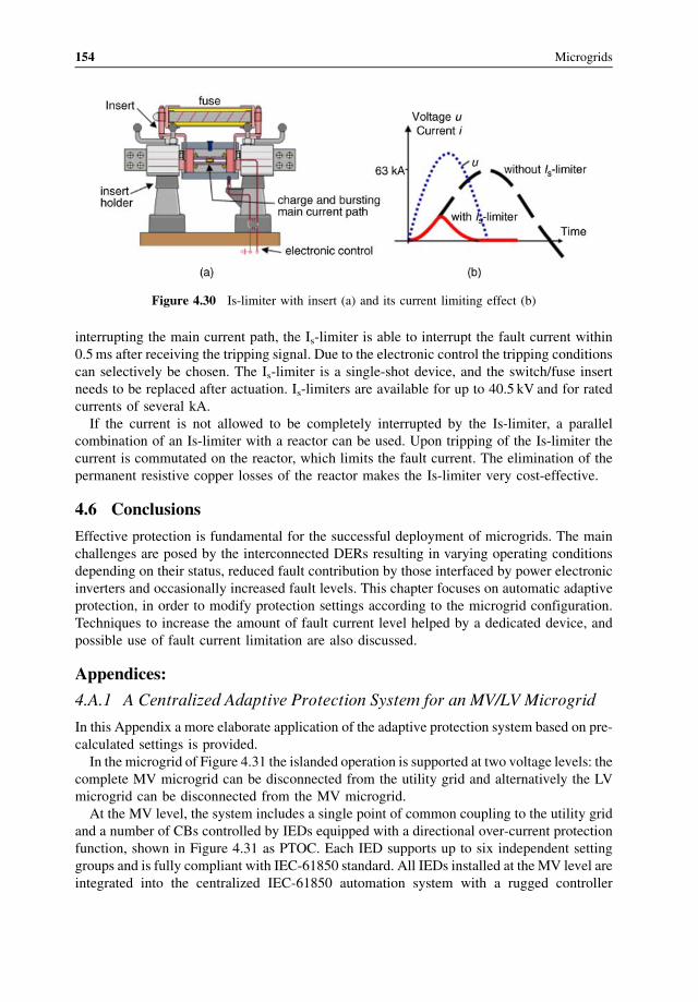
interrupting the main current path, the Is-limiter is able to interrupt the fault current within

0.5ms after receiving the tripping signal. Due to the electronic control the tripping conditions

can selectively be chosen. The Is-limiter is a single-shot device, and the switch/fuse insert

needs to be replaced after actuation. Is-limiters are available for up to 40.5 kV and for rated

currents of several kA.

If the current is not allowed to be completely interrupted by the Is-limiter, a parallel

combination of an Is-limiter with a reactor can be used. Upon tripping of the Is-limiter the

current is commutated on the reactor, which limits the fault current. The elimination of the

permanent resistive copper losses of the reactor makes the Is-limiter very cost-effective.

4.6 Conclusions

Effective protection is fundamental for the successful deployment of microgrids. The main

challenges are posed by the interconnected DERs resulting in varying operating conditions

depending on their status, reduced fault contribution by those interfaced by power electronic

inverters and occasionally increased fault levels. This chapter focuses on automatic adaptive

protection, in order to modify protection settings according to the microgrid configuration.

Techniques to increase the amount of fault current level helped by a dedicated device, and

possible use of fault current limitation are also discussed.

Appendices:

4.A.1 A Centralized Adaptive Protection System for an MV/LV Microgrid

In this Appendix a more elaborate application of the adaptive protection system based on pre-

calculated settings is provided.

In the microgrid of Figure 4.31 the islanded operation is supported at two voltage levels: the

complete MV microgrid can be disconnected from the utility grid and alternatively the LV

microgrid can be disconnected from the MV microgrid.

At the MV level, the system includes a single point of common coupling to the utility grid

and a number of CBs controlled by IEDs equipped with a directional over-current protection

function, shown in Figure 4.31 as PTOC. Each IED supports up to six independent setting

groups and is fully compliant with IEC-61850 standard. All IEDs installed at the MV level are

integrated into the centralized IEC-61850 automation system with a rugged controller

Figure 4.30 Is-limiter with insert (a) and its current limiting effect (b)

154 Microgrids

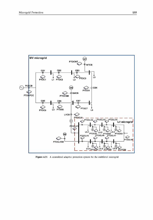
installed at the primary substation (point of common coupling) serving as the core for making

the control decisions, as well as providing data and event logging, reporting and human–

machine interface (HMI) functionality.

At the LV level, the system consists of a number of LV circuit breakers also equipped with

electronic trip units which are capable of performing directional over-current protection

functions, and also support two setting groups and Modbus communications via a serial

bus [11]. A centralized controller remote terminal unit (RTU) is installed at the point of

coupling of the LV to MV networks at the secondary distribution substation. It provides both

Modbus master and Modbus to IEC-61850 protocol conversion/gateway functionality, so that

the data from the LV side may also be integrated into the centralized IEC-61850 automation

system and considered in the programmed logic running at the MV primary station computer.

The controllers at both MVand LV levels communicate with the field protection devices at

the corresponding levels and between each other. The main objective of the controllers is to

adjust protection settings of each field relay with regard to the current state of the microgrid

(both grid configuration and status of DERs are taken into consideration). It is effectuated by a

programmed logic control continuously running in each controller for a periodic check and

management of relay settings.

There are two major steps in the design and implementation of this concept:

� offline system configuration and� online system operation.

4.A.1.1 Offline System Configuration

A set of the most common microgrid configurations and DER productions is created for

offline fault analysis. Fault currents passing through all monitored CBs are calculated by

simulating short circuits (3-phase, 2-phase, phase-to-ground etc.) at different locations of the

protected microgrid. During repetitive short-circuit calculations a microgrid topology or the

status of a single DER is modified between iterations.

Based on the simulation results, the settings for various network configurations are modeled

for relevant microgrid configurations (e.g. islanded, grid-connected with DER off, grid-

connected with DER on or radial/closed loop), and the IED setting groups are programmed

accordingly.

For the MV part of the system (Figure 4.31), the various network configurations and

topology changes that require control action – particularly changing the setting groups – are

identified by the status of the corresponding circuit breakers in Table 4.7.

Table 4.7 Setting groups for network configurations at MV level

CB status Operating mode description Corresponding

setting group

PCCCB – on, SMCB, CB4 – off Grid connected mode; radial; no large DG SG1

PCCCB – on, SMCB – on, CB4 – off Grid connected mode; radial; Large DG

contribution

SG2

PCCB – off, SMCB. WTCB – on Islanded SG3

All CBs on Grid connected mode; closed loop; large DER

contribution

SG4

156 Microgrids

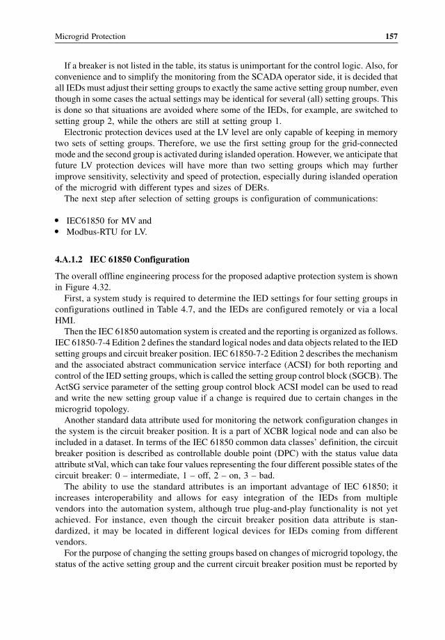
If a breaker is not listed in the table, its status is unimportant for the control logic. Also, for

convenience and to simplify the monitoring from the SCADA operator side, it is decided that

all IEDs must adjust their setting groups to exactly the same active setting group number, even

though in some cases the actual settings may be identical for several (all) setting groups. This

is done so that situations are avoided where some of the IEDs, for example, are switched to

setting group 2, while the others are still at setting group 1.

Electronic protection devices used at the LV level are only capable of keeping in memory

two sets of setting groups. Therefore, we use the first setting group for the grid-connected

mode and the second group is activated during islanded operation. However, we anticipate that

future LV protection devices will have more than two setting groups which may further

improve sensitivity, selectivity and speed of protection, especially during islanded operation

of the microgrid with different types and sizes of DERs.

The next step after selection of setting groups is configuration of communications:

� IEC61850 for MV and� Modbus-RTU for LV.

4.A.1.2 IEC 61850 Configuration

The overall offline engineering process for the proposed adaptive protection system is shown

in Figure 4.32.

First, a system study is required to determine the IED settings for four setting groups in

configurations outlined in Table 4.7, and the IEDs are configured remotely or via a local

HMI.

Then the IEC 61850 automation system is created and the reporting is organized as follows.

IEC 61850-7-4 Edition 2 defines the standard logical nodes and data objects related to the IED

setting groups and circuit breaker position. IEC 61850-7-2 Edition 2 describes the mechanism

and the associated abstract communication service interface (ACSI) for both reporting and

control of the IED setting groups, which is called the setting group control block (SGCB). The

ActSG service parameter of the setting group control block ACSI model can be used to read

and write the new setting group value if a change is required due to certain changes in the

microgrid topology.

Another standard data attribute used for monitoring the network configuration changes in

the system is the circuit breaker position. It is a part of XCBR logical node and can also be

included in a dataset. In terms of the IEC 61850 common data classes’ definition, the circuit

breaker position is described as controllable double point (DPC) with the status value data

attribute stVal, which can take four values representing the four different possible states of the

circuit breaker: 0 – intermediate, 1 – off, 2 – on, 3 – bad.

The ability to use the standard attributes is an important advantage of IEC 61850; it

increases interoperability and allows for easy integration of the IEDs from multiple

vendors into the automation system, although true plug-and-play functionality is not yet

achieved. For instance, even though the circuit breaker position data attribute is stan-

dardized, it may be located in different logical devices for IEDs coming from different

vendors.

For the purpose of changing the setting groups based on changes of microgrid topology, the

status of the active setting group and the current circuit breaker position must be reported by


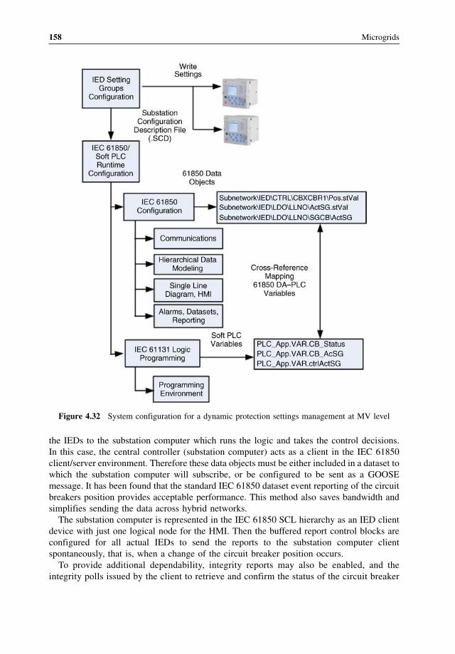
the IEDs to the substation computer which runs the logic and takes the control decisions.

In this case, the central controller (substation computer) acts as a client in the IEC 61850

client/server environment. Therefore these data objects must be either included in a dataset to

which the substation computer will subscribe, or be configured to be sent as a GOOSE

message. It has been found that the standard IEC 61850 dataset event reporting of the circuit

breakers position provides acceptable performance. This method also saves bandwidth and

simplifies sending the data across hybrid networks.

The substation computer is represented in the IEC 61850 SCL hierarchy as an IED client

device with just one logical node for the HMI. Then the buffered report control blocks are

configured for all actual IEDs to send the reports to the substation computer client

spontaneously, that is, when a change of the circuit breaker position occurs.

To provide additional dependability, integrity reports may also be enabled, and the

integrity polls issued by the client to retrieve and confirm the status of the circuit breaker

Figure 4.32 System configuration for a dynamic protection settings management at MV level

158 Microgrids

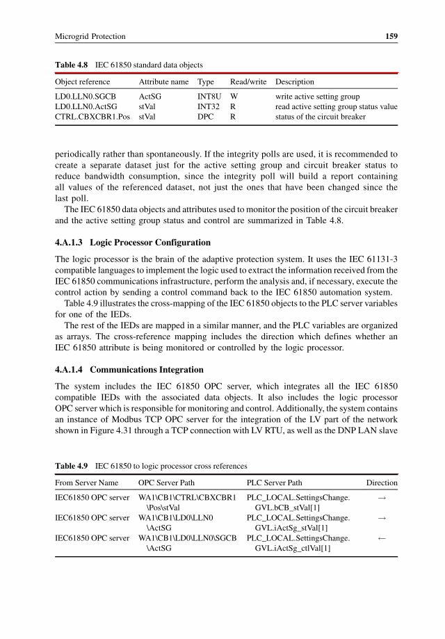
periodically rather than spontaneously. If the integrity polls are used, it is recommended to

create a separate dataset just for the active setting group and circuit breaker status to

reduce bandwidth consumption, since the integrity poll will build a report containing

all values of the referenced dataset, not just the ones that have been changed since the

last poll.

The IEC 61850 data objects and attributes used to monitor the position of the circuit breaker

and the active setting group status and control are summarized in Table 4.8.

4.A.1.3 Logic Processor Configuration

The logic processor is the brain of the adaptive protection system. It uses the IEC 61131-3

compatible languages to implement the logic used to extract the information received from the

IEC 61850 communications infrastructure, perform the analysis and, if necessary, execute the

control action by sending a control command back to the IEC 61850 automation system.

Table 4.9 illustrates the cross-mapping of the IEC 61850 objects to the PLC server variables

for one of the IEDs.

The rest of the IEDs are mapped in a similar manner, and the PLC variables are organized

as arrays. The cross-reference mapping includes the direction which defines whether an

IEC 61850 attribute is being monitored or controlled by the logic processor.

4.A.1.4 Communications Integration

The system includes the IEC 61850 OPC server, which integrates all the IEC 61850

compatible IEDs with the associated data objects. It also includes the logic processor

OPC server which is responsible for monitoring and control. Additionally, the system contains

an instance of Modbus TCP OPC server for the integration of the LV part of the network

shown in Figure 4.31 through a TCP connection with LV RTU, as well as the DNP LAN slave

Table 4.8 IEC 61850 standard data objects

Object reference Attribute name Type Read/write Description

LD0.LLN0.SGCB ActSG INT8U W write active setting group

LD0.LLN0.ActSG stVal INT32 R read active setting group status value

CTRL.CBXCBR1.Pos stVal DPC R status of the circuit breaker

Table 4.9 IEC 61850 to logic processor cross references

From Server Name OPC Server Path PLC Server Path Direction

IEC61850 OPC server WA1\CB1\CTRL\CBXCBR1

\Pos\stVal

PLC_LOCAL.SettingsChange.

GVL.bCB_stVal[1]

!

IEC61850 OPC server WA1\CB1\LD0\LLN0

\ActSG


GVL.iActSg_stVal[1]

!

IEC61850 OPC server WA1\CB1\LD0\LLN0\SGCB

\ActSG


GVL.iActSg_ctlVal[1]


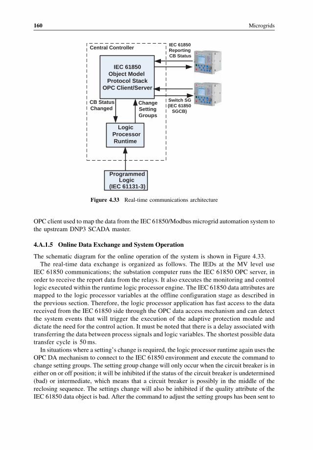
OPC client used to map the data from the IEC 61850/Modbus microgrid automation system to

the upstream DNP3 SCADA master.

4.A.1.5 Online Data Exchange and System Operation

The schematic diagram for the online operation of the system is shown in Figure 4.33.

The real-time data exchange is organized as follows. The IEDs at the MV level use

IEC 61850 communications; the substation computer runs the IEC 61850 OPC server, in

order to receive the report data from the relays. It also executes the monitoring and control

logic executed within the runtime logic processor engine. The IEC 61850 data attributes are

mapped to the logic processor variables at the offline configuration stage as described in

the previous section. Therefore, the logic processor application has fast access to the data

received from the IEC 61850 side through the OPC data access mechanism and can detect

the system events that will trigger the execution of the adaptive protection module and

dictate the need for the control action. It must be noted that there is a delay associated with

transferring the data between process signals and logic variables. The shortest possible data

transfer cycle is 50ms.

In situations where a setting’s change is required, the logic processor runtime again uses the

OPC DA mechanism to connect to the IEC 61850 environment and execute the command to

change setting groups. The setting group change will only occur when the circuit breaker is in

either on or off position; it will be inhibited if the status of the circuit breaker is undetermined

(bad) or intermediate, which means that a circuit breaker is possibly in the middle of the

reclosing sequence. The settings change will also be inhibited if the quality attribute of the

IEC 61850 data object is bad. After the command to adjust the setting groups has been sent to

IEC 61850 Object Model Protocol Stack

OPC Client/Server

Logic Processor Runtime

IEC 61850 ReportingCB Status

Central Controller

Switch SG (IEC 61850

SGCB)

Programmed Logic

(IEC 61131-3)

CB Status Changed

Change Setting Groups

Figure 4.33 Real-time communications architecture

160 Microgrids

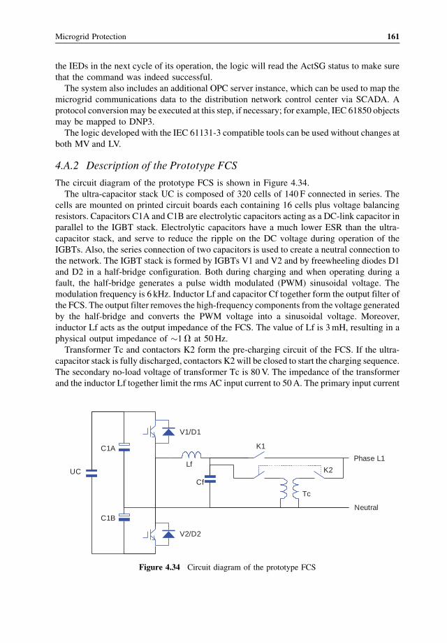
the IEDs in the next cycle of its operation, the logic will read the ActSG status to make sure

that the command was indeed successful.

The system also includes an additional OPC server instance, which can be used to map the

microgrid communications data to the distribution network control center via SCADA. A

protocol conversionmay be executed at this step, if necessary; for example, IEC 61850 objects

may be mapped to DNP3.

The logic developed with the IEC 61131-3 compatible tools can be used without changes at

both MV and LV.

4.A.2 Description of the Prototype FCS

The circuit diagram of the prototype FCS is shown in Figure 4.34.

The ultra-capacitor stack UC is composed of 320 cells of 140 F connected in series. The

cells are mounted on printed circuit boards each containing 16 cells plus voltage balancing

resistors. Capacitors C1A and C1B are electrolytic capacitors acting as a DC-link capacitor in

parallel to the IGBT stack. Electrolytic capacitors have a much lower ESR than the ultra-

capacitor stack, and serve to reduce the ripple on the DC voltage during operation of the

IGBTs. Also, the series connection of two capacitors is used to create a neutral connection to

the network. The IGBT stack is formed by IGBTs V1 and V2 and by freewheeling diodes D1

and D2 in a half-bridge configuration. Both during charging and when operating during a

fault, the half-bridge generates a pulse width modulated (PWM) sinusoidal voltage. The

modulation frequency is 6 kHz. Inductor Lf and capacitor Cf together form the output filter of

the FCS. The output filter removes the high-frequency components from the voltage generated

by the half-bridge and converts the PWM voltage into a sinusoidal voltage. Moreover,

inductor Lf acts as the output impedance of the FCS. The value of Lf is 3mH, resulting in a

physical output impedance of �1V at 50Hz.

Transformer Tc and contactors K2 form the pre-charging circuit of the FCS. If the ultra-

capacitor stack is fully discharged, contactors K2 will be closed to start the charging sequence.

The secondary no-load voltage of transformer Tc is 80V. The impedance of the transformer

and the inductor Lf together limit the rms AC input current to 50A. The primary input current

Neutral

Phase L1

UC

C1A

C1B

V1/D1

V2/D2

Lf

Cf

Tc

K1

K2

Figure 4.34 Circuit diagram of the prototype FCS


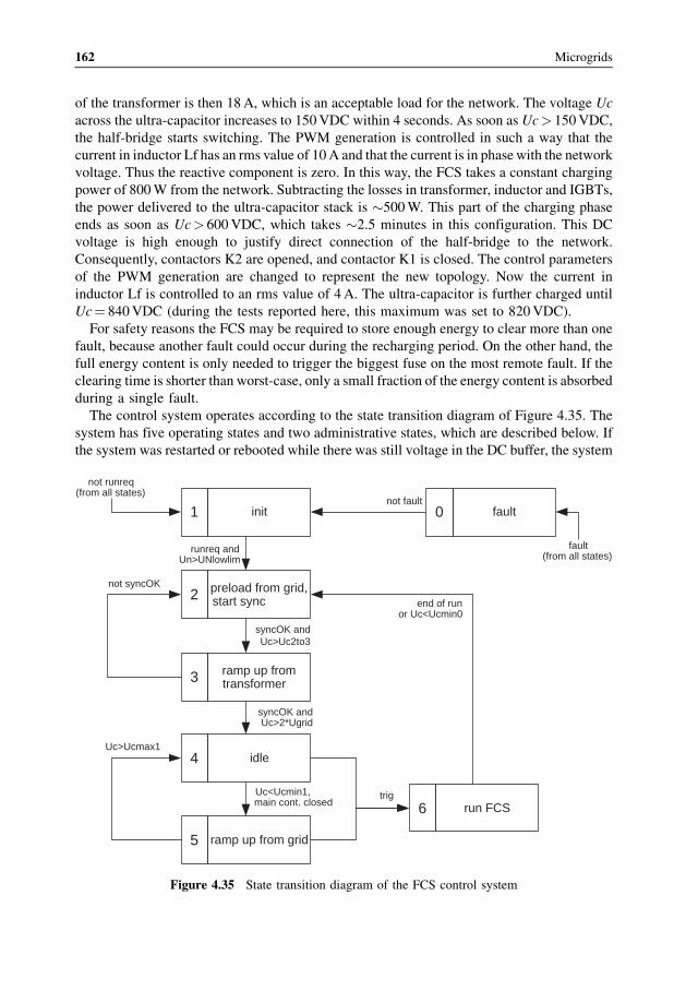
of the transformer is then 18A, which is an acceptable load for the network. The voltage Uc

across the ultra-capacitor increases to 150VDC within 4 seconds. As soon as Uc> 150VDC,

the half-bridge starts switching. The PWM generation is controlled in such a way that the

current in inductor Lf has an rms value of 10A and that the current is in phase with the network

voltage. Thus the reactive component is zero. In this way, the FCS takes a constant charging

power of 800W from the network. Subtracting the losses in transformer, inductor and IGBTs,

the power delivered to the ultra-capacitor stack is �500W. This part of the charging phase

ends as soon as Uc> 600VDC, which takes �2.5 minutes in this configuration. This DC

voltage is high enough to justify direct connection of the half-bridge to the network.

Consequently, contactors K2 are opened, and contactor K1 is closed. The control parameters

of the PWM generation are changed to represent the new topology. Now the current in

inductor Lf is controlled to an rms value of 4A. The ultra-capacitor is further charged until

Uc¼ 840VDC (during the tests reported here, this maximum was set to 820VDC).

For safety reasons the FCS may be required to store enough energy to clear more than one

fault, because another fault could occur during the recharging period. On the other hand, the

full energy content is only needed to trigger the biggest fuse on the most remote fault. If the

clearing time is shorter than worst-case, only a small fraction of the energy content is absorbed

during a single fault.

The control system operates according to the state transition diagram of Figure 4.35. The

system has five operating states and two administrative states, which are described below. If

the system was restarted or rebooted while there was still voltage in the DC buffer, the system

1 init

runreq and Un>UNlowlim

5 ramp up from grid

syncOK andUc>Uc2to3

4 idle

6 run FCS

fault(from all states)

not runreq(from all states)

0 faultnot fault

2 preload from grid,start sync

not syncOK

Uc<Ucmin1,main cont. closed

trig

end of runor Uc<Ucmin0

syncOK and Uc>2*Ugrid

3 ramp up fromtransformer

Uc>Ucmax1

Figure 4.35 State transition diagram of the FCS control system

162 Microgrids

would automatically proceed through the diagram until it reached the state which is most

appropriate for the actual DC voltage. During a reboot, all contactors are opened and the

IGBTs are switched to a passive state so that possibly destructive transients cannot occur.

� state 0 – Whenever a hardware-related fault has occurred, the system enters state 0. The

system will remain in state 0 until all fault conditions have been removed and an

appropriate delay time has elapsed. Within state 0, the fault reset logic has its own state

machine.� state 1 – When the FCS is started or the software is rebooted, the system enters state 1. In

state 1, all variables are initialized. The FCS can be enabled/disabled from the user

interface.� state 2 – Contactors K2 are closed so that the ultra-capacitor is charged via the pre-

charging transformer, and pre-charging continues until the DC voltage exceeds 2 to 3 times

a threshold Uc, which is presently set to 150 VDC. When both the synchronization and the

voltage threshold condition are fulfilled, the system will enter state 3.� state 3 – Contactors K2 remain closed, but now PWM on the inverter will start so that the

DC voltage can be further ramped up. The half-bridge is operated in current-control mode.

The measured current in inductor Lf is decomposed into an active (in-phase) component

and a reactive (out-of-phase) component. These components are the inputs of two

controllers, whose outputs are used to calculate the phase and amplitude of the sinewave

generated by the PWM. The reference for the reactive part is zero, the reference for the

active part is set to 10A. The minus sign is used because the positive polarity of the

current is defined as flowing from the FCS into the grid. This state is finished when the DC

voltageUc is high enough for the inverter to be connected directly to the network, which is

the case when Uc> 2�Ugrid, that is, twice the peak value of the grid voltage. The system

then enters state 4.� state 4 – This is the idle state, in which the system is ready for operation but remains idle,

to minimize losses. Because both the ultra-capacitor stack and the electrolytic capacitors

are provided with voltage sharing resistors, the DC voltage will decrease gradually and a

regular top-up is needed to retain the voltage. This recharge is done in state 5 and is

initiated ifUc<UCmin1. Threshold parameterUCmin1 is presently set to 780V. This also

means that if the system enters state 4 from state 3 (condition of transition: Uc> 2� Ugrid,which is in the order of 600V), it will immediately move on to state 5. State 4 is purposely

used as an intermediate state. A hardware interlock ensures that contactor K1 can only be

closed after contactors K2 have opened and the system is only allowed to enter state 5 after

the closing of contactor K1 has been confirmed.� state 5 – The operation of state 5 is very similar to that of state 3. However, the inverter is

now connected to the grid directly, instead of via the transformer, which means that the

settings of the PWM are different and that the two current controllers use different control

parameters and reference values. In state 5, the reactive current controller has a reference

value of a few amps capacitive, so that the inverter will supply the capacitive current

flowing into filter capacitor Cf. In this way, the power factor of the input current remains

close to 1. In the prototype, the reference value for the active current controller is set to 4A.� state 6 – From both states 4 and 5, the system is allowed to enter state 6. This transition

occurs when the fault detection logic has detected a probable fault in the network. During

the transition to state 6, the sinewave generator for the PWM is detached from the


phase -looked loop (PL L) and rem ains running with a fixed fre quency value. Th e voltage

dip associa ted with the fault may have caused the PLL to obser ve a frequency step.

There fore the measur ed value of the fre quency is saved in a FIFO buffer in 100 ms. If a

fault is detected, the PWM gener ation cont inues on the basis of a 100-m s-old value of the

frequency, which gener ally will be a reliable pre- fault value . In sta te 6, the curr ent

control lers are inactive and the PWM uses a fixed amp litude for the outpu t voltage, equal to

the pre-fau lt value of Ugr id. In addition to that, the PWM cal culation include s a virtua l

impeda nce which can virtua lly add both induc tive and resistive com ponents to the outpu t

inductor. With the lapse of time , the v irtual impeda nce will incr ease, which mak es it

possibl e for the other gener ators in the networ k to regain cont rol of the voltage and p hase of

the network. After a pres et time – now set to 5 secon ds – the FCS will leave state 6 and

enter state 2. Dependi ng on the remainin g DC voltage after this act ion, the system may

subse quently p roceed to state 3, 4 or 5. If during its action in state 6, the DC voltage drops

too low, defined as UC < Ucmin0 , the system wi ll immedia tely enter state 2. The value of

Ucmin0 is pres ently set to 600 V.

References

1. Feero, W., Dawson, D., and Stevens, J. “Protection Issues of the Microgrid Concept”. Available http://certs.lbl.

gov/pdf/protection-mg.pdf.

2. Al-Nasseri, H., Redfern, M.A., and O’Gorman, R. (2005) “Protecting microgrid systems containing solid-state

converter generation”, Int. Conf. on Future Power Systems.

3. Vilathgamuwa, D.M., Loh, P.C., and Li, Y. (2006) Protection of microgrids during utility voltage sags. IEEE T.

Ind. Electron., 53 (5), 1427–1436.

4. Driesen, J., Vermeyen, P., and Belmans, R. (2007) Protection issues in microgrids with multiple distributed

generation units, 4th Power Conversion Conf., Nagoya.

5. Nukkhajoei, H. and Lasseter, R.H. (2007) “Microgrid Protection”, IEEE PES General Meeting.

6. EPRI (2006) “Overview of SEMI F47-0706” [online]. Available www.f47testing.com.

7. KEMA Limited (2005) “The contribution to distribution network fault levels from the connection of distributed

generation”.

8. Bower, W. and Ropp, M. (March 2002) “Evaluation of islanding detection methods for photovoltaic utility

interactive power systems,” IEA-PVPS, Online report T5-09. Available: http://www.oja-services.nl/iea-pvps/

products/download/rep5_09.pdf.

9. Jayawarna, N. (2004) “Fault current contribution from power converters”, EU Microgrids project, Available

www.microgrids.eu.

10. Rockefeller, G.D. et al. (1988) Adaptive Transmission Relaying Concepts for Improved Performance. IEEE

Transactions on Power Delivery, 3 (4), 1446–1458.

11. ABB SACE SpA (2007), “Low voltage moulded case circuit breakers Tmax”, Product brochure, Available http://

library.abb.com/global/scot/scot209.nsf/veritydisplay/117ea5b751d87f12c125734e002a25dc/$File/

1SDC210015B0203.pdf.

12. ABB SACE SpA (2008), “DOC simulation tool”, User Manual version 1.0.

13. Shustov, A. and Valov, B. (2006) L€osungswege der Integrationsprobleme dezentraler Energieerzeugungsanlagen

in elektrischen Verteilungsnetzen, Vortr€age des internationalen wissenschaftlich-technischen Seminars, Poly-

technische Universit€at Tomsk, 10.11.04.

14. CIGRE WG (2003) A3.10 “Fault Current Limiters – Fault Current Limiters in Electrical Medium and High

Voltage Systems”, CIGRE Technical Brochure, No. 239.

15. CIGRE WG (2006) A3.16 “Guideline on the impacts of fault current limiting devices on protection systems”,

A3-06 (SC) 33 IWD.

16. Lindmayer, M., Marzahn, E., Mutzke, A. et al. (2004) “The process of arc-splitting between metal plates in low

voltage arc chutes”, 22nd Int. Conf. on Electrical Contacts, Seattle.

17. ABB Carol Emag (2008) “Is limiter”, Product brochure, Available http://library.abb.com/global/scot/scot235.nsf/

veritydisplay/31656b3a0912262ac12574f700565d1e/$File/2243-08%20E_300dpi.pdf.

164 Microgrids

http://certs.lbl.gov/pdf/protection-mg.pdf

http://certs.lbl.gov/pdf/protection-mg.pdf

www.f47testing.com

http://www.oja-services.nl/iea-pvps/products/download/rep5_09.pdf

http://www.oja-services.nl/iea-pvps/products/download/rep5_09.pdf

www.microgrids.eu

http://library.abb.com/global/scot/scot209.nsf/veritydisplay/117ea5b751d87f12c125734e002a25dc/$File/1SDC210015B0203.pdf



http://library.abb.com/global/scot/scot235.nsf/veritydisplay/31656b3a0912262ac12574f700565d1e/$File/2243-08%20E_300dpi.pdf

http://library.abb.com/global/scot/scot235.nsf/veritydisplay/31656b3a0912262ac12574f700565d1e/$File/2243-08%20E_300dpi.pdf

5

Operation of Multi-Microgrids

Jo~ao Abel Pe Sc as Lopes, Andr�e Madureira, Nuno Gil and Fernanda Resende

5.1 Int roduction

This chapter aims to stud y the managem ent of distribution networ ks with an increased

micro grid penetra tion, that is, corr esponding to a situatio n whe re mos t of the low voltage (LV)

networ ks turn into active micro grids. It is therefore assum ed that the mi crogrid conce pt is

extended, lea ding to the developme nt of a new concept – the multi-micro grid [1]. A ful l

exploitation of this conce pt involves the d esign of a new control architecture as well as the

development of new man agement tools or the adaptation o f existing distribution managem ent

system s (DMS) tools.

The novel conce pt of multi-mi crogrids correspo nds to a high-level structure , formed at the

medium voltage (MV ) level, consi sting of several LV mi crogrids and distributed generat ion

(DG) units connec ted to adjacent MV feed ers. For the purpos e of grid cont rol and man age-

ment, microgri ds, DG units and MV load s under act ive dem and-side man agement cont rol can

be consider ed as active cells in this type of power system. In this new scena rio, the possibi lity

of having some MV responsive loads able to receive control request s under a load curtai lment

strategy is regarded as a way to ensure additional anci llary service s.

A large nu mber of LV networks with micro sources and loads, that are no longe r passive

eleme nts of the distribution grid, then need to be opera ted toge ther in a coord inated way.

There fore, the system to be managed increas es largely in complexity and dimens ion, requiring

a com pletely new cont rol and man agement architectu re. Th is arch itecture is illus trated in

Figure 5.1.

An effective man agement of thi s type of system requires the development of a hierar chical

control arch itecture , where cont rol will be exercised by an intermed iate cont roller – the

central auto nomous man agement controlle r (CAM C) – to be instal led at the MV bus level of a

high voltage (HV)/MV substation, under the responsibility of the distribution system operator

(DSO) and will be in charge of a multi-microgrid system. In this way, the complexity of the



system can be shared among several smaller individual control agents, behaving like a small

DMS that is able to tackle the scheduling problem of generating units (DG and microsources)

and other control devices that are installed in the system in both normal and emergency

conditions.

In this context, the deployment of a communications infrastructure as a means for

achieving full observability of the distribution network is crucial. This can be achieved by

exploiting a smart metering infrastructure, which will allow a coordinated and integrated

management of individual elements at the LV level, such as microgrids (and corresponding

microgenerators, loads and storage devices). DG units and loads participating in active

demand-side management strategies, directly connected to the MV grid, may require a

dedicated communication infrastructure. This local communication infrastructure will be

the key driver for managing the distribution network in a more efficient way and

consequently maximizing the integration of DG and microgeneration, especially renew-

able-based power sources.

DMS

CAMC

RTU

MGCC

MGCC

MGCC

CAMCRTU

HV

MV

HV

MV

LV

LV

LVDG

DG

Figure 5.1 Control and management architecture of a multi-microgrid system

166 Microgrids

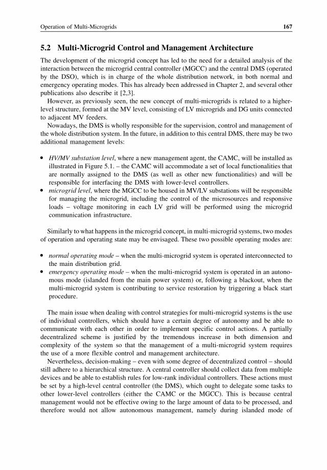
5.2 Multi-Microgrid Control and Management Architecture

The development of the microgrid concept has led to the need for a detailed analysis of the

interaction between the microgrid central controller (MGCC) and the central DMS (operated

by the DSO), which is in charge of the whole distribution network, in both normal and

emergency operating modes. This has already been addressed in Chapter 2, and several other

publications also describe it [2,3].

However, as previously seen, the new concept of multi-microgrids is related to a higher-

level structure, formed at the MV level, consisting of LV microgrids and DG units connected

to adjacent MV feeders.

Nowadays, the DMS is wholly responsible for the supervision, control and management of

the whole distribution system. In the future, in addition to this central DMS, there may be two

additional management levels:

� HV/MV substation level, where a new management agent, the CAMC, will be installed as

illustrated in Figure 5.1. – the CAMC will accommodate a set of local functionalities that

are normally assigned to the DMS (as well as other new functionalities) and will be

responsible for interfacing the DMS with lower-level controllers.� microgrid level, where the MGCC to be housed in MV/LV substations will be responsible

for managing the microgrid, including the control of the microsources and responsive

loads – voltage monitoring in each LV grid will be performed using the microgrid

communication infrastructure.

Similarly to what happens in the microgrid concept, in multi-microgrid systems, two modes

of operation and operating state may be envisaged. These two possible operating modes are:

� normal operating mode – when the multi-microgrid system is operated interconnected to

the main distribution grid.� emergency operating mode – when the multi-microgrid system is operated in an autono-

mous mode (islanded from the main power system) or, following a blackout, when the

multi-microgrid system is contributing to service restoration by triggering a black start

procedure.

The main issue when dealing with control strategies for multi-microgrid systems is the use

of individual controllers, which should have a certain degree of autonomy and be able to

communicate with each other in order to implement specific control actions. A partially

decentralized scheme is justified by the tremendous increase in both dimension and

complexity of the system so that the management of a multi-microgrid system requires

the use of a more flexible control and management architecture.

Nevertheless, decision-making – even with some degree of decentralized control – should

still adhere to a hierarchical structure. A central controller should collect data from multiple

devices and be able to establish rules for low-rank individual controllers. These actions must

be set by a high-level central controller (the DMS), which ought to delegate some tasks to

other lower-level controllers (either the CAMC or the MGCC). This is because central

management would not be effective owing to the large amount of data to be processed, and

therefore would not allow autonomous management, namely during islanded mode of

Operation of Multi-Microgrids 167

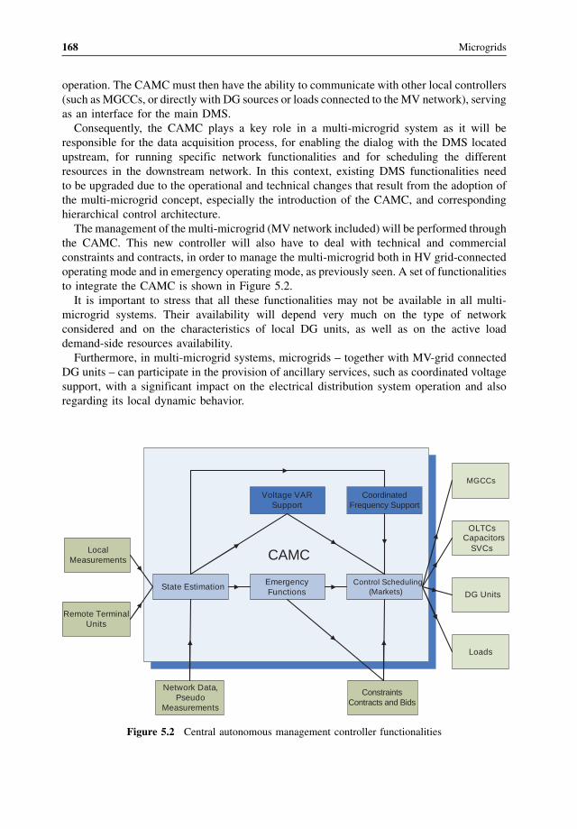
operation. The CAMC must then have the ability to communicate with other local controllers

(such as MGCCs, or directly with DG sources or loads connected to the MV network), serving

as an interface for the main DMS.

Consequently, the CAMC plays a key role in a multi-microgrid system as it will be

responsible for the data acquisition process, for enabling the dialog with the DMS located

upstream, for running specific network functionalities and for scheduling the different

resources in the downstream network. In this context, existing DMS functionalities need

to be upgraded due to the operational and technical changes that result from the adoption of

the multi-microgrid concept, especially the introduction of the CAMC, and corresponding

hierarchical control architecture.

The management of the multi-microgrid (MV network included) will be performed through

the CAMC. This new controller will also have to deal with technical and commercial

constraints and contracts, in order to manage the multi-microgrid both in HV grid-connected

operating mode and in emergency operating mode, as previously seen. A set of functionalities

to integrate the CAMC is shown in Figure 5.2.

It is important to stress that all these functionalities may not be available in all multi-

microgrid systems. Their availability will depend very much on the type of network

considered and on the characteristics of local DG units, as well as on the active load

demand-side resources availability.

Furthermore, in multi-microgrid systems, microgrids – together with MV-grid connected

DG units – can participate in the provision of ancillary services, such as coordinated voltage

support, with a significant impact on the electrical distribution system operation and also

regarding its local dynamic behavior.

CAMCLocalMeasurements

Remote TerminalUnits

State Estimation EmergencyFunctions

Control Scheduling (Markets)

Voltage VARSupport

CoordinatedFrequency Support

Network Data,Pseudo

Measurements

ConstraintsContracts and Bids

MGCCs

OLTCsCapacitors

SVCs

DG Units

Loads

Figure 5.2 Central autonomous management controller functionalities

168 Microgrids

The need to study the dynamic behavior of a multi-microgrid, to evaluate the islanding

feasibility, involves dealing with hundreds (or even thousands) of microgenerators, which may

lead to a significant computational burden when developing these simulations. So dynamic

equivalents for microgrids are of utmost importance for developing such studies.

Several key aspects of multi-microgrid operation, developed within the framework of the

EU R&D project, More Microgrids [4,5], are addressed in the following sections, namely

regarding some of the most important functionalities available at the CAMC level. Bearing in

mind the relevance of some of these functionalities and the need to perform some of the key

studies, such as dynamic behavior analysis, the following topics are addressed:

� coordinated voltage/var support for normal operation,� coordinated frequency control for islanded operation,� local black start – restoration of the MV grid following a blackout,� definition of dynamic equivalents for microgrids.

5.3 Coordinated Voltage/var Support

5.3.1 Introduction

Large-scale integration of DERs (DG in particular) may pose serious operational problems for

the DSO. One of the major concerns that arises is related to the voltage rise effect as a result of

the massive presence of these generation units in the distribution system, namely in LV

networks [6]. In these systems, conventional voltage regulation methods are not suited for

tackling this problem effectively as they do not address variable power injections provided by

DG units, so voltage control is an issue that must be dealt with efficiently.

Due to operational issues, most DSOs require that DGs operate at zero reactive power or at a

fixed power factor. This limits the amount of DG installed capacity, in order to guarantee

admissible voltage profiles in the worst-case scenario. Several approaches can be found in the

scientific literature that address voltage control in distribution grids with the presence of DG.

However, these proposals do not take into consideration coordinated operation at MVand LV

levels and/or the specific characteristics of distribution networks.

Consequently, new approaches for voltage control must be developed, based on the full use

of the resources available, especially DG and microgeneration units, taking into account the

specific characteristics of distribution networks (in particular, LV grids that usually have very

resistive lines). This is particularly important in the case of LV networks where both active and

reactive power control is needed for an efficient voltage control scheme. In some extreme

cases, if no local storage is available, it may even be necessary to spill some local generation in

order to avoid voltage rise problems [7].

5.3.2 Mathematical Formulation

A hierarchical coordinated approach for voltage/var control in distribution systems with high

penetration of DG can be formulated as a multi-objective optimization problem. The proposed

formulation of this problem aims at minimizing active power losses and microgeneration

curtailment, subject to a set of technical and operational constraints such as voltage and line

loading levels [8].


The main control variables identified are: reactive power from MV-connected DG sources,

on-load tap changing (OLTC) transformer tap settings and microgeneration curtailment.

Consequently, this problem becomes a mixed integer, nonlinear optimization problem, since it

deals with both continuous and discrete variables.

The objective function and the constraints used to solve this problem are presented

below.

min a �PPloss þ ð1� aÞ �PmGshedð Þsubject to:

PGi � PL

i ¼XN

k¼1

Vi � Vk � ðGik � cos uik þ Bik � sin uikÞ

QGi � QL

i ¼XN

k¼1

Vi � Vk � ðGik � sin uik þ Bik � cos uikÞ

Sik � Smaxik

Vmini � Vi � Vmax

i

Qmini � QG

i � Qmaxi

tmini � ti � tmax

i

Where

a is a decision parameter to be defined by the decision-maker, in this case the DSO

PGi , P

Li are the active power generation from DG and microgeneration and the active power

consumption at bus i, respectively

Vi is the voltage at bus i

Gik is the real part of the element in the admittance matrix (Y-bus) corresponding to the ith

row and kth column

Bik is the imaginary part of the element in the Y-bus corresponding to the ith row and kth

column

uik is the difference in voltage angle between the ith and kth buses

QGi , Q

Li are the reactive power generation/consumption at bus i, respectively

Sik is the apparent power flow in branch ik

Smaxik is the maximum apparent power flows in branch ik

Vi is the voltage at bus i

Vmini , Vmax

i are the minimum and maximum voltage at bus i, respectively

QGi is the reactive power generation at bus i

Qmini ,Qmax

i are the minimum and maximum reactive power generation at bus i, respectively

ti is the transformer tap, or capacitor step, position of the OLTC transformer or capacitor

bank i

tmini , tmax

i are the minimum and maximum taps of OLTC transformer or capacitor bank i.

Considering the specificities of the voltage control problem, particularly the fact that it

comprises both discrete variables (transformer taps) and continuous variables (active or

reactive power generation), a meta-heuristic approach – evolutionary particle swarm

(5.1)

(5.2)

(5.3)

(5.4)

(5.5)

(5.6)

(5.7)

170 Microgrids

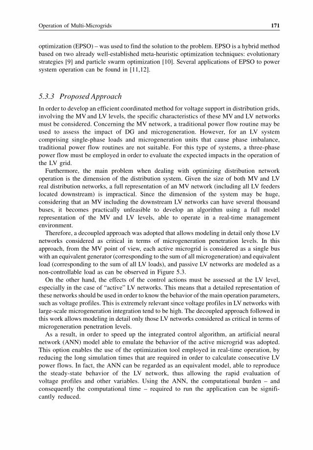
optimization (EPSO) – was used to find the solution to the problem. EPSO is a hybrid method

based on two already well-established meta-heuristic optimization techniques: evolutionary

strategies [9] and particle swarm optimization [10]. Several applications of EPSO to power

system operation can be found in [11,12].

5.3.3 Proposed Approach

In order to develop an efficient coordinated method for voltage support in distribution grids,

involving the MV and LV levels, the specific characteristics of these MV and LV networks

must be considered. Concerning the MV network, a traditional power flow routine may be

used to assess the impact of DG and microgeneration. However, for an LV system

comprising single-phase loads and microgeneration units that cause phase imbalance,

traditional power flow routines are not suitable. For this type of systems, a three-phase

power flow must be employed in order to evaluate the expected impacts in the operation of

the LV grid.

Furthermore, the main problem when dealing with optimizing distribution network

operation is the dimension of the distribution system. Given the size of both MV and LV

real distribution networks, a full representation of an MV network (including all LV feeders

located downstream) is impractical. Since the dimension of the system may be huge,

considering that an MV including the downstream LV networks can have several thousand

buses, it becomes practically unfeasible to develop an algorithm using a full model

representation of the MV and LV levels, able to operate in a real-time management

environment.

Therefore, a decoupled approach was adopted that allows modeling in detail only those LV

networks considered as critical in terms of microgeneration penetration levels. In this

approach, from the MV point of view, each active microgrid is considered as a single bus

with an equivalent generator (corresponding to the sum of all microgeneration) and equivalent

load (corresponding to the sum of all LV loads), and passive LV networks are modeled as a

non-controllable load as can be observed in Figure 5.3.

On the other hand, the effects of the control actions must be assessed at the LV level,

especially in the case of “active” LV networks. This means that a detailed representation of

these networks should be used in order to know the behavior of the main operation parameters,

such as voltage profiles. This is extremely relevant since voltage profiles in LV networks with

large-scale microgeneration integration tend to be high. The decoupled approach followed in

this work allows modeling in detail only those LV networks considered as critical in terms of

microgeneration penetration levels.

As a result, in order to speed up the integrated control algorithm, an artificial neural

network (ANN) model able to emulate the behavior of the active microgrid was adopted.

This option enables the use of the optimization tool employed in real-time operation, by

reducing the long simulation times that are required in order to calculate consecutive LV

power flows. In fact, the ANN can be regarded as an equivalent model, able to reproduce

the steady-state behavior of the LV network, thus allowing the rapid evaluation of

voltage profiles and other variables. Using the ANN, the computational burden – and

consequently the computational time – required to run the application can be signifi-

cantly reduced.


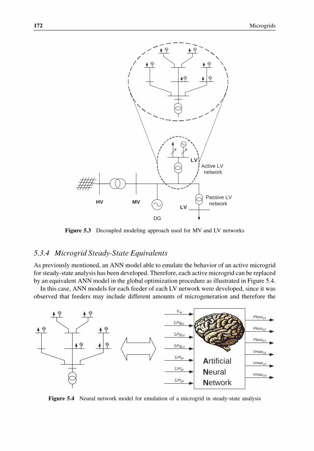
5.3.4 Microgrid Steady-State Equivalents

As previously mentioned, an ANN model able to emulate the behavior of an active microgrid

for steady-state analysis has been developed. Therefore, each activemicrogrid can be replaced

by an equivalent ANNmodel in the global optimization procedure as illustrated in Figure 5.4.

In this case, ANN models for each feeder of each LV network were developed, since it was

observed that feeders may include different amounts of microgeneration and therefore the

MVHV

Active LV network

DG

Passive LV network

LV

LV

Figure 5.3 Decoupled modeling approach used for MV and LV networks

Vsp

ΣPgp1

Plossp1

Vmaxp1

ΣPgp2

ΣPgp3

ΣPlp1

ΣPlp2

ΣPlp3

Artificial Neural Network

Plossp2

Plossp3

Vmaxp2

Vmaxp3

Figure 5.4 Neural network model for emulation of a microgrid in steady-state analysis

172 Microgrids

cause for an overvoltage may be originated from one single feeder with excessive micro-

generation integration.

In Figure 5.4

Vsp is the voltage at the MV/LV substation

SPgpi is the total active power generation in phase i

SPlpi is the total active power load in phase i

Plosspi is the total active power losses in phase i

Vmaxpi is the maximum voltage value in phase i

In order to generate the dataset corresponding to the inputs chosen to train the ANN, a large

number of three-phase power flows must be computed, considering different combinations of

the inputs (i.e. several values for the voltage reference at the MV/LV transformer, for the

power produced by each microgenerator and for the load), in order to calculate the active

power losses and assess the voltage profiles in each of these scenarios.

For this purpose, a three-phase power flow routine was developed in order to enable the

analysis of the steady-state behavior of LV networks, considering their specific character-

istics: phase imbalances due to the connection of single-phase loads and single-phase

microgeneration units exploiting different technologies.

The power flow solution method used is based on the one presented in [13] and is used for

three-phase, four-wire radial distribution networks relying on a backward–forward technique,

which is extremely fast to reach convergence.

From the tests that were performed, it was seen that the ANN with best performance was a

two-layer feed-forward ANN with sigmoid hidden neurons and linear output neurons. Still, it

must be pointed out that in case there is a change in topology of the “active” LV network, a

new ANNmust be computed. This means that it is necessary to update the data and generate a

new dataset, followed by a retraining of an updated ANN, which may be considered as a

drawback of this method.

In order to efficiently use the approach developed, it is necessary to automate the procedure

of retraining the ANNs. First of all, the main changes that trigger the need for retraining the

ANNs must be identified. These changes are mostly changes in the topology of the networks

due to the inclusion (or removal) of additional DGs, microgeneration units or loads, the set-up

(or upgrade) of a line or transformer and the expansion of the LV grid.

5.3.5 Development of the Tool

The algorithm developed for voltage control is designed to be used as an online function

available for the DSO. This algorithm is intended to be integrated as a software module that

will be housed in the CAMC.

Exploiting the communication infrastructure available in multi-microgrids, the CAMCwill

be able to collect critical information from the several devices in the network, namely data

from load and RES forecast modules and generation dispatch, in order to assess voltage

profiles, branch overload levels and active power losses. Using this information, the voltage

control algorithm is run and, after it has successfully terminated, produces a set of commands

in the form of setpoints. These commands are then sent to the several devices such as DG

units, microgeneration units (via the corresponding MGCC) and OLTC transformers. This


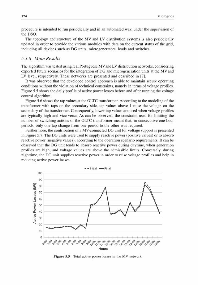
procedure is intended to run periodically and in an automated way, under the supervision of

the DSO.

The topology and structure of the MV and LV distribution systems is also periodically

updated in order to provide the various modules with data on the current status of the grid,

including all devices such as DG units, microgenerators, loads and switches.

5.3.6 Main Results

The algorithmwas tested using real PortugueseMVand LV distribution networks, considering

expected future scenarios for the integration of DG and microgeneration units at the MVand

LV level, respectively. These networks are presented and described in [7].

It was observed that the developed control approach is able to maintain secure operating

conditions without the violation of technical constraints, namely in terms of voltage profiles.

Figure 5.5 shows the daily profile of active power losses before and after running the voltage

control algorithm.

Figure 5.6 shows the tap values at the OLTC transformer. According to the modeling of the

transformer with taps on the secondary side, tap values above 1 raise the voltage on the

secondary of the transformer. Consequently, lower tap values are used when voltage profiles

are typically high and vice versa. As can be observed, the constraint used for limiting the

number of switching actions of the OLTC transformer meant that, in consecutive one-hour

periods, only one tap change from one period to the other was required.

Furthermore, the contribution of a MV-connected DG unit for voltage support is presented

in Figure 5.7. The DG units were used to supply reactive power (positive values) or to absorb

reactive power (negative values), according to the operation scenario requirements. It can be

observed that the DG unit tends to absorb reactive power during daytime, when generation

profiles are high, and voltage values are above the admissible limits. Conversely, during

nighttime, the DG unit supplies reactive power in order to raise voltage profiles and help in

reducing active power losses.

0

10

20

30

40

50

60

70

80

90

100

Act

ive

Po

wer

Lo

sses

(kW

)

Hours

Initial Final

0:00

1:00

2:00

3:00

4:00

5:00

6:00

7:00

8:00

9:00

10:0

011

:00

12:0

013

:00

14:0

015

:00

16:0

017

:00

18:0

019

:00

20:0

021

:00

22:0

023

:00

Figure 5.5 Total active power losses in the MV network

174 Microgrids

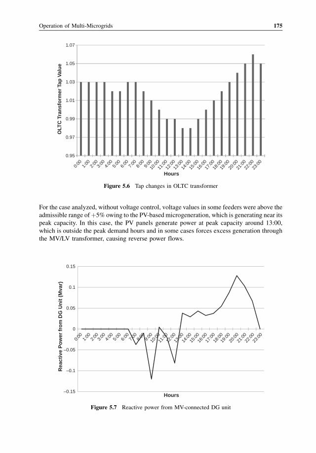
For the case analyzed, without voltage control, voltage values in some feeders were above the

admissible range ofþ5% owing to the PV-based microgeneration, which is generating near its

peak capacity. In this case, the PV panels generate power at peak capacity around 13:00,

which is outside the peak demand hours and in some cases forces excess generation through

the MV/LV transformer, causing reverse power flows.

0.95

0.97

0.99

1.01

1.03

1.05

1.07

OLT

C T

ran

sfo

rmer

Tap

Val

ue

Hours

0:00

1:00

2:00

3:00

4:00

5:00

6:00

7:00

8:00

9:00

10:0

011

:00

12:0

013

:00

14:0

015

:00

16:0

017

:00

18:0

019

:00

20:0

021

:00

22:0

023

:00

Figure 5.6 Tap changes in OLTC transformer

–0.15

–0.1

–0.05

0

0.05

0.1

0.15

Rea

ctiv

e P

ow

er fr

om

DG

Un

it (

Mva

r)

Hours

0:00

1:00

2:00

3:00

4:00

5:00

6:00

7:00

8:00

9:00

10:0

011

:00

12:0

013

:00

14:0

015

:00

16:0

017

:00

18:0

019

:00

20:0

021

:00

22:0

023

:00

Figure 5.7 Reactive power from MV-connected DG unit


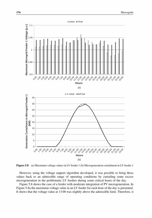
However, using the voltage support algorithm developed, it was possible to bring these

values back to an admissible range of operating conditions by curtailing some excess

microgeneration in the problematic LV feeders during some critical hours of the day.

Figure 5.8 shows the case of a feeder with moderate integration of PV microgeneration. In

Figure 5.8a the maximum voltage value in an LV feeder for each hour of the day is presented.

It shows that the voltage value at 13:00 was slightly above the admissible limit. Therefore, it

0.9

0.95

1

1.05

1.1M

axim

um

Mic

rog

rid

Fee

der

1 V

olt

age

(p.u

.)

Hours

Initial Final

(a)

(b)

0

5

10

15

20

25

30

35

40

Gen

erat

ion

Cu

rtai

lmen

t in

Mic

rog

rid

Fee

der

1

(kW

)

Hours

Initial Final

0:00

1:00

2:00

3:00

4:00

5:00

6:00

7:00

8:00

9:00

10:0

011

:00

12:0

013

:00

14:0

015

:00

16:0

017

:00

18:0

019

:00

20:0

021

:00

22:0

023

:00

0:00

1:00

2:00

3:00

4:00

5:00

6:00

7:00

8:00

9:00

10:0

011

:00

12:0

013

:00

14:0

015

:00

16:0

017

:00

18:0

019

:00

20:0

021

:00

22:0

023

:00

Figure 5.8 (a) Maximum voltage values in LV feeder 1 (b) Microgeneration curtailment in LV feeder 1

176 Microgrids

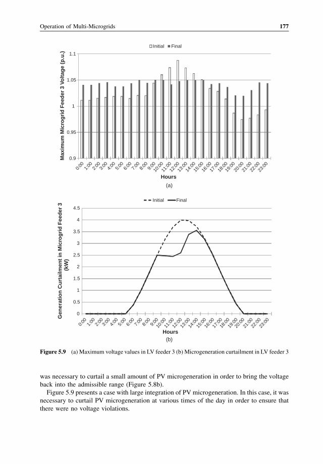
was necessary to curtail a small amount of PV microgeneration in order to bring the voltage

back into the admissible range (Figure 5.8b).

Figure 5.9 presents a case with large integration of PV microgeneration. In this case, it was

necessary to curtail PV microgeneration at various times of the day in order to ensure that

there were no voltage violations.

0.9

0.95

1

1.05

1.1

Max

imu

m M

icro

gri

d F

eed

er 3

Vo

ltag

e (p

.u.)

Hours

Initial Final

(a)

(b)

0

0.5

1

1.5

2

2.5

3

3.5

4

4.5

Gen

erat

ion

Cu

rtai

lmen

t in

Mic

rog

rid

Fee

der

3

(kW

)

Hours

Initial Final

0:00

1:00

2:00

3:00

4:00

5:00

6:00

7:00

8:00

9:00

10:0

011

:00

12:0

013

:00

14:0

015

:00

16:0

017

:00

18:0

019

:00

20:0

021

:00

22:0

023

:00

0:00

1:00

2:00

3:00

4:00

5:00

6:00

7:00

8:00

9:00

10:0

011

:00

12:0

013

:00

14:0

015

:00

16:0

017

:00

18:0

019

:00

20:0

021

:00

22:0

023

:00

Figure 5.9 (a) Maximum voltage values in LV feeder 3 (b) Microgeneration curtailment in LV feeder 3


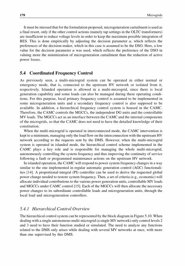
It must be stressed that for the formulation proposed, microgeneration curtailment is used as

a final resort, only if the other control actions (namely tap settings in the OLTC transformers)

are insufficient to reduce voltage levels in order to keep the maximum possible integration of

RES. This is done empirically by adjusting the decision parameter a, which reflects the

preferences of the decision-maker, which in this case is assumed to be the DSO. Here, a low

value for the decision parameter a was used, which reflects the preference of the DSO in

valuing more the minimization of microgeneration curtailment than the reduction of active

power losses.

5.4 Coordinated Frequency Control

As previously seen, a multi-microgrid system can be operated in either normal or

emergency mode, that is, connected to the upstream HV network or isolated from it,

respectively. Islanded operation is allowed in a multi-microgrid, since there is local

generation capability and some loads can also be managed during these operating condi-

tions. For this purpose, local primary frequency control is assumed to be implemented in

some microgeneration units and a secondary frequency control is also supposed to be

available. In addition, a hierarchical frequency control system is housed in the CAMC.

Therefore, the CAMC controls the MGCCs, the independent DG units and the controllable

MV loads. The MGCCs act as an interface between the CAMC and the internal components

of the microgrids, so that the CAMC does not need to have the detailed knowledge of their

constitution.

When the multi-microgrid is operated in interconnected mode, the CAMC intervention is

kept to a minimum, managing only the load flow on the interconnection with the upstream HV

network according to the requests sent by the DMS. However, when the multi-microgrid

system is operated in islanded mode, the hierarchical control scheme implemented in the

CAMC plays a key role and is responsible for managing the whole multi-microgrid,

autonomously controlling the system frequency and thus improving the continuity of service

following a fault or programmed maintenance actions on the upstream HV network.

In islanded operation, the CAMCwill respond to power system frequency changes in a way

similar to the one implemented in regular automatic generation control (AGC) functionali-

ties [14]. A proportional-integral (PI) controller can be used to derive the requested global

power change needed to restore system frequency. Then, a set of criteria (e.g., economic) will

allocate individual contributions to the various power generation units, controllable MV loads

and MGCCs under CAMC control [15]. Each of the MGCCs will then allocate the necessary

power changes to its subordinate controllable loads and microgeneration units, through the

local load and microgeneration controllers.

5.4.1 Hierarchical Control Overview

The hierarchical control system can be represented by the block diagram in Figure 5.10. When

dealing with a single autonomous multi-microgrid (a singleMV network) only control levels 2

and 3 need to have their function studied or simulated. The need to analyze any functions

related to the DMS only arises while dealing with several MV networks at once, with more

than one supervised by this DMS.

178 Microgrids

5.4.1.1 Control Level 2 – CAMC

As mentioned earlier, the commands needed to modify power generation and loads originate

in the CAMC. These commands are sent to MGCCs, to local DG units and also to controllable

MV loads. MGCCs act as an interface between the CAMC and the internal active components

of the microgrids, so that the CAMC doesn’t need to have the details of each microgrid’s

constitution.

While the MV multi-microgrid is connected to the upstream HV network, the CAMC

limits its autonomous intervention to a minimum. However, in islanded operation, the

CAMC will step in and respond to power system frequency changes in a way similar to that

implemented in regular AGC functionalities. A PI controller is then used to derive the

requested global power change needed to restore system frequency. Then, an economic

allocation algorithm will allocate contributions for this power change to the various power

generation units, controllable MV loads and MGCCs under CAMC control, but only if they

are willing, at that point in time, to participate in frequency regulation. Instead of strictly

economic criteria, it is of course possible to use another different criterion or combination

of criteria.

DMS

CAMC

MCOLTCSVC Load LC

MGCC

DG

Control Level 1

Control Level 2

Control Level 3

Figure 5.10 Hierarchical control scheme of a multi-microgrid system


It should be noted that the CAMC will only act if strictly required, and will not try to

globally change setpoints in order to achieve a near optimum point of operation of the whole

multi-microgrid. This justifies the choice of using power setpoint variations and not absolute

power setpoints. Using power setpoint variations provides a simple way to have a higher-order

control system, either automatic or manual, that would independently adjust microsource or

DG output to setpoints other than the system optimal ones. One example of this “control

system” could be the microsource individual owners who would adjust microturbines, for

instance, according to their heating needs.

5.4.1.2 Control Level 3 – MGCC

Each of the MGCCs will also allocate the necessary power changes to its subordinate

controllable loads and microgeneration units, through the load controllers (LC) and micro-

source controllers (MC). Some of these microsources do not usually have full regulation

capabilities and will not normally be asked to change power generation. This can be the case

for both PV and wind generation, due to limitations in primary resource availability. In this

case, however, it is possible to consider that generation can be curtailed in case of an excess

power imbalance.

5.4.1.3 Load-Shedding

The approach adopted for load-shedding, in the context of this hierarchical control system, is

fairly different from the one used in conventional systems, because the hierarchical control

system which supervises the controllable loads isn’t capable of acting in near instantaneous

time frames (mainly owing to communication system limitations). Therefore, in these

circumstances, load-shedding is not expected to reduce the amplitude of the frequency

excursions in the few seconds following a disturbance. It should be seen more as a kind of

secondary reserve – rather than an emergency resource – helping the frequency to return to the

rated value faster or without depending so much on the availability of renewable resources or

other generation systems.

The main difference that distinguishes microsources from controllable loads is that it is not

feasible to keep loads disconnected indefinitely (except for this detail, loads could be regarded

simply as negative generation). It is thus mandatory to reconnect as much load as possible

after the system returns to a near normal frequency value. This is accomplished through the

use of a control loop that runs on a larger timescale, reconnecting loads after the system has

been running at a near steady-state condition for a predefined period of time.

Starting from the assumption that the system – after some time of running stable and near

the rated frequency – is capable of supporting the connection of further loads, the control

systems starts to reconnect the most expensive/important ones first. This is done step by step,

always ensuring that there is enough available reserve on the multi-microgrid in order not to

unnecessarily compromise the system’s stability. Before each new reconnection, the control

system waits for the frequency to stabilize.

5.4.1.4 Energy Storage Systems

A cluster of several storage devices (e.g. flywheels and batteries) could, if integrated into the

hierarchical control system, efficiently establish a storage reserve that would be of great help

180 Microgrids

to the islanded operation of the network at both the microgrid and the multi-microgrid level.

Also, we are assuming that most of these storage devices have interface inverters of the

voltage source inverter (VSI) type, which can have their output power controlled on the basis

of frequency droop.

Therefore, these storage devices can help in two possible ways: (a) they can act

autonomously, with their output power PVSI responding to system frequency changes,

providing energy used to initially balance the system using a proportional control element

as described next or (b) they can receive setpoints controlled from a central location, in a

hierarchical way.

PVSI ¼ KP � f rated � fð Þ

These two control methods are not mutually exclusive: while an autonomous response will

undoubtedly improve the system’s response to the initial frequency deviations following a

disturbance, the hierarchical system can take over after that initial response and reallocate

each source and storage element contribution according to some predefined criteria. This two-

step approach can be justified by the intrinsically slow nature of the hierarchical control

system, which suggests that grid-connected storage devices under hierarchical control should

be regarded as a secondary reserve while, at the same time, they should be capable of acting

autonomously in order to be able to limit initial frequency excursions.

5.4.2 Hierarchical Control Details

In this approach, the system’s frequency is continuously monitored by the CAMC

(Figure 5.11). Every time interval Ts (sample time), if triggered by significant changes

in frequency, the CAMC will send control setpoints to every MGCC, other DG units and

controllable loads. This sample time Ts cannot be very small, mainly because of the

constraints imposed by the communication system on which this control system depends.

Therefore, the frequency error and the frequency error integral will be used to determine the

additional power DP to be requested to the available contributors under CAMC control:

MGCCs, DG units and controllable loads. This approach effectively implements a kind of PI

controller.

DP ¼ KP þ KI

1

s

� �

� f rated � fð Þ (5.8)

It should be noted that this additional power can have negative values if the frequency rises

above its rated value. In this way, the CAMC can also respond to other disturbances, such as

load loss while in islanded mode, instructing the distributed generation to reduce power output

(including microgeneration curtailment, if necessary), eventually reconnecting some loads

still disconnected at the moment.

If the required power variation DP is larger than a predefined threshold (related to a

deadband), the control systemwill proceed to determine how to optimally distribute the power

requests through the available sources. Unitary generation costs for each of the sources

(MGCCs and other DG units) can be used for this purpose.


The optimization can be based on standard linear optimization techniques:

subject to

minx z ¼ cTxP

x ¼ DP

x � b1

x � b2

Where the vectors represent

c generation cost and load curtailment prices

x generation or load setpoint variations

b1 smallest variations allowed (lower bounds)

b2 largest variations allowed (upper bounds).

Read system frequency error and integral of frequency error

ΔP > ΔP min?

Determine ΔP

Run optimization algorithm to allocate setpoints to MGCCs, independent

DGs and controllable loads

Yes

No

Send setpoints to MGCC controlled microsources and loads

Run optimization algorithm (once for each MGCC) to allocate setpoints to microsources

and loads controlled by the MGCCs

Send setpoints only to larger DGs and controllable loads

Figure 5.11 Implementation flowchart

(5.9)

(5.10)

(5.11)

(5.12)

182 Microgrids

The set of restrictions can also define which generators/loads participate in frequency

regulation. This can be done by setting to zero the ith elements of both b1 and b2,

corresponding to units that cannot be adjusted.

Because loads are considered as negative generation, the corresponding coefficients

(elements in vector c of prices) are negative.

In order to avoid globally changing setpoints (e.g. decreasing production from expensive

microsources and replacing them with less expensive ones), it is necessary to adjust the lower

and upper bounds in the optimization procedure according to the DP value:

DP > 0 ) b1 ¼ 0

DP < 0 ) b2 ¼ 0

�

(5.13)

The enforcement of the above described conditions ensures that no microsource will

decrease its production, so that another one can increase it (i.e. there will not be any

unsolicited power transfers between microsources).

This optimization is performed each sample period Ts and will originate a vector

representing the power generation changes to be requested from microgrids (MGCCs),

independent DG units (e.g. combined heat and power – CHP) and loads (MV load-shedding

operations).

Each MGCC will now use the power change requested by the CAMC to establish the main

restriction of a new optimization procedure, which could be identical to the one used before by

the CAMC. This optimization will now help determine the power changes to be requested

from microsources and controllable loads under MGCC control, thus one level below in the

hierarchical control structure.

5.4.3 Main Results

Using the described coordinated frequency control methods, the system is able to handle

severe network disturbances such as islanding events. It can also perform load-following by

scheduling power generation among generation units and microgrids under its control. A

dynamic simulation platformwas developed for evaluation purposes and includes an extended

version of the multi-microgrid test network shown in Figure 5.12 [16].

Figure 5.13 illustrates the frequency control approach described, by showing the response

of the hierarchical control system to a sudden islanding and also to gradual load changes in

islanded mode. In this test case, the MV multi-microgrid network has a total load of 19.9MW

and is importing approximately 5.3MW of active power from the upstream HV network.

The test disturbances include the disconnection of the HV/MV branch, effectively islanding

the multi-microgrid system, and also a load change at several nodes at a rate of 4% per second

for 10 s (for total increase of nearly 0.9MW). These disturbances are also pictured in

Figure 5.13.

The results show how the hierarchical control adopted in this multi-microgrid manages to

recover the frequency to the rated value after islanding. Although the minimum frequency

value after the disturbance remains practically unaltered, in the moments that follow, the

system evolves in a much better way.

The success of the frequency recovery is in part due to the fact that the CAMC is sending

setpoints to the microgrids and other DG units dispersed on the MV network. The


microsources inside the microgrids are also subject to setpoint attribution according to a

similar price-dependent optimization algorithm. Figure 5.14 shows the microgrid setpoint

modifications and how they are directly translated into individual setpoints for each of the

microsources within that same microgrid.

When the multi-microgrid system does not have sufficient reserves to respond to a large

loss of imported power, load curtailment may be required. This control system is designed to

support these actions as well, as demonstrated in Figure 5.15.

The hierarchical control algorithm is thus capable of acting on controllable loads,

integrating them into the optimization process. The expected benefits include the increase

in system response speed (Figure 5.15), while still complying with the optimization rules

in use.

VSIDiesel

CHP2

MicroGrid

Hydro

DFIM

CHP

CH

P1

Hydro

Hydro

DFIM2

MicroGrid

MicroGrid

MicroGridMicroGrid

MicroGrid

MicroGrid

MicroGrid NMVR13ABus

NMVBus

FeederA 1

HV Network

Figure 5.12 Multi-microgrid extended test network

0 20 40 60 80 100 120 140 160 1800

0.2

0.4

0.6

0.8

1

Time (s)

Pow

er (M

W)

HV Imported Power (1:5 scale)Load Change (NLV11A, NLV18A)Load Change (NLV1A, NLV6A)

0 20 40 60 80 100 120 140 160 18048.6

48.8

49

49.2

49.4

49.6

49.8

50

50.2

Time (s)

Freq

uenc

y (H

z)

With Hierarchical ControlWithout Hierarchical Control

Figure 5.13 Test disturbances and frequency behavior with and without secondary control

184 Microgrids

Loads are disconnected according to their “cost” or importance. Figure 5.15 (right)

illustrates how load-curtailment occurs, showing two of the larger loads, but considered

less important. These loads begin to be curtailed soon after the main disturbance (islanding).

On the other hand, more expensive/important loads would begin to be disconnected later, after

all the less expensive ones have attained their minimum values.

As mentioned, the test network contains several VSI devices coupled to storage elements.

The output of VSI is based on the frequency error through the use of a proportional controller.

Figure 5.16 illustrates VSI influence on the frequency variation of the sample test system,

together with an example of the power output of a large VSI (connected at the MV level) and

one of the microgrids’ VSIs. All the previously shown simulation results benefit from the

usage of the storage elements as active and autonomous participants in frequency regulation.

It should be noted that the VSIs are also programmed to emulate the behavior of unregulated

synchronous machines, which may mask the influence of the proportional controllers during

the initial phase of heavier disturbances.

These examples show how the setpoint modification commands sent to DG units, micro-

grids and controllable loads enable the frequency to return to the rated value in a reasonable

amount of time. In addition, the control system can resort to load-shedding, in order to better

support the transition to islanded operation in scenarios of low multi-microgrid power

0 20 40 60 80 100 120 140 160 180–0.1

–0.05

0

0.05

0.1

0.15

0.2

Time (s)

Pow

er (M

W)

MicroGrid SetpointMicroGrid Output Power

0 20 40 60 80 100 120 140 160 1800.2

0.4

0.6

0.8

1

1.2

Time (s)

Pow

er (p

u)

Fuel Cell & Microturbine SetpointsFuel Cell Output PowerMicroturbine Output Power

Figure 5.14 Example microgrid external and internal setpoint commands and output power

0 20 40 60 80 10048.6

48.8

49

49.2

49.4

49.6

49.8

50

50.2

Time (s)

Freq

uenc

y (H

z)

Without Centralized Load SheddingWith Centralized Load Shedding

0 20 40 60 80 100 120 140 160 1800

0.2

0.4

0.6

0.8

1

Time (s)

Pow

er (M

W)

NMVCHP LoadNMVCHPA2 Load

Figure 5.15 Influence of load shedding and shedding steps during islanding


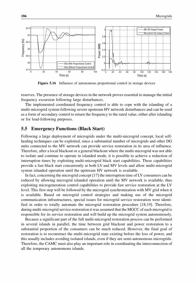
reserves. The presence of storage devices in the network proves essential to manage the initial

frequency excursion following large disturbances.

The implemented coordinated frequency control is able to cope with the islanding of a

multi-microgrid system following severe upstream HV network disturbances and can be used

as a form of secondary control to return the frequency to the rated value, either after islanding

or for load-following purposes.

5.5 Emergency Functions (Black Start)

Following a large deployment of microgrids under the multi-microgrid concept, local self-

healing techniques can be exploited, since a substantial number of microgrids and other DG

units connected to the MV network can provide service restoration in its area of influence.

Therefore, after a local blackout or a general blackout where the multi-microgrid was not able

to isolate and continue to operate in islanded mode, it is possible to achieve a reduction of

interruption times by exploiting multi-microgrid black start capabilities. These capabilities

provide a fast black start concurrently at both LV and MV levels and allow multi-microgrid

system islanded operation until the upstream HV network is available.

In fact, concerning the microgrid concept [17] the interruption time of LV consumers can be

reduced by allowing microgrid islanded operation until the MV network is available, thus

exploiting microgeneration control capabilities to provide fast service restoration at the LV

level. This first step will be followed by the microgrid synchronization with MV grid when it

is available. Based on microgrid control strategies and making use of the microgrid

communication infrastructures, special issues for microgrid service restoration were identi-

fied in order to totally automate the microgrid restoration procedure [18,19]. Therefore,

during multi-microgrid service restoration it was assumed that theMGCC of each microgrid is

responsible for its service restoration and will build up the microgrid system autonomously.

Because a significant part of the full multi-microgrid restoration process can be performed

in several islands in parallel, the time between grid blackout and power restoration to a

substantial proportion of the consumers can be much reduced. However, the final goal of

restoration is to reconstruct the multi-microgrid state existing before the loss of power, and

this usually includes avoiding isolated islands, even if they are semi-autonomous microgrids.

Therefore, the CAMC must also play an important role in coordinating the interconnection of

all the temporary autonomous islands.

0 20 40 60 80 10047.5

48

48.5

49

49.5

50

50.5

Time (s)

Freq

uenc

y (H

z)

Pow

er (M

M)

VSIs With Proportional ControlVSIs Without Proportional Control

0 20 40 60 80 100 120 140 160 180–0.2

0

0.2

0.4

0.6

0.8

1

Time (s)

MV VSI Output PowerMicroGrid VSI Output Power

Figure 5.16 Influence of autonomous proportional control in storage devices

186 Microgrids

In a multi-microgrid, the rules required to accomplish a successful restoration can be more

general than those that can be adopted in a HV/VHV network. This fact is almost unavoidable

because MV networks can be extremely diverse as regards network characteristics and types

of energy sources, power electronics interfaces and loads. Therefore, it can become difficult to

find a very specific set of rules that fits every network and every operation point of a network.

The black start software module to be implemented on the CAMC is responsible for

managing this set of rules and conditions to be checked during restoration. These rules and

conditions define a sequence of control actions to be carried out during multi-microgrid

restoration and must be coordinated and planned beforehand. For this purpose, a sequence of

control actions can be identified and evaluated through numerical simulation. The proposed

sequence of control actions, to be stored at the CAMC level, allows the definition of a

procedure that aims at the full automation of the entire multi-microgrid service restoration

procedure and subsequent synchronization with the upstream HV system.

5.5.1 Restoration Guidelines

Multi-microgrid restoration will be triggered if a general or local blackout occurs or if major

disturbances affecting the HV upstream system do not allow the multi-microgrid to be

supplied from the HV side after a predefined time interval. The CAMC should then be able to

receive information from the DMS about the service restoration status at the HV level in order

to decide about launching a black start procedure. In addition, the CAMC will guide multi-

microgrid service restoration, based on information about the last multi-microgrid load and

generation scenarios. This information is kept in a maintained database together with the

information about restart availability of DG units connected to the MV network and is used to

further adjust and refine the sequence of control actions, mostly identified in advance and

embedded into the CAMC software, which will finally lead the system to a state similar to the

pre-fault scenario.

The CAMC is also used for secondary frequency control during load-following conditions

when the multi-microgrid is operated in islanded mode, as presented in Section 5.4. In order to

balance generation and load, the CAMC generates setpoints based on system frequency

changes and sends them to the MGCC and to controllable DG units. In turn, the MGCCs will

act as intermediate controllers between the CAMC and the microgrid internal controllers.

MGCCs are responsible for scheduling the corresponding power change among the micro-

generation units by sending setpoints to the corresponding controllers.

The MGCC is also responsible for guiding the microgrid black start procedure, and so it is

assumed that microgrid service restoration is carried out autonomously when the microgrid is

operated in islanded mode until the MV network is available. As several islands will be

formed during the early stages of the multi-microgrid black start procedure, it is also assumed

that the automatic secondary frequency control system embedded into the CAMC software is

initially turned off. This allows a simpler coordination of the restoration procedure, while

ensuring that no contradictory commands ever arise.

Thus, the information exchange between the CAMC and local controllers during the multi-

microgrid black start procedure will mainly involve switching orders. The purpose of these

commands is to rebuild the MV network and also to connect DG units, microgrids and MV

loads, according to general monitoring information (e.g. voltage levels, system frequency and

grid status). All this information is received and processed by the CAMC through the


communication infrastructure that is supposed to be available. Verification of synchronization

conditions is performed locally.

Another basic requirement is the availability of DG units connected to theMV network with

black start capability. Its restart procedure is carried out prior to network energization, so it is

not reflected in the MV network. The same happens with the several microgrids with black

start capability.

Furthermore, it is also assumed that it is possible to prepare the network for energization. To

accomplish this, after system collapse, the following requirements should be taken into

account:

� the multi-microgrid is disconnected from the upstream HV network,� multi-microgrid feeders are fully sectionalized,� microgrids are disconnected from the MV network,� DG units and loads are disconnected from the MV network,� the HV/MV transformer is disconnected from the HV and MV networks,� all MV/LV transformers are disconnected from the MV and LV networks,� all the reactive power sources, such as shunt capacitor banks, are switched off.

From this starting point, the multi-microgrid restoration procedure is carried out with the

aim of supplying consumers as soon as possible, while satisfying the system operation

conditions. So, after a general blackout, the CAMCwill perform service restoration in a multi-

microgrid based on information stored in a database about the last multi-microgrid load

scenario, as described before, by performing the following generic sequence of actions (the

first two steps include the actions described in the previous paragraph):

1. disconnecting all loads, sectionalize the corresponding MV/LV transformers and switch-

ing off the reactive power sources – after a general blackout all the loads, transformers

and shunt capacitor banks should be disconnected in order to avoid large frequency and

voltage deviations when energizing the MV network.

2. sectionalizing the multi-microgrid around each microgrid and around each DG unit with

black start capability – this leads to the creation of small islands inside the multi-

microgrid, since after their autonomous black start, microgrids keep operating in islanded

mode feeding some amount or its own entire load. Other higher powered generators may

be also supplying their protected loads (e.g. some diesel groups and CHP units). These

islands will all be later synchronized together.

3. building the MV network – a diesel group or other black start capable generator (most

probably a synchronous machine) is used to energize the initial part of the MV

network, which comprises some unloaded transformers downstream and some paths

that allow the synchronization of other units feeding their own loads (e.g. CHP

islands) or feeding important loads. The energization of the initial part of the MV

network is carried out step by step in order to avoid large voltage and frequency

deviations.

4. synchronization of islands with the MV network – each one of the existing islands can

now be synchronized with the MV network when the corresponding path is energized, in

order to strengthen the multi-microgrid system. The synchronization conditions (phase

sequence, frequency and voltage difference) should be verified in order to avoid large

188 Microgrids

transient currents. As most of the microgrids are capable of autonomous black start – even

if in limited operating conditions – they may not need to be connected at this point.

5. connection of a certain amount of important load – connection of important loads is

performed if the DG units connected to the MV network are capable of supplying these

loads. The amount of power to be connected should take into account the generation

capacity in order to avoid large frequency and voltage deviations during load connection.

6. energization of the remainingMV branches and the MV/LV transformers upstream of the

microgrid – at this stage the islands containing isolated DG units are already synchro-

nized and the multi-microgrid is strong enough to energize the remaining branches of the

MV network. However, as the multi-microgrid comprises a large number of MV/LV

unloaded transformers, their energization should be carried out in several steps in order to

avoid large inrush currents. Thus, the MV/LV transformers upstream of the several

microgrids are energized first, in order to allow for the microgrid synchronization with the

MV network.

7. synchronization of microgrids with the MV network – microgrids operated in islanded

mode can then be synchronized with the MV network. For this purpose the synchroniza-

tion conditions should be verified.

8. energization of the remaining MV/LV transformers – in order to be possible to

completely restore the load, all the MV/LV unloaded transformers should be energized.

They are divided into several groups which are energized at different times in order to

avoid large inrush currents. Afterwards the MV/LV transformers upstream of the

uncontrollable DG units are also energized.

9. load restoration – at this stage the MV network is fully energized and some loads can be

connected depending on the generation capacity.

10. connection of uncontrollable DG units connected to the MV network – at this stage it is

supposed that multi-microgrid becomes sufficiently strong to smooth voltage and

frequency variations due to power fluctuations in non-controllable DG units, allowing

their connection to the MV network. MV paths are also created, so that DG units without

black start capability can absorb power from the grid in order to restart.

11. load increase – in order to feed as much load as possible, other loads can then be

connected.

12. activation of the automatic frequency control – the automatic frequency control is now

activated in order to ensure that the multi-microgrid system frequency is near its nominal

value while the multi-microgrid is operated in islanded mode.

13. multi-microgrid reconnection to the upstream HV network when it becomes available –

the synchronization conditions should be verified again, after the synchronization order is

given by the CAMC. The HV/MV transformer should be previously energized from the

HV side and the synchronization is performed through MV switches.

The technical feasibility of the proposed sequence of control actions, which allows multi-

microgrid service restoration was evaluated using the test network presented in Figure 5.12.

5.5.2 Sample Restoration Procedure

The feasibility of the proposed sequence of actions to carry out multi-microgrid service

restoration is demonstrated in this section through numerical simulations.


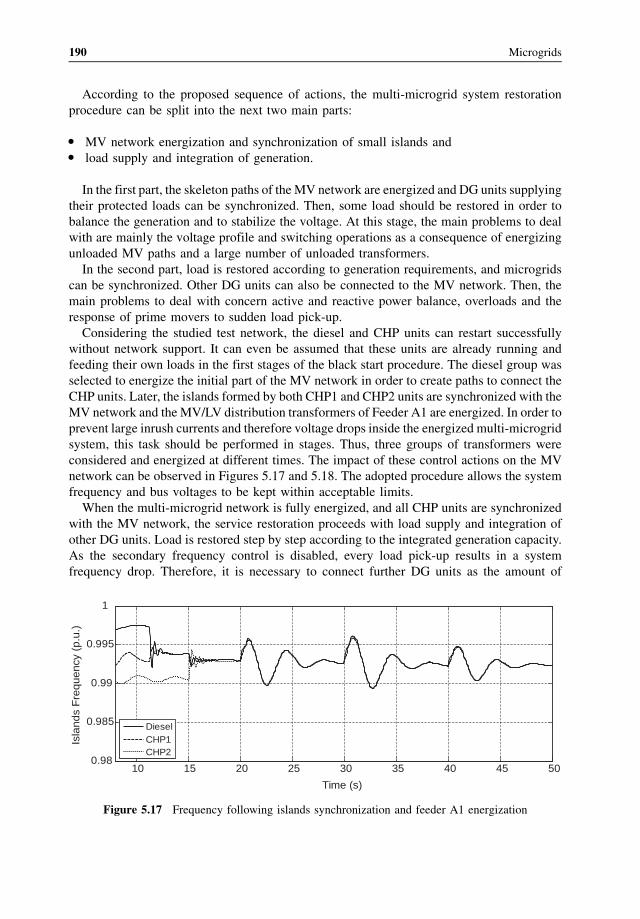
According to the proposed sequence of actions, the multi-microgrid system restoration

procedure can be split into the next two main parts:

� MV network energization and synchronization of small islands and� load supply and integration of generation.

In the first part, the skeleton paths of the MV network are energized and DG units supplying

their protected loads can be synchronized. Then, some load should be restored in order to

balance the generation and to stabilize the voltage. At this stage, the main problems to deal

with are mainly the voltage profile and switching operations as a consequence of energizing

unloaded MV paths and a large number of unloaded transformers.

In the second part, load is restored according to generation requirements, and microgrids

can be synchronized. Other DG units can also be connected to the MV network. Then, the

main problems to deal with concern active and reactive power balance, overloads and the

response of prime movers to sudden load pick-up.

Considering the studied test network, the diesel and CHP units can restart successfully

without network support. It can even be assumed that these units are already running and

feeding their own loads in the first stages of the black start procedure. The diesel group was

selected to energize the initial part of the MV network in order to create paths to connect the

CHP units. Later, the islands formed by both CHP1 and CHP2 units are synchronized with the

MV network and the MV/LV distribution transformers of Feeder A1 are energized. In order to

prevent large inrush currents and therefore voltage drops inside the energized multi-microgrid

system, this task should be performed in stages. Thus, three groups of transformers were

considered and energized at different times. The impact of these control actions on the MV

network can be observed in Figures 5.17 and 5.18. The adopted procedure allows the system

frequency and bus voltages to be kept within acceptable limits.

When the multi-microgrid network is fully energized, and all CHP units are synchronized

with the MV network, the service restoration proceeds with load supply and integration of

other DG units. Load is restored step by step according to the integrated generation capacity.

As the secondary frequency control is disabled, every load pick-up results in a system

frequency drop. Therefore, it is necessary to connect further DG units as the amount of

10 15 20 25 30 35 40 45 500.98

0.985

0.99

0.995

1

Time (s)

Isla

nds

Fre

quen

cy (

p.u.

)

DieselCHP1CHP2

Figure 5.17 Frequency following islands synchronization and feeder A1 energization

190 Microgrids

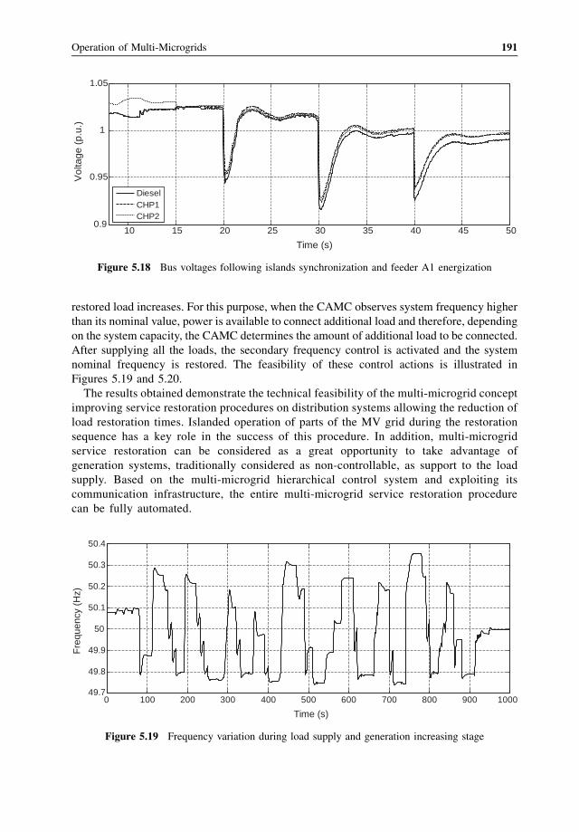
restored load increases. For this purpose, when the CAMC observes system frequency higher

than its nominal value, power is available to connect additional load and therefore, depending

on the system capacity, the CAMC determines the amount of additional load to be connected.

After supplying all the loads, the secondary frequency control is activated and the system

nominal frequency is restored. The feasibility of these control actions is illustrated in

Figures 5.19 and 5.20.

The results obtained demonstrate the technical feasibility of the multi-microgrid concept

improving service restoration procedures on distribution systems allowing the reduction of

load restoration times. Islanded operation of parts of the MV grid during the restoration

sequence has a key role in the success of this procedure. In addition, multi-microgrid

service restoration can be considered as a great opportunity to take advantage of

generation systems, traditionally considered as non-controllable, as support to the load

supply. Based on the multi-microgrid hierarchical control system and exploiting its

communication infrastructure, the entire multi-microgrid service restoration procedure

can be fully automated.

10 15 20 25 30 35 40 45 500.9

0.95

1

1.05

Time (s)

Vol

tage

(p.

u.)

DieselCHP1CHP2

Figure 5.18 Bus voltages following islands synchronization and feeder A1 energization

0 100 200 300 400 500 600 700 800 900 100049.7

49.8

49.9

50

50.1

50.2

50.3

50.4

Time (s)

Fre

quen

cy (

Hz)

Figure 5.19 Frequency variation during load supply and generation increasing stage


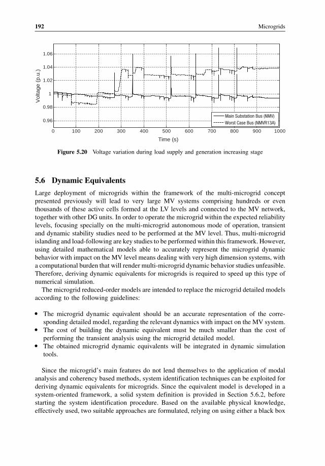
5.6 Dynamic Equivalents

Large deployment of microgrids within the framework of the multi-microgrid concept

presented previously will lead to very large MV systems comprising hundreds or even

thousands of these active cells formed at the LV levels and connected to the MV network,

together with other DG units. In order to operate the microgrid within the expected reliability

levels, focusing specially on the multi-microgrid autonomous mode of operation, transient

and dynamic stability studies need to be performed at the MV level. Thus, multi-microgrid

islanding and load-following are key studies to be performed within this framework. However,

using detailed mathematical models able to accurately represent the microgrid dynamic

behavior with impact on the MV level means dealing with very high dimension systems, with

a computational burden that will render multi-microgrid dynamic behavior studies unfeasible.

Therefore, deriving dynamic equivalents for microgrids is required to speed up this type of

numerical simulation.

The microgrid reduced-order models are intended to replace the microgrid detailed models

according to the following guidelines:

� The microgrid dynamic equivalent should be an accurate representation of the corre-

sponding detailed model, regarding the relevant dynamics with impact on the MV system.� The cost of building the dynamic equivalent must be much smaller than the cost of

performing the transient analysis using the microgrid detailed model.� The obtained microgrid dynamic equivalents will be integrated in dynamic simulation

tools.

Since the microgrid’s main features do not lend themselves to the application of modal

analysis and coherency based methods, system identification techniques can be exploited for

deriving dynamic equivalents for microgrids. Since the equivalent model is developed in a

system-oriented framework, a solid system definition is provided in Section 5.6.2, before

starting the system identification procedure. Based on the available physical knowledge,

effectively used, two suitable approaches are formulated, relying on using either a black box

0 100 200 300 400 500 600 700 800 900 1000

0.96

0.98

1

1.02

1.04

1.06

Time (s)

Vol

tage

(p.

u.)

Main Substation Bus (NMV)Worst Case Bus (NMVR13A)

Figure 5.20 Voltage variation during load supply and generation increasing stage

192 Microgrids

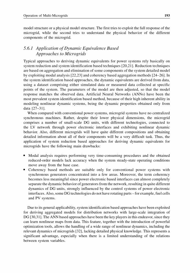
model structure or a physical model structure. The first tries to exploit the full response of the

microgrid, while the second tries to understand the physical behavior of the different

components of the microgrid.

5.6.1 Application of Dynamic Equivalence BasedApproaches to Microgrids

Typical approaches to deriving dynamic equivalents for power systems rely basically on

system reduction and system identification based techniques [20,21]. Reduction techniques

are based on aggregation and elimination of some components of the system detailed model

by exploiting modal analysis [22,23] and coherency based aggregation methods [24–26]. In

the system identification based approaches, the dynamic equivalents are derived from data,

using a dataset comprising either simulated data or measured data collected at specific

points of the system. The parameters of the model are then adjusted, so that the model

response matches the observed data. Artificial Neural Networks (ANNs) have been the

most prevalent system identification based method, because of their high inherent ability in

modeling nonlinear dynamic systems, being the dynamic properties obtained only from

data [27–31].

When compared with conventional power systems, microgrid systems have no centralized

synchronous machines. Rather, despite their lower physical dimensions, the microgrid

comprises a number of small-scale DG units, with different technologies, connected to

the LV network through power electronic interfaces and exhibiting nonlinear dynamic

behavior. Also, different microgrids will have quite different compositions and obtaining

detailed information about all of their components will be a very difficult task. Thus, the

application of system reduction based approaches for deriving dynamic equivalents for

microgrids have the following main drawbacks:

� Modal analysis requires performing very time-consuming procedures and the obtained

reduced-order models lack accuracy when the system steady-state operating conditions

move away from the base case.� Coherency based methods are suitable only for conventional power systems with

synchronous generators concentrated into a few areas. Moreover, the term coherency

becomes less meaningful since power electronic based interfaces can almost completely

separate the dynamic behavior of generators from the network, resulting in quite different

dynamics of DG units, strongly influenced by the control systems of power electronic

interfaces. Also, someDG technologies do not have rotating parts – for example, fuel cells

and PV systems.

Due to its general applicability, system identification based approaches have been exploited

for deriving aggregated models for distribution networks with large-scale integration of

DG [30,31]. The ANN based approaches have been the key players in this endeavor, since they

can learn nonlinear maps from data. This feature, together with the introduction of powerful

optimization tools, allows the handling of a wide range of nonlinear dynamics, including the

relevant dynamics of microgrids [32], lacking detailed physical knowledge. This represents a

significant advantage, especially when there is a limited understanding of the relations

between system variables.


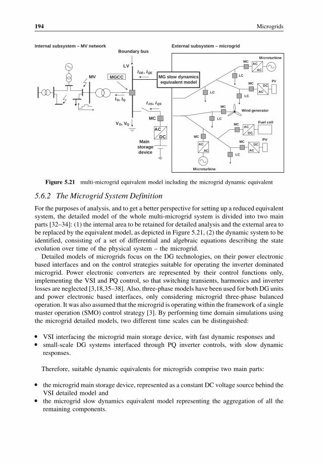
5.6.2 The Microgrid System Definition

For the purposes of analysis, and to get a better perspective for setting up a reduced equivalent

system, the detailed model of the whole multi-microgrid system is divided into two main

parts [32–34]: (1) the internal area to be retained for detailed analysis and the external area to

be replaced by the equivalent model, as depicted in Figure 5.21, (2) the dynamic system to be

identified, consisting of a set of differential and algebraic equations describing the state

evolution over time of the physical system – the microgrid.

Detailed models of microgrids focus on the DG technologies, on their power electronic

based interfaces and on the control strategies suitable for operating the inverter dominated

microgrid. Power electronic converters are represented by their control functions only,

implementing the VSI and PQ control, so that switching transients, harmonics and inverter

losses are neglected [3,18,35–38]. Also, three-phase models have been used for both DG units

and power electronic based interfaces, only considering microgrid three-phase balanced

operation. It was also assumed that the microgrid is operating within the framework of a single

master operation (SMO) control strategy [3]. By performing time domain simulations using

the microgrid detailed models, two different time scales can be distinguished:

� VSI interfacing the microgrid main storage device, with fast dynamic responses and� small-scale DG systems interfaced through PQ inverter controls, with slow dynamic

responses.

Therefore, suitable dynamic equivalents for microgrids comprise two main parts:

� the microgrid main storage device, represented as a constant DC voltage source behind the

VSI detailed model and� the microgrid slow dynamics equivalent model representing the aggregation of all the

remaining components.

External subsystem – microgridInternal subsystem – MV network

MV

LV

Boundary bus

ID, IQ

VD, VQ

MC

AC

DCMain

storagedevice

IDE, IQE

I DS, IQS

MG slow dynamics equivalent model

MGCC

Microturbine

MC

LC

Fuel cellMC

MC

LCLC

LC

MC

LC

AC

AC

AC

DC

Microturbine

Wind generator

PV

AC

DCMC

AC

AC

PV

AC

DCMC

Figure 5.21 multi-microgrid equivalent model including the microgrid dynamic equivalent

194 Microgrids

Then the aim of the system identification procedure is to identify the equivalent model able

to represent the microgrid slow dynamic behavior, as represented in Figure 5.21. Thus, based

on the system definition and using the engineering expertise, the numerical set-up was

implemented – a dedicated dynamic simulation platform able to design suitable numerical

experiments with microgrids, in order to produce sufficiently informative datasets. Also, the

simulation platform should be able to evaluate the performance of the microgrid reduced-

order models at the final stage of the system identification procedure.

Then, the microgrid detailed model is excited through simulated disturbance scenarios into

the MV network, such as multi-microgrid islanding and load-following when the multi-

microgrid is operated autonomously, being the microgrid dynamics captured by means of both

the input and output electrical signals measured at the system boundary according to a suitable

sample time. Boundary bus voltages – expressed in the D-Q synchronous reference frame –

and system angular frequency are considered as inputs, while the boundary bus injected

currents in the tie lines, also expressed in the D-Q reference frame, are considered as outputs.

Node elimination and aggregation is performed by making the injected currents of the

aggregated model equal to the currents in the tie-lines. Thus, the microgrid slow dynamics

equivalent model is disturbed by both boundary bus voltage and system frequency variations,

reacting by varying the injected currents into the boundary bus, operating according to the

principles of a Norton model [34].

5.6.3 Developing Micogrid Dynamic Equivalents

Developing reduced-order models, using system identification based procedures, requires the

following main tasks to be performed:

� data generation,� model structure selection,� identification method selection,� model validation.

However, nonlinear system identification based techniques are application dependent.

General guidelines recommend using the available prior knowledge as well as the engineering

expertise to derive models as close as possible to their intended purpose. Regarding the model

structure selection, the physical insights about the microgrid dynamic behavior have been

combined with the formal properties of the models, yielding two promising approaches:

� black-box modeling based on a time delay neural network (TDNN) model structure,

aiming to exploit the full response of the microgrid when excited after a disturbance and� physical modeling, seeking to understand the physical behavior of the different compo-

nents of the microgrid.

5.6.3.1 TDNN Based Dynamic Equivalents

The TDNN based on the multi-layer perceptron (MLP) neural networks have high capability

for dealing with complicated nonlinear problems. When well-trained, the TDNN can replace

the microgrid’s slow dynamics and it is expected that it will properly interact with the retained

network for a wide range of operating conditions. In the following, we describe the main tasks


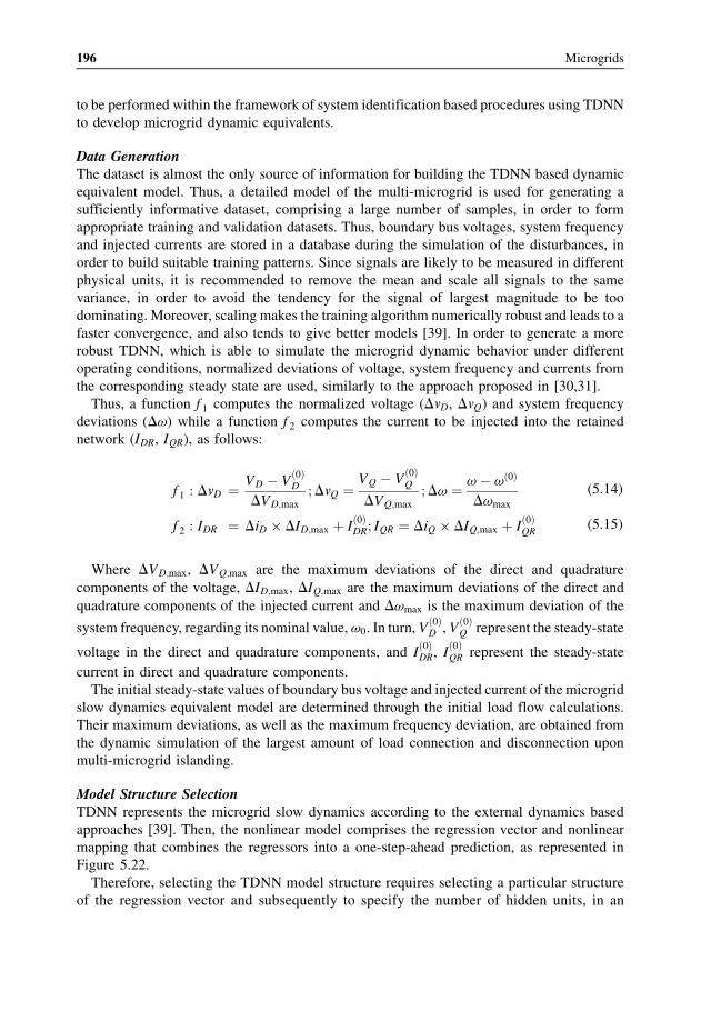
to be performed within the framework of system identification based procedures using TDNN

to develop microgrid dynamic equivalents.

Data GenerationThe dataset is almost the only source of information for building the TDNN based dynamic

equivalent model. Thus, a detailed model of the multi-microgrid is used for generating a

sufficiently informative dataset, comprising a large number of samples, in order to form

appropriate training and validation datasets. Thus, boundary bus voltages, system frequency

and injected currents are stored in a database during the simulation of the disturbances, in

order to build suitable training patterns. Since signals are likely to be measured in different

physical units, it is recommended to remove the mean and scale all signals to the same

variance, in order to avoid the tendency for the signal of largest magnitude to be too

dominating. Moreover, scaling makes the training algorithm numerically robust and leads to a

faster convergence, and also tends to give better models [39]. In order to generate a more

robust TDNN, which is able to simulate the microgrid dynamic behavior under different

operating conditions, normalized deviations of voltage, system frequency and currents from

the corresponding steady state are used, similarly to the approach proposed in [30,31].

Thus, a function f 1 computes the normalized voltage (DvD, DvQ) and system frequency

deviations (Dv) while a function f 2 computes the current to be injected into the retained

network (IDR, IQR), as follows:

f 1 : DvD ¼ VD � V0ð ÞD

DVD;max

;DvQ ¼ VQ � V0ð ÞQ

DVQ;max

;Dv ¼ v� v 0ð Þ

Dvmax

f 2 : IDR ¼ DiD � DID;max þ I0ð ÞDR; IQR ¼ DiQ � DIQ;max þ I

0ð ÞQR

Where DVD;max, DVQ;max are the maximum deviations of the direct and quadrature

components of the voltage, DID;max, DIQ;max are the maximum deviations of the direct and

quadrature components of the injected current and Dvmax is the maximum deviation of the

system frequency, regarding its nominal value, v0. In turn, V0ð ÞD , V

0ð ÞQ represent the steady-state

voltage in the direct and quadrature components, and I0ð ÞDR, I

0ð ÞQR represent the steady-state

current in direct and quadrature components.

The initial steady-state values of boundary bus voltage and injected current of the microgrid

slow dynamics equivalent model are determined through the initial load flow calculations.

Their maximum deviations, as well as the maximum frequency deviation, are obtained from

the dynamic simulation of the largest amount of load connection and disconnection upon

multi-microgrid islanding.

Model Structure SelectionTDNN represents the microgrid slow dynamics according to the external dynamics based

approaches [39]. Then, the nonlinear model comprises the regression vector and nonlinear

mapping that combines the regressors into a one-step-ahead prediction, as represented in

Figure 5.22.

Therefore, selecting the TDNN model structure requires selecting a particular structure

of the regression vector and subsequently to specify the number of hidden units, in an

(5.14)

(5.15)

196 Microgrids

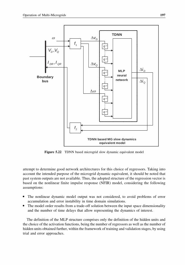
attempt to determine good network architectures for this choice of regressors. Taking into

account the intended purpose of the microgrid dynamic equivalent, it should be noted that

past system outputs are not available. Thus, the adopted structure of the regression vector is

based on the nonlinear finite impulse response (NFIR) model, considering the following

assumptions:

� The nonlinear dynamic model output was not considered, to avoid problems of error

accumulation and error instability in time domain simulations.� The model order results from a trade-off solution between the input space dimensionality

and the number of time delays that allow representing the dynamics of interest.

The definition of the MLP structure comprises only the definition of the hidden units and

the choice of the activation functions, being the number of regressors as well as the number of

hidden units obtained further, within the framework of training and validation stages, by using

trial and error approaches.

Boundarybus

1f

QD VV ,

MLPneural

network

ω

q–1

q–1

q–1

q–1

q–1

q–1

QRDR II ,

2f

DvΔ

QvΔ

ωΔ

DiΔ

QiΔ

TDNN

TDNN based MG slow dynamics equivalent model

Figure 5.22 TDNN based microgrid slow dynamic equivalent model


Estimation of the TDNN Adjustable ParametersAt this stage the MLP network is trained using the back-propagation method, with the

Levenberg–Marquardt algorithm, in order to provide the best possible one step ahead

prediction in the sense of the mean square error. Due to its simplicity, early stopping is

also used in order to avoid overfitting, thus realizing the best bias/variance trade-off. Since we

always want the trained neural network model to also be validated on a validation dataset not

used to extract training patterns, the collected dataset is then split between the training and

validation datasets. Some care needs to be taken in order to guarantee similar properties

between the two datasets regarding the representation of the system properties. As several

MLP neural networks with randomly initialized parameters are trained, the validation error is

also used as the first criterion to reject poor models.

Model ValidationAfter the training procedure, the performance of the TDNN based equivalent models with less

generalization error is evaluated in the dynamic simulation platform. A microgrid slow

dynamics equivalent model is then embedded in the validation module forming the multi-

microgrid equivalent model. The model performance is evaluated by comparing its response

following perturbations that occur in the retained subsystem not used during the training phase

with the response obtained using the microgrid detailed model. For this purpose, in addition to

the TDNN itself, the auxiliary functions f 1 and f 2 are included in the dynamic simulation,

interfacing the TDNN and the retained system according to Figure 5.22. Thus, at each time

step, the microgrid slow dynamics equivalent model recognizes the operating status of the

retained network through the boundary bus voltage and system frequency and injects the

corresponding current into the retained subsystem.

5.6.3.2 Dynamic Equivalents Based on Physical Modeling

Using a physical modeling approach the available physical knowledge regarding the micro-

grid composition and microgrid slow dynamic behavior is explicitly incorporated within the

model structure and, therefore, the requirements to build the dataset are less demanding. Thus,

the system identification main stages are related to the model structure selection and to the

identification method, as described next.

Model Structure SelectionThe physical laws that approximate the microgrid slow dynamics under study are similar to

those that govern the active power control in a diesel engine [33], reacting to the system

frequency variations by changing the output power, as can be seen in Figure 5.23.

Since the microgrid slow dynamics reduced-order model is required to behave according

to the principles of the Norton model, the instantaneous power theory [40] was used in order

to determine the network injected current. For this purpose, only physical laws are used

without parameterization, so that the parameters of the physical model structure whose

values have to be estimated during the identification procedure are gathered into the

parameter vector, u, as

u ¼ R K1 K2 T2 TD½ � (5.16)

The block of instantaneous power theory requires only the implementation of the

algebraic equations needed for computing the current injected on the retained subsystem

198 Microgrids

(IDR, IQR), based on the boundary bus voltage (VD, VQ) and on the active power delivered by

the microgrid slow dynamics equivalent model, Pm. In addition, a given reactive power is

used, Qref , corresponding either to a predefined value linked to the power factor of the DG

units or to a reactive power setpoint sent by the MGCC, according to the SMO control

strategy [3].

The Identification MethodIn order to estimate the parameters of the physically parameterized model structure, a suitable

identification method is required. For this purpose the EPSO tool [11,12] was adopted as a

global optimization tool together with the sum square error (SSE) criterion [33,34]. In this

context, the vector of parameters (u) provides the particle phenotype descriptions correspond-

ing to the particle positions into the predefined parameter space. The parameter estimation

procedure is performed online. For each particle, the loss function expressed in terms of the

SSE is evaluated by performing time domain simulations. Therefore, some interaction

between the EPSO algorithm and the multi-microgrid equivalent model is required, as

can be seen in Figure 5.24.

After defining the search space through both the minimum and maximum values of each

parameter into the parameter vector, it is expected that the EPSO algorithm will perform the

search to the global optimum or, at least, to a good local optimum in the SSE sense. For this

purpose, after mutation has been performed by the EPSO algorithm, the following sequence of

steps has to be carried out for each particle in the swarm:

1. The evaluation function sends the particle object parameters to the microgrid slow

dynamics equivalent model.

2. A pre-specified set of disturbances occurring at defined time instants is simulated over a

certain time period.

3. The microgrid equivalent model response is compared with the target response, which was

generated from the microgrid detailed model, yielding an error sequence.

4. The SSE is then calculated and sent back to the evaluation function.

Based on the SSE magnitude, the EPSO algorithm performs selection in order to build the

swarm corresponding to the next generation. The above procedure is repeated, while the

EPSO algorithm termination condition is not verified. Then, it is expected that the microgrid

slow dynamics equivalent model thus obtained will present the best performance in time

–+

R1

−

+

+12

2

+sTK

11+sTD

sK1−

gridω

1=refω

ωΔ am bm

max,mT

min,mT

mm PT =

Instantaneous powertheory

DV

QV

tω

refQ

DRI

QRI

Figure 5.23 Model structure of the microgrid slow dynamics equivalent model


domain simulations, so that the validation procedure is embedded into the parameter

estimation stage.

It should be mentioned that, for a fixed and known value of Qref , fitting the current injected

into the retained subsystem is similar to fitting the injected active power. Therefore, the

dataset is created by the microgrid slow dynamics subsystem active power and the SSE is

defined in this sense.

5.6.4 Main Results

The approaches presented in the previous sections are used to derive dynamic equivalents for

microgrids using suitable test systems representing the multi-microgrid system. The micro-

grid slow dynamics equivalent models are connected to the system boundary bus in parallel

with the microgrid main storage device, in order to replace the microgrid detailed model, thus

forming the multi-microgrid equivalent model. The performance of the microgrid dynamic

equivalents is evaluated by comparing the time domain responses of both the multi-microgrid

detailed model and the multi-microgrid equivalent model, considering disturbances not used

for extracting training patterns. Also, new initial steady-state operating conditions were

considered, regarding the load and generation levels inside the microgrid and at the MV

distribution network. Both microgrid dynamic equivalent models present a very high

accuracy, with computational time savings, demonstrating the feasibility of the pursued

system identification based approaches.

EPSO algorithm

Search space definition

iθ

+Target

–Σ

( )tεDataset

iH

Time domain solution of differential equations and controlsSteady state network solution

Dynamic simulation of MMG equivalent model

Dynamic models

Synchronous machines

Main storage device with VSI control

MG slow dynamics equivalent model

Simulink S -function coded in MATLAB m -file

Algebraic equations of MMG equivalent model

QD EE ,

QRDR II ,

Replication

Mutation

Evaluation function

SelectionPower system

matrices in D-QChanging multimachine power system matrices

Scenarios for the perturbation conditions

SSEcalculation

Figure 5.24 Flowchart of the parameters estimation procedure in microgrid physical modeling

200 Microgrids

Regarding the TDNN based microgrid dynamic equivalent, the worst-case scenario was veri-

fiedwhen the initial steady-state operating conditionsmoved from the base case bymodifying the

load inside the microgrid. For this scenario the sequence of actions was simulated as:

� multi-microgrid islanding at t¼ 5 s,� connection and disconnection of an amount of load at t¼ 20 s and at t¼ 40 s, respectively.

The comparison between the TDNN based microgrid dynamic equivalent and the microgrid

detailed model power responses can be seen in Figure 5.25. It can be concluded that this

reduced-order model is effective in representing the dynamic behavior of the microgrid

detailed model. Although the reactive power behavior presents a small loss of accuracy, this

effect is quite small on the retained subsystem as can be observed from the boundary bus

voltage and the system frequency behavior. The use of normalized deviations extends the

TDNN capability of generalization to represent the microgrid dynamic behavior when the

steady-state operating conditions move away from the base case. However, a very large

computational effort is required to derive this reduced-order model and its domain of validity

is restricted to the microgrid composition used for generating the dataset. Replacing the

microgrid requires a new training procedure. These weaknesses have been overcome by using

the microgrid physical model.

Then, a physical microgrid dynamic equivalent was derived using another test system

comprising a microgrid with quite different composition and new steady-state operating

conditions. The obtained reduced-order model of the microgrid was used to replace the

microgrid in the same test system used in the case of TDNN based microgrid dynamic

0 20 40 60–100

–50

0

50

100

Time (s)

MG

-P

(kW

)

0 20 40 60–40

–35

–30

–25

–20

Time (s)

MG

-Q (

kVA

r)

0 20 40 600.98

0.99

1

1.01

1.02

Time (s)

Bou

ndar

y bu

s V

rms

(p.u

.)

0 20 40 6049

49.5

50

50.5

51

Time (s)

Fre

quen

cy (

Hz)

MMG detailed modelMMG equivalent model

Figure 5.25 Performance of the TDNN based microgrid dynamic equivalent: behavior of microgrid

active and reactive power, boundary bus voltage and system frequency


equivalents. In order to compare the performance of the two models, the same scenario of

operation was used and the results obtained are presented in Figure 5.26, which shows that the

models have similar performance.

The response of the physical microgrid dynamic equivalent is in good agreement with that

obtained using the multi-microgrid detailed model, demonstrating the effectiveness of the

physical microgrid dynamic equivalent in representing the microgrid dynamic behavior,

following multi-microgrid islanding and under load-following conditions upon multi-micro-

grid islanding. Using the available physical knowledge it was possible to select a proper model

structure with physical representation, which can be easily integrated in dynamic simulation

tools, being the domain of validity extended to represent the microgrid dynamic behavior with

respect to the MV network with the required accuracy.

5.7 Conclusions

The definition of an effective control scheme for multi-microgrid operation is a key issue in

order to accommodate efficiently microgeneration and MV-connected DG units. In particular,

it is extremely important to specify the interactions among controllers, and namely the CAMC

that plays a central role in this control architecture.

The control strategy to be adopted should then be based on a hierarchical scheme, ensuring

both autonomy and redundancy. A communication strategy for multi-microgrid systems is

also important and must be capable of allowing an exchange of information able to handle

properly the dimension and complexity of the system. Furthermore, the control strategy must

0 20 40 60–40

–35

–30

–25

–20

Time (s)

MG

- Q

(kV

Ar)

0 20 40 60–100

–50

0

50

100

Time (s)

MG

- P

(kW

)

0 20 40 600.98

0.99

1

1.01

1.02

Time (s)

Bou

ndar

y bu

s V

rms

(p.u

.)

0 20 40 6049

49.5

50

50.5

51

Time (s)

Fre

quen

cy (

Hz)

MMG detailed modelMMG equivalent model

Figure 5.26 Performance of the physical microgrid dynamic equivalent: behavior of microgrid active

and reactive power, boundary bus voltage and system frequency

202 Microgrids

take into accou nt the two possi ble operating modes in a multi-m icrogrid system : (a) Grid-

connec ted and (b) Islande d mode.

The main functions to be include d in the CAMC, housed at the HV/MV substat ion level,

should be adapted and/or duplica ted from the traditional DMS modu les. The functions

identified in this chapt er wer e: Coo rdinated voltage var suppor t, coord inated frequency

suppor t and eme rgency function s (black start). Advanced voltage control functi onalities, as

the ones describ ed in this chapter, will enabl e large scale integration of DG and micro-

generat ion wi thout jeopardizi ng the grid o perating condi tions and op timizing its perform ance.

Regarding the mul ti-microgr id stability asse ssment , dynamic and tran sient studies are

require d focus ing on the multi-mi crogrid islande d mode of operation. Multi-mic rogrid

islanding and load-fo llowing will play key role in thes e stud ies. Since perform ing these

studies using deta iled modeling appro aches will be not be prac tical, micro grid dynam ic

equivalents have been developed in order to speed up time doma in simulat ions. For this

purpos e, system iden tification based techniq ues exploiting TDNN and physical mode ling can

be used. From the studies perf ormed we can deduce that p hysical micro grid dynam ic

equivalents are well fitted for this purpos e.

The main issues to be dealt with in the fut ure are the deploym ent of smart meter ing

infras tructure as a means of pushing forward the development of micro grids as an integrated

part of the general smart grid conce pt. Th e costs of developing the micro grid and multi-

micro grid conce pts appear to be large and their economi c feasibil ity needs to be careful ly

evaluated. However, if thes e concepts are integrated within a smart meter ing deploym ent, to

be used to manage comme rcially the trade of ele ctricity (either consumed or generat ed) it will

become easier to get an early succe ssful depl oyment. Th is requi res that an advanced meter ing

infras tructure shoul d be conce ived in order to accommod ate the additional commun ication

require ment that will allow the control and management of the microgri d.

In addi tion, future challe nges shoul d include tac kling the issues resu lting from massive

integration of distributed storage devices. Distri buted storage tec hnologie s can be based on

mobil e storage such as elect ric vehicles or o n stationar y storage, which includes fuel cells,

regenerative fuel cells and lithium -ion batterie s. Th e full deploym ent of the microgrid and

multi-mi crogrid concepts requi res the development of distributed storage tech nologies and

the assessment of their impact conce rning techn ical, economi c and regulatory issues.

Compl ementarily, a full assessm ent o f active dem and-side managem ent strategies must

also be carrie d out.

Developing the sma rt grid conce pt mea ns increas ing flexibility for generat ion, consump-

tion and grid man agement. Microgr ids are a way of bringin g addi tional flexibility to the

system dealing with these three components. Also very important is the need to define the

rules for this flexibility, which can include contractual supply of this capability (centralized/

bilateral, voluntary/mandatory). This means that appropriate regulation and adequate solu-

tions need to be sought for and developed within this field.

References

1. European Project “Advanced Architectures and Control Concepts for More Microgrids – More Microgrids”,

Project Reference no. 19864. Available at: http://www.smartgrids.eu/node/14.

2. Lopes, J.A.P. et al. (2003) “Management of Microgrids”, presented at the International Electric Equipment

Conference, Bilbao, Spain.


http://www.smartgrids.eu/node/14

3. Lopes, J.A.P., Moreira, C.L., and Madureira, A.G. (2006) Defining control strategies for microgrids islanded

operation. IEEE T. Power Syst., 21, 916–924.

4. Madureira, A.G., Pereira, J.C., Gil, N.J. et al. (2011) Advanced control and management functionalities for multi-

microgrids. Eur. T. Electr. Power, 21 (2), 1159–1177.

5. Resende, F.O., Gil, N.J., and Lopes, J.A.P. (2011) Service restoration on distribution systems using multi-

microgrids. Eur. T. Electr. Power, 21 (2), 1327–1342.

6. Masters, C.L. (2002) Voltage rise – The big issue when connecting embedded generation to long 11kV overhead

lines. Power Eng. J., 16 (1), 5–12.

7. Madureira, A.G. and Lopes, J.A.P. (2009) Coordinated voltage support in distribution networks with distributed

generation and microgrids. IET Renewable Power Generation , 3 (4), 439–454.

8. Madureira, A. (2012) Coordinated Voltage Control in multi-microgrids, LAP Lambert Academic Publishing,

Saarbrucken.

9. Schwefel, H.P. (1995) Evolution and Optimum Seeking, John Wiley & Sons, New York.

10. Kennedy, J. and Eberhart, R. (1995) “Particle swarm optimization”, in Proc. IEEE International Conference on

Neural Networks, vol. 4, Perth, Australia, pp. 1942–1948.

11. Miranda, V. and Fonseca, N. (2002) “EPSO – Best-of-two-worlds meta-heuristic applied to power system

problems”, in Proc. 2002 Congress on Evolutionary Computation, Honolulu, Hawaii, pp. 1080–1085.

12. Miranda, V. and Fonseca, N. (2002) “EPSO – Evolutionary Particle Swarm Optimization, a new algorithm with

applications in power systems”, in Proc. 2002 Asia Pacific IEEE/PES Transmission and Distribution Conference

and Exhibition 2002, vol. 2, Yokohama, Japan, pp. 745–750.

13. Ciric, R.M., Feltrin, A.P., and Ochoa, L.F. (2003) Power flow in four-wire distribution networks – General

approach. IEEE T. Power Syst., 18 (4), 1283–1290.

14. Kundur, P. (1994) Power System Stability and Control, McGraw-Hill, New York.

15. Gil, N.J. and Lopes, J.A.P. (2007) “Hierarchical Frequency Control Scheme for Islanded Multi-Microgrids

Operation”, in Proc. IEEE PES PowerTech 2007, Lausanne, Switzerland.

16. Gil, N.J. and Lopes, J.A.P. (2008) “Exploiting Automated Demand Response, Generation and Storage Capabili-

ties for Hierarchical Frequency Control in Islanded multi-microgrids”, in Proc. 16th Power Systems Computation

Conference, Glasgow, Scotland.

17. Microgrids Project Deliverable DD1 (2009), “Emergency strategies and algorithms”, J.A. PeScas Lopes. Availableat: http://microgrids.power.ece.ntua.gr/micro/micro200/deliverables/Deliverable_DD1.pdf.

18. Moreira, C.L., Resende, F.O., and Lopes, J.A.P. (2007) Using low voltage microgrids for service restoration. IEEE

T. Power Syst., 22 (1), 395–403.

19. Lopes, J.A.P., Moreira, C.L., and Resende, F.O. (2005) “Microgrids black-start and islanding operation”, in Proc.

15th Power Systems Computation Conference, Li�ege, Belgium.

20. Milano, F. and Srivastava, K. (2009) Dynamic REI equivalents for short circuit and transient stability analyses.

Electr. Pow. Syst. Res., 79 (6), 878–887.

21. Ramirez, J.M., Hern�andez, B.V., and Correa, R.E. (2012) Dynamic equivalence by an optimal strategy. Electr.

Pow. Syst. Res., 84 (1), 58–64.

22. Undrill, J. and Turner, A. (1971) Construction of power system electromechanical equivalents by modal analysis.

IEEE T. Power Ap. Syst., PAS-90 (5), 2049–2059.

23. Marinescu, B., Mallem, B., and Rouco, L. (2010) Large-scale power system dynamic equivalents based on

standard and border synchrony. IEEE T. Power Syst., 25 (4), 1873–1882.

24. Miah, A.M. (2011) Study of a coherency-based simple dynamic equivalent for transient stability assessment. IET

Generation, Transmission & Distribution, 5 (4), 405–416.

25. Podmore, R. and Germond, A. (April 1977) “Development of dynamic equivalents for transient stability studies”,

Systems Control, Inc. Technical Report.

26. Pires de Souza, E.J.S. (2008) Identification of coherent generators considering the electrical proximity for drastic

dynamic equivalents. Electr. Pow. Syst. Res., 78 (7), 1169–1174.

27. DeTuglie, E., Guida, L., Torelli, F. et al. (2004) “Identification of dynamic voltage-current power system

equivalents through artificial neural networks”, in Proc. Bulk Power System Dynamics and Control – VI, Cortina

d’Ampezzo, Italy.

28. Stankovic, A.M. and Saric, A.T (2003) “An integrative approach to transient power system analysis with standard

and ANN-based dynamic models”, in Proc. 2003 IEEE Bologna PowerTech Conference, Bologna, Italy.

29. Shakouri, G.H. and Hamid, R.R. (2009) Identification of a continuous time nonlinear state space model for the

external power system dynamic equivalent by neural networks. Int. J. Elec. Power, 31 (7–8), 334–344.

204 Microgrids

http://microgrids.power.ece.ntua.gr/micro/micro200/deliverables/Deliverable_DD1.pdf

30. Azmy, A.M., Erlich, I., and Sowa, P. (2004) Artificial neural network-based dynamic equivalents for distribution

systems containing active sources. Proc. IEE Proceedings – Generation. Transmission and Distribution, 151 (6),

681–688.

31. Azmy, A.M. and Erlich, I. (2004) “Identification of Dynamic Equivalents for Distribution Power Networks using

Recurrent ANNs”, in Proc. IEEE PES Power Systems Conference and Exposition, vol. 1, New York City, USA,

pp. 348–353.

32. Resende, F.O., Moreira, C.L., and PeScas Lopes, J.A. (2006) “Identification of Dynamic Equivalents for

Microgrids with High Penetration of Solar Energy using ANNs,” in Proc. 3rd European Conference of PV-

Hybrid and Mini-Grid, Aix en Provence, France.

33. Resende, F.O. and Lopes, J.A.P. (2007) “Development of Dynamic Equivalents for Microgrids using System

Identification Theory”, in Proc. 2007 IEEE Power Tech, Lausanne, Switzerland, pp. 1033–1038.

34. Resende, F.O. (2007) “Contributions for Microgrids Dynamic Modelling and Operation”, PhD Thesis, Faculty of

Engineering, Porto University, Porto.

35. Barsali, S., Ceraolo, M., Pelacchi, P., and Poli, D. (2002) “Control techniques of Dispersed Generators to improve

the continuity of electricity supply”, in Proc. 2002 IEEE Power Engineering Society Winter Meeting, vol. 2, New

York, USA, pp. 789–794.

36. Caldon, R., Rossetto, F., and Turri, R. (2003) “Analysis of dynamic performance of dispersed generation

connected through inverter to distribution networks”, in Proc. 17th International Conference on Electricity

Distribution – CIRED, Barcelona, Spain.

37. El-Sharkh, M.Y., Rahman, A., Alam, M.S. et al. (2004) Analysis of active and reactive power control of a stand-

alone PEM fuel cell power plant. IEEE T. Power Syst., 19 (4), 2022–2028.

38. Katiraei, F., Iravani, M.R., and Lehn, P.W. (2005) Micro-grid autonomous operation during and subsequent to

islanding process. IEEE T. Power Deliver., 20 (1), 248–257.

39. Nelles, O. (2001) Nonlinear system identification, in From Classical Approaches to Neural Networks and Fuzzy

Models, Springer Inc., New York.

40. Akagi, H., Kanazawa, Y., and Nabae, A. (1984) Instantaneous reactive power compensators comprising switching

devices without energy storage components. IEEE T. Ind. Appl., IA-20 (3), 625–630.


6

Pilot Sites: Success Storiesand Learnt Lessons

George Kariniotakis, Aris Dimeas and Frank Van Overbeeke (Sections 6.1, 6.2)

6.1 Introducti on

The operation of microgrids offers the possibility of coordinating distributed resources in a more

or less decentralized way, so that they behave as a single producer or load in energy markets. In

this way, the full benefits of distributed resources can be exploited in a consistent, manageable

way. A method for a systematic analysis of these benefits including a quantified evaluation is

provided in Chapter 7, but a number of real-world microgrids are already in operation

worldwide [1,2] as off-grid applications, pilot cases and full-scale demonstrations. Significant

experience and various lessons can be already learnt from these real-world operating microgrids

of all types, that is, community/utility, commercial, industrial, institutional, campus, military

and remote off-grid, including pilot projects and commercial scale demonstrations.

The aim of this chapter is to provide a non-exhaustive overview of real-world microgrids

currently in operation across the world, specifically in Europe, the USA, Japan, China and South

America. Many of these demonstrations have been presented in a series of dedicated microgrid

symposiums held in Berkeley, California, USA (2005), Mont Tremblant, Quebec, Canada

(2006), Nagoya, Japan (2007), Kythnos Island, Greece (2008), San Diego, California, USA

(2009), Vancouver, BC, Canada (2010), Jeju Island, Korea (2011), �Evora, Portugal (2012),Santiago, Chile (2013). Presentations and other materials from these events are available at [3].

A number of equally interesting microgrid applications, such as in Bornholm island in

Denmark, Jeju island in Korea and off-grid microgrids in Canada, are not included, since it was

clearly impossible to cover all efforts in such a dynamically developing field in a single chapter.

6.2 Overvi ew of Microgrid Projects in Europe

In the Europe an Union (EU ), microgri ds form a key component in the Strategic Research

Agenda for Europe’s Electricity Networks of the Future [4]. In the past few years, substantial



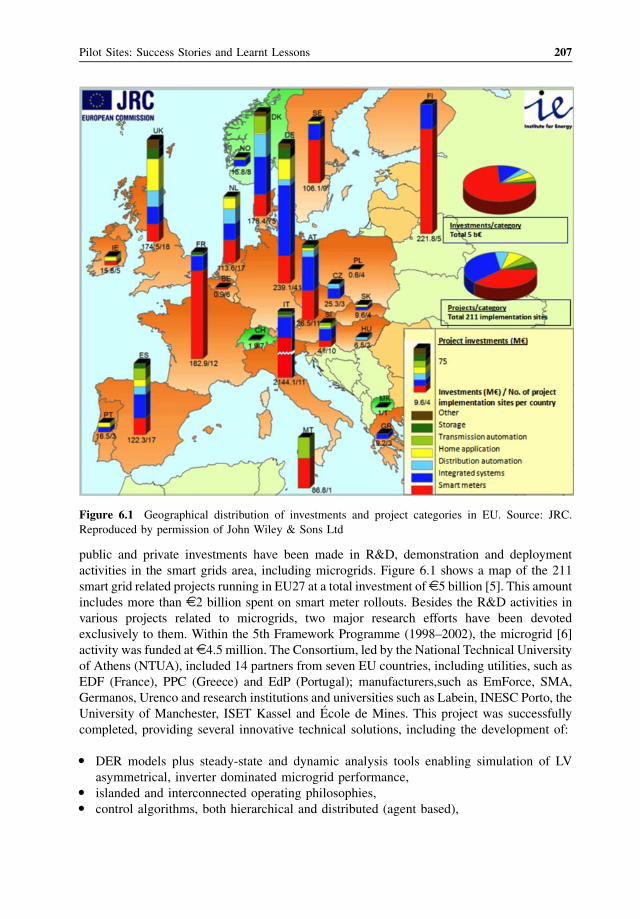
public and private investments have been made in R&D, demonstration and deployment

activities in the smart grids area, including microgrids. Figure 6.1 shows a map of the 211

smart grid related projects running in EU27 at a total investment of D5 billion [5]. This amount

includes more than D2 billion spent on smart meter rollouts. Besides the R&D activities in

various projects related to microgrids, two major research efforts have been devoted

exclusively to them. Within the 5th Framework Programme (1998–2002), the microgrid [6]

activity was funded at D4.5 million. The Consortium, led by the National Technical University

of Athens (NTUA), included 14 partners from seven EU countries, including utilities, such as

EDF (France), PPC (Greece) and EdP (Portugal); manufacturers,such as EmForce, SMA,

Germanos, Urenco and research institutions and universities such as Labein, INESC Porto, the

University of Manchester, ISET Kassel and �Ecole de Mines. This project was successfully

completed, providing several innovative technical solutions, including the development of:

� DER models plus steady-state and dynamic analysis tools enabling simulation of LV

asymmetrical, inverter dominated microgrid performance,� islanded and interconnected operating philosophies,� control algorithms, both hierarchical and distributed (agent based),

Figure 6.1 Geographical distribution of investments and project categories in EU. Source: JRC.

Reproduced by permission of John Wiley & Sons Ltd

Pilot Sites: Success Stories and Learnt Lessons 207

� local black start strategies,� definitions of DER interface response and intelligence requirements,� grounding and protection schemes,� methods for quantification of reliability benefits,� laboratory microgrids of various complexities and functionalities.

A follow-up project titled More Microgrids [7] within the 6th Framework Programme

(2002–2006) was funded at D8.5 million. This second consortium, comprising 22 partners

from 11EU countries, was again led by NTUA and included manufacturers such as Siemens,

ABB, SMA, ZIV, I-Power, Anco, Germanos and EMforce; power utilities from Denmark,

Germany, Portugal, the Netherlands and Poland, and research teams from Greece, the UK,

France, Spain, Portugal, FYROM and Germany.

The achievements of this project include:

� investigation of new DER controllers to provide effective and efficient operation of

microgrids,� development of alternative control strategies using next generation information and

communications technology,� application of innovative protection methods,� technical and commercial integration of multiple microgrids, including interface of several

microgrids with the utility distribution management systems,� studies of the impact on power system operation, including benefits quantification of

microgrids at regional, national and EU levels,� studies of the impact on the development of electricity network infrastructures, including

quantification of the benefits of microgrids, to the reinforcement and replacement strategy

of the ageing EU electricity infrastructure,� field trials of alternative control strategies in actual installations, with experimental

validation of various microgrid architectures in interconnected and islanded modes,

and during transitions, testing of power electronics components and interfaces, and of

alternative control strategies, communication protocols.

Thechangeof scale from laboratories to realworldpilot sites, realizedby theMoreMicrogrids

project, has been a crucial step in drawing practical conclusions on different aspects of the

operation andmanagement ofmicrogrids. Thepilot sites include rural, residential, industrial and

commercial microgrids in several countries. Two large laboratories were also used as pilot

sites.This enabled field tests,whichwouldhavebeen risky tocarryouton real-worldmicrogrids.

The Table 6.1 and Figure 6.2 give an overview of the pilot sites.

The following sections provide a description of the first three pilot microgrids mentioned in

Table 6.1, the experimentation objectives at each pilot site, an overview of the results and

some conclusions and lessons learnt.

6.2.1 Field Test in Gaidouromandra, Kythnos Microgrid (Greece):Decentralized, Intelligent Load Control in an Isolated System

The pilot microgrid electrifies an isolated settlement of 12 houses in a small valley of Kythnos,

an island in the Aegean Sea, Greece (Figure 6.3).

208 Microgrids

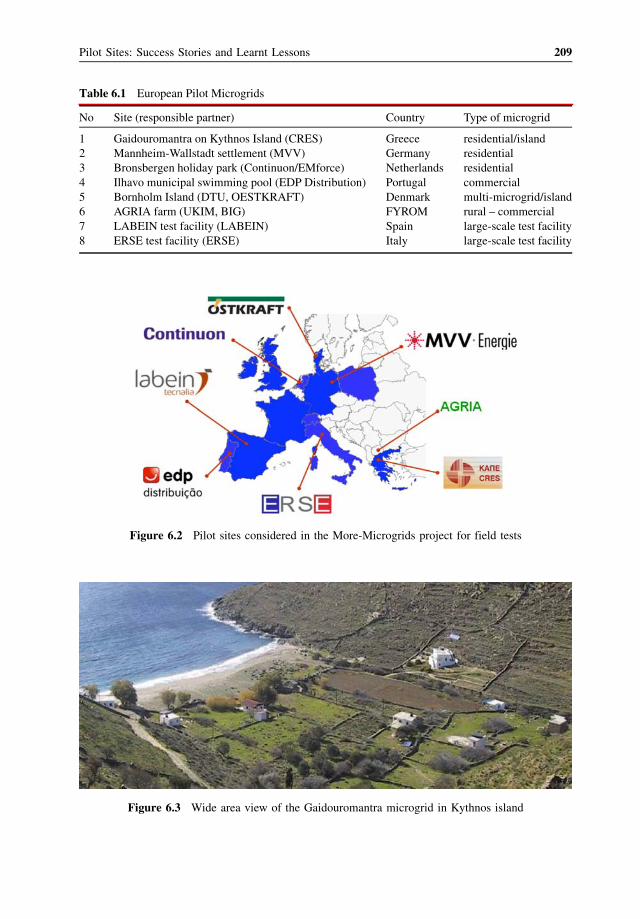
Table 6.1 European Pilot Microgrids

No Site (responsible partner) Country Type of microgrid

1 Gaidouromantra on Kythnos Island (CRES) Greece residential/island

2 Mannheim-Wallstadt settlement (MVV) Germany residential

3 Bronsbergen holiday park (Continuon/EMforce) Netherlands residential

4 Ilhavo municipal swimming pool (EDP Distribution) Portugal commercial

5 Bornholm Island (DTU, OESTKRAFT) Denmark multi-microgrid/island

6 AGRIA farm (UKIM, BIG) FYROM rural – commercial

7 LABEIN test facility (LABEIN) Spain large-scale test facility

8 ERSE test facility (ERSE) Italy large-scale test facility

Figure 6.2 Pilot sites considered in the More-Microgrids project for field tests

Figure 6.3 Wide area view of the Gaidouromantra microgrid in Kythnos island


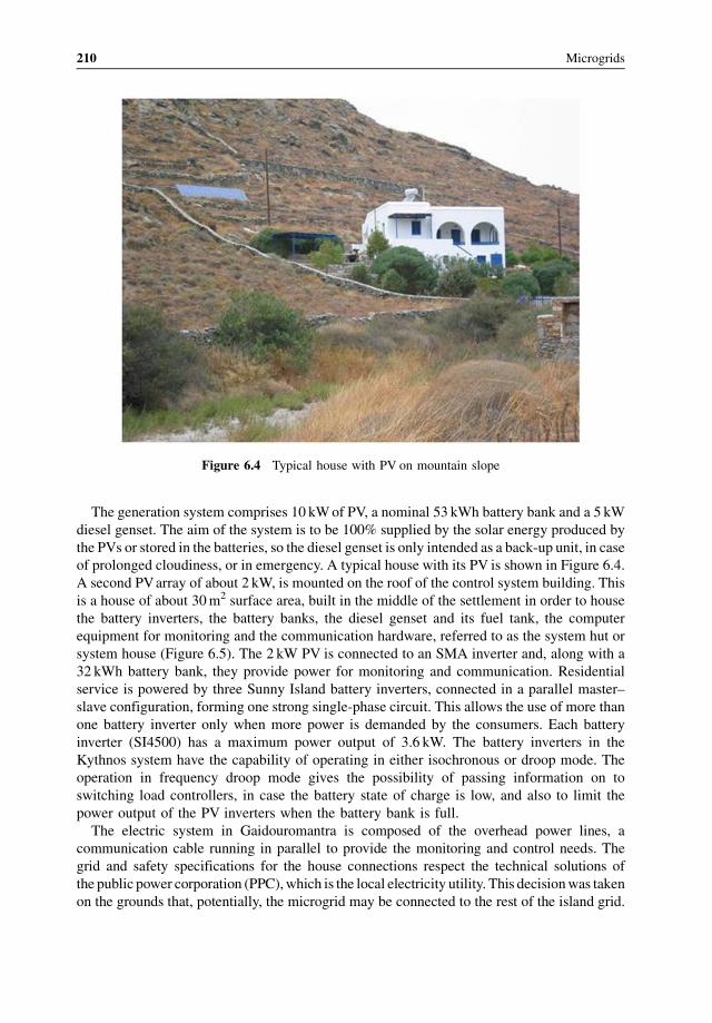
The generation system comprises 10 kWof PV, a nominal 53 kWh battery bank and a 5 kW

diesel genset. The aim of the system is to be 100% supplied by the solar energy produced by

the PVs or stored in the batteries, so the diesel genset is only intended as a back-up unit, in case

of prolonged cloudiness, or in emergency. A typical house with its PV is shown in Figure 6.4.

A second PVarray of about 2 kW, is mounted on the roof of the control system building. This

is a house of about 30m2 surface area, built in the middle of the settlement in order to house

the battery inverters, the battery banks, the diesel genset and its fuel tank, the computer

equipment for monitoring and the communication hardware, referred to as the system hut or

system house (Figure 6.5). The 2 kW PV is connected to an SMA inverter and, along with a

32 kWh battery bank, they provide power for monitoring and communication. Residential

service is powered by three Sunny Island battery inverters, connected in a parallel master–

slave configuration, forming one strong single-phase circuit. This allows the use of more than

one battery inverter only when more power is demanded by the consumers. Each battery

inverter (SI4500) has a maximum power output of 3.6 kW. The battery inverters in the

Kythnos system have the capability of operating in either isochronous or droop mode. The

operation in frequency droop mode gives the possibility of passing information on to

switching load controllers, in case the battery state of charge is low, and also to limit the

power output of the PV inverters when the battery bank is full.

The electric system in Gaidouromantra is composed of the overhead power lines, a

communication cable running in parallel to provide the monitoring and control needs. The

grid and safety specifications for the house connections respect the technical solutions of

the public power corporation (PPC),which is the local electricity utility. This decisionwas taken

on the grounds that, potentially, the microgrid may be connected to the rest of the island grid.

Figure 6.4 Typical house with PV on mountain slope

210 Microgrids

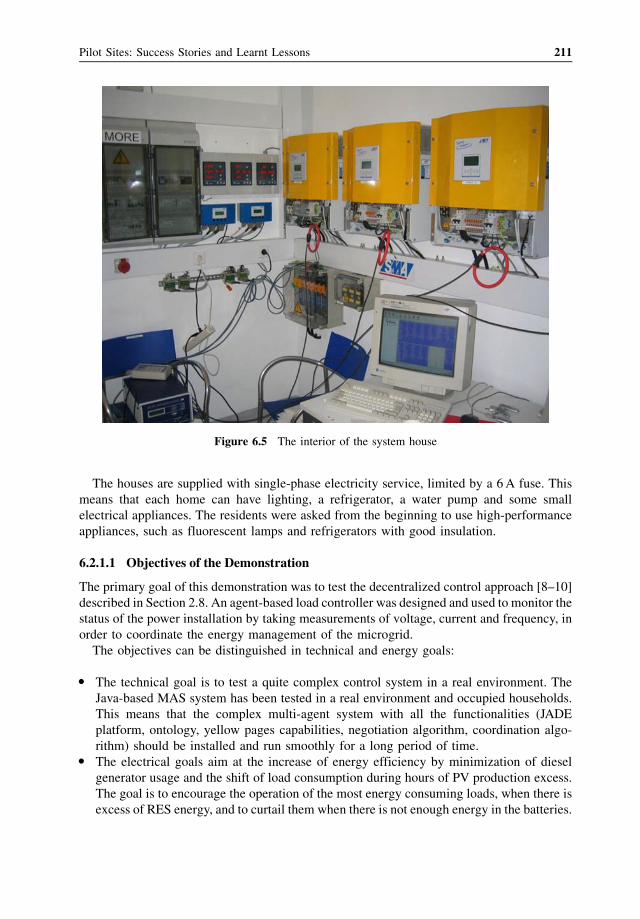
The houses are supplied with single-phase electricity service, limited by a 6A fuse. This

means that each home can have lighting, a refrigerator, a water pump and some small

electrical appliances. The residents were asked from the beginning to use high-performance

appliances, such as fluorescent lamps and refrigerators with good insulation.

6.2.1.1 Objectives of the Demonstration

The primary goal of this demonstration was to test the decentralized control approach [8–10]

described in Section 2.8. An agent-based load controller was designed and used to monitor the

status of the power installation by taking measurements of voltage, current and frequency, in

order to coordinate the energy management of the microgrid.

The objectives can be distinguished in technical and energy goals:

� The technical goal is to test a quite complex control system in a real environment. The

Java-based MAS system has been tested in a real environment and occupied households.

This means that the complex multi-agent system with all the functionalities (JADE

platform, ontology, yellow pages capabilities, negotiation algorithm, coordination algo-

rithm) should be installed and run smoothly for a long period of time.� The electrical goals aim at the increase of energy efficiency by minimization of diesel

generator usage and the shift of load consumption during hours of PV production excess.

The goal is to encourage the operation of the most energy consuming loads, when there is

excess of RES energy, and to curtail them when there is not enough energy in the batteries.

Figure 6.5 The interior of the system house


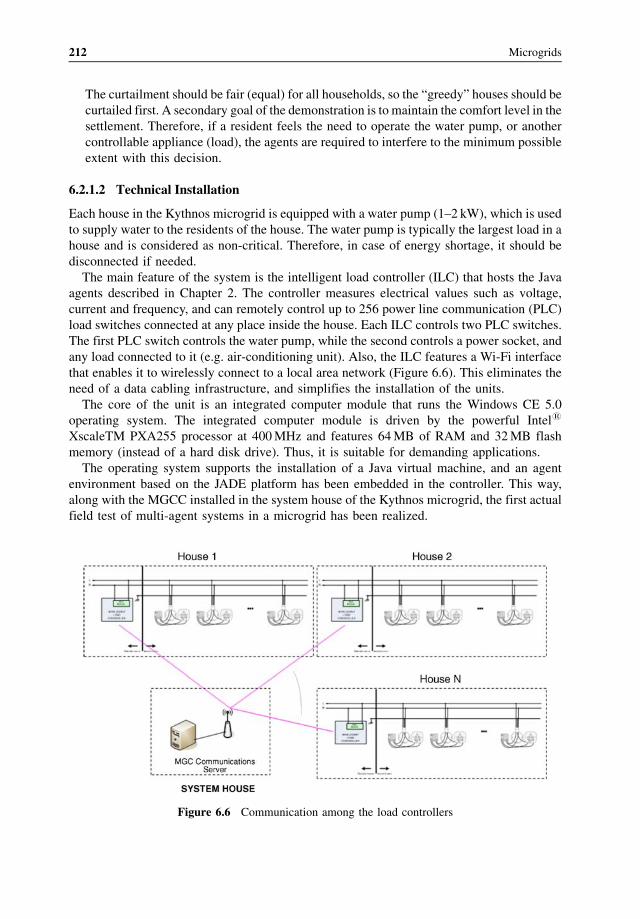
The curtailment should be fair (equal) for all households, so the “greedy” houses should be

curtailed first. A secondary goal of the demonstration is to maintain the comfort level in the

settlement. Therefore, if a resident feels the need to operate the water pump, or another

controllable appliance (load), the agents are required to interfere to the minimum possible

extent with this decision.

6.2.1.2 Technical Installation

Each house in the Kythnos microgrid is equipped with a water pump (1–2 kW), which is used

to supply water to the residents of the house. The water pump is typically the largest load in a

house and is considered as non-critical. Therefore, in case of energy shortage, it should be

disconnected if needed.

The main feature of the system is the intelligent load controller (ILC) that hosts the Java

agents described in Chapter 2. The controller measures electrical values such as voltage,

current and frequency, and can remotely control up to 256 power line communication (PLC)

load switches connected at any place inside the house. Each ILC controls two PLC switches.

The first PLC switch controls the water pump, while the second controls a power socket, and

any load connected to it (e.g. air-conditioning unit). Also, the ILC features a Wi-Fi interface

that enables it to wirelessly connect to a local area network (Figure 6.6). This eliminates the

need of a data cabling infrastructure, and simplifies the installation of the units.

The core of the unit is an integrated computer module that runs the Windows CE 5.0

operating system. The integrated computer module is driven by the powerful Intel1

XscaleTM PXA255 processor at 400MHz and features 64MB of RAM and 32MB flash

memory (instead of a hard disk drive). Thus, it is suitable for demanding applications.

The operating system supports the installation of a Java virtual machine, and an agent

environment based on the JADE platform has been embedded in the controller. This way,

along with the MGCC installed in the system house of the Kythnos microgrid, the first actual

field test of multi-agent systems in a microgrid has been realized.

Figure 6.6 Communication among the load controllers

212 Microgrids

The ILC hosts an integrated web server, through which it is feasible to remotely control the

operation of each controller. During the installation in the Kythnos microgrid, a broadband

internet connection has allowed remote control through a virtual private network. As a result,

commands have been sent and data exchanged among the ILCs, the MGCC and authorized

users who were not required to be onsite.

Figure 6.7 shows how the ILCs are connected in the house electricity network. Each ILC

unit is connected to the power line outside the house, between the energy (kWh) meter and

the house’s electrical panel. The PLC switches are installed inside the electrical installation

of the household.

Figure 6.8 shows pictures of the installed load controllers. For the installation of the ILCs,

5 houses were selected plus the System House where the battery inverters (Sunny Islands) are

installed.

Figure 6.7 Connection of the load controller in the house electricity network. Reproduced by

permission of the IEEE

Figure 6.8 Installation of the load controllers outside the houses


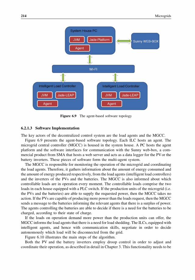
6.2.1.3 Software Implementation

The key actors of the decentralized control system are the load agents and the MGCC.

Figure 6.9 presents the agent-based software topology. Each ILC hosts an agent. The

microgrid central controller (MGCC) is housed in the system house. A PC hosts the agent

platform and the software interfaces for communication with the Sunny web-box, a com-

mercial product from SMA that hosts a web server and acts as a data logger for the PVor the

battery inverters. These pieces of software form the multi-agent system.

The MGCC is responsible for monitoring the operation of the microgrid and coordinating

the load agents. Therefore, it gathers information about the amount of energy consumed and

the amount of energy produced respectively, from the load agents (intelligent load controllers)

and the inverters of the PVs and the batteries. The MGCC is also informed about which

controllable loads are in operation every moment. The controllable loads comprise the two

loads in each house equipped with a PLC switch. If the production units of the microgrid (i.e.

the PVs and the batteries) are able to supply the requested power, then the MGCC takes no

action. If the PVs are capable of producing more power than the loads request, then theMGCC

sends a message to the batteries informing the relevant agents that there is a surplus of power.

The agents controlling the batteries are able to decide if there is a need for the batteries to be

charged, according to their state of charge.

If the loads on operation demand more power than the production units can offer, the

MGCC informs the load agents that there is a need for load shedding. The ILCs, equipped with

intelligent agents, and hence with communication skills, negotiate in order to decide

autonomously which load will be disconnected from the grid.

Figure 6.10 illustrates the main steps of the algorithm.

Both the PV and the battery inverters employ droop control in order to adjust and

coordinate their operation, as described in detail in Chapter 3. This functionality needs to be

Figure 6.9 The agent-based software topology

214 Microgrids

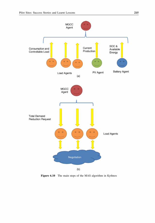
Figure 6.10 The main steps of the MAS algorithm in Kythnos


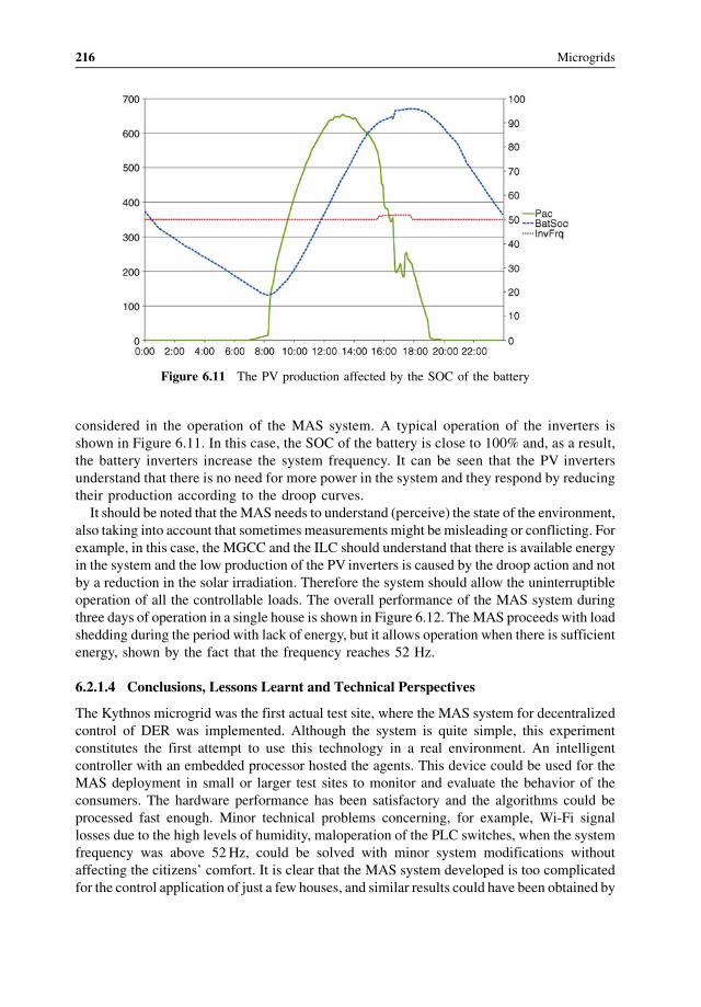
considered in the operation of the MAS system. A typical operation of the inverters is

shown in Figure 6.11. In this case, the SOC of the battery is close to 100% and, as a result,

the battery inverters increase the system frequency. It can be seen that the PV inverters

understand that there is no need for more power in the system and they respond by reducing

their production according to the droop curves.

It should be noted that theMAS needs to understand (perceive) the state of the environment,

also taking into account that sometimes measurements might be misleading or conflicting. For

example, in this case, the MGCC and the ILC should understand that there is available energy

in the system and the low production of the PV inverters is caused by the droop action and not

by a reduction in the solar irradiation. Therefore the system should allow the uninterruptible

operation of all the controllable loads. The overall performance of the MAS system during

three days of operation in a single house is shown in Figure 6.12. TheMAS proceeds with load

shedding during the period with lack of energy, but it allows operation when there is sufficient

energy, shown by the fact that the frequency reaches 52 Hz.

6.2.1.4 Conclusions, Lessons Learnt and Technical Perspectives

The Kythnos microgrid was the first actual test site, where the MAS system for decentralized

control of DER was implemented. Although the system is quite simple, this experiment

constitutes the first attempt to use this technology in a real environment. An intelligent

controller with an embedded processor hosted the agents. This device could be used for the

MAS deployment in small or larger test sites to monitor and evaluate the behavior of the

consumers. The hardware performance has been satisfactory and the algorithms could be

processed fast enough. Minor technical problems concerning, for example, Wi-Fi signal

losses due to the high levels of humidity, maloperation of the PLC switches, when the system

frequency was above 52Hz, could be solved with minor system modifications without

affecting the citizens’ comfort. It is clear that the MAS system developed is too complicated

for the control application of just a few houses, and similar results could have been obtained by

Figure 6.11 The PV production affected by the SOC of the battery

216 Microgrids

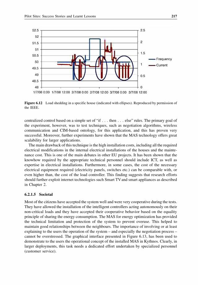
centralized control based on a simple set of “if . . . then . . . else” rules. The primary goal of

the experiment, however, was to test techniques, such as negotiation algorithms, wireless

communication and CIM-based ontology, for this application, and this has proven very

successful. Moreover, further experiments have shown that the MAS technology offers great

scalability for larger applications.

The main drawback of this technique is the high installation costs, including all the required

electrical modifications in the internal electrical installations of the houses and the mainte-

nance cost. This is one of the main debates in other EU projects. It has been shown that the

knowhow required by the appropriate technical personnel should include ICT, as well as

expertise in electrical installations. Furthermore, in some cases, the cost of the necessary

electrical equipment required (electricity panels, switches etc.) can be comparable with, or

even higher than, the cost of the load controller. This finding suggests that research efforts

should further exploit internet technologies such Smart TVand smart appliances as described

in Chapter 2.

6.2.1.5 Societal

Most of the citizens have accepted the system well and were very cooperative during the tests.

They have allowed the installation of the intelligent controllers acting autonomously on their

non-critical loads and they have accepted their cooperative behavior based on the equality

principle of sharing the energy consumption. The MAS for energy optimization has provided

the technical limitation and protection of the system to prevent overuse. This helped to

maintain good relationships between the neighbours. The importance of involving or at least

explaining to the users the operation of the system – and especially the negotiation process –

cannot be overstressed. The graphical interface presented in Figure 6.13, has been used to

demonstrate to the users the operational concept of the installed MAS in Kythnos. Clearly, in

larger deployments, this task needs a dedicated effort undertaken by specialized personnel

(customer service).

Figure 6.12 Load shedding in a specific house (indicated with ellipses). Reproduced by permission of

the IEEE.


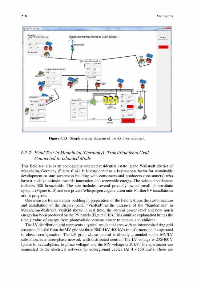
6.2.2 Field Test in Mannheim (Germany): Transition from GridConnected to Islanded Mode

This field test site is an ecologically oriented residential estate in the Wallstadt district of

Mannheim, Germany (Figure 6.14). It is considered as a key success factor for sustainable

development to start awareness building with consumers and producers (pro-sumers) who

have a positive attitude towards innovation and renewable energy. The selected settlement

includes 580 households. The site includes several privately owned small photovoltaic

systems (Figure 6.15) and one private Whispergen cogeneration unit. Further PV installations

are in progress.

One measure for awareness building in preparation of the field test was the customization

and installation of the display panel “VisiKid” at the entrance of the “Kinderhaus” in

Mannheim-Wallstadt. VisiKid shows in real time, the current power level and how much

energy has been produced by the PV panels (Figure 6.16). This intuitive explanation brings the

timely value of energy from photovoltaic systems closer to parents and children.

The LV distribution grid represents a typical residential area with an intermeshed ring grid

structure. It is fed from theMV grid via three 20/0.4 kV, 400 kVA transformers, and is operated

in closed configuration. The LV grid, whose neutral is directly grounded at the MV/LV

substation, is a three-phase network with distributed neutral. The LV voltage is 230/400V

(phase to neutral/phase to phase voltage) and the MV voltage is 20 kV. The apartments are

connected to the electrical network by underground cables (Al 4� 150mm2). There are

Figure 6.13 Simple electric diagram of the Kythnos microgrid

218 Microgrids

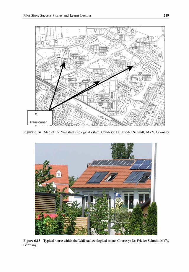
Figure 6.14 Map of the Wallstadt ecological estate. Courtesy: Dr. Frieder Schmitt, MVV, Germany

Figure 6.15 Typical house within theWallstadt ecological estate. Courtesy: Dr. Frieder Schmitt, MVV,

Germany


27 distribution boxes and further underground cables, which complete the LV grid in

Wallstadt. Within the More Microgrids project, the LV grid was modified in order to prepare

it for optional islanding. The new distribution area, including all relevant loads, distributed

generators and storage, is served by one transformer. Power quality and grid characteristics

have been monitored since 2006.

6.2.2.1 Description of the Experiments and Evaluation Results

For awareness building, the socio-economic experiment “Washing with the sun” was

successfully realized. This was used to evaluate the willingness of customers to change

the usage of household appliances, such as washing machines, dishwashers and tumble-

dryers, to promote the consumption of local and solar-produced electricity. In days of good

solar production, a message was sent to the participants specifying a time interval with high

solar production and recommending the use of appliances in this period. A total of 24

households participated and shifted their loads significantly.

Two sets of technical experiments have been achieved in Wallstadt:

� realization of seamless transition between grid connected and islanded mode,� installations of software agents responsible for the management of loads, storage and

generators.

Seamless Transition between Grid Connected and Islanded ModeWithin the grid segment just described, the team prepared the Kinderhaus to operate as a

microgrid, comprising two PV systems with a Sunny-Backup System, controllable loads and

adding sufficiently designed battery storage as buffer, able to supply 10 kW for 1 hour.

To prove the feasibility of an iterative switching from islanded to grid-connected mode and

vice versa, an additional battery for stabilizing the frequency was installed, in combination

with a system of inverters able to realize an islandedmode. This battery (48V 105Ah, 21A for

5 h) has been used, in combination with a system for the single purpose of regulating the

frequency, while switching to islanded mode.

Figure 6.16 The VisiKid panel, displaying the PV generation at the Kinderhaus entrance. Courtesy:

Dr. Frieder Schmitt, MVV, Germany

220 Microgrids

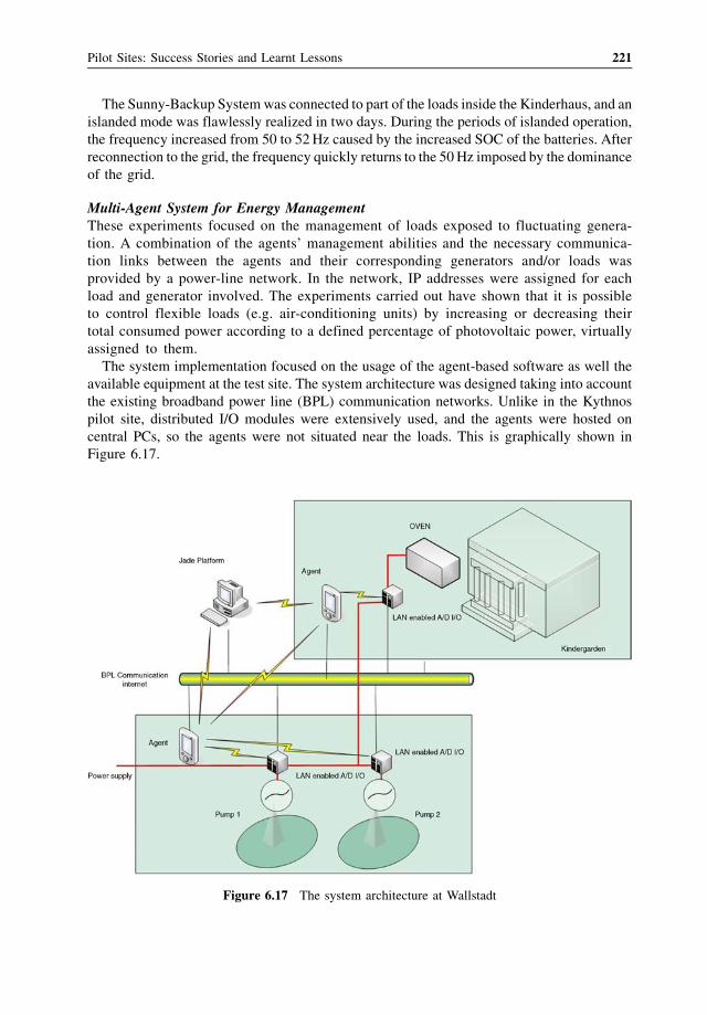
The Sunny-Backup Systemwas connected to part of the loads inside the Kinderhaus, and an

islanded mode was flawlessly realized in two days. During the periods of islanded operation,

the frequency increased from 50 to 52Hz caused by the increased SOC of the batteries. After

reconnection to the grid, the frequency quickly returns to the 50Hz imposed by the dominance

of the grid.

Multi-Agent System for Energy ManagementThese experiments focused on the management of loads exposed to fluctuating genera-

tion. A combination of the agents’ management abilities and the necessary communica-

tion links between the agents and their corresponding generators and/or loads was

provided by a power-line network. In the network, IP addresses were assigned for each

load and generator involved. The experiments carried out have shown that it is possible

to control flexible loads (e.g. air-conditioning units) by increasing or decreasing their

total consumed power according to a defined percentage of photovoltaic power, virtually

assigned to them.

The system implementation focused on the usage of the agent-based software as well the

available equipment at the test site. The system architecture was designed taking into account

the existing broadband power line (BPL) communication networks. Unlike in the Kythnos

pilot site, distributed I/O modules were extensively used, and the agents were hosted on

central PCs, so the agents were not situated near the loads. This is graphically shown in

Figure 6.17.

Figure 6.17 The system architecture at Wallstadt


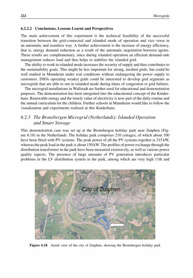
6.2.2.2 Conclusions, Lessons Learnt and Perspectives

The main achievement of this experiment is the technical feasibility of the successful

transition between the grid-connected and islanded mode of operation and vice versa in

an automatic and seamless way. A further achievement is the increase of energy efficiency,

that is, energy demand reduction as a result of the automatic negotiation between agents.

These results are complementary, since during islanded operation an efficient demand-side

management reduces load and thus helps to stabilize the islanded grid.

The ability to work in islanded mode increases the security of supply and thus contributes to

the sustainability goals. This might be less important for strong, meshed grids, but could be

well studied in Mannheim under real conditions without endangering the power supply to

customers. DSOs operating weaker grids could be interested to develop grid segments as

microgrids that are able to run in islanded mode during times of congestion or grid failures.

The microgrid installations in Wallstadt are further used for educational and demonstration

purposes. The demonstration has been integrated into the educational concept of the Kinder-

haus. Renewable energy and the timely value of electricity is now part of the daily routine and

the annual curriculum for the children. Further schools in Mannheim would like to follow the

visualization and experiments realized at this Kinderhaus.

6.2.3 The Bronsbergen Microgrid (Netherlands): Islanded Operationand Smart Storage

This demonstration case was set up at the Bronsbergen holiday park near Zutphen (Fig-

ure 6.18) in the Netherlands. The holiday park comprises 210 cottages, of which about 100

have been fitted with PV systems. The peak power of all the PV systems together is 315 kW,

whereas the peak load in the park is about 150 kW. The profiles of power exchange through the

distribution transformer in the park have been measured extensively, as well as various power

quality aspects. The presence of large amounts of PV generation introduces particular

problems in the LV distribution system in the park, among which are very high 11th and

Figure 6.18 Aerial view of the city of Zutphen, showing the Bronsbergen holiday park

222 Microgrids

13th harmonic currents and voltages. This situation, combined with the fact that, in high

summer, the daily electricity consumption is more or less equal to the daily PV generation,

made an ideal opportunity to explore the advantages of local storage, in combination with the

improvement of power quality. This microgrid was therefore selected by Continuon (now

Liander) for tests with “smart storage” and islanded operation.

A flexible AC distribution system (FADCS) has been proposed to address the following

existing problems:

� Zero-sequence currents – third harmonic currents from the PV inverters cause considerable

currents in the neutral conductor of the three-phase system, resulting in circulating currents

on the delta side of the distribution transformer.� Harmonics – the PV inverters inject considerable amounts of harmonics into the network.

Also, the combined input capacitance of all inverters, together with the inductance of the

distribution transformer, causes the system to show a poorly damped resonance at around

650Hz. This resonance is excited heavily by the inverters.� Asymmetry – the predominantly single-phase loads and generators result in poor symme-

try of the three-phase voltages.

Moreover, the FADCS can be combined with electricity storage in batteries, which will

support the envisaged islanded operation. Sunlight has supplied a total of 720 battery cells,

each rated 2V/500Ah. The cells have been placed in four containers of 180 cells each. The

smart storage and FACDS have been designed based on the microgrid concept.

The experimentation involved the contribution of several industrial actors:

� Liander, the local distribution network operator, acquired the test cottage (Figure 6.19)

right next to the distribution transformer and made the battery containers, all the cabling

and the distribution panels.

Figure 6.19 Outside view of the cottage used as the system house


� EMforce designed, manufactured and installed the inverters, the battery monitoring system

and all control systems.� Sunlight Systems manufactured and supplied the batteries.

6.2.3.1 Objectives of the Demonstration

Before any equipment was built, the three partners compiled a project plan outlining the

following seven objectives:

1. Islanded operation of the microgridDuring an average summer day, the microgrid should be capable of operating in islanded

mode for a period of 24 hours. On a day with less than average irradiation from the sun, the

microgrid may not be able to sustain 24 hours of islanded operation, but it should be able to

survive 4 hours of islanded operation. In the Netherlands 4 hours is the maximum duration

of a supply interruption for which a network operator is not required to pay a compensation

to its customers.

2. Automatic isolation and reconnectionThe microgrid shall be equipped with an autonomous protection device which disconnects

the microgrid from the external public utility network when a fault occurs on the external

system. Furthermore, a system should be in place which is able to synchronize the

microgrid to the external network once its voltage has returned, and to cause the

interruption device to reconnect to the network. Internal faults must be handled selectively

by the fuse on the faulted feeder. As a logical consequence of this approach, individual

feeders have been installed for each of the storage systems. The fuses on these feeders will

isolate the respective storage system in case of a fault within that system.

Upon an enabling signal from the MGCC the protection device must reconnect the

microgrid to the external network. For this purpose, the device shall be equipped with a

synchronization detection facility. The FACDS must sense the voltage on the external

network and adjust the voltage and frequency of the microgrid such that synchronous

reconnection is possible. Reconnection must be established within one minute after it has

detected that the voltage and frequency on the external network is within the statutory

limits.

3. Fault level of the microgridExternal faults: The short-circuit behavior of the FACDS should be such that it does not

switch off during a fault on the incoming feeder from the public network, under the

assumption that the protection system installed on that feeder operates as specified and

isolates the microgrid from the feeder. Within 200ms after the isolation is effective, the

voltage within the microgrid should return to its normal value (i.e. 230V within the

tolerances as indicated in EN50166).

Internal faults: The FACDS must be able to generate a fault current high enough to

blow a 200 A fuse within 5 s. This corresponds to a minimum rms fault current of approx.

1200A for 5 s. If the fault impedance is so low that the FACDS could not supply the fault

current at its nominal output voltage, the voltage shall be lowered so as to limit the

current to a value that can be sustained by the FACDS for 5 s. The aim here is to

demonstrate that the islanded microgrid complies with the same safety standards as in

grid-connected mode.

224 Microgrids

4. Harmonic voltage distortionThe FACDS should absorb and/or compensate harmonics within the microgrid to such an

extent that each harmonic voltage from 100Hz up to 2000Hz complies with the planning

level. The initial assumption for the planning level is: 1% of the rated 50Hz voltage for

each odd harmonic, except for the 9th, 15th, 21st, 27th, 39th; 0.2% of the rated 50Hz

voltage for even harmonics and for the 9th, 15th, 21st, 27th, 39th. If the harmonic level

introduced by the public network would lead to very high harmonic currents between the

public network and the FACDS, this requirement has to be verified in islanded mode only.

5. Energy management and lifetime optimization of the storage systemThis involved the development and test of a so-called battery agent, which monitors the

state of the battery and can issue requests for a regular full recharge to balance the

individual cells and optimize the service life of the battery.

6. Parallel operation of invertersFor the evaluation of parallel operation of inverters, two identical FACDS have been built

which are rated each for half the energy storage performance required. In order to be able to

bridge short time periods with a single unit in operation, each unit shall be able to supply

the full load current of the microgrid. Restrictions on the maximum power that can be

absorbed by a single unit are acceptable.

The inverters shall not operate in master–slave mode; their control systems shall be

designed such that parallel operation and a reasonable degree of load sharing is achieved

without exchange of control signals between the two units.

7. Black start of the microgridThe aim of this last objective is to demonstrate that the microgrid is capable of black

starting from the battery.

6.2.3.2 Description of the Pilot Site

In order to be able to perform the experimentation mentioned, a circuit breaker was installed

between the MV/LV transformer feeding the holiday park and the main LV busbar. Also, a

number of fuses and contactors were added in order to provide sufficient flexibility in the

various operating modes needed for the tests. The single-line diagram of Figure 6.20

illustrates these modifications. Two fuse groups were used to connect the inverters to the

microgrid. If no testing was going on, the microgrid could be connected directly to the

transformer so that all equipment, including the circuit breaker, could be isolated and safely

accessible for staff.

The circuit breaker and the distribution board for the storage system were installed inside

the system room (Figure 6.21), between the two inverter cubicles.

For reasons of size, weight and safety the batteries were installed in four purpose-

designed containers, located in the “garden” of the cottage as illustrated in Figures 6.22

and 6.23.

The microgrid was controlled by an MGCC, which is designed to send setpoints to the two

inverters, and contains the logic for automatic disconnection and reconnection of the

microgrid. The circuit breaker was set so that if disconnection was caused by a fault current,

it would trip automatically. If the microgrid was islanded as a consequence of an MV

disconnection, an islanding test algorithm, implemented in the MGCC, would have detected

that event and instructed the circuit breaker to open.


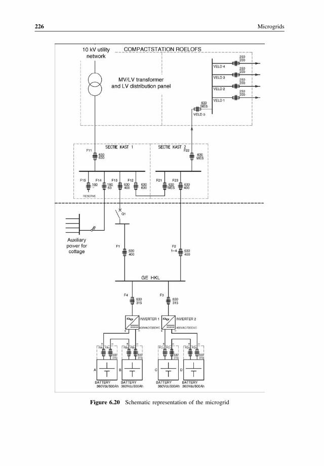
Figure 6.20 Schematic representation of the microgrid

226 Microgrids

The computer on which the MGCC was implemented also served as a platform for the

battery monitoring system, which measured the voltage across each group of six battery cells.

All measurements were logged on a second-by-second basis.

Each inverter was connected to a string of 360 cells connected in series, each rated at 2V,

500Ah. The rated voltage of a battery string was therefore 720V.

Figure 6.21 The system room with switchgear cabinet (center) and inverters

Figure 6.22 View of the cottage and the battery containers. The distribution transformer is in the

concrete box at the top right of the open container


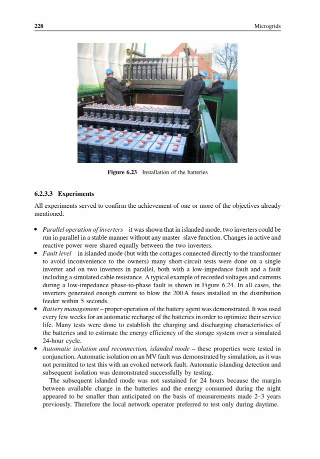
6.2.3.3 Experiments

All experiments served to confirm the achievement of one or more of the objectives already

mentioned:

� Parallel operation of inverters – it was shown that in islanded mode, two inverters could be

run in parallel in a stable manner without any master–slave function. Changes in active and

reactive power were shared equally between the two inverters.� Fault level – in islanded mode (but with the cottages connected directly to the transformer

to avoid inconvenience to the owners) many short-circuit tests were done on a single

inverter and on two inverters in parallel, both with a low-impedance fault and a fault

including a simulated cable resistance. A typical example of recorded voltages and currents

during a low-impedance phase-to-phase fault is shown in Figure 6.24. In all cases, the

inverters generated enough current to blow the 200A fuses installed in the distribution

feeder within 5 seconds.� Battery management – proper operation of the battery agent was demonstrated. It was used

every fewweeks for an automatic recharge of the batteries in order to optimize their service

life. Many tests were done to establish the charging and discharging characteristics of

the batteries and to estimate the energy efficiency of the storage system over a simulated

24-hour cycle.� Automatic isolation and reconnection, islanded mode – these properties were tested in

conjunction. Automatic isolation on anMV fault was demonstrated by simulation, as it was

not permitted to test this with an evoked network fault. Automatic islanding detection and

subsequent isolation was demonstrated successfully by testing.

The subsequent islanded mode was not sustained for 24 hours because the margin

between available charge in the batteries and the energy consumed during the night

appeared to be smaller than anticipated on the basis of measurements made 2–3 years

previously. Therefore the local network operator preferred to test only during daytime.

Figure 6.23 Installation of the batteries

228 Microgrids

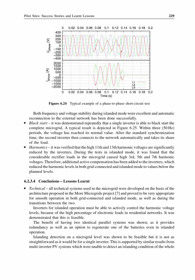
Both frequency and voltage stability during islanded modewere excellent and automatic

reconnection to the external network has been done successfully.� Black start – it was demonstrated repeatedly that a single inverter is able to black start the

complete microgrid. A typical result is depicted in Figure 6.25. Within three (50 Hz)

periods, the voltage has reached its normal value. After the standard synchronization

time, the second inverter then connects to the network automatically and takes its share

of the load.� Harmonics – it was verified that the high 11th and 13th harmonic voltages are significantly

reduced by the inverters. During the tests in islanded mode, it was found that the

considerable rectifier loads in the microgrid caused high 3rd, 5th and 7th harmonic

voltages. Therefore, additional active compensation has been added to the inverters, which

reduced the harmonic levels in both grid-connected and islanded mode to values below the

planned levels.

6.2.3.4 Conclusions – Lessons Learnt

� Technical – all technical systems used in the microgrid were developed on the basis of the

architecture proposed in the More Microgrids project [7] and proved to be very appropriate

for smooth operation in both grid-connected and islanded mode, as well as during the

transitions between the two.

Inverters for islanded operation must be able to actively control the harmonic voltage

levels, because of the high percentage of electronic loads in residential networks. It was

demonstrated that this is feasible.

The benefit of having two identical parallel systems was shown, as it provides

redundancy as well as an option to regenerate one of the batteries even in islanded

operation.

Islanding detection on a microgrid level was shown to be feasible but it is not as

straightforward as it would be for a single inverter. This is supported by similar results from

multi-inverter PV systems which were unable to detect an islanding condition of the whole

Figure 6.24 Typical example of a phase-to-phase short-circuit test


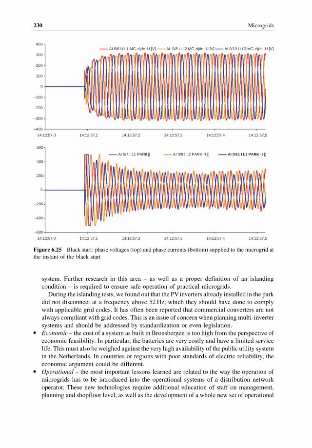
system. Further research in this area – as well as a proper definition of an islanding

condition – is required to ensure safe operation of practical microgrids.

During the islanding tests, we found out that the PV inverters already installed in the park

did not disconnect at a frequency above 52Hz, which they should have done to comply

with applicable grid codes. It has often been reported that commercial converters are not

always compliant with grid codes. This is an issue of concern when planning multi-inverter

systems and should be addressed by standardization or even legislation.� Economic – the cost of a system as built in Bronsbergen is too high from the perspective of

economic feasibility. In particular, the batteries are very costly and have a limited service

life. This must also beweighed against the very high availability of the public utility system

in the Netherlands. In countries or regions with poor standards of electric reliability, the

economic argument could be different.� Operational – the most important lessons learned are related to the way the operation of

microgrids has to be introduced into the operational systems of a distribution network

operator. These new technologies require additional education of staff on management,

planning and shopfloor level, as well as the development of a whole new set of operational

–400

–300

–200

–100

0

100

200

300

400

14:12:57,514:12:57,414:12:57,314:12:57,214:12:57,114:12:57,0

U [V]AI 0/6 U L1 MG zijde - AI 0/8 U L2 MG zijde -U [V] AI 0/10 U L3 MG zijde -U [V]

–600

–400

–200

0

200

400

600

14:12:57,514:12:57,414:12:57,314:12:57,214:12:57,114:12:57,0

I []AI 0/7 I L1 PARK - I []AI 0/9 I L2 PARK - I []AI 0/11 I L3 PARK -

Figure 6.25 Black start: phase voltages (top) and phase currents (bottom) supplied to the microgrid at

the instant of the black start

230 Microgrids

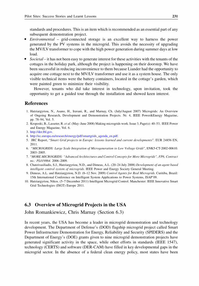
standar ds and proce dures. This is an item which is reco mmende d as an esse ntial part of any

subse quent demonst ration project.� Enviro nmental – grid-co nnected storage is an excellent way to harne ss the power

gener ated by the PV systems in the micro grid. This avoids the neces sity o f upgra ding

the MV/LV transformer to cope with the high power gener ation during summe r days at low

load.� Societ al – it has not been easy to generat e int erest for these activities with the tena nts of the

cottage s in the holiday park, although the project is happen ing on their doorstep . We have

been successf ul in reduc ing inco nvenience to them because Liand er had the opportuni ty to

acquire one cottage next to the MV /LV transf ormer and use it as a syst em house. The only

visibl e technical item s were the battery containers , locate d in the cottage’s garde n, which

were painted green to minimi ze their visibi lity.

However, tenants who did take interest in technol ogy, upon invitation, took the

opportuni ty to get a guide d tour thro ugh the installa tion and showed keen interest .

References

1. Hatziargyriou, N., Asano, H., Iravani, R., and Marnay, Ch. (July/August 2007) Microgrids: An Overview

of Ongoing Research, Development and Demonstration Projects. Nr. 4, IEEE Power&Energy Magazine,

pp. 78–94, Vol. 5.

2. Kroposki, B., Lasseter, R. et al. (May–June 2008) Making microgrids work. Issue 3, Page(s): 40–53, IEEE Power

and Energy Magazine, Vol. 6.

3. http://der.lbl.gov.

4. http://ec.europa.eu/research/energy/pdf/smartgrids_agenda_en.pdf.

5. JRC Report, “Smart Grid projects in Europe: lessons learned and current developments”. EUR 24856 EN,

2011.

6. “MICROGRIDS: Large Scale Integration of Microgeneration to Low Voltage Grids”, ENK5-CT-2002-00610.

2003–2005.

7. “MORE MICROGRIDS: “Advanced Architectures and Control Concepts for More Microgrids”, FP6, Contract

no.: PL019864. 2006–2009.

8. Chatzivasiliadis, S.J., Hatziargyriou, N.D., and Dimeas, A.L. (20–24 July 2008) Development of an agent based

intelligent control system of microgrids. IEEE Power and Energy Society General Meeting.

9. Dimeas, A.L. and Hatziargyriou, N.D. (8–12 Nov. 2009) Control Agents for Real Microgrids. Curitiba, Brazil:

15th International Conference on Intelligent System Applications to Power Systems, ISAP’09.

10. Hatziargyriou, Nikos. (5–7 December 2011) Intelligent Microgrid Control. Manchester: IEEE Innovative Smart

Grid Technologies (ISGT) Europe 2011.

6.3 Overview of Microgrid Projects in the USA

John Romankiewicz, Chris Marnay (Section 6.3)

In recent years, the USA has become a leader in microgrid demonstration and technology

development. The Department of Defense’s (DOD) flagship microgrid project called Smart

Power Infrastructure Demonstration for Energy, Reliability and Security (SPIDERS) and the

Department of Energy’s (DOE) grants given to nine microgrid demonstration projects have

generated significant activity in the space, while other efforts in standards (IEEE 1547),

technology (CERTS) and software (DER-CAM) have filled in key developmental gaps in the

microgrid sector. In the absence of a federal clean energy policy, most states have been


http://der.lbl.gov

http://ec.europa.eu/research/energy/pdf/smartgrids_agenda_en.pdf

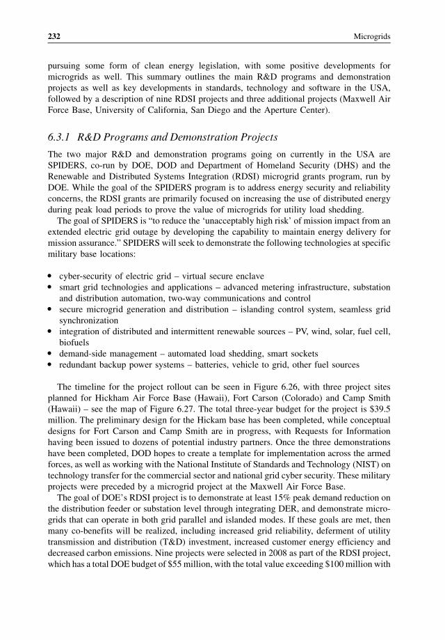
pursuing some form of clean energy legislation, with some positive developments for

microgrids as well. This summary outlines the main R&D programs and demonstration

projects as well as key developments in standards, technology and software in the USA,

followed by a description of nine RDSI projects and three additional projects (Maxwell Air

Force Base, University of California, San Diego and the Aperture Center).

6.3.1 R&D Programs and Demonstration Projects

The two major R&D and demonstration programs going on currently in the USA are

SPIDERS, co-run by DOE, DOD and Department of Homeland Security (DHS) and the

Renewable and Distributed Systems Integration (RDSI) microgrid grants program, run by

DOE. While the goal of the SPIDERS program is to address energy security and reliability

concerns, the RDSI grants are primarily focused on increasing the use of distributed energy

during peak load periods to prove the value of microgrids for utility load shedding.

The goal of SPIDERS is “to reduce the ‘unacceptably high risk’ of mission impact from an

extended electric grid outage by developing the capability to maintain energy delivery for

mission assurance.” SPIDERS will seek to demonstrate the following technologies at specific

military base locations:

� cyber-security of electric grid – virtual secure enclave� smart grid technologies and applications – advanced metering infrastructure, substation

and distribution automation, two-way communications and control� secure microgrid generation and distribution – islanding control system, seamless grid

synchronization� integration of distributed and intermittent renewable sources – PV, wind, solar, fuel cell,

biofuels� demand-side management – automated load shedding, smart sockets� redundant backup power systems – batteries, vehicle to grid, other fuel sources

The timeline for the project rollout can be seen in Figure 6.26, with three project sites

planned for Hickham Air Force Base (Hawaii), Fort Carson (Colorado) and Camp Smith

(Hawaii) – see the map of Figure 6.27. The total three-year budget for the project is $39.5

million. The preliminary design for the Hickam base has been completed, while conceptual

designs for Fort Carson and Camp Smith are in progress, with Requests for Information

having been issued to dozens of potential industry partners. Once the three demonstrations

have been completed, DOD hopes to create a template for implementation across the armed

forces, as well as working with the National Institute of Standards and Technology (NIST) on

technology transfer for the commercial sector and national grid cyber security. These military

projects were preceded by a microgrid project at the Maxwell Air Force Base.

The goal of DOE’s RDSI project is to demonstrate at least 15% peak demand reduction on

the distribution feeder or substation level through integrating DER, and demonstrate micro-

grids that can operate in both grid parallel and islanded modes. If these goals are met, then

many co-benefits will be realized, including increased grid reliability, deferment of utility

transmission and distribution (T&D) investment, increased customer energy efficiency and

decreased carbon emissions. Nine projects were selected in 2008 as part of the RDSI project,

which has a total DOE budget of $55 million, with the total value exceeding $100 million with

232 Microgrids

Figure 6.26 SPIDERS implementation plan [4]. Source: DOD 2011, contact: Jason Stamp, Sandia

Labs. Sourced from DOD PPT: http://e2s2.ndia.org/schedule/Documents/2012%20Abstracts/

Breakout%20Sessions/14191.pdf. Reproduced by permission of Jason Stamp

Figure 6.27 Map of DOE RDSI projects


http://e2s2.ndia.org/schedule/Documents/2012%20Abstracts/Breakout%20Sessions/14191.pdf

http://e2s2.ndia.org/schedule/Documents/2012%20Abstracts/Breakout%20Sessions/14191.pdf

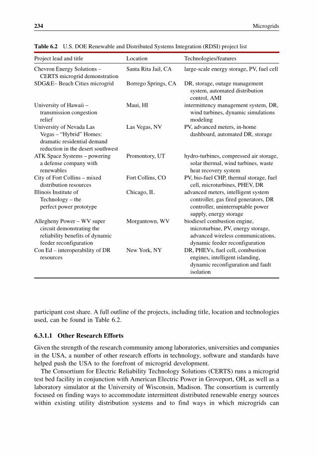
participant cost share. A full outline of the projects, including title, location and technologies

used, can be found in Table 6.2.

6.3.1.1 Other Research Efforts

Given the strength of the research community among laboratories, universities and companies

in the USA, a number of other research efforts in technology, software and standards have

helped push the USA to the forefront of microgrid development.

The Consortium for Electric Reliability Technology Solutions (CERTS) runs a microgrid

test bed facility in conjunction with American Electric Power in Groveport, OH, as well as a

laboratory simulator at the University of Wisconsin, Madison. The consortium is currently

focused on finding ways to accommodate intermittent distributed renewable energy sources

within existing utility distribution systems and to find ways in which microgrids can

Table 6.2 U.S. DOE Renewable and Distributed Systems Integration (RDSI) project list

Project lead and title Location Technologies/features

Chevron Energy Solutions –

CERTS microgrid demonstration

Santa Rita Jail, CA large-scale energy storage, PV, fuel cell

SDG&E– Beach Cities microgrid Borrego Springs, CA DR, storage, outage management

system, automated distribution

control, AMI

University of Hawaii –

transmission congestion

relief

Maui, HI intermittency management system, DR,

wind turbines, dynamic simulations

modeling

University of Nevada Las

Vegas – “Hybrid” Homes:

dramatic residential demand

reduction in the desert southwest

Las Vegas, NV PV, advanced meters, in-home

dashboard, automated DR, storage

ATK Space Systems – powering

a defense company with

renewables

Promontory, UT hydro-turbines, compressed air storage,

solar thermal, wind turbines, waste

heat recovery system

City of Fort Collins – mixed

distribution resources

Fort Collins, CO PV, bio-fuel CHP, thermal storage, fuel

cell, microturbines, PHEV, DR

Illinois Institute of

Technology – the

perfect power prototype

Chicago, IL advanced meters, intelligent system

controller, gas fired generators, DR

controller, uninterruptable power

supply, energy storage

Allegheny Power – WV super

circuit demonstrating the

reliability benefits of dynamic

feeder reconfiguration

Morgantown, WV biodiesel combustion engine,

microturbine, PV, energy storage,

advanced wireless communications,

dynamic feeder reconfiguration

Con Ed – interoperability of DR

resources

New York, NY DR, PHEVs, fuel cell, combustion

engines, intelligent islanding,

dynamic reconfiguration and fault

isolation

234 Microgrids

seamlessly connect to and island from the grid. Currently, CERTS is adding multiple hardware

units to its test bed facility, including:

� CERTS compatible conventional synchronous generator� flexible energy management system for dispatch� intelligent load shedding� commercially available, stand-alone electricity storage device with CERTS controls� PV emulator and inverter with CERTS controls.

CERTS technology has been applied in other microgrid projects around the USA, such as

the Santa Rita Jail project led by Chevron Energy Solutions.

In the area of software development, the Distributed Energy Resources Customer Adoption

Model (DER-CAM) has been developed by researchers at Lawrence Berkeley National

Laboratory (LBNL) to predict and optimize the capacity, and minimize the cost of operating

distributed generation and CHP for individual customer sites or microgrids. Based on specific

site load (space heat, hot water, gas, cooling and electricity) and price information (electricity

tariffs, fuel costs, operation and maintenance costs etc.), the model makes economic decisions

on the distributed generation or CHP technologies that the user should adopt and how that

technology should be operated. A schematic for DER-CAM can be seen in Figure 6.28. The

model has been used internationally for about 10 years now.

Also in the area of software development, Energy Surety Micro-grids (ESM) is an

assessment tool, with some similarities to DER-CAM and an eye towards assessing the

possible application of microgrids at military bases. ESM uses a risk assessment methodology

for the critical power delivery functions and needs of military bases, hospitals or communities.

To assess the specific military applications, the US Army Engineer Research and Develop-

ment Center (ERDC) has teamed up with Sandia National Laboratories to look at how

microgrids can be implemented, not only at home bases, but also in field applications, such as

forward base camps and tactical operation centers. So far, 12 bases across the USA have been

evaluated, with more in the pipeline.

Figure 6.28 DER-CAM functionality


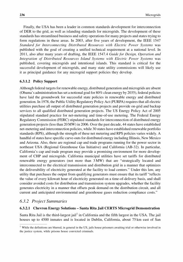
Finally, the USA has been a leader in common standards development for interconnection

of DER to the grid, as well as islanding standards for microgrids. The development of these

standards has streamlined business and safety operations for many projects and states trying to

form regulations in these areas. In 2003, after five years of development, the IEEE 1547

Standard for Interconnecting Distributed Resources with Electric Power Systems was

published with the goal of creating a unified technical requirement at a national level. In

2011, also after many years of drafting, the IEEE 1547.4 Guide for Design, Operation and

Integration of Distributed Resources Island Systems with Electric Power Systems was

published, covering microgrids and intentional islands. This standard is critical for the

successful development of microgrids, and many state utility commissions will likely use

it as principal guidance for any microgrid support policies they develop.

6.3.1.2 Policy Support

Although federal targets for renewable energy, distributed generation andmicrogrids are absent

(Obama’s administration has set a notional goal for 80% clean energy by 2035), federal policies

have laid the groundwork for successful state policies in renewable energy and distributed

generation. In 1978, the Public Utility Regulatory Policy Act (PURPA) requires that all electric

utilities purchase all output of distributed generation projects and provide on-grid and backup

services to all qualified distributed generation projects. The US Energy Policy Act of 2005

stipulated standard practice for net-metering and time-of-use metering. The Federal Energy

Regulatory Commission (FERC) stipulated standards for interconnection of distributed energy

generation projects (less than 20MW) in 2006. Over the past decade, 44 states have established

net-metering and interconnection policies, while 30 states have established renewable portfolio

standards (RPS), although the strength of these net metering and RPS policies varies widely. A

handful of states have specific carve-outs for distributed energy including Illinois, NewMexico

and Arizona. Also, there are regional cap and trade programs running for the power sector in

northeast USA (Regional Greenhouse Gas Initiative) and California (AB-32). In particular,

California’s cap and trade program may provide a promising environment for more develop-

ment of CHP and microgrids. California municipal utilities have set tariffs for distributed

renewable energy generators (not more than 3MW) that are “strategically located and

interconnected to the electrical transmission and distribution grid in a manner that optimizes

the deliverability of electricity generated at the facility to load centers.” Under this law, any

utility that purchases the output from qualifying generators must ensure that its tariff “reflects

the value of every kilowatt hour of electricity generated on a time-of-delivery basis, and shall

consider avoided costs for distribution and transmission system upgrades, whether the facility

generates electricity in a manner that offsets peak demand on the distribution circuit, and all

current and anticipated environmental and greenhouse gases reduction compliance costs.”

6.3.2 Project Summaries

6.3.2.1 Chevron Energy Solutions – Santa Rita Jail CERTS Microgrid Demonstration

Santa Rita Jail is the third-largest jail1 in California and the fifth largest in the USA. The jail

houses up to 4500 inmates and is located in Dublin, California, about 75 km east of San

1 While the definitions are blurred, in general in the US, jails house prisoners awaiting trial or otherwise involved in

the justice system, while prisons house convicted criminals.

236 Microgrids

Francisco (Figure 6.29). Due to a series of installed DER and efficiency measures at the jail, it

is often referred to as the “Green Jail.” The aim of the microgrid project there is to demonstrate

the first implementation of the CERTS microgrid technology, combined with large-scale

energy storage, new and legacy renewable energy sources and a fuel cell. The goals as outlined

by Alameda Country (the local county government in charge of the jail) are as follows:

� reduce peak electrical load and monthly demand charges� store renewable and fuel cell energy overproduction� shift electrical loads to off-peak hours� improve grid reliability and reduce electrical voltage surges and spikes� enable the jail to be a net-zero electrical facility during the most expensive summer peak

hours� expand the jail’s onsite generation capacity to include three renewable energy sources:

solar PV, wind turbines and solar water heaters.

Over the past decade, the project has implemented various energy efficiency measures and

installed a wide array of distributed energy technologies, which have slowly accumulated into

a full microgrid. In the spring of 2002, the jail installed a 1.2MW rated rooftop PV array,

followed in 2006 by a 1MW molten carbonate fuel cell (MCFC) with CHP capability. Most

recently, with the aid of DOE and California Energy Commission (CEC) grant money, as well

as funding and participation from industry partners Chevron Energy Solutions, Satcon Power

Systems and Pacific Gas and Electric, the jail has gained full microgrid capabilities with the

Figure 6.29 Recent photo of Santa Rita Jail, with ground mounted tracking solar PV in the foreground

and batteries and fuel cell directly behind


installation of a large 2MW, 4MWh lithium-iron-phosphate battery, an islanding switch and

associated power electronic upgrades.

In addition to generation equipment, the jail has also implemented a series of building

equipment retrofits to improve efficiency and reduce peak electricity demand. AT-8 lighting

ballast retrofit completed in 2009 was estimated to save 225 kW from the peak power demand

and 1.34GWh of electricity annually. Second, the 2010 installation of induction lighting in

day rooms will save 217 kW peak power and 1.55GWh annually. These two measures

represent a 15% savings in peak power at the jail. Also, a number of other efficiency

improvements were implemented in the middle of the 1990s targeting HVAC systems,

lighting, refrigeration and other end-uses, which altogether decreased peak demand by

912 kW. Among them, an upgraded chiller took an estimated 423 kW off the peak power

demand. The jail also plans to install a roof-mounted solar-thermal system which, when

operational, will provide 40% of its hot water needs.

Lawrence Berkeley National Laboratory (LBNL) has also been an active partner with the

jail, using its DER-CAM model a number of times throughout the development of the

microgrid, to analyze electricity and heat requirements and to develop plans for the jail to meet

its needs at minimum cost. Also, battery chemistries were compared, operating schedules that

minimized risk were developed and opportunities for participation in demand response and

ancillary services markets are now being analyzed.

6.3.2.2 SDG&E – Borrego Springs Microgrid Technologies Used

Borrego Springs is a small residential community located 90 miles northeast of San Diego.

The microgrid there can be described as a utility-scale microgrid with its primary partner

being San Diego Gas and Electric (SDG&E) and its primary focus is on smart grid service

delivery models (Figure 6.30). The goal of the project is to provide a proof-of-concept test as

to how information technologies and distributed energy resources (solar PV and batteries

primarily) can increase utility asset utilization and reliability. The community already had

many rooftop solar PV systems installed and is a somewhat isolated area fed only by a single

sub-transmission line. Islanding of the entire substation area is being explored.

The project’s partners include Lockheed Martin, IBM, Advanced Energy Storage, Horizon

Energy, Oracle, Motorola, Pacific Northwest National Laboratories and University of

California, San Diego. DOE supported the project with $7.5 million of federal funding, with

additional funding coming from SDG&E ($4.1m), CEC ($2.8m), and other partners ($0.8m).

The total microgrid installed capacity will be about 4MW, with the main technologies

being two 1.8MW diesel generators, a large 500 kW/1500 kWh battery at the substation, three

smaller 50 kWh batteries, six 4 kW/8 kWh home energy storage units, about 700 kW of

rooftop solar PV and 125 residential home area network systems. The project will also

incorporate feeder automation system technologies (FAST), outage management systems and

price driven load management.

6.3.2.3 University of Hawaii – Transmission Congestion Relief

Hawaii is an ideal site for microgrids with its high energy costs, heavy reliance on oil,

significant reliability issues and abundant renewable energy resources (solar, wind, tide and

wave). The University of Hawaii’s microgrid project’s main goal is to develop and demon-

strate an integrated monitoring, communications, data base, applications, and decision

238 Microgrids

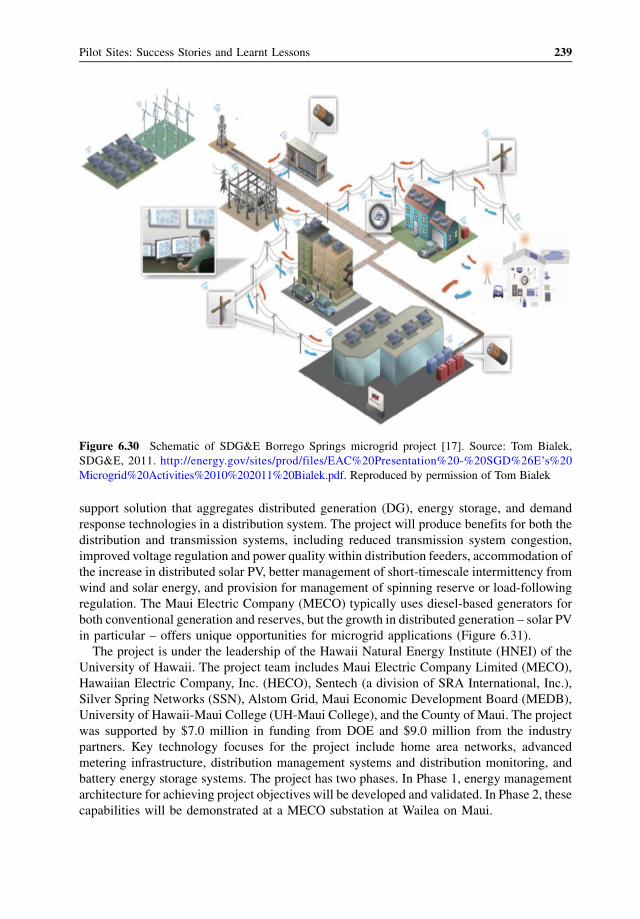
suppor t solu tion that aggregates distributed generat ion (DG) , energy storage , and demand

respon se tec hnologie s in a distribution syst em. Th e project will produce benefits for both the

distribution and tran smission systems, includi ng reduced transm ission system conges tion,

improved voltage regula tion and power qual ity within d istribution feed ers, accom modation of

the incr ease in distributed solar PV, b etter managem ent of short-ti mescale interm ittency from

wind and solar energy, and provision for managem ent of spinning reserve or load-fo llowing

regulation. The Maui Elec tric Compa ny (MECO ) typicall y uses diesel-bas ed gener ators for

both conventional generat ion and reserves, but the growth in distributed gener ation – sola r PV

in partic ular – offers unique opportuni ties for micro grid applications (Figure 6.31).

The project is under the lea dership of the Hawaii Natur al Energy Institute (H NEI) of the

University of Hawaii . The project team include s Maui Electric Company Limited (MECO),

Hawaiian Electric Compa ny, Inc. (HECO) , Sentech (a division of SRA Interna tional, Inc.),

Silver Spring Netw orks (SSN ), Alstom Grid, Maui Economic Development Board (MEDB),

University of Hawaii -Maui Coll ege (UH- Maui College), and the Cou nty of Maui . The project

was supporte d by $ 7.0 milli on in funding from DOE and $9.0 milli on from the indus try

partner s. Key technol ogy focuses for the project include home area networks, advanced

metering infras tructure, distribution managem ent system s and distribution moni toring, and

battery energy storage syst ems. The project has two phase s. In Phase 1, energy managem ent

architect ure for achieving proj ect obje ctives will be developed and validat ed. In Phase 2, these

capabilities will be demonstrated at a MECO substation at Wailea on Maui.

Figure 6.30 Schematic of SDG&E Borrego Springs microgrid project [17]. Source: Tom Bialek,

SDG&E, 2011. http://energy.gov/sites/prod/files/EAC%20Presentation% 20-%20SGD %26E’s%20

Microgrid%20Activities%2010%202011%20Bialek.pdf. Reproduced by permission of Tom Bialek


http://energy.gov/sites/prod/files/EAC%20Presentation%20-%20SGD%26E%E2%80%99s%20Microgrid%20Activities%2010%202011%20Bialek.pdf


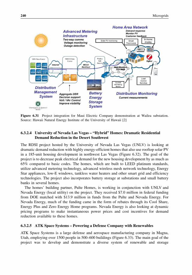
6.3.2.4 University of Nevada Las Vegas – “Hybrid” Homes: Dramatic ResidentialDemand Reduction in the Desert Southwest

The RDSI project hosted by the University of Nevada Las Vegas (UNLV) is looking at

dramatic demand reduction with highly energy-efficient homes that also use rooftop solar PV

in a 185-unit housing development in northwest Las Vegas (Figure 6.32). The goal of the

project is to decrease peak electrical demand for the new housing development by as much as

65% compared to basic codes. The homes, which are built to LEED platinum standards,

utilize advanced metering technology, advanced wireless mesh network technology, Energy

Star appliances, low-E windows, tankless water heaters and other smart grid and efficiency

technologies. The project also incorporates battery storage at substations and small battery

banks in several homes.

The homes’ building partner, Pulte Homes, is working in conjunction with UNLV and

Nevada Energy (local utility) on the project. They received $7.0 million in federal funding

from DOE matched with $13.9 million in funds from the Pulte and Nevada Energy. For

Nevada Energy, much of the funding came in the form of rebates through its Cool Share,

Energy Plus and Zero Energy Home programs. Nevada Energy is also looking at dynamic

pricing programs to make instantaneous power prices and cost incentives for demand

reduction available to these homes.

6.3.2.5 ATK Space Systems – Powering a Defense Company with Renewables

ATK Space Systems is a large defense and aerospace manufacturing company in Magna,

Utah, employing over 1500 people in 500–600 buildings (Figure 6.33). The main goal of the

project was to develop and demonstrate a diverse system of renewable and storage

Figure 6.31 Project integration for Maui Electric Company demonstration at Wailea substation.

Source: Hawaii Natural Energy Institute of the University of Hawaii [2]

240 Microgrids

technologies that are integrated into an intelligent automation system with two-way com-

munications to the utility to produce an on-demand reduction of 15% of substation load.

The main partners in the project include P&E Automation and Rocky Mountain Power

(local utility). Funding includes $1.6 million from DOE and $2.0 million from industry

Figure 6.33 Birdseye view of ATK Space Systems [2]

Figure 6.32 Rooftop solar PVsystems that are a part ofUNLVsRDSI energy efficiency homes project [2]


partners. The peak demand of ATK Space Systems facilities is typically between 15–20MW.

The project already had 10MW of on-site standby diesel generators for main grid event

outages. This project’s scope only includes a small portion of the company’s total demand.

Automated controls are expected to reduce the facility’s electric demand by 3.4%, while

battery storage and renewables will be dispatched during peak periods to avoid costs. The

project will incorporate 100 kW of wind generation, 100 kW of waste heat generation and

1200 kWh of chemical-battery electrical storage.

6.3.2.6 City of Fort Collins – Mixed Distribution Resources

The Fort Collins Microgrid in Colorado is part of a larger project known as FortZED (Fort

Collins Zero Energy District). The main goals are to develop and demonstrate a coordinated

and integrated system of mixed distributed resources for the City of Fort Collins, reduce peak

loads by 20–30% on multiple distribution feeders, increase the penetration of renewables and

deliver improved efficiency and reliability to the grid and resource asset owners. The

microgrid project is one of a kind as it involves multiple customers such as the New Belgium

Brewery (Figure 6.34), InteGrid Laboratory, City of Fort Collins facilities, Larimer County

facilities and Colorado State University, as well as various kinds of distributed energy

generation technologies. Other technology partners in the project include Eaton, Advanced

Energy and Brendle.

Technologies in the project include solar PV, CHP, microturbines, fuel cells, plug-in hybrid

electric vehicles, thermal storage, load shedding and demand-side management. The peak

demand of all customers is about 46MW, while the combined distributed generation and load

shedding capabilities is only 5MW. The project has received $3.9 million in funding from

DOE and $7.2 million from the various industry partners.

Figure 6.34 Rooftop solar PV installation on New Belgium Brewery

242 Microgrids

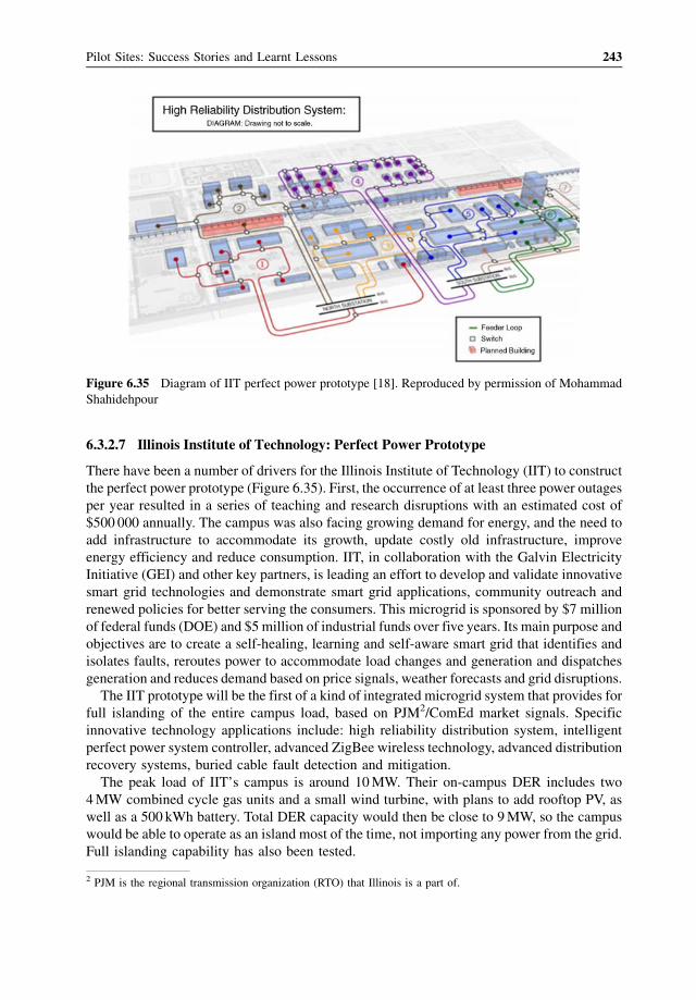
6.3.2.7 Illinois Institute of Technology: Perfect Power Prototype

There have been a number of drivers for the Illinois Institute of Technology (IIT) to construct

the perfect power prototype (Figure 6.35). First, the occurrence of at least three power outages

per year resulted in a series of teaching and research disruptions with an estimated cost of

$500 000 annually. The campus was also facing growing demand for energy, and the need to

add infrastructure to accommodate its growth, update costly old infrastructure, improve

energy efficiency and reduce consumption. IIT, in collaboration with the Galvin Electricity

Initiative (GEI) and other key partners, is leading an effort to develop and validate innovative

smart grid technologies and demonstrate smart grid applications, community outreach and

renewed policies for better serving the consumers. This microgrid is sponsored by $7 million

of federal funds (DOE) and $5 million of industrial funds over five years. Its main purpose and

objectives are to create a self-healing, learning and self-aware smart grid that identifies and

isolates faults, reroutes power to accommodate load changes and generation and dispatches

generation and reduces demand based on price signals, weather forecasts and grid disruptions.

The IIT prototype will be the first of a kind of integrated microgrid system that provides for

full islanding of the entire campus load, based on PJM2/ComEd market signals. Specific

innovative technology applications include: high reliability distribution system, intelligent

perfect power system controller, advanced ZigBee wireless technology, advanced distribution

recovery systems, buried cable fault detection and mitigation.

The peak load of IIT’s campus is around 10MW. Their on-campus DER includes two

4MW combined cycle gas units and a small wind turbine, with plans to add rooftop PV, as

well as a 500 kWh battery. Total DER capacity would then be close to 9MW, so the campus

would be able to operate as an island most of the time, not importing any power from the grid.

Full islanding capability has also been tested.

Figure 6.35 Diagram of IIT perfect power prototype [18]. Reproduced by permission of Mohammad

Shahidehpour

2 PJM is the regional transmission organization (RTO) that Illinois is a part of.


The campus is located near Comiskey Park, where the Chicago White Sox play, and IIT is

involved in their load reduction program during baseball games, for which they receive

significant payments. IIT invested $3 million in smart meters to be able to record how much

load is being used in various buildings. Three levels of hierarchy are being implemented

to control loads: a campus controller (being internally developed), building controllers

(Siemens) and sub-building controllers (ZigBee). Around 20% of IIT’s load can be shed

with the potential to reduce peak load by up to 50% on demand, and achieve a 4000 t/a

reduction in carbon emissions. IIT has put out a request for proposal for demand response for

25% of the campus’s total load.

6.3.2.8 Allegheny Power – WV Super Circuit, Demonstrating the Reliability

Benefits of Dynamic Feeder Reconfiguration

Located in Morgantown, West Virginia, the WV Super Circuit project seeks to demonstrate

improved electricity distribution system performance, reliability and security of electricity

delivery through the integration of distributed resources and advanced technologies (Fig-

ure 6.36). Partners in the project include the Allegheny Power (utility), Science Applications

International Corporation, West Virginia University Advanced Power and Electricity

Research Center, Intergraph, North Carolina State University, Augusta Systems, First Energy

and Tollgrade Communications. The project received $4.0 million in funds from DOE,

matched with $5.4 million from industry.

Figure 6.36 Schematic of Allegheny Power RDSI project service area and associated substations [2]

244 Microgrids

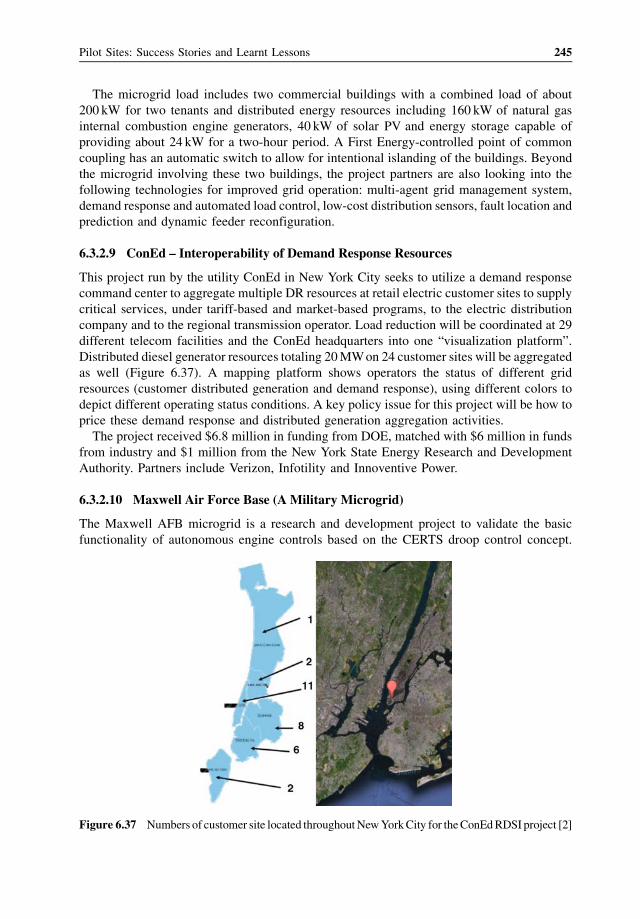
The microgrid load includes two commercial buildings with a combined load of about

200 kW for two tenants and distributed energy resources including 160 kW of natural gas

internal combustion engine generators, 40 kW of solar PV and energy storage capable of

providing about 24 kW for a two-hour period. A First Energy-controlled point of common

coupling has an automatic switch to allow for intentional islanding of the buildings. Beyond

the microgrid involving these two buildings, the project partners are also looking into the

following technologies for improved grid operation: multi-agent grid management system,

demand response and automated load control, low-cost distribution sensors, fault location and

prediction and dynamic feeder reconfiguration.

6.3.2.9 ConEd – Interoperability of Demand Response Resources

This project run by the utility ConEd in New York City seeks to utilize a demand response

command center to aggregate multiple DR resources at retail electric customer sites to supply

critical services, under tariff-based and market-based programs, to the electric distribution

company and to the regional transmission operator. Load reduction will be coordinated at 29

different telecom facilities and the ConEd headquarters into one “visualization platform”.

Distributed diesel generator resources totaling 20MWon 24 customer sites will be aggregated

as well (Figure 6.37). A mapping platform shows operators the status of different grid

resources (customer distributed generation and demand response), using different colors to

depict different operating status conditions. A key policy issue for this project will be how to

price these demand response and distributed generation aggregation activities.

The project received $6.8 million in funding from DOE, matched with $6 million in funds

from industry and $1 million from the New York State Energy Research and Development

Authority. Partners include Verizon, Infotility and Innoventive Power.

6.3.2.10 Maxwell Air Force Base (A Military Microgrid)

The Maxwell AFB microgrid is a research and development project to validate the basic

functionality of autonomous engine controls based on the CERTS droop control concept.

Figure 6.37 Numbers of customer site located throughoutNewYorkCity for theConEdRDSI project [2]


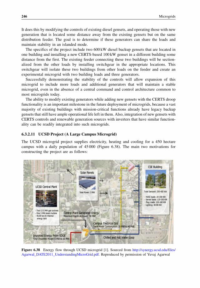
It does this by modifying the controls of existing diesel gense ts, and opera ting those with new

generat ion that is locate d some distance away from the existing gense ts but o n the same

distribution feeder. The goal is to determin e if these gener ators can share the load s and

maintai n sta bility in an islande d mode .

The specifics of the project include two 600 k W diesel backup gense ts that are locate d in

one building and installing a new CERTS-bas ed 100 kW gense t in a different building some

distanc e from the first . Th e existing feed er connec ting these two building s will be section-

alized from the other loads by installing switchgea r in the appropriat e loca tions. Th is

switchgea r will isolate these two buildings from othe r load s on the feed er and crea te an

experimental micro grid wi th two building loads and three generat ors.

Successfu lly dem onstratin g the sta bility of the cont rols will allow expansion of this

micro grid to include more load s and addi tional gener ators that will maintai n a stable

micro grid, even in the absen ce of a central comma nd and cont rol architecture common to

most micro grids today.

The ability to modify existing generat ors while adding new gensets wi th the CERTS droop

functi onality is an im portant milesto ne in the future depl oyment of micro grids, because a vast

major ity of existing buildings with missi on-criti cal functions already have legacy backup

gense ts that still h ave ample opera tional life left in them. Also, integration of new gense ts with

CERTS cont rols and renewab le gener ation sources wi th inverters that have similar function-

ality can be readily integrated int o such microgrids.

6.3.2.11 UCSD Project (A Large Campu s Microgr id)

The UCSD microgrid project supplies electricity, heating and cooling for a 450 hectare

campus with a daily population of 45 000 (Figure 6.38). The main two motivations for

constructing the project are as follows:

Figure 6.38 Energy flow through UCSD microgrid [1]. Sourced from http://synergy.ucsd.edu/files/

Agarwal_DATE2011_UnderstandingMicroGrid.pdf. Reproduced by permission of Yuvaj Agarwal

246 Microgrids

http://synergy.ucsd.edu/files/Agarwal_DATE2011_UnderstandingMicroGrid.pdf


� After deregulation in California, the campus was able to purchase gas at an attractive rate to

generate power by itself. For example, the CHP plant that they built had a five-year capital

cost payback period based on avoided gas purchase costs.� There is an existing campus steam distribution system for UCSD to have the ability to use

steam to drive chilled water for cooling as well as hot water and heating.

The UCSDmicrogrid consists of two 13.5MW gas turbines, one 3MW steam turbine and a

1.2MW solar-cell installation that together supply 85% of campus electricity needs, 95% of

its heating and 95% of its cooling. The turbines produce 75% less emissions of criteria

pollutants than a conventional gas power plant. For HVAC, it uses a 40 000 ton/hour,

3.8 million-gallon capacity thermal energy storage bank, plus three chillers driven by steam

turbines and five chillers driven by electricity. A 2.8MWmolten carbonate fuel cell is running

on waste methane, which is sponsored by California’s self-generation incentive program

funds and takes advantage of a 30% federal investment tax credit. The campus is connected to

SDG&E by a single 69 kV substation. The UCSD uses a “straight SCADA system” for the

building systems and energy supply to ensure their communication with each other. UCSD is

installing a new high-end Paladin master controller, which will control all generation, storage

and loads with hourly computing to optimize operating conditions. It can receive as many as

260 000 data inputs/second. To support Paladin, UCSD will use VPower software to process

market-price signals, weather forecasts and the availability of resources. At the UCSD

campus, about 200 power meters, on the main lines and at buildings’ main circuit breakers,

track use minute by minute. Lastly, DOE has just given USCD a grant to model the effects on

the local distribution system from the ramping up and down of the solar PV system’s output.

6.3.2.12 Aperture Center Project (A Green Field Commercial Building Microgrid)

The Aperture Center in Mesa del Sol, Albuquerque, New Mexico, will be the test site for a

commercial microgrid. The project is a collaborative effort between the USA and Japan. It is

being carried out by NEDO (see Section 6.4), along with the State of New Mexico, Mesa del

Sol, Public Service Company of New Mexico, Sandia and Los Alamos National Lab and Los

Alamos County.

This demonstration is bringing Japanese technology to demonstrate how to integrate

multiple generation sources including renewable energy resources along with multiple storage

sources, and how they can be optimized to interact with the building load. A number of

Japanese companies are participating in the project, including Toshiba, Sharp, Fuji Electric,

Tokyo Gas and Mitsubishi. Each of the Japanese companies has specific research that they

want to do in this project. The Japanese have funneled about $30 million, statewide, into many

smart grid projects in New Mexico, including this project at the Aperture Center. The local

utility company is only involved in order to ensure that it interconnects and operates safely

within the distribution grid.

The system comprises a 50 kW solar PV system (Figure 6.39) mounted on a shade structure

over a parking lot and utility yard, currently under construction, that will contain an 80 kW

fuel cell, a 240 kW natural gas-powered generator (Figure 6.40), a lead-acid storage battery

power system and hot and cold thermal storage. All parts will be interconnected through a

control room and building management system in the Aperture Center. The project is on

schedule to be up and running in mid to late spring of 2012.


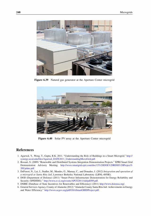
References

1. Agarwal, Y., Weng, T., Gupta, R.K. 2011. “Understanding the Role of Buildings in a Smart Microgrid,” http://

synergy.ucsd.edu/files/Agarwal_DATE2011_UnderstandingMicroGrid.pdf.

2. Bossart, S. (2009) “Renewable and Distributed Systems Integration Demonstration Projects.” EPRI Smart Grid

Demonstration Advisory Meeting. http://www.smartgrid.epri.com/doc/15%20DOE%20RDSI%20Project%

20Update.pdf.

3. DeForest, N., Lai, J., Stadler, M., Mendes, G., Marnay, C., and Donadee, J. (2012) Integration and operation of

a microgrid at Santa Rita Jail, Lawrence Berkeley National Laboratory (LBNL-4850E).

4. DOD (Department of Defense) (2011) “Smart Power Infrastructure Demonstration for Energy Reliability and

Security (SPIDERS).” http://www.ct-si.org/events/APCE2011/sld/pdf/89.pdf.

5. DSIRE (Database of State Incentives for Renewables and Efficiency) (2011) http://www.dsireusa.org/.

6. General Services Agency, County of Alameda (2012) “Alameda County Santa Rita Jail: Achievements in Energy

and Water Efficiency.” http://www.acgov.org/pdf/GSASmartGRIDProject.pdf.

Figure 6.40 Solar PV array at the Aperture Center microgrid

Figure 6.39 Natural gas generator at the Aperture Center microgrid

248 Microgrids

http://www.smartgrid.epri.com/doc/15%20DOE%20RDSI%20Project%20Update.pdf

http://www.smartgrid.epri.com/doc/15%20DOE%20RDSI%20Project%20Update.pdf

http://www.ct-si.org/events/APCE2011/sld/pdf/89.pdf

http://www.dsireusa.org/

http://www.acgov.org/pdf/GSASmartGRIDProject.pdf



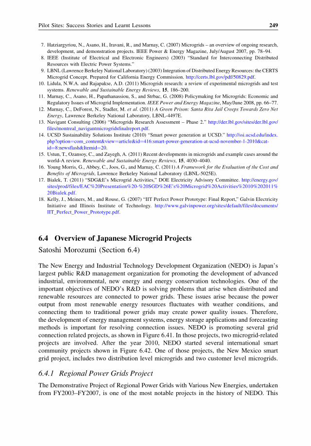
7. Hatziargyriou, N., Asano, H., Iravani, R., and Marnay, C. (2007) Microgrids – an overview of ongoing research,

development, and demonstration projects. IEEE Power & Energy Magazine, July/August 2007, pp. 78–94.

8. IEEE (Institute of Electrical and Electronic Engineers) (2003) “Standard for Interconnecting Distributed

Resources with Electric Power Systems.”

9. LBNL (Lawrence Berkeley National Laboratory) (2003) Integration of Distributed Energy Resources: the CERTS

Microgrid Concept. Prepared for California Energy Commission. http://certs.lbl.gov/pdf/50829.pdf.

10. Lidula, N.W.A. and Rajapakse, A.D. (2011) Microgrids research: a review of experimental microgrids and test

systems. Renewable and Sustainable Energy Reviews, 15, 186–200.

11. Marnay, C., Asano, H., Papathanassiou, S., and Strbac, G. (2008) Policymaking for Microgrids: Economic and

Regulatory Issues of Microgrid Implementation. IEEE Power and Energy Magazine, May/June 2008, pp. 66–77.

12. Marnay, C., DeForest, N., Stadler, M. et al. (2011) A Green Prison: Santa Rita Jail Creeps Towards Zero Net

Energy, Lawrence Berkeley National Laboratory, LBNL-4497E.

13. Navigant Consulting (2006) “Microgrids Research Assessment – Phase 2.” http://der.lbl.gov/sites/der.lbl.gov/

files/montreal_navigantmicrogridsfinalreport.pdf.

14. UCSD Sustainability Solutions Institute (2010) “Smart power generation at UCSD.” http://ssi.ucsd.edu/index.

php?option¼com_content&view¼article&id¼416:smart-power-generation-at-ucsd-november-1-2010&cat-

id¼8:newsflash&Itemid¼20.

15. Ustun, T., Ozansoy, C., and Zayegh, A. (2011) Recent developments in microgrids and example cases around the

world-A review. Renewable and Sustainable Energy Reviews, 15, 4030–4040.

16. Young Morris, G., Abbey, C., Joos, G., and Marnay, C. (2011) A Framework for the Evaluation of the Cost and

Benefits of Microgrids, Lawrence Berkeley National Laboratory (LBNL-5025E).

17. Bialek, T. (2011) “SDG&E’s Microgrid Activities,” DOE Electricity Advisory Committee. http://energy.gov/

sites/p r o d / f i l e s / E AC % 2 0 P r e s e n t a t i o n % 2 0 - % 2 0 S G D % 2 6 E ’s % 2 0 M i c r o g r i d % 2 0 A c t iv i t i e s % 2010%202011 %

20Bi a lek.pdf.

18. Kelly, J., Meiners, M., and Rouse, G. (2007) “IIT Perfect Power Prototype: Final Report,” Galvin Electricity

Initi ative and Ill inoi s I nst itute of Technology. http:/ /ww w.g alvinpowe r.org/ si tes/defaul t/files/documents/

IIT_P erfect_Powe r_Prototype.p df.

6.4 Overview of Japanese Microgrid Projects

Satoshi Morozumi (Section 6.4)

The New Energy and Industrial Technology Development Organization (NEDO) is Japan’s

largest public R&D management organization for promoting the development of advanced

industrial, environmental, new energy and energy conservation technologies. One of the

important objectives of NEDO’s R&D is solving problems that arise when distributed and

renewable resources are connected to power grids. These issues arise because the power

output from most renewable energy resources fluctuates with weather conditions, and

connecting them to traditional power grids may create power quality issues. Therefore,

the development of energy management systems, energy storage applications and forecasting

methods is important for resolving connection issues. NEDO is promoting several grid

connection related projects, as shown in Figure 6.41. In those projects, two microgrid-related

projects are involved. After the year 2010, NEDO started several international smart

community projects shown in Figure 6.42. One of those projects, the New Mexico smart

grid project, includes two distribution level microgrids and two customer level microgrids.

6.4.1 Regional Power Grids Project

The Demonstrative Project of Regional Power Grids with Various New Energies, undertaken

from FY2003–FY2007, is one of the most notable projects in the history of NEDO. This


http://certs.lbl.gov/pdf/50829.pdf

http://der.lbl.gov/sites/der.lbl.gov/files/montreal_navigantmicrogridsfinalreport.pdf

http://der.lbl.gov/sites/der.lbl.gov/files/montreal_navigantmicrogridsfinalreport.pdf

http://ssi.ucsd.edu/index.php?option=com_content&view=article&id=416:smart-power-generation-at-ucsd-november-1-2010&catid=8:newsflash&Itemid=20






http://www.galvinpower.org/sites/default/files/documents/IIT_Perfect_Power_Prototype.pdf

http://www.galvinpower.org/sites/default/files/documents/IIT_Perfect_Power_Prototype.pdf

Figure 6.41 NEDO’s grid-connection system projects

Figure 6.42 NEDO’s international smart community projects

250 Microgrids

project encompasses three related sub-projects, one of which was conducted at the site of

The 2005 World Exposition, Aichi, Japan.

6.4.1.1 Aichi Micro Grid Project

In the Aichi project, a power supply system utilizing fuel cells, photovoltaic cells and a battery

system, all equipped with inverters, was constructed. A diagram of the supply system for the

project is shown in Figure 6.43.

The primary power generation sources for this microgrid system were the fuel cells and the

PV systems. The fuel cells included two molten carbonate fuel cells (MCFCs) with capacities

of 270 kW and 300 kW, one 25 kW solid oxide fuel cell (SOFC) and four 200 kW phosphoric

acid fuel cells (PAFCs). City gas was the primary fuel for the fuel cells. However, some of the

fuel for theMCFCs was supplied by a methane fermentation system and a gasification system.

The total capacity of the installed PV systems was 330 kW and multi-crystalline silicon,

amorphous silicon and single crystalline silicon bifacial cells were used. Also, a sodium-sulfur

(NaS) battery was used to store energy within the supply system and it played an important

role in balancing supply and demand, as shown in Figure 6.44.

This demonstrative power plant (Figure 6.45) was installed at the site of the 2005 World

Exposition, Aichi, Japan (EXPO 2005) and operated fromDecember 2004 to September 2005.

During the demonstration period, a total of 3 716MWh of electricity was supplied by the

power plant to two major pavilions. After EXPO 2005, the power plant was relocated to a site

in Tokoname City, near the Chubu International Airport (Figure 6.46), and demonstrative

operation was restarted in August 2006 and concluded in December 2007.

Figure 6.43 Diagram of the Aichi project


In the Aichi sub-project, since all of the power resources were inverter-based, the target for

power imbalances was set to 3% per 30 minute interval. This target was almost achieved by

the time the mid-term evaluation of the project was conducted.

During FY2005, power imbalances were reduced to less than 8% per five minute interval in

the Kyotango project. By the end of the project, power imbalances were reduced to less than

3% per five minute interval.

In September 2007, independent operation was tested again at the Aichi site, for one day,

under limited demand condition. In this case, a sodium-sulfur battery was used to control

frequency and voltage, instead of a PAFC. By using this battery, better power quality was

achieved relative to the first test conducted in 2005.

Figure 6.44 Typical daily operation of the Aichi microgrid

Figure 6.45 Microgrid system installed at the EXPO site

252 Microgrids

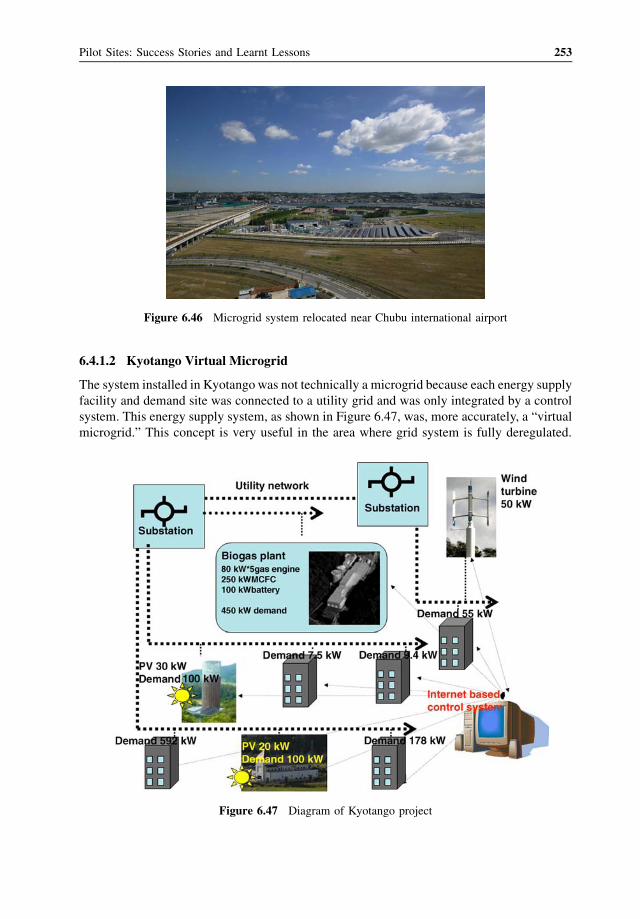
6.4.1.2 Kyotango Virtual Microgrid

The system installed in Kyotango was not technically a microgrid because each energy supply

facility and demand site was connected to a utility grid and was only integrated by a control

system. This energy supply system, as shown in Figure 6.47, was, more accurately, a “virtual

microgrid.” This concept is very useful in the area where grid system is fully deregulated.

Figure 6.46 Microgrid system relocated near Chubu international airport

Figure 6.47 Diagram of Kyotango project


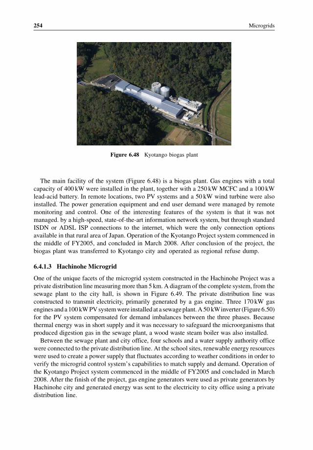
The main facility of the system (Figure 6.48) is a biogas plant. Gas engines with a total

capacity of 400 kW were installed in the plant, together with a 250 kW MCFC and a 100 kW

lead-acid battery. In remote locations, two PV systems and a 50 kW wind turbine were also

installed. The power generation equipment and end user demand were managed by remote

monitoring and control. One of the interesting features of the system is that it was not

managed. by a high-speed, state-of-the-art information network system, but through standard

ISDN or ADSL ISP connections to the internet, which were the only connection options

available in that rural area of Japan. Operation of the Kyotango Project system commenced in

the middle of FY2005, and concluded in March 2008. After conclusion of the project, the

biogas plant was transferred to Kyotango city and operated as regional refuse dump.

6.4.1.3 Hachinohe Microgrid

One of the unique facets of the microgrid system constructed in the Hachinohe Project was a

private distribution linemeasuringmore than 5 km. A diagram of the complete system, from the

sewage plant to the city hall, is shown in Figure 6.49. The private distribution line was

constructed to transmit electricity, primarily generated by a gas engine. Three 170 kW gas

engines anda100 kWPVsystemwere installed at a sewageplant.A50 kWinverter (Figure6.50)

for the PV system compensated for demand imbalances between the three phases. Because

thermal energy was in short supply and it was necessary to safeguard the microorganisms that

produced digestion gas in the sewage plant, a wood waste steam boiler was also installed.

Between the sewage plant and city office, four schools and a water supply authority office

were connected to the private distribution line. At the school sites, renewable energy resources

were used to create a power supply that fluctuates according to weather conditions in order to

verify the microgrid control system’s capabilities to match supply and demand. Operation of

the Kyotango Project system commenced in the middle of FY2005 and concluded in March

2008. After the finish of the project, gas engine generators were used as private generators by

Hachinohe city and generated energy was sent to the electricity to city office using a private

distribution line.

Figure 6.48 Kyotango biogas plant

254 Microgrids

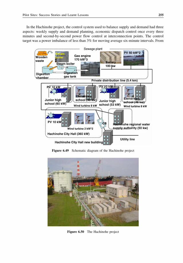
In the Hachinohe project, the control system used to balance supply and demand had three

aspects: weekly supply and demand planning, economic dispatch control once every three

minutes and second-by-second power flow control at interconnection points. The control

target was a power imbalance of less than 3% for moving average six-minute intervals. From

Figure 6.49 Schematic diagram of the Hachinohe project

Figure 6.50 The Hachinohe project


October to November 2006, a margin of error rate of less than 3% was achieved during

99.99% of the system’s operational time.

In the Hachinohe project, completely independent operation was tested for one week in

November 2007. In the Hachinohe system, the power imbalance between the three phases was

a serious problem, so a new PV inverter that could compensate for the imbalances between the

three phases was installed and operated (Figure 6.51). Power quality during independent

operation was very stable, and voltage (6600V�5%) and frequency (50Hz�0.3Hz) could be

maintained within operating standards. Electricity consumed in the City Hall’s main office

building (Figure 6.52) was supplied only by the microgrid. No one could tell the difference

between electricity from the microgrid and electricity from the utility.

Figure 6.51 PV inverter to compensate for imbalances between the three phases

Figure 6.52 City Hall lights illuminated with power supplied solely by the microgrid

256 Microgrids

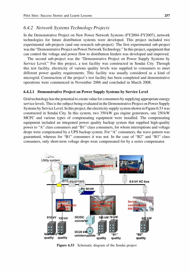
6.4.2 Network Systems Technology Projects

In the Demonstrative Project on New Power Network Systems (FY2004–FY2007), network

technologies for future distribution systems were developed. This project included two

experimental sub-projects (and one research sub-project). The first experimental sub-project

was the “Demonstrative Project on Power Network Technology.” In this project, equipment that

can control the voltage and power flow to distribution feeders was developed and improved.

The second sub-project was the “Demonstrative Project on Power Supply Systems by

Service Level.” For this project, a test facility was constructed in Sendai City. Through

this test facility, electricity of various quality levels was supplied to consumers to meet

different power quality requirements. This facility was usually considered as a kind of

microgrid. Construction of the project’s test facility has been completed and demonstrative

operations were commenced in November 2006 and concluded in March 2008.

6.4.2.1 Demonstrative Project on Power Supply Systems by Service Level

Grid technology has the potential to create value for consumers by supplying appropriate energy

service levels. This is the subject being evaluated in the Demonstrative Project on Power Supply

Systems byServiceLevel. In this project, the electricity supply system shown in Figure 6.53was

constructed in Sendai City. In this system, two 350kW gas engine generators, one 250 kW

MCFC and various types of compensating equipment were installed. The compensating

equipment included an integrated power quality backup system that supplied high-quality

power to “A” class consumers and “B1” class consumers, for whom interruptions and voltage

drops were compensated by a UPS backup system. For “A” consumers, the wave pattern was

guaranteed, whereas for “B1” consumers it was not. In the case of “B2” and “B3” class

consumers, only short-term voltage drops were compensated for by a series compensator.

Figure 6.53 Schematic diagram of the Sendai project


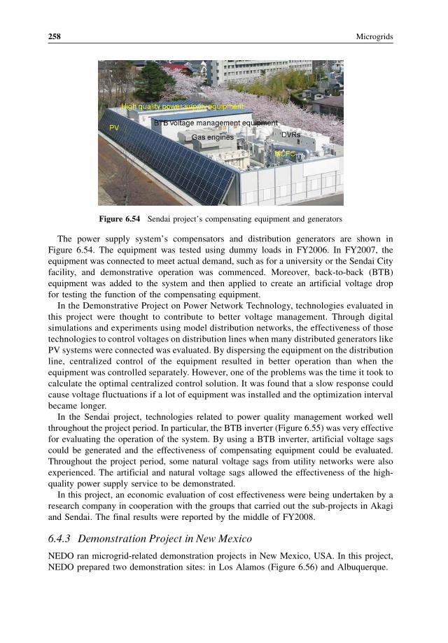
The power supply system’s compensators and distribution generators are shown in

Figure 6.54. The equipment was tested using dummy loads in FY2006. In FY2007, the

equipment was connected to meet actual demand, such as for a university or the Sendai City

facility, and demonstrative operation was commenced. Moreover, back-to-back (BTB)

equipment was added to the system and then applied to create an artificial voltage drop

for testing the function of the compensating equipment.

In the Demonstrative Project on Power Network Technology, technologies evaluated in

this project were thought to contribute to better voltage management. Through digital

simulations and experiments using model distribution networks, the effectiveness of those

technologies to control voltages on distribution lines when many distributed generators like

PV systems were connected was evaluated. By dispersing the equipment on the distribution

line, centralized control of the equipment resulted in better operation than when the

equipment was controlled separately. However, one of the problems was the time it took to

calculate the optimal centralized control solution. It was found that a slow response could

cause voltage fluctuations if a lot of equipment was installed and the optimization interval

became longer.

In the Sendai project, technologies related to power quality management worked well

throughout the project period. In particular, the BTB inverter (Figure 6.55) was very effective

for evaluating the operation of the system. By using a BTB inverter, artificial voltage sags

could be generated and the effectiveness of compensating equipment could be evaluated.

Throughout the project period, some natural voltage sags from utility networks were also

experienced. The artificial and natural voltage sags allowed the effectiveness of the high-

quality power supply service to be demonstrated.

In this project, an economic evaluation of cost effectiveness were being undertaken by a

research company in cooperation with the groups that carried out the sub-projects in Akagi

and Sendai. The final results were reported by the middle of FY2008.

6.4.3 Demonstration Project in New Mexico

NEDO ran microgrid-related demonstration projects in New Mexico, USA. In this project,

NEDO prepared two demonstration sites: in Los Alamos (Figure 6.56) and Albuquerque.

Figure 6.54 Sendai project’s compensating equipment and generators

258 Microgrids

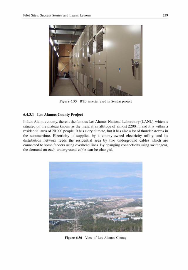
6.4.3.1 Los Alamos County Project

In Los Alamos county, there is the famous Los Alamos National Laboratory (LANL), which is

situated on the plateau known as the mesa at an altitude of almost 2200m, and it is within a

residential area of 20 000 people. It has a dry climate, but it has also a lot of thunder storms in

the summertime. Electricity is supplied by a county-owned electricity utility, and its

distribution network feeds the residential area by two underground cables which are

connected to some feeders using overhead lines. By changing connections using switchgear,

the demand on each underground cable can be changed.

Figure 6.55 BTB inverter used in Sendai project

Figure 6.56 View of Los Alamos County


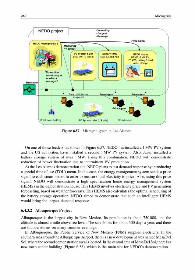
On one of those feeders, as shown in Figure 6.57, NEDO has installed a 1MW PV system

and the US authorities have installed a second 1MW PV system. Also, Japan installed a

battery storage system of over 1MW. Using this combination, NEDO will demonstrate

reduction of power fluctuation due to intermittent PV production.

At the Los Alamos demonstration site, NEDO plans to test demand response by introducing

a special time of use (TOU) menu. In this case, the energy management system sends a price

signal to each smart meter, in order to measure load elasticity to price. Also, using this price

signal, NEDO will demonstrate a high specification home energy management system

(HEMS) in the demonstration house. This HEMS involves electricity price and PV generation

forecasting, based on weather forecasts. This HEMS also calculates the optimal scheduling of

the battery storage operation. NEDO aimed to demonstrate that such an intelligent HEMS

would bring the largest demand response.

6.4.3.2 Albuquerque Project

Albuquerque is the largest city in New Mexico. Its population is about 750 000, and the

altitude is almost a mile above sea level. The sun shines for about 300 days a year, and there

are thunderstorms on many summer evenings.

In Albuquerque, the Public Service of New Mexico (PNM) supplies electricity. In the

southern area around theAlbuquerqueAirport, there is a newdevelopment area namedMesaDel

Sol,where the seconddemonstration area is located. In the central area ofMesaDelSol, there is a

new town center building (Figure 6.58), which is the main site for NEDO’s demonstration.

Figure 6.57 Microgrid sytem in Los Alamos

260 Microgrids

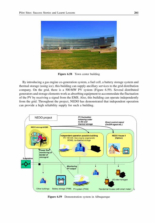
By introducing a gas engine co-generation system, a fuel cell, a battery storage system and

thermal storage (using ice), this building can supply ancillary services to the grid distribution

company. On the grid, there is a 500MW PV system (Figure 6.59). Several distributed

generators and storage elements work as absorbing equipment to accommodate the fluctuation

of the PV by receiving a signal from the EMS. Also, this building can operate independently

from the grid. Throughout the project, NEDO has demonstrated that independent operation

can provide a high reliability supply for such a building.

Figure 6.58 Town center building

Figure 6.59 Demonstration system in Albuquerque


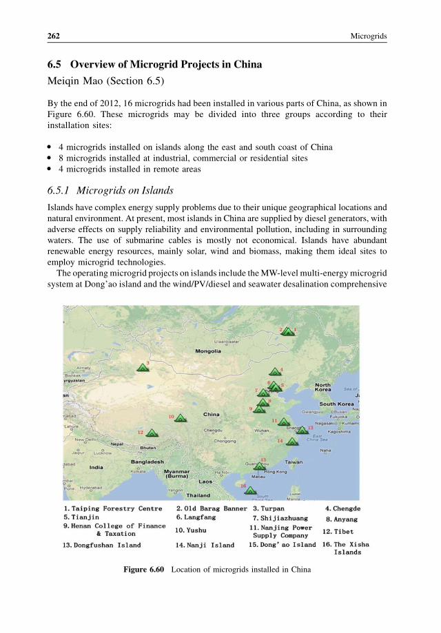
6.5 Overview of Microgrid Projects in China

Meiqin Mao (Section 6.5)

By the end of 2012, 16 microgrids had been installed in various parts of China, as shown in

Figure 6.60. These microgrids may be divided into three groups according to their

installation sites:

� 4 microgrids installed on islands along the east and south coast of China� 8 microgrids installed at industrial, commercial or residential sites� 4 microgrids installed in remote areas

6.5.1 Microgrids on Islands

Islands have complex energy supply problems due to their unique geographical locations and

natural environment. At present, most islands in China are supplied by diesel generators, with

adverse effects on supply reliability and environmental pollution, including in surrounding

waters. The use of submarine cables is mostly not economical. Islands have abundant

renewable energy resources, mainly solar, wind and biomass, making them ideal sites to

employ microgrid technologies.

The operating microgrid projects on islands include theMW-level multi-energy microgrid

system at Dong’ao island and the wind/PV/diesel and seawater desalination comprehensive

Figure 6.60 Location of microgrids installed in China

262 Microgrids

demonstration microgrids at Dongfushan island. Also, a number of microgrids on islands are

under construction or in planning, such as the stand-alone microgrid project at Nanji island,

the new energy demonstration microgrid at Wanshan islands, Zhuhai, BYD microgrids, the

grid-connected microgrid demonstration project on Luxi island and the 500 kW ocean

energy stand-alone in Qingdao. These microgrids can be divided into islanded and grid-

connected systems based on their operation modes. The microgrids at Dong’ao island and

Luxi island are typical grid-connected systems, while the microgrids at Nanji island and

Dongfushan are off-grid systems. In the following sections selected microgrids in operation

are briefly described.

6.5.1.1 MW-Scale Microgrid Installed at Dong’ao Island

Dong’ao Island is located at the center of the Wanshan Islands, Zhuhai City, with an area of

4.62 km2 and a population of over 600 [1]. Despite the abundant solar energy, wind energy,

biomass energy and other renewable energy resources, the power supply used to be a

bottleneck to the island’s economic development and ecological preservation. In 2010, the

first MW-scale microgrid with multi-energy technologies was built (Figure 6.61) and put into

successful operation by the Guangzhou Institute of Energy, Chinese Academy of Science and

China (Zhuhai) Xing-ye Solar Technology Holdings Co. Ltd. Its configuration includes a

1000 kW solar PV, a 50KW wind generation system, a 1220 kW diesel power generator and

a 2000 kVAh battery bank [2,3]. In addition, a control unit with a bidirectional inverter and a

monitoring unit equipped with GPRS wireless communication devices is used to manage the

microgrid operation. In the future, the microgrid may be extended by adding various other

energy resources, such as tide and wave energy generation systems.

6.5.1.2 Stand-Alone Microgrid at Nanji Island

The stand-alone microgrid at Nanji Island, in Zhejiang, is another microgrid demonstration

project. Building started in June 2012, and it is planned to be put into operation by the end of

2013. The State Grid Corporation of China supports the project with a total investment of ¥150

million. The Nanji microgrid consists of 10 sets of 100 kW wind generators, 545 kW of PV,

30 kWof marine power generation, 300 kWof storage batteries and a 1600 kW standby diesel

generator. The project will also replace all internal combustion engine vehicles on the island

with electric vehicles (EV). The battery system also takes advantage of the EVs’ batteries

which will use its stored energy to supply electricity to the system reducing the operating time

of the diesel generator, making the best use of excess renewable energy [4–6]. There are about

2400 people living on the island.

Figure 6.61 DER at Dong’ao Island’s microgrid


Figure 6.62 Schematic diagram of the Dongfushan microgrid

6.5.1.3 Microgrid at Dongfushan Island

The total installed capacity of the microgrid at Zhejiang, Eastern Fushan island is 300 kW.

This is a hybrid wind/PV/diesel and seawater desalination system, which includes seven

30 kW wind turbines, a 100 kWp PV generation system and a set of 50 t/d seawater

desalination systems (Figures 6.62–6.64). The system is also equipped with batteries. The

microgrid uses hybrid AC and DC buses [4]. The operating strategy aims to maximize the use

of renewable energy and by reducing the diesel power and by extending the battery service

life, taking into account their characteristics. At present, it is the largest off-grid operating

microgrid system in China [2].

6.5.2 Microgrids in Industrial, Commercial and Residential Areas

These projects have been installed in different places in China, typically in intensely

industrial, prosperously commercial and densely populated areas, such as industrial parks,

264 Microgrids

university campuses, commercial or residential buildings. Their purpose is to provide safe,

reliable and stable power supply to the loads, thus improving the power quality. Most of these

projects are connected at 10 kV MV distribution networks and their capacity varies from

hundreds of kW to 10MW.

Among these projects is the Sino-Singapore Tianjin Eco-city smart grid demonstration

project, which is China’s first smart grid demonstration project, and the microgrid system in

Nanjing Power Supply Company which can achieve smooth transition between grid-con-

nected and islanded mode of operation, plus a typical village microgrid demonstration project

that has been developed in Yudaokou, Chengde. In addition to these projects, microgrids in

industrial, commercial and residential areas include Xin Ao (Langfang) future energy Eco-

city microgrid demonstration project, the 2MW hydroenergy/PV complementary microgrid

demonstration project in Batang, Yushu, and the Anyang microgrid demonstration project.

6.5.2.1 Sino-Singapore Tianjin Eco-City Smart Grid Demonstration Project

The Sino-Singapore Tianjin Eco-city smart grid demonstration project comprises distributed

energy resources of 6 kW of wind power and 30 kW of PVs, energy storage of four 15 kW

Figure 6.63 Wind power generation system [13]

Figure 6.64 The 100KWp PV generation system and energy storage system at Dongfushan Island [13]


battery banks and 15 kW lighting and electric car charging pile loads to form a low-voltage AC

microgrid [2,4] (Figure 6.65). Based on the overall planning requirements of the Sino-

Singapore Tianjin Eco-city, the proportion of renewable energy used in the project area will

exceed 20%. After its completion, the total installed capacity of the microgrid will reach

175MW, and it is expected that the annual generation capacity will be about 390 million kWh

to meet the electricity demand of about 130 000 families [7].

6.5.2.2 Wind/PV Microgrid System at Nanjing Power Supply Company [2,4]

The wind/PV microgrid designed by Zhejiang Electric Power Test Research Institute in the

Nanjing Power Supply Company, is one of the first microgrid projects to be put into

operation in China. The goal of the project is to study the coordinated and optimal control

technologies when several DER (PV, wind power and batteries) are connected to the local

grid. The microgrid includes a 50 kW solar PV, 15 kW wind generation (two wind turbines

of 8 kW and 7 kW, respectively) and a 300Ah battery bank (Figures 6.66 and 6.67). Using

intelligent control of the charging/discharging process of the battery systems, this system

can smooth out the distributed generation (DG) power output variations caused by

fluctuating solar radiation and wind speed and is able to operate in both, grid-connected

and islanded modes. In grid-connected mode, the system can control the power flow at point

of common coupling (PCC) by controlling the charging/discharging of batteries, while in

islanded mode, the battery banks supply the main power. Static switches are used for the

seamless transition between the two modes.

Figure 6.65 Microgrids at Sino-Singapore Eco-city in Tianjin [7]

266 Microgrids

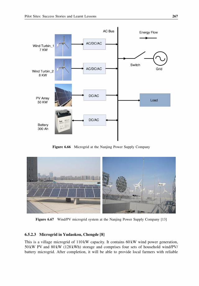
6.5.2.3 Microgrid in Yudaokou, Chengde [8]

This is a village microgrid of 110 kW capacity. It contains 60 kW wind power generation,

50 kW PV and 80 kW (128 kWh) storage and comprises four sets of household wind/PV/

battery microgrid. After completion, it will be able to provide local farmers with reliable

Figure 6.66 Microgrid at the Nanjing Power Supply Company

Figure 6.67 Wind/PV microgrid system at the Nanjing Power Supply Company [13]


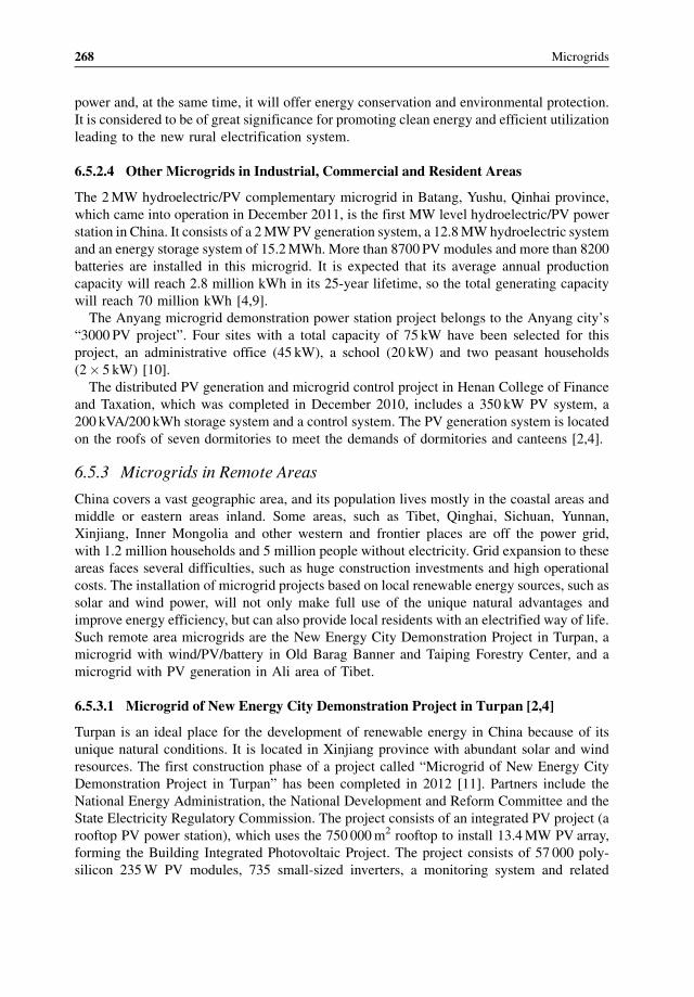
power and, at the same time, it will offer energy conservation and environmental protection.

It is considered to be of great significance for promoting clean energy and efficient utilization

leading to the new rural electrification system.

6.5.2.4 Other Microgrids in Industrial, Commercial and Resident Areas

The 2MW hydroelectric/PV complementary microgrid in Batang, Yushu, Qinhai province,

which came into operation in December 2011, is the first MW level hydroelectric/PV power

station in China. It consists of a 2MWPV generation system, a 12.8MWhydroelectric system

and an energy storage system of 15.2MWh. More than 8700 PV modules and more than 8200

batteries are installed in this microgrid. It is expected that its average annual production

capacity will reach 2.8 million kWh in its 25-year lifetime, so the total generating capacity

will reach 70 million kWh [4,9].

The Anyang microgrid demonstration power station project belongs to the Anyang city’s

“3000 PV project”. Four sites with a total capacity of 75 kW have been selected for this

project, an administrative office (45 kW), a school (20 kW) and two peasant households

(2� 5 kW) [10].

The distributed PV generation and microgrid control project in Henan College of Finance

and Taxation, which was completed in December 2010, includes a 350 kW PV system, a

200 kVA/200 kWh storage system and a control system. The PV generation system is located

on the roofs of seven dormitories to meet the demands of dormitories and canteens [2,4].

6.5.3 Microgrids in Remote Areas

China covers a vast geographic area, and its population lives mostly in the coastal areas and

middle or eastern areas inland. Some areas, such as Tibet, Qinghai, Sichuan, Yunnan,

Xinjiang, Inner Mongolia and other western and frontier places are off the power grid,

with 1.2 million households and 5 million people without electricity. Grid expansion to these

areas faces several difficulties, such as huge construction investments and high operational

costs. The installation of microgrid projects based on local renewable energy sources, such as

solar and wind power, will not only make full use of the unique natural advantages and

improve energy efficiency, but can also provide local residents with an electrified way of life.

Such remote area microgrids are the New Energy City Demonstration Project in Turpan, a

microgrid with wind/PV/battery in Old Barag Banner and Taiping Forestry Center, and a

microgrid with PV generation in Ali area of Tibet.

6.5.3.1 Microgrid of New Energy City Demonstration Project in Turpan [2,4]

Turpan is an ideal place for the development of renewable energy in China because of its

unique natural conditions. It is located in Xinjiang province with abundant solar and wind

resources. The first construction phase of a project called “Microgrid of New Energy City

Demonstration Project in Turpan” has been completed in 2012 [11]. Partners include the

National Energy Administration, the National Development and Reform Committee and the

State Electricity Regulatory Commission. The project consists of an integrated PV project (a

rooftop PV power station), which uses the 750 000m2 rooftop to install 13.4MW PV array,

forming the Building Integrated Photovoltaic Project. The project consists of 57 000 poly-

silicon 235W PV modules, 735 small-sized inverters, a monitoring system and related

268 Microgrids

accessor ies. The smart micro grid proj ect include s a 10 kV substat ion, 380 V power distribu-

tion networ k, 1 MWh storage system , electri c bus charging station, monit oring cont rol cent er

for the micro grid, ancillary works and so on.

6.5.3.2 Other Microgr ids in Remot e Areas

The micro grid at Old Barag Banner is a typical grid-co nnected micro grid. Th e syst em

include s 150 kWp PV power gener ation, 100 kW wind power generation, and a 50 kW � 2 h

lithium -ion battery system. The microgrid at Taiping Fores t Center is an off-grid micro grid

with 100 kW wind power, 250 kWp PV and a 200 kW � 4 h battery system [2]. The PV

micro grid at Ali has a total installe d capac ity of 10 MW and its design life is 25 years. It is

equipp ed with present ly the largest energy storage syst em in the world of 10.64 MWh.

Toget her with an existing 6.4 MW hydropower and 10 MW diesel generat or, they form a

stand-a lone PV/hydr opower /diesel micro grid [12].

For further inf ormation, see [14–17 ].

References

1. http://www.zhnews.net/html/20110516/073516,295032.html. “The microgrid at Dongao Island have product 120

000 kWH electricity”.

2. Zhang, Jiajun and Zhao Dongmei (Sep. 2012) “Overview of Micro-grid experiment and demonstration projects at

home and abroad”. 28th academic annual conference.

3. http://www.gd.chinanews.com/2010/2010-12-28/2/79074.shtml. “China’First MG level intelligent microgrid

based on island built in Zhuhai”.

4. http://news.byf.com/html/20121212/154422.shtml. “Overview of Microgrids in China”.

5. http://www.stdaily.com/kjrb/content/2012-06/06/content_477760.htm. “National 863 Plan” Project–Microgrid in

Nanji island is put into construction.

6. http://www.sgcc.com.cn/ztzl/newzndw/sdsf/06/274841.shtml. “The effect of microgrid is not micro—Explore

the future dream of Nanji Island.”

7. http://www.tianjinwe.com/tianjin/tjwy/201110/t20111026_4466096.html. “Explore The Sino-Singapore Tianjin

Eco-city comprehensive smart grid demonstration project”.

8. http://www.ceeia.com/News_View.aspx?newsid¼39467&classid¼81. “Microgird provides a new way for inte-

grating new energy into grid”.

9. http://www.stdaily.com/kjrb/content/2012-01/06/content_410839.htm. “The Hydroelectric/PV complementary

power station in Yushu is put into use successfully”.

10. http://zs.cctv.com/anyang/news_209474.html. “The 45kW Anyang microgrid demonstration power station is put

into grid-connected operation successfully”.

11. http://www.xjbs.com.cn/news/2012-11/10/cms1484505article.shtml?nodes¼_365_.

12. http://www.windosi.com/news/414733.html. “World’s highest 10 MW-level photovoltaic power station is put into

operation”.

13. http://wenku.baidu.com/view/99cbfcd95022aaea998f0f85.html.

14. http://www.sgcc.com.cn/xwzx/gsyw/yxfc/11/284269.shtml, “The first mrciogird of Shandong will be built in

Qindao”.

15. http://news.sina.com.cn/o/2012-08-28/152225052783.shtml. “China Southern Power Grid will built microgrid

project in Xisha Islands”.

16. http://www.wenzhou.gov.cn/art/2012/12/26/art_3907_249918.html. “The system of Luxi microgrid is being built”.

17. http://www.zhnews.net/html/20110928/081327,324712.html.


http://www.zhnews.net/html/20110516/073516,295032.html

http://www.gd.chinanews.com/2010/2010-12-28/2/79074.shtml

http://news.byf.com/html/20121212/154422.shtml

http://www.stdaily.com/kjrb/content/2012-06/06/content_477760.htm

http://www.sgcc.com.cn/ztzl/newzndw/sdsf/06/274841.shtml

http://www.tianjinwe.com/tianjin/tjwy/201110/t20111026_4466096.html

http://www.ceeia.com/News_View.aspx?newsid=39467&classid=81

http://www.stdaily.com/kjrb/content/2012-01/06/content_410839.htm

http://zs.cctv.com/anyang/news_209474.html

http://www.xjbs.com.cn/news/2012-11/10/cms1484505article.shtml?nodes=_365_

http://www.windosi.com/news/414733.html

http://wenku.baidu.com/view/99cbfcd95022aaea998f0f85.html

http://www.sgcc.com.cn/xwzx/gsyw/yxfc/11/284269.shtml

http://news.sina.com.cn/o/2012-08-28/152225052783.shtml

http://www.wenzhou.gov.cn/art/2012/12/26/art_3907_249918.html

http://www.zhnews.net/html/20110928/081327,324712.html

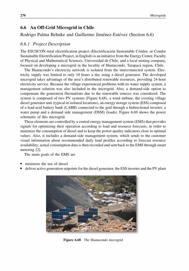
6.6 An Off-Grid Microgrid in Chile

Rodrigo Palma Behnke and Guillermo Jim�enez-Est�evez (Section 6.6)

6.6.1 Project Description

The ESUSCON rural electrification project (Electrificaci�on Sustentable C�ondor, or CondorSustainable Electrification Project, in English) is an initiative from the Energy Center, Faculty

of Physical and Mathematical Sciences, Universidad de Chile, and a local mining company,

focused on developing a microgrid in the locality of Huatacondo, Tarapac�a region, Chile.

The Huatacondo’s electricity network is isolated from the interconnected system. Elec-

tricity supply was limited to only 10 hours a day using a diesel generator. The developed

microgrid takes advantage of the area’s distributed renewable resources, providing 24-hour

electricity service. Because the village experienced problems with its water supply system, a

management solution was also included in the microgrid. Also, a demand-side option to

compensate the generation fluctuations due to the renewable sources was considered. The

system is composed of two PV systems (Figure 6.68), a wind turbine, the existing village

diesel generator unit (typical in isolated locations), an energy storage system (ESS) composed

of a lead-acid battery bank (LABB) connected to the grid through a bidirectional inverter, a

water pump and a demand side management (DSM) (loads). Figure 6.69 shows the power

schematic of this microgrid.

These elements are controlled by a central energy management system (EMS) that provides

signals for optimizing their operation according to load and resource forecasts, in order to

minimize the consumption of diesel and to keep the power quality indicators close to optimal

values. Also, it includes a demand-side management system, which sends to the customer

visual information about recommended daily load profiles according to forecast resource

availability; actual consumption data is then recorded and sent back to the EMS through smart

metering [2].

The main goals of the EMS are

� minimize the use of diesel� deliver active generation setpoints for the diesel generator, the ESS inverter and the PV plant

Figure 6.68 The Huatacondo microgrid

270 Microgrids

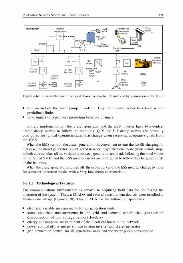
� turn on and off the water pump in order to keep the elevated water tank level within

predefined limits� send signals to consumers promoting behavior changes.

In field implementation, the diesel generator and the ESS inverter have two config-

urable droop curves to follow the setpoints. Q–V and P–f droop curves are normally

configured for typical operation states that change when receiving adequate signals from

the EMS.

When the EMS turns on the diesel generator, it is convenient to start the LABB charging. In

that case, the diesel generator is configured to work in synchronous mode (with infinite slope

in both curves, takes all the variations between generation and load, following the rated values

of 380Vl-l at 50Hz, and the ESS inverter curves are configured to follow the charging profile

of the batteries.

When the diesel generator is turned off, the droop curves of the ESS inverter change to those

for a master operation mode, with a very low droop characteristic.

6.6.1.1 Technological Features

The communications infrastructure is devoted to acquiring field data for optimizing the

operation of the system. Thus, a SCADA and several measurement devices were installed at

Huatacondo village (Figure 6.70). This SCADA has the following capabilities:

� electrical variable measurements for all generation units� some electrical measurements in the grid and control capabilities (connection/

disconnection of low voltage network feeders)� energy consumption measurement of the electrical loads in the network� power control of the energy storage system inverter and diesel generator� grid connection control for all generation units and the water pump consumption

Figure 6.69 Renewable-based microgrid: Power schematic. Reproduced by permission of the IEEE


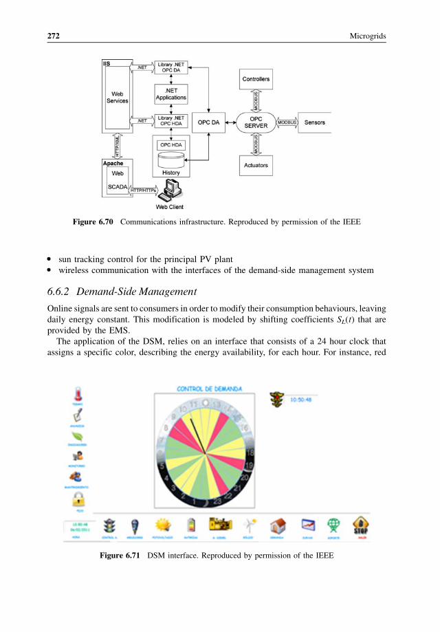
� sun tracking control for the principal PV plant� wireless communication with the interfaces of the demand-side management system

6.6.2 Demand-Side Management

Online signals are sent to consumers in order to modify their consumption behaviours, leaving

daily energy constant. This modification is modeled by shifting coefficients SL(t) that are

provided by the EMS.

The application of the DSM, relies on an interface that consists of a 24 hour clock that

assigns a specific color, describing the energy availability, for each hour. For instance, red

Figure 6.70 Communications infrastructure. Reproduced by permission of the IEEE

Figure 6.71 DSM interface. Reproduced by permission of the IEEE

272 Microgrids

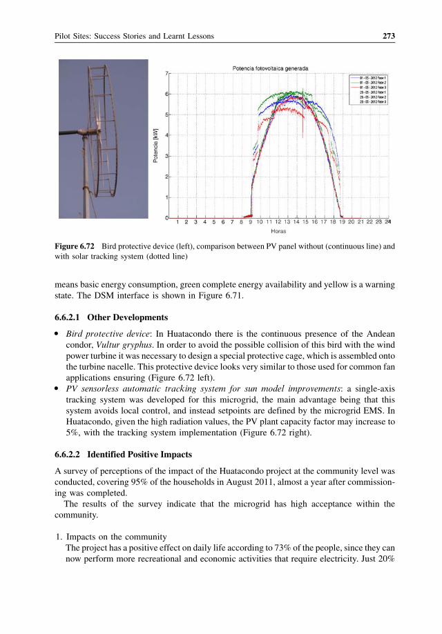
means basic energy consumption, green complete energy availability and yellow is a warning

state. The DSM interface is shown in Figure 6.71.

6.6.2.1 Other Developments

� Bird protective device: In Huatacondo there is the continuous presence of the Andean

condor, Vultur gryphus. In order to avoid the possible collision of this bird with the wind

power turbine it was necessary to design a special protective cage, which is assembled onto

the turbine nacelle. This protective device looks very similar to those used for common fan

applications ensuring (Figure 6.72 left).� PV sensorless automatic tracking system for sun model improvements: a single-axis

tracking system was developed for this microgrid, the main advantage being that this

system avoids local control, and instead setpoints are defined by the microgrid EMS. In

Huatacondo, given the high radiation values, the PV plant capacity factor may increase to

5%, with the tracking system implementation (Figure 6.72 right).

6.6.2.2 Identified Positive Impacts

A survey of perceptions of the impact of the Huatacondo project at the community level was

conducted, covering 95% of the households in August 2011, almost a year after commission-

ing was completed.

The results of the survey indicate that the microgrid has high acceptance within the

community.

1. Impacts on the community

The project has a positive effect on daily life according to 73% of the people, since they can

now perform more recreational and economic activities that require electricity. Just 20%

Figure 6.72 Bird protective device (left), comparison between PV panel without (continuous line) and

with solar tracking system (dotted line)


consider ed that the microgri d brings neither posi tive nor negative effects, while 7%

believed that having elect ricity 24 hours a day might have negative effects on the

commun ity.

2. Impacts on the ph ysical environm ent and landscap e� 57.5% consider ed the micro grid to have no effect on the fauna , whi le 42. 5% expressed

concern about possible collisio ns betwee n the condor s that regula rly fly in the area and

the wind turbine.� 92.5% stated that the project does n ot affect the vegetati on, sinc e the installation of the

equipme nt is far from the area of far ms, crops and native vegetation.� 82.5% reported a positive effect on the landscap e, becau se the project bri ngs modernity

and technol ogical innovation, 12.5% stated that the project does not affect the local

landscap e, while 5% consider ed the project to have negative effects on the landscap e.

3. Impacts on produc tive activitie s� Most of the people said that it is now possible to un dertake new economi c activities o r to

enhance the existing ones. Specifically, 27% believed that the project is beneficial for

the developme nt of touris m and assoc iated serv ices; 23% said that it will benefit

agricultu re through irrig ation techno logy; 18% suggeste d that the proj ect woul d benefit

construc tion activities now that the daily period in which they can use electric tools has

been extended. Finally, the remainin g 32% felt that there coul d be a negative impact on

agricultu ral development, becau se farmers might neglect their farms and crops whi le

pursuing other activitie s that are now possi ble.

Over the time that the micro grid has been operating, the opera tors have gath ered the

following evidence:� no equi pment failur es over the 2 010–2011 perio d� high level of com mitment of the com munit y for maint enance activitie s and demand

response programs� high level of interest shown by the peopl e in charge of maintenan ce and opera tion

activities, demonst rated by low rotation in the membe rship of the maintenan ce team� no accident s involving peopl e or animals

Additiona lly, the syst em provides other opera tional benefits:� diesel consumpt ion reduced b y 50% whe n comp ared with the previous opera tion

scheme� improved relia bility levels� higher power quality

References

1. Alvial-Palavicino, C., Garrido-Echeverr�ıa, N., Jim�enez-Est�evez, G., Reyes, L., and Palma-Behnke, L. (2011) A

methodology for community engagement in the introduction of renewable based smart microgrid. Energy for

Sustainable Development, 15 (3), (SI), 314–323.

2. Palma-Behnke, R., Reyes-Chamorro, L., and Jimenez-Estevez, G. (2012) Smart solutions for isolated locations.

IEEE PES General Meeting.

3. http://synergy.ucsd.edu/files/Agarwal_DATE2011_UnderstandingMicroGrid.pdf.

274 Microgrids

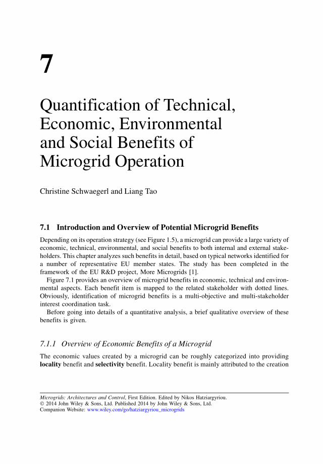
http://synergy.ucsd.edu/files/Agarwal_DATE2011_UnderstandingMicroGrid.pdf.

7

Quantification of Technical,Economic, Environmentaland Social Benefits ofMicrogrid Operation

Christine Schw aegerl and Liang Tao

7.1 Int roduction and Overvi ew of Potential Microg rid Benefits

Dependi ng on its opera tion strategy (see Figur e 1.5), a mi crogrid can provide a large variet y of

economi c, techn ical, environm ental, and social benefits to both internal and external sta ke-

holders. Th is chapter analyzes such benefits in deta il, based on typical networks identified for

a number o f represe ntative EU membe r states . Th e stud y has been com pleted in the

framework of the EU R&D project, More Microgrid s [1].

Figure 7.1 provides an overview of micro grid benefits in economic, technic al and environ-

mental aspec ts. Each benefit item is map ped to the related stakehol der with dotted lines.

Obviously, iden tification of micro grid benefits is a multi-o bjective and multi-s takehol der

interest coord inati on task.

Before going into details of a quantitat ive analysi s, a brief qualitat ive overview of these

benefits is given.

7.1.1 Overview of Economic Benefits of a Microgrid

The economic values c reated by a m icrogrid can b e roughly c at egorized into prov iding

local ity benefit and selectivity benefit. Localit y benefit is m ai nl y att ributed to the creation



of an internal “over-the-grid” energy market within the microgrid, where microsource units

could sell at prices higher than the prices at wholesale level and end consumers could buy

at prices lower than the retail level. This is equivalent to Market Policy 1 (good citizen

behavior), analytically described in Section 2.7.2. Selectivity benefit is associated with

optimization of real-time dispatch decisions that minimize opportunity cost of the whole

microgrid with consideration of technical and environmental constraints. This is equivalent

to Market Policy 2 (ideal citizen behavior), analytically described in Section 2.7.2.

Both locality and selectivity benefits can be attributed to either the consumer side or the

microsource side, where a proper market design/interest allocation mechanism is needed to

ensure a reasonable split of both benefits between consumer and microsource owner. From

a macro-economics point of view, the locality benefits of a microgrid can be grouped into

two aspects:

� microgrid can act as an initiator of local retail and service markets,� microgrid can act as a hedging tool against potential risks of price volatility, outage, load

growth and so on.

The selectivity benefit of a microgrid can also be further categorized in the following two

aspects:

� microgrid can act as an aggregator of both supply- and demand-side players,� microgrid can serve as an interest arbitrator for different stakeholders.

EconomicBenefits

EnvironmentalBenefits

TechnicalBenefits

Peak LoadShaving

VoltageRegulation

EnergyLoss

Reduction

ReliabilityEnhacement

NetworkHedging Value

GHG Reduction

Consumer

Micro-source

DSO

LocalConsumer

Benefit

MicrosourceBenefit

Figure 7.1 Overview of microgrid benefits

276 Microgrids

7.1.2 Overview of Technical Benefits of a Microgrid

A microgrid can potentially improve the technical performance of the local distribution grid

mainly in the following aspects:

� energy loss reduction due to decreased line power flows,� improved voltage quality via coordinated reactive power control and constrained active

power dispatch,� relief of congested networks and devices, for example during peak loading through

selective scheduling of microsource outputs,� enhancement of supply reliability via partial or complete islanding during loss of main

grid. When the total number of microgrids reaches a sufficiently high share in LV

substations, similar technical benefits can be expected in upstream grids as a consequence

of multi-microgrid operation.

The actual level of technical benefits depends mainly on two factors: the optimality of

microsource allocation and the degree of coordination among different players. Effective

planning of microsource size and location can maximize unit contribution to system

performance and random interconnection of oversized microsources in weak grids, but

it can create more technical problems than the benefits it provides. It is also critically

important that a real-time, multi-unit coordination platform, in either centralized or

decentralized form (see Chapter 2) is needed to maintain targeted microgrid technical

performance at all times.

7.1.3 Overview of Environmental and Social Benefits of a Microgrid

Environmental benefits of a microgrid can be expected from two aspects: shift toward

renewable or low-emission (e.g. natural gas) fuels and adoption of more energy-efficient

energy supply solutions (e.g. combined heat and power applications) including demand-

side integration. With widespread national support policies for distributed renewable

resources – for example, photovoltaics – the fuel-switching credit of microgrid is expected

to grow as RES costs decrease over the years. Application of CHP and district heating and/

or cooling concepts, on the other hand, varies significantly from region to region and is

expected to find considerably different levels of acceptance across Europe. Demand side

response, either manual or automated, is also greatly facilitated by the controlled operation

of a microgrid.

Social benefits of microgrids can be mainly expected from:

� raising public awareness and fostering incentives for energy saving and GHG emission

reduction,� creation of new research and job opportunities,� electrification of remote or underdeveloped areas.

All of these listed impacts, however, can be seen as long-term effects, and although

qualitatively easy to understand, can be very difficult to quantify.

Quantification of Technical, Economic, Environmental and Social Benefits 277

7.2 Setup of Benefit Quantification Study

7.2.1 Methodology for Simulation and Analysis

For this book, an analysis of different microgrid benefits was carried out on a yearly basis

using the sequential Monte Carlo simulation method (Figure 7.2). Due to the cyclic nature of

both electricity market prices and renewable (e.g. photovoltaic) output, intraday microgrid

schedules are created and evaluated as hourly settlement results. Annual outcome of the

optimization algorithm is consequently a statistical summary of individual daily simulations.

In this section, the general framework of this analysis is outlined.

Typical annual profiles of load, RES generation and market prices have been

synthesized, based on measurements or historical data. As microgrids are typically

located at LV level, with mainly small residential or commercial customers, there are

significant variations in load curves, which, in combination with the uncertainties from

RES output as well as (wholesale) electricity price, turn the day-ahead microgrid

scheduling task into a highly stochastic problem. Since prediction errors are inevitable,

potential microgrid benefits evaluated from simulated or forecast data should be viewed

as best-case results – that is, actual operation decisions might be sub-optimal, thus

leading to lower benefits.

In order to deal with the modeling requirements of different microsource types, RES units,

storage and demand-side response resources are dispatched at priority, and then the DG unit

schedules are created for active and reactive powers, respectively. For the DG unit commit-

ment, genetic algorithms or simply priority lists can be used to determine the optimal DG on/

off states. Quadratic/linear programming models can be used for optimal power dispatch, as

discussed in Section 2.7.4.

The formulation described in Section 2.7.4 can be further expanded by assigning cost

functions to greenhouse gas (GHG) emissions and technical aspects, such as losses

or reliability of supply and external factors can be internalized within the economic

criteria, leading to an economic formulation of the optimal control strategy problem

that considers:

� retail revenues collected from end customers,� revenues of selling electricity to wholesale market,

Daily cycles from beginning (e.g. day 1) to end (e.g. day 365)

Step 1Interpretation of grid data + production of

stochastic RES curves

Step 2Determine storage / DSM schedules for

considered days

Step 3DG unit commitment and P/Q dispatch for

considered days

Step 4Check detailed load flow conditions and perform

statistical summary

Linear Programming used for constrained load shifting

Genetic Algorithm used for deciding DG switching states;Quadratic Programming used for optimizing DG P/Q outputs

Figure 7.2 Algorithm overview of microgrid benefit quantification study

278 Microgrids

� total cost of buying electricity from wholesale market,� overall generation cost of DG (fuel, startup/shutdown, operation and maintenance cost),� total emission cost from electricity generation,� cost of energy losses in the grid,� total cost of electricity generated from RES units,� total control and communication costs for operating the microgrid.

Obviously, this total opportunity cost objective function is an artificial entry in a liberalized

electricity market, as it represents the interests of multiple entities, and, in practice, requires

extensive collaboration and compromise among the various actors.

For the optimization problem, three sets of system operational constraints are applied:

1. active and reactive energy balances in the microgrid, including the connection to the

upstream network,

2. DG physical constraints, regarding minimum on and off operation time (thermal

constraints) and minimum and maximum energy outputs,

3. network constraints – that is, voltage limits and overload limits of transformers and circuits.

After creation of a complete schedule, load flows are run to calculate power losses and to

check voltage and loading conditions in the network. Due to the large amount of output data,

network variables are recorded as discrete probability density functions via a statistical

summary procedure.

7.2.2 European Study Case Microgrids

It is not possible to quantify microgrid benefits considering a “typical” average system.

Constitution and performance of microgrids are generally subject to a huge variety of

internal and external factors, which can be summarized under the following three

categories:

1. geographical location, which determines types of power network, RES productivity,

energy portfolios for electricity generation and electricity prices,

2. time, which determines microsource penetration scenarios and cost developments,

3. sensitivities, which relate to individual market, regulatory and operational impact factors.

To quantify microgrid benefits at European level, an evaluation framework was developed

to accommodate the majority of input and output parameters at a manageable level of data

complexity. Based on this framework, typical European distribution networks of different

types were studied, as shown in Figure 7.3. The results of this study are presented in

Section 7.3. These results are critically influenced by the assumptions listed in the following

subsections of Section 7.2, and therefore should be treated only as indications of future trends

and the type of studies required.

Installed generation capacity and annual energy consumption vary significantly across the

different European countries examined. Figure 7.4 demonstrates the basic assumptions made

in the study: average wholesale prices are 40–90D /MWh, national CO2 emission levels vary

between 400 kg and 800 kg/MWh and end user retail electricity prices (split into energy,

network charges and taxes) are 6–28Dct/kWh.


Figure 7.3 European study case networks (DE¼Germany, DK¼Denmark, GR¼Greece, IT¼ Italy,

MK¼ FYROM, NL¼The Netherlands, PL¼ Poland, PT¼ Portugal, UK¼United Kingdom)

0

5

10

15

20

25

30

MKUKPTPLNLITGRDKDE

€ct/k

Wh

0

10

20

30

40

50

60

70

80

90

100

UKPTPLNLMKITGRDKDE

Euro/MWh

0

100

200

300

400

500

600

700

800

900kgCO2_eq/MWh

Wholesale priceEmission

taxes

grid_meter

wholesale

Figure 7.4 Retail/wholesale tariff structures and emission levels considered

280 Microgrids

7.2.2.1 Development of European Microgrids from 2010 to 2040

For the adopted evaluation framework, four future microgrid scenarios are defined for the

years 2010, 2020, 2030 and 2040, that satisfy 10, 20, 30 and 40%, respectively, of their own

demands by RES and bio-fueled heat-driven CHP units. This facilitates cross-national

comparison, despite the regional differences in terms of adopted microsource technologies.

In order to minimize the potential number of simulation cases, microsource allocation is

assumed to be optimal for all cases. The RES and CHP self-supply level of the microgrids

annual energy needs is kept below 50%. This is essential, since a higher level of self-

supplied energy ratio would imply that the RES power installations (i.e. penetration level in

terms of power rating) should be higher than 150% in countries where microgrids are

dominated by intermittent RES technologies with lowfull load hours (FLH) (< 2000 h/a).

The FLH is defined as the equivalent number of hours that DGs would operate under

nominal capacity, in order to provide the same amount of annual energy. As active power

outputs from intermittent RES and heat-driven CHP units are not naturally dispatchable, the

controllability of a microgrid relies mainly on the installation of dispatchable microsources

and storage devices.

After definition of a microgrid configuration aimed at satisfying local energy needs, the

share of typical microgrids within national power systems (microgrid dissemination ratio) per

country and region are assumed to be as shown in Figure 7.5, for 2010, 2020, 2030 and 2040,

with pessimistic (P) and optimistic (O) assumptions.

Detailed penetration scenarios of RES and CHP units assumed in each simulated case are

given in Figure 7.6. It is noted that countries with high RES energy production from PV

(IT, PT) or wind turbines (PL) are likely to have microgrid configurations of more than

100% RES penetration levels (installed microsource capacity compared to maximum load)

by 2040.

7.2.2.2 Basic Cost Assumptions

Figure 7.7 shows the range of cost/kWh microsource generation, assumed for different

technologies between 2010 and 2040. High cost reductions are expected for PV and fuel cell

0%

5%

10%

15%

20%

25%

30%

35%

DE_P DE_O DK_P DK_O GR_P GR_O IT_P IT_O MK_P MK_O NL_P NL_O PL_P PL_O PT_P PT_O UK_P UK_O

2010

2020

2030

2040

Figure 7.5 Microgrid dissemination ratio in EU national grids (O¼ optimistic assumptions,

P¼ pessimistic assumptions)


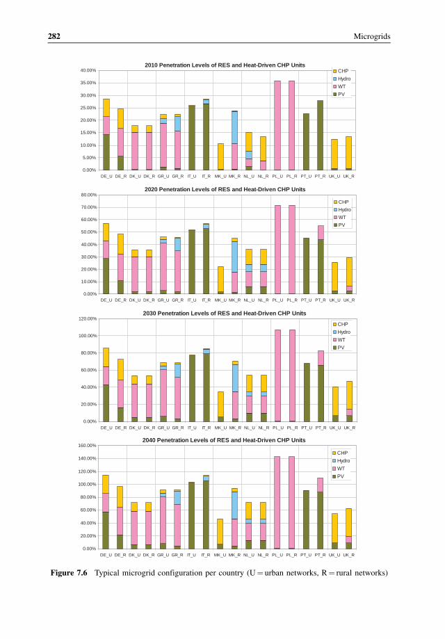
2010 Penetration Levels of RES and Heat-Driven CHP Units

0.00%

5.00%

10.00%

15.00%

20.00%

25.00%

30.00%

35.00%

40.00%

DE_U DE_R DK_U DK_R GR_U GR_R IT_U IT_R MK_U MK_R NL_U NL_R PL_U PL_R PT_U PT_R UK_U UK_R 2020 Penetration Levels of RES and Heat-Driven CHP Units

0.00%

10.00%

20.00%

30.00%

40.00%

50.00%

60.00%

70.00%

80.00%


0.00%

20.00%

40.00%

60.00%

80.00%

100.00%

120.00%


0.00%

20.00%

40.00%

60.00%

80.00%

100.00%

120.00%

140.00%

160.00%

DE_U DE_R DK_U DK_R GR_U GR_R IT_U IT_R MK_U MK_R NL_U NL_R PL_U PL_R PT_U PT_R UK_U UK_R

CHPHydroWTPV

CHPHydroWTPV

CHPHydroWTPV

CHPHydroWTPV

Figure 7.6 Typical microgrid configuration per country (U¼ urban networks, R¼ rural networks)

282 Microgrids

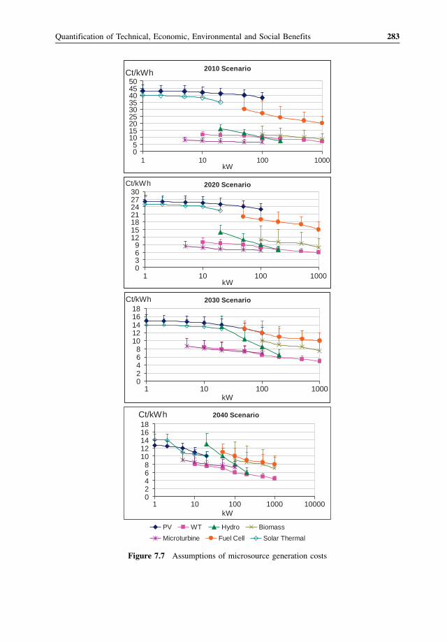
2010 Scenario

05

101520253035404550

1 10 100 1000

Ct/kWh

2020 Scenario

0369

12151821242730

1 10 100 1000

Ct/kWh

2030 Scenario

02468

1012141618

1 10 100 1000

Ct/kWh

2040 Scenario

02468

1012141618

1 10 100 1000 10000

Ct/kWh

PV WT Hydro BiomassMicroturbine Fuel Cell Solar Thermal

kW

kW

kW

kW

Figure 7.7 Assumptions of microsource generation costs


technologies from 2010 to 2040, while the costs of other RES technologies are assumed to be

more stable over the years. Natural gas based microsources are assumed to face increasing fuel

costs in the future.

For a consistent calculation of net present value (NPV), interest rate (depreciation rate) of

all examined countries is assumed to be constant at 5% throughout the examined period.

Electricity market price levels are assumed to remain constant over time.

Dispatchable micro-generators are the main controllable generating units within a micro-

grid, so system operation optimization decisions will be strongly dependent on their cost

functions, which can be expressed as:

k ¼ aþ b � Pþ c � P2 (7.1)

P as active power output of dispatchable MS unit, k as per kWh generation cost

a constant order coefficient, which includes power-related investment and installation

costs as they are independent on real-time dispatch decisions

b first-order coefficient, which is derived from energy-related fuel, operation and

maintenance costs, as well as emission costs

c second-order coefficient, which mainly relates to unit efficiency related costs.

Costs for control, metering and communication mainly depend on the complexity of the

microgrid (the number of nodes to be monitored and controlled). Assuming 5000 h/a as FLH

of load demand, the average annual energy demand observed per node (as load substation) is

50–160 MWh/a for most microgrids tested.

Ensuing cost calculations for control, metering and communication can be described as

follows:

Define:kact as annual active control cost of a node;Kctrl as investment cost of control device

kmet as annual metering fee;kcom as annual communication fee;bas NPV factor

Then: kact ¼Kctrl

bþ kmetþkconð Þ; bffi 12:5

1

að20years lifetimeÞ

Assume: For2010; Kctrl ¼ 500euro; kmet ¼ 100euro=a; kcon ¼ 60euro=a;

For 2040; Kctrl ¼ 250euro; kmet ¼ 50 euro=a; kcon ¼ 30euro=a;

Then: kact ¼500=12:5þ100þ60ð Þeuro=a¼ 200euro=a in 2010

250=12:5þ50þ30ð Þeuro=a¼ 100euro=a in 2040

(

) Per MWh control; metering; communication cost¼ 100;200½ �euro=a50;160½ �MWh=a

¼ 0:6;4½ �euro=MWh

(7.2)

It should be noted that the differential cost of transforming a distribution network with DER

to a microgrid comprises exactly the costs for control, metering and communication.

Equation (7.2) suggests that microgrid benefits must exceed 0.6–4D /MWh to justify active

control measures. As this additional cost is not dependent on microsource operation decisions,

it is used for comparison with the estimated microgrid benefits.

284 Microgrids

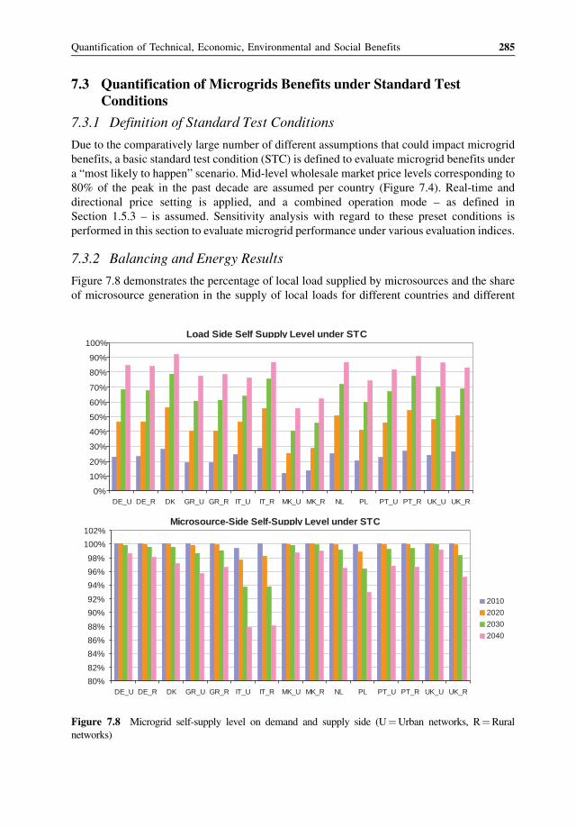
7.3 Quantification of Microgrids Benefits under Standard TestConditions

7.3.1 Definition of Standard Test Conditions

Due to the comparatively large number of different assumptions that could impact microgrid

benefits, a basic standard test condition (STC) is defined to evaluate microgrid benefits under

a “most likely to happen” scenario. Mid-level wholesale market price levels corresponding to

80% of the peak in the past decade are assumed per country (Figure 7.4). Real-time and

directional price setting is applied, and a combined operation mode – as defined in

Section 1.5.3 – is assumed. Sensitivity analysis with regard to these preset conditions is

performed in this section to evaluate microgrid performance under various evaluation indices.

7.3.2 Balancing and Energy Results

Figure 7.8 demonstrates the percentage of local load supplied by microsources and the share

of microsource generation in the supply of local loads for different countries and different

Load Side Self Supply Level under STC

DE_U DE_R DK GR_U GR_R IT_U IT_R MK_U MK_R NL PL PT_U PT_R UK_U UK_R

Microsource-Side Self-Supply Level under STC


2010

2020

2030

2040

0%

10%

20%

30%

40%

50%

60%

70%

80%

90%

100%

80%

82%

84%

86%

88%

90%

92%

94%

96%

98%

100%

102%

Figure 7.8 Microgrid self-supply level on demand and supply side (U¼Urban networks, R¼Rural

networks)


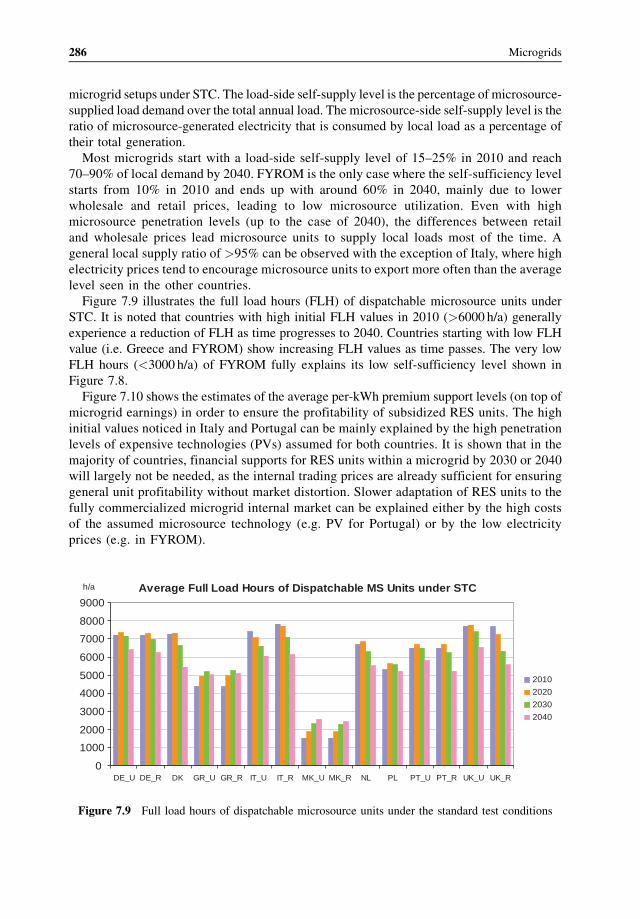
microgrid setups under STC. The load-side self-supply level is the percentage of microsource-

supplied load demand over the total annual load. The microsource-side self-supply level is the

ratio of microsource-generated electricity that is consumed by local load as a percentage of

their total generation.

Most microgrids start with a load-side self-supply level of 15–25% in 2010 and reach

70–90% of local demand by 2040. FYROM is the only case where the self-sufficiency level

starts from 10% in 2010 and ends up with around 60% in 2040, mainly due to lower

wholesale and retail prices, leading to low microsource utilization. Even with high

microsource penetration levels (up to the case of 2040), the differences between retail

and wholesale prices lead microsource units to supply local loads most of the time. A

general local supply ratio of >95% can be observed with the exception of Italy, where high

electricity prices tend to encourage microsource units to export more often than the average

level seen in the other countries.

Figure 7.9 illustrates the full load hours (FLH) of dispatchable microsource units under

STC. It is noted that countries with high initial FLH values in 2010 (>6000 h/a) generally

experience a reduction of FLH as time progresses to 2040. Countries starting with low FLH

value (i.e. Greece and FYROM) show increasing FLH values as time passes. The very low

FLH hours (<3000 h/a) of FYROM fully explains its low self-sufficiency level shown in

Figure 7.8.

Figure 7.10 shows the estimates of the average per-kWh premium support levels (on top of

microgrid earnings) in order to ensure the profitability of subsidized RES units. The high

initial values noticed in Italy and Portugal can be mainly explained by the high penetration

levels of expensive technologies (PVs) assumed for both countries. It is shown that in the

majority of countries, financial supports for RES units within a microgrid by 2030 or 2040

will largely not be needed, as the internal trading prices are already sufficient for ensuring

general unit profitability without market distortion. Slower adaptation of RES units to the

fully commercialized microgrid internal market can be explained either by the high costs

of the assumed microsource technology (e.g. PV for Portugal) or by the low electricity

prices (e.g. in FYROM).

Average Full Load Hours of Dispatchable MS Units under STC


h/a

2010

2020

2030

2040

0

1000

2000

3000

4000

5000

6000

7000

8000

9000

Figure 7.9 Full load hours of dispatchable microsource units under the standard test conditions

286 Microgrids

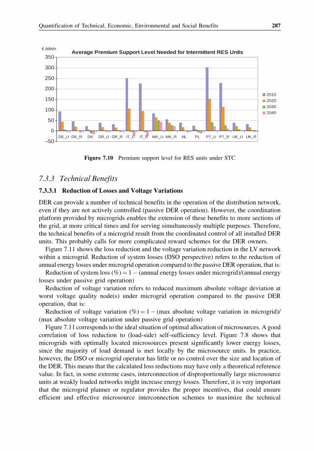
7.3.3 Technical Benefits

7.3.3.1 Reduction of Losses and Voltage Variations

DER can provide a number of technical benefits in the operation of the distribution network,

even if they are not actively controlled (passive DER operation). However, the coordination

platform provided by microgrids enables the extension of these benefits to more sections of

the grid, at more critical times and for serving simultaneously multiple purposes. Therefore,

the technical benefits of a microgrid result from the coordinated control of all installed DER

units. This probably calls for more complicated reward schemes for the DER owners.

Figure 7.11 shows the loss reduction and the voltage variation reduction in the LV network

within a microgrid. Reduction of system losses (DSO perspective) refers to the reduction of

annual energy losses undermicrogrid operation compared to the passive DER operation, that is:

Reduction of system loss (%)¼ 1� (annual energy losses under microgrid)/(annual energy

losses under passive grid operation)

Reduction of voltage variation refers to reduced maximum absolute voltage deviation at

worst voltage quality node(s) under microgrid operation compared to the passive DER

operation, that is:

Reduction of voltage variation (%)¼ 1� (max absolute voltage variation in microgrid)/

(max absolute voltage variation under passive grid operation)

Figure 7.11 corresponds to the ideal situation of optimal allocation of microsources. A good

correlation of loss reduction to (load-side) self-sufficiency level. Figure 7.8 shows that

microgrids with optimally located microsources present significantly lower energy losses,

since the majority of load demand is met locally by the microsource units. In practice,

however, the DSO or microgrid operator has little or no control over the size and location of

the DER. This means that the calculated loss reductions may have only a theoretical reference

value. In fact, in some extreme cases, interconnection of disproportionally large microsource

units at weakly loaded networks might increase energy losses. Therefore, it is very important

that the microgrid planner or regulator provides the proper incentives, that could ensure

efficient and effective microsource interconnection schemes to maximize the technical

Average Premium Support Level Needed for Intermittent RES Units

–50

0

50

100

150

200

250

300

350


2010

2020

2030

2040

€ /MWh

Figure 7.10 Premium support level for RES units under STC


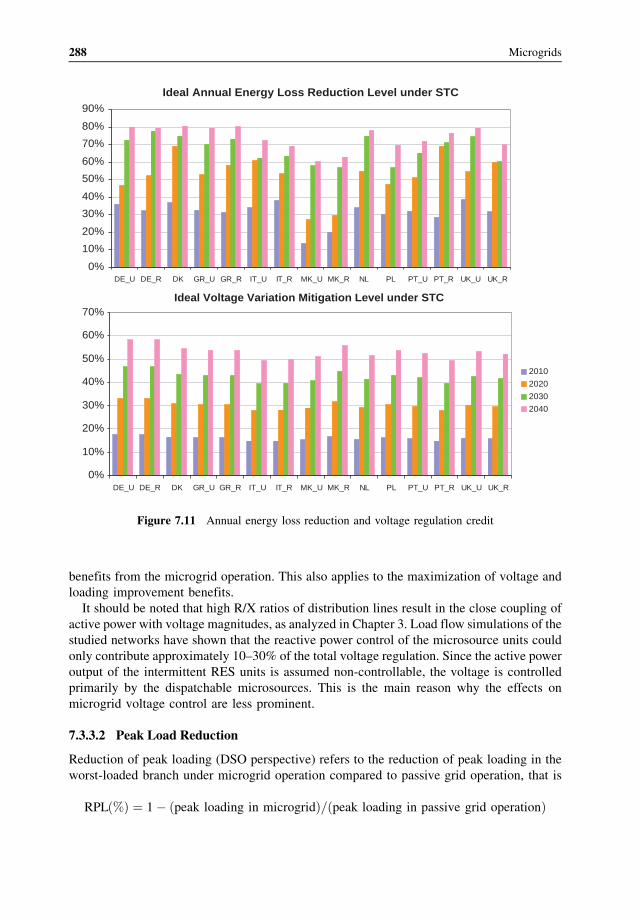
benefits from the microgrid operation. This also applies to the maximization of voltage and

loading improvement benefits.

It should be noted that high R/X ratios of distribution lines result in the close coupling of

active power with voltage magnitudes, as analyzed in Chapter 3. Load flow simulations of the

studied networks have shown that the reactive power control of the microsource units could

only contribute approximately 10–30% of the total voltage regulation. Since the active power

output of the intermittent RES units is assumed non-controllable, the voltage is controlled

primarily by the dispatchable microsources. This is the main reason why the effects on

microgrid voltage control are less prominent.

7.3.3.2 Peak Load Reduction

Reduction of peak loading (DSO perspective) refers to the reduction of peak loading in the

worst-loaded branch under microgrid operation compared to passive grid operation, that is

RPLð%Þ ¼ 1� ðpeak loading in microgridÞ=ðpeak loading in passive grid operationÞ

Ideal Annual Energy Loss Reduction Level under STC



2010

2020

2030

2040

Ideal Voltage Variation Mitigation Level under STC

0%

10%

20%

30%

40%

50%

60%

70%

80%

90%

0%

10%

20%

30%

40%

50%

60%

70%

Figure 7.11 Annual energy loss reduction and voltage regulation credit

288 Microgrids

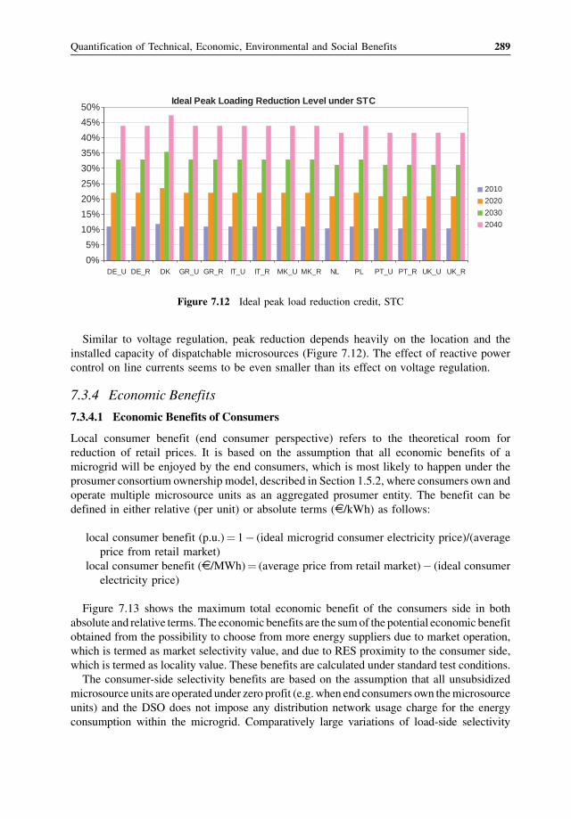
Similar to voltage regulation, peak reduction depends heavily on the location and the

installed capacity of dispatchable microsources (Figure 7.12). The effect of reactive power

control on line currents seems to be even smaller than its effect on voltage regulation.

7.3.4 Economic Benefits

7.3.4.1 Economic Benefits of Consumers

Local consumer benefit (end consumer perspective) refers to the theoretical room for

reduction of retail prices. It is based on the assumption that all economic benefits of a

microgrid will be enjoyed by the end consumers, which is most likely to happen under the

prosumer consortium ownership model, described in Section 1.5.2, where consumers own and

operate multiple microsource units as an aggregated prosumer entity. The benefit can be

defined in either relative (per unit) or absolute terms (D /kWh) as follows:

local consumer benefit (p.u.)¼ 1� (ideal microgrid consumer electricity price)/(average

price from retail market)

local consumer benefit (D /MWh)¼ (average price from retail market)� (ideal consumer

electricity price)

Figure 7.13 shows the maximum total economic benefit of the consumers side in both

absolute and relative terms. The economic benefits are the sumof the potential economic benefit

obtained from the possibility to choose from more energy suppliers due to market operation,

which is termed as market selectivity value, and due to RES proximity to the consumer side,

which is termed as locality value. These benefits are calculated under standard test conditions.

The consumer-side selectivity benefits are based on the assumption that all unsubsidized

microsource units are operated under zero profit (e.g.when end consumers own themicrosource

units) and the DSO does not impose any distribution network usage charge for the energy

consumption within the microgrid. Comparatively large variations of load-side selectivity


2010

2020

2030

2040

0%

5%

10%

15%

20%

25%

30%

35%

40%

45%

50%Ideal Peak Loading Reduction Level under STC

Figure 7.12 Ideal peak load reduction credit, STC


benefits have been observed in the various cases due to the different FLH values of dispatchable

microsource units and the profit margins between retail prices and microsource costs. As

essentially FLH of microsource units is also determined by market prices, the consumer-side

selectivity benefit level can be seen to be extremely sensitive to electricity market prices.

Unlike benefits obtained frommarket selectivity, RES locality benefit is totally dependent on

their financial support. This means by default, that market forces will not provide such benefits

to consumers due to natural cash flows within a microgrid. If a microgrid comprises only

subsidized RES units that are priority dispatched, then consumers will not enjoy any selectivity

benefit and the RES locality value – avoided use of system (UoS) charge – will be the

only benefit for them. As consumer-side RES locality benefits are deduced from the standard

grid charges, UoS charge tariffs determine the national variations in locality benefit value.

Overall, cost saving potentials range from 0.002 Ct/kWh in 2010 to 0.05 Ct/kWh in 2040.

The majority of results indicate cost savings ranging from 7%� 5% in 2010 to 25%� 10% in

2040. These savings do not include taxes incurred in retail prices that vary widely among the

examined countries.

Maximum Total Consumer Benefit (per MW) under STC

0

10

20

30

40

50

60



2010

2020

2030

2040

Maximum Total Consumer Benefit (% of Original) under STC

0%

5%

10%

15%

20%

25%

30%

35%

40%

€/MWh

Figure 7.13 Maximum total consumer benefit

290 Microgrids

It should be noted that consumers will enjoy the above benefits only with market policy 1

(Section 2.7.3), while with market policy 2, they will have to pay the same electricity prices as

without microgrids.

7.3.4.2 Economic Benefits of Microsource Owners

Microsource benefit (microsource perspective) mainly refers to the maximum potential of

increasing the selling price under a microgrid setting. This benefit is of course based on the

assumption that consumers and the microgrid operator do not benefit economically from

the microgrid operation. It can be defined either as a relative value (%) or an absolute value

(D /kWh):

microsource benefit (p.u.)¼ 1� (average wholesale price/average price for aggregated

microgrid operation)

micro source benefit (D /kWh)¼ (average price for aggregated microgrid operation)�(average wholesale price)

Similar to the total local consumer benefit, the total microsource benefit is composed of

the locality benefit and the selectivity benefit. Figure 7.14 shows the maximum total benefit

on the dispatchable microsource side in both absolute (D /MWh) and relative (%) terms.

Variations in microsource costs from 2010 to 2040 basically have negligible impacts on

total benefit levels of all examined countries – this can be explained by looking at the

maximum total microsource benefit simply as the difference between average retail and

wholesale prices in an examined country, which stays largely constant despite microsource

cost variation and market price changes. This will be discussed further in the sensitivity

analysis of Section 7.4.

Microsource locality benefit is the difference between microsource cost and wholesale

price level. It is actually an indication of “opportune operation loss” if the microsource units

are forced to sell to the wholesale market instead of local consumers. None of the tested

microgrid scenarios under a mid-level price and a real-time pricing setting could provide a

direct microsource profit by selling directly to wholesale market.

The selectivity value on the microsource side equals the benefit obtained by consumer-side

selectivity, that is incurred by energy consumption from local sources. To reach the full extent

of selectivity benefit, consumers are expected to pay the same tariffs as before the microgrid

implementation, and the DSO is not expected to charge locally consumed microsource energy

for the grid usage. The selectivity benefit approximately yields the maximum achievable

profit margin for the units. There is a very close correlation between microsource profitability

and retail market price level, enabling high profits at 60–70D /MWh for high-price countries

(e.g. Italy and UK) and much lower results around 20D /MWh for low-price countries (e.g.

Greece and FYROM).

7.3.5 Environmental Benefits

The total emission reduction (regulator perspective) index is the reduction of GHG emission

level per kWh consumption in a microgrid when compared to the passive grid operation. It can

be defined either as relative value (%) or absolute value (D /kWh):


total emission reduction (p.u.)¼ 1 – (GHG emission level in microgrid)/(national GHG

emission level, passive case)

total emission reduction (kg/kWh)¼ (national GHG emission level, passive case) – (GHG

emission level in microgrid)

Although SO2, NOX and particle matter emission reductions are also expected from

microgrid operation, there are currently no explicit trading platforms within Europe as the

European ETS market, thus reduction effects under these criteria can be viewed largely as by-

products of GHG emission control.

Figure 7.15 demonstrates the environmental benefits of microgrids in absolute and relative

values. Microgrid GHG emission levels generally converge to around 200 kg (CO2 equiv-

alent)/MWh by 2040, despite very different starting points in 2010 – this convergence can be

explained by the high resemblance of load-side self-sufficiency level in 2040. GHG reduction

credits of microgrid are represented as a percentage of the original emission levels of each

examined country. It is quite obvious that countries starting with high emission levels could

Maximum Total MS Benefit (per MW) under STC


Maximum Total MS Benefit (% of Original) under STC


2010

2020

2030

2040

0

10

20

30

40

50

60

70

80

90

0%

20%

40%

60%

80%

100%

120%

140%

160%

180%

€/MWh

Figure 7.14 Maximum total microsource benefit, STC

292 Microgrids

expect reduction credits as high as over 50% (e.g. Greece and Poland), while countries with

lower initial emission (e.g. Italy) enjoy comparatively smaller credits by 2040.

7.3.6 Reliability Improvement

With sufficient local generation and storage capacity, a microgrid can operate in islanded (off-

grid) mode serving either the entire load or part of the load, namely the critical loads. The

technical requirements of the power electronic interfaces of the DER to enable effective

transition from interconnected to islanded operation and to sustain operation of a microgrid in

islanded mode were discussed in Chapter 3.

An optimum level of reliability is defined mainly during the planning phase of microgrids,

when costs for additional investments and operation are compared to avoided outage costs.

Depending on the interruption costs and the given reliability of supply for networks without

any microsources, different microgrid reliability benefits can be achieved at European level.


kgCO2/MWh


2010

2020

2030

2040

Average GHG Emission Level per Microgrid under STC

STC Microgrid’s Emission Saving Credit Compared to National Level

0

100

200

300

400

500

600

700

800

0%

10%

20%

30%

40%

50%

60%

Figure 7.15 Average microgrid GHG emission level and emission saving credit, STC


7.3.6.1 Economic Benefits Achieved by Reliability Improvement

Figure 7.16 compares the maximum economic benefits for different networks obtained by

improved reliability. The x-axis represents the product of the total load of the network times

the unavailability of this network in each year, symbolized by PQ. Benefits in each country are

almost linear in relation to PQ, as interruption costs without DG increase with increasing total

demand and unavailability. This leads to higher benefits of microgrid operation. The higher

the outage costs, the higher economic benefits that can be achieved, as shown by the

maximum, average and minimum interruption cost model.

7.3.6.2 System Reliability Indices

A reduction of system unavailability Q, by the installation of microgrids that enable (partial)

islanded operation, is demonstrated in Figure 7.17 for selected European networks, compared

to the case without microsources.

100015002000250030003500

1600Eco

nom

ic b

ene

fit [E

uro/

a]

0 200 400 600 800 1000 1200 1400

Average cost modelMaximum cost modelMinimum cost model

Assumed interruption costs

0500

theNether-lands

Italyrural

Italyurban

Portugal rural

Germanyurban

Pload[kW]*Q[h/a]

Figure 7.16 Economic benefit comparison of microgrids on European level

Figure 7.17 System unavailability comparison of different countries

294 Microgrids

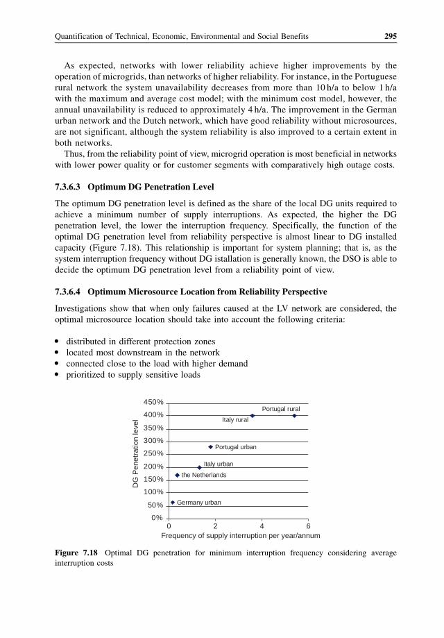
As expected, networks with lower reliability achieve higher improvements by the

operation of microgrids, than networks of higher reliability. For instance, in the Portuguese

rural network the system unavailability decreases from more than 10 h/a to below 1 h/a

with the maximum and average cost model; with the minimum cost model, however, the

annual unavailability is reduced to approximately 4 h/a. The improvement in the German

urban network and the Dutch network, which have good reliability without microsources,

are not significant, although the system reliability is also improved to a certain extent in

both networks.

Thus, from the reliability point of view, microgrid operation is most beneficial in networks

with lower power quality or for customer segments with comparatively high outage costs.

7.3.6.3 Optimum DG Penetration Level

The optimum DG penetration level is defined as the share of the local DG units required to

achieve a minimum number of supply interruptions. As expected, the higher the DG

penetration level, the lower the interruption frequency. Specifically, the function of the

optimal DG penetration level from reliability perspective is almost linear to DG installed

capacity (Figure 7.18). This relationship is important for system planning; that is, as the

system interruption frequency without DG istallation is generally known, the DSO is able to

decide the optimum DG penetration level from a reliability point of view.

7.3.6.4 OptimumMicrosource Location from Reliability Perspective

Investigations show that when only failures caused at the LV network are considered, the

optimal microsource location should take into account the following criteria:

� distributed in different protection zones� located most downstream in the network� connected close to the load with higher demand� prioritized to supply sensitive loads

0%

50%

100%

150%

200%

250%

300%

350%

400%

450%

0 2Frequency of supply interruption per year/annum

4 6

DG

Pen

etra

tion

leve

l

Germany urban

the Netherlands

Italy urban

Portugal urban

Italy rural

Portugal rural

Figure 7.18 Optimal DG penetration for minimum interruption frequency considering average

interruption costs


When failures at the MVand HV level are also considered, different microsource locations

have the same effect on the frequency of load interruption; in this case, microsources improve

system reliability regardless of their location in the LV grid.

7.3.7 Social Aspects of Microgrid Deployment

Three major social benefits of microgrids can be identified as follows:

7.3.7.1 Raise Public Awareness and Foster Incentives for Energy Saving and

Emission Cutting

Depending on the microgrid model, DER-created values are shared among end consumers of a

network. Residential and commercial participants of a microgrid will likely enjoy better

electricity tariffs and can even be rewarded by incentive programs if they own RES micro-

sources or participate in demand-side integration (DSI) programmes. This type of economic

signal (efficiency values created within a microgrid) can be seen as a strong driving force for

acceptance and promotion of microgrids.

7.3.7.2 Creation of New Research and Job Opportunities

Microgrid implementation requires knowledge, expertise and customized hardware and

software solutions that are currently not directly available for both supply- and demand-

side players in the market. Opportunities for new research posts and job openings will be

offered for technology providers, device manufactures, research institutes, and so on.

Opportunities will become available not only in the design (stereotyping) and installation

(standardization) stages, but also in daily operation and maintenance of a microgrid, for

example requirements for real-time metering, communication and control both within and

outside of microgrids.

7.3.7.3 Electrification of Remote or Underdeveloped Areas

For a long time, it has been widely acknowledged that DER units are extremely well suited for

electrifying remote or underdeveloped regions, where it is not economic to interconnect to a

nearby distribution grid or where there is simply lack of basic electric infrastructure. The

microgrid concept provides a platform for aggregating isolated sectors of self-sufficient

households or communities based on limited micro-generators and storage units into a more

robust network with balancing and control capacities. Reliable and affordable supply of

electricity via microgrid can be seen as a critical step for modernization and industrialization

of the local economy.

7.4 Impact of External Market Prices and Pricing Policies

7.4.1 Sensitivity Analysis

7.4.1.1 External Market Price Policies

External market prices have a critical impact on microgrid profitability. In Figure 7.19, three

potential price settings are assumed, as inputs to the sensitivity analysis of microgrid

profitability (see also Section 1.5.3 and Table 1.1):

296 Microgrids

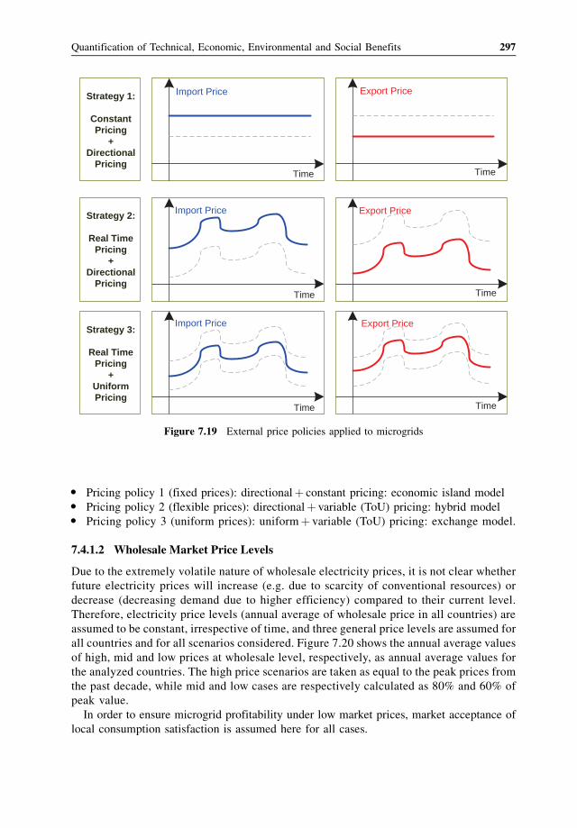
� Pricing policy 1 (fixed prices): directionalþ constant pricing: economic island model� Pricing policy 2 (flexible prices): directionalþ variable (ToU) pricing: hybrid model� Pricing policy 3 (uniform prices): uniformþ variable (ToU) pricing: exchange model.

7.4.1.2 Wholesale Market Price Levels

Due to the extremely volatile nature of wholesale electricity prices, it is not clear whether

future electricity prices will increase (e.g. due to scarcity of conventional resources) or

decrease (decreasing demand due to higher efficiency) compared to their current level.

Therefore, electricity price levels (annual average of wholesale price in all countries) are

assumed to be constant, irrespective of time, and three general price levels are assumed for

all countries and for all scenarios considered. Figure 7.20 shows the annual average values

of high, mid and low prices at wholesale level, respectively, as annual average values for

the analyzed countries. The high price scenarios are taken as equal to the peak prices from

the past decade, while mid and low cases are respectively calculated as 80% and 60% of

peak value.

In order to ensure microgrid profitability under low market prices, market acceptance of

local consumption satisfaction is assumed here for all cases.

Strategy 1:

ConstantPricing

+Directional

PricingTime

Import Price

Time

Export Price

Time

Import Price

Time

Export Price

Time

Import Price

Time

Export Price

Strategy 2:

Real TimePricing

+Directional

Pricing

Strategy 3:

Real TimePricing

+UniformPricing

Figure 7.19 External price policies applied to microgrids


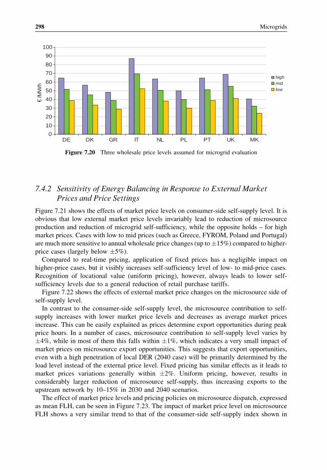
7.4.2 Sensitivity of Energy Balancing in Response to External MarketPrices and Price Settings

Figure 7.21 shows the effects of market price levels on consumer-side self-supply level. It is

obvious that low external market price levels invariably lead to reduction of microsource

production and reduction of microgrid self-sufficiency, while the opposite holds – for high

market prices. Cases with low to mid prices (such as Greece, FYROM, Poland and Portugal)

are much more sensitive to annual wholesale price changes (up to�15%) compared to higher-

price cases (largely below �5%).

Compared to real-time pricing, application of fixed prices has a negligible impact on

higher-price cases, but it visibly increases self-sufficiency level of low- to mid-price cases.

Recognition of locational value (uniform pricing), however, always leads to lower self-

sufficiency levels due to a general reduction of retail purchase tariffs.

Figure 7.22 shows the effects of external market price changes on the microsource side of

self-supply level.

In contrast to the consumer-side self-supply level, the microsource contribution to self-

supply increases with lower market price levels and decreases as average market prices

increase. This can be easily explained as prices determine export opportunities during peak

price hours. In a number of cases, microsource contribution to self-supply level varies by

�4%, while in most of them this falls within �1%, which indicates a very small impact of

market prices on microsource export opportunities. This suggests that export opportunities,

even with a high penetration of local DER (2040 case) will be primarily determined by the

load level instead of the external price level. Fixed pricing has similar effects as it leads to

market prices variations generally within �2%. Uniform pricing, however, results in

considerably larger reduction of microsource self-supply, thus increasing exports to the

upstream network by 10–15% in 2030 and 2040 scenarios.

The effect of market price levels and pricing policies on microsource dispatch, expressed

as mean FLH, can be seen in Figure 7.23. The impact of market price level on microsource

FLH shows a very similar trend to that of the consumer-side self-supply index shown in

0

10

20

30

40

50

60

70

80

90

100

DE DK GR IT NL PL PT UK MK

highmidlow

€/M

Wh

Figure 7.20 Three wholesale price levels assumed for microgrid evaluation

298 Microgrids

Figure 7.21. FLH of low-price cases exhibits higher sensitivity to average wholesale price

variations (up to �60% in the case of FYROM), while high-price cases (e.g. Germany,

Denmark, Italy, the Netherland and the UK) generally experience variations less than�10%

and are hardly impacted by wholesale market price levels.

Fixed pricing, as defined in Section 1.5.3, has negligible effects on high-price cases, but can

increase DER FLH by as much as 80% compared to real time (ToU) pricing for low-price

cases, such as FYROM, Greece and Poland. This can be understood as the benefit of price

stability in adverse market settings. Uniform pricing provides a 20% to 80% FLH reduction in

2010, which is decreased drastically with time; for example, in some cases FLH starts to

increase by 2040 as a result of uniform pricing.

The effects of market price levels and pricing policies on the required premium support

level for RES can be seen in Figure 7.24. The support levels are calculated as the difference

between mean RES production cost and average retail prices. Owing to the linear correlation

between market prices and required RES support, variations in average wholesale prices level

induces proportional changes in required RES support, that is higher prices lead to reduction

of required support and vice versa. In general, a �25% market price variations leads to a

change in required RES support by 10–20%.

Figure 7.21 Market price and pricing policy impact on consumer-side self-supply


Fixed (constant) pricing leads to an increase in the required premium support for some

countries (e.g. DE, IT, NL and PT) and lower support for others (e.g. DK, PL and the UK).

Uniform pricing, on the other hand, is assumed not to interfere with RES support and

consequently has no impact on required national support levels.

7.4.3 Sensitivity of Technical Benefits (Losses) in Response to ExternalMarket Prices and Price Settings

Figure 7.25 shows the impacts of market price levels and price settings on losses. The trends

are similar to those of the load-side self-sufficiency level index of Figure 7.21, since

losses are roughly dependent on the levels of microsource exports for all examined

simulation cases.

Figure 7.22 Market price and pricing policy impact on microsource contribution to self-supply

300 Microgrids

7.4.4 Sensitivity of Economic Benefits in Response to External MarketPrices and Price Settings

7.4.4.1 Consumer Side

The effects of market price variations and different pricing policies on the total economic

benefit on the consumer side are shown in Figure 7.26. Differences between the various

cases under the same wholesale price variations are comparatively small, indicating a

benefit variation �20% to �40% for a �25% variation of market prices. Fixed pricing has

mostly negative impacts on maximum consumer benefit, with small benefit reductions

under 10% for most cases except FYROM, where a benefit reduction as high as 35% is

calculated due to a drastic reduction of microsource full load hours (even to zero). Uniform

pricing could significantly raise the maximum total consumer benefit by 2–6 times initially

in 2010, but this increase is quickly damped with time.

Figure 7.23 Market price and pricing policy impact on microsource full load hours


7.4.4.2 Microsource Side

The potential effects of market price variations and pricing policies on the maximum total

benefit of microsources are shown in Figure 7.27. The total microsource benefit is almost

solely determined by the difference between the selling price and the average wholesale price

in the market. Wholesale market price levels and fixed pricing schemes have basically

negligible impacts (below 5%) on its value except the case of FYROM. Uniform pricing,

however, is potentially capable of changing the mean microsource selling price and can

therefore lead to total microsource benefit changes as high as �50% to �100%.

7.4.5 Sensitivity of Environmental Benefits in Response to Market Pricesand Price Settings

The effects of market price levels and pricing policies on microgrid emission savings are

shown in Figure 7.28. There is a close correlation between microgrids self-sufficiency level

Figure 7.24 Market price and pricing policy impact on RES premium support level

302 Microgrids

and its emission reduction credit. There are different national emission level baselines and

large variations of emission levels in response to external prices and pricing settings, but the

actual impact of both criteria is comparatively small (less than �10%). The only exception is

the effect of uniform pricing, which could potentially lead to a reduction of more than 25% in

terms of GHG savings compared to real-time pricing.

7.5 Impact of Microgrid Operation Strategy

Figure 7.29 compares the maximum total consumer benefit obtained from the combined

operation mode (the objective function is the summarized total cost, and all technical

constraints are applied) used as a reference to the following three individual operating

strategies for one sample microgrid (UK urban) in 2010 to 2040 scenarios:

� Economic strategy: objective function is the maximization of profits as seen from

microsource aggregator perspective; no network technical constraints are applied.

Figure 7.25 Market price and pricing policy impact on loss reduction credit


� Technical strategy: objective function is the minimization of losses; all technical network

constraints are applied as seen from a DSO perspective.� Environmental strategy: objective function is the minimization of emissions from a

regulator perspective; no network technical constraints are applied.

It can be seen that the differences between the strategies are not significant when the self-

supply level of a microgrid is below 50%.

As expected, multi-objective optimization provides a balanced set of benefits, while the

single-objective optimizations provide higher benefits for the respective individual benefit at

the expense of the other benefits.

In order to facilitate illustration, the following primary indices are defined:

economic index¼maximum profit per kWh sold energy

technical index¼ annual grid energy losses in kWh per year

environmental index¼ avoided GHG emission in CO2 equivalent per kWh

Figure 7.26 Market price and pricing policy impact on maximum load-side benefit

304 Microgrids

These indices are calculated for each of the three strategies and compared to the corre-

sponding indices obtained from the combined multi-objective optimization for the studied

European microgrids. The relative differences are plotted respectively in Figures 7.30–7.32 as

percentage values where the multi-objective calculation results are taken as reference (i.e. the

denominator).

It can be clearly seen that the combined multi-objective optimization provides a balanced

satisfaction of all objectives and can be physically viewed as a compromise between the

different microgrid stakeholders in order to arrive at the global optimum of economic,

technical and environmental performances.

In Figures 7.33 and Figure 7.34, the voltage and loading reduction indices are compared for

all examined cases. It can be seen that the combined strategy achieves the same level of

network performance as the technical optimization strategy, while the economic and environ-

mental optimization strategies fail to do so.

Figure 7.27 Market price and pricing policy impact on maximum microsource side benefit


Figure 7.28 Market price and pricing policy impact on emission savings

26% 52% 72% 82%

economic mode technical mode environmental modepoly. (economic mode) poly. (technical mode) poly. (environmental mode)

Total consumer benefit

–15%

–10%

–5%

0%

5%

10%

15%

Self-supply level

Figure 7.29 Sample microgrid operation mode impact over different self-supply levels

306 Microgrids

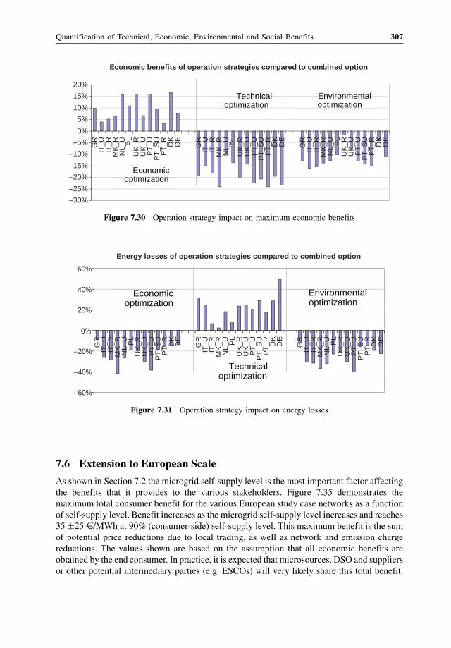
7.6 Extension to European Scale

As shown in Section 7.2 the microgrid self-supply level is the most important factor affecting

the benefits that it provides to the various stakeholders. Figure 7.35 demonstrates the

maximum total consumer benefit for the various European study case networks as a function

of self-supply level. Benefit increases as the microgrid self-supply level increases and reaches

35 �25 D /MWh at 90% (consumer-side) self-supply level. This maximum benefit is the sum

of potential price reductions due to local trading, as well as network and emission charge

reductions. The values shown are based on the assumption that all economic benefits are

obtained by the end consumer. In practice, it is expected that microsources, DSO and suppliers

or other potential intermediary parties (e.g. ESCOs) will very likely share this total benefit.

GR

IT_U

IT_R

MK

_RN

L_U PL

UK

_RU

K_U

PT

_UP

T_S

UP

T_R D

KD

E

GR

IT_U

IT_R

MK

_RN

L_U PL

UK

_RU

K_U

PT

_UP

T_S

UP

T_R D

KD

E

GR

IT_U

IT_R

MK

_RN

L_U PL

UK

_RU

K_U

PT

_UP

T_S

UP

T_R D

KD

E

Economic optimization

Technical optimization

Environmental optimization

Economic benefits of operation strategies compared to combined option

–30%

–25%

–20%

–15%

–10%

–5%

0%

5%

10%

15%

20%

Figure 7.30 Operation strategy impact on maximum economic benefits

GR

IT_

UIT

_R

MK

_R

NL

_U PL

UK

_R

UK

_U

PT

_U

PT

_S

UP

T_

RD

KD

E

GR

IT_

UIT

_R

MK

_R

NL

_U PL

UK

_R

UK

_U

PT

_U

PT

_S

UP

T_

RD

KD

E

GR

IT_

UIT

_R

MK

_R

NL

_U PL

UK

_R

UK

_U

PT

_U

PT

_S

UP

T_

RD

KD

E


P



Energy losses of operation strategies compared to combined option

–60%

–40%

–20%

0%

20%

40%

60%

Figure 7.31 Operation strategy impact on energy losses


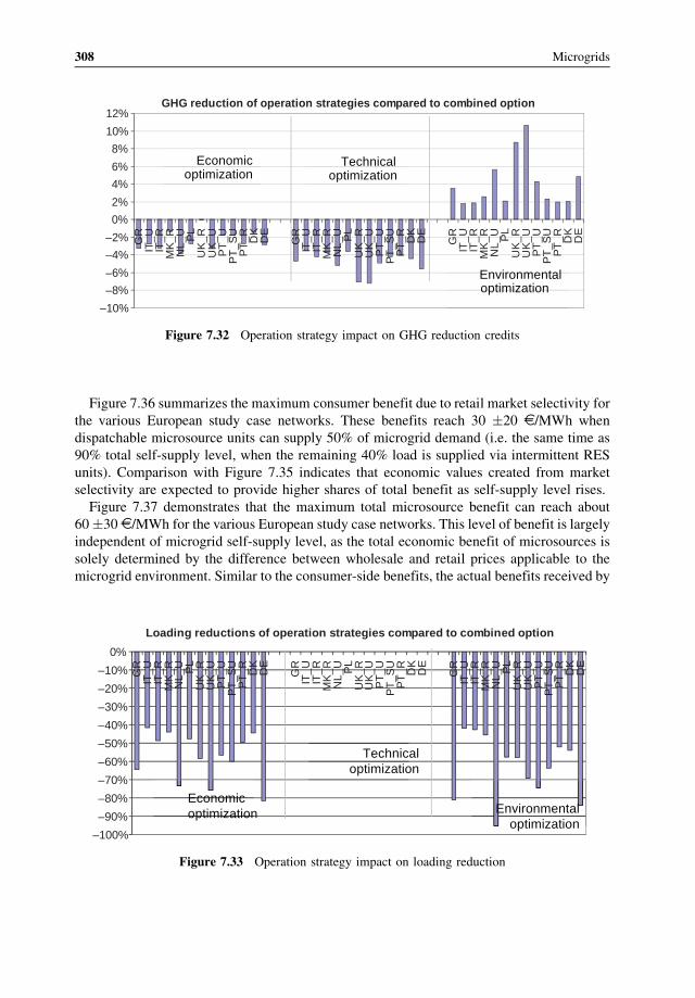
Figure 7.36 summarizes the maximum consumer benefit due to retail market selectivity for

the various European study case networks. These benefits reach 30 �20 D /MWh when

dispatchable microsource units can supply 50% of microgrid demand (i.e. the same time as

90% total self-supply level, when the remaining 40% load is supplied via intermittent RES

units). Comparison with Figure 7.35 indicates that economic values created from market

selectivity are expected to provide higher shares of total benefit as self-supply level rises.

Figure 7.37 demonstrates that the maximum total microsource benefit can reach about

60�30 D /MWh for the various European study case networks. This level of benefit is largely

independent of microgrid self-supply level, as the total economic benefit of microsources is

solely determined by the difference between wholesale and retail prices applicable to the

microgrid environment. Similar to the consumer-side benefits, the actual benefits received by

GR

IT_U

IT_R

MK

_RN

L_U PL

UK

_RU

K_U

PT

_UP

T_S

UP

T_R D

KD

E

GR

IT_U

IT_R

MK

_RN

L_U PL

UK

_RU

K_U

PT

_UP

T_S

UP

T_R D

KD

E

GR

IT_U

IT_R

MK

_RN

L_U PL

UK

_RU

K_U

PT

_UP

T_S

UP

T_R D

KD

E




–10%

–8%

–6%

–4%

–2%

0%

2%

4%

6%

8%

10%

12%GHG reduction of operation strategies compared to combined option

Figure 7.32 Operation strategy impact on GHG reduction credits

0%

GR

IT_U

IT_R

MK

_RN

L_U PL

UK

_RU

K_U

PT

_UP

T_S

UP

T_R D

KD

E

GR

IT_U

IT_R

MK

_RN

L_U PL

UK

_RU

K_U

PT

_UP

T_S

UP

T_R D

KD

E

GR

IT_U

IT_R

MK

_RN

L_U PL

UK

_RU

K_U

PT

_UP

T_S

UP

T_R D

KD

E

–100%

–90%

–80%

–70%

–60%

–50%

–40%

–30%

–20%

–10%

Economicoptimization

Technicaloptimization

Environmentaloptimization

Loading reductions of operation strategies compared to combined option

Figure 7.33 Operation strategy impact on loading reduction

308 Microgrids

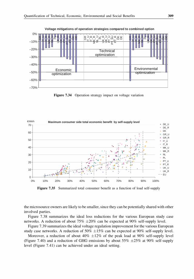
the microsource owners are likely to be smaller, since they can be potentially shared with other

involved parties.

Figure 7.38 summarizes the ideal loss reductions for the various European study case

networks. A reduction of about 75% �20% can be expected at 90% self-supply level.

Figure 7.39 summarizes the ideal voltage regulation improvement for the various European

study case networks. A reduction of 50% �15% can be expected at 90% self-supply level.

Moreover, a reduction of about 40% �12% of the peak load at 90% self-supply level

(Figure 7.40) and a reduction of GHG emissions by about 55% �25% at 90% self-supply

level (Figure 7.41) can be achieved under an ideal setting.

Voltage mitigations of operation strategies compared to combined option

–70%

–60%

–50%

–40%

–30%

–20%

–10%

0%

GR

IT_U

IT_R

MK

_RN

L_U

PL

UK

_RU

K_U

PT

_UP

T_S

UP

T_R D

KD

E

GR

IT_U

IT_R

MK

_RN

L_U

PL

UK

_RU

K_U

PT

_UP

T_S

UP

T_R D

KD

E

GR

IT_U

IT_R

MK

_RN

L_U

PL

UK

_RU

K_U

PT

_UP

T_S

UP

T_R D

KD

E




Figure 7.34 Operation strategy impact on voltage variation

Maximum consumer side total economic benefit by self-supply level

0

10

20

30

40

50

60

70

0% 10% 20% 30% 40% 50% 60% 70% 80% 90% 100%

/MWhDE_UDE_RDKGR_UGR_RIT_UIT_RMK_UMK_RNLPLPT_UPT_RUK_UUK_REU

Figure 7.35 Summarized total consumer benefit as a function of load self-supply


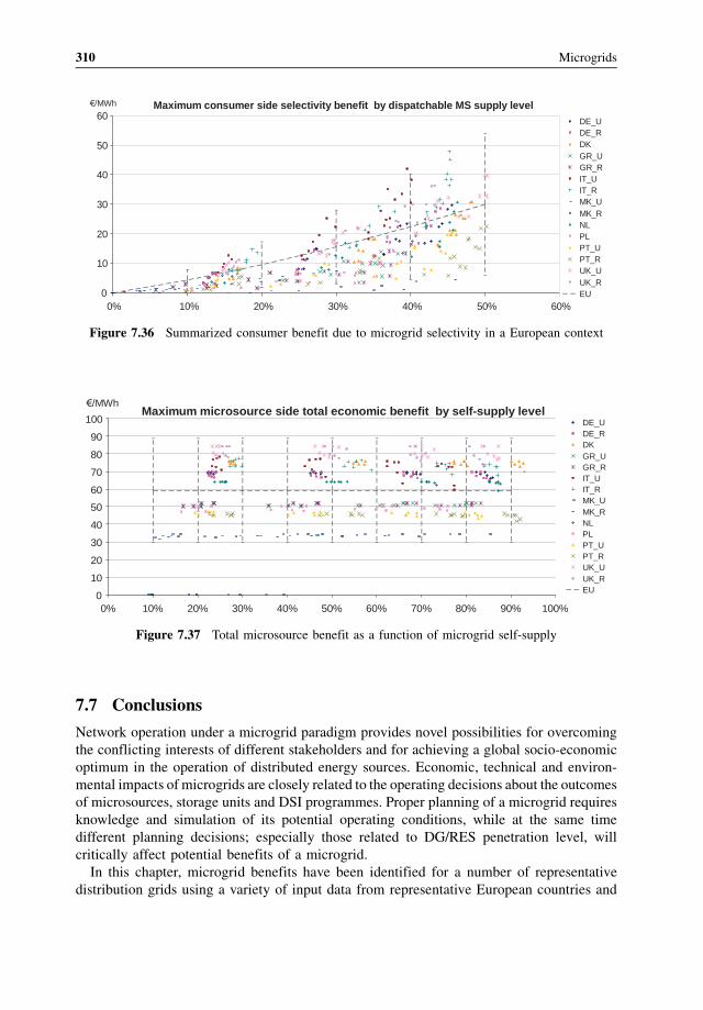
7.7 Conclusions

Network operation under a microgrid paradigm provides novel possibilities for overcoming

the conflicting interests of different stakeholders and for achieving a global socio-economic

optimum in the operation of distributed energy sources. Economic, technical and environ-

mental impacts of microgrids are closely related to the operating decisions about the outcomes

of microsources, storage units and DSI programmes. Proper planning of a microgrid requires

knowledge and simulation of its potential operating conditions, while at the same time

different planning decisions; especially those related to DG/RES penetration level, will

critically affect potential benefits of a microgrid.

In this chapter, microgrid benefits have been identified for a number of representative

distribution grids using a variety of input data from representative European countries and

Maximum consumer side selectivity benefit by dispatchable MS supply level

0

10

20

30

40

50

60

0% 10% 20% 30% 40% 50% 60%

/MWh

DE_UDE_RDKGR_UGR_RIT_UIT_RMK_UMK_RNLPLPT_UPT_RUK_UUK_REU

Figure 7.36 Summarized consumer benefit due to microgrid selectivity in a European context

0

10

20

30

40

50

60

70

80

90

100

0% 10% 20% 30% 40% 50% 60% 70% 80% 90% 100%

/MWh


Maximum microsource side total economic benefit by self-supply level

Figure 7.37 Total microsource benefit as a function of microgrid self-supply

310 Microgrids

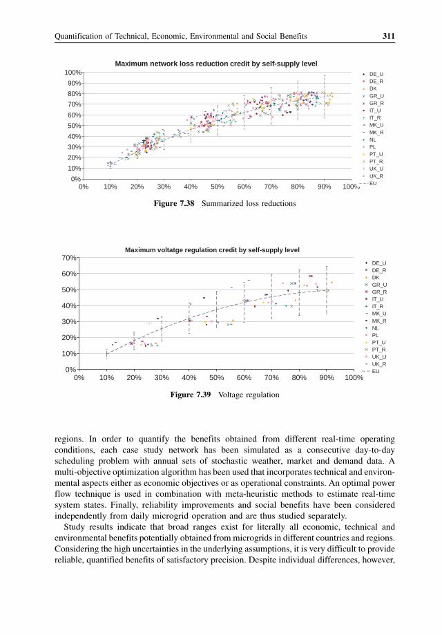
regions. In order to quantify the benefits obtained from different real-time operating

conditions, each case study network has been simulated as a consecutive day-to-day

scheduling problem with annual sets of stochastic weather, market and demand data. A

multi-objective optimization algorithm has been used that incorporates technical and environ-

mental aspects either as economic objectives or as operational constraints. An optimal power

flow technique is used in combination with meta-heuristic methods to estimate real-time

system states. Finally, reliability improvements and social benefits have been considered

independently from daily microgrid operation and are thus studied separately.

Study results indicate that broad ranges exist for literally all economic, technical and

environmental benefits potentially obtained frommicrogrids in different countries and regions.

Considering the high uncertainties in the underlying assumptions, it is very difficult to provide

reliable, quantified benefits of satisfactory precision. Despite individual differences, however,

Maximum network loss reduction credit by self-supply level

0%

10%

20%

30%

40%

50%

60%

70%

80%

90%

100%

0% 10% 20% 30% 40% 50% 60% 70% 80% 90% 100%


Figure 7.38 Summarized loss reductions

Maximum voltatge regulation credit by self-supply level

0%

10%

20%

30%

40%

50%

60%

70%

0% 10% 20% 30% 40% 50% 60% 70% 80% 90% 100%


Figure 7.39 Voltage regulation


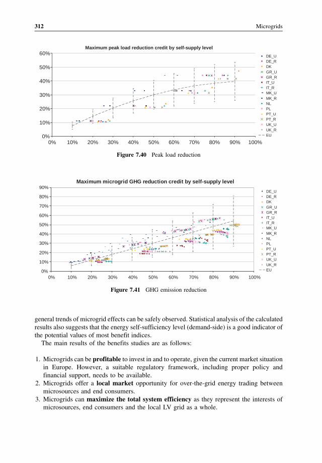
general trends of microgrid effects can be safely observed. Statistical analysis of the calculated

results also suggests that the energy self-sufficiency level (demand-side) is a good indicator of

the potential values of most benefit indices.

The main results of the benefits studies are as follows:

1. Microgrids can be profitable to invest in and to operate, given the current market situation

in Europe. However, a suitable regulatory framework, including proper policy and

financial support, needs to be available.

2. Microgrids offer a local market opportunity for over-the-grid energy trading between

microsources and end consumers.

3. Microgrids can maximize the total system efficiency as they represent the interests of

microsources, end consumers and the local LV grid as a whole.

Maximum peak load reduction credit by self-supply level

0%

10%

20%

30%

40%

50%

60%

0% 10% 20% 30% 40% 50% 60% 70% 80% 90% 100%


Figure 7.40 Peak load reduction

0%

10%

20%

30%

40%

50%

60%

70%

80%

90%

100%90%80%70%60%50%40%30%20%10%0%


Maximum microgrid GHG reduction credit by self-supply level

Figure 7.41 GHG emission reduction

312 Microgrids

4. Microgr ids allow for real-time , multi -objective dispat ch op timization to achieve eco-

nomic, technical and environm ental aims at the same time .

5. Microgr ids can accommodat e different owne rship models and provide end consumer

motivat ion whe re other conce pts fail to do so.

Benefi ts of Microgr id Oper ation

A micro grid coul d poten tially offer econom ic benefits (singl e or multipl e from list) such as:

� price reduction for end consum ers,� increas ed revenues for mi crosourc es,� investment defe rral for distribution system opera tors.

Economic benefits arise mainly from localit y value s create d by local retai l mar ket and

selectivity value s create d by optim ized real-time disp atch decisions.

To achieve the expected econom ic benefits, it is neces sary to reco gnize local (over-th e-grid)

energy tradin g within a micro grid, to appl y real-ti me import and export prices for micro grids

and to have an (optimal ) RES suppor t scheme and favorable tariffs.

A micro grid coul d potenti ally offer technical benefits (single or multipl e from list) such as:

� energy loss reduc tion,� lower voltage variation,� peak load ing (cong estion) relief,� reliab ility improveme nt.

Technical benefits can b e either traded in a loca l serv ice market betwee n micro source and

DSO or impleme nted as pri ce signals. To achieve the expected technical benefits, optim al

dimens ioning and alloca tion of micro sources as well as coord inated multi-u nit micro source

dispatc h, based on real-ti me grid conditions is necessar y.

Environm ental benefits of microgri d can b e mainly attributed to:

� shift toward renewable or low-em ission fuels used by internal micro sourc es,� adopt ion of more energy-efficie nt technol ogies, such as CHP,� adopt ion of DSI options.

Socia l benefits of microgrids can be summa rized as:

� raising public awareness and fostering incentive for energy saving and GHG emission

reduction,� creation of new research and job opportunities,� electrification of remote or underdeveloped areas.

Reference

1. More Microgrids (2006–2009) Advanced Architectures and Control Concepts for More Microgrids, FP6 STREP,

Contract no.: PL019864., http://www.microgrids.eu.


Index

active networks, 2

active power control, 82–83

agent

based load controller, 211

communication, 54-56, 59, 60

language, 54, 59, 60

definition, 52

directory facilitator, 56

management system, 56, 60

reactive, 53–54

vs. intelligent, 53–55, 60

AMS, agent management system, 56

ancillary services, 14, 89

ATP/EMTP, 87–88

auction

algorithms, 60

applications, 63

Dutch, 61

English, 60

automated meter reading, 28

benefit quantification study, 278

benefits of microgrids

economic, 289

environmental and social, 277

operation, 291

technical, 300

business models, 15

centralized control approach, 34

centralized, 32

CHP units, 9

consumer, 12

control, 28

centralized, 36

decentralized, 51

functionalities, 26

master – slave, 82–83

controllable elements in a microgrid, 8

costs, 18

customer, 12

decentralized control approach, 34

demand side, 14

bidding, 43

integration, 7, 10

DG owner/operator, 12

directional pricing, 20

dispatchable loads, 8

distributed generators, 3

distribution management system, DMS, 30

distribution system operator, 13

DSO monopoly model, 16

economic benefits of micro-source owners, 291

economic operation, 41

energy service company, 13

FORECASTING, 35

forecasting

demand, 37

electricity prices, 38

heat demand, 39

RES, 48

uncertainties on predictions, 40

wind and PV production, 38



foundation of intelligent physical agents,

FIPA, 55

game theory, 69

IEC-61850, 154

incentive-based demand response, 14

intelligent load controller, 212

intelligent local controllers, 81

internet of energy, 27

inverters

control of, 103

droops, 103

control, 103

implications of line parameters, 92

inductive coupling, 104

provision of ancillary services, 89

secondary control, 87

stability in interconnected operation, 107

stability in islanded mode, 100

transition between islanded and connected

modes, 110

voltage source, 85

JADE, 55

java agent development framework, 55

local control, 26

locational value, 19

market models, 12

liberalized, 17

prosumer consortium, 18

market policies, 42

market regulator, 12

MC, 30

MGCC, 30, 32, 38, 40, 41, 126, 167, 214

in Kythnos, 212

microgeneration technologies, 3

microgrid central controller, 30, 126, 167, 214

microgrid control architecture, 28

microgrid controller, 7, 41

microgrid field test

in Bronsbergen, 222

in Chile, 270

in China, 262

in Gaidouromandra, 208

in Germany, 218

in Greece, 208

in Japan, 249

in Kythnos, 208

in Mannheim, 218

in Netherlands, 222

in U.S, 231

microgrids, 2, 4

operators, 7, 10–12, 31

pilot sites, 206

multi agent reinforcement learning, 64

Q-Learning, 65, 66

multi agent system, 52, 54, 56

in Kythnos, 249

multi-microgrids, 4, 35, 165

control and management architecture, 167

coordinated voltage var support, 169

dynamic equivalents, 192

emergency functions, 186

frequency control, 178

functionalities, 167, 168

openness of the system, 35

operation strategies of microgrids, 10

optimisation problem, 34, 35, 45, 46

optimum DG penetration level, 295

peak load reduction, 288, 312

pilot sites, 206

price-based demand response, 14

prosumer, 12, 18

protection, 117

adaptive, 118, 125

centralized adaptive, 126, 154

challenges for microgrids, 118

cost, 119, 124, 145

dependability, 118

differential, 120

distance, 119

external faults, 121, 224

fault location, 122, 127

internal faults, 122, 224

major problems, 118

over-current, 119

distribution feeder, 120, 121

redundancy, 119, 145

security, 119

selectivity, 118

sensitivity, 118

speed, 118

reduction of losses, 287

reliability improvement, 293, 294, 311

316 Index

remote terminal units, 28

retail supplier, 13

revenues, 18, 46, 51

satisfaction of local consumption, 19, 21

scalability, 60, 70, 217

smart grids, 1, 2, 13, 207

state estimation, 72

fuzzy, 74

microgrid, 73

Index 317