Embed Size (px)
Citation preview

arX
iv:1
101.
4950
v2 [
mat
h.A
G]
7 F
eb 2
011
ARC SPACES AND ROGERS-RAMANUJAN IDENTITIES
CLEMENS BRUSCHEK∗, HUSSEIN MOURTADA, AND JAN SCHEPERS†
Abstract. Arc spaces have been introduced in algebraic geometry as a toolto study singularities but they show strong connections with combinatoricsas well. Exploiting these relations we obtain a new approach to the classicalRogers-Ramanujan Identities. The linking object is the Hilbert-Poincare seriesof the arc space over a point of the base variety. In the case of the double pointthis is precisely the generating series for the integer partitions without equalor consecutive parts.
1. Introduction
Arc spaces describe formal power series solutions (in one variable) to polynomialequations. They first appeared in the work of Nash (published later as [Nas95]),who investigated their relation to some intrinsic data of a resolution of singular-ities of a fixed algebraic variety. He asked whether there is a bijection betweenthe irreducible components of the arc space based at the singular locus and the setof essential divisors. While this so-called ‘Nash problem’ is still actively studied(see for instance the recent papers [LJR08, PS10, PP10, FdB10] and the overview[Ish07]), in the last decade arc spaces have gained much interest from algebraicgeometers, through their role in motivic integration and their utility in birationalgeometry. Arc spaces show strong relations with combinatorics as well. In thepresent text we indicate how to exploit this connection both for geometric as wellas combinatorial benefit. In particular, we expose a surprising connection with thewell-known Rogers-Ramanujan identities.
Let us emphasize the main algebraic and combinatorial aspects presented here.First, we suggest to study local algebro-geometric properties of algebraic (or ana-lytic) varieties via natural Hilbert-Poincare series attached to arc spaces. In con-trast to already existing such series this one is sensitive to the non-reduced struc-ture of the arc space. Second, we propose to derive identities between partitions bylooking at suitable ideals in a polynomial ring in countably many variables endowedwith a natural grading. Connecting both ideas will demand handling Grobner basisin countably many variables, a problem which has been successfully dealt with indifferent contexts over the last years (see [HS09, Dra10]). In the present situation– that is for very specific ideals – salvation from the natural obstruction of beinginfinitely generated comes in the shape of a derivation making the respective idealsdifferential.
We briefly indicate the connection between arc spaces and partitions. Let f ∈k[x1, . . . , xn] be a polynomial in n variables x1, . . . , xn with coefficients in a fieldk. We denote the formal power series ring in one variable t over the field k byk[[t]]. The arc space X∞ of the algebraic variety X defined by f is the set of powerseries solutions x(t) = (x1(t), . . . , xn(t)) ∈ k[[t]]n to the equation f(x(t)) = 0. This
∗FWF project P21461 and I382.†Postdoctoral Fellow of the Research Foundation - Flanders (FWO)MSC2010 Subject Classification: 14B05, 11P84, 05A17, 13P10.
1

2 CLEMENS BRUSCHEK, HUSSEIN MOURTADA, AND JAN SCHEPERS
set turns out to be eventually algebraic in the sense that it is given by polynomialequations (though there are countably many of them). Indeed, expanding f(x(t))as a power series in t gives
f(x(t)) = F0 + F1t+ F2t2 + · · ·
where the Fi are polynomials in the coefficients of t in x(t). Therefore, a given vectorof formal power series a(t) ∈ k[[t]]n is an element of the arc space X∞ if and only ifits coefficients fulfill the equations F0, F1, . . . . Algebraically the corresponding setof solutions is described by its coordinate algebra
J∞(X) = k[x(i)j ; 1 ≤ j ≤ n, i ∈ N]/(F0, F1, . . .),
where N = {0, 1, 2, . . .}. The variable x(i)j corresponds to the coefficient of ti in
xj(t). We will mostly be interested in the case where a(0) is a point on X (withoutloss of generality we may assume that this is the origin). The resulting algebra,
obtained from J∞(X) by substituting x(0)j = 0, is called the focussed arc algebra
and denoted by J0∞(X); we write fi for the image of Fi under this substitution:
J0∞(X) = k[x
(i)j ; 1 ≤ j ≤ n, i ≥ 1]/(f1, f2, . . .).
This algebra is naturally graded by the weight function wtx(i)j = i since fℓ is
homogeneous of weight ℓ. In the special case of n = 1 we will write yi instead
of x(i)1 . Integer partitions arise naturally when computing weights of monomials
in J0∞(A1). Recall that a partition of m ∈ N is an r-tuple of positive integers
λ1 ≤ λ2 ≤ · · · ≤ λr with λ1 + · · ·+ λr = m. The λi are the parts of the partitionand r is its length. A monomial yα1
1 · · · yαee has weight α1 ·1+ · · ·+αe ·e. Asking for
the number of monomials (up to coefficients) of some weight m is thus asking forthe number of partitions of m. This is precisely what we capture when computingthe Hilbert-Poincare series of J0
∞(A1). In general, the Hilbert-Poincare series ofJ0∞(X) is defined as
HPJ0∞
(X)(t) =∞∑
j=0
dimk
(J0∞(X)
)j· tj ,
where(J0∞(X)
)jdenotes the jth homogeneous component of J0
∞(X). In the simple
case of X = A1 we may use the generating function for partitions to representHPJ0
∞(A1)(t) by
H :=∏
i≥1
1
1− ti.
By the general theory of Grobner basis HPJ0∞
(X)(t) is identical with the Hilbert-Poincare series of the algebra
k[x(i)j ; 1 ≤ j ≤ n, i ≥ 1]/L(I),
where L(I) denotes the leading ideal of I = (f0, f1, . . .) (with respect to a chosenmonomial ordering). The leading ideal is much simpler since it is generated bymonomials. Computing the Hilbert-Poincare series of the respective algebra corre-sponds to counting partitions, leaving out those coming from weights of monomialsin L(I). In the simple example of f = y2, these will be all partitions withoutrepeated or consecutive parts. Such partitions are part of the well-known Rogers-Ramanujan identity: the number of partitions of n into parts congruent to 1 or4 modulo 5 is equal to the number of partitions of n into parts that are neitherrepeated nor consecutive (see [And98]). This gives:

ARC SPACES AND ROGERS-RAMANUJAN IDENTITIES 3
Theorem. Let k be field of characteristic 0. For X : y2 = 0 we compute
HPJ0∞
(X)(t) =∏
i≥1i≡1,4 mod 5
1
1− ti.
More generally, we obtain using Gordon’s generalizations of the Rogers-Ramanujanidentities for X : yn = 0, n ≥ 2:
Theorem.
HPJ0∞
(X)(t) = H ·∏
i≥1i≡0,n,n+1mod 2n+1
(1− ti).
The computation of L(I) in these rather simple looking cases is nontrivial. It iscarried out in Section 5.
Moreover, standard techniques from commutative algebra allow to compute a re-cursion for the Hilbert-Poincare series in the case of X : y2 = 0:
Proposition. The generating series HPJ0∞
(X)(t) is the t-adic limit of the sequenceof formal power series Ad defined by:
A1 = A2 = 1, and Ad = Ad−1 + td−2Ad−2 for d ≥ 3.
The above proposition was first found in an empirical way in [AB89], and it leadsto the Rogers-Ramanujan identities (see Section 5).
Returning to the geometric aspect of the series attached to arc spaces, we computethem in other interesting cases: for smooth points, for rational double points ofsurfaces, and for normal crossings singularities. In these cases the simple geometryof the jet schemes permits to compute the Hilbert-Poincare series defined above,and we find the following (see Propositions 3.4, 3.8 and 3.9).
Proposition. With the above introduced notation, we have:
(1) If p is a smooth point on a variety X of dimension d, then
HPJp∞(X) =
∏
i≥1
1
1− ti
d
,
(2) if X is a surface with a rational double point at p then
HPJp∞
(X)(t) =
(1
1− t
)3∏
i≥2
1
1− ti
2
,
(3) if X = {x1 · · ·xd+1 = 0} ⊂ Ad+1k , and p is a point in the intersection of
precisely e components, then
HPJp∞(X)(t) =
(e−1∏
i=1
1
1− ti
)d+1∏
i≥e
1
1− ti
d
.
In the past several generating series have been associated to the arc space of a(singular) variety by Denef and Loeser (see [DL99, DL01]), in analogy with thep-adic case. All those series are defined in the motivic setting and take values in apower series ring with coefficients in (a localization of) a Grothendieck ring. Theyare rational. Some of those series encode more information about the singularitiesthan others. For a comparison between them see [Nic05a, Nic05b, CPGP10]. While

4 CLEMENS BRUSCHEK, HUSSEIN MOURTADA, AND JAN SCHEPERS
those series are concerned with the reduced structure of the arc space, our series issensitive to the non-reduced structure as well, although it is not rational in general.We discuss more geometric motivation for introducing the above Hilbert-Poincareseries in Section 3 (after Definition 3.1).
The structure of the paper is as follows: in Section 2, we define jet schemes and arcspaces and recall some basic facts about them. In Section 3 we introduce the arcHilbert-Poincare series, we discuss its properties and we compute it in particularcases. Section 4 recalls basic facts about partitions and the Rogers-Ramanujanidentities. Section 5 is devoted to the main theorem. For the convenience of thereader, we recall the facts about Hilbert-Poincare series and Grobner bases that weuse in the paper in an appendix (Section 6).
Acknowledgements. The authors thank the organizers of YMIS for preparing theground for this joint research. The first named author expresses his gratitude toHerwig Hauser, Georg Regensburger and Josef Schicho for many useful discussionson these topics; the second named author is grateful to Monique Lejeune-Jalabertfor introducing him to Hilbert-Poincare series; the third named author thanks Jo-hannes Nicaise for explaining him several facts about arc spaces in detail and hethanks the Institut des Hautes Etudes Scientifiques, where part of this work wasdone, for hospitality.
2. Jet schemes and arc spaces
Let k be a field. Let X = Spec(k[x1, . . . , xn]/(g1, . . . , gr)
)be an affine scheme of
finite type over k. For l ∈ {1, . . . , r}, and j ∈ {0, . . . ,m}, we define the polynomial
G(j)l ∈ k[x
(i)s ; 1 ≤ s ≤ n, 0 ≤ i ≤ m] as the coefficient of tj in the expansion of
(1) gl(x(0)1 + x
(1)1 t+ · · ·+ x
(m)1 tm, . . . , x(0)n + x(1)n t+ · · ·+ x(m)
n tm).
Then the mth jet scheme Xm of X is
Xm := Spec
(k[x
(i)s ; 1 ≤ s ≤ n, 0 ≤ i ≤ m]
(G(j)l ; 1 ≤ l ≤ r, 0 ≤ j ≤ m)
).
In particular, we have that X0 = X . Of course, we do not need to fix m in advance,
and we can define G(j)l ∈ k[x
(i)s ; 1 ≤ s ≤ n, i ∈ N] for all j ∈ N as above. Here
N = {0, 1, . . .}. Then the arc space X∞ of X is
X∞ := Spec
(k[x
(i)s ; 1 ≤ s ≤ n, i ∈ N]
(G(j)l ; 1 ≤ l ≤ r, j ∈ N)
).
The functorial definition is also useful. Let X be a scheme of finite type over k andlet m ∈ N. The functor
Fm : k-Schemes → Sets
which to an affine scheme defined by a k-algebra A associates
Fm(Spec(A)) = Homk
(Spec
(A[t]/(tm+1)
), X)
is representable by the k-scheme Xm (see for example [Ish07, Voj07]). The arcspace X∞ represents the functor F∞ that associates to a k-algebra A the setHomk
(Spf(A[[t]]), X
), where Spf denotes the formal spectrum.
For m, p ∈ N,m > p, the truncation homomorphism A[t]/(tm+1) → A[t]/(tp+1)induces a canonical projection πm,p : Xm → Xp. These morphisms clearly verifyπm,p ◦πq,m = πq,p for p < m < q. We denote the canonical projection πm,0 : Xm →

ARC SPACES AND ROGERS-RAMANUJAN IDENTITIES 5
X0 by πm. For m ∈ N we also have the truncation morphism A[[t]] → A[t]/(tm+1).It gives rise to a canonical morphism ψm : X∞ −→ Xm.Assume now that k has characteristic zero. In that case we can explicitly determinethe ideals defining the jet schemes and the arc space. Let S = k[x1, . . . , xn] and
Sm = k[x(i)s ; 1 ≤ s ≤ n, 0 ≤ i ≤ m]. Let D be the k-derivation on Sm defined by
D(x(i)s ) := x
(i+1)s if 0 ≤ i < m, and D(x
(m)s ) := 0. We embed S in Sm by mapping
xi to x(0)i .
Proposition 2.1. Let X = Spec(S/(g1, . . . , gr)
)and let Jm(X) be the coordinate
ring of Xm. Then
Jm(X) =Sm
(Dj(gl); 1 ≤ l ≤ r, 0 ≤ j ≤ m).
Proof. Since k has characteristic zero, we may equally well replace xi by
x(0)i
0!+x(1)i
1!t+ · · ·+
x(m)i
m!tm
to obtain the equations of the jet space. For g ∈ S we denote then
φ(g) := g
(x(0)1
0!+x(1)1
1!t+ · · ·+
x(m)1
m!tm, . . . ,
x(0)n
0!+x(1)n
1!t+ · · ·+
x(m)n
m!tm).
Then we have
τm(φ(g)
)=
m∑
j=0
Dj(g)
j!tj ,
where τm means truncation at degree m. To see this, it is sufficient to remarkthat it is true for g = xi, and that both sides of the equality are additive andmultiplicative in g (after truncating at degree m). The proposition follows. �
Similarly, the coordinate ring J∞(X) of X∞ is given by
J∞(X) =k[x
(i)s ; 1 ≤ s ≤ n, i ∈ N]
(Dj(gl); 1 ≤ l ≤ r, j ∈ N).
Here D(x(i)s ) = x
(i+1)s for all i ∈ N. For further understanding of the equations of
the jet schemes and their relation with Bell polynomials, see [Bru09, Bru10].
3. The arc Hilbert-Poincare series
In this section we introduce and discuss the Hilbert-Poincare series of the arc alge-bra of a (not necessarily reduced nor irreducible) algebraic variety X , focussed ata point p of X . Since this will be a local invariant, we may restrict ourselves to Xbeing a closed subscheme of affine space. For generalities about Hilbert-Poincareseries of graded algebras we refer to the appendix (Section 6).
As above, let k be a field of characteristic zero. Although for most of the state-ments it is not necessary that k is algebraically closed, we will assume it for conve-nience. Let X be a subscheme of affine n-space over k, defined by some ideal I in
k[x1, . . . , xn]. We define a grading on the polynomial ring k[x(i)j ; 1 ≤ j ≤ n, i ∈ N]
by putting the weight of x(i)j equal to i. We prefer to use the terminology ‘weight’
instead of ‘degree’ here, in order not to confuse with the usual degree. It is easy to
see that the ideal I∞ of k[x(i)j ; 1 ≤ j ≤ n, i ∈ N] defining the arc space X∞ is ho-
mogeneous (with respect to the weight) and hence the arc algebra J∞(X) is gradedas well (this follows for instance from Proposition 2.1). Similarly the jet algebrasJm(X) are graded. Let p be any point of X and denote by κ(p) the residue field at

6 CLEMENS BRUSCHEK, HUSSEIN MOURTADA, AND JAN SCHEPERS
p. After identifying J0(X) with the coordinate ring of X we obtain a natural mapfrom J0(X) to κ(p).
Definition 3.1. We define the focussed arc algebra of X at p as
J∞(X)⊗J0(X) κ(p)
and we denote it by Jp∞(X). Analogously, we define the focussed jet algebras of X
at p by
Jpm(X) := Jm(X)⊗J0(X) κ(p).
Using the above grading, we write HPJp∞(X)(t) respectively HPJp
m(X)(t) for their
Hilbert-Poincare series as graded κ(p)-algebras. We call this the arc Hilbert-Poin-care series at p respectively the mth jet Hilbert-Poincare series at p.
In fact, the focussed arc algebra at a point p is the coordinate ring of the schemetheoretic fiber of the morphism ψ0 : X∞ → X over p. Note that the weight zeropart of Jp
∞(X) or Jpm(X) is always a one-dimensional κ(p)-vector space.
In the special case that X is a hypersurface given by a polynomial F ∈ k[x1, . . . , xn]with F (0) = 0, this boils down to the following. We define F0 to be F in the
variables x(0)1 , . . . , x
(0)n . Then we put F1 := DF0, F2 := DF1, . . ., where D is the
derivation from Section 2. The arc algebra J∞(X) is given as the quotient of
k[x(i)j ; 1 ≤ j ≤ n, i ∈ N] by (F0, F1, . . .) (see Proposition 2.1). And J0
∞(X) is the
quotient of k[x(i)j ; 1 ≤ j ≤ n, i ≥ 1] by (f0, f1, . . .), where fi is Fi evaluated in
x(0)1 = · · · = x
(0)n = 0.
Remark. Besides that the arc Hilbert-Poincare series is very natural to look atwhen working with arc spaces, its introduction is motivated by the following. IfX is for instance a hypersurface then the ideal I0m = (f0, f1, . . .) defining the fiberover the origin of the mth jet space of X is generated by polynomials depending
only on a subset of the variables of the polynomial ring k[x(i)j ; 1 ≤ j ≤ n, i ≥ 1].
Heuristically, for a given m ∈ N, the more X is singular, the less variables appearin I0m. So this series was meant as a Hironaka type invariant of the singularity (see[BHM10]), that is a kind of measure of the number of variables appearing in I0m.Note also that since the jet spaces are far from being equidimensional in general (see[Mou, Mou10a]), the jet algebras have a big homological complexity, what makesit difficult to compute the series introduced above.
Remark. We can define the graded structure on J∞(X) more intrinsically as follows,with X as above. For an extension field K of k, the K-rational points of X∞
correspond to morphisms of k-algebras
γ : Γ(X,OX) → K[[t]].
For λ ∈ k× we have an automorphism ϕλ of K[[t]] determined by t 7→ λt. Bycomposing ϕλ with γ we obtain a natural action of k× on X∞ and hence on itscoordinate ring J∞(X). An element f ∈ J∞(X) is then called homogeneous ofweight i if λ · f = λif , for all λ ∈ k×.
We consider the truncation operator
τ≤r : k[[t]] → k[t] :∑
i≥0
aiti 7→
r∑
i=0
aiti.
Then we have the following simple observation.
Proposition 3.2. τ≤m HPJpm(X)(t) = τ≤m HPJp
∞(X)(t).

ARC SPACES AND ROGERS-RAMANUJAN IDENTITIES 7
Now let X and Y be closed subschemes of Ank respectively Am
k . Recall that one
calls p ∈ X and q ∈ Y analytically isomorphic if OX,p and OY,q are isomorphick-algebras.
Proposition 3.3. If p ∈ X and q ∈ Y are analytically isomorphic then
HPJp∞(X)(t) = HPJq
∞(Y )(t).
Proof. The fiber of πX : X∞ → X over p is a scheme over κ(p) whose K-rationalpoints, for an extension field K of κ(p), correspond to the set of morphisms ofk-algebras
γ : Γ(X,OX) → K[[t]]
such that γ−1((t))= p. Since K[[t]] is complete, γ factors uniquely through OX,p.
We conclude that the fiber of πX : X∞ → X over p is determined by OX,p.To see that the graded structure of the fibers of πX and πY above p respectively q
agree, we can use the intrinsic description of the graded structure from the previousremark. �
Next we compute the arc Hilbert-Poincare series at a smooth point. We use thenotation
H :=∏
i≥1
1
1− ti.
Proposition 3.4. Let X be an irreducible closed subscheme of Ank of dimension d
and let p ∈ X be a smooth point. Then
HPJp∞(X)(t) = Hd.
Proof. By definition OX,p is a regular local ring, and hence an integral domain.ThereforeX is reduced, and thus an integral scheme. Denote by e the transcendencedegree of κ(p) over k. From dimension theory (e.g. Thm. A and Cor. 13.4 on p.290in [Eis95]) it follows that the dimension of OX,p equals d − e. The complete local
ring OX,p is regular as well and hence isomorphic to κ(p)[[x1, . . . , xd−e]] (Prop.10.16 in [Eis95]). By the theorem of the primitive element, κ(p) is isomorphicto k(y1, . . . , ye)[x]/(f), where we may assume f ∈ k[y1, . . . , ye, x]. Hence κ(p) isisomorphic to the residue field of the point (f, z1, . . . , zd−e−1) in the affine space
Spec k[y1, . . . , ye, x, z1, . . . , zd−e−1].
From Proposition 3.3 it follows that it suffices to compute the arc Hilbert-Poincareseries at a point q of Y := Ad
k. This is an easy task, since Jm(Y ) is the polynomialring
k[x(i)j ; 1 ≤ j ≤ d, 0 ≤ i ≤ m],
and Jqm(Y ) equals
κ(q)[x(i)j ; 1 ≤ j ≤ d, 1 ≤ i ≤ m].
The variables form a regular sequence in this ring, and hence it follows easily fromLemma 6.1 that
HPJqm(Y )(t) =
(m∏
i=1
1
1− ti
)d
.
Now we use Proposition 3.2 to finish the proof. �
In Section 4 we discuss the connection of this result with partitions. We leave theproof of the following proposition to the reader.

8 CLEMENS BRUSCHEK, HUSSEIN MOURTADA, AND JAN SCHEPERS
Proposition 3.5. Let X and Y be closed subschemes of Ank respectively Am
k . Letp ∈ X and q ∈ Y . Then
HPJ
(p,q)∞ (X×Y )
(t) = HPJp∞(X)(t) · HPJq
∞(Y )(t).
The multiplicity of a singular point on a hypersurface can be easily read from thearc Hilbert-Poincare series, as the reader may convince himself of:
Proposition 3.6. Let X be a hypersurface in Ank defined by a polynomial F ∈
k[x1, . . . , xn] with F (0) = 0. Then X has multiplicity r at the origin if and only ifr is the maximal number such that
τ≤r−1 HPJ0∞
(X)(t) = τ≤r−1Hn.
Moreover, τ≤r HPJ0∞
(X)(t) = τ≤rHn − tr.
Next we derive a formula for the arc Hilbert-Poincare series of the focussed arcalgebra at a canonical hypersurface singularity of maximal multiplicity. First werecall the definition of a canonical singularity. Let X be a normal variety. Assumethat X is Q-Gorenstein (i.e. rKX is Cartier for some r ≥ 1). Let f : Y → X be alog resolution. This means that f is a proper birational morphism from a smoothvariety Y such that the exceptional locus is a simple normal crossings divisor withirreducible components Ei, i ∈ I. We have a linear equivalence
KY = f∗KX +∑
i
aiEi
for uniquely determined ai ∈ Q (these are called discrepancy coefficients). ThenX has canonical singularities if ai ≥ 0 for all i. We say that X has a canonicalsingularity at a point p ∈ X if there exists a neighbourhood U of p in X withcanonical singularities. Note that if X is a hypersurface in An
k , then X is Gorenstein(i.e. KX is Cartier) and all ai are then integers. In that case, if X has a canonicalsingularity at a closed point p, the multiplicity of p is at most the dimension of X .This follows by computing the discrepancy coefficient of the exceptional divisor ofthe blowing-up in p.
Proposition 3.7. Let X be a normal hypersurface in Ank with a canonical singu-
larity of multiplicity n− 1 at the origin. Then
HPJ0∞
(X)(t) =
(n−2∏
i=1
1
1− ti
)n ∏
i≥n−1
1
1− ti
n−1
.
Proof. Let X be defined by the polynomial F . We use the notations Fi and fi asbefore. Then fi = 0 for 0 ≤ i ≤ n − 2. To deduce the result, it suffices to showthat for every m ≥ n− 1 the polynomials fn−1, fn, . . . , fm form a regular sequence
in the polynomial ring k[x(i)j ; 1 ≤ j ≤ n, 1 ≤ i ≤ m], in view of Lemma 6.1 and
Proposition 3.2.Since the question is local, we may assume that all singularities of X are canonical.We will use a theorem by Ein and Mustata that characterizes canonical singularitiesby the fact that their jet spaces are irreducible (see Thm. 1.3 in [EM04]). It is wellknown that the natural maps πm : Xm → X are locally trivial fibrations above the
smooth part of X , with fiber isomorphic to A(n−1)mk . Hence the dimension of Xm
is precisely (n− 1)(m+1). Since Xm is irreducible, it follows that the fiber π−1m (0)
has dimension at most (n− 1)(m+ 1)− 1. From dimension theory (e.g. Cor. 13.4in [Eis95]) we deduce that the codimension of the ideal I0m := (fn−1, fn, . . . , fm)
in Am := k[x(i)j ; 1 ≤ j ≤ n, 1 ≤ i ≤ m] is at least nm −
((n − 1)(m + 1) − 1
)=
m−n+2. From the principal ideal theorem (Thm. 10.2 of [Eis95]) we get then that
ARC SPACES AND ROGERS-RAMANUJAN IDENTITIES 9
the codimension of I0m is precisely m− n+ 2. Since a polynomial ring over a fieldis Cohen-Macaulay, we may apply the unmixedness theorem (Cor. 18.14 of [Eis95])to deduce that every associated prime of I0m is minimal. But the codimension ofI0m+1 in Am+1 is at least m − n + 3, so this means that fm+1 is not contained inany minimal prime ideal containing I0m, considered as ideal of Am+1. Hence fm+1
does not belong to an associated prime ideal of I0m, and thus it is a nonzerodivisormodulo I0m (see Thm. 3.1(b) of [Eis95]). �
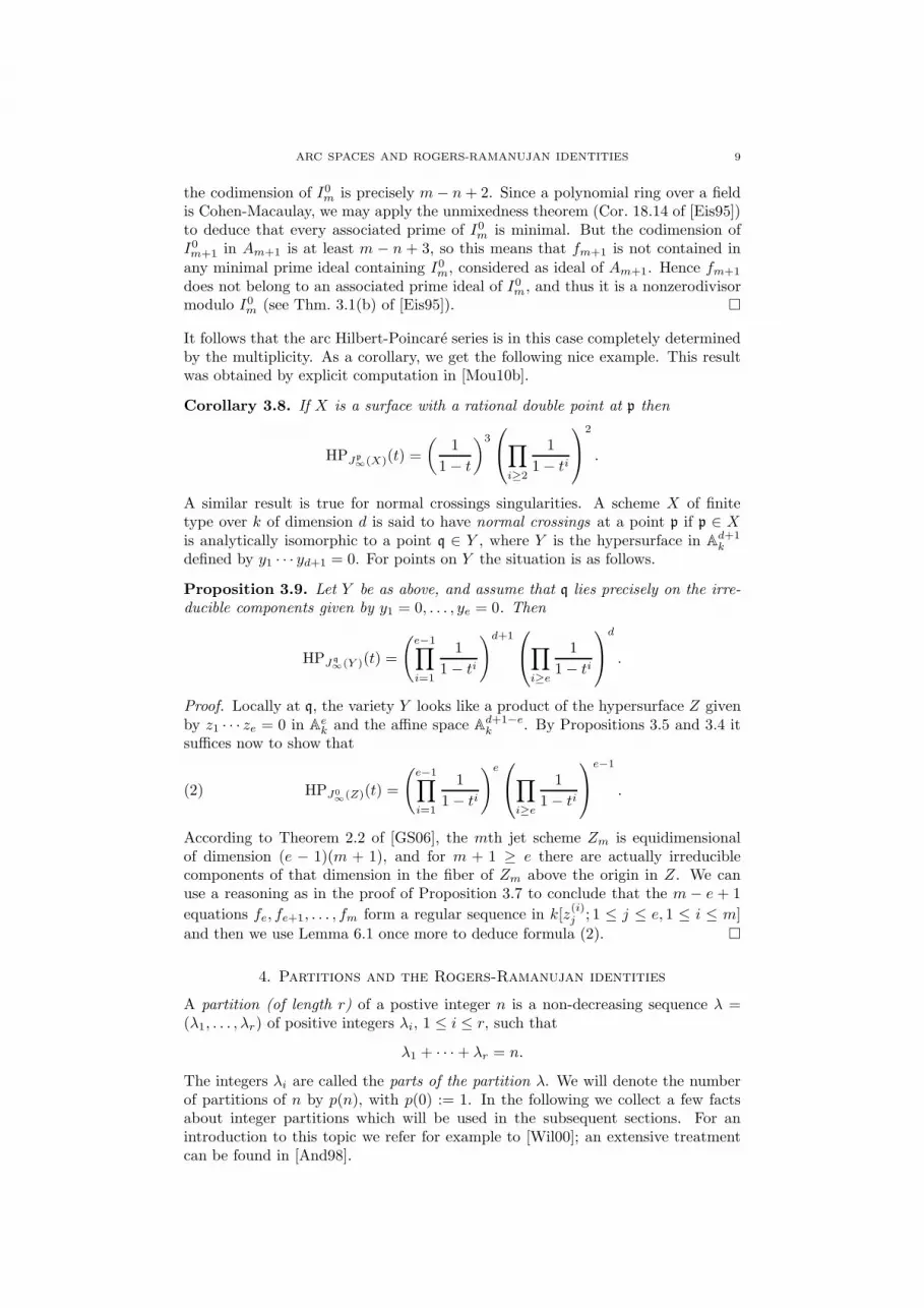
It follows that the arc Hilbert-Poincare series is in this case completely determinedby the multiplicity. As a corollary, we get the following nice example. This resultwas obtained by explicit computation in [Mou10b].
Corollary 3.8. If X is a surface with a rational double point at p then
HPJp∞
(X)(t) =
(1
1− t
)3∏
i≥2
1
1− ti
2
.
A similar result is true for normal crossings singularities. A scheme X of finitetype over k of dimension d is said to have normal crossings at a point p if p ∈ Xis analytically isomorphic to a point q ∈ Y , where Y is the hypersurface in Ad+1
k
defined by y1 · · · yd+1 = 0. For points on Y the situation is as follows.
Proposition 3.9. Let Y be as above, and assume that q lies precisely on the irre-ducible components given by y1 = 0, . . . , ye = 0. Then
HPJq∞(Y )(t) =
(e−1∏
i=1
1
1− ti
)d+1∏
i≥e
1
1− ti
d
.
Proof. Locally at q, the variety Y looks like a product of the hypersurface Z givenby z1 · · · ze = 0 in Ae
k and the affine space Ad+1−ek . By Propositions 3.5 and 3.4 it
suffices now to show that
(2) HPJ0∞
(Z)(t) =
(e−1∏
i=1
1
1− ti
)e∏
i≥e
1
1− ti
e−1
.
According to Theorem 2.2 of [GS06], the mth jet scheme Zm is equidimensionalof dimension (e − 1)(m + 1), and for m + 1 ≥ e there are actually irreduciblecomponents of that dimension in the fiber of Zm above the origin in Z. We canuse a reasoning as in the proof of Proposition 3.7 to conclude that the m − e + 1
equations fe, fe+1, . . . , fm form a regular sequence in k[z(i)j ; 1 ≤ j ≤ e, 1 ≤ i ≤ m]
and then we use Lemma 6.1 once more to deduce formula (2). �
4. Partitions and the Rogers-Ramanujan identities
A partition (of length r) of a postive integer n is a non-decreasing sequence λ =(λ1, . . . , λr) of positive integers λi, 1 ≤ i ≤ r, such that
λ1 + · · ·+ λr = n.
The integers λi are called the parts of the partition λ. We will denote the numberof partitions of n by p(n), with p(0) := 1. In the following we collect a few factsabout integer partitions which will be used in the subsequent sections. For anintroduction to this topic we refer for example to [Wil00]; an extensive treatmentcan be found in [And98].

10 CLEMENS BRUSCHEK, HUSSEIN MOURTADA, AND JAN SCHEPERS
Proposition 4.1. The generating series of the partition function p has the follow-ing infinite product representation:
∞∑
i=0
p(n)tn =∏
i≥1
1
1− ti.
Note, that this is precisely the series H which we have obtained as the Hilbert-Poincare series of the graded algebra k[y1, y2, . . .] where the grading is given bywt yi = i. More generally, the arc Hilbert-Poincare series of an d-dimensional va-riety at a smooth point was given by Hd. This leads us to expect a connectionbetween the Hilbert-Poincare series of arc algebras and partitions.
The following result is known in the literature as the (first) Rogers-Ramanujanidentity. For a classical proof and an account of its history, see Chpt. 7 of [And98].
Theorem 4.2 (Rogers-Ramanujan identity). The number of partitions of n intoparts congruent to 1 or 4 modulo 5 is equal to the number of partitions of n intoparts that are neither repeated nor consecutive.
Many proofs of this identity can be found in the literature. See for instance [And89]for an overview of some of them. The Rogers-Ramanujan identity was generalizedby Gordon. The statement that we need is the following, see Theorem 7.5 from[And98].
Theorem 4.3. Let k ≥ 2. Let Bk(n) denote the number of partitions of n of theform (λ1, . . . , λr), where λj − λj+k−1 ≥ 2 for all j ∈ {1, . . . , r − k + 1}. Let Ak(n)denote the number of partitions of n into parts which are not congruent to 0, k ork + 1 modulo 2k + 1. Then Ak(n) = Bk(n) for all n.
The analytic counterpart of Theorem 4.2 can be formulated as (see Corollary 7.9in [And98]):
Corollary 4.4 (Rogers-Ramanujan identity, analytic form). Theorem 4.2 is equiv-alent to the identity
1 +t
1− t+
t4
(1− t)(1 − t2)+
t9
(1− t)(1− t2)(1− t3)+ · · · =
∏
i≥1i≡1,4 mod 5
1
(1− ti).
The analytic analogue of Theorem 4.3 is somewhat more involved and we will notformulate it here. The interested reader can find it in Andrews’ book.
5. The arc Hilbert-Poincare series of yn = 0 and the
Rogers-Ramanujan identities
We are now going to compute the Hilbert-Poincare series of the focussed arc algebra(at the origin) of the closed subscheme X of A1
k given by yn = 0, i.e. X is the n-foldpoint, where n ≥ 2. We fix n and as before we denote by Fi and fi, i ∈ N, the gen-erators of the defining ideals of J∞(X) in k[y0, y1, . . .] and of J0
∞(X) in k[y1, y2, . . .]respectively. Here we take F0 := yn0 and Fi := D(Fi−1) for i ≥ 1, where D is thek-derivation that sends yi to yi+1 (see Proposition 2.1). Then fi = Fi|y0=0. Todescribe them explicitly, we need to introduce Bell polynomials.
Let i ≥ 1, 1 ≤ j ≤ i. The Bell polynomial Bi,j ∈ Z[y1, . . . , yi−j+1] is defined by theformula
Bi,j :=∑
(i!
(1!)k1(2!)k2 · · ·((i− j + 1)!
)ki−j+1
)yk11 yk2
2 · · · yki−j+1
i−j+1
k1!k2! · · · ki−j+1!,

ARC SPACES AND ROGERS-RAMANUJAN IDENTITIES 11
where we sum over all tuples (k1, k2, . . . , ki−j+1) of nonnegative integers such that
k1 + k2 + · · ·+ ki−j+1 = j and k1 + 2k2 + · · ·+ (i− j + 1)ki−j+1 = i.
Actually, the coefficient of yk11 · · · y
ki−j+1
i−j+1 equals the number of possibilities to par-tition a set with i elements into k1 singletons, k2 subsets with two elements, andso on. We put Bi,j := 0 if j > i. From the main result of [Bru10] we deduce:
Proposition 5.1. We have F0 = yn0 and for i ≥ 1,
Fi =
n−1∑
j=0
n!
j!Bi,n−j y
j0.
It follows that fi = 0 if i < n, and for i ≥ n,
fi = n!Bi,n.
We endow k[y0, y1, . . .] with the following monomial ordering: for α, β ∈ N(N) wehave yα > yβ if and only if wtα > wtβ or, in case of equality, the last non-zeroentry of α − β is negative (i.e., a weighted reverse lexicographic ordering). Theleading term of Fi with respect to this ordering is determined by Proposition 5.1:
Proposition 5.2. Let i ≥ 0 and write i = qn + r with 0 ≤ r < n. The leadingterm of Fi is
lt(Fi) =
(n
r
)i!
(q!)n−r((q + 1)!
)r yn−rq yrq+1.
For i ≥ n, this is also the leading term of fi.
It will turn out that these leading terms generate the leading ideal of the idealI = (fi; i ≥ n) of k[y1, y2, . . .], i.e., the ideal generated by the leading monomials ofall polynomials in I. Theorem 6.3 from the appendix tells us that we can deducethe arc Hilbert-Poincare series from this leading ideal. For this, we need to computea Grobner basis. All results about Grobner basis theory that we need are collectedin the appendix as well.
Remark. The results in the appendix are stated for polynomial rings in finitely manyvariables. In the proof of the next crucial lemma we will use them for countablymany variables. We may do this, since we can ‘approximate’ the arc Hilbert-Poincare series according to Proposition 3.2. We will explain this more preciselyafter the proof of the lemma.
Lemma 5.3. The leading ideal of I = (fi; i ≥ n) is given by L(I) = (lm(fi); i ≥ n).
Before giving the proof of this lemma, we will give some concrete computations forn = 4 to explain the ideas of the proof. By Grobner basis theory it suffices to showthat all S-polynomials on the fi reduce to zero modulo {fi; i ≥ n}, since the Si,j
form a basis of the syzygies on the leading terms of the fi (see Proposition 6.5 andTheorem 6.6). From Proposition 5.2 we deduce that
S(fi, fj) = S(Fi, Fj)|y0=0,
and so we can equally well show that the S(Fi, Fj) reduce to zero modulo {Fi; i ≥ 0}.Moreover we may restrict to those pairs Fi, Fj for which the leading monomials havea nontrivial common factor by Proposition 6.4 (this is Step 2.1 in the proof of the
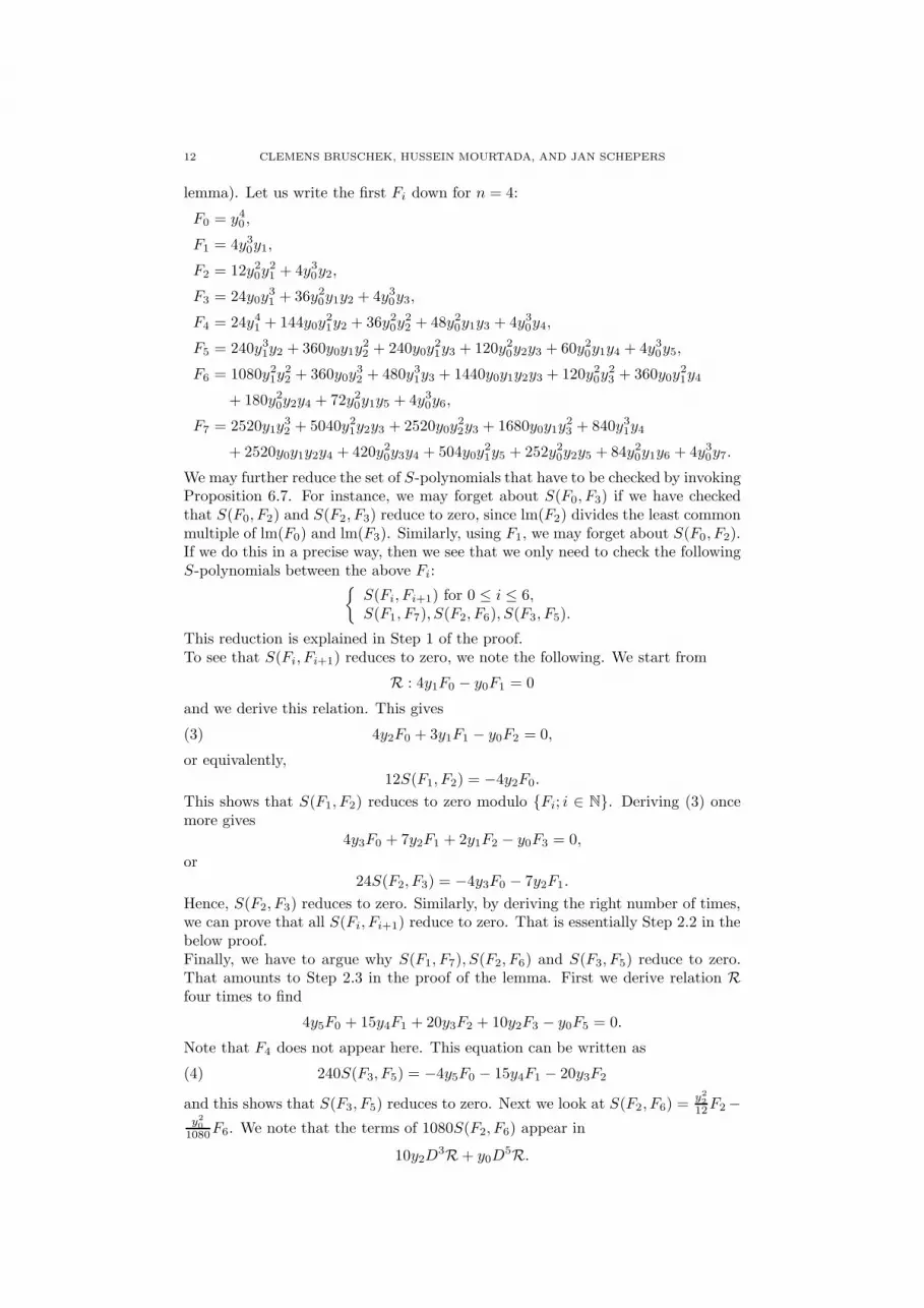
12 CLEMENS BRUSCHEK, HUSSEIN MOURTADA, AND JAN SCHEPERS
lemma). Let us write the first Fi down for n = 4:
F0 = y40 ,
F1 = 4y30y1,
F2 = 12y20y21 + 4y30y2,
F3 = 24y0y31 + 36y20y1y2 + 4y30y3,
F4 = 24y41 + 144y0y21y2 + 36y20y
22 + 48y20y1y3 + 4y30y4,
F5 = 240y31y2 + 360y0y1y22 + 240y0y
21y3 + 120y20y2y3 + 60y20y1y4 + 4y30y5,
F6 = 1080y21y22 + 360y0y
32 + 480y31y3 + 1440y0y1y2y3 + 120y20y
23 + 360y0y
21y4
+ 180y20y2y4 + 72y20y1y5 + 4y30y6,
F7 = 2520y1y32 + 5040y21y2y3 + 2520y0y
22y3 + 1680y0y1y
23 + 840y31y4
+ 2520y0y1y2y4 + 420y20y3y4 + 504y0y21y5 + 252y20y2y5 + 84y20y1y6 + 4y30y7.
We may further reduce the set of S-polynomials that have to be checked by invokingProposition 6.7. For instance, we may forget about S(F0, F3) if we have checkedthat S(F0, F2) and S(F2, F3) reduce to zero, since lm(F2) divides the least commonmultiple of lm(F0) and lm(F3). Similarly, using F1, we may forget about S(F0, F2).If we do this in a precise way, then we see that we only need to check the followingS-polynomials between the above Fi:{
S(Fi, Fi+1) for 0 ≤ i ≤ 6,S(F1, F7), S(F2, F6), S(F3, F5).
This reduction is explained in Step 1 of the proof.To see that S(Fi, Fi+1) reduces to zero, we note the following. We start from
R : 4y1F0 − y0F1 = 0
and we derive this relation. This gives
(3) 4y2F0 + 3y1F1 − y0F2 = 0,
or equivalently,12S(F1, F2) = −4y2F0.
This shows that S(F1, F2) reduces to zero modulo {Fi; i ∈ N}. Deriving (3) oncemore gives
4y3F0 + 7y2F1 + 2y1F2 − y0F3 = 0,
or24S(F2, F3) = −4y3F0 − 7y2F1.
Hence, S(F2, F3) reduces to zero. Similarly, by deriving the right number of times,we can prove that all S(Fi, Fi+1) reduce to zero. That is essentially Step 2.2 in thebelow proof.Finally, we have to argue why S(F1, F7), S(F2, F6) and S(F3, F5) reduce to zero.That amounts to Step 2.3 in the proof of the lemma. First we derive relation Rfour times to find
4y5F0 + 15y4F1 + 20y3F2 + 10y2F3 − y0F5 = 0.
Note that F4 does not appear here. This equation can be written as
(4) 240S(F3, F5) = −4y5F0 − 15y4F1 − 20y3F2
and this shows that S(F3, F5) reduces to zero. Next we look at S(F2, F6) =y22
12F2−y20
1080F6. We note that the terms of 1080S(F2, F6) appear in
10y2D3R+ y0D
5R.

ARC SPACES AND ROGERS-RAMANUJAN IDENTITIES 13
From this we deduce that
1080S(F2, F6) = −40y2y4F0 − 110y2y3F1 − 10y1y2F3 − 4y0y6F0 − 19y0y5F1
− 35y0y4F2 − 30y0y3F3 + y0y1F5.
Again F4 does not appear, but this does not yet show that S(F2, F6) reduces tozero, since
lm(S(F2, F6)) = y20y31y3 < y0y
41y2 = lm(y0y1F5)
for instance. But we do recognize 240y1S(F3, F5) and hence we can replace thisusing (4). We find
1080S(F2, F6) = (−40y2y4 + 4y1y5 − 4y0y6)F0 + (−110y2y3 + 15y1y4 − 19y0y5)F1
+ (20y1y3 − 35y0y4)F2 − 30y0y3F3.
This shows that S(F2, F6) reduces to zero. We proceed analogously for S(F1, F7) =y32
4 F1 −y30
2520F7. First we look at
90y22D2R+ y20D
6R.
In there we recognize 2520S(F1, F7), 2160y0y2S(F3, F5) and 2160y1S(F2, F6). Wereplace the latter two and we find the following after some computations:
2520S(F1, F7) = (−360y22y3 + 80y1y2y4 − 8y21y5 − 36y0y2y5 + 8y0y1y6 − 4y20y7)F0
+ (220y1y2y3 − 30y21y4 − 135y0y2y4 + 38y0y1y5 − 23y20y6)F1
+ (−40y21y3 − 180y0y2y3 + 70y0y1y4 − 54y20y5)F2
+ (60y0y1y3 − 65y20y4)F3 − 40y20y3F4.
Unfortunately this does not show yet that S(F1, F7) reduces to zero. We have:
lm(S(F1, F7)) = y30y21y2y3 < y20y
41y3 = lm(y20y3F4) = lm(y0y1y3F3) = lm(y21y3F2).
This implies that (−40y21y3, 60y0y1y3,−40y20y3) forms a homogeneous syzygy onthe leading terms of (F2, F3, F4). We already know that a basis for these syzygiesis given by S2,3 and S3,4. Indeed, we may compute that
−40y21y3F2 + 60y0y1y3F3 − 40y20y3F4 = −480y1y3S(F2, F3) + 960y0y3S(F3, F4)
Moreover, we explained that S(F2, F3) and S(F3, F4) reduce to zero modulo {Fi; i ≥0}. Replacing their expressions in terms of the Fi, we conclude that S(F1, F7)reduces to zero as well.From this example, we see that it will be useful for the proof of Lemma 5.3 to keeptrack of the leading monomials of the relevant S-polynomials.
Proposition 5.4. Let q ≥ 1, 0 ≤ r ≤ n− 1. Then
lm(S(fqn+r, fqn+r+1)
)=
yq−1yn−r−2q yr+2
q+1 if q ≥ 2, r 6= n− 1,
y2qyn−2q+1 yq+2 if q ≥ 2, r = n− 1,
yn−r+11 yr−1
2 y3 if q = 1, r 6= 0.
We remark that S(fn, fn+1) = 0.
Proof. In all three cases we have written the second biggest monomial with degreen+ 1 and weight q(n+1)+ r+ 1 in the variables y1, y2, . . .. We only have to showthat the monomial occurs with nonzero coefficient in S(fqn+r, fqn+r+1). UsingProposition 5.2 we see that this S-polynomial is a multiple of
(n− r)(q!)(qn + r + 1)yq+1fqn+r − (r + 1)((q + 1)!
)yqfqn+r+1.

14 CLEMENS BRUSCHEK, HUSSEIN MOURTADA, AND JAN SCHEPERS
Assume for instance that q ≥ 2 and r 6= n−1. A computation using Proposition 5.1gives then
(n+ r + 2)(n!)((qn+ r + 1)!
)((q − 1)!
)(q!)n−r−3
((q + 1)!
)r+1((r + 2)!
)((n− r − 2)!
) 6= 0
as the coefficient of yq−1yn−r−2q yr+2
q+1 in the above expression. The other cases aretreated similarly. �
Proposition 5.5. Let q ≥ 1, 1 ≤ r ≤ n− 1. Then
lm(S(fqn+r, f(q+1)n+n−r)
)=
yq−1yn−r−2q yr+1
q+1yn−rq+2 if q ≥ 2, r 6= n− 1,
yq−1yn−2q+1 y
2q+2 if q ≥ 2, r = n− 1,
yn−r1 yr+1
2 yn−r−23 y4 if q = 1, r 6= n− 1,
y21yn−22 y4 if q = 1, r = n− 1.
Proof. Now S(fqn+r, f(q+1)n+n−r) is a multiple of
(5)((q + 1)n+ n− r)!
(qn+ r)!yn−rq+2 fqn+r −
((q + 2)!
)n−r
(q!)n−ryn−rq f(q+1)n+n−r.
In the first case, we have written the second biggest monomial with degree 2n− r,weight (q + 1)(2n− r), and subject to the additional condition that yq or yq+2 hasdegree at least n−r. It only occurs in the first term of (5) due to the factor yn−r−2
q .In the second case a small computation using Proposition 5.1 shows that the secondbiggest monomial y2qy
n−3q+1 y
2q+2 does not occur in S(fqn+r, f(q+1)n+n−r) (if n ≥ 3).
We have written the third biggest, which appears with nonzero coefficient in (5).If q = 1, then we can compute that no terms containing only y1, y2, y3 occur in(5). We have written the biggest monomial containing y4 of degree 2n− r, weight2(2n− r), and subject to the additional condition that y1 or y3 has degree at leastn− r. It appears in (5) with nonzero coefficient. �
Proof of Lemma 5.3. We will show that the fi form a Grobner basis of I. Usingthe notation of the appendix, we will first show that the Si,j with n ≤ i < j and
j = i + 1 or
i = qn+ r, j = (q + 1)n+ n− r for q ≥ 1, 1 ≤ r ≤ n− 1 or
fi and fj have relatively prime leading monomials
form a homogeneous basis for the syzygies on the leading terms of the fi. In thesecond step we will show that all elements of this basis reduce to zero modulo{fi; i ≥ n}. From Theorem 6.6 we conclude then that the fi are indeed a Grobnerbasis.
Step 1. The set of Si,j described above forms a basis of the syzygies.From Proposition 6.5 we know already that the set of all Si,j forms a homogeneousbasis for the syzygies on the fi. If lm(fi) and lm(fj) are not coprime then byProposition 5.2 the syzygy Si,j is of the type Sqn,qn+r for q ≥ 1, 0 < r < n orSqn+r,qn+s, where q ≥ 1, 0 < r < n, r < s < 2n.For r descending from n− 1 down to 2 we use Proposition 6.7 with gi = fqn, gj =fqn+r and gk = fqn+r−1. Indeed, the least common multiple of lm(fqn) and
lm(fqn+r) equals ynq y
rq+1 and this is of course divisible by lm(gk) = yn−r+1
q yr−1q+1 . So
we remove the syzygies Sqn,qn+n−1, . . . , Sqn,qn+2 and we are still left with a basis.Next we choose r ∈ {1, . . . , n − 2}, and we let s descend from n down to r + 2.We use again Proposition 6.7, now with gi = fqn+r, gj = fqn+s and gk = fqn+s−1.The least common multiple of lm(fqn+r) and lm(fqn+s) equals yn−r
q ysq+1 and this

ARC SPACES AND ROGERS-RAMANUJAN IDENTITIES 15
is divisible by lm(gk) = yn−s+1q ys−1
q+1 . For these values of r and s we remove thesyzygies Sqn+r,qn+s and we still have a basis.Next we let r go up from 1 to n−2 and we choose s ∈ {n+1, n+2, . . . , 2n− r−1}.We take gi = fqn+r, gj = fqn+s and gk = fqn+r+1. The least common multiple of
lm(fqn+r) and lm(fqn+s) equals then yn−rq y2n−s
q+1 ys−nq+2 . This is divisible by lm(gk) =
yn−r−1q yr+1
q+1 . For these values of r and s we can again remove the syzygies Sqn+r,qn+s
and we keep a basis.Finally we choose r ∈ {2, . . . , n − 1}, and we let s descend from 2n − 1 down to2n− r + 1. We take gi = fqn+r, gj = fqn+s and gk = fqn+s−1. The least common
multiple of lm(fqn+r) and lm(fqn+s) equals then yn−rq yrq+1y
s−nq+2 . This is divisible
by lm(gk) = y2n−s+1q+1 ys−n−1
q+2 . For these values of r and s we remove once more thesyzygies Sqn+r,qn+s and we find the basis that we were looking for.
Step 2. All the elements of this basis reduce to zero modulo {fi; i ≥ n}.Step 2.1. First we note that S(fi, fj) reduces to zero modulo {fi; i ≥ n} if lm(fi)and lm(fj) are relatively prime by Proposition 6.4.
Step 2.2. For the other two cases we will exploit the differential structure of theideal F0, F1, . . . . We have Fi = Di(F0), where D is the k-derivation determined byD(yj) = yj+1 for j ≥ 0. Since F0 = yn0 and F1 = D(yn0 ) = nyn−1
0 y1 we have thesimple relation
(6) R : ny1F0 − y0F1 = 0.
Let q ≥ 1 and r ∈ {0, . . . , n− 1}. Applying Dq(n+1)+r to the relation R (using thegeneralized Leibniz rule) and evaluating in y0 = 0 yields
0 = −
(q(n+ 1) + r
n− 1
)yq(n+1)+r−n+1fn
+
q(n+1)+r−1∑
α=n
(q(n+ 1) + r
α
)[nyq(n+1)+r−α+1fα − yq(n+1)+r−αfα+1
]
+ ny1fq(n+1)+r
= n
(q(n+ 1) + r
q
)yq+1fqn+r + n
(q(n+ 1) + r
q − 1
)yqfqn+r+1
−
[(q(n+ 1) + r
q + 1
)yq+1fqn+r +
(q(n+ 1) + r
q
)yqfqn+r+1
]+ E
=(q(n+ 1) + r)! (n− r)
(q + 1)! (qn+ r)!yq+1fqn+r −
(q(n+ 1) + r)! (r + 1)
q! (qn+ r + 1)!yqfqn+r+1 + E,
where we denote by E the remaining terms in the expression of the derivative. Thepolynomial E is a Z-linear combination of yq(n+1)+r−n+1fn, . . . , yq+2fqn+r−1 and
yq−1fqn+r+2, . . . , y1fq(n+1)+r. Note that Dq(n+1)+rR has weight q(n + 1) + r + 1and is homogeneous of degree n + 1 with respect to the standard grading. Themonomial M = yn−r
q yr+1q+1 is maximal among those monomials which are of weight
q(n+1)+ r+1 and degree n+1. It cannot appear in E and it is the least commonmultiple of the leading monomials of fqn+r and fqn+r+1. Hence we conclude that
(q(n+ 1) + r)! (n− r)
(q + 1)! (qn+ r)!yq+1fqn+r −
(q(n+ 1) + r)! (r + 1)
q! (qn+ r + 1)!yqfqn+r+1
is a multiple of the S-polynomial S(fqn+r, fqn+r+1) (this can also easily be deducedfrom Proposition 5.2).Moreover, we have seen in the proof of Proposition 5.4 that the second biggestmonomial of weight q(n + 1) + r + 1 and degree n + 1 in y1, y2, . . . does occur in

16 CLEMENS BRUSCHEK, HUSSEIN MOURTADA, AND JAN SCHEPERS
S(fqn+r, fqn+r+1). Thus the equation
(q(n+ 1) + r)! (n − r)
(q + 1)! (qn+ r)!yq+1fqn+r −
(q(n+ 1) + r)! (r + 1)
q! (qn+ r + 1)!yqfqn+r+1 = −E
shows that S(fqn+r, fqn+r+1) reduces to zero modulo {fi; i ≥ n}.
Step 2.3. Now let q ≥ 1, 1 ≤ r ≤ n− 1. We are left with showing that
S(fqn+r, f(q+1)n+n−r)
reduces to zero modulo {fi; i ≥ n}. We use descending induction on r, starting withthe initial cases r = n− 1 and r = n− 2. For r = n− 1 we consider the relation Rfrom equation (6). Analogously to Step 2.2, we derive it (n + 1)(q + 1) − 1 timesand put y0 = 0 to find that
0 = −
((n+ 1)(q + 1)− 1
n− 1
)y(n+1)(q+1)−nfn
+
(n+1)(q+1)−2∑
α=n
((n+ 1)(q + 1)− 1
α
)[ny(n+1)(q+1)−αfα − y(n+1)(q+1)−1−αfα+1
]
+ ny1f(n+1)(q+1)−1
=((q + 1)(n+ 1)− 1)! (n+ 1)
(q + 2)! (qn+ n− 1)!yq+2fqn+n−1
−((q + 1)(n+ 1)− 1)! (n+ 1)
q! (qn+ n+ 1)!yqfqn+n+1 + E,
where E is a Z-linear combination of
y(n+1)(q+1)−nfn, . . . , yq+3fqn+n−2, yq+1fqn+n, yq−1fqn+n+2, . . . , y1f(n+1)(q+1)−1.
However, the coefficient of yq+1fqn+n in E equals
n
((n+ 1)(q + 1)− 1
qn+ n
)−
((n+ 1)(q + 1)− 1
qn+ n− 1
)= 0.
It follows that
((q + 1)(n+ 1)− 1)! (n+ 1)
(q + 2)! (qn+ n− 1)!yq+2fqn+n−1 −
((q + 1)(n+ 1)− 1)! (n+ 1)
q! (qn+ n+ 1)!yqfqn+n+1
is a multiple of S(fqn+n−1, fqn+n+1) since the monomial yqyn−1q+1 yq+2, which is the
least common multiple of the leading monomials of fqn+n−1 and fqn+n+1, cannotoccur in E. Moreover, from Proposition 5.2 and Proposition 5.5 we conclude thatS(fqn+n−1, fqn+n+1) reduces to zero modulo {fi; i ≥ n}.
Next consider r = n− 2 (and n ≥ 3). We look at the two relations
A1 :(q!)2(q + 2)!(
(q + 1)(n+ 1)− 2)!yq+2D
(q+1)(n+1)−2R∣∣y0=0
= 0
and
A2 :q!((q + 2)!
)2((q + 1)(n+ 1)
)!yqD
(q+1)(n+1)R∣∣y0=0
= 0.
We expand the left hand side of A1 as a Q-linear combination of
yq+2yq(n+1)fn, . . . , yq+2y1fq(n+1)+n−1,
and the left hand side of A2 as a Q-linear combination of
yqyq(n+1)+2fn, . . . , yqy1f(q+1)(n+1).

ARC SPACES AND ROGERS-RAMANUJAN IDENTITIES 17
A computation shows that the coefficient of y2q+2fqn+n−2 in A1 equals
(n+ 2)(q!)2
(qn+ n− 2)!
and that the coefficient of y2qfqn+n+2 in A2 is
−(n+ 2)
((q + 2)!
)2
(qn+ n+ 2)!.
It follows from Proposition 5.2 that a multiple of S(fqn+n−2, fqn+n+2) occurs inthe left hand side of A1+A2. By a similar computation we see that the term of A1
containing yq+1yq+2fqn+n−1 and the term of A2 containing yq+1yqfqn+n+1 form amultiple of yq+1S(fqn+n−1, fqn+n+1) in A1 +A2. From the above we already knowthat we may express this as a linear combination of
yq+1y(q+1)(n+1)−nfn, . . . , yq+1yq+3fqn+n−2,yq+1yq−1fqn+n+2, . . . , yq+1y1f(q+1)(n+1)−1.
Putting everything together, we conclude that we can write S(fqn+n−2, fqn+n+2)as a linear combination of
yq+2yq(n+1)fn, . . . , yq+2yq+3fqn+n−3,yq+2yqfqn+n, . . . , yq+2y1fq(n+1)+n−1,yqyq(n+1)+2fn, . . . , yqyq+2fqn+n,
yqyq−1fqn+n+3, . . . , yqy1f(q+1)(n+1),yq+1y(q+1)(n+1)−nfn, . . . , yq+1yq+3fqn+n−2,yq+1yq−1fqn+n+2, . . . , yq+1y1f(q+1)(n+1)−1.
We want to apply Propositions 5.5 and 5.2 to conclude that S(fqn+n−2, fqn+n+2)reduces to zero modulo {fi; i ≥ n}. The only problem is the appearance ofyqyq+2fqn+n (twice) in the above list. However, we can compute that its coeffi-cient in A1 +A2 equals zero!
Finally, let r ≤ n− 3 (and n ≥ 4). We look at the relations
A1 :(q!)n−r(q + 2)!(q(n+ 1) + r + 1
)!yn−r−1q+2 Dq(n+1)+r+1R
∣∣y0=0
= 0
and
A2 :q!((q + 2)!
)n−r
(q(n+ 1) + 2n− r − 1
)!yn−r−1q Dq(n+1)+2n−r−1R
∣∣y0=0
= 0.
We expand the left hand side of A1 as a Q-linear combination of
yn−r−1q+2 yq(n+1)+r+2−nfn, . . . , y
n−r−1q+2 y1fq(n+1)+r+1,
and the left hand side of A2 as a Q-linear combination of
yn−r−1q yq(n+1)+n−rfn, . . . , y
n−r−1q y1fq(n+1)+2n−r−1.
As before, we may check that a multiple of
S(fqn+r, f(q+1)n+n−r)
occurs in the left hand side of A1 +A2. Similarly, multiples of
yq+1S(fqn+r+1, f(q+1)n+n−r−1) and yqyq+2S(fqn+r+2, f(q+1)n+n−r−2)
occur there. By induction, we know that the latter two S-polynomials reduce tozero modulo {fi; i ≥ n} and we replace them by their expression in terms of thefi. More precisely: S(fqn+r, f(q+1)n+n−r) can be expressed as a linear combinationof terms of the form Mfa where M is a monomial of degree n − r and where

18 CLEMENS BRUSCHEK, HUSSEIN MOURTADA, AND JAN SCHEPERS
wtM + a = (q + 1)(2n− r). The maximum of lm(Mfa) can be attained at severalplaces. A careful analysis learns that
lm(Mfa) ≤ yq−1yn−r−3q yr+3
q+1yn−r−1q+2 =: N,
where the latter monomial can occur as
lm(yq−1yn−r−1q+2 fqn+r+3), lm
(yq+1S(fqn+r+1, f(q+1)n+n−r−1)
),
or as lm(yqyq+2S(fqn+r+2, f(q+1)n+n−r−2)
)
by Propositions 5.2 and 5.5. Here (and from now on) we assume that q ≥ 2. Thecase q = 1 can be treated in a similar way. Only the following expressions of theform Mfa have N as leading monomial:
yn−r−1q+2 yq−1fqn+r+3, yq−1y
n−r−3q y2q+2f(q+1)n+n−r−3,
yq−1yn−r−3q yq+1yq+2f(q+1)n+n−r−2, yq−1y
n−r−3q y2q+1f(q+1)n+n−r−1.
Since lm(S(fqn+r, f(q+1)n+n−r)
)< N we cannot yet conclude that this S-polynomi-
al reduces to zero, but we see that the four expressions above must give rise to ahomogeneous syzygy on the leading terms of
fqn+r+3, f(q+1)n+n−r−3, f(q+1)n+n−r−2, f(q+1)n+n−r−1.
From Step 1 we know that a basis for these syzygies is given by
Sqn+r+3,(q+1)n+n−r−3, S(q+1)n+n−r−3,(q+1)n+n−r−2,and S(q+1)n+n−r−2,(q+1)n+n−r−1.
By induction and by Step 2.2 we know that the corresponding S-polynomials reduceto zero modulo {fi; i ≥ n}. Using this, we conclude that S(fqn+r, f(q+1)n+n−r) canbe expressed as a linear combination of terms Mfa as above, and with lm(Mfa) <N . But we may repeat a similar argument to get rid of all monomials between
lm(S(fqn+r, f(q+1)n+n−r)
)= yq−1y
n−r−2q yr+1
q+1yn−rq+2
and N . We just have to remark that at no stage of this process the monomial
yn−rq yrq+1y
n−rq+2
appears as leading monomial of a term (since in all terms there are factors yq−1,yq−2, . . . or yq+3, yq+4, . . . involved). This ends the proof of the lemma. �
Remark. We could have avoided to use polynomial rings in countably many vari-ables. In fact the following holds: the leading monomials of (fn, fn+1, . . . , fn+m) ofweight less than or equal to n+m are generated by lm(fi), n ≤ i ≤ n+m. In otherwords: there exists a Grobner basis of (fn, . . . , fn+m) such that all added elementswill be of weight larger than or equal to n+m+ 1.
5.1. Computation of the arc Hilbert-Poincare series of the n-fold point.
Using Gordon’s generalization of the Rogers-Ramanujan identity (Theorem 4.2) weimmediately obtain an explicit description of the arc Hilbert-Poincare series of then-fold point by a combinatorial interpretation of the leading ideal L(I) as it wascomputed in Lemma 5.3.
Theorem 5.6. The Hilbert-Poincare series of the focussed arc algebra J0∞(X) of
the n-fold point X = {yn = 0} ⊂ A1k over the origin equals:
HPJ0∞
(X)(t) = H ·∏
i≥1i≡0,n,n+1mod 2n+1
(1− ti).

ARC SPACES AND ROGERS-RAMANUJAN IDENTITIES 19
Equivalently,
HPJ0∞
(X)(t) =∏
i≥1i6≡0,n,n+1mod 2n+1
1
1− ti.
Proof. It is a general fact from the theory of Hilbert-Poincare series that the Hilbert-Poincare series of a homogeneous ideal is precisely the Hilbert-Poincare series ofthe leading ideal (see Theorem 6.3), i.e.,
HPJ0∞
(X)(t) = HPk[yi;i≥1]/L(I)(t),
where I is as in Lemma 5.3. By that lemma and Proposition 5.2 the leading idealL(I) is generated by monomials of the form yn−r
q yrq+1 for q ≥ 1 and 0 ≤ r ≤ n− 1.Recall that the weight of a monomial yα = yα1
i1· · · yαe
ieis precisely α1 · i1 + · · · +
αe · ie. Thus factoring out L(I) and computing the Hilbert-Poincare series of thecorresponding graded algebra is equivalent to counting partitions (λ1, . . . , λs) ofnatural numbers such that λj − λj+n−1 > 2 for all j. This is precisely what iscounted in Theorem 4.3. Hence, we obtain:
HPJ0∞
(X)(t) =∏
i≥1i6≡0,n,n+1mod 2n+1
1
1− ti.
The fact that the right hand side of this equation equals the generating series ofthe number of partitions of n into parts which are not congruent to 0, n or n + 1modulo 2n+ 1 is standard in the theory of generating series. �
5.2. An alternative approach to Rogers-Ramanujan. In the previous sectionwe used a combinatorial interpretation of the leading ideal of I = (fn, fn+1, . . .) tocompute the Hilbert-Poincare series of the corresponding graded algebra. Thereare commutative algebra methods to do this as well which yield an alternative ap-proach to the (first) Rogers-Ramanujan identity. Of course, we consider the casewhere n = 2 here, i.e. the case of the double point. We will obtain a recursionformula for the generating functions appearing in the Rogers-Ramanujan identitywhich has already been considered by Andrews and Baxter in [AB89], though thepresent approach gives a natural way to obtain it.
Consider the graded algebra S = k[yi; i ≥ 1]/L(I). It is immediate (see the proofof Theorem 5.6) that its Hilbert-Poincare series equals the generating series ofthe number of partitions of an integer n without repeated or consecutive parts.Differently, we compute the Hilbert-Poincare series of S by recursively defining asequence of formal power series (generating functions) in t which converges in the(t)-adic topology to the desired Hilbert-Poincare series. We will simply write k[≥ d]for the polynomial ring k[yi; i ≥ d]. It will be endowed with the grading wt yi = i.The ideal generated by y2i , yiyi+1 for i ≥ d in k[≥ d] will be denoted by Id. We willstill write Id for the “same” ideal in k[≥ d′] if d′ ≤ d. As usual, if E is an ideal ina ring R and f ∈ R then we denote the ideal quotient, i.e.,
{a ∈ R ; a · f ∈ E}
by (E : f).
Corollary 6.2 implies that
HPk[≥d]/Id(t) = HPk[≥d]/(Id,yd)(t) + td · HPk[≥d]/(Id:yd)(t).
Moreover, a quick computation shows the following.

20 CLEMENS BRUSCHEK, HUSSEIN MOURTADA, AND JAN SCHEPERS
Proposition 5.7. With the notation introduced above we have:
(Id, yd) = (yd, Id+1)
(Id : yd) = (yd, yd+1, Id+2).
This immediately implies
HPk[≥d]/Id(t) = HPk[≥d+1]/Id+1(t) + td ·HPk[≥d+2]/Id+2
(t).
For simplicity of notation let h(d) stand for HPk[≥d]/Id(t). Then:
(7) h(d) = h(d+ 1) + td · h(d+ 2)
and:
Proposition 5.8. For the Hilbert-Poincare series HPJ0∞
(X)(t) = h(1) we obtain
h(1) = Ad · h(d) +Bd+1 · h(d+ 1)
for d ≥ 1 with Ai, Bi ∈ k[[t]] fulfilling the following recursion
Ad = Ad−1 +Bd
Bd+1 = Ad−1 · td−1
with initial conditions A1 = A2 = 1 and B2 = 0, B3 = t.
Proof. By the discussion above h(1) equals h(2)+ t · h(3); hence, A1 = A2 = 1 andB2 = 0, B3 = t. Assume now that
h(1) = Ad · h(d) +Bd+1 · h(d+ 1)
holds for some d ≥ 2. By equation (7) substituting for h(d) yields
h(1) = Ad · (h(d+ 1) + td · h(d+ 2)) +Bd+1 · h(d+ 1)
= (Ad +Bd+1) · h(d+ 1) + (Ad · td) · h(d+ 2)
from which the assertion follows. �
If (sd)d∈N is a sequence of formal power series sd ∈ k[[t]] we will denote by lim sdits limit – if it exists – in the (t)-adic topology. Since ordBd ≥ d−2 it is immediatethat both limAd and limBd exist, in fact: limBd = 0 and
h(1) = limAd.
The recursion from Proposition 5.8 can easily be simplified. We obtain:
Corollary 5.9. With the above introduced notation HPJ0∞
(X)(t) = limAd whereAd fulfills
Ad = Ad−1 + td−2 · Ad−2
with initial conditions A1 = A2 = 1.
The recursion appearing in this corollary is well-known since Andrews and Baxter[AB89]. Its limit is precisely the infinite product
∏
i≥1i≡1,4 mod 5
1
1− ti,
i.e., the generating series of the number of partitions with parts equal to 1 or 4modulo 5. Note, that our construction gives the generating series Gi defined inthe paper by Andrews and Baxter an interpretation as Hilbert-Poincare series ofthe quotients k[≥ i]/Ii. This immediately implies that the series Gi are of theform Gi = 1+
∑j≥iGijt
j (this observation was called an ‘empirical hypothesis’ by
Andrews and Baxter).

ARC SPACES AND ROGERS-RAMANUJAN IDENTITIES 21
6. Appendix: Hilbert-Poincare series and Grobner bases
In this section we collect some of the basics about the theory of Hilbert-Poincareseries. For a detailed introduction, especially proofs, we refer to [GP02]. We alsorecall some results on Grobner basis theory from [CLO97].
Let A be a (Z-)graded k-algebra and let M = ⊕i∈ZMi be a graded A-module withith graded pieces Ai andMi of finite k-dimension. The Hilbert function HM : Z → Z
of M is defined by HM (i) = dimkMi, and its corresponding generating series
HPM (t) =∑
i∈Z
HM (i)ti ∈ Z((t))
is called the Hilbert-Poincare series of M . It is well-known that if A is a Noetheriank-algebra generated by homogeneous elements x1, . . . , xn of degrees d1, . . . , dn andM is a finitely generated A-module then
HPM (t) =QM (t)∏n
i=1(1− tdi)
for some QM (t) ∈ Z[t] which is called the (weighted) first Hilbert series of M . If Arespectively M is non-Noetherian then the Hilbert-Poincare series of M need notbe rational anymore. For the rest of this section we assume that the polynomialring k[x1, . . . , xn] is graded (not necessarily standard graded). The notions of ho-mogeneous ideal and degree are to be understood relative to this grading. If M isgraded then for any integer d we write M(d) for the dth twist of M , i.e., the gradedA-module with M(d)i =Mi+d.
The following Lemma follows immediately from additivity of dimension:
Lemma 6.1 (Lemma 5.1.2 in [GP02]). Let A and M be as above. Let d be a non-negative integer, f ∈ Ad and ϕ : M(−d) → M be defined by ϕ(m) = f · m; thenker(ϕ) and coker(ϕ) are graded A/(f)-modules with the induced gradings and
HPM (t) = td · HPM (t) + HPcoker(ϕ)(t)− td · HPker(ϕ)(t).
As an immediate consequence we obtain the useful:
Corollary 6.2 (Lemma 5.2.2 in [GP02]). Let I ⊆ k[x1, . . . , xn] be a homogeneousideal, and let f ∈ k[x1, . . . , xn] be a homogeneous polynomial of degree d then
HPk[x]/I(t) = HPk[x]/(I,f)(t) + tdHPk[x]/(I:f)(t).
For homogeneous ideals the leading ideal already determines the Hilbert-Poincareseries. After fixing a monomial order, the leading ideal L(I) of an ideal I ink[x1, . . . , xn] is defined as the (monomial) ideal generated by the leading mono-mials of all elements in I. Then one has:
Theorem 6.3 (Theorem 5.2.6 in [GP02]). Let > be any monomial ordering onk[x1, . . . , xn], let I ⊆ k[x] be a homogeneous ideal and denote by L(I) its leadingideal with respect to >. Then
HPk[x]/I(t) = HPk[x]/L(I)(t).
To compute the leading ideal one can use Grobner bases. Let I be an ideal in thepolynomial ring k[x1, . . . , xn] with a fixed monomial order <. Then {g1, . . . , gl} ⊂ Iis called a Grobner basis of I if L(I) is generated by {lm(gi) ; 1 ≤ i ≤ l}, wherewe write lm for ‘leading monomial’. For f ∈ k[x1, . . . , xn] and a subset H ={h1, . . . , hs} of k[x1, . . . , xn] one says that f reduces to zero modulo H if
f = a1h1 + · · ·+ ashs

22 CLEMENS BRUSCHEK, HUSSEIN MOURTADA, AND JAN SCHEPERS
for ai ∈ k[x1, . . . , xn], such that lm(f) ≥ lm(aihi) whenever aihi 6= 0. One writesf →H 0.Finally we need the definition of a syzygy. Let F = (f1, . . . , fs) ∈ (k[x1, . . . , xn])
s.A syzygy on the leading terms of the fi is an s-tuple (h1, . . . , hs) ∈ (k[x1, . . . , xn])
s
such thats∑
i=1
hi lt(fi) = 0,
where lt stands for ‘leading term’. The set of syzygies S(F) on the leading termsof F form a k[x1, . . . , xn]-submodule of (k[x1, . . . , xn])
s. A generating set of thismodule is called a basis. With F = {f1, . . . , fs}, we will say that a syzygy(h1, . . . , hs) ∈ S(F) reduces to zero modulo F if
s∑
i=1
hifi →F 0.
If each hi consists of a single term cixαi and xαi lm(fi) is a fixed monomial xα if
ci 6= 0, then the syzygy (h1, . . . , hs) is called homogeneous of multidegree α. Fori < j let xγ be the least common multiple of the leading monomials of fi and fj .One calls
S(fi, fj) :=xγ
lt(fi)fi −
xγ
lt(fj)fj
the S-polynomial of fi and fj. It gives rise to the homogeneous syzygy
Si,j :=xγ
lt(fi)ei −
xγ
lt(fj)ej ,
where ei and ej denote standard basis vectors of (k[x1, . . . , xn])s. Then we have
the following results:
Proposition 6.4 (Proposition 4 p.103 in [CLO97]). Let G ⊂ k[x1, . . . , xn] be afinite set. Assume that f, g ∈ G have relatively prime leading monomials. ThenS(f, g) →G 0.
Proposition 6.5 (Proposition 8 p.105 in [CLO97]). For an s-tuple of polynomials(f1, . . . , fs) ∈ (k[x1, . . . , xn])
s we have that the set of all Si,j form a homogeneousbasis of the syzygies on the leading terms of the fi.
Theorem 6.6 (Theorem 9 p.106 in [CLO97]). Let G = (g1, . . . , gs) be an s-tupleof polynomials and let I be the ideal of k[x1, . . . , xn] generated by G = {g1, . . . , gs}.Then G is a Grobner basis for I if and only if every element of a homogeneousbasis for the syzygies S(G) reduces to zero modulo G.
Proposition 6.7 (Proposition 10 p.107 in [CLO97]). Let G = (g1, . . . , gs) be an s-tuple of polynomials. Suppose that we have a subset S ⊂ {Si,j ; 1 ≤ i < j ≤ s} thatis a basis of S(G). Moreover, suppose that we have distinct elements gi, gj, gk suchthat lm(gk) divides the least common multiple of lm(gi) and lm(gj). If Si,k, Sj,k ∈ S,then S \ {Si,j} is also a basis of S(G). Here we put Si,j := Sj,i if i > j.
References
[AB89] G. E. Andrews and R. J. Baxter. A motivated proof of the Rogers-Ramanujan identi-ties. Amer. Math. Monthly, 96(5):401–409, 1989.
[And89] G. E. Andrews. On the proofs of the Rogers-Ramanujan identities. In q-series andpartitions (Minneapolis, MN, 1988), volume 18 of IMA Vol. Math. Appl., pages 1–14.Springer, New York, 1989.
[And98] G. E. Andrews. The theory of partitions. Cambridge Mathematical Library. CambridgeUniversity Press, Cambridge, 1998. Reprint of the 1976 original.
ARC SPACES AND ROGERS-RAMANUJAN IDENTITIES 23
[BHM10] J. Berthomieu, P. Hivert, and H. Mourtada. Computing Hironaka’s invariants: ridgeand directrix. In Arithmetic, Geometry, Crypthography and Coding Theory 2009, vol-ume 521 of Contemp. Math., pages 9–20. Amer. Math. Soc., Providence, RI, 2010.
[Bru09] C. Bruschek. The linearization principle in infinite dimensional algebraic geometry.PhD thesis, 2009.
[Bru10] C. Bruschek. Jet algebras and Bell polynomials. Preprint, 2010.[CLO97] D. Cox, J. Little, and D. O’Shea. Ideals, varieties, and algorithms. Undergraduate
Texts in Mathematics. Springer-Verlag, New York, second edition, 1997. An introduc-tion to computational algebraic geometry and commutative algebra.
[CPGP10] H. Cobo Pablos and P. Gonzalez Perez. Arithmetic motivic Poincare series of toricvarieties. Preprint, arXiv:1011.3696v1 [math.AG], 2010.
[DL99] J. Denef and F. Loeser. Germs of arcs on singular algebraic varieties and motivicintegration. Invent. Math., 135(1):201–232, 1999.
[DL01] J. Denef and F. Loeser. Definable sets, motives and p-adic integrals. J. Amer. Math.Soc., 14(2):429–469 (electronic), 2001.
[Dra10] J. Draisma. Finiteness for the k-factor model and chirality varieties. Adv. Math.,223(1):243–256, 2010.
[Eis95] D. Eisenbud. Commutative algebra, volume 150 of Graduate Texts in Mathematics.Springer-Verlag, New York, 1995. With a view toward algebraic geometry.
[EM04] L. Ein and M. Mustata. Inversion of adjunction for local complete intersection varieties.Amer. J. Math., 126(6):1355–1365, 2004.
[FdB10] J. Fernandez de Bobadilla. Nash problem for surface singularities is a topological prob-lem. Preprint, arXiv:1011.6335v1 [math.AG], 2010.
[GP02] G.-M. Greuel and G. Pfister. A Singular introduction to commutative algebra.Springer-Verlag, Berlin, 2002. With contributions by Olaf Bachmann, Christoph Lossenand Hans Schonemann, With 1 CD-ROM (Windows, Macintosh, and UNIX).
[GS06] R. A. Goward, Jr. and K. E. Smith. The jet scheme of a monomial scheme. Comm.Algebra, 34(5):1591–1598, 2006.
[HS09] C. J. Hillar and S. Sullivant. Finite Grobner bases in infinite dimensional polynomialrings and applications. Preprint, arXiv:0908.1777v1 [math.AC], 2009.
[Ish07] S. Ishii. Jet schemes, arc spaces and the Nash problem. C. R. Math. Acad. Sci. Soc.R. Can., 29(1):1–21, 2007.
[LJR08] M. Lejeune-Jalabert and A. J. Reguera. Exceptional divisors which are not uniruledbelong to the image of the Nash map. Preprint, arXiv:0811.2421v1 [math.AG], 2008.
[Mou] H. Mourtada. Jet schemes of complex plane branches and equisingularity. To appearin Ann. Inst. Fourier.
[Mou10a] H. Mourtada. Jet schemes of toric surfaces. Preprint, 2010.[Mou10b] H. Mourtada. Sur les espaces des jets de quelques varietes algebriques singulieres. PhD
thesis, 2010.[Nas95] J. Nash, Jr. Arc structure of singularities. Duke Math. J., 81(1):31–38 (1996), 1995. A
celebration of John F. Nash, Jr.[Nic05a] J. Nicaise. Arcs and resolution of singularities. Manuscripta Math., 116(3):297–322,
2005.[Nic05b] J. Nicaise. Motivic generating series for toric surface singularities. Math. Proc. Cam-
bridge Philos. Soc., 138(3):383–400, 2005.[PP10] M. Pe Pereira. Nash problem for quotient surface singularities. Preprint,
arXiv:1011.3792v1 [math.AG], 2010.[PS10] C. Plenat and M. Spivakovsky. The Nash problem of arcs and the rational double point
E6. Preprint, arXiv:1011.2426v1 [math.AG], 2010.[Voj07] P. Vojta. Jets via Hasse-Schmidt derivations. In Diophantine geometry, volume 4 of
CRM Series, pages 335–361. Ed. Norm., Pisa, 2007.[Wil00] H. Wilf. Lectures on integer partitions. PIMS lectures, 2000.
University of Vienna, Nordbergstr. 15, 1090 Vienna, Austria
E-mail address: [email protected]
Universite de Versailles Saint-Quentin-en-Yvelines, 45 Avenue des Etats-Unis, 78035,
Cedex Versailles
E-mail address: [email protected]
K.U.Leuven, Celestijnenlaan 200B, 3001 Leuven, Belgium
E-mail address: [email protected]


