Embed Size (px)
Citation preview
E L S E V I E R 0 2 6 7 - 7 2 6 1 ( 9 5 ) 0 0 0 3 1 - 3
Soil Dynamics and Earthquake Engineering 15 (1996) 83-94 Copyright © 1996 Elsevier Science Limited Printed in Great Britain. All rights reserved
0267-7261/96/$15.00
Applications of statistical and GIS techniques to slope instability zonation (1:50.000 Fabriano
geological map sheet)*
Lucia Luzi Gruppo Nazionale per la Difesa dai Terremoti, CNR, via Nizza 128, Roma, Italy
&
Floriana Pergalani Istituto di Ricerca sul Rischio Sismico, CNR, via Ampere 56, Milano, Italy
(Received 26 July 1995; accepted 4 August 1995)
The aim of this work is the evaluation of the vulnerability of landslides in static, pseudostatic and dynamic conditions, to produce slope instability maps. A deterministic approach, using a GIS, (ILWlS 1.4 - The Integrated Land and Water Information System User's Manual, Enschede, 1993, The Netherlands) is presented. The analysis in static and pseudostatic conditions, using the infinite slol~: analysis and the ordinary slice method, is carried out and the values of Fs (factor of safety) and Kc (coefficient of critical horizontal acceleration) are evaluated; the analysis in dynamic condition is performed, using Newmark's method, (Geotechnique, 1965, 23, 139-60), and the value of the final displacement during the application of an accelerogram is calculated. The applied methodolo- gies and the results for the area corresponding to the NE sector of the 1:50.000 "Fabriano" (Marehe Region, Italy) geological map sheet, are presented.
Key words: earthquake, landslide, slope instability, GIS.
INTRODUCTION
Slope instability problem,; exist over a wide range of scale, terrain and climatic conditions.
There are five general concepts, 1 that have to be considered when a slope instability zonation has to be performed.
The first deals with the definition of the type of analysis that has to be done:
(a) danger to life; (b) danger to structures; (c) danger to social well[ being; (d) danger of land loss.
The second point regards the causes that determine landslides that can be natural or man induced.
Then, as third point, the problem of the choice of the
*Paper presented at the Session SGF3 - - Microzonation and Site Effects, XXIV General Assembly of European Seismolo- gical Commission, Athens, 19-23 September 1994.
area arises. This implies the availability of data, the financial availability, the time in which the project has to be completed and the accessibility of the area to be studied. Before starting a landslide hazard project it is advisable to consider a cost/benefit ratio to select the area having the lowest one.
As the fourth point, the degree of accuracy depends on the combination of different factors:
83
1. scale factors; that directly depend on the purpose for which the maps are executed. Following some examples 2-4 the optimum cost/benefit ratio is the one that uses a hierarchical methodology:
(a) regional scale (< 1:100.000) used to identify broad landslide problem areas; the maps pro- duced are for agencies that deal with regional planning. The areas investigated are of a thou- sand square kilometres or more;
(b)medium scale (,,d :25.000-,,d :50.000) prinei- paUy for agencies dealing with intermunicipal
84 L. Luzi, F. Pergalani
planning and studies for local engineering works. The areas investigated are of several hundreds of square kilometres;
(c) large scale (~1 : 5.000-,-,1 : 10.000) used for pro- blems of local slope instability, for planning of infrastructures, housing and industrial projects. The size of the areas to evaluate is of several tens of square kilometres;
(d) detailed scale ( > 1 : 5.000) mainly for companies or municipal agencies dealing with hazard of individual sites, with a maximum size of several hectares;
2. data availability; there are five main data sources of information': literature collection, existing maps, remote sensing data, in particular aerial photo- graphs and laboratory test results;
3. method utilized; it has to satisfy the requirements of an ideal map of slope instability zonation, such as
• providing informations about the spatial variabil- ity, the temporal probability, type, magnitude, velocity, runout distance and retrogression limits of the mass movements. 5
The final aspect to be considered is the location of the element at risk in relation to the hazard process, that means considering the structures standing on the terrain potentially affected by mass movements.
There are many approaches used for such a mapping and usually they do not provide the amount of informa- tion needed by an ideal map; some of them do not give exact and reproducible values for slope instability zona- tion, while others try to assess slope instability giving exact values.
Many authors have classified in different ways the principal approaches to slope instability mapping. Hansen I proposed the following distinction between:
(a) earth science approach, that principally focuses on the determination of slope instability conditions by mapping; the main advantage of this method is the possibility of application over large areas and of a rapid zonation. It lacks of a high degree of accuracy.
A further distinction can be made between:
1. direct approach, based principally on geomor- phological mapping, since the hazard is basi- cally assessed in the field;
2. indirect approach, that evaluates the impor- tance of the combination of different landslide triggering factors, mostly using statistical tech- niques. The results can be extrapolated to land- slide free areas having similar combinations of triggering factors;
(b) engineering approach, that focuses the interest on the stability of a site or a slope. The input data derive from laboratory tests and can be used to determine safety parameters. The advantage of this method is the high accuracy achieved, pro- vided that the input data and the methods utilized are also accurate. The disadvantage is the unsuit- ability for rapid zonations.
METHODOLOGY
For slope stability analysis the following scheme is proposed:
1. stability analysis in static and pseudostatic condi- tion;
2. stability analysis in dynamic condition.
For the first situation the analysis can be performed using deterministic methods, to obtain coefficients such as Fs 6 (factor of safety) or Kc 6 (coefficient of critical horizontal acceleration) for observed landslides or for landslide free areas; statistical methods can also be applied on point data (considering only the landslides) or on area data (considering the landslides and their bivariate or multivariate 7 relationships with triggering factors).
For the second situation deterministic approaches are proposed, where the output is represented by the final displacement of a landslide, during the application of an accelerogram.
For the stability analysis in static, pseudostatic and dynamic conditions, a deterministic approach using a GIS s is presented and an application on the NE sector of the 1 : 50.000 "Fabriano" (Marche Region, Italy) geolo- gical map sheet is shown.
The results obtained using statistical approaches on point data are illustrated in other papers, 9-11 while a statistical approach on area data will be the next step of the research.
Analysis in static and pseudostatic conditions: a deterministic approach
The aim of the deterministic analysis in static and pseudostatic conditions is the evaluation of the factor of safety (Fs) and of the coefficient of critical horizontal acceleration (Kc) for landslides and landslide free areas.
When a defined slope surface is considered, only the conditions required for static stability, or limit equili- brium, are taken into account; this is assumed for systems of forces that are just on the point of failing without giving informations about the displacements that accompany failure.
The accuracy of the analysis results depends on the appropriate analysis method selected and on the basis of the assumed failure mechanism, and also on the soil parameters which should represent the field conditions.
Applications of statistical and GIS techniques to slope instability zonation 85
Usually the analysis is carried out along two-dimen- sional sections drawn in the dip direction of the slope, assumed to have a unit width along the strike direction.
Therefore it is assumed that stresses, which are parallel to the strike of the ground surface are only of a limited extension. This is a limitation for slopes having a high geometrical variability in the three directions of the space. Two methods to obtain the value of Fs and Kc are used:
1. the infinite slope analysis 12 (ISA); 2. the ordinary slices method 13 (OSM).
These two standard methods are modified and adapted to a GIS. s
Infinite slope analysis method (ISA)
According to this method the factor of safety is expressed as (Graham6):
c' + (7 - m. % ) . z . cos 2/3. tan ~b' Fs = (1)
7" z . sin/3, cos
where: c' = effective cohesion (kPa) 7 = unit weight of soil (kN/m 3) m = groundwater/soil thickness ratio Zw/Z (dimension-
less) Zw = height of water table above failure surface (m) z = depth of the failure :~urface below the terrain sur-
face (m) 7w = unit weight of water (kN/m 3) /3 = terrain surface inclination (°) ¢' = effective angle of internal friction (o)
In a GIS s this formula can be applied to each terrain unit, termed pixel, of a raster map, using as input the geometrical and geotechnical parameters coming from several data layers.
The limit of this approach is that every pixel is con- sidered unconnected to its neighbours, so that the value of the factor of safety can be under or over estimated.
It is assumed that the material is cohesionless where the soil thickness is unknown, so that the calculation is independent from the depth factor. The Fs can be evaluated as:
Fs = (7 - m. 7w) tan ~b t 7 " tan ~ (2)
In pseudostatic conditions the slope stability can be evaluated, after introducing a horizontal force equal to Kc. W, where W is the weight of the material and Kc is a coefficient termed critical )horizontal acceleration.
The factor of safety eqn (1) becomes:
setting Fs equal to the unit it is possible to calculate the correspondent Kc coefficient:
Kc = c'/cos 2/3 + (7 - m. 7w)' z- tan ~b' - 7" z- tan/3 7" z + 7 ' z . tan/3 , tan ~b' (4)
As for the Fs, this equation can be applied to every pixel of the terrain to produce a hazard map having the same limitations.
It is assumed that the material is cohesionless where the soil thickness is unknown, so that the calculation is independent from the depth factor. The Kc can be evaluated as:
Kc = (7 - m . 7w)" tan ~b' - 7 • t a n / 3 7 + 7" tan ~ . tan ~b' (5)
Ordinary slices method ( O S M )
This method was originally developed in Sweden, to be applied on landslides affecting the Swedish railways in Goteborg harbour. 13 The slide mass is divided into a number of slices by vertical planes and the resultant of the forces acting on the sides of the slice is neglected to simplify the calculation.
The factor of safety is expressed as the ratio between the maximum available resisting moment and the acting moment:
ER. [c'. b. sec/3+ (W. cos/3 - u. b. sec/3), tan ~'] Fs =
E(R. W. sin ~)
(6)
where: R = radius defining the sliding surface b = width on the slice W= weight of the slice u = average pore pressure along the base of the slice
This method can be applied to the pixels of a digital image, considering them as three dimensional 'slices' with constant width, length and sliding angle; with this assumption it is also possible to bring into the calculation the third dimension.
For each 'slice', the acting force and the resistant force, expressed by the Mohr -Cou lomb criterion, supposed to act in the dip direction, can be calculated.
All the forces can be decomposed in a three- dimensional xyz space and the acting and the resistant forces can be summed in the three directions and the
C' + (7" Z " COS 2 /3 - - 7 " Z" Kc. cos/3, sin/3 - % .zw. cos 2/3) • tan ~' Fs = (3)
7 " z ' s i n / 3 " c o s B + 7 . z . K c . co s =/3
86 L. L u z i , F. P e r g a l a n i
correspondent factors of safety can be calculated:
~Sx Fsx = ~T~
' Y]Sy eSy Y]Ty
ESz Fsz= r~T~
(7)
where s is the resistance force and T is the acting force. The total factor of safety is assumed as the average of
the three:
F s t o t = ~/ FS2~ Fs2y -.[- Fs 2 3 (8)
'To evaluate the critical acceleration coefficient it is possible to start with the general formula used to calcu- late the factor of safety. An external force, proportional to the weight of the body, can be introduced, obtaining:
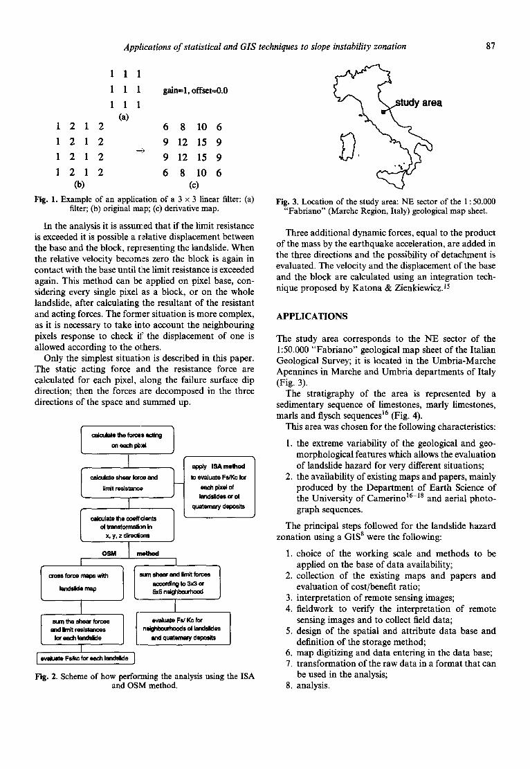
has been discussed. A possible solution to overcome this problem could be the use of neighbourhood operations and filters available in ILWIS. s A linear filter is used that consists of a 3 x 3 or a 5 x 5 matrix, a gain and an offset. The values of the matrix are multiplied by the values of the corresponding pixels in the raster map, then the results are summed up and the obtained value is multi- plied by the gain and added to the offset. The final result is assigned to the central pixel. An example of the application of a linear filter is shown in Fig. 1.
Using linear filters it is possible to add the contribution of surrounding pixels to the central pixel stability, using OSM.
After the steps described in the section regarding the ordinary slice method for the calculation of F s and Kc, a
filter can be applied to the force maps and the resultant of the forces can be assigned to the central pixel. Differ- ent matrices (3 x 3 or 5 x 5) can be used to evaluate different responses of the Fs or of the K c values to different size of the neighbourhoods and also to the different weights that may be assigned to the neighbouring pixels.
F s - c '- sec/3 + [(7 - m. % ) . z -cos /3 , tan ~b'] - K c . 7 . z . sin/3, t an¢ '
7 " z ' s i n / 3 + K c - 7 . z . c o s / 3 (9)
To work in three dimensions three different external forces can be introduced, each force proportional to the weight of the body. From eqn (4) it can be obtained:
Z S l x - Fsx " E T l x K c x =
E S 2 x + Fsx • E T 2 x
E S l y - F s y . ~ T l y K c y = ~ S 2 y + Fsy . E T 2y
ZSlz - Fsz • ETlz Kcz =
E S 2 z + Fsz • E T 2 z (10)
where:
S1 = c ' . sec /3 + [ ( 7 - m ' % ) ' z ' c o s / 3 . tan q/]
T1 = 7" z- sin/3
$ 2 = K c . 7 " z . sin/3- tan ~b'
T 2 = K c . 7 . z . co s fl
The total K c is:
KCtot = ~ K c 2 + K 4 + Kc] (11)
Ordinary slices method using neighbour operations and filtering
In the section regarding the infinite slope analysis method the limit due to the fact that each 'slice' is considered as unconnected to the surrounding 'slices'
Different approaches are used with a 3 x 5 or 5 x 5 matrix:
1. the central pixel is simply the sum of the neigh- bours;
2. the central pixel is the sum of the neighbours, assigning them a weight proportional to the inverse of the distance from the central one (the central pixel has weight 1);
3. the central pixel is the sum of the neighbours, assigning them a weight proportional to the inverse of the distance from the central one (the central pixel has weight 2).
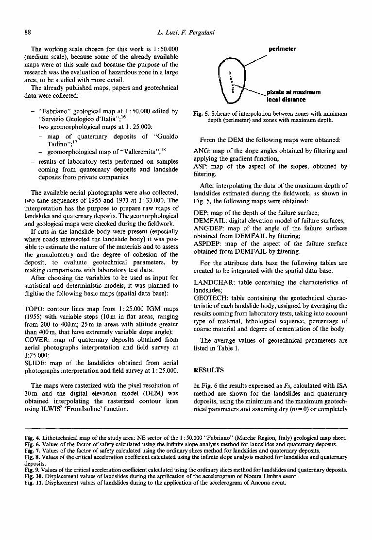
A summary of the methodologies described above is represented by the flowchart shown in Fig. 2.
Analysis in dynamic condition: a deterministic approach
The method adopted to determine the displacement of a landslide during an earthquake is the one proposed by Newmark. 14
This method calculates the response of a body, that stands on an inclined surface, to a seismic acceleration acting at the base. The aim of the calculation is to determine the relative displacement induced by an earth- quake of known characteristics and to estimate the stability of a mass during a seismic event. The base- block interface has a rigid-plastic behaviour and the resistance of the body is expressed by the Mohr - Coulomb criterion.
Applications of statistical and GIS techniques to slope instability zonation 87
1 1 1
1 1 1
1 1 1 (a)
gain=l, offset=O.O
1 2 1 2 6 8 1 0 6
1 2 1 2 9 12 15 9
1 2 1 2 9 12 15 9
1 2 1 2 6 8 1 0 6 (b) (c)
Fig. I. Example of an application of a 3 x 3 linear filter: (a) filter; (b) original maLp; (c) derivative map.
In the analysis it is assumed that if the limit resistance is exceeded it is possible a relative displacement between the base and the block, representing the landslide. When the relative velocity becomes zero the block is again in contact with the base until the limit resistance is exceeded again. This method can be applied on pixel base, con- sidering every single pixel as a block, or on the whole landslide, after calculating the resultant of the resistant and acting forces. The former situation is more complex, as it is necessary to take into account the neighbouring pixels response to check if the displacement of one is allowed according to the others.
Only the simplest situation is described in this paper. The static acting force and the resistance force are calculated for each pixel, along the failure surface dip direction; then the forces are decomposed in the three directions of the space and summed up.
I calculate the for~s acting 1 each i~(el
apply ISA mehxl calculate sheer lo~=e and to evaluate Fs/Kc for
limit resistan~D each pixel of landslldes or of
I quaternary deposits
of transforma~:,n in x, y, z directions
OSM I m~ltl~l I
I l
sum 1he shear forces / and Jjrlrlit r e s J ~ s 1 for each landslide
I
I
| at:truing to ~Y'J or ~_ SxS n a ~ r h o o d
I evaluate Fs/Ke for
nelghl0ourtmods of landslides and quatemaly deposits
Fig. 2. Scheme of how performing the analysis using the ISA and OSM method.
a
i
Fig. 3. Location of the study area: NE sector of the 1 : 50.000 "Fabriano" (Marche Region, Italy) geological map sheet.
Three additional dynamic forces, equal to the product of the mass by the earthquake acceleration, are added in the three directions and the possibility of detachment is evaluated. The velocity and the displacement of the base and the block are calculated using an integration tech- nique proposed by Katona & Zienkiewicz. 15
APPLICATIONS
The study area corresponds to the NE sector of the 1:50.000 "Fabriano" geological map sheet of the Italian Geological Survey; it is located in the Umbria-Marche Apennines in Marche and Umbria departments of Italy (Fig. 3).
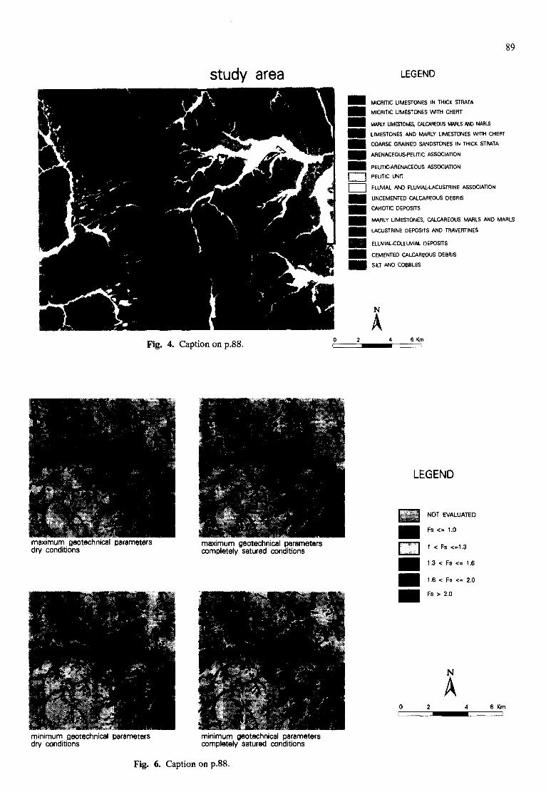
The stratigraphy of the area is represented by a sedimentary sequence of limestones, marly limestones, marls and flysch sequences 16 (Fig. 4).
This area was chosen for the following characteristics:
1. the extreme variability of the geological and geo- morphological features which allows the evaluation of landslide hazard for very different situations;
2. the availability of existing maps and papers, mainly produced by the Department of Earth Science of the University of Camerino 16 is and aerial photo- graph sequences.
The principal steps followed for the landslide hazard zonation using a GIS s were the following:
1. choice of the working scale and methods to be applied on the base of data availability;
2. collection of the existing maps and papers and evaluation of cost/benefit ratio;
3. interpretation of remote sensing images; 4. fieldwork to verify the interpretation of remote
sensing images and to collect field data; 5. design of the spatial and attribute data base and
definition of the storage method; 6. map digitizing and data entering in the data base; 7. transformation of the raw data in a format that can
be used in the analysis; 8. analysis.
88 L. Luzi,
The working scale chosen for this work is 1:50.000 (medium scale), because some of the already available maps were at this scale and because the purpose of the research was the evaluation of hazardous zone in a large area, to be studied with more detail.
The already published maps, papers and geotechnical data were collected:
- "Fabriano" geological map at 1 : 50.000 edited by "Servizio Geologico d'Italia"; 16
- two geomorphological maps at 1 : 25.000:
- m a p of quaternary deposits of "Gualdo Tadino"; 17
- geomorphological map of"Valleremita"; 18
- results of laboratory tests performed on samples coming from quaternary deposits and landslide deposits from private companies.
The available aerial photographs were also collected, two time sequences of 1955 and 1971 at 1 : 33.000. The interpretation has the purpose to prepare raw maps of landslides and quaternary deposits. The geomorphological and geological maps were checked during the fieldwork.
If cuts in the landslide body were present (especially where roads intersected the landslide body) it was pos- sible to estimate the nature of the materials and to assess the granulometry and the degree of cohesion of the deposit, to evaluate geotechnical parameters, by making comparisons with laboratory test data.
After choosing the variables to be used as input for statistical and deterministic models, it was planned to digitise the following basic maps (spatial data base):
TOPO: contour lines map from 1:25.000 IGM maps (1955) with variable steps (10m in flat areas, ranging from 200 to 400 m; 25 m in areas with altitude greater than 400 m, that have extremely variable slope angle); COVER: map of quaternary deposits obtained from aerial photographs interpretation and field survey at 1:25.000; SLIDE: map of the landslides obtained from aerial photographs interpretation and field survey at 1 : 25.000.
The maps were rasterized with the pixel resolution of 30m and the digital elevation model (DEM) was obtained interpolating the rasterized contour lines using ILWIS 8 'Fromlsoline' function.
F. Pergalani
pcrim©ter
Fig. 5. Scheme of interpolation between zones with minimum depth (perimeter) and zones with maximum depth.
From the DEM the following maps were obtained:
ANG: map of the slope angles obtained by filtering and applying the gradient function; ASP: map of the aspect of the slopes, obtained by filtering.
After interpolating the data of the maximum depth of landslides estimated during the fieldwork, as shown in Fig. 5, the following maps were obtained:
DEP: map of the depth of the failure surface; DEMFAIL: digital elevation model of failure surfaces; ANGDEP: map of the angle of the failure surfaces obtained from DEMFAIL by filtering; ASPDEP: map of the aspect of the failure surface obtained from DEMFAIL by filtering.
For the attribute data base the following tables are created to be integrated with the spatial data base:
LANDCHAR: table containing the characteristics of landslides; GEOTECH: table containing the geotechnical charac- teristic of each landslide body, assigned by averaging the results coming from laboratory tests, taking into account type of material, lithological sequence, percentage of coarse material and degree of cementation of the body.
The average values of geotechnical parameters are listed in Table 1.
RESULTS
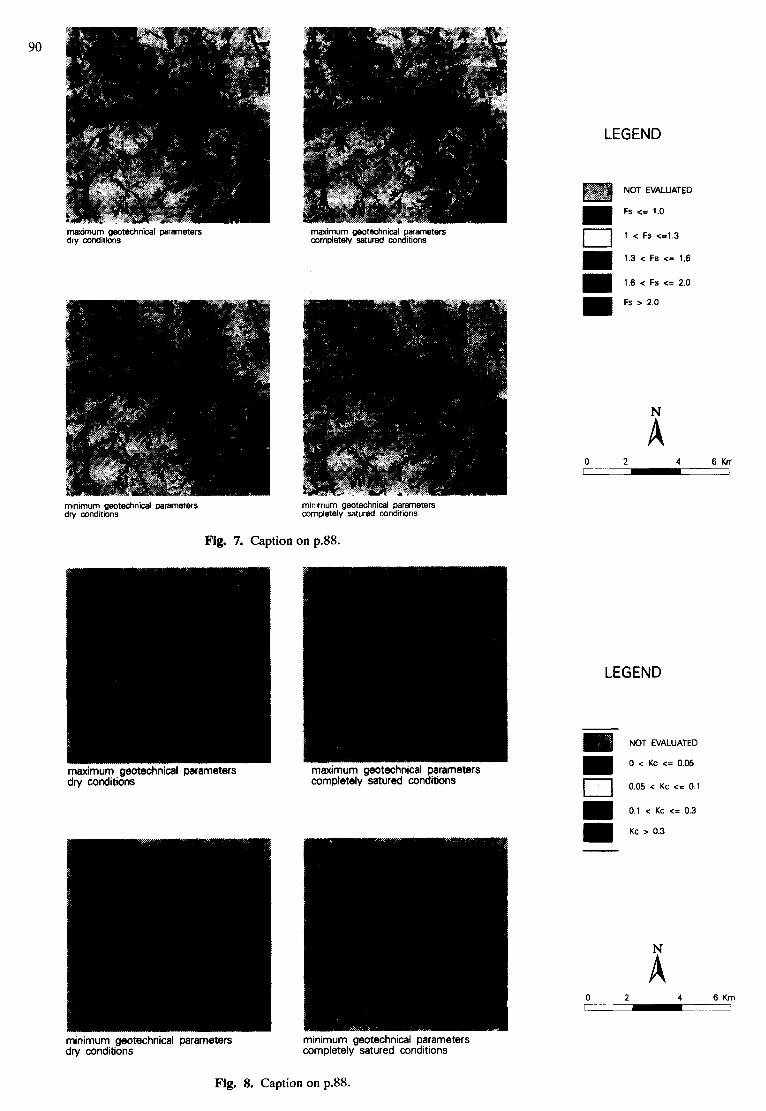
In Fig. 6 the results expressed as Fs, calculated with ISA method are shown for the landslides and quaternary deposits, using the minimum and the maximum geotech- nical parameters and assuming dry (m = 0) or completely
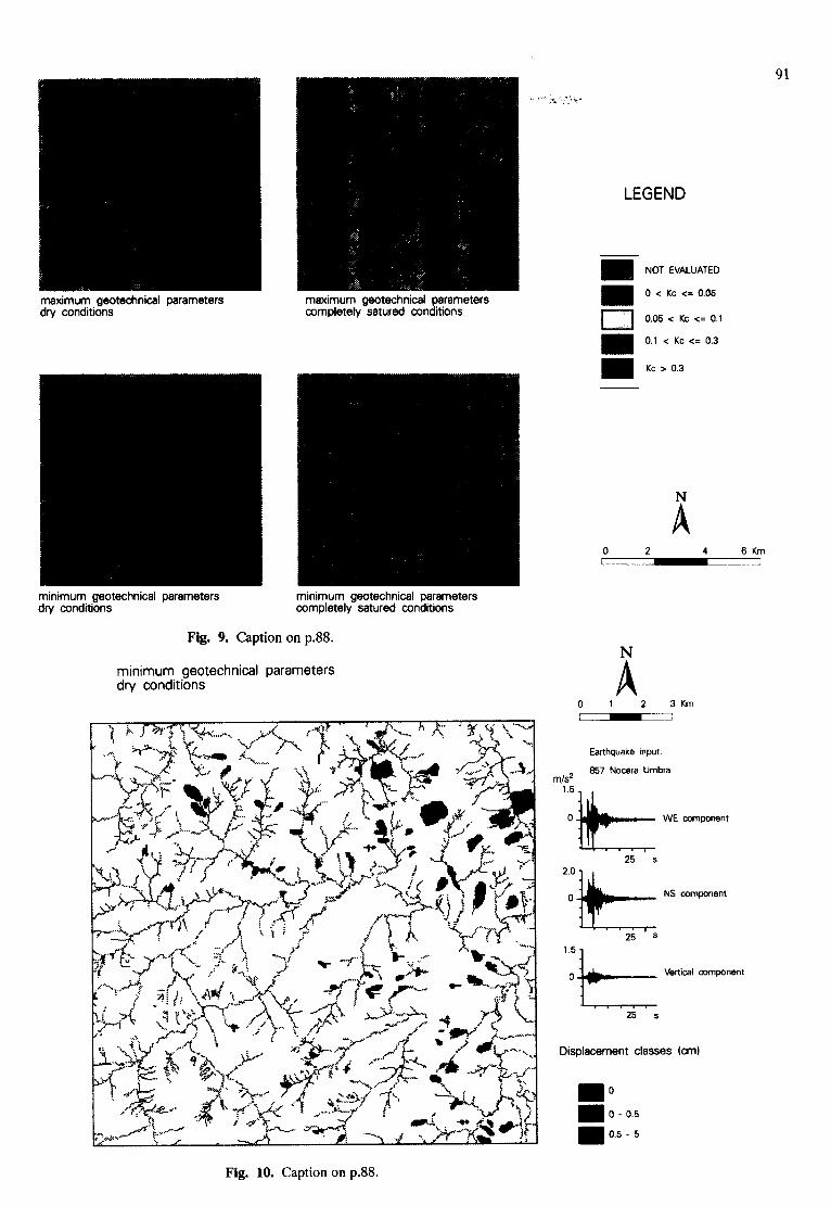
Fig. 4. Lithotechnical map of the study area: NE sector of the 1 : 50.000 "Fabriano" (Marche Region, Italy) geological map sheet. Fig. 6. Values of the factor of safety calculated using the infinite slope analysis method for landslides and quaternary deposits. Fig. 7. Values of the factor of safety calculated using the ordinary slices method for landslides and quaternary deposits. Fig. 8. Values of the critical acceleration coefficient calculated using the infinite slope analysis method for landslides and quaternary deposits. Fig. 9. Values of the critical acceleration coefficient calculated using the ordinary slices method for landslides and quaternary deposits. Fig. 10. Displacement values of landslides during the application of the accelerogram of Nocera Umbra event. Fig. 11. Displacement values of landslides during to the application of the accelerogram of Ancona event.
study area
m n n n m m m
F-~ m m m m m m m
89
LEGEND
MICRrrlc LIMESTONES IN THICK STRATA
MICRITIC LIMESTONES WITH CHERT
MARLY UMES~ONE& CALCAREOUS MARLS AND MARLS
LIMESTONES AND MARLY LIMESTONES WITH CHERT
COARSE GRAINED SANDSTONES IN THICK STRATA
ARENACEOUS-PELITIC ASSOCIATION
PELITIC-ARENACEOUS ASSOCIATION
PELITIC UNIT
FLUVIAL AND FLUVIAL-LACUSTRINE ASSOCIATION
UNCEMENTED CALCAREOUS DEBRIS
CAHOTIC DEPOSITS
MARLY LIMESTONES, CALCAREOUS MARLS AND MARLS
LACUSTRINE DEPOSITS AND TRAVERTINES
ELUVIAL-COLLUVIAL DEPOSITS
CEMENTED CALCAREOUS DEBRIS
SILT AND COBBLES
Fig. 4. Caption on p.88.
N
A 4 6Km
LEGEND
maximum geotechnical parameters dry conditions
maximum geotechnical parameters completely satured conditions
NOT EVALUATED
m Fs <= 1.0
I < Fs <=1.3
m 1.3 < Fs <= 1.6
m 1.6 < Fs <= 2.0
m Fs > 2.0
minimum geotechnical parameters dry conditions
minimum geotechnical parameters completely satured conditions
Fig. 6. Caption on p.88.
0 2 I
N
A 4 6 K m
I
90
maximum geotechnical parameters dry conditions
maximum geotechnical parameters completely satured conditions
m F--l
LEGEND
NOT EVALUATED
Fs <= 1.0
1 < Fs <=1.3
1.3 < Fs <= 1.6
1.6 < Fs <= 2.0
Fs > 2.0
N
A 6Krr
minimum geotechnical parameters dw conditions
minimum geotechnical parameters completely satured conditions
Fig. 7. Caption on p.88.
LEGEND
maximum geotechnical parameters dry conditions
maximum geotechnical parameters completely satured conditions
BB m
NOT EVALUATED
0 < Kc <= 0.05
0.05 < Kc <= 0.1
0.1 < Kc <= 0.3
Kc > 0.3
minimum geotechnical parameters dry conditions
m i n i m u m geotechnicat parameters comp le te l y satured condi t ions
0 I
N
A 4 6Krn
I
Fig. 8. Caption on p.88.
91
LEGEND
maximum geotechnical parameters dry conditions
maximum geotechnical parameters completely satured conditions
NOT EVALUATED
0 < Kc < : 0.05
0.05 < Kc <= 0.1
0.1 < Kc < : 0.3
Kc • 0.3
minimum geotechnical parameters dry conditions
minimum geotechnical parameters completely satured conditions
Fig. 9. Caption on p.88.
minimum geotechnical parameters dry conditions
r -
N
A 6 K m
I
N
A 1 2 3 Km
- -7
Earthquake input:
857 Nocera Umbra m/s 2
25 s
25 s
1.5 t
0 . . .L.
t- ' ' ' 2 5 ' s
WE component
NS component
Vertical component
Displacement classes (cm)
~ 0
m 0 - 0.5
m 0 .5 - 5
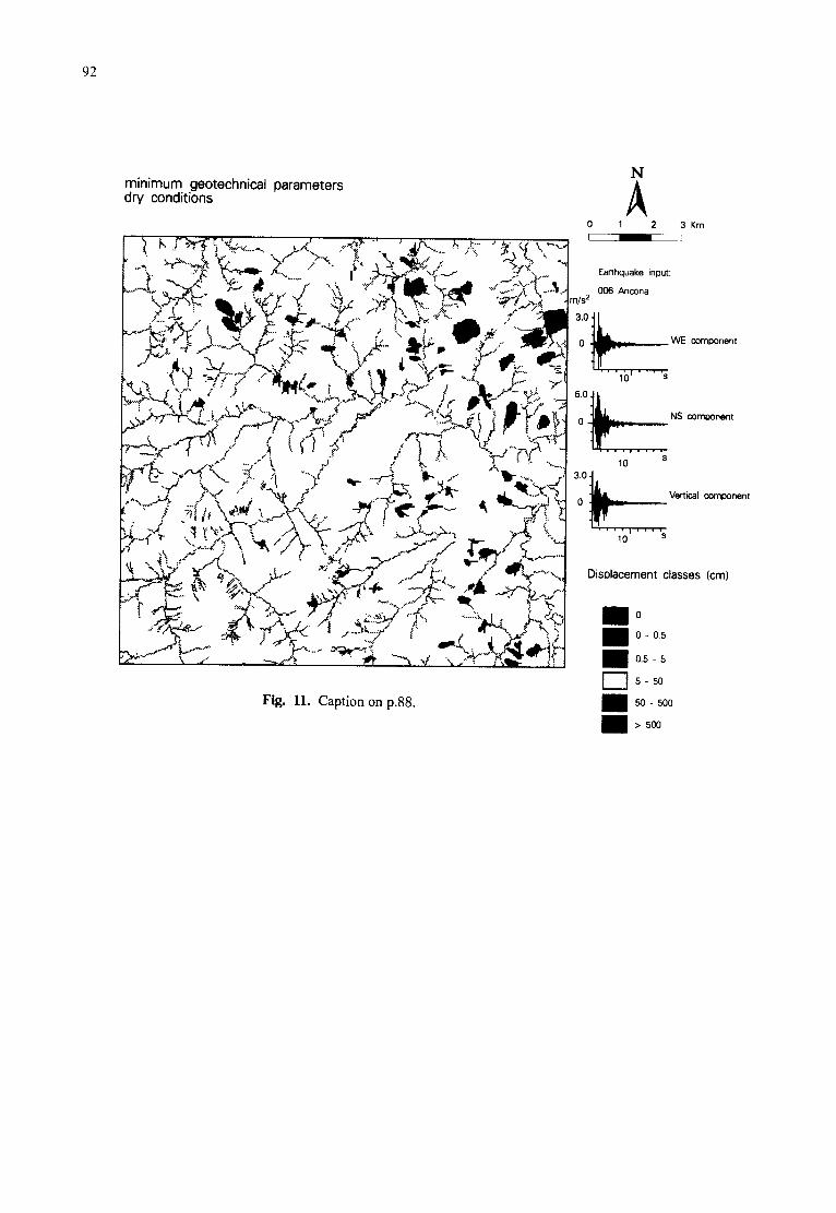
Fig. 10. Caption on p.88.
oo~ < I
oo~ - ~ II
o~-~ I ]
s-~.o II
~o-o I
oI
(wo) sesselo lueweoeldS!C]
s .... i OL
.,Ib
lueu~woo leg!~eA o
o'£ ol
lueuodwoo SN ~ 0
0!i
s .... ,Or, ,,
i1~ lueuodwoo 3M-~ 0
I1" o'~
~s/w euoou~ 900
:lndu! e)lenbqlie3
r I
w)l £ Z t 0
V N
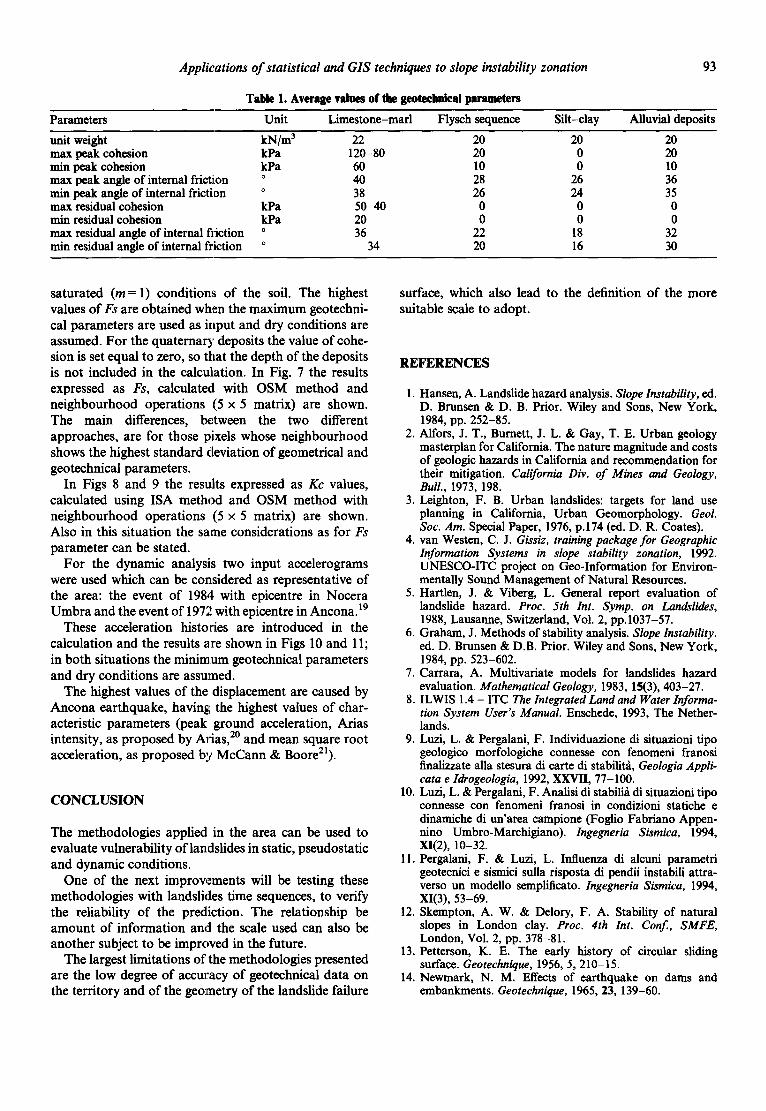
• 88"d uo uo!lde D 11 "ll!,~l
r ~ , ~', : .-~.~" t ~,k,.. ~ I
"~"~ , ix .: ~..~'~ !. ! " [ ".,.," "it t~. ~v_~.,.. I
,..,. , .... "~ , .,<yet '- " ,~ k --. ~,
~"\~"'~"C TM X,~/~ ~ ",/ ~ ~q~ ,~ ~ i.< / tl
"- ,: ", .i h
: ,', L_ ~, 1 t.:. 0" J ! ,J \C~+~": ~" -I
#" ,,,/' t <
-r-. " 11, ~ /i~ t- -~., /:..~.:
.,.._~.. : ~.-'~
r" ~... j -.
• ..~ 4." "-4 ,, ,4:v ~'`
suop,!puoo /up sJe],eweJed leo!uqoel.oe6 wnw!u!w
~6
Applications o f statistical and GIS techniques to slope instability zonation
Table 1. Average values of the geoteclmieal parameters
93
Parameters Unit Limestone-marl Flyseh sequence Silt-day Alluvial deposits
unit weight kN/m 3 22 max peak cohesion kPa 120-80 rain peak cohesion kPa 60 max peak angle of internal friction ° 40 rain peak angle of internal friction o 38 max residual cohesion kPa 50-40 rain residual cohesion kPa 20 max residual angle of internal fi%tion o 36 rain residual angle of internal friction o 34
20 20 20 20 0 20 10 0 10 28 26 36 26 24 35
0 0 0 0 0 0
22 18 32 20 16 30
saturated (m = 1) conditions of the soil. The highest values of Fs are obtained when the maximum geotechni- cal parameters are used as input and dry conditions are assumed. For the quaternary deposits the value of cohe- sion is set equal to zero, so that the depth of the deposits is not included in the ealculLation. In Fig. 7 the results expressed as Fs, calculated with OSM method and neighbourhood operations (5 x 5 matrix) are shown. The main differences, between the two different approaches, are for those pixels whose neighbourhood shows the highest standard deviation of geometrical and geoteehnical parameters.
In Figs 8 and 9 the results expressed as Kc values, calculated using ISA method and OSM method with neighbourhood operations (5 x 5 matrix) are shown. Also in this situation the same considerations as for Fs parameter can be stated.
For the dynamic analysis two input accelerograms were used which can be considered as representative of the area: the event of 1984 with epicentre in Nocera Umbra and the event of 1972 with epicentre in Ancona.19
These acceleration histories are introduced in the calculation and the results are shown in Figs 10 and 11; in both situations the minimum geotechnical parameters and dry conditions are assttmed.
The highest values of the displacement are caused by Ancona earthquake, having; the highest values of char- acteristic parameters (peak ground acceleration, Arias intensity, as proposed by Arias, 2° and mean square root acceleration, as proposed by McCann & Boore21).
CONCLUSION
The methodologies applied in the area can be used to evaluate vulnerability of landslides in static, pseudostatic and dynamic conditions.
One of the next improvements will be testing these methodologies with landslides time sequences, to verify the reliability of the prediction. The relationship be amount of information and the scale used can also be another subject to be improved in the future.
The largest limitations of the methodologies presented are the low degree of accuracy of geotechnieal data on the territory and of the geometry of the landslide failure
surface, which also lead to the definition of the more suitable scale to adopt.
REFERENCES
1. Hansen, A. Landslide hazard analysis. Slope Instability, ed. D. Brnnsen & D. B. Prior. Wiley and Sons, New York, 1984, pp. 252-85.
2. Allots, J. T., BurneR, J. L. & Gay, T. E. Urban geology masterplan for California. The nature magnitude and costs of geologic hazards in California and recommendation for their mitigation. California Div. of Mines and Geology, Bull., 1973, 198.
3. Leighton, F. B. Urban landslides: targets for land use planning in California, Urban Geomorphology. Geol. Soc. Am. Special Paper, 1976, p.174 (ed. D. R. Coates).
4. van Westen, C. J. Gissiz, training package for Geographic Information Systems in slope stability zonation, 1992. UNESCO-ITC project on Geo-Information for Environ- mentally Sound Management of Natural Resources.
5. Hartlen, J. & Viberg, L. General report evaluation of landslide hazard. Proc. 5th Int. Symp. on Landslides, 1988, Lausanne, Switzerland, Vol. 2, pp. 1037-57.
6. Graham, J. Methods of stability analysis. Slope Instability. ed. D. Brunsen & D.B. Prior. Wiley and Sons, New York, 1984, pp. 523-602.
7. Carrara, A. Multivariate models for landslides hazard evaluation. Mathematical Geology, 1983, 15(3), 403-27.
8. ILWIS 1.4 - ITC The Integrated Land and Water Informa- tion System User's Manual. Enschede, 1993, The Nether- lands.
9. Luzi, L. & Pergalani, F. Individuazione di situazioni tipo geologico morfologiche eonnesse con fenomeni franosi finalizzate alia stesura di carte di stabilitfi, Geologia Appli- cata e Idrogeologia, 1992, XXVII, 77-100.
10. Luzi, L. & Pergalani, F. Analisi di stabilifi di situazioni tipo connesse con fenomeni franosi in condizioni statiche e dinamiche di un'area campione (Foglio Fabriano Appen- nino Umbro-Marchigiano). lngegneria Sismica, 1994, XI(2), 10-32.
11. Pergalani, F. & Luzi, L. Influenza di alcuni parametri geotecnici e sismici sulla risposta di pendii instabili attra- verso un modello sempliticato, lngegneria Sismica, 1994, XI(3), 53-69.
12. Skempton, A. W. & Delory, F. A. Stability of natural slopes in London clay. Proc. 4th Int. Conf., SMFE, London, Vol. 2, pp. 378-81.
13. Petterson, K. E. The early history of circular sliding surface. Geotechnique, 1956, 5, 210-15.
14. Newmark, N. M. Effects of earthquake on dams and embankments. Geotechnique, 1965, 23, 139-60.

94 L. Luzi, F. Pergalani
15. Katona, M. G. & Zienkiewicz, O.C. A unified set of single step algorithm - - part 3: the beta-m method, a general- ization of Newmark scheme. Int. J. numer. Meth. Engng, 1985, 21, 190-210.
16. Centamore, E., Chiocchini, M., Chiocchini, U., Dramis, F., Giardini, G., Jacobacci, A., Martelli, G., Micarelli, A. & Potetti, M. Note illustrative del F. 301 Fabriano, 1979, Servizio Geologico d'Italia.
17. Bosi, C., Coltorti, M. & Dramis, F. Carta del Quaternario del bacino di Gualdo Tadino, 1987, Tipografia ERREBI, Falconara.
18. Ciccacci, F., D'Alessandro, L., Dramis, F., Lupia Palmieri, E. & Pambianchi, G. Carta geomorfologica del compren- sorio di Valleremita (Appennino Umbro Marchigiano Set- tentrionale), 1986, Tipografia SGS (Roma).
19. ENEA-ENEL Commissione per 1o studio dei problemi sismici connessi con la realizzazione di impianti nucleari. Contributo alia caratterizzazione della sismicith del terri- torio italiano. Convegno annuale del Progetto Finalizzato Geodinamica, 1981, Udine.
20. Arias, A. A Measure of Earthquake Intensity, Seismic Design for Nuclear Power Plants. ed. R. J. Hansen. Mas- sachusetts Institute of Technology, 1970.
21. McCann, M. W. & Boore, D. M. Variability in ground motion: root mean square acceleration and peak accelera- tion for the 1971 S. Fernando California Earthquake. Bull. Seism. Am., 1983.


