ANSYS Internal Combustion Engines Tutorial Guide

ANSYS Internal Combustion Engines TutorialGuide

Release 16.0ANSYS, Inc.January 2015Southpointe

2600 ANSYS DriveCanonsburg, PA 15317 ANSYS, Inc. is

certified to ISO9001:2008.

[email protected]://www.ansys.com(T) 724-746-3304(F) 724-514-9494

Copyright and Trademark Information

© 2014-2015 SAS IP, Inc. All rights reserved. Unauthorized use, distribution or duplication is prohibited.

ANSYS, ANSYS Workbench, Ansoft, AUTODYN, EKM, Engineering Knowledge Manager, CFX, FLUENT, HFSS, AIMand any and all ANSYS, Inc. brand, product, service and feature names, logos and slogans are registered trademarksor trademarks of ANSYS, Inc. or its subsidiaries in the United States or other countries. ICEM CFD is a trademarkused by ANSYS, Inc. under license. CFX is a trademark of Sony Corporation in Japan. All other brand, product,service and feature names or trademarks are the property of their respective owners.

Disclaimer Notice

THIS ANSYS SOFTWARE PRODUCT AND PROGRAM DOCUMENTATION INCLUDE TRADE SECRETS AND ARE CONFID-ENTIAL AND PROPRIETARY PRODUCTS OF ANSYS, INC., ITS SUBSIDIARIES, OR LICENSORS. The software productsand documentation are furnished by ANSYS, Inc., its subsidiaries, or affiliates under a software license agreementthat contains provisions concerning non-disclosure, copying, length and nature of use, compliance with exportinglaws, warranties, disclaimers, limitations of liability, and remedies, and other provisions. The software productsand documentation may be used, disclosed, transferred, or copied only in accordance with the terms and conditionsof that software license agreement.

ANSYS, Inc. is certified to ISO 9001:2008.

U.S. Government Rights

For U.S. Government users, except as specifically granted by the ANSYS, Inc. software license agreement, the use,duplication, or disclosure by the United States Government is subject to restrictions stated in the ANSYS, Inc.software license agreement and FAR 12.212 (for non-DOD licenses).

Third-Party Software

See the legal information in the product help files for the complete Legal Notice for ANSYS proprietary softwareand third-party software. If you are unable to access the Legal Notice, please contact ANSYS, Inc.

Published in the U.S.A.

Table of Contents

1. Tutorial: Solving a Cold Flow Simulation . . . . . . . . . . . . . . . . . . . . . . . . . . . . . . . . . . . . . . . . . . . . . . . . . . . . . . . . . . . . . . . . . . . . . . . . . . . . . . . . . . . . . . . . . . . . . . . . 11.1. Preparation .... . . . . . . . . . . . . . . . . . . . . . . . . . . . . . . . . . . . . . . . . . . . . . . . . . . . . . . . . . . . . . . . . . . . . . . . . . . . . . . . . . . . . . . . . . . . . . . . . . . . . . . . . . . . . . . . . . . . . . . . . . . . . . . . . . . 21.2. Step 1: Setting the Properties ... . . . . . . . . . . . . . . . . . . . . . . . . . . . . . . . . . . . . . . . . . . . . . . . . . . . . . . . . . . . . . . . . . . . . . . . . . . . . . . . . . . . . . . . . . . . . . . . . . . . . . . . . . 21.3. Step 2: Performing the Decomposition .... . . . . . . . . . . . . . . . . . . . . . . . . . . . . . . . . . . . . . . . . . . . . . . . . . . . . . . . . . . . . . . . . . . . . . . . . . . . . . . . . . . . . . . . . . . 41.4. Step 3: Meshing .... . . . . . . . . . . . . . . . . . . . . . . . . . . . . . . . . . . . . . . . . . . . . . . . . . . . . . . . . . . . . . . . . . . . . . . . . . . . . . . . . . . . . . . . . . . . . . . . . . . . . . . . . . . . . . . . . . . . . . . . . . . 121.5. Step 4: Setting up the Simulation .... . . . . . . . . . . . . . . . . . . . . . . . . . . . . . . . . . . . . . . . . . . . . . . . . . . . . . . . . . . . . . . . . . . . . . . . . . . . . . . . . . . . . . . . . . . . . . . . . . 151.6. Step 5: Running the Solution .... . . . . . . . . . . . . . . . . . . . . . . . . . . . . . . . . . . . . . . . . . . . . . . . . . . . . . . . . . . . . . . . . . . . . . . . . . . . . . . . . . . . . . . . . . . . . . . . . . . . . . . . 281.7. Step 6: Obtaining the Results ... . . . . . . . . . . . . . . . . . . . . . . . . . . . . . . . . . . . . . . . . . . . . . . . . . . . . . . . . . . . . . . . . . . . . . . . . . . . . . . . . . . . . . . . . . . . . . . . . . . . . . . . . 301.8. Step 7: Postprocessing .... . . . . . . . . . . . . . . . . . . . . . . . . . . . . . . . . . . . . . . . . . . . . . . . . . . . . . . . . . . . . . . . . . . . . . . . . . . . . . . . . . . . . . . . . . . . . . . . . . . . . . . . . . . . . . . . . 571.9. Summary .... . . . . . . . . . . . . . . . . . . . . . . . . . . . . . . . . . . . . . . . . . . . . . . . . . . . . . . . . . . . . . . . . . . . . . . . . . . . . . . . . . . . . . . . . . . . . . . . . . . . . . . . . . . . . . . . . . . . . . . . . . . . . . . . . . . . . 621.10. Further Improvements .... . . . . . . . . . . . . . . . . . . . . . . . . . . . . . . . . . . . . . . . . . . . . . . . . . . . . . . . . . . . . . . . . . . . . . . . . . . . . . . . . . . . . . . . . . . . . . . . . . . . . . . . . . . . . . . 62

2. Tutorial: Solving a Port Flow Simulation . . . . . . . . . . . . . . . . . . . . . . . . . . . . . . . . . . . . . . . . . . . . . . . . . . . . . . . . . . . . . . . . . . . . . . . . . . . . . . . . . . . . . . . . . . . . . . . 632.1. Preparation .... . . . . . . . . . . . . . . . . . . . . . . . . . . . . . . . . . . . . . . . . . . . . . . . . . . . . . . . . . . . . . . . . . . . . . . . . . . . . . . . . . . . . . . . . . . . . . . . . . . . . . . . . . . . . . . . . . . . . . . . . . . . . . . . . . 642.2. Step 1: Setting the Properties ... . . . . . . . . . . . . . . . . . . . . . . . . . . . . . . . . . . . . . . . . . . . . . . . . . . . . . . . . . . . . . . . . . . . . . . . . . . . . . . . . . . . . . . . . . . . . . . . . . . . . . . . 642.3. Step 2: Performing the Decomposition .... . . . . . . . . . . . . . . . . . . . . . . . . . . . . . . . . . . . . . . . . . . . . . . . . . . . . . . . . . . . . . . . . . . . . . . . . . . . . . . . . . . . . . . . . 652.4. Step 3: Meshing .... . . . . . . . . . . . . . . . . . . . . . . . . . . . . . . . . . . . . . . . . . . . . . . . . . . . . . . . . . . . . . . . . . . . . . . . . . . . . . . . . . . . . . . . . . . . . . . . . . . . . . . . . . . . . . . . . . . . . . . . . . . 762.5. Step 4: Setting up the Simulation .... . . . . . . . . . . . . . . . . . . . . . . . . . . . . . . . . . . . . . . . . . . . . . . . . . . . . . . . . . . . . . . . . . . . . . . . . . . . . . . . . . . . . . . . . . . . . . . . . . 782.6. Step 5: Running the Solution .... . . . . . . . . . . . . . . . . . . . . . . . . . . . . . . . . . . . . . . . . . . . . . . . . . . . . . . . . . . . . . . . . . . . . . . . . . . . . . . . . . . . . . . . . . . . . . . . . . . . . . . . 842.7. Step 6: Obtaining the Results ... . . . . . . . . . . . . . . . . . . . . . . . . . . . . . . . . . . . . . . . . . . . . . . . . . . . . . . . . . . . . . . . . . . . . . . . . . . . . . . . . . . . . . . . . . . . . . . . . . . . . . . . . 922.8. Summary .... . . . . . . . . . . . . . . . . . . . . . . . . . . . . . . . . . . . . . . . . . . . . . . . . . . . . . . . . . . . . . . . . . . . . . . . . . . . . . . . . . . . . . . . . . . . . . . . . . . . . . . . . . . . . . . . . . . . . . . . . . . . . . . . . . . 1062.9. Further Improvements .... . . . . . . . . . . . . . . . . . . . . . . . . . . . . . . . . . . . . . . . . . . . . . . . . . . . . . . . . . . . . . . . . . . . . . . . . . . . . . . . . . . . . . . . . . . . . . . . . . . . . . . . . . . . . . . 106

3. Tutorial: Solving a Combustion Simulation for a Sector . . . . . . . . . . . . . . . . . . . . . . . . . . . . . . . . . . . . . . . . . . . . . . . . . . . . . . . . . . . . . . . . . . . . . 1073.1. Preparation .... . . . . . . . . . . . . . . . . . . . . . . . . . . . . . . . . . . . . . . . . . . . . . . . . . . . . . . . . . . . . . . . . . . . . . . . . . . . . . . . . . . . . . . . . . . . . . . . . . . . . . . . . . . . . . . . . . . . . . . . . . . . . . . . 1083.2. Step 1: Setting the Properties ... . . . . . . . . . . . . . . . . . . . . . . . . . . . . . . . . . . . . . . . . . . . . . . . . . . . . . . . . . . . . . . . . . . . . . . . . . . . . . . . . . . . . . . . . . . . . . . . . . . . . . 1083.3. Step 2: Performing the Decomposition .... . . . . . . . . . . . . . . . . . . . . . . . . . . . . . . . . . . . . . . . . . . . . . . . . . . . . . . . . . . . . . . . . . . . . . . . . . . . . . . . . . . . . . . 1103.4. Step 3: Meshing .... . . . . . . . . . . . . . . . . . . . . . . . . . . . . . . . . . . . . . . . . . . . . . . . . . . . . . . . . . . . . . . . . . . . . . . . . . . . . . . . . . . . . . . . . . . . . . . . . . . . . . . . . . . . . . . . . . . . . . . . . 1173.5. Step 4: Setting up the Simulation .... . . . . . . . . . . . . . . . . . . . . . . . . . . . . . . . . . . . . . . . . . . . . . . . . . . . . . . . . . . . . . . . . . . . . . . . . . . . . . . . . . . . . . . . . . . . . . . . 1193.6. Step 5: Running the Solution .... . . . . . . . . . . . . . . . . . . . . . . . . . . . . . . . . . . . . . . . . . . . . . . . . . . . . . . . . . . . . . . . . . . . . . . . . . . . . . . . . . . . . . . . . . . . . . . . . . . . . . 1333.7. Step 6: Obtaining the Results ... . . . . . . . . . . . . . . . . . . . . . . . . . . . . . . . . . . . . . . . . . . . . . . . . . . . . . . . . . . . . . . . . . . . . . . . . . . . . . . . . . . . . . . . . . . . . . . . . . . . . . . 1363.8. Summary .... . . . . . . . . . . . . . . . . . . . . . . . . . . . . . . . . . . . . . . . . . . . . . . . . . . . . . . . . . . . . . . . . . . . . . . . . . . . . . . . . . . . . . . . . . . . . . . . . . . . . . . . . . . . . . . . . . . . . . . . . . . . . . . . . . . 1713.9. Further Improvements .... . . . . . . . . . . . . . . . . . . . . . . . . . . . . . . . . . . . . . . . . . . . . . . . . . . . . . . . . . . . . . . . . . . . . . . . . . . . . . . . . . . . . . . . . . . . . . . . . . . . . . . . . . . . . . . 171

4. Tutorial: Solving a Gasoline Direct Injection Engine Simulation . . . . . . . . . . . . . . . . . . . . . . . . . . . . . . . . . . . . . . . . . . . . . . . . . . . . . . . . 1734.1. Preparation .... . . . . . . . . . . . . . . . . . . . . . . . . . . . . . . . . . . . . . . . . . . . . . . . . . . . . . . . . . . . . . . . . . . . . . . . . . . . . . . . . . . . . . . . . . . . . . . . . . . . . . . . . . . . . . . . . . . . . . . . . . . . . . . . 1744.2. Step 1: Setting the Properties ... . . . . . . . . . . . . . . . . . . . . . . . . . . . . . . . . . . . . . . . . . . . . . . . . . . . . . . . . . . . . . . . . . . . . . . . . . . . . . . . . . . . . . . . . . . . . . . . . . . . . . 1744.3. Step 2: Performing the Decomposition .... . . . . . . . . . . . . . . . . . . . . . . . . . . . . . . . . . . . . . . . . . . . . . . . . . . . . . . . . . . . . . . . . . . . . . . . . . . . . . . . . . . . . . . 1764.4. Step 3: Meshing .... . . . . . . . . . . . . . . . . . . . . . . . . . . . . . . . . . . . . . . . . . . . . . . . . . . . . . . . . . . . . . . . . . . . . . . . . . . . . . . . . . . . . . . . . . . . . . . . . . . . . . . . . . . . . . . . . . . . . . . . . 1894.5. Step 4: Setting up the Simulation .... . . . . . . . . . . . . . . . . . . . . . . . . . . . . . . . . . . . . . . . . . . . . . . . . . . . . . . . . . . . . . . . . . . . . . . . . . . . . . . . . . . . . . . . . . . . . . . . 1904.6. Step 5: Running the Solution .... . . . . . . . . . . . . . . . . . . . . . . . . . . . . . . . . . . . . . . . . . . . . . . . . . . . . . . . . . . . . . . . . . . . . . . . . . . . . . . . . . . . . . . . . . . . . . . . . . . . . . 2084.7. Step 6: Obtaining the Results ... . . . . . . . . . . . . . . . . . . . . . . . . . . . . . . . . . . . . . . . . . . . . . . . . . . . . . . . . . . . . . . . . . . . . . . . . . . . . . . . . . . . . . . . . . . . . . . . . . . . . . . 2124.8. Summary .... . . . . . . . . . . . . . . . . . . . . . . . . . . . . . . . . . . . . . . . . . . . . . . . . . . . . . . . . . . . . . . . . . . . . . . . . . . . . . . . . . . . . . . . . . . . . . . . . . . . . . . . . . . . . . . . . . . . . . . . . . . . . . . . . . . 2524.9. Further Improvements .... . . . . . . . . . . . . . . . . . . . . . . . . . . . . . . . . . . . . . . . . . . . . . . . . . . . . . . . . . . . . . . . . . . . . . . . . . . . . . . . . . . . . . . . . . . . . . . . . . . . . . . . . . . . . . . 252

Index .... . . . . . . . . . . . . . . . . . . . . . . . . . . . . . . . . . . . . . . . . . . . . . . . . . . . . . . . . . . . . . . . . . . . . . . . . . . . . . . . . . . . . . . . . . . . . . . . . . . . . . . . . . . . . . . . . . . . . . . . . . . . . . . . . . . . . . . . . . . . . . . . . . . . . 253

iiiRelease 16.0 - © SAS IP, Inc. All rights reserved. - Contains proprietary and confidential information

of ANSYS, Inc. and its subsidiaries and affiliates.

Release 16.0 - © SAS IP, Inc. All rights reserved. - Contains proprietary and confidential informationof ANSYS, Inc. and its subsidiaries and affiliates.iv

Chapter 1: Tutorial: Solving a Cold Flow Simulation

A three dimensional single cylinder CFD simulation of a 4-stroke engine is performed under motoredconditions (cold flow) in this tutorial. Detailed boundary conditions are shown in Figure 1.1: ProblemSchematic (p. 1). Engine simulation is started from Intake valve opening (IVO) followed by air flowduring intake stroke. Air is compressed as piston moves towards top dead centre (TDC). This is followedby expansion of air as piston moves towards bottom Dead centre (BDC). This tutorial serves as an intro-duction in releasing the streamlined workflow between pre-processing, solver and post processing whilecarrying out simulations with Fluent.

Figure 1.1: Problem Schematic

This tutorial illustrates the following steps:

• Launch IC Engine system.

• Read an existing geometry into IC Engine.

• Decompose the geometry.

• Define the mesh setup and mesh the geometry.

• Run the simulation.

• Examine the results in the report.

• Perform additional postprocessing in CFD-Post.

This tutorial is written with the assumption that you are familiar with the IC Engine system and thatyou have a good working knowledge of ANSYS Workbench.

1Release 16.0 - © SAS IP, Inc. All rights reserved. - Contains proprietary and confidential information


1.1. Preparation1.2. Step 1: Setting the Properties1.3. Step 2: Performing the Decomposition1.4. Step 3: Meshing1.5. Step 4: Setting up the Simulation1.6. Step 5: Running the Solution1.7. Step 6: Obtaining the Results1.8. Step 7: Postprocessing1.9. Summary1.10. Further Improvements

1.1. Preparation

1. Copy the files (demo_eng.x_t and lift.prof) to your working folder.

To access tutorials and their input files on the ANSYS Customer Portal, go to http://support.an-sys.com/training.

2. Start Workbench.

1.2. Step 1: Setting the Properties

1. Create an IC Engine analysis system in the Workbench interface by dragging or double-clicking IC Engineunder Analysis Systems in the Toolbox.

Release 16.0 - © SAS IP, Inc. All rights reserved. - Contains proprietary and confidential informationof ANSYS, Inc. and its subsidiaries and affiliates.2

Tutorial: Solving a Cold Flow Simulation

http://support.ansys.com/training


2. If the Properties view is not already visible, right-click ICE, cell 2, and select Properties from the contextmenu.

3. Select Cold Flow Simulation from the Simulation Type drop-down list.

4. In the Properties dialog box under Engine Inputs enter 144.3 for Connecting Rod Length.

5. Enter 45 for Crank Radius.

6. Retain 0 for Piston Offset/Wrench.

7. Enter 0.5 for Minimum Lift.

8. Click Browse File next to Lift Curve. The File Open dialog box opens. Select the valve profile filelift.prof and click Open.



Step 1: Setting the Properties

1.3. Step 2: Performing the Decomposition

Here you will read the geometry and prepare it for decomposition. Double-click the Geometry cell toopen the DesignModeler.

1. Select Millimeter from the Units menu.

2. Import the geometry file,demo_eng.x_t.

File > Import External Geometry File...

3. Click Generate to complete the import feature.



4. Click Input Manager located in the IC Engine toolbar.



Step 2: Performing the Decomposition

a. Selec IVO from Decomposition Position drop-down list.

b. Click next to Inlet Faces, select the face of the inlet valve and click Apply.

c. Click next to Outlet Faces, select the face of the exhaust valve and click Apply.

d. Select the four faces as shown in Figure 1.2: Cylinder Faces (p. 7) for Cylinder Faces and click Apply.



Figure 1.2: Cylinder Faces

e. Retain selection of Yes from the Symmetry Face Option drop-down list.

f. Select the three faces shown in Figure 1.3: Symmetry Faces (p. 7) for Symmetry Faces and clickApply.

Figure 1.3: Symmetry Faces




g. Retain the selection of Full Topology from the Topology Option drop-down list.

h. Retain selection of No for Crevice Option.

i. Retain selection of No for Validate Compression Ratio.

j. Retain selection of InValve from the Valve Type drop-down list.

k. Select the valve body as shown in Figure 1.4: Intake Valve (p. 8) for Valve Bodies and click Apply.

Figure 1.4: Intake Valve

l. Select the valve seat face as shown in Figure 1.5: Intake Valve Seat (p. 9) for Valve Seat Faces andclick Apply.



Figure 1.5: Intake Valve Seat

m. Select invalve1 from the Valve Profile drop-down list.

n. Right-click on IC Valves Data in the Details of InputManager and select Add New IC Valves DataGroup from the context menu.

o. In this IC Valves Data group following the steps for the intake valve, set the other valve body toExValve and set its profile to exvalve1. Select the valve seat face of that valve as shown in Fig-ure 1.6: Exhaust Valve Seat (p. 10).




Figure 1.6: Exhaust Valve Seat

p. Retain the default options under Under IC Advanced Options.

q. After all the settings are done click Generate .



You can see that the Decomposition Angle is set to 329.6 after clicking on Generate.

5. Click Decompose ( located in the IC Engine toolbar).

Note

The decomposition process will take a few minutes.




Figure 1.7: Decomposed Geometry

6. You can close the DesignModeler, after the geometry is decomposed without any errors.

7. Save the project by giving it a proper name (demo_tut.wbpj).

File > Save

1.4. Step 3: Meshing

Here you will mesh the decomposed geometry.

1. Click Edit Mesh Settings in Properties of Schematic A4: Mesh under IC Engine to open the ICEngineMesh Settings dialog box.



a. Select Coarse from the Mesh Type drop-down list.

b. Click OK to create mesh controls according to the settings.

c. Right-click on Mesh, cell 4, and click Update from the context menu.

Note

You can also open Meshing by double-clicking on Mesh cell in the ICE analysissystem.

1. Click IC Setup Mesh ( located in the IC Engine toolbar).



Step 3: Meshing

This shows the mesh controls in details.

2. Retain the default settings in the IC Mesh Parameters dialog box and click OK

3. Then click IC Generate Mesh ( located in the IC Engine toolbar)to generate the mesh.



Figure 1.8: Meshed Geometry

4. Close the ANSYS Meshing window once the mesh is generated.

5. Before starting to run the solution, update the Mesh cell. You can do this by right-clicking on Mesh cell in the Workbench window and selecting Update from thecontext menu.

2. Save the project.

File > Save

Note

It is a good practice to save the project after each cell update.

1.5. Step 4: Setting up the Simulation

After the decomposed geometry is meshed properly, you can set boundary conditions, monitors, andpostprocessing images or set the Keygrid crank angles. You can also decide which data and imagesshould be included in the report.




Step 4: Setting up the Simulation

2. Click Edit Solver Settings to open the Solver Settings dialog box.

Note

In the Solver Settings dialog box you can check the default settings in the various tabs.If required you can change the settings.



a. In the Basic Settings tab you can see that the under-relaxation factors (URF) and mesh details willbe included in the final report. Also the default models are used and the flow is initialized.

• Enter 2000 for Engine Speed.

b. Click the Boundary Conditions tab.

i. Double-click ice-outlet-exvalve-1–port to open the Edit Boundary Conditions dialog box.




A. Enter -1325 pascal for Gauge Pressure.

B. Enter 333 k for Temperature.

C. Click OK to close the dialog box.

ii. Select ice-inlet-invalve-1–port and click Edit.



C. Click OK to close the Edit Boundary Conditions dialog box.

iii. Click Create to open the Create Boundary Conditions dialog box.



A. Select cyl-head from the list of Zones.


C. Click Create.

D. Similarly set the liner which includes the three zones —cyl-piston, cyl-quad, and cyl-trito 318k.

E. Also set piston to 318 k.




F. Close the Create Boundary Conditions dialog box.

c. In the Monitor Definitions tab you can see that four volume monitors have been set. Cell EquivolumeSkewness, Turbulent Kinetic Energy, Temperature, and Pressure will be plotted on the zonesfluid-ch, fluid-layer-cylinder, and fluid-piston.

You will add volume monitors of volume and mass for the chamber zone.

i. Click Create to open the Monitor Definition dialog box.



ii. Select the chambers zones — fluid-ch, fluid-layer-cylinder, and fluid-piston from the list ofZones.

iii. Retain the selection of Volume from the Type drop-down list.

iv. Select Volume from the Report Type drop-down list.

v. Click Create.

vi. Retaining the selection of the Zones and Type, select Mass from the Report Type drop-downlist and click Create.

vii. Close the Monitor Definition dialog box.




d. In the Initialization tab you can see the default set values for the various parameters. You will bedeleting the existing patching conditions and adding new ones.



i. Click Patch to open the to open the Patching Zones dialog box.

ii. For the inlet port, select fluid-invalve-1–port, fluid-invalve-1–vlayer, and fluid-invalve-1–ibfrom the list of Zone.

iii. Select Pressure from the list of Variable.

iv. Enter -21325 for Value(pascal) and click Create.

v. Similarly patch the same zones for Temperature value 313 k.

vi. For outlet port, patch zones fluid-exvalve-1–port, fluid-exvalve-1–vlayer, and fluid-exvalve-1–ib to Pressure equal to -1325 pascal and Temperature equal to 333 k.




vii. For chamber select fluid-chfluid-layer-cylinder, and fluid-piston from the list under Zone andpatch the Temperature to a value of 348 k.

viii. Close the Patching Zones dialog box.

e. In the Solution Control tab select Yes from the Enable Adaptive Timestep drop-down list. Retainthe default settings.



• In the Solution Summary tab you can select from the list and check the plots in the SummaryChart.




f. In the Post Processing tab you can see that velocity-magnitude contours on the surface of cut-planewill be saved during simulation and displayed In a table format in the report.



i. Double-click image-1 to open the Edit Image dialog box.




ii. Select Yes from the Overlay with Vectors drop-down list.

iii. Click OK.

3. Click OK to set and close the Solver Settings dialog box.


File >Save

1.6. Step 5: Running the Solution

In this step you will run the solution.

1. Double-click the Setup cell.



2. Ensure that Double Precision is enabled under Options.

3. Change the Processing Options as required.

4. Click OK in the Fluent Launcher dialog box.

Note

ANSYS Fluent opens. It will read the mesh file and setup the case till initializing andpatching the solution.

5. Click Run Calculation in the navigation pane.



Step 5: Running the Solution

6. As you can see Number of Time Steps is already set to 2940 which is calculated from the Number ofCA to Run set in the Basic Settings tab of Solver Settings dialog box.

7. Click Calculate.

8. Close the Fluent window after it finishes running the solution.


File > Save

Note

Running the solution can take around forty hours for a 8 CPU machine. You can openthe project file provided and check the results of intermediate steps in CFD-Post. Theintermediate solution is also provided as a separate project. You can open this projectand continue the simulation.

1.7. Step 6: Obtaining the Results

1. Go to the ANSYS Workbench window.

2. Right-click on the Results cell and click on Update from the context menu.



3. Once the Results cell is updated, view the files by clicking on Files from the View menu.

View > Files



Step 6: Obtaining the Results

4. Right-click on Report.html from the list of files, and click Open Containing Folder from the contextmenu.

5. In the Report folder double click on Report.html to open the report.



• You can check the node count and mesh count of the cell zones in the table, Mesh Information forICE.




• You can see the change in volume-average cell skewness with crank angle, in the chart Monitor: MaxCell Equivolume Skew (fluid-piston fluid-layer-cylinder fluid-ch). Also the table Cell count at crankangles, shows the mesh count at 0 and 180 degree crank angles.



• You can see the boundary conditions set, in the table Boundary Conditions.




• Check the piston and valve lift profiles in the figures displayed below.






• The table Relaxations at crank angles, shows the under-relaxation factors at different crank angles.

• The table Dynamic Mesh Events, shows the events at different crank angles.






• In the section IC Engine System Inputs check engine inputs you have entered in the Properties dialogbox. It also lists the Journal Customization files if they are provided.



• Check the mesh motion in the section Solution Data.




• Check the velocity contour animation under section Solution Data.



• Observe the saved images of the mesh at the cut-plane in the table mesh-on-ice_cutplane_1.




• Similarly observe the saved images of the velocity contours on the cut-plane in the table velocity-magnitude on ”ice_cutplane_1”.



• Check the residuals in the Residuals table. The residual chart is saved after every 180 degrees.




• Check the Last iteration residual values corresponding to each time step chart.



• Observe the chart of swirl ratio at different crank angles in chart Swirl Ratio.




• Observe the chart of tumble at different crank angles in charts Tumble Ratio and Cross Tumble Ratio.






• Check the changes in time steps.



• Check the Number of Iterations per Time Step.




• Observe the convergence history of static pressure in the figure below.



• Observe the convergence history of static temperature in the figure below.




• Observe the convergence history of turbulent kinetic energy in the figure below.



• Observe the convergence history of mass static pressure.




• Observe the convergence history of volume static pressure.



1.8. Step 7: Postprocessing

In this step you will display the velocity vectors in CFD-Post.

1. Double-click the Results cell to open CFD-Post.

2. You can choose the time step at which you want to display the velocity vectors. Open the Timestep Se-

lector dialog box by selecting Timestep Selector ( ) from the Tools menu.

Tools > Timestep Selector



Step 7: Postprocessing

1. Select the Step of your choice from the list and click Apply.

2. Close the Timestep Selector dialog box.

3. Select Streamline ( ) from the Insert menu.

Insert > Streamline

a. Retain the default name and click OK in the Insert Streamline dialog box.



b. Click Location Editor ( ) next to Locations, in the Geometry tab.

c. Select all items under ICE in the Location Selector dialog box and click OK.

d. Enter 3 for Max Points.

e. Enter 1 for Line Width under the Symbol tab.

f. Click Apply.




4. Include the image in the report.

a. Select Figure ( ) from the Insert menu

Insert > Figure

b. Retain the default name and click OK.

Note

This will copy the image displayed in the 3D Viewer, to the list under Report inthe Outline tree.



c. Click the Report Viewer tab in the display window and click Refresh ( ).

Note

The vectors figure is displayed in the report.




5. To save the appended report, click Publish ( ).

This concludes the tutorial which demonstrated the setup and solution for a cold flow simulation of anIC engine.

1.9. Summary

In this tutorial you have learnt how streamlined workflow is achieved in WB-ICE. Motored engine oper-ation was performed using K-epsilon with standard wall treatment turbulence model in Fluent.

1.10. Further Improvements

You may use mesh refinement while using keygrids for accurate results. You can refer to Motored val-idation results on EKM.



Chapter 2: Tutorial: Solving a Port Flow Simulation

In this tutorial of port flow analysis, you will measure mass and angular momentum flux (swirl andtumble) for given cylinder head and intake port design over varying valve lifts of 2mm, 6mm and 10mm.You will create swirl monitor planes at 30 mm, 45 mm, and 60 mm below the cylinder head. The inlet,outlet and wall boundary conditions are as shown in the Figure 2.1: Problem Schematic (p. 63). Initialconditions are pressure 101325 Pa and temperature 300 K. The tutorial illustrates the following stepsin setting up and solving a port flow simulation of an IC engine.




• Define mesh setup and mesh the geometry.

• Add design points to observe the change in results with change in input parameters.







2.1. Preparation2.2. Step 1: Setting the Properties2.3. Step 2: Performing the Decomposition2.4. Step 3: Meshing2.5. Step 4: Setting up the Simulation2.6. Step 5: Running the Solution2.7. Step 6: Obtaining the Results2.8. Summary2.9. Further Improvements

2.1. Preparation

1. Copy the file (tut_port.x_t) to your working folder.


2. Start Workbench.


1. Create an IC Engine analysis system in the Workbench interface by dragging or double-clicking on ICEngine under Analysis Systems in the Toolbox.

2. Right-click on ICE, cell 2, and click Properties (if it is not already visible) from the context menu.


Tutorial: Solving a Port Flow Simulation



3. Select Port Flow Simulation from the Simulation Type drop-down list.

Note

The ICE cell is updated after you select Port Flow Simulation. You can now proceedto decomposition.


Here you will read the geometry and prepare it for decomposition. Double-click on the Geometry cellto open the DesignModeler.


2. Import the geometry file,tut_port.x_t.







a. Select the face as shown in Figure 2.2: Cylinder Faces (p. 67) for Cylinder Faces and click Apply.



Figure 2.2: Cylinder Faces

b. Retain Yes from the Symmetry Face Option drop-down list.

c. Select the face shown in Figure 2.3: Symmetry Faces (p. 68) for Symmetry Faces and click Apply.





d. For Post Planes Dist. From Ref. you can enter the distance at which you would like to have thepostprocessing plane(s). It is a semicolon separated list, for e.g. you can enter 30;45;60.



Figure 2.4: Postprocessing Planes

The representation of the reference planes and the postprocessing planes is visible in the geometryafter you enter the distances. These planes are required for creating swirl monitors in Fluent.

e. Retain selection of InValve from the Valve Type drop-down list.

f. Select the valve body as shown in Figure 2.5: Intake Valve (p. 70) for Valve Bodies and click Apply.





g. Select the valve seat face as shown in Figure 2.6: Intake Valve Seat (p. 71) for Valve Seat Faces andclick Apply.




h. Enter 2 for Valve Lift.

i. Right-click on IC Valves Data in the Details of InputManager and select Add New IC Valves DataGroup from the context menu.

j. In this IC Valves Data group following the steps for the intake valve, set the other valve body toExValve. Select the valve seat face of that valve as shown in Figure 2.7: Exhaust Valve Seat (p. 72).





k. Retain 0 for Valve Lift.

Note

This port will be automatically deactivated.

l. Click next to Inlet/(Plenum Inlet) Faces, select the face of the inlet valve and click Apply.



Figure 2.8: Inlet Face

m. Select Hemisphere from the Plenum Type drop-down list.

n. Retain the default value for Inlet Extension Length.

o. Enter 100 for Plenum Size.

p. Retain the default value for Plenum Blend Rad.

q. The Outlet Plenum Option is set to Yes.

r. Enter 130 for Cylinder Extension Length .

s. Retain the default selection of Cylinder for Pleum Type.

t. Enter 160 for Plenum Size.

Note

The default values Plenum Size and Cylinder Extension Length are reduced sothat the number of mesh elements generated will be reduced. This will reduce thesolution time. This is one way to optimize the solution.




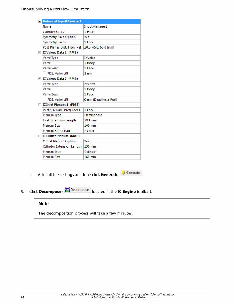
u. After all the settings are done click Generate .


Note





6. Add an input parameter.

Note

Most of the port flow simulations are done to study the effect of valve lift on the velocity,mass flow rate, and other flow parameters. Here you will add design points. Valve lift isselected as the input parameter for this tutorial.

a. Select InputManager1 from the Tree Outline.

b. Enable FD1 next to Valve Lift for the InValve.




This will create a parameter for this component. A dialog box opens asking you to name the parameter.Enter ValveLift for the Parameter Name. Click OK to close the dialog box.

A Parameters cell is added to the ICE system and the Parameter Set is connected to the cell.

7. Close the DesignModeler.

8. Save the project by giving it a proper name (demo_port.wbpj).



1. Right-click on Mesh, cell 4, and click Update from the context menu.



In a single step it will first create the mesh controls, then generate the mesh and finally update the meshcell.

Note

If you want to check or change the mesh settings click Edit Mesh Settings in Propertiesof Schematic A4: Mesh under IC Engine.

For this tutorial you are going to retain the default mesh settings.



Step 3: Meshing



File > Save

Note



After the decomposed geometry is meshed properly you can set boundary conditions, monitors, andpostprocessing images. You can also decide which data and images should be included in the report.





Note


a. In the Basic Settings tab you can see that the default models are used and the flow is initialized usingFMG.




b. In the Boundary Conditions tab you can see that the wall ice-slipwall-outplenum and ice-slipwall-inplenum1 are set to slipwall with Temperature set to 300.



ice-outlet is set as Pressure Outlet with Gauge Pressure set to –5000 and Temperature set to 300.Similarly for ice-inlet-inplenum1 which is set to type Pressure Inlet, Temperature is set to 300 andGauge Pressure to 0.

c. In the Monitor Definitions tab you can see that four surface monitors have been set. Three plot theFlow Rate of swirl on the three swirl planes you have define in the Input Manager. One surfacemonitor plots the Mass Flow Rate on ice-inlet-inplenum1 and ice-outlet.




d. In the Post Processing tab you can see that four images are saved during simulation. Velocity-magnitude contours plotted on the surface of cut-plane and all the swirl planes will be saved duringsimulation and displayed in a table format in the report.



The details will be displayed after selecting the image name and clicking Edit.




Note

For this tutorial you will be using the default solver settings. You can try changing thesettings and observe the difference in the results.

3. After checking the settings close the Solver Settings dialog box.

4. Right-click the ICE Solver Setup cell and click on Update from the context menu.


In this step you will setup the solution.

1. Double-click on the Setup cell.



2. Ensure that Double Precision is enabled under Options.

3. You can run the simulation in parallel with increased number of processors to complete the solution inless time.

4. Click OK in the Fluent Launcher dialog box.

Note

ANSYS Fluent opens. It will read the mesh file and setup the case.

5. For the solution of this tutorial you will use monitor based convergence criteria. To achieve this you willdefine one velocity-magnitude surface monitor on an interior face zone and then will use this data fordefining convergence criteria.

• Select Monitors from the navigation pane and click Create... under the Surface Monitors group box.




a. Retain the default name of surf-mon-5.

b. Enable Write.

c. Select Area-Weighted Average from the Report Type drop-down list.

d. Select Velocity... and Velocity Magnitude from the Field Variable drop-down lists.

e. Select ice-int-chamber1–outplenum from the list of Surfaces.

f. Click OK in the Surface Monitor dialog box and close it.

6. Add convergence criteria for the Area-Weighted Average monitor.

• Click Convergence Manager... under the Convergence Monitors group box.



a. In the Convergence Manager dialog box enable the monitor surf-mon-5 which you have just created.

Note

The solution is considered to be converged if the criteria of all of the Active mon-itors are satisfied.

b. Enter 5e-05 as the Stop Criterion for surf-mon-5.

Note

Stop Criterion indicates the criterion below which the solution is considered to beconverged.

c. Enter 600 as the Initial Iterations to Ignore for surf-mon-5.

Note

Enter a value in the Initial Iterations to Ignore column if you expect your solutionto fluctuate in the initial iterations. Enter a value that represents the number of it-erations you anticipate the fluctuations to continue. The convergence monitor cal-culation will begin after the entered number of iterations have been completed.For more information refer to, Convergence Manager in the Fluent User's Guide.

d. Enable Print for surf-mon-5.

e. Click OK to set and close the Convergence Manager dialog box.





• Enter 1200 for the Number of Iterations.

8. Add an output parameter.

Note

To quantify the output result, mass flow rate is defined as the output parameter. So atthe end of this design points study, change in the mass flow rate for the above definedvalve lifts can be observed.

a. Click Parameters... from the Define menu.

b. In the Parameters dialog box click Create and select Fluxes... from the drop-down list.



i. Retain selection of Mass Flow Rate from the Options list.

ii. Select ice-outlet from the list of Boundaries.

iii. Click Save Output Parameter....




Enter MassFlowRate for the Name of and click OK to close the Save Output Parameter dialogbox.

iv. Close the Flux Reports dialog box.

v. The parameter MassFlowRate is added under Output Parameters in the Parameters dialogbox. Click Close.

9. Go to the ANSYS Workbench window. The parameter loop is now complete.



10. In ANSYS Workbench double-click on the parameter bar or right-mouse click and select Edit... from thecontext menu to access the Parameters and Design Points workspace.

11. In the Parameters and Design Points view, you will see the work area of Table of Design Points. Enter 6and 10 in the column of P1–ValveLift.

12. Enable the check box next to Retain which will enable all check boxes in the Retain column for the designpoints you have added.

13. After adding the desired valve lift values click Update All Design Points ( ) fromthe menu bar.

Note

Click Yes in the message dialog box that appears.




Now the simulation will run for each design point. This process will take some time to complete. As solutionfor each design point is completed its output parameter is updated in the Table of Design Points underMassFlowRate.

Note

Updating the design points can take around 5 hours on a 8 CPU machine. You can open theproject file provided and check the results.


1. Right-click on the Results cell and click Update from the context menu.



2. Once the Results cell is updated, view the files by clicking Files from the View menu.

3. View > Files

Right-click Report.html from the list of files, and click Open Containing Folder from the context menu.

• In the Report folder double-click Report.html to open the report.







• You can see the boundary conditions set, in the table Boundary Conditions.

• The table Models, shows the models selected for the simulation.




In the table Equations you can see for which equations the simulation has been solved.

The Relaxations table displays the under relaxation factors set for the various variables.

• The Pressure-Velocity Coupling table displays the settings.



The Discretization Scheme table displays the discretization schemes set for the various variables.

• Check the animation of velocity magnitude on the cut-plane in the section Solution Data.




• In a Table you can observe the velocity-magnitude contours on the swirl planes which you have created.These images are taken at the end of the simulation.

• You can also observe the contours of pressure on the cut-plane taken in intervals, in another table.



• Check the residuals.




• Check the mass flow rate surface monitor plot. Also you can check the mass flow rate plots on the swirlplanes.











• In a chart under Design Points report you can check the values of input parameter against the outputparameter.



• In different tables you can observe the velocity magnitude contours on the different swirl planes forthe design points which you have created. These images are taken at the end of the simulation.

• In another table you can observe the contours of velocity magnitude on the cut-plane for the differentdesign points. These images are taken at the end of the simulation.




This concludes the tutorial which demonstrated the setup and solution for a port flow simulation of anIC engine.

2.8. Summary

In this tutorial, you have learned to set up and solve an IC Engine problem. You have also learned howto use ANSYS Workbench parametric system, which is here used for varying the valve lifts and examiningtheir effect on mass flow rate.


This tutorial presents streamlined workflow between pre-processing, solver and post processing forease of port flow simulations and performing parametric analysis for varying valve lifts. You may usedifferent meshing strategies for accurate results. You may use parametric system in workbench foranalysis of different port angles, valve seat inclinations etc.



Chapter 3: Tutorial: Solving a Combustion Simulation for a Sector

In this tutorial a complete Direct injection (DI) compression ignition (CI) engine geometry is transformedinto 60° sector in-order to reduce mesh size and solution time. Detailed boundary conditions are asshown in the Figure 3.1: Problem Schematic (p. 107). Sector simulation is started at intake valve Closing(IVC) with initial conditions as 3.45 bar and 404 K, species mass fraction of O2=0.1369, N2=0.7473,CO2=0.0789, H2O=0.0369. n-heptane (nc7h16) is used as surrogate for diesel fuel and is injected 8 degreesbefore compression (Top Dead Centre). Engine rpm is increased from 1500 rpm to 2000 rpm and itseffect on unburnt fuel is examined. This tutorial illustrates the following steps in setting up and solvinga combustion simulation for a sector.





• Define the solver setup.








3.1. Preparation

1. Copy the files (tut_comb_sect.x_t,injection-profile,Diesel_1comp_35sp_chem.inp,and Diesel_1comp_35sp_therm.dat) to your working folder.


2. Start Workbench.




Tutorial: Solving a Combustion Simulation for a Sector







3. Select Combustion Simulation from the Simulation Type drop-down list.

4. Select Sector from the Combustion Simulation Type drop-down list.

5. Enter 165 for Connecting Rod Length.


7. From the Input option for IVC and EVO drop-down list select Enter Direct Values.

8. Enter 570 for IVC (Inlet Valve Closed).

Note

This will be set as the decomposition crank angle.

9. Enter 833 for EVO (Exhaust Valve Open).

10. Right-click ICE cell and select Update from the context menu.






2. Import the geometry file,tut_comb_sect.x_t.

File >Import External Geometry File...






a. Retain the selection IVC for Decomposition Position.

Note

The inlet valve closing (IVC) angle is chosen as the geometry decomposition angle,since for combustion simulation you are more interested in the power stroke ofthe engine cycle, starting from closing of valves to the end of the compressionstroke.

b. Retain Complete Geometry from the Sector Decomposition Type drop-down list as the inputgeometry you have chosen is a complete geometry.

c. Select the face as shown in Figure 3.2: Cylinder Face (p. 113) for Cylinder Faces and click Apply.



Figure 3.2: Cylinder Face

d. Retain 60 ° for Sector Angle drop-down list.

Note

This will slice the geometry into a sector of 60 °.

e. Select Yes for Validate Compression Ratio.

f. Enter 15.83 for Compression Ratio.

g. Retain the default setting 3 for Crevice H/T Ratio.

h. Select the valve bodies as shown in Figure 3.3: Valves (p. 114) for Valve and click Apply.




Figure 3.3: Valves

i. Select the valve seat faces as shown in Figure 3.4: Valve Seats (p. 115) for Valve Seat and click Apply.



Figure 3.4: Valve Seats

j. Retain the selection of Height and Radius for Spray Location Option under IC Injection 1.

k. Enter 0.3 mm for Spray Location, Height.

l. Enter 0.5 mm for Spray Location, Radius.

Note

Depending upon the height and radius the spray location is calculated..

m. Enter 70° for Spray Angle.

n. After all the settings are done click Generate .





6. During decomposition a warning pops up asking if you would like to compensate for the difference incompression ratio.

Click Yes.

Note

The decomposition process will take a few minutes. During decomposition the followingchanges take place:

1. The engine port is divided into a sector of the given Sector Angle.

2. The valves are removed.



3. The clearance volume is formed into a crevice.

4. The compression ratio difference is adjusted in the crevice.

5. The piston is moved to the appropriate position as per the Decomposition CrankAngle.



8. Save the project by giving it a proper name (demo_sector.wbpj).

File >Save





Step 3: Meshing

1. Right-click on the Mesh cell in the IC Engine analysis system and select Update from the context menu.

Note

This meshing process will take a few minutes.

2. You can double-click the Mesh cell to check the mesh. See Figure 3.6: Meshed Geometry (p. 118)





File >Save

Note



After the decomposed geometry is meshed properly you can set boundary conditions, monitors, andpostprocessing images. You can also decide which data and images should be included in the report.

1. If the Properties view is not already visible, right-click ICE Solver Setup, cell 5, and select Propertiesfrom the context menu.





Note


a. Click the Basic Settings tab.

i. Enter 1500 for Engine Speed.



Enable the check box next to Engine Speed. This will add an engine speed input para-meter.

ii. The Number of CA to Run is set to 263.

Note

You have entered the IVC and EVO as 570 and 833. You are interested only inthe compression and power stroke. So the Number of CA to Run is automat-ically calculated from these values.




iii. Click Browse next to Profile File and select injection-profile.prof in the Select ProfileFile dialog box.

Note

You will be using this file to set the Total Flow Rate and Velocity Magnitudein the Injection Properties dialog box.

b. In the Physics Settings tab select Diesel Unsteady Flamelet from the Species Model drop-downlist in the Combustion Model group box.

c. In the Physics Settings tab click Chemistry tab.



i. Click Browse next to Chemkin File and select the file Diesel_1comp_35sp_chem.inp fromyour working folder.

ii. Similarly select the file Diesel_1comp_35sp_therm.dat for Thermal Data File from yourworking folder.

d. In the Physics Settings tab click Boundary tab.

• Enter the values shown in Table 3.1: Species Composition (p. 123) for the Oxid values for the listedSpecies.

Table 3.1: Species Composition

OxidSpecies

0.1369o2

0.7473n2

0.0789co2

0.0369h20




e. In the Physics Settings tab click Injection tab. Select injection-0 from the list and click Edit to openthe Injection Properties dialog box.



i. Select uniform from the Diameter Distribution drop-down list.

ii. Enter 0.1415e-3 for Diameter.

iii. Enter 712 for Start CA.

iv. Enter 738.2 for End CA.

v. Enter 0.0845e-3 for Cone Radius.




vi. Click the Constant button next to Total Flow Rate and select injection_mass massflowratefrom the drop-down menu.

vii. Click the Constant button next to Velocity Magnitude and select injection_vel velocity fromthe drop-down menu.

viii. Click OK to apply the settings.

f. In the Boundary Conditions tab you can see that no default settings are present. For this tutorialyou will create some wall boundary conditions. Click Create to open the Create Boundary Conditionsdialog box.

i. Select ice-cyl-chamber-bottom from the Zones list. Retain the default selection of wall as theType and set the Temperature to 440. Click Create.

ii. Make same settings for zones ice-cyl-chamber-top and ice-cyl-piston.

iii. For zone ice-piston set the Temperature to 560.

iv. Similarly for ice-sector-top-faces set the Temperature to 480.



v. Close the Create Boundary Conditions dialog box.

g. In the Monitor Definitions tab you can see that nine volume monitors have been set on the zonesice-fluid-chamber-bottom, ice-fluid-chamber-top, and ice-fluid-piston. You will set additionalmonitors.

i. Click Create.

ii. In the Monitor Definition dialog box select all in the list of Zones.

iii. Retain selection of Volume for Type.




iv. Select Mass-Average from the Report Type drop-down list.

v. Select Phi from the Field Variable drop-down list.

vi. Click Create. A volume monitor named mass-average-phi-mon is created.

vii. Now select DPM Monitor from the Type.



viii. Select injected-mass from the Injection Fate drop-down list.

ix. Select all-injections from the list of Injection.

x. Click Create. A monitor by the name of injected-mass-all-injections-mon is created.

xi. Select influid-mass from the Injection Fate drop-down list and click Create to create a monitorof influid-mass-all-injections-mon.




h. In the Initialization tab enter 243412.5 for Gauge Pressure and 404 for Temperature.



i. In the Post Processing tab you can see four types of images will be saved during simulation anddisplayed In a table format in the report. The details will be displayed after selecting the image nameand clicking Edit.




3. Click OK to close the Solver Settings dialog box.

4. Right-click on the Solution cell and click on Properties to open the Properties of Schematic window(if not already open).



a. In the Properties of Schematic window ensure that the Initialization Method is set to SolverControlled.

b. Disable Solution Monitoring.


File >Save


In this step you will start the simulation.






3. Click OK in the FLUENT Launcher dialog box.

Note


4. To add an output parameter select Parameters from the Define menu.

Define >Parameters...



a. In the Parameters dialog box click Create and select Volume Integrals... from the drop-down list.

b. In the Volume Integrals dialog box retain selection of Mass-Average from the Report Type list.

c. Select Species... and Mass fraction of nc7h16 from the Field Variable drop-down list.

d. Select all zones from the list of Cell Zones.

e. Click Save Output Parameter....

f. In the Save Output Parameter dialog box enter unburnt_fuel for Name and click OK.




g. Close the Volume Integrals and Parameters dialog box.

5. Return to Workbench window.

6. Double-click on Parameter Set.

a. In the Table of Design Points you can see DP 0. Under P1–rpm enter 2000 for DP 1.

b. Enable the check box next to Retain.

c. Click Update All Design Points.






View >Files

3. Right-click Report.html from the list of files, and click Open Containing Folder from the context menu.











• You can see the boundary conditions, under-relaxations factors, and other setup conditions underSetup.

• Check the animation of mesh on the cut-plane in the section Solution Data.



• Check the two animations of particle traces in the section Solution Data. Both show the animationfrom different views.






• Check the animation of temperature.




• Check the animation of velocity magnitude.



• In a Table you can observe the mesh images at various stages of the simulation.




• In two tables you can observe the particle traces images at various stages of simulation from two differentviews.






• In another Table you can observe the temperature contours on the cut plane. These images are takenat the end of the simulation.



• You can also observe the velocity-magnitude contours on the cut-plane in another Table. These imagesare taken at the end of the simulation.




• Under Charts you will find plots of Residuals and Last iteration residual corresponding to each timestep






• You will find plots for Swirl Ratio, Tumble Ratio, and Cross Tumble Ratio.








• You will find plots of AHRR (Apparent Heat Release Rate) and Number of Iterations per Time Step.Apparent heat release rate is defined as:

where

1.35 (can also be computed from Fluent)

Volume of sector, m3 X number of sectors

Absolute pressure, Pa

Crank Angle






• Monitors of Mass-Average phi, Mass-Average Turbulent Kinetic Energy, and Volume IntegralDensity are plotted against the crank angle.









• The report also includes the plots of Max Static Pressure, Max Static Temperature, and Max VelocityMagnitude on the surfaces ice-fluid-piston, ice fluid chamber-top and ice fluid chamber-bottomat different crank angles.








• Chart plotting the Penetration length of injection-0 per Time Step is also included in the report..




• Monitor plots of Volume Average Static Pressure, Volume Average Static Temperature, and VolumeStatic Pressure against Crank Angle can be checked in the report.








• Monitor plots of Total mass influid for all injections per Time Step, Total mass injected for all in-jections per Time Step, and Total mass evaporated for all injections per Time Step against CrankAngle can be checked in the report.









• Lastly in the report you can see the chart of rpm vs unburnt-fuel.



This concludes the tutorial which demonstrated the setup and solution for the combustion simulationof a sector of an IC engine.

3.8. Summary

In this tutorial Diesel Unsteady Flamelet (DUFL) non-premixed combustion model was used to simulateturbulent combustion process. Pressure trace and heat release rate were examined. You also learnedhow to use parametric system in Workbench for varying engine rpm and examining its effect on fuelburning.


This tutorial presents streamlined workflow between pre-processing, solver and post processing forease of diesel sector simulations and performing parametric analysis of engine operating variables. Youmay switch on pollutant models and compare Nox and Soot.



Further Improvements


Chapter 4: Tutorial: Solving a Gasoline Direct Injection EngineSimulation

A three dimensional single cylinder CFD simulation, of a 4-stroke spray guided Gasoline Direct Injection(GDI) Spark Ignition (SI) engine, is performed in this tutorial. Detailed boundary conditions are shownin Figure 4.1: Problem Schematic (p. 173). Engine simulation is started from Intake valve opening (IVO)and fuel is injected during the intake stroke. Homogeneous fuel air mixture is compressed and sparkignited 15° before compression Top Dead Center (TDC).


This is followed by power stroke and subsequent exhaust stroke. This tutorial illustrates the followingsteps in setting up and solving a Gasoline Direct Injection engine combustion simulation.


• Read an existing geometry into IC Engine system.





This tutorial is written with the assumption that you are familiar with the IC Engine system and thatyou have a good working knowledge of ANSYS Workbench. For more information on IC Engines refer



to the user guide of Internal Combustion Engines in Workbench, on the ANSYS Customer Portal or inthe ANSYS Help Viewer.


4.1. Preparation

1. Copy the files (tut_gdi_comb.x_t,comb_lift.prof,footprint.txt,massflowrate.csv,and velocity-0.7cd.csv) to your working folder.


2. Start Workbench.




Tutorial: Solving a Gasoline Direct Injection Engine Simulation




3. Select Combustion Simulation from the Simulation Type drop-down list.

4. Select Full Engine Full Cycle from the Combustion Simulation Type drop-down list.




5. Enter 144.3 for Connecting Rod Length.


7. Retain 0.2 for Minimum Lift.

8. Click Browse File next to Lift Curve. The File Open dialog box opens. Select the valve profile filecomb_lift.prof and click Open.




2. Import the geometry file,tut_gdi_comb.x_t.





4. Create a spark point.

Note

Before creating a point ensure that the Display Points button is pressed to enableyou to see the point created in the graphics window.

Create > Point

a. In the Details View enter Spark for Point.

b. Select Construction Point from the Type drop-down list.




c. Select Manual Input from the Definition drop-down list.

d. Under the Point Group 1 enter -0.94526,5.5096, and -1.6782 for X Coordinate, Y Coordinate,and Z Coordinate, respectively.

e. Right click and click Generate from the context menu. See Figure 4.3: Spark, Beam and FootprintPoints (p. 180).

5. Similarly create a beam point before invoking Input Manager.

Create >Point

a. In the Details View enter Beam for Point.

b. Select Construction Point from the Type drop-down list.

c. Select Manual Input from the Definition drop-down list.

d. Under the Point Group 1 enter 0,-6, and 8.58 for X Coordinate, Y Coordinate, and Z Coordinate,respectively.

e. Right click and click Generate from the context menu. See Figure 4.3: Spark, Beam and FootprintPoints (p. 180).

6. To create a footprint point you need to create a plane first.

a. Create a plane.

Create >New Plane

b. In the Details View enter inj_plane for Plane.



c. Select From Point and Normal from the Type drop-down list.

d. Select the beam point created (Beam) for Base Point.

e. Select the face and then the direction as shown in Figure 4.2: Direction for Normal Defined by (p. 179)for Normal Defined by.

Figure 4.2: Direction for Normal Defined by

f. Right click and click Generate from the context menu.

g. Create the footprint point.

Create >Point

h. In the Details View enter Footprint for Point.




i. Select Construction Point from the Type drop-down list.

j. Select From Coordinates File from the Definition drop-down list.

k. Click the button next to Coordinates File text box ( ) and select the file footprint.txt.

l. Select the plane created, inj_plane for Base Plane.

m. Retain the default settings for the rest, right click and click Generate from the context menu. SeeFigure 4.3: Spark, Beam and Footprint Points (p. 180).

Figure 4.3: Spark, Beam and Footprint Points




a. Retain selection of Specified Angle for Decomposition Position.

b. Enter 323 for Decomposition Angle.

Note

This is just before IVO.

c. Click next to Inlet Faces, select the face of the inlet valve and click Apply.




d. Click next to Outlet Faces, select the face of the exhaust valve and click Apply.

e. Select the face as shown in Figure 4.4: Cylinder Face (p. 183) for Cylinder Faces and click Apply.



Figure 4.4: Cylinder Face

f. Symmetry Face Option will be set to Yes. Retain the selection.

g. Select the three faces shown in Figure 4.5: Symmetry Faces (p. 184) for Symmetry Faces and clickApply.





h. Retain the selection of Full Topology from the Topology Option drop-down list.

i. Retain selection of No for Crevice Option.

j. Select Yes for Validate Compression Ratio.

k. Enter 10.25 for Compression Ratio.

l. Select the Spark point created for Spark Points. See Figure 4.3: Spark, Beam and FootprintPoints (p. 180).

m. Select the valve body as shown in Figure 4.6: Intake Valve (p. 185) for Valve Bodies and click Apply.




n. Select the valve seat face as shown in Figure 4.7: Intake Valve Seat (p. 185) for Valve Seat Faces andclick Apply.


o. Select invalve1 from the Valve Profile drop-down list.




p. Right-click on IC Valves Data in the Details of InputManager and select Add New IC Valves DataGroup from the context menu.

q. In this IC Valves Data group following the steps for the intake valve, set the other valve body toExValve and set its profile to exvalve1. Select the valve seat face of that valve as shown in Fig-ure 4.8: Exhaust Valve Seat (p. 186).


r. Under IC Injection 1 select the option Beam Origin, Footprint from the Spray Location Optiondrop-down list.

s. Select the Beam point created before for Injection Beam Origin. See Figure 4.3: Spark, Beam andFootprint Points (p. 180). Click Apply.

t. Select the 3 points after creating Footprint as shown in Figure 4.3: Spark, Beam and FootprintPoints (p. 180) for Footprint Point.



u. After all the settings are done click Generate .


9. During decomposition you get a warning informing you that the chamber will not be decomposed.

The chamber will be decomposed between the insert_angle and the delete_angle. Click OK to continue.

10. Then you get a warning about the compression ratio validation.




Click OK to continue.

Note


11. Click Show Spray Cone to check the view of the injections.





13. Save the project by giving it a proper name (demo_comb.wbpj).

Note

Once decomposition is completed you can open the icSolverSettings.txt filesaved in the ~demo_comb_files\dp0\ICE\ICE folder and check the insert_angleand the delete_angle.



1. Right-click on Mesh, cell 4, and click Update from the context menu. In a single step it will first create themesh controls, then generate the mesh and finally update the mesh cell.

Note

If you want to check or change the mesh settings click Edit Mesh Settings in Propertiesof Schematic A4: Mesh under IC Engine. For this tutorial you are going to retain thedefault mesh settings. This meshing process will take a few minutes.




Step 3: Meshing


File > Save

Note



After the decomposed geometry is meshed properly you can set keygrids, boundary conditions, monitors,and postprocessing images. You can also decide which data and images should be included in the report.

1. If the Properties view is not already visible, right-click ICE Solver Setup, cell 5, and select Propertiesfrom the context menu.

2. To set the KeyGrids select Yes from the KeyGrid drop-down list.

3. Click Select KeyGrid Angles to open the KeyGrid Angle Selection dialog box.



a. Click Add Angle.




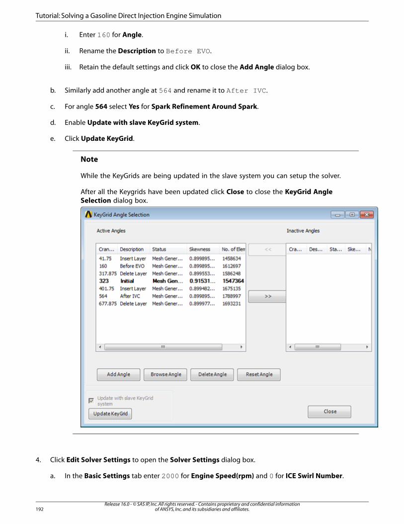
i. Enter 160 for Angle.

ii. Rename the Description to Before EVO.

iii. Retain the default settings and click OK to close the Add Angle dialog box.

b. Similarly add another angle at 564 and rename it to After IVC.

c. For angle 564 select Yes for Spark Refinement Around Spark.

d. Enable Update with slave KeyGrid system.

e. Click Update KeyGrid.

Note

While the KeyGrids are being updated in the slave system you can setup the solver.

After all the Keygrids have been updated click Close to close the KeyGrid AngleSelection dialog box.


a. In the Basic Settings tab enter 2000 for Engine Speed(rpm) and 0 for ICE Swirl Number.



b. Click Read Profile File.

i. In the Browse profile file click Profile Files (.prof) (*.prof) and select CSV Files (.csv) (*.csv).

ii. Select the file massflowrate.csv from your working folder and click Open.

iii. In the Read CSV File dialog box that open rename the Profile Name as massflowrate andclick OK.

iv. Similarly read the velocity-0.7cd.csv file and rename it as velocity.

You can click Profile Editor and check the profile charts.




c. In the Physics Settings tab select SI Engine from the Engine Type drop-down list and Partial Pre-mixed from the Species Model drop-down list.

i. Click the Premix tab.

A. Select G Equation from the Premixed Model list.

B. Select Peters from the Flame Speed Model drop-down list.

C. Select Yes for Blind Modifier.

ii. Click the Injection tab you can see that three injections have been created.



A. Select all three injections —injection-0, injection-1, and injection-2 and click Edit.

Note

You can select all three injections by pressing Ctrl key and then selecting.




B. Set the values in the Injection Properties dialog box as shown in the Table 4.1: InjectionProperties (p. 196).

Table 4.1: Injection Properties

ValueParameter

n-octane-liquidMaterial

c8h18<iso>Evaporating Species

293Temperature

420Start CA

438.4End CA

3Cone Angle

massflowrate massflowrateTotal Flow Rate

velocity velocityVelocity Magnitude

300e-6Max Diameter

55e-6Mean Diameter

3Spread Param

iii. Click the Spark tab. Select Spark-0 and click Edit to open the Spark Properties dialog box.

A. Enter 705 for Start Crank Angle.



B. Select Turbulent Length from the Flame Speed Model drop-down list.

C. Click OK to close the Spark Properties dialog box.

iv. Click the Inert tab.

A. Select Fixed H/C Ratio from the Inert Model drop-down list.

B. Retain the default setting of 2.25 for H/C Ratio.

d. Click the Boundary Conditions tab.

i. Double-click ice-outlet-exvalve-1–port to open the Edit Boundary Conditions dialog box.






C. In the Species tab enter 0.98 for Inert Stream.

D. Click OK to close the dialog box.

ii. Select ice-inlet-invalve-1–port and click Edit.



C. Click OK to close the Edit Boundary Conditions dialog box.

iii. Click Create to open the Create Boundary Conditions dialog box.

Set the Temperature for the for the zones as shown in the table.

Table 4.2: Boundary Conditions

Boundary ConditionZonePart

485kcyl-head, invalve1–ch, and exvalve1–chHead

485kpistonPiston

500kcyl-triLiner

777kexvalve1–ib, exvalve1–ob, and exvalve1–stemExhaust valve

485kexvalve1–port and exvalve1–seat,Exhaust port



400kinvalve1–ib, invalve1–ob, and invalve1–stemIntake valve

313kinvalve1–port and invalve1–seat,Intake port

iv. After creating all the above boundary conditions close the Create Boundary Conditions dialogbox.

e. In the Monitor Definitions tab you can see that four volume monitors have been set on the zonefluid-ch. You will create some additional monitors.

i. Select the monitor mass-avg-pressure-mon from the list and click Edit.

A. Select New Variable from the Field Variable drop-down list.

B. In the Add Quantity/Varaible dialog box select Pressure from the Quantity drop-downlist.

C. Select Absolute pressure from the Quantity Subtype drop-down list and click OK.

D. Close the Monitor Definition dialog box.

ii. Click Create to open the Monitor Definition dialog box.




iii. Select fluid-ch from the list of Zones.

A. Select Volume from the Type drop-down list.

B. Select Mass from the Report Type drop-down list.

C. Click Create.

iv. For the same zone create a volume monitor by selecting Volume from the Report Type drop-down list.

v. Similarly for the same zone create a volume monitor with Mass-Average selected from theReport Type drop-down list. From the Field Variable drop-down list select Phi.

vi. Select DPM Monitor from the Type drop-down list.

A. Select influid-mass from the Injection Fate drop-down list.

B. Select all-injections from the list of Injection and click Create.

C. Similarly retaining the selection of all-injections, select injected-mass from the InjectionFate drop-down list and click Create.

D. Create another monitor by selecting vapor-mass from the Injection Fate drop-down list



f. In the Initialization tab you can see the default set values for the various parameters.




i. Click Patch to open the to open the Patching Zones dialog box.

ii. For the inlet port, select fluid-invalve-1–port, fluid-invalve-1–vlayer, and fluid-invalve-1–ibfrom the list of Zone.

iii. Select Pressure from the list of Variable.

iv. Enter -21325 for Value(pascal) and click Create.

v. Similarly patch the same zones for Temperature value 313 k.

vi. For outlet port, patch zones fluid-exvalve-1–port, fluid-exvalve-1–vlayer, and fluid-exvalve-1–ib to Pressure equal to -1325 pascal, Temperature equal to 1070 k, and Inert Variableto 1.



vii. For chamber select fluid-ch from the list under Zone and patch the Temperature to 1070 k,Pressure to 4025 pascal, and Inert Variable to 1.

Table 4.3: Patching

ValueZonesVariable

-21325 pascalfluid-invalve-1–port,fluid-invalve-1–vlayer,fluid-invalve-1–ib

Pressure

313 kfluid-invalve-1–port,fluid-invalve-1–vlayer,fluid-invalve-1–ib

Temperature

-1325 pascalfluid-exvalve-1–port,fluid-exvalve-1–vlayer,fluid-exvalve-1–ib

Pressure

1070 kfluid-exvalve-1–port,fluid-exvalve-1–vlayer,fluid-exvalve-1–ib

Temperature

4025 pascalfluid-chPressure

1070 kfluid-chTemperature

1fluid-chInert Variable

1fluid-exvalve-1–port,fluid-exvalve-1–vlayer,fluid-exvalve-1–ib

Inert Variable




viii. Close the Patching Zones dialog box.

g. In the Solution Control tab enter 419 under Start CA for PDF.

i. Right-click in Save Case/Date group box and select Insert Row Below from the context menu.

ii. Enter 419 for Crank Angle and add Before_inj_st as Comment.

iii. Similarly add angle 440 as After_inj_end and 700 as Before_spark.

h. In the Post Processing tab you can see that velocity-magnitude contours on the surface of cut-planewill be saved during simulation and displayed In a table format in the report.

i. Double-click image-1 to open the Edit Image dialog box.



A. Select Yes from the Overlay with Vectors drop-down list.

B. Click OK to close the Edit Image dialog box.

ii. Click Create in the Post Processing tab.

A. Select ice_cutplane_1 from the list of Surfaces.

B. Select Temperature from the Quantity drop-down list.

C. Select No for DPM.

D. Select Yes from the Overlay with Vectors drop-down list.

E. Click Create.

iii. Click Add Iso Surface.




A. In the Add Iso Surface dialog box enter iso-surface-flame for Surface Name.

B. Select New Variable from the Quantity drop-down list.

I. In the Add Quantity/Variable dialog box select User Defined from the Quantitydrop-down list.

II. Enter mean-distance-from-flame for User Defined.

C. Retain Absolute Value for Iso Value Input.

D. Retain 0 for Absolute Value.

E. Click OK to close the Add Iso Surface dialog box.

iv. To add another post processing image, select iso-surface-flame from the list of Surfaces.



A. Retain the selection of ice_cutplane_1–view for View.

B. Select mean-distance-from-plane from the Quantity drop-down list.

C. Select No from the DPM drop-down list.

D. Enter 705 for Start Crank Angle(deg).

E. Enter 1043 for End Crank Angle(deg).

F. Click Create and close the Create Image dialog box.




5. Click OK to close the Solver Settings dialog box.


File > Save


In this step you will start the simulation.





3. Click OK in the FLUENT Launcher dialog box.

Note


4. In the tree expand Models and double click on Discrete Phase.




• In the Discrete Phase Model dialog box enter 500 for Number of Continuous Phase Iterationsper DPM Iteration and click OK.



This will reduce solution time.





a. Retain the default set Number of Time Steps.

Note

The Number of Time Steps are automatically calculated from the entered startand end crank angles.

b. Click Calculate.






View >Files

3. Right-click Report.html from the list of files, and click Open Containing Folder from the context menu.






You can see the Max Cell Equivolume Skew monitor.



• You can see the boundary conditions, under-relaxations factors, and other setup conditions underSetup.




• The table of the dynamic mesh events can also be seen in the report.






You can check the engine inputs.



• Check the animation of mesh on the cut-plane in the section Solution Data.

There are also additional mesh animations on the three injection planes.




• Check the animations of particle traces of three injections. The animation are shown from differentviews.
















• Check the animations of temperature on cut-plane as well as the iso surface.






• Check the animation of velocity magnitude on the cut-plane.



• In a Table you can observe the mesh images at various stages of the simulation.




There are also additional mesh animations on the three injection planes.



• You can observe the particle traces images at various stages of simulation from two different views inthe different tables.









• In another Table you can observe the temperature contours on the cut plane as well as on the iso-surface.






• You can also observe the velocity-magnitude contours on the cut-plane in another Table.



• You can check the residual plot in the Table: Residuals.




• Under Charts you will find plots for the last iteration residual values, Swirl Ratio, Tumble Ratio, andCross Tumble Ratio.








• You will find plot of AHRR (Apparent Heat Release Rate) and Area-Weighted Average Static Temper-ature. Apparent heat release rate is defined as:

where

1.35 (can also be computed from Fluent)

Volume of sector, m3 X number of sectors

Absolute pressure, Pa

Crank Angle






• Monitors of Mass-Average Turbulent Kinetic Energy and Number of Iterations per Time Step areplotted against the crank angle.






• The report also includes the plots of Mass-Average Absolute Pressure, Mass-Average Static Temper-ature, Mass-Average Turbulent Kinetic Energy, and Mass Static Pressure on fluid-ch at differentcrank angles.






• Chart plotting the penetration length of the three injections is also included in the report.






• Monitor plots of Volume Static Pressure, Total mass influid for all injections per Time Step, Totalmass injected for all injections per Time Step and Total mass evaporarted for all injections perTime Step against Crank Angle can be checked in the report.









This concludes the tutorial which demonstrated the setup and solution for the combustion simulationof a sector of an IC engine.

4.8. Summary

In this tutorial spray was injected in engine using Discrete Phase Model of Fluent. Fuel air mixture wasthen spark ignited by using spark model in Fluent. Partially premixed Combustion model was used forsimulating turbulent combustion process. Pressure trace and heat release rate were examined.

You have also learnt on how to use key-grids and use different meshing strategies.


This tutorial presents streamlined workflow between pre-processing, solver and post processing forease of GDI simulations. You may obtain more accurate solution by using temperature and/or compos-ition dependent material properties.



Index




Documents

ANSYS Internal Combustion Engines Tutorial Guide