Embed Size (px)
Citation preview

ANSYS CFX Tutorials

ANSYS CFX Tutorials
2
DraftDraft
Table of Contents1. Introduction to the CFX Tutorials ...................................................................................................... 23
Preparing a Working Directory ............................................................................................. 23Setting the Working Directory and Starting ANSYS CFX .......................................................... 23Playing a Tutorial Session File .............................................................................................. 24Changing the Display Colors ................................................................................................ 24Editor Buttons ................................................................................................................... 24Using Help ....................................................................................................................... 25
2. Simulating Flow in a Static Mixer Using CFX in Standalone Mode .......................................................... 27Tutorial Features ................................................................................................................ 27Overview of the Problem to Solve ......................................................................................... 28Before You Begin ............................................................................................................... 28Starting CFX-Pre ............................................................................................................... 28Defining a Case in CFX-Pre ................................................................................................. 29Synopsis of Quick Setup Mode ............................................................................................. 30Workflow Overview ........................................................................................................... 30Creating a New Case .......................................................................................................... 30Setting the Physics Definition ............................................................................................... 30Importing a Mesh ............................................................................................................... 31Using the Viewer ............................................................................................................... 31Defining Model Data .......................................................................................................... 32Defining Boundaries ........................................................................................................... 32Setting Boundary Data ........................................................................................................ 33Setting Flow Specification ................................................................................................... 33Setting Temperature Specification ......................................................................................... 33Reviewing the Boundary Condition Definitions ....................................................................... 33Creating the Second Inlet Boundary Definition ........................................................................ 33Creating the Outlet Boundary Definition ................................................................................ 34Moving to General Mode ..................................................................................................... 34Setting Solver Control ......................................................................................................... 34Writing the CFX-Solver Input (.def) File ................................................................................ 35Playing the Session File and Starting CFX-Solver Manager ........................................................ 35Obtaining a Solution Using CFX-Solver Manager .................................................................... 35Start the Run ..................................................................................................................... 36Move from CFX-Solver to CFD-Post ..................................................................................... 37Viewing the Results in CFD-Post .......................................................................................... 37Workflow Overview ........................................................................................................... 38Setting the Edge Angle for a Wireframe Object ........................................................................ 38Creating a Point for the Origin of the Streamline ...................................................................... 39Creating a Streamline Originating from a Point ........................................................................ 40Rearranging the Point ......................................................................................................... 41Configuring a Default Legend .............................................................................................. 42Creating a Slice Plane ......................................................................................................... 43Defining Slice Plane Geometry ............................................................................................. 43Configuring Slice Plane Views .............................................................................................. 44Rendering Slice Planes ........................................................................................................ 44Coloring the Slice Plane ...................................................................................................... 45Moving the Slice Plane ....................................................................................................... 46Adding Contours ............................................................................................................... 46Working with Animations .................................................................................................... 47Showing the Animation Dialog Box ....................................................................................... 48Creating the First Keyframe ................................................................................................. 48
iiiRelease 12.0 - © 2009 ANSYS Canada Ltd. All rights reserved. Contains proprietary and confidentialinformation of ANSYS, Inc. and its subsidiaries and affiliates.
DraftDraft
Creating the Second Keyframe ............................................................................................. 49Viewing the Animation ....................................................................................................... 51Modifying the Animation .................................................................................................... 52Saving a Movie .................................................................................................................. 53Quitting CFD-Post ............................................................................................................. 53
3. Simulating Flow in a Static Mixer Using Workbench ............................................................................. 55Tutorial Features ................................................................................................................ 55Overview of the Problem to Solve ......................................................................................... 56Before You Begin ............................................................................................................... 56Starting ANSYS Workbench ................................................................................................ 56Starting CFX-Pre from ANSYS Workbench ............................................................................ 57Creating the Simulation Definition ........................................................................................ 58Setting the Physics Definition ............................................................................................... 58Defining Boundaries ........................................................................................................... 58Setting Boundary Data ........................................................................................................ 58Creating the Second Inlet Boundary Definition ........................................................................ 59Creating the Outlet Boundary Definition ................................................................................ 59Moving to General Mode ..................................................................................................... 59Using the Viewer ............................................................................................................... 60Setting Solver Control ......................................................................................................... 60Refresh the Project ............................................................................................................. 61Obtaining a Solution ........................................................................................................... 61Display the Results in CFD-Post ........................................................................................... 63Viewing the Results in CFD-Post .......................................................................................... 63Workflow Overview ........................................................................................................... 64Setting the Edge Angle for a Wireframe Object ........................................................................ 65Creating a Point for the Origin of the Streamline ...................................................................... 66Creating a Streamline Originating from a Point ........................................................................ 67Rearranging the Point ......................................................................................................... 68Configuring a Default Legend .............................................................................................. 69Creating a Slice Plane ......................................................................................................... 70Defining Slice Plane Geometry ............................................................................................. 70Configuring Slice Plane Views .............................................................................................. 71Rendering Slice Planes ........................................................................................................ 72Coloring the Slice Plane ...................................................................................................... 73Moving the Slice Plane ....................................................................................................... 73Adding Contours ............................................................................................................... 73Working with Animations .................................................................................................... 75Showing the Animation Dialog Box ....................................................................................... 76Creating the First Keyframe ................................................................................................. 76Creating the Second Keyframe ............................................................................................. 77Viewing the Animation ....................................................................................................... 79Modifying the Animation .................................................................................................... 80Saving a Movie .................................................................................................................. 81Closing the Applications ...................................................................................................... 81
4. Flow in a Static Mixer (Refined Mesh) ............................................................................................... 83Tutorial Features ................................................................................................................ 83Overview of the Problem to Solve ......................................................................................... 84Before You Begin ............................................................................................................... 84Starting CFX-Pre ............................................................................................................... 84Defining a Simulation using General Mode in CFX-Pre ............................................................. 84Workflow Overview ........................................................................................................... 84Creating a New Case .......................................................................................................... 85Importing a Mesh ............................................................................................................... 85
Release 12.0 - © 2009 ANSYS Canada Ltd. All rights reserved. Contains proprietary and confidentialinformation of ANSYS, Inc. and its subsidiaries and affiliates.iv
DraftANSYS CFX TutorialsDraft
Importing CCL .................................................................................................................. 86Viewing Domain Settings .................................................................................................... 86Viewing the Boundary Condition Setting ................................................................................ 87Defining Solver Parameters .................................................................................................. 87Writing the CFX-Solver Input (.def) File ................................................................................ 88Playing the Session File and Starting CFX-Solver Manager ........................................................ 88Obtaining a Solution with CFX-Solver ................................................................................... 89Workflow Overview ........................................................................................................... 89Starting the Run with an Initial Values File .............................................................................. 90Confirming Results ............................................................................................................ 90Moving from CFX-Solver to CFD-Post .................................................................................. 90Viewing the Results in CFD-Post .......................................................................................... 91Creating a Slice Plane ......................................................................................................... 91Coloring the Slice Plane ...................................................................................................... 92Loading Results from Tutorial 1 for Comparison ...................................................................... 92Creating a Second Slice Plane .............................................................................................. 93Comparing Slice Planes using Multiple Views ......................................................................... 93Viewing the Surface Mesh on the Outlet ................................................................................. 94Looking at the Inflated Elements in Three Dimensions .............................................................. 95Viewing the Surface Mesh on the Mixer Body ......................................................................... 96Viewing the Layers of Inflated Elements on a Plane .................................................................. 96Viewing the Mesh Statistics ................................................................................................. 96Viewing the Mesh Elements with Largest Face Angle ................................................................ 97Viewing the Mesh Elements with Largest Face Angle Using a Point ............................................. 97Quitting CFD-Post ............................................................................................................. 98
5. Flow in a Process Injection Mixing Pipe .............................................................................................. 99Tutorial Features ................................................................................................................ 99Overview of the Problem to Solve ....................................................................................... 100Before You Begin ............................................................................................................. 101Starting CFX-Pre ............................................................................................................. 101Defining a Simulation using General Mode in CFX-Pre ........................................................... 101Workflow Overview .......................................................................................................... 101Creating a New Case ......................................................................................................... 102Importing a Mesh ............................................................................................................. 102Setting Temperature-Dependent Material Properties ................................................................ 103Plotting an Expression ....................................................................................................... 104Evaluating an Expression ................................................................................................... 104Modify Material Properties ................................................................................................ 104Creating the Domain ......................................................................................................... 105Creating the Side Inlet Boundary ......................................................................................... 105Creating the Main Inlet Boundary ........................................................................................ 106Creating the Main Outlet Boundary ..................................................................................... 107Setting Initial Values ......................................................................................................... 107Setting Solver Control ....................................................................................................... 107Writing the CFX-Solver Input (.def) File .............................................................................. 108Obtaining a Solution Using CFX-Solver Manager .................................................................. 108Moving from CFX-Solver Manager to CFD-Post .................................................................... 109Viewing the Results in CFD-Post ........................................................................................ 109Workflow Overview .......................................................................................................... 109Modifying the Outline of the Geometry ................................................................................ 109Creating and Modifying Streamlines Originating from the Main Inlet ......................................... 109Modifying Streamline Color Ranges .................................................................................... 110Coloring Streamlines with a Constant Color .......................................................................... 110Creating Streamlines Originating from the Side Inlet ............................................................... 111
vRelease 12.0 - © 2009 ANSYS Canada Ltd. All rights reserved. Contains proprietary and confidentialinformation of ANSYS, Inc. and its subsidiaries and affiliates.
DraftANSYS CFX TutorialsDraft
Examining Turbulence Kinetic Energy ................................................................................. 111Exiting CFD-Post ............................................................................................................. 112
6. Flow from a Circular Vent ............................................................................................................... 113Tutorial Features .............................................................................................................. 113Overview of the Problem to Solve ....................................................................................... 114Before You Begin ............................................................................................................. 114Starting CFX-Pre ............................................................................................................. 115Defining a Multiple-Analysis Simulation in CFX-Pre .............................................................. 115Importing the Mesh .......................................................................................................... 115Creating an Additional Variable ........................................................................................... 116Renaming the Analysis ...................................................................................................... 116Creating the Domain ......................................................................................................... 116Creating the Boundaries .................................................................................................... 117Setting Initial Values ......................................................................................................... 119Setting Solver Control ....................................................................................................... 119Creating a Transient Flow Analysis ...................................................................................... 120Modifying the Analysis Type .............................................................................................. 120Modifying the Boundary Conditions .................................................................................... 120Initialization Values .......................................................................................................... 122Modifying the Solver Control ............................................................................................. 122Output Control ................................................................................................................. 123Configuring Simulation Control .......................................................................................... 124Writing the CFX-Solver Input File ....................................................................................... 125Obtaining Solutions to the Steady-State and Transient Configurations ........................................ 125Viewing the Results in CFD-Post ........................................................................................ 126Displaying Smoke Density Using an Isosurface ...................................................................... 126Viewing the Results at Different Time Steps .......................................................................... 127Generating Titled Image Files ............................................................................................. 127Generating a Movie .......................................................................................................... 128
7. Flow Around a Blunt Body ............................................................................................................. 131Tutorial Features .............................................................................................................. 131Overview of the Problem to Solve ....................................................................................... 132Before You Begin ............................................................................................................. 132Starting CFX-Pre ............................................................................................................. 133Defining a Case in CFX-Pre ............................................................................................... 133Importing the Mesh .......................................................................................................... 133Creating the Domain ......................................................................................................... 133Creating Composite Regions .............................................................................................. 134Creating the Boundaries .................................................................................................... 135Setting Initial Values ......................................................................................................... 137Setting Solver Control ....................................................................................................... 137Writing the CFX-Solver Input (.def) File .............................................................................. 137Obtaining a Solution Using CFX-Solver Manager .................................................................. 138Obtaining a Solution in Serial ............................................................................................. 138Obtaining a Solution in Parallel ........................................................................................... 138Viewing the Results in CFD-Post ........................................................................................ 142Using Symmetry Plane to Display the Full Geometry .............................................................. 142Creating Velocity Vectors ................................................................................................... 143Displaying Pressure Distribution on Body and Symmetry Plane ................................................ 145Creating Surface Streamlines to Display the Path of Air along the Surface of the Body .................. 145Moving Objects ............................................................................................................... 146Creating a Surface Plot of y+ .............................................................................................. 146Demonstrating Power Syntax .............................................................................................. 147Viewing the Mesh Partitions (Parallel Only) .......................................................................... 148
Release 12.0 - © 2009 ANSYS Canada Ltd. All rights reserved. Contains proprietary and confidentialinformation of ANSYS, Inc. and its subsidiaries and affiliates.vi
DraftANSYS CFX TutorialsDraft
8. Buoyant Flow in a Partitioned Cavity ................................................................................................ 149Tutorial Features .............................................................................................................. 149Overview of the Problem to Solve ....................................................................................... 150Before You Begin ............................................................................................................. 150Starting CFX-Pre ............................................................................................................. 151Defining a Case in CFX-Pre ............................................................................................... 151Importing the Mesh .......................................................................................................... 151Analysis Type .................................................................................................................. 152Creating the Domain ......................................................................................................... 153Creating the Boundaries .................................................................................................... 154Setting Initial Values ......................................................................................................... 155Setting Output Control ...................................................................................................... 155Setting Solver Control ....................................................................................................... 156Writing the CFX-Solver Input (.def) File .............................................................................. 156Obtaining a Solution using CFX-Solver Manager ................................................................... 157Viewing the Results in CFD-Post ........................................................................................ 157Simple Report ................................................................................................................. 157Plots for Customized Reports ............................................................................................. 157Customized Report ........................................................................................................... 160Animations ..................................................................................................................... 160Completion ..................................................................................................................... 160
9. Free Surface Flow Over a Bump ...................................................................................................... 161Tutorial Features .............................................................................................................. 161Overview of the Problem to Solve ....................................................................................... 162Approach to the Problem ................................................................................................... 162Before You Begin ............................................................................................................. 162Starting CFX-Pre ............................................................................................................. 162Defining a Simulation in CFX-Pre ....................................................................................... 163Importing the Mesh .......................................................................................................... 163Creating Expressions for Initial and Boundary Conditions ........................................................ 164Creating the Domain ......................................................................................................... 165Creating the Boundaries .................................................................................................... 166Setting Initial Values ......................................................................................................... 168Setting Mesh Adaption Parameters ...................................................................................... 169Setting the Solver Controls ................................................................................................. 170Writing the CFX-Solver Input (.def) File .............................................................................. 170Obtaining a Solution using CFX-Solver Manager ................................................................... 171Viewing the Results in CFD-Post ........................................................................................ 172Creating Velocity Vector Plots ............................................................................................. 172Viewing Mesh Refinement ................................................................................................. 173Creating an Isosurface to Show the Free Surface .................................................................... 176Creating a Polyline that Follows the Free Surface ................................................................... 176Creating a Chart to Show the Height of the Surface ................................................................. 176Further Postprocessing ...................................................................................................... 177Using a Supercritical Outlet Condition ................................................................................. 177
10. Supersonic Flow Over a Wing ........................................................................................................ 179Tutorial Features .............................................................................................................. 179Overview of the Problem to Solve ....................................................................................... 180Approach to the Problem ................................................................................................... 180Before You Begin ............................................................................................................. 180Starting CFX-Pre ............................................................................................................. 180Defining a Case in CFX-Pre ............................................................................................... 181Importing the Mesh .......................................................................................................... 181Creating the Domain ......................................................................................................... 181
viiRelease 12.0 - © 2009 ANSYS Canada Ltd. All rights reserved. Contains proprietary and confidentialinformation of ANSYS, Inc. and its subsidiaries and affiliates.
DraftANSYS CFX TutorialsDraft
Creating the Boundaries .................................................................................................... 182Creating Domain Interfaces ................................................................................................ 184Setting Initial Values ......................................................................................................... 184Setting the Solver Controls ................................................................................................. 185Writing the CFX-Solver Input (.def) File .............................................................................. 185Obtaining a Solution Using CFX-Solver Manager .................................................................. 186Viewing the Results in CFD-Post ........................................................................................ 186Displaying Mach Information ............................................................................................. 186Displaying Pressure Information ......................................................................................... 186Displaying Temperature Information .................................................................................... 187Displaying Pressure With User Vectors ................................................................................. 187
11. Flow Through a Butterfly Valve ..................................................................................................... 189Tutorial Features .............................................................................................................. 189Overview of the Problem to Solve ....................................................................................... 190Approach to the Problem ................................................................................................... 191Before You Begin ............................................................................................................. 191Starting CFX-Pre ............................................................................................................. 191Defining a Simulation in CFX-Pre ....................................................................................... 191Creating a New Case ......................................................................................................... 191Importing the Mesh .......................................................................................................... 192Defining the Properties of the Sand ...................................................................................... 192Creating the Domain ......................................................................................................... 193Creating the Inlet Velocity Profile ........................................................................................ 195Creating the Boundary Conditions ....................................................................................... 196Setting Initial Values ......................................................................................................... 200Setting the Solver Controls ................................................................................................. 200Writing the CFX-Solver Input (.def) File .............................................................................. 201Obtaining a Solution Using CFX-Solver Manager .................................................................. 201Viewing the Results in CFD-Post ........................................................................................ 201Erosion Due to Sand Particles ............................................................................................. 202Displaying Erosion on the Pipe Wall .................................................................................... 202Setting the Particle Tracks .................................................................................................. 203Creating the Particle Track Symbols ..................................................................................... 203Creating a Particle Track Animation ..................................................................................... 203Determining Minimum, Maximum, and Average Pressure Values .............................................. 204
12. Flow in a Catalytic Converter ........................................................................................................ 207Tutorial Features .............................................................................................................. 207Overview of the Problem to Solve ....................................................................................... 208Approach to the Problem ................................................................................................... 209Before You Begin ............................................................................................................. 209Starting CFX-Pre ............................................................................................................. 209Defining a Case in CFX-Pre ............................................................................................... 209Importing the Meshes ........................................................................................................ 209Creating the Fluid Domain ................................................................................................. 212Creating the Porous Domain ............................................................................................... 212Creating the Boundaries .................................................................................................... 213Creating the Domain Interfaces ........................................................................................... 214Setting Initial Values ......................................................................................................... 215Setting Solver Control ....................................................................................................... 215Setting a Discretization Option ........................................................................................... 216Writing the CFX-Solver Input (.def) File .............................................................................. 216Obtaining a Solution using CFX-Solver Manager ................................................................... 217Viewing the Results in CFD-Post ........................................................................................ 217Viewing the Mesh on a GGI Interface ................................................................................... 217
Release 12.0 - © 2009 ANSYS Canada Ltd. All rights reserved. Contains proprietary and confidentialinformation of ANSYS, Inc. and its subsidiaries and affiliates.viii
DraftANSYS CFX TutorialsDraft
Creating User Locations .................................................................................................... 218Creating Plots .................................................................................................................. 219Exporting Polyline Data .................................................................................................... 221
13. Non-Newtonian Fluid Flow in an Annulus ........................................................................................ 223Tutorial Features .............................................................................................................. 223Background Theory .......................................................................................................... 224Overview of the Problem to Solve ....................................................................................... 225Before You Begin ............................................................................................................. 225Starting CFX-Pre ............................................................................................................. 226Defining a Case in CFX-Pre ............................................................................................... 226Importing the Mesh .......................................................................................................... 226Creating the Fluid ............................................................................................................. 226Creating the Domain ......................................................................................................... 228Creating the Boundaries .................................................................................................... 228Setting Initial Values ......................................................................................................... 229Setting Solver Control ....................................................................................................... 230Writing the CFX-Solver Input (.def) File .............................................................................. 230Obtaining a Solution using CFX-Solver Manager ................................................................... 231Viewing the Results in CFD-Post ........................................................................................ 231
14. Flow in an Axial Rotor/Stator ........................................................................................................ 235Tutorial Features .............................................................................................................. 235Overview of the Problem to Solve ....................................................................................... 236Before You Begin ............................................................................................................. 238Starting CFX-Pre ............................................................................................................. 238Defining a Frozen Rotor Case in CFX-Pre ............................................................................. 239Basic Settings .................................................................................................................. 239Component Definition ....................................................................................................... 239Physics Definition ............................................................................................................ 240Interface Definition .......................................................................................................... 241Boundary Definition ......................................................................................................... 241Final Operations ............................................................................................................... 241Writing the CFX-Solver Input (.def) File .............................................................................. 241Obtaining a Solution to the Frozen Rotor Model ..................................................................... 242Obtaining a Solution in Serial ............................................................................................. 242Obtaining a Solution With Local Parallel .............................................................................. 242Obtaining a Solution with Distributed Parallel ........................................................................ 242Viewing the Frozen Rotor Results in CFD-Post ...................................................................... 243Initializing Turbo-Post ....................................................................................................... 243Viewing Three Domain Passages ......................................................................................... 243Blade Loading Turbo Chart ................................................................................................ 244Setting up a Transient Rotor-Stator Calculation ...................................................................... 244Playing a Session File ....................................................................................................... 244Opening the Existing Case ................................................................................................. 245Modifying the Physics Definition ........................................................................................ 245Setting Output Control ...................................................................................................... 246Modifying Execution Control ............................................................................................. 246Writing the CFX-Solver Input (.def) File .............................................................................. 247Obtaining a Solution to the Transient Rotor-Stator Model ......................................................... 247Serial Solution ................................................................................................................. 247Parallel Solution ............................................................................................................... 247Monitoring the Run .......................................................................................................... 248Viewing the Transient Rotor-Stator Results in CFD-Post .......................................................... 248Initializing Turbo-Post ....................................................................................................... 248Displaying a Surface of Constant Span ................................................................................. 248
ixRelease 12.0 - © 2009 ANSYS Canada Ltd. All rights reserved. Contains proprietary and confidentialinformation of ANSYS, Inc. and its subsidiaries and affiliates.
DraftANSYS CFX TutorialsDraft
Using Multiple Turbo Viewports .......................................................................................... 248Creating a Turbo Surface at Mid-Span .................................................................................. 248Setting up Instancing Transformations .................................................................................. 249Animating the movement of the Rotor relative to the Stator ...................................................... 249Further Postprocessing ...................................................................................................... 250
15. Reacting Flow in a Mixing Tube ..................................................................................................... 251Tutorial Features .............................................................................................................. 251Overview of the Problem to Solve ....................................................................................... 252Modeling Approach .......................................................................................................... 254Before You Begin ............................................................................................................. 254Starting CFX-Pre ............................................................................................................. 254Defining a Case in CFX-Pre ............................................................................................... 255Importing the Mesh .......................................................................................................... 255Creating a Multicomponent Fluid ........................................................................................ 255Creating an Additional Variable to Model pH ......................................................................... 259Formulating the Reaction and pH as Expressions .................................................................... 259Creating the Domain ......................................................................................................... 264Creating a Subdomain to Model the Chemical Reactions .......................................................... 266Creating the Boundary Conditions ....................................................................................... 267Setting Initial Values ......................................................................................................... 270Setting Solver Control ....................................................................................................... 270Writing the CFX-Solver Input (.def) File .............................................................................. 271Obtaining a Solution using CFX-Solver Manager ................................................................... 271Viewing the Results in CFD-Post ........................................................................................ 271
16. Conjugate Heat Transfer in a Heating Coil ....................................................................................... 273Tutorial Features .............................................................................................................. 273Overview of the Problem to Solve ....................................................................................... 274Before You Begin ............................................................................................................. 275Starting CFX-Pre ............................................................................................................. 275Defining a Case in CFX-Pre ............................................................................................... 275Importing the Mesh .......................................................................................................... 275Editing the Material Properties ............................................................................................ 276Defining the Calcium Carbonate Deposit Material .................................................................. 276Creating the Domains ........................................................................................................ 277Creating the Boundaries .................................................................................................... 278Creating the Domain Interface ............................................................................................ 279Setting Solver Control ....................................................................................................... 280Writing the CFX-Solver Input (.def) File .............................................................................. 280Obtaining a Solution using CFX-Solver Manager ................................................................... 281Viewing the Results in CFD-Post ........................................................................................ 281Heating Coil Temperature Range ......................................................................................... 281Creating a Cylindrical Locator ............................................................................................ 282Specular Lighting ............................................................................................................. 284Moving the Light Source ................................................................................................... 284Exporting the Results to ANSYS ......................................................................................... 284Exporting Data from CFX-Solver Manager ........................................................................... 284
17. Multiphase Flow in a Mixing Vessel ................................................................................................ 287Tutorial Features .............................................................................................................. 287Overview of the Problem to Solve ....................................................................................... 288Before You Begin ............................................................................................................. 289Starting CFX-Pre ............................................................................................................. 289Defining a Case in CFX-Pre ............................................................................................... 290Importing the Meshes ........................................................................................................ 290Creating the Domains ........................................................................................................ 292
Release 12.0 - © 2009 ANSYS Canada Ltd. All rights reserved. Contains proprietary and confidentialinformation of ANSYS, Inc. and its subsidiaries and affiliates.x
DraftANSYS CFX TutorialsDraft
Creating the Boundaries .................................................................................................... 294Creating the Domain Interfaces ........................................................................................... 298Setting Initial Values ......................................................................................................... 302Setting Solver Control ....................................................................................................... 303Adding Monitor Points ...................................................................................................... 303Writing the CFX-Solver Input (.def) File .............................................................................. 304Obtaining a Solution using CFX-Solver Manager ................................................................... 304Examining the Results in CFD-Post ..................................................................................... 305Creating a Plane Locator .................................................................................................... 305Plotting Velocity .............................................................................................................. 305Plotting Pressure Distribution ............................................................................................. 306Plotting Volume Fractions .................................................................................................. 306Plotting Shear Strain Rate and Shear Stress ........................................................................... 306Calculating Torque and Power Requirements ......................................................................... 307
18. Gas-Liquid Flow in an Airlift Reactor ............................................................................................. 309Tutorial Features .............................................................................................................. 309Overview of the Problem to Solve ....................................................................................... 310Before You Begin ............................................................................................................. 311Starting CFX-Pre ............................................................................................................. 311Defining a Case in CFX-Pre ............................................................................................... 311Importing the Mesh .......................................................................................................... 311Creating the Domain ......................................................................................................... 312Creating the Boundary Conditions ....................................................................................... 313Setting Initial Values ......................................................................................................... 316Setting Solver Control ....................................................................................................... 317Writing the CFX-Solver Input (.def) File .............................................................................. 318Obtaining a Solution using CFX-Solver Manager ................................................................... 318Viewing the Results in CFD-Post ........................................................................................ 318Creating Water Velocity Vector Plots .................................................................................... 319Creating Volume Fraction Plots ........................................................................................... 319Displaying the Entire Airlift Reactor Geometry ...................................................................... 321Additional Fine Mesh Simulation Results ............................................................................. 321
19. Air Conditioning Simulation .......................................................................................................... 323Tutorial Features .............................................................................................................. 323Overview of the Problem to Solve ....................................................................................... 324Before You Begin ............................................................................................................. 325Starting CFX-Pre ............................................................................................................. 326Defining a Case in CFX-Pre ............................................................................................... 326Importing the Mesh .......................................................................................................... 326Importing CEL Expressions ............................................................................................... 326Compiling the Fortran Subroutine for the Thermostat .............................................................. 328Creating a User CEL Function for the Thermostat ................................................................... 329Setting the Analysis Type ................................................................................................... 330Creating the Domain ......................................................................................................... 330Creating the Boundaries .................................................................................................... 331Setting Initial Values ......................................................................................................... 334Setting Solver Control ....................................................................................................... 335Setting Output Control ...................................................................................................... 335Writing the CFX-Solver Input (.def) File .............................................................................. 337Obtaining a Solution using CFX-Solver Manager ................................................................... 337Viewing the Results in CFD-Post ........................................................................................ 338Creating Graphics Objects ................................................................................................. 338Creating an Animation ...................................................................................................... 340Further Steps ................................................................................................................... 341
xiRelease 12.0 - © 2009 ANSYS Canada Ltd. All rights reserved. Contains proprietary and confidentialinformation of ANSYS, Inc. and its subsidiaries and affiliates.
DraftANSYS CFX TutorialsDraft
20. Combustion and Radiation in a Can Combustor ................................................................................. 343Tutorial Features .............................................................................................................. 343Overview of the Problem to Solve ....................................................................................... 344Using Eddy Dissipation and P1 Models ................................................................................ 345Before You Begin ............................................................................................................. 345Starting CFX-Pre ............................................................................................................. 346Defining a Case Using Eddy Dissipation and P1 Models in CFX-Pre .......................................... 346Importing the Mesh .......................................................................................................... 346Creating a Reacting Mixture ............................................................................................... 346Creating the Domain ......................................................................................................... 347Creating the Boundaries .................................................................................................... 348Setting Initial Values ......................................................................................................... 350Setting Solver Control ....................................................................................................... 351Writing the CFX-Solver Input (.def) File .............................................................................. 352Obtaining a Solution using CFX-Solver Manager ................................................................... 352Viewing the Results in CFD-Post ........................................................................................ 352Temperature Within the Domain .......................................................................................... 352The NO Concentration in the Combustor .............................................................................. 353Printing a Greyscale Graphic .............................................................................................. 353Calculating NO Mass Fraction at the Outlet ........................................................................... 353Viewing Flow Field .......................................................................................................... 354Viewing Radiation ............................................................................................................ 355Defining a Simulation Using Laminar Flamelet and Discrete Transfer Models in ANSYSCFX-Pre ......................................................................................................................... 355Playing a Session File ....................................................................................................... 356Creating a New Case ......................................................................................................... 356Modifying the Reacting Mixture ......................................................................................... 356Modifying the Domain ...................................................................................................... 357Modifying the Boundaries .................................................................................................. 357Setting Initial Values ......................................................................................................... 358Setting Solver Control ....................................................................................................... 359Writing the CFX-Solver Input (.def) File .............................................................................. 359Obtaining a Solution Using ANSYS CFX-Solver Manager ....................................................... 359Viewing the Results in ANSYS CFD-Post ............................................................................. 360Viewing Temperature within the Domain .............................................................................. 360Viewing the NO Concentration in the Combustor ................................................................... 360Calculating NO Concentration ............................................................................................ 360Viewing CO Concentration ................................................................................................ 361Calculating CO Mass Fraction at the Outlet ........................................................................... 361Further Postprocessing ...................................................................................................... 361
21. Cavitation Around a Hydrofoil ....................................................................................................... 363Tutorial Features .............................................................................................................. 363Overview of the Problem to Solve ....................................................................................... 364Before You Begin ............................................................................................................. 364Starting CFX-Pre ............................................................................................................. 365Creating an Initial Simulation ............................................................................................. 365Defining a Case in CFX-Pre ............................................................................................... 365Importing the Mesh .......................................................................................................... 365Loading Materials ............................................................................................................ 365Creating the Domain ......................................................................................................... 366Creating the Boundaries .................................................................................................... 366Setting Initial Values ......................................................................................................... 368Setting Solver Control ....................................................................................................... 369Writing the CFX-Solver Input (.def) File .............................................................................. 369
Release 12.0 - © 2009 ANSYS Canada Ltd. All rights reserved. Contains proprietary and confidentialinformation of ANSYS, Inc. and its subsidiaries and affiliates.xii
DraftANSYS CFX TutorialsDraft
Obtaining an Initial Solution using CFX-Solver Manager ......................................................... 369Viewing the Results of the Initial Simulation ......................................................................... 370Plotting Pressure Distribution Data ...................................................................................... 370Exporting Pressure Distribution Data ................................................................................... 372Saving the Post-Processing State ......................................................................................... 372Preparing a Simulation with Cavitation ................................................................................. 373Modifying the Initial Case in CFX-Pre ................................................................................. 373Adding Cavitation ............................................................................................................ 373Modifying Solver Control .................................................................................................. 373Modifying Execution Control ............................................................................................. 373Writing the CFX-Solver Input (.def) File .............................................................................. 374Obtaining a Cavitation Solution using CFX-Solver Manager ..................................................... 374Viewing the Results of the Cavitation Simulation ................................................................... 375
22. Fluid Structure Interaction and Mesh Deformation ............................................................................. 377Tutorial Features .............................................................................................................. 377Overview of the Problem to Solve ....................................................................................... 378Modeling the Ball Dynamics .............................................................................................. 379Before You Begin ............................................................................................................. 379Starting CFX-Pre ............................................................................................................. 380Defining a Simulation in CFX-Pre ....................................................................................... 380Defining a Simulation in CFX-Pre ....................................................................................... 380Importing the Mesh .......................................................................................................... 380Importing the Required Expressions ..................................................................................... 381Setting the Analysis Type ................................................................................................... 382Creating the Domain ......................................................................................................... 382Creating the Subdomain .................................................................................................... 383Creating the Boundaries .................................................................................................... 383Setting Initial Values ......................................................................................................... 386Setting Solver Control ....................................................................................................... 386Setting Output Control ...................................................................................................... 386Writing the CFX-Solver Input (.def) File .............................................................................. 387Obtaining a Solution using the CFX-Solver Manager .............................................................. 388Viewing the Results in CFD-Post ........................................................................................ 388Creating a Slice Plane ....................................................................................................... 388Creating a Point ............................................................................................................... 389Creating an Animation with Velocity Vectors ......................................................................... 389
23. Oscillating Plate with Two-Way Fluid-Structure Interaction ................................................................. 391Tutorial Features .............................................................................................................. 391Overview of the Problem to Solve ....................................................................................... 392Before You Begin ............................................................................................................. 392Creating the Project .......................................................................................................... 393Adding Analyses Systems to the Project ............................................................................... 393Adding a New Material for the Project ................................................................................. 395Adding Geometry to the Project .......................................................................................... 397Defining the Physics in ANSYS Mechanical .......................................................................... 397Generating the Mesh for the Structural System ....................................................................... 398Assigning the Material to Geometry ..................................................................................... 398Basic Analysis Settings ...................................................................................................... 398Inserting Loads ................................................................................................................ 399Completing the Setup for the Structural System ...................................................................... 400Creating Named Selections for the Project ............................................................................ 400Generating the Mesh for the Fluid System ............................................................................. 402Defining the Physics and ANSYS Multi-field Settings in ANSYS CFX-Pre ................................. 403Setting the Analysis Type ................................................................................................... 403
xiiiRelease 12.0 - © 2009 ANSYS Canada Ltd. All rights reserved. Contains proprietary and confidentialinformation of ANSYS, Inc. and its subsidiaries and affiliates.
DraftANSYS CFX TutorialsDraft
Creating the Fluid ............................................................................................................. 404Creating the Domain ......................................................................................................... 404Creating the Boundaries .................................................................................................... 405Setting Initial Values ......................................................................................................... 406Setting Solver Control ....................................................................................................... 407Setting Output Control ...................................................................................................... 408Obtaining a Solution using ANSYS CFX-Solver Manager ........................................................ 409Viewing Results in ANSYS CFD-Post .................................................................................. 409Plotting Results on the Solid ............................................................................................... 410Creating an Animation ...................................................................................................... 411
24. Optimizing Flow in a Static Mixer .................................................................................................. 413Tutorial Features .............................................................................................................. 413Overview of the Problem to Solve ....................................................................................... 414Creating a Working Directory ............................................................................................. 414Setting Up ANSYS Workbench ........................................................................................... 415Creating the Project .......................................................................................................... 415Creating the Geometry in DesignModeler ............................................................................. 415Creating the Solid ............................................................................................................. 415Creating the Mesh with CFX-Mesh ...................................................................................... 421Setting up the Case with CFX-Pre ....................................................................................... 422Solving the Case with CFX-Solver Manager .......................................................................... 424Setting the Output Parameter in CFD-Post ............................................................................ 424Investigating the Impact of Changing Input Parameters Manually .............................................. 426Changing Input Parameters Using Design Exploration ............................................................. 426
25. Aerodynamic & Structural Performance of a Centrifugal Compressor .................................................... 429Tutorial Features .............................................................................................................. 429Overview of the Problem to Solve ....................................................................................... 430Before You Begin ............................................................................................................. 431Starting ANSYS Workbench and Creating a BladeGen System .................................................. 432Reviewing the Centrifugal Compressor Geometry in BladeGen ................................................. 433Creating a CFD Mesh using ANSYS TurboGrid ..................................................................... 434Defining the Shroud Tip .................................................................................................... 434Creating the Topology ....................................................................................................... 435Modifying the Topology .................................................................................................... 435Specifying Mesh Data Settings ........................................................................................... 438Generating the CFD Mesh .................................................................................................. 439Defining an Aerodynamic Simulation using CFX-Pre .............................................................. 440Creating a New Case ......................................................................................................... 440Obtaining a Solution to the Aerodynamic Simulation using CFX-Solver ..................................... 441Viewing the Results of the Aerodynamic Simulation in CFD-Post .............................................. 442Simulating Structural Stresses due to Pressure Loads .............................................................. 443Simulating Structural Stresses due to Rotation ....................................................................... 445
26. Axial Turbine Equilibrium and Non-Equilibrium Steam Predictions ...................................................... 447Tutorial Features .............................................................................................................. 447Overview of the Problem to Solve ....................................................................................... 448Before You Begin ............................................................................................................. 450Starting CFX-Pre ............................................................................................................. 450Defining the Equilibrium Case in CFX-Pre ............................................................................ 451Basic Settings .................................................................................................................. 451Component Definition ....................................................................................................... 451Physics Definition ............................................................................................................ 452Interface Definition .......................................................................................................... 453Boundary Definition ......................................................................................................... 453Final Operations ............................................................................................................... 453
Release 12.0 - © 2009 ANSYS Canada Ltd. All rights reserved. Contains proprietary and confidentialinformation of ANSYS, Inc. and its subsidiaries and affiliates.xiv
DraftANSYS CFX TutorialsDraft
Defining the Properties of Water .......................................................................................... 453Modifications to Domain and Boundary Conditions ................................................................ 456Setting Initial Values ......................................................................................................... 456Writing the CFX-Solver Input (.def) File .............................................................................. 457Obtaining a Solution for the Equilibrium Case ....................................................................... 457Viewing the Equilibrium Case Results in CFD-Post ................................................................ 457Displaying the Equilibrium Solution Variables using Contour Plots ............................................ 458Defining the Non-Equilibrium Case in CFX-Pre ..................................................................... 459Opening the Existing Simulation ......................................................................................... 459Modifying the Domains ..................................................................................................... 459Writing the CFX-Solver Input (.def) File .............................................................................. 462Obtaining a Solution for the Non-Equilibrium Case ................................................................ 462Viewing the Non-Equilibrium Case Results in CFD-Post ......................................................... 462Displaying the Non-Equilibrium Solution Variables using Contour Plots ..................................... 463
27. Modeling a Gear Pump using an Immersed Solid ............................................................................... 467Tutorial Features .............................................................................................................. 467Overview of the Problem to Solve ....................................................................................... 468Before You Begin ............................................................................................................. 469Starting CFX-Pre ............................................................................................................. 469Defining a Case in CFX-Pre ............................................................................................... 469Importing the Mesh .......................................................................................................... 470Creating Expressions for Time Step and Total Time ................................................................ 470Setting the Analysis Type ................................................................................................... 470Creating the Domains ........................................................................................................ 471Creating an Immersed Solid Domain .................................................................................... 471Creating the Stationary Fluid Domain .................................................................................. 472Creating the Rotating Fluid Domain ..................................................................................... 473Creating the Domain Interface ............................................................................................ 473Creating Boundary Conditions ............................................................................................ 475Inlet Boundary ................................................................................................................. 475Outlet Boundary ............................................................................................................... 476Setting Solver Control ....................................................................................................... 476Setting Output Control ...................................................................................................... 477Writing the CFX-Solver Input (.def) File .............................................................................. 477Obtaining a Solution for Simulation using CFX-Solver Manager ............................................... 478Viewing the Results in CFD-Post ........................................................................................ 478Creating a Chart of Mass Flow versus Time ........................................................................... 478Creating a Velocity Vector Plot ............................................................................................ 479Changing the Appearance in Preparation for a Movie .............................................................. 480Generating an Animated Movie ........................................................................................... 481
28. Drop Curve for Cavitating Flow in a Pump ....................................................................................... 483Tutorial Features .............................................................................................................. 483Overview of the Problem to Solve ....................................................................................... 484Before You Begin ............................................................................................................. 485Starting CFX-Pre ............................................................................................................. 485High Pressure Simulation of Pump without Cavitation Model ................................................... 485Importing the Mesh .......................................................................................................... 485Loading Materials ............................................................................................................ 486Creating the Domain ......................................................................................................... 486Creating the Boundaries .................................................................................................... 487Creating Domain Interfaces ................................................................................................ 488Setting Initial Values ......................................................................................................... 489Setting Solver Control ....................................................................................................... 490Writing the CFX-Solver Input (.def) File .............................................................................. 490
xvRelease 12.0 - © 2009 ANSYS Canada Ltd. All rights reserved. Contains proprietary and confidentialinformation of ANSYS, Inc. and its subsidiaries and affiliates.
DraftANSYS CFX TutorialsDraft
Obtaining a Solution using CFX-Solver Manager ................................................................... 490Post-Processing the Solution for High-Pressure Simulation of Pump without Cavitation Model ....... 491High Pressure Simulation of Pump with Cavitation Model ....................................................... 491Defining the Simulation in CFX-Pre .................................................................................... 491Obtaining a Solution using CFX-Solver Manager ................................................................... 494Post-Processing the Solution for High-Pressure Simulation of Pump with Cavitation Model ........... 494Pump Simulation with Cavitation Model Over Range of Inlet Pressures ...................................... 495Writing CFX-Solver Input (.def) Files for Lower Inlet Pressures ................................................ 496Obtaining Solutions using CFX-Solver Manager .................................................................... 496Viewing the Solution for the Pump Simulation with Cavitation Model ........................................ 497
29. Spray Dryer ............................................................................................................................... 503Tutorial Features .............................................................................................................. 503Overview of the Problem to Solve ....................................................................................... 504Before You Begin ............................................................................................................. 505Starting CFX-Pre ............................................................................................................. 505Defining a Steady-State Simulation in CFX-Pre ..................................................................... 505Importing the Mesh .......................................................................................................... 505Importing the Evaporating CCL Drops Model Template ........................................................... 506Editing the Domain ........................................................................................................... 506Creating and Editing the Boundary Conditions ....................................................................... 507Creating a Domain Interface ............................................................................................... 510Setting Solver Control ....................................................................................................... 510Setting Output Control ...................................................................................................... 511Writing the CFX-Solver Input (.def) File .............................................................................. 511Obtaining a Solution Using CFX-Solver Manager .................................................................. 511Viewing the Results in CFD-Post ........................................................................................ 512Displaying the Temperature Using a Contour Plot ................................................................... 512Displaying the Water Mass Fraction Using a Contour Plot ........................................................ 512Displaying the Liquid Water Averaged Mean Particle Diameter Using a Contour Plot .................... 512Displaying the Liquid Water Averaged Temperature Using a Contour Plot ................................... 512Displaying the Liquid Water Temperature Using Particle Tracking ............................................. 513Displaying the Diameter of a Water Drop Using Particle Tracking ............................................. 513
30. Coal Combustion ........................................................................................................................ 515Tutorial Features .............................................................................................................. 515Overview of the Problem to Solve ....................................................................................... 515Before You Begin ............................................................................................................. 517Starting CFX-Pre ............................................................................................................. 517Coal Combustion Simulation .............................................................................................. 517Importing the Mesh .......................................................................................................... 518Importing the Coal Combustion Materials CCL File ................................................................ 518Creating the Domain ......................................................................................................... 519Creating the Boundary Conditions ....................................................................................... 521Setting Solver Control ....................................................................................................... 526Writing the CFX-Solver Input (.def) File .............................................................................. 528Obtaining a Solution for the Simulation using CFX-Solver Manager .......................................... 528Viewing the Results in CFD-Post ........................................................................................ 528Coal Combustion Simulation with Swirl ............................................................................... 530Opening an Existing Simulation .......................................................................................... 530Editing the Boundary Conditions ......................................................................................... 530Creating a Domain Interface ............................................................................................... 531Writing the CFX-Solver Input (.def) File .............................................................................. 531Obtaining a Solution for the Simulation with Swirl using CFX-Solver Manager ........................... 532Viewing the Results for Simulation with Swirl in CFD-Post ..................................................... 532Coal Combustion Simulation with Swirl and Nitrogen Oxide .................................................... 533
Release 12.0 - © 2009 ANSYS Canada Ltd. All rights reserved. Contains proprietary and confidentialinformation of ANSYS, Inc. and its subsidiaries and affiliates.xvi
DraftANSYS CFX TutorialsDraft
Opening an Existing Simulation .......................................................................................... 533Editing the Domain ........................................................................................................... 534Writing the CFX-Solver Input (.def) File .............................................................................. 534Obtaining a Solution for the Simulation with Swirl and Nitrogen Oxide using CFX-SolverManager ......................................................................................................................... 535Viewing the Results for the Simulation with Swirl and Nitrogen Oxide in CFD-Post ..................... 535
31. Steam Jet ................................................................................................................................... 537Tutorial Features .............................................................................................................. 537Overview of the Problem to Solve ....................................................................................... 538Before You Begin ............................................................................................................. 538Starting CFX-Pre ............................................................................................................. 538Defining a Case in CFX-Pre ............................................................................................... 539Importing the Mesh .......................................................................................................... 539Importing the Steam Jet CCL .............................................................................................. 539Creating a Steady State Analysis ......................................................................................... 540Creating and Loading Materials .......................................................................................... 540Creating the Domain ......................................................................................................... 542Creating Subdomains ........................................................................................................ 544Creating Boundaries ......................................................................................................... 549Creating a Time Step Expression ......................................................................................... 551Setting Solver Control ....................................................................................................... 552Writing the CFX-Solver Input (.def) File .............................................................................. 552Obtaining a Solution for Simulation using CFX-Solver Manager ............................................... 552Viewing the Results in CFD-Post ........................................................................................ 553Displaying the Steam Molar Fraction ................................................................................... 553Displaying the Gas to Liquid Mass Transfer Rate ................................................................... 553Displaying the Liquid to Gas Mass Transfer Rate ................................................................... 554Displaying the Gas to Liquid and Liquid to Gas Phase Transfer Rates in Synchronous Views .......... 554Creating a Chart to Plot the False Time Step Along a Line ........................................................ 555
32. Fluid Flow and Heat Transfer in a Mixing Elbow ............................................................................... 557Create a Working Directory ................................................................................................ 558Launch ANSYS CFD-Post ................................................................................................. 559Display the Solution in ANSYS CFD-Post ............................................................................ 563View and Check the Mesh .................................................................................................. 565View Simulation Values using the Function Calculator ............................................................. 568Become Familiar with the Viewer Controls ............................................................................ 569Create an Instance Reflection ............................................................................................. 572Show Velocity on the Symmetry Plane .................................................................................. 572Show Flow Distribution in the Elbow ................................................................................... 574Show the Vortex Structure .................................................................................................. 577Compare a Contour Plot to the Display of a Variable on a Boundary ........................................... 578Chart Temperature vs. Distance ........................................................................................... 581Create a Table to Show Mixing ........................................................................................... 584Review and Modify a Report .............................................................................................. 586Create a Custom Variable and Animate the Display ................................................................. 587Loading and Comparing the Results to Those in a Refined Mesh ............................................... 588Save Your Work ............................................................................................................... 590Generated Files ................................................................................................................ 592
33. Turbo Postprocessing ................................................................................................................... 593Problem Description ......................................................................................................... 593Create a Working Directory ................................................................................................ 594Launching ANSYS CFD-Post ............................................................................................. 595Displaying the Solution in ANSYS CFD-Post ........................................................................ 599Initializing the Turbomachinery Components ......................................................................... 601
xviiRelease 12.0 - © 2009 ANSYS Canada Ltd. All rights reserved. Contains proprietary and confidentialinformation of ANSYS, Inc. and its subsidiaries and affiliates.
DraftANSYS CFX TutorialsDraft

Comparing the Blade-to-Blade, Meridional, and 3D Views ....................................................... 601Displaying Contours on Meridional Isosurfaces ...................................................................... 603Displaying a 360-Degree View ............................................................................................ 604Calculating and Displaying Values of Variables ...................................................................... 605Displaying the Inlet to Outlet Chart ...................................................................................... 607Generating and Viewing Turbo Reports ................................................................................. 609
Release 12.0 - © 2009 ANSYS Canada Ltd. All rights reserved. Contains proprietary and confidentialinformation of ANSYS, Inc. and its subsidiaries and affiliates.xviii
DraftANSYS CFX TutorialsDraft
List of Figures2.1. Static Mixer with 2 Inlet Pipes and 1 Outlet Pipe ................................................................................ 283.1. Static Mixer with 2 Inlet Pipes and 1 Outlet Pipe ................................................................................ 565.1. Injection Mixing Pipe .................................................................................................................. 1007.1. External Air Flow Over a Generic Vehicle Body ............................................................................... 1329.1. Mesh around the bump ................................................................................................................ 17413.1. Shear Stress of a Shear-thickening Fluid ........................................................................................ 22413.2. Apparent Viscosity of a Shear-thickening Fluid ............................................................................... 22414.1. Geometry subsection ................................................................................................................. 23817.1. Cut-away Diagram of the Mixer ................................................................................................... 28917.2. Impeller Mesh Region ............................................................................................................... 29018.1. Cut-away Diagram of the Airlift Reactor ....................................................................................... 31023.1. Project setup for two-way FSI analysis .......................................................................................... 39424.1. Static Mixer with 2 Inlet Pipes and 1 Outlet Pipe ............................................................................ 41425.1. Modifying Control Points on the Hub Layer ................................................................................... 43625.2. Adding Edge Split Controls near the Leading Edge on the Hub Layer ................................................. 43725.3. Modifying Control Points on the Shroud Tip Layer ......................................................................... 43832.1. Problem Specification ................................................................................................................ 55832.2. The Hexahedral Grid for the Mixing Elbow ................................................................................... 56632.3. Orientation Control Cursor Types ................................................................................................. 57032.4. Right-click Menus Vary by Cursor Position .................................................................................... 57132.5. Velocity on the Symmetry Plane .................................................................................................. 57332.6. Velocity on the Symmetry Plane (Enhanced Contrast) ...................................................................... 57432.7. Vector Plot of Velocity ............................................................................................................... 57532.8. Streamlines of Turbulence Kinetic Energy ..................................................................................... 57632.9. Absolute Helicity Vortex ............................................................................................................ 57832.10. Boundary Pressure vs. a Contour Plot of Pressure .......................................................................... 58032.11. Chart of Output Temperatures at the Outlet .................................................................................. 58232.12. Chart of Output Temperatures at Two Locations ............................................................................ 58432.13. Comparing Contour Plots of Temperature on Two Mesh Densities .................................................... 58932.14. Displaying Differences in Contour Plots of Temperature on Two Mesh Densities ................................. 59033.1. Problem Specification ................................................................................................................ 594
xixRelease 12.0 - © 2009 ANSYS Canada Ltd. All rights reserved. Contains proprietary and confidentialinformation of ANSYS, Inc. and its subsidiaries and affiliates.
DraftDraft

Release 12.0 - © 2009 ANSYS Canada Ltd. All rights reserved. Contains proprietary and confidentialinformation of ANSYS, Inc. and its subsidiaries and affiliates.

List of Tables15.1. Properties of the Dilute Sulfuric Acid Solution ............................................................................... 25315.2. Properties of the Dilute Sodium Hydroxide Solution ........................................................................ 25315.3. Properties of the Salt Water Product ............................................................................................. 25328.1. Pump Performance Data ............................................................................................................. 495
xxiRelease 12.0 - © 2009 ANSYS Canada Ltd. All rights reserved. Contains proprietary and confidentialinformation of ANSYS, Inc. and its subsidiaries and affiliates.
DraftDraft

Release 12.0 - © 2009 ANSYS Canada Ltd. All rights reserved. Contains proprietary and confidentialinformation of ANSYS, Inc. and its subsidiaries and affiliates.
Chapter 1. Introduction to the CFXTutorialsThe CFX tutorials are designed to introduce general techniques used in CFX and to provide tips on advanced modeling.
The initial tutorials introduce general principles used in CFX, including setting up the physical models, runningCFX-Solver and visualizing the results in CFD-Post; the later tutorials highlight specialized features of CFX.
Preparing a Working DirectoryANSYS CFX uses a working directory as the default location for loading and saving files for a particular session orproject. Before you run a tutorial, you must create a working directory.
• If you plan to run through the whole tutorial, copy the files that are listed near the beginning of the tutorial to yourworking directory. These files are located in <CFXROOT>/examples and<CFXROOT>/etc/model-templates, where <CFXROOT> is the installation directory for ANSYS CFX. Byworking with copies of the example files in a new directory, you prevent accidental changes to any of the files thatcame with your installation.
• If you plan to run the provided tutorial session file so that you can immediately run the simulation in CFX-Solver,there is no need to copy any files.
• If you were directed here at some point during a tutorial, return to that location.
Setting the Working Directory and StartingANSYS CFXBefore you start CFX-Pre, CFX-Solver Manager, or CFD-Post, set the working directory. The procedure for settingthe working directory and starting ANSYS CFX depends on how you run ANSYS CFX:
• Workbench
1. Start ANSYS Workbench. In Microsoft Windows, select Start > All Programs > ANSYS 12.0 > ANSYSWorkbench.
2. From the tool bar, click Save As and use the Save in field to set the directory to which you want to save theproject file. This directory will be referred to as the working directory. Set the project name in the File namefield and click Save.
3. Right-click on the Setup cell and select Edit to launch CFX-Pre.
4. If you were directed here at some point during a tutorial, return to that location.
• Standalone
1. Start the ANSYS CFX Launcher.
You can start the ANSYS CFX Launcher in any of the following ways:
• On Windows:
• From the Start menu, go to All Programs > ANSYS 12.0 > CFX > ANSYS CFX 12.0.
• In a DOS window that has its path set up correctly to run CFX, enter cfx5 (otherwise, you will needto type the full pathname of the cfx5 command).
• On UNIX, enter cfx5 in a terminal window that has its path set up to run CFX.
2. Select the Working Directory on the ANSYS CFX Launcher window.
3. Click the CFX-Pre 12.0 button.
23Release 12.0 - © 2009 ANSYS Canada Ltd. All rights reserved. Contains proprietary and confidentialinformation of ANSYS, Inc. and its subsidiaries and affiliates.
DraftDraft
4. If you were directed here at some point during a tutorial, return to that location.
Playing a Tutorial Session FileEvery tutorial involves instructions for setting up a simulation in CFX-Pre. If you want to skip past those instructions
and have CFX-Pre set up the simulation automatically, you can run the tutorial session file specified in the tutorial1.
NoteSession files and tutorial session files can be played only in ANSYS CFX standalone, not in ANSYSWorkbench
To play a tutorial session file:
1. If required, launch CFX-Pre.
2. Select Session > Play Tutorial.
3. Select the required tutorial session file (.pre) for the tutorial. This file is located in <CFXROOT>/examplesand <CFXROOT>/etc/model-templates, where <CFXROOT> is the installation directory for ANSYSCFX.
4. Click Open.
5. If an Information dialog box appears, click OK. CFX-Pre writes a CFX-Solver input file (filename.def) in thedirectory set as your Working Directory. This file is written in the background while CFX-Pre remains open.
6. On the CFX-Pre menu bar, select File > Quit.
7. On the ANSYS CFX Launcher click the CFX-Solver Manager 12. button.
8. On the CFX-Solver Manager menu bar, select File > Define Run. The Define Run dialog box appears.
9. On the Define Run dialog box, click the browse button . In the CFX-Solver File dialog box that appears,choose the filename.def file and click Open.
10. If you were directed here at some point during a tutorial, return to that location.
Changing the Display ColorsIf viewing objects in ANSYS CFX becomes difficult due to contrast with the background, you can change the colorsfor improved viewing. The color options are set in different places, depending on how you run CFX:
1. Select Edit > Options. The Options dialog box appears.
The Options dialog box appears.
2. Adjust the color settings under CFX-Pre > Graphics Style (for CFX-Pre) or CFD-Post > Viewer (forCFD-Post).
3. Click OK.
4. If you were directed here at some point during a tutorial, return to that location.
Editor ButtonsThe ANSYS CFX interface uses editors to enter the data required to set up and post-process a simulation. The editorshave standard buttons, which are described next:
• Apply applies the information contained within all the tabs of an editor.
1Some tutorials have more than one tutorial session file; each covers a particular set of CFX-Pre setup instructions.
Release 12.0 - © 2009 ANSYS Canada Ltd. All rights reserved. Contains proprietary and confidentialinformation of ANSYS, Inc. and its subsidiaries and affiliates.24
DraftPlaying a Tutorial Session FileDraft
• OK is the same as Apply, except that the editor automatically closes.
• Cancel and Close both close the editor without applying or saving any changes.
• Reset returns the settings for the object to those stored in the database for all the tabs. The settings are stored inthe database each time the Apply button is clicked.
• Defaults restores the system default settings for all the tabs of the edited object.
Using HelpTo invoke the help browser, select Help > Master Contents.
You may also try using context-sensitive help. Context-sensitive help is provided for many of the object editors andother parts of the interface. To invoke the context-sensitive help for a particular editor or other feature, ensure that thefeature is active, place the mouse pointer over it, then press F1. Not every area of the interface supports context-sensitivehelp. If context-sensitive help is not available for the feature of interest, select Help > Master Contents and try usingthe search or index features in the help browser.
25Release 12.0 - © 2009 ANSYS Canada Ltd. All rights reserved. Contains proprietary and confidentialinformation of ANSYS, Inc. and its subsidiaries and affiliates.
DraftUsing HelpDraft

Release 12.0 - © 2009 ANSYS Canada Ltd. All rights reserved. Contains proprietary and confidentialinformation of ANSYS, Inc. and its subsidiaries and affiliates.
Chapter 2. Simulating Flow in a StaticMixer Using CFX in Standalone ModeThis tutorial includes:
• Tutorial Features (p. 27)
• Overview of the Problem to Solve (p. 28)
• Before You Begin (p. 28)
• Starting CFX-Pre (p. 28)
• Defining a Case in CFX-Pre (p. 29)
• Obtaining a Solution Using CFX-Solver Manager (p. 35)
• Viewing the Results in CFD-Post (p. 37)
This tutorial simulates a static mixer consisting of two inlet pipes delivering water into a mixing vessel; the water exitsthrough an outlet pipe. A general workflow is established for analyzing the flow of fluid into and out of a mixer.
Tutorial FeaturesIn this tutorial you will learn about:
• Using Quick Setup mode in CFX-Pre to set up a problem.
• Modifying the outline plot in CFD-Post.
• Using streamlines in CFD-Post to trace the flow field from a point.
• Viewing temperature using colored planes and contours in CFD-Post.
• Creating an animation and saving it to an MPEG file.
DetailsFeatureComponent
Quick Setup WizardUser ModeCFX-Pre
Steady StateAnalysis Type
General FluidFluid Type
Single DomainDomain Type
k-EpsilonTurbulence Model
Thermal EnergyHeat Transfer
Inlet (Subsonic)Boundary Conditions
Outlet (Subsonic)
Wall: No-Slip
Wall: Adiabatic
Physical Time ScaleTimestep
AnimationPlotsCFD-Post
Contour
27Release 12.0 - © 2009 ANSYS Canada Ltd. All rights reserved. Contains proprietary and confidentialinformation of ANSYS, Inc. and its subsidiaries and affiliates.
DraftDraft
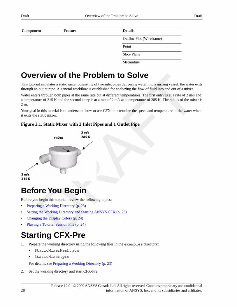
DetailsFeatureComponent
Outline Plot (Wireframe)
Point
Slice Plane
Streamline
Overview of the Problem to SolveThis tutorial simulates a static mixer consisting of two inlet pipes delivering water into a mixing vessel; the water exitsthrough an outlet pipe. A general workflow is established for analyzing the flow of fluid into and out of a mixer.
Water enters through both pipes at the same rate but at different temperatures. The first entry is at a rate of 2 m/s anda temperature of 315 K and the second entry is at a rate of 2 m/s at a temperature of 285 K. The radius of the mixer is2 m.
Your goal in this tutorial is to understand how to use CFX to determine the speed and temperature of the water whenit exits the static mixer.
Figure 2.1. Static Mixer with 2 Inlet Pipes and 1 Outlet Pipe
Before You BeginBefore you begin this tutorial, review the following topics:
• Preparing a Working Directory (p. 23)
• Setting the Working Directory and Starting ANSYS CFX (p. 23)
• Changing the Display Colors (p. 24)
• Playing a Tutorial Session File (p. 24)
Starting CFX-Pre1. Prepare the working directory using the following files in the examples directory:
• StaticMixerMesh.gtm
• StaticMixer.pre
For details, see Preparing a Working Directory (p. 23)
2. Set the working directory and start CFX-Pre
Release 12.0 - © 2009 ANSYS Canada Ltd. All rights reserved. Contains proprietary and confidentialinformation of ANSYS, Inc. and its subsidiaries and affiliates.28
DraftOverview of the Problem to SolveDraft
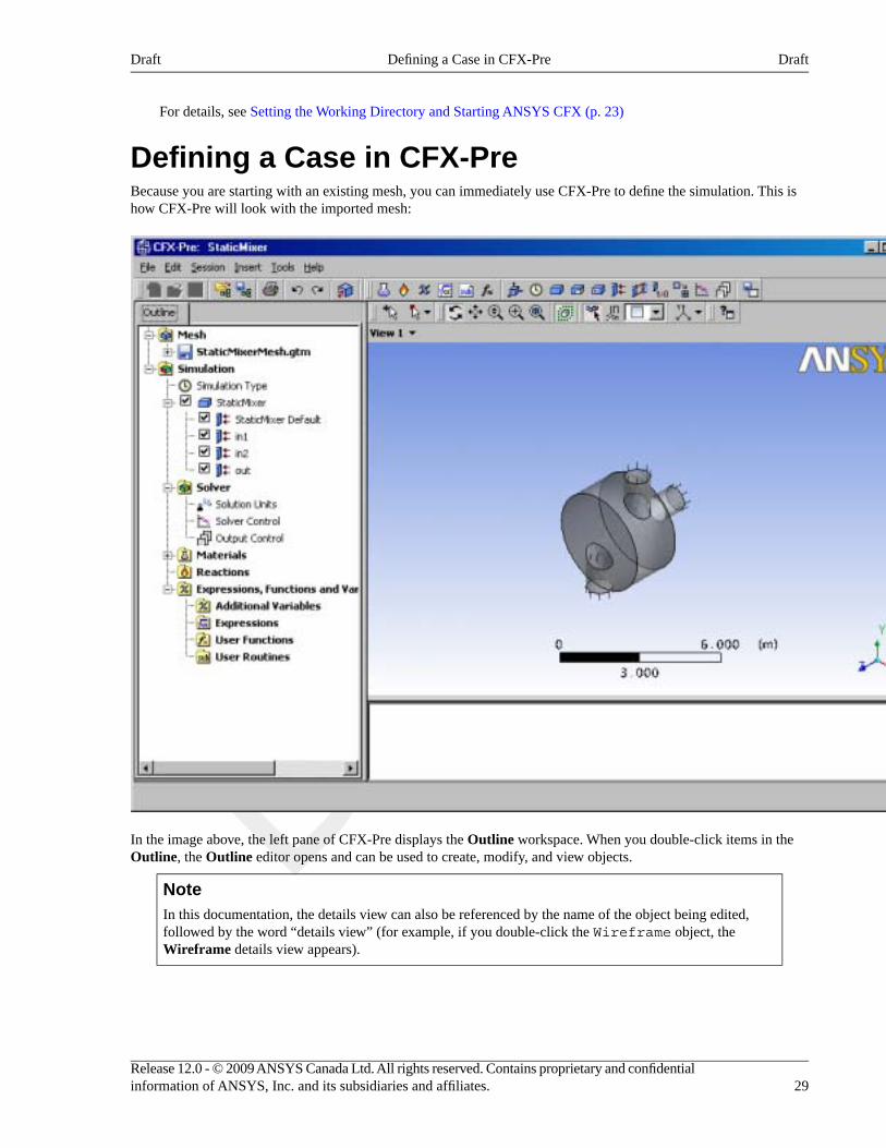
For details, see Setting the Working Directory and Starting ANSYS CFX (p. 23)
Defining a Case in CFX-PreBecause you are starting with an existing mesh, you can immediately use CFX-Pre to define the simulation. This ishow CFX-Pre will look with the imported mesh:
In the image above, the left pane of CFX-Pre displays the Outline workspace. When you double-click items in theOutline, the Outline editor opens and can be used to create, modify, and view objects.
NoteIn this documentation, the details view can also be referenced by the name of the object being edited,followed by the word “details view” (for example, if you double-click the Wireframe object, theWireframe details view appears).
29Release 12.0 - © 2009 ANSYS Canada Ltd. All rights reserved. Contains proprietary and confidentialinformation of ANSYS, Inc. and its subsidiaries and affiliates.
DraftDefining a Case in CFX-PreDraft
Synopsis of Quick Setup ModeQuick Setup mode provides a simple wizard-like interface for setting up simple cases. This is useful for getting familiarwith the basic elements of a CFD problem setup. This section describes using Quick Setup mode to develop a simulationin CFX-Pre.
Workflow OverviewThis tutorial follows the general workflow for Quick Setup mode:
1. Creating a New Case (p. 30)
2. Setting the Physics Definition (p. 30)
3. Importing a Mesh (p. 31)
4. Defining Model Data (p. 32)
5. Defining Boundaries (p. 32)
6. Setting Boundary Data (p. 33)
7. Setting Flow Specification (p. 33)
8. Setting Temperature Specification (p. 33)
9. Reviewing the Boundary Condition Definitions (p. 33)
10. Creating the Second Inlet Boundary Definition (p. 33)
11. Creating the Outlet Boundary Definition (p. 34)
12. Moving to General Mode (p. 34)
13. Writing the CFX-Solver Input (.def) File (p. 35)
Creating a New CaseBefore importing and working with a mesh, a simulation needs to be started using Quick Setup mode.
1. If required, launch CFX-Pre.
2. Select File > New Case.
The New Case File dialog box is displayed.
3. Select Quick Setup and click OK.
NoteIf this is the first time you are running this software, a message box will appear notifying you thatautomatic generation of the default domain is active. To avoid seeing this message again uncheckShow This Message Again.
4. Select File > Save Case As.
5. Under File name, type: StaticMixer
6. Click Save.
Setting the Physics DefinitionYou need to specify the fluids used in a simulation. A variety of fluids are already defined as library materials. Forthis tutorial you will use a prepared fluid, Water, which is defined to be water at 25°C.
1. Ensure that Simulation Definition is displayed at the top of the details view.
2. Under Fluid select Water.
Release 12.0 - © 2009 ANSYS Canada Ltd. All rights reserved. Contains proprietary and confidentialinformation of ANSYS, Inc. and its subsidiaries and affiliates.30
DraftSynopsis of Quick Setup ModeDraft
Importing a MeshAt least one mesh must be imported before physics are applied.
1. In Simulation Definition, under Mesh File, click Browse .
The Import Mesh dialog box appears.
2. Under Files of type, select CFX Mesh (*gtm *cfx).
3. From your working directory, select StaticMixerMesh.gtm.
4. Click Open.
The mesh loads.
5. Click Next.
Using the ViewerNow that the mesh is loaded, take a moment to explore how you can use the viewer toolbar to zoom in or out and torotate the object in the viewer.
Using the Zoom ToolsThere are several icons available for controlling the level of zoom in the viewer.
1. Click Zoom Box
2. Click and drag a rectangular box over the geometry.
3. Release the mouse button to zoom in on the selection.
The geometry zoom changes to display the selection at a greater resolution.
4. Click Fit View to re-center and re-scale the geometry.
Rotating the GeometryIf you need to rotate an object or to view it from a new angle, you can use the viewer toolbar.
1. Click Rotate on the viewer toolbar.
2. Click and drag within the geometry repeatedly to test the rotation of the geometry.
The geometry rotates based on the direction of movement.
Notice how the mouse cursor changes depending on where you are in the viewer:
31Release 12.0 - © 2009 ANSYS Canada Ltd. All rights reserved. Contains proprietary and confidentialinformation of ANSYS, Inc. and its subsidiaries and affiliates.
DraftImporting a MeshDraft
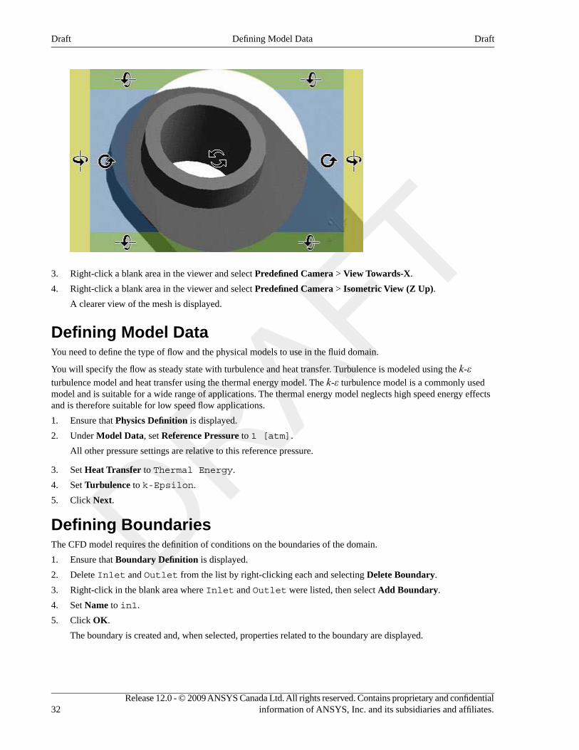
3. Right-click a blank area in the viewer and select Predefined Camera > View Towards-X.
4. Right-click a blank area in the viewer and select Predefined Camera > Isometric View (Z Up).
A clearer view of the mesh is displayed.
Defining Model DataYou need to define the type of flow and the physical models to use in the fluid domain.
You will specify the flow as steady state with turbulence and heat transfer. Turbulence is modeled using the k-εturbulence model and heat transfer using the thermal energy model. The k-ε turbulence model is a commonly usedmodel and is suitable for a wide range of applications. The thermal energy model neglects high speed energy effectsand is therefore suitable for low speed flow applications.
1. Ensure that Physics Definition is displayed.
2. Under Model Data, set Reference Pressure to 1 [atm].
All other pressure settings are relative to this reference pressure.
3. Set Heat Transfer to Thermal Energy.
4. Set Turbulence to k-Epsilon.
5. Click Next.
Defining BoundariesThe CFD model requires the definition of conditions on the boundaries of the domain.
1. Ensure that Boundary Definition is displayed.
2. Delete Inlet and Outlet from the list by right-clicking each and selecting Delete Boundary.
3. Right-click in the blank area where Inlet and Outlet were listed, then select Add Boundary.
4. Set Name to in1.
5. Click OK.
The boundary is created and, when selected, properties related to the boundary are displayed.
Release 12.0 - © 2009 ANSYS Canada Ltd. All rights reserved. Contains proprietary and confidentialinformation of ANSYS, Inc. and its subsidiaries and affiliates.32
DraftDefining Model DataDraft
Setting Boundary DataOnce boundaries are created, you need to create associated data. Based on Figure 2.1, “Static Mixer with 2 Inlet Pipesand 1 Outlet Pipe” (p. 28), you will define the velocity and temperature for the first inlet.
1. Ensure that Boundary Data is displayed.
2. Set Boundary Type to Inlet.
3. Set Location to in1.
Setting Flow SpecificationOnce boundary data is defined, the boundary needs to have the flow specification assigned.
1. Ensure that Flow Specification is displayed.
2. Set Option to Normal Speed.
3. Set Normal Speed to 2 [m s^-1].
Setting Temperature SpecificationOnce flow specification is defined, the boundary needs to have temperature assigned.
1. Ensure that Temperature Specification is displayed.
2. Set Static Temperature to 315 [K].
Reviewing the Boundary Condition DefinitionsDefining the boundary condition for in1 required several steps. Here the settings are reviewed for accuracy.
Based on Figure 2.1, “Static Mixer with 2 Inlet Pipes and 1 Outlet Pipe” (p. 28), the first inlet boundary conditionconsists of a velocity of 2 m/s and a temperature of 315 K at one of the side inlets.
• Review the boundary in1 settings for accuracy. They should be as follows:
ValueSettingTab
InletBoundary TypeBoundary Data
in1Location
Normal SpeedOptionFlow Specification
2 [m s^-1]Normal Speed
315 [K]Static TemperatureTemperature Specification
Creating the Second Inlet Boundary DefinitionBased on Figure 2.1, “Static Mixer with 2 Inlet Pipes and 1 Outlet Pipe” (p. 28), you know the second inlet boundarycondition consists of a velocity of 2 m/s and a temperature of 285 K at one of the side inlets. You will define that now.
1. Under Boundary Definition, right-click in the selector area and select Add Boundary.
2. Create a new boundary named in2 with these settings:
ValueSettingTab
InletBoundary TypeBoundary Data
33Release 12.0 - © 2009 ANSYS Canada Ltd. All rights reserved. Contains proprietary and confidentialinformation of ANSYS, Inc. and its subsidiaries and affiliates.
DraftSetting Boundary DataDraft
ValueSettingTab
in2Location
Normal SpeedOptionFlow Specification
2 [m s^-1]Normal Speed
285 [K]Static TemperatureTemperature Specification
Creating the Outlet Boundary DefinitionNow that the second inlet boundary has been created, the same concepts can be applied to building the outlet boundary.
1. Create a new boundary named out with these settings:
ValueSettingTab
OutletBoundary TypeBoundary Data
outLocation
Average Static PressureOptionFlow Specification
0 [Pa]Relative Pressure
2. Click Next.
Moving to General ModeThere are no further boundary conditions that need to be set. All 2D exterior regions that have not been assigned to aboundary condition are automatically assigned to the default boundary condition.
• Set Operation to Enter General Mode and click Finish.
The three boundary conditions are displayed in the viewer as sets of arrows at the boundary surfaces. Inlet boundaryarrows are directed into the domain. Outlet boundary arrows are directed out of the domain.
Setting Solver ControlSolver Control parameters control aspects of the numerical solution generation process.
While an upwind advection scheme is less accurate than other advection schemes, it is also more robust. This advectionscheme is suitable for obtaining an initial set of results, but in general should not be used to obtain final accurate results.
The time scale can be calculated automatically by the solver or set manually. The Automatic option tends to beconservative, leading to reliable, but often slow, convergence. It is often possible to accelerate convergence by applyinga time scale factor or by choosing a manual value that is more aggressive than the Automatic option. In this tutorial,you will select a physical time scale, leading to convergence that is twice as fast as the Automatic option.
1. Click Solver Control .
2. On the Basic Settings tab, set Advection Scheme > Option to Upwind.
3. Set Convergence Control > Fluid Timescale Control > Timescale Control to Physical Timescale andset the physical timescale value to 2 [s].
4. Click OK.
Release 12.0 - © 2009 ANSYS Canada Ltd. All rights reserved. Contains proprietary and confidentialinformation of ANSYS, Inc. and its subsidiaries and affiliates.34
DraftCreating the Outlet Boundary DefinitionDraft
Writing the CFX-Solver Input (.def) FileThe simulation file, StaticMixer.cfx, contains the simulation definition in a format that can be loaded by CFX-Pre,allowing you to complete (if applicable), restore, and modify the simulation definition. The simulation file differs fromthe CFX-Solver input file in that it can be saved at any time while defining the simulation.
1. Click Define Run .
2. Set File name to StaticMixer.def.
3. Click Save.
The CFX-Solver input file (StaticMixer.def) is created. CFX-Solver Manager automatically starts and, onthe Define Run dialog box, the Solver Input File is set.
4. If you are notified the file already exists, click Overwrite.
This file is provided in the tutorial directory and may exist in your working directory if you have copied it there.
5. When you are finished, select File > Quit in CFX-Pre.
6. If prompted, click Yes or Save & Quit to save StaticMixer.cfx.
7. Proceed to Obtaining a Solution Using CFX-Solver Manager (p. 35).
Playing the Session File and Starting CFX-Solver ManagerNoteThis task is required only if you are starting here with the session file that was provided in the examplesdirectory. If you have performed all the tasks in the previous steps, proceed directly to Obtaining a SolutionUsing CFX-Solver Manager (p. 35).
Events in CFX-Pre can be recorded to a session file and then played back at a later date to drive CFX-Pre. Sessionfiles have been created for each tutorial so that the problems can be set up rapidly in CFX-Pre, if desired.
1. If required, launch CFX-Pre.
2. Select Session > Play Tutorial.
3. Select StaticMixer.pre.
4. Click Open.
A CFX-Solver input file is written.
5. Select File > Quit.
6. Launch the CFX-Solver Manager from CFX Launcher.
7. After the CFX-Solver starts, select File > Define Run.
8. Under CFX-Solver Input File, click Browse .
9. Select StaticMixer.def, located in the working directory.
10. Proceed to Obtaining a Solution Using CFX-Solver Manager (p. 35).
Obtaining a Solution Using CFX-Solver ManagerCFX-Solver Manager has a visual interface that displays a variety of results and should be used when plotted dataneeds to be viewed during problem solving.
35Release 12.0 - © 2009 ANSYS Canada Ltd. All rights reserved. Contains proprietary and confidentialinformation of ANSYS, Inc. and its subsidiaries and affiliates.
DraftWriting the CFX-Solver Input (.def) FileDraft
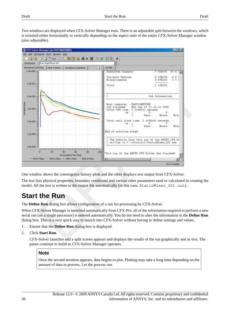
Two windows are displayed when CFX-Solver Manager runs. There is an adjustable split between the windows, whichis oriented either horizontally or vertically depending on the aspect ratio of the entire CFX-Solver Manager window(also adjustable).
One window shows the convergence history plots and the other displays text output from CFX-Solver.
The text lists physical properties, boundary conditions and various other parameters used or calculated in creating themodel. All the text is written to the output file automatically (in this case, StaticMixer_001.out).
Start the RunThe Define Run dialog box allows configuration of a run for processing by CFX-Solver.
When CFX-Solver Manager is launched automatically from CFX-Pre, all of the information required to perform a newserial run (on a single processor) is entered automatically. You do not need to alter the information in the Define Rundialog box. This is a very quick way to launch into CFX-Solver without having to define settings and values.
1. Ensure that the Define Run dialog box is displayed.
2. Click Start Run.
CFX-Solver launches and a split screen appears and displays the results of the run graphically and as text. Thepanes continue to build as CFX-Solver Manager operates.
NoteOnce the second iteration appears, data begins to plot. Plotting may take a long time depending on theamount of data to process. Let the process run.
Release 12.0 - © 2009 ANSYS Canada Ltd. All rights reserved. Contains proprietary and confidentialinformation of ANSYS, Inc. and its subsidiaries and affiliates.36
DraftStart the RunDraft
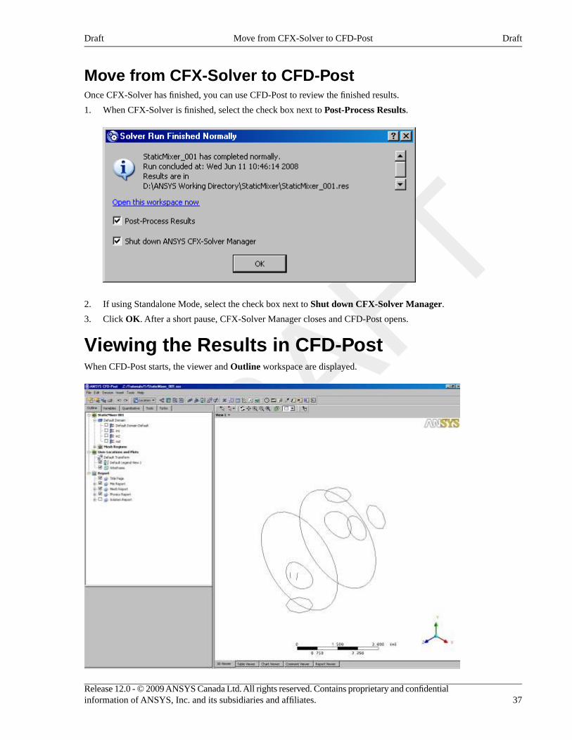
Move from CFX-Solver to CFD-PostOnce CFX-Solver has finished, you can use CFD-Post to review the finished results.
1. When CFX-Solver is finished, select the check box next to Post-Process Results.
2. If using Standalone Mode, select the check box next to Shut down CFX-Solver Manager.
3. Click OK. After a short pause, CFX-Solver Manager closes and CFD-Post opens.
Viewing the Results in CFD-PostWhen CFD-Post starts, the viewer and Outline workspace are displayed.
37Release 12.0 - © 2009 ANSYS Canada Ltd. All rights reserved. Contains proprietary and confidentialinformation of ANSYS, Inc. and its subsidiaries and affiliates.
DraftMove from CFX-Solver to CFD-PostDraft
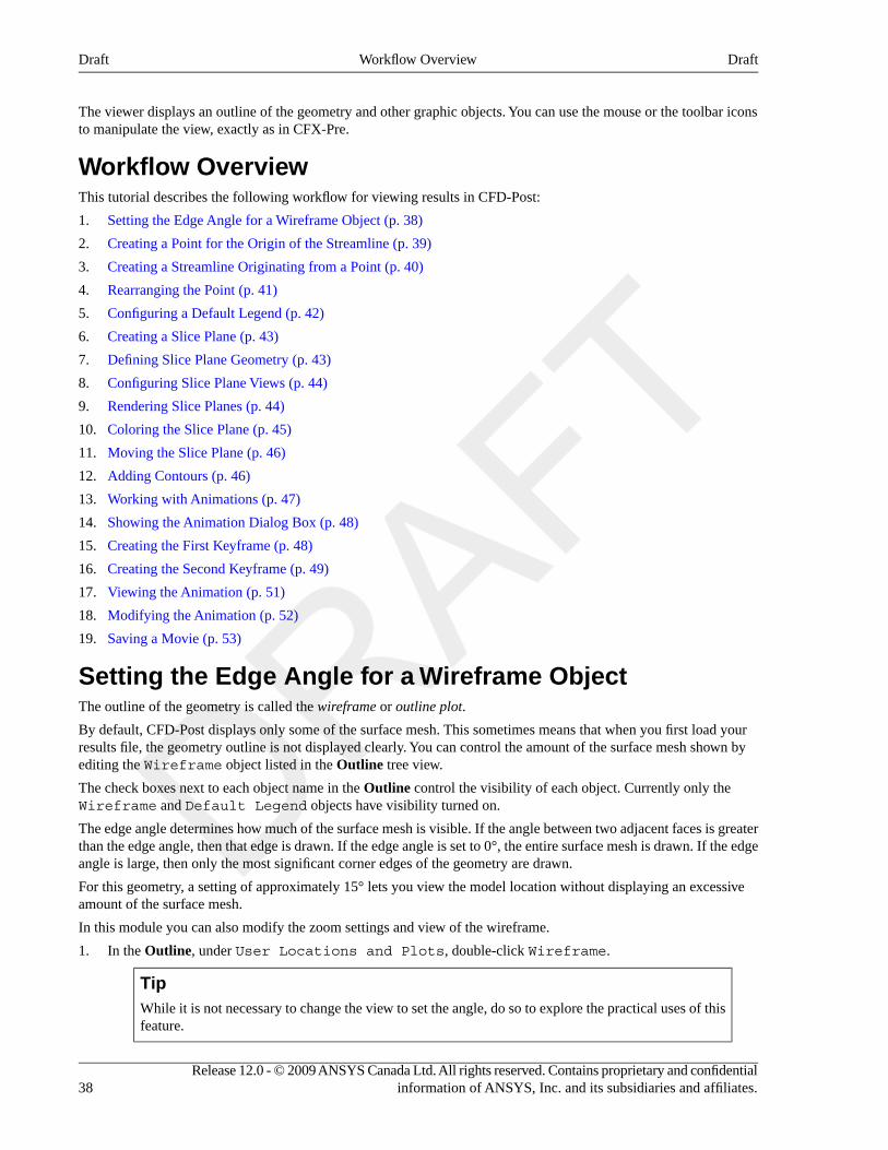
The viewer displays an outline of the geometry and other graphic objects. You can use the mouse or the toolbar iconsto manipulate the view, exactly as in CFX-Pre.
Workflow OverviewThis tutorial describes the following workflow for viewing results in CFD-Post:
1. Setting the Edge Angle for a Wireframe Object (p. 38)
2. Creating a Point for the Origin of the Streamline (p. 39)
3. Creating a Streamline Originating from a Point (p. 40)
4. Rearranging the Point (p. 41)
5. Configuring a Default Legend (p. 42)
6. Creating a Slice Plane (p. 43)
7. Defining Slice Plane Geometry (p. 43)
8. Configuring Slice Plane Views (p. 44)
9. Rendering Slice Planes (p. 44)
10. Coloring the Slice Plane (p. 45)
11. Moving the Slice Plane (p. 46)
12. Adding Contours (p. 46)
13. Working with Animations (p. 47)
14. Showing the Animation Dialog Box (p. 48)
15. Creating the First Keyframe (p. 48)
16. Creating the Second Keyframe (p. 49)
17. Viewing the Animation (p. 51)
18. Modifying the Animation (p. 52)
19. Saving a Movie (p. 53)
Setting the Edge Angle for a Wireframe ObjectThe outline of the geometry is called the wireframe or outline plot.
By default, CFD-Post displays only some of the surface mesh. This sometimes means that when you first load yourresults file, the geometry outline is not displayed clearly. You can control the amount of the surface mesh shown byediting the Wireframe object listed in the Outline tree view.
The check boxes next to each object name in the Outline control the visibility of each object. Currently only theWireframe and Default Legend objects have visibility turned on.
The edge angle determines how much of the surface mesh is visible. If the angle between two adjacent faces is greaterthan the edge angle, then that edge is drawn. If the edge angle is set to 0°, the entire surface mesh is drawn. If the edgeangle is large, then only the most significant corner edges of the geometry are drawn.
For this geometry, a setting of approximately 15° lets you view the model location without displaying an excessiveamount of the surface mesh.
In this module you can also modify the zoom settings and view of the wireframe.
1. In the Outline, under User Locations and Plots, double-click Wireframe.
TipWhile it is not necessary to change the view to set the angle, do so to explore the practical uses of thisfeature.
Release 12.0 - © 2009 ANSYS Canada Ltd. All rights reserved. Contains proprietary and confidentialinformation of ANSYS, Inc. and its subsidiaries and affiliates.38
DraftWorkflow OverviewDraft
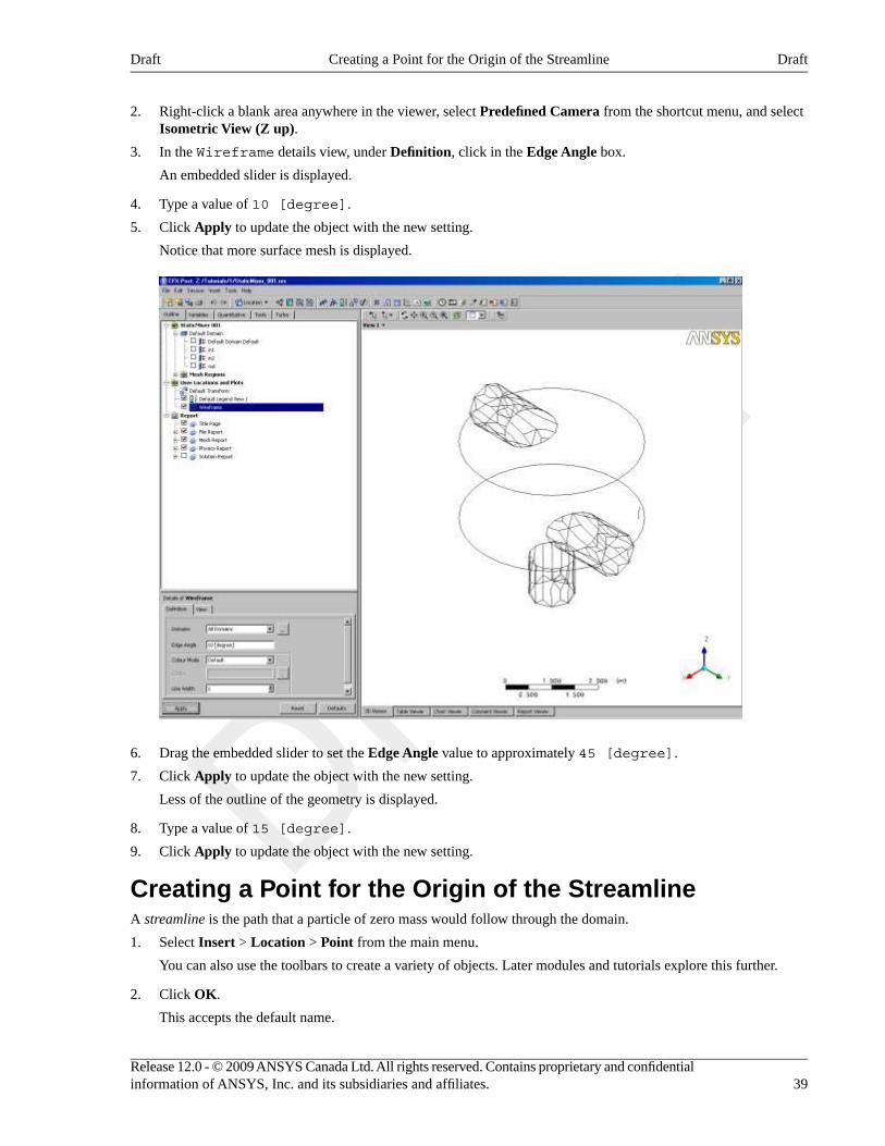
2. Right-click a blank area anywhere in the viewer, select Predefined Camera from the shortcut menu, and selectIsometric View (Z up).
3. In the Wireframe details view, under Definition, click in the Edge Angle box.
An embedded slider is displayed.
4. Type a value of 10 [degree].
5. Click Apply to update the object with the new setting.
Notice that more surface mesh is displayed.
6. Drag the embedded slider to set the Edge Angle value to approximately 45 [degree].
7. Click Apply to update the object with the new setting.
Less of the outline of the geometry is displayed.
8. Type a value of 15 [degree].
9. Click Apply to update the object with the new setting.
Creating a Point for the Origin of the StreamlineA streamline is the path that a particle of zero mass would follow through the domain.
1. Select Insert > Location > Point from the main menu.
You can also use the toolbars to create a variety of objects. Later modules and tutorials explore this further.
2. Click OK.
This accepts the default name.
39Release 12.0 - © 2009 ANSYS Canada Ltd. All rights reserved. Contains proprietary and confidentialinformation of ANSYS, Inc. and its subsidiaries and affiliates.
DraftCreating a Point for the Origin of the StreamlineDraft
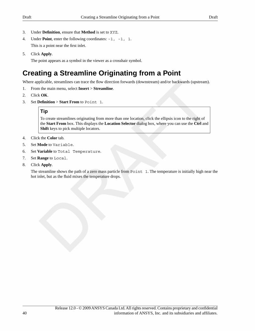
3. Under Definition, ensure that Method is set to XYZ.
4. Under Point, enter the following coordinates: -1, -1, 1.
This is a point near the first inlet.
5. Click Apply.
The point appears as a symbol in the viewer as a crosshair symbol.
Creating a Streamline Originating from a PointWhere applicable, streamlines can trace the flow direction forwards (downstream) and/or backwards (upstream).
1. From the main menu, select Insert > Streamline.
2. Click OK.
3. Set Definition > Start From to Point 1.
TipTo create streamlines originating from more than one location, click the ellipsis icon to the right ofthe Start From box. This displays the Location Selector dialog box, where you can use the Ctrl andShift keys to pick multiple locators.
4. Click the Color tab.
5. Set Mode to Variable.
6. Set Variable to Total Temperature.
7. Set Range to Local.
8. Click Apply.
The streamline shows the path of a zero mass particle from Point 1. The temperature is initially high near thehot inlet, but as the fluid mixes the temperature drops.
Release 12.0 - © 2009 ANSYS Canada Ltd. All rights reserved. Contains proprietary and confidentialinformation of ANSYS, Inc. and its subsidiaries and affiliates.40
DraftCreating a Streamline Originating from a PointDraft
Rearranging the PointOnce created, a point can be rearranged manually or by setting specific coordinates.
TipIn this module, you may choose to display various views and zooms from the Predefined Camera option
in the shortcut menu (such as Isometric View (Z up) or View Towards -X) and by using Zoom Box
if you prefer to change the display.
1. In Outline, under User Locations and Plots double-click Point 1.
Properties for the selected user location are displayed.
2. Under Point, set these coordinates: -1, -2.9, 1.
3. Click Apply.
The point is moved and the streamline redrawn.
4. In the viewer toolbar, click Select and ensure that the adjacent toolbar icon is set to Single Select .
While in select mode, you cannot use the left mouse button to re-orient the object in the viewer.
41Release 12.0 - © 2009 ANSYS Canada Ltd. All rights reserved. Contains proprietary and confidentialinformation of ANSYS, Inc. and its subsidiaries and affiliates.
DraftRearranging the PointDraft
5. In the viewer, drag Point 1 (appears as a yellow addition sign) to a new location within the mixer.
The point position is updated in the details view and the streamline is redrawn at the new location. The pointmoves normal in relation to the viewing direction.
6. Click Rotate .
TipYou can also click in the viewer area, and press the space bar to toggle between Select and ViewingMode. A way to pick objects from Viewing Mode is to hold down Ctrl + Shift while clicking on anobject with the left mouse button.
7. Under Point, reset these coordinates: -1, -1, 1.
8. Click Apply.
The point appears at its original location.
9. Right-click a blank area in the viewer and select Predefined Camera > View Towards -X.
Configuring a Default LegendYou can modify the appearance of the default legend.
The default legend appears whenever a plot is created that is colored by a variable. The streamline color is based ontemperature; therefore, the legend shows the temperature range. The color pattern on the legend's color bar is banded
in accordance with the bands in the plot1.
The default legend displays values for the last eligible plot that was opened in the details view. To maintain a legend
definition during a CFD-Post session, you can create a new legend by clicking Legend .
Because there are many settings that can be customized for the legend, this module allows you the freedom to experimentwith them. In the last steps you will set up a legend, based on the default legend, with a minor modification to theposition.
TipWhen editing values, you can restore the values that were present when you began editing by clicking Reset.To restore the factory-default values, click Default.
1. Double-click Default Legend View 1.
The Definition tab of the default legend is displayed.
2. Apply the following settings
ValueSettingTab
User SpecifiedTitle ModeDefinition
Streamline Temp.Title
(Selected)Horizontal
BottomLocation > Y Justification
1An exception occurs when one or more bands in a contour plot represent values beyond the legend's range. In this case, such bands are coloredusing a color that is extrapolated slightly past the range of colors shown in the legend. This can happen only when a user-specified range is used forthe legend.
Release 12.0 - © 2009 ANSYS Canada Ltd. All rights reserved. Contains proprietary and confidentialinformation of ANSYS, Inc. and its subsidiaries and affiliates.42
DraftConfiguring a Default LegendDraft
3. Click Apply.
The appearance and position of the legend changes based on the settings specified.
4. Modify various settings in Definition and click Apply after each change.
5. Select the Appearance tab.
6. Modify a variety of settings in the Appearance and click Apply after each change.
7. Click Defaults.
8. Click Apply.
9. Under Outline, in User Locations and Plots, clear the check boxes for Point 1 and Streamline1.
Since both are no longer visible, the associated legend no longer appears.
Creating a Slice PlaneDefining a slice plane allows you to obtain a cross-section of the geometry.
In CFD-Post you often view results by coloring a graphic object. The graphic object could be an isosurface, a vectorplot, or in this case, a plane. The object can be a fixed color or it can vary based on the value of a variable.
You already have some objects defined by default (listed in the Outline). You can view results on the boundaries ofthe static mixer by coloring each boundary object by a variable. To view results within the geometry (that is, onnon-default locators), you will create new objects.
You can use the following methods to define a plane:
• Three Points: creates a plane from three specified points.
• Point and Normal: defines a plane from one point on the plane and a normal vector to the plane.
• YZ Plane, ZX Plane, and XY Plane: similar to Point and Normal, except that the normal is definedto be normal to the indicated plane.
1. From the main menu, select Insert > Location > Plane or click Location > Plane.
2. In the Insert Plane window, type: Slice
3. Click OK.
The Geometry, Color, Render, and View tabs let you switch between settings.
4. Click the Geometry tab.
Defining Slice Plane GeometryYou need to choose the vector normal to the plane. You want the plane to lie in the x-y plane, hence its normal vectorpoints along the z-axis. You can specify any vector that points in the z-direction, but you will choose the most obvious(0,0,1).
1. If required, under Geometry, expand Definition.
2. Under Method select Point and Normal.
3. Under Point enter 0,0,1.
4. Under Normal enter 0, 0,1.
5. Click Apply.
Slice appears under User Locations and Plots. Rotate the view to see the plane.
43Release 12.0 - © 2009 ANSYS Canada Ltd. All rights reserved. Contains proprietary and confidentialinformation of ANSYS, Inc. and its subsidiaries and affiliates.
DraftCreating a Slice PlaneDraft
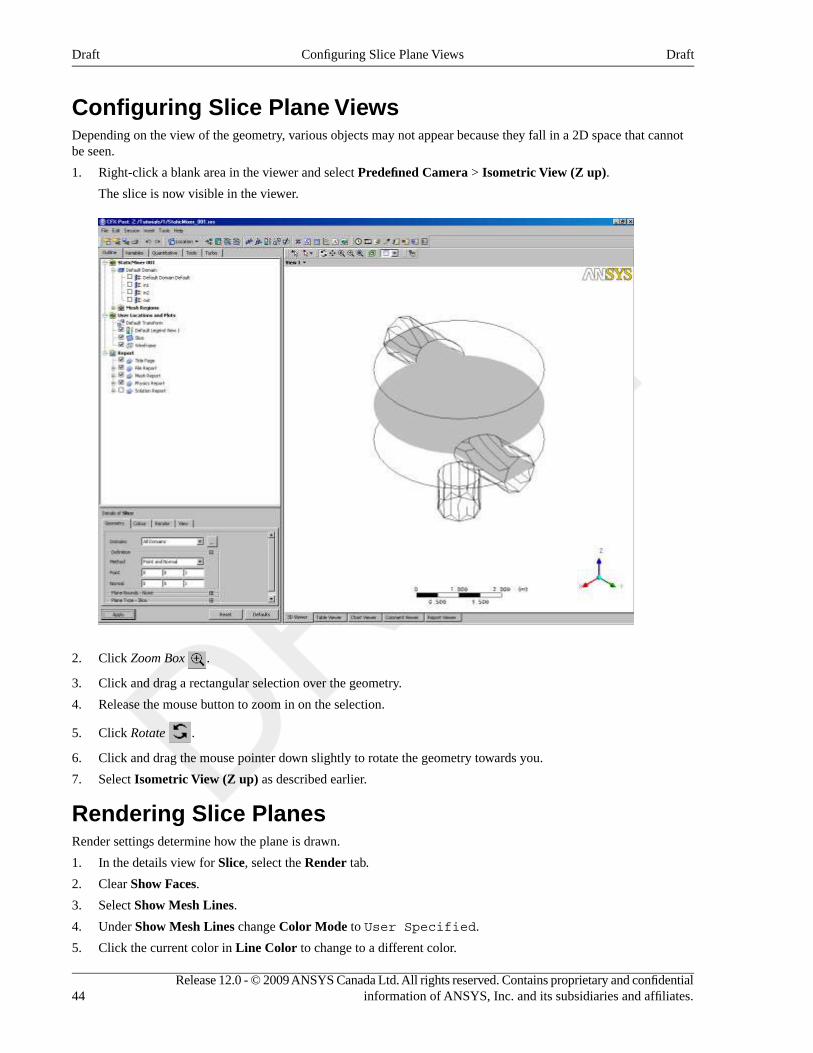
Configuring Slice Plane ViewsDepending on the view of the geometry, various objects may not appear because they fall in a 2D space that cannotbe seen.
1. Right-click a blank area in the viewer and select Predefined Camera > Isometric View (Z up).
The slice is now visible in the viewer.
2. Click Zoom Box .
3. Click and drag a rectangular selection over the geometry.
4. Release the mouse button to zoom in on the selection.
5. Click Rotate .
6. Click and drag the mouse pointer down slightly to rotate the geometry towards you.
7. Select Isometric View (Z up) as described earlier.
Rendering Slice PlanesRender settings determine how the plane is drawn.
1. In the details view for Slice, select the Render tab.
2. Clear Show Faces.
3. Select Show Mesh Lines.
4. Under Show Mesh Lines change Color Mode to User Specified.
5. Click the current color in Line Color to change to a different color.
Release 12.0 - © 2009 ANSYS Canada Ltd. All rights reserved. Contains proprietary and confidentialinformation of ANSYS, Inc. and its subsidiaries and affiliates.44
DraftConfiguring Slice Plane ViewsDraft
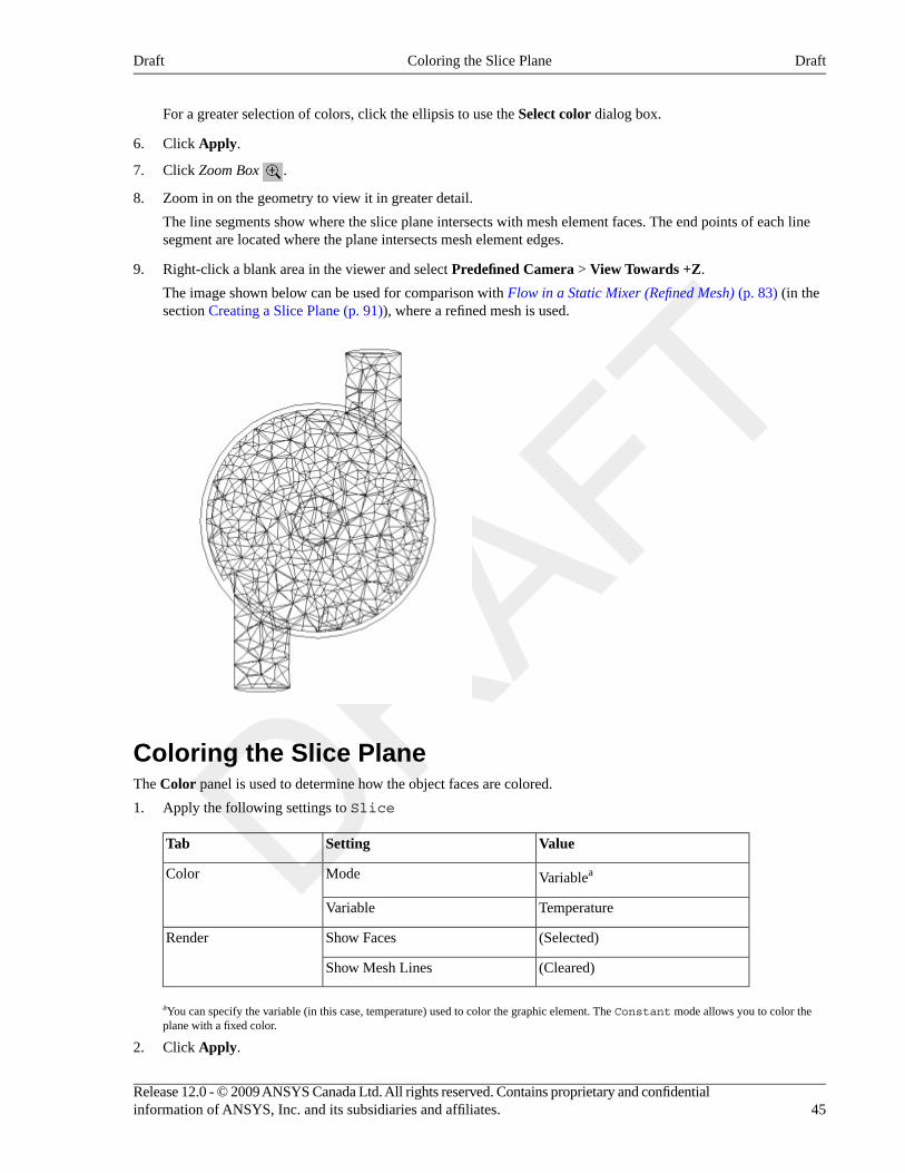
For a greater selection of colors, click the ellipsis to use the Select color dialog box.
6. Click Apply.
7. Click Zoom Box .
8. Zoom in on the geometry to view it in greater detail.
The line segments show where the slice plane intersects with mesh element faces. The end points of each linesegment are located where the plane intersects mesh element edges.
9. Right-click a blank area in the viewer and select Predefined Camera > View Towards +Z.
The image shown below can be used for comparison with Flow in a Static Mixer (Refined Mesh) (p. 83) (in thesection Creating a Slice Plane (p. 91)), where a refined mesh is used.
Coloring the Slice PlaneThe Color panel is used to determine how the object faces are colored.
1. Apply the following settings to Slice
ValueSettingTab
VariableaModeColor
TemperatureVariable
(Selected)Show FacesRender
(Cleared)Show Mesh Lines
aYou can specify the variable (in this case, temperature) used to color the graphic element. The Constant mode allows you to color theplane with a fixed color.
2. Click Apply.
45Release 12.0 - © 2009 ANSYS Canada Ltd. All rights reserved. Contains proprietary and confidentialinformation of ANSYS, Inc. and its subsidiaries and affiliates.
DraftColoring the Slice PlaneDraft
Hot water (red) enters from one inlet and cold water (blue) from the other.
Moving the Slice PlaneThe plane can be moved to different locations.
1. Right-click a blank area in the viewer and select Predefined Camera > Isometric View (Z up) from the shortcutmenu.
2. Click the Geometry tab.
Review the settings in Definition under Point and under Normal.
3. Click Single Select .
4. Click and drag the plane to a new location that intersects the domain.
As you drag the mouse, the viewer updates automatically. Note that Point updates with new settings.
5. Set Point settings to 0,0,1.
6. Click Apply.
7. Click Rotate .
8. Turn off visibility of Slice by clearing the check box next to Slice in the Outline tree view.
Adding ContoursContours connect all points of equal value for a scalar variable (for example, Temperature) and help to visualizevariable values and gradients. Colored bands fill the spaces between contour lines. Each band is colored by the averagecolor of its two bounding contour lines (even if the latter are not displayed).
1. Right-click a blank area in the viewer and select Predefined Camera > Isometric View (Z up) from the shortcutmenu.
2. Select Insert > Contour from the main menu or click Contour .
The Insert Contour dialog box is displayed.
3. Set Name to Slice Contour.
4. Click OK.
5. Apply the following settings
ValueSettingTab
SliceLocationsGeometry
TemperatureVariable
SlicePlane Type
(Selected)Show Contour BandsRender
6. Click Apply.
Release 12.0 - © 2009 ANSYS Canada Ltd. All rights reserved. Contains proprietary and confidentialinformation of ANSYS, Inc. and its subsidiaries and affiliates.46
DraftMoving the Slice PlaneDraft
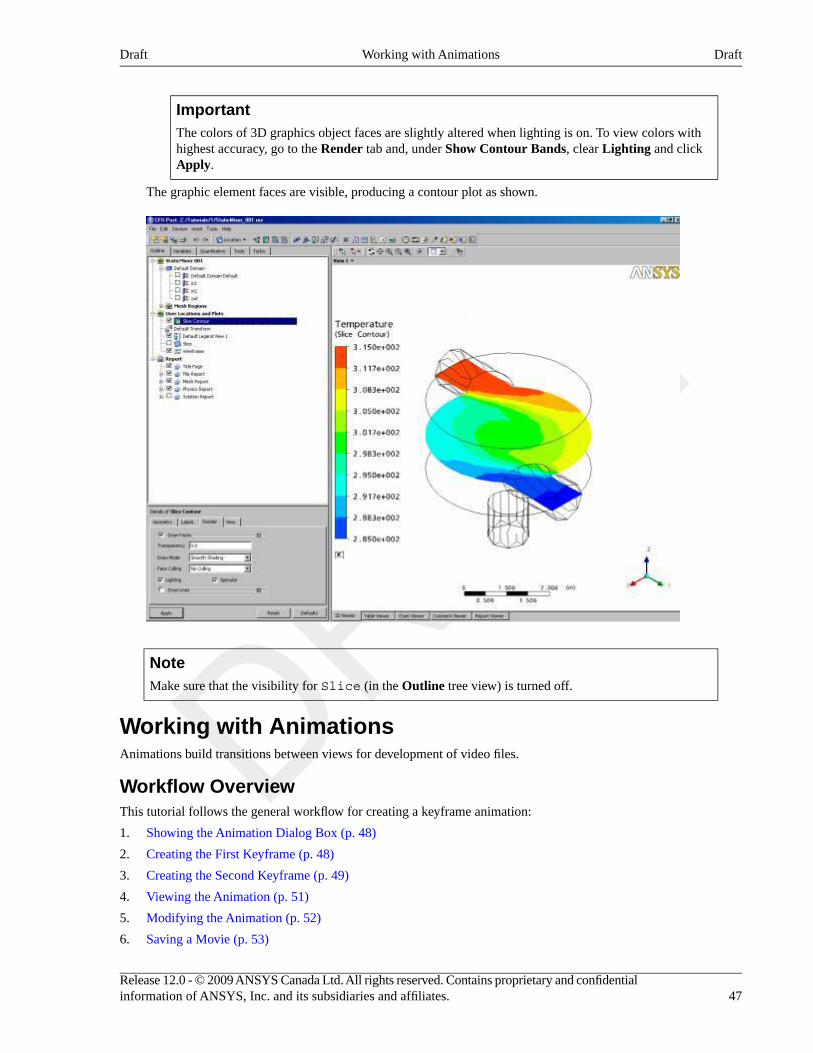
ImportantThe colors of 3D graphics object faces are slightly altered when lighting is on. To view colors withhighest accuracy, go to the Render tab and, under Show Contour Bands, clear Lighting and clickApply.
The graphic element faces are visible, producing a contour plot as shown.
NoteMake sure that the visibility for Slice (in the Outline tree view) is turned off.
Working with AnimationsAnimations build transitions between views for development of video files.
Workflow OverviewThis tutorial follows the general workflow for creating a keyframe animation:
1. Showing the Animation Dialog Box (p. 48)
2. Creating the First Keyframe (p. 48)
3. Creating the Second Keyframe (p. 49)
4. Viewing the Animation (p. 51)
5. Modifying the Animation (p. 52)
6. Saving a Movie (p. 53)
47Release 12.0 - © 2009 ANSYS Canada Ltd. All rights reserved. Contains proprietary and confidentialinformation of ANSYS, Inc. and its subsidiaries and affiliates.
DraftWorking with AnimationsDraft
Showing the Animation Dialog BoxThe Animation dialog box is used to define keyframes and to export to a video file.
• Select Tools > Animation or click Animation .
The Animation dialog box can be repositioned as required.
Creating the First KeyframeKeyframes are required in order to produce an animation. You need to define the first viewer state, a second (and final)viewer state, and set the number of interpolated intermediate frames.
1. Right-click a blank area in the viewer and select Predefined Camera > Isometric View (Z up).
2. In the Outline, under User Locations and Plots, turn off the visibility of Slice Contour and turnon the visibility of Slice.
3. Select the Keyframe Animation toggle.
4. In the Animation dialog box, click New .
A new keyframe named KeyframeNo1 is created. This represents the current image displayed in the viewer.
Release 12.0 - © 2009 ANSYS Canada Ltd. All rights reserved. Contains proprietary and confidentialinformation of ANSYS, Inc. and its subsidiaries and affiliates.48
DraftShowing the Animation Dialog BoxDraft

Creating the Second KeyframeDefine the second keyframe and the number of intermediate frames:
1. In the Outline, under User Locations and Plots, double-click Slice.
2. On the Geometry tab, set Point coordinate values to (0,0,-1.99).
3. Click Apply.
The slice plane moves to the bottom of the mixer.
49Release 12.0 - © 2009 ANSYS Canada Ltd. All rights reserved. Contains proprietary and confidentialinformation of ANSYS, Inc. and its subsidiaries and affiliates.
DraftCreating the Second KeyframeDraft
4. In the Animation dialog box, click New .
KeyframeNo2 is created and represents the image displayed in the viewer.
5. Select KeyframeNo1.
6. Set # of Frames (located below the list of keyframes) to 20.
This is the number of intermediate frames used when going from KeyframeNo1 to KeyframeNo2. This numberis displayed in the Frames column for KeyframeNo1.
7. Press Enter.
The Frame # column shows the frame in which each keyframe appears. KeyframeNo1 appears at frame 1 sinceit defines the start of the animation. KeyframeNo2 is at frame 22 since you have 20 intermediate frames (frames2 to 21) in between KeyframeNo1 and KeyframeNo2.
Release 12.0 - © 2009 ANSYS Canada Ltd. All rights reserved. Contains proprietary and confidentialinformation of ANSYS, Inc. and its subsidiaries and affiliates.50
DraftCreating the Second KeyframeDraft
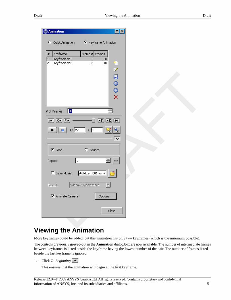
Viewing the AnimationMore keyframes could be added, but this animation has only two keyframes (which is the minimum possible).
The controls previously greyed-out in the Animation dialog box are now available. The number of intermediate framesbetween keyframes is listed beside the keyframe having the lowest number of the pair. The number of frames listedbeside the last keyframe is ignored.
1. Click To Beginning .
This ensures that the animation will begin at the first keyframe.
51Release 12.0 - © 2009 ANSYS Canada Ltd. All rights reserved. Contains proprietary and confidentialinformation of ANSYS, Inc. and its subsidiaries and affiliates.
DraftViewing the AnimationDraft
2. Click Play the animation .
The animation plays from frame 1 to frame 22. It plays relatively slowly because the slice plane must be updatedfor each frame.
Modifying the AnimationTo make the plane sweep through the whole geometry, you will set the starting position of the plane to be at the topof the mixer. You will also modify the Range properties of the plane so that it shows the temperature variation better.As the animation is played, you can see the hot and cold water entering the mixer. Near the bottom of the mixer (wherethe water flows out) you can see that the temperature is quite uniform. The new temperature range lets you view themixing process more accurately than the global range used in the first animation.
1. Apply the following settings to Slice
ValueSettingTab
0, 0, 1.99PointGeometry
VariableModeColor
TemperatureVariable
User SpecifiedRange
295 [K]Min
305 [K]Max
2. Click Apply.
The slice plane moves to the top of the static mixer.
NoteDo not double-click in the next step.
3. In the Animation dialog box, single click (do not double-click) KeyframeNo1 to select it.
If you had double-clicked KeyFrameNo1, the plane and viewer states would have been redefined according to
the stored settings for KeyFrameNo1. If this happens, click Undo and try again to select the keyframe.
4. Click Set Keyframe .
The image in the viewer replaces the one previously associated with KeyframeNo1.
5. Double-click KeyframeNo2.
The object properties for the slice plane are updated according to the settings in KeyFrameNo2.
6. Apply the following settings to Slice
ValueSettingTab
VariableModeColor
TemperatureVariable
User SpecifiedRange
Release 12.0 - © 2009 ANSYS Canada Ltd. All rights reserved. Contains proprietary and confidentialinformation of ANSYS, Inc. and its subsidiaries and affiliates.52
DraftModifying the AnimationDraft
ValueSettingTab
295 [K]Min
305 [K]Max
7. Click Apply.
8. In the Animation dialog box, single-click KeyframeNo2.
9. Click Set Keyframe to save the new settings to KeyframeNo2.
Saving a Movie1. Click More Animation Options to view the additional options.
The Loop and Bounce radio buttons determine what happens when the animation reaches the last keyframe.When Loop is selected, the animation repeats itself the number of times defined by Repeat. When Bounce isselected, every other cycle is played in reverse order, starting with the second.
2. Select the check box next to Save Movie.
3. Click Browse next to Save Movie.
4. Set Format to MPEG1.
5. Under File name type: StaticMixer.mpg
6. If required, set the path location to a different directory.
7. Click Save.
The movie file name (including path) has been set, but the animation has not yet been produced.
8. Click To Beginning .
9. Click Play the animation .
10. If prompted to overwrite an existing movie click Overwrite.
The animation plays and builds an MPEG file.
11. Click the Options button at the bottom of the Animation dialog box.
In Advanced, you can see that a Frame Rate of 24 frames per second was used to create the animation. Theanimation you produced contains a total of 22 frames, so it takes just under 1 second to play in a media player.
12. Click Cancel to close the dialog box.
13. Close the Animation dialog box.
14. Review the animation in third-party software as required.
Quitting CFD-PostWhen finished with CFD-Post, exit the current window:
1. When you are finished, select File > Quit to exit CFD-Post.
2. Click Quit if prompted to save.
53Release 12.0 - © 2009 ANSYS Canada Ltd. All rights reserved. Contains proprietary and confidentialinformation of ANSYS, Inc. and its subsidiaries and affiliates.
DraftSaving a MovieDraft

Release 12.0 - © 2009 ANSYS Canada Ltd. All rights reserved. Contains proprietary and confidentialinformation of ANSYS, Inc. and its subsidiaries and affiliates.
Chapter 3. Simulating Flow in a StaticMixer Using WorkbenchThis tutorial simulates a static mixer consisting of two inlet pipes delivering water into a mixing vessel; the water exitsthrough an outlet pipe. A general workflow is established for analyzing the flow of fluid into and out of a mixer usingANSYS Workbench.
This tutorial includes:
• Tutorial Features (p. 55)
• Overview of the Problem to Solve (p. 56)
• Before You Begin (p. 56)
• Starting ANSYS Workbench (p. 56)
• Starting CFX-Pre from ANSYS Workbench (p. 57)
• Obtaining a Solution (p. 61)
• Viewing the Results in CFD-Post (p. 63)
For introductory information about ANSYS Workbench, see ANSYS CFX in ANSYS Workbench (p. 31) in ANSYSCFX Introduction.
Tutorial FeaturesIn this tutorial you will learn about:
• Using ANSYS Workbench to set up a project.
• Using Quick Setup mode in CFX-Pre to set up a problem.
• Using ANSYS CFX-Solver Manager to obtain a solution.
• Modifying the outline plot in CFD-Post.
• Using streamlines in CFD-Post to trace the flow field from a point.
• Viewing temperature using colored planes and contours in CFD-Post.
• Creating an animation and saving it as a movie file.
DetailsFeatureComponent
Quick Setup WizardUser ModeCFX-Pre
Steady StateAnalysis Type
General FluidFluid Type
Single DomainDomain Type
k-EpsilonTurbulence Model
Thermal EnergyHeat Transfer
Inlet (Subsonic)Boundary Conditions
Outlet (Subsonic)
Wall: No-Slip
55Release 12.0 - © 2009 ANSYS Canada Ltd. All rights reserved. Contains proprietary and confidentialinformation of ANSYS, Inc. and its subsidiaries and affiliates.
DraftDraft
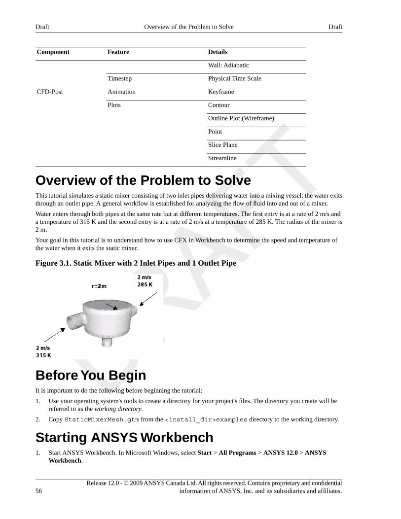
DetailsFeatureComponent
Wall: Adiabatic
Physical Time ScaleTimestep
KeyframeAnimationCFD-Post
ContourPlots
Outline Plot (Wireframe)
Point
Slice Plane
Streamline
Overview of the Problem to SolveThis tutorial simulates a static mixer consisting of two inlet pipes delivering water into a mixing vessel; the water exitsthrough an outlet pipe. A general workflow is established for analyzing the flow of fluid into and out of a mixer.
Water enters through both pipes at the same rate but at different temperatures. The first entry is at a rate of 2 m/s anda temperature of 315 K and the second entry is at a rate of 2 m/s at a temperature of 285 K. The radius of the mixer is2 m.
Your goal in this tutorial is to understand how to use CFX in Workbench to determine the speed and temperature ofthe water when it exits the static mixer.
Figure 3.1. Static Mixer with 2 Inlet Pipes and 1 Outlet Pipe
Before You BeginIt is important to do the following before beginning the tutorial:
1. Use your operating system's tools to create a directory for your project's files. The directory you create will bereferred to as the working directory.
2. Copy StaticMixerMesh.gtm from the <install_dir>examples directory to the working directory.
Starting ANSYS Workbench1. Start ANSYS Workbench. In Microsoft Windows, select Start > All Programs > ANSYS 12.0 > ANSYS
Workbench.
Release 12.0 - © 2009 ANSYS Canada Ltd. All rights reserved. Contains proprietary and confidentialinformation of ANSYS, Inc. and its subsidiaries and affiliates.56
DraftOverview of the Problem to SolveDraft
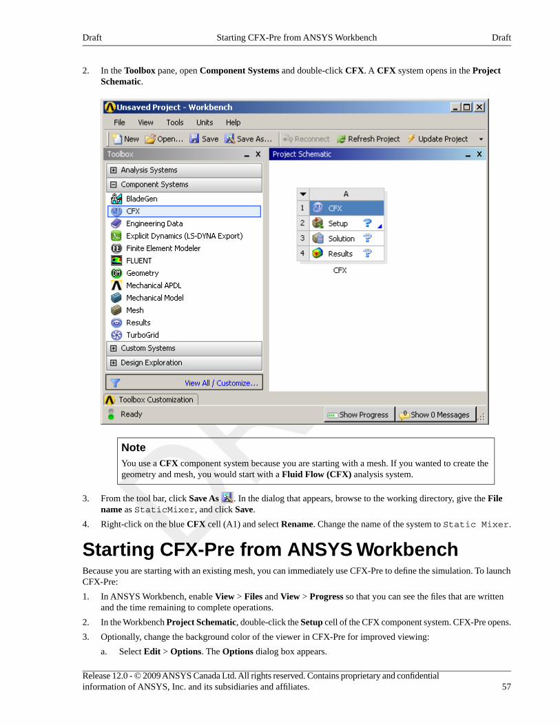
2. In the Toolbox pane, open Component Systems and double-click CFX. A CFX system opens in the ProjectSchematic.
NoteYou use a CFX component system because you are starting with a mesh. If you wanted to create thegeometry and mesh, you would start with a Fluid Flow (CFX) analysis system.
3. From the tool bar, click Save As . In the dialog that appears, browse to the working directory, give the Filename as StaticMixer, and click Save.
4. Right-click on the blue CFX cell (A1) and select Rename. Change the name of the system to Static Mixer.
Starting CFX-Pre from ANSYS WorkbenchBecause you are starting with an existing mesh, you can immediately use CFX-Pre to define the simulation. To launchCFX-Pre:
1. In ANSYS Workbench, enable View > Files and View > Progress so that you can see the files that are writtenand the time remaining to complete operations.
2. In the Workbench Project Schematic, double-click the Setup cell of the CFX component system. CFX-Pre opens.
3. Optionally, change the background color of the viewer in CFX-Pre for improved viewing:
a. Select Edit > Options. The Options dialog box appears.
57Release 12.0 - © 2009 ANSYS Canada Ltd. All rights reserved. Contains proprietary and confidentialinformation of ANSYS, Inc. and its subsidiaries and affiliates.
DraftStarting CFX-Pre from ANSYS WorkbenchDraft
b. Adjust the color settings under CFX-Pre > Graphics Style. For example, you could set the Background >Color Type to Solid and the Color to white.
c. Click OK.
Creating the Simulation DefinitionBefore importing and working with the mesh, you need to create a simulation; in this example, you will use QuickSetup mode. Quick Setup mode provides a simple wizard-like interface for setting up simple cases. This is useful forgetting familiar with the basic elements of a CFD problem setup.
1. In CFX-Pre, select Tools > Quick Setup Mode. The Quick Setup Wizard opens, enabling you to define thissingle-phase simulation.
2. Under Working Fluid select Water. This is a fluid already defined in the library of materials as water at 25°C.
3. Under Mesh File, click Browse .
The Import Mesh dialog box appears.
4. From your working directory, select StaticMixerMesh.gtm and click Open.
The mesh loads, which enables you to apply physics.
5. Click Next.
Setting the Physics DefinitionYou need to define the type of flow and the physical models to use in the fluid domain.
The flow is steady state and you will specify the turbulence and heat transfer. Turbulence is modeled using the k-εturbulence model and heat transfer using the thermal energy model. The k-ε turbulence model is a commonly usedmodel and is suitable for a wide range of applications. The thermal energy model neglects high speed energy effectsand is therefore suitable for low speed flow applications.
1. Under Model Data, note that the Reference Pressure is set to 1 [atm].
All other pressure settings are relative to this reference pressure.
2. Set Heat Transfer to Thermal Energy.
3. Leave Turbulence at its default setting, k-Epsilon.
4. Click Next.
Defining BoundariesThe CFD model requires the definition of conditions on the boundaries of the domain.
1. Delete Inlet and Outlet from the list by right-clicking each and selecting Delete Boundary.
2. Right-click in the blank area where Inlet and Outlet were listed, then select Add Boundary.
3. Set Name to in1.
4. Click OK.
The boundary is created and, when selected, properties related to the boundary are displayed.
Setting Boundary DataOnce boundaries are created, you need to create associated data. Based on Figure 3.1, “Static Mixer with 2 Inlet Pipesand 1 Outlet Pipe” (p. 56), you will define the velocity and temperature for the first inlet.
Release 12.0 - © 2009 ANSYS Canada Ltd. All rights reserved. Contains proprietary and confidentialinformation of ANSYS, Inc. and its subsidiaries and affiliates.58
DraftCreating the Simulation DefinitionDraft
1. In the Boundary Definition for in1, set Boundary Type to Inlet.
2. Set Location to in1.
3. Set the Flow Specification Option to Normal Speed and set Normal Speed to: 2 [m s^-1]
4. Set the Temperature Specification Static Temperature to 315 [K] (note the units).
Creating the Second Inlet Boundary DefinitionBased on Figure 3.1, “Static Mixer with 2 Inlet Pipes and 1 Outlet Pipe” (p. 56), you know the second inlet boundarycondition consists of a velocity of 2 m/s and a temperature of 285 K at one of the side inlets. You will define that now.
1. Under Boundary Definition, right-click in the selector area and select Add Boundary.
2. Create a new boundary named in2 with these settings:
ValueSettingTab
InletBoundary TypeBoundary Data
in2Location
Normal SpeedOptionFlow Specification
2 [m s^-1]Normal Speed
285 [K]Static TemperatureTemperature Specification
Creating the Outlet Boundary DefinitionNow that the second inlet boundary has been created, the same concepts can be applied to building the outlet boundary.
1. Create a new boundary named out with these settings:
ValueSettingTab
OutletBoundary TypeBoundary Data
outLocation
Average Static PressureOptionFlow Specification
0 [Pa]Relative Pressure
2. Click Next.
Moving to General ModeThere are no further boundary conditions that need to be set. All 2D exterior regions that have not been assigned to aboundary condition are automatically assigned to the default boundary condition.
1. Set Operation to Enter General Mode.
2. Click Finish.
The three boundary conditions are displayed in the viewer as sets of arrows at the boundary surfaces. Inlet boundaryarrows are directed into the domain. Outlet boundary arrows are directed out of the domain.
59Release 12.0 - © 2009 ANSYS Canada Ltd. All rights reserved. Contains proprietary and confidentialinformation of ANSYS, Inc. and its subsidiaries and affiliates.
DraftCreating the Second Inlet Boundary DefinitionDraft
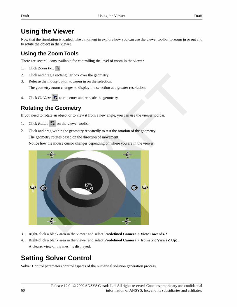
Using the ViewerNow that the simulation is loaded, take a moment to explore how you can use the viewer toolbar to zoom in or out andto rotate the object in the viewer.
Using the Zoom ToolsThere are several icons available for controlling the level of zoom in the viewer.
1. Click Zoom Box
2. Click and drag a rectangular box over the geometry.
3. Release the mouse button to zoom in on the selection.
The geometry zoom changes to display the selection at a greater resolution.
4. Click Fit View to re-center and re-scale the geometry.
Rotating the GeometryIf you need to rotate an object or to view it from a new angle, you can use the viewer toolbar.
1. Click Rotate on the viewer toolbar.
2. Click and drag within the geometry repeatedly to test the rotation of the geometry.
The geometry rotates based on the direction of movement.
Notice how the mouse cursor changes depending on where you are in the viewer:
3. Right-click a blank area in the viewer and select Predefined Camera > View Towards-X.
4. Right-click a blank area in the viewer and select Predefined Camera > Isometric View (Z Up).
A clearer view of the mesh is displayed.
Setting Solver ControlSolver Control parameters control aspects of the numerical solution generation process.
Release 12.0 - © 2009 ANSYS Canada Ltd. All rights reserved. Contains proprietary and confidentialinformation of ANSYS, Inc. and its subsidiaries and affiliates.60
DraftUsing the ViewerDraft
While an upwind advection scheme is less accurate than other advection schemes, it is also more robust. This advectionscheme is suitable for obtaining an initial set of results, but in general should not be used to obtain final accurate results.
The time scale can be calculated automatically by the solver or set manually. The Automatic option tends to beconservative, leading to reliable, but often slow, convergence. It is often possible to accelerate convergence by applyinga time scale factor or by choosing a manual value that is more aggressive than the Automatic option. In this tutorial,you will select a physical time scale, leading to convergence that is twice as fast as the Automatic option.
1. In the CFX-Pre tool bar, click Solver Control .
2. On the Basic Settings tab, set Advection Scheme > Option to Upwind.
3. Set Convergence Control > Fluid Timescale Control > Timescale Control to Physical Timescale andset the physical timescale value to 2 [s].
4. Click OK.
Refresh the ProjectNow that the simulation setup is complete, refresh the project:
1. In ANSYS Workbench, enable View > Files and View > Progress so you can see the files that are written andthe time remaining to complete the refresh.
2. Right-click on the Solution cell and select Refresh.
3. If the Solution cell displays a prompt to perform an update, right-click on the Solution cell and select Update.
Obtaining a SolutionTo obtain a solution, you need to launch the CFX-Solver Manager and subsequently use it to start the solver:
1. Double-click on the ANSYS Workbench Solution cell. The CFX-Solver Manager appears with the Define Rundialog box displayed.
The Define Run dialog box enables configuration of a run for processing by CFX-Solver. In this case, all of theinformation required to perform a new serial run (on a single processor) is entered automatically. You do not needto alter the information in the Define Run dialog box.
2. Click Start Run.
CFX-Solver launches and a split screen appears and displays the results of the run graphically and as text. Thepanes continue to build as CFX-Solver Manager operates.
One window shows the convergence history plots and the other displays text output from CFX-Solver. The textlists physical properties, boundary conditions, and various other parameters used or calculated in creating themodel. All the text is written to the output file automatically (in this case, StaticMixer_001.out).
61Release 12.0 - © 2009 ANSYS Canada Ltd. All rights reserved. Contains proprietary and confidentialinformation of ANSYS, Inc. and its subsidiaries and affiliates.
DraftRefresh the ProjectDraft
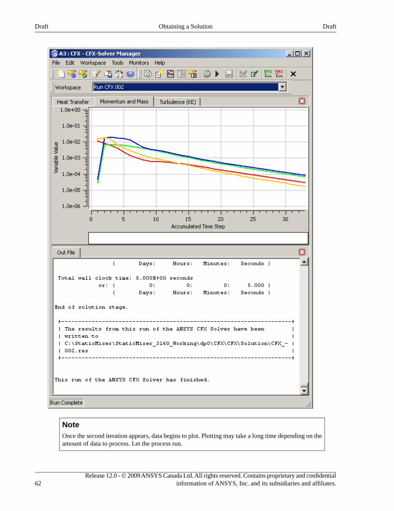
NoteOnce the second iteration appears, data begins to plot. Plotting may take a long time depending on theamount of data to process. Let the process run.
Release 12.0 - © 2009 ANSYS Canada Ltd. All rights reserved. Contains proprietary and confidentialinformation of ANSYS, Inc. and its subsidiaries and affiliates.62
DraftObtaining a SolutionDraft
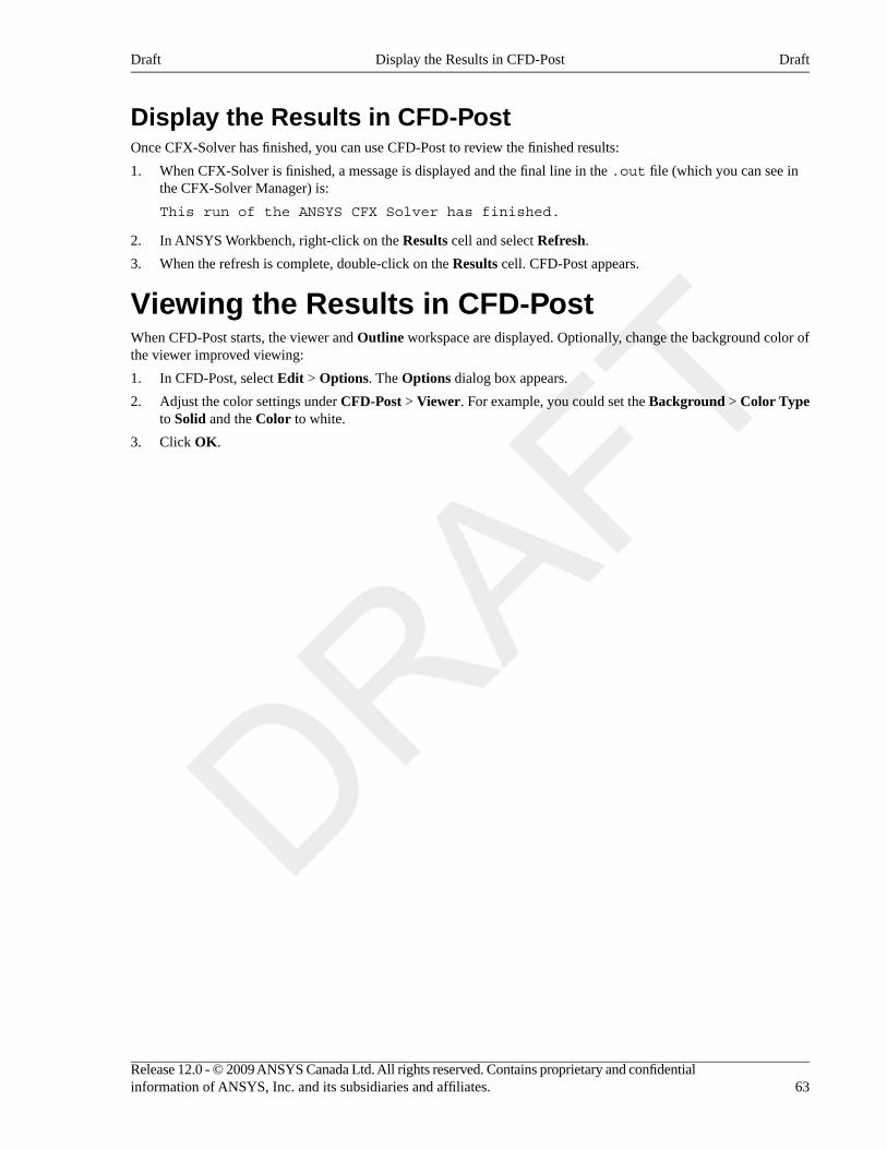
Display the Results in CFD-PostOnce CFX-Solver has finished, you can use CFD-Post to review the finished results:
1. When CFX-Solver is finished, a message is displayed and the final line in the .out file (which you can see inthe CFX-Solver Manager) is:
This run of the ANSYS CFX Solver has finished.
2. In ANSYS Workbench, right-click on the Results cell and select Refresh.
3. When the refresh is complete, double-click on the Results cell. CFD-Post appears.
Viewing the Results in CFD-PostWhen CFD-Post starts, the viewer and Outline workspace are displayed. Optionally, change the background color ofthe viewer improved viewing:
1. In CFD-Post, select Edit > Options. The Options dialog box appears.
2. Adjust the color settings under CFD-Post > Viewer. For example, you could set the Background > Color Typeto Solid and the Color to white.
3. Click OK.
63Release 12.0 - © 2009 ANSYS Canada Ltd. All rights reserved. Contains proprietary and confidentialinformation of ANSYS, Inc. and its subsidiaries and affiliates.
DraftDisplay the Results in CFD-PostDraft
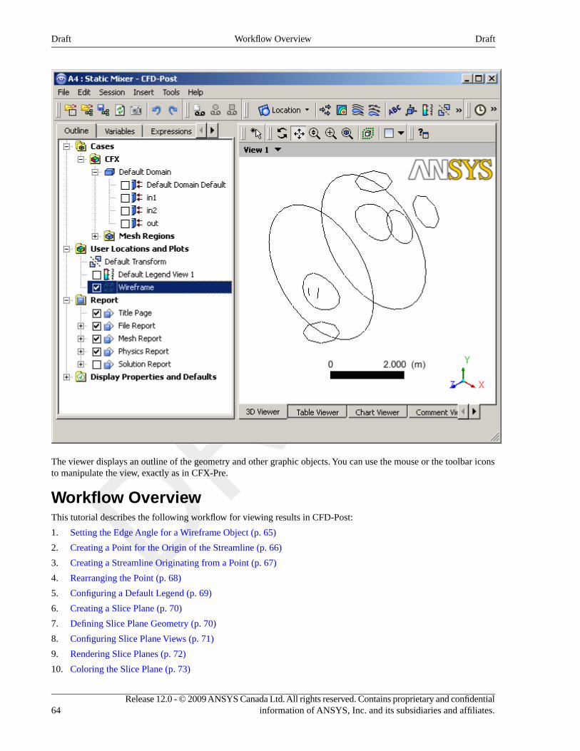
The viewer displays an outline of the geometry and other graphic objects. You can use the mouse or the toolbar iconsto manipulate the view, exactly as in CFX-Pre.
Workflow OverviewThis tutorial describes the following workflow for viewing results in CFD-Post:
1. Setting the Edge Angle for a Wireframe Object (p. 65)
2. Creating a Point for the Origin of the Streamline (p. 66)
3. Creating a Streamline Originating from a Point (p. 67)
4. Rearranging the Point (p. 68)
5. Configuring a Default Legend (p. 69)
6. Creating a Slice Plane (p. 70)
7. Defining Slice Plane Geometry (p. 70)
8. Configuring Slice Plane Views (p. 71)
9. Rendering Slice Planes (p. 72)
10. Coloring the Slice Plane (p. 73)
Release 12.0 - © 2009 ANSYS Canada Ltd. All rights reserved. Contains proprietary and confidentialinformation of ANSYS, Inc. and its subsidiaries and affiliates.64
DraftWorkflow OverviewDraft
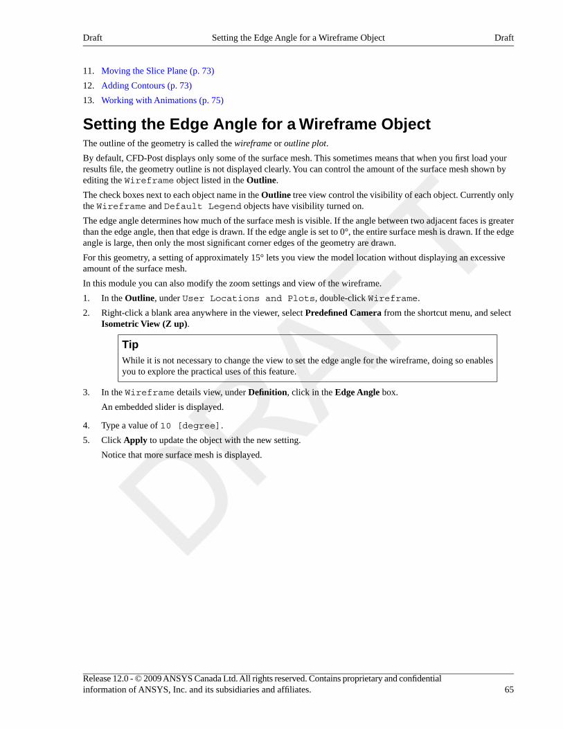
11. Moving the Slice Plane (p. 73)
12. Adding Contours (p. 73)
13. Working with Animations (p. 75)
Setting the Edge Angle for a Wireframe ObjectThe outline of the geometry is called the wireframe or outline plot.
By default, CFD-Post displays only some of the surface mesh. This sometimes means that when you first load yourresults file, the geometry outline is not displayed clearly. You can control the amount of the surface mesh shown byediting the Wireframe object listed in the Outline.
The check boxes next to each object name in the Outline tree view control the visibility of each object. Currently onlythe Wireframe and Default Legend objects have visibility turned on.
The edge angle determines how much of the surface mesh is visible. If the angle between two adjacent faces is greaterthan the edge angle, then that edge is drawn. If the edge angle is set to 0°, the entire surface mesh is drawn. If the edgeangle is large, then only the most significant corner edges of the geometry are drawn.
For this geometry, a setting of approximately 15° lets you view the model location without displaying an excessiveamount of the surface mesh.
In this module you can also modify the zoom settings and view of the wireframe.
1. In the Outline, under User Locations and Plots, double-click Wireframe.
2. Right-click a blank area anywhere in the viewer, select Predefined Camera from the shortcut menu, and selectIsometric View (Z up).
TipWhile it is not necessary to change the view to set the edge angle for the wireframe, doing so enablesyou to explore the practical uses of this feature.
3. In the Wireframe details view, under Definition, click in the Edge Angle box.
An embedded slider is displayed.
4. Type a value of 10 [degree].
5. Click Apply to update the object with the new setting.
Notice that more surface mesh is displayed.
65Release 12.0 - © 2009 ANSYS Canada Ltd. All rights reserved. Contains proprietary and confidentialinformation of ANSYS, Inc. and its subsidiaries and affiliates.
DraftSetting the Edge Angle for a Wireframe ObjectDraft
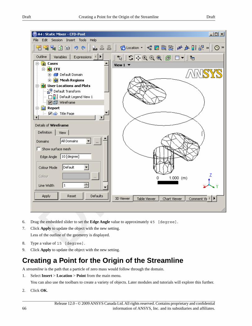
6. Drag the embedded slider to set the Edge Angle value to approximately 45 [degree].
7. Click Apply to update the object with the new setting.
Less of the outline of the geometry is displayed.
8. Type a value of 15 [degree].
9. Click Apply to update the object with the new setting.
Creating a Point for the Origin of the StreamlineA streamline is the path that a particle of zero mass would follow through the domain.
1. Select Insert > Location > Point from the main menu.
You can also use the toolbars to create a variety of objects. Later modules and tutorials will explore this further.
2. Click OK.
Release 12.0 - © 2009 ANSYS Canada Ltd. All rights reserved. Contains proprietary and confidentialinformation of ANSYS, Inc. and its subsidiaries and affiliates.66
DraftCreating a Point for the Origin of the StreamlineDraft
This accepts the default name.
3. Set Definition > Method to XYZ.
4. Under Point, enter the following coordinates: -1, -1, 1.
This is a point near the first inlet.
5. Click Apply.
The point appears as a symbol in the viewer as a crosshair symbol.
Creating a Streamline Originating from a PointWhere applicable, streamlines can trace the flow direction forwards (downstream) and/or backwards (upstream).
1. From the main menu, select Insert > Streamline.
2. Click OK.
3. Set Definition > Start From to Point 1.
TipTo create streamlines originating from more than one location, click the ellipsis icon to the right ofthe Start From box. This displays the Location Selector dialog box, where you can use the Ctrl andShift keys to pick multiple locators.
4. Click the Color tab.
5. Set Mode to Variable.
6. Set Variable to Total Temperature.
7. Set Range to Local.
8. Click Apply.
The streamline shows the path of a zero mass particle from Point 1. The temperature is initially high near thehot inlet, but as the fluid mixes the temperature drops.
67Release 12.0 - © 2009 ANSYS Canada Ltd. All rights reserved. Contains proprietary and confidentialinformation of ANSYS, Inc. and its subsidiaries and affiliates.
DraftCreating a Streamline Originating from a PointDraft
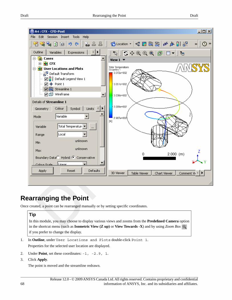
Rearranging the PointOnce created, a point can be rearranged manually or by setting specific coordinates.
TipIn this module, you may choose to display various views and zooms from the Predefined Camera option
in the shortcut menu (such as Isometric View (Z up) or View Towards -X) and by using Zoom Box
if you prefer to change the display.
1. In Outline, under User Locations and Plots double-click Point 1.
Properties for the selected user location are displayed.
2. Under Point, set these coordinates: -1, -2.9, 1.
3. Click Apply.
The point is moved and the streamline redrawn.
Release 12.0 - © 2009 ANSYS Canada Ltd. All rights reserved. Contains proprietary and confidentialinformation of ANSYS, Inc. and its subsidiaries and affiliates.68
DraftRearranging the PointDraft
4. In the viewer toolbar, click Select and ensure that the adjacent toolbar icon is set to Single Select .
While in select mode, you cannot use the left mouse button to re-orient the object in the viewer.
5. In the viewer, drag Point 1 (appears as a yellow addition sign) to a new location within the mixer.
The point position is updated in the details view and the streamline is redrawn at the new location. The pointmoves normal in relation to the viewing direction.
6. Click Rotate .
TipYou can also click in the viewer area, and press the space bar to toggle between Select and ViewingMode. A way to pick objects from Viewing Mode is to hold down Ctrl + Shift while clicking on anobject with the left mouse button.
7. Under Point, reset these coordinates: -1, -1, 1.
8. Click Apply.
The point appears at its original location.
9. Right-click a blank area in the viewer and select Predefined Camera > View Towards -X.
Configuring a Default LegendYou can modify the appearance of the default legend.
The default legend appears whenever a plot is created that is colored by a variable. The streamline color is based ontemperature; therefore, the legend shows the temperature range. The color pattern on the legend's color bar is banded
in accordance with the bands in the plot1.
The default legend displays values for the last eligible plot that was opened in the details view. To maintain a legend
definition during a CFD-Post session, you can create a new legend by clicking Legend .
Because there are many settings that can be customized for the legend, this module allows you the freedom to experimentwith them. In the last steps you will set up a legend, based on the default legend, with a minor modification to theposition.
TipWhen editing values, you can restore the values that were present when you began editing by clicking Reset.To restore the factory-default values, click Default.
1. Double-click Default Legend View 1.
The Definition tab of the default legend is displayed.
2. Apply the following settings
1An exception occurs when one or more bands in a contour plot represent values beyond the legend's range. In this case, such bands are coloredusing a color that is extrapolated slightly past the range of colors shown in the legend. This can happen only when a user-specified range is used forthe legend.
69Release 12.0 - © 2009 ANSYS Canada Ltd. All rights reserved. Contains proprietary and confidentialinformation of ANSYS, Inc. and its subsidiaries and affiliates.
DraftConfiguring a Default LegendDraft
ValueSettingTab
User SpecifiedTitle ModeDefinition
Streamline Temp.Title
(Selected)Horizontal
BottomLocation > Y Justification
3. Click Apply.
The appearance and position of the legend changes based on the settings specified.
4. Modify various settings in Definition and click Apply after each change.
5. Select Appearance.
6. Modify a variety of settings in the Appearance and click Apply after each change.
7. Click Defaults.
8. Click Apply.
9. Under Outline, in User Locations and Plots, clear the check boxes for Point 1 and Streamline1.
Since both are no longer visible, the associated legend no longer appears.
Creating a Slice PlaneDefining a slice plane allows you to obtain a cross-section of the geometry.
In CFD-Post you often view results by coloring a graphic object. The graphic object could be an isosurface, a vectorplot, or in this case, a plane. The object can be a fixed color or it can vary based on the value of a variable.
You already have some objects defined by default (listed in the Outline). You can view results on the boundaries ofthe static mixer by coloring each boundary object by a variable. To view results within the geometry (that is, onnon-default locators), you will create new objects.
You can use the following methods to define a plane:
• Three Points: creates a plane from three specified points.
• Point and Normal: defines a plane from one point on the plane and a normal vector to the plane.
• YZ Plane, ZX Plane, and XY Plane: similar to Point and Normal, except that the normal is definedto be normal to the indicated plane.
1. From the main menu, select Insert > Location > Plane or click Location > Plane.
2. In the Insert Plane window, type: Slice
3. Click OK.
The details view for the plane appears; the Geometry, Color, Render, and View tabs let you configure thecharacteristics of the plane.
Defining Slice Plane GeometryYou need to choose the vector normal to the plane. You want the plane to lie in the x-y plane, hence its normal vectorpoints along the z-axis. You can specify any vector that points in the z-direction, but you will choose the most obvious(0,0,1).
1. On the Geometry tab, expand Definition.
Release 12.0 - © 2009 ANSYS Canada Ltd. All rights reserved. Contains proprietary and confidentialinformation of ANSYS, Inc. and its subsidiaries and affiliates.70
DraftCreating a Slice PlaneDraft
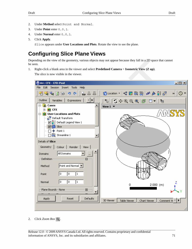
2. Under Method select Point and Normal.
3. Under Point enter 0,0,1.
4. Under Normal enter 0,0,1.
5. Click Apply.
Slice appears under User Locations and Plots. Rotate the view to see the plane.
Configuring Slice Plane ViewsDepending on the view of the geometry, various objects may not appear because they fall in a 2D space that cannotbe seen.
1. Right-click a blank area in the viewer and select Predefined Camera > Isometric View (Z up).
The slice is now visible in the viewer.
2. Click Zoom Box .
71Release 12.0 - © 2009 ANSYS Canada Ltd. All rights reserved. Contains proprietary and confidentialinformation of ANSYS, Inc. and its subsidiaries and affiliates.
DraftConfiguring Slice Plane ViewsDraft
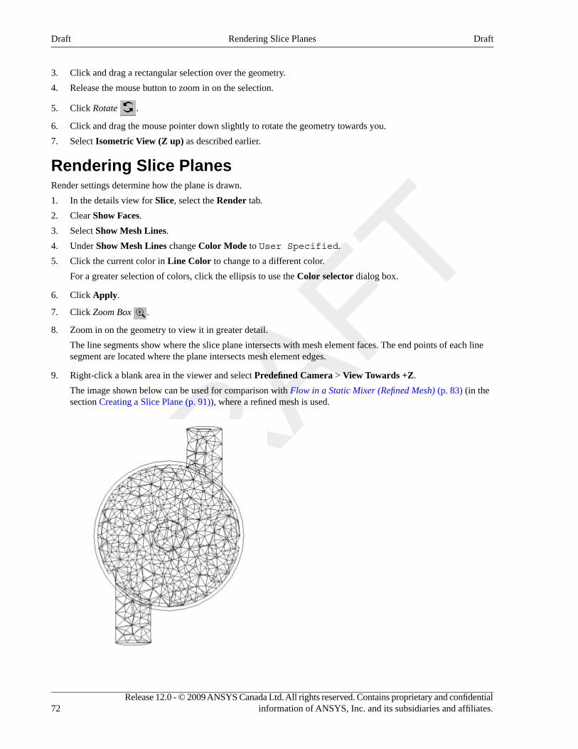
3. Click and drag a rectangular selection over the geometry.
4. Release the mouse button to zoom in on the selection.
5. Click Rotate .
6. Click and drag the mouse pointer down slightly to rotate the geometry towards you.
7. Select Isometric View (Z up) as described earlier.
Rendering Slice PlanesRender settings determine how the plane is drawn.
1. In the details view for Slice, select the Render tab.
2. Clear Show Faces.
3. Select Show Mesh Lines.
4. Under Show Mesh Lines change Color Mode to User Specified.
5. Click the current color in Line Color to change to a different color.
For a greater selection of colors, click the ellipsis to use the Color selector dialog box.
6. Click Apply.
7. Click Zoom Box .
8. Zoom in on the geometry to view it in greater detail.
The line segments show where the slice plane intersects with mesh element faces. The end points of each linesegment are located where the plane intersects mesh element edges.
9. Right-click a blank area in the viewer and select Predefined Camera > View Towards +Z.
The image shown below can be used for comparison with Flow in a Static Mixer (Refined Mesh) (p. 83) (in thesection Creating a Slice Plane (p. 91)), where a refined mesh is used.
Release 12.0 - © 2009 ANSYS Canada Ltd. All rights reserved. Contains proprietary and confidentialinformation of ANSYS, Inc. and its subsidiaries and affiliates.72
DraftRendering Slice PlanesDraft
Coloring the Slice PlaneThe Color panel is used to determine how the object faces are colored.
1. Apply the following settings to Slice
ValueSettingTab
VariableaModeColor
TemperatureVariable
(Selected)Show FacesRender
(Cleared)Show Mesh Lines
aYou can specify the variable (in this case, temperature) used to color the graphic element. The Constant mode allows you to color theplane with a fixed color.
2. Click Apply.
Hot water (red) enters from one inlet and cold water (blue) from the other.
Moving the Slice PlaneYou can move the plane to different locations:
1. Right-click a blank area in the viewer and select Predefined Camera > Isometric View (Z up) from the shortcutmenu.
2. Click the Geometry tab.
Review the settings in Definition under Point and under Normal.
3. Click Single Select .
4. Click and drag the plane to a new location that intersects the domain.
As you drag the mouse, the viewer updates automatically. Note that Point updates with new settings.
5. Type in Point settings of 0,0,1.
6. Click Apply.
7. Click Rotate .
8. Turn off the visibility for Slice by clearing the check box next to Slice in the Outline tree view.
Adding ContoursContours connect all points of equal value for a scalar variable (for example, Temperature) and help to visualizevariable values and gradients. Colored bands fill the spaces between contour lines. Each band is colored by the averagecolor of its two bounding contour lines (even if the latter are not displayed).
1. Right-click a blank area in the viewer and select Predefined Camera > Isometric View (Z up) from the shortcutmenu.
2. Select Insert > Contour from the main menu or click Contour .
The Insert Contour dialog box is displayed.
3. Set Name to Slice Contour.
73Release 12.0 - © 2009 ANSYS Canada Ltd. All rights reserved. Contains proprietary and confidentialinformation of ANSYS, Inc. and its subsidiaries and affiliates.
DraftColoring the Slice PlaneDraft
4. Click OK.
5. Apply the following settings
ValueSettingTab
SliceLocationsGeometry
TemperatureVariable
(Selected)Show Contour LinesRender
6. Click Apply.
ImportantThe colors of 3D graphics object faces are slightly altered when lighting is on. To view colors withhighest accuracy, go to the Render tab and, under Show Faces, clear Lighting and click Apply.
The graphic element faces are visible, producing a contour plot as shown.
Release 12.0 - © 2009 ANSYS Canada Ltd. All rights reserved. Contains proprietary and confidentialinformation of ANSYS, Inc. and its subsidiaries and affiliates.74
DraftAdding ContoursDraft
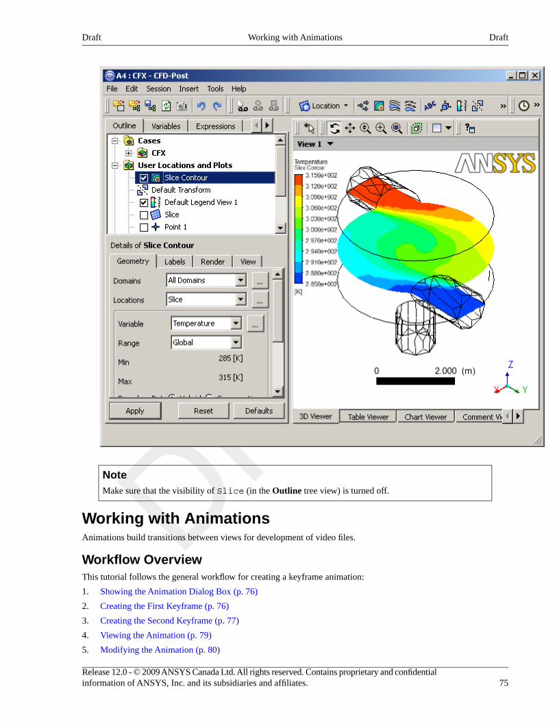
NoteMake sure that the visibility of Slice (in the Outline tree view) is turned off.
Working with AnimationsAnimations build transitions between views for development of video files.
Workflow OverviewThis tutorial follows the general workflow for creating a keyframe animation:
1. Showing the Animation Dialog Box (p. 76)
2. Creating the First Keyframe (p. 76)
3. Creating the Second Keyframe (p. 77)
4. Viewing the Animation (p. 79)
5. Modifying the Animation (p. 80)
75Release 12.0 - © 2009 ANSYS Canada Ltd. All rights reserved. Contains proprietary and confidentialinformation of ANSYS, Inc. and its subsidiaries and affiliates.
DraftWorking with AnimationsDraft
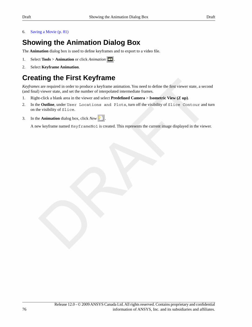
6. Saving a Movie (p. 81)
Showing the Animation Dialog BoxThe Animation dialog box is used to define keyframes and to export to a video file.
1. Select Tools > Animation or click Animation .
2. Select Keyframe Animation.
Creating the First KeyframeKeyframes are required in order to produce a keyframe animation. You need to define the first viewer state, a second(and final) viewer state, and set the number of interpolated intermediate frames.
1. Right-click a blank area in the viewer and select Predefined Camera > Isometric View (Z up).
2. In the Outline, under User Locations and Plots, turn off the visibility of Slice Contour and turnon the visibility of Slice.
3. In the Animation dialog box, click New .
A new keyframe named KeyframeNo1 is created. This represents the current image displayed in the viewer.
Release 12.0 - © 2009 ANSYS Canada Ltd. All rights reserved. Contains proprietary and confidentialinformation of ANSYS, Inc. and its subsidiaries and affiliates.76
DraftShowing the Animation Dialog BoxDraft
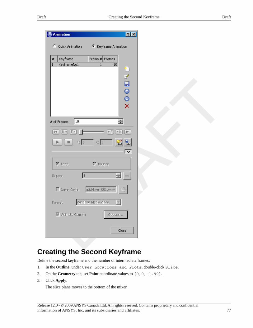
Creating the Second KeyframeDefine the second keyframe and the number of intermediate frames:
1. In the Outline, under User Locations and Plots, double-click Slice.
2. On the Geometry tab, set Point coordinate values to (0,0,-1.99).
3. Click Apply.
The slice plane moves to the bottom of the mixer.
77Release 12.0 - © 2009 ANSYS Canada Ltd. All rights reserved. Contains proprietary and confidentialinformation of ANSYS, Inc. and its subsidiaries and affiliates.
DraftCreating the Second KeyframeDraft
4. In the Animation dialog box, click New .
KeyframeNo2 is created and represents the image displayed in the viewer.
5. Select KeyframeNo1 so that you can set the number of frames to be interpolated between the two keyframes.
6. Set # of Frames (located below the list of keyframes) to 20.
This is the number of intermediate frames used when going from KeyframeNo1 to KeyframeNo2. This numberis displayed in the Frames column for KeyframeNo1.
7. Press Enter.
The Frame # column shows the frame in which each keyframe appears. KeyframeNo1 appears at frame 1 sinceit defines the start of the animation. KeyframeNo2 is at frame 22 since you have 20 intermediate frames (frames2 to 21) in between KeyframeNo1 and KeyframeNo2.
Release 12.0 - © 2009 ANSYS Canada Ltd. All rights reserved. Contains proprietary and confidentialinformation of ANSYS, Inc. and its subsidiaries and affiliates.78
DraftCreating the Second KeyframeDraft

Viewing the AnimationMore keyframes could be added, but this animation has only two keyframes (which is the minimum possible).
The controls previously greyed-out in the Animation dialog box are now available. The number of intermediate framesbetween keyframes is listed beside the keyframe having the lowest number of the pair. The number of frames listedbeside the last keyframe is ignored.
1. Click To Beginning .
This ensures that the animation will begin at the first keyframe.
79Release 12.0 - © 2009 ANSYS Canada Ltd. All rights reserved. Contains proprietary and confidentialinformation of ANSYS, Inc. and its subsidiaries and affiliates.
DraftViewing the AnimationDraft
2. Click Play the animation .
The animation plays from frame 1 to frame 22. It plays relatively slowly because the slice plane must be updatedfor each frame.
Modifying the AnimationTo make the plane sweep through the whole geometry, you will set the starting position of the plane to be at the topof the mixer. You will also modify the Range properties of the plane so that it shows the temperature variation better.As the animation is played, you can see the hot and cold water entering the mixer. Near the bottom of the mixer (wherethe water flows out) you can see that the temperature is quite uniform. The new temperature range lets you view themixing process more accurately than the global range used in the first animation.
1. Apply the following settings to Slice
ValueSettingTab
0, 0, 1.99PointGeometry
VariableModeColor
TemperatureVariable
User SpecifiedRange
295 [K]Min
305 [K]Max
2. Click Apply.
The slice plane moves to the top of the static mixer.
NoteDo not double-click in the next step.
3. In the Animation dialog box, single click (do not double-click) KeyframeNo1 to select it.
If you had double-clicked KeyFrameNo1, the plane and viewer states would have been redefined according to
the stored settings for KeyFrameNo1. If this happens, click Undo and try again to select the keyframe.
4. Click Set Keyframe .
The image in the viewer replaces the one previously associated with KeyframeNo1.
5. Double-click KeyframeNo2.
The object properties for the slice plane are updated according to the settings in KeyFrameNo2.
6. Apply the following settings to Slice
ValueSettingTab
VariableModeColor
TemperatureVariable
User SpecifiedRange
Release 12.0 - © 2009 ANSYS Canada Ltd. All rights reserved. Contains proprietary and confidentialinformation of ANSYS, Inc. and its subsidiaries and affiliates.80
DraftModifying the AnimationDraft
ValueSettingTab
295 [K]Min
305 [K]Max
7. Click Apply.
8. In the Animation dialog box, single-click KeyframeNo2.
9. Click Set Keyframe to save the new settings to KeyframeNo2.
Saving a Movie1. Click More Animation Options to view the additional options.
The Loop and Bounce radio buttons determine what happens when the animation reaches the last keyframe.When Loop is selected, the animation repeats itself the number of times defined by Repeat. When Bounce isselected, every other cycle is played in reverse order, starting with the second.
2. Select Save Movie.
3. Set Format to MPEG1.
4. Click Browse next to Save Movie.
5. Under File name type: StaticMixer.mpg
6. If required, set the path location to a different directory. You may want to set the directory to your workingdirectory so that the animation will be in the same location as the project files; however, ANSYS Workbench willnot store the file as part of the project.
7. Click Save.
The movie file name (including path) has been set, but the animation has not yet been produced.
8. Click To Beginning .
9. Click Play the animation .
10. If prompted to overwrite an existing movie click Overwrite.
The animation plays and builds an MPEG file.
11. Click the Options button at the bottom of the Animation dialog box.
In Advanced, you can see that a Frame Rate of 24 frames per second was used to create the animation. Theanimation you produced contains a total of 22 frames, so it takes just under 1 second to play in a media player.
12. Click Cancel to close the dialog box.
13. Close the Animation dialog box.
14. View the animation using a media player.
Closing the ApplicationsBefore you close the project, take a moment to look at the files listed in the Files view. You will see the project file,StaticMixer.wbpj, and the files that ANSYS Workbench created (CFX-Solver Input, CFX-Solver Output,CFX-Solver Results, CFX-Pre Case, CFD-Post State, and Design Point files). Any files that you added to that part ofthe file system (such as the movie file) will not be listed.
81Release 12.0 - © 2009 ANSYS Canada Ltd. All rights reserved. Contains proprietary and confidentialinformation of ANSYS, Inc. and its subsidiaries and affiliates.
DraftSaving a MovieDraft

Close ANSYS Workbench (and the applications it launched) by selecting File > Exit from ANSYS Workbench.ANSYS Workbench prompts you to save all of your project files.
Release 12.0 - © 2009 ANSYS Canada Ltd. All rights reserved. Contains proprietary and confidentialinformation of ANSYS, Inc. and its subsidiaries and affiliates.82
DraftClosing the ApplicationsDraft
Chapter 4. Flow in a Static Mixer (RefinedMesh)This tutorial includes:
• Tutorial Features (p. 83)
• Overview of the Problem to Solve (p. 84)
• Before You Begin (p. 84)
• Starting CFX-Pre (p. 84)
• Defining a Simulation using General Mode in CFX-Pre (p. 84)
• Obtaining a Solution with CFX-Solver (p. 89)
• Viewing the Results in CFD-Post (p. 91)
Tutorial FeaturesIn this tutorial you will learn about:
• Using the General Mode of CFX-Pre (this mode is used for more complex cases).
• Rerunning a problem with a refined mesh.
• Importing CCL to copy the definition of a different simulation into the current simulation.
• Viewing the mesh with a Sphere Volume locator and a Surface Plot.
• Using the Report Viewer to analyze mesh quality.
DetailsFeatureComponent
General ModeUser ModeCFX-Pre
Steady StateAnalysis Type
General FluidFluid Type
Single DomainDomain Type
k-EpsilonTurbulence Model
Thermal EnergyHeat Transfer
Inlet (Subsonic)Boundary Conditions
Outlet (Subsonic)
Wall: No-Slip
Wall: Adiabatic
Physical Time ScaleTimestep
Slice PlanePlotsCFD-Post
Sphere Volume
Viewing the MeshOther
83Release 12.0 - © 2009 ANSYS Canada Ltd. All rights reserved. Contains proprietary and confidentialinformation of ANSYS, Inc. and its subsidiaries and affiliates.
DraftDraft
Overview of the Problem to SolveIn this tutorial, you use a refined mesh to obtain a better solution to the Static Mixer problem created in SimulatingFlow in a Static Mixer Using CFX in Standalone Mode (p. 27). You establish a general workflow for analyzing theflow of fluid into and out of a mixer. This tutorial uses a specific problem to teach the general approach taken whenworking with an existing mesh.
You start a new simulation in CFX-Pre and import the refined mesh. This tutorial introduces General Mode-the modeused for most tutorials-in CFX-Pre. The physics for this tutorial are the same as for Simulating Flow in a Static MixerUsing CFX in Standalone Mode (p. 27); therefore, you can import the physics settings used in that tutorial to savetime.
Before You BeginIf this is the first tutorial you are working with, it is important to review the following topics before beginning:
• Preparing a Working Directory (p. 23)
• Setting the Working Directory and Starting ANSYS CFX (p. 23)
• Changing the Display Colors (p. 24)
• Playing a Tutorial Session File (p. 24)
Starting CFX-Pre1. Prepare the working directory using the following files in the examples directory:
• StaticMixerRefMesh.gtm
• StaticMixerRef.pre
• StaticMixer.def
• StaticMixer_001.res
For details, see Preparing a Working Directory (p. 23)
2. Set the working directory and start CFX-Pre
For details, see Setting the Working Directory and Starting ANSYS CFX (p. 23)
Defining a Simulation using General Mode inCFX-PreAfter having completed meshing, CFX-Pre is used as a consistent and intuitive interface for the definition of complexCFD problems.
Workflow OverviewThis section provides a brief summary of the topics so that you can see the workflow:
1. Creating a New Case (p. 85)
2. Importing a Mesh (p. 85)
3. Importing CCL (p. 86)
4. Viewing Domain Settings (p. 86)
5. Viewing the Boundary Condition Setting (p. 87)
6. Defining Solver Parameters (p. 87)
Release 12.0 - © 2009 ANSYS Canada Ltd. All rights reserved. Contains proprietary and confidentialinformation of ANSYS, Inc. and its subsidiaries and affiliates.84
DraftOverview of the Problem to SolveDraft
7. Writing the CFX-Solver Input (.def) File (p. 88)
As an alternative to these steps, you can set up the simulation automatically by following the procedures in Playingthe Session File and Starting CFX-Solver Manager (p. 88).
To begin this tutorial and create a new simulation in CFX-Pre, continue from Creating a New Case (p. 85).
Creating a New CaseBefore importing and working with a mesh, a simulation needs to be developed using General mode.
NoteTwo procedures are documented. Depending on your installation of CFX, follow either the Standaloneprocedure or the Workbench procedure.
Procedure in Standalone1. If required, launch CFX-Pre.
2. Select File > New Case.
3. Select General in the New Case dialog box and click OK.
4. Select File > Save Case As.
5. Under File name, type StaticMixerRef and click Save.
6. Proceed to Importing a Mesh (p. 85).
Procedure in Workbench1. If required, launch ANSYS Workbench.
2. Click Empty Project.
The Project page appears displaying an unsaved project.
3. Select File > Save or click Save .
4. If required, set the path location to your working directory.
5. Under File name, type StaticMixerRef and click Save.
6. Click Start CFX-Pre under Advanced CFD on the left hand task bar.
7. Select File > New Case.
8. Click General in the New Case dialog, and then click OK.
9. Select File > Save Case As.
10. Under File name, type StaticMixerRef and click Save.
Importing a MeshAt least one mesh must be imported before physics are applied.
An assembly is a group of mesh regions that are topologically connected. Each assembly can contain only one mesh,but multiple assemblies are permitted. The Mesh tree shows the regions in Assembly in a tree structure. The levelbelow Assembly displays 3D regions and the level below each 3D region shows the 2D regions associated with it.The check box next to each item in the Mesh tree indicates the visibility status of the object in the viewer; you canclick these to toggle visibility.
1. Select File > Import > Mesh or right-click Mesh and select Import Mesh > Other.
2. In the Import Mesh dialog box, select StaticMixerRefMesh.gtm from your working directory.
85Release 12.0 - © 2009 ANSYS Canada Ltd. All rights reserved. Contains proprietary and confidentialinformation of ANSYS, Inc. and its subsidiaries and affiliates.
DraftCreating a New CaseDraft
This is a mesh that is more refined than the one used in Tutorial 1.
3. Click Open.
4. Right-click a blank area in the viewer and select Predefined Camera > Isometric View (Z up) from the shortcutmenu.
Importing CCLSince the physics for this simulation is very similar to that for Tutorial 1, you can save time by importing the settingsused there.
The CCL contains settings that reference mesh regions. For example, the outlet boundary condition references themesh region named out. In this tutorial, the name of the mesh regions are the same as in Tutorial 1, so you can importthe CCL without error.
The physics for a simulation can be saved to a CCL (CFX Command Language) file at any time by selecting File >Export > CCL. However, a number of other files can also be used as sources to import CCL including:
• Simulation files (*.cfx)
• Results files (*.res)
• CFX-Solver input files(*.def)
NoteIf you import CCL that references non-existent mesh regions, you will get errors.
1. Select File > Import > CCL.
The Import CCL dialog box appears.
2. Under Import Method, select Replace.
Replace is useful if you have defined physics and want to update or replace them with newly imported physics.
3. Under File type, select CFX-Solver Files (*def *res).
4. Select StaticMixer.def created in Tutorial 1. If you did not work through Tutorial 1, you can copy this filefrom the examples directory.
5. Click Open.
6. Select the Outline tab.
TipTo select Outline you may need to click the navigation icons next to the tabs to move ‘forward' or‘backward' through the various tabs.
The tree view displays a summary of the current simulation in a tree structure. Some items may be recognizedfrom Tutorial 1-for example the boundary condition objects in1, in2, and out.
Viewing Domain SettingsIt is useful to review the options available in General Mode.
Various domain settings can be set. These include:
• Basic Settings
Specifies the location of the domain, coordinate frame settings and the fluids/solids that are present in the domain.You also reference pressure, buoyancy and whether the domain is stationary or rotating. Mesh motion can also beset.
Release 12.0 - © 2009 ANSYS Canada Ltd. All rights reserved. Contains proprietary and confidentialinformation of ANSYS, Inc. and its subsidiaries and affiliates.86
DraftImporting CCLDraft
• Fluid Models
Sets models that apply to the fluid(s) in the domain, such as heat transfer, turbulence, combustion, and radiationmodels. An option absent in Tutorial 1 is Turbulent Wall Functions, which is set to Scalable. Wall functionsmodel the flow in the near-wall region. For the k-epsilon turbulence model, you should always use scalable wallfunctions.
• Initialization
Sets the initial conditions for the current domain only. This is generally used when multiple domains exist to allowsetting different initial conditions in each domain, but can also be used to initialize single-domain simulations.Global initialization allows the specification of initial conditions for all domains that do not have domain-specificinitialization.
1. On the Outline tree view, under Simulation > Flow Analysis 1, double-click Default Domain.
The domain Default Domain is opened for editing.
2. Click the Basic Settings tab and review, but do not change, the current settings.
3. Click Fluid Models and review, but do not change, the current settings.
4. Click Initialization and review, but do not change, the current settings.
5. Click Close.
Viewing the Boundary Condition SettingFor the k-epsilon turbulence model, you must specify the turbulent nature of the flow entering through the inlet boundary.For this simulation, the default setting of Medium (Intensity = 5%) is used. This is a sensible setting if youdo not know the turbulence properties of the incoming flow.
1. Under Default Domain, double-click in1.
2. Click the Boundary Details tab and review the settings for Flow Regime, Mass and Momentum, Turbulenceand Heat Transfer.
3. Click Close.
Defining Solver ParametersSolver Control parameters control aspects of the numerical-solution generation process.
In Tutorial 1 you set some solver control parameters, such as Advection Scheme and Timescale Control, while otherparameters were set automatically by CFX-Pre.
In this tutorial, High Resolution is used for the advection scheme. This is more accurate than the Upwind Schemeused in Tutorial 1. You usually require a smaller timestep when using this model. You can also expect the solution totake a higher number of iterations to converge when using this model.
1. Select Insert > Solver > Solver Control from the menu bar or click Solver Control .
2. Apply the following Basic Settings
ValueSetting
High ResolutionAdvection Scheme > Option
150Convergence Control > Max. Iterationsa
Physical TimescaleConvergence Control > Fluid Timescale Control > TimescaleControl
87Release 12.0 - © 2009 ANSYS Canada Ltd. All rights reserved. Contains proprietary and confidentialinformation of ANSYS, Inc. and its subsidiaries and affiliates.
DraftViewing the Boundary Condition SettingDraft
ValueSetting
0.5 [s]Convergence Control > Fluid Timescale Control > PhysicalTimescale
aIf your solution does not meet the convergence criteria after this number of timesteps, the CFX-Solver will stop.
3. Click Apply.
4. Click the Advanced Options tab.
5. Ensure that Global Dynamic Model Control is selected.
6. Click OK.
Writing the CFX-Solver Input (.def) FileOnce all boundaries are created you move from CFX-Pre into CFX-Solver.
The simulation file-StaticMixerRef.cfx-contains the simulation definition in a format that can be loaded byCFX-Pre, allowing you to complete (if applicable), restore, and modify the simulation definition. The simulation filediffers from the CFX-Solver input file in two important ways:
• The simulation file can be saved at any time while defining the simulation.
• The CFX-Solver input file is an encapsulated set of meshes and CCL defining a solver run, and is a subset of thedata in the simulation file.
1. Click Define Run .
The Write Solver Input File dialog box is displayed.
2. If required, set the path to your working directory.
3. Apply the following settings:
ValueSetting
StaticMixerRef.defFile name
4. Click Save.
The CFX-Solver input file (StaticMixerRef.def) is created. CFX-Solver Manager automatically starts and,on the Define Run dialog box, the Solver Input File is set.
5. If you are notified in CFX-Pre that the file already exists, click Overwrite.
6. Quit CFX-Pre, saving the simulation (.cfx) file.
7. Proceed to Obtaining a Solution with CFX-Solver (p. 89).
Playing the Session File and Starting CFX-Solver ManagerIf you have performed all the tasks in the previous steps, proceed directly to Obtaining a Solution withCFX-Solver (p. 89).
Two procedures are documented. Depending on your installation of CFX follow either the standalone procedure orthe ANSYS Workbench procedure.
Procedure in Standalone1. If required, launch CFX-Pre.
Release 12.0 - © 2009 ANSYS Canada Ltd. All rights reserved. Contains proprietary and confidentialinformation of ANSYS, Inc. and its subsidiaries and affiliates.88
DraftWriting the CFX-Solver Input (.def) FileDraft
2. Select Session > Play Tutorial.
3. Select StaticMixerRef.pre.
4. Click Open.
A CFX-Solver input file is written.
5. Select File > Quit.
6. Launch CFX-Solver Manager from CFX Launcher.
7. After CFX-Solver starts, select File > Define Run.
8. Under CFX-Solver Input File, click Browse .
9. Select StaticMixerRef.def, located in the working directory.
10. Proceed to Obtaining a Solution with CFX-Solver (p. 89).
Procedure in ANSYS Workbench1. If required, launch ANSYS Workbench.
2. Click Empty Project.
3. Select File > Save or click Save .
4. Under File name, type StaticMixerRef and click Save.
5. Click Start CFX-Pre.
6. Select Session > Play Tutorial.
7. Select StaticMixerRef.pre.
8. Click Open.
A CFX-Solver input file is written.
9. Click the CFX-Solver tab.
10. Select File > Define Run.
11. Under CFX-Solver Input File, click Browse .
12. Select StaticMixerRef.def, located in the working directory.
Obtaining a Solution with CFX-SolverTwo windows are displayed when CFX-Solver Manager runs. There is an adjustable split between the windows whichis oriented either horizontally or vertically, depending on the aspect ratio of the entire CFX-Solver Manager window(also adjustable).
Workflow OverviewThis section provides a brief summary of the topics to follow as a general workflow:
1. Starting the Run with an Initial Values File (p. 90)
2. Confirming Results (p. 90)
3. Moving from CFX-Solver to CFD-Post (p. 90)
89Release 12.0 - © 2009 ANSYS Canada Ltd. All rights reserved. Contains proprietary and confidentialinformation of ANSYS, Inc. and its subsidiaries and affiliates.
DraftObtaining a Solution with CFX-SolverDraft
Starting the Run with an Initial Values FileIn CFX-Solver Manager, the Define Run dialog box is visible and Solver Input File has automatically been set to theCFX-Solver input file from CFX-Pre: StaticMixerRef.def.
Configure the settings so that the results from Tutorial 1 (contained in StaticMixer_001.res) will be used toinitialize the solution:
1. Select Initial Values Specification.
2. Set Initial Values Specification > Initial Values > Initial Values 1 > Initial Values 1 Settings > File Name toStaticMixer_001.res.
If you did not complete the first tutorial, you can use StaticMixer_001.res from your working directory.
3. Set Use Mesh From to Solver Input File.
4. Clear Initial Values Specification > Continue History From.
This will cause the CFX-Solver to use the results in the StaticMixer_001.res file as a basic initial guessfor the solution, and will cause the iteration count to start from 1 instead of from the last iteration number in theinitial values file.
5. Click Start Run.
NoteConvergence information is plotted once the second outer loop iteration is complete.
Confirming ResultsWhen the run is finished, specific information appears in the text window of CFX-Solver Manager.
To confirm that results interpolation was successful, look in the text window in CFX-Solver Manager. The followingtext appears before the convergence history begins:
+---------------------------------------------------------+| Initial Conditions Supplied by Fields in the Input Files+---------------------------------------------------------+
This lists the variables that were interpolated from the results file. After the final iteration, a message similar to thefollowing content appears:
CFD Solver finished: Tue Oct 19 08:06:45 2004CFD Solver wall clock seconds: 1.7100E+02
This indicates that CFX-Solver has successfully calculated the solution for the problem to the specified accuracy orhas run out of coefficient loops.
1. When CFX-Solver is finished, ensure that the check box next to Post-Process Results is cleared to preventCFD-Post from launching at this time.
2. Click OK. Review the results on the Out File tab for details on the run results.
Moving from CFX-Solver to CFD-PostOnce CFX-Solver has finished, you can use CFD-Post to review the finished results.
1. Select Tools > Post-Process Results or click Post-Process Results in the toolbar.
Release 12.0 - © 2009 ANSYS Canada Ltd. All rights reserved. Contains proprietary and confidentialinformation of ANSYS, Inc. and its subsidiaries and affiliates.90
DraftStarting the Run with an Initial Values FileDraft
2. In the Start ANSYS CFD-Post dialog box, next to Results File, ensure that StaticMixerRef_001.res is
set. If it is not, click Browse and select StaticMixerRef_001.res (located in the working directory).
3. If using CFX-Solver in Standalone Mode, select Shut down CFX-Solver Manager.
This forces Standalone CFX-Solver to close. This option is not required in Workbench.
4. Click OK.
After a short pause, CFD-Post starts.
Viewing the Results in CFD-PostIn the following sections, you will explore the differences between the mesh and the results from this tutorial andtutorial 1.
Creating a Slice PlaneMore information exists for use by CFD-Post in this tutorial than in Tutorial 1 because the slice plane is more detailed.
Once a new slice plane is created it can be compared with Tutorial 1. There are three noticeable differences betweenthe two slice planes.
• Around the edges of the mixer geometry there are several layers of narrow rectangles. This is the region where themesh contains prismatic elements (which are created as inflation layers). The bulk of the geometry containstetrahedral elements.
• There are more lines on the plane than there were in Tutorial 1. This is because the slice plane intersects with moremesh elements.
• The curves of the mixer are smoother than in Tutorial 1 because the finer mesh better represents the true geometry.
1. Right-click a blank area in the viewer and select Predefined Camera > Isometric View (Z up).
2. From the menu bar, select Insert > Location > Plane or under Location, click Plane.
3. In the Insert Plane dialog box, type Slice and click OK.
The Geometry, Color, Render and View tabs let you switch between settings.
4. Apply the following settings
ValueSettingTab
Default DomainDomainsGeometry
XY PlaneDefinition > Method
1 [m]Definition > Z
SlicePlane Type
(Cleared)Show FacesRender
(Selected)Show Mesh Lines
5. Click Apply.
6. Right-click a blank area in the viewer and select Predefined Camera > View Towards +Z.
7. Click Zoom Box .
8. Zoom in on the geometry to view it in greater detail.
91Release 12.0 - © 2009 ANSYS Canada Ltd. All rights reserved. Contains proprietary and confidentialinformation of ANSYS, Inc. and its subsidiaries and affiliates.
DraftViewing the Results in CFD-PostDraft
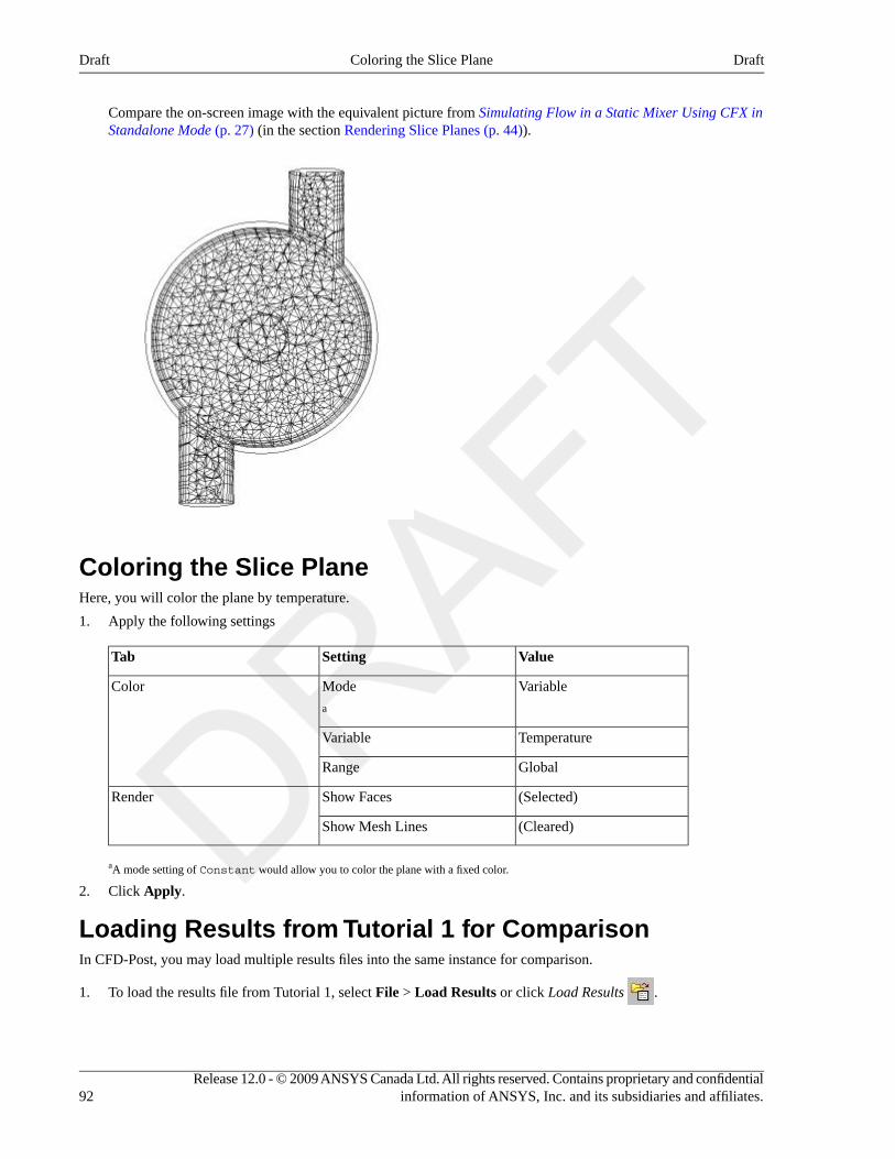
Compare the on-screen image with the equivalent picture from Simulating Flow in a Static Mixer Using CFX inStandalone Mode (p. 27) (in the section Rendering Slice Planes (p. 44)).
Coloring the Slice PlaneHere, you will color the plane by temperature.
1. Apply the following settings
ValueSettingTab
VariableModeColor
a
TemperatureVariable
GlobalRange
(Selected)Show FacesRender
(Cleared)Show Mesh Lines
aA mode setting of Constant would allow you to color the plane with a fixed color.
2. Click Apply.
Loading Results from Tutorial 1 for ComparisonIn CFD-Post, you may load multiple results files into the same instance for comparison.
1. To load the results file from Tutorial 1, select File > Load Results or click Load Results .
Release 12.0 - © 2009 ANSYS Canada Ltd. All rights reserved. Contains proprietary and confidentialinformation of ANSYS, Inc. and its subsidiaries and affiliates.92
DraftColoring the Slice PlaneDraft
2. Be careful not to click Open until instructed to do so. In the Load Results File dialog box, selectStaticMixer_001.res in the <CFXROOT>\examples directory or from your working directory if it hasbeen copied.
3. On the right side of the dialog box, there are three frames:
• Case options
• Additional actions
• CFX run history and multi-configuration options.
Under Case options, select Keep current cases loaded and ensure that Open in new view is selected.
4. Under Additional actions, ensure that the Clear user state before loading check box is cleared.
5. Under CFX run history and multi-configuration options, ensure that Load only the last results is selected.
6. Click Open to load the results.
In the tree view, there is now a second group of domains, meshes and boundary conditions with the headingStaticMixer_001.
7. Double-click the Wireframe object under User Locations and Plots.
8. In the Definition tab, set Edge Angle to 5 [degree].
9. Click Apply.
10. Click Synchronize camera in displayed views so that all viewports maintain the same camera position.
11. Right-click a blank area in the viewer and select Predefined Camera > Isometric View (Z up).
Both meshes are now displayed in a line along the Y axis. Notice that one mesh is of a higher resolution than theother.
12. Set Edge Angle to 30 [degree].
13. Click Apply.
Creating a Second Slice Plane1. In the tree view, right-click the plane named Slice and select Duplicate.
2. Click OK to accept the default name Slice 1.
3. In the tree view, double-click the plane named Slice 1.
4. On the Geometry tab, set Domains to Default Domain.
5. On the Color tab, ensure that Range is set to Global.
6. Click Apply.
7. Double-click Slice and make sure that Range is set to Global.
Comparing Slice Planes using Multiple ViewsThe visibility status of each object is maintained separately for each viewport. This allows some planes to be shown
while others are hidden. However, you can also use the Synchronize visibility in displayed views to synchronizethe visibility of objects that you add.
1. In the viewer toolbar, click Synchronize visibility in displayed views to deselect the option.
2. Click in the viewport that is set to show View 1, then clear the visibility check box for Slice in the Outline treeview and ensure that the visibility check box for Slice 1 is selected.
93Release 12.0 - © 2009 ANSYS Canada Ltd. All rights reserved. Contains proprietary and confidentialinformation of ANSYS, Inc. and its subsidiaries and affiliates.
DraftCreating a Second Slice PlaneDraft
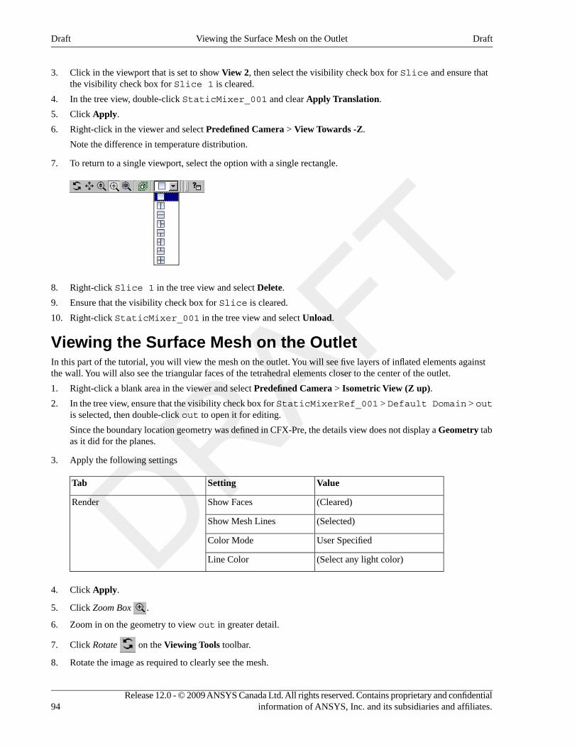
3. Click in the viewport that is set to show View 2, then select the visibility check box for Slice and ensure thatthe visibility check box for Slice 1 is cleared.
4. In the tree view, double-click StaticMixer_001 and clear Apply Translation.
5. Click Apply.
6. Right-click in the viewer and select Predefined Camera > View Towards -Z.
Note the difference in temperature distribution.
7. To return to a single viewport, select the option with a single rectangle.
8. Right-click Slice 1 in the tree view and select Delete.
9. Ensure that the visibility check box for Slice is cleared.
10. Right-click StaticMixer_001 in the tree view and select Unload.
Viewing the Surface Mesh on the OutletIn this part of the tutorial, you will view the mesh on the outlet. You will see five layers of inflated elements againstthe wall. You will also see the triangular faces of the tetrahedral elements closer to the center of the outlet.
1. Right-click a blank area in the viewer and select Predefined Camera > Isometric View (Z up).
2. In the tree view, ensure that the visibility check box for StaticMixerRef_001 > Default Domain > outis selected, then double-click out to open it for editing.
Since the boundary location geometry was defined in CFX-Pre, the details view does not display a Geometry tabas it did for the planes.
3. Apply the following settings
ValueSettingTab
(Cleared)Show FacesRender
(Selected)Show Mesh Lines
User SpecifiedColor Mode
(Select any light color)Line Color
4. Click Apply.
5. Click Zoom Box .
6. Zoom in on the geometry to view out in greater detail.
7. Click Rotate on the Viewing Tools toolbar.
8. Rotate the image as required to clearly see the mesh.
Release 12.0 - © 2009 ANSYS Canada Ltd. All rights reserved. Contains proprietary and confidentialinformation of ANSYS, Inc. and its subsidiaries and affiliates.94
DraftViewing the Surface Mesh on the OutletDraft
Looking at the Inflated Elements in Three DimensionsTo show more clearly what effect inflation has on the shape of the elements, you will use volume objects to show twoindividual elements. The first element that will be shown is a normal tetrahedral element; the second is a prismaticelement from an inflation layer of the mesh.
Leave the surface mesh on the outlet visible to help see how surface and volume meshes are related.
1. From the menu bar, select Insert > Location > Volume or, under Location click Volume.
2. In the Insert Volume dialog box, type Tet Volume and click OK.
3. Apply the following settings
ValueSettingTab
SphereDefinition > MethodGeometry
0.08, 0, -2Definition > Point
a
0.14 [m]Definition > Radius
Below IntersectionDefinition > Mode
(Cleared)Inclusive
b
RedColorColor
0.3Show Faces > TransparencyRender
(Selected)Show Mesh Lines
1Show Mesh Lines > Line Width
User SpecifiedShow Mesh Lines > Color Mode
GreyShow Mesh Lines > Line Color
aThe z slider's minimum value corresponds to the minimum z value of the entire geometry, which, in this case, occurs at the outlet.bOnly elements that are entirely contained within the sphere volume will be included.
4. Click Apply to create the volume object.
5. Right-click Tet Volume and choose Duplicate.
6. In the Duplicate Tet Volume dialog box, type Prism Volume and click OK.
7. Double-click Prism Volume.
8. Apply the following settings
ValueSettingTab
-0.22, 0.4, -1.85Definition > PointGeometry
0.206 [m]Definition > Radius
OrangeColorColor
9. Click Apply.
95Release 12.0 - © 2009 ANSYS Canada Ltd. All rights reserved. Contains proprietary and confidentialinformation of ANSYS, Inc. and its subsidiaries and affiliates.
DraftLooking at the Inflated Elements in Three DimensionsDraft
Viewing the Surface Mesh on the Mixer Body1. Double-click the Default Domain Default object.
2. Apply the following settings
ValueSettingTab
(Selected)Show FacesRender
(Selected)Show Mesh Lines
2Line Width
3. Click Apply.
Viewing the Layers of Inflated Elements on a PlaneYou will see the layers of inflated elements on the wall of the main body of the mixer. Within the body of the mixer,there will be many lines that are drawn wherever the face of a mesh element intersects the slice plane.
1. From the menu bar, select Insert > Location > Plane or under Location, click Plane.
2. In the Insert Plane dialog box, type Slice 2 and click OK.
3. Apply the following settings
ValueSettingTab
YZ PlaneDefinition > MethodGeometry
0 [m]Definition > X
(Cleared)Show FacesRender
(Selected)Show Mesh Lines
4. Click Apply.
5. Turn off the visibility of all objects except Slice 2.
6. To see the plane clearly, right-click in the viewer and select Predefined Camera > View Towards -X.
Viewing the Mesh StatisticsYou can use the Report Viewer to check the quality of your mesh. For example, you can load a .def file into CFD-Postand check the mesh quality before running the .def file in the solver.
1. Click the Report Viewer tab (located below the viewer window).
A report appears. Look at the table shown in the “Mesh Report” section.
2. Double-click Report > Mesh Report in the Outline tree view.
3. In the Mesh Report details view, select Statistics > Maximum Face Angle.
4. Click Refresh Preview.
Note that a new table, showing the maximum face angle for all elements in the mesh, has been added to the “MeshReport” section of the report. The maximum face angle is reported as 148.95°.
Release 12.0 - © 2009 ANSYS Canada Ltd. All rights reserved. Contains proprietary and confidentialinformation of ANSYS, Inc. and its subsidiaries and affiliates.96
DraftViewing the Surface Mesh on the Mixer BodyDraft
As a result of generating this mesh statistic for the report, a new variable, Maximum Face Angle, has been createdand stored at every node. This variable will be used in the next section.
Viewing the Mesh Elements with Largest Face AngleIn this section, you will visualize the mesh elements that have a Maximum Face Angle value greater than 140°.
1. Click the 3D Viewer tab (located below the viewer window).
2. Right-click a blank area in the viewer and select Predefined Camera > Isometric View (Z up).
3. In the Outline tree view, select the visibility check box of Wireframe.
4. From the menu bar, select Insert > Location > Volume or under Location, click Volume.
5. In the Insert Volume dialog box, type Max Face Angle Volume and click OK.
6. Apply the following settings
ValueSettingTab
IsovolumeDefinition > MethodGeometry
Maximum Face AngleDefinition > Variable
a
Above ValueDefinition > Mode
140 [degree]Definition > Value
(Selected)Inclusive
b
aSelect Maximum Face Angle from the larger list of variables available by clicking to the right of the Variable box.
bThis includes any elements that have at least one node with a variable value greater than or equal to the given value.
7. Click Apply.
The volume object appears in the viewer.
Viewing the Mesh Elements with Largest Face Angle Usinga PointNext, you will create a point object to show a node that has the maximum value of Maximum Face Angle. Thepoint object will be represented by a 3D yellow crosshair symbol. In order to avoid obscuring the point object withthe volume object, you may want to turn off the visibility of the latter.
1. From the menu bar, select Insert > Location > Point or under Location, click Point.
2. Click OK to use the default name.
3. Apply the following settings
ValueSettingTab
Variable MaximumDefinition > MethodGeometry
Default DomainDefinition > Location
Maximum Face AngleDefinition > Variable
97Release 12.0 - © 2009 ANSYS Canada Ltd. All rights reserved. Contains proprietary and confidentialinformation of ANSYS, Inc. and its subsidiaries and affiliates.
DraftViewing the Mesh Elements with Largest Face AngleDraft
ValueSettingTab
2Symbol SizeSymbol
4. Click Apply.
Quitting CFD-PostTwo procedures are documented. Depending on your installation of CFX, follow either the standalone procedure orthe ANSYS Workbench procedure.
Procedure in Standalone1. When you are finished, select File > Quit to exit CFD-Post.
2. Click Quit if prompted to save.
Procedure in Workbench1. When you are finished, select File > Close to close the current file.
2. Click Close if prompted to save.
3. Return to the Project page. Select File > Close Project.
4. Select No, then close Workbench.
Release 12.0 - © 2009 ANSYS Canada Ltd. All rights reserved. Contains proprietary and confidentialinformation of ANSYS, Inc. and its subsidiaries and affiliates.98
DraftQuitting CFD-PostDraft
Chapter 5. Flow in a Process InjectionMixing PipeThis tutorial includes:
• Tutorial Features (p. 99)
• Overview of the Problem to Solve (p. 100)
• Before You Begin (p. 101)
• Starting CFX-Pre (p. 101)
• Defining a Simulation using General Mode in CFX-Pre (p. 101)
• Obtaining a Solution Using CFX-Solver Manager (p. 108)
• Viewing the Results in CFD-Post (p. 109)
Tutorial FeaturesIn this tutorial you will learn about:
• Applying a profile boundary using data stored in a file.
• Visualizing the velocity on a boundary in CFX-Pre.
• Using the CFX Expression Language (CEL) to describe temperature dependent fluid properties in CFX-Pre.
• Using the k-epsilon turbulence model.
• Using streamlines in CFD-Post to track flow through the domain.
DetailsFeatureComponent
General ModeUser ModeCFX-Pre
Steady StateAnalysis Type
General FluidFluid Type
Single DomainDomain Type
k-EpsilonTurbulence Model
Thermal EnergyHeat Transfer
Boundary Profile VisualizationBoundary Conditions
Inlet (Profile)
Inlet (Subsonic)
Outlet (Subsonic)
Wall: No-Slip
Wall: Adiabatic
CEL (CFX Expression Language)
Physical Time ScaleTimestep
99Release 12.0 - © 2009 ANSYS Canada Ltd. All rights reserved. Contains proprietary and confidentialinformation of ANSYS, Inc. and its subsidiaries and affiliates.
DraftDraft
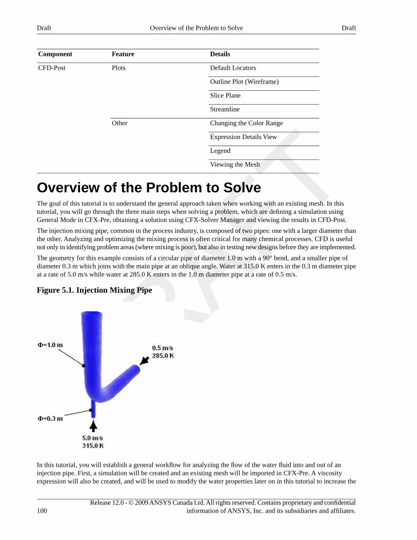
DetailsFeatureComponent
Default LocatorsPlotsCFD-Post
Outline Plot (Wireframe)
Slice Plane
Streamline
Changing the Color RangeOther
Expression Details View
Legend
Viewing the Mesh
Overview of the Problem to SolveThe goal of this tutorial is to understand the general approach taken when working with an existing mesh. In thistutorial, you will go through the three main steps when solving a problem, which are defining a simulation usingGeneral Mode in CFX-Pre, obtaining a solution using CFX-Solver Manager and viewing the results in CFD-Post.
The injection mixing pipe, common in the process industry, is composed of two pipes: one with a larger diameter thanthe other. Analyzing and optimizing the mixing process is often critical for many chemical processes. CFD is usefulnot only in identifying problem areas (where mixing is poor), but also in testing new designs before they are implemented.
The geometry for this example consists of a circular pipe of diameter 1.0 m with a 90° bend, and a smaller pipe ofdiameter 0.3 m which joins with the main pipe at an oblique angle. Water at 315.0 K enters in the 0.3 m diameter pipeat a rate of 5.0 m/s while water at 285.0 K enters in the 1.0 m diameter pipe at a rate of 0.5 m/s.
Figure 5.1. Injection Mixing Pipe
In this tutorial, you will establish a general workflow for analyzing the flow of the water fluid into and out of aninjection pipe. First, a simulation will be created and an existing mesh will be imported in CFX-Pre. A viscosityexpression will also be created, and will be used to modify the water properties later on in this tutorial to increase the
Release 12.0 - © 2009 ANSYS Canada Ltd. All rights reserved. Contains proprietary and confidentialinformation of ANSYS, Inc. and its subsidiaries and affiliates.100
DraftOverview of the Problem to SolveDraft
solution accuracy. Finally, initial values will be set and a solution will be found using CFX-Solver Manager. The resultswill then be viewed in CFD-Post. Streamlines originating from the main inlet will be generated to show the flow ofthe water into and out of the injection pipe.
Before You BeginIf this is the first tutorial you are working with, it is important to review the following topics before beginning:
• Preparing a Working Directory (p. 23)
• Setting the Working Directory and Starting ANSYS CFX (p. 23)
• Changing the Display Colors (p. 24)
• Playing a Tutorial Session File (p. 24)
Starting CFX-Pre1. Prepare the working directory using the following files in the examples directory:
• InjectMixer.pre
• InjectMixer_velocity_profile.csv
• InjectMixerMesh.gtm
For details, see Preparing a Working Directory (p. 23)
2. Set the working directory and start CFX-Pre
For details, see Setting the Working Directory and Starting ANSYS CFX (p. 23)
Defining a Simulation using General Mode inCFX-PreIf you want to set up the simulation automatically using a tutorial session file, run InjectMixer.pre. For details,see Playing a Tutorial Session File (p. 24). Then proceed to Obtaining a Solution Using CFX-Solver Manager (p. 108).
If you want to set up the simulation manually, continue with the following steps.
Workflow OverviewThis section provides a brief summary of the topics to follow as a general workflow:
1. Creating a New Case (p. 102)
2. Importing a Mesh (p. 102)
3. Setting Temperature-Dependent Material Properties (p. 103)
4. Plotting an Expression (p. 104)
5. Evaluating an Expression (p. 104)
6. Modify Material Properties (p. 104)
7. Creating the Domain (p. 105)
8. Creating the Side Inlet Boundary (p. 105)
9. Creating the Main Inlet Boundary (p. 106)
10. Creating the Main Outlet Boundary (p. 107)
11. Setting Initial Values (p. 107)
101Release 12.0 - © 2009 ANSYS Canada Ltd. All rights reserved. Contains proprietary and confidentialinformation of ANSYS, Inc. and its subsidiaries and affiliates.
DraftBefore You BeginDraft
12. Setting Solver Control (p. 107)
13. Writing the CFX-Solver Input (.def) File (p. 108)
Creating a New CaseBefore importing and working with a mesh, a simulation needs to be started using General Mode.
NoteTwo procedures are documented. Depending on your installation of CFX follow either the Standaloneprocedure or the ANSYS Workbench procedure.
Procedure in Standalone1. If required, launch CFX-Pre.
2. Select File > New Case.
3. Ensure General is selected and click OK.
4. Select File > Save Case As.
5. Under File name, type InjectMixer.
6. Click Save.
7. Proceed to Importing a Mesh (p. 102).
Procedure in ANSYS Workbench1. If required, launch ANSYS Workbench.
2. Click Empty Project.
The Project page will appear displaying an unsaved project.
3. Select File > Save or click Save .
4. If required, set the path location to your working directory.
5. Under File name, type InjectMixer.
6. Click Save.
7. Click Start CFX-Pre under Advanced CFD on the left hand task bar.
8. Select File > New Case.
9. Click General in the New Case File window and then click OK.
10. Select File > Save Case As.
11. Under File name, type InjectMixer.
12. Click Save.
Importing a MeshThe following steps will demonstrate how to import a mesh.
1. Edit Case Options > General in the Outline tree view and ensure that Automatic Default Domain isturned off.
Default Domain generation should be turned off because you will create a new domain manually, later in thistutorial.
2. Select File > Import > Mesh.
Release 12.0 - © 2009 ANSYS Canada Ltd. All rights reserved. Contains proprietary and confidentialinformation of ANSYS, Inc. and its subsidiaries and affiliates.102
DraftCreating a New CaseDraft
3. From your working directory, select InjectMixerMesh.gtm.
4. Click Open.
5. Right-click a blank area in the viewer and select Predefined Camera > Isometric View (Y up) from the shortcutmenu.
Setting Temperature-Dependent Material PropertiesViscosity varies with temperature, which implies that the water will behave differently when coming through the 1.0m and the 0.3 m diameter pipes. In the following steps, you will create an expression for viscosity as a function oftemperature. This expression will then be used to modify the properties of the library material: Water to increase theaccuracy of the solution. By setting temperature-dependant material properties, Viscosity will be made to vary linearlywith temperature between the following conditions:
• μ=1.8E-03 N s m-2 at T=275.0 K
• μ=5.45E-04 N s m-2 at T=325.0 K
The variable T (Temperature) is a CFX System Variable recognized by CFX-Pre, denoting static temperature. Allvariables, expressions, locators, functions, and constants can be viewed by double-clicking the appropriate entry (suchas Additional Variables or Expressions) in the tree view.
All expressions must have consistent units. You should be careful if using temperature in an expression with unitsother than [K].
The Expressions tab lets you define, modify, evaluate, plot, copy, delete and browse through expressions used withinCFX-Pre.
1. From the main menu, select Insert > Expressions, Functions and Variables > Expression.
2. In the New Expression dialog box, type Tupper.
3. Click OK.
The details view for the Tupper equation is displayed.
4. Under Definition, type 325 [K].
5. Click Apply to create the expression.
The expression is added to the list of existing expressions.
6. Right-click in the Expressions workspace and select Insert > Expression.
7. In the New Expression dialog box, type Tlower.
8. Click OK.
9. Under Definition, type 275 [K].
10. Click Apply to create the expression.
The expression is added to the list of existing expressions.
11. Create expressions for Visupper, Vislower and VisT using the following values.
DefinitionName
5.45E-04 [N s m^-2]Visupper
1.8E-03 [N s m^-2]Vislower
Vislower+(Visupper-Vislower)*(T-Tlower)/(Tupper-Tlower)VisT
103Release 12.0 - © 2009 ANSYS Canada Ltd. All rights reserved. Contains proprietary and confidentialinformation of ANSYS, Inc. and its subsidiaries and affiliates.
DraftSetting Temperature-Dependent Material PropertiesDraft
Plotting an Expression1. Right-click VisT in the Expressions tree view, and then select Edit.
The Expressions details view for VisT appears.
TipAlternatively, double-clicking the expression also opens the Expressions details view.
2. Click the Plot tab and apply the following settings
ValueSettingTab
10Number of PointsPlot
(Selected)T
275 [K]Start of Range
325 [K]End of Range
3. Click Plot Expression.
A plot showing the variation of the expression VisT with the variable T is displayed.
Evaluating an Expression1. Click the Evaluate tab.
2. In T, type 300 [K].
This is between the start and end range defined in the last module.
3. Click Evaluate Expression.
A value of around 0.0011[kg m^-1 s^-1] for VisT at the given value of T appears in the Value field.
Modify Material PropertiesAs mentioned earlier in this tutorial, the default material properties of Water will be modified using the Viscosityexpression to increase the accuracy of the solution.
1. Click the Outline tab.
2. Double-click Water under Materials to display the Basic Settings tab.
3. Click the Material Properties tab.
4. Expand Transport Properties.
5. Select Dynamic Viscosity.
6. Under Dynamic Viscosity, click in Dynamic Viscosity.
7. Click Enter Expression .
8. Enter the expression VisT into the data box.
9. Click OK.
Release 12.0 - © 2009 ANSYS Canada Ltd. All rights reserved. Contains proprietary and confidentialinformation of ANSYS, Inc. and its subsidiaries and affiliates.104
DraftPlotting an ExpressionDraft
Creating the DomainThe domain will be set to use the thermal energy heat transfer model, and the −k ε (k-epsilon) turbulence model.
Both General Options and Fluid Models are changed in this module. The Initialization tab is for setting domain-specificinitial conditions, which are not used in this tutorial. Instead, global initialization is used to set the starting conditions.
1. Ensure that no default domain is present under Flow Analysis 1. If a default domain is present, right-clickit and select Delete.
2. Select Insert > Domain from the main menu or click Domain .
3. In the Insert Domain dialog box, type InjectMixer.
4. Click OK.
5. Apply the following settings
ValueSettingTab
B1.P3Location and Type > LocationBasic Settings
Fluid 1Fluid and Particle Definitions
WaterFluid and Particle Definitions> Fluid 1 > Material
0 [atm]Domain Models > Pressure >Reference Pressure
6. Click Fluid Models.
7. Apply the following settings
ValueSetting
Thermal EnergyHeat Transfer > Option
8. Click OK.
Creating the Side Inlet BoundaryThe side inlet boundary needs to be defined.
1. Select Insert > Boundary from the main menu or click Boundary .
2. Set Name to side inlet.
NoteA boundary named after a region will use that region as its location by default.
3. Click OK.
4. Apply the following settings
ValueSettingTab
InletBoundary TypeBasic Settings
105Release 12.0 - © 2009 ANSYS Canada Ltd. All rights reserved. Contains proprietary and confidentialinformation of ANSYS, Inc. and its subsidiaries and affiliates.
DraftCreating the DomainDraft
ValueSettingTab
side inletLocation
Normal SpeedMass and Momentum > OptionBoundary Details
5 [m s^-1]Mass and Momentum > Normal Speed
Static TemperatureHeat Transfer > Option
315 [K]Heat Transfer > Static Temperature
5. Click OK.
Creating the Main Inlet BoundaryThe main inlet boundary for the large pipe needs to be defined. This inlet is defined using a velocity profile found inthe examples directory. Profile data needs to be initialized before the boundary can be created.
You will create a plot showing the velocity profile data, marked by higher velocities near the center of the inlet, andlower velocities near the inlet walls.
1. Select Tools > Initialize Profile Data.
2. Under Data File, click Browse .
3. From your working directory, select InjectMixer_velocity_profile.csv.
4. Click Open.
5. Click OK.
The profile data is read into memory.
6. Select Insert > Boundary from the main menu or click Boundary .
7. Set name Name to main inlet.
8. Click OK.
9. Apply the following settings
ValueSettingTab
InletBoundary TypeBasic Settings
main inletLocation
(Selected)Profile Boundary Conditions >Use Profile Data
main inletProfile Boundary Setup >Profile Name
10. Click Generate Values.
This causes the profile values of U, V, W to be applied at the nodes on the main inlet boundary, and U, V, Wentries to be made in Boundary Details. To later modify the velocity values at the main inlet and reset values tothose read from the BC Profile file, revisit Basic Settings for this boundary and click Generate Values.
11. Apply the following settings
Release 12.0 - © 2009 ANSYS Canada Ltd. All rights reserved. Contains proprietary and confidentialinformation of ANSYS, Inc. and its subsidiaries and affiliates.106
DraftCreating the Main Inlet BoundaryDraft
ValueSettingTab
SubsonicFlow Regime > OptionBoundary Details
Medium (Intensity = 5%)Turbulence > Option
Static TemperatureHeat Transfer > Option
285 [K]Heat Transfer > StaticTemperature
(Selected)Boundary ContourPlot Options
WBoundary Contour > ProfileVariable
12. Click OK.
13. Zoom into the main inlet to view the inlet velocity contour.
Creating the Main Outlet BoundaryIn this module you create the outlet boundary. All other surfaces which have not been explicitly assigned a boundarywill remain in the InjectMixer Default object, which is shown in the tree view. This boundary uses a No-SlipAdiabatic Wall by default.
1. Select Insert > Boundary from the main menu or click Boundary .
2. Set Name to outlet.
3. Click OK.
4. Apply the following settings
ValueSettingTab
OutletBoundary TypeBasic Settings
outletLocation
SubsonicFlow Regime > OptionBoundary Details
Average Static PressureMass and Momentum > Option
0 [Pa]Relative Pressure
5. Click OK.
Setting Initial ValuesFor this tutorial, the initial values will be set automatically. An automatic guess is sufficient for this particular problem.
1. Click Global Initialization and review, but do not change, the current settings.
2. Click Close.
Setting Solver Control1. Click Solver Control .
107Release 12.0 - © 2009 ANSYS Canada Ltd. All rights reserved. Contains proprietary and confidentialinformation of ANSYS, Inc. and its subsidiaries and affiliates.
DraftCreating the Main Outlet BoundaryDraft
2. Apply the following settings
ValueSettingTab
Specified Blend FactorAdvection Scheme > OptionBasic Settings
0.75Advection Scheme > BlendFactor
50Convergence Control > Max.Iterations
Physical TimescaleConvergence Control > FluidTimescale Control > TimescaleControl
2 [s]Convergence Control > FluidTimescale Control > PhysicalTimescale
a
RMSConvergence Criteria >Residual Type
1.E-4Convergence Criteria >Residual Target b
aThe physical timescale that will be setup is derived from the pipe diameter (1 m) and the rate at which the water flows in the pipe (0.5 m/s).bAn RMS value of at least 1.E-5 is usually required for adequate convergence, but the default value is sufficient for demonstration purposes.
3. Click OK.
Writing the CFX-Solver Input (.def) FileOnce the problem has been defined you move from General Mode into CFX-Solver.
1. Click Define Run .
2. Apply the following settings:
ValueSetting
InjectMixer.defFile name
3. Click Save.
The CFX-Solver input file (InjectMixer.def) is created. CFX-Solver Manager automatically starts and, onthe Define Run dialog box, the Solver Input File is set.
4. When you are finished, select File > Quit in CFX-Pre.
5. Click Save & Quit if prompted, to save InjectMixer.cfx
6. Proceed to Obtaining a Solution Using CFX-Solver Manager (p. 108).
Obtaining a Solution Using CFX-Solver ManagerAt this point, CFX-Solver Manager is running, and the Define Run dialog box is displayed, with the CFX-Solver inputfile set.
Release 12.0 - © 2009 ANSYS Canada Ltd. All rights reserved. Contains proprietary and confidentialinformation of ANSYS, Inc. and its subsidiaries and affiliates.108
DraftWriting the CFX-Solver Input (.def) FileDraft
1. Click Start Run.
2. When the run ends, ensure that the check box next to Post-Process Results is cleared and click OK to close thedialog box.
Moving from CFX-Solver Manager to CFD-Post1. Select Tools > Post-Process Results or click Post-Process Results .
2. If using CFX-Solver Manager in standalone mode, optionally select Shut down CFX-Solver Manager.
3. Click OK.
Viewing the Results in CFD-PostWhen CFD-Post starts, the viewer and Outline workspace display by default.
Workflow OverviewThis section provides a brief summary of the topics to follow as a general workflow:
1. Modifying the Outline of the Geometry (p. 109)
2. Creating and Modifying Streamlines Originating from the Main Inlet (p. 109)
3. Modifying Streamline Color Ranges (p. 110)
4. Coloring Streamlines with a Constant Color (p. 110)
5. Creating Streamlines Originating from the Side Inlet (p. 111)
6. Examining Turbulence Kinetic Energy (p. 111)
Modifying the Outline of the GeometryThroughout this and the following examples, use your mouse and the Viewing Tools toolbar to manipulate the geometryas required at any time.
1. In the tree view, double-click Wireframe.
2. Set the Edge Angle to 15 [degree].
3. Click Apply.
Creating and Modifying Streamlines Originating from theMain InletWhen you complete this module you will see streamlines (mainly blue and green) starting at the main inlet of thegeometry and proceeding to the outlet. Above where the side pipe meets the main pipe, there is an area where the flowre-circulates rather than flowing roughly tangent to the direction of the pipe walls.
1. Select Insert > Streamline from the main menu or click Streamline .
2. Under Name, type MainStream.
3. Click OK.
4. Apply the following settings
ValueSettingTab
3D StreamlineTypeGeometry
109Release 12.0 - © 2009 ANSYS Canada Ltd. All rights reserved. Contains proprietary and confidentialinformation of ANSYS, Inc. and its subsidiaries and affiliates.
DraftMoving from CFX-Solver Manager to CFD-PostDraft
ValueSettingTab
main inletDefinition > Start From
5. Click Apply.
6. Right-click a blank area in the viewer, select Predefined Camera from the shortcut menu, then select IsometricView (Y up).
The pipe is displayed with the main inlet in the bottom right of the viewer.
Modifying Streamline Color RangesYou can change the appearance of the streamlines using the Range setting on the Color tab.
1. Under User Locations and Plots, modify the streamline object MainStream by applying the following settings
ValueSettingTab
LocalRangeColor
2. Click Apply.
The color map is fitted to the range of velocities found along the streamlines. The streamlines therefore collectivelycontain every color in the color map.
3. Apply the following settings
ValueSettingTab
User SpecifiedRangeColor
0.2 [m s^-1]Min
2.2 [m s^-1]Max
NotePortions of streamlines that have values outside the range shown in the legend are colored accordingto the color at the nearest end of the legend. When using tubes or symbols (which contain faces), moreaccurate colors are obtained with lighting turned off.
4. Click Apply.
The streamlines are colored using the specified range of velocity values.
Coloring Streamlines with a Constant Color1. Apply the following settings
ValueSettingTab
ConstantModeColor
(Green)Color
Release 12.0 - © 2009 ANSYS Canada Ltd. All rights reserved. Contains proprietary and confidentialinformation of ANSYS, Inc. and its subsidiaries and affiliates.110
DraftModifying Streamline Color RangesDraft
Color can be set to green by selecting it from the color pallet, or by repeatedly clicking on the color box until itcycles through to the default green color.
2. Click Apply.
Creating Streamlines Originating from the Side InletThe following steps illustrate using this feature to add a streamline object that originates at the side inlet.
1. Right-click MainStream and select Duplicate from the shortcut menu.
2. In the Name window, type SideStream.
3. Click OK.
4. Double-click the newly created streamline, SideStream.
5. Apply the following settings
ValueSettingTab
side inletDefinition > Start FromGeometry
ConstantModeColor
(Red)Color
6. Click Apply.
Red streamlines appear, starting from the side inlet.
7. For better view, select Isometric View (Y up).
Examining Turbulence Kinetic EnergyAway from walls, turbulence kinetic energy has an influence on the level of mixing. A plane will be created to viewthe Turbulence Kinetic Energy variable within the domain.
NoteThis module has multiple changes compiled into single steps in preparation for other tutorials that providefewer specific instructions.
1. Turn off the visibility of both the MainStream and the SideStream objects.
2. Create a plane named Plane 1 that is normal to X and passing through the X = 0 Point. To do so, specificinstructions follow.
1. From the main menu, select Insert > Location > Plane and click OK.
2. In the Details view set Definition > Method to YZ Plane and X to 0 [m].
3. Click Apply.
3. Color the plane using the variable Turbulence Kinetic Energy, to show regions of high turbulence. Todo so, apply the settings below.
ValueSettingTab
VariableModeColor
Turbulence Kinetic EnergyVariable
111Release 12.0 - © 2009 ANSYS Canada Ltd. All rights reserved. Contains proprietary and confidentialinformation of ANSYS, Inc. and its subsidiaries and affiliates.
DraftCreating Streamlines Originating from the Side InletDraft
4. Click Apply.
5. Experiment with other variables to color this plane (for example, Temperature to show the temperature mixingof the two streams).
Commonly used variables are in the drop-down menu. A full list of available variables can be viewed by clicking
next to the Variable data box.
Exiting CFD-PostWhen finished with CFD-Post exit the current window.
Two procedures are documented. Depending on your installation of CFX, follow either the Standalone procedure orthe ANSYS Workbench procedure.
Procedure in Standalone1. When you are finished, select File > Quit to exit CFD-Post.
2. Click Quit if prompted to save.
Procedure in ANSYS Workbench1. When you are finished, select File > Close to close the current file.
2. Click Close if prompted to save.
3. Return to the Project page. Select File > Close Project.
4. Select No, then close ANSYS Workbench.
Release 12.0 - © 2009 ANSYS Canada Ltd. All rights reserved. Contains proprietary and confidentialinformation of ANSYS, Inc. and its subsidiaries and affiliates.112
DraftExiting CFD-PostDraft
Chapter 6. Flow from a Circular VentThis tutorial includes:
• Tutorial Features (p. 113)
• Overview of the Problem to Solve (p. 114)
• Before You Begin (p. 114)
• Starting CFX-Pre (p. 115)
• Defining a Multiple-Analysis Simulation in CFX-Pre (p. 115)
• Obtaining Solutions to the Steady-State and Transient Configurations (p. 125)
• Viewing the Results in CFD-Post (p. 126)
Tutorial FeaturesIn this tutorial you will learn about:
• Setting up a transient problem in CFX-Pre.
• Using an opening type boundary in CFX-Pre.
• Making use of multiple configurations in CFX-Pre
• Modeling smoke using additional variables in CFX-Pre.
• Visualizing a smoke plume using an Isosurface in CFD-Post.
• Creating an image for printing, and generating a movie in CFD-Post.
DetailsFeatureComponent
General ModeUser ModeCFX-Pre
Steady StateAnalysis Type
Transient
General FluidFluid Type
Single DomainDomain Type
k-EpsilonTurbulence Model
Inlet (Subsonic)Boundary Conditions
Opening
Wall: No-Slip
Auto Time ScaleTimestep
Transient Example
MultipleConfiguration
Transient Results File
AnimationPlotsCFD-Post
Isosurface
113Release 12.0 - © 2009 ANSYS Canada Ltd. All rights reserved. Contains proprietary and confidentialinformation of ANSYS, Inc. and its subsidiaries and affiliates.
DraftDraft
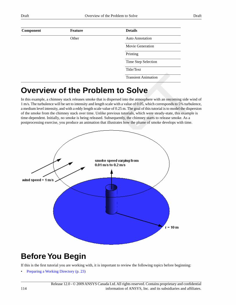
DetailsFeatureComponent
Auto AnnotationOther
Movie Generation
Printing
Time Step Selection
Title/Text
Transient Animation
Overview of the Problem to SolveIn this example, a chimney stack releases smoke that is dispersed into the atmosphere with an oncoming side wind of1 m/s. The turbulence will be set to intensity and length scale with a value of 0.05, which corresponds to 5% turbulence,a medium level intensity, and with a eddy length scale value of 0.25 m. The goal of this tutorial is to model the dispersionof the smoke from the chimney stack over time. Unlike previous tutorials, which were steady-state, this example istime-dependent. Initially, no smoke is being released. Subsequently, the chimney starts to release smoke. As apostprocessing exercise, you produce an animation that illustrates how the plume of smoke develops with time.
Before You BeginIf this is the first tutorial you are working with, it is important to review the following topics before beginning:
• Preparing a Working Directory (p. 23)
Release 12.0 - © 2009 ANSYS Canada Ltd. All rights reserved. Contains proprietary and confidentialinformation of ANSYS, Inc. and its subsidiaries and affiliates.114
DraftOverview of the Problem to SolveDraft
• Setting the Working Directory and Starting ANSYS CFX (p. 23)
• Changing the Display Colors (p. 24)
• Playing a Tutorial Session File (p. 24)
Starting CFX-Pre1. Prepare the working directory using the following files in the examples directory:
• CircVent.pre
• CircVentMesh.gtm
For details, see Preparing a Working Directory (p. 23).
2. Set the working directory and start CFX-Pre.
For details, see Setting the Working Directory and Starting ANSYS CFX (p. 23).
Defining a Multiple-Analysis Simulation inCFX-PreIf you want to set up the simulation automatically using a tutorial session file, run CircVent.pre. For details, seePlaying a Tutorial Session File (p. 24). Then proceed to Obtaining Solutions to the Steady-State and TransientConfigurations (p. 125).
If you want to set up the simulation manually, proceed to the following steps:
This section describes the step-by-step definition of the flow physics in CFX-Pre for a simulation with two analyses.First is a steady-state analysis with no smoke being produced by the chimney. The second analysis takes the setup forthe steady state and adapts it for a transient analysis. The results from the steady-state analysis will be used as the initialguess for the transient analysis.
1. Select File > New Case.
2. Select General and click OK.
3. Select File > Save Case As.
4. Set File name to CircVent.
5. Click Save.
Importing the Mesh1. Edit Case Options > General in the Outline tree view and ensure that Automatic Default Domain is
turned off.
Default Domain generation should be turned off because you will create a new domain manually, later in thistutorial.
2. Select File > Import > Mesh.
3. From your working directory, select CircVentMesh.gtm.
4. Click Open.
5. Right-click a blank area in the viewer and select Predefined Camera > Isometric View (Z up) from the shortcutmenu.
115Release 12.0 - © 2009 ANSYS Canada Ltd. All rights reserved. Contains proprietary and confidentialinformation of ANSYS, Inc. and its subsidiaries and affiliates.
DraftStarting CFX-PreDraft
Creating an Additional VariableIn this tutorial an Additional Variable (non-reacting scalar component) will be used to model the dispersion of smokefrom the vent.
NoteWhile smoke is not required for the steady-state simulation, including it here prevents you from having toset up time value interpolation in the transient analysis.
1. From the menu bar, select Insert > Expressions, Functions and Variables > Additional Variable.
2. Set Name to smoke.
3. Click OK.
4. Set Variable Type to Volumetric.
5. Set Units to [kg m^-3].
6. Click OK.
Renaming the AnalysisTo rename the existing analysis:
1. From the Outline Tree, right-click Simulation > Flow Analysis 1 and click Rename.
2. Rename the analysis to Steady State Analysis.
Creating the DomainYou will create a fluid domain that includes support for smoke as an Additional Variable.
To Create a New Domain
1. Select Insert > Domain from the menu bar, or click Domain , then set the name to CircVent and click
OK.
2. Apply the following settings
ValueSettingTab
B1.P3Location and Type > LocationBasic Settings
Fluid 1Fluid and Particle Definitions
Air at 25 CFluid and Particle Definitions > Fluid 1> Material
0 [atm]Domain Models > Pressure > ReferencePressure
NoneHeat Transfer > OptionFluid Models
smokeAdditional Variable Models > AdditionalVariable
(Selected)Additional Variable Models > AdditionalVariable > smoke
Release 12.0 - © 2009 ANSYS Canada Ltd. All rights reserved. Contains proprietary and confidentialinformation of ANSYS, Inc. and its subsidiaries and affiliates.116
DraftCreating an Additional VariableDraft
ValueSettingTab
(Selected)Additional Variable Models > AdditionalVariable > smoke > KinematicDiffusivity
1.0E-5 [m^2 s^-1]aAdditional Variable Models > AdditionalVariable > smoke > KinematicDiffusivity > Kinematic Diffusivity
a1.0E-5 [m^2 s^-1] is a representative kinematic diffusivity value for smoke in air.
3. Click OK.
Creating the BoundariesThis is an example of external flow, since fluid is flowing over an object and not through an enclosure such as a pipenetwork (which would be an example of internal flow). In external flow problems, some inlets will be made sufficientlylarge that they do not affect the CFD solution. However, the length scale values produced by the Default Intensityand AutoCompute Length Scale option for turbulence are based on inlet size. They are appropriate for internal flowproblems and particularly, cylindrical pipes. In general, you need to set the turbulence intensity and length scaleexplicitly for large inlets in external flow problems. If you do not have a value for the length scale, you can use a lengthscale based on a typical length of the object over which the fluid is flowing. In this case, you will choose a turbulencelength scale which is one-tenth of the diameter of the vent.
For parts of the boundary where the flow direction changes, or is unknown, an opening boundary can be used. Anopening boundary allows flow to both enter and leave the fluid domain during the course of the analysis.
Inlet BoundaryYou will create the inlet boundary with velocity components set consistently with the problem description.
1. Select Insert > Boundary from the menu bar or click Boundary .
2. Set Name to Wind.
3. Click OK.
4. Apply the following settings
ValueSettingTab
InletBoundary TypeBasic Settings
WindLocation
Cart. Vel. ComponentsMass And Momentum > OptionBoundary Details
1 [m s^-1]Mass and Momentum > U
0 [m s^-1]Mass and Momentum > V
0 [m s^-1]Mass and Momentum > W
Intensity and Length ScaleTurbulence > Option
0.05aTurbulence > Fractional Intensity
0.25 [m]bTurbulence > Eddy Length Scale
117Release 12.0 - © 2009 ANSYS Canada Ltd. All rights reserved. Contains proprietary and confidentialinformation of ANSYS, Inc. and its subsidiaries and affiliates.
DraftCreating the BoundariesDraft
ValueSettingTab
ValueAdditional Variables > smoke > Option
0 [kg m^-3]cAdditional Variables > smoke > Add. Var.Value
aFrom the problem description.bFrom the problem description.cThe smoke value that will be set up corresponds to no smoke at the inlet.
5. Click OK.
NoteThe boundary marker vectors used to display boundary conditions (inlets, outlets, openings) are normal tothe boundary surface regardless of the actual direction specification. To plot vectors in the direction of flow,select Boundary Vector under the Plot Options tab for the inlet boundary, and on the Labels and MarkersOptions tab (accessible from Case Options > Labels and Markers on the Outline tree view), ensure thatSettings > Show Boundary Markers is selected and Show Inlet Markers is cleared .
Opening BoundaryYou will create an opening boundary with pressure and flow direction specified. If fluid enters the domain through theopening, it should have turbulence intensity and length scale, as well as smoke concentration, set to the same valuesas for the inlet.
1. Select Insert > Boundary from the menu bar or click Boundary .
2. Set Name to Atmosphere.
3. Click OK.
4. Apply the following settings
ValueSettingTab
OpeningBoundary TypeBasic Settings
AtmosphereLocation
Opening Pres. and DirnMass And Momentum > OptionBoundary Details
0 [Pa]Mass and Momentum > Relative Pressure
Normal to Boundary ConditionFlow Direction > Option
Intensity and Length ScaleTurbulence > Option
0.05Turbulence > Fractional Intensity
0.25 [m]Turbulence > Eddy Length Scale
ValueAdditional Variables > smoke > Option
0 [kg m^-3]Additional Variables > smoke > Add. Var.Value
5. Click OK.
Release 12.0 - © 2009 ANSYS Canada Ltd. All rights reserved. Contains proprietary and confidentialinformation of ANSYS, Inc. and its subsidiaries and affiliates.118
DraftCreating the BoundariesDraft
Inlet for the VentYou will create the vent inlet boundary with a normal velocity of 0.01 m/s as prescribed in the problem descriptionand no smoke release. The turbulence level for the inlet vent will be determined from turbulence intensity and eddyviscosity ratio.
1. Select Insert > Boundary from the menu bar or click Boundary .
2. Set Name to Vent.
3. Click OK.
4. Apply the following settings
ValueSettingTab
InletBoundary TypeBasic Settings
VentLocation
0.01 [m s^-1]Mass And Momentum > Normal SpeedBoundary Details
Intensity and Eddy ViscosityRatio
Turbulence > Option
0.05Turbulence > Fractional Intensity
10Turbulence > Eddy Viscosity Ratio
ValueAdditional Variables > smoke > Option
0 [kg m^-3]Additional Variables > smoke > Add. Var.Value
5. Click OK.
Setting Initial ValuesFor this tutorial, the automatic initial values are suitable. Review and apply the default settings:
1. Click Global Initialization .
2. Review the settings for velocity, pressure, turbulence and the smoke.
3. Click OK.
Setting Solver ControlCFX-Solver has the ability to calculate physical time step size for steady-state problems. If you do not know the timestep size to set for your problem, you can use the Auto Timescale option.
1. Click Solver Control .
2. Apply the following settings
ValueSettingTab
75Convergence Control > Max. IterationsBasic Settings
3. Note that Convergence Control > Fluid Timescale Control > Timescale Control is set to Auto Timescale.
119Release 12.0 - © 2009 ANSYS Canada Ltd. All rights reserved. Contains proprietary and confidentialinformation of ANSYS, Inc. and its subsidiaries and affiliates.
DraftSetting Initial ValuesDraft
4. Click OK.
Creating a Transient Flow AnalysisIn this part of the tutorial, you will duplicate the steady-state analysis and adapt it to set up a transient flow analysisin CFX-Pre.
1. From the Outline tree view, right-click Simulation > Steady State Analysis and select Duplicate.
2. Right-click Simulation > Copy of Steady State Analysis and select Rename.
3. Rename the analysis to Transient Analysis.
Modifying the Analysis TypeIn this step you will set the new analysis to a type of transient. Later, you will set the concentration of smoke for thetransient analysis to rise asymptotically to its final concentration with time, so it is necessary to ensure that the intervalbetween the time steps is smaller at the beginning of the simulation than at the end.
1. In the Outline tree view, ensure that Simulation > Transient Analysis is expanded.
2. From the Outline tree view, right-click Simulation > Transient Analysis > Analysis Type andselect Edit.
3. Apply the following settings
ValueSettingTab
TransientAnalysis Type > OptionBasic Settings
30 [s]Analysis Type > Time Duration > TotalTime
4*0.25, 2*0.5, 2*1.0, 13*2.0 [s]Analysis Type > Time Steps >
Timestepsab
ValueAnalysis Type > Initial Time > Option
0 [s]Analysis Type > Initial Time > Time
aDo NOT click Enter Expression to enter lists of values. Enter the list without the units, then set the units in the drop-down list.
bThis list specifies 4 timesteps of 0.25 [s], then 2 timesteps of 0.5 [s], and so on.
4. Click OK.
Modifying the Boundary ConditionsThe only boundary condition that needs altering for the transient analysis is the Vent boundary condition. In thesteady-state calculation, this boundary had a small amount of air flowing through it. In the transient calculation, moreair passes through the vent and there is a time-dependent concentration of smoke in the air. This is initially zero, butbuilds up to a larger value. The smoke concentration will be specified using the CFX Expression Language.
To Modify the Vent Inlet Boundary Condition1. In the Outline tree view, ensure that Simulation > Transient Analysis > CircVent is expanded.
2. Right-click Simulation > Transient Analysis > CircVent > Vent and select Edit.
3. Apply the following settings:
Release 12.0 - © 2009 ANSYS Canada Ltd. All rights reserved. Contains proprietary and confidentialinformation of ANSYS, Inc. and its subsidiaries and affiliates.120
DraftCreating a Transient Flow AnalysisDraft
ValueSettingTab
0.2 [m s^-1]Mass And Momentum > Normal SpeedBoundary Details
Leave the Vent details view open for now.
You are going to create an expression for smoke concentration. The concentration is zero for time t=0 and buildsup to a maximum of 1 kg m^-3.
4. Create a new expression by selecting Insert > Expressions, Functions and Variables > Expression from themenu bar. Set the name to TimeConstant.
5. Apply the following settings
DefinitionName
3 [s]TimeConstant
6. Click Apply to create the expression.
7. Create the following expressions with specific settings, remembering to click Apply after each is defined:
DefinitionName
1 [kg m^-3]FinalConcentration
FinalConcentration*abs(1-exp(-t/TimeConstant))ExpFunction
a
aWhen entering this function, you can select most of the required items by right-clicking in the Definition window in the Expression detailsview instead of typing them. The names of the existing expressions are under the Expressions menu. The exp and abs functions are underFunctions > CEL. The variable t is under Variables.
NoteThe abs function takes the modulus (or magnitude) of its argument. Even though the expression (1-exp (-t/TimeConstant)) can never be less than zero, the abs function is included to ensure that thenumerical error in evaluating it near to zero will never make the expression evaluate to a negativenumber.
Next, you will visualize how the concentration of smoke issued from the vent varies with time.
Plotting Smoke Concentration1. Double-click ExpFunction in the Expressions tree view.
2. Apply the following settings
ValueSettingTab
(Selected)tPlot
0 [s]t > Start of Range
30 [s]t > End of Range
3. Click Plot Expression.
121Release 12.0 - © 2009 ANSYS Canada Ltd. All rights reserved. Contains proprietary and confidentialinformation of ANSYS, Inc. and its subsidiaries and affiliates.
DraftModifying the Boundary ConditionsDraft
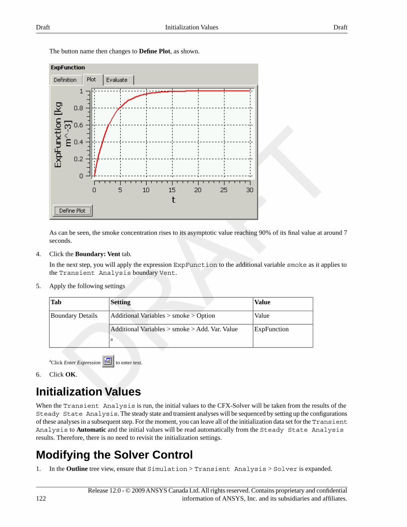
The button name then changes to Define Plot, as shown.
As can be seen, the smoke concentration rises to its asymptotic value reaching 90% of its final value at around 7seconds.
4. Click the Boundary: Vent tab.
In the next step, you will apply the expression ExpFunction to the additional variable smoke as it applies tothe Transient Analysis boundary Vent.
5. Apply the following settings
ValueSettingTab
ValueAdditional Variables > smoke > OptionBoundary Details
ExpFunctionAdditional Variables > smoke > Add. Var. Value
a
aClick Enter Expression to enter text.
6. Click OK.
Initialization ValuesWhen the Transient Analysis is run, the initial values to the CFX-Solver will be taken from the results of theSteady State Analysis. The steady state and transient analyses will be sequenced by setting up the configurationsof these analyses in a subsequent step. For the moment, you can leave all of the initialization data set for the TransientAnalysis to Automatic and the initial values will be read automatically from the Steady State Analysisresults. Therefore, there is no need to revisit the initialization settings.
Modifying the Solver Control1. In the Outline tree view, ensure that Simulation > Transient Analysis > Solver is expanded.
Release 12.0 - © 2009 ANSYS Canada Ltd. All rights reserved. Contains proprietary and confidentialinformation of ANSYS, Inc. and its subsidiaries and affiliates.122
DraftInitialization ValuesDraft
2. Right-click Simulation > Transient Analysis > Solver > Solver Control and select Edit.
3. Set Convergence Control > Max. Coeff. Loops to 3.
4. Leave the other settings at their default values.
5. Click OK to set the solver control parameters.
Output ControlTo allow results to be viewed at different time steps, it is necessary to create transient results files at specified times.The transient results files do not have to contain all solution data. In this step, you will create minimal transient resultsfiles.
To Create Minimal Transient Results Files1. In the Outline tree view, double click Simulation > Transient Analysis > Solver > Output
Control.
2. Click the Trn Results tab.
3. In the Transient Results tree view, click Add new item , set Name to Transient Results 1, and click
OK.
4. Apply the following settings to Transient Results 1:
ValueSetting
Selected VariablesOption
Pressure, Velocity, smokeOutput Variables List
a
Time ListOutput Frequency > Option
1, 2, 3 [s]Output Frequency > Time List
b
aClick the ellipsis icon to select items if they do not appear in the drop-down list. Use the Ctrl key to select multiple items.
bDo NOT click Enter Expression to enter lists of values. Enter the list without the units, then set the units in the drop-down list.
5. Click Apply.
6. In the Transient Results tree view, click Add new item set Name to Transient Results 2, and click
OK.
This creates a second transient results object. Each object can result in the production of many transient resultsfiles.
7. Apply the following settings to Transient Results 2:
ValueSetting
Selected VariablesOption
Pressure, Velocity, smokeOutput Variables List
Time IntervalOutput Frequency > Option
123Release 12.0 - © 2009 ANSYS Canada Ltd. All rights reserved. Contains proprietary and confidentialinformation of ANSYS, Inc. and its subsidiaries and affiliates.
DraftOutput ControlDraft
ValueSetting
4 [s]Output Frequency > Time Interval
a
aA transient results file will be produced every 4 s (including 0 s) and at 1 s, 2 s and 3 s. The files will contain no mesh, and data for only thethree selected variables. This reduces the size of the minimal results files. A full results file is always written at the end of the run.
8. Click OK.
Configuring Simulation ControlWith two types of analysis for this simulation, configuration control is used to sequence these analyses.
Configuration Control for the Steady State AnalysisTo set up the Steady State Analysis so that it will start at the beginning of the simulation:
1. In the Outline tree view, ensure that Simulation Control is expanded.
2. Right-click Simulation Control > Configurations and select Insert > Configuration.
3. Set Name to Steady State.
4. Click OK.
5. Apply the following settings
ValueSettingTab
Steady State AnalysisFlow AnalysisGeneral Settings
Start of SimulationActivation Conditions > Activation Condition1 > Option
6. Click OK.
Configuration Control for the Transient AnalysisTo set up the Transient Analysis so that it will start upon the completion of the Steady State Analysis:
1. Right-click Simulation Control > Configurations and select Insert > Configuration.
2. Set Name to Transient.
3. Click OK.
4. Apply the following settings
ValueSettingTab
Transient AnalysisFlow AnalysisGeneral Settings
End of ConfigurationActivation Conditions > Activation Condition1 > Option
Steady StateActivation Conditions > Activation Condition1 > Configuration Name
SelectedConfiguration Execution ControlRun Definition
Release 12.0 - © 2009 ANSYS Canada Ltd. All rights reserved. Contains proprietary and confidentialinformation of ANSYS, Inc. and its subsidiaries and affiliates.124
DraftConfiguring Simulation ControlDraft
ValueSettingTab
SelectedConfiguration Execution Control > InitialValues Specification
Configuration ResultsConfiguration Execution Control > InitialValues Specification > Initial Values > InitialValues 1 > Option
Steady StateConfiguration Execution Control > InitialValues Specification > Initial Values > InitialValues 1 > Configuration Name
5. Click OK.
Writing the CFX-Solver Input File1. From the Outline tree view, right-click Simulation Control and select Write Solver Input File.
2. Apply the following settings:
ValueSetting
CFX-Solver Input Files (*.mdef)File of type
CircVent.mdefFile name
3. Click Save.
This will create CircVent.mdef as well as a directory named CircVent that contains SteadyState.cfgand Transient.cfg.
4. Quit CFX-Pre, saving the case (.cfx) file.
Obtaining Solutions to the Steady-State andTransient ConfigurationsYou can obtain a solution to the steady-state and transient configurations by using the following procedure.
1. Start CFX-Solver Manager.
2. From the menu bar, select File > Define Run.
3. Apply the following settings
ValueSetting
CircVent.mdefSolver Input File
Global SettingsEdit Configuration
4. Click Start Run.
CFX-Solver Manager will start with the solution of the steady-state configuration.
5. In the Workspace drop-down menu, select SteadyState_001. The residual plots for six equations will appear:U - Mom, V - Mom, W - Mom, P - Mass, K-TurbKE, and E-Diss.K (the three momentum conservation equations,
125Release 12.0 - © 2009 ANSYS Canada Ltd. All rights reserved. Contains proprietary and confidentialinformation of ANSYS, Inc. and its subsidiaries and affiliates.
DraftWriting the CFX-Solver Input FileDraft
the mass conservation equation and equations for the turbulence kinetic energy and turbulence eddy dissipation).The Momentum and Mass tab contains four of the plots and the other two are under Turbulence Quantities.The residual for the smoke equation is also plotted but registers no values since it is not initialized.
6. Upon the successful completion of the steady-state configuration, the solution of the transient configuration startsautomatically. Notice that the text output generated by the CFX-Solver in the Run Transient 001Workspacewill be more than you have seen for steady-state problems. This is because each timestep consists of several inner(coefficient) iterations. At the end of each timestep, information about various quantities is printed to the textoutput area. The residual for the smoke equation is now plotted under the Additional Variables tab.
7. Upon the successful completion of the transient configuration, ensure that the check box beside Post-ProcessResults is cleared and click OK to close the message indicating the successful completion of the transient solution.
8. Upon the successful completion of the combined steady-state and transient configurations, ensure that the checkbox beside Post-Process Results is cleared and click OK to close the message indicating the successful completionof the simulation.
9. In the CFX-Solver Manager, set Workspace to Run CircVent 001.
10. From the menu bar, select Tools > Post-Process Results.
11. On the Start CFD-Post dialog box, select Shut down CFX-Solver Manager and click OK.
Viewing the Results in CFD-PostIn this tutorial, you will create an isosurface to illustrate the pattern of smoke concentration. Also, you will view resultsat different time steps. Finally, you will animate the results to view the dispersion of smoke from the vent over time,and you will save the animation as an MPEG file.
Displaying Smoke Density Using an IsosurfaceAn isosurface is a surface of constant value of a variable. For instance, it could be a surface consisting of all pointswhere the velocity is 1 [m s^-1]. In this case, you are going to create an isosurface of smoke concentration (smokeis the Additional Variable that you specified earlier).
1. In CFD-Post, right-click a blank area in the viewer and select Predefined Camera > Isometric View (Z up).
This ensures that the view is set to a position that is best suited to display the results.
2. From the menu bar, select Insert > Location > Isosurface, or under Location on the toolbar, click Isosurface.
3. Click OK to accept the default name.
4. Apply the following settings:
ValueSettingTab
smokeVariableGeometry
0.005 [kg m^-3]Value
5. Click Apply.
• A bumpy surface is displayed, showing the smoke emanating from the vent.
• The surface is rough because the mesh is coarse. For a smoother surface, you would re-run the problem witha smaller mesh length scale.
• The surface will be a constant color because the default settings on the Color tab were used.
• When Color Mode is set to either Constant or Use Plot Variable for an isosurface, the isosurfaceis displayed in one color.
Release 12.0 - © 2009 ANSYS Canada Ltd. All rights reserved. Contains proprietary and confidentialinformation of ANSYS, Inc. and its subsidiaries and affiliates.126
DraftViewing the Results in CFD-PostDraft
6. In Geometry, experiment by changing the Value setting so that you can see the shape of the plume more clearly.
Zoom in and rotate the geometry, as required.
7. When you have finished, set Value to 0.002 [kg m^-3].
8. Right-click a blank spot in the viewer and select Predefined Camera > Isometric View (Z up).
Viewing the Results at Different Time StepsWhen CFD-Post is loaded, the results that are immediately available are those at the final time step; in this case, att = 30 s (this is nominally designated Final State). The Timestep Selector shows the Configuration, the step of theSimulation, the Step (outer loop) number, the Time (simulated time in seconds) of the configuration and the Type ofresults file that was saved at that time step for the configuration. You can see that Partial results files were saved (asrequested in CFX-Pre) for all time steps in the transient configuration except for the last one.
1. Click Timestep Selector .
2. Load the results for a Time value of 2 s by double-clicking the appropriate row in the Timestep Selector.
After a short pause, the Current Timestep (located just below the title bar of the Timestep Selector) will beupdated with the new time step number.
3. Load the time value of 4 s using the Timestep Selector.
The smoke has now spread out even more, and is being carried by the wind.
4. Double-click some more time values to see how the smoke plume grows with time.
5. Finish by loading a time value of 12 s.
Generating Titled Image FilesYou can produce titled image output from CFD-Post.
Adding a TitleFirst, you will add text to the viewer so that the printed output has a title.
1. Select Insert > Text from the menu bar or click Create text .
2. Click OK to accept default name.
3. In the Text String box, enter the following text.
Isosurface showing smoke concentration of 0.002 kg/m^3 after
NoteFurther text will be added at a later stage to complete this title.
4. Select Embed Auto Annotation.
5. Set Type to Time Value.
In the text line, note that <aa> has been added to the end. This is where the time value will be placed.
6. Click Apply to create the title.
7. Click the Location tab to modify the position of the title.
The default settings for text objects center text at the top of the screen. To experiment with the position of thetext, change the settings on the Location tab.
127Release 12.0 - © 2009 ANSYS Canada Ltd. All rights reserved. Contains proprietary and confidentialinformation of ANSYS, Inc. and its subsidiaries and affiliates.
DraftViewing the Results at Different Time StepsDraft
8. Under the Appearance tab, change Color Mode to User Specified and select a new color.
9. Click Apply.
JPEG outputCFD-Post can save images in several different formats. In this section you will save an image in JPEG format.
1. Select File > Save Picture, or click Save Picture .
2. Set Format to JPEG.
3. Click Browse next to the File data box.
4. Browse to the directory where you want the file saved.
5. Enter a name for the JPEG file.
6. Click Save to set the file name and directory.
This sets the path and name for the file.
7. To save the file, click Save on the Save Picture dialog box.
To view the file or make a hard copy, use an application that supports JPEG files.
8. Turn off the visibility of the text object to hide it.
Generating a MovieYou can generate an MPEG file to show the transient flow of the plume of smoke. To generate a movie file, you usethe Animation dialog box.
1. In the Timestep Selector, ensure that a time value of 0 s is loaded.
2. Click Animation .
3. Ensure that Quick Animation is selected.
4. Position the geometry so that you will be able to see the plume of smoke.
5. In the object tree of the Animation dialog box, click Timesteps.
6. Click More Animation Options to show more animation settings.
7. Ensure that the Repeat forever button next to Repeat is not selected (not depressed).
8. Select Save Movie.
9. Set Format to MPEG1.
10. Click Browse next to Save Movie.
11. Set File name to CircVent.mpg.
12. If required, set the path location to a different directory.
13. Click Save.
The movie file name (including path) has been set, but the animation has not yet been produced.
14. Click Play the animation .
• The movie will be created as the animation proceeds.
• This will be slow, since results for each timestep will be loaded and objects will be created.
• To view the movie file, you need to use a viewer that supports the MPEG format.
Release 12.0 - © 2009 ANSYS Canada Ltd. All rights reserved. Contains proprietary and confidentialinformation of ANSYS, Inc. and its subsidiaries and affiliates.128
DraftGenerating a MovieDraft

NoteTo explore additional animation options, click the Options button. On the Advanced tab of AnimationOptions, there is a check box called Save Frames As Image Files. By selecting this check box, theJPEG or PPM files used to encode each frame of the movie will persist after movie creation; otherwise,they will be deleted.
15. When you have finished, quit CFD-Post.
129Release 12.0 - © 2009 ANSYS Canada Ltd. All rights reserved. Contains proprietary and confidentialinformation of ANSYS, Inc. and its subsidiaries and affiliates.
DraftGenerating a MovieDraft

Release 12.0 - © 2009 ANSYS Canada Ltd. All rights reserved. Contains proprietary and confidentialinformation of ANSYS, Inc. and its subsidiaries and affiliates.
Chapter 7. Flow Around a Blunt BodyThis tutorial includes:
• Tutorial Features (p. 131)
• Overview of the Problem to Solve (p. 132)
• Before You Begin (p. 132)
• Starting CFX-Pre (p. 133)
• Defining a Case in CFX-Pre (p. 133)
• Obtaining a Solution Using CFX-Solver Manager (p. 138)
• Viewing the Results in CFD-Post (p. 142)
Tutorial FeaturesIn this tutorial you will learn about:
• Solving and post-processing a case where the geometry has been omitted on one side of a symmetry plane.
• Using free-slip wall boundaries as a compromise between accurate flow modeling and computational grid size.
• Accurately modeling the near-wall flow using Shear Stress Transport (SST) turbulence model.
• Running the CFX-Solver in parallel (optional).
• Creating vector plots in CFD-Post with uniform spacing between the vectors.
• Creating a macro using power syntax in CFD-Post.
DetailsFeatureComponent
General ModeUser ModeCFX-Pre
Steady StateAnalysis Type
Ideal GasFluid Type
Single DomainDomain Type
Shear Stress TransportTurbulence Model
IsothermalHeat Transfer
Inlet (Subsonic)Boundary Conditions
Outlet (Subsonic)
Symmetry Plane
Wall: No-Slip
Wall: Free-Slip
Physical Time ScaleTimestep
Parallel processingCFX-Solver Manager
Default LocatorsPlotsCFD-Post
Outline Plot (Wireframe)
131Release 12.0 - © 2009 ANSYS Canada Ltd. All rights reserved. Contains proprietary and confidentialinformation of ANSYS, Inc. and its subsidiaries and affiliates.
DraftDraft
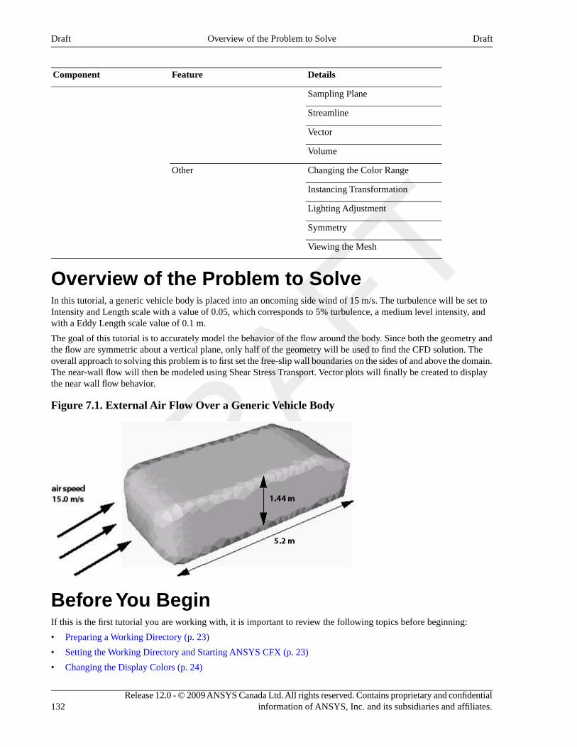
DetailsFeatureComponent
Sampling Plane
Streamline
Vector
Volume
Changing the Color RangeOther
Instancing Transformation
Lighting Adjustment
Symmetry
Viewing the Mesh
Overview of the Problem to SolveIn this tutorial, a generic vehicle body is placed into an oncoming side wind of 15 m/s. The turbulence will be set toIntensity and Length scale with a value of 0.05, which corresponds to 5% turbulence, a medium level intensity, andwith a Eddy Length scale value of 0.1 m.
The goal of this tutorial is to accurately model the behavior of the flow around the body. Since both the geometry andthe flow are symmetric about a vertical plane, only half of the geometry will be used to find the CFD solution. Theoverall approach to solving this problem is to first set the free-slip wall boundaries on the sides of and above the domain.The near-wall flow will then be modeled using Shear Stress Transport. Vector plots will finally be created to displaythe near wall flow behavior.
Figure 7.1. External Air Flow Over a Generic Vehicle Body
Before You BeginIf this is the first tutorial you are working with, it is important to review the following topics before beginning:
• Preparing a Working Directory (p. 23)
• Setting the Working Directory and Starting ANSYS CFX (p. 23)
• Changing the Display Colors (p. 24)
Release 12.0 - © 2009 ANSYS Canada Ltd. All rights reserved. Contains proprietary and confidentialinformation of ANSYS, Inc. and its subsidiaries and affiliates.132
DraftOverview of the Problem to SolveDraft
• Playing a Tutorial Session File (p. 24)
Starting CFX-Pre1. Prepare the working directory using the following files in the examples directory:
• BluntBody.pre
• BluntBodyDist.cse
• BluntBodyMesh.gtm
For details, see Preparing a Working Directory (p. 23)
2. Set the working directory and start CFX-Pre
For details, see Setting the Working Directory and Starting ANSYS CFX (p. 23)
Defining a Case in CFX-PreIf you want to set up the simulation automatically using a tutorial session file, run BluntBody.pre. For details, seePlaying a Tutorial Session File (p. 24). Then proceed to Obtaining a Solution Using CFX-Solver Manager (p. 138).
If you want to set up the simulation manually, proceed to the following steps:
1. Select File > New Case.
2. Select General and click OK.
3. Select File > Save Case As.
4. Under File name, type BluntBody.
5. Click Save.
Importing the Mesh1. Edit Case Options > General in the Outline tree view and ensure that Automatic Default Domain is
turned off.
Default Domain generation should be turned off because you will create a new domain manually, later in thistutorial.
2. Right-click Mesh and select Import Mesh > Other. The Import Mesh dialog box appears.
3. Apply the following settings:
ValueSetting
BluntBodyMesh.gtmFile name
4. Click Open.
Creating the DomainThe flow of air in the domain is expected to be turbulent and approximately isothermal at 288 K. TheShear Stress Transport (SST) turbulence model with automatic wall function treatment will be used because of itshighly accurate predictions of flow separation. To take advantage of the SST model, the boundary layer should beresolved with at least 10 mesh nodes. In order to reduce computational time, the mesh in this tutorial is much coarserthan that.
133Release 12.0 - © 2009 ANSYS Canada Ltd. All rights reserved. Contains proprietary and confidentialinformation of ANSYS, Inc. and its subsidiaries and affiliates.
DraftStarting CFX-PreDraft
This tutorial uses air as an ideal gas as the fluid. When modeling a compressible flow using the ideal gas approximationto calculate density variations, it is important to set a realistic reference pressure. This is because some fluid propertiesdepend on the absolute fluid pressure (calculated as the static pressure plus the reference pressure which is chosen tobe 1 atm).
TipFor more details, see The Shear Stress Transport (SST) (p. 77).
1. Ensure that Flow Analysis 1 > Default Domain is deleted. If not, right-click Default Domain andselect Delete.
2. Click Domain , and set the name to BluntBody.
3. Apply the following settings to BluntBody:
ValueSettingTab
B1.P3Location and Type > LocationBasic Settings
Fluid 1Fluid and Particle Definitions
Air Ideal GasFluid and Particle Definitions > Fluid 1 > Material
1 [atm]Domain Models > Pressure > Reference Pressure
IsothermalHeat Transfer > OptionFluid Models
288 [K]Heat Transfer > Fluid Temperature
Shear Stress TransportTurbulence > Option
4. Click OK.
Creating Composite RegionsAn imported mesh may contain many 2D regions. For the purpose of creating boundary conditions, it can sometimesbe useful to group several 2D regions together and apply a single boundary to the composite 2D region. In this case,you are going to create a Union between two regions that both require a free-slip wall boundary.
1. From the main menu, select Insert > Regions > Composite Region.
2. Set the name to FreeWalls and click OK.
3. Apply the following settings:
ValueSettingTab
2DDimension (Filter)Basic Settings
4. Click beside the Region List dialog box, to display the Selection Dialog. Hold down the Ctrl key and select
Free1 and Free2.
5. Click OK.
Release 12.0 - © 2009 ANSYS Canada Ltd. All rights reserved. Contains proprietary and confidentialinformation of ANSYS, Inc. and its subsidiaries and affiliates.134
DraftCreating Composite RegionsDraft
Creating the BoundariesThe simulation requires inlet, outlet, wall (no slip and free-slip) and symmetry plane boundaries. The regions for theseboundaries were defined when the mesh was created (except for the composite region just created for the free-slip wallboundary).
Inlet Boundary
1. Click Boundary .
2. Under Name, type Inlet.
3. Apply the following settings:
ValueSettingTab
InletBoundary TypeBasic Settings
InletLocation
SubsonicFlow Regime > OptionBoundary Details
Normal SpeedMass and Momentum > Option
15 [m s^-1]Mass and Momentum > Normal Speed
Intensity and Length ScaleTurbulence > Option
0.05aTurbulence > Fractional Intensity
0.1 [m]bTurbulence > Eddy Len. Scale
aFrom the problem description.bFrom the problem description.
4. Click OK.
Outlet Boundary1. Create a new boundary named Outlet.
2. Apply the following settings:
ValueSettingTab
OutletBoundary TypeBasic Settings
OutletLocation
Static PressureMass and Momentum > OptionBoundary Details
0 [Pa]Mass and Momentum > Relative Pressure
3. Click OK.
Free-Slip Wall BoundaryThe top and side surfaces of the rectangular region will use free-slip wall boundaries.
• On free-slip walls the shear stress is set to zero so that the fluid is not retarded.
135Release 12.0 - © 2009 ANSYS Canada Ltd. All rights reserved. Contains proprietary and confidentialinformation of ANSYS, Inc. and its subsidiaries and affiliates.
DraftCreating the BoundariesDraft
• The velocity normal to the wall is also set to zero.
• The velocity parallel to the wall is calculated during the solution.
This boundary is an approximation that may not accurately represent the true flow conditions. By using a free-slip wallboundary, the flow modeling will be less accurate but the computational grid size can be reduced by modeling less ofthe surroundings. If this case were modeling a wind tunnel experiment, the geometry would match the size and shapeof the wind tunnel and use no-slip walls. If this case were modeling a blunt body open to the atmosphere, a much largerdomain would be used to minimize the effect of the far-field boundary, and the far-field boundary type would be setto either a free-slip wall or a pressure-specified entrainment opening.
You will apply a single boundary to both walls by using the composite region defined earlier.
1. Create a new boundary named FreeWalls.
2. Apply the following settings:
ValueSettingTab
WallBoundary TypeBasic Settings
FreeWallsLocation
Free Slip WallMass and Momentum > OptionBoundary Details
3. Click OK.
Symmetry Plane Boundary1. Create a new boundary named SymP.
2. Apply the following settings:
ValueSettingTab
SymmetryBoundary TypeBasic Settings
SymPLocation
3. Click OK.
Wall Boundary on the Blunt Body Surface1. Create a new boundary named Body.
2. Apply the following settings:
ValueSettingTab
WallBoundary TypeBasic Settings
BodyLocation
No Slip WallMass and Momentum > OptionBoundary Details
3. Click OK.
The remaining 2D regions (in this case, just the low Z face) will be assigned the default boundary which is an adiabatic,no-slip wall condition. In this case, the name of the default boundary is BluntBody Default. Although the boundaries
Release 12.0 - © 2009 ANSYS Canada Ltd. All rights reserved. Contains proprietary and confidentialinformation of ANSYS, Inc. and its subsidiaries and affiliates.136
DraftCreating the BoundariesDraft
Body and BluntBody Default are identical (except for their locations), the Body boundary was created so that, duringpost-processing, its location can by conveniently distinguished from the other adiabatic, no-slip wall surfaces.
Setting Initial ValuesThe initial conditions are consistent with inlet boundaries.
1. Click Global Initialization .
2. Apply the following settings:
ValueSettingTab
Automatic with ValueInitial Conditions > Cartesian VelocityComponents > Option
Global Settings
15 [m s^-1]Initial Conditions > Cartesian VelocityComponents > U
0 [m s^-1]Initial Conditions > Cartesian VelocityComponents > V
0 [m s^-1]Initial Conditions > Cartesian VelocityComponents > W
3. Click OK.
Setting Solver Control1. Click Solver Control .
2. Apply the following settings:
ValueSettingTab
60Convergence Control > Max. IterationsBasic Settings
Physical TimescaleConvergence Control > Fluid Timescale Control >Timescale Control
2 [s]aConvergence Control > Fluid Timescale Control >Physical Timescale
1e-05Convergence Criteria > Residual Target
aBased on the air speed and the size of the object.
3. Click OK.
Writing the CFX-Solver Input (.def) File
1. Click Define Run .
2. Apply the following settings:
137Release 12.0 - © 2009 ANSYS Canada Ltd. All rights reserved. Contains proprietary and confidentialinformation of ANSYS, Inc. and its subsidiaries and affiliates.
DraftSetting Initial ValuesDraft
ValueSetting
BluntBody.defFile name
3. Click Save.
CFX-Solver Manager automatically starts and, on the Define Run dialog box, the Solver Input File is set.
4. If using Standalone Mode, quit CFX-Pre, saving the simulation (.cfx) file at your discretion.
Obtaining a Solution Using CFX-Solver ManagerThis tutorial introduces the parallel solver capabilities of CFX.
NoteThe results produced will be identical, whether produced by a parallel or serial run.
If you do not want to solve this tutorial in parallel (on more than one processor) or you do not have a license to run theCFX-Solver in parallel, proceed to Obtaining a Solution in Serial (p. 138).
If you do not know if you have a license to run the CFX-Solver in parallel, you should either ask your systemadministrator, or query the license server (see the ANSYS, Inc. Licensing Guide (which is installed with the ANSYSLicense Manager) for details). Alternatively proceed to Obtaining a Solution in Serial (p. 138).
If you would like to solve this tutorial in parallel on the same machine, proceed to Obtaining a Solution with LocalParallel (p. 139).
If you would like to solve this tutorial in parallel across different machines, proceed to Obtaining a Solution withDistributed Parallel (p. 139).
Obtaining a Solution in SerialWhen CFX-Solver Manager has started, you can obtain a solution to the CFD problem by using the following procedure.
1. Click Start Run.
2. When CFX-Solver is finished, select the check box next to Post-Process Results.
3. If using Standalone Mode, select the check box next to Shut down CFX-Solver Manager.
4. Click OK. Continue this tutorial from Viewing the Results in CFD-Post (p. 142).
Obtaining a Solution in Parallel
Background to Parallel Running in CFXUsing the parallel capability of the CFX-Solver allows you to divide a large CFD problem so that it can run on morethan one processor/machine at once. This saves time and, when multiple machines are used, avoids problems whicharise when a CFD calculation requires more memory than a single machine has available. The partition (division) ofthe CFD problem is automatic.
A number of events occur when you set up a parallel run and then ask the CFX-Solver to calculate the solution:
• Your mesh will be divided into the number of partitions that you have chosen.
• The CFX-Solver runs separately on each of the partitions on the selected machine(s).
• The results that one CFX-Solver process calculates affects the other CFX-Solver processes at the interface betweenthe different sections of the mesh.
• All of the CFX-Solver processes are required to communicate with each other and this is handled by the masterprocess.
Release 12.0 - © 2009 ANSYS Canada Ltd. All rights reserved. Contains proprietary and confidentialinformation of ANSYS, Inc. and its subsidiaries and affiliates.138
DraftObtaining a Solution Using CFX-Solver ManagerDraft
• The master process always runs on the machine that you are logged into when the parallel run starts. The otherCFX-Solver processes are slave processes and may be run on other machines.
• After the problem has been solved, a single results file is written. It will be identical to a results file from the sameproblem run as a serial process, with one exception: an extra variable Real partition number will beavailable for the parallel run. This variable will be used later in this tutorial during post processing.
Obtaining a Solution with Local ParallelTo run in local parallel mode, the machine you are on must have more than one processor.
In CFX-Solver Manager, the Define Run dialog box should already be open.
1. Leave Type of Run set to Full.
If Type of Run was instead set to Partitioner Only, your mesh would be split into a number of partitionsbut would not be run in the CFX-Solver afterwards.
2. Set Run Mode to a parallel mode suitable for your configuration; for example, HP MPI Local Parallel.
This is the recommended method for most applications.
3. If required, click Add Partition to add more partitions.
By default, 2 partitions are assigned.
4. Select Show Advanced Controls.
5. Click the Partitioner tab at the top of the dialog box.
6. Use the default MeTiS partitioner.
Your model will be divided into two sections, with each section running in its own CFX-Solver process. Thedefault is the MeTiS partitioner because it produces more efficient partitions than either RecursiveCoordinate Bisection or User Specified Direction.
7. Click Start Run.
8. When CFX-Solver is finished, select the check box next to Post-Process Results.
9. If using Standalone Mode, select the check box next to Shut down CFX-Solver Manager.
10. Click OK.
Continue this tutorial from Text Output when Running in Parallel (p. 140).
Obtaining a Solution with Distributed ParallelBefore running in Distributed Parallel mode, please ensure that your system has been configured as described in theinstallation documentation.
In CFX-Solver Manager, the Define Run dialog box should already be open.
1. Leave Type of Run set to Full.
If Type of Run was instead set to Partitioner Only, your mesh would be split into a number of partitionsbut would not be run in the CFX-Solver afterwards.
2. Set Run Mode to a parallel mode suitable for your environment; for example, HP MPI DistributedParallel.
The name of the machine that you are currently logged into should be in the Host Name list. You are going torun with two partitions on two different machines, so another machine must be added.
3. Click Insert Host to specify a new host machine.
139Release 12.0 - © 2009 ANSYS Canada Ltd. All rights reserved. Contains proprietary and confidentialinformation of ANSYS, Inc. and its subsidiaries and affiliates.
DraftObtaining a Solution in ParallelDraft
• The Select Parallel Hosts dialog box is displayed. This is where you choose additional machines to run yourprocesses.
• Your system administrator should have set up a hosts file containing a list of the machines that are availableto run the parallel CFX-Solver.
• The Host Name column displays names of available hosts.
• The second column shows the number of processors on that machine.
• The third shows the relative processor speed: a processor on a machine with a relative speed of 1 wouldtypically be twice as fast as a machine with a relative speed of 0.5.
• The last column displays operating system information.
• This information is read from the hosts file; if any information is missing or incorrect your system administratorshould correct the hosts file.
NoteThe # processors, relative speed and system information does not have to be specified to be ableto run on a host.
4. Select the name of another machine in the Host Name list.
Select a machine that you can log into.
5. Click Add.
The name of the machine is added to the Host Name column.
NoteEnsure that the machine that you are currently logged into is in the Hosts Name list in the Define Rundialog box.
6. Close the Select Parallel Hosts dialog box.
7. Select Show Advanced Controls.
8. Click the Partitioner tab at the top of the dialog box.
9. Use the default MeTiS partitioner.
Your model will be divided into two sections, with each section running in its own CFX-Solver process. Thedefault is the MeTiS partitioner because it produces more efficient partitions than either RecursiveCoordinate Bisection or User Specified Direction.
10. Click Start Run to begin the parallel run.
11. Click OK on the pop-up message.
12. When CFX-Solver is finished, select the check box next to Post-Process Results.
13. If using Standalone Mode, select the check box next to Shut down CFX-Solver Manager.
14. Click OK.
Text Output when Running in ParallelThe text output area shows what is being written to the output file. You will see information similar to the following:
+--------------------------------------------------------------------+ | Job Information | +--------------------------------------------------------------------+
Release 12.0 - © 2009 ANSYS Canada Ltd. All rights reserved. Contains proprietary and confidentialinformation of ANSYS, Inc. and its subsidiaries and affiliates.140
DraftObtaining a Solution in ParallelDraft
Run mode: partitioning run
Host computer: fastmachine1 Job started: Tue Jan 20 14:13:27 2009
This tells you that the information following is concerned with the partitioning. After the partitioning job has finished,you will find:
+--------------------------------------------------------------------+ | Partitioning Information | +--------------------------------------------------------------------+
Partitioning information for domain: BluntBody
+------------------+------------------------+-----------------+ | Elements | Vertices | Faces | +------+------------------+------------------------+-----------------+ | Part | Number % | Number % %Ovlp | Number % | +------+------------------+------------------------+-----------------+ | Full | 131878 | 37048 | 11318 | +------+------------------+------------------------+-----------------+ | 1 | 67873 50.4 | 19431 50.4 4.0 | 5705 49.5 | | 2 | 66865 49.6 | 19151 49.6 4.0 | 5820 50.5 | +------+------------------+------------------------+-----------------+ | Sum | 134738 100.0 | 38582 100.0 4.0 | 11525 100.0 | +------+------------------+------------------------+-----------------+
+--------------------------------------------------------------------+ | Partitioning CPU-Time Requirements | +--------------------------------------------------------------------+
- Preparations 3.689E-01 seconds - Low-level mesh partitioning 5.599E-02 seconds - Global partitioning information 9.998E-03 seconds - Element and face partitioning information 7.999E-03 seconds - Vertex partitioning information 0.000E+00 seconds - Partitioning information compression 0.000E+00 seconds - Summed CPU-time for mesh partitioning 4.609E-01 seconds
+--------------------------------------------------------------------+ | Job Information | +--------------------------------------------------------------------+
Host computer: fastmachine1 Job finished: Tue Jan 20 14:13:29 2009
Total CPU time: 9.749E-01 seconds or: ( 0: 0: 0: 0.975 ) ( Days: Hours: Minutes: Seconds )
Total wall clock time: 2.000E+00 seconds
141Release 12.0 - © 2009 ANSYS Canada Ltd. All rights reserved. Contains proprietary and confidentialinformation of ANSYS, Inc. and its subsidiaries and affiliates.
DraftObtaining a Solution in ParallelDraft
or: ( 0: 0: 0: 2.000 ) ( Days: Hours: Minutes: Seconds )
This marks the end of the partitioning job. The CFX-Solver now begins to solve your parallel run:
+--------------------------------------------------------------------+| Job Information |+--------------------------------------------------------------------+Run mode: parallel run (HP MPI Distributed Parallel)Host computer: fastmachine1Par. Process: Master running on mesh partition: 1Job started: Thu Nov 28 15:19:20 2005Host computer: slowermachinePar. Process: Slave running on mesh partition: 2Job started: Thu Nov 28 15:24:55 2005
The machine that you are logged into runs the master process, and controls the overall simulation. The second machineselected will run the slave process. If you had more than two processes, each additional process is run as a slave process.
The master process in this example is running on the mesh partition number 1 and the slave is running on partitionnumber 2. You can find out which nodes and elements are in each partition by using CFD-Post later on in the tutorial.
When the CFX-Solver finishes, the output file displays the job information and a pop-up message to indicate completionof the run.
Viewing the Results in CFD-PostIn CFD-Post, you will create an instance transform object to recreate the full geometry. This full geometry will thenbe displayed using a reflection transform. You will also create a vector plot that will let you see how the flow behavesaround the body as well as a pressure plot displaying the pressure distribution on the body. In order to show the pathof air along the surface of the blunt body, you will make a surface streamline. Finally, the values of the dimensionless
wall distance +y will be examined to make sure the mesh used in the simulation was fine enough near the walls.
Using Symmetry Plane to Display the Full GeometryEarlier in this tutorial you used a symmetry plane boundary because the entire blunt body is symmetrical about a plane.Due to this symmetry, it was necessary to use only half of the full geometry to calculate the CFD results. However,for visualization purposes, it is helpful to use the full blunt body. CFD-Post is able to recreate the full data set fromthe half that was originally calculated. This is done by creating an Instance Transform object.
Manipulating the GeometryYou need to manipulate the geometry so that you will be able to see what happens when you use the symmetry plane.The CFD-Post features that you have used in earlier tutorials will not be described in detail. New features will bedescribed in detail.
• Right-click a blank area in the viewer and select Predefined Camera > View Towards +X.
Creating an Instance TransformInstance Transforms are used to visualize a full geometry representation in cases where the simulation took advantageof symmetry to solve for only part of the geometry. There are three types of transforms that you can use: Rotation,Translation, Reflection/Mirroring. In this tutorial, you will create a Reflection transform located on a plane.
1. Click Location > Plane and set the name to Reflection Plane.
2. Apply the following settings:
Release 12.0 - © 2009 ANSYS Canada Ltd. All rights reserved. Contains proprietary and confidentialinformation of ANSYS, Inc. and its subsidiaries and affiliates.142
DraftViewing the Results in CFD-PostDraft
ValueSettingTab
ZX PlaneDefinition > MethodGeometry
(cleared)Show FacesRender
3. Click Apply.
This creates a plane at y=0 by default, at the same location as the symmetry plane defined in CFX-Pre. Now theinstance transform can be created using this Plane:
4. From the main menu, select Insert > Instance Transform and accept the default name.
5. Apply the following settings:
ValueSettingTab
(Cleared)Instancing Info From DomainDefinition
(Cleared)Apply Rotation
(Selected)Apply Reflection
Reflection PlaneApply Reflection > Plane
6. Click Apply.
Using the Reflection TransformYou can use the transform when creating or editing graphics objects. For example, you can modify the Wireframeview to use it as follows:
1. Under the Outline tab, in User Locations and Plots, apply the following settings to Wireframe:
ValueSettingTab
Instance Transform 1Apply Instancing Transform > TransformView
2. Click Apply.
3. Zoom so that the geometry fills the Viewer.
You will see the full blunt body.
Creating Velocity VectorsYou are now going to create a vector plot to show velocity vectors behind the blunt body. You need to first create anobject to act as a locator, which, in this case, will be a sampling plane. Then, create the vector plot itself.
Creating the Sampling PlaneA sampling plane is a plane with evenly spaced sampling points on it.
1. Right-click a blank area in the viewer and select Predefined Camera > View Towards +Y.
This ensures that the changes can be seen.
2. Create a new plane named Sample.
143Release 12.0 - © 2009 ANSYS Canada Ltd. All rights reserved. Contains proprietary and confidentialinformation of ANSYS, Inc. and its subsidiaries and affiliates.
DraftCreating Velocity VectorsDraft
3. Apply the following settings to create a sampling plane that is parallel to the XZ plane and located at x= 6 m, y=0.001 m and z= 1 m relative to blunt object:
ValueSettingTab
Point and NormalDefinition > MethodGeometry
6, -0.001, 1Definition > Point
0, 1, 0Definition > Normal
RectangularPlane Bounds > Type
2.5 [m]Plane Bounds > X Size
2.5 [m]Plane Bounds > Y Size
SamplePlane Type
20Plane Type > X Samples
20Plane Type > Y Samples
(Cleared)Show FacesRender
(Selected)Show Mesh Lines
4. Click Apply.
You can zoom in on the sampling plane to see the location of the sampling points (where lines intersect). Thereare a total of 400 (20 * 20) sampling points on the plane. A vector can be created at each sampling point.
5. Turn off the visibility of Sample.
Creating a Vector Plot Using Different Sampling Methods
1. Click Vector and accept the default name.
2. Apply the following settings:
ValueSettingTab
SampleDefinition > LocationsGeometry
VertexDefinition > Sampling
0.25Symbol SizeSymbol
3. Click Apply.
4. Zoom until the vector plot is roughly the same size as the viewer.
You should be able to see a region of recirculation behind the blunt body.
5. Ignore the vertices on the sampling plane and increase the density of the vectors by applying the following settings:
ValueSettingTab
Equally SpacedDefinition > SamplingGeometry
Release 12.0 - © 2009 ANSYS Canada Ltd. All rights reserved. Contains proprietary and confidentialinformation of ANSYS, Inc. and its subsidiaries and affiliates.144
DraftCreating Velocity VectorsDraft
ValueSettingTab
1000Definition > # of Points
6. Click Apply.
7. Change the location of the Vector plot by applying the following setting:
ValueSettingTab
SymPDefinition > LocationsGeometry
8. Click Apply.
Displaying Pressure Distribution on Body and SymmetryPlane1. Apply the following settings to the boundary named Body:
ValueSettingTab
VariableModeColor
PressureVariable
Instance Transform 1Apply Instancing Transform > TransformView
2. Click Apply.
3. Apply the following settings to SymP:
ValueSettingTab
(Cleared)Show FacesRender
(Selected)Show Mesh Lines
4. Click Apply.
You will be able to see the mesh around the blunt body, with the mesh length scale decreasing near the body, butstill coarse in the region of recirculation. By zooming in, you will be able to see the layers of inflated elementsnear the body.
Creating Surface Streamlines to Display the Path of Airalong the Surface of the BodyIn order to show the path of air along the surface of the blunt body, surface streamlines can be made as follows:
1. Turn off the visibility of Body, SymP and Vector 1.
2. Create a new plane named Starter.
3. Apply the following settings:
145Release 12.0 - © 2009 ANSYS Canada Ltd. All rights reserved. Contains proprietary and confidentialinformation of ANSYS, Inc. and its subsidiaries and affiliates.
DraftDisplaying Pressure Distribution on Body and Symmetry PlaneDraft
ValueSettingTab
YZ PlaneDefinition > MethodGeometry
-0.1 [m]X
4. Click Apply.
5. Right-click a blank area in the viewer and select Predefined Camera > Isometric View (Z up).
The plane appears just upstream of the blunt body.
6. Turn off the visibility of the plane.
This hides the plane from view, although the plane still exists.
7. Click Streamline and click OK to accept the default name.
8. Apply the following settings:
ValueSettingTab
Surface StreamlineTypeGeometry
BodyDefinition > Surfaces
LocationsDefinition > Start From
StarterDefinition > Locations
100Definition > Max Points
ForwardDefinition > Direction
9. Click Apply.
The surface streamlines appear on half of the surface of the blunt body. They start near the upstream end because thestarting points were formed by projecting nodes from the plane to the blunt body.
Moving ObjectsIn CFD-Post, you can reposition some locator objects directly in the viewer by using the mouse.
1. Turn on the visibility of the plane named Starter.
2. Select the Single Select mouse pointer from the Selection Tools toolbar.
3. In the viewer, click the Starter plane to select it, then use the left mouse button to drag it along the X axis.
Notice that the streamlines are redrawn as the plane moves.
Creating a Surface Plot of y+The velocity next to a no-slip wall boundary changes rapidly from a value of zero at the wall to the free stream valuea short distance away from the wall. This layer of high velocity gradient is known as the boundary layer. Many meshesare not fine enough near a wall to accurately resolve the velocity profile in the boundary layer. Wall functions can beused in these cases to apply an assumed functional shape of the velocity profile. Other grids are fine enough that theydo not require wall functions, and application of the latter has little effect. The majority of cases fall somewhere inbetween these two extremes, where the boundary layer is partially resolved by nodes near the wall and wall functionsare used to supplement accuracy where the nodes are not sufficiently clustered near the wall.
Release 12.0 - © 2009 ANSYS Canada Ltd. All rights reserved. Contains proprietary and confidentialinformation of ANSYS, Inc. and its subsidiaries and affiliates.146
DraftMoving ObjectsDraft
One indicator of the closeness of the first node to the wall is the dimensionless wall distance +y . It is good practice to
examine the values of +y at the end of your simulation. At the lower limit, a value of +y less than or equal to 11indicates that the first node is within the laminar sublayer of the boundary flow. Values larger than this indicate thatan assumed logarithmic shape of the velocity profile is being used to model the boundary layer portion between thewall and the first node. Ideally you should confirm that there are several nodes (3 or more) resolving the boundarylayer profile. If this is not observed, it is highly recommended that more nodes be added near the wall surfaces in orderto improve simulation accuracy. In this tutorial, a coarse mesh is used to reduce the run time. Thus, the grid is far toocoarse to resolve any of the boundary layer profile, and the solution is not highly accurate.
Surface Plot of y+
A surface plot is one which colors a surface according to the values of a variable: in this case, +y . A surface plot of+y can be obtained as follows:
1. Turn off the visibility of all previous plots.
2. Under the Outline tab, apply the following settings to BluntBodyDefault:
ValueSettingTab
VariableModeColor
YplusaVariable
Instance Transform 1Apply Instancing Transform > TransformView
aClick the ellipsis icon to the right of the Variable dropdown menu to view a full list of variables, including Yplus.
3. Click Apply.
4. Under the Outline tab, apply the following settings to Body:
ValueSettingTab
VariableModeColor
YplusaVariable
Instance Transform 1Apply Instancing Transform > TransformView
aClick the ellipsis icon to the right of the Variable dropdown menu to view a full list of variables, including Yplus.
5. Click Apply.
Demonstrating Power SyntaxThis section demonstrates a power syntax macro used to evaluate the variation of any variable in the direction of thex-axis. This is an example of power syntax programming in CFD-Post.
A macro containing CCL and power syntax will be loaded by playing a session file. This macro will be executed byentering a line of power syntax in the Command Editor dialog box. The macro tells CFD-Post to create slice planes,normal to the X axis, at 20 evenly-spaced locations from the beginning to the end of the domain. On each plane, itmeasures and prints the minimum, maximum, and average values for a specified variable (using conservative values).The planes are colored using the specified variable.
147Release 12.0 - © 2009 ANSYS Canada Ltd. All rights reserved. Contains proprietary and confidentialinformation of ANSYS, Inc. and its subsidiaries and affiliates.
DraftDemonstrating Power SyntaxDraft
NoteThe CFD-Post engine can respond to CCL commands issued directly, or to commands issued using thegraphical user interface. The Command Editor dialog box can be used to enter any valid CCL commanddirectly.
1. Play the session file named BluntBodyDist.cse.
2. Right-click a blank area in the viewer and select Predefined Camera > View Towards -X.
3. Select Tools > Command Editor from the menu bar.
4. Type the following line into the Command Editor dialog box (the quotation marks and the semi-colon arerequired):
!BluntBodyDist("Velocity u");
5. Click Process.
The minimum, maximum and average values of the variable at each X location are written to the fileBluntBody.txt. The results can be viewed by opening the file in a text editor.
You can also run the macro with a different variable.
To view the content of the session file (which contains explanatory comments), open the session file in a text editor.It contains all of the CCL and power syntax commands and will provide a better understanding of how the macroworks.
Viewing the Mesh Partitions (Parallel Only)If you solved this tutorial in parallel, then an additional variable named Real partition number will be availablein CFD-Post
1. Create an Isosurface of Real partition number equal to 1.
2. Create a second Isosurface of Real partition number equal to 1.999.
The two Isosurfaces show the edges of the two partitions. The gap between the two plots shows the overlap nodes.These were contained in both partitions 1 and 2.
When you have finished looking at the results, quit CFD-Post.
Release 12.0 - © 2009 ANSYS Canada Ltd. All rights reserved. Contains proprietary and confidentialinformation of ANSYS, Inc. and its subsidiaries and affiliates.148
DraftViewing the Mesh Partitions (Parallel Only)Draft
Chapter 8. Buoyant Flow in a PartitionedCavityThis tutorial includes:
• Tutorial Features (p. 149)
• Overview of the Problem to Solve (p. 150)
• Before You Begin (p. 150)
• Starting CFX-Pre (p. 151)
• Defining a Case in CFX-Pre (p. 151)
• Obtaining a Solution using CFX-Solver Manager (p. 157)
• Viewing the Results in CFD-Post (p. 157)
Tutorial FeaturesIn this tutorial you will learn about:
• Using CFX-4 Mesh Import.
• Setting up a time dependent (transient) simulation.
• Modeling buoyant flow.
DetailsFeatureComponent
General ModeUser ModeCFX-Pre
TransientAnalysis Type
General FluidFluid Type
Single DomainDomain Type
LaminarTurbulence Model
Thermal EnergyHeat Transfer
Buoyant Flow
Symmetry PlaneBoundary Conditions
Outlet (Subsonic)
Wall: No-Slip
Wall: Adiabatic
Wall: Fixed Temperature
Output Control
Transient ExampleTimestep
Transient Results File
Default LocatorsPlotsCFD-Post
149Release 12.0 - © 2009 ANSYS Canada Ltd. All rights reserved. Contains proprietary and confidentialinformation of ANSYS, Inc. and its subsidiaries and affiliates.
DraftDraft
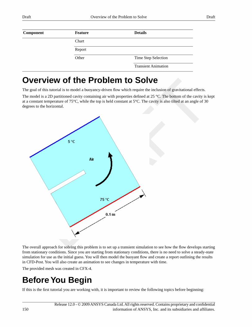
DetailsFeatureComponent
Chart
Report
Time Step SelectionOther
Transient Animation
Overview of the Problem to SolveThe goal of this tutorial is to model a buoyancy-driven flow which require the inclusion of gravitational effects.
The model is a 2D partitioned cavity containing air with properties defined at 25 °C. The bottom of the cavity is keptat a constant temperature of 75°C, while the top is held constant at 5°C. The cavity is also tilted at an angle of 30degrees to the horizontal.
The overall approach for solving this problem is to set up a transient simulation to see how the flow develops startingfrom stationary conditions. Since you are starting from stationary conditions, there is no need to solve a steady-statesimulation for use as the initial guess. You will then model the buoyant flow and create a report outlining the resultsin CFD-Post. You will also create an animation to see changes in temperature with time.
The provided mesh was created in CFX-4.
Before You BeginIf this is the first tutorial you are working with, it is important to review the following topics before beginning:
Release 12.0 - © 2009 ANSYS Canada Ltd. All rights reserved. Contains proprietary and confidentialinformation of ANSYS, Inc. and its subsidiaries and affiliates.150
DraftOverview of the Problem to SolveDraft
• Preparing a Working Directory (p. 23)
• Setting the Working Directory and Starting ANSYS CFX (p. 23)
• Changing the Display Colors (p. 24)
• Playing a Tutorial Session File (p. 24)
Starting CFX-Pre1. Prepare the working directory using the following files in the examples directory:
• Buoyancy2D.geo
• Buoyancy2D.pre
For details, see Preparing a Working Directory (p. 23)
2. Set the working directory and start CFX-Pre
For details, see Setting the Working Directory and Starting ANSYS CFX (p. 23)
Defining a Case in CFX-PreIf you want to set up the simulation automatically using a tutorial session file, run Buoyancy2D.pre. For details,see Playing a Tutorial Session File (p. 24). Then proceed to Obtaining a Solution using CFX-Solver Manager (p. 157).
If you want to set up the simulation manually, you are going to import a hexahedral mesh originally generated inCFX-4. The mesh contains labelled regions which will enable you to apply the relevant boundary conditions for thisproblem.
1. Create a new case using General Mode.
2. Select File > Save Case As and set File name to Buoyancy2D.
3. Click Save.
Importing the Mesh1. Edit Case Options > General in the Outline tree view and ensure that Automatic Default Domain is
turned off.
Default Domain generation should be turned off because you will create a new domain manually, later in thistutorial.
2. Right-click Mesh and select Import Mesh > Other. The Import Mesh dialog box appears.
3. Apply the following settings:
ValueSetting
Buoyancy2D.geoaFile name
CFX-4 (*geo)Files of type
mOptions > Mesh Units
aThis file is in your tutorial directory.
4. Click Open.
151Release 12.0 - © 2009 ANSYS Canada Ltd. All rights reserved. Contains proprietary and confidentialinformation of ANSYS, Inc. and its subsidiaries and affiliates.
DraftStarting CFX-PreDraft
Analysis TypeThe default units and coordinate frame settings are suitable for this tutorial, but the analysis type needs to be set totransient.
You will notice physics validation messages as the case is set to Transient. These errors will be fixed later in thetutorial.
1. Click Analysis Type .
2. Apply the following settings:
ValueSettingTab
TransientAnalysis Type > OptionBasic Settings
2 [s]aAnalysis Type > Time Duration > TotalTime
0.025 [s]bAnalysis Type > Time Steps >Timesteps
0 [s]Analysis Type > Initial Time > Time
aThe total time is the total duration, in real time, for the simulation. For this tutorial, the total time will be set to 2 seconds since it is the timeperiod we are interested in.bIn this example the simulation moves forward in 0.025 s increments until the total time is reached. The step size was determined as a function
of the temperature difference −T T( )max min between the top and bottom of the cavity, and the length scale of the model L( )scale ,
according to: = −t L β T Tg( )( )Δ /g scale max min , where g is the gravity vector and β is the thermal expansivity. For details
on computing a fluid time scale estimate, see the theory guide.
3. Click OK.
Release 12.0 - © 2009 ANSYS Canada Ltd. All rights reserved. Contains proprietary and confidentialinformation of ANSYS, Inc. and its subsidiaries and affiliates.152
DraftAnalysis TypeDraft
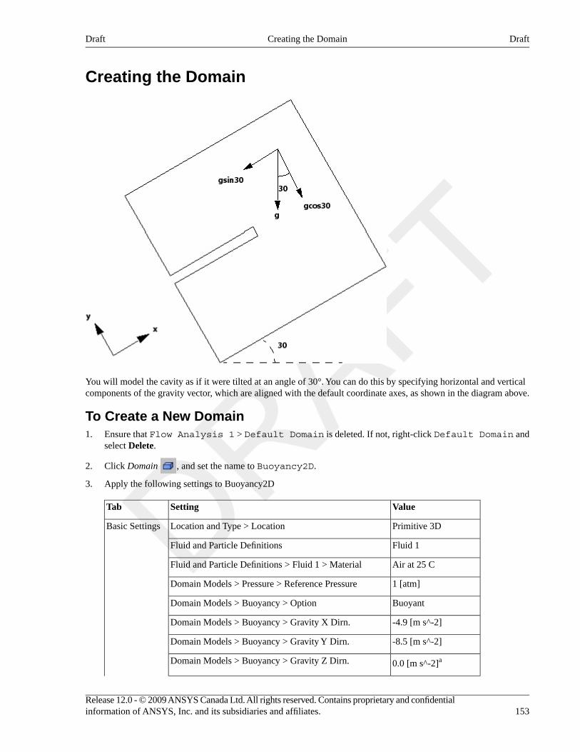
Creating the Domain
You will model the cavity as if it were tilted at an angle of 30°. You can do this by specifying horizontal and verticalcomponents of the gravity vector, which are aligned with the default coordinate axes, as shown in the diagram above.
To Create a New Domain1. Ensure that Flow Analysis 1 > Default Domain is deleted. If not, right-click Default Domain and
select Delete.
2. Click Domain , and set the name to Buoyancy2D.
3. Apply the following settings to Buoyancy2D
ValueSettingTab
Primitive 3DLocation and Type > LocationBasic Settings
Fluid 1Fluid and Particle Definitions
Air at 25 CFluid and Particle Definitions > Fluid 1 > Material
1 [atm]Domain Models > Pressure > Reference Pressure
BuoyantDomain Models > Buoyancy > Option
-4.9 [m s^-2]Domain Models > Buoyancy > Gravity X Dirn.
-8.5 [m s^-2]Domain Models > Buoyancy > Gravity Y Dirn.
0.0 [m s^-2]aDomain Models > Buoyancy > Gravity Z Dirn.
153Release 12.0 - © 2009 ANSYS Canada Ltd. All rights reserved. Contains proprietary and confidentialinformation of ANSYS, Inc. and its subsidiaries and affiliates.
DraftCreating the DomainDraft
ValueSettingTab
40 [C]bDomain Models > Buoyancy > Buoy. Ref. Temp.
Thermal EnergyHeat Transfer > OptionFluid Models
None (Laminar)Turbulence > Option
aThis produces a gravity vector that simulates the tilt of the cavity.bEnsure that the unit setting is correct. This is just an approximate representative domain temperature.
Initialization will be set up using Global Initialization , so there is no need to visit the Initialization tab.
4. Click OK.
Creating the Boundaries
Hot and Cold Wall BoundaryCreate a wall boundary with a fixed temperature of 75 °C on the bottom surface of the cavity, as follows:
1. Create a new boundary named hot.
2. Apply the following settings
ValueSettingTab
WallBoundary TypeBasic Settings
WALLHOTLocation
TemperatureHeat Transfer > OptionBoundaryDetails
75 [C]Heat Transfer > Fixed Temperature
3. Click OK.
4. Create a new boundary named cold.
5. Apply the following settings
ValueSettingTab
WallBoundary TypeBasic Settings
WALLCOLDLocation
TemperatureHeat Transfer > OptionBoundaryDetails
5 [C]Heat Transfer > Fixed Temperature
6. Click OK.
Symmetry Plane BoundaryA single symmetry plane boundary can be used for the front and back of the cavity. Symmetry, which can make a 3Dproblem into a 2D problem, can be used when the geometry and mesh are invariant normal to the symmetry surface.
1. Create a new boundary named SymP.
Release 12.0 - © 2009 ANSYS Canada Ltd. All rights reserved. Contains proprietary and confidentialinformation of ANSYS, Inc. and its subsidiaries and affiliates.154
DraftCreating the BoundariesDraft
2. Apply the following settings
ValueSettingTab
SymmetryBoundary TypeBasic Settings
SYMMET1, SYMMET2aLocation
aUse the Ctrl key to select more than one region.
3. Click OK.
The default adiabatic wall boundary will be applied automatically to the remaining boundaries.
Setting Initial ValuesYou should set initial settings using the Automatic with Value option when defining a transient simulation.Using this option, the first run will use the specified initial conditions (the air is at rest with a temperature of 5 °C)while subsequent runs will use results file data for initial conditions.
1. Click Global Initialization .
2. Apply the following settings
ValueSettingTab
Automatic withValue
Initial Conditions > Cartesian Velocity Components> Option
Global Settings
0 [m s^-1]Initial Conditions > Cartesian Velocity Components> U
0 [m s^-1]Initial Conditions > Cartesian Velocity Components> V
0 [m s^-1]Initial Conditions > Cartesian Velocity Components> W
0 [Pa]Initial Conditions > Static Pressure > Relative Pressure
5 [C]Initial Conditions > Temperature > Temperature
3. Click OK.
Setting Output Control1. Click Output Control .
2. Click the Trn Results tab.
3. In the Transient Results tree view, click Add new item , set Name to Transient Results 1, and click
OK.
4. Apply the following settings to Transient Results 1:
ValueSetting
Selected VariablesOption
155Release 12.0 - © 2009 ANSYS Canada Ltd. All rights reserved. Contains proprietary and confidentialinformation of ANSYS, Inc. and its subsidiaries and affiliates.
DraftSetting Initial ValuesDraft
ValueSetting
Pressure, Temperature, VelocityOutput Variables Lista
Time IntervalOutput Frequency > Option
0.1 [s]bOutput Frequency > Time Interval
aClick the ellipsis icon to select items if they do not appear in the drop-down list. Use the Ctrl key to select multiple items.bThe Time Interval option specifies the simulation time interval between the writing of each file. The time interval will be set to 0.1 s, whichis 4 times the time step that was set up earlier. There is no need to set a smaller time interval because it does not affect the solution accuracy.Choosing a smaller time interval would simply result in more output files.
5. Click OK.
Setting Solver Control1. Click Solver Control .
2. Apply the following settings
ValueSettingTab
High ResolutionAdvection Scheme > OptionBasic Settings
5aConvergence Control > Max. Coeff. Loops
RMSConvergence Criteria > Residual Type
1.E-4bConvergence Criteria > Residual Target
aThe maximum coefficient loops option determines the maximum number of iterations per time step. It is recommended to set the maximumcoefficient loops to between 3 and 5. For this tutorial, it was chosen to be 5, which ensures no net imbalance.bAn RMS value of at least 1.E-5 is usually required for adequate convergence, but the default value of 1.E-4 is sufficient for demonstrationpurposes.
3. Click OK.
Writing the CFX-Solver Input (.def) File
1. Click Define Run .
2. Apply the following settings:
ValueSetting
Buoyancy2D.defFile name
3. Click Save.
CFX-Solver Manager automatically starts and, on the Define Run dialog box, the Solver Input File is set.
4. If using Standalone Mode, quit CFX-Pre, saving the simulation (.cfx) file at your discretion.
Release 12.0 - © 2009 ANSYS Canada Ltd. All rights reserved. Contains proprietary and confidentialinformation of ANSYS, Inc. and its subsidiaries and affiliates.156
DraftSetting Solver ControlDraft
Obtaining a Solution using CFX-Solver ManagerWhen CFX-Pre has shut down and CFX-Solver Manager has started, you can obtain a solution to the CFD problemby using the following procedure.
NoteRecall that the output displayed on the Out File tab of the CFX-Solver Manager is more complicated fortransient problems than for steady-state problems. Each timestep consists of several iterations, and afterthe timestep, information about various quantities is printed.
1. Click Start Run.
2. Select the check box next to Post-Process Results when the completion message appears at the end of the run.
3. If using Standalone Mode, select the check box next to Shut down CFX-Solver Manager.
4. Click OK.
Viewing the Results in CFD-PostIn this section, you will create a customized report in CFD-Post. You will also, optionally, make an animation to seechanges in temperature with time.
Simple ReportFirst, you will view a report that is created with little effort:
1. Click the Report Viewer tab. Note that the report loads with some automatically-generated statistical information.
2. In the Outline tree view, under Report, experiment with the various settings for Mesh Report, PhysicsReport and other report objects. These settings control the report contents. On the Report Viewer tab, you canclick Refresh to see the changes to your report.
Plots for Customized ReportsHere, you will create the following objects in preparation for generating a more customized report:
• Contour plot of temperature
• Point locators (for observing temperature)
• Comment
• Figure showing the contour plot and point locator
• Time chart showing the temperature at the point locator
• Table.
Contour Plot of Temperature1. Click the 3D Viewer tab and right-click a blank area of the viewer, then select Predefined Camera > View
Towards -Z.
2. Select Insert > Contour from the main menu.
3. Accept the default name by clicking OK.
4. Set Locations to SymP.
5. Set Variable to Temperature.
6. Click Apply.
157Release 12.0 - © 2009 ANSYS Canada Ltd. All rights reserved. Contains proprietary and confidentialinformation of ANSYS, Inc. and its subsidiaries and affiliates.
DraftObtaining a Solution using CFX-Solver ManagerDraft
The contour plot shows the temperature at the end of the simulation, since CFD-Post loads values for the last timestepby default. You can load different timesteps using the Timestep Selector dialog box, accessible by selecting Tools >Timestep Selector from the main menu.
Before proceeding, turn off the visibility of the contour plot.
Point LocatorsTwo points will be created to generate a time chart of temperature vs. time later on in this tutorial. The two points werechosen to be located half way in between the bottom and top cavity, close to where the average temperature is goingto be.
1. From the main menu, select Insert > Location > Point.
2. Accept the default name by clicking OK.
3. Set Method to XYZ.
4. Set Point coordinates to 0.098, 0.05, 0.00125.
5. Click Apply.
Note the location of Point 1 in the viewer.
6. Right-click the Point 1 object in the tree view and select Duplicate from the shortcut menu.
7. Accept the default name by clicking OK.
8. Right-click the Point 2 object in the tree view and select Edit from the shortcut menu.
9. Change the x-coordinate to 0.052.
10. Click Apply.
Note the location of Point 2 in the viewer.
Comment
1. Click Create comment .
2. Accept the default name by clicking OK.
A comment object appears in the tree view, under the Report object.
3. Set Heading to Buoyant Flow in a Partitioned Cavity.
4. In the large text box, type:
This is a sample paragraph.
FigureFigures are CCL objects that can be used to store and switch between different views in a given viewport. By selectinga figure, the information contained in the figure, such as the camera angle, zoom level, lighting and the visibility settingof each object in the tree view, is applied to the active viewport and is usable in reports.
1. Click the 3D Viewer tab.
2. Select Insert > Figure from the main menu.
3. Accept the default name by clicking OK.
The Make copies of objects check box determines whether or not the objects that are visible in the viewer arecopied. If objects are copied, then the copies are used in the figure instead of the originals. Since you are not usingmultiple views or figures, the check box setting does not matter.
A figure object will appear under the Report branch in the tree view.
Release 12.0 - © 2009 ANSYS Canada Ltd. All rights reserved. Contains proprietary and confidentialinformation of ANSYS, Inc. and its subsidiaries and affiliates.158
DraftPlots for Customized ReportsDraft
Time Chart of TemperatureTime charts use expressions or a point locator to plot the variation of a scalar value with time. In this tutorial, thevariation of temperature versus time will be plotted.
1. Select Insert > Chart from the main menu.
2. Accept the default name by clicking OK.
3. Set Type to XY-Transient or Sequence.
4. Set Title to Temperature versus Time.
5. Click the Data Series tab.
6. Right-click in the Data Series list box and select New, or click New .
7. Set Name to Temperature at Point 1.
8. Set Location to Point 1.
9. Click the X Axis tab.
10. Set Data Selection > Expression to Time.
11. Click the Y Axis tab.
12. Set Data Selection > Variable to Temperature.
13. Ensure that the Refresh chart on Apply check box (at the bottom of the details view) is selected.
This causes the chart to be regenerated in the Chart Viewer tab each time you apply changes in the details view.(When the Refresh chart on Apply check box is cleared, the chart will be regenerated only when you manuallyrefresh it. One way to refresh the chart is to click the Refresh button at the top of the Chart Viewer tab.)
14. Click Apply.
A chart object will appear under the Report branch in the tree view.
It may take some time for the chart to appear because every transient results file will be loaded in order to generatethe time chart.
15. Click New (on the Data Series tab).
16. Set Name to Temperature at Point 2.
17. Set Location to Point 2.
18. Click Apply.
A second chart line will appear in the chart, representing the temperature at Point 2.
Table of Temperature Values1. Select Insert > Table from the main menu.
2. Accept the default name by clicking OK.
A table object will appear under the Report branch in the tree view.
3. Set the following:
ValueCell
LocationA1
Point 1A2
Point 2A3
159Release 12.0 - © 2009 ANSYS Canada Ltd. All rights reserved. Contains proprietary and confidentialinformation of ANSYS, Inc. and its subsidiaries and affiliates.
DraftPlots for Customized ReportsDraft
ValueCell
TemperatureB1
=probe(Temperature)@Point 1B2
=probe(Temperature)@Point 2B3
The table shows temperatures at the end of the simulation, since CFD-Post loads values for the last timestep by default.You can load different timesteps using the Timestep Selector dialog box, accessible by selecting Tools > TimestepSelector.
Customized ReportRight-click the Report object and select Refresh Preview from the shortcut menu. Look at the report in the ReportViewer tab. Note that, in addition to the automatically-generated objects that you saw earlier when creating a simplereport, this report also includes the customized figure, time chart and table described above.
AnimationsYou may want to create an animation of the buoyant flow over time. Use the animation feature to see the changingtemperature field. The animation feature was used in Flow from a Circular Vent (p. 113).
CompletionWhen you have finished, quit CFD-Post.
Release 12.0 - © 2009 ANSYS Canada Ltd. All rights reserved. Contains proprietary and confidentialinformation of ANSYS, Inc. and its subsidiaries and affiliates.160
DraftCustomized ReportDraft
Chapter 9. Free Surface Flow Over aBumpThis tutorial includes:
• Tutorial Features (p. 161)
• Overview of the Problem to Solve (p. 162)
• Approach to the Problem (p. 162)
• Before You Begin (p. 162)
• Starting CFX-Pre (p. 162)
• Defining a Simulation in CFX-Pre (p. 163)
• Obtaining a Solution using CFX-Solver Manager (p. 171)
• Viewing the Results in CFD-Post (p. 172)
• Using a Supercritical Outlet Condition (p. 177)
Tutorial FeaturesIn this tutorial you will set up a 2D problem in which you:
• Import a mesh.
• Set up appropriate boundary conditions for a free surface simulation. (Free surface simulations are more sensitiveto incorrect boundary and initial guess settings than other more basic models.)
• Use mesh adaption to refine the mesh where the volume fraction gradient is greatest. (The refined mesh aids in thedevelopment of a sharp interface between the liquid and gas.)
DetailsFeatureComponent
General ModeUser ModeCFX-Pre
Steady StateAnalysis Type
General FluidFluid Type
Single DomainDomain Type
k-EpsilonTurbulence Model
IsothermalHeat Transfer
Buoyant Flow
Homogeneous ModelMultiphase
InletBoundary Conditions
Opening
Outlet
Symmetry Plane
Wall: No Slip
161Release 12.0 - © 2009 ANSYS Canada Ltd. All rights reserved. Contains proprietary and confidentialinformation of ANSYS, Inc. and its subsidiaries and affiliates.
DraftDraft
DetailsFeatureComponent
CEL (CFX Expression Language)
Mesh Adaption
Physical Time ScaleTimestep
Default LocatorsPlotsCFD-Post
Isosurface
Polyline
Sampling Plane
Vector
Volume
Chart CreationOther
Title/Text
Viewing the Mesh
Overview of the Problem to SolveThis tutorial demonstrates the simulation of a free surface flow.
The geometry consists of a 2D channel in which the bottom of the channel is interrupted by a semicircular bump ofradius 30 mm. The problem environment comprises air at 1 Pa and isothermal water; the normal inlet speed is 0.26m/s; the incoming water has a turbulence intensity of 5%. The flow upstream of the bump is subcritical. The downstreamboundary conditions (the height of the water) were estimated for this tutorial; you can do this using an analytical 1Dcalculation or data tables for flow over a bump.
Approach to the ProblemA geometry and mesh is provided. You will create a two-phase homogenous setting and the expressions that will beused in setting initial values and boundary conditions. Later, you will use mesh adaption to improve the accuracy ofthe downstream simulation.
Before You BeginIf this is the first tutorial you are working with, it is important to review the following topics before beginning:
• Preparing a Working Directory (p. 23)
• Setting the Working Directory and Starting ANSYS CFX (p. 23)
• Changing the Display Colors (p. 24)
• Playing a Tutorial Session File (p. 24)
Starting CFX-Pre1. Prepare the working directory using the following files in the examples directory:
• Bump2D.pre
Release 12.0 - © 2009 ANSYS Canada Ltd. All rights reserved. Contains proprietary and confidentialinformation of ANSYS, Inc. and its subsidiaries and affiliates.162
DraftOverview of the Problem to SolveDraft
• Bump2DExpressions.ccl
• Bump2Dpatran.out
For details, see Preparing a Working Directory (p. 23)
2. Set the working directory and start CFX-Pre.
For details, see Setting the Working Directory and Starting ANSYS CFX (p. 23)
Defining a Simulation in CFX-PreIf you want to set up the simulation automatically using a tutorial session file, run Bump2D.pre. For details, seePlaying a Tutorial Session File (p. 24). Then proceed to Obtaining a Solution using CFX-Solver Manager (p. 171).
If you want to set up the simulation manually, proceed to the following steps:
1. Select File > New Case.
2. Select General and click OK.
3. Select File > Save Case As.
4. Under File name, type Bump2D.
5. Click Save.
Importing the Mesh1. Right-click Mesh and select Import Mesh > Other. The Import Mesh dialog box appears.
2. Apply the following settings:
ValueSetting
Bump2Dpatran.outFile name
PATRAN Neutral (*out *neu)Files of type
mOptions > Mesh units
3. Click Open.
4. To best orient the view, right-click a blank area in the viewer and select Predefined Camera > View Towards -Zfrom the shortcut menu.
Viewing the Region LabelsEnable the display of region labels so that you can see where you will define boundaries later in this tutorial:
1. In the Outline tree view, edit Case Options > Labels and Markers.
2. Apply the following settings:
ValueSettingTab
(Selected)Show LabelsSettings
(Selected)Show Labels > Show Primitive 3D Labels
(Selected)Show Labels > Show Primitive 2D Labels
3. Click OK.
163Release 12.0 - © 2009 ANSYS Canada Ltd. All rights reserved. Contains proprietary and confidentialinformation of ANSYS, Inc. and its subsidiaries and affiliates.
DraftDefining a Simulation in CFX-PreDraft
Creating Expressions for Initial and Boundary ConditionsSimulation of free surface flows usually requires defining boundary and initial conditions to set up appropriate pressureand volume fraction fields. You will need to create expressions using CEL (CFX Expression Language) to define theseconditions.
In this simulation, the following conditions are set and require expressions:
• An inlet boundary where the volume fraction above the free surface is 1 for air and 0 for water, and below the freesurface is 0 for air and 1 for water.
• A pressure-specified outlet boundary, where the pressure above the free surface is constant and the pressure belowthe free surface is a hydrostatic distribution. This requires you to know the approximate height of the fluid at theoutlet. In this case, an analytical solution for 1D flow over a bump was used to determine the value for DownH inCreating Expressions in CEL (p. 164). The simulation is not sensitive to the exact outlet fluid height, so anapproximation is sufficient. You will examine the effect of the outlet boundary condition in the postprocessingsection and confirm that it does not affect the validity of the results. It is necessary to specify such a boundarycondition to force the flow downstream of the bump into the supercritical regime.
• An initial pressure field for the domain with a similar pressure distribution to that of the outlet boundary.
Either create expressions using the Expressions workspace or read in expressions from the example file provided:
• Creating Expressions in CEL (p. 164)
• Reading Expressions From a File (p. 165)
Creating Expressions in CELThe expressions you create in this step are the same as the ones provided in Reading Expressions From a File (p. 165),so you can choose to follow either set of instructions.
1. Right-click Expressions, Functions and Variables > Expressions in the tree view and selectInsert > Expression.
2. Set the name to UpH and click OK to create the upstream free surface height.
3. Set Definition to 0.069 [m], and then click Apply.
4. Use the same method to create the expressions listed in the table below. These are expressions for the downstreamfree surface height, the fluid density, the buoyancy reference density, the calculated density of the fluid (density- buoyancy reference density), the upstream volume fractions of air and water, the upstream pressure distribution,the downstream volume fractions of air and water, and the downstream pressure distribution.
DefinitionName
0.022 [m]DownH
997 [kg m^-3]DenWater
1.185 [kg m^-3]DenRef
(DenWater - DenRef)DenH
step((y-UpH)/1[m])UpVFAir
1-UpVFAirUpVFWater
DenH*g*UpVFWater*(UpH-y)UpPres
step((y-DownH)/1[m])DownVFAir
1-DownVFAirDownVFWater
Release 12.0 - © 2009 ANSYS Canada Ltd. All rights reserved. Contains proprietary and confidentialinformation of ANSYS, Inc. and its subsidiaries and affiliates.164
DraftCreating Expressions for Initial and Boundary ConditionsDraft
DefinitionName
DenH*g*DownVFWater*(DownH-y)DownPres
5. Proceed to Creating the Domain (p. 165).
Reading Expressions From a File1. If you have not done so already, copy the file <CFXROOT>/examples/Bump2DExpressions.ccl to your
working directory.
2. Select File > Import > CCL.
3. In the Import CCL dialog box, ensure that the Append option is selected.
4. Select Bump2DExpressions.ccl.
5. Click Open.
6. After the file has been imported, use the Expressions tree view to view the expressions that have been created.
Creating the DomainSet up a homogenous, two-fluid environment:
1. Edit Case Options > General in the Outline tree view and ensure that Automatic Default Domain isturned on. A domain named Default Domain should appear under the Simulation > Flow Analysis1 branch.
2. Double-click Default Domain.
3. Under Fluid and Particle Definitions, delete Fluid 1 and create a new fluid named Air.
4. Confirm that the following settings are configured:
ValueSettingTab
AirFluid and Particle DefinitionsBasic Settings
Air at 25 CFluid and Particle Definitions > Air > Material
5. Click Add new item and create a new fluid named Water.
6. Apply the following settings:
ValueSettingTab
WaterFluid and Particle DefinitionsBasic Settings
WateraFluid and Particle Definitions > Water > Material
1 [atm]Domain Models > Pressure > Reference Pressure
BuoyantDomain Models > Buoyancy > Option
0 [m s^-2]Domain Models > Buoyancy > Gravity X Dirn.
-gDomain Models > Buoyancy > Gravity Y Dirn.b
0 [m s^-2]Domain Models > Buoyancy > Gravity Z Dirn.
165Release 12.0 - © 2009 ANSYS Canada Ltd. All rights reserved. Contains proprietary and confidentialinformation of ANSYS, Inc. and its subsidiaries and affiliates.
DraftCreating the DomainDraft
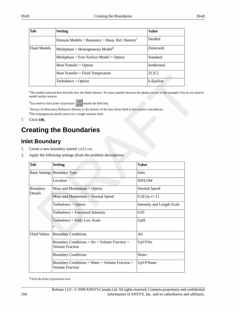
ValueSettingTab
DenRefDomain Models > Buoyancy > Buoy. Ref. Densityc
(Selected)Multiphase > Homogeneous ModeldFluid Models
StandardMultiphase > Free Surface Model > Option
IsothermalHeat Transfer > Option
25 [C]Heat Transfer > Fluid Temperature
k-EpsilonTurbulence > Option
aThe models selected here describe how the fluids interact. No mass transfer between the phases occurs in this example. You do not need tomodel surface tension.
bYou need to click Enter Expression beside the field first.
cAlways set Buoyancy Reference Density to the density of the least dense fluid in free surface calculations.dThe homogeneous model solves for a single solution field.
7. Click OK.
Creating the Boundaries
Inlet Boundary1. Create a new boundary named inflow.
2. Apply the following settings (from the problem description):
ValueSettingTab
InletBoundary TypeBasic Settings
INFLOWLocation
Normal SpeedMass and Momentum > OptionBoundaryDetails
0.26 [m s^-1]Mass and Momentum > Normal Speed
Intensity and Length ScaleTurbulence > Option
0.05Turbulence > Fractional Intensity
UpHTurbulence > Eddy Len. Scale
a
AirBoundary ConditionsFluid Values
UpVFAirBoundary Conditions > Air > Volume Fraction >Volume Fraction
WaterBoundary Conditions
UpVFWaterBoundary Conditions > Water > Volume Fraction >Volume Fraction
aClick the Enter Expression icon.
Release 12.0 - © 2009 ANSYS Canada Ltd. All rights reserved. Contains proprietary and confidentialinformation of ANSYS, Inc. and its subsidiaries and affiliates.166
DraftCreating the BoundariesDraft
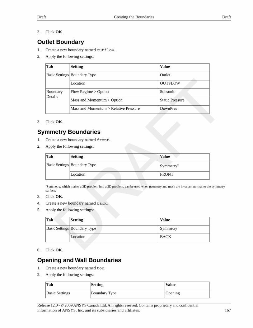
3. Click OK.
Outlet Boundary1. Create a new boundary named outflow.
2. Apply the following settings:
ValueSettingTab
OutletBoundary TypeBasic Settings
OUTFLOWLocation
SubsonicFlow Regime > OptionBoundaryDetails
Static PressureMass and Momentum > Option
DownPresMass and Momentum > Relative Pressure
3. Click OK.
Symmetry Boundaries1. Create a new boundary named front.
2. Apply the following settings:
ValueSettingTab
SymmetryaBoundary TypeBasic Settings
FRONTLocation
aSymmetry, which makes a 3D problem into a 2D problem, can be used when geometry and mesh are invariant normal to the symmetrysurface.
3. Click OK.
4. Create a new boundary named back.
5. Apply the following settings:
ValueSettingTab
SymmetryBoundary TypeBasic Settings
BACKLocation
6. Click OK.
Opening and Wall Boundaries1. Create a new boundary named top.
2. Apply the following settings:
ValueSettingTab
OpeningBoundary TypeBasic Settings
167Release 12.0 - © 2009 ANSYS Canada Ltd. All rights reserved. Contains proprietary and confidentialinformation of ANSYS, Inc. and its subsidiaries and affiliates.
DraftCreating the BoundariesDraft
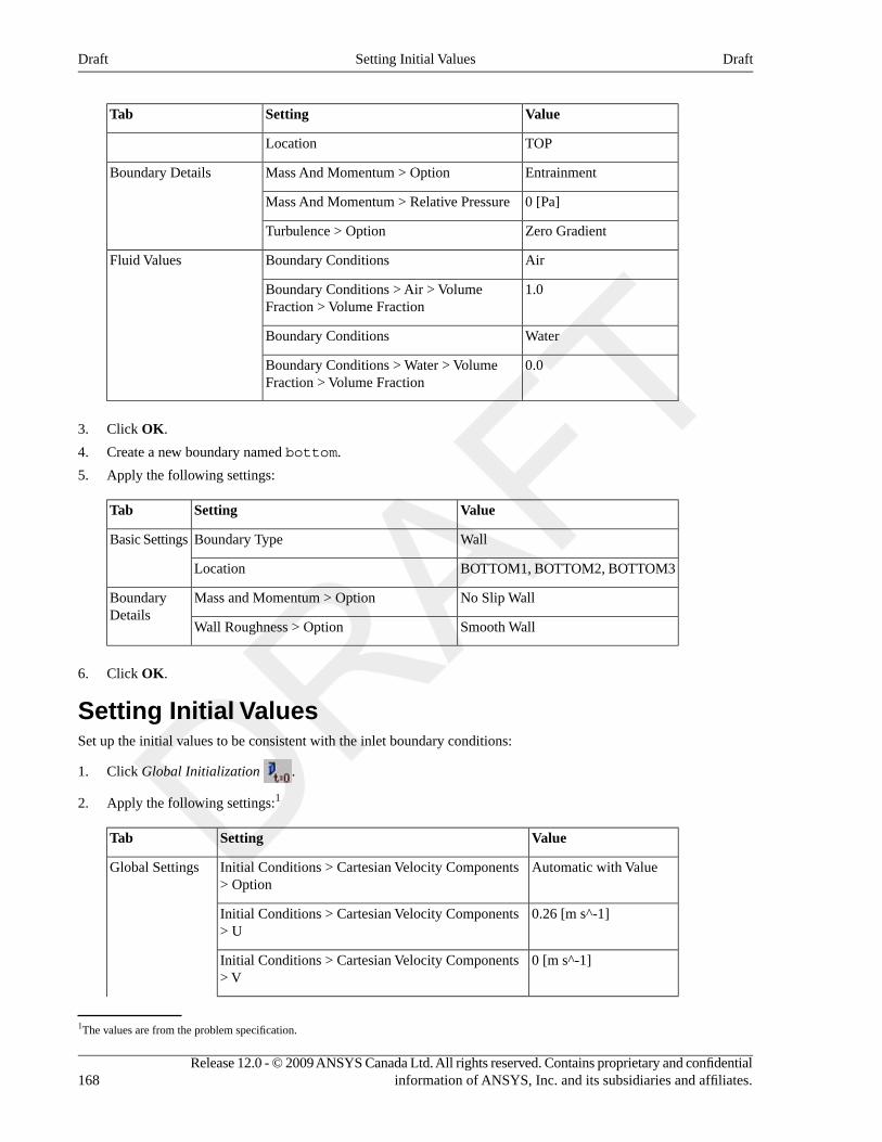
ValueSettingTab
TOPLocation
EntrainmentMass And Momentum > OptionBoundary Details
0 [Pa]Mass And Momentum > Relative Pressure
Zero GradientTurbulence > Option
AirBoundary ConditionsFluid Values
1.0Boundary Conditions > Air > VolumeFraction > Volume Fraction
WaterBoundary Conditions
0.0Boundary Conditions > Water > VolumeFraction > Volume Fraction
3. Click OK.
4. Create a new boundary named bottom.
5. Apply the following settings:
ValueSettingTab
WallBoundary TypeBasic Settings
BOTTOM1, BOTTOM2, BOTTOM3Location
No Slip WallMass and Momentum > OptionBoundaryDetails
Smooth WallWall Roughness > Option
6. Click OK.
Setting Initial ValuesSet up the initial values to be consistent with the inlet boundary conditions:
1. Click Global Initialization .
2. Apply the following settings:1
ValueSettingTab
Automatic with ValueInitial Conditions > Cartesian Velocity Components> Option
Global Settings
0.26 [m s^-1]Initial Conditions > Cartesian Velocity Components> U
0 [m s^-1]Initial Conditions > Cartesian Velocity Components> V
1The values are from the problem specification.
Release 12.0 - © 2009 ANSYS Canada Ltd. All rights reserved. Contains proprietary and confidentialinformation of ANSYS, Inc. and its subsidiaries and affiliates.168
DraftSetting Initial ValuesDraft
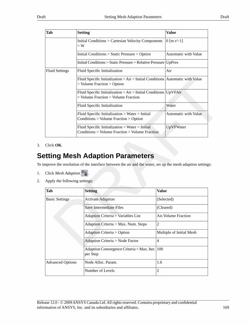
ValueSettingTab
0 [m s^-1]Initial Conditions > Cartesian Velocity Components> W
Automatic with ValueInitial Conditions > Static Pressure > Option
UpPresInitial Conditions > Static Pressure > Relative Pressure
AirFluid Specific InitializationFluid Settings
Automatic with ValueFluid Specific Initialization > Air > Initial Conditions> Volume Fraction > Option
UpVFAirFluid Specific Initialization > Air > Initial Conditions> Volume Fraction > Volume Fraction
WaterFluid Specific Initialization
Automatic with ValueFluid Specific Initialization > Water > InitialConditions > Volume Fraction > Option
UpVFWaterFluid Specific Initialization > Water > InitialConditions > Volume Fraction > Volume Fraction
3. Click OK.
Setting Mesh Adaption ParametersTo improve the resolution of the interface between the air and the water, set up the mesh adaption settings:
1. Click Mesh Adaption .
2. Apply the following settings:
ValueSettingTab
(Selected)Activate AdaptionBasic Settings
(Cleared)Save Intermediate Files
Air.Volume FractionAdaption Criteria > Variables List
2Adaption Criteria > Max. Num. Steps
Multiple of Initial MeshAdaption Criteria > Option
4Adaption Criteria > Node Factor
100Adaption Convergence Criteria > Max. Iter.per Step
1.6Node Alloc. Param.Advanced Options
2Number of Levels
169Release 12.0 - © 2009 ANSYS Canada Ltd. All rights reserved. Contains proprietary and confidentialinformation of ANSYS, Inc. and its subsidiaries and affiliates.
DraftSetting Mesh Adaption ParametersDraft
NoteYou can find descriptions of the mesh adaption process and of the parameters you are setting in MeshAdaption (p. 195) in the ANSYS CFX-Pre User's Guide. The values used here were determined throughexperimentation.
3. Click OK.
Setting the Solver ControlsNoteSetting Max. Iterations to 200 (below) and Number of (Adaption) Levels to 2 with a Max. Iter. per Stepof 100 timesteps each (in the previous section), results in a total maximum number of timesteps of 400(2*100+200=400).
1. Click Solver Control .
2. Apply the following settings:
ValueSettingTab
200Convergence Control > Max. IterationsBasic Settings
Physical TimescaleConvergence Control >Fluid Timescale Control> Timescale Control
0.25 [s] aConvergence Control >Fluid Timescale Control> Physical Timescale
(Selected)Multiphase ControlAdvanced Options
(Selected)Multiphase Control > Volume FractionCoupling
CoupledMultiphase Control > Volume FractionCoupling > Option
aThis value is based on the time it takes the water to flow over the bump.
NoteSelecting these options on the solver control activates the Coupled Volume Fraction solution algorithm.This algorithm typically converges better than the Segregated Volume Faction algorithm forbuoyancy-driven problems such as this tutorial. The Segregated Volume Faction algorithm wouldhave required a 0.05 second timescale, as compared with 0.25 seconds for the Coupled Volume Fractionalgorithm.
3. Click OK.
Writing the CFX-Solver Input (.def) File
1. Click Define Run .
2. Apply the following settings:
Release 12.0 - © 2009 ANSYS Canada Ltd. All rights reserved. Contains proprietary and confidentialinformation of ANSYS, Inc. and its subsidiaries and affiliates.170
DraftSetting the Solver ControlsDraft
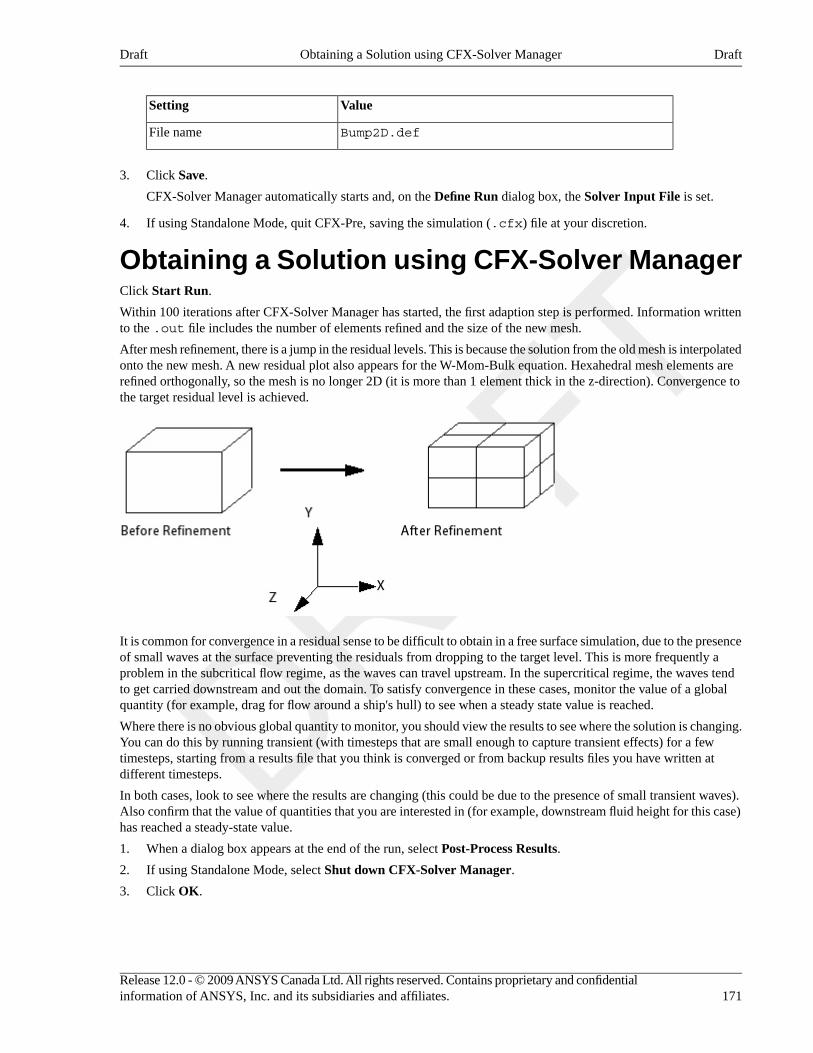
ValueSetting
Bump2D.defFile name
3. Click Save.
CFX-Solver Manager automatically starts and, on the Define Run dialog box, the Solver Input File is set.
4. If using Standalone Mode, quit CFX-Pre, saving the simulation (.cfx) file at your discretion.
Obtaining a Solution using CFX-Solver ManagerClick Start Run.
Within 100 iterations after CFX-Solver Manager has started, the first adaption step is performed. Information writtento the .out file includes the number of elements refined and the size of the new mesh.
After mesh refinement, there is a jump in the residual levels. This is because the solution from the old mesh is interpolatedonto the new mesh. A new residual plot also appears for the W-Mom-Bulk equation. Hexahedral mesh elements arerefined orthogonally, so the mesh is no longer 2D (it is more than 1 element thick in the z-direction). Convergence tothe target residual level is achieved.
It is common for convergence in a residual sense to be difficult to obtain in a free surface simulation, due to the presenceof small waves at the surface preventing the residuals from dropping to the target level. This is more frequently aproblem in the subcritical flow regime, as the waves can travel upstream. In the supercritical regime, the waves tendto get carried downstream and out the domain. To satisfy convergence in these cases, monitor the value of a globalquantity (for example, drag for flow around a ship's hull) to see when a steady state value is reached.
Where there is no obvious global quantity to monitor, you should view the results to see where the solution is changing.You can do this by running transient (with timesteps that are small enough to capture transient effects) for a fewtimesteps, starting from a results file that you think is converged or from backup results files you have written atdifferent timesteps.
In both cases, look to see where the results are changing (this could be due to the presence of small transient waves).Also confirm that the value of quantities that you are interested in (for example, downstream fluid height for this case)has reached a steady-state value.
1. When a dialog box appears at the end of the run, select Post-Process Results.
2. If using Standalone Mode, select Shut down CFX-Solver Manager.
3. Click OK.
171Release 12.0 - © 2009 ANSYS Canada Ltd. All rights reserved. Contains proprietary and confidentialinformation of ANSYS, Inc. and its subsidiaries and affiliates.
DraftObtaining a Solution using CFX-Solver ManagerDraft
Viewing the Results in CFD-PostDisplay the distribution of volume fraction of water in the domain:
1. To best orient the view, right-click on a blank area in the viewer and select Predefined Camera > View Towards-Z.
2. Zoom in so the geometry fills the viewer.
3. In the tree view, edit Bump2D_001 > Default Domain > front.
4. Apply the following settings:
ValueSettingTab
VariableModeColor
Water.Volume FractionVariable
5. Click Apply.
6. Clear the check box next to front.
Creating Velocity Vector PlotsThe next step involves creating a sampling plane upon which to display velocity vectors for Water.
1. Select Insert > Location > Plane to create a new plane named Plane 1.
2. Apply the following settings:
ValueSettingTab
XY PlaneDefinition > MethodGeometry
RectangularPlane Bounds > Type
1.25 [m]aPlane Bounds > X Size
0.3 [m]Plane Bounds > Y Size
0 [degree]Plane Bounds > X Angle
SamplePlane Type
160bX Samples
40Y Samples
(Cleared)Show FacesRender
(Selected)Show Mesh Lines
aThe Plane Bounds settings overlap the plane with the wireframe. You can experiment with other values and click Apply to see the results.bThe Plane Samples settings produce square elements. You can experiment with other values and click Apply to see the results.
3. Click Apply.
4. Clear the check box next to Plane 1.
5. Create a new vector named Vector 1.
6. Apply the following settings:
Release 12.0 - © 2009 ANSYS Canada Ltd. All rights reserved. Contains proprietary and confidentialinformation of ANSYS, Inc. and its subsidiaries and affiliates.172
DraftViewing the Results in CFD-PostDraft
ValueSettingTab
Plane 1Definition > LocationsGeometry
Water.VelocityDefinition > Variable
a
0.5Symbol SizeSymbol
aBecause fluids in a free-surface calculation share the same velocity field, only the velocity of the first non-vapor fluid is available. The otherallowed velocities are superficial velocities. For details, see Further Postprocessing (p. 177).
7. Click Apply.
8. Apply the following settings:
ValueSettingTab
Air.Superficial VelocityDefinition > VariableGeometry
0.15Symbol SizeSymbol
(Selected)Normalize Symbols
9. Click Apply.
Viewing Mesh RefinementIn this section, you will view the surface mesh on one of the symmetry boundaries, create volume objects to showwhere the mesh was modified, and create a vector plot to visualize the added mesh nodes.
1. Clear the check box next to Vector 1.
2. Zoom in so the geometry fills the Viewer.
3. In Outline under Default Domain, edit front.
4. Apply the following settings:
ValueSettingTab
ConstantModeColor
(Cleared)Show FacesRender
(Selected)Show Mesh Lines
5. Click Apply.
• The mesh has been refined near the free surface.
• In the transition region between different levels of refinement, tetrahedral and pyramidal elements are usedbecause it is not possible to recreate hexahedral elements in CFX. Near the inlet, the aspect ratio of theseelements increases.
• Avoid performing mesh refinement on high-aspect-ratio hex meshes as this will produce high aspect ratiotetrahedral-elements and result in poor mesh quality.
173Release 12.0 - © 2009 ANSYS Canada Ltd. All rights reserved. Contains proprietary and confidentialinformation of ANSYS, Inc. and its subsidiaries and affiliates.
DraftViewing Mesh RefinementDraft
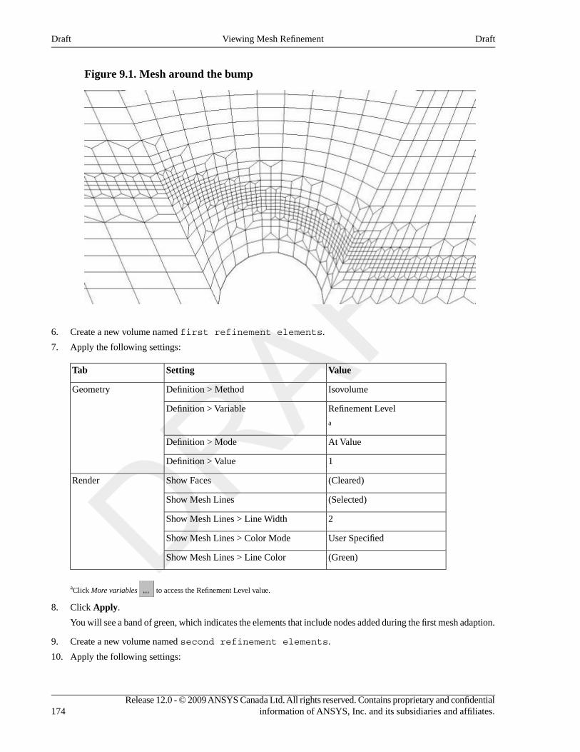
Figure 9.1. Mesh around the bump
6. Create a new volume named first refinement elements.
7. Apply the following settings:
ValueSettingTab
IsovolumeDefinition > MethodGeometry
Refinement LevelDefinition > Variable
a
At ValueDefinition > Mode
1Definition > Value
(Cleared)Show FacesRender
(Selected)Show Mesh Lines
2Show Mesh Lines > Line Width
User SpecifiedShow Mesh Lines > Color Mode
(Green)Show Mesh Lines > Line Color
aClick More variables to access the Refinement Level value.
8. Click Apply.
You will see a band of green, which indicates the elements that include nodes added during the first mesh adaption.
9. Create a new volume named second refinement elements.
10. Apply the following settings:
Release 12.0 - © 2009 ANSYS Canada Ltd. All rights reserved. Contains proprietary and confidentialinformation of ANSYS, Inc. and its subsidiaries and affiliates.174
DraftViewing Mesh RefinementDraft
ValueSettingTab
IsovolumeDefinition > MethodGeometry
Refinement LevelDefinition > Variable
At ValueDefinition >Mode
2Definition > Value
WhiteColorColor
(Selected)Show FacesRender
(Selected)Show Mesh Lines
4Show Mesh Lines > Line Width
User SpecifiedShow Mesh Lines > Color Mode
(Black)Show Mesh Lines > Line Color
11. Click Apply.
You will see a band of white (with black lines); this indicates the elements that include nodes added during thesecond mesh adaption.
12. Zoom in to a region where the mesh has been refined.
The Refinement Level variable holds an integer value at each node, which is either 0, 1, or 2 (because you useda maximum of two adaption levels).
The nodal values of refinement level will be visualized next.
13. Create a new vector named Vector 2.
14. Apply the following settings:
ValueSettingTab
Default DomainDefinition > LocationsGeometry
(Any Vector Variable)Definition > Variable
a
VariableModeColor
Refinement LevelVariable
CubeSymbolSymbol
0.02Symbol Size
(Selected)Normalize Symbols
aThe variable's magnitude and direction do not matter because you will change the vector symbol to a cube with a normalized size.
15. Click Apply.
In Vector 2, Blue nodes (Refinement Level 0 according to the color legend) are part of the original mesh. Greennodes (Refinement Level 1) were added during the first adaption step. Red nodes (Refinement Level 2) were addedduring the second adaption step. Note that some elements contain combinations of blue, green, and red nodes.
175Release 12.0 - © 2009 ANSYS Canada Ltd. All rights reserved. Contains proprietary and confidentialinformation of ANSYS, Inc. and its subsidiaries and affiliates.
DraftViewing Mesh RefinementDraft
Creating an Isosurface to Show the Free SurfaceLater in this tutorial, you will create a chart to show the variation in free surface height along the channel. The datafor the chart will be sampled along a polyline that follows the free surface. To make the polyline, you will use theintersection between one of the symmetry planes and an isosurface that follows the free surface. Start by creating anisosurface on the free surface:
1. Turn off the visibility for all objects except Wireframe.
2. Create a new isosurface named Isosurface 1.
3. Apply the following settings:
ValueSettingTab
Water.Volume FractionDefinition > VariableGeometry
0.5Definition > Value
4. Click Apply.
Creating isosurfaces using this method is a good way to visualize a free surface in a 3D simulation.
5. Right-click any blank area in the viewer, select Predefined Camera, then select Isometric View (Y up).
Creating a Polyline that Follows the Free SurfaceCreate a polyline along the isosurface that you created in the previous step:
1. Turn off the visibility of Isosurface 1.
2. Create a new polyline named Polyline 1.
3. Apply the following settings:
ValueSettingTab
Boundary IntersectionMethodGeometry
frontBoundary List
Isosurface 1Intersect With
4. Click Apply.
A green line is displayed that follows the high-Z edge of the isosurface.
Creating a Chart to Show the Height of the SurfaceCreate a chart that plots the free surface height using the polyline that you created in the previous step:
1. Create a new chart named Chart 1.
The Chart Viewer tab is selected.
2. Apply the following settings:
ValueSettingTab
Free Surface Height for Flowover a Bump
TitleGeneral
Release 12.0 - © 2009 ANSYS Canada Ltd. All rights reserved. Contains proprietary and confidentialinformation of ANSYS, Inc. and its subsidiaries and affiliates.176
DraftCreating an Isosurface to Show the Free SurfaceDraft
ValueSettingTab
free surface heightNameData Series
Polyline 1Location
XVariableX Axis
YVariableY Axis
RectangleSymbolsLine Display
3. Click Apply.
As discussed in Creating Expressions for Initial and Boundary Conditions (p. 164), an approximate outlet elevation isimposed as part of the boundary, even though the flow is supercritical. The chart illustrates the effect of this, in thatthe water level rises just before the exit plane. It is evident from this plot that imposing the elevation does not affectthe upstream flow.
The chart shows a wiggle in the elevation of the free surface interface at the inlet. This is related to an over-specificationof conditions at the inlet because both the inlet velocity and elevation were specified. For a subcritical inlet, only thevelocity or the total energy should be specified. The wiggle is due to a small inconsistency between the specifiedelevation and the elevation computed by the solver to obtain critical conditions at the bump. The wiggle is analogousto one found if pressure and velocity were both specified at a subsonic inlet in a converging-diverging nozzle withchoked flow at the throat.
Further PostprocessingYou may want to create some plots using the <Fluid>.Superficial Velocity variables. This is the fluidvolume fraction multiplied by the fluid velocity and is sometimes called the volume flux. It is useful to use this variablefor vector plots in separated multiphase flow, as you will only see a vector where a significant amount of that phaseexists.
TipYou can right-click on an existing vector plot and select a new vector variable.
Using a Supercritical Outlet ConditionFor supercritical free surface flows, the supercritical outlet boundary is usually the most appropriate boundary for theoutlet because it does not rely on the specification of the outlet pressure distribution (which depends on an estimate ofthe free surface height at the outlet). The supercritical outlet boundary requires a relative pressure specification for thegas only; no pressure information is required for the liquid at the outlet. For this tutorial, the relative gas pressure atthe outlet should be set to 0 Pa.
The supercritical outlet condition may admit multiple solutions. To find the supercritical solution, it is often necessaryto start with a static pressure outlet condition (as previously done in this tutorial) or an average static pressure conditionwhere the pressure is set consistent with an elevation to drive the solution into the supercritical regime. The outletcondition can then be changed to the supercritical option.
177Release 12.0 - © 2009 ANSYS Canada Ltd. All rights reserved. Contains proprietary and confidentialinformation of ANSYS, Inc. and its subsidiaries and affiliates.
DraftFurther PostprocessingDraft

Release 12.0 - © 2009 ANSYS Canada Ltd. All rights reserved. Contains proprietary and confidentialinformation of ANSYS, Inc. and its subsidiaries and affiliates.
Chapter 10. Supersonic Flow Over aWingThis tutorial includes:
• Tutorial Features (p. 179)
• Overview of the Problem to Solve (p. 180)
• Approach to the Problem (p. 180)
• Before You Begin (p. 180)
• Starting CFX-Pre (p. 180)
• Defining a Case in CFX-Pre (p. 181)
• Obtaining a Solution Using CFX-Solver Manager (p. 186)
• Viewing the Results in CFD-Post (p. 186)
Tutorial FeaturesIn this tutorial you will learn about:
• Setting up a supersonic flow simulation.
• Using the Shear Stress Transport turbulence model to accurately resolve flow around a wing surface.
• Defining a custom vector to display pressure distribution.
DetailsFeatureComponent
General ModeUser ModeCFX-Pre
Steady StateAnalysis Type
Air Ideal GasFluid Type
Single DomainDomain Type
Shear Stress TransportTurbulence Model
Total EnergyHeat Transfer
Inlet (Supersonic)Boundary Conditions
Outlet (Supersonic)
Symmetry Plane
Wall: No-Slip
Wall: Adiabatic
Wall: Free-Slip
Fluid-Fluid (No Frame Change)Domain Interfaces
Maximum TimescaleTimestep
ContourPlotsCFD-Post
Vector
Variable Details ViewOther
179Release 12.0 - © 2009 ANSYS Canada Ltd. All rights reserved. Contains proprietary and confidentialinformation of ANSYS, Inc. and its subsidiaries and affiliates.
DraftDraft
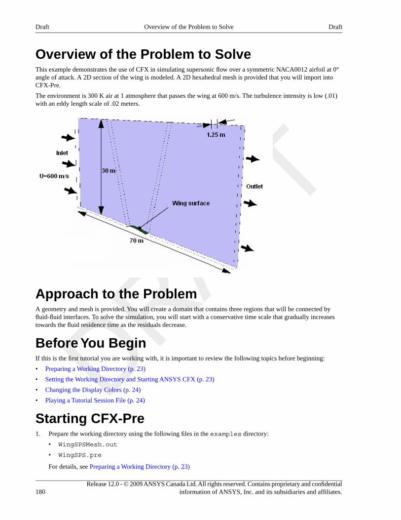
Overview of the Problem to SolveThis example demonstrates the use of CFX in simulating supersonic flow over a symmetric NACA0012 airfoil at 0°angle of attack. A 2D section of the wing is modeled. A 2D hexahedral mesh is provided that you will import intoCFX-Pre.
The environment is 300 K air at 1 atmosphere that passes the wing at 600 m/s. The turbulence intensity is low (.01)with an eddy length scale of .02 meters.
Approach to the ProblemA geometry and mesh is provided. You will create a domain that contains three regions that will be connected byfluid-fluid interfaces. To solve the simulation, you will start with a conservative time scale that gradually increasestowards the fluid residence time as the residuals decrease.
Before You BeginIf this is the first tutorial you are working with, it is important to review the following topics before beginning:
• Preparing a Working Directory (p. 23)
• Setting the Working Directory and Starting ANSYS CFX (p. 23)
• Changing the Display Colors (p. 24)
• Playing a Tutorial Session File (p. 24)
Starting CFX-Pre1. Prepare the working directory using the following files in the examples directory:
• WingSPSMesh.out
• WingSPS.pre
For details, see Preparing a Working Directory (p. 23)
Release 12.0 - © 2009 ANSYS Canada Ltd. All rights reserved. Contains proprietary and confidentialinformation of ANSYS, Inc. and its subsidiaries and affiliates.180
DraftOverview of the Problem to SolveDraft
2. Set the working directory and start CFX-Pre
For details, see Setting the Working Directory and Starting ANSYS CFX (p. 23)
Defining a Case in CFX-PreIf you want to set up the simulation automatically using a tutorial session file, run WingSPS.pre. For details, seePlaying a Tutorial Session File (p. 24). Then proceed to Obtaining a Solution Using CFX-Solver Manager (p. 186).
If you want to set up the simulation manually, proceed to the following steps:
1. Select File > New Case.
2. Select General and click OK.
3. Select File > Save Case As.
4. Under File name, type WingSPS.
5. Click Save.
Importing the Mesh1. Right-click Mesh and select Import Mesh > Other. The Import Mesh dialog box appears.
2. Apply the following settings
ValueSetting
PATRAN NeutralFiles of type
mOptions > Mesh Units
WingSPSMesh.outFile name
3. Click Open.
4. To best orient the view, right-click a blank area in the viewer and select Predefined Camera > Isometric View(Y up) from the shortcut menu.
Creating the Domain1. Edit Case Options > General in the Outline tree view and ensure that Automatic Default Domain is
turned on. A domain named Default Domain should now appear under the Simulation branch.
2. Double-click Default Domain and apply the following settings
ValueSettingTab
WING ELEMENTSLocation and Type > LocationBasic Settings
Fluid 1Fluid and Particle Definitions
Air Ideal GasFluid and Particle Definitions >Fluid 1 > Material
1 [atm]Domain Models > Pressure >
Reference Pressurea
Total EnergybHeat Transfer > OptionFluid Models
181Release 12.0 - © 2009 ANSYS Canada Ltd. All rights reserved. Contains proprietary and confidentialinformation of ANSYS, Inc. and its subsidiaries and affiliates.
DraftDefining a Case in CFX-PreDraft
ValueSettingTab
Shear Stress TransportTurbulence > Option
aWhen using an ideal gas, it is important to set an appropriate reference pressure because some properties depend on the absolute pressurelevel.bThe Total Energy model is appropriate for high-speed flows because it includes kinetic energy effects.
3. Click OK.
Creating the Boundaries
Creating an Inlet Boundary1. Create a new boundary named Inlet.
2. Apply the following settings
ValueSettingTab
InletBoundary TypeBasic Settings
INLETLocation
SupersonicFlow Regime > OptionBoundary Details
Cart. Vel. & PressureMass And Momentum > Option
600 [m s^-1]Mass And Momentum > U
0 [m s^-1]Mass And Momentum > V
0 [m s^-1]Mass And Momentum > W
0 [Pa]Mass And Momentum > Rel. Static Pres.
Intensity and Length ScaleTurbulence > Option
0.01Turbulence > Fractional Intensity
0.02 [m]Turbulence > Eddy Len. Scale
300 [K]Heat Transfer > Static Temperature
3. Click OK.
Creating an Outlet Boundary1. Create a new boundary named Outlet.
2. Apply the following settings
ValueSettingTab
OutletBoundary TypeBasic Settings
OUTLETLocation
SupersonicFlow Regime > OptionBoundary Details
Release 12.0 - © 2009 ANSYS Canada Ltd. All rights reserved. Contains proprietary and confidentialinformation of ANSYS, Inc. and its subsidiaries and affiliates.182
DraftCreating the BoundariesDraft
3. Click OK.
Creating the Symmetry Plane Boundaries1. Create a new boundary named SymP1.
2. Apply the following settings
ValueSettingTab
Symmetry aBoundary TypeBasic Settings
SIDE1Location
aSymmetry, which can make a 3D problem into a 2D problem, can be used when geometry and mesh are invariant normal to the symmetrysurface.
3. Click OK.
4. Create a new boundary named SymP2.
5. Apply the following settings
ValueSettingTab
SymmetryBoundary TypeBasic Settings
SIDE2Location
6. Click OK.
7. Create a new boundary named Bottom.
8. Apply the following settings
ValueSettingTab
SymmetryBoundary TypeBasic Settings
BOTTOMLocation
9. Click OK.
Creating a Free Slip Boundary1. Create a new boundary named Top.
2. Apply the following settings
ValueSettingTab
WallBoundary TypeBasic Settings
TOPLocation
Free Slip WallMass And Momentum > OptionBoundary Details
3. Click OK.
183Release 12.0 - © 2009 ANSYS Canada Ltd. All rights reserved. Contains proprietary and confidentialinformation of ANSYS, Inc. and its subsidiaries and affiliates.
DraftCreating the BoundariesDraft
Creating a Wall Boundary1. Create a new boundary named WingSurface.
2. Apply the following settings
ValueSettingTab
WallBoundary TypeBasic Settings
WING_NodesLocation
a
a If particular items do not appear in the drop-down list, click the ellipsis icon to see all available items.
3. Click OK.
Creating Domain InterfacesThe imported mesh contains three regions that will be connected with domain interfaces.
1. Create a new domain interface named Domain Interface 1.
2. Apply the following settings
ValueSettingTab
Fluid FluidInterface TypeBasic Settings
Primitive 2D AInterface Side 1 > Region List
a
Primitive 2D, Primitive 2D BInterface Side 2 > Region List
a If particular items do not appear in the drop-down list, click the ellipsis icon to see all available items.
3. Click OK.
Setting Initial ValuesFor high-speed compressible flow, the CFX-Solver usually requires sensible initial conditions to be set for the velocityfield.
1. Click Global Initialization .
2. Apply the following settings: 1
ValueSettingTab
Automatic withValue
Initial Conditions > Cartesian Velocity Components > OptionGlobal Settings
600 [m s^-1]Initial Conditions > Cartesian Velocity Components > U
0 [m s^-1]Initial Conditions > Cartesian Velocity Components > V
1The values are from the problem specification.
Release 12.0 - © 2009 ANSYS Canada Ltd. All rights reserved. Contains proprietary and confidentialinformation of ANSYS, Inc. and its subsidiaries and affiliates.184
DraftCreating Domain InterfacesDraft
ValueSettingTab
0 [m s^-1]Initial Conditions > Cartesian Velocity Components > W
Automatic withValue
Initial Conditions > Temperature > Option
300 [K]Initial Conditions > Temperature > Temperature
3. Click OK.
Setting the Solver ControlsThe residence time for the fluid is the length of the domain divided by the speed of the liquid; using values from theproblem specification, the result is approximately:
70 [m] / 600 [m s^-1] = 0.117 [s]
In the next step, you will set a maximum timescale, then the solver will start with a conservative time scale that graduallyincreases towards the fluid-residence time as the residuals decrease.
1. Click Solver Control .
2. Apply the following settings
ValueSettingTab
(Selected)Convergence Control > Fluid TimescaleControl > Maximum Timescale
Basic Settings
0.1 [s]Convergence Control > Fluid TimescaleControl > Maximum Timescale > MaximumTimescale
1.0e-05Convergence Criteria > Residual Target
3. Click OK.
Writing the CFX-Solver Input (.def) File
1. Click Define Run .
2. Apply the following settings
ValueSetting
WingSPS.defFile name
3. Click Save.
CFX-Solver Manager automatically starts and, on the Define Run dialog box, the Solver Input File is set.
4. If using Standalone Mode, quit CFX-Pre, saving the simulation (.cfx) file at your discretion.
185Release 12.0 - © 2009 ANSYS Canada Ltd. All rights reserved. Contains proprietary and confidentialinformation of ANSYS, Inc. and its subsidiaries and affiliates.
DraftSetting the Solver ControlsDraft
Obtaining a Solution Using CFX-Solver ManagerAt this point, CFX-Solver Manager is running, and the Define Run dialog box is displayed, with the CFX-Solver inputfile set.
1. Click Start Run.
2. Select the check box next to Post-Process Results when the completion message appears at the end of the run.
3. If using Standalone Mode, select the check box next to Shut down CFX-Solver Manager.
4. Click OK.
Viewing the Results in CFD-PostThe following topics will be discussed:
• Displaying Mach Information (p. 186)
• Displaying Pressure Information (p. 186)
• Displaying Temperature Information (p. 187)
• Displaying Pressure With User Vectors (p. 187)
Displaying Mach InformationThe first view configured shows that the bulk of the flow over the wing has a Mach Number of over 1.5.
1. To best orient the view, select View Towards -Z by typing Shift +Z.
2. Zoom in so the geometry fills the Viewer.
3. Create a new contour named SymP2Mach.
4. Apply the following settings
ValueSettingTab
SymP2LocationsGeometry
Mach NumberVariable
User SpecifiedRange
1Min
2Max
21# of Contours
5. Click Apply.
6. Clear the check box next to SymP2Mach.
Displaying Pressure InformationTo display pressure information, create a contour plot that shows the pressure field:
1. Create a new contour named SymP2Pressure.
2. Apply the following settings
Release 12.0 - © 2009 ANSYS Canada Ltd. All rights reserved. Contains proprietary and confidentialinformation of ANSYS, Inc. and its subsidiaries and affiliates.186
DraftObtaining a Solution Using CFX-Solver ManagerDraft
ValueSettingTab
SymP2LocationsGeometry
PressureVariable
GlobalRange
3. Click Apply.
4. Clear the check box next to SymP2Pressure.
Displaying Temperature InformationYou can confirm that a significant energy loss occurs around the wing's leading edge by plotting temperature on SymP2.
1. Create a new contour named SymP2Temperature.
2. Apply the following settings
ValueSettingTab
SymP2LocationsGeometry
TemperatureVariable
GlobalRange
3. Click Apply.
The contour shows that the temperature at the wing's leading edge is approximately 180 K higher than the inlettemperature.
4. Clear the check box next to SymP2Temperature.
Displaying Pressure With User VectorsYou can also create a user vector to show the pressure acting on the wing:
1. Create a new variable named Variable 1.
2. Apply the following settings
ValueSettingName
(Selected)VectorVariable 1
(Pressure+101325[Pa])*Normal XX Expression
(Pressure+101325[Pa])*Normal YY Expression
(Pressure+101325[Pa])*Normal ZZ Expression
3. Click Apply.
4. Create a new vector named Vector 1.
5. Apply the following settings
187Release 12.0 - © 2009 ANSYS Canada Ltd. All rights reserved. Contains proprietary and confidentialinformation of ANSYS, Inc. and its subsidiaries and affiliates.
DraftDisplaying Temperature InformationDraft
ValueSettingTab
WingSurfaceLocationsGeometry
Variable 1Variable
0.04Symbol SizeSymbol
6. Click Apply.
7. Zoom in on the wing in order to see the created vector plot.
Release 12.0 - © 2009 ANSYS Canada Ltd. All rights reserved. Contains proprietary and confidentialinformation of ANSYS, Inc. and its subsidiaries and affiliates.188
DraftDisplaying Pressure With User VectorsDraft
Chapter 11. Flow Through a ButterflyValveThis tutorial includes:
• Tutorial Features (p. 189)
• Overview of the Problem to Solve (p. 190)
• Approach to the Problem (p. 191)
• Before You Begin (p. 191)
• Starting CFX-Pre (p. 191)
• Defining a Simulation in CFX-Pre (p. 191)
• Obtaining a Solution Using CFX-Solver Manager (p. 201)
• Viewing the Results in CFD-Post (p. 201)
Tutorial FeaturesIn this tutorial you will learn about:
• Using a rough wall boundary in CFX-Pre to simulate the pipe wall
• Creating a fully developed inlet velocity profile using the CFX Expression Language
• Setting up a Particle Tracking simulation in CFX-Pre to trace sand particles
• Animating particle tracks in CFD-Post to trace sand particles through the domain
• Performing quantitative calculation of average static pressure in CFD-Post on the outlet boundary.
DetailsFeatureComponent
General ModeUser ModeCFX-Pre
Steady StateAnalysis Type
General FluidFluid Type
Single DomainDomain Type
k-EpsilonTurbulence Model
NoneHeat Transfer
Particle Tracking
Inlet (Profile)Boundary Conditions
Inlet (Subsonic)
Outlet (Subsonic)
Symmetry Plane
Wall: No-Slip
Wall: Rough
CEL (CFX Expression Language)
189Release 12.0 - © 2009 ANSYS Canada Ltd. All rights reserved. Contains proprietary and confidentialinformation of ANSYS, Inc. and its subsidiaries and affiliates.
DraftDraft
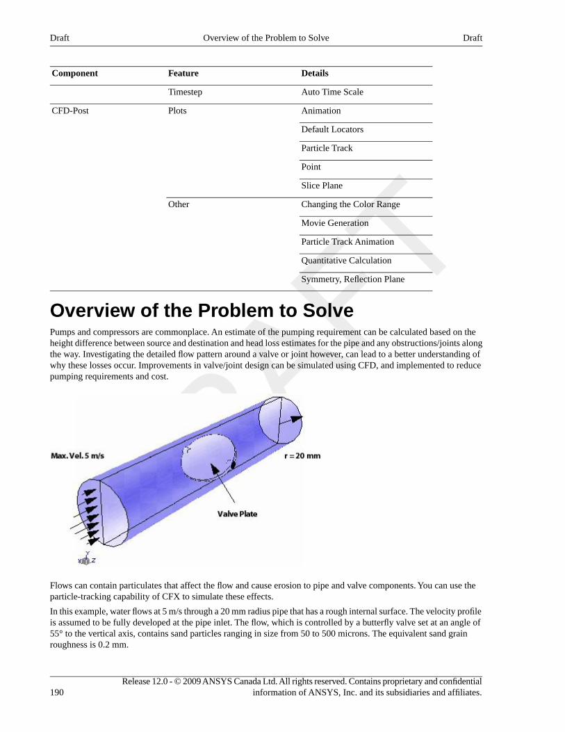
DetailsFeatureComponent
Auto Time ScaleTimestep
AnimationPlotsCFD-Post
Default Locators
Particle Track
Point
Slice Plane
Changing the Color RangeOther
Movie Generation
Particle Track Animation
Quantitative Calculation
Symmetry, Reflection Plane
Overview of the Problem to SolvePumps and compressors are commonplace. An estimate of the pumping requirement can be calculated based on theheight difference between source and destination and head loss estimates for the pipe and any obstructions/joints alongthe way. Investigating the detailed flow pattern around a valve or joint however, can lead to a better understanding ofwhy these losses occur. Improvements in valve/joint design can be simulated using CFD, and implemented to reducepumping requirements and cost.
Flows can contain particulates that affect the flow and cause erosion to pipe and valve components. You can use theparticle-tracking capability of CFX to simulate these effects.
In this example, water flows at 5 m/s through a 20 mm radius pipe that has a rough internal surface. The velocity profileis assumed to be fully developed at the pipe inlet. The flow, which is controlled by a butterfly valve set at an angle of55° to the vertical axis, contains sand particles ranging in size from 50 to 500 microns. The equivalent sand grainroughness is 0.2 mm.
Release 12.0 - © 2009 ANSYS Canada Ltd. All rights reserved. Contains proprietary and confidentialinformation of ANSYS, Inc. and its subsidiaries and affiliates.190
DraftOverview of the Problem to SolveDraft
The reference temperature is 300 K; the reference pressure is 1 atm.
Approach to the ProblemA geometry and mesh is provided. You will create sand particles and a domain that contains water; for one part of thesimulation the water and sand will be fully coupled, and for the other part of the simulation they will be one-waycoupled. To increase the accuracy of the simulation, the inlet will be given a velocity profile that simulates afully-developed boundary layer.
To solve the simulation, you will create two sets of identical particles. The first set will be fully coupled to predict theeffect of the particles on the continuous phase flow field and allow the particles to influence the flow field. The secondset will be one-way coupled but will contain a much higher number of particles to provide a more accurate calculationof the particle volume fraction and local forces on walls, but without affecting the flow field.
Before You BeginIf this is the first tutorial you are working with, it is important to review the following topics before beginning:
• Preparing a Working Directory (p. 23)
• Setting the Working Directory and Starting ANSYS CFX (p. 23)
• Changing the Display Colors (p. 24)
• Playing a Tutorial Session File (p. 24)
Starting CFX-Pre1. Prepare the working directory using the following files in the examples directory:
• PipeValveMesh.gtm
• PipeValve.pre
For details, see Preparing a Working Directory (p. 23)
2. Set the working directory and start CFX-Pre
For details, see Setting the Working Directory and Starting ANSYS CFX (p. 23)
Defining a Simulation in CFX-PreIf you want to set up the simulation automatically using a tutorial session file, run PipeValve.pre. For details, seePlaying a Tutorial Session File (p. 24). Then proceed to Obtaining a Solution Using CFX-Solver Manager (p. 201).
If you want to set up the simulation manually, proceed to Creating a New Case (p. 191)
Creating a New Case1. Start CFX-Pre.
2. Select File > New Case.
3. Select General and click OK.
4. Select File > Save Case As.
5. Under File name, type PipeValve.
6. Click Save.
191Release 12.0 - © 2009 ANSYS Canada Ltd. All rights reserved. Contains proprietary and confidentialinformation of ANSYS, Inc. and its subsidiaries and affiliates.
DraftApproach to the ProblemDraft
Importing the Mesh1. Right-click Mesh and select Import Mesh > CFX Mesh. The Import Mesh dialog box appears.
2. Apply the following settings:
ValueSetting
PipeValveMesh.gtmFile name
3. Click Open.
Defining the Properties of the SandThe material properties of the sand particles used in the simulation need to be defined. Heat transfer and radiationmodeling are not used in this simulation, so the only properties that need to be defined are the density of the sand andthe diameter range.
To calculate the effect of the particles on the continuous fluid, between 100 and 1000 particles are usually required.However, if accurate information about the particle volume fraction or local forces on wall boundaries is required,then a much larger number of particles needs to be modeled.
When you create the domain, choose either full coupling or one-way coupling between the particle and continuousphase. Full coupling is needed to predict the effect of the particles on the continuous phase flow field but has a higherCPU cost than one-way coupling; one-way coupling simply predicts the particle paths during post-processing basedon the flow field, but without affecting the flow field.
To optimize CPU usage, you can create two sets of identical particles. The first set should be fully coupled and around200 particles will be used. This allows the particles to influence the flow field. The second set uses one-way couplingbut contains 5000 particles. This provides a more accurate calculation of the particle volume fraction and local forceson walls. (These values are defined in the inlet boundary definition.)
For this tutorial you will create a “Sand Fully Coupled” boundary condition that has 200 particles moving with a massflow rate of 0.01 kg/s and a “Sand One Way Coupled” boundary condition that has 5000 particles moving with a massflow rate of 0.01 kg/s. In both cases the sand density is 2300 [kg m^-3]; particle diameters range from 50 e-6 m. to500 e-6 m. with an average diameter of 250 e-6 m. and a standard deviation of 70 e-6 m. You will set a Finnie erosionmodel with a velocity power factor of 2 and a reference velocity of 1 m/s.
1. Click Insert Material then create a new material named Sand Fully Coupled.
2. Apply the following settings:
ValueSettingTab
Particle SolidsMaterial GroupBasic Settings
(Selected)Thermodynamic State
2300 [kg m^-3]aThermodynamic Properties > Equation of State> Density
Material Properties
(Selected)Thermodynamic Properties > Specific HeatCapacity
0 [J kg^-1 K^-1]Thermodynamic Properties > Specific HeatCapacity > Specific Heat Capacity b
(Selected)Thermodynamic Properties > Reference State
Release 12.0 - © 2009 ANSYS Canada Ltd. All rights reserved. Contains proprietary and confidentialinformation of ANSYS, Inc. and its subsidiaries and affiliates.192
DraftImporting the MeshDraft
ValueSettingTab
Specified PointThermodynamic Properties > Reference State> Option
300 [K]cThermodynamic Properties > Reference State> Ref. Temperature
aFrom the problem description.bThis value is not used because heat transfer is not modeled in this tutorial.cFrom the problem description.
3. Click OK.
4. Under Materials, right-click Sand Fully Coupled and select Duplicate from the shortcut menu.
5. Rename the duplicate as Sand One Way Coupled.
6. Sand One Way Coupled is created with properties identical to Sand Fully Coupled.
Creating the DomainSet up an environment that has water and sand defined in two ways—one in which the sand is fully coupled, and onein which the sand is one-way coupled:
1. Edit Case Options > General in the Outline tree view and ensure that Automatic Default Domain isturned on. A domain named Default Domain should appear under the Simulation > Flow Analysis1 branch.
2. Double-click Default Domain.
3. Under Fluid and Particle Definitions, delete Fluid 1 and click Add new item to create three new materials
named Water, Sand Fully Coupled, and Sand One Way Coupled.
4. Apply the following settings, which are taken from the problem description:
ValueSettingTab
WaterFluid and Particle DefinitionsBasic Settings
WaterFluid and Particle Definitions > Water > Material
Sand Fully CoupledFluid and Particle Definitions
Sand Fully Coupled aFluid and Particle Definitions > Sand Fully Coupled> Material
Particle Transport SolidFluid and Particle Definitions > Sand Fully Coupled> Morphology > Option
(Selected)Fluid and Particle Definitions > Sand Fully Coupled> Morphology > Particle Diameter Distribution
Normal in Diameter byMass
Fluid and Particle Definitions > Sand Fully Coupled> Morphology > Particle Diameter Distribution >Option
50e-6 [m]Fluid and Particle Definitions > Sand Fully Coupled> Morphology > Particle Diameter Distribution >Minimum Diameter
193Release 12.0 - © 2009 ANSYS Canada Ltd. All rights reserved. Contains proprietary and confidentialinformation of ANSYS, Inc. and its subsidiaries and affiliates.
DraftCreating the DomainDraft
ValueSettingTab
500e-6 [m]Fluid and Particle Definitions > Sand Fully Coupled> Morphology > Particle Diameter Distribution >Maximum Diameter
250e-6 [m]Fluid and Particle Definitions > Sand Fully Coupled> Morphology > Particle Diameter Distribution >Mean Diameter
70e-6 [m]Fluid and Particle Definitions > Sand Fully Coupled> Morphology > Particle Diameter Distribution >Std. Deviation
Sand One Way CoupledFluid and Particle Definitions
Sand One Way Coupled bFluid and Particle Definitions > Sand One WayCoupled > Material
Particle Transport SolidFluid and Particle Definitions > Sand One WayCoupled > Morphology > Option
(Selected)Fluid and Particle Definitions > Sand One WayCoupled > Morphology > Particle DiameterDistribution
Normal in Diameter byMass
Fluid and Particle Definitions > Sand One WayCoupled > Morphology > Particle DiameterDistribution > Option
50e-6 [m]Fluid and Particle Definitions > Sand One WayCoupled > Morphology > Particle DiameterDistribution > Minimum Diameter
500e-6 [m]Fluid and Particle Definitions > Sand One WayCoupled > Morphology > Particle DiameterDistribution > Maximum Diameter
250e-6 [m]Fluid and Particle Definitions > Sand One WayCoupled > Morphology > Particle DiameterDistribution > Mean Diameter
70e-6 [m]Fluid and Particle Definitions > Sand One WayCoupled > Morphology > Particle DiameterDistribution > Std. Deviation
1 [atm]Domain Models > Pressure > Reference Pressure
NoneHeat Transfer > OptionFluid Models
k-EpsiloncTurbulence > Option
Sand Fully CoupledFluidFluid SpecificModels
FinnieFluid > Sand Fully Coupled > Erosion Model >Option
2.0Fluid > Sand Fully Coupled > Erosion Model > Vel.Power Factor
Release 12.0 - © 2009 ANSYS Canada Ltd. All rights reserved. Contains proprietary and confidentialinformation of ANSYS, Inc. and its subsidiaries and affiliates.194
DraftCreating the DomainDraft
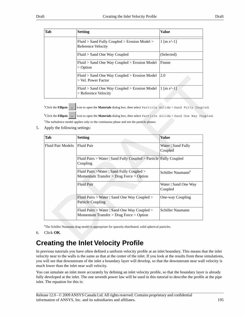
ValueSettingTab
1 [m s^-1]Fluid > Sand Fully Coupled > Erosion Model >Reference Velocity
(Selected)Fluid > Sand One Way Coupled
FinnieFluid > Sand One Way Coupled > Erosion Model> Option
2.0Fluid > Sand One Way Coupled > Erosion Model> Vel. Power Factor
1 [m s^-1]Fluid > Sand One Way Coupled > Erosion Model> Reference Velocity
aClick the Ellipsis icon to open the Materials dialog box, then select Particle Solids > Sand Fully Coupled.
bClick the Ellipsis icon to open the Materials dialog box, then select Particle Solids > Sand One Way Coupled.
cThe turbulence model applies only to the continuous phase and not the particle phases.
5. Apply the following settings:
ValueSettingTab
Water | Sand FullyCoupled
Fluid PairFluid Pair Models
Fully CoupledFluid Pairs > Water | Sand Fully Coupled > ParticleCoupling
Schiller NaumannaFluid Pairs >Water | Sand Fully Coupled >Momentum Transfer > Drag Force > Option
Water | Sand One WayCoupled
Fluid Pair
One-way CouplingFluid Pairs > Water | Sand One Way Coupled >Particle Coupling
Schiller NaumannFluid Pairs > Water | Sand One Way Coupled >Momentum Transfer > Drag Force > Option
aThe Schiller Naumann drag model is appropriate for sparsely-distributed, solid spherical particles.
6. Click OK.
Creating the Inlet Velocity ProfileIn previous tutorials you have often defined a uniform velocity profile at an inlet boundary. This means that the inletvelocity near to the walls is the same as that at the center of the inlet. If you look at the results from these simulations,you will see that downstream of the inlet a boundary layer will develop, so that the downstream near wall velocity ismuch lower than the inlet near wall velocity.
You can simulate an inlet more accurately by defining an inlet velocity profile, so that the boundary layer is alreadyfully developed at the inlet. The one seventh power law will be used in this tutorial to describe the profile at the pipeinlet. The equation for this is:
195Release 12.0 - © 2009 ANSYS Canada Ltd. All rights reserved. Contains proprietary and confidentialinformation of ANSYS, Inc. and its subsidiaries and affiliates.
DraftCreating the Inlet Velocity ProfileDraft
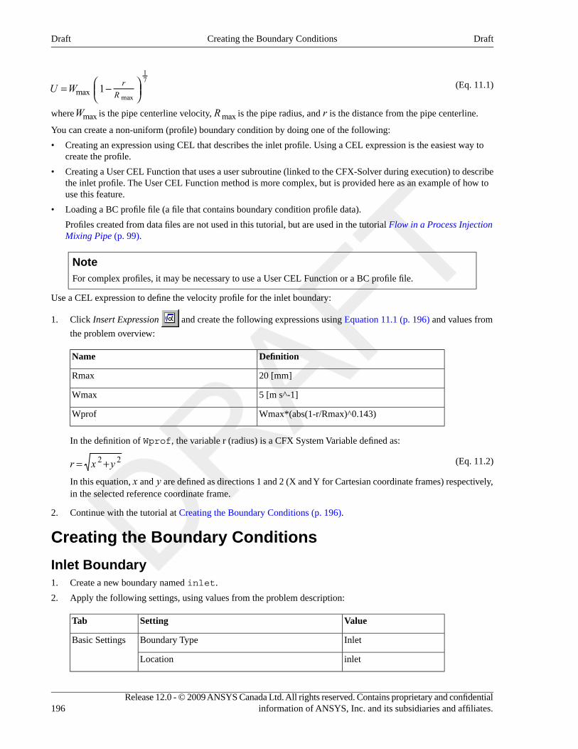
(Eq. 11.1)= ⎛⎝⎜
− ⎞⎠⎟
U W 1 rRmax
max
17
where Wmax is the pipe centerline velocity, Rmax is the pipe radius, and r is the distance from the pipe centerline.
You can create a non-uniform (profile) boundary condition by doing one of the following:
• Creating an expression using CEL that describes the inlet profile. Using a CEL expression is the easiest way tocreate the profile.
• Creating a User CEL Function that uses a user subroutine (linked to the CFX-Solver during execution) to describethe inlet profile. The User CEL Function method is more complex, but is provided here as an example of how touse this feature.
• Loading a BC profile file (a file that contains boundary condition profile data).
Profiles created from data files are not used in this tutorial, but are used in the tutorial Flow in a Process InjectionMixing Pipe (p. 99).
NoteFor complex profiles, it may be necessary to use a User CEL Function or a BC profile file.
Use a CEL expression to define the velocity profile for the inlet boundary:
1. Click Insert Expression and create the following expressions using Equation 11.1 (p. 196) and values from
the problem overview:
DefinitionName
20 [mm]Rmax
5 [m s^-1]Wmax
Wmax*(abs(1-r/Rmax)^0.143)Wprof
In the definition of Wprof, the variable r (radius) is a CFX System Variable defined as:
(Eq. 11.2)= +r x y2 2
In this equation, x and y are defined as directions 1 and 2 (X and Y for Cartesian coordinate frames) respectively,in the selected reference coordinate frame.
2. Continue with the tutorial at Creating the Boundary Conditions (p. 196).
Creating the Boundary Conditions
Inlet Boundary1. Create a new boundary named inlet.
2. Apply the following settings, using values from the problem description:
ValueSettingTab
InletBoundary TypeBasic Settings
inletLocation
Release 12.0 - © 2009 ANSYS Canada Ltd. All rights reserved. Contains proprietary and confidentialinformation of ANSYS, Inc. and its subsidiaries and affiliates.196
DraftCreating the Boundary ConditionsDraft
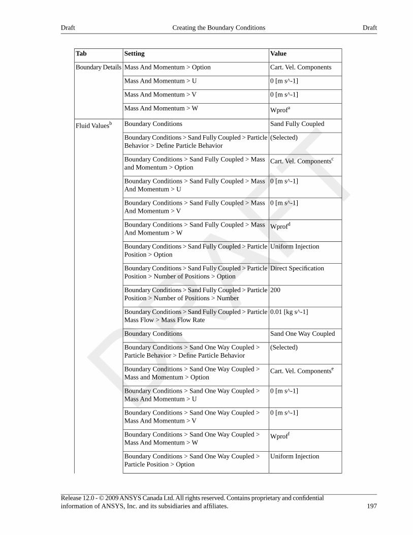
ValueSettingTab
Cart. Vel. ComponentsMass And Momentum > OptionBoundary Details
0 [m s^-1]Mass And Momentum > U
0 [m s^-1]Mass And Momentum > V
WprofaMass And Momentum > W
Sand Fully CoupledBoundary ConditionsFluid Valuesb
(Selected)Boundary Conditions > Sand Fully Coupled > ParticleBehavior > Define Particle Behavior
Cart. Vel. ComponentscBoundary Conditions > Sand Fully Coupled > Massand Momentum > Option
0 [m s^-1]Boundary Conditions > Sand Fully Coupled > MassAnd Momentum > U
0 [m s^-1]Boundary Conditions > Sand Fully Coupled > MassAnd Momentum > V
WprofdBoundary Conditions > Sand Fully Coupled > MassAnd Momentum > W
Uniform InjectionBoundary Conditions > Sand Fully Coupled > ParticlePosition > Option
Direct SpecificationBoundary Conditions > Sand Fully Coupled > ParticlePosition > Number of Positions > Option
200Boundary Conditions > Sand Fully Coupled > ParticlePosition > Number of Positions > Number
0.01 [kg s^-1]Boundary Conditions > Sand Fully Coupled > ParticleMass Flow > Mass Flow Rate
Sand One Way CoupledBoundary Conditions
(Selected)Boundary Conditions > Sand One Way Coupled >Particle Behavior > Define Particle Behavior
Cart. Vel. ComponentseBoundary Conditions > Sand One Way Coupled >Mass and Momentum > Option
0 [m s^-1]Boundary Conditions > Sand One Way Coupled >Mass And Momentum > U
0 [m s^-1]Boundary Conditions > Sand One Way Coupled >Mass And Momentum > V
WproffBoundary Conditions > Sand One Way Coupled >Mass And Momentum > W
Uniform InjectionBoundary Conditions > Sand One Way Coupled >Particle Position > Option
197Release 12.0 - © 2009 ANSYS Canada Ltd. All rights reserved. Contains proprietary and confidentialinformation of ANSYS, Inc. and its subsidiaries and affiliates.
DraftCreating the Boundary ConditionsDraft
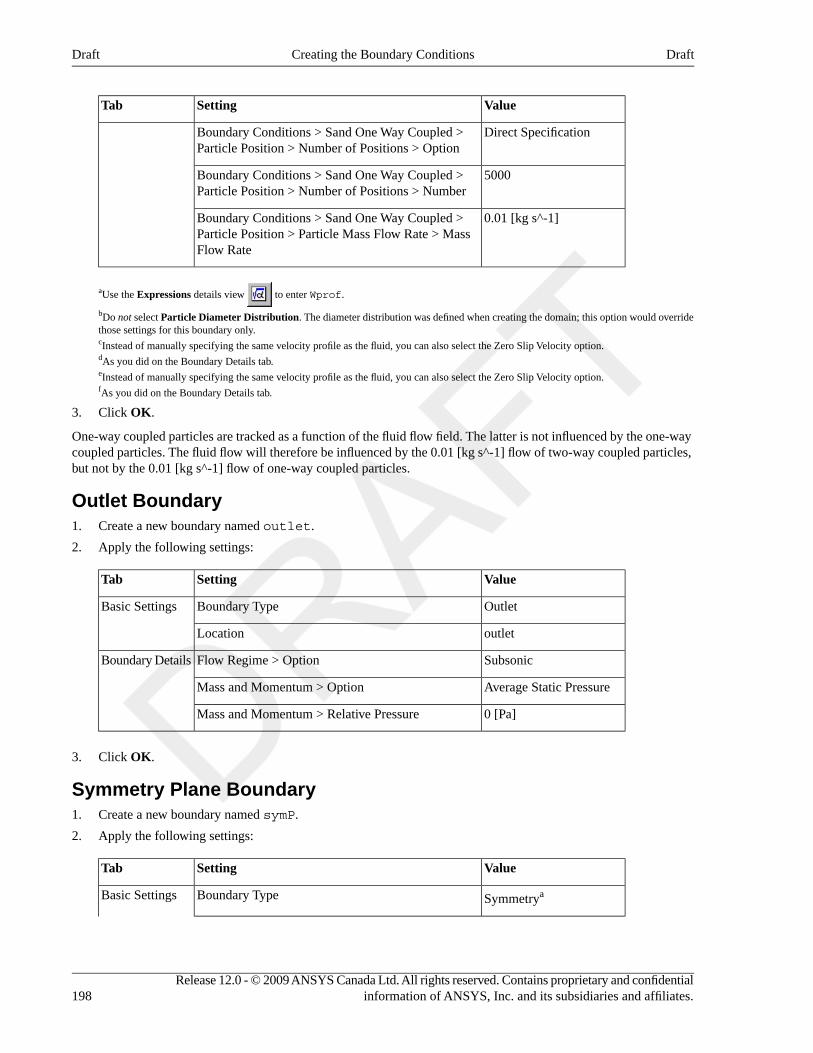
ValueSettingTab
Direct SpecificationBoundary Conditions > Sand One Way Coupled >Particle Position > Number of Positions > Option
5000Boundary Conditions > Sand One Way Coupled >Particle Position > Number of Positions > Number
0.01 [kg s^-1]Boundary Conditions > Sand One Way Coupled >Particle Position > Particle Mass Flow Rate > MassFlow Rate
aUse the Expressions details view to enter Wprof.
bDo not select Particle Diameter Distribution. The diameter distribution was defined when creating the domain; this option would overridethose settings for this boundary only.cInstead of manually specifying the same velocity profile as the fluid, you can also select the Zero Slip Velocity option.dAs you did on the Boundary Details tab.eInstead of manually specifying the same velocity profile as the fluid, you can also select the Zero Slip Velocity option.fAs you did on the Boundary Details tab.
3. Click OK.
One-way coupled particles are tracked as a function of the fluid flow field. The latter is not influenced by the one-waycoupled particles. The fluid flow will therefore be influenced by the 0.01 [kg s^-1] flow of two-way coupled particles,but not by the 0.01 [kg s^-1] flow of one-way coupled particles.
Outlet Boundary1. Create a new boundary named outlet.
2. Apply the following settings:
ValueSettingTab
OutletBoundary TypeBasic Settings
outletLocation
SubsonicFlow Regime > OptionBoundary Details
Average Static PressureMass and Momentum > Option
0 [Pa]Mass and Momentum > Relative Pressure
3. Click OK.
Symmetry Plane Boundary1. Create a new boundary named symP.
2. Apply the following settings:
ValueSettingTab
SymmetryaBoundary TypeBasic Settings
Release 12.0 - © 2009 ANSYS Canada Ltd. All rights reserved. Contains proprietary and confidentialinformation of ANSYS, Inc. and its subsidiaries and affiliates.198
DraftCreating the Boundary ConditionsDraft
ValueSettingTab
symPLocation
aSymmetry can be used when geometry and mesh are invariant normal to the symmetry surface.
3. Click OK.
Pipe Wall Boundary1. Create a new boundary named pipe wall.
2. Apply the following settings:
ValueSettingTab
WallBoundary TypeBasicSettings
pipe wallLocation
Rough WallWall Roughness > OptionBoundaryDetails
0.2 [mm]aWall Roughness > Sand Grain Roughness
Sand Fully CoupledBoundary ConditionsFluid Values
Restitution CoefficientBoundary Conditions > Sand Fully Coupled > Velocity >Option
0.8bBoundary Conditions > Sand Fully Coupled > Velocity >Perpendicular Coeff.
1Boundary Conditions > Sand Fully Coupled > Velocity >Parallel Coeff.
aFrom the problem description. Make sure that you change the units to millimeters. The thickness of the first element should be of the sameorder as the roughness height.bThis value would typically come from experimental or reference data.
3. Apply the same setting values for Sand One Way Coupled as for Sand Fully Coupled.
4. Click OK.
Editing the Default Boundary1. In the Outline tree view, edit the boundary named Default Domain Default.
2. Apply the following settings:
ValueSettingTab
Sand Fully CoupledBoundary ConditionsFluid Values
0.9aBoundary Conditions > Sand Fully Coupled> Velocity > Perpendicular Coeff.
Sand One Way CoupledBoundary Conditions
199Release 12.0 - © 2009 ANSYS Canada Ltd. All rights reserved. Contains proprietary and confidentialinformation of ANSYS, Inc. and its subsidiaries and affiliates.
DraftCreating the Boundary ConditionsDraft
ValueSettingTab
0.9Boundary Conditions > Sand One WayCoupled > Velocity > Perpendicular Coeff.
aThis value would typically come from experimental or reference data. For this tutorial, the pipe wall and butterfly valve are considered tobe made of different materials, so their perpendicular coefficients are different.
3. Click OK.
Setting Initial ValuesSet up the initial values to be consistent with the inlet boundary conditions:
1. Click Global Initialization .
2. Apply the following settings:
ValueSettingTab
Automatic with ValueInitial Conditions > Cartesian VelocityComponents > Option
Global Settings
0 [m s^-1]Initial Conditions > Cartesian VelocityComponents > Option > U
0 [m s^-1]Initial Conditions > Cartesian VelocityComponents > Option > V
WprofInitial Conditions > Cartesian VelocityComponents > Option > W
3. Click OK.
Setting the Solver Controls1. Click Solver Control .
2. Apply the following settings:
ValueSettingTab
High ResolutionAdvection Scheme > OptionBasic Settings
(Selected)Particle Integration > Max. Particle Intg. Time StepParticle Control
1e+10 [s]Particle Integration > Max. Particle Intg. Time Step> Value
(Selected)Particle Termination Control
(Selected)Particle Termination Control > Maximum TrackingTime
10 [s]Particle Termination Control > Maximum TrackingTime > Value
Release 12.0 - © 2009 ANSYS Canada Ltd. All rights reserved. Contains proprietary and confidentialinformation of ANSYS, Inc. and its subsidiaries and affiliates.200
DraftSetting Initial ValuesDraft
ValueSettingTab
(Selected)Particle Termination Control > Maximum TrackingDistance
10 [m]Particle Termination Control > Maximum TrackingDistance > Value
(Selected)Particle Termination Control > Max. Num.Integration Steps
10000aParticle Termination Control > Max. Num.Integration Steps > Value
aThis value controls the number of mesh elements a particle is allowed to cross and therefore must take into account the size and density ofthe mesh.
NoteThe numeric values in the preceding table are all designed to put a high upper limit on the amount ofprocessing that will be done. For example, the tracking time of 10 seconds would allow a particle toget caught in an eddy for a reasonable amount of time.
3. Click OK.
Writing the CFX-Solver Input (.def) File
1. Click Define Run .
2. Apply the following settings:
ValueSetting
PipeValve.defFile name
3. Click Save.
CFX-Solver Manager automatically starts and, on the Define Run dialog box, the Solver Input File is set.
4. If using Standalone Mode, quit CFX-Pre, saving the simulation (.cfx) file at your discretion.
Obtaining a Solution Using CFX-Solver ManagerWhen CFX-Pre has shut down and CFX-Solver Manager has started, you can obtain a solution to the CFD problemby using the procedure that follows.
1. Ensure the Define Run dialog box is displayed and click Start Run.
2. Select the check box next to Post-Process Results when the completion message appears at the end of the run.
3. If using Standalone Mode, select the check box next to Shut down CFX-Solver Manager.
4. Click OK.
Viewing the Results in CFD-PostIn this section, you will first plot erosion on the valve surface and side walls due to the sand particles. You will thencreate an animation of particle tracks through the domain.
201Release 12.0 - © 2009 ANSYS Canada Ltd. All rights reserved. Contains proprietary and confidentialinformation of ANSYS, Inc. and its subsidiaries and affiliates.
DraftWriting the CFX-Solver Input (.def) FileDraft
Erosion Due to Sand ParticlesAn important consideration in this simulation is erosion to the pipe wall and valve due to the sand particles. A goodindication of erosion is given by the Erosion Rate Density parameter, which corresponds to pressure and shearstress due to the flow.
1. Edit the object named Default Domain Default.
2. Apply the following settings using the Ellipsis as required for variable selection
ValueSettingTab
VariableModeColor
Sand One Way Coupled.Erosion Rate DensityaVariable
User SpecifiedRange
0 [kg m^-2 s^-1]Min
25 [kg m^-2 s^-1]bMax
aThis is statistically better than Sand Fully Coupled.Erosion Rate Density because many more particles were calculated forSand One Way Coupled.bThis range is used to gain a better resolution of the wall shear stress values around the edge of the valve surfaces.
3. Click Apply.
As can be seen, the highest values occur on the edges of the valve where most particles strike. Erosion of the lowZ side of the valve would occur more quickly than for the high Z side.
Displaying Erosion on the Pipe WallSet the user specified range for coloring to resolve areas of stress on the pipe wall near of the valve:
1. Ensure that the check box next to Res PT for Sand Fully Coupled is cleared.
2. Ensure that the check box next to Default Domain Default is cleared.
3. Edit the object named pipe wall.
4. Apply the following settings:
ValueSettingTab
VariableModeColor
Sand One Way Coupled.Erosion Rate DensityVariable
User SpecifiedRange
0 [kg m^-2 s^-1]Min
25 [kg m^-2 s^-1]Max
5. Click Apply.
6. Optionally, fill the check box next to Default Domain Default to see how sand particles have deflectedoff the butterfly valve then to the pipe wall.
Release 12.0 - © 2009 ANSYS Canada Ltd. All rights reserved. Contains proprietary and confidentialinformation of ANSYS, Inc. and its subsidiaries and affiliates.202
DraftErosion Due to Sand ParticlesDraft
Setting the Particle TracksDefault particle track objects are created at the start of the session. One particle track is created for each set of particlesin the simulation. You are going to make use of the default object for Sand Fully Coupled.
The default object draws 25 tracks as lines from the inlet to outlet. The Info tab shows information about the totalnumber of tracks, the index range, and the track numbers that are drawn.
1. Edit the object named Res PT for Sand Fully Coupled.
2. Apply the following settings:
ValueSettingTab
20aMax TracksGeometry
aThis value improves the resolution of the tracks generated.
3. Click Apply.
4. Right-click on a blank area anywhere in the viewer, select Predefined Camera from the shortcut menu and selectView Towards +X to view the particle track.
Creating the Particle Track Symbols1. Turn off the visibility for all objects except Wireframe.
2. Edit the object named Res PT for Sand Fully Coupled.
3. Apply the following settings:
ValueSettingTab
VariableModeColor
Sand Fully Coupled.Velocity wVariable
(Selected)Show SymbolsSymbol
0 [s]Show Symbols > Max Time
0 [s]Show Symbols > Min Time
0.07 [s]Show Symbols > Interval
BallShow Symbols > Symbol
1.2Show Symbols > Scale
4. Clear Show Tracks.
5. Click Apply.
Symbols are placed at the start of each track.
Creating a Particle Track AnimationThe following steps describe how to create a particle tracking animation using Quick Animation. Similar effects canbe achieved in more detail using the Keyframe Animation option, which allows full control over all aspects on ananimation.
203Release 12.0 - © 2009 ANSYS Canada Ltd. All rights reserved. Contains proprietary and confidentialinformation of ANSYS, Inc. and its subsidiaries and affiliates.
DraftSetting the Particle TracksDraft
1. Right-click a blank area in the viewer and select Predefined Camera > Isometric View (Y up) from the shortcutmenu.
2. Right-click an edge of the flat side on the half cylinder and select Reflect/Mirror from the shortcut menu. ClickX Axis to choose it as the normal direction.
NoteAlternatively, you can apply Reflect/Mirror, by double-clicking Default Domain to open up theDetails panel. In the Instancing tab enable Apply Reflection and select Method to YZ Plane. ClickApply.
3. Select Tools > Animation or click Animation .
4. Select Quick Animation.
5. Select Res PT for Sand Fully Coupled:
6. Click Options to display the Animation Options dialog box, then clear Override Symbol Settings to ensurethe symbol type and size are kept at their specified settings for the animation playback. Click OK.
NoteThe arrow pointing downward in the bottom right corner of the Animation Window will reveal theOptions button if it is not immediately visible.
7. Select Loop.
8. Clear Repeat forever and ensure Repeat is set to 1.
9. Select Save Movie.
10. Set Format to MPEG1.
11. Click Browse and enter tracks.mpg as the file name.
12. Click Play the animation .
13. If prompted to overwrite an existing movie, click Overwrite.
The animation plays and builds an .mpg file.
14. Close the Animation dialog box.
Determining Minimum, Maximum, and Average PressureValuesOn the outlet boundary you created in CFX-Pre, you set the Average Static Pressure to 0.0 [Pa]. To see the effectof this:
1. From the main menu select Tools > Function Calculator.
The Function Calculator is displayed. It allows you to perform a wide range of quantitative calculations on yourresults.
NoteYou should use Conservative variable values when performing calculations and Hybrid values forvisualization purposes. Conservative values are set by default in CFD-Post but you can manuallychange the setting for each variable in the Variables Workspace, or the settings for all variables byusing the Function Calculator. For details, see Hybrid and Conservative Variable Values (p. 189) inthe ANSYS CFX Reference Guide.
Release 12.0 - © 2009 ANSYS Canada Ltd. All rights reserved. Contains proprietary and confidentialinformation of ANSYS, Inc. and its subsidiaries and affiliates.204
DraftDetermining Minimum, Maximum, and Average Pressure ValuesDraft
2. Set Function to maxVal.
3. Set Location to outlet.
4. Set Variable to Pressure.
5. Click Calculate.
The result is the maximum value of pressure at the outlet.
6. Perform the calculation again using minVal to obtain the minimum pressure at the outlet.
7. Select areaAve, and then click Calculate.
• This calculates the area weighted average of pressure.
• The average pressure is approximately zero, as specified by the boundary.
Other FeaturesThe geometry was created using a symmetry plane. In addition to the Reflect/Mirror option from the shortcut menu,you also can display the other half of the geometry by creating a YZ Plane at X = 0 and then editing the DefaultTransform object to use this plane as a reflection plane.
When you have finished viewing the results, quit CFD-Post.
205Release 12.0 - © 2009 ANSYS Canada Ltd. All rights reserved. Contains proprietary and confidentialinformation of ANSYS, Inc. and its subsidiaries and affiliates.
DraftDetermining Minimum, Maximum, and Average Pressure ValuesDraft

Release 12.0 - © 2009 ANSYS Canada Ltd. All rights reserved. Contains proprietary and confidentialinformation of ANSYS, Inc. and its subsidiaries and affiliates.
Chapter 12. Flow in a Catalytic ConverterThis tutorial includes:
• Tutorial Features (p. 207)
• Overview of the Problem to Solve (p. 208)
• Approach to the Problem (p. 209)
• Before You Begin (p. 209)
• Starting CFX-Pre (p. 209)
• Defining a Case in CFX-Pre (p. 209)
• Obtaining a Solution using CFX-Solver Manager (p. 217)
• Viewing the Results in CFD-Post (p. 217)
Tutorial FeaturesIn this tutorial you will learn about:
• Using multiple meshes in CFX-Pre.
• Joining meshes together using static fluid-fluid domain interfaces between the inlet/outlet flanges and the centralcatalyst body.
• Applying a source of resistance using a directional loss model.
• Creating a chart to show pressure drop versus Z coordinate in CFD-Post.
• Exporting data from a line locator to a file.
DetailsFeatureComponent
General ModeUser ModeCFX-Pre
Steady StateAnalysis Type
Multiple Domain (Fluid, Porous)Domain Type
Ideal GasFluid Type
k-EpsilonTurbulence Model
IsothermalHeat Transfer
Inlet (Subsonic)Boundary Conditions
Outlet (Subsonic)
Wall: No-Slip
Fluid-Fluid (No Frame Change)Domain Interfaces
Fluid-Porous
Physical Time ScaleTimestep
ContourPlotsCFD-Post
Default Locators
Outline Plot (Wireframe)
207Release 12.0 - © 2009 ANSYS Canada Ltd. All rights reserved. Contains proprietary and confidentialinformation of ANSYS, Inc. and its subsidiaries and affiliates.
DraftDraft
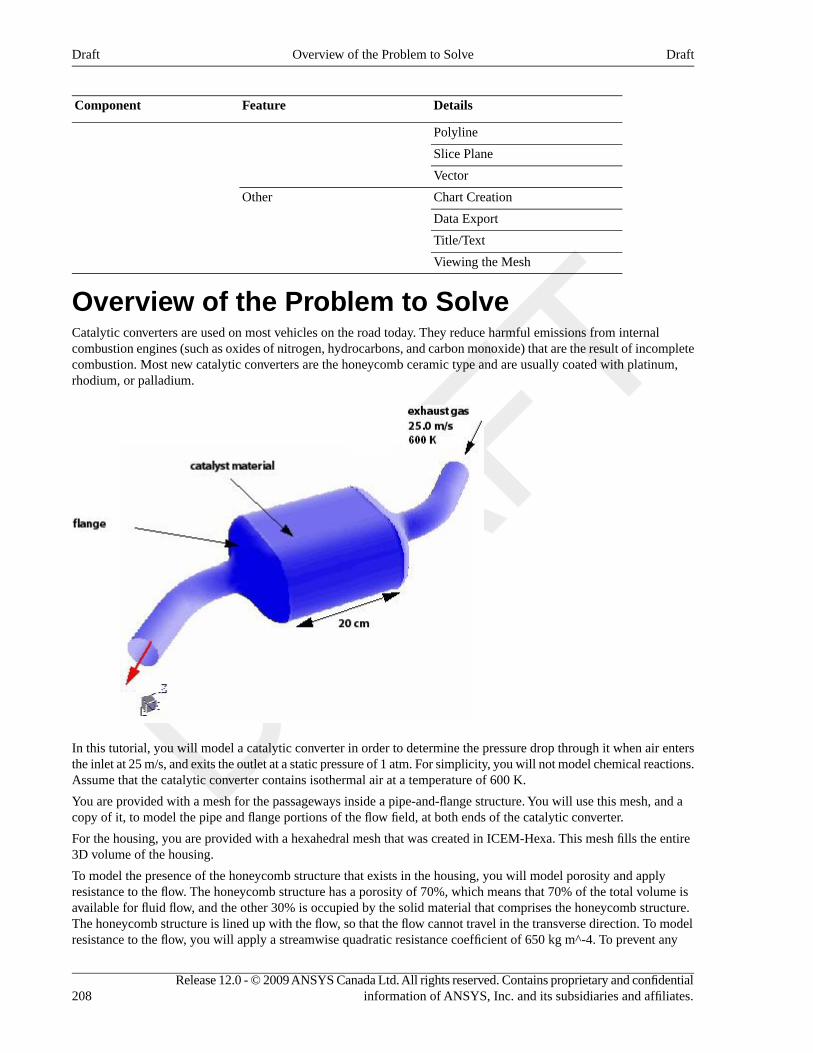
DetailsFeatureComponent
Polyline
Slice Plane
Vector
Chart CreationOther
Data Export
Title/Text
Viewing the Mesh
Overview of the Problem to SolveCatalytic converters are used on most vehicles on the road today. They reduce harmful emissions from internalcombustion engines (such as oxides of nitrogen, hydrocarbons, and carbon monoxide) that are the result of incompletecombustion. Most new catalytic converters are the honeycomb ceramic type and are usually coated with platinum,rhodium, or palladium.
In this tutorial, you will model a catalytic converter in order to determine the pressure drop through it when air entersthe inlet at 25 m/s, and exits the outlet at a static pressure of 1 atm. For simplicity, you will not model chemical reactions.Assume that the catalytic converter contains isothermal air at a temperature of 600 K.
You are provided with a mesh for the passageways inside a pipe-and-flange structure. You will use this mesh, and acopy of it, to model the pipe and flange portions of the flow field, at both ends of the catalytic converter.
For the housing, you are provided with a hexahedral mesh that was created in ICEM-Hexa. This mesh fills the entire3D volume of the housing.
To model the presence of the honeycomb structure that exists in the housing, you will model porosity and applyresistance to the flow. The honeycomb structure has a porosity of 70%, which means that 70% of the total volume isavailable for fluid flow, and the other 30% is occupied by the solid material that comprises the honeycomb structure.The honeycomb structure is lined up with the flow, so that the flow cannot travel in the transverse direction. To modelresistance to the flow, you will apply a streamwise quadratic resistance coefficient of 650 kg m^-4. To prevent any
Release 12.0 - © 2009 ANSYS Canada Ltd. All rights reserved. Contains proprietary and confidentialinformation of ANSYS, Inc. and its subsidiaries and affiliates.208
DraftOverview of the Problem to SolveDraft
significant transverse flow, apply a quadratic resistance coefficient of 6500 kg m^-4 in the transverse direction. Thesegiven resistance coefficients are based on the superficial flow velocity, rather than the true flow velocity.
Approach to the ProblemYou will first import the mesh for the housing. You will then import a mesh for one of the two flanges. You will thenproduce another flange mesh by transforming the first.
You will create one porous domain for the housing, and one fluid domain for both flanges.
You will model a honeycomb structure inside the housing by specifying a porosity and applying a directional momentumloss model.
Before You BeginIf this is the first tutorial you are working with, it is important to review the following topics before beginning:
• Preparing a Working Directory (p. 23)
• Setting the Working Directory and Starting ANSYS CFX (p. 23)
• Changing the Display Colors (p. 24)
• Playing a Tutorial Session File (p. 24)
Starting CFX-Pre1. Prepare the working directory using the following files in the examples directory:
• CatConvHousing.hex
• CatConvMesh.gtm
• CatConv.pre
For details, see Preparing a Working Directory (p. 23)
2. Set the working directory and start CFX-Pre
For details, see Setting the Working Directory and Starting ANSYS CFX (p. 23)
Defining a Case in CFX-PreIf you want to set up the simulation automatically using a tutorial session file, run CatConv.pre. For details, seePlaying a Tutorial Session File (p. 24). Then proceed to Obtaining a Solution using CFX-Solver Manager (p. 217).
If you want to set up the simulation manually, proceed to the following steps:
1. Start CFX-Pre if necessary.
2. Select File > New Case.
3. Select General and click OK.
4. Select File > Save Case As.
5. Under File name, type CatConv.
6. Click Save.
Importing the MeshesThe mesh for this catalytic converter comprises three distinct parts:
• The outlet section (pipe and flange).
209Release 12.0 - © 2009 ANSYS Canada Ltd. All rights reserved. Contains proprietary and confidentialinformation of ANSYS, Inc. and its subsidiaries and affiliates.
DraftApproach to the ProblemDraft
• The inlet section (pipe and flange).
You will copy and rotate the outlet section through 180 degrees to create this section.
• The catalyst (or monolith).
Next you will import the catalyst housing and a generic inlet/outlet section from provided files.
Importing the Housing MeshThe first mesh that you will import, CatConvHousing.hex, is a hexahedral mesh for the catalyst housing. Themesh was originally created in ICEM-Hexa using mesh units of centimeters. Because this type of mesh file does notspecify the mesh units, you must specify them manually. The imported mesh has a width in the x-direction of 21 cmand a length in the z-direction of 20 cm.
1. Edit Case Options > General in the Outline tree view and ensure that Automatic Default Domain isturned off.
Default Domain generation should be turned off because you will create a new domain manually, later in thistutorial.
2. Right-click Mesh and select Import Mesh > Other.
The Import Mesh dialog box appears.
3. Apply the following settings:
ValueSetting
All Types(*)Files of type
ICEM CFDMesh Format
cmOptions > Mesh Units
CatConvHousing.hexFile name
4. Click Open.
Later in this tutorial, you will create a porous domain for the housing in order to simulate flow through a honeycombstructure.
Importing the Pipe and Flange MeshThe second mesh that you will import, CatConvMesh.gtm, is a mesh for a pipe and flange. The mesh has units ofcentimeters. Because this type of mesh file does specify the mesh units, there is no need to specify them manually.
1. Right-click Mesh and select Import Mesh > CFX Mesh.
2. Apply the following settings:
ValueSetting
CatConvMesh.gtmFile name
3. Click Open.
You now have a pipe and flange on the outlet end of the housing. In the next step, you will create a transformed copyof the pipe and flange for the inlet end.
Release 12.0 - © 2009 ANSYS Canada Ltd. All rights reserved. Contains proprietary and confidentialinformation of ANSYS, Inc. and its subsidiaries and affiliates.210
DraftImporting the MeshesDraft
Creating a Second Pipe and Flange MeshCreate a transformed copy of the pipe and flange mesh:
1. Right-click CatConvMesh.gtm and select Transform Mesh.
The Mesh Transformation Editor dialog box appears.
2. Apply the following settings:
ValueSetting
RotationTransformation
Rotation AxisRotation Option
0, 0, 0.16From
0, 1, 0.16aTo
SpecifiedRotation Angle Option
180 [degree]Rotation Angle
(Selected)Multiple Copies
1Multiple Copies > # of Copies
aThis specifies an axis located at the center of the housing parallel to the y-axis.
3. Click OK.
Later in this tutorial, you will create a fluid domain for both pipe and flange sections.
Creating a Single Region for Both Pipe and Flange MeshesThe outlet pipe and flange region is B1.P3. The inlet pipe and flange region is B1.P3 2.
There are three basic options for creating fluid domains on these regions:
• Create two similar domains: one that applies to B1.P3, and one that applies to B1.P3 2.
• Create one domain that applies to both B1.P3 and B1.P3 2.
• Create one domain that applies to one composite region, the latter referring to B1.P3 and B1.P3 2.
For demonstration purposes, you will create a composite region and use it as the location for a single fluid domain.
Create a single region that includes both pipe-flange regions:
1. Create a new composite region by selecting Insert > Regions > Composite Region.
2. In the Insert Region dialog box, set the name to CatConverter.
3. Click OK.
4. Apply the following settings:
ValueSettingTab
3DDimension (Filter)Basic Settings
B1.P3, B1.P3 2Region List
5. Click OK.
211Release 12.0 - © 2009 ANSYS Canada Ltd. All rights reserved. Contains proprietary and confidentialinformation of ANSYS, Inc. and its subsidiaries and affiliates.
DraftImporting the MeshesDraft
Creating the Fluid DomainFor this simulation you will use an isothermal heat transfer model and assume turbulent flow. Create the fluid domainusing the composite region that you created earlier:
1. Ensure that no default domain is present under Flow Analysis 1. If a default domain is present, right-clickit and select Delete.
2. Create a new domain by selecting Insert > Domain, or click Domain .
3. In the Insert Domain dialog box, set the name to Pipes.
4. Click OK.
5. Apply the following settings (the values are taken from the problem description):
ValueSettingTab
CatConverterLocation and Type > LocationBasic Settings
Fluid DomainLocation and Type > Domain Type
Fluid 1Fluid and Particle Definitions
Air Ideal GasFluid and Particle Definitions > Fluid 1 > Material
1 [atm]Domain Models > Pressure > Reference Pressure
IsothermalHeat Transfer > OptionFluid Models
600 [K]Heat Transfer > Fluid Temperature
6. Click OK.
Creating the Porous DomainThe catalyst-coated honeycomb structure will be modeled using a porous domain with a directional source of quadraticresistance, as described in the problem description. The streamwise directional resistance is aligned with the Z axis.
For quadratic resistances, the pressure drop is modeled using:
(Eq. 12.1)= −∂∂
UK Upx Q ii
where KQ is the quadratic resistance coefficient, Ui is the local velocity in the i direction, and ∂∂pxi
is the pressure drop
gradient in the i direction.
1. Create a new domain by selecting Insert > Domain, or click Domain .
2. In the Insert Domain dialog box, set the name to Housing.
3. Click OK.
4. Apply the following settings:
ValueSettingTab
LIVEaLocation and Type > LocationBasic Settings
Porous DomainLocation and Type > Domain Type
Release 12.0 - © 2009 ANSYS Canada Ltd. All rights reserved. Contains proprietary and confidentialinformation of ANSYS, Inc. and its subsidiaries and affiliates.212
DraftCreating the Fluid DomainDraft
ValueSettingTab
Fluid 1Fluid and Particle Definitions
Air Ideal GasFluid and Particle Definitions > Fluid 1 > Material
1 [atm]Domain Models > Pressure > Reference Pressure
ValueVolume Porosity > OptionPorositySettings
0.7Volume Porosity > Volume Porosity
Directional LossLoss Model > Option
SuperficialbLoss Model > Loss Velocity Type
Cartesian ComponentsLoss Model > Directional Loss > Streamwise Direction >Option
0Loss Model > Directional Loss > Streamwise Direction >X Component
0Loss Model > Directional Loss > Streamwise Direction >Y Component
-1Loss Model > Directional Loss > Streamwise Direction >Z Component
Linear and QuadraticResistance Coefficients
Loss Model > Directional Loss > Streamwise Loss >Option
(Selected)Loss Model > Directional Loss > Streamwise Loss >Quadratic Resistance Coefficient
650 [kg m^-4]cLoss Model > Directional Loss > Streamwise Loss >Quadratic Resistance Coefficient > Quadratic Coefficient
Streamwise CoefficientMultiplier
Loss Model > Directional Loss > Transverse Loss > Option
10cLoss Model > Directional Loss > Transverse Loss >Multiplier
IsothermalHeat Transfer > OptionFluid Models
600 [K]Heat Transfer > Fluid Temperature
aThis is the entire housing section as predefined in the mesh.bSuperficial velocity is the velocity at which the flow would travel if the porosity of the domain were 100%. It is less than the true velocity.cFrom the problem description.
5. Click OK.
Creating the BoundariesCreate the inlet and outlet boundaries using the values given in the problem description.
Creating the Inlet Boundary1. Create a new boundary in domain Pipes named Inlet.
213Release 12.0 - © 2009 ANSYS Canada Ltd. All rights reserved. Contains proprietary and confidentialinformation of ANSYS, Inc. and its subsidiaries and affiliates.
DraftCreating the BoundariesDraft
2. Apply the following settings:
ValueSettingTab
InletBoundary TypeBasic Settings
PipeEnd 2Location
25 [m s^-1]bMass and Momentum > Normal SpeedBoundary Detailsa
aThe default level of turbulence is suitable for this application.bFrom the problem description.
3. Click OK.
Creating the Outlet BoundarySet up the outlet with a static pressure boundary:
1. Create a new boundary in domain Pipes named Outlet.
2. Apply the following settings:
ValueSettingTab
OutletBoundary TypeBasic Settings
PipeEndLocation
Static PressureMass and Momentum > OptionBoundary Details
0 [Pa]Mass and Momentum > Relative Pressure
3. Click OK.
The remaining outer surfaces are automatically assigned to the default (no slip wall) boundaries: HousingDefault and Pipes Default.
Creating the Domain InterfacesYou will next create a pair of domain interfaces to model the connection between the fluid and porous domains. Themeshes on the interfaces are dissimilar, so a General Grid Interface (GGI) connection method is required. Domaininterfaces are capable of modeling changes in reference frame as well as other changes that are not applicable to thissimulation.
Two interfaces are required, one to connect the inlet flange to the catalyst housing and one to connect the outlet flangeto the catalyst housing.
1. Create a new domain interface by selecting Insert > Domain Interface, or click Domain Interface .
2. In the Insert Domain Interface dialog box, set the name to InletSide.
3. Click OK.
4. Apply the following settings:
ValueSettingTab
Fluid PorousInterface TypeBasic Settings
Release 12.0 - © 2009 ANSYS Canada Ltd. All rights reserved. Contains proprietary and confidentialinformation of ANSYS, Inc. and its subsidiaries and affiliates.214
DraftCreating the Domain InterfacesDraft
ValueSettingTab
PipesInterface Side 1 > Domain (Filter)
FlangeEnd 2Interface Side 1 > Region List
HousingInterface Side 2 > Domain (Filter)
INLETInterface Side 2 > Region List
GGIMesh Connection Method > MeshConnection > Option
5. Click OK.
6. Create a similar domain interface named OutletSide that connects FlangeEnd (in domain Pipes) toOUTLET (in domain Housing).
Setting Initial ValuesA sensible guess for the initial velocity is the expected velocity through the catalyst housing. You can assumeincompressible flow and apply conservation of mass to obtain an approximate velocity of 2.8 [m s^-1] through thehousing based on the following known information:
• The inlet velocity: 25 [m s^-1]
• The cross sectional area of the inlet and housing, which can be determined using the function calculator in CFD-Post:0.001913 m^2 and 0.024039 m^2 respectively
• The porosity of the honeycomb structure: 70%
1. Click Global Initialization .
2. Apply the following settings:
ValueSettingTab
Automatic with ValueInitial Conditions > Cartesian VelocityComponents > Option
Global Settings
0 [m s^-1]Initial Conditions > Cartesian VelocityComponents > U
0 [m s^-1]Initial Conditions > Cartesian VelocityComponents > V
-2.8 [m s^-1]Initial Conditions > Cartesian VelocityComponents > W
3. Click OK.
Setting Solver ControlAssuming velocities of 25 m/s in the inlet and outlet pipes, and 2.8 m/s in the catalyst housing, an approximate fluidresidence time of 0.1 s can be calculated. A sensible time step is 1/4 to 1/2 of the fluid residence time. In this case, usea time step of 0.04 s.
For the convergence criteria, an RMS value of at least 1e-05 is usually required for adequate convergence, but thedefault value of 1e-04 is sufficient for demonstration purposes.
215Release 12.0 - © 2009 ANSYS Canada Ltd. All rights reserved. Contains proprietary and confidentialinformation of ANSYS, Inc. and its subsidiaries and affiliates.
DraftSetting Initial ValuesDraft
1. Click Solver Control .
2. Apply the following settings:
ValueSettingTab
Physical TimescaleConvergence Control > Fluid TimescaleControl > Timescale Control
Basic Settings
0.04 [s]Convergence Control >Fluid Timescale Control> Physical Timescale
3. Click OK.
Setting a Discretization OptionThe porous cs discretisation option expert parameter specifies how the pressure is treated at interfacesto a porous domain: 1=constant static pressure; 2=constant total pressure. Constant total pressure is the preferred andmore physical setting. However, when using this setting, in cases where there are sections of the porous interface wherethere is little or no flow normal to the interface, the CFX-Solver may fail to converge. These convergence difficultiesmay be overcome by using the less physical constant static pressure setting.
This simulation involves flow that moves from a fluid domain into a porous domain, approaching the interface atvarious angles. In this case, better convergence can be achieved by changing the porous cs discretisationoption expert parameter from the default value of 2 to 1.
1. Click Insert > Solver > Expert Parameter.
2. Apply the following settings in the Expert Parameters details view:
ValueSettingTab
(Selected)Miscellaneous > porous cs discretizationoption
Discretization
1Miscellaneous > porous cs discretizationoption > Value
3. Click OK.
Writing the CFX-Solver Input (.def) File
1. Click Define Run .
2. Apply the following settings:
ValueSetting
CatConv.defFile name
3. Click Save.
CFX-Solver Manager automatically starts and, on the Define Run dialog box, the Solver Input File is set.
4. If using Standalone Mode, quit CFX-Pre, saving the simulation (.cfx) file at your discretion.
Release 12.0 - © 2009 ANSYS Canada Ltd. All rights reserved. Contains proprietary and confidentialinformation of ANSYS, Inc. and its subsidiaries and affiliates.216
DraftSetting a Discretization OptionDraft
Obtaining a Solution using CFX-Solver ManagerAt this point, CFX-Solver Manager is running.
1. Ensure that the Define Run dialog box is displayed.
2. Click Start Run.
CFX-Solver runs and attempts to obtain a solution. This may take a long time, depending on your system. Eventuallya dialog box is displayed.
3. Select the check box next to Post-Process Results when the completion message appears at the end of the run.
4. If using Standalone Mode, select the check box next to Shut down CFX-Solver Manager.
5. Click OK.
Viewing the Results in CFD-PostIn this section, you will inspect the GGI interface to see the lack of node alignment that characterizes this type ofinterface. You will also create plots showing the distribution of temperature and pressure on a flat plane that intersectsthe catalytic converter. You will then make a chart showing pressure versus Z coordinate using data from a polylinethat runs around the perimeter of the catalytic converter. Finally, you will export data from the polyline to a file. Sucha file could be used in other programs, or could be loaded into CFD-Post (for example, to use as data for a chart line).
The topics in this section include:
• Viewing the Mesh on a GGI Interface (p. 217)
• Creating User Locations (p. 218)
• Creating Plots (p. 219)
• Exporting Polyline Data (p. 221)
Viewing the Mesh on a GGI InterfaceIn this section, you will examine a GGI interface. As a preliminary step, do the following:
1. When CFD-Post opens, if you see the Domain Selector dialog box, ensure that both domains are selected, thenclick OK.
2. Edit User Locations and Plots > Wireframe.
3. Set Edge Angle to 10 [degree] and click Apply to see more of the mesh surface.
4. Turn off the visibility of User Locations and Plots > Wireframe.
5. Right-click a blank area in the viewer and select Predefined Camera > View Towards -Z.
In the Outline tree view, four interface sides are listed. There are two sides to the interface between the housing andthe inlet. Similarly, there are two sides to the corresponding interface on the outlet side.
Examine the interface on the inlet side to see the nature of the GGI connection:
1. In the Outline tree view, edit InletSide Side 1.
2. Apply the following settings:
ValueSettingTab
(Cleared)Show FacesRender
(Selected)Show Mesh Lines
User SpecifiedShow Mesh Lines > Color Mode
217Release 12.0 - © 2009 ANSYS Canada Ltd. All rights reserved. Contains proprietary and confidentialinformation of ANSYS, Inc. and its subsidiaries and affiliates.
DraftObtaining a Solution using CFX-Solver ManagerDraft
ValueSettingTab
(Red)Show Mesh Lines > Line Color
3. Click Apply.
4. In the Outline tree view, edit InletSide Side 2.
5. Apply the following settings:
ValueSettingTab
(Cleared)Show FacesRender
(Selected)Show Mesh Lines
User SpecifiedShow Mesh Lines > Color Mode
(Green)Show Mesh Lines > Line Color
6. Click Apply.
7. Click Fit View to re-center and re-scale the geometry.
You can now see the tetrahedral/prism and hexahedral mesh on each side of the GGI interface. This interface was usedto produce a connection between dissimilar meshes before the solution was calculated. Notice that there are moretetrahedral/prism elements than hexahedral elements and that the extent of the two meshes is not quite the same (thisis most noticeable on the curved edges).
Creating User LocationsIn this section, you will create locators that you will use to make plots.
To make it easier to see the locators, adjust the view as follows:
1. Turn on the visibility of User Locations and Plots > Wireframe.
2. Turn off the visibility of Pipes > InletSide Side 1 and Housing > InletSide Side 2.
Creating a Slice PlaneLater in this tutorial, you will produce a contour plot and a vector plot. Both of these plots require a slice plane locator.
Create a slice plane through the geometry as follows:
1. Right-click a blank area in the viewer and select Predefined Camera > View Towards +Y.
2. Create a new plane named Plane 1.
3. Apply the following settings:
ValueSettingTab
ZX PlaneDefinition > MethodGeometry
0.0 [m]Definition > Y
VariableModeColor
PressureVariable
Release 12.0 - © 2009 ANSYS Canada Ltd. All rights reserved. Contains proprietary and confidentialinformation of ANSYS, Inc. and its subsidiaries and affiliates.218
DraftCreating User LocationsDraft
4. Click Apply.
Creating a PolylineLater in this tutorial, you will make a chart that plots data from a polyline.
The Method used to create the polyline can be From File, Boundary Intersection, or From Contour.If you select From File, you must specify a file containing point definitions in the required format.
In this tutorial, you will use the Boundary Intersection method. This creates a polyline from the intersectingline between a boundary object and a location (for example, between a wall and a plane). The points on the polylineare where the intersecting line cuts through a surface mesh edge.
You will be able to see the polyline following the intersecting line between the wall, inlet and outlet boundaries andthe slice plane.
1. Create a new polyline named Polyline 1.
2. Apply the following settings:
ValueSettingTab
Boundary IntersectionMethodGeometry
Housing Default, Pipes DefaultaBoundary List
Plane 1Intersect With
ConstantModeColor
(Yellow)Color
3Line WidthRender
aClick the ellipsis icon to select multiple items using the Ctrl key.
3. Click Apply.
Creating PlotsIn this section, you will make plots on the slice plane and polyline locators.
Creating a Contour Plot of PressureYou will now create a contour plot to observe the pressure change throughout the main body of the catalytic converter:
1. Clear Plane 1 in the Outline tab.
2. Create a new contour plot named Contour 1.
3. Apply the following settings:
ValueSettingTab
Plane 1LocationsGeometry
PressureVariable
GlobalRange
30a# of Contours
219Release 12.0 - © 2009 ANSYS Canada Ltd. All rights reserved. Contains proprietary and confidentialinformation of ANSYS, Inc. and its subsidiaries and affiliates.
DraftCreating PlotsDraft
ValueSettingTab
(Cleared)Show Contour BandsRender
aDetermined by experiment.
4. Click Apply.
From the contour plot, you can see that the pressure falls steadily through the main body of the catalytic converter.
Creating a Vector Plot on the Slice PlaneCreate a vector plot to display the recirculation zone:
1. Create a new vector plot named Vector 1.
2. Apply the following settings:
ValueSettingTab
Plane 1LocationsGeometry
0.1Symbol SizeSymbol
(Selected)Normalize Symbols
3. Click Apply.
Notice that the flow separates from the walls, where the inlet pipe expands into the flange, setting up a recirculationzone. The flow is uniform through the catalyst housing.
Creating a Chart of Pressure versus the Z CoordinateIn this section, you will make a chart to see if the pressure drop is, as expected, linear by plotting a line graph of pressureagainst the z-coordinate. In this case you will use CFD-Post to produce the graph, but you could also export the data,then read it into any standard plotting package.
1. Create a new chart named Chart 1.
2. Apply the following settings:
ValueSettingTab
Pressure Drop through a CatalyticConverter
TitleGeneral
Pressure DropNameData Series
Polyline 1Data Source > Location
ZData Selection > VariableX Axis
PressureData Selection > VariableY Axis
NoneLine Display > Line StyleLine Display
RectangleLine Display > Symbols
3Sizes > SymbolChart Display
Release 12.0 - © 2009 ANSYS Canada Ltd. All rights reserved. Contains proprietary and confidentialinformation of ANSYS, Inc. and its subsidiaries and affiliates.220
DraftCreating PlotsDraft
3. Click Apply.
Through the main body of the catalytic converter you can see that the pressure drop is linear. This is in the regionfrom approximately Z=0.06 to Z=0.26. The two lines show the pressure on each side of the wall. You can see anoticeable difference in pressure between the two walls on the inlet side of the housing (at around Z=0.26).
4. If required, in the Outline tree view, select Contour 1, Polyline 1, and Vector 1.
5. Click the 3D Viewer tab, then right-click a blank area and select Predefined Camera > View Towards +Y.
You should now see that the flow enters the housing from the inlet pipe at a slight angle, producing a higherpressure on the high X wall of the housing.
Exporting Polyline DataYou can export data from a polyline for use in other software.
Export data as follows:
1. From the main menu, select File > Export.
2. Apply the following settings:
ValueSettingTab
Polyline 1LocationsOptions
(Selected)aExport Geometry Information
PressureSelect Variables
3PrecisionFormatting
aThis ensures X, Y, and Z to be sent to the output file.
3. Click Save.
The file export.csv will be written to the current working directory in a comma-separated variable format.This file can be opened in any text editor. You can use the exported data file to plot charts in other software suchas a Microsoft Excel spreadsheet.
4. When finished, quit CFD-Post.
221Release 12.0 - © 2009 ANSYS Canada Ltd. All rights reserved. Contains proprietary and confidentialinformation of ANSYS, Inc. and its subsidiaries and affiliates.
DraftExporting Polyline DataDraft

Release 12.0 - © 2009 ANSYS Canada Ltd. All rights reserved. Contains proprietary and confidentialinformation of ANSYS, Inc. and its subsidiaries and affiliates.
Chapter 13. Non-Newtonian Fluid Flowin an AnnulusThis tutorial includes:
• Tutorial Features (p. 223)
• Background Theory (p. 224)
• Overview of the Problem to Solve (p. 225)
• Before You Begin (p. 225)
• Starting CFX-Pre (p. 226)
• Defining a Case in CFX-Pre (p. 226)
• Obtaining a Solution using CFX-Solver Manager (p. 231)
• Viewing the Results in CFD-Post (p. 231)
Tutorial FeaturesIn this tutorial you will learn about:
• Using CFX Expression Language (CEL) to define the properties of a shear-thickening fluid.
• Using the Moving Wall feature to apply a rotation to the fluid at a wall boundary.
DetailsFeatureComponent
General ModeUser ModeCFX-Pre
Steady StateAnalysis Type
General FluidFluid Type
Single DomainDomain Type
LaminarTurbulence Model
NoneHeat Transfer
Symmetry PlaneBoundary Conditions
Wall: No-Slip
Wall: Moving
CEL (CFX Expression Language)
Auto Time ScaleTimestep
Sampling PlanePlotsCFD-Post
Vector
223Release 12.0 - © 2009 ANSYS Canada Ltd. All rights reserved. Contains proprietary and confidentialinformation of ANSYS, Inc. and its subsidiaries and affiliates.
DraftDraft
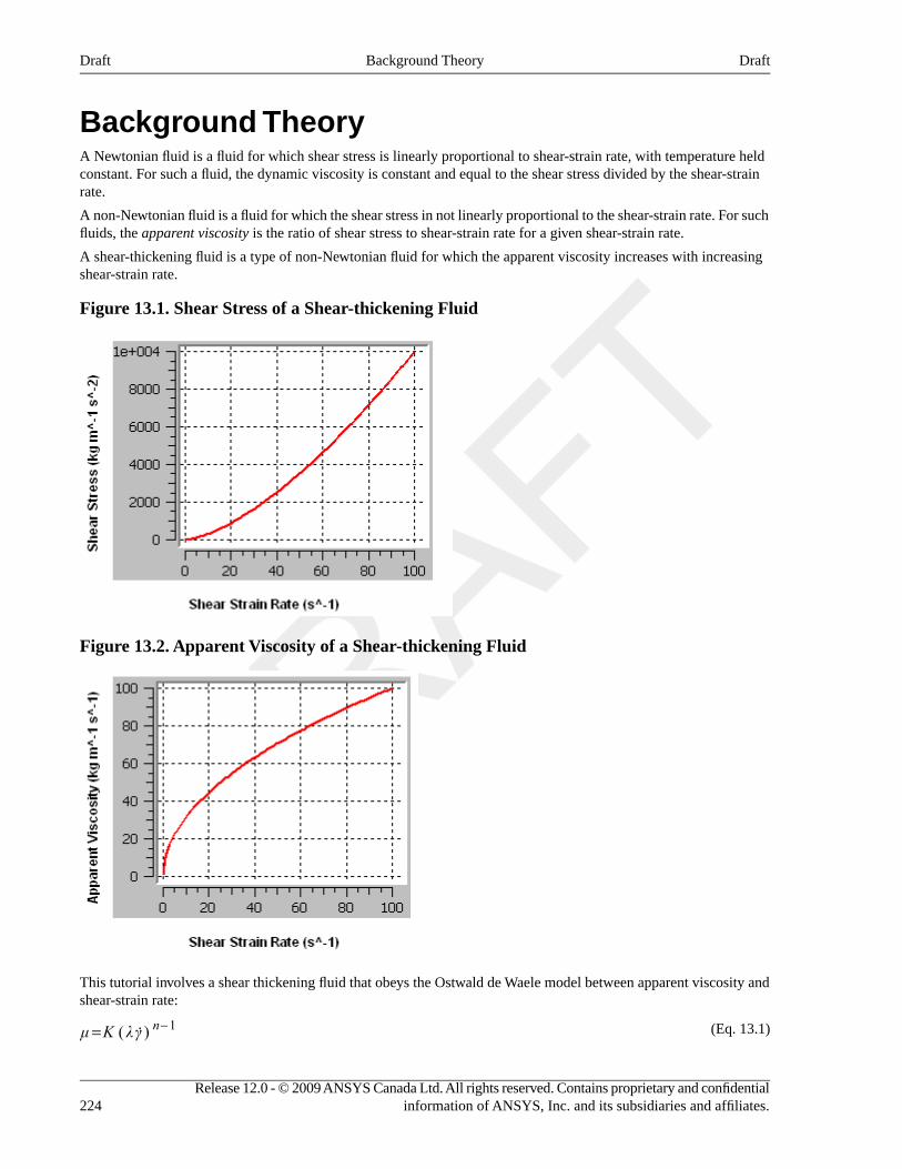
Background TheoryA Newtonian fluid is a fluid for which shear stress is linearly proportional to shear-strain rate, with temperature heldconstant. For such a fluid, the dynamic viscosity is constant and equal to the shear stress divided by the shear-strainrate.
A non-Newtonian fluid is a fluid for which the shear stress in not linearly proportional to the shear-strain rate. For suchfluids, the apparent viscosity is the ratio of shear stress to shear-strain rate for a given shear-strain rate.
A shear-thickening fluid is a type of non-Newtonian fluid for which the apparent viscosity increases with increasingshear-strain rate.
Figure 13.1. Shear Stress of a Shear-thickening Fluid
Figure 13.2. Apparent Viscosity of a Shear-thickening Fluid
This tutorial involves a shear thickening fluid that obeys the Ostwald de Waele model between apparent viscosity andshear-strain rate:
(Eq. 13.1)= −μ K λγ( ˙) n 1
Release 12.0 - © 2009 ANSYS Canada Ltd. All rights reserved. Contains proprietary and confidentialinformation of ANSYS, Inc. and its subsidiaries and affiliates.224
DraftBackground TheoryDraft
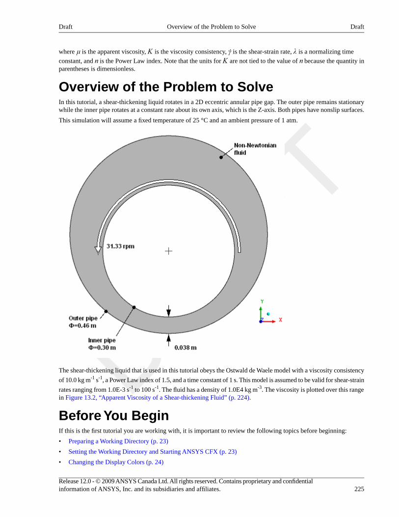
where μ is the apparent viscosity, K is the viscosity consistency, γ̇ is the shear-strain rate, λ is a normalizing time
constant, and n is the Power Law index. Note that the units for K are not tied to the value of n because the quantity inparentheses is dimensionless.
Overview of the Problem to SolveIn this tutorial, a shear-thickening liquid rotates in a 2D eccentric annular pipe gap. The outer pipe remains stationarywhile the inner pipe rotates at a constant rate about its own axis, which is the Z-axis. Both pipes have nonslip surfaces.
This simulation will assume a fixed temperature of 25 °C and an ambient pressure of 1 atm.
The shear-thickening liquid that is used in this tutorial obeys the Ostwald de Waele model with a viscosity consistency
of 10.0 kg m-1 s-1, a Power Law index of 1.5, and a time constant of 1 s. This model is assumed to be valid for shear-strain
rates ranging from 1.0E-3 s-1 to 100 s-1. The fluid has a density of 1.0E4 kg m-3. The viscosity is plotted over this rangein Figure 13.2, “Apparent Viscosity of a Shear-thickening Fluid” (p. 224).
Before You BeginIf this is the first tutorial you are working with, it is important to review the following topics before beginning:
• Preparing a Working Directory (p. 23)
• Setting the Working Directory and Starting ANSYS CFX (p. 23)
• Changing the Display Colors (p. 24)
225Release 12.0 - © 2009 ANSYS Canada Ltd. All rights reserved. Contains proprietary and confidentialinformation of ANSYS, Inc. and its subsidiaries and affiliates.
DraftOverview of the Problem to SolveDraft
• Playing a Tutorial Session File (p. 24)
Starting CFX-Pre1. Prepare the working directory using the following files in the examples directory:
• NonNewton.pre
• NonNewtonMesh.gtm
For details, see Preparing a Working Directory (p. 23)
2. Set the working directory and start CFX-Pre.
For details, see Setting the Working Directory and Starting ANSYS CFX (p. 23)
Defining a Case in CFX-PreIf you want to set up the simulation automatically using a tutorial session file, run NonNewton.pre. For details, seePlaying a Tutorial Session File (p. 24). Then proceed to Obtaining a Solution using CFX-Solver Manager (p. 231).
If you want to set up the simulation manually, proceed to the following steps:
1. Select File > New Case.
2. Select General and click OK.
3. Select File > Save Case As.
4. Under File name, type NonNewton.
5. Click Save.
Importing the Mesh1. Edit Case Options > General in the Outline tree view and ensure that Automatic Default Domain is
turned off.
Default Domain generation should be turned off because you will create a new domain manually, later in thistutorial.
2. Right-click Mesh and select Import Mesh > CFX Mesh.
3. Apply the following settings:
ValueSetting
NonNewtonMesh.gtmFile name
4. Click Open.
Creating the FluidAs stated in the problem description, the shear-thickening liquid that is used in this tutorial obeys the Ostwald de Waele
model with a viscosity consistency (K) of 10.0 kg m-1 s-1, a Power Law index (n) of 1.5, and a time constant of 1 s.
This model is assumed to be valid for shear-strain rates ranging from 1.0E-3 s-1 to 100 s-1. The fluid has a density of
1.0E4 kg m-3.
1. Create a new material named myfluid.
2. Apply the following settings:
Release 12.0 - © 2009 ANSYS Canada Ltd. All rights reserved. Contains proprietary and confidentialinformation of ANSYS, Inc. and its subsidiaries and affiliates.226
DraftStarting CFX-PreDraft
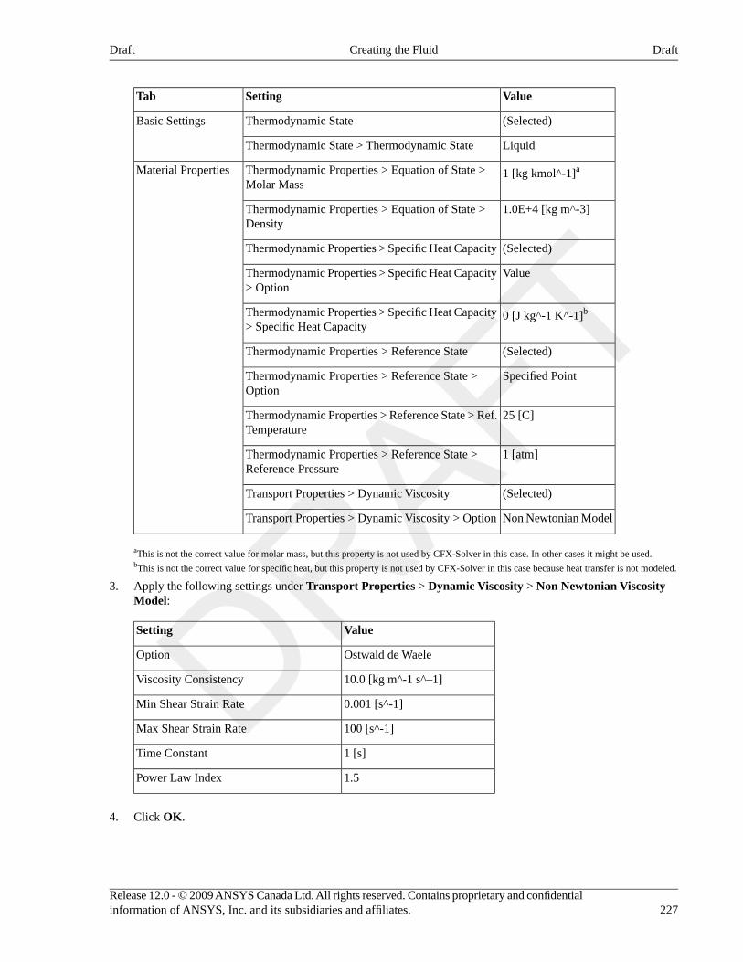
ValueSettingTab
(Selected)Thermodynamic StateBasic Settings
LiquidThermodynamic State > Thermodynamic State
1 [kg kmol^-1]aThermodynamic Properties > Equation of State >Molar Mass
Material Properties
1.0E+4 [kg m^-3]Thermodynamic Properties > Equation of State >Density
(Selected)Thermodynamic Properties > Specific Heat Capacity
ValueThermodynamic Properties > Specific Heat Capacity> Option
0 [J kg^-1 K^-1]bThermodynamic Properties > Specific Heat Capacity> Specific Heat Capacity
(Selected)Thermodynamic Properties > Reference State
Specified PointThermodynamic Properties > Reference State >Option
25 [C]Thermodynamic Properties > Reference State > Ref.Temperature
1 [atm]Thermodynamic Properties > Reference State >Reference Pressure
(Selected)Transport Properties > Dynamic Viscosity
Non Newtonian ModelTransport Properties > Dynamic Viscosity > Option
aThis is not the correct value for molar mass, but this property is not used by CFX-Solver in this case. In other cases it might be used.bThis is not the correct value for specific heat, but this property is not used by CFX-Solver in this case because heat transfer is not modeled.
3. Apply the following settings under Transport Properties > Dynamic Viscosity > Non Newtonian ViscosityModel:
ValueSetting
Ostwald de WaeleOption
10.0 [kg m^-1 s^–1]Viscosity Consistency
0.001 [s^-1]Min Shear Strain Rate
100 [s^-1]Max Shear Strain Rate
1 [s]Time Constant
1.5Power Law Index
4. Click OK.
227Release 12.0 - © 2009 ANSYS Canada Ltd. All rights reserved. Contains proprietary and confidentialinformation of ANSYS, Inc. and its subsidiaries and affiliates.
DraftCreating the FluidDraft
Creating the DomainThe flow is expected to be laminar because the Reynolds number, based on the rotational speed, the maximum widthof the pipe gap, and a representative viscosity (calculated using the shear-strain rate in the widest part of the gap,assuming a linear velocity profile), is approximately 30, which is well within the laminar-flow range.
From the problem description, the fluid is isothermal at 25 °C and the ambient pressure is atmospheric.
Create a fluid domain that uses the non-Newtonian fluid you created in the previous section, and specify laminar,isothermal flow with a reference pressure of 1 atmosphere:
1. Ensure that Flow Analysis 1 > Default Domain is deleted. If not, right-click Default Domain andselect Delete.
2. Click Domain and set the name to NonNewton.
3. Apply the following settings to NonNewton:
ValueSettingTab
B8LocationBasic Settings
Fluid 1Fluid and Particle Definitions
myfluidFluid and Particle Definitions > Fluid 1 > Material
1 [atm]Domain Models > Pressure > Reference Pressure
IsothermalHeat Transfer > OptionFluid Models
25 CHeat Transfer > Fluid Temperature
None (Laminar)Turbulence > Option
4. Click OK.
Creating the BoundariesThe inner and outer pipes both have nonslip surfaces. A rotating-wall boundary is required for the inner pipe. For theouter pipe, which is stationary, the default boundary is suitable. By not explicitly creating a boundary for the outerpipe, the latter receives the default wall boundary.
This tutorial models 2D flow in a pipe gap, where the latter is infinite in the Z-direction. The flow domain models athin 3D slice (in fact, just one layer of mesh elements) that has two surfaces of constant-Z coordinate that each requirea boundary. Symmetry boundary conditions are suitable in this case, since there is no pressure gradient or velocitygradient in the Z-direction.
Wall Boundary for the Inner PipeFrom the problem description, the inner pipe rotates at 31.33 rpm about the Z-axis. Create a wall boundary for theinner pipe that indicates this rotation:
1. Create a new boundary named rotwall.
2. Apply the following settings:
ValueSettingTab
WallBoundary TypeBasic Settings
Release 12.0 - © 2009 ANSYS Canada Ltd. All rights reserved. Contains proprietary and confidentialinformation of ANSYS, Inc. and its subsidiaries and affiliates.228
DraftCreating the DomainDraft
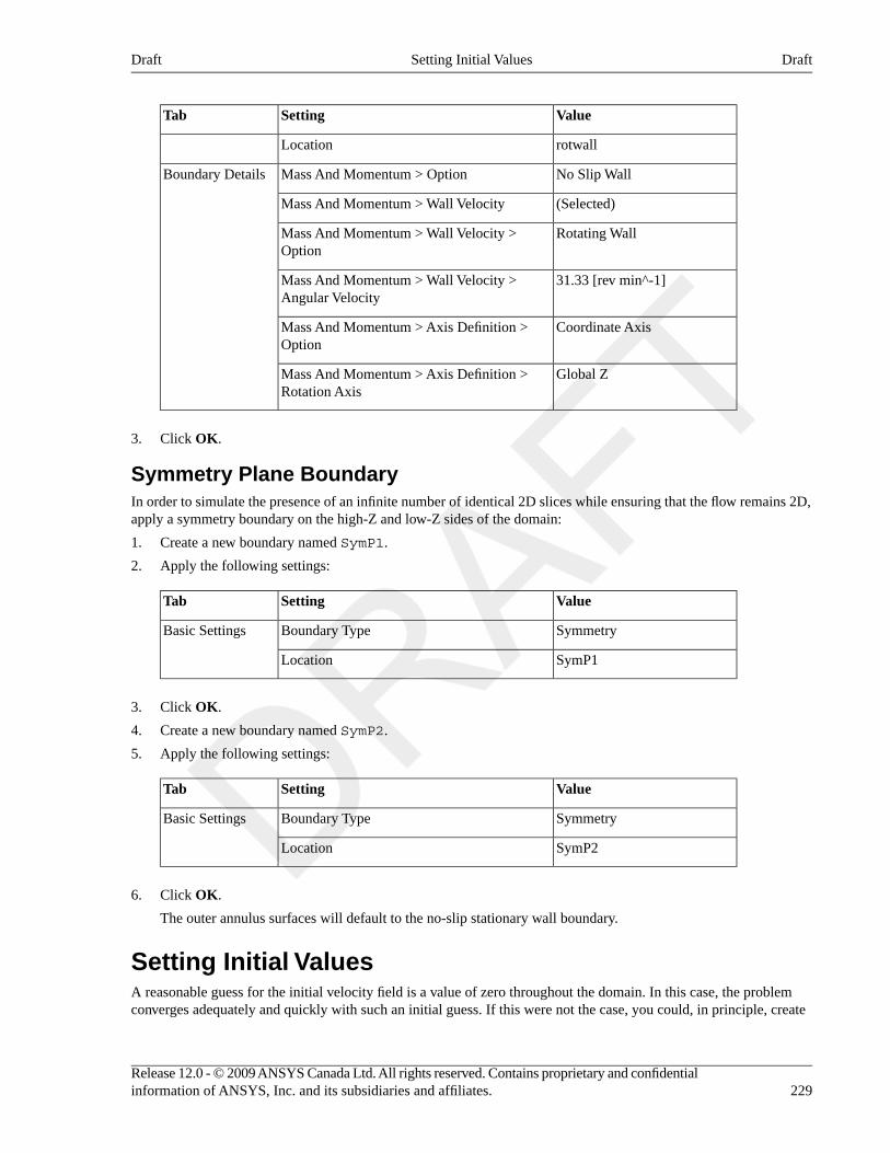
ValueSettingTab
rotwallLocation
No Slip WallMass And Momentum > OptionBoundary Details
(Selected)Mass And Momentum > Wall Velocity
Rotating WallMass And Momentum > Wall Velocity >Option
31.33 [rev min^-1]Mass And Momentum > Wall Velocity >Angular Velocity
Coordinate AxisMass And Momentum > Axis Definition >Option
Global ZMass And Momentum > Axis Definition >Rotation Axis
3. Click OK.
Symmetry Plane BoundaryIn order to simulate the presence of an infinite number of identical 2D slices while ensuring that the flow remains 2D,apply a symmetry boundary on the high-Z and low-Z sides of the domain:
1. Create a new boundary named SymP1.
2. Apply the following settings:
ValueSettingTab
SymmetryBoundary TypeBasic Settings
SymP1Location
3. Click OK.
4. Create a new boundary named SymP2.
5. Apply the following settings:
ValueSettingTab
SymmetryBoundary TypeBasic Settings
SymP2Location
6. Click OK.
The outer annulus surfaces will default to the no-slip stationary wall boundary.
Setting Initial ValuesA reasonable guess for the initial velocity field is a value of zero throughout the domain. In this case, the problemconverges adequately and quickly with such an initial guess. If this were not the case, you could, in principle, create
229Release 12.0 - © 2009 ANSYS Canada Ltd. All rights reserved. Contains proprietary and confidentialinformation of ANSYS, Inc. and its subsidiaries and affiliates.
DraftSetting Initial ValuesDraft
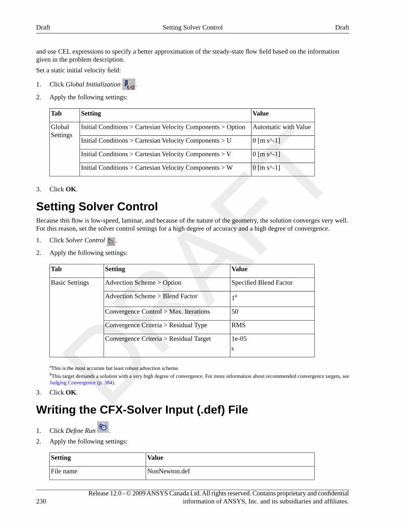
and use CEL expressions to specify a better approximation of the steady-state flow field based on the informationgiven in the problem description.
Set a static initial velocity field:
1. Click Global Initialization .
2. Apply the following settings:
ValueSettingTab
Automatic with ValueInitial Conditions > Cartesian Velocity Components > OptionGlobalSettings
0 [m s^-1]Initial Conditions > Cartesian Velocity Components > U
0 [m s^-1]Initial Conditions > Cartesian Velocity Components > V
0 [m s^-1]Initial Conditions > Cartesian Velocity Components > W
3. Click OK.
Setting Solver ControlBecause this flow is low-speed, laminar, and because of the nature of the geometry, the solution converges very well.For this reason, set the solver control settings for a high degree of accuracy and a high degree of convergence.
1. Click Solver Control .
2. Apply the following settings:
ValueSettingTab
Specified Blend FactorAdvection Scheme > OptionBasic Settings
1aAdvection Scheme > Blend Factor
50Convergence Control > Max. Iterations
RMSConvergence Criteria > Residual Type
1e-05Convergence Criteria > Residual Target
b
aThis is the most accurate but least robust advection scheme.bThis target demands a solution with a very high degree of convergence. For more information about recommended convergence targets, seeJudging Convergence (p. 384).
3. Click OK.
Writing the CFX-Solver Input (.def) File
1. Click Define Run .
2. Apply the following settings:
ValueSetting
NonNewton.defFile name
Release 12.0 - © 2009 ANSYS Canada Ltd. All rights reserved. Contains proprietary and confidentialinformation of ANSYS, Inc. and its subsidiaries and affiliates.230
DraftSetting Solver ControlDraft
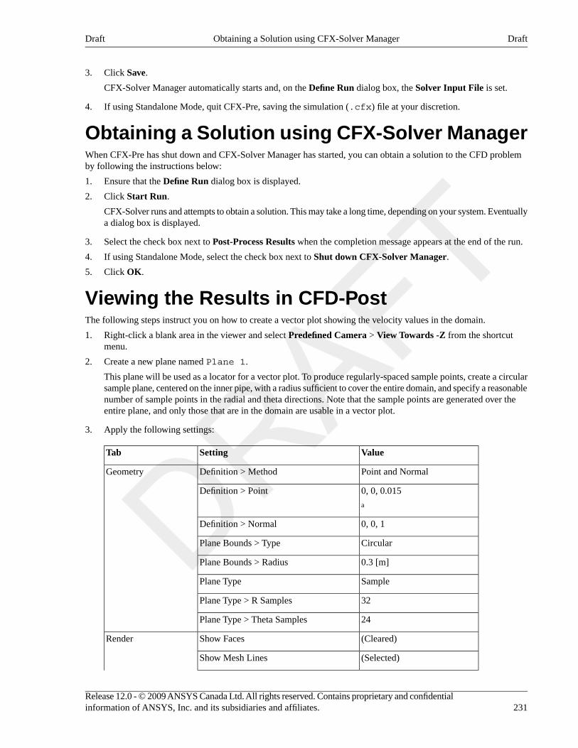
3. Click Save.
CFX-Solver Manager automatically starts and, on the Define Run dialog box, the Solver Input File is set.
4. If using Standalone Mode, quit CFX-Pre, saving the simulation (.cfx) file at your discretion.
Obtaining a Solution using CFX-Solver ManagerWhen CFX-Pre has shut down and CFX-Solver Manager has started, you can obtain a solution to the CFD problemby following the instructions below:
1. Ensure that the Define Run dialog box is displayed.
2. Click Start Run.
CFX-Solver runs and attempts to obtain a solution. This may take a long time, depending on your system. Eventuallya dialog box is displayed.
3. Select the check box next to Post-Process Results when the completion message appears at the end of the run.
4. If using Standalone Mode, select the check box next to Shut down CFX-Solver Manager.
5. Click OK.
Viewing the Results in CFD-PostThe following steps instruct you on how to create a vector plot showing the velocity values in the domain.
1. Right-click a blank area in the viewer and select Predefined Camera > View Towards -Z from the shortcutmenu.
2. Create a new plane named Plane 1.
This plane will be used as a locator for a vector plot. To produce regularly-spaced sample points, create a circularsample plane, centered on the inner pipe, with a radius sufficient to cover the entire domain, and specify a reasonablenumber of sample points in the radial and theta directions. Note that the sample points are generated over theentire plane, and only those that are in the domain are usable in a vector plot.
3. Apply the following settings:
ValueSettingTab
Point and NormalDefinition > MethodGeometry
0, 0, 0.015Definition > Point
a
0, 0, 1Definition > Normal
CircularPlane Bounds > Type
0.3 [m]Plane Bounds > Radius
SamplePlane Type
32Plane Type > R Samples
24Plane Type > Theta Samples
(Cleared)Show FacesRender
(Selected)Show Mesh Lines
231Release 12.0 - © 2009 ANSYS Canada Ltd. All rights reserved. Contains proprietary and confidentialinformation of ANSYS, Inc. and its subsidiaries and affiliates.
DraftObtaining a Solution using CFX-Solver ManagerDraft
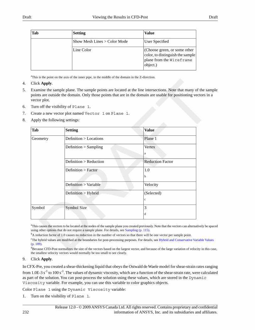
ValueSettingTab
User SpecifiedShow Mesh Lines > Color Mode
(Choose green, or some othercolor, to distinguish the sample
Line Color
plane from the Wireframeobject.)
aThis is the point on the axis of the inner pipe, in the middle of the domain in the Z-direction.
4. Click Apply.
5. Examine the sample plane. The sample points are located at the line intersections. Note that many of the samplepoints are outside the domain. Only those points that are in the domain are usable for positioning vectors in avector plot.
6. Turn off the visibility of Plane 1.
7. Create a new vector plot named Vector 1 on Plane 1.
8. Apply the following settings:
ValueSettingTab
Plane 1Definition > LocationsGeometry
VertexDefinition > Sampling
a
Reduction FactorDefinition > Reduction
1.0Definition > Factor
b
VelocityDefinition > Variable
(Selected)Definition > Hybrid
c
3Symbol SizeSymbol
d
aThis causes the vectors to be located at the nodes of the sample plane you created previously. Note that the vectors can alternatively be spacedusing other options that do not require a sample plane. For details, see Sampling (p. 115).bA reduction factor of 1.0 causes no reduction in the number of vectors so that there will be one vector per sample point.cThe hybrid values are modified at the boundaries for post-processing purposes. For details, see Hybrid and Conservative Variable Values(p. 189).dBecause CFD-Post normalizes the size of the vectors based on the largest vector, and because of the large variation of velocity in this case,the smallest velocity vectors would normally be too small to see clearly.
9. Click Apply.
In CFX-Pre, you created a shear-thickening liquid that obeys the Ostwald de Waele model for shear-strain rates ranging
from 1.0E-3 s-1 to 100 s-1. The values of dynamic viscosity, which are a function of the shear-strain rate, were calculatedas part of the solution. You can post-process the solution using these values, which are stored in the DynamicViscosity variable. For example, you can use this variable to color graphics objects.
Color Plane 1 using the Dynamic Viscosity variable:
1. Turn on the visibility of Plane 1.
Release 12.0 - © 2009 ANSYS Canada Ltd. All rights reserved. Contains proprietary and confidentialinformation of ANSYS, Inc. and its subsidiaries and affiliates.232
DraftViewing the Results in CFD-PostDraft
2. Edit Plane 1.
3. Apply the following settings:
ValueSettingTab
VariableModeColor
Dynamic ViscosityVariable
(Selected)Show FacesRender
4. Click Apply
Try plotting Shear Strain Rate on the same plane. Note that the distribution is somewhat different than that ofDynamic Viscosity, as a consequence of the non-linear relationship (see Figure 13.2, “Apparent Viscosity of aShear-thickening Fluid” (p. 224)).
When you have finished, quit CFD-Post.
233Release 12.0 - © 2009 ANSYS Canada Ltd. All rights reserved. Contains proprietary and confidentialinformation of ANSYS, Inc. and its subsidiaries and affiliates.
DraftViewing the Results in CFD-PostDraft

Release 12.0 - © 2009 ANSYS Canada Ltd. All rights reserved. Contains proprietary and confidentialinformation of ANSYS, Inc. and its subsidiaries and affiliates.
Chapter 14. Flow in an Axial Rotor/StatorThis tutorial includes:
• Tutorial Features (p. 235)
• Overview of the Problem to Solve (p. 236)
• Before You Begin (p. 238)
• Starting CFX-Pre (p. 238)
• Defining a Frozen Rotor Case in CFX-Pre (p. 239)
• Obtaining a Solution to the Frozen Rotor Model (p. 242)
• Viewing the Frozen Rotor Results in CFD-Post (p. 243)
• Setting up a Transient Rotor-Stator Calculation (p. 244)
• Obtaining a Solution to the Transient Rotor-Stator Model (p. 247)
• Viewing the Transient Rotor-Stator Results in CFD-Post (p. 248)
Tutorial FeaturesIn this tutorial you will learn about:
• Using the Turbo Wizard in CFX-Pre to quickly specify a turbomachinery application.
• Multiple Frames of Reference and Generalized Grid Interface.
• Using a Frozen Rotor interface between the rotor and stator domains.
• Modifying an existing simulation.
• Setting up a transient calculation.
• Using a Transient Rotor-Stator interface condition to replace a Frozen Rotor interface.
• Creating a transient animation showing domain movement in CFD-Post.
DetailsFeatureComponent
Turbo WizardUser ModeCFX-Pre
Steady StateAnalysis Type
Transient
Ideal GasFluid Type
Multiple DomainDomain Type
Rotating Frame of Reference
k-EpsilonTurbulence Model
Total EnergyHeat Transfer
Inlet (Subsonic)Boundary Conditions
Outlet (Subsonic)
Wall: No-Slip
Wall: Adiabatic
235Release 12.0 - © 2009 ANSYS Canada Ltd. All rights reserved. Contains proprietary and confidentialinformation of ANSYS, Inc. and its subsidiaries and affiliates.
DraftDraft
DetailsFeatureComponent
Frozen RotorDomain Interfaces
Periodic
Transient Rotor Stator
Physical Time ScaleTimestep
Transient Example
Transient Results File
RestartCFX-Solver Manager
Parallel Processing
AnimationPlotsCFD-Post
Isosurface
Surface Group
Turbo Post
Changing the Color RangeOther
Chart Creation
Instancing Transformation
MPEG Generation
Quantitative Calculation
Time Step Selection
Transient Animation
Overview of the Problem to SolveThe goal of this tutorial is to set up a transient calculation of the Rotor-Stator to then create an animation showing itsdomain movement.
The full geometry of the axial rotor/stator contains 60 stator blades and 113 rotor blades. The following figure showsapproximately half of the full geometry. The Inflow and Outflow labels show the location of the modeled section inFigure 14.1, “Geometry subsection” (p. 238).
Release 12.0 - © 2009 ANSYS Canada Ltd. All rights reserved. Contains proprietary and confidentialinformation of ANSYS, Inc. and its subsidiaries and affiliates.236
DraftOverview of the Problem to SolveDraft
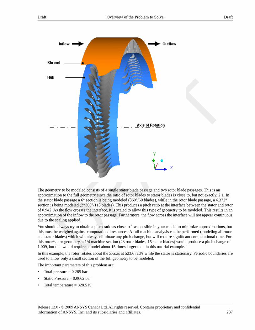
The geometry to be modeled consists of a single stator blade passage and two rotor blade passages. This is anapproximation to the full geometry since the ratio of rotor blades to stator blades is close to, but not exactly, 2:1. Inthe stator blade passage a 6° section is being modeled (360°/60 blades), while in the rotor blade passage, a 6.372°section is being modeled (2*360°/113 blades). This produces a pitch ratio at the interface between the stator and rotorof 0.942. As the flow crosses the interface, it is scaled to allow this type of geometry to be modeled. This results in anapproximation of the inflow to the rotor passage. Furthermore, the flow across the interface will not appear continuousdue to the scaling applied.
You should always try to obtain a pitch ratio as close to 1 as possible in your model to minimize approximations, butthis must be weighed against computational resources. A full machine analysis can be performed (modeling all rotorand stator blades) which will always eliminate any pitch change, but will require significant computational time. Forthis rotor/stator geometry, a 1/4 machine section (28 rotor blades, 15 stator blades) would produce a pitch change of1.009, but this would require a model about 15 times larger than in this tutorial example.
In this example, the rotor rotates about the Z-axis at 523.6 rad/s while the stator is stationary. Periodic boundaries areused to allow only a small section of the full geometry to be modeled.
The important parameters of this problem are:
• Total pressure = 0.265 bar
• Static Pressure = 0.0662 bar
• Total temperature = 328.5 K
237Release 12.0 - © 2009 ANSYS Canada Ltd. All rights reserved. Contains proprietary and confidentialinformation of ANSYS, Inc. and its subsidiaries and affiliates.
DraftOverview of the Problem to SolveDraft
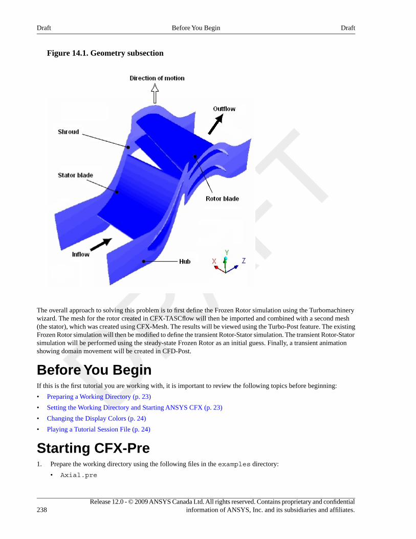
Figure 14.1. Geometry subsection
The overall approach to solving this problem is to first define the Frozen Rotor simulation using the Turbomachinerywizard. The mesh for the rotor created in CFX-TASCflow will then be imported and combined with a second mesh(the stator), which was created using CFX-Mesh. The results will be viewed using the Turbo-Post feature. The existingFrozen Rotor simulation will then be modified to define the transient Rotor-Stator simulation. The transient Rotor-Statorsimulation will be performed using the steady-state Frozen Rotor as an initial guess. Finally, a transient animationshowing domain movement will be created in CFD-Post.
Before You BeginIf this is the first tutorial you are working with, it is important to review the following topics before beginning:
• Preparing a Working Directory (p. 23)
• Setting the Working Directory and Starting ANSYS CFX (p. 23)
• Changing the Display Colors (p. 24)
• Playing a Tutorial Session File (p. 24)
Starting CFX-Pre1. Prepare the working directory using the following files in the examples directory:
• Axial.pre
Release 12.0 - © 2009 ANSYS Canada Ltd. All rights reserved. Contains proprietary and confidentialinformation of ANSYS, Inc. and its subsidiaries and affiliates.238
DraftBefore You BeginDraft
• AxialIni.pre
• AxialIni_001.res
• rotor.grd
• stator.gtm
For details, see Preparing a Working Directory (p. 23)
2. Set the working directory and start CFX-Pre
For details, see Setting the Working Directory and Starting ANSYS CFX (p. 23)
Defining a Frozen Rotor Case in CFX-PreIf you want to set up the simulation automatically using a tutorial session file, run AxialIni.pre. For details, seePlaying a Tutorial Session File (p. 24). Then proceed to Obtaining a Solution to the Frozen Rotor Model (p. 242).
Otherwise, this simulation will be set up manually using the Turbomachinery wizard in CFX-Pre. This pre-processingmode is designed to simplify the setup of turbomachinery simulations.
1. Select File > New Case.
2. Select Turbomachinery and click OK.
3. Select File > Save Case As.
4. Under File name, type AxialIni.
5. Click Save.
Basic Settings1. Set Machine Type to Axial Turbine.
2. Click Next.
Component DefinitionTwo new components are required. As they are created, meshes are imported.
1. Right-click in the blank area and select Add Component from the shortcut menu.
2. Create a new component of type Stationary, named S1.
3. Apply the following setting
ValueSetting
stator.gtmaMesh > File
aYou may have to select the CFX Mesh (*gtm *cfx) option under Files of type.
4. Create a new component of type Rotating, named R1.
5. Apply the following settings
ValueSetting
523.6 [radian s^-1]Component Type > Value
rotor.grdaMesh File > File
239Release 12.0 - © 2009 ANSYS Canada Ltd. All rights reserved. Contains proprietary and confidentialinformation of ANSYS, Inc. and its subsidiaries and affiliates.
DraftDefining a Frozen Rotor Case in CFX-PreDraft
ValueSetting
mOptions > Mesh Units
aYou may have to select the CFX-TASCflow (*grd) option under File Type.
NoteThe components must be ordered as above (stator then rotor) in order for the interface to be createdcorrectly. The order of the two components can be changed by right-clicking on S1 and selectingMove Component Up.
When a component is defined, Turbo Mode will automatically select a list of regions that correspond to certainboundary types. This information should be reviewed in the Region Information section to ensure that all iscorrect. This information will be used to help set up boundary conditions and interfaces. The upper case turboregions that are selected (e.g., HUB) correspond to the region names in the CFX-TASCflow grd file. CFX-TASCflowturbomachinery meshes use these names consistently.
6. Click Next.
Physics DefinitionIn this section, you will set properties of the fluid domain and some solver parameters.
1. Apply the following settings
ValueSettingTab
Air Ideal GasFluidPhysicsDefinition
Steady StateAnalysis Type > Type
0.25 [atm]Model Data > Reference Pressure
Total EnergyModel Data > Heat Transfer
k-EpsilonModel Data > Turbulence
(Selected)Inflow/Outflow Boundary Templates > P-Total Inlet MassFlow Outlet
0 [atm]Inflow/Outflow Boundary Templates > P-Total
340 [K]Inflow/Outflow Boundary Templates > T-Total
Per ComponentInflow/Outflow Boundary Templates > Mass Flow
0.06 [kg s^-1]Inflow/Outflow Boundary Templates > Mass Flow Rate
Normal to BoundaryInflow/Outflow Boundary Templates > Flow Direction
Frozen RotorInterface > Default Type
High ResolutionSolver Parameters > Advection Scheme
Physical TimescaleSolver Parameters > Convergence Control
Release 12.0 - © 2009 ANSYS Canada Ltd. All rights reserved. Contains proprietary and confidentialinformation of ANSYS, Inc. and its subsidiaries and affiliates.240
DraftPhysics DefinitionDraft
ValueSettingTab
0.002 [s]aSolver Parameters > Physical Timescale
aThis time scale is approximately equal to 1 / ω, which is often appropriate for rotating machinery applications.
2. Click Next.
Interface DefinitionCFX-Pre will try to create appropriate interfaces using the region names presented previously in the Region Informationsection. In this case, you should see that a periodic interface has been generated for both the rotor and the stator. Theseare required when modeling a small section of the true geometry. An interface is also required to connect the twocomponents together across the frame change.
1. Review the various interfaces but do not change them.
2. Click Next.
Boundary DefinitionCFX-Pre will try to create appropriate boundary conditions using the region names presented previously in the RegionInformation section. In this case, you should see a list of boundary conditions that have been generated. They can beedited or deleted in the same way as the interface connections that were set up earlier.
1. Review the various boundary definitions but do not change them.
2. Click Next.
Final Operations1. Set Operation to Enter General Mode.
2. Click Finish.
After you click Finish, a dialog box appears stating that the Turbo report will not be included in the solver filebecause you are entering General Mode.
3. Click Yes to continue.
Writing the CFX-Solver Input (.def) File
1. Click Define Run .
2. Apply the following settings:
ValueSetting
AxialIni.defFile name
3. Click Save.
CFX-Solver Manager automatically starts and, on the Define Run dialog box, the Solver Input File is set.
4. If using Standalone Mode, quit CFX-Pre, saving the simulation (.cfx) file at your discretion.
241Release 12.0 - © 2009 ANSYS Canada Ltd. All rights reserved. Contains proprietary and confidentialinformation of ANSYS, Inc. and its subsidiaries and affiliates.
DraftInterface DefinitionDraft
Obtaining a Solution to the Frozen Rotor ModelCompared to previous tutorials, the mesh for this tutorial contains many more nodes (although it is still too coarse toperform a high quality CFD simulation). This results in a corresponding increase in solution time for the problem.Solving this problem in parallel is recommended, if possible. Your machine should have a minimum of 256MB ofmemory to run this tutorial.
More detailed information about setting up CFX to run in parallel is available. For details, see Flow Around a BluntBody (p. 131).
You can solve this example using Serial, Local Parallel or Distributed Parallel.
• Obtaining a Solution in Serial (p. 242)
• Obtaining a Solution With Local Parallel (p. 242)
• Obtaining a Solution with Distributed Parallel (p. 242)
Obtaining a Solution in SerialIf you do not have a license to run CFX in parallel you can run in serial by clicking the Start Run button whenCFX-Solver Manager has opened up. Solution time in serial is approximately 45 minutes on a 1GHz processor.
1. Click Start Run on the Define Run dialog box.
CFX-Solver runs and attempts to obtain a solution. This may take a long time, depending on your system. Eventuallya dialog box is displayed.
2. Select the check box next to Post-Process Results when the completion message appears at the end of the run.
3. If using Standalone Mode, select the check box next to Shut down CFX-Solver Manager.
4. Click OK.
When you are finished, proceed to Viewing the Frozen Rotor Results in CFD-Post (p. 243).
Obtaining a Solution With Local ParallelTo run in local parallel, the machine you are on must have more than one processor.
1. Set Run Mode to a parallel mode suitable for your environment; for example, HP MPI Local Parallel.
2. If required, click Add Partition to add more partitions.
By default, 2 partitions are assigned.
3. Click Start Run.
4. Select the check box next to Post-Process Results when the completion message appears at the end of the run.
5. If using Standalone Mode, select the check box next to Shut down CFX-Solver Manager.
6. Click OK.
When you are finished, proceed to Viewing the Frozen Rotor Results in CFD-Post (p. 243).
Obtaining a Solution with Distributed Parallel1. Set Run Mode to a parallel mode suitable for your environment; for example, HP MPI Distributed
Parallel.
One partition should already be assigned to the host that you are logged into.
2. Click Insert Host to specify a new parallel host.
Release 12.0 - © 2009 ANSYS Canada Ltd. All rights reserved. Contains proprietary and confidentialinformation of ANSYS, Inc. and its subsidiaries and affiliates.242
DraftObtaining a Solution to the Frozen Rotor ModelDraft
3. In Select Parallel Hosts, select another host name (this should be a machine that you can log into using the sameuser name).
4. Click Add, and then Close.
The names of the two selected machines should be listed in the Host Name column of the Define Run dialogbox.
5. Click Start Run.
6. Select the check box next to Post-Process Results when the completion message appears at the end of the run.
7. If using Standalone Mode, select the check box next to Shut down CFX-Solver Manager.
8. Click OK.
Viewing the Frozen Rotor Results in CFD-PostThe Turbo-Post feature will be demonstrated in the following sections. This feature is designed to greatly reduce theeffort taken to post-process turbomachinery simulations.Turbo Workspace (p. 213)
Initializing Turbo-PostWhen initializing turbo components, span, a (axial) and r (radial) and Theta coordinates are generated for eachcomponent. Therefore, after entering the Turbo workspace and initializing the turbo components, you will be ready tostart using the turbo-specific features offered in the Turbo workspace immediately. These features include Turbo TreeView, Turbo Surface, Turbo Line and Turbo Plots. For details see Turbo Workspace (p. 213)
To initialize Turbo-Post, the properties of each component must be entered. This includes entering information aboutthe inlet, outlet, hub, shroud, blade and periodic regions. Specification of the number of instances of each turbocomponent (e.g., stator, rotor, etc.) needed to represent the full geometry around the rotation axis is also required.
1. Click the Turbo tab.
The Turbo Initialization dialog box is displayed, and asks you whether you want to auto-initialize all components.
NoteIf you do not see the Turbo Initialization dialog box, or as an alternative to using that dialog box,you can initialize all components by clicking the Initialize All Components button which is visibleinitially by default, or after double-clicking the Initialization object in the Turbo tree view.
2. Click Yes.
The Turbo tree view shows the two components in domains R1 and S1. In this case, the initialization workswithout problems. If there was a problem initializing a component, this would be indicated in the tree view.
Viewing Three Domain PassagesNext, you will create an instancing transformation to plot three domain passages; three blade passages for the statorand six blade passages for the rotor. It was chosen to create three times the geometry that was used in the simulationto help visualize the variation of pressure. Seeing neighboring passages will give a better understanding of the pressurevariation through the axial rotor/stator.
The instancing properties of each domain have already been entered during Initialization. In the next steps, you willcreate a surface group plot to color the blade and hub surfaces with the same variable.
1. From the main menu, select Insert > Location > Surface Group.
2. Click OK.
The default name is accepted.
243Release 12.0 - © 2009 ANSYS Canada Ltd. All rights reserved. Contains proprietary and confidentialinformation of ANSYS, Inc. and its subsidiaries and affiliates.
DraftViewing the Frozen Rotor Results in CFD-PostDraft
3. Apply the following settings
ValueSettingTab
R1 Blade, R1 Hub, S1 Blade, S1 HubLocationsGeometry
VariableModeColor
PressureVariable
4. Click Apply.
5. Click the Turbo tab.
6. Open Plots > 3D View for editing.
7. Apply the following settings
ValueSettingTab
R1Instancing > Domain3D View
3Instancing > # of Copies
8. Click Apply.
9. Apply the following settings
ValueSettingTab
S1Instancing > Domain3D View
3Instancing > # of Copies
10. Click Apply.
Blade Loading Turbo ChartIn this section, you will create a plot of pressure around the stator blade at a given spanwise location.
• In the Turbo tree view, double-click Blade Loading.
This profile of the pressure curve is typical for turbomachinery applications.
When you are finished viewing the chart, quit CFD-Post.
Setting up a Transient Rotor-Stator CalculationThis section describes the step-by-step definition of the flow physics in CFX-Pre. The existing steady-state frozen-rotorsimulation is modified to define the transient rotor-stator simulation. If you have not already completed the frozen-rotorsimulation, please refer to Defining a Frozen Rotor Case in CFX-Pre (p. 239) before proceeding with the transientrotor-stator simulation.
Playing a Session FileIf you want to set up the simulation automatically and continue to Obtaining a Solution to the Transient Rotor-StatorModel (p. 247), run Axial.pre.
Release 12.0 - © 2009 ANSYS Canada Ltd. All rights reserved. Contains proprietary and confidentialinformation of ANSYS, Inc. and its subsidiaries and affiliates.244
DraftBlade Loading Turbo ChartDraft
NoteThe session file creates a new simulation named Axial.cfx and will not modify the existing database.It also copies the required initial values file from the examples directory to the current working directory.
Opening the Existing CaseThis step involves opening the original simulation and saving it to a different location.
1. Start CFX-Pre.
2. Open the results file named AxialIni_001.res.
3. Save the case as Axial.cfx in your working directory.
Modifying the Physics DefinitionYou need to modify the domain to define a transient simulation. You are going to run for a time interval such that therotor blades pass through 1 pitch (6.372°) using 10 time steps. This is generally too few time steps to obtain high qualityresults, but is sufficient for tutorial purposes. The time step size is calculated as follows:
Note
== ⋅ ≈
≈ ≈ −π
Rotational Speed 523.6 rad/sRotor Pitch Modeled 2 ( 2 rad/113) 0.1112 radTime to pass through 1 pitch ( 0.1112 rad) / ( 523.6 rad/s ) 2.124 e 4 s
Since 10 time steps are used over this interval each time step should be 2.124e-5 s.
1. Select Tools > Turbo Mode.
Basic Settings is displayed.
2. Click Next.
Component Definition is displayed.
3. Click Next.
Physics Definition is displayed.
4. Apply the following settings
ValueSettingTab
Air Ideal GasFluidPhysicsDefinition
TransientAnalysis Type > Type
2.124e-4 [s]aAnalysis Type > Total Time
2.124e-5 [s]bAnalysis Type > Time Steps
Transient Rotor StatorInterface > Default Type
aThis gives 10 timesteps of 2.124e-5 sbThis timestep will be used until the total time is reached
245Release 12.0 - © 2009 ANSYS Canada Ltd. All rights reserved. Contains proprietary and confidentialinformation of ANSYS, Inc. and its subsidiaries and affiliates.
DraftOpening the Existing CaseDraft
NoteA transient rotor-stator calculation often runs through more than one pitch. In these cases, it may beuseful to look at variable data averaged over the time interval required to complete 1 pitch. You canthen compare data for each pitch rotation to see if a “steady state” has been achieved, or if the flow isstill developing.
5. Click Next.
A warning message is displayed.
6. Click Yes.
Interface Definition is displayed.
7. Click Next.
Boundary Definition is displayed.
8. Click Next.
Final Operations is displayed.
9. Ensure that Operation is set to Enter General Mode.
10. Click Finish.
A message box notifies you that a turbo report will not be included in the solver file.
11. Click Yes to continue.
Initial values are required, but will be supplied later using a results file.
Setting Output Control1. Click Output Control .
2. Click the Trn Results tab.
3. In the Transient Results tree view, click Add new item , set Name to Transient Results 1, and click
OK.
4. Apply the following settings
Selected VariablesOption
Pressure, Velocity, Velocity inStn Frame
Output Variables Lista
Time IntervalOutput Frequency > Option
2.124e-5 [s]Output Frequency > Time Interval
aUse the Ctrl key to select more than one variable.
5. Click OK.
Modifying Execution Control1. Click Execution Control .
2. Apply the following settings
Release 12.0 - © 2009 ANSYS Canada Ltd. All rights reserved. Contains proprietary and confidentialinformation of ANSYS, Inc. and its subsidiaries and affiliates.246
DraftSetting Output ControlDraft
ValueSettingTab
Axial.defaSolver Input FileRun Definition
aYou do not need to set the path unless you are planning on saving the solver file somewhere other than the working directory.
3. Confirm that the rest of the execution control settings are set appropriately.
4. Click OK.
Writing the CFX-Solver Input (.def) File
1. Click Define Run .
A warning will appear, due to a lack of initial values.
Initial values are required, but will be supplied later using a results file.
2. Click Yes.
3. If using Standalone Mode, quit CFX-Pre, saving the simulation (.cfx) file at your discretion.
Obtaining a Solution to the TransientRotor-Stator ModelWhen the CFX-Solver Manager has started you will need to specify an initial values file before starting the CFX-Solver.
Serial SolutionIf you do not have a license, or do not want to run CFX in parallel, you can run it in serial. Solution time in serial issimilar to the first part of this tutorial.
1. Select Run Definition > Initial Values Specification.
2. Under Initial Values Specification > Initial Values, select Initial Values 1.
3. Under Initial Values Specification > Initial Values > Initial Values 1 Settings > File Name, click Browse .
4. Select AxialIni_001.res from your working directory.
5. Click Open.
6. Under Initial Values Specification > Use Mesh From, select Solver Input File.
7. Click Start Run.
CFX-Solver runs and attempts to obtain a solution. This can take a long time depending on your system. Eventuallya dialog box is displayed.
8. When CFX-Solver is finished, select the check box next to Post-Process Results.
9. If using Standalone Mode, select the check box next to Shut down CFX-Solver Manager.
10. Click OK. Continue this tutorial from Monitoring the Run (p. 248).
Parallel SolutionYou can solve this example using either local parallel or distributed parallel, in the same way as in the first part of thistutorial. For details, see Obtaining a Solution to the Frozen Rotor Model (p. 242).
247Release 12.0 - © 2009 ANSYS Canada Ltd. All rights reserved. Contains proprietary and confidentialinformation of ANSYS, Inc. and its subsidiaries and affiliates.
DraftWriting the CFX-Solver Input (.def) FileDraft
Monitoring the RunDuring the solution, look for the additional information that is provided for transient rotor-stator runs. Each time therotor is rotated to its next position, the number of degrees of rotation and the fraction of a pitch moved is given. Youshould see that after 10 timesteps the rotor has been moved through 1 pitch.
Viewing the Transient Rotor-Stator Results inCFD-PostTo examine the transient interaction between the rotor and stator, you are going to create a blade-to-blade animationof pressure. A turbo surface will be used as the basis for this plot.
Initializing Turbo-PostAll the pre processing will be done during the initialization of the turbo components. Only few steps will therefore berequired to display a surface of constant span and create a turbo surface later on in this tutorial.
1. Click the Turbo tab.
The Turbo Initialization dialog box is displayed, and asks you whether you want to auto-initialize all components.
NoteIf you do not see the Turbo Initialization dialog box, or as an alternative to using that dialog box,you can initialize all components by clicking the Initialize All Components button which is visibleinitially by default, or after double-clicking the Initialization object in the Turbo tree view.
2. Click Yes.
Both components (domains) are now being initialized based on the automatically selected turbo regions. Whenthe process is complete, a green turbine icon appears next to each component entry in the list. Also, the viewerdisplays a green background mesh for each initialized component.
3. Double-click Component 1 (S1) and review the automatically-selected turbo regions.
Displaying a Surface of Constant Span• In the Turbo tree view, double-click Blade-to-Blade.
A surface of constant span appears, colored by pressure. This object can be edited and then redisplayed using thedetails view.
Using Multiple Turbo Viewports1. In the Turbo tree view, double-click Initialization.
2. Click Three Views.
Left view is 3D View, top right is Blade-to-Blade and bottom right is Meridional view.
3. Click Single View.
Creating a Turbo Surface at Mid-Span1. Create a Turbo Surface by selecting Insert > Location > Turbo Surface from the drop down menu with a
Constant Span and value of 0.5.
Release 12.0 - © 2009 ANSYS Canada Ltd. All rights reserved. Contains proprietary and confidentialinformation of ANSYS, Inc. and its subsidiaries and affiliates.248
DraftMonitoring the RunDraft
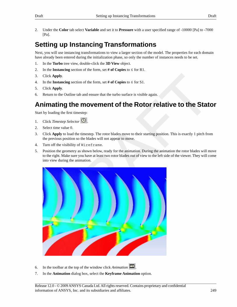
2. Under the Color tab select Variable and set it to Pressure with a user specified range of -10000 [Pa] to -7000[Pa].
Setting up Instancing TransformationsNext, you will use instancing transformations to view a larger section of the model. The properties for each domainhave already been entered during the initialization phase, so only the number of instances needs to be set.
1. In the Turbo tree view, double-click the 3D View object.
2. In the Instancing section of the form, set # of Copies to 6 for R1.
3. Click Apply.
4. In the Instancing section of the form, set # of Copies to 6 for S1.
5. Click Apply.
6. Return to the Outline tab and ensure that the turbo surface is visible again.
Animating the movement of the Rotor relative to the StatorStart by loading the first timestep:
1. Click Timestep Selector .
2. Select time value 0.
3. Click Apply to load the timestep. The rotor blades move to their starting position. This is exactly 1 pitch fromthe previous position so the blades will not appear to move.
4. Turn off the visibility of Wireframe.
5. Position the geometry as shown below, ready for the animation. During the animation the rotor blades will moveto the right. Make sure you have at least two rotor blades out of view to the left side of the viewer. They will comeinto view during the animation.
6. In the toolbar at the top of the window click Animation .
7. In the Animation dialog box, select the Keyframe Animation option.
249Release 12.0 - © 2009 ANSYS Canada Ltd. All rights reserved. Contains proprietary and confidentialinformation of ANSYS, Inc. and its subsidiaries and affiliates.
DraftSetting up Instancing TransformationsDraft
8. Click New to create KeyFrameNo1.
9. Select KeyframeNo1, then set # of Frames to 9, then press Enter while in the # of Frames box.
TipBe sure to press Enter and confirm that the new number appears in the list before continuing.
10. Use the Timestep Selector to load the final timestep.
11. In the Animation dialog box, click New to create KeyframeNo2.
12. Click More Animation Options to expand the Animation dialog box.
13. Click Options and set Transient Case to TimeValue Interpolation. Click OK.
The animation now contains a total of 11 frames (9 intermediate frames plus the two Keyframes), one for eachof the available time values.
14. In the expanded Animation dialog box, select Save Movie.
15. Set Format to MPEG1.
16. Click Browse , next to the Save Movie box and then set the file name to an appropriate file name.
17. If frame 1 is not loaded (shown in the F: text box at the bottom of the Animation dialog box), click To Beginning to load it.
Wait for CFD-Post to finish loading the objects for this frame before proceeding.
18. Click Play the animation .
• It takes a while for the animation to complete.
• To view the movie file, you will need to use a media player that supports the MPEG format.
You will be able to see from the animation, and from the plots created previously, that the flow is not continuousacross the interface. This is because a pitch change occurs. The relatively coarse mesh and the small number oftimesteps used in the transient simulation also contribute to this. The movie was created with a narrow pressurerange compared to the global range which exaggerates the differences across the interface.
Further PostprocessingYou can use the Turbo Calculator to produce a report on the performance of the turbine.
1. Edit the Gas Turbine Performance macro in the Turbo tree view.
2. Set Ref Radius to 0.4575 and leave other settings at their default values.
3. Click Calculate.
4. Click View Report.
Release 12.0 - © 2009 ANSYS Canada Ltd. All rights reserved. Contains proprietary and confidentialinformation of ANSYS, Inc. and its subsidiaries and affiliates.250
DraftFurther PostprocessingDraft
Chapter 15. Reacting Flow in a MixingTubeThis tutorial includes:
• Tutorial Features (p. 251)
• Overview of the Problem to Solve (p. 252)
• Modeling Approach (p. 254)
• Before You Begin (p. 254)
• Starting CFX-Pre (p. 254)
• Defining a Case in CFX-Pre (p. 255)
• Obtaining a Solution using CFX-Solver Manager (p. 271)
• Viewing the Results in CFD-Post (p. 271)
Tutorial FeaturesIn this tutorial you will learn about:
• Creating and using a multicomponent fluid in CFX-Pre.
• Using CEL to model a reaction in CFX-Pre.
• Using an algebraic Additional Variable to model a scalar distribution.
• Using a subdomain as the basis for component sources.
DetailsFeatureComponent
General ModeUser ModeCFX-Pre
Steady StateAnalysis Type
Variable Composition MixtureFluid Type
Single DomainDomain Type
k-EpsilonTurbulence Model
Thermal EnergyHeat Transfer
Component SourceParticle Tracking
Inlet (Subsonic)Boundary Conditions
Outlet (Subsonic)
Symmetry Plane
Wall: Adiabatic
Additional Variables
CEL (CFX Expression Language)
Physical Time ScaleTimestep
251Release 12.0 - © 2009 ANSYS Canada Ltd. All rights reserved. Contains proprietary and confidentialinformation of ANSYS, Inc. and its subsidiaries and affiliates.
DraftDraft
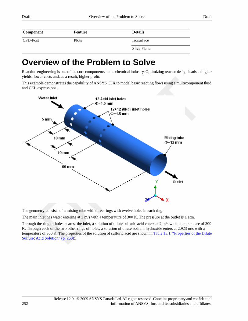
DetailsFeatureComponent
IsosurfacePlotsCFD-Post
Slice Plane
Overview of the Problem to SolveReaction engineering is one of the core components in the chemical industry. Optimizing reactor design leads to higheryields, lower costs and, as a result, higher profit.
This example demonstrates the capability of ANSYS CFX to model basic reacting flows using a multicomponent fluidand CEL expressions.
The geometry consists of a mixing tube with three rings with twelve holes in each ring.
The main inlet has water entering at 2 m/s with a temperature of 300 K. The pressure at the outlet is 1 atm.
Through the ring of holes nearest the inlet, a solution of dilute sulfuric acid enters at 2 m/s with a temperature of 300K. Through each of the two other rings of holes, a solution of dilute sodium hydroxide enters at 2.923 m/s with atemperature of 300 K. The properties of the solution of sulfuric acid are shown in Table 15.1, “Properties of the DiluteSulfuric Acid Solution” (p. 253):.
Release 12.0 - © 2009 ANSYS Canada Ltd. All rights reserved. Contains proprietary and confidentialinformation of ANSYS, Inc. and its subsidiaries and affiliates.252
DraftOverview of the Problem to SolveDraft
Table 15.1. Properties of the Dilute Sulfuric Acid Solution
ValueProperty
19.517 kg kmol^-1Molar mass
1078 kg m^-3Density
4190 J kg^-1 K^-1Specific heat capacity
0.001 kg m^-1 s^-1Dynamic Viscosity
0.6 W m^-1 K^-1Thermal Conductivity
Through the remaining two rings of holes, a solution of dilute sodium hydroxide (an alkali) enters with a temperatureof 300K. The properties of the solution of sodium hydroxide are shown in Table 15.2, “Properties of the Dilute SodiumHydroxide Solution” (p. 253).
Table 15.2. Properties of the Dilute Sodium Hydroxide Solution
ValueProperty
18.292 kg kmol^-1Molar mass
1029 kg m^-3Density
4190 J kg^-1 K^-1Specific heat capacity
0.001 kg m^-1 s^-1Dynamic Viscosity
0.6 W m^-1 K^-1Thermal Conductivity
The acid and alkali undergo an exothermic reaction to form a solution of sodium sulfate (a type of salt) and wateraccording to the reaction:
+ → +H SO 2NaOH Na SO 2H O2 4 2 4 2
Mixing the acid and alkali solutions in a stoichiometric ratio (and allowing them to react completely) would result ina salt water solution that would include water from each of the original solutions plus water produced during thereaction. The properties of this salt water product are shown in Table 15.3, “Properties of the Salt Water Product” (p. 253).
Table 15.3. Properties of the Salt Water Product
ValueSetting
18.600 kg kmol^-1Molar mass
1031 kg m^-3Density
4190 J kg^-1 K^-1Specific heat capacity
0.001 kg m^-1 s^-1Dynamic Viscosity
0.6 W m^-1 K^-1Thermal Conductivity
The heat of reaction is 460 kJ per kg of dilute acid solution.
253Release 12.0 - © 2009 ANSYS Canada Ltd. All rights reserved. Contains proprietary and confidentialinformation of ANSYS, Inc. and its subsidiaries and affiliates.
DraftOverview of the Problem to SolveDraft
The flow is assumed to be fully turbulent and turbulence is assumed to have a significant effect on the reaction rate.
After running the simulation, you will plot the distribution of pH in the tube, and determine the extent to which thepH is neutralized at the outlet. You will also plot mass fraction distributions of acid, alkali and product.
Modeling ApproachIn order to reduce memory requirements and solution time, only a 30° slice of the geometry will be modeled, andsymmetry boundary conditions will be applied to represent the remaining geometry.
The reaction between acid and alkali is represented as a single-step irreversible liquid-phase reaction:
+ →A B C
Reagent A (dilute sulfuric acid) is injected through a ring of holes near the start of the tube. As it flows along the tubeit reacts with Reagent B (dilute sodium hydroxide) which is injected through a further two rings of holes downstream.The product, C, remains in solution.
You will create a variable-composition mixture1 that contains water, the reactants, and the product. To model thereaction, you will use CEL expressions to govern the mass sources for the acid, alkali and product components. Youwill also use CEL expressions to govern the thermal energy source. Providing mass and energy sources over a volumerequires a subdomain. Because the reaction may occur anywhere in the domain, you will create a subdomain thatoccupies the entire flow domain.
To model the pH, you will create an algebraic Additional Variable that is governed by a CEL expression for pH. TheAdditional Variable will be available in the solution results for analysis during post-processing.
Before You BeginIf this is the first tutorial you are working with, it is important to review the following topics before beginning:
• Preparing a Working Directory (p. 23)
• Setting the Working Directory and Starting ANSYS CFX (p. 23)
• Changing the Display Colors (p. 24)
• Playing a Tutorial Session File (p. 24)
Starting CFX-Pre1. Prepare the working directory using the following files in the examples directory:
• Reactor.pre
• ReactorExpressions.ccl
• ReactorMesh.gtm
For details, see Preparing a Working Directory (p. 23)
2. Set the working directory and start CFX-Pre
For details, see Setting the Working Directory and Starting ANSYS CFX (p. 23)
1You can also model this type of reaction using a reacting mixture as your fluid. There is a tutorial that uses a reacting mixture: Combustion andRadiation in a Can Combustor (p. 343).
Release 12.0 - © 2009 ANSYS Canada Ltd. All rights reserved. Contains proprietary and confidentialinformation of ANSYS, Inc. and its subsidiaries and affiliates.254
DraftModeling ApproachDraft
Defining a Case in CFX-PreIf you want to set up the simulation automatically using a tutorial session file, run Reactor.pre. For details, seePlaying a Tutorial Session File (p. 24). Then proceed to Obtaining a Solution using CFX-Solver Manager (p. 271).
If you want to set up the simulation manually, proceed to the following steps:
1. Select File > New Case.
2. Select General and click OK.
3. Select File > Save Case As.
4. Under File name, type Reactor.
5. Click Save.
Importing the Mesh1. Right-click Mesh and select Import Mesh > CFX Mesh.
The Import Mesh dialog box appears.
2. Apply the following settings:
ValueSetting
ReactorMesh.gtmFile name
3. Click Open.
Creating a Multicomponent FluidIn addition to providing template fluids, CFX allows you to create custom fluids for use in all your CFX models. Acustom fluid may be defined as a pure substance, but may also be defined as a mixture, consisting of a number oftransported fluid components. This type of fluid model is useful for applications involving mixtures, reactions, andcombustion.
In order to define custom fluids, CFX-Pre provides the Material details view. This tool allows you to define your ownfluids as pure substances, fixed composition mixtures or variable composition mixtures using a range of templateproperty sets defined for common materials.
The mixing tube application requires a fluid made up from four separate materials (or components). The componentsare the reactants and products of a simple chemical reaction together with a neutral carrier liquid. You are first goingto define the materials that take part in the reaction (acid, alkali and product) as pure substances. The neutral carrierliquid is water, and is already defined. Finally, you will create a variable composition mixture consisting of these fourmaterials. This is the fluid that you will use in your simulation. A variable composition mixture (as opposed to a fixedcomposition mixture) is required because the proportion of each component will change throughout the simulationdue to the reaction.
Acid PropertiesThe properties of the dilute sulfuric acid solution were stated in the problem description.
1. Create a new material named acid.
2. Apply the following settings:
ValueSettingTab
Pure SubstanceOptionBasic Settings
255Release 12.0 - © 2009 ANSYS Canada Ltd. All rights reserved. Contains proprietary and confidentialinformation of ANSYS, Inc. and its subsidiaries and affiliates.
DraftDefining a Case in CFX-PreDraft
ValueSettingTab
(Selected)Thermodynamic State
LiquidThermodynamic State > Thermodynamic State
General MaterialOptionMaterial Properties
ValueThermodynamic Properties > Equation of State >Option
19.517 [kg kmol^-1]aThermodynamic Properties > Equation of State >Molar Mass
1078 [kg m^-3]Thermodynamic Properties > Equation of State >Density
(Selected)Thermodynamic Properties > Specific HeatCapacity
ValueThermodynamic Properties > Specific HeatCapacity > Option
4190 [J kg^-1 K^-1]Thermodynamic Properties > Specific HeatCapacity > Specific Heat Capacity
(Selected)Transport Properties > Dynamic Viscosity
ValueTransport Properties > Dynamic Viscosity > Option
0.001 [kg m^-1 s^-1]Transport Properties > Dynamic Viscosity >Dynamic Viscosity
(Selected)Transport Properties > Thermal Conductivity
ValueTransport Properties > Thermal Conductivity >Option
0.6 [W m^-1 K^-1]Transport Properties > Thermal Conductivity >Thermal Conductivity
aThe Molar Masses for the three materials do not affect the solution except through the post-processed variables Molar Concentration andMolar Fraction.
3. Click OK.
Alkali PropertiesThe properties of the dilute sodium hydroxide solution were stated in the problem description.
1. Create a new material named alkali.
2. Apply the following settings:
ValueSettingTab
Pure SubstanceOptionBasic Settings
(Selected)Thermodynamic State
LiquidThermodynamic State > Thermodynamic State
Release 12.0 - © 2009 ANSYS Canada Ltd. All rights reserved. Contains proprietary and confidentialinformation of ANSYS, Inc. and its subsidiaries and affiliates.256
DraftCreating a Multicomponent FluidDraft
ValueSettingTab
General MaterialOptionMaterial Properties
ValueThermodynamic Properties > Equation of State >Option
18.292 [kg kmol^-1]Thermodynamic Properties > Equation of State >Molar Mass
1029 [kg m^-3]Thermodynamic Properties > Equation of State >Density
(Selected)Thermodynamic Properties > Specific HeatCapacity
ValueThermodynamic Properties > Specific HeatCapacity > Option
4190 [J kg^-1 K^-1]Thermodynamic Properties > Specific HeatCapacity > Specific Heat Capacity
(Selected)Transport Properties > Dynamic Viscosity
ValueTransport Properties > Dynamic Viscosity > Option
0.001 [kg m^-1 s^-1]Transport Properties > Dynamic Viscosity >Dynamic Viscosity
(Selected)Transport Properties > Thermal Conductivity
ValueTransport Properties > Thermal Conductivity >Option
0.6 [W m^-1 K^-1]Transport Properties > Thermal Conductivity >Thermal Conductivity
3. Click OK.
Reaction Product PropertiesThe properties of the salt water product were stated in the problem description.
1. Create a new material named product.
2. Apply the following settings:
ValueSettingTab
Pure SubstanceOptionBasic Settings
(Selected)Thermodynamic State
LiquidThermodynamic State > Thermodynamic State
General MaterialOptionMaterial Properties
ValueThermodynamic Properties > Equation of State >Option
257Release 12.0 - © 2009 ANSYS Canada Ltd. All rights reserved. Contains proprietary and confidentialinformation of ANSYS, Inc. and its subsidiaries and affiliates.
DraftCreating a Multicomponent FluidDraft
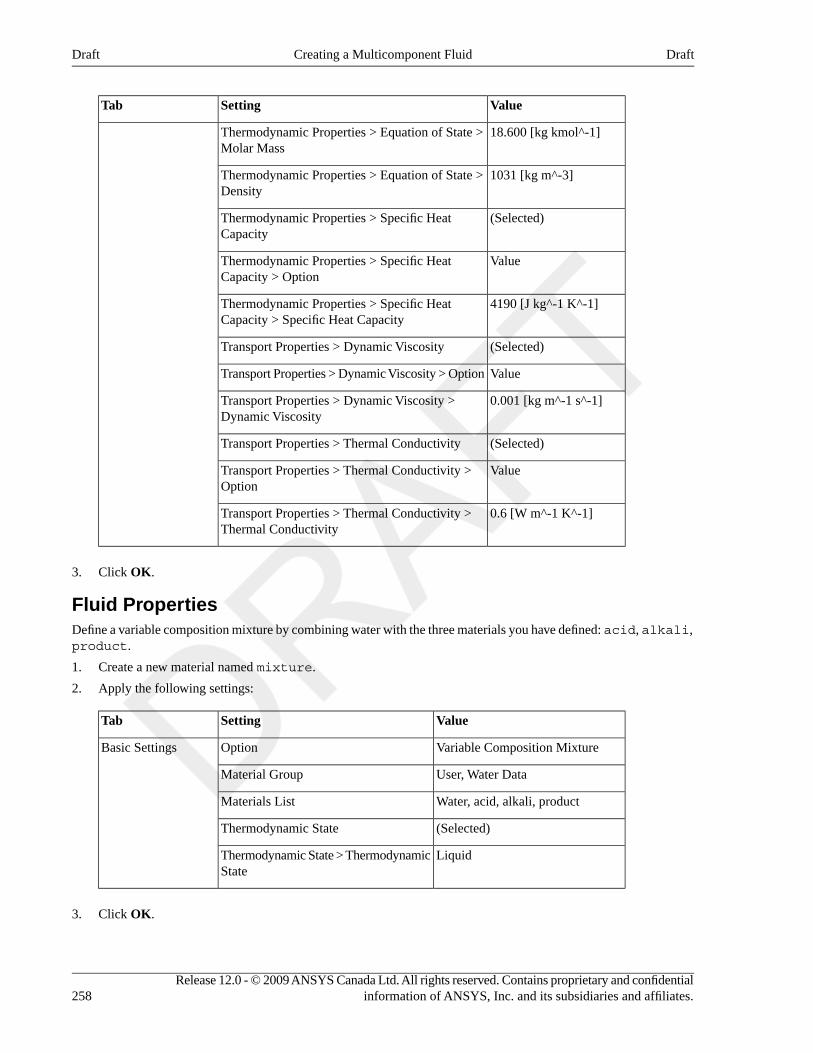
ValueSettingTab
18.600 [kg kmol^-1]Thermodynamic Properties > Equation of State >Molar Mass
1031 [kg m^-3]Thermodynamic Properties > Equation of State >Density
(Selected)Thermodynamic Properties > Specific HeatCapacity
ValueThermodynamic Properties > Specific HeatCapacity > Option
4190 [J kg^-1 K^-1]Thermodynamic Properties > Specific HeatCapacity > Specific Heat Capacity
(Selected)Transport Properties > Dynamic Viscosity
ValueTransport Properties > Dynamic Viscosity > Option
0.001 [kg m^-1 s^-1]Transport Properties > Dynamic Viscosity >Dynamic Viscosity
(Selected)Transport Properties > Thermal Conductivity
ValueTransport Properties > Thermal Conductivity >Option
0.6 [W m^-1 K^-1]Transport Properties > Thermal Conductivity >Thermal Conductivity
3. Click OK.
Fluid PropertiesDefine a variable composition mixture by combining water with the three materials you have defined: acid, alkali,product.
1. Create a new material named mixture.
2. Apply the following settings:
ValueSettingTab
Variable Composition MixtureOptionBasic Settings
User, Water DataMaterial Group
Water, acid, alkali, productMaterials List
(Selected)Thermodynamic State
LiquidThermodynamic State > ThermodynamicState
3. Click OK.
Release 12.0 - © 2009 ANSYS Canada Ltd. All rights reserved. Contains proprietary and confidentialinformation of ANSYS, Inc. and its subsidiaries and affiliates.258
DraftCreating a Multicomponent FluidDraft

Creating an Additional Variable to Model pHYou are going to use an Additional Variable to model the distribution of pH in the mixing tube. You can createAdditional Variables and use them in selected fluids in your domain.
1. Create a new Additional Variable named MixturePH.
2. Apply the following settings:
ValueSettingTab
SpecificVariable TypeBasic Settings
[kg kg^-1]Units
ScalarTensor Type
3. Click OK.
This Additional Variable is now available for use when you create or modify a domain. You will set other propertiesof the Additional Variable, including how it is calculated, when you apply it to the domain later in this tutorial.
Formulating the Reaction and pH as ExpressionsThis section includes:
• Stoichiometric Ratio (p. 259)
• Reaction Source Terms (p. 261)
• Calculating pH (p. 262)
• Loading the Expressions to Model the Reaction and pH (p. 264)
The first section shows a derivation for the mass-based stoichiometric ratio of alkali solution to acid solution. Thisratio is used for calculating various quantities throughout this tutorial.
The second subsection (Reaction Source Terms (p. 261)) shows you how reactions and reaction kinetics can be formulatedusing the Eddy Break Up (EBU) model.
The third subsection (Calculating pH (p. 262)), shows you how pH is calculated.
In the fourth subsection (Loading the Expressions to Model the Reaction and pH (p. 264)) you will use a provided fileto load CEL expressions for the reaction source terms and the pH.
Stoichiometric RatioThe mass-based stoichiometric ratio of alkali solution to acid solution is a quantity that is used in several calculationsin this tutorial. It represents the mass ratio of alkali solution to acid solution which leads to complete reaction with noexcess alkali or acid (that is, neutral pH). This section of the tutorial shows you how to calculate the stoichiometricratio, and introduces other quantities that are used in this tutorial.
The alkali solution contains water and sodium hydroxide. In the alkali solution, it is assumed that the sodium hydroxidemolecules completely dissociate into ions according to the following reaction:
⇒ ++ −NaOH Na OH
The acid solution contains water and sulfuric acid. In the acid solution, it is assumed that the sulfuric acid moleculescompletely dissociate into ions according to the following reaction:
⇒ ++ −H SO 2H SO2 4 42
259Release 12.0 - © 2009 ANSYS Canada Ltd. All rights reserved. Contains proprietary and confidentialinformation of ANSYS, Inc. and its subsidiaries and affiliates.
DraftCreating an Additional Variable to Model pHDraft
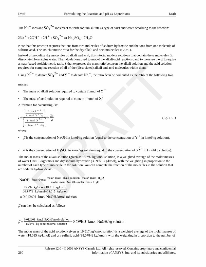
The +Na ions and −SO42 ions react to form sodium sulfate (a type of salt) and water according to the reaction:
+ + + ⇒ ++ − + −2Na 2OH 2H SO Na SO 2H O42
2 4 2
Note that this reaction requires the ions from two molecules of sodium hydroxide and the ions from one molecule ofsulfuric acid. The stoichiometric ratio for the dry alkali and acid molecules is 2-to-1.
Instead of modeling dry molecules of alkali and acid, this tutorial models solutions that contain these molecules (indissociated form) plus water. The calculations used to model the alkali-acid reactions, and to measure the pH, requirea mass-based stoichiometric ratio, i, that expresses the mass ratio between the alkali solution and the acid solutionrequired for complete reaction of all of the (dissociated) alkali and acid molecules within them.
Using −X2 to denote −SO42 and +Y to denote +Na , the ratio i can be computed as the ratio of the following two
masses:
• The mass of alkali solution required to contain 2 kmol of +Y
• The mass of acid solution required to contain 1 kmol of −X2
A formula for calculating i is:
(Eq. 15.1)= =
⎛⎝⎜
⎞⎠⎟
⎛
⎝⎜⎜
⎞
⎠⎟⎟
++
−
−
i αβ
2β
α
2 kmol Y
kmol Y /kg
1 kmol X 2
kmol X 2 /kg
where:
• β is the concentration of NaOH in kmol/kg solution (equal to the concentration of +Y in kmol/kg solution).
• α is the concentration of H SO2 4 in kmol/kg solution (equal to the concentration of −X2 in kmol/kg solution).
The molar mass of the alkali solution (given as 18.292 kg/kmol solution) is a weighted average of the molar massesof water (18.015 kg/kmol) and dry sodium hydroxide (39.9971 kg/kmol), with the weighting in proportion to thenumber of each type of molecule in the solution. You can compute the fraction of the molecules in the solution thatare sodium hydroxide as:
=
=
=
−−
−−
NaOH fraction
0.012601 kmol NaOH/kmol solution
molar mass alkali solution molar mass H Omolar mass NaOH molar mass H O
18.292 kg/kmol 18.015 kg/kmol39.9971 kg/kmol 18.015 kg/kmol
2
2
β can then be calculated as follows:
= =β 0.689E-3 kmol NaOH/kg solution0.012601 kmol NaOH/kmol solution18.292 kg solution/kmol solution
The molar mass of the acid solution (given as 19.517 kg/kmol solution) is a weighted average of the molar masses ofwater (18.015 kg/kmol) and dry sulfuric acid (98.07848 kg/kmol), with the weighting in proportion to the number of
Release 12.0 - © 2009 ANSYS Canada Ltd. All rights reserved. Contains proprietary and confidentialinformation of ANSYS, Inc. and its subsidiaries and affiliates.260
DraftFormulating the Reaction and pH as ExpressionsDraft
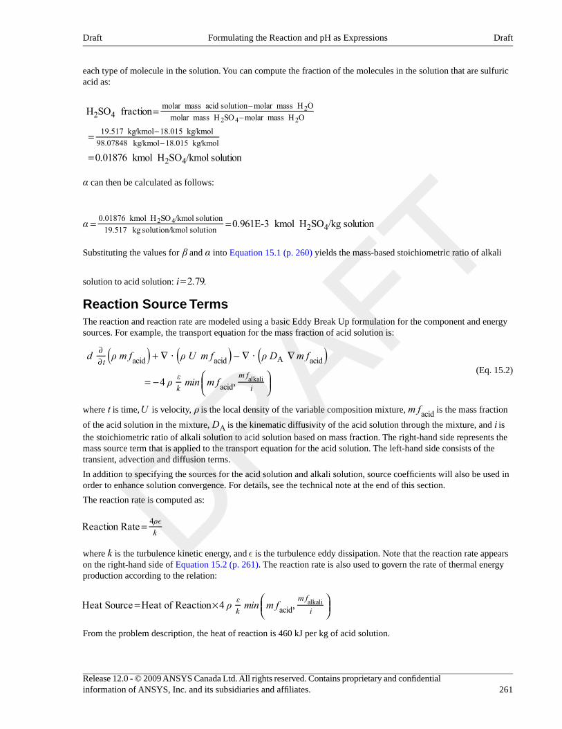
each type of molecule in the solution. You can compute the fraction of the molecules in the solution that are sulfuricacid as:
=
=
=
−−
−−
H SO fraction
0.01876 kmol H SO /kmol solution
2 4molar mass acid solution molar mass H O
molar mass H SO molar mass H O
19.517 kg/kmol 18.015 kg/kmol98.07848 kg/kmol 18.015 kg/kmol
2 4
2
2 4 2
α can then be calculated as follows:
= =α 0.961E-3 kmol H SO /kg solution0.01876 kmol H SO /kmol solution19.517 kg solution/kmol solution 2 4
2 4
Substituting the values for β and α into Equation 15.1 (p. 260) yields the mass-based stoichiometric ratio of alkali
solution to acid solution: =i 2.79.
Reaction Source TermsThe reaction and reaction rate are modeled using a basic Eddy Break Up formulation for the component and energysources. For example, the transport equation for the mass fraction of acid solution is:
(Eq. 15.2)
+ ∇ − ∇ ∇
= − ⎛⎝⎜
⎞⎠⎟
∂∂
d ρ m f ρ U m f ρ D m f
ρ min m f
( ) ( ) ( )· ·
4 ,
t
εk
m fi
acid acid A acid
acidalkali
where t is time, U is velocity, ρ is the local density of the variable composition mixture, m facid is the mass fraction
of the acid solution in the mixture, DA is the kinematic diffusivity of the acid solution through the mixture, and i isthe stoichiometric ratio of alkali solution to acid solution based on mass fraction. The right-hand side represents themass source term that is applied to the transport equation for the acid solution. The left-hand side consists of thetransient, advection and diffusion terms.
In addition to specifying the sources for the acid solution and alkali solution, source coefficients will also be used inorder to enhance solution convergence. For details, see the technical note at the end of this section.
The reaction rate is computed as:
=Reaction Rate ρk
4 ε
where k is the turbulence kinetic energy, and ε is the turbulence eddy dissipation. Note that the reaction rate appearson the right-hand side of Equation 15.2 (p. 261). The reaction rate is also used to govern the rate of thermal energyproduction according to the relation:
= × ⎛⎝⎜
⎞⎠⎟
ρ min m fHeat Source Heat of Reaction 4 ,εk
m fiacid
alkali
From the problem description, the heat of reaction is 460 kJ per kg of acid solution.
261Release 12.0 - © 2009 ANSYS Canada Ltd. All rights reserved. Contains proprietary and confidentialinformation of ANSYS, Inc. and its subsidiaries and affiliates.
DraftFormulating the Reaction and pH as ExpressionsDraft
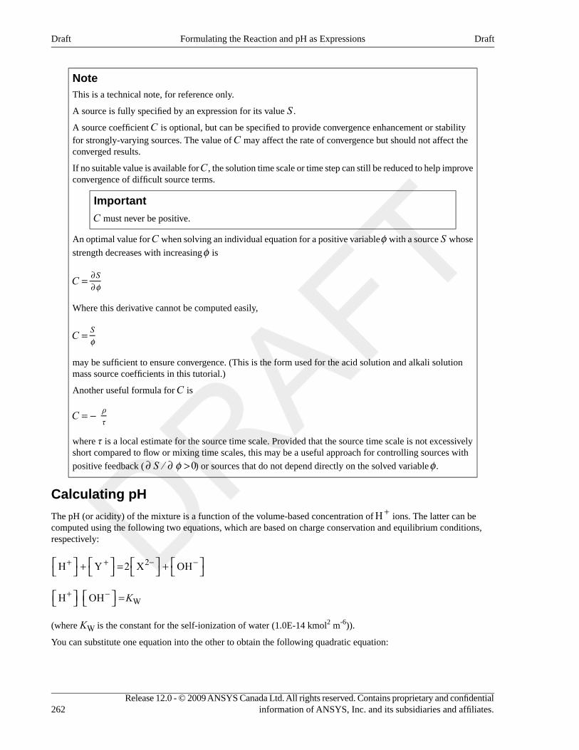
NoteThis is a technical note, for reference only.
A source is fully specified by an expression for its value S .
A source coefficient C is optional, but can be specified to provide convergence enhancement or stabilityfor strongly-varying sources. The value of C may affect the rate of convergence but should not affect theconverged results.
If no suitable value is available for C, the solution time scale or time step can still be reduced to help improveconvergence of difficult source terms.
Important
C must never be positive.
An optimal value for C when solving an individual equation for a positive variable φ with a source S whose
strength decreases with increasing φ is
= φ∂∂
C S
Where this derivative cannot be computed easily,
= φC S
may be sufficient to ensure convergence. (This is the form used for the acid solution and alkali solutionmass source coefficients in this tutorial.)
Another useful formula for C is
= −C ρτ
where τ is a local estimate for the source time scale. Provided that the source time scale is not excessivelyshort compared to flow or mixing time scales, this may be a useful approach for controlling sources with
positive feedback ( φ∂ ∂ >S ⁄ 0) or sources that do not depend directly on the solved variable φ .
Calculating pH
The pH (or acidity) of the mixture is a function of the volume-based concentration of +H ions. The latter can becomputed using the following two equations, which are based on charge conservation and equilibrium conditions,respectively:
⎡⎣
⎤⎦ + ⎡
⎣⎤⎦ = ⎡
⎣⎤⎦ + ⎡
⎣⎤⎦
+ + − −H Y 2 X OH2
⎡⎣ ⎤⎦ ⎡⎣ ⎤⎦ =+ − KH OH W
(where KW is the constant for the self-ionization of water (1.0E-14 kmol2 m-6)).
You can substitute one equation into the other to obtain the following quadratic equation:
Release 12.0 - © 2009 ANSYS Canada Ltd. All rights reserved. Contains proprietary and confidentialinformation of ANSYS, Inc. and its subsidiaries and affiliates.262
DraftFormulating the Reaction and pH as ExpressionsDraft
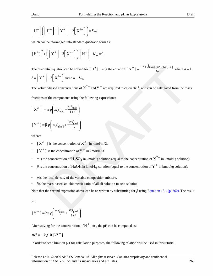
⎡⎣⎢
⎤⎦⎥
⎛⎝⎜
⎡⎣⎢
⎤⎦⎥
+ ⎡⎣⎢
⎤⎦⎥
− ⎡⎣
⎤⎦
⎞⎠⎟
=+ + + − KH H Y 2 X2W
which can be rearranged into standard quadratic form as:
+ ⎛⎝⎜
⎡⎣⎢
⎤⎦⎥
− ⎡⎣
⎤⎦
⎞⎠⎟
⎡⎣⎢
⎤⎦⎥ − =+ + − + K[ H ] Y 2 X H 0
2 2W
The quadratic equation can be solved for +[ H ] using the equation =+ − + −H[ ] b b aca
max[ ( 4 ), 0]2
2 where =a 1,
= ⎡⎣⎢
⎤⎦⎥
− ⎡⎣
⎤⎦
+ −b Y 2 X2 and = −c KW.
The volume-based concentrations of −X2 and +Y are required to calculate b, and can be calculated from the mass
fractions of the components using the following expressions:
⎡⎣
⎤⎦ =
⎛⎝⎜ +
⎞⎠⎟
−+
m fX α ρm f
i2
acid 1prod
=⎛⎝⎜ +
⎞⎠⎟
++
m f[ Y ] β ρi m f
ialkali 1prod
where:
• −[ X ]2 is the concentration of −X2 in kmol/m^3.
• +[ Y ] is the concentration of +Y in kmol/m^3.
• α is the concentration of H SO2 4 in kmol/kg solution (equal to the concentration of −X2 in kmol/kg solution).
• β is the concentration of NaOH in kmol/kg solution (equal to the concentration of +Y in kmol/kg solution).
• ρ is the local density of the variable composition mixture.
• i is the mass-based stoichiometric ratio of alkali solution to acid solution.
Note that the second expression above can be re-written by substituting for β using Equation 15.1 (p. 260). The result
is:
=⎛⎝⎜ +
⎞⎠⎟
++
α[ Y ] 2 ρm fi
m f
i1alkali prod
After solving for the concentration of +H ions, the pH can be computed as:
= − +pH Hlog10 [ ]
In order to set a limit on pH for calculation purposes, the following relation will be used in this tutorial:
263Release 12.0 - © 2009 ANSYS Canada Ltd. All rights reserved. Contains proprietary and confidentialinformation of ANSYS, Inc. and its subsidiaries and affiliates.
DraftFormulating the Reaction and pH as ExpressionsDraft
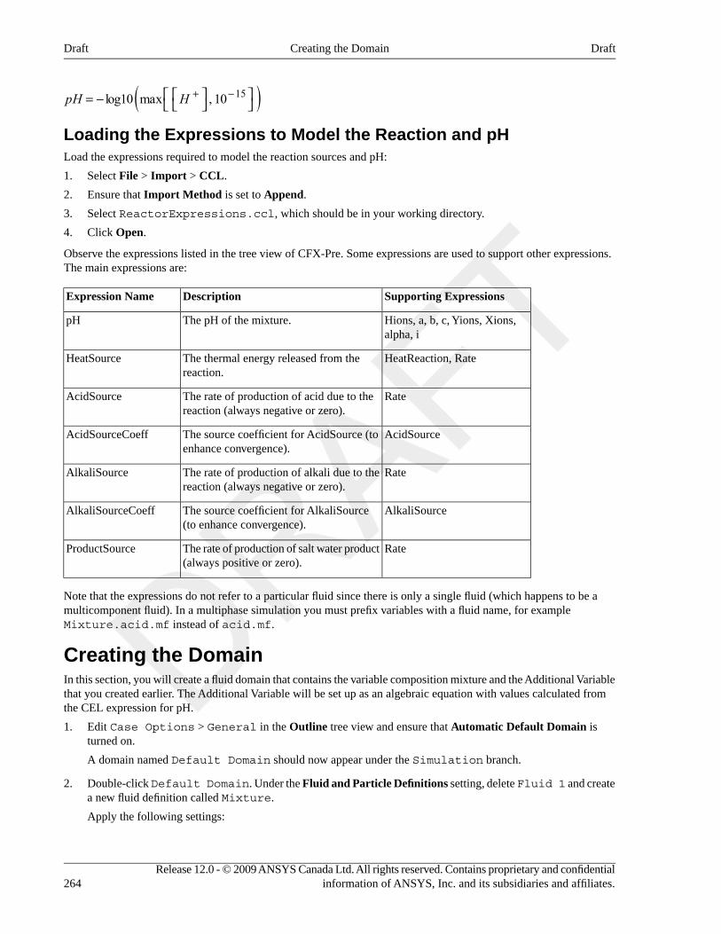
= − ⎡⎣
⎡⎣
⎤⎦
⎤⎦
+ −pH H( )log10 max , 10 15
Loading the Expressions to Model the Reaction and pHLoad the expressions required to model the reaction sources and pH:
1. Select File > Import > CCL.
2. Ensure that Import Method is set to Append.
3. Select ReactorExpressions.ccl, which should be in your working directory.
4. Click Open.
Observe the expressions listed in the tree view of CFX-Pre. Some expressions are used to support other expressions.The main expressions are:
Supporting ExpressionsDescriptionExpression Name
Hions, a, b, c, Yions, Xions,alpha, i
The pH of the mixture.pH
HeatReaction, RateThe thermal energy released from thereaction.
HeatSource
RateThe rate of production of acid due to thereaction (always negative or zero).
AcidSource
AcidSourceThe source coefficient for AcidSource (toenhance convergence).
AcidSourceCoeff
RateThe rate of production of alkali due to thereaction (always negative or zero).
AlkaliSource
AlkaliSourceThe source coefficient for AlkaliSource(to enhance convergence).
AlkaliSourceCoeff
RateThe rate of production of salt water product(always positive or zero).
ProductSource
Note that the expressions do not refer to a particular fluid since there is only a single fluid (which happens to be amulticomponent fluid). In a multiphase simulation you must prefix variables with a fluid name, for exampleMixture.acid.mf instead of acid.mf.
Creating the DomainIn this section, you will create a fluid domain that contains the variable composition mixture and the Additional Variablethat you created earlier. The Additional Variable will be set up as an algebraic equation with values calculated fromthe CEL expression for pH.
1. Edit Case Options > General in the Outline tree view and ensure that Automatic Default Domain isturned on.
A domain named Default Domain should now appear under the Simulation branch.
2. Double-click Default Domain. Under the Fluid and Particle Definitions setting, delete Fluid 1 and createa new fluid definition called Mixture.
Apply the following settings:
Release 12.0 - © 2009 ANSYS Canada Ltd. All rights reserved. Contains proprietary and confidentialinformation of ANSYS, Inc. and its subsidiaries and affiliates.264
DraftCreating the DomainDraft
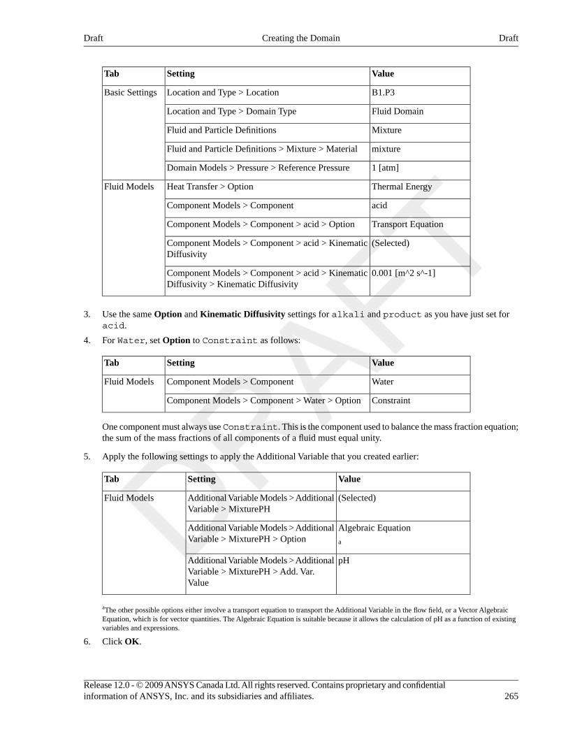
ValueSettingTab
B1.P3Location and Type > LocationBasic Settings
Fluid DomainLocation and Type > Domain Type
MixtureFluid and Particle Definitions
mixtureFluid and Particle Definitions > Mixture > Material
1 [atm]Domain Models > Pressure > Reference Pressure
Thermal EnergyHeat Transfer > OptionFluid Models
acidComponent Models > Component
Transport EquationComponent Models > Component > acid > Option
(Selected)Component Models > Component > acid > KinematicDiffusivity
0.001 [m^2 s^-1]Component Models > Component > acid > KinematicDiffusivity > Kinematic Diffusivity
3. Use the same Option and Kinematic Diffusivity settings for alkali and product as you have just set foracid.
4. For Water, set Option to Constraint as follows:
ValueSettingTab
WaterComponent Models > ComponentFluid Models
ConstraintComponent Models > Component > Water > Option
One component must always use Constraint. This is the component used to balance the mass fraction equation;the sum of the mass fractions of all components of a fluid must equal unity.
5. Apply the following settings to apply the Additional Variable that you created earlier:
ValueSettingTab
(Selected)Additional Variable Models > AdditionalVariable > MixturePH
Fluid Models
Algebraic EquationAdditional Variable Models > AdditionalVariable > MixturePH > Option a
pHAdditional Variable Models > AdditionalVariable > MixturePH > Add. Var.Value
aThe other possible options either involve a transport equation to transport the Additional Variable in the flow field, or a Vector AlgebraicEquation, which is for vector quantities. The Algebraic Equation is suitable because it allows the calculation of pH as a function of existingvariables and expressions.
6. Click OK.
265Release 12.0 - © 2009 ANSYS Canada Ltd. All rights reserved. Contains proprietary and confidentialinformation of ANSYS, Inc. and its subsidiaries and affiliates.
DraftCreating the DomainDraft
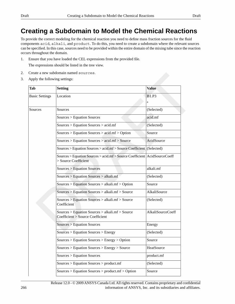
Creating a Subdomain to Model the Chemical ReactionsTo provide the correct modeling for the chemical reaction you need to define mass fraction sources for the fluidcomponents acid, alkali, and product. To do this, you need to create a subdomain where the relevant sourcescan be specified. In this case, sources need to be provided within the entire domain of the mixing tube since the reactionoccurs throughout the domain.
1. Ensure that you have loaded the CEL expressions from the provided file.
The expressions should be listed in the tree view.
2. Create a new subdomain named sources.
3. Apply the following settings:
ValueSettingTab
B1.P3LocationBasic Settings
a
(Selected)SourcesSources
acid.mfSources > Equation Sources
(Selected)Sources > Equation Sources > acid.mf
SourceSources > Equation Sources > acid.mf > Option
AcidSourceSources > Equation Sources > acid.mf > Source
(Selected)Sources > Equation Sources > acid.mf > Source Coefficient
AcidSourceCoeffSources > Equation Sources > acid.mf > Source Coefficient> Source Coefficient
alkali.mfSources > Equation Sources
(Selected)Sources > Equation Sources > alkali.mf
SourceSources > Equation Sources > alkali.mf > Option
AlkaliSourceSources > Equation Sources > alkali.mf > Source
(Selected)Sources > Equation Sources > alkali.mf > SourceCoefficient
AlkaliSourceCoeffSources > Equation Sources > alkali.mf > SourceCoefficient > Source Coefficient
EnergySources > Equation Sources
(Selected)Sources > Equation Sources > Energy
SourceSources > Equation Sources > Energy > Option
HeatSourceSources > Equation Sources > Energy > Source
product.mfSources > Equation Sources
(Selected)Sources > Equation Sources > product.mf
SourceSources > Equation Sources > product.mf > Option
Release 12.0 - © 2009 ANSYS Canada Ltd. All rights reserved. Contains proprietary and confidentialinformation of ANSYS, Inc. and its subsidiaries and affiliates.266
DraftCreating a Subdomain to Model the Chemical ReactionsDraft
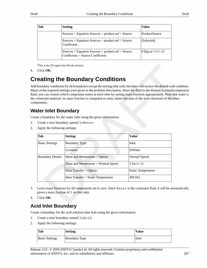
ValueSettingTab
ProductSourceSources > Equation Sources > product.mf > Source
(Selected)Sources > Equation Sources > product.mf > SourceCoefficient
0 [kg m^-3 s^-1]Sources > Equation Sources > product.mf > SourceCoefficient > Source Coefficient
aThis is the 3D region that fills the domain.
4. Click OK.
Creating the Boundary ConditionsAdd boundary conditions for all boundaries except the mixing tube wall; the latter will receive the default wall condition.Many of the required settings were given in the problem description. Since the fluid in the domain is a multicomponentfluid, you can control which component enters at each inlet by setting mass fractions appropriately. Note that water isthe constraint material; its mass fraction is computed as unity minus the sum of the mass fractions of the othercomponents.
Water Inlet BoundaryCreate a boundary for the water inlet using the given information:
1. Create a new boundary named InWater.
2. Apply the following settings:
ValueSettingTab
InletBoundary TypeBasic Settings
InWaterLocation
Normal SpeedMass and Momentum > OptionBoundary Details
2 [m s^-1]Mass and Momentum > Normal Speed
Static TemperatureHeat Transfer > Option
300 [K]Heat Transfer > Static Temperature
3. Leave mass fractions for all components set to zero. Since Water is the constraint fluid, it will be automaticallygiven a mass fraction of 1 on this inlet.
4. Click OK.
Acid Inlet BoundaryCreate a boundary for the acid solution inlet hole using the given information:
1. Create a new boundary named InAcid.
2. Apply the following settings:
ValueSettingTab
InletBoundary TypeBasic Settings
267Release 12.0 - © 2009 ANSYS Canada Ltd. All rights reserved. Contains proprietary and confidentialinformation of ANSYS, Inc. and its subsidiaries and affiliates.
DraftCreating the Boundary ConditionsDraft
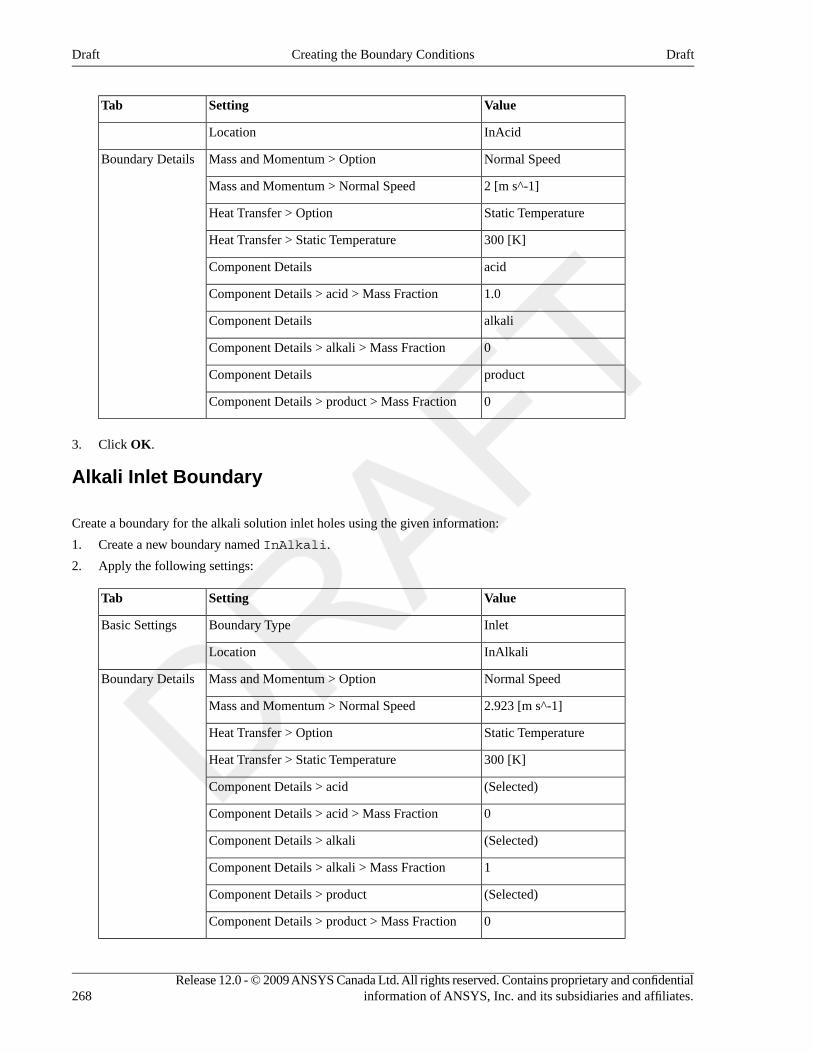
ValueSettingTab
InAcidLocation
Normal SpeedMass and Momentum > OptionBoundary Details
2 [m s^-1]Mass and Momentum > Normal Speed
Static TemperatureHeat Transfer > Option
300 [K]Heat Transfer > Static Temperature
acidComponent Details
1.0Component Details > acid > Mass Fraction
alkaliComponent Details
0Component Details > alkali > Mass Fraction
productComponent Details
0Component Details > product > Mass Fraction
3. Click OK.
Alkali Inlet Boundary
Create a boundary for the alkali solution inlet holes using the given information:
1. Create a new boundary named InAlkali.
2. Apply the following settings:
ValueSettingTab
InletBoundary TypeBasic Settings
InAlkaliLocation
Normal SpeedMass and Momentum > OptionBoundary Details
2.923 [m s^-1]Mass and Momentum > Normal Speed
Static TemperatureHeat Transfer > Option
300 [K]Heat Transfer > Static Temperature
(Selected)Component Details > acid
0Component Details > acid > Mass Fraction
(Selected)Component Details > alkali
1Component Details > alkali > Mass Fraction
(Selected)Component Details > product
0Component Details > product > Mass Fraction
Release 12.0 - © 2009 ANSYS Canada Ltd. All rights reserved. Contains proprietary and confidentialinformation of ANSYS, Inc. and its subsidiaries and affiliates.268
DraftCreating the Boundary ConditionsDraft
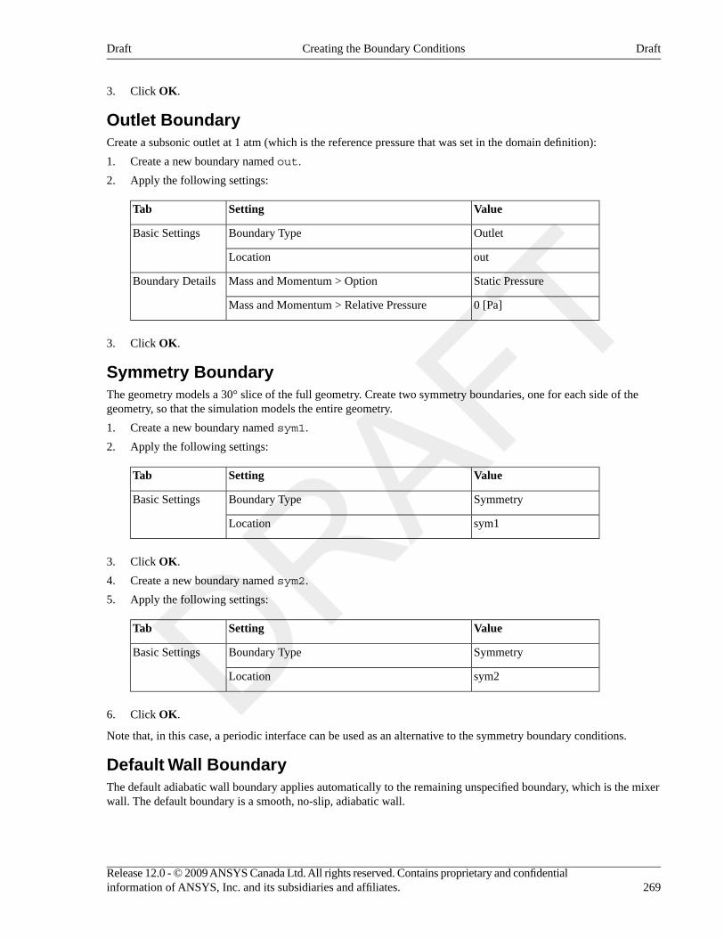
3. Click OK.
Outlet BoundaryCreate a subsonic outlet at 1 atm (which is the reference pressure that was set in the domain definition):
1. Create a new boundary named out.
2. Apply the following settings:
ValueSettingTab
OutletBoundary TypeBasic Settings
outLocation
Static PressureMass and Momentum > OptionBoundary Details
0 [Pa]Mass and Momentum > Relative Pressure
3. Click OK.
Symmetry BoundaryThe geometry models a 30° slice of the full geometry. Create two symmetry boundaries, one for each side of thegeometry, so that the simulation models the entire geometry.
1. Create a new boundary named sym1.
2. Apply the following settings:
ValueSettingTab
SymmetryBoundary TypeBasic Settings
sym1Location
3. Click OK.
4. Create a new boundary named sym2.
5. Apply the following settings:
ValueSettingTab
SymmetryBoundary TypeBasic Settings
sym2Location
6. Click OK.
Note that, in this case, a periodic interface can be used as an alternative to the symmetry boundary conditions.
Default Wall BoundaryThe default adiabatic wall boundary applies automatically to the remaining unspecified boundary, which is the mixerwall. The default boundary is a smooth, no-slip, adiabatic wall.
269Release 12.0 - © 2009 ANSYS Canada Ltd. All rights reserved. Contains proprietary and confidentialinformation of ANSYS, Inc. and its subsidiaries and affiliates.
DraftCreating the Boundary ConditionsDraft
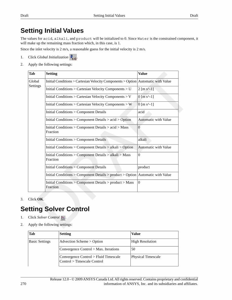
Setting Initial ValuesThe values for acid, alkali, and product will be initialized to 0. Since Water is the constrained component, itwill make up the remaining mass fraction which, in this case, is 1.
Since the inlet velocity is 2 m/s, a reasonable guess for the initial velocity is 2 m/s.
1. Click Global Initialization .
2. Apply the following settings:
ValueSettingTab
Automatic with ValueInitial Conditions > Cartesian Velocity Components > OptionGlobalSettings
2 [m s^-1]Initial Conditions > Cartesian Velocity Components > U
0 [m s^-1]Initial Conditions > Cartesian Velocity Components > V
0 [m s^-1]Initial Conditions > Cartesian Velocity Components > W
acidInitial Conditions > Component Details
Automatic with ValueInitial Conditions > Component Details > acid > Option
0Initial Conditions > Component Details > acid > MassFraction
alkaliInitial Conditions > Component Details
Automatic with ValueInitial Conditions > Component Details > alkali > Option
0Initial Conditions > Component Details > alkali > MassFraction
productInitial Conditions > Component Details
Automatic with ValueInitial Conditions > Component Details > product > Option
0Initial Conditions > Component Details > product > MassFraction
3. Click OK.
Setting Solver Control1. Click Solver Control .
2. Apply the following settings:
ValueSettingTab
High ResolutionAdvection Scheme > OptionBasic Settings
50Convergence Control > Max. Iterations
Physical TimescaleConvergence Control > Fluid TimescaleControl > Timescale Control
Release 12.0 - © 2009 ANSYS Canada Ltd. All rights reserved. Contains proprietary and confidentialinformation of ANSYS, Inc. and its subsidiaries and affiliates.270
DraftSetting Initial ValuesDraft
ValueSettingTab
0.01 [s]aConvergence Control > Fluid TimescaleControl > Physical Timescale
aThe length of mixing tube is 0.06 m and inlet velocity is 2 m/s. An estimate of the dynamic time scale is 0.03 s. An appropriate time stepwould be 1/4 to 1/2 of this value.
3. Click OK.
Writing the CFX-Solver Input (.def) File
1. Click Define Run .
2. Apply the following settings:
ValueSetting
Reactor.defFile name
3. Click Save.
CFX-Solver Manager automatically starts and, on the Define Run dialog box, the Solver Input File is set.
4. If using Standalone Mode, quit CFX-Pre, saving the simulation (.cfx) file at your discretion.
Obtaining a Solution using CFX-Solver ManagerWhen CFX-Solver Manager has started, obtain a solution to the CFD problem as follows:
1. Ensure Define Run is displayed.
2. Select Show Advanced Controls. On the Solver tab, select Executable Settings > Double Precision.
This provides the precision required to evaluate the expression for pH.
3. Click Start Run.
CFX-Solver runs and attempts to obtain a solution. This may take a long time, depending on your system. Eventuallya dialog box is displayed.
4. Select the check box next to Post-Process Results when the completion message appears at the end of the run.
5. If using Standalone Mode, select the check box next to Shut down CFX-Solver Manager.
6. Click OK.
Viewing the Results in CFD-PostTo see the nature and extent of the reaction process, examine the pH, the mass fractions, and turbulence quantities ona plane as follows:
1. Create an XY slice plane through Z = 0.
2. Turn off the visibility of the plane you just created.
3. Create contour plots of the following variables on that plane:
• MixturePH
• acid.Mass Fraction
• alkali.Mass Fraction
271Release 12.0 - © 2009 ANSYS Canada Ltd. All rights reserved. Contains proprietary and confidentialinformation of ANSYS, Inc. and its subsidiaries and affiliates.
DraftWriting the CFX-Solver Input (.def) FileDraft

• product.Mass Fraction
• Turbulence Kinetic Energy
• Turbulence Eddy Dissipation
4. Create an expression for Turbulence Eddy Dissipation/Turbulence Kinetic Energy and createa contour plot using that expression. This quantity is an indicator of the reaction rate — it represents 1 / mixingtimescale.
Release 12.0 - © 2009 ANSYS Canada Ltd. All rights reserved. Contains proprietary and confidentialinformation of ANSYS, Inc. and its subsidiaries and affiliates.272
DraftViewing the Results in CFD-PostDraft
Chapter 16. Conjugate Heat Transfer ina Heating CoilThis tutorial includes:
• Tutorial Features (p. 273)
• Overview of the Problem to Solve (p. 274)
• Before You Begin (p. 275)
• Starting CFX-Pre (p. 275)
• Defining a Case in CFX-Pre (p. 275)
• Obtaining a Solution using CFX-Solver Manager (p. 281)
• Viewing the Results in CFD-Post (p. 281)
• Exporting the Results to ANSYS (p. 284)
Tutorial FeaturesIn this tutorial you will learn about:
• Creating and using a solid domain as a heating coil in CFX-Pre.
• Creating a domain interface.
• Modeling conjugate heat transfer in CFX-Pre.
• Using electricity to power a heat source.
• Plotting temperature on a cylindrical locator in CFD-Post.
• Lighting in CFD-Post.
• Exporting thermal and mechanical data to be used with ANSYS Multi-field solver.
ImportantNote that this tutorial uses the electromagnetic model which is a BETA feature in the current release.
DetailsFeatureComponent
General ModeUser ModeCFX-Pre
Steady StateAnalysis Type
General FluidFluid Type
Multiple DomainDomain Type
k-EpsilonTurbulence Model
Thermal EnergyHeat Transfer
Conjugate Heat Transfer
Electrical Resistance Heating
Electrical Heating CoilBoundary Conditions
Inlet (Subsonic)
273Release 12.0 - © 2009 ANSYS Canada Ltd. All rights reserved. Contains proprietary and confidentialinformation of ANSYS, Inc. and its subsidiaries and affiliates.
DraftDraft
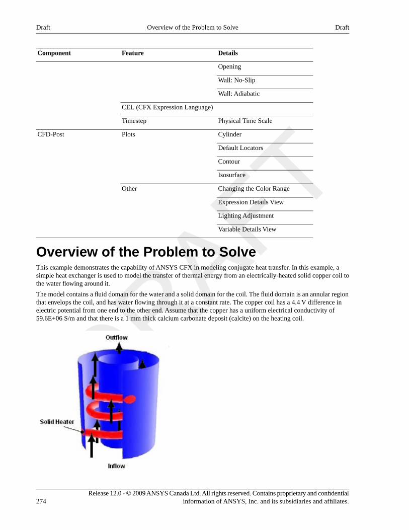
DetailsFeatureComponent
Opening
Wall: No-Slip
Wall: Adiabatic
CEL (CFX Expression Language)
Physical Time ScaleTimestep
CylinderPlotsCFD-Post
Default Locators
Contour
Isosurface
Changing the Color RangeOther
Expression Details View
Lighting Adjustment
Variable Details View
Overview of the Problem to SolveThis example demonstrates the capability of ANSYS CFX in modeling conjugate heat transfer. In this example, asimple heat exchanger is used to model the transfer of thermal energy from an electrically-heated solid copper coil tothe water flowing around it.
The model contains a fluid domain for the water and a solid domain for the coil. The fluid domain is an annular regionthat envelops the coil, and has water flowing through it at a constant rate. The copper coil has a 4.4 V difference inelectric potential from one end to the other end. Assume that the copper has a uniform electrical conductivity of59.6E+06 S/m and that there is a 1 mm thick calcium carbonate deposit (calcite) on the heating coil.
Release 12.0 - © 2009 ANSYS Canada Ltd. All rights reserved. Contains proprietary and confidentialinformation of ANSYS, Inc. and its subsidiaries and affiliates.274
DraftOverview of the Problem to SolveDraft
This tutorial also includes an optional step that demonstrates the use of the CFX to ANSYS Data Transfer tool to exportthermal and mechanical stress data for use with ANSYS Multi-field solver. A results file is provided in case you wantto skip the model creation and solution steps within ANSYS CFX.
Before You BeginIf this is the first tutorial you are working with, it is important to review the following topics before beginning:
• Preparing a Working Directory (p. 23)
• Setting the Working Directory and Starting ANSYS CFX (p. 23)
• Changing the Display Colors (p. 24)
• Playing a Tutorial Session File (p. 24)
Starting CFX-Pre1. Prepare the working directory using the following files in the examples directory:
• HeatingCoil.pre
• HeatingCoil_001.res
• HeatingCoilMesh.gtm
For details, see Preparing a Working Directory (p. 23)
2. Set the working directory and start CFX-Pre
For details, see Setting the Working Directory and Starting ANSYS CFX (p. 23)
Defining a Case in CFX-PreIf you want to set up the simulation automatically using a tutorial session file, run HeatingCoil.pre. For details,see Playing a Tutorial Session File (p. 24). Then proceed to Obtaining a Solution using CFX-Solver Manager (p. 281).
If you want to set up the simulation manually, proceed to the following steps:
1. Select File > New Case.
2. Select General and click OK.
3. Select File > Save Case As.
4. Under File name, type HeatingCoil.
5. Click Save.
Importing the Mesh1. Edit Case Options > General in the Outline tree view and ensure that Automatic Default Domain and
Automatic Default Interfaces are turned off.
Default Domain generation should be turned off because you will create the fluid and solid domains and interfacesmanually later in this tutorial.
2. Click OK.
3. Right-click Mesh and select Import Mesh > CFX Mesh. The Import Mesh dialog box appears.
4. Apply the following settings:
275Release 12.0 - © 2009 ANSYS Canada Ltd. All rights reserved. Contains proprietary and confidentialinformation of ANSYS, Inc. and its subsidiaries and affiliates.
DraftBefore You BeginDraft
ValueSetting
HeatingCoilMesh.gtmFile name
5. Click Open.
6. Right-click a blank area in the viewer and select Predefined Camera > Isometric View (Z up) from the shortcutmenu.
Editing the Material Properties1. Expand Materials from the tree view and double-click Copper.
2. Apply the following settings to Copper:
ValueSettingTab
(Selected)Electromagnetic Properties > Electrical ConductivityMaterialProperties
59.6E+06 [S m^-1]Electromagnetic Properties > Electrical Conductivity >Electrical Conductivity
3. Click OK.
Defining the Calcium Carbonate Deposit MaterialCreate a new material definition that will be used to model the calcium carbonate deposit on the heating coil:
1. Click Insert Material then create a new material named Calcium Carbonate.
2. Apply the following settings:
ValueSettingTab
UserMaterial GroupBasic Settings
(Selected)Thermodynamic State
SolidThermodynamic State > Thermodynamic State
100.087 [kg kmol^-1]Thermodynamic Properties > Equation of State> Molar Mass
Material Properties
2.71 [g cm^-3]Thermodynamic Properties > Equation of State> Density
(Selected)Thermodynamic Properties > Specific HeatCapacity
0.9 [J g^-1 K^-1]Thermodynamic Properties > Specific HeatCapacity > Specific Heat Capacity
(Selected)Transport Properties > Thermal Conductivity
3.85 [W m^-1 K^-1]Transport Properties > Thermal Conductivity> Thermal Conductivity
Release 12.0 - © 2009 ANSYS Canada Ltd. All rights reserved. Contains proprietary and confidentialinformation of ANSYS, Inc. and its subsidiaries and affiliates.276
DraftEditing the Material PropertiesDraft
3. Click OK.
Creating the DomainsThis simulation requires both a fluid domain and a solid domain. First, you will create a fluid domain for the annularregion of the heat exchanger.
Creating a Fluid DomainThe fluid domain will include the region of fluid flow but exclude the solid copper heater coil.
1. Ensure that Flow Analysis 1 > Default Domain is deleted. If not, right-click Default Domain andselect Delete.
2. Click Domain and set the name to FluidZone.
3. Apply the following settings to FluidZone
ValueSettingTab
B1.P3aLocation and Type > LocationBasic Settings
Fluid 1Fluid and Particle Definitions
WaterFluid and Particle Definitions > Fluid 1 >Material
1 [atm]Domain Models > Pressure > Reference Pressure
Thermal EnergyHeat Transfer > OptionFluid Models
(Selected)Domain InitializationInitialization
aThis region name may be different depending on how the mesh was created. You should pick the region that forms the exterior surface ofthe volume surrounding the coil.
4. Click OK.
Creating a Solid DomainSince you know that the copper heating element will be much hotter than the fluid, you can initialize the temperatureto a reasonable value. The initialization option that is set when creating a domain applies only to that domain.
Note that the electromagnetic model is a BETA feature in the current release. Since it is required by this tutorial, youneed to activate BETA features as follows:
1. Edit Case Options > General in the Outline tree view and select Enable Beta Features.
2. Click OK.
Create the solid domain as follows:
1. Create a new domain named SolidZone.
2. Apply the following settings:
ValueSettingTab
B2.P3Location and Type > LocationBasic Settings
Solid DomainLocation and Type > Domain Type
277Release 12.0 - © 2009 ANSYS Canada Ltd. All rights reserved. Contains proprietary and confidentialinformation of ANSYS, Inc. and its subsidiaries and affiliates.
DraftCreating the DomainsDraft
ValueSettingTab
Solid 1Solid Definitions
CopperSolid Definitions> Solid 1 > Solid 1 > Material
Thermal EnergyHeat Transfer > OptionSolid Models
(Selected)Electromagnetic Model
Electric PotentialElectromagnetic Model > Electric Field Model > Option
(Selected)Domain InitializationInitialization
Automatic with ValueDomain Initialization > Initial Conditions > Temperature> Option
550 [K]Domain Initialization > Initial Conditions > Temperature> Temperature
3. Click OK.
Creating the Boundaries
Heating Coil BoundariesIn order to pass electricity through the heating coil, specify 0 V at one end and 4.4 V at the other end:
1. Create a new boundary named Ground in the domain SolidZone.
2. Apply the following settings:
ValueSettingTab
WallBoundary TypeBasic Settings
F11.B2.P3aLocation
VoltageElectric Field > OptionBoundary Details
0 [V]Electric Field > Voltage
aThis region name may be different depending on how the mesh was created. You should pick one end of the heating coil.
3. Click OK.
4. Create a similar boundary named Hot at the other end of the coil, region F12.B2.P3, and apply 4.4 V.
Inlet BoundaryYou will now create an inlet boundary for the cooling fluid (Water).
1. Create a new boundary named inflow in the domain FluidZone.
2. Apply the following settings:
ValueSettingTab
InletBoundary TypeBasic Settings
Release 12.0 - © 2009 ANSYS Canada Ltd. All rights reserved. Contains proprietary and confidentialinformation of ANSYS, Inc. and its subsidiaries and affiliates.278
DraftCreating the BoundariesDraft
ValueSettingTab
inflowLocation
Normal SpeedMass and Momentum > OptionBoundary Details
0.4 [m s^-1]Mass and Momentum > Normal Speed
Static TemperatureHeat Transfer > Option
300 [K]Heat Transfer > Static Temperature
3. Click OK.
Opening BoundaryAn opening boundary is appropriate for the exit in this case because, at some stage during the solution, the coiledheating element will cause some recirculation at the exit. At an opening boundary you need to set the temperature offluid that enters through the boundary. In this case it is useful to base this temperature on the fluid temperature at theoutlet, since you expect the fluid to be flowing mostly out through this opening.
1. Create a new expression named OutletTemperature.
2. Set Definition to areaAve(T)@outflow
3. Click Apply.
4. Create a new boundary named outflow in the domain FluidZone.
5. Apply the following settings:
ValueSettingTab
OpeningBoundary TypeBasic Settings
outflowLocation
Opening Pres. and DirnMass and Momentum > OptionBoundary Details
0 [Pa]Mass and Momentum > Relative Pressure
Static TemperatureHeat Transfer > Option
OutletTemperatureHeat Transfer > Static Temperature
6. Click OK.
The default adiabatic wall boundary will be applied automatically to the remaining unspecified external boundaries ofthe fluid domain.
Two more boundary conditions are generated automatically when a domain interface is created to connect the fluidand solid domains. The domain interface is discussed in the next section.
Creating the Domain InterfaceIf you have Automatic Default Interfaces turned on, then an interface called Default Fluid Solid Interfaceis created automatically and listed in the tree view. In this case, delete the default interface and proceed to creating anew one.
1. Create a new domain interface named Fluid Solid Interface and apply the following settings:
279Release 12.0 - © 2009 ANSYS Canada Ltd. All rights reserved. Contains proprietary and confidentialinformation of ANSYS, Inc. and its subsidiaries and affiliates.
DraftCreating the Domain InterfaceDraft
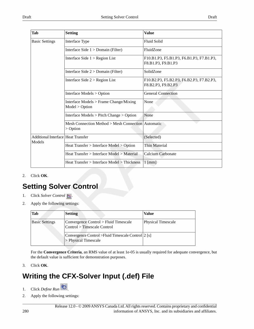
ValueSettingTab
Fluid SolidInterface TypeBasic Settings
FluidZoneInterface Side 1 > Domain (Filter)
F10.B1.P3, F5.B1.P3, F6.B1.P3, F7.B1.P3,F8.B1.P3, F9.B1.P3
Interface Side 1 > Region List
SolidZoneInterface Side 2 > Domain (Filter)
F10.B2.P3, F5.B2.P3, F6.B2.P3, F7.B2.P3,F8.B2.P3, F9.B2.P3
Interface Side 2 > Region List
General ConnectionInterface Models > Option
NoneInterface Models > Frame Change/MixingModel > Option
NoneInterface Models > Pitch Change > Option
AutomaticMesh Connection Method > Mesh Connection> Option
(Selected)Heat TransferAdditional InterfaceModels
Thin MaterialHeat Transfer > Interface Model > Option
Calcium CarbonateHeat Transfer > Interface Model > Material
1 [mm]Heat Transfer > Interface Model > Thickness
2. Click OK.
Setting Solver Control1. Click Solver Control .
2. Apply the following settings:
ValueSettingTab
Physical TimescaleConvergence Control > Fluid TimescaleControl > Timescale Control
Basic Settings
2 [s]Convergence Control >Fluid Timescale Control> Physical Timescale
For the Convergence Criteria, an RMS value of at least 1e-05 is usually required for adequate convergence, butthe default value is sufficient for demonstration purposes.
3. Click OK.
Writing the CFX-Solver Input (.def) File
1. Click Define Run .
2. Apply the following settings:
Release 12.0 - © 2009 ANSYS Canada Ltd. All rights reserved. Contains proprietary and confidentialinformation of ANSYS, Inc. and its subsidiaries and affiliates.280
DraftSetting Solver ControlDraft
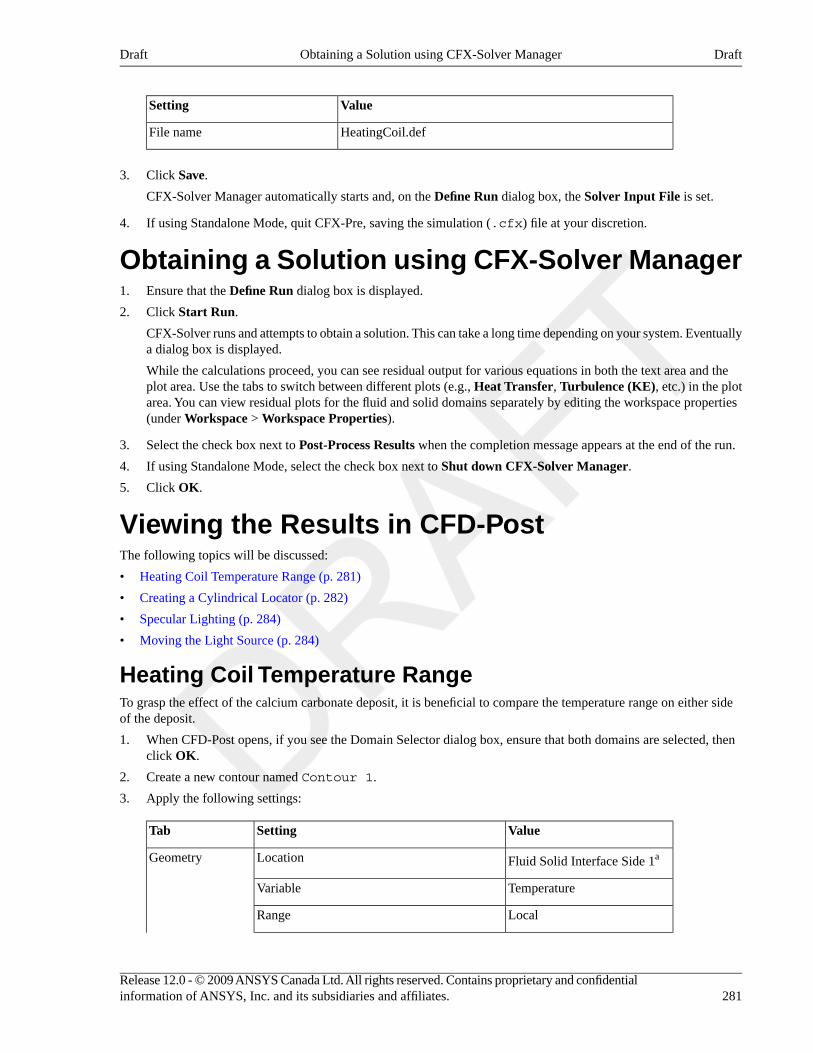
ValueSetting
HeatingCoil.defFile name
3. Click Save.
CFX-Solver Manager automatically starts and, on the Define Run dialog box, the Solver Input File is set.
4. If using Standalone Mode, quit CFX-Pre, saving the simulation (.cfx) file at your discretion.
Obtaining a Solution using CFX-Solver Manager1. Ensure that the Define Run dialog box is displayed.
2. Click Start Run.
CFX-Solver runs and attempts to obtain a solution. This can take a long time depending on your system. Eventuallya dialog box is displayed.
While the calculations proceed, you can see residual output for various equations in both the text area and theplot area. Use the tabs to switch between different plots (e.g., Heat Transfer, Turbulence (KE), etc.) in the plotarea. You can view residual plots for the fluid and solid domains separately by editing the workspace properties(under Workspace > Workspace Properties).
3. Select the check box next to Post-Process Results when the completion message appears at the end of the run.
4. If using Standalone Mode, select the check box next to Shut down CFX-Solver Manager.
5. Click OK.
Viewing the Results in CFD-PostThe following topics will be discussed:
• Heating Coil Temperature Range (p. 281)
• Creating a Cylindrical Locator (p. 282)
• Specular Lighting (p. 284)
• Moving the Light Source (p. 284)
Heating Coil Temperature RangeTo grasp the effect of the calcium carbonate deposit, it is beneficial to compare the temperature range on either sideof the deposit.
1. When CFD-Post opens, if you see the Domain Selector dialog box, ensure that both domains are selected, thenclick OK.
2. Create a new contour named Contour 1.
3. Apply the following settings:
ValueSettingTab
Fluid Solid Interface Side 1aLocationGeometry
TemperatureVariable
LocalRange
281Release 12.0 - © 2009 ANSYS Canada Ltd. All rights reserved. Contains proprietary and confidentialinformation of ANSYS, Inc. and its subsidiaries and affiliates.
DraftObtaining a Solution using CFX-Solver ManagerDraft
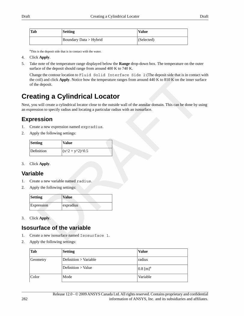
ValueSettingTab
(Selected)Boundary Data > Hybrid
aThis is the deposit side that is in contact with the water.
4. Click Apply.
5. Take note of the temperature range displayed below the Range drop-down box. The temperature on the outersurface of the deposit should range from around 400 K to 740 K.
Change the contour location to Fluid Solid Interface Side 2 (The deposit side that is in contact withthe coil) and click Apply. Notice how the temperature ranges from around 440 K to 810 K on the inner surfaceof the deposit.
Creating a Cylindrical LocatorNext, you will create a cylindrical locator close to the outside wall of the annular domain. This can be done by usingan expression to specify radius and locating a particular radius with an isosurface.
Expression1. Create a new expression named expradius.
2. Apply the following settings:
ValueSetting
(x^2 + y^2)^0.5Definition
3. Click Apply.
Variable1. Create a new variable named radius.
2. Apply the following settings:
ValueSetting
expradiusExpression
3. Click Apply.
Isosurface of the variable1. Create a new isosurface named Isosurface 1.
2. Apply the following settings:
ValueSettingTab
radiusDefinition > VariableGeometry
0.8 [m]aDefinition > Value
VariableModeColor
Release 12.0 - © 2009 ANSYS Canada Ltd. All rights reserved. Contains proprietary and confidentialinformation of ANSYS, Inc. and its subsidiaries and affiliates.282
DraftCreating a Cylindrical LocatorDraft
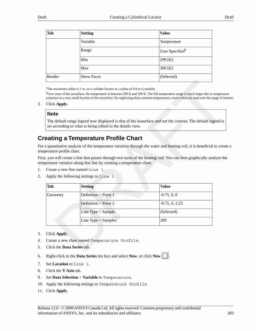
ValueSettingTab
TemperatureVariable
User SpecifiedbRange
299 [K]Min
309 [K]Max
(Selected)Show FacesRender
aThe maximum radius is 1 m, so a cylinder locator at a radius of 0.8 m is suitable.bOver most of the isosurface, the temperature is between 299 K and 309 K. The full temperature range is much larger due to temperatureextremes on a very small fraction of the isosurface. By neglecting those extreme temperatures, more colors are used over the range of interest.
3. Click Apply.
NoteThe default range legend now displayed is that of the isosurface and not the contour. The default legend isset according to what is being edited in the details view.
Creating a Temperature Profile ChartFor a quantitative analysis of the temperature variation through the water and heating coil, it is beneficial to create atemperature profile chart.
First, you will create a line that passes through two turns of the heating coil. You can then graphically analyze thetemperature variance along that line by creating a temperature chart.
1. Create a new line named Line 1.
2. Apply the following settings to Line 1
ValueSettingTab
-0.75, 0, 0Definition > Point 1Geometry
-0.75, 0, 2.25Definition > Point 2
(Selected)Line Type > Sample
200Line Type > Samples
3. Click Apply.
4. Create a new chart named Temperature Profile.
5. Click the Data Series tab.
6. Right-click in the Data Series list box and select New, or click New .
7. Set Location to Line 1.
8. Click the Y Axis tab.
9. Set Data Selection > Variable to Temperature.
10. Apply the following settings to Temperature Profile
11. Click Apply.
283Release 12.0 - © 2009 ANSYS Canada Ltd. All rights reserved. Contains proprietary and confidentialinformation of ANSYS, Inc. and its subsidiaries and affiliates.
DraftCreating a Cylindrical LocatorDraft
You can see from the chart that the temperature spikes upward when entering the deposit region and is at its maximumat the center of the coil turns.
Specular LightingSpecular lighting is on by default. Specular lighting allows glaring bright spots on the surface of an object, dependingon the orientation of the surface and the position of the light. You can disable specular lighting as follows:
1. Apply the following settings to Isosurface 1
ValueSettingTab
(Cleared)Show Faces > SpecularRender
2. Click Apply.
Moving the Light SourceTo move the light source, click within the 3-D Viewer, then press and hold Shift while pressing the arrow keys left,right, up or down.
TipIf using the Standalone version, you can move the light source by positioning the mouse pointer in theviewer, holding down the Ctrl key, and dragging using the right mouse button.
Exporting the Results to ANSYSThis optional step involves generating an ANSYS .cdb data file from the results generated in CFX-Solver. The .cdbfile could then be used with the ANSYS Multi-field solver to measure the combined effects of thermal and mechanicalstresses on the solid heating coil.
There are two possible ways to export data to ANSYS:
• Use CFX-Solver Manager to export data. For details, see Exporting Data from CFX-Solver Manager (p. 284).
• Use CFD-Post to export data. This involves:
1. Importing a surface mesh from ANSYS into CFD-Post, and associating the surface with the corresponding2D region in the CFX-Solver results file.
2. Exporting the data to a file containing SFE commands that represent surface element thermal or mechanicalstress values.
3. Loading the commands created in the previous step into ANSYS and visualizing the loads.
Exporting Data from CFX-Solver ManagerSince the heat transfer in the solid domain was calculated in ANSYS CFX, the 3D thermal data will be exported usingelement type 3D Thermal (70). The mechanical stresses are calculated on the liquid side of the liquid-solidinterface. These values will be exported using element type 2D Stress (154).
Thermal Data1. Start CFX-Solver Manager.
2. Select Tools > Export to ANSYS MultiField.
The Export to ANSYS MultiField Solver dialog box appears.
Release 12.0 - © 2009 ANSYS Canada Ltd. All rights reserved. Contains proprietary and confidentialinformation of ANSYS, Inc. and its subsidiaries and affiliates.284
DraftSpecular LightingDraft
3. Apply the following settings:
ValueSetting
HeatingCoil_001.resResults File
HeatingCoil_001_ansysfsi_70.cdbExport File
SolidZoneDomain Name > Domain
Domain Name > Boundary
a
3D Thermal (70)Export Options > ANSYS Element Type
aLeave Boundary empty since the entire volume is exported for 3D data.
4. Click Export.
When the export is complete, click OK to acknowledge the message and continue with the next steps to exportdata for Mechanical Stresses (p. 285).
Mechanical Stresses1. Apply the following settings in the Export to ANSYS MultiField Solver dialog box (see Step 2 (p. 284) above):
ValueSetting
HeatingCoil_001.resResults File
HeatingCoil_001_ansysfsi_154.cdbExport File
FluidZoneDomain Name > Domain
FluidZone DefaultDomain Name > Boundary
2D Stress (154)Export Options > ANSYS Element Type
2. Click Export.
You now have two exported files that can be used with ANSYS Multi-field solver. When you are finished, closeCFX-Solver Manager and CFD-Post.
285Release 12.0 - © 2009 ANSYS Canada Ltd. All rights reserved. Contains proprietary and confidentialinformation of ANSYS, Inc. and its subsidiaries and affiliates.
DraftExporting Data from CFX-Solver ManagerDraft

Release 12.0 - © 2009 ANSYS Canada Ltd. All rights reserved. Contains proprietary and confidentialinformation of ANSYS, Inc. and its subsidiaries and affiliates.
Chapter 17. Multiphase Flow in a MixingVesselThis tutorial includes:
• Tutorial Features (p. 287)
• Overview of the Problem to Solve (p. 288)
• Before You Begin (p. 289)
• Starting CFX-Pre (p. 289)
• Defining a Case in CFX-Pre (p. 290)
• Obtaining a Solution using CFX-Solver Manager (p. 304)
• Examining the Results in CFD-Post (p. 305)
Tutorial FeaturesIn this tutorial you will learn about:
• Setting up a multiphase flow simulation involving air and water.
• Importing meshes that have CFX-4 and CFX Mesh file formats.
• Setting up a simulation using multiple frames of reference.
• Using a fluid dependent turbulence model to set different turbulence options for each fluid.
• Specifying buoyant flow.
• Specifying a degassing outlet boundary to allow air, but not water, to escape from the boundary.
• Connecting two domains (one for a tank and one for an impeller inside the tank) via Frozen Rotor interfaces.
• Modeling rotational periodicity using periodic boundary conditions.
• Using periodic GGI interfaces where the mesh does not match exactly.
• Using thin surfaces for blade and baffle surfaces.
DetailsFeatureComponent
General ModeUser ModeCFX-Pre
Steady StateAnalysis Type
General FluidFluid Type
Multiple DomainDomain Type
Rotating Frame of Reference
Dispersed Phase Zero EquationTurbulence Model
Fluid-Dependent
k-Epsilon
NoneHeat Transfer
Buoyant Flow
287Release 12.0 - © 2009 ANSYS Canada Ltd. All rights reserved. Contains proprietary and confidentialinformation of ANSYS, Inc. and its subsidiaries and affiliates.
DraftDraft
DetailsFeatureComponent
Multiphase
Inlet (Subsonic)Boundary Conditions
Outlet (Degassing)
Wall: Thin Surface
Wall: (Slip Depends on VolumeFraction)
Frozen RotorDomain Interfaces
Periodic
Thin Surface Partners
Output Control
Physical Time ScaleTimestep
Default LocatorsPlotsCFD-Post
Slice Plane
Quantitative CalculationOther
Overview of the Problem to SolveThis example simulates the mixing of water and air in a mixing vessel. The geometry consists of a mixing tank vessel,an air injection pipe, four baffles, a rotating impeller, and a shaft that runs vertically through the vessel. The impellerrotates at 84 rpm about the X-axis (in the counterclockwise direction, when viewed from above). Air is injected intothe vessel through an inlet pipe located below the impeller at a speed of 5 m/s. The inlet pipe diameter is 2.48 cm.Assume that both the water and air remain at a constant temperature of 25°C and that the air is incompressible, witha density equal to that at 25°C and 1 atmosphere. Also assume that the air bubbles are 3 mm in diameter.
Examine the steady-state distribution of air in the tank. Also calculate the torque and power required to turn the impellerat 84 rpm.
Release 12.0 - © 2009 ANSYS Canada Ltd. All rights reserved. Contains proprietary and confidentialinformation of ANSYS, Inc. and its subsidiaries and affiliates.288
DraftOverview of the Problem to SolveDraft
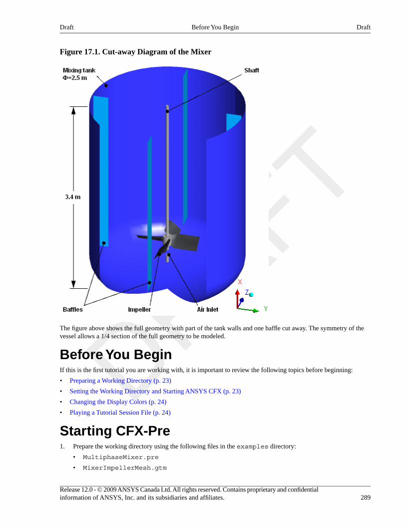
Figure 17.1. Cut-away Diagram of the Mixer
The figure above shows the full geometry with part of the tank walls and one baffle cut away. The symmetry of thevessel allows a 1/4 section of the full geometry to be modeled.
Before You BeginIf this is the first tutorial you are working with, it is important to review the following topics before beginning:
• Preparing a Working Directory (p. 23)
• Setting the Working Directory and Starting ANSYS CFX (p. 23)
• Changing the Display Colors (p. 24)
• Playing a Tutorial Session File (p. 24)
Starting CFX-Pre1. Prepare the working directory using the following files in the examples directory:
• MultiphaseMixer.pre
• MixerImpellerMesh.gtm
289Release 12.0 - © 2009 ANSYS Canada Ltd. All rights reserved. Contains proprietary and confidentialinformation of ANSYS, Inc. and its subsidiaries and affiliates.
DraftBefore You BeginDraft
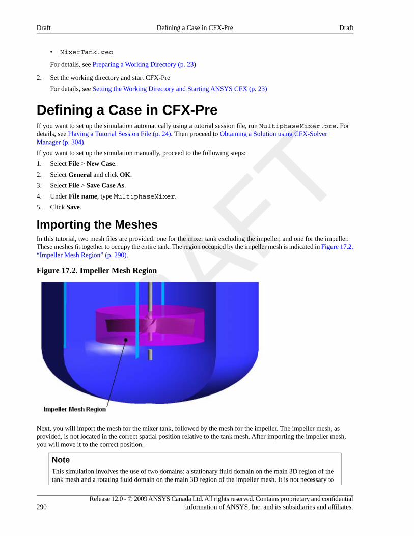
• MixerTank.geo
For details, see Preparing a Working Directory (p. 23)
2. Set the working directory and start CFX-Pre
For details, see Setting the Working Directory and Starting ANSYS CFX (p. 23)
Defining a Case in CFX-PreIf you want to set up the simulation automatically using a tutorial session file, run MultiphaseMixer.pre. Fordetails, see Playing a Tutorial Session File (p. 24). Then proceed to Obtaining a Solution using CFX-SolverManager (p. 304).
If you want to set up the simulation manually, proceed to the following steps:
1. Select File > New Case.
2. Select General and click OK.
3. Select File > Save Case As.
4. Under File name, type MultiphaseMixer.
5. Click Save.
Importing the MeshesIn this tutorial, two mesh files are provided: one for the mixer tank excluding the impeller, and one for the impeller.These meshes fit together to occupy the entire tank. The region occupied by the impeller mesh is indicated in Figure 17.2,“Impeller Mesh Region” (p. 290).
Figure 17.2. Impeller Mesh Region
Next, you will import the mesh for the mixer tank, followed by the mesh for the impeller. The impeller mesh, asprovided, is not located in the correct spatial position relative to the tank mesh. After importing the impeller mesh,you will move it to the correct position.
NoteThis simulation involves the use of two domains: a stationary fluid domain on the main 3D region of thetank mesh and a rotating fluid domain on the main 3D region of the impeller mesh. It is not necessary to
Release 12.0 - © 2009 ANSYS Canada Ltd. All rights reserved. Contains proprietary and confidentialinformation of ANSYS, Inc. and its subsidiaries and affiliates.290
DraftDefining a Case in CFX-PreDraft
use separate meshes in this type of simulation, as long as there are 3D regions available for locating thesetwo domains.
Importing the Mixer Tank MeshThe mixer tank mesh is provided as a CFX-4 mesh file (*.geo). Import it as follows:
1. Edit Case Options > General in the Outline tree view and ensure that Automatic Default Domain andAutomatic Default Interfaces are turned off.
Default Domain and Interface generation should be turned off because you will be manually creating domainsand interfaces for the impeller and main tank later in this tutorial.
2. Right-click Mesh and select Import Mesh > Other.
The Import Mesh dialog box appears.
3. Apply the following settings:
ValueSetting
CFX-4(*geo)Files of type
MixerTank.geoFile name
mOptions > Mesh Units
(Cleared)aAdvanced Options > CFX-4 Options > Create 3D Regions on >Fluid Regions (USER3D, POROUS)
aIn this case, the mesh file contains USER3D regions that you do not need.
4. Click Open.
Importing the Impeller MeshThe impeller mesh is provided as a CFX Mesh file (*.gtm). Import it as follows:
1. Right-click Mesh and select Import Mesh > Other to import the second mesh. The Import Mesh dialog boxappears.
2. Apply the following settings:
ValueSetting
CFX Mesh (*gtm *cfx)Files of type
MixerImpellerMesh.gtmFile name
3. Click Open.
4. Right-click a blank area in the viewer and select Predefined Camera > Isometric View (X up) to view the meshassemblies.
Relocating the Impeller MeshIn the next step you will move the impeller mesh to its correct position.
1. Right-click MixerImpellerMesh.gtm and select Transform Mesh.
The Mesh Transformation Editor dialog box appears.
291Release 12.0 - © 2009 ANSYS Canada Ltd. All rights reserved. Contains proprietary and confidentialinformation of ANSYS, Inc. and its subsidiaries and affiliates.
DraftImporting the MeshesDraft
2. Apply the following settings:
ValueSetting
TranslationTransformation
DeltasMethod
0.275, 0, 0Dx, Dy, Dz
3. Click Apply then Close.
Viewing the Mesh at the Tank Periodic Boundary1. In the Outline workspace, expand the tree to show MixerTank.geo > Principal 3D Regions >
Primitive 3D > Principal 2D Regions.
2. Click the primitive region BLKBDY_TANK_PER2.
You can now see the mesh on one of the periodic regions of the tank. To reduce the solution time for this tutorial, themesh used is very coarse. This is not a suitable mesh to obtain accurate results, but it is sufficient for demonstrationpurposes.
NoteIf you do not see the surface mesh, highlighting may be turned off. If highlighting is disabled, toggle
Highlighting . The default highlight type will show the surface mesh for any selected regions. If you
see a different highlighting type, you can alter it by selecting Edit > Options and browsing to CFX-Pre >Graphics Style.
Creating the DomainsThe mixer requires two domains: a rotating impeller domain and a stationary tank domain. Both domains contain wateras a continuous phase and air as a dispersed phase. The domains will model turbulence, buoyancy, and forces betweenthe fluids.
Rotating Domain for the ImpellerAs stated in the problem description, the impeller rotates at 84 rpm.
1. Ensure that no default domain is present under Flow Analysis 1. If a default domain is present, right-clickit and select Delete.
2. Click Domain and set the name to impeller.
3. Under the Fluid and Particle Definitions setting, delete Fluid 1 and create a new fluid definition called Air.
4. Click Add new item and name it Water
5. Apply the following settings:
ValueSettingTab
MainLocation and Type > LocationBasicSettings
AirFluid and Particle Definitions
Air at 25 CFluid and Particle Definitions > Air > Material
Release 12.0 - © 2009 ANSYS Canada Ltd. All rights reserved. Contains proprietary and confidentialinformation of ANSYS, Inc. and its subsidiaries and affiliates.292
DraftCreating the DomainsDraft
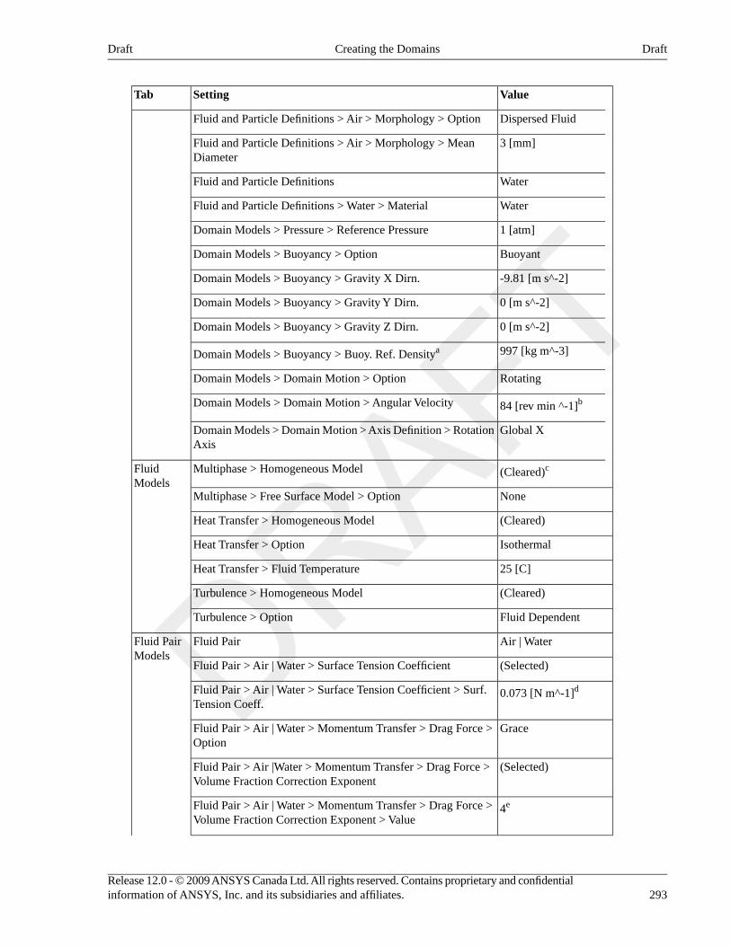
ValueSettingTab
Dispersed FluidFluid and Particle Definitions > Air > Morphology > Option
3 [mm]Fluid and Particle Definitions > Air > Morphology > MeanDiameter
WaterFluid and Particle Definitions
WaterFluid and Particle Definitions > Water > Material
1 [atm]Domain Models > Pressure > Reference Pressure
BuoyantDomain Models > Buoyancy > Option
-9.81 [m s^-2]Domain Models > Buoyancy > Gravity X Dirn.
0 [m s^-2]Domain Models > Buoyancy > Gravity Y Dirn.
0 [m s^-2]Domain Models > Buoyancy > Gravity Z Dirn.
997 [kg m^-3]Domain Models > Buoyancy > Buoy. Ref. Densitya
RotatingDomain Models > Domain Motion > Option
84 [rev min ^-1]bDomain Models > Domain Motion > Angular Velocity
Global XDomain Models > Domain Motion > Axis Definition > RotationAxis
(Cleared)cMultiphase > Homogeneous ModelFluidModels
NoneMultiphase > Free Surface Model > Option
(Cleared)Heat Transfer > Homogeneous Model
IsothermalHeat Transfer > Option
25 [C]Heat Transfer > Fluid Temperature
(Cleared)Turbulence > Homogeneous Model
Fluid DependentTurbulence > Option
Air | WaterFluid PairFluid PairModels
(Selected)Fluid Pair > Air | Water > Surface Tension Coefficient
0.073 [N m^-1]dFluid Pair > Air | Water > Surface Tension Coefficient > Surf.Tension Coeff.
GraceFluid Pair > Air | Water > Momentum Transfer > Drag Force >Option
(Selected)Fluid Pair > Air |Water > Momentum Transfer > Drag Force >Volume Fraction Correction Exponent
4eFluid Pair > Air | Water > Momentum Transfer > Drag Force >Volume Fraction Correction Exponent > Value
293Release 12.0 - © 2009 ANSYS Canada Ltd. All rights reserved. Contains proprietary and confidentialinformation of ANSYS, Inc. and its subsidiaries and affiliates.
DraftCreating the DomainsDraft
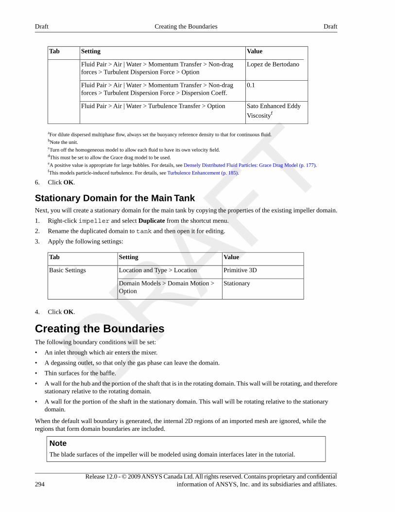
ValueSettingTab
Lopez de BertodanoFluid Pair > Air | Water > Momentum Transfer > Non-dragforces > Turbulent Dispersion Force > Option
0.1Fluid Pair > Air | Water > Momentum Transfer > Non-dragforces > Turbulent Dispersion Force > Dispersion Coeff.
Sato Enhanced Eddy
ViscosityfFluid Pair > Air | Water > Turbulence Transfer > Option
aFor dilute dispersed multiphase flow, always set the buoyancy reference density to that for continuous fluid.bNote the unit.cTurn off the homogeneous model to allow each fluid to have its own velocity field.dThis must be set to allow the Grace drag model to be used.eA positive value is appropriate for large bubbles. For details, see Densely Distributed Fluid Particles: Grace Drag Model (p. 177).fThis models particle-induced turbulence. For details, see Turbulence Enhancement (p. 185).
6. Click OK.
Stationary Domain for the Main TankNext, you will create a stationary domain for the main tank by copying the properties of the existing impeller domain.
1. Right-click impeller and select Duplicate from the shortcut menu.
2. Rename the duplicated domain to tank and then open it for editing.
3. Apply the following settings:
ValueSettingTab
Primitive 3DLocation and Type > LocationBasic Settings
StationaryDomain Models > Domain Motion >Option
4. Click OK.
Creating the BoundariesThe following boundary conditions will be set:
• An inlet through which air enters the mixer.
• A degassing outlet, so that only the gas phase can leave the domain.
• Thin surfaces for the baffle.
• A wall for the hub and the portion of the shaft that is in the rotating domain. This wall will be rotating, and thereforestationary relative to the rotating domain.
• A wall for the portion of the shaft in the stationary domain. This wall will be rotating relative to the stationarydomain.
When the default wall boundary is generated, the internal 2D regions of an imported mesh are ignored, while theregions that form domain boundaries are included.
NoteThe blade surfaces of the impeller will be modeled using domain interfaces later in the tutorial.
Release 12.0 - © 2009 ANSYS Canada Ltd. All rights reserved. Contains proprietary and confidentialinformation of ANSYS, Inc. and its subsidiaries and affiliates.294
DraftCreating the BoundariesDraft
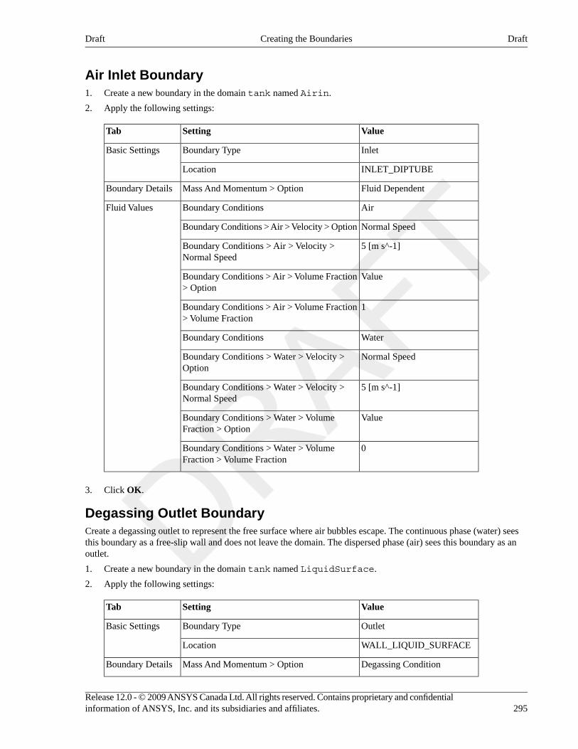
Air Inlet Boundary1. Create a new boundary in the domain tank named Airin.
2. Apply the following settings:
ValueSettingTab
InletBoundary TypeBasic Settings
INLET_DIPTUBELocation
Fluid DependentMass And Momentum > OptionBoundary Details
AirBoundary ConditionsFluid Values
Normal SpeedBoundary Conditions > Air > Velocity > Option
5 [m s^-1]Boundary Conditions > Air > Velocity >Normal Speed
ValueBoundary Conditions > Air > Volume Fraction> Option
1Boundary Conditions > Air > Volume Fraction> Volume Fraction
WaterBoundary Conditions
Normal SpeedBoundary Conditions > Water > Velocity >Option
5 [m s^-1]Boundary Conditions > Water > Velocity >Normal Speed
ValueBoundary Conditions > Water > VolumeFraction > Option
0Boundary Conditions > Water > VolumeFraction > Volume Fraction
3. Click OK.
Degassing Outlet BoundaryCreate a degassing outlet to represent the free surface where air bubbles escape. The continuous phase (water) seesthis boundary as a free-slip wall and does not leave the domain. The dispersed phase (air) sees this boundary as anoutlet.
1. Create a new boundary in the domain tank named LiquidSurface.
2. Apply the following settings:
ValueSettingTab
OutletBoundary TypeBasic Settings
WALL_LIQUID_SURFACELocation
Degassing ConditionMass And Momentum > OptionBoundary Details
295Release 12.0 - © 2009 ANSYS Canada Ltd. All rights reserved. Contains proprietary and confidentialinformation of ANSYS, Inc. and its subsidiaries and affiliates.
DraftCreating the BoundariesDraft
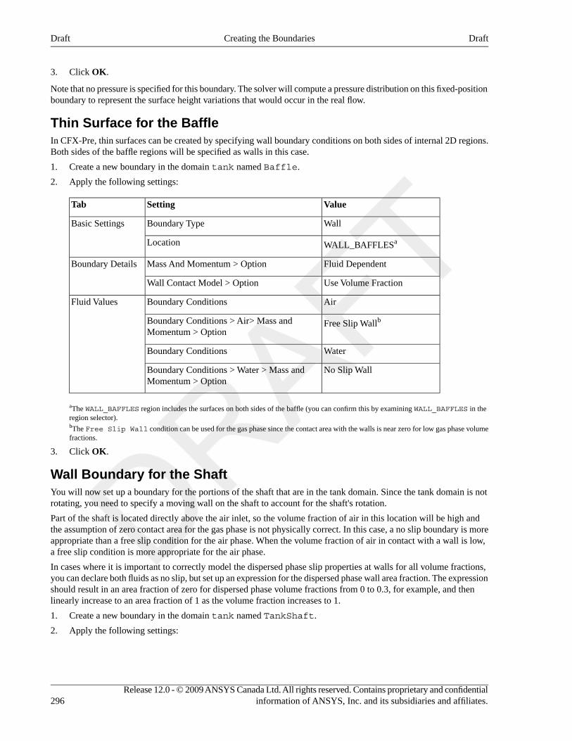
3. Click OK.
Note that no pressure is specified for this boundary. The solver will compute a pressure distribution on this fixed-positionboundary to represent the surface height variations that would occur in the real flow.
Thin Surface for the BaffleIn CFX-Pre, thin surfaces can be created by specifying wall boundary conditions on both sides of internal 2D regions.Both sides of the baffle regions will be specified as walls in this case.
1. Create a new boundary in the domain tank named Baffle.
2. Apply the following settings:
ValueSettingTab
WallBoundary TypeBasic Settings
WALL_BAFFLESaLocation
Fluid DependentMass And Momentum > OptionBoundary Details
Use Volume FractionWall Contact Model > Option
AirBoundary ConditionsFluid Values
Free Slip WallbBoundary Conditions > Air> Mass andMomentum > Option
WaterBoundary Conditions
No Slip WallBoundary Conditions > Water > Mass andMomentum > Option
aThe WALL_BAFFLES region includes the surfaces on both sides of the baffle (you can confirm this by examining WALL_BAFFLES in theregion selector).bThe Free Slip Wall condition can be used for the gas phase since the contact area with the walls is near zero for low gas phase volumefractions.
3. Click OK.
Wall Boundary for the ShaftYou will now set up a boundary for the portions of the shaft that are in the tank domain. Since the tank domain is notrotating, you need to specify a moving wall on the shaft to account for the shaft's rotation.
Part of the shaft is located directly above the air inlet, so the volume fraction of air in this location will be high andthe assumption of zero contact area for the gas phase is not physically correct. In this case, a no slip boundary is moreappropriate than a free slip condition for the air phase. When the volume fraction of air in contact with a wall is low,a free slip condition is more appropriate for the air phase.
In cases where it is important to correctly model the dispersed phase slip properties at walls for all volume fractions,you can declare both fluids as no slip, but set up an expression for the dispersed phase wall area fraction. The expressionshould result in an area fraction of zero for dispersed phase volume fractions from 0 to 0.3, for example, and thenlinearly increase to an area fraction of 1 as the volume fraction increases to 1.
1. Create a new boundary in the domain tank named TankShaft.
2. Apply the following settings:
Release 12.0 - © 2009 ANSYS Canada Ltd. All rights reserved. Contains proprietary and confidentialinformation of ANSYS, Inc. and its subsidiaries and affiliates.296
DraftCreating the BoundariesDraft
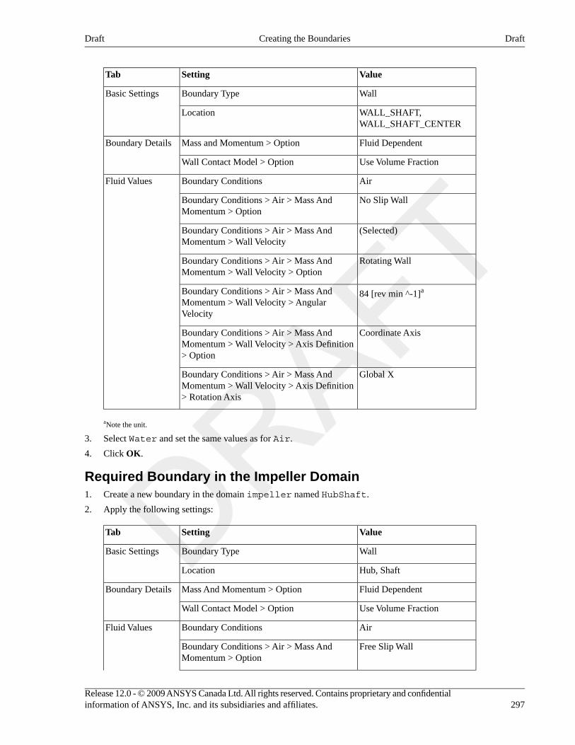
ValueSettingTab
WallBoundary TypeBasic Settings
WALL_SHAFT,WALL_SHAFT_CENTER
Location
Fluid DependentMass and Momentum > OptionBoundary Details
Use Volume FractionWall Contact Model > Option
AirBoundary ConditionsFluid Values
No Slip WallBoundary Conditions > Air > Mass AndMomentum > Option
(Selected)Boundary Conditions > Air > Mass AndMomentum > Wall Velocity
Rotating WallBoundary Conditions > Air > Mass AndMomentum > Wall Velocity > Option
84 [rev min ^-1]aBoundary Conditions > Air > Mass AndMomentum > Wall Velocity > AngularVelocity
Coordinate AxisBoundary Conditions > Air > Mass AndMomentum > Wall Velocity > Axis Definition> Option
Global XBoundary Conditions > Air > Mass AndMomentum > Wall Velocity > Axis Definition> Rotation Axis
aNote the unit.
3. Select Water and set the same values as for Air.
4. Click OK.
Required Boundary in the Impeller Domain1. Create a new boundary in the domain impeller named HubShaft.
2. Apply the following settings:
ValueSettingTab
WallBoundary TypeBasic Settings
Hub, ShaftLocation
Fluid DependentMass And Momentum > OptionBoundary Details
Use Volume FractionWall Contact Model > Option
AirBoundary ConditionsFluid Values
Free Slip WallBoundary Conditions > Air > Mass AndMomentum > Option
297Release 12.0 - © 2009 ANSYS Canada Ltd. All rights reserved. Contains proprietary and confidentialinformation of ANSYS, Inc. and its subsidiaries and affiliates.
DraftCreating the BoundariesDraft
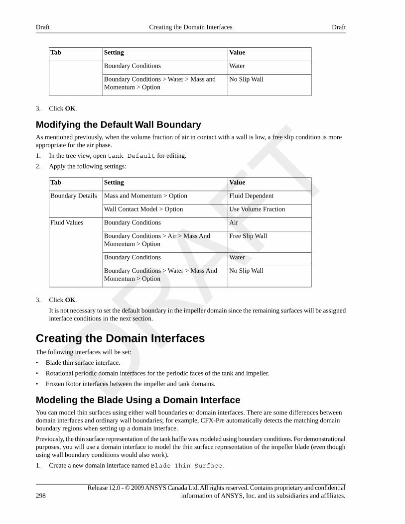
ValueSettingTab
WaterBoundary Conditions
No Slip WallBoundary Conditions > Water > Mass andMomentum > Option
3. Click OK.
Modifying the Default Wall BoundaryAs mentioned previously, when the volume fraction of air in contact with a wall is low, a free slip condition is moreappropriate for the air phase.
1. In the tree view, open tank Default for editing.
2. Apply the following settings:
ValueSettingTab
Fluid DependentMass and Momentum > OptionBoundary Details
Use Volume FractionWall Contact Model > Option
AirBoundary ConditionsFluid Values
Free Slip WallBoundary Conditions > Air > Mass AndMomentum > Option
WaterBoundary Conditions
No Slip WallBoundary Conditions > Water > Mass AndMomentum > Option
3. Click OK.
It is not necessary to set the default boundary in the impeller domain since the remaining surfaces will be assignedinterface conditions in the next section.
Creating the Domain InterfacesThe following interfaces will be set:
• Blade thin surface interface.
• Rotational periodic domain interfaces for the periodic faces of the tank and impeller.
• Frozen Rotor interfaces between the impeller and tank domains.
Modeling the Blade Using a Domain InterfaceYou can model thin surfaces using either wall boundaries or domain interfaces. There are some differences betweendomain interfaces and ordinary wall boundaries; for example, CFX-Pre automatically detects the matching domainboundary regions when setting up a domain interface.
Previously, the thin surface representation of the tank baffle was modeled using boundary conditions. For demonstrationalpurposes, you will use a domain interface to model the thin surface representation of the impeller blade (even thoughusing wall boundary conditions would also work).
1. Create a new domain interface named Blade Thin Surface.
Release 12.0 - © 2009 ANSYS Canada Ltd. All rights reserved. Contains proprietary and confidentialinformation of ANSYS, Inc. and its subsidiaries and affiliates.298
DraftCreating the Domain InterfacesDraft
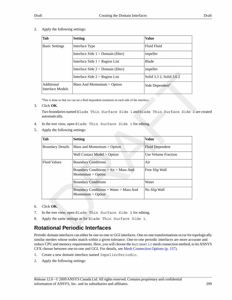
2. Apply the following settings:
ValueSettingTab
Fluid FluidInterface TypeBasic Settings
impellerInterface Side 1 > Domain (filter)
BladeInterface Side 1 > Region List
impellerInterface Side 2 > Domain (filter)
Solid 3.3 2, Solid 3.6 2Interface Side 2 > Region List
Side DependentaMass And Momentum > OptionAdditionalInterface Models
aThis is done so that we can set a fluid dependent treatment on each side of the interface.
3. Click OK.
Two boundaries named Blade Thin Surface Side 1 and Blade Thin Surface Side 2 are createdautomatically.
4. In the tree view, open Blade Thin Surface Side 1 for editing.
5. Apply the following settings:
ValueSettingTab
Fluid DependentMass and Momentum > OptionBoundary Details
Use Volume FractionWall Contact Model > Option
AirBoundary ConditionsFluid Values
Free Slip WallBoundary Conditions > Air > Mass AndMomentum > Option
WaterBoundary Conditions
No Slip WallBoundary Conditions > Water > Mass AndMomentum > Option
6. Click OK.
7. In the tree view, open Blade Thin Surface Side 2 for editing.
8. Apply the same settings as for Blade Thin Surface Side 1.
Rotational Periodic InterfacesPeriodic domain interfaces can either be one-to-one or GGI interfaces. One-to-one transformations occur for topologicallysimilar meshes whose nodes match within a given tolerance. One-to-one periodic interfaces are more accurate andreduce CPU and memory requirements. Here, you will choose the Automatic mesh connection method, to let ANSYSCFX choose between one-to-one and GGI. For details, see Mesh Connection Options (p. 157).
1. Create a new domain interface named ImpellerPeriodic.
2. Apply the following settings:
299Release 12.0 - © 2009 ANSYS Canada Ltd. All rights reserved. Contains proprietary and confidentialinformation of ANSYS, Inc. and its subsidiaries and affiliates.
DraftCreating the Domain InterfacesDraft
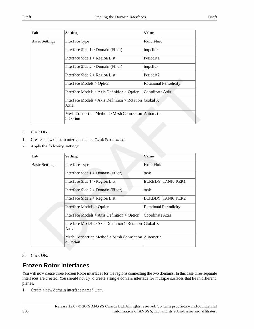
ValueSettingTab
Fluid FluidInterface TypeBasic Settings
impellerInterface Side 1 > Domain (Filter)
Periodic1Interface Side 1 > Region List
impellerInterface Side 2 > Domain (Filter)
Periodic2Interface Side 2 > Region List
Rotational PeriodicityInterface Models > Option
Coordinate AxisInterface Models > Axis Definition > Option
Global XInterface Models > Axis Definition > RotationAxis
AutomaticMesh Connection Method > Mesh Connection> Option
3. Click OK.
1. Create a new domain interface named TankPeriodic.
2. Apply the following settings:
ValueSettingTab
Fluid FluidInterface TypeBasic Settings
tankInterface Side 1 > Domain (Filter)
BLKBDY_TANK_PER1Interface Side 1 > Region List
tankInterface Side 2 > Domain (Filter)
BLKBDY_TANK_PER2Interface Side 2 > Region List
Rotational PeriodicityInterface Models > Option
Coordinate AxisInterface Models > Axis Definition > Option
Global XInterface Models > Axis Definition > RotationAxis
AutomaticMesh Connection Method > Mesh Connection> Option
3. Click OK.
Frozen Rotor InterfacesYou will now create three Frozen Rotor interfaces for the regions connecting the two domains. In this case three separateinterfaces are created. You should not try to create a single domain interface for multiple surfaces that lie in differentplanes.
1. Create a new domain interface named Top.
Release 12.0 - © 2009 ANSYS Canada Ltd. All rights reserved. Contains proprietary and confidentialinformation of ANSYS, Inc. and its subsidiaries and affiliates.300
DraftCreating the Domain InterfacesDraft
2. Apply the following settings:
ValueSettingTab
Fluid FluidInterface TypeBasic Settings
impellerInterface Side 1 > Domain (Filter)
TopInterface Side 1 > Region List
tankInterface Side 2 > Domain (Filter)
BLKBDY_TANK_TOPInterface Side 2 > Region List
General ConnectionInterface Models > Option
Frozen RotorInterface Models > Frame Change/MixingModel > Option
3. Click OK.
4. Create a new domain interface named Bottom.
5. Apply the following settings:
ValueSettingTab
Fluid FluidInterface TypeBasic Settings
impellerInterface Side 1 > Domain (Filter)
BottomInterface Side 1 > Region List
tankInterface Side 2 > Domain (Filter)
BLKBDY_TANK_BOTInterface Side 2 > Region List
General ConnectionInterface Models > Option
Frozen RotorInterface Models > Frame Change/MixingModel > Option
6. Click OK.
7. Create a new domain interface named Outer.
8. Apply the following settings:
ValueSettingTab
Fluid FluidInterface TypeBasic Settings
impellerInterface Side 1 > Domain (Filter)
OuterInterface Side 1 > Region List
tankInterface Side 2 > Domain (Filter)
BLKBDY_TANK_OUTERInterface Side 2 > Region List
General ConnectionInterface Models > Option
301Release 12.0 - © 2009 ANSYS Canada Ltd. All rights reserved. Contains proprietary and confidentialinformation of ANSYS, Inc. and its subsidiaries and affiliates.
DraftCreating the Domain InterfacesDraft
ValueSettingTab
Frozen RotorInterface Models > Frame Change/MixingModel > Option
9. Click OK.
For more details about the Frozen Rotor interface, see Frozen Rotor (p. 150).
Setting Initial ValuesYou will set the initial volume fraction of air to 0, and allow the initial volume fraction of water to be computedautomatically. Since the volume fractions must sum to unity, the initial volume fraction of water will be 1.
It is important to understand how the velocity is initialized in this tutorial. Here, both fluids use Automatic for theCartesian Velocity Components option. When the Automatic option is used, the initial velocity field will be basedon the velocity values set at inlets, openings, and outlets. In this tutorial, the only boundary that has a set velocity valueis the inlet, which specifies a velocity of 5 [m s^-1] for both phases. Without setting the Velocity Scale parameter, theresulting initial guess would be a uniform velocity of 5 [m s^-1] in the X-direction throughout the domains for bothphases. This is clearly not suitable since the water phase is enclosed by the tank. When the boundary velocity conditionsare not representative of the expected domain velocities, the Velocity Scale parameter should be used to set arepresentative domain velocity. In this case the velocity scale for water is set to zero, causing the initial velocity forthe water to be zero. The velocity scale is not set for air, resulting in an initial velocity of 5 [m s^-1] in the X-directionfor the air. This should not be a problem since the initial volume fraction of the air is zero everywhere.
1. Click Global Initialization .
2. Apply the following settings:
ValueSettingTab
AirFluid Specific InitializationFluid Settings
Automatic with ValueFluid Specific Initialization > Air > Initial Conditions> Volume Fraction > Option
0Fluid Specific Initialization > Air > Initial Conditions> Volume Fraction > Volume Fraction
WaterFluid Specific Initialization
AutomaticFluid Specific Initialization > Water > InitialConditions > Cartesian Velocity Components > Option
(Selected)Fluid Specific Initialization > Water > InitialConditions > Cartesian Velocity Components >Velocity Scale
0 [m s^-1]Fluid Specific Initialization > Water > InitialConditions > Cartesian Velocity Components >Velocity Scale > Value
3. Click OK.
Release 12.0 - © 2009 ANSYS Canada Ltd. All rights reserved. Contains proprietary and confidentialinformation of ANSYS, Inc. and its subsidiaries and affiliates.302
DraftSetting Initial ValuesDraft
Setting Solver ControlGenerally, two different time scales exist for multiphase mixers. The first is a small time scale based on the rotationalspeed of the impeller, typically taken as 1 / ω, resulting in a time scale of 0.11 s for this case. The second time scaleis usually larger and based on the recirculation time of the continuous phase in the mixer.
Using a time step based on the rotational speed of the impeller will be more robust, but convergence will be slow sinceit takes time for the flow field in the mixer to develop. Using a larger time step reduces the number of iterations requiredfor the mixer flow field to develop, but reduces robustness. You will need to experiment to find an optimum time step.
1. Click Solver Control .
2. Apply the following settings:
ValueSettingTab
High ResolutionAdvection Scheme > OptionBasic Settings
100aConvergence Control > Max. Iterations
Physical TimescaleConvergence Control > Fluid TimescaleControl > Timescale Control
2 [s]bConvergence Control > Fluid TimescaleControl > Physical Timescale
(Default)cConvergence Criteria
aFor advice on setting time steps in multiphase simulations, see Timestepping (p. 201).bThis is an aggressive time step for this case.cThe default is an RMS value of 1.0E-04. If you are using a maximum edge length of 0.005 m or less to produce a finer mesh, use a targetresidual of 1.0E-05 to obtain a more accurate solution.
3. Click OK.
Adding Monitor PointsYou can monitor the value of an expression during the solver run so that you can view the volume fraction of air inthe tank (the gas hold up). The gas hold up is often used to judge convergence in these types of simulations by converginguntil a steady-state value is achieved.
1. Create the following expressions:
TankAirHoldUp = volumeAve(Air.vf)@tankImpellerAirHoldUp = volumeAve(Air.vf)@impellerTotalAirHoldUp = (volume()@tank * TankAirHoldUp + volume()@impeller * ImpellerAirHoldUp) / (volume()@tank + volume()@impeller)
2. Click Output Control .
3. Apply the following settings:
ValueSettingTab
(Selected)Monitor OptionsMonitor
303Release 12.0 - © 2009 ANSYS Canada Ltd. All rights reserved. Contains proprietary and confidentialinformation of ANSYS, Inc. and its subsidiaries and affiliates.
DraftSetting Solver ControlDraft
4. Create a new Monitor Points and Expressions item named Total Air Holdup.
5. Apply the following settings to Total Air Holdup:
ValueSetting
ExpressionOption
TotalAirHoldUpExpression Value
6. Click OK.
Writing the CFX-Solver Input (.def) File
1. Click Define Run .
2. Apply the following settings:
ValueSetting
MultiphaseMixer.defFile name
3. Click Save.
If you are notified the file already exists, click Overwrite.
4. Click OK.
5. If using Standalone Mode, quit CFX-Pre, saving the simulation (.cfx) file at your discretion.
Obtaining a Solution using CFX-Solver ManagerStart the simulation from CFX-Solver Manager:
1. Ensure Define Run is displayed.
2. Click Start Run.
CFX-Solver runs and attempts to obtain a solution. This can take a long time depending on your system.
After a run has finished, examine some of the information printed at the end of the OUT file.
A common quantity of interest is the mass balance; this compares the amount of fluid leaving the domain to theamount entering.
• In most cases, the global imbalance should be less than 0.1% in a converged solution.
• For a single-phase simulation, the mass balance information is given for the P-Mass equation.
• For a multiphase simulation, the mass balance information is given for the P-Vol equation.
• This is not the volumetric flow balance information, but is the summation of the phasic continuity mass balanceinformation.
3. Select the check box next to Post-Process Results when the completion message appears at the end of the run.
4. If using Standalone Mode, select the check box next to Shut down CFX-Solver Manager.
5. Click OK.
Release 12.0 - © 2009 ANSYS Canada Ltd. All rights reserved. Contains proprietary and confidentialinformation of ANSYS, Inc. and its subsidiaries and affiliates.304
DraftWriting the CFX-Solver Input (.def) FileDraft
Examining the Results in CFD-PostAfter CFD-Post has started and the tank and mixer domains have been loaded, the mixer geometry appears in theviewer. Orient the view so that the X-axis points up as follows:
• Right-click a blank area in the viewer and select Predefined Camera > Isometric View (X up).
You will create some plots showing the distributions of velocity and other variables. You will also calculate the torqueand power required to turn the impeller at 84 rpm.
Creating a Plane LocatorCreate a vertical plane that extends from the shaft to the tank wall at a location far from the baffle. This plane will beused as a locator for various plots, such as velocity vector plots and plots showing the distribution of air.
1. Create a new plane named Plane 1.
2. Apply the following settings:
ValueSettingTab
Three PointsDefinition > MethodGeometry
1, 0, 0Definition > Point 1
0, 1, -0.9Definition > Point 2
0, 0, 0Definition > Point 3
3. Click Apply.
Plotting VelocityRecall that the homogeneous multiphase option was not used when specifying the domain settings (see the setting forFluid Models > Multiphase Options > Homogeneous Model in Rotating Domain for the Impeller (p. 292)). As aconsequence, the air and water velocity fields may differ from each other. Plot the velocity of water, then air on Plane1:
1. Create a new vector plot named Vector 1.
2. Apply the following settings:
ValueSettingTab
Plane 1Definition > LocationsGeometry
Water.Velocity in Stn FrameaVariable
0.2Symbol SizeSymbol
(Selected)Normalize Symbols
aUsing this variable, instead of Water.Velocity, results in the velocity vectors appearing to be continuous at the interface between the rotatingand stationary domains. Velocity variables that do not include a frame specification always use the local reference frame.
3. Click Apply.
4. Turn off the visibility of Plane 1 to better see the vector plot.
5. Observe the vector plot (in particular, near the top of the tank). Note that the water is not flowing out of the domain.
305Release 12.0 - © 2009 ANSYS Canada Ltd. All rights reserved. Contains proprietary and confidentialinformation of ANSYS, Inc. and its subsidiaries and affiliates.
DraftExamining the Results in CFD-PostDraft
6. Change the variable to Air.Velocity in Stn Frame and click Apply.
Observe this vector plot, noting how the air moves upward all the way to the water surface, where it escapes.
7. Turn off the visibility of Vector 1 in preparation for the next plots.
Plotting Pressure DistributionColor Plane 1 to see the pressure distribution:
1. Turn on the visibility of Plane 1.
2. Apply the following settings to Plane 1:
ValueSettingTab
VariableModeColor
PressureVariable
LocalRange
3. Click Apply.
Note that the pressure field computed by the solver excludes the hydrostatic pressure corresponding to the specifiedbuoyancy reference density. The pressure field including this hydrostatic component (as well as the referencepressure) can by visualized by plotting Absolute Pressure.
Plotting Volume FractionsTo see the distribution of air, color Plane 1 by the volume fraction of air:
1. Apply the following settings to Plane 1:
ValueSettingTab
VariableModeColor
Air.Volume FractionVariable
User SpecifiedRange
0Min
0.04Max
2. Click Apply.
The user-specified range was made much narrower than the Global and Local ranges in order to better show thevariation.
Plotting Shear Strain Rate and Shear StressAreas of high shear strain rate or shear stress are typically also areas where the highest mixing occurs.
To see where the most of the mixing occurs, color Plane 1 by shear strain rate.
1. Apply the following settings to Plane 1:
Release 12.0 - © 2009 ANSYS Canada Ltd. All rights reserved. Contains proprietary and confidentialinformation of ANSYS, Inc. and its subsidiaries and affiliates.306
DraftPlotting Pressure DistributionDraft
ValueSettingTab
Air.Shear Strain RateVariableColor
User SpecifiedRange
0 [s^-1]Min
15 [s^-1]Max
2. Click Apply.
The user-specified range was made much narrower than the Global and Local ranges in order to better show thevariation.
3. Modify the coloring of the MultiphaseMixer_001 > tank > tank Default object by applying thefollowing settings:
ValueSettingTab
VariableModeColor
Water.Wall ShearVariable
LocalRange
4. Click Apply.
The legend for this plot shows the range of wall shear values.
The global maximum wall shear stress is much higher than the maximum value on the default walls. The globalmaximum values occur on the TankShaft boundary directly above the inlet. Although these values are very high,the shear force exerted on this boundary is small since the contact area fraction of water is very small there.
Calculating Torque and Power RequirementsCalculate the torque and power required to spin the impeller at 84 rpm:
1. Select Tools > Function Calculator from the main menu or click Show Function Calculator .
2. Apply the following settings:
ValueSettingTab
torqueFunctionFunction Calculator
Blade Thin Surface Side 1Location
Global XAxis
All FluidsFluid
3. Click Calculate to find the torque about the X-axis imparted by both fluids on location Blade Thin SurfaceSide 1.
4. Repeat the calculation, setting Location to Blade Thin Surface Side 2.
The sum of these two torques is approximately -67.4 [N m] about the X-axis. Multiplying by -4 to find the torquerequired by all of the impeller blades gives a required torque of approximately 270 [N m] about the X-axis. You could
307Release 12.0 - © 2009 ANSYS Canada Ltd. All rights reserved. Contains proprietary and confidentialinformation of ANSYS, Inc. and its subsidiaries and affiliates.
DraftCalculating Torque and Power RequirementsDraft

also include the contributions from the locations HubShaft and TankShaft; however in this case their contributionsare negligible.
The power requirement is simply the required torque multiplied by the rotational speed (84 rpm = 8.8 rad/s): Power = 270N m * 8.8 rad/s = 2376 W.
Remember that this value is the power requirement for the work done on the fluids; it does not account for any mechanicallosses, motor efficiencies etc. Also note that the accuracy of these results is significantly affected by the coarseness ofthe mesh. You should not use a mesh of this length scale to obtain accurate quantitative results.
Release 12.0 - © 2009 ANSYS Canada Ltd. All rights reserved. Contains proprietary and confidentialinformation of ANSYS, Inc. and its subsidiaries and affiliates.308
DraftCalculating Torque and Power RequirementsDraft
Chapter 18. Gas-Liquid Flow in an AirliftReactorThis tutorial includes:
• Tutorial Features (p. 309)
• Overview of the Problem to Solve (p. 310)
• Before You Begin (p. 311)
• Starting CFX-Pre (p. 311)
• Defining a Case in CFX-Pre (p. 311)
• Obtaining a Solution using CFX-Solver Manager (p. 318)
• Viewing the Results in CFD-Post (p. 318)
• Additional Fine Mesh Simulation Results (p. 321)
Tutorial FeaturesIn this tutorial you will learn about:
• Setting up a multiphase flow simulation involving air and water.
• Using a fluid dependent turbulence model to set different turbulence options for each fluid.
• Specifying buoyant flow.
• Specifying a degassing outlet boundary to allow air, but not water, to escape from the boundary.
• Using face culling in CFD-Post to turn off the visibility of one side of a surface.
DetailsFeatureComponent
GeneralUser ModeCFX-Pre
Steady StateAnalysis Type
General FluidFluid Type
Single DomainDomain Type
Dispersed Phase Zero EquationTurbulence Model
Fluid-Dependent Turbulence Model
k-Epsilon
NoneHeat Transfer
Buoyant Flow
Multiphase
Inlet (Subsonic)Boundary Conditions
Outlet (Degassing)
Symmetry Plane
309Release 12.0 - © 2009 ANSYS Canada Ltd. All rights reserved. Contains proprietary and confidentialinformation of ANSYS, Inc. and its subsidiaries and affiliates.
DraftDraft
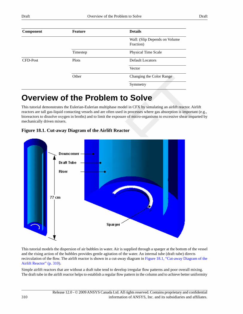
DetailsFeatureComponent
Wall: (Slip Depends on VolumeFraction)
Physical Time ScaleTimestep
Default LocatorsPlotsCFD-Post
Vector
Changing the Color RangeOther
Symmetry
Overview of the Problem to SolveThis tutorial demonstrates the Eulerian-Eulerian multiphase model in CFX by simulating an airlift reactor. Airliftreactors are tall gas-liquid contacting vessels and are often used in processes where gas absorption is important (e.g.,bioreactors to dissolve oxygen in broths) and to limit the exposure of micro-organisms to excessive shear imparted bymechanically driven mixers.
Figure 18.1. Cut-away Diagram of the Airlift Reactor
This tutorial models the dispersion of air bubbles in water. Air is supplied through a sparger at the bottom of the vesseland the rising action of the bubbles provides gentle agitation of the water. An internal tube (draft tube) directsrecirculation of the flow. The airlift reactor is shown in a cut-away diagram in Figure 18.1, “Cut-away Diagram of theAirlift Reactor” (p. 310).
Simple airlift reactors that are without a draft tube tend to develop irregular flow patterns and poor overall mixing.The draft tube in the airlift reactor helps to establish a regular flow pattern in the column and to achieve better uniformity
Release 12.0 - © 2009 ANSYS Canada Ltd. All rights reserved. Contains proprietary and confidentialinformation of ANSYS, Inc. and its subsidiaries and affiliates.310
DraftOverview of the Problem to SolveDraft
in temperature, concentration, and pH in the liquid phase, but sometimes at the expense of decreased mass transferfrom gas to liquid.
This tutorial also demonstrates the use of pairs of internal wall boundaries to model thin 3D features. In this case, apair of wall boundaries is used to model the draft tube. Other applications include baffles and guide vanes. In thepostprocessing section of this tutorial, you will learn how to use face culling to hide one side of a boundary. Thistechnique enables you to independently color each boundary of a pair of back-to-back boundaries (located at the sameposition in 3D space, but with opposite orientation).
The airlift reactor that is modeled here is very similar to the laboratory bench scale prototype used by García-Calvoand Letón.
A formal analysis of this simulation involving a finer mesh is available at the end of this tutorial. For details, seeAdditional Fine Mesh Simulation Results (p. 321).
Before You BeginIf this is the first tutorial you are working with, it is important to review the following topics before beginning:
• Preparing a Working Directory (p. 23)
• Setting the Working Directory and Starting ANSYS CFX (p. 23)
• Changing the Display Colors (p. 24)
• Playing a Tutorial Session File (p. 24)
Starting CFX-Pre1. Prepare the working directory using the following files in the examples directory:
• BubbleColumn.pre
• BubbleColumnMesh.gtm
For details, see Preparing a Working Directory (p. 23)
2. Set the working directory and start CFX-Pre
For details, see Setting the Working Directory and Starting ANSYS CFX (p. 23)
Defining a Case in CFX-PreIf you want to set up the simulation automatically and continue to Obtaining a Solution using CFX-SolverManager (p. 318), run BubbleColumn.pre.
1. Select File > New Case.
2. Select General and click OK.
3. Select File > Save Case As.
4. Under File name, type BubbleColumn.
5. Click Save.
Importing the Mesh1. Right-click Mesh and select Import Mesh > Other. The Import Mesh dialog box appears.
2. Apply the following settings:
311Release 12.0 - © 2009 ANSYS Canada Ltd. All rights reserved. Contains proprietary and confidentialinformation of ANSYS, Inc. and its subsidiaries and affiliates.
DraftBefore You BeginDraft
ValueSetting
BubbleColumnMesh.gtmFile name
3. Click Open.
Creating the Domain1. Edit Case Options > General in the Outline tree view and ensure that Automatic Default Domain is
turned on. A domain named Default Domain should now appear under the Simulation branch.
2. Double-click Default Domain.
3. In the Basic Settings tab, under Fluid and Particle Definitions, delete Fluid 1 and create a new fluid definitioncalled Air.
4. Use the button to create a new fluid named Water.
5. Apply the following settings:
ValueSettingTab
B1.P3, B2.P3Location and Type > LocationBasicSettings
AirFluid and Particle Definitions
Air at 25 CFluid and Particle Definitions > Air > Material
Dispersed FluidFluid and Particle Definitions > Air > Morphology > Option
6 [mm]Fluid and Particle Definitions > Air > Morphology > MeanDiameter
WaterFluid and Particle Definitions
WaterFluid and Particle Definitions > Water > Material
1 [atm]Domain Models > Pressure > Reference Pressure
BuoyantDomain Models > Buoyancy > Option
0 [m s^-2]Domain Models > Buoyancy > Gravity X Dirn.
-9.81 [m s^-2]Domain Models > Buoyancy > Gravity Y Dirn.
0 [m s^-2]Domain Models > Buoyancy > Gravity Z Dirn.
997 [kg m^-3]Domain Models > Buoyancy > Buoy. Ref. Densitya
(Cleared)Multiphase > Homogeneous ModelFluidModels b
NoneMultiphase > Free Surface Model > Option
(Cleared)Heat Transfer > Homogeneous Model
IsothermalHeat Transfer > Option
25 [C]Heat Transfer > Fluid Temperature
Release 12.0 - © 2009 ANSYS Canada Ltd. All rights reserved. Contains proprietary and confidentialinformation of ANSYS, Inc. and its subsidiaries and affiliates.312
DraftCreating the DomainDraft
ValueSettingTab
(Cleared)Turbulence > Homogeneous Model
Fluid DependentTurbulence > Option
Air | WaterFluid PairFluid PairModels
(Selected)Fluid Pair > Air | Water > Surface Tension Coefficient
0.072 [N m^-1]Fluid Pair > Air | Water > Surface Tension Coefficient > Surf.Tension Coeff. c
GraceFluid Pair > Air | Water > Momentum Transfer > Drag Force >Option
(Selected)Fluid Pair > Air | Water > Momentum Transfer > Drag Force >Volume Fraction Correction Exponent
2Fluid Pair > Air | Water > Momentum Transfer > Drag Force >Volume Fraction Correction Exponent > Value d
Lopez de BertodanoFluid Pair > Air | Water > Momentum Transfer > Non-dragforces > Turbulent Dispersion Force > Option
0.3Fluid Pair > Air | Water > Momentum Transfer > Non-dragforces > Turbulent Dispersion Force > Dispersion Coeff.
Sato Enhanced EddyViscosity
Fluid Pair > Air | Water > Turbulence Transfer > Option
e
aFor dilute dispersed multiphase flow, always set the buoyancy reference density to that for continuous fluid.bTurn off the homogeneous model to allow each fluid to have its own velocity field.cThis must be set to allow the Grace drag model to be used.dA positive value is appropriate for large bubbles. For details, see Densely Distributed Fluid Particles: Grace Drag Model (p. 177).eThis models particle-induced turbulence. For details, see Turbulence Enhancement (p. 185).
6. Click OK.
Creating the Boundary ConditionsFor this simulation of the airlift reactor, the required boundary conditions are:
• An inlet for air on the sparger.
• A degassing outlet for air at the liquid surface.
• A pair of wall boundaries for the draft tube.
• An exterior wall for the outer wall, base and sparger tube.
• Symmetry planes.
Inlet BoundaryAt the sparger, create an inlet boundary that injects air at 0.3 m/s with a volume fraction of 0.25:
1. Create a new boundary named Sparger.
2. Apply the following settings:
313Release 12.0 - © 2009 ANSYS Canada Ltd. All rights reserved. Contains proprietary and confidentialinformation of ANSYS, Inc. and its subsidiaries and affiliates.
DraftCreating the Boundary ConditionsDraft
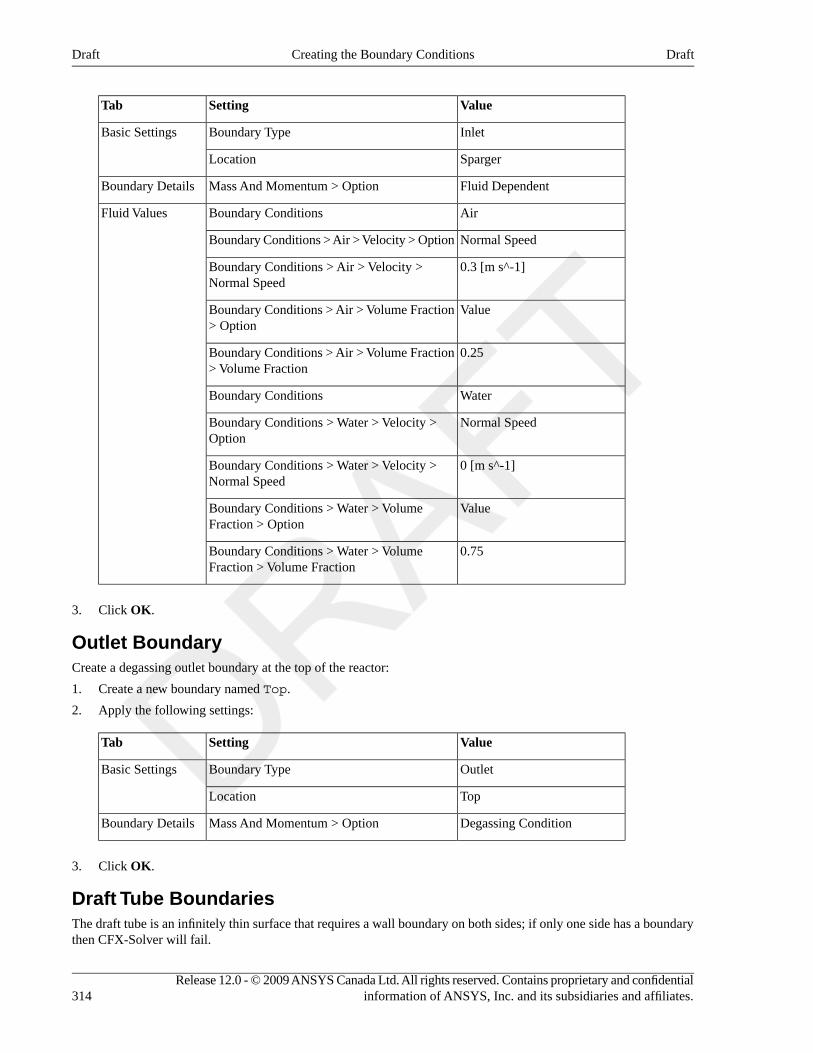
ValueSettingTab
InletBoundary TypeBasic Settings
SpargerLocation
Fluid DependentMass And Momentum > OptionBoundary Details
AirBoundary ConditionsFluid Values
Normal SpeedBoundary Conditions > Air > Velocity > Option
0.3 [m s^-1]Boundary Conditions > Air > Velocity >Normal Speed
ValueBoundary Conditions > Air > Volume Fraction> Option
0.25Boundary Conditions > Air > Volume Fraction> Volume Fraction
WaterBoundary Conditions
Normal SpeedBoundary Conditions > Water > Velocity >Option
0 [m s^-1]Boundary Conditions > Water > Velocity >Normal Speed
ValueBoundary Conditions > Water > VolumeFraction > Option
0.75Boundary Conditions > Water > VolumeFraction > Volume Fraction
3. Click OK.
Outlet BoundaryCreate a degassing outlet boundary at the top of the reactor:
1. Create a new boundary named Top.
2. Apply the following settings:
ValueSettingTab
OutletBoundary TypeBasic Settings
TopLocation
Degassing ConditionMass And Momentum > OptionBoundary Details
3. Click OK.
Draft Tube BoundariesThe draft tube is an infinitely thin surface that requires a wall boundary on both sides; if only one side has a boundarythen CFX-Solver will fail.
Release 12.0 - © 2009 ANSYS Canada Ltd. All rights reserved. Contains proprietary and confidentialinformation of ANSYS, Inc. and its subsidiaries and affiliates.314
DraftCreating the Boundary ConditionsDraft
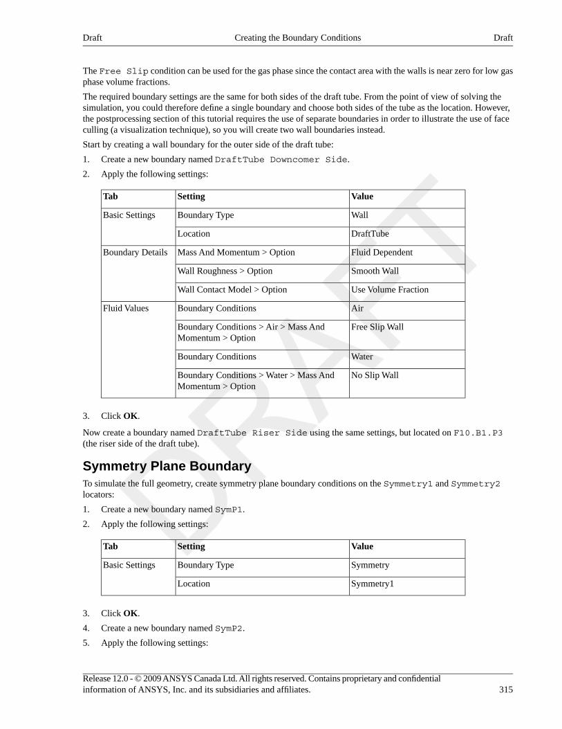
The Free Slip condition can be used for the gas phase since the contact area with the walls is near zero for low gasphase volume fractions.
The required boundary settings are the same for both sides of the draft tube. From the point of view of solving thesimulation, you could therefore define a single boundary and choose both sides of the tube as the location. However,the postprocessing section of this tutorial requires the use of separate boundaries in order to illustrate the use of faceculling (a visualization technique), so you will create two wall boundaries instead.
Start by creating a wall boundary for the outer side of the draft tube:
1. Create a new boundary named DraftTube Downcomer Side.
2. Apply the following settings:
ValueSettingTab
WallBoundary TypeBasic Settings
DraftTubeLocation
Fluid DependentMass And Momentum > OptionBoundary Details
Smooth WallWall Roughness > Option
Use Volume FractionWall Contact Model > Option
AirBoundary ConditionsFluid Values
Free Slip WallBoundary Conditions > Air > Mass AndMomentum > Option
WaterBoundary Conditions
No Slip WallBoundary Conditions > Water > Mass AndMomentum > Option
3. Click OK.
Now create a boundary named DraftTube Riser Side using the same settings, but located on F10.B1.P3(the riser side of the draft tube).
Symmetry Plane BoundaryTo simulate the full geometry, create symmetry plane boundary conditions on the Symmetry1 and Symmetry2locators:
1. Create a new boundary named SymP1.
2. Apply the following settings:
ValueSettingTab
SymmetryBoundary TypeBasic Settings
Symmetry1Location
3. Click OK.
4. Create a new boundary named SymP2.
5. Apply the following settings:
315Release 12.0 - © 2009 ANSYS Canada Ltd. All rights reserved. Contains proprietary and confidentialinformation of ANSYS, Inc. and its subsidiaries and affiliates.
DraftCreating the Boundary ConditionsDraft
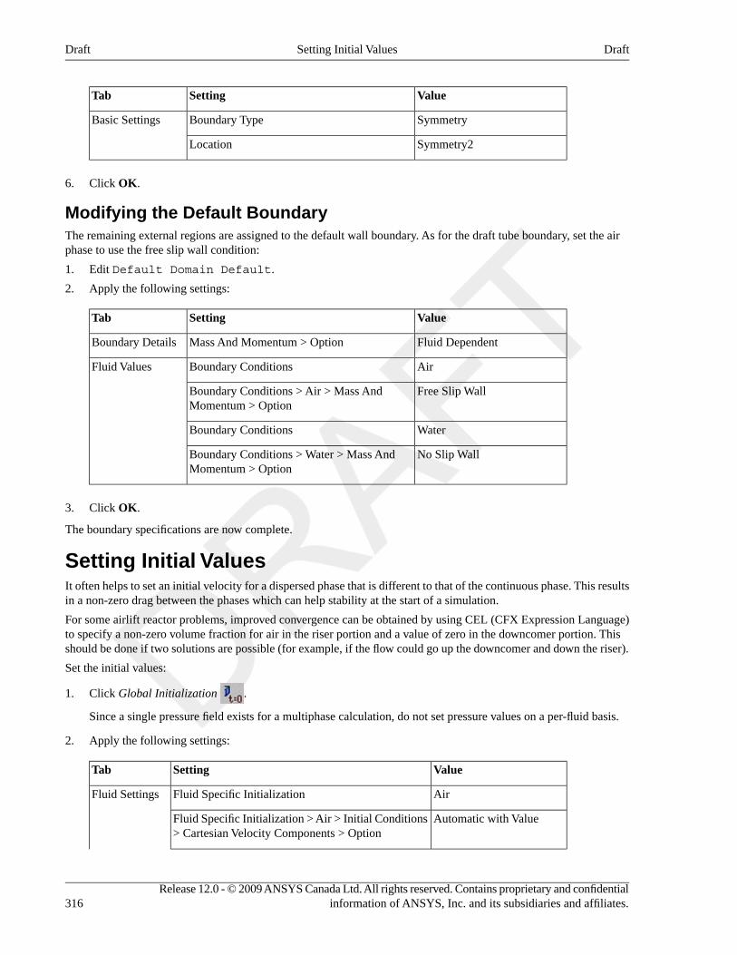
ValueSettingTab
SymmetryBoundary TypeBasic Settings
Symmetry2Location
6. Click OK.
Modifying the Default BoundaryThe remaining external regions are assigned to the default wall boundary. As for the draft tube boundary, set the airphase to use the free slip wall condition:
1. Edit Default Domain Default.
2. Apply the following settings:
ValueSettingTab
Fluid DependentMass And Momentum > OptionBoundary Details
AirBoundary ConditionsFluid Values
Free Slip WallBoundary Conditions > Air > Mass AndMomentum > Option
WaterBoundary Conditions
No Slip WallBoundary Conditions > Water > Mass AndMomentum > Option
3. Click OK.
The boundary specifications are now complete.
Setting Initial ValuesIt often helps to set an initial velocity for a dispersed phase that is different to that of the continuous phase. This resultsin a non-zero drag between the phases which can help stability at the start of a simulation.
For some airlift reactor problems, improved convergence can be obtained by using CEL (CFX Expression Language)to specify a non-zero volume fraction for air in the riser portion and a value of zero in the downcomer portion. Thisshould be done if two solutions are possible (for example, if the flow could go up the downcomer and down the riser).
Set the initial values:
1. Click Global Initialization .
Since a single pressure field exists for a multiphase calculation, do not set pressure values on a per-fluid basis.
2. Apply the following settings:
ValueSettingTab
AirFluid Specific InitializationFluid Settings
Automatic with ValueFluid Specific Initialization > Air > Initial Conditions> Cartesian Velocity Components > Option
Release 12.0 - © 2009 ANSYS Canada Ltd. All rights reserved. Contains proprietary and confidentialinformation of ANSYS, Inc. and its subsidiaries and affiliates.316
DraftSetting Initial ValuesDraft
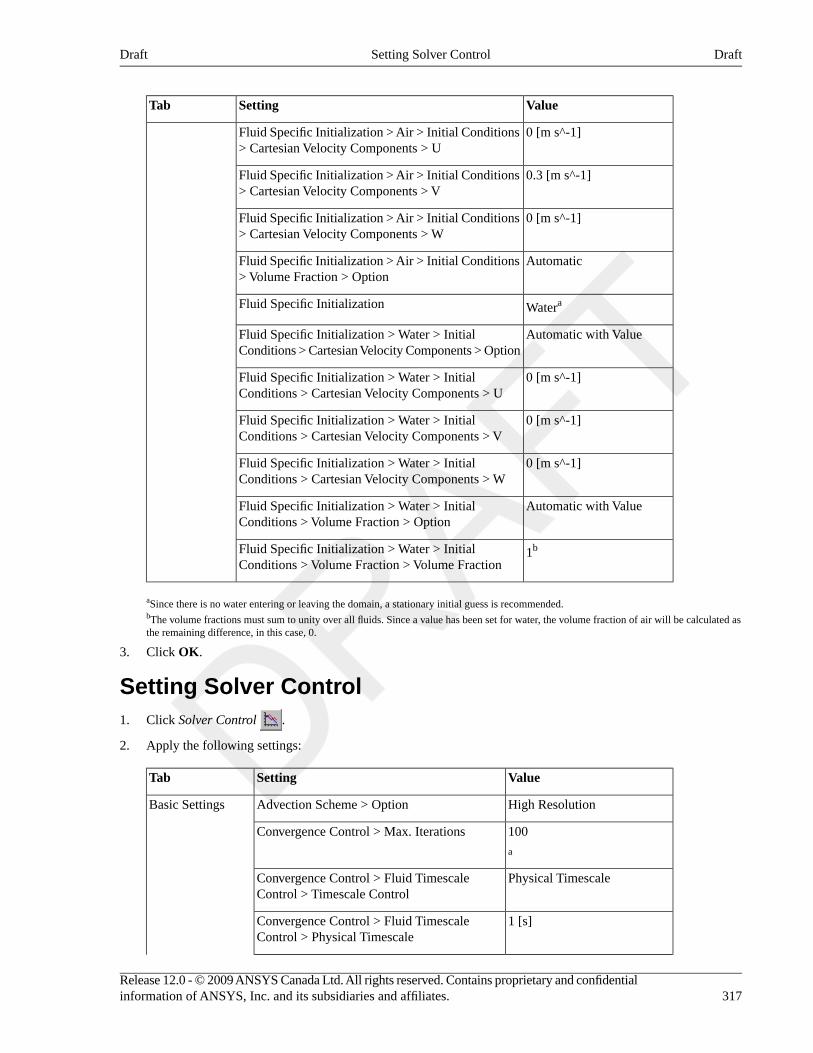
ValueSettingTab
0 [m s^-1]Fluid Specific Initialization > Air > Initial Conditions> Cartesian Velocity Components > U
0.3 [m s^-1]Fluid Specific Initialization > Air > Initial Conditions> Cartesian Velocity Components > V
0 [m s^-1]Fluid Specific Initialization > Air > Initial Conditions> Cartesian Velocity Components > W
AutomaticFluid Specific Initialization > Air > Initial Conditions> Volume Fraction > Option
WateraFluid Specific Initialization
Automatic with ValueFluid Specific Initialization > Water > InitialConditions > Cartesian Velocity Components > Option
0 [m s^-1]Fluid Specific Initialization > Water > InitialConditions > Cartesian Velocity Components > U
0 [m s^-1]Fluid Specific Initialization > Water > InitialConditions > Cartesian Velocity Components > V
0 [m s^-1]Fluid Specific Initialization > Water > InitialConditions > Cartesian Velocity Components > W
Automatic with ValueFluid Specific Initialization > Water > InitialConditions > Volume Fraction > Option
1bFluid Specific Initialization > Water > InitialConditions > Volume Fraction > Volume Fraction
aSince there is no water entering or leaving the domain, a stationary initial guess is recommended.bThe volume fractions must sum to unity over all fluids. Since a value has been set for water, the volume fraction of air will be calculated asthe remaining difference, in this case, 0.
3. Click OK.
Setting Solver Control1. Click Solver Control .
2. Apply the following settings:
ValueSettingTab
High ResolutionAdvection Scheme > OptionBasic Settings
100Convergence Control > Max. Iterations
a
Physical TimescaleConvergence Control > Fluid TimescaleControl > Timescale Control
1 [s]Convergence Control > Fluid TimescaleControl > Physical Timescale
317Release 12.0 - © 2009 ANSYS Canada Ltd. All rights reserved. Contains proprietary and confidentialinformation of ANSYS, Inc. and its subsidiaries and affiliates.
DraftSetting Solver ControlDraft
ValueSettingTab
1.0E-04Convergence Criteria > Residual Target
b
(Selected)Convergence Criteria > Conservation Target
0.01Convergence Criteria > Conservation Target >Value
aFor advice on setting time steps in multiphase simulations, see Timestepping (p. 201).bIf you are using a maximum edge length of 0.005 m or less to produce a finer mesh, use a target residual of 1.0E-05 to obtain a moreaccurate solution.
3. Click OK.
Writing the CFX-Solver Input (.def) File
1. Click Define Run .
2. Apply the following settings:
ValueSetting
BubbleColumn.defFile name
3. Click Save.
CFX-Solver Manager automatically starts and, on the Define Run dialog box, the Solver Input File is set.
4. If using Standalone Mode, quit CFX-Pre, saving the simulation (.cfx) file at your discretion.
Obtaining a Solution using CFX-Solver ManagerStart the simulation from CFX-Solver Manager:
NoteIf you are using a fine mesh for a formal quantitative analysis of the flow in the reactor, the solution timewill be significantly longer than for the coarse mesh. You can run the simulation in parallel to reduce thesolution time. For details, see Obtaining a Solution in Parallel (p. 138).
1. Ensure Define Run is displayed.
2. Click Start Run.
CFX-Solver runs and attempts to obtain a solution. This can take a long time depending on your system.
3. Select the check box next to Post-Process Results when the completion message appears at the end of the run.
4. If using Standalone Mode, select the check box next to Shut down CFX-Solver Manager.
5. Click OK.
Viewing the Results in CFD-PostYou will first create plots of velocity and volume fraction. You will then display the entire geometry.
Release 12.0 - © 2009 ANSYS Canada Ltd. All rights reserved. Contains proprietary and confidentialinformation of ANSYS, Inc. and its subsidiaries and affiliates.318
DraftWriting the CFX-Solver Input (.def) FileDraft
Because the simulation in this tutorial is conducted on a coarse grid, the results are only suitable for a qualitativedemonstration of the multiphase capability of ANSYS CFX.
The following topics will be discussed:
• Creating Water Velocity Vector Plots (p. 319)
• Creating Volume Fraction Plots (p. 319)
• Displaying the Entire Airlift Reactor Geometry (p. 321)
Creating Water Velocity Vector Plots1. Right-click a blank area in the viewer and select Predefined Camera > View Towards -Z.
2. Create a new vector plot named Vector 1.
3. Apply the following settings:
ValueSettingTab
SymP1Definition > LocationsGeometry
Water.VelocityDefinition > Variable
User SpecifiedRangeColor
0 [m s^-1]Min
1 [m s^-1]Max
0.3Symbol SizeSymbol
4. Click Apply.
5. In the tree view, right-click Vector 1, select Duplicate, and click OK to accept the default name, Vector2.
6. Edit Vector 2.
7. On the Geometry tab, set Definition > Variable to Air.Velocity and click Apply.
8. Compare Vector 1 and Vector 2 by toggling the visibility of each one.
Zoom in as required.
Observe that the air flows upward, leaving the tank, at the degassing outlet.
Note that the air rises faster than the water in the riser and descends slower than the water in the downcomer.
Creating Volume Fraction PlotsPlot the volume fraction of air on the symmetry plane SymP1:
1. Right-click a blank area in the viewer and select Predefined Camera > View Towards -Z.
2. Turn on the visibility of SymP1.
3. Edit SymP1.
4. Apply the following settings to SymP1:
ValueSettingTab
VariableModeColor
319Release 12.0 - © 2009 ANSYS Canada Ltd. All rights reserved. Contains proprietary and confidentialinformation of ANSYS, Inc. and its subsidiaries and affiliates.
DraftCreating Water Velocity Vector PlotsDraft
ValueSettingTab
Air.Volume FractionVariable
User SpecifiedRange
0Min
0.025Max
5. Click Apply.
Observe the volume fraction values throughout the domain.
6. Turn off the visibility of SymP1.
Next, plot the volume fraction of air on each side of the draft tube:
1. Right-click a blank area in the viewer and select Predefined Camera > Isometric View (Y up).
2. Turn on the visibility of DraftTube Downcomer Side.
3. Modify DraftTube Downcomer Side by applying the following settings:
ValueSettingTab
VariableModeColor
Air.Volume FractionVariable
User SpecifiedRange
0Min
0.025Max
4. Click Apply.
5. Rotate the plot in the viewer to see both sides of DraftTube Downcomer Side.
Notice that the plot appears on both sides of the DraftTube Downcomer Side boundary. When viewingplots on internal surfaces, you must ensure that you are viewing the correct side. You will make use of the faceculling rendering feature to turn off the visibility of the plot on the side of the boundary for which the plot doesnot apply.
The DraftTube Downcomer Side boundary represents the side of the internal surface in the downcomer(in this case, outer) region of the reactor. To confirm this, you could make a vector plot of the variable Normal(representing the face normal vectors) on the locator DraftTube Downcomer Side; the fluid is on the sideopposite the normal vectors.
In this case, you need to turn off the “front” faces of the plot; The front faces are, by definition, on the same sideof the plot as the normal vectors.
6. Modify DraftTube Downcomer Side by applying the following settings:
ValueSettingTab
Front FacesShow Faces > Face CullingRender
7. Click Apply.
Release 12.0 - © 2009 ANSYS Canada Ltd. All rights reserved. Contains proprietary and confidentialinformation of ANSYS, Inc. and its subsidiaries and affiliates.320
DraftCreating Volume Fraction PlotsDraft
8. Rotate the image in the viewer to see the effect of face culling on DraftTube Downcomer Side. You shouldsee that the color appears on the downcomer side only.
9. Turn on the visibility of DraftTube Riser Side.
10. Color the DraftTube Riser Side object using the same color and rendering settings as for DraftTubeDowncomer Side.
The normal vectors for DraftTube Riser Side point opposite to those of DraftTube DowncomerSide, so the faces on DraftTube Riser Side are plotted only on the riser (in this case, inner) side of theairlift reactor.
Rotating the geometry will now correctly show the air volume fraction on each side of the draft tube.
Face culling was needed to prevent interference between the plots on each side of the draft tube. To demonstrate this,try turning off face culling for DraftTube Downcomer Side and watch the effect on the riser side. You mightnotice that the plot from the downcomer side interferes with, or even completely overrides, the riser-side plot. Resultsmay vary, which is why face culling should always be used to prevent possible interference.
Displaying the Entire Airlift Reactor GeometryDisplay the entire airlift reactor geometry by expanding User Locations and Plots and double-clicking theDefault Transform object:
1. Apply the following settings to Default Transform:
ValueSettingTab
(Cleared)Instancing Info From DomainDefinition
12# of Copies
(Selected)Apply Rotation
Principal AxisApply Rotation > Method
YApply Rotation > Axis
12Apply Rotation > # of Passages
2. Click Apply.
Additional Fine Mesh Simulation ResultsA formal analysis of this airlift reactor was carried out on a finer grid (having 21000+ nodes and a maximum edgelength of 0.005 m).
The analysis showed a region of air bubble recirculation at the top of the reactor on the downcomer side. This wasconfirmed by zooming in on a vector plot of Air.Velocity on SymP1 near the top of the downcomer. A similarplot of Water.Velocity revealed no recirculation of the water.
Other results of the simulation:
• Due to their large 0.006 m diameter, the air bubbles quickly attained a significant terminal slip velocity (i.e., theterminal velocity relative to water). The resulting terminal slip velocity, obtained using the Grace drag model, isconsistent with the prediction by Maneri and Mendelson and the prediction by Baker and Chao. These correlations
predict a terminal slip velocity of about 0.23 m s-1 to 0.25 m s-1 for air bubbles of the diameter specified.
• The values of gas hold-up (the average volume fraction of air in the riser), the superficial gas velocity (the risingvelocity, relative to the reactor vessel, of gas bubbles in the riser, multiplied by the gas hold-up), and the liquidvelocity in the downcomer agree with the results reported by García-Calvo and Letón, for gas hold-up values of
321Release 12.0 - © 2009 ANSYS Canada Ltd. All rights reserved. Contains proprietary and confidentialinformation of ANSYS, Inc. and its subsidiaries and affiliates.
DraftDisplaying the Entire Airlift Reactor GeometryDraft
0.03 or less. At higher values of gas hold-up, the multifluid model does not account for pressure-volume worktransferred from gas to liquid due to isothermal expansion of the bubbles. The simulation therefore tends tounder-predict both the superficial gas velocity in the riser, and the liquid velocity in the downcomer for gas hold-upvalues greater than 0.03.
NoteMultiphase results files contain the vector variable Fluid.Superficial Velocity defined asFluid.Volume Fraction multiplied by Fluid.Velocity. This is sometimes also referred toas the fluid volume flux. The components of this vector variable are available as scalar variables (forexample, Fluid.Superficial Velocity X).
Many reference texts on airlift reactors cite the Hughmark correlation as a standard for gas hold-up and superficial gasvelocity in airlift reactors. However, the Hughmark correlation should not be used when liquid flow is concurrent withgas at velocities exceeding 0.1 m/s. In the airlift reactor described in this tutorial, the liquid velocity in the riser clearlyexceeds 0.2 m/s, and the Hughmark correlation is therefore not applicable.
Release 12.0 - © 2009 ANSYS Canada Ltd. All rights reserved. Contains proprietary and confidentialinformation of ANSYS, Inc. and its subsidiaries and affiliates.322
DraftAdditional Fine Mesh Simulation ResultsDraft
Chapter 19. Air Conditioning SimulationThis tutorial includes:
• Tutorial Features (p. 323)
• Overview of the Problem to Solve (p. 324)
• Before You Begin (p. 325)
• Starting CFX-Pre (p. 326)
• Defining a Case in CFX-Pre (p. 326)
• Obtaining a Solution using CFX-Solver Manager (p. 337)
• Viewing the Results in CFD-Post (p. 338)
• Further Steps (p. 341)
ImportantYou must have the required Fortran compiler installed and set in your system path in order to run thistutorial. For details on which Fortran compiler is required for your platform, see the applicable ANSYS,Inc. installation guide. If you are not sure which Fortran compiler is installed on your system, try runningthe cfx5mkext command (found in <CFXROOT>/bin) from the command line and read the outputmessages.
Tutorial FeaturesIn this tutorial you will learn about:
• Importing CEL expressions.
• @REGION CEL syntax.
• Setting up a user CEL function.
• Setting up a monitor point to observe the temperature at a prescribed location.
• Using the Monte Carlo radiation model with a directional source of radiation.
• Post-processing a transient simulation.
DetailsFeatureComponent
General ModeUser ModeCFX-Pre
TransientAnalysis Type
General FluidFluid Type
Single DomainDomain Type
k-EpsilonTurbulence Model
Thermal EnergyHeat Transfer
Monte CarloRadiation
Buoyant Flow
Boundary Profile VisualizationBoundary Conditions
Inlet (Profile)
323Release 12.0 - © 2009 ANSYS Canada Ltd. All rights reserved. Contains proprietary and confidentialinformation of ANSYS, Inc. and its subsidiaries and affiliates.
DraftDraft
DetailsFeatureComponent
Outlet (Subsonic)
Wall: No-Slip
Wall: Adiabatic
Wall: Fixed Temperature
Transient Results FilesOutput Control
Monitor Points
User CEL FunctionCEL (CFX Expression Language)
AnimationPlotsCFD-Post
Isosurface
Point
Slice Plane
Text Label with Auto AnnotationOther
Changing the Color Range
Legend
Time Step Selection
Transient Animation with MPEGGeneration
Overview of the Problem to SolveThis tutorial simulates a room with a thermostat-controlled air conditioner.
Release 12.0 - © 2009 ANSYS Canada Ltd. All rights reserved. Contains proprietary and confidentialinformation of ANSYS, Inc. and its subsidiaries and affiliates.324
DraftOverview of the Problem to SolveDraft
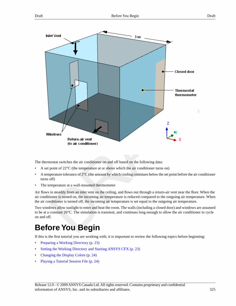
The thermostat switches the air conditioner on and off based on the following data:
• A set point of 22°C (the temperature at or above which the air conditioner turns on)
• A temperature tolerance of 2°C (the amount by which cooling continues below the set point before the air conditionerturns off)
• The temperature at a wall-mounted thermometer
Air flows in steadily from an inlet vent on the ceiling, and flows out through a return-air vent near the floor. When theair conditioner is turned on, the incoming air temperature is reduced compared to the outgoing air temperature. Whenthe air conditioner is turned off, the incoming air temperature is set equal to the outgoing air temperature.
Two windows allow sunlight to enter and heat the room. The walls (including a closed door) and windows are assumedto be at a constant 26°C. The simulation is transient, and continues long enough to allow the air conditioner to cycleon and off.
Before You BeginIf this is the first tutorial you are working with, it is important to review the following topics before beginning:
• Preparing a Working Directory (p. 23)
• Setting the Working Directory and Starting ANSYS CFX (p. 23)
• Changing the Display Colors (p. 24)
• Playing a Tutorial Session File (p. 24)
325Release 12.0 - © 2009 ANSYS Canada Ltd. All rights reserved. Contains proprietary and confidentialinformation of ANSYS, Inc. and its subsidiaries and affiliates.
DraftBefore You BeginDraft
Starting CFX-Pre1. Prepare the working directory using the following files in the examples directory:
• HVAC.pre
• HVAC_expressions.ccl
• HVACMesh.gtm
• TStat_Control.F
NoteYou must have a Fortran compiler installed on your system to perform this tutorial.
For details, see Preparing a Working Directory (p. 23)
2. Set the working directory and start CFX-Pre
For details, see Setting the Working Directory and Starting ANSYS CFX (p. 23)
Defining a Case in CFX-PreIf you want to set up the simulation automatically using a tutorial session file, run HVAC.pre. For details, see Playinga Tutorial Session File (p. 24). Then proceed to Obtaining a Solution using CFX-Solver Manager (p. 337).
If you want to set up the simulation manually, proceed to the following steps:
1. Select File > New Case.
2. Select General and click OK.
3. Select File > Save Case As.
4. Under File name, type HVAC.
5. Click Save.
Importing the Mesh1. Right-click Mesh and select Import Mesh > CFX Mesh.
The Import Mesh dialog box appears.
2. Apply the following settings:
ValueSetting
HVACMesh.gtmFile name
3. Click Open.
4. Right-click a blank area in the viewer and select Predefined Camera > Isometric View (Z up) from the shortcutmenu.
Importing CEL ExpressionsThis tutorial uses several CEL expressions to store parameters and to evaluate other quantities that are required by thesimulation. Import all of the expressions from the provided file:
1. Select File > Import > CCL.
2. Ensure that Import Method is set to Append.
Release 12.0 - © 2009 ANSYS Canada Ltd. All rights reserved. Contains proprietary and confidentialinformation of ANSYS, Inc. and its subsidiaries and affiliates.326
DraftStarting CFX-PreDraft
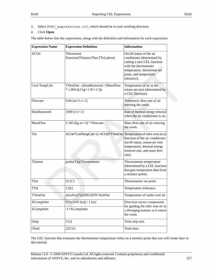
3. Select HVAC_expressions.ccl, which should be in your working directory.
4. Click Open.
The table below lists the expressions, along with the definition and information for each expression:
InformationExpression DefinitionExpression Name
On/off status of the airconditioner (determined by
ThermostatFunction(TSensor,TSet,TTol,aitern)
ACOn
calling a user CEL functionwith the thermometertemperature, thermostat setpoint, and temperaturetolerance).
Temperature of air at thereturn-air vent (determined bya CEL function).
TVentOut - (HeatRemoved / (MassFlow* 1.004 [kJ kg^-1 K^-1 ]))
Cool TempCalc
Volumetric flow rate of airentering the room.
0.06 [m^3 s^-1]Flowrate
Rate of thermal energy removalwhen the air conditioner is on.
1000 [J s^-1]HeatRemoved
Mass flow rate of air enteringthe room.
1.185 [kg m^-3] * FlowrateMassFlow
Temperature of inlet vent air (afunction of the air conditioner
ACOn*CoolTempCalc+(1-ACOn)*TVentOutTIn
on/off status, return-air venttemperature, thermal energyremoval rate, and mass flowrate).
Thermometer temperature(determined by a CEL function
probe(T)@ThermometerTSensor
that gets temperature data froma monitor point).
Thermometer set point.22 [C]TSet
Temperature tolerance.2 [K]TTol
Temperature of outlet vent air.areaAve(T)@REGION:VentOutTVentOut
Direction vector componentsfor guiding the inlet vent air in
5*(x-0.05 [m]) / 1 [m]XCompInlet
-1+XCompInletZCompInlet a diverging manner as it entersthe room.
Time step size.3 [s]tStep
Total time.225 [s]tTotal
The CEL function that evaluates the thermometer temperature relies on a monitor point that you will create later inthis tutorial.
327Release 12.0 - © 2009 ANSYS Canada Ltd. All rights reserved. Contains proprietary and confidentialinformation of ANSYS, Inc. and its subsidiaries and affiliates.
DraftImporting CEL ExpressionsDraft
The CEL expression for the air conditioner on/off status requires a compiled Fortran subroutine and a user CEL functionthat uses the subroutine. These are created next, starting with the compiled subroutine.
NoteThe expression for the return-air vent temperature, TVentOut, makes use of @REGION CEL syntax,which indicates the mesh region named VentOut, rather than a boundary named VentOut. For detailsabout @REGION CEL syntax, see Using Locators in Expressions (p. 156) in ANSYS CFX ReferenceGuide.
Compiling the Fortran Subroutine for the ThermostatA Fortran subroutine that simulates the thermostat is provided in the installation directory for your software(<CFXROOT>/examples/). Before the subroutine can be used, it must be compiled for your platform.
You can compile the subroutine at any time before running CFX-Solver. The operation is performed at this point inthe tutorial so that you have a better understanding of the values you need to specify in CFX-Pre when creating a UserCEL Function. The cfx5mkext command is used to compile the subroutine as described below.
1. Copy the subroutine TStat_Control.F to your working directory (if you have not already done so).
2. Examine the contents of this file in any text editor to gain a better understanding of this subroutine.
This file was created by modifying the ucf_template.F file, which is available in the<CFXROOT>/examples/ directory.
3. Select Tools > Command Editor.
4. Type the following command in the Command Editor dialog box (make sure you do not miss the semicolon atthe end of the line):
! system ("cfx5mkext TStat_Control.F") == 0 or die "cfx5mkext failed";
• This is equivalent to executing the following at an OS command prompt:
cfx5mkext TStat_Control.F
• The ! indicates that the following line is to be interpreted as power syntax and not CCL. Everything after the! symbol is processed as Perl commands.
• system is a Perl function to execute a system command.
• The “== 0 or die” will cause an error message to be returned if, for some reason, there is an error inprocessing the command.
5. Click Process to compile the subroutine.
NoteYou can use the -double option (i.e., cfx5mkext -double TStat_Control.F) to compilethe subroutine for use with double precision CFX-Solver executables.
A subdirectory will have been created in your working directory whose name is system dependent (e.g., on Linux itis named linux). This sub directory contains the shared object library.
NoteIf you are running problems in parallel over multiple platforms then you will need to create thesesubdirectories using the cfx5mkext command for each different platform.
• You can view more details about the cfx5mkext command by running cfx5mkext -help.
Release 12.0 - © 2009 ANSYS Canada Ltd. All rights reserved. Contains proprietary and confidentialinformation of ANSYS, Inc. and its subsidiaries and affiliates.328
DraftCompiling the Fortran Subroutine for the ThermostatDraft
• You can set a Library Name and Library Path using the -name and -dest options respectively.
• If these are not specified, the default Library Name is that of your Fortran file and the default Library Path is yourcurrent working directory.
• Close the Command Editor dialog box.
Creating a User CEL Function for the ThermostatThe expression for the air conditioner on/off status is named ACOn. This expression consists of a call to a user CELfunction, Thermostat Function, which needs to be created.
Before you create the user CEL function, you will first create a user routine that holds basic information about thecompiled Fortran subroutine. You will then create a user function, Thermostat Function, so that it is associatedwith the user routine.
Create the user routine:
1. From the main menu, select Insert > Expressions, Functions and Variables > User Routine or click User
Routine .
2. Set the name to Thermostat Routine.
3. Apply the following settings:
ValueSettingTab
User CEL FunctionOptionBasic Settings
ac_onaCalling Name
TStat_ControlbLibrary Name
(Working Directory)cLibrary Path
aThis is the name of the subroutine within the Fortran file. Always use lower case letters for the calling name, even if the subroutine name inthe Fortran file is in upper case.bThis is the name passed to the cfx5mkext command by the -name option. If the -name option is not specified, a default is used. The defaultis the Fortran file name without the .F extension.cSet this to your working directory.
4. Click OK.
Create the user CEL function:
1. From the main menu, select Insert > Expressions, Functions and Variables > User Function or click User
Function .
2. Set the name to Thermostat Function.
3. Apply the following settings:
ValueSettingTab
User FunctionOptionBasic Settings
Thermostat RoutineUser Routine Name
[K], [K], [K], []aArgument Units
329Release 12.0 - © 2009 ANSYS Canada Ltd. All rights reserved. Contains proprietary and confidentialinformation of ANSYS, Inc. and its subsidiaries and affiliates.
DraftCreating a User CEL Function for the ThermostatDraft
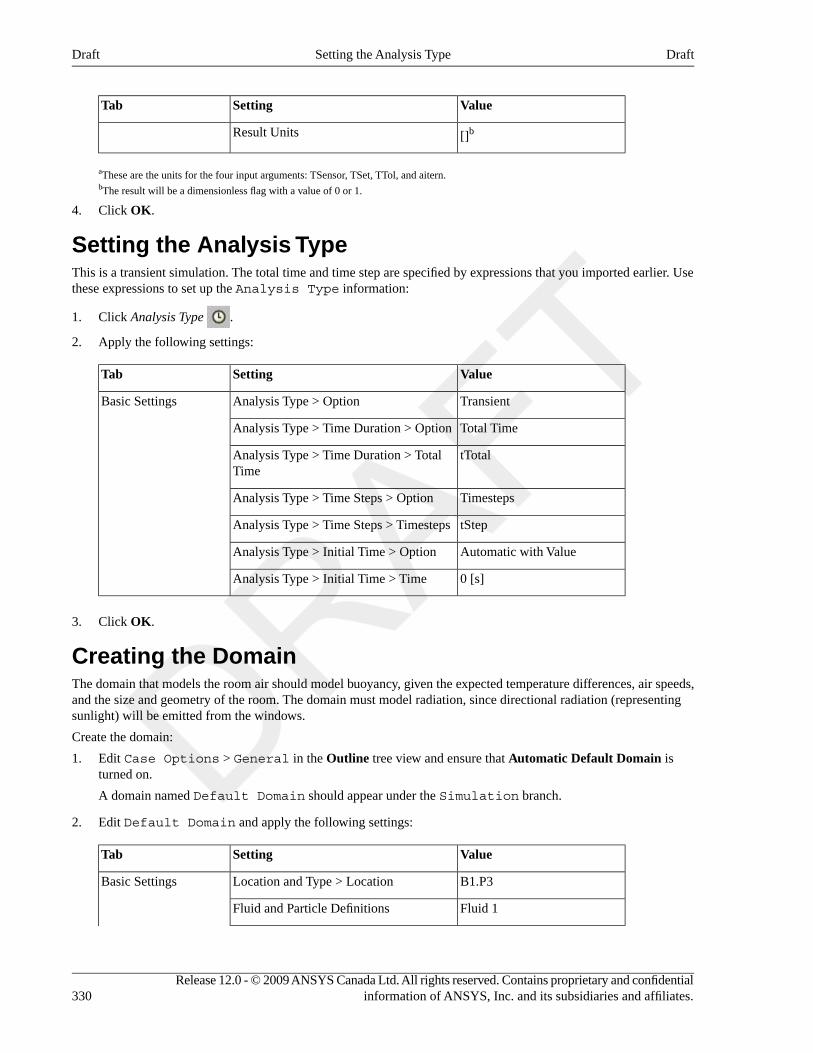
ValueSettingTab
[]bResult Units
aThese are the units for the four input arguments: TSensor, TSet, TTol, and aitern.bThe result will be a dimensionless flag with a value of 0 or 1.
4. Click OK.
Setting the Analysis TypeThis is a transient simulation. The total time and time step are specified by expressions that you imported earlier. Usethese expressions to set up the Analysis Type information:
1. Click Analysis Type .
2. Apply the following settings:
ValueSettingTab
TransientAnalysis Type > OptionBasic Settings
Total TimeAnalysis Type > Time Duration > Option
tTotalAnalysis Type > Time Duration > TotalTime
TimestepsAnalysis Type > Time Steps > Option
tStepAnalysis Type > Time Steps > Timesteps
Automatic with ValueAnalysis Type > Initial Time > Option
0 [s]Analysis Type > Initial Time > Time
3. Click OK.
Creating the DomainThe domain that models the room air should model buoyancy, given the expected temperature differences, air speeds,and the size and geometry of the room. The domain must model radiation, since directional radiation (representingsunlight) will be emitted from the windows.
Create the domain:
1. Edit Case Options > General in the Outline tree view and ensure that Automatic Default Domain isturned on.
A domain named Default Domain should appear under the Simulation branch.
2. Edit Default Domain and apply the following settings:
ValueSettingTab
B1.P3Location and Type > LocationBasic Settings
Fluid 1Fluid and Particle Definitions
Release 12.0 - © 2009 ANSYS Canada Ltd. All rights reserved. Contains proprietary and confidentialinformation of ANSYS, Inc. and its subsidiaries and affiliates.330
DraftSetting the Analysis TypeDraft
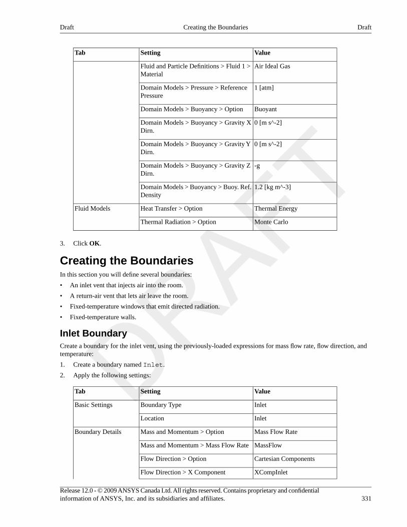
ValueSettingTab
Air Ideal GasFluid and Particle Definitions > Fluid 1 >Material
1 [atm]Domain Models > Pressure > ReferencePressure
BuoyantDomain Models > Buoyancy > Option
0 [m s^-2]Domain Models > Buoyancy > Gravity XDirn.
0 [m s^-2]Domain Models > Buoyancy > Gravity YDirn.
-gDomain Models > Buoyancy > Gravity ZDirn.
1.2 [kg m^-3]Domain Models > Buoyancy > Buoy. Ref.Density
Thermal EnergyHeat Transfer > OptionFluid Models
Monte CarloThermal Radiation > Option
3. Click OK.
Creating the BoundariesIn this section you will define several boundaries:
• An inlet vent that injects air into the room.
• A return-air vent that lets air leave the room.
• Fixed-temperature windows that emit directed radiation.
• Fixed-temperature walls.
Inlet BoundaryCreate a boundary for the inlet vent, using the previously-loaded expressions for mass flow rate, flow direction, andtemperature:
1. Create a boundary named Inlet.
2. Apply the following settings:
ValueSettingTab
InletBoundary TypeBasic Settings
InletLocation
Mass Flow RateMass and Momentum > OptionBoundary Details
MassFlowMass and Momentum > Mass Flow Rate
Cartesian ComponentsFlow Direction > Option
XCompInletFlow Direction > X Component
331Release 12.0 - © 2009 ANSYS Canada Ltd. All rights reserved. Contains proprietary and confidentialinformation of ANSYS, Inc. and its subsidiaries and affiliates.
DraftCreating the BoundariesDraft
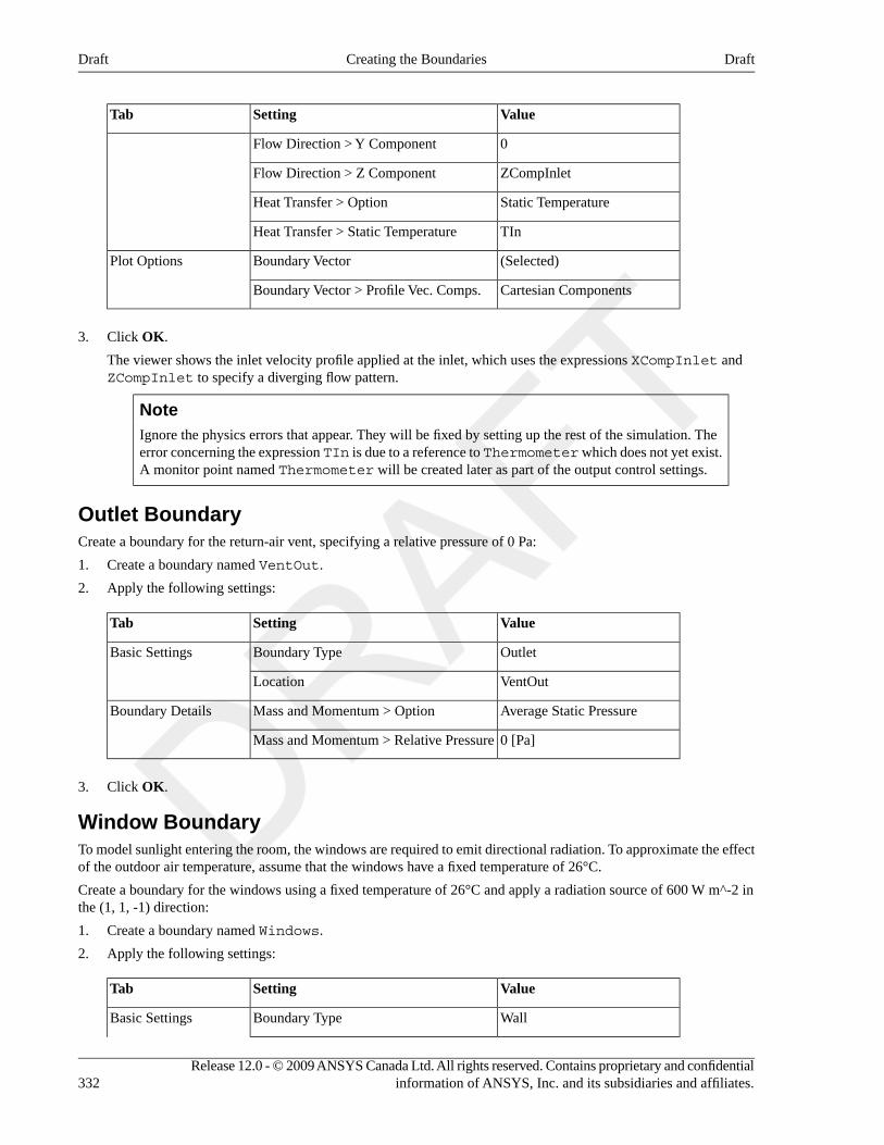
ValueSettingTab
0Flow Direction > Y Component
ZCompInletFlow Direction > Z Component
Static TemperatureHeat Transfer > Option
TInHeat Transfer > Static Temperature
(Selected)Boundary VectorPlot Options
Cartesian ComponentsBoundary Vector > Profile Vec. Comps.
3. Click OK.
The viewer shows the inlet velocity profile applied at the inlet, which uses the expressions XCompInlet andZCompInlet to specify a diverging flow pattern.
NoteIgnore the physics errors that appear. They will be fixed by setting up the rest of the simulation. Theerror concerning the expression TIn is due to a reference to Thermometer which does not yet exist.A monitor point named Thermometer will be created later as part of the output control settings.
Outlet BoundaryCreate a boundary for the return-air vent, specifying a relative pressure of 0 Pa:
1. Create a boundary named VentOut.
2. Apply the following settings:
ValueSettingTab
OutletBoundary TypeBasic Settings
VentOutLocation
Average Static PressureMass and Momentum > OptionBoundary Details
0 [Pa]Mass and Momentum > Relative Pressure
3. Click OK.
Window BoundaryTo model sunlight entering the room, the windows are required to emit directional radiation. To approximate the effectof the outdoor air temperature, assume that the windows have a fixed temperature of 26°C.
Create a boundary for the windows using a fixed temperature of 26°C and apply a radiation source of 600 W m^-2 inthe (1, 1, -1) direction:
1. Create a boundary named Windows.
2. Apply the following settings:
ValueSettingTab
WallBoundary TypeBasic Settings
Release 12.0 - © 2009 ANSYS Canada Ltd. All rights reserved. Contains proprietary and confidentialinformation of ANSYS, Inc. and its subsidiaries and affiliates.332
DraftCreating the BoundariesDraft
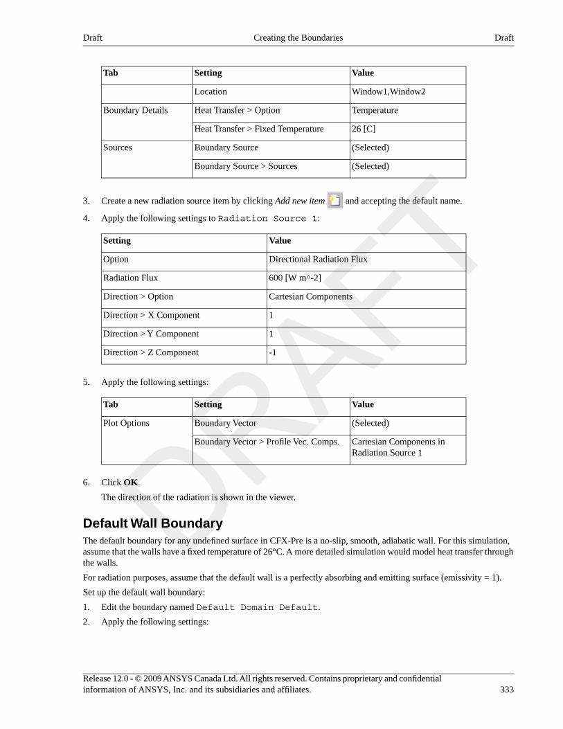
ValueSettingTab
Window1,Window2Location
TemperatureHeat Transfer > OptionBoundary Details
26 [C]Heat Transfer > Fixed Temperature
(Selected)Boundary SourceSources
(Selected)Boundary Source > Sources
3. Create a new radiation source item by clicking Add new item and accepting the default name.
4. Apply the following settings to Radiation Source 1:
ValueSetting
Directional Radiation FluxOption
600 [W m^-2]Radiation Flux
Cartesian ComponentsDirection > Option
1Direction > X Component
1Direction > Y Component
-1Direction > Z Component
5. Apply the following settings:
ValueSettingTab
(Selected)Boundary VectorPlot Options
Cartesian Components inRadiation Source 1
Boundary Vector > Profile Vec. Comps.
6. Click OK.
The direction of the radiation is shown in the viewer.
Default Wall BoundaryThe default boundary for any undefined surface in CFX-Pre is a no-slip, smooth, adiabatic wall. For this simulation,assume that the walls have a fixed temperature of 26°C. A more detailed simulation would model heat transfer throughthe walls.
For radiation purposes, assume that the default wall is a perfectly absorbing and emitting surface (emissivity = 1).
Set up the default wall boundary:
1. Edit the boundary named Default Domain Default.
2. Apply the following settings:
333Release 12.0 - © 2009 ANSYS Canada Ltd. All rights reserved. Contains proprietary and confidentialinformation of ANSYS, Inc. and its subsidiaries and affiliates.
DraftCreating the BoundariesDraft
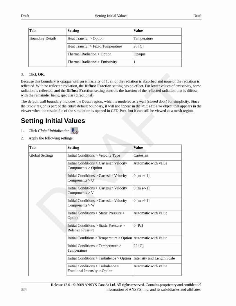
ValueSettingTab
TemperatureHeat Transfer > OptionBoundary Details
26 [C]Heat Transfer > Fixed Temperature
OpaqueThermal Radiation > Option
1Thermal Radiation > Emissivity
3. Click OK.
Because this boundary is opaque with an emissivity of 1, all of the radiation is absorbed and none of the radiation isreflected. With no reflected radiation, the Diffuse Fraction setting has no effect. For lower values of emissivity, someradiation is reflected, and the Diffuse Fraction setting controls the fraction of the reflected radiation that is diffuse,with the remainder being specular (directional).
The default wall boundary includes the Door region, which is modeled as a wall (closed door) for simplicity. Sincethe Door region is part of the entire default boundary, it will not appear in the Wireframe object that appears in theviewer when the results file of the simulation is opened in CFD-Post, but it can still be viewed as a mesh region.
Setting Initial Values1. Click Global Initialization .
2. Apply the following settings:
ValueSettingTab
CartesianInitial Conditions > Velocity TypeGlobal Settings
Automatic with ValueInitial Conditions > Cartesian VelocityComponents > Option
0 [m s^-1]Initial Conditions > Cartesian VelocityComponents > U
0 [m s^-1]Initial Conditions > Cartesian VelocityComponents > V
0 [m s^-1]Initial Conditions > Cartesian VelocityComponents > W
Automatic with ValueInitial Conditions > Static Pressure >Option
0 [Pa]Initial Conditions > Static Pressure >Relative Pressure
Automatic with ValueInitial Conditions > Temperature > Option
22 [C]Initial Conditions > Temperature >Temperature
Intensity and Length ScaleInitial Conditions > Turbulence > Option
Automatic with ValueInitial Conditions > Turbulence >Fractional Intensity > Option
Release 12.0 - © 2009 ANSYS Canada Ltd. All rights reserved. Contains proprietary and confidentialinformation of ANSYS, Inc. and its subsidiaries and affiliates.334
DraftSetting Initial ValuesDraft
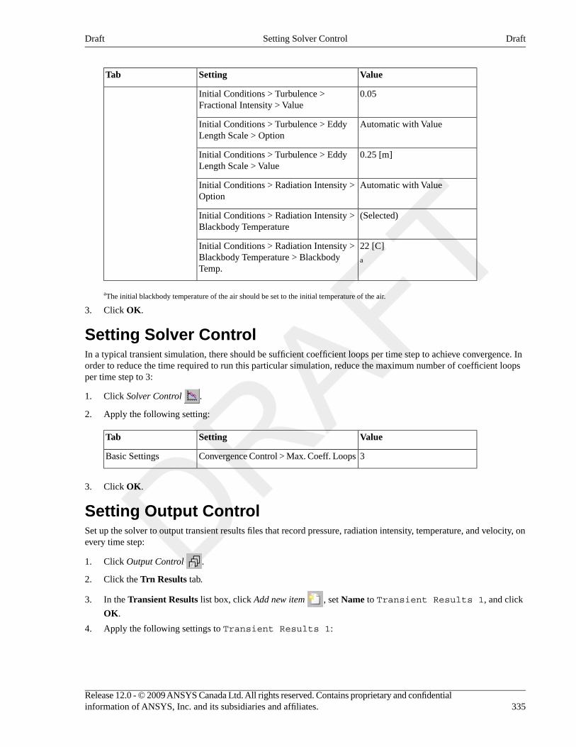
ValueSettingTab
0.05Initial Conditions > Turbulence >Fractional Intensity > Value
Automatic with ValueInitial Conditions > Turbulence > EddyLength Scale > Option
0.25 [m]Initial Conditions > Turbulence > EddyLength Scale > Value
Automatic with ValueInitial Conditions > Radiation Intensity >Option
(Selected)Initial Conditions > Radiation Intensity >Blackbody Temperature
22 [C]Initial Conditions > Radiation Intensity >Blackbody Temperature > BlackbodyTemp.
a
aThe initial blackbody temperature of the air should be set to the initial temperature of the air.
3. Click OK.
Setting Solver ControlIn a typical transient simulation, there should be sufficient coefficient loops per time step to achieve convergence. Inorder to reduce the time required to run this particular simulation, reduce the maximum number of coefficient loopsper time step to 3:
1. Click Solver Control .
2. Apply the following setting:
ValueSettingTab
3Convergence Control > Max. Coeff. LoopsBasic Settings
3. Click OK.
Setting Output ControlSet up the solver to output transient results files that record pressure, radiation intensity, temperature, and velocity, onevery time step:
1. Click Output Control .
2. Click the Trn Results tab.
3. In the Transient Results list box, click Add new item , set Name to Transient Results 1, and click
OK.
4. Apply the following settings to Transient Results 1:
335Release 12.0 - © 2009 ANSYS Canada Ltd. All rights reserved. Contains proprietary and confidentialinformation of ANSYS, Inc. and its subsidiaries and affiliates.
DraftSetting Solver ControlDraft
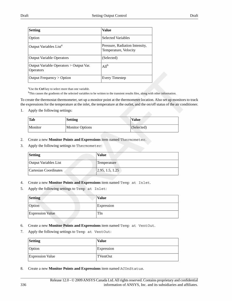
ValueSetting
Selected VariablesOption
Pressure, Radiation Intensity,Temperature, Velocity
Output Variables Lista
(Selected)Output Variable Operators
AllbOutput Variable Operators > Output Var.Operators
Every TimestepOutput Frequency > Option
aUse the Ctrl key to select more than one variable.bThis causes the gradients of the selected variables to be written to the transient results files, along with other information.
To create the thermostat thermometer, set up a monitor point at the thermometer location. Also set up monitors to trackthe expressions for the temperature at the inlet, the temperature at the outlet, and the on/off status of the air conditioner.
1. Apply the following settings:
ValueSettingTab
(Selected)Monitor OptionsMonitor
2. Create a new Monitor Points and Expressions item named Thermometer.
3. Apply the following settings to Thermometer:
ValueSetting
TemperatureOutput Variables List
2.95, 1.5, 1.25Cartesian Coordinates
4. Create a new Monitor Points and Expressions item named Temp at Inlet.
5. Apply the following settings to Temp at Inlet:
ValueSetting
ExpressionOption
TInExpression Value
6. Create a new Monitor Points and Expressions item named Temp at VentOut.
7. Apply the following settings to Temp at VentOut:
ValueSetting
ExpressionOption
TVentOutExpression Value
8. Create a new Monitor Points and Expressions item named ACOnStatus.
Release 12.0 - © 2009 ANSYS Canada Ltd. All rights reserved. Contains proprietary and confidentialinformation of ANSYS, Inc. and its subsidiaries and affiliates.336
DraftSetting Output ControlDraft
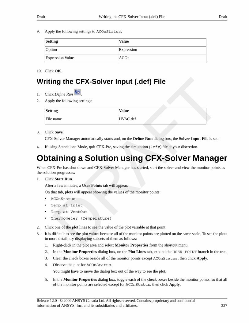
9. Apply the following settings to ACOnStatus:
ValueSetting
ExpressionOption
ACOnExpression Value
10. Click OK.
Writing the CFX-Solver Input (.def) File
1. Click Define Run .
2. Apply the following settings:
ValueSetting
HVAC.defFile name
3. Click Save.
CFX-Solver Manager automatically starts and, on the Define Run dialog box, the Solver Input File is set.
4. If using Standalone Mode, quit CFX-Pre, saving the simulation (.cfx) file at your discretion.
Obtaining a Solution using CFX-Solver ManagerWhen CFX-Pre has shut down and CFX-Solver Manager has started, start the solver and view the monitor points asthe solution progresses:
1. Click Start Run.
After a few minutes, a User Points tab will appear.
On that tab, plots will appear showing the values of the monitor points:
• ACOnStatus
• Temp at Inlet
• Temp at VentOut
• Thermometer (Temperature)
2. Click one of the plot lines to see the value of the plot variable at that point.
3. It is difficult to see the plot values because all of the monitor points are plotted on the same scale. To see the plotsin more detail, try displaying subsets of them as follows:
1. Right-click in the plot area and select Monitor Properties from the shortcut menu.
2. In the Monitor Properties dialog box, on the Plot Lines tab, expand the USER POINT branch in the tree.
3. Clear the check boxes beside all of the monitor points except ACOnStatus, then click Apply.
4. Observe the plot for ACOnStatus.
You might have to move the dialog box out of the way to see the plot.
5. In the Monitor Properties dialog box, toggle each of the check boxes beside the monitor points, so that allof the monitor points are selected except for ACOnStatus, then click Apply.
337Release 12.0 - © 2009 ANSYS Canada Ltd. All rights reserved. Contains proprietary and confidentialinformation of ANSYS, Inc. and its subsidiaries and affiliates.
DraftWriting the CFX-Solver Input (.def) FileDraft
6. Observe the plots for Temp at Inlet, Temp at VentOut, and Thermometer (Temperature).
7. Click OK to close the Monitor Properties dialog box.
4. Select the check box next to Post-Process Results when the completion message appears at the end of the run.
5. If using Standalone Mode, select the check box next to Shut down CFX-Solver Manager.
6. Click Ok.
Viewing the Results in CFD-PostYou will first create some graphic objects to visualize the temperature distribution and the thermometer location. Youwill then create an animation to show how the temperature distribution changes.
Creating Graphics ObjectsIn this section, you will create two planes and an isosurface of constant temperature, all colored by temperature. Youwill also create a color legend and a text label that reports the thermometer temperature.
Creating PlanesIn order to show the key features of the temperature distribution, create two planes colored by temperature as follows:
1. Load the res file (HVAC_001.res) if you did not elect to load the results directly from CFX-Solver Manager.
2. Right-click a blank area in the viewer, select Predefined Camera > Isometric View (Z up).
3. Create a ZX-Plane named Plane 1 with Y=1.5 [m]. Color it by Temperature using a user specified rangefrom 19 [C] to 23 [C]. Turn off lighting (on the Render tab) so that the colors are accurate and can beinterpreted properly using the legend.
4. Create an XY plane named Plane 2 with Z=0.35 [m]. Color it using the same settings as for the first plane,and turn off lighting.
Creating an IsosurfaceIn order to show the plumes of cool air from the inlet vent, create a surface of constant temperature as follows:
1. Click Timestep Selector . The Timestep Selector dialog box appears.
2. Double-click the value: 12 s.
The time step is set to 12 s so that the cold air plume is visible.
3. Create an isosurface named Cold Plume as a surface of Temperature = 19 °C.
4. Color the isosurface by Temperature (select Use Plot Variable) and use the same color range as forthe planes. Although the color of the isosurface will not show variation (by definition), it will be consistent withthe coloration of the planes.
5. On the Render tab for the isosurface, set Transparency to 0.5. Leave lighting turned on to help show the 3Dshape of the isosurface.
6. Click Apply.
NoteThe isosurface will not be visible in some time steps, but you will be able to see it when playing theanimation (a step carried out later).
Release 12.0 - © 2009 ANSYS Canada Ltd. All rights reserved. Contains proprietary and confidentialinformation of ANSYS, Inc. and its subsidiaries and affiliates.338
DraftViewing the Results in CFD-PostDraft
Adjusting the LegendThe legend title should not name the locator of any particular object since all objects are colored by the same variableand use the same range. Remove the locator name from the title and, in preparation for making an MPEG video laterin this tutorial, increase the text size:
1. Edit Default Legend View 1.
2. On the Definition tab, change Title Mode to Variable.
This will remove the locator name from the legend.
3. Click the Appearance tab, then:
1. Change Precision to 2, Fixed.
2. Change Text Height to 0.03.
4. Click Apply.
Creating a Point for the ThermometerIn the next section, you will create a text label that displays the value of the expression TSensor, which representsthe thermometer temperature. During the solver run, this expression was evaluated using a monitor point namedThermometer. Although this monitor point data is stored in the results file, it cannot be accessed. In order to supportthe expression for TSensor, create a point called Thermometer at the same location:
1. From the main menu, select Insert > Location > Point.
2. Set Name to Thermometer.
3. Set Point to (2.95,1.5,1.25).
4. Click Apply.
A marker appears at the thermometer location in the viewer.
Creating a Text LabelCreate a text label that shows the currently-selected time step and thermometer temperature.
1. Click Text .
2. Accept the default name and click OK.
3. Apply the following settings:
ValueSettingTab
Time Elapsed:Text StringDefinition
(Selected)aEmbed Auto Annotation
Time ValueType
aThe full text string should now be Time Elapsed: <aa>. The <aa> string represents the location where text is to be substituted.
4. Click More to add a second line of text to the text object.
5. Apply the following settings:
ValueSettingTab
Sensor Temperature:Text StringDefinition
339Release 12.0 - © 2009 ANSYS Canada Ltd. All rights reserved. Contains proprietary and confidentialinformation of ANSYS, Inc. and its subsidiaries and affiliates.
DraftCreating Graphics ObjectsDraft
ValueSettingTab
(the second one)
(Selected)Embed Auto Annotation
ExpressionType
TSensorExpression
0.03HeightAppearance
6. Click Apply.
7. Ensure that the visibility for Text 1 is turned on.
The text label appears in the viewer, near the top.
Creating an Animation1. Ensure that the view is set to Isometric View (Z up).
2. Click Timestep Selector .
3. Double-click the first time value (0 s).
4. In the toolbar at the top of the window click Animation .
5. In the Animation dialog box, select the Keyframe Animation option.
6. Click New to create KeyframeNo1.
7. Select KeyframeNo1, then set # of Frames to 200, then press Enter while in the # of Frames box.
TipBe sure to press Enter and confirm that the new number appears in the list before continuing.
This will place 200 intermediate frames between the first and (yet to be created) second key frames, for a total of202 frames. This will produce an animation lasting about 8.4 s since the frame rate will be 24 frames per second.Since there are 76 unique frames, each frame will be shown at least once.
8. Use the Timestep Selector to load the last time value (225 s).
9. In the Animation dialog box, click New to create KeyframeNo2.
The # of Frames parameter has no effect for the last keyframe, so leave it at the default value.
10. Click More Animation Options to expand the Animation dialog box.
11. Select Save Movie.
12. Set Format to MPEG1.
13. Specify a file name for the movie file.
14. Click the Options button.
15. Change Image Size to 720 x 480 (or a similar resolution).
16. Click the Advanced tab, and note the Quality setting. If your movie player cannot play the resulting MPEG, youcan try using the Low or Custom quality settings.
17. Click OK.
Release 12.0 - © 2009 ANSYS Canada Ltd. All rights reserved. Contains proprietary and confidentialinformation of ANSYS, Inc. and its subsidiaries and affiliates.340
DraftCreating an AnimationDraft
18. Click To Beginning to rewind the active key frame to KeyframeNo1.
19. Click Save animation state and save the animation to a file. This will enable you to quickly restore the
animation in case you want to make changes. Animations are not restored by loading ordinary state files (thosewith the .cst extension).
20. Click Play the animation .
21. If prompted to overwrite an existing movie, click Overwrite.
The animation plays and builds an mpg file.
22. When you have finished, quit CFD-Post.
Further Steps• This tutorial uses an aggressive flow rate of air, a coarse mesh, large time steps, and a low cap on the maximum
number of coefficient loops per time step. Running this tutorial with a flow rate of air that is closer to 5 changes
of air per hour (0.03 m3 s-1), a finer mesh, smaller time steps, and a larger cap on the maximum number of coefficientloops, will produce more accurate results.
• Running this simulation for a longer total time will allow you to see more on/off cycles of the air conditioner.
341Release 12.0 - © 2009 ANSYS Canada Ltd. All rights reserved. Contains proprietary and confidentialinformation of ANSYS, Inc. and its subsidiaries and affiliates.
DraftFurther StepsDraft

Release 12.0 - © 2009 ANSYS Canada Ltd. All rights reserved. Contains proprietary and confidentialinformation of ANSYS, Inc. and its subsidiaries and affiliates.
Chapter 20. Combustion and Radiationin a Can CombustorThis tutorial includes:
• Tutorial Features (p. 343)
• Overview of the Problem to Solve (p. 344)
• Using Eddy Dissipation and P1 Models (p. 345)
• Before You Begin (p. 345)
• Starting CFX-Pre (p. 346)
• Defining a Case Using Eddy Dissipation and P1 Models in CFX-Pre (p. 346)
• Obtaining a Solution using CFX-Solver Manager (p. 352)
• Viewing the Results in CFD-Post (p. 352)
• Defining a Simulation Using Laminar Flamelet and Discrete Transfer Models in ANSYS CFX-Pre (p. 355)
• Obtaining a Solution Using ANSYS CFX-Solver Manager (p. 359)
• Viewing the Results in ANSYS CFD-Post (p. 360)
• Further Postprocessing (p. 361)
Tutorial FeaturesIn this tutorial you will learn about:
• Creating thin surfaces for the inlet vanes.
• Using a Reacting Mixture.
• Using the Eddy Dissipation Combustion Model.
• Using the Flamelet Model.
• Changing the Combustion model in a simulation.
• Using the P1 Radiation Model in CFX-Pre.
• Using the Discrete Transfer Radiation Model in CFX-Pre.
• Using the NOx model in CFX-Pre.
• Changing object color maps in CFD-Post to prepare a greyscale image.
DetailsFeatureComponent
General ModeUser ModeCFX-Pre
Steady StateAnalysis Type
Reacting MixtureFluid Type
Single DomainDomain Type
k-EpsilonTurbulence Model
Thermal EnergyHeat Transfer
Combustion
343Release 12.0 - © 2009 ANSYS Canada Ltd. All rights reserved. Contains proprietary and confidentialinformation of ANSYS, Inc. and its subsidiaries and affiliates.
DraftDraft
DetailsFeatureComponent
Radiation
Inlet (Subsonic)Boundary Conditions
Outlet (Subsonic)
Wall: No-Slip
Wall: Adiabatic
Wall: Thin Surface
Physical Time ScaleTimestep
Outline Plot (Wireframe)PlotsCFD-Post
Sampling Plane
Slice Plane
Vector
Changing the Color RangeOther
Color map
Legend
Quantitative Calculation
Overview of the Problem to SolveThe can combustor is a feature of the gas turbine engine. Arranged around a central annulus, can combustors aredesigned to minimize emissions, burn very efficiently and keep wall temperatures as low as possible. This tutorial isdesigned to give a qualitative impression of the flow and temperature distributions. The basic geometry is shown belowwith a section of the outer wall cut away.
Release 12.0 - © 2009 ANSYS Canada Ltd. All rights reserved. Contains proprietary and confidentialinformation of ANSYS, Inc. and its subsidiaries and affiliates.344
DraftOverview of the Problem to SolveDraft
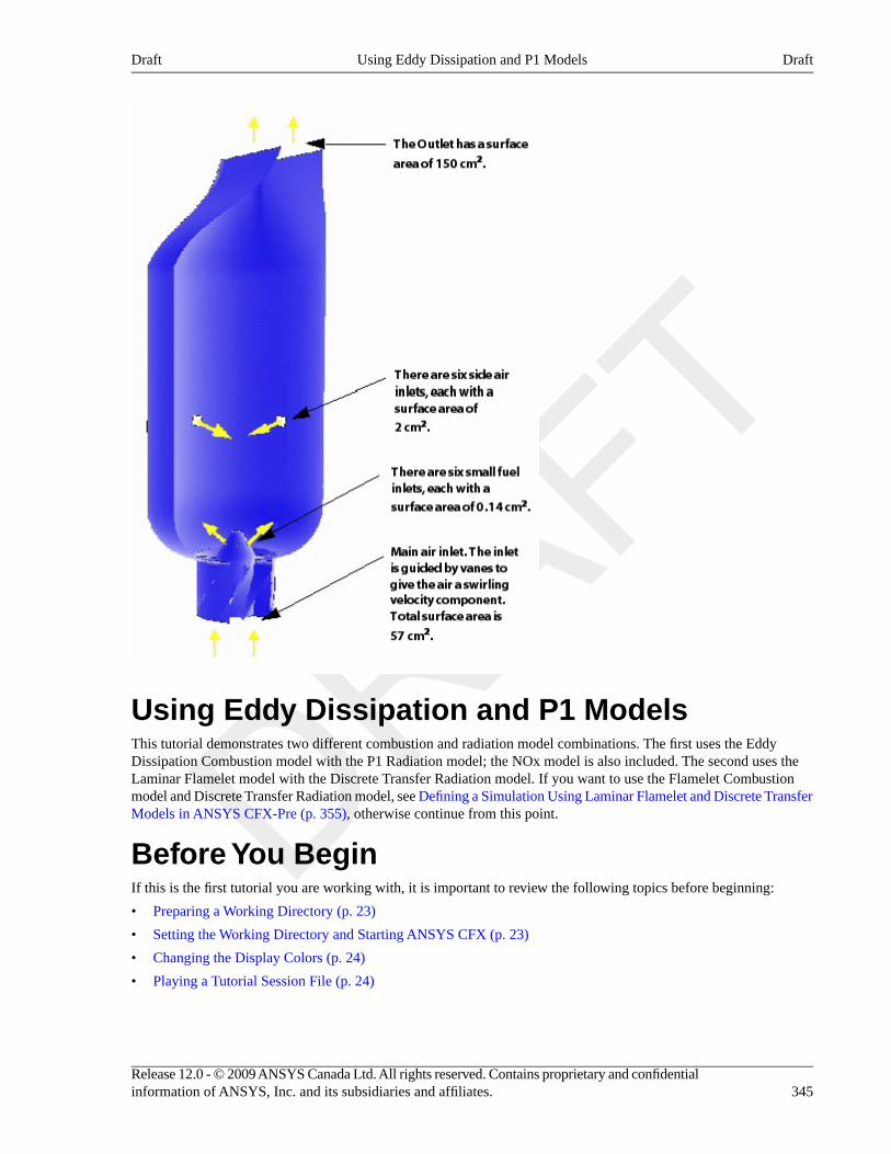
Using Eddy Dissipation and P1 ModelsThis tutorial demonstrates two different combustion and radiation model combinations. The first uses the EddyDissipation Combustion model with the P1 Radiation model; the NOx model is also included. The second uses theLaminar Flamelet model with the Discrete Transfer Radiation model. If you want to use the Flamelet Combustionmodel and Discrete Transfer Radiation model, see Defining a Simulation Using Laminar Flamelet and Discrete TransferModels in ANSYS CFX-Pre (p. 355), otherwise continue from this point.
Before You BeginIf this is the first tutorial you are working with, it is important to review the following topics before beginning:
• Preparing a Working Directory (p. 23)
• Setting the Working Directory and Starting ANSYS CFX (p. 23)
• Changing the Display Colors (p. 24)
• Playing a Tutorial Session File (p. 24)
345Release 12.0 - © 2009 ANSYS Canada Ltd. All rights reserved. Contains proprietary and confidentialinformation of ANSYS, Inc. and its subsidiaries and affiliates.
DraftUsing Eddy Dissipation and P1 ModelsDraft
Starting CFX-Pre1. Prepare the working directory using the following files in the examples directory:
• CombustorMesh.gtm
• CombustorEDM.pre
• CombustorFlamelet.pre
• CombustorEDM.cfx
For details, see Preparing a Working Directory (p. 23)
2. Set the working directory and start CFX-Pre
For details, see Setting the Working Directory and Starting ANSYS CFX (p. 23)
Defining a Case Using Eddy Dissipation and P1Models in CFX-PreIf you want to set up the simulation automatically using a tutorial session file, run CombustorEDM.pre. For details,see Playing a Tutorial Session File (p. 24). Then proceed to Obtaining a Solution using CFX-Solver Manager (p. 352).
If you want to set up the simulation manually, proceed to the following steps:
You will first define a domain that includes a variable composition mixture. These mixtures are used to model combustingand reacting flows in CFX.
1. Select File > New Case.
2. Select General and click OK.
3. Select File > Save Case As.
4. Under File name, type CombustorEDM.
5. Click Save.
6. If prompted, click Overwrite.
This file is provided in the tutorial directory and may exist in your working directory if you have copied it there.
Importing the Mesh1. Right-click Mesh and select Import Mesh > Other. The Import Mesh dialog box appears.
2. Apply the following setting
ValueSetting
CombustorMesh.gtmFile name
3. Click Open.
Creating a Reacting MixtureTo allow combustion modeling, you must create a variable composition mixture.
To create the variable composition mixture1. Create a new material named Methane Air Mixture.
Release 12.0 - © 2009 ANSYS Canada Ltd. All rights reserved. Contains proprietary and confidentialinformation of ANSYS, Inc. and its subsidiaries and affiliates.346
DraftStarting CFX-PreDraft
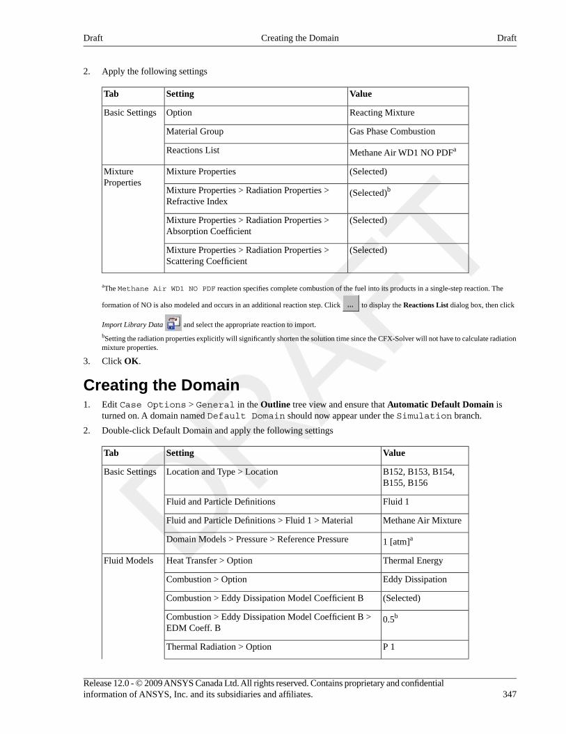
2. Apply the following settings
ValueSettingTab
Reacting MixtureOptionBasic Settings
Gas Phase CombustionMaterial Group
Methane Air WD1 NO PDFaReactions List
(Selected)Mixture PropertiesMixtureProperties
(Selected)bMixture Properties > Radiation Properties >Refractive Index
(Selected)Mixture Properties > Radiation Properties >Absorption Coefficient
(Selected)Mixture Properties > Radiation Properties >Scattering Coefficient
aThe Methane Air WD1 NO PDF reaction specifies complete combustion of the fuel into its products in a single-step reaction. The
formation of NO is also modeled and occurs in an additional reaction step. Click to display the Reactions List dialog box, then click
Import Library Data and select the appropriate reaction to import.
bSetting the radiation properties explicitly will significantly shorten the solution time since the CFX-Solver will not have to calculate radiationmixture properties.
3. Click OK.
Creating the Domain1. Edit Case Options > General in the Outline tree view and ensure that Automatic Default Domain is
turned on. A domain named Default Domain should now appear under the Simulation branch.
2. Double-click Default Domain and apply the following settings
ValueSettingTab
B152, B153, B154,B155, B156
Location and Type > LocationBasic Settings
Fluid 1Fluid and Particle Definitions
Methane Air MixtureFluid and Particle Definitions > Fluid 1 > Material
1 [atm]aDomain Models > Pressure > Reference Pressure
Thermal EnergyHeat Transfer > OptionFluid Models
Eddy DissipationCombustion > Option
(Selected)Combustion > Eddy Dissipation Model Coefficient B
0.5bCombustion > Eddy Dissipation Model Coefficient B >EDM Coeff. B
P 1Thermal Radiation > Option
347Release 12.0 - © 2009 ANSYS Canada Ltd. All rights reserved. Contains proprietary and confidentialinformation of ANSYS, Inc. and its subsidiaries and affiliates.
DraftCreating the DomainDraft
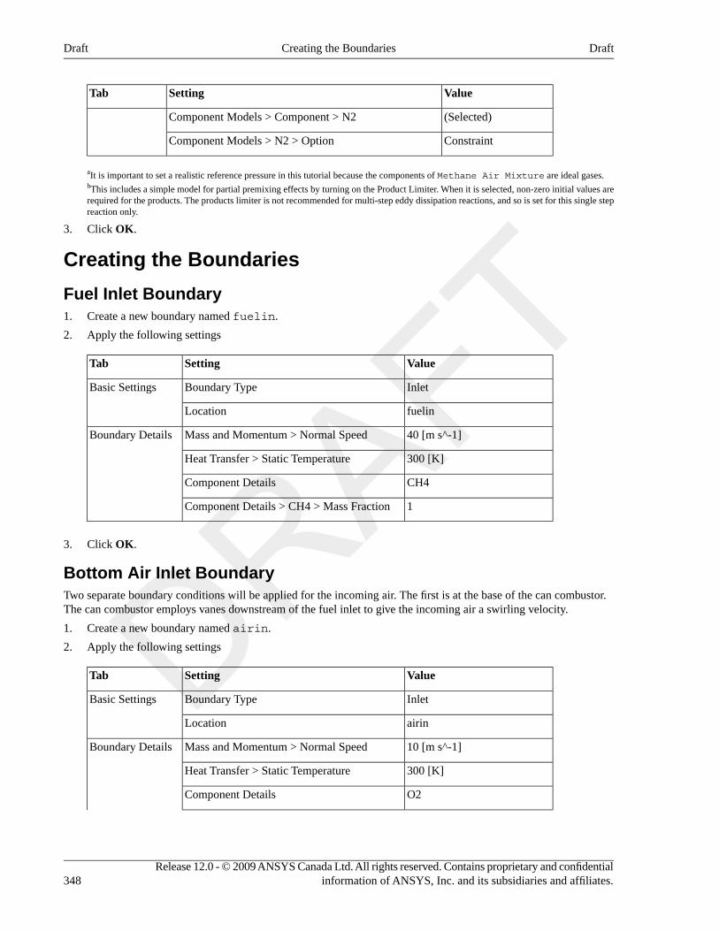
ValueSettingTab
(Selected)Component Models > Component > N2
ConstraintComponent Models > N2 > Option
aIt is important to set a realistic reference pressure in this tutorial because the components of Methane Air Mixture are ideal gases.bThis includes a simple model for partial premixing effects by turning on the Product Limiter. When it is selected, non-zero initial values arerequired for the products. The products limiter is not recommended for multi-step eddy dissipation reactions, and so is set for this single stepreaction only.
3. Click OK.
Creating the Boundaries
Fuel Inlet Boundary1. Create a new boundary named fuelin.
2. Apply the following settings
ValueSettingTab
InletBoundary TypeBasic Settings
fuelinLocation
40 [m s^-1]Mass and Momentum > Normal SpeedBoundary Details
300 [K]Heat Transfer > Static Temperature
CH4Component Details
1Component Details > CH4 > Mass Fraction
3. Click OK.
Bottom Air Inlet BoundaryTwo separate boundary conditions will be applied for the incoming air. The first is at the base of the can combustor.The can combustor employs vanes downstream of the fuel inlet to give the incoming air a swirling velocity.
1. Create a new boundary named airin.
2. Apply the following settings
ValueSettingTab
InletBoundary TypeBasic Settings
airinLocation
10 [m s^-1]Mass and Momentum > Normal SpeedBoundary Details
300 [K]Heat Transfer > Static Temperature
O2Component Details
Release 12.0 - © 2009 ANSYS Canada Ltd. All rights reserved. Contains proprietary and confidentialinformation of ANSYS, Inc. and its subsidiaries and affiliates.348
DraftCreating the BoundariesDraft
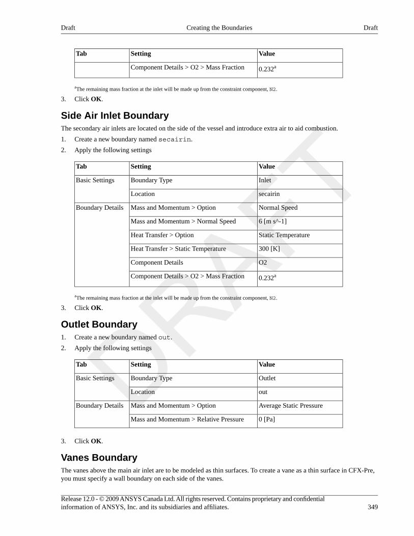
ValueSettingTab
0.232aComponent Details > O2 > Mass Fraction
aThe remaining mass fraction at the inlet will be made up from the constraint component, N2.
3. Click OK.
Side Air Inlet BoundaryThe secondary air inlets are located on the side of the vessel and introduce extra air to aid combustion.
1. Create a new boundary named secairin.
2. Apply the following settings
ValueSettingTab
InletBoundary TypeBasic Settings
secairinLocation
Normal SpeedMass and Momentum > OptionBoundary Details
6 [m s^-1]Mass and Momentum > Normal Speed
Static TemperatureHeat Transfer > Option
300 [K]Heat Transfer > Static Temperature
O2Component Details
0.232aComponent Details > O2 > Mass Fraction
aThe remaining mass fraction at the inlet will be made up from the constraint component, N2.
3. Click OK.
Outlet Boundary1. Create a new boundary named out.
2. Apply the following settings
ValueSettingTab
OutletBoundary TypeBasic Settings
outLocation
Average Static PressureMass and Momentum > OptionBoundary Details
0 [Pa]Mass and Momentum > Relative Pressure
3. Click OK.
Vanes BoundaryThe vanes above the main air inlet are to be modeled as thin surfaces. To create a vane as a thin surface in CFX-Pre,you must specify a wall boundary on each side of the vanes.
349Release 12.0 - © 2009 ANSYS Canada Ltd. All rights reserved. Contains proprietary and confidentialinformation of ANSYS, Inc. and its subsidiaries and affiliates.
DraftCreating the BoundariesDraft
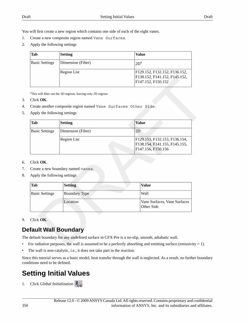
You will first create a new region which contains one side of each of the eight vanes.
1. Create a new composite region named Vane Surfaces.
2. Apply the following settings
ValueSettingTab
2DaDimension (Filter)Basic Settings
F129.152, F132.152, F136.152,F138.152, F141.152, F145.152,F147.152, F150.152
Region List
aThis will filter out the 3D regions, leaving only 2D regions
3. Click OK.
4. Create another composite region named Vane Surfaces Other Side.
5. Apply the following settings
ValueSettingTab
2DDimension (Filter)Basic Settings
F129.153, F132.153, F136.154,F138.154, F141.155, F145.155,F147.156, F150.156
Region List
6. Click OK.
7. Create a new boundary named vanes.
8. Apply the following settings
ValueSettingTab
WallBoundary TypeBasic Settings
Vane Surfaces, Vane SurfacesOther Side
Location
9. Click OK.
Default Wall BoundaryThe default boundary for any undefined surface in CFX-Pre is a no-slip, smooth, adiabatic wall.
• For radiation purposes, the wall is assumed to be a perfectly absorbing and emitting surface (emissivity = 1).
• The wall is non-catalytic, i.e., it does not take part in the reaction.
Since this tutorial serves as a basic model, heat transfer through the wall is neglected. As a result, no further boundaryconditions need to be defined.
Setting Initial Values1. Click Global Initialization .
Release 12.0 - © 2009 ANSYS Canada Ltd. All rights reserved. Contains proprietary and confidentialinformation of ANSYS, Inc. and its subsidiaries and affiliates.350
DraftSetting Initial ValuesDraft
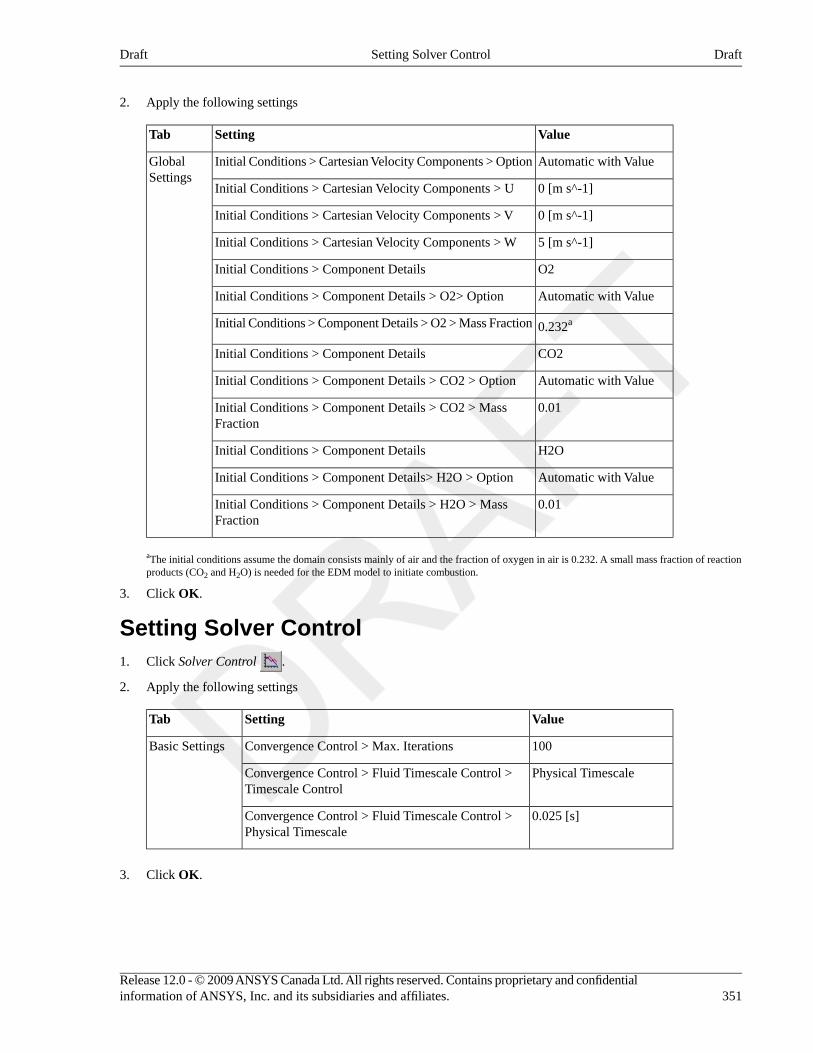
2. Apply the following settings
ValueSettingTab
Automatic with ValueInitial Conditions > Cartesian Velocity Components > OptionGlobalSettings
0 [m s^-1]Initial Conditions > Cartesian Velocity Components > U
0 [m s^-1]Initial Conditions > Cartesian Velocity Components > V
5 [m s^-1]Initial Conditions > Cartesian Velocity Components > W
O2Initial Conditions > Component Details
Automatic with ValueInitial Conditions > Component Details > O2> Option
0.232aInitial Conditions > Component Details > O2 > Mass Fraction
CO2Initial Conditions > Component Details
Automatic with ValueInitial Conditions > Component Details > CO2 > Option
0.01Initial Conditions > Component Details > CO2 > MassFraction
H2OInitial Conditions > Component Details
Automatic with ValueInitial Conditions > Component Details> H2O > Option
0.01Initial Conditions > Component Details > H2O > MassFraction
aThe initial conditions assume the domain consists mainly of air and the fraction of oxygen in air is 0.232. A small mass fraction of reactionproducts (CO2 and H2O) is needed for the EDM model to initiate combustion.
3. Click OK.
Setting Solver Control1. Click Solver Control .
2. Apply the following settings
ValueSettingTab
100Convergence Control > Max. IterationsBasic Settings
Physical TimescaleConvergence Control > Fluid Timescale Control >Timescale Control
0.025 [s]Convergence Control > Fluid Timescale Control >Physical Timescale
3. Click OK.
351Release 12.0 - © 2009 ANSYS Canada Ltd. All rights reserved. Contains proprietary and confidentialinformation of ANSYS, Inc. and its subsidiaries and affiliates.
DraftSetting Solver ControlDraft
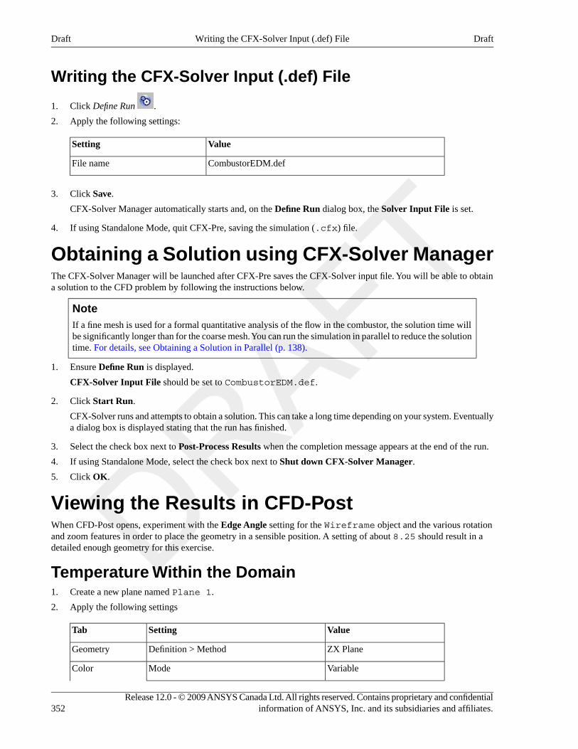
Writing the CFX-Solver Input (.def) File
1. Click Define Run .
2. Apply the following settings:
ValueSetting
CombustorEDM.defFile name
3. Click Save.
CFX-Solver Manager automatically starts and, on the Define Run dialog box, the Solver Input File is set.
4. If using Standalone Mode, quit CFX-Pre, saving the simulation (.cfx) file.
Obtaining a Solution using CFX-Solver ManagerThe CFX-Solver Manager will be launched after CFX-Pre saves the CFX-Solver input file. You will be able to obtaina solution to the CFD problem by following the instructions below.
NoteIf a fine mesh is used for a formal quantitative analysis of the flow in the combustor, the solution time willbe significantly longer than for the coarse mesh. You can run the simulation in parallel to reduce the solutiontime. For details, see Obtaining a Solution in Parallel (p. 138).
1. Ensure Define Run is displayed.
CFX-Solver Input File should be set to CombustorEDM.def.
2. Click Start Run.
CFX-Solver runs and attempts to obtain a solution. This can take a long time depending on your system. Eventuallya dialog box is displayed stating that the run has finished.
3. Select the check box next to Post-Process Results when the completion message appears at the end of the run.
4. If using Standalone Mode, select the check box next to Shut down CFX-Solver Manager.
5. Click OK.
Viewing the Results in CFD-PostWhen CFD-Post opens, experiment with the Edge Angle setting for the Wireframe object and the various rotationand zoom features in order to place the geometry in a sensible position. A setting of about 8.25 should result in adetailed enough geometry for this exercise.
Temperature Within the Domain1. Create a new plane named Plane 1.
2. Apply the following settings
ValueSettingTab
ZX PlaneDefinition > MethodGeometry
VariableModeColor
Release 12.0 - © 2009 ANSYS Canada Ltd. All rights reserved. Contains proprietary and confidentialinformation of ANSYS, Inc. and its subsidiaries and affiliates.352
DraftWriting the CFX-Solver Input (.def) FileDraft
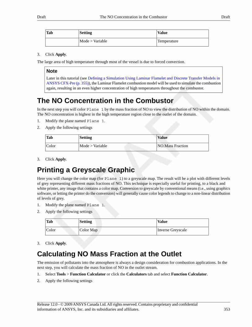
ValueSettingTab
TemperatureMode > Variable
3. Click Apply.
The large area of high temperature through most of the vessel is due to forced convection.
NoteLater in this tutorial (see Defining a Simulation Using Laminar Flamelet and Discrete Transfer Models inANSYS CFX-Pre (p. 355)), the Laminar Flamelet combustion model will be used to simulate the combustionagain, resulting in an even higher concentration of high temperatures throughout the combustor.
The NO Concentration in the CombustorIn the next step you will color Plane 1 by the mass fraction of NO to view the distribution of NO within the domain.The NO concentration is highest in the high temperature region close to the outlet of the domain.
1. Modify the plane named Plane 1.
2. Apply the following settings
ValueSettingTab
NO.Mass FractionMode > VariableColor
3. Click Apply.
Printing a Greyscale GraphicHere you will change the color map (for Plane 1) to a greyscale map. The result will be a plot with different levelsof grey representing different mass fractions of NO. This technique is especially useful for printing, to a black andwhite printer, any image that contains a color map. Conversion to greyscale by conventional means (i.e., using graphicssoftware, or letting the printer do the conversion) will generally cause color legends to change to a non-linear distributionof levels of grey.
1. Modify the plane named Plane 1.
2. Apply the following settings
ValueSettingTab
Inverse GreyscaleColor MapColor
3. Click Apply.
Calculating NO Mass Fraction at the OutletThe emission of pollutants into the atmosphere is always a design consideration for combustion applications. In thenext step, you will calculate the mass fraction of NO in the outlet stream.
1. Select Tools > Function Calculator or click the Calculators tab and select Function Calculator.
2. Apply the following settings
353Release 12.0 - © 2009 ANSYS Canada Ltd. All rights reserved. Contains proprietary and confidentialinformation of ANSYS, Inc. and its subsidiaries and affiliates.
DraftThe NO Concentration in the CombustorDraft
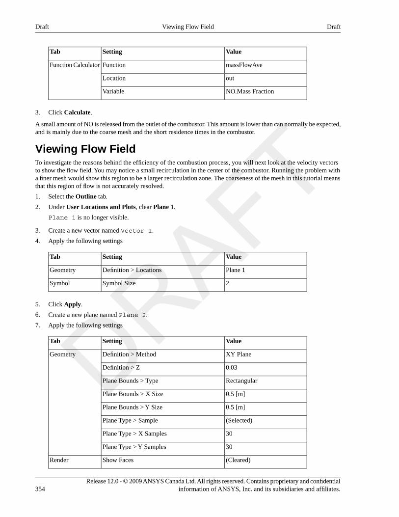
ValueSettingTab
massFlowAveFunctionFunction Calculator
outLocation
NO.Mass FractionVariable
3. Click Calculate.
A small amount of NO is released from the outlet of the combustor. This amount is lower than can normally be expected,and is mainly due to the coarse mesh and the short residence times in the combustor.
Viewing Flow FieldTo investigate the reasons behind the efficiency of the combustion process, you will next look at the velocity vectorsto show the flow field. You may notice a small recirculation in the center of the combustor. Running the problem witha finer mesh would show this region to be a larger recirculation zone. The coarseness of the mesh in this tutorial meansthat this region of flow is not accurately resolved.
1. Select the Outline tab.
2. Under User Locations and Plots, clear Plane 1.
Plane 1 is no longer visible.
3. Create a new vector named Vector 1.
4. Apply the following settings
ValueSettingTab
Plane 1Definition > LocationsGeometry
2Symbol SizeSymbol
5. Click Apply.
6. Create a new plane named Plane 2.
7. Apply the following settings
ValueSettingTab
XY PlaneDefinition > MethodGeometry
0.03Definition > Z
RectangularPlane Bounds > Type
0.5 [m]Plane Bounds > X Size
0.5 [m]Plane Bounds > Y Size
(Selected)Plane Type > Sample
30Plane Type > X Samples
30Plane Type > Y Samples
(Cleared)Show FacesRender
Release 12.0 - © 2009 ANSYS Canada Ltd. All rights reserved. Contains proprietary and confidentialinformation of ANSYS, Inc. and its subsidiaries and affiliates.354
DraftViewing Flow FieldDraft
8. Click Apply.
9. Modify Vector 1.
10. Apply the following setting
ValueSettingTab
Plane 2Definition > LocationsGeometry
11. Click Apply.
To view the swirling velocity field, right-click in the viewer and select Predefined Camera > View Towards -Z.
You may also want to turn off the wireframe visibility. In the region near the fuel and air inlets, the swirl componentof momentum (theta direction) results in increased mixing with the surrounding fluid and a higher residence time inthis region. As a result, more fuel is burned.
Viewing RadiationTry examining the distribution of Incident Radiation and Radiation Intensity throughout the domain.
When you are finished, quit CFD-Post.
Defining a Simulation Using Laminar Flameletand Discrete Transfer Models in ANSYS CFX-PreIn this second part of the tutorial, you will start with the simulation from the first part of the tutorial and modify it touse the Laminar Flamelet combustion and Discrete Transfer radiation models. Running the simulation a second timewill demonstrate the differences in the combustion models, including the variance in carbon dioxide distribution, whichis shown below.
355Release 12.0 - © 2009 ANSYS Canada Ltd. All rights reserved. Contains proprietary and confidentialinformation of ANSYS, Inc. and its subsidiaries and affiliates.
DraftViewing RadiationDraft
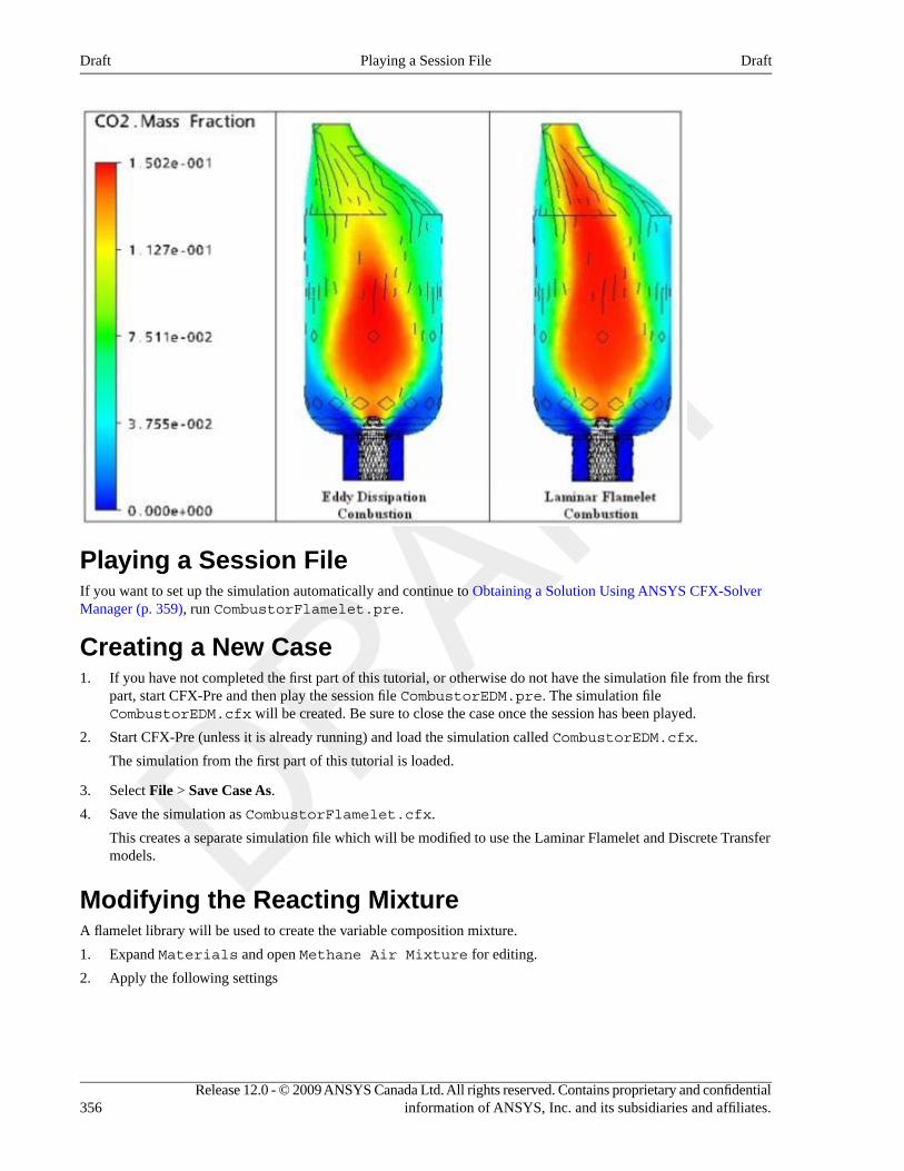
Playing a Session FileIf you want to set up the simulation automatically and continue to Obtaining a Solution Using ANSYS CFX-SolverManager (p. 359), run CombustorFlamelet.pre.
Creating a New Case1. If you have not completed the first part of this tutorial, or otherwise do not have the simulation file from the first
part, start CFX-Pre and then play the session file CombustorEDM.pre. The simulation fileCombustorEDM.cfx will be created. Be sure to close the case once the session has been played.
2. Start CFX-Pre (unless it is already running) and load the simulation called CombustorEDM.cfx.
The simulation from the first part of this tutorial is loaded.
3. Select File > Save Case As.
4. Save the simulation as CombustorFlamelet.cfx.
This creates a separate simulation file which will be modified to use the Laminar Flamelet and Discrete Transfermodels.
Modifying the Reacting MixtureA flamelet library will be used to create the variable composition mixture.
1. Expand Materials and open Methane Air Mixture for editing.
2. Apply the following settings
Release 12.0 - © 2009 ANSYS Canada Ltd. All rights reserved. Contains proprietary and confidentialinformation of ANSYS, Inc. and its subsidiaries and affiliates.356
DraftPlaying a Session FileDraft
ValueSettingTab
Methane Air FLL STP and NO PDFaReactions ListBasic Settings
aClick to display the Reactions List dialog box, then click Import Library Data and select the appropriate reaction to import.
3. Click OK.
NoteSome physics validation messages appear after this reaction is selected. In this situation, the messagescan be safely ignored as the physics will be corrected once the domains and boundary conditions aremodified.
Modifying the Domain1. Double-click the Default Domain.
2. Apply the following settings
ValueSettingTab
PDF FlameletCombustion > OptionFluid Models
Discrete TransferThermal Radiation > Option
N2Component Models > Component
ConstraintComponent Models > Component > N2 > Option
NOComponent Models > Component
Transport EquationComponent Models > Component > NO > Option
(All other components)aComponent Models > Component
AutomaticComponent Models > Component > (All othercomponents) > Option
aSelect these one at a time and check each of them.
3. Click OK.
Modifying the Boundaries
Fuel Inlet Boundary1. Modify the boundary named fuelin.
2. Apply the following settings
ValueSettingTab
FuelMixture > OptionBoundary Details
NOComponent Details
Mass FractionComponent Details > NO > Option
357Release 12.0 - © 2009 ANSYS Canada Ltd. All rights reserved. Contains proprietary and confidentialinformation of ANSYS, Inc. and its subsidiaries and affiliates.
DraftModifying the DomainDraft
ValueSettingTab
0Component Details > NO > Mass Fraction
3. Click OK.
Bottom Air Inlet Boundary1. Modify the boundary named airin.
2. Apply the following settings
ValueSettingTab
OxidiserMixture > OptionBoundary Details
NOComponent Details
Mass FractionComponent Details > NO > Option
0Component Details > NO > Mass Fraction
3. Click OK.
Side Air Inlet Boundary1. Modify the boundary named secairin.
2. Apply the following settings
ValueSettingTab
OxidiserMixture > OptionBoundary Details
NOComponent Details
Mass FractionComponent Details > NO > Option
0Component Details > NO > Mass Fraction
3. Click OK.
Setting Initial Values1. Click Global Initialization .
2. Apply the following settings
ValueSettingTab
NOInitial Conditions > Component DetailsGlobalSettings
Automatic with ValueInitial Conditions > Component Details > NO > Option
0Initial Conditions > Component Details > NO > MassFraction
Release 12.0 - © 2009 ANSYS Canada Ltd. All rights reserved. Contains proprietary and confidentialinformation of ANSYS, Inc. and its subsidiaries and affiliates.358
DraftSetting Initial ValuesDraft
3. Click OK.
Setting Solver ControlTo reduce the amount of CPU time required for solving the radiation equations, you can select to solve them only every10 iterations.
1. Click Solver Control .
2. Apply the following settings
ValueSettingTab
(Selected)Dynamic Model Control > Global Dynamic Model ControlAdvancedOptions
(Selected)Thermal Radiation Control
(Selected)Thermal Radiation Control > Iteration Interval
10Thermal Radiation Control > Iteration Interval > Iteration Interval
3. Click OK.
Writing the CFX-Solver Input (.def) File
1. Click Define Run .
2. Apply the following settings:
ValueSetting
CombustorFlamelet.defFile name
3. Click Save.
CFX-Solver Manager automatically starts and, on the Define Run dialog box, the Solver Input File is set.
4. If using Standalone Mode, quit CFX-Pre, saving the simulation (.cfx) file at your discretion.
Obtaining a Solution Using ANSYS CFX-SolverManagerWhen CFX-Solver Manager has started, you can obtain a solution to the CFD problem by using the following procedure:
1. Ensure Define Run is displayed.
CFX-Solver Input File should be set to CombustorFlamelet.def.
2. Click Start Run.
CFX-Solver runs and attempts to obtain a solution. This can take a long time depending on your system. Eventuallya dialog box is displayed.
3. When CFX-Solver is finished, select the check box next to Post-Process Results.
4. If using Standalone Mode, select the check box next to Shut down CFX-Solver Manager.
5. Click OK.
359Release 12.0 - © 2009 ANSYS Canada Ltd. All rights reserved. Contains proprietary and confidentialinformation of ANSYS, Inc. and its subsidiaries and affiliates.
DraftSetting Solver ControlDraft
Viewing the Results in ANSYS CFD-PostIn this section, you will plot the Temperature in the Domain, the NO Concentration in the Combustor, and the COConcentration. You will also use the Function Calculator to calculate the NO Concentration, and the CO Mass Fractionat the Outlet.
Viewing Temperature within the Domain1. Create a new plane named Plane 1.
2. Apply the following settings
ValueSettingTab
ZX PlaneDefinition > MethodGeometry
0Definition > Y
VariableModeColor
TemperatureMode > Variable
3. Click Apply.
Viewing the NO Concentration in the Combustor1. Modify the plane named Plane 1.
2. Apply the following settings
ValueSettingTab
NO.Mass FractionMode > VariableColor
3. Click Apply.
Calculating NO ConcentrationThe next calculation shows the amount of NO at the outlet.
1. Select Tools > Function Calculator or click the Calculators tab and select Function Calculator.
2. Apply the following settings
ValueSettingTab
massFlowAveFunctionFunction Calculator
outLocation
NO.Mass FractionVariable
3. Click Calculate.
Release 12.0 - © 2009 ANSYS Canada Ltd. All rights reserved. Contains proprietary and confidentialinformation of ANSYS, Inc. and its subsidiaries and affiliates.360
DraftViewing the Results in ANSYS CFD-PostDraft
Viewing CO ConcentrationThe next plot will show the concentration of CO (carbon monoxide), which is a by-product of incomplete combustionand is poisonous in significant concentrations. As you will see, the highest values are very close to the fuel inlet andin the regions of highest temperature.
1. Modify the plane named Plane 1.
2. Apply the following settings
ValueSettingTab
CO.Mass FractionMode > VariableColor
LocalRange
3. Click Apply.
Calculating CO Mass Fraction at the OutletIn the next step, you will calculate the mass fraction of CO in the outlet stream.
1. Select Tools > Function Calculator or click the Calculators tab and select Function Calculator.
2. Apply the following settings
ValueSettingTab
massFlowAveFunctionFunction Calculator
outLocation
CO.Mass FractionVariable
3. Click Calculate.
There is approximately 0.4% CO by mass in the outlet stream.
Further Postprocessing1. Try putting some plots of your choice into the Viewer. You can plot the concentration of other species and compare
values to those found for the Eddy Dissipation model.
2. Examine the distribution of Incident Radiation and Radiation Intensity throughout the domain.
3. Load one combustion model, then load the other using the Keep current cases loaded option in the Load ResultsFile dialog box. You can compare both models in the viewer at once, in terms of mass fractions of various materials,as well as total temperature and other relevant measurements.
361Release 12.0 - © 2009 ANSYS Canada Ltd. All rights reserved. Contains proprietary and confidentialinformation of ANSYS, Inc. and its subsidiaries and affiliates.
DraftViewing CO ConcentrationDraft

Release 12.0 - © 2009 ANSYS Canada Ltd. All rights reserved. Contains proprietary and confidentialinformation of ANSYS, Inc. and its subsidiaries and affiliates.
Chapter 21. Cavitation Around aHydrofoilThis tutorial includes:
• Tutorial Features (p. 363)
• Overview of the Problem to Solve (p. 364)
• Before You Begin (p. 364)
• Starting CFX-Pre (p. 365)
• Creating an Initial Simulation (p. 365)
• Obtaining an Initial Solution using CFX-Solver Manager (p. 369)
• Viewing the Results of the Initial Simulation (p. 370)
• Preparing a Simulation with Cavitation (p. 373)
• Obtaining a Cavitation Solution using CFX-Solver Manager (p. 374)
• Viewing the Results of the Cavitation Simulation (p. 375)
Tutorial FeaturesIn this tutorial you will learn about:
• Modeling flow with cavitation.
• Using vector reduction in CFD-Post to clarify a vector plot with many arrows.
• Importing and exporting data along a polyline.
• Plotting computed and experimental results.
DetailsFeatureComponent
General ModeUser ModeCFX-Pre
Steady StateAnalysis Type
General FluidFluid Type
Single DomainDomain Type
k-EpsilonTurbulence Model
IsothermalHeat Transfer
Multiphase
Inlet (Subsonic)Boundary Conditions
Outlet (Subsonic)
Symmetry Plane
Wall: No-Slip
Wall: Free-Slip
Physical Time ScaleTimestep
363Release 12.0 - © 2009 ANSYS Canada Ltd. All rights reserved. Contains proprietary and confidentialinformation of ANSYS, Inc. and its subsidiaries and affiliates.
DraftDraft
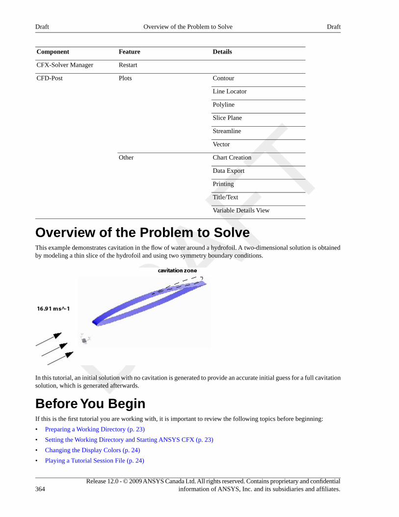
DetailsFeatureComponent
RestartCFX-Solver Manager
ContourPlotsCFD-Post
Line Locator
Polyline
Slice Plane
Streamline
Vector
Chart CreationOther
Data Export
Printing
Title/Text
Variable Details View
Overview of the Problem to SolveThis example demonstrates cavitation in the flow of water around a hydrofoil. A two-dimensional solution is obtainedby modeling a thin slice of the hydrofoil and using two symmetry boundary conditions.
In this tutorial, an initial solution with no cavitation is generated to provide an accurate initial guess for a full cavitationsolution, which is generated afterwards.
Before You BeginIf this is the first tutorial you are working with, it is important to review the following topics before beginning:
• Preparing a Working Directory (p. 23)
• Setting the Working Directory and Starting ANSYS CFX (p. 23)
• Changing the Display Colors (p. 24)
• Playing a Tutorial Session File (p. 24)
Release 12.0 - © 2009 ANSYS Canada Ltd. All rights reserved. Contains proprietary and confidentialinformation of ANSYS, Inc. and its subsidiaries and affiliates.364
DraftOverview of the Problem to SolveDraft
Starting CFX-Pre1. Prepare the working directory using the following files in the examples directory:
• HydrofoilExperimentalCp.csv
• HydrofoilGrid.def
• HydrofoilIni.pre
• Hydrofoil.pre
• HydrofoilIni_001.res
For details, see Preparing a Working Directory (p. 23)
2. Set the working directory and start CFX-Pre
For details, see Setting the Working Directory and Starting ANSYS CFX (p. 23)
Creating an Initial SimulationThis section describes the step-by-step definition of the flow physics in CFX-Pre.
Defining a Case in CFX-PreIf you want to set up the simulation automatically using a tutorial session file, run HydrofoilIni.pre. For details,see Playing a Tutorial Session File (p. 24). Then proceed to Obtaining an Initial Solution using CFX-SolverManager (p. 369).
If you want to set up the simulation manually, proceed to the following steps:
1. Start CFX-Pre.
2. Select File > New Case.
3. Select General and click OK.
4. Select File > Save Case As.
5. Under File name, type HydrofoilIni.
6. Click Save.
Importing the Mesh1. Right-click Mesh and select Import Mesh > Other. The Import Mesh dialog box appears.
2. Apply the following settings
ValueSetting
CFX-Solver Input (*.def, *.res, *.trn, *.bak)Files of type
HydrofoilGrid.defFile name
3. Click Open.
4. Right-click a blank area in the viewer and select Predefined Camera > View Towards -Z.
Loading MaterialsSince this tutorial uses Water Vapour at 25 C and Water at 25 C, you need to load these materials.
365Release 12.0 - © 2009 ANSYS Canada Ltd. All rights reserved. Contains proprietary and confidentialinformation of ANSYS, Inc. and its subsidiaries and affiliates.
DraftStarting CFX-PreDraft
1. In the Outline tree view, right-click Materials and select Import Library Data.
The Select Library Data to Import dialog box is displayed.
2. Expand Water Data.
3. Select both Water Vapour at 25 C and Water at 25 C by holding Crtl when selecting.
4. Click OK.
Creating the DomainThe fluid domain used for this simulation contains liquid water and water vapor. The volume fractions are initially setso that the domain is filled entirely with liquid.
1. Edit Case Options > General in the Outline tree view and ensure that Automatic Default Domain isturned on. A domain named Default Domain should now appear under the Simulation > Flow Analysis1 branch.
2. Double-click Default Domain.
3. Under Fluid and Particle Definitions, delete Fluid 1 and create a new fluid definition called Liquid Water.
Use the button to create another fluid named Water Vapor.
Apply the following settings:
ValueSettingTab
Liquid WaterFluid and Particle DefinitionsBasic Settings
Water at 25 CFluid and Particle Definitions > Liquid Water > Material
Water VaporFluid and Particle Definitions
Water Vapour at 25 CFluid and Particle Definitions > Water Vapor > Material
a
0 [atm]Domain Models > Pressure > Reference Pressure
(Selected)Multiphase > Homogeneous ModelFluid Models
IsothermalHeat Transfer > Option
300 [K]Heat Transfer > Fluid Temperature
k-EpsilonTurbulence > Option
aThese two fluids have consistent reference enthalpies.
4. Click OK.
Creating the BoundariesThe simulation requires inlet, outlet, wall and symmetry plane boundaries. The regions for these boundaries wereimported with the grid file.
Inlet Boundary1. Create a new boundary named Inlet.
2. Apply the following settings
Release 12.0 - © 2009 ANSYS Canada Ltd. All rights reserved. Contains proprietary and confidentialinformation of ANSYS, Inc. and its subsidiaries and affiliates.366
DraftCreating the DomainDraft
ValueSettingTab
InletBoundary TypeBasic Settings
INLocation
16.91 [m s^-1]Mass And Momentum > Normal SpeedBoundary Details
Intensity and Length ScaleTurbulence > Option
0.03Turbulence > Fractional Intensity
0.0076 [m]Turbulence > Eddy Len. Scale
Liquid WaterBoundary ConditionsFluid Values
1Boundary Conditions > Liquid Water > VolumeFraction > Volume Fraction
Water VaporBoundary Conditions
0Boundary Conditions > Water Vapor > VolumeFraction > Volume Fraction
3. Click OK.
Outlet Boundary1. Create a new boundary named Outlet.
2. Apply the following settings
ValueSettingTab
OutletBoundary TypeBasic Settings
OUTLocation
Static PressureMass And Momentum > OptionBoundary Details
51957 [Pa]Mass And Momentum > Relative Pressure
3. Click OK.
Free Slip Wall Boundary1. Create a new boundary named SlipWalls.
2. Apply the following settings
ValueSettingTab
WallBoundary TypeBasic Settings
BOT, TOPLocation
Free Slip WallMass And Momentum > OptionBoundary Details
3. Click OK.
367Release 12.0 - © 2009 ANSYS Canada Ltd. All rights reserved. Contains proprietary and confidentialinformation of ANSYS, Inc. and its subsidiaries and affiliates.
DraftCreating the BoundariesDraft
Symmetry Plane Boundaries1. Create a new boundary named Sym1.
2. Apply the following settings
ValueSettingTab
SymmetryBoundary TypeBasic Settings
SYM1Location
3. Click OK.
1. Create a new boundary named Sym2.
2. Apply the following settings
ValueSettingTab
SymmetryBoundary TypeBasic Settings
SYM2Location
3. Click OK.
Setting Initial Values1. Click Global Initialization .
2. Apply the following settings
ValueSettingTab
Automatic with ValueInitial Conditions > Cartesian Velocity Components > OptionGlobalSettings
16.91 [m s^-1]Initial Conditions > Cartesian Velocity Components > U
0 [m s^-1]Initial Conditions > Cartesian Velocity Components > V
0 [m s^-1]Initial Conditions > Cartesian Velocity Components > W
Liquid WaterFluid Specific InitializationFluidSettings
Automatic with ValueFluid Specific Initialization > Liquid Water > InitialConditions > Volume Fraction > Option
1Fluid Specific Initialization > Liquid Water > InitialConditions > Volume Fraction > Volume Fraction
Water VaporFluid Specific Initialization
Automatic with ValueFluid Specific Initialization > Water Vapor > InitialConditions > Volume Fraction > Option
0Fluid Specific Initialization > Water Vapor > InitialConditions > Volume Fraction > Volume Fraction
Release 12.0 - © 2009 ANSYS Canada Ltd. All rights reserved. Contains proprietary and confidentialinformation of ANSYS, Inc. and its subsidiaries and affiliates.368
DraftSetting Initial ValuesDraft
3. Click OK.
Setting Solver Control1. Click Solver Control .
2. Apply the following settings
ValueSettingTab
100Convergence Control > Max. IterationsBasic Settings
Physical TimescaleConvergence Control > Fluid TimescaleControl > Timescale Control
0.01 [s]Convergence Control > Fluid TimescaleControl > Physical Timescale
NoteFor the Convergence Criteria, an RMS value of at least 1e-05 is usually required for adequateconvergence, but the default value is sufficient for demonstration purposes.
3. Click OK.
Writing the CFX-Solver Input (.def) File
1. Click Define Run .
2. Apply the following settings
ValueSetting
HydrofoilIni.defFile name
3. Click Save.
CFX-Solver Manager automatically starts and, on the Define Run dialog box, the Solver Input File is set.
4. Quit CFX-Pre, saving the simulation (.cfx) file at your discretion.
Obtaining an Initial Solution using CFX-SolverManagerWhile the calculations proceed, you can see residual output for various equations in both the text area and the plotarea. Use the tabs to switch between different plots (e.g., Momentum and Mass, Turbulence Quantities, etc.) in theplot area. You can view residual plots for the fluid and solid domains separately by editing the workspace properties.
1. Ensure that the Define Run dialog box is displayed.
2. Click Start Run.
CFX-Solver runs and attempts to obtain a solution. This can take a long time depending on your system. Eventuallya dialog box is displayed.
3. Select the check box next to Post-Process Results when the completion message appears at the end of the run.
369Release 12.0 - © 2009 ANSYS Canada Ltd. All rights reserved. Contains proprietary and confidentialinformation of ANSYS, Inc. and its subsidiaries and affiliates.
DraftSetting Solver ControlDraft
4. If using Standalone Mode, select the check box next to Shut down CFX-Solver Manager.
5. Click Ok.
Viewing the Results of the Initial SimulationThe following topics will be discussed:
• Plotting Pressure Distribution Data (p. 370)
• Exporting Pressure Distribution Data (p. 372)
• Saving the Post-Processing State (p. 372)
Plotting Pressure Distribution DataIn this section, you will create a plot of the pressure coefficient distribution around the hydrofoil. The data will thenbe exported to a file for later comparison with data from the cavitating flow case, which will be run later in this tutorial.
1. Right-click a blank area in the viewer and select Predefined Camera > View Towards -Z.
2. Insert a new plane named Slice.
3. Apply the following settings
ValueSettingTab
XY PlaneDefinition > MethodGeometry
5e-5 [m]Definition > Z
(Cleared)Show FacesRender
4. Click Apply.
5. Create a new polyline named Foil by selecting Insert > Location > Polyline from the main menu.
6. Apply the following settings
ValueSettingTab
Boundary IntersectionMethodGeometry
Default Domain DefaultBoundary List
SliceIntersect With
7. Click Apply.
Zoom in on the center of the hydrofoil (near the cavity) to confirm the polyline wraps around the hydrofoil.
8. Define the following expressions, remembering to click Apply after entering each definition:
DefinitionName
(Pressure-51957[Pa])/(0.5*996.2[kg m^-3]*16.91[m s^-1]^2)PCoef
(X-minVal(X)@Foil)/(maxVal(X)@Foil-minVal(X)@Foil)aFoilChord
aThis creates a normalized chord, measured in the X direction, ranging from 0 at the leading edge to 1 at the trailing edge of the hydrofoil.
9. Create a new variable named Pressure Coefficient.
Release 12.0 - © 2009 ANSYS Canada Ltd. All rights reserved. Contains proprietary and confidentialinformation of ANSYS, Inc. and its subsidiaries and affiliates.370
DraftViewing the Results of the Initial SimulationDraft
10. Apply the following settings
ValueSetting
ExpressionMethod
(Selected)Scalar
PCoefExpression
11. Click Apply.
12. Create a new variable named Chord.
13. Apply the following settings
ValueSetting
ExpressionMethod
(Selected)Scalar
FoilChordExpression
14. Click Apply.
NoteAlthough the variables that were just created are only needed at points along the polyline, they existthroughout the domain.
Now that the variables Chord and Pressure Coefficient exist, they can be associated with the previouslydefined polyline (the locator) to form a chart line. This chart line will be added to the chart object, which is creatednext.
1. Select Insert > Chart from the main menu.
2. Set the name to Pressure Coefficient Distribution.
3. Apply the following settings
ValueSettingTab
Pressure Coefficient DistributionTitleGeneral
Solver CpNameData Series
FoilLocation
ChordData Selection > VariableX Axis
(Cleared)Axis Range > Determine ranges automatically
0Axis Range > Min
1Axis Range > Max
(Cleared)Axis Labels > Use data for axis labels
Normalized Chord PositionAxis Labels > Custom Label
371Release 12.0 - © 2009 ANSYS Canada Ltd. All rights reserved. Contains proprietary and confidentialinformation of ANSYS, Inc. and its subsidiaries and affiliates.
DraftPlotting Pressure Distribution DataDraft
ValueSettingTab
Pressure CoefficientData Selection > VariableY Axis
(Cleared)Axis Range > Determine Ranges Automatically
-0.5Axis Range > Min
0.4Axis Range > Max
(Selected)Axis Range > Invert Axis
(Cleared)Axis Labels > Use data for axis labels
Pressure CoefficientAxis Labels > Custom Label
4. Click Apply.
5. The chart appears on the Chart Viewer tab.
Exporting Pressure Distribution DataYou will now export the chord and pressure coefficient data along the polyline. This data will be imported and usedin a chart later in this tutorial for comparison with the results for when cavitation is present.
1. Select File > Export. The Export dialog box appears
2. Apply the following settings
ValueSettingTab
NoCavCpData.csvFileOptions
FoilLocations
(Selected)aExport Geometry Information
Chord, Pressure CoefficientSelect Variables
aThis causes X, Y, Z data to be included in the export file.
3. Click Save.
The file NoCavCpData.csv will be written in the working directory.
Saving the Post-Processing StateIf you are running CFD-Post in Standalone Mode, you will need to save the post-processing state for use later in thistutorial, as follows:
1. Select File > Save State As.
2. Under File name type Cp_plot, then click Save.
In the next part of this tutorial, the solver will be run with cavitation turned on. Similar post-processing follows, andthe effect of cavitation on the pressure distribution around the hydrofoil will be illustrated in a chart.
Release 12.0 - © 2009 ANSYS Canada Ltd. All rights reserved. Contains proprietary and confidentialinformation of ANSYS, Inc. and its subsidiaries and affiliates.372
DraftExporting Pressure Distribution DataDraft
Preparing a Simulation with CavitationEarlier in this tutorial, you ran a simulation without cavitation. The solution from that simulation will serve as thestarting point for the next simulation, which involves cavitation.
Modifying the Initial Case in CFX-PreIf you want to set up the simulation automatically and continue to Obtaining a Cavitation Solution using CFX-SolverManager (p. 374), run Hydrofoil.pre.
1. Start CFX-Pre.
2. Select File > Open Case.
3. Select HydrofoilIni_001.res and click Open.
4. Save the case as Hydrofoil.cfx.
Adding Cavitation1. Double-click Default Domain in the Outline tree view.
2. Apply the following settings
ValueSettingTab
CavitationFluid Pairs > Liquid Water | Water Vapor >Mass Transfer > Option
Fluid PairModels
(Selected)Fluid Pairs > Liquid Water | Water Vapor >Mass Transfer > Cavitation > SaturationPressure
3574 [Pa]aFluid Pairs > Liquid Water | Water Vapor >Mass Transfer > Cavitation > SaturationPressure > Saturation Pressure
aAlthough saturation pressure is optional, it must be set for this example. It is optional because saturation pressure can also be set by settinga homogeneous binary mixture, but one has not been used in this tutorial.
3. Click OK.
Modifying Solver Control1. Click Solver Control .
2. Apply the following settings
ValueSettingTab
150aConvergence Control > Max. IterationsBasic Settings
aThis allows up to 150 further iterations, when run as a restart.
3. Click OK.
Modifying Execution Control1. Click Execution Control
373Release 12.0 - © 2009 ANSYS Canada Ltd. All rights reserved. Contains proprietary and confidentialinformation of ANSYS, Inc. and its subsidiaries and affiliates.
DraftPreparing a Simulation with CavitationDraft
.
2. Apply the following settings
ValueSettingTab
Hydrofoil.defaSolver Input FileRun Definition
aYou do not need to set the path unless you are planning on saving the solver file somewhere other than the working directory.
3. Confirm that the rest of the execution control settings are set appropriately.
4. Click OK.
Writing the CFX-Solver Input (.def) File
1. Click Define Run .
CFX-Solver Manager automatically starts and, on the Define Run dialog box, the Solver Input File and executioncontrol settings are set.
2. If using Standalone Mode, quit CFX-Pre, saving the simulation (.cfx) file at your discretion.
Obtaining a Cavitation Solution using CFX-SolverManager1. Ensure the Define Run dialog box is displayed.
CFX-Solver Input File should be set to Hydrofoil.def.
2. Apply the following settings to set the Initial Values File.
ValueSettingTab
SelectedInitial Values SpecificationRun Definition
Initial Values 1Initial Values Specification > Initial Values
HydrofoilIni_001.resInitial Values Specification > Initial Values
> Initial Values 1 Settings > File Namea
aClick Browse and select the file from the working directory.
This is the solution from the starting-point run.
3. Click Start Run.
CFX-Solver runs and attempts to obtain a solution. This can take a long time depending on your system. Eventuallya dialog box is displayed.
4. Click Yes to post-process the results.
5. If using Standalone Mode, quit CFX-Solver Manager.
Release 12.0 - © 2009 ANSYS Canada Ltd. All rights reserved. Contains proprietary and confidentialinformation of ANSYS, Inc. and its subsidiaries and affiliates.374
DraftWriting the CFX-Solver Input (.def) FileDraft
Viewing the Results of the Cavitation SimulationYou will restore the state file saved earlier in this tutorial while preventing the first solution (which has no cavitation)from loading. This will cause the plot of pressure distribution to use data from the currently loaded solution (whichhas cavitation). Data from the first solution will be added to the chart object by importing NoCavCpData.csv (thefile that was exported earlier). A file containing experimental data will also be imported and added to the plot. Theresulting chart will show all three sets of data (solver data with cavitation, solver data without cavitation, and experimentaldata).
NoteThe experimental data is provided in <CFXROOT>/examples/HydrofoilExperimentalCp.csvwhich must be copied to your working directory before proceeding with this part of the tutorial.
NoteIf using ANSYS Workbench, CFD-Post will already be in the state in which you left it in the first part ofthis tutorial. In this case, proceed to step 5 below.
1. Select File > Load State.
2. Clear Load results.
3. Select Cp_plot.cst.
4. Click Open.
5. Click the Chart Viewer tab.
6. Edit Report > Pressure Coefficient Distribution.
7. Click the Data Series tab.
8. Apply the following setting:
ValueSettingTab
Solver Cp - with cavitationNameData Series
This reflects the fact that the user-defined variable Pressure Coefficient is now based on the currentresults.
9. Click Apply.
You will now add the chart line from the first simulation.
10. Create a new polyline named NoCavCpPolyline.
11. Apply the following setting:
ValueSettingTab
NoCavCpData.csvFileGeometry
12. Click Apply.
The data in the file is used to create a polyline with values of Pressure Coefficient and Chord storedat each point on it.
13. Edit Report > Pressure Coefficient Distribution.
14. Click the Data Series tab.
375Release 12.0 - © 2009 ANSYS Canada Ltd. All rights reserved. Contains proprietary and confidentialinformation of ANSYS, Inc. and its subsidiaries and affiliates.
DraftViewing the Results of the Cavitation SimulationDraft
15. Click New .
16. Select Series 2 from the list box.
17. Apply the following settings:
ValueSettingTab
Solver Cp - no cavitationNameData Series
NoCavCpPolylineLocation
(Selected)Custom Data Selection
Chord on NoCavCpPolylineX Axis > Variable
Pressure Coefficient on NoCavCpPolylineY Axis > Variable
18. Click Apply.
The chart line (containing data from the first solution) is created, added to the chart object, and displayed on theChart Viewer tab.
You will now add a chart line to show experimental results.
19. Click New .
20. Apply the following settings
ValueSettingTab
Experimental Cp - withcavitation
NameData Series
(Selected)Data Source > File
HydrofoilExperimentalCp.csvData Source > File
AutomaticLine Display > Line StyleLine Display
RectangleLine Display > Symbols
21. Click Apply.
The chart line (containing experimental data) is created, added to the chart object, and displayed on the ChartViewer tab.
22. If you want to save an image of the chart, select File > Save Picture from the main menu while the Chart Viewertab is selected. This will allow you to save the chart to an image file.
23. When you are finished, close CFD-Post.
Release 12.0 - © 2009 ANSYS Canada Ltd. All rights reserved. Contains proprietary and confidentialinformation of ANSYS, Inc. and its subsidiaries and affiliates.376
DraftViewing the Results of the Cavitation SimulationDraft
Chapter 22. Fluid Structure Interactionand Mesh DeformationThis tutorial includes:
• Tutorial Features (p. 377)
• Overview of the Problem to Solve (p. 378)
• Before You Begin (p. 379)
• Starting CFX-Pre (p. 380)
• Defining a Simulation in CFX-Pre (p. 380)
• Obtaining a Solution using the CFX-Solver Manager (p. 388)
• Viewing the Results in CFD-Post (p. 388)
Tutorial FeaturesIn this tutorial you will learn about:
• Moving mesh
• Fluid-solid interaction (without modeling solid deformation)
• Movie creation
• Monitoring points.
DetailsFeatureComponent
General ModeUser ModeCFX-Pre
TransientAnalysis Type
General FluidFluid Type
Single DomainDomain Type
k-EpsilonTurbulence Model
NoneHeat Transfer
Output Control
CEL (CFX Expression Language)
OpeningBoundary Conditions
Symmetry
Wall
TransientTimestep
Transient Results File
AnimationPlotsCFD-Post
Point
377Release 12.0 - © 2009 ANSYS Canada Ltd. All rights reserved. Contains proprietary and confidentialinformation of ANSYS, Inc. and its subsidiaries and affiliates.
DraftDraft
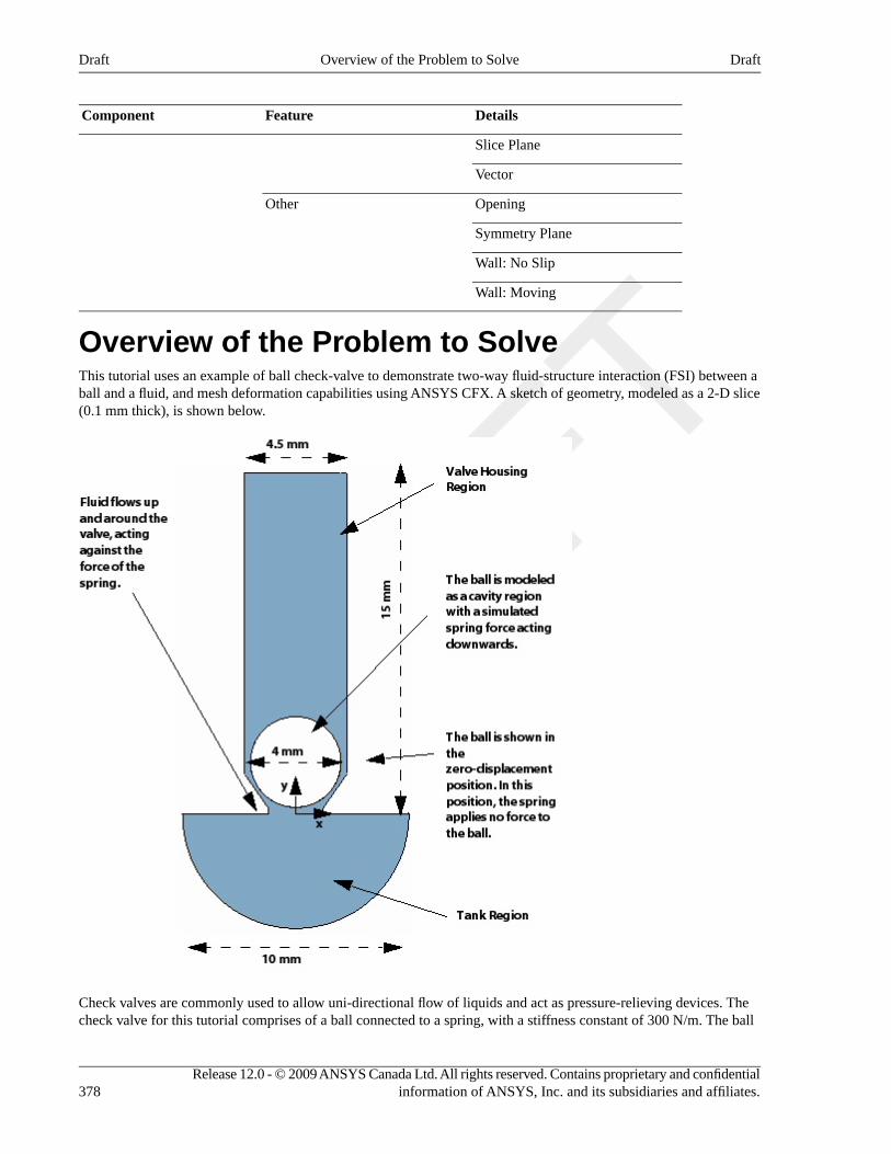
DetailsFeatureComponent
Slice Plane
Vector
OpeningOther
Symmetry Plane
Wall: No Slip
Wall: Moving
Overview of the Problem to SolveThis tutorial uses an example of ball check-valve to demonstrate two-way fluid-structure interaction (FSI) between aball and a fluid, and mesh deformation capabilities using ANSYS CFX. A sketch of geometry, modeled as a 2-D slice(0.1 mm thick), is shown below.
Check valves are commonly used to allow uni-directional flow of liquids and act as pressure-relieving devices. Thecheck valve for this tutorial comprises of a ball connected to a spring, with a stiffness constant of 300 N/m. The ball
Release 12.0 - © 2009 ANSYS Canada Ltd. All rights reserved. Contains proprietary and confidentialinformation of ANSYS, Inc. and its subsidiaries and affiliates.378
DraftOverview of the Problem to SolveDraft
is made of steel with density of 7800 kg/m3 and 4 mm diameter. The liquid medium for this tutorial comprises of atank region filled with Methanol (CH4O) at 25 C and 1 atm, which is located below the valve housing region. Highpressure from the liquid (6 atm relative pressure at the tank opening) causes the ball to move up, thus allowing thefluid to leave. The spring pushes the ball downward when the ball is raised above its initial position. The pressurevariation causes the ball to oscillate along y-axis as a result of an imbalance in the spring forces; the ball stops movingwhen forces on it are in equilibrium. The forces on the ball are the force due to the spring (not shown in the figure)and the force due to fluid flow. Gravity is neglected here for simplicity. The ball is represented as a cavity region inthe mesh.
This tutorial explores the fluid mesh deformation resulting due to the fluid-solid interaction between the ball and thesurrounding fluid; the deformation of ball itself is not modeled. CEL expressions are used to account for the motionof the ball, determined by solving a solid dynamics equation that depends upon the forces acting on the ball.
Modeling the Ball DynamicsWhen defining your own simulations, the mesh motion may already be known. In such cases, it can be specifiedexplicitly using the CEL. In this tutorial, the mesh motion is not known a priori, and will be calculated using the forcesthat act on the ball. Before setting up the simulation for this tutorial, this section outlines the basis of dynamics equationthat describes the motion of the ball.
According to Newton's Second Law, the time rate of change in the ball's linear momentum is proportional to the netforce acting on the ball. In differential form, the equation to be solved for the motion of the ball is:
(Eq. 22.1)∗ = −mBall ( velBall) FFlow FSpringddt
where mBall is the mass of the ball (which is constant), velBall is the velocity of the ball in the y coordinate direction,
FFlow is the flow (viscous and drag) force acting on the ball, and FSpring is the spring force acting on the ball.
The left hand side of the equation is discretized to include an expression for the new displacement of the ball (relativeto the spring's neutral position). The time derivative of the ball velocity is discretized as:
(Eq. 22.2)= −( velBall)ddt
velBallNew velBallOldtStep
where velBallNew is further discretized as:
(Eq. 22.3)= −velBallNew dBallNew dBallOldtStep
The new displacement of the ball also appears in the expression for spring force:
(Eq. 22.4)= ×FSpring kSpring dBallNewThe discrete form of the equation of motion for the ball is re-assembled, and the ball displacement is isolated as:
(Eq. 22.5)=
⎛
⎝⎜⎜ +
⎛
⎝⎜ +
⎞
⎠⎟
⎞
⎠⎟⎟
⎛
⎝⎜ +
⎞
⎠⎟
× ×
dBallNewFFlow
kSpring
mBall velBallOldtStep
mBall dBallOld
tStep2
mBall
tStep2
No further substitutions are required because all of these quantities are available through the CFX Expression Languageas presented later in this tutorial.
Before You BeginIf this is the first tutorial you are working with, it is important to review the following topics before beginning:
• Preparing a Working Directory (p. 23)
• Setting the Working Directory and Starting ANSYS CFX (p. 23)
379Release 12.0 - © 2009 ANSYS Canada Ltd. All rights reserved. Contains proprietary and confidentialinformation of ANSYS, Inc. and its subsidiaries and affiliates.
DraftModeling the Ball DynamicsDraft
• Changing the Display Colors (p. 24)
• Playing a Tutorial Session File (p. 24)
Starting CFX-Pre1. Prepare the working directory using the following files in the examples directory:
• ValveFSI.pre
• ValveFSI_expressions.ccl
• ValveFSI.out
For details, see Preparing a Working Directory (p. 23)
2. Set the working directory and start CFX-Pre
For details, see Setting the Working Directory and Starting ANSYS CFX (p. 23)
Defining a Simulation in CFX-PreThis section describes the step-by-step definition of the flow physics in CFX-Pre as outlined below:
• Defining a Simulation in CFX-Pre (p. 380)
• Importing the Mesh (p. 380)
• Importing the Required Expressions (p. 381)
• Setting the Analysis Type (p. 382)
• Creating the Domain (p. 382)
• Creating the Subdomain (p. 383)
• Creating the Boundaries (p. 383)
• Setting Initial Values (p. 386)
• Setting Solver Control (p. 386)
• Setting Output Control (p. 386)
• Writing the CFX-Solver Input (.def) File (p. 387)
Defining a Simulation in CFX-PreIf you want to set up the simulation automatically using a tutorial session file, run ValveFSI.pre. For details, seePlaying a Tutorial Session File (p. 24). Then proceed to Obtaining a Solution using the CFX-Solver Manager (p. 388).
If you want to set up the simulation manually, proceed to the following steps:
1. Start CFX-Pre.
2. Select File > New Case.
3. Select General and click OK.
4. Select File > Save Case As.
5. Under File name, type ValveFSI.
6. Click Save.
Importing the Mesh1. Right-click Mesh and select Import Mesh > Other. The Import Mesh dialog box appears.
2. Apply the following settings:
Release 12.0 - © 2009 ANSYS Canada Ltd. All rights reserved. Contains proprietary and confidentialinformation of ANSYS, Inc. and its subsidiaries and affiliates.380
DraftStarting CFX-PreDraft
ValueSetting
PATRAN NeutralFiles of type
ValveFSI.outFile name
mm aOptions > Mesh Units
a This mesh was created using units of millimeters; however, the units are not stored with this type of mesh. Set Mesh Units to mm whenimporting the mesh into CFX-Pre so that the mesh remains the intended size.
3. Click Open.
Importing the Required ExpressionsThe expressions created in this step will determine the motion of the ball.
These expressions are provided in a CCL file. By importing the expression, you avoid the need to type each of theexpressions by hand.
1. Select File > Import > CCL.
This file is located in the working directory.
2. Select ValveFSI_expressions.ccl
This file contains following expressions that are used later in the tutorial:
PurposeExpression
DefinitionName
These expressions define the values for duration andtimesteps that were chosen to study the transient
5.0e-5 [s]tStep
7.5e-3 [s]tTotalresponse of ball under the effect of spring forces andthe forces due to fluid flow.
This expression defines the ball motion required for thespecification of mesh motion for the ball boundary. Fordetails, see Modeling the Ball Dynamics.
dBallNumer/dBallDenomdBallNew
These are intermediate expressions used for thecalculation of dBallNew.
300 [N m^-1]kSpring
7800 [kg m^-3]denBall
pi * (2.0 [mm])^2 * 1e-4 [m]volBall
denBall * volBallmBall
force_y()@BallFFlow
areaAve(Mesh Velocity v)@BallvelBallOld a
areaAve(Total Mesh DisplacementY)@Ball
dBallOld a
FFlow + mBall*velBallOld/tStep +mBall*dBallOld/tStep^2
dBallNumer
kSpring+mBall/tStep^2dBallDenom
a These expressions use areaAve function calls that are evaluated using solution data from the end of the previous time step; These calls arenot updated during the solution of the mesh displacement equations. Thus, dBallOld and velBallOld represent the required ‘old’ values.
3. Ensure that Import Method is set to Append.
381Release 12.0 - © 2009 ANSYS Canada Ltd. All rights reserved. Contains proprietary and confidentialinformation of ANSYS, Inc. and its subsidiaries and affiliates.
DraftImporting the Required ExpressionsDraft
4. Click Open.
You can review the imported expressions in the tree view.
Setting the Analysis Type1. Click Analysis Type .
2. Apply the following settings
ValueSettingTab
TransientAnalysis Type > OptionBasic Settings
tTotalAnalysis Type > Time Duration > Total Time
tStepAnalysis Type > Time Steps > Timesteps
0 [s]Analysis Type > Initial Time > Time
3. Click OK.
NoteYou may ignore the physics validation message regarding the lack of transient results files. You will setup transient results files later.
Creating the Domain1. Edit Case Options > General in the Outline tree view and ensure that Automatic Default Domain is
turned on.
A domain named Default Domain should appear under the Simulation branch.
2. Double-click Default Domain and apply the following settings
ValueSettingTab
CV3D REGION, CV3D SUBLocation and Type > LocationBasic Settings
Fluid DomainLocation and Type > Domain Type
Fluid 1Fluid and Particle Definitions
Methanol CH4O aFluid and Particle Definitions > Fluid 1 >Material
1 [atm]Domain Models > Pressure > ReferencePressure
Regions of Motion Specified bDomain Models > Mesh Deformation >Option
(Expand)Domain Models > Mesh Deformation > MeshMotion Model
Increase Near Small VolumesDomain Models > Mesh Deformation > MeshMotion Model > Mesh Stiffness > Option
Release 12.0 - © 2009 ANSYS Canada Ltd. All rights reserved. Contains proprietary and confidentialinformation of ANSYS, Inc. and its subsidiaries and affiliates.382
DraftSetting the Analysis TypeDraft
ValueSettingTab
IsothermalHeat Transfer > OptionFluid Models
25 [C]Heat Transfer > Fluid Temperature
a Click the Ellipsis icon to open the Fluids List dialog box, then click Import Library Data to open the Select Library Data to
Import dialog box. In that dialog box, expand Constant Property Liquids in the tree, then select Methanol CH4O and click OK.Next, select Methanol CH4O in the Material dialog box and click OK.b The Regions of Motion Specified option permits wall boundaries and subdomains to move, and makes mesh motion settings available.
3. Click OK.
Creating the Subdomain1. Create a new subdomain named Tank.
2. Apply the following settings
ValueSettingTab
CV3D SUBLocationBasic Settings
Stationary aOptionMesh Motion
a The stationary option for the tank volume (subdomain) ensures that the mesh does not fold at the sharp corner that exists where the valvejoins the tank.
3. Click OK.
Creating the BoundariesThis section outlines the steps for creating the following boundary conditions and applying the mesh deformationspecifications. The regions for these boundary conditions were imported with the mesh file.
• Ball Boundary (p. 383)
• Symmetry Boundary (p. 384)
• Vertical-Valve Wall Boundary (p. 384)
• Tank Opening Boundary (p. 385)
• Valve Opening Boundary (p. 385)
Mesh deformation specifications are applied to two and three dimensional regions of the domain (i.e. boundaries andsubdomains, respectively). For example, the Ball boundary uses mesh motion specification in the form of balldisplacement, which is given by the expression dBallNew. However, mesh deformation specifications are also usedin this tutorial to help ensure that the mesh does not fold, as set for the Tank subdomain, earlier in the tutorial, andthe TankOpen boundary (see below).
Ball BoundaryTo move the ball, create a wall boundary with a displacement in the Y direction given by the expression dBallNew.
1. Create a new boundary named Ball.
2. Apply the following settings:
383Release 12.0 - © 2009 ANSYS Canada Ltd. All rights reserved. Contains proprietary and confidentialinformation of ANSYS, Inc. and its subsidiaries and affiliates.
DraftCreating the SubdomainDraft
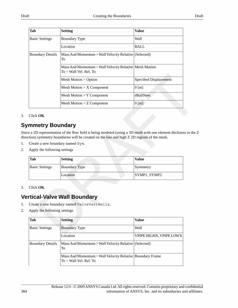
ValueSettingTab
WallBoundary TypeBasic Settings
BALLLocation
(Selected)Mass And Momentum > Wall Velocity RelativeTo
Boundary Details
Mesh MotionMass And Momentum > Wall Velocity RelativeTo > Wall Vel. Rel. To
Specified DisplacementMesh Motion > Option
0 [m]Mesh Motion > X Component
dBallNewMesh Motion > Y Component
0 [m]Mesh Motion > Z Component
3. Click OK.
Symmetry BoundarySince a 2D representation of the flow field is being modeled (using a 3D mesh with one element thickness in the Zdirection) symmetry boundaries will be created on the low and high Z 2D regions of the mesh.
1. Create a new boundary named Sym.
2. Apply the following settings
ValueSettingTab
SymmetryBoundary TypeBasic Settings
SYMP1, SYMP2Location
3. Click OK.
Vertical-Valve Wall Boundary1. Create a new boundary named ValveVertWalls.
2. Apply the following settings
ValueSettingTab
WallBoundary TypeBasic Settings
VPIPE HIGHX, VPIPE LOWXLocation
(Selected)Mass And Momentum > Wall Velocity RelativeTo
Boundary Details
Boundary FrameMass And Momentum > Wall Velocity RelativeTo > Wall Vel. Rel. To
Release 12.0 - © 2009 ANSYS Canada Ltd. All rights reserved. Contains proprietary and confidentialinformation of ANSYS, Inc. and its subsidiaries and affiliates.384
DraftCreating the BoundariesDraft
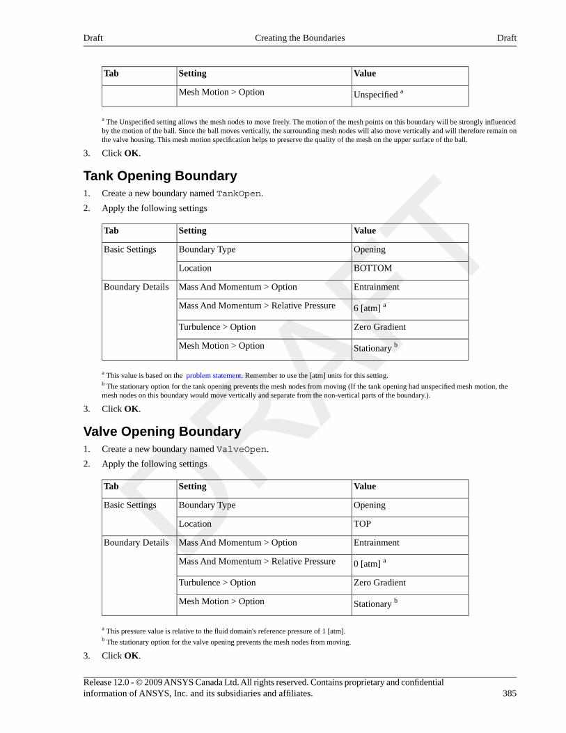
ValueSettingTab
Unspecified aMesh Motion > Option
a The Unspecified setting allows the mesh nodes to move freely. The motion of the mesh points on this boundary will be strongly influencedby the motion of the ball. Since the ball moves vertically, the surrounding mesh nodes will also move vertically and will therefore remain onthe valve housing. This mesh motion specification helps to preserve the quality of the mesh on the upper surface of the ball.
3. Click OK.
Tank Opening Boundary1. Create a new boundary named TankOpen.
2. Apply the following settings
ValueSettingTab
OpeningBoundary TypeBasic Settings
BOTTOMLocation
EntrainmentMass And Momentum > OptionBoundary Details
6 [atm] aMass And Momentum > Relative Pressure
Zero GradientTurbulence > Option
Stationary bMesh Motion > Option
a This value is based on the problem statement. Remember to use the [atm] units for this setting.b The stationary option for the tank opening prevents the mesh nodes from moving (If the tank opening had unspecified mesh motion, themesh nodes on this boundary would move vertically and separate from the non-vertical parts of the boundary.).
3. Click OK.
Valve Opening Boundary1. Create a new boundary named ValveOpen.
2. Apply the following settings
ValueSettingTab
OpeningBoundary TypeBasic Settings
TOPLocation
EntrainmentMass And Momentum > OptionBoundary Details
0 [atm] aMass And Momentum > Relative Pressure
Zero GradientTurbulence > Option
Stationary bMesh Motion > Option
a This pressure value is relative to the fluid domain's reference pressure of 1 [atm].b The stationary option for the valve opening prevents the mesh nodes from moving.
3. Click OK.
385Release 12.0 - © 2009 ANSYS Canada Ltd. All rights reserved. Contains proprietary and confidentialinformation of ANSYS, Inc. and its subsidiaries and affiliates.
DraftCreating the BoundariesDraft
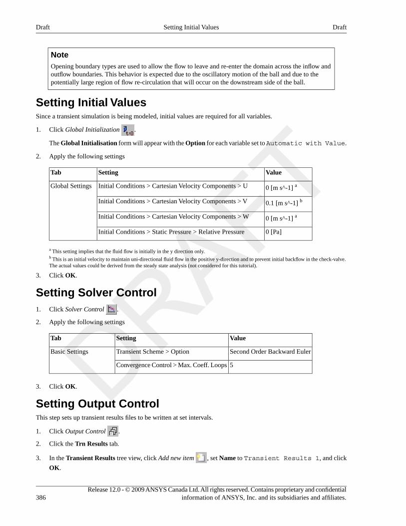
NoteOpening boundary types are used to allow the flow to leave and re-enter the domain across the inflow andoutflow boundaries. This behavior is expected due to the oscillatory motion of the ball and due to thepotentially large region of flow re-circulation that will occur on the downstream side of the ball.
Setting Initial ValuesSince a transient simulation is being modeled, initial values are required for all variables.
1. Click Global Initialization .
The Global Initialisation form will appear with the Option for each variable set to Automatic with Value.
2. Apply the following settings
ValueSettingTab
0 [m s^-1] aInitial Conditions > Cartesian Velocity Components > UGlobal Settings
0.1 [m s^-1] bInitial Conditions > Cartesian Velocity Components > V
0 [m s^-1] aInitial Conditions > Cartesian Velocity Components > W
0 [Pa]Initial Conditions > Static Pressure > Relative Pressure
a This setting implies that the fluid flow is initially in the y direction only.b This is an initial velocity to maintain uni-directional fluid flow in the positive y-direction and to prevent initial backflow in the check-valve.The actual values could be derived from the steady state analysis (not considered for this tutorial).
3. Click OK.
Setting Solver Control1. Click Solver Control .
2. Apply the following settings
ValueSettingTab
Second Order Backward EulerTransient Scheme > OptionBasic Settings
5Convergence Control > Max. Coeff. Loops
3. Click OK.
Setting Output ControlThis step sets up transient results files to be written at set intervals.
1. Click Output Control .
2. Click the Trn Results tab.
3. In the Transient Results tree view, click Add new item , set Name to Transient Results 1, and click
OK.
Release 12.0 - © 2009 ANSYS Canada Ltd. All rights reserved. Contains proprietary and confidentialinformation of ANSYS, Inc. and its subsidiaries and affiliates.386
DraftSetting Initial ValuesDraft
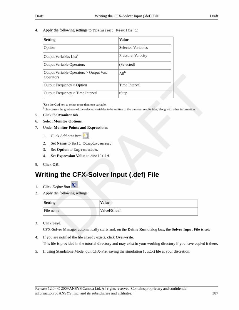
4. Apply the following settings to Transient Results 1:
ValueSetting
Selected VariablesOption
Pressure, VelocityOutput Variables Lista
(Selected)Output Variable Operators
AllbOutput Variable Operators > Output Var.Operators
Time IntervalOutput Frequency > Option
tStepOutput Frequency > Time Interval
aUse the Ctrl key to select more than one variable.bThis causes the gradients of the selected variables to be written to the transient results files, along with other information.
5. Click the Monitor tab.
6. Select Monitor Options.
7. Under Monitor Points and Expressions:
1. Click Add new item .
2. Set Name to Ball Displacement.
3. Set Option to Expression.
4. Set Expression Value to dBallOld.
8. Click OK.
Writing the CFX-Solver Input (.def) File
1. Click Define Run .
2. Apply the following settings:
ValueSetting
ValveFSI.defFile name
3. Click Save.
CFX-Solver Manager automatically starts and, on the Define Run dialog box, the Solver Input File is set.
4. If you are notified the file already exists, click Overwrite.
This file is provided in the tutorial directory and may exist in your working directory if you have copied it there.
5. If using Standalone Mode, quit CFX-Pre, saving the simulation (.cfx) file at your discretion.
387Release 12.0 - © 2009 ANSYS Canada Ltd. All rights reserved. Contains proprietary and confidentialinformation of ANSYS, Inc. and its subsidiaries and affiliates.
DraftWriting the CFX-Solver Input (.def) FileDraft
Obtaining a Solution using the CFX-SolverManagerThe steps to begin the solver run are outlined below:
1. In CFX-Solver Manager, ensure that Define Run dialog box is displayed.
If CFX-Solver Manager is launched from CFX-Pre, the information required to perform a solver run is enteredautomatically in the Define Run dialog box.
2. Click Start Run.
The solver run begins and the progress is displayed in a split screen.
3. Click the User Points tab and monitor the value of Ball Displacement as the solution proceeds.
The largest value of ball displacement occurs at around 20th timestep and the oscillations begin to settle downafter around 100 timesteps.
4. Select the check box next to Post-Process Results when the completion message appears at the end of the run.
5. If using Standalone Mode, select the check box next to Shut down CFX-Solver Manager.
6. Click Ok.
Viewing the Results in CFD-PostThis section outlines the following steps for creating the user locations, plots, and animation in CFD-Post. You willcreate an XY plane that lies midway between the two symmetry planes. The plane will be used to show mesh movement;it will also serve as a locator for a vector plot that will be used in an animation.
• Creating a Slice Plane (p. 388)
• Creating a Point (p. 389)
• Creating an Animation with Velocity Vectors (p. 389)
Creating a Slice Plane1. Right-click a blank area in the viewer and select Predefined Camera > View Towards -Z.
2. Create a new plane and accept the default name.
3. Apply the following settings
ValueSettingTab
XY PlaneDefinition > MethodGeometry
5e-05 [m] aDefinition > Z
(Cleared)Show FacesRender
(Selected)Show Mesh Lines
a This setting creates an XY plane that lies midway between the two symmetry planes.
4. Click Apply to create the plane.
Release 12.0 - © 2009 ANSYS Canada Ltd. All rights reserved. Contains proprietary and confidentialinformation of ANSYS, Inc. and its subsidiaries and affiliates.388
DraftObtaining a Solution using the CFX-Solver ManagerDraft
Creating a Point1. Create a point at (0, 0.0003, 0.0001) using the XYZ method. This is a reference point for the low Y point
of the ball at timestep 0. Click Apply.
2. Click Timestep Selector and load the results for a few different timesteps, selecting one entry at a time. For
example, double-click rows with the step values of 0, 10, 20, 50, and 90 to see the ball in different positions. Themesh deformation will also be visible.
The maximum displacement, which was also monitored earlier in the CFX-Solver, occurs at around 20 timesteps beforethe ball reaches equilibrium.
Creating an Animation with Velocity VectorsYou will create a vector plot and create an animation showing the velocity in the domain as the ball is displaced.
1. Turn off the visibility of Plane 1.
2. Create a vector plot, set Locations to Plane 1 and leave Variable set to Velocity. Click Apply.
3. Using the timestep selector, load time value 0.
4. Click Animation found in the toolbar.
The Animation dialog box appears.
5. In the Animation dialog box, apply the following settings:
1. Select Keyframe Animation.
2. Click New to create KeyframeNo1.
3. Highlight KeyframeNo1, then change # of Frames to 148. This will produce an animation keyframe ateach time step, resulting in a movie that plays for just over six seconds.
6. Load the last timestep (150) using the timestep selector.
7. In the Animation dialog box, apply the following settings:
1. Click New to create KeyframeNo2.
The # of Frames parameter has no effect for the last keyframe, so leave it at the default value.
2. Click More Animation Options to expand the Animation dialog box.
3. Click the Options button to open the Animation Options dialog box.
4. On the Options tab, change Image Size to 720 X 480 (NTSC).
5. Click the Advanced tab, then set Quality to Custom.
6. Clear Variable Bit Rate and set Bit Rate to 3000000.
This limits the bit rate so that the movie will play in most players. You can lower this value if your playercannot handle this bit rate.
7. Click OK.
8. Select Save Movie.
9. Set Format to MPEG1.
10. Click Browse next to Save Movie and set a file name for the movie file.
If the file path is not given, the file will be saved in the working directory.
389Release 12.0 - © 2009 ANSYS Canada Ltd. All rights reserved. Contains proprietary and confidentialinformation of ANSYS, Inc. and its subsidiaries and affiliates.
DraftCreating a PointDraft
11. Click Open. This sets the movie file name and path, but does not create the movie.
12. If frame 1 is not loaded (shown in the F: text box at the bottom of the Animation dialog box), clickTo Beginning to load it.
Wait for CFD-Post to finish loading the objects for this frame before proceeding.
13. Click Play the animation .
The movie is created as the animation proceeds. This will be slow, since a timestep must be loaded andobjects must be created for each frame. To view the movie file, you need to use a viewer that supports theMPEG format.
8. When you have finished, exit from CFD-Post.
Release 12.0 - © 2009 ANSYS Canada Ltd. All rights reserved. Contains proprietary and confidentialinformation of ANSYS, Inc. and its subsidiaries and affiliates.390
DraftCreating an Animation with Velocity VectorsDraft
Chapter 23. Oscillating Plate withTwo-Way Fluid-Structure InteractionThis tutorial includes:
• Tutorial Features (p. 391)
• Overview of the Problem to Solve (p. 392)
• Before You Begin (p. 392)
• Creating the Project (p. 393)
• Adding Analyses Systems to the Project (p. 393)
• Adding a New Material for the Project (p. 395)
• Adding Geometry to the Project (p. 397)
• Defining the Physics in ANSYS Mechanical (p. 397)
• Completing the Setup for the Structural System (p. 400)
• Creating Named Selections for the Project (p. 400)
• Generating the Mesh for the Fluid System (p. 402)
• Defining the Physics and ANSYS Multi-field Settings in ANSYS CFX-Pre (p. 403)
• Obtaining a Solution using ANSYS CFX-Solver Manager (p. 409)
• Viewing Results in ANSYS CFD-Post (p. 409)
Tutorial FeaturesIn this tutorial you will learn about:
• Moving mesh
• Fluid-structure interaction (including modeling structural deformation using ANSYS)
• Running an ANSYS Multi-field (MFX) simulation
• Post-processing two results files simultaneously.
DetailsFeatureComponent
General ModeUser ModeCFX-Pre
TransientAnalysis Type
ANSYS Multi-field
General FluidFluid Type
Single DomainDomain Type
LaminarTurbulence Model
NoneHeat Transfer
Monitor PointsOutput Control
Transient Results File
391Release 12.0 - © 2009 ANSYS Canada Ltd. All rights reserved. Contains proprietary and confidentialinformation of ANSYS, Inc. and its subsidiaries and affiliates.
DraftDraft
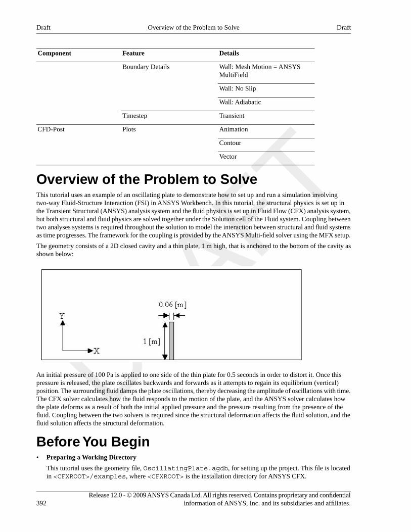
DetailsFeatureComponent
Wall: Mesh Motion = ANSYSMultiField
Boundary Details
Wall: No Slip
Wall: Adiabatic
TransientTimestep
AnimationPlotsCFD-Post
Contour
Vector
Overview of the Problem to SolveThis tutorial uses an example of an oscillating plate to demonstrate how to set up and run a simulation involvingtwo-way Fluid-Structure Interaction (FSI) in ANSYS Workbench. In this tutorial, the structural physics is set up inthe Transient Structural (ANSYS) analysis system and the fluid physics is set up in Fluid Flow (CFX) analysis system,but both structural and fluid physics are solved together under the Solution cell of the Fluid system. Coupling betweentwo analyses systems is required throughout the solution to model the interaction between structural and fluid systemsas time progresses. The framework for the coupling is provided by the ANSYS Multi-field solver using the MFX setup.
The geometry consists of a 2D closed cavity and a thin plate, 1 m high, that is anchored to the bottom of the cavity asshown below:
An initial pressure of 100 Pa is applied to one side of the thin plate for 0.5 seconds in order to distort it. Once thispressure is released, the plate oscillates backwards and forwards as it attempts to regain its equilibrium (vertical)position. The surrounding fluid damps the plate oscillations, thereby decreasing the amplitude of oscillations with time.The CFX solver calculates how the fluid responds to the motion of the plate, and the ANSYS solver calculates howthe plate deforms as a result of both the initial applied pressure and the pressure resulting from the presence of thefluid. Coupling between the two solvers is required since the structural deformation affects the fluid solution, and thefluid solution affects the structural deformation.
Before You Begin• Preparing a Working Directory
This tutorial uses the geometry file, OscillatingPlate.agdb, for setting up the project. This file is locatedin <CFXROOT>/examples, where <CFXROOT> is the installation directory for ANSYS CFX.
Release 12.0 - © 2009 ANSYS Canada Ltd. All rights reserved. Contains proprietary and confidentialinformation of ANSYS, Inc. and its subsidiaries and affiliates.392
DraftOverview of the Problem to SolveDraft
Copy the supplied geometry file, OscillatingPlate.agdb, to a directory of your choice. This directory willbe referred to as the working directory in this tutorial.
By working with copy of the geometry file in a new directory, you prevent accidental changes to the file that camewith your installation.
• Changing the Appearance of Workspace in ANSYS Workbench
If this is the first tutorial you are working with, see Changing the Display Colors (p. 24) for information on howto change the appearance of workspace and display settings in ANSYS Workbench.
Creating the Project1. Open ANSYS Workbench.
On a Windows platform: Use the Windows Start menu and select ANSYS 12.0 > ANSYS Workbench from thelist of installed programs.
The Project Schematic appears with an Unsaved Project. By default, ANSYS Workbench is configured to showthe Getting Started dialog box that describes basic operations in ANSYS Workbench. Click the [X] icon to closethis dialog box. To turn on or off this dialog box, select Tools > Options from the main menu and set ProjectManagement > Startup > Show Getting Started Dialog as desired.
2. Select File > Save or click Save .
A Save As dialog box appears. Select the path to your working directory to store files created during this tutorial.For details, see Preparing a Working Directory.
3. Under File name, type OscillatingPlate and click Save.
The project files and their associated folder locations appear under Files View on the Project Schematic. To makethe Files View window visible, select View > Files from the main menu of ANSYS Workbench.
Adding Analyses Systems to the ProjectIn ANSYS Workbench, the two-way FSI analysis can be performed by setting up coupled analyses systems, comprisingof a Transient Structural (ANSYS) system and a Fluid Flow (CFX) system as outlined in this section.
1. Expand the Analysis Systems option in the toolbox, located on the left side of the ANSYS Workbench window,and select the Transient Structural (ANSYS) template. Double-click the template, or drag it onto the ProjectSchematic to create a standalone system.
A Transient Structural (ANSYS) system is added to the Project Schematic, with its name highlighted.
2. Type in the new name Structural to replace the highlighted text; this name will be used while referring tothe Transient Structural (ANSYS) system in this tutorial.
If you missed to see the highlighted text, right-click on the first cell in the system and select Rename as shownin the following figure. The name will be highlighted, now you can change the highlighted text by typing in thenew name.
393Release 12.0 - © 2009 ANSYS Canada Ltd. All rights reserved. Contains proprietary and confidentialinformation of ANSYS, Inc. and its subsidiaries and affiliates.
DraftCreating the ProjectDraft
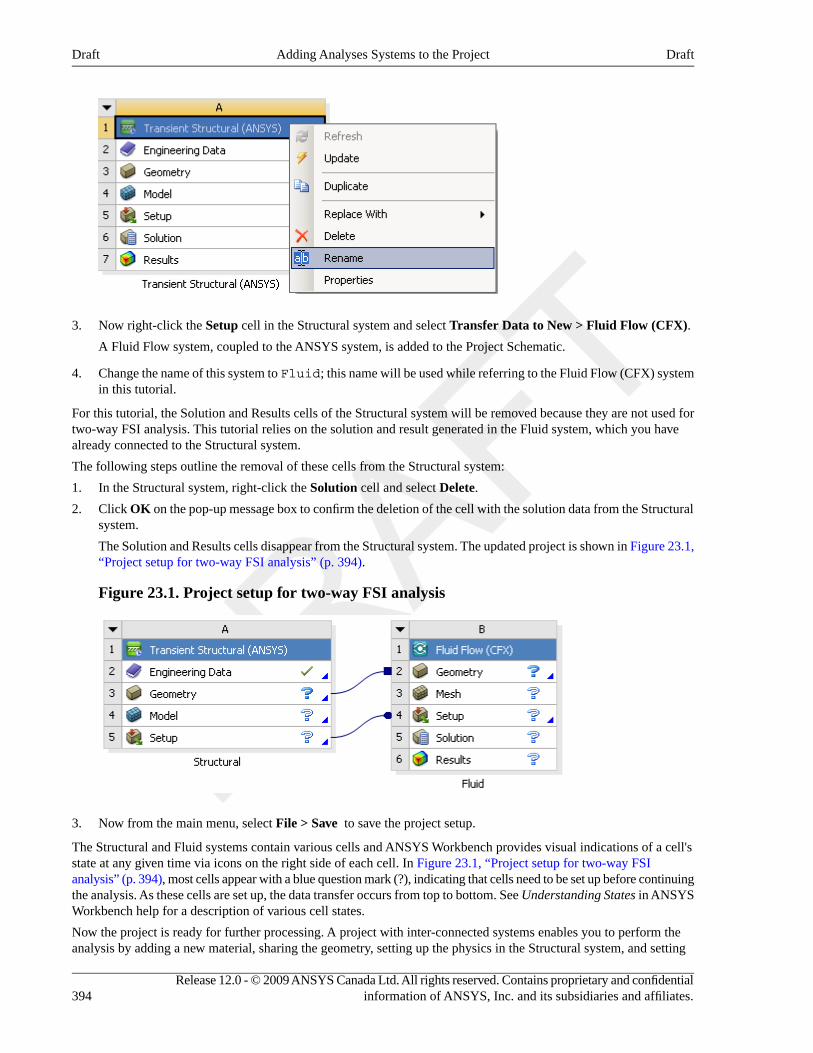
3. Now right-click the Setup cell in the Structural system and select Transfer Data to New > Fluid Flow (CFX).
A Fluid Flow system, coupled to the ANSYS system, is added to the Project Schematic.
4. Change the name of this system to Fluid; this name will be used while referring to the Fluid Flow (CFX) systemin this tutorial.
For this tutorial, the Solution and Results cells of the Structural system will be removed because they are not used fortwo-way FSI analysis. This tutorial relies on the solution and result generated in the Fluid system, which you havealready connected to the Structural system.
The following steps outline the removal of these cells from the Structural system:
1. In the Structural system, right-click the Solution cell and select Delete.
2. Click OK on the pop-up message box to confirm the deletion of the cell with the solution data from the Structuralsystem.
The Solution and Results cells disappear from the Structural system. The updated project is shown in Figure 23.1,“Project setup for two-way FSI analysis” (p. 394).
Figure 23.1. Project setup for two-way FSI analysis
3. Now from the main menu, select File > Save to save the project setup.
The Structural and Fluid systems contain various cells and ANSYS Workbench provides visual indications of a cell'sstate at any given time via icons on the right side of each cell. In Figure 23.1, “Project setup for two-way FSIanalysis” (p. 394), most cells appear with a blue question mark (?), indicating that cells need to be set up before continuingthe analysis. As these cells are set up, the data transfer occurs from top to bottom. See Understanding States in ANSYSWorkbench help for a description of various cell states.
Now the project is ready for further processing. A project with inter-connected systems enables you to perform theanalysis by adding a new material, sharing the geometry, setting up the physics in the Structural system, and setting
Release 12.0 - © 2009 ANSYS Canada Ltd. All rights reserved. Contains proprietary and confidentialinformation of ANSYS, Inc. and its subsidiaries and affiliates.394
DraftAdding Analyses Systems to the ProjectDraft
up the physics in the Fluid system. Later, the analysis will be performed in the Fluid system for solving and viewingresults.
In Figure 23.1, “Project setup for two-way FSI analysis” (p. 394), the Engineering Data cell appears in an up-to-datestate, because a default material definition is already available for the project. However, the default material is notused in this tutorial. Thus, the next step in the analysis is to add a new material with properties desired for exhibitingan oscillation under the influence of external pressure, as outlined in Overview of the Problem to Solve (p. 392). Thenew material can be created using the Engineering Data application in ANSYS Workbench, as described in the nextsection.
Adding a New Material for the ProjectThis section describes how to create a new material named Plate, define its properties suitable for oscillation, and setit as the default material for the analysis.
1. On the Project Schematic, double-click the Engineering Data cell in the Structural system.
The Outline and Properties windows appear below the Project Schematic.
2. In the Outline Filter window, ensure that Engineering Data is selected.
3. In the Outline of Schematic A2: Engineering Data window, click the empty row at the bottom of the table toadd a new material for the project. Type in the name Plate.
Plate is created and appears with a blue question mark (?), indicating that plate properties need to be defined.
4. Now from toolboxes located on the left side of the ANSYS Workbench window, expand the Physical Propertiestoolbox. Select Density and drag it onto the cell containing Plate in the Outline of Schematic A2: EngineeringData window.
Density is added as the plate property in the Properties of Outline Row 4: Plate window, as shown in thefollowing figure.
395Release 12.0 - © 2009 ANSYS Canada Ltd. All rights reserved. Contains proprietary and confidentialinformation of ANSYS, Inc. and its subsidiaries and affiliates.
DraftAdding a New Material for the ProjectDraft
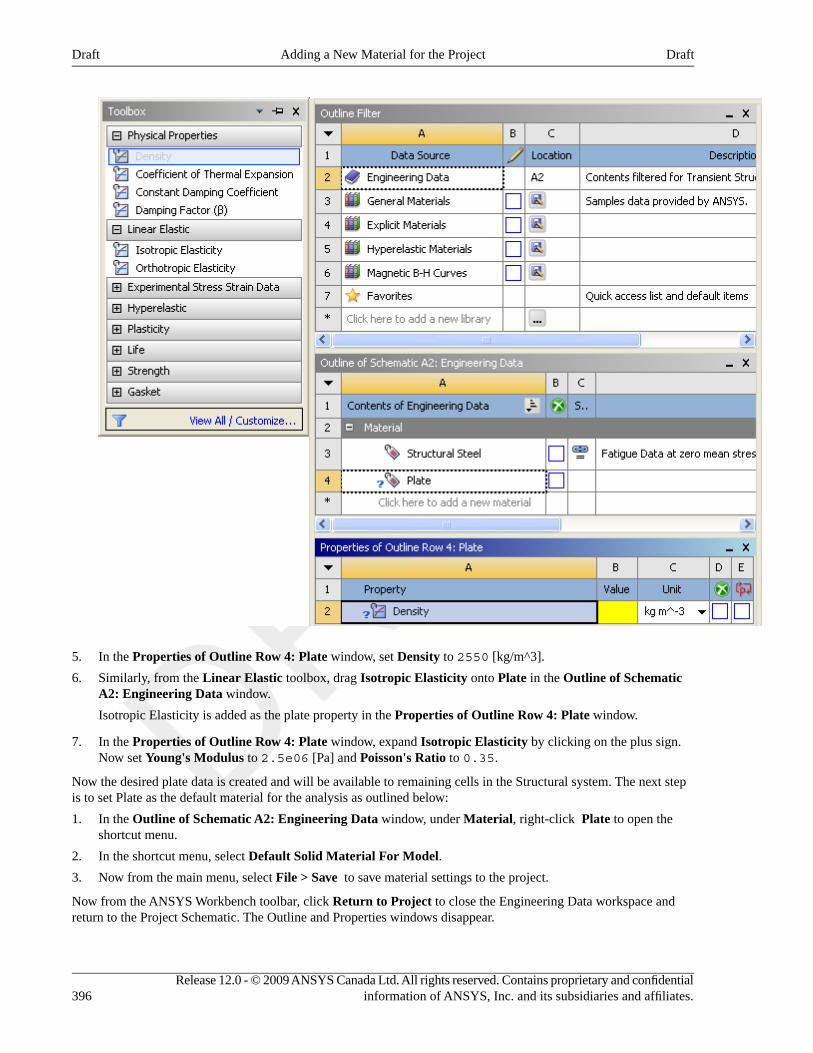
5. In the Properties of Outline Row 4: Plate window, set Density to 2550 [kg/m^3].
6. Similarly, from the Linear Elastic toolbox, drag Isotropic Elasticity onto Plate in the Outline of SchematicA2: Engineering Data window.
Isotropic Elasticity is added as the plate property in the Properties of Outline Row 4: Plate window.
7. In the Properties of Outline Row 4: Plate window, expand Isotropic Elasticity by clicking on the plus sign.Now set Young's Modulus to 2.5e06 [Pa] and Poisson's Ratio to 0.35.
Now the desired plate data is created and will be available to remaining cells in the Structural system. The next stepis to set Plate as the default material for the analysis as outlined below:
1. In the Outline of Schematic A2: Engineering Data window, under Material, right-click Plate to open theshortcut menu.
2. In the shortcut menu, select Default Solid Material For Model.
3. Now from the main menu, select File > Save to save material settings to the project.
Now from the ANSYS Workbench toolbar, click Return to Project to close the Engineering Data workspace andreturn to the Project Schematic. The Outline and Properties windows disappear.
Release 12.0 - © 2009 ANSYS Canada Ltd. All rights reserved. Contains proprietary and confidentialinformation of ANSYS, Inc. and its subsidiaries and affiliates.396
DraftAdding a New Material for the ProjectDraft
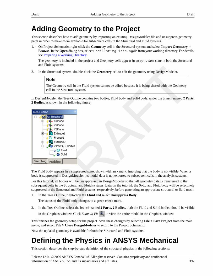
Adding Geometry to the ProjectThis section describes how to add geometry by importing an existing DesignModeler file and unsuppress geometryparts in order to make them available for subsequent cells in the Structural and Fluid systems.
1. On Project Schematic, right-click the Geometry cell in the Structural system and select Import Geometry >Browse. In the Open dialog box, select OscillatingPlate.agdb from your working directory. For details,see Preparing a Working Directory.
The geometry is included in the project and Geometry cells appear in an up-to-date state in both the Structuraland Fluid systems.
2. In the Structural system, double-click the Geometry cell to edit the geometry using DesignModeler.
NoteThe Geometry cell in the Fluid system cannot be edited because it is being shared with the Geometrycell in the Structural system.
In DesignModeler, the Tree Outline contains two bodies, Fluid body and Solid body, under the branch named 2 Parts,2 Bodies, as shown in the following figure.
The Fluid body appears in a suppressed state, shown with an x mark, implying that the body is not visible. When abody is suppressed in DesignModeler, its model data is not exported to subsequent cells in the analysis systems.
For this tutorial, all bodies will be unsuppressed in DesignModeler so that all geometry data is transferred to thesubsequent cells in the Structural and Fluid systems. Later in the tutorial, the Solid and Fluid body will be selectivelysuppressed in the Structural and Fluid systems, respectively, before generating an appropriate structural or fluid mesh.
1. In the Tree Outline, right-click the Fluid and select Unsuppress Body.
The status of the Fluid body changes to a green check mark.
2. In the Tree Outline, select the branch named 2 Parts, 2 Bodies, both the Fluid and Solid bodies should be visible
in the Graphics window. Click Zoom to Fit to view the entire model in the Graphics window.
This finishes the geometry setup for the project. Save these changes by selecting File > Save Project from the mainmenu, and select File > Close DesignModeler to return to the Project Schematic.
Now the updated geometry is available for both the Structural and Fluid systems.
Defining the Physics in ANSYS MechanicalThis section describes the step-by-step definition of the structural physics in the following sections:
397Release 12.0 - © 2009 ANSYS Canada Ltd. All rights reserved. Contains proprietary and confidentialinformation of ANSYS, Inc. and its subsidiaries and affiliates.
DraftAdding Geometry to the ProjectDraft
• Generating the Mesh for the Structural System (p. 398)
• Assigning the Material to Geometry (p. 398)
• Basic Analysis Settings (p. 398)
• Inserting Loads (p. 399)
Generating the Mesh for the Structural SystemThis section describes how to generate mesh for the Structural system.
1. On the Project Schematic, double-click the Model cell in the Structural system.
The ANSYS Mechanical application appears.
2. In ANSYS Mechanical, expand Project > Model > Geometry in the tree view.
Two geometries, Solid and Fluid, appear in the tree view. Click Zoom to Fit to view the entire model in the
Graphics window.
For the Structural system, mesh needs to generated from the Solid body. As such, the Fluid body will be suppressedbefore the mesh generation operation.
3. Right-click the Fluid geometry and select Suppress Body from the shortcut menu.
The Fluid body becomes suppressed and its status changes to an x mark. Click Zoom to Fit to re-size the
model suitable for viewing in the Graphics window.
4. In the tree view, right-click Mesh and select Generate Mesh from the shortcut menu.
The hex mesh is generated.
Assigning the Material to Geometry1. In ANSYS Mechanical, expand Project > Model > Geometry in the tree view and select Solid.
The details of Solid appear in the Details view below the Outline tree view.
2. In the Details view, ensure Material > Assignment is set to Plate. Otherwise, click on the material name anduse the arrow that appears next to the material name to make appropriate changes.
Basic Analysis SettingsThis section outlines the steps to set up an ANSYS Multi-field run using the transient mechanical analysis, with atimestep of 0.1 s and a time duration of 5 s. For the given material properties of the plate, the time duration is chosento allow the plate to oscillate just a few times, and the timestep is chosen to resolve those oscillations to a reasonabledegree.
1. In ANSYS Mechanical, expand Project > Model > Transient in the tree view and select Analysis Settings.
The details of Analysis Settings appear in the Details view below the Outline tree view.
2. In the Details view, specify the following settings under Step Controls:
NoteDo not type in units while entering data for the time settings, Time Step and Step End Time.
• Set Auto Time Stepping to Off
• Set Time Step to 0.1
• Set Step End Time to 5.
Release 12.0 - © 2009 ANSYS Canada Ltd. All rights reserved. Contains proprietary and confidentialinformation of ANSYS, Inc. and its subsidiaries and affiliates.398
DraftGenerating the Mesh for the Structural SystemDraft
Inserting LoadsThe loads applied for the finite element analysis are equivalent to the boundary conditions in fluid analysis. In thissection, you will set a fixed support, a fluid-solid interface, and a pressure load. On the surfaces of the plate that liecoincident with the symmetry planes, no loads are set. As a result, the default of an unconstrained condition will beapplied on these surfaces. For this particular application, this is a reasonable approximation of the frictionless supportthat would otherwise be applied.
Fixed SupportThe fixed support is required to hold the bottom of the thin plate in place.
1. In ANSYS Mechanical, expand Project > Model and right-click Transient in the tree view and select Insert >Fixed Support from the shortcut menu.
2. Rotate the geometry using the Rotate button so that the bottom (low-y) face of the solid is visible, then select
Face and click the low-y face.
That face should be highlighted to indicate the selection.
3. In the Details view, click Apply to set the fixed support.
The text next to the Geometry setting changes to 1 Face.
If the Apply button is not visible, select Fixed Support in the tree view and, in the Details view, click on the textnext to the Geometry setting to make the Apply button re-appear.
Fluid-Solid InterfaceThe fluid-solid interface defines the interface between the fluid in the Fluid system and the solid in the Structuralsystem. This interface is defined on regions in the structural model. Data is exchanged across this interface during theexecution of the simulation.
1. In ANSYS Mechanical, expand Project > Model and right-click Transient in the tree view and select Insert >Fluid Solid Interface from the shortcut menu.
2. Using the same face-selection procedure described earlier in Fixed Support (p. 399), select the three faces of thegeometry that form the interface between the structural model and the fluid model (low-x, high-y and high-xfaces) by holding down Ctrl to select multiple faces.
Note that this load (fluid-solid interface) is automatically given an interface number of 1.
Pressure LoadThe pressure load provides the initial additional pressure of 100 [Pa] for the first 0.5 seconds of the simulation. Itis defined using a step function.
1. In ANSYS Mechanical, expand Project > Model and right-click Transient in the tree view and select Insert >Pressure from the shortcut menu.
2. Select the low-x face for Geometry and click Apply.
3. In the Details view, select Magnitude, and using the arrow that appears, select Tabular data.
4. Under Tabular Data at the bottom right of the ANSYS Mechanical window, set a pressure of 100 in the tablerow corresponding to a time of 0.
NoteDo not type in units while entering the tabular data. The units for time and pressure in this table arethe global units of [s] and [Pa], respectively.
399Release 12.0 - © 2009 ANSYS Canada Ltd. All rights reserved. Contains proprietary and confidentialinformation of ANSYS, Inc. and its subsidiaries and affiliates.
DraftInserting LoadsDraft
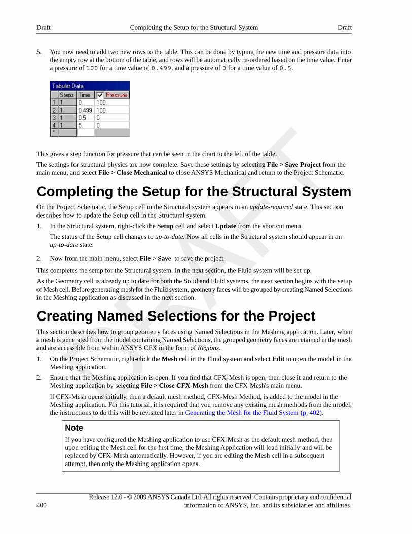
5. You now need to add two new rows to the table. This can be done by typing the new time and pressure data intothe empty row at the bottom of the table, and rows will be automatically re-ordered based on the time value. Entera pressure of 100 for a time value of 0.499, and a pressure of 0 for a time value of 0.5.
This gives a step function for pressure that can be seen in the chart to the left of the table.
The settings for structural physics are now complete. Save these settings by selecting File > Save Project from themain menu, and select File > Close Mechanical to close ANSYS Mechanical and return to the Project Schematic.
Completing the Setup for the Structural SystemOn the Project Schematic, the Setup cell in the Structural system appears in an update-required state. This sectiondescribes how to update the Setup cell in the Structural system.
1. In the Structural system, right-click the Setup cell and select Update from the shortcut menu.
The status of the Setup cell changes to up-to-date. Now all cells in the Structural system should appear in anup-to-date state.
2. Now from the main menu, select File > Save to save the project.
This completes the setup for the Structural system. In the next section, the Fluid system will be set up.
As the Geometry cell is already up to date for both the Solid and Fluid systems, the next section begins with the setupof Mesh cell. Before generating mesh for the Fluid system, geometry faces will be grouped by creating Named Selectionsin the Meshing application as discussed in the next section.
Creating Named Selections for the ProjectThis section describes how to group geometry faces using Named Selections in the Meshing application. Later, whena mesh is generated from the model containing Named Selections, the grouped geometry faces are retained in the meshand are accessible from within ANSYS CFX in the form of Regions.
1. On the Project Schematic, right-click the Mesh cell in the Fluid system and select Edit to open the model in theMeshing application.
2. Ensure that the Meshing application is open. If you find that CFX-Mesh is open, then close it and return to theMeshing application by selecting File > Close CFX-Mesh from the CFX-Mesh's main menu.
If CFX-Mesh opens initially, then a default mesh method, CFX-Mesh Method, is added to the model in theMeshing application. For this tutorial, it is required that you remove any existing mesh methods from the model;the instructions to do this will be revisited later in Generating the Mesh for the Fluid System (p. 402).
NoteIf you have configured the Meshing application to use CFX-Mesh as the default mesh method, thenupon editing the Mesh cell for the first time, the Meshing Application will load initially and will bereplaced by CFX-Mesh automatically. However, if you are editing the Mesh cell in a subsequentattempt, then only the Meshing application opens.
Release 12.0 - © 2009 ANSYS Canada Ltd. All rights reserved. Contains proprietary and confidentialinformation of ANSYS, Inc. and its subsidiaries and affiliates.400
DraftCompleting the Setup for the Structural SystemDraft
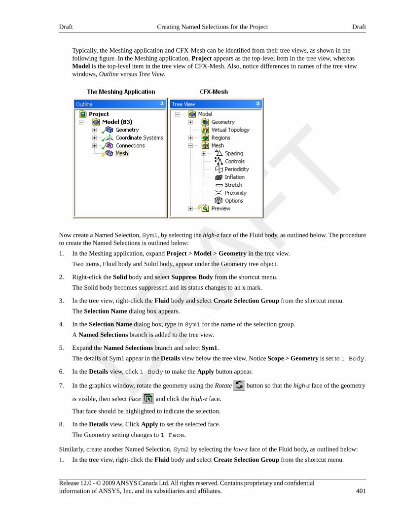
Typically, the Meshing application and CFX-Mesh can be identified from their tree views, as shown in thefollowing figure. In the Meshing application, Project appears as the top-level item in the tree view, whereasModel is the top-level item in the tree view of CFX-Mesh. Also, notice differences in names of the tree viewwindows, Outline versus Tree View.
Now create a Named Selection, Sym1, by selecting the high-z face of the Fluid body, as outlined below. The procedureto create the Named Selections is outlined below:
1. In the Meshing application, expand Project > Model > Geometry in the tree view.
Two items, Fluid body and Solid body, appear under the Geometry tree object.
2. Right-click the Solid body and select Suppress Body from the shortcut menu.
The Solid body becomes suppressed and its status changes to an x mark.
3. In the tree view, right-click the Fluid body and select Create Selection Group from the shortcut menu.
The Selection Name dialog box appears.
4. In the Selection Name dialog box, type in Sym1 for the name of the selection group.
A Named Selections branch is added to the tree view.
5. Expand the Named Selections branch and select Sym1.
The details of Sym1 appear in the Details view below the tree view. Notice Scope > Geometry is set to 1 Body.
6. In the Details view, click 1 Body to make the Apply button appear.
7. In the graphics window, rotate the geometry using the Rotate button so that the high-z face of the geometry
is visible, then select Face and click the high-z face.
That face should be highlighted to indicate the selection.
8. In the Details view, Click Apply to set the selected face.
The Geometry setting changes to 1 Face.
Similarly, create another Named Selection, Sym2 by selecting the low-z face of the Fluid body, as outlined below:
1. In the tree view, right-click the Fluid body and select Create Selection Group from the shortcut menu.
401Release 12.0 - © 2009 ANSYS Canada Ltd. All rights reserved. Contains proprietary and confidentialinformation of ANSYS, Inc. and its subsidiaries and affiliates.
DraftCreating Named Selections for the ProjectDraft
The Selection Name dialog box appears.
2. In the Selection Name dialog box, type in Sym2 for the name of the selection group.
Sym2 is added to the Named Selection branch in the tree view.
3. Select Sym2 in the tree view.
The details of Sym2 appear in the Details view below the tree view. Notice Scope > Geometry is set to 1 Body.
4. In the Details view, click 1 Body to make the Apply button appear.
5. In the graphics window, rotate the geometry using the Rotate button so that the low-z face of the geometry
is visible, then select Face and click the low-z face.
That face should be highlighted to indicate the selection.
6. In the Details view, Click Apply to set the selected face.
The Geometry setting changes to 1 Face.
This finishes the creation of Named Selections on the Fluid body. Do not close the Meshing application yet, the tutorialcontinues to set up mesh settings and generate mesh for the Fluid system in the next section.
Generating the Mesh for the Fluid System1. In the Meshing application, expand Project > Model > Geometry in the tree view.
Two geometries, Solid and Fluid, appear under Geometry.
For the Fluid system, mesh needs to generated from the Fluid body, thus the Solid body will be suppressed. Themesh for the Solid body has already been generated earlier in this tutorial.
2. In the tree view, expand Project > Model > Mesh and ensure that the Mesh branch does not contain any otherobjects. Otherwise, right-click such objects and select Delete from the shortcut menu.
Typically, if you have configured the Meshing application to use CFX-Mesh for meshing, then CFX-MeshMethod is added as a default mesh method under the Mesh branch. In such a case, right-click CFX-Mesh Methodand select Delete to remove it from the Mesh branch.
3. Ensure Mesh is selected in the tree view.
The details of Mesh appear in the Details view below the Outline tree view.
4. In the Details view, set Sizing > Relevance Center to Medium.
This controls the grid resolution of the mesh.
5. Now in the tree view, right-click Mesh and select Insert > Method from the shortcut menu.
Method is added to Mesh branch in the tree view. In the details view, Apply and Cancel buttons appear next tothe Geometry Setting.
6. Click anywhere on the geometry in the viewer to select the Fluid body.
7. In the details view, click on the Apply button next to the Geometry setting.
Notice Scope > Geometry is now set to 1 Body.
8. In the details view, set the following mesh settings in the following order:
1. Set Definition > Method to Sweep.
2. Set Free Face Mesh Type to All Tri.
3. Set Sweep Num Divs = 1.
Release 12.0 - © 2009 ANSYS Canada Ltd. All rights reserved. Contains proprietary and confidentialinformation of ANSYS, Inc. and its subsidiaries and affiliates.402
DraftGenerating the Mesh for the Fluid SystemDraft
9. Now in the tree view, right-click Mesh and select Generate Mesh from the shortcut menu.
The mesh is generated.
10. This finishes the mesh generation for the Fluid system. From the main menu, select File > Save Project to savethese changes to the project, and select File > Close Meshing to return to the Project Schematic.
On the Project Schematic, the Mesh cell in the Fluid system appears in an update-required state.
• Right-click the Mesh cell and select Update from the shortcut menu.
Updating of the Meshing cell is required as opening ANSYS CFX-Pre, from the Setup cell, with an out-of-dateMeshing cell can potentially corrupt the project.
Defining the Physics and ANSYS Multi-fieldSettings in ANSYS CFX-PreThis section describes the step-by-step definition of the flow physics and ANSYS Multi-field settings in the followingsections:
• Setting the Analysis Type (p. 403)
• Creating the Fluid (p. 404)
• Creating the Domain (p. 404)
• Creating the Boundaries (p. 405)
• Setting Initial Values (p. 406)
• Setting Solver Control (p. 407)
• Setting Output Control (p. 408)
Setting the Analysis TypeA transient ANSYS Multi-field run executes as a series of timesteps. In ANSYS CFX-Pre, the Analysis Type tab isused to enable both an ANSYS Multi-field run and to specify time-related settings for the coupled solver run. ANSYSCFX-Pre reads the ANSYS input file, which is automatically passed by ANSYS Workbench, in order to determinefluid-solid interfaces created in ANSYS Mechanical.
1. On the Project Schematic, double-click the Setup cell in the Fluid system to launch the ANSYS CFX-Preapplication.
2. In ANSYS CFX-Pre, click Analysis Type .
3. Apply the following settings:
ValueSettingTab
ANSYS MultiFieldExternal Solver Coupling > OptionBasic Settings
Total TimeCoupling Time Control > Coupling Time Duration >Option
5 [s]Coupling Time Control > Coupling Time Duration > TotalTime
TimestepsCoupling Time Control > Coupling Time Steps > Option
0.1 [s]Coupling Time Control > Coupling Time Steps >Timesteps
403Release 12.0 - © 2009 ANSYS Canada Ltd. All rights reserved. Contains proprietary and confidentialinformation of ANSYS, Inc. and its subsidiaries and affiliates.
DraftDefining the Physics and ANSYS Multi-field Settings in ANSYS CFX-PreDraft
ValueSettingTab
TransientAnalysis Type > Option
Coupling Time
Duration aAnalysis Type > Time Duration > Option
Coupling Timesteps aAnalysis Type > Time Steps > Option
Coupling Initial Timea
Analysis Type > Initial Time > Option
a Once the timesteps and time duration are specified for the ANSYS Multi-field run (coupling run), CFX automatically picks up these settingsand it is not possible to set the timestep and time duration independently. Hence the only option available for Time Duration is CouplingTime Duration, and similarly for the related settings Time Step and Initial Time.
4. Click OK.
Creating the FluidA custom fluid is created with user-specified properties.
1. Click Material and set the name of the material to Fluid.
2. Apply the following settings:
ValueSettingTab
Pure SubstanceOptionBasic Settings
(Selected)Thermodynamic State
LiquidThermodynamic State > Thermodynamic State
1 [kg kmol^-1] aEquation of State > Molar MassMaterialProperties
1 [kg m^-3] bEquation of State > Density
(Selected)Transport Properties > Dynamic Viscosity
0.2 [Pa s] bTransport Properties > Dynamic Viscosity > DynamicViscosity
aThe molar mass is not used for this tutorial setup and has been set only for the completeness of the fluid property.bThe fluid properties are chosen to ensure that the plate generates a reasonable amplitude of vibration that doesn't decay too fast under theinfluence of fluid.
3. Click OK.
Creating the DomainIn order to allow ANSYS Solver to communicate mesh displacements to CFX-Solver, mesh motion must be activatedin CFX.
1. Edit Case Options > General in the Outline tree view and ensure that Automatic Default Domain isturned on. A domain named Default Domain should now appear under the Simulation branch.
2. Double-click Default Domain and apply the following settings
Release 12.0 - © 2009 ANSYS Canada Ltd. All rights reserved. Contains proprietary and confidentialinformation of ANSYS, Inc. and its subsidiaries and affiliates.404
DraftCreating the FluidDraft

ValueSettingTab
Fluid 1Fluid and Particle DefinitionsBasic Settings
FluidFluid and Particle Definitions > Fluid 1 >Material
1 [atm] aDomain Models > Pressure > ReferencePressure
Regions of MotionSpecified
Domain Models > Mesh Deformation >Option
NoneHeat Transfer > OptionFluid Models
None (Laminar)Turbulence > Option
aThe reference pressure has no effect on this simulation so leave it as the default.
3. Click OK.
Creating the BoundariesIn addition to the symmetry conditions, this tutorial requires boundary conditions for an external boundary resultingfrom the fluid-solid interface as outlined below:
• Fluid Solid External Boundary (p. 405)
• Symmetry Boundaries (p. 406)
Fluid Solid External BoundaryThe interface between ANSYS and CFX is considered as an external boundary in CFX-Solver with its mesh displacementbeing defined by the ANSYS Multi-field coupling process. This section outlines the steps to create a Boundary Typefor CFX and specify a matching ANSYS interface. This specification sets up CFX-Solver to pass forces to ANSYSsolver on this boundary, and to receive the mesh displacement calculations from the ANSYS solver under the effectof forces from CFX or other defined loads.
When an ANSYS Multi-field specification is being made in CFX-Pre, it is necessary to provide the name and numberof the matching Fluid Solid Interface that was created in ANSYS Mechanical, in the form of FSIN_#, where # isthe interface number that was created in the ANSYS Mechanical application. Since the interface number in ANSYSMechanical was 1, the name in question is FSIN_1. (If the interface number had been 2, then the name would havebeen FSIN_2, and so on.)
On this boundary, CFX will send ANSYS the forces on the interface, and ANSYS will send back the total meshdisplacement it calculates given the forces passed from CFX and the other defined loads.
1. Create a new boundary named Interface.
2. Apply the following settings
ValueSettingTab
WallBoundary TypeBasic Settings
F33.30, F34.30, F35.30aLocation
ANSYS MultiFieldMesh Motion > OptionBoundary Details
Total Mesh DisplacementMesh Motion > Receive From ANSYS
405Release 12.0 - © 2009 ANSYS Canada Ltd. All rights reserved. Contains proprietary and confidentialinformation of ANSYS, Inc. and its subsidiaries and affiliates.
DraftCreating the BoundariesDraft
ValueSettingTab
FSIN_1Mesh Motion > ANSYS Interface
Total ForceMesh Motion > Send to ANSYS
aAlternatively, the geometry faces could be grouped together and named using Named Selections in the Meshing application.
3. Click OK.
Symmetry BoundariesSince a 2D representation of the flow field is being modeled (using a 3D mesh with one element thickness in the Zdirection) symmetry boundaries will be created on the low and high Z 2D regions of the mesh.
1. Create a new boundary named Sym1.
2. Apply the following settings
ValueSettingTab
SymmetryBoundary TypeBasic Settings
Sym1Location
3. Click OK.
4. Create a new boundary named Sym2.
5. Apply the following settings
ValueSettingTab
SymmetryBoundary TypeBasic Settings
Sym2Location
6. Click OK.
Setting Initial ValuesSince a transient simulation is being modeled, initial values are required for all variables.
1. Click Global Initialization .
2. Apply the following settings:
ValueSettingTab
0 [m s^-1] aInitial Conditions > Cartesian VelocityComponents > U
Global Settings
0 [m s^-1] aInitial Conditions > Cartesian VelocityComponents > V
0 [m s^-1] aInitial Conditions > Cartesian VelocityComponents > W
Release 12.0 - © 2009 ANSYS Canada Ltd. All rights reserved. Contains proprietary and confidentialinformation of ANSYS, Inc. and its subsidiaries and affiliates.406
DraftSetting Initial ValuesDraft
ValueSettingTab
0 [Pa] aInitial Conditions > Static Pressure > RelativePressure
aThese settings ensure that the fluid is at rest initially, and the flow is generated by the initial motion of the plate.
3. Click OK.
Setting Solver ControlVarious ANSYS Multi-field settings are contained under Solver Control under the External Coupling tab. Most ofthese settings do not need to be changed for this simulation.
Within each timestep, a series of coupling or stagger iterations are performed to ensure that CFX-Solver, Mechanicaland the data exchanged between the two solvers are all consistent. Within each stagger iteration, Mechanical andCFX-Solver both run once each, but which one runs first is a user-specifiable setting. In general, it is slightly moreefficient to choose the solver that drives the simulation to run first. In this case, the simulation is being driven by theinitial pressure applied in Mechanical, so Mechanical is set to solve before CFX-Solver within each stagger iteration.
1. Click Solver Control .
2. Apply the following settings:
ValueSettingTab
Second Order BackwardEuler
Transient Scheme > OptionBasic Settings
3Convergence Control > Max. Coeff. Loops
Before CFX FieldsCoupling Step Control > Solution SequenceControl > Solve ANSYS Fields
External Coupling
FZCoupling Data Transfer Control > AnsysVariable
(Selected)Coupling Data Transfer Control > AnsysVariable > FZ
(Selected)Coupling Data Transfer Control > AnsysVariable > FZ > Convergence Target
1aCoupling Data Transfer Control > AnsysVariable > FZ > Convergence Target >Convergence Target
UZCoupling Data Transfer Control > AnsysVariable
(Selected)Coupling Data Transfer Control > AnsysVariable > UZ
(Selected)Coupling Data Transfer Control > AnsysVariable > UZ > Convergence Target
407Release 12.0 - © 2009 ANSYS Canada Ltd. All rights reserved. Contains proprietary and confidentialinformation of ANSYS, Inc. and its subsidiaries and affiliates.
DraftSetting Solver ControlDraft
ValueSettingTab
1 aCoupling Data Transfer Control > AnsysVariable > UZ > Convergence Target >Convergence Target
aSince the Z component of both the force (FZ) and resultant displacement (UZ) are negligible for this 2–D case, their convergence targets areset to large values in order to negate their influence when determining load convergence.
3. Click OK.
Setting Output ControlThis step sets up transient results files to be written at set intervals.
1. Click Output Control .
2. Click the Trn Results tab.
3. In the Transient Results tree view, click Add new item , accept the default name and click OK.
4. Apply the following settings:
ValueSetting
Selected VariablesOption
Pressure, Total MeshDisplacement, Velocity
Output Variable List
Every Coupling StepaOutput Frequency > Option
aThis setting writes a transient results file every multi-field timestep.
5. Click the Monitor tab.
6. Select Monitor Options.
7. Under Monitor Points and Expressions:
1. Click Add new item and accept the default name.
2. Set Option to Cartesian Coordinates.
3. Set Output Variables List to Total Mesh Displacement X.
4. Set Cartesian Coordinates to [0, 1, 0].
This monitor point measures the x-component of the total mesh displacement at the top of the plate.
8. Click OK.
The settings for fluid physics are now complete. From the main menu, select File > Save Project to save these changesto the project, and select File > Quit to close ANSYS CFX-Pre and return to the Project Schematic.
Release 12.0 - © 2009 ANSYS Canada Ltd. All rights reserved. Contains proprietary and confidentialinformation of ANSYS, Inc. and its subsidiaries and affiliates.408
DraftSetting Output ControlDraft
Obtaining a Solution using ANSYS CFX-SolverManagerThe execution of an ANSYS Multi-field simulation requires both the CFX and ANSYS solvers to be running andcommunicating with each other. This section outlines the steps to launch both solvers and monitor the output usingANSYS CFX-Solver Manager.
1. On the Project Schematic, double-click the Solution cell in the Fluid system to launch the ANSYS CFX-SolverManager application.
ANSYS Workbench generates the CFX-Solver input file and passes it to ANSYS CFX-Solver Manager.
2. In ANSYS CFX-Solver Manager, ensure that Define Run dialog box is displayed.
On the Define Run dialog box, Solver Input File is set automatically by ANSYS Workbench. The CFX-Solverinput file contains settings for an ANSYS Multi-field simulation, thus MultiField tab appears on the Define Rundialog box.
3. On the MultiField tab, ANSYS Input File is set automatically by ANSYS Workbench.
4. On UNIX systems, you may need to manually specify where the ANSYS installation is if it is not in the defaultlocation. In this case, you must provide the path to the v120/ansys directory.
5. Click Start Run.
The run begins by some initial processing of the ANSYS Multi-field input which results in the creation of a filecontaining the necessary multi-field commands for ANSYS, and then the ANSYS Solver is started. The CFX Solveris then started in such a way that it knows how to communicate with the ANSYS Solver.
After the run is under way, two new plots appear in ANSYS CFX-Solver Manager:
• ANSYS Field Solver (Structural) This plot is produced only when the solid physics is set to use large displacementsor when other non-linear analyses are performed. It shows convergence of the ANSYS Solver. Full details of thequantities are described in the ANSYS user documentation. In general, the CRIT quantities are the convergencecriteria for each relevant variable, and the L2 quantities represent the L2 Norm of the relevant variable. Forconvergence, the L2 Norm should be below the criteria. The x-axis of the plot is the cumulative iteration numberfor ANSYS, which does not correspond to either timesteps or stagger iterations. Several ANSYS iterations will beperformed for each timestep, depending on how quickly ANSYS converges. You will usually see a somewhat spikyplot, as each quantity will be unconverged at the start of each timestep, and then convergence will improve.
• ANSYS Interface Loads (Structural) This plot shows the convergence for each quantity that is part of the dataexchanged between the CFX and ANSYS Solvers. Six lines appear, corresponding to three force components (FX,FY, and FZ) and three displacement components (UX, UY, and UZ). Each quantity is converged when the plotshows a negative value. The x-axis of the plot corresponds to the cumulative number of stagger iterations (couplingiterations) and there are several of these for every timestep. Again, a spiky plot is expected as the quantities willnot be converged at the start of a timestep.
The ANSYS out file is displayed in ANSYS CFX-Solver Manager as an extra tab. Similar to the CFX out file, this isa text file recording output from ANSYS as the solution progresses.
1. Click the User Points tab and watch how the top of the plate displaces as the solution develops.
When the solver run has finished, a completion message appears in a dialog box.
2. Click OK.
From the main menu, select File > Quit to close ANSYS CFX-Solver Manager and return to the Project Schematic.
Viewing Results in ANSYS CFD-PostOn the Project Schematic, double-click the Results cell in the Fluid system to launch the ANSYS CFD-Post application.
409Release 12.0 - © 2009 ANSYS Canada Ltd. All rights reserved. Contains proprietary and confidentialinformation of ANSYS, Inc. and its subsidiaries and affiliates.
DraftObtaining a Solution using ANSYS CFX-Solver ManagerDraft
Being an ANSYS Multi-field run, both the CFX and ANSYS results files will be opened up in CFD-Post.
Plotting Results on the SolidWhen ANSYS CFD-Post reads an ANSYS results file, all the ANSYS variables are available to plot on the solid,including stresses and strains. The mesh regions available for plots by default are limited to the full boundary of thesolid, plus certain named regions which are automatically created when particular types of load are added in Simulation.For example, any Fluid-Solid Interface will have a corresponding mesh region with a name such as FSIN 1. In thiscase, there is also a named region corresponding to the location of the fixed support, but in general pressure loads donot result in a named region.
You can add extra mesh regions for plotting by creating named selections in Simulation - see the Simulation productdocumentation for more details. Note that the named selection must have a name which contains only English letters,numbers and underscores for the named mesh region to be successfully created.
Note that when ANSYS CFD-Post loads an ANSYS results file, the true global range for each variable is notautomatically calculated, as this would add a substantial amount of time depending on how long it takes to load sucha file (you can turn on this calculation using Edit > Options and using the Pre-calculate variable global rangessetting under CFD-Post > Files). When the global range is first used for plotting a variable, it is calculated as the rangewithin the current timestep. As subsequent timesteps are loaded into CFD-Post, the Global Range is extended eachtime variable values are found outside the previous Global Range.
1. Turn on the visibility of Default Boundary (under ANSYS at 5s > Default Domain).
2. Right-click a blank area in the viewer and select Predefined Camera > View Towards +Z. Zoom into the plateto see it clearly.
3. Apply the following settings to Default Boundary:
ValueSettingTab
VariableModeColor
Von Mises StressVariable
4. Click Apply.
5. Select Tools > Timestep Selector from the task bar to open the Timestep Selector dialog box. Notice that aseparate list of timesteps is available for each results file loaded, although for this case the lists are the same. Bydefault, Sync Cases is set to By Time Value which means that each time you change the timestep for oneresults file, CFD-Post will automatically load the results corresponding to the same time value for all other resultsfiles.
6. Set Match to Nearest Available.
7. Change to a time value of 1 [s] and click Apply.
The corresponding transient results are loaded and you can see the mesh move in both the CFX and ANSYS regions.
1. Turn off the visibility of Default Boundary (under ANSYS at 1s > Default Domain).
2. Create a contour plot, set Locations to ANSYS > Default Boundary and Fluid > Sym2, and set Variableto Total Mesh Displacement. Click Apply.
3. Using the timestep selector, load time value 0.8 [s] (which is where the maximum total mesh displacement occurs).
This verifies that the contours of Total Mesh Displacement are continuous through both the ANSYS and CFXregions.
Many FSI cases will have only relatively small mesh displacements, which can make visualization of the meshdisplacement difficult. ANSYS CFD-Post allows you to visually magnify the mesh deformation for ease of viewingsuch displacements. Although it is not strictly necessary for this case, which has mesh displacements which are easilyvisible unmagnified, this is illustrated by the next few instructions.
Release 12.0 - © 2009 ANSYS Canada Ltd. All rights reserved. Contains proprietary and confidentialinformation of ANSYS, Inc. and its subsidiaries and affiliates.410
DraftPlotting Results on the SolidDraft
1. Using the timestep selector, load time value 0.1 [s] (which has a much smaller mesh displacement than the currentlyloaded timestep).
2. Place the mouse over somewhere in the viewer where the background color is showing. Right-click and selectDeformation > Auto. Notice that the mesh displacements are now exaggerated. The Auto setting is calculatedto make the largest mesh displacement a fixed percentage of the domain size.
3. To return the deformations to their true scale, right-click and select Deformation > True Scale.
Creating an Animation1. Using the Timestep Selector dialog box, ensure the time value of 0.1 [s] is loaded.
2. Turn off the visibility of Contour 1.
3. Turn on the visibility of Sym2.
4. Apply the following settings to Sym2.
ValueSettingTab
VariableModeColor
PressureVariable
5. Click Apply.
6. Create a vector plot, set Locations to Sym1 and leave Variable set to Velocity. Set Color to be Constantand choose black. Click Apply.
7. Turn on the visibility of Default Boundary (under ANSYS at 0.1s > Default Domain), and setColor to a constant blue.
8. Click Animation .
The Animation dialog box appears.
9. Select Keyframe Animation.
10. In the Animation dialog box:
1. Click New to create KeyframeNo1.
2. Highlight KeyframeNo1, then change # of Frames to 48.
3. Load the last timestep (50) using the timestep selector.
4. Click New to create KeyframeNo2.
The # of Frames parameter has no effect for the last keyframe, so leave it at the default value.
5. Select Save Movie.
6. Set Format to MPEG1.
7. Click Browse next to Save Movie to set a path and file name for the movie file.
If the file path is not given, the file will be saved in the directory from which CFD-Post was launched.
8. Click Save.
The movie file name (including path) will be set, but the movie will not be created yet.
9. If frame 1 is not loaded (shown in the F: text box in the middle of the Animation dialog box), click ToBeginning to load it.
411Release 12.0 - © 2009 ANSYS Canada Ltd. All rights reserved. Contains proprietary and confidentialinformation of ANSYS, Inc. and its subsidiaries and affiliates.
DraftCreating an AnimationDraft
Wait for CFD-Post to finish loading the objects for this frame before proceeding.
10. Click Play the animation .
The movie will be created as the animation proceeds. This will be slow, since a timestep must be loaded andobjects must be created for each frame. To view the movie file, you need to use a viewer that supports theMPEG format.
11. Save the results by selecting File > Save Project from the main menu.
When you are finished viewing results in ANSYS CFD-Post, return to the Project Page and select File > Exit to exitfrom ANSYS Workbench.
Release 12.0 - © 2009 ANSYS Canada Ltd. All rights reserved. Contains proprietary and confidentialinformation of ANSYS, Inc. and its subsidiaries and affiliates.412
DraftCreating an AnimationDraft
Chapter 24. Optimizing Flow in a StaticMixerDesign Exploration is a Workbench component that you can use to examine the effect of changing parameters in asystem. In this example, you will see how changing the geometry of a static mixer changes the effectiveness of themixing of water at two different temperatures. The measure of the mixing will be the output temperature.
NoteDesign Exploration has the following restrictions:
• Design Exploration is available only on Windows.
This tutorial includes:
• Tutorial Features (p. 413)
• Overview of the Problem to Solve (p. 414)
• Creating a Working Directory (p. 414)
• Setting Up ANSYS Workbench (p. 415)
• Creating the Project (p. 415)
• Creating the Geometry in DesignModeler (p. 415)
• Creating the Mesh with CFX-Mesh (p. 421)
• Setting up the Case with CFX-Pre (p. 422)
• Solving the Case with CFX-Solver Manager (p. 424)
• Setting the Output Parameter in CFD-Post (p. 424)
• Investigating the Impact of Changing Input Parameters Manually (p. 426)
• Changing Input Parameters Using Design Exploration (p. 426)
Tutorial FeaturesIn this tutorial you will learn about:
• Creating a geometry in DesignModeler and creating a mesh in CFX-Mesh.
• Using General mode in CFX-Pre to set up a problem.
• Using Design Exploration to vary characteristics of the problem to see how you can improve the mixing.
DetailsFeatureComponent
Geometry CreationDesignModeler
Mesh CreationCFX-Mesh
Named Selections
General ModeUser ModeCFX-Pre
Steady StateAnalysis Type
General FluidFluid Type
Single DomainDomain Type
413Release 12.0 - © 2009 ANSYS Canada Ltd. All rights reserved. Contains proprietary and confidentialinformation of ANSYS, Inc. and its subsidiaries and affiliates.
DraftDraft
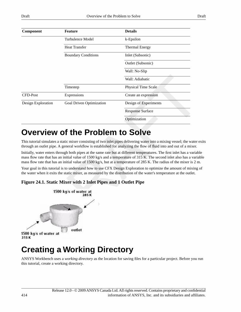
DetailsFeatureComponent
k-EpsilonTurbulence Model
Thermal EnergyHeat Transfer
Inlet (Subsonic)Boundary Conditions
Outlet (Subsonic)
Wall: No-Slip
Wall: Adiabatic
Physical Time ScaleTimestep
Create an expressionExpressionsCFD-Post
Design of ExperimentsGoal Driven OptimizationDesign Exploration
Response Surface
Optimization
Overview of the Problem to SolveThis tutorial simulates a static mixer consisting of two inlet pipes delivering water into a mixing vessel; the water exitsthrough an outlet pipe. A general workflow is established for analyzing the flow of fluid into and out of a mixer.
Initially, water enters through both pipes at the same rate but at different temperatures. The first inlet has a variablemass flow rate that has an initial value of 1500 kg/s and a temperature of 315 K. The second inlet also has a variablemass flow rate that has an initial value of 1500 kg/s, but at a temperature of 285 K. The radius of the mixer is 2 m.
Your goal in this tutorial is to understand how to use CFX Design Exploration to optimize the amount of mixing ofthe water when it exits the static mixer, as measured by the distribution of the water's temperature at the outlet.
Figure 24.1. Static Mixer with 2 Inlet Pipes and 1 Outlet Pipe
Creating a Working DirectoryANSYS Workbench uses a working directory as the location for saving files for a particular project. Before you runthis tutorial, create a working directory.
Release 12.0 - © 2009 ANSYS Canada Ltd. All rights reserved. Contains proprietary and confidentialinformation of ANSYS, Inc. and its subsidiaries and affiliates.414
DraftOverview of the Problem to SolveDraft
Setting Up ANSYS WorkbenchBefore you begin using ANSYS Workbench, you have to configure the Geometry Import option settings for use withthis tutorial:
1. Launch ANSYS Workbench.
2. From the ANSYS Workbench menu bar, select Tools > Options. The Options configuration dialog appears.
3. In the Options configuration dialog, select Geometry Import
a. Ensure Parameters is enabled and remove the "DS" from Filtering Prefixes and Suffixes.
b. Enable Named Selections and remove the name "NS" from Filtering Prefixes.
c. Click OK.
Creating the ProjectTo create the project, you save an empty project:
1. From the ANSYS Workbench menu bar, select File > Save As and save the project as StaticMixerDX.wbpjin your working directory. This directory will be the location for all of the project files that you create during thetutorial.
2. From Toolbox > Analysis Systems, drag the Fluid Flow (CFX) system onto the Project Schematic.
Creating the Geometry in DesignModelerNow you can create a geometry by using DesignModeler:
1. In the Fluid Flow (CFX) system, right-click Geometry and select New Geometry. DesignModeler starts.
2. If DesignModeler displays a window for selecting the desired length unit, select Meter as the desired length unitand click OK. (Note that this window will not appear if you have previously set a default unit of measurement.)
Creating the SolidYou create geometry in DesignModeler by creating two-dimensional sketches and extruding, revolving, sweeping, orlofting these to add or remove material. To create the main body of the Static Mixer, you draw a sketch of a cross-sectionand revolve it.
1. In the Tree Outline, click ZXPlane.
Each sketch is created in a plane. By selecting ZXPlane before creating a sketch, you ensure that the sketch youare about to create is based on the ZX plane.
2. Click New Sketch on the Active Plane/Sketch Toolbar, which is located above the Graphics window.
3. In the Tree Outline, click Sketch1.
4. Select the Sketching tab (below the Tree Outline) to view the available sketching tool boxes.
Setting Up the GridBefore starting your sketch, set up a grid on the plane in which you will draw the sketch. The grid facilitates the precisepositioning of points (when Snap is enabled).
1. Click Settings (in the Sketching tab) to open the Settings Toolbox.
2. Click Grid and select Show in 2D and Snap.
3. Click Major Grid Spacing and set it to 1.
415Release 12.0 - © 2009 ANSYS Canada Ltd. All rights reserved. Contains proprietary and confidentialinformation of ANSYS, Inc. and its subsidiaries and affiliates.
DraftSetting Up ANSYS WorkbenchDraft
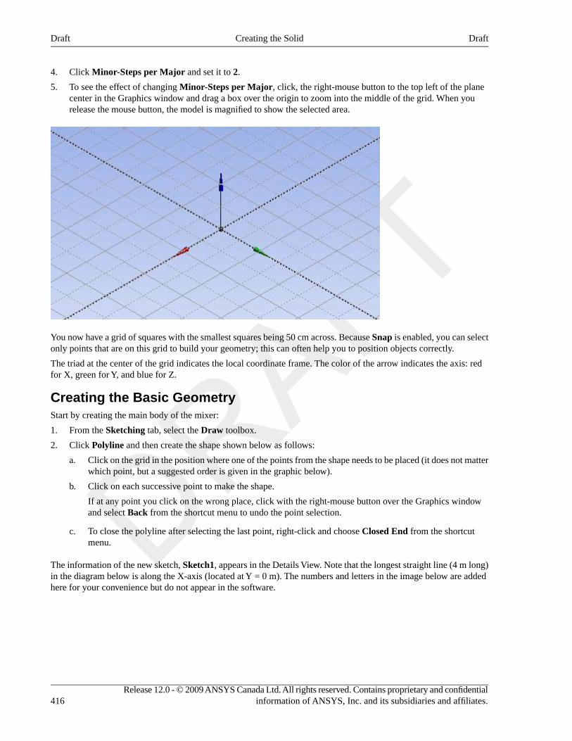
4. Click Minor-Steps per Major and set it to 2.
5. To see the effect of changing Minor-Steps per Major, click, the right-mouse button to the top left of the planecenter in the Graphics window and drag a box over the origin to zoom into the middle of the grid. When yourelease the mouse button, the model is magnified to show the selected area.
You now have a grid of squares with the smallest squares being 50 cm across. Because Snap is enabled, you can selectonly points that are on this grid to build your geometry; this can often help you to position objects correctly.
The triad at the center of the grid indicates the local coordinate frame. The color of the arrow indicates the axis: redfor X, green for Y, and blue for Z.
Creating the Basic GeometryStart by creating the main body of the mixer:
1. From the Sketching tab, select the Draw toolbox.
2. Click Polyline and then create the shape shown below as follows:
a. Click on the grid in the position where one of the points from the shape needs to be placed (it does not matterwhich point, but a suggested order is given in the graphic below).
b. Click on each successive point to make the shape.
If at any point you click on the wrong place, click with the right-mouse button over the Graphics windowand select Back from the shortcut menu to undo the point selection.
c. To close the polyline after selecting the last point, right-click and choose Closed End from the shortcutmenu.
The information of the new sketch, Sketch1, appears in the Details View. Note that the longest straight line (4 m long)in the diagram below is along the X-axis (located at Y = 0 m). The numbers and letters in the image below are addedhere for your convenience but do not appear in the software.
Release 12.0 - © 2009 ANSYS Canada Ltd. All rights reserved. Contains proprietary and confidentialinformation of ANSYS, Inc. and its subsidiaries and affiliates.416
DraftCreating the SolidDraft
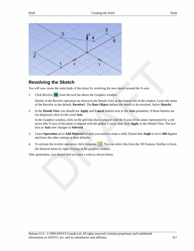
Revolving the SketchYou will now create the main body of the mixer by revolving the new sketch around the X-axis.
1. Click Revolve from the tool bar above the Graphics window.
Details of the Revolve operation are shown in the Details View at the bottom left of the window. Leave the nameof the Revolve as the default, Revolve1. The Base Object defines the sketch to be revolved. Select Sketch1.
2. In the Details View you should see Apply and Cancel buttons next to the Axis parameter; if those buttons arenot displayed, click on the word Axis.
In the Graphics window, click on the grid line that is aligned with the X-axis of the plane represented by a redarrow (the X-axis of the plane is aligned with the global Z-axis), then click Apply in the Details View. The textnext to Axis now changes to Selected.
3. Leave Operation set to Add Material because you need to create a solid. Ensure that Angle is set to 360 degreesand leave the other settings at their defaults.
4. To activate the revolve operation, click Generate . You can select this from the 3D Features Toolbar or from
the shortcut menu by right-clicking in the graphics window.
After generation, you should find you have a solid as shown below.
417Release 12.0 - © 2009 ANSYS Canada Ltd. All rights reserved. Contains proprietary and confidentialinformation of ANSYS, Inc. and its subsidiaries and affiliates.
DraftCreating the SolidDraft
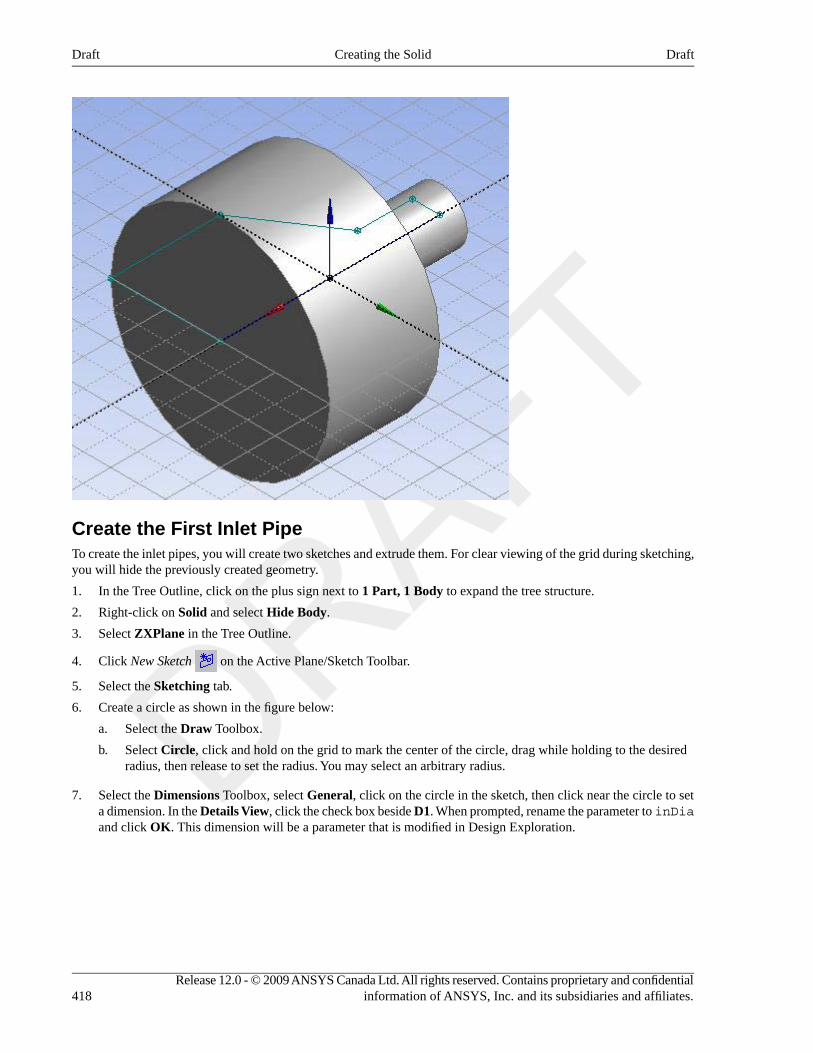
Create the First Inlet PipeTo create the inlet pipes, you will create two sketches and extrude them. For clear viewing of the grid during sketching,you will hide the previously created geometry.
1. In the Tree Outline, click on the plus sign next to 1 Part, 1 Body to expand the tree structure.
2. Right-click on Solid and select Hide Body.
3. Select ZXPlane in the Tree Outline.
4. Click New Sketch on the Active Plane/Sketch Toolbar.
5. Select the Sketching tab.
6. Create a circle as shown in the figure below:
a. Select the Draw Toolbox.
b. Select Circle, click and hold on the grid to mark the center of the circle, drag while holding to the desiredradius, then release to set the radius. You may select an arbitrary radius.
7. Select the Dimensions Toolbox, select General, click on the circle in the sketch, then click near the circle to seta dimension. In the Details View, click the check box beside D1. When prompted, rename the parameter to inDiaand click OK. This dimension will be a parameter that is modified in Design Exploration.
Release 12.0 - © 2009 ANSYS Canada Ltd. All rights reserved. Contains proprietary and confidentialinformation of ANSYS, Inc. and its subsidiaries and affiliates.418
DraftCreating the SolidDraft
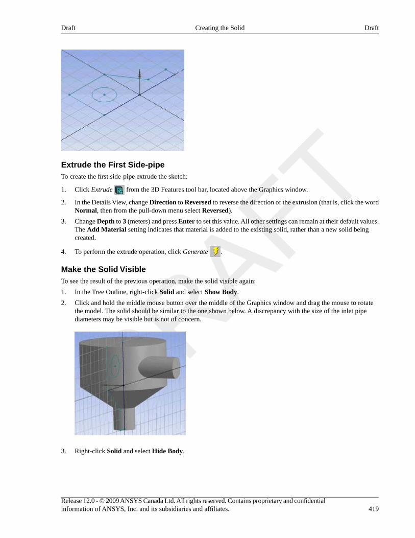
Extrude the First Side-pipeTo create the first side-pipe extrude the sketch:
1. Click Extrude from the 3D Features tool bar, located above the Graphics window.
2. In the Details View, change Direction to Reversed to reverse the direction of the extrusion (that is, click the wordNormal, then from the pull-down menu select Reversed).
3. Change Depth to 3 (meters) and press Enter to set this value. All other settings can remain at their default values.The Add Material setting indicates that material is added to the existing solid, rather than a new solid beingcreated.
4. To perform the extrude operation, click Generate .
Make the Solid VisibleTo see the result of the previous operation, make the solid visible again:
1. In the Tree Outline, right-click Solid and select Show Body.
2. Click and hold the middle mouse button over the middle of the Graphics window and drag the mouse to rotatethe model. The solid should be similar to the one shown below. A discrepancy with the size of the inlet pipediameters may be visible but is not of concern.
3. Right-click Solid and select Hide Body.
419Release 12.0 - © 2009 ANSYS Canada Ltd. All rights reserved. Contains proprietary and confidentialinformation of ANSYS, Inc. and its subsidiaries and affiliates.
DraftCreating the SolidDraft
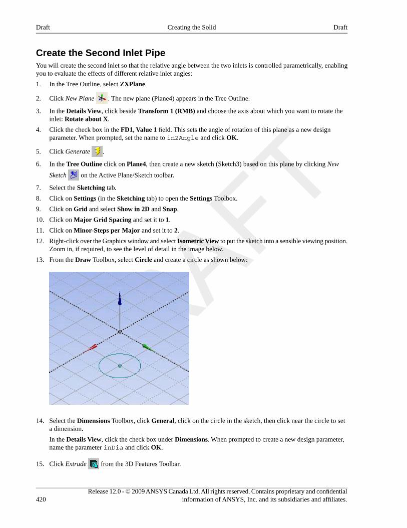
Create the Second Inlet PipeYou will create the second inlet so that the relative angle between the two inlets is controlled parametrically, enablingyou to evaluate the effects of different relative inlet angles:
1. In the Tree Outline, select ZXPlane.
2. Click New Plane . The new plane (Plane4) appears in the Tree Outline.
3. In the Details View, click beside Transform 1 (RMB) and choose the axis about which you want to rotate theinlet: Rotate about X.
4. Click the check box in the FD1, Value 1 field. This sets the angle of rotation of this plane as a new designparameter. When prompted, set the name to in2Angle and click OK.
5. Click Generate .
6. In the Tree Outline click on Plane4, then create a new sketch (Sketch3) based on this plane by clicking New
Sketch on the Active Plane/Sketch toolbar.
7. Select the Sketching tab.
8. Click on Settings (in the Sketching tab) to open the Settings Toolbox.
9. Click on Grid and select Show in 2D and Snap.
10. Click on Major Grid Spacing and set it to 1.
11. Click on Minor-Steps per Major and set it to 2.
12. Right-click over the Graphics window and select Isometric View to put the sketch into a sensible viewing position.Zoom in, if required, to see the level of detail in the image below.
13. From the Draw Toolbox, select Circle and create a circle as shown below:
14. Select the Dimensions Toolbox, click General, click on the circle in the sketch, then click near the circle to seta dimension.
In the Details View, click the check box under Dimensions. When prompted to create a new design parameter,name the parameter inDia and click OK.
15. Click Extrude from the 3D Features Toolbar.
Release 12.0 - © 2009 ANSYS Canada Ltd. All rights reserved. Contains proprietary and confidentialinformation of ANSYS, Inc. and its subsidiaries and affiliates.420
DraftCreating the SolidDraft
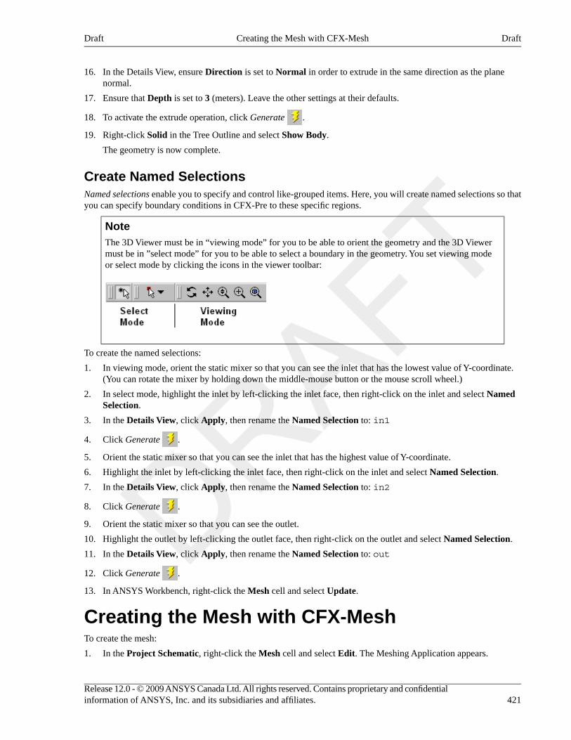
16. In the Details View, ensure Direction is set to Normal in order to extrude in the same direction as the planenormal.
17. Ensure that Depth is set to 3 (meters). Leave the other settings at their defaults.
18. To activate the extrude operation, click Generate .
19. Right-click Solid in the Tree Outline and select Show Body.
The geometry is now complete.
Create Named SelectionsNamed selections enable you to specify and control like-grouped items. Here, you will create named selections so thatyou can specify boundary conditions in CFX-Pre to these specific regions.
NoteThe 3D Viewer must be in “viewing mode” for you to be able to orient the geometry and the 3D Viewermust be in ”select mode” for you to be able to select a boundary in the geometry. You set viewing modeor select mode by clicking the icons in the viewer toolbar:
To create the named selections:
1. In viewing mode, orient the static mixer so that you can see the inlet that has the lowest value of Y-coordinate.(You can rotate the mixer by holding down the middle-mouse button or the mouse scroll wheel.)
2. In select mode, highlight the inlet by left-clicking the inlet face, then right-click on the inlet and select NamedSelection.
3. In the Details View, click Apply, then rename the Named Selection to: in1
4. Click Generate .
5. Orient the static mixer so that you can see the inlet that has the highest value of Y-coordinate.
6. Highlight the inlet by left-clicking the inlet face, then right-click on the inlet and select Named Selection.
7. In the Details View, click Apply, then rename the Named Selection to: in2
8. Click Generate .
9. Orient the static mixer so that you can see the outlet.
10. Highlight the outlet by left-clicking the outlet face, then right-click on the outlet and select Named Selection.
11. In the Details View, click Apply, then rename the Named Selection to: out
12. Click Generate .
13. In ANSYS Workbench, right-click the Mesh cell and select Update.
Creating the Mesh with CFX-MeshTo create the mesh:
1. In the Project Schematic, right-click the Mesh cell and select Edit. The Meshing Application appears.
421Release 12.0 - © 2009 ANSYS Canada Ltd. All rights reserved. Contains proprietary and confidentialinformation of ANSYS, Inc. and its subsidiaries and affiliates.
DraftCreating the Mesh with CFX-MeshDraft
2. If required, on the Meshing Application's Meshing Options panel, click OK to accept the default settings.
3. Expand Project > Model (A3) and right-click Mesh. Select Edit in CFX-Mesh. CFX-Mesh starts.
4. In CFX-Mesh, click Generate Volume Mesh.
Setting up the Case with CFX-PreNow that the mesh has been created, you can use CFX-Pre to define the simulation. To set up the case with CFX-Pre:
1. In ANSYS Workbench, save the project. (The save operation is automatic in most situations, but must be performedmanually when mesh operations have been completed; this improves overall performance.)
2. Double-click the Setup cell. CFX-Pre appears with the mesh file loaded.
3. In CFX-Pre, create an expression named inMassFlow:
a. In the Tree Outline, expand Expressions, Functions and Variables and right-click Expression > Insert> Expression.
b. Give the new expression the name: inMassFlow
c. In the Definition area, type: 1500 [kg s^-1]
Click Apply.
4. Right-click inMassFlow and select Use as Workbench Input Parameter.
5. Define the characteristics of the domain:
a. Click the Outline tab.
b. Double-click Simulation > Flow Analysis 1 > Default Domain to open it for editing.
c. Apply the following settings:
ValueSettingTab
Fluid 1Fluid and Particle DefinitionsBasic Settings
WaterFluid and Particle Definitions > Fluid 1 >Material
1 [atm]Domain Models > Pressure > ReferencePressure
Thermal EnergyHeat Transfer > OptionFluids Models
d. Click OK.
6. Create the first inlet boundary:
a. From the CFX-Pre menu bar, select Insert > Boundary.
b. In the Insert Boundary dialog, name the new boundary in1 and click OK.
c. Apply the following settings to in1:
ValueSettingTab
InletBoundary TypeBasic Settings
in1Location
Mass Flow RateMass and Momentum > OptionBoundary Details
Release 12.0 - © 2009 ANSYS Canada Ltd. All rights reserved. Contains proprietary and confidentialinformation of ANSYS, Inc. and its subsidiaries and affiliates.422
DraftSetting up the Case with CFX-PreDraft
ValueSettingTab
inMassFlowaMass Flow Rate
315 [K]Heat Transfer > Static Temperature
aTo enter this expression name into the Mass Flow Rate field, click in the blank field, click on the Enter Expression icon that appears,right-click in the blank field, then select the inMassFlow expression that appears.
d. Click OK.
7. Create the second inlet boundary:
a. From the CFX-Pre menu bar, select Insert > Boundary.
b. In the Insert Boundary dialog, name the new boundary in2 and click OK.
c. Apply the following settings to in2:
ValueSettingTab
InletBoundary TypeBasic Settings
in2Location
Mass Flow RateMass and Momentum > OptionBoundary Details
inMassFlowaMass Flow Rate
285 [K]Heat Transfer > Static Temperature
aTo enter this expression name into the Mass Flow Rate field, click in the blank field, click on the Enter Expression icon that appears,right-click in the blank field, then select the inMassFlow expression that appears.
d. Click OK.
8. Create the outlet boundary:
a. From the CFX-Pre menu bar, select Insert > Boundary.
b. In the Insert Boundary dialog, name the new boundary out and click OK.
c. Apply the following settings to out:
ValueSettingTab
OutletBoundary TypeBasic Settings
outLocation
0 [Pa]Mass and Momentum > Relative PressureBoundary Details
d. Click OK. CFX-Pre and ANSYS Workbench both update automatically. The three boundary conditions aredisplayed in the viewer as sets of arrows at the boundary surfaces. Inlet boundary arrows are directed intothe domain; outlet boundary arrows are directed out of the domain.
9. Solver Control parameters control aspects of the numerical solution generation process. Set the solver controlsas follows:
a. Click Solver Control .
423Release 12.0 - © 2009 ANSYS Canada Ltd. All rights reserved. Contains proprietary and confidentialinformation of ANSYS, Inc. and its subsidiaries and affiliates.
DraftSetting up the Case with CFX-PreDraft
b. On the Basic Settings tab, set Advection Scheme > Option to Upwind.
While an upwind advection scheme is less accurate than other advection schemes, it is also more robust.This advection scheme is suitable for obtaining an initial set of results, but in general should not be used toobtain final results.
c. Set Convergence Control > Fluid Timescale Control > Timescale Control to Physical Timescaleand set the physical timescale value to 2 [s].
The time scale can be calculated automatically by the solver or set manually. The Automatic option tendsto be conservative, leading to reliable, but often slow, convergence. It is often possible to accelerateconvergence by applying a time scale factor or by choosing a manual value that is more aggressive than theAutomatic option. By selecting a physical time scale, you obtain a convergence that is twice as fast as theAutomatic option.
d. Click OK. CFX-Pre and ANSYS Workbench both update automatically.
Solving the Case with CFX-Solver Manager1. In the Project Schematic, right-click the Solution cell and select Edit. CFX-Solver Manager appears.
2. On the CFX-Solver Manager Define Run dialog, click Start Run.
CFX-Solver launches and a split screen appears and displays the results of the run graphically and as text. Thepanes continue to build as CFX-Solver Manager operates.
Once the second iteration appears, data begins to plot. Plotting may take a long time depending on the amount ofdata to process. Let the process run.
3. When the run completes, click OK. CFX-Solver Manager and ANSYS Workbench both update automatically.
4. In CFX-Solver Manager, select File > Quit.
5. In the Project Schematic, right-click the Results cell and select Refresh. When the refresh is complete, right-clickthe Results cell again and select Edit. CFD-Post starts.
Setting the Output Parameter in CFD-PostWhen CFD-Post starts, it displays the 3D Viewer and the Outline workspace.
Release 12.0 - © 2009 ANSYS Canada Ltd. All rights reserved. Contains proprietary and confidentialinformation of ANSYS, Inc. and its subsidiaries and affiliates.424
DraftSolving the Case with CFX-Solver ManagerDraft
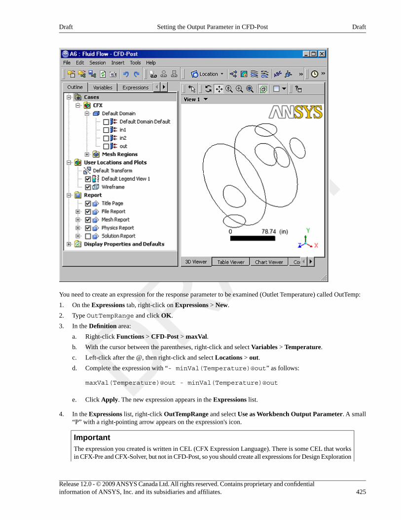
You need to create an expression for the response parameter to be examined (Outlet Temperature) called OutTemp:
1. On the Expressions tab, right-click on Expressions > New.
2. Type OutTempRange and click OK.
3. In the Definition area:
a. Right-click Functions > CFD-Post > maxVal.
b. With the cursor between the parentheses, right-click and select Variables > Temperature.
c. Left-click after the @, then right-click and select Locations > out.
d. Complete the expression with “- minVal(Temperature)@out” as follows:
maxVal(Temperature)@out - minVal(Temperature)@out
e. Click Apply. The new expression appears in the Expressions list.
4. In the Expressions list, right-click OutTempRange and select Use as Workbench Output Parameter. A small“P” with a right-pointing arrow appears on the expression's icon.
ImportantThe expression you created is written in CEL (CFX Expression Language). There is some CEL that worksin CFX-Pre and CFX-Solver, but not in CFD-Post, so you should create all expressions for Design Exploration
425Release 12.0 - © 2009 ANSYS Canada Ltd. All rights reserved. Contains proprietary and confidentialinformation of ANSYS, Inc. and its subsidiaries and affiliates.
DraftSetting the Output Parameter in CFD-PostDraft
output parameters in CFD-Post. Any expression created in CFX-Pre and used as a Design Explorationoutput parameter could potentially cause fatal errors during the Design Exploration run.
Investigating the Impact of Changing InputParameters ManuallyBefore using Design Exploration, you will manually change the input parameters to see what effect each has on therate of mixing. As you make changes to parameters in ANSYS Workbench, CFX-Pre and ANSYS DesignModelerwill update automatically; ensure that those programs are open so that you can see the changes take place.
1. In the Project Schematic, right-click Parameters and select Edit. A new set of views opens.
2. Select View > Project Schematic. The Project Schematic reappears.
Note the value of OutTempRange.
3. Highlight Parameters (cell A7) and in the Outline of Schematic A7 view, change in2Angle value from 0 to –45.
4. Update the Geometry cell and notice how the geometry changes in ANSYS DesignModeler.
Update the Results cell and note the value of OutTempRange.
5. Highlight Parameters (cell A7) and in the Outline of Schematic A7 view, reset in2Angle value to 0, then changeinDia from 1 to 1.5.
Update the Results cell and note the value of OutTempRange.
6. Update the Geometry cell and notice how the geometry changes in ANSYS DesignModeler.
7. Highlight Parameters (cell A7) and in the Outline of Schematic A7 view, reset inDia to 1, then changeinMassFlow from 1500 to 1600.
8. Update the Setup cell and notice how the expression changes in CFX-Pre.
Update the Results cell and note the value of OutTempRange.
As you changed the input parameters you should have seen changes to the output parameter that were similar to thefollowing:
OutTempRangeMassFlowAveinDiain2Angle
0.87912 K150010
0.77213 K15001–45
2.10320 K15001.50
0.97278 K160010
Recall that the goal of this design study is to maximize the mixing (which occurs when OutTempRange reaches itsminimum value). From these manual tests, it appears that the best results are obtained by changing the input angle ofone inlet. We will now automate that manual process of repeatedly changing variable values by using DesignExploration.
Changing Input Parameters Using DesignExplorationIn this section you will use Design Exploration's Goal Driven Optimization feature to minimize the value ofOutTempRange.
Release 12.0 - © 2009 ANSYS Canada Ltd. All rights reserved. Contains proprietary and confidentialinformation of ANSYS, Inc. and its subsidiaries and affiliates.426
DraftInvestigating the Impact of Changing Input Parameters ManuallyDraft
1. From the Design Exploration toolbox, drag a Goal Driven Optimization system to the Project Schematic(under the Parameter Set bar).
2. Select the Design of Experiments cell.
3. In the Outline of Schematic B2 view:
a. Enable in2Angle and inMassFlow; clear inDia.
b. Select cell P3 – inMassFlow (cell A6). In the Properties of Outline A6: P3 view, set:
• Lower Bound: 1000
• Upper Bound: 2000
• Initial Value: 1500
c. Select cell P2 – in2Angle (cell A5). In the Properties of Outline A5: P2 view, set:
• Lower Bound: –45
• Upper Bound: 0
• Initial Value: –45
4. In the ANSYS Workbench toolbar, ensure that View > Table is set.
5. In the Project Schematic, right-click the Design of Experiments cell and select Refresh. ANSYS Workbenchrecalculates all of the values for the input and output parameters. To do this more efficiently, it also closes anyopen ANSYS CFX applications and runs them in the background.
427Release 12.0 - © 2009 ANSYS Canada Ltd. All rights reserved. Contains proprietary and confidentialinformation of ANSYS, Inc. and its subsidiaries and affiliates.
DraftChanging Input Parameters Using Design ExplorationDraft

Release 12.0 - © 2009 ANSYS Canada Ltd. All rights reserved. Contains proprietary and confidentialinformation of ANSYS, Inc. and its subsidiaries and affiliates.
Chapter 25. Aerodynamic & StructuralPerformance of a CentrifugalCompressorThis tutorial includes:
• Tutorial Features (p. 429)
• Overview of the Problem to Solve (p. 430)
• Before You Begin (p. 431)
• Starting ANSYS Workbench and Creating a BladeGen System (p. 432)
• Reviewing the Centrifugal Compressor Geometry in BladeGen (p. 433)
• Creating a CFD Mesh using ANSYS TurboGrid (p. 434)
• Defining an Aerodynamic Simulation using CFX-Pre (p. 440)
• Obtaining a Solution to the Aerodynamic Simulation using CFX-Solver (p. 441)
• Viewing the Results of the Aerodynamic Simulation in CFD-Post (p. 442)
• Simulating Structural Stresses due to Pressure Loads (p. 443)
• Simulating Structural Stresses due to Rotation (p. 445)
NoteThis tutorial is intended to be run on Windows-based machines only.
Tutorial FeaturesThis tutorial addresses the following features of ANSYS Workbench.
DetailsFeatureComponent
Transfer of geometry to ANSYSTurboGrid.
GeometryANSYS BladeGen
H/J/C/L-Grid TopologyMeshANSYS TurboGrid
Shroud Tip defined by Profile
Control Point Movements
Edge Split Controls
Transfer of Mesh to a CFX System
Used to define a TurbomachineryCFD Simulation
Turbo ModeCFX-Pre
Centrifugal CompressorMachine Type
RotatingComponent Type
Steady StateAnalysis Type
P-Total Inlet Mass Flow OutletBoundary Template
429Release 12.0 - © 2009 ANSYS Canada Ltd. All rights reserved. Contains proprietary and confidentialinformation of ANSYS, Inc. and its subsidiaries and affiliates.
DraftDraft
DetailsFeatureComponent
Cylindrical ComponentsFlow Direction
Single DomainDomain Type
Physical TimescaleTimestep
Computed Results TableReportCFD-Post
Blade Loading Span 50
Streamwise Plot of Pt and P
Velocity Streamlines Stream BladeTE
CFX Pressure data applied toStructural Simulation
Static Structural AnalysisStatic Structural (ANSYS)System
Fixed Support
Von Mises StressesStatic Structural Solutions
Total Deformation
Overview of the Problem to SolveThis tutorial makes use of several ANSYS software components to simulate the aerodynamic and structural performanceof a centrifugal compressor.
Release 12.0 - © 2009 ANSYS Canada Ltd. All rights reserved. Contains proprietary and confidentialinformation of ANSYS, Inc. and its subsidiaries and affiliates.430
DraftOverview of the Problem to SolveDraft
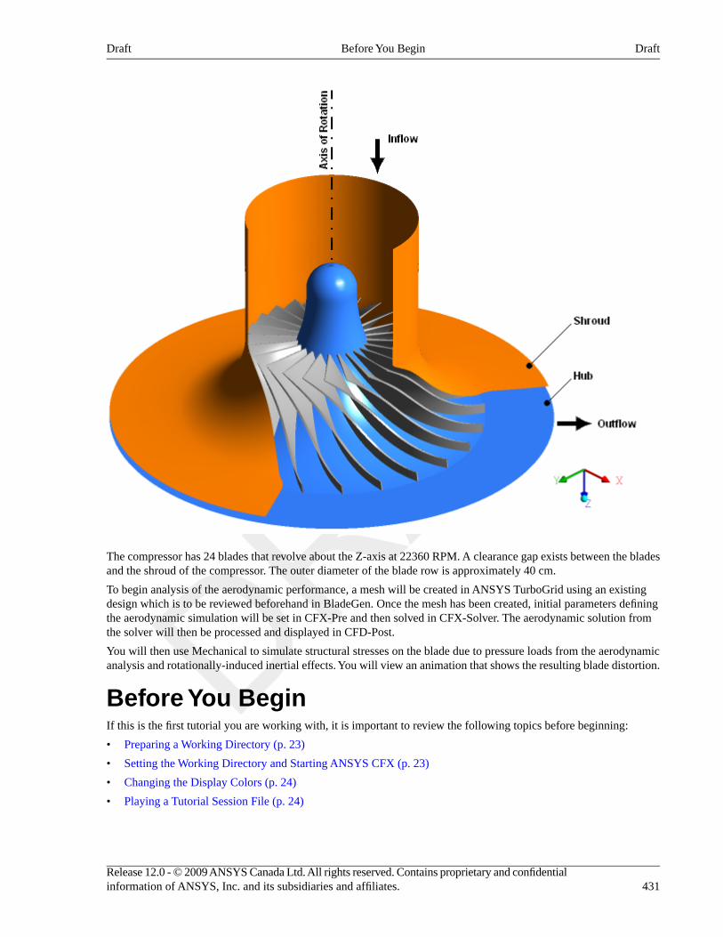
The compressor has 24 blades that revolve about the Z-axis at 22360 RPM. A clearance gap exists between the bladesand the shroud of the compressor. The outer diameter of the blade row is approximately 40 cm.
To begin analysis of the aerodynamic performance, a mesh will be created in ANSYS TurboGrid using an existingdesign which is to be reviewed beforehand in BladeGen. Once the mesh has been created, initial parameters definingthe aerodynamic simulation will be set in CFX-Pre and then solved in CFX-Solver. The aerodynamic solution fromthe solver will then be processed and displayed in CFD-Post.
You will then use Mechanical to simulate structural stresses on the blade due to pressure loads from the aerodynamicanalysis and rotationally-induced inertial effects. You will view an animation that shows the resulting blade distortion.
Before You BeginIf this is the first tutorial you are working with, it is important to review the following topics before beginning:
• Preparing a Working Directory (p. 23)
• Setting the Working Directory and Starting ANSYS CFX (p. 23)
• Changing the Display Colors (p. 24)
• Playing a Tutorial Session File (p. 24)
431Release 12.0 - © 2009 ANSYS Canada Ltd. All rights reserved. Contains proprietary and confidentialinformation of ANSYS, Inc. and its subsidiaries and affiliates.
DraftBefore You BeginDraft
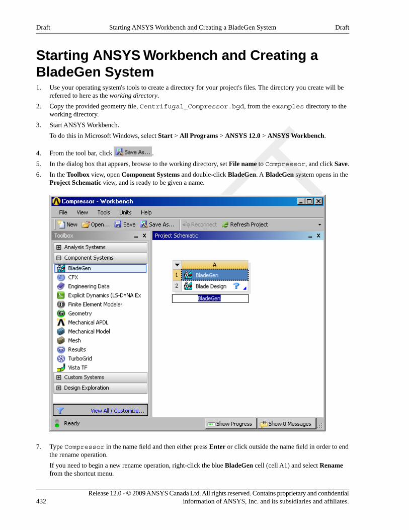
Starting ANSYS Workbench and Creating aBladeGen System1. Use your operating system's tools to create a directory for your project's files. The directory you create will be
referred to here as the working directory.
2. Copy the provided geometry file, Centrifugal_Compressor.bgd, from the examples directory to theworking directory.
3. Start ANSYS Workbench.
To do this in Microsoft Windows, select Start > All Programs > ANSYS 12.0 > ANSYS Workbench.
4. From the tool bar, click .
5. In the dialog box that appears, browse to the working directory, set File name to Compressor, and click Save.
6. In the Toolbox view, open Component Systems and double-click BladeGen. A BladeGen system opens in theProject Schematic view, and is ready to be given a name.
7. Type Compressor in the name field and then either press Enter or click outside the name field in order to endthe rename operation.
If you need to begin a new rename operation, right-click the blue BladeGen cell (cell A1) and select Renamefrom the shortcut menu.
Release 12.0 - © 2009 ANSYS Canada Ltd. All rights reserved. Contains proprietary and confidentialinformation of ANSYS, Inc. and its subsidiaries and affiliates.432
DraftStarting ANSYS Workbench and Creating a BladeGen SystemDraft
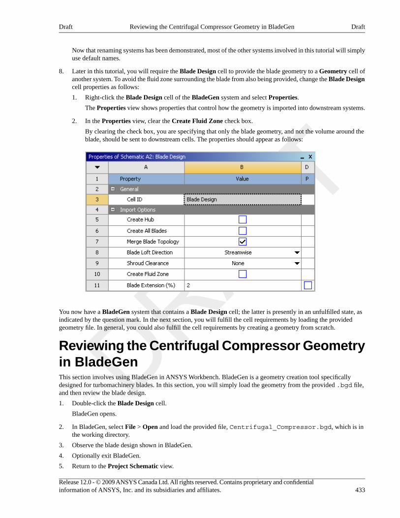
Now that renaming systems has been demonstrated, most of the other systems involved in this tutorial will simplyuse default names.
8. Later in this tutorial, you will require the Blade Design cell to provide the blade geometry to a Geometry cell ofanother system. To avoid the fluid zone surrounding the blade from also being provided, change the Blade Designcell properties as follows:
1. Right-click the Blade Design cell of the BladeGen system and select Properties.
The Properties view shows properties that control how the geometry is imported into downstream systems.
2. In the Properties view, clear the Create Fluid Zone check box.
By clearing the check box, you are specifying that only the blade geometry, and not the volume around theblade, should be sent to downstream cells. The properties should appear as follows:
You now have a BladeGen system that contains a Blade Design cell; the latter is presently in an unfulfilled state, asindicated by the question mark. In the next section, you will fulfill the cell requirements by loading the providedgeometry file. In general, you could also fulfill the cell requirements by creating a geometry from scratch.
Reviewing the Centrifugal Compressor Geometryin BladeGenThis section involves using BladeGen in ANSYS Workbench. BladeGen is a geometry creation tool specificallydesigned for turbomachinery blades. In this section, you will simply load the geometry from the provided .bgd file,and then review the blade design.
1. Double-click the Blade Design cell.
BladeGen opens.
2. In BladeGen, select File > Open and load the provided file, Centrifugal_Compressor.bgd, which is inthe working directory.
3. Observe the blade design shown in BladeGen.
4. Optionally exit BladeGen.
5. Return to the Project Schematic view.
433Release 12.0 - © 2009 ANSYS Canada Ltd. All rights reserved. Contains proprietary and confidentialinformation of ANSYS, Inc. and its subsidiaries and affiliates.
DraftReviewing the Centrifugal Compressor Geometry in BladeGenDraft
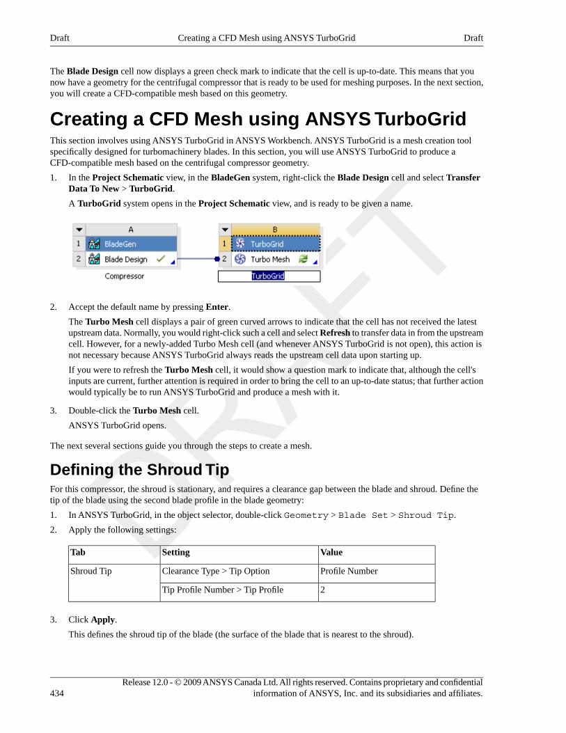
The Blade Design cell now displays a green check mark to indicate that the cell is up-to-date. This means that younow have a geometry for the centrifugal compressor that is ready to be used for meshing purposes. In the next section,you will create a CFD-compatible mesh based on this geometry.
Creating a CFD Mesh using ANSYS TurboGridThis section involves using ANSYS TurboGrid in ANSYS Workbench. ANSYS TurboGrid is a mesh creation toolspecifically designed for turbomachinery blades. In this section, you will use ANSYS TurboGrid to produce aCFD-compatible mesh based on the centrifugal compressor geometry.
1. In the Project Schematic view, in the BladeGen system, right-click the Blade Design cell and select TransferData To New > TurboGrid.
A TurboGrid system opens in the Project Schematic view, and is ready to be given a name.
2. Accept the default name by pressing Enter.
The Turbo Mesh cell displays a pair of green curved arrows to indicate that the cell has not received the latestupstream data. Normally, you would right-click such a cell and select Refresh to transfer data in from the upstreamcell. However, for a newly-added Turbo Mesh cell (and whenever ANSYS TurboGrid is not open), this action isnot necessary because ANSYS TurboGrid always reads the upstream cell data upon starting up.
If you were to refresh the Turbo Mesh cell, it would show a question mark to indicate that, although the cell'sinputs are current, further attention is required in order to bring the cell to an up-to-date status; that further actionwould typically be to run ANSYS TurboGrid and produce a mesh with it.
3. Double-click the Turbo Mesh cell.
ANSYS TurboGrid opens.
The next several sections guide you through the steps to create a mesh.
Defining the Shroud TipFor this compressor, the shroud is stationary, and requires a clearance gap between the blade and shroud. Define thetip of the blade using the second blade profile in the blade geometry:
1. In ANSYS TurboGrid, in the object selector, double-click Geometry > Blade Set > Shroud Tip.
2. Apply the following settings:
ValueSettingTab
Profile NumberClearance Type > Tip OptionShroud Tip
2Tip Profile Number > Tip Profile
3. Click Apply.
This defines the shroud tip of the blade (the surface of the blade that is nearest to the shroud).
Release 12.0 - © 2009 ANSYS Canada Ltd. All rights reserved. Contains proprietary and confidentialinformation of ANSYS, Inc. and its subsidiaries and affiliates.434
DraftCreating a CFD Mesh using ANSYS TurboGridDraft
Creating the TopologyIn ANSYS TurboGrid, you may choose a topology pattern based on the type of machine being analyzed. For thisgeometry, the H/J/C/L-Grid topology will be used.
1. In the object selector, double-click Topology Set.
2. Apply the following settings:
ValueSettingTab
H/J/C/L-GridTopology Definition > MethodDefinition
0.2aInclude O-Grid > Width Factor
H-Grid Not MatchingTip Topology > Shroud
aA reduced O-Grid width helps to improve mesh quality where the blade thickness is a large fraction of the passage width, as is the case atthe upstream end of the hub.
3. Click Apply to set the topology.
4. Right-click Topology Set and turn off Suspend Object Updates.
After a short time, the topology is generated.
5. Click Freeze to freeze the topology settings.
This prevents unintended automatic changes to the topology.
You now have a mesh topology that requires some adjustments before it is suitable for use in creating a mesh. Youcan see a 2D preview of the mesh on each of the two layers.
Modifying the TopologyThe mesh previews on the hub and shroud tip layers reveal areas that have low mesh angles. You will increase meshorthogonality in those areas by using control points. You will also adjust the mesh density locally by using edge splitcontrols.
Modifying the Hub Layer1. Select Display > Blade-to-Blade View > Use Passage Excluding Tip Transform.
The Passage Excluding Tip transform affects how blade-to-blade coordinates are calculated in preparationfor viewing with the Blade-to-Blade (Theta-M') transform (in the next step). Compared to the Full transform,the Passage Excluding Tip transform usually exhibits less distortion in the viewer for blades that have atip that varies in span. By choosing a transform explicitly, you prevent ANSYS TurboGrid from selecting one ofthese transforms automatically.
2. Right-click a blank area in the viewer and select Transformation > Blade-to-Blade (Theta-M').
3. Click Hide all geometry objects .
4. Turn off the visibility of Layers > Shroud Tip (by clearing the check box next to it) to make the hub topologymore visible.
5. Open Layers > Hub in the object editor and note that, in the object editor, the mesh measures are shown in redtext.
6. Double-click Minimum Face Angle to highlight the areas of the mesh that have the smallest angles.
The areas that have the smallest angles are marked with red lines in the viewer.
435Release 12.0 - © 2009 ANSYS Canada Ltd. All rights reserved. Contains proprietary and confidentialinformation of ANSYS, Inc. and its subsidiaries and affiliates.
DraftCreating the TopologyDraft
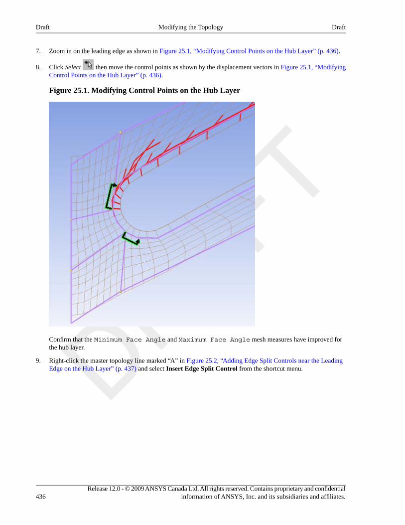
7. Zoom in on the leading edge as shown in Figure 25.1, “Modifying Control Points on the Hub Layer” (p. 436).
8. Click Select then move the control points as shown by the displacement vectors in Figure 25.1, “ModifyingControl Points on the Hub Layer” (p. 436).
Figure 25.1. Modifying Control Points on the Hub Layer
Confirm that the Minimum Face Angle and Maximum Face Angle mesh measures have improved forthe hub layer.
9. Right-click the master topology line marked “A” in Figure 25.2, “Adding Edge Split Controls near the LeadingEdge on the Hub Layer” (p. 437) and select Insert Edge Split Control from the shortcut menu.
Release 12.0 - © 2009 ANSYS Canada Ltd. All rights reserved. Contains proprietary and confidentialinformation of ANSYS, Inc. and its subsidiaries and affiliates.436
DraftModifying the TopologyDraft
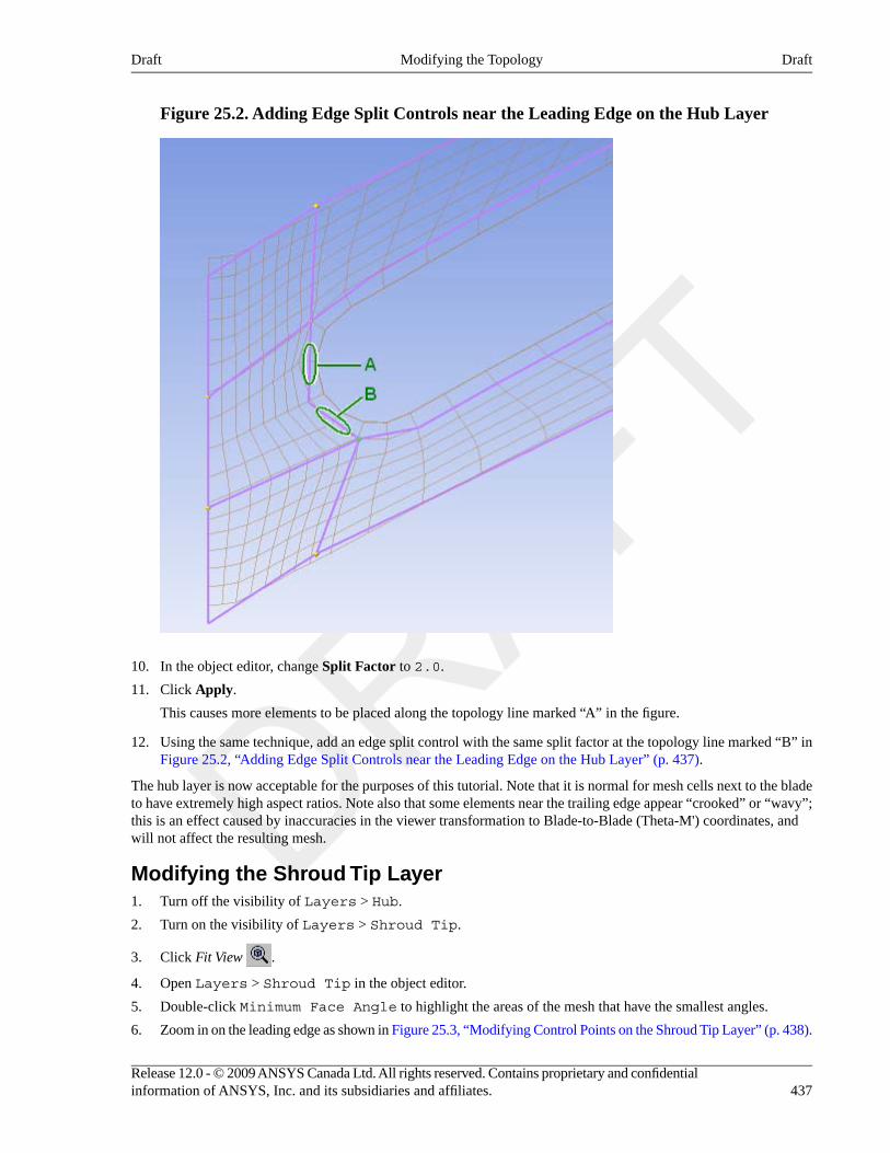
Figure 25.2. Adding Edge Split Controls near the Leading Edge on the Hub Layer
10. In the object editor, change Split Factor to 2.0.
11. Click Apply.
This causes more elements to be placed along the topology line marked “A” in the figure.
12. Using the same technique, add an edge split control with the same split factor at the topology line marked “B” inFigure 25.2, “Adding Edge Split Controls near the Leading Edge on the Hub Layer” (p. 437).
The hub layer is now acceptable for the purposes of this tutorial. Note that it is normal for mesh cells next to the bladeto have extremely high aspect ratios. Note also that some elements near the trailing edge appear “crooked” or “wavy”;this is an effect caused by inaccuracies in the viewer transformation to Blade-to-Blade (Theta-M') coordinates, andwill not affect the resulting mesh.
Modifying the Shroud Tip Layer1. Turn off the visibility of Layers > Hub.
2. Turn on the visibility of Layers > Shroud Tip.
3. Click Fit View .
4. Open Layers > Shroud Tip in the object editor.
5. Double-click Minimum Face Angle to highlight the areas of the mesh that have the smallest angles.
6. Zoom in on the leading edge as shown in Figure 25.3, “Modifying Control Points on the Shroud Tip Layer” (p. 438).
437Release 12.0 - © 2009 ANSYS Canada Ltd. All rights reserved. Contains proprietary and confidentialinformation of ANSYS, Inc. and its subsidiaries and affiliates.
DraftModifying the TopologyDraft
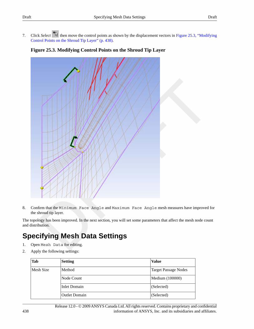
7. Click Select then move the control points as shown by the displacement vectors in Figure 25.3, “ModifyingControl Points on the Shroud Tip Layer” (p. 438).
Figure 25.3. Modifying Control Points on the Shroud Tip Layer
8. Confirm that the Minimum Face Angle and Maximum Face Angle mesh measures have improved forthe shroud tip layer.
The topology has been improved. In the next section, you will set some parameters that affect the mesh node countand distribution.
Specifying Mesh Data Settings1. Open Mesh Data for editing.
2. Apply the following settings:
ValueSettingTab
Target Passage NodesMethodMesh Size
Medium (100000)Node Count
(Selected)Inlet Domain
(Selected)Outlet Domain
Release 12.0 - © 2009 ANSYS Canada Ltd. All rights reserved. Contains proprietary and confidentialinformation of ANSYS, Inc. and its subsidiaries and affiliates.438
DraftSpecifying Mesh Data SettingsDraft
ValueSettingTab
Element Count and SizeSpanwise Blade Distribution Parameters > MethodPassage
25Spanwise Blade Distribution Parameters > # ofElements
11Spanwise Blade Distribution Parameters > ConstElements
Element Count and SizeO-Grid > Method
6O-Grid > # of Elements
(Selected)Inlet Domain > Override default # of ElementsInlet/Outlet
50Inlet Domain > Override default # of Elements > # ofElements
(Selected)Outlet Domain > Override default # of Elements
25Outlet Domain > Override default # of Elements > #of Elements
3. Click Apply.
NoteYour mesh quality could decrease slightly after increasing the node count. If so, you might want tomake minor adjustments to the hub and shroud control points to improve the quality of your meshbefore saving it and using it in the aerodynamic simulation that follows.
4. Open Layers for editing.
5. In the list of layers in the object editor, right-click Hub and select Insert Layer After to insert a layer midwaybetween the hub and shroud tip layers.
This helps to guide the mesh along the blade in the spanwise direction.
Generating the CFD MeshWith the topology and mesh data defined, the next step is to create a mesh.
1. Click Insert > Mesh.
After a few moments, the mesh is generated.
You may have noticed that some mesh statistics still show problems. Except for extremely dense meshes, it isnormal that the mesh elements next to the walls have very high length ratios and volume ratios. Further actionsto improve mesh quality are beyond the scope of this tutorial.
2. Optionally quit ANSYS TurboGrid.
3. Return to the Project Schematic view.
439Release 12.0 - © 2009 ANSYS Canada Ltd. All rights reserved. Contains proprietary and confidentialinformation of ANSYS, Inc. and its subsidiaries and affiliates.
DraftGenerating the CFD MeshDraft
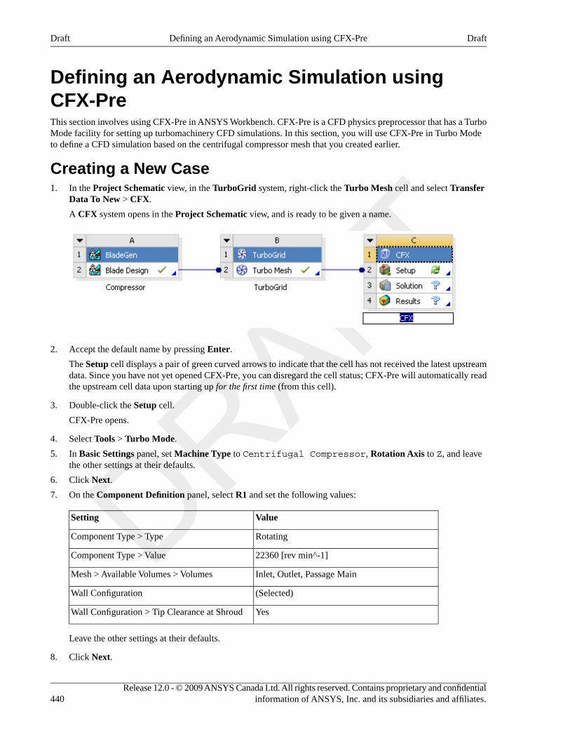
Defining an Aerodynamic Simulation usingCFX-PreThis section involves using CFX-Pre in ANSYS Workbench. CFX-Pre is a CFD physics preprocessor that has a TurboMode facility for setting up turbomachinery CFD simulations. In this section, you will use CFX-Pre in Turbo Modeto define a CFD simulation based on the centrifugal compressor mesh that you created earlier.
Creating a New Case1. In the Project Schematic view, in the TurboGrid system, right-click the Turbo Mesh cell and select Transfer
Data To New > CFX.
A CFX system opens in the Project Schematic view, and is ready to be given a name.
2. Accept the default name by pressing Enter.
The Setup cell displays a pair of green curved arrows to indicate that the cell has not received the latest upstreamdata. Since you have not yet opened CFX-Pre, you can disregard the cell status; CFX-Pre will automatically readthe upstream cell data upon starting up for the first time (from this cell).
3. Double-click the Setup cell.
CFX-Pre opens.
4. Select Tools > Turbo Mode.
5. In Basic Settings panel, set Machine Type to Centrifugal Compressor, Rotation Axis to Z, and leavethe other settings at their defaults.
6. Click Next.
7. On the Component Definition panel, select R1 and set the following values:
ValueSetting
RotatingComponent Type > Type
22360 [rev min^-1]Component Type > Value
Inlet, Outlet, Passage MainMesh > Available Volumes > Volumes
(Selected)Wall Configuration
YesWall Configuration > Tip Clearance at Shroud
Leave the other settings at their defaults.
8. Click Next.
Release 12.0 - © 2009 ANSYS Canada Ltd. All rights reserved. Contains proprietary and confidentialinformation of ANSYS, Inc. and its subsidiaries and affiliates.440
DraftDefining an Aerodynamic Simulation using CFX-PreDraft
9. On the Physics Definition panel, set the following values:
ValueSetting
Air Ideal GasFluid
Steady StateAnalysis Type > Type
1 [atm]Model Data > Reference Pressure
(Selected)Inflow/Outflow Boundary Templates > P-TotalInlet Mass Flow Outlet
0 [atm]Inflow/Outflow Boundary Templates > P-Total
20 [C]Inflow/Outflow Boundary Templates > T-Total
Per ComponentInflow/Outflow Boundary Templates > MassFlow
0.167 [kg s^-1]Inflow/Outflow Boundary Templates > MassFlow Rate
Cylindrical ComponentsInflow/Outflow Boundary Templates > FlowDirection
1, 0, 0Inflow/Outflow Boundary Templates > InflowDirection (a, r, t)
Physical TimescaleSolver Parameters > Convergence Control
0.0002 [s]Solver Parameters > Physical Timescale
Leave the other settings at their defaults.
10. Click Next.
11. On the Interface Definition panel, verify that each interface is set correctly; click an interface listed in the treeview and then examine the associated settings (shown in the lower portion of the panel) and highlighted regionsin the viewer.
If no regions appear highlighted in the viewer, ensure that highlighting is turned on in the viewer toolbar.
12. Click Next.
13. On the Boundary Definition panel, verify that each boundary is set correctly; click a boundary listed in the treeview and then examine the associated settings and highlighted regions.
14. Click Next.
15. On the Final Operations panel, leave the operation set to Enter General Mode and click Finish.
16. Optionally quit CFX-Pre.
17. Return to the Project Schematic view.
Obtaining a Solution to the AerodynamicSimulation using CFX-SolverGenerate a solution for the CFD simulation that you just prepared:
1. Right-click the Solution cell of the CFX system and select Update.
441Release 12.0 - © 2009 ANSYS Canada Ltd. All rights reserved. Contains proprietary and confidentialinformation of ANSYS, Inc. and its subsidiaries and affiliates.
DraftObtaining a Solution to the Aerodynamic Simulation using CFX-SolverDraft
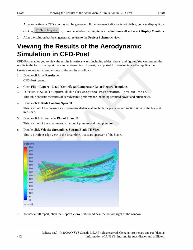
After some time, a CFD solution will be generated. If the progress indicator is not visible, you can display it by
clicking or, to see detailed output, right-click the Solution cell and select Display Monitors.
2. After the solution has been generated, return to the Project Schematic view.
Viewing the Results of the AerodynamicSimulation in CFD-PostCFD-Post enables you to view the results in various ways, including tables, charts, and figures. You can present theresults in the form of a report that can be viewed in CFD-Post, or exported for viewing in another application.
Create a report and examine some of the results as follows:
1. Double-click the Results cell.
CFD-Post opens.
2. Click File > Report > Load 'Centrifugal Compressor Rotor Report' Template.
3. In the tree view, under Report, double-click Computed Performance Results Table.
This table presents measures of aerodynamic performance including required power and efficiencies.
4. Double-click Blade Loading Span 50.
This is a plot of the pressure vs. streamwise distance along both the pressure and suction sides of the blade atmid-span.
5. Double-click Streamwise Plot of Pt and P.
This is a plot of the streamwise variation of pressure and total pressure.
6. Double-click Velocity Streamlines Stream Blade TE View.
This is a trailing-edge view of the streamlines that start upstream of the blade.
7. To view a full report, click the Report Viewer tab found near the bottom right of the window.
Release 12.0 - © 2009 ANSYS Canada Ltd. All rights reserved. Contains proprietary and confidentialinformation of ANSYS, Inc. and its subsidiaries and affiliates.442
DraftViewing the Results of the Aerodynamic Simulation in CFD-PostDraft
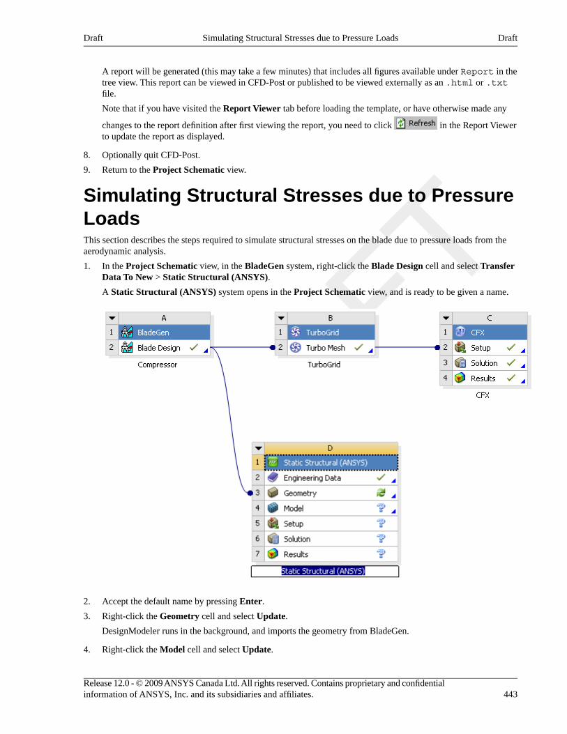
A report will be generated (this may take a few minutes) that includes all figures available under Report in thetree view. This report can be viewed in CFD-Post or published to be viewed externally as an .html or .txtfile.
Note that if you have visited the Report Viewer tab before loading the template, or have otherwise made any
changes to the report definition after first viewing the report, you need to click in the Report Viewerto update the report as displayed.
8. Optionally quit CFD-Post.
9. Return to the Project Schematic view.
Simulating Structural Stresses due to PressureLoadsThis section describes the steps required to simulate structural stresses on the blade due to pressure loads from theaerodynamic analysis.
1. In the Project Schematic view, in the BladeGen system, right-click the Blade Design cell and select TransferData To New > Static Structural (ANSYS).
A Static Structural (ANSYS) system opens in the Project Schematic view, and is ready to be given a name.
2. Accept the default name by pressing Enter.
3. Right-click the Geometry cell and select Update.
DesignModeler runs in the background, and imports the geometry from BladeGen.
4. Right-click the Model cell and select Update.
443Release 12.0 - © 2009 ANSYS Canada Ltd. All rights reserved. Contains proprietary and confidentialinformation of ANSYS, Inc. and its subsidiaries and affiliates.
DraftSimulating Structural Stresses due to Pressure LoadsDraft
ANSYS Mechanical runs in the background, and imports the solid model of the centrifugal compressor.
5. Connect the Solution cell of the CFX system to the Setup cell of the Static Structural (ANSYS) system.
This makes the CFD solution data available for use in a structural analysis.
6. Double-click the Setup cell. If a dialog box asks you if you want to read the upstream data, click Yes.
ANSYS Mechanical opens so that you can prepare a static structural analysis.
7. Select the following object from the tree view: Project > Model (D4) > Static Structural (D5)> Imported Load (Solution) > Imported Pressure.
8. In the details view, click the field beside Scope > Geometry, then select the blade surface (the large surface; notthe thin surface along the edge) by clicking it in the viewer.
9. In the details view next to Scope > Geometry, click Apply.
The field beside Geometry should now display the text “1 Face”. You have now chosen the solid model surfaceonto which to apply the CFD pressure data.
10. In the details view, click the field beside Transfer Definition > CFD Surface, and select R1 Blade from thedrop-down.
You have now chosen the CFD boundary from which to get the CFD pressure data.
11. Right-click Project > Model (D4) > Static Structural (D5) in the tree view and select Insert >Fixed Support.
12. In the viewer, right-click a blank area of the screen and select View > Bottom.
13. Select the long thin face of the blade that is at the forefront of the displayed geometry.
14. In the details view next to Scope > Geometry, click Apply.
The face that you selected is now connected to the hub.
15. In the tree view, right-click Project > Model (D4) > Static Structural (D5) > Solution (D6)and select Insert > Stress > Equivalent (von-Mises).
16. From the tool bar, click Solve and wait for the solver to finish.
17. To verify that the pressure data was applied correctly to the blade, inspect Project > Model (D4) > StaticStructural (D5) > Imported Load (Solution) > Imported Pressure > Imported LoadTransfer Summary.
The significant discrepancy shown in the load transfer summary is due to a difference in geometry; the surfaceonto which the CFX pressures were mapped does not include the blade tip or trailing-edge surfaces. In general,accurate load mapping requires that the surfaces match in terms of geometry and the length scale of mesh elements.
18. Click Project > Model (D4) > Static Structural (D5) > Solution (D6) > EquivalentStress to prepare to examine the von-Mises stress results.
19. Animate the physical deformation of the blade along with the associated von-Mises stress results, by clicking
Play in the Graph window.
NoteYou may need to drag the viewer window up in order to see the Graph window.
20. Right-click Project > Model (D4) > Static Structural (D5) > Solution (D6) and selectInsert > Deformation > Total.
21. From the tool bar, click Solve .
Release 12.0 - © 2009 ANSYS Canada Ltd. All rights reserved. Contains proprietary and confidentialinformation of ANSYS, Inc. and its subsidiaries and affiliates.444
DraftSimulating Structural Stresses due to Pressure LoadsDraft
When the solver has finished, select Project > Model (D4) > Static Structural (D5) > Solution(D6) > Total Deformation to prepare to examine the Total Deformation solution.
22. Animate the physical deformation by clicking the Play button in the Graph window.
23. Select File > Close Mechanical.
24. Return to the Project Schematic view.
Simulating Structural Stresses due to RotationThis section shows how to add inertial effects due to rotation.
1. Right-click the upper-left corner of the Static Structural (ANSYS) system and select Duplicate.
A second Static Structural (ANSYS) system appears, with its Geometry, and Model cells taking informationfrom the same sources as in the original system.
2. Rename the newly created system from Copy of Static Structural (ANSYS) to With Rotation.
3. Right-click the Model cell in the new system and select Update.
Wait until you see a green check mark in that cell.
4. Double-click the Setup cell in the new system.
ANSYS Mechanical opens.
5. Make sure that Project > Model (E4) > Static Structural (E5) is selected in the tree view, thenclick the Inertial button in the toolbar and select Rotational Velocity.
6. From the main menu, select Units > RPM.
7. In the details view for Rotational Velocity, change Definition > Define By to Components.
8. In the details view, set Definition > Z Component to 22360.
(The value will become 22360 RPM (ramped) when you finish entering the number.)
9. From the tool bar, click Solve .
10. To animate the total deformation or equivalent stress of the blade, select the corresponding object (either TotalDeformation or Equivalent Stress, respectively) under Project > Model (E4) > Static
Structural (E5) > Solution (E6) and click Play in the Graph window.
11. Select File > Close Mechanical.
12. Return to the Project Schematic view.
13. From the tool bar, click to save the project.
14. Exit ANSYS Workbench.
445Release 12.0 - © 2009 ANSYS Canada Ltd. All rights reserved. Contains proprietary and confidentialinformation of ANSYS, Inc. and its subsidiaries and affiliates.
DraftSimulating Structural Stresses due to RotationDraft

Release 12.0 - © 2009 ANSYS Canada Ltd. All rights reserved. Contains proprietary and confidentialinformation of ANSYS, Inc. and its subsidiaries and affiliates.
Chapter 26. Axial Turbine Equilibriumand Non-Equilibrium Steam PredictionsThis tutorial includes:
• Tutorial Features (p. 447)
• Overview of the Problem to Solve (p. 448)
• Before You Begin (p. 450)
• Starting CFX-Pre (p. 450)
• Defining the Equilibrium Case in CFX-Pre (p. 451)
• Obtaining a Solution for the Equilibrium Case (p. 457)
• Viewing the Equilibrium Case Results in CFD-Post (p. 457)
• Defining the Non-Equilibrium Case in CFX-Pre (p. 459)
• Obtaining a Solution for the Non-Equilibrium Case (p. 462)
• Viewing the Non-Equilibrium Case Results in CFD-Post (p. 462)
Tutorial FeaturesIn this tutorial you will learn about:
• Selection of material properties from the International Association for the Properties of Water and Steam (IAPWS)database.
• Setting property table ranges.
• Setting up an equilibrium steam calculation.
• Reviewing solution variables particular to the equilibrium solution.
• Setting up a non-equilibrium steam calculation.
• Post-processing features special to the non-equilibrium solution.
• Reviewing solution variables particular to the non-equilibrium solution.
DetailsFeatureComponent
Turbo WizardUser ModeANSYS CFX-Pre
Axial TurbineMachine Type
Binary Homogeneous MixtureFluid Type
(equilibrium solution)
Multi-Fluid Model(non-equilibrium solution)
Multiple DomainDomain Type
k-EpsilonTurbulence Model
Total Energy (equilibriumsolution)
Heat Transfer
447Release 12.0 - © 2009 ANSYS Canada Ltd. All rights reserved. Contains proprietary and confidentialinformation of ANSYS, Inc. and its subsidiaries and affiliates.
DraftDraft
DetailsFeatureComponent
Fluid Dependent(non-equilibrium solution)
Inlet (subsonic): TotalPressure/Temperature and
Boundary Conditions
Mass Fraction(s) (equilibriumsolution)
Inlet (subsonic): TotalPressure/Temperature, VolumeFractions and Droplet Number(non-equilibrium solution)
Outlet: Static Pressure
Frozen RotorDomain Interfaces
Periodic
Physical Time ScaleTimestep
IAPWS Water DatabaseMaterial Properties
Small droplet heat transfer,small droplet phase change(non-equilibrium solution)
Fluid Pair Models
Nucleation, small droplettemperature, droplets with
Fluid Models
phase change (non-equilibriumsolution)
Turbo SurfaceLocationCFD-Post
ContourPlots
Overview of the Problem to SolveThe following tutorial uses an axial turbine to demonstrate setting up and executing equilibrium and non-equilibriumsteam calculations using the IAPWS water database for properties.
The full geometry contains 60 stator blades and 113 rotor blades. The following figure shows approximately half ofthe full geometry. The inflow average velocity is in the order of 100 m/s.
Release 12.0 - © 2009 ANSYS Canada Ltd. All rights reserved. Contains proprietary and confidentialinformation of ANSYS, Inc. and its subsidiaries and affiliates.448
DraftOverview of the Problem to SolveDraft
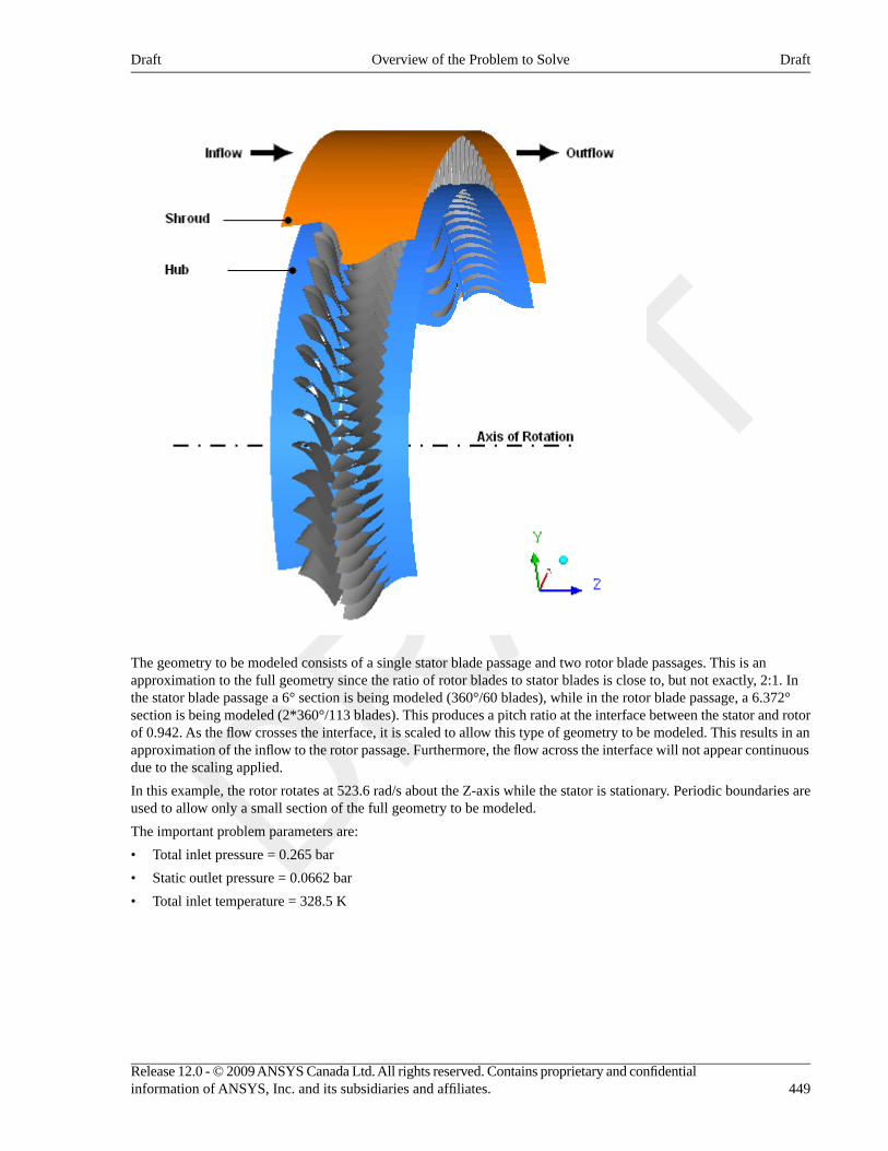
The geometry to be modeled consists of a single stator blade passage and two rotor blade passages. This is anapproximation to the full geometry since the ratio of rotor blades to stator blades is close to, but not exactly, 2:1. Inthe stator blade passage a 6° section is being modeled (360°/60 blades), while in the rotor blade passage, a 6.372°section is being modeled (2*360°/113 blades). This produces a pitch ratio at the interface between the stator and rotorof 0.942. As the flow crosses the interface, it is scaled to allow this type of geometry to be modeled. This results in anapproximation of the inflow to the rotor passage. Furthermore, the flow across the interface will not appear continuousdue to the scaling applied.
In this example, the rotor rotates at 523.6 rad/s about the Z-axis while the stator is stationary. Periodic boundaries areused to allow only a small section of the full geometry to be modeled.
The important problem parameters are:
• Total inlet pressure = 0.265 bar
• Static outlet pressure = 0.0662 bar
• Total inlet temperature = 328.5 K
449Release 12.0 - © 2009 ANSYS Canada Ltd. All rights reserved. Contains proprietary and confidentialinformation of ANSYS, Inc. and its subsidiaries and affiliates.
DraftOverview of the Problem to SolveDraft
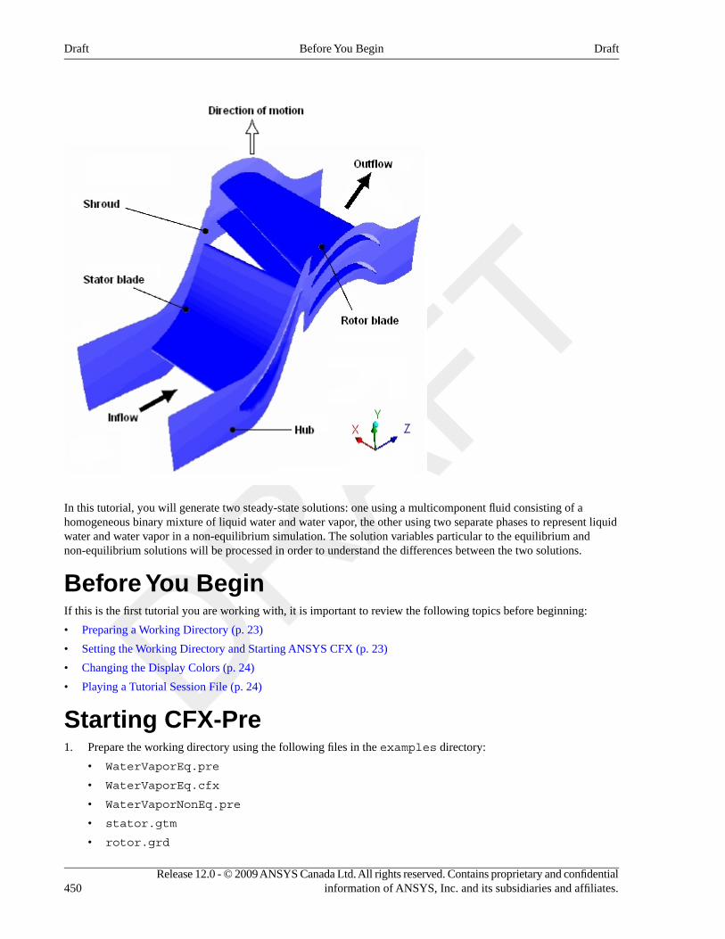
In this tutorial, you will generate two steady-state solutions: one using a multicomponent fluid consisting of ahomogeneous binary mixture of liquid water and water vapor, the other using two separate phases to represent liquidwater and water vapor in a non-equilibrium simulation. The solution variables particular to the equilibrium andnon-equilibrium solutions will be processed in order to understand the differences between the two solutions.
Before You BeginIf this is the first tutorial you are working with, it is important to review the following topics before beginning:
• Preparing a Working Directory (p. 23)
• Setting the Working Directory and Starting ANSYS CFX (p. 23)
• Changing the Display Colors (p. 24)
• Playing a Tutorial Session File (p. 24)
Starting CFX-Pre1. Prepare the working directory using the following files in the examples directory:
• WaterVaporEq.pre
• WaterVaporEq.cfx
• WaterVaporNonEq.pre
• stator.gtm
• rotor.grd
Release 12.0 - © 2009 ANSYS Canada Ltd. All rights reserved. Contains proprietary and confidentialinformation of ANSYS, Inc. and its subsidiaries and affiliates.450
DraftBefore You BeginDraft
For details, see Preparing a Working Directory (p. 23)
2. Set the working directory and start CFX-Pre.
For details, see Setting the Working Directory and Starting ANSYS CFX (p. 23)
Defining the Equilibrium Case in CFX-PreThe following sections describe the equilibrium simulation setup in CFX-Pre.
If you want to set up the simulation automatically and continue to Obtaining a Solution for the Equilibrium Case (p. 457),run WaterVaporEq.pre.
This tutorial uses the Turbomachinery wizard in CFX-Pre. This pre-processing mode is designed to simplify the setupof turbomachinery simulations.
1. Start CFX-Pre if necessary.
2. Select File > New Case.
3. Select Turbomachinery and click OK.
4. Select File > Save Case As.
5. Under File name, type WaterVaporEq.
6. If you are notified the file already exists, click Overwrite.
This file is provided in the tutorial directory and may exist in your working directory if you have copied it there.
7. Click Save.
Basic Settings1. Set Machine Type to Axial Turbine.
2. Click Next.
Component DefinitionTwo new components are required. As you specify them, CFX-Pre imports the meshes.
1. Right-click a blank area near the Component Definition tree and select Add Component from the shortcut menu.
2. Create a new component of type Stationary, named S1.
3. Apply the following setting:
ValueSetting
stator.gtmaMesh > File
aYou may have to select the CFX Mesh option under Files of type in order to see the file.
4. Create a new component of type Rotating, named R1.
5. Apply the following settings:
ValueSetting
523.6 [radian s^-1]Component Type >Value
rotor.grdaMesh > File
451Release 12.0 - © 2009 ANSYS Canada Ltd. All rights reserved. Contains proprietary and confidentialinformation of ANSYS, Inc. and its subsidiaries and affiliates.
DraftDefining the Equilibrium Case in CFX-PreDraft
ValueSetting
mOptions > Mesh Units
aYou may have to select the CFX-TASCflow (*grd) option under Files of type in order to see the file.
NoteThe components must be ordered as above (stator then rotor) in order for the interface to be createdcorrectly. The order of the two components can be changed, if necessary, by right-clicking S1 andselecting Move Component Up.
When a component is defined, Turbo Mode will automatically select a list of regions that have been recognizedas potential boundaries and interfaces. This information should be reviewed in the Region Information section,situated below the Mesh section, to ensure that all is correct. This information will be used to help set up boundaryconditions and interfaces. The upper case turbo regions that are selected (e.g., HUB) correspond to the regionnames in the CFX-TASCflow grd file. CFX-TASCflow turbomachinery meshes use these names consistently.
6. Click Next.
Physics DefinitionIn this section, you will set properties of the fluid domain and some solver parameters. Note that initially you willchoose the fluid to be Water Ideal Gas, but later you will create a new fluid based on the IAPWS database forwater and override this initial setting with it.
1. Apply the following settings
ValueSettingTab
Water Ideal GasFluidPhysics Definition
Steady StateAnalysis Type > Type
0 [atm]aModel Data > Reference Pressure
Total EnergyModel Data > Heat Transfer
k-EpsilonModel Data > Turbulence
(Selected)Inflow/Outflow Boundary Templates >P-Total Inlet P-Static Outlet
0.265 [bar]Inflow/Outflow Boundary Templates >P-Total
0.0662 [bar]Inflow/Outflow Boundary Templates >P-Static
328.5 [K]bInflow/Outflow Boundary Templates >T-Total
Frozen RotorInterface > Default Type
Physical TimescaleSolver Parameters > Convergence Control
Release 12.0 - © 2009 ANSYS Canada Ltd. All rights reserved. Contains proprietary and confidentialinformation of ANSYS, Inc. and its subsidiaries and affiliates.452
DraftPhysics DefinitionDraft
ValueSettingTab
0.0005 [s]cSolver Parameters > Physical Timescale
aBecause this tutorial involves vaporization, it is recommended that absolute pressures be used throughout. This can be accomplished bysetting the reference pressure to 0 atm.bFrom the problem description.cThe physical timescale that will be set up is derived from the rotational speed of the 113 rotor blades. Also see the ANSYS CFX Best PracticesGuide for Turbomachinery, where an explanation of how this value is calculated is provided.
2. Click Next.
Interface DefinitionCFX-Pre will try to create appropriate interfaces using the region names viewed previously in the Region Informationsection (in the Component Definition setup screen). In this case, you should see that a periodic interface has beengenerated for both the rotor and the stator. The generated periodic interface can be edited or deleted. Interfaces arerequired when modeling a small section of the true geometry. An interface is also needed to connect the two componentstogether across the frame change.
1. Review the various interfaces but do not change them.
2. Click Next.
Boundary DefinitionCFX-Pre will try to create appropriate boundary conditions using the region names presented previously in the RegionInformation section. In this case, you should see a list of generated boundary conditions. They can be edited or deletedin the same way as the interface connections that were set up earlier.
1. Review the various boundary definitions but do not change them.
2. Click Next.
Final Operations1. Set Operation to Enter General Mode.
2. Click Finish.
After you click Finish, a dialog box appears stating that Turbo report will not be included in the solver file becauseyou are entering General Mode.
3. Click Yes to continue.
Defining the Properties of WaterEarlier in the physics definition portion of the Turbomachinery wizard, you specified Water Ideal Gas as thefluid in the domain. Here, you will specify a homogeneous binary mixture to replace it. To create the mixture, you willtake two pure fluids from the IAPWS database for water and combine them. The pure fluids that will be combined areH2Og, representing water vapor, and H2Ol, representing liquid water. The mixture will be named H2Olg.
The present simulations use the published IAPWS-IF97 (International Association for the Properties of Water andSteam - Industrial Formulation 1997) water tables for properties. The published IAPWS-IF97 equations have beenimplemented in ANSYS CFX, allowing you to directly select them for use in your simulations. The present exampleuses these properties in a tabular format requiring you to specify the range of the properties (such as min/max pressureand temperature bounds) and the number of data points in each table. Note that the IAPWS-IF97 properties have beentested for extrapolation into metastable regions, a fact that will be used for the non-equilibrium calculations that requirethis kind of state information.
453Release 12.0 - © 2009 ANSYS Canada Ltd. All rights reserved. Contains proprietary and confidentialinformation of ANSYS, Inc. and its subsidiaries and affiliates.
DraftInterface DefinitionDraft
1. Click Material
2. Name the new material H2Og.
3. Enter the following settings for H2Og:
ValueSettingTab
IAPWS IF97Material GroupBasic Settings
(Selected)Thermodynamic State
GasThermodynamic State > ThermodynamicState
(Selected)Thermodynamic Properties > TableGeneration
Material Properties
(Selected)Thermodynamic Properties > TableGeneration > Minimum Temperature
250 [K]aThermodynamic Properties > TableGeneration > Minimum Temperature >Min. Temperature
(Selected)Thermodynamic Properties > TableGeneration > Maximum Temperature
400 [K]Thermodynamic Properties > TableGeneration > Maximum Temperature >Max. Temperature
(Selected)Thermodynamic Properties > TableGeneration > Minimum Absolute Pressure
0.01 [bar]Thermodynamic Properties > TableGeneration > Minimum Absolute Pressure> Min. Absolute Pres.
(Selected)Thermodynamic Properties > TableGeneration > Maximum Absolute Pressure
0.6 [bar]Thermodynamic Properties > TableGeneration > Maximum Absolute Pressure> Max. Absolute Pres.
(Selected)Thermodynamic Properties > TableGeneration > Maximum Points
100Thermodynamic Properties > TableGeneration > Maximum Points >Maximum Points
aThe H2Og minimum temperature is set to 250 K as the vapor might possibly supercool (in the NES calculations) to temperatures lower thanthe triple point temperature.
4. Click OK.
5. In the Outline tree, under Materials, right-click H2Og and select Duplicate.
Release 12.0 - © 2009 ANSYS Canada Ltd. All rights reserved. Contains proprietary and confidentialinformation of ANSYS, Inc. and its subsidiaries and affiliates.454
DraftDefining the Properties of WaterDraft
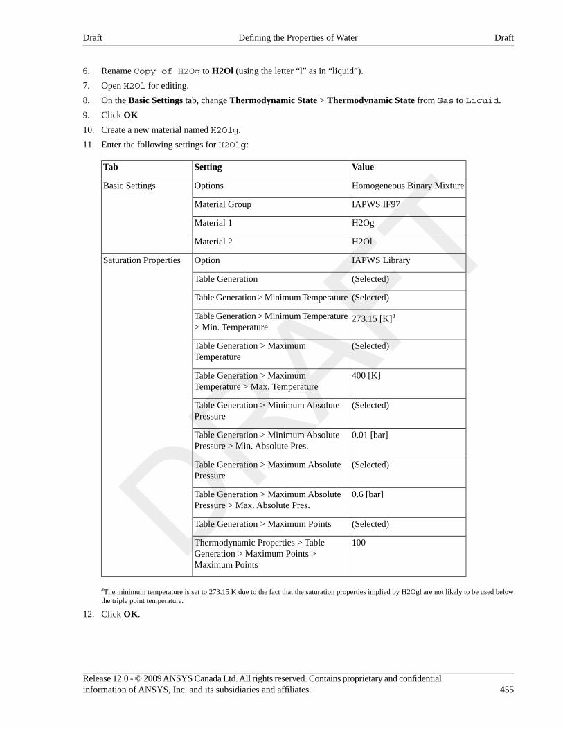
6. Rename Copy of H2Og to H2Ol (using the letter “l” as in “liquid”).
7. Open H2Ol for editing.
8. On the Basic Settings tab, change Thermodynamic State > Thermodynamic State from Gas to Liquid.
9. Click OK
10. Create a new material named H2Olg.
11. Enter the following settings for H2Olg:
ValueSettingTab
Homogeneous Binary MixtureOptionsBasic Settings
IAPWS IF97Material Group
H2OgMaterial 1
H2OlMaterial 2
IAPWS LibraryOptionSaturation Properties
(Selected)Table Generation
(Selected)Table Generation > Minimum Temperature
273.15 [K]aTable Generation > Minimum Temperature> Min. Temperature
(Selected)Table Generation > MaximumTemperature
400 [K]Table Generation > MaximumTemperature > Max. Temperature
(Selected)Table Generation > Minimum AbsolutePressure
0.01 [bar]Table Generation > Minimum AbsolutePressure > Min. Absolute Pres.
(Selected)Table Generation > Maximum AbsolutePressure
0.6 [bar]Table Generation > Maximum AbsolutePressure > Max. Absolute Pres.
(Selected)Table Generation > Maximum Points
100Thermodynamic Properties > TableGeneration > Maximum Points >Maximum Points
aThe minimum temperature is set to 273.15 K due to the fact that the saturation properties implied by H2Ogl are not likely to be used belowthe triple point temperature.
12. Click OK.
455Release 12.0 - © 2009 ANSYS Canada Ltd. All rights reserved. Contains proprietary and confidentialinformation of ANSYS, Inc. and its subsidiaries and affiliates.
DraftDefining the Properties of WaterDraft
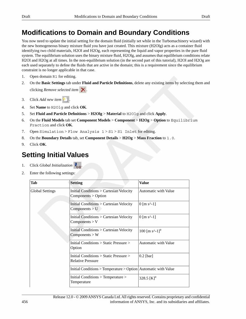
Modifications to Domain and Boundary ConditionsYou now need to update the initial setting for the domain fluid (initially set while in the Turbomachinery wizard) withthe new homogeneous binary mixture fluid you have just created. This mixture (H2Olg) acts as a container fluididentifying two child materials, H2Ol and H2Og, each representing the liquid and vapor properties in the pure fluidsystem. The equilibrium solution uses the binary mixture fluid, H2Olg, and assumes that equilibrium conditions relateH2Ol and H2Og at all times. In the non-equilibrium solution (in the second part of this tutorial), H2Ol and H2Og areeach used separately to define the fluids that are active in the domain; this is a requirement since the equilibriumconstraint is no longer applicable in that case.
1. Open domain R1 for editing.
2. On the Basic Settings tab under Fluid and Particle Definitions, delete any existing items by selecting them and
clicking Remove selected item .
3. Click Add new item .
4. Set Name to H2Olg and click OK.
5. Set Fluid and Particle Definitions > H2Olg > Material to H2Olg and click Apply.
6. On the Fluid Models tab set Component Models > Component > H2Og > Option to EquilibriumFraction and click OK.
7. Open Simulation > Flow Analysis 1 > S1 > S1 Inlet for editing.
8. On the Boundary Details tab, set Component Details > H2Og > Mass Fraction to 1.0.
9. Click OK.
Setting Initial Values1. Click Global Initialization .
2. Enter the following settings:
ValueSettingTab
Automatic with ValueInitial Conditions > Cartesian VelocityComponents > Option
Global Settings
0 [m s^-1]Initial Conditions > Cartesian VelocityComponents > U
0 [m s^-1]Initial Conditions > Cartesian VelocityComponents > V
100 [m s^-1]aInitial Conditions > Cartesian VelocityComponents > W
Automatic with ValueInitial Conditions > Static Pressure >Option
0.2 [bar]Initial Conditions > Static Pressure >Relative Pressure
Automatic with ValueInitial Conditions > Temperature > Option
328.5 [K]aInitial Conditions > Temperature >Temperature
Release 12.0 - © 2009 ANSYS Canada Ltd. All rights reserved. Contains proprietary and confidentialinformation of ANSYS, Inc. and its subsidiaries and affiliates.456
DraftModifications to Domain and Boundary ConditionsDraft
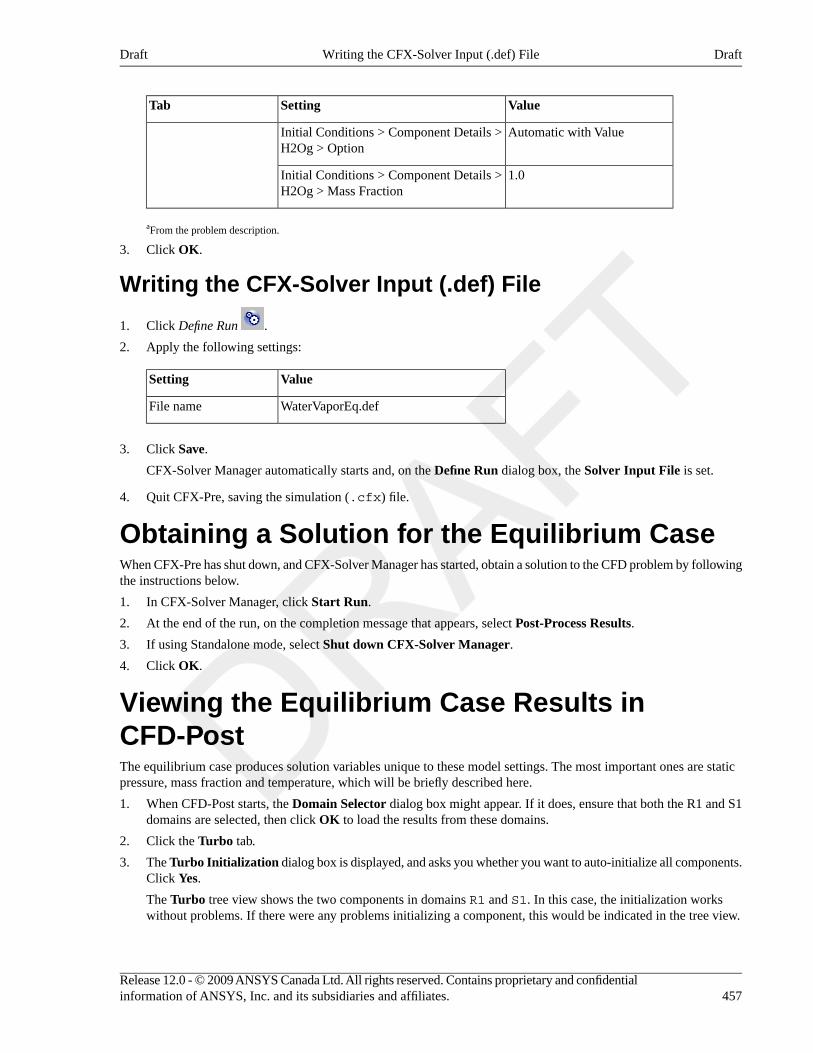
ValueSettingTab
Automatic with ValueInitial Conditions > Component Details >H2Og > Option
1.0Initial Conditions > Component Details >H2Og > Mass Fraction
aFrom the problem description.
3. Click OK.
Writing the CFX-Solver Input (.def) File
1. Click Define Run .
2. Apply the following settings:
ValueSetting
WaterVaporEq.defFile name
3. Click Save.
CFX-Solver Manager automatically starts and, on the Define Run dialog box, the Solver Input File is set.
4. Quit CFX-Pre, saving the simulation (.cfx) file.
Obtaining a Solution for the Equilibrium CaseWhen CFX-Pre has shut down, and CFX-Solver Manager has started, obtain a solution to the CFD problem by followingthe instructions below.
1. In CFX-Solver Manager, click Start Run.
2. At the end of the run, on the completion message that appears, select Post-Process Results.
3. If using Standalone mode, select Shut down CFX-Solver Manager.
4. Click OK.
Viewing the Equilibrium Case Results inCFD-PostThe equilibrium case produces solution variables unique to these model settings. The most important ones are staticpressure, mass fraction and temperature, which will be briefly described here.
1. When CFD-Post starts, the Domain Selector dialog box might appear. If it does, ensure that both the R1 and S1domains are selected, then click OK to load the results from these domains.
2. Click the Turbo tab.
3. The Turbo Initialization dialog box is displayed, and asks you whether you want to auto-initialize all components.Click Yes.
The Turbo tree view shows the two components in domains R1 and S1. In this case, the initialization workswithout problems. If there were any problems initializing a component, this would be indicated in the tree view.
457Release 12.0 - © 2009 ANSYS Canada Ltd. All rights reserved. Contains proprietary and confidentialinformation of ANSYS, Inc. and its subsidiaries and affiliates.
DraftWriting the CFX-Solver Input (.def) FileDraft
NoteIf you do not see the Turbo Initialization dialog box, or as an alternative to using that dialog box,you can initialize all components by clicking the Initialize All Components button which is visibleinitially by default, or after double-clicking the Initialization object in the Turbo tree view.
Displaying the Equilibrium Solution Variables usingContour PlotsMake a 2D surface at 50% span to be used as a locator for plots:
1. On the main menu select Insert > Location > Turbo Surface and name it Turbo Surface 1.
2. On the Geometry tab, set Method to Constant Span and Value to 0.5.
3. Click Apply.
4. Turn off the visibility of Turbo Surface 1.
Static Pressure and Mass Fraction Contour PlotsIn the equilibrium solution, phase transition occurs the moment saturation conditions are reached in the flow. Theamount of moisture ultimately created from phase transition is determined in the following manner.
The static pressure solution field yields the saturation enthalpy through the function h P( )sat , available from the
IAPWS database. During the solution, if the predicted mixture static enthalpy, h, falls below h P( )sat at any point,the mass fraction of the condensed phase (also called wetness) can be directly calculated also based on the IAPWS
properties. The degree to which wetness is generated depends on the amount by which h is less than h P( )sat .
Note that the mass fraction is predicted at each iteration in the solution, and is used to update other two-phase mixtureproperties required at each step in the solution. The final results therefore include all of the two-phase influences, butassuming equilibrium conditions. The equilibrium solution mass fraction contour plot will be compared to thenon-equilibrium solution one in Viewing the Non-Equilibrium Case Results in CFD-Post (p. 462).
In the next step, you are asked to create the pressure and mass fraction contour plots.
1. Create a static pressure contour plot on Turbo Surface 1:
1. Create a new contour plot named Static Pressure.
2. In the Details view on the Geometry tab, set Locations to Turbo Surface 1 and Variable to Pressure,then click Apply.
2. Turn off the visibility of Static Pressure when you have finished observing the results.
3. Create a contour plot on Turbo Surface 1 that shows the mass fraction of the liquid phase:
1. Create a new contour plot named Mass Fraction of Liquid Phase.
2. In the Details view on the Geometry tab, set Locations to Turbo Surface 1 and Variable toH2Ol.Mass Fraction, then click Apply.
4. Turn off the visibility of Mass Fraction of Liquid Phase when you have finished observing the results.
Static Temperature Contour PlotsIn the equilibrium solution, the condensed and gas phases share the same temperature and, as a result, predictions ofthermodynamic losses are not possible.
In the following step you are asked to view the temperature field in the solution, and note that, due to the equilibriumconstraint, it represents conditions for the mixture.
1. Create a contour plot on Turbo Surface 1 that shows the static temperature.
Release 12.0 - © 2009 ANSYS Canada Ltd. All rights reserved. Contains proprietary and confidentialinformation of ANSYS, Inc. and its subsidiaries and affiliates.458
DraftDisplaying the Equilibrium Solution Variables using Contour PlotsDraft
1. Create a new contour plot named Static Temperature.
2. In the Details view on the Geometry tab, set Locations to Turbo Surface 1 and Variable toTemperature, then click Apply.
2. Once you have observed the results save the state and exit CFD-Post.
Defining the Non-Equilibrium Case in CFX-PreThe non-equilibrium calculation introduces a number of additional transport equations to the equilibrium solution,namely volume fractions for each phase and droplet number for all condensing phases. In addition, energy equationsneed to be specified for each of the phases in the solution. The setup of these equations is automated based on modelselections to be described subsequently. Important to the predictions are interphase heat and mass transfer between thevapor and condensed phases due to small droplets created by homogeneous nucleation. Selection of the required phasepair conditions is made easier by provision of special small droplet models (where small droplet implies droplet sizesgenerally below one μm). Phase transition is initiated based on predicted metastable state (measured by supercoolinglevel) conditions in the flow in conjunction with a classical homogeneous nucleation model.
The non-equilibrium solution is therefore closely dependent on the evolving conditions along the flow path leading tophase transition and subsequent strong interaction (by heat/mass transfer) between phases.
If you want to set up the non-equilibrium simulation automatically and continue to Obtaining a Solution for theNon-Equilibrium Case (p. 462), run WaterVaporNonEq.pre.
Opening the Existing Simulation1. Start CFX-Pre if necessary.
2. Select File > Open Case.
3. If required, set the path location to the tutorial directory.
4. Select the simulation file WaterVaporEq.cfx.
5. Click Open.
6. Select File > Save Case As.
7. Change the name to WaterVaporNonEq.cfx.
8. Click Save.
Modifying the DomainsThe non-equilibrium case is different from the equilibrium case in that the creation of the second phase (that is, theliquid water) is based on vapor supercooling in conjunction with fluid expansion rate and a nucleation model. Thelocation where the phase transition happens is not specified, but evolves as part of the solution.
In this section, you will specify a nucleation model for the phase that is considered condensable. For details on thenucleation model, see Droplet Condensation Model (p. 196) in ANSYS CFX-Solver Modeling Guide.
You will also set the droplet number and volume fraction of the condensable phase to zero at the inlet. The condensablephase will appear within the domain by homogeneous nucleation. If this case were to involve wetness at the inlet, youwould have a choice of specifying either droplet number or droplet diameter as a boundary along with the volumefraction.
1. Open domain R1.
2. On the Basic Settings tab under Fluid and Particle Definitions, delete any existing items by selecting them and
clicking Remove selected item .
3. Create two new materials named H2Og and H2Ol by using the Add new item icon.
459Release 12.0 - © 2009 ANSYS Canada Ltd. All rights reserved. Contains proprietary and confidentialinformation of ANSYS, Inc. and its subsidiaries and affiliates.
DraftDefining the Non-Equilibrium Case in CFX-PreDraft
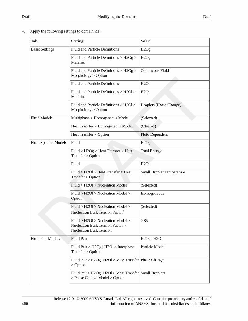
4. Apply the following settings to domain R1:
ValueSettingTab
H2OgFluid and Particle DefinitionsBasic Settings
H2OgFluid and Particle Definitions > H2Og >Material
Continuous FluidFluid and Particle Definitions > H2Og >Morphology > Option
H2OlFluid and Particle Definitions
H2OlFluid and Particle Definitions > H2Ol >Material
Droplets (Phase Change)Fluid and Particle Definitions > H2Ol >Morphology > Option
(Selected)Multiphase > Homogeneous ModelFluid Models
(Cleared)Heat Transfer > Homogeneous Model
Fluid DependentHeat Transfer > Option
H2OgFluidFluid Specific Models
Total EnergyFluid > H2Og > Heat Transfer > HeatTransfer > Option
H2OlFluid
Small Droplet TemperatureFluid > H2Ol > Heat Transfer > HeatTransfer > Option
(Selected)Fluid > H2Ol > Nucleation Model
HomogeneousFluid > H2Ol > Nucleation Model >Option
(Selected)Fluid > H2Ol > Nucleation Model >
Nucleation Bulk Tension Factora
0.85Fluid > H2Ol > Nucleation Model >Nucleation Bulk Tension Factor >Nucleation Bulk Tension
H2Og | H2OlFluid PairFluid Pair Models
Particle ModelFluid Pair > H2Og | H2Ol > InterphaseTransfer > Option
Phase ChangeFluid Pair > H2Og | H2Ol > Mass Transfer> Option
Small DropletsFluid Pair > H2Og | H2Ol > Mass Transfer> Phase Change Model > Option
Release 12.0 - © 2009 ANSYS Canada Ltd. All rights reserved. Contains proprietary and confidentialinformation of ANSYS, Inc. and its subsidiaries and affiliates.460
DraftModifying the DomainsDraft
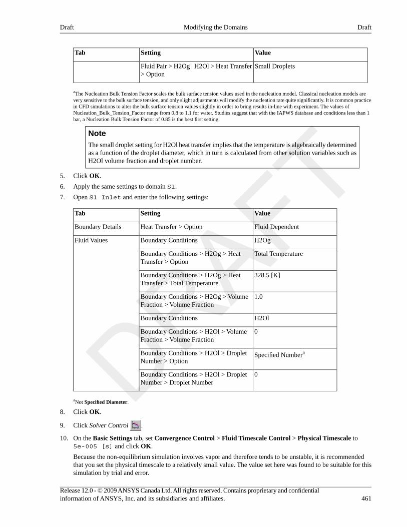
ValueSettingTab
Small DropletsFluid Pair > H2Og | H2Ol > Heat Transfer> Option
aThe Nucleation Bulk Tension Factor scales the bulk surface tension values used in the nucleation model. Classical nucleation models arevery sensitive to the bulk surface tension, and only slight adjustments will modify the nucleation rate quite significantly. It is common practicein CFD simulations to alter the bulk surface tension values slightly in order to bring results in-line with experiment. The values ofNucleation_Bulk_Tension_Factor range from 0.8 to 1.1 for water. Studies suggest that with the IAPWS database and conditions less than 1bar, a Nucleation Bulk Tension Factor of 0.85 is the best first setting.
NoteThe small droplet setting for H2Ol heat transfer implies that the temperature is algebraically determinedas a function of the droplet diameter, which in turn is calculated from other solution variables such asH2Ol volume fraction and droplet number.
5. Click OK.
6. Apply the same settings to domain S1.
7. Open S1 Inlet and enter the following settings:
ValueSettingTab
Fluid DependentHeat Transfer > OptionBoundary Details
H2OgBoundary ConditionsFluid Values
Total TemperatureBoundary Conditions > H2Og > HeatTransfer > Option
328.5 [K]Boundary Conditions > H2Og > HeatTransfer > Total Temperature
1.0Boundary Conditions > H2Og > VolumeFraction > Volume Fraction
H2OlBoundary Conditions
0Boundary Conditions > H2Ol > VolumeFraction > Volume Fraction
Specified NumberaBoundary Conditions > H2Ol > DropletNumber > Option
0Boundary Conditions > H2Ol > DropletNumber > Droplet Number
aNot Specified Diameter.
8. Click OK.
9. Click Solver Control .
10. On the Basic Settings tab, set Convergence Control > Fluid Timescale Control > Physical Timescale to5e-005 [s] and click OK.
Because the non-equilibrium simulation involves vapor and therefore tends to be unstable, it is recommendedthat you set the physical timescale to a relatively small value. The value set here was found to be suitable for thissimulation by trial and error.
461Release 12.0 - © 2009 ANSYS Canada Ltd. All rights reserved. Contains proprietary and confidentialinformation of ANSYS, Inc. and its subsidiaries and affiliates.
DraftModifying the DomainsDraft
Writing the CFX-Solver Input (.def) File
1. Click Define Run .
2. Apply the following settings:
ValueSetting
WaterVaporNonEq.defFile name
3. Click Save.
CFX-Solver Manager automatically starts and, on the Define Run dialog box, the Solver Input File is set.
4. Quit CFX-Pre, saving the simulation (.cfx) file at your discretion.
Obtaining a Solution for the Non-EquilibriumCaseThe Define Run dialog box will be displayed when CFX-Solver Manager launches. CFX-Solver Input File willalready be set to the name of the CFX-Solver input file just written.
1. Click Start Run.
CFX-Solver runs and attempts to obtain a solution. This can take some time depending on your system. Eventuallya dialog box appears.
NoteYou may notice messages in the solver output regarding problems with evaluating material properties.This is a result of the absolute pressure reaching values outside the range of internal material propertytables. In this case, the messages are temporary and stop appearing well before convergence. If youencounter a simulation where the messages persist, or you otherwise suspect that the results might beadversely affected, you can change the ranges of internal material property tables by editing the relevantmaterials in CFX-Pre.
2. At the end of the run, on the completion message that appears, select Post-Process Results.
3. If using Standalone mode, select Shut down CFX-Solver Manager.
4. Click OK.
Viewing the Non-Equilibrium Case Results inCFD-PostThe non-equilibrium calculation creates a number of solution variables. The most important ones, which are brieflydescribed in the following section, are supercooling, nucleation rate, droplet number, mass fraction, and particlediameter.
1. When CFD-Post starts, the Domain Selector dialog box might appear. If it does, ensure that both the R1 and S1domains are selected, then click OK to load the results from these domains.
2. Click the Turbo tab.
3. The Turbo Initialization dialog box is displayed, and asks you whether you want to auto-initialize all components.Click Yes.
Release 12.0 - © 2009 ANSYS Canada Ltd. All rights reserved. Contains proprietary and confidentialinformation of ANSYS, Inc. and its subsidiaries and affiliates.462
DraftWriting the CFX-Solver Input (.def) FileDraft
The Turbo tree view shows the two components in domains R1 and S1. In this case, the initialization workswithout problems. If there were any problems initializing a component, this would be indicated in the tree view.
NoteIf you do not see the Turbo Initialization dialog box, or as an alternative to using that dialog box,you can initialize all components by clicking the Initialize All Components button which is visibleinitially by default, or after double-clicking the Initialization object in the Turbo tree view.
Displaying the Non-Equilibrium Solution Variables usingContour PlotsMake a 2D surface at 50% span to be used as a locator for plots:
1. On the main menu select Insert > Location > Turbo Surface and name it Turbo Surface 1.
2. On the Geometry tab, set Method to Constant Span and Value to 0.5.
3. Click Apply.
4. Turn off the visibility of Turbo Surface 1.
Supercooling Contour PlotThe non-equilibrium solution provides considerable detail on conditions related to phase transition. In particular, thesolution tracks the evolution of metastable conditions in the flow through a supercooling variable obtained on the basisof local pressure and gas phase temperature. The supercooling level is the primary variable influencing the nucleationmodel. The nucleation model provides an estimate of the rate of production of critically sized nuclei that are stableenough to grow in a supercooled vapor flow.
In the next step, you will plot the level of supercooling, where the supercooling represents the difference between thesaturation temperature, set by the local pressure in the flow, and the associated local gas phase temperature. At theinlet, supercooling is often shown as negative, indicating superheated conditions. At equilibrium conditions, nosupercooling is allowed since liquid and vapor phases always share the same temperature. Also, critical homogeneousnucleation at pressures below one atmosphere generally involves supercooling levels of up to 35 to 40K, dependingon rate of expansion in the flow.
1. Create a supercooling contour plot on Turbo Surface 1.
This will display the degree of non-equilibrium conditions in the gas phase prior to homogeneous phase transition.
1. Create a new contour plot named Supercooling.
2. In the Details view on the Geometry tab, set Locations to Turbo Surface 1 and Variable toH2Og.Supercooling then click Apply.
2. Turn off the visibility of Supercooling when you have finished observing the results.
Nucleation Rate and Droplet Number Contour PlotsIn the next step, you will plot the nucleation rate to show the level of nucleation attained, along with the droplet numberconcentration that is present in the flow following nucleation. Note that the nucleation rates reach very high levels,with peak values remaining in the flow for only a short time (that is, as long as supercooled conditions remain). Thesupercooled droplets released at nucleation grow rapidly, taking mass from the vapor phase and releasing thermalenergy, which acts to rapidly reduce vapor supercooling to near zero. This fact removes further significant nucleationand is why the phase transition process is limited to a narrow region in the flow in most cases.
1. Create a nucleation rate contour plot on Turbo Surface 1.
This will display the nucleation front at the point of maximum supercooling.
1. Create a new contour plot named Nucleation Rate.
463Release 12.0 - © 2009 ANSYS Canada Ltd. All rights reserved. Contains proprietary and confidentialinformation of ANSYS, Inc. and its subsidiaries and affiliates.
DraftDisplaying the Non-Equilibrium Solution Variables using Contour PlotsDraft
2. In the Details view on the Geometry tab, set Locations to Turbo Surface 1 and Variable toH2Ol.Nucleation Rate.
3. Set Range to Local and then click Apply.
2. Turn off the visibility of Nucleation Rate when you have finished observing the results.
3. Create a droplet number contour plot on Turbo Surface 1.
This will display the predicted droplet concentration resulting from phase transition.
1. Create a new contour plot named Droplet Number.
2. In the Details view on the Geometry tab, set Locations to Turbo Surface 1 and Variable toH2Ol.Droplet Number.
3. Click Apply.
4. Turn off the visibility of Droplet Number when you have finished observing the results.
Mass Fraction and Particle Diameter Contour PlotsIn this section, you will plot the mass fraction (or wetness) of the condensed phase. From the mass fraction and dropletnumber, it is possible to derive a particle diameter, which you will also plot in this section. Notice that the particlediameters appear in the flow at very small sizes, in the range of 5.0E-9 m, but grow rapidly so that, when leaving thenucleation zone, they are approximately an order of magnitude larger. Since the pressure is dropping through theturbine, droplet sizes continue to increase along with the wetness. To emphasize the particle diameters proceeding outof the nucleation zone, you will set the contour range for viewing. In flow regions near walls, where expansion rate isreduced, small amounts of liquid may have droplet diameters that grow to large sizes relative to those coming fromthe nucleation zone. Without setting the range, these particle diameters near the walls will be emphasized.
1. Create a contour plot showing the mass fraction of the condensed phase on Turbo Surface 1.
Condensed droplets grow in size and accumulate mass at the expense of the gas phase.
1. Create a new contour plot named Mass Fraction of Condensed Phase H2Ol.
2. In the details view on the Geometry tab, set Locations to Turbo Surface 1 and Variable to H2Ol.MassFraction.
3. Click Apply.
Comparing the mass fraction in the non-equilibrium case to the equilibrium solution previously viewed, youcan see that phase transition is considerably delayed such that it occurs in the blade passages of the rotorrather than the stator. This is a typical consequence of non-equilibrium flow, and reflects real flow situations.
2. Turn off the visibility of Mass Fraction of Condensed Phase H2Ol when you have finished observing the results.
3. Create a particle diameter contour plot on Turbo Surface 1.
The size of the condensed droplets is calculated from the droplet number and volume fraction of the condensedphase.
1. Create a new contour plot named Particle Diameter.
2. In the Details view on the Geometry tab, set Locations to Turbo Surface 1 and Variable toH2Ol.Particle Diameter.
3. Set Range to User Specified then set Min to 0 [m] and Max to 1e-07 [m].
4. Click Apply.
4. Turn off the visibility of Particle Diameter when you have finished observing the results.
Release 12.0 - © 2009 ANSYS Canada Ltd. All rights reserved. Contains proprietary and confidentialinformation of ANSYS, Inc. and its subsidiaries and affiliates.464
DraftDisplaying the Non-Equilibrium Solution Variables using Contour PlotsDraft
Gas and Condensed Phase Static Temperature Contour PlotsIn a non-equilibrium prediction, the gas phase temperature is different from the condensed phase temperature. Theformer is determined from a transport equation and the latter from an algebraic relationship relating droplet temperatureto its diameter (through a small droplet model already described).
In this section, you will plot the different temperature fields. It should be noted that, for the case of the condensedphase temperature field, before droplets are actually formed, there is no meaningful droplet temperature. At the pointdroplets are formed by nucleation, their temperature is at the gas phase. Once the droplets have grown in size, theirtemperature is very close to the saturation temperature. Because the non-equilibrium solution considers the condensedphase temperatures separate from the gas phase, the influence of thermodynamic losses are included in the predictions.This is because it becomes possible to account for heat flow between the vapor and condensed phases as they passthrough the domain. Due to this, non-equilibirum efficiency predictions are more accurate than ones obtained usingan equilibrium model.
1. Create a gas phase static temperature contour plot on Turbo Surface 1:
1. Create a new contour plot named Gas Phase Static Temperature.
2. In the Details view on the Geometry tab, set Locations to Turbo Surface 1 and Variable toH2Og.Temperature.
3. Click Apply.
2. Turn off the visibility of Gas Phase Static Temperature when you have finished observing the results.
3. Create a condensed phase static temperature contour plot on Turbo Surface 1.
1. Create a new contour plot named Condensed Phase Static Temperature.
2. In the Details view on the Geometry tab, set Locations to Turbo Surface 1 and Variable toH2Ol.Temperature.
3. Click Apply.
4. Once you have observed the results, save the state and exit CFD-Post.
465Release 12.0 - © 2009 ANSYS Canada Ltd. All rights reserved. Contains proprietary and confidentialinformation of ANSYS, Inc. and its subsidiaries and affiliates.
DraftDisplaying the Non-Equilibrium Solution Variables using Contour PlotsDraft

Release 12.0 - © 2009 ANSYS Canada Ltd. All rights reserved. Contains proprietary and confidentialinformation of ANSYS, Inc. and its subsidiaries and affiliates.
Chapter 27. Modeling a Gear Pump usingan Immersed SolidThis tutorial includes:
• Tutorial Features (p. 467)
• Overview of the Problem to Solve (p. 468)
• Before You Begin (p. 469)
• Starting CFX-Pre (p. 469)
• Defining a Case in CFX-Pre (p. 469)
• Importing the Mesh (p. 470)
• Creating Expressions for Time Step and Total Time (p. 470)
• Setting the Analysis Type (p. 470)
• Creating the Domains (p. 471)
• Creating the Domain Interface (p. 473)
• Creating Boundary Conditions (p. 475)
• Setting Solver Control (p. 476)
• Setting Output Control (p. 477)
• Writing the CFX-Solver Input (.def) File (p. 477)
• Obtaining a Solution for Simulation using CFX-Solver Manager (p. 478)
• Viewing the Results in CFD-Post (p. 478)
Tutorial FeaturesIn this tutorial you will learn about:
• Setting up an immersed solids domain.
• Applying a counter-rotating wall boundary.
• Monitoring an expression during a solver run.
• Creating an XY-transient chart in CFD-Post.
• Creating an animation.
DetailsFeatureComponent
General ModeUser ModeCFX-Pre
Immersed SolidDomain Type
Fluid Domain
TransientAnalysis Type
Continuous FluidFluid Type
Inlet BoundaryBoundary Conditions
Outlet Boundary
467Release 12.0 - © 2009 ANSYS Canada Ltd. All rights reserved. Contains proprietary and confidentialinformation of ANSYS, Inc. and its subsidiaries and affiliates.
DraftDraft
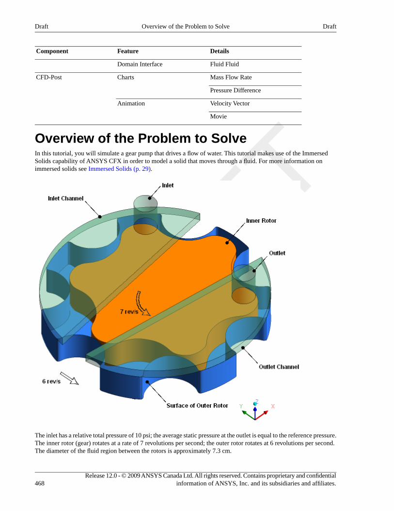
DetailsFeatureComponent
Fluid FluidDomain Interface
Mass Flow RateChartsCFD-Post
Pressure Difference
Velocity VectorAnimation
Movie
Overview of the Problem to SolveIn this tutorial, you will simulate a gear pump that drives a flow of water. This tutorial makes use of the ImmersedSolids capability of ANSYS CFX in order to model a solid that moves through a fluid. For more information onimmersed solids see Immersed Solids (p. 29).
The inlet has a relative total pressure of 10 psi; the average static pressure at the outlet is equal to the reference pressure.The inner rotor (gear) rotates at a rate of 7 revolutions per second; the outer rotor rotates at 6 revolutions per second.The diameter of the fluid region between the rotors is approximately 7.3 cm.
Release 12.0 - © 2009 ANSYS Canada Ltd. All rights reserved. Contains proprietary and confidentialinformation of ANSYS, Inc. and its subsidiaries and affiliates.468
DraftOverview of the Problem to SolveDraft
You will use an immersed solid domain to model the inner rotor, a rotating fluid domain to model the water immediatelysurrounding the inner rotor, and a stationary fluid domain to model the water in the inlet and outlet channels. To modelthe stationary pump housing (not shown in the figure), you will apply a counter-rotating wall condition to the top (highZ) surface of the rotating fluid domain, on the non-overlap portion (which lies between the inlet and outlet channels).To model the upper surfaces of the teeth of the outer rotor, you will apply a rotating wall condition on the non-overlapportions of the lower (low Z) surfaces of the inlet and outlet chambers. For more information about non-overlapconditions, see Non-overlap Boundary Conditions (p. 158) in ANSYS CFX-Solver Modeling Guide.
The following conditions will be met to promote the establishment of a cyclic flow pattern:
• The mesh of the rotating domain should be rotationally periodic so that it looks the same after each (outer) rotortooth passes.
• The mesh on the outer boundary of the immersed solid domain should be rotationally periodic so that it looks thesame after each (inner) rotor tooth passes. (The mesh inside the immersed solid domain has no effect in this tutorial.)
• An integer number of time steps should pass as one rotor tooth passes.
Before You BeginIt is strongly recommended that you complete the previous tutorials before trying this one. However, if this is the firsttutorial you are working with, it is important to review the following topics before beginning:
• Preparing a Working Directory (p. 23)
• Setting the Working Directory and Starting ANSYS CFX (p. 23)
• Changing the Display Colors (p. 24)
• Playing a Tutorial Session File (p. 24)
Starting CFX-Pre1. Prepare the working directory using the following files in the examples directory:
• ImmersedSolid.pre
• ImmersedSolid.gtm
For details, see Preparing a Working Directory (p. 23)
2. Set the working directory and start CFX-Pre.
For details, see Setting the Working Directory and Starting ANSYS CFX (p. 23).
Defining a Case in CFX-PreIf you want to set up the case automatically using a tutorial session file, run ImmersedSolid.pre. For details, seePlaying a Tutorial Session File (p. 24). Then proceed to Obtaining a Solution for Simulation using CFX-SolverManager (p. 478).
If you want to set up the case manually, proceed to the following steps:
This section describes the step-by-step definition of the flow physics in CFX-Pre for a steady-state simulation.
1. Select File > New Case.
2. Select General and click OK.
3. Select File > Save Case As.
4. Under File name, type ImmersedSolid.cfx.
5. Click Save.
469Release 12.0 - © 2009 ANSYS Canada Ltd. All rights reserved. Contains proprietary and confidentialinformation of ANSYS, Inc. and its subsidiaries and affiliates.
DraftBefore You BeginDraft
Importing the Mesh1. Edit Case Options > General in the Outline tree view and ensure that Automatic Default Domain is
turned off.
Default domain generation should be turned off because you will create three domains manually later in thistutorial.
2. Select File > Import > Mesh.
3. In the Import Mesh dialog box, set Files of type to CFX Mesh (*gtm *cfx) and selectImmersedSolid.gtm from your working directory.
4. Click Open.
Creating Expressions for Time Step and TotalTimeNext, you will create an expression defining the time step size for this transient analysis. One tooth of the inner (orouter) rotor passes every 1/42 s. Choose a time step that resolves this motion in 30 intervals.
1. From the main menu, select Insert > Expressions, Functions and Variables > Expression.
2. In the Insert Expression dialog box, type dt.
3. Click OK.
4. Set Definition, to (1/42)[s]/30.
5. Click Apply to create the expression.
Next, you will create an expression defining the total simulation time. Make the simulation run long enough for 3 rotorteeth to pass: 3/42 s. This will give the solution time to establish a periodic nature.
1. Create an expression called total time.
2. Set Definition to (3/42)[s].
3. Click Apply.
Setting the Analysis TypeDefine the simulation as transient, using the expressions you created earlier.
1. Under the Outline tab, edit Analysis Type .
2. Apply the following settings:
ValueSettingTab
NoneExternal Solver Coupling > OptionBasic Settings
TransientAnalysis Type > Option
Total TimeAnalysis Type > Time Duration >Option
total timeaAnalysis Type > Time Duration > TotalTime
TimestepsAnalysis Type > Time Steps > Option
Release 12.0 - © 2009 ANSYS Canada Ltd. All rights reserved. Contains proprietary and confidentialinformation of ANSYS, Inc. and its subsidiaries and affiliates.470
DraftImporting the MeshDraft
ValueSettingTab
dtAnalysis Type > Time Steps >Timesteps
Automatic with ValueAnalysis Type > Initial Time > Option
0 [s]Analysis Type > Initial Time > Time
aYou first need to click Enter Expression beside the field.
3. Click OK.
Creating the DomainsThis simulation requires three domains: two fluid domains and one immersed solid domain. First you will create animmersed solid domain.
Creating an Immersed Solid DomainEnsure that no default domain is present under Flow Analysis 1. If a default domain is present, right-click it andselect Delete.
Create the immersed solid domain as follows:
1. Select Insert > Domain from the main menu, or click Domain .
2. In the Insert Domain dialog box, set the name to ImmersedSolid and click OK.
3. Apply the following settings:
ValueSettingTab
Inner RotorLocation and Type > LocationBasic Settings
Immersed SolidLocation and Type > Domain Type
Coord 0Location and Type > Coordinate Frame
RotatingDomain Models > Domain Motion >Option
7 [rev s^-1]Domain Models > Domain Motion >Angular Velocity
Two PointsDomain Models > Domain Motion >Axis Definition > Option
0.00383, 0, 0Domain Models > Domain Motion >Axis Definition > Rotation Axis From
0.00383, 0, 1Domain Models > Domain Motion >Axis Definition > Rotation Axis To
4. Click OK.
471Release 12.0 - © 2009 ANSYS Canada Ltd. All rights reserved. Contains proprietary and confidentialinformation of ANSYS, Inc. and its subsidiaries and affiliates.
DraftCreating the DomainsDraft
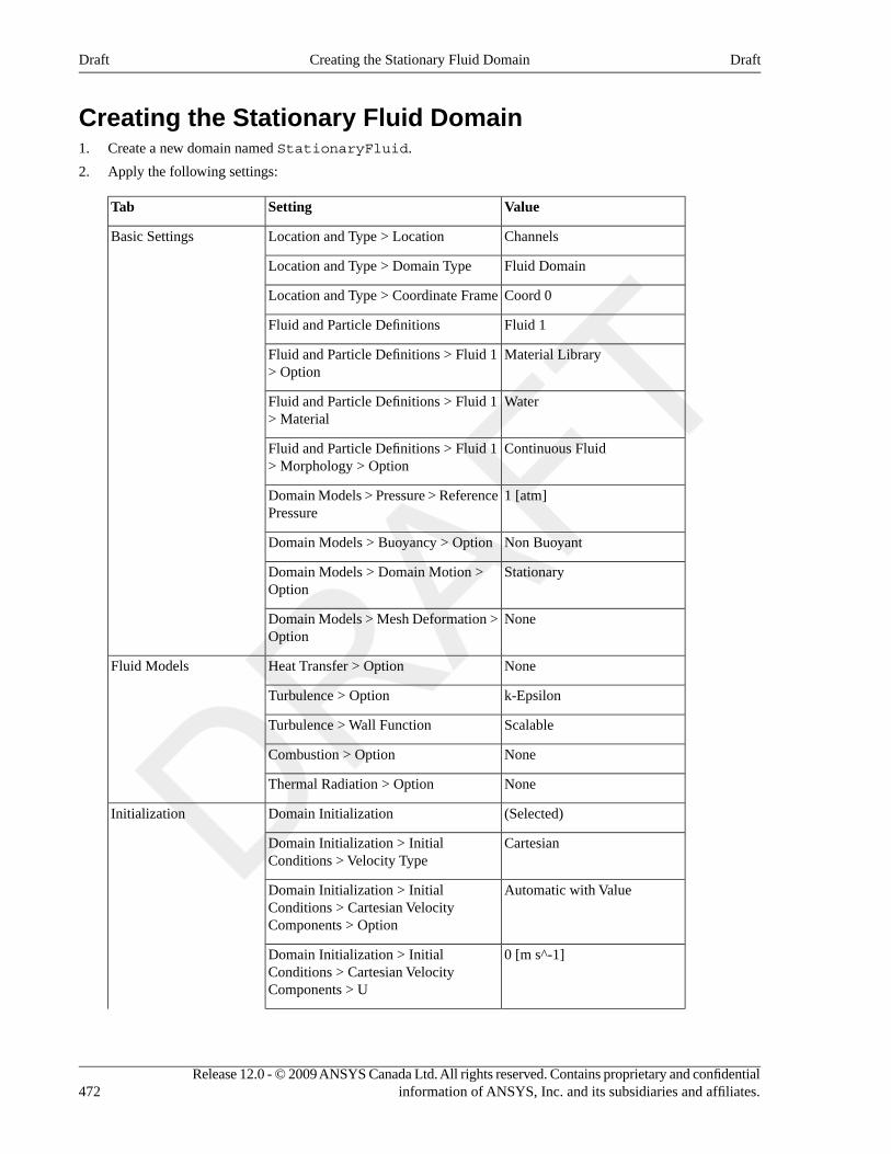
Creating the Stationary Fluid Domain1. Create a new domain named StationaryFluid.
2. Apply the following settings:
ValueSettingTab
ChannelsLocation and Type > LocationBasic Settings
Fluid DomainLocation and Type > Domain Type
Coord 0Location and Type > Coordinate Frame
Fluid 1Fluid and Particle Definitions
Material LibraryFluid and Particle Definitions > Fluid 1> Option
WaterFluid and Particle Definitions > Fluid 1> Material
Continuous FluidFluid and Particle Definitions > Fluid 1> Morphology > Option
1 [atm]Domain Models > Pressure > ReferencePressure
Non BuoyantDomain Models > Buoyancy > Option
StationaryDomain Models > Domain Motion >Option
NoneDomain Models > Mesh Deformation >Option
NoneHeat Transfer > OptionFluid Models
k-EpsilonTurbulence > Option
ScalableTurbulence > Wall Function
NoneCombustion > Option
NoneThermal Radiation > Option
(Selected)Domain InitializationInitialization
CartesianDomain Initialization > InitialConditions > Velocity Type
Automatic with ValueDomain Initialization > InitialConditions > Cartesian VelocityComponents > Option
0 [m s^-1]Domain Initialization > InitialConditions > Cartesian VelocityComponents > U
Release 12.0 - © 2009 ANSYS Canada Ltd. All rights reserved. Contains proprietary and confidentialinformation of ANSYS, Inc. and its subsidiaries and affiliates.472
DraftCreating the Stationary Fluid DomainDraft
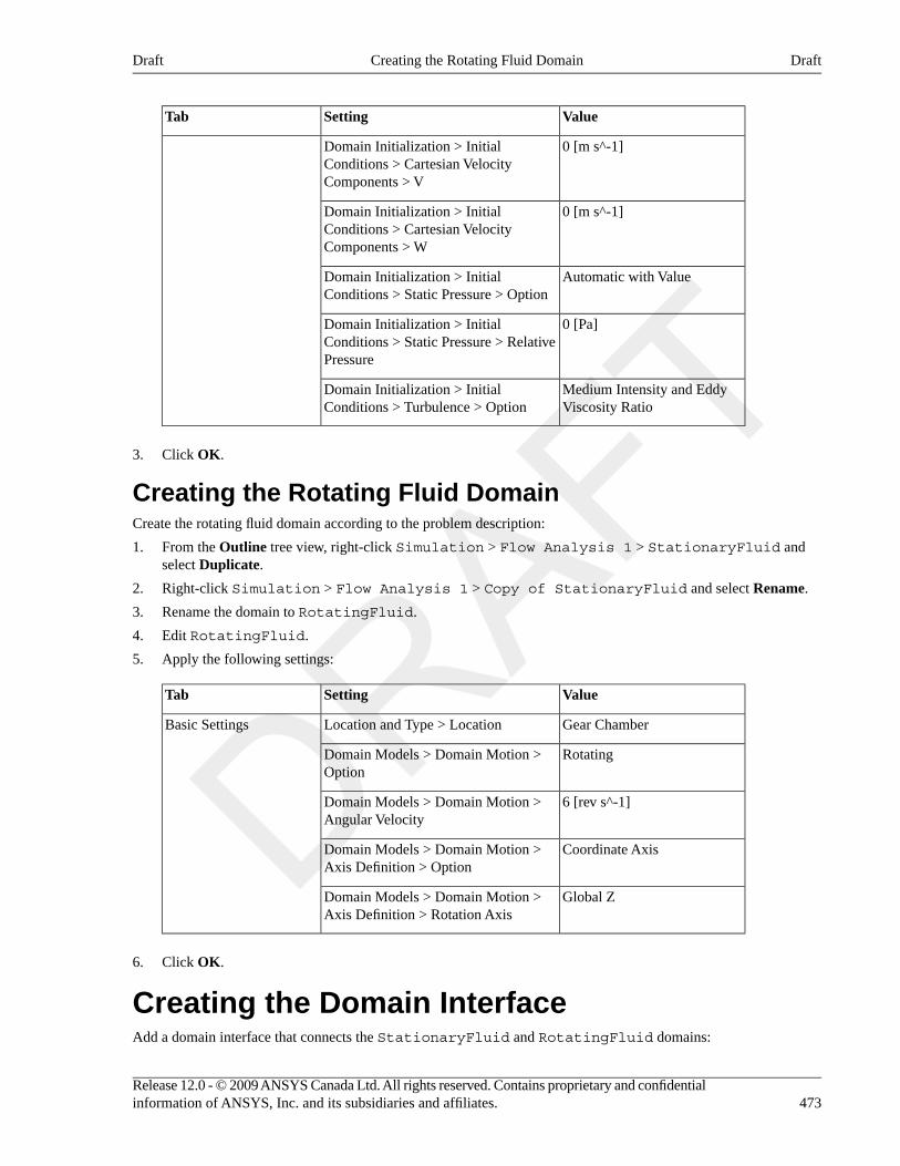
ValueSettingTab
0 [m s^-1]Domain Initialization > InitialConditions > Cartesian VelocityComponents > V
0 [m s^-1]Domain Initialization > InitialConditions > Cartesian VelocityComponents > W
Automatic with ValueDomain Initialization > InitialConditions > Static Pressure > Option
0 [Pa]Domain Initialization > InitialConditions > Static Pressure > RelativePressure
Medium Intensity and EddyViscosity Ratio
Domain Initialization > InitialConditions > Turbulence > Option
3. Click OK.
Creating the Rotating Fluid DomainCreate the rotating fluid domain according to the problem description:
1. From the Outline tree view, right-click Simulation > Flow Analysis 1 > StationaryFluid andselect Duplicate.
2. Right-click Simulation > Flow Analysis 1 > Copy of StationaryFluid and select Rename.
3. Rename the domain to RotatingFluid.
4. Edit RotatingFluid.
5. Apply the following settings:
ValueSettingTab
Gear ChamberLocation and Type > LocationBasic Settings
RotatingDomain Models > Domain Motion >Option
6 [rev s^-1]Domain Models > Domain Motion >Angular Velocity
Coordinate AxisDomain Models > Domain Motion >Axis Definition > Option
Global ZDomain Models > Domain Motion >Axis Definition > Rotation Axis
6. Click OK.
Creating the Domain InterfaceAdd a domain interface that connects the StationaryFluid and RotatingFluid domains:
473Release 12.0 - © 2009 ANSYS Canada Ltd. All rights reserved. Contains proprietary and confidentialinformation of ANSYS, Inc. and its subsidiaries and affiliates.
DraftCreating the Rotating Fluid DomainDraft
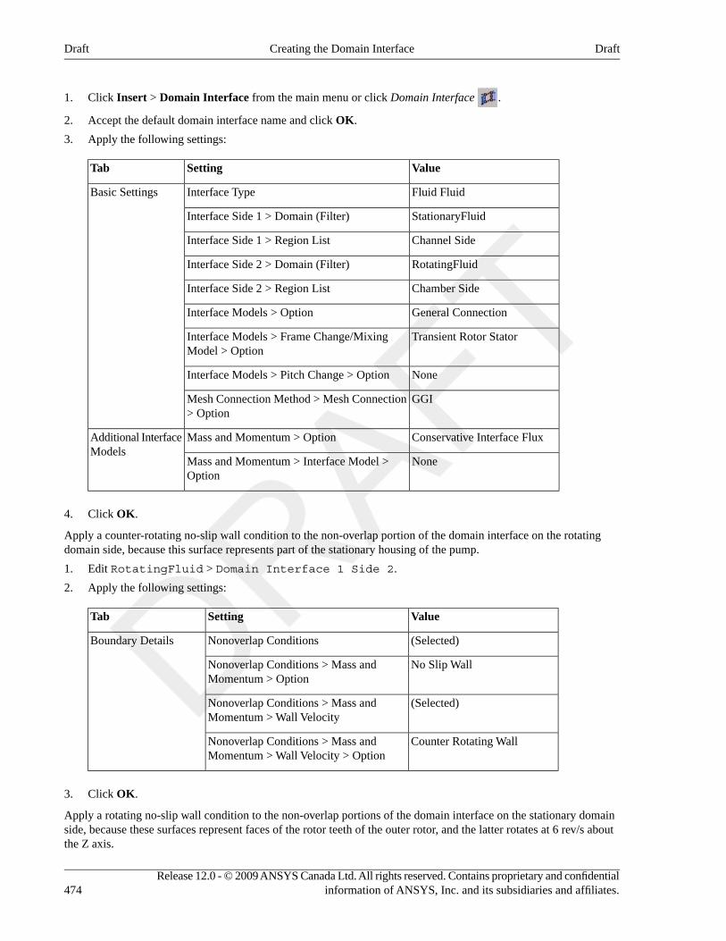
1. Click Insert > Domain Interface from the main menu or click Domain Interface .
2. Accept the default domain interface name and click OK.
3. Apply the following settings:
ValueSettingTab
Fluid FluidInterface TypeBasic Settings
StationaryFluidInterface Side 1 > Domain (Filter)
Channel SideInterface Side 1 > Region List
RotatingFluidInterface Side 2 > Domain (Filter)
Chamber SideInterface Side 2 > Region List
General ConnectionInterface Models > Option
Transient Rotor StatorInterface Models > Frame Change/MixingModel > Option
NoneInterface Models > Pitch Change > Option
GGIMesh Connection Method > Mesh Connection> Option
Conservative Interface FluxMass and Momentum > OptionAdditional InterfaceModels
NoneMass and Momentum > Interface Model >Option
4. Click OK.
Apply a counter-rotating no-slip wall condition to the non-overlap portion of the domain interface on the rotatingdomain side, because this surface represents part of the stationary housing of the pump.
1. Edit RotatingFluid > Domain Interface 1 Side 2.
2. Apply the following settings:
ValueSettingTab
(Selected)Nonoverlap ConditionsBoundary Details
No Slip WallNonoverlap Conditions > Mass andMomentum > Option
(Selected)Nonoverlap Conditions > Mass andMomentum > Wall Velocity
Counter Rotating WallNonoverlap Conditions > Mass andMomentum > Wall Velocity > Option
3. Click OK.
Apply a rotating no-slip wall condition to the non-overlap portions of the domain interface on the stationary domainside, because these surfaces represent faces of the rotor teeth of the outer rotor, and the latter rotates at 6 rev/s aboutthe Z axis.
Release 12.0 - © 2009 ANSYS Canada Ltd. All rights reserved. Contains proprietary and confidentialinformation of ANSYS, Inc. and its subsidiaries and affiliates.474
DraftCreating the Domain InterfaceDraft
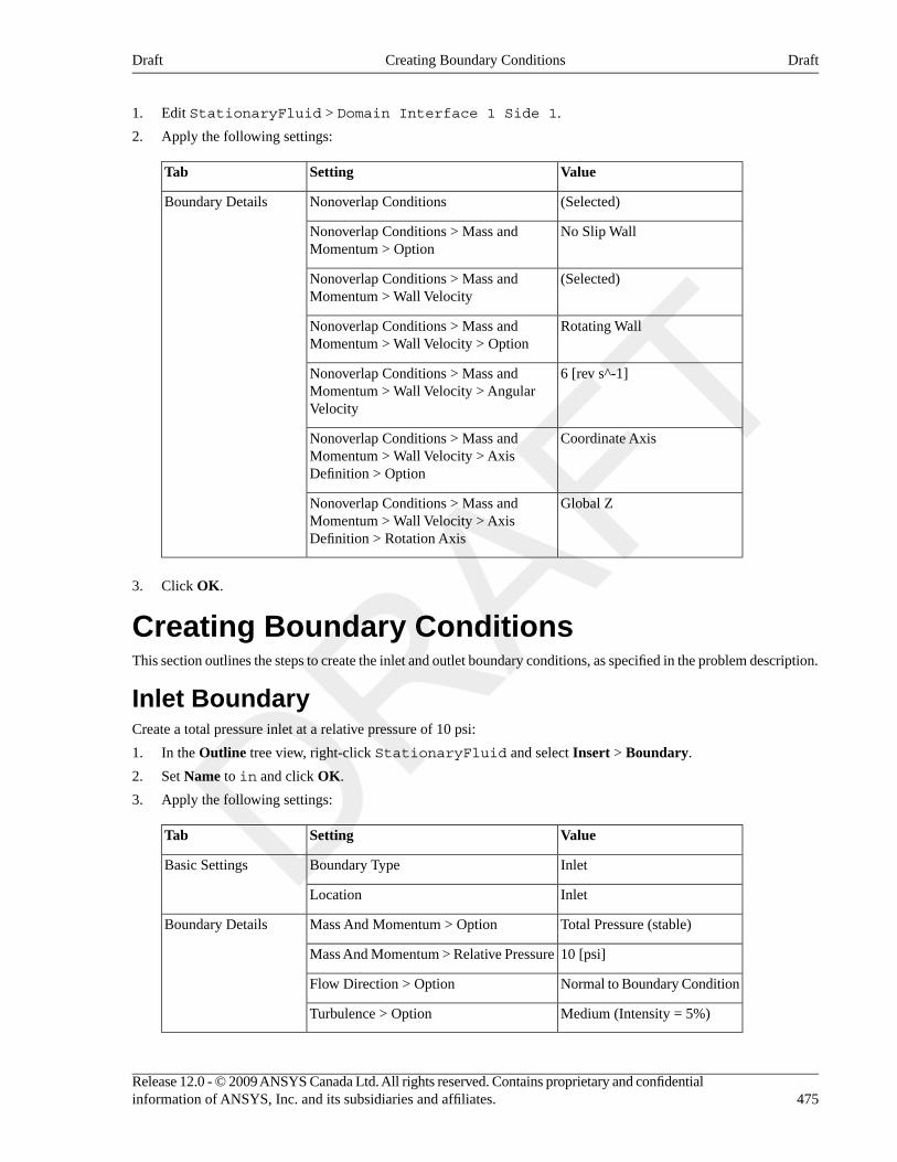
1. Edit StationaryFluid > Domain Interface 1 Side 1.
2. Apply the following settings:
ValueSettingTab
(Selected)Nonoverlap ConditionsBoundary Details
No Slip WallNonoverlap Conditions > Mass andMomentum > Option
(Selected)Nonoverlap Conditions > Mass andMomentum > Wall Velocity
Rotating WallNonoverlap Conditions > Mass andMomentum > Wall Velocity > Option
6 [rev s^-1]Nonoverlap Conditions > Mass andMomentum > Wall Velocity > AngularVelocity
Coordinate AxisNonoverlap Conditions > Mass andMomentum > Wall Velocity > AxisDefinition > Option
Global ZNonoverlap Conditions > Mass andMomentum > Wall Velocity > AxisDefinition > Rotation Axis
3. Click OK.
Creating Boundary ConditionsThis section outlines the steps to create the inlet and outlet boundary conditions, as specified in the problem description.
Inlet BoundaryCreate a total pressure inlet at a relative pressure of 10 psi:
1. In the Outline tree view, right-click StationaryFluid and select Insert > Boundary.
2. Set Name to in and click OK.
3. Apply the following settings:
ValueSettingTab
InletBoundary TypeBasic Settings
InletLocation
Total Pressure (stable)Mass And Momentum > OptionBoundary Details
10 [psi]Mass And Momentum > Relative Pressure
Normal to Boundary ConditionFlow Direction > Option
Medium (Intensity = 5%)Turbulence > Option
475Release 12.0 - © 2009 ANSYS Canada Ltd. All rights reserved. Contains proprietary and confidentialinformation of ANSYS, Inc. and its subsidiaries and affiliates.
DraftCreating Boundary ConditionsDraft
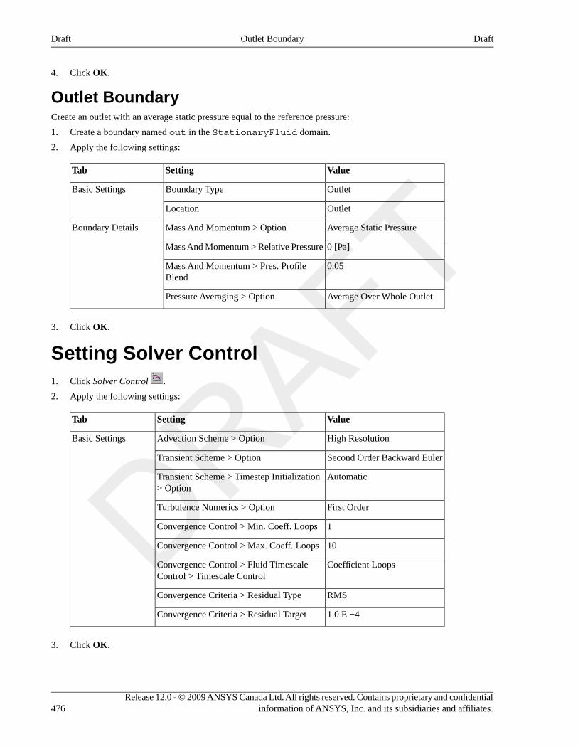
4. Click OK.
Outlet BoundaryCreate an outlet with an average static pressure equal to the reference pressure:
1. Create a boundary named out in the StationaryFluid domain.
2. Apply the following settings:
ValueSettingTab
OutletBoundary TypeBasic Settings
OutletLocation
Average Static PressureMass And Momentum > OptionBoundary Details
0 [Pa]Mass And Momentum > Relative Pressure
0.05Mass And Momentum > Pres. ProfileBlend
Average Over Whole OutletPressure Averaging > Option
3. Click OK.
Setting Solver Control1. Click Solver Control .
2. Apply the following settings:
ValueSettingTab
High ResolutionAdvection Scheme > OptionBasic Settings
Second Order Backward EulerTransient Scheme > Option
AutomaticTransient Scheme > Timestep Initialization> Option
First OrderTurbulence Numerics > Option
1Convergence Control > Min. Coeff. Loops
10Convergence Control > Max. Coeff. Loops
Coefficient LoopsConvergence Control > Fluid TimescaleControl > Timescale Control
RMSConvergence Criteria > Residual Type
1.0 E −4Convergence Criteria > Residual Target
3. Click OK.
Release 12.0 - © 2009 ANSYS Canada Ltd. All rights reserved. Contains proprietary and confidentialinformation of ANSYS, Inc. and its subsidiaries and affiliates.476
DraftOutlet BoundaryDraft

Setting Output ControlSet up the solver to output transient results files that record pressure, velocity, and velocity in the stationary frame, onevery time step:
1. Click Output Control .
2. Click the Trn Results tab.
3. In the Transient Results list box, click Add new item , set Name to Transient Results 1, and click
OK.
4. Apply the following settings to Transient Results 1:
ValueSetting
Selected VariablesOption
DefaultFile Compression
Pressure, Velocity, Velocity inStn Frame
Output Variables List
(Selected)Output Boundary Flows
AllOutput Boundary Flows > Boundary Flows
Every TimestepOutput Frequency > Option
5. Click the Monitor tab.
6. Select Monitor Options.
7. Under Monitor Points and Expressions:
1. Click Add new item .
2. Accept the default name and click OK.
3. Set Option to Expression.
4. Set Expression Value to massFlow()@in.
8. Click OK.
Writing the CFX-Solver Input (.def) File1. Click Define Run .
2. Apply the following settings:
ValueSetting
ImmersedSolid.defFile name
3. Click Save.
CFX-Solver Manager automatically starts and, on the Define Run dialog box, the Solver Input File is set.
477Release 12.0 - © 2009 ANSYS Canada Ltd. All rights reserved. Contains proprietary and confidentialinformation of ANSYS, Inc. and its subsidiaries and affiliates.
DraftSetting Output ControlDraft
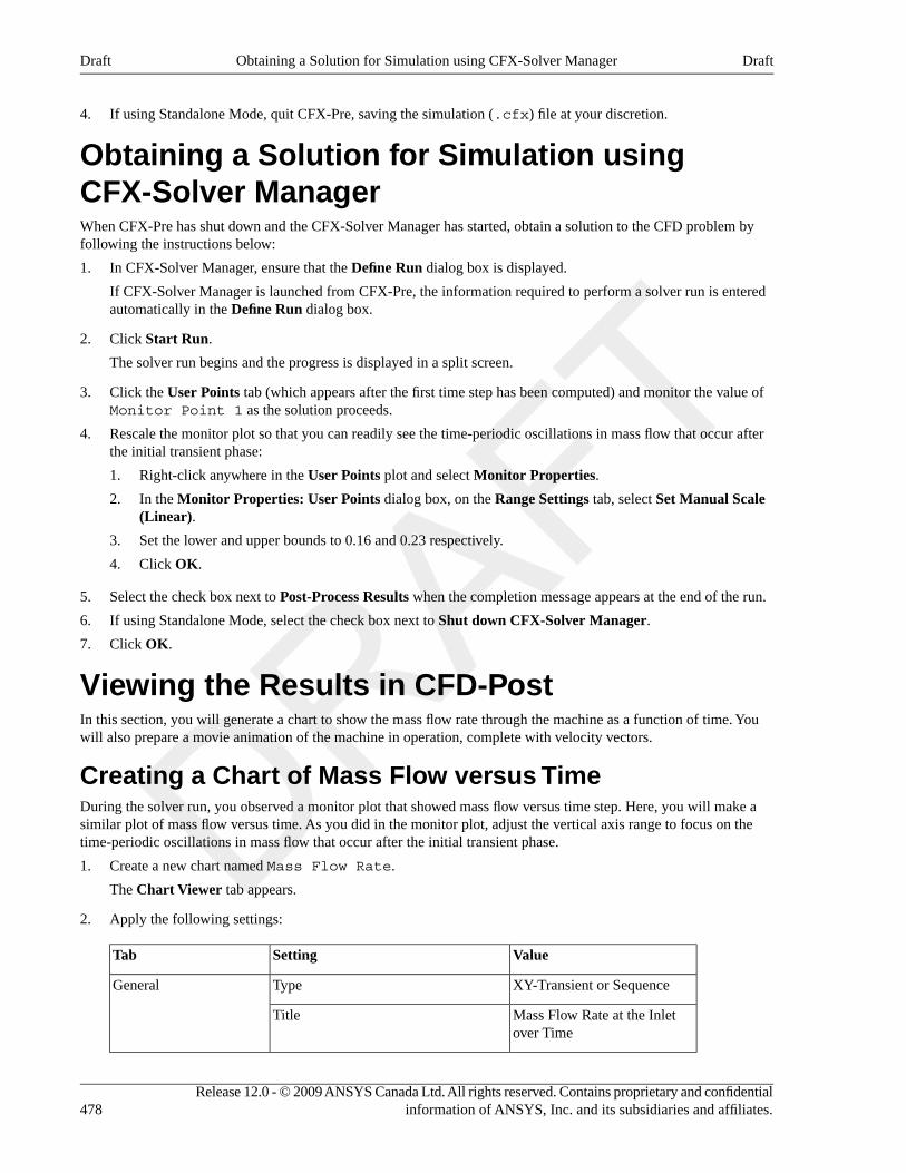
4. If using Standalone Mode, quit CFX-Pre, saving the simulation (.cfx) file at your discretion.
Obtaining a Solution for Simulation usingCFX-Solver ManagerWhen CFX-Pre has shut down and the CFX-Solver Manager has started, obtain a solution to the CFD problem byfollowing the instructions below:
1. In CFX-Solver Manager, ensure that the Define Run dialog box is displayed.
If CFX-Solver Manager is launched from CFX-Pre, the information required to perform a solver run is enteredautomatically in the Define Run dialog box.
2. Click Start Run.
The solver run begins and the progress is displayed in a split screen.
3. Click the User Points tab (which appears after the first time step has been computed) and monitor the value ofMonitor Point 1 as the solution proceeds.
4. Rescale the monitor plot so that you can readily see the time-periodic oscillations in mass flow that occur afterthe initial transient phase:
1. Right-click anywhere in the User Points plot and select Monitor Properties.
2. In the Monitor Properties: User Points dialog box, on the Range Settings tab, select Set Manual Scale(Linear).
3. Set the lower and upper bounds to 0.16 and 0.23 respectively.
4. Click OK.
5. Select the check box next to Post-Process Results when the completion message appears at the end of the run.
6. If using Standalone Mode, select the check box next to Shut down CFX-Solver Manager.
7. Click OK.
Viewing the Results in CFD-PostIn this section, you will generate a chart to show the mass flow rate through the machine as a function of time. Youwill also prepare a movie animation of the machine in operation, complete with velocity vectors.
Creating a Chart of Mass Flow versus TimeDuring the solver run, you observed a monitor plot that showed mass flow versus time step. Here, you will make asimilar plot of mass flow versus time. As you did in the monitor plot, adjust the vertical axis range to focus on thetime-periodic oscillations in mass flow that occur after the initial transient phase.
1. Create a new chart named Mass Flow Rate.
The Chart Viewer tab appears.
2. Apply the following settings:
ValueSettingTab
XY-Transient or SequenceTypeGeneral
Mass Flow Rate at the Inletover Time
Title
Release 12.0 - © 2009 ANSYS Canada Ltd. All rights reserved. Contains proprietary and confidentialinformation of ANSYS, Inc. and its subsidiaries and affiliates.478
DraftObtaining a Solution for Simulation using CFX-Solver ManagerDraft
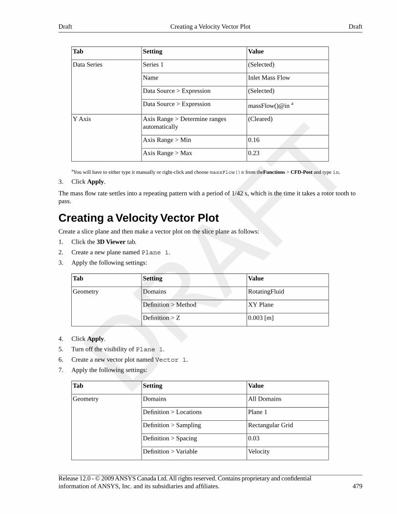
ValueSettingTab
(Selected)Series 1Data Series
Inlet Mass FlowName
(Selected)Data Source > Expression
massFlow()@in aData Source > Expression
(Cleared)Axis Range > Determine rangesautomatically
Y Axis
0.16Axis Range > Min
0.23Axis Range > Max
aYou will have to either type it manually or right-click and choose massFlow()@ from theFunctions > CFD-Post and type in.
3. Click Apply.
The mass flow rate settles into a repeating pattern with a period of 1/42 s, which is the time it takes a rotor tooth topass.
Creating a Velocity Vector PlotCreate a slice plane and then make a vector plot on the slice plane as follows:
1. Click the 3D Viewer tab.
2. Create a new plane named Plane 1.
3. Apply the following settings:
ValueSettingTab
RotatingFluidDomainsGeometry
XY PlaneDefinition > Method
0.003 [m]Definition > Z
4. Click Apply.
5. Turn off the visibility of Plane 1.
6. Create a new vector plot named Vector 1.
7. Apply the following settings:
ValueSettingTab
All DomainsDomainsGeometry
Plane 1Definition > Locations
Rectangular GridDefinition > Sampling
0.03Definition > Spacing
VelocityDefinition > Variable
479Release 12.0 - © 2009 ANSYS Canada Ltd. All rights reserved. Contains proprietary and confidentialinformation of ANSYS, Inc. and its subsidiaries and affiliates.
DraftCreating a Velocity Vector PlotDraft
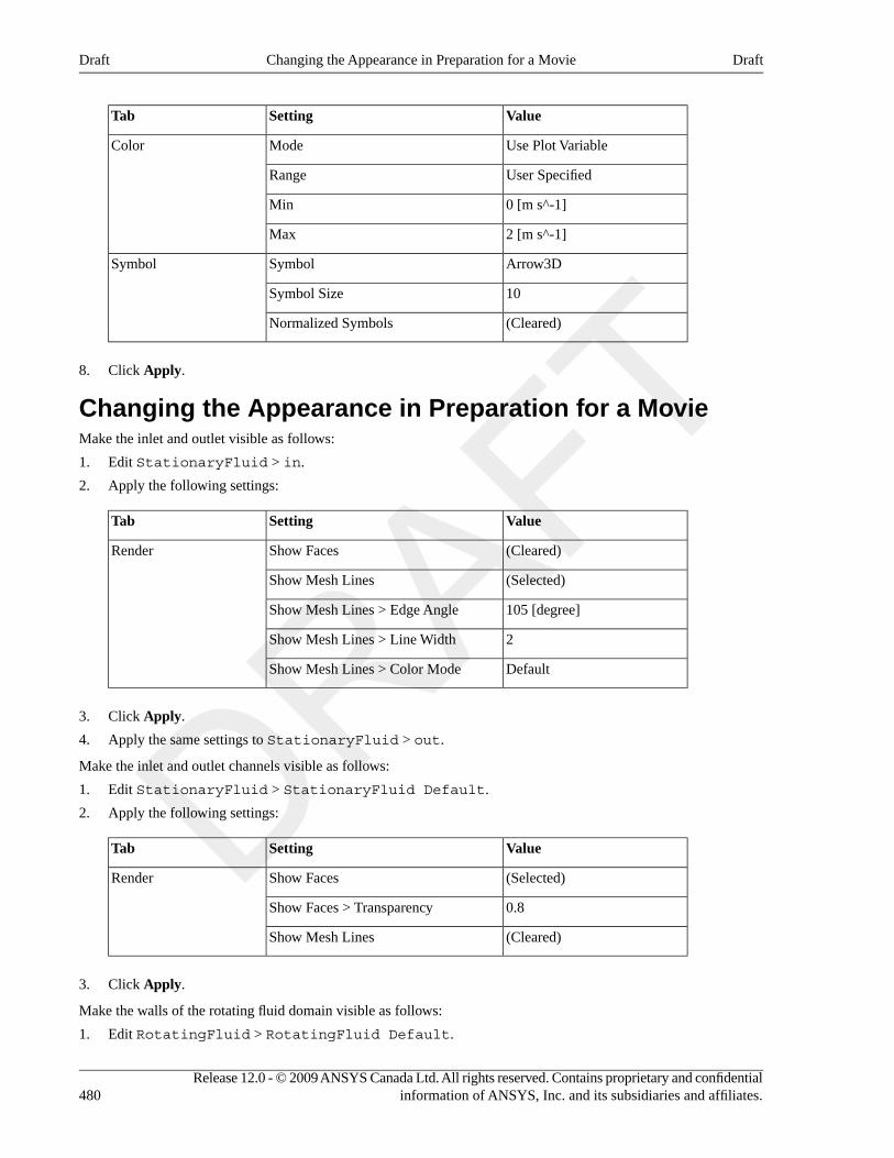
ValueSettingTab
Use Plot VariableModeColor
User SpecifiedRange
0 [m s^-1]Min
2 [m s^-1]Max
Arrow3DSymbolSymbol
10Symbol Size
(Cleared)Normalized Symbols
8. Click Apply.
Changing the Appearance in Preparation for a MovieMake the inlet and outlet visible as follows:
1. Edit StationaryFluid > in.
2. Apply the following settings:
ValueSettingTab
(Cleared)Show FacesRender
(Selected)Show Mesh Lines
105 [degree]Show Mesh Lines > Edge Angle
2Show Mesh Lines > Line Width
DefaultShow Mesh Lines > Color Mode
3. Click Apply.
4. Apply the same settings to StationaryFluid > out.
Make the inlet and outlet channels visible as follows:
1. Edit StationaryFluid > StationaryFluid Default.
2. Apply the following settings:
ValueSettingTab
(Selected)Show FacesRender
0.8Show Faces > Transparency
(Cleared)Show Mesh Lines
3. Click Apply.
Make the walls of the rotating fluid domain visible as follows:
1. Edit RotatingFluid > RotatingFluid Default.
Release 12.0 - © 2009 ANSYS Canada Ltd. All rights reserved. Contains proprietary and confidentialinformation of ANSYS, Inc. and its subsidiaries and affiliates.480
DraftChanging the Appearance in Preparation for a MovieDraft
2. Apply the following settings:
ValueSettingTab
ConstantModeColor
(White)Color
(Selected)Show FacesRender
0.0Show Faces > Transparency
(Cleared)Show Mesh Lines
3. Click Apply.
Make the walls of the immersed solid domain visible as follows:
1. Edit ImmersedSolid > ImmersedSolid Default.
2. Apply the following settings:
ValueSettingTab
ConstantModeColor
(Blue)Color
(Selected)Show FacesRender
0.0Show Faces > Transparency
(Cleared)Show Mesh Lines
3. Click Apply.
Make the following other changes in preparation for the animation that you will create in the next section:
1. Right-click a blank area in the viewer and select Predefined Camera > View Towards +Z.
2. Rotate the view a few degrees so that you can see the 3D nature of the geometery.
3. Turn off the visibility of User Locations and Plots > Wireframe.
Generating an Animated MovieIn this section, you will generate an animation that shows the changing velocity field on Plane 1. To take advantageof the periodic nature of the solution, you will record a short animation that can be played in a repeating loop in anMPEG player. Start the animation at the 61st time step (a time at which the flow has settled into a repeating pattern)and end it at the 90th time step. The 60th time step corresponds with 2/42 s, and the 90th corresponds with 3/42 s; the1/42 s interval is the period over which the solution repeats. Because the 60th and 90th time steps look the same, the60th time step is omitted to avoid having a pair of adjacent identical frames in the animation when the latter is playedin a repeating loop.
1. Click Timestep Selector and load the time value of 0.048413 s (which is the 61st time step).
2. Click Animation .
3. In the Animation dialog box, select the Keyframe Animation option.
481Release 12.0 - © 2009 ANSYS Canada Ltd. All rights reserved. Contains proprietary and confidentialinformation of ANSYS, Inc. and its subsidiaries and affiliates.
DraftGenerating an Animated MovieDraft
4. Click New to create KeyFrameNo1.
5. Select KeyframeNo1, then set # of Frames to 28, then press Enter while the cursor is in the # of Frames box.
TipBe sure to press Enter and confirm that the new number appears in the list before continuing.
6. Use the Timestep Selector to load the time value of 0.071429 s (which is the 90th time step).
7. In the Animation dialog box, click New to create KeyframeNo2.
8. Ensure that More Animation Options is pushed down to show more animation settings.
9. Select Loop.
10. Ensure that the Repeat forever button next to Repeat is not selected (not pushed down).
11. Select Save Movie.
12. Set Format to MPEG1.
13. Click Browse next to Save Movie.
14. Set File name to ImmersedSolid.mpg.
15. If required, set the path location to a different directory.
16. Click Save.
The movie file name (including path) has been set, but the animation has not yet been produced.
17. Click To Beginning .
This ensures that the animation will begin at the first keyframe.
18. Click Play the animation .
• The MPEG will be created as the animation proceeds.
• This will be slow, since results for each time step will be loaded and objects will be created.
• To view the movie file, you need to use a viewer that supports the MPEG format.
NoteTo explore additional animation options, click the Options button. On the Advanced tab of theAnimation Options dialog box, there is a Save Frames As Image Files check box. By selecting thischeck box, the JPEG or PPM files used to encode each frame of the movie will persist after moviecreation; otherwise, they will be deleted.
19. When you have finished, quit CFD-Post.
Release 12.0 - © 2009 ANSYS Canada Ltd. All rights reserved. Contains proprietary and confidentialinformation of ANSYS, Inc. and its subsidiaries and affiliates.482
DraftGenerating an Animated MovieDraft
Chapter 28. Drop Curve for CavitatingFlow in a PumpThis tutorial includes:
• Tutorial Features (p. 483)
• Overview of the Problem to Solve (p. 484)
• Before You Begin (p. 485)
• Starting CFX-Pre (p. 485)
• High Pressure Simulation of Pump without Cavitation Model (p. 485)
• High Pressure Simulation of Pump with Cavitation Model (p. 491)
• Pump Simulation with Cavitation Model Over Range of Inlet Pressures (p. 495)
Tutorial FeaturesIn this tutorial you will learn about:
• Preparing and running a series of related simulations to generate cavitation performance data for a pump.
• Creating a drop curve chart in CFD-Post.
• Using isosurfaces in CFD-Post to visualize regions of cavitation.
DetailsFeatureComponent
General ModeUser ModeCFX-Pre
Steady StateAnalysis Type
Transient
Water at 25 CFluid Type
Water Vapour at 25 C
Homogeneous ModelFluid Models
Single DomainDomain Type
k-EpsilonTurbulence Model
IsothermalHeat Transfer
Inlet (Subsonic)Boundary Conditions
Outlet (Subsonic)
Wall (Counter Rotating)
Physical Time ScaleTimestep
ContourPlotsCFD-Post
483Release 12.0 - © 2009 ANSYS Canada Ltd. All rights reserved. Contains proprietary and confidentialinformation of ANSYS, Inc. and its subsidiaries and affiliates.
DraftDraft
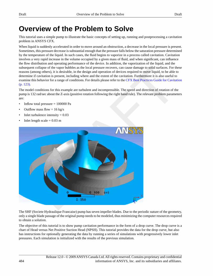
Overview of the Problem to SolveThis tutorial uses a simple pump to illustrate the basic concepts of setting up, running and postprocessing a cavitationproblem in ANSYS CFX.
When liquid is suddenly accelerated in order to move around an obstruction, a decrease in the local pressure is present.Sometimes, this pressure decrease is substantial enough that the pressure falls below the saturation pressure determinedby the temperature of the liquid. In such cases, the fluid begins to vaporize in a process called cavitation. Cavitationinvolves a very rapid increase in the volume occupied by a given mass of fluid, and when significant, can influencethe flow distribution and operating performance of the device. In addition, the vaporization of the liquid, and thesubsequent collapse of the vapor bubbles as the local pressure recovers, can cause damage to solid surfaces. For thesereasons (among others), it is desirable, in the design and operation of devices required to move liquid, to be able todetermine if cavitation is present, including where and the extent of the cavitation. Furthermore it is also useful toexamine this behavior for a range of conditions. For details please refer to the CFX Best Practices Guide for Cavitation(p. 123).
The model conditions for this example are turbulent and incompressible. The speed and direction of rotation of thepump is 132 rad/sec about the Z-axis (positive rotation following the right hand rule). The relevant problem parametersare:
• Inflow total pressure = 100000 Pa
• Outflow mass flow = 16 kg/s
• Inlet turbulence intensity = 0.03
• Inlet length scale = 0.03 m
The SHF (Societe Hydraulique Francaise) pump has seven impeller blades. Due to the periodic nature of the geometry,only a single blade passage of the original pump needs to be modeled, thus minimizing the computer resources requiredto obtain a solution.
The objective of this tutorial is to show pump cavitation performance in the form of a drop curve. The drop curve is achart of Head versus Net Positive Suction Head (NPSH). This tutorial provides the data for the drop curve, but alsohas instructions for optionally generating the data by running a series of simulations with progressively lower inletpressures. Each simulation is initialized with the results of the previous simulation.
Release 12.0 - © 2009 ANSYS Canada Ltd. All rights reserved. Contains proprietary and confidentialinformation of ANSYS, Inc. and its subsidiaries and affiliates.484
DraftOverview of the Problem to SolveDraft
Before You BeginIf this is the first tutorial you are working with, it is important to review the following topics before beginning:
• Preparing a Working Directory (p. 23)
• Setting the Working Directory and Starting ANSYS CFX (p. 23)
• Changing the Display Colors (p. 24)
• Playing a Tutorial Session File (p. 24)
Starting CFX-Pre1. Prepare the working directory using the following files in the examples directory:
• CavitationIni.pre
• CavitationIni.cfx
• Cavitation_100000.pre
• Cavitation.gtm
For details, see Preparing a Working Directory (p. 23)
2. Set the working directory and start CFX-Pre
For details, see Setting the Working Directory and Starting ANSYS CFX (p. 23)
High Pressure Simulation of Pump withoutCavitation ModelA steady-state high-pressure (inlet pressure of 100,000 Pa) simulation of the pump without cavitation (that is, simulationof the pump without water vapor) will first be set up to be used as an initial values file for the cavitation simulationlater on in the tutorial.
If you want to set up the simulation automatically using a tutorial session file, run CavitationIni.pre. For details,see Playing a Tutorial Session File (p. 24). Then proceed to Obtaining a Solution using CFX-Solver Manager (p. 490).
If you want to set up the simulation manually, proceed to the following steps:
1. Select File > New Case.
2. Select General and click OK.
3. Select File > Save Case As.
4. Under File name, type CavitationIni.cfx.
5. Click Save.
6. Choose to overwrite CavitationIni.cfx if the software asks you for confirmation.
Importing the Mesh1. Right-click Mesh and select Import Mesh > Other.
The Import Mesh dialog box appears.
2. Apply the following settings
ValueSetting
CFX Mesh (*gtm *cfx)Files of type
485Release 12.0 - © 2009 ANSYS Canada Ltd. All rights reserved. Contains proprietary and confidentialinformation of ANSYS, Inc. and its subsidiaries and affiliates.
DraftBefore You BeginDraft
ValueSetting
Cavitation.gtmFile name
3. Click Open.
Loading MaterialsSince this tutorial uses water at 25 °C and water vapor at 25 °C, you need to load these materials. Note that you willonly use the liquid water for the first part of the tutorial. The vapor is being loaded now in anticipation of using it forthe cavitation model later in the tutorial.
1. In the Outline tree view, right-click Simulation > Materials and select Import Library Data.
The Select Library Data to Import dialog box is displayed.
2. Expand Water Data.
3. Select both Water at 25 C and Water Vapour at 25 C, holding the Ctrl key.
4. Click OK.
Creating the Domain1. Edit Case Options > General in the Outline tree view and ensure that Automatic Default Domain is
turned on.
A domain named Default Domain should appear under the Simulation branch.
2. Rename Default Domain to Pump.
3. Edit Pump.
4. Under Fluid and Particle Definitions, delete Fluid 1 and create a new fluid definition named LiquidWater.
5. Apply the following settings:
ValueSettingTab
Liquid WaterFluid and Particle DefinitionsBasic Settings
Water at 25 CaFluid and Particle Definitions > LiquidWater > Material
0 [atm]Domain Models > Pressure > ReferencePressure
RotatingDomain Models > Domain Motion >Option
132 [radian s^-1]Domain Models > Domain Motion >Angular Velocity
aClick the Ellipsis icon to open the Fluids List dialog box.
6. Click OK.
Release 12.0 - © 2009 ANSYS Canada Ltd. All rights reserved. Contains proprietary and confidentialinformation of ANSYS, Inc. and its subsidiaries and affiliates.486
DraftLoading MaterialsDraft
Creating the Boundaries
Inlet Boundary1. Create a new boundary named Inlet.
2. Apply the following settings:
ValueSettingTab
InletBoundary TypeBasic Settings
INBlock INFLOWLocation
Stat. Frame Tot. PressMass And Momentum > OptionBoundary Details
100000 [Pa]Mass And Momentum > Relative Pressure
Cartesian ComponentsFlow Direction > Option
0Flow Direction > X Component
0Flow Direction > Y Component
1Flow Direction > Z Component
Intensity and Length ScaleTurbulence > Option
0.03Turbulence > Option > Fractional Intensity
0.03 [m]Turbulence > Option > Eddy Length Scale
3. Click OK.
Outlet Boundary1. Create a new boundary named Outlet.
2. Apply the following settings:
ValueSettingTab
OutletBoundary TypeBasic Settings
OUTBlock OUTFLOWLocation
Mass Flow RateMass and Momentum > OptionBoundary Details
16 [kg/s]Mass and Momentum > Mass Flow Rate
3. Click OK.
Wall BoundariesSet up the hub and shroud to be a stationary (non-rotating) wall.
1. Create a new boundary named Stationary Wall.
2. Apply the following settings to Stationary Wall:
487Release 12.0 - © 2009 ANSYS Canada Ltd. All rights reserved. Contains proprietary and confidentialinformation of ANSYS, Inc. and its subsidiaries and affiliates.
DraftCreating the BoundariesDraft
ValueSettingTab
WallBoundary TypeBasic Settings
OUTBlock HUB, OUTBlock
SHROUD aLocation
(Selected)Mass and Momentum > Wall VelocityBoundary Details
Counter Rotating WallMass and Momentum > Wall Velocity >Option
aClick the Ellipsis icon to open the Selection Diaglog dialog box. In that dialog box, select OUTBlock HUB and OUTBlock SHROUD,
holding the CTRL key. Click OK.
3. Click OK.
Creating Domain Interfaces1. Click Insert > Domain Interface and, in the dialog box that appears, set Name to Periodic Interface
and click OK.
2. Apply the following settings to Periodic Interface:
ValueSettingTab
INBlock PER1, OUTBlock
PER1, Passage PER1aInterface Side 1 > Region ListBasic Settings
INBlock PER2, OUTBlock
PER2, Passage PER2bInterface Side 2 > Region List
Rotational PeriodicityInterface Models > Option
aClick the Ellipsis icon to open the Selection Diaglog dialog box. In that dialog box, select INBlock PER1,OUTBlock PER1
and Passage PER1, holding the CTRL key. Click OK.
bClick the Ellipsis icon to open the Selection Diaglog dialog box. In that dialog box, select INBlock PER2,OUTBlock PER2
and Passage PER2, holding the CTRL key. Click OK.
3. Click OK.
Inblock to Passage Interface1. Select Insert > Domain Interface and in the dialog box that appears, set Name to Inblock to Passage
Interface and click OK.
2. Apply the following settings to Inblock to Passage Interface:
ValueSettingTab
OUTFLOW INBlockInterface Side 1 > Region ListBasic Settings
INFLOW PassageInterface Side 2 > Region List
1:1Mesh Connection Method > MeshConnection > Option
Release 12.0 - © 2009 ANSYS Canada Ltd. All rights reserved. Contains proprietary and confidentialinformation of ANSYS, Inc. and its subsidiaries and affiliates.488
DraftCreating Domain InterfacesDraft
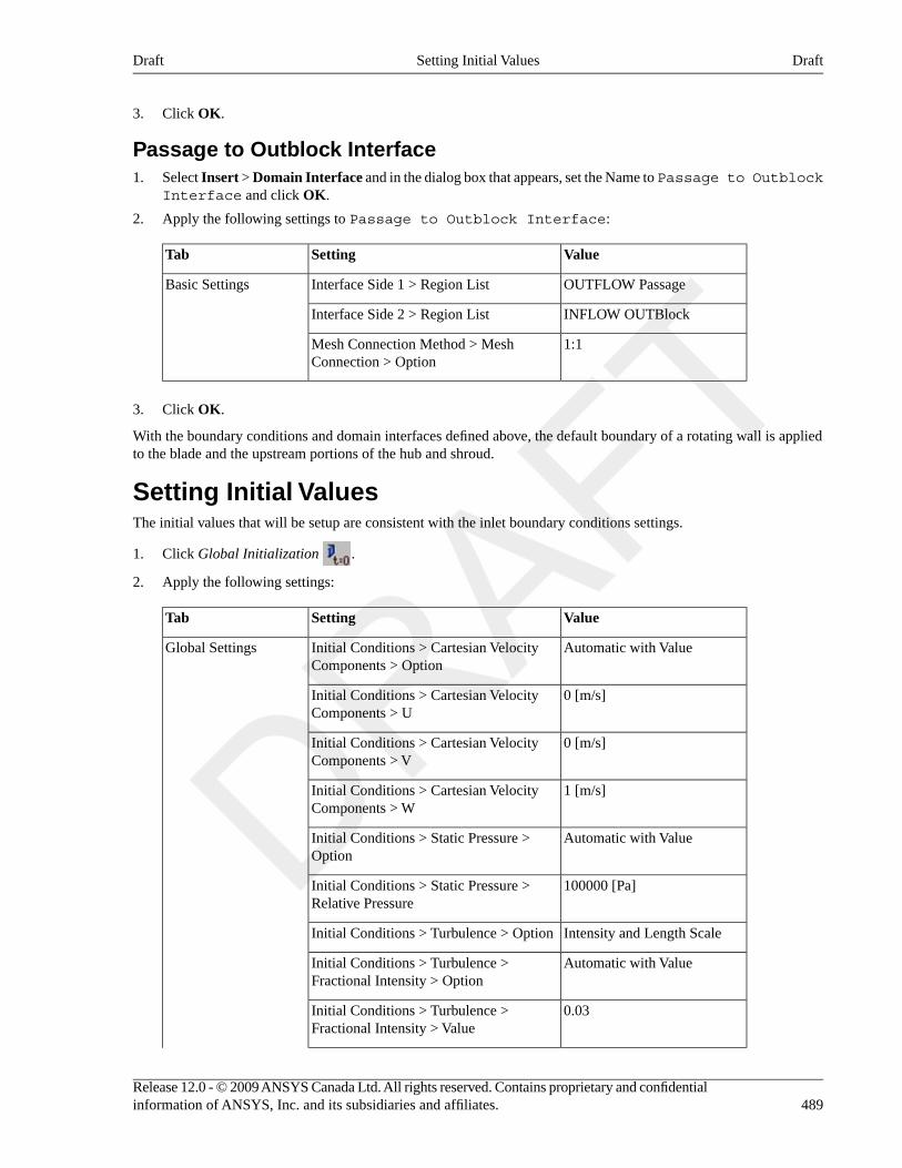
3. Click OK.
Passage to Outblock Interface1. Select Insert > Domain Interface and in the dialog box that appears, set the Name to Passage to Outblock
Interface and click OK.
2. Apply the following settings to Passage to Outblock Interface:
ValueSettingTab
OUTFLOW PassageInterface Side 1 > Region ListBasic Settings
INFLOW OUTBlockInterface Side 2 > Region List
1:1Mesh Connection Method > MeshConnection > Option
3. Click OK.
With the boundary conditions and domain interfaces defined above, the default boundary of a rotating wall is appliedto the blade and the upstream portions of the hub and shroud.
Setting Initial ValuesThe initial values that will be setup are consistent with the inlet boundary conditions settings.
1. Click Global Initialization .
2. Apply the following settings:
ValueSettingTab
Automatic with ValueInitial Conditions > Cartesian VelocityComponents > Option
Global Settings
0 [m/s]Initial Conditions > Cartesian VelocityComponents > U
0 [m/s]Initial Conditions > Cartesian VelocityComponents > V
1 [m/s]Initial Conditions > Cartesian VelocityComponents > W
Automatic with ValueInitial Conditions > Static Pressure >Option
100000 [Pa]Initial Conditions > Static Pressure >Relative Pressure
Intensity and Length ScaleInitial Conditions > Turbulence > Option
Automatic with ValueInitial Conditions > Turbulence >Fractional Intensity > Option
0.03Initial Conditions > Turbulence >Fractional Intensity > Value
489Release 12.0 - © 2009 ANSYS Canada Ltd. All rights reserved. Contains proprietary and confidentialinformation of ANSYS, Inc. and its subsidiaries and affiliates.
DraftSetting Initial ValuesDraft
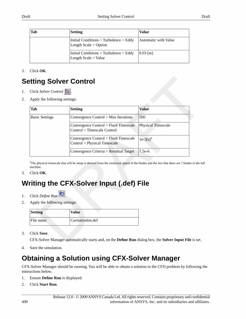
ValueSettingTab
Automatic with ValueInitial Conditions > Turbulence > EddyLength Scale > Option
0.03 [m]Initial Conditions > Turbulence > EddyLength Scale > Value
3. Click OK.
Setting Solver Control1. Click Solver Control .
2. Apply the following settings:
ValueSettingTab
500Convergence Control > Max IterationsBasic Settings
Physical TimescaleConvergence Control > Fluid TimescaleControl > Timescale Control
1e-3[s]aConvergence Control > Fluid TimescaleControl > Physical Timescale
7.5e-6Convergence Criteria > Residual Target
aThe physical timescale that will be setup is derived from the rotational speed of the blades and the fact that there are 7 blades in the fullmachine.
3. Click OK.
Writing the CFX-Solver Input (.def) File
1. Click Define Run .
2. Apply the following settings:
ValueSetting
CavitationIni.defFile name
3. Click Save.
CFX-Solver Manager automatically starts and, on the Define Run dialog box, the Solver Input File is set.
4. Save the simulation.
Obtaining a Solution using CFX-Solver ManagerCFX-Solver Manager should be running. You will be able to obtain a solution to the CFD problem by following theinstructions below.
1. Ensure Define Run is displayed.
2. Click Start Run.
Release 12.0 - © 2009 ANSYS Canada Ltd. All rights reserved. Contains proprietary and confidentialinformation of ANSYS, Inc. and its subsidiaries and affiliates.490
DraftSetting Solver ControlDraft
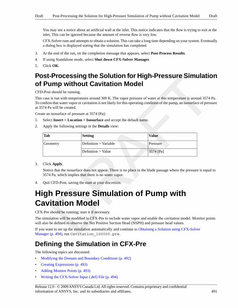
You may see a notice about an artificial wall at the inlet. This notice indicates that the flow is trying to exit at theinlet. This can be ignored because the amount of reverse flow is very low.
CFX-Solver runs and attempts to obtain a solution. This can take a long time depending on your system. Eventuallya dialog box is displayed stating that the simulation has completed.
3. At the end of the run, on the completion message that appears, select Post-Process Results.
4. If using Standalone mode, select Shut down CFX-Solver Manager.
5. Click OK.
Post-Processing the Solution for High-Pressure Simulationof Pump without Cavitation ModelCFD-Post should be running.
This case is run with temperatures around 300 K. The vapor pressure of water at this temperature is around 3574 Pa.To confirm that water vapor or cavitation is not likely for this operating condition of the pump, an isosurface of pressureat 3574 Pa will be created.
Create an isosurface of pressure at 3574 [Pa]:
1. Select Insert > Location > Isosurface and accept the default name.
2. Apply the following settings in the Details view:
ValueSettingTab
PressureDefinition > VariableGeometry
3574 [Pa]Definition > Value
3. Click Apply.
Notice that the isosurface does not appear. There is no place in the blade passage where the pressure is equal to3574 Pa, which implies that there is no water vapor.
4. Quit CFD-Post, saving the state at your discretion.
High Pressure Simulation of Pump withCavitation ModelCFX-Pre should be running; start it if necessary.
The simulation will be modified in CFX-Pre to include water vapor and enable the cavitation model. Monitor pointswill also be defined to observe the Net Positive Suction Head (NSPH) and pressure head values.
If you want to set up the simulation automatically and continue to Obtaining a Solution using CFX-SolverManager (p. 494), run Cavitation_100000.pre.
Defining the Simulation in CFX-PreThe following topics are discussed:
• Modifying the Domain and Boundary Conditions (p. 492)
• Creating Expressions (p. 493)
• Adding Monitor Points (p. 493)
• Writing the CFX-Solver Input (.def) File (p. 494)
491Release 12.0 - © 2009 ANSYS Canada Ltd. All rights reserved. Contains proprietary and confidentialinformation of ANSYS, Inc. and its subsidiaries and affiliates.
DraftPost-Processing the Solution for High-Pressure Simulation of Pump without Cavitation ModelDraft
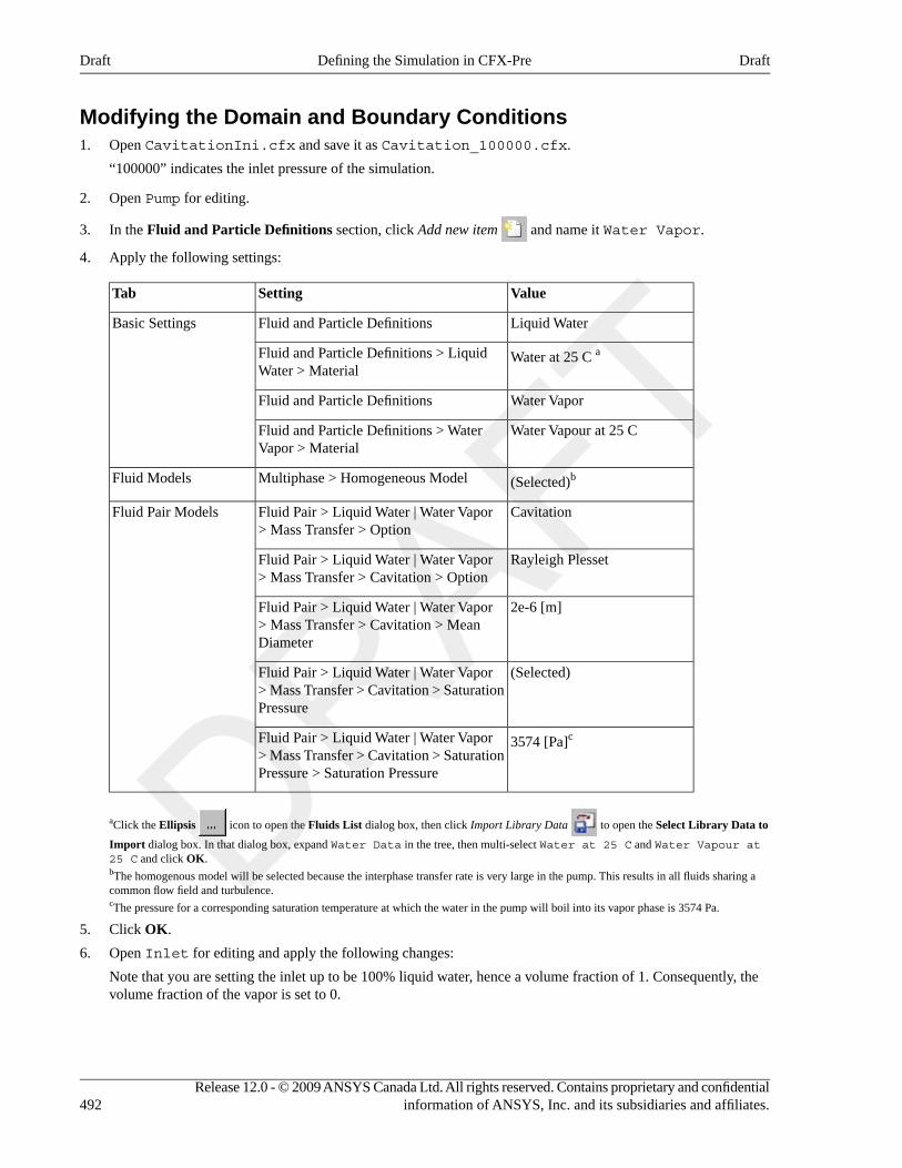
Modifying the Domain and Boundary Conditions1. Open CavitationIni.cfx and save it as Cavitation_100000.cfx.
“100000” indicates the inlet pressure of the simulation.
2. Open Pump for editing.
3. In the Fluid and Particle Definitions section, click Add new item and name it Water Vapor.
4. Apply the following settings:
ValueSettingTab
Liquid WaterFluid and Particle DefinitionsBasic Settings
Water at 25 C aFluid and Particle Definitions > LiquidWater > Material
Water VaporFluid and Particle Definitions
Water Vapour at 25 CFluid and Particle Definitions > WaterVapor > Material
(Selected)bMultiphase > Homogeneous ModelFluid Models
CavitationFluid Pair > Liquid Water | Water Vapor> Mass Transfer > Option
Fluid Pair Models
Rayleigh PlessetFluid Pair > Liquid Water | Water Vapor> Mass Transfer > Cavitation > Option
2e-6 [m]Fluid Pair > Liquid Water | Water Vapor> Mass Transfer > Cavitation > MeanDiameter
(Selected)Fluid Pair > Liquid Water | Water Vapor> Mass Transfer > Cavitation > SaturationPressure
3574 [Pa]cFluid Pair > Liquid Water | Water Vapor> Mass Transfer > Cavitation > SaturationPressure > Saturation Pressure
aClick the Ellipsis icon to open the Fluids List dialog box, then click Import Library Data to open the Select Library Data to
Import dialog box. In that dialog box, expand Water Data in the tree, then multi-select Water at 25 C and Water Vapour at25 C and click OK.bThe homogenous model will be selected because the interphase transfer rate is very large in the pump. This results in all fluids sharing acommon flow field and turbulence.cThe pressure for a corresponding saturation temperature at which the water in the pump will boil into its vapor phase is 3574 Pa.
5. Click OK.
6. Open Inlet for editing and apply the following changes:
Note that you are setting the inlet up to be 100% liquid water, hence a volume fraction of 1. Consequently, thevolume fraction of the vapor is set to 0.
Release 12.0 - © 2009 ANSYS Canada Ltd. All rights reserved. Contains proprietary and confidentialinformation of ANSYS, Inc. and its subsidiaries and affiliates.492
DraftDefining the Simulation in CFX-PreDraft
ValueSettingTab
Water VaporBoundary ConditionsFluid Values
0Boundary Conditions > Water Vapor >Volume Fraction > Volume Fraction
Liquid WaterBoundary Conditions
1Boundary Conditions > Liquid Water >Volume Fraction > Volume Fraction
7. Click OK.
8. Open Outlet for editing.
9. On the Boundary Details tab, set Mass and Momentum > Option to Bulk Mass Flow Rate and MassFlow Rate to 16 [kg s^-1].
10. Click OK.
Creating ExpressionsExpressions defining the Net Positive Suction Head (NPSH) and Head are created in order to monitor their values asthe inlet pressure is decreased. By monitoring these values a drop curve can be produced.
• Create the following expressions.
DefinitionName
massFlowAve(Total Pressure in StnFrame)@Inlet
Ptin
massFlowAve(Total Pressure in StnFrame)@Outlet
Ptout
996.82 [kg m^-3]Wden
(Ptout-Ptin)/(Wden*g)Head
(Ptin- Pvap)/(Wden*g)NPSH
3574 [Pa]Pvap
Adding Monitor PointsTwo monitor points will be added to track the NPSH and head using the expressions created in the previous step.
1. Click Output Control .
2. On the Monitor tab, select Monitor Options and click Add new item .
3. Enter NPSH Point as the name of the monitor point then enter the following settings:
ValueSettingTab
ExpressionMonitor Options > Monitor Points andExpressions > NPSH Point > Option
Monitor
493Release 12.0 - © 2009 ANSYS Canada Ltd. All rights reserved. Contains proprietary and confidentialinformation of ANSYS, Inc. and its subsidiaries and affiliates.
DraftDefining the Simulation in CFX-PreDraft
ValueSettingTab
NPSHMonitor Options > Monitor Points andExpressions > NPSH Point > ExpressionValue
4. Create a second monitor point named Head Point with the same parameters as the first, with the exceptionthat Expression Value is set to Head.
5. Click OK.
Writing the CFX-Solver Input (.def) File
1. Click Define Run .
2. Apply the following settings:
ValueSetting
Cavitation_100000.defFile name
3. Click Save.
CFX-Solver Manager automatically starts and, on the Define Run dialog box, the Solver Input File is set.
4. Save the simulation.
Obtaining a Solution using CFX-Solver ManagerCFX-Solver Manager should be running. Obtain a solution to the CFD problem by following these instructions:
1. Ensure Define Run is displayed.
2. Select Initial Values Specification.
3. Select CavitationIni_001.res for the initial values file using the Browse tool.
4. Click Start Run.
You may see a notice about an artificial wall at the inlet. This notice indicates that the flow is trying to exit at theinlet. This can be ignored because the amount of reverse flow is very low.
CFX-Solver runs and attempts to obtain a solution. This will not require many iterations or much time, dependingon your system, because only minor changes have been made from the initial simulation. A dialog box is displayedstating that the simulation has completed.
5. At the end of the run, on the completion message that appears, select Post-Process Results.
6. If using Standalone mode, select Shut down CFX-Solver Manager.
7. Click OK.
Post-Processing the Solution for High-Pressure Simulationof Pump with Cavitation ModelYou will create an isosurface to observe the volume fraction of water vapor at 25 °C. Note that the pressure below thethreshold is the same as found earlier in High Pressure Simulation of Pump without Cavitation Model (p. 485).
Create an isosurface for the volume fraction of water vapor at 25 °C, at 0.1:
Release 12.0 - © 2009 ANSYS Canada Ltd. All rights reserved. Contains proprietary and confidentialinformation of ANSYS, Inc. and its subsidiaries and affiliates.494
DraftObtaining a Solution using CFX-Solver ManagerDraft
1. CFD-Post should be running; start it if necessary.
2. Click Insert > Location > Isosurface and accept the default name.
3. Apply the following settings in the Details view:
ValueSettingTab
Water Vapor.Volume FractionDefinition > VariableGeometry
0.1Definition > Value
4. Click Apply.
Notice that the isosurface is clear. There is no water vapor at 25 °C in the blade passage for the simulation withcavitation because at an inlet total pressure of 100000Pa, the minimum static pressure in the model is above thevapor pressure.
5. Quit CFD-Post saving the state at your discretion.
Pump Simulation with Cavitation Model OverRange of Inlet PressuresIn order to construct a drop curve for this cavitation case, the inlet pressure must be decremented from its initial valueof 100000 Pa to 17500 Pa, and the Head and NPSH values must be recorded for each simulation. The results areprovided in Table 28.1, “Pump Performance Data” (p. 495).
Table 28.1. Pump Performance Data
Head
m
NPSH
m
Inlet Pressure
Pa
3.537e+019.859e+00100000
3.535e+017.813e+0080000
3.535e+015.767e+0060000
3.536e+013.721e+0040000
3.538e+012.698e+0030000
3.534e+011.675e+0020000
3.528e+011.470e+0018000
3.184e+011.419e+0017500
Optionally, if you want to generate the data shown in Table 28.1, “Pump Performance Data” (p. 495), then follow theinstructions in the following two sections (Writing CFX-Solver Input (.def) Files for Lower Inlet Pressures (p. 496)and Obtaining Solutions using CFX-Solver Manager (p. 496)). Those instructions involve running several simulationsin order to obtain a set of results files. As a benefit to doing this, you will have the results files required to completean optional postprocessing exercise at the end of this tutorial. This optional postprocessing exercise involves usingisosurfaces to visualize the regions of cavitation, and visually comparing these isosurfaces between different resultsfiles.
If you want to use the provided table data to produce a drop curve, proceed to Generating a Drop Curve (p. 497).
495Release 12.0 - © 2009 ANSYS Canada Ltd. All rights reserved. Contains proprietary and confidentialinformation of ANSYS, Inc. and its subsidiaries and affiliates.
DraftPump Simulation with Cavitation Model Over Range of Inlet PressuresDraft
Writing CFX-Solver Input (.def) Files for Lower InletPressuresProduce a set of definition (.def) files for the simulation, with each definition file specifying a progressively lowervalue for the inlet pressure:
1. CFX-Pre should be running; start it if necessary.
2. Open Cavitation_100000.cfx.
3. Open Simulation > Flow Analysis 1 > Pump > Inlet.
4. On the Boundary Details tab change Mass and Momentum > Relative Pressure to 80000 [Pa].
5. Click OK.
6. Right-click Simulation and select Write Solver Input File.
7. Set File name to Cavitation_80000.def.
8. Click Save.
9. Change the inlet pressure and save a corresponding CFX-Solver input file for each of the 6 other pressures: 60000Pa, 40000 Pa, 30000 Pa, 20000 Pa, 18000 Pa, and 17500 Pa.
NoteThere are other techniques for defining a set of related simulations. For example, you could use configurationcontrol, as demonstrated in Flow from a Circular Vent (p. 113).
Obtaining Solutions using CFX-Solver ManagerRun each of the CFX-Solver input files that you created in the previous step:
1. Start CFX-Solver Manager if it is not already running.
2. Ensure Define Run is displayed.
3. Under Solver Input File, click Browse and select Cavitation_80000.def.
4. Select Initial Values Specification.
5. Select Cavitation_100000_001.res for the initial values file using the Browse tool.
6. Click Start Run.
You may see a notice about an artificial wall at the inlet. This notice indicates that the flow is trying to exit at theinlet. This can be ignored because the amount of reverse flow is very low.
CFX-Solver runs and attempts to obtain a solution. This can take a long time depending on your system. Eventuallya dialog box is displayed stating that the simulation has completed.
7. When the completion message appears at the end of the run, click OK without selecting the option to post-processthe results.
8. Repeat this process until you have run all the CFX-Solver input files for all 6 other inlet pressures: 60000 Pa,40000 Pa, 30000 Pa, 20000 Pa, 18000 Pa, and 17500 Pa. The pump simulation with cavitation model at an inletpressure of 17500 Pa will converge poorly because the performance of the pump is decreasing considerably aroundthat pressure. Note that the initial values should be taken from the previously generated results (.res) file.
Release 12.0 - © 2009 ANSYS Canada Ltd. All rights reserved. Contains proprietary and confidentialinformation of ANSYS, Inc. and its subsidiaries and affiliates.496
DraftWriting CFX-Solver Input (.def) Files for Lower Inlet PressuresDraft
Viewing the Solution for the Pump Simulation withCavitation ModelTo see the pump performance, you will generate a drop curve to show the pump performance over a range of inletpressures. After generating the drop curve, there is an optional exercise for visualizing the cavitation regions usingisosurfaces.
The optional exercise of visualizing the cavitation regions requires the results files from the 60000 Pa, 40000 Pa, 20000Pa, and 17500 Pa simulations. If you have not generated those results files and want to complete the optional exercise,then generate the results files by following the instructions in:
• Writing CFX-Solver Input (.def) Files for Lower Inlet Pressures (p. 496)
• Obtaining Solutions using CFX-Solver Manager (p. 496)
Generating a Drop CurveTo generate a drop curve, you will need the values for Net Positive Suction Head (NPSH) and head as the inlet pressuredecreases. This data is provided in Table 28.1, “Pump Performance Data” (p. 495). If you want to use that data, proceedto Creating a Table of the Head and NPSH Values (p. 497). If you have chosen to run all of the simulations and haveobtained all of the results files, you can obtain the drop curve data yourself by following the instructions in the Creatinga Head-versus-NPSH Chart (Optional Exercise) (p. 499) section.
Creating a Table of the Head and NPSH Values1. Start CFD-Post.
2. Click Insert > Table and set the name to Drop Curve Values.
3. Enter the values from Table 28.1, “Pump Performance Data” (p. 495) for the 8 inlet pressures in the table.
Enter the NPSH values in the left column and the head values in the right column.
4. Click Save Table , and apply the following settings:
ValueSetting
Drop Curve ValuesFile name
Comma Separated Values — ExcelReadable (*.csv)
Files of type
5. Click Save.
Creating a Head-versus-NPSH Chart1. Click Insert > Chart.
2. Set the name to Drop Curve and click OK.
3. Apply the following settings:
ValueSettingTab
Drop CurveTitleGeneral
(Selected)Data Source > FileData Series
Drop Curve Values.csvaData Source > File > Browse
497Release 12.0 - © 2009 ANSYS Canada Ltd. All rights reserved. Contains proprietary and confidentialinformation of ANSYS, Inc. and its subsidiaries and affiliates.
DraftViewing the Solution for the Pump Simulation with Cavitation ModelDraft
ValueSettingTab
(Cleared)Axis Range > Determine rangesautomatically
X Axis
0Axis Range > Min
10Axis Range > Max
(Cleared)Axis Labels > Use data for axis labels
NPSH [m]Axis Labels > Custom Label
(Cleared)Axis Range > Determine rangesautomatically
Y Axis
0Axis Range > Min
45Axis Range > Max
(Cleared)Axis Labels > Use data for axis labels
Head [m]Axis Labels > Custom Label
TriangleLine Display > SymbolsLine Display
aCreated in the previous steps.
4. Click Apply and proceed to Viewing the Drop Curve (p. 498).
Viewing the Drop CurveHere is what the drop curve created in the earlier steps should look like:
Release 12.0 - © 2009 ANSYS Canada Ltd. All rights reserved. Contains proprietary and confidentialinformation of ANSYS, Inc. and its subsidiaries and affiliates.498
DraftViewing the Solution for the Pump Simulation with Cavitation ModelDraft
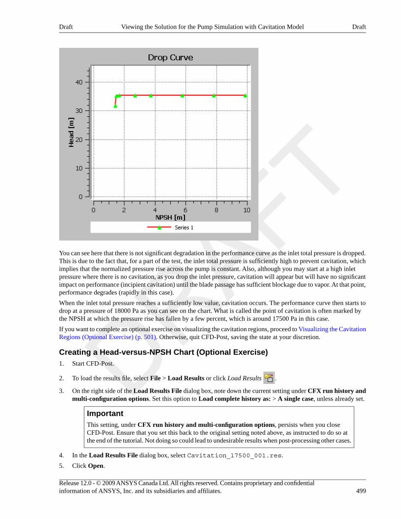
You can see here that there is not significant degradation in the performance curve as the inlet total pressure is dropped.This is due to the fact that, for a part of the test, the inlet total pressure is sufficiently high to prevent cavitation, whichimplies that the normalized pressure rise across the pump is constant. Also, although you may start at a high inletpressure where there is no cavitation, as you drop the inlet pressure, cavitation will appear but will have no significantimpact on performance (incipient cavitation) until the blade passage has sufficient blockage due to vapor. At that point,performance degrades (rapidly in this case).
When the inlet total pressure reaches a sufficiently low value, cavitation occurs. The performance curve then starts todrop at a pressure of 18000 Pa as you can see on the chart. What is called the point of cavitation is often marked bythe NPSH at which the pressure rise has fallen by a few percent, which is around 17500 Pa in this case.
If you want to complete an optional exercise on visualizing the cavitation regions, proceed to Visualizing the CavitationRegions (Optional Exercise) (p. 501). Otherwise, quit CFD-Post, saving the state at your discretion.
Creating a Head-versus-NPSH Chart (Optional Exercise)1. Start CFD-Post.
2. To load the results file, select File > Load Results or click Load Results .
3. On the right side of the Load Results File dialog box, note down the current setting under CFX run history andmulti-configuration options. Set this option to Load complete history as: > A single case, unless already set.
ImportantThis setting, under CFX run history and multi-configuration options, persists when you closeCFD-Post. Ensure that you set this back to the original setting noted above, as instructed to do so atthe end of the tutorial. Not doing so could lead to undesirable results when post-processing other cases.
4. In the Load Results File dialog box, select Cavitation_17500_001.res.
5. Click Open.
499Release 12.0 - © 2009 ANSYS Canada Ltd. All rights reserved. Contains proprietary and confidentialinformation of ANSYS, Inc. and its subsidiaries and affiliates.
DraftViewing the Solution for the Pump Simulation with Cavitation ModelDraft
When you started the CFX-Solver run using initial values, by default theContinue History From option was on.This enables the results file to retain a reference to the initial value results file. When the final results file is loadedinto CFD-Post using the Load complete history as: A single case, it includes results from all the initial valuesfiles as well as the final results. Each of the previous initial values files is available as a timestep (in this case asequence) through the Timestep Selector.
6. Click OK when prompted with a Process Multiple Results as a Sequence message.
7. Click Insert > Chart or click Chart .
8. Set the name to Drop Curve and click OK.
9. Apply the following settings:
ValueSettingTab
XY - Transient or SequenceTypeGeneral
Drop CurveTitle
(Selected)Data Source > ExpressionData Series
HeadData Source > Expression
NPSHData Selection > ExpressionX Axis
(Cleared)Axis Range > Determine rangesautomatically
Y Axis
0Axis Range > Min
45Axis Range > Max
TriangleLine Display > SymbolsLine Display
10. Click Apply and proceed to Viewing the Drop Curve (p. 500).
Viewing the Drop CurveHere is what the drop curve created in the earlier steps should look like:
Release 12.0 - © 2009 ANSYS Canada Ltd. All rights reserved. Contains proprietary and confidentialinformation of ANSYS, Inc. and its subsidiaries and affiliates.500
DraftViewing the Solution for the Pump Simulation with Cavitation ModelDraft
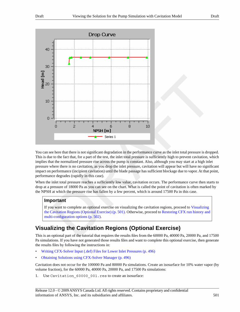
You can see here that there is not significant degradation in the performance curve as the inlet total pressure is dropped.This is due to the fact that, for a part of the test, the inlet total pressure is sufficiently high to prevent cavitation, whichimplies that the normalized pressure rise across the pump is constant. Also, although you may start at a high inletpressure where there is no cavitation, as you drop the inlet pressure, cavitation will appear but will have no significantimpact on performance (incipient cavitation) until the blade passage has sufficient blockage due to vapor. At that point,performance degrades (rapidly in this case).
When the inlet total pressure reaches a sufficiently low value, cavitation occurs. The performance curve then starts todrop at a pressure of 18000 Pa as you can see on the chart. What is called the point of cavitation is often marked bythe NPSH at which the pressure rise has fallen by a few percent, which is around 17500 Pa in this case.
ImportantIf you want to complete an optional exercise on visualizing the cavitation regions, proceed to Visualizingthe Cavitation Regions (Optional Exercise) (p. 501). Otherwise, proceed to Restoring CFX run history andmulti-configuration options (p. 502).
Visualizing the Cavitation Regions (Optional Exercise)This is an optional part of the tutorial that requires the results files from the 60000 Pa, 40000 Pa, 20000 Pa, and 17500Pa simulations. If you have not generated those results files and want to complete this optional exercise, then generatethe results files by following the instructions in:
• Writing CFX-Solver Input (.def) Files for Lower Inlet Pressures (p. 496)
• Obtaining Solutions using CFX-Solver Manager (p. 496)
Cavitation does not occur for the 100000 Pa and 80000 Pa simulations. Create an isosurface for 10% water vapor (byvolume fraction), for the 60000 Pa, 40000 Pa, 20000 Pa, and 17500 Pa simulations:
1. Use Cavitation_60000_001.res to create an isosurface:
501Release 12.0 - © 2009 ANSYS Canada Ltd. All rights reserved. Contains proprietary and confidentialinformation of ANSYS, Inc. and its subsidiaries and affiliates.
DraftViewing the Solution for the Pump Simulation with Cavitation ModelDraft
1. Launch CFD-Post and load Cavitation_60000_001.res.
2. Select Insert > Location > Isosurface and accept the default name.
3. Apply the following settings in the details view:
ValueSettingTab
Water Vapor.Volume FractionDefinition > VariableGeometry
0.1Definition > Value
4. Click Apply.
2. Add Cavitation_40000_001.res to the current results:
1. Select File > Load Results.
2. Under Case options, select both Keep current cases loaded and Open in new view.
3. Select Cavitation_40000_001.res.
4. Click Open.
5. Click a blank area inside the viewport named View 2 (which contains the results that you just loaded) tomake that viewport active, then turn on visibility for the isosurface in the Outline tree view.
3. In a similar way, load Cavitation_20000_001.res and Cavitation_17500_001.res and make theisosurface visible on these results.
4. Click Synchronize camera in displayed views so that all viewports maintain the same camera position.
5. Rotate the view (from any viewport) to inspect the results.
Observe that the amount of water vapor increases as the inlet pressure decreases.
ImportantIf you created the drop curve by setting the CFX run history and multi-configuration options, proceedto Restoring CFX run history and multi-configuration options (p. 502). Otherwise, quit CFD-Post, savingthe state at your discretion.
Restoring CFX run history and multi-configuration optionsAs mentioned above the setting under CFX run history and multi-configuration options persists when you closeCFD-Post. This section outlines the steps to restore CFX run history and multi-configuration options to its originalsetting.
1. Select File > Close to close the current file.
2. Click Close if prompted to save.
3. Load a results file by selecting File > Load Results or click Load Results .
4. On the right side of the Load Results File dialog box, restore the original settings under CFX run history andmulti-configuration options.
5. In the Load Results File dialog box, select Cavitation_17500_001.res.
6. Click Open.
7. Quit CFD-Post, by selecting File > Quit.
Release 12.0 - © 2009 ANSYS Canada Ltd. All rights reserved. Contains proprietary and confidentialinformation of ANSYS, Inc. and its subsidiaries and affiliates.502
DraftViewing the Solution for the Pump Simulation with Cavitation ModelDraft
Chapter 29. Spray DryerThis tutorial includes:
• Tutorial Features (p. 503)
• Overview of the Problem to Solve (p. 504)
• Before You Begin (p. 505)
• Starting CFX-Pre (p. 505)
• Defining a Steady-State Simulation in CFX-Pre (p. 505)
• Obtaining a Solution Using CFX-Solver Manager (p. 511)
• Viewing the Results in CFD-Post (p. 512)
Tutorial FeaturesIn this tutorial you will learn about:
• Importing a CCL file in CFX-Pre.
• Editing and creating boundary conditions in CFX-Pre.
• Adding particles that evaporate.
• Creating a domain interface in CFX-Pre.
• Creating contour plots and inserting particle tracking in CFD-Post.
DetailsFeatureComponent
General ModeUser ModeCFX-Pre
Steady StateAnalysis Type
General FluidFluid Type
Single DomainDomain Type
Water NozzleBoundary Conditions
Air Inlet
Outlet
Domain 1 Default
Fluid FluidDomain Interface
Physical TimescaleTimescale
SelectedParticle Coupling Control
SelectedExtra Output Variables List
Contour PlotsPlotsCFD-Post
Particle Tracking
503Release 12.0 - © 2009 ANSYS Canada Ltd. All rights reserved. Contains proprietary and confidentialinformation of ANSYS, Inc. and its subsidiaries and affiliates.
DraftDraft
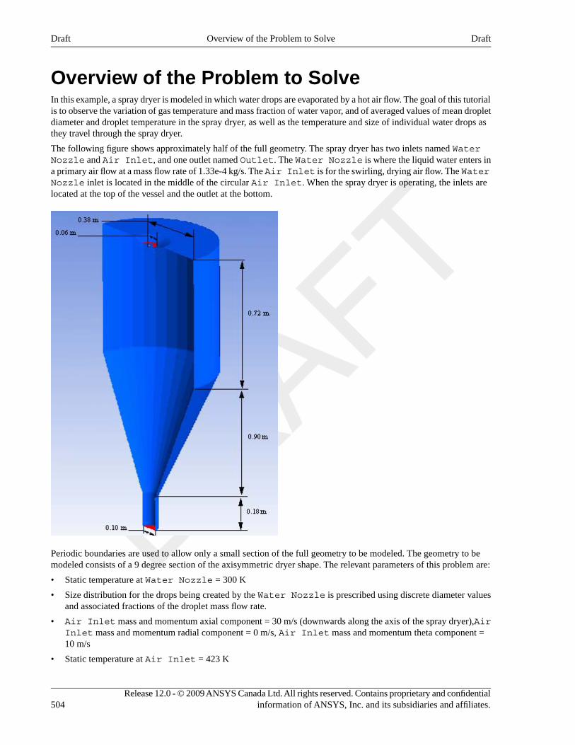
Overview of the Problem to SolveIn this example, a spray dryer is modeled in which water drops are evaporated by a hot air flow. The goal of this tutorialis to observe the variation of gas temperature and mass fraction of water vapor, and of averaged values of mean dropletdiameter and droplet temperature in the spray dryer, as well as the temperature and size of individual water drops asthey travel through the spray dryer.
The following figure shows approximately half of the full geometry. The spray dryer has two inlets named WaterNozzle and Air Inlet, and one outlet named Outlet. The Water Nozzle is where the liquid water enters ina primary air flow at a mass flow rate of 1.33e-4 kg/s. The Air Inlet is for the swirling, drying air flow. The WaterNozzle inlet is located in the middle of the circular Air Inlet. When the spray dryer is operating, the inlets arelocated at the top of the vessel and the outlet at the bottom.
Periodic boundaries are used to allow only a small section of the full geometry to be modeled. The geometry to bemodeled consists of a 9 degree section of the axisymmetric dryer shape. The relevant parameters of this problem are:
• Static temperature at Water Nozzle = 300 K
• Size distribution for the drops being created by the Water Nozzle is prescribed using discrete diameter valuesand associated fractions of the droplet mass flow rate.
• Air Inlet mass and momentum axial component = 30 m/s (downwards along the axis of the spray dryer),AirInlet mass and momentum radial component = 0 m/s, Air Inlet mass and momentum theta component =10 m/s
• Static temperature at Air Inlet = 423 K
Release 12.0 - © 2009 ANSYS Canada Ltd. All rights reserved. Contains proprietary and confidentialinformation of ANSYS, Inc. and its subsidiaries and affiliates.504
DraftOverview of the Problem to SolveDraft
• Relative pressure at Outlet = 0 Pa
• Normal speed of Water = 10 m/s
The approach for solving this problem is to first import a CCL file with the fluid properties, domain and boundaryconditions in CFX-Pre. Minor changes will be made to the information imported from the CCL file. Boundary conditionsand a domain interface will also be added. In CFD-Post, contour plots will be created to see the variation of temperature,mass fraction of water, average mean particle diameter of liquid water, and averaged temperature of liquid water inthe spray dryer. Finally, particle tracking will be used for plotting the temperature of liquid water.
Before You BeginIf this is the first tutorial you are working with, it is important to review the following topics before beginning:
• Preparing a Working Directory (p. 23)
• Setting the Working Directory and Starting ANSYS CFX (p. 23)
• Changing the Display Colors (p. 24)
• Playing a Tutorial Session File (p. 24)
Starting CFX-Pre1. Prepare the working directory using the following files in the examples directory:
• SprayDryer.pre
• spraydryer9.gtm
2. In addition to the files from the examples directory, the evaporating_drops.ccl file from theetc/model-templates directory, should also be copied over to the working directory.
For details, see Preparing a Working Directory (p. 23)
3. Set the working directory and start CFX-Pre
For details, see Setting the Working Directory and Starting ANSYS CFX (p. 23)
Defining a Steady-State Simulation in CFX-PreIf you want to set up the simulation automatically using a tutorial session file, run SprayDryer.pre. For details,see Playing a Tutorial Session File (p. 24). Then proceed to Obtaining a Solution Using CFX-Solver Manager (p. 511).
If you want to set up the simulation manually, proceed to the following steps:
This section describes the step-by-step definition of the flow physics in CFX-Pre for a steady-state simulation.
1. Select File > New Case.
2. Select General and click OK.
3. Edit Case Options > General in the Outline tree view and ensure that Automatic Default Domain isturned off.
4. Select File > Save Case As.
5. Under File name, type SprayDryer.
6. Click Save.
Importing the Mesh1. Select File > Import > Mesh.
2. Apply the following settings
505Release 12.0 - © 2009 ANSYS Canada Ltd. All rights reserved. Contains proprietary and confidentialinformation of ANSYS, Inc. and its subsidiaries and affiliates.
DraftBefore You BeginDraft
ValueSetting
CFX Mesh (*gtm *cfx)Files of type
spraydryer9.gtmFile name
3. Click Open.
Importing the Evaporating CCL Drops Model TemplateANSYS CFX Command Language (CCL) consists of commands used to carry out actions in CFX-Pre, CFX-SolverManager and CFD-Post. The physics for this simulation such as materials, domain and domain properties will beimported as a CCL. We will first analyze the evaporating_drops.ccl model template and then import it intothe simulation.
NoteThe physics for a simulation can be saved to a CCL (CFX Command Language) file at any time by selectingFile > Export > CCL.
1. Open evaporating_drops.ccl with a text editor and take the time to look at the information it contains.
The template sets up the materials water vapor H2O with a thermal conductivity of 193e-04 W/mK and waterliquid H2Ol, which enters from the Water Nozzle. Note that the water data could also have been imported fromthe library in CFX-Pre. The template also creates a continuous gas phase named Gas mixture containing H2Oand Air Ideal Gas and a binary mixture of H2O and H2Ol, which determines the rate of evaporation of thewater. A domain named Domain 1 that includes the Gas mixture and H2Ol as a fluid pair as well as an inletboundary is also specified in the CCL file. The inlet boundary is set up with a default static temperature of 573K.
2. Select File > Import > CCL
The Import CCL dialog box appears.
3. Under Import Method, select Append. This will start with the existing CCL already generated and append theimported CCL.
NoteReplace is useful if you have defined physics and want to update or replace them with newly-importedphysics.
4. Select evaporating_drops.ccl.
5. Click Open.
NoteAn error message related to the parameter Location will appear in the message window. This error occursas the CCL contains a location placeholder that is not part of the mesh. Ignore this error message as theissue will be addressed when Domain 1 is being edited.
Editing the DomainThe fluid domain imported in the CCL file will be edited in this section.
1. In the tree view, right-click Domain 1, then click Edit.
2. Apply the following settings:
Release 12.0 - © 2009 ANSYS Canada Ltd. All rights reserved. Contains proprietary and confidentialinformation of ANSYS, Inc. and its subsidiaries and affiliates.506
DraftImporting the Evaporating CCL Drops Model TemplateDraft
ValueSettingTab
B34Location and Type > LocationBasic Settings
BuoyantDomain Models > Buoyancy > Option
0.0 [m s^-1]Domain Models > Buoyancy > GravityX Dirn.
-9.81 [m s^-1]Domain Models > Buoyancy > GravityY Dirn.
0.0 [m s^-1]Domain Models > Buoyancy > GravityZ Dirn.
1.2 [kg m^-3] aDomain Models > Buoyancy > Buoy.Ref. Density
Gas mixtureFluidFluid Specific Models
Non Buoyant bFluid > Gas mixture > Fluid BuoyancyModel > Option
H2OlFluid
Density DifferenceFluid > H2Ol > Fluid Buoyancy Model> Option
aThe buoyancy reference density is set to 1.2 as representative of air.bSince any natural convection in the gas can be neglected, we can set the fluid to non buoyant.
3. Click OK.
Creating and Editing the Boundary ConditionsIn this section, the Inlet and Domain 1 Default boundary conditions that were imported in the CCL file willbe edited. Two boundary conditions, Air Inlet and Outlet will also be created for the spray dryer simulation.
Water Nozzle BoundaryThe inlet boundary where the water enters in a primary air flow will be renamed and edited with the particle mass flowrate set consistent with the problem description. The particle diameter distribution will be set to Discrete DiameterDistribution, which will allow us to have particles of more than one specified diameter. Diameter values will belisted as specified in the problem description. A mass fraction as well as a number fraction will be specified for eachof the diameter entries. The total of mass fractions and the total of number fractions will sum to unity.
1. In the tree view, under Domain 1, right-click inlet, then click Rename. Set the new name to Water Nozzle.
2. In the tree view, right-click Water Nozzle, then click Edit.
3. Apply the following settings:
ValueSettingTab
InletBoundary TypeBasic Settings
two fluid nozzleLocation
Normal SpeedMass and Momentum > OptionBoundary Details
507Release 12.0 - © 2009 ANSYS Canada Ltd. All rights reserved. Contains proprietary and confidentialinformation of ANSYS, Inc. and its subsidiaries and affiliates.
DraftCreating and Editing the Boundary ConditionsDraft
ValueSettingTab
10.0 [m s^-1]Mass and Momentum > Normal Speed
Static TemperatureHeat Transfer > Option
300.0 KHeat Transfer > Static Temperature
Normal SpeedH2Ol > Mass and Momentum > OptionFluid Values
10.0 [m s^-1]H2Ol > Mass and Momentum > NormalSpeed
500aH2Ol > Particle Position > Number ofPositions > Number
3.32e-6 [kg s^-1]bH2Ol > Particle Mass Flow > Mass FlowRate
Discrete Diameter DistributionH2Ol > Particle Diameter Distribution >Option
5.9e-6, 1.25e-5, 1.39e-5,1.54e-5, 1.7e-5, 1.88e-5,
H2Ol > Particle Diameter Distribution >Diameter List
2.09e-5, 2.27e-5, 2.48e-5,3.11e-5 [m]
10*0.1H2Ol > Particle Diameter Distribution >Mass Fraction List
10*0.1H2Ol > Particle Diameter Distribution >Number Fraction List
Static TemperatureH2Ol > Heat Transfer > Option
300.0 KH2Ol > Heat Transfer > Static Temperature
aThe number of representative drops was chosen to be 500 through experience of particle transport calculations.bNote that this mass flow is only 1/40th of the total mass flow rate of water because only a 9 degree sector is modeled.
4. Click OK.
Air Inlet BoundaryA second inlet in which the swirling, drying air flow will enter will be created with temperature component, mass andmomentum axial, radial and theta components set consistent with the problem description.
1. Select Insert > Boundary from the main menu or click Boundary .
2. Under Name, type Air Inlet.
3. Click OK.
4. Apply the following settings:
ValueSettingTab
InletBoundary TypeBasic Settings
air inletLocation
Release 12.0 - © 2009 ANSYS Canada Ltd. All rights reserved. Contains proprietary and confidentialinformation of ANSYS, Inc. and its subsidiaries and affiliates.508
DraftCreating and Editing the Boundary ConditionsDraft
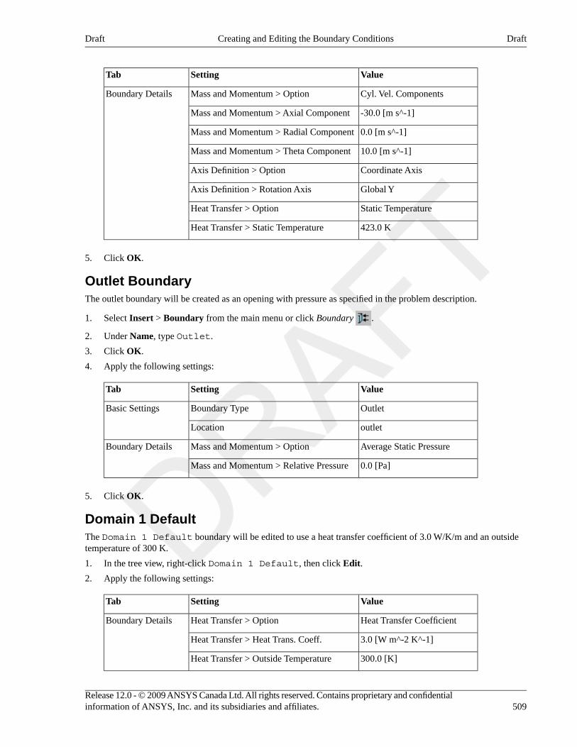
ValueSettingTab
Cyl. Vel. ComponentsMass and Momentum > OptionBoundary Details
-30.0 [m s^-1]Mass and Momentum > Axial Component
0.0 [m s^-1]Mass and Momentum > Radial Component
10.0 [m s^-1]Mass and Momentum > Theta Component
Coordinate AxisAxis Definition > Option
Global YAxis Definition > Rotation Axis
Static TemperatureHeat Transfer > Option
423.0 KHeat Transfer > Static Temperature
5. Click OK.
Outlet BoundaryThe outlet boundary will be created as an opening with pressure as specified in the problem description.
1. Select Insert > Boundary from the main menu or click Boundary .
2. Under Name, type Outlet.
3. Click OK.
4. Apply the following settings:
ValueSettingTab
OutletBoundary TypeBasic Settings
outletLocation
Average Static PressureMass and Momentum > OptionBoundary Details
0.0 [Pa]Mass and Momentum > Relative Pressure
5. Click OK.
Domain 1 DefaultThe Domain 1 Default boundary will be edited to use a heat transfer coefficient of 3.0 W/K/m and an outsidetemperature of 300 K.
1. In the tree view, right-click Domain 1 Default, then click Edit.
2. Apply the following settings:
ValueSettingTab
Heat Transfer CoefficientHeat Transfer > OptionBoundary Details
3.0 [W m^-2 K^-1]Heat Transfer > Heat Trans. Coeff.
300.0 [K]Heat Transfer > Outside Temperature
509Release 12.0 - © 2009 ANSYS Canada Ltd. All rights reserved. Contains proprietary and confidentialinformation of ANSYS, Inc. and its subsidiaries and affiliates.
DraftCreating and Editing the Boundary ConditionsDraft
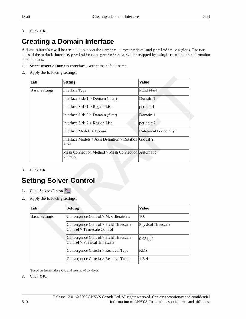
3. Click OK.
Creating a Domain InterfaceA domain interface will be created to connect the Domain 1, periodic1 and periodic 2 regions. The twosides of the periodic interface, periodic1 and periodic 2, will be mapped by a single rotational transformationabout an axis.
1. Select Insert > Domain Interface. Accept the default name.
2. Apply the following settings:
ValueSettingTab
Fluid FluidInterface TypeBasic Settings
Domain 1Interface Side 1 > Domain (filter)
periodic1Interface Side 1 > Region List
Domain 1Interface Side 2 > Domain (filter)
periodic 2Interface Side 2 > Region List
Rotational PeriodicityInterface Models > Option
Global YInterface Models > Axis Definition > RotationAxis
AutomaticMesh Connection Method > Mesh Connection> Option
3. Click OK.
Setting Solver Control1. Click Solver Control .
2. Apply the following settings:
ValueSettingTab
100Convergence Control > Max. IterationsBasic Settings
Physical TimescaleConvergence Control > Fluid TimescaleControl > Timescale Control
0.05 [s]aConvergence Control > Fluid TimescaleControl > Physical Timescale
RMSConvergence Criteria > Residual Type
1.E-4Convergence Criteria > Residual Target
aBased on the air inlet speed and the size of the dryer.
3. Click OK.
Release 12.0 - © 2009 ANSYS Canada Ltd. All rights reserved. Contains proprietary and confidentialinformation of ANSYS, Inc. and its subsidiaries and affiliates.510
DraftCreating a Domain InterfaceDraft
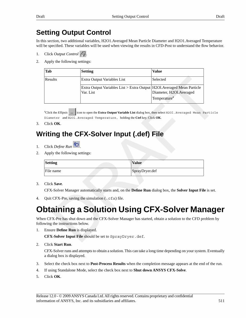
Setting Output ControlIn this section, two additional variables, H2O1.Averaged Mean Particle Diameter and H2O1.Averaged Temperaturewill be specified. These variables will be used when viewing the results in CFD-Post to understand the flow behavior.
1. Click Output Control .
2. Apply the following settings:
ValueSettingTab
SelectedExtra Output Variables ListResults
H2Ol.Averaged Mean ParticleDiameter, H2Ol.Averaged
Temperaturea
Extra Output Variables List > Extra OutputVar. List
aClick the Ellipsis icon to open the Extra Output Variable List dialog box, then select H2Ol.Averaged Mean Particle
Diameter and H2Ol.Averaged Temperature, holding the Ctrl key. Click OK.
3. Click OK.
Writing the CFX-Solver Input (.def) File
1. Click Define Run .
2. Apply the following settings:
ValueSetting
SprayDryer.defFile name
3. Click Save.
CFX-Solver Manager automatically starts and, on the Define Run dialog box, the Solver Input File is set.
4. Quit CFX-Pre, saving the simulation (.cfx) file.
Obtaining a Solution Using CFX-Solver ManagerWhen CFX-Pre has shut down and the CFX-Solver Manager has started, obtain a solution to the CFD problem byfollowing the instructions below.
1. Ensure Define Run is displayed.
CFX-Solver Input File should be set to SprayDryer.def.
2. Click Start Run.
CFX-Solver runs and attempts to obtain a solution. This can take a long time depending on your system. Eventuallya dialog box is displayed.
3. Select the check box next to Post-Process Results when the completion message appears at the end of the run.
4. If using Standalone Mode, select the check box next to Shut down ANSYS CFX-Solve.
5. Click OK.
511Release 12.0 - © 2009 ANSYS Canada Ltd. All rights reserved. Contains proprietary and confidentialinformation of ANSYS, Inc. and its subsidiaries and affiliates.
DraftSetting Output ControlDraft
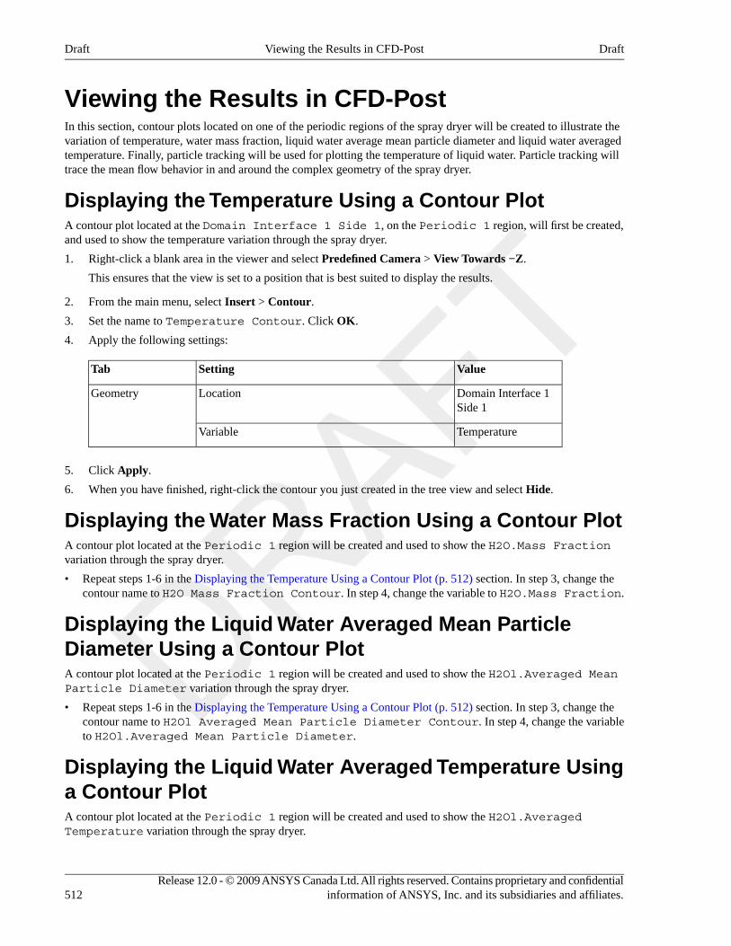
Viewing the Results in CFD-PostIn this section, contour plots located on one of the periodic regions of the spray dryer will be created to illustrate thevariation of temperature, water mass fraction, liquid water average mean particle diameter and liquid water averagedtemperature. Finally, particle tracking will be used for plotting the temperature of liquid water. Particle tracking willtrace the mean flow behavior in and around the complex geometry of the spray dryer.
Displaying the Temperature Using a Contour PlotA contour plot located at the Domain Interface 1 Side 1, on the Periodic 1 region, will first be created,and used to show the temperature variation through the spray dryer.
1. Right-click a blank area in the viewer and select Predefined Camera > View Towards −Z.
This ensures that the view is set to a position that is best suited to display the results.
2. From the main menu, select Insert > Contour.
3. Set the name to Temperature Contour. Click OK.
4. Apply the following settings:
ValueSettingTab
Domain Interface 1Side 1
LocationGeometry
TemperatureVariable
5. Click Apply.
6. When you have finished, right-click the contour you just created in the tree view and select Hide.
Displaying the Water Mass Fraction Using a Contour PlotA contour plot located at the Periodic 1 region will be created and used to show the H2O.Mass Fractionvariation through the spray dryer.
• Repeat steps 1-6 in the Displaying the Temperature Using a Contour Plot (p. 512) section. In step 3, change thecontour name to H2O Mass Fraction Contour. In step 4, change the variable to H2O.Mass Fraction.
Displaying the Liquid Water Averaged Mean ParticleDiameter Using a Contour PlotA contour plot located at the Periodic 1 region will be created and used to show the H2Ol.Averaged MeanParticle Diameter variation through the spray dryer.
• Repeat steps 1-6 in the Displaying the Temperature Using a Contour Plot (p. 512) section. In step 3, change thecontour name to H2Ol Averaged Mean Particle Diameter Contour. In step 4, change the variableto H2Ol.Averaged Mean Particle Diameter.
Displaying the Liquid Water Averaged Temperature Usinga Contour PlotA contour plot located at the Periodic 1 region will be created and used to show the H2Ol.AveragedTemperature variation through the spray dryer.
Release 12.0 - © 2009 ANSYS Canada Ltd. All rights reserved. Contains proprietary and confidentialinformation of ANSYS, Inc. and its subsidiaries and affiliates.512
DraftViewing the Results in CFD-PostDraft
• Repeat steps 1-6 in the Displaying the Temperature Using a Contour Plot (p. 512) section. In step 3, change thecontour name to H2Ol Averaged Temperature Contour. In step 4, change the variable toH2Ol.Averaged Temperature.
Displaying the Liquid Water Temperature Using ParticleTrackingThis section outlines the steps for using particle tracking to trace the variation of the water temperature.
1. Right-click a blank area in the viewer and select Predefined Camera > Isometric View (Z up).
This ensures that the view is set to a position that is best suited to display the results.
2. From the main menu, select Insert > Particle Track.
3. Set the name to H2Ol Temperature. Click OK.
4. Apply the following settings:
ValueSettingTab
VariableModeColor
H20l.TemperatureVariable
5. Click Apply.
From the contours and particle tracks, notice that the water droplets entering the spray dryer through the WaterNozzle recirculates in the region between the two inlets before merging in with the stream of hot air enteringthe spray dryer through the Air Inlet. Based on this flow of the water drop, the temperature of the hot gascoming from the Air Inlet decreases as the process takes place. During the spray drying cycle, the air transfersits thermal energy to the liquid water drops, leading to evaporation. As the air carries the thermal energy byconvection, liquid water droplets that are close to the Air Inlet see their temperature increase, which leadsto evaporation, resulting in a decrease in droplet diameter and an increase in the amount of water vapor.
Displaying the Diameter of a Water Drop Using ParticleTrackingThis section outlines the steps for using particle tracking to trace the variation of water droplet diameter.
1. Repeat steps 2-5 in the Displaying the Liquid Water Temperature Using Particle Tracking (p. 513) section. In step3, change the name to H2Ol Mean Particle Diameter. In step 4, change the variable name to H20l.MeanParticle Diameter
From the water drop diameter particle track, we can see that as the air from the Air Inlet transfers its thermalenergy to the liquid water, the diameter of water drops decreases as they evaporate. So when the water drop moveaway from the Water Nozzle, its diameter decreases as a function of the temperature increase.
2. Quit CFD-Post, saving the state (.cst) file at your discretion.
513Release 12.0 - © 2009 ANSYS Canada Ltd. All rights reserved. Contains proprietary and confidentialinformation of ANSYS, Inc. and its subsidiaries and affiliates.
DraftDisplaying the Liquid Water Temperature Using Particle TrackingDraft

Release 12.0 - © 2009 ANSYS Canada Ltd. All rights reserved. Contains proprietary and confidentialinformation of ANSYS, Inc. and its subsidiaries and affiliates.
Chapter 30. Coal CombustionThis tutorial includes:
• Tutorial Features (p. 515)
• Overview of the Problem to Solve (p. 515)
• Before You Begin (p. 517)
• Starting CFX-Pre (p. 517)
• Coal Combustion Simulation (p. 517)
• Coal Combustion Simulation with Swirl (p. 530)
• Coal Combustion Simulation with Swirl and Nitrogen Oxide (p. 533)
Tutorial FeaturesIn this tutorial you will learn about:
• Importing a CCL file in CFX-Pre.
• Setting up and using Proximate/Ultimate analysis for hydrocarbon fuels in CFX-Pre.
• Viewing the results for nitrogen oxide in CFD-Post.
DetailsFeatureComponent
General ModeUser ModeCFX-Pre
Steady StateAnalysis Type
Reacting Mixture, HydrocarbonFuel
Fluid Type
ImportCCL File
Single DomainDomain Type
Coal InletBoundaries
Air Inlet
Outlet
No-slip Wall
Periodic
Symmetry
Particle TrackingPlotsCFD-Post
Overview of the Problem to SolveIn this tutorial, you will model coal combustion and radiation in a furnace. Three different coal combustion simulationswill be set up:
• Coal Combustion with no-swirl burners where there is no release of nitrogen oxide during the burning process.
• Coal Combustion with swirl burners where there is no release of nitrogen oxide during the burning process.
515Release 12.0 - © 2009 ANSYS Canada Ltd. All rights reserved. Contains proprietary and confidentialinformation of ANSYS, Inc. and its subsidiaries and affiliates.
DraftDraft
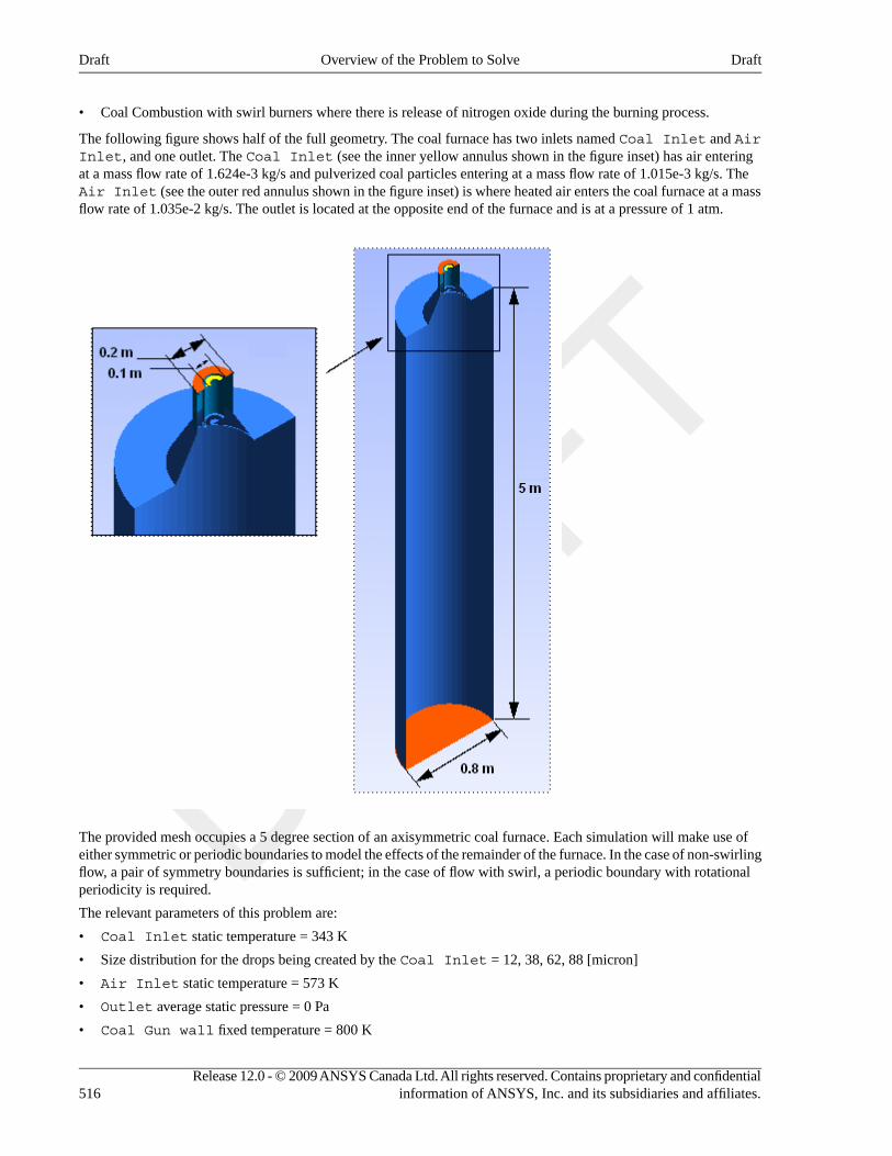
• Coal Combustion with swirl burners where there is release of nitrogen oxide during the burning process.
The following figure shows half of the full geometry. The coal furnace has two inlets named Coal Inlet and AirInlet, and one outlet. The Coal Inlet (see the inner yellow annulus shown in the figure inset) has air enteringat a mass flow rate of 1.624e-3 kg/s and pulverized coal particles entering at a mass flow rate of 1.015e-3 kg/s. TheAir Inlet (see the outer red annulus shown in the figure inset) is where heated air enters the coal furnace at a massflow rate of 1.035e-2 kg/s. The outlet is located at the opposite end of the furnace and is at a pressure of 1 atm.
The provided mesh occupies a 5 degree section of an axisymmetric coal furnace. Each simulation will make use ofeither symmetric or periodic boundaries to model the effects of the remainder of the furnace. In the case of non-swirlingflow, a pair of symmetry boundaries is sufficient; in the case of flow with swirl, a periodic boundary with rotationalperiodicity is required.
The relevant parameters of this problem are:
• Coal Inlet static temperature = 343 K
• Size distribution for the drops being created by the Coal Inlet = 12, 38, 62, 88 [micron]
• Air Inlet static temperature = 573 K
• Outlet average static pressure = 0 Pa
• Coal Gun wall fixed temperature = 800 K
Release 12.0 - © 2009 ANSYS Canada Ltd. All rights reserved. Contains proprietary and confidentialinformation of ANSYS, Inc. and its subsidiaries and affiliates.516
DraftOverview of the Problem to SolveDraft
• Coal Inlet wall fixed temperature = 343 K
• Air Inlet wall fixed temperature = 573 K
• Furnace wall fixed temperature = 1400 K
• O2 mass fraction = 0.232
• Proximate/ultimate analysis data for the coal. Note that proximate/ultimate analysis data is used to characterize theproperties of the coal including the content of moisture, volatile, free carbon, and ash, as well as the mass fractionsof carbon, hydrogen and oxygen (the major components), sulfur and nitrogen.
The approach for solving this problem is to first import, into CFX-Pre, a CCL file with the proximate/ultimate analysisdata for the coal and the required materials and reactions. The first simulation will be without nitrogen oxide or swirl.Only small changes to the boundary conditions will be made to create the second simulation, which has swirl in theflow. After each of the first two simulations, you will use CFD-Post to see the variation of temperature, water massfraction and radiation intensity. You will examine particle tracks colored by temperature and by ash mass fraction. Thelast simulation has swirl and also involves the release of nitrogen oxide. Finally, you will use CFD-Post to see thedistribution of nitrogen oxide in the third simulation.
Before You BeginIf this is the first tutorial you are working with, it is important to review the following topics before beginning:
• Preparing a Working Directory (p. 23)
• Setting the Working Directory and Starting ANSYS CFX (p. 23)
• Changing the Display Colors (p. 24)
• Playing a Tutorial Session File (p. 24)
Starting CFX-Pre1. Prepare the working directory using the following files in the examples directory:
• CoalCombustion.gtm
• CoalCombustion_Reactions_Materials.ccl
• CoalCombustion_nonox.pre
• CoalCombustion_nonox_swirl.pre
• CoalCombustion_noxcpp_swirl.pre
For details, see Preparing a Working Directory (p. 23).
2. Set the working directory and start CFX-Pre.
For details, see Setting the Working Directory and Starting ANSYS CFX (p. 23)
Coal Combustion SimulationIf you want to set up the simulation automatically using a tutorial session file, run CoalCombustion_nonox.pre.For details, see Playing a Tutorial Session File (p. 24). Then proceed to Obtaining a Solution for the Simulation usingCFX-Solver Manager (p. 528).
If you want to set up the simulation manually, proceed to the following steps:
You will first create a simulation where there is no release of nitrogen oxide, a hazardous chemical, during the process.Swirl burners will not be used in this simulation.
1. Select File > New Case.
2. Select General and click OK.
517Release 12.0 - © 2009 ANSYS Canada Ltd. All rights reserved. Contains proprietary and confidentialinformation of ANSYS, Inc. and its subsidiaries and affiliates.
DraftBefore You BeginDraft
3. Edit Case Options > General in the Outline tree view and ensure that Automatic Default Domain andAutomatic Default Interfaces are turned off.
4. Select File > Save Case As.
5. Set File name to CoalCombustion_nonox.cfx.
6. Click Save.
Importing the Mesh1. Select File > Import > Mesh.
2. Set Files of type to CFX Mesh(*gtm *cfx).
3. Select CoalCombustion.gtm from your working directory.
4. Click Open.
5. Right-click a blank area in the viewer and select Predefined Camera > Isometric View (Z up) from the shortcutmenu.
Importing the Coal Combustion Materials CCL FileCFX Command Language (CCL) consists of commands used to carry out actions in CFX-Pre, CFX-Solver Manager,and CFD-Post. The proximate/ultimate analysis data for the coal as well as the materials and reactions required for thecombustion simulation will be imported from the CCL file. You will review, then import, the contents of theCoalCombustion_Reactions_Materials.ccl file.
NoteThe physics for a simulation can be saved to a CCL (CFX Command Language) file at any time by selectingFile > Export > CCL.
1. Open CoalCombustion_Reactions_Materials.ccl with a text editor and take the time to look at theinformation it contains.
The CCL sets up the following reactions:
• Fuel Gas Oxygen
• HC Fuel Char Field
• HC Fuel Devolat
• Prompt NO Fuel Gas PDF
• Thermal NO PDF.
The CCL also sets up the following materials:
• Ash
• Char
• Fuel Gas
• Gas mixture
• HC Fuel
• HC Fuel Gas Binary Mixture
• Raw Combustible
The reactions Prompt NO Fuel Gas PDF and Thermal NO PDF are used only in the third simulation.Other pure substances required for the simulation will be loaded from the standard CFX-Pre materials library.
2. In CFX-Pre, select File > Import > CCL.
Release 12.0 - © 2009 ANSYS Canada Ltd. All rights reserved. Contains proprietary and confidentialinformation of ANSYS, Inc. and its subsidiaries and affiliates.518
DraftImporting the MeshDraft
The Import CCL dialog box appears.
3. Under Import Method, select Replace.
This will replace the materials list in the current simulation with the ones in the newly imported CCL.
4. Under Import Method, select Auto-load materials.
This will load pure materials such as CO2, H2O, N2, O2, and NO — the materials referenced by the importedmixtures and reactions — from the CFX-Pre materials library.
5. Select CoalCombustion_Reactions_Materials.ccl (the file you reviewed earlier).
6. Click Open.
7. Expand the Materials and Reactions branches under Simulation to make sure that all the materialsand reactions described above are present.
Creating the DomainCreate a new domain named Furnace as follows:
1. Right-click Simulation > Flow Analysis 1 in the Outline tree view and click Insert > Domain.
2. Set Name to Furnace.
3. Click OK
4. On the Basic Settings, tab under Fluid and Particle Definitions, delete Fluid 1 and create a new fluid definitionnamed Gas Mixture.
5. Click Add new item and create a new fluid definition named HC Fuel.
6. Apply the following settings:
ValueSettingTab
B40Location and Type > LocationBasic Settings
Gas MixtureFluid and Particle Definitions
Gas MixtureaFluid and Particle Definitions > GasMixture > Material
Continuous FluidFluid and Particle Definitions > GasMixture > Morphology > Option
HC FuelFluid and Particle Definitions
HC FuelbFluid and Particle Definitions > HC Fuel> Material
Particle Transport SolidFluid and Particle Definitions > HC Fuel> Morphology > Option
(Selected)Fluid and Particle Definitions > HC Fuel> Morphology > Particle DiameterChange
Mass EquivalentFluid and Particle Definitions > HC Fuel> Morphology > Particle DiameterChange > Option
519Release 12.0 - © 2009 ANSYS Canada Ltd. All rights reserved. Contains proprietary and confidentialinformation of ANSYS, Inc. and its subsidiaries and affiliates.
DraftCreating the DomainDraft
ValueSettingTab
(Selected)Multiphase > Multiphase ReactionsFluid Models
HC Fuel Char Field, HC FuelDevolat
Multiphase > Multiphase Reactions >Reactions List
Fluid DependentHeat Transfer > Option
Fluid DependentCombustion > Option
Fluid DependentThermal Radiation > Option
Gas MixtureFluidFluid Specific Models
Thermal EnergyFluid > Gas Mixture > Heat Transfer >Heat Transfer > Option
Discrete TransferFluid > Gas Mixture > ThermalRadiation > Option
(Selected)Fluid > Gas Mixture > ThermalRadiation > Number of Rays
32cFluid > Gas Mixture > ThermalRadiation > Number of Rays > Numberof Rays
HC FuelFluid
Particle TemperatureFluid > HC Fuel > Heat Transfer > HeatTransfer > Option
Gas Mixture | HC FuelFluid PairFluid Pair Models
Fully CoupledFluid Pair > Gas Mixture | HC Fuel >Particle Coupling
Schiller NaumannFluid Pair > Gas Mixture | HC Fuel >Momentum Transfer > Drag Force >Option
Ranz MarshallFluid Pair > Gas Mixture | HC Fuel >Heat Transfer > Option
OpaqueFluid Pair > Gas Mixture | HC Fuel >Thermal Radiation Transfer > Option
1dFluid Pair > Gas Mixture | HC Fuel >Thermal Radiation Transfer > Emissivity
(Selected)Fluid Pair > Gas Mixture | HC Fuel >Thermal Radiation Transfer > ParticleCoupling
Release 12.0 - © 2009 ANSYS Canada Ltd. All rights reserved. Contains proprietary and confidentialinformation of ANSYS, Inc. and its subsidiaries and affiliates.520
DraftCreating the DomainDraft
ValueSettingTab
Fully CoupledFluid Pair > Gas Mixture | HC Fuel >Thermal Radiation Transfer > ParticleCoupling > Particle Coupling
aClick the Ellipsis icon to open the Selection Dialog dialog box, then select Gas Mixture under the Gas Phase Combustion
branch. Click OK.
bClick the Ellipsis icon to open the Material dialog box, then select HC Fuel under the Particle Solids branch. Click OK.
cIncreasing the number of rays to 32 from the default 8, increases the number of rays leaving the bounding surfaces and increases the accuracyof the thermal radiation calculation.dWith this setting, the particles are modeled as black bodies.
7. Click OK.
Creating the Boundary ConditionsIn this section you will create boundary conditions for the coal inlet, the air inlet, the outlet, and multiple no-slip walls.You will also create two symmetry-plane boundary conditions for this no-swirl case.
Coal Inlet BoundaryYou will create the coal inlet boundary with mass flow rate and static temperature set consistently with the problemdescription. The particle diameter distribution will be set to Discrete Diameter Distribution to modelparticles of more than one specified diameter. Diameter values will be listed as specified in the problem description.A mass fraction as well as a number fraction will be specified for each of the diameter entries. The total of massfractions and the total of number fractions will sum to unity.
1. Create a boundary named Coal Inlet.
2. Apply the following settings to Coal Inlet:
ValueSettingTab
InletBoundary TypeBasic Settings
CoalInletLocation
Mass Flow RateMass and Momentum > OptionBoundary Details
0.001624 [kg s^-1]Mass and Momentum > Mass Flow Rate
Normal to Boundary ConditionFlow Direction > Option
Static TemperatureHeat Transfer > Option
343 [K]Heat Transfer > Static Temperature
O2Component Details
Mass FractionComponent Details > O2 > Option
0.232Component Details > O2 > Mass Fraction
(Selected)Boundary Conditions > HC Fuel > ParticleBehavior > Define Particle Behavior
Fluid Values
521Release 12.0 - © 2009 ANSYS Canada Ltd. All rights reserved. Contains proprietary and confidentialinformation of ANSYS, Inc. and its subsidiaries and affiliates.
DraftCreating the Boundary ConditionsDraft
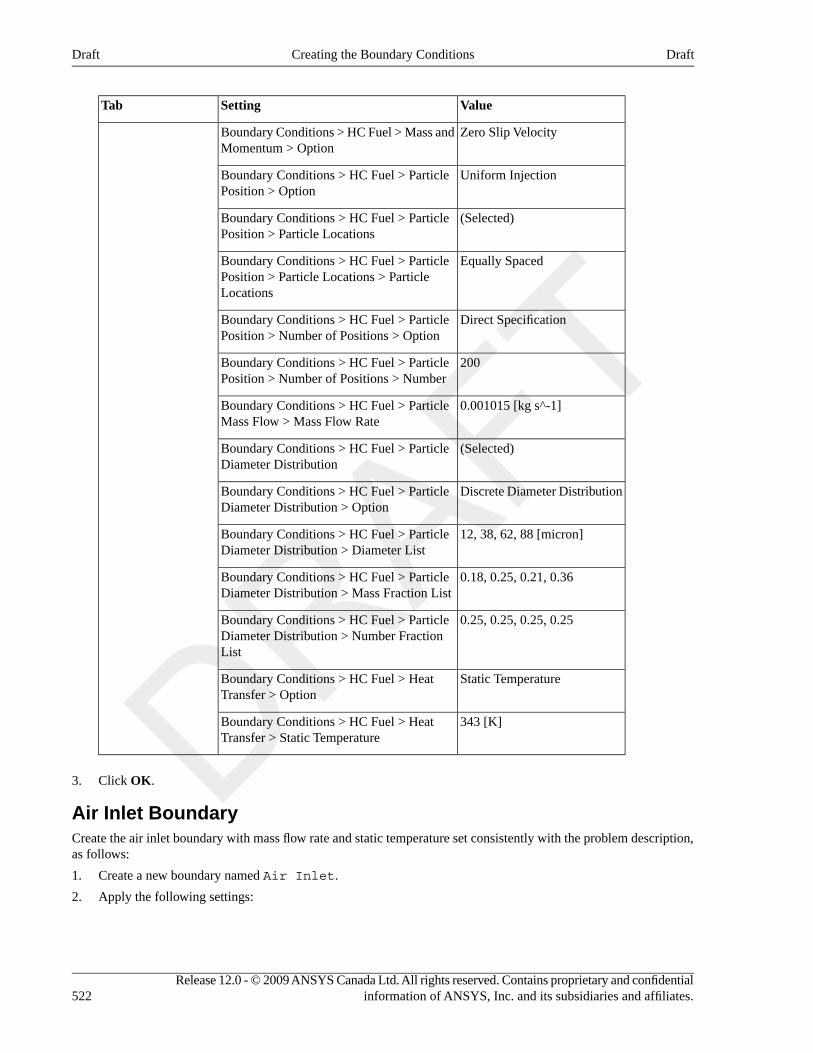
ValueSettingTab
Zero Slip VelocityBoundary Conditions > HC Fuel > Mass andMomentum > Option
Uniform InjectionBoundary Conditions > HC Fuel > ParticlePosition > Option
(Selected)Boundary Conditions > HC Fuel > ParticlePosition > Particle Locations
Equally SpacedBoundary Conditions > HC Fuel > ParticlePosition > Particle Locations > ParticleLocations
Direct SpecificationBoundary Conditions > HC Fuel > ParticlePosition > Number of Positions > Option
200Boundary Conditions > HC Fuel > ParticlePosition > Number of Positions > Number
0.001015 [kg s^-1]Boundary Conditions > HC Fuel > ParticleMass Flow > Mass Flow Rate
(Selected)Boundary Conditions > HC Fuel > ParticleDiameter Distribution
Discrete Diameter DistributionBoundary Conditions > HC Fuel > ParticleDiameter Distribution > Option
12, 38, 62, 88 [micron]Boundary Conditions > HC Fuel > ParticleDiameter Distribution > Diameter List
0.18, 0.25, 0.21, 0.36Boundary Conditions > HC Fuel > ParticleDiameter Distribution > Mass Fraction List
0.25, 0.25, 0.25, 0.25Boundary Conditions > HC Fuel > ParticleDiameter Distribution > Number FractionList
Static TemperatureBoundary Conditions > HC Fuel > HeatTransfer > Option
343 [K]Boundary Conditions > HC Fuel > HeatTransfer > Static Temperature
3. Click OK.
Air Inlet BoundaryCreate the air inlet boundary with mass flow rate and static temperature set consistently with the problem description,as follows:
1. Create a new boundary named Air Inlet.
2. Apply the following settings:
Release 12.0 - © 2009 ANSYS Canada Ltd. All rights reserved. Contains proprietary and confidentialinformation of ANSYS, Inc. and its subsidiaries and affiliates.522
DraftCreating the Boundary ConditionsDraft
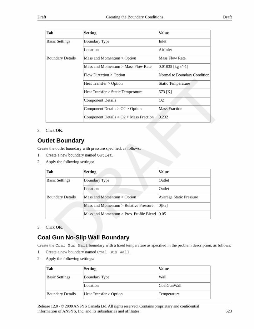
ValueSettingTab
InletBoundary TypeBasic Settings
AirInletLocation
Mass Flow RateMass and Momentum > OptionBoundary Details
0.01035 [kg s^-1]Mass and Momentum > Mass Flow Rate
Normal to Boundary ConditionFlow Direction > Option
Static TemperatureHeat Transfer > Option
573 [K]Heat Transfer > Static Temperature
O2Component Details
Mass FractionComponent Details > O2 > Option
0.232Component Details > O2 > Mass Fraction
3. Click OK.
Outlet BoundaryCreate the outlet boundary with pressure specified, as follows:
1. Create a new boundary named Outlet.
2. Apply the following settings:
ValueSettingTab
OutletBoundary TypeBasic Settings
OutletLocation
Average Static PressureMass and Momentum > OptionBoundary Details
0[Pa]Mass and Momentum > Relative Pressure
0.05Mass and Momentum > Pres. Profile Blend
3. Click OK.
Coal Gun No-Slip Wall BoundaryCreate the Coal Gun Wall boundary with a fixed temperature as specified in the problem description, as follows:
1. Create a new boundary named Coal Gun Wall.
2. Apply the following settings:
ValueSettingTab
WallBoundary TypeBasic Settings
CoalGunWallLocation
TemperatureHeat Transfer > OptionBoundary Details
523Release 12.0 - © 2009 ANSYS Canada Ltd. All rights reserved. Contains proprietary and confidentialinformation of ANSYS, Inc. and its subsidiaries and affiliates.
DraftCreating the Boundary ConditionsDraft
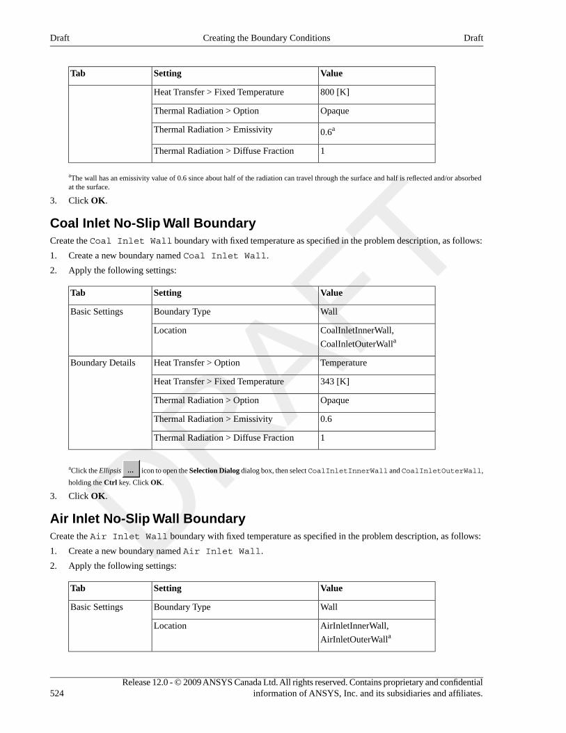
ValueSettingTab
800 [K]Heat Transfer > Fixed Temperature
OpaqueThermal Radiation > Option
0.6aThermal Radiation > Emissivity
1Thermal Radiation > Diffuse Fraction
aThe wall has an emissivity value of 0.6 since about half of the radiation can travel through the surface and half is reflected and/or absorbedat the surface.
3. Click OK.
Coal Inlet No-Slip Wall BoundaryCreate the Coal Inlet Wall boundary with fixed temperature as specified in the problem description, as follows:
1. Create a new boundary named Coal Inlet Wall.
2. Apply the following settings:
ValueSettingTab
WallBoundary TypeBasic Settings
CoalInletInnerWall,
CoalInletOuterWallaLocation
TemperatureHeat Transfer > OptionBoundary Details
343 [K]Heat Transfer > Fixed Temperature
OpaqueThermal Radiation > Option
0.6Thermal Radiation > Emissivity
1Thermal Radiation > Diffuse Fraction
aClick the Ellipsis icon to open the Selection Dialog dialog box, then select CoalInletInnerWall and CoalInletOuterWall,
holding the Ctrl key. Click OK.
3. Click OK.
Air Inlet No-Slip Wall BoundaryCreate the Air Inlet Wall boundary with fixed temperature as specified in the problem description, as follows:
1. Create a new boundary named Air Inlet Wall.
2. Apply the following settings:
ValueSettingTab
WallBoundary TypeBasic Settings
AirInletInnerWall,
AirInletOuterWallaLocation
Release 12.0 - © 2009 ANSYS Canada Ltd. All rights reserved. Contains proprietary and confidentialinformation of ANSYS, Inc. and its subsidiaries and affiliates.524
DraftCreating the Boundary ConditionsDraft
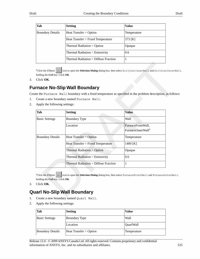
ValueSettingTab
TemperatureHeat Transfer > OptionBoundary Details
573 [K]Heat Transfer > Fixed Temperature
OpaqueThermal Radiation > Option
0.6Thermal Radiation > Emissivity
1Thermal Radiation > Diffuse Fraction
aClick the Ellipsis icon to open the Selection Dialog dialog box, then select AirInletInnerWall and AirInletOuterWall,
holding the Ctrl key. Click OK.
3. Click OK.
Furnace No-Slip Wall BoundaryCreate the Furnace Wall boundary with a fixed temperature as specified in the problem description, as follows:
1. Create a new boundary named Furnace Wall.
2. Apply the following settings:
ValueSettingTab
WallBoundary TypeBasic Settings
FurnaceFrontWall,
FurnaceOuterWallaLocation
TemperatureHeat Transfer > OptionBoundary Details
1400 [K]Heat Transfer > Fixed Temperature
OpaqueThermal Radiation > Option
0.6Thermal Radiation > Emissivity
1Thermal Radiation > Diffuse Fraction
aClick the Ellipsis icon to open the Selection Dialog dialog box, then select FurnaceFrontWall and FurnaceOuterWall,
holding the Ctrl key. Click OK.
3. Click OK.
Quarl No-Slip Wall Boundary1. Create a new boundary named Quarl Wall.
2. Apply the following settings:
ValueSettingTab
WallBoundary TypeBasic Settings
QuarlWallLocation
TemperatureHeat Transfer > OptionBoundary Details
525Release 12.0 - © 2009 ANSYS Canada Ltd. All rights reserved. Contains proprietary and confidentialinformation of ANSYS, Inc. and its subsidiaries and affiliates.
DraftCreating the Boundary ConditionsDraft
ValueSettingTab
1200 [K]Heat Transfer > Fixed Temperature
OpaqueThermal Radiation > Option
0.6Thermal Radiation > Emissivity
1Thermal Radiation > Diffuse Fraction
3. Click OK.
Symmetry Plane BoundariesYou will use symmetry plane boundaries on the front and back regions of the cavity.
Symmetry Plane 1 Boundary1. Create a new boundary named Symmetry Plane 1.
2. Apply the following settings:
ValueSettingTab
SymmetryBoundary TypeBasic Settings
PeriodicSide1Location
3. Click OK.
Symmetry Plane 2 Boundary1. Create a new boundary named Symmetry Plane 2.
2. Apply the following settings:
ValueSettingTab
SymmetryBoundary TypeBasic Settings
PeriodicSide2Location
3. Click OK.
Setting Solver Control1. Click Solver Control .
2. Apply the following settings:
ValueSettingTab
600Convergence Control > Max. IterationsBasic Settings
Physical TimescaleConvergence Control > Fluid TimescaleControl > Timescale Control
Release 12.0 - © 2009 ANSYS Canada Ltd. All rights reserved. Contains proprietary and confidentialinformation of ANSYS, Inc. and its subsidiaries and affiliates.526
DraftSymmetry Plane 1 BoundaryDraft
ValueSettingTab
0.005 [s]aConvergence Control > Fluid TimescaleControl > Physical Timescale
(Selected)Particle Coupling Control > First Iterationfor Particle Calculation
Particle Control
25bParticle Coupling Control > First Iterationfor Particle Calculation > First Iteration
(Selected)Particle Coupling Control > IterationFrequency
10cParticle Coupling Control > IterationFrequency > Iteration Frequency
(Selected)Particle Under Relaxation Factors
0.75Particle Under Relaxation Factors > Vel.Under Relaxation
0.75Particle Under Relaxation Factors > Energy
0.75Particle Under Relaxation Factors > Mass
(Selected)Particle Ignition
1000 [K]Particle Ignition > Ignition Temperature
(Selected)Particle Source Smoothing
SmoothParticle Source Smoothing > Option
(Selected)Thermal Radiation ControlAdvanced Options
(Selected)Thermal Radiation Control > CoarseningControl
(Selected)Thermal Radiation Control > CoarseningControl > Target Coarsening Rate
16dThermal Radiation Control > CoarseningControl > Target Coarsening Rate > Rate
aBased on the air inlet speed and the size of the combustor.bThe First Iteration parameter sets the coefficient-loop iteration number at which particles are first tracked; it allows the continuous-phaseflow to develop before tracking droplets through the flow. Experience has shown that the value usually has to be increased to 25 from thedefault of 10.cThe Iteration Frequency parameter is the frequency at which particles are injected into the flow after the First Iteration for Particle Calculationiteration number. The iteration frequency allows the continuous phase to settle down between injections because it is affected by sources ofmomentum, heat, and mass from the droplet phase. Experience has shown that the value usually has to be increased to 10 from the default of5.dThe Target Coarsening Rate parameter controls the size of the radiation element required for calculating Thermal Radiation. Decreasing thesize of the element to 16, from the default 64, increases the accuracy of the solution obtained, while increasing the computing time requiredfor the calculations.
3. Click OK.
527Release 12.0 - © 2009 ANSYS Canada Ltd. All rights reserved. Contains proprietary and confidentialinformation of ANSYS, Inc. and its subsidiaries and affiliates.
DraftSetting Solver ControlDraft
Writing the CFX-Solver Input (.def) File
1. Click Define Run .
2. Apply the following settings:
ValueSetting
CoalCombustion_nonox.defFile name
3. Click Save.
CFX-Solver Manager automatically starts and, on the Define Run dialog box, the Solver Input File is set.
4. Quit CFX-Pre, saving the simulation (.cfx) file.
Obtaining a Solution for the Simulation using CFX-SolverManagerWhen CFX-Pre has shut down and the CFX-Solver Manager has started, obtain a solution to the CFD problem byfollowing the instructions below:
1. Ensure that the Define Run dialog box is displayed.
Solver Input File should be set to CoalCombustion_nonox.def.
2. Click Start Run.
CFX-Solver runs and attempts to obtain a solution. This can take a long time depending on your system. Eventuallya dialog box is displayed.
3. At the end of the run, on the completion message that appears, select Post-Process Results.
4. If using Standalone mode, select Shut down CFX-Solver Manager.
5. Click OK.
Viewing the Results in CFD-PostIn this section, you will make plots showing the variation of temperature, water mass fraction, and radiation intensityon the Symmetry Plane 1 boundary. You will also color the particle tracks, which were produced by the solverand included in the results file, by temperature and by ash mass fraction. The particle tracks help to illustrate the meanflow behavior in the coal furnace.
Displaying the Temperature on a Symmetry Plane1. Right-click a blank area in the viewer and select Predefined Camera > Isometric View (Z up).
This orients the geometry with the inlets at the top, as shown at the beginning of this tutorial.
2. Edit Cases > CoalCombustion_nonox_001 > Furnace > Symmetry Plane 1.
3. Apply the following settings:
ValueSettingTab
VariableModeColor
TemperatureVariable
Release 12.0 - © 2009 ANSYS Canada Ltd. All rights reserved. Contains proprietary and confidentialinformation of ANSYS, Inc. and its subsidiaries and affiliates.528
DraftWriting the CFX-Solver Input (.def) FileDraft
ValueSettingTab
(Selected)Show FacesRender
(Cleared)aLighting
aTurning off the lighting makes the colors accurate in the 3D view, but can make it more difficult to perceive depth. As an alternative toturning off the lighting, you can try rotating the view to a different position.
4. Click Apply.
As expected for a non-swirling case, the flame appears a significant distance away from the burner. The flame islikely unstable, as evidenced by the rate of solver convergence; the next simulation in this tutorial involves swirl,which tends to stabilize the flame, and has much faster solver convergence.
Displaying the Water Mass FractionChange the variable used for coloring the plot to H2O.Mass Fraction and click Apply.
From the plot it can be seen that water is produced a significant distance away from the burner, as was the flame inthe previous plot. As expected, the mass fraction of water is high where the temperature is high.
Displaying the Radiation Intensity1. Change the variable used for coloring the plot to Radiation Intensity and click Apply.
This plot is directly related to the temperature plot. This result is consistent with radiation being proportional totemperature to the fourth power.
2. When you are finished, right-click Symmetry Plane 1 in the Outline tree view and select Hide.
Displaying the Temperature of the Fuel ParticlesColor the existing particle tracks for the solid particles by temperature:
1. Edit Cases > CoalCombustion_nonox_001 > Res PT for HC Fuel.
2. Apply the following settings:
ValueSettingTab
VariableModeColor
TemperatureVariable
3. Click Apply.
Observing the particle tracks, you can see that coal enters the chamber at a temperature of around 343 K. Thetemperature of the coal, as it moves away from the inlet, rises as it reacts with the air entering from the inlet. Thegeneral location where the temperature of the coal increases rapidly is close to the location where the flame appearsto be according to the plots created earlier. Downstream of this location, the temperature of the coal particlesbegins to drop.
Displaying the Ash Mass Fraction using Particle Tracking1. Change the plot of the particle tracks so that they are colored by HC Fuel.Ash.Mass Fraction.
The ashes form in the flame region, as expected.
2. Quit CFD-Post, saving the state (.cst) file at your discretion.
529Release 12.0 - © 2009 ANSYS Canada Ltd. All rights reserved. Contains proprietary and confidentialinformation of ANSYS, Inc. and its subsidiaries and affiliates.
DraftViewing the Results in CFD-PostDraft
Coal Combustion Simulation with SwirlYou will now create a simulation where swirl burners are used and where there is no release of nitrogen oxide duringthe process. Swirl burners inject a fuel axially into the combustion chamber surrounded by an annular flow of oxidant(normally air) which has, upon injection, some tangential momentum. This rotational component, together with theusually divergent geometry of the burner mouth, cause two important effects:
• They promote intense mixing between fuel and air, which is important for an efficient and stable combustion, andlow emissions.
• They originate a recirculation region, just at the burner mouth, which traps hot combustion products and acts as apermanent ignition source, hence promoting the stability of the flame.
If you want to set up the simulation automatically using a tutorial session file, runCoalCombustion_nonox_swirl.pre. For details, see Playing a Tutorial Session File (p. 24). Then proceedto Obtaining a Solution for the Simulation with Swirl using CFX-Solver Manager (p. 532).
If you want to set up the simulation manually, proceed to the following section.
Opening an Existing Simulation1. Start CFX-Pre if necessary.
2. Select File > Open Case.
3. From your working directory, select CoalCombustion_nonox.cfx and click Open.
4. Select File > Save Case As.
5. Set File name to CoalCombustion_nonox_swirl.cfx.
6. Click Save.
Editing the Boundary ConditionsTo add swirl to the flow, you will edit the Air Inlet boundary to change the flow direction specification fromNormal to Boundary Condition to Cylindrical Components. You will also edit the Outlet boundaryto change the Pressure Profile Blend setting from 0.05 to 0; the reason for this change is explained later.You will also delete the two symmetry plane boundary conditions and replace them with a periodic domain interface.
Air Inlet Boundary1. Edit Simulation > Flow Analysis 1 > Furnace > Air Inlet.
2. Apply the following settings:
ValueSettingTab
Cylindrical ComponentsFlow Direction > OptionBoundary Details
0.88Flow Direction > Axial Component
0Flow Direction > Radial Component
1Flow Direction > Theta Component
Global ZAxis Definition > Rotational Axis
3. Click OK.
Release 12.0 - © 2009 ANSYS Canada Ltd. All rights reserved. Contains proprietary and confidentialinformation of ANSYS, Inc. and its subsidiaries and affiliates.530
DraftCoal Combustion Simulation with SwirlDraft
Outlet BoundaryThe average pressure boundary condition leaves the pressure profile unspecified while constraining the average pressureto the specified value. In some situations, leaving the profile fully unspecified is too weak and convergence difficultiesmay result. The 'Pressure Profile Blend' feature works around this by blending between a unspecified pressure profileand a fully specified pressure profile. By default, the pressure profile blend is 5%. For swirling flow, however, imposingany amount of a uniform pressure profile is inconsistent with the radial pressure profile which should naturally developin response to the fluid rotation, and the pressure profile blend must be set to 0.
1. Edit Simulation > Flow Analysis 1 > Furnace > Outlet.
2. Apply the following settings:
ValueSettingTab
Average Static PressureMass and Momentum > OptionBoundary Details
0Mass and Momentum > Pres. Profile Blend
3. Click OK.
Deleting the Symmetry Plane Boundaries1. In the Outline tree view, right-click Simulation > Flow Analysis 1 > Furnace > Symmetry Plane
1, then select Delete.
2. Delete the other symmetry boundary as well.
Creating a Domain InterfaceYou will insert a domain interface to connect the Periodic Side 1 and Periodic Side 2 regions.
1. Create a domain interface named Periodic.
2. Apply the following settings:
ValueSettingTab
Fluid FluidInterface TypeBasic Settings
PeriodicSide1Interface Side 1 > Region List
PeriodicSide2Interface Side 2 > Region List
Rotational PeriodicityInterface Models > Option
3. Click OK.
Writing the CFX-Solver Input (.def) File
1. Click Define Run .
2. Apply the following settings:
ValueSetting
CoalCombustion_nonox_swirl.defFile name
531Release 12.0 - © 2009 ANSYS Canada Ltd. All rights reserved. Contains proprietary and confidentialinformation of ANSYS, Inc. and its subsidiaries and affiliates.
DraftCreating a Domain InterfaceDraft
3. Click Save.
CFX-Solver Manager automatically starts and, on the Define Run dialog box, the Solver Input File is set.
4. Quit CFX-Pre, saving the simulation (.cfx) file.
Obtaining a Solution for the Simulation with Swirl usingCFX-Solver ManagerWhen CFX-Pre has shut down and the CFX-Solver Manager has started, obtain a solution to the CFD problem byfollowing the instructions below.
1. Ensure that the Define Run dialog box is displayed.
Solver Input File should be set to CoalCombustion_nonox_swirl.def.
2. Click Start Run.
CFX-Solver runs and attempts to obtain a solution. This can take a long time depending on your system. Eventuallya dialog box is displayed.
3. At the end of the run, on the completion message that appears, select Post-Process Results.
4. If using Standalone mode, select Shut down CFX-Solver Manager.
5. Click OK.
Viewing the Results for Simulation with Swirl in CFD-PostIn this section, you will make plots showing the variation of temperature, water mass fraction, and radiation intensityon the Periodic Side 1 boundary. You will also color the existing particle tracks by temperature and by ash massfraction.
Displaying the Temperature on a Periodic Interface1. Right-click a blank area in the viewer and select Predefined Camera > Isometric View (Z up).
2. Edit Cases > CoalCombustion_nonox_swirl_001 > Furnace > Periodic Side 1.
3. Apply the following settings:
ValueSettingTab
VariableModeColor
TemperatureVariable
(Selected)Show FacesRender
(Cleared)Lighting
4. Click Apply.
As expected, the flame appears much closer to the burner than in the previous simulation which had no swirl.This is due to the fact that the swirl component applied to the air from Air Inlet tends to entrain coal particlesand keep them near the burner for longer, thus helping them to burn.
Displaying the Water Mass FractionChange the variable used for coloring the plot to H2O.Mass Fraction and click Apply.
Release 12.0 - © 2009 ANSYS Canada Ltd. All rights reserved. Contains proprietary and confidentialinformation of ANSYS, Inc. and its subsidiaries and affiliates.532
DraftObtaining a Solution for the Simulation with Swirl using CFX-Solver ManagerDraft
Similar to the no-swirl case, the mass fraction of water with swirl is directly proportional to the temperature of thefurnace.
Displaying the Radiation Intensity1. Change the variable used for coloring the plot to Radiation Intensity and click Apply.
2. When you are finished, right-click Periodic Side 1 in the Outline tree view and select Hide.
Displaying the Temperature using Particle Tracking1. Edit Cases > CoalCombustion_nonox_swirl_001 > Res PT for HC Fuel.
2. Apply the following settings:
ValueSettingTab
VariableModeColor
TemperatureVariable
3. Click Apply.
Displaying the Ash Mass Fraction using Particle Tracking1. Change the plot of the particle tracks so that they are colored by HC Fuel.Ash.Mass Fraction.
2. Quit CFD-Post, saving the state (.cst) file at your discretion.
Coal Combustion Simulation with Swirl andNitrogen OxideYou will now create a simulation that involves both swirl and the release of nitrogen oxide. The CCL file that waspreviously imported contains the nitrogen oxide material,NO, and reactions,Prompt NO Fuel Gas PDF andThermal NO PDF, required for this combustion simulation. Nitrogen oxide is calculated as a postprocessing stepin the solver.
If you want to set up the simulation automatically using a tutorial session file, runCoalCombustion_noxcpp_swirl.pre. For details, see Playing a Tutorial Session File (p. 24). Then proceedto Obtaining a Solution for the Simulation with Swirl and Nitrogen Oxide using CFX-Solver Manager (p. 535).
If you want to set up the simulation manually, proceed to the following section.
Opening an Existing Simulation1. Start CFX-Pre if necessary.
2. Select File > Open Case.
3. From your working directory, select CoalCombustion_nonox_swirl.cfx and click Open.
4. Select File > Save Case As.
5. Set File name to CoalCombustion_noxcpp_swirl.cfx.
6. Click Save.
533Release 12.0 - © 2009 ANSYS Canada Ltd. All rights reserved. Contains proprietary and confidentialinformation of ANSYS, Inc. and its subsidiaries and affiliates.
DraftCoal Combustion Simulation with Swirl and Nitrogen OxideDraft
Editing the DomainIn this section, you will edit the Furnace domain by adding the new material NO to the materials list. CFX-Solverrequires that you specify enough information for the mass fraction of NO at each of the system inlets. In this case, setthe NO mass fraction at the air and coal inlets to zero.
1. Edit Simulation > Flow Analysis 1 > Furnace.
2. Apply the following settings:
ValueSettingTab
Gas MixtureFluidFluid Specific Models
(Selected)Fluid > Gas Mixture > Combustion >Chemistry Post Processing
NOFluid > Gas Mixture > Combustion >Chemistry Post Processing > Materials List
Prompt NO Fuel GasPDF,Thermal NO PDF
Fluid > Gas Mixture > Combustion >Chemistry Post Processing > Reactions List
These settings enable the combustion simulation with nitrogen oxide (NO) as a postprocessing step in the solver.The NO reactions are defined in the same way as any participating reaction but the simulation of the NO reactionsis performed after the combustion simulation of the air and coal. With this one-way simulation, the NO will haveno effect on the combustion simulation of the air and coal.
3. Click OK.
4. Edit Simulation > Flow Analysis 1 > Furnace > Air Inlet.
5. Apply the following settings:
ValueSettingTab
NOComponent DetailsBoundary Details
0.0Component Details > NO > Mass Fraction
6. Click OK.
7. Edit Simulation > Flow Analysis 1 > Furnace > Coal Inlet.
8. Apply the following settings:
ValueSettingTab
NOComponent DetailsBoundary Details
0.0Component Details > NO > Mass Fraction
9. Click OK.
Writing the CFX-Solver Input (.def) File
1. Click Define Run .
Release 12.0 - © 2009 ANSYS Canada Ltd. All rights reserved. Contains proprietary and confidentialinformation of ANSYS, Inc. and its subsidiaries and affiliates.534
DraftEditing the DomainDraft
2. Apply the following settings:
ValueSetting
CoalCombustion_noxcpp_swirl.defFile name
3. Click Save.
4. Quit CFX-Pre, saving the simulation as CoalCombustion_noxcpp_swirl.cfx.
Obtaining a Solution for the Simulation with Swirl andNitrogen Oxide using CFX-Solver ManagerWhen CFX-Pre has shut down and the CFX-Solver Manager has started, obtain a solution to the CFD problem byfollowing the instructions below.
1. Ensure that the Define Run dialog box is displayed.
Solver Input File should be set to CoalCombustion_noxcpp_swirl.def.
2. Select Initial Values Specification.
3. Select CoalCombustion_nonox_swirl_001.res for the initial values file using the Browse tool.
The fluid solution from the previous case has not changed for this simulation. Loading the results from the previouscase as an initial guess eliminates the need for the solver to solve for the fluids solutions again.
4. Click Start Run.
CFX-Solver runs and attempts to obtain a solution. This can take a long time depending on your system. Eventuallya dialog box is displayed stating that the run has finished.
5. At the end of the run, on the completion message that appears, select Post-Process Results.
6. If using Standalone mode, select Shut down CFX-Solver Manager.
7. Click OK.
Viewing the Results for the Simulation with Swirl andNitrogen Oxide in CFD-PostIn this section, you will make a plot on thePeriodic Side 1 region showing the variation of concentration ofnitrogen oxide through the coal furnace.
1. Right-click a blank area in the viewer and select Predefined Camera > Isometric View (Z up).
2. Edit Cases > CoalCombustion_noxcpp_swirl_001 > Furnace > Periodic Side 1.
3. Apply the following settings:
ValueSettingTab
VariableModeColor
NO.Mass FractionVariable
(Selected)Show FacesRender
(Cleared)Lighting
535Release 12.0 - © 2009 ANSYS Canada Ltd. All rights reserved. Contains proprietary and confidentialinformation of ANSYS, Inc. and its subsidiaries and affiliates.
DraftObtaining a Solution for the Simulation with Swirl and Nitrogen Oxide using CFX-Solver ManagerDraft

4. Click Apply.
You can see that NO is produced in the high-temperature region near the inlet. Further downstream, the massfraction of NO is more uniform.
5. Quit CFD-Post, saving the state (.cst) file at your discretion.
Release 12.0 - © 2009 ANSYS Canada Ltd. All rights reserved. Contains proprietary and confidentialinformation of ANSYS, Inc. and its subsidiaries and affiliates.536
DraftViewing the Results for the Simulation with Swirl and Nitrogen Oxide in CFD-PostDraft
Chapter 31. Steam JetThis tutorial includes:
• Tutorial Features (p. 537)
• Overview of the Problem to Solve (p. 538)
• Before You Begin (p. 538)
• Starting CFX-Pre (p. 538)
• Defining a Case in CFX-Pre (p. 539)
• Obtaining a Solution for Simulation using CFX-Solver Manager (p. 552)
• Viewing the Results in CFD-Post (p. 553)
Tutorial FeaturesIn this tutorial you will learn about:
• Importing a CCL file in CFX-Pre.
• High speed multi-component, multiphase flow with interphase mass transfer.
• Model customization using CEL.
• Handling mass sources based on species transfer.
• Source linearization.
DetailsFeatureComponent
General ModeUser ModeCFX-Pre
Single DomainDomain Type
Steady StateAnalysis Type
Continuous FluidFluid Type
Dispersed Fluid
ImportCCL File
Inlet BoundaryBoundary Conditions
Opening Boundary
Outlet Boundary
Steam Jet Default
Symmetry Boundary
Physical TimescaleTimestep
Default LocatorsPlotsCFD-Post
Line Locator
Chart CreationOther
537Release 12.0 - © 2009 ANSYS Canada Ltd. All rights reserved. Contains proprietary and confidentialinformation of ANSYS, Inc. and its subsidiaries and affiliates.
DraftDraft
Overview of the Problem to SolveThis tutorial investigates the simulation of a high-speed wet steam jet into air. Such a simulation might be producedby a leaking steam, or high-pressure hot water pipe, just down stream of the actual leak point. The air is cold and dry,causing the steam to condense further as it mixes with the air. This tutorial is based on a two-fluid model and comprisesof the following components: a pure liquid, a disperse phase fluid representing the water and a two-component gas,and a continuous phase fluid representing the steam and air. Mass transfer occurs between two fluids as the watercondenses or evaporates. This is simulated explicitly using mass sources and sinks in the two fluids. The mass transferitself is modeled as a return to equilibrium based on the difference between the actual molar concentration of steam inair to the saturation value. The rate of mass transfer is modeled using a very simple Sherwood number-based massdiffusion at the surface of liquid drops. The geometry is two dimensional and cylindrically symmetric with the far fieldmodeled using an outlet normal to the symmetry axis down stream and an opening in all other directions.
The steam jet has an inlet at the end of an injection pipe, where the gas and liquid enter the system at a normal speedof 341 m s^-1. Symmetry boundaries are used on two sides of the domain because a thin section of the geometry ismodeled and there is no swirl. An opening boundary is used around the outside edges of the domain; the openingcondition prescribes a flow direction normal to the boundary in order to provide sufficient constraints on the solution.
Some of the relevant parameters of this problem are:
• Static temperature of the injected gas and liquid = 373 K
• Average static pressure around the domain = 0 Pa
• Temperature around the domain = 25 °C
To set up this simulation, you will first import the mesh and CCL files that contain the required expressions andAdditional Variable definitions. You will then define:
• the required materials
• a domain that involves both gas and liquid water
• subdomains that account for gas-to-liquid and liquid-to-gas phase changes
• boundary conditions
Before You BeginIt is strongly recommended that you complete the previous tutorials before trying this one. However, if this is the firsttutorial you are working with, it is important to review the following topics before beginning:
• Preparing a Working Directory (p. 23)
• Setting the Working Directory and Starting ANSYS CFX (p. 23)
• Changing the Display Colors (p. 24)
• Playing a Tutorial Session File (p. 24)
Starting CFX-Pre1. Prepare the working directory using the following files in the examples directory:
• SteamJet.pre
• steam_jet.gtm
• steam_jet_expressions.ccl
• steam_jet_additional_variables.ccl
2. Set the working directory and start CFX-Pre.
For details, see Setting the Working Directory and Starting ANSYS CFX (p. 23).
Release 12.0 - © 2009 ANSYS Canada Ltd. All rights reserved. Contains proprietary and confidentialinformation of ANSYS, Inc. and its subsidiaries and affiliates.538
DraftOverview of the Problem to SolveDraft
Defining a Case in CFX-PreIf you want to set up the case automatically using a tutorial session file, run SteamJet.pre. For details, see Playinga Tutorial Session File (p. 24). Then proceed to Obtaining a Solution for Simulation using CFX-Solver Manager (p. 552).
If you want to set up the case manually, proceed to the following steps:
This section describes the step-by-step definition of the flow physics in CFX-Pre for a steady-state simulation.
1. Select File > New Case.
2. Select General and click OK.
3. Edit Case Options > General in the Outline tree view and ensure that Automatic Default Domain andAutomatic Default Interfaces are turned off.
4. Select File > Save Case As.
5. Set File name to SteamJet.cfx.
6. Click Save.
Importing the Mesh1. Select File > Import > Mesh.
2. In the Import Mesh dialog box, set Files of type to CFX Mesh (*gtm *cfx) and select steam_jet.gtmfrom your working directory.
3. Click Open.
Importing the Steam Jet CCLANSYS CFX Command Language (CCL) consists of commands used to carry out actions in CFX-Pre, CFX-SolverManager, and CFD-Post. Expressions and Additional Variables required for the steam jet simulation will be importedfrom CCL files. This section outlines the steps to analyze steam_jet_expressions.ccl andsteam_jet_additional_variables.ccl, and then import them into the simulation.
NoteThe physics for a case can be saved to a CCL (CFX Command Language) file at any time by selecting File> Export > CCL.
1. Select CCL files from your working directory, and open them one at a time with a text editor and take the timeto look at the information they contain. For details on setting up the working directory, see Starting CFX-Pre (p. 538).The information contained in the CCL files is outlined below:
• The CCl file steam_jet_expressions.ccl creates expressions required for setting up the followingdata:
• Liquid/gas interface
• Interphase diffusive transport coefficient
• Heats of vaporization
• Liquid-gas mass transfer for water
• Continuity linearization with respect to P,
• Local false step linearization of the IPMT.
• The CCL file steam_jet_additional_variables.ccl creates the following Additional Variables:
• Pressure linearization coefficient PCoef
• Water IPMT flux liquid to gas WaFluxLG
539Release 12.0 - © 2009 ANSYS Canada Ltd. All rights reserved. Contains proprietary and confidentialinformation of ANSYS, Inc. and its subsidiaries and affiliates.
DraftDefining a Case in CFX-PreDraft
• Water IPMT flux gas to liquid WaFluxGL
• Local IPMT false timestep FalseDt
• Saturation temperature for post SatTemp
• Saturation pressure for post SatPres
• Latent heat at saturation for post SatLHeat
2. Select File > Import > CCL
The Import CCL dialog box appears.
3. Under Import Method, select Append. This options appends the changes to the existing case.
NoteThe Replace option is useful if you have defined the physics and want to update or replace the existingphysics using the newly imported CCL.
4. From your working directory, select steam_jet_expressions.ccl.
5. Click Open. The CCL is now loaded as indicated by the status bar in the bottom right corner of the window. Aftera short pause, the CCL and the Outline tree view will be updated.
6. Repeat steps 2 to 5 to import steam_jet_additional_variables.ccl.
7. In the Outline tree view, expand the Additional Variables and Expressions branches underSimulation > Expressions, Functions and Variables to confirm that new objects have beenadded after importing the CCL files.
Creating a Steady State AnalysisThe characteristics of this case do not change as a function of time, and therefore a steady state analysis is appropriate.
1. Click Analysis Type .
2. Apply the following settings:
ValueSettingTab
NoneExternal Solver Coupling > OptionBasic Settings
Steady StateAnalysis Type > Option
3. Click OK.
Creating and Loading MaterialsIn addition to providing template fluids, CFX allows you to create custom fluids for use in all your CFX models. Acustom fluid may be defined as a pure substance, but may also be defined as a mixture, consisting of a number oftransported fluid components. This type of fluid model is useful for applications involving mixtures, reactions, andcombustion.
In order to define custom fluids, CFX-Pre provides the Material details view. This tool allows you to define your ownfluids as pure substances, fixed composition mixtures or variable composition mixtures using a range of templateproperty sets defined for common materials.
The steam jet application requires two mixtures made up from three separate materials (or components). You are firstgoing to load the materials that take part in the process (Steam3v and Steam3l). The Air Ideal Gas materialis already loaded. Finally, you will create a variable composition mixture as well as a fixed composition mixture
Release 12.0 - © 2009 ANSYS Canada Ltd. All rights reserved. Contains proprietary and confidentialinformation of ANSYS, Inc. and its subsidiaries and affiliates.540
DraftCreating a Steady State AnalysisDraft
consisting of these three materials. In a variable composition mixture, the proportion of each component will changethroughout the simulation; while in a fixed composition mixture, the proportion of each component is fixed.
Loading the Steam3l, Steam3v, and Steam3vl MaterialsLoad the materials Steam3l, Steam3v, and Steam3vl from the CFX-Pre Materials Library.
1. In the Outline tree view, right-click Simulation > Materials and select Import Library Data.
The Select Library Data to Import dialog box appears.
2. Click the browse button next to File to Import.
The Import CCL dialog box appears.
3. Under Import Method, select Append. This options appends the CCL changes to the existing case.
4. Select MATERIALS-iapws.ccl from the etc/materials-extra directory and click Open.
5. In the Select Library Data to Import dialog box, expand Wet Steam and select Steam3vl.
6. Click OK.
7. In the Outline tree view, expand Simulation > Materials to confirm that Steam3l, Steam3v, andSteam3vl have been added to the list.
Creating the Gas Mixture MaterialCreate a new material named Gas mixture that will be composed of Air Ideal Gas and Steam3v. Thismaterial will be injected into the gas inlet during the steady state simulation.
1. Create a new material named Gas mixture.
2. Apply the following settings:
ValueSettingTab
Variable Composition MixtureOptionBasic Settings
Air Ideal Gas, Steam3vaMaterials List
aClick the Ellipsis icon to open the Materials List dialog box, then select multiple items by holding the Ctrl key. Click OK.
3. Click OK.
Creating the Liquid Mixture MaterialCreate a new material named Liquid mixture that will be composed of Steam3l.
1. Create a new material named Liquid mixture.
2. Apply the following settings:
ValueSettingTab
Fixed Composition MixtureOptionBasic Settings
Steam3lMaterials List
1.0Child Materials > Steam3l > Mass Fraction
3. Click OK.
541Release 12.0 - © 2009 ANSYS Canada Ltd. All rights reserved. Contains proprietary and confidentialinformation of ANSYS, Inc. and its subsidiaries and affiliates.
DraftCreating and Loading MaterialsDraft
Creating the DomainThis section outlines the steps to create a new domain Steam Jet.
1. Select Insert > Domain from the menu bar, or click Domain .
2. In the Insert Domain dialog box, set the name to Steam Jet and click OK.
3. On the Basic Settings tab, apply the following settings under Location and Type:
ValueSetting
B26Location
Fluid DomainDomain Type
Coord 0Coordinate Frame
4. On the Basic Settings tab, delete any existing items under Fluid and Particle Definitions by selecting them and
clicking Remove selected item .
5. Under Fluid and Particle Definitions, create two fluid definitions named Gas and Liquid by using the Add
new item icon.
The new fluids named Gas and Liquid appear under Fluid and Particle Definitions.
6. On the Basic Settings tab, apply the following settings under Fluid and Particle Definitions:
ValueSetting
Gas(List Box)
Gas mixtureGas > Material
Continuous FluidGas > Morphology > Option
Liquid(List Box)
Liquid mixtureLiquid > Material
Dispersed FluidLiquid > Morphology > Option
liqLengthaLiquid > Morphology > Mean Diameter
aClick the Enter Expression icon to specify the CEL expression.
7. On the Fluid Models tab, apply the following settings:
ValueSetting
Fluid DependentHeat Transfer > Option
Fluid DependentTurbulence > Option
NoneCombustion > Option
NoneThermal Radiation > Option
Release 12.0 - © 2009 ANSYS Canada Ltd. All rights reserved. Contains proprietary and confidentialinformation of ANSYS, Inc. and its subsidiaries and affiliates.542
DraftCreating the DomainDraft
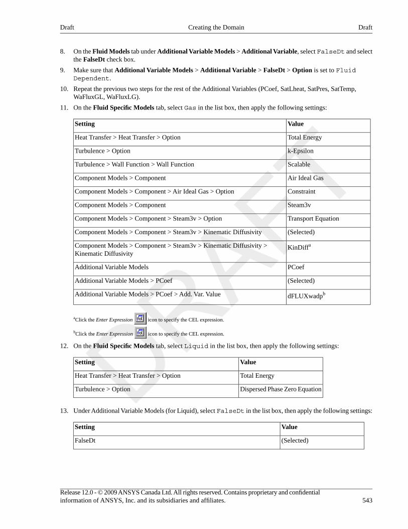
8. On the Fluid Models tab under Additional Variable Models > Additional Variable, select FalseDt and selectthe FalseDt check box.
9. Make sure that Additional Variable Models > Additional Variable > FalseDt > Option is set to FluidDependent.
10. Repeat the previous two steps for the rest of the Additional Variables (PCoef, SatLheat, SatPres, SatTemp,WaFluxGL, WaFluxLG).
11. On the Fluid Specific Models tab, select Gas in the list box, then apply the following settings:
ValueSetting
Total EnergyHeat Transfer > Heat Transfer > Option
k-EpsilonTurbulence > Option
ScalableTurbulence > Wall Function > Wall Function
Air Ideal GasComponent Models > Component
ConstraintComponent Models > Component > Air Ideal Gas > Option
Steam3vComponent Models > Component
Transport EquationComponent Models > Component > Steam3v > Option
(Selected)Component Models > Component > Steam3v > Kinematic Diffusivity
KinDiffaComponent Models > Component > Steam3v > Kinematic Diffusivity >Kinematic Diffusivity
PCoefAdditional Variable Models
(Selected)Additional Variable Models > PCoef
dFLUXwadpbAdditional Variable Models > PCoef > Add. Var. Value
aClick the Enter Expression icon to specify the CEL expression.
bClick the Enter Expression icon to specify the CEL expression.
12. On the Fluid Specific Models tab, select Liquid in the list box, then apply the following settings:
ValueSetting
Total EnergyHeat Transfer > Heat Transfer > Option
Dispersed Phase Zero EquationTurbulence > Option
13. Under Additional Variable Models (for Liquid), select FalseDt in the list box, then apply the following settings:
ValueSetting
(Selected)FalseDt
543Release 12.0 - © 2009 ANSYS Canada Ltd. All rights reserved. Contains proprietary and confidentialinformation of ANSYS, Inc. and its subsidiaries and affiliates.
DraftCreating the DomainDraft
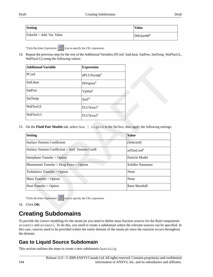
ValueSetting
DtFalseMfaFalseDt > Add. Var. Value
aClick the Enter Expression icon to specify the CEL expression.
14. Repeat the previous step for the rest of the Additional Variables (PCoef, SatLheat, SatPres, SatTemp, WaFluxGL,WaFluxLG) using the following values:
ExpressionAdditional Variable
dFLUXwadpaPCoef
HtVapwaaSatLheat
VpWataSatPres
SatTaSatTemp
FLUXwa1aWaFluxGL
FLUXwa2aWaFluxLG
15. On the Fluid Pair Models tab, select Gas | Liquid in the list box, then apply the following settings:
ValueSetting
(Selected)Surface Tension Coefficient
srfTenCoefaSurface Tension Coefficient > Surf. Tension Coeff.
Particle ModelInterphase Transfer > Option
Schiller NaumannMomentum Transfer > Drag Force > Option
NoneTurbulence Transfer > Option
NoneMass Transfer > Option
Ranz MarshallHeat Transfer > Option
aClick the Enter Expression icon to specify the CEL expression.
16. Click OK.
Creating SubdomainsTo provide the correct modeling for the steam jet you need to define mass fraction sources for the fluid componentssteam3v and steam3l. To do this, you need to create a subdomain where the relevant sources can be specified. Inthis case, sources need to be provided within the entire domain of the steam jet since the reaction occurs throughoutthe domain.
Gas to Liquid Source SubdomainThis section outlines the steps to create a new subdomain GastoLiq.
Release 12.0 - © 2009 ANSYS Canada Ltd. All rights reserved. Contains proprietary and confidentialinformation of ANSYS, Inc. and its subsidiaries and affiliates.544
DraftCreating SubdomainsDraft
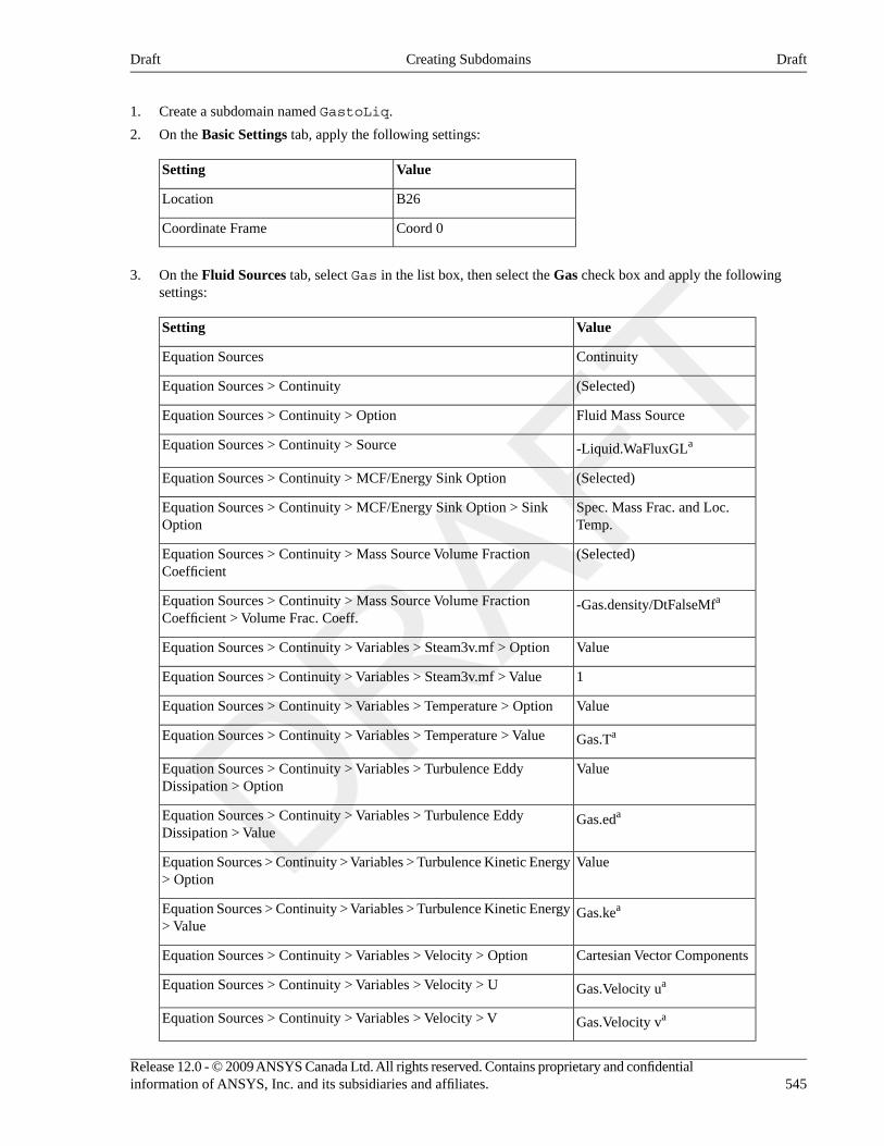
1. Create a subdomain named GastoLiq.
2. On the Basic Settings tab, apply the following settings:
ValueSetting
B26Location
Coord 0Coordinate Frame
3. On the Fluid Sources tab, select Gas in the list box, then select the Gas check box and apply the followingsettings:
ValueSetting
ContinuityEquation Sources
(Selected)Equation Sources > Continuity
Fluid Mass SourceEquation Sources > Continuity > Option
-Liquid.WaFluxGLaEquation Sources > Continuity > Source
(Selected)Equation Sources > Continuity > MCF/Energy Sink Option
Spec. Mass Frac. and Loc.Temp.
Equation Sources > Continuity > MCF/Energy Sink Option > SinkOption
(Selected)Equation Sources > Continuity > Mass Source Volume FractionCoefficient
-Gas.density/DtFalseMfaEquation Sources > Continuity > Mass Source Volume FractionCoefficient > Volume Frac. Coeff.
ValueEquation Sources > Continuity > Variables > Steam3v.mf > Option
1Equation Sources > Continuity > Variables > Steam3v.mf > Value
ValueEquation Sources > Continuity > Variables > Temperature > Option
Gas.TaEquation Sources > Continuity > Variables > Temperature > Value
ValueEquation Sources > Continuity > Variables > Turbulence EddyDissipation > Option
Gas.edaEquation Sources > Continuity > Variables > Turbulence EddyDissipation > Value
ValueEquation Sources > Continuity > Variables > Turbulence Kinetic Energy> Option
Gas.keaEquation Sources > Continuity > Variables > Turbulence Kinetic Energy> Value
Cartesian Vector ComponentsEquation Sources > Continuity > Variables > Velocity > Option
Gas.Velocity uaEquation Sources > Continuity > Variables > Velocity > U
Gas.Velocity vaEquation Sources > Continuity > Variables > Velocity > V
545Release 12.0 - © 2009 ANSYS Canada Ltd. All rights reserved. Contains proprietary and confidentialinformation of ANSYS, Inc. and its subsidiaries and affiliates.
DraftCreating SubdomainsDraft
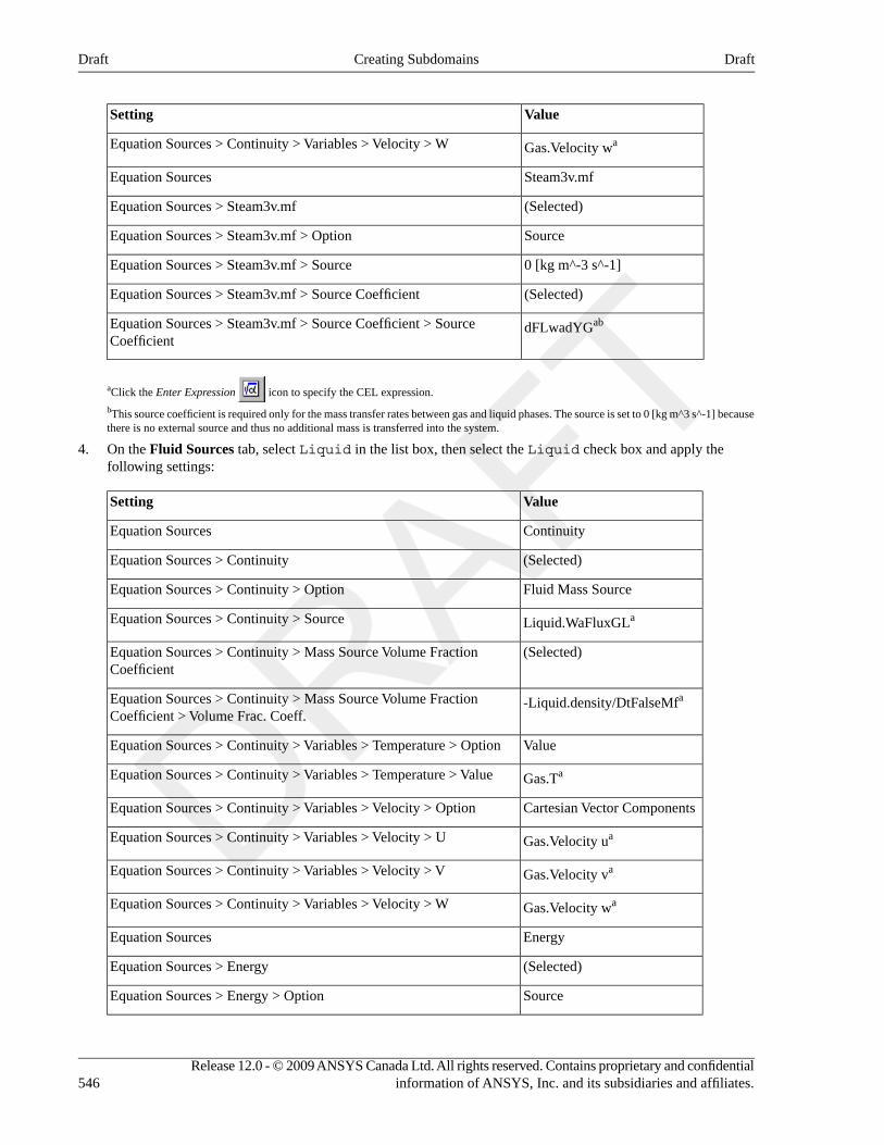
ValueSetting
Gas.Velocity waEquation Sources > Continuity > Variables > Velocity > W
Steam3v.mfEquation Sources
(Selected)Equation Sources > Steam3v.mf
SourceEquation Sources > Steam3v.mf > Option
0 [kg m^-3 s^-1]Equation Sources > Steam3v.mf > Source
(Selected)Equation Sources > Steam3v.mf > Source Coefficient
dFLwadYGabEquation Sources > Steam3v.mf > Source Coefficient > SourceCoefficient
aClick the Enter Expression icon to specify the CEL expression.
bThis source coefficient is required only for the mass transfer rates between gas and liquid phases. The source is set to 0 [kg m^3 s^-1] becausethere is no external source and thus no additional mass is transferred into the system.
4. On the Fluid Sources tab, select Liquid in the list box, then select the Liquid check box and apply thefollowing settings:
ValueSetting
ContinuityEquation Sources
(Selected)Equation Sources > Continuity
Fluid Mass SourceEquation Sources > Continuity > Option
Liquid.WaFluxGLaEquation Sources > Continuity > Source
(Selected)Equation Sources > Continuity > Mass Source Volume FractionCoefficient
-Liquid.density/DtFalseMfaEquation Sources > Continuity > Mass Source Volume FractionCoefficient > Volume Frac. Coeff.
ValueEquation Sources > Continuity > Variables > Temperature > Option
Gas.TaEquation Sources > Continuity > Variables > Temperature > Value
Cartesian Vector ComponentsEquation Sources > Continuity > Variables > Velocity > Option
Gas.Velocity uaEquation Sources > Continuity > Variables > Velocity > U
Gas.Velocity vaEquation Sources > Continuity > Variables > Velocity > V
Gas.Velocity waEquation Sources > Continuity > Variables > Velocity > W
EnergyEquation Sources
(Selected)Equation Sources > Energy
SourceEquation Sources > Energy > Option
Release 12.0 - © 2009 ANSYS Canada Ltd. All rights reserved. Contains proprietary and confidentialinformation of ANSYS, Inc. and its subsidiaries and affiliates.546
DraftCreating SubdomainsDraft
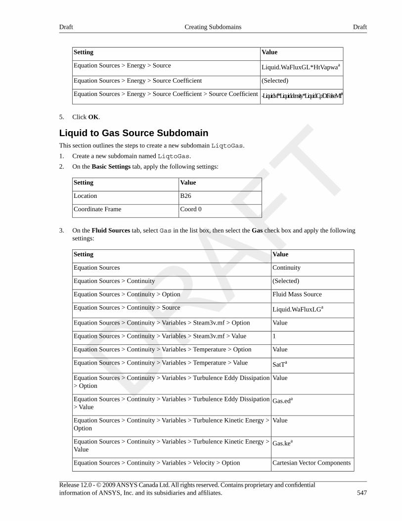
ValueSetting
Liquid.WaFluxGL*HtVapwaaEquation Sources > Energy > Source
(Selected)Equation Sources > Energy > Source Coefficient
-Liquid.vf*Liquid.density*Liquid.Cp/DtFalseMfaEquation Sources > Energy > Source Coefficient > Source Coefficient
5. Click OK.
Liquid to Gas Source SubdomainThis section outlines the steps to create a new subdomain LiqtoGas.
1. Create a new subdomain named LiqtoGas.
2. On the Basic Settings tab, apply the following settings:
ValueSetting
B26Location
Coord 0Coordinate Frame
3. On the Fluid Sources tab, select Gas in the list box, then select the Gas check box and apply the followingsettings:
ValueSetting
ContinuityEquation Sources
(Selected)Equation Sources > Continuity
Fluid Mass SourceEquation Sources > Continuity > Option
Liquid.WaFluxLGaEquation Sources > Continuity > Source
ValueEquation Sources > Continuity > Variables > Steam3v.mf > Option
1Equation Sources > Continuity > Variables > Steam3v.mf > Value
ValueEquation Sources > Continuity > Variables > Temperature > Option
SatTaEquation Sources > Continuity > Variables > Temperature > Value
ValueEquation Sources > Continuity > Variables > Turbulence Eddy Dissipation> Option
Gas.edaEquation Sources > Continuity > Variables > Turbulence Eddy Dissipation> Value
ValueEquation Sources > Continuity > Variables > Turbulence Kinetic Energy >Option
Gas.keaEquation Sources > Continuity > Variables > Turbulence Kinetic Energy >Value
Cartesian Vector ComponentsEquation Sources > Continuity > Variables > Velocity > Option
547Release 12.0 - © 2009 ANSYS Canada Ltd. All rights reserved. Contains proprietary and confidentialinformation of ANSYS, Inc. and its subsidiaries and affiliates.
DraftCreating SubdomainsDraft
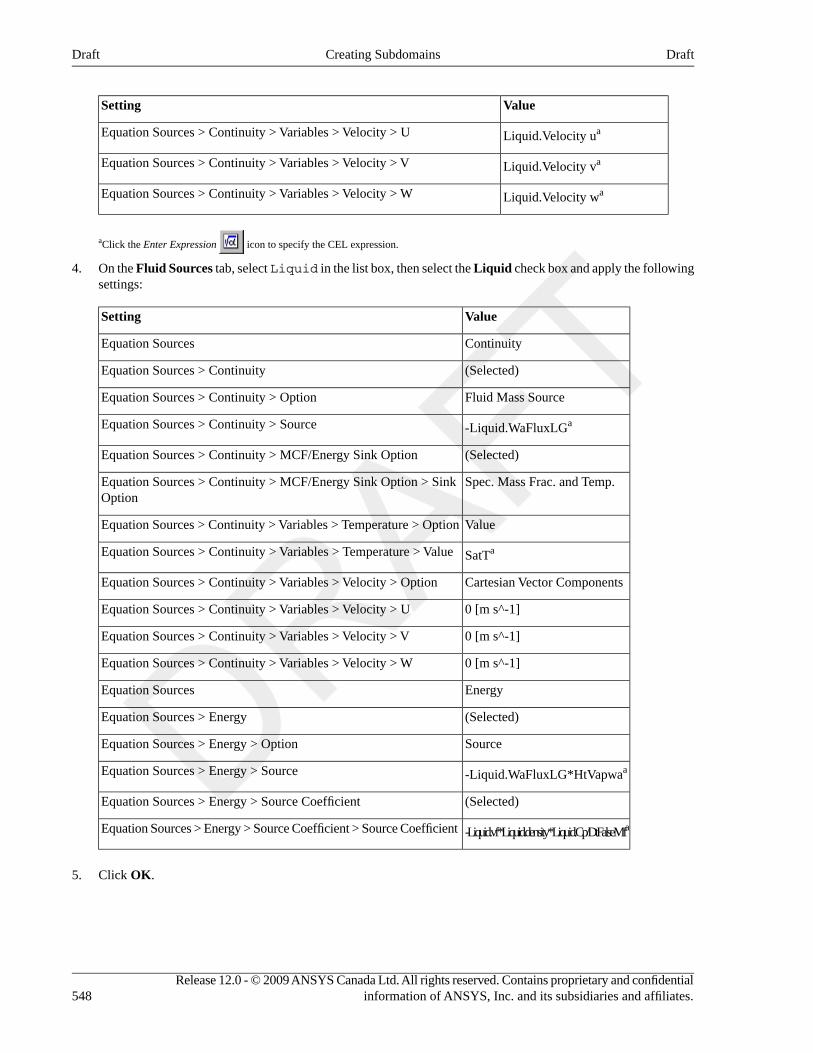
ValueSetting
Liquid.Velocity uaEquation Sources > Continuity > Variables > Velocity > U
Liquid.Velocity vaEquation Sources > Continuity > Variables > Velocity > V
Liquid.Velocity waEquation Sources > Continuity > Variables > Velocity > W
aClick the Enter Expression icon to specify the CEL expression.
4. On the Fluid Sources tab, select Liquid in the list box, then select the Liquid check box and apply the followingsettings:
ValueSetting
ContinuityEquation Sources
(Selected)Equation Sources > Continuity
Fluid Mass SourceEquation Sources > Continuity > Option
-Liquid.WaFluxLGaEquation Sources > Continuity > Source
(Selected)Equation Sources > Continuity > MCF/Energy Sink Option
Spec. Mass Frac. and Temp.Equation Sources > Continuity > MCF/Energy Sink Option > SinkOption
ValueEquation Sources > Continuity > Variables > Temperature > Option
SatTaEquation Sources > Continuity > Variables > Temperature > Value
Cartesian Vector ComponentsEquation Sources > Continuity > Variables > Velocity > Option
0 [m s^-1]Equation Sources > Continuity > Variables > Velocity > U
0 [m s^-1]Equation Sources > Continuity > Variables > Velocity > V
0 [m s^-1]Equation Sources > Continuity > Variables > Velocity > W
EnergyEquation Sources
(Selected)Equation Sources > Energy
SourceEquation Sources > Energy > Option
-Liquid.WaFluxLG*HtVapwaaEquation Sources > Energy > Source
(Selected)Equation Sources > Energy > Source Coefficient
-Liquid.vf*Liquid.density*Liquid.Cp/DtFalseMfaEquation Sources > Energy > Source Coefficient > Source Coefficient
5. Click OK.
Release 12.0 - © 2009 ANSYS Canada Ltd. All rights reserved. Contains proprietary and confidentialinformation of ANSYS, Inc. and its subsidiaries and affiliates.548
DraftCreating SubdomainsDraft
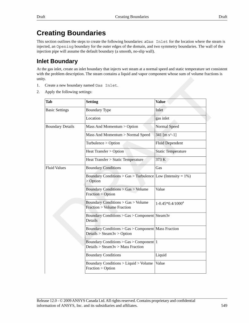
Creating BoundariesThis section outlines the steps to create the following boundaries: aGas Inlet for the location where the steam isinjected, an Opening boundary for the outer edges of the domain, and two symmetry boundaries. The wall of theinjection pipe will assume the default boundary (a smooth, no-slip wall).
Inlet BoundaryAt the gas inlet, create an inlet boundary that injects wet steam at a normal speed and static temperature set consistentwith the problem description. The steam contains a liquid and vapor component whose sum of volume fractions isunity.
1. Create a new boundary named Gas Inlet.
2. Apply the following settings:
ValueSettingTab
InletBoundary TypeBasic Settings
gas inletLocation
Normal SpeedMass And Momentum > OptionBoundary Details
341 [m s^-1]Mass And Momentum > Normal Speed
Fluid DependentTurbulence > Option
Static TemperatureHeat Transfer > Option
373 KHeat Transfer > Static Temperature
GasBoundary ConditionsFluid Values
Low (Intensity = 1%)Boundary Conditions > Gas > Turbulence> Option
ValueBoundary Conditions > Gas > VolumeFraction > Option
1-0.45*0.4/1000aBoundary Conditions > Gas > VolumeFraction > Volume Fraction
Steam3vBoundary Conditions > Gas > ComponentDetails
Mass FractionBoundary Conditions > Gas > ComponentDetails > Steam3v > Option
1Boundary Conditions > Gas > ComponentDetails > Steam3v > Mass Fraction
LiquidBoundary Conditions
ValueBoundary Conditions > Liquid > VolumeFraction > Option
549Release 12.0 - © 2009 ANSYS Canada Ltd. All rights reserved. Contains proprietary and confidentialinformation of ANSYS, Inc. and its subsidiaries and affiliates.
DraftCreating BoundariesDraft
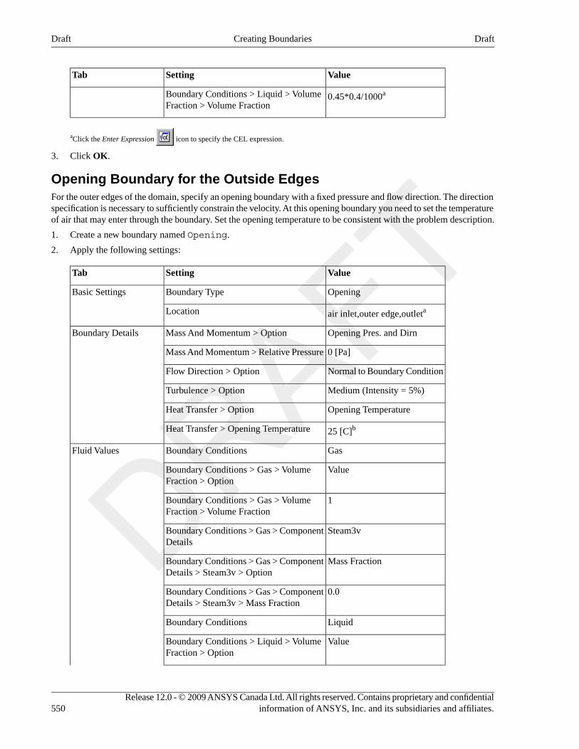
ValueSettingTab
0.45*0.4/1000aBoundary Conditions > Liquid > VolumeFraction > Volume Fraction
aClick the Enter Expression icon to specify the CEL expression.
3. Click OK.
Opening Boundary for the Outside EdgesFor the outer edges of the domain, specify an opening boundary with a fixed pressure and flow direction. The directionspecification is necessary to sufficiently constrain the velocity. At this opening boundary you need to set the temperatureof air that may enter through the boundary. Set the opening temperature to be consistent with the problem description.
1. Create a new boundary named Opening.
2. Apply the following settings:
ValueSettingTab
OpeningBoundary TypeBasic Settings
air inlet,outer edge,outletaLocation
Opening Pres. and DirnMass And Momentum > OptionBoundary Details
0 [Pa]Mass And Momentum > Relative Pressure
Normal to Boundary ConditionFlow Direction > Option
Medium (Intensity = 5%)Turbulence > Option
Opening TemperatureHeat Transfer > Option
25 [C]bHeat Transfer > Opening Temperature
GasBoundary ConditionsFluid Values
ValueBoundary Conditions > Gas > VolumeFraction > Option
1Boundary Conditions > Gas > VolumeFraction > Volume Fraction
Steam3vBoundary Conditions > Gas > ComponentDetails
Mass FractionBoundary Conditions > Gas > ComponentDetails > Steam3v > Option
0.0Boundary Conditions > Gas > ComponentDetails > Steam3v > Mass Fraction
LiquidBoundary Conditions
ValueBoundary Conditions > Liquid > VolumeFraction > Option
Release 12.0 - © 2009 ANSYS Canada Ltd. All rights reserved. Contains proprietary and confidentialinformation of ANSYS, Inc. and its subsidiaries and affiliates.550
DraftCreating BoundariesDraft
ValueSettingTab
0Boundary Conditions > Liquid > VolumeFraction > Volume Fraction
aClick the Ellipsis icon to open the selection dialog box, then select multiple items by holding the Ctrl key. Click OK.
bEnsure that units are set to [C].
3. Click OK.
Creating the Symmetry Plane Boundaries1. Create a new boundary named SymP1.
2. Apply the following settings:
ValueSettingTab
SymmetryBoundary TypeBasic Settings
F29.26Location
3. Click OK.
4. Create a new boundary named SymP2.
5. Apply the following settings:
ValueSettingTab
SymmetryBoundary TypeBasic Settings
F27.26Location
6. Click OK.
Creating a Time Step ExpressionThe conditions at each boundary determine the size of the time scale used in the time step. Generally, you can estimatean effective time step by dividing the displacement by the velocity at which a fluid is travelling. In this case, however,the velocity at the gas inlet approaches the speed of sound and the time step must be calculated by taking the heightof the inlet and dividing it by the velocity at which the steam enters the system. The lower velocities at the outlet andopening boundaries allow the time step to be increased after the gas inlet properties have converged. Once all the valuesat the inlet, outlet, and openings have converged, a much larger time step is used to allow the overall solution to settle.In order to account for all these time step changes, an expression will be created.
Since the flow velocities are high at the jet inlet, you need to use a very small time step to capture the property variationsat this location. The flow velocity decreases as you move away from the jet inlet, thus the time step can be increasedsystematically for better efficiency. You will now create a time step control expression called Dtstep that ramps upthe time scale in stages:
1. Right-click Expressions in the Outline tree view and select Insert > Expression.
2. Set the name to Dtstep and click OK.
3. In the Definition area, type or copy and paste the following expression:
step(20.5-aitern)*1.0e-5 [s] + step(aitern-20.5)*step(100.5-aitern)*1.0e-4[s] + step(aitern-100.5)*step(300.5-aitern)*2.0e-4 [s] +
551Release 12.0 - © 2009 ANSYS Canada Ltd. All rights reserved. Contains proprietary and confidentialinformation of ANSYS, Inc. and its subsidiaries and affiliates.
DraftCreating a Time Step ExpressionDraft
step(aitern-300.5)*step(500.5-aitern)*5.0e-4 [s] + step(aitern-500.5)*1.0e-3[s]
4. Click Apply.
Setting Solver Control
1. Click Solver Control .
2. Apply the following settings:
ValueSettingTab
High ResolutionAdvection Scheme > OptionBasic Settings
1500Convergence Control > Max Iterations
Physical TimescaleConvergence Control > Fluid TimescaleControl > Timescale Control
Dtstep aConvergence Control > Fluid TimescaleControl > Physical Timescale
RMSConvergence Criteria > Residual Type
1.0E-4Convergence Criteria > Residual Target
(Selected)Dynamic Model Control > Global DynamicModel Control
Advanced Options
(Selected)Multiphase Control
(Selected)Multiphase Control > Volume FractionCoupling
SegregatedMultiphase Control > Volume FractionCoupling > Option
aClick the Enter Expression icon to specify the CEL expression.
3. Click OK.
Writing the CFX-Solver Input (.def) File
1. Click Define Run .
2. In the Write Solver Input File dialog box, set File name to SteamJet.def and click Save.
3. If using Standalone Mode, quit CFX-Pre, saving the case (.cfx) file at your discretion.
Obtaining a Solution for Simulation usingCFX-Solver ManagerWhen CFX-Pre has shut down and the CFX-Solver Manager has started, obtain a solution to the CFD problem byfollowing the instructions below:
Release 12.0 - © 2009 ANSYS Canada Ltd. All rights reserved. Contains proprietary and confidentialinformation of ANSYS, Inc. and its subsidiaries and affiliates.552
DraftSetting Solver ControlDraft
1. Ensure Define Run is displayed.
CFX-Solver Input File should be set to SteamJet.def
2. Click Start Run.
CFX-Solver runs and attempts to obtain a solution. This can take a long time depending on your system. Eventuallya dialog box is displayed.
3. Note the number of iterations required to obtain a solution.
4. Select the check box next to Post-Process Results when the completion message appears at the end of the run.
5. If using Standalone Mode, select the check box next to Shut down ANSYS CFX-Solver Manager.
6. Click OK.
Viewing the Results in CFD-PostIn this section, the steam molar fraction in the gas fluid, the gas to liquid and liquid to gas mass transfer rates, and thefalse time step will be illustrated on various regions.
Displaying the Steam Molar Fraction1. Right-click a blank area in the viewer and select Predefined Camera > View Towards -Z.
This ensures that the view is set to a position that is best suited to display the results.
2. From the menu bar, select Insert > Contour.
3. Under Name, type Steam Molar Fraction and click OK.
4. Apply the following settings:
ValueSettingTab
SymP2LocationsGeometry
Gas.Steam3v.MolarFraction
Variable
5. Click Apply.
This will result in SymP2 shown colored by the molar fraction of steam. The steam enters at the Gas Inlet andtherefore has a higher gas to liquid mass transfer rate at this location. You may want to zoom in near the gas inlet toview the molar fraction variation more closely.
Displaying the Gas to Liquid Mass Transfer Rate1. In the tree view, clear the check box beside Steam Molar Fraction to hide it.
2. Right-click a blank area in the viewer and select Predefined Camera > View Towards -Z.
This ensures that the view is set to a position that is best suited to display the results.
3. From the menu bar, select Insert > Contour.
4. Under Name, type Gas to Liquid Flux and click OK.
5. Apply the following settings:
553Release 12.0 - © 2009 ANSYS Canada Ltd. All rights reserved. Contains proprietary and confidentialinformation of ANSYS, Inc. and its subsidiaries and affiliates.
DraftViewing the Results in CFD-PostDraft
ValueSettingTab
SymP2LocationsGeometry
Liquid.WaFluxGLVariable
6. Click Apply.
This will result in SymP2 shown colored by the gas to liquid mass transfer rate. The steam enters at the Gas Inletand therefore has a higher gas to liquid mass transfer rate at this location. You may want to zoom in near the gas inletto view the mass transfer rate variation more closely.
Displaying the Liquid to Gas Mass Transfer Rate1. In the tree view, clear the check box beside Gas to Liquid Flux to hide it.
2. Right-click a blank area in the viewer and select Predefined Camera > View Towards -Z.
This ensures that the view is set to a position that is best suited to display the results.
3. From the menu bar, select Insert > Contour.
4. Under Name, type Liquid to Gas Flux and click OK.
5. Apply the following settings:
ValueSettingTab
SymP2LocationsGeometry
Liquid.WaFluxLGVariable
6. Click Apply.
This will result in SymP2 shown colored by the liquid to gas mass transfer rate. The steam enters at the Gas Inletand therefore has a higher liquid to gas mass transfer rate at this location. You may want to zoom in near the gas inletto view the mass transfer rate variation more closely.
Displaying the Gas to Liquid and Liquid to Gas PhaseTransfer Rates in Synchronous Views1. In the viewer tool bar, open the viewport drop-down menu and click the option with two horizontal viewports.
2. In the viewer tool bar, click Synchronize camera in displayed views .
3. Click a blank area in View 2 so that it becomes the active view.
4. In the tree view, select the check box beside Gas to Liquid Flux.
NoteUnder User Locations and Plots in the tree view, ensure that only Liquid to GasFlux is visible in View 1, and only Gas to Liquid Flux is visible in View 2.
5. In View 2, right-click a blank area in the viewer and select Predefined Camera > View Towards -Z.
This ensures that the view is set to a position that is best suited to display the results.
You may want to zoom in near the gas inlet to view the differences between the gas to liquid and liquid to gas phasetransfer rates.
Release 12.0 - © 2009 ANSYS Canada Ltd. All rights reserved. Contains proprietary and confidentialinformation of ANSYS, Inc. and its subsidiaries and affiliates.554
DraftDisplaying the Liquid to Gas Mass Transfer RateDraft
Creating a Chart to Plot the False Time Step Along a Line1. In the tree view, right-click User Locations and Plots and select Insert > Location > Line.
2. In the Insert Line dialogue box, use the default name and click OK.
3. Apply the following settings:
ValueSettingTab
Two PointsDefinition > MethodGeometry
0, 0.005, 0.0002Definition > Point 1
5, 0.005, 0.0002Definition > Point 2
(Selected)Line Type > Cut
4. Click Apply.
5. From the menu bar, select Insert > Chart.
6. Name the chart False Time Step and click OK.
7. Apply the following settings:
ValueSettingTab
False Time StepTitleGeneral
Line 1Data Source > LocationData Series
XData Selection > VariableX Axis
Liquid.FalseDtData Selection > VariableY Axis
(Selected)Axis Range > Logarithmic Scale
8. Click Apply.
The false time step peaks where the interphase mass transfer rate changes sign, and hence goes through zero. This istrue because the false time step is inversely proportional to the absolute mass transfer rate.
When you have finished viewing the chart, quit CFD-Post.
555Release 12.0 - © 2009 ANSYS Canada Ltd. All rights reserved. Contains proprietary and confidentialinformation of ANSYS, Inc. and its subsidiaries and affiliates.
DraftCreating a Chart to Plot the False Time Step Along a LineDraft

Release 12.0 - © 2009 ANSYS Canada Ltd. All rights reserved. Contains proprietary and confidentialinformation of ANSYS, Inc. and its subsidiaries and affiliates.
Chapter 32. Fluid Flow and Heat Transferin a Mixing ElbowThis tutorial illustrates how to use ANSYS CFD-Post to visualize a three-dimensional turbulent fluid flow and heattransfer problem in a mixing elbow. The mixing elbow configuration is encountered in piping systems in power plantsand process industries. It is often important to predict the flow field and temperature field in the area of the mixingregion in order to properly design the junction.
This tutorial demonstrates how to do the following:
• Create a Working Directory (p. 558)
• Launch ANSYS CFD-Post (p. 559)
• Display the Solution in ANSYS CFD-Post (p. 563)
• Save Your Work (p. 590)
• Generated Files (p. 592)
Problem DescriptionThe problem to be considered is shown schematically in Figure 32.1, “Problem Specification” (p. 558). A cold fluid at20° C flows into the pipe through a large inlet and mixes with a warmer fluid at 40° C that enters through a smallerinlet located at the elbow. The pipe dimensions are in inches, but the fluid properties and boundary conditions are givenin SI units. The Reynolds number for the flow at the larger inlet is 50,800, so the flow has been modeled as beingturbulent.
NoteThis tutorial is derived from an existing ANSYS FLUENT case. The combination of SI and Imperial unitsis not typical, but follows an ANSYS FLUENT example.
Because the geometry of the mixing elbow is symmetric, only half of the elbow is modeled.
557Release 12.0 - © 2009 ANSYS Canada Ltd. All rights reserved. Contains proprietary and confidentialinformation of ANSYS, Inc. and its subsidiaries and affiliates.
DraftDraft
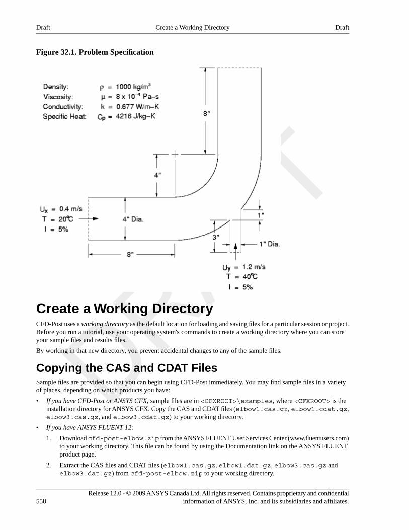
Figure 32.1. Problem Specification
Create a Working DirectoryCFD-Post uses a working directory as the default location for loading and saving files for a particular session or project.Before you run a tutorial, use your operating system's commands to create a working directory where you can storeyour sample files and results files.
By working in that new directory, you prevent accidental changes to any of the sample files.
Copying the CAS and CDAT FilesSample files are provided so that you can begin using CFD-Post immediately. You may find sample files in a varietyof places, depending on which products you have:
• If you have CFD-Post or ANSYS CFX, sample files are in <CFXROOT>\examples, where <CFXROOT> is theinstallation directory for ANSYS CFX. Copy the CAS and CDAT files (elbow1.cas.gz, elbow1.cdat.gz,elbow3.cas.gz, and elbow3.cdat.gz) to your working directory.
• If you have ANSYS FLUENT 12:
1. Download cfd-post-elbow.zip from the ANSYS FLUENT User Services Center (www.fluentusers.com)to your working directory. This file can be found by using the Documentation link on the ANSYS FLUENTproduct page.
2. Extract the CAS files and CDAT files (elbow1.cas.gz, elbow1.dat.gz, elbow3.cas.gz andelbow3.dat.gz) from cfd-post-elbow.zip to your working directory.
Release 12.0 - © 2009 ANSYS Canada Ltd. All rights reserved. Contains proprietary and confidentialinformation of ANSYS, Inc. and its subsidiaries and affiliates.558
DraftCreate a Working DirectoryDraft
Note• These tutorials are prepared on a Windows system. The screen shots and graphic images in the
tutorials may be slightly different than the appearance on your system, depending on the operatingsystem or graphics card.
• The case name is derived from the name of the results file that you load with the final extensionremoved. Thus, if you load elbow1.cdat.gz the case name will be elbow1.cdat; if you loadelbow1.cdat, the case name will be elbow1. The case names used in this tutorial are elbow1 andelbow3.
Launch ANSYS CFD-PostBefore you start CFD-Post, set the working directory. The procedure for setting the working directory and startingCFD-Post depends on whether you will launch CFD-Post standalone, from the ANSYS CFX Launcher, from ANSYSWorkbench, or from ANSYS FLUENT:
• To run CFD-Post standalone, from the Start menu, right-click All Programs > ANSYS 12.0 > ANSYS CFD-Postand select Properties. Type the path to your working directory in the Start in field and click OK, then click AllPrograms > ANSYS 12.0 > ANSYS CFD-Post to launch CFD-Post.
• To run ANSYS CFX Launcher
1. Start the ANSYS CFX Launcher.
You can run the ANSYS CFX Launcher in any of the following ways:
• On Windows:
• From the Start menu, go to All Programs > ANSYS 12.0 > CFX > ANSYS CFX 12.0.
• In a DOS window that has its path set up correctly to run ANSYS CFX, enter cfx5launch (otherwise,you will need to type the full pathname of the cfx command, which will be something similar toC:\Program Files\ANSYS Inc\v120\CFX\bin).
• On UNIX, enter cfx5launch in a terminal window that has its path set up to run ANSYS CFX (thepath will be something similar to /usr/ansys_inc/v120/CFX/bin).
2. Select the Working Directory (where you copied the sample files).
3. Click the CFD-Post 12.0 button.
• ANSYS Workbench
1. Start ANSYS Workbench.
2. From the menu bar, select File > Save As and save the project file to the directory that you want to be theworking directory.
3. Open the Component Systems toolbox and double-click Results. A Results system opens in the ProjectSchematic.
4. Right-click on the A2 Results cell and select Edit. CFD-Post opens.
• ANSYS FLUENT
1. Click the ANSYS FLUENT icon ( ) in the ANSYS program group to open ANSYS FLUENT Launcher.
ANSYS FLUENT Launcher allows you to decide which version of ANSYS FLUENT you will use, based onyour geometry and on your processing capabilities.
559Release 12.0 - © 2009 ANSYS Canada Ltd. All rights reserved. Contains proprietary and confidentialinformation of ANSYS, Inc. and its subsidiaries and affiliates.
DraftLaunch ANSYS CFD-PostDraft
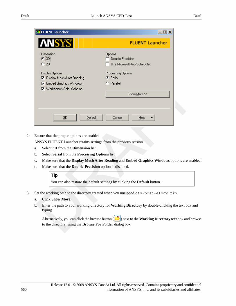
2. Ensure that the proper options are enabled.
ANSYS FLUENT Launcher retains settings from the previous session.
a. Select 3D from the Dimension list.
b. Select Serial from the Processing Options list.
c. Make sure that the Display Mesh After Reading and Embed Graphics Windows options are enabled.
d. Make sure that the Double-Precision option is disabled.
TipYou can also restore the default settings by clicking the Default button.
3. Set the working path to the directory created when you unzipped cfd-post-elbow.zip.
a. Click Show More.
b. Enter the path to your working directory for Working Directory by double-clicking the text box andtyping.
Alternatively, you can click the browse button ( ) next to the Working Directory text box and browse
to the directory, using the Browse For Folder dialog box.
Release 12.0 - © 2009 ANSYS Canada Ltd. All rights reserved. Contains proprietary and confidentialinformation of ANSYS, Inc. and its subsidiaries and affiliates.560
DraftLaunch ANSYS CFD-PostDraft
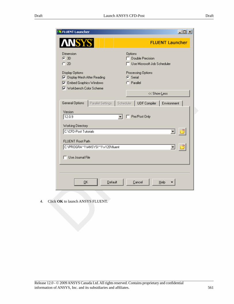
4. Click OK to launch ANSYS FLUENT.
561Release 12.0 - © 2009 ANSYS Canada Ltd. All rights reserved. Contains proprietary and confidentialinformation of ANSYS, Inc. and its subsidiaries and affiliates.
DraftLaunch ANSYS CFD-PostDraft
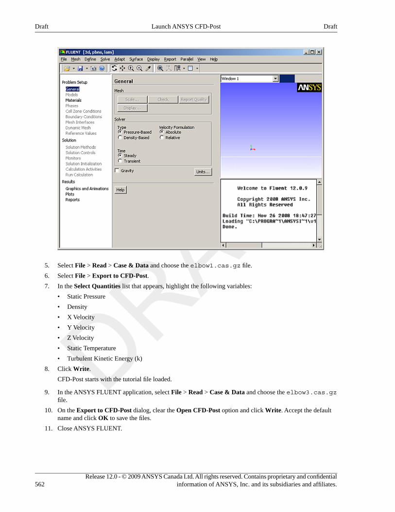
5. Select File > Read > Case & Data and choose the elbow1.cas.gz file.
6. Select File > Export to CFD-Post.
7. In the Select Quantities list that appears, highlight the following variables:
• Static Pressure
• Density
• X Velocity
• Y Velocity
• Z Velocity
• Static Temperature
• Turbulent Kinetic Energy (k)
8. Click Write.
CFD-Post starts with the tutorial file loaded.
9. In the ANSYS FLUENT application, select File > Read > Case & Data and choose the elbow3.cas.gzfile.
10. On the Export to CFD-Post dialog, clear the Open CFD-Post option and click Write. Accept the defaultname and click OK to save the files.
11. Close ANSYS FLUENT.
Release 12.0 - © 2009 ANSYS Canada Ltd. All rights reserved. Contains proprietary and confidentialinformation of ANSYS, Inc. and its subsidiaries and affiliates.562
DraftLaunch ANSYS CFD-PostDraft
Display the Solution in ANSYS CFD-PostIn the steps that follow, you will visualize various aspects of the flow for the solution using CFD-Post. You will:
• Prepare the case and set the viewer options
• View the mesh and check it by using the Mesh Calculator
• View simulation values using the Function Calculator
• Become familiar with the 3D Viewer controls
• Create an instance reflection
• Show fluid velocity on the symmetry plane
• Create a vector plot to show the flow distribution in the elbow
• Create streamlines to show the flow distribution in the elbow
• Show the vortex structure
• Use multiple viewports to compare a contour plot to the display of a variable on a boundary
• Chart the changes to temperature at two places along the pipe
• Create a table to show mixing
• Review and modify a report
• Create a custom variable and cause the plane to move through the domain to show how the values of a customvariable change at different locations in the geometry
• Compare the results to those in a refined mesh
• Save your work
• Create an animation of a plane moving through the domain.
Prepare the Case and Set the Viewer Options1. If you have launched CFD-Post from ANSYS FLUENT, proceed to the next step. For all other situations, load
the simulation from the data file (elbow1.cdat.gz) from the menu bar by selecting File > Load Results. Inthe Load Results File dialog, select elbow1.cdat.gz and click Open.
2. If you see a pop-up that discusses Global Variables Ranges, it can be ignored. Click OK.
The mixing elbow appears in the 3D Viewer in an isometric orientation. The wireframe appears in the view andthere is a check mark beside User Location and Plots > Wireframe in the Outline tree view; the check markindicates that the wireframe is visible in the 3D Viewer.
3. Optionally, set the viewer background to white:
a. Right-click on the viewer and select Viewer Options.
b. In the Options dialog, select CFD-Post > Viewer.
c. Set:
• Background > Color Type to Solid.
• Background > Color to white. To do this, click the bar beside the Color label to cycle through 10 basiccolors. (Click the right-mouse button to cycle backwards.) Alternatively, you can choose any color by
clicking to the right of the Color option.
• Text Color to black (as above).
• Edge Color to black (as above).
d. Click OK to have the settings take effect.
563Release 12.0 - © 2009 ANSYS Canada Ltd. All rights reserved. Contains proprietary and confidentialinformation of ANSYS, Inc. and its subsidiaries and affiliates.
DraftDisplay the Solution in ANSYS CFD-PostDraft
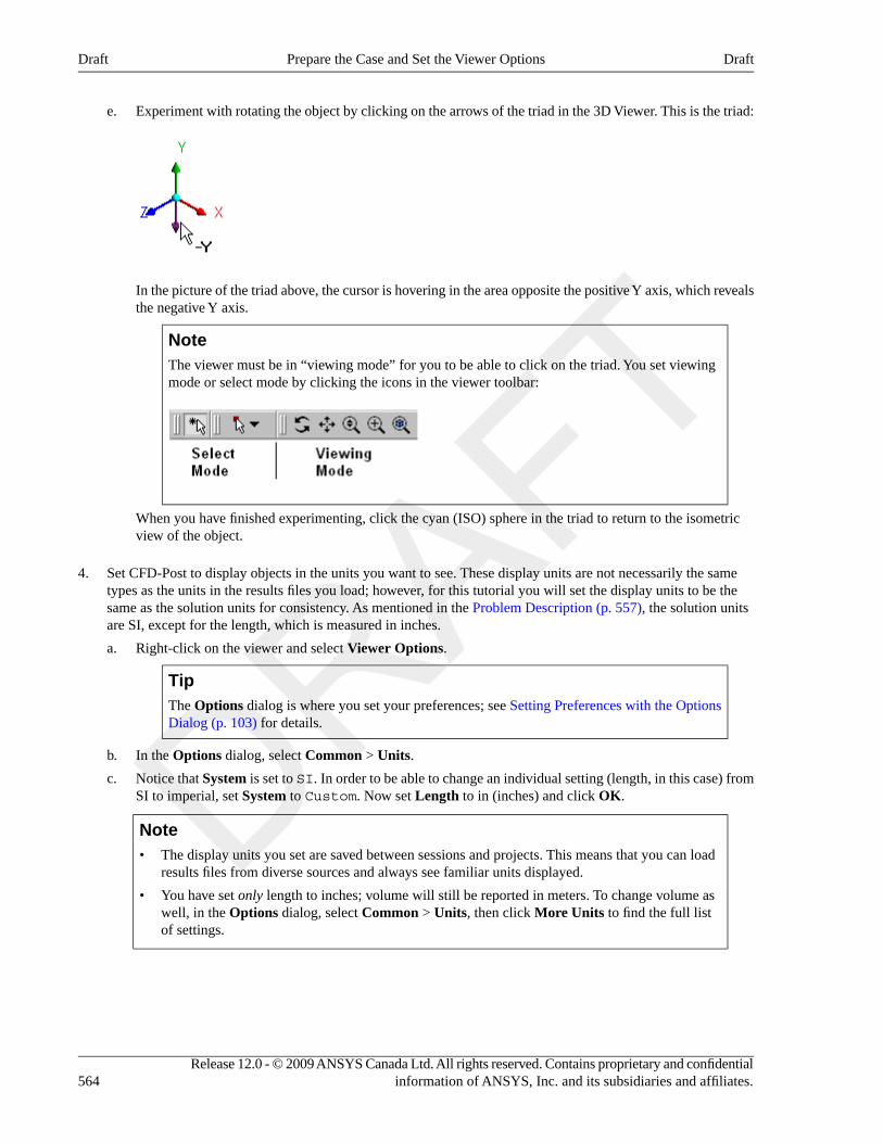
e. Experiment with rotating the object by clicking on the arrows of the triad in the 3D Viewer. This is the triad:
In the picture of the triad above, the cursor is hovering in the area opposite the positive Y axis, which revealsthe negative Y axis.
NoteThe viewer must be in “viewing mode” for you to be able to click on the triad. You set viewingmode or select mode by clicking the icons in the viewer toolbar:
When you have finished experimenting, click the cyan (ISO) sphere in the triad to return to the isometricview of the object.
4. Set CFD-Post to display objects in the units you want to see. These display units are not necessarily the sametypes as the units in the results files you load; however, for this tutorial you will set the display units to be thesame as the solution units for consistency. As mentioned in the Problem Description (p. 557), the solution unitsare SI, except for the length, which is measured in inches.
a. Right-click on the viewer and select Viewer Options.
TipThe Options dialog is where you set your preferences; see Setting Preferences with the OptionsDialog (p. 103) for details.
b. In the Options dialog, select Common > Units.
c. Notice that System is set to SI. In order to be able to change an individual setting (length, in this case) fromSI to imperial, set System to Custom. Now set Length to in (inches) and click OK.
Note• The display units you set are saved between sessions and projects. This means that you can load
results files from diverse sources and always see familiar units displayed.
• You have set only length to inches; volume will still be reported in meters. To change volume aswell, in the Options dialog, select Common > Units, then click More Units to find the full listof settings.
Release 12.0 - © 2009 ANSYS Canada Ltd. All rights reserved. Contains proprietary and confidentialinformation of ANSYS, Inc. and its subsidiaries and affiliates.564
DraftPrepare the Case and Set the Viewer OptionsDraft
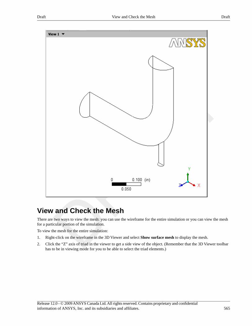
View and Check the MeshThere are two ways to view the mesh: you can use the wireframe for the entire simulation or you can view the meshfor a particular portion of the simulation.
To view the mesh for the entire simulation:
1. Right-click on the wireframe in the 3D Viewer and select Show surface mesh to display the mesh.
2. Click the “Z” axis of triad in the viewer to get a side view of the object. (Remember that the 3D Viewer toolbarhas to be in viewing mode for you to be able to select the triad elements.)
565Release 12.0 - © 2009 ANSYS Canada Ltd. All rights reserved. Contains proprietary and confidentialinformation of ANSYS, Inc. and its subsidiaries and affiliates.
DraftView and Check the MeshDraft
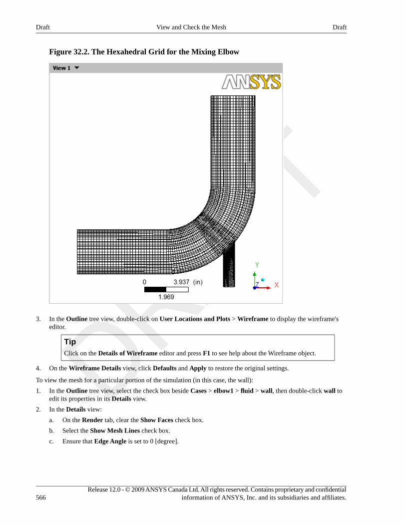
Figure 32.2. The Hexahedral Grid for the Mixing Elbow
3. In the Outline tree view, double-click on User Locations and Plots > Wireframe to display the wireframe'seditor.
TipClick on the Details of Wireframe editor and press F1 to see help about the Wireframe object.
4. On the Wireframe Details view, click Defaults and Apply to restore the original settings.
To view the mesh for a particular portion of the simulation (in this case, the wall):
1. In the Outline tree view, select the check box beside Cases > elbow1 > fluid > wall, then double-click wall toedit its properties in its Details view.
2. In the Details view:
a. On the Render tab, clear the Show Faces check box.
b. Select the Show Mesh Lines check box.
c. Ensure that Edge Angle is set to 0 [degree].
Release 12.0 - © 2009 ANSYS Canada Ltd. All rights reserved. Contains proprietary and confidentialinformation of ANSYS, Inc. and its subsidiaries and affiliates.566
DraftView and Check the MeshDraft
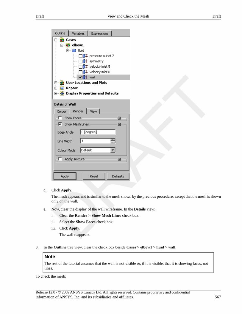
d. Click Apply.
The mesh appears and is similar to the mesh shown by the previous procedure, except that the mesh is shownonly on the wall.
e. Now, clear the display of the wall wireframe. In the Details view:
i. Clear the Render > Show Mesh Lines check box.
ii. Select the Show Faces check box.
iii. Click Apply.
The wall reappears.
3. In the Outline tree view, clear the check box beside Cases > elbow1 > fluid > wall.
NoteThe rest of the tutorial assumes that the wall is not visible or, if it is visible, that it is showing faces, notlines.
To check the mesh:
567Release 12.0 - © 2009 ANSYS Canada Ltd. All rights reserved. Contains proprietary and confidentialinformation of ANSYS, Inc. and its subsidiaries and affiliates.
DraftView and Check the MeshDraft
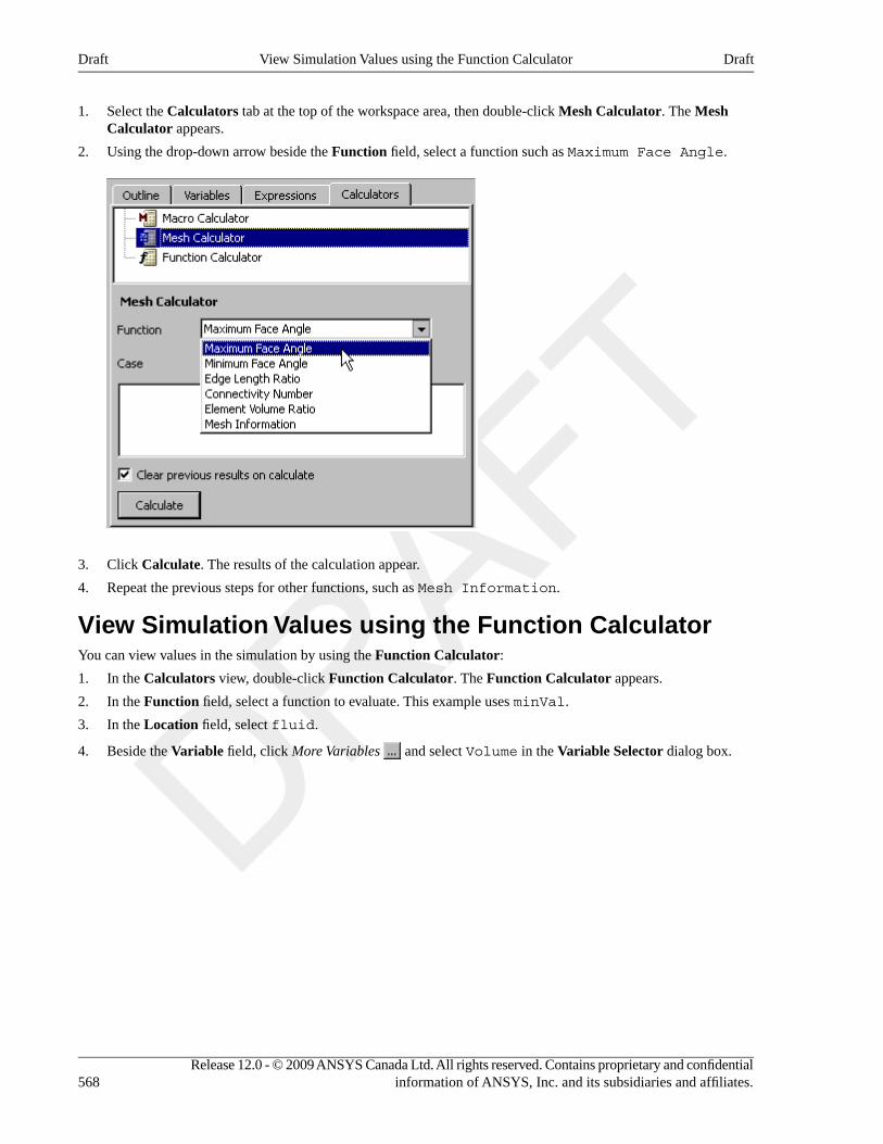
1. Select the Calculators tab at the top of the workspace area, then double-click Mesh Calculator. The MeshCalculator appears.
2. Using the drop-down arrow beside the Function field, select a function such as Maximum Face Angle.
3. Click Calculate. The results of the calculation appear.
4. Repeat the previous steps for other functions, such as Mesh Information.
View Simulation Values using the Function CalculatorYou can view values in the simulation by using the Function Calculator:
1. In the Calculators view, double-click Function Calculator. The Function Calculator appears.
2. In the Function field, select a function to evaluate. This example uses minVal.
3. In the Location field, select fluid.
4. Beside the Variable field, click More Variables and select Volume in the Variable Selector dialog box.
Release 12.0 - © 2009 ANSYS Canada Ltd. All rights reserved. Contains proprietary and confidentialinformation of ANSYS, Inc. and its subsidiaries and affiliates.568
DraftView Simulation Values using the Function CalculatorDraft
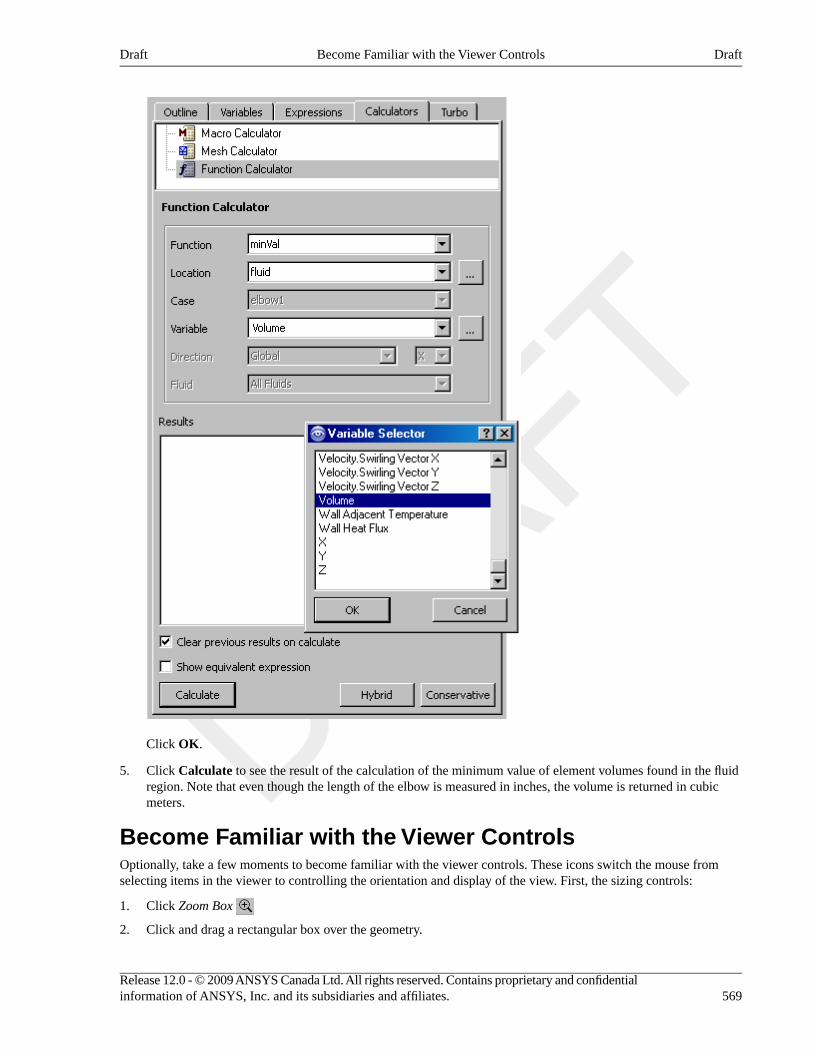
Click OK.
5. Click Calculate to see the result of the calculation of the minimum value of element volumes found in the fluidregion. Note that even though the length of the elbow is measured in inches, the volume is returned in cubicmeters.
Become Familiar with the Viewer ControlsOptionally, take a few moments to become familiar with the viewer controls. These icons switch the mouse fromselecting items in the viewer to controlling the orientation and display of the view. First, the sizing controls:
1. Click Zoom Box
2. Click and drag a rectangular box over the geometry.
569Release 12.0 - © 2009 ANSYS Canada Ltd. All rights reserved. Contains proprietary and confidentialinformation of ANSYS, Inc. and its subsidiaries and affiliates.
DraftBecome Familiar with the Viewer ControlsDraft
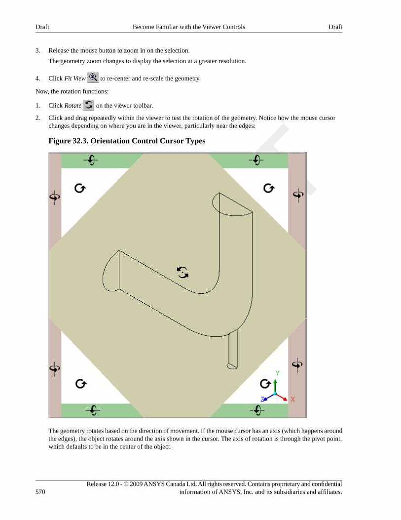
3. Release the mouse button to zoom in on the selection.
The geometry zoom changes to display the selection at a greater resolution.
4. Click Fit View to re-center and re-scale the geometry.
Now, the rotation functions:
1. Click Rotate on the viewer toolbar.
2. Click and drag repeatedly within the viewer to test the rotation of the geometry. Notice how the mouse cursorchanges depending on where you are in the viewer, particularly near the edges:
Figure 32.3. Orientation Control Cursor Types
The geometry rotates based on the direction of movement. If the mouse cursor has an axis (which happens aroundthe edges), the object rotates around the axis shown in the cursor. The axis of rotation is through the pivot point,which defaults to be in the center of the object.
Release 12.0 - © 2009 ANSYS Canada Ltd. All rights reserved. Contains proprietary and confidentialinformation of ANSYS, Inc. and its subsidiaries and affiliates.570
DraftBecome Familiar with the Viewer ControlsDraft
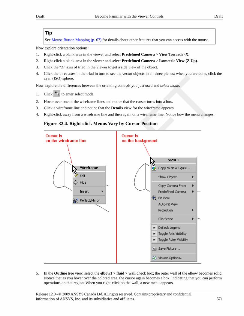
TipSee Mouse Button Mapping (p. 67) for details about other features that you can access with the mouse.
Now explore orientation options:
1. Right-click a blank area in the viewer and select Predefined Camera > View Towards -X.
2. Right-click a blank area in the viewer and select Predefined Camera > Isometric View (Z Up).
3. Click the “Z” axis of triad in the viewer to get a side view of the object.
4. Click the three axes in the triad in turn to see the vector objects in all three planes; when you are done, click thecyan (ISO) sphere.
Now explore the differences between the orienting controls you just used and select mode.
1. Click to enter select mode.
2. Hover over one of the wireframe lines and notice that the cursor turns into a box.
3. Click a wireframe line and notice that the Details view for the wireframe appears.
4. Right-click away from a wireframe line and then again on a wireframe line. Notice how the menu changes:
Figure 32.4. Right-click Menus Vary by Cursor Position
5. In the Outline tree view, select the elbow1 > fluid > wall check box; the outer wall of the elbow becomes solid.Notice that as you hover over the colored area, the cursor again becomes a box, indicating that you can performoperations on that region. When you right-click on the wall, a new menu appears.
571Release 12.0 - © 2009 ANSYS Canada Ltd. All rights reserved. Contains proprietary and confidentialinformation of ANSYS, Inc. and its subsidiaries and affiliates.
DraftBecome Familiar with the Viewer ControlsDraft
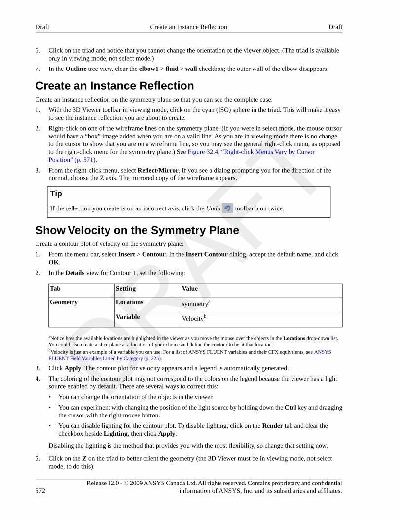
6. Click on the triad and notice that you cannot change the orientation of the viewer object. (The triad is availableonly in viewing mode, not select mode.)
7. In the Outline tree view, clear the elbow1 > fluid > wall checkbox; the outer wall of the elbow disappears.
Create an Instance ReflectionCreate an instance reflection on the symmetry plane so that you can see the complete case:
1. With the 3D Viewer toolbar in viewing mode, click on the cyan (ISO) sphere in the triad. This will make it easyto see the instance reflection you are about to create.
2. Right-click on one of the wireframe lines on the symmetry plane. (If you were in select mode, the mouse cursorwould have a “box” image added when you are on a valid line. As you are in viewing mode there is no changeto the cursor to show that you are on a wireframe line, so you may see the general right-click menu, as opposedto the right-click menu for the symmetry plane.) See Figure 32.4, “Right-click Menus Vary by CursorPosition” (p. 571).
3. From the right-click menu, select Reflect/Mirror. If you see a dialog prompting you for the direction of thenormal, choose the Z axis. The mirrored copy of the wireframe appears.
Tip
If the reflection you create is on an incorrect axis, click the Undo toolbar icon twice.
Show Velocity on the Symmetry PlaneCreate a contour plot of velocity on the symmetry plane:
1. From the menu bar, select Insert > Contour. In the Insert Contour dialog, accept the default name, and clickOK.
2. In the Details view for Contour 1, set the following:
ValueSettingTab
symmetryaLocationsGeometry
VelocitybVariable
aNotice how the available locations are highlighted in the viewer as you move the mouse over the objects in the Locations drop-down list.You could also create a slice plane at a location of your choice and define the contour to be at that location.bVelocity is just an example of a variable you can use. For a list of ANSYS FLUENT variables and their CFX equivalents, see ANSYSFLUENT Field Variables Listed by Category (p. 225).
3. Click Apply. The contour plot for velocity appears and a legend is automatically generated.
4. The coloring of the contour plot may not correspond to the colors on the legend because the viewer has a lightsource enabled by default. There are several ways to correct this:
• You can change the orientation of the objects in the viewer.
• You can experiment with changing the position of the light source by holding down the Ctrl key and draggingthe cursor with the right mouse button.
• You can disable lighting for the contour plot. To disable lighting, click on the Render tab and clear thecheckbox beside Lighting, then click Apply.
Disabling the lighting is the method that provides you with the most flexibility, so change that setting now.
5. Click on the Z on the triad to better orient the geometry (the 3D Viewer must be in viewing mode, not selectmode, to do this).
Release 12.0 - © 2009 ANSYS Canada Ltd. All rights reserved. Contains proprietary and confidentialinformation of ANSYS, Inc. and its subsidiaries and affiliates.572
DraftCreate an Instance ReflectionDraft
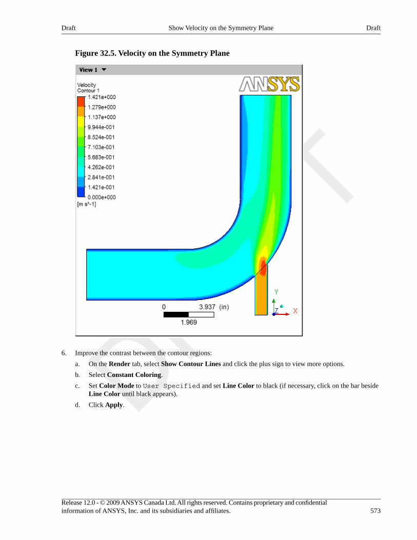
Figure 32.5. Velocity on the Symmetry Plane
6. Improve the contrast between the contour regions:
a. On the Render tab, select Show Contour Lines and click the plus sign to view more options.
b. Select Constant Coloring.
c. Set Color Mode to User Specified and set Line Color to black (if necessary, click on the bar besideLine Color until black appears).
d. Click Apply.
573Release 12.0 - © 2009 ANSYS Canada Ltd. All rights reserved. Contains proprietary and confidentialinformation of ANSYS, Inc. and its subsidiaries and affiliates.
DraftShow Velocity on the Symmetry PlaneDraft
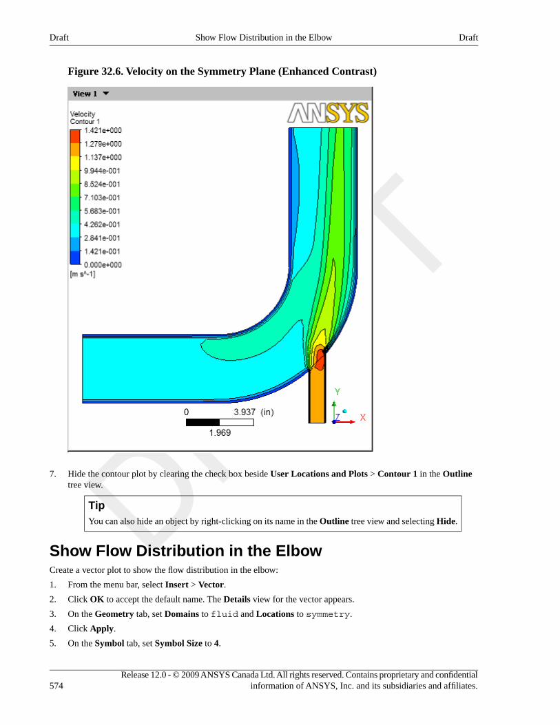
Figure 32.6. Velocity on the Symmetry Plane (Enhanced Contrast)
7. Hide the contour plot by clearing the check box beside User Locations and Plots > Contour 1 in the Outlinetree view.
TipYou can also hide an object by right-clicking on its name in the Outline tree view and selecting Hide.
Show Flow Distribution in the ElbowCreate a vector plot to show the flow distribution in the elbow:
1. From the menu bar, select Insert > Vector.
2. Click OK to accept the default name. The Details view for the vector appears.
3. On the Geometry tab, set Domains to fluid and Locations to symmetry.
4. Click Apply.
5. On the Symbol tab, set Symbol Size to 4.
Release 12.0 - © 2009 ANSYS Canada Ltd. All rights reserved. Contains proprietary and confidentialinformation of ANSYS, Inc. and its subsidiaries and affiliates.574
DraftShow Flow Distribution in the ElbowDraft
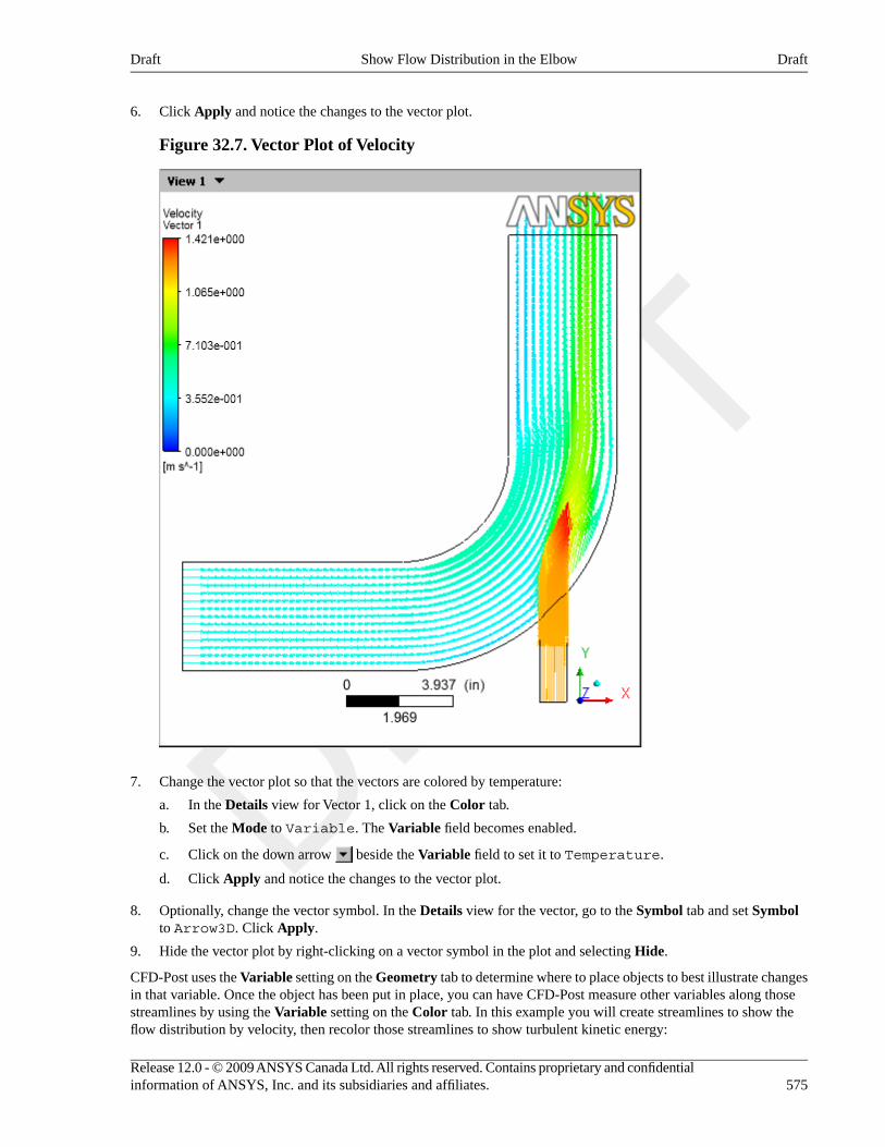
6. Click Apply and notice the changes to the vector plot.
Figure 32.7. Vector Plot of Velocity
7. Change the vector plot so that the vectors are colored by temperature:
a. In the Details view for Vector 1, click on the Color tab.
b. Set the Mode to Variable. The Variable field becomes enabled.
c. Click on the down arrow beside the Variable field to set it to Temperature.
d. Click Apply and notice the changes to the vector plot.
8. Optionally, change the vector symbol. In the Details view for the vector, go to the Symbol tab and set Symbolto Arrow3D. Click Apply.
9. Hide the vector plot by right-clicking on a vector symbol in the plot and selecting Hide.
CFD-Post uses the Variable setting on the Geometry tab to determine where to place objects to best illustrate changesin that variable. Once the object has been put in place, you can have CFD-Post measure other variables along thosestreamlines by using the Variable setting on the Color tab. In this example you will create streamlines to show theflow distribution by velocity, then recolor those streamlines to show turbulent kinetic energy:
575Release 12.0 - © 2009 ANSYS Canada Ltd. All rights reserved. Contains proprietary and confidentialinformation of ANSYS, Inc. and its subsidiaries and affiliates.
DraftShow Flow Distribution in the ElbowDraft
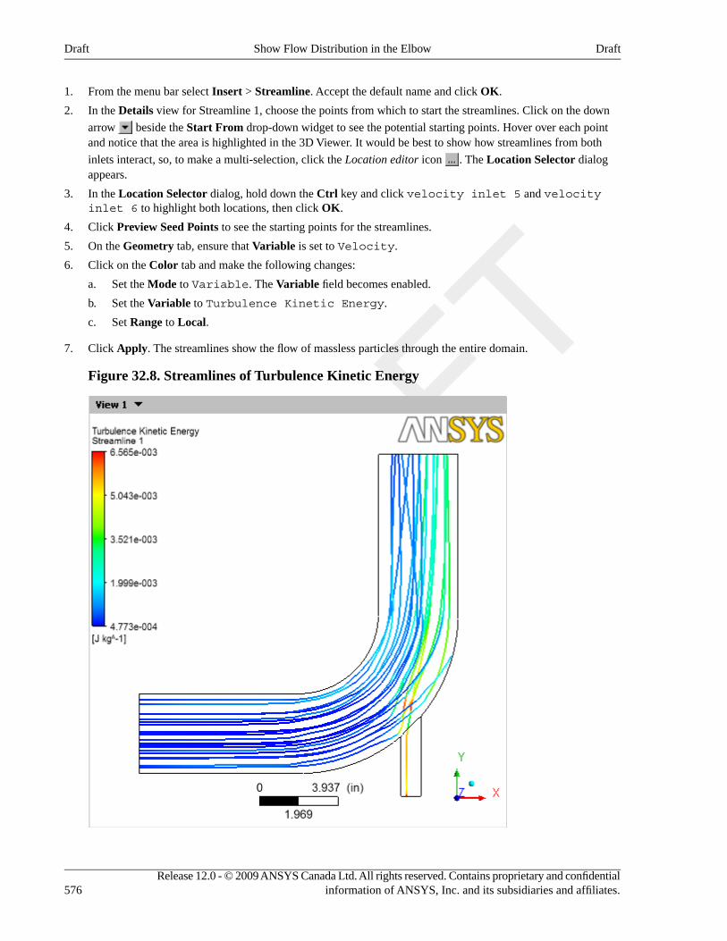
1. From the menu bar select Insert > Streamline. Accept the default name and click OK.
2. In the Details view for Streamline 1, choose the points from which to start the streamlines. Click on the down
arrow beside the Start From drop-down widget to see the potential starting points. Hover over each pointand notice that the area is highlighted in the 3D Viewer. It would be best to show how streamlines from both
inlets interact, so, to make a multi-selection, click the Location editor icon . The Location Selector dialogappears.
3. In the Location Selector dialog, hold down the Ctrl key and click velocity inlet 5 and velocityinlet 6 to highlight both locations, then click OK.
4. Click Preview Seed Points to see the starting points for the streamlines.
5. On the Geometry tab, ensure that Variable is set to Velocity.
6. Click on the Color tab and make the following changes:
a. Set the Mode to Variable. The Variable field becomes enabled.
b. Set the Variable to Turbulence Kinetic Energy.
c. Set Range to Local.
7. Click Apply. The streamlines show the flow of massless particles through the entire domain.
Figure 32.8. Streamlines of Turbulence Kinetic Energy
Release 12.0 - © 2009 ANSYS Canada Ltd. All rights reserved. Contains proprietary and confidentialinformation of ANSYS, Inc. and its subsidiaries and affiliates.576
DraftShow Flow Distribution in the ElbowDraft
8. Select the check box beside Vector 1. The vectors appear, but are largely hidden by the streamlines. To correctthis, highlight Streamline 1 in the Outline tree view and press Delete. The vectors are now clearly visible,
but the work you did to create the streamlines is gone. Click the Undo icon to restore Streamline 1.
9. Hide the vector plot and the streamlines by clearing the check boxes beside Vector 1 and Streamline 1 in theOutline tree view.
Show the Vortex StructureCFD-Post displays vortex core regions to enable you to better understand the processes in your simulation. In thisexample you will look at helicity method for vortex cores, but in your own work you would use the vortex core methodthat you find most instructive.
1. In the Outline tree view:
a. Under User Locations and Plots, clear the checkbox for Wireframe.
b. Under Cases > elbow1 > fluid, select the check box for wall.
c. Double-click on wall to edit its properties. On the Render tab, set Transparency to 0.75 and click Apply.
This makes the pipe easy to see while also making it possible to see objects inside the pipe.
2. From the menu bar, select Insert > Location > Vortex Core Region and click OK to accept the default name.
3. In the Details view for Vortex Core Region 1 on the Geometry tab, set Method to Absolute Helicityand Level to .01. On the Render tab, set Transparency to 0.2. Click Apply.
The absolute helicity vortex that is displayed is created by a mixture of effects from the walls, the curve in themain pipe, and the interaction of the fluids. If you had chosen the vorticity method instead, wall effects woulddominate.
4. On the Color tab, click on the colored bar in the Color field until the bar is green. Click Apply.
This improves the contrast between the vortex region and the blue walls.
5. Right-click in the 3D Viewer and select Predefined Camera > Isometric View (Y up).
6. In the Outline tree view, select the check box beside Streamline 1. This shows how the streamlines are affectedby the vortex regions.
577Release 12.0 - © 2009 ANSYS Canada Ltd. All rights reserved. Contains proprietary and confidentialinformation of ANSYS, Inc. and its subsidiaries and affiliates.
DraftShow the Vortex StructureDraft
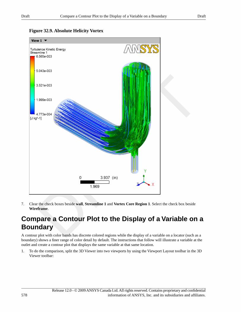
Figure 32.9. Absolute Helicity Vortex
7. Clear the check boxes beside wall, Streamline 1 and Vortex Core Region 1. Select the check box besideWireframe.
Compare a Contour Plot to the Display of a Variable on aBoundaryA contour plot with color bands has discrete colored regions while the display of a variable on a locator (such as aboundary) shows a finer range of color detail by default. The instructions that follow will illustrate a variable at theoutlet and create a contour plot that displays the same variable at that same location.
1. To do the comparison, split the 3D Viewer into two viewports by using the Viewport Layout toolbar in the 3DViewer toolbar:
Release 12.0 - © 2009 ANSYS Canada Ltd. All rights reserved. Contains proprietary and confidentialinformation of ANSYS, Inc. and its subsidiaries and affiliates.578
DraftCompare a Contour Plot to the Display of a Variable on a BoundaryDraft
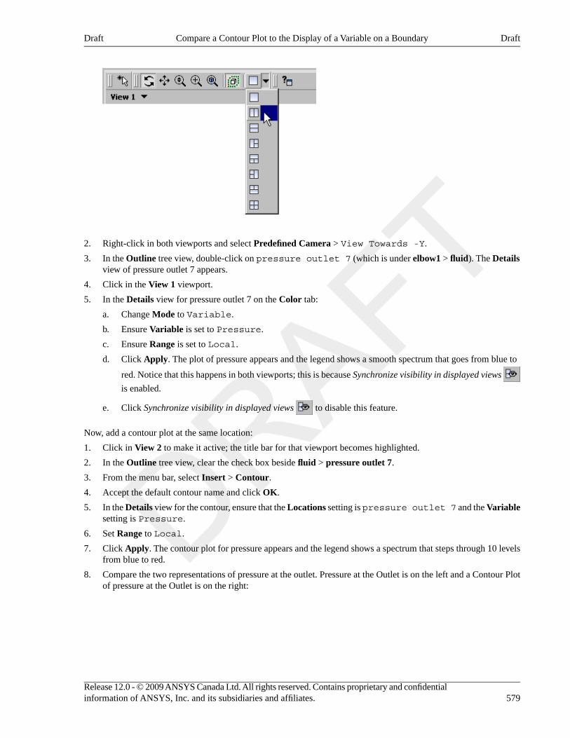
2. Right-click in both viewports and select Predefined Camera > View Towards -Y.
3. In the Outline tree view, double-click on pressure outlet 7 (which is under elbow1 > fluid). The Detailsview of pressure outlet 7 appears.
4. Click in the View 1 viewport.
5. In the Details view for pressure outlet 7 on the Color tab:
a. Change Mode to Variable.
b. Ensure Variable is set to Pressure.
c. Ensure Range is set to Local.
d. Click Apply. The plot of pressure appears and the legend shows a smooth spectrum that goes from blue to
red. Notice that this happens in both viewports; this is because Synchronize visibility in displayed views
is enabled.
e. Click Synchronize visibility in displayed views to disable this feature.
Now, add a contour plot at the same location:
1. Click in View 2 to make it active; the title bar for that viewport becomes highlighted.
2. In the Outline tree view, clear the check box beside fluid > pressure outlet 7.
3. From the menu bar, select Insert > Contour.
4. Accept the default contour name and click OK.
5. In the Details view for the contour, ensure that the Locations setting is pressure outlet 7 and the Variablesetting is Pressure.
6. Set Range to Local.
7. Click Apply. The contour plot for pressure appears and the legend shows a spectrum that steps through 10 levelsfrom blue to red.
8. Compare the two representations of pressure at the outlet. Pressure at the Outlet is on the left and a Contour Plotof pressure at the Outlet is on the right:
579Release 12.0 - © 2009 ANSYS Canada Ltd. All rights reserved. Contains proprietary and confidentialinformation of ANSYS, Inc. and its subsidiaries and affiliates.
DraftCompare a Contour Plot to the Display of a Variable on a BoundaryDraft
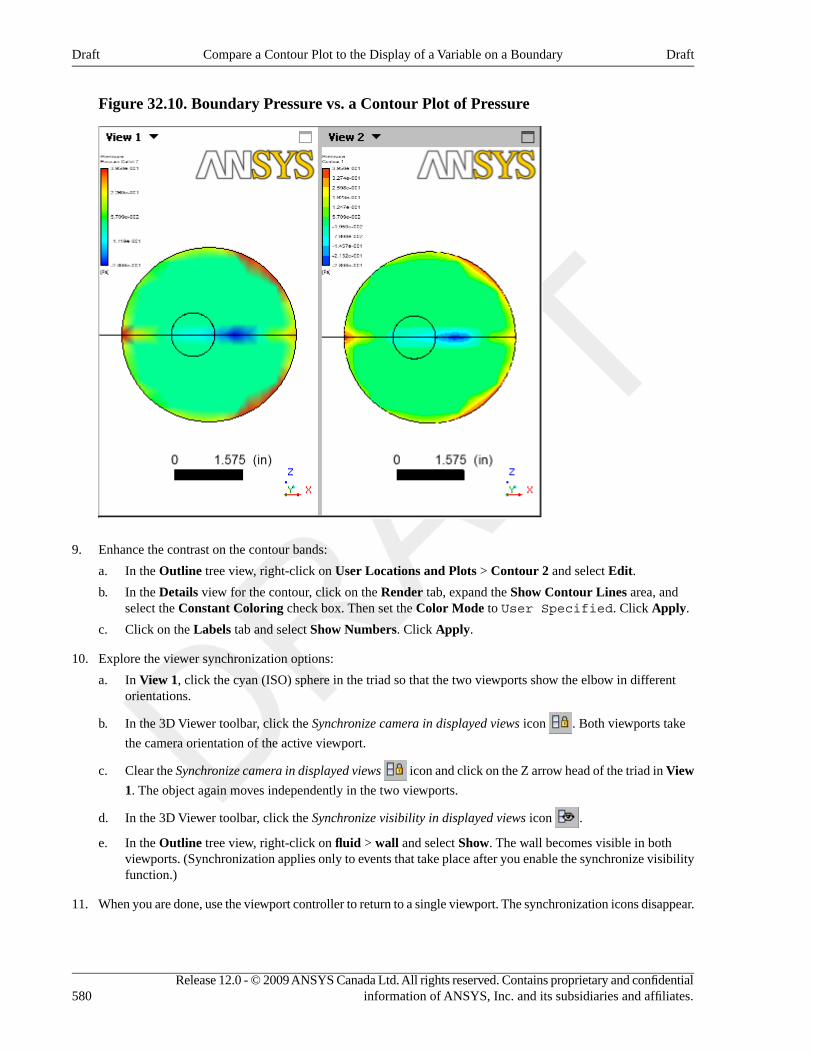
Figure 32.10. Boundary Pressure vs. a Contour Plot of Pressure
9. Enhance the contrast on the contour bands:
a. In the Outline tree view, right-click on User Locations and Plots > Contour 2 and select Edit.
b. In the Details view for the contour, click on the Render tab, expand the Show Contour Lines area, andselect the Constant Coloring check box. Then set the Color Mode to User Specified. Click Apply.
c. Click on the Labels tab and select Show Numbers. Click Apply.
10. Explore the viewer synchronization options:
a. In View 1, click the cyan (ISO) sphere in the triad so that the two viewports show the elbow in differentorientations.
b. In the 3D Viewer toolbar, click the Synchronize camera in displayed views icon . Both viewports take
the camera orientation of the active viewport.
c. Clear the Synchronize camera in displayed views icon and click on the Z arrow head of the triad in View
1. The object again moves independently in the two viewports.
d. In the 3D Viewer toolbar, click the Synchronize visibility in displayed views icon .
e. In the Outline tree view, right-click on fluid > wall and select Show. The wall becomes visible in bothviewports. (Synchronization applies only to events that take place after you enable the synchronize visibilityfunction.)
11. When you are done, use the viewport controller to return to a single viewport. The synchronization icons disappear.
Release 12.0 - © 2009 ANSYS Canada Ltd. All rights reserved. Contains proprietary and confidentialinformation of ANSYS, Inc. and its subsidiaries and affiliates.580
DraftCompare a Contour Plot to the Display of a Variable on a BoundaryDraft
Chart Temperature vs. DistanceWe want to show temperature vs. distance at the outlet of the pipe. We will create a chart to do that, but the chartrequires a line where we can sample values.
1. In the Outline tree view in the User Location and Plots area, right-click and select Hide All, then click in thecheck boxes to enable the Default Legend View 1 and the Wireframe.
2. Click the cyan (ISO) sphere in the triad so that you can again see the full elbow.
3. Create a line at the centerline of the outlet:
a. On the menu bar, select Insert > Location > Line. In the Insert Line dialog, accept the default name andclick OK.
b. Accept the default values and click Apply. A yellow line appears near the inside of the elbow.
c. In the Details view for Line 1, set the following:
ValueSettingTab
4, 7.999, 0.001bPoint 1aGeometry
8, 7.999, 0.001Point 2
CutcLine Type
VariableModeColor
TemperatureVariable
LocalRange
2Line WidthRender
aThe units are taken from the 3D Viewer options setting, which you can access from the menu bar by selecting Edit > Options.bThe Z value ensures that the line unambiguously passes through the domain.cThis setting constrains the line to be within the object.
d. Click Apply.
4. Create a chart that samples the points on Line 1:
a. On the menu bar, select Insert > Chart. In the Insert Chart dialog, accept the default name and click OK.
b. In the Details view for Chart 1, on the General tab set Title to Output Temperatures.
c. On the Data Series tab, right-click in the empty list box and select New, then set Name to Temperatureat Line 1 and Location to Line 1.
d. On the X Axis tab, set Variable to X.
e. On the Y Axis tab, set Variable to Temperature.
f. Click Apply. A chart similar to the following appears in the Chart Viewer:
581Release 12.0 - © 2009 ANSYS Canada Ltd. All rights reserved. Contains proprietary and confidentialinformation of ANSYS, Inc. and its subsidiaries and affiliates.
DraftChart Temperature vs. DistanceDraft
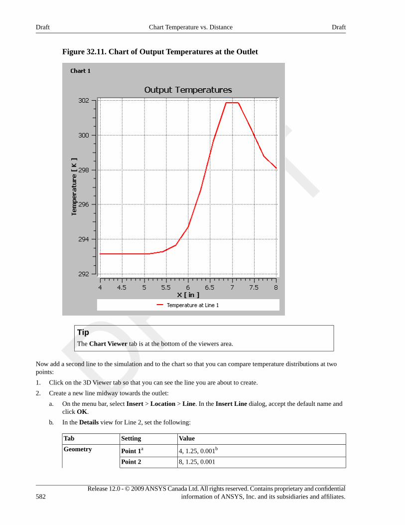
Figure 32.11. Chart of Output Temperatures at the Outlet
TipThe Chart Viewer tab is at the bottom of the viewers area.
Now add a second line to the simulation and to the chart so that you can compare temperature distributions at twopoints:
1. Click on the 3D Viewer tab so that you can see the line you are about to create.
2. Create a new line midway towards the outlet:
a. On the menu bar, select Insert > Location > Line. In the Insert Line dialog, accept the default name andclick OK.
b. In the Details view for Line 2, set the following:
ValueSettingTab
4, 1.25, 0.001bPoint 1aGeometry
8, 1.25, 0.001Point 2
Release 12.0 - © 2009 ANSYS Canada Ltd. All rights reserved. Contains proprietary and confidentialinformation of ANSYS, Inc. and its subsidiaries and affiliates.582
DraftChart Temperature vs. DistanceDraft
ValueSettingTab
CutcLine Type
VariableModeColor
TemperatureVariable
LocalRange
2Line WidthRender
aThe units are taken from the 3D Viewer options setting, which you can access from the menu bar by selecting Edit > Options.bThe Z value ensures that the line unambiguously passes through the domain.cThis setting constrains the line to be within the object.
c. Click Apply. A second line appears near the middle of the top section of pipe.
3. Add Line 2 to the existing chart:
a. Right-click on Outline > Report > Chart 1 and select Edit.
b. In the Details view for Chart 1, click on the Data Series tab, then click the New icon . A new series
appears.
Select Series 2 and set the following:
ValueSettingTab
Temperature at Line 2NameSeries
Line 2Location
c. Click Apply. A chart similar to the following appears in the Chart Viewer:
583Release 12.0 - © 2009 ANSYS Canada Ltd. All rights reserved. Contains proprietary and confidentialinformation of ANSYS, Inc. and its subsidiaries and affiliates.
DraftChart Temperature vs. DistanceDraft
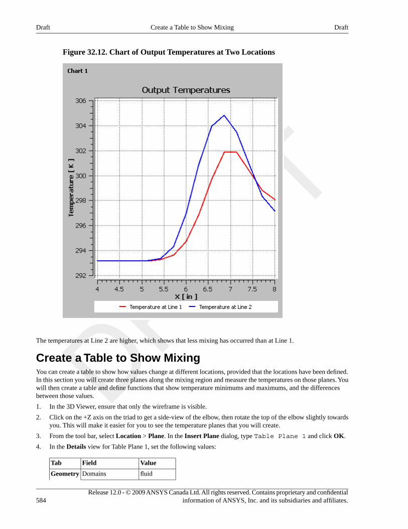
Figure 32.12. Chart of Output Temperatures at Two Locations
The temperatures at Line 2 are higher, which shows that less mixing has occurred than at Line 1.
Create a Table to Show MixingYou can create a table to show how values change at different locations, provided that the locations have been defined.In this section you will create three planes along the mixing region and measure the temperatures on those planes. Youwill then create a table and define functions that show temperature minimums and maximums, and the differencesbetween those values.
1. In the 3D Viewer, ensure that only the wireframe is visible.
2. Click on the +Z axis on the triad to get a side-view of the elbow, then rotate the top of the elbow slightly towardsyou. This will make it easier for you to see the temperature planes that you will create.
3. From the tool bar, select Location > Plane. In the Insert Plane dialog, type Table Plane 1 and click OK.
4. In the Details view for Table Plane 1, set the following values:
ValueFieldTab
fluidDomainsGeometry
Release 12.0 - © 2009 ANSYS Canada Ltd. All rights reserved. Contains proprietary and confidentialinformation of ANSYS, Inc. and its subsidiaries and affiliates.584
DraftCreate a Table to Show MixingDraft
ValueFieldTab
ZX PlaneDefinition > Method
-6.04Definition > Y
VariableModeColor
TemperatureVariable
LocalRange
(clear)LightingRender
5. Click Apply.
6. Right-click on Table Plane 1 and select Duplicate. The Duplicate dialog appears.
In the Duplicate dialog, accept the default name Table Plane 2 and click OK.
In the Outline view, double-click on Table Plane 2 and on the Geometry tab change Definition > Y to -0.55.Click Apply.
7. Repeat the previous step, duplicating Table Plane 2 to make Table Plane 3 and changing Definition> Y to 2.18. Click Apply.
8. Repeat the previous step, duplicating Table Plane 3 to make Table Plane 4 and changing Definition> Y to 5.04. Click Apply.
Now, create a table:
1. From the menu bar, select Insert > Table. Accept the default table name and click OK. The Table Viewer opens.
2. Type in the following headings:
DCBA
DifferenceMax. TemperatureMin. TemperatureDistance to Outlet1
3. For the ”Distance to Outlet” column, create an equation that gives the distance from the outlet (which is at the 8”mark). Click on cell A2, then in the Table Viewer's Insert bar, select Function > CFD-Post > minVal. In thecell definition field you see =minVal()@, which will be the base of the equation. With the cursor between theparentheses, type Y. Move the cursor after the @ sign and either type Table Plane 1 or select Insert > Location> Table Plane 1. The expression you have created gives the value of Y for Table Plane 1. To determine thedistance of Table Plane 1 from the outlet, complete the equation as follows, being careful to add 8[in]- to thebeginning of the equation to set the location of the outlet:
=8[in]-minVal(Y)@Table Plane 1
When you click away from cell A2, the equation is solved as 1.404e+01 [in].
4. Complete the rest of the table by entering the following cell definitions:
DCBA
DifferenceMax. TemperatureMin. TemperatureDistance to Outlet1
=maxVal(T)@TablePlane 1-
=maxVal(T)@TablePlane 1
=minVal(T)@TablePlane 1
=8[in]-minVal(Y)@TablePlane 1
2
minVal(T)@Table Plane1
=maxVal(T)@TablePlane 2-
=maxVal(T)@TablePlane 2
=minVal(T)@TablePlane 2
=8[in]-minVal(Y)@TablePlane 2
3
585Release 12.0 - © 2009 ANSYS Canada Ltd. All rights reserved. Contains proprietary and confidentialinformation of ANSYS, Inc. and its subsidiaries and affiliates.
DraftCreate a Table to Show MixingDraft
minVal(T)@Table Plane2
=maxVal(T)@TablePlane 3-
=maxVal(T)@TablePlane 3
=minVal(T)@TablePlane 3
=8[in]-minVal(Y)@TablePlane 3
4
minVal(T)@Table Plane3
=maxVal(T)@TablePlane 4-
=maxVal(T)@TablePlane 4
=minVal(T)@TablePlane 4
=8[in]-minVal(Y)@TablePlane 4
5
minVal(T)@Table Plane4
=maxVal(T)@pressureoutlet 7-
=maxVal(T)@pressureoutlet 7
=minVal(T)@pressureoutlet 7
=8[in]-minVal(Y)@pressureoutlet 7
6
minVal(T)@pressureoutlet 7
As you complete the table, notice that the minimum temperature values stay constant, but the maximum valuesdecrease as mixing occurs.
NoteThe sixth row determines the values at the outlet, rather than on a plane you defined.
5. The default format for cell data is appropriate for some variables, but it is not appropriate here. Click on cell A2,
then while depressing the Shift key, click in the lower-right cell (D6). Click on the Number Formatting icon
in the Table Viewer toolbar. In the Cell Formatting dialog, set Precision to 2, change Scientific to Fixed, andclick OK.
Review and Modify a ReportAs you work, ANSYS CFD-Post automatically updates a report, which you can see in the Report Viewer. At any timeyou can publish the report to an HTML file. In this section you will add a picture of the elbow and produce an HTMLreport:
1. Click on the Report Viewer tab at the bottom of the viewer to view the current report.
2. In the Outline tree view, double-click on the Report > Title Page. In the Title field on the Content tab of theDetails of Report Title Page, type: Analysis of Heat Transfer in a Mixing Elbow
3. Click Apply, then Refresh Preview to update the contents of the Report Viewer.
4. In the Outline tree view, ensure that only User Location and Plots > Contour 1, Default Legend View 1, andWireframe are visible, then double-click Contour 1. On the Geometry tab, set Variable to Temperatureand click Apply.
5. On the menu bar, select Insert > Figure. The Insert Figure dialog appears. Accept the default name and clickOK.
6. In the Outline tree view, double-click Report > Figure 1. In the Caption field, type Temperature on theSymmetry Plane and click Apply.
7. Click on the 3D Viewer, then click on the cyan (ISO) sphere in the triad.
8. Click on the Report Viewer.
9. On the top frame of the Report Viewer, click the Refresh icon . The report is updated with a picture
of the mixing elbow at the end of the report.
10. Optionally, click Publish to create an HTML version of the report. In the Publish Report dialog, click OK. Thereport is written to Report.htm in your working directory.
Release 12.0 - © 2009 ANSYS Canada Ltd. All rights reserved. Contains proprietary and confidentialinformation of ANSYS, Inc. and its subsidiaries and affiliates.586
DraftReview and Modify a ReportDraft
11. Right-click in the Outline view and select Hide All, then select Wireframe.
TipFor more information about reports, see Report (p. 41).
Create a Custom Variable and Animate the DisplayIn this section you will generate an expression using the CFX Expression Language (CEL), which you can then usein CFD-Post in place of a numeric value. You will then associate the expression with a variable, which you will alsocreate. Finally, you will create a plane that displays the new variable, then move the plane to see how the values forthe variable change.
1. Define a custom expression for the dynamic head formula (rho|V|^2)/2 as follows:
a. On the tab bar at the top of the workspace area, select Expressions. Right-click in the Expressions area andselect New.
b. In the New Expression dialog, type: DynamicHeadExp
c. Click OK.
d. In the Definition area, type in this definition:
Density * abs(Velocity)^2 / 2
where:
• Density is a variable
• abs is a CEL function (abs is unnecessary in this example, it simply illustrates the use of a CEL function)
• Velocity is a variable
TipYou can learn which predefined functions, variables, expression, locations, and constants areavailable by right-clicking in the Definition area.
e. Click Apply.
2. Associate the expression with a variable (as the plane you define in the next step can display only variables):
a. On the tab bar at the top of the workspace area, select Variables. Right-click in the Variables area and selectNew.
b. In the New Variable dialog, type: DynamicHeadVar
c. Click OK.
d. In the Details view for DynamicHeadVar, click the drop-down arrow beside Expression and chooseDynamicHeadExp. Click Apply.
3. Create a plane and animate it:
a. Click on the 3D Viewer tab.
b. Right-click on the wireframe and select Insert > YZ Plane.
c. If you see a dialog that asks in which direction you want the normal to point, choose the direction appropriatefor your purposes.
A plane that maps the distribution of the default variable (Pressure) appears.
d. On the Color tab, set Variable to ”DynamicHeadVar”. On the Render tab, clear Lighting.Click Apply.
The plane now maps the dynamic head distribution.
587Release 12.0 - © 2009 ANSYS Canada Ltd. All rights reserved. Contains proprietary and confidentialinformation of ANSYS, Inc. and its subsidiaries and affiliates.
DraftCreate a Custom Variable and Animate the DisplayDraft
e. In the 3D Viewer in with the mouse cursor in select mode, click on the plane and drag it to various placesin the object to see how the location changes the DynamicHeadVar values displayed.
f. Right-click on the plane and select Animate. The Animation dialog appears and the plane moves throughthe entire domain, displaying changes to the DynamicHeadVar values as it moves.
g. On the Animation dialog, click the Stop icon , then click Close.
TipYou can define multiple planes and animate them concurrently. First, stop any animations currentlyrunning, then create a new plane. To animate both planes, hold down Ctrl to select multiple planes
on the Animation dialog and press the Play icon .
4. In the upper-left corner of the 3D Viewer, click the down arrow beside Figure 1 and change it to View 1.
5. In the Outline view, right-click beside User Locations and Plots and select Hide All, then select Wireframeand Default Legend View 1 to make them visible.
Loading and Comparing the Results to Those in a RefinedMeshTo this point you have been working with a coarse mesh. In this section you will compare the results from that meshto those from a refined mesh:
1. Select File > Load Results. The Load Results File dialog appears
2. On the Load Results File dialog, select Keep current cases loaded and keep the other settings unchanged.
3. Select elbow3.cdat.gz (or elbow3.cdat) and click Open.
In the 3D Viewer, there are now two viewports: in the title bar for View 1 you have elbow1, and in View 2 youhave elbow3. In the Outline tree view under Cases you have elbow1 and elbow3; all boundaries associated witheach case are listed separately and can be controlled separately. You also have a new entry: Cases > CaseComparison.
4. In the Toolbar, select Synchronize camera in displayed views .
If the two cases are not oriented in the same way, clear the Synchronize camera in displayed views icon and
then select it again.
Examine the operation of CFD-Post when the two views are not synchronized and when they are synchronized:
1. In the viewer toolbar, clear Synchronize visibility in displayed views .
2. With the focus in View 1, select Insert > Contour and create a contour of pressure on pressure outlet 7 thatdisplays values in the local range.
Note that the contour appears only in View 1. When visibility is not synchronized, changes you make to UserLocation and Plots settings apply only to the currently active view.
3. In either view (while in viewing mode), click on the Z axis on the triad. Both views show their cases from theperspective of the Z axis.
4. In the viewer toolbar, select Synchronize visibility in displayed views .
5. With the focus on the view that contains elbow3, select Insert > Contour. Accept the default name and clickOK. Define a contour that displays temperature on the symmetry plane:
Release 12.0 - © 2009 ANSYS Canada Ltd. All rights reserved. Contains proprietary and confidentialinformation of ANSYS, Inc. and its subsidiaries and affiliates.588
DraftLoading and Comparing the Results to Those in a Refined MeshDraft
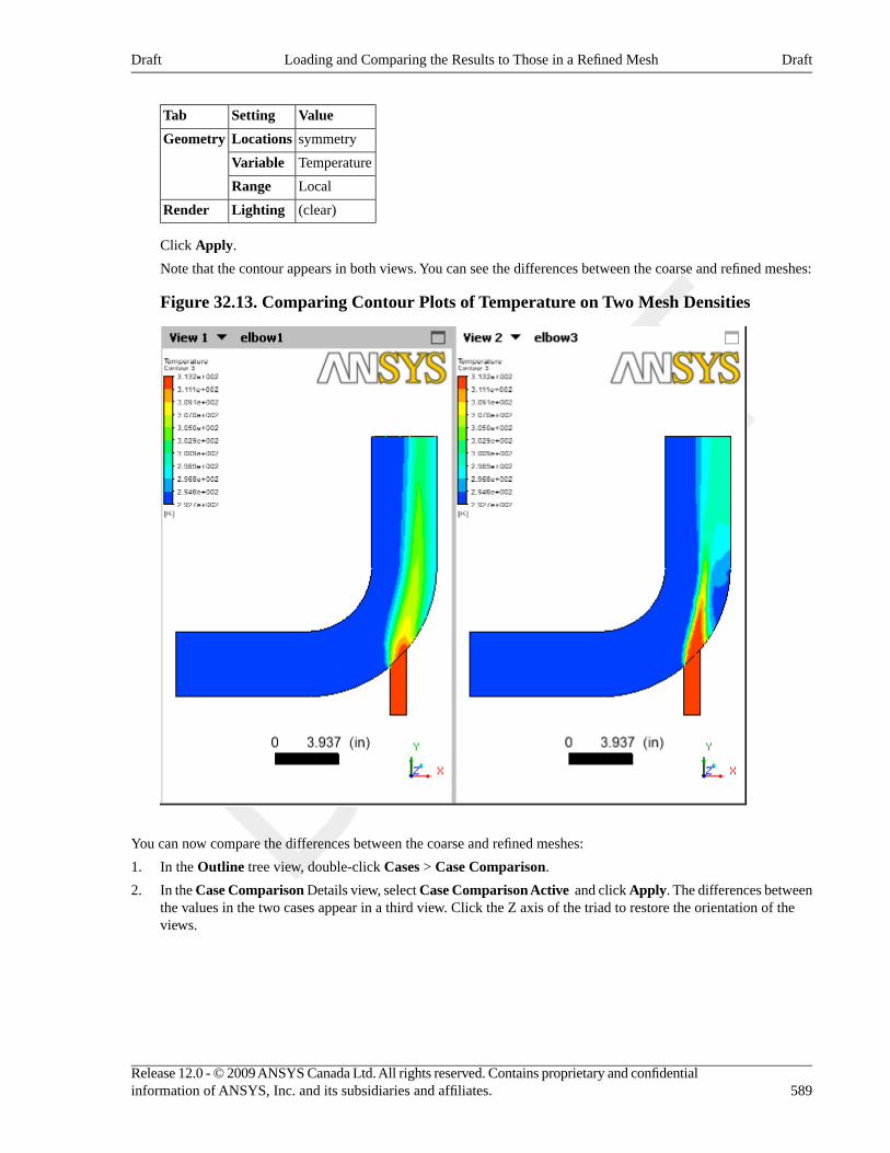
ValueSettingTab
symmetryLocationsGeometry
TemperatureVariable
LocalRange
(clear)LightingRender
Click Apply.
Note that the contour appears in both views. You can see the differences between the coarse and refined meshes:
Figure 32.13. Comparing Contour Plots of Temperature on Two Mesh Densities
You can now compare the differences between the coarse and refined meshes:
1. In the Outline tree view, double-click Cases > Case Comparison.
2. In the Case Comparison Details view, select Case Comparison Active and click Apply. The differences betweenthe values in the two cases appear in a third view. Click the Z axis of the triad to restore the orientation of theviews.
589Release 12.0 - © 2009 ANSYS Canada Ltd. All rights reserved. Contains proprietary and confidentialinformation of ANSYS, Inc. and its subsidiaries and affiliates.
DraftLoading and Comparing the Results to Those in a Refined MeshDraft
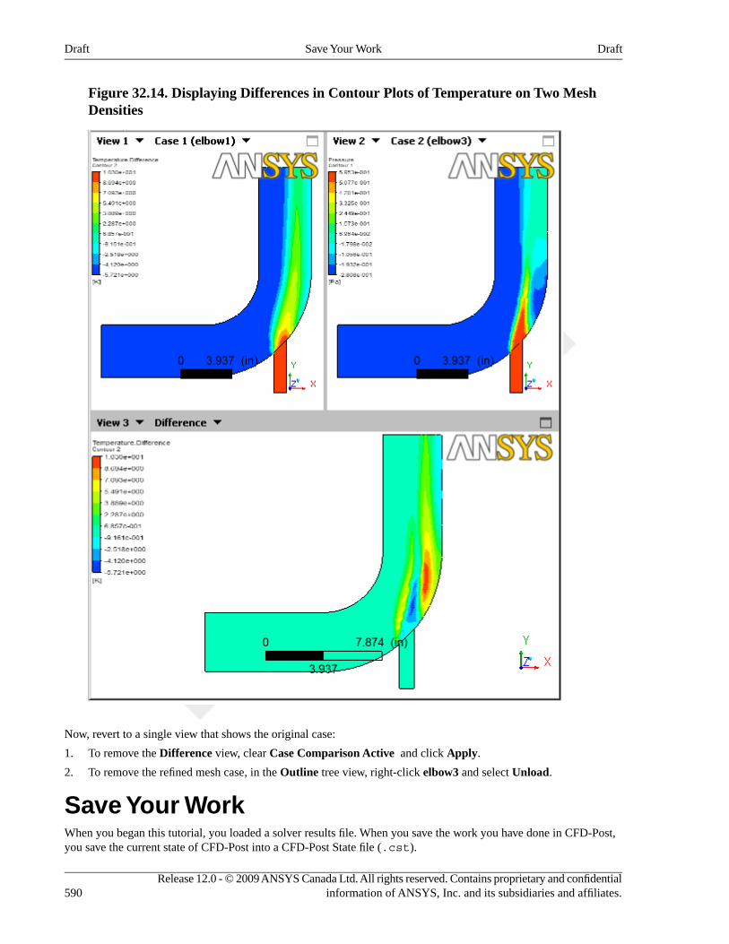
Figure 32.14. Displaying Differences in Contour Plots of Temperature on Two MeshDensities
Now, revert to a single view that shows the original case:
1. To remove the Difference view, clear Case Comparison Active and click Apply.
2. To remove the refined mesh case, in the Outline tree view, right-click elbow3 and select Unload.
Save Your WorkWhen you began this tutorial, you loaded a solver results file. When you save the work you have done in CFD-Post,you save the current state of CFD-Post into a CFD-Post State file (.cst).
Release 12.0 - © 2009 ANSYS Canada Ltd. All rights reserved. Contains proprietary and confidentialinformation of ANSYS, Inc. and its subsidiaries and affiliates.590
DraftSave Your WorkDraft
1. How you save your work depends on whether you are running CFD-Post standalone or from within ANSYSWorkbench:
• From CFD-Post standalone:
1. From the menu bar, select File > Save State.
This operation saves the expression, custom variable, and the settings for the objects in a .cst file andsaves the state of the animation in a .can file. The .cas.gz and .cdat.gz files remain unchanged.
2. A Warning dialog asks if you want to save the animation state. Click OK.
3. Optionally, confirm the state file's contents: close the current file from the menu bar by selecting File >Close (or press Ctrl+W) then reload the state file (select File > Load State and choose the file that yousaved in step 1.)
• From ANSYS Workbench:
1. From the CFD-Post menu bar, select File > Quit. ANSYS Workbench saves the state file automatically.
2. In the ANSYS Workbench Project Schematic, double-click on the Results cell. CFD-Post re-openswith the state file loaded.
2. Save a picture of the current state of the simulation: In the Outline view, show Contour 1. With the focus in the
3D Viewer, click Save Picture from the tool bar. In the Save Picture dialog, click Save. A PNG file of thecurrent state of the viewer is saved to <casename>.png (elbow1.png) in your working directory.
TipTo learn about the options on the Save Picture dialog, see Save Picture Command (p. 91).
3. You can recreate the animation you made in the previous section and save it to a file:
a. Click on the cyan (ISO) sphere in the triad to orient the elbow to display Plane 1.
b. In the Outline view, clear Contour 1 and show Plane 1.
c. Right-click on Plane 1 in the 3D Viewer and select Animate. The Animation dialog appears and the planemoves through the entire domain.
d. Click the stop icon .
e. If necessary, display the full animation control set by clicking .
591Release 12.0 - © 2009 ANSYS Canada Ltd. All rights reserved. Contains proprietary and confidentialinformation of ANSYS, Inc. and its subsidiaries and affiliates.
DraftSave Your WorkDraft
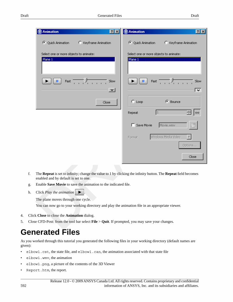
f. The Repeat is set to infinity; change the value to 1 by clicking the infinity button. The Repeat field becomesenabled and by default is set to one.
g. Enable Save Movie to save the animation to the indicated file.
h. Click Play the animation .
The plane moves through one cycle.
You can now go to your working directory and play the animation file in an appropriate viewer.
4. Click Close to close the Animation dialog.
5. Close CFD-Post: from the tool bar select File > Quit. If prompted, you may save your changes.
Generated FilesAs you worked through this tutorial you generated the following files in your working directory (default names aregiven):
• elbow1.cst, the state file, and elbow1.can, the animation associated with that state file
• elbow1.wmv, the animation
• elbow1.png, a picture of the contents of the 3D Viewer
• Report.htm, the report.
Release 12.0 - © 2009 ANSYS Canada Ltd. All rights reserved. Contains proprietary and confidentialinformation of ANSYS, Inc. and its subsidiaries and affiliates.592
DraftGenerated FilesDraft
Chapter 33.Turbo PostprocessingThis tutorial demonstrates the turbomachinery postprocessing capabilities of CFD-Post.
In this example, you will read ANSYS FLUENT case and data files (without doing any calculations) and perform anumber of turbomachinery-specific postprocessing operations.
This tutorial demonstrates:
• Displaying the Solution in ANSYS CFD-Post (p. 599)
• Initializing the Turbomachinery Components (p. 601)
• Comparing the Blade-to-Blade, Meridional, and 3D Views (p. 601)
• Displaying Contours on Meridional Isosurfaces (p. 603)
• Displaying a 360-Degree View (p. 604)
• Calculating and Displaying Values of Variables (p. 605)
• Displaying the Inlet to Outlet Chart (p. 607)
• Generating and Viewing Turbo Reports (p. 609)
Problem DescriptionThis tutorial considers the problem of a centrifugal compressor shown schematically in Figure 33.1, “ProblemSpecification” (p. 594). The model comprises a single 3D sector of the compressor to take advantage of the circumferentialperiodicity in the problem. The flow of air through the compressor is simulated and the postprocessing capabilities ofCFD-Post are used to display realistic, full 360-degree images of the solution obtained.
593Release 12.0 - © 2009 ANSYS Canada Ltd. All rights reserved. Contains proprietary and confidentialinformation of ANSYS, Inc. and its subsidiaries and affiliates.
DraftDraft
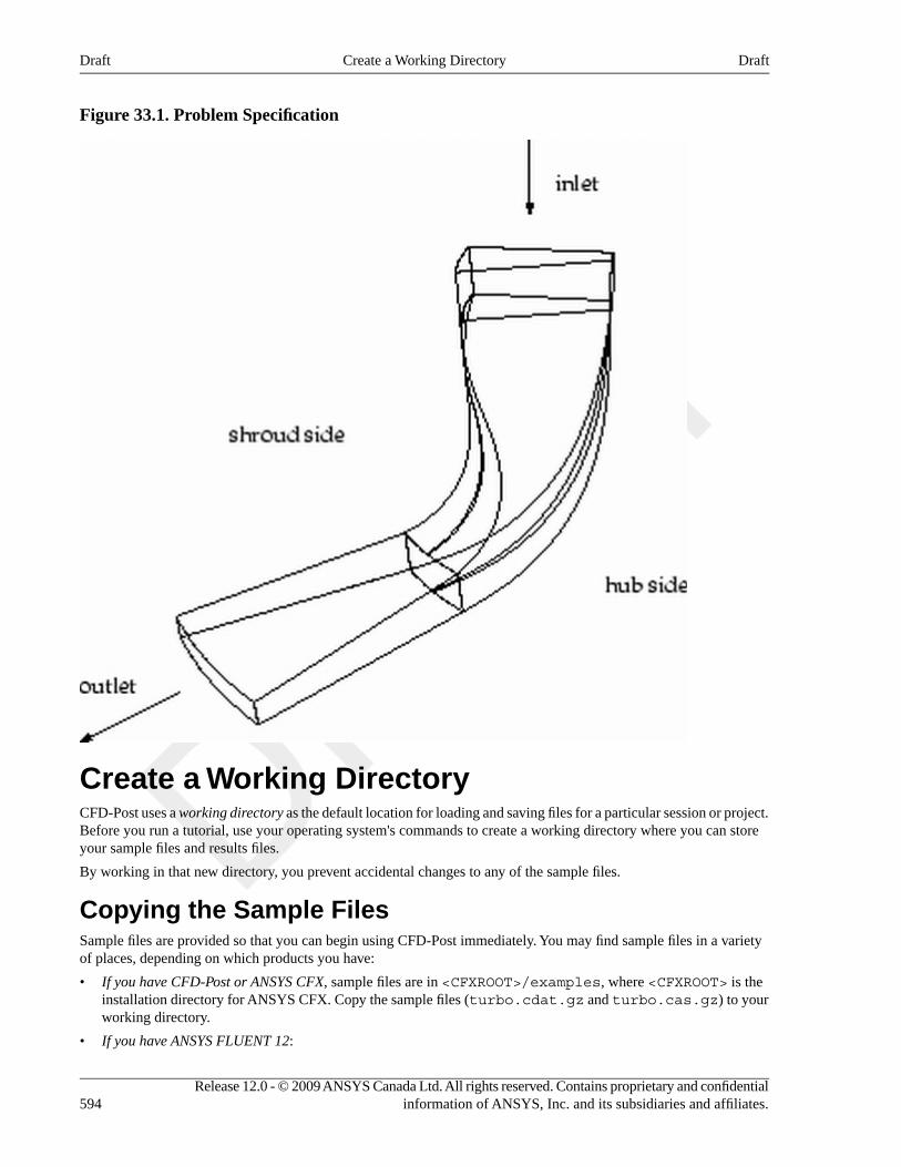
Figure 33.1. Problem Specification
Create a Working DirectoryCFD-Post uses a working directory as the default location for loading and saving files for a particular session or project.Before you run a tutorial, use your operating system's commands to create a working directory where you can storeyour sample files and results files.
By working in that new directory, you prevent accidental changes to any of the sample files.
Copying the Sample FilesSample files are provided so that you can begin using CFD-Post immediately. You may find sample files in a varietyof places, depending on which products you have:
• If you have CFD-Post or ANSYS CFX, sample files are in <CFXROOT>/examples, where <CFXROOT> is theinstallation directory for ANSYS CFX. Copy the sample files (turbo.cdat.gz and turbo.cas.gz) to yourworking directory.
• If you have ANSYS FLUENT 12:
Release 12.0 - © 2009 ANSYS Canada Ltd. All rights reserved. Contains proprietary and confidentialinformation of ANSYS, Inc. and its subsidiaries and affiliates.594
DraftCreate a Working DirectoryDraft
1. Download cfd-post-turbo.zip from the ANSYS FLUENT User Services Center (www.fluentusers.com)to your working directory. This file can be found by using the Documentation link on the ANSYS FLUENTproduct page.
2. Extract the CAS files and DAT files (turbo.cas.gz and turbo.dat.gz) from cfd-post-turbo.zipto your working directory.
Note• These tutorials are prepared on a Windows system. The screen shots and graphic images in the
tutorials may be slightly different than the appearance on your system, depending on the operatingsystem or graphics card.
• The case name is derived from the name of the results file that you load with the final extensionremoved. Thus, if you load turbo.cdat.gz the case name will be turbo.cdat; if you load turbo.cdat,the case name will be turbo. The case name used in this tutorial is turbo.
Launching ANSYS CFD-PostBefore you start CFD-Post, set the working directory. The procedure for setting the working directory and startingCFD-Post depends on whether you will run CFD-Post standalone, from the ANSYS CFX Launcher, from ANSYSWorkbench, or from ANSYS FLUENT:
• To run CFD-Post standalone, from the Start menu, right-click All Programs > ANSYS 12.0 > ANSYS CFD-Postand select Properties. Type the path to your working directory in the Start in field and click OK, then click AllPrograms > ANSYS 12.0 > ANSYS CFD-Post to launch CFD-Post.
• To run ANSYS CFX Launcher
1. Start the ANSYS CFX Launcher.
You can run the CFX Launcher in any of the following ways:
• On Windows:
• From the Start menu, go to All Programs > ANSYS 12.0 > CFX > ANSYS CFX 12.0.
• In a DOS window that has its path set up correctly to run CFX, enter cfx5launch (otherwise, youwill need to type the full pathname of the cfx command, which will be something similar to C:\ProgramFiles\ANSYS Inc\v120\CFX\bin).
• On UNIX, enter cfx5launch in a terminal window that has its path set up to run CFX (the path will besomething similar to /usr/ansys_inc/v120/CFX/bin).
2. Select the Working Directory (where you copied the sample files).
3. Click the CFD-Post 12.0 button.
• ANSYS Workbench
1. Start ANSYS Workbench.
2. From the menu bar, select File > Save As and save the project file to the directory that you want to be theworking directory.
3. Open the Component Systems toolbox and double-click Results. A Results system opens in the ProjectSchematic.
4. Right-click on the A2 Results cell and select Edit. CFD-Post opens.
• ANSYS FLUENT
1. Click the ANSYS FLUENT icon ( ) in the ANSYS program group to open ANSYS FLUENT Launcher.
595Release 12.0 - © 2009 ANSYS Canada Ltd. All rights reserved. Contains proprietary and confidentialinformation of ANSYS, Inc. and its subsidiaries and affiliates.
DraftLaunching ANSYS CFD-PostDraft
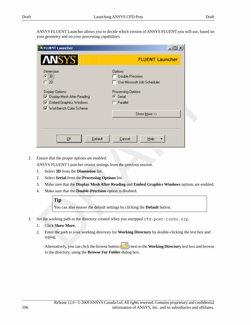
ANSYS FLUENT Launcher allows you to decide which version of ANSYS FLUENT you will use, based onyour geometry and on your processing capabilities.
2. Ensure that the proper options are enabled.
ANSYS FLUENT Launcher retains settings from the previous session.
1. Select 3D from the Dimension list.
2. Select Serial from the Processing Options list.
3. Make sure that the Display Mesh After Reading and Embed Graphics Windows options are enabled.
4. Make sure that the Double-Precision option is disabled.
TipYou can also restore the default settings by clicking the Default button.
3. Set the working path to the directory created when you unzipped cfd-post-turbo.zip.
1. Click Show More.
2. Enter the path to your working directory for Working Directory by double-clicking the text box andtyping.
Alternatively, you can click the browse button ( ) next to the Working Directory text box and browse
to the directory, using the Browse For Folder dialog box.
Release 12.0 - © 2009 ANSYS Canada Ltd. All rights reserved. Contains proprietary and confidentialinformation of ANSYS, Inc. and its subsidiaries and affiliates.596
DraftLaunching ANSYS CFD-PostDraft

4. Click OK to launch ANSYS FLUENT.
597Release 12.0 - © 2009 ANSYS Canada Ltd. All rights reserved. Contains proprietary and confidentialinformation of ANSYS, Inc. and its subsidiaries and affiliates.
DraftLaunching ANSYS CFD-PostDraft
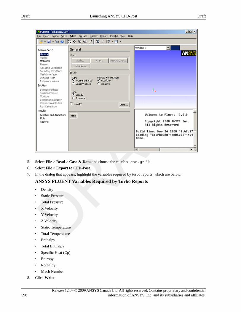
5. Select File > Read > Case & Data and choose the turbo.cas.gz file.
6. Select File > Export to CFD-Post.
7. In the dialog that appears, highlight the variables required by turbo reports, which are below:
ANSYS FLUENT Variables Required by Turbo Reports
• Density
• Static Pressure
• Total Pressure
• X Velocity
• Y Velocity
• Z Velocity
• Static Temperature
• Total Temperature
• Enthalpy
• Total Enthalpy
• Specific Heat (Cp)
• Entropy
• Rothalpy
• Mach Number
8. Click Write.
Release 12.0 - © 2009 ANSYS Canada Ltd. All rights reserved. Contains proprietary and confidentialinformation of ANSYS, Inc. and its subsidiaries and affiliates.598
DraftLaunching ANSYS CFD-PostDraft
CFD-Post starts with the tutorial file loaded.
Displaying the Solution in ANSYS CFD-PostIn the steps that follow, you will visualize various aspects of the flow for the case using CFD-Post. You will:
• Prepare the case and set the viewer options
• Initialize the turbomachinery components
• Compare the blade-to-blade, meridional, and 3D views
• Compare contours on meridional isosurfaces
• Calculate and display the values of variables
• Display a 360-degree view
• Display the inlet-to-outlet chart
• Generate and view a Turbo report
Prepare the Case and Set the Viewer Options1. If CFD-Post has not been started from ANSYS FLUENT, load the CDAT file (turbo.cdat.gz) from the
menu bar by selecting File > Load Results. In the Load Results File dialog, select turbo.cdat.gz and clickOpen.
2. If you see a pop-up that discusses Global Variables Ranges, it can be ignored. Click OK.
The turbo blade appears in the viewer in an isometric orientation. The Wireframe appears in the 3D Viewer andthere is a check mark beside Wireframe in the Outline workspace; the check mark indicates that the wireframeis visible in the 3D Viewer.
3. Set CFD-Post to display the units you want to see. These display units are not necessarily the same types as theunits in the results files you load; however, for this tutorial you will set the display units to be the same as thesolution units.
1. Right-click on the viewer and select Viewer Options.
TipThe Options dialog is where you set your preferences; see Setting Preferences with the OptionsDialog (p. 103) for details.
2. In the Options dialog, select Common > Units.
3. Set System to SI and click OK.
NoteThe display units you set are saved between sessions and projects. This means that you can load resultsfiles from diverse sources and always see familiar units displayed.
4. Double-click Wireframe in the Outline workspace to see the Details view. To display the mesh, set Edge Angleto 0 degrees and click Apply. The Edge Angle is the angle between one edge of a mesh face and its neighboringface. Setting an edge angle in CFD-Post defines a minimum angle for drawing parts of the surface mesh. Whenyou set a small angle, the mesh becomes visible.
TipWith the mouse focus on CFD-Post and the mouse over the Details of Wireframe editor, press F1 tosee help about the Wireframe object.
599Release 12.0 - © 2009 ANSYS Canada Ltd. All rights reserved. Contains proprietary and confidentialinformation of ANSYS, Inc. and its subsidiaries and affiliates.
DraftDisplaying the Solution in ANSYS CFD-PostDraft
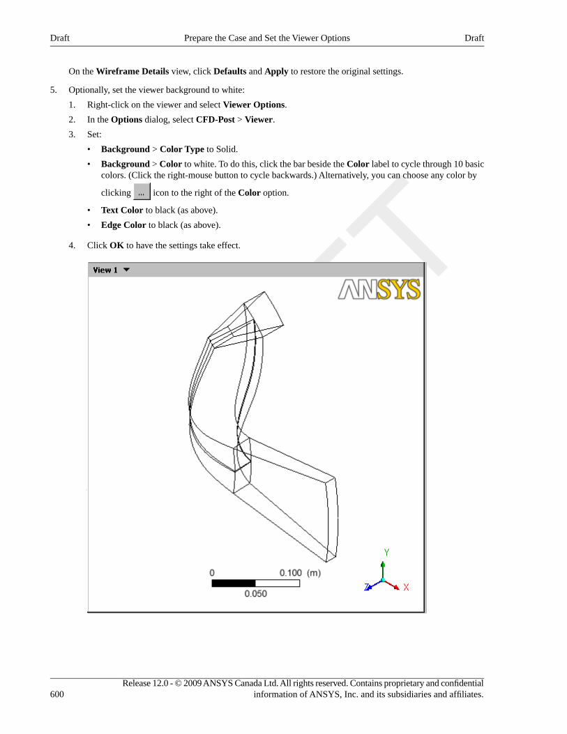
On the Wireframe Details view, click Defaults and Apply to restore the original settings.
5. Optionally, set the viewer background to white:
1. Right-click on the viewer and select Viewer Options.
2. In the Options dialog, select CFD-Post > Viewer.
3. Set:
• Background > Color Type to Solid.
• Background > Color to white. To do this, click the bar beside the Color label to cycle through 10 basiccolors. (Click the right-mouse button to cycle backwards.) Alternatively, you can choose any color by
clicking icon to the right of the Color option.
• Text Color to black (as above).
• Edge Color to black (as above).
4. Click OK to have the settings take effect.
Release 12.0 - © 2009 ANSYS Canada Ltd. All rights reserved. Contains proprietary and confidentialinformation of ANSYS, Inc. and its subsidiaries and affiliates.600
DraftPrepare the Case and Set the Viewer OptionsDraft
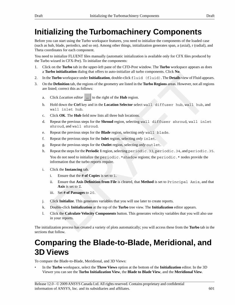
Initializing the Turbomachinery ComponentsBefore you can start using the Turbo workspace features, you need to initialize the components of the loaded case(such as hub, blade, periodics, and so on). Among other things, initialization generates span, a (axial), r (radial), andTheta coordinates for each component.
You need to initialize FLUENT files manually (automatic initialization is available only for CFX files produced bythe Turbo wizard in CFX-Pre). To initialize the components:
1. Click on the Turbo tab in the upper-left pane of the CFD-Post window. The Turbo workspace appears as doesa Turbo initialization dialog that offers to auto-initialize all turbo components. Click No.
2. In the Turbo workspace under Initialization, double-click fluid (fluid). The Details view of Fluid appears.
3. On the Definition tab, the regions of the geometry are listed in the Turbo Regions areas. However, not all regionsare listed; correct this as follows:
a. Click Location editor to the right of the Hub region.
b. Hold down the Ctrl key and in the Location Selector select wall diffuser hub, wall hub, andwall inlet hub.
c. Click OK. The Hub field now lists all three hub locations.
d. Repeat the previous steps for the Shroud region, selecting wall diffuser shroud, wall inletshroud, and wall shroud.
e. Repeat the previous steps for the Blade region, selecting only wall blade.
f. Repeat the previous steps for the Inlet region, selecting only inlet.
g. Repeat the previous steps for the Outlet region, selecting only outlet.
h. Repeat the steps for the Periodic 1 region, selecting periodic.33, periodic.34, and periodic.35.
You do not need to initialize the periodic.*shadow regions; the periodic.* nodes provide theinformation that the turbo reports require.
i. Click the Instancing tab.
i. Ensure that the # of Copies is set to 1.
ii. Ensure that Axis Definition from File is cleared, that Method is set to Principal Axis, and thatAxis is set to Z.
iii. Set # of Passages to 20.
j. Click Initialize. This generates variables that you will use later to create reports.
k. Double-click Initialization at the top of the Turbo tree view. The Initialization editor appears.
l. Click the Calculate Velocity Components button. This generates velocity variables that you will also usein your reports.
The initialization process has created a variety of plots automatically; you will access these from the Turbo tab in thesections that follow.
Comparing the Blade-to-Blade, Meridional, and3D ViewsTo compare the Blade-to-Blade, Meridional, and 3D Views:
• In the Turbo workspace, select the Three Views option at the bottom of the Initialization editor. In the 3DViewer you can see the Turbo Initialization View, the Blade to Blade View, and the Meridional View.
601Release 12.0 - © 2009 ANSYS Canada Ltd. All rights reserved. Contains proprietary and confidentialinformation of ANSYS, Inc. and its subsidiaries and affiliates.
DraftInitializing the Turbomachinery ComponentsDraft
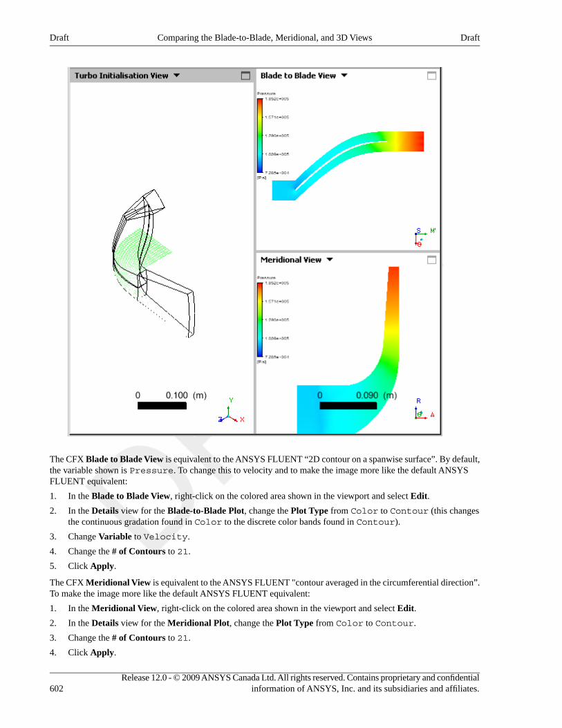
The CFX Blade to Blade View is equivalent to the ANSYS FLUENT “2D contour on a spanwise surface”. By default,the variable shown is Pressure. To change this to velocity and to make the image more like the default ANSYSFLUENT equivalent:
1. In the Blade to Blade View, right-click on the colored area shown in the viewport and select Edit.
2. In the Details view for the Blade-to-Blade Plot, change the Plot Type from Color to Contour (this changesthe continuous gradation found in Color to the discrete color bands found in Contour).
3. Change Variable to Velocity.
4. Change the # of Contours to 21.
5. Click Apply.
The CFX Meridional View is equivalent to the ANSYS FLUENT "contour averaged in the circumferential direction”.To make the image more like the default ANSYS FLUENT equivalent:
1. In the Meridional View, right-click on the colored area shown in the viewport and select Edit.
2. In the Details view for the Meridional Plot, change the Plot Type from Color to Contour.
3. Change the # of Contours to 21.
4. Click Apply.
Release 12.0 - © 2009 ANSYS Canada Ltd. All rights reserved. Contains proprietary and confidentialinformation of ANSYS, Inc. and its subsidiaries and affiliates.602
DraftComparing the Blade-to-Blade, Meridional, and 3D ViewsDraft
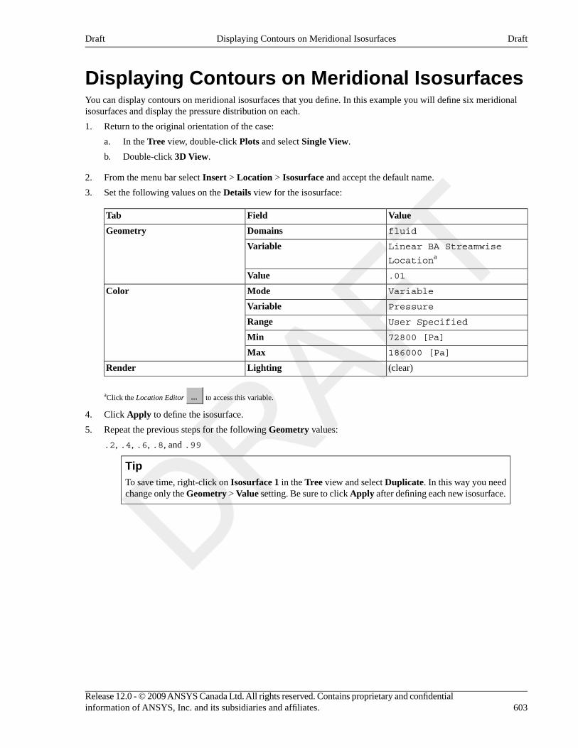
Displaying Contours on Meridional IsosurfacesYou can display contours on meridional isosurfaces that you define. In this example you will define six meridionalisosurfaces and display the pressure distribution on each.
1. Return to the original orientation of the case:
a. In the Tree view, double-click Plots and select Single View.
b. Double-click 3D View.
2. From the menu bar select Insert > Location > Isosurface and accept the default name.
3. Set the following values on the Details view for the isosurface:
ValueFieldTab
fluidDomainsGeometry
Linear BA Streamwise
LocationaVariable
.01Value
VariableModeColor
PressureVariable
User SpecifiedRange
72800 [Pa]Min
186000 [Pa]Max
(clear)LightingRender
aClick the Location Editor to access this variable.
4. Click Apply to define the isosurface.
5. Repeat the previous steps for the following Geometry values:
.2, .4, .6, .8, and .99
TipTo save time, right-click on Isosurface 1 in the Tree view and select Duplicate. In this way you needchange only the Geometry > Value setting. Be sure to click Apply after defining each new isosurface.
603Release 12.0 - © 2009 ANSYS Canada Ltd. All rights reserved. Contains proprietary and confidentialinformation of ANSYS, Inc. and its subsidiaries and affiliates.
DraftDisplaying Contours on Meridional IsosurfacesDraft
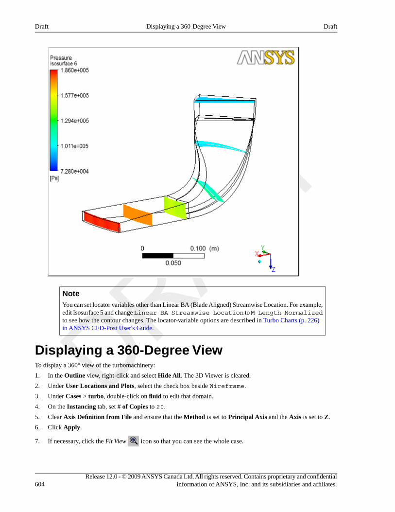
NoteYou can set locator variables other than Linear BA (Blade Aligned) Streamwise Location. For example,edit Isosurface 5 and change Linear BA Streamwise Location to M Length Normalizedto see how the contour changes. The locator-variable options are described in Turbo Charts (p. 226)in ANSYS CFD-Post User's Guide.
Displaying a 360-Degree ViewTo display a 360° view of the turbomachinery:
1. In the Outline view, right-click and select Hide All. The 3D Viewer is cleared.
2. Under User Locations and Plots, select the check box beside Wireframe.
3. Under Cases > turbo, double-click on fluid to edit that domain.
4. On the Instancing tab, set # of Copies to 20.
5. Clear Axis Definition from File and ensure that the Method is set to Principal Axis and the Axis is set to Z.
6. Click Apply.
7. If necessary, click the Fit View icon so that you can see the whole case.
Release 12.0 - © 2009 ANSYS Canada Ltd. All rights reserved. Contains proprietary and confidentialinformation of ANSYS, Inc. and its subsidiaries and affiliates.604
DraftDisplaying a 360-Degree ViewDraft
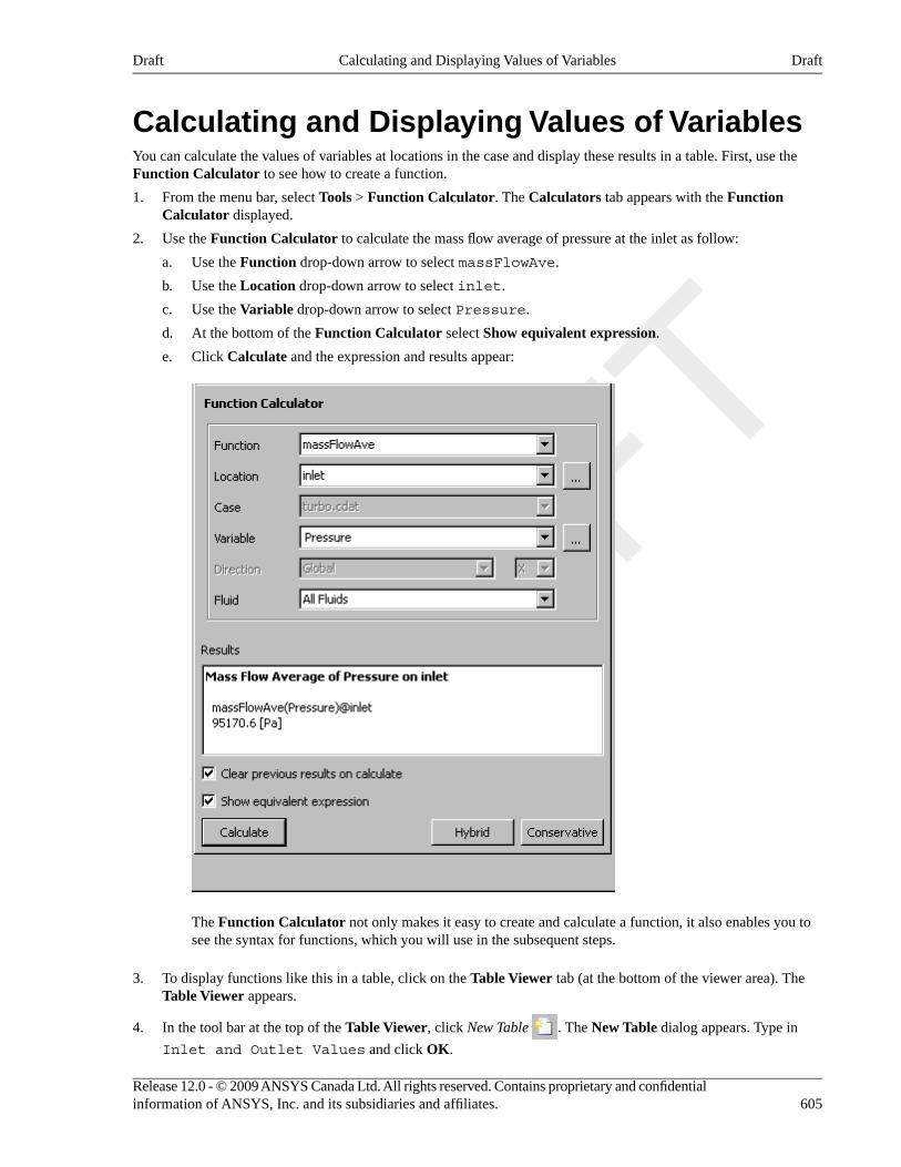
Calculating and Displaying Values of VariablesYou can calculate the values of variables at locations in the case and display these results in a table. First, use theFunction Calculator to see how to create a function.
1. From the menu bar, select Tools > Function Calculator. The Calculators tab appears with the FunctionCalculator displayed.
2. Use the Function Calculator to calculate the mass flow average of pressure at the inlet as follow:
a. Use the Function drop-down arrow to select massFlowAve.
b. Use the Location drop-down arrow to select inlet.
c. Use the Variable drop-down arrow to select Pressure.
d. At the bottom of the Function Calculator select Show equivalent expression.
e. Click Calculate and the expression and results appear:
The Function Calculator not only makes it easy to create and calculate a function, it also enables you tosee the syntax for functions, which you will use in the subsequent steps.
3. To display functions like this in a table, click on the Table Viewer tab (at the bottom of the viewer area). TheTable Viewer appears.
4. In the tool bar at the top of the Table Viewer, click New Table . The New Table dialog appears. Type in
Inlet and Outlet Values and click OK.
605Release 12.0 - © 2009 ANSYS Canada Ltd. All rights reserved. Contains proprietary and confidentialinformation of ANSYS, Inc. and its subsidiaries and affiliates.
DraftCalculating and Displaying Values of VariablesDraft
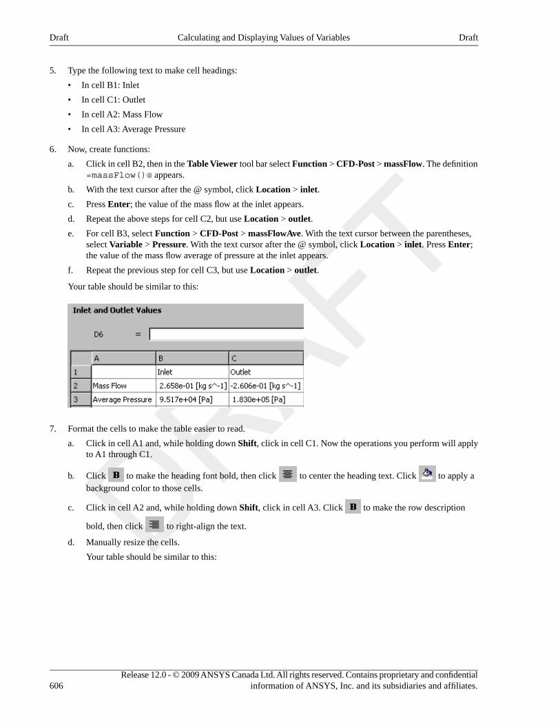
5. Type the following text to make cell headings:
• In cell B1: Inlet
• In cell C1: Outlet
• In cell A2: Mass Flow
• In cell A3: Average Pressure
6. Now, create functions:
a. Click in cell B2, then in the Table Viewer tool bar select Function > CFD-Post > massFlow. The definition=massFlow()@ appears.
b. With the text cursor after the @ symbol, click Location > inlet.
c. Press Enter; the value of the mass flow at the inlet appears.
d. Repeat the above steps for cell C2, but use Location > outlet.
e. For cell B3, select Function > CFD-Post > massFlowAve. With the text cursor between the parentheses,select Variable > Pressure. With the text cursor after the @ symbol, click Location > inlet. Press Enter;the value of the mass flow average of pressure at the inlet appears.
f. Repeat the previous step for cell C3, but use Location > outlet.
Your table should be similar to this:
7. Format the cells to make the table easier to read.
a. Click in cell A1 and, while holding down Shift, click in cell C1. Now the operations you perform will applyto A1 through C1.
b. Click to make the heading font bold, then click to center the heading text. Click to apply abackground color to those cells.
c. Click in cell A2 and, while holding down Shift, click in cell A3. Click to make the row description
bold, then click to right-align the text.
d. Manually resize the cells.
Your table should be similar to this:
Release 12.0 - © 2009 ANSYS Canada Ltd. All rights reserved. Contains proprietary and confidentialinformation of ANSYS, Inc. and its subsidiaries and affiliates.606
DraftCalculating and Displaying Values of VariablesDraft
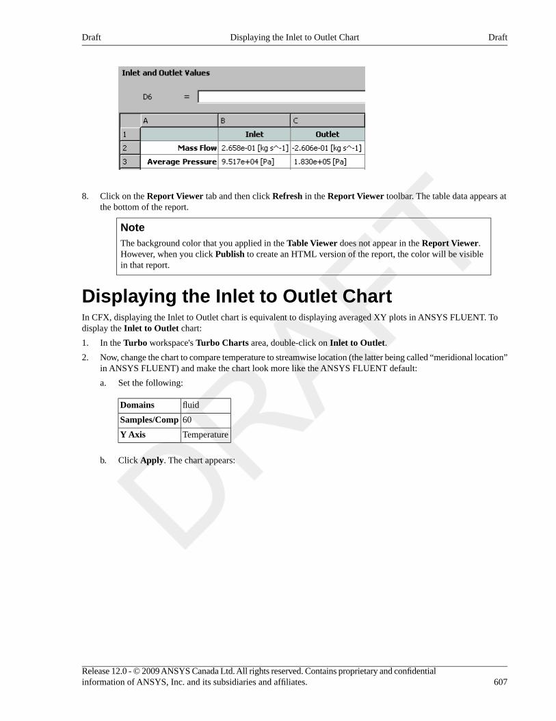
8. Click on the Report Viewer tab and then click Refresh in the Report Viewer toolbar. The table data appears atthe bottom of the report.
NoteThe background color that you applied in the Table Viewer does not appear in the Report Viewer.However, when you click Publish to create an HTML version of the report, the color will be visiblein that report.
Displaying the Inlet to Outlet ChartIn CFX, displaying the Inlet to Outlet chart is equivalent to displaying averaged XY plots in ANSYS FLUENT. Todisplay the Inlet to Outlet chart:
1. In the Turbo workspace's Turbo Charts area, double-click on Inlet to Outlet.
2. Now, change the chart to compare temperature to streamwise location (the latter being called “meridional location”in ANSYS FLUENT) and make the chart look more like the ANSYS FLUENT default:
a. Set the following:
fluidDomains
60Samples/Comp
TemperatureY Axis
b. Click Apply. The chart appears:
607Release 12.0 - © 2009 ANSYS Canada Ltd. All rights reserved. Contains proprietary and confidentialinformation of ANSYS, Inc. and its subsidiaries and affiliates.
DraftDisplaying the Inlet to Outlet ChartDraft
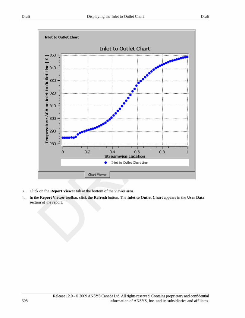
3. Click on the Report Viewer tab at the bottom of the viewer area.
4. In the Report Viewer toolbar, click the Refresh button. The Inlet to Outlet Chart appears in the User Datasection of the report.
Release 12.0 - © 2009 ANSYS Canada Ltd. All rights reserved. Contains proprietary and confidentialinformation of ANSYS, Inc. and its subsidiaries and affiliates.608
DraftDisplaying the Inlet to Outlet ChartDraft
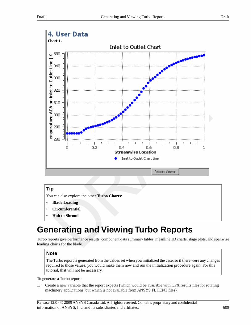
TipYou can also explore the other Turbo Charts:
• Blade Loading
• Circumferential
• Hub to Shroud
Generating and Viewing Turbo ReportsTurbo reports give performance results, component data summary tables, meanline 1D charts, stage plots, and spanwiseloading charts for the blade.
NoteThe Turbo report is generated from the values set when you initialized the case, so if there were any changesrequired to those values, you would make them now and run the initialization procedure again. For thistutorial, that will not be necessary.
To generate a Turbo report:
1. Create a new variable that the report expects (which would be available with CFX results files for rotatingmachinery applications, but which is not available from ANSYS FLUENT files).
609Release 12.0 - © 2009 ANSYS Canada Ltd. All rights reserved. Contains proprietary and confidentialinformation of ANSYS, Inc. and its subsidiaries and affiliates.
DraftGenerating and Viewing Turbo ReportsDraft
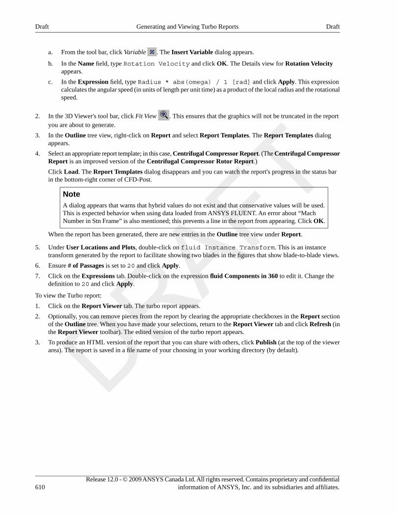
a. From the tool bar, click Variable . The Insert Variable dialog appears.
b. In the Name field, type Rotation Velocity and click OK. The Details view for Rotation Velocityappears.
c. In the Expression field, type Radius * abs(omega) / 1 [rad] and click Apply. This expressioncalculates the angular speed (in units of length per unit time) as a product of the local radius and the rotationalspeed.
2. In the 3D Viewer's tool bar, click Fit View . This ensures that the graphics will not be truncated in the reportyou are about to generate.
3. In the Outline tree view, right-click on Report and select Report Templates. The Report Templates dialogappears.
4. Select an appropriate report template; in this case, Centrifugal Compressor Report. (The Centrifugal CompressorReport is an improved version of the Centrifugal Compressor Rotor Report.)
Click Load. The Report Templates dialog disappears and you can watch the report's progress in the status barin the bottom-right corner of CFD-Post.
NoteA dialog appears that warns that hybrid values do not exist and that conservative values will be used.This is expected behavior when using data loaded from ANSYS FLUENT. An error about “MachNumber in Stn Frame” is also mentioned; this prevents a line in the report from appearing. Click OK.
When the report has been generated, there are new entries in the Outline tree view under Report.
5. Under User Locations and Plots, double-click on fluid Instance Transform. This is an instancetransform generated by the report to facilitate showing two blades in the figures that show blade-to-blade views.
6. Ensure # of Passages is set to 20 and click Apply.
7. Click on the Expressions tab. Double-click on the expression fluid Components in 360 to edit it. Change thedefinition to 20 and click Apply.
To view the Turbo report:
1. Click on the Report Viewer tab. The turbo report appears.
2. Optionally, you can remove pieces from the report by clearing the appropriate checkboxes in the Report sectionof the Outline tree. When you have made your selections, return to the Report Viewer tab and click Refresh (inthe Report Viewer toolbar). The edited version of the turbo report appears.
3. To produce an HTML version of the report that you can share with others, click Publish (at the top of the viewerarea). The report is saved in a file name of your choosing in your working directory (by default).
Release 12.0 - © 2009 ANSYS Canada Ltd. All rights reserved. Contains proprietary and confidentialinformation of ANSYS, Inc. and its subsidiaries and affiliates.610
DraftGenerating and Viewing Turbo ReportsDraft


