Embed Size (px)
Citation preview
An Investigation into the Oxyturbine Power Cycles with
100% CO2 Capture and Zero NOx emission
Hirbod Varasteh
A thesis submitted in partial fulfilment of the requirement of
Staffordshire University for the degree of Doctor of Philosophy
December 2020
i
Abstract
The world is facing serious issues related to global warming due to the massive use
of fossil fuel sources. Global warming coupled with growing energy demand causes
environmental concern. Carbon capture and storage (CCS) are promising technologies
for achieving shortly to medium-term solution Green House Gas GHG emission
reduction goals. The development of CCS for fossil fuel power generation can reduce
carbon dioxide emission and produce electricity with lower capital cost (Capex),
operating cost (Opex) in comparison with other renewable energies in the short and
medium-term while reducing exergy destruction and increasing efficiency.
Oxy-fuel combustion technology is an effective way to increase the CO2 capture
ability of oxy-fuel combustion power plants. Also, its advantages in contrast to other
CCS technologies include low fuel consumption, near-zero CO2 emission, high
combustion efficiency, flue gas volume reduction, and fewer nitrogen oxides (NOx)
formation. In this technology, the air is replaced with nearly pure oxygen as an
oxidiser. The combustion exhaust is mainly the composition of CO2 and H2O. Then
CO2 can be separated from the water through lower-cost technologies such as the water
condensation technology, which has lower power consumption. In this thesis, the
major proposed oxy-combustion gas turbine power cycles (Oxyturbine cycles) have
been investigated and compared by means of process simulation and techno-economic
evaluation.
The investigated cycles in chapter 2 are SCOC-CC, COOPERATE Cycle,
MATIANT, E-MATIANT, CC_MATIANT, Graz cycle, S-Graz cycle, Modified
GRAZ, AZEP 85%, AZEP 100%, ZEITMOP Cycle, COOLCEP-S Cycle, Novel
O2/CO2, NetPower, CES. These cycles were modelled with Aspen Plus based on the
available cycle data from literature; then, parametric studies are performed after
modelling validations. In this PhD thesis, a review of the Air Separation Unit (ASU)
and the CO2 Compression and Purification Unit (CPU) are presented. The Technology
Readiness Level (TRL), Sensitivities and pilot industrial demonstration for oxy-
combustion power cycle have also been studied.
ii
In chapter 3, the methodology of the thesis and oxy-combustion cycles of process
modelling is indicated. Also, the theories and thermodynamic formulas including
mass, energy and exergy balances of Oxy combustion cycle were determined in the
MATLAB code to calculate thermodynamic parameters in order to evaluate these
cycles; the MATLAB codes are developed to link with Aspen Plus software to
simulate the Oxy-fuel power cycle processes with the input data. In this chapter,
techno-economic formulas were determined to calculate LCOE for oxy-combustion
cycles.
In chapter 4, the exergy destruction in each component of the oxy-combustion
power cycle is studied. Results indicate that the exergy destruction in combustion is
more than other components and the heat exchanger is the second component with the
highest exergy destruction; hence improving these two components are very important
to reduce total exergy destruction.
In chapter 5, the Sensitivity and exergy analysis of the Semi-Closed Oxy-fuel
Combustion Combined Cycle (SCOC-CC) and E-MATIANT are investigated in
detail. TIT and efficiency of SCOC-CC cycle with respect to COP and fuel flowrate
was drawn, and also a 3D plot of exergy destruction and TIT were indicated in this
section. The Efficiency vs working flowrate for E-MATIANT was determined, and it
indicates the maximum turbine efficiency is 46.9% at 290 kg/s based on the available
technology for the E-MATIANT cycle.
In chapter 6, the sensitivity and exergy analysis of COOPERATE cycle is
determined, and the sensitivity of the Efficiency vs working flowrate for
COOPERATE cycle was plotted. Also, a pie chart for exergy destruction of equipment
is determined. The exergy analysis indicates that the total exergy destruction in the
COOPERATE cycle is minimum at 318 kg/s working flowrates; it is verified that the
exergy efficiency and energy efficiency are maximum at this working flowrate.
In chapter 7, the simulation results of the NetPower cycle showed that the efficiency
increases up to 1% with 2.5 oC reduction of ΔTmin in constant Combustion Outlet
Temperature (COT) and constant recycled flow rates; however, the efficiency
increases faster in constant flow rate compared to the constant COT. Also, NetPower
cycle simulation indicates that COT and heat exchanger have a critical role in
NetPower cycle performance and overall efficiency.
iii
In chapter 8, the results of the TIT sensitivity for the S-CES cycle and the NetPower
cycle indicates that the slope of cycle efficiency was higher in the NetPower cycle,
which could be explained by the higher impact that the TIT produced in the turbine
and the main heat exchanger for the NetPower cycle.
At the end, exergoeconomic, Techno-economic, Technology Readiness Level
(TRL) and parametric comparison in Oxyturbine Power cycles are indicated in chapter
9 and the Radar chart for comparison of the oxy-combustion cycles were determined
and the results were discussed more depth in this capture. Furthermore, Techno-
economic analysis was conducted according to the oxy-combustion modelling and
included performance, cost rate, Levelised Cost of Electricity (LCOE). The oxy-
combustion cycles parameters were compared by means of TIT, TOT, CO2/kWh,
COP, Exergy, Thermal efficiency, Technology Readiness Level (TRL) bar diagrams
and Multi-Criteria Decision Analysis (MCDA) with radar diagrams are provided to
choose the best possible Oxyturbine cycles.
This PhD research provides a benchmark for comparing the oxy-combustion gas
turbine power cycles and drew a road map for the development of these cycles for
low carbon, high efficiency and low-cost energy in soon future.
.

iv
Acknowledgements
I would like to express my deepest appreciation to my principal supervisor Professor
Hamidreza Gohari Darabkhani, who has provided me with the opportunity to work
under his supervision. Without his guidance and persistent help, this dissertation would
not have been possible. His scientific feedback, Knowledge and expert advice made
this research attainable. I also owe my gratitude to my second supervisor Professor
Torfeh Sadat-Shafai for his support during this research.
I would like to thank my wife, Mrs Hamraz, and my daughter Tida for supporting me
during my PhD. Also, thanks to my mother and my father, Mrs Shahnaz and Mr
Mohammad Saeid, who have been there to help me at any stage of my life.
I would also like to acknowledge Staffordshire University for the provision of PhD
studentship and sponsoring this research. I especially thank the Engineering
department at Staffordshire University to support me.
v
Contents
Abstract .................................................................................................................................................. i
Acknowledgements ............................................................................................................................... iv
Contents …………………………………………………………………………………………………v
List of Figures ....................................................................................................................................... xi
List of Tables ...................................................................................................................................... xvi
Abbreviations .................................................................................................................................... xviii
Subscripts ............................................................................................................................................ xix
Symbols ………………………………………………………………………………………………..xx
Chapter 1: Introduction .................................................................................................................... 1
1.1 Aim of this research project ..................................................................................................... 2
1.2 Objectives ................................................................................................................................ 3
1.3 Introduction to the gas turbine technology ............................................................................... 5
1.4 Categories of gas turbines ........................................................................................................ 6
1.5 Type of gas turbine .................................................................................................................. 8
1.5.1 Single-shaft gas turbine .................................................................................................. 9
1.5.2 Dual shaft gas turbine with a power turbine ................................................................. 10
1.5.3 Triple shaft gas turbine with a power turbine ............................................................... 11
1.5.4 Open and closed thermodynamic cycles of gas turbine ................................................ 13
1.6 Environmental impact ............................................................................................................ 16
1.7 Summary ................................................................................................................................ 19
Chapter 2: Literature review of Oxyturbine power cycles and gas-CCS Technologies ................. 20
2.1 Introduction ............................................................................................................................ 20
2.2 Main Technologies in CO2 Capture ....................................................................................... 21
2.2.1 Post-combustion capture .............................................................................................. 21
2.2.1.1 Physical Absorption ............................................................................................ 22
2.2.1.2 Selective exhaust gas recirculation (S-EGR) method ......................................... 23
2.2.1.3 Chemical Absorption - Amine Absorption/Stripping Technology ..................... 25
2.2.1.4 Physical Adsorbent ............................................................................................. 26
2.2.1.5 Chemical Adsorbent (Amine-Based) .................................................................. 26
2.2.2 Pre-combustion capture ................................................................................................ 27
2.2.2.1 Chemical process ................................................................................................ 27
2.2.2.2 Membrane ........................................................................................................... 28
2.2.2.3 Hydrogen production technologies ..................................................................... 29
vi
2.2.2.3.1 Steam Methane Reforming (SMR) ................................................................ 29
2.2.2.3.2 Autothermal Reforming (ATR) ...................................................................... 30
2.2.2.3.3 Vacuum pressure swing adsorption (VPSA) cycle ........................................ 31
2.2.2.3.4 Renewable sources ......................................................................................... 32
2.2.3 Oxy-fuel combustion capture ....................................................................................... 33
2.2.3.1 Oxy-combustion classification ............................................................................ 34
2.2.4 CO2 Capture technology conclusion ............................................................................ 37
2.3 Oxygen production and Air Separation Units (ASU) ............................................................ 39
2.3.1 Cryogenic Air Separation Unit (ASU) ......................................................................... 39
2.3.1.1 Pilot-scale ........................................................................................................... 41
2.3.1.2 ASU development ............................................................................................... 41
2.3.2 Non-cryogenic Air Separation Unit (ASU) .................................................................. 42
2.3.2.1 Adsorption .......................................................................................................... 42
2.3.2.2 Pressure Swing Adsorption (PSA) ...................................................................... 42
2.3.2.2.1 Vacuum Pressure Swing Adsorption (VPSA) ................................................ 43
2.3.2.3 Chemical processes ............................................................................................. 44
2.3.2.4 Polymeric membranes ......................................................................................... 45
2.3.2.5 Ion Transport Membrane (ITM) ......................................................................... 45
2.3.2.6 Chemical Looping Combustion (CLC) ............................................................... 46
2.4 CO2 Compression and Purification Unit (CPU) ..................................................................... 46
2.5 Semi-Closed Oxy-Combustion Combined Cycle (SCOC-CC) .............................................. 49
2.5.1 SCOC-CC technologies ................................................................................................ 51
2.6 The COOPERATE cycle ....................................................................................................... 51
2.6.1 The COOPERATE cycle technologies ......................................................................... 53
2.7 The MATIANT cycle ............................................................................................................ 54
2.8 The E-MATIANT cycle ......................................................................................................... 55
2.9 CC-MATIANT cycle ............................................................................................................. 57
2.9.1 CC-METIANT technologies ........................................................................................ 59
2.10 The Graz cycle .................................................................................................................. 61
2.10.1 Graz cycle technologies ........................................................................................... 62
2.11 The S-Graz cycle ............................................................................................................... 63
2.11.1 The S-Graz cycle technologies ................................................................................ 64
2.12 The AZEP 100% cycle ...................................................................................................... 65
2.12.1 The AZEP 100% cycle technologies ....................................................................... 66
2.13 The AZEP 85% cycle ........................................................................................................ 67
2.14 The ZEITMOP cycle ......................................................................................................... 67
2.14.1 ZEITMOP technologies ........................................................................................... 69
2.15 The COOLCEP-S cycle .................................................................................................... 70
2.15.1 COOLCEP technologies .......................................................................................... 72
2.16 The COOLCEP-C cycle .................................................................................................... 72
vii
2.16.1 COOLCEP-C technologies ...................................................................................... 73
2.17 Novel O2/CO2 (Cao and Zheng, 2006) .............................................................................. 74
2.17.1 The Novel O2 /CO2 technologies ............................................................................. 75
2.18 NetPower cycle ................................................................................................................. 76
2.18.1 NetPower demonstration ......................................................................................... 78
2.18.1.1 Turbine ................................................................................................................ 79
2.18.1.2 Combustion ......................................................................................................... 79
2.18.1.3 Heat exchanger ................................................................................................... 80
2.19 CES Cycle ......................................................................................................................... 81
2.19.1 The CES technologies ............................................................................................. 82
2.19.2 CES demonstration .................................................................................................. 82
2.19.2.1 Combustion ......................................................................................................... 83
2.19.2.2 Turbine ................................................................................................................ 84
2.20 Natural Gas Combined Cycle (NGCC) ............................................................................. 85
2.21 The NGCC power plant with PCC .................................................................................... 85
2.22 Summary ........................................................................................................................... 87
Chapter 3: Methodology and Process modelling of the leading Oxyturbine cycles ....................... 89
3.1 Introduction ............................................................................................................................ 89
3.2 Oxy-combustion power cycle theories and calculations ........................................................ 90
3.2.1 Thermodynamic concept and equations ....................................................................... 90
3.2.1.1 Continuity ........................................................................................................... 90
3.2.1.2 Energy conservation ........................................................................................... 91
3.2.1.3 Energy quality (second law of thermodynamic) ................................................. 91
3.2.1.4 Thermodynamic cycles ....................................................................................... 92
3.2.2 Exergy equations for the oxyfuel combustion cycle ..................................................... 93
3.2.3 Exergy destruction equations ....................................................................................... 97
3.2.4 EOS for gas turbine and steam turbine ......................................................................... 94
3.3 Modelling and simulation ...................................................................................................... 96
3.3.1 Plant simulation with a numerical approach................................................................. 96
3.3.2 Aspen Plus pros and cons ............................................................................................. 96
3.3.3 Modelling equipment in Aspen Plus ............................................................................ 97
3.3.3.1 Distillation column ............................................................................................. 97
3.3.3.2 Stripper (or desorption) ....................................................................................... 97
3.3.3.3 Absorption (opposite of striping) ........................................................................ 98
3.3.3.4 Separator blocks in Aspen Plus ........................................................................... 98
3.3.4 MATLAB Code link with Aspen Plus ......................................................................... 99
3.4 Oxy combustion cycles modelling and simulation ................................................................ 99
3.4.1 The SCOC-CC cycle modelling and analysis ............................................................... 99
3.4.2 The COOPERATE cycle modelling and analysis ...................................................... 104
viii
3.4.3 The E-MATIANT cycle modelling and analysis........................................................ 108
3.4.4 The CC_MATIANT cycle modelling and analysis .................................................... 112
3.4.5 The Graz cycle modelling and analysis ...................................................................... 116
3.4.6 The S-Graz cycle modelling and analysis .................................................................. 120
3.4.7 The AZEP 100% cycle modelling and analysis ......................................................... 124
3.4.8 The ZEITMOP cycle modelling and analysis ............................................................ 128
3.4.9 The COOLCEP-S cycle modelling and analysis ........................................................ 132
3.4.10 The COOLCEP-C cycle modelling and analysis ................................................... 136
3.4.11 The Novel O2/CO2 (Cao and Zheng, 2006) modelling and analysis ...................... 140
3.4.12 The NetPower cycle modelling and analysis ......................................................... 145
3.4.13 The S-CES cycle modelling and analysis .............................................................. 151
3.5 Sensitivity comparison of CES and NetPower ..................................................................... 159
3.6 Techno-economic analysis of oxy-combustion cycles ......................................................... 159
3.6.1 Cost rate ..................................................................................................................... 159
3.7 Summary .............................................................................................................................. 165
Chapter 4: Exergy analysis of leading oxy-combustion cycles .................................................... 166
4.1 The SCOC-CC cycle modelling and analysis ...................................................................... 166
4.2 The COOPERATE cycle modelling and analysis ................................................................ 168
4.3 The E-MATIANT cycle modelling and analysis ................................................................. 170
4.4 The CC_MATIANT cycle modelling and analysis .............................................................. 172
4.5 The Graz cycle modelling and analysis ............................................................................... 174
4.6 The S-Graz cycle modelling and analysis ............................................................................ 176
4.7 The AZEP 100% cycle modelling and analysis ................................................................... 178
4.8 The ZEITMOP cycle modelling and analysis ...................................................................... 180
4.9 The COOLCEP-S cycle modelling and analysis.................................................................. 182
4.10 The COOLCEP-C cycle modelling and analysis ............................................................ 184
4.11 The Novel O2/CO2 (Cao and Zheng, 2006) modelling and analysis ............................... 186
4.12 The NetPower cycle modelling and analysis ................................................................... 188
4.13 The S-CES cycle modelling and analysis ........................................................................ 190
4.14 Summary ......................................................................................................................... 192
Chapter 5: Sensitivity and exergy analysis of Semi-Closed Oxy-fuel Combustion Combined
Cycle (SCOC-CC) and E-MATIANT .................................................................................. 194
5.1 Sensitivity analysis of Semi-Closed Oxy-fuel Combustion Combined Cycle (SCOC-CC) . 194
5.1.1 Introduction ................................................................................................................ 194
5.1.2 Sensitivity analysis results .......................................................................................... 195
5.1.3 Summary .................................................................................................................... 206
5.2 Sensitivity and exergy analysis of E-MATIANT cycle ....................................................... 207
5.2.1 Introduction ................................................................................................................ 207
5.2.2 Sensitivity analysis results .......................................................................................... 208
ix
5.2.3 Summary .................................................................................................................... 210
Chapter 6: Sensitivity and exergy analysis of COOPERATE cycle ............................................ 211
6.1 Introduction .......................................................................................................................... 211
6.2 Sensitivity analysis results .............................................................................................. 211
6.3 Summary .............................................................................................................................. 220
Chapter 7: Sensitivity analysis of the heat exchanger design in NetPower oxy-combustion cycle
for carbon capture ................................................................................................................ 221
7.1 Introduction .......................................................................................................................... 221
7.2 Analysing of NetPower cycle .............................................................................................. 222
7.2.1 NetPower cycle .......................................................................................................... 222
7.2.2 NetPower simulation with Aspen Plus ....................................................................... 224
7.2.2.1 Recovery Heat Exchanger: ............................................................................... 224
7.2.2.2 Recovery Heat Exchanger modelling in Aspen Plus ........................................ 225
7.2.2.3 CO2 Direct-fired Turbine .................................................................................. 226
7.2.2.4 Turbine with cooling blades modelling in Aspen Plus ..................................... 227
7.2.3 Turbine with cooling blade modelling in Aspen Plus by exergy analysis .................. 228
7.2.3.1 Recycle gas compression loop .......................................................................... 231
7.3 Evaluation of ΔTmin from the composite curve and grand compost curve of multi-stream
heat exchanger ............................................................................................................................... 233
7.4 Heat exchanger design sensitivity analysis for NetPower cycle .......................................... 234
7.4.1 Sensitivity analysis with a constant recycled flow rate .............................................. 235
7.4.2 Sensitivity analysis with constant COT ...................................................................... 237
7.5 Design and cost analysis of NetPower plant ........................................................................ 239
7.6 Summary .............................................................................................................................. 241
Chapter 8: Leading Oxy-combustion power cycles: NetPower and Supercritical CES ............... 242
8.1 Introduction .......................................................................................................................... 242
8.1.1 CES supercritical cycle .............................................................................................. 243
8.1.2 CES supercritical plant modelling .............................................................................. 247
8.1.3 Sensitivity analysis of TIT for Supercritical CES (S-CES) cycle .............................. 252
8.1.4 Sensitivity analysis of COP for Supercritical CES (S-CES) cycle ............................. 254
8.1.5 Sensitivity analysis of cooling water temperature in the heat exchanger ................... 255
8.2 NetPower cycle .................................................................................................................... 255
8.2.1 NetPower plant modelling .......................................................................................... 257
8.2.2 Sensitivity analysis of the TIT for the NetPower cycle .............................................. 259
8.2.3 Sensitivity analysis of heat exchanger for NetPower cycle ........................................ 259
8.3 Compare TIT sensitivity for CES and NetPower cycle ....................................................... 260
8.4 Pilot and industrial demonstration of Oxyturbine power cycles .......................................... 261
8.4.1 Oxy combustion cycle demonstration ........................................................................ 261
x
8.5 Summary .............................................................................................................................. 263
Chapter 9: Techno-economic, Technology Readiness Level (TRL) and parametric comparison in
Oxyturbine Power cycles ..................................................................................................... 264
9.1 Introduction .......................................................................................................................... 264
9.2 TIT comparison of oxy-combustion cycles .......................................................................... 264
9.3 TOT comparison of oxy-combustion cycles ........................................................................ 267
9.4 COP (Combustion Outlet Pressure) comparison of oxy-combustion cycles ........................ 269
9.5 Exergy and thermal efficiency comparison of oxy-combustion cycles ................................ 271
9.6 CO2/kWh for storage comparison of oxy-combustion cycles .............................................. 273
9.7 TRL (Technology Readiness Level) .................................................................................... 274
9.7.1 Combustion TRL ........................................................................................................ 275
9.7.2 CO2 Compression and Purification Unit (CPU) TRL ................................................. 276
9.7.3 SCOCC-CC TRL ........................................................................................................ 277
9.7.4 Graze cycle TRL ........................................................................................................ 278
9.7.5 CES TRL .................................................................................................................... 278
9.7.6 NetPower TRL ........................................................................................................... 278
9.8 Performance analysis ........................................................................................................... 279
9.9 Techno-economic analysis of oxy-combustion cycles ......................................................... 281
9.9.1 Exergoeconomic ......................................................................................................... 285
9.9.2 LCOE ......................................................................................................................... 290
9.10 Radar chart for comparison of the oxy-combustion cycles ............................................. 294
9.11 Summary ......................................................................................................................... 298
Chapter 10: Conclusions and future works .................................................................................... 299
10.1 Conclusions ..................................................................................................................... 299
10.2 Future work and critical appraisal ................................................................................... 302
Reference ........................................................................................................................................... 304
Appendix (A) (MATLAB Code) ........................................................................................................ 315
xi
List of Figures
Figure 1.1 Power generation in the UK for seven days from 08-Jan-2020 to 15-Jan-2020 (MyGridGB,
2020) ........................................................................................................................................ 1
Figure 1.2 Typical gas turbine cycle ...................................................................................................... 6
Figure 1.3 Schematic of a single spool gas turbine with hot end drive (Tony Giampaolo, 2015).......... 9
Figure 1.4 Schematic of a single spool gas turbine with a cold end drive (Tony Giampaolo, 2015) ..... 9
Figure 1.5 GasTurb schematic of single shaft gas turbine (Gasturb, 2018) ......................................... 10
Figure 1.6 GasTurb schematic of a dual-shaft gas turbine (Gasturb, 2018) ......................................... 11
Figure 1.7 GasTurb schematic of a triple gas turbine (Gasturb, 2018) ................................................ 12
Figure 1.8 Triple shafts open cycle gas turbine with intercooler(Ying et al., 2016) ............................ 14
Figure 1.9 Single shaft closed cycle gas turbine with intercooler and recuperator (Soares, 2015) ...... 14
Figure 2.1 Schematic diagram of Post-combustion capture (Ahmad, 2019) ........................................ 21
Figure 2.2 Schematic diagram of NGCC with S-EGR and CO2 capture unit (Merkel et al., 2013) ..... 24
Figure 2.3 Schematic diagram of 100 kW pilot scale S-EGR with PDMS membrane (Russo et al.,
2018) ...................................................................................................................................... 25
Figure 2.4 Process Flow Diagram of a basic chemical absorption process for amine-based CO2 capture
(MacDowell et al., 2010) ....................................................................................................... 25
Figure 2.5 Schematic diagram of pre-combustion capture (Jansen et al., 2015) .................................. 28
Figure 2.6 Schematic diagram of using membrane for pre-combustion capture (MTR, 2018) ............ 28
Figure 2.7 Schematic diagram of Autothermal Reforming (AR) (Antonini et al., 2020) .................... 31
Figure 2.8 Schematic diagram of VPSA hydrogen production (Antonini et al., 2020)........................ 32
Figure 2.9 Schematic diagram of oxy-combustion capture .................................................................. 33
Figure 2.10 A cryogenic air separation unit with two-column distillation and compression of oxygen
in a gaseous state (Manso and Nord, 2020) ........................................................................... 40
Figure 2.11 ASU development ............................................................................................................. 41
Figure 2.12 Pressure Swing Absorption (Kwon et al., 2011) ............................................................... 43
Figure 2.13 Vacuum Pressure Swing Adsorption (Laboo, 2020) ......................................................... 44
Figure 2.14 Ion transport membrane (ITM) ......................................................................................... 45
Figure 2.15 Schematic diagram of CLC (Ingegneria et al., 2012) ....................................................... 46
Figure 2.16 CO2 Compression and Purification Unit (Chaubey 2010) ................................................ 47
Figure 2.17 Schematic Process Flow Diagram of CPU (Almås, 2012) ................................................ 48
Figure 2.18 Semi-closed oxy-combustion combined cycle (SCOC-CC) (Davison, 2015) .................. 50
Figure 2.19 COOPERATE cycle Process flow diagram (Yantovski, 1996) ........................................ 52
Figure 2.20 E-MATIANT schematic diagram (Manso and Nord, 2020) ............................................. 55
Figure 2.21 T-S Diagram of E-MATIANT cycle (Mathieu, 2004) ...................................................... 56
Figure 2.22 CC-MATIANT cycle (Mathieu and Nihart, 1999) ........................................................... 58
Figure 2.23 T-S diagram of CC-MATIANT (Mathieu and Nihart, 1999) ........................................... 58
Figure 2.24 Modified CC-MATIANT cycle by (Zhao et al., 2017) ..................................................... 60
Figure 2.25 T-S diagram of modified MATIANT cycle by (Zhao et al., 2017) .................................. 60
xii
Figure 2.26 Graz cycle (ASME 2003, Atlanta) (Wolfgang Sanz et al., 2005) ..................................... 62
Figure 2.27 High steam content Graz cycle (S- GC) schematic diagram (Jericha, Sanz and Göttlich,
2008a) .................................................................................................................................... 64
Figure 2.28 The AZEPT 100% case (Sundkvist et al., 2005) .............................................................. 66
Figure 2.29 The AZEP 85% case (Sundkvist et al. 2005b) .................................................................. 67
Figure 2.30 ZEITMOP schematic diagram (Yantovski et al., 2004) ................................................... 68
Figure 2.31 T-S diagram of the ZEITMOP cycle (Yantovski et al., 2004) ......................................... 69
Figure 2.32 COOLCEP-S cycle schematic (Liu et al., 2017) .............................................................. 71
Figure 2.33 T-S diagram of the COOLCEP-S (Liu et al., 2017) .......................................................... 71
Figure 2.34 COOLCEP-C (Zhang et al., 2010) .................................................................................... 73
Figure 2.35 T–S diagram in the COOLCEP-C system (Zhang et al., 2010) ........................................ 73
Figure 2.36 Process Flow Diagram of novel O2/CO2 cycle system (Cao and Zheng, 2006) ................ 75
Figure 2.37 NetPower cycle schematic diagram (Davison, 2015) ....................................................... 76
Figure 2.38 5MWth combustor operating at 300 bar (Allam et al., 2017) ........................................... 79
Figure 2.39 Heatric Printed Circuit Heat Exchanger (Heatric, 2020) .................................................. 80
Figure 2.40 CES schematic diagram (Davison, 2015) ......................................................................... 81
Figure 2.41 20MWt Oxy-Fuel Combustor (Anderson et al., 2008) ..................................................... 83
Figure 2.42 170 MWt Oxy-Fuel Combustor (Anderson et al., 2008) .................................................. 84
Figure 2.43 Natural Gas Combined Cycle (NGCC) (Davison, 2015) .................................................. 85
Figure 2.44 Natural Gas with PCC (Dillon et al., 2013) ...................................................................... 86
Figure 3.1 Different classifications of exergy (Marmolejo-Correa and Gundersen, 2015) .................. 94
Figure 3.2 New classification of the exergy for pressure-volume-temperature PVT systems (Quality,
2011) ...................................................................................................................................... 95
Figure 3.3 Aspen Plus modelling of SCOC-CC ................................................................................. 101
Figure 3.4 Aspen Plus modelling of COOPERATE cycle ................................................................. 105
Figure 3.5 Aspen Plus modelling of E-MATIANT cycle .................................................................. 109
Figure 3.6 Aspen Plus modelling of CC-MATIANT cycle ................................................................ 113
Figure 3.7 Aspen Plus modelling of Graz cycle ................................................................................. 117
Figure 3.8 Aspen Plus modelling of S-Graz cycle ............................................................................. 121
Figure 3.9 Aspen Plus modelling of AZEP 100% cycle .................................................................... 125
Figure 3.10 Aspen Plus modelling of ZEITMOP cycle ..................................................................... 129
Figure 3.11 Aspen Plus modelling of COOLCEP-S cycle ................................................................. 133
Figure 3.12 Aspen Plus modelling of COOLCEP-C cycle ................................................................ 137
Figure 3.13 Aspen Plus modelling of O2/CO2 cycle .......................................................................... 141
Figure 3.14 Aspen Plus modelling of NetPower cycle ....................................................................... 146
Figure 3.15 Aspen Plus modelling of S-CES cycle ............................................................................ 152
Figure 4.1 Exergy destruction for each equipment of SCOC-CC ...................................................... 167
Figure 4.2 Exergy destruction percentage of SCOC-CC .................................................................... 167
Figure 4.3 Exergy destruction per MWe for SCOC-CC .................................................................... 168
Figure 4.4 Exergy destruction of each equipment for COOPERATE cycle ...................................... 169
xiii
Figure 4.5 Percentage of exergy distraction for each component....................................................... 169
Figure 4.6 Exergy destruction per MWe for COOPERATE Cycle .................................................... 170
Figure 4.7 Exergy destruction for each equipment of E-MATIANT ................................................. 171
Figure 4.8 Exergy destruction percentage for E-MATIANT ............................................................. 171
Figure 4.9 Exergy destruction per MWe production for E-MATIANT ............................................. 172
Figure 4.10 Exergy destruction for CC-MATIANT ........................................................................... 173
Figure 4.11 Exergy destruction percentage of CC-MATIANT .......................................................... 173
Figure 4.12 Exergy destruction per MWe production for CC-MATIANT ........................................ 174
Figure 4.13 Exergy destruction for Graz cycle .................................................................................. 175
Figure 4.14 Exergy destruction percentage for Graz cycle ................................................................ 175
Figure 4.15 Exergy destruction per MWe for Graz cycle .................................................................. 176
Figure 4.16 Exergy destruction for S-Graz cycle ............................................................................... 177
Figure 4.17 Exergy destruction percentage for S-Graz cycle ............................................................. 177
Figure 4.18 Exergy destruction per MWe for S-Graz cycle ............................................................... 178
Figure 4.19 Exergy destruction of AZEP 100% ................................................................................. 179
Figure 4.20 Exergy destruction percentage for AZEP 100% ............................................................. 179
Figure 4.21 Exergy destruction per MWe for AZEP 100% .............................................................. 180
Figure 4.22 Exergy destruction of ZEITMOP .................................................................................... 181
Figure 4.23 Exergy destruction percentage for ZEITMOP ................................................................ 181
Figure 4.24 Exergy destruction per MWe for ZEITMOP .................................................................. 182
Figure 4.25 Exergy destruction for COOLCEP-S .............................................................................. 183
Figure 4.26 Exergy destruction percentage for COOLCEP-S ............................................................ 183
Figure 4.27 Exergy destruction per MWe for COOLCEP-S .............................................................. 184
Figure 4.28 Exergy destruction for COOLCEP-C ............................................................................. 185
Figure 4.29 Exergy destruction percentage for COOLCEP-C ........................................................... 185
Figure 4.30 Exergy destruction per MWe for COOLCEP-C ............................................................. 186
Figure 4.31 Exergy destruction for Novel O2/CO2 cycle ................................................................... 187
Figure 4.32 Exergy destruction percentage for NovelO2/CO2 cycle .................................................. 187
Figure 4.33 Exergy destruction MW/MWe for NovelO2/CO2 cycle ................................................. 188
Figure 4.34 Exergy destruction for NetPower .................................................................................... 189
Figure 4.35 Exergy destruction percentage for NetPower.................................................................. 189
Figure 4.36 Exergy destruction MWe/MW for NetPower ................................................................. 190
Figure 4.37 Exergy destruction for S-CES ......................................................................................... 191
Figure 4.38 Exergy destruction percentage for S-CES ....................................................................... 191
Figure 4.39 Exergy destruction MWe/MW for S-CES ...................................................................... 192
Figure 5.1 Sensitivity of power cycle with Gas turbine pressure ratio ............................................... 195
Figure 5.2 Sensitivity of Network to Pressure ratio ........................................................................... 196
Figure 5.3 Efficiency with respect to Flowrate and COP ................................................................... 197
Figure 5.4 TIT with respect to COP and fuel flowrate ....................................................................... 197
Figure 5.5 Efficiency respect to COP of a steam turbine for SCOC-CC............................................ 198
xiv
Figure 5.6 Efficiency with respect to COP of the steam turbine ........................................................ 198
Figure 5.7 Gas turbine work to TIT ................................................................................................... 199
Figure 5.8 Thermal efficiency with respect to TIT ............................................................................ 200
Figure 5.9 Thermal efficiency with respect to TIT of gas turbine ...................................................... 201
Figure 5.10 Exergy destruction for each component SCOC-CC cycle .............................................. 201
Figure 5.11 3D plot of exergy destruction with respect to flowrate and COP.................................... 202
Figure 5.12 3D TIT with respect to COP and flowrate ...................................................................... 203
Figure 5.13 Stacked bar chart of exergy destruction .......................................................................... 204
Figure 5.14 TIT respect to Specific work MW/kg ............................................................................. 205
Figure 5.15 Efficiency vs working flowrate for E-MATIANT .......................................................... 208
Figure 5.16 Total exergy destruction, Network and efficiency for E-MATIANT ............................. 209
Figure 6.1 The sensitivity of Efficiency vs working flowrate for COOPERATE cycle ..................... 212
Figure 6.2 The sensitivity of Network vs working flowrate for COOPERATE cycle ....................... 212
Figure 6.3 Comparison of Energy efficiency and Exergy efficiency vs working flowrate ................ 213
Figure 6.4 Exergy destruction of equipment for COOPERATE cycle ............................................... 213
Figure 6.5 Pie chart for exergy destruction of equipment .................................................................. 214
Figure 6.6 Exergy destruction vs working flowrate for COOPERATE cycle .................................... 215
Figure 6.7 Exergy destruction vs min approach temperature and flowrate ........................................ 216
Figure 6.8 Total exergy destruction vs efficiency of COOPERATE cycle ........................................ 217
Figure 6.9 Efficiency Vs Working flowrate and Heat exchanger approach temperature ................... 218
Figure 6.10 Exergy destruction vs flowrate and heat exchanger approach temperature .................... 218
Figure 6.11 Exergy destruction per MWe for COOPERATE Cycle .................................................. 219
Figure 7.1 Model of the improved continuous expansion model with N (number of cooled expansion
steps) by Scaccabarozzi, Gatti (Scaccabarozzi, Gatti, and Martelli 2017, 551-560) ............ 227
Figure 7.2 Turbine block model in Aspen Plus .................................................................................. 228
Figure 7.3 NetPower Turbine with a cooling blade............................................................................ 229
Figure 7.4 Aspen Plus model of NetPower cycle ............................................................................... 232
Figure 7.5 Composite curve ............................................................................................................... 233
Figure 7.6 Grand composite curve ..................................................................................................... 234
Figure 7.7 Efficiency related to ΔTmin for constant recycled flow rate ............................................ 235
Figure 7.8 COT related to ΔTmin for constant recycled flow rate ..................................................... 235
Figure 7.9 Overall heat transfer coefficient UA to ΔTmin for constant recycled flow rate ............... 236
Figure 7.10 The required power for recycled compression loop relates to ΔTmin in a constant recycled
flow rate (the power demand is approximately constant) .................................................... 236
Figure 7.11 Turbine power output related to ΔTmin for constant recycled flow rate ........................ 237
Figure 7.12 Flow rate related to ΔTmin for constant COT 1150 °C .................................................. 238
Figure 7.13 Required power of recycled compression loop against ΔTmin for constant COT 1150 °C
............................................................................................................................................. 238
Figure 7.14 Efficiency related to ΔTmin with constant COT 1150 °C .............................................. 239
Figure 8.1. Supercritical CES Schematic diagram (Ferrari et al., 2017b) .......................................... 244
xv
Figure 8.2. Aspen Plus modelling of Supercritical Oxyturbine cycle ................................................ 250
Figure 8.3. Aspen Plus model flow diagram of Oxyturbine power island in a Supercritical cycle .... 250
Figure 8.4. Efficiency & TIT of Super-CES with respect to Natural gas flowrate in HP turbine ...... 252
Figure 8.5. TIT (LP, MP, HP) Turbine with respect to Natural gas flowrate ..................................... 253
Figure 8.6. the Sensitivity of natural gas flowrate (LPT, MPT, HPT) to efficiency .......................... 253
Figure 8.7. Efficiency vs recycle water pump pressure for S-CES cycle ........................................... 254
Figure 8.8. Efficiency vs cooling water temperature in S-CES .......................................................... 255
Figure 8.9. Schematic modelling NetPower cycle with Aspen Plus .................................................. 257
Figure 8.10. Oxyturbine cycle for NetPower cycle ............................................................................ 258
Figure 8.11. The efficiency of NetPower cycle vs TIT ...................................................................... 259
Figure 8.12. Efficiency related to ΔTmin for constant recycled flow rate ......................................... 260
Figure 8.13. The sensitivity of cycle efficiency with respect to TIT for HPT of CES and NetPower
cycle ..................................................................................................................................... 261
Figure 9.1 TIT comparison of Oxy-combustion cycles ...................................................................... 267
Figure 9.2 TOT Comparison of oxy-combustion cycle ...................................................................... 269
Figure 9.3 COP Comparison of oxy-combustion cycles .................................................................... 271
Figure 9.4 Thermal Efficiency and Exergy Efficiency Comparison .................................................. 273
Figure 9.5 Oxy-combustion cycles TRL comparison ......................................................................... 277
Figure 9.6 Comparison of oxy-combustion cost rate in the bar chart................................................. 284
Figure 9.7 Comparison of exergoeconmic of oxy-combustion cycles ............................................... 289
Figure 9.8 LCOE comparison of oxy-combustion cycles in the bar chart ......................................... 293
Figure 9.9 Separate radar chart for each oxy-combustion cycle ........................................................ 295
Figure 9.10 Separate radar chart for each oxy-combustion cycle....................................................... 296
xvi
List of Tables
Table 1.1 Chapters refer back to objectives and novelty ........................................................................ 4
Table 1.2 Comparison of an industrial gas turbine with an aero-derivation gas turbine (Tony
Giampaolo, MSME 2014) ........................................................................................................ 8
Table 1.3 Comparison of gas turbine based on the number of shafts (Forsthoffer, 2011) ................... 13
Table 1.4 Comparison of the closed cycle a with open cycle gas turbine (Soares, 2015) .................... 15
Table 2.1 Classification of oxy-combustion cycle ............................................................................... 36
Table 2.2 The advantages and disadvantages of each technology (Figueroa et al., 2008) ................... 37
Table 2.3 Comparison of different carbon capture technologies (Wall, 2007) .................................... 38
Table 2.4 Comparison of COOPERATE and Combined Cycle (Yantovski, 1996) ............................. 54
Table 2.5 Operating parameters for E-MATIANT Cycle (Mathieu, 2004) .......................................... 56
Table 3.1 Thermodynamic power cycle types ...................................................................................... 92
Table 3.2 Standard molar chemical exergy of different substances at P0=1.0 atm and T0=298.15 K
(Ibrahim Dincer, 2013) .......................................................................................................... 96
Table 3.3 Exergy balance equations for oxy-fuel combustion power cycle (Karaağaç, Kabul and Oğul,
2019) ...................................................................................................................................... 93
Table 3.4 Equation Of State (EOS) ...................................................................................................... 94
Table 3.5 Stream properties of SCOC-CC cycle from Aspen plus modelling ................................... 102
Table 3.6 Stream properties of SCOC-CC cycle from Aspen plus modelling ................................... 103
Table 3.7 Stream properties of COOPERATE cycle from Aspen plus modelling ............................. 106
Table 3.8 Stream properties of COOPERATE cycle from Aspen plus modelling ............................. 107
Table 3.9 Stream properties of E-MATIANT cycle from Aspen Plus modelling .............................. 110
Table 3.10 Stream properties of E-MATIANT cycle from Aspen Plus modelling ........................... 111
Table 3.11 Stream properties of CC-MATIANT cycle from Aspen Plus modelling ......................... 114
Table 3.12 Stream properties of CC-MATIANT cycle from Aspen Plus modelling ......................... 115
Table 3.13 Stream properties of Graz cycle from Aspen Plus modelling .......................................... 118
Table 3.14 Stream properties of Graz cycle from Aspen Plus modelling .......................................... 119
Table 3.15 Stream properties of S-Graz cycle from Aspen Plus modelling ....................................... 122
Table 3.16 Stream properties of S-Graz cycle from Aspen Plus modelling ....................................... 123
Table 3.17 Stream properties of AZEP 100% cycle from Aspen Plus modelling .............................. 126
Table 3.18 Stream properties of AZEP 100% cycle from Aspen Plus modelling .............................. 127
Table 3.19 Stream properties of ZEITMOP cycle from Aspen Plus modelling ................................. 130
Table 3.20 Stream properties of ZEITMOP cycle from Aspen Plus modelling ................................. 131
Table 3.21 Stream properties of COOLCEP-S cycle from Aspen Plus modelling ............................ 134
Table 3.22 Stream properties of COOLCEP-S cycle from Aspen Plus modelling ............................ 135
Table 3.23 Stream properties of COOLCEP-C cycle from Aspen Plus modelling ............................ 138
Table 3.24 Stream properties of COOLCEP-C cycle from Aspen Plus modelling ............................ 139
Table 3.25 Stream properties of O2/CO2 cycle from Aspen plus modelling ...................................... 142
Table 3.26 Stream properties of O2/CO2 cycle from Aspen plus modelling ...................................... 143
xvii
Table 3.27 Stream properties of O2/CO2 cycle from Aspen plus modelling ...................................... 144
Table 3.28 Stream properties of NetPower cycle from Aspen Plus modelling .................................. 147
Table 3.29 Stream properties of NetPower cycle from Aspen Plus modelling .................................. 148
Table 3.30 Stream properties of NetPower cycle from Aspen Plus modelling .................................. 149
Table 3.31 Stream properties of NetPower cycle from Aspen Plus modelling .................................. 150
Table 3.32 Stream properties of S-CES cycle from Aspen Plus modelling ....................................... 153
Table 3.33 Stream properties of S-CES cycle from Aspen Plus modelling ....................................... 154
Table 3.34 Stream properties of S-CES cycle from Aspen Plus modelling ....................................... 155
Table 3.35 Stream properties of S-CES cycle from Aspen Plus modelling ....................................... 156
Table 3.36 Stream properties of S-CES cycle from Aspen Plus modelling ....................................... 157
Table 3.37 Stream properties of S-CES cycle from Aspen Plus modelling ....................................... 158
Table 3.38 Equations for calculating the purchase cost (Z) for the components (Sahu and Sanjay,
2017) (Seyyedi, Ajam and Farahat, 2010). .......................................................................... 160
Table 3.39 GT cost function (Carapellucci et al., 2017) .................................................................... 161
Table 3.40 Estimated investment costs (W. Sanz et al., 2005) .......................................................... 162
Table 3.41 Marshal and swift cost index at various years (Khaljani, Khoshbakhti Saray and Bahlouli,
2015) .................................................................................................................................... 163
Table 5.1 The optimum design point of E-MATIANT Cycle ............................................................ 208
Table 7.1 NetPower cycle simulate result validated with IEA report ................................................ 232
Table 8.1 The composition percentage of Supercritical CES cycle working fluid (IEAGHG, 2015) 245
Table 8.2. The pressure of fuel gas and coolant temperature in each turbine (IEAGHG, 2015) ........ 245
Table 8.3. The natural gas mole fraction ............................................................................................ 248
Table 8.4. ASU Outlet mole fraction ................................................................................................. 249
Table 8.5. Comparing the results of the CES model with the IEA Report (IEAGHG, 2015) ............ 251
Table 8.6. Results of NetPower compared with the data published in the IEA 2015 report .............. 258
Table 9.1 TIT of oxy-combustion cycles ........................................................................................... 266
Table 9.2 Turbine Outlet Temperature (TOT) of oxy-combustion cycle ........................................... 268
Table 9.3 Combustion Outlet Pressure (COP) of Oxy-combustion cycle .......................................... 270
Table 9.4 Thermal and exergy efficiency of oxy-combustion cycles ................................................. 272
Table 9.5 CO2/kWh for oxy-combustion cycles ................................................................................. 274
Table 9.6 Technology Readiness Level (Oettinger 2015): ................................................................. 275
Table 9.7 Oxy-combustion and units TRL comparison ..................................................................... 276
Table 9.8 Performance analysis of oxy combustions turbine by Aspen plus modelling analysis ...... 280
Table 9.9 Cost analysis of each component for oxy-combustion cycles: ........................................... 282
Table 9.10 Overall cost rate of oxy-combustion cycles ..................................................................... 283
Table 9.11 Exergoeconomic analysis for oxy-combustion cycles...................................................... 288
Table 9.12 Levelised Cost Of Electricity (LCOE) for oxy-combustion cycles .................................. 292
Table 9.13 Comparison parameters of Oxy-Combustion cycles ........................................................ 294
Table 9.14 Normalised parameters of Oxy-Combustion cycles ......................................................... 294
xviii
Abbreviations
AC Avoidance Cost
ACC Aker Clean Carbon
AFT Adiabatic Flame Temperature
AR Air Reactor
ASU Air Separation Unit
AZEP Advanced Zero-Emission Power cycle
CCGT Combined Cycle Gas Turbine
CCS Carbon Capture & Storage
CCS Carbon Capture and Sequestration
CES Clean energy system
CF Capacity Factor
CI Cost Index
CLC Chemical Looping Combustion
COOLCEP Cool Clean Efficient Power
COOPERATE CO2 Prevented Emission Recuperative Advanced Turbine Energy Cycle
COP Combustion Outlet Pressure
COT Combustion Outlet Temperature
CRF Capital Recovery Factor
DoE Department of Energy
Eff Efficiency
EO Equation Oriented
EOR Enhance Oil Recovery
EOS Equation of State
FCF Fixed Charge Factor
FGR Flue Gas Recirculation
FOM Fixed Operating Maintenance
FSC Fixed-Site Carrier
FTT Florida Turbine Technology
GHG Global Greenhouse Gas
HPT High-Pressure Turbine
HRSG Heat Recovery Steam Generator
HTT Hight-Temperature Turbine
HX Heat Exchanger
IEA International Energy Agency
IGCC Integrated Gasification Combined Cycle
IGCC-CCS Integrated Gasification Combined Cycle - Carbon Capture & Storage
ITM Ion Transport Membrane
LCOE Levelized cost of electricity
LNG Liquefied Natural Gas
MHE Main Heat Exchanger
NGCC Natural Gas Combined Cycle
OITM Oxygen Ion Transport Membranes
Oxyturbine Oxy-combustion
PCC Post Combustion Capture
xix
PDMS Polydimethylsiloxane
PFD Process Flow Diagram
RFG Recycled Flue Gas
SCOC-CC Semi-closed oxy-combustion combined cycle
S-EGR Selective exhaust gas recirculation
SFC Specific fuel consumption
SM Sequential Modular
TBC Thermal Barrier Coating
TCR Total Capital Requirement
TIP Turbine Inlet Pressure
TIT Turbine Inlet Temperature
TOT Turbine Outlet Temperature
TRL Technology Readiness Level
UA Overall Heat Coefficient
UNFCCC United Nations Framework Convention on Climate Change
VOM Variable Operating Maintenance
ZEITMOP Zero Emission Ion Transport Membrane Oxygen Power
ZEPP Zero Emission Power Plant
Subscripts
0 Environmental state
ch Chemical
d Destruction
f Fuel
i Inlet
k Number of components
l Loss
o Outlet
p Product
ph Physical
T Temperature
th Thermal
xx
Symbols
𝑚𝑖 Input mass flow rate
𝑚𝑜 Output mass flow rate
𝜕𝑚
𝜕𝑡 Mass rate of a control volume
𝜌𝑖 Density of input flow
𝑉𝑖 Volume of input flow
𝐴𝑖 Area of input flow
𝜌𝑜 Density of output flow
𝑉𝑜 Volume of output flow
𝐴𝑜 Area of output flow
𝐸𝑖 Energy rate of input flow
�� Heat rate
𝐸�� Energy rate of output flow
�� Work rate
𝜕𝑆𝑐𝑣
𝜕𝑡 Entropy rate of a control volume
�� Entropy rate of input flow
𝑆𝑔𝑒𝑛 Entropy generation rate of a control volume
𝑖 Numbers of input
𝑒 Number of exits
𝑜 Number of output
𝑘 Number of heat rate
𝐸𝑥𝑖 Exergy rate of input
𝑄�� Heat rate of a control volume
𝐸𝑥𝑜 Exergy rate of output
𝐸𝑥𝑑 Exergy destruction rate of a control volume
𝐸𝑥𝐶𝐻𝐸 Chemical exergy
𝐸𝑥𝑇 Exergy rate of temperature
𝐸𝑥𝑝 Exergy rate of pressure
𝑆�� Entropy rate of input flow
𝑄𝑐𝑣 Heat rate of a control volume
𝐸�� Exergy rate of work
𝑃 Pressure
𝑇 Temperature
𝑅 Ideal gas constant
𝑐𝑝 Heat capacity of constant pressure

xxi
𝑇𝑜 Temperature of reference
𝑃𝑜 Pressure of reference
𝑘 Specific heat ratio
Δ𝐺𝑇0 Standard Gibson free energy
𝑊𝑛𝑒𝑡 Net power output
��𝑓𝑢𝑒𝑙 Mass flow rate of fuel
Δ𝐻𝑇0 Standard enthalpy of reaction
𝜂 Efficiency
𝐼��𝑒𝑠𝑡 Exergy destruction rate
𝑊𝑔𝑡 Work rate of gas turbine
1
Chapter 1: Introduction
Greenhouse gases are the main reason for the increase in the global mean
temperature and climate change. Climate change is caused by the increased greenhouse
effect; Carbon dioxide (CO2) emissions from power plants and energy sectors are one
of the GHG emissions, but it has major contributors to global greenhouse gas (GHG)
emissions. The carbon budget for 2 oC scenarios have an upper limit on the cumulative
CO2 and is in the range of 800-1400 GTCO2, and the carbon budget for 1.5 oC
scenarios is in the range of 200-800 GtCO2 (IEAGHG, 2019). Furthermore, Natural
Gas( NG) demand is forecasted to increase 2.5% a year for the next ten years
(IEAGHG, 2020).
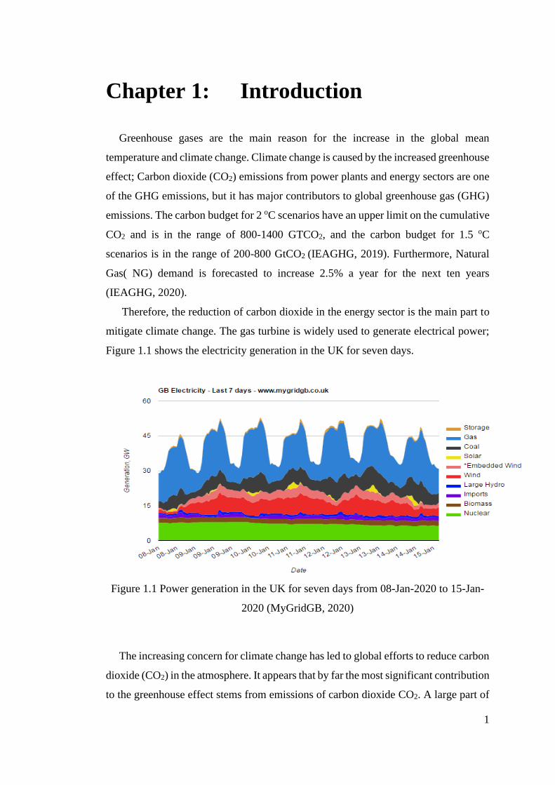
Therefore, the reduction of carbon dioxide in the energy sector is the main part to
mitigate climate change. The gas turbine is widely used to generate electrical power;
Figure 1.1 shows the electricity generation in the UK for seven days.
Figure 1.1 Power generation in the UK for seven days from 08-Jan-2020 to 15-Jan-
2020 (MyGridGB, 2020)
The increasing concern for climate change has led to global efforts to reduce carbon
dioxide (CO2) in the atmosphere. It appears that by far the most significant contribution
to the greenhouse effect stems from emissions of carbon dioxide CO2. A large part of
2
the CO2 emission is produced by combusting fossil fuels in conventional power plants
and industrial processes (United State Environmental Protection Agency, 2018).
The gas turbine power generation is more flexible to respond to electrical demand,
and this is the advantage of the gas turbine to renewable energy, however, conventional
gas turbines burn fossil fuels and release a massive amount of CO2 equivalent emission
in the environment.
The power generation from fossil fuels is likely to continue in future to respond the
energy demand and conventional power plants produce 74% in 2040 even under new
policy scenario, The oil, gas and coal will resource 27%, 24% and 23% respectively
of energy demand in 2040 (Gonzalez-Salazar, Kirsten and Prchlik, 2018).
In order to meet the electricity demand as well as the CO2 mitigation targets, it is
essential to increase the efficiency of fossil-fuel-based energy conversion systems
along with the implementation of carbon capture and storage (CCS) technologies.
There are three carbon capture technologies, including precombustion, oxyfuel
combustion and post-combustion. Oxy-fuel combustion is one of the main carbon
capture technologies that aim to provide zero NOx emission and pure CO2 streams
ready for sequestration. The development of oxyfuel combustion technologies can lead
to high-efficiency clean energy power plants.,the markets opportunity for this project
is quite attractive, and the project dissemination in the energy industry is extensive.
1.1 Aim of this research project
This PhD project is aiming to provide a critical review of state of the art gas-fired
oxy-turbine cycles with a key focus on the leading proposed cycles, including
NetPower Cycle, CES Cycle, MATIANT Cycle, AZEP Cycle, and Graz Cycle. Also
these cycle are compared based on the different aspect including exergoeconomic,
LCOE, performance, TRL and exergy By the completion of this research, a platform
for the process simulation and performance analysis of these type of cycles is provided
using Aspen Plus software.
It is anticipated that as a result of this study, a road map for the development and
deployment of the oxy-turbine power cycles as a clean replacement for the
conventional power plants in the UK and worldwide is presented, which includes
detailed technical information in these cycles. It is the first time several oxy-
3
combustion cycles technologies are investigated and compared together. Also, it is the
first time these cycles are modelled with software and analysed with different
parameters. The output of this PhD thesis will be a platform to develop the next
generation of oxy-turbine power cycles.
1.2 Objectives
In order to achieve the aim stated in the section above, the following objectives
must be reached:
A. To investigate Carbon Capture, Air Separation Unit (ASU) and CO2
Purification and Compression Unit (CPU) technologies.
B. To investigate the oxy-combustion power cycles.
C. To simulate the oxy-combustion cycles with Aspen Plus and tabulate the
results of process modelling at each point.
D. To assess the exergy destruction in components of the oxy-combustion
cycles to compare the efficiency of the component to each other.
E. To compare the parameters of oxy-combustion cycle including TIT, TOT,
CO2/kWh, COP, Exergy, Thermal efficiency, Technology Readiness Level
(TRL) to provide a benchmark for comparing oxy-combustion cycles.
F. To study the sensitivity of leading oxy-combustion cycles.
G. To investigate pilot and industrial demonstration of Oxyturbine power
cycles and comparison in terms of cost and efficiency.
H. To evaluate the performance of the oxy-combustion cycles according to the
Aspen plus modelling.
I. To assess the cost rate and Levelized Cost Of Energy (LCOE) for oxy-
combustion cycles.
J. To compare several parameters on the radar diagram.
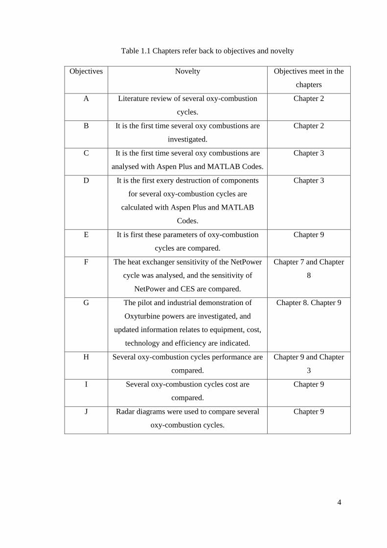
Table 1.1, indicates where these objectives are met and stating the novelty.
4
Table 1.1 Chapters refer back to objectives and novelty
Objectives Novelty Objectives meet in the
chapters
A Literature review of several oxy-combustion
cycles.
Chapter 2
B It is the first time several oxy combustions are
investigated.
Chapter 2
C It is the first time several oxy combustions are
analysed with Aspen Plus and MATLAB Codes.
Chapter 3
D It is the first exery destruction of components
for several oxy-combustion cycles are
calculated with Aspen Plus and MATLAB
Codes.
Chapter 3
E It is first these parameters of oxy-combustion
cycles are compared.
Chapter 9
F The heat exchanger sensitivity of the NetPower
cycle was analysed, and the sensitivity of
NetPower and CES are compared.
Chapter 7 and Chapter
8
G The pilot and industrial demonstration of
Oxyturbine powers are investigated, and
updated information relates to equipment, cost,
technology and efficiency are indicated.
Chapter 8. Chapter 9
H Several oxy-combustion cycles performance are
compared.
Chapter 9 and Chapter
3
I Several oxy-combustion cycles cost are
compared.
Chapter 9
J Radar diagrams were used to compare several
oxy-combustion cycles.
Chapter 9
5
1.3 Introduction to the gas turbine technology
The idea of the gas turbine goes back long ago, John Wilkins (1614-1672) used the
motion of air that ascends the chimney to turn a rod (EAVES PSK, 1971), but the gas
turbine goes back to Barber (1791) for the basic concept of power generation (Horlock
and Bathie, 2004).
The gas turbine was used extensively 40 years ago in power generation and different
industries. There are various types of the gas turbine with different fuels such as natural
gas, diesel fuel, biomass gas.
The first generation gas turbine has major problems with the efficiency penalty of
the compressor, and the compressor was driven independently in the early design of
the gas turbine. Also, the turbine must be highly efficient to produce enough power to
drive the compressor and generate the power network. One of the first gas turbines
was developed by Armengaud and Lemae (French engineers) in 1904, the power
network was about 10kW, and overall efficiency was approximately 3%. The first
industrial gas turbine was produced by Brown Boveri in 1939; the network output was
4 MW. Whittle produced a gas turbine with enough power network for propulsion;
The exhaust gas can produce a high-speed jet for aircraft propulsion in 1930.
The heavy gas turbine had been developed to produce electrical power by combined
cycle gas turbine with a bottom cycle of the steam turbine (CCGT) (Horlock and
Bathie, 2004). Gas turbine material technologies are developed during the last 20
years. The cooling method of the blade and new coating materials let the turbines work
in the higher temperature such as NetPower cycle and CES cycle; in recent years, the
development of composer pressure ratio support increased turbine efficiency up to
60%.
Gas turbines convert the chemical energy of the fuel into whether mechanical
energy or kinetic energy. There are two types of gas turbines, including power
generation gas turbine that converts the chemical energy of the fuel to shaft power to
produce electricity and gas turbine for aircraft which produce thrust to propel it
(Schobeiri, 2018).
The main concept of gas turbine thermodynamics is receiving fuel energy at a high
temperature at the combustor (C) to produce work at the gas turbine (A) and release
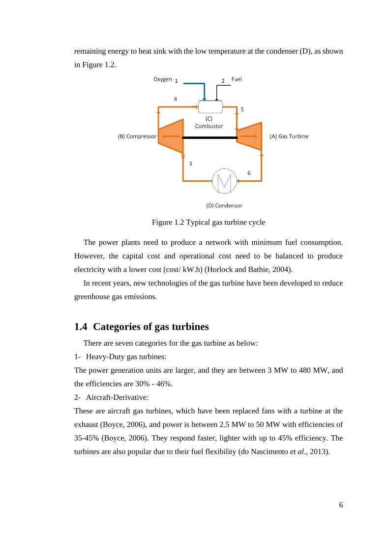
6
remaining energy to heat sink with the low temperature at the condenser (D), as shown
in Figure 1.2.
Figure 1.2 Typical gas turbine cycle
The power plants need to produce a network with minimum fuel consumption.
However, the capital cost and operational cost need to be balanced to produce
electricity with a lower cost (cost/ kW.h) (Horlock and Bathie, 2004).
In recent years, new technologies of the gas turbine have been developed to reduce
greenhouse gas emissions.
1.4 Categories of gas turbines
There are seven categories for the gas turbine as below:
1- Heavy-Duty gas turbines:
The power generation units are larger, and they are between 3 MW to 480 MW, and
the efficiencies are 30% - 46%.
2- Aircraft-Derivative:
These are aircraft gas turbines, which have been replaced fans with a turbine at the
exhaust (Boyce, 2006), and power is between 2.5 MW to 50 MW with efficiencies of
35-45% (Boyce, 2006). They respond faster, lighter with up to 45% efficiency. The
turbines are also popular due to their fuel flexibility (do Nascimento et al., 2013).
7
3- Industrial gas turbine:
These types of gas turbines are used for medium-range power and are usually rated
between 5–15 MW for the compressor of petrochemical plants with low efficiencies
about 30% (Boyce, 2006).
One type of them is the Rolls-Royce Industrial Trent family gas turbine. This
turbine produces high power with variable speed which is suitable for natural gas
liquefaction, gas transportation, and gas injection for oil recovery. ALSTOM, General
Electric, and Siemens-Westinghouse are the main manufacturer of the large single-
shaft gas turbine with more than 250 MW per unit.
Industrial gas turbines can be used for different sectors because of their flexibility.
These turbines can be used for mechanical drive systems, chemical industries,
transportations, pump drives and power generation (Ahmed F. El-Sayed, 2017).
4- Small gas turbine:
The radial turbines with centrifugal compressors produce power between 0.5-2.5 MW
with a very low efficiency of 15-25% (Boyce, 2006).
5- Micro-Turbine:
These turbines can produce power up to 300 kW, and they are used for industries and
domestic clients. These gas turbines are open cycle gas turbines with different features
such as high-speed operation, compact size, variable speed, low maintenance, easy
installation, simple operability (Marco Antônio Rosa do Nascimento, 2005).
6- Gas turbines at sea:
The first successful boat with a gas turbine was Motor Gun Boat in 1947, and the
first fast patrol boat with a gas turbine was fabricated by Rolls Royce Proteus. General
electric fabricated LM services for U.S Navy Bruke Destroyer, Italian Lupo Farigate,
AEGIS Gruiser. The advantages of the gas turbine for naive industries are compact
size, low noise and high power density (Ahmed F. El-Sayed, 2017).
7- Gas turbines at the ground:
U.S. tank M1A1 Abram has used the AlliedSignal Lycoming AGT1500 gas turbine.
Also, a gas turbine engine is used for Union Pacific in the United States to operate
locomotives. The gas turbine produces electricity to the electric power motors of the
locomotive (Union Pacific, 2020). Lightweight, reliability and compactness are the
advantages of a gas turbine for road transportation. The gas turbine engine has a
vibration-free operation compared with the reciprocating engine, and it has a lower
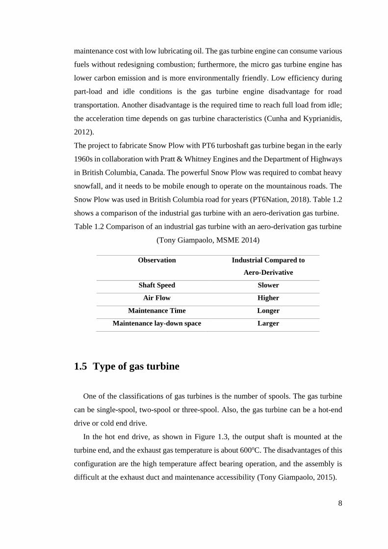
8
maintenance cost with low lubricating oil. The gas turbine engine can consume various
fuels without redesigning combustion; furthermore, the micro gas turbine engine has
lower carbon emission and is more environmentally friendly. Low efficiency during
part-load and idle conditions is the gas turbine engine disadvantage for road
transportation. Another disadvantage is the required time to reach full load from idle;
the acceleration time depends on gas turbine characteristics (Cunha and Kyprianidis,
2012).
The project to fabricate Snow Plow with PT6 turboshaft gas turbine began in the early
1960s in collaboration with Pratt & Whitney Engines and the Department of Highways
in British Columbia, Canada. The powerful Snow Plow was required to combat heavy
snowfall, and it needs to be mobile enough to operate on the mountainous roads. The
Snow Plow was used in British Columbia road for years (PT6Nation, 2018). Table 1.2
shows a comparison of the industrial gas turbine with an aero-derivation gas turbine.
Table 1.2 Comparison of an industrial gas turbine with an aero-derivation gas turbine
(Tony Giampaolo, MSME 2014)
Observation Industrial Compared to
Aero-Derivative
Shaft Speed Slower
Air Flow Higher
Maintenance Time Longer
Maintenance lay-down space Larger
1.5 Type of gas turbine
One of the classifications of gas turbines is the number of spools. The gas turbine
can be single-spool, two-spool or three-spool. Also, the gas turbine can be a hot-end
drive or cold end drive.
In the hot end drive, as shown in Figure 1.3, the output shaft is mounted at the
turbine end, and the exhaust gas temperature is about 600oC. The disadvantages of this
configuration are the high temperature affect bearing operation, and the assembly is
difficult at the exhaust duct and maintenance accessibility (Tony Giampaolo, 2015).

9
Figure 1.3 Schematic of a single spool gas turbine with hot end drive (Tony
Giampaolo, 2015)
In the cold end drive, as shown in Figure 1.4, the output shaft is mounted at the
front of the compressor. The advantages of this configuration are the accessibility of
driven equipment, ease to service, maintenance, and work on ambient temperature
(Tony Giampaolo, 2015).
Figure 1.4 Schematic of a single spool gas turbine with a cold end drive (Tony
Giampaolo, 2015)
1.5.1 Single-shaft gas turbine
In the single-shaft gas turbine, as shown in Figure 1.5, one shaft connects the
compressor to the turbine. The air is drawn into the compressor to increase its pressure;
then, high-pressure air burns with fuel to produce by-products at the high temperature.
The hot output flue of combustion enters the turbine to produce power. Part of the
power output is transferred through the shaft and absorbed by the compressor. The
remaining power is used to drive a generator to produce electricity (Razak, 2007).
As shown in Figure 1.5, the air enters and exits the compressor in the process between
stage (2-3), the combustor process is between stage (31-4), the expansion process
(turbine) is between stage (41-5).
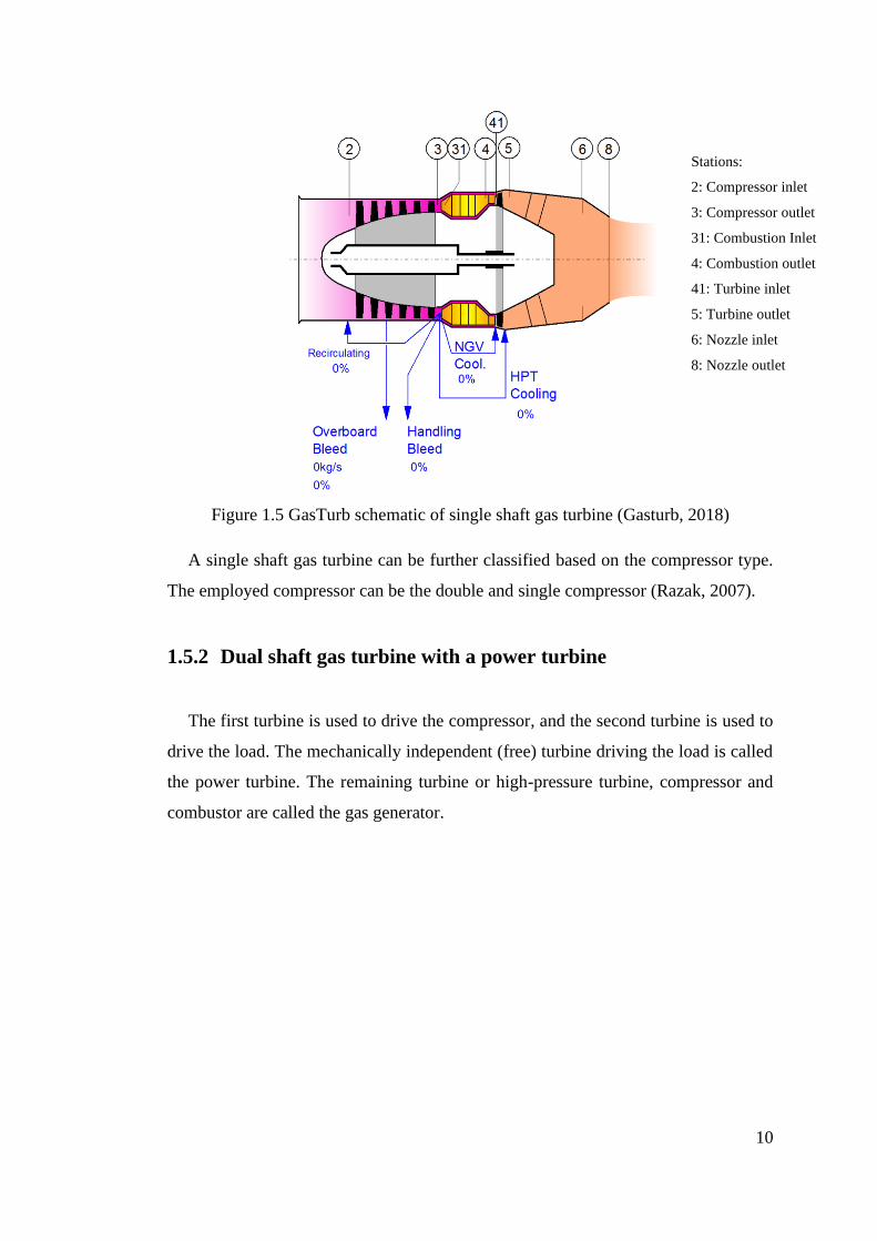
10
Figure 1.5 GasTurb schematic of single shaft gas turbine (Gasturb, 2018)
A single shaft gas turbine can be further classified based on the compressor type.
The employed compressor can be the double and single compressor (Razak, 2007).
1.5.2 Dual shaft gas turbine with a power turbine
The first turbine is used to drive the compressor, and the second turbine is used to
drive the load. The mechanically independent (free) turbine driving the load is called
the power turbine. The remaining turbine or high-pressure turbine, compressor and
combustor are called the gas generator.
Stations:
2: Compressor inlet
3: Compressor outlet
31: Combustion Inlet
4: Combustion outlet
41: Turbine inlet
5: Turbine outlet
6: Nozzle inlet
8: Nozzle outlet
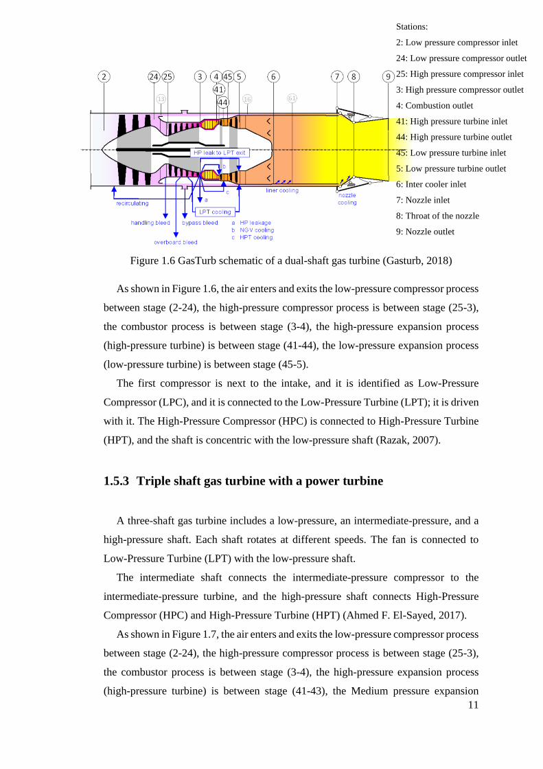
11
Figure 1.6 GasTurb schematic of a dual-shaft gas turbine (Gasturb, 2018)
As shown in Figure 1.6, the air enters and exits the low-pressure compressor process
between stage (2-24), the high-pressure compressor process is between stage (25-3),
the combustor process is between stage (3-4), the high-pressure expansion process
(high-pressure turbine) is between stage (41-44), the low-pressure expansion process
(low-pressure turbine) is between stage (45-5).
The first compressor is next to the intake, and it is identified as Low-Pressure
Compressor (LPC), and it is connected to the Low-Pressure Turbine (LPT); it is driven
with it. The High-Pressure Compressor (HPC) is connected to High-Pressure Turbine
(HPT), and the shaft is concentric with the low-pressure shaft (Razak, 2007).
1.5.3 Triple shaft gas turbine with a power turbine
A three-shaft gas turbine includes a low-pressure, an intermediate-pressure, and a
high-pressure shaft. Each shaft rotates at different speeds. The fan is connected to
Low-Pressure Turbine (LPT) with the low-pressure shaft.
The intermediate shaft connects the intermediate-pressure compressor to the
intermediate-pressure turbine, and the high-pressure shaft connects High-Pressure
Compressor (HPC) and High-Pressure Turbine (HPT) (Ahmed F. El-Sayed, 2017).
As shown in Figure 1.7, the air enters and exits the low-pressure compressor process
between stage (2-24), the high-pressure compressor process is between stage (25-3),
the combustor process is between stage (3-4), the high-pressure expansion process
(high-pressure turbine) is between stage (41-43), the Medium pressure expansion
Stations:
2: Low pressure compressor inlet
24: Low pressure compressor outlet
25: High pressure compressor inlet
3: High pressure compressor outlet
4: Combustion outlet
41: High pressure turbine inlet
44: High pressure turbine outlet
45: Low pressure turbine inlet
5: Low pressure turbine outlet
6: Inter cooler inlet
7: Nozzle inlet
8: Throat of the nozzle
9: Nozzle outlet
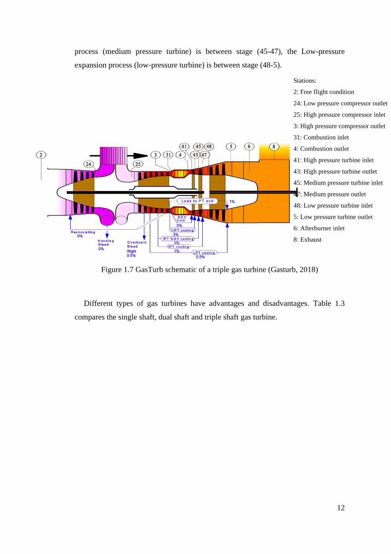
12
process (medium pressure turbine) is between stage (45-47), the Low-pressure
expansion process (low-pressure turbine) is between stage (48-5).
Figure 1.7 GasTurb schematic of a triple gas turbine (Gasturb, 2018)
Different types of gas turbines have advantages and disadvantages. Table 1.3
compares the single shaft, dual shaft and triple shaft gas turbine.
Stations:
2: Free flight condition
24: Low pressure compressor outlet
25: High pressure compressor inlet
3: High pressure compressor outlet
31: Combustion inlet
4: Combustion outlet
41: High pressure turbine inlet
43: High pressure turbine outlet
45: Medium pressure turbine inlet
47: Medium pressure outlet
48: Low pressure turbine inlet
5: Low pressure turbine outlet
6: Afterburner inlet
8: Exhaust
8: Throat of the nozzle
9: Nozzle outlet
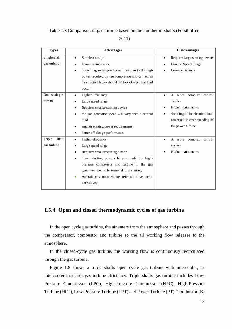
13
Table 1.3 Comparison of gas turbine based on the number of shafts (Forsthoffer,
2011)
Types Advantages Disadvantages
Single shaft
gas turbine
• Simplest design
• Lower maintenance
• preventing over-speed conditions due to the high
power required by the compressor and can act as
an effective brake should the loss of electrical load
occur
• Requires large starting device
• Limited Speed Range
• Lower efficiency
Dual shaft gas
turbine
• Higher Efficiency
• Large speed range
• Requires smaller starting device
• the gas generator speed will vary with electrical
load
• smaller starting power requirements
• better off-design performance
• A more complex control
system
• Higher maintenance
• shedding of the electrical load
can result in over-speeding of
the power turbine
Triple shaft
gas turbine
• Higher efficiency
• Large speed range
• Requires smaller starting device
• lower starting powers because only the high-
pressure compressor and turbine in the gas
generator need to be turned during starting
• Aircraft gas turbines are referred to as aero-
derivatives
• A more complex control
system
• Higher maintenance
1.5.4 Open and closed thermodynamic cycles of gas turbine
In the open cycle gas turbine, the air enters from the atmosphere and passes through
the compressor, combustor and turbine so the all working flow releases to the
atmosphere.
In the closed-cycle gas turbine, the working flow is continuously recirculated
through the gas turbine.
Figure 1.8 shows a triple shafts open cycle gas turbine with intercooler, as
intercooler increases gas turbine efficiency. Triple shafts gas turbine includes Low-
Pressure Compressor (LPC), High-Pressure Compressor (HPC), High-Pressure
Turbine (HPT), Low-Pressure Turbine (LPT) and Power Turbine (PT). Combustor (B)
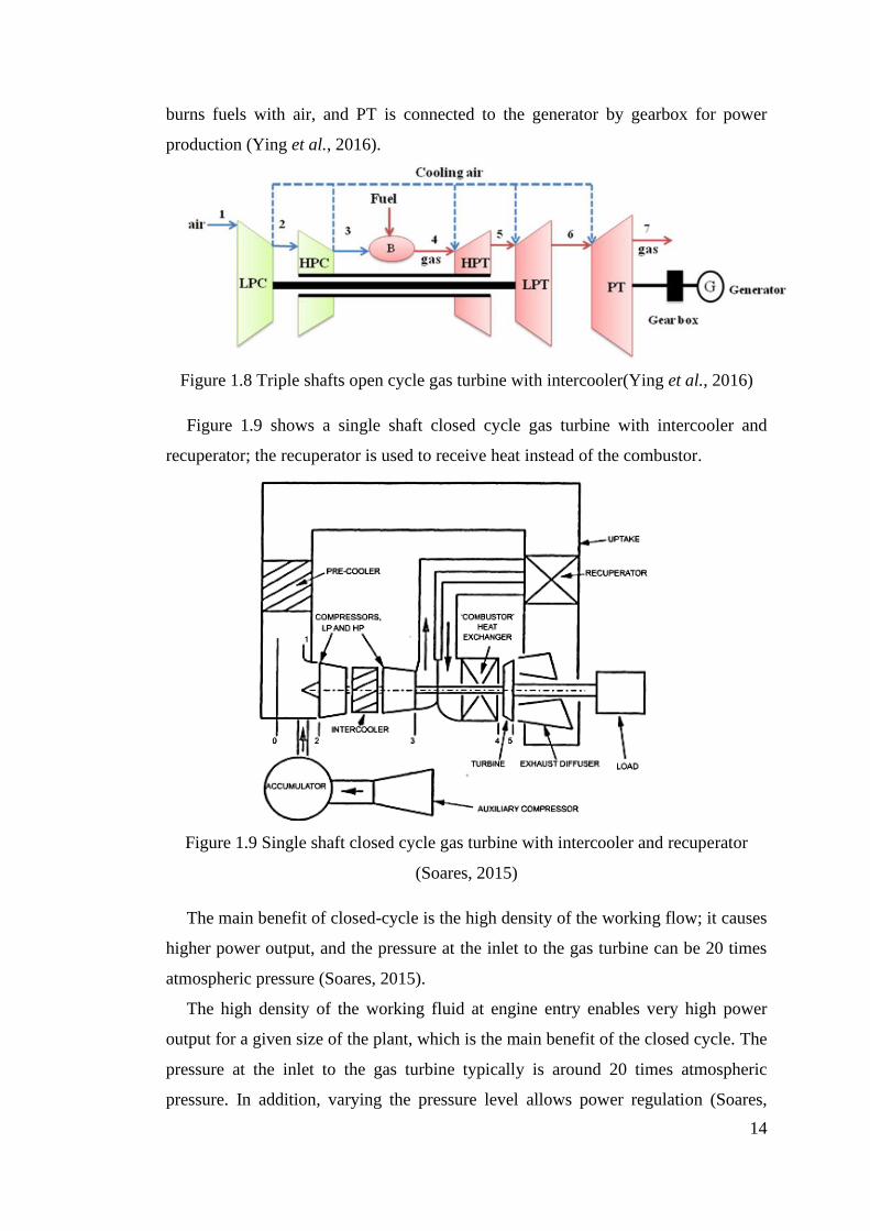
14
burns fuels with air, and PT is connected to the generator by gearbox for power
production (Ying et al., 2016).
Figure 1.8 Triple shafts open cycle gas turbine with intercooler(Ying et al., 2016)
Figure 1.9 shows a single shaft closed cycle gas turbine with intercooler and
recuperator; the recuperator is used to receive heat instead of the combustor.
Figure 1.9 Single shaft closed cycle gas turbine with intercooler and recuperator
(Soares, 2015)
The main benefit of closed-cycle is the high density of the working flow; it causes
higher power output, and the pressure at the inlet to the gas turbine can be 20 times
atmospheric pressure (Soares, 2015).
The high density of the working fluid at engine entry enables very high power
output for a given size of the plant, which is the main benefit of the closed cycle. The
pressure at the inlet to the gas turbine typically is around 20 times atmospheric
pressure. In addition, varying the pressure level allows power regulation (Soares,
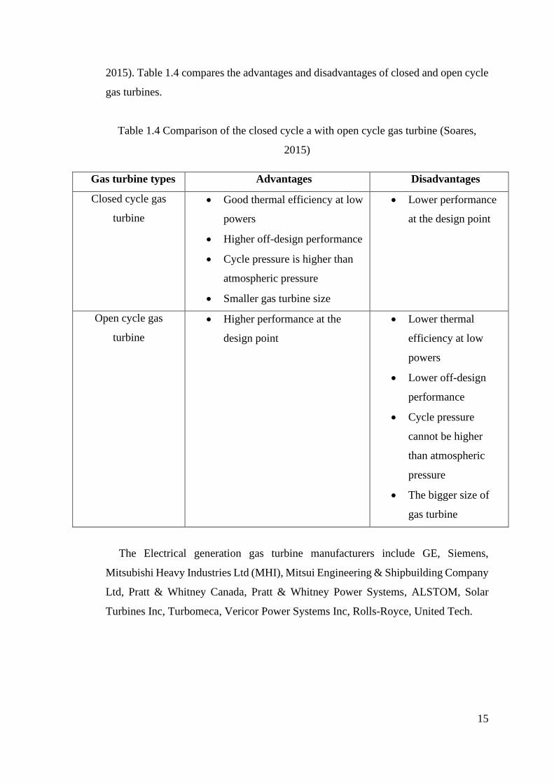
15
2015). Table 1.4 compares the advantages and disadvantages of closed and open cycle
gas turbines.
Table 1.4 Comparison of the closed cycle a with open cycle gas turbine (Soares,
2015)
Gas turbine types Advantages Disadvantages
Closed cycle gas
turbine
• Good thermal efficiency at low
powers
• Higher off-design performance
• Cycle pressure is higher than
atmospheric pressure
• Smaller gas turbine size
• Lower performance
at the design point
Open cycle gas
turbine
• Higher performance at the
design point
• Lower thermal
efficiency at low
powers
• Lower off-design
performance
• Cycle pressure
cannot be higher
than atmospheric
pressure
• The bigger size of
gas turbine
The Electrical generation gas turbine manufacturers include GE, Siemens,
Mitsubishi Heavy Industries Ltd (MHI), Mitsui Engineering & Shipbuilding Company
Ltd, Pratt & Whitney Canada, Pratt & Whitney Power Systems, ALSTOM, Solar
Turbines Inc, Turbomeca, Vericor Power Systems Inc, Rolls-Royce, United Tech.
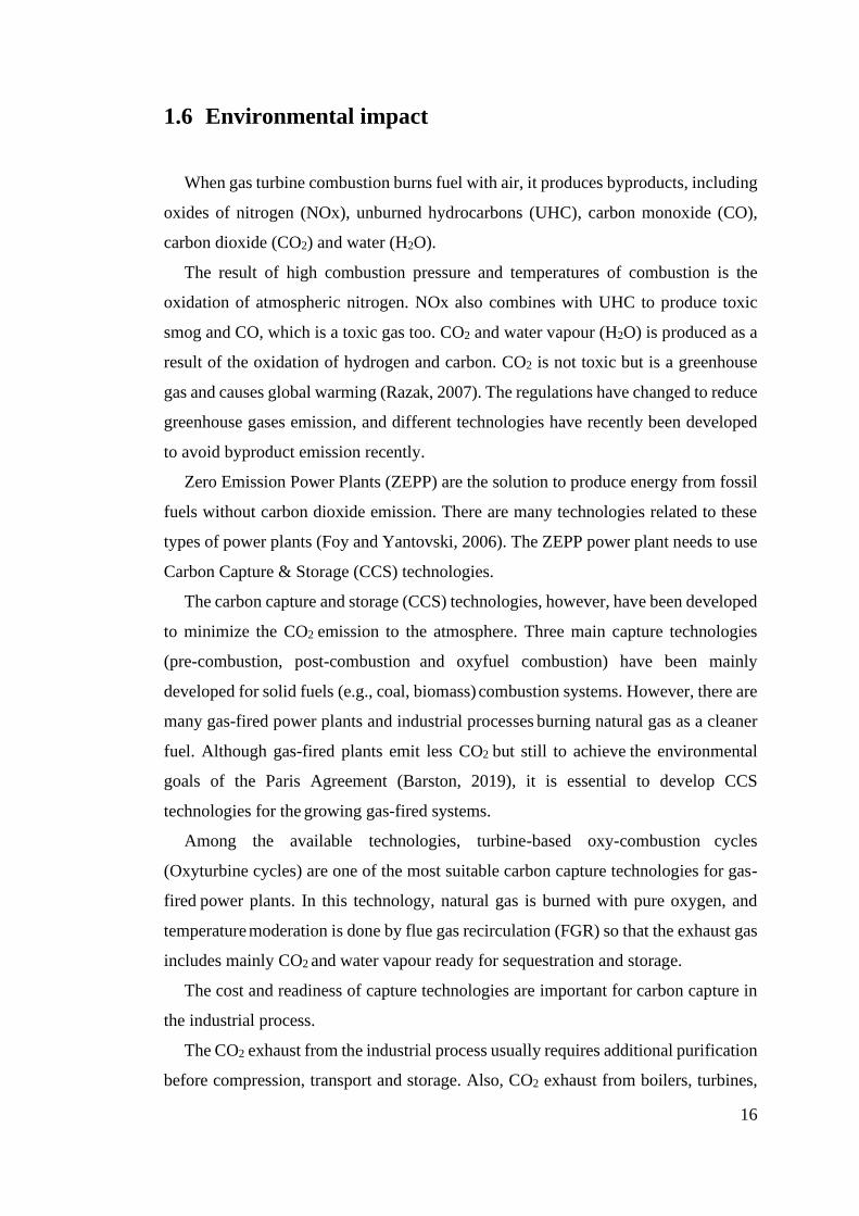
16
1.6 Environmental impact
When gas turbine combustion burns fuel with air, it produces byproducts, including
oxides of nitrogen (NOx), unburned hydrocarbons (UHC), carbon monoxide (CO),
carbon dioxide (CO2) and water (H2O).
The result of high combustion pressure and temperatures of combustion is the
oxidation of atmospheric nitrogen. NOx also combines with UHC to produce toxic
smog and CO, which is a toxic gas too. CO2 and water vapour (H2O) is produced as a
result of the oxidation of hydrogen and carbon. CO2 is not toxic but is a greenhouse
gas and causes global warming (Razak, 2007). The regulations have changed to reduce
greenhouse gases emission, and different technologies have recently been developed
to avoid byproduct emission recently.
Zero Emission Power Plants (ZEPP) are the solution to produce energy from fossil
fuels without carbon dioxide emission. There are many technologies related to these
types of power plants (Foy and Yantovski, 2006). The ZEPP power plant needs to use
Carbon Capture & Storage (CCS) technologies.
The carbon capture and storage (CCS) technologies, however, have been developed
to minimize the CO2 emission to the atmosphere. Three main capture technologies
(pre-combustion, post-combustion and oxyfuel combustion) have been mainly
developed for solid fuels (e.g., coal, biomass) combustion systems. However, there are
many gas-fired power plants and industrial processes burning natural gas as a cleaner
fuel. Although gas-fired plants emit less CO2 but still to achieve the environmental
goals of the Paris Agreement (Barston, 2019), it is essential to develop CCS
technologies for the growing gas-fired systems.
Among the available technologies, turbine-based oxy-combustion cycles
(Oxyturbine cycles) are one of the most suitable carbon capture technologies for gas-
fired power plants. In this technology, natural gas is burned with pure oxygen, and
temperature moderation is done by flue gas recirculation (FGR) so that the exhaust gas
includes mainly CO2 and water vapour ready for sequestration and storage.
The cost and readiness of capture technologies are important for carbon capture in
the industrial process.
The CO2 exhaust from the industrial process usually requires additional purification
before compression, transport and storage. Also, CO2 exhaust from boilers, turbines,
17
cement kilns, iron and steel furnaces and direct iron reduction processes require
additional technologies to concentrate dilute steams to be economical for
transportation and storage.
Carbon separation processes are similar to carbon capture for power plants and
include chemical or physical adsorption, absorption, membrane and liquefaction or
cryogenic separation. These processes can be divided into three main categories,
including pre-combustion, post-combustion and oxyfuel combustion processes
(OECD/IEA, 2011).
The increasing concern for climate change has led to global efforts to reduce carbon
dioxide (CO2) in the environment. It appears that by far the largest contribution to the
greenhouse effect stems from emissions of carbon dioxide CO2. A large part of the
CO2 emission are produced by the combustion of fossil fuels in conventional power
plants and industrial processes. However, Carbon Capture and Sequestration (CCS)
technologies have been developed to minimise the CO2 emission to the atmosphere.
Natural gas has the lowest CO2 emissions per unit of energy of all fossil fuels at about
14 kg CO2/GJ, compared to oil with about 20 kg CO2/GJ and coal with about 25 kg
CO2/GJ. Although gas-fired plants emit less CO2 but still to achieve the environmental
goals of the Paris Agreement, it is essential to develop CCS technologies for the
growing gas-fired systems. Among the available technologies, turbine-based oxy-
combustion cycles (Oxyturbine cycles) are one of the most suitable carbon capture
technologies for gas-fired power plants. In this technology, natural gas is burned with
pure oxygen, and temperature moderation is done by Flue Gas Recirculation (FGR) so
that the exhaust gas includes mainly CO2 and water vapour ready for sequestration and
storage. Recent developments in oxy-combustion technology have reduced the cost of
capture and made it competitive with post-combustion technology.
Coal-fired power plants need to either implement costly carbon capture techniques
or to switch to gas-fired power plants. Gas-fired power plants are the best replacement
for the coal-fired power plant to decrease CO2 emissions and increase power plant
efficiency. The two Oxyturbine power cycles with maximum carbon capture and
highest efficiencies were introduced by two companies, CES ( Clean Energy System)
and NetPower. These two cycles are recently have been developed to the
demonstration phase.
18
Oxy-combustion is a thermodynamic cycle that burns fuel with pure oxygen. In a
conventional plant, fuel burns with air which includes a significant amount of N2
(Scaccabarozzi, Gatti and Martelli, 2017). CO2-rich and H2O-rich are cycle fluids for
a recent power cycle.
Oxy-combustion compared with post-combustion and pre-combustion methods
have a lower capital cost and higher efficiency, which means lower carbon dioxide
penalty. The advantages of Oxyturbine cycles are very low emission of nitrogen
oxides, minimum chemical process and the ability to capture nearly 100% of carbon
dioxide emissions (Chaudhry et al., 2018). However, the disadvantages of Oxyturbine
cycles are a high initial capital cost, ASU energy penalty and difficulties in retrofitting
the old plants.
Over the last 30 years, different layouts have been proposed, including the Semi-
Closed Oxy-Combustion Combined Cycle (SCOC-CC), the MATIANT cycle, the
NetPower cycle, the Graz cycle, and the CES cycle. The SCOC-CC, MATIANT and
NetPower cycles with CO2 working fluid, while the Graz and the CES cycles have
H2O working fluid (Scaccabarozzi, Gatti and Martelli, 2017). In the former case,
CO2 capture is performed simply by splitting a part of the main flow, while in the
second case water condensation produces a stream rich in carbon dioxide, which then
can be easily captured via partial condensation (however, in both cases, a further
purification step may be required depending on CO2 purity specifications)
(Scaccabarozzi, Gatti and Martelli, 2017).
The CES cycle is essentially an internal combustion steam cycle using the injection
of steam and liquid water in the combustor to moderate the firing temperature. Pure
oxygen is used as an oxygen and natural gas (or other fuels) as fuel. At the exit of the
combustor, the mixture of H2O and CO2 expands in a turbine (eventually with reheat)
and then it is cooled down in a water condenser (Scaccabarozzi, Gatti and Martelli,
2017). A further improvement of the cycle is presented, called Supercritical CES,
employing a combustor operating at supercritical steam conditions (Mancuso et al.,
2015).
Complete reviews of the available Oxy-combustion cycle options can be found in
the recent report published by the International Energy Agency (IEA) Green House
Gas program and co-authored by AMEC-Foster Wheeler and Politecnico di
Milano(Mancuso et al., 2015).
19
1.7 Summary
In this chapter, the aim and objectives of the PhD thesis are discussed, then it has
an introduction of the gas turbine. There are different types of gas turbines based on
the number of the spool. Single shaft gas turbine is the simplest in design, but it has
lower efficiency. Dual shaft gas turbines have higher efficiency and large speed range,
but it needs more maintenance and complex control. Triple spool gas turbines has
higher efficiency and can be used as an aircraft gas turbines, but it needs more
maintenance and complex control too. Conventional gas turbines burn fuel with air
and produce carbon dioxide as a byproduct. In the end, The byproducts of the gas
turbine and the environmental impact are introduced.
20
Chapter 2: Literature review of
Oxyturbine power cycles and gas-
CCS Technologies
2.1 Introduction
Oxy-fuel combustion technology is an effective way of capturing CO2 from power
plants and industrial processes while increasing efficiency and reducing the cost. In
this technology, the air is replaced with nearly pure oxygen as an oxidizer, the working
flow will be enriched with CO2 and H2O, and then CO2 can separate from the water
with the condensation method. This has lower power consumption compared to other
methods of carbon capture, such as pre-combustion and post-combustion technologies.
The oxy-combustion in gas turbine power plants (Oxyturbine power cycles) is seen
as one of the best solutions to capture CO2 from new and retrofitted gas-fired power
stations. Therefore, studies to evaluate cycle configurations and flexibilities, process
and performance simulations, sensitivity techno-economic analysis are highly
essential to be carried out.
In this chapter, the following oxy-combustion power cycles are introduced, and the
operational parameters are presented: SCOC-CC, COOPERATE Cycle, MATIANT,
E-MATIANT, CC_MATIANT, Graz and S-Graz cycles, AZEP 85% and 100%,
ZEITMOP, ZEITMOP Cycle, COOLCEP-S Cycle, Novel O2/CO2 (Cao and Zheng,
2006), NetPower and CES Cycles, then these cycles are modelled with Aspen Plus in
next chapter (Chapter 3) based on these operational parameters from this chapter
(Chapter 2), and also the simulation results and discussions will be presented in the
next chapter (Chapter 3). The natural gas combined cycle with Post-combustion
capture (NGCC-PCC or NGCC or CCGT) and Integrated Gasification Combined
Cycle (IGCC), as reference cycles, are also investigated in order to compare with these
oxy-combustion cycles.
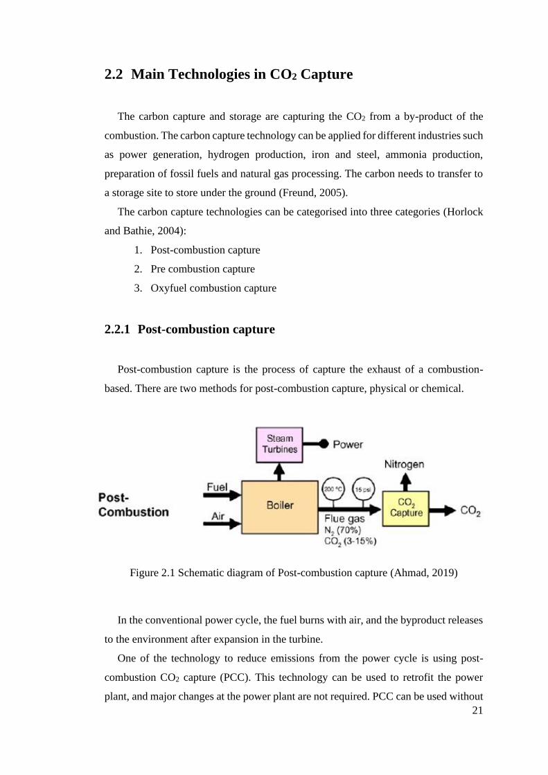
21
2.2 Main Technologies in CO2 Capture
The carbon capture and storage are capturing the CO2 from a by-product of the
combustion. The carbon capture technology can be applied for different industries such
as power generation, hydrogen production, iron and steel, ammonia production,
preparation of fossil fuels and natural gas processing. The carbon needs to transfer to
a storage site to store under the ground (Freund, 2005).
The carbon capture technologies can be categorised into three categories (Horlock
and Bathie, 2004):
1. Post-combustion capture
2. Pre combustion capture
3. Oxyfuel combustion capture
2.2.1 Post-combustion capture
Post-combustion capture is the process of capture the exhaust of a combustion-
based. There are two methods for post-combustion capture, physical or chemical.
Figure 2.1 Schematic diagram of Post-combustion capture (Ahmad, 2019)
In the conventional power cycle, the fuel burns with air, and the byproduct releases
to the environment after expansion in the turbine.
One of the technology to reduce emissions from the power cycle is using post-
combustion CO2 capture (PCC). This technology can be used to retrofit the power
plant, and major changes at the power plant are not required. PCC can be used without
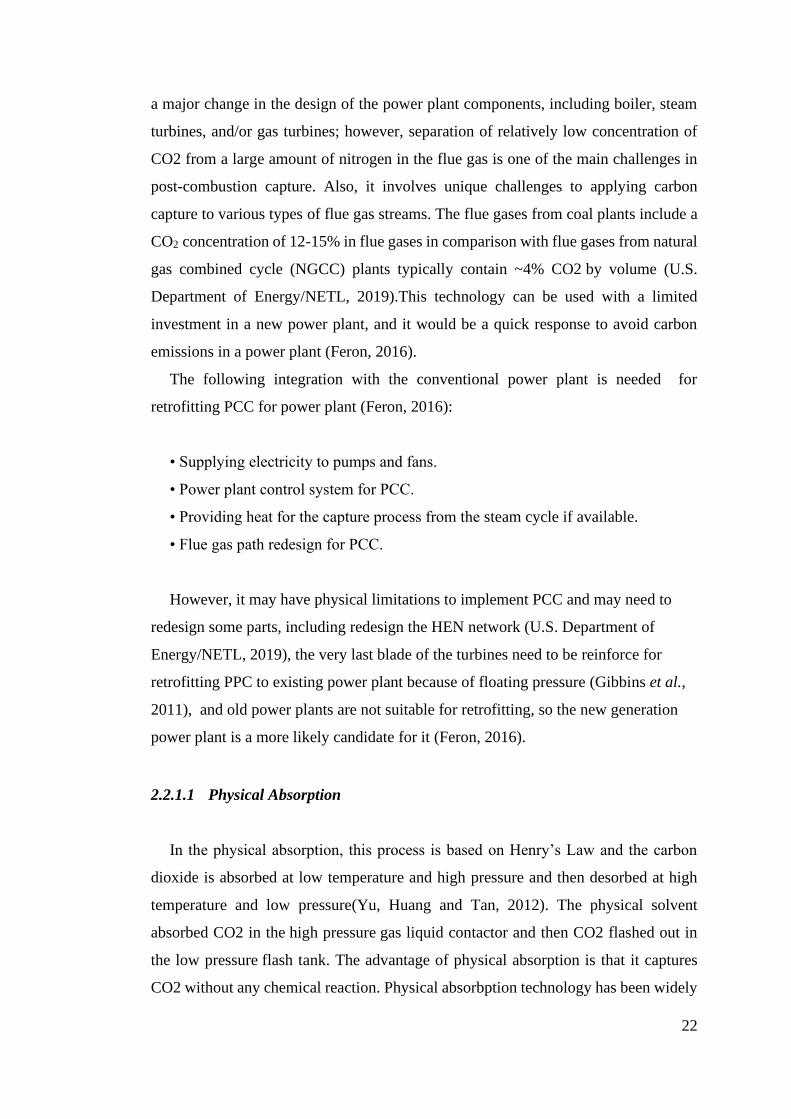
22
a major change in the design of the power plant components, including boiler, steam
turbines, and/or gas turbines; however, separation of relatively low concentration of
CO2 from a large amount of nitrogen in the flue gas is one of the main challenges in
post-combustion capture. Also, it involves unique challenges to applying carbon
capture to various types of flue gas streams. The flue gases from coal plants include a
CO2 concentration of 12-15% in flue gases in comparison with flue gases from natural
gas combined cycle (NGCC) plants typically contain ~4% CO2 by volume (U.S.
Department of Energy/NETL, 2019).This technology can be used with a limited
investment in a new power plant, and it would be a quick response to avoid carbon
emissions in a power plant (Feron, 2016).
The following integration with the conventional power plant is needed for
retrofitting PCC for power plant (Feron, 2016):
• Supplying electricity to pumps and fans.
• Power plant control system for PCC.
• Providing heat for the capture process from the steam cycle if available.
• Flue gas path redesign for PCC.
However, it may have physical limitations to implement PCC and may need to
redesign some parts, including redesign the HEN network (U.S. Department of
Energy/NETL, 2019), the very last blade of the turbines need to be reinforce for
retrofitting PPC to existing power plant because of floating pressure (Gibbins et al.,
2011), and old power plants are not suitable for retrofitting, so the new generation
power plant is a more likely candidate for it (Feron, 2016).
2.2.1.1 Physical Absorption
In the physical absorption, this process is based on Henry’s Law and the carbon
dioxide is absorbed at low temperature and high pressure and then desorbed at high
temperature and low pressure(Yu, Huang and Tan, 2012). The physical solvent
absorbed CO2 in the high pressure gas liquid contactor and then CO2 flashed out in
the low pressure flash tank. The advantage of physical absorption is that it captures
CO2 without any chemical reaction. Physical absorbption technology has been widely
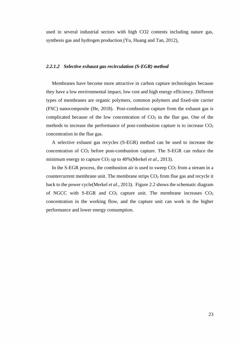
23
used in several industrial sectors with high CO2 contents including nature gas,
synthesis gas and hydrogen production (Yu, Huang and Tan, 2012).
2.2.1.2 Selective exhaust gas recirculation (S-EGR) method
Membranes have become more attractive in carbon capture technologies because
they have a low environmental impact, low cost and high energy efficiency. Different
types of membranes are organic polymers, common polymers and fixed-site carrier
(FSC) nanocomposite (He, 2018). Post-combustion capture from the exhaust gas is
complicated because of the low concentration of CO2 in the flue gas. One of the
methods to increase the performance of post-combustion capture is to increase CO2
concentration in the flue gas.
A selective exhaust gas recycles (S-EGR) method can be used to increase the
concentration of CO2 before post-combustion capture. The S-EGR can reduce the
minimum energy to capture CO2 up to 40%(Merkel et al., 2013).
In the S-EGR process, the combustion air is used to sweep CO2 from a stream in a
countercurrent membrane unit. The membrane strips CO2 from flue gas and recycle it
back to the power cycle(Merkel et al., 2013). Figure 2.2 shows the schematic diagram
of NGCC with S-EGR and CO2 capture unit. The membrane increases CO2
concentration in the working flow, and the capture unit can work in the higher
performance and lower energy consumption.
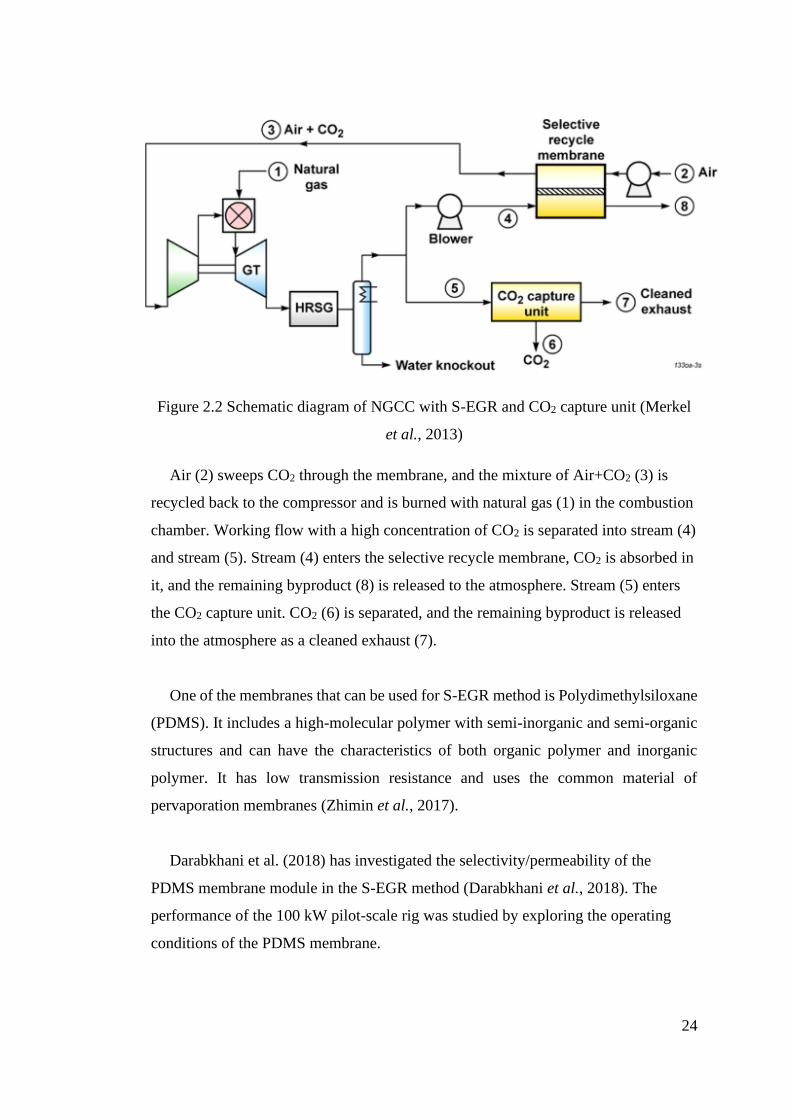
24
Figure 2.2 Schematic diagram of NGCC with S-EGR and CO2 capture unit (Merkel
et al., 2013)
Air (2) sweeps CO2 through the membrane, and the mixture of Air+CO2 (3) is
recycled back to the compressor and is burned with natural gas (1) in the combustion
chamber. Working flow with a high concentration of CO2 is separated into stream (4)
and stream (5). Stream (4) enters the selective recycle membrane, CO2 is absorbed in
it, and the remaining byproduct (8) is released to the atmosphere. Stream (5) enters
the CO2 capture unit. CO2 (6) is separated, and the remaining byproduct is released
into the atmosphere as a cleaned exhaust (7).
One of the membranes that can be used for S-EGR method is Polydimethylsiloxane
(PDMS). It includes a high-molecular polymer with semi-inorganic and semi-organic
structures and can have the characteristics of both organic polymer and inorganic
polymer. It has low transmission resistance and uses the common material of
pervaporation membranes (Zhimin et al., 2017).
Darabkhani et al. (2018) has investigated the selectivity/permeability of the
PDMS membrane module in the S-EGR method (Darabkhani et al., 2018). The
performance of the 100 kW pilot-scale rig was studied by exploring the operating
conditions of the PDMS membrane.
25
Figure 2.3 Schematic diagram of 100 kW pilot scale S-EGR with PDMS
membrane (Russo et al., 2018)
2.2.1.3 Chemical Absorption - Amine Absorption/Stripping Technology
The chemical absorption process includes absorber and stripper. The flue gas
contains CO2 that entered the absorber from the bottom and is contacted to absorbent,
then CO2-rich absorbent flows go into a stripper for the thermal regeneration process
(Yu, Huang and Tan, 2012).
Figure 2.4 Process Flow Diagram of a basic chemical absorption process for amine-
based CO2 capture (MacDowell et al., 2010)
26
2.2.1.4 Physical Adsorbent
Adsorption process are different from the absorption process; in the absorption
process, molecules form fluid transfer to a solid surface, which produces a film of the
adsorbate on the surface of the adsorbent. In the reversible process, which is called
desorption, the molecule is separated from the surface, but in the absorption process,
the absorbate is dissolved (Artioli, 2008).
One of the carbonaceous adsorption, which is used widely, is activated carbon. It is
used to capture carbon dioxide with low sensitivity to moisture, low cost and high
thermal stability (Yu, Huang and Tan, 2012).
2.2.1.5 Chemical Adsorbent (Amine-Based)
In the chemical adsorption, acidic CO2 molecules interact with the surface of the
adsorbent with the formation of covalent bonding such as an amine (basic organic
group).
Amine adsorbents are used widely, and it has low heat capacity and needs low heat
for regeneration, but it has a high cost and low adsorption capacity of CO2.
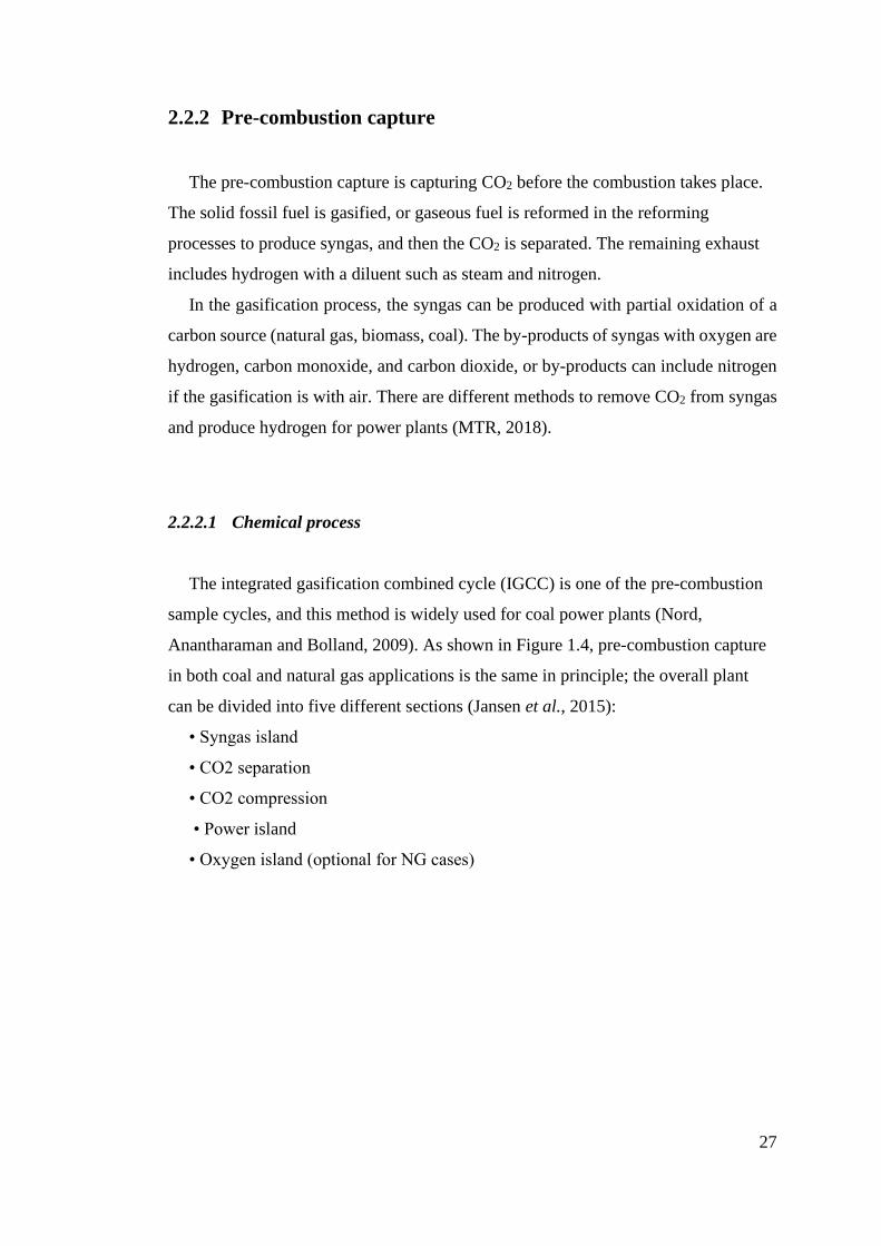
27
2.2.2 Pre-combustion capture
The pre-combustion capture is capturing CO2 before the combustion takes place.
The solid fossil fuel is gasified, or gaseous fuel is reformed in the reforming
processes to produce syngas, and then the CO2 is separated. The remaining exhaust
includes hydrogen with a diluent such as steam and nitrogen.
In the gasification process, the syngas can be produced with partial oxidation of a
carbon source (natural gas, biomass, coal). The by-products of syngas with oxygen are
hydrogen, carbon monoxide, and carbon dioxide, or by-products can include nitrogen
if the gasification is with air. There are different methods to remove CO2 from syngas
and produce hydrogen for power plants (MTR, 2018).
2.2.2.1 Chemical process
The integrated gasification combined cycle (IGCC) is one of the pre-combustion
sample cycles, and this method is widely used for coal power plants (Nord,
Anantharaman and Bolland, 2009). As shown in Figure 1.4, pre-combustion capture
in both coal and natural gas applications is the same in principle; the overall plant
can be divided into five different sections (Jansen et al., 2015):
• Syngas island
• CO2 separation
• CO2 compression
• Power island
• Oxygen island (optional for NG cases)
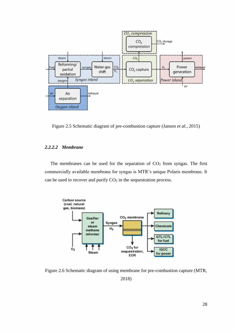
28
Figure 2.5 Schematic diagram of pre-combustion capture (Jansen et al., 2015)
2.2.2.2 Membrane
The membranes can be used for the separation of CO2 from syngas. The first
commercially available membrane for syngas is MTR’s unique Polaris membrane. It
can be used to recover and purify CO2 in the sequestration process.
Figure 2.6 Schematic diagram of using membrane for pre-combustion capture (MTR,
2018)
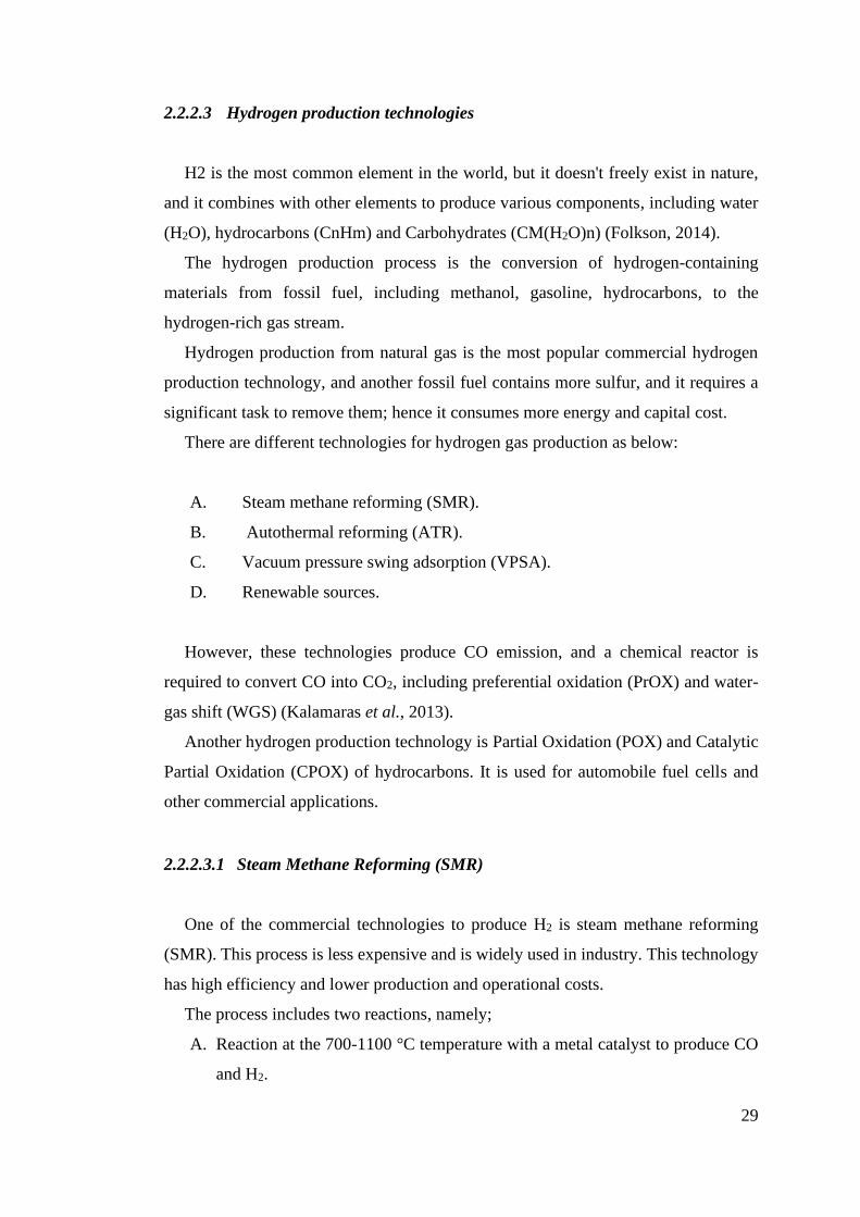
29
2.2.2.3 Hydrogen production technologies
H2 is the most common element in the world, but it doesn't freely exist in nature,
and it combines with other elements to produce various components, including water
(H2O), hydrocarbons (CnHm) and Carbohydrates (CM(H2O)n) (Folkson, 2014).
The hydrogen production process is the conversion of hydrogen-containing
materials from fossil fuel, including methanol, gasoline, hydrocarbons, to the
hydrogen-rich gas stream.
Hydrogen production from natural gas is the most popular commercial hydrogen
production technology, and another fossil fuel contains more sulfur, and it requires a
significant task to remove them; hence it consumes more energy and capital cost.
There are different technologies for hydrogen gas production as below:
A. Steam methane reforming (SMR).
B. Autothermal reforming (ATR).
C. Vacuum pressure swing adsorption (VPSA).
D. Renewable sources.
However, these technologies produce CO emission, and a chemical reactor is
required to convert CO into CO2, including preferential oxidation (PrOX) and water-
gas shift (WGS) (Kalamaras et al., 2013).
Another hydrogen production technology is Partial Oxidation (POX) and Catalytic
Partial Oxidation (CPOX) of hydrocarbons. It is used for automobile fuel cells and
other commercial applications.
2.2.2.3.1 Steam Methane Reforming (SMR)
One of the commercial technologies to produce H2 is steam methane reforming
(SMR). This process is less expensive and is widely used in industry. This technology
has high efficiency and lower production and operational costs.
The process includes two reactions, namely;
A. Reaction at the 700-1100 °C temperature with a metal catalyst to produce CO
and H2.
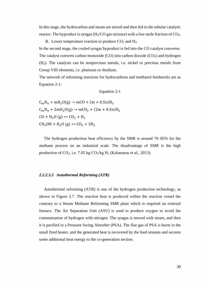
30
In this stage, the hydrocarbon and steam are mixed and then fed in the tubular catalytic
reactor. The byproduct is syngas (H2/CO gas mixture) with a low mole fraction of CO2.
B. Lower temperature reaction to produce CO2 and H2.
In the second stage, the cooled syngas byproduct is fed into the CO catalyst converter.
The catalyst converts carbon monoxide (CO) into carbon dioxide (CO2) and hydrogen
(H2). The catalysts can be nonprecious metals, i.e. nickel or precious metals from
Group VIII elements, i.e. platinum or rhodium.
The network of reforming reactions for hydrocarbons and methanol feedstocks are as
Equation 2-1:
Equation 2-1
CmHn + mH2O(g) → mCO + (m + 0.5n)H2
CmHn + 2mH2O(g) → mCO2 + (2m + 0.5n)H2
CO + H2O (g) ↔ CO2 + H2
CH3OH + H2O (g) ↔ CO2 + 3H2
The hydrogen production heat efficiency by the SMR is around 70–85% for the
methane process on an industrial scale. The disadvantage of SMR is the high
production of CO2, i.e. 7.05 kg CO2/kg H2 (Kalamaras et al., 2013).
2.2.2.3.2 Autothermal Reforming (ATR)
Autothermal reforming (ATR) is one of the hydrogen production technology, as
shown in Figure 2.7. The reaction heat is produced within the reaction vessel the
contrary to a Steam Methane Reforming SMR plant which is required an external
furnace. The Air Separation Unit (ASU) is used to produce oxygen to avoid the
contamination of hydrogen with nitrogen. The syngas is moved with steam, and then
it is purified in a Pressure Swing Absorber (PSA). The flue gas of PSA is burnt in the
small fired heater, and the generated heat is recovered by the feed streams and secures
some additional heat energy to the co-generation section.

31
Figure 2.7 Schematic diagram of Autothermal Reforming (AR) (Antonini et al.,
2020)
The advantage of ART is the heating source; it does not require external heat and
is less expensive than Steam Methane Reformer (SMR). Steam Methane Reforming is
an endothermic process, and this reaction needs to take energy. Hence external heat
source is required, but Autothermal reforming is the combination of endothermic
reforming (demanding energy through steam reforming) and exothermic reforming
(releasing energy through partial oxidation reactions). The second advantage of ART
is shutting down and starting very fast, with a large amount of hydrogen production
(Kalamaras et al., 2013).
2.2.2.3.3 Vacuum pressure swing adsorption (VPSA) cycle
Vacuum pressure swing adsorption (VPSA) is shown in Figure 2.8. The hydrogen
purification and CO2 capture are combined in one process. This cycle includes a high-
pressure adsorption stage (ads) and produces high purity H2. The captured CO2 is
dehydrated and compressed, and flue gas is burned in the furnace (Antonini et al.,
2020). Another advantage of the VPSA unit is the flexibility of retrofitting existing
hydrogen production equipment and partly uses it for H2 production.
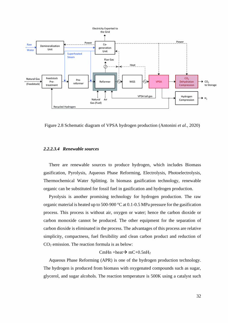
32
Figure 2.8 Schematic diagram of VPSA hydrogen production (Antonini et al., 2020)
2.2.2.3.4 Renewable sources
There are renewable sources to produce hydrogen, which includes Biomass
gasification, Pyrolysis, Aqueous Phase Reforming, Electrolysis, Photoelectrolysis,
Thermochemical Water Splitting. In biomass gasification technology, renewable
organic can be substituted for fossil fuel in gasification and hydrogen production.
Pyrolysis is another promising technology for hydrogen production. The raw
organic material is heated up to 500-900 °C at 0.1-0.5 MPa pressure for the gasification
process. This process is without air, oxygen or water; hence the carbon dioxide or
carbon monoxide cannot be produced. The other equipment for the separation of
carbon dioxide is eliminated in the process. The advantages of this process are relative
simplicity, compactness, fuel flexibility and clean carbon product and reduction of
CO2 emission. The reaction formula is as below:
CmHn +heat→ mC+0.5nH2
Aqueous Phase Reforming (APR) is one of the hydrogen production technology.
The hydrogen is produced from biomass with oxygenated compounds such as sugar,
glycerol, and sugar alcohols. The reaction temperature is 500K using a catalyst such
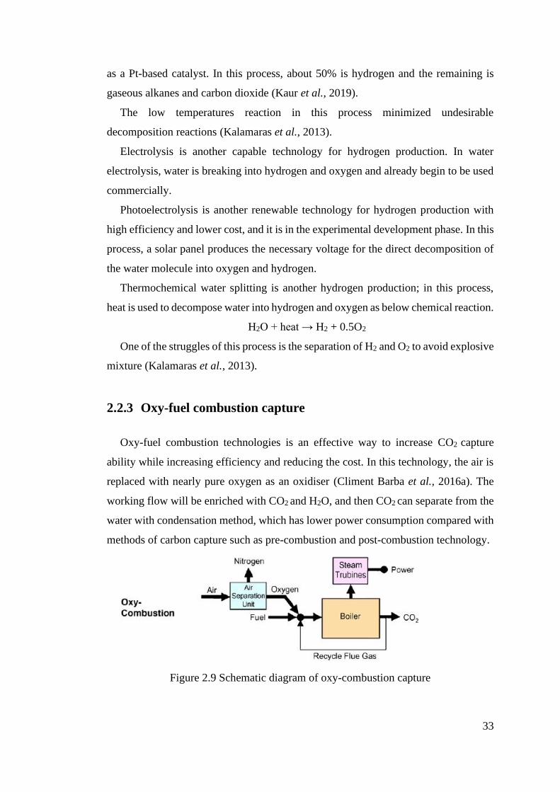
33
as a Pt-based catalyst. In this process, about 50% is hydrogen and the remaining is
gaseous alkanes and carbon dioxide (Kaur et al., 2019).
The low temperatures reaction in this process minimized undesirable
decomposition reactions (Kalamaras et al., 2013).
Electrolysis is another capable technology for hydrogen production. In water
electrolysis, water is breaking into hydrogen and oxygen and already begin to be used
commercially.
Photoelectrolysis is another renewable technology for hydrogen production with
high efficiency and lower cost, and it is in the experimental development phase. In this
process, a solar panel produces the necessary voltage for the direct decomposition of
the water molecule into oxygen and hydrogen.
Thermochemical water splitting is another hydrogen production; in this process,
heat is used to decompose water into hydrogen and oxygen as below chemical reaction.
H2O + heat → H2 + 0.5O2
One of the struggles of this process is the separation of H2 and O2 to avoid explosive
mixture (Kalamaras et al., 2013).
2.2.3 Oxy-fuel combustion capture
Oxy-fuel combustion technologies is an effective way to increase CO2 capture
ability while increasing efficiency and reducing the cost. In this technology, the air is
replaced with nearly pure oxygen as an oxidiser (Climent Barba et al., 2016a). The
working flow will be enriched with CO2 and H2O, and then CO2 can separate from the
water with condensation method, which has lower power consumption compared with
methods of carbon capture such as pre-combustion and post-combustion technology.
Figure 2.9 Schematic diagram of oxy-combustion capture
34
As shown in Figure 2.9, in the oxy-combustion process, fuel burns with pure
oxygen instead of air and the by-products of combustion are CO2 and H2O.
The high purity oxygen needs to be mixed with the recycled flue gas (RFG) before
combustion to provide a similar condition of air fired configuration for combustion
(Figueroa et al., 2008).
The CO2 from the oxy-combustion stream can be separated by condensing water
vapour. In the oxy-combustion process, the separation from CO2 is very easy, but the
problem moves to the Air Separation Unit (ASU) or other oxygen separation unit; this
part consumes a large amount of energy which results in an efficiency penalty. (Matteo
and Romano, 2019).
The oxy-combustion Adiabatic Flame Temperature (AFT) is higher than air
combustion, and the recycled flue gas is required to reduce the temperature. Also, the
furnace has higher gas emissivity because of the high concentration of CO2 and H2O.
Furthermore, the volume of the recycled gas in the oxy-combustion cycle is less
than the air combustion cycle, and the density of the recycle flue is higher; the
molecular weight of CO2 is 44, but N2 is 28 (Wall, 2007).
The fuel and pure oxygen of oxy-combustion need to be near stoichiometric for the
best adjustment. The oxy-combustion allows the smaller size of equipment without a
controller for NOx, and the byproducts are mainly CO2 and water. CO2 can be easily
separated from water by condensing and cooling process.
The oxy-combustion cycle is not entirely zero-emission, and it is near-zero-
emission. Because some part of water vapour is recycled and the extra water vapour
emits into the atmosphere, furthermore during the purification process of carbon
dioxide, the extra contaminant is emitted into the atmosphere by flue gas.
The various zero-emission cycles for both water and CO2 recirculation was
presented by Yantovsky and Degtiarev (1993), and the results indicate recirculation of
CO2 has a much higher efficiency than H2O recirculation (Manso, 2013).
2.2.3.1 Oxy-combustion classification
The oxy-combustion cycle can be categorized into five levels, as shown in Table
2.1:
1. Level 1 (Oxy-combustion oxygen production type)
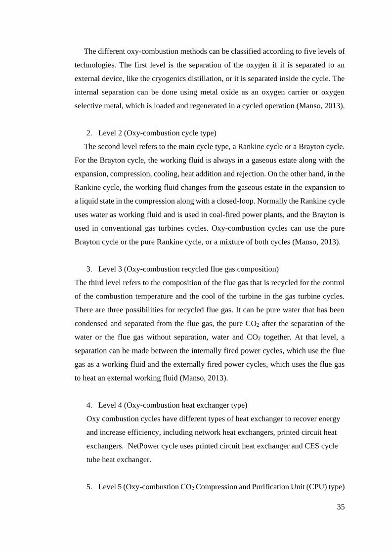
35
The different oxy-combustion methods can be classified according to five levels of
technologies. The first level is the separation of the oxygen if it is separated to an
external device, like the cryogenics distillation, or it is separated inside the cycle. The
internal separation can be done using metal oxide as an oxygen carrier or oxygen
selective metal, which is loaded and regenerated in a cycled operation (Manso, 2013).
2. Level 2 (Oxy-combustion cycle type)
The second level refers to the main cycle type, a Rankine cycle or a Brayton cycle.
For the Brayton cycle, the working fluid is always in a gaseous estate along with the
expansion, compression, cooling, heat addition and rejection. On the other hand, in the
Rankine cycle, the working fluid changes from the gaseous estate in the expansion to
a liquid state in the compression along with a closed-loop. Normally the Rankine cycle
uses water as working fluid and is used in coal-fired power plants, and the Brayton is
used in conventional gas turbines cycles. Oxy-combustion cycles can use the pure
Brayton cycle or the pure Rankine cycle, or a mixture of both cycles (Manso, 2013).
3. Level 3 (Oxy-combustion recycled flue gas composition)
The third level refers to the composition of the flue gas that is recycled for the control
of the combustion temperature and the cool of the turbine in the gas turbine cycles.
There are three possibilities for recycled flue gas. It can be pure water that has been
condensed and separated from the flue gas, the pure CO2 after the separation of the
water or the flue gas without separation, water and CO2 together. At that level, a
separation can be made between the internally fired power cycles, which use the flue
gas as a working fluid and the externally fired power cycles, which uses the flue gas
to heat an external working fluid (Manso, 2013).
4. Level 4 (Oxy-combustion heat exchanger type)
Oxy combustion cycles have different types of heat exchanger to recover energy
and increase efficiency, including network heat exchangers, printed circuit heat
exchangers. NetPower cycle uses printed circuit heat exchanger and CES cycle
tube heat exchanger.
5. Level 5 (Oxy-combustion CO2 Compression and Purification Unit (CPU) type)
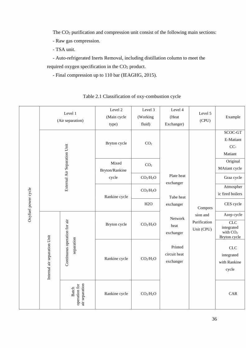
36
The CO2 purification and compression unit consist of the following main sections:
- Raw gas compression.
- TSA unit.
- Auto-refrigerated Inerts Removal, including distillation column to meet the
required oxygen specification in the CO2 product.
- Final compression up to 110 bar (IEAGHG, 2015).
Table 2.1 Classification of oxy-combustion cycle
Ox
yfu
el p
ow
er c
ycl
e
Level 1
(Air separation)
Level 2
(Main cycle
type)
Level 3
(Working
fluid)
Level 4
(Heat
Exchanger)
Level 5
(CPU) Example
Ex
tern
al A
ir S
epar
atio
n U
nit
Bryton cycle CO2
Plate heat
exchanger
Tube heat
exchanger
Network
heat
exchanger
Printed
circuit heat
exchanger
Compres
sion and
Purification
Unit (CPU)
SCOC-GT
E-Matiant
CC-
Matiant
Mixed
Bryton/Rankine
cycle
CO2 Original
MAtiant cycle
CO2/H2O Graz cycle
Rankine cycle
CO2/H2O Atmospher
ic fired boilers
H2O CES cycle
Inte
rnal
air
sep
arat
ion
Un
it
Co
nti
nu
ou
s o
per
atio
n f
or
air
sep
arat
ion
Bryton cycle CO2/H2O
Azep cycle
CLC
integrated
with CO2
Bryton cycle
Rankine cycle CO2/H2O
CLC
integrated
with Rankine
cycle
Bat
ch
op
erat
ion
fo
r
air
sep
arat
ion
Rankine cycle CO2/H2O CAR
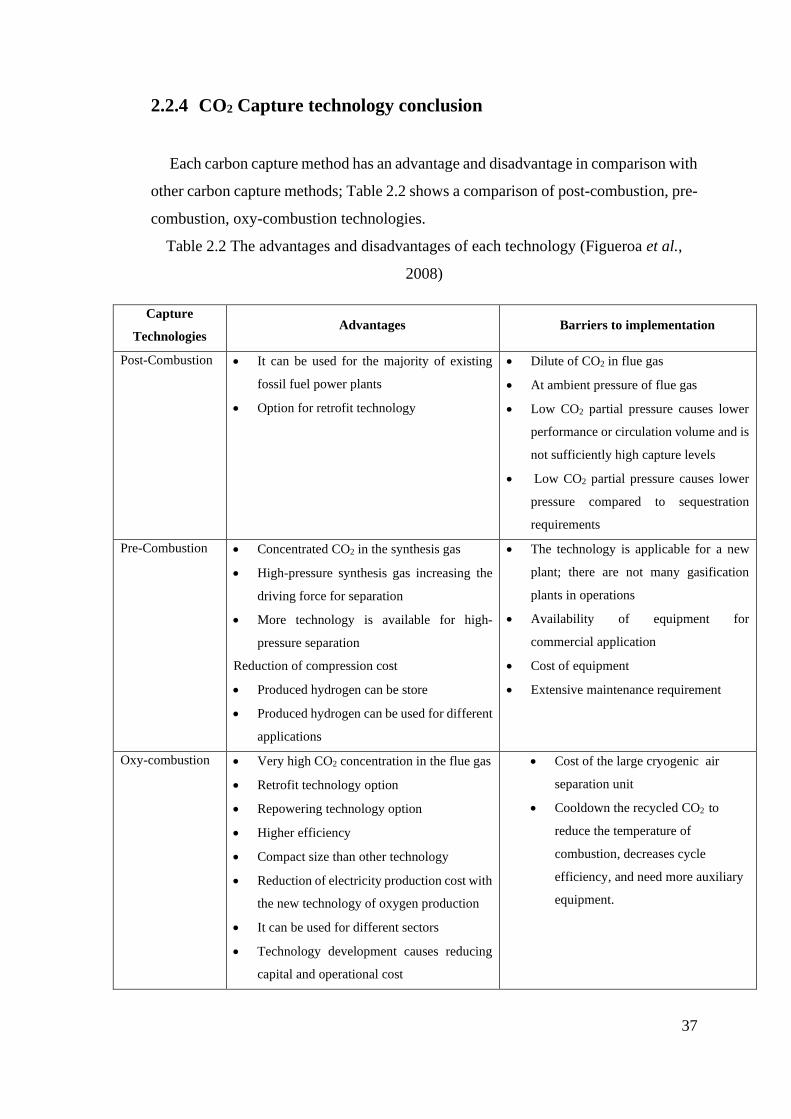
37
2.2.4 CO2 Capture technology conclusion
Each carbon capture method has an advantage and disadvantage in comparison with
other carbon capture methods; Table 2.2 shows a comparison of post-combustion, pre-
combustion, oxy-combustion technologies.
Table 2.2 The advantages and disadvantages of each technology (Figueroa et al.,
2008)
Capture
Technologies Advantages Barriers to implementation
Post-Combustion • It can be used for the majority of existing
fossil fuel power plants
• Option for retrofit technology
• Dilute of CO2 in flue gas
• At ambient pressure of flue gas
• Low CO2 partial pressure causes lower
performance or circulation volume and is
not sufficiently high capture levels
• Low CO2 partial pressure causes lower
pressure compared to sequestration
requirements
Pre-Combustion • Concentrated CO2 in the synthesis gas
• High-pressure synthesis gas increasing the
driving force for separation
• More technology is available for high-
pressure separation
Reduction of compression cost
• Produced hydrogen can be store
• Produced hydrogen can be used for different
applications
• The technology is applicable for a new
plant; there are not many gasification
plants in operations
• Availability of equipment for
commercial application
• Cost of equipment
• Extensive maintenance requirement
Oxy-combustion • Very high CO2 concentration in the flue gas
• Retrofit technology option
• Repowering technology option
• Higher efficiency
• Compact size than other technology
• Reduction of electricity production cost with
the new technology of oxygen production
• It can be used for different sectors
• Technology development causes reducing
capital and operational cost
• Cost of the large cryogenic air
separation unit
• Cooldown the recycled CO2 to
reduce the temperature of
combustion, decreases cycle
efficiency, and need more auxiliary
equipment.
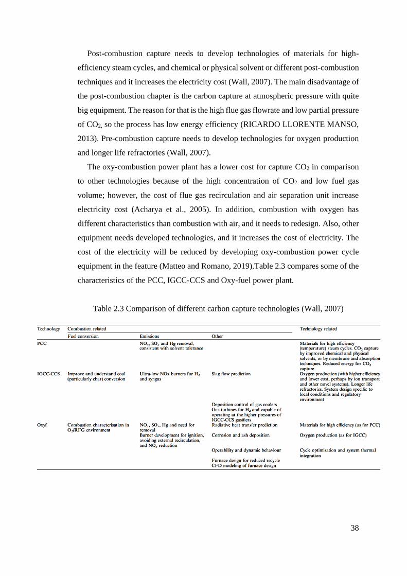
38
Post-combustion capture needs to develop technologies of materials for high-
efficiency steam cycles, and chemical or physical solvent or different post-combustion
techniques and it increases the electricity cost (Wall, 2007). The main disadvantage of
the post-combustion chapter is the carbon capture at atmospheric pressure with quite
big equipment. The reason for that is the high flue gas flowrate and low partial pressure
of CO2, so the process has low energy efficiency (RICARDO LLORENTE MANSO,
2013). Pre-combustion capture needs to develop technologies for oxygen production
and longer life refractories (Wall, 2007).
The oxy-combustion power plant has a lower cost for capture CO2 in comparison
to other technologies because of the high concentration of CO2 and low fuel gas
volume; however, the cost of flue gas recirculation and air separation unit increase
electricity cost (Acharya et al., 2005). In addition, combustion with oxygen has
different characteristics than combustion with air, and it needs to redesign. Also, other
equipment needs developed technologies, and it increases the cost of electricity. The
cost of the electricity will be reduced by developing oxy-combustion power cycle
equipment in the feature (Matteo and Romano, 2019).Table 2.3 compares some of the
characteristics of the PCC, IGCC-CCS and Oxy-fuel power plant.
Table 2.3 Comparison of different carbon capture technologies (Wall, 2007)
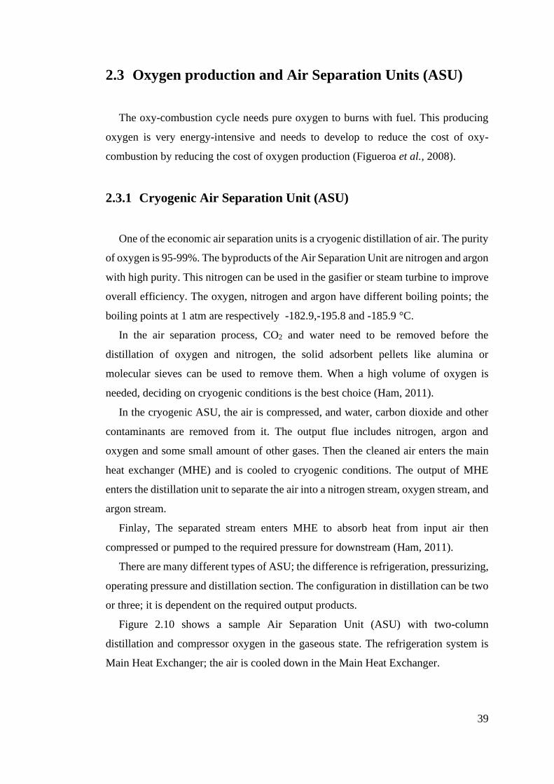
39
2.3 Oxygen production and Air Separation Units (ASU)
The oxy-combustion cycle needs pure oxygen to burns with fuel. This producing
oxygen is very energy-intensive and needs to develop to reduce the cost of oxy-
combustion by reducing the cost of oxygen production (Figueroa et al., 2008).
2.3.1 Cryogenic Air Separation Unit (ASU)
One of the economic air separation units is a cryogenic distillation of air. The purity
of oxygen is 95-99%. The byproducts of the Air Separation Unit are nitrogen and argon
with high purity. This nitrogen can be used in the gasifier or steam turbine to improve
overall efficiency. The oxygen, nitrogen and argon have different boiling points; the
boiling points at 1 atm are respectively -182.9,-195.8 and -185.9 °C.
In the air separation process, CO2 and water need to be removed before the
distillation of oxygen and nitrogen, the solid adsorbent pellets like alumina or
molecular sieves can be used to remove them. When a high volume of oxygen is
needed, deciding on cryogenic conditions is the best choice (Ham, 2011).
In the cryogenic ASU, the air is compressed, and water, carbon dioxide and other
contaminants are removed from it. The output flue includes nitrogen, argon and
oxygen and some small amount of other gases. Then the cleaned air enters the main
heat exchanger (MHE) and is cooled to cryogenic conditions. The output of MHE
enters the distillation unit to separate the air into a nitrogen stream, oxygen stream, and
argon stream.
Finlay, The separated stream enters MHE to absorb heat from input air then
compressed or pumped to the required pressure for downstream (Ham, 2011).
There are many different types of ASU; the difference is refrigeration, pressurizing,
operating pressure and distillation section. The configuration in distillation can be two
or three; it is dependent on the required output products.
Figure 2.10 shows a sample Air Separation Unit (ASU) with two-column
distillation and compressor oxygen in the gaseous state. The refrigeration system is
Main Heat Exchanger; the air is cooled down in the Main Heat Exchanger.
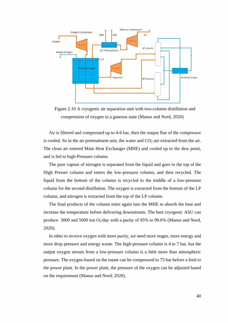
40
Figure 2.10 A cryogenic air separation unit with two-column distillation and
compression of oxygen in a gaseous state (Manso and Nord, 2020)
Air is filtered and compressed up to 4-6 bar, then the output flue of the compressor
is cooled. So in the air pretreatment unit, the water and CO2 are extracted from the air.
The clean air entered Main Heat Exchanger (MHE) and cooled up to the dew point,
and is fed to high-Pressure column.
The pure vapour of nitrogen is separated from the liquid and goes to the top of the
High Presser column and enters the low-pressure column, and then recycled. The
liquid from the bottom of the column is recycled to the middle of a low-pressure
column for the second distillation. The oxygen is extracted from the bottom of the LP
column, and nitrogen is extracted from the top of the LP column.
The final products of the column enter again into the MHE to absorb the heat and
increase the temperature before delivering downstream. The best cryogenic ASU can
produce 3000 and 5000 ton O2/day with a purity of 95% to 99.6% (Manso and Nord,
2020).
In other to receive oxygen with more purity, we need more stages, more energy and
more drop pressure and energy waste. The high-pressure column is 4 to 7 bar, but the
output oxygen stream from a low-pressure column is a little more than atmospheric
pressure. The oxygen-based on the estate can be compressed to 75 bar before a feed to
the power plant. In the power plant, the pressure of the oxygen can be adjusted based
on the requirement (Manso and Nord, 2020).
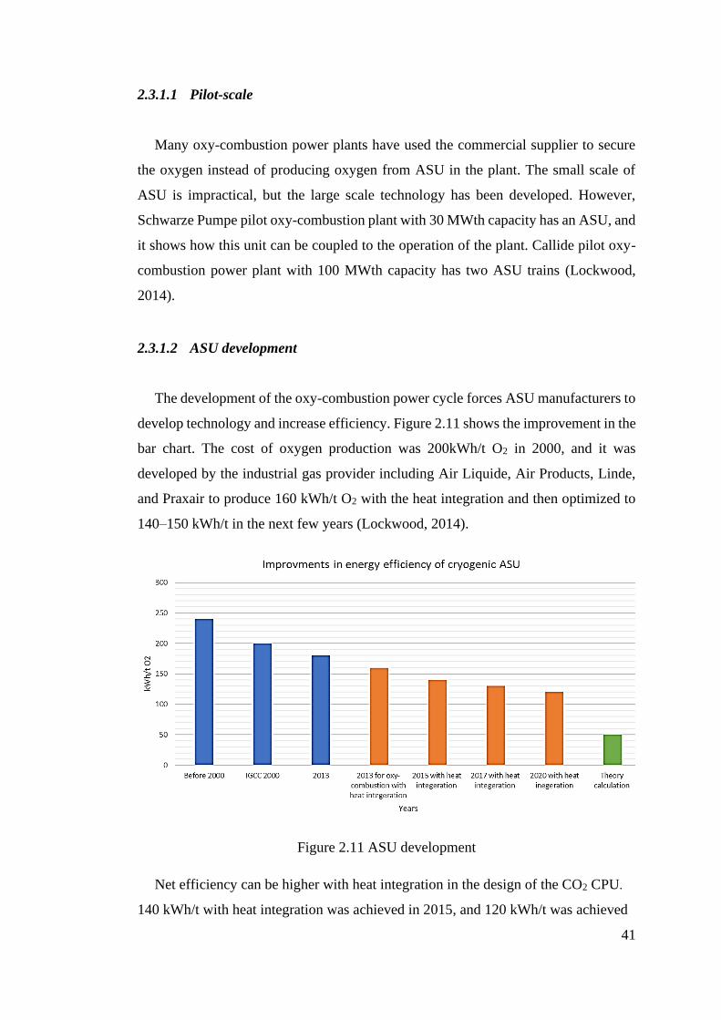
41
2.3.1.1 Pilot-scale
Many oxy-combustion power plants have used the commercial supplier to secure
the oxygen instead of producing oxygen from ASU in the plant. The small scale of
ASU is impractical, but the large scale technology has been developed. However,
Schwarze Pumpe pilot oxy-combustion plant with 30 MWth capacity has an ASU, and
it shows how this unit can be coupled to the operation of the plant. Callide pilot oxy-
combustion power plant with 100 MWth capacity has two ASU trains (Lockwood,
2014).
2.3.1.2 ASU development
The development of the oxy-combustion power cycle forces ASU manufacturers to
develop technology and increase efficiency. Figure 2.11 shows the improvement in the
bar chart. The cost of oxygen production was 200kWh/t O2 in 2000, and it was
developed by the industrial gas provider including Air Liquide, Air Products, Linde,
and Praxair to produce 160 kWh/t O2 with the heat integration and then optimized to
140–150 kWh/t in the next few years (Lockwood, 2014).
Figure 2.11 ASU development
Net efficiency can be higher with heat integration in the design of the CO2 CPU.
140 kWh/t with heat integration was achieved in 2015, and 120 kWh/t was achieved
42
with further development by 2020. The energy consumption is expected to get
reduced more and will be closer to the actual overall energy of separation. The
theoretical energy consumption of an air separation unit is calculated 50 kWh/t
(Perrin et al., 2013). It can be closer to the theoretical energy consumption by the
development and arrangement of combining compressor and waste heat recovery
(Aneke and Wang, 2015).
2.3.2 Non-cryogenic Air Separation Unit (ASU)
The cryogenic ASU consume high energy and has a negative effect on the
performance and efficiency of the power plant. There are several types of non-
cryogenic air separation units:
2.3.2.1 Adsorption
In the adsorption process, synthetic or natural materials are used to adsorb nitrogen
(Smith and Klosek, 2001). The adsorption process can be Pressure Swing Adsorption
(PSA) or Temperature Swing Operation (TSA), but most of the commercial applicants
use the PSA because longer cycle times are needed for TSA to heat up the bed of solid
particles during regeneration of sorbent (Kelly (Kailai) Thambimuthu (Australia,
2005).
2.3.2.2 Pressure Swing Adsorption (PSA)
Pressure Swing Adsorption (PSA) process is based on the adsorptive separation of
cycle character. The PSA cycles consist of two basic steps: adsorption and desorption.
In the adsorption process, the adsorbable elements are selectively removed from the
gas. In the desorption (regeneration), the elements are removed from the adsorbent so
that it is ready for the next cycle.
The main principle of the PSA process is to reduce pressure by less absorbable gas
to clean the adsorbent bed, and then it can be prepared for the next cycle (Kelly (Kailai)
Thambimuthu (Australia, 2005).
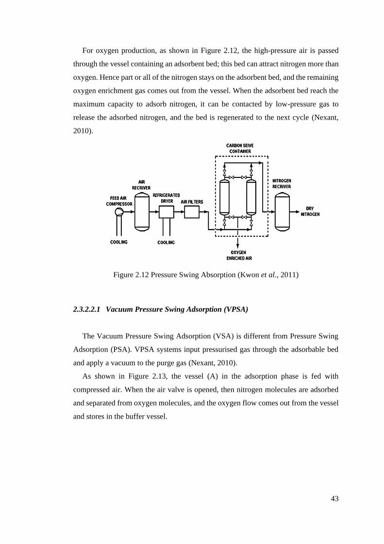
43
For oxygen production, as shown in Figure 2.12, the high-pressure air is passed
through the vessel containing an adsorbent bed; this bed can attract nitrogen more than
oxygen. Hence part or all of the nitrogen stays on the adsorbent bed, and the remaining
oxygen enrichment gas comes out from the vessel. When the adsorbent bed reach the
maximum capacity to adsorb nitrogen, it can be contacted by low-pressure gas to
release the adsorbed nitrogen, and the bed is regenerated to the next cycle (Nexant,
2010).
Figure 2.12 Pressure Swing Absorption (Kwon et al., 2011)
2.3.2.2.1 Vacuum Pressure Swing Adsorption (VPSA)
The Vacuum Pressure Swing Adsorption (VSA) is different from Pressure Swing
Adsorption (PSA). VPSA systems input pressurised gas through the adsorbable bed
and apply a vacuum to the purge gas (Nexant, 2010).
As shown in Figure 2.13, the vessel (A) in the adsorption phase is fed with
compressed air. When the air valve is opened, then nitrogen molecules are adsorbed
and separated from oxygen molecules, and the oxygen flow comes out from the vessel
and stores in the buffer vessel.
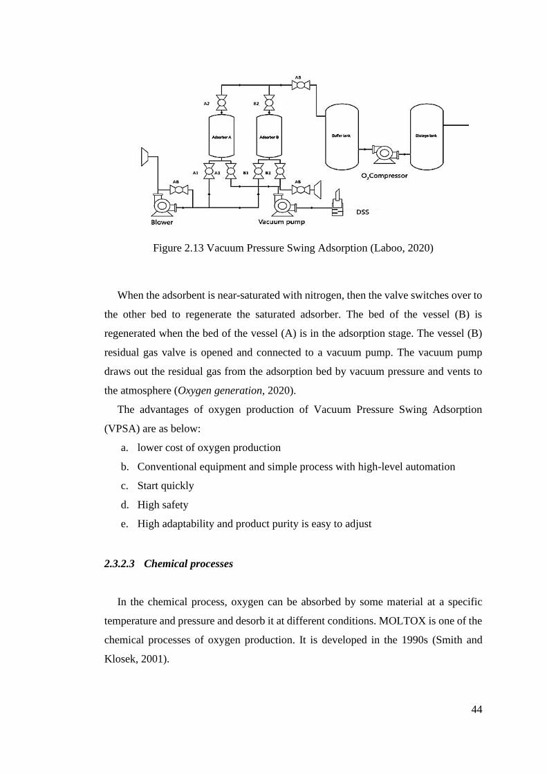
44
Figure 2.13 Vacuum Pressure Swing Adsorption (Laboo, 2020)
When the adsorbent is near-saturated with nitrogen, then the valve switches over to
the other bed to regenerate the saturated adsorber. The bed of the vessel (B) is
regenerated when the bed of the vessel (A) is in the adsorption stage. The vessel (B)
residual gas valve is opened and connected to a vacuum pump. The vacuum pump
draws out the residual gas from the adsorption bed by vacuum pressure and vents to
the atmosphere (Oxygen generation, 2020).
The advantages of oxygen production of Vacuum Pressure Swing Adsorption
(VPSA) are as below:
a. lower cost of oxygen production
b. Conventional equipment and simple process with high-level automation
c. Start quickly
d. High safety
e. High adaptability and product purity is easy to adjust
2.3.2.3 Chemical processes
In the chemical process, oxygen can be absorbed by some material at a specific
temperature and pressure and desorb it at different conditions. MOLTOX is one of the
chemical processes of oxygen production. It is developed in the 1990s (Smith and
Klosek, 2001).
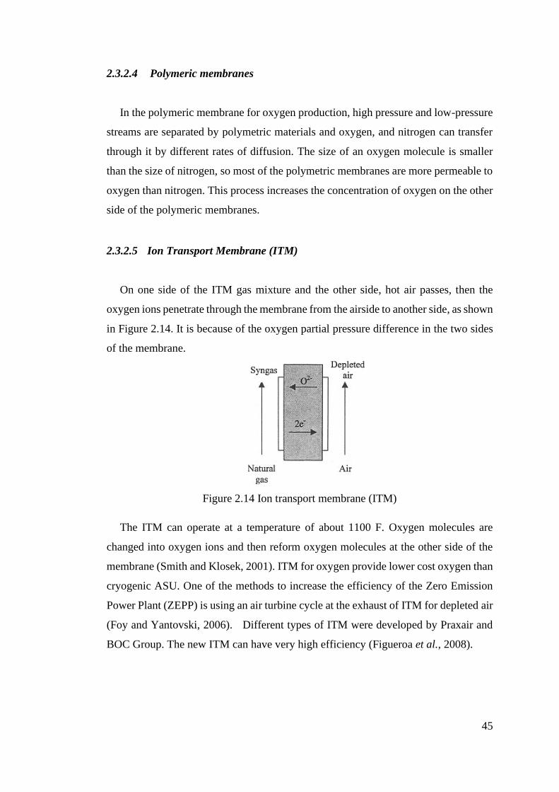
45
2.3.2.4 Polymeric membranes
In the polymeric membrane for oxygen production, high pressure and low-pressure
streams are separated by polymetric materials and oxygen, and nitrogen can transfer
through it by different rates of diffusion. The size of an oxygen molecule is smaller
than the size of nitrogen, so most of the polymetric membranes are more permeable to
oxygen than nitrogen. This process increases the concentration of oxygen on the other
side of the polymeric membranes.
2.3.2.5 Ion Transport Membrane (ITM)
On one side of the ITM gas mixture and the other side, hot air passes, then the
oxygen ions penetrate through the membrane from the airside to another side, as shown
in Figure 2.14. It is because of the oxygen partial pressure difference in the two sides
of the membrane.
Figure 2.14 Ion transport membrane (ITM)
The ITM can operate at a temperature of about 1100 F. Oxygen molecules are
changed into oxygen ions and then reform oxygen molecules at the other side of the
membrane (Smith and Klosek, 2001). ITM for oxygen provide lower cost oxygen than
cryogenic ASU. One of the methods to increase the efficiency of the Zero Emission
Power Plant (ZEPP) is using an air turbine cycle at the exhaust of ITM for depleted air
(Foy and Yantovski, 2006). Different types of ITM were developed by Praxair and
BOC Group. The new ITM can have very high efficiency (Figueroa et al., 2008).
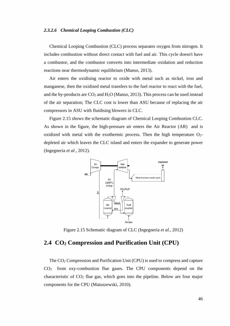
46
2.3.2.6 Chemical Looping Combustion (CLC)
Chemical Looping Combustion (CLC) process separates oxygen from nitrogen. It
includes combustion without direct contact with fuel and air. This cycle doesn't have
a combustor, and the combustor converts into intermediate oxidation and reduction
reactions near thermodynamic equilibrium (Manso, 2013).
Air enters the oxidising reactor to oxide with metal such as nickel, iron and
manganese, then the oxidised metal transfers to the fuel reactor to react with the fuel,
and the by-products are CO2 and H2O (Manso, 2013). This process can be used instead
of the air separation; The CLC cost is lower than ASU because of replacing the air
compressors in ASU with fluidising blowers in CLC.
Figure 2.15 shows the schematic diagram of Chemical Looping Combustion CLC.
As shown in the figure, the high-pressure air enters the Air Reactor (AR) and is
oxidized with metal with the exothermic process. Then the high temperature O2-
depleted air which leaves the CLC island and enters the expander to generate power
(Ingegneria et al., 2012).
Figure 2.15 Schematic diagram of CLC (Ingegneria et al., 2012)
2.4 CO2 Compression and Purification Unit (CPU)
The CO2 Compression and Purification Unit (CPU) is used to compress and capture
CO2 from oxy-combustion flue gases. The CPU components depend on the
characteristic of CO2 flue gas, which goes into the pipeline. Below are four major
components for the CPU (Matuszewski, 2010).
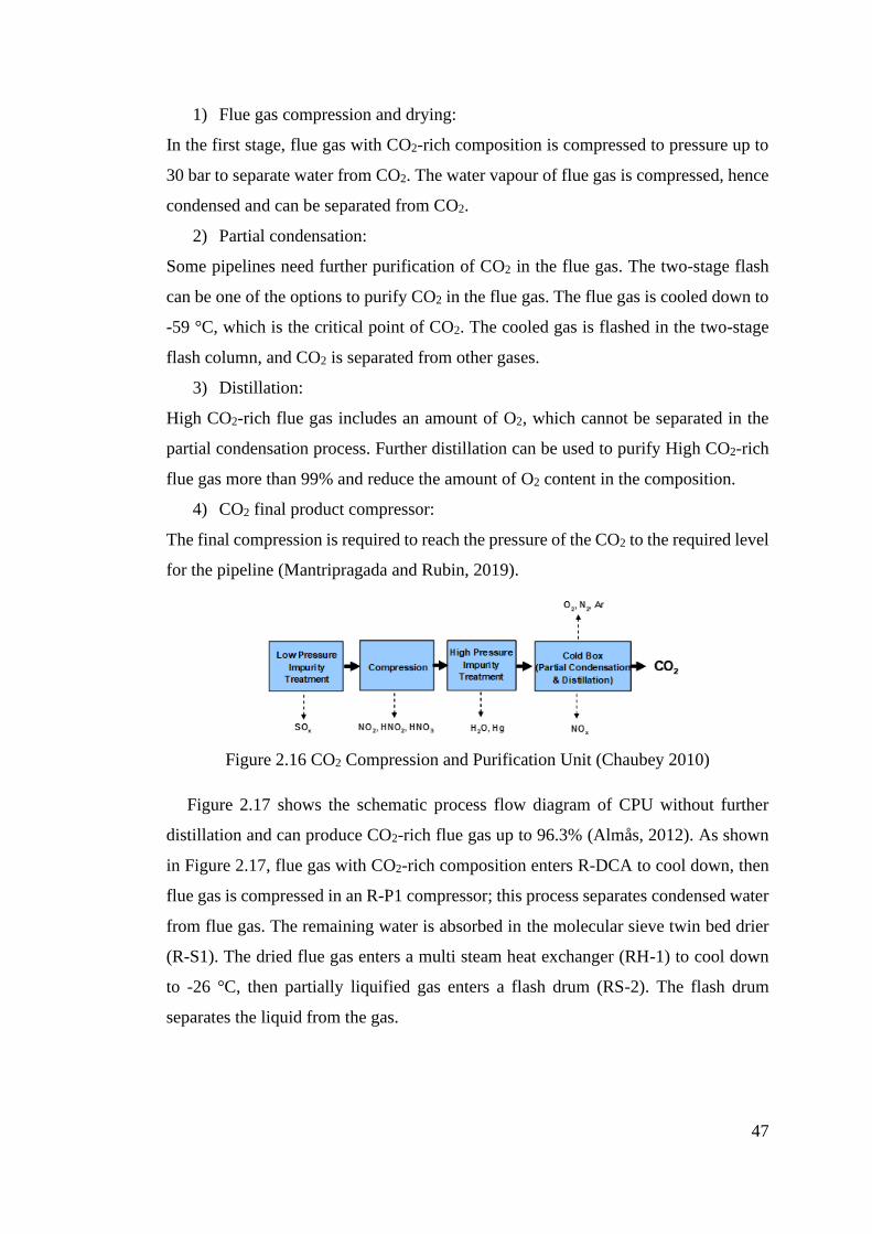
47
1) Flue gas compression and drying:
In the first stage, flue gas with CO2-rich composition is compressed to pressure up to
30 bar to separate water from CO2. The water vapour of flue gas is compressed, hence
condensed and can be separated from CO2.
2) Partial condensation:
Some pipelines need further purification of CO2 in the flue gas. The two-stage flash
can be one of the options to purify CO2 in the flue gas. The flue gas is cooled down to
-59 °C, which is the critical point of CO2. The cooled gas is flashed in the two-stage
flash column, and CO2 is separated from other gases.
3) Distillation:
High CO2-rich flue gas includes an amount of O2, which cannot be separated in the
partial condensation process. Further distillation can be used to purify High CO2-rich
flue gas more than 99% and reduce the amount of O2 content in the composition.
4) CO2 final product compressor:
The final compression is required to reach the pressure of the CO2 to the required level
for the pipeline (Mantripragada and Rubin, 2019).
Figure 2.16 CO2 Compression and Purification Unit (Chaubey 2010)
Figure 2.17 shows the schematic process flow diagram of CPU without further
distillation and can produce CO2-rich flue gas up to 96.3% (Almås, 2012). As shown
in Figure 2.17, flue gas with CO2-rich composition enters R-DCA to cool down, then
flue gas is compressed in an R-P1 compressor; this process separates condensed water
from flue gas. The remaining water is absorbed in the molecular sieve twin bed drier
(R-S1). The dried flue gas enters a multi steam heat exchanger (RH-1) to cool down
to -26 °C, then partially liquified gas enters a flash drum (RS-2). The flash drum
separates the liquid from the gas.
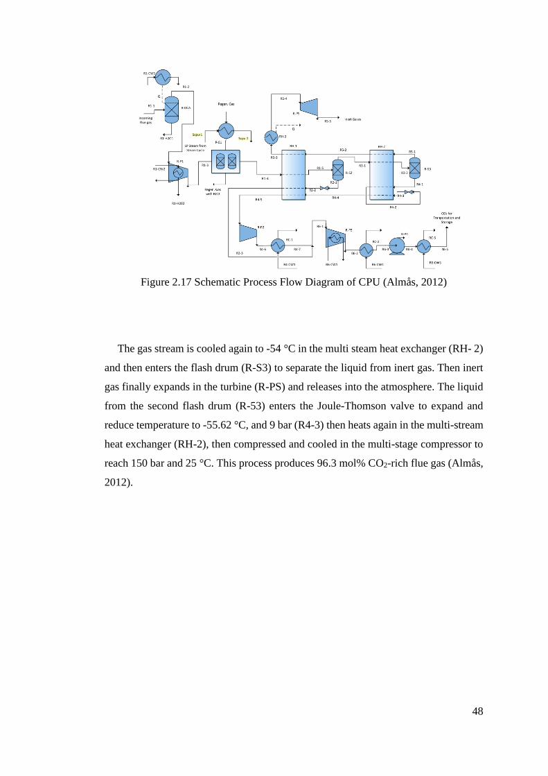
48
Figure 2.17 Schematic Process Flow Diagram of CPU (Almås, 2012)
The gas stream is cooled again to -54 °C in the multi steam heat exchanger (RH- 2)
and then enters the flash drum (R-S3) to separate the liquid from inert gas. Then inert
gas finally expands in the turbine (R-PS) and releases into the atmosphere. The liquid
from the second flash drum (R-53) enters the Joule-Thomson valve to expand and
reduce temperature to -55.62 °C, and 9 bar (R4-3) then heats again in the multi-stream
heat exchanger (RH-2), then compressed and cooled in the multi-stage compressor to
reach 150 bar and 25 °C. This process produces 96.3 mol% CO2-rich flue gas (Almås,
2012).
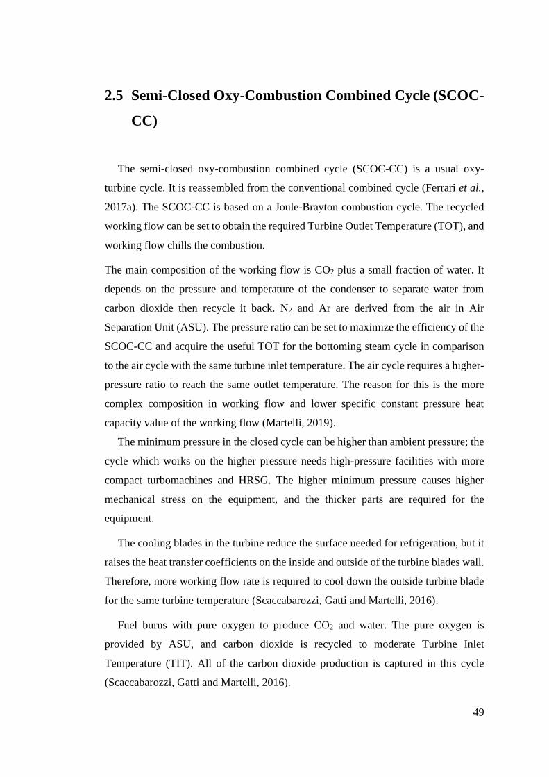
49
2.5 Semi-Closed Oxy-Combustion Combined Cycle (SCOC-
CC)
The semi-closed oxy-combustion combined cycle (SCOC-CC) is a usual oxy-
turbine cycle. It is reassembled from the conventional combined cycle (Ferrari et al.,
2017a). The SCOC-CC is based on a Joule-Brayton combustion cycle. The recycled
working flow can be set to obtain the required Turbine Outlet Temperature (TOT), and
working flow chills the combustion.
The main composition of the working flow is CO2 plus a small fraction of water. It
depends on the pressure and temperature of the condenser to separate water from
carbon dioxide then recycle it back. N2 and Ar are derived from the air in Air
Separation Unit (ASU). The pressure ratio can be set to maximize the efficiency of the
SCOC-CC and acquire the useful TOT for the bottoming steam cycle in comparison
to the air cycle with the same turbine inlet temperature. The air cycle requires a higher-
pressure ratio to reach the same outlet temperature. The reason for this is the more
complex composition in working flow and lower specific constant pressure heat
capacity value of the working flow (Martelli, 2019).
The minimum pressure in the closed cycle can be higher than ambient pressure; the
cycle which works on the higher pressure needs high-pressure facilities with more
compact turbomachines and HRSG. The higher minimum pressure causes higher
mechanical stress on the equipment, and the thicker parts are required for the
equipment.
The cooling blades in the turbine reduce the surface needed for refrigeration, but it
raises the heat transfer coefficients on the inside and outside of the turbine blades wall.
Therefore, more working flow rate is required to cool down the outside turbine blade
for the same turbine temperature (Scaccabarozzi, Gatti and Martelli, 2016).
Fuel burns with pure oxygen to produce CO2 and water. The pure oxygen is
provided by ASU, and carbon dioxide is recycled to moderate Turbine Inlet
Temperature (TIT). All of the carbon dioxide production is captured in this cycle
(Scaccabarozzi, Gatti and Martelli, 2016).
50
The gas flue of the condenser is mainly carbon dioxide. A part of carbon dioxide is
extracted for compression and transportation to a storage unit, and the remaining
carbon dioxide is recycled to the compressor (Chik, 2017). The schematic flow
diagram is shown in Figure 2.18.
Figure 2.18 Semi-closed oxy-combustion combined cycle (SCOC-CC) (Davison,
2015)
The SCOC-CC was investigated in (Dahlquist et al., 2013). It is shown that
reducing the temperature of the recycled exhaust gases as much as possible could not
increase the efficiency further, and the optimum heatsink temperature is calculated
60°C. The optimum pressure ratio is found 45 bar; however, the efficiency graph is
rather flat, and at 34 bar pressure, the efficiency only reduces 0.16 efficiency point
(Dahlquist et al., 2013)
The lower pressure ratio increases the exhaust gas temperature to 620 °C. It can
provide an excellent opportunity for easy upgrades turbine inlet temperature of the HP-
Steam turbine towards 590-600 o C. The author mentioned that the gas properties of
the oxy-combustion cycle are suitable for the bottoming cycle. The energy is more in
the high-temperature region in comparison to the conventional combined cycle;
51
therefore, HRSG has better efficiency than a standard combined cycle (Dahlquist et
al., 2013).
Sundkvist et al. (2014) also investigated two alternatives of SCOC-CC with
recirculation of the working fluid with the composition of CO2 and H2O, but the molar
fraction of the H2O is different due to different conditions for the condenser. The
SCOC-CC plant with a high temperature (98oC) configuration for recycling working
flow at the HRSG outlet has an efficiency of 41.9%. Still, the cycle with higher
temperature and low steam content has a higher efficiency of 48%. Sundkvist et al.
(2014) mentioned that the best design for SCOC-CC is an oxy-combustion cycle with
a flue gas temperature of 630°C. The efficiency would be reduced by 0.2% by
changing the flue gas temperature from 590°C to 630°C for entering HRSG, but it can
be compensated by enhancement in the turbomachinery design (Sundkvist et al.,
2014).
Chiesa and Lozza estimated 39% efficiency for integrated gasification combined
cycle (Chiesa and Lozza, 1999), but Lozza et al. estimated 46.17% efficiency (Lozza
et al., 2009). The turbine exhaust gas enters HRSG (heat recovery and steam
generator), then flue gas enters the condenser, and water is condensed and separated
from flue gas.
2.5.1 SCOC-CC technologies
One of the simplest oxy-combustion cycle configurations is SCOC-CC. But, the
working flow has a composition of CO2 and H2O; hence the SCOC-CC power plant
turbomachines are required to be designed and developed. The turbine blades and
cooling channels need to be redesigned for working flow with the properties of CO2-
rich. The development of new equipment for CO2-rich working flow is costly and
needs R&D efforts (IEAGHG, 2015).
2.6 The COOPERATE cycle
A 10 MW Zero-Emission Power Plant (ZEPP) with liquid CO2 cogeneration cycle
with 48% is introduced by Yantovski et al. (1993, 1994a) and Wall et al. (1995), and
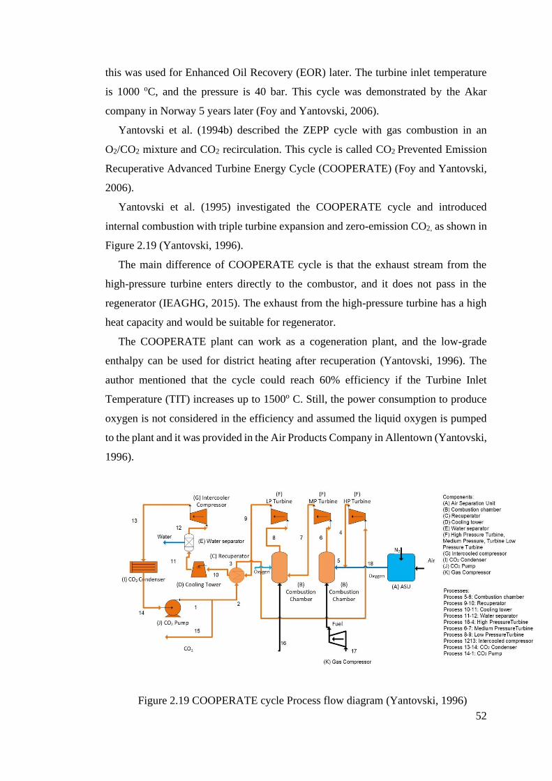
52
this was used for Enhanced Oil Recovery (EOR) later. The turbine inlet temperature
is 1000 oC, and the pressure is 40 bar. This cycle was demonstrated by the Akar
company in Norway 5 years later (Foy and Yantovski, 2006).
Yantovski et al. (1994b) described the ZEPP cycle with gas combustion in an
O2/CO2 mixture and CO2 recirculation. This cycle is called CO2 Prevented Emission
Recuperative Advanced Turbine Energy Cycle (COOPERATE) (Foy and Yantovski,
2006).
Yantovski et al. (1995) investigated the COOPERATE cycle and introduced
internal combustion with triple turbine expansion and zero-emission CO2, as shown in
Figure 2.19 (Yantovski, 1996).
The main difference of COOPERATE cycle is that the exhaust stream from the
high-pressure turbine enters directly to the combustor, and it does not pass in the
regenerator (IEAGHG, 2015). The exhaust from the high-pressure turbine has a high
heat capacity and would be suitable for regenerator.
The COOPERATE plant can work as a cogeneration plant, and the low-grade
enthalpy can be used for district heating after recuperation (Yantovski, 1996). The
author mentioned that the cycle could reach 60% efficiency if the Turbine Inlet
Temperature (TIT) increases up to 1500o C. Still, the power consumption to produce
oxygen is not considered in the efficiency and assumed the liquid oxygen is pumped
to the plant and it was provided in the Air Products Company in Allentown (Yantovski,
1996).
Figure 2.19 COOPERATE cycle Process flow diagram (Yantovski, 1996)
53
The COOPERATE cycle consists of Air Separation Unit (ASU), combustion from a
mixture of fuel, oxygen and recycled carbon dioxide, three turbines, a carbon dioxide
compressor, a condenser, and sequestration carbon dioxide. The maximum pressure
and temperature of the turbine inlet working flow are 240 bar and 1250˚C (Yantovski,
1996). The simple carbon dioxide internal combustion cycle is more suitable for
increasing efficiency due to temperature increase (Yantovski, 1996).
2.6.1 The COOPERATE cycle technologies
Recuperation is a unique feature of the COOPERATE cycle. In the ordinary cycle,
the amount of enthalpy (exergy) in the exhaust gas of the turbine is so great, and it
cannot be transferred to the recycled working flow before combustion. Thus, the
thermochemical recuperation with a catalyst is used to reform a fraction of fuel + CO2
mixture to CO + H2. This endothermic reaction takes extra enthalpy (exergy) of
exhaust gases of the turbine.
In the COOPERATE cycle, the temperature of working flow declines in the turbine
and the ordinary recuperation can be used to absorb the enthalpy (exergy) (Yantovski,
1996). The COOPERATE cycle presents 46.9% to 55.2% efficiency for TIT between
950 °C and 1350 °C and the pressure range between 4 and 240 bar (Foy and Yantovski,
2006). The pressure and temperature of turbine inlet gases in the COOPERATE cycle
were not feasible for the turbine manufacturer before, but high pressure and
temperature can be achieved in the new generation of the turbine.
Yantovski (1994c) developed a new cycle, and the cycle has 50% efficiency with
feasible turbine inlet states of 600°C at 240 bar and 1300°C at 40 bar. This feasible
cycle (COOPERATE-DEMO) is quasi-combined (Yantovski, 1996); this cycle
includes two parts:
Rankine cycle with high pressure and working flue of CO2
Brayton cycle with low pressure and working flue of CO2
The cycle is compared with a standard combined cycle by (Yantovski, 1996), as
shown in Table 2.4.
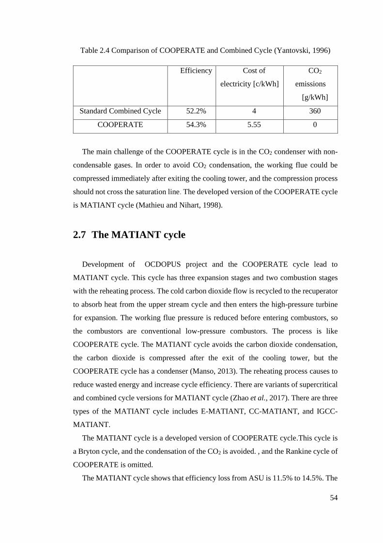
54
Table 2.4 Comparison of COOPERATE and Combined Cycle (Yantovski, 1996)
Efficiency Cost of
electricity [c/kWh]
CO2
emissions
[g/kWh]
Standard Combined Cycle 52.2% 4 360
COOPERATE 54.3% 5.55 0
The main challenge of the COOPERATE cycle is in the CO2 condenser with non-
condensable gases. In order to avoid CO2 condensation, the working flue could be
compressed immediately after exiting the cooling tower, and the compression process
should not cross the saturation line. The developed version of the COOPERATE cycle
is MATIANT cycle (Mathieu and Nihart, 1998).
2.7 The MATIANT cycle
Development of OCDOPUS project and the COOPERATE cycle lead to
MATIANT cycle. This cycle has three expansion stages and two combustion stages
with the reheating process. The cold carbon dioxide flow is recycled to the recuperator
to absorb heat from the upper stream cycle and then enters the high-pressure turbine
for expansion. The working flue pressure is reduced before entering combustors, so
the combustors are conventional low-pressure combustors. The process is like
COOPERATE cycle. The MATIANT cycle avoids the carbon dioxide condensation,
the carbon dioxide is compressed after the exit of the cooling tower, but the
COOPERATE cycle has a condenser (Manso, 2013). The reheating process causes to
reduce wasted energy and increase cycle efficiency. There are variants of supercritical
and combined cycle versions for MATIANT cycle (Zhao et al., 2017). There are three
types of the MATIANT cycle includes E-MATIANT, CC-MATIANT, and IGCC-
MATIANT.
The MATIANT cycle is a developed version of COOPERATE cycle.This cycle is
a Bryton cycle, and the condensation of the CO2 is avoided. , and the Rankine cycle of
COOPERATE is omitted.
The MATIANT cycle shows that efficiency loss from ASU is 11.5% to 14.5%. The
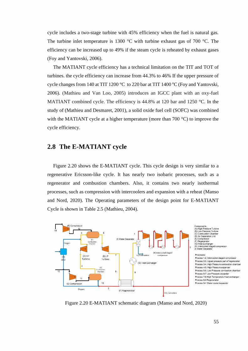
55
cycle includes a two-stage turbine with 45% efficiency when the fuel is natural gas.
The turbine inlet temperature is 1300 °C with turbine exhaust gas of 700 °C. The
efficiency can be increased up to 49% if the steam cycle is reheated by exhaust gases
(Foy and Yantovski, 2006).
The MATIANT cycle efficiency has a technical limitation on the TIT and TOT of
turbines. the cycle efficiency can increase from 44.3% to 46% If the upper pressure of
cycle changes from 140 at TIT 1200 °C to 220 bar at TIT 1400 oC (Foy and Yantovski,
2006). (Mathieu and Van Loo, 2005) introduces an IGCC plant with an oxy-fuel
MATIANT combined cycle. The efficiency is 44.8% at 120 bar and 1250 °C. In the
study of (Mathieu and Desmaret, 2001), a solid oxide fuel cell (SOFC) was combined
with the MATIANT cycle at a higher temperature (more than 700 °C) to improve the
cycle efficiency.
2.8 The E-MATIANT cycle
Figure 2.20 shows the E-MATIANT cycle. This cycle design is very similar to a
regenerative Ericsson-like cycle. It has nearly two isobaric processes, such as a
regenerator and combustion chambers. Also, it contains two nearly isothermal
processes, such as compression with intercoolers and expansion with a reheat (Manso
and Nord, 2020). The Operating parameters of the design point for E-MATIANT
Cycle is shown in Table 2.5 (Mathieu, 2004).
Figure 2.20 E-MATIANT schematic diagram (Manso and Nord, 2020)
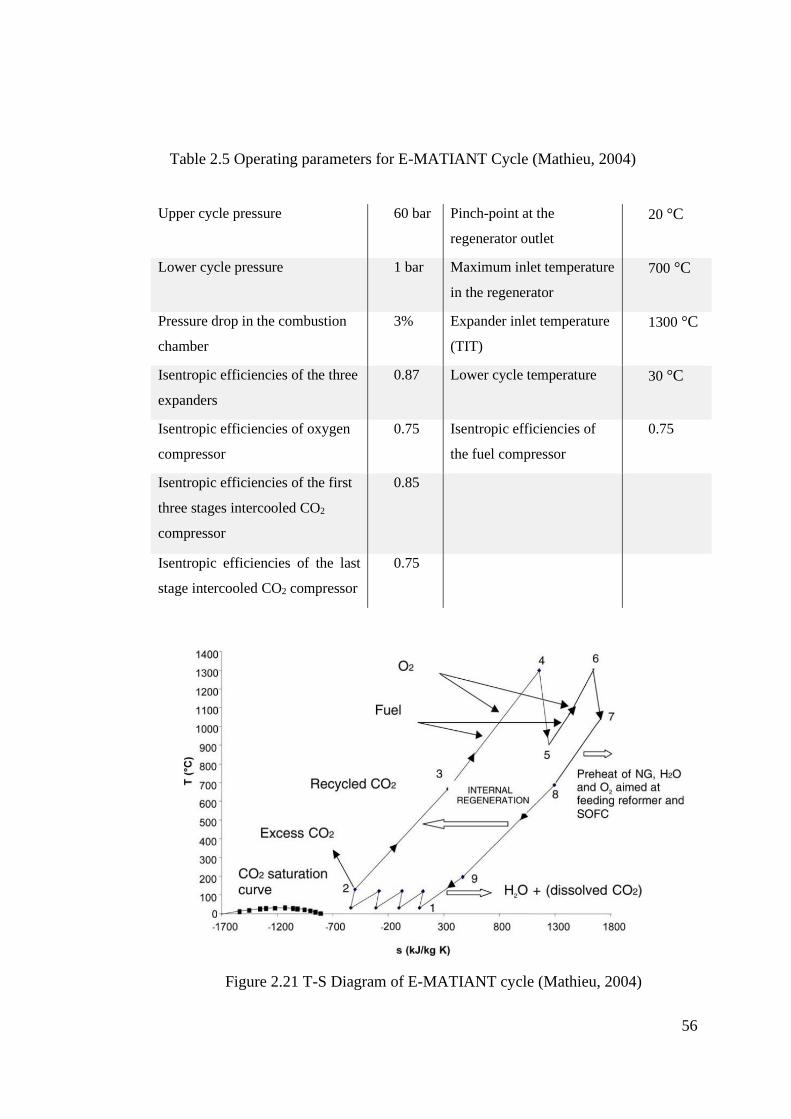
56
Table 2.5 Operating parameters for E-MATIANT Cycle (Mathieu, 2004)
Upper cycle pressure 60 bar Pinch-point at the
regenerator outlet
20 °C
Lower cycle pressure 1 bar Maximum inlet temperature
in the regenerator
700 °C
Pressure drop in the combustion
chamber
3% Expander inlet temperature
(TIT)
1300 °C
Isentropic efficiencies of the three
expanders
0.87 Lower cycle temperature 30 °C
Isentropic efficiencies of oxygen
compressor
0.75 Isentropic efficiencies of
the fuel compressor
0.75
Isentropic efficiencies of the first
three stages intercooled CO2
compressor
0.85
Isentropic efficiencies of the last
stage intercooled CO2 compressor
0.75
Figure 2.21 T-S Diagram of E-MATIANT cycle (Mathieu, 2004)
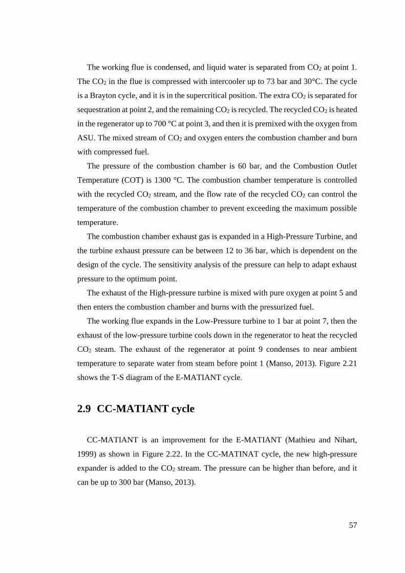
57
The working flue is condensed, and liquid water is separated from CO2 at point 1.
The CO2 in the flue is compressed with intercooler up to 73 bar and 30°C. The cycle
is a Brayton cycle, and it is in the supercritical position. The extra CO2 is separated for
sequestration at point 2, and the remaining CO2 is recycled. The recycled CO2 is heated
in the regenerator up to 700 °C at point 3, and then it is premixed with the oxygen from
ASU. The mixed stream of CO2 and oxygen enters the combustion chamber and burn
with compressed fuel.
The pressure of the combustion chamber is 60 bar, and the Combustion Outlet
Temperature (COT) is 1300 °C. The combustion chamber temperature is controlled
with the recycled CO2 stream, and the flow rate of the recycled CO2 can control the
temperature of the combustion chamber to prevent exceeding the maximum possible
temperature.
The combustion chamber exhaust gas is expanded in a High-Pressure Turbine, and
the turbine exhaust pressure can be between 12 to 36 bar, which is dependent on the
design of the cycle. The sensitivity analysis of the pressure can help to adapt exhaust
pressure to the optimum point.
The exhaust of the High-pressure turbine is mixed with pure oxygen at point 5 and
then enters the combustion chamber and burns with the pressurized fuel.
The working flue expands in the Low-Pressure turbine to 1 bar at point 7, then the
exhaust of the low-pressure turbine cools down in the regenerator to heat the recycled
CO2 steam. The exhaust of the regenerator at point 9 condenses to near ambient
temperature to separate water from steam before point 1 (Manso, 2013). Figure 2.21
shows the T-S diagram of the E-MATIANT cycle.
2.9 CC-MATIANT cycle
CC-MATIANT is an improvement for the E-MATIANT (Mathieu and Nihart,
1999) as shown in Figure 2.22. In the CC-MATINAT cycle, the new high-pressure
expander is added to the CO2 stream. The pressure can be higher than before, and it
can be up to 300 bar (Manso, 2013).
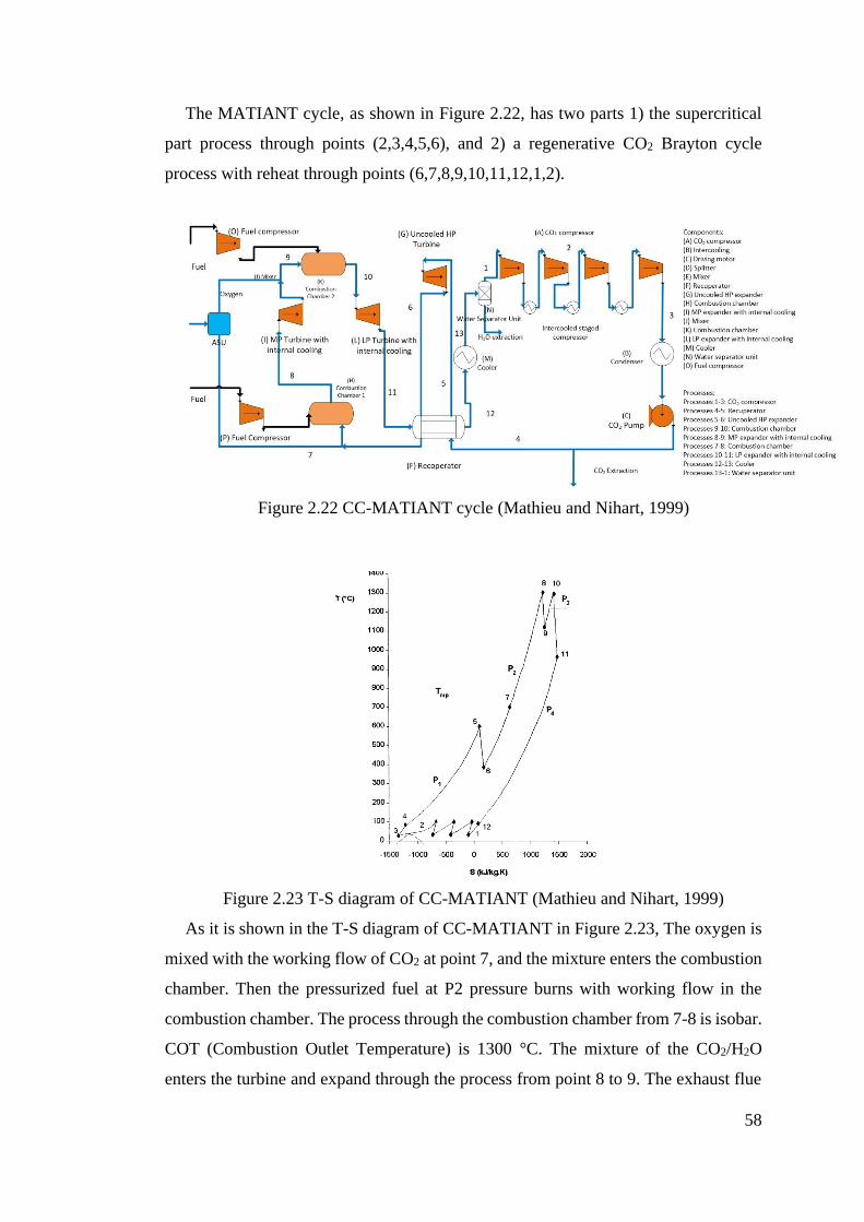
58
The MATIANT cycle, as shown in Figure 2.22, has two parts 1) the supercritical
part process through points (2,3,4,5,6), and 2) a regenerative CO2 Brayton cycle
process with reheat through points (6,7,8,9,10,11,12,1,2).
Figure 2.22 CC-MATIANT cycle (Mathieu and Nihart, 1999)
Figure 2.23 T-S diagram of CC-MATIANT (Mathieu and Nihart, 1999)
As it is shown in the T-S diagram of CC-MATIANT in Figure 2.23, The oxygen is
mixed with the working flow of CO2 at point 7, and the mixture enters the combustion
chamber. Then the pressurized fuel at P2 pressure burns with working flow in the
combustion chamber. The process through the combustion chamber from 7-8 is isobar.
COT (Combustion Outlet Temperature) is 1300 °C. The mixture of the CO2/H2O
enters the turbine and expand through the process from point 8 to 9. The exhaust flue
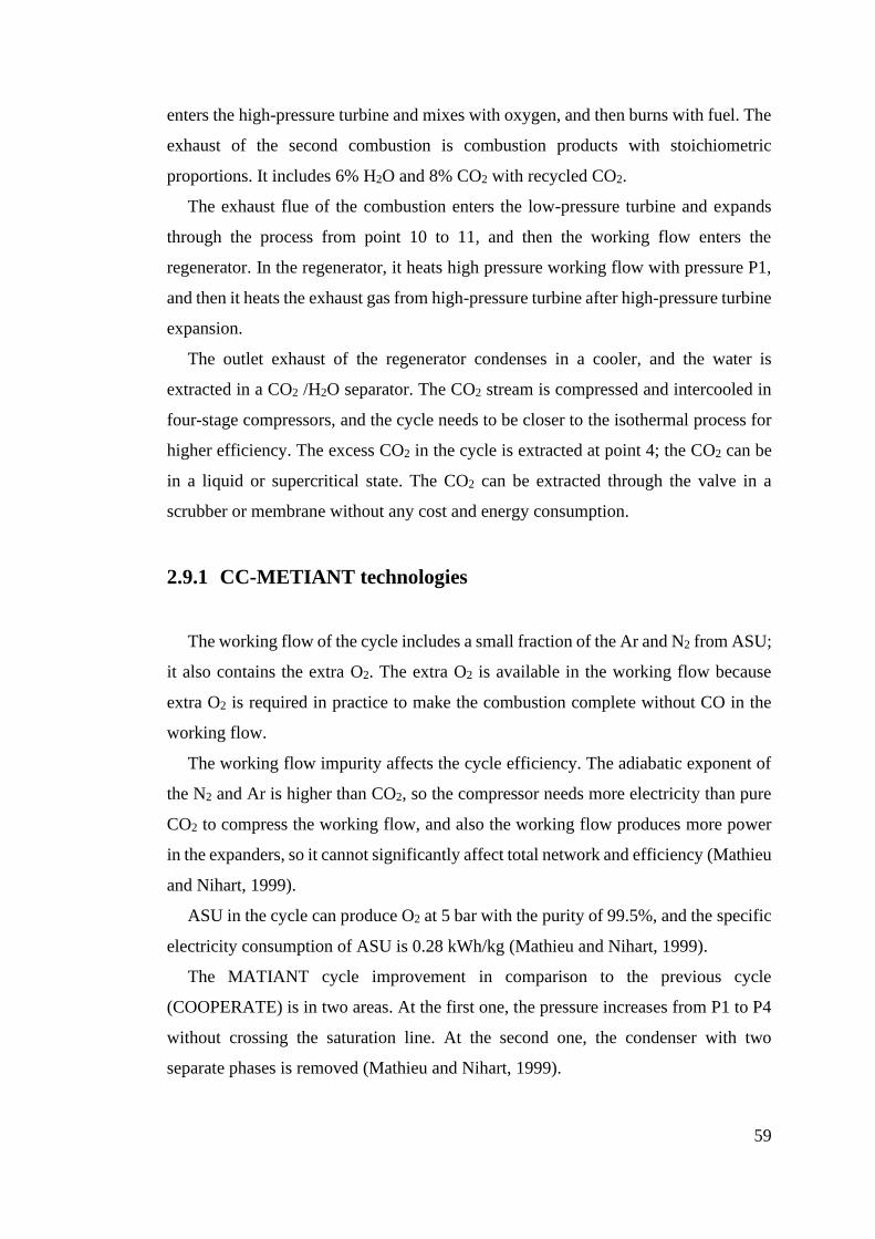
59
enters the high-pressure turbine and mixes with oxygen, and then burns with fuel. The
exhaust of the second combustion is combustion products with stoichiometric
proportions. It includes 6% H2O and 8% CO2 with recycled CO2.
The exhaust flue of the combustion enters the low-pressure turbine and expands
through the process from point 10 to 11, and then the working flow enters the
regenerator. In the regenerator, it heats high pressure working flow with pressure P1,
and then it heats the exhaust gas from high-pressure turbine after high-pressure turbine
expansion.
The outlet exhaust of the regenerator condenses in a cooler, and the water is
extracted in a CO2 /H2O separator. The CO2 stream is compressed and intercooled in
four-stage compressors, and the cycle needs to be closer to the isothermal process for
higher efficiency. The excess CO2 in the cycle is extracted at point 4; the CO2 can be
in a liquid or supercritical state. The CO2 can be extracted through the valve in a
scrubber or membrane without any cost and energy consumption.
2.9.1 CC-METIANT technologies
The working flow of the cycle includes a small fraction of the Ar and N2 from ASU;
it also contains the extra O2. The extra O2 is available in the working flow because
extra O2 is required in practice to make the combustion complete without CO in the
working flow.
The working flow impurity affects the cycle efficiency. The adiabatic exponent of
the N2 and Ar is higher than CO2, so the compressor needs more electricity than pure
CO2 to compress the working flow, and also the working flow produces more power
in the expanders, so it cannot significantly affect total network and efficiency (Mathieu
and Nihart, 1999).
ASU in the cycle can produce O2 at 5 bar with the purity of 99.5%, and the specific
electricity consumption of ASU is 0.28 kWh/kg (Mathieu and Nihart, 1999).
The MATIANT cycle improvement in comparison to the previous cycle
(COOPERATE) is in two areas. At the first one, the pressure increases from P1 to P4
without crossing the saturation line. At the second one, the condenser with two
separate phases is removed (Mathieu and Nihart, 1999).
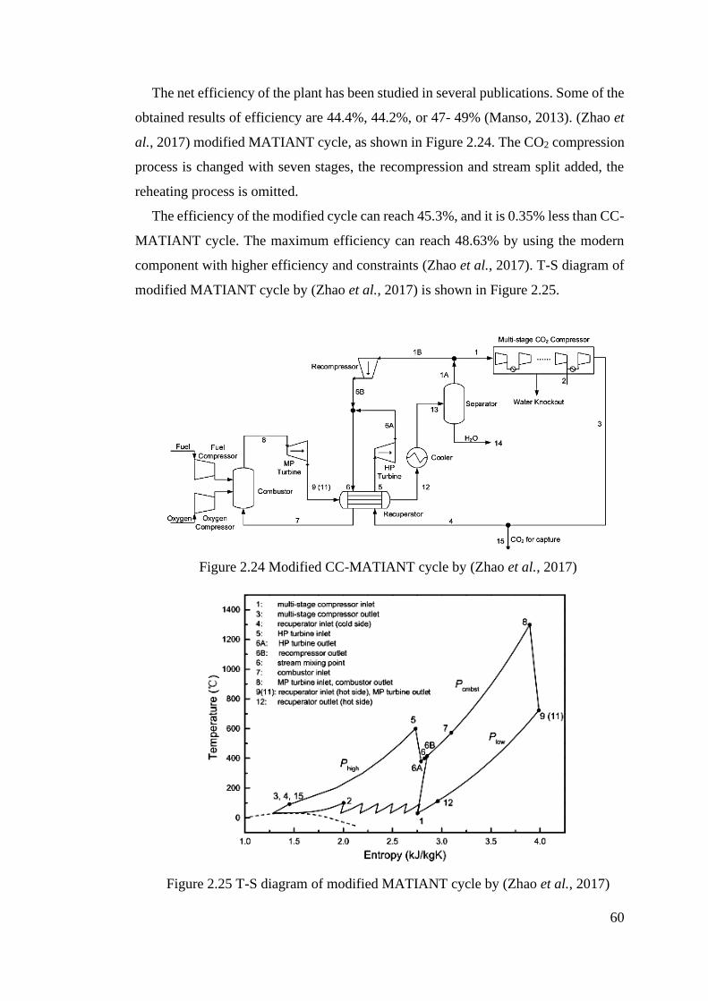
60
The net efficiency of the plant has been studied in several publications. Some of the
obtained results of efficiency are 44.4%, 44.2%, or 47- 49% (Manso, 2013). (Zhao et
al., 2017) modified MATIANT cycle, as shown in Figure 2.24. The CO2 compression
process is changed with seven stages, the recompression and stream split added, the
reheating process is omitted.
The efficiency of the modified cycle can reach 45.3%, and it is 0.35% less than CC-
MATIANT cycle. The maximum efficiency can reach 48.63% by using the modern
component with higher efficiency and constraints (Zhao et al., 2017). T-S diagram of
modified MATIANT cycle by (Zhao et al., 2017) is shown in Figure 2.25.
Figure 2.24 Modified CC-MATIANT cycle by (Zhao et al., 2017)
Figure 2.25 T-S diagram of modified MATIANT cycle by (Zhao et al., 2017)
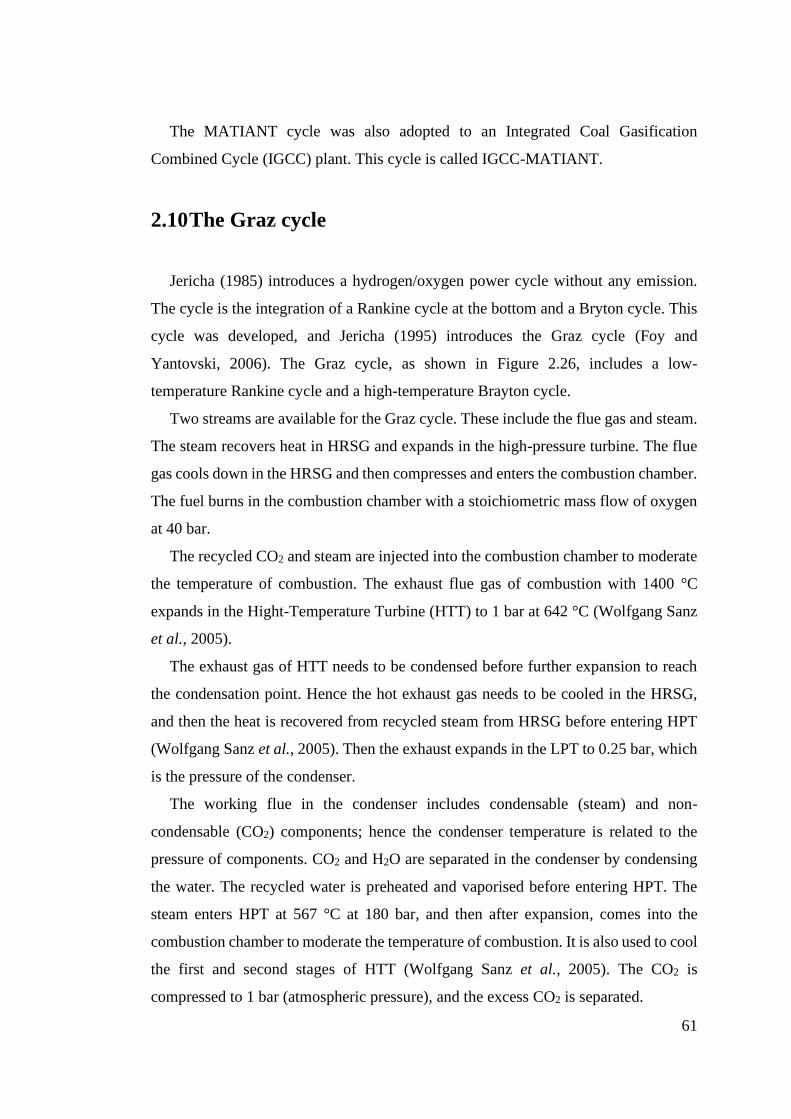
61
The MATIANT cycle was also adopted to an Integrated Coal Gasification
Combined Cycle (IGCC) plant. This cycle is called IGCC-MATIANT.
2.10 The Graz cycle
Jericha (1985) introduces a hydrogen/oxygen power cycle without any emission.
The cycle is the integration of a Rankine cycle at the bottom and a Bryton cycle. This
cycle was developed, and Jericha (1995) introduces the Graz cycle (Foy and
Yantovski, 2006). The Graz cycle, as shown in Figure 2.26, includes a low-
temperature Rankine cycle and a high-temperature Brayton cycle.
Two streams are available for the Graz cycle. These include the flue gas and steam.
The steam recovers heat in HRSG and expands in the high-pressure turbine. The flue
gas cools down in the HRSG and then compresses and enters the combustion chamber.
The fuel burns in the combustion chamber with a stoichiometric mass flow of oxygen
at 40 bar.
The recycled CO2 and steam are injected into the combustion chamber to moderate
the temperature of combustion. The exhaust flue gas of combustion with 1400 °C
expands in the Hight-Temperature Turbine (HTT) to 1 bar at 642 °C (Wolfgang Sanz
et al., 2005).
The exhaust gas of HTT needs to be condensed before further expansion to reach
the condensation point. Hence the hot exhaust gas needs to be cooled in the HRSG,
and then the heat is recovered from recycled steam from HRSG before entering HPT
(Wolfgang Sanz et al., 2005). Then the exhaust expands in the LPT to 0.25 bar, which
is the pressure of the condenser.
The working flue in the condenser includes condensable (steam) and non-
condensable (CO2) components; hence the condenser temperature is related to the
pressure of components. CO2 and H2O are separated in the condenser by condensing
the water. The recycled water is preheated and vaporised before entering HPT. The
steam enters HPT at 567 °C at 180 bar, and then after expansion, comes into the
combustion chamber to moderate the temperature of combustion. It is also used to cool
the first and second stages of HTT (Wolfgang Sanz et al., 2005). The CO2 is
compressed to 1 bar (atmospheric pressure), and the excess CO2 is separated.
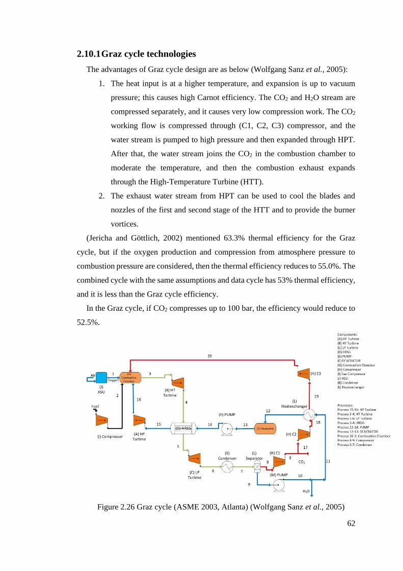
62
2.10.1 Graz cycle technologies
The advantages of Graz cycle design are as below (Wolfgang Sanz et al., 2005):
1. The heat input is at a higher temperature, and expansion is up to vacuum
pressure; this causes high Carnot efficiency. The CO2 and H2O stream are
compressed separately, and it causes very low compression work. The CO2
working flow is compressed through (C1, C2, C3) compressor, and the
water stream is pumped to high pressure and then expanded through HPT.
After that, the water stream joins the CO2 in the combustion chamber to
moderate the temperature, and then the combustion exhaust expands
through the High-Temperature Turbine (HTT).
2. The exhaust water stream from HPT can be used to cool the blades and
nozzles of the first and second stage of the HTT and to provide the burner
vortices.
(Jericha and Göttlich, 2002) mentioned 63.3% thermal efficiency for the Graz
cycle, but if the oxygen production and compression from atmosphere pressure to
combustion pressure are considered, then the thermal efficiency reduces to 55.0%. The
combined cycle with the same assumptions and data cycle has 53% thermal efficiency,
and it is less than the Graz cycle efficiency.
In the Graz cycle, if CO2 compresses up to 100 bar, the efficiency would reduce to
52.5%.
Figure 2.26 Graz cycle (ASME 2003, Atlanta) (Wolfgang Sanz et al., 2005)
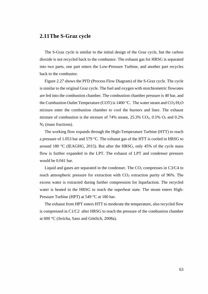
63
2.11 The S-Graz cycle
The S-Graz cycle is similar to the initial design of the Graz cycle, but the carbon
dioxide is not recycled back to the combustor. The exhaust gas for HRSG is separated
into two parts, one part enters the Low-Pressure Turbine, and another part recycles
back to the combustor.
Figure 2.27 shows the PFD (Process Flow Diagram) of the S-Graz cycle. The cycle
is similar to the original Graz cycle. The fuel and oxygen with stoichiometric flowrates
are fed into the combustion chamber. The combustion chamber pressure is 40 bar, and
the Combustion Outlet Temperature (COT) is 1400 °C. The water steam and CO2/H2O
mixture enter the combustion chamber to cool the burners and liner. The exhaust
mixture of combustion is the mixture of 74% steam, 25.3% CO2, 0.5% O2 and 0.2%
N2 (mass fractions).
The working flow expands through the High-Temperature Turbine (HTT) to reach
a pressure of 1.053 bar and 579 °C. The exhaust gas of the HTT is cooled in HRSG to
around 180 °C (IEAGHG, 2015). But after the HRSG, only 45% of the cycle mass
flow is further expanded in the LPT. The exhaust of LPT and condenser pressure
would be 0.041 bar.
Liquid and gases are separated in the condenser. The CO2 compresses in C3/C4 to
reach atmospheric pressure for extraction with CO2 extraction purity of 96%. The
excess water is extracted during further compression for liquefaction. The recycled
water is heated in the HRSG to reach the superheat state. The steam enters High-
Pressure Turbine (HPT) at 549 °C at 180 bar.
The exhaust from HPT enters HTT to moderate the temperature, also recycled flow
is compressed in C1/C2 after HRSG to reach the pressure of the combustion chamber
at 600 °C (Jericha, Sanz and Göttlich, 2008a).
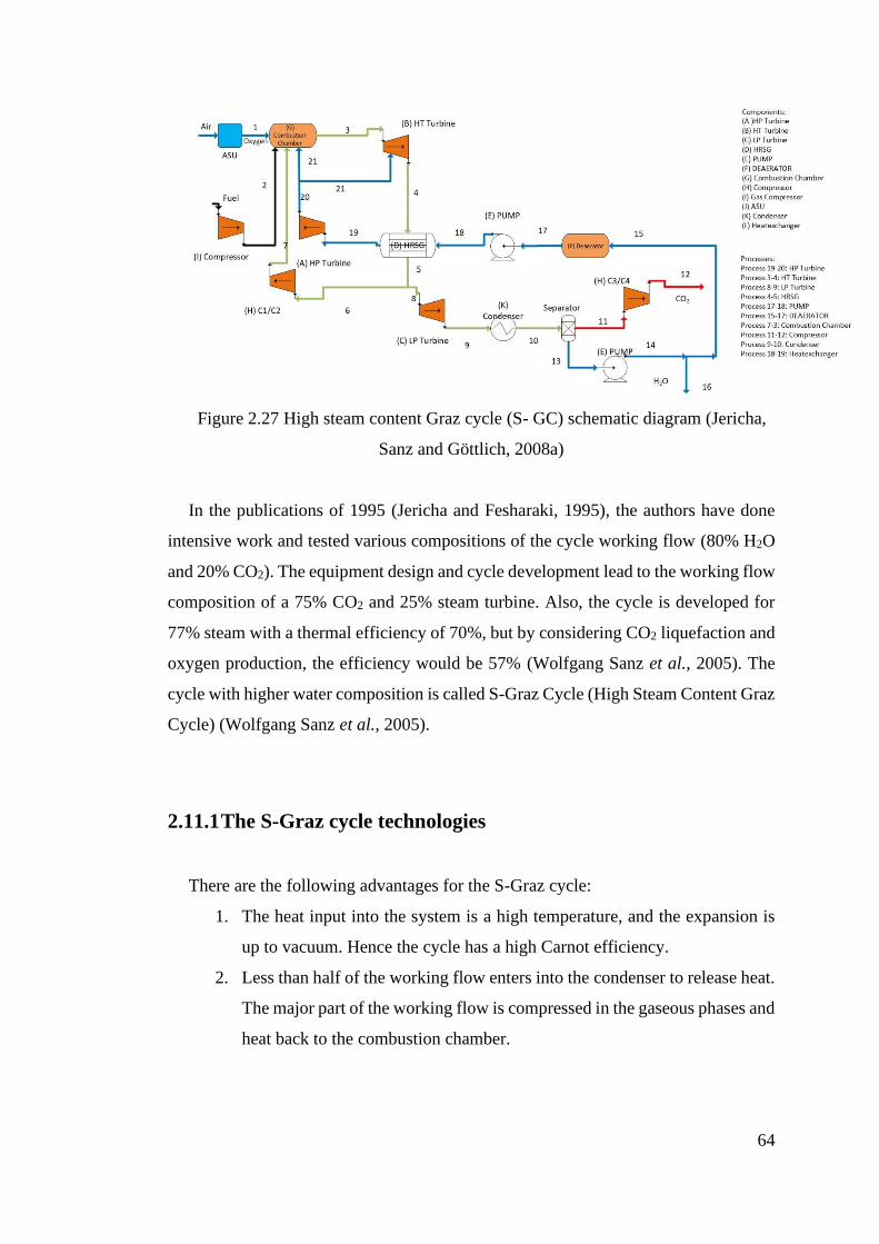
64
Figure 2.27 High steam content Graz cycle (S- GC) schematic diagram (Jericha,
Sanz and Göttlich, 2008a)
In the publications of 1995 (Jericha and Fesharaki, 1995), the authors have done
intensive work and tested various compositions of the cycle working flow (80% H2O
and 20% CO2). The equipment design and cycle development lead to the working flow
composition of a 75% CO2 and 25% steam turbine. Also, the cycle is developed for
77% steam with a thermal efficiency of 70%, but by considering CO2 liquefaction and
oxygen production, the efficiency would be 57% (Wolfgang Sanz et al., 2005). The
cycle with higher water composition is called S-Graz Cycle (High Steam Content Graz
Cycle) (Wolfgang Sanz et al., 2005).
2.11.1 The S-Graz cycle technologies
There are the following advantages for the S-Graz cycle:
1. The heat input into the system is a high temperature, and the expansion is
up to vacuum. Hence the cycle has a high Carnot efficiency.
2. Less than half of the working flow enters into the condenser to release heat.
The major part of the working flow is compressed in the gaseous phases and
heat back to the combustion chamber.
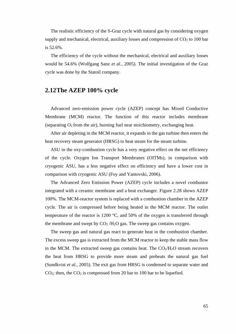
65
The realistic efficiency of the S-Graz cycle with natural gas by considering oxygen
supply and mechanical, electrical, auxiliary losses and compression of CO2 to 100 bar
is 52.6%.
The efficiency of the cycle without the mechanical, electrical and auxiliary losses
would be 54.6% (Wolfgang Sanz et al., 2005). The initial investigation of the Graz
cycle was done by the Statoil company.
2.12 The AZEP 100% cycle
Advanced zero-emission power cycle (AZEP) concept has Mixed Conductive
Membrane (MCM) reactor. The function of this reactor includes membrane
(separating O2 from the air), burning fuel near stoichiometry, exchanging heat.
After air depleting in the MCM reactor, it expands in the gas turbine then enters the
heat recovery steam generator (HRSG) to heat steam for the steam turbine.
ASU in the oxy-combustion cycle has a very negative effect on the net efficiency
of the cycle. Oxygen Ion Transport Membranes (OITMs), in comparison with
cryogenic ASU, has a less negative effect on efficiency and have a lower cost in
comparison with cryogenic ASU (Foy and Yantovski, 2006).
The Advanced Zero Emission Power (AZEP) cycle includes a novel combustor
integrated with a ceramic membrane and a heat exchanger. Figure 2.28 shows AZEP
100%. The MCM-reactor system is replaced with a combustion chamber in the AZEP
cycle. The air is compressed before being heated in the MCM reactor. The outlet
temperature of the reactor is 1200 °C, and 50% of the oxygen is transferred through
the membrane and swept by CO2 /H2O gas. The sweep gas contains oxygen.
The sweep gas and natural gas react to generate heat in the combustion chamber.
The excess sweep gas is extracted from the MCM reactor to keep the stable mass flow
in the MCM. The extracted sweep gas contains heat. The CO2/H2O stream recovers
the heat from HRSG to provide more steam and preheats the natural gas fuel
(Sundkvist et al., 2005). The exit gas from HRSG is condensed to separate water and
CO2; then, the CO2 is compressed from 20 bar to 100 bar to be liquefied.
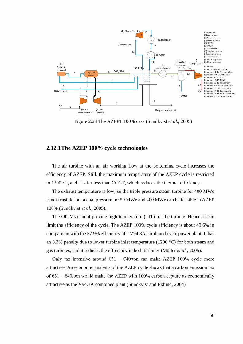
66
Figure 2.28 The AZEPT 100% case (Sundkvist et al., 2005)
2.12.1 The AZEP 100% cycle technologies
The air turbine with an air working flow at the bottoming cycle increases the
efficiency of AZEP. Still, the maximum temperature of the AZEP cycle is restricted
to 1200 °C, and it is far less than CCGT, which reduces the thermal efficiency.
The exhaust temperature is low, so the triple pressure steam turbine for 400 MWe
is not feasible, but a dual pressure for 50 MWe and 400 MWe can be feasible in AZEP
100% (Sundkvist et al., 2005).
The OITMs cannot provide high-temperature (TIT) for the turbine. Hence, it can
limit the efficiency of the cycle. The AZEP 100% cycle efficiency is about 49.6% in
comparison with the 57.9% efficiency of a V94.3A combined cycle power plant. It has
an 8.3% penalty due to lower turbine inlet temperature (1200 °C) for both steam and
gas turbines, and it reduces the efficiency in both turbines (Möller et al., 2005).
Only tax intensive around €31 – €40/ton can make AZEP 100% cycle more
attractive. An economic analysis of the AZEP cycle shows that a carbon emission tax
of €31 – €40/ton would make the AZEP with 100% carbon capture as economically
attractive as the V94.3A combined plant (Sundkvist and Eklund, 2004).
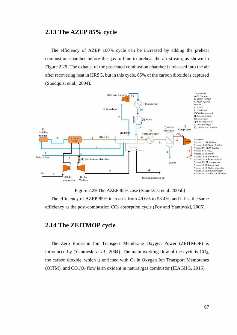
67
2.13 The AZEP 85% cycle
The efficiency of AZEP 100% cycle can be increased by adding the preheat
combustion chamber before the gas turbine to preheat the air stream, as shown in
Figure 2.29. The exhaust of the preheated combustion chamber is released into the air
after recovering heat in HRSG, but in this cycle, 85% of the carbon dioxide is captured
(Sundquist et al., 2004).
Figure 2.29 The AZEP 85% case (Sundkvist et al. 2005b)
The efficiency of AZEP 85% increases from 49.6% to 53.4%, and it has the same
efficiency as the post-combustion CO2 absorption cycle (Foy and Yantovski, 2006).
2.14 The ZEITMOP cycle
The Zero Emission Ion Transport Membrane Oxygen Power (ZEITMOP) is
introduced by (Yantovski et al., 2004). The main working flow of the cycle is CO2,
the carbon dioxide, which is enriched with O2 in Oxygen Ion Transport Membranes
(OITM), and CO2/O2 flow is an oxidant in natural/gas combustor (IEAGHG, 2015).
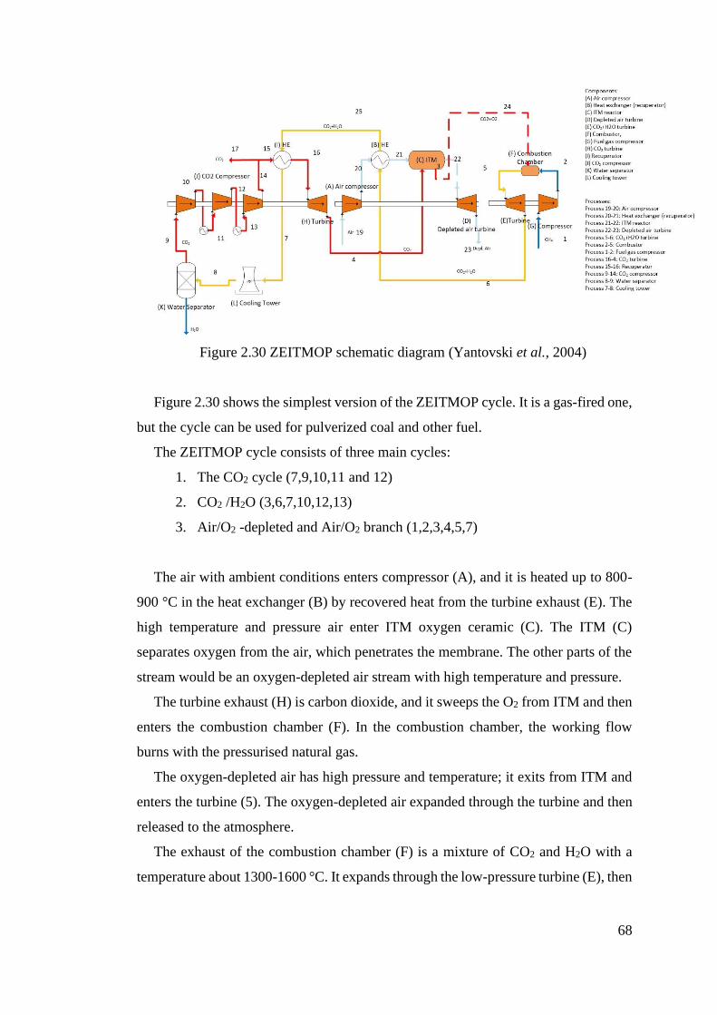
68
Figure 2.30 ZEITMOP schematic diagram (Yantovski et al., 2004)
Figure 2.30 shows the simplest version of the ZEITMOP cycle. It is a gas-fired one,
but the cycle can be used for pulverized coal and other fuel.
The ZEITMOP cycle consists of three main cycles:
1. The CO2 cycle (7,9,10,11 and 12)
2. CO2 /H2O (3,6,7,10,12,13)
3. Air/O2 -depleted and Air/O2 branch (1,2,3,4,5,7)
The air with ambient conditions enters compressor (A), and it is heated up to 800-
900 °C in the heat exchanger (B) by recovered heat from the turbine exhaust (E). The
high temperature and pressure air enter ITM oxygen ceramic (C). The ITM (C)
separates oxygen from the air, which penetrates the membrane. The other parts of the
stream would be an oxygen-depleted air stream with high temperature and pressure.
The turbine exhaust (H) is carbon dioxide, and it sweeps the O2 from ITM and then
enters the combustion chamber (F). In the combustion chamber, the working flow
burns with the pressurised natural gas.
The oxygen-depleted air has high pressure and temperature; it exits from ITM and
enters the turbine (5). The oxygen-depleted air expanded through the turbine and then
released to the atmosphere.
The exhaust of the combustion chamber (F) is a mixture of CO2 and H2O with a
temperature about 1300-1600 °C. It expands through the low-pressure turbine (E), then
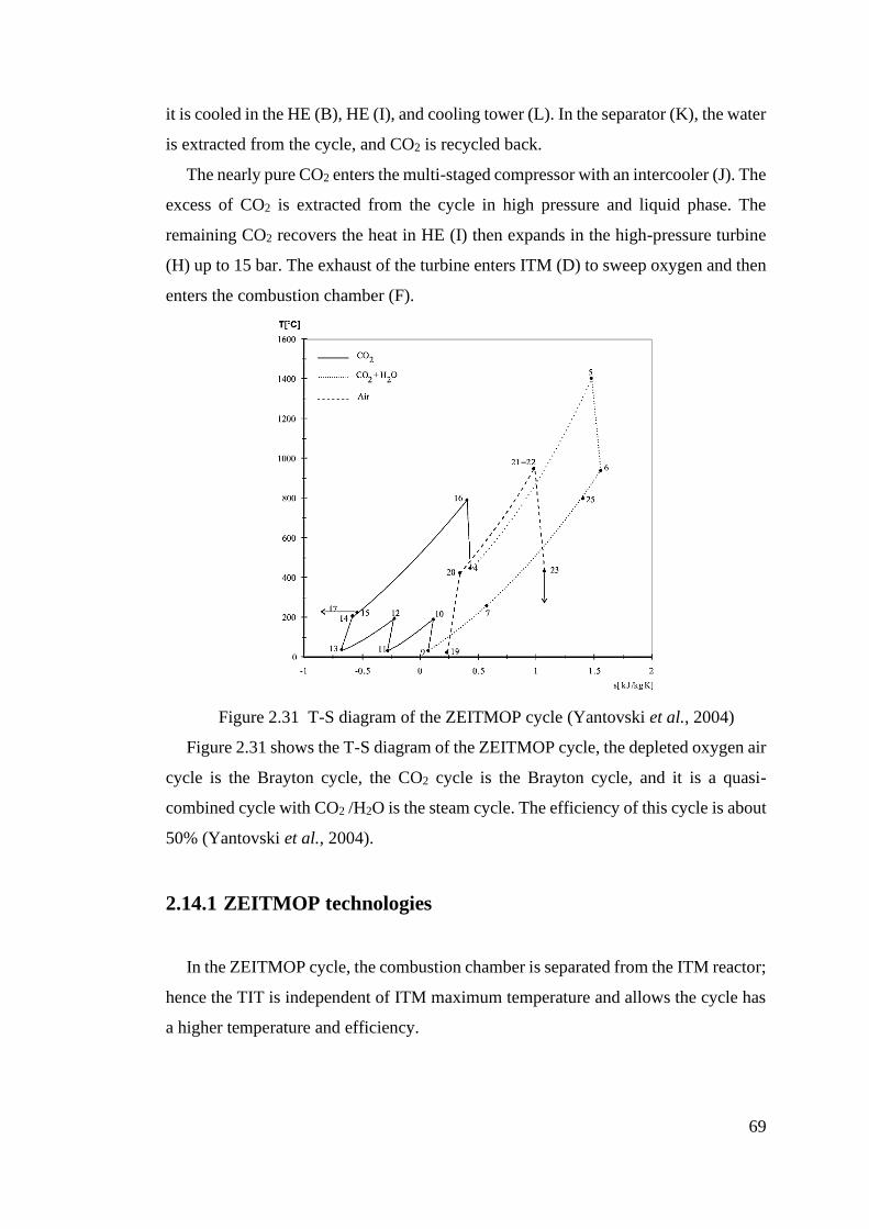
69
it is cooled in the HE (B), HE (I), and cooling tower (L). In the separator (K), the water
is extracted from the cycle, and CO2 is recycled back.
The nearly pure CO2 enters the multi-staged compressor with an intercooler (J). The
excess of CO2 is extracted from the cycle in high pressure and liquid phase. The
remaining CO2 recovers the heat in HE (I) then expands in the high-pressure turbine
(H) up to 15 bar. The exhaust of the turbine enters ITM (D) to sweep oxygen and then
enters the combustion chamber (F).
Figure 2.31 T-S diagram of the ZEITMOP cycle (Yantovski et al., 2004)
Figure 2.31 shows the T-S diagram of the ZEITMOP cycle, the depleted oxygen air
cycle is the Brayton cycle, the CO2 cycle is the Brayton cycle, and it is a quasi-
combined cycle with CO2 /H2O is the steam cycle. The efficiency of this cycle is about
50% (Yantovski et al., 2004).
2.14.1 ZEITMOP technologies
In the ZEITMOP cycle, the combustion chamber is separated from the ITM reactor;
hence the TIT is independent of ITM maximum temperature and allows the cycle has
a higher temperature and efficiency.
70
If the combustion temperature rises to 1500 °C, then the efficiency of the ZEITMOP
cycle would be 56%, and if the TIT is 1300 °C, the efficiency would be around 46%
(Foy and Yantovski, 2006).
The ZEITMOP cycle needs to be optimized, and it may reach higher efficiency
through the optimisation and can be used for all types of fossil fuel. ZEITMOP cycle
can be one of the best options for the power plant demonstration (Foy and Yantovski,
2006).
2.15 The COOLCEP-S cycle
The Cool Clean Efficient Power (COOLCEP) is used LNG as a heat sink because
the temperature of LNG is about 110K and much lower than ambient air or water
temperature. The cold exergy can be used to decrease the temperature of the heat sink
of the cycle (Zheng, 2011). This process causes an increase in the Carnot efficiency of
the cycle.
The COOLCEP power cycle is a zero CO2 emission and highly efficient cycle. The
fuel of the COOLCEP cycle is a novel Liquefied Natural Gas (LNG). The COOLCEP
power plant is a supercritical CO2 Rankine cycle. In the cold sink of the power plant,
the LNG evaporation system provides refrigeration for the CO2 subcritical evaporation
process.
Figure 2.33 shows the PFD (Process Flow Diagram) of the COOLCEP-S. In the
main cycle, the low-temperature CO2 with the temperature of -50 °C in liquid phases
(1) is pumped up to 30 bar. The output of the pump is heated through the EVA1. The
pure oxygen from ASU is compressed and mixed with the working flow of CO2 after
the pump. The mixed working flow is heated through remunerator; the heat is
recovered from the exhaust gas of the turbine. The outlet of the recuperator is injected
into the combustion chamber and burns with natural gas, then the exhaust of the
combustion chamber expands through the turbine. The turbine exhaust is cooled down
in the recuperator to recover heat for downstream. It is cooled further in LNG-cooled
heat exchanger HEX1 to condense water and separate it from CO2.
The water is separated from CO2 at the separator and extracted from the cycle (12).
The remaining working flow, which is mainly CO2, is condensed (14) by LNG
evaporation and then recycled back. The remaining non-condensed gases are extracted
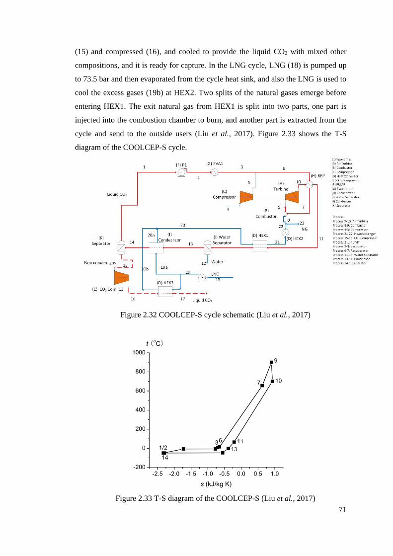
71
(15) and compressed (16), and cooled to provide the liquid CO2 with mixed other
compositions, and it is ready for capture. In the LNG cycle, LNG (18) is pumped up
to 73.5 bar and then evaporated from the cycle heat sink, and also the LNG is used to
cool the excess gases (19b) at HEX2. Two splits of the natural gases emerge before
entering HEX1. The exit natural gas from HEX1 is split into two parts, one part is
injected into the combustion chamber to burn, and another part is extracted from the
cycle and send to the outside users (Liu et al., 2017). Figure 2.33 shows the T-S
diagram of the COOLCEP-S cycle.
Figure 2.32 COOLCEP-S cycle schematic (Liu et al., 2017)
Figure 2.33 T-S diagram of the COOLCEP-S (Liu et al., 2017)
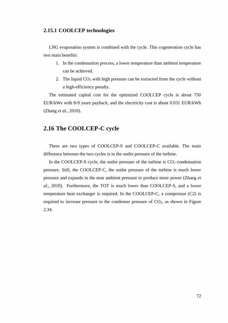
72
2.15.1 COOLCEP technologies
LNG evaporation system is combined with the cycle. This cogeneration cycle has
two main benefits:
1. In the condensation process, a lower temperature than ambient temperature
can be achieved.
2. The liquid CO2 with high pressure can be extracted from the cycle without
a high-efficiency penalty.
The estimated capital cost for the optimized COOLCEP cycle is about 750
EUR/kWe with 8-9 years payback, and the electricity cost is about 0.031 EUR/kWh
(Zhang et al., 2010).
2.16 The COOLCEP-C cycle
There are two types of COOLCEP-S and COOLCEP-C available. The main
difference between the two cycles is in the outlet pressure of the turbine.
In the COOLCEP-S cycle, the outlet pressure of the turbine is CO2 condensation
pressure. Still, the COOLCEP-C, the outlet pressure of the turbine is much lower
pressure and expands in the near ambient pressure to produce more power (Zhang et
al., 2010). Furthermore, the TOT is much lower than COOLCEP-S, and a lower
temperature heat exchanger is required. In the COOLCEP-C, a compressor (C2) is
required to increase pressure to the condenser pressure of CO2, as shown in Figure
2.34.
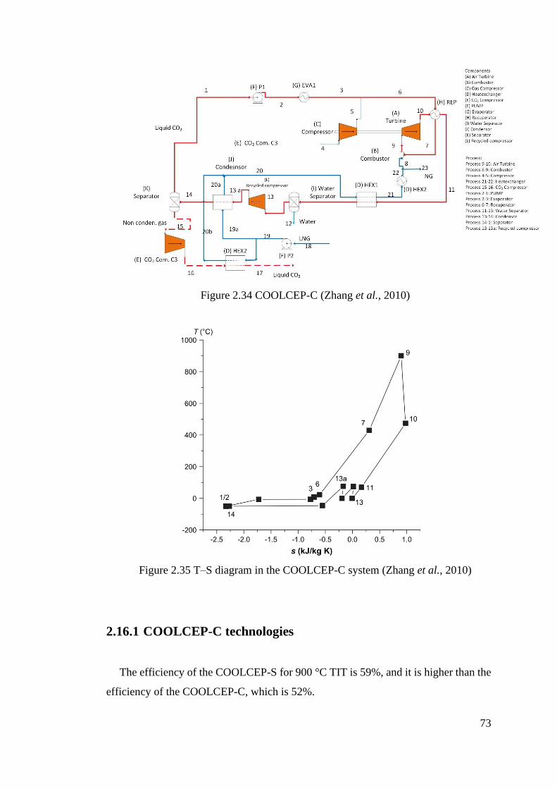
73
Figure 2.34 COOLCEP-C (Zhang et al., 2010)
Figure 2.35 T–S diagram in the COOLCEP-C system (Zhang et al., 2010)
2.16.1 COOLCEP-C technologies
The efficiency of the COOLCEP-S for 900 °C TIT is 59%, and it is higher than the
efficiency of the COOLCEP-C, which is 52%.
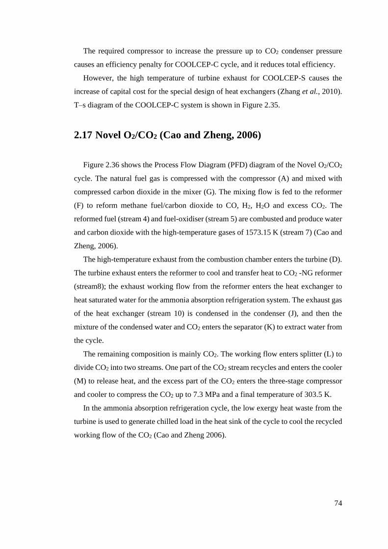
74
The required compressor to increase the pressure up to CO2 condenser pressure
causes an efficiency penalty for COOLCEP-C cycle, and it reduces total efficiency.
However, the high temperature of turbine exhaust for COOLCEP-S causes the
increase of capital cost for the special design of heat exchangers (Zhang et al., 2010).
T–s diagram of the COOLCEP-C system is shown in Figure 2.35.
2.17 Novel O2/CO2 (Cao and Zheng, 2006)
Figure 2.36 shows the Process Flow Diagram (PFD) diagram of the Novel O2/CO2
cycle. The natural fuel gas is compressed with the compressor (A) and mixed with
compressed carbon dioxide in the mixer (G). The mixing flow is fed to the reformer
(F) to reform methane fuel/carbon dioxide to CO, H2, H2O and excess CO2. The
reformed fuel (stream 4) and fuel-oxidiser (stream 5) are combusted and produce water
and carbon dioxide with the high-temperature gases of 1573.15 K (stream 7) (Cao and
Zheng, 2006).
The high-temperature exhaust from the combustion chamber enters the turbine (D).
The turbine exhaust enters the reformer to cool and transfer heat to CO2 -NG reformer
(stream8); the exhaust working flow from the reformer enters the heat exchanger to
heat saturated water for the ammonia absorption refrigeration system. The exhaust gas
of the heat exchanger (stream 10) is condensed in the condenser (J), and then the
mixture of the condensed water and CO2 enters the separator (K) to extract water from
the cycle.
The remaining composition is mainly CO2. The working flow enters splitter (L) to
divide CO2 into two streams. One part of the CO2 stream recycles and enters the cooler
(M) to release heat, and the excess part of the CO2 enters the three-stage compressor
and cooler to compress the CO2 up to 7.3 MPa and a final temperature of 303.5 K.
In the ammonia absorption refrigeration cycle, the low exergy heat waste from the
turbine is used to generate chilled load in the heat sink of the cycle to cool the recycled
working flow of the CO2 (Cao and Zheng 2006).
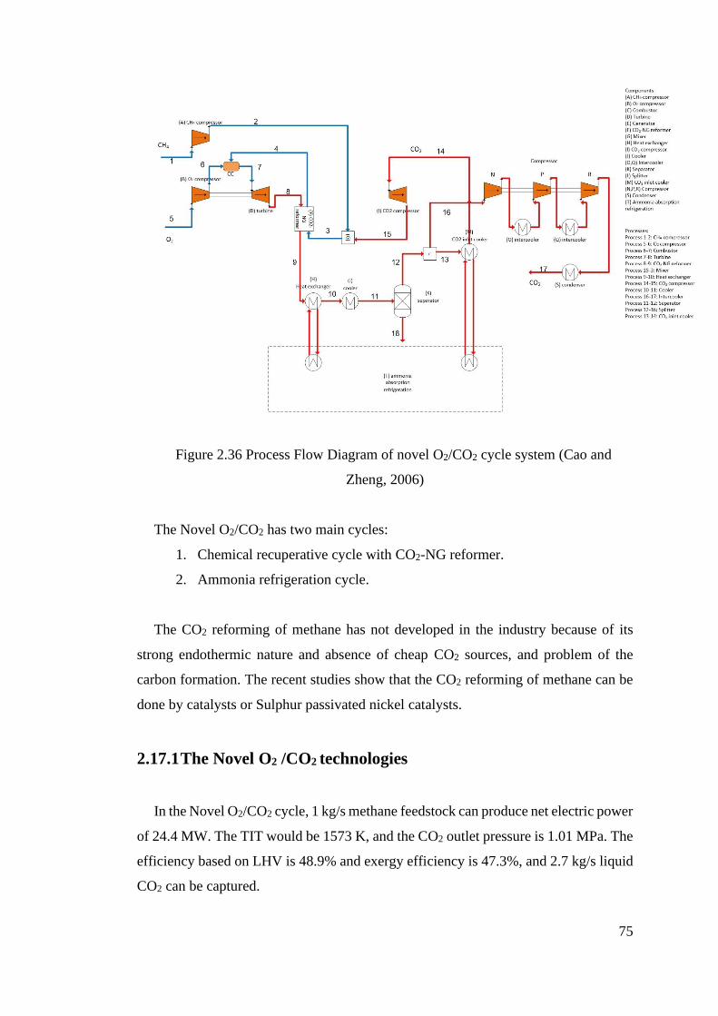
75
Figure 2.36 Process Flow Diagram of novel O2/CO2 cycle system (Cao and
Zheng, 2006)
The Novel O2/CO2 has two main cycles:
1. Chemical recuperative cycle with CO2-NG reformer.
2. Ammonia refrigeration cycle.
The CO2 reforming of methane has not developed in the industry because of its
strong endothermic nature and absence of cheap CO2 sources, and problem of the
carbon formation. The recent studies show that the CO2 reforming of methane can be
done by catalysts or Sulphur passivated nickel catalysts.
2.17.1 The Novel O2 /CO2 technologies
In the Novel O2/CO2 cycle, 1 kg/s methane feedstock can produce net electric power
of 24.4 MW. The TIT would be 1573 K, and the CO2 outlet pressure is 1.01 MPa. The
efficiency based on LHV is 48.9% and exergy efficiency is 47.3%, and 2.7 kg/s liquid
CO2 can be captured.
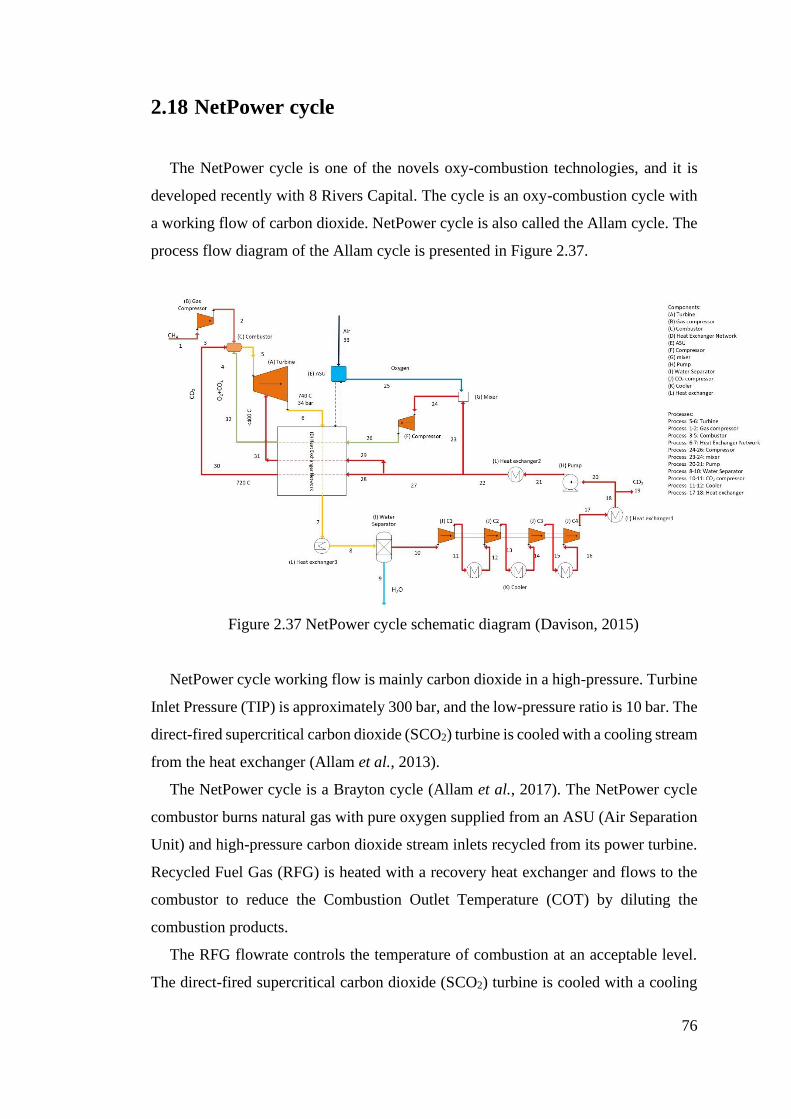
76
2.18 NetPower cycle
The NetPower cycle is one of the novels oxy-combustion technologies, and it is
developed recently with 8 Rivers Capital. The cycle is an oxy-combustion cycle with
a working flow of carbon dioxide. NetPower cycle is also called the Allam cycle. The
process flow diagram of the Allam cycle is presented in Figure 2.37.
Figure 2.37 NetPower cycle schematic diagram (Davison, 2015)
NetPower cycle working flow is mainly carbon dioxide in a high-pressure. Turbine
Inlet Pressure (TIP) is approximately 300 bar, and the low-pressure ratio is 10 bar. The
direct-fired supercritical carbon dioxide (SCO2) turbine is cooled with a cooling stream
from the heat exchanger (Allam et al., 2013).
The NetPower cycle is a Brayton cycle (Allam et al., 2017). The NetPower cycle
combustor burns natural gas with pure oxygen supplied from an ASU (Air Separation
Unit) and high-pressure carbon dioxide stream inlets recycled from its power turbine.
Recycled Fuel Gas (RFG) is heated with a recovery heat exchanger and flows to the
combustor to reduce the Combustion Outlet Temperature (COT) by diluting the
combustion products.
The RFG flowrate controls the temperature of combustion at an acceptable level.
The direct-fired supercritical carbon dioxide (SCO2) turbine is cooled with a cooling
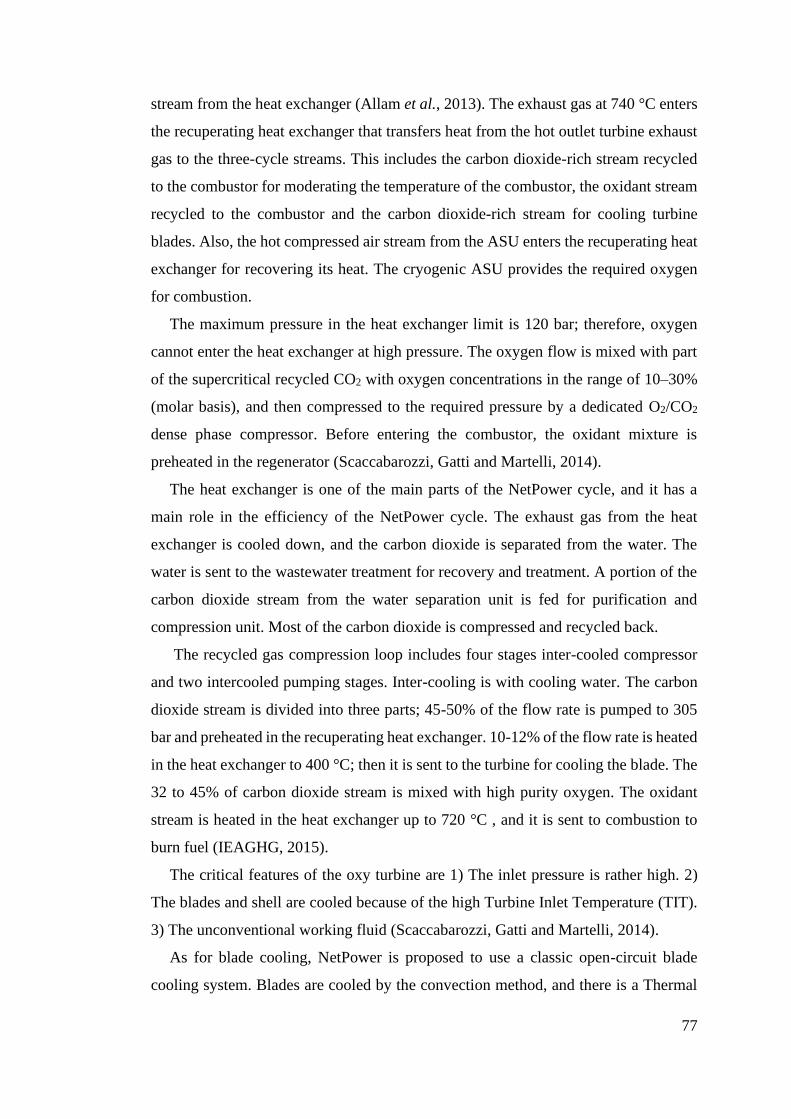
77
stream from the heat exchanger (Allam et al., 2013). The exhaust gas at 740 °C enters
the recuperating heat exchanger that transfers heat from the hot outlet turbine exhaust
gas to the three-cycle streams. This includes the carbon dioxide-rich stream recycled
to the combustor for moderating the temperature of the combustor, the oxidant stream
recycled to the combustor and the carbon dioxide-rich stream for cooling turbine
blades. Also, the hot compressed air stream from the ASU enters the recuperating heat
exchanger for recovering its heat. The cryogenic ASU provides the required oxygen
for combustion.
The maximum pressure in the heat exchanger limit is 120 bar; therefore, oxygen
cannot enter the heat exchanger at high pressure. The oxygen flow is mixed with part
of the supercritical recycled CO2 with oxygen concentrations in the range of 10–30%
(molar basis), and then compressed to the required pressure by a dedicated O2/CO2
dense phase compressor. Before entering the combustor, the oxidant mixture is
preheated in the regenerator (Scaccabarozzi, Gatti and Martelli, 2014).
The heat exchanger is one of the main parts of the NetPower cycle, and it has a
main role in the efficiency of the NetPower cycle. The exhaust gas from the heat
exchanger is cooled down, and the carbon dioxide is separated from the water. The
water is sent to the wastewater treatment for recovery and treatment. A portion of the
carbon dioxide stream from the water separation unit is fed for purification and
compression unit. Most of the carbon dioxide is compressed and recycled back.
The recycled gas compression loop includes four stages inter-cooled compressor
and two intercooled pumping stages. Inter-cooling is with cooling water. The carbon
dioxide stream is divided into three parts; 45-50% of the flow rate is pumped to 305
bar and preheated in the recuperating heat exchanger. 10-12% of the flow rate is heated
in the heat exchanger to 400 °C; then it is sent to the turbine for cooling the blade. The
32 to 45% of carbon dioxide stream is mixed with high purity oxygen. The oxidant
stream is heated in the heat exchanger up to 720 °C , and it is sent to combustion to
burn fuel (IEAGHG, 2015).
The critical features of the oxy turbine are 1) The inlet pressure is rather high. 2)
The blades and shell are cooled because of the high Turbine Inlet Temperature (TIT).
3) The unconventional working fluid (Scaccabarozzi, Gatti and Martelli, 2014).
As for blade cooling, NetPower is proposed to use a classic open-circuit blade
cooling system. Blades are cooled by the convection method, and there is a Thermal
78
Barrier Coating (TBC) on the blades to protect them from high temperature and
corrosion. The heat transfer coefficient of CO2 is significantly high; therefore, film
cooling for the gas turbine is appropriate (Allam et al., 2013).
One of the limitations of the Allam cycle is ASU operational parameters along with
equipment constraints (Fernandes et al., 2019); the cost of technology is another
challenge of the NetPower. The NetPower equipment is required to redesign to
overcome the limitations by using high pressure, highly recuperative, oxyfuel,
supercritical CO2 cycle (Power and Systems, 2017).
2.18.1 NetPower demonstration
The Allam cycle is one of the successful cycles, which is reached to the
demonstration phase, 8 Rivers capital developed the Allam cycle for nearly seven
years. NetPower company, which is owned by eight rivers, Exelon Generation and
CB& I, developed the natural gas Allam cycle.
50 MW natural gas demonstration plant was completed in LA Porte, Texas, the
USA by NetPower, and the first fire of plant had achieved success in May 2018. The
plant is fully operational of the cycle with start-up, shut down, emergency operation,
load following and partial load operation. 8 Rivers developed and designed the plant
process and EPC (Engineering, Procurement and Construction) of the plant performed
by CBI, and Exelon operates the plant.
The plant includes a novel supercritical CO2 combustion Turbine, which is
developed by Toshiba on a commercial scale. The 50 MWth demonstration plant was
developed and simulated by 8 Rivers. All sizing and capacity are the actual design
size.
Heatric company designed and fabricated the advanced high pressure printed circuit
heat exchanger, which is one of the main parts of the power plant. The electrical output
of the power plant is 25 MWe from 50MWth, and the power plant was built over a
two-year period. 300 MWth NetPower plant is planned to demonstrate in 2022. The
plant is based on natural gas (Flin, 2019).
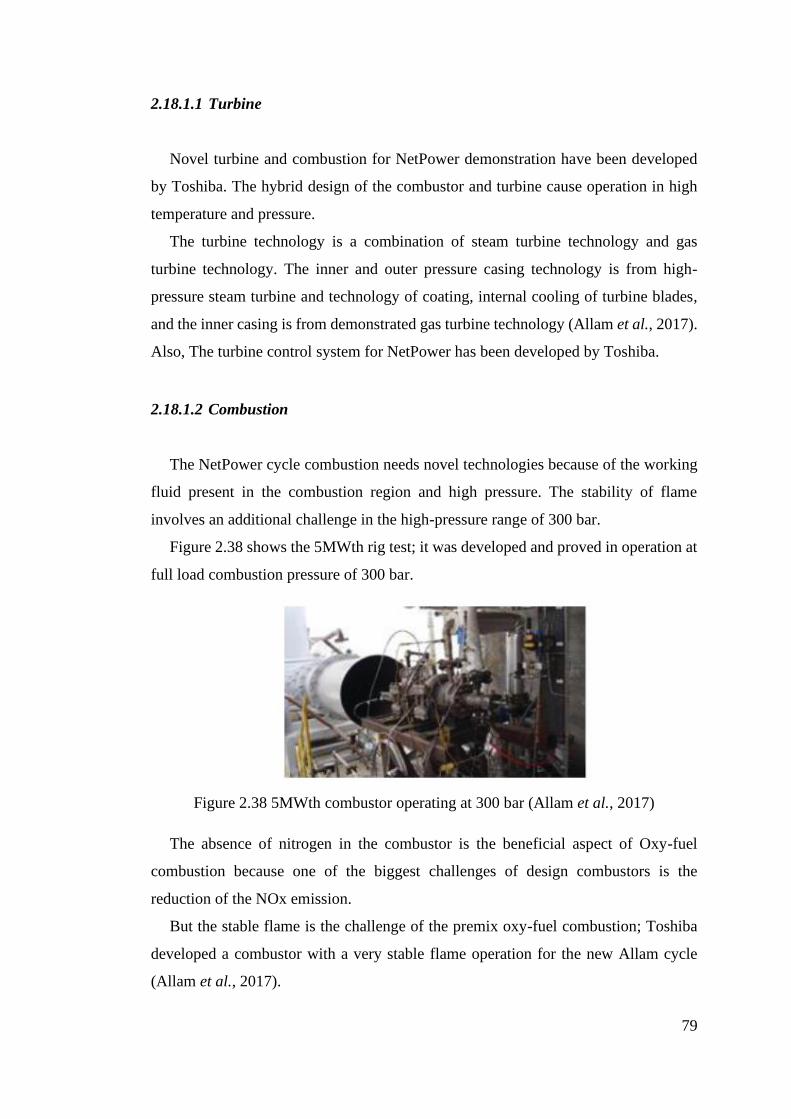
79
2.18.1.1 Turbine
Novel turbine and combustion for NetPower demonstration have been developed
by Toshiba. The hybrid design of the combustor and turbine cause operation in high
temperature and pressure.
The turbine technology is a combination of steam turbine technology and gas
turbine technology. The inner and outer pressure casing technology is from high-
pressure steam turbine and technology of coating, internal cooling of turbine blades,
and the inner casing is from demonstrated gas turbine technology (Allam et al., 2017).
Also, The turbine control system for NetPower has been developed by Toshiba.
2.18.1.2 Combustion
The NetPower cycle combustion needs novel technologies because of the working
fluid present in the combustion region and high pressure. The stability of flame
involves an additional challenge in the high-pressure range of 300 bar.
Figure 2.38 shows the 5MWth rig test; it was developed and proved in operation at
full load combustion pressure of 300 bar.
Figure 2.38 5MWth combustor operating at 300 bar (Allam et al., 2017)
The absence of nitrogen in the combustor is the beneficial aspect of Oxy-fuel
combustion because one of the biggest challenges of design combustors is the
reduction of the NOx emission.
But the stable flame is the challenge of the premix oxy-fuel combustion; Toshiba
developed a combustor with a very stable flame operation for the new Allam cycle
(Allam et al., 2017).
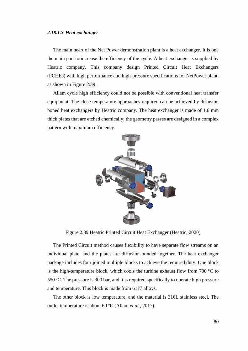
80
2.18.1.3 Heat exchanger
The main heart of the Net Power demonstration plant is a heat exchanger. It is one
the main part to increase the efficiency of the cycle. A heat exchanger is supplied by
Heatric company. This company design Printed Circuit Heat Exchangers
(PCHEs) with high performance and high-pressure specifications for NetPower plant,
as shown in Figure 2.39.
Allam cycle high efficiency could not be possible with conventional heat transfer
equipment. The close temperature approaches required can be achieved by diffusion
boned heat exchangers by Heatric company. The heat exchanger is made of 1.6 mm
thick plates that are etched chemically; the geometry passes are designed in a complex
pattern with maximum efficiency.
Figure 2.39 Heatric Printed Circuit Heat Exchanger (Heatric, 2020)
The Printed Circuit method causes flexibility to have separate flow streams on an
individual plate, and the plates are diffusion bonded together. The heat exchanger
package includes four joined multiple blocks to achieve the required duty. One block
is the high-temperature block, which cools the turbine exhaust flow from 700 °C to
550 °C. The pressure is 300 bar, and it is required specifically to operate high pressure
and temperature. This block is made from 6177 alloys.
The other block is low temperature, and the material is 316L stainless steel. The
outlet temperature is about 60 °C (Allam et al., 2017).
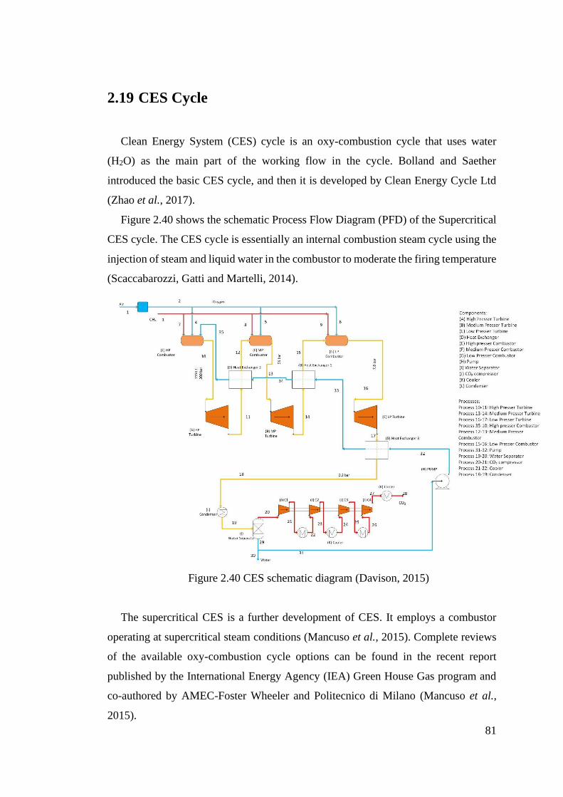
81
2.19 CES Cycle
Clean Energy System (CES) cycle is an oxy-combustion cycle that uses water
(H2O) as the main part of the working flow in the cycle. Bolland and Saether
introduced the basic CES cycle, and then it is developed by Clean Energy Cycle Ltd
(Zhao et al., 2017).
Figure 2.40 shows the schematic Process Flow Diagram (PFD) of the Supercritical
CES cycle. The CES cycle is essentially an internal combustion steam cycle using the
injection of steam and liquid water in the combustor to moderate the firing temperature
(Scaccabarozzi, Gatti and Martelli, 2014).
Figure 2.40 CES schematic diagram (Davison, 2015)
The supercritical CES is a further development of CES. It employs a combustor
operating at supercritical steam conditions (Mancuso et al., 2015). Complete reviews
of the available oxy-combustion cycle options can be found in the recent report
published by the International Energy Agency (IEA) Green House Gas program and
co-authored by AMEC-Foster Wheeler and Politecnico di Milano (Mancuso et al.,
2015).
82
Supercritical CES Power cycle includes three turbines, compressor, and combustor.
Natural gas is divided three-part, 23% of natural gas compressed to 310 bar is fed to
the HP combustor, and 33% is fed to the MP, and the remaining is fed to the LP
combustor. Fuel gases are preheated before feeding combustors. Pure oxygen is
produced from ASU and compressed for HP combustor, and remaining are preheated
before feeding to LP and MP combustor.
Exhaust gas from HPT is separated into two parts; one part is fed to the MP
combustor and the remaining is directly fed to MPT for cooling the turbine to control
blade metal temperature. Also, Exhaust gas from MPT is separated into two parts, one
part is fed to the LP combustor, and the remaining is directly fed to LPT for the cooling
turbine to control blade metal temperature.
There are four main units for supercritical CES cycle with carbon capture
(IEAGHG, 2015): 1) Power Island 2) CO2 purification and compression 3) Air
Separation Unit (ASU) 4) Utility and of Site.
2.19.1 The CES technologies
During last decade, CES cycle efficiency is improved from 20% to 30% (50 MW
J79/Deploy 2nd Generation Deploy), 35,45% (200 MW 3th Generation
CES/Siemens/TriGen OFT900) and 50% (400MW CES/Siemens/TriGen) (Business
and October, 2012). Clean Energy System (CES) demonstrates the project for testing,
analyzing and design of modified Siemens SGT-900 gas turbine with the company of
Siemens Energy and Florida Turbine Technology (FTT) and the US. Department of
Energy (DoE) funding program (Climent Barba et al., 2016b).
2.19.2 CES demonstration
The CES (Clean Energy System) power plant has main technical issues for
designing the steam turbine with an inlet temperature of 1300 oC. The conventional
steam turbine inlet temperature is 565 oC.
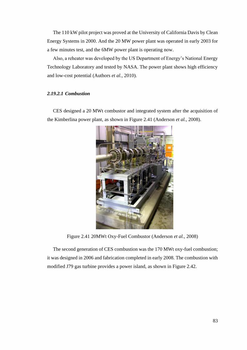
83
The 110 kW pilot project was proved at the University of California Davis by Clean
Energy Systems in 2000. And the 20 MW power plant was operated in early 2003 for
a few minutes test, and the 6MW power plant is operating now.
Also, a reheater was developed by the US Department of Energy’s National Energy
Technology Laboratory and tested by NASA. The power plant shows high efficiency
and low-cost potential (Authors et al., 2010).
2.19.2.1 Combustion
CES designed a 20 MWt combustor and integrated system after the acquisition of
the Kimberlina power plant, as shown in Figure 2.41 (Anderson et al., 2008).
Figure 2.41 20MWt Oxy-Fuel Combustor (Anderson et al., 2008)
The second generation of CES combustion was the 170 MWt oxy-fuel combustion;
it was designed in 2006 and fabrication completed in early 2008. The combustion with
modified J79 gas turbine provides a power island, as shown in Figure 2.42.
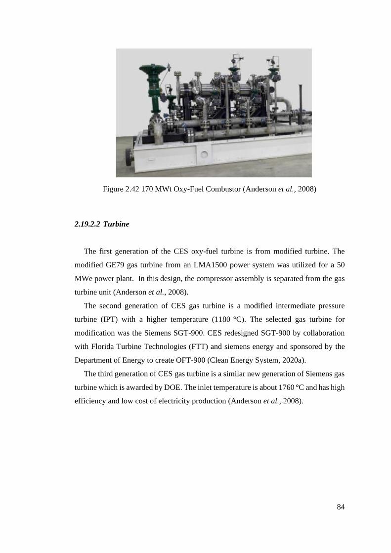
84
Figure 2.42 170 MWt Oxy-Fuel Combustor (Anderson et al., 2008)
2.19.2.2 Turbine
The first generation of the CES oxy-fuel turbine is from modified turbine. The
modified GE79 gas turbine from an LMA1500 power system was utilized for a 50
MWe power plant. In this design, the compressor assembly is separated from the gas
turbine unit (Anderson et al., 2008).
The second generation of CES gas turbine is a modified intermediate pressure
turbine (IPT) with a higher temperature (1180 °C). The selected gas turbine for
modification was the Siemens SGT-900. CES redesigned SGT-900 by collaboration
with Florida Turbine Technologies (FTT) and siemens energy and sponsored by the
Department of Energy to create OFT-900 (Clean Energy System, 2020a).
The third generation of CES gas turbine is a similar new generation of Siemens gas
turbine which is awarded by DOE. The inlet temperature is about 1760 °C and has high
efficiency and low cost of electricity production (Anderson et al., 2008).
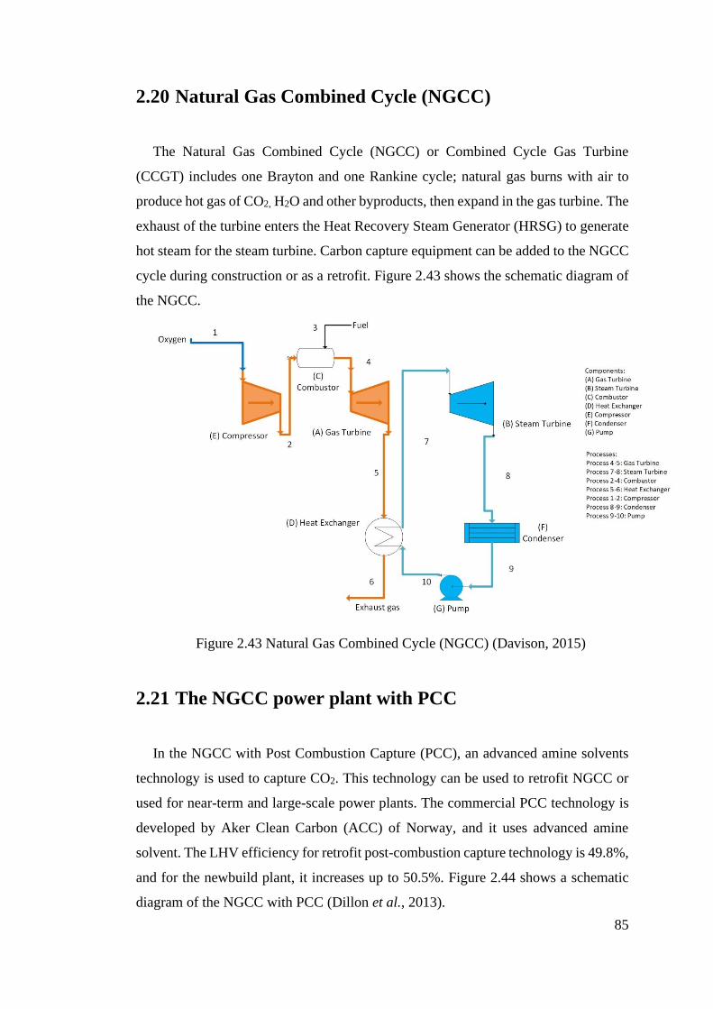
85
2.20 Natural Gas Combined Cycle (NGCC)
The Natural Gas Combined Cycle (NGCC) or Combined Cycle Gas Turbine
(CCGT) includes one Brayton and one Rankine cycle; natural gas burns with air to
produce hot gas of CO2, H2O and other byproducts, then expand in the gas turbine. The
exhaust of the turbine enters the Heat Recovery Steam Generator (HRSG) to generate
hot steam for the steam turbine. Carbon capture equipment can be added to the NGCC
cycle during construction or as a retrofit. Figure 2.43 shows the schematic diagram of
the NGCC.
Figure 2.43 Natural Gas Combined Cycle (NGCC) (Davison, 2015)
2.21 The NGCC power plant with PCC
In the NGCC with Post Combustion Capture (PCC), an advanced amine solvents
technology is used to capture CO2. This technology can be used to retrofit NGCC or
used for near-term and large-scale power plants. The commercial PCC technology is
developed by Aker Clean Carbon (ACC) of Norway, and it uses advanced amine
solvent. The LHV efficiency for retrofit post-combustion capture technology is 49.8%,
and for the newbuild plant, it increases up to 50.5%. Figure 2.44 shows a schematic
diagram of the NGCC with PCC (Dillon et al., 2013).
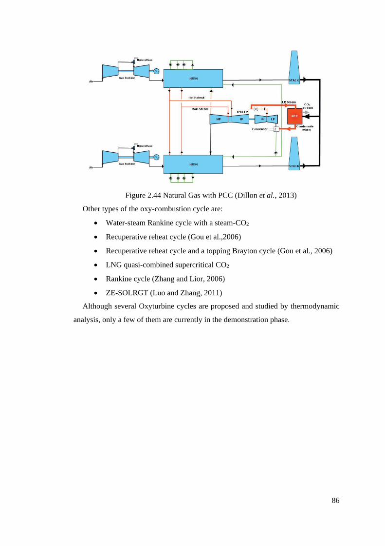
86
Figure 2.44 Natural Gas with PCC (Dillon et al., 2013)
Other types of the oxy-combustion cycle are:
• Water-steam Rankine cycle with a steam-CO2
• Recuperative reheat cycle (Gou et al.,2006)
• Recuperative reheat cycle and a topping Brayton cycle (Gou et al., 2006)
• LNG quasi-combined supercritical CO2
• Rankine cycle (Zhang and Lior, 2006)
• ZE-SOLRGT (Luo and Zhang, 2011)
Although several Oxyturbine cycles are proposed and studied by thermodynamic
analysis, only a few of them are currently in the demonstration phase.
87
2.22 Summary
This chapter has reviewed various technologies and issues related to main
technologies of CO2 capture, environmental impact, oxygen production and air
separation unit and CO2 compression and purification unit. Conventional gas turbines
burn fuel with air and produce carbon dioxide as a byproduct. Zero Emission Power
Plants (ZEPP) is the solution to avoid carbon dioxide emission. The ZEPP power plant
needs to use Carbon Capture & Storage (CCS) technologies.
In this chapter, three main carbon capture technologies are investigated and
compared in detail. An oxy-fuel combustion power cycle is a promising technology
among other CCS technologies; it can produce very high CO2 concentration in the flue
gas with high efficiency. Recent technology development for oxy-fuel combustion
causes reducing capital and operational cost. The air Separation Unite (ASU) is one of
the challenges for oxy-fuel combustion technology and need to be improved for better
cycle efficiency and have the main impact on the efficiency of the oxy-combustion
cycle. Different methods of oxygen productions, including Cryogenic Air Separation
(ASU), adoption, Pressure Swing Adsorption (PSA), Chemical processes and
membranes, are investigated in this chapter.
Then, the oxy-combustion power cycles are investigated, and their main
characteristics and parameters are presented. These oxy-combustion cycles are SCOC-
CC, COOPERATE Cycle, MATIANT, E-MATIANT, CC_MATIANT, Graz and S-
Graz cycles, AZEP 85% and 100%, ZEITMOP Cycle, COOLCEP-S Cycle, Novel
O2/CO2 (Cao and Zheng, 2006), NetPower and CES Cycle. The oxy-combustion
cycles offer high overall efficiencies for power generation while they offer high purity
of CO2 capture without producing NOx; however, they need technically advanced
components.
The Air Separation Unit (ASU) as an oxygen production unit requires high
electricity consumption; this technology needs to develop to reduce auxiliary load.
Other oxygen production technology also is used, including Ion Transport Membrane
(ITM) in ZEITMOP cycle or Oxygen Ion Transport Membrane (OITM) in AZEP
100% and AZEP 80% cycle.
The highest efficiencies of oxy-combustion power cycles belong to S-Graze 57%,
NetPower 55.1% and COOLCEP-S 59%. The S-CES cycle with steam working flow
88
is 48.9%, and ZEITMOP with ITM oxygen production technology is 51%, and AZEP
100% with OITM is 49.6%. Among these cycles, only NetPower and S-CES are
recently in the demonstration stage, and these are investigated in detail in Chapters 7
and 8.
The recycled working flow for NetPower, E-MATIANT, CC-MATIANT are CO2,
and the recycled working flow for Graz, S-Graz, AZEP 100% and AZEP 85% cycles
are a mixture of CO2 and H2O. The recycle working flow for the gas turbine cycle of
SCOC-CC is CO2, but the steam turbine cycle of SCOC-CC is H2O. The recycled
working flow for the ZEITMOP cycle is CO2; however, it used air/oxygen depleted in
its air cycle. The working recycled working flow for the S-CES cycle is H2O. These
cycles apply different technologies based on oxygen production methods and recycled
working flow composition.
89
Chapter 3: Methodology and Process
modelling of the leading Oxyturbine
cycles
3.1 Introduction
Process simulation software can be used for four stages of a power plant design,
including development, research, design and production. The software can be used to
test specific designs under various design conditions without the need for running
experiments. The process modelling can replace lab work and support research and
development without the extensive cost of laboratory experiments and demonstration
of the pilot plant. Also, the software can be used in the design stage for sizing the
components of power cycles. In the production stage, the software can analyze the
sensitivity of parameters without risk (Fogler and Gurmen, 2002).
Different types of process simulation software are developed recently, including
ChemCad, AspenOne, gProms, BOAST, COMSOL, Eclipse, Thermoflex and
ProSimplus software.
Among other software, the Aspen Plus is more user-friendly and can be used for real-
world power plants from the research and development stage to monitoring full-scale
power plants. Advanced System for Process Engineering (ASPEN) software was
developed by researchers at MIT’s laboratory in 1980. This software was
commercialized with Aspen Tech company and has been developed for simulation of
different types of processes (Uchechukwu Megwai, 2014).
Aveva’s Pro II is cheaper than Aspen Plus software and leads in the mining industry;
however, it’s mostly designed for steady-state and can’t change the converge method
as easy as is Aspen Plus; also, Aspen Plus has a large database(ChemEngGuy, 2021).
DWSIM is free and open-source software and performs similar tasks as Aspen plus
commercial software. It can serve as an alternative process software for offshore
petroleum production. Also, DWSIM has the same accuracy as Aspen Plus
(Tangsriwong et al., 2020).
90
3.2 Oxy-combustion power cycle theories and calculations
3.2.1 Thermodynamic concept and equations
Aspen Plus software uses the first principles of the thermodynamic to calculate
parameters of the equipment, including turbine, compressor, heat exchanger,
distillation and separator.
3.2.1.1 Continuity
The conservation of mass, along with conservation of energy and momentum, are
the fundamental concept of physics. The thermodynamic and fluid mechanic problem
can be solved with this fundamental concept. Conservation of mass is maintained by
summation of input mass minus summation of output mass equal to change in mass
in the control volume. The mass balance of control volume for the transient system is
shown in Equation 3-1.
∑ 𝑚𝑖
𝑖
− ∑ 𝑚𝑜
𝑜
=𝜕𝑚
𝜕𝑡
Equation 3-1
The mass in the turbomachine with the steady-state condition is constant over time,
and it holds for all equipment in the steady-state. The mass balance for the steady-state
process is shown in Equation 3-2.
∑ 𝑚𝑖
𝑖
= ∑ 𝑚𝑜
𝑜
Equation 3-2
The conservation of the mass can be written based on the velocity, density and
area for a steady-state turbomachine, as shown in Equation 3-3.
𝜌𝑖𝑉𝑖𝐴𝑖 = 𝜌𝑜𝑉𝑜𝐴𝑜 Equation 3-3
91
3.2.1.2 Energy conservation
Another fundamental concept of physics is the first law of thermodynamic or
energy conservation law. It means the amount of energy is constant, and energy is
neither destroyed nor created. The energy can be converted from one form to
another, but the total energy within the domain remains constant. The energy balance
for steady-state control volume is shown in Equation 3-4.
∑ 𝐸𝑖
𝑖
+ �� = ∑ 𝐸��
𝑜
+ �� Equation 3-4
3.2.1.3 Energy quality (second law of thermodynamic)
The second law of thermodynamic is entropy balance. Entropy, same as energy
and mass, is the extensive property and can be transferred into or out of control
volume by mass streams. Since entropy is a property, it changes from one state to
another. The entropy rate balance for the transient system is shown in Equation 3-5.
𝜕𝑆𝑐𝑣
𝜕𝑡= ∑
𝑄
𝑇
𝑖
+ ∑ ��
𝑖
− ∑ ��
𝑒
+ 𝑆𝑔𝑒𝑛
Equation 3-5
The 𝑆𝑔𝑒𝑛 indicates the entropy generation rate due to irreversibility within the
control volume. The entropy rate balance for the steady-state system is shown in
Equation 3-6
∑ ��
𝑖
+ ∑𝑄
𝑇
𝑖
+ 𝑆𝑔𝑒𝑛 = ∑ ��
𝑜
+ ∑𝑄
𝑇
𝑜
Equation 3-6
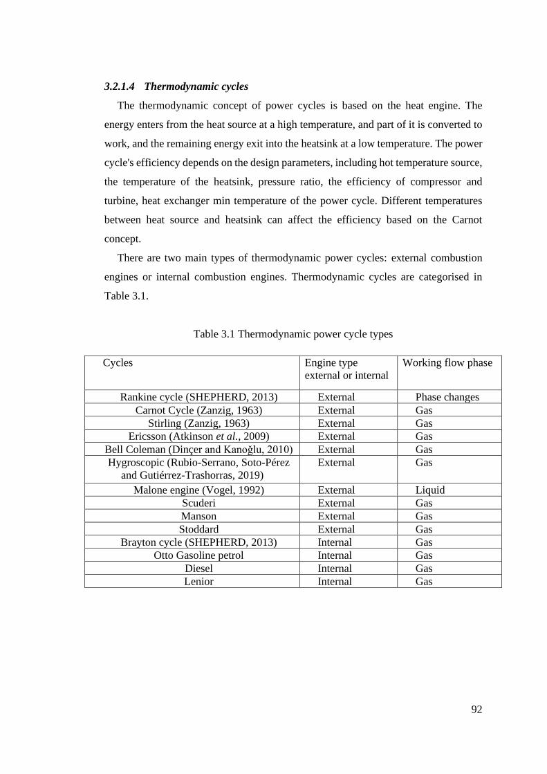
92
3.2.1.4 Thermodynamic cycles
The thermodynamic concept of power cycles is based on the heat engine. The
energy enters from the heat source at a high temperature, and part of it is converted to
work, and the remaining energy exit into the heatsink at a low temperature. The power
cycle's efficiency depends on the design parameters, including hot temperature source,
the temperature of the heatsink, pressure ratio, the efficiency of compressor and
turbine, heat exchanger min temperature of the power cycle. Different temperatures
between heat source and heatsink can affect the efficiency based on the Carnot
concept.
There are two main types of thermodynamic power cycles: external combustion
engines or internal combustion engines. Thermodynamic cycles are categorised in
Table 3.1.
Table 3.1 Thermodynamic power cycle types
Cycles Engine type
external or internal
Working flow phase
Rankine cycle (SHEPHERD, 2013) External Phase changes
Carnot Cycle (Zanzig, 1963) External Gas
Stirling (Zanzig, 1963) External Gas
Ericsson (Atkinson et al., 2009) External Gas
Bell Coleman (Dinçer and Kanoǧlu, 2010) External Gas
Hygroscopic (Rubio-Serrano, Soto-Pérez
and Gutiérrez-Trashorras, 2019)
External Gas
Malone engine (Vogel, 1992) External Liquid
Scuderi External Gas
Manson External Gas
Stoddard External Gas
Brayton cycle (SHEPHERD, 2013) Internal Gas
Otto Gasoline petrol Internal Gas
Diesel Internal Gas
Lenior Internal Gas
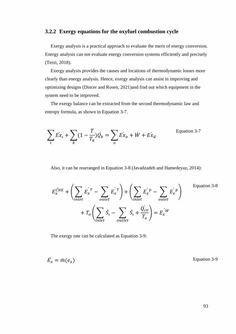
93
3.2.2 Exergy equations for the oxyfuel combustion cycle
Exergy analysis is a practical approach to evaluate the merit of energy conversion.
Energy analysis can not evaluate energy conversion systems efficiently and precisely
(Terzi, 2018).
Exergy analysis provides the causes and locations of thermodynamic losses more
clearly than energy analysis. Hence, exergy analysis can assist in improving and
optimizing designs (Dincer and Rosen, 2021)and find out which equipment in the
system need to be improved.
The exergy balance can be extracted from the second thermodynamic law and
entropy formula, as shown in Equation 3-7.
∑ 𝐸𝑥𝑖
𝑖
+ ∑(1 −𝑇
𝑇𝑘)𝑄��
𝑘
= ∑ 𝐸𝑥𝑜
𝑜
+ �� + 𝐸𝑥𝑑
Equation 3-7
Also, it can be rearranged in Equation 3-8 (Javadzadeh and Hamedeyaz, 2014):
𝐸𝑥𝐶𝐻𝐸 + ( ∑ 𝐸𝑥
𝑇
𝑖𝑛𝑙𝑒𝑡
− ∑ 𝐸𝑥𝑇
𝑜𝑢𝑙𝑒𝑡
) + ( ∑ 𝐸𝑥𝑝
𝑖𝑛𝑙𝑒𝑡
− ∑ 𝐸𝑥𝑝
𝑜𝑢𝑙𝑒𝑡
)
+ 𝑇𝑜 ( ∑ 𝑆��
𝑖𝑛𝑙𝑒𝑡
− ∑ 𝑆��
𝑜𝑢𝑡𝑙𝑒𝑡
+𝑄𝑐𝑣
𝑇𝑜) = 𝐸𝑥
𝑊
Equation 3-8
The exergy rate can be calculated as Equation 3-9:
𝐸�� = ��(𝑒𝑥) Equation 3-9

94
Figure 3.1 the early classification of the exergy and Szargurt el at. (1988) classified
the total exergy include thermal, potential and kinetic exergy. Also, the thermal exergy
includes chemical, physical, exergy.
Figure 3.1 Different classifications of exergy (Marmolejo-Correa and Gundersen,
2015)
Figure 3.2 shows the new classification for exergy; this classification is used for the
exergy analysis in this thesis. Total exergy includes chemical and physical exergy, and
chemical exergy includes mixing and separation (molar fraction of components) and
chemical reaction (chemical exergy inside the substance). The physical exergy
includes thermo-mechanical and mechanical exergy.
Thermo-mechanical exergy is temperature and pressure based. These are used for
most of the thermodynamic cycles. The mechanical exergy is kinetic and potential,
which is usually considered constant in the thermodynamic cycle.
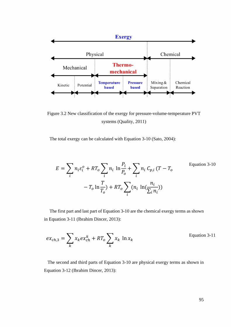
95
Figure 3.2 New classification of the exergy for pressure-volume-temperature PVT
systems (Quality, 2011)
The total exergy can be calculated with Equation 3-10 (Sato, 2004):
𝐸 = ∑ 𝑛𝑖𝜀𝑖𝑜
𝑖
+ 𝑅𝑇𝑜 ∑ 𝑛𝑖 ln𝑃𝑖
𝑃𝑜𝑖
+ ∑ 𝑛𝑖 𝐶𝑝,𝑖
𝑖
(𝑇 − 𝑇𝑜
− 𝑇𝑜 ln𝑇
𝑇𝑜) + 𝑅𝑇𝑜 ∑(𝑛𝑖 ln(
𝑛𝑖
∑ 𝑛𝑖𝑖))
𝑖
Equation 3-10
The first part and last part of Equation 3-10 are the chemical exergy terms as shown
in Equation 3-11 (Ibrahim Dincer, 2013):
𝑒𝑥𝑐ℎ,3 = ∑ 𝑥𝑘𝑒𝑥𝑐ℎ𝑘
𝑘
+ 𝑅𝑇𝑜 ∑ 𝑥𝑘 ln 𝑥𝑘
𝑘
Equation 3-11
The second and third parts of Equation 3-10 are physical exergy terms as shown in
Equation 3-12 (Ibrahim Dincer, 2013):
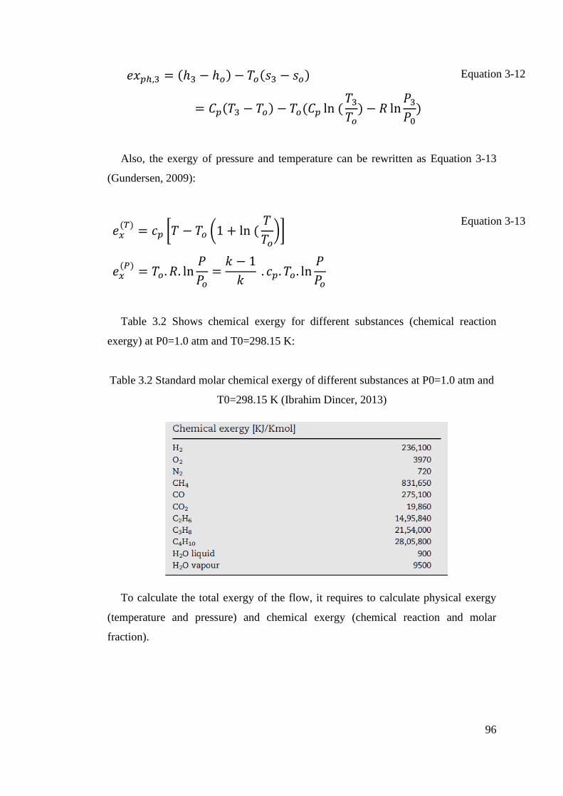
96
𝑒𝑥𝑝ℎ,3 = (ℎ3 − ℎ𝑜) − 𝑇𝑜(𝑠3 − 𝑠𝑜)
= 𝐶𝑝(𝑇3 − 𝑇𝑜) − 𝑇𝑜(𝐶𝑝 ln (𝑇3
𝑇𝑜) − 𝑅 ln
𝑃3
𝑃0)
Equation 3-12
Also, the exergy of pressure and temperature can be rewritten as Equation 3-13
(Gundersen, 2009):
𝑒𝑥(𝑇)
= 𝑐𝑝 [𝑇 − 𝑇𝑜 (1 + ln (𝑇
𝑇𝑜)]
𝑒𝑥(𝑃)
= 𝑇𝑜. 𝑅. ln𝑃
𝑃𝑜=
𝑘 − 1
𝑘 . 𝑐𝑝. 𝑇𝑜. ln
𝑃
𝑃𝑜
Equation 3-13
Table 3.2 Shows chemical exergy for different substances (chemical reaction
exergy) at P0=1.0 atm and T0=298.15 K:
Table 3.2 Standard molar chemical exergy of different substances at P0=1.0 atm and
T0=298.15 K (Ibrahim Dincer, 2013)
To calculate the total exergy of the flow, it requires to calculate physical exergy
(temperature and pressure) and chemical exergy (chemical reaction and molar
fraction).
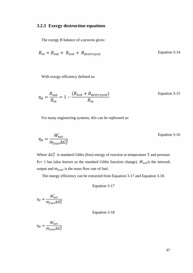
97
3.2.3 Exergy destruction equations
The exergy B balance of a process gives:
𝐵𝑖𝑛 = 𝐵𝑜𝑢𝑡 + 𝐵𝑙𝑜𝑠𝑡 + 𝐵𝑑𝑒𝑠𝑡𝑟𝑜𝑦𝑒𝑑
Equation 3-14
With exergy efficiency defined as:
𝜂𝐵 =𝐵𝑜𝑢𝑡
𝐵𝑖𝑛= 1 −
(𝐵𝑙𝑜𝑠𝑡 + 𝐵𝑑𝑒𝑠𝑡𝑟𝑜𝑦𝑒𝑑)
𝐵𝑖𝑛
Equation 3-15
For many engineering systems, this can be rephrased as:
𝜂𝐵 =𝑊𝑛𝑒𝑡
��𝑓𝑢𝑒𝑙Δ𝐺𝑇0
Equation 3-16
Where ∆𝐺𝑇0 is standard Gibbs (free) energy of reaction at temperature T and pressure
P0= 1 bar (also known as the standard Gibbs function change). ��𝑛𝑒𝑡is the network
output and ��𝑓𝑢𝑒𝑙 is the mass flow rate of fuel.
The energy efficiency can be extracted from Equation 3-17 and Equation 3-18.
Equation 3-17
𝜂𝐸 =𝑊𝑛𝑒𝑡
��𝑓𝑢𝑒𝑙Δ𝐻𝑇0
Equation 3-18
𝜂𝐵 =𝑊𝑛𝑒𝑡
��𝑓𝑢𝑒𝑙Δ𝐺𝑇0
98
∆𝐻𝑇0 is the standard enthalpy of reaction at temperature T and pressure P0 = 1 bar,
and always ∆𝐺𝑇0 < ∆𝐻𝑇
0 so the energy efficiency must be smaller than the exergy
efficiency. Sankey diagram can be used to show exergy flow in each oxy-combustion
cycle. (Sharifzadeh, Meghdari and Rashtchian, 2017). The methane chemical energy
per kg can be calculated by multiply 1.06 to LHV of Methane (Ahmadi, Dincer and
Rosen, 2011). The total input exergy into the system is based on Equation 3-19:
Equation 3-19
Chemical exergy fuel = 802361j
mol× 1.06 × m
mol
s= total chemical exergy
Total Chemical exergy fuel + physical exergy from oxygen = Total input exer
Table 3.3 shows the exergy balance for the oxy-combustion power cycle.
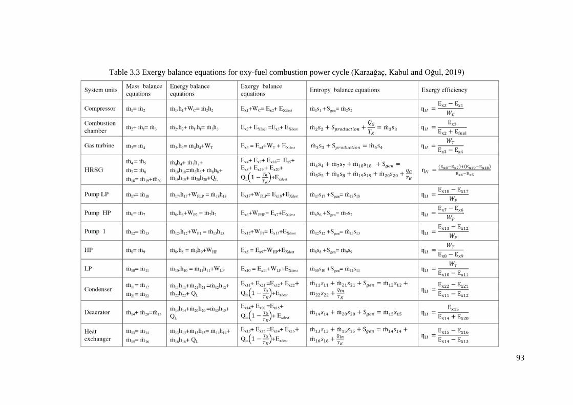
93
Table 3.3 Exergy balance equations for oxy-fuel combustion power cycle (Karaağaç, Kabul and Oğul, 2019)
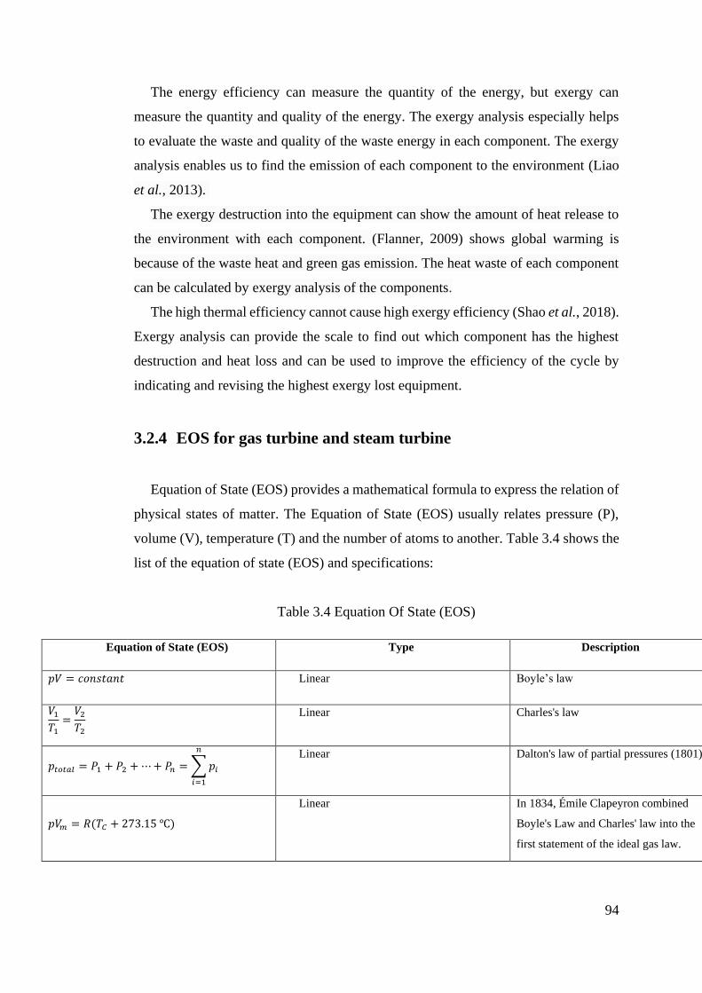
94
The energy efficiency can measure the quantity of the energy, but exergy can
measure the quantity and quality of the energy. The exergy analysis especially helps
to evaluate the waste and quality of the waste energy in each component. The exergy
analysis enables us to find the emission of each component to the environment (Liao
et al., 2013).
The exergy destruction into the equipment can show the amount of heat release to
the environment with each component. (Flanner, 2009) shows global warming is
because of the waste heat and green gas emission. The heat waste of each component
can be calculated by exergy analysis of the components.
The high thermal efficiency cannot cause high exergy efficiency (Shao et al., 2018).
Exergy analysis can provide the scale to find out which component has the highest
destruction and heat loss and can be used to improve the efficiency of the cycle by
indicating and revising the highest exergy lost equipment.
3.2.4 EOS for gas turbine and steam turbine
Equation of State (EOS) provides a mathematical formula to express the relation of
physical states of matter. The Equation of State (EOS) usually relates pressure (P),
volume (V), temperature (T) and the number of atoms to another. Table 3.4 shows the
list of the equation of state (EOS) and specifications:
Table 3.4 Equation Of State (EOS)
Equation of State (EOS) Type Description
𝑝𝑉 = 𝑐𝑜𝑛𝑠𝑡𝑎𝑛𝑡 Linear Boyle’s law
𝑉1
𝑇1
=𝑉2
𝑇2
Linear Charles's law
𝑝𝑡𝑜𝑡𝑎𝑙 = 𝑃1 + 𝑃2 + ⋯ + 𝑃𝑛 = ∑ 𝑝𝑖
𝑛
𝑖=1
Linear Dalton's law of partial pressures (1801)
𝑝𝑉𝑚 = 𝑅(𝑇𝐶 + 273.15 ℃)
Linear In 1834, Émile Clapeyron combined
Boyle's Law and Charles' law into the
first statement of the ideal gas law.
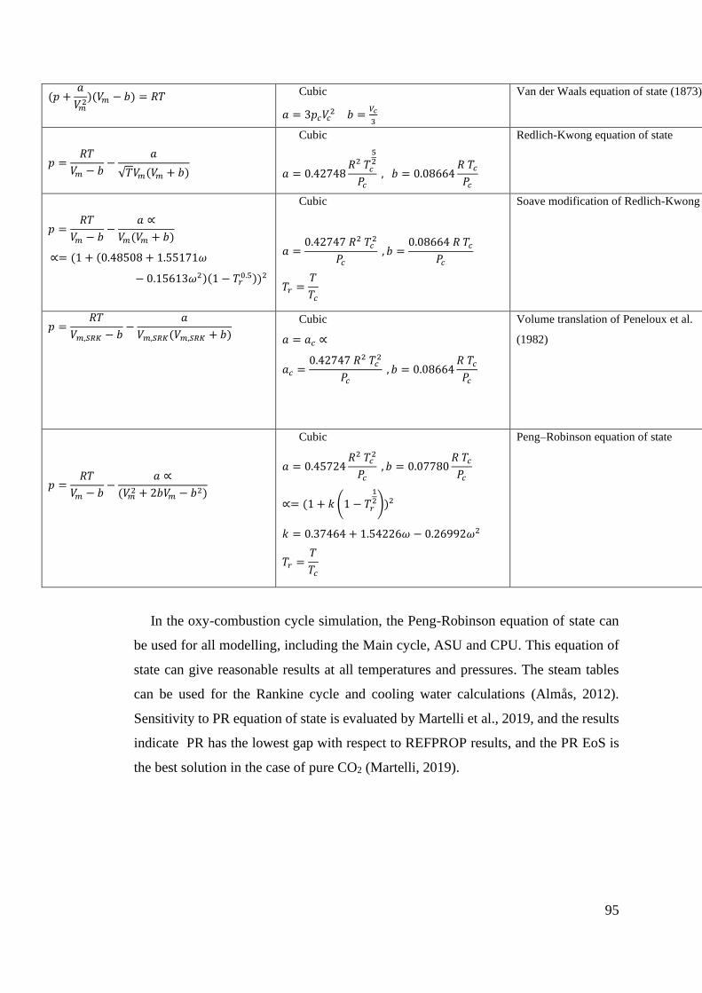
95
(𝑝 +𝑎
𝑉𝑚2
)(𝑉𝑚 − 𝑏) = 𝑅𝑇
Cubic
𝑎 = 3𝑝𝑐𝑉𝑐2 𝑏 =
𝑉𝑐
3
Van der Waals equation of state (1873)
𝑝 =𝑅𝑇
𝑉𝑚 − 𝑏−
𝑎
√𝑇𝑉𝑚(𝑉𝑚 + 𝑏)
Cubic
𝑎 = 0.42748𝑅2 𝑇𝑐
52
𝑃𝑐
, 𝑏 = 0.08664𝑅 𝑇𝑐
𝑃𝑐
Redlich-Kwong equation of state
𝑝 =𝑅𝑇
𝑉𝑚 − 𝑏−
𝑎 ∝
𝑉𝑚(𝑉𝑚 + 𝑏)
∝= (1 + (0.48508 + 1.55171𝜔
− 0.15613𝜔2)(1 − 𝑇𝑟0.5))2
Cubic
𝑎 =0.42747 𝑅2 𝑇𝑐
2
𝑃𝑐
, 𝑏 =0.08664 𝑅 𝑇𝑐
𝑃𝑐
𝑇𝑟 =𝑇
𝑇𝑐
Soave modification of Redlich-Kwong
𝑝 =𝑅𝑇
𝑉𝑚,𝑆𝑅𝐾 − 𝑏−
𝑎
𝑉𝑚,𝑆𝑅𝐾(𝑉𝑚,𝑆𝑅𝐾 + 𝑏)
Cubic
𝑎 = 𝑎𝑐 ∝
𝑎𝑐 =0.42747 𝑅2 𝑇𝑐
2
𝑃𝑐
, 𝑏 = 0.08664𝑅 𝑇𝑐
𝑃𝑐
Volume translation of Peneloux et al.
(1982)
𝑝 =𝑅𝑇
𝑉𝑚 − 𝑏−
𝑎 ∝
(𝑉𝑚2 + 2𝑏𝑉𝑚 − 𝑏2)
Cubic
𝑎 = 0.45724𝑅2 𝑇𝑐
2
𝑃𝑐
, 𝑏 = 0.07780𝑅 𝑇𝑐
𝑃𝑐
∝= (1 + 𝑘 (1 − 𝑇𝑟
12))2
𝑘 = 0.37464 + 1.54226𝜔 − 0.26992𝜔2
𝑇𝑟 =𝑇
𝑇𝑐
Peng–Robinson equation of state
In the oxy-combustion cycle simulation, the Peng-Robinson equation of state can
be used for all modelling, including the Main cycle, ASU and CPU. This equation of
state can give reasonable results at all temperatures and pressures. The steam tables
can be used for the Rankine cycle and cooling water calculations (Almås, 2012).
Sensitivity to PR equation of state is evaluated by Martelli et al., 2019, and the results
indicate PR has the lowest gap with respect to REFPROP results, and the PR EoS is
the best solution in the case of pure CO2 (Martelli, 2019).
96
3.3 Modelling and simulation
3.3.1 Plant simulation with a numerical approach
There are two main numerical approach methods to calculate thermodynamic points
and evaluation of thermodynamic properties for power plant components. These two
methods are the sequential modular (SM) approach and the Equation Oriented (EO)
approach.
In the Sequential Modular (SM) approach, the calculation is based on the
subsequent block; the Output of each component is calculated based on the input and
parameters of the block. The output result of each component will be the input of the
following component.
In the equation oriented (EO) approach, The set of the equations are calculated
based on the mass and energy balance and operation mode by simulation toolbox. It
can easily simulate the thermodynamic cycle without the limitation of the SM strategy.
However, the solution algorithm needs to be robust and reliable, and the solvers are
more dependent on the initial point of iteration (Macchi, 2017).
3.3.2 Aspen Plus pros and cons
Aspen Plus software can be used for modelling power cycle and chemical
processes. A large database of working fluids is available in Aspen Plus. Also,
different EOSs can be selected for the calculation of the thermodynamic properties of
the working fluid.
The Peng Robinson is a simple EOS, and it can be selected in Aspen Plus for
modelling Gas turbine cycle. Also, advanced EOSs are available in Aspen Plus to be
use for modelling of working fluid near saturation area or critical point. Besides, Aspen
Plus can calculate mixed working fluid properties with two or more components to
simulate a complex cycle.
One of the weaknesses of the Aspen Plus software is to define user-defined
components and model actual turbines. The turbine block is a basic version of the
turbine and can describe with isentropic efficiency. It cannot be linked to working fluid
properties and other cycle and turbine parameters. Hence the accurate modelling of
97
turbine block required the definition of ad hoc models; the Aspen Plus software does
not have a cooled turbine block, the combustor outlet temperature reached is higher
than the maximum temperature allowed by the walls materials, but the cooling flow
can not enter the expander block in different cooled step (Scaccabarozzi, Gatti and
Martelli, 2014).
Also, Aspen Plus has limitations to model off-design and dynamic analysis because
of fixed parameters of the blocks and the governing equations (Macchi, 2017).
In the simulation, the efficiency penalty of vanes, cooling blades of turbine and walls
of combustion or heat loss through the pipes are not taken into account and cycle
efficiency penalty can be 2-3% of simulation efficiency (Cao and Zheng, 2006).
3.3.3 Modelling equipment in Aspen Plus
3.3.3.1 Distillation column
It is the general known process where multi-components are separated into pure
components based on their difference in boiling points. This column typically consists
of an enriching section where concentrated vapours are sent to the condenser and a
stripping section where liquid/heavies are present.
The separation of components from a liquid mixture based on their vapour pressure
or boiling point is called distillation.
The distillation has varied types as followings:
1. Flash evaporation
2. Fractional distillation
3. Steam distillation
4. Simple Distillation
5. Azeotropic distillation
3.3.3.2 Stripper (or desorption)
The opposite process to absorption is generally called stripping. The operation of
removing absorbed solute from the solvent is called stripping. For example,
98
Ammonia is dissolved in water through the absorption process. The removal of
absorbed Ammonia from the solvent (water) is called stripping. The stripping is also
called a desorption process.
The flash stripper was used to model the separation of Carbon dioxide from water,
It is essentially a distillation process where the heavy product is water/liquid, and the
lighter product is generally a mixture of volatile organic materials. Generally,
steam/air is used for heating purposes in the column. The separator simulates
equilibrium phase separation (Haydary, 2019).
3.3.3.3 Absorption (opposite of striping)
In absorption (also called gas absorption, gas scrubbing, or gas washing), there is a
transfer of one or more species from the gas phase to a liquid solvent. The species
transferred to the liquid phase are referred to as solutes or absorbate. Absorption
involves no change in the chemical species present in the system. Absorption is used
to separate gas mixtures, remove impurities, or recover valuable chemicals. The
operation of removing the absorbed solute from the solvent is called stripping.
Absorbers usually are used with strippers to permit regeneration (or recovery) and
recycling of the absorbent (Nguyen, 2012).
Absorption: gas is purified; solute is absorbed from the gas into the liquid stream
Stripping: liquid is purified; solute stripped from the liquid into a gas (Wankat, 1988)
3.3.3.4 Separator blocks in Aspen Plus
The Separator Blocks, Sep and Sep2, combine feed streams and then split the
resulting stream based on your specifications. When the details of the separation are
unknown or unimportant, you can use Sep and Sep2 instead of rigorous separation
models (such as distillation or absorption models) to save computational time.
The flash blocks, Flash 2 and Flash 3, determine the thermal and phase conditions
of a mixture with one or more inlet streams. You can generate heating or cooling curve
tables for these models.
The flash blocks represent single-stage separators such as knock-out drums. They
perform a phase equilibrium flash calculation based on the specifications. Adiabatic,
99
isothermal and isobaric flashes, and dew or bubble points, are among the calculations
(Machner, 1958).
Decanter block can be used for the separation of two liquid phases but without a vapour
phase (Machner, 1958). Decant process is used to draw off the liquid without
disturbing the sediment.
3.3.4 MATLAB Code link with Aspen Plus
The MATLAB code is provided to link Aspen Plus software to MATLAB. The
output data from Aspen Plus simulation input to the MATLAB software for further
calculation of the other parameters of the cycle. Also, the MATLAB code allows to
change design parameters of the power cycle and input them into the Aspen Plus
software for simulation and output of the Aspen Plus simulation send back to the
MATLAB (Appendix A).
The code in the MATLAB M file can create a local COM automation server to
interface MATLAB with Aspen Plus and run the Aspen Plus software based on the
MATLAB input (Tang, Boulter and Kitching, 2003). In this thesis, MATLAB code
help to calculate the exergy of each component, cost and other parameters; hence the
bar charts and graphs can be drawn with MATLAB. Furthermore, optimisation can be
performed with MATLAB code in future papers.
3.4 Oxy combustion cycles modelling and simulation
3.4.1 The SCOC-CC cycle modelling and analysis
Figure 3.3 shows the Semi-Closed Oxy-Combustion Combined Cycle SCOC-CC
cycle model in Aspen Plus software based on the schematic presented in Figure 2.18
of chapter 2; it has two parts steam cycle and gas turbine cycle.
The fuel and pure oxygen burn in the combustion and recycled CO2 stream enter
combustion to cool the combustion to 1517 oC, and the exhaust flow (Stream 2) from
combustion enters to the Gas turbine for expanding from 45.8 bar to 1.07 bar pressure.
100
The gas turbine exhaust flue (Steam 3) enters HRSG for recovering heat for the steam
cycle. Low pressure and temperature exhaust from HRSG (Steam 4) enters the
condenser to condense water and separate from carbon dioxide. The part of carbon
dioxide exhaust from the condenser (Stream 5) is compressed and recycled back to the
combustion (Stream 1). The Schematic Process Flow Diagram of SCOC-CC is shown
in Figure 3.3. Oxygen is fed from ASU to the cycle and thereby avoiding the post-
combustion process for removing CO2 in comparison with GT-CC with post-
combustion capture (Bolland and Saether, 1992).
The Steam cycle working flow is mainly water, and High pressure and temperature
water (Stream S4) enters the turbine for expansion. The exhaust flue from ,the steam
turbine (Steam S6) enters the condenser and then pumped back to the HRSG (Stream
S5). The stream properties are in Table 3.5.
Table 3.5 working flow properties at each stage for SCOC-CC cycle, the main working
flow for the steam cycle is water, and recycled working flow for the gas turbine is
carbon dioxide.
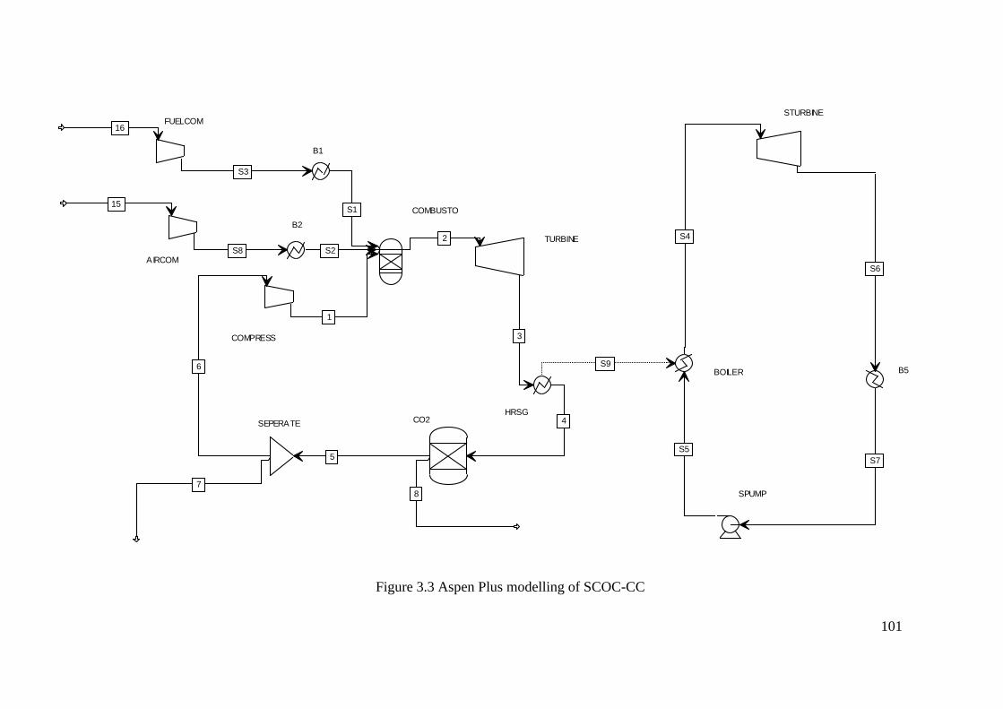
101
Figure 3.3 Aspen Plus modelling of SCOC-CC
COMPRESS
COMBUSTO
TURBINE
SEPERATE CO2HRSG
AIRCOM
FUELCOM
BOILER
STURBINE
B5
SPUMP
B1
B2
1
2
3
4
5
6
78
15
16
S1
S2
S4
S5
S6
S7
S3
S8
S9
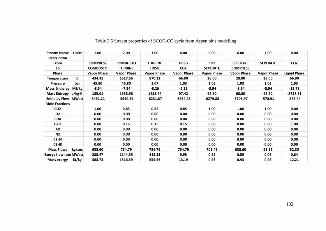
102
Table 3.5 Stream properties of SCOC-CC cycle from Aspen plus modelling
Stream Name Units 1.00 2.00 3.00 4.00 5.00 6.00 7.00 8.00
Description
From COMPRESS COMBUSTO TURBINE HRSG CO2 SEPERATE SEPERATE CO2
To COMBUSTO TURBINE HRSG CO2 SEPERATE COMPRESS
Phase Vapor Phase Vapor Phase Vapor Phase Vapor Phase Vapor Phase Vapor Phase Vapor Phase Liquid Phase
Temperature C 434.31 1517.56 870.22 66.90 28.00 28.00 28.00 66.90
Pressure bar 45.80 45.80 1.07 1.03 1.03 1.03 1.03 1.03
Mass Enthalpy MJ/kg -8.54 -7.34 -8.26 -9.21 -8.94 -8.94 -8.94 -15.78
Mass Entropy J/kg-K 189.01 1338.96 1488.44 97.42 68.80 68.80 68.80 -8728.61
Enthalpy Flow MWatt -5451.21 -5540.29 -6231.87 -6954.28 -6279.88 -5708.97 -570.91 -825.44
Mole Fractions
CO2 1.00 0.85 0.85 0.85 1.00 1.00 1.00 0.00
O2 0.00 0.00 0.00 0.00 0.00 0.00 0.00 0.00
CH4 0.00 0.00 0.00 0.00 0.00 0.00 0.00 0.00
H2O 0.00 0.15 0.15 0.15 0.00 0.00 0.00 1.00
AR 0.00 0.00 0.00 0.00 0.00 0.00 0.00 0.00
N2 0.00 0.00 0.00 0.00 0.00 0.00 0.00 0.00
C2H4 0.00 0.00 0.00 0.00 0.00 0.00 0.00 0.00
C3H8 0.00 0.00 0.00 0.00 0.00 0.00 0.00 0.00
Mass Flows kg/sec 638.60 754.79 754.79 754.79 702.46 638.60 63.86 52.30
Exergy flow rate MWatt 235.47 1144.55 419.33 9.95 0.65 0.59 0.06 0.64
Mass exergy kJ/kg 368.73 1516.39 555.56 13.19 0.93 0.93 0.93 12.21
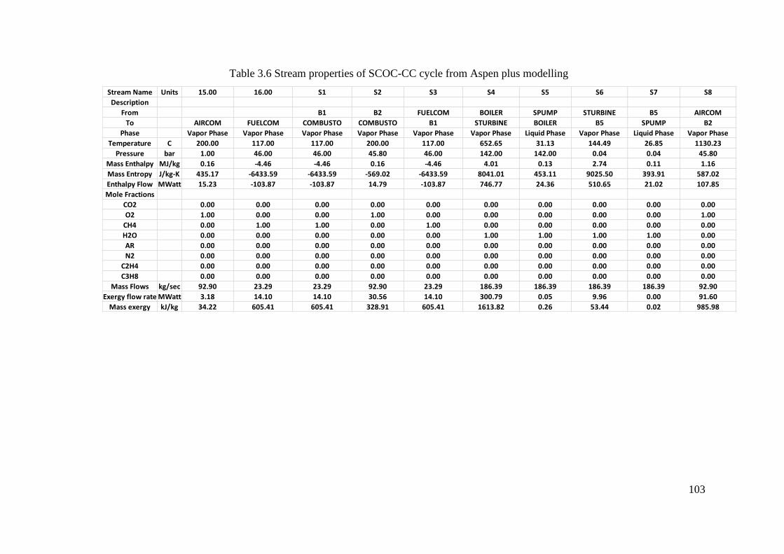
103
Table 3.6 Stream properties of SCOC-CC cycle from Aspen plus modelling
Stream Name Units 15.00 16.00 S1 S2 S3 S4 S5 S6 S7 S8
Description
From B1 B2 FUELCOM BOILER SPUMP STURBINE B5 AIRCOM
To AIRCOM FUELCOM COMBUSTO COMBUSTO B1 STURBINE BOILER B5 SPUMP B2
Phase Vapor Phase Vapor Phase Vapor Phase Vapor Phase Vapor Phase Vapor Phase Liquid Phase Vapor Phase Liquid Phase Vapor Phase
Temperature C 200.00 117.00 117.00 200.00 117.00 652.65 31.13 144.49 26.85 1130.23
Pressure bar 1.00 46.00 46.00 45.80 46.00 142.00 142.00 0.04 0.04 45.80
Mass Enthalpy MJ/kg 0.16 -4.46 -4.46 0.16 -4.46 4.01 0.13 2.74 0.11 1.16
Mass Entropy J/kg-K 435.17 -6433.59 -6433.59 -569.02 -6433.59 8041.01 453.11 9025.50 393.91 587.02
Enthalpy Flow MWatt 15.23 -103.87 -103.87 14.79 -103.87 746.77 24.36 510.65 21.02 107.85
Mole Fractions
CO2 0.00 0.00 0.00 0.00 0.00 0.00 0.00 0.00 0.00 0.00
O2 1.00 0.00 0.00 1.00 0.00 0.00 0.00 0.00 0.00 1.00
CH4 0.00 1.00 1.00 0.00 1.00 0.00 0.00 0.00 0.00 0.00
H2O 0.00 0.00 0.00 0.00 0.00 1.00 1.00 1.00 1.00 0.00
AR 0.00 0.00 0.00 0.00 0.00 0.00 0.00 0.00 0.00 0.00
N2 0.00 0.00 0.00 0.00 0.00 0.00 0.00 0.00 0.00 0.00
C2H4 0.00 0.00 0.00 0.00 0.00 0.00 0.00 0.00 0.00 0.00
C3H8 0.00 0.00 0.00 0.00 0.00 0.00 0.00 0.00 0.00 0.00
Mass Flows kg/sec 92.90 23.29 23.29 92.90 23.29 186.39 186.39 186.39 186.39 92.90
Exergy flow rate MWatt 3.18 14.10 14.10 30.56 14.10 300.79 0.05 9.96 0.00 91.60
Mass exergy kJ/kg 34.22 605.41 605.41 328.91 605.41 1613.82 0.26 53.44 0.02 985.98

104
3.4.2 The COOPERATE cycle modelling and analysis
Figure 3.3 shows the three stages COOPERATE cycle model in Aspen Plus based
on the schematic of the cycle presented in Figure 2.19 of chapter 2. The cycle
includes the main heat exchanger and two combustions. Table 3.5 shows the steam
cycle properties of the modelled COOPERATE cycle; the recycled working flow is
mainly carbon dioxide.
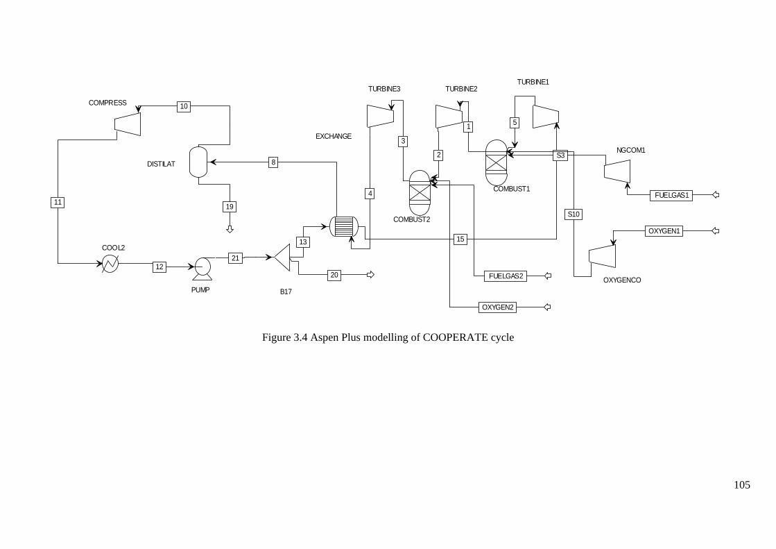
105
Figure 3.4 Aspen Plus modelling of COOPERATE cycle
COMBUST1
COMBUST2
TURBINE2TURBINE3TURBINE1
DISTILAT
COMPRESS
COOL2
PUMP B17
EXCHANGE
NGCOM1
OXYGENCO
1
2
3
4
5
OXYGEN1
8
10
11
12
13 15
FUELGAS2
OXYGEN2
FUELGAS1
19
20
21
S3
S10
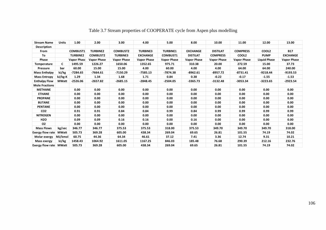
106
Table 3.7 Stream properties of COOPERATE cycle from Aspen plus modelling
Stream Name Units 1.00 2.00 3.00 4.00 5.00 8.00 10.00 11.00 12.00 13.00
Description
From COMBUST1 TURBINE2 COMBUST2 TURBINE3 TURBINE1 EXCHANGE DISTILAT COMPRESS COOL2 B17
To TURBINE2 COMBUST2 TURBINE3 EXCHANGE COMBUST1 DISTILAT COMPRESS COOL2 PUMP EXCHANGE
Phase Vapor Phase Vapor Phase Vapor Phase Vapor Phase Vapor Phase Vapor Phase Vapor Phase Vapor Phase Liquid Phase Vapor Phase
Temperature C 1495.59 1226.27 1650.06 1352.65 975.71 310.38 20.00 272.59 15.00 37.73
Pressure bar 60.00 15.00 15.00 4.00 60.00 4.00 4.00 64.00 64.00 240.00
Mass Enthalpy kJ/kg -7284.65 -7664.61 -7150.29 -7585.13 -7874.38 -8962.61 -8957.72 -8731.41 -9218.44 -9193.53
Mass Entropy kJ/kg-K 1.29 1.34 1.68 1.71 0.84 0.38 -0.22 -0.17 -1.55 -1.53
Enthalpy Flow MWatt -2526.06 -2657.82 -2685.15 -2848.45 -2504.05 -3365.73 -3132.48 -3053.34 -3223.65 -2923.54
Mole Fractions
METHANE 0.00 0.00 0.00 0.00 0.00 0.00 0.00 0.00 0.00 0.00
ETHANE 0.00 0.00 0.00 0.00 0.00 0.00 0.00 0.00 0.00 0.00
PROPANE 0.00 0.00 0.00 0.00 0.00 0.00 0.00 0.00 0.00 0.00
BUTANE 0.00 0.00 0.00 0.00 0.00 0.00 0.00 0.00 0.00 0.00
PENTANE 0.00 0.00 0.00 0.00 0.00 0.00 0.00 0.00 0.00 0.00
CO2 0.91 0.91 0.84 0.84 0.99 0.84 0.99 0.99 0.99 0.99
NITROGEN 0.00 0.00 0.00 0.00 0.00 0.00 0.00 0.00 0.00 0.00
H2O 0.09 0.09 0.16 0.16 0.00 0.16 0.00 0.00 0.00 0.00
O2 0.00 0.00 0.00 0.00 0.00 0.00 0.00 0.00 0.00 0.00
Mass Flows kg/sec 346.77 346.77 375.53 375.53 318.00 375.53 349.70 349.70 349.70 318.00
Exergy flow rate MWatt 505.73 369.28 605.00 438.34 269.04 69.65 26.81 101.55 74.19 74.02
Molar exergy MJ/kmol 60.75 44.36 64.34 46.61 37.12 7.41 3.36 12.74 9.31 10.21
Mass exergy kJ/kg 1458.43 1064.92 1611.05 1167.25 846.03 185.48 76.68 290.39 212.16 232.76
Exergy flow rate MWatt 505.73 369.28 605.00 438.34 269.04 69.65 26.81 101.55 74.19 74.02
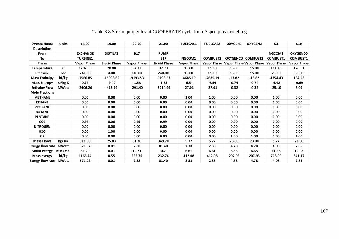
107
Table 3.8 Stream properties of COOPERATE cycle from Aspen plus modelling
Stream Name Units 15.00 19.00 20.00 21.00 FUELGAS1 FUELGAS2 OXYGEN1 OXYGEN2 S3 S10
Description
From EXCHANGE DISTILAT B17 PUMP NGCOM1 OXYGENCO
To TURBINE1 B17 NGCOM1 COMBUST2 OXYGENCO COMBUST2 COMBUST1 COMBUST1
Phase Vapor Phase Liquid Phase Vapor Phase Liquid Phase Vapor Phase Vapor Phase Vapor Phase Vapor Phase Vapor Phase Vapor Phase
Temperature C 1202.65 20.00 37.73 37.73 15.00 15.00 15.00 15.00 161.45 176.61
Pressure bar 240.00 4.00 240.00 240.00 15.00 15.00 15.00 15.00 75.00 60.00
Mass Enthalpy kJ/kg -7566.85 -15993.60 -9193.53 -9193.53 -4685.19 -4685.19 -13.82 -13.82 -4354.43 134.53
Mass Entropy kJ/kg-K 0.79 -9.40 -1.53 -1.53 -6.54 -6.54 -0.74 -0.74 -6.42 -0.69
Enthalpy Flow MWatt -2406.26 -413.19 -291.40 -3214.94 -27.01 -27.01 -0.32 -0.32 -25.10 3.09
Mole Fractions
METHANE 0.00 0.00 0.00 0.00 1.00 1.00 0.00 0.00 1.00 0.00
ETHANE 0.00 0.00 0.00 0.00 0.00 0.00 0.00 0.00 0.00 0.00
PROPANE 0.00 0.00 0.00 0.00 0.00 0.00 0.00 0.00 0.00 0.00
BUTANE 0.00 0.00 0.00 0.00 0.00 0.00 0.00 0.00 0.00 0.00
PENTANE 0.00 0.00 0.00 0.00 0.00 0.00 0.00 0.00 0.00 0.00
CO2 0.99 0.00 0.99 0.99 0.00 0.00 0.00 0.00 0.00 0.00
NITROGEN 0.00 0.00 0.00 0.00 0.00 0.00 0.00 0.00 0.00 0.00
H2O 0.00 1.00 0.00 0.00 0.00 0.00 0.00 0.00 0.00 0.00
O2 0.00 0.00 0.00 0.00 0.00 0.00 1.00 1.00 0.00 1.00
Mass Flows kg/sec 318.00 25.83 31.70 349.70 5.77 5.77 23.00 23.00 5.77 23.00
Exergy flow rate MWatt 371.02 0.01 7.38 81.40 2.38 2.38 4.78 4.78 4.08 7.85
Molar exergy MJ/kmol 51.20 0.01 10.21 10.21 6.61 6.61 6.65 6.65 11.36 10.92
Mass exergy kJ/kg 1166.74 0.55 232.76 232.76 412.08 412.08 207.95 207.95 708.09 341.17
Exergy flow rate MWatt 371.02 0.01 7.38 81.40 2.38 2.38 4.78 4.78 4.08 7.85

108
3.4.3 The E-MATIANT cycle modelling and analysis
Figure 3.5 shows the E -MATIANT cycle model in Aspen Plus software based on
the schematic presented in Figure 2.20 of chapter 2.; The gas turbine cycle including
a High-Pressure Turbine (HPT) and Low-Pressure Turbine (LPT). Table 3.9 shows
working flow properties at each stage for the E-MATIANT cycle, the main working
flow for the steam cycle is water, and the recycled working flow for the gas turbine is
carbon dioxide.
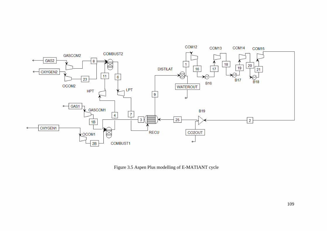
109
Figure 3.5 Aspen Plus modelling of E-MATIANT cycle
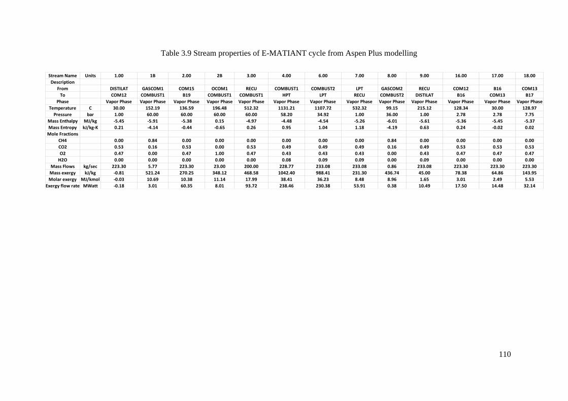
110
Table 3.9 Stream properties of E-MATIANT cycle from Aspen Plus modelling
Stream Name Units 1.00 1B 2.00 2B 3.00 4.00 6.00 7.00 8.00 9.00 16.00 17.00 18.00
Description
From DISTILAT GASCOM1 COM15 OCOM1 RECU COMBUST1 COMBUST2 LPT GASCOM2 RECU COM12 B16 COM13
To COM12 COMBUST1 B19 COMBUST1 COMBUST1 HPT LPT RECU COMBUST2 DISTILAT B16 COM13 B17
Phase Vapor Phase Vapor Phase Vapor Phase Vapor Phase Vapor Phase Vapor Phase Vapor Phase Vapor Phase Vapor Phase Vapor Phase Vapor Phase Vapor Phase Vapor Phase
Temperature C 30.00 152.19 136.59 196.48 512.32 1131.21 1107.72 532.32 99.15 215.12 128.34 30.00 128.97
Pressure bar 1.00 60.00 60.00 60.00 60.00 58.20 34.92 1.00 36.00 1.00 2.78 2.78 7.75
Mass Enthalpy MJ/kg -5.45 -5.91 -5.38 0.15 -4.97 -4.48 -4.54 -5.26 -6.01 -5.61 -5.36 -5.45 -5.37
Mass Entropy kJ/kg-K 0.21 -4.14 -0.44 -0.65 0.26 0.95 1.04 1.18 -4.19 0.63 0.24 -0.02 0.02
Mole Fractions
CH4 0.00 0.84 0.00 0.00 0.00 0.00 0.00 0.00 0.84 0.00 0.00 0.00 0.00
CO2 0.53 0.16 0.53 0.00 0.53 0.49 0.49 0.49 0.16 0.49 0.53 0.53 0.53
O2 0.47 0.00 0.47 1.00 0.47 0.43 0.43 0.43 0.00 0.43 0.47 0.47 0.47
H2O 0.00 0.00 0.00 0.00 0.00 0.08 0.09 0.09 0.00 0.09 0.00 0.00 0.00
Mass Flows kg/sec 223.30 5.77 223.30 23.00 200.00 228.77 233.08 233.08 0.86 233.08 223.30 223.30 223.30
Mass exergy kJ/kg -0.81 521.24 270.25 348.12 468.58 1042.40 988.41 231.30 436.74 45.00 78.38 64.86 143.95
Molar exergy MJ/kmol -0.03 10.69 10.38 11.14 17.99 38.41 36.23 8.48 8.96 1.65 3.01 2.49 5.53
Exergy flow rate MWatt -0.18 3.01 60.35 8.01 93.72 238.46 230.38 53.91 0.38 10.49 17.50 14.48 32.14
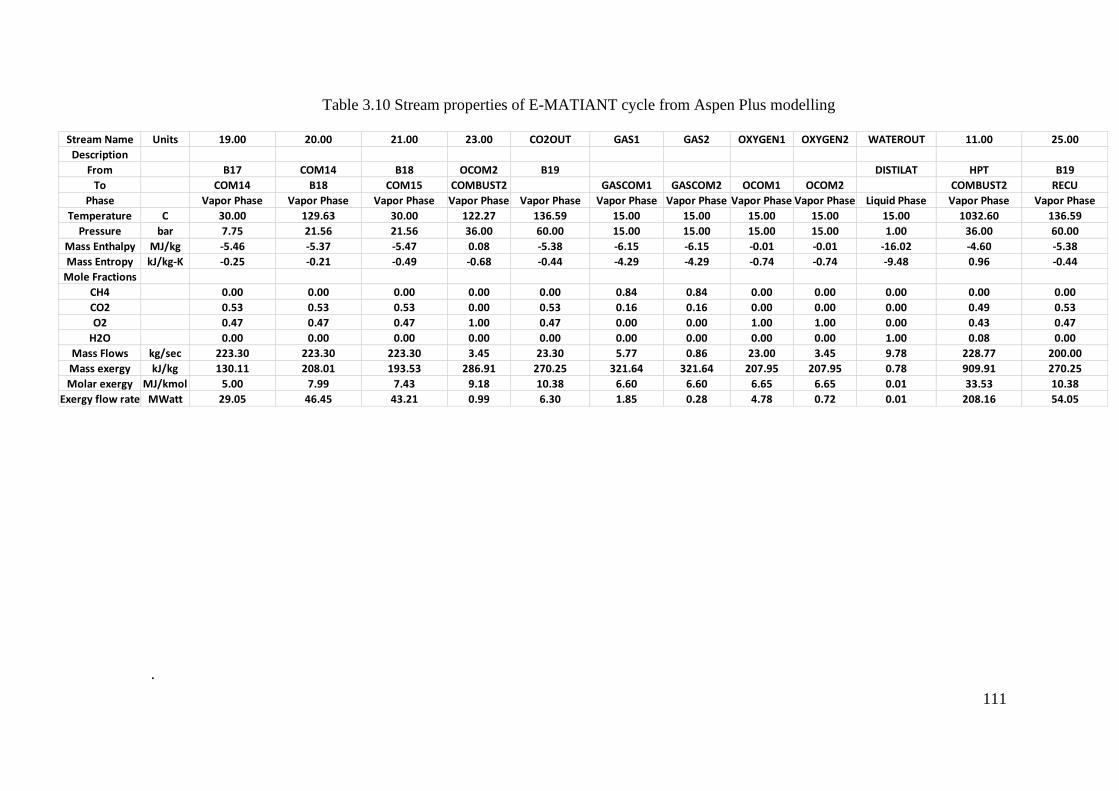
111
Table 3.10 Stream properties of E-MATIANT cycle from Aspen Plus modelling
.
Stream Name Units 19.00 20.00 21.00 23.00 CO2OUT GAS1 GAS2 OXYGEN1 OXYGEN2 WATEROUT 11.00 25.00
Description
From B17 COM14 B18 OCOM2 B19 DISTILAT HPT B19
To COM14 B18 COM15 COMBUST2 GASCOM1 GASCOM2 OCOM1 OCOM2 COMBUST2 RECU
Phase Vapor Phase Vapor Phase Vapor Phase Vapor Phase Vapor Phase Vapor Phase Vapor Phase Vapor Phase Vapor Phase Liquid Phase Vapor Phase Vapor Phase
Temperature C 30.00 129.63 30.00 122.27 136.59 15.00 15.00 15.00 15.00 15.00 1032.60 136.59
Pressure bar 7.75 21.56 21.56 36.00 60.00 15.00 15.00 15.00 15.00 1.00 36.00 60.00
Mass Enthalpy MJ/kg -5.46 -5.37 -5.47 0.08 -5.38 -6.15 -6.15 -0.01 -0.01 -16.02 -4.60 -5.38
Mass Entropy kJ/kg-K -0.25 -0.21 -0.49 -0.68 -0.44 -4.29 -4.29 -0.74 -0.74 -9.48 0.96 -0.44
Mole Fractions
CH4 0.00 0.00 0.00 0.00 0.00 0.84 0.84 0.00 0.00 0.00 0.00 0.00
CO2 0.53 0.53 0.53 0.00 0.53 0.16 0.16 0.00 0.00 0.00 0.49 0.53
O2 0.47 0.47 0.47 1.00 0.47 0.00 0.00 1.00 1.00 0.00 0.43 0.47
H2O 0.00 0.00 0.00 0.00 0.00 0.00 0.00 0.00 0.00 1.00 0.08 0.00
Mass Flows kg/sec 223.30 223.30 223.30 3.45 23.30 5.77 0.86 23.00 3.45 9.78 228.77 200.00
Mass exergy kJ/kg 130.11 208.01 193.53 286.91 270.25 321.64 321.64 207.95 207.95 0.78 909.91 270.25
Molar exergy MJ/kmol 5.00 7.99 7.43 9.18 10.38 6.60 6.60 6.65 6.65 0.01 33.53 10.38
Exergy flow rate MWatt 29.05 46.45 43.21 0.99 6.30 1.85 0.28 4.78 0.72 0.01 208.16 54.05
112
3.4.4 The CC_MATIANT cycle modelling and analysis
Figure 3.6 shows the CC-MATIANT cycle model in Aspen Plus software based on
the schematic presented in Figure 2.22 of chapter 2. The gas turbine cycle including
High-Pressure Turbine (HPT) and Low-Pressure Turbine (LPT).
Table 3.11 shows working flow properties at each stage for the CC-MATIANT
cycle, the main working flow for the steam cycle is water, and the recycled working
flow for the gas turbine is carbon dioxide.
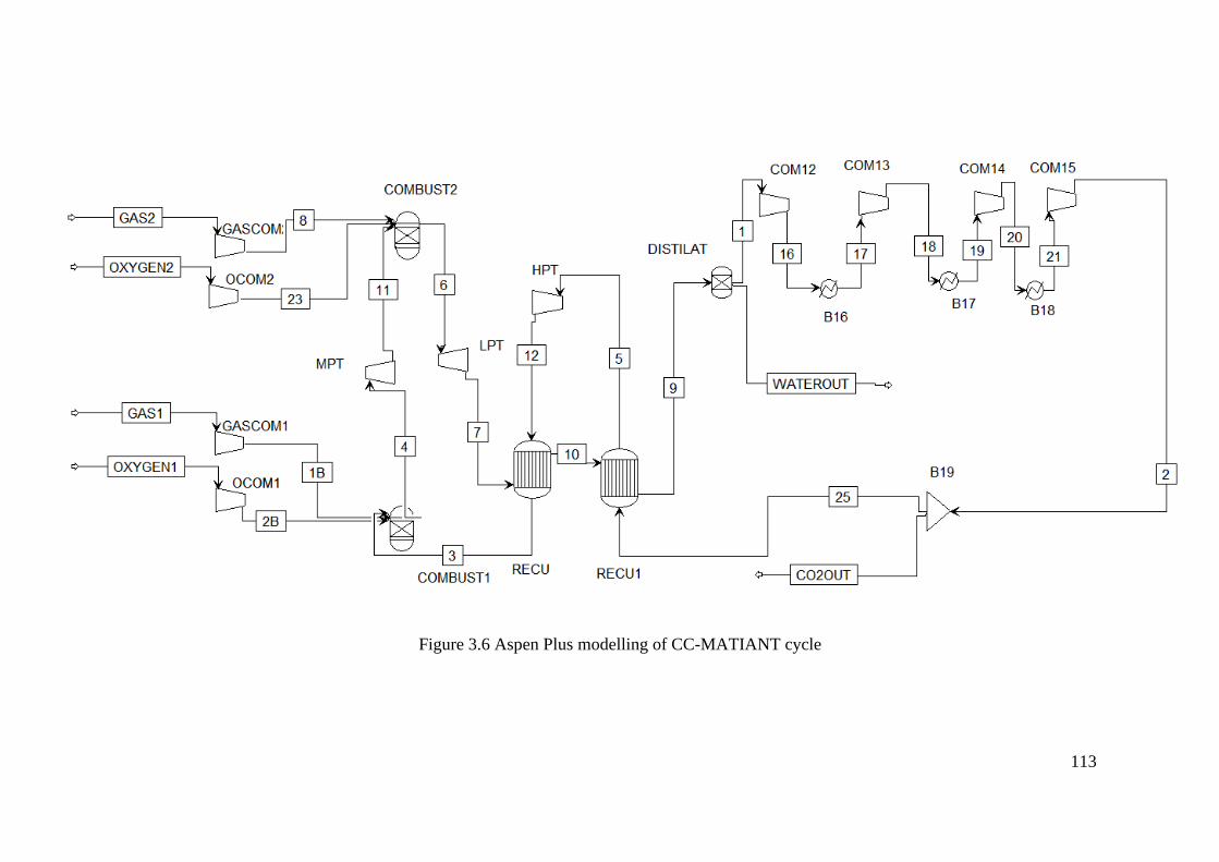
113
Figure 3.6 Aspen Plus modelling of CC-MATIANT cycle
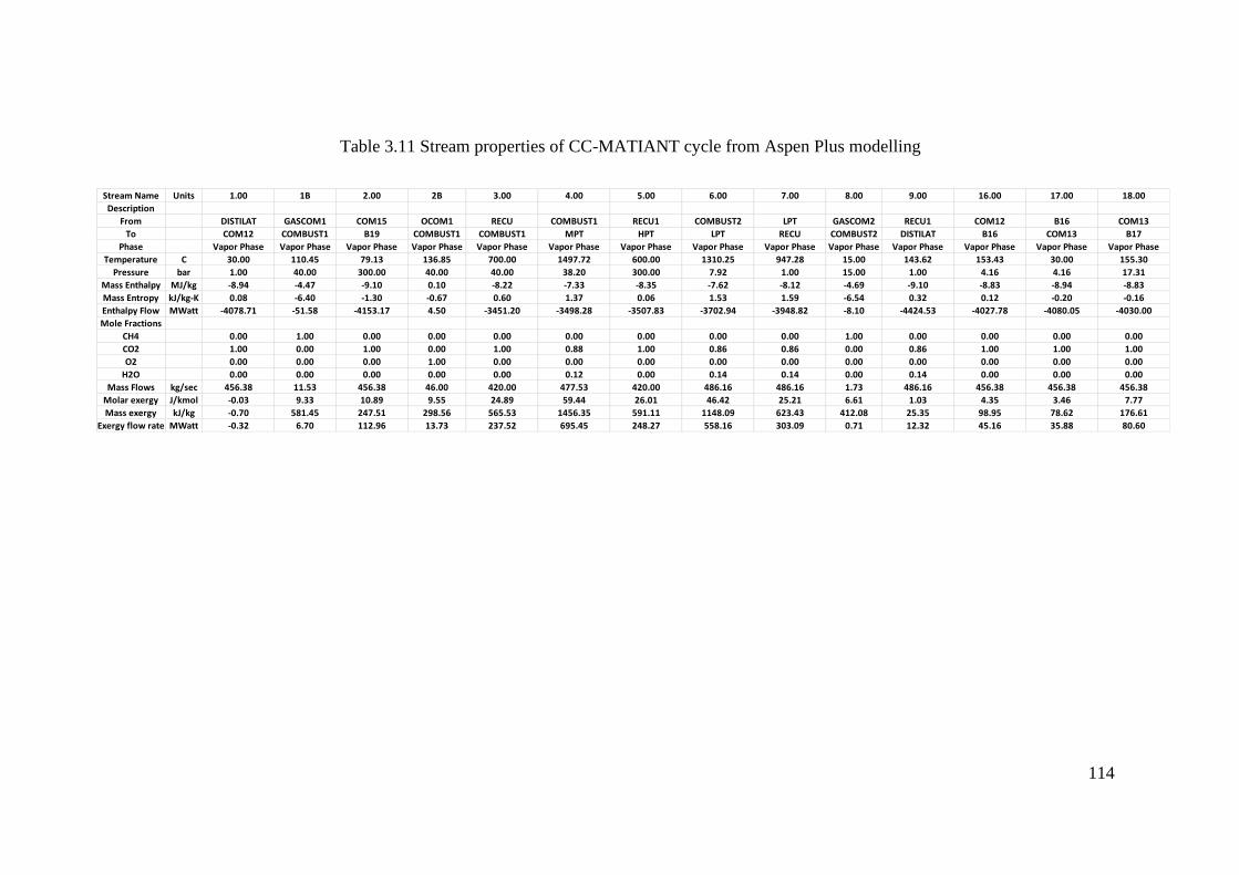
114
Table 3.11 Stream properties of CC-MATIANT cycle from Aspen Plus modelling
Stream Name Units 1.00 1B 2.00 2B 3.00 4.00 5.00 6.00 7.00 8.00 9.00 16.00 17.00 18.00
Description
From DISTILAT GASCOM1 COM15 OCOM1 RECU COMBUST1 RECU1 COMBUST2 LPT GASCOM2 RECU1 COM12 B16 COM13
To COM12 COMBUST1 B19 COMBUST1 COMBUST1 MPT HPT LPT RECU COMBUST2 DISTILAT B16 COM13 B17
Phase Vapor Phase Vapor Phase Vapor Phase Vapor Phase Vapor Phase Vapor Phase Vapor Phase Vapor Phase Vapor Phase Vapor Phase Vapor Phase Vapor Phase Vapor Phase Vapor Phase
Temperature C 30.00 110.45 79.13 136.85 700.00 1497.72 600.00 1310.25 947.28 15.00 143.62 153.43 30.00 155.30
Pressure bar 1.00 40.00 300.00 40.00 40.00 38.20 300.00 7.92 1.00 15.00 1.00 4.16 4.16 17.31
Mass Enthalpy MJ/kg -8.94 -4.47 -9.10 0.10 -8.22 -7.33 -8.35 -7.62 -8.12 -4.69 -9.10 -8.83 -8.94 -8.83
Mass Entropy kJ/kg-K 0.08 -6.40 -1.30 -0.67 0.60 1.37 0.06 1.53 1.59 -6.54 0.32 0.12 -0.20 -0.16
Enthalpy Flow MWatt -4078.71 -51.58 -4153.17 4.50 -3451.20 -3498.28 -3507.83 -3702.94 -3948.82 -8.10 -4424.53 -4027.78 -4080.05 -4030.00
Mole Fractions
CH4 0.00 1.00 0.00 0.00 0.00 0.00 0.00 0.00 0.00 1.00 0.00 0.00 0.00 0.00
CO2 1.00 0.00 1.00 0.00 1.00 0.88 1.00 0.86 0.86 0.00 0.86 1.00 1.00 1.00
O2 0.00 0.00 0.00 1.00 0.00 0.00 0.00 0.00 0.00 0.00 0.00 0.00 0.00 0.00
H2O 0.00 0.00 0.00 0.00 0.00 0.12 0.00 0.14 0.14 0.00 0.14 0.00 0.00 0.00
Mass Flows kg/sec 456.38 11.53 456.38 46.00 420.00 477.53 420.00 486.16 486.16 1.73 486.16 456.38 456.38 456.38
Molar exergy J/kmol -0.03 9.33 10.89 9.55 24.89 59.44 26.01 46.42 25.21 6.61 1.03 4.35 3.46 7.77
Mass exergy kJ/kg -0.70 581.45 247.51 298.56 565.53 1456.35 591.11 1148.09 623.43 412.08 25.35 98.95 78.62 176.61
Exergy flow rate MWatt -0.32 6.70 112.96 13.73 237.52 695.45 248.27 558.16 303.09 0.71 12.32 45.16 35.88 80.60
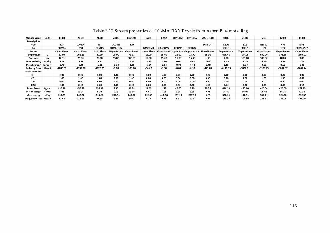
115
Table 3.12 Stream properties of CC-MATIANT cycle from Aspen Plus modelling
Stream Name Units 19.00 20.00 21.00 23.00 CO2OUT GAS1 GAS2 OXYGEN1 OXYGEN2 WATEROUT 10.00 25.00 5.00 12.00 11.00
Description
From B17 COM14 B18 OCOM2 B19 DISTILAT RECU B19 RECU1 HPT MPT
To COM14 B18 COM15 COMBUST2 GASCOM1 GASCOM2 OCOM1 OCOM2 RECU1 RECU1 HPT RECU COMBUST2
Phase Vapor Phase Vapor Phase Liquid Phase Vapor Phase Vapor Phase Vapor Phase Vapor Phase Vapor Phase Vapor Phase Liquid Phase Vapor Phase Vapor Phase Vapor Phase Vapor Phase Vapor Phase
Temperature C 30.00 165.81 30.00 15.00 79.13 15.00 15.00 15.00 15.00 15.00 696.42 79.13 600.00 375.36 1209.10
Pressure bar 17.31 75.00 75.00 15.00 300.00 15.00 15.00 15.00 15.00 1.00 1.00 300.00 300.00 40.00 9.00
Mass Enthalpy MJ/kg -8.95 -8.85 -9.14 -0.01 -9.10 -4.69 -4.69 -0.01 -0.01 -16.02 -8.45 -9.10 -8.35 -8.60 -7.74
Mass Entropy kJ/kg-K -0.49 -0.46 -1.31 -0.74 -1.30 -6.54 -6.54 -0.74 -0.74 -9.48 1.29 -1.30 0.06 0.12 1.41
Enthalpy Flow MWatt -4086.01 -4038.00 -4170.25 -0.10 -331.06 -54.02 -8.10 -0.64 -0.10 -477.00 -4110.25 -3822.11 -3507.83 -3612.62 -3694.74
Mole Fractions
CH4 0.00 0.00 0.00 0.00 0.00 1.00 1.00 0.00 0.00 0.00 0.00 0.00 0.00 0.00 0.00
CO2 1.00 1.00 1.00 0.00 1.00 0.00 0.00 0.00 0.00 0.00 0.86 1.00 1.00 1.00 0.88
O2 0.00 0.00 0.00 1.00 0.00 0.00 0.00 1.00 1.00 0.00 0.00 0.00 0.00 0.00 0.00
H2O 0.00 0.00 0.00 0.00 0.00 0.00 0.00 0.00 0.00 1.00 0.14 0.00 0.00 0.00 0.12
Mass Flows kg/sec 456.38 456.38 456.38 6.90 36.38 11.53 1.73 46.00 6.90 29.78 486.16 420.00 420.00 420.00 477.53
Molar exergy J/kmol 6.81 10.96 9.39 6.65 10.89 6.61 6.61 6.65 6.65 0.01 15.45 10.89 26.01 14.26 42.14
Mass exergy kJ/kg 154.75 249.07 213.26 207.95 247.51 412.08 412.08 207.95 207.95 0.78 382.10 247.51 591.11 324.00 1032.38
Exergy flow rate MWatt 70.63 113.67 97.33 1.43 9.00 4.75 0.71 9.57 1.43 0.02 185.76 103.95 248.27 136.08 493.00

116
3.4.5 The Graz cycle modelling and analysis
Figure 3.7 shows the Graz cycle model in Aspen Plus software based on the
schematic presented in Figure 2.26 of chapter 2; The cycle has two types of recycled
working flow. The water is pumped back to the combustion, and carbon dioxide is
compressed back to the combustion.
Table 3.13 shows working flow properties at each stage for the Graz cycle, the main
working flow for the steam cycle is water, and the recycled working flow for the gas
turbine is carbon dioxide.
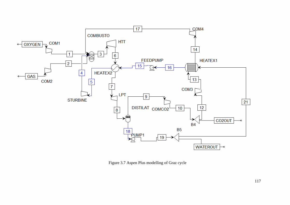
117
Figure 3.7 Aspen Plus modelling of Graz cycle
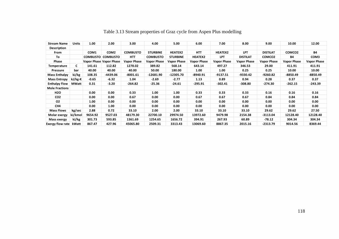
118
Table 3.13 Stream properties of Graz cycle from Aspen Plus modelling
Stream Name Units 1.00 2.00 3.00 4.00 5.00 6.00 7.00 8.00 9.00 10.00 12.00
Description
From COM1 COM2 COMBUSTO STURBINE HEATEX2 HTT HEATEX2 LPT DISTILAT COMCO2 B4
To COMBUSTO COMBUSTO HTT COMBUSTO STURBINE HEATEX2 LPT DISTILAT COMCO2 B4 COM3
Phase Vapor Phase Vapor Phase Vapor Phase Vapor Phase Vapor Phase Vapor Phase Vapor Phase Vapor Phase Vapor Phase Vapor Phase Vapor Phase
Temperature C 141.61 112.82 1278.02 389.82 568.14 643.14 497.27 346.53 29.00 411.91 411.91
Pressure bar 40.00 40.00 40.00 50.00 180.00 1.00 1.00 0.25 0.25 10.00 10.00
Mass Enthalpy kJ/kg 108.35 -4439.06 -8001.61 -12681.90 -12305.70 -8940.91 -9137.51 -9330.42 -9260.82 -8850.49 -8850.49
Mass Entropy kJ/kg-K -0.65 -6.32 1.04 -2.69 -2.77 1.13 0.89 0.94 0.28 0.37 0.37
Enthalpy Flow MWatt 0.31 -3.20 -264.82 -25.36 -24.61 -295.91 -302.41 -308.80 -274.30 -262.15 -243.39
Mole Fractions
H2O 0.00 0.00 0.33 1.00 1.00 0.33 0.33 0.33 0.16 0.16 0.16
CO2 0.00 0.00 0.67 0.00 0.00 0.67 0.67 0.67 0.84 0.84 0.84
O2 1.00 0.00 0.00 0.00 0.00 0.00 0.00 0.00 0.00 0.00 0.00
CH4 0.00 1.00 0.00 0.00 0.00 0.00 0.00 0.00 0.00 0.00 0.00
Mass Flows kg/sec 2.88 0.72 33.10 2.00 2.00 33.10 33.10 33.10 29.62 29.62 27.50
Molar exergy kJ/kmol 9654.92 9527.03 48179.30 22700.10 29974.50 13972.60 9479.98 2154.38 -3113.04 12128.40 12128.40
Mass exergy kJ/kg 301.73 593.85 1361.69 1254.65 1656.72 394.91 267.93 60.89 -78.12 304.34 304.34
Exergy flow rate kWatt 867.47 427.96 45065.80 2509.31 3313.43 13069.60 8867.35 2015.16 -2313.79 9014.56 8369.44
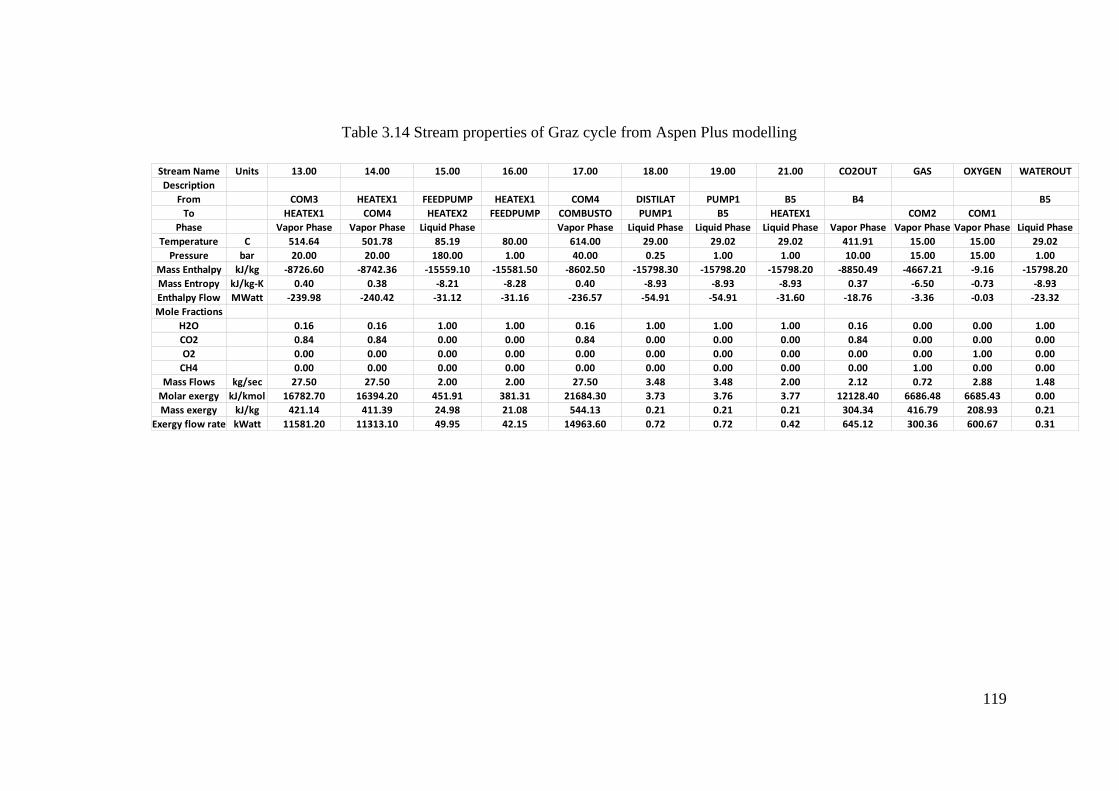
119
Table 3.14 Stream properties of Graz cycle from Aspen Plus modelling
Stream Name Units 13.00 14.00 15.00 16.00 17.00 18.00 19.00 21.00 CO2OUT GAS OXYGEN WATEROUT
Description
From COM3 HEATEX1 FEEDPUMP HEATEX1 COM4 DISTILAT PUMP1 B5 B4 B5
To HEATEX1 COM4 HEATEX2 FEEDPUMP COMBUSTO PUMP1 B5 HEATEX1 COM2 COM1
Phase Vapor Phase Vapor Phase Liquid Phase Vapor Phase Liquid Phase Liquid Phase Liquid Phase Vapor Phase Vapor Phase Vapor Phase Liquid Phase
Temperature C 514.64 501.78 85.19 80.00 614.00 29.00 29.02 29.02 411.91 15.00 15.00 29.02
Pressure bar 20.00 20.00 180.00 1.00 40.00 0.25 1.00 1.00 10.00 15.00 15.00 1.00
Mass Enthalpy kJ/kg -8726.60 -8742.36 -15559.10 -15581.50 -8602.50 -15798.30 -15798.20 -15798.20 -8850.49 -4667.21 -9.16 -15798.20
Mass Entropy kJ/kg-K 0.40 0.38 -8.21 -8.28 0.40 -8.93 -8.93 -8.93 0.37 -6.50 -0.73 -8.93
Enthalpy Flow MWatt -239.98 -240.42 -31.12 -31.16 -236.57 -54.91 -54.91 -31.60 -18.76 -3.36 -0.03 -23.32
Mole Fractions
H2O 0.16 0.16 1.00 1.00 0.16 1.00 1.00 1.00 0.16 0.00 0.00 1.00
CO2 0.84 0.84 0.00 0.00 0.84 0.00 0.00 0.00 0.84 0.00 0.00 0.00
O2 0.00 0.00 0.00 0.00 0.00 0.00 0.00 0.00 0.00 0.00 1.00 0.00
CH4 0.00 0.00 0.00 0.00 0.00 0.00 0.00 0.00 0.00 1.00 0.00 0.00
Mass Flows kg/sec 27.50 27.50 2.00 2.00 27.50 3.48 3.48 2.00 2.12 0.72 2.88 1.48
Molar exergy kJ/kmol 16782.70 16394.20 451.91 381.31 21684.30 3.73 3.76 3.77 12128.40 6686.48 6685.43 0.00
Mass exergy kJ/kg 421.14 411.39 24.98 21.08 544.13 0.21 0.21 0.21 304.34 416.79 208.93 0.21
Exergy flow rate kWatt 11581.20 11313.10 49.95 42.15 14963.60 0.72 0.72 0.42 645.12 300.36 600.67 0.31
120
3.4.6 The S-Graz cycle modelling and analysis
Figure 3.15 shows the S-Graz cycle model in Aspen Plus software based on the
schematic presented in Figure 2.27 of chapter 2. Table 3.15 shows working flow
properties at each stage for the S-Graz cycle, the recycled working flow is water, and
it is pumped back to the combustion. The other recycled working flow is the exhaust
of the turbine, and it is compressed back to the combustion, and composition is
mainly water and carbon dioxide.
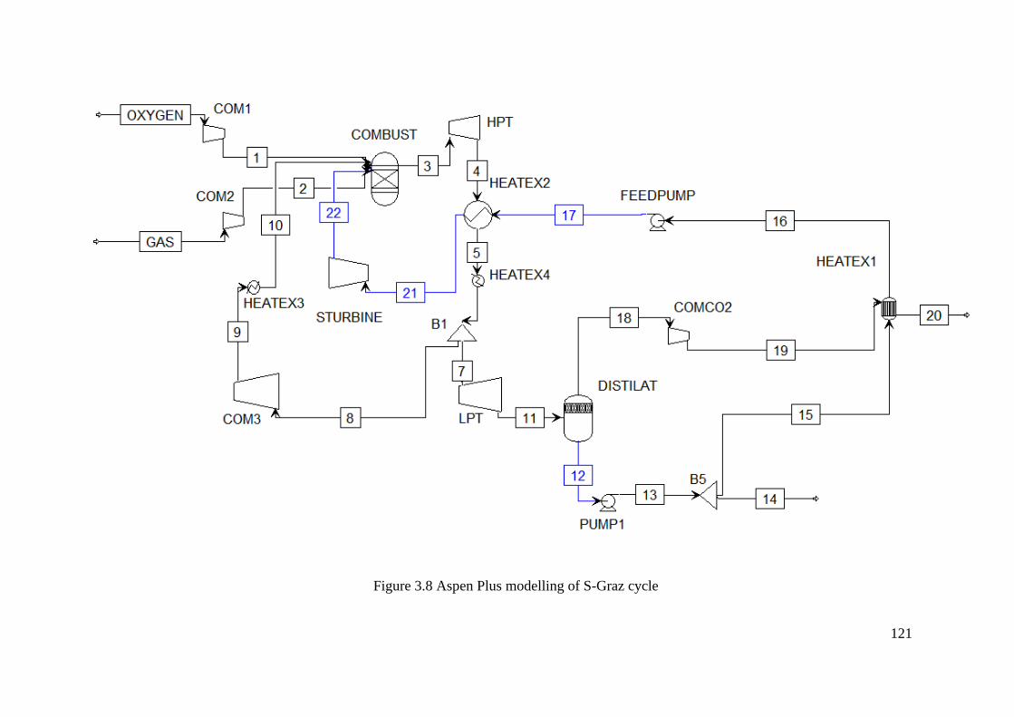
121
Figure 3.8 Aspen Plus modelling of S-Graz cycle
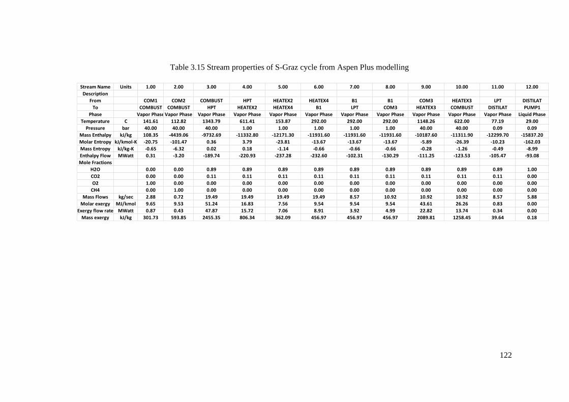
122
Table 3.15 Stream properties of S-Graz cycle from Aspen Plus modelling
Stream Name Units 1.00 2.00 3.00 4.00 5.00 6.00 7.00 8.00 9.00 10.00 11.00 12.00
Description
From COM1 COM2 COMBUST HPT HEATEX2 HEATEX4 B1 B1 COM3 HEATEX3 LPT DISTILAT
To COMBUST COMBUST HPT HEATEX2 HEATEX4 B1 LPT COM3 HEATEX3 COMBUST DISTILAT PUMP1
Phase Vapor PhaseVapor Phase Vapor Phase Vapor Phase Vapor Phase Vapor Phase Vapor Phase Vapor Phase Vapor Phase Vapor Phase Vapor Phase Liquid Phase
Temperature C 141.61 112.82 1343.79 611.41 153.87 292.00 292.00 292.00 1148.26 622.00 77.19 29.00
Pressure bar 40.00 40.00 40.00 1.00 1.00 1.00 1.00 1.00 40.00 40.00 0.09 0.09
Mass Enthalpy kJ/kg 108.35 -4439.06 -9732.69 -11332.80 -12171.30 -11931.60 -11931.60 -11931.60 -10187.60 -11311.90 -12299.70 -15837.20
Molar Entropy kJ/kmol-K -20.75 -101.47 0.36 3.79 -23.81 -13.67 -13.67 -13.67 -5.89 -26.39 -10.23 -162.03
Mass Entropy kJ/kg-K -0.65 -6.32 0.02 0.18 -1.14 -0.66 -0.66 -0.66 -0.28 -1.26 -0.49 -8.99
Enthalpy Flow MWatt 0.31 -3.20 -189.74 -220.93 -237.28 -232.60 -102.31 -130.29 -111.25 -123.53 -105.47 -93.08
Mole Fractions
H2O 0.00 0.00 0.89 0.89 0.89 0.89 0.89 0.89 0.89 0.89 0.89 1.00
CO2 0.00 0.00 0.11 0.11 0.11 0.11 0.11 0.11 0.11 0.11 0.11 0.00
O2 1.00 0.00 0.00 0.00 0.00 0.00 0.00 0.00 0.00 0.00 0.00 0.00
CH4 0.00 1.00 0.00 0.00 0.00 0.00 0.00 0.00 0.00 0.00 0.00 0.00
Mass Flows kg/sec 2.88 0.72 19.49 19.49 19.49 19.49 8.57 10.92 10.92 10.92 8.57 5.88
Molar exergy MJ/kmol 9.65 9.53 51.24 16.83 7.56 9.54 9.54 9.54 43.61 26.26 0.83 0.00
Exergy flow rate MWatt 0.87 0.43 47.87 15.72 7.06 8.91 3.92 4.99 22.82 13.74 0.34 0.00
Mass exergy kJ/kg 301.73 593.85 2455.35 806.34 362.09 456.97 456.97 456.97 2089.81 1258.45 39.64 0.18
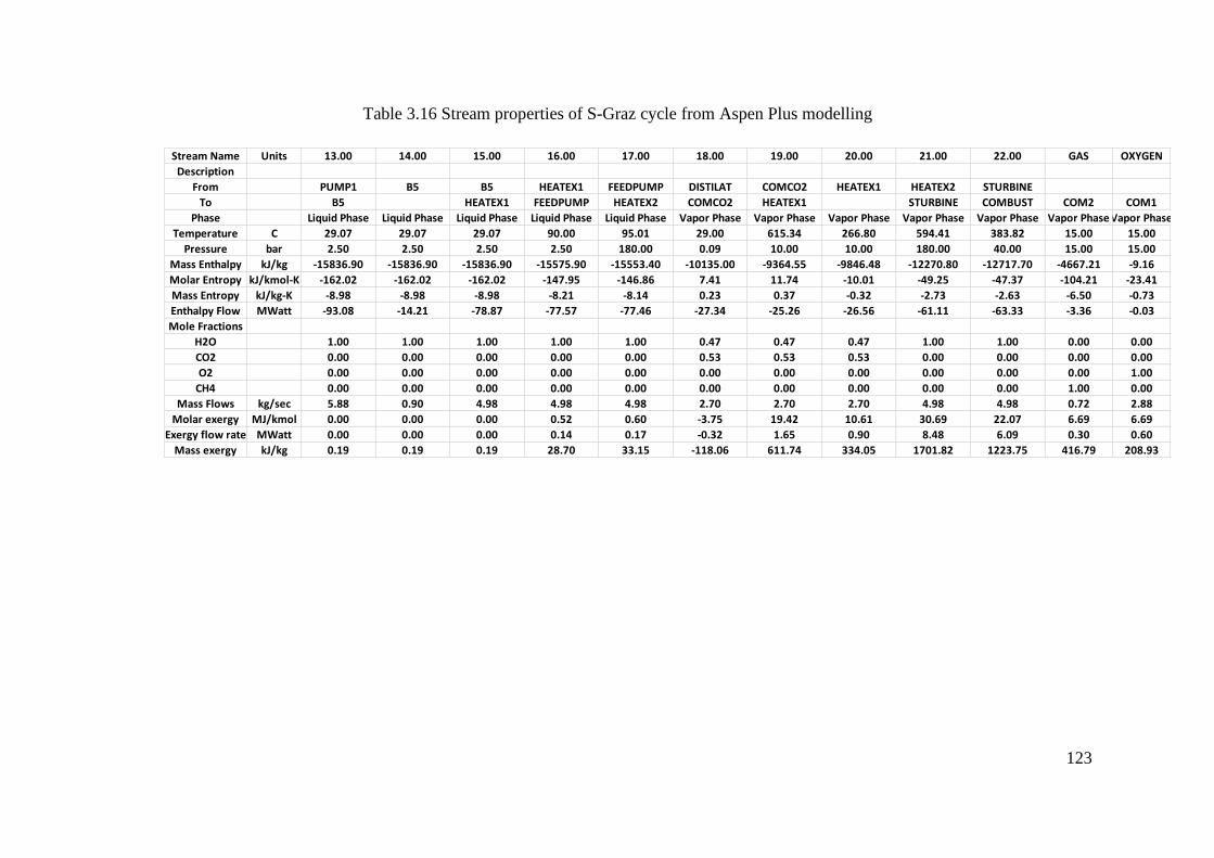
123
Table 3.16 Stream properties of S-Graz cycle from Aspen Plus modelling
Stream Name Units 13.00 14.00 15.00 16.00 17.00 18.00 19.00 20.00 21.00 22.00 GAS OXYGEN
Description
From PUMP1 B5 B5 HEATEX1 FEEDPUMP DISTILAT COMCO2 HEATEX1 HEATEX2 STURBINE
To B5 HEATEX1 FEEDPUMP HEATEX2 COMCO2 HEATEX1 STURBINE COMBUST COM2 COM1
Phase Liquid Phase Liquid Phase Liquid Phase Liquid Phase Liquid Phase Vapor Phase Vapor Phase Vapor Phase Vapor Phase Vapor Phase Vapor PhaseVapor Phase
Temperature C 29.07 29.07 29.07 90.00 95.01 29.00 615.34 266.80 594.41 383.82 15.00 15.00
Pressure bar 2.50 2.50 2.50 2.50 180.00 0.09 10.00 10.00 180.00 40.00 15.00 15.00
Mass Enthalpy kJ/kg -15836.90 -15836.90 -15836.90 -15575.90 -15553.40 -10135.00 -9364.55 -9846.48 -12270.80 -12717.70 -4667.21 -9.16
Molar Entropy kJ/kmol-K -162.02 -162.02 -162.02 -147.95 -146.86 7.41 11.74 -10.01 -49.25 -47.37 -104.21 -23.41
Mass Entropy kJ/kg-K -8.98 -8.98 -8.98 -8.21 -8.14 0.23 0.37 -0.32 -2.73 -2.63 -6.50 -0.73
Enthalpy Flow MWatt -93.08 -14.21 -78.87 -77.57 -77.46 -27.34 -25.26 -26.56 -61.11 -63.33 -3.36 -0.03
Mole Fractions
H2O 1.00 1.00 1.00 1.00 1.00 0.47 0.47 0.47 1.00 1.00 0.00 0.00
CO2 0.00 0.00 0.00 0.00 0.00 0.53 0.53 0.53 0.00 0.00 0.00 0.00
O2 0.00 0.00 0.00 0.00 0.00 0.00 0.00 0.00 0.00 0.00 0.00 1.00
CH4 0.00 0.00 0.00 0.00 0.00 0.00 0.00 0.00 0.00 0.00 1.00 0.00
Mass Flows kg/sec 5.88 0.90 4.98 4.98 4.98 2.70 2.70 2.70 4.98 4.98 0.72 2.88
Molar exergy MJ/kmol 0.00 0.00 0.00 0.52 0.60 -3.75 19.42 10.61 30.69 22.07 6.69 6.69
Exergy flow rate MWatt 0.00 0.00 0.00 0.14 0.17 -0.32 1.65 0.90 8.48 6.09 0.30 0.60
Mass exergy kJ/kg 0.19 0.19 0.19 28.70 33.15 -118.06 611.74 334.05 1701.82 1223.75 416.79 208.93

124
3.4.7 The AZEP 100% cycle modelling and analysis
Figure 3.9 shows the CC-MATIANT cycle model in Aspen Plus software based
on the schematic presented in Figure 2.28 of chapter 2. Table 3.17 shows stream
properties at each stage for AZEP 100% cycle; there are three working flows in this
cycle. In the air cycle, working flow is air, and air enters MCM after compression,
then depleted hot air enters the turbine for expansion. In the steam cycle, water is
working flow, and steam enters the turbine after recovery heat. In the gas turbine
cycle, the working flow is a mixture of water and carbon dioxide, and the hot stream
enters the gas turbine for expansion after the MCM unit.
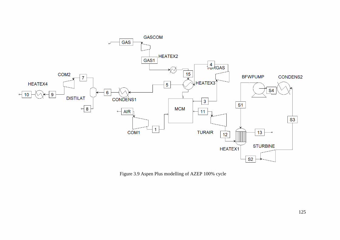
125
Figure 3.9 Aspen Plus modelling of AZEP 100% cycle
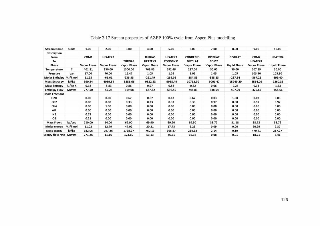
126
Table 3.17 Stream properties of AZEP 100% cycle from Aspen Plus modelling
Stream Name Units 1.00 2.00 3.00 4.00 5.00 6.00 7.00 8.00 9.00 10.00
Description
From COM1 HEATEX3 TURGAS HEATEX3 CONDENS1 DISTILAT DISTILAT COM2 HEATEX4
To TURGAS HEATEX3 CONDENS1 DISTILAT COM2 HEATEX4
Phase Vapor Phase Vapor Phase Vapor Phase Vapor Phase Vapor Phase Vapor Phase Vapor Phase Liquid Phase Vapor Phase Liquid Phase
Temperature C 401.81 250.00 1300.00 769.85 692.48 217.00 30.00 30.00 507.89 30.00
Pressure bar 17.00 70.00 16.47 1.05 1.05 1.05 1.05 1.05 103.90 103.90
Molar Enthalpy MJ/kmol 11.28 -65.61 -235.53 -261.49 -265.02 -284.89 -388.23 -287.34 -367.21 -399.40
Mass Enthalpy kJ/kg 390.84 -4089.54 -8856.66 -9832.83 -9965.49 -10712.90 -9001.47 -15949.20 -8514.09 -9260.33
Mass Entropy kJ/kg-K 0.18 -5.83 0.86 0.97 0.84 -0.22 0.06 -9.25 0.13 -1.53
Enthalpy Flow MWatt 277.50 -57.25 -619.08 -687.32 -696.59 -748.83 -348.54 -497.29 -329.67 -358.56
Mole Fractions
H2O 0.00 0.00 0.67 0.67 0.67 0.67 0.03 1.00 0.03 0.03
CO2 0.00 0.00 0.33 0.33 0.33 0.33 0.97 0.00 0.97 0.97
CH4 0.00 1.00 0.00 0.00 0.00 0.00 0.00 0.00 0.00 0.00
AIR 0.00 0.00 0.00 0.00 0.00 0.00 0.00 0.00 0.00 0.00
N2 0.79 0.00 0.00 0.00 0.00 0.00 0.00 0.00 0.00 0.00
O2 0.21 0.00 0.00 0.00 0.00 0.00 0.00 0.00 0.00 0.00
Mass Flows kg/sec 710.00 14.00 69.90 69.90 69.90 69.90 38.72 31.18 38.72 38.72
Molar exergy MJ/kmol 11.02 12.79 47.02 20.21 17.73 6.23 0.09 0.00 20.29 9.37
Mass exergy kJ/kg 382.06 797.26 1768.27 760.13 666.87 234.33 2.14 0.19 470.41 217.27
Exergy flow rate MWatt 271.26 11.16 123.60 53.13 46.61 16.38 0.08 0.01 18.21 8.41
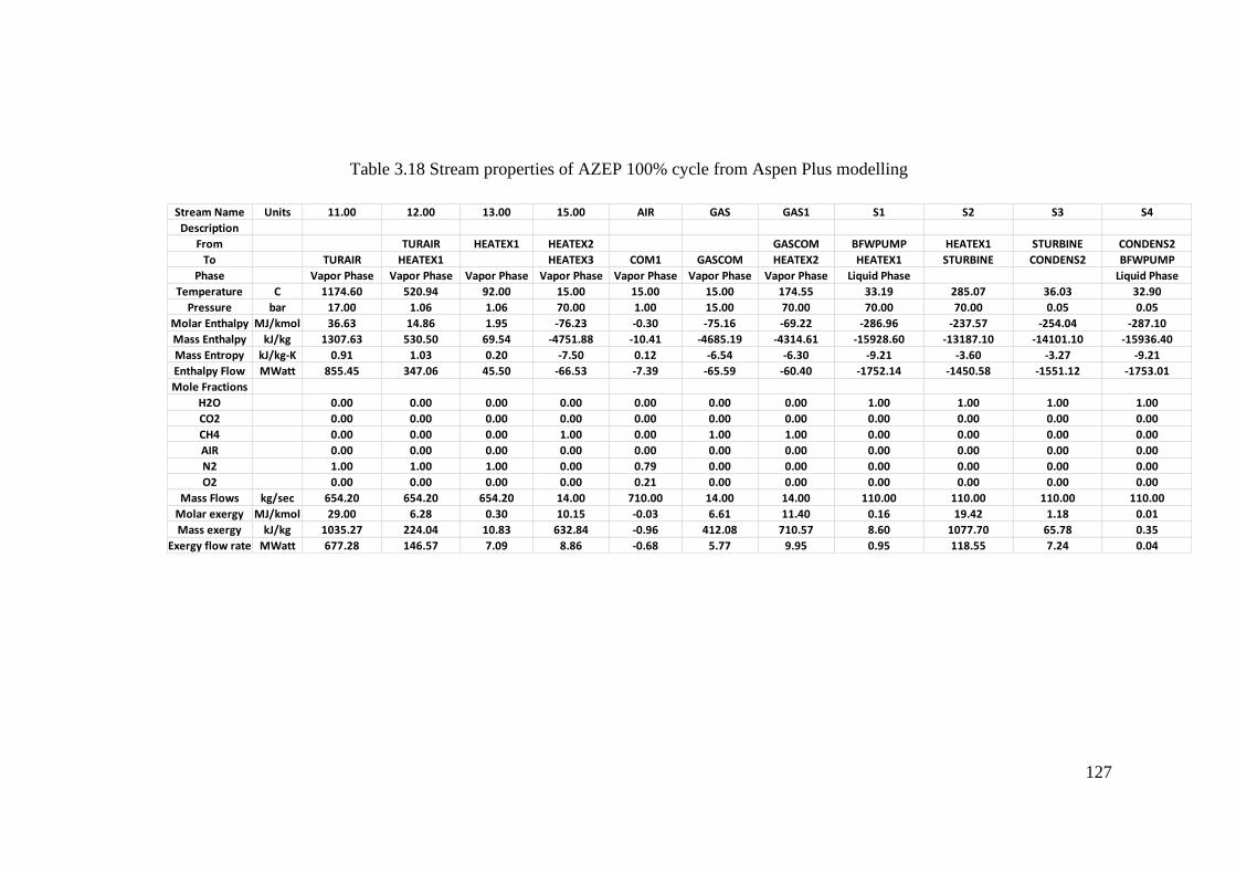
127
Table 3.18 Stream properties of AZEP 100% cycle from Aspen Plus modelling
Stream Name Units 11.00 12.00 13.00 15.00 AIR GAS GAS1 S1 S2 S3 S4
Description
From TURAIR HEATEX1 HEATEX2 GASCOM BFWPUMP HEATEX1 STURBINE CONDENS2
To TURAIR HEATEX1 HEATEX3 COM1 GASCOM HEATEX2 HEATEX1 STURBINE CONDENS2 BFWPUMP
Phase Vapor Phase Vapor Phase Vapor Phase Vapor Phase Vapor Phase Vapor Phase Vapor Phase Liquid Phase Liquid Phase
Temperature C 1174.60 520.94 92.00 15.00 15.00 15.00 174.55 33.19 285.07 36.03 32.90
Pressure bar 17.00 1.06 1.06 70.00 1.00 15.00 70.00 70.00 70.00 0.05 0.05
Molar Enthalpy MJ/kmol 36.63 14.86 1.95 -76.23 -0.30 -75.16 -69.22 -286.96 -237.57 -254.04 -287.10
Mass Enthalpy kJ/kg 1307.63 530.50 69.54 -4751.88 -10.41 -4685.19 -4314.61 -15928.60 -13187.10 -14101.10 -15936.40
Mass Entropy kJ/kg-K 0.91 1.03 0.20 -7.50 0.12 -6.54 -6.30 -9.21 -3.60 -3.27 -9.21
Enthalpy Flow MWatt 855.45 347.06 45.50 -66.53 -7.39 -65.59 -60.40 -1752.14 -1450.58 -1551.12 -1753.01
Mole Fractions
H2O 0.00 0.00 0.00 0.00 0.00 0.00 0.00 1.00 1.00 1.00 1.00
CO2 0.00 0.00 0.00 0.00 0.00 0.00 0.00 0.00 0.00 0.00 0.00
CH4 0.00 0.00 0.00 1.00 0.00 1.00 1.00 0.00 0.00 0.00 0.00
AIR 0.00 0.00 0.00 0.00 0.00 0.00 0.00 0.00 0.00 0.00 0.00
N2 1.00 1.00 1.00 0.00 0.79 0.00 0.00 0.00 0.00 0.00 0.00
O2 0.00 0.00 0.00 0.00 0.21 0.00 0.00 0.00 0.00 0.00 0.00
Mass Flows kg/sec 654.20 654.20 654.20 14.00 710.00 14.00 14.00 110.00 110.00 110.00 110.00
Molar exergy MJ/kmol 29.00 6.28 0.30 10.15 -0.03 6.61 11.40 0.16 19.42 1.18 0.01
Mass exergy kJ/kg 1035.27 224.04 10.83 632.84 -0.96 412.08 710.57 8.60 1077.70 65.78 0.35
Exergy flow rate MWatt 677.28 146.57 7.09 8.86 -0.68 5.77 9.95 0.95 118.55 7.24 0.04
128
3.4.8 The ZEITMOP cycle modelling and analysis
Figure 3.10 shows the Zero Emission Ion Transport Membrane Oxygen Power
(ZEITMOP) cycle model in Aspen Plus software based on the schematic presented in
Figure 2.30 of chapter 2; ZEITMOP cycle is integrated to a high-temperature
membrane for oxygen production (OTM). As the membrane requires a hot pressurized
air stream to separate O2, the externally heated air cycle can be present as a side cycle
of the principal CO2 cycle (ZEITMOP) or as the main power cycle (AZEP) (Ferrari et
al., 2017a). Table 3.19 shows stream properties at each stage for the ZEITMOP cycle;
there are three types of working flow in the cycle.
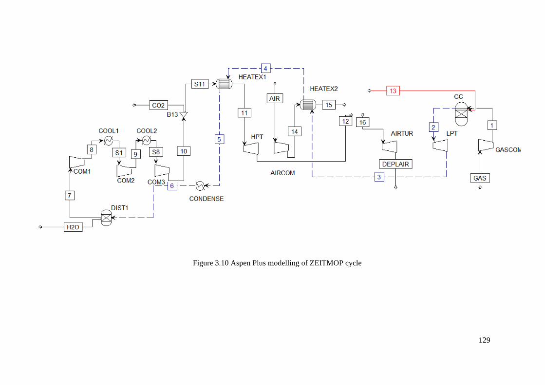
129
Figure 3.10 Aspen Plus modelling of ZEITMOP cycle
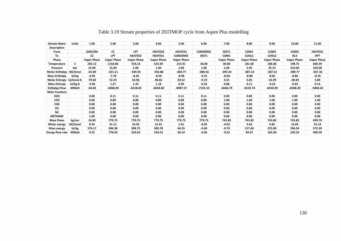
130
Table 3.19 Stream properties of ZEITMOP cycle from Aspen Plus modelling
Stream Name Units 1.00 2.00 3.00 4.00 5.00 6.00 7.00 8.00 9.00 10.00 11.00
Description
From GASCOM CC LPT HEATEX2 HEATEX1 CONDENSE DIST1 COM1 COM2 COM3 HEATEX1
To CC LPT HEATEX2 HEATEX1 CONDENSE DIST1 COM1 COOL1 COOL2 B13 HPT
Phase Vapor Phase Vapor Phase Vapor Phase Vapor Phase Vapor Phase Vapor Phase Vapor Phase Vapor Phase Vapor Phase Vapor Phase
Temperature C 256.12 1156.86 724.23 610.39 213.91 30.00 30.00 181.60 186.06 198.75 600.39
Pressure bar 15.00 15.00 1.00 1.00 1.00 1.00 1.00 5.95 35.33 210.00 210.00
Molar Enthalpy MJ/kmol -65.00 -321.11 -344.95 -350.88 -369.77 -380.56 -393.24 -387.14 -387.52 -389.77 -367.32
Mass Enthalpy kJ/kg -4.05 -7.78 -8.36 -8.50 -8.96 -9.22 -8.94 -8.80 -8.81 -8.86 -8.35
Molar Entropy kJ/kmol-K -79.64 52.24 54.96 48.66 20.52 -9.19 3.55 5.05 -10.29 -28.69 5.89
Mass Entropy kJ/kg-K -4.96 1.27 1.33 1.18 0.50 -0.22 0.08 0.11 -0.23 -0.65 0.13
Enthalpy Flow MWatt -64.82 -6068.05 -6518.69 -6630.60 -6987.57 -7191.53 -6646.79 -6543.74 -6550.09 -6588.20 -5840.42
Mole Fractions
H2O 0.00 0.11 0.11 0.11 0.11 0.11 0.00 0.00 0.00 0.00 0.00
CO2 0.00 0.89 0.89 0.89 0.89 0.89 1.00 1.00 1.00 1.00 1.00
CH4 0.00 0.00 0.00 0.00 0.00 0.00 0.00 0.00 0.00 0.00 0.00
O2 0.00 0.00 0.00 0.00 0.00 0.00 0.00 0.00 0.00 0.00 0.00
N2 0.00 0.00 0.00 0.00 0.00 0.00 0.00 0.00 0.00 0.00 0.00
METHANE 1.00 0.00 0.00 0.00 0.00 0.00 0.00 0.00 0.00 0.00 0.00
Mass Flows kg/sec 16.00 779.75 779.75 779.75 779.75 779.75 743.82 743.82 743.82 743.82 699.70
Molar exergy MJ/kmol 9.24 41.11 16.45 12.41 1.91 -0.02 -0.03 5.62 9.82 13.05 25.19
Mass exergy kJ/kg 576.17 996.38 398.75 300.78 46.35 -0.60 -0.70 127.68 223.09 296.50 572.39
Exergy flow rate MWatt 9.22 776.93 310.93 234.53 36.14 -0.46 -0.52 94.97 165.94 220.54 400.50
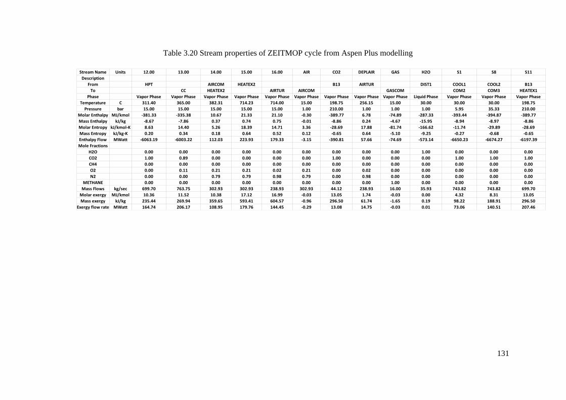
131
Table 3.20 Stream properties of ZEITMOP cycle from Aspen Plus modelling
Stream Name Units 12.00 13.00 14.00 15.00 16.00 AIR CO2 DEPLAIR GAS H2O S1 S8 S11
Description
From HPT AIRCOM HEATEX2 B13 AIRTUR DIST1 COOL1 COOL2 B13
To CC HEATEX2 AIRTUR AIRCOM GASCOM COM2 COM3 HEATEX1
Phase Vapor Phase Vapor Phase Vapor Phase Vapor Phase Vapor Phase Vapor Phase Vapor Phase Vapor Phase Vapor Phase Liquid Phase Vapor Phase Vapor Phase Vapor Phase
Temperature C 311.40 365.00 382.31 714.23 714.00 15.00 198.75 256.15 15.00 30.00 30.00 30.00 198.75
Pressure bar 15.00 15.00 15.00 15.00 15.00 1.00 210.00 1.00 1.00 1.00 5.95 35.33 210.00
Molar Enthalpy MJ/kmol -381.33 -335.38 10.67 21.33 21.10 -0.30 -389.77 6.78 -74.89 -287.33 -393.44 -394.87 -389.77
Mass Enthalpy kJ/kg -8.67 -7.86 0.37 0.74 0.75 -0.01 -8.86 0.24 -4.67 -15.95 -8.94 -8.97 -8.86
Molar Entropy kJ/kmol-K 8.63 14.40 5.26 18.39 14.71 3.36 -28.69 17.88 -81.74 -166.62 -11.74 -29.89 -28.69
Mass Entropy kJ/kg-K 0.20 0.34 0.18 0.64 0.52 0.12 -0.65 0.64 -5.10 -9.25 -0.27 -0.68 -0.65
Enthalpy Flow MWatt -6063.19 -6003.22 112.03 223.93 179.33 -3.15 -390.81 57.66 -74.69 -573.14 -6650.23 -6674.27 -6197.39
Mole Fractions
H2O 0.00 0.00 0.00 0.00 0.00 0.00 0.00 0.00 0.00 1.00 0.00 0.00 0.00
CO2 1.00 0.89 0.00 0.00 0.00 0.00 1.00 0.00 0.00 0.00 1.00 1.00 1.00
CH4 0.00 0.00 0.00 0.00 0.00 0.00 0.00 0.00 0.00 0.00 0.00 0.00 0.00
O2 0.00 0.11 0.21 0.21 0.02 0.21 0.00 0.02 0.00 0.00 0.00 0.00 0.00
N2 0.00 0.00 0.79 0.79 0.98 0.79 0.00 0.98 0.00 0.00 0.00 0.00 0.00
METHANE 0.00 0.00 0.00 0.00 0.00 0.00 0.00 0.00 1.00 0.00 0.00 0.00 0.00
Mass Flows kg/sec 699.70 763.75 302.93 302.93 238.93 302.93 44.12 238.93 16.00 35.93 743.82 743.82 699.70
Molar exergy MJ/kmol 10.36 11.52 10.38 17.12 16.99 -0.03 13.05 1.74 -0.03 0.00 4.32 8.31 13.05
Mass exergy kJ/kg 235.44 269.94 359.65 593.41 604.57 -0.96 296.50 61.74 -1.65 0.19 98.22 188.91 296.50
Exergy flow rate MWatt 164.74 206.17 108.95 179.76 144.45 -0.29 13.08 14.75 -0.03 0.01 73.06 140.51 207.46

132
3.4.9 The COOLCEP-S cycle modelling and analysis
Figure 3.11 shows the Cool Clean Efficient Power (COOLCEP) -S cycle model in
Aspen Plus software based on the schematic presented in Figure 2.32 of chapter 2;
Table 3.21 shows stream properties and each stage for COOLCEP-S cycle, there are
two main streams in this cycle.
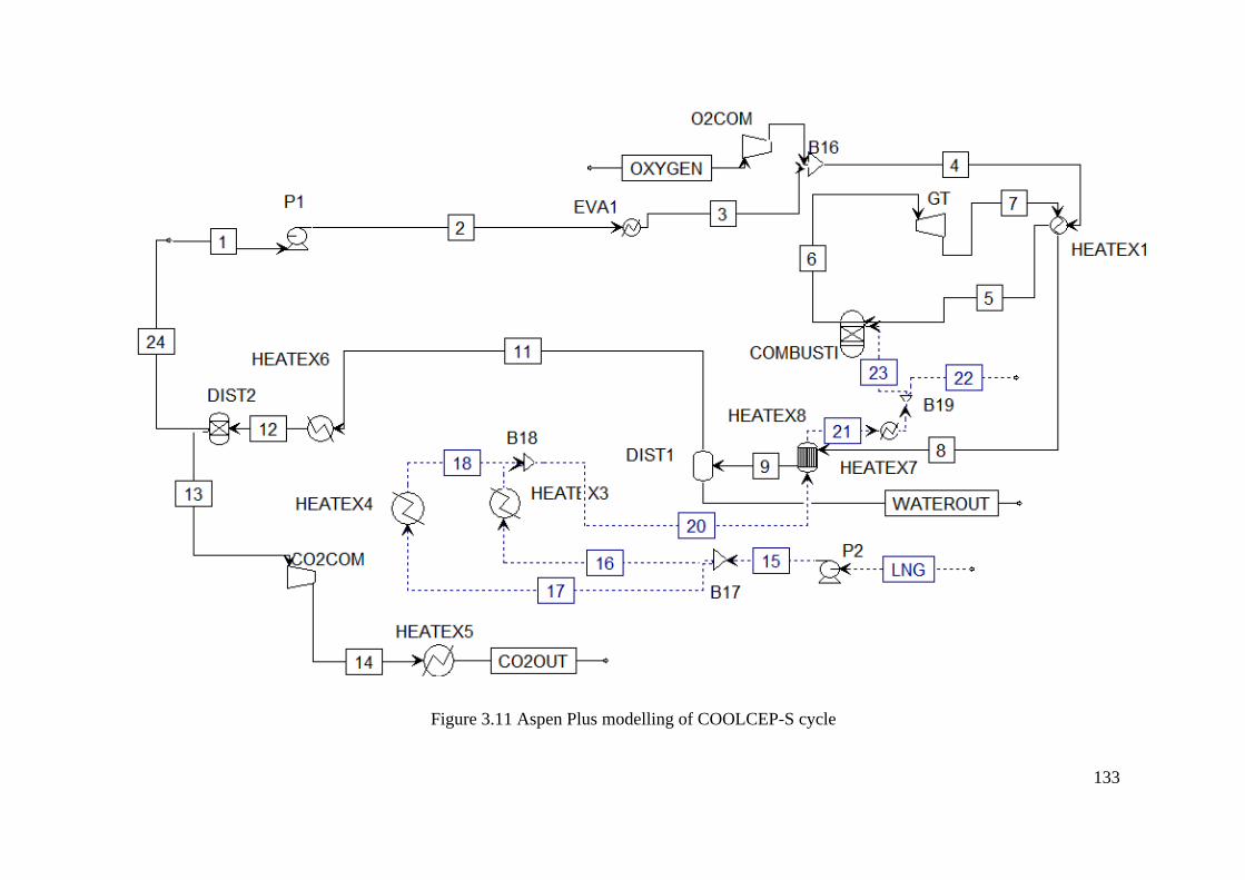
133
Figure 3.11 Aspen Plus modelling of COOLCEP-S cycle
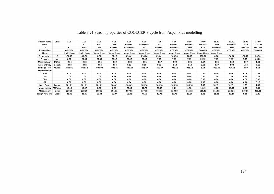
134
Table 3.21 Stream properties of COOLCEP-S cycle from Aspen Plus modelling
Stream Name Units 1.00 2.00 3.00 4.00 5.00 6.00 7.00 8.00 9.00 10.00 11.00 12.00 13.00 14.00
From P1 EVA1 B16 HEATEX1 COMBUSTI GT HEATEX1 HEATEX8 O2COM DIST1 HEATEX6 DIST2 CO2COM
To P1 EVA1 B16 HEATEX1 COMBUSTI GT HEATEX1 HEATEX8 DIST1 B16 HEATEX6 DIST2 CO2COM HEATEX5
Stream Class CONVEN CONVEN CONVEN CONVEN CONVEN CONVEN CONVEN CONVEN CONVEN CONVEN CONVEN CONVEN CONVEN CONVEN
Phase Liquid Phase Liquid Phase Vapor Phase Vapor Phase Vapor Phase Vapor Phase Vapor Phase Vapor Phase Vapor Phase Vapor Phase Vapor Phase
Temperature C -50.10 -48.84 8.00 27.16 650.41 898.80 696.41 105.36 74.00 596.04 0.00 -50.10 -50.10 20.30
Pressure bar 6.97 29.68 29.40 29.12 29.12 29.12 7.15 7.15 7.15 29.12 7.15 7.15 7.15 60.00
Mass Enthalpy MJ/kg -9.34 -9.33 -8.96 -8.69 -8.03 -8.01 -8.27 -8.92 -8.95 0.57 -8.95 -9.32 -8.17 -8.06
Mass Entropy kJ/kg-K -2.03 -2.02 -0.62 -0.54 0.62 0.89 0.92 -0.10 -0.18 0.18 -0.37 -2.02 -1.13 -1.02
Enthalpy Flow MWatt -948.81 -948.52 -909.98 -908.35 -839.20 -842.47 -869.37 -938.51 -941.58 1.64 -919.40 -957.62 -8.89 -8.76
Mole Fractions
H2O 0.00 0.00 0.00 0.00 0.00 0.04 0.04 0.04 0.04 0.00 0.00 0.00 0.06 0.06
CO2 1.00 1.00 1.00 0.96 0.96 0.96 0.96 0.96 0.96 0.00 1.00 1.00 0.78 0.78
CH4 0.00 0.00 0.00 0.00 0.00 0.00 0.00 0.00 0.00 0.00 0.00 0.00 0.00 0.00
O2 0.00 0.00 0.00 0.04 0.04 0.00 0.00 0.00 0.00 1.00 0.00 0.00 0.16 0.16
Mass Flows kg/sec 101.61 101.61 101.61 104.49 104.49 105.18 105.18 105.18 105.18 2.88 102.71 102.71 1.09 1.09
Molar exergy MJ/kmol 10.10 10.07 8.37 8.33 22.13 31.78 20.37 5.21 4.98 16.49 4.88 10.04 6.07 9.35
Mass exergy kJ/kg 229.38 228.79 190.12 191.12 507.96 737.78 472.78 120.90 115.72 515.46 111.08 228.26 149.67 230.31
Exergy flow rate Watt 23.31 23.25 19.32 19.97 53.08 77.60 49.73 12.72 12.17 1.48 11.41 23.44 0.16 0.25
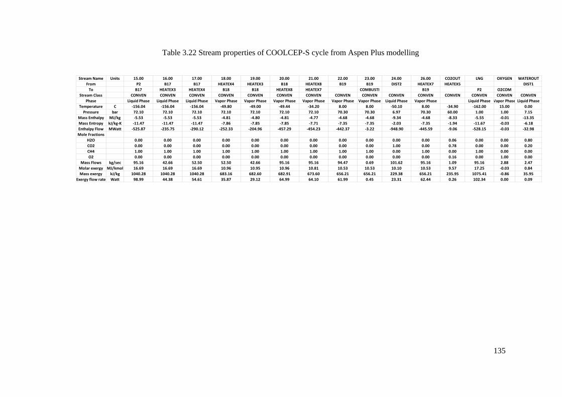
135
Table 3.22 Stream properties of COOLCEP-S cycle from Aspen Plus modelling
Stream Name Units 15.00 16.00 17.00 18.00 19.00 20.00 21.00 22.00 23.00 24.00 26.00 CO2OUT LNG OXYGEN WATEROUT
From P2 B17 B17 HEATEX4 HEATEX3 B18 HEATEX8 B19 B19 DIST2 HEATEX7 HEATEX5 DIST1
To B17 HEATEX3 HEATEX4 B18 B18 HEATEX8 HEATEX7 COMBUSTI B19 P2 O2COM
Stream Class CONVEN CONVEN CONVEN CONVEN CONVEN CONVEN CONVEN CONVEN CONVEN CONVEN CONVEN CONVEN CONVEN CONVEN CONVEN
Phase Liquid Phase Liquid Phase Liquid Phase Vapor Phase Vapor Phase Vapor Phase Vapor Phase Vapor Phase Vapor Phase Liquid Phase Vapor Phase Liquid Phase Vapor Phase Liquid Phase
Temperature C -156.04 -156.04 -156.04 -49.80 -49.00 -49.44 -34.20 8.00 8.00 -50.10 8.00 -34.90 -162.00 15.00 0.00
Pressure bar 72.10 72.10 72.10 72.10 72.10 72.10 72.10 70.30 70.30 6.97 70.30 60.00 1.00 1.00 7.15
Mass Enthalpy MJ/kg -5.53 -5.53 -5.53 -4.81 -4.80 -4.81 -4.77 -4.68 -4.68 -9.34 -4.68 -8.33 -5.55 -0.01 -13.35
Mass Entropy kJ/kg-K -11.47 -11.47 -11.47 -7.86 -7.85 -7.85 -7.71 -7.35 -7.35 -2.03 -7.35 -1.94 -11.67 -0.03 -6.18
Enthalpy Flow MWatt -525.87 -235.75 -290.12 -252.33 -204.96 -457.29 -454.23 -442.37 -3.22 -948.90 -445.59 -9.06 -528.15 -0.03 -32.98
Mole Fractions
H2O 0.00 0.00 0.00 0.00 0.00 0.00 0.00 0.00 0.00 0.00 0.00 0.06 0.00 0.00 0.80
CO2 0.00 0.00 0.00 0.00 0.00 0.00 0.00 0.00 0.00 1.00 0.00 0.78 0.00 0.00 0.20
CH4 1.00 1.00 1.00 1.00 1.00 1.00 1.00 1.00 1.00 0.00 1.00 0.00 1.00 0.00 0.00
O2 0.00 0.00 0.00 0.00 0.00 0.00 0.00 0.00 0.00 0.00 0.00 0.16 0.00 1.00 0.00
Mass Flows kg/sec 95.16 42.66 52.50 52.50 42.66 95.16 95.16 94.47 0.69 101.62 95.16 1.09 95.16 2.88 2.47
Molar exergy MJ/kmol 16.69 16.69 16.69 10.96 10.95 10.96 10.81 10.53 10.53 10.10 10.53 9.57 17.25 -0.03 0.84
Mass exergy kJ/kg 1040.28 1040.28 1040.28 683.16 682.60 682.91 673.60 656.21 656.21 229.38 656.21 235.95 1075.41 -0.86 35.95
Exergy flow rate Watt 98.99 44.38 54.61 35.87 29.12 64.99 64.10 61.99 0.45 23.31 62.44 0.26 102.34 0.00 0.09
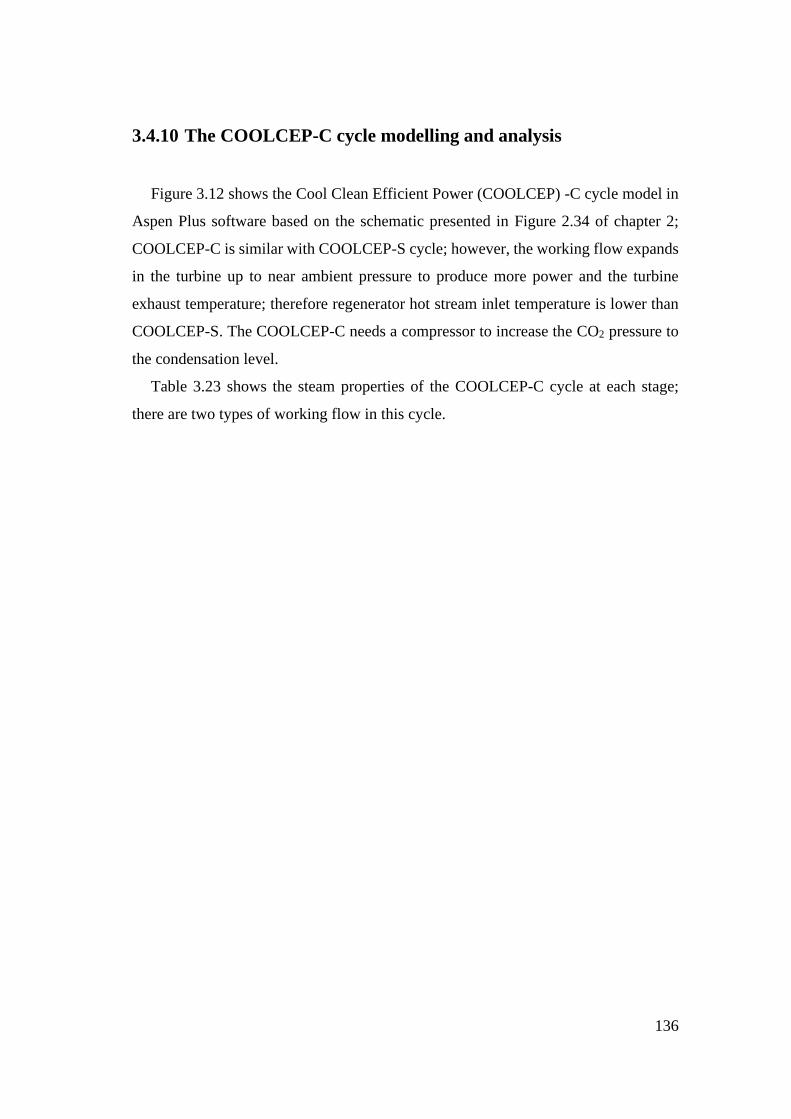
136
3.4.10 The COOLCEP-C cycle modelling and analysis
Figure 3.12 shows the Cool Clean Efficient Power (COOLCEP) -C cycle model in
Aspen Plus software based on the schematic presented in Figure 2.34 of chapter 2;
COOLCEP-C is similar with COOLCEP-S cycle; however, the working flow expands
in the turbine up to near ambient pressure to produce more power and the turbine
exhaust temperature; therefore regenerator hot stream inlet temperature is lower than
COOLCEP-S. The COOLCEP-C needs a compressor to increase the CO2 pressure to
the condensation level.
Table 3.23 shows the steam properties of the COOLCEP-C cycle at each stage;
there are two types of working flow in this cycle.
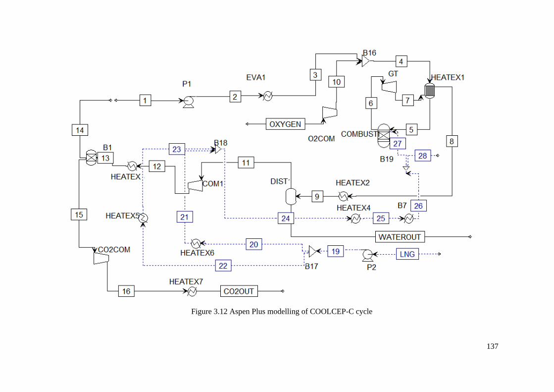
137
Figure 3.12 Aspen Plus modelling of COOLCEP-C cycle
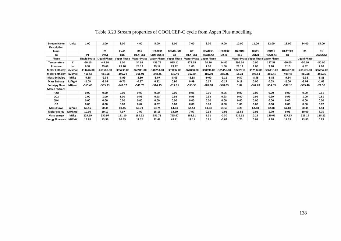
138
Table 3.23 Stream properties of COOLCEP-C cycle from Aspen Plus modelling
Stream Name Units 1.00 2.00 3.00 4.00 5.00 6.00 7.00 8.00 9.00 10.00 11.00 12.00 13.00 14.00 15.00
Description
From P1 EVA1 B16 HEATEX1 COMBUSTI GT HEATEX1 HEATEX2 O2COM DIST1 COM1 HEATEX3 B1 B1
To P1 EVA1 B16 HEATEX1 COMBUSTI GT HEATEX1 HEATEX2 DIST1 B16 COM1 HEATEX3 B1 CO2COM
Phase Liquid Phase Liquid Phase Vapor Phase Vapor Phase Vapor Phase Vapor Phase Vapor Phase Vapor Phase Vapor Phase Vapor Phase Vapor Phase Liquid Phase
Temperature C -50.10 -49.10 8.00 34.91 439.79 915.11 472.18 70.20 14.00 596.64 0.00 157.58 -50.00 -50.10 -50.00
Pressure bar 6.97 29.68 29.40 29.12 29.12 29.12 1.00 1.00 1.00 29.12 1.00 7.10 7.10 6.97 7.10
Molar Enthalpy kJ/kmol -411676.00 -411580.00 -395739.00 -366911.00 -348251.00 -339492.00 -362838.00 -380896.00 -385456.00 18209.10 -392534.00 -386410.00 -409427.00 -411676.00 -356052.00
Molar Enthalpy kJ/kmol -411.68 -411.58 -395.74 -366.91 -348.25 -339.49 -362.84 -380.90 -385.46 18.21 -392.53 -386.41 -409.43 -411.68 -356.05
Mass Enthalpy kJ/kg -9.35 -9.35 -8.99 -8.50 -8.07 -8.03 -8.58 -9.00 -9.11 0.57 -8.95 -8.81 -9.34 -9.35 -8.85
Mass Entropy kJ/kg-K -2.09 -2.09 -0.71 -0.57 0.32 0.90 0.99 0.17 -0.17 0.18 0.00 0.03 -2.06 -2.09 -1.03
Enthalpy Flow MJ/sec -565.46 -565.33 -543.57 -541.70 -514.15 -517.91 -553.53 -581.08 -588.03 1.87 -562.87 -554.09 -587.10 -565.46 -21.50
Mole Fractions
H2O 0.00 0.00 0.00 0.00 0.00 0.06 0.06 0.06 0.06 0.00 0.00 0.00 0.00 0.00 0.11
CO2 1.00 1.00 1.00 0.93 0.93 0.93 0.93 0.93 0.93 0.00 0.99 0.99 0.99 1.00 0.81
CH4 0.00 0.00 0.00 0.00 0.00 0.00 0.00 0.00 0.00 0.00 0.00 0.00 0.00 0.00 0.00
O2 0.00 0.00 0.00 0.07 0.07 0.00 0.00 0.00 0.00 1.00 0.00 0.00 0.00 0.00 0.07
Mass Flows kg/sec 60.45 60.45 60.45 63.74 63.74 64.53 64.53 64.53 64.53 3.29 62.88 62.88 62.88 60.45 2.43
Molar exergy MJ/kmol 10.09 10.17 7.97 7.97 15.18 32.39 7.97 0.14 -0.01 16.53 0.01 5.70 9.96 10.09 4.75
Mass exergy kJ/kg 229.19 230.97 181.10 184.52 351.71 765.67 188.31 3.31 -0.30 516.62 0.19 130.01 227.13 229.19 118.22
Exergy flow rate MWatt 13.85 13.96 10.95 11.76 22.42 49.41 12.15 0.21 -0.02 1.70 0.01 8.18 14.28 13.85 0.29
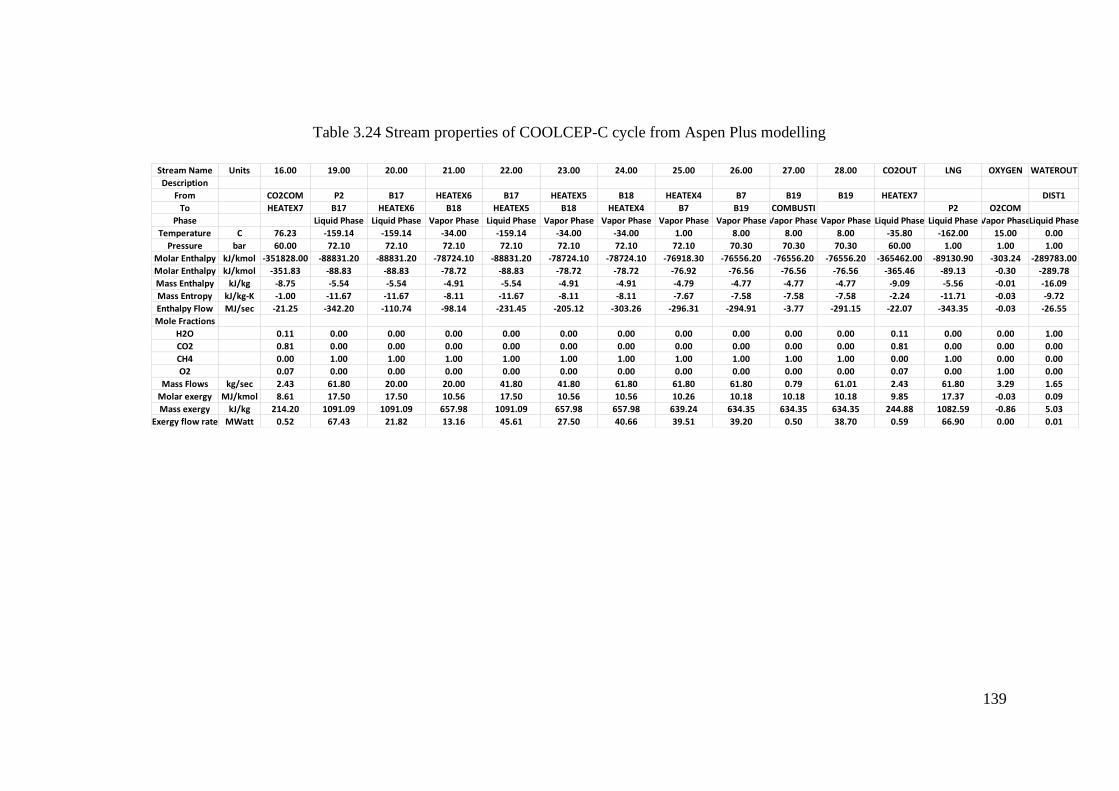
139
Table 3.24 Stream properties of COOLCEP-C cycle from Aspen Plus modelling
Stream Name Units 16.00 19.00 20.00 21.00 22.00 23.00 24.00 25.00 26.00 27.00 28.00 CO2OUT LNG OXYGEN WATEROUT
Description
From CO2COM P2 B17 HEATEX6 B17 HEATEX5 B18 HEATEX4 B7 B19 B19 HEATEX7 DIST1
To HEATEX7 B17 HEATEX6 B18 HEATEX5 B18 HEATEX4 B7 B19 COMBUSTI P2 O2COM
Phase Liquid Phase Liquid Phase Vapor Phase Liquid Phase Vapor Phase Vapor Phase Vapor Phase Vapor Phase Vapor Phase Vapor Phase Liquid Phase Liquid Phase Vapor PhaseLiquid Phase
Temperature C 76.23 -159.14 -159.14 -34.00 -159.14 -34.00 -34.00 1.00 8.00 8.00 8.00 -35.80 -162.00 15.00 0.00
Pressure bar 60.00 72.10 72.10 72.10 72.10 72.10 72.10 72.10 70.30 70.30 70.30 60.00 1.00 1.00 1.00
Molar Enthalpy kJ/kmol -351828.00 -88831.20 -88831.20 -78724.10 -88831.20 -78724.10 -78724.10 -76918.30 -76556.20 -76556.20 -76556.20 -365462.00 -89130.90 -303.24 -289783.00
Molar Enthalpy kJ/kmol -351.83 -88.83 -88.83 -78.72 -88.83 -78.72 -78.72 -76.92 -76.56 -76.56 -76.56 -365.46 -89.13 -0.30 -289.78
Mass Enthalpy kJ/kg -8.75 -5.54 -5.54 -4.91 -5.54 -4.91 -4.91 -4.79 -4.77 -4.77 -4.77 -9.09 -5.56 -0.01 -16.09
Mass Entropy kJ/kg-K -1.00 -11.67 -11.67 -8.11 -11.67 -8.11 -8.11 -7.67 -7.58 -7.58 -7.58 -2.24 -11.71 -0.03 -9.72
Enthalpy Flow MJ/sec -21.25 -342.20 -110.74 -98.14 -231.45 -205.12 -303.26 -296.31 -294.91 -3.77 -291.15 -22.07 -343.35 -0.03 -26.55
Mole Fractions
H2O 0.11 0.00 0.00 0.00 0.00 0.00 0.00 0.00 0.00 0.00 0.00 0.11 0.00 0.00 1.00
CO2 0.81 0.00 0.00 0.00 0.00 0.00 0.00 0.00 0.00 0.00 0.00 0.81 0.00 0.00 0.00
CH4 0.00 1.00 1.00 1.00 1.00 1.00 1.00 1.00 1.00 1.00 1.00 0.00 1.00 0.00 0.00
O2 0.07 0.00 0.00 0.00 0.00 0.00 0.00 0.00 0.00 0.00 0.00 0.07 0.00 1.00 0.00
Mass Flows kg/sec 2.43 61.80 20.00 20.00 41.80 41.80 61.80 61.80 61.80 0.79 61.01 2.43 61.80 3.29 1.65
Molar exergy MJ/kmol 8.61 17.50 17.50 10.56 17.50 10.56 10.56 10.26 10.18 10.18 10.18 9.85 17.37 -0.03 0.09
Mass exergy kJ/kg 214.20 1091.09 1091.09 657.98 1091.09 657.98 657.98 639.24 634.35 634.35 634.35 244.88 1082.59 -0.86 5.03
Exergy flow rate MWatt 0.52 67.43 21.82 13.16 45.61 27.50 40.66 39.51 39.20 0.50 38.70 0.59 66.90 0.00 0.01
140
3.4.11 The Novel O2/CO2 (Cao and Zheng, 2006) modelling and
analysis
Figure 3.13 shows the Novel O2/CO2 cycle model in Aspen Plus software based on the
schematic presented in Figure 2.36 of chapter 2. This cycle includes a gas turbine,
CO2-NG reformer and ammonia absorption refrigeration cycle. In this cycle, O2 is the
oxidizer of the fuel, and CO2 is the working fluid (Cao and Zheng, 2006). The by-
product of burring the fuel and O2 in the combustion is H2O and CO2; the CO2 is
separated from H2O through a cooling process. Table 3.14 shows steam properties at
each stage for the O2/CO2 cycle; the recycled working flow is carbon dioxide.
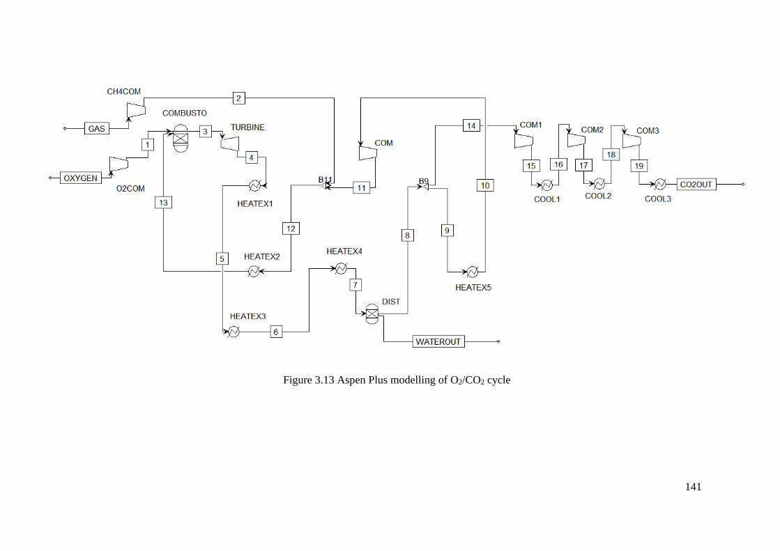
141
Figure 3.13 Aspen Plus modelling of O2/CO2 cycle
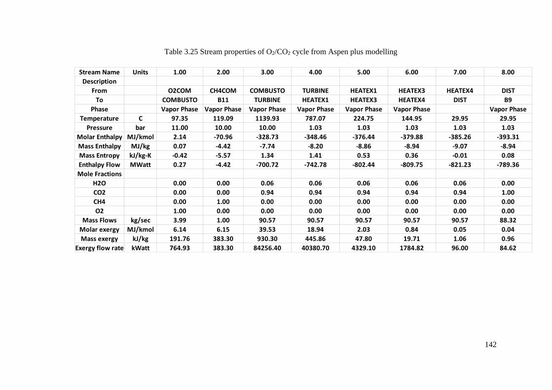
142
Table 3.25 Stream properties of O2/CO2 cycle from Aspen plus modelling
Stream Name Units 1.00 2.00 3.00 4.00 5.00 6.00 7.00 8.00
Description
From O2COM CH4COM COMBUSTO TURBINE HEATEX1 HEATEX3 HEATEX4 DIST
To COMBUSTO B11 TURBINE HEATEX1 HEATEX3 HEATEX4 DIST B9
Phase Vapor Phase Vapor Phase Vapor Phase Vapor Phase Vapor Phase Vapor Phase Vapor Phase
Temperature C 97.35 119.09 1139.93 787.07 224.75 144.95 29.95 29.95
Pressure bar 11.00 10.00 10.00 1.03 1.03 1.03 1.03 1.03
Molar Enthalpy MJ/kmol 2.14 -70.96 -328.73 -348.46 -376.44 -379.88 -385.26 -393.31
Mass Enthalpy MJ/kg 0.07 -4.42 -7.74 -8.20 -8.86 -8.94 -9.07 -8.94
Mass Entropy kJ/kg-K -0.42 -5.57 1.34 1.41 0.53 0.36 -0.01 0.08
Enthalpy Flow MWatt 0.27 -4.42 -700.72 -742.78 -802.44 -809.75 -821.23 -789.36
Mole Fractions
H2O 0.00 0.00 0.06 0.06 0.06 0.06 0.06 0.00
CO2 0.00 0.00 0.94 0.94 0.94 0.94 0.94 1.00
CH4 0.00 1.00 0.00 0.00 0.00 0.00 0.00 0.00
O2 1.00 0.00 0.00 0.00 0.00 0.00 0.00 0.00
Mass Flows kg/sec 3.99 1.00 90.57 90.57 90.57 90.57 90.57 88.32
Molar exergy MJ/kmol 6.14 6.15 39.53 18.94 2.03 0.84 0.05 0.04
Mass exergy kJ/kg 191.76 383.30 930.30 445.86 47.80 19.71 1.06 0.96
Exergy flow rate kWatt 764.93 383.30 84256.40 40380.70 4329.10 1784.82 96.00 84.62
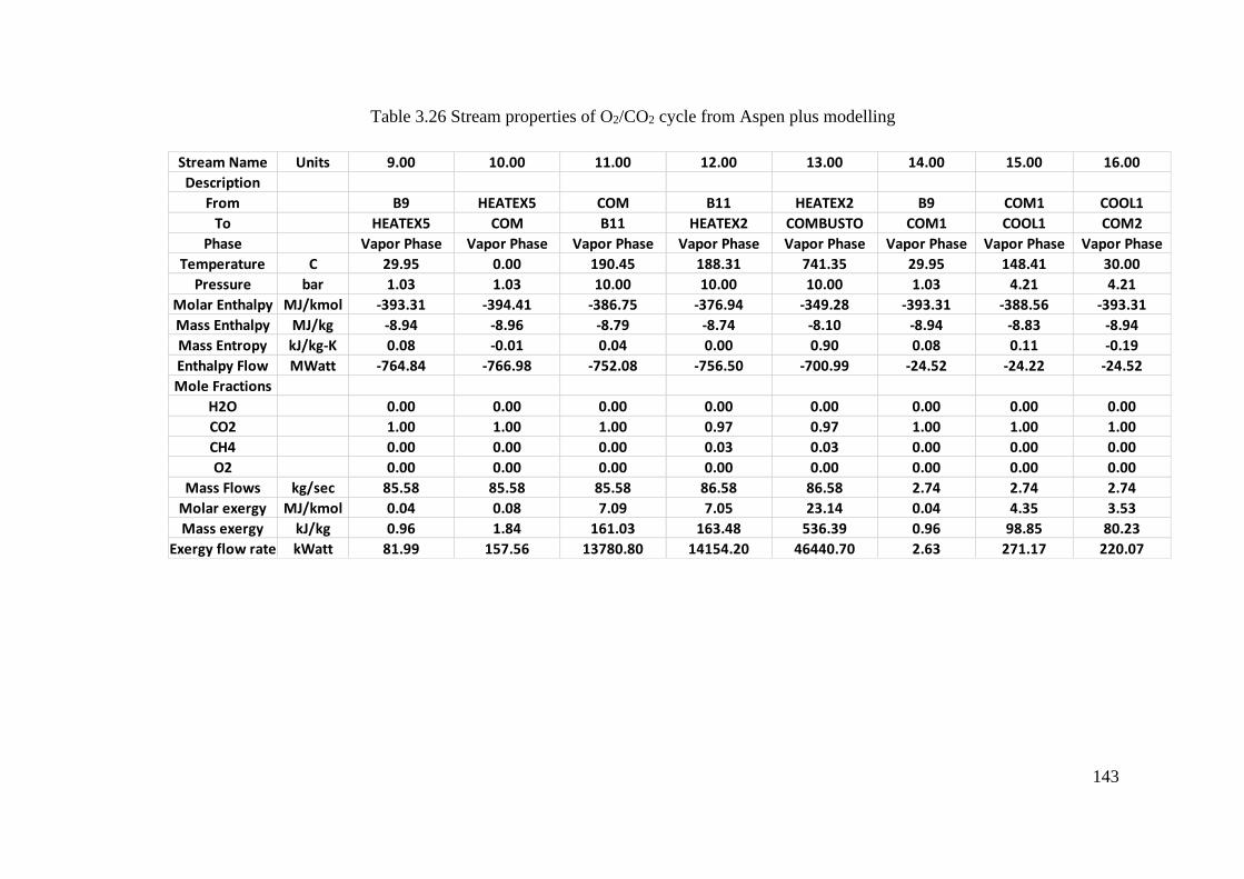
143
Table 3.26 Stream properties of O2/CO2 cycle from Aspen plus modelling
Stream Name Units 9.00 10.00 11.00 12.00 13.00 14.00 15.00 16.00
Description
From B9 HEATEX5 COM B11 HEATEX2 B9 COM1 COOL1
To HEATEX5 COM B11 HEATEX2 COMBUSTO COM1 COOL1 COM2
Phase Vapor Phase Vapor Phase Vapor Phase Vapor Phase Vapor Phase Vapor Phase Vapor Phase Vapor Phase
Temperature C 29.95 0.00 190.45 188.31 741.35 29.95 148.41 30.00
Pressure bar 1.03 1.03 10.00 10.00 10.00 1.03 4.21 4.21
Molar Enthalpy MJ/kmol -393.31 -394.41 -386.75 -376.94 -349.28 -393.31 -388.56 -393.31
Mass Enthalpy MJ/kg -8.94 -8.96 -8.79 -8.74 -8.10 -8.94 -8.83 -8.94
Mass Entropy kJ/kg-K 0.08 -0.01 0.04 0.00 0.90 0.08 0.11 -0.19
Enthalpy Flow MWatt -764.84 -766.98 -752.08 -756.50 -700.99 -24.52 -24.22 -24.52
Mole Fractions
H2O 0.00 0.00 0.00 0.00 0.00 0.00 0.00 0.00
CO2 1.00 1.00 1.00 0.97 0.97 1.00 1.00 1.00
CH4 0.00 0.00 0.00 0.03 0.03 0.00 0.00 0.00
O2 0.00 0.00 0.00 0.00 0.00 0.00 0.00 0.00
Mass Flows kg/sec 85.58 85.58 85.58 86.58 86.58 2.74 2.74 2.74
Molar exergy MJ/kmol 0.04 0.08 7.09 7.05 23.14 0.04 4.35 3.53
Mass exergy kJ/kg 0.96 1.84 161.03 163.48 536.39 0.96 98.85 80.23
Exergy flow rate kWatt 81.99 157.56 13780.80 14154.20 46440.70 2.63 271.17 220.07
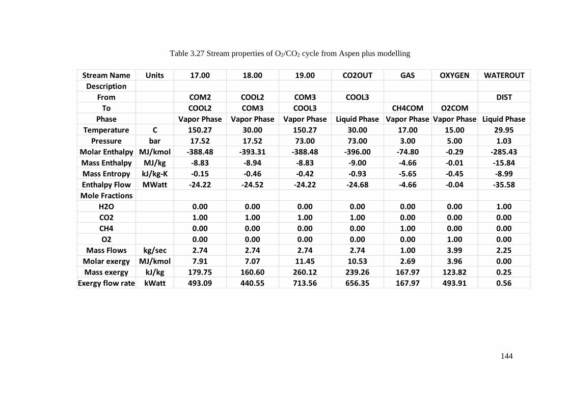
144
Table 3.27 Stream properties of O2/CO2 cycle from Aspen plus modelling
Stream Name Units 17.00 18.00 19.00 CO2OUT GAS OXYGEN WATEROUT
Description
From COM2 COOL2 COM3 COOL3 DIST
To COOL2 COM3 COOL3 CH4COM O2COM
Phase Vapor Phase Vapor Phase Vapor Phase Liquid Phase Vapor Phase Vapor Phase Liquid Phase
Temperature C 150.27 30.00 150.27 30.00 17.00 15.00 29.95
Pressure bar 17.52 17.52 73.00 73.00 3.00 5.00 1.03
Molar Enthalpy MJ/kmol -388.48 -393.31 -388.48 -396.00 -74.80 -0.29 -285.43
Mass Enthalpy MJ/kg -8.83 -8.94 -8.83 -9.00 -4.66 -0.01 -15.84
Mass Entropy kJ/kg-K -0.15 -0.46 -0.42 -0.93 -5.65 -0.45 -8.99
Enthalpy Flow MWatt -24.22 -24.52 -24.22 -24.68 -4.66 -0.04 -35.58
Mole Fractions
H2O 0.00 0.00 0.00 0.00 0.00 0.00 1.00
CO2 1.00 1.00 1.00 1.00 0.00 0.00 0.00
CH4 0.00 0.00 0.00 0.00 1.00 0.00 0.00
O2 0.00 0.00 0.00 0.00 0.00 1.00 0.00
Mass Flows kg/sec 2.74 2.74 2.74 2.74 1.00 3.99 2.25
Molar exergy MJ/kmol 7.91 7.07 11.45 10.53 2.69 3.96 0.00
Mass exergy kJ/kg 179.75 160.60 260.12 239.26 167.97 123.82 0.25
Exergy flow rate kWatt 493.09 440.55 713.56 656.35 167.97 493.91 0.56

145
3.4.12 The NetPower cycle modelling and analysis
The NetPower cycle is one of the novels oxy-combustion technologies, and it is
developed recently with 8 Rivers Capital. The cycle is an oxy-combustion cycle with
the working flow of carbon dioxide. The flow diagram of the Allam cycle is presented
in Figure 2.37 and is described in detail in chapters 8 and 9.

146
Figure 3.14 Aspen Plus modelling of NetPower cycle
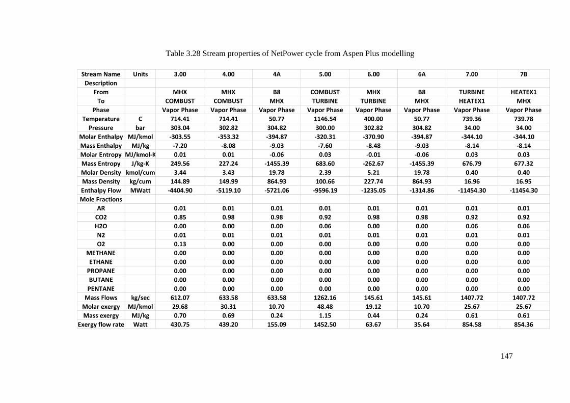
147
Table 3.28 Stream properties of NetPower cycle from Aspen Plus modelling
Stream Name Units 3.00 4.00 4A 5.00 6.00 6A 7.00 7B
Description
From MHX MHX B8 COMBUST MHX B8 TURBINE HEATEX1
To COMBUST COMBUST MHX TURBINE TURBINE MHX HEATEX1 MHX
Phase Vapor Phase Vapor Phase Vapor Phase Vapor Phase Vapor Phase Vapor Phase Vapor Phase Vapor Phase
Temperature C 714.41 714.41 50.77 1146.54 400.00 50.77 739.36 739.78
Pressure bar 303.04 302.82 304.82 300.00 302.82 304.82 34.00 34.00
Molar Enthalpy MJ/kmol -303.55 -353.32 -394.87 -320.31 -370.90 -394.87 -344.10 -344.10
Mass Enthalpy MJ/kg -7.20 -8.08 -9.03 -7.60 -8.48 -9.03 -8.14 -8.14
Molar Entropy MJ/kmol-K 0.01 0.01 -0.06 0.03 -0.01 -0.06 0.03 0.03
Mass Entropy J/kg-K 249.56 227.24 -1455.39 683.60 -262.67 -1455.39 676.79 677.32
Molar Density kmol/cum 3.44 3.43 19.78 2.39 5.21 19.78 0.40 0.40
Mass Density kg/cum 144.89 149.99 864.93 100.66 227.74 864.93 16.96 16.95
Enthalpy Flow MWatt -4404.90 -5119.10 -5721.06 -9596.19 -1235.05 -1314.86 -11454.30 -11454.30
Mole Fractions
AR 0.01 0.01 0.01 0.01 0.01 0.01 0.01 0.01
CO2 0.85 0.98 0.98 0.92 0.98 0.98 0.92 0.92
H2O 0.00 0.00 0.00 0.06 0.00 0.00 0.06 0.06
N2 0.01 0.01 0.01 0.01 0.01 0.01 0.01 0.01
O2 0.13 0.00 0.00 0.00 0.00 0.00 0.00 0.00
METHANE 0.00 0.00 0.00 0.00 0.00 0.00 0.00 0.00
ETHANE 0.00 0.00 0.00 0.00 0.00 0.00 0.00 0.00
PROPANE 0.00 0.00 0.00 0.00 0.00 0.00 0.00 0.00
BUTANE 0.00 0.00 0.00 0.00 0.00 0.00 0.00 0.00
PENTANE 0.00 0.00 0.00 0.00 0.00 0.00 0.00 0.00
Mass Flows kg/sec 612.07 633.58 633.58 1262.16 145.61 145.61 1407.72 1407.72
Molar exergy MJ/kmol 29.68 30.31 10.70 48.48 19.12 10.70 25.67 25.67
Mass exergy MJ/kg 0.70 0.69 0.24 1.15 0.44 0.24 0.61 0.61
Exergy flow rate Watt 430.75 439.20 155.09 1452.50 63.67 35.64 854.58 854.36
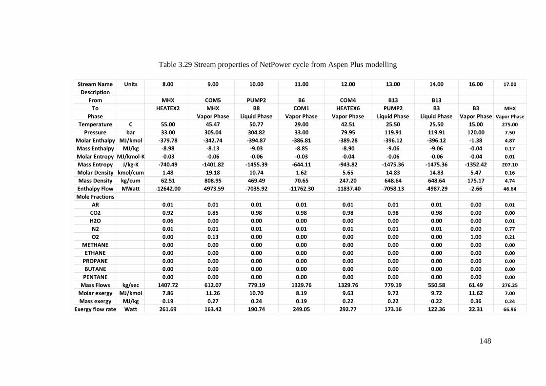
148
Table 3.29 Stream properties of NetPower cycle from Aspen Plus modelling
Stream Name Units 8.00 9.00 10.00 11.00 12.00 13.00 14.00 16.00 17.00
Description
From MHX COM5 PUMP2 B6 COM4 B13 B13
To HEATEX2 MHX B8 COM1 HEATEX6 PUMP2 B3 B3 MHX
Phase Vapor Phase Liquid Phase Vapor Phase Vapor Phase Liquid Phase Liquid Phase Vapor Phase Vapor Phase
Temperature C 55.00 45.47 50.77 29.00 42.51 25.50 25.50 15.00 275.00
Pressure bar 33.00 305.04 304.82 33.00 79.95 119.91 119.91 120.00 7.50
Molar Enthalpy MJ/kmol -379.78 -342.74 -394.87 -386.81 -389.28 -396.12 -396.12 -1.38 4.87
Mass Enthalpy MJ/kg -8.98 -8.13 -9.03 -8.85 -8.90 -9.06 -9.06 -0.04 0.17
Molar Entropy MJ/kmol-K -0.03 -0.06 -0.06 -0.03 -0.04 -0.06 -0.06 -0.04 0.01
Mass Entropy J/kg-K -740.49 -1401.82 -1455.39 -644.11 -943.82 -1475.36 -1475.36 -1352.42 207.10
Molar Density kmol/cum 1.48 19.18 10.74 1.62 5.65 14.83 14.83 5.47 0.16
Mass Density kg/cum 62.51 808.95 469.49 70.65 247.20 648.64 648.64 175.17 4.74
Enthalpy Flow MWatt -12642.00 -4973.59 -7035.92 -11762.30 -11837.40 -7058.13 -4987.29 -2.66 46.64
Mole Fractions
AR 0.01 0.01 0.01 0.01 0.01 0.01 0.01 0.00 0.01
CO2 0.92 0.85 0.98 0.98 0.98 0.98 0.98 0.00 0.00
H2O 0.06 0.00 0.00 0.00 0.00 0.00 0.00 0.00 0.01
N2 0.01 0.01 0.01 0.01 0.01 0.01 0.01 0.00 0.77
O2 0.00 0.13 0.00 0.00 0.00 0.00 0.00 1.00 0.21
METHANE 0.00 0.00 0.00 0.00 0.00 0.00 0.00 0.00 0.00
ETHANE 0.00 0.00 0.00 0.00 0.00 0.00 0.00 0.00 0.00
PROPANE 0.00 0.00 0.00 0.00 0.00 0.00 0.00 0.00 0.00
BUTANE 0.00 0.00 0.00 0.00 0.00 0.00 0.00 0.00 0.00
PENTANE 0.00 0.00 0.00 0.00 0.00 0.00 0.00 0.00 0.00
Mass Flows kg/sec 1407.72 612.07 779.19 1329.76 1329.76 779.19 550.58 61.49 276.25
Molar exergy MJ/kmol 7.86 11.26 10.70 8.19 9.63 9.72 9.72 11.62 7.00
Mass exergy MJ/kg 0.19 0.27 0.24 0.19 0.22 0.22 0.22 0.36 0.24
Exergy flow rate Watt 261.69 163.42 190.74 249.05 292.77 173.16 122.36 22.31 66.96
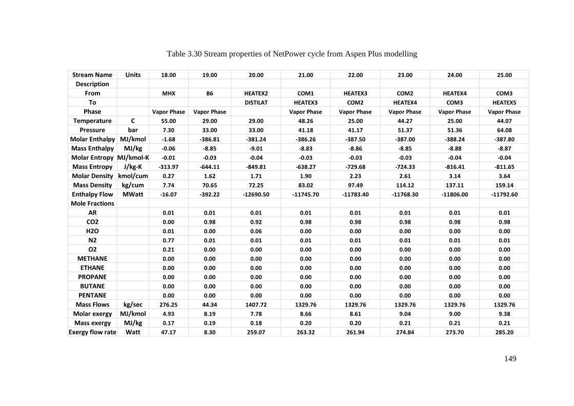
149
Table 3.30 Stream properties of NetPower cycle from Aspen Plus modelling
Stream Name Units 18.00 19.00 20.00 21.00 22.00 23.00 24.00 25.00
Description
From MHX B6 HEATEX2 COM1 HEATEX3 COM2 HEATEX4 COM3
To DISTILAT HEATEX3 COM2 HEATEX4 COM3 HEATEX5
Phase Vapor Phase Vapor Phase Vapor Phase Vapor Phase Vapor Phase Vapor Phase Vapor Phase
Temperature C 55.00 29.00 29.00 48.26 25.00 44.27 25.00 44.07
Pressure bar 7.30 33.00 33.00 41.18 41.17 51.37 51.36 64.08
Molar Enthalpy MJ/kmol -1.68 -386.81 -381.24 -386.26 -387.50 -387.00 -388.24 -387.80
Mass Enthalpy MJ/kg -0.06 -8.85 -9.01 -8.83 -8.86 -8.85 -8.88 -8.87
Molar Entropy MJ/kmol-K -0.01 -0.03 -0.04 -0.03 -0.03 -0.03 -0.04 -0.04
Mass Entropy J/kg-K -313.97 -644.11 -849.81 -638.27 -729.68 -724.33 -816.41 -811.65
Molar Density kmol/cum 0.27 1.62 1.71 1.90 2.23 2.61 3.14 3.64
Mass Density kg/cum 7.74 70.65 72.25 83.02 97.49 114.12 137.11 159.14
Enthalpy Flow MWatt -16.07 -392.22 -12690.50 -11745.70 -11783.40 -11768.30 -11806.00 -11792.60
Mole Fractions
AR 0.01 0.01 0.01 0.01 0.01 0.01 0.01 0.01
CO2 0.00 0.98 0.92 0.98 0.98 0.98 0.98 0.98
H2O 0.01 0.00 0.06 0.00 0.00 0.00 0.00 0.00
N2 0.77 0.01 0.01 0.01 0.01 0.01 0.01 0.01
O2 0.21 0.00 0.00 0.00 0.00 0.00 0.00 0.00
METHANE 0.00 0.00 0.00 0.00 0.00 0.00 0.00 0.00
ETHANE 0.00 0.00 0.00 0.00 0.00 0.00 0.00 0.00
PROPANE 0.00 0.00 0.00 0.00 0.00 0.00 0.00 0.00
BUTANE 0.00 0.00 0.00 0.00 0.00 0.00 0.00 0.00
PENTANE 0.00 0.00 0.00 0.00 0.00 0.00 0.00 0.00
Mass Flows kg/sec 276.25 44.34 1407.72 1329.76 1329.76 1329.76 1329.76 1329.76
Molar exergy MJ/kmol 4.93 8.19 7.78 8.66 8.61 9.04 9.00 9.38
Mass exergy MJ/kg 0.17 0.19 0.18 0.20 0.20 0.21 0.21 0.21
Exergy flow rate Watt 47.17 8.30 259.07 263.32 261.94 274.84 273.70 285.20
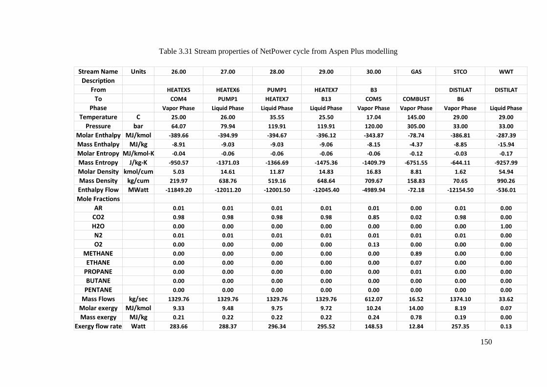
150
Table 3.31 Stream properties of NetPower cycle from Aspen Plus modelling
Stream Name Units 26.00 27.00 28.00 29.00 30.00 GAS STCO WWT
Description
From HEATEX5 HEATEX6 PUMP1 HEATEX7 B3 DISTILAT DISTILAT
To COM4 PUMP1 HEATEX7 B13 COM5 COMBUST B6
Phase Vapor Phase Liquid Phase Liquid Phase Liquid Phase Vapor Phase Vapor Phase Vapor Phase Liquid Phase
Temperature C 25.00 26.00 35.55 25.50 17.04 145.00 29.00 29.00
Pressure bar 64.07 79.94 119.91 119.91 120.00 305.00 33.00 33.00
Molar Enthalpy MJ/kmol -389.66 -394.99 -394.67 -396.12 -343.87 -78.74 -386.81 -287.39
Mass Enthalpy MJ/kg -8.91 -9.03 -9.03 -9.06 -8.15 -4.37 -8.85 -15.94
Molar Entropy MJ/kmol-K -0.04 -0.06 -0.06 -0.06 -0.06 -0.12 -0.03 -0.17
Mass Entropy J/kg-K -950.57 -1371.03 -1366.69 -1475.36 -1409.79 -6751.55 -644.11 -9257.99
Molar Density kmol/cum 5.03 14.61 11.87 14.83 16.83 8.81 1.62 54.94
Mass Density kg/cum 219.97 638.76 519.16 648.64 709.67 158.83 70.65 990.26
Enthalpy Flow MWatt -11849.20 -12011.20 -12001.50 -12045.40 -4989.94 -72.18 -12154.50 -536.01
Mole Fractions
AR 0.01 0.01 0.01 0.01 0.01 0.00 0.01 0.00
CO2 0.98 0.98 0.98 0.98 0.85 0.02 0.98 0.00
H2O 0.00 0.00 0.00 0.00 0.00 0.00 0.00 1.00
N2 0.01 0.01 0.01 0.01 0.01 0.01 0.01 0.00
O2 0.00 0.00 0.00 0.00 0.13 0.00 0.00 0.00
METHANE 0.00 0.00 0.00 0.00 0.00 0.89 0.00 0.00
ETHANE 0.00 0.00 0.00 0.00 0.00 0.07 0.00 0.00
PROPANE 0.00 0.00 0.00 0.00 0.00 0.01 0.00 0.00
BUTANE 0.00 0.00 0.00 0.00 0.00 0.00 0.00 0.00
PENTANE 0.00 0.00 0.00 0.00 0.00 0.00 0.00 0.00
Mass Flows kg/sec 1329.76 1329.76 1329.76 1329.76 612.07 16.52 1374.10 33.62
Molar exergy MJ/kmol 9.33 9.48 9.75 9.72 10.24 14.00 8.19 0.07
Mass exergy MJ/kg 0.21 0.22 0.22 0.22 0.24 0.78 0.19 0.00
Exergy flow rate Watt 283.66 288.37 296.34 295.52 148.53 12.84 257.35 0.13

151
3.4.13 The S-CES cycle modelling and analysis
Figure 3.15 shows the S-CES cycle model in Aspen Plus software based on the
schematic presented in Figure 2.40 of chapter 2; the S-CES is also described in detail
in chapter 9. Table 3.16 shows steam properties at each stage for the S-CES cycle, and
water is recycled as the working flow.
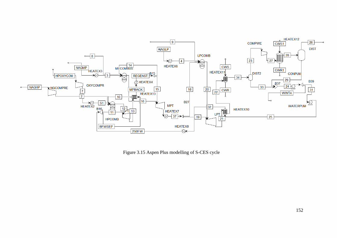
152
Figure 3.15 Aspen Plus modelling of S-CES cycle
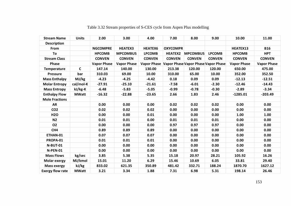
153
Table 3.32 Stream properties of S-CES cycle from Aspen Plus modelling
Stream Name Units 2.00 3.00 4.00 7.00 8.00 9.00 10.00 11.00
Description
From NGCOMPRE HEATEX3 HEATEX6 OXYCOMPR HEATEX13 B16
To HPCOMB MPCOMBUS LPCOMB HEATEX2 MPCOMBUS LPCOMB HPCOMB HPT
Stream Class CONVEN CONVEN CONVEN CONVEN CONVEN CONVEN CONVEN CONVEN
Phase Vapor Phase Vapor Phase Vapor Phase Vapor Phase Vapor Phase Vapor Phase Vapor Phase Vapor Phase
Temperature C 147.14 140.00 130.00 213.38 120.00 120.00 650.00 475.00
Pressure bar 310.03 69.00 10.00 310.00 65.00 10.00 352.00 352.50
Mass Enthalpy MJ/kg -4.23 -4.25 -4.42 0.18 0.09 0.09 -12.13 -12.51
Molar Entropy cal/mol-K -27.91 -25.10 -21.61 -7.58 -6.01 -2.30 -12.46 -14.43
Mass Entropy kJ/kg-K -6.48 -5.83 -5.05 -0.99 -0.78 -0.30 -2.89 -3.34
Enthalpy Flow MWatt -16.32 -22.88 -23.65 2.66 1.83 2.46 -1285.01 -203.49
Mole Fractions
AR 0.00 0.00 0.00 0.02 0.02 0.02 0.00 0.00
CO2 0.02 0.02 0.02 0.00 0.00 0.00 0.00 0.00
H2O 0.00 0.00 0.01 0.00 0.00 0.00 1.00 1.00
N2 0.01 0.01 0.00 0.01 0.01 0.01 0.00 0.00
O2 0.00 0.00 0.00 0.97 0.97 0.97 0.00 0.00
CH4 0.89 0.89 0.89 0.00 0.00 0.00 0.00 0.00
ETHAN-01 0.07 0.07 0.07 0.00 0.00 0.00 0.00 0.00
PROPA-01 0.01 0.01 0.01 0.00 0.00 0.00 0.00 0.00
N-BUT-01 0.00 0.00 0.00 0.00 0.00 0.00 0.00 0.00
N-PEN-01 0.00 0.00 0.00 0.00 0.00 0.00 0.00 0.00
Mass Flows kg/sec 3.85 5.38 5.35 15.18 20.97 28.21 105.92 16.26
Molar exergy MJ/kmol 15.01 11.20 6.29 15.46 10.69 6.05 33.81 29.40
Mass exergy kJ/kg 833.02 621.35 350.89 481.42 332.71 188.24 1870.70 1627.12
Exergy flow rate MWatt 3.21 3.34 1.88 7.31 6.98 5.31 198.14 26.46
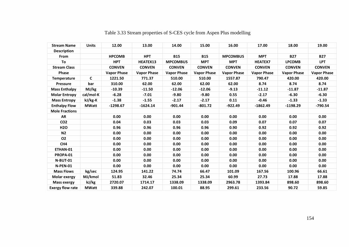
154
Table 3.33 Stream properties of S-CES cycle from Aspen Plus modelling
Stream Name Units 12.00 13.00 14.00 15.00 16.00 17.00 18.00 19.00
Description
From HPCOMB HPT B15 B15 MPCOMBUS MPT B27 B27
To HPT HEATEX13 MPCOMBUS MPT MPT HEATEX7 LPCOMB LPT
Stream Class CONVEN CONVEN CONVEN CONVEN CONVEN CONVEN CONVEN CONVEN
Phase Vapor Phase Vapor Phase Vapor Phase Vapor Phase Vapor Phase Vapor Phase Vapor Phase Vapor Phase
Temperature C 1221.50 771.37 510.00 510.00 1557.87 790.47 420.00 420.00
Pressure bar 310.00 62.00 62.00 62.00 62.00 8.74 8.74 8.74
Mass Enthalpy MJ/kg -10.39 -11.50 -12.06 -12.06 -9.13 -11.12 -11.87 -11.87
Molar Entropy cal/mol-K -6.28 -7.01 -9.80 -9.80 0.55 -2.17 -6.30 -6.30
Mass Entropy kJ/kg-K -1.38 -1.55 -2.17 -2.17 0.11 -0.46 -1.33 -1.33
Enthalpy Flow MWatt -1298.67 -1624.14 -901.44 -801.72 -922.49 -1862.49 -1198.29 -790.54
Mole Fractions
AR 0.00 0.00 0.00 0.00 0.00 0.00 0.00 0.00
CO2 0.04 0.03 0.03 0.03 0.09 0.07 0.07 0.07
H2O 0.96 0.96 0.96 0.96 0.90 0.92 0.92 0.92
N2 0.00 0.00 0.00 0.00 0.00 0.00 0.00 0.00
O2 0.00 0.00 0.00 0.00 0.00 0.00 0.00 0.00
CH4 0.00 0.00 0.00 0.00 0.00 0.00 0.00 0.00
ETHAN-01 0.00 0.00 0.00 0.00 0.00 0.00 0.00 0.00
PROPA-01 0.00 0.00 0.00 0.00 0.00 0.00 0.00 0.00
N-BUT-01 0.00 0.00 0.00 0.00 0.00 0.00 0.00 0.00
N-PEN-01 0.00 0.00 0.00 0.00 0.00 0.00 0.00 0.00
Mass Flows kg/sec 124.95 141.22 74.74 66.47 101.09 167.56 100.96 66.61
Molar exergy MJ/kmol 51.83 32.46 25.34 25.34 60.99 27.73 17.88 17.88
Mass exergy kJ/kg 2720.07 1714.17 1338.09 1338.09 2963.78 1393.84 898.60 898.60
Exergy flow rate MWatt 339.88 242.07 100.01 88.95 299.61 233.56 90.72 59.85
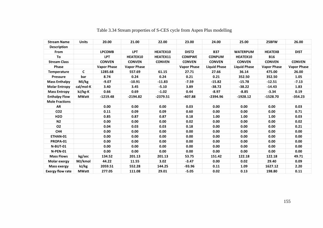
155
Table 3.34 Stream properties of S-CES cycle from Aspen Plus modelling
Stream Name Units 20.00 21.00 22.00 23.00 24.00 25.00 25BFW 26.00
Description
From LPCOMB LPT HEATEX10 DIST2 B37 WATERPUM HEATEX8 DIST
To LPT HEATEX10 HEATEX11 COMPWE CONPUM HEATEX10 B16
Stream Class CONVEN CONVEN CONVEN CONVEN CONVEN CONVEN CONVEN CONVEN
Phase Vapor Phase Vapor Phase Vapor Phase Liquid Phase Liquid Phase Vapor Phase Vapor Phase
Temperature C 1285.68 557.69 61.15 27.71 27.66 36.14 475.00 26.00
Pressure bar 8.74 0.24 0.24 0.21 0.21 352.50 352.50 1.05
Mass Enthalpy MJ/kg -9.07 -10.91 -11.83 -7.59 -15.82 -15.78 -12.51 -7.13
Molar Entropy cal/mol-K 3.40 3.45 -5.10 3.89 -38.72 -38.22 -14.43 1.83
Mass Entropy kJ/kg-K 0.66 0.69 -1.02 0.44 -8.97 -8.85 -3.34 0.19
Enthalpy Flow MWatt -1219.48 -2194.82 -2379.51 -407.88 -2394.96 -1928.12 -1528.70 -354.23
Mole Fractions
AR 0.00 0.00 0.00 0.03 0.00 0.00 0.00 0.03
CO2 0.11 0.09 0.09 0.60 0.00 0.00 0.00 0.71
H2O 0.85 0.87 0.87 0.18 1.00 1.00 1.00 0.03
N2 0.00 0.00 0.00 0.02 0.00 0.00 0.00 0.02
O2 0.04 0.03 0.03 0.18 0.00 0.00 0.00 0.21
CH4 0.00 0.00 0.00 0.00 0.00 0.00 0.00 0.00
ETHAN-01 0.00 0.00 0.00 0.00 0.00 0.00 0.00 0.00
PROPA-01 0.00 0.00 0.00 0.00 0.00 0.00 0.00 0.00
N-BUT-01 0.00 0.00 0.00 0.00 0.00 0.00 0.00 0.00
N-PEN-01 0.00 0.00 0.00 0.00 0.00 0.00 0.00 0.00
Mass Flows kg/sec 134.52 201.13 201.13 53.75 151.42 122.18 122.18 49.71
Molar exergy MJ/kmol 44.22 11.55 3.02 -3.47 0.00 0.02 29.40 0.09
Mass exergy kJ/kg 2059.51 552.28 144.25 -93.96 0.11 1.09 1627.12 2.20
Exergy flow rate MWatt 277.05 111.08 29.01 -5.05 0.02 0.13 198.80 0.11
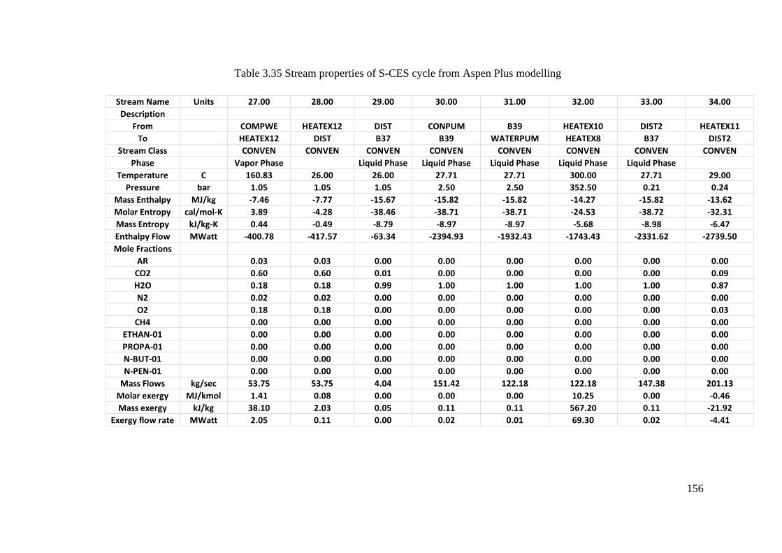
156
Table 3.35 Stream properties of S-CES cycle from Aspen Plus modelling
Stream Name Units 27.00 28.00 29.00 30.00 31.00 32.00 33.00 34.00
Description
From COMPWE HEATEX12 DIST CONPUM B39 HEATEX10 DIST2 HEATEX11
To HEATEX12 DIST B37 B39 WATERPUM HEATEX8 B37 DIST2
Stream Class CONVEN CONVEN CONVEN CONVEN CONVEN CONVEN CONVEN CONVEN
Phase Vapor Phase Liquid Phase Liquid Phase Liquid Phase Liquid Phase Liquid Phase
Temperature C 160.83 26.00 26.00 27.71 27.71 300.00 27.71 29.00
Pressure bar 1.05 1.05 1.05 2.50 2.50 352.50 0.21 0.24
Mass Enthalpy MJ/kg -7.46 -7.77 -15.67 -15.82 -15.82 -14.27 -15.82 -13.62
Molar Entropy cal/mol-K 3.89 -4.28 -38.46 -38.71 -38.71 -24.53 -38.72 -32.31
Mass Entropy kJ/kg-K 0.44 -0.49 -8.79 -8.97 -8.97 -5.68 -8.98 -6.47
Enthalpy Flow MWatt -400.78 -417.57 -63.34 -2394.93 -1932.43 -1743.43 -2331.62 -2739.50
Mole Fractions
AR 0.03 0.03 0.00 0.00 0.00 0.00 0.00 0.00
CO2 0.60 0.60 0.01 0.00 0.00 0.00 0.00 0.09
H2O 0.18 0.18 0.99 1.00 1.00 1.00 1.00 0.87
N2 0.02 0.02 0.00 0.00 0.00 0.00 0.00 0.00
O2 0.18 0.18 0.00 0.00 0.00 0.00 0.00 0.03
CH4 0.00 0.00 0.00 0.00 0.00 0.00 0.00 0.00
ETHAN-01 0.00 0.00 0.00 0.00 0.00 0.00 0.00 0.00
PROPA-01 0.00 0.00 0.00 0.00 0.00 0.00 0.00 0.00
N-BUT-01 0.00 0.00 0.00 0.00 0.00 0.00 0.00 0.00
N-PEN-01 0.00 0.00 0.00 0.00 0.00 0.00 0.00 0.00
Mass Flows kg/sec 53.75 53.75 4.04 151.42 122.18 122.18 147.38 201.13
Molar exergy MJ/kmol 1.41 0.08 0.00 0.00 0.00 10.25 0.00 -0.46
Mass exergy kJ/kg 38.10 2.03 0.05 0.11 0.11 567.20 0.11 -21.92
Exergy flow rate MWatt 2.05 0.11 0.00 0.02 0.01 69.30 0.02 -4.41
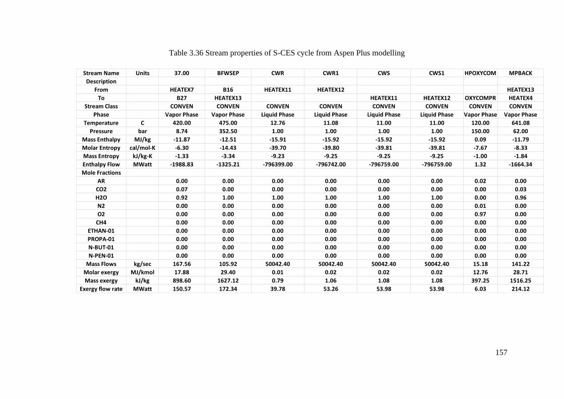
157
Table 3.36 Stream properties of S-CES cycle from Aspen Plus modelling
Stream Name Units 37.00 BFWSEP CWR CWR1 CWS CWS1 HPOXYCOM MPBACK
Description
From HEATEX7 B16 HEATEX11 HEATEX12 HEATEX13
To B27 HEATEX13 HEATEX11 HEATEX12 OXYCOMPR HEATEX4
Stream Class CONVEN CONVEN CONVEN CONVEN CONVEN CONVEN CONVEN CONVEN
Phase Vapor Phase Vapor Phase Liquid Phase Liquid Phase Liquid Phase Liquid Phase Vapor Phase Vapor Phase
Temperature C 420.00 475.00 12.76 11.08 11.00 11.00 120.00 641.08
Pressure bar 8.74 352.50 1.00 1.00 1.00 1.00 150.00 62.00
Mass Enthalpy MJ/kg -11.87 -12.51 -15.91 -15.92 -15.92 -15.92 0.09 -11.79
Molar Entropy cal/mol-K -6.30 -14.43 -39.70 -39.80 -39.81 -39.81 -7.67 -8.33
Mass Entropy kJ/kg-K -1.33 -3.34 -9.23 -9.25 -9.25 -9.25 -1.00 -1.84
Enthalpy Flow MWatt -1988.83 -1325.21 -796399.00 -796742.00 -796759.00 -796759.00 1.32 -1664.34
Mole Fractions
AR 0.00 0.00 0.00 0.00 0.00 0.00 0.02 0.00
CO2 0.07 0.00 0.00 0.00 0.00 0.00 0.00 0.03
H2O 0.92 1.00 1.00 1.00 1.00 1.00 0.00 0.96
N2 0.00 0.00 0.00 0.00 0.00 0.00 0.01 0.00
O2 0.00 0.00 0.00 0.00 0.00 0.00 0.97 0.00
CH4 0.00 0.00 0.00 0.00 0.00 0.00 0.00 0.00
ETHAN-01 0.00 0.00 0.00 0.00 0.00 0.00 0.00 0.00
PROPA-01 0.00 0.00 0.00 0.00 0.00 0.00 0.00 0.00
N-BUT-01 0.00 0.00 0.00 0.00 0.00 0.00 0.00 0.00
N-PEN-01 0.00 0.00 0.00 0.00 0.00 0.00 0.00 0.00
Mass Flows kg/sec 167.56 105.92 50042.40 50042.40 50042.40 50042.40 15.18 141.22
Molar exergy MJ/kmol 17.88 29.40 0.01 0.02 0.02 0.02 12.76 28.71
Mass exergy kJ/kg 898.60 1627.12 0.79 1.06 1.08 1.08 397.25 1516.25
Exergy flow rate MWatt 150.57 172.34 39.78 53.26 53.98 53.98 6.03 214.12
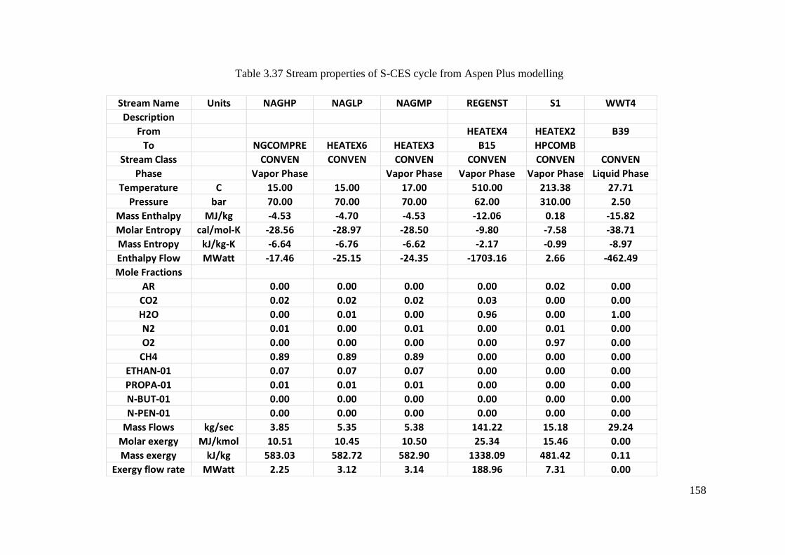
158
Table 3.37 Stream properties of S-CES cycle from Aspen Plus modelling
Stream Name Units NAGHP NAGLP NAGMP REGENST S1 WWT4
Description
From HEATEX4 HEATEX2 B39
To NGCOMPRE HEATEX6 HEATEX3 B15 HPCOMB
Stream Class CONVEN CONVEN CONVEN CONVEN CONVEN CONVEN
Phase Vapor Phase Vapor Phase Vapor Phase Vapor Phase Liquid Phase
Temperature C 15.00 15.00 17.00 510.00 213.38 27.71
Pressure bar 70.00 70.00 70.00 62.00 310.00 2.50
Mass Enthalpy MJ/kg -4.53 -4.70 -4.53 -12.06 0.18 -15.82
Molar Entropy cal/mol-K -28.56 -28.97 -28.50 -9.80 -7.58 -38.71
Mass Entropy kJ/kg-K -6.64 -6.76 -6.62 -2.17 -0.99 -8.97
Enthalpy Flow MWatt -17.46 -25.15 -24.35 -1703.16 2.66 -462.49
Mole Fractions
AR 0.00 0.00 0.00 0.00 0.02 0.00
CO2 0.02 0.02 0.02 0.03 0.00 0.00
H2O 0.00 0.01 0.00 0.96 0.00 1.00
N2 0.01 0.00 0.01 0.00 0.01 0.00
O2 0.00 0.00 0.00 0.00 0.97 0.00
CH4 0.89 0.89 0.89 0.00 0.00 0.00
ETHAN-01 0.07 0.07 0.07 0.00 0.00 0.00
PROPA-01 0.01 0.01 0.01 0.00 0.00 0.00
N-BUT-01 0.00 0.00 0.00 0.00 0.00 0.00
N-PEN-01 0.00 0.00 0.00 0.00 0.00 0.00
Mass Flows kg/sec 3.85 5.35 5.38 141.22 15.18 29.24
Molar exergy MJ/kmol 10.51 10.45 10.50 25.34 15.46 0.00
Mass exergy kJ/kg 583.03 582.72 582.90 1338.09 481.42 0.11
Exergy flow rate MWatt 2.25 3.12 3.14 188.96 7.31 0.00
159
3.5 Sensitivity comparison of CES and NetPower
The supercritical CES power cycle is the best cycle of CES with respect to
efficiency. Therefore, the supercritical CES power cycle is going to be compared with
the recent NetPower cycle. The initial condition for supercritical CES and NetPower
are equal. In order to calculate the efficiency of the turbines, it is required to calculate
cooling blade parameters. In this paper, the turbine efficiency for both the CES cycle
and the NetPower cycles are assumed constant.
In chapter 8, The NetPower and Supercritical CES cycle, modelling and simulation
were carried out using Aspen Plus to study the efficiency of cycles on different
parameters of Turbine Inlet Temperature (TIT), Combustion Outlet Pressure (COP),
minimum approach temperature of the heat exchanger. The sensitivity of cycle
efficiency on the TIT for the supercritical CES are compared with NetPower in one
diagram.
3.6 Techno-economic analysis of oxy-combustion cycles
The economic feasibility of oxy-combustion cycles is the key to develop and
commercialise these cycles. The cost of oxy-fuel combustion with CCS technologies
depends on several factors, including Capital cost, operation cost, fuel price and
maintenance costs (Hu, 2011). Techno-economic analysis needs to perform a cost
evaluation and engineering study of oxy-combustion cycle; in this subchapter, the
techno-economics of oxy-combustion cycles in terms of cost rate and levelised Cost
of Electricity (LCOE) are studied.
3.6.1 Cost rate
The cost of power cycle equipment can be calculated from Table 3.38 & Table 3.39.
The annual cost of the plant includes annual fuel cost, operating cost, and capital cost.
The capital cost and maintenance cost of each equipment can be calculated from
Equation 3-21 (Seyyedi, Ajam and Farahat, 2010), ��𝑖 𝑢𝑛𝑖𝑡 𝑖𝑠 ($/𝑠)
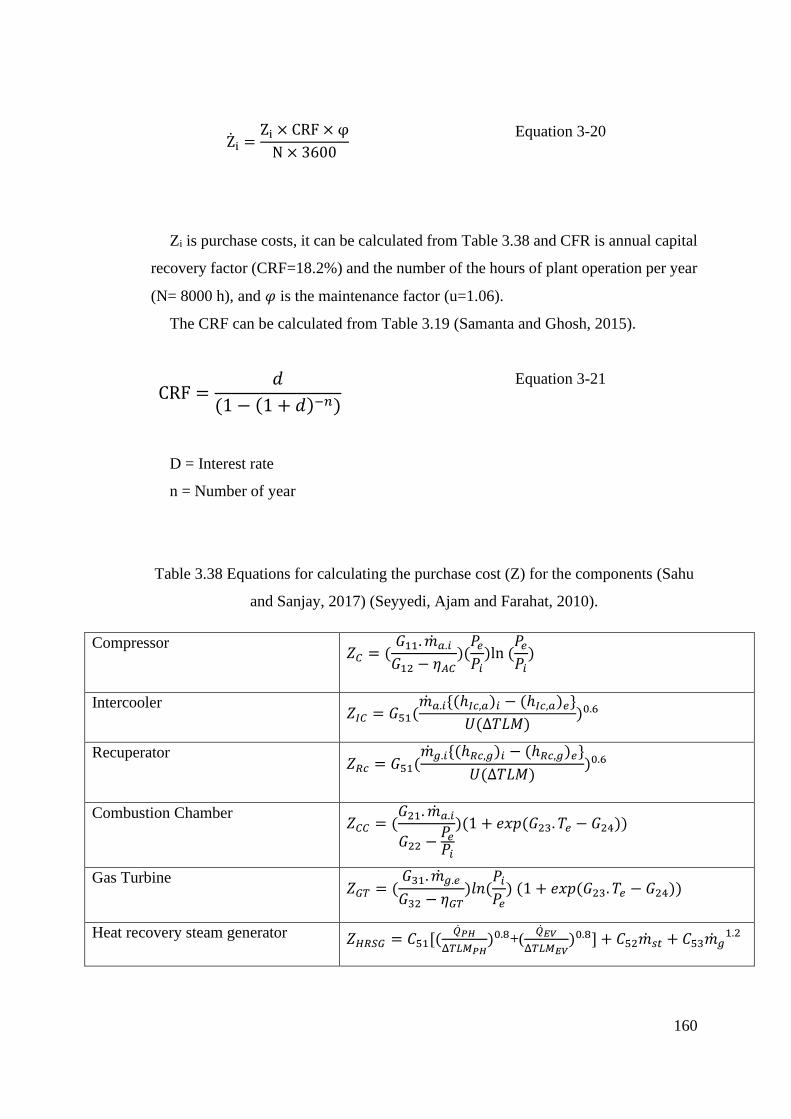
160
Zi =Zi × CRF × φ
N × 3600
Equation 3-20
Zi is purchase costs, it can be calculated from Table 3.38 and CFR is annual capital
recovery factor (CRF=18.2%) and the number of the hours of plant operation per year
(N= 8000 h), and 𝜑 is the maintenance factor (u=1.06).
The CRF can be calculated from Table 3.19 (Samanta and Ghosh, 2015).
CRF =𝑑
(1 − (1 + 𝑑)−𝑛)
Equation 3-21
D = Interest rate
n = Number of year
Table 3.38 Equations for calculating the purchase cost (Z) for the components (Sahu
and Sanjay, 2017) (Seyyedi, Ajam and Farahat, 2010).
Compressor 𝑍𝐶 = (
𝐺11. ��𝑎.𝑖
𝐺12 − 𝜂𝐴𝐶)(
𝑃𝑒
𝑃𝑖)ln (
𝑃𝑒
𝑃𝑖)
Intercooler 𝑍𝐼𝐶 = 𝐺51(
��𝑎.𝑖{(ℎ𝐼𝑐,𝑎)𝑖 − (ℎ𝐼𝑐,𝑎)𝑒}
𝑈(Δ𝑇𝐿𝑀))0.6
Recuperator 𝑍𝑅𝑐 = 𝐺51(
��𝑔.𝑖{(ℎ𝑅𝑐,𝑔)𝑖 − (ℎ𝑅𝑐,𝑔)𝑒}
𝑈(Δ𝑇𝐿𝑀))0.6
Combustion Chamber 𝑍𝐶𝐶 = (
𝐺21. ��𝑎.𝑖
𝐺22 −𝑃𝑒
𝑃𝑖
)(1 + 𝑒𝑥𝑝(𝐺23. 𝑇𝑒 − 𝐺24))
Gas Turbine
𝑍𝐺𝑇 = (𝐺31. ��𝑔.𝑒
𝐺32 − 𝜂𝐺𝑇)𝑙𝑛(
𝑃𝑖
𝑃𝑒) (1 + 𝑒𝑥𝑝(𝐺23. 𝑇𝑒 − 𝐺24))
Heat recovery steam generator 𝑍𝐻𝑅𝑆𝐺 = 𝐶51[(��𝑃𝐻
Δ𝑇𝐿𝑀𝑃𝐻)0.8+(
��𝐸𝑉
Δ𝑇𝐿𝑀𝐸𝑉)0.8] + 𝐶52��𝑠𝑡 + 𝐶53��𝑔
1.2
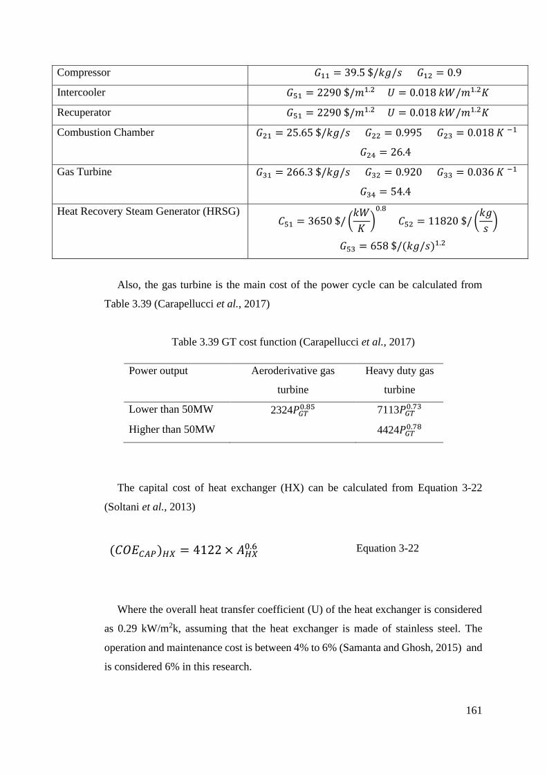
161
Compressor 𝐺11 = 39.5 $/𝑘𝑔/𝑠 𝐺12 = 0.9
Intercooler 𝐺51 = 2290 $/𝑚1.2 𝑈 = 0.018 𝑘𝑊/𝑚1.2𝐾
Recuperator 𝐺51 = 2290 $/𝑚1.2 𝑈 = 0.018 𝑘𝑊/𝑚1.2𝐾
Combustion Chamber 𝐺21 = 25.65 $/𝑘𝑔/𝑠 𝐺22 = 0.995 𝐺23 = 0.018 𝐾 −1
𝐺24 = 26.4
Gas Turbine 𝐺31 = 266.3 $/𝑘𝑔/𝑠 𝐺32 = 0.920 𝐺33 = 0.036 𝐾 −1
𝐺34 = 54.4
Heat Recovery Steam Generator (HRSG) 𝐶51 = 3650 $/ (
𝑘𝑊
𝐾)
0.8
𝐶52 = 11820 $/ (𝑘𝑔
𝑠)
𝐺53 = 658 $/(𝑘𝑔/𝑠)1.2
Also, the gas turbine is the main cost of the power cycle can be calculated from
Table 3.39 (Carapellucci et al., 2017)
Table 3.39 GT cost function (Carapellucci et al., 2017)
Power output Aeroderivative gas
turbine
Heavy duty gas
turbine
Lower than 50MW 2324𝑃𝐺𝑇0.85 7113𝑃𝐺𝑇
0.73
Higher than 50MW 4424𝑃𝐺𝑇0.78
The capital cost of heat exchanger (HX) can be calculated from Equation 3-22
(Soltani et al., 2013)
(𝐶𝑂𝐸𝐶𝐴𝑃)𝐻𝑋 = 4122 × 𝐴𝐻𝑋0.6
Equation 3-22
Where the overall heat transfer coefficient (U) of the heat exchanger is considered
as 0.29 kW/m2k, assuming that the heat exchanger is made of stainless steel. The
operation and maintenance cost is between 4% to 6% (Samanta and Ghosh, 2015) and
is considered 6% in this research.
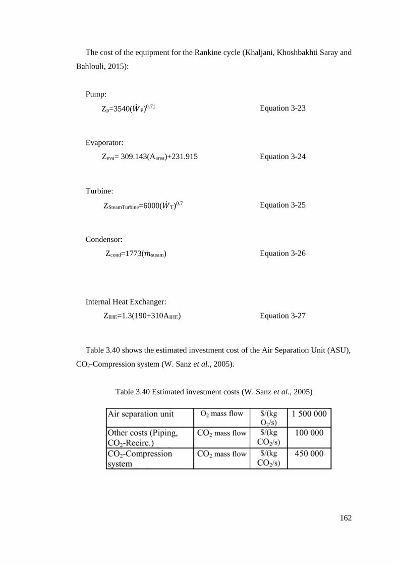
162
The cost of the equipment for the Rankine cycle (Khaljani, Khoshbakhti Saray and
Bahlouli, 2015):
Pump:
Zp=3540(��P)0.71 Equation 3-23
Evaporator:
Zeva= 309.143(Aarea)+231.915 Equation 3-24
Turbine:
ZSteamTurbine=6000(��T)0.7 Equation 3-25
Condensor:
Zcond=1773(��steam) Equation 3-26
Internal Heat Exchanger:
ZIHE=1.3(190+310AIHE) Equation 3-27
Table 3.40 shows the estimated investment cost of the Air Separation Unit (ASU),
CO2-Compression system (W. Sanz et al., 2005).
Table 3.40 Estimated investment costs (W. Sanz et al., 2005)
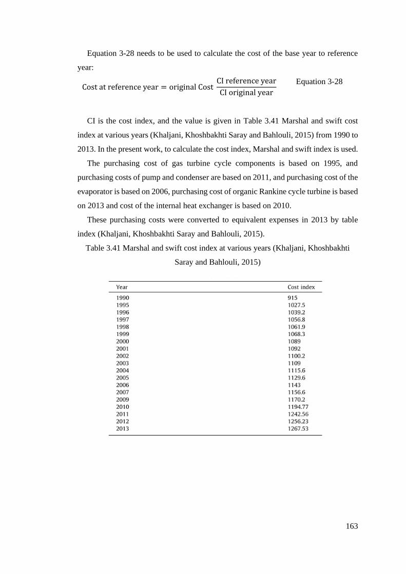
163
Equation 3-28 needs to be used to calculate the cost of the base year to reference
year:
Cost at reference year = original Cost CI reference year
CI original year
Equation 3-28
CI is the cost index, and the value is given in Table 3.41 Marshal and swift cost
index at various years (Khaljani, Khoshbakhti Saray and Bahlouli, 2015) from 1990 to
2013. In the present work, to calculate the cost index, Marshal and swift index is used.
The purchasing cost of gas turbine cycle components is based on 1995, and
purchasing costs of pump and condenser are based on 2011, and purchasing cost of the
evaporator is based on 2006, purchasing cost of organic Rankine cycle turbine is based
on 2013 and cost of the internal heat exchanger is based on 2010.
These purchasing costs were converted to equivalent expenses in 2013 by table
index (Khaljani, Khoshbakhti Saray and Bahlouli, 2015).
Table 3.41 Marshal and swift cost index at various years (Khaljani, Khoshbakhti
Saray and Bahlouli, 2015)
164
Fuel cost can be calculated from the following formula (Sahu and Sanjay, 2017):
Cf = cf × mf × LHV
Equation 3-29
The fuel cost per energy unit (on an LHV basis) is 𝑐𝑓 = 0.004 $/𝑀𝐽 (Sahu and
Sanjay, 2016). The total capital cost of purchasing and maintenance is
𝑍�� = ∑ 𝑍𝑖
Equation 3-30
Total overall cost rate includes fuel cost, operating cost and purchasing cost, and
can be calculated from the following formula:
CT = cf × mf × LHV + ∑ Zi
Equation 3-31
Cost of electricity consumption is 170 Euro/MWh and 170*1.18=200.6 $/MWh.
165
3.7 Summary
In this chapter, the oxy-combustion cycle theories for this PhD thesis are indicated; it
includes the calculation method for the thermodynamic of oxy-combustion cycles,
exergy analysis method are indicated, and EOS of the gas turbine and steam turbine
for this PhD thesis has been defined. Furthermore, methodology for sensitivity analysis
of oxy-combustion cycles are defined and CES, and NetPower sensitivity
methodology is indicated. The techno-economic analysis formula and calculation
method are explained for oxy-combustion cycles; these formulas are used for techno-
economic calculation in chapter 9.
Then, The simulations of the oxy-combustions cycle were presented, the simulation
process flow diagrams of each cycle were shown, and the detailed working flow
properties were tabulated. These simulation data can be used for the oxy-combustion
analysis of the next chapter.
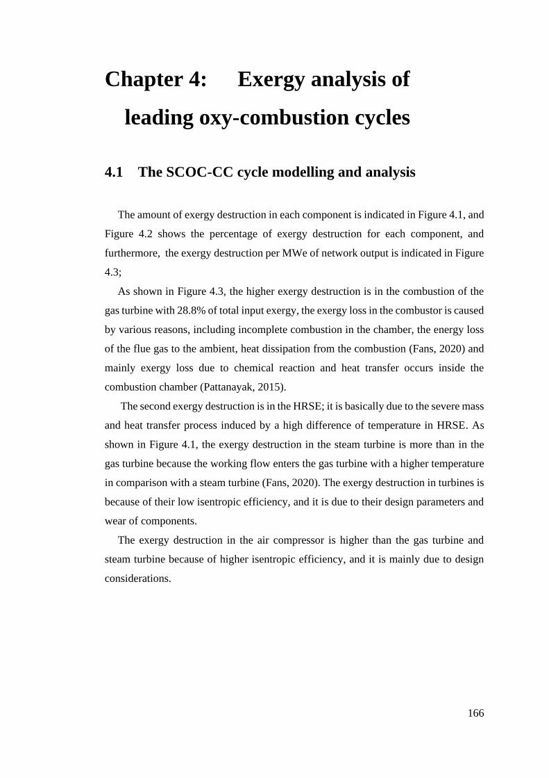
166
Chapter 4: Exergy analysis of
leading oxy-combustion cycles
4.1 The SCOC-CC cycle modelling and analysis
The amount of exergy destruction in each component is indicated in Figure 4.1, and
Figure 4.2 shows the percentage of exergy destruction for each component, and
furthermore, the exergy destruction per MWe of network output is indicated in Figure
4.3;
As shown in Figure 4.3, the higher exergy destruction is in the combustion of the
gas turbine with 28.8% of total input exergy, the exergy loss in the combustor is caused
by various reasons, including incomplete combustion in the chamber, the energy loss
of the flue gas to the ambient, heat dissipation from the combustion (Fans, 2020) and
mainly exergy loss due to chemical reaction and heat transfer occurs inside the
combustion chamber (Pattanayak, 2015).
The second exergy destruction is in the HRSE; it is basically due to the severe mass
and heat transfer process induced by a high difference of temperature in HRSE. As
shown in Figure 4.1, the exergy destruction in the steam turbine is more than in the
gas turbine because the working flow enters the gas turbine with a higher temperature
in comparison with a steam turbine (Fans, 2020). The exergy destruction in turbines is
because of their low isentropic efficiency, and it is due to their design parameters and
wear of components.
The exergy destruction in the air compressor is higher than the gas turbine and
steam turbine because of higher isentropic efficiency, and it is mainly due to design
considerations.
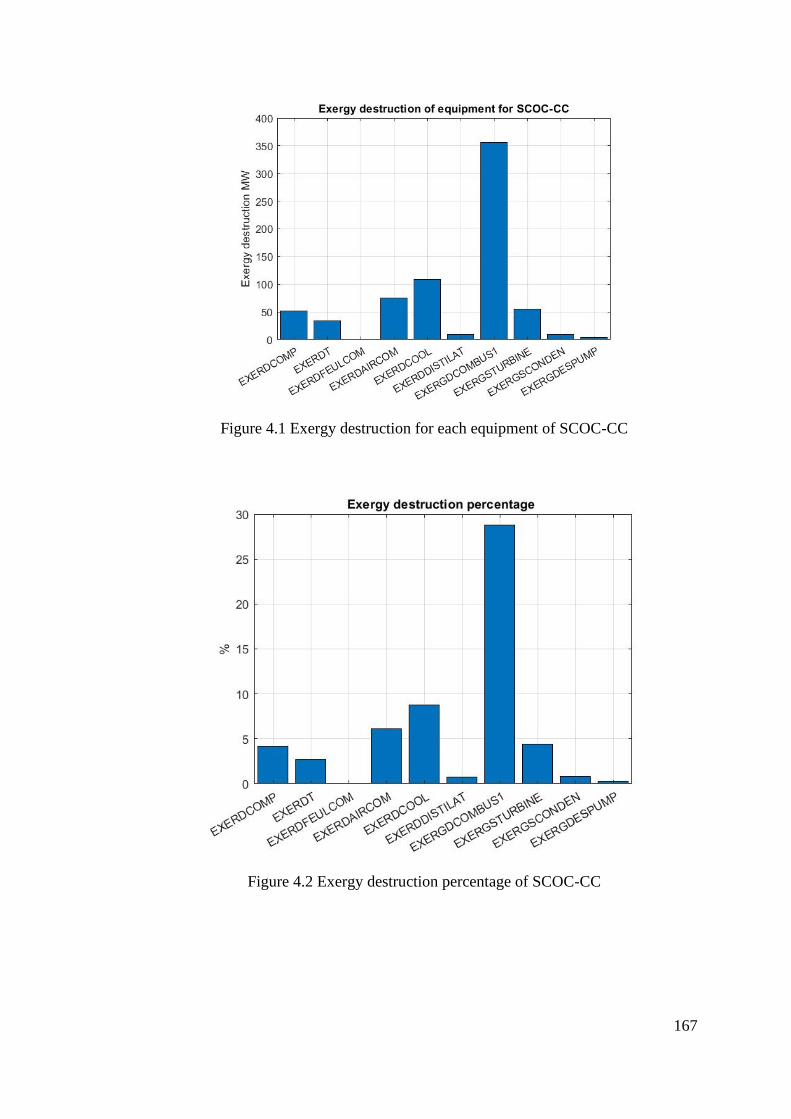
167
Figure 4.1 Exergy destruction for each equipment of SCOC-CC
Figure 4.2 Exergy destruction percentage of SCOC-CC
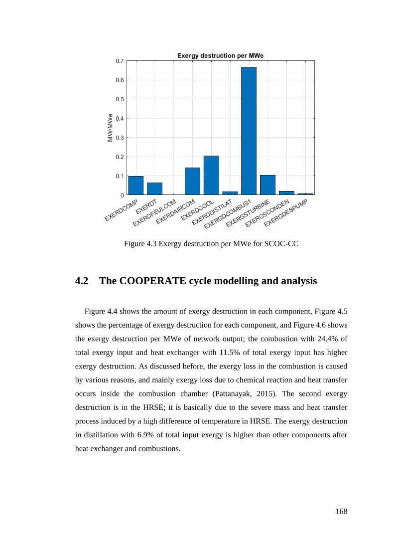
168
Figure 4.3 Exergy destruction per MWe for SCOC-CC
4.2 The COOPERATE cycle modelling and analysis
Figure 4.4 shows the amount of exergy destruction in each component, Figure 4.5
shows the percentage of exergy destruction for each component, and Figure 4.6 shows
the exergy destruction per MWe of network output; the combustion with 24.4% of
total exergy input and heat exchanger with 11.5% of total exergy input has higher
exergy destruction. As discussed before, the exergy loss in the combustion is caused
by various reasons, and mainly exergy loss due to chemical reaction and heat transfer
occurs inside the combustion chamber (Pattanayak, 2015). The second exergy
destruction is in the HRSE; it is basically due to the severe mass and heat transfer
process induced by a high difference of temperature in HRSE. The exergy destruction
in distillation with 6.9% of total input exergy is higher than other components after
heat exchanger and combustions.
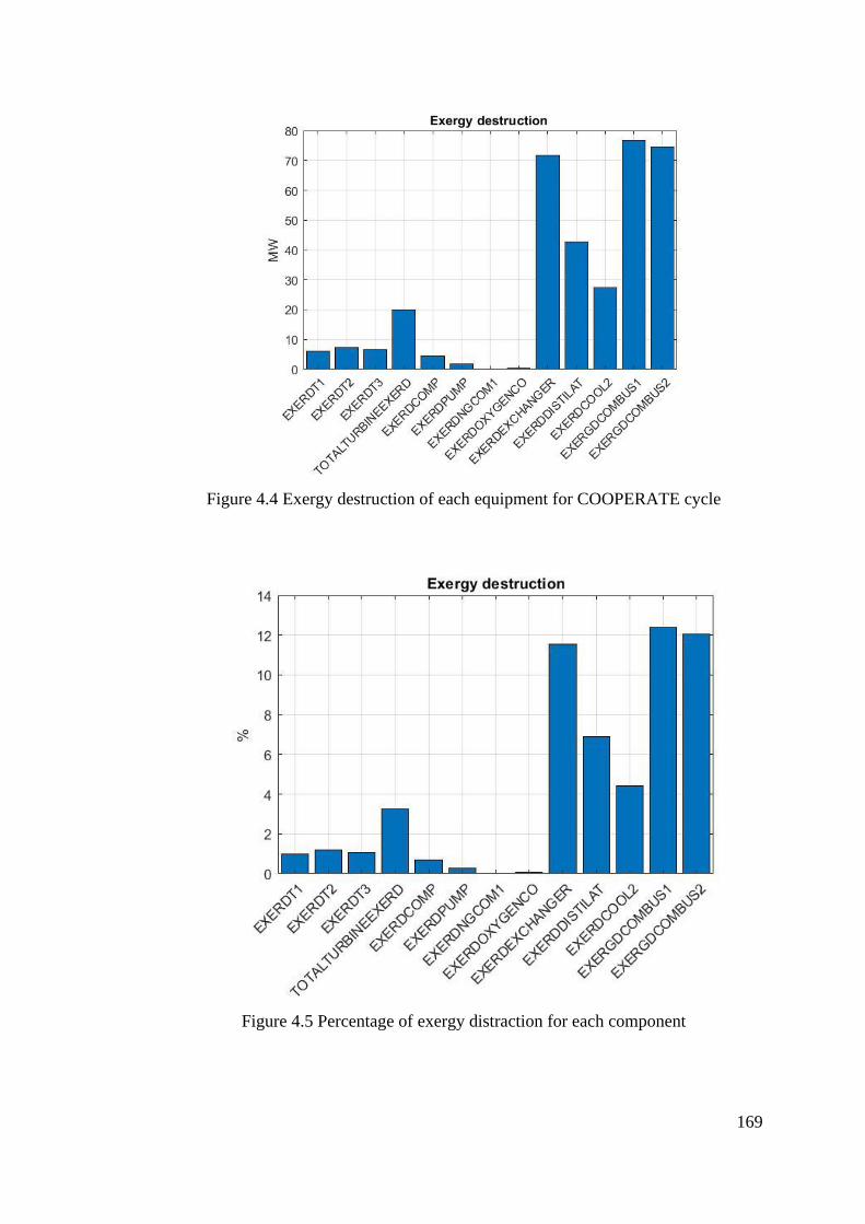
169
Figure 4.4 Exergy destruction of each equipment for COOPERATE cycle
Figure 4.5 Percentage of exergy distraction for each component
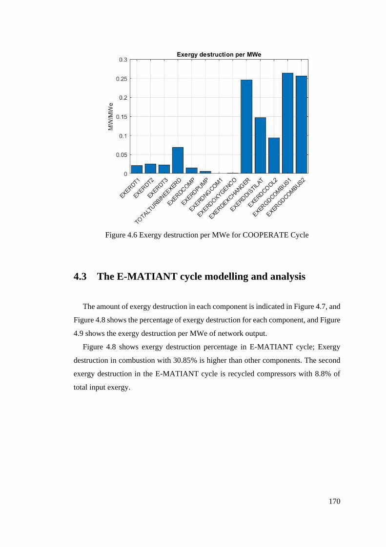
170
Figure 4.6 Exergy destruction per MWe for COOPERATE Cycle
4.3 The E-MATIANT cycle modelling and analysis
The amount of exergy destruction in each component is indicated in Figure 4.7, and
Figure 4.8 shows the percentage of exergy destruction for each component, and Figure
4.9 shows the exergy destruction per MWe of network output.
Figure 4.8 shows exergy destruction percentage in E-MATIANT cycle; Exergy
destruction in combustion with 30.85% is higher than other components. The second
exergy destruction in the E-MATIANT cycle is recycled compressors with 8.8% of
total input exergy.
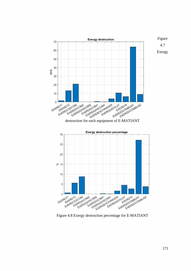
171
Figure
4.7
Exergy
destruction for each equipment of E-MATIANT
Figure 4.8 Exergy destruction percentage for E-MATIANT
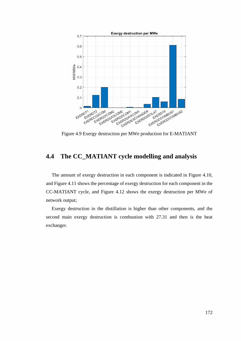
172
Figure 4.9 Exergy destruction per MWe production for E-MATIANT
4.4 The CC_MATIANT cycle modelling and analysis
The amount of exergy destruction in each component is indicated in Figure 4.10,
and Figure 4.11 shows the percentage of exergy destruction for each component in the
CC-MATIANT cycle, and Figure 4.12 shows the exergy destruction per MWe of
network output;
Exergy destruction in the distillation is higher than other components, and the
second main exergy destruction is combustion with 27.31 and then is the heat
exchanger.
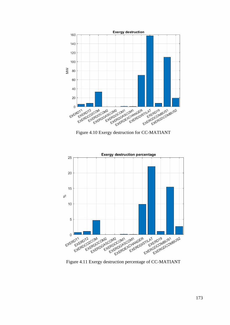
173
Figure 4.10 Exergy destruction for CC-MATIANT
Figure 4.11 Exergy destruction percentage of CC-MATIANT
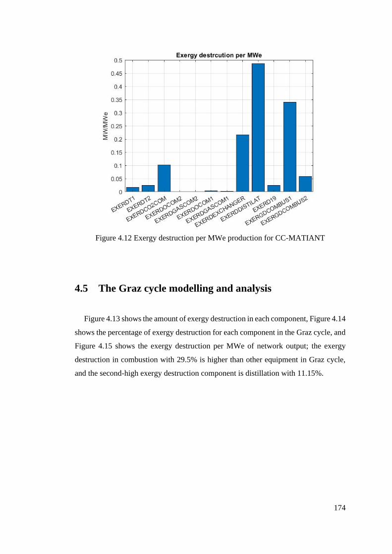
174
Figure 4.12 Exergy destruction per MWe production for CC-MATIANT
4.5 The Graz cycle modelling and analysis
Figure 4.13 shows the amount of exergy destruction in each component, Figure 4.14
shows the percentage of exergy destruction for each component in the Graz cycle, and
Figure 4.15 shows the exergy destruction per MWe of network output; the exergy
destruction in combustion with 29.5% is higher than other equipment in Graz cycle,
and the second-high exergy destruction component is distillation with 11.15%.
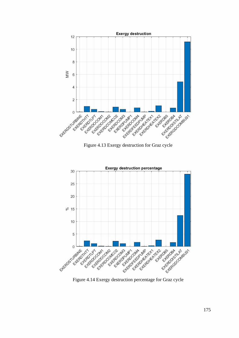
175
Figure 4.13 Exergy destruction for Graz cycle
Figure 4.14 Exergy destruction percentage for Graz cycle
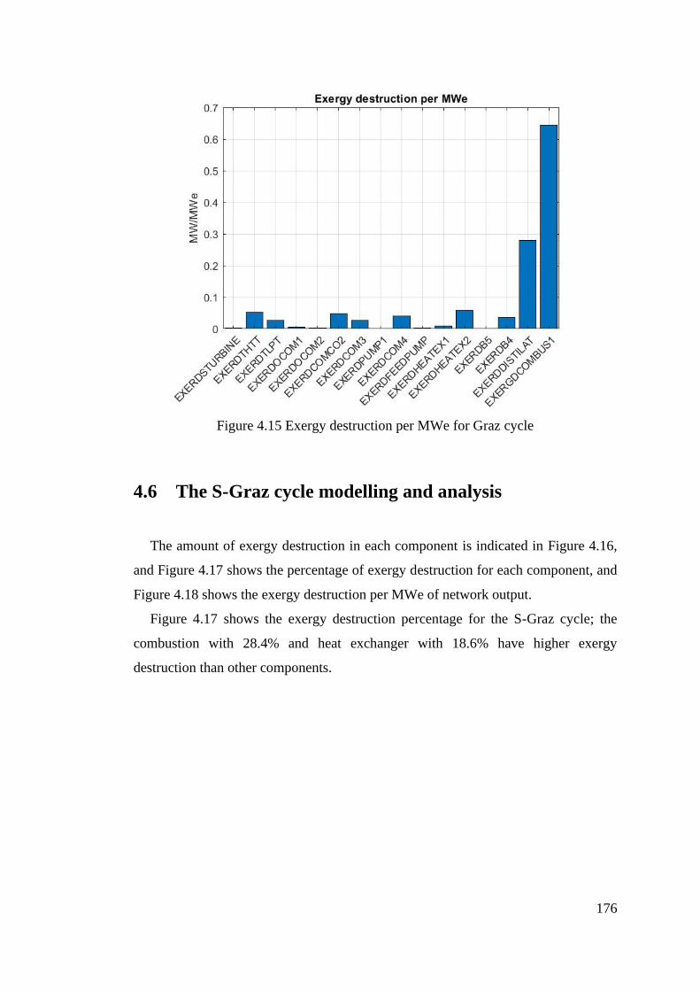
176
Figure 4.15 Exergy destruction per MWe for Graz cycle
4.6 The S-Graz cycle modelling and analysis
The amount of exergy destruction in each component is indicated in Figure 4.16,
and Figure 4.17 shows the percentage of exergy destruction for each component, and
Figure 4.18 shows the exergy destruction per MWe of network output.
Figure 4.17 shows the exergy destruction percentage for the S-Graz cycle; the
combustion with 28.4% and heat exchanger with 18.6% have higher exergy
destruction than other components.
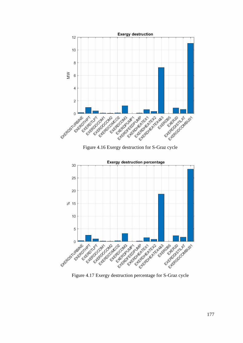
177
Figure 4.16 Exergy destruction for S-Graz cycle
Figure 4.17 Exergy destruction percentage for S-Graz cycle
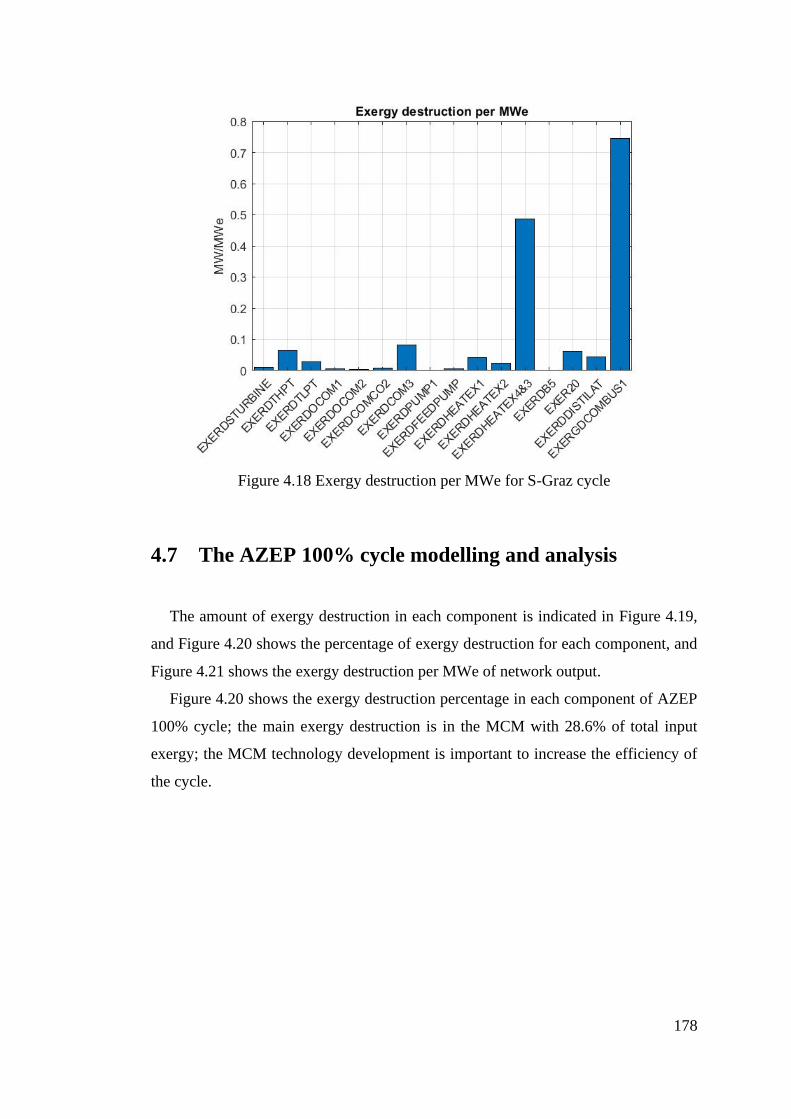
178
Figure 4.18 Exergy destruction per MWe for S-Graz cycle
4.7 The AZEP 100% cycle modelling and analysis
The amount of exergy destruction in each component is indicated in Figure 4.19,
and Figure 4.20 shows the percentage of exergy destruction for each component, and
Figure 4.21 shows the exergy destruction per MWe of network output.
Figure 4.20 shows the exergy destruction percentage in each component of AZEP
100% cycle; the main exergy destruction is in the MCM with 28.6% of total input
exergy; the MCM technology development is important to increase the efficiency of
the cycle.
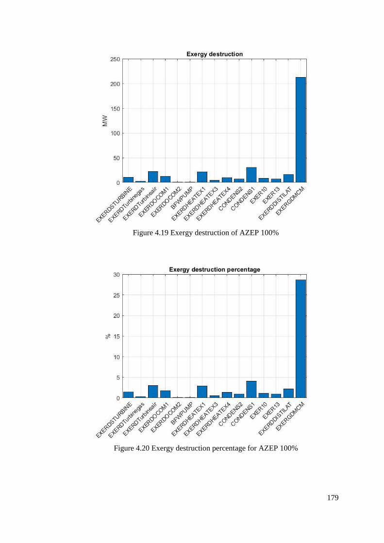
179
Figure 4.19 Exergy destruction of AZEP 100%
Figure 4.20 Exergy destruction percentage for AZEP 100%
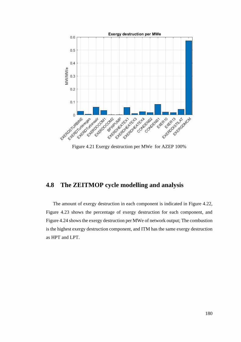
180
Figure 4.21 Exergy destruction per MWe for AZEP 100%
4.8 The ZEITMOP cycle modelling and analysis
The amount of exergy destruction in each component is indicated in Figure 4.22,
Figure 4.23 shows the percentage of exergy destruction for each component, and
Figure 4.24 shows the exergy destruction per MWe of network output; The combustion
is the highest exergy destruction component, and ITM has the same exergy destruction
as HPT and LPT.
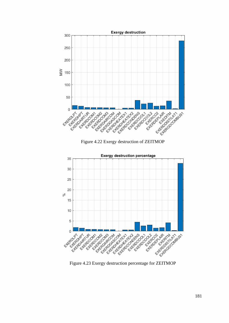
181
Figure 4.22 Exergy destruction of ZEITMOP
Figure 4.23 Exergy destruction percentage for ZEITMOP
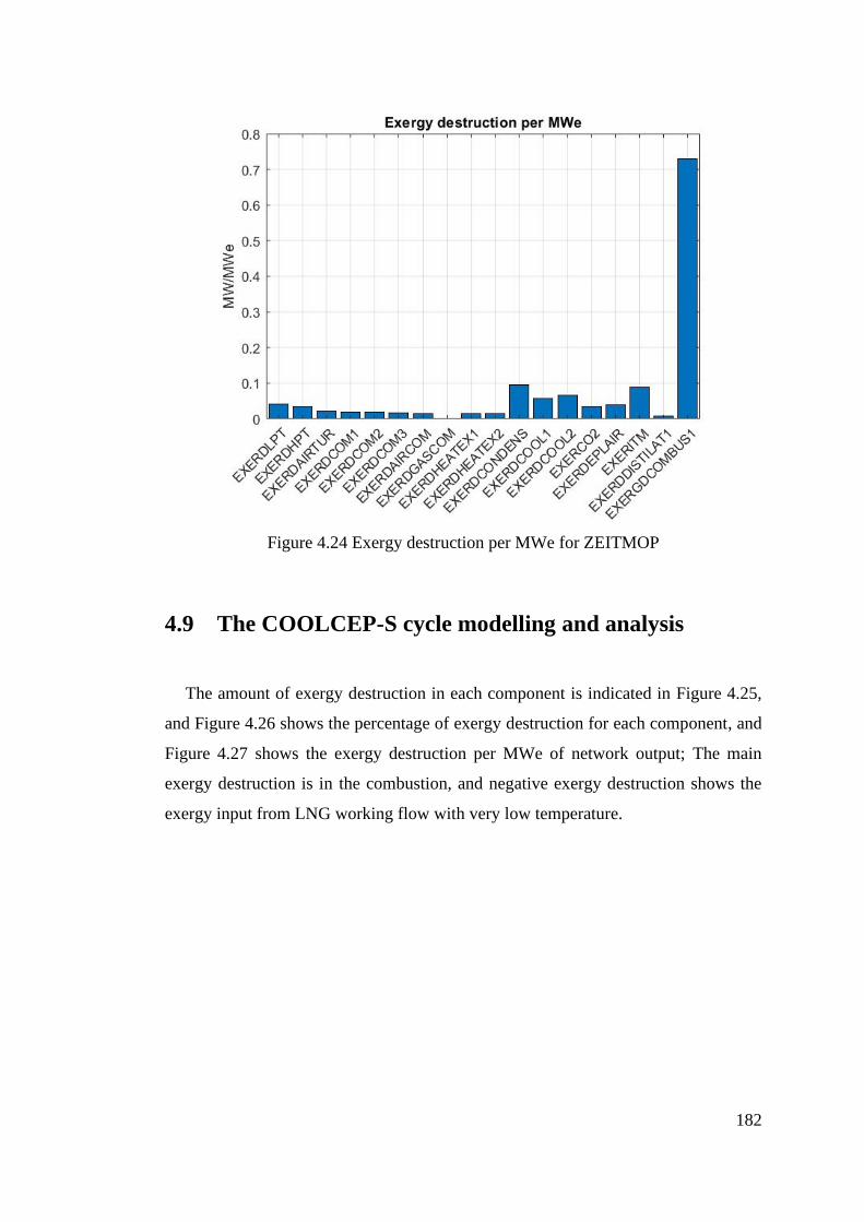
182
Figure 4.24 Exergy destruction per MWe for ZEITMOP
4.9 The COOLCEP-S cycle modelling and analysis
The amount of exergy destruction in each component is indicated in Figure 4.25,
and Figure 4.26 shows the percentage of exergy destruction for each component, and
Figure 4.27 shows the exergy destruction per MWe of network output; The main
exergy destruction is in the combustion, and negative exergy destruction shows the
exergy input from LNG working flow with very low temperature.
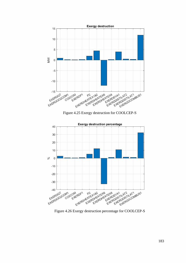
183
Figure 4.25 Exergy destruction for COOLCEP-S
Figure 4.26 Exergy destruction percentage for COOLCEP-S
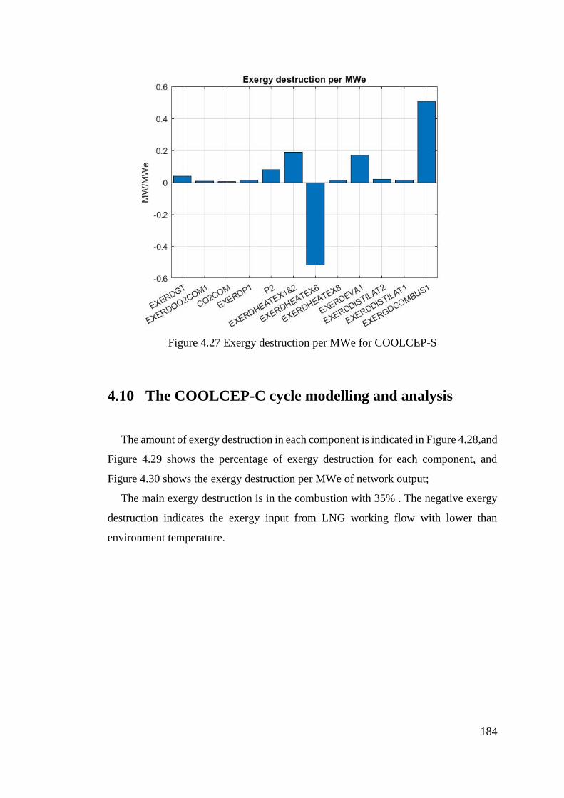
184
Figure 4.27 Exergy destruction per MWe for COOLCEP-S
4.10 The COOLCEP-C cycle modelling and analysis
The amount of exergy destruction in each component is indicated in Figure 4.28,and
Figure 4.29 shows the percentage of exergy destruction for each component, and
Figure 4.30 shows the exergy destruction per MWe of network output;
The main exergy destruction is in the combustion with 35% . The negative exergy
destruction indicates the exergy input from LNG working flow with lower than
environment temperature.
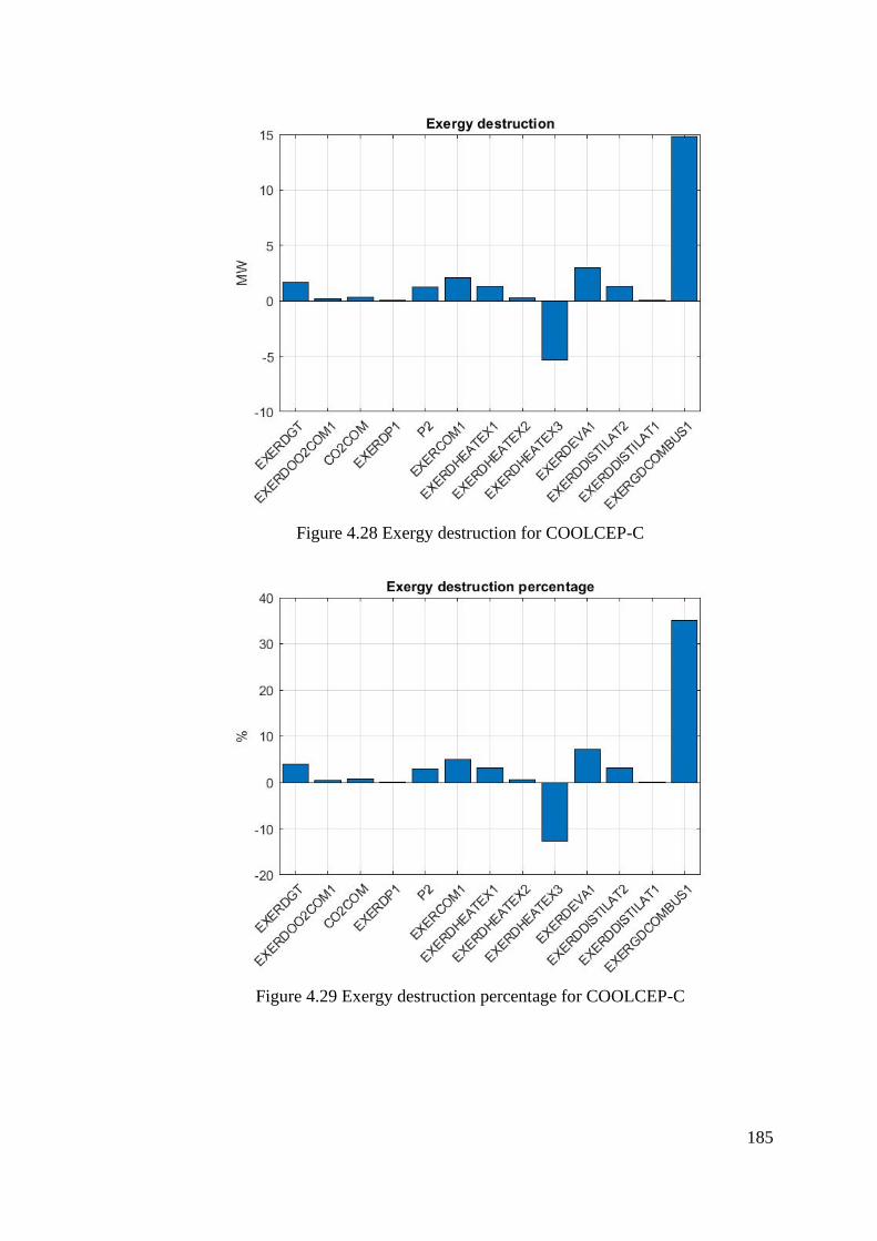
185
Figure 4.28 Exergy destruction for COOLCEP-C
Figure 4.29 Exergy destruction percentage for COOLCEP-C
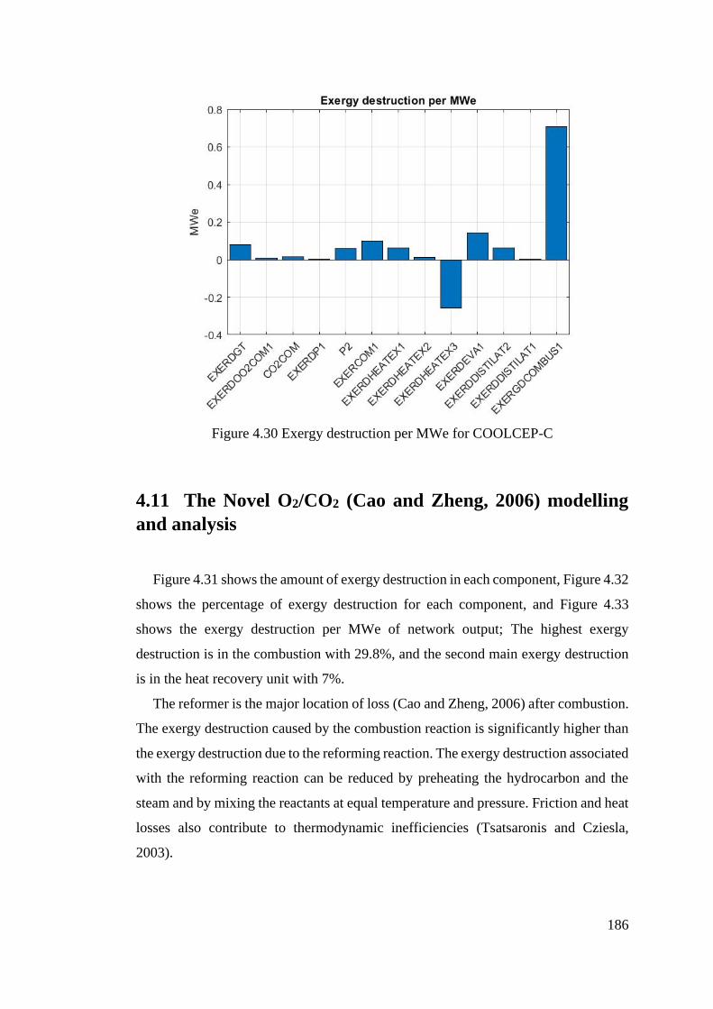
186
Figure 4.30 Exergy destruction per MWe for COOLCEP-C
4.11 The Novel O2/CO2 (Cao and Zheng, 2006) modelling
and analysis
Figure 4.31 shows the amount of exergy destruction in each component, Figure 4.32
shows the percentage of exergy destruction for each component, and Figure 4.33
shows the exergy destruction per MWe of network output; The highest exergy
destruction is in the combustion with 29.8%, and the second main exergy destruction
is in the heat recovery unit with 7%.
The reformer is the major location of loss (Cao and Zheng, 2006) after combustion.
The exergy destruction caused by the combustion reaction is significantly higher than
the exergy destruction due to the reforming reaction. The exergy destruction associated
with the reforming reaction can be reduced by preheating the hydrocarbon and the
steam and by mixing the reactants at equal temperature and pressure. Friction and heat
losses also contribute to thermodynamic inefficiencies (Tsatsaronis and Cziesla,
2003).
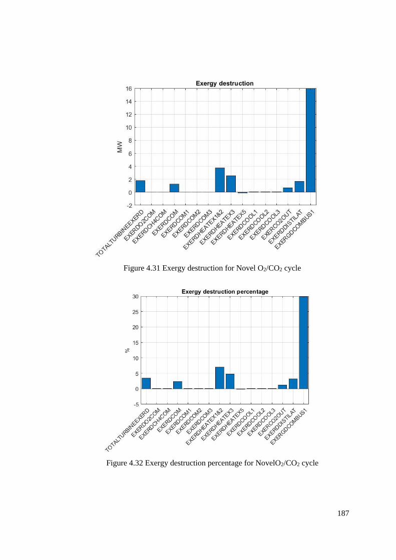
187
Figure 4.31 Exergy destruction for Novel O2/CO2 cycle
Figure 4.32 Exergy destruction percentage for NovelO2/CO2 cycle
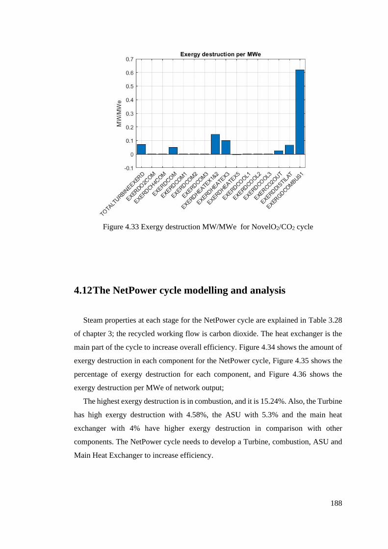
188
Figure 4.33 Exergy destruction MW/MWe for NovelO2/CO2 cycle
4.12 The NetPower cycle modelling and analysis
Steam properties at each stage for the NetPower cycle are explained in Table 3.28
of chapter 3; the recycled working flow is carbon dioxide. The heat exchanger is the
main part of the cycle to increase overall efficiency. Figure 4.34 shows the amount of
exergy destruction in each component for the NetPower cycle, Figure 4.35 shows the
percentage of exergy destruction for each component, and Figure 4.36 shows the
exergy destruction per MWe of network output;
The highest exergy destruction is in combustion, and it is 15.24%. Also, the Turbine
has high exergy destruction with 4.58%, the ASU with 5.3% and the main heat
exchanger with 4% have higher exergy destruction in comparison with other
components. The NetPower cycle needs to develop a Turbine, combustion, ASU and
Main Heat Exchanger to increase efficiency.
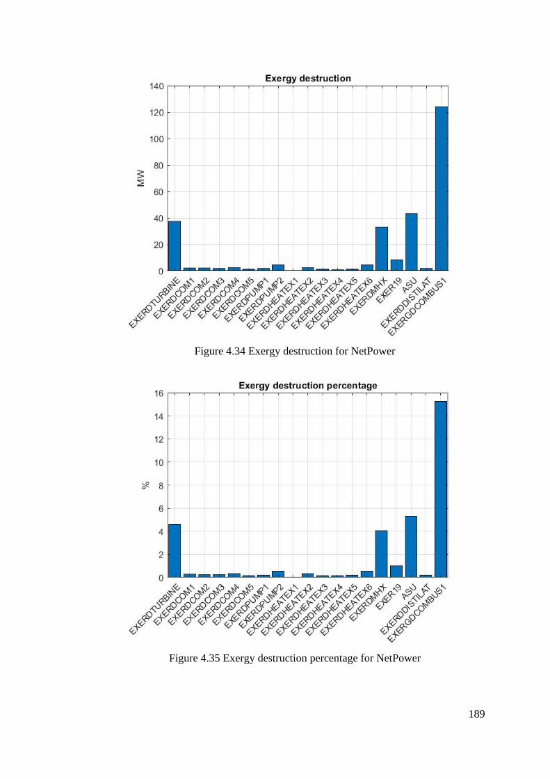
189
Figure 4.34 Exergy destruction for NetPower
Figure 4.35 Exergy destruction percentage for NetPower
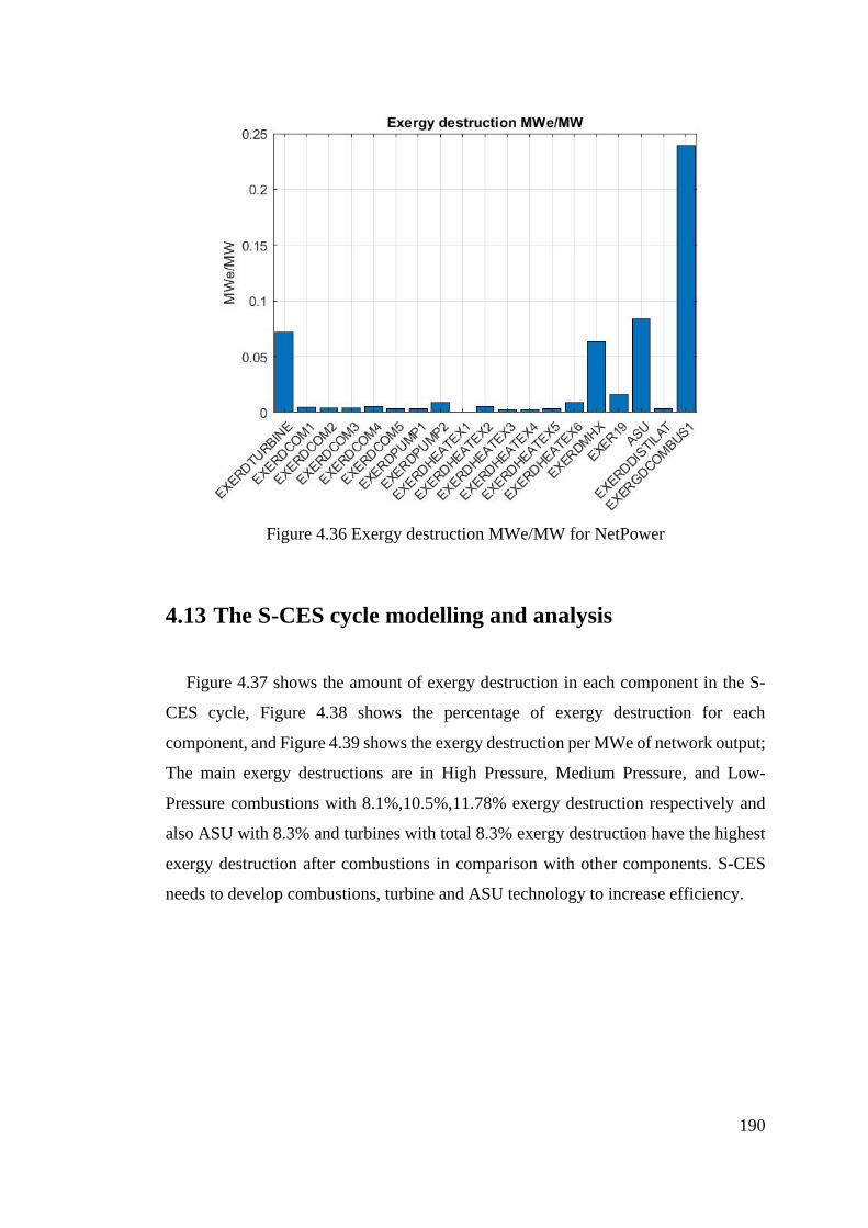
190
Figure 4.36 Exergy destruction MWe/MW for NetPower
4.13 The S-CES cycle modelling and analysis
Figure 4.37 shows the amount of exergy destruction in each component in the S-
CES cycle, Figure 4.38 shows the percentage of exergy destruction for each
component, and Figure 4.39 shows the exergy destruction per MWe of network output;
The main exergy destructions are in High Pressure, Medium Pressure, and Low-
Pressure combustions with 8.1%,10.5%,11.78% exergy destruction respectively and
also ASU with 8.3% and turbines with total 8.3% exergy destruction have the highest
exergy destruction after combustions in comparison with other components. S-CES
needs to develop combustions, turbine and ASU technology to increase efficiency.
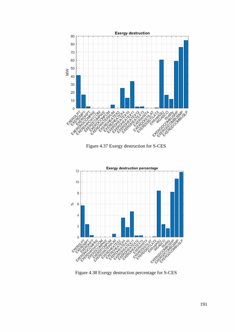
191
Figure 4.37 Exergy destruction for S-CES
Figure 4.38 Exergy destruction percentage for S-CES
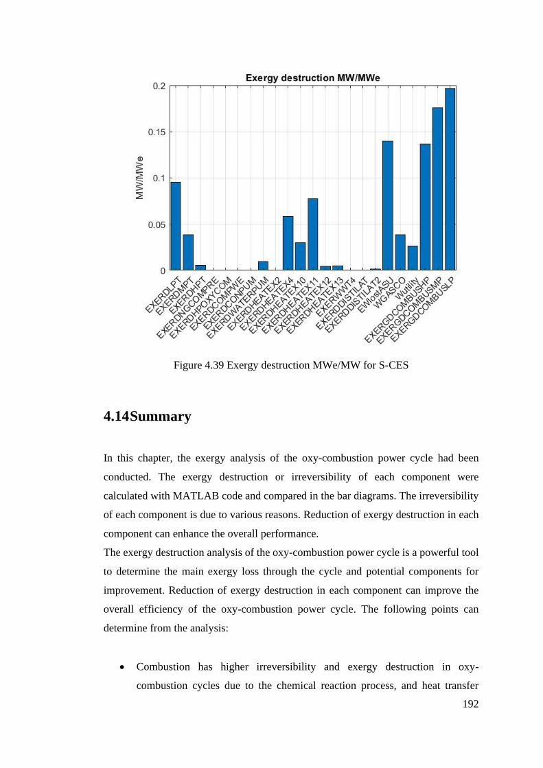
192
Figure 4.39 Exergy destruction MWe/MW for S-CES
4.14 Summary
In this chapter, the exergy analysis of the oxy-combustion power cycle had been
conducted. The exergy destruction or irreversibility of each component were
calculated with MATLAB code and compared in the bar diagrams. The irreversibility
of each component is due to various reasons. Reduction of exergy destruction in each
component can enhance the overall performance.
The exergy destruction analysis of the oxy-combustion power cycle is a powerful tool
to determine the main exergy loss through the cycle and potential components for
improvement. Reduction of exergy destruction in each component can improve the
overall efficiency of the oxy-combustion power cycle. The following points can
determine from the analysis:
• Combustion has higher irreversibility and exergy destruction in oxy-
combustion cycles due to the chemical reaction process, and heat transfer
193
occurs in the combustion chambers. One of the ways to reduce exergy loss in
combustion is preheating the reactants in the combustion chamber (Oyedepo
et al., 2015). Improving combustion technologies is one of the critical points
to increase the overall efficiency of the oxy-combustion power cycle, and this
component needs to develop in future for the oxy-combustion power cycle.
• The second main exergy loss in oxy-combustions are HRSG or heat exchanger
due to heat transfer between two-stream. Therefore, improving the efficiency
of HRSG can reduce exergy destruction and improve overall efficiency. The
efficiency of HRSG and heat exchangers can be increased by increasing the
temperature of inlet gas (Bunyamanid et al., 2016) or reducing the min
approach temperature with proper design.
• The higher turbine inlet temperature causes lower exergy destruction, and
increasing the TIT will cause more turbine output work. To increase the turbine
inlet temperature, turbine blade coating need to develop to resist high
temperature (Oyedepo et al., 2015). Development in blade cooling technology
and blade coating can reduce exergy destruction in the turbine and increase the
overall efficiency of the oxy-combustion cycle.
• Improving turbine and compressor isentropic efficiency can reduce exergy
destruction in these components. The design parameters of turbomachinery
have a higher effect on the isentropic efficiency, including the aerodynamic
surface of the blade and main body.
• Recovering heat from turbine exhaust can recover exergy from downstream
and use it again. The combined cycle is one of the best technology to recover
exergy from the exhaust of the gas turbine.
• The reformer has better application in the oxy-combustion cycle due to the
quantity a duality of heat load; for example, the CO2-NG reforming technology
can recover exergy from turbine exhaust effectively due to the endothermic
nature of the process.
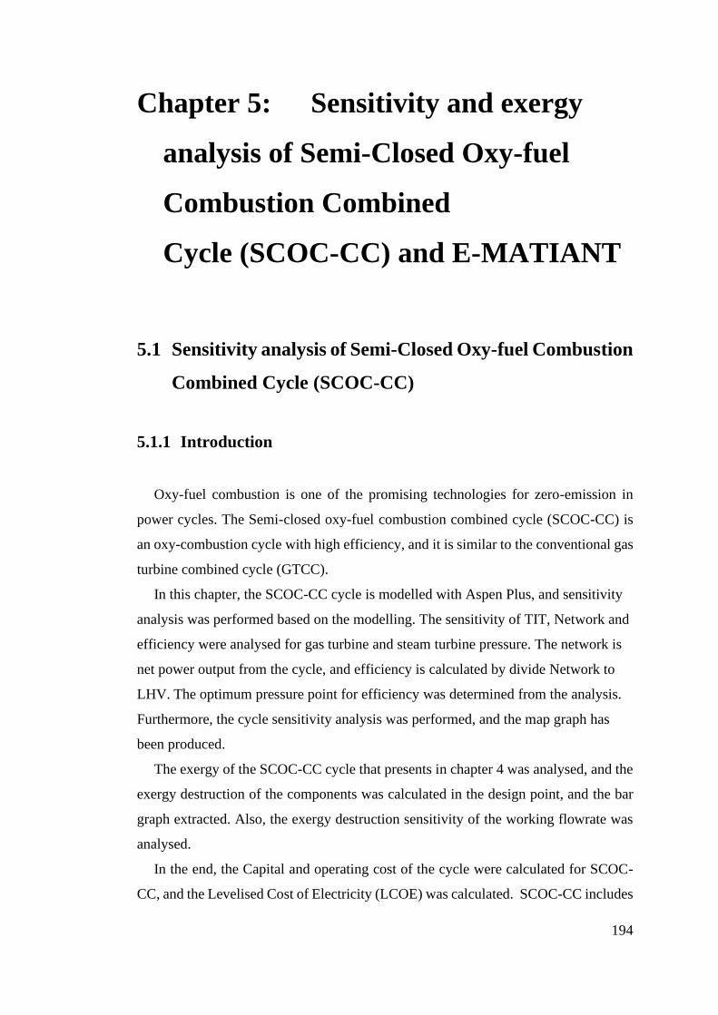
194
Chapter 5: Sensitivity and exergy
analysis of Semi-Closed Oxy-fuel
Combustion Combined
Cycle (SCOC-CC) and E-MATIANT
5.1 Sensitivity analysis of Semi-Closed Oxy-fuel Combustion
Combined Cycle (SCOC-CC)
5.1.1 Introduction
Oxy-fuel combustion is one of the promising technologies for zero-emission in
power cycles. The Semi-closed oxy-fuel combustion combined cycle (SCOC-CC) is
an oxy-combustion cycle with high efficiency, and it is similar to the conventional gas
turbine combined cycle (GTCC).
In this chapter, the SCOC-CC cycle is modelled with Aspen Plus, and sensitivity
analysis was performed based on the modelling. The sensitivity of TIT, Network and
efficiency were analysed for gas turbine and steam turbine pressure. The network is
net power output from the cycle, and efficiency is calculated by divide Network to
LHV. The optimum pressure point for efficiency was determined from the analysis.
Furthermore, the cycle sensitivity analysis was performed, and the map graph has
been produced.
The exergy of the SCOC-CC cycle that presents in chapter 4 was analysed, and the
exergy destruction of the components was calculated in the design point, and the bar
graph extracted. Also, the exergy destruction sensitivity of the working flowrate was
analysed.
In the end, the Capital and operating cost of the cycle were calculated for SCOC-
CC, and the Levelised Cost of Electricity (LCOE) was calculated. SCOC-CC includes
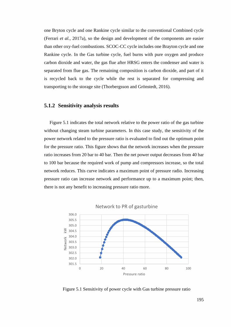
195
one Bryton cycle and one Rankine cycle similar to the conventional Combined cycle
(Ferrari et al., 2017a), so the design and development of the components are easier
than other oxy-fuel combustions. SCOC-CC cycle includes one Brayton cycle and one
Rankine cycle. In the Gas turbine cycle, fuel burns with pure oxygen and produce
carbon dioxide and water, the gas flue after HRSG enters the condenser and water is
separated from flue gas. The remaining composition is carbon dioxide, and part of it
is recycled back to the cycle while the rest is separated for compressing and
transporting to the storage site (Thorbergsson and Grönstedt, 2016).
5.1.2 Sensitivity analysis results
Figure 5.1 indicates the total network relative to the power ratio of the gas turbine
without changing steam turbine parameters. In this case study, the sensitivity of the
power network related to the pressure ratio is evaluated to find out the optimum point
for the pressure ratio. This figure shows that the network increases when the pressure
ratio increases from 20 bar to 40 bar. Then the net power output decreases from 40 bar
to 100 bar because the required work of pump and compressors increase, so the total
network reduces. This curve indicates a maximum point of pressure radio. Increasing
pressure ratio can increase network and performance up to a maximum point; then,
there is not any benefit to increasing pressure ratio more.
Figure 5.1 Sensitivity of power cycle with Gas turbine pressure ratio
301.5
302.0
302.5
303.0
303.5
304.0
304.5
305.0
305.5
306.0
0 20 40 60 80 100
Net
wo
rk
kW
Pressure ratio
Network to PR of gasturbine
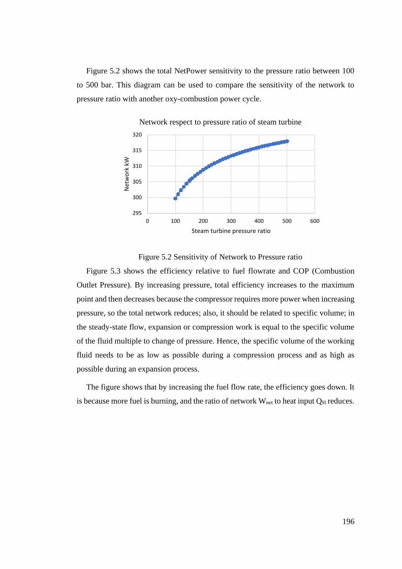
196
Figure 5.2 shows the total NetPower sensitivity to the pressure ratio between 100
to 500 bar. This diagram can be used to compare the sensitivity of the network to
pressure ratio with another oxy-combustion power cycle.
Figure 5.2 Sensitivity of Network to Pressure ratio
Figure 5.3 shows the efficiency relative to fuel flowrate and COP (Combustion
Outlet Pressure). By increasing pressure, total efficiency increases to the maximum
point and then decreases because the compressor requires more power when increasing
pressure, so the total network reduces; also, it should be related to specific volume; in
the steady-state flow, expansion or compression work is equal to the specific volume
of the fluid multiple to change of pressure. Hence, the specific volume of the working
fluid needs to be as low as possible during a compression process and as high as
possible during an expansion process.
The figure shows that by increasing the fuel flow rate, the efficiency goes down. It
is because more fuel is burning, and the ratio of network Wnet to heat input QH reduces.
295
300
305
310
315
320
0 100 200 300 400 500 600
Net
wo
rk k
W
Steam turbine pressure ratio
Network respect to pressure ratio of steam turbine
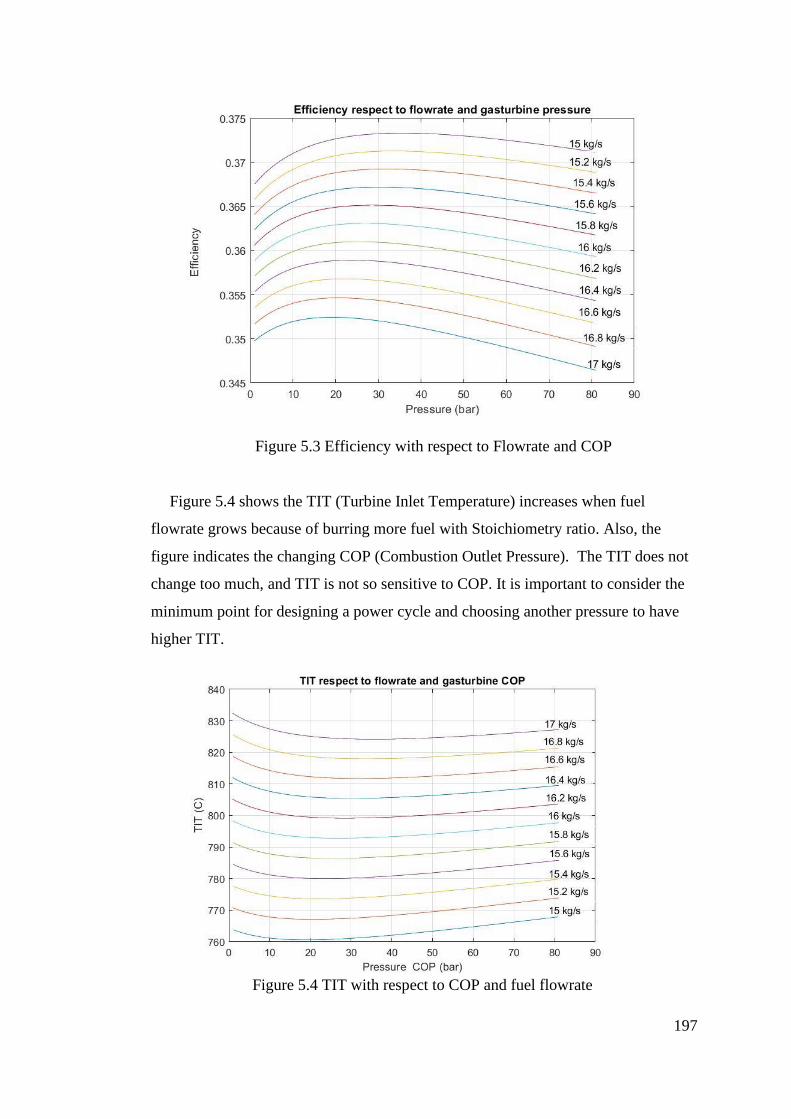
197
Figure 5.3 Efficiency with respect to Flowrate and COP
Figure 5.4 shows the TIT (Turbine Inlet Temperature) increases when fuel
flowrate grows because of burring more fuel with Stoichiometry ratio. Also, the
figure indicates the changing COP (Combustion Outlet Pressure). The TIT does not
change too much, and TIT is not so sensitive to COP. It is important to consider the
minimum point for designing a power cycle and choosing another pressure to have
higher TIT.
Figure 5.4 TIT with respect to COP and fuel flowrate
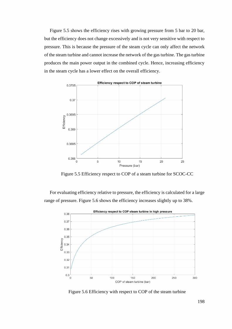
198
Figure 5.5 shows the efficiency rises with growing pressure from 5 bar to 20 bar,
but the efficiency does not change excessively and is not very sensitive with respect to
pressure. This is because the pressure of the steam cycle can only affect the network
of the steam turbine and cannot increase the network of the gas turbine. The gas turbine
produces the main power output in the combined cycle. Hence, increasing efficiency
in the steam cycle has a lower effect on the overall efficiency.
Figure 5.5 Efficiency respect to COP of a steam turbine for SCOC-CC
For evaluating efficiency relative to pressure, the efficiency is calculated for a large
range of pressure. Figure 5.6 shows the efficiency increases slightly up to 38%.
Figure 5.6 Efficiency with respect to COP of the steam turbine
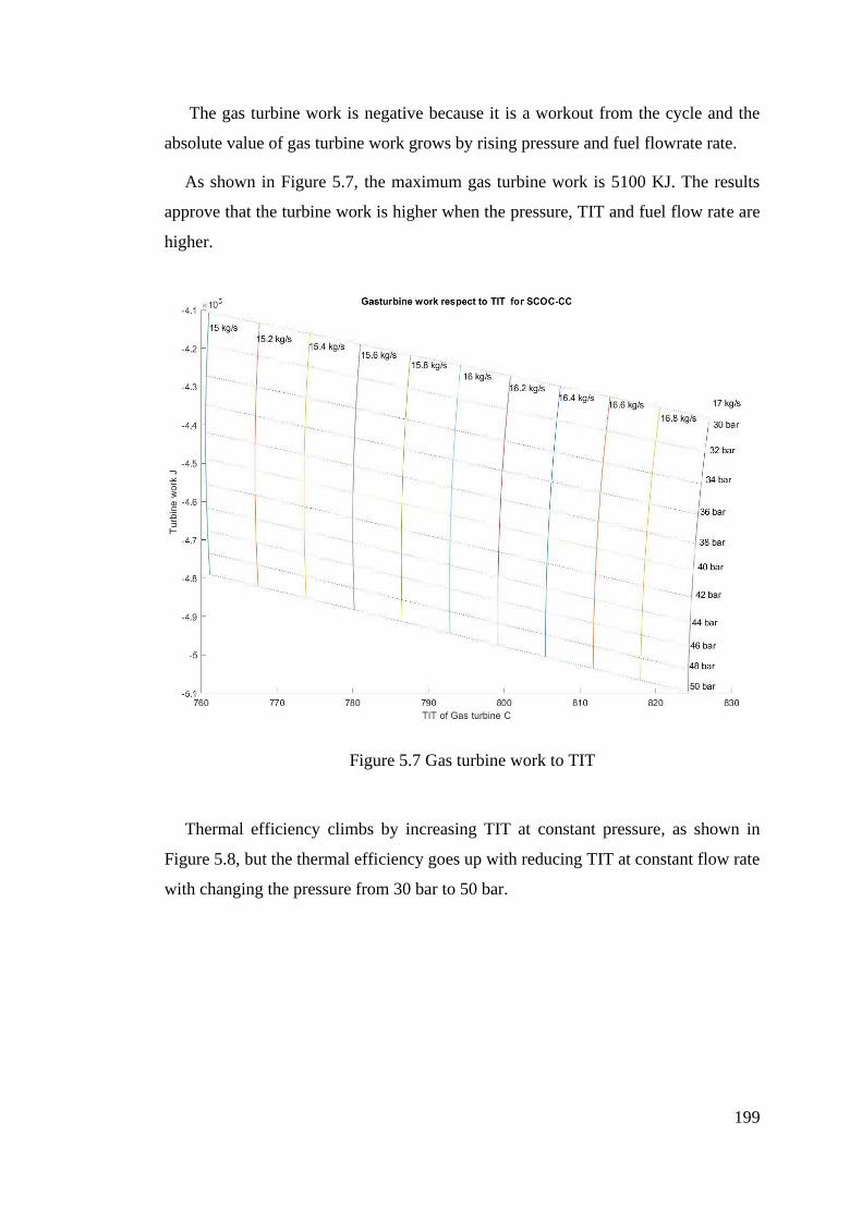
199
The gas turbine work is negative because it is a workout from the cycle and the
absolute value of gas turbine work grows by rising pressure and fuel flowrate rate.
As shown in Figure 5.7, the maximum gas turbine work is 5100 KJ. The results
approve that the turbine work is higher when the pressure, TIT and fuel flow rate are
higher.
Figure 5.7 Gas turbine work to TIT
Thermal efficiency climbs by increasing TIT at constant pressure, as shown in
Figure 5.8, but the thermal efficiency goes up with reducing TIT at constant flow rate
with changing the pressure from 30 bar to 50 bar.
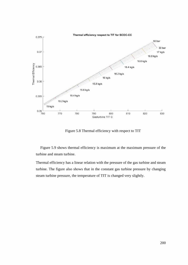
200
Figure 5.8 Thermal efficiency with respect to TIT
Figure 5.9 shows thermal efficiency is maximum at the maximum pressure of the
turbine and steam turbine.
Thermal efficiency has a linear relation with the pressure of the gas turbine and steam
turbine. The figure also shows that in the constant gas turbine pressure by changing
steam turbine pressure, the temperature of TIT is changed very slightly.
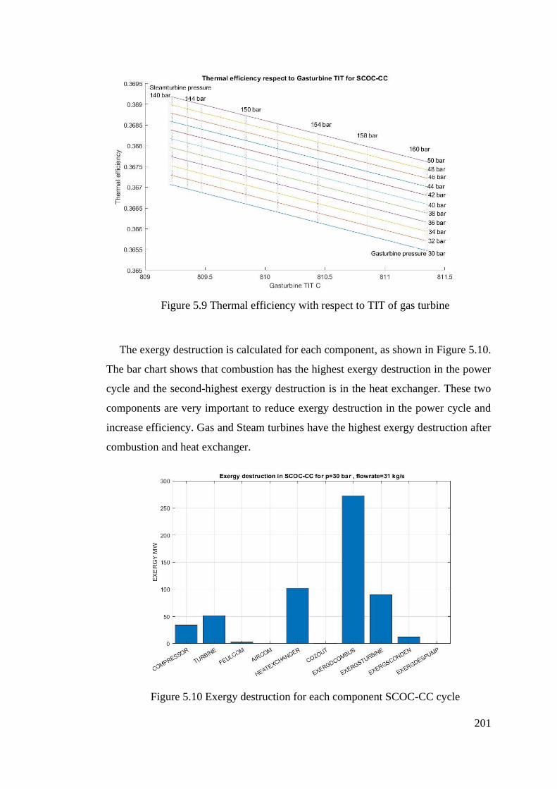
201
Figure 5.9 Thermal efficiency with respect to TIT of gas turbine
The exergy destruction is calculated for each component, as shown in Figure 5.10.
The bar chart shows that combustion has the highest exergy destruction in the power
cycle and the second-highest exergy destruction is in the heat exchanger. These two
components are very important to reduce exergy destruction in the power cycle and
increase efficiency. Gas and Steam turbines have the highest exergy destruction after
combustion and heat exchanger.
Figure 5.10 Exergy destruction for each component SCOC-CC cycle
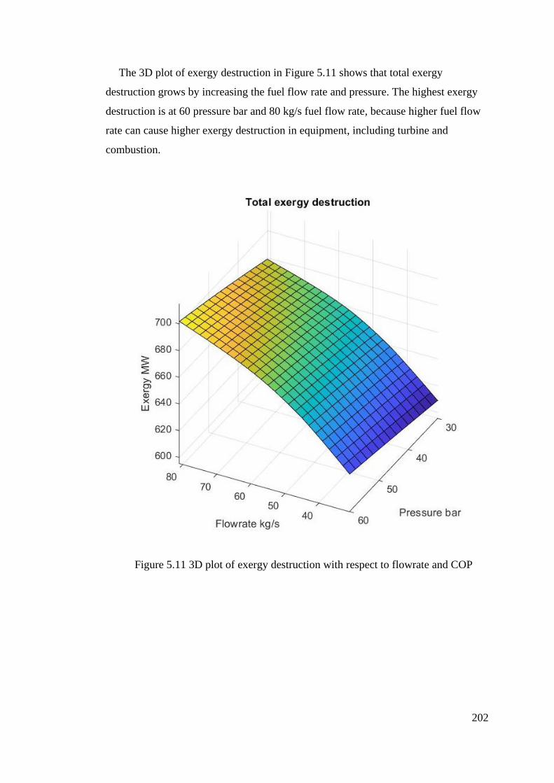
202
The 3D plot of exergy destruction in Figure 5.11 shows that total exergy
destruction grows by increasing the fuel flow rate and pressure. The highest exergy
destruction is at 60 pressure bar and 80 kg/s fuel flow rate, because higher fuel flow
rate can cause higher exergy destruction in equipment, including turbine and
combustion.
Figure 5.11 3D plot of exergy destruction with respect to flowrate and COP
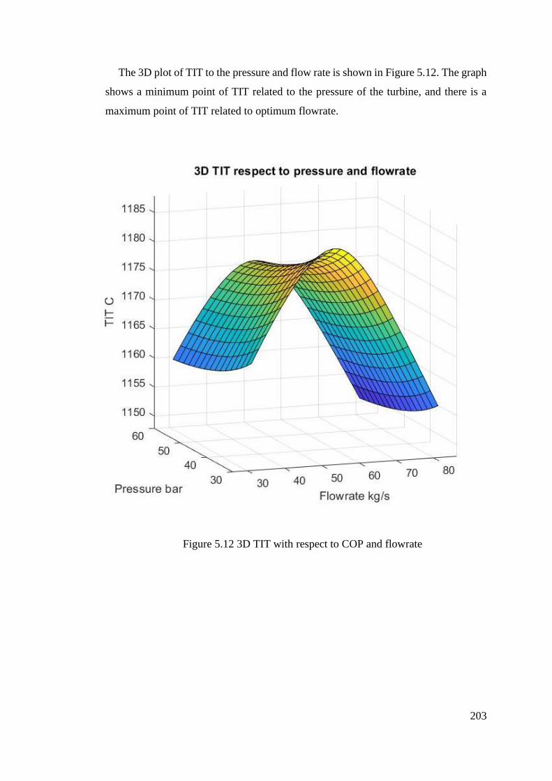
203
The 3D plot of TIT to the pressure and flow rate is shown in Figure 5.12. The graph
shows a minimum point of TIT related to the pressure of the turbine, and there is a
maximum point of TIT related to optimum flowrate.
Figure 5.12 3D TIT with respect to COP and flowrate
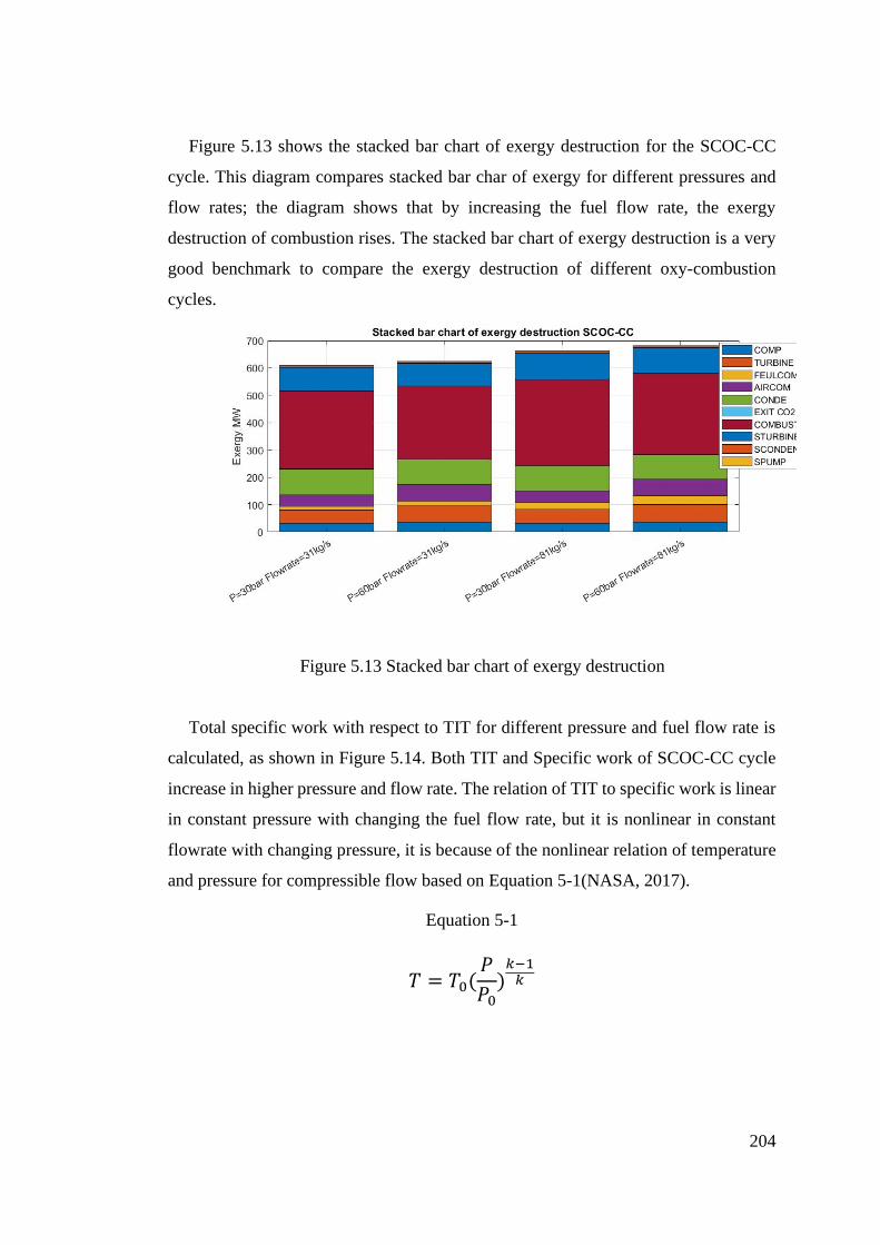
204
Figure 5.13 shows the stacked bar chart of exergy destruction for the SCOC-CC
cycle. This diagram compares stacked bar char of exergy for different pressures and
flow rates; the diagram shows that by increasing the fuel flow rate, the exergy
destruction of combustion rises. The stacked bar chart of exergy destruction is a very
good benchmark to compare the exergy destruction of different oxy-combustion
cycles.
Figure 5.13 Stacked bar chart of exergy destruction
Total specific work with respect to TIT for different pressure and fuel flow rate is
calculated, as shown in Figure 5.14. Both TIT and Specific work of SCOC-CC cycle
increase in higher pressure and flow rate. The relation of TIT to specific work is linear
in constant pressure with changing the fuel flow rate, but it is nonlinear in constant
flowrate with changing pressure, it is because of the nonlinear relation of temperature
and pressure for compressible flow based on Equation 5-1(NASA, 2017).
Equation 5-1
𝑇 = 𝑇0(𝑃
𝑃0)
𝑘−1𝑘
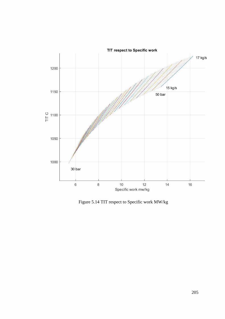
205
Figure 5.14 TIT respect to Specific work MW/kg
206
5.1.3 Summary
SCOC-CC is one of the promising oxy-combustion cycles with high efficiency, and
technology development of equipment for this cycle can increase the cycle efficiency.
The full sensitivity analysis of the cycle was performed for different flowrate, TIT and
pressure. Also, the exergy destruction of components was calculated, and the bar chart
was extracted; it is shown that exergy destruction in combustion and HRSG are higher
in comparison to other components. The performance analysis of the SCOC-CC cycle
and Techno-economic analysis of the cycle was calculated.
In this chapter, the sensitivity of Network with respect to the gas turbine pressure
ratio was analysed for SCOC-CC, and it indicates that the maximum work is at 40
pressure ratio. The sensitivity of efficiency with respect to the flowrate and
Combustion Outlet Pressure (COP) indicates that reduction of working flow from 15
kg/s to 17 kg/s can grow the efficiency from 35% to 37%; the overall efficiency of the
cycle increases by increasing the cycle pressure (COP), however, it is shown that the
efficiency of the cycle by increasing COP from 400 bar to 600 bar, increases less than
1%, and it does not have the benefit to the cycle by considering the capital cost. The
results indicate the TIT of the power cycle is changing with respect to fuel flowrate
because the best fuel flowrate is stoichiometry ratio, and the maximum TIT occurs in
the stoichiometry ratio, but the TIT is nearly constant with respect to the pressure. The
overall exergy destruction grows from 600 MW to 700 MW by increasing the fuel
flow rate from 31 kg/s to 81 kg/s and Combustion Outlet Pressure (COP) from 30 bar
to 60 bar.
207
5.2 Sensitivity and exergy analysis of E-MATIANT cycle
5.2.1 Introduction
In this chapter, E-MATIANT Oxy-fuel combustion is investigated. The cycle
includes one supercritical Rankine like cycle and a Bryton cycle. The Aspen Plus
modelling of the cycle was provided for analysing the thermodynamics parameters of
the E-MATIANT cycle. The sensitivities of cycle parameters were analysed. Then the
graphs of exergy, efficiency, Network vs working flow rates were extracted. Likewise,
exergy destruction of the component at the design point was calculated and shown in
a bar graph. The exergy bar graph can show the most exergy destruction of components
in the cycle and help the designer to develop these components.
The increasing concern about climate change has addressed the efforts of
researchers and scientists to develop the power cycles with CCS (Carbon Capture and
Storage). The oxy-fuel combustion power cycle is one of the promising technologies
to separate and sequestrate CO2. The by-product of oxy-combustion is CO2 and H2O.
Hence, the CO2 can be separated from H2O by cooling the flue below the dew point.
The isentropic efficiencies are 85% for a three-stage compressor and 80% for one
stage compressor. The fuel is assumed to feed the combustion at 17 °C and 3 bar. The
cycle sensitivity is minimal to the temperature and pressure of the fuel. The fuel
pressure depends on the network, and it can be as high as 40 or 60 bar (Mathieu and
Nihart, 1999).
The required fuel pressure depends on the combustion pressure. The compression
can be low or zero. If the pressure is lower than the network, it would be possible to
recover from the expander. In this case, preheating of the fuel is required before
injection to the combustion (Mathieu and Nihart, 1999). Table 5.1 indicates the
optimum design point of the E-MATIANT cycle with the maximum possible TIT of
1300 oC.
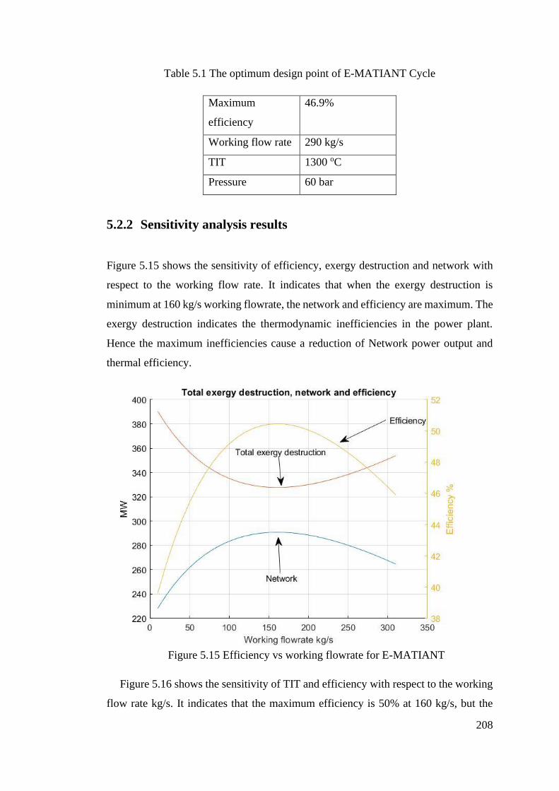
208
Table 5.1 The optimum design point of E-MATIANT Cycle
Maximum
efficiency
46.9%
Working flow rate 290 kg/s
TIT 1300 oC
Pressure 60 bar
5.2.2 Sensitivity analysis results
Figure 5.15 shows the sensitivity of efficiency, exergy destruction and network with
respect to the working flow rate. It indicates that when the exergy destruction is
minimum at 160 kg/s working flowrate, the network and efficiency are maximum. The
exergy destruction indicates the thermodynamic inefficiencies in the power plant.
Hence the maximum inefficiencies cause a reduction of Network power output and
thermal efficiency.
Figure 5.15 Efficiency vs working flowrate for E-MATIANT
Figure 5.16 shows the sensitivity of TIT and efficiency with respect to the working
flow rate kg/s. It indicates that the maximum efficiency is 50% at 160 kg/s, but the
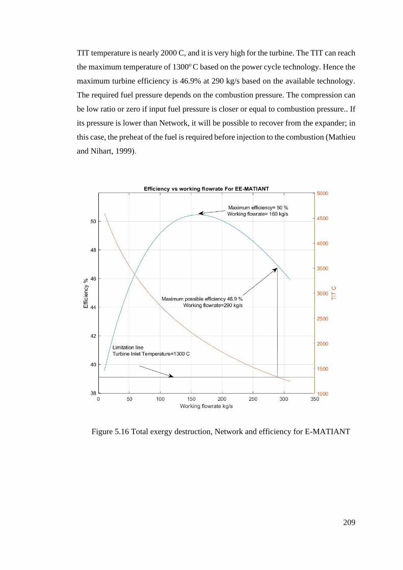
209
TIT temperature is nearly 2000 C, and it is very high for the turbine. The TIT can reach
the maximum temperature of 1300o C based on the power cycle technology. Hence the
maximum turbine efficiency is 46.9% at 290 kg/s based on the available technology.
The required fuel pressure depends on the combustion pressure. The compression can
be low ratio or zero if input fuel pressure is closer or equal to combustion pressure.. If
its pressure is lower than Network, it will be possible to recover from the expander; in
this case, the preheat of the fuel is required before injection to the combustion (Mathieu
and Nihart, 1999).
Figure 5.16 Total exergy destruction, Network and efficiency for E-MATIANT
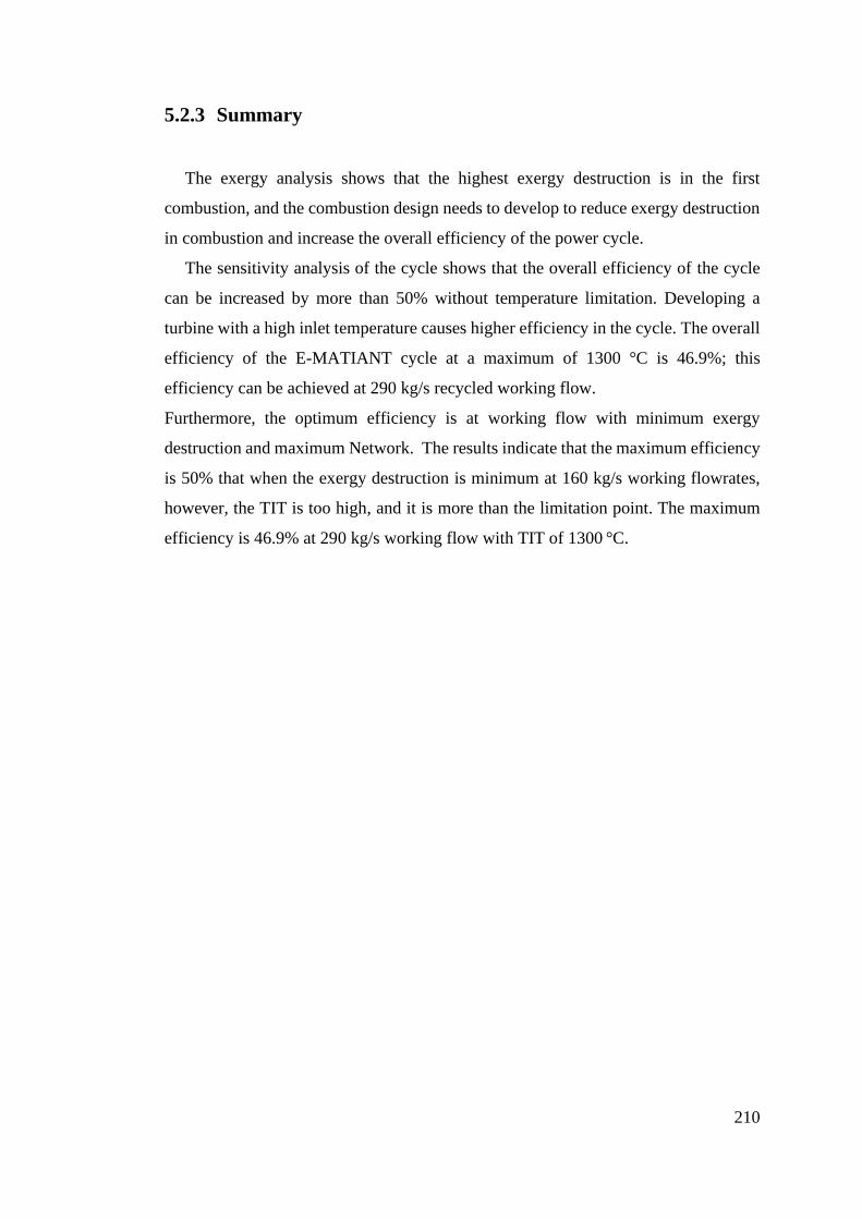
210
5.2.3 Summary
The exergy analysis shows that the highest exergy destruction is in the first
combustion, and the combustion design needs to develop to reduce exergy destruction
in combustion and increase the overall efficiency of the power cycle.
The sensitivity analysis of the cycle shows that the overall efficiency of the cycle
can be increased by more than 50% without temperature limitation. Developing a
turbine with a high inlet temperature causes higher efficiency in the cycle. The overall
efficiency of the E-MATIANT cycle at a maximum of 1300 °C is 46.9%; this
efficiency can be achieved at 290 kg/s recycled working flow.
Furthermore, the optimum efficiency is at working flow with minimum exergy
destruction and maximum Network. The results indicate that the maximum efficiency
is 50% that when the exergy destruction is minimum at 160 kg/s working flowrates,
however, the TIT is too high, and it is more than the limitation point. The maximum
efficiency is 46.9% at 290 kg/s working flow with TIT of 1300 °C.
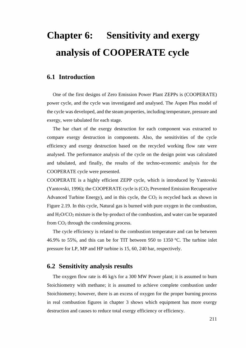
211
Chapter 6: Sensitivity and exergy
analysis of COOPERATE cycle
6.1 Introduction
One of the first designs of Zero Emission Power Plant ZEPPs is (COOPERATE)
power cycle, and the cycle was investigated and analysed. The Aspen Plus model of
the cycle was developed, and the steam properties, including temperature, pressure and
exergy, were tabulated for each stage.
The bar chart of the exergy destruction for each component was extracted to
compare exergy destruction in components. Also, the sensitivities of the cycle
efficiency and exergy destruction based on the recycled working flow rate were
analysed. The performance analysis of the cycle on the design point was calculated
and tabulated, and finally, the results of the techno-economic analysis for the
COOPERATE cycle were presented.
COOPERATE is a highly efficient ZEPP cycle, which is introduced by Yantovski
(Yantovski, 1996); the COOPERATE cycle is (CO2 Prevented Emission Recuperative
Advanced Turbine Energy), and in this cycle, the CO2 is recycled back as shown in
Figure 2.19. In this cycle, Natural gas is burned with pure oxygen in the combustion,
and H2O/CO2 mixture is the by-product of the combustion, and water can be separated
from CO2 through the condensing process.
The cycle efficiency is related to the combustion temperature and can be between
46.9% to 55%, and this can be for TIT between 950 to 1350 °C. The turbine inlet
pressure for LP, MP and HP turbine is 15, 60, 240 bar, respectively.
6.2 Sensitivity analysis results
The oxygen flow rate is 46 kg/s for a 300 MW Power plant; it is assumed to burn
Stoichiometry with methane; it is assumed to achieve complete combustion under
Stoichiometry; however, there is an excess of oxygen for the proper burning process
in real combustion figures in chapter 3 shows which equipment has more exergy
destruction and causes to reduce total exergy efficiency or efficiency.
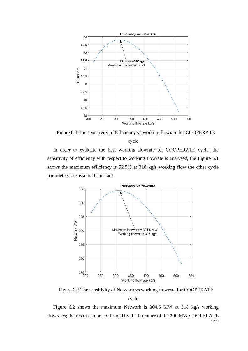
212
Figure 6.1 The sensitivity of Efficiency vs working flowrate for COOPERATE
cycle
In order to evaluate the best working flowrate for COOPERATE cycle, the
sensitivity of efficiency with respect to working flowrate is analysed, the Figure 6.1
shows the maximum efficiency is 52.5% at 318 kg/s working flow the other cycle
parameters are assumed constant.
Figure 6.2 The sensitivity of Network vs working flowrate for COOPERATE
cycle
Figure 6.2 shows the maximum Network is 304.5 MW at 318 kg/s working
flowrates; the result can be confirmed by the literature of the 300 MW COOPERATE
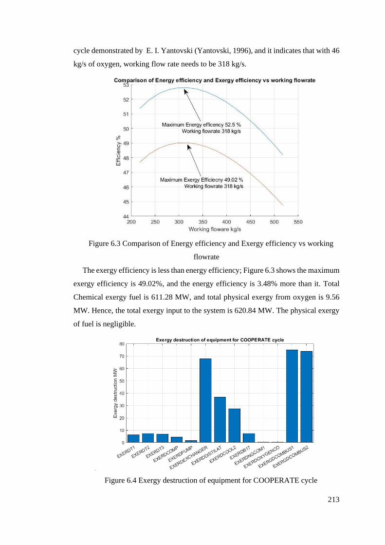
213
cycle demonstrated by E. I. Yantovski (Yantovski, 1996), and it indicates that with 46
kg/s of oxygen, working flow rate needs to be 318 kg/s.
Figure 6.3 Comparison of Energy efficiency and Exergy efficiency vs working
flowrate
The exergy efficiency is less than energy efficiency; Figure 6.3 shows the maximum
exergy efficiency is 49.02%, and the energy efficiency is 3.48% more than it. Total
Chemical exergy fuel is 611.28 MW, and total physical exergy from oxygen is 9.56
MW. Hence, the total exergy input to the system is 620.84 MW. The physical exergy
of fuel is negligible.
Figure 6.4 Exergy destruction of equipment for COOPERATE cycle
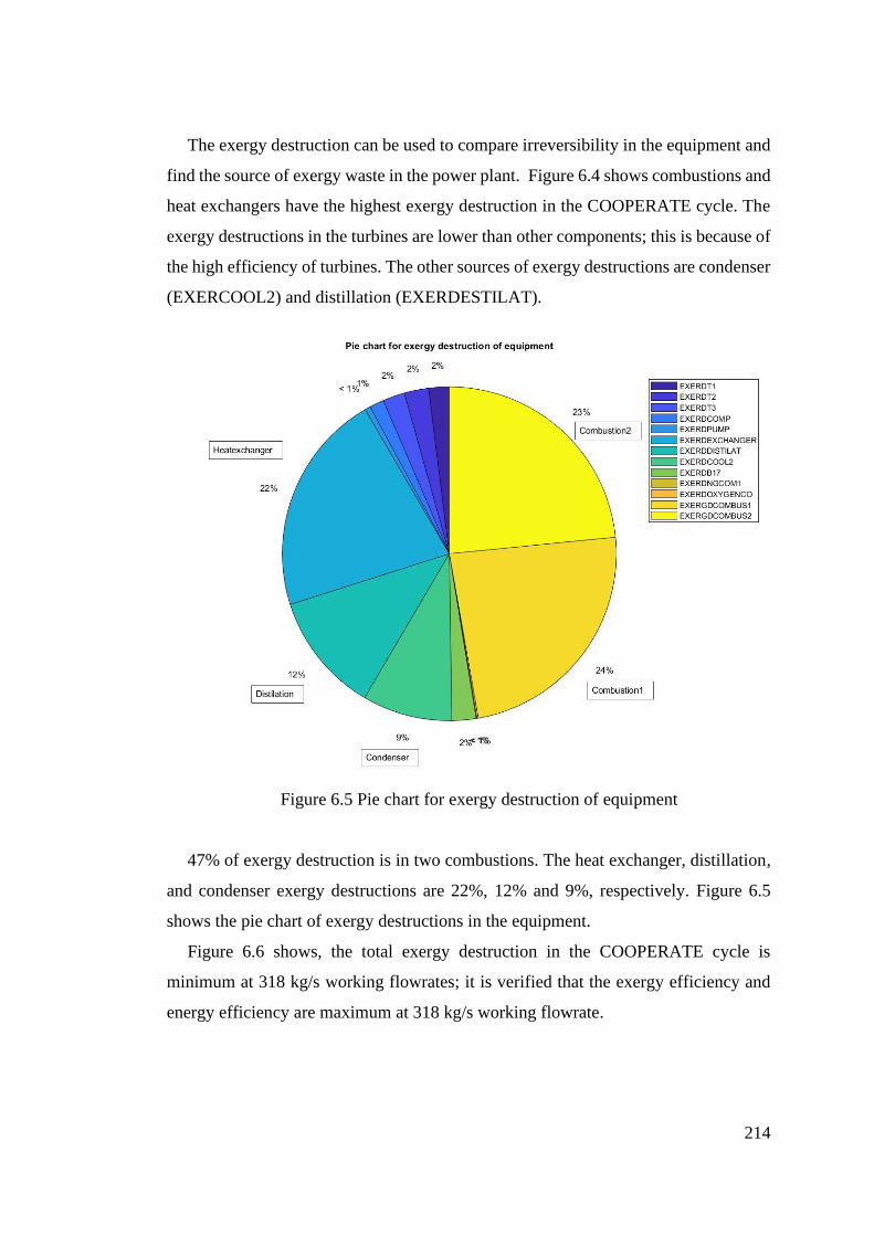
214
The exergy destruction can be used to compare irreversibility in the equipment and
find the source of exergy waste in the power plant. Figure 6.4 shows combustions and
heat exchangers have the highest exergy destruction in the COOPERATE cycle. The
exergy destructions in the turbines are lower than other components; this is because of
the high efficiency of turbines. The other sources of exergy destructions are condenser
(EXERCOOL2) and distillation (EXERDESTILAT).
Figure 6.5 Pie chart for exergy destruction of equipment
47% of exergy destruction is in two combustions. The heat exchanger, distillation,
and condenser exergy destructions are 22%, 12% and 9%, respectively. Figure 6.5
shows the pie chart of exergy destructions in the equipment.
Figure 6.6 shows, the total exergy destruction in the COOPERATE cycle is
minimum at 318 kg/s working flowrates; it is verified that the exergy efficiency and
energy efficiency are maximum at 318 kg/s working flowrate.
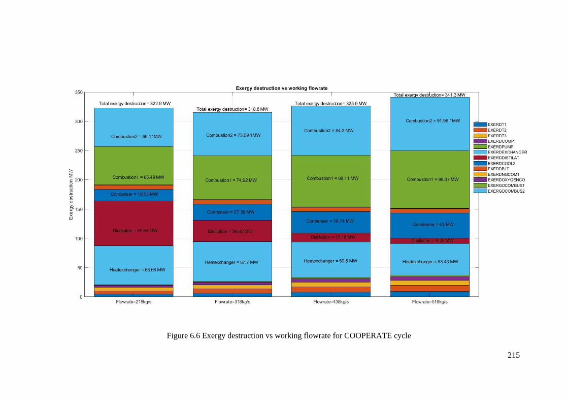
215
Figure 6.6 Exergy destruction vs working flowrate for COOPERATE cycle
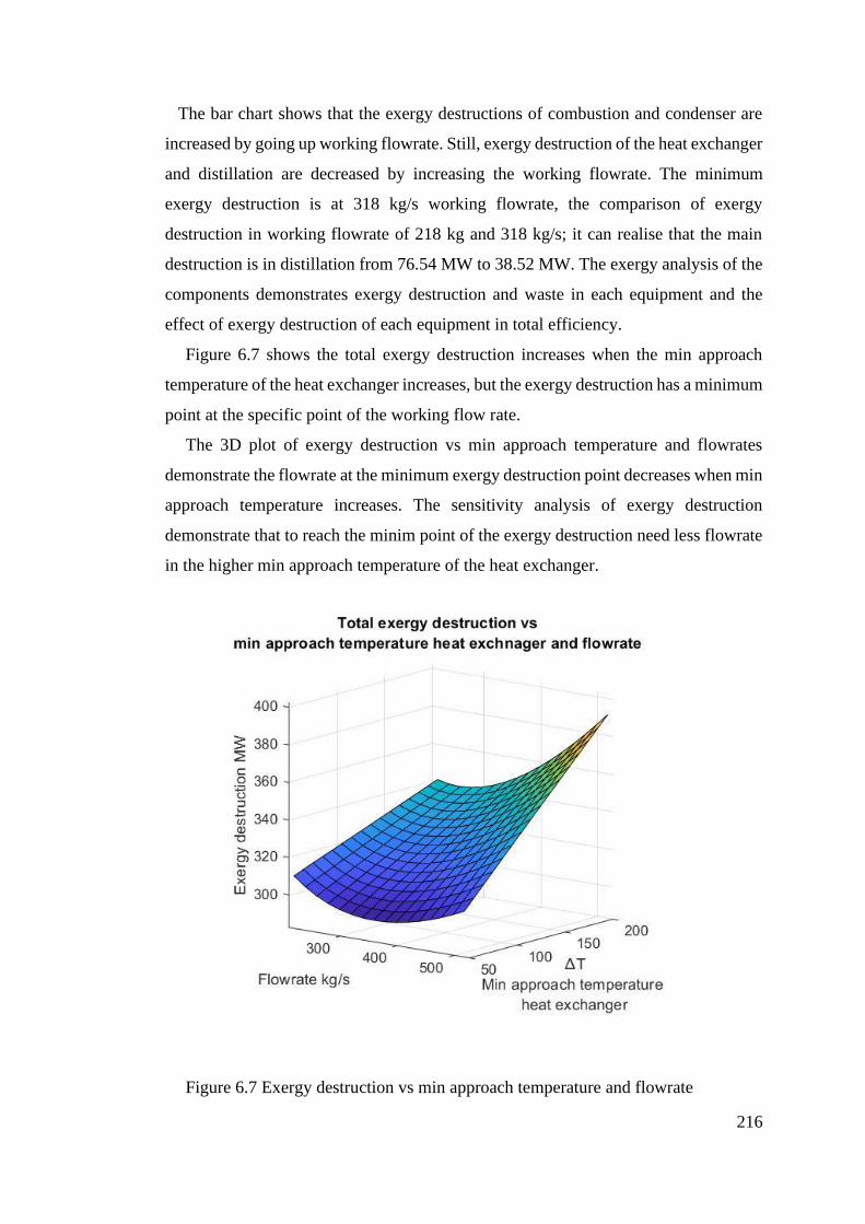
216
The bar chart shows that the exergy destructions of combustion and condenser are
increased by going up working flowrate. Still, exergy destruction of the heat exchanger
and distillation are decreased by increasing the working flowrate. The minimum
exergy destruction is at 318 kg/s working flowrate, the comparison of exergy
destruction in working flowrate of 218 kg and 318 kg/s; it can realise that the main
destruction is in distillation from 76.54 MW to 38.52 MW. The exergy analysis of the
components demonstrates exergy destruction and waste in each equipment and the
effect of exergy destruction of each equipment in total efficiency.
Figure 6.7 shows the total exergy destruction increases when the min approach
temperature of the heat exchanger increases, but the exergy destruction has a minimum
point at the specific point of the working flow rate.
The 3D plot of exergy destruction vs min approach temperature and flowrates
demonstrate the flowrate at the minimum exergy destruction point decreases when min
approach temperature increases. The sensitivity analysis of exergy destruction
demonstrate that to reach the minim point of the exergy destruction need less flowrate
in the higher min approach temperature of the heat exchanger.
Figure 6.7 Exergy destruction vs min approach temperature and flowrate
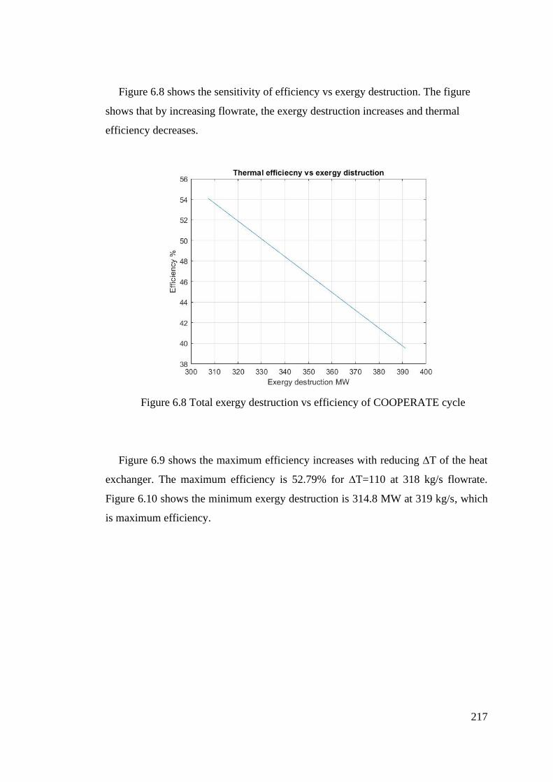
217
Figure 6.8 shows the sensitivity of efficiency vs exergy destruction. The figure
shows that by increasing flowrate, the exergy destruction increases and thermal
efficiency decreases.
Figure 6.8 Total exergy destruction vs efficiency of COOPERATE cycle
Figure 6.9 shows the maximum efficiency increases with reducing ∆T of the heat
exchanger. The maximum efficiency is 52.79% for ∆T=110 at 318 kg/s flowrate.
Figure 6.10 shows the minimum exergy destruction is 314.8 MW at 319 kg/s, which
is maximum efficiency.
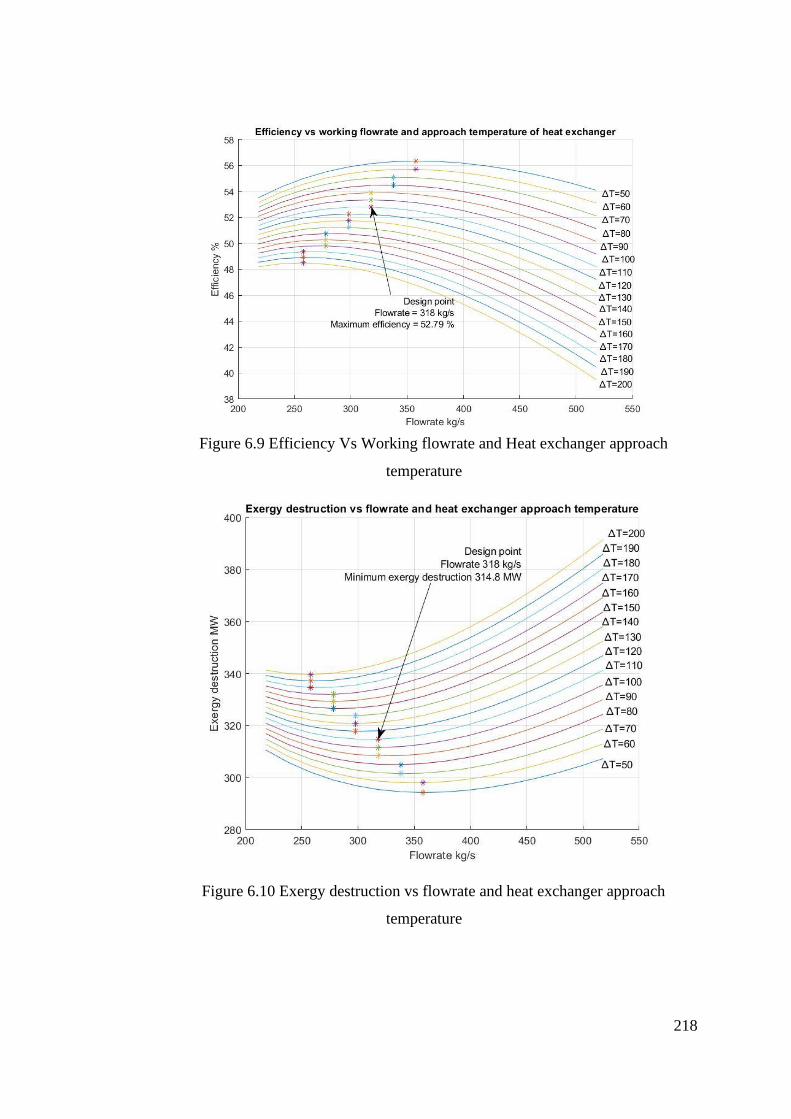
218
Figure 6.9 Efficiency Vs Working flowrate and Heat exchanger approach
temperature
Figure 6.10 Exergy destruction vs flowrate and heat exchanger approach
temperature
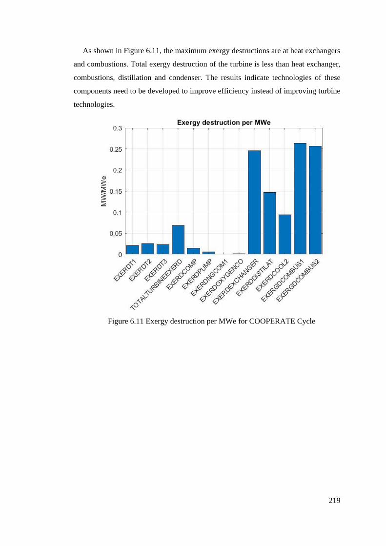
219
As shown in Figure 6.11, the maximum exergy destructions are at heat exchangers
and combustions. Total exergy destruction of the turbine is less than heat exchanger,
combustions, distillation and condenser. The results indicate technologies of these
components need to be developed to improve efficiency instead of improving turbine
technologies.
Figure 6.11 Exergy destruction per MWe for COOPERATE Cycle
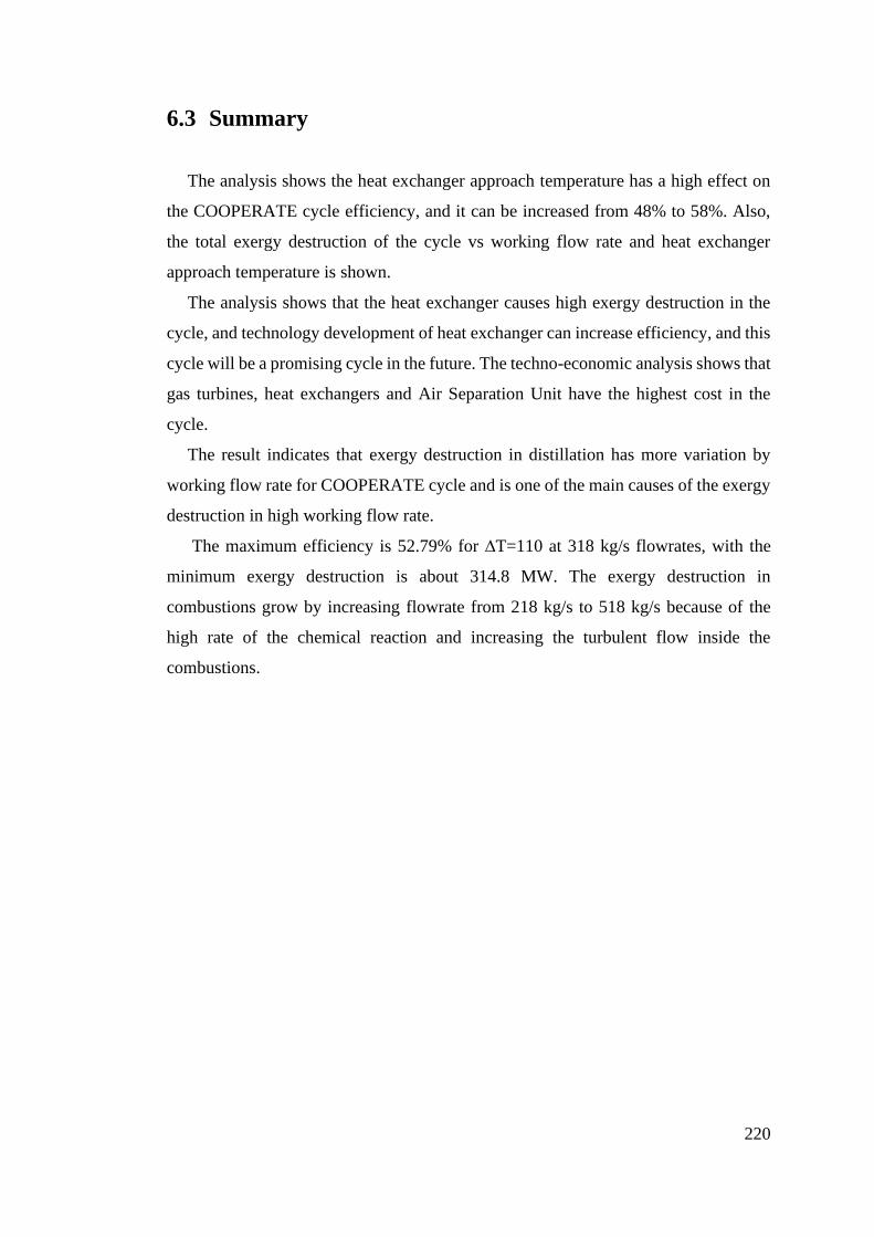
220
6.3 Summary
The analysis shows the heat exchanger approach temperature has a high effect on
the COOPERATE cycle efficiency, and it can be increased from 48% to 58%. Also,
the total exergy destruction of the cycle vs working flow rate and heat exchanger
approach temperature is shown.
The analysis shows that the heat exchanger causes high exergy destruction in the
cycle, and technology development of heat exchanger can increase efficiency, and this
cycle will be a promising cycle in the future. The techno-economic analysis shows that
gas turbines, heat exchangers and Air Separation Unit have the highest cost in the
cycle.
The result indicates that exergy destruction in distillation has more variation by
working flow rate for COOPERATE cycle and is one of the main causes of the exergy
destruction in high working flow rate.
The maximum efficiency is 52.79% for ∆T=110 at 318 kg/s flowrates, with the
minimum exergy destruction is about 314.8 MW. The exergy destruction in
combustions grow by increasing flowrate from 218 kg/s to 518 kg/s because of the
high rate of the chemical reaction and increasing the turbulent flow inside the
combustions.
221
Chapter 7: Sensitivity analysis of the
heat exchanger design in NetPower
oxy-combustion cycle for carbon
capture
7.1 Introduction
For gas turbines, several Oxy-combustion power cycles (Oxyturbine cycles) have
been investigated by means of thermodynamic analysis. NetPower cycle is one of the
leading oxyturbine power cycles with almost full carbon capture capability from the
natural gas-fired power plant. In this chapter, sensitivity analysis of the heat exchanger
design in NetPower cycle is completed by means of process modelling. The heat
capacity variation and supercritical carbon dioxide with gaseous admixtures are
considered for multi-zone analysis with Aspen Plus software. It is found that the heat
exchanger design has a major role in increasing the efficiency of NetPower cycle. The
pinch-point analysis is done to extract the composite and grand composite curve for
the heat exchanger. In this paper, the relationship between the cycle efficiency and the
minimum approach temperature (∆Tmin) of the heat exchanger has also been
evaluated. An increase in ∆Tmin causes a decrease in the temperature of the recycled
flue gases (RFG) and an overall decrease in the required power for the recycled gas
compressor. The main challenge in the design of heat exchangers in power plants is a
tradeoff between Capital and Operational costs. To achieve lower ∆Tmin, a larger size
of a heat exchanger is required. This means a higher capital cost but leading to better
heat recovery and lower operational costs. To achieve this, ∆Tmin is selected from the
minimum point in the diagrams of capital and operational costs.
This study provides an insight into the NetPower Oxy-combustion cycle’s
performance analysis and operational condition based on its heat exchanger design.
Greenhouse gases are the main reason for warming the atmosphere temperature and
climate change. Several oxyturbine cycles are proposed and studied by thermodynamic
222
analysis; only two cycles of CES and Allam (NetPower) are currently in the
demonstration phase, both funded by DOE in the US.
The Allam cycle is one of the novels oxy-combustion technologies, and it is
developed recently with 8 Rivers Capital. The 8 Rivers, Exelon Generation, and CB&I
are owners of NetPower. NetPower develops the natural gas Allam cycle, and it is
currently building a 50 MWth natural gas demonstration power plant in La Porte,
Texas (Allam et al., 2017). This article presents the latest results of our investigation
on the effects of heat exchanger design on the NetPower oxyturbine cycle with full
carbon capture.
7.2 Analysing of NetPower cycle
7.2.1 NetPower cycle
NetPower cycle was introduced by Rodney Allam. NetPower cycle working flow
is mainly carbon dioxide in a high-pressure and turbine inlet pressure (TIP) is
approximately 300 bar and low-pressure-ratio of 10. It is a highly recuperated Bryton
cycle (Allam et al., 2017). NetPower cycle combustor burns natural gas with pure
oxygen supplied from an Air Separation Unit (ASU) and high-pressure carbon dioxide
stream inlets recycled from its power turbine. Recycle Fuel Gas (RFG) is heated with
a recovery heat exchanger and flows to the combustor to reduce the Combustion Outlet
Temperature (COT) by diluting the combustion products. The RFG flowrate controls
the temperature of combustion at an acceptable level. The direct-fired supercritical
carbon dioxide (SCO2) turbine is cooled with a cooling stream from the heat exchanger
(Allam et al., 2013).
The exhaust gas with 740°C enters recuperating heat exchanger that transfers heat
from hot outlet turbine exhaust gas to the three-cycle streams. It includes the carbon
dioxide-rich stream recycled to the combustor (to the moderate temperature of
combustor), the oxidant stream recycled to the combustor and the carbon dioxide-rich
223
stream for cooling turbine blades. Also, the hot compressed air stream from ASU (Air
Separation Unit) enters recuperating heat exchanger for recovering its heat.
The heat exchanger is one of the main parts of NetPower cycle, and it has a main
role in NetPower cycle efficiency. The exhaust gas from the heat exchanger is cooled
down, and the carbon dioxide is separated from the water. The water is sent to the
wastewater treatment for recovery and treatment. A portion of carbon dioxide stream
form water separation unites sent for purification and compression unite. Most carbon
dioxide is compressed and recycled back.
Recycle gas compression loop includes four stages intercooled compressor and two
intercooled pumping stages. Inter cooling is with cooling water. The carbon dioxide
stream is divided into three parts; 45-50% of flow rate is pumped to 305 bars and
preheated in the recuperating heat exchanger. 10-12% of the flowrate after heated in
the heat exchanger up to a maximum of 400 °C, then it is sent to the turbine for the
cooling blade.
The 32 -45% of carbon dioxide stream is mixed with high purity oxygen the oxidant
stream is heated in heat exchanger up to 720 °C and It is sent to combustion to burn
fuel (IEAGHG, 2015).
NetPower Plant includes three main parts:
1. NetPower cycle
2. Recycle compression loop
3. Carbon dioxide purification and compression
The Air Separation Unit, CO2 purification compression unit, utility and offside units
are extracted from the IEA report 2015, and these are considered constant in this model
(IEA 2015 report).

224
7.2.2 NetPower simulation with Aspen Plus
7.2.2.1 Recovery Heat Exchanger:
The heat exchanger on NetPower cycle can be a compact multi-channel plate-fin
design or printed circuit in Nickel-alloy (e.g. Alloy 617)(IEAGHG, 2015).
Heatric Company supplies four printed circuit heat exchangers (PCHEs) for
NetPower to commission the 50 MW demonstration plant in Texas (Heatric 2016).
PCHEs is a multi-stream heat exchanger type. The PCHEs is replaced with
conventional Heat Exchanger Network (HEN) on NetPower Cycle. Therefore the total
annual cost (TAC) is decreased. A Multi-Stream Heat Exchanger (MSHE) enables a
simultaneous heat exchange between more than two streams in a single unit (Joda et
al., 2011). The multi-stream heat exchanger is a special case of a Heat Exchanger
Network without external utilities. Therefore, classical pinch analysis can be
performed on a Multi-stream heat exchanger (Watson and Barton, 2016).
Heatric PCHEs are manufactured by diffusion bonding; these are fabricated with
no joints, welds or points of failure, resulting in units combining exceptional strength
and integrity with high efficiency. PCHEs are smaller and lighter than conventional
heat exchangers; their specifications are high-pressure capabilities, high range
temperature, small size, higher structural integrity (Diffusion bonding technology
2016).
The heat exchanger cost effects strongly on the final plant cost. A smaller minimum
temperature approach ΔTmin for heat exchanger increases efficiency but also
increases the capital cost (CAPEX). Therefore, it is required to optimise between
capital cost, operational cost (OPEX) and efficiency. CAPEX vs OPEX studies is
required to find an optimum operating point of the system. The cost of heat exchange
affects significantly by minimum approach temperature (ΔTmin) and pressure drop.
The cold streams include two high-rich recycled carbon dioxide streams and one
oxidant stream. The high-rich recycled carbon dioxide stream includes one Recycled
Flue Gas RFG, which is heated and enters to combustion; another stream is cooling
turbine stream, which is heated and enters turbine for the cooling blade. Oxidant
stream is heated and enters combustion for burning fuel.
225
The hot streams include an exhaust stream from the turbine and hot gas from ASU.
The huge difference between the heat capacity of carbon dioxide in hot and cold
streams causes a significant imbalance. In order to avoid imbalance in heat transfer,
first, the cold streams are heated up with heat from the operation of the CO2 recycle
compressor outside the multi-stream heat exchanger and hot air from ASU
compressors inside the multi-stream heat exchanger. Then, they are heated with
exhaust gas from the turbine (Allam et al. 2017).
7.2.2.2 Recovery Heat Exchanger modelling in Aspen Plus
The recovery heat exchanger is modelled with multi-stream heat exchanger
MHeatX block in Aspen Plus; this calculates heat duty between multi hot and cold
streams. Furthermore, this block calculates the overall UA (overall heat transfer
coefficient) for the exchanger, minimum approach temperature ΔTmin, Number of
Transfer Units (NTU), analyses a detailed zone analysis and composite curve
(AspenTech).
The design parameters of multi-stream heat exchanger for NetPower cycle are
dependent on the following items:
1. Flow rate composition
2. Heat capacities
3. Temperatures of stream
In order to calculate design parameters of multi-stream heat exchanger for a power
plant, it requires all material of energy balance, design of combustion and turbine to
be done. Energy integration can be considered the last step of the design for the power
plant. After calculation of design parameters such as UA (overall heat transfer
coefficient) and Δ𝑇min. In order to design an efficient multi-seam heat exchanger with
minimum size and cost, the following parameters should be considered:
1. Temperature difference
2. Conducting material
3. Fluid turbulence (more turbulent more heat exchange)
4. Fluid velocity
5. Surface area
6. Direction of Flow
226
The main issue in heat exchanger design for the power plant cycle is a pinch point.
During partial load or unsteady state circumstances, sometimes pinch point or
temperature crossover might happen in the multi-stream heat exchanger. In these
conditions, the heat exchanger will not perform effectively.
7.2.2.3 CO2 Direct-fired Turbine
The turbine is one of the important parts of a power plant cycle. The turbine cooling
causes difficulties in calculations to find the efficiency of CO2 Direct-fired turbine. In
our simulation, the efficiency of the turbine for NetPower cycle is considered constant.
First Supercritical CO2 (S-CO2) turbine is supplied with Toshiba for the plant build
in Texas, USA (Toshiba 2016). NetPower cycle turbine is intercooling turbine, and it
requires the following developments.
NetPower turbine has higher inlet pressure than a conventional turbine, so the shell
requires adoption. Blades and shells require cooling because of the TIT of the
NetPower cycle. Working flow in NetPower cycle is carbon dioxide, so it is necessary
that the conventional facilities are redesigned for carbon dioxide working flow. The
blades in the NetPower turbine are cooling with the open circuit blade cooling method,
and they are protected with cooling film and cooled by convection.
Higher Inlet turbine temperature (TIT) causes higher efficiency in NetPower cycle.
The metal working temperature of turbine blades is a barrier to increase turbine
temperature. The efficiency of the power turbine will increase by increasing its
metalworking temperature. Furthermore, the heat transfer coefficient of the cooling
flow, which is almost pure carbon dioxide is very high compared to conventional
cooling flow.
The exergy of a system is the maximum energy that is available to be used.
Increasing gas turbine inlet temperature decreases in combustion chamber exergy
destruction (Kaviri, Jaafar and Lazim, 2012). This is due to the fact that this increase
leads to decreasing entropy destruction. On the other side, TIT in power turbines is
required to be of a higher value to avoid exergy destruction (Sanjay, 2011). Increasing
TIT increases both efficiency and specific work output (Sanjay, 2011) significantly. In
NetPower cycle, TIT (Turbine Inlet Temperature) or COT (Combustion Outlet
Temperature) is controlled with Recycle Gas Flow (RGF), while multi-flow heat
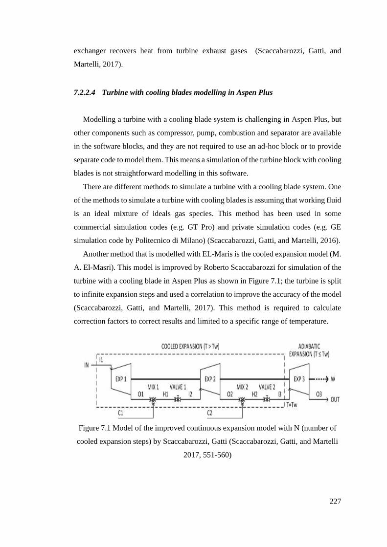
227
exchanger recovers heat from turbine exhaust gases (Scaccabarozzi, Gatti, and
Martelli, 2017).
7.2.2.4 Turbine with cooling blades modelling in Aspen Plus
Modelling a turbine with a cooling blade system is challenging in Aspen Plus, but
other components such as compressor, pump, combustion and separator are available
in the software blocks, and they are not required to use an ad-hoc block or to provide
separate code to model them. This means a simulation of the turbine block with cooling
blades is not straightforward modelling in this software.
There are different methods to simulate a turbine with a cooling blade system. One
of the methods to simulate a turbine with cooling blades is assuming that working fluid
is an ideal mixture of ideals gas species. This method has been used in some
commercial simulation codes (e.g. GT Pro) and private simulation codes (e.g. GE
simulation code by Politecnico di Milano) (Scaccabarozzi, Gatti, and Martelli, 2016).
Another method that is modelled with EL-Maris is the cooled expansion model (M.
A. El-Masri). This model is improved by Roberto Scaccabarozzi for simulation of the
turbine with a cooling blade in Aspen Plus as shown in Figure 7.1; the turbine is split
to infinite expansion steps and used a correlation to improve the accuracy of the model
(Scaccabarozzi, Gatti, and Martelli, 2017). This method is required to calculate
correction factors to correct results and limited to a specific range of temperature.
Figure 7.1 Model of the improved continuous expansion model with N (number of
cooled expansion steps) by Scaccabarozzi, Gatti (Scaccabarozzi, Gatti, and Martelli
2017, 551-560)
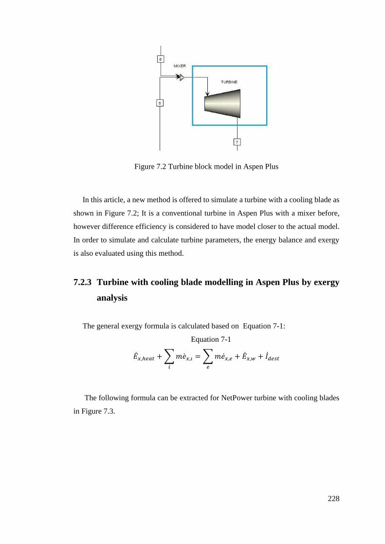
228
Figure 7.2 Turbine block model in Aspen Plus
In this article, a new method is offered to simulate a turbine with a cooling blade as
shown in Figure 7.2; It is a conventional turbine in Aspen Plus with a mixer before,
however difference efficiency is considered to have model closer to the actual model.
In order to simulate and calculate turbine parameters, the energy balance and exergy
is also evaluated using this method.
7.2.3 Turbine with cooling blade modelling in Aspen Plus by exergy
analysis
The general exergy formula is calculated based on Equation 7-1:
Equation 7-1
��𝑥,ℎ𝑒𝑎𝑡 + ∑ 𝑚𝑒𝑥,𝑖
𝑖
= ∑ 𝑚𝑒𝑥,𝑒
𝑒
+ ��𝑥,𝑤 + 𝐼��𝑒𝑠𝑡
The following formula can be extracted for NetPower turbine with cooling blades
in Figure 7.3.
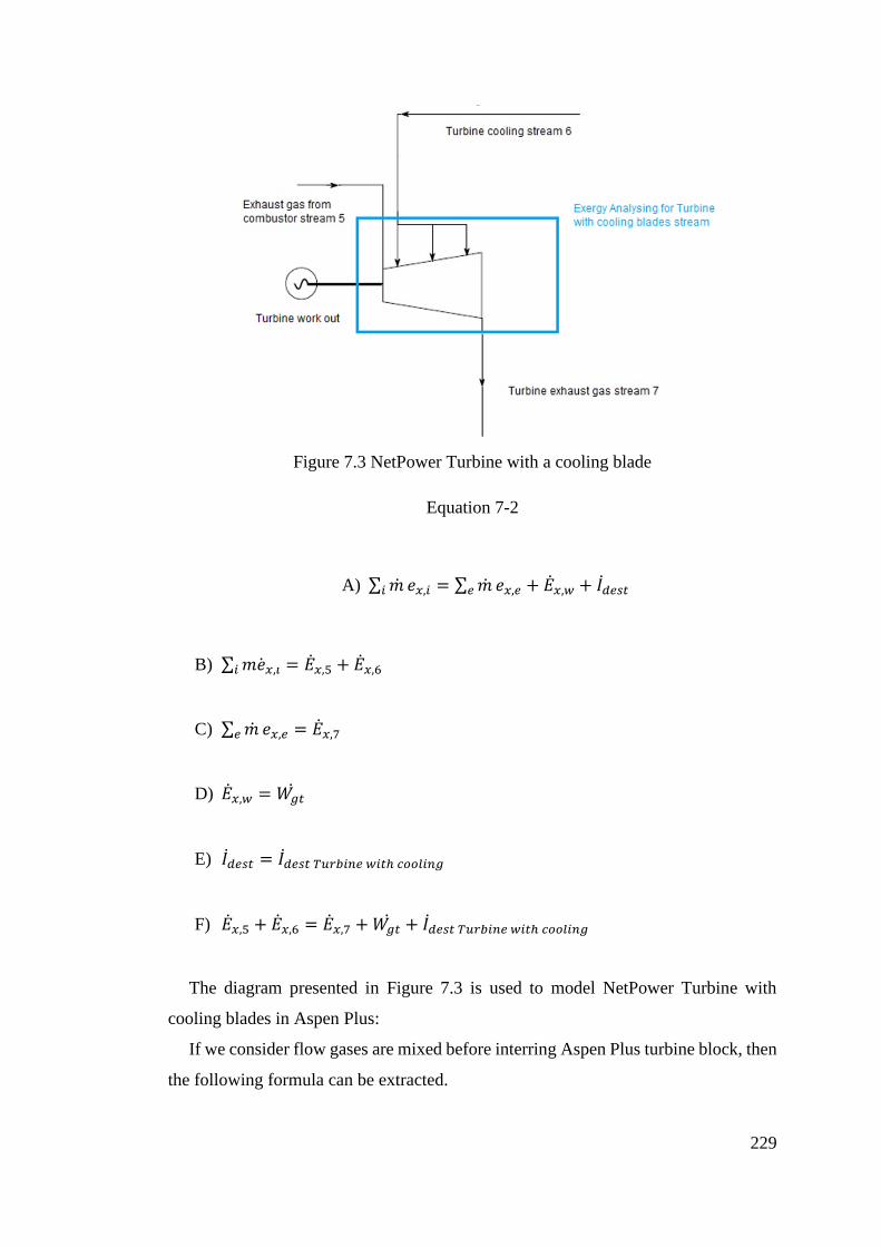
229
Figure 7.3 NetPower Turbine with a cooling blade
Equation 7-2
A) ∑ ��𝑖 𝑒𝑥,𝑖 = ∑ ��𝑒 𝑒𝑥,𝑒 + ��𝑥,𝑤 + 𝐼��𝑒𝑠𝑡
B) ∑ 𝑚𝑒𝑥,𝑖𝑖 = ��𝑥,5 + ��𝑥,6
C) ∑ ��𝑒 𝑒𝑥,𝑒 = ��𝑥,7
D) ��𝑥,𝑤 = 𝑊𝑔𝑡
E) 𝐼��𝑒𝑠𝑡 = 𝐼��𝑒𝑠𝑡 𝑇𝑢𝑟𝑏𝑖𝑛𝑒 𝑤𝑖𝑡ℎ 𝑐𝑜𝑜𝑙𝑖𝑛𝑔
F) ��𝑥,5 + ��𝑥,6 = ��𝑥,7 + 𝑊𝑔𝑡 + 𝐼��𝑒𝑠𝑡 𝑇𝑢𝑟𝑏𝑖𝑛𝑒 𝑤𝑖𝑡ℎ 𝑐𝑜𝑜𝑙𝑖𝑛𝑔
The diagram presented in Figure 7.3 is used to model NetPower Turbine with
cooling blades in Aspen Plus:
If we consider flow gases are mixed before interring Aspen Plus turbine block, then
the following formula can be extracted.
230
Equation 7-3
A) ��𝑥,ℎ𝑒𝑎𝑡 + ∑ 𝑚𝑒𝑥,𝑖𝑖 = ∑ 𝑚𝑒𝑥,𝑒𝑒 + ��𝑥,𝑤 + 𝐼��𝑒𝑠𝑡
B) ∑ 𝑚𝑒𝑥,𝑖𝑖 = ��𝑥,5 + ��𝑥,6
C) ∑ ��𝑒 𝑒𝑥,𝑒 = ��𝑥,7
D) ��𝑥,𝑤 = 𝑊𝑔𝑡
E) 𝐼��𝑒𝑠𝑡 𝑎𝑠𝑝𝑒𝑛 𝑚𝑜𝑑𝑒𝑙 = 𝐼��𝑒𝑠𝑡 𝑇𝑢𝑟𝑏𝑖𝑛𝑒 𝑎𝑠𝑝𝑒𝑛 + 𝐼��𝑖𝑥𝑒𝑟
F) ��𝑥,5 + ��𝑥,6 = ��𝑥,7 + 𝑊𝑔𝑡 + 𝐼��𝑒𝑠𝑡 𝑎𝑠𝑝𝑒𝑛 𝑚𝑜𝑑𝑒𝑙
hence the following equation is extracted:
Equation 7-4
A) 0 = 𝐼��𝑠𝑝𝑒𝑛 𝑚𝑜𝑑𝑒𝑙 − 𝐼��𝑒𝑠𝑡 𝑇𝑢𝑟𝑏𝑖𝑛𝑒 𝑤𝑖𝑡ℎ 𝑐𝑜𝑜𝑙𝑖𝑛𝑔
B) 𝐼��𝑒𝑠𝑡 𝑇𝑢𝑟𝑏𝑖𝑛𝑒 𝑎𝑠𝑝𝑒𝑛 + 𝐼��𝑖𝑥𝑒𝑟 = 𝐼��𝑒𝑠𝑡 𝑇𝑢𝑟𝑏𝑖𝑛𝑒 𝑤𝑖𝑡ℎ 𝑐𝑜𝑜𝑙𝑖𝑛𝑔
C) 𝐼��𝑒𝑠𝑡 𝑇𝑢𝑟𝑏𝑖𝑛𝑒 𝑎𝑠𝑝𝑒𝑛 = 𝐼��𝑒𝑠𝑡 𝑇𝑢𝑟𝑏𝑖𝑛𝑒 𝑤𝑖𝑡ℎ 𝑐𝑜𝑜𝑙𝑖𝑛𝑔 − 𝐼��𝑖𝑥𝑒𝑟
The equation shows that in order to model the turbine with the cooling system in
Aspen Plus, the recycled cooling stream and exhaust gas of combustion can be mixed,
and exergy destructs in the mixer before interring turbine block.
The equation shows that destruction in the Aspen Plus model turbine is less than
the turbine with a cooling system. Therefore, the entropy generation in the Aspen Plus
model is less than the turbine with cooling blades, and it is extracted from the equation
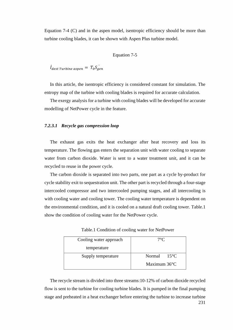
231
Equation 7-4 (C) and in the aspen model, isentropic efficiency should be more than
turbine cooling blades, it can be shown with Aspen Plus turbine model.
Equation 7-5
𝐼��𝑒𝑠𝑡 𝑇𝑢𝑟𝑏𝑖𝑛𝑒 𝑎𝑠𝑝𝑒𝑛 = 𝑇0𝑆𝑔𝑒𝑛
In this article, the isentropic efficiency is considered constant for simulation. The
entropy map of the turbine with cooling blades is required for accurate calculation.
The exergy analysis for a turbine with cooling blades will be developed for accurate
modelling of NetPower cycle in the feature.
7.2.3.1 Recycle gas compression loop
The exhaust gas exits the heat exchanger after heat recovery and loss its
temperature. The flowing gas enters the separation unit with water cooling to separate
water from carbon dioxide. Water is sent to a water treatment unit, and it can be
recycled to reuse in the power cycle.
The carbon dioxide is separated into two parts, one part as a cycle by-product for
cycle stability exit to sequestration unit. The other part is recycled through a four-stage
intercooled compressor and two intercooled pumping stages, and all intercooling is
with cooling water and cooling tower. The cooling water temperature is dependent on
the environmental condition, and it is cooled on a natural draft cooling tower. Table.1
show the condition of cooling water for the NetPower cycle.
Cooling water approach
temperature
7°C
Supply temperature Normal 15°C
Maximum 36°C
The recycle stream is divided into three streams:10-12% of carbon dioxide recycled
flow is sent to the turbine for cooling turbine blades. It is pumped in the final pumping
stage and preheated in a heat exchanger before entering the turbine to increase turbine
Table.1 Condition of cooling water for NetPower
cycle
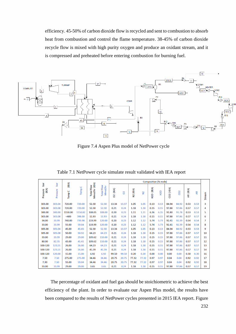
232
efficiency. 45-50% of carbon dioxide flow is recycled and sent to combustion to absorb
heat from combustion and control the flame temperature. 38-45% of carbon dioxide
recycle flow is mixed with high purity oxygen and produce an oxidant stream, and it
is compressed and preheated before entering combustion for burning fuel.
The percentage of oxidant and fuel gas should be stoichiometric to achieve the best
efficiency of the plant. In order to evaluate our Aspen Plus model, the results have
been compared to the results of NetPower cycles presented in 2015 IEA report. Figure
Table 7.1 NetPower cycle simulate result validated with IEA report
Figure 7.4 Aspen Plus model of NetPower cycle
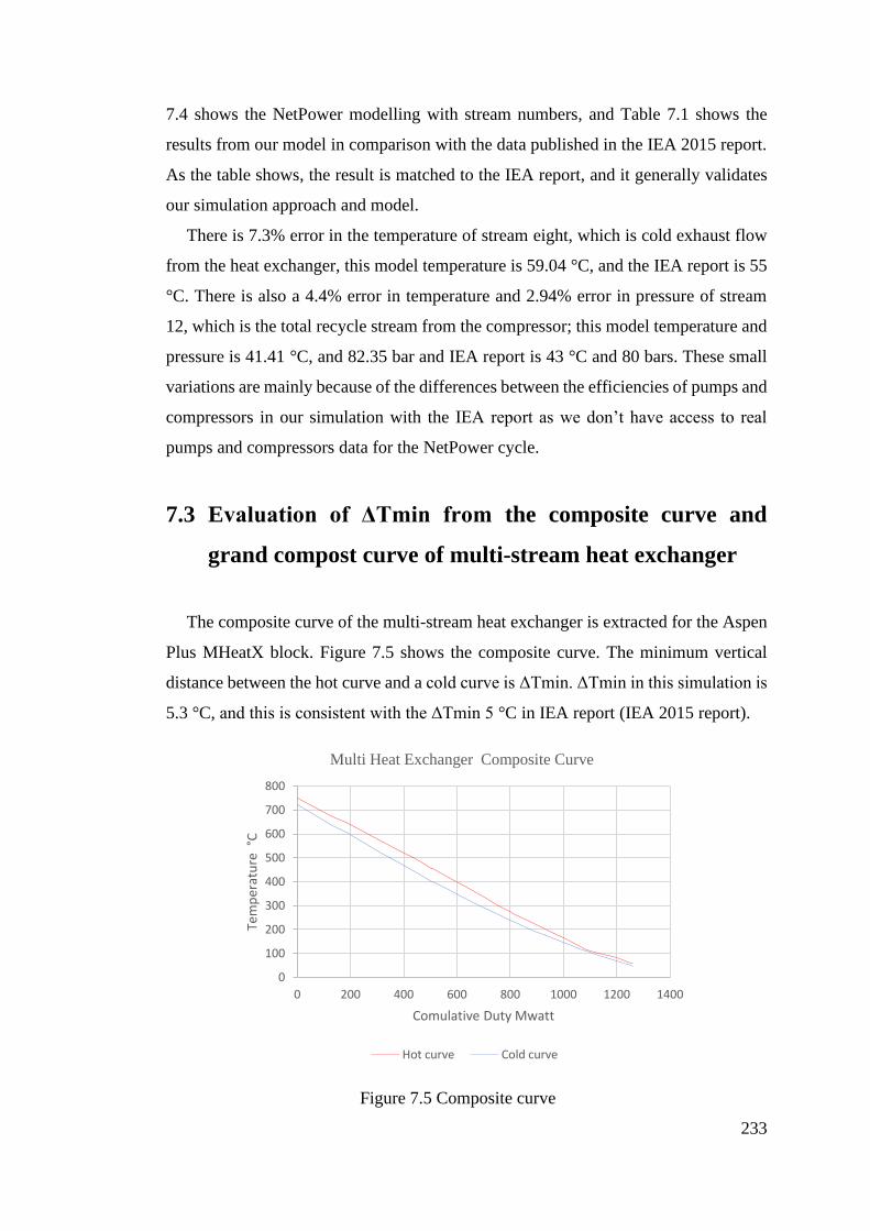
233
7.4 shows the NetPower modelling with stream numbers, and Table 7.1 shows the
results from our model in comparison with the data published in the IEA 2015 report.
As the table shows, the result is matched to the IEA report, and it generally validates
our simulation approach and model.
There is 7.3% error in the temperature of stream eight, which is cold exhaust flow
from the heat exchanger, this model temperature is 59.04 °C, and the IEA report is 55
°C. There is also a 4.4% error in temperature and 2.94% error in pressure of stream
12, which is the total recycle stream from the compressor; this model temperature and
pressure is 41.41 °C, and 82.35 bar and IEA report is 43 °C and 80 bars. These small
variations are mainly because of the differences between the efficiencies of pumps and
compressors in our simulation with the IEA report as we don’t have access to real
pumps and compressors data for the NetPower cycle.
7.3 Evaluation of ΔTmin from the composite curve and
grand compost curve of multi-stream heat exchanger
The composite curve of the multi-stream heat exchanger is extracted for the Aspen
Plus MHeatX block. Figure 7.5 shows the composite curve. The minimum vertical
distance between the hot curve and a cold curve is ΔTmin. ΔTmin in this simulation is
5.3 °C, and this is consistent with the ΔTmin 5 °C in IEA report (IEA 2015 report).
Figure 7.5 Composite curve
0
100
200
300
400
500
600
700
800
0 200 400 600 800 1000 1200 1400
Tem
per
atu
re °
C
Comulative Duty Mwatt
Multi Heat Exchanger Composite Curve
Hot curve Cold curve
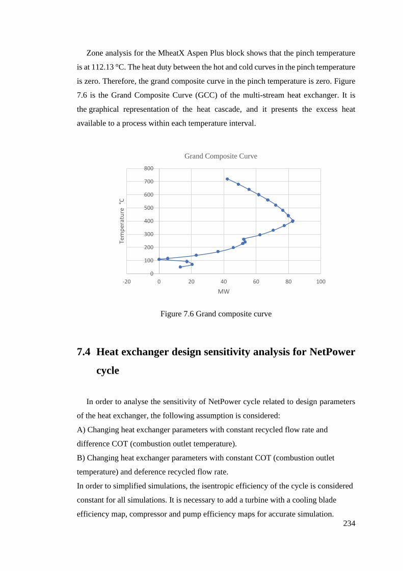
234
Zone analysis for the MheatX Aspen Plus block shows that the pinch temperature
is at 112.13 °C. The heat duty between the hot and cold curves in the pinch temperature
is zero. Therefore, the grand composite curve in the pinch temperature is zero. Figure
7.6 is the Grand Composite Curve (GCC) of the multi-stream heat exchanger. It is
the graphical representation of the heat cascade, and it presents the excess heat
available to a process within each temperature interval.
Figure 7.6 Grand composite curve
7.4 Heat exchanger design sensitivity analysis for NetPower
cycle
In order to analyse the sensitivity of NetPower cycle related to design parameters
of the heat exchanger, the following assumption is considered:
A) Changing heat exchanger parameters with constant recycled flow rate and
difference COT (combustion outlet temperature).
B) Changing heat exchanger parameters with constant COT (combustion outlet
temperature) and deference recycled flow rate.
In order to simplified simulations, the isentropic efficiency of the cycle is considered
constant for all simulations. It is necessary to add a turbine with a cooling blade
efficiency map, compressor and pump efficiency maps for accurate simulation.
0
100
200
300
400
500
600
700
800
-20 0 20 40 60 80 100
Tem
per
atu
re °
C
MW
Grand Composite Curve
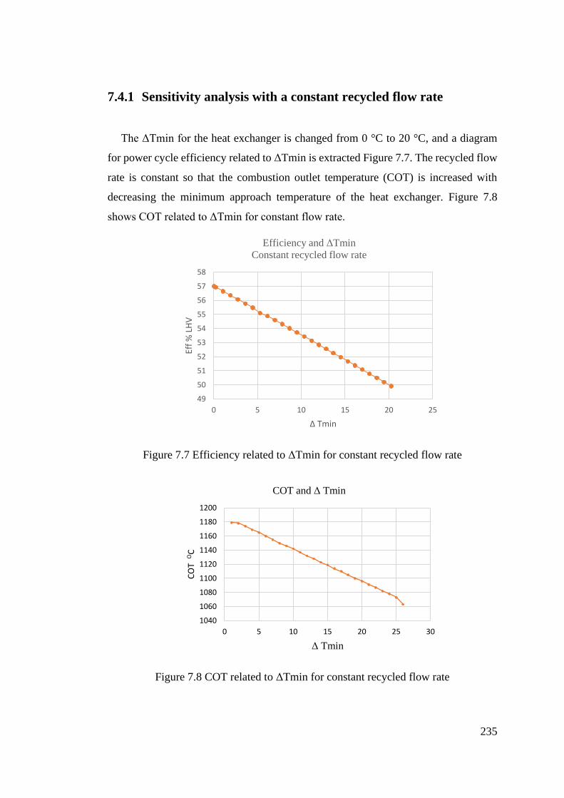
235
7.4.1 Sensitivity analysis with a constant recycled flow rate
The ΔTmin for the heat exchanger is changed from 0 °C to 20 °C, and a diagram
for power cycle efficiency related to ΔTmin is extracted Figure 7.7. The recycled flow
rate is constant so that the combustion outlet temperature (COT) is increased with
decreasing the minimum approach temperature of the heat exchanger. Figure 7.8
shows COT related to ΔTmin for constant flow rate.
Figure 7.7 Efficiency related to ΔTmin for constant recycled flow rate
Figure 7.8 COT related to ΔTmin for constant recycled flow rate
49
50
51
52
53
54
55
56
57
58
0 5 10 15 20 25
Eff
% L
HV
Δ Tmin
Efficiency and ΔTmin
Constant recycled flow rate
1040
1060
1080
1100
1120
1140
1160
1180
1200
0 5 10 15 20 25 30
CO
T O
C
Δ Tmin
COT and Δ Tmin
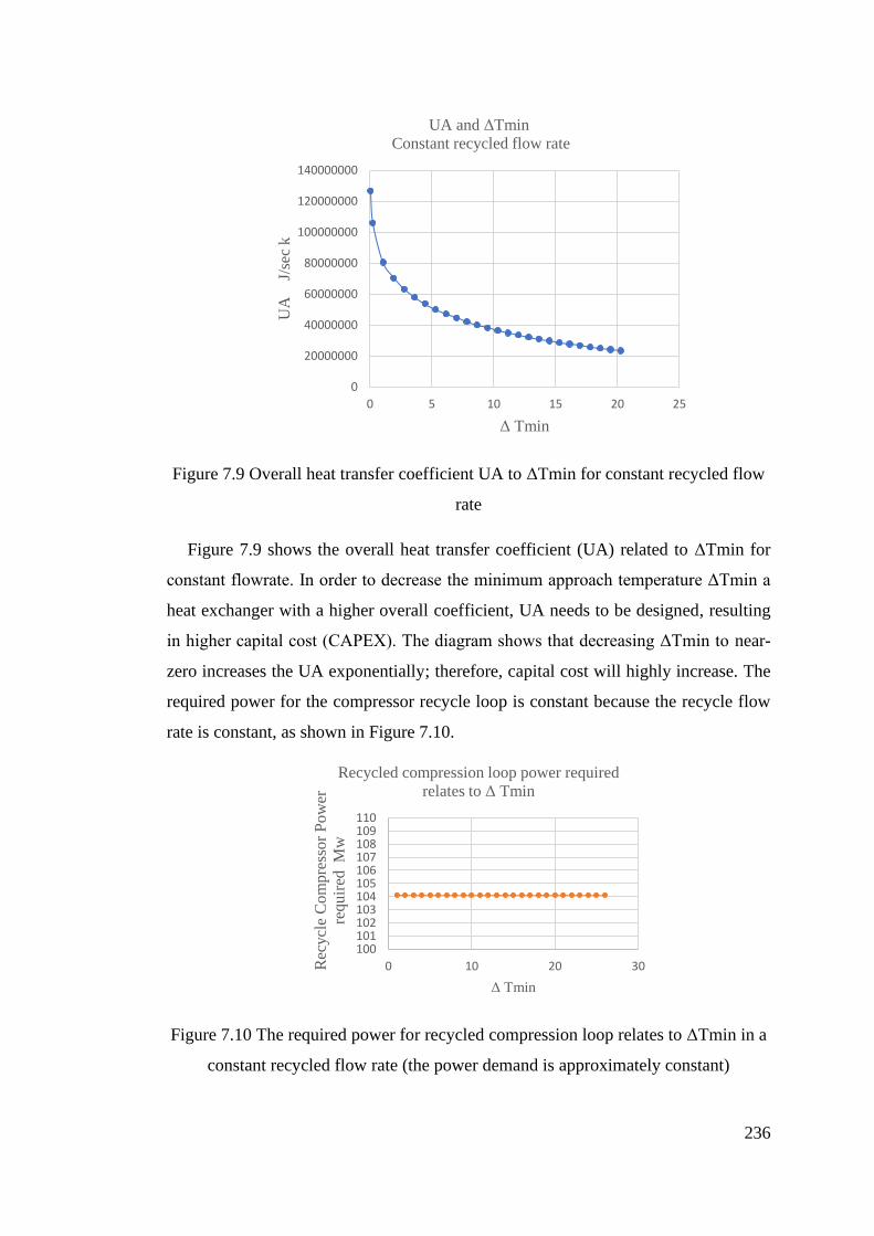
236
Figure 7.9 Overall heat transfer coefficient UA to ΔTmin for constant recycled flow
rate
Figure 7.9 shows the overall heat transfer coefficient (UA) related to ΔTmin for
constant flowrate. In order to decrease the minimum approach temperature ΔTmin a
heat exchanger with a higher overall coefficient, UA needs to be designed, resulting
in higher capital cost (CAPEX). The diagram shows that decreasing ΔTmin to near-
zero increases the UA exponentially; therefore, capital cost will highly increase. The
required power for the compressor recycle loop is constant because the recycle flow
rate is constant, as shown in Figure 7.10.
Figure 7.10 The required power for recycled compression loop relates to ΔTmin in a
constant recycled flow rate (the power demand is approximately constant)
0
20000000
40000000
60000000
80000000
100000000
120000000
140000000
0 5 10 15 20 25
UA
J/se
c k
Δ Tmin
UA and ΔTmin
Constant recycled flow rate
100101102103104105106107108109110
0 10 20 30Rec
ycl
e C
om
pre
ssor
Pow
er
req
uir
ed M
w
Δ Tmin
Recycled compression loop power required
relates to Δ Tmin
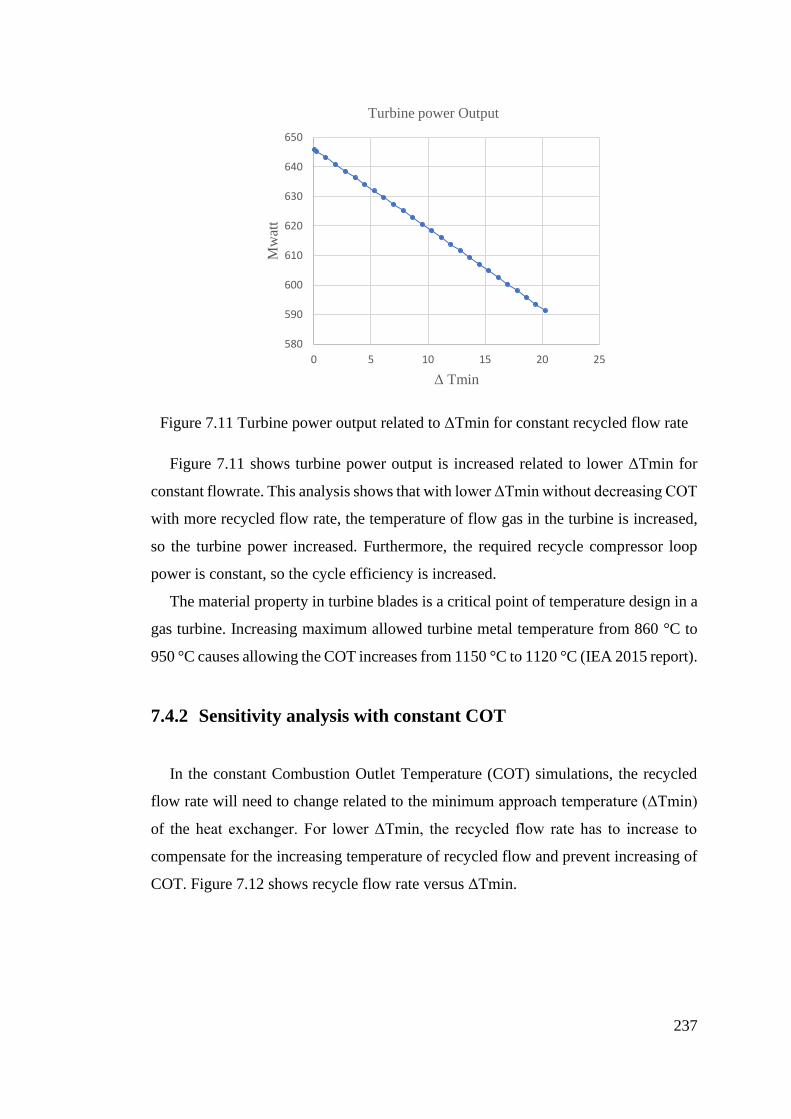
237
Figure 7.11 Turbine power output related to ΔTmin for constant recycled flow rate
Figure 7.11 shows turbine power output is increased related to lower ΔTmin for
constant flowrate. This analysis shows that with lower ΔTmin without decreasing COT
with more recycled flow rate, the temperature of flow gas in the turbine is increased,
so the turbine power increased. Furthermore, the required recycle compressor loop
power is constant, so the cycle efficiency is increased.
The material property in turbine blades is a critical point of temperature design in a
gas turbine. Increasing maximum allowed turbine metal temperature from 860 °C to
950 °C causes allowing the COT increases from 1150 °C to 1120 °C (IEA 2015 report).
7.4.2 Sensitivity analysis with constant COT
In the constant Combustion Outlet Temperature (COT) simulations, the recycled
flow rate will need to change related to the minimum approach temperature (ΔTmin)
of the heat exchanger. For lower ΔTmin, the recycled flow rate has to increase to
compensate for the increasing temperature of recycled flow and prevent increasing of
COT. Figure 7.12 shows recycle flow rate versus ΔTmin.
580
590
600
610
620
630
640
650
0 5 10 15 20 25
Mw
att
Δ Tmin
Turbine power Output
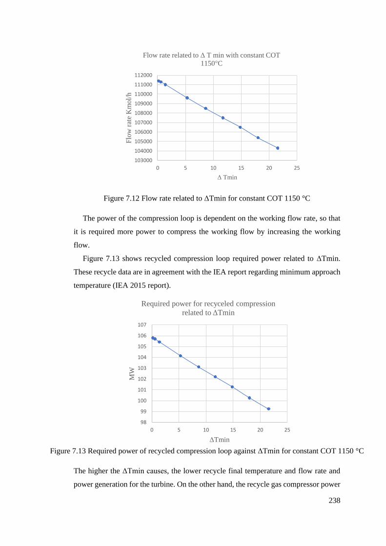
238
Figure 7.12 Flow rate related to ΔTmin for constant COT 1150 °C
The power of the compression loop is dependent on the working flow rate, so that
it is required more power to compress the working flow by increasing the working
flow.
Figure 7.13 shows recycled compression loop required power related to ΔTmin.
These recycle data are in agreement with the IEA report regarding minimum approach
temperature (IEA 2015 report).
The higher the ΔTmin causes, the lower recycle final temperature and flow rate and
power generation for the turbine. On the other hand, the recycle gas compressor power
103000
104000
105000
106000
107000
108000
109000
110000
111000
112000
0 5 10 15 20 25
Flo
w r
ate
Km
ol/
h
Δ Tmin
Flow rate related to Δ T min with constant COT
1150°C
98
99
100
101
102
103
104
105
106
107
0 5 10 15 20 25
MW
ΔTmin
Required power for recyceled compression
related to ΔTmin
Figure 7.13 Required power of recycled compression loop against ΔTmin for constant COT 1150 °C
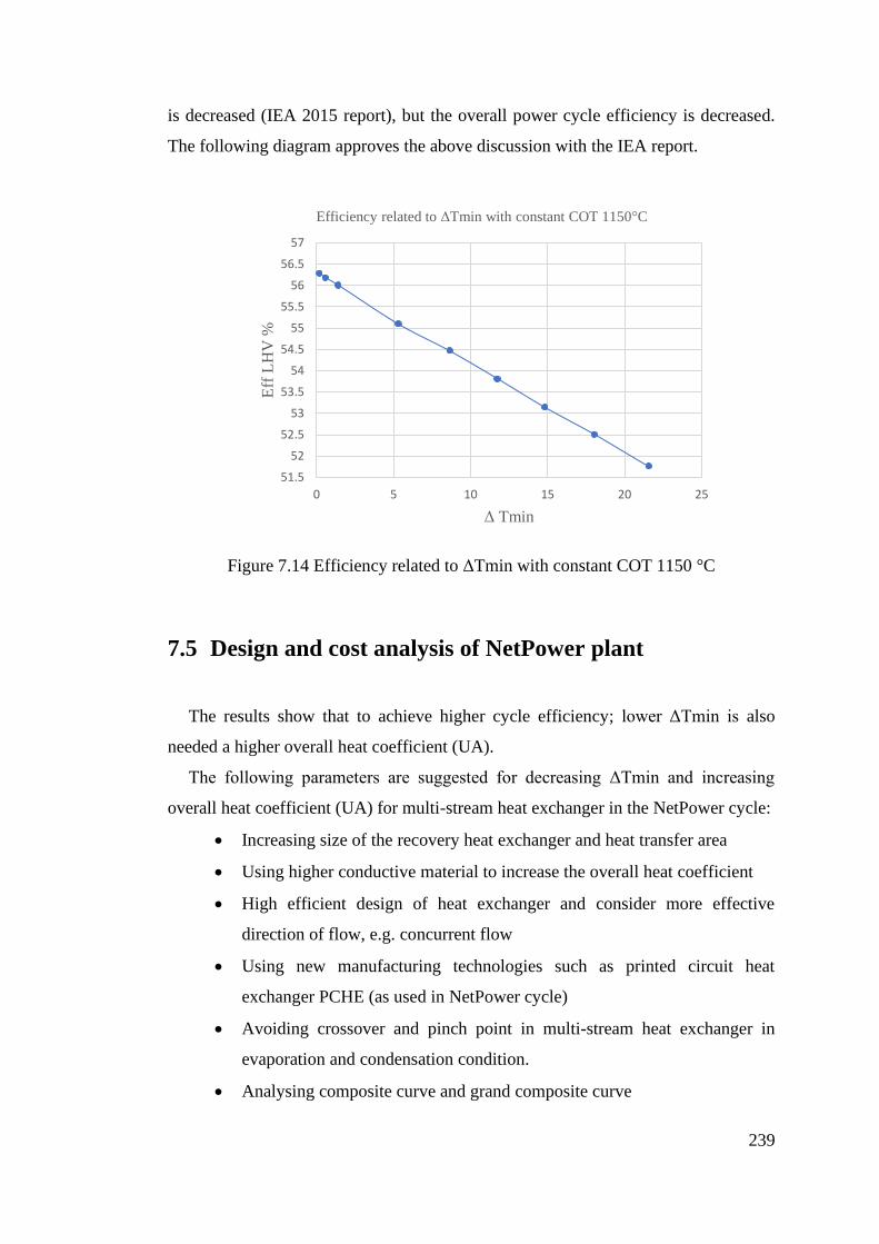
239
is decreased (IEA 2015 report), but the overall power cycle efficiency is decreased.
The following diagram approves the above discussion with the IEA report.
Figure 7.14 Efficiency related to ΔTmin with constant COT 1150 °C
7.5 Design and cost analysis of NetPower plant
The results show that to achieve higher cycle efficiency; lower ΔTmin is also
needed a higher overall heat coefficient (UA).
The following parameters are suggested for decreasing ΔTmin and increasing
overall heat coefficient (UA) for multi-stream heat exchanger in the NetPower cycle:
• Increasing size of the recovery heat exchanger and heat transfer area
• Using higher conductive material to increase the overall heat coefficient
• High efficient design of heat exchanger and consider more effective
direction of flow, e.g. concurrent flow
• Using new manufacturing technologies such as printed circuit heat
exchanger PCHE (as used in NetPower cycle)
• Avoiding crossover and pinch point in multi-stream heat exchanger in
evaporation and condensation condition.
• Analysing composite curve and grand composite curve
51.5
52
52.5
53
53.5
54
54.5
55
55.5
56
56.5
57
0 5 10 15 20 25
Eff
LH
V %
Δ Tmin
Efficiency related to ΔTmin with constant COT 1150°C
240
• Implementation of the above items (to achieve lower ΔTmin) increases the
cost of the multi heat exchanger component in the power cycles.
The following parameters should be considered to design and evaluate the cost of
heat exchange for the NetPower plant: Heat recovery with multi-stream heat exchanger
saves energy cost by reducing hot and cold utilities. The capital cost (CAPEX) of
utilities and operational cost (OPEX) of utilities are reduced. The capital cost of heat
exchanger price will increase by lower ΔTmin. In order to reduce pressure drop in the
multi-stream heat exchanger, the CAPEX will increase, but energy cost and OPEX
will drop.
The efficiency is increased, and operational energy cost is reduced by lower ΔTmin.
In order to design a multi-stream heat exchanger for the NetPower plant, it is required
to tradeoff between capital cost (CAPEX) and operational cost (OPEX) for specifying
ΔTmin.
241
7.6 Summary
In this chapter, the sensitivity of the NetPower oxyturbine cycle is analysed by
means of process modelling in Aspen Plus software. The results show that heat
exchanger design has important effects on the efficiency, capital cost, saving energy
and operational cost of the cycle.
The simulation results show that the efficiency increases with lower ΔTmin in both
constant COT and constant recycled flow rates. The COT shows an increase by
decreasing ΔTmin with a constant recycled flow rate. The efficiency increases faster
in constant flow rate compared to the constant COT.
The power demand for the recycling compression loop was found to be highly
dependent on the recycle flow rate, and with a constant flow rate, the recycle
compression loop power demand is constant. The higher ΔTmin with constant COT
causes lower recycle final temperature, lower flow rate and lower turbine power
output. The modelling shows that the power demand of the recycle compression loop
was decreased, and in total, the efficiency decreased by more than 1%. These results
are consistent with the results presented in the IEA 2015 report (IEA, 2015).
The overall heat coefficient (UA) diagram of the heat exchanger related to ΔTmin
shows that decreasing ΔTmin near-zero causes an exponentially increase in the capital
cost. The tradeoff between the capital cost and efficiency in the NetPower cycle is very
critical and will be justified by selecting an efficient ΔTmin.
In order to reach higher cycle efficiencies, COT will need to be increased. This
shows that the material property of turbine blades or turbine blades cooling strategies
have a critical role in increasing the efficiency of the NetPower Cycle. Furthermore,
designing heat exchangers with higher overall heat coefficient (UA) and lower ΔTmin
results in higher efficiencies in the NetPower cycle. This means heat exchanger has a
critical role in NetPower cycle performance and overall efficiency, and therefore it is
very important to invest in new heat exchanger manufacturing technologies, materials
and design methods resulting in lower capital and operational cost of the cycle in the
near future.
242
Chapter 8: Leading Oxy-combustion
power cycles: NetPower and
Supercritical CES
8.1 Introduction
Several oxyturbine cycles have been introduced by means of thermodynamic
analysis. However, only NetPower and Supercritical CES cycles have recently
proceeded to the demonstration phase. The NetPower cycle recirculates only carbon
dioxide as the working fluid, and the Supercritical CES cycle uses water as its working
fluid. The Supercritical CES cycle that has the best efficiency among other types of
CES cycles includes high, medium and low-pressure turbines (HP, MP, and LP) and
the exhaust gas from the high-pressure turbine is reheated and expanded in an MP and
LP. Pure oxygen is produced in an Air Separation Unit (ASU) and directly injected
into the combustion chamber. The NetPower cycle includes a single turbine with high
inlet pressure and a main multi-stream heat exchanger. Pure oxygen is produced in the
ASU and mixed with the recycled carbon dioxide before being introducing to the
combustion chamber. Both cycles include recycling loops and carbon dioxide
purification sections. These novel cycles reduce the cost for power generation with
complete CO2 capture and sequestration with nearly zero-emission.
In this chapter, The NetPower and Supercritical CES Cycles are investigated by
means of process simulation and the technologies and utilised facilities compared
using sensitivity analysis. Both cycles are simulated with Aspen Plus software with
the same initial conditions, and the simulation results are compared with the IEA 2015
report for validation. The sensitivity of both cycles are analysed with respect to the
Turbine Inlet Temperature (TIT), Combustion Outlet Pressure (COP) and Heat
Exchanger Approach Temperature (HET). The efficiencies are extracted for both the
NetPower and CES cycles, and the partial load behaviour of the cycles are
investigated. The initial results show that the NetPower cycle is more sensitive to the
Turbine Inlet Temperature (TIT) variations in comparison with the S-CES cycle. The
243
results of this paper provide a platform for a comprehensive techno-economical and
sensitivity analysis of the NetPower and Supercritical CES Cycles as the leading Oxy-
combustion power cycles with full carbon capture.
In this chapter, these two cycles are compared in terms of the sensitivity of cycles
with respect to Turbine Inlet Temperature (TIT), Combustion Outlet Pressure (COP)
and heat exchanger approach temperature. Between the available technologies for
carbon capture, turbine-based oxy-combustion cycles seem to be a hopeful carbon-free
solution for the production of electricity.
In this chapter, NetPower and Supercritical CES Cycles are investigated by means
of process simulation and the technologies and utilized facilities are compared using
sensitivity analysis. In order to make a fair comparison between these cycles, each
cycle has been modelled, and its thermodynamic and economic performances have
been estimated on a common design basis. The results of the thermodynamic
calculations indicate a net electric efficiency of 55.1% for the NetPower cycle and
48.9% for the supercritical CES. The economic analysis shows that the NetPower cycle
has the lowest Cost of Electricity (COE), equal to 88.3 €/MWh, and the other cycles
are in the range of 93–95 €/MWh (Mancuso et al., 2015).
8.1.1 CES supercritical cycle
The Clean Energy System (CES) cycle is an oxy-combustion cycle that uses water
(H2O) as the main part of the working flow in the cycle. Bolland and Saether
introduced a basic CES Cycle which was developed by Clean Energy Cycle Ltd (Zhao
et al., 2017). During the last decade, CES cycle efficiency has improved from 20% to
30% (50 MW J79/Deploy 2nd Generation Deploy) to 35,45% ( 200 MW 3th Generation
CES/Siemens/TriGen OFT900) and 50% (400MW CES/Siemens/TriGen) (Business
and October, 2012).
Clean Energy System (CES) demonstrate project for testing, analyzing and design
of modified Siemens SGT-900 gas turbine with the company of Siemens Energy and
Florida Turbine Technology (FTT) and the US. Department of Energy (DOE) funding
program (Climent Barba et al., 2016a). Figure 8.1 shows the schematic process flow
diagram (PFD) of the Supercritical CES cycle.
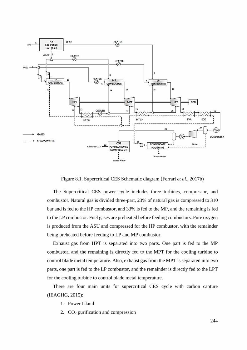
244
Figure 8.1. Supercritical CES Schematic diagram (Ferrari et al., 2017b)
The Supercritical CES power cycle includes three turbines, compressor, and
combustor. Natural gas is divided three-part, 23% of natural gas is compressed to 310
bar and is fed to the HP combustor, and 33% is fed to the MP, and the remaining is fed
to the LP combustor. Fuel gases are preheated before feeding combustors. Pure oxygen
is produced from the ASU and compressed for the HP combustor, with the remainder
being preheated before feeding to LP and MP combustor.
Exhaust gas from HPT is separated into two parts. One part is fed to the MP
combustor, and the remaining is directly fed to the MPT for the cooling turbine to
control blade metal temperature. Also, exhaust gas from the MPT is separated into two
parts, one part is fed to the LP combustor, and the remainder is directly fed to the LPT
for the cooling turbine to control blade metal temperature.
There are four main units for supercritical CES cycle with carbon capture
(IEAGHG, 2015):
1. Power Island
2. CO2 purification and compression
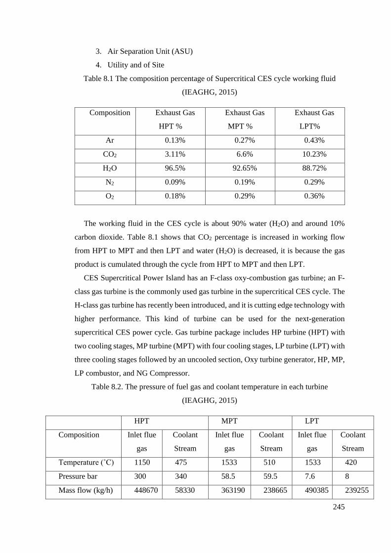
245
3. Air Separation Unit (ASU)
4. Utility and of Site
Table 8.1 The composition percentage of Supercritical CES cycle working fluid
(IEAGHG, 2015)
Composition Exhaust Gas
HPT %
Exhaust Gas
MPT %
Exhaust Gas
LPT%
Ar 0.13% 0.27% 0.43%
CO2 3.11% 6.6% 10.23%
H2O 96.5% 92.65% 88.72%
N2 0.09% 0.19% 0.29%
O2 0.18% 0.29% 0.36%
The working fluid in the CES cycle is about 90% water (H2O) and around 10%
carbon dioxide. Table 8.1 shows that CO2 percentage is increased in working flow
from HPT to MPT and then LPT and water (H2O) is decreased, it is because the gas
product is cumulated through the cycle from HPT to MPT and then LPT.
CES Supercritical Power Island has an F-class oxy-combustion gas turbine; an F-
class gas turbine is the commonly used gas turbine in the supercritical CES cycle. The
H-class gas turbine has recently been introduced, and it is cutting edge technology with
higher performance. This kind of turbine can be used for the next-generation
supercritical CES power cycle. Gas turbine package includes HP turbine (HPT) with
two cooling stages, MP turbine (MPT) with four cooling stages, LP turbine (LPT) with
three cooling stages followed by an uncooled section, Oxy turbine generator, HP, MP,
LP combustor, and NG Compressor.
Table 8.2. The pressure of fuel gas and coolant temperature in each turbine
(IEAGHG, 2015)
HPT MPT LPT
Composition Inlet flue
gas
Coolant
Stream
Inlet flue
gas
Coolant
Stream
Inlet flue
gas
Coolant
Stream
Temperature (˚C) 1150 475 1533 510 1533 420
Pressure bar 300 340 58.5 59.5 7.6 8
Mass flow (kg/h) 448670 58330 363190 238665 490385 239255
246
HPT (Coolant stream) / (Inlet flue gas) ratio = 58330/448670 = 0.13
MPT (Coolant stream) / (Inlet flue gas) ratio = 238665/363190 = 0.657
LPT (Coolant stream) / (Inlet flue gas) ratio = 239255/490385 = 0.488
Table 8.2 shows that TIT in HPT is 1150˚ C less than TIT in MPT and LPT;
therefore, the ratio of coolant stream to inlet fuel gas is higher than HPT. Turbine
efficiencies of MPT and LPT are highly affected by the coolant stream, and it needs to
be considered in the simulation and modelling of the CES cycle. The heat recovery
section and BFW system include BFW economizer, Steam superheater, Inert gas
heater, Regenerator heater, BWF pump, Deaerator drum. The Fuel gas condenser
package and compressor package includes condenser package, fuel gas condensate
pump, wet fuel gas compressors, and condensate separators intercooler. The CO2
purification and compression section includes CO2-rich gas compression, condensate
separator, intercoolers, TSA (Temperature Swing Adsorption).
An ASU (Air Separation Unit) uses a substantial amount of oxyturbine plant
energy. There are several methods to separate oxygen from the air, such as the
cryogenic distillation process, membrane technology, and pressure swing adsorption.
The ASU for the supercritical CES cycle is a cryogenic distillation process. In this
process, the air is cooled to liquify then selectively distil nitrogen, oxygen, argon and
other rare inert gases at their various boiling temperatures. The output of the ASU is
oxygen with 97% purity and which is fed directly to the MP and LP combustor and
compressed for the HP combustor.
The utility unit uses part of the energy of the cycle to provide an operation for the
power plant; it includes a cooling system, natural gas receiving system, raw material
system, demineralized water system, firefighting system and others.
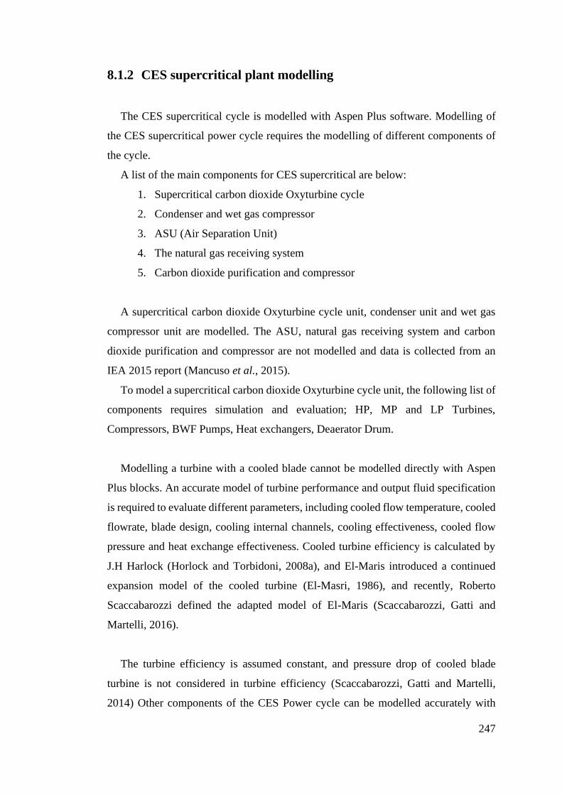
247
8.1.2 CES supercritical plant modelling
The CES supercritical cycle is modelled with Aspen Plus software. Modelling of
the CES supercritical power cycle requires the modelling of different components of
the cycle.
A list of the main components for CES supercritical are below:
1. Supercritical carbon dioxide Oxyturbine cycle
2. Condenser and wet gas compressor
3. ASU (Air Separation Unit)
4. The natural gas receiving system
5. Carbon dioxide purification and compressor
A supercritical carbon dioxide Oxyturbine cycle unit, condenser unit and wet gas
compressor unit are modelled. The ASU, natural gas receiving system and carbon
dioxide purification and compressor are not modelled and data is collected from an
IEA 2015 report (Mancuso et al., 2015).
To model a supercritical carbon dioxide Oxyturbine cycle unit, the following list of
components requires simulation and evaluation; HP, MP and LP Turbines,
Compressors, BWF Pumps, Heat exchangers, Deaerator Drum.
Modelling a turbine with a cooled blade cannot be modelled directly with Aspen
Plus blocks. An accurate model of turbine performance and output fluid specification
is required to evaluate different parameters, including cooled flow temperature, cooled
flowrate, blade design, cooling internal channels, cooling effectiveness, cooled flow
pressure and heat exchange effectiveness. Cooled turbine efficiency is calculated by
J.H Harlock (Horlock and Torbidoni, 2008a), and El-Maris introduced a continued
expansion model of the cooled turbine (El-Masri, 1986), and recently, Roberto
Scaccabarozzi defined the adapted model of El-Maris (Scaccabarozzi, Gatti and
Martelli, 2016).
The turbine efficiency is assumed constant, and pressure drop of cooled blade
turbine is not considered in turbine efficiency (Scaccabarozzi, Gatti and Martelli,
2014) Other components of the CES Power cycle can be modelled accurately with
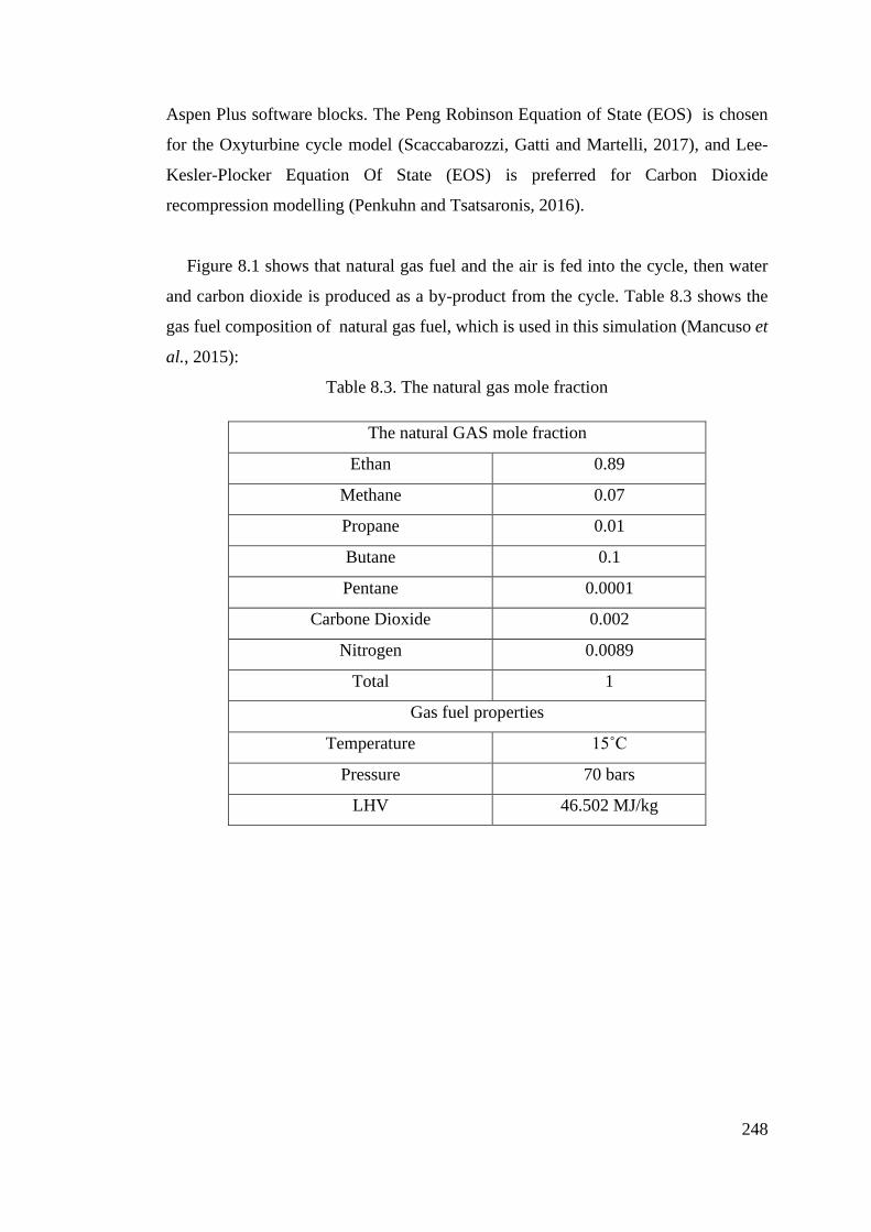
248
Aspen Plus software blocks. The Peng Robinson Equation of State (EOS) is chosen
for the Oxyturbine cycle model (Scaccabarozzi, Gatti and Martelli, 2017), and Lee-
Kesler-Plocker Equation Of State (EOS) is preferred for Carbon Dioxide
recompression modelling (Penkuhn and Tsatsaronis, 2016).
Figure 8.1 shows that natural gas fuel and the air is fed into the cycle, then water
and carbon dioxide is produced as a by-product from the cycle. Table 8.3 shows the
gas fuel composition of natural gas fuel, which is used in this simulation (Mancuso et
al., 2015):
Table 8.3. The natural gas mole fraction
The natural GAS mole fraction
Ethan 0.89
Methane 0.07
Propane 0.01
Butane 0.1
Pentane 0.0001
Carbone Dioxide 0.002
Nitrogen 0.0089
Total 1
Gas fuel properties
Temperature 15˚C
Pressure 70 bars
LHV 46.502 MJ/kg
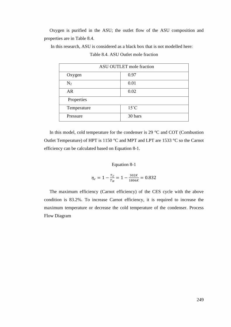
249
Oxygen is purified in the ASU; the outlet flow of the ASU composition and
properties are in Table 8.4.
In this research, ASU is considered as a black box that is not modelled here:
Table 8.4. ASU Outlet mole fraction
ASU OUTLET mole fraction
Oxygen 0.97
N2 0.01
AR 0.02
Properties
Temperature 15˚C
Pressure 30 bars
In this model, cold temperature for the condenser is 29 °C and COT (Combustion
Outlet Temperature) of HPT is 1150 °C and MPT and LPT are 1533 °C so the Carnot
efficiency can be calculated based on Equation 8-1.
Equation 8-1
𝜂𝑐 = 1 −𝑇𝐶
𝑇𝐻= 1 −
302𝐾
1806𝐾= 0.832
The maximum efficiency (Carnot efficiency) of the CES cycle with the above
condition is 83.2%. To increase Carnot efficiency, it is required to increase the
maximum temperature or decrease the cold temperature of the condenser. Process
Flow Diagram
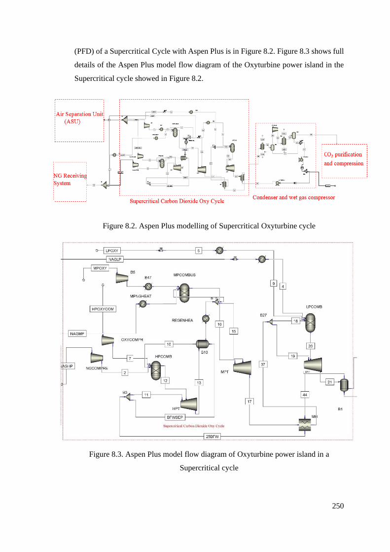
250
(PFD) of a Supercritical Cycle with Aspen Plus is in Figure 8.2. Figure 8.3 shows full
details of the Aspen Plus model flow diagram of the Oxyturbine power island in the
Supercritical cycle showed in Figure 8.2.
Figure 8.2. Aspen Plus modelling of Supercritical Oxyturbine cycle
Figure 8.3. Aspen Plus model flow diagram of Oxyturbine power island in a
Supercritical cycle
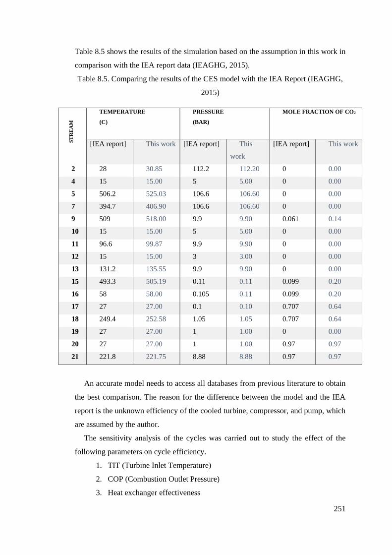
251
Table 8.5 shows the results of the simulation based on the assumption in this work in
comparison with the IEA report data (IEAGHG, 2015).
Table 8.5. Comparing the results of the CES model with the IEA Report (IEAGHG,
2015)
ST
RE
AM
TEMPERATURE
(C)
PRESSURE
(BAR)
MOLE FRACTION OF CO2
[IEA report] This work [IEA report] This
work
[IEA report] This work
2 28 30.85 112.2 112.20 0 0.00
4 15 15.00 5 5.00 0 0.00
5 506.2 525.03 106.6 106.60 0 0.00
7 394.7 406.90 106.6 106.60 0 0.00
9 509 518.00 9.9 9.90 0.061 0.14
10 15 15.00 5 5.00 0 0.00
11 96.6 99.87 9.9 9.90 0 0.00
12 15 15.00 3 3.00 0 0.00
13 131.2 135.55 9.9 9.90 0 0.00
15 493.3 505.19 0.11 0.11 0.099 0.20
16 58 58.00 0.105 0.11 0.099 0.20
17 27 27.00 0.1 0.10 0.707 0.64
18 249.4 252.58 1.05 1.05 0.707 0.64
19 27 27.00 1 1.00 0 0.00
20 27 27.00 1 1.00 0.97 0.97
21 221.8 221.75 8.88 8.88 0.97 0.97
An accurate model needs to access all databases from previous literature to obtain
the best comparison. The reason for the difference between the model and the IEA
report is the unknown efficiency of the cooled turbine, compressor, and pump, which
are assumed by the author.
The sensitivity analysis of the cycles was carried out to study the effect of the
following parameters on cycle efficiency.
1. TIT (Turbine Inlet Temperature)
2. COP (Combustion Outlet Pressure)
3. Heat exchanger effectiveness
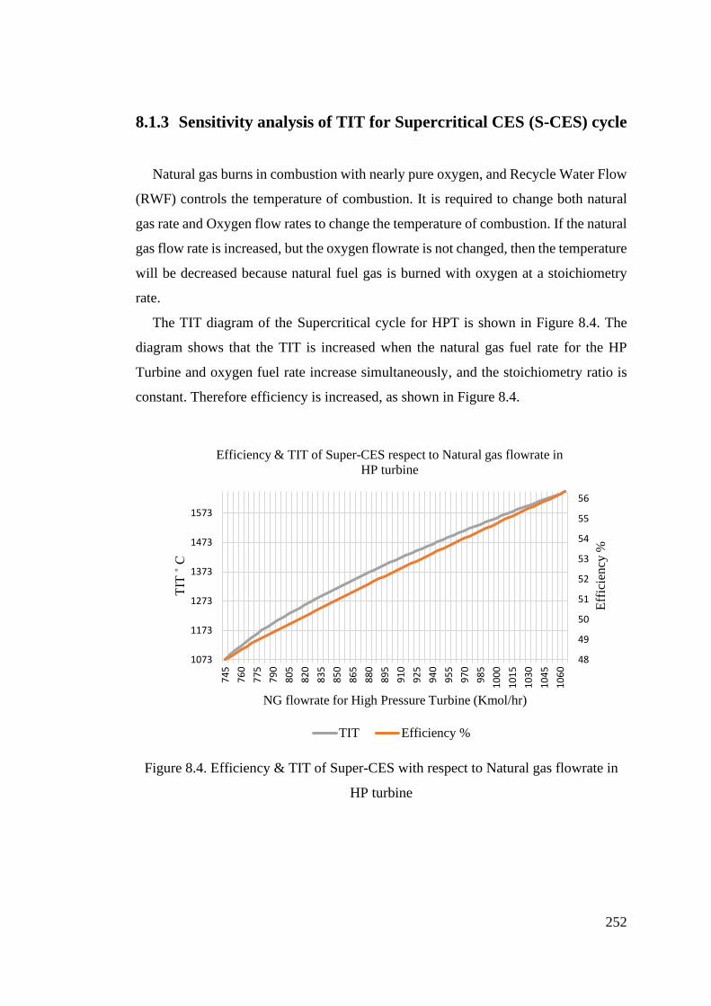
252
8.1.3 Sensitivity analysis of TIT for Supercritical CES (S-CES) cycle
Natural gas burns in combustion with nearly pure oxygen, and Recycle Water Flow
(RWF) controls the temperature of combustion. It is required to change both natural
gas rate and Oxygen flow rates to change the temperature of combustion. If the natural
gas flow rate is increased, but the oxygen flowrate is not changed, then the temperature
will be decreased because natural fuel gas is burned with oxygen at a stoichiometry
rate.
The TIT diagram of the Supercritical cycle for HPT is shown in Figure 8.4. The
diagram shows that the TIT is increased when the natural gas fuel rate for the HP
Turbine and oxygen fuel rate increase simultaneously, and the stoichiometry ratio is
constant. Therefore efficiency is increased, as shown in Figure 8.4.
Figure 8.4. Efficiency & TIT of Super-CES with respect to Natural gas flowrate in
HP turbine
48
49
50
51
52
53
54
55
56
1073
1173
1273
1373
1473
1573
74
5
76
0
77
5
79
0
80
5
82
0
83
5
85
0
86
5
88
0
89
5
91
0
92
5
94
0
95
5
97
0
98
5
10
00
10
15
10
30
10
45
10
60
Eff
icie
ncy
%
TIT
˚ C
NG flowrate for High Pressure Turbine (Kmol/hr)
Efficiency & TIT of Super-CES respect to Natural gas flowrate in
HP turbine
TIT Efficiency %
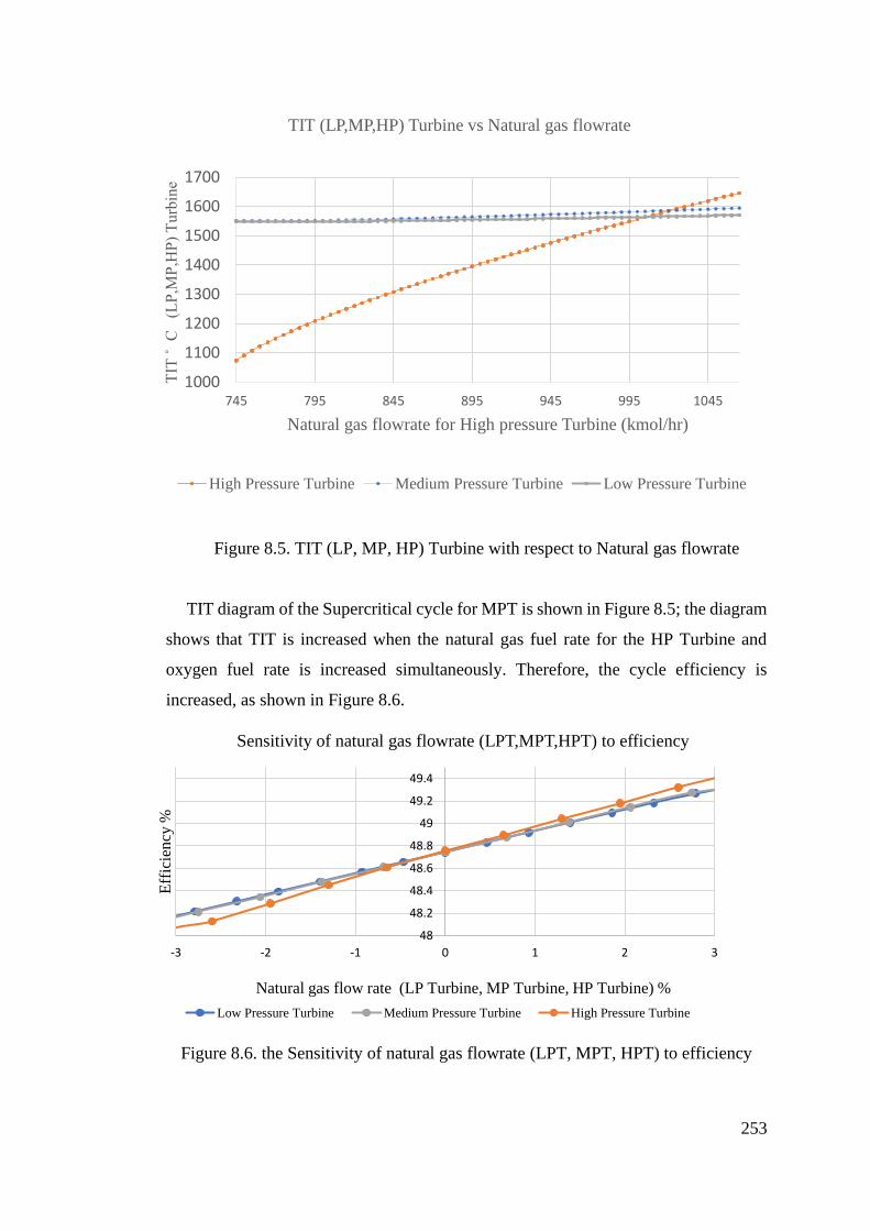
253
Figure 8.5. TIT (LP, MP, HP) Turbine with respect to Natural gas flowrate
TIT diagram of the Supercritical cycle for MPT is shown in Figure 8.5; the diagram
shows that TIT is increased when the natural gas fuel rate for the HP Turbine and
oxygen fuel rate is increased simultaneously. Therefore, the cycle efficiency is
increased, as shown in Figure 8.6.
Figure 8.6. the Sensitivity of natural gas flowrate (LPT, MPT, HPT) to efficiency
1000
1100
1200
1300
1400
1500
1600
1700
745 795 845 895 945 995 1045
TIT
˚
C
(L
P,M
P,H
P)
Tu
rbin
e
Natural gas flowrate for High pressure Turbine (kmol/hr)
TIT (LP,MP,HP) Turbine vs Natural gas flowrate
High Pressure Turbine Medium Pressure Turbine Low Pressure Turbine
48
48.2
48.4
48.6
48.8
49
49.2
49.4
-3 -2 -1 0 1 2 3
Eff
icie
ncy
%
Natural gas flow rate (LP Turbine, MP Turbine, HP Turbine) %
Sensitivity of natural gas flowrate (LPT,MPT,HPT) to efficiency
Low Pressure Turbine Medium Pressure Turbine High Pressure Turbine
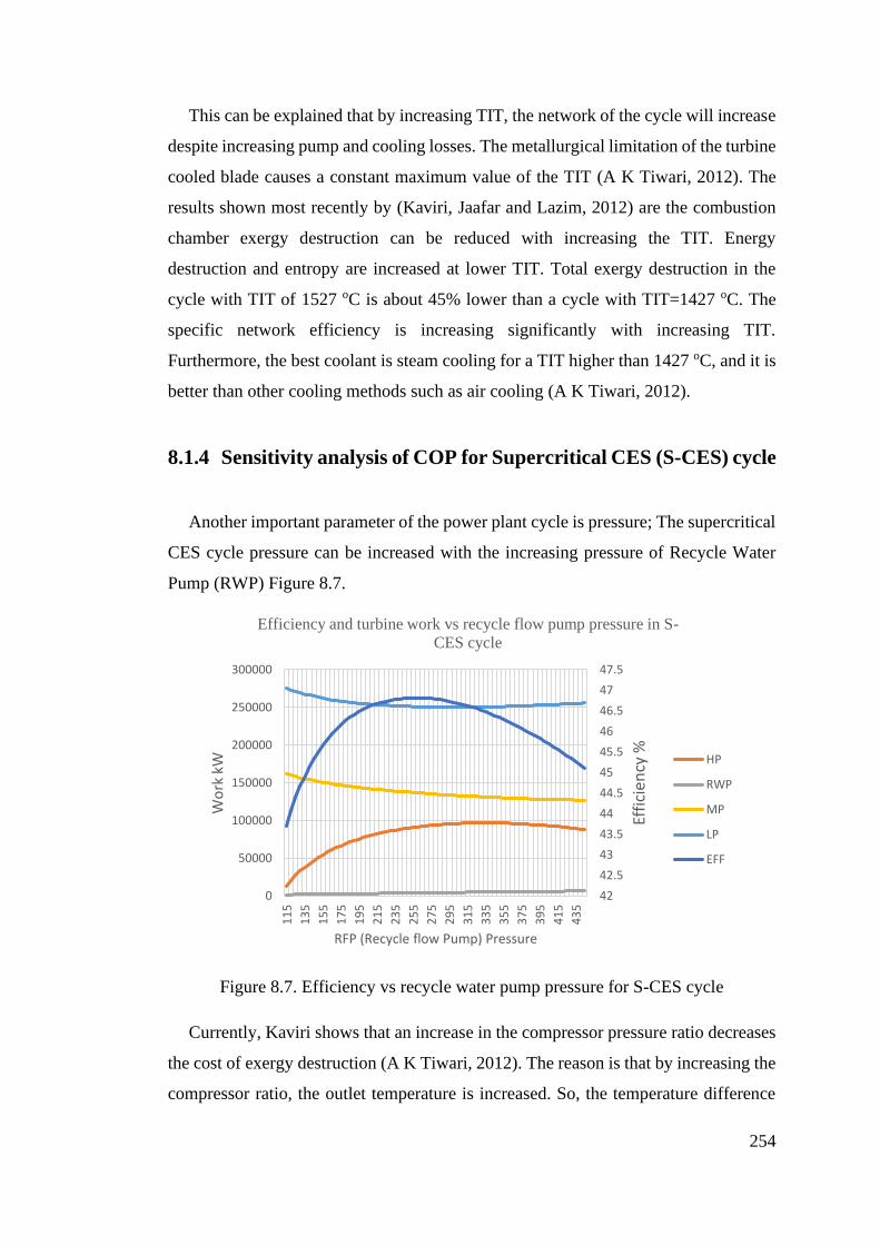
254
This can be explained that by increasing TIT, the network of the cycle will increase
despite increasing pump and cooling losses. The metallurgical limitation of the turbine
cooled blade causes a constant maximum value of the TIT (A K Tiwari, 2012). The
results shown most recently by (Kaviri, Jaafar and Lazim, 2012) are the combustion
chamber exergy destruction can be reduced with increasing the TIT. Energy
destruction and entropy are increased at lower TIT. Total exergy destruction in the
cycle with TIT of 1527 oC is about 45% lower than a cycle with TIT=1427 oC. The
specific network efficiency is increasing significantly with increasing TIT.
Furthermore, the best coolant is steam cooling for a TIT higher than 1427 oC, and it is
better than other cooling methods such as air cooling (A K Tiwari, 2012).
8.1.4 Sensitivity analysis of COP for Supercritical CES (S-CES) cycle
Another important parameter of the power plant cycle is pressure; The supercritical
CES cycle pressure can be increased with the increasing pressure of Recycle Water
Pump (RWP) Figure 8.7.
Figure 8.7. Efficiency vs recycle water pump pressure for S-CES cycle
Currently, Kaviri shows that an increase in the compressor pressure ratio decreases
the cost of exergy destruction (A K Tiwari, 2012). The reason is that by increasing the
compressor ratio, the outlet temperature is increased. So, the temperature difference
42
42.5
43
43.5
44
44.5
45
45.5
46
46.5
47
47.5
0
50000
100000
150000
200000
250000
300000
11
5
13
5
15
5
17
5
19
5
21
5
23
5
25
5
27
5
29
5
31
5
33
5
35
5
37
5
39
5
41
5
43
5
Effi
cien
cy %
Wo
rk k
W
RFP (Recycle flow Pump) Pressure
Efficiency and turbine work vs recycle flow pump pressure in S-
CES cycle
HP
RWP
MP
LP
EFF
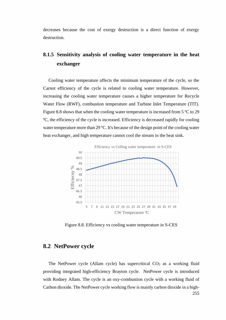
255
decreases because the cost of exergy destruction is a direct function of exergy
destruction.
8.1.5 Sensitivity analysis of cooling water temperature in the heat
exchanger
Cooling water temperature affects the minimum temperature of the cycle, so the
Carnot efficiency of the cycle is related to cooling water temperature. However,
increasing the cooling water temperature causes a higher temperature for Recycle
Water Flow (RWF), combustion temperature and Turbine Inlet Temperature (TIT).
Figure 8.8 shows that when the cooling water temperature is increased from 5 ºC to 29
ºC, the efficiency of the cycle is increased. Efficiency is decreased rapidly for cooling
water temperature more than 29 ºC. It's because of the design point of the cooling water
heat exchanger, and high temperature cannot cool the stream in the heat sink.
Figure 8.8. Efficiency vs cooling water temperature in S-CES
8.2 NetPower cycle
The NetPower cycle (Allam cycle) has supercritical CO2 as a working fluid
providing integrated high-efficiency Brayton cycle. NetPower cycle is introduced
with Rodney Allam. The cycle is an oxy-combustion cycle with a working fluid of
Carbon dioxide. The NetPower cycle working flow is mainly carbon dioxide in a high-
45.5
46
46.5
47
47.5
48
48.5
49
49.5
50
5 7 9 11 13 15 17 19 21 23 25 27 29 31 33 35 37 39
Eff
icie
cny %
CW Temperature oC
Efficiency vs Colling water temperature in S-CES
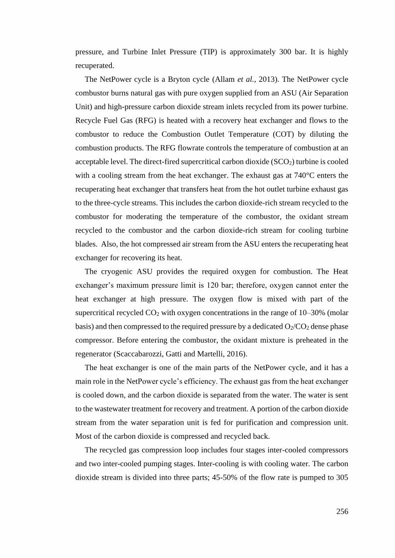
256
pressure, and Turbine Inlet Pressure (TIP) is approximately 300 bar. It is highly
recuperated.
The NetPower cycle is a Bryton cycle (Allam et al., 2013). The NetPower cycle
combustor burns natural gas with pure oxygen supplied from an ASU (Air Separation
Unit) and high-pressure carbon dioxide stream inlets recycled from its power turbine.
Recycle Fuel Gas (RFG) is heated with a recovery heat exchanger and flows to the
combustor to reduce the Combustion Outlet Temperature (COT) by diluting the
combustion products. The RFG flowrate controls the temperature of combustion at an
acceptable level. The direct-fired supercritical carbon dioxide (SCO2) turbine is cooled
with a cooling stream from the heat exchanger. The exhaust gas at 740°C enters the
recuperating heat exchanger that transfers heat from the hot outlet turbine exhaust gas
to the three-cycle streams. This includes the carbon dioxide-rich stream recycled to the
combustor for moderating the temperature of the combustor, the oxidant stream
recycled to the combustor and the carbon dioxide-rich stream for cooling turbine
blades. Also, the hot compressed air stream from the ASU enters the recuperating heat
exchanger for recovering its heat.
The cryogenic ASU provides the required oxygen for combustion. The Heat
exchanger’s maximum pressure limit is 120 bar; therefore, oxygen cannot enter the
heat exchanger at high pressure. The oxygen flow is mixed with part of the
supercritical recycled CO2 with oxygen concentrations in the range of 10–30% (molar
basis) and then compressed to the required pressure by a dedicated O2/CO2 dense phase
compressor. Before entering the combustor, the oxidant mixture is preheated in the
regenerator (Scaccabarozzi, Gatti and Martelli, 2016).
The heat exchanger is one of the main parts of the NetPower cycle, and it has a
main role in the NetPower cycle’s efficiency. The exhaust gas from the heat exchanger
is cooled down, and the carbon dioxide is separated from the water. The water is sent
to the wastewater treatment for recovery and treatment. A portion of the carbon dioxide
stream from the water separation unit is fed for purification and compression unit.
Most of the carbon dioxide is compressed and recycled back.
The recycled gas compression loop includes four stages inter-cooled compressors
and two inter-cooled pumping stages. Inter-cooling is with cooling water. The carbon
dioxide stream is divided into three parts; 45-50% of the flow rate is pumped to 305
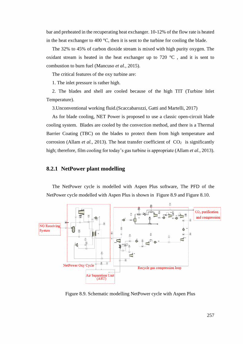
257
bar and preheated in the recuperating heat exchanger. 10-12% of the flow rate is heated
in the heat exchanger to 400 °C, then it is sent to the turbine for cooling the blade.
The 32% to 45% of carbon dioxide stream is mixed with high purity oxygen. The
oxidant stream is heated in the heat exchanger up to 720 °C , and it is sent to
combustion to burn fuel (Mancuso et al., 2015).
The critical features of the oxy turbine are:
1. The inlet pressure is rather high.
2. The blades and shell are cooled because of the high TIT (Turbine Inlet
Temperature).
3.Unconventional working fluid.(Scaccabarozzi, Gatti and Martelli, 2017)
As for blade cooling, NET Power is proposed to use a classic open-circuit blade
cooling system. Blades are cooled by the convection method, and there is a Thermal
Barrier Coating (TBC) on the blades to protect them from high temperature and
corrosion (Allam et al., 2013). The heat transfer coefficient of CO2 is significantly
high; therefore, film cooling for today’s gas turbine is appropriate (Allam et al., 2013).
8.2.1 NetPower plant modelling
The NetPower cycle is modelled with Aspen Plus software, The PFD of the
NetPower cycle modelled with Aspen Plus is shown in Figure 8.9 and Figure 8.10.
Figure 8.9. Schematic modelling NetPower cycle with Aspen Plus
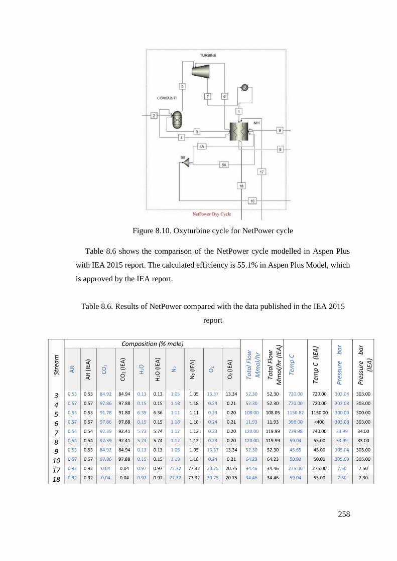
258
Figure 8.10. Oxyturbine cycle for NetPower cycle
Table 8.6 shows the comparison of the NetPower cycle modelled in Aspen Plus
with IEA 2015 report. The calculated efficiency is 55.1% in Aspen Plus Model, which
is approved by the IEA report.
Table 8.6. Results of NetPower compared with the data published in the IEA 2015
report
Stre
am
Composition (% mole)
Tota
l Flo
w
Mm
ol/
hr
Tota
l Flo
w
Mm
ol/
hr
(IEA
)
Tem
p C
Tem
p C
(IE
A)
Pre
ssu
re
ba
r
Pre
ssu
re
ba
r
(IEA
)
AR
AR
(IE
A)
CO
2
CO
2 (
IEA
)
H2O
H2O
(IE
A)
N2
N2 (
IEA
)
O2
O2
(IEA
)
3 0.53 0.53 84.92 84.94 0.13 0.13 1.05 1.05 13.37 13.34 52.30 52.30 720.00 720.00 303.04 303.00
4 0.57 0.57 97.86 97.88 0.15 0.15 1.18 1.18 0.24 0.21 52.30 52.30 720.00 720.00 303.08 303.00
5 0.53 0.53 91.78 91.80 6.35 6.36 1.11 1.11 0.23 0.20 108.00 108.05 1150.82 1150.00 300.00 300.00
6 0.57 0.57 97.86 97.88 0.15 0.15 1.18 1.18 0.24 0.21 11.93 11.93 398.00 <400 303.08 303.00
7 0.54 0.54 92.39 92.41 5.73 5.74 1.12 1.12 0.23 0.20 120.00 119.99 739.98 740.00 33.99 34.00
8 0.54 0.54 92.39 92.41 5.73 5.74 1.12 1.12 0.23 0.20 120.00 119.99 59.04 55.00 33.99 33.00
9 0.53 0.53 84.92 84.94 0.13 0.13 1.05 1.05 13.37 13.34 52.30 52.30 45.65 45.00 305.04 305.00
10 0.57 0.57 97.86 97.88 0.15 0.15 1.18 1.18 0.24 0.21 64.23 64.23 50.92 50.00 305.08 305.00
17 0.92 0.92 0.04 0.04 0.97 0.97 77.32 77.32 20.75 20.75 34.46 34.46 275.00 275.00 7.50 7.50
18 0.92 0.92 0.04 0.04 0.97 0.97 77.32 77.32 20.75 20.75 34.46 34.46 59.04 55.00 7.50 7.30
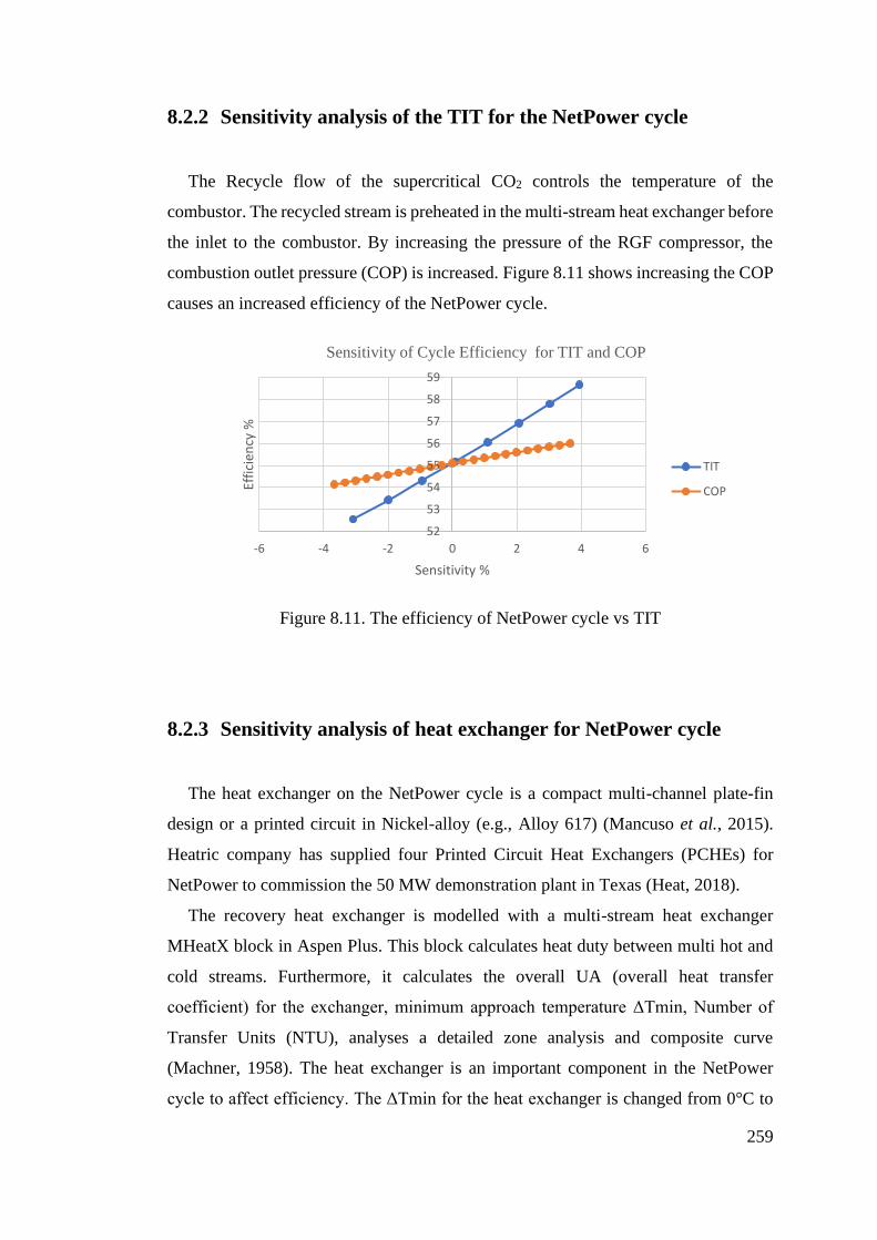
259
8.2.2 Sensitivity analysis of the TIT for the NetPower cycle
The Recycle flow of the supercritical CO2 controls the temperature of the
combustor. The recycled stream is preheated in the multi-stream heat exchanger before
the inlet to the combustor. By increasing the pressure of the RGF compressor, the
combustion outlet pressure (COP) is increased. Figure 8.11 shows increasing the COP
causes an increased efficiency of the NetPower cycle.
Figure 8.11. The efficiency of NetPower cycle vs TIT
8.2.3 Sensitivity analysis of heat exchanger for NetPower cycle
The heat exchanger on the NetPower cycle is a compact multi-channel plate-fin
design or a printed circuit in Nickel-alloy (e.g., Alloy 617) (Mancuso et al., 2015).
Heatric company has supplied four Printed Circuit Heat Exchangers (PCHEs) for
NetPower to commission the 50 MW demonstration plant in Texas (Heat, 2018).
The recovery heat exchanger is modelled with a multi-stream heat exchanger
MHeatX block in Aspen Plus. This block calculates heat duty between multi hot and
cold streams. Furthermore, it calculates the overall UA (overall heat transfer
coefficient) for the exchanger, minimum approach temperature ΔTmin, Number of
Transfer Units (NTU), analyses a detailed zone analysis and composite curve
(Machner, 1958). The heat exchanger is an important component in the NetPower
cycle to affect efficiency. The ΔTmin for the heat exchanger is changed from 0°C to
52
53
54
55
56
57
58
59
-6 -4 -2 0 2 4 6
Effi
cien
cy %
Sensitivity %
Sensitivity of Cycle Efficiency for TIT and COP
TIT
COP
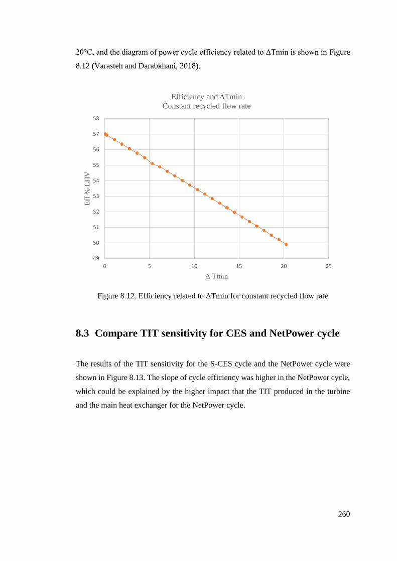
260
20°C, and the diagram of power cycle efficiency related to ΔTmin is shown in Figure
8.12 (Varasteh and Darabkhani, 2018).
Figure 8.12. Efficiency related to ΔTmin for constant recycled flow rate
8.3 Compare TIT sensitivity for CES and NetPower cycle
The results of the TIT sensitivity for the S-CES cycle and the NetPower cycle were
shown in Figure 8.13. The slope of cycle efficiency was higher in the NetPower cycle,
which could be explained by the higher impact that the TIT produced in the turbine
and the main heat exchanger for the NetPower cycle.
49
50
51
52
53
54
55
56
57
58
0 5 10 15 20 25
Eff
% L
HV
Δ Tmin
Efficiency and ΔTmin
Constant recycled flow rate
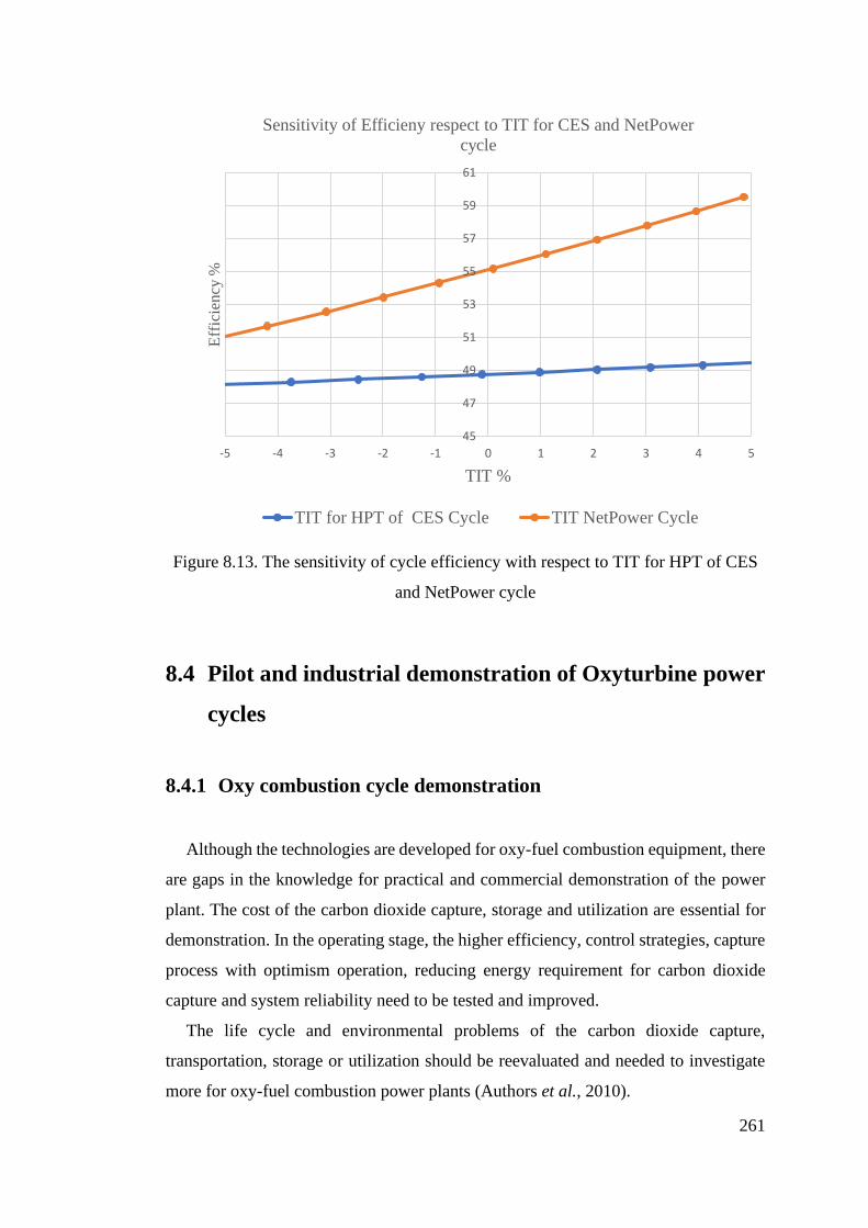
261
Figure 8.13. The sensitivity of cycle efficiency with respect to TIT for HPT of CES
and NetPower cycle
8.4 Pilot and industrial demonstration of Oxyturbine power
cycles
8.4.1 Oxy combustion cycle demonstration
Although the technologies are developed for oxy-fuel combustion equipment, there
are gaps in the knowledge for practical and commercial demonstration of the power
plant. The cost of the carbon dioxide capture, storage and utilization are essential for
demonstration. In the operating stage, the higher efficiency, control strategies, capture
process with optimism operation, reducing energy requirement for carbon dioxide
capture and system reliability need to be tested and improved.
The life cycle and environmental problems of the carbon dioxide capture,
transportation, storage or utilization should be reevaluated and needed to investigate
more for oxy-fuel combustion power plants (Authors et al., 2010).
45
47
49
51
53
55
57
59
61
-5 -4 -3 -2 -1 0 1 2 3 4 5
Eff
icie
ncy
%
TIT %
Sensitivity of Efficieny respect to TIT for CES and NetPower
cycle
TIT for HPT of CES Cycle TIT NetPower Cycle

262
The main two leading oxy-combustion plants are NetPower and CES power plants
which are in the demonstration phase.
The NetPower cycle has established a 50 MW demonstration power plant in Texas,
and the power plant is under operation now; and NetPower has planned to bring a 300
MW plant online in 2022 (Patel, 2019).
Clean energy system company developed CES cycle, 5MW CES Power plant
established at the CES test site in Kimberlina, CA in August 2003. CES company has
planned to construct a 50 MW oxy-combustion power plant in southern California.
263
8.5 Summary
Based on the analysis of the CES and the NetPower cycles, real plant investment
decisions are affected by technology and regional characteristics as below:
• The results of the TIT sensitivity for the S-CES cycle and the NetPower cycle
indicate that the slope of cycle efficiency was higher in the NetPower cycle, which
could be explained by the higher impact that the TIT produced in the turbine and
the main heat exchanger for the NetPower cycle.
• Increasing recycle flow pressure increases efficiency in the NetPower cycle, but
efficiency is decreased in the S-CES cycle because more work is required for the
RWF.
• Cooling water temperature affects the minimum temperature of the S-CES cycle;
this leads to an increase in efficiency until it reaches the maximum point and then
decreases.
• The main heat exchanger (Network Heat Exchanger) of the NetPower cycle has a
significant effect on efficiency. Decreasing ΔTmin causes an increase in cycle
efficiency.
• The analysis also indicates that TIT, COP, and heat exchanger effectiveness are
the main parameters affecting cycle efficiency. To evaluate cycle parameters more
accurately, an ad-hoc model of cooled turbine and heat exchanger is required
instead of using a simplified block of Aspen Plus software.
As future work, An accurate model of a cooled blade turbine and heat exchanger need
also be developed for precise sensitivity analysis and optimization of the power cycle
parameters. The NetPower is more flexible in operation than a combined cycle, and it
is projected to be more economical without tax on carbon (Flin, 2019).
CES company modified a traditional gas turbine to operate with Steam/CO2 drive gas
rather than an air-based drive gas. CES technology enables the turbine to extract
three times more power than a conventional gas turbine (CES, 2020b).
264
Chapter 9: Techno-economic,
Technology Readiness Level (TRL)
and parametric comparison in
Oxyturbine Power cycles
9.1 Introduction
Oxy-combustion cycles are necessary to especially advance the technologies (van
der Spek, Ramirez and Faaij, 2017); during last two decades, the oxy-combustion
cycles technologies are developed, and some of the technologies have proceeded to
commercial state, (Van Der Spek et al., 2017); however, there is a gap in comparison
of available oxy-combustion technologies.
This chapter aims to compare the oxy-combustion cycles in term of parameters,
technology readiness level (TRL), performance and economy. The cycle parameters,
including Turbine Inlet Temperature (TIT), Turbine Outlet Temperature (TOT),
Combustion Outlet Pressure (COP), thermal and exergy efficiency, carbon dioxide per
KWh of electricity, are studied and compared in detail. Also, the Technology
Readiness Level (TRL) are assessed in detail and compared. Then, the performance,
cost rates and LCOE for oxy-combustion cycles are analysed and compared, and the
radar diagram is drawn to compare all deliberated parameters.
9.2 TIT comparison of oxy-combustion cycles
Turbine Inlet Temperature (TIT) is an important parameter of the oxy-combustion
cycle; TIT can affect oxy-combustion cycle performance, Higher TIT can increase the
net power output of the cycle and increase the efficiency (Calli, Colpan and Gunerhan,
2018); however, higher TIT can be achieved by the development of gas turbine
technologies including development of cooling blade system, new materials for
265
thermal barrier coating (TBC) for turbine blade, blade construction and layering
(Higher temperatures in turbines - Kraftwerk Forschung, 2020)
The turbine blade cooling system is one of the technology to increase Turbine Inlet
Temperature (TIT); however, it causes energy losses in the turbines and lower
aerodynamic efficiency; hence it has a negative impact to efficiency (Horlock and
Torbidoni, 2008b)
Table 9.1 shows TIT for each oxy-combustion cycle, It's combined from modelling
and data extracted from literature, and the TIT of S-CES is high (1533°C). Hence, this
cycle need developed technology for a gas turbine blade. Clean energy system
company with collaboration by Siemens Energy and Florida Turbine Technologies
(FTT) and sponsored by the Department of Energy recently developed OFT-900
oxy-fuel turbine and can reach to highest temperature up to 1976°C (Clean Energy
System, 2020b) and CES Power cycle is in the demonstration stage. The Novel
O2/CO2 (Cao and Zheng, 2006) cycle also has 1573 °C TIT, this cycle is not in the
demonstration stage, and more development of technologies is required. NetPower
cycle TIT temperature is 1150 °C, and Toshiba ESS delivered the turbine and
combustor, which are the system's crucial components.
As shown in Figure 9.1, the highest TIT s belongs to the S-CES and Novel O2/CO2;
the gas turbine with high TIT needs blade-cooling and developed technology. The
efficiency of the turbine can be increased by developed technologies for cooling blade
and blade thermal barrier coating.
NetPower TIT is lower than S-CES and this can be the advantage of the cycle in
comparison with S-CES, and it has less dependency on the new technology for cooling
blade and blades thermal barrier coating; however, the gas turbine needs new
technology for high purity CO2 working flow.
AZEP 100% and 80% have lower TIT in comparison with other cycles, so the
technology development in the cooling blade and blade thermal coating barrier cannot
increase the efficiency of the cycle considerably.
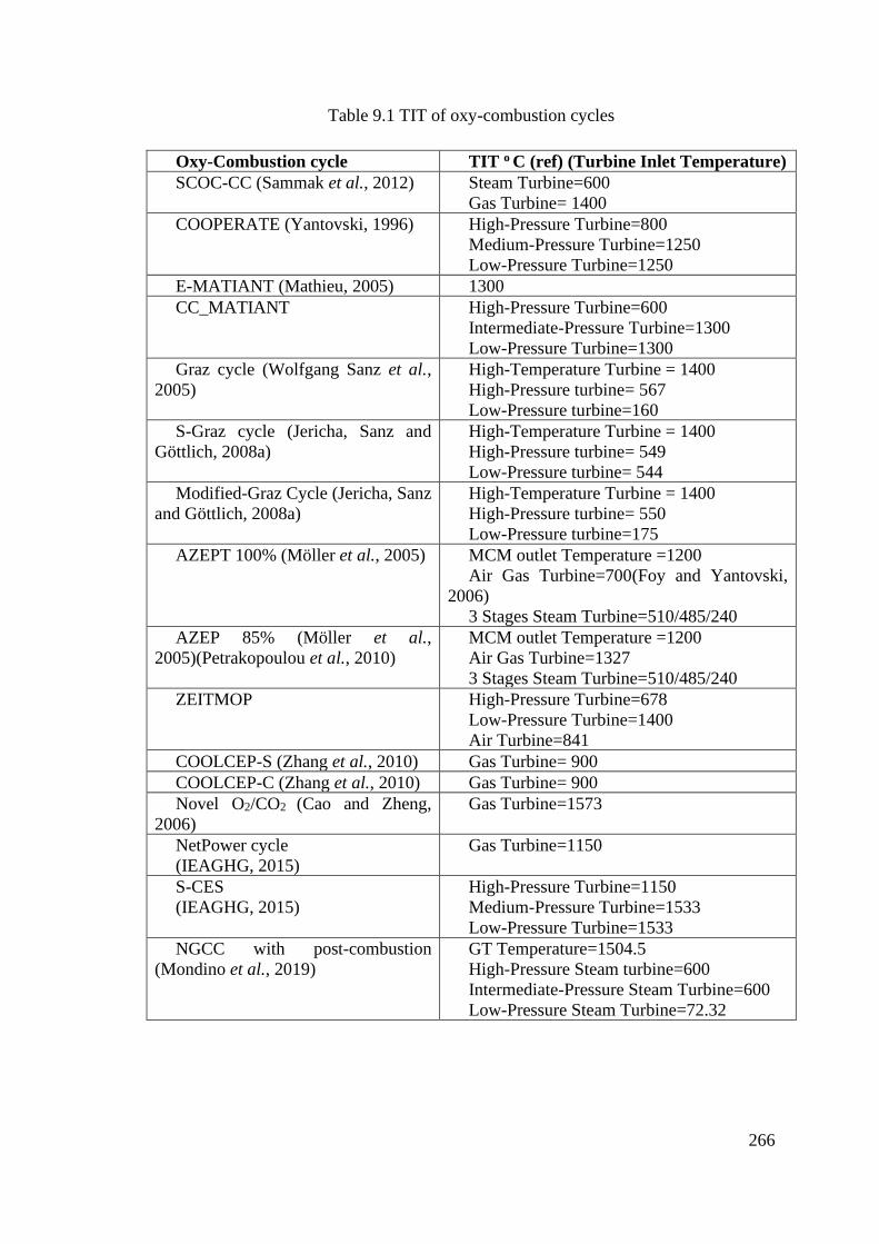
266
Table 9.1 TIT of oxy-combustion cycles
Oxy-Combustion cycle TIT o C (ref) (Turbine Inlet Temperature)
SCOC-CC (Sammak et al., 2012) Steam Turbine=600
Gas Turbine= 1400
COOPERATE (Yantovski, 1996) High-Pressure Turbine=800
Medium-Pressure Turbine=1250
Low-Pressure Turbine=1250
E-MATIANT (Mathieu, 2005) 1300
CC_MATIANT High-Pressure Turbine=600
Intermediate-Pressure Turbine=1300
Low-Pressure Turbine=1300
Graz cycle (Wolfgang Sanz et al.,
2005)
High-Temperature Turbine = 1400
High-Pressure turbine= 567
Low-Pressure turbine=160
S-Graz cycle (Jericha, Sanz and
Göttlich, 2008a)
High-Temperature Turbine = 1400
High-Pressure turbine= 549
Low-Pressure turbine= 544
Modified-Graz Cycle (Jericha, Sanz
and Göttlich, 2008a)
High-Temperature Turbine = 1400
High-Pressure turbine= 550
Low-Pressure turbine=175
AZEPT 100% (Möller et al., 2005) MCM outlet Temperature =1200
Air Gas Turbine=700(Foy and Yantovski,
2006)
3 Stages Steam Turbine=510/485/240
AZEP 85% (Möller et al.,
2005)(Petrakopoulou et al., 2010)
MCM outlet Temperature =1200
Air Gas Turbine=1327
3 Stages Steam Turbine=510/485/240
ZEITMOP High-Pressure Turbine=678
Low-Pressure Turbine=1400
Air Turbine=841
COOLCEP-S (Zhang et al., 2010) Gas Turbine= 900
COOLCEP-C (Zhang et al., 2010) Gas Turbine= 900
Novel O2/CO2 (Cao and Zheng,
2006)
Gas Turbine=1573
NetPower cycle
(IEAGHG, 2015)
Gas Turbine=1150
S-CES
(IEAGHG, 2015)
High-Pressure Turbine=1150
Medium-Pressure Turbine=1533
Low-Pressure Turbine=1533
NGCC with post-combustion
(Mondino et al., 2019)
GT Temperature=1504.5
High-Pressure Steam turbine=600
Intermediate-Pressure Steam Turbine=600
Low-Pressure Steam Turbine=72.32
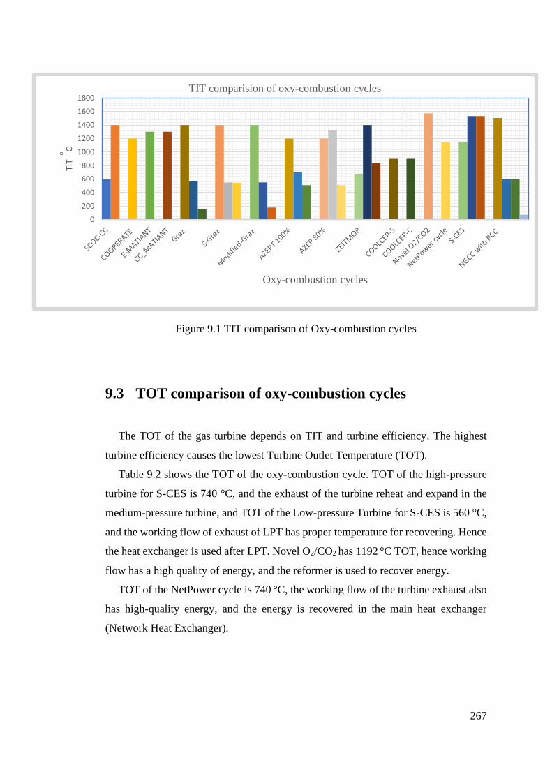
267
Figure 9.1 TIT comparison of Oxy-combustion cycles
9.3 TOT comparison of oxy-combustion cycles
The TOT of the gas turbine depends on TIT and turbine efficiency. The highest
turbine efficiency causes the lowest Turbine Outlet Temperature (TOT).
Table 9.2 shows the TOT of the oxy-combustion cycle. TOT of the high-pressure
turbine for S-CES is 740 °C, and the exhaust of the turbine reheat and expand in the
medium-pressure turbine, and TOT of the Low-pressure Turbine for S-CES is 560 °C,
and the working flow of exhaust of LPT has proper temperature for recovering. Hence
the heat exchanger is used after LPT. Novel O2/CO2 has 1192 °C TOT, hence working
flow has a high quality of energy, and the reformer is used to recover energy.
TOT of the NetPower cycle is 740 °C, the working flow of the turbine exhaust also
has high-quality energy, and the energy is recovered in the main heat exchanger
(Network Heat Exchanger).
0
200
400
600
800
1000
1200
1400
1600
1800
TIT
o
C
Oxy-combustion cycles
TIT comparision of oxy-combustion cycles
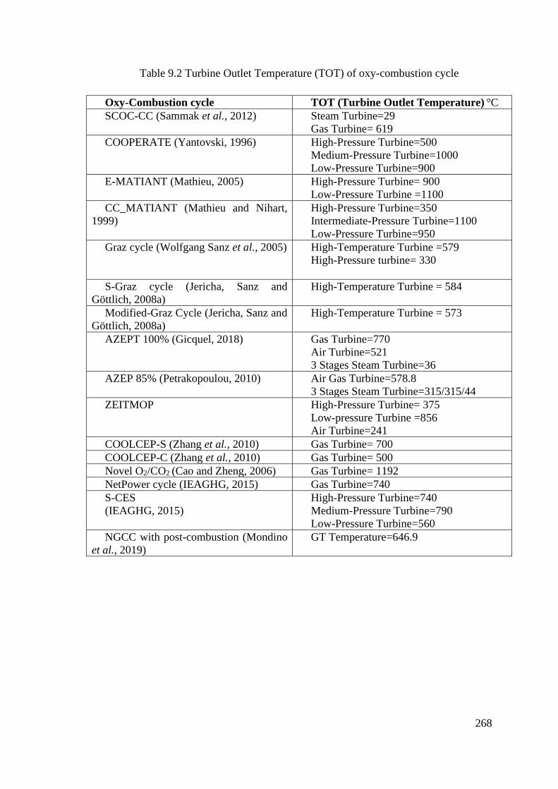
268
Table 9.2 Turbine Outlet Temperature (TOT) of oxy-combustion cycle
Oxy-Combustion cycle TOT (Turbine Outlet Temperature) °C
SCOC-CC (Sammak et al., 2012) Steam Turbine=29
Gas Turbine= 619
COOPERATE (Yantovski, 1996) High-Pressure Turbine=500
Medium-Pressure Turbine=1000
Low-Pressure Turbine=900
E-MATIANT (Mathieu, 2005) High-Pressure Turbine= 900
Low-Pressure Turbine =1100
CC_MATIANT (Mathieu and Nihart,
1999)
High-Pressure Turbine=350
Intermediate-Pressure Turbine=1100
Low-Pressure Turbine=950
Graz cycle (Wolfgang Sanz et al., 2005) High-Temperature Turbine =579
High-Pressure turbine= 330
S-Graz cycle (Jericha, Sanz and
Göttlich, 2008a)
High-Temperature Turbine = 584
Modified-Graz Cycle (Jericha, Sanz and
Göttlich, 2008a)
High-Temperature Turbine = 573
AZEPT 100% (Gicquel, 2018) Gas Turbine=770
Air Turbine=521
3 Stages Steam Turbine=36
AZEP 85% (Petrakopoulou, 2010) Air Gas Turbine=578.8
3 Stages Steam Turbine=315/315/44
ZEITMOP High-Pressure Turbine= 375
Low-pressure Turbine =856
Air Turbine=241
COOLCEP-S (Zhang et al., 2010) Gas Turbine= 700
COOLCEP-C (Zhang et al., 2010) Gas Turbine= 500
Novel O2/CO2 (Cao and Zheng, 2006) Gas Turbine= 1192
NetPower cycle (IEAGHG, 2015) Gas Turbine=740
S-CES
(IEAGHG, 2015)
High-Pressure Turbine=740
Medium-Pressure Turbine=790
Low-Pressure Turbine=560
NGCC with post-combustion (Mondino
et al., 2019)
GT Temperature=646.9
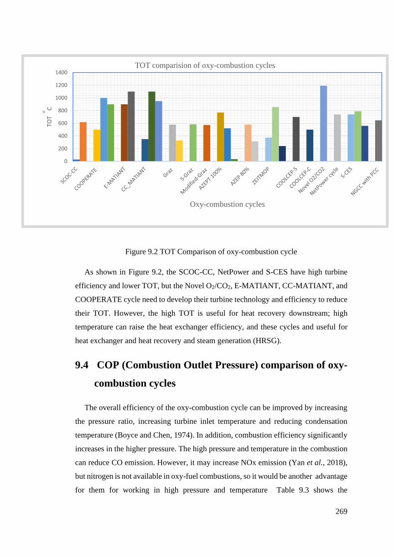
269
Figure 9.2 TOT Comparison of oxy-combustion cycle
As shown in Figure 9.2, the SCOC-CC, NetPower and S-CES have high turbine
efficiency and lower TOT, but the Novel O2/CO2, E-MATIANT, CC-MATIANT, and
COOPERATE cycle need to develop their turbine technology and efficiency to reduce
their TOT. However, the high TOT is useful for heat recovery downstream; high
temperature can raise the heat exchanger efficiency, and these cycles and useful for
heat exchanger and heat recovery and steam generation (HRSG).
9.4 COP (Combustion Outlet Pressure) comparison of oxy-
combustion cycles
The overall efficiency of the oxy-combustion cycle can be improved by increasing
the pressure ratio, increasing turbine inlet temperature and reducing condensation
temperature (Boyce and Chen, 1974). In addition, combustion efficiency significantly
increases in the higher pressure. The high pressure and temperature in the combustion
can reduce CO emission. However, it may increase NOx emission (Yan et al., 2018),
but nitrogen is not available in oxy-fuel combustions, so it would be another advantage
for them for working in high pressure and temperature Table 9.3 shows the
0
200
400
600
800
1000
1200
1400
TOT
o
C
Oxy-combustion cycles
TOT comparision of oxy-combustion cycles
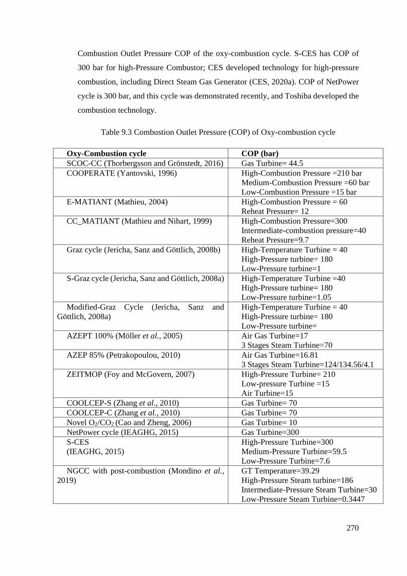
270
Combustion Outlet Pressure COP of the oxy-combustion cycle. S-CES has COP of
300 bar for high-Pressure Combustor; CES developed technology for high-pressure
combustion, including Direct Steam Gas Generator (CES, 2020a). COP of NetPower
cycle is 300 bar, and this cycle was demonstrated recently, and Toshiba developed the
combustion technology.
Table 9.3 Combustion Outlet Pressure (COP) of Oxy-combustion cycle
Oxy-Combustion cycle COP (bar)
SCOC-CC (Thorbergsson and Grönstedt, 2016) Gas Turbine= 44.5
COOPERATE (Yantovski, 1996) High-Combustion Pressure =210 bar
Medium-Combustion Pressure =60 bar
Low-Combustion Pressure =15 bar
E-MATIANT (Mathieu, 2004) High-Combustion Pressure = 60
Reheat Pressure= 12
CC_MATIANT (Mathieu and Nihart, 1999) High-Combustion Pressure=300
Intermediate-combustion pressure=40
Reheat Pressure=9.7
Graz cycle (Jericha, Sanz and Göttlich, 2008b) High-Temperature Turbine = 40
High-Pressure turbine= 180
Low-Pressure turbine=1
S-Graz cycle (Jericha, Sanz and Göttlich, 2008a) High-Temperature Turbine =40
High-Pressure turbine= 180
Low-Pressure turbine=1.05
Modified-Graz Cycle (Jericha, Sanz and
Göttlich, 2008a)
High-Temperature Turbine = 40
High-Pressure turbine= 180
Low-Pressure turbine=
AZEPT 100% (Möller et al., 2005) Air Gas Turbine=17
3 Stages Steam Turbine=70
AZEP 85% (Petrakopoulou, 2010) Air Gas Turbine=16.81
3 Stages Steam Turbine=124/134.56/4.1
ZEITMOP (Foy and McGovern, 2007) High-Pressure Turbine= 210
Low-pressure Turbine =15
Air Turbine=15
COOLCEP-S (Zhang et al., 2010) Gas Turbine= 70
COOLCEP-C (Zhang et al., 2010) Gas Turbine= 70
Novel O2/CO2 (Cao and Zheng, 2006) Gas Turbine= 10
NetPower cycle (IEAGHG, 2015) Gas Turbine=300
S-CES
(IEAGHG, 2015)
High-Pressure Turbine=300
Medium-Pressure Turbine=59.5
Low-Pressure Turbine=7.6
NGCC with post-combustion (Mondino et al.,
2019)
GT Temperature=39.29
High-Pressure Steam turbine=186
Intermediate-Pressure Steam Turbine=30
Low-Pressure Steam Turbine=0.3447
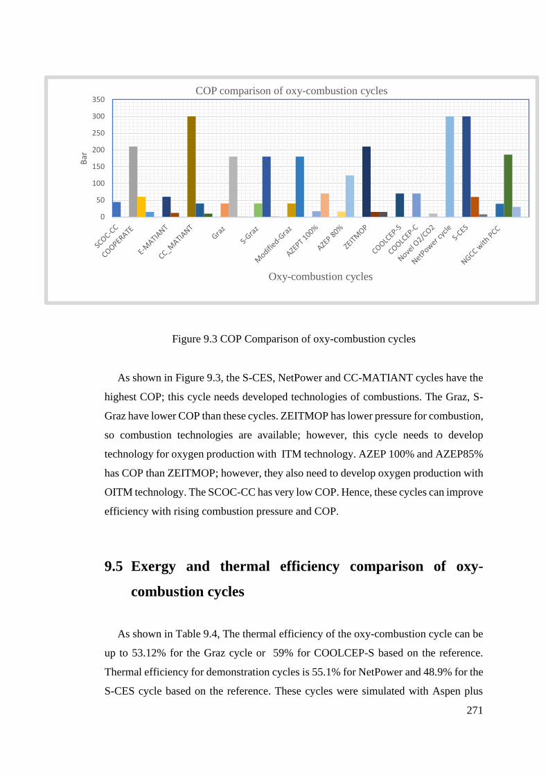
271
Figure 9.3 COP Comparison of oxy-combustion cycles
As shown in Figure 9.3, the S-CES, NetPower and CC-MATIANT cycles have the
highest COP; this cycle needs developed technologies of combustions. The Graz, S-
Graz have lower COP than these cycles. ZEITMOP has lower pressure for combustion,
so combustion technologies are available; however, this cycle needs to develop
technology for oxygen production with ITM technology. AZEP 100% and AZEP85%
has COP than ZEITMOP; however, they also need to develop oxygen production with
OITM technology. The SCOC-CC has very low COP. Hence, these cycles can improve
efficiency with rising combustion pressure and COP.
9.5 Exergy and thermal efficiency comparison of oxy-
combustion cycles
As shown in Table 9.4, The thermal efficiency of the oxy-combustion cycle can be
up to 53.12% for the Graz cycle or 59% for COOLCEP-S based on the reference.
Thermal efficiency for demonstration cycles is 55.1% for NetPower and 48.9% for the
S-CES cycle based on the reference. These cycles were simulated with Aspen plus
0
50
100
150
200
250
300
350
Bar
Oxy-combustion cycles
COP comparison of oxy-combustion cycles
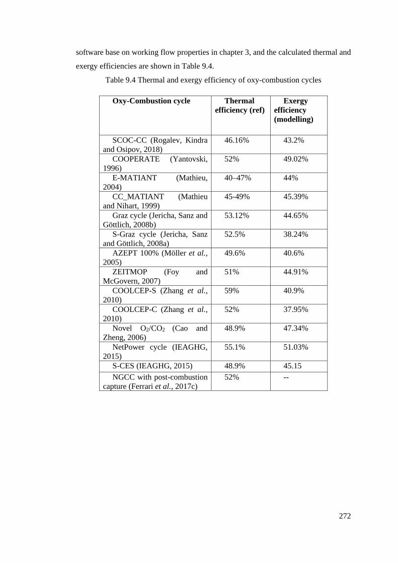
272
software base on working flow properties in chapter 3, and the calculated thermal and
exergy efficiencies are shown in Table 9.4.
Table 9.4 Thermal and exergy efficiency of oxy-combustion cycles
Oxy-Combustion cycle Thermal
efficiency (ref)
Exergy
efficiency
(modelling)
SCOC-CC (Rogalev, Kindra
and Osipov, 2018)
46.16% 43.2%
COOPERATE (Yantovski,
1996)
52% 49.02%
E-MATIANT (Mathieu,
2004)
40–47% 44%
CC_MATIANT (Mathieu
and Nihart, 1999)
45-49% 45.39%
Graz cycle (Jericha, Sanz and
Göttlich, 2008b)
53.12% 44.65%
S-Graz cycle (Jericha, Sanz
and Göttlich, 2008a)
52.5% 38.24%
AZEPT 100% (Möller et al.,
2005)
49.6% 40.6%
ZEITMOP (Foy and
McGovern, 2007)
51% 44.91%
COOLCEP-S (Zhang et al.,
2010)
59% 40.9%
COOLCEP-C (Zhang et al.,
2010)
52% 37.95%
Novel O2/CO2 (Cao and
Zheng, 2006)
48.9% 47.34%
NetPower cycle (IEAGHG,
2015)
55.1% 51.03%
S-CES (IEAGHG, 2015) 48.9% 45.15
NGCC with post-combustion
capture (Ferrari et al., 2017c)
52% --
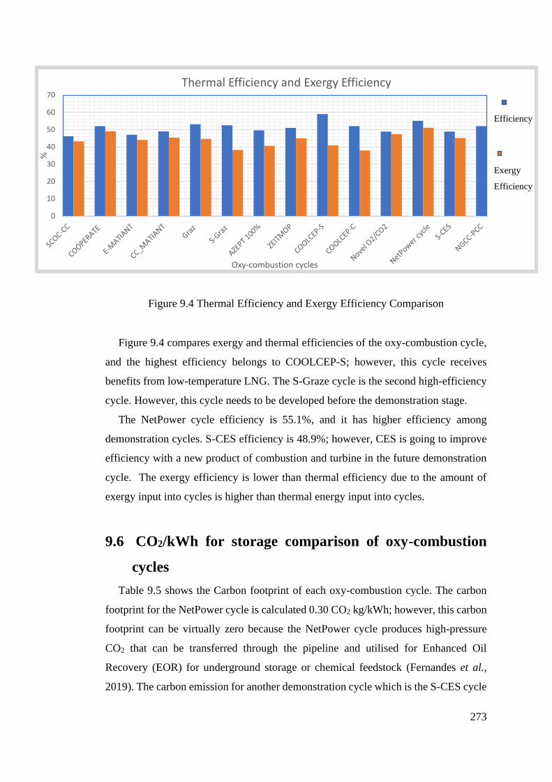
273
Figure 9.4 Thermal Efficiency and Exergy Efficiency Comparison
Figure 9.4 compares exergy and thermal efficiencies of the oxy-combustion cycle,
and the highest efficiency belongs to COOLCEP-S; however, this cycle receives
benefits from low-temperature LNG. The S-Graze cycle is the second high-efficiency
cycle. However, this cycle needs to be developed before the demonstration stage.
The NetPower cycle efficiency is 55.1%, and it has higher efficiency among
demonstration cycles. S-CES efficiency is 48.9%; however, CES is going to improve
efficiency with a new product of combustion and turbine in the future demonstration
cycle. The exergy efficiency is lower than thermal efficiency due to the amount of
exergy input into cycles is higher than thermal energy input into cycles.
9.6 CO2/kWh for storage comparison of oxy-combustion
cycles
Table 9.5 shows the Carbon footprint of each oxy-combustion cycle. The carbon
footprint for the NetPower cycle is calculated 0.30 CO2 kg/kWh; however, this carbon
footprint can be virtually zero because the NetPower cycle produces high-pressure
CO2 that can be transferred through the pipeline and utilised for Enhanced Oil
Recovery (EOR) for underground storage or chemical feedstock (Fernandes et al.,
2019). The carbon emission for another demonstration cycle which is the S-CES cycle
0
10
20
30
40
50
60
70
%
Oxy-combustion cycles
Thermal Efficiency and Exergy Efficiency
Efficiency
Exergy
Efficiency
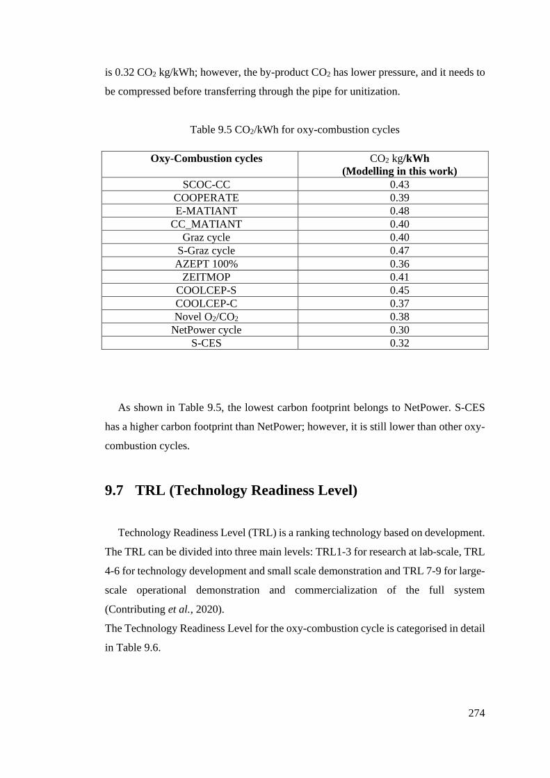
274
is 0.32 CO2 kg/kWh; however, the by-product CO2 has lower pressure, and it needs to
be compressed before transferring through the pipe for unitization.
Table 9.5 CO2/kWh for oxy-combustion cycles
Oxy-Combustion cycles CO2 kg/kWh
(Modelling in this work)
SCOC-CC 0.43
COOPERATE 0.39
E-MATIANT 0.48
CC_MATIANT 0.40
Graz cycle 0.40
S-Graz cycle 0.47
AZEPT 100% 0.36
ZEITMOP 0.41
COOLCEP-S 0.45
COOLCEP-C 0.37
Novel O2/CO2 0.38
NetPower cycle 0.30
S-CES 0.32
As shown in Table 9.5, the lowest carbon footprint belongs to NetPower. S-CES
has a higher carbon footprint than NetPower; however, it is still lower than other oxy-
combustion cycles.
9.7 TRL (Technology Readiness Level)
Technology Readiness Level (TRL) is a ranking technology based on development.
The TRL can be divided into three main levels: TRL1-3 for research at lab-scale, TRL
4-6 for technology development and small scale demonstration and TRL 7-9 for large-
scale operational demonstration and commercialization of the full system
(Contributing et al., 2020).
The Technology Readiness Level for the oxy-combustion cycle is categorised in detail
in Table 9.6.
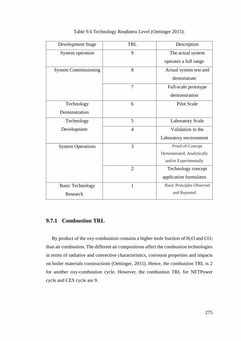
275
Table 9.6 Technology Readiness Level (Oettinger 2015):
Development Stage TRL Description
System operation 9 The actual system
operates a full range
System Commissioning 8 Actual system test and
demonstrate
7 Full-scale prototype
demonstration
Technology
Demonstration
6 Pilot Scale
Technology
Development
5 Laboratory Scale
4 Validation in the
Laboratory environment
System Operations 3 Proof-of-Concept
Demonstrated, Analytically
and/or Experimentally
2 Technology concept
application formulates
Basic Technology
Research
1 Basic Principles Observed
and Reported
9.7.1 Combustion TRL
By product of the oxy-combustion contains a higher mole fraction of H2O and CO2
than air combustion. The different air compositions affect the combustion technologies
in terms of radiative and convective characteristics, corrosion properties and impacts
on boiler materials constructions (Oettinger, 2015). Hence, the combustion TRL is 2
for another oxy-combustion cycle. However, the combustion TRL for NETPower
cycle and CES cycle are 9.
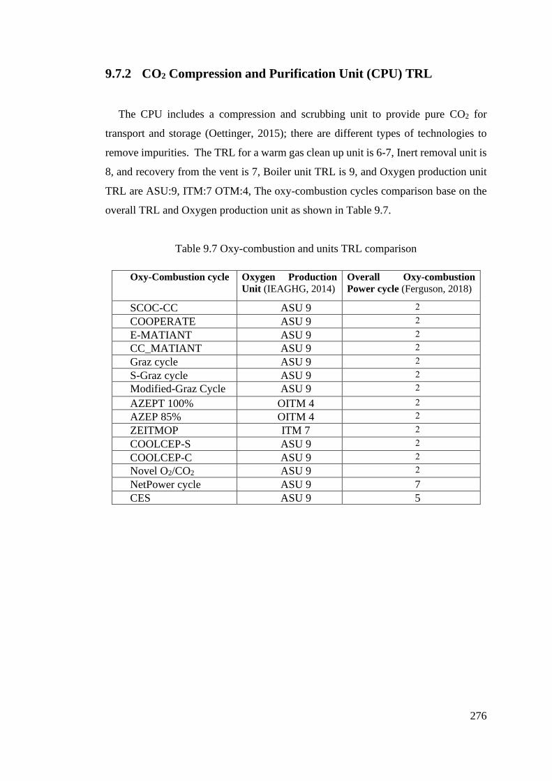
276
9.7.2 CO2 Compression and Purification Unit (CPU) TRL
The CPU includes a compression and scrubbing unit to provide pure CO2 for
transport and storage (Oettinger, 2015); there are different types of technologies to
remove impurities. The TRL for a warm gas clean up unit is 6-7, Inert removal unit is
8, and recovery from the vent is 7, Boiler unit TRL is 9, and Oxygen production unit
TRL are ASU:9, ITM:7 OTM:4, The oxy-combustion cycles comparison base on the
overall TRL and Oxygen production unit as shown in Table 9.7.
Table 9.7 Oxy-combustion and units TRL comparison
Oxy-Combustion cycle Oxygen Production
Unit (IEAGHG, 2014)
Overall Oxy-combustion
Power cycle (Ferguson, 2018)
SCOC-CC ASU 9 2
COOPERATE ASU 9 2
E-MATIANT ASU 9 2
CC_MATIANT ASU 9 2
Graz cycle ASU 9 2
S-Graz cycle ASU 9 2
Modified-Graz Cycle ASU 9 2
AZEPT 100% OITM 4 2
AZEP 85% OITM 4 2
ZEITMOP ITM 7 2
COOLCEP-S ASU 9 2
COOLCEP-C ASU 9 2
Novel O2/CO2 ASU 9 2
NetPower cycle ASU 9 7
CES ASU 9 5
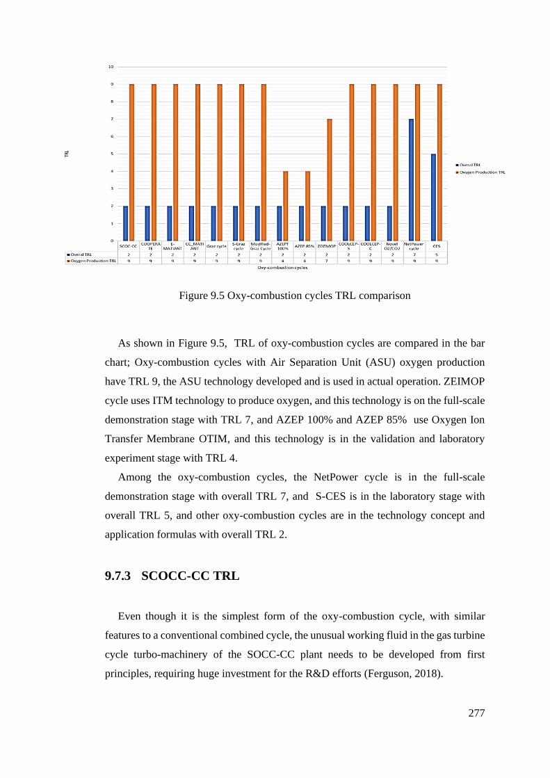
277
Figure 9.5 Oxy-combustion cycles TRL comparison
As shown in Figure 9.5, TRL of oxy-combustion cycles are compared in the bar
chart; Oxy-combustion cycles with Air Separation Unit (ASU) oxygen production
have TRL 9, the ASU technology developed and is used in actual operation. ZEIMOP
cycle uses ITM technology to produce oxygen, and this technology is on the full-scale
demonstration stage with TRL 7, and AZEP 100% and AZEP 85% use Oxygen Ion
Transfer Membrane OTIM, and this technology is in the validation and laboratory
experiment stage with TRL 4.
Among the oxy-combustion cycles, the NetPower cycle is in the full-scale
demonstration stage with overall TRL 7, and S-CES is in the laboratory stage with
overall TRL 5, and other oxy-combustion cycles are in the technology concept and
application formulas with overall TRL 2.
9.7.3 SCOCC-CC TRL
Even though it is the simplest form of the oxy-combustion cycle, with similar
features to a conventional combined cycle, the unusual working fluid in the gas turbine
cycle turbo-machinery of the SOCC-CC plant needs to be developed from first
principles, requiring huge investment for the R&D efforts (Ferguson, 2018).
278
9.7.4 Graze cycle TRL
The Graz cycle has been studied by various institutes and has been modified to
improve efficiency. The predicted net efficiency has been reported as 48.6%. Particular
attention has been given to the development of the turbo-machinery, especially the
high-temperature turbine, which requires a completely new design. Another important
issue is related to the use of an H2O-rich stream being used for turbine blade cooling.
Overall, the cycle is still immature and needs to be developed further (Ferguson, 2018).
9.7.5 CES TRL
The above announcement on the CES website indicates that it is are undertaking a
feasibility study into using biomass-derived syngas in its own oxy-fuel Gas
Generator followed by its gas cycle to produce carbon-negative power and that it
plans to deploy a small scale commercial demonstration “BioCCS” plant at the
Kimberlina Facility.
9.7.6 NetPower TRL
Considering that a 50 MWth demonstration plant is undergoing commissioning at
this time, Wood judges the TRL level of the Net Power system to be TRL-7.
NetPower successfully achieved the first supercritical carbon dioxide power plant with
carbon capture in La Porte, TX and test facilities including 50MWth Toshiba Energy
Systems & Solutions Corporation (Toshiba) and combustor. The combustor is
integrated with the turbine, and power is generated, NetPower has planed the global
development 300MWe, and this power plant will be commercially deployed in 2022
(TMI Staff & Contributors, 2018).
279
9.8 Performance analysis
The performance comparison of oxy-combustion cycles is made in Table 9.8, the
oxy-combustion cycle was modelled in the chapter by modelling the oxy-combustion
cycles in chapter 3. The results are used for a performance comparison of oxy-
combustion cycles.
Table 9.8 shows performance analysis of oxy-combustion cycles for each
equipment, fuel consumption, maintenance cost and purchasing cost. The performance
analysis of oxy-combustion cycles indicates the energy consumption for each
component and the relationship between the performance and each component of oxy-
combustion cycles. The table also shows the efficiency of each oxy-combustion cycle
with Air Separation Unit (ASU) and CO2 compression and Purification Unit (CPU)
and without them. The comparison indicates an efficiency penalty due to ASU and
CPU.
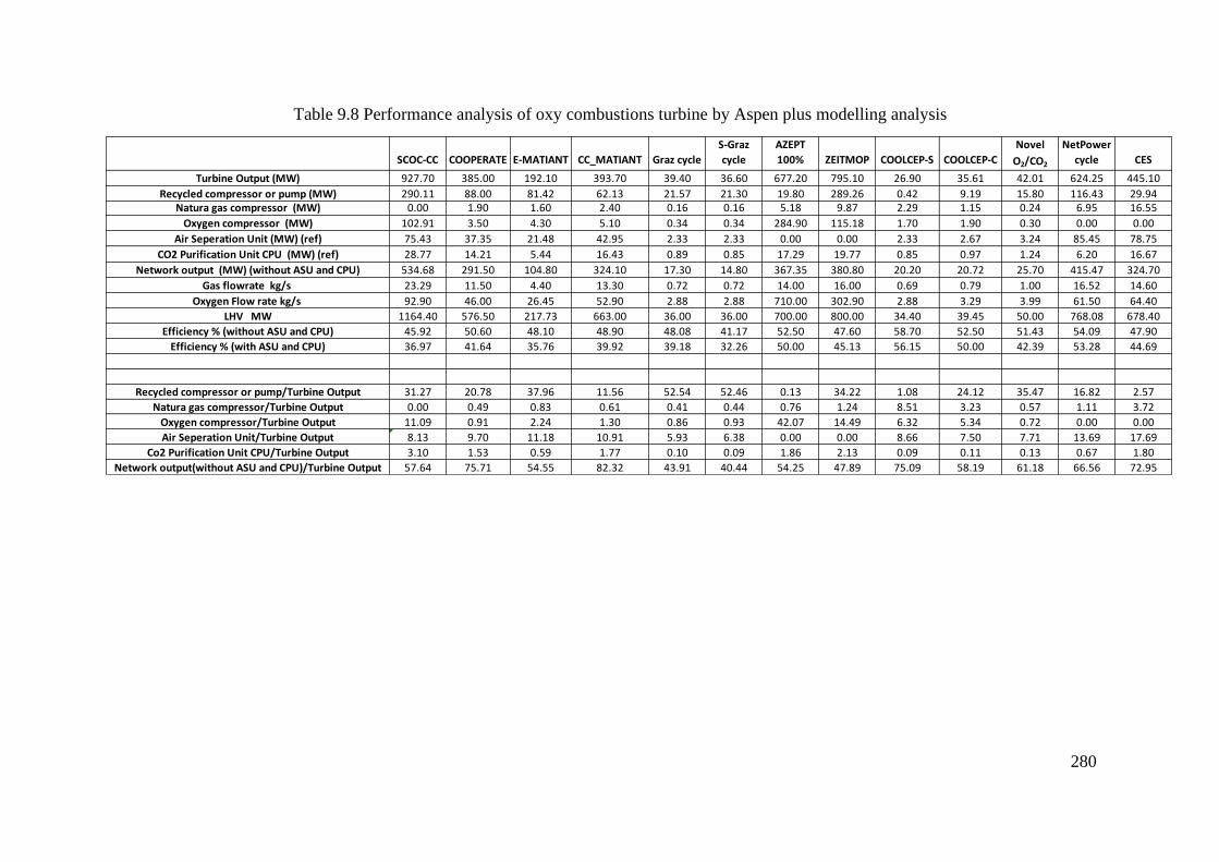
280
Table 9.8 Performance analysis of oxy combustions turbine by Aspen plus modelling analysis
SCOC-CC COOPERATE E-MATIANT CC_MATIANT Graz cycle
S-Graz
cycle
AZEPT
100% ZEITMOP COOLCEP-S COOLCEP-C
Novel
O2/CO2
NetPower
cycle CES
Turbine Output (MW) 927.70 385.00 192.10 393.70 39.40 36.60 677.20 795.10 26.90 35.61 42.01 624.25 445.10
Recycled compressor or pump (MW) 290.11 88.00 81.42 62.13 21.57 21.30 19.80 289.26 0.42 9.19 15.80 116.43 29.94Natura gas compressor (MW) 0.00 1.90 1.60 2.40 0.16 0.16 5.18 9.87 2.29 1.15 0.24 6.95 16.55
Oxygen compressor (MW) 102.91 3.50 4.30 5.10 0.34 0.34 284.90 115.18 1.70 1.90 0.30 0.00 0.00
Air Seperation Unit (MW) (ref) 75.43 37.35 21.48 42.95 2.33 2.33 0.00 0.00 2.33 2.67 3.24 85.45 78.75
CO2 Purification Unit CPU (MW) (ref) 28.77 14.21 5.44 16.43 0.89 0.85 17.29 19.77 0.85 0.97 1.24 6.20 16.67
Network output (MW) (without ASU and CPU) 534.68 291.50 104.80 324.10 17.30 14.80 367.35 380.80 20.20 20.72 25.70 415.47 324.70
Gas flowrate kg/s 23.29 11.50 4.40 13.30 0.72 0.72 14.00 16.00 0.69 0.79 1.00 16.52 14.60
Oxygen Flow rate kg/s 92.90 46.00 26.45 52.90 2.88 2.88 710.00 302.90 2.88 3.29 3.99 61.50 64.40
LHV MW 1164.40 576.50 217.73 663.00 36.00 36.00 700.00 800.00 34.40 39.45 50.00 768.08 678.40
Efficiency % (without ASU and CPU) 45.92 50.60 48.10 48.90 48.08 41.17 52.50 47.60 58.70 52.50 51.43 54.09 47.90
Efficiency % (with ASU and CPU) 36.97 41.64 35.76 39.92 39.18 32.26 50.00 45.13 56.15 50.00 42.39 53.28 44.69
Recycled compressor or pump/Turbine Output 31.27 20.78 37.96 11.56 52.54 52.46 0.13 34.22 1.08 24.12 35.47 16.82 2.57
Natura gas compressor/Turbine Output 0.00 0.49 0.83 0.61 0.41 0.44 0.76 1.24 8.51 3.23 0.57 1.11 3.72
Oxygen compressor/Turbine Output 11.09 0.91 2.24 1.30 0.86 0.93 42.07 14.49 6.32 5.34 0.72 0.00 0.00
Air Seperation Unit/Turbine Output 8.13 9.70 11.18 10.91 5.93 6.38 0.00 0.00 8.66 7.50 7.71 13.69 17.69
Co2 Purification Unit CPU/Turbine Output 3.10 1.53 0.59 1.77 0.10 0.09 1.86 2.13 0.09 0.11 0.13 0.67 1.80
Network output(without ASU and CPU)/Turbine Output 57.64 75.71 54.55 82.32 43.91 40.44 54.25 47.89 75.09 58.19 61.18 66.56 72.95
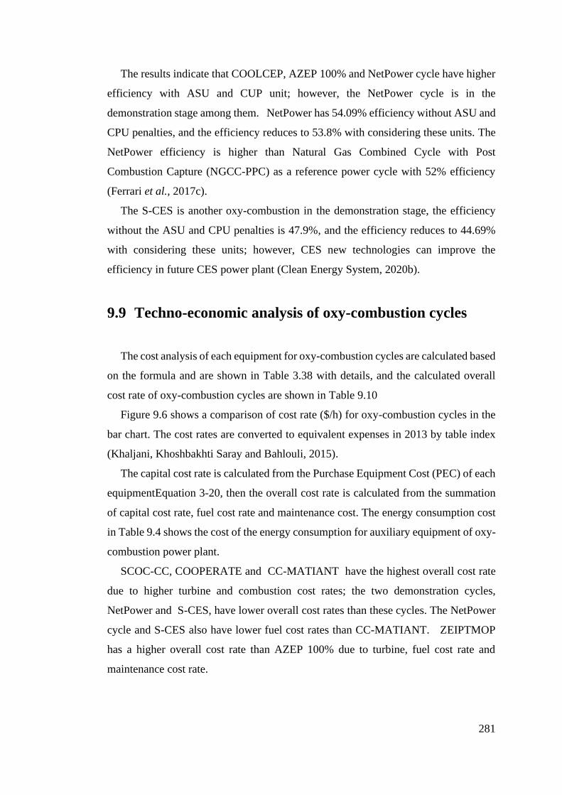
281
The results indicate that COOLCEP, AZEP 100% and NetPower cycle have higher
efficiency with ASU and CUP unit; however, the NetPower cycle is in the
demonstration stage among them. NetPower has 54.09% efficiency without ASU and
CPU penalties, and the efficiency reduces to 53.8% with considering these units. The
NetPower efficiency is higher than Natural Gas Combined Cycle with Post
Combustion Capture (NGCC-PPC) as a reference power cycle with 52% efficiency
(Ferrari et al., 2017c).
The S-CES is another oxy-combustion in the demonstration stage, the efficiency
without the ASU and CPU penalties is 47.9%, and the efficiency reduces to 44.69%
with considering these units; however, CES new technologies can improve the
efficiency in future CES power plant (Clean Energy System, 2020b).
9.9 Techno-economic analysis of oxy-combustion cycles
The cost analysis of each equipment for oxy-combustion cycles are calculated based
on the formula and are shown in Table 3.38 with details, and the calculated overall
cost rate of oxy-combustion cycles are shown in Table 9.10
Figure 9.6 shows a comparison of cost rate ($/h) for oxy-combustion cycles in the
bar chart. The cost rates are converted to equivalent expenses in 2013 by table index
(Khaljani, Khoshbakhti Saray and Bahlouli, 2015).
The capital cost rate is calculated from the Purchase Equipment Cost (PEC) of each
equipmentEquation 3-20, then the overall cost rate is calculated from the summation
of capital cost rate, fuel cost rate and maintenance cost. The energy consumption cost
in Table 9.4 shows the cost of the energy consumption for auxiliary equipment of oxy-
combustion power plant.
SCOC-CC, COOPERATE and CC-MATIANT have the highest overall cost rate
due to higher turbine and combustion cost rates; the two demonstration cycles,
NetPower and S-CES, have lower overall cost rates than these cycles. The NetPower
cycle and S-CES also have lower fuel cost rates than CC-MATIANT. ZEIPTMOP
has a higher overall cost rate than AZEP 100% due to turbine, fuel cost rate and
maintenance cost rate.
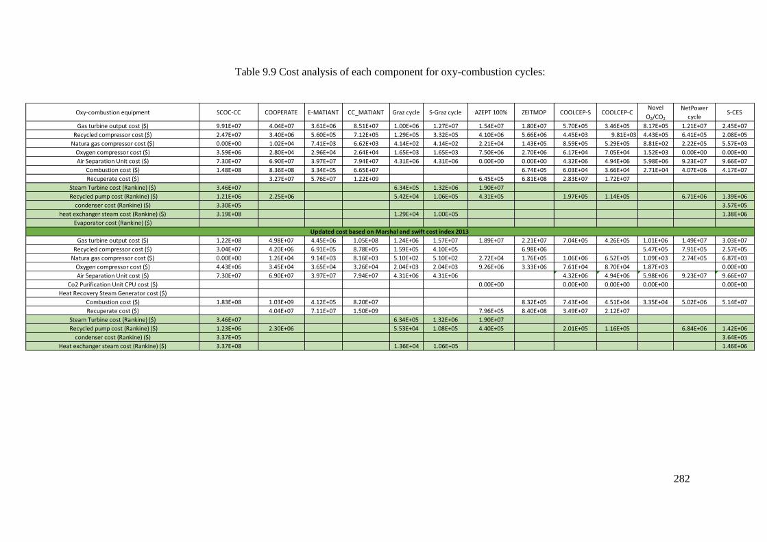
282
Table 9.9 Cost analysis of each component for oxy-combustion cycles:
Oxy-combustion equipment SCOC-CC COOPERATE E-MATIANT CC_MATIANT Graz cycle S-Graz cycle AZEPT 100% ZEITMOP COOLCEP-S COOLCEP-CNovel
O2/CO2
NetPower
cycle S-CES
Gas turbine output cost ($) 9.91E+07 4.04E+07 3.61E+06 8.51E+07 1.00E+06 1.27E+07 1.54E+07 1.80E+07 5.70E+05 3.46E+05 8.17E+05 1.21E+07 2.45E+07
Recycled compressor cost ($) 2.47E+07 3.40E+06 5.60E+05 7.12E+05 1.29E+05 3.32E+05 4.10E+06 5.66E+06 4.45E+03 9.81E+03 4.43E+05 6.41E+05 2.08E+05
Natura gas compressor cost ($) 0.00E+00 1.02E+04 7.41E+03 6.62E+03 4.14E+02 4.14E+02 2.21E+04 1.43E+05 8.59E+05 5.29E+05 8.81E+02 2.22E+05 5.57E+03
Oxygen compressor cost ($) 3.59E+06 2.80E+04 2.96E+04 2.64E+04 1.65E+03 1.65E+03 7.50E+06 2.70E+06 6.17E+04 7.05E+04 1.52E+03 0.00E+00 0.00E+00
Air Separation Unit cost ($) 7.30E+07 6.90E+07 3.97E+07 7.94E+07 4.31E+06 4.31E+06 0.00E+00 0.00E+00 4.32E+06 4.94E+06 5.98E+06 9.23E+07 9.66E+07
Combustion cost ($) 1.48E+08 8.36E+08 3.34E+05 6.65E+07 6.74E+05 6.03E+04 3.66E+04 2.71E+04 4.07E+06 4.17E+07
Recuperate cost ($) 3.27E+07 5.76E+07 1.22E+09 6.45E+05 6.81E+08 2.83E+07 1.72E+07
Steam Turbine cost (Rankine) ($) 3.46E+07 6.34E+05 1.32E+06 1.90E+07
Recycled pump cost (Rankine) ($) 1.21E+06 2.25E+06 5.42E+04 1.06E+05 4.31E+05 1.97E+05 1.14E+05 6.71E+06 1.39E+06
condenser cost (Rankine) ($) 3.30E+05 3.57E+05
heat exchanger steam cost (Rankine) ($) 3.19E+08 1.29E+04 1.00E+05 1.38E+06
Evaporator cost (Rankine) ($)
Gas turbine output cost ($) 1.22E+08 4.98E+07 4.45E+06 1.05E+08 1.24E+06 1.57E+07 1.89E+07 2.21E+07 7.04E+05 4.26E+05 1.01E+06 1.49E+07 3.03E+07
Recycled compressor cost ($) 3.04E+07 4.20E+06 6.91E+05 8.78E+05 1.59E+05 4.10E+05 6.98E+06 5.47E+05 7.91E+05 2.57E+05
Natura gas compressor cost ($) 0.00E+00 1.26E+04 9.14E+03 8.16E+03 5.10E+02 5.10E+02 2.72E+04 1.76E+05 1.06E+06 6.52E+05 1.09E+03 2.74E+05 6.87E+03
Oxygen compressor cost ($) 4.43E+06 3.45E+04 3.65E+04 3.26E+04 2.04E+03 2.04E+03 9.26E+06 3.33E+06 7.61E+04 8.70E+04 1.87E+03 0.00E+00
Air Separation Unit cost ($) 7.30E+07 6.90E+07 3.97E+07 7.94E+07 4.31E+06 4.31E+06 4.32E+06 4.94E+06 5.98E+06 9.23E+07 9.66E+07
Co2 Purification Unit CPU cost ($) 0.00E+00 0.00E+00 0.00E+00 0.00E+00 0.00E+00
Heat Recovery Steam Generator cost ($)
Combustion cost ($) 1.83E+08 1.03E+09 4.12E+05 8.20E+07 8.32E+05 7.43E+04 4.51E+04 3.35E+04 5.02E+06 5.14E+07
Recuperate cost ($) 4.04E+07 7.11E+07 1.50E+09 7.96E+05 8.40E+08 3.49E+07 2.12E+07
Steam Turbine cost (Rankine) ($) 3.46E+07 6.34E+05 1.32E+06 1.90E+07
Recycled pump cost (Rankine) ($) 1.23E+06 2.30E+06 5.53E+04 1.08E+05 4.40E+05 2.01E+05 1.16E+05 6.84E+06 1.42E+06
condenser cost (Rankine) ($) 3.37E+05 3.64E+05
Heat exchanger steam cost (Rankine) ($) 3.37E+08 1.36E+04 1.06E+05 1.46E+06
Updated cost based on Marshal and swift cost index 2013
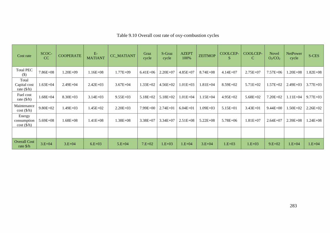
283
Table 9.10 Overall cost rate of oxy-combustion cycles
Cost rate SCOC-
CC COOPERATE
E-
MATIANT CC_MATIANT
Graz
cycle
S-Graz
cycle
AZEPT
100% ZEITMOP
COOLCEP-
S
COOLCEP-
C
Novel
O2/CO2
NetPower
cycle S-CES
Total PEC
($) 7.86E+08 1.20E+09 1.16E+08 1.77E+09 6.41E+06 2.20E+07 4.85E+07 8.74E+08 4.14E+07 2.75E+07 7.57E+06 1.20E+08 1.82E+08
Total
Capital cost
rate ($/h)
1.63E+04 2.49E+04 2.42E+03 3.67E+04 1.33E+02 4.56E+02 1.01E+03 1.81E+04 8.59E+02 5.71E+02 1.57E+02 2.49E+03 3.77E+03
Fuel cost
rate ($/h) 1.68E+04 8.30E+03 3.14E+03 9.55E+03 5.18E+02 5.18E+02 1.01E+04 1.15E+04 4.95E+02 5.68E+02 7.20E+02 1.11E+04 9.77E+03
Maintenance
cost ($/h) 9.80E+02 1.49E+03 1.45E+02 2.20E+03 7.99E+00 2.74E+01 6.04E+01 1.09E+03 5.15E+01 3.43E+01 9.44E+00 1.50E+02 2.26E+02
Energy
consumption
cost ($/h)
5.69E+08 1.68E+08 1.41E+08 1.38E+08 3.38E+07 3.34E+07 2.51E+08 5.22E+08 5.78E+06 1.81E+07 2.64E+07 2.39E+08 1.24E+08
Overall Cost
rate $/h 3.E+04 3.E+04 6.E+03 5.E+04 7.E+02 1.E+03 1.E+04 3.E+04 1.E+03 1.E+03 9.E+02 1.E+04 1.E+04
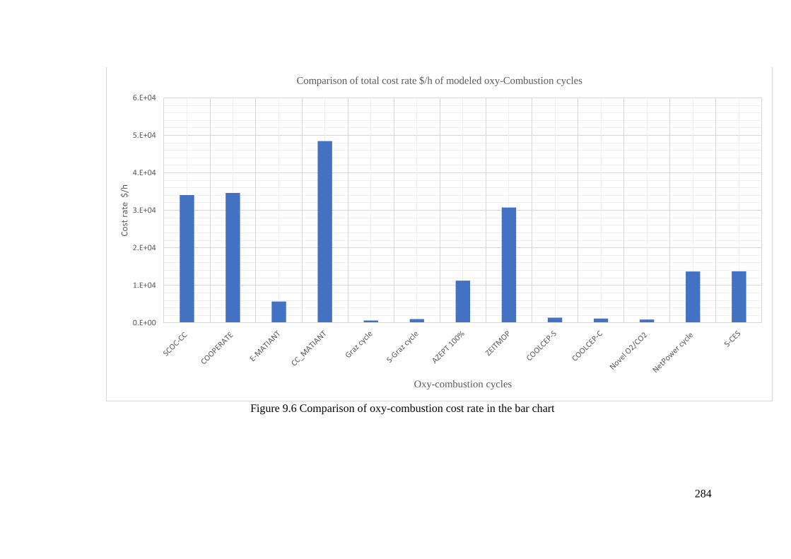
284
Figure 9.6 Comparison of oxy-combustion cost rate in the bar chart
0.E+00
1.E+04
2.E+04
3.E+04
4.E+04
5.E+04
6.E+04
Co
st r
ate
$/h
Oxy-combustion cycles
Comparison of total cost rate $/h of modeled oxy-Combustion cycles
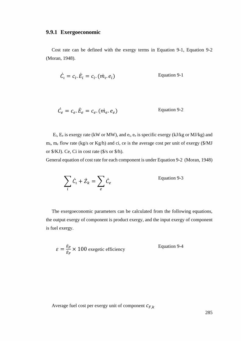
285
9.9.1 Exergoeconomic
Cost rate can be defined with the exergy terms in Equation 9-1, Equation 9-2
(Moran, 1948).
𝐶�� = 𝑐𝑖 . ��𝑖 = 𝑐𝑖 . (𝑚𝑖 . 𝑒𝑖) Equation 9-1
𝐶�� = 𝑐𝑒 . ��𝑒 = 𝑐𝑒 . (𝑚𝑒 . 𝑒𝑒) Equation 9-2
Ei, Ee is exergy rate (kW or MW), and ei, ee is specific exergy (kJ/kg or MJ/kg) and
mi, me flow rate (kg/s or Kg/h) and ci, ce is the average cost per unit of exergy ($/MJ
or $/KJ). Ce, Ci in cost rate ($/s or $/h).
General equation of cost rate for each component is under Equation 9-2 (Moran, 1948)
∑ 𝐶��
𝑖
+ ��𝑘 = ∑ ��𝑒
𝑒
Equation 9-3
The exergoeconomic parameters can be calculated from the following equations,
the output exergy of component is product exergy, and the input exergy of component
is fuel exergy.
𝜀 =��𝑃
��𝐹× 100 exegetic efficiency
Equation 9-4
Average fuel cost per exergy unit of component 𝑐𝐹,𝑘
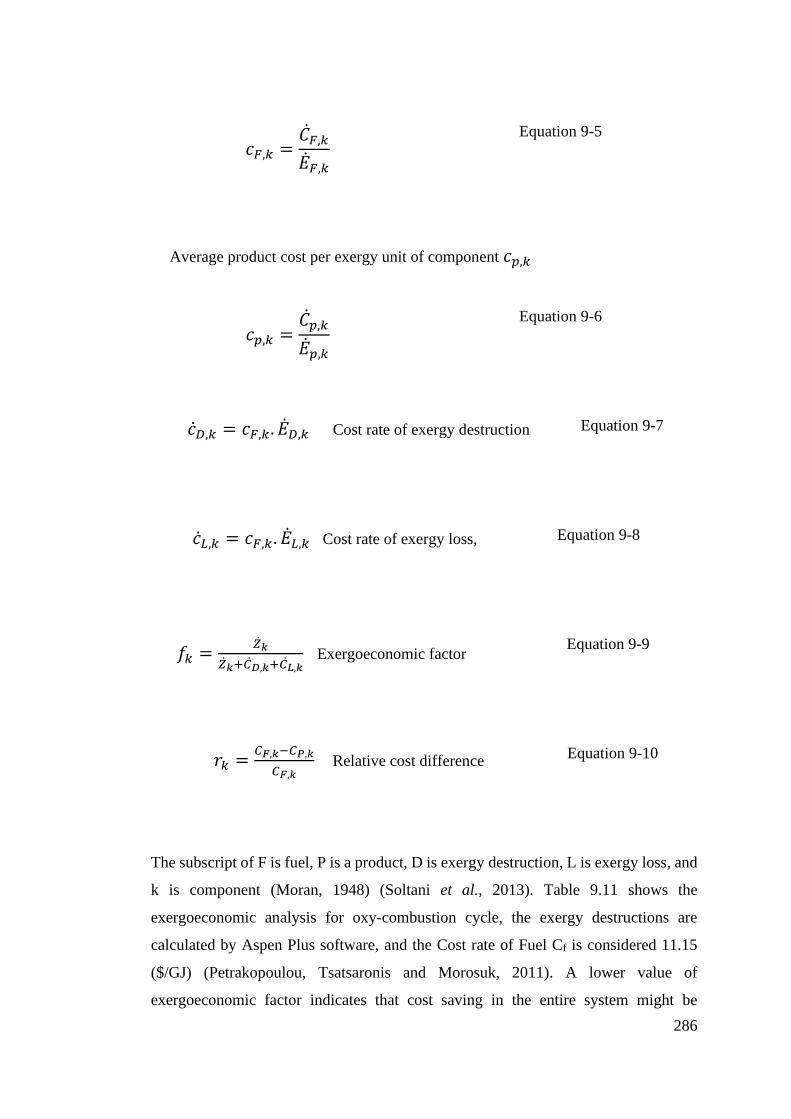
286
𝑐𝐹,𝑘 =��𝐹,𝑘
��𝐹,𝑘
Equation 9-5
Average product cost per exergy unit of component 𝑐𝑝,𝑘
𝑐𝑝,𝑘 =��𝑝,𝑘
��𝑝,𝑘
Equation 9-6
��𝐷,𝑘 = 𝑐𝐹,𝑘. ��𝐷,𝑘 Cost rate of exergy destruction Equation 9-7
��𝐿,𝑘 = 𝑐𝐹,𝑘. ��𝐿,𝑘 Cost rate of exergy loss, Equation 9-8
𝑓𝑘 =��𝑘
��𝑘+��𝐷,𝑘+��𝐿,𝑘 Exergoeconomic factor
Equation 9-9
𝑟𝑘 =𝐶𝐹,𝑘−𝐶𝑃,𝑘
𝐶𝐹,𝑘 Relative cost difference
Equation 9-10
The subscript of F is fuel, P is a product, D is exergy destruction, L is exergy loss, and
k is component (Moran, 1948) (Soltani et al., 2013). Table 9.11 shows the
exergoeconomic analysis for oxy-combustion cycle, the exergy destructions are
calculated by Aspen Plus software, and the Cost rate of Fuel Cf is considered 11.15
($/GJ) (Petrakopoulou, Tsatsaronis and Morosuk, 2011). A lower value of
exergoeconomic factor indicates that cost saving in the entire system might be
287
achieved by reducing exergy destruction in components and improving component
efficiency, even by increasing capital investment, on another side, when the value of
exergoeconomic factor is high the investment cost can be decreased with the expense
of increasing exergy destruction in the component (Moran, 1948).
Figure 9.7 compares the exergoeconomic factor for different oxy-combustion cycles;
the highest exergoeconomic factors belong to COOPERATE cycle with f = 72.4% and
CC-MATIANT with f = 75.5%, hence these cycles are not required more capital
investment to reduce exergy destruction in component, and the investment cannot have
more benefit for the cycle efficiency.
The exergoeconomic factors of NetPower are f=46.1%, and S-CES is f= 46.5%; hence,
these cycles have a capacity for additional capital investment to reduce exergy
destruction in components and increase the overall efficiency.
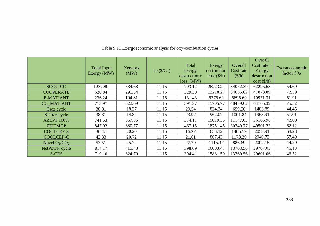
288
Table 9.11 Exergoeconomic analysis for oxy-combustion cycles
Total Input
Exergy (MW)
Network
(MW) Cf ($/GJ)
Total
exergy
destruction+
loss (MW)
Exergy
destruction
cost ($/h)
Overall
Cost rate
($/h)
Overall
Cost rate +
Exergy
destruction
cost ($/h)
Exergoeconomic
factor f %
SCOC-CC 1237.80 534.68 11.15 703.12 28223.24 34072.39 62295.63 54.69
COOPERATE 620.84 291.54 11.15 329.30 13218.27 34655.62 47873.89 72.39
E-MATIANT 236.24 104.81 11.15 131.43 5275.62 5695.69 10971.31 51.91
CC_MATIANT 713.97 322.69 11.15 391.27 15705.77 48459.62 64165.39 75.52
Graz cycle 38.81 18.27 11.15 20.54 824.34 659.56 1483.89 44.45
S-Graz cycle 38.81 14.84 11.15 23.97 962.07 1001.84 1963.91 51.01
AZEPT 100% 741.53 367.35 11.15 374.17 15019.35 11147.63 26166.98 42.60
ZEITMOP 847.92 380.77 11.15 467.15 18751.45 30749.77 49501.22 62.12
COOLCEP-S 36.47 20.20 11.15 16.27 653.12 1405.79 2058.91 68.28
COOLCEP-C 42.33 20.72 11.15 21.61 867.43 1173.29 2040.72 57.49
Novel O2/CO2 53.51 25.72 11.15 27.79 1115.47 886.69 2002.15 44.29
NetPower cycle 814.17 415.48 11.15 398.69 16003.47 13703.56 29707.03 46.13
S-CES 719.10 324.70 11.15 394.41 15831.50 13769.56 29601.06 46.52
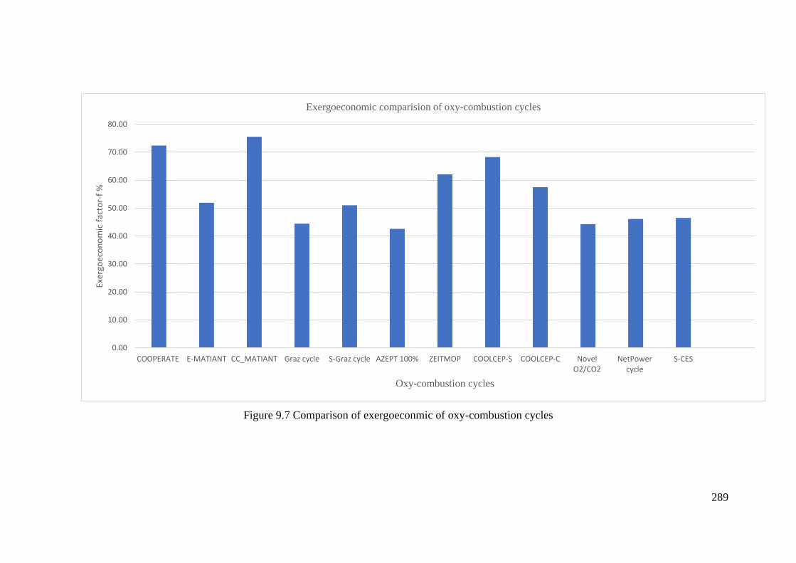
289
Figure 9.7 Comparison of exergoeconmic of oxy-combustion cycles
0.00
10.00
20.00
30.00
40.00
50.00
60.00
70.00
80.00
COOPERATE E-MATIANT CC_MATIANT Graz cycle S-Graz cycle AZEPT 100% ZEITMOP COOLCEP-S COOLCEP-C NovelO2/CO2
NetPowercycle
S-CES
Exer
goec
on
om
ic f
acto
r-f
%
Oxy-combustion cycles
Exergoeconomic comparision of oxy-combustion cycles
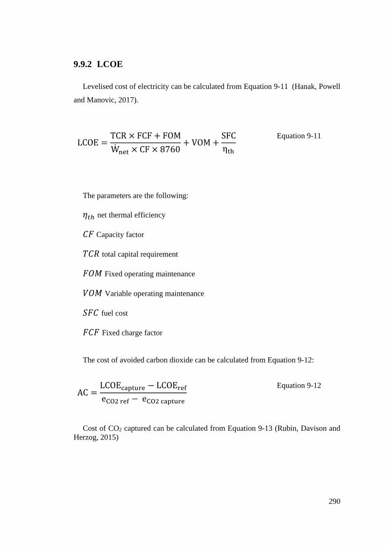
290
9.9.2 LCOE
Levelised cost of electricity can be calculated from Equation 9-11 (Hanak, Powell
and Manovic, 2017).
LCOE =TCR × FCF + FOM
Wnet × CF × 8760+ VOM +
SFC
ηth
Equation 9-11
The parameters are the following:
𝜂𝑡ℎ net thermal efficiency
𝐶𝐹 Capacity factor
𝑇𝐶𝑅 total capital requirement
𝐹𝑂𝑀 Fixed operating maintenance
𝑉𝑂𝑀 Variable operating maintenance
𝑆𝐹𝐶 fuel cost
𝐹𝐶𝐹 Fixed charge factor
The cost of avoided carbon dioxide can be calculated from Equation 9-12:
AC =LCOEcapture − LCOEref
eCO2 ref − eCO2 capture
Equation 9-12
Cost of CO2 captured can be calculated from Equation 9-13 (Rubin, Davison and
Herzog, 2015)
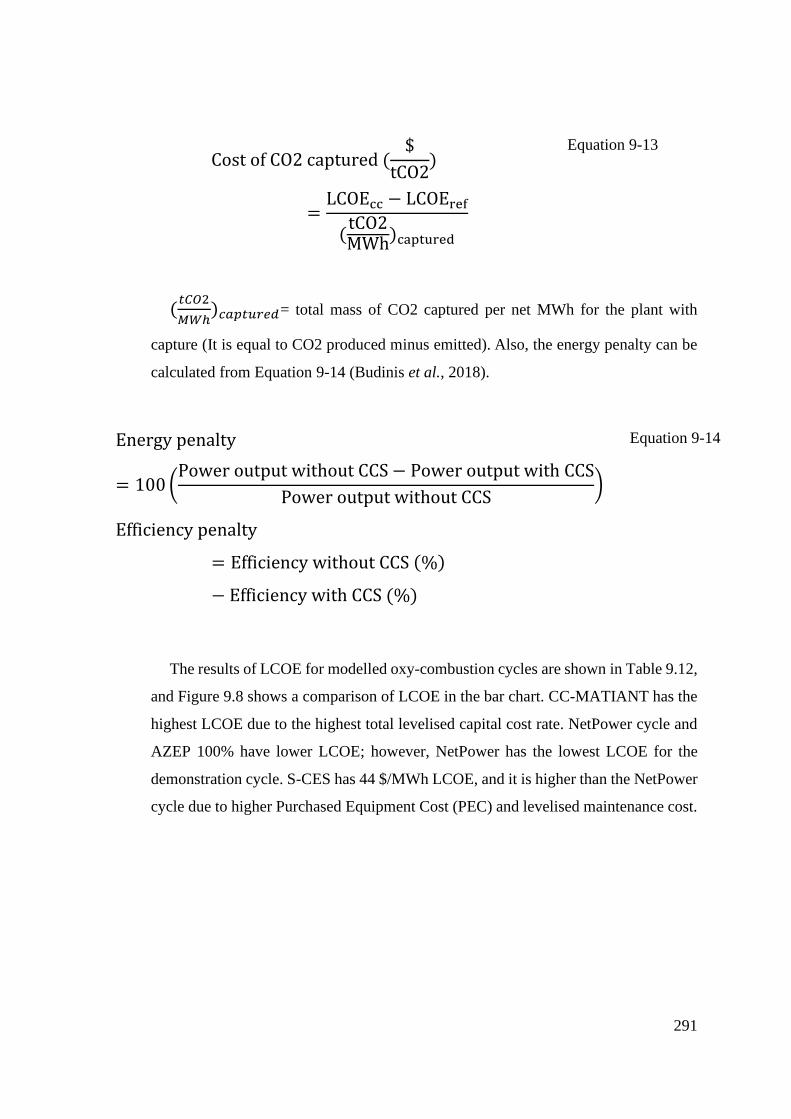
291
Cost of CO2 captured ($
tCO2)
=LCOEcc − LCOEref
(tCO2MWh
)captured
Equation 9-13
(𝑡𝐶𝑂2
𝑀𝑊ℎ)𝑐𝑎𝑝𝑡𝑢𝑟𝑒𝑑= total mass of CO2 captured per net MWh for the plant with
capture (It is equal to CO2 produced minus emitted). Also, the energy penalty can be
calculated from Equation 9-14 (Budinis et al., 2018).
Energy penalty
= 100 (Power output without CCS − Power output with CCS
Power output without CCS)
Efficiency penalty
= Efficiency without CCS (%)
− Efficiency with CCS (%)
Equation 9-14
The results of LCOE for modelled oxy-combustion cycles are shown in Table 9.12,
and Figure 9.8 shows a comparison of LCOE in the bar chart. CC-MATIANT has the
highest LCOE due to the highest total levelised capital cost rate. NetPower cycle and
AZEP 100% have lower LCOE; however, NetPower has the lowest LCOE for the
demonstration cycle. S-CES has 44 $/MWh LCOE, and it is higher than the NetPower
cycle due to higher Purchased Equipment Cost (PEC) and levelised maintenance cost.
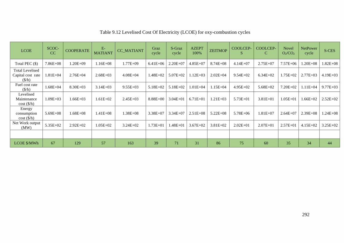
292
Table 9.12 Levelised Cost Of Electricity (LCOE) for oxy-combustion cycles
LCOE SCOC-
CC COOPERATE
E-
MATIANT CC_MATIANT
Graz
cycle
S-Graz
cycle
AZEPT
100% ZEITMOP
COOLCEP-
S
COOLCEP-
C
Novel
O2/CO2
NetPower
cycle S-CES
Total PEC ($) 7.86E+08 1.20E+09 1.16E+08 1.77E+09 6.41E+06 2.20E+07 4.85E+07 8.74E+08 4.14E+07 2.75E+07 7.57E+06 1.20E+08 1.82E+08
Total Levelised
Capital cost rate
($/h)
1.81E+04 2.76E+04 2.68E+03 4.08E+04 1.48E+02 5.07E+02 1.12E+03 2.02E+04 9.54E+02 6.34E+02 1.75E+02 2.77E+03 4.19E+03
Fuel cost rate
($/h) 1.68E+04 8.30E+03 3.14E+03 9.55E+03 5.18E+02 5.18E+02 1.01E+04 1.15E+04 4.95E+02 5.68E+02 7.20E+02 1.11E+04 9.77E+03
Levelised
Maintenance
cost ($/h)
1.09E+03 1.66E+03 1.61E+02 2.45E+03 8.88E+00 3.04E+01 6.71E+01 1.21E+03 5.73E+01 3.81E+01 1.05E+01 1.66E+02 2.52E+02
Energy
consumption
cost ($/h)
5.69E+08 1.68E+08 1.41E+08 1.38E+08 3.38E+07 3.34E+07 2.51E+08 5.22E+08 5.78E+06 1.81E+07 2.64E+07 2.39E+08 1.24E+08
Net Work output
(MW) 5.35E+02 2.92E+02 1.05E+02 3.24E+02 1.73E+01 1.48E+01 3.67E+02 3.81E+02 2.02E+01 2.07E+01 2.57E+01 4.15E+02 3.25E+02
LCOE $/MWh 67 129 57 163 39 71 31 86 75 60 35 34 44
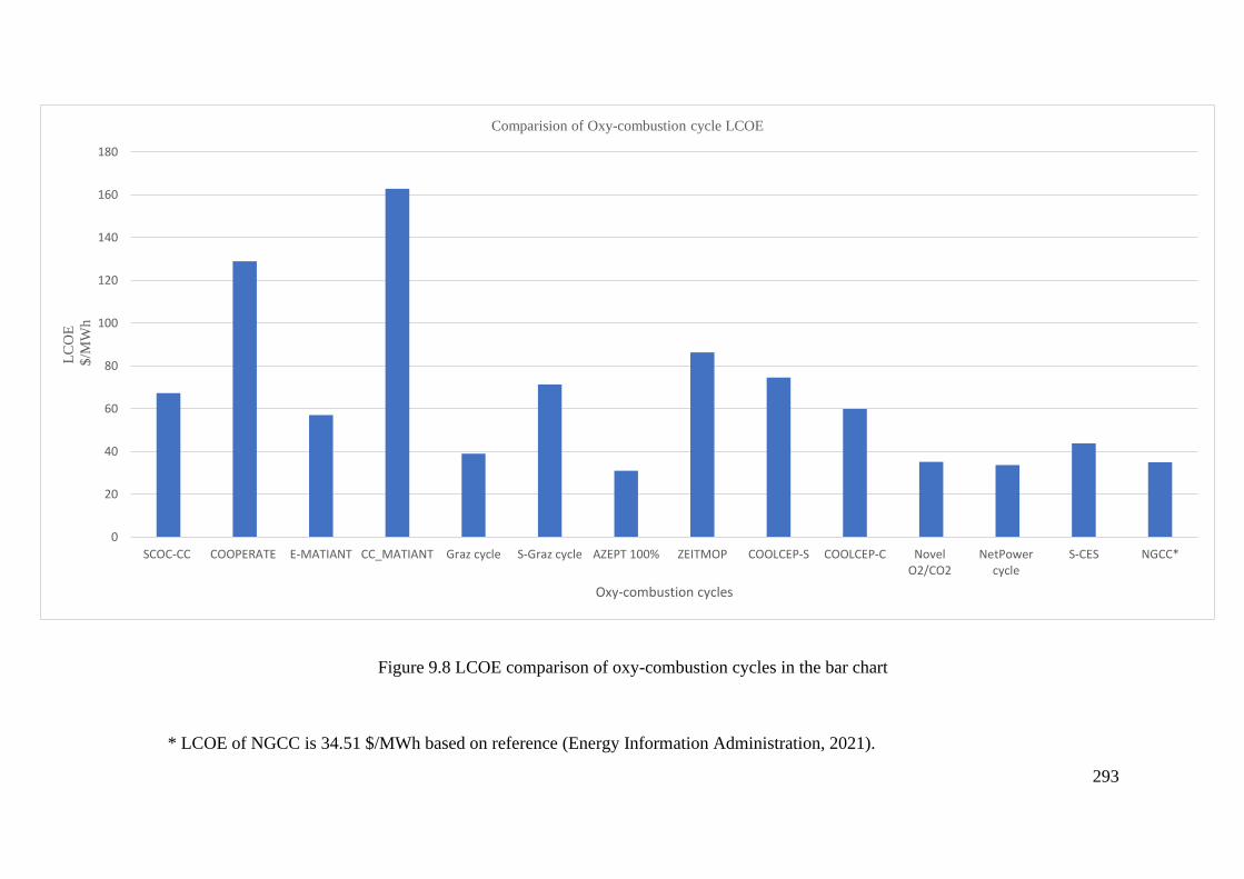
293
Figure 9.8 LCOE comparison of oxy-combustion cycles in the bar chart
* LCOE of NGCC is 34.51 $/MWh based on reference (Energy Information Administration, 2021).
0
20
40
60
80
100
120
140
160
180
SCOC-CC COOPERATE E-MATIANT CC_MATIANT Graz cycle S-Graz cycle AZEPT 100% ZEITMOP COOLCEP-S COOLCEP-C NovelO2/CO2
NetPowercycle
S-CES NGCC*
LC
OE
$/M
Wh
Oxy-combustion cycles
Comparision of Oxy-combustion cycle LCOE
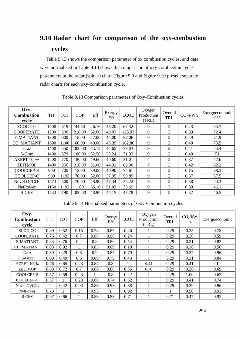
294
9.10 Radar chart for comparison of the oxy-combustion
cycles
Table 9.13 shows the comparison parameter of ox combustion cycles, and data
were normalised in Table 9.14 shows the comparison of oxy-combustion cycle
parameters in the radar (spider) chart. Figure 9.9 and Figure 9.10 present separate
radar charts for each oxy-combustion cycle.
Table 9.13 Comparison parameters of Oxy-Combustion cycles
Oxy-
Combustion
cycle
TIT TOT COP Eff Exergy
Eff LCOE
Oxygen
Production
(TRL)
Overall
TRL CO2/kWh
Exergoeconomic
f %
SCOC-CC 1400 619 44.50 46.16 43.20 67.32 9 2 0.43 54.7
COOPERATE 1200 500 210.00 52.00 49.02 128.93 9 2 0.39 72.4
E-MATIANT 1300 900 15.00 47.00 44.00 57.06 9 2 0.49 51.9
CC_MATIANT 1300 1100 60.00 49.00 45.39 162.86 9 2 0.40 75.5
Graz 1400 350 300.00 53.12 44.65 39.03 9 2 0.41 44.4
S-Graz 1400 579 180.00 52.50 38.24 71.32 9 2 0.48 51
AZEPT 100% 1200 770 180.00 49.60 40.60 31.01 4 2 0.37 42.6
ZEITMOP 1400 856 210.00 51.00 44.91 86.36 7 2 0.42 62.1
COOLCEP-S 900 700 15.00 59.00 40.90 74.61 9 2 0.15 68.3
COOLCEP-C 900 1192 70.00 52.00 37.95 59.89 9 2 0.37 57.5
Novel O2/CO2 1573 500 70.00 48.90 47.34 35.22 9 2 0.38 44.3
NetPower 1150 1192 1.00 55.10 51.03 33.69 9 7 0.30 46.1
S-CES 1533 790 300.00 48.90 45.15 43.78 9 5 0.32 46.5
Table 9.14 Normalised parameters of Oxy-Combustion cycles
Oxy-
Combustion
cycle
TIT TOT COP Eff Exergy
Eff LCOE
Oxygen
Production
(TRL)
Overall
TRL
CO2/kW
h Exergoeconomic
SCOC-CC 0.89 0.52 0.15 0.78 0.85 0.46 1 0.29 0.35 0.78
COOPERATE 0.76 0.42 0.7 0.88 0.96 0.24 1 0.29 0.38 0.59
E-MATIANT 0.83 0.76 0.2 0.8 0.86 0.54 1 0.29 0.31 0.82
CC_MATIANT 0.83 0.92 1 0.83 0.89 0.19 1 0.29 0.38 0.56
Graz 0.89 0.29 0.6 0.9 0.87 0.79 1 0.29 0.37 0.96
S-Graz 0.89 0.49 0.6 0.89 0.75 0.43 1 0.29 0.31 0.84
AZEPT 100% 0.76 0.65 0.23 0.84 0.8 1 0.44 0.29 0.41 1
ZEITMOP 0.89 0.72 0.7 0.86 0.88 0.36 0.78 0.29 0.36 0.69
COOLCEP-S 0.57 0.59 0.23 1 0.8 0.42 1 0.29 1.00 0.62
COOLCEP-C 0.57 1 0.23 0.88 0.74 0.52 1 0.29 0.41 0.74
Novel O2/CO2 1 0.42 0.03 0.83 0.93 0.88 1 0.29 0.39 0.96
NetPower 0.73 1 1 0.93 1 0.92 1 1 0.50 0.92
S-CES 0.97 0.66 1 0.83 0.88 0.71 1 0.71 0.47 0.92
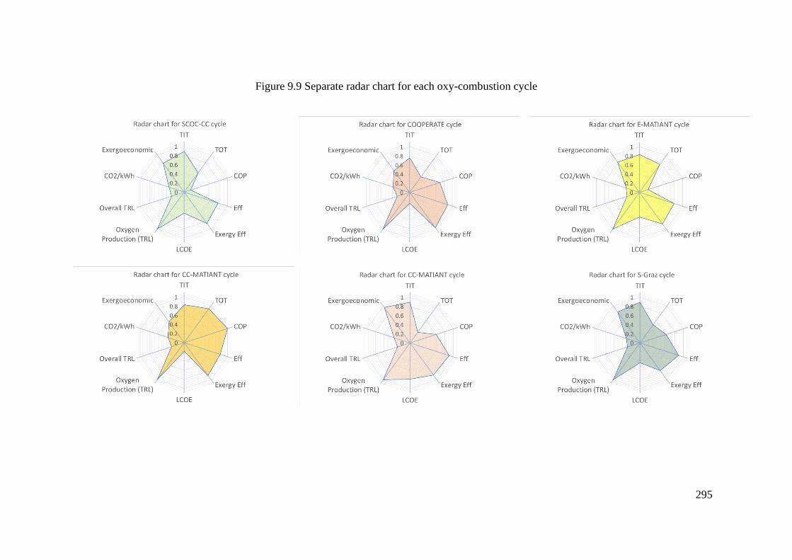
295
Figure 9.9 Separate radar chart for each oxy-combustion cycle
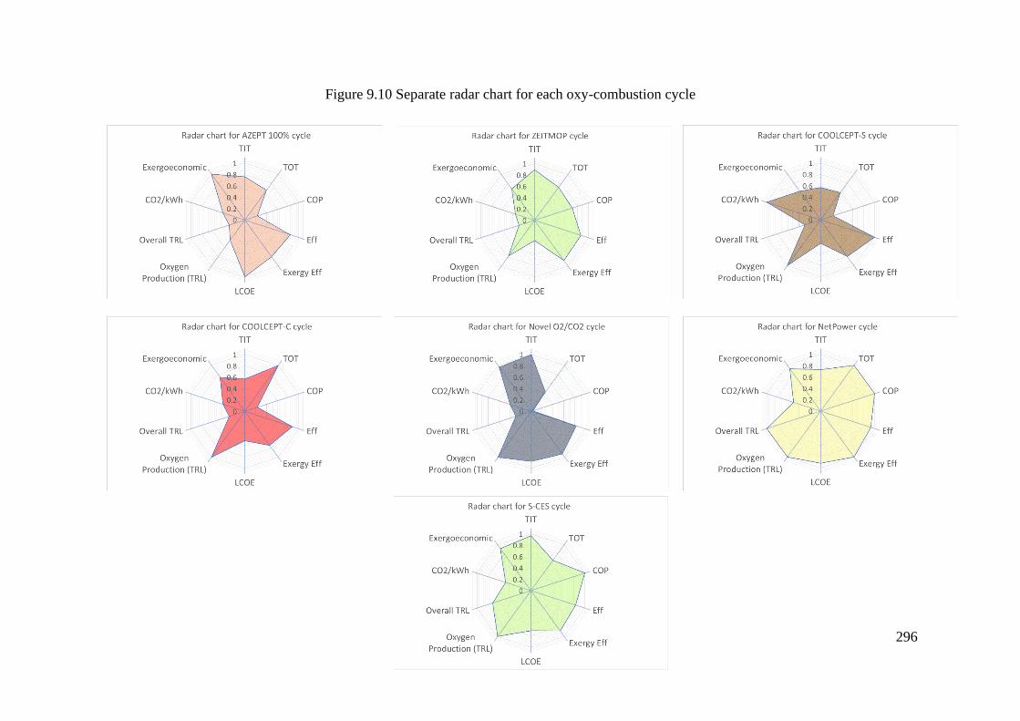
296
Figure 9.10 Separate radar chart for each oxy-combustion cycle
297
The normalised parameters of oxy-combustion cycles are presented in Table 9.14, and
the TIT, TOT, COP, Eff, Exergy Eff, LCOE, Oxygen Production (TRL), Overall TRL,
CO2/kWh, Exergoeconomic f % parameters of the oxy-combustion cycle are
compared.
Based on Figure 9.9, Figure 9.10, it can be concluded COOLCEP-S, NetPower,
AZEPT 100% have better thermal, exergy efficiency than other oxy-combustion
cycles; however, COOLCEP-S, AZEPT 100% have lower COP, TIT and TRL. In
addition, NetPower has lower LCOE; hence, the electricity price of NetPower is lower
than COOLCEP-S, AZEPT 100%.
The exergoeconomic factor for NetPower, S-CES, Novel O2/CO2, Graz, AZEPT
100% are far from ideal, so these cycles can be improved by more capital investment,
and the capital investment can reduce exergy destruction in the component and reduce
electricity cost. In terms of carbon emission production, COOLCEP-S, NetPower, S-
CES cycles present lower emissions than other cycles, however, the COOLCEP-S
needs to develop technologies based on the TRL, and it has higher electricity cost than
NetPower and S-CES.
CC-MATIANT present better overall parameters, including thermal, exergy
efficiency, COP, TIT in comparison with other cycles; however, it needs to develop
because of lower TRL and the cost of electricity, LCOE, is high.
ZEITMOP cycle also presents better efficiency and parameters, including TIT,
TOT, COP; however, it has Low overall TRL and Oxygen production TRL, and the
Oxygen production technology needs to develop for this cycle. Also, it shows a higher
levelised cost of electricity LCOE in comparison with other cycles.
S-CES and NetPower cycles present proper efficiency with lower carbon emission,
and they have the highest TRL among other oxy-combustion cycles. These two cycles
are only demonstration cycles with very low cost of electricity in comparison with
other cycles; however, the NetPower cycle has higher TIT, TOT and TRL. The
NetPower cycle can get more benefit than the S-CES cycle from high-efficiency heat
recovery because of higher Turbine Outlet Temperature (TOT), but the TIT of the S-
CES cycle is higher than NetPower, so it needs more developed technology for
combustion and cooling blade system, which CES company recently developed.
298
9.11 Summary
This PhD thesis concludes most of the oxy-combustion cycles are studied from cycle
performance and parameters including TIT, TOT, COP, Eff, Exergy Eff, LCOE,
Oxygen Production (TRL), Overall TRL, CO2/kWh, Exergoeconomic f % parameters
of oxy-combustion.
The results indicate that the NetPower and S-CES are developed in technologies to
have higher TIT in comparison with other cycles, TIT of NetPower is 1150 °C, and S-
CES is 1553 °C; however, these cycles need to develop in exergoeconomic factor and
more capital investment can benefit cycle with lower exergy destruction in component
and reduce the cost of electricity.
The NetPower, COOLCEP-C, and CC-MATIANT cycles have high Turbine Outlet
Temperatures with TOT of 790 °C, 1192 °C, 1100 °C, respectively which aid the heat
recovery efficiency from the turbine exhaust gas and these cycles are proper options
to use heat exchanger equipment.
The highest Combustion Outlet Pressures (COP) belong to NetPower, S-CES and
CC-MATIANT, which are 300 bar. Hence, these cycles need to have developed
combustion and turbine technologies. Amon this cycle, the NetPower and S-CES were
developed as high-pressure components.
Also, NetPower with 0.3 CO2 kg/kWh and S-CES with 0.32 CO2 kg/kWh present
a more environment-friendly oxy-combustion power plant, with a lower Carbon
dioxide emission per electricity production.
The COOPERATE cycle with f = 72.4% and CC-MATIANT with f = 75.5% have
high exergoeconomic factors, and more capital investment cannot reduce the more
exergy destruction in the component to benefit efficiency; however, the NetPower with
f=46.1% and S-CES with f= 46.5% need more capital investment to benefit efficiency
from reducing exergy destruction in cycle components, in addition, these cycles
present better LCOE.
299
Chapter 10: Conclusions and future
works
10.1 Conclusions
In this chapter, the summary of the concluded results and discussion through the
research chapters are presented. The thesis objectives are met through the chapters as
follows. The Carbon Capture, Air Separation Unit (ASU) and CO2 Purification and
Compression Unit (CPU) technologies, and the oxy-combustion power cycles are
investigated in detail in chapter 2. Also, pilot and industrial demonstration of
Oxyturbine power cycles and comparison in terms of cost and efficiency are
investigated in this chapter. The exergy destruction in components of the oxy-
combustion cycles to compare the efficiency of the component to each other are
accessed in chapter 4, and the sensitivity of leading oxy-combustion cycles was studied
in chapter 5 and 6. the parameters of the oxy-combustion cycle, including TIT, TOT,
CO2/kWh, COP, Exergy, Thermal efficiency, Technology Readiness Level (TRL) to
provide a benchmark for comparing oxy-combustion cycles are compared in chapter
9, and performance, LCOE, and exergoeconomic of the oxy-combustion cycles
according to the Aspen plus modelling in this chapter. In the end, the radar diagrams
to compare oxy-combustion cycles were determined in chapter 9.
Following the conclusion, the key point of future works is outlined. In chapter 1,
Gas turbines, the main technologies of CCS (Carbon Capture & Storage), Oxygen
production, including cryogenic and non-cryogenic Air Separation Unit (ASU) and
CO2 Compression and Purification Unit (CPU) were investigated. The thermodynamic
cycles of post-combustion capture, pre-combustion capture and oxy-combustion
capture were studied and described in detail; also advantages and disadvantages of
CCS technologies were tabulated and explained in detail in the conclusion of Chapter
1. The main disadvantage of the post-combustion capture is the carbon capture at
atmospheric pressure. Pre-combustion capture technologies need to develop oxygen
production and long life refractories. The oxy-combustion power plant shows a lower
cost for capturing CO2 in comparison with other technologies because of the high
concentration of CO2 and low fuel gas volume; however, the cost of flue gas
recirculation and air separation unit increase the electricity cost.
300
The thermodynamic of oxy-combustion cycle including SCOC-CC, COOPERATE
Cycle, MATIANT, E-MATIANT, CC_MATIANT, Graz and S-Graz cycles, AZEP
85% and 100%, ZEITMOP, ZEITMOP Cycle, COOLCEP-S Cycle, Novel O2/CO2
(Cao and Zheng, 2006), NetPower and CES Cycles were investigated with details in
chapter 2. The thermodynamic cycle of the oxy-combustion cycles was extracted from
the literature, and process flow diagrams of the oxy-combustion cycles were drawn in
this chapter. The process flow diagrams were explained in detail, and each process was
clarified in the diagrams. Furthermore, in chapter 2, the technologies of each oxy-
combustion cycle were discussed in detail. The advantages, disadvantages and cost of
each of the cycle technologies were mentioned in this chapter.
In chapter 3, the modelling of the oxy-combustion cycles was provided by using
Aspen Plus software. Also, the software of process modelling was considered, and the
pros and cons of Aspen plus software were mentioned in the first part of the chapter.
The oxy-combustions cycles were simulated based on the modelled cycles with Aspen
plus software. The stream parameters, including temperature, pressure, flow rate,
composition, were calculated and tabulated in this chapter. The results are a reference
for the oxy-combustion power cycles calculation; also, the exergy flowrates of streams
were calculated for the cycles. The results indicate that the combustion has higher
irreversibility and exergy destruction in oxy-combustion cycles due to the chemical
reaction process, and heat transfer occurs in the combustion chambers such as SCOC-
CC with 28.8% and COOPERATE with 24.4% of total input exergy.
The second main exergy loss in oxy-combustions are HRSG or heat exchanger due
to heat transfer between two-stream; therefore, improving the efficiency of HRSG can
reduce exergy destruction and improve overall efficiency.
Furthermore, the exergy destruction in each component was shown in bar charts for
oxy-combustion cycles to compare irreversibilities and inefficiencies in each
component of the cycle. The exergy destruction can be used to find the most exergy
destructive component, and it shows that for improving the cycle efficiency and
reducing energy penalties in the oxy-combustion power plant, these components need
to be developed.
Thermodynamics theory formula, exergy analysis equations, Equation of State
(EOS) for oxy-combustion cycle were discussed in chapter 3; These equations are
301
fundamental equations for the analysis of oxy-combustion; they are a reference for
thermodynamic analysis of oxy-combustion cycles.
Techno-economic, sensitivity and exergy analysis of main oxy-combustion cycle
including SCOC-CC, E-MATIANT, and COOPERATE cycles were studied in
chapters 5 and 6. These chapters were prepared and written up into three papers for
high-rank journals. The sensitivity and 3D graphs of the exergy destruction vs flow
rate and pressure for the SCOC-CC cycle were plotted, and the thermal and exergy
efficiency sensitivity vs working flow rate for the E-MATIANT cycle was presented
in chapter 5. The sensitivity analysis of SCOC-CC indicates that the maximum work
is at 40 pressure ratio. The sensitivity of efficiency with respect to the flowrate and
Combustion Outlet Pressure (COP) indicates that reduction of working flow from 15
kg/s to 17 kg/s can grow the efficiency from 35% to 37%; The overall efficiency of
the E-MATIANT cycle at a maximum of 1300 °C is 46.9%; this efficiency can be
achieved at 290 kg/s recycled working flow.
In chapter 6, the exergy destruction sensitivity of the COOPERATE cycle was
presented in the bar chart. Also, the 3D plot of exergy destruction vs min approach
temperature and flowrates were demonstrated; The results indicate the flowrate at the
minimum exergy destruction point decreases when the min approach temperature
increases. The results indicate that the maximum efficiency of COOPERATE cycle is
52.79% for ∆T=110 at 318 kg/s flowrates with the minimum exergy destruction is
about 314.8 MW. The exergy destruction in combustions grow by increasing flowrate
from 218 kg/s to 518 kg/s because of the high rate of the chemical reaction and
increasing the turbulent flow inside the combustions.
The sensitivity of the heat exchanger design of NetPower was analysed by Aspen
plus software in chapter 7. The sensitivity of efficiency vs ∆Tmin with constant COT
and the constant flow rate was plotted; also, the design and cost analysis of heat
exchanger were discussed. The result was published as a peer-reviewed journal paper.
In Chapter 8, NetPower and CES, two leading oxy-combustion cycles were compared.
The efficiency sensitivity vs TIT for CES and NetPower cycle were compared. The
results of the TIT sensitivity for the S-CES cycle and the NetPower cycle indicates
that the slope of cycle efficiency was higher in the NetPower cycle, which could be
explained by the higher impact that the TIT produced in the turbine and the main heat
302
exchanger for the NetPower cycle. The results were presented at the GHG-14
conference and in SSN peer-review procedia.
The pilot and industrial demonstration of the Oxyturbine power cycles were
investigated in chapter 8. In this chapter, demonstration cycles including CES and
NetPower were analysed in detail, and the technologies of turbine, heat exchanger and
combustor for each cycle were assessed.
Techno-economic, Risk, Technology Readiness Level (TRL) and parametric
comparison in Oxyturbine Power Cycles were analysed in chapter 9. In this chapter,
TIT, TOT, COP, exergy and thermal efficiency, carbon emission per kWh, TRL of the
oxy-combustion cycle were compared in tables and bar charts. The performance
analysis of the oxy-combustion cycle was compared, and techno-economic analysis
was compared in terms of cost rate and LCOE; these were also presented in bar charts
and, the radar diagram of parameters for comparing the oxy-combustion cycles was
presented. The results indicate that that the NetPower and S-CES are developed in
technologies to have higher TIT in comparison with other cycles, TIT of NetPower is
1150 °C, and S-CES is 1553 °C; however, the NetPower with f=46.1% and S-CES
with f= 46.5% need more capital investment to benefit efficiency from reducing exergy
destruction in cycle components, in addition, these cycles present better LCOE.
This PhD research is presenting the comparison of the proposed or demonstrated
oxy-combustion cycles. It can be used to draw a road map for the development and
deployment of low carbon, higher efficiency and low-cost energy, and it would be a
reference for future researchers in oxy-combustion cycles.
10.2 Future work and critical appraisal
The future extensions of this research are outlined briefly as follows:
• Multi-objective optimisation of Oxy-combustion cycles in respect to
design parameters: The design parameters of the oxy-combustion cycle
need to consider the production of electricity with minimum exergy
destruction, minimum cost and minimum impact on the environment. In
order to design the oxy-combustion power cycle with high efficiency at low
cost, the trade-off between efficiency and cost is needed to be considered.
Multi-objective optimization is used to find the best trade-off between cycle

303
design parameters. The optimised cycle will have lower exergy destruction,
minimum fuel consumption, minimum capital cost and minimum impact on
the environment.
• Thermochemical analysis of the working flow composition for oxy-
combustion cycles: The working flow composition has the main impact on
the efficiency of the combustion, turbine and heat exchanger.
Thermochemical optimisation of the oxy-combustion cycle needs to be
studied to indicate the composition with higher overall efficiency for oxy-
combustion cycles.
304
Reference
A K Tiwari, M. M. H. and M. I. (2012) ‘Effect of Operating Parameters on the Performance
of Combined Cycle Power Plant’, Journal of Industrial Microbiology and
Biotechnology. doi: 10.1007/s10295-007-0291-8.
Ahmad, F. (2019) Dynamic Scheduling and Control of MEA Absorption Processes for CO 2
Capture Using gProms.
Ahmadi, P., Dincer, I. and Rosen, M. A. (2011) ‘Exergy, exergoeconomic and
environmental analyses and evolutionary algorithm based multi-objective
optimization of combined cycle power plants’, Energy, 36(10), pp. 5886–5898. doi:
10.1016/j.energy.2011.08.034.
Ahmed F. El-Sayed (2017) Aircraft Propulsion and Gas Turbine Engines, Second Edition.
Allam, R. et al. (2017) ‘Demonstration of the Allam Cycle: An Update on the Development
Status of a High Efficiency Supercritical Carbon Dioxide Power Process Employing
Full Carbon Capture’, Energy Procedia, 114(November 2016), pp. 5948–5966. doi:
10.1016/j.egypro.2017.03.1731.
Allam, R. J. et al. (2013) ‘High efficiency and low cost of electricity generation from fossil
fuels while eliminating atmospheric emissions, including carbon dioxide’, Energy
Procedia, 37, pp. 1135–1149. doi: 10.1016/j.egypro.2013.05.211.
Almås, K. (2012) ‘Coal-fired Power Plants based on Oxy-combustion with Carbon Capture :
Combustion Conditions and Water Consumption’, pp. 13–100.
Anderson, R. E. et al. (2008) ‘Adapting gas turbines to zero emission oxy-fuel power
plants’, Proceedings of the ASME Turbo Expo, 2, pp. 781–791. doi:
10.1115/GT2008-51377.
Aneke, M. and Wang, M. (2015) ‘Potential for improving the energy efficiency of cryogenic
air separation unit (ASU) using binary heat recovery cycles’, Applied Thermal
Engineering, 81, pp. 223–231. doi: 10.1016/J.APPLTHERMALENG.2015.02.034.
Antonini, C. et al. (2020) ‘Hydrogen production from natural gas and biomethane with
carbon capture and storage - A techno-environmental analysis’, Sustainable Energy
and Fuels, 4(6), pp. 2967–2986. doi: 10.1039/d0se00222d.
Artioli, Y. (2008) ‘Adsorption’, in Encyclopedia of Ecology, Five-Volume Set. Elsevier Inc.,
pp. 60–65. doi: 10.1016/B978-008045405-4.00252-4.
Atkinson, J. et al. (2009) Design and operation. Available at:
https://www.ncbi.nlm.nih.gov/books/NBK143274/.
Authors, C. L. et al. (2010) ‘Capture of CO2’, Energy & fuels, 24(MAIJUN), pp. 3687–
3697.
Barston, R. P. (2019) ‘The Paris agreement’, in Modern Diplomacy, pp. 492–505. doi:
10.4324/9781351270090-20.
Bolland, O. and Saether, S. (1992) ‘New Concepts for Natural Gas Fired Power Plants’,
Energy Conversion and Management, 33(5–8), pp. 467–475.
Boyce, M. P. (2006) Gas Turbine Third Edition Engineering.
Boyce, M. P. and Chen, M. S. (1974) ‘OPTIMIZATION OF VARIOUS GAS TURBINE
CYCLES.’, in, pp. 91–100.
Budinis, S. et al. (2018) ‘An assessment of CCS costs, barriers and potential’, Energy
Strategy Reviews, 22(May), pp. 61–81. doi: 10.1016/j.esr.2018.08.003.
Bunyamanid, Y. et al. (2016) ‘An Analysis of Energy and Carbon Intensities and Exergy
Efficiency in Natural Gas Combined-Cycle Power Plants: A Case Study of
Thailand’, MATEC Web of Conferences, 68, pp. 6–11. doi:
305
10.1051/matecconf/20166814001.
Business, W. and October, M. (2012) ‘Advanced Turbine Developments for Oxy-
Combustion TriGen TM Plants 2012 WESTCARB Business Meeting’.
Calli, O., Colpan, C. O. and Gunerhan, H. (2018) ‘Performance Assessment of a Biomass-
Fired Regenerative ORC System Through Energy and Exergy Analyses’, in
Exergetic, Energetic and Environmental Dimensions. Elsevier Inc., pp. 253–277. doi:
10.1016/B978-0-12-813734-5.00015-9.
Cao, W. and Zheng, D. (2006) ‘Exergy regeneration in an O2/CO2 gas turbine cycle with
chemical recuperation by CO2 reforming of methane’, Energy Conversion and
Management, 47(18–19), pp. 3019–3030. doi: 10.1016/j.enconman.2006.03.010.
Carapellucci, R. et al. (2017) ‘IMECE2013-63492’, pp. 1–12.
CES (2020a) Direct Steam Gas Generators — Clean Energy Systems. Available at:
http://www.cleanenergysystems.com/gas-generators (Accessed: 3 December 2020).
CES (2020b) Oxy-Fuel Turbines — Clean Energy Systems. Available at:
http://www.cleanenergysystems.com/oxy-fuel-turbines (Accessed: 2 December
2020).
Chaudhry, G. et al. (2018) ‘Analysis of oxy-fuel combustion power cycle utilizing a
pressurized coal combustor The MIT Faculty has made this article openly available .
Please share how this access benefits you . Your story matters . Citation Elsevier
License Publisher Version Access’.
ChemEngGuy (2021) What is PRO/II from Schneider Electric / AVEVA ? – ChemEngGuy.
Available at: https://www.chemicalengineeringguy.com/the-blog/process-
simulation/what-is-pro-ii-from-schneider-electric-aveva/ (Accessed: 25 July 2021).
Chiesa, P. and Lozza, G. (1999) ‘CO2 emission abatement in igcc power plants by
semiclosed cycles: Part a with oxygen-blown combustion’, Journal of Engineering
for Gas Turbines and Power, 121(4), pp. 635–641. doi: 10.1115/1.2818519.
Chik, M. N. (2017) ‘Journal of Energy’, pp. 1–12.
Clean Energy System (2020a) Oxy-Fuel Turbines — Clean Energy Systems. Available at:
http://www.cleanenergysystems.com/oxy-fuel-turbines (Accessed: 3 June 2020).
Clean Energy System (2020b) Oxy-Fuel Turbines — Clean Energy Systems. Available at:
http://www.cleanenergysystems.com/oxy-fuel-turbines (Accessed: 3 December
2020).
Climent Barba, F. et al. (2016a) ‘A technical evaluation, performance analysis and risk
assessment of multiple novel oxy-turbine power cycles with complete CO2 capture’,
Journal of Cleaner Production, 133, pp. 971–985. doi:
10.1016/j.jclepro.2016.05.189.
Climent Barba, F. et al. (2016b) ‘A technical evaluation, performance analysis and risk
assessment of multiple novel oxy-turbine power cycles with complete CO2capture’,
Journal of Cleaner Production, 133, pp. 971–985. doi:
10.1016/j.jclepro.2016.05.189.
Contributing, T. N. et al. (2020) A survey of key technological innovations for the low-
carbon economy.
Cunha, H. E. and Kyprianidis, K. G. (2012) ‘Investigation of the potential of gas turbines for
vehicular applications’, Proceedings of the ASME Turbo Expo, 3(June 2012), pp. 51–
64. doi: 10.1115/GT2012-68402.
Dahlquist, A. et al. (2013) ‘Optimization of an oxyfuel combined cycle regarding
performance and complexity level’, Proceedings of the ASME Turbo Expo, 2(July
2016). doi: 10.1115/GT2013-94755.
Darabkhani, H. G. et al. (2018) ‘Design, process simulation and construction of a 100 kW
pilot-scale CO2 membrane rig: Improving in situ CO2 capture using selective
306
exhaust gas recirculation (S-EGR)’, Journal of Natural Gas Science and
Engineering, 50(September 2017), pp. 128–138. doi: 10.1016/j.jngse.2017.09.012.
Davison, J. (2015) ‘Techno-Economic Assessment of Oxy- Combustion Turbine Power
Plants with CO 2 Capture Outline of Presentation Background and scope of the
study’, (October).
Dillon, D. et al. (2013) ‘Post-combustion capture on natural gas combined cycle plants: A
technical and economical evaluation of retrofit, new build, and the application of
exhaust gas recycle’, Energy Procedia, 37, pp. 2397–2405. doi:
10.1016/j.egypro.2013.06.121.
Dinçer, I. and Kanoǧlu, M. (2010) Refrigeration Systems and Applications, Second Edition,
Refrigeration Systems and Applications, Second Edition. doi:
10.1002/9780470661093.
Dincer, I. and Rosen, M. A. (2021) ‘Exergy and energy analyses’, Exergy, pp. 23–35. doi:
10.1016/B978-0-12-824372-5.00002-6.
EAVES PSK (1971) Gas turbines for power generation, Electronics and Power. doi:
10.1049/ep.1971.0241.
El-Masri, M. A. (1986) ‘On thermodynamics of gas-turbine cycles: Part 2—A model for
expansion in cooled turbines’, Journal of Engineering for Gas Turbines and Power,
108(1), pp. 151–159. doi: 10.1115/1.3239862.
Energy Information Administration, U. (2021) ‘Levelized Costs of New Generation
Resources in the Annual Energy Outlook 2021’.
Fans, T. (2020) ‘Energy , Exergy and Economic Analyses of a’.
Ferguson, S. (2018) ‘Assessing the Cost Reduction Potential and Competitiveness of Novel
(Next Generation) UK Carbon Capture Technology Benchmarking State-of-the-art
and Next Generation Technologies’, (February).
Fernandes, D. et al. (2019) ‘Process and Carbon Footprint Analyses of the Allam Cycle
Power Plant Integrated with an Air Separation Unit’, International Journal of
Chemical Engineering, 2019, pp. 325–340. doi: 10.1155/2019/6035856.
Feron, P. H. M. (2016) Absorption-Based Post-Combustion Capture of Carbon Dioxide
(Woodhead Publishing Series in Energy).
Ferrari, N. et al. (2017a) ‘Oxy-turbine for Power Plant with CO2 Capture’, Energy
Procedia, 114(November 2016), pp. 471–480. doi: 10.1016/j.egypro.2017.03.1189.
Ferrari, N. et al. (2017b) ‘Oxy-turbine for Power Plant with CO2 Capture’, Energy
Procedia, 114(November 2016), pp. 471–480. doi: 10.1016/j.egypro.2017.03.1189.
Ferrari, N. et al. (2017c) ‘Oxy-turbine for Power Plant with CO2 Capture’, Energy
Procedia, 114, pp. 471–480. doi: 10.1016/j.egypro.2017.03.1189.
Figueroa, J. D. et al. (2008) ‘Advances in CO2 capture technology-The U.S. Department of
Energy’s Carbon Sequestration Program’, International Journal of Greenhouse Gas
Control, 2(1), pp. 9–20. doi: 10.1016/S1750-5836(07)00094-1.
Flanner, M. G. (2009) ‘Integrating anthropogenic heat flux with global climate models’,
Geophysical Research Letters, 36(2), pp. 1–5. doi: 10.1029/2008GL036465.
Flin, D. (2019) First fire for La Porte carbon capture demo | Gas Turbine World. Available
at: https://gasturbineworld.com/first-fire-for-la-porte-carbon-capture-demo/
(Accessed: 26 May 2020).
Folkson, R. (2014) Alternative fuels and advanced vehicle technologies for improved
environmental performance: Towards zero carbon transportation, Alternative Fuels
and Advanced Vehicle Technologies for Improved Environmental Performance:
Towards Zero Carbon Transportation. doi: 10.1533/9780857097422.
Forsthoffer, W. E. (2011) Forsthoffers Best Practice Handbook for Rotating Machinery by
William E Forsthoffer (z-lib.org).
307
Foy, K. and McGovern, J. (2007) ‘Analysis of the effects of combining air separation with
combustion in a zero emissions (ZEITMOP) cycle’, Energy Conversion and
Management, 48(11), pp. 3046–3052. doi: 10.1016/j.enconman.2007.06.041.
Foy, K. and Yantovski, E. (2006) ‘History and state-of-the-art of fuel fired zero emission
power cycles’, International Journal of Thermodynamics, 9(2), pp. 37–63. doi:
10.5541/ijot.1034000170.
Freund, P. (2005) ‘IPCC Special Report on Carbon dioxide Capture and Storage Contents’,
IPCC Special Report on Carbon dioxide Capture and Storage, (En línea), pp. 52–71.
Gasturb (2018) GasTurb 13 Design and Off-Design Performance of Gas Turbines.
Gibbins, J. et al. (2011) ‘2 th Meeting of the International Post-Combustion CO 2 Capture
Network 2 p Retrofitting Post Combustion Capture Retrofitting Post Combustion
Capture to Existing Power Plant Acknowledgements: DECC, RCUK, IEA GHG’.
Available at: https://www.netl.doe.gov/coal/carbon-capture/post-combustion
(Accessed: 25 July 2021).
Gicquel, R. (2018) Online course and simulator for engineering thermodynamics. Available
at: https://direns.mines-paristech.fr/Sites/Thopt/en/co/cycles-
combines.html%0Adirens.mines-paristech.fr/Sites/Thopt/en/co/chambres-
combustion.html (Accessed: 21 July 2020).
Gonzalez-Salazar, M. A., Kirsten, T. and Prchlik, L. (2018) ‘Review of the operational
flexibility and emissions of gas- and coal-fired power plants in a future with growing
renewables’, Renewable and Sustainable Energy Reviews, 82(July 2017), pp. 1497–
1513. doi: 10.1016/j.rser.2017.05.278.
Gundersen, T. (2009) THE CONCEPT OF EXERGY AND ENERGY QUALITY.
Ham, L. van der (2011) Improving the Second law efficiency of a cryogenic air separation
unit Thesis for the degree of Philosophiae Doctor.
Hanak, D. P., Powell, D. and Manovic, V. (2017) ‘Techno-economic analysis of oxy-
combustion coal-fired power plant with cryogenic oxygen storage’, Applied Energy,
191, pp. 193–203. doi: 10.1016/j.apenergy.2017.01.049.
Haydary, J. (2019) Chemical Process Design and Aspen Plus and Aspen HYSYS
Applications.
He, X. (2018) ‘The Latest Development on Membrane Materials and Processes for Post-
combustion CO 2 Capture: A Review OPEN ACCESS Citation: He X. The Latest
Development on Membrane Materials and Processes for Post-combustion CO 2
Capture: A Review’, ScienceForecast Publications LLC., |. SF J Material Chem
Eng, 1(1), p. 1009. Available at: https://scienceforecastoa.com/ (Accessed: 24
August 2020).
Heat, C. (2018) ‘News : Heatric supplies Circuit Heat advanced recuperator for NET Power
’ s first- Heatric supplies advanced recuperator for NET Power ’ s first-of-a- kind
supercritical CO2 power plant’.
Heatric (2020) Printed Circuit Heat Exchangers - High-Integrity Equipment | Heatric.
Available at: https://www.heatric.com/heat-exchangers/ (Accessed: 3 June 2020).
Higher temperatures in turbines - Kraftwerk Forschung (2020). Available at:
http://kraftwerkforschung.info/en/higher-temperatures-in-turbines/ (Accessed: 3
December 2020).
Horlock, J. H. and Bathie, W. W. (2004) Advanced Gas Turbine Cycles, Journal of
Engineering for Gas Turbines and Power. doi: 10.1115/1.1789994.
Horlock, J. H. and Torbidoni, L. (2008a) ‘Calculations of cooled turbine efficiency’, Journal
of Engineering for Gas Turbines and Power, 130(1), p. 011703. doi:
10.1115/1.2771250.
Horlock, J. H. and Torbidoni, L. (2008b) ‘Calculations of cooled turbine efficiency’, Journal
308
of Engineering for Gas Turbines and Power, 130(1). doi: 10.1115/1.2771250.
Hu, Y. (2011) CO 2 capture from oxy-fuel combustion power plants.
Ibrahim Dincer, M. A. R. (2013) Chemical Exergy, Chemical Exergy.
IEAGHG (2014) ‘ASSESSMENT OF EMERGING CO 2 CAPTURE TECHNOLOGIES
AND THEIR POTENTIAL TO Report : 2014 / TR4 December 2014’, (December).
IEAGHG (2015) ‘Oxy-Combustion Turbine Power Plants’, 2015/05, August, 2015,
(August).
IEAGHG (2019) ‘IEA GREENHOUSE GAS R&D PROGRAMME CCS in Energy and
Climate Scenarios’. Available at: www.ieaghg.org (Accessed: 25 July 2021).
IEAGHG (2020) Future Role of CCS Technologies in the Power Sector. Available at:
https://ieaghg.org/publications/technical-reports/reports-list/9-technical-reports/1046-
2020-08-future-role-of-ccs-technologies-in-the-power-sector (Accessed: 25 July
2021).
Ingegneria, F. et al. (2012) ‘Politecnico di milano’, pp. 1–11.
Jansen, D. et al. (2015) ‘Pre-combustion CO2 capture’, International Journal of Greenhouse
Gas Control, 40, pp. 167–187. doi: 10.1016/j.ijggc.2015.05.028.
Javadzadeh, Y. and Hamedeyaz, S. (2014) ‘Floating Drug Delivery Systems for Eradication
of Helicobacter pylori in Treatment of Peptic Ulcer Disease’, Trends in Helicobacter
pylori Infection, i(tourism), p. 13. doi: 10.5772/57353.
Jericha, H. and Fesharaki, M. (1995) ‘Graz cycle - 1500°C max temperature potential H2 -
O2 fired CO2 capture with CH4 - O2 firing’, American Society of Mechanical
Engineers (Paper).
Jericha, H. and Göttlich, E. (2002) ‘Conceptual design for an industrial prototype GRAZ
CYCLE power plant’, American Society of Mechanical Engineers, International Gas
Turbine Institute, Turbo Expo (Publication) IGTI, 2 A, pp. 413–420. doi:
10.1115/GT2002-30118.
Jericha, H., Sanz, W. and Göttlich, E. (2008a) ‘Design concept for large output Graz Cycle
gas turbines’, Journal of Engineering for Gas Turbines and Power, 130(1). doi:
10.1115/1.2747260.
Jericha, H., Sanz, W. and Göttlich, E. (2008b) ‘Design concept for large output Graz Cycle
gas turbines’, Journal of Engineering for Gas Turbines and Power, 130(1), pp. 1–10.
doi: 10.1115/1.2747260.
Joda, F. et al. (2011) ‘Improving multi-stream heat exchanger design by reducing the
number of sections’, 2011 4th International Conference on Modeling, Simulation
and Applied Optimization, ICMSAO 2011. doi: 10.1109/ICMSAO.2011.5775470.
Kalamaras, C. M. et al. (2013) ‘Conference Paper Hydrogen Production Technologies:
Current State and Future Developments’, Conference Papers in Energy, 2013. doi:
10.1155/2013/690627.
Karaağaç, M. O., Kabul, A. and Oğul, H. (2019) ‘First- and second-law thermodynamic
analyses of a combined natural gas cycle power plant: Sankey and Grossman
diagrams’, Turkish Journal of Physics, 43(1), pp. 93–108. doi: 10.3906/fiz-1809-9.
Kaur, R. et al. (2019) ‘Thermochemical Route for Biohydrogen Production’, in
Biohydrogen. Elsevier, pp. 187–218. doi: 10.1016/b978-0-444-64203-5.00008-3.
Kaviri, A. G., Jaafar, M. N. M. and Lazim, T. M. (2012) ‘Modeling and multi-objective
exergy based optimization of a combined cycle power plant using a genetic
algorithm’, Energy Conversion and Management, 58, pp. 94–103. doi:
10.1016/j.enconman.2012.01.002.
Kelly (Kailai) Thambimuthu (Australia (2005) ‘Capture of CO 2’.
Khaljani, M., Khoshbakhti Saray, R. and Bahlouli, K. (2015) ‘Comprehensive analysis of
energy, exergy and exergo-economic of cogeneration of heat and power in a
309
combined gas turbine and organic Rankine cycle’, Energy Conversion and
Management, 97, pp. 154–165. doi: 10.1016/j.enconman.2015.02.067.
Kwon, S. et al. (2011) ‘CO2 Sorption’, in Coal Gasification and Its Applications. Elsevier,
pp. 293–339. doi: 10.1016/b978-0-8155-2049-8.10010-5.
Laboo (2020) Vacuum Pressure swing adsorption oxygen. Available at:
http://www.laboogas.net/Products/pressure swing adsorption/49.html (Accessed: 15
October 2020).
Liao, M. et al. (2013) ‘Decomposition of embodied exergy flows in manufactured products
and implications for carbon tariff policies’, Asia Europe Journal, 11(3), pp. 265–283.
doi: 10.1007/s10308-013-0357-3.
Liu, M. et al. (2017) ‘IMECE2008-66467’, pp. 1–12.
Lockwood, T. (2014) ‘Developments in oxyfuel combustion of coal’, IEA Clean Coal
Centre, CCC/240, London, United Kingdom, (10), pp. 1–122.
Lozza, G. et al. (2009) CO2 Capture from Natural Gas Combined Cycles, 1st International
Conference …. Available at: http://www.co2club.it/agenda/full paper/Lozza_full
paper.pdf (Accessed: 6 December 2018).
Macchi, E. (2017) ‘Organic Rankine Cycle (ORC) Power Systems’, Organic Rankine Cycle
(ORC) Power Systems. doi: 10.1016/c2014-0-04239-6.
MacDowell, N. et al. (2010) ‘An overview of CO2 capture technologies’, Energy and
Environmental Science, 3(11), pp. 1645–1669. doi: 10.1039/c004106h.
Machner, K. (1958) ‘Die Mikrobestimmung von Hippursäure im Urin’, Fresenius’
Zeitschrift für Analytische Chemie, 163(1), p. 69. doi: 10.1007/BF00447266.
Mancuso, L. et al. (2015) ‘Oxy-combustion turbine power plants. Report: 2015/05’, Ieaghg,
(August).
Manso, R. L. (2013) ‘CO2 capture in power plants-using the oxy-combustion principle’,
(July), p. 93. Available at: http://www.diva-
portal.org/smash/get/diva2:652833/FULLTEXT01.pdf.
Manso, R. L. and Nord, L. O. (2020) CO2 capture in power plants-using the oxy-combustion
principle.
Mantripragada, H. C. and Rubin, E. S. (2019) IECM Technical Documentation: CO 2
Purification Unit (CPU) Models. Available at: www.iecm-online.com (Accessed: 14
October 2020).
Marco Antônio Rosa do Nascimento (2005) ‘Micro gas turbine engine’, Tribology and
Lubrication Technology, 61(1), pp. 12–13. doi: 10.1007/978-0-387-48998-8_967.
Marmolejo-Correa, D. and Gundersen, T. (2015) ‘A new efficiency parameter for exergy
analysis in low temperature processes’, International Journal of Exergy, 17(2), pp.
135–170. doi: 10.1504/IJEX.2015.069988.
Martelli, E. (2019) POLITECNICO DI MILANO Thermodynamic Analysis and Numerical
Optimization of the NET Power oxycombustion cycle.
Mathieu, P. (2004) ‘Towards the hydrogen era using near-zero CO2 emissions energy
systems’, Energy, 29(12-15 SPEC. ISS.), pp. 1993–2002. doi:
10.1016/j.energy.2004.03.007.
Mathieu, P. (2005) ‘Zero Emission Technologies: An Option for Climate Change
Mitigation’, International Journal of Green Energy, 2(2), pp. 193–199. doi:
10.1081/ge-200058979.
Mathieu, P. and Van Loo, F. (2005) ‘Modeling of an IGCC plant based on an oxy-fuel
combustion combined cycle’, ECOS 2005 - Proceedings of the 18th International
Conference on Efficiency, Cost, Optimization, Simulation, and Environmental Impact
of Energy Systems, pp. 651–658. Available at:
https://www.researchgate.net/publication/290188450_Modeling_of_an_IGCC_plant
310
_based_on_an_oxy-fuel_combustion_combined_cycle (Accessed: 18 April 2020).
Mathieu, P. and Nihart, R. (1998) ‘Zero emission MATIANT cycle’, American Society of
Mechanical Engineers (Paper), 111111(GT). doi: 10.1115/98-gt-383.
Mathieu, P. and Nihart, R. (1999) ‘Sensitivity analysis of the MATIANT cycle’, Energy
Conversion and Management, 40(15), pp. 1687–1700. doi: 10.1016/S0196-
8904(99)00062-X.
Matteo, R. : and Romano, C. (2019) POLITECNICO DI MILANO Post-combustion CO 2
Capture from a Natural Gas Combined Cycle with CO 2 membranes.
Matuszewski, M. (2010) ‘Cost and Performance for Low-Rank Pulverized Coal
Oxycombustion Energy Plants’, (September), p. 442.
Merkel, T. C. et al. (2013) ‘Selective exhaust gas recycle with membranes for CO2 capture
from natural gas combined cycle power plants’, Industrial and Engineering
Chemistry Research, 52(3), pp. 1150–1159. doi: 10.1021/ie302110z.
Möller, B. F. et al. (2005) AZEP gas turbine combined cycle power plants - Thermo-
economic analysis, ECOS 2005 - Proceedings of the 18th International Conference
on Efficiency, Cost, Optimization, Simulation, and Environmental Impact of Energy
Systems.
Mondino, G. et al. (2019) ‘Moving bed temperature swing adsorption for CO2 capture from
a natural gas combined cycle power plant’, International Journal of Greenhouse Gas
Control, 85(June), pp. 58–70. doi: 10.1016/j.ijggc.2019.03.021.
Moran, B.-G. T.-M. J. (1948) ‘Thermal design and optimization By Adrian’, p. 58.
MTR (2018) CO2 Removal from Syngas - Membrane Technology and Research, MTR
Membrane Technology and Research. Available at: https://www.mtrinc.com/our-
business/refinery-and-syngas/co2-removal-from-syngas/ (Accessed: 25 August
2020).
MyGridGB (2020) MyGridGB – Charting British electricity. Available at:
http://www.mygridgb.co.uk/ (Accessed: 8 December 2020).
NASA (2017) ‘Isentropic Flow Equations’, (M), pp. 1–4. Available at:
https://www.grc.nasa.gov/www/k-
12/VirtualAero/BottleRocket/airplane/isentrop.html (Accessed: 30 July 2021).
do Nascimento, M. A. R. et al. (2013) ‘Micro Gas Turbine Engine: A Review’, in Progress
in Gas Turbine Performance. InTech. doi: 10.5772/54444.
Nexant (2010) ‘Air Separation Technology Cryogenic air separation units ( ASU ),
membrane , and adsorption ( PSA , VSA ) technologies are discussed . Cost
estimates for producing oxygen , nitrogen ( and argon ) from air using an ASU and
producing oxygen using a VSA are’, (February).
Nguyen, T. K. (2012) Chapter 5 Absorption and Stripping, Solutions. Available at:
http://www.cgscgs.com/ga_tt.htm (Accessed: 8 March 2020).
Nord, L. O., Anantharaman, R. and Bolland, O. (2009) ‘Design and off-design analyses of a
pre-combustion CO2 capture process in a natural gas combined cycle power plant’,
International Journal of Greenhouse Gas Control, 3(4), pp. 385–392. doi:
10.1016/j.ijggc.2009.02.001.
OECD/IEA (2011) Technology Roadmap Carbon Capture and Storage in Industrial
Applications UNITED, SpringerReference. doi: 10.1007/springerreference_7300.
Oettinger, M. (2015) ‘Capture 1 – Oxy-Combustion Capture’, pp. 1–37.
Oxygen generation (2020).
Oyedepo, S. O. et al. (2015) ‘Exergy costing analysis and performance evaluation of
selected gas turbine power plants’, Cogent Engineering, 2(1). doi:
10.1080/23311916.2015.1101048.
Patel, S. (2019) ‘300-MW Natural Gas Allam Cycle Power Plant Targeted for 2022’, Power.
311
Available at: https://www.powermag.com/300-mw-natural-gas-allam-cycle-power-
plant-targeted-for-2022/ (Accessed: 2 December 2020).
Pattanayak, L. (2015) ‘Thermodynamic modeling and exergy analysis of gas turbine cycle
for different boundary conditions’, International Journal of Power Electronics and
Drive Systems, 6(2), pp. 205–215. doi: 10.11591/ijpeds.v6.i2.pp205-215.
Penkuhn, M. and Tsatsaronis, G. (2016) ‘Exergy Analysis of the Allam Cycle’, The 5th
International Symposium - Supercritical CO2 Power Cycles, pp. 1–18. Available at:
http://sco2symposium.com/www2/sco2/papers2016/OxyFuel/040paper.pdf.
Perrin, N. et al. (2013) ‘Oxycombustion for carbon capture on coal power plants and
industrial processes: Advantages, innovative solutions and key projects’, Energy
Procedia, 37, pp. 1389–1404. doi: 10.1016/j.egypro.2013.06.015.
Petrakopoulou, F. (2010) ‘Comparative Evaluation of Power Plants with CO2 Capture:
Thermodynamic, Economic and Environmental Performance’, p. 230.
Petrakopoulou, F. et al. (2010) ‘Exergy-based analyses of an advanced zero emission plant’,
International Journal of Low-Carbon Technologies, 5(4), pp. 231–238. doi:
10.1093/ijlct/ctq028.
Petrakopoulou, F., Tsatsaronis, G. and Morosuk, T. (2011) ‘Exergoeconomic analysis of an
advanced zero emission plant’, Journal of Engineering for Gas Turbines and Power,
133(11). doi: 10.1115/1.4003641.
Power, N. E. T. and Systems, M. P. (2017) ‘NET Power ’ s CO2 cycle : the breakthrough
that CCS needs’, pp. 2–4. Available at:
https://www.modernpowersystems.com/features/featurenet-powers-co2-cycle-the-
breakthrough-that-ccs-needs/ (Accessed: 25 July 2021).
PT6Nation (2018) The PT6 Nation - From the Archives: Early Rumblings of the PT6-
powered Snowplow. Available at:
http://www.pt6nation.com/en/community/story/from-the-archives-early-rumbli/
(Accessed: 17 October 2020).
Quality, E. (2011) ‘A N I NTRODUCTION TO T HE C ONCEPT OF E XERGY’, (March),
pp. 1–26.
Razak, A. M. Y. (2007) Industrial gas turbines Performance and operability.
RICARDO LLORENTE MANSO (2013) CO2 capture in power plants-using the oxy-
combustion principle. Norwegian University of Science and Technology.
Rogalev, A., Kindra, V. and Osipov, S. (2018) ‘Modeling methods for oxy-fuel combustion
cycles with multicomponent working fluid’, AIP Conference Proceedings,
2047(November). doi: 10.1063/1.5081653.
Rubin, E. S., Davison, J. E. and Herzog, H. J. (2015) ‘The cost of CO2 capture and storage’,
International Journal of Greenhouse Gas Control, 40, pp. 378–400. doi:
10.1016/j.ijggc.2015.05.018.
Rubio-Serrano, F. J., Soto-Pérez, F. and Gutiérrez-Trashorras, A. J. (2019) ‘Influence of
cooling temperature increase in a hygroscopic cycle on the performance of the
cooling equipment’, Energy Conversion and Management, 200, p. 112080. doi:
10.1016/j.enconman.2019.112080.
Russo, G. et al. (2018) ‘Selective-exhaust gas recirculation for CO2 capture using membrane
technology’, Journal of Membrane Science, 549(March), pp. 649–659. doi:
10.1016/j.memsci.2017.10.052.
Sahu, M. K. and Sanjay (2016) ‘Investigation of the effect of air film blade cooling on
thermoeconomics of gas turbine based power plant cycle’, Energy, 115, pp. 1320–
1330. doi: 10.1016/j.energy.2016.09.069.
Sahu, M. K. and Sanjay (2017) ‘Thermoeconomic investigation of power utilities:
Intercooled recuperated gas turbine cycle featuring cooled turbine blades’, Energy,
312
138, pp. 490–499. doi: 10.1016/j.energy.2017.07.083.
Samanta, S. and Ghosh, S. (2015) ‘A techno-economic analysis of partial repowering of a
210 MW coal fired power plant’, Advances in Energy Research, 3(3), pp. 167–179.
doi: 10.12989/eri.2015.3.3.167.
Sammak, M. et al. (2012) ‘Conceptual mean-line design of single and twin-shaft oxy-fuel
gas turbine in a semi-closed oxy-fuel combustion combined cycle’, Proceedings of
the ASME Turbo Expo, 3(8), pp. 289–297. doi: 10.1115/GT2012-69470.
Sanz, W. et al. (2005) ‘A further step towards a graz cycle power plant for CO2 capture’,
Proceedings of the ASME Turbo Expo, 5, pp. 181–190. doi: 10.1115/GT2005-68456.
Sanz, Wolfgang et al. (2005) ‘Thermodynamic and economic investigation of an improved
Graz Cycle power plant for CO2 capture’, Journal of Engineering for Gas Turbines
and Power, 127(4), pp. 765–772. doi: 10.1115/1.1850944.
Sato, N. (2004) Chemical Energy and Exergy: An Introduction to Chemical
Thermodynamics for ... - Norio Sato - Google Books. Available at:
https://books.google.co.uk/books?hl=en&lr=&id=HMZd9OqejYIC&oi=fnd&pg=PP
9&ots=FsmDziZ90A&sig=IkJzgHCpzk55uVXVhU617g9JT4U&redir_esc=y#v=one
page&q&f=false (Accessed: 31 March 2020).
Scaccabarozzi, R., Gatti, M. and Martelli, E. (2014) Thermodynamic Analysis and
Numerical Optimization of the NET Power oxycombustion cycle, Politechnico Di
Milano.
Scaccabarozzi, R., Gatti, M. and Martelli, E. (2016) ‘Thermodynamic analysis and
numerical optimization of the NET Power oxy-combustion cycle’, Applied Energy,
178, pp. 505–526. doi: 10.1016/j.apenergy.2016.06.060.
Scaccabarozzi, R., Gatti, M. and Martelli, E. (2017) ‘Thermodynamic Optimization and
Part-load Analysis of the NET Power Cycle’, Energy Procedia, 114(November
2016), pp. 551–560. doi: 10.1016/j.egypro.2017.03.1197.
Schobeiri, M. T. (2018) Design ,.
Seyyedi, S. M., Ajam, H. and Farahat, S. (2010) ‘A new approach for optimization of
thermal power plant based on the exergoeconomic analysis and structural
optimization method: Application to the CGAM problem’, Energy Conversion and
Management, 51(11), pp. 2202–2211. doi: 10.1016/j.enconman.2010.03.014.
Shao, Y. et al. (2018) ‘Comparison and analysis of thermal efficiency and exergy efficiency
in energy systems by case study’, in Energy Procedia. Elsevier Ltd, pp. 161–168.
doi: 10.1016/j.egypro.2018.10.081.
Sharifzadeh, M., Meghdari, M. and Rashtchian, D. (2017) ‘Multi-objective design and
operation of Solid Oxide Fuel Cell (SOFC) Triple Combined-cycle Power
Generation systems: Integrating energy efficiency and operational safety’, Applied
Energy, 185(1), pp. 345–361. doi: 10.1016/j.apenergy.2016.11.010.
SHEPHERD, P. J. (2013) Fundamentals of Thermodynamics, A Course in Theoretical
Physics. doi: 10.1002/9781118516911.ch5.
Smith, A. R. and Klosek, J. (2001) ‘A review of air separation technologies and their
integration with energy conversion processes’, Fuel Processing Technology, 70(2),
pp. 115–134. doi: 10.1016/S0378-3820(01)00131-X.
Soares, C. (2015) Gas Turbines : A Handbook of Air, Land and Sea Applications.
Soltani, S. et al. (2013) ‘A comparative exergoeconomic analysis of two biomass and co-
firing combined power plants’, Energy Conversion and Management, 76, pp. 83–91.
doi: 10.1016/j.enconman.2013.07.030.
Van Der Spek, M. et al. (2017) ‘Techno-economic Performance of State-of-the-Art Oxyfuel
Technology for Low-CO2 Coal-fired Electricity Production’, Energy Procedia,
114(November 2016), pp. 6432–6439. doi: 10.1016/j.egypro.2017.03.1779.
313
van der Spek, M., Ramirez, A. and Faaij, A. (2017) ‘Challenges and uncertainties of ex ante
techno-economic analysis of low TRL CO2 capture technology: Lessons from a case
study of an NGCC with exhaust gas recycle and electric swing adsorption’, Applied
Energy, 208, pp. 920–934. doi: 10.1016/j.apenergy.2017.09.058.
Sundkvist, S. G. et al. (2005) ‘Azep gas turbine combined cycle power plants - Thermal
optimisation and LCA analysis’, Greenhouse Gas Control Technologies, pp. 263–
271. doi: 10.1016/B978-008044704-9/50027-6.
Sundkvist, S. G. et al. (2014) ‘Concept for a combustion system in oxyfuel gas turbine
combined cycles’, Journal of Engineering for Gas Turbines and Power, 136(10).
doi: 10.1115/1.4027296.
Tang, Y., Boulter, S. L. and Kitching, R. L. (2003) ‘Heat and smoke effects on the
germination of seeds from soil seed banks across forest edges between subtropical
rainforest and eucalypt forest at Lamington National Park, south-eastern Queensland,
Australia’, Australian Journal of Botany, 51(3), pp. 227–237. doi: 10.1071/BT02091.
Tangsriwong, K. et al. (2020) ‘IOP Conference Series: Earth and Environmental Science
Modeling of chemical processes using commercial and open-source software: A
comparison between Aspen Plus and DWSIM Modeling of chemical processes using
commercial and open-source software: A comparis’, 463, p. 12057. doi:
10.1088/1755-1315/463/1/012057.
Terzi, R. (2018) ‘Application of Exergy Analysis to Energy Systems’, Application of
Exergy. doi: 10.5772/INTECHOPEN.74433.
Thorbergsson, E. and Grönstedt, T. (2016) ‘A Thermodynamic Analysis of Two Competing
Mid-Sized Oxyfuel Combustion Combined Cycles’, Journal of Energy, 2016, pp. 1–
14. doi: 10.1155/2016/2438431.
TMI Staff & Contributors (2018) First fire of 50 MW combustor in CO2-based power plant -
Turbomachinery MagazineTurbomachinery Magazine. Available at:
https://www.turbomachinerymag.com/first-fire-of-50-mw-combustor-in-co2-based-
power-plant/ (Accessed: 4 December 2020).
Tony Giampaolo, M. P. E. (2015) Gas Turbine Handbook: Principles and Practice, Fifth
Edition. Available at: https://books.google.co.uk/books?id=NcVUCAAAQBAJ.
Tsatsaronis, G. and Cziesla, F. (2003) ‘EXERGY ANALYSIS OF SIMPLE PROCESSES’,
I.
U.S. Department of Energy/NETL (2019) Post-Combustion CO2 Capture | netl.doe.gov.
Available at: https://www.netl.doe.gov/coal/carbon-capture/post-combustion
(Accessed: 25 July 2021).
Union Pacific (2020) UP: Gas Turbine Locomotives. Available at:
https://www.up.com/aboutup/special_trains/gas-turbine/index.htm (Accessed: 17
October 2020).
United State Environmental Protection Agency (2018) ‘Sources of Greenhouse Gas
Emissions | Greenhouse Gas (GHG) Emissions | US EPA’, Greenhouse Gas
Emissions. Available at: https://www.epa.gov/ghgemissions/sources-greenhouse-gas-
emissions (Accessed: 17 July 2021).
Varasteh, H. and Darabkhani, H. G. (2018) ‘Sensitivity Analysis of the Heat Exchanger
Design in NetPower Oxy- Combustion Cycle for Carbon Capture’, (May), p. 103.
doi: 10.1999/1307-6892/85218.
Vogel, E. F. (1992) ‘Plantwide Process Control Simulation’, Practical Distillation Control,
pp. 86–95. doi: 10.1007/978-1-4757-0277-4_6.
Wall, T. F. (2007) ‘Combustion processes for carbon capture’, Proceedings of the
Combustion Institute, 31 I(1), pp. 31–47. doi: 10.1016/j.proci.2006.08.123.
Wankat, P. C. (1988) Absorption and stripping.
314
Watson, H. A. J. and Barton, P. I. (2016) ‘Simulation and Design Methods for Multiphase
Multistream Heat Exchangers’, IFAC-PapersOnLine, 49(7), pp. 839–844. doi:
10.1016/J.IFACOL.2016.07.294.
Yan, Y. et al. (2018) ‘Effects of Inlet Parameters on Combustion Performance in Gas
Turbine Combustor’, International Journal of Turbo and Jet Engines, 35(4), pp.
339–350. doi: 10.1515/tjj-2016-0058.
Yantovski, E. et al. (2004) ‘Zero-emission fuel-fired power plants with ion transport
membrane’, Energy, 29(12-15 SPEC. ISS.), pp. 2077–2088. doi:
10.1016/j.energy.2004.03.013.
Yantovski, E. I. (1996) ‘The COOPERATE — Demo power cycle’, Fuel and Energy
Abstracts, 37(3), p. 209. doi: 10.1016/0140-6701(96)88930-2.
Ying, Y. et al. (2016) ‘Study on gas turbine engine fault diagnostic approach with a hybrid
of gray relation theory and gas-path analysis’, Advances in Mechanical Engineering,
8(1). doi: 10.1177/1687814015627769.
Yu, C. H., Huang, C. H. and Tan, C. S. (2012) ‘A review of CO2 capture by absorption and
adsorption’, Aerosol and Air Quality Research, 12(5), pp. 745–769. doi:
10.4209/aaqr.2012.05.0132.
Zanzig, J. (1963) The stirling cycle engine, SAE Technical Papers. doi: 10.4271/630315.
Zhang, N. et al. (2010) ‘COOLCEP (cool clean efficient power): A novel CO2-capturing
oxy-fuel power system with LNG (liquefied natural gas) coldness energy utilization’,
Energy, 35(2), pp. 1200–1210. doi: 10.1016/j.energy.2009.04.002.
Zhao, Y. et al. (2017) ‘Thermodynamic study of an improved MATIANT cycle with stream
split and recompression’, Applied Thermal Engineering, 125, pp. 452–469. doi:
10.1016/j.applthermaleng.2017.05.023.
Zheng, L. (2011) Oxy-fuel combustion for power generation and carbon dioxide (CO2)
capture, Oxy-Fuel Combustion for Power Generation and Carbon Dioxide (CO.
Woodhead. doi: 10.1533/9780857090980.
Zhimin, H. et al. (2017) ‘Study on Polydimethylsiloxane Desorption Membrane of CO2-
Dimethyl carbonate System’, in Energy Procedia. Elsevier Ltd, pp. 210–215. doi:
10.1016/j.egypro.2017.07.024.
315
Appendix (A) (MATLAB Code)