An Introduction to Dynamic Bayesian Networks for Automatic Speech Recognition

Marcus Uneson – An Introduction to Dynamic Bayesian Networks for Automatic Speech Recognition

An Introduction to Dynamic Bayesian Networks

for Automatic Speech Recognition

Marcus UnesonLund University

Abstract Bayesian Networks are a particular type ofGraphical Models, providing a general andflexible framework to model, factor, andcompute joint probability distributions amongrandom variables in a compact and efficientway.

For speech recognition, a BN permits eachspeech frame to be associated with an arbitraryset of random variables. They can be used toaugment well-known statistical paradigmssuch as Hidden Markov Models bydecomposing each state into several variables,outside acoustics representing for instancearticulators or speech rate. Factoring jointprobability distributions may potentially leadto more meaningful state representations aswell as more efficient processing. Bayesiannetworks have also been applied for languagemodeling.

Bayesian networks are rather new in the fieldof automatic speech recognition. Within thescope of a term paper, we provide anintroduction to their main properties and givesome examples of their current use.

1. Introduction

1.1 Purpose and ScopeThe purpose of this paper is to provide a firstintroduction to Bayesian Networks (BNs), withsome examples of their use in AutomaticSpeech Recognition (ASR).

'Introduction' is indeed a keyword – on onehand, it should be possible to follow the paperwithout any particular familiarity with thesubject; on the other, anyone who wishes just alittle bit more than a high-level view will haveto dig in the references, or the references of thereferences.

Given the very limited scope, thepresentation of the theoretical foundations ismostly absent. For the same reason, there are no

discussions at all of algorithms orimplementational details. While many of thesesubjects – learning algorithms, for one – certainlyare central and interesting (and, in some cases,huge), only some pointers can be given here.

1.2 OrganizationThe paper is organized as follows. In Section 2, theproblem of statistical speech recognition is verybriefly summarized, and a typical current systembased on HMMs (Hidden Markov Models) isoutlined. Some recurring shortcomings of such asystem are mentioned.

Section 3 presents Bayesian Networks (BNs) ingeneral. First, it introduces Graphical Models(GMs), which represent stochastic processes asgraphs in a flexible and unifying way (for instance,well-known statistical machinery such as HMMsmay also be readily represented as GMs). Then itturns to BNs, the particular subtype of GMs whichis the main topic of this paper, theirrepresentation, and their usage. Finally, it outlinesDynamic BNs (DBNs), an extension of BNs tohandle time series (such as speech signals) andsequences.

Section 4 tries to tie (D)BNs and ASR together.First, some advantages of DBNs to the currentmethod of choice, HMM, are commented, and away of expressing HMMs as DBNs is shown.Finally, some examples of how BNs have beenused in recent approaches to DBN-based speechrecognition are given: for representingarticulators, pitch/energy, and language models.

1.3 DBN-ASR ResearchersBayesian networks have only very recently beenapplied to ASR. While the field is exciting andrather active (Zweig's seminal PhD thesis, Zweig(1998), is one of the most cited papers on ASR inthe latest years), most things remain to be done,and it is too early to identify any best practices.Much of the groundwork has been done at UCLA,Berkeley. Researchers with particular interest andimportant publications in the field include amongothers Geoffrey Zweig, Jeff Bilmes, Khalid Daouid,Murat Deviren, Karen Livescu, Todd Stephenson.

1(10)


2. Background

2.1 Statistical Speech RecognitionThe overview given in this section is based onHolmes & Holmes (2001), Zweig (1998), Zweig& Russell (1998), Bilmes (1999), Deviren (2004).However, on this general level, comparablepresentations could be found in most any workon ASR.

2.1.1 OverviewHuman speech perception can be thought of asthe mapping of an acoustic time signal tomeaningful linguistic units. Following thisview, Automatic Speech Recognition (ASR) isthe task of defining an association between theacoustic signal and the linguistic units in such away that it can be implemented on a computer.

The acoustic signal holds strong randomcomponents, and perhaps it is only logical thatmost recent approaches employ a probabilisticframework. The question to be answered bysuch a system is "what is the most probablelinguistic representation W, given an acousticwaveform A?", or, more mathematically put, tofind W* = arg maxw P (W|A). By Bayes' rule andby considering P(A) as a constant, this formulamay be rewritten as

)()|(maxarg*)|(maxarg* WPWAPWAWPW ww ===

In doing so, the problem is split into twoindependent subproblems, which may beattacked separately: one acoustic (estimatingthe a posteriori probability P(A|W) of aparticular sequence of acoustic observations A,given a sequence of linguistic units W) and onelinguistic (estimating the a priori probability ofW, P(W). This approach is known as 'source-channel model'.

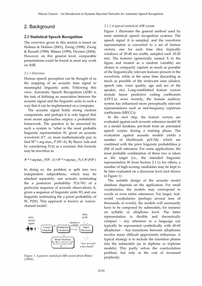
Figure 1. A generic statistical ASR system (from Bilmes(1999)).

2.1.2 A typical statistical ASR systemFigure 1 illustrates the general method used bymost statistical speech recognition systems. Thespeech signal A is sampled, and the waveformrepresentation is converted to a set of featurevectors, one for each time slice (typicallywindows of 20-40 ms width, sampled each 10-20ms). The features (generically named X in thefigure and treated as a random variable) arechosen to compactly capture as much as possibleof the linguistically relevant features present in thewaveform, while at the same time discarding asmuch as possible of the irrelevant ones (dialect,speech rate, voice quality, age and sex of thespeaker, etc). Long-established feature vectorsinclude linear predictive coding coefficients(LPCCs); more recently, the human auditorysystem has influenced more perceptually relevantrepresentations such as mel-frequency cepstrumcoefficients (MFCCs).

In the next step, the feature vectors areevaluated against each acoustic utterance model Min a model database, pre-built from an annotatedspeech corpus during a training phase. Theevaluation against acoustic models yields anumber of likelihoods p(X|M), which arecombined with the prior linguistic probabilities p(M) of each utterance. For some applications, themost probable combination of these two is takenas the target (i.e., the intended linguisticrepresentation W from Section 2.1.1); for others, anumber of high-scoring candidates may be kept tobe later evaluated on a discourse level (not shownin Figure 1).

The suitable design of the acoustic modeldatabase depends on the application. For smallvocabularies, the models may correspond towords or even entire utterances. For larger, real-world vocabularies (perhaps several tens ofthousands of words), the models will necessarilyhave to be composed by submodels, for instanceon syllable or allophone level. The latterrepresentation is flexible and theoreticallycompact – any utterance in a language cantypically be represented symbolically with 40-60allophones – but transitions between allophonesinvolve many difficult approximity influences. Atypical strategy is to include the transition phasesinto the submodels (as in diphone or triphonemodels). This partly solves the coarticulationproblem, but only at the cost of increasedperplexity.

2(10)


The evaluation against the acoustic modelsdoes not usually happen directly. Instead, mostmethods use one or more hidden (i.e., non-observable) variables to represent the currentstate of the speech generation process (thepronunciation model), and maintains aprobability distribution for each observation ina given state (the acoustic model).

2.2 HMM-based systems

2.2.1 Properties of HMM-based systemsIn an ASR system based on Hidden MarkovModels (HMMs), the predominant techniquefor the last decades, two variables are used foreach time slice: one visible Ot (for theobservation at time t) and one hidden Qt (forthe system's state at time t). The latter is usuallyidentified with the current phonetic unit. Inaddition to the (stationary) observationprobabilities associated with each of the Nstates, an HMM keeps a representation of theinitial state probability P(s1) and the statetransition probabilities, P(st+1|st) for each state(also stationary; as in all Markovian models, thestate is assumed to be independent of theprevious history).

The joint probability P(q, o) of a certain statesequence q = q1q2q3...qT given a certainobservation sequence o = o1o2o3...oT may bewritten

)|()|()|()(),(2

1111 tt

T

ttt qoPqqPqoPqPqoP ∏

=−=

There are efficient (O(n2)) algorithms fortraining the parameters (the observation andtransition probabilities and the initial stateprobabilities); for computing the probability ofa certain observation sequence; and for findingthe most probable state sequence given anobservation sequence (Rabiner 1989).

2.2.2 Weaknesses of HMM-based systemsThere are many existing HMM-based ASRsystems, some of them commercial, whichexhibit good recognition performance inconditions closely resembling those of thetraining settings. However, in more varyingconditions, they are generally not very robust,and performance may decrease drasticallywhen facing common real-world (real-word?)phenomena, such as noisy environments,differing speech rates, dialectal variation, and

non-native accents (Holmes & Holmes (2001),Zweig (1998)).

While many state-of-the-art systems with somesuccess employ different adaption techniques toovercome such difficulties, there are arguablycertain inherent restrictions to the entire approach.Most importantly, HMMs encode all stateinformation in just one single variable – to aHMM-based system, speech is little more than afinite sequence of atomic elements, each takenfrom a (likewise finite) set of phonetic states. Thisview excludes potentially importantgeneralizations about the peculiarities of thespeaker – temporary ones, such as position andmovement of the articulators (lips, tongue, jaw,voicelessness, nasalization, etc), as well as morepermanent, such as the speaker's sex and dialect(Zweig (1998)).

3. Bayesian Networks

3.1 Graphical models

3.1.1 What is a graphical model?In a graphical model (Whittaker 1990; sometimescalled "probabilistic graphical model"), a stochasticprocess is described as a graph. The graphcontains a qualitative part, its topography, and aquantitative part, a set of conditional probabilityfunctions. In fact, the entire model can be thoughtof as "a compact and convenient way ofrepresenting a joint probability distribution over afinite set of variables" (after Bengtsson (1999)).

The nodes in a graphical model represent a setof (hidden or observed) random variables X ={X1...Xn}, whose ranges may be continuous ordiscrete. The edges encode the central concept ofconditional independence between variables.

3.1.2 Conditional independenceIf A, B, C are random variables, A is said to beconditionally independent of C given B (written A┴C|B) iff P(A|B, C) = P(A|B); intuitively, this meansthat if we know B, the evidence of C does notinfluence our belief in A. Exactly how conditionalindependence is asserted in the edges of agraphical model may vary. See Section 3.2 for anexample from Bayesian networks, and Stephenson(2000) or Murphy (2001) for useful overviews.

Conditional independence assertions areextremely important. First and foremost, theyallow local inferences. This means that calculations

3(10)


of joint probability distributions ofconditionally independent subsets of variablescan be performed separately, reducingcomplexity. Furthermore, such conditionallyindependent subsets can be combined to formcomplex structures in a modular way.

Disciplined use of conditional independenceassertions whenever depencies aren't strictlynecessary (with the definition of 'necessary' tobe decided by the task at hand) will result insparse networks, i.e., networks with relativelyfew edges per node. This will in itself create atleast three important advantages compared tofully-connected models (Bilmes (2000)):

• sparse network structures have fewercomputational and memory requirements;

• sparse networks are less susceptible to noisein training data (i.e., lower variance) andless prone to overfitting (the smaller thefreedom – here, number of random variables– the less risk that meaningless regularity inthe data will be treated as significant); and

• the resulting structure might reveal high-level knowledge about the underlyingproblem domain that was previouslydrowned out by many extra dependencies.

3.1.3 Properties and subtypes of GMsGMs are very versatile. Combining useful traitsfrom graph theory and probability theory, theyoffer an intuitive, visual representation ofconditional independence, efficient algorithmsfor fast inference, and strong representationalpower. In Michael Jordan's words, they"provide a natural tool for dealing with twoproblems that occur throughout appliedmathematics and engineering – uncertainty andcomplexity" (Jordan (2004)).

Many important current models, such asHMMs, can be expressed as particular instancesof GMs; and a central algorithm such as theBaum-Welch algorithm for HMM training isjust a special case of GM inference (Bilmes(2000)). Indeed, the GM framework is flexibleenough to subsume many existing importanttechniques and by its proponents it is greeted asa unifying statistical framework, greatlyfacilitating experimentation with new statisticalmethods (not only for ASR). Toolkits for GMs

which permits such experimentation areincreasingly available; for ASR, see Bilmes &Zweig (2002).

There are many different types of GMs, eachwith a different formal semantic interpretationand a concomitant different idea of the wayconditional independence is encoded in the graphtopology. Broadly, GMs can be divided intosubclasses according to the graphs they are builtupon: the most important are undirected GMs,where edges denote correlation (Markov randomfields); and directed acyclic GMs, where edgesinformally denote causality (Bayesian networks).The former type is popular among physicists,while the second is much used in AI and,increasingly, ASR research (Murphy (2001)). Therest of this paper will only deal with Bayesiannetworks.

3.2 Bayesian networks

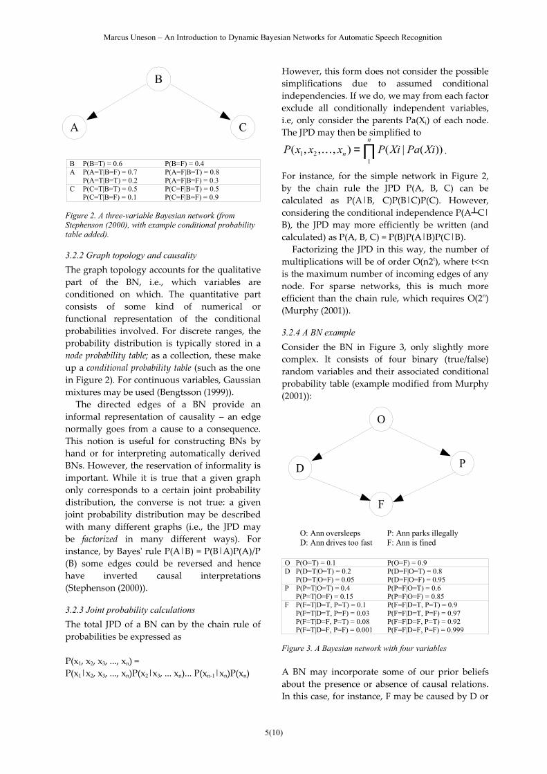
3.2.1 What is a Bayesian network?A Bayesian network is a particular kind of GM: agraph where the each node denote one randomvariable Xi ∊ {X1, X2, ..., Xn} and the (absence of)edges imply conditional independencies. Thehallmark of a BN is that it is built on a directedand acyclic graph. To each variable, a priorconditional probability distribution is associated.Most of the theory for BNs is due to Pearl (1988).

Figure 2 gives an example of a simple Bayesiannetwork, consisting of three binary (T[rue]/F[alse])variables with associated probabilities.

In this BN, the random variable A isconditionally dependent on B, but not on C, i.e. P(A|B, C) = P(A|B). Another way of formulatingthe same fact is to say that the value of C isirrelevant for the local probability P(A, B). Thetable specifies the conditional probabilitydistribution of each node Xi for each combinationof values of its immediate predecessors, whichmore commonly are known as the node's parents.In this paper, the parents of a given node aredenoted Pa(Xi), following Stephenson (2000).

Note that the BN in Figure 2 does not expressthat A and C are totally independent, but only thatB encodes any information from A that influencesC and vice versa. For instance, let A denote "Danwears his coat" and C "Dan has ice in his hair".While A and C are likely to be correlated, theymight still be conditionally independent given forinstance B, "it is a cold day".

4(10)


B P(B=T) = 0.6 P(B=F) = 0.4A P(A=T|B=F) = 0.7

P(A=T|B=T) = 0.2P(A=F|B=T) = 0.8P(A=F|B=F) = 0.3

C P(C=T|B=T) = 0.5P(C=T|B=F) = 0.1

P(C=F|B=T) = 0.5 P(C=F|B=F) = 0.9

Figure 2. A three-variable Bayesian network (fromStephenson (2000), with example conditional probabilitytable added).

3.2.2 Graph topology and causalityThe graph topology accounts for the qualitativepart of the BN, i.e., which variables areconditioned on which. The quantitative partconsists of some kind of numerical orfunctional representation of the conditionalprobabilities involved. For discrete ranges, theprobability distribution is typically stored in anode probability table; as a collection, these makeup a conditional probability table (such as the onein Figure 2). For continuous variables, Gaussianmixtures may be used (Bengtsson (1999)).

The directed edges of a BN provide aninformal representation of causality – an edgenormally goes from a cause to a consequence.This notion is useful for constructing BNs byhand or for interpreting automatically derivedBNs. However, the reservation of informality isimportant. While it is true that a given graphonly corresponds to a certain joint probabilitydistribution, the converse is not true: a givenjoint probability distribution may be describedwith many different graphs (i.e., the JPD maybe factorized in many different ways). Forinstance, by Bayes' rule P(A|B) = P(B|A)P(A)/P(B) some edges could be reversed and hencehave inverted causal interpretations(Stephenson (2000)).

3.2.3 Joint probability calculationsThe total JPD of a BN can by the chain rule ofprobabilities be expressed as

P(x1, x2, x3, ..., xn) = P(x1|x2, x3, ..., xn)P(x2|x3, ... xn)... P(xn-1|xn)P(xn)

However, this form does not consider the possiblesimplifications due to assumed conditionalindependencies. If we do, we may from each factorexclude all conditionally independent variables,i.e, only consider the parents Pa(Xi) of each node.The JPD may then be simplified to

∏=n

n XiPaXiPxxxP1

21 ))(|(),,,( .

For instance, for the simple network in Figure 2,by the chain rule the JPD P(A, B, C) can becalculated as P(A|B, C)P(B|C)P(C). However,considering the conditional independence P(A┴C|B), the JPD may more efficiently be written (andcalculated) as P(A, B, C) = P(B)P(A|B)P(C|B).

Factorizing the JPD in this way, the number ofmultiplications will be of order O(n2t), where t<<nis the maximum number of incoming edges of anynode. For sparse networks, this is much moreefficient than the chain rule, which requires O(2n)(Murphy (2001)).

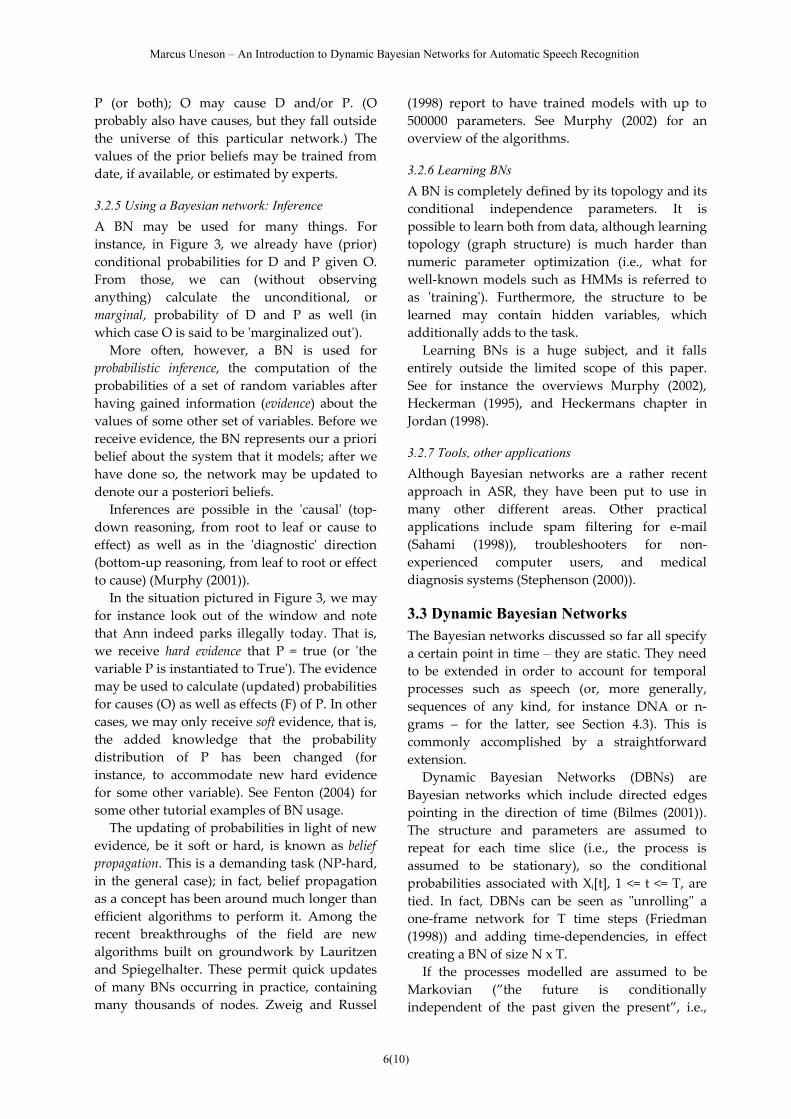
3.2.4 A BN exampleConsider the BN in Figure 3, only slightly morecomplex. It consists of four binary (true/false)random variables and their associated conditionalprobability table (example modified from Murphy(2001)):

O

D P

F

O: Ann oversleeps P: Ann parks illegallyD: Ann drives too fast F: Ann is fined

O P(O=T) = 0.1 P(O=F) = 0.9D P(D=T|O=T) = 0.2 P(D=F|O=T) = 0.8

P(D=T|O=F) = 0.05 P(D=F|O=F) = 0.95P P(P=T|O=T) = 0.4 P(P=F|O=T) = 0.6

P(P=T|O=F) = 0.15 P(P=F|O=F) = 0.85F P(F=T|D=T, P=T) = 0.1 P(F=F|D=T, P=T) = 0.9

P(F=T|D=T, P=F) = 0.03 P(F=F|D=T, P=F) = 0.97P(F=T|D=F, P=T) = 0.08 P(F=F|D=F, P=T) = 0.92P(F=T|D=F, P=F) = 0.001 P(F=F|D=F, P=F) = 0.999

Figure 3. A Bayesian network with four variables

A BN may incorporate some of our prior beliefsabout the presence or absence of causal relations.In this case, for instance, F may be caused by D or

5(10)

B

A C


P (or both); O may cause D and/or P. (Oprobably also have causes, but they fall outsidethe universe of this particular network.) Thevalues of the prior beliefs may be trained fromdate, if available, or estimated by experts.

3.2.5 Using a Bayesian network: InferenceA BN may be used for many things. Forinstance, in Figure 3, we already have (prior)conditional probabilities for D and P given O.From those, we can (without observinganything) calculate the unconditional, ormarginal, probability of D and P as well (inwhich case O is said to be 'marginalized out').

More often, however, a BN is used forprobabilistic inference, the computation of theprobabilities of a set of random variables afterhaving gained information (evidence) about thevalues of some other set of variables. Before wereceive evidence, the BN represents our a prioribelief about the system that it models; after wehave done so, the network may be updated todenote our a posteriori beliefs.

Inferences are possible in the 'causal' (top-down reasoning, from root to leaf or cause toeffect) as well as in the 'diagnostic' direction(bottom-up reasoning, from leaf to root or effectto cause) (Murphy (2001)).

In the situation pictured in Figure 3, we mayfor instance look out of the window and notethat Ann indeed parks illegally today. That is,we receive hard evidence that P = true (or 'thevariable P is instantiated to True'). The evidencemay be used to calculate (updated) probabilitiesfor causes (O) as well as effects (F) of P. In othercases, we may only receive soft evidence, that is,the added knowledge that the probabilitydistribution of P has been changed (forinstance, to accommodate new hard evidencefor some other variable). See Fenton (2004) forsome other tutorial examples of BN usage.

The updating of probabilities in light of newevidence, be it soft or hard, is known as beliefpropagation. This is a demanding task (NP-hard,in the general case); in fact, belief propagationas a concept has been around much longer thanefficient algorithms to perform it. Among therecent breakthroughs of the field are newalgorithms built on groundwork by Lauritzenand Spiegelhalter. These permit quick updatesof many BNs occurring in practice, containingmany thousands of nodes. Zweig and Russel

(1998) report to have trained models with up to500000 parameters. See Murphy (2002) for anoverview of the algorithms.

3.2.6 Learning BNsA BN is completely defined by its topology and itsconditional independence parameters. It ispossible to learn both from data, although learningtopology (graph structure) is much harder thannumeric parameter optimization (i.e., what forwell-known models such as HMMs is referred toas 'training'). Furthermore, the structure to belearned may contain hidden variables, whichadditionally adds to the task.

Learning BNs is a huge subject, and it fallsentirely outside the limited scope of this paper.See for instance the overviews Murphy (2002),Heckerman (1995), and Heckermans chapter inJordan (1998).

3.2.7 Tools, other applicationsAlthough Bayesian networks are a rather recentapproach in ASR, they have been put to use inmany other different areas. Other practicalapplications include spam filtering for e-mail(Sahami (1998)), troubleshooters for non-experienced computer users, and medicaldiagnosis systems (Stephenson (2000)).

3.3 Dynamic Bayesian Networks The Bayesian networks discussed so far all specifya certain point in time – they are static. They needto be extended in order to account for temporalprocesses such as speech (or, more generally,sequences of any kind, for instance DNA or n-grams – for the latter, see Section 4.3). This iscommonly accomplished by a straightforwardextension.

Dynamic Bayesian Networks (DBNs) areBayesian networks which include directed edgespointing in the direction of time (Bilmes (2001)).The structure and parameters are assumed torepeat for each time slice (i.e., the process isassumed to be stationary), so the conditionalprobabilities associated with Xi[t], 1 <= t <= T, aretied. In fact, DBNs can be seen as "unrolling" aone-frame network for T time steps (Friedman(1998)) and adding time-dependencies, in effectcreating a BN of size N x T.

If the processes modelled are assumed to beMarkovian (”the future is conditionallyindependent of the past given the present”, i.e.,

6(10)


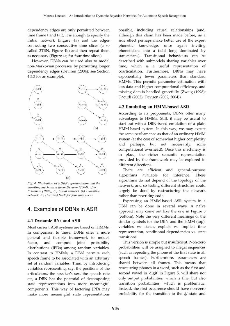
dependency edges are only permitted betweentime frame t and t+1), it is enough to specify theinitial network (Figure 4a) and the edgesconnecting two consecutive time slices (a socalled 2TBN, Figure 4b) and then repeat themas necessary (Figure 4c, for four time slices).

However, DBNs can be used also to modelnon-Markovian processes, by permitting longerdependency edges (Deviren (2004); see Section4.3.3 for an example).

Fig. 4. Illustration of a DBN representation and theunrolling mechanism (from Deviren (2004), afterFriedman (1998)) (a) Initial network. (b) Transitionnetwork. (c) Unrolled DBN for four time slices.

4. Examples of DBNs in ASR

4.1 Dynamic BNs and ASRMost current ASR systems are based on HMMs.In comparison to these, DBNs offer a moregeneral and flexible framework to model,factor, and compute joint probabilitydistributions (JPDs) among random variables.In contrast to HMMs, a DBN permits eachspeech frame to be associated with an arbitraryset of random variables. Thus, by introducingvariables representing, say, the positions of thearticulators, the speaker's sex, the speech rateetc, a DBN has the potential of decomposingstate representations into more meaningfulcomponents. This way of factoring JPDs maymake more meaningful state representations

possible, including causal relationships (and,although this claim has been made before, as aside effect perhaps make better use of the expertphonetic knowledge, once again invitingphoneticians into a field long dominated bystatisticians). Transitional behaviours can bedescribed with submodels sharing variables overtime, which is a useful representation ofcoarticulation. Furthermore, DBNs may haveexponentially fewer parameters than standardHMMs. This permits parameter estimation withless data and higher computational efficiency, andmissing data is handled gracefully (Zweig (1998);Daoudi (2002); Deviren (2002, 2004)).

4.2 Emulating an HMM-based ASRAccording to its proponents, DBNs offer manyadvantages to HMMs. Still, it may be useful tostart out with a DBN-based emulation of a plainHMM-based system. In this way, we may expectthe same performance as that of an ordinary HMMsystem (at the cost of somewhat higher complexityand perhaps, but not necessarily, somecomputational overhead). Once this machinery isin place, the richer semantic representationprovided by the framework may be explored indifferent directions.

There are efficient and general-purposealgorithms available for inference. Thesealgorithms do not depend of the topology of thenetwork, and so testing different structures couldlargely be done by restructuring the networkrather than rewriting code.

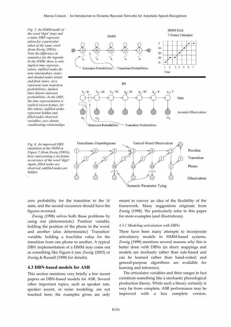
Expressing an HMM-based ASR system in aDBN can be done in several ways. A naïveapproach may come out like the one in Figure 5(bottom). Note the very different meanings of thesimilar symbols for the DBN and the HMM (top):variables vs. states, explicit vs. implicit timerepresentation, conditional dependencies vs. statetransitions.

This version is simple but insufficient. Non-zeroprobabilities will be assigned to illegal sequences(such as repeating the phone of the first state in allspeech frames). Furthermore, parameters areshared between all frames. This means thatreoccurring phones in a word, such as the first andsecond vowel in 'digit' in Figure 5, will share notonly output probabilities, which is fine, but alsotransition probabilities, which is problematic.Instead, the first occurence should have non-zeroprobability for the transition to the /j/ state and

7(10)


zero probability for the transition to the /t/state, and the second occurence should have thefigures reversed.

Zweig (1998) solves both these problems byusing one (deterministic) 'Position' variable,holding the position of the phone in the word,and another (also deterministic) 'Transition'variable, holding a true/false value for thetransition from one phone to another. A typicalDBN implementation of a HMM may come outas something like Figure 6 (see Zweig (2003) orZweig & Russell (1998) for details).

4.3 DBN-based models for ASRThis section mentions very briefly a few recentpapers on DBN-based models for ASR. Severalother important topics, such as speaker rate,speaker accent, or noise modeling, are nottouched here; the examples given are only

meant to convey an idea of the flexibility of theframework. Many suggestions originate fromZweig (1998). We particularly refer to this paperfor more examples (and illustrations).

4.3.1 Modeling articulation with DBNsThere have been many attempts to incorporatearticulatory models in HMM-based systems.Zweig (1998) mentions several reasons why this isbetter done with DBNs (in short: mappings andmodels are stochastic rather than rule-based andcan be learned rather than hand-coded; andgeneral-purpose algorithms are available forlearning and inference).

The articulator variables and their ranges in factconstitute something like a stochastic phonologicalproduction theory. While such a theory certainly isvery far from complete, ASR performance may beimproved with a less complete version.

8(10)

Fig. 5. An HMM model ofthe word 'digit' (top) anda naïve DBN represen-tation for a particulartoken of the same word(from Zweig (2003)). Note the difference insemantics for the legends:In the HMM, there is onlyimplicit time represen-tation; unfilled nodes de-note intermediary statesand shaded nodes initialand final states; arcsrepresent state transitionprobabilities; dashedlines denote emissionprobabilities. In the DBN,the time representation isexplicit (seven frames, forthis token); unfilled nodesrepresent hidden andfilled nodes observedvariables; arcs denoteconditioning relationships

Fig. 6. An improved DBNemulation of the HMM inFigure 5 (from Zweig (2003)),here representing a six-frameoccurrence of the word 'digit' .Again, filled nodes areobserved, unfilled nodes arehidden .


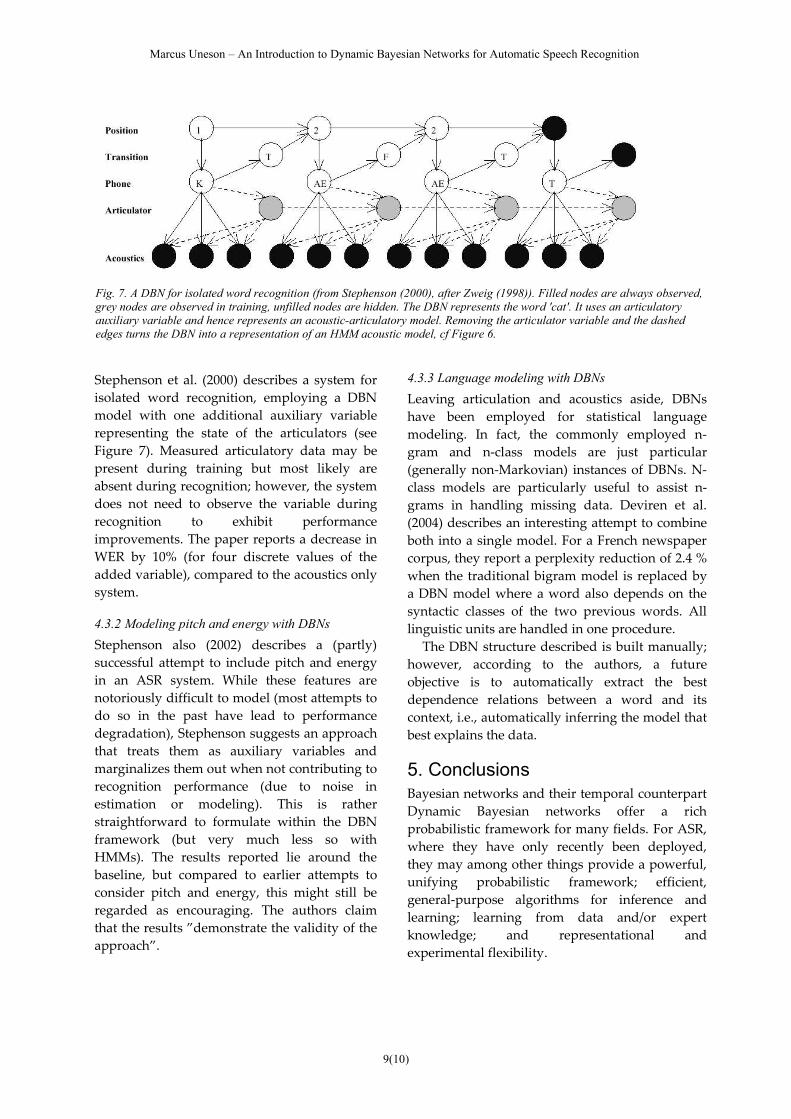
Stephenson et al. (2000) describes a system forisolated word recognition, employing a DBNmodel with one additional auxiliary variablerepresenting the state of the articulators (seeFigure 7). Measured articulatory data may bepresent during training but most likely areabsent during recognition; however, the systemdoes not need to observe the variable duringrecognition to exhibit performanceimprovements. The paper reports a decrease inWER by 10% (for four discrete values of theadded variable), compared to the acoustics onlysystem.

4.3.2 Modeling pitch and energy with DBNsStephenson also (2002) describes a (partly)successful attempt to include pitch and energyin an ASR system. While these features arenotoriously difficult to model (most attempts todo so in the past have lead to performancedegradation), Stephenson suggests an approachthat treats them as auxiliary variables andmarginalizes them out when not contributing torecognition performance (due to noise inestimation or modeling). This is ratherstraightforward to formulate within the DBNframework (but very much less so withHMMs). The results reported lie around thebaseline, but compared to earlier attempts toconsider pitch and energy, this might still beregarded as encouraging. The authors claimthat the results ”demonstrate the validity of theapproach”.

4.3.3 Language modeling with DBNsLeaving articulation and acoustics aside, DBNshave been employed for statistical languagemodeling. In fact, the commonly employed n-gram and n-class models are just particular(generally non-Markovian) instances of DBNs. N-class models are particularly useful to assist n-grams in handling missing data. Deviren et al.(2004) describes an interesting attempt to combineboth into a single model. For a French newspapercorpus, they report a perplexity reduction of 2.4 %when the traditional bigram model is replaced bya DBN model where a word also depends on thesyntactic classes of the two previous words. Alllinguistic units are handled in one procedure.

The DBN structure described is built manually;however, according to the authors, a futureobjective is to automatically extract the bestdependence relations between a word and itscontext, i.e., automatically inferring the model thatbest explains the data.

5. ConclusionsBayesian networks and their temporal counterpartDynamic Bayesian networks offer a richprobabilistic framework for many fields. For ASR,where they have only recently been deployed,they may among other things provide a powerful,unifying probabilistic framework; efficient,general-purpose algorithms for inference andlearning; learning from data and/or expertknowledge; and representational andexperimental flexibility.

9(10)

Fig. 7. A DBN for isolated word recognition (from Stephenson (2000), after Zweig (1998)). Filled nodes are always observed,grey nodes are observed in training, unfilled nodes are hidden. The DBN represents the word 'cat'. It uses an articulatoryauxiliary variable and hence represents an acoustic-articulatory model. Removing the articulator variable and the dashededges turns the DBN into a representation of an HMM acoustic model, cf Figure 6.


ReferencesBengtsson, H. (1999) Bayesian Networks - a self-

contained introduction with implementation remarks,Unpublished Master's Thesis, Lund Institute ofTechnology, Lund, Sweden.

Bilmes, J. (1999) Natural Statistical Models forAutomatic Speech Recognition, Unpublished PhDthesis, International Computer Science Institute,Berkeley.

Bilmes, J. (2000) Dynamic Bayesian Multinets,Proceedings of the 16th Conference on Uncertainty inArtificial Intelligence, Stanford, July 2000

Bilmes, J. (2001) Graphical Models and AutomaticSpeech Recognition (Technical Report UWEETR-2001-0005): University of Washington, Departmentof Electrical Engineering.

Bilmes, J., and Zweig, G. (2002) The GraphicalModels Toolkit: An Open Source Software SystemFor Speech and Time-Series Processing, Proceedingsof the International Conference on Acoustics Speech andSignal Processing (ICASSP 2002), Orlando

Daoudi, K. (2002) Automatic Speech Recognition:The New Millennium, Proceedings of the 15thInternational Conference on Industrial andEngineering, Applications of Artificial Intelligence andExpert Systems: Developments in Applied ArtificialIntelligence, 253-263.

Deviren, M. (2002) Dynamic Bayesian Networks forAutomatic Speech Recognition, Proceedings of theThe Eighteenth National Conference on ArtificialIntelligence, Edmonton

Deviren, M. (2004) Systèmes de reconnaissance de laparole revisités : Réseaux Bayésiens dynamiques etnouveaux paradigmes, Unpublished PhD thesis,Université Henri Poincaré, Nancy.

Deviren, M., Daoudi, K., and Smaîli, K. (2004)Language Modeling using Dynamic BayesianNetworks, Proceedings of the LREC 2004, Lisbon,May 2004

Fenton, N. (2004) Probability Theory and BayesianBelief Nets. Web course (accessed 20050114):http://www.dcs.qmw.ac.uk/ ~norman/ BBNs/BBNs.htm .

Friedman, N., Murphy, K., and Russell, S. (1998)Learning the structure of dynamic probabilisticnetworks, Proceedings of the UAI'98, Madison,Wisconsin

Heckerman, D. (1995) A tutorial on learning withBayesian networks (Technical Report MSR-TR-95-06), Redmond, Washington, USA: MicrosoftResearch.

Heckerman, D. (1998) A tutorial on learning withBayesian networks, in M. Jordan (ed.), Learning inGraphical Models, MIT Press.

Jordan, M. I. (2004) Graphical Models, Statistical Science,19, 140-155.

Murphy, K. (2001) An Introduction to GraphicalModels. Unpublished tutorial. http://www.ai.mit.edu/~murphyk/Bayes/bayes.html

Murphy, K. (2002) Dynamic Bayesian Networks:Representation, Inference and Learning, UnpublishedPhD thesis, UC Berkeley.

Pearl, J. (1988) Probabilistic Reasoning in IntelligentSystems:Networks of Plausible Inference, MorganKaufmann., San Mateo,California.

Rabiner, L. R. (1989) A Tutorial on Hidden MarkovModels and Selected Applications in SpeechRecognition, Proc of the IEEE, 77, 2, 257-286.

Sahami, M., Dumais, S., Heckerman, D., and Horvitz, E.(1998) A Bayesian Approach to Filtering Junk E-mail,Proceedings of the AAAI'98 Workshop on Learning forText Categorization, Madison, Wisconsin, July 27 1998

Stephenson, T. A. (2000) An Introduction to BayesianNetwork Theory and Usage (Technical report IDIAP-RR00-03): IDIAP.

Stephenson, T. A., Bourlard, H., Bengio, S., and Morris,A. C. (2000) Automatic speech recognition usingdynamic Bayesian networks with both acoustic andarticulatory variables, Proceedings of the ICSLP 2000,October 2000, 951-954.

Stephenson, T. A., Escofet, J., Magimai-Doss, M., andBourlard, H. (2002) Dynamic Bayesian Network BasedSpeech Recognition with Pitch and Energy asAuxiliary Variables, Proceedings of the IEEEInternational Workshop on Neural Networks for for SignalProcessing (NNSP 2002)

Whittaker, J. (1990) Graphical Models in AppliedMultivariate Statistics, John Wiley & Sons Ltd,Chichester,UK.

Zweig, G. (1998) Speech Recognition with DynamicBayesian Networks, Unpublished Doctorate thesis,University of California, Berkeley.

Zweig, G. (2003) Bayesian network structures andinference techniques for automatic speech recognition,Computer Speech and Language, 17, 173-193.

Zweig, G., and Russell, S. (1998) Speech Recognitionwith Dynamic Bayesian Networks, Proceedings of theThe fifteenth national/tenth conference on Artificialintelligence/Innovative applications of artificial intelligence,173-180.

10(10)

Documents

An Introduction to Dynamic Bayesian Networks for Automatic Speech Recognition