RICERCA DI SISTEMA ELETTRICO

An Immersed Volume Method for Large Eddy Simulation of compressible flows

G. Rossi, N.M. Arcidiacono, F.R. Picchia, B. Favini

Report RdS/2011/211

Agenzia Nazionale per le Nuove Tecnologie, l’Energia e lo Sviluppo Economico Sostenibile

AN IMMERSED VOLUME METHOD FOR LARGE EDDY SIMULATION OF COMPRESSIBLE FLOWS

D. Cecere, E. Giacomazzi, N.M. Arcidiacono, F.R. Picchia, F.Donato

ENEA

Settembre 2011

Report Ricerca di Sistema Elettrico

Accordo di Programma Ministero dello Sviluppo Economico – ENEA

Area: Produzione di energia elettrica e protezione dell’ambiente

Progetto: 2.2 – Studi sull’utilizzo pulito dei combustibili fossili, cattura e sequestro della CO2

Responsabile Progetto: Antonio Calabrò, ENEA

Pag. di

Copia di

Unità UTTEI - COMSO

Classificazione UTTEI-COMSO COMSO/2011/009IL /

Distribuzione: Interna/Libera

Progetto

CERSE- Ricerca di Sistema Elettrico

AdP Ministero dello Sviluppo Economico – ENEA

Area: Produzione e fonti energetiche

Tema: 5.2.2.2 Tecnologie innovative per migliorare i

rendimenti di conversione delle centrali a polverino di carbone

Parole chiave - MILD Combustion - Turbine a gas - Trapped vortex - Simulazione numerica

Attività Aumento dell’efficienza delle tecnologie di cattura della CO2 con produzione di elettricità “zero emission”

Titolo An Immersed Volume Method for Large Eddy Simulation of compressible flows Autori D. Cecere, E. Giacomazzi, N.M. Arcidiacono, F.R. Picchia, F. Donato ENEA UTTEI/COMSO

Sommario Il documento descrive l’applicazione di una nuova tecnica , denominata Immersed Volume Method (IVM), per consentire il trattamento di geometrie complesse 3D da parte di un codice CFD di tipo compressibile alle differenze finite basato su griglie strutturate non uniformi e ‘staggered’. La tecnica è stata implementata nel codice HeaRT e validata con un caso test significativo.

4 D.Cecere S.Giammartini

3 E.Giacomazzi

2 N.M.Arcidiacono

1 F.R. Picchia

0 F. Donato Rev Descrizione Redazione Data Convalida Data Approvazione Data

An Immersed Volume Method for Large Eddy

Simulation of compressible flows

D. Cecere,a, E. Giacomazzia, N.M. Arcidiaconoa, F.R. Picchiaa, F. Donatoa

aSustainable Combustion Laboratories, ENEA, Rome, Italy.

Abstract

In this work a technique for treating complex geometries in a compressible

code using staggered non uniform cartesian grids and finite difference method

is developed. The new method developed is called Immersed Volume Method

(IVM) and consists in the application (to each scalar of the Navier Stokes

equations) of a finite volume method in the cartesian cells cutted by the

complex surface geometry. Accurate description of the real three dimensional

geometry inside the cell volume is preserved by means of triangulated surface

description (STL stereolithography) instead of approximating it by a plane.

Since in the finite volume method, the geometric quantities of the cutted cell

like face’s areas, volume, volume centroid, face’s areas centroids are needed,

all these properties are evaluated by means of a specific code developed for

this goal. In the Navier-Stokes solver, the finite volume method is applied

to the cutted cells. The uxes are formulated using a modified version of the

advection upstream splitting method (AUSM) originally proposed by Liou

and Steffen. The recontruction of the variables at the cell interfaces, is done

by means of a third order TVD (Total Variation Diminishing) interpolator.

This choice is related to the future application of the method to combustors

with complex geometries, and so the limitation of numerical wiggles for the

chemical species is a must. In this way, the overall second-order accuracy

of the base solver is preserved. The Large Eddy Simulation (LES) solver is

parallelized using domain decomposition and message passing interface. The

robustness and accuracy of the method is validated using LES of a ow past

a cube.

Key words:

Complex Geometries, Cut-Cell Method, Finite Difference Staggered

Approach, Large Eddy Simulation.

1. Introduction

The development of Large Eddy Simulation (LES) as a methodology ap-

plied to a wide variety of turbulent flows, ranging from problems of scientific

interest to those with engineering applications has been possible due to a

rapid increase in computational power. In all engineering computational

fluid dynamic problems in order to obtain satisfactory results the primary

goals of a successful LES are accuracy, robustness and handling of complex

three-dimensional geometry. In fact many flow physical problem involve geo-

metrical complexities with irregular boundaries that usually are not alligned

with the grid. Unstructured grids doesn’t present constraint on the cell size

and aspect ratio, but they are known to be not well suited for time-resolving

turbulent flow computations as LES. The numerical method should not be

sensitive to aliasing errors. Finite difference schemes provide good resolu-

tion while staggering of variables leads to improved robustness respect to a

collocated approach without sacrificing conservation [1]. Total energy con-

servation, in fact, is guaranteed by the full conservative form of the governing

2

equations. Staggered grids have been proposed earlier for solution of the com-

pressible Navier-Stokes equations, recent research includes that of Kopriva

[2] who uses a spectral method along with staggering of flux location with

respect to the conserved variables, Djambazov et al. [3] that used a higher-

order staggered (in space and time) method to solve the linearized Euler

equations for computational aeroacoustics, Nagarajan et al. [1] that solved

Navier-Stokes equations adopting high order compact schemes on staggered

arrengements of the conserved variables. Two major class of methods are

suitable for treating arbitrarily complex geometries with cartesian grids and

distinguished on the basis of their approach to impose boundary conditions in

the cells cut by the solid interface. The first is the classical Immersed Boun-

day (IB) methods where special interpolations are adopted to set the value

of dependent variables in the cut cells [4; 5]. These methods are attractive

because of their semplicity, but their major drowbacks are the occurrence of

non-divergence free velocities in incompressible flows and spurius non physi-

cal pressure oscillations in compressible ones due to not observation of strict

conservation of quantities as mass, momentum and kinetic energy near the

irregular boundaries [6; 7]. A second class of IB methods is the cut-cell

method (also called Cartesian grid methods) introduced first by Clarke [8].

The cut-cell method is based on a finite-volume discretization of the flow

equations in the cells cut by the immersed interface and the discrete con-

servation is verified. For sharp-interface cartesian grid methods, the ”small

cell problem” [9] of numerical instability would arise when finite difference or

finite volume methods are applied to small-sized irregular cut grid cells. This

may significantly restrict the time steps in temporal integration. Johansen

3

and Colella [10] adopted a flux redistribution procedure. Most notable is

the cell merging technique used by Chung [13] that link small cells and ad-

jacent fluid cells to form a master-slave pair. Very few cut cell method for

staggered grids have been reported in literature: Meyer et al. [11] proposed

a conservative, second-order accurate Cartesian cut-cell for incompressible

Navier-Stokes equations on three-dimensional non uniform staggered grids

applicable to finite-volume discretization. To ensure numerical stability for

small cells they follow the conservative mixing procedure by Hu et al. [12].

Cheny et al. [14] proposed a new IB method, based on the MAC method

[15] for staggered Cartesian grids where the irregular boundary is sharply

represented by its level-set function and flow variables are computed in the

cut cells and not interpolated. On a non-staggered grid, not only the ve-

locity and pressure are colocated at nodes , but the position and geometry

of the associated cells is also identical. With a staggered grid, the density

cell and the cells associated with each of the three velocity components are

at a different location and will generally have a different shape when they

are cut by an embedded boundary. A cut cell scheme for a staggered grid

must deal with this extra complexity in a consistent manner. The purpose

of this work is to present a new efficient, conservative, second-order accurate

Cartesian cut-cell method, called Immersed Volume Method (IVM) for the

compressible Navier-Stokes equations solved by finite difference method on

three-dimensional not uniform staggered grids. This method is suitable for

the extension to solid/fluid heat conduction and to moving boundaries. The

immersed boundary is represented by means of a triangulated surface (STL

representation). The full geometrical characteristics of the cut cells are iden-

4

tified in a preprocessor procedure. Flow variables fluxes are computed in the

cut cells and in a second adjacent layer to couple finite volume with finite

difference method. The IVM method, by means of finite volume method,

solves exactly the flow variables in the cut cells and links the velocities and

energy fluxes to the thermodynamic variable changes and overcoming in this

way the drowbacks of classical IB methods. The finite volume method is then

applied also to a second layer to couple IVM to the finite difference method

of the general code. The flow variables are stored at the cut-cell centroid and,

to ensure numerical stability for small cells, the basic idea is to combine sev-

eral neighbouring cells together so that the interfaces between merged cells

are ignored and waves can travel in a newly combined larger cell without

reducing the global time step [16; 17]. The paper is organized as follows. In

section 2 we describe the procedures adopted for determining the geometrical

characteristics of the cut cells. Section 3 presents the IVM discretization for

the calculation of continuity, momentum and energy convective and diffusive

fluxes. Section 4 is devoted to a numerical test on canonical non reactive

flows at low Reynolds number for assessing the accuracy and robustness of

the IVM method.

2. Cut cell characteristics evaluation

In the Immersed Volume Method a finite volume approach is applied to

the two cell’s layers adjacent to the solid surface. The first layer consists of

cells that are directly cut from the solid surface, while the latter is formed by

fluid cells that are in contact with cut cells. The presence of this second layer

is needed to connect the finite volume method with the finite difference one.

5

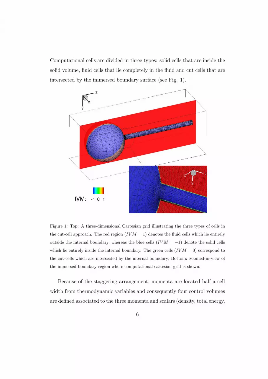
Computational cells are divided in three types: solid cells that are inside the

solid volume, fluid cells that lie completely in the fluid and cut cells that are

intersected by the immersed boundary surface (see Fig. 1).

Figure 1: Top: A three-dimensional Cartesian grid illustrating the three types of cells in

the cut-cell approach. The red region (IV M = 1) denotes the fluid cells which lie entirely

outside the internal boundary, whereas the blue cells (IV M = −1) denote the solid cells

which lie entirely inside the internal boundary. The green cells (IV M = 0) correspond to

the cut-cells which are intersected by the internal boundary; Bottom: zoomed-in-view of

the immersed boundary region where computational cartesian grid is shown.

Because of the staggering arrangement, momenta are located half a cell

width from thermodynamic variables and consequently four control volumes

are defined associated to the three momenta and scalars (density, total energy,

6

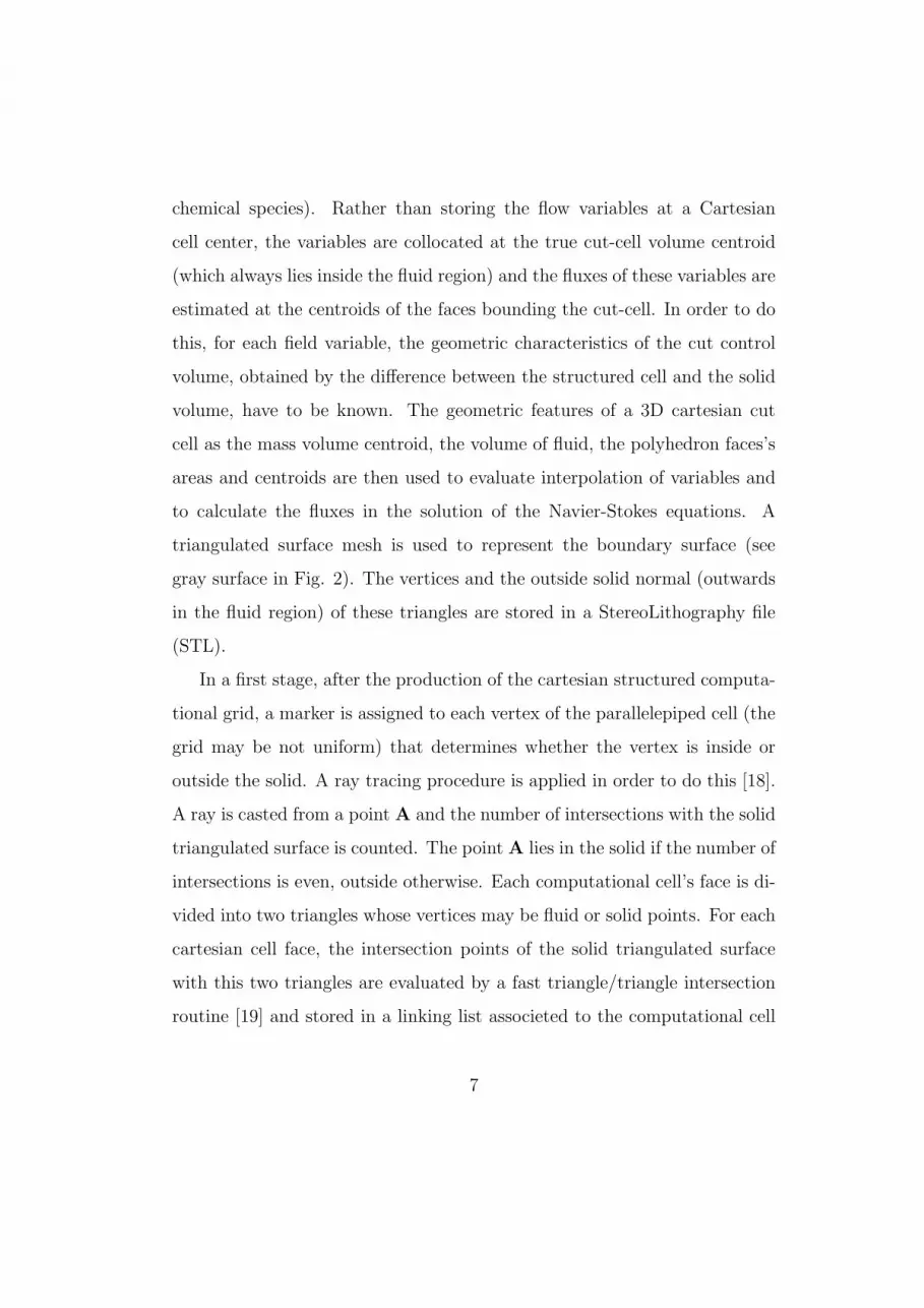
chemical species). Rather than storing the flow variables at a Cartesian

cell center, the variables are collocated at the true cut-cell volume centroid

(which always lies inside the fluid region) and the fluxes of these variables are

estimated at the centroids of the faces bounding the cut-cell. In order to do

this, for each field variable, the geometric characteristics of the cut control

volume, obtained by the difference between the structured cell and the solid

volume, have to be known. The geometric features of a 3D cartesian cut

cell as the mass volume centroid, the volume of fluid, the polyhedron faces’s

areas and centroids are then used to evaluate interpolation of variables and

to calculate the fluxes in the solution of the Navier-Stokes equations. A

triangulated surface mesh is used to represent the boundary surface (see

gray surface in Fig. 2). The vertices and the outside solid normal (outwards

in the fluid region) of these triangles are stored in a StereoLithography file

(STL).

In a first stage, after the production of the cartesian structured computa-

tional grid, a marker is assigned to each vertex of the parallelepiped cell (the

grid may be not uniform) that determines whether the vertex is inside or

outside the solid. A ray tracing procedure is applied in order to do this [18].

A ray is casted from a point A and the number of intersections with the solid

triangulated surface is counted. The point A lies in the solid if the number of

intersections is even, outside otherwise. Each computational cell’s face is di-

vided into two triangles whose vertices may be fluid or solid points. For each

cartesian cell face, the intersection points of the solid triangulated surface

with this two triangles are evaluated by a fast triangle/triangle intersection

routine [19] and stored in a linking list associeted to the computational cell

7

Figure 2: Example of STL boundary surface representation and cut cell. Black line:

cut structured cell; Blu line: immersed boundary surface/cut cell intersection; gray line:

immersed boundary surface represented by triangulation, gray solid: internal solid part of

the immersed boundary.

face. For each cartesian cell face, the intersection points are ordered to form

a polyline that divides the face into two polygons respectively in the fluid and

solid region (remember that the vertices of the face are mapped as internal or

external to the solid as shown for all points in Fig. 1). The wet polygons are

triangularized by a Delaunay triangulation, where the intersection polyline

of each face is adopted as a constrain. This boolean operations are performed

for all the faces of the cell. The faces’ wet polygons form a 3D polyhedron

8

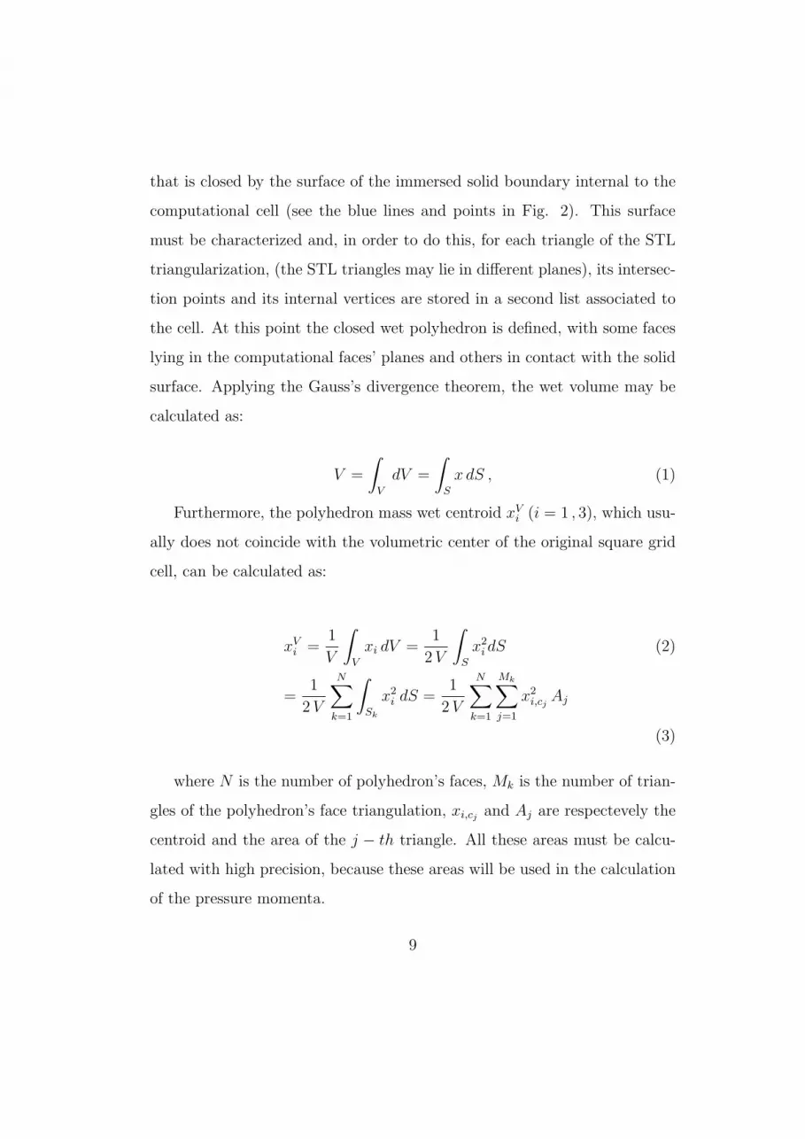
that is closed by the surface of the immersed solid boundary internal to the

computational cell (see the blue lines and points in Fig. 2). This surface

must be characterized and, in order to do this, for each triangle of the STL

triangularization, (the STL triangles may lie in different planes), its intersec-

tion points and its internal vertices are stored in a second list associated to

the cell. At this point the closed wet polyhedron is defined, with some faces

lying in the computational faces’ planes and others in contact with the solid

surface. Applying the Gauss’s divergence theorem, the wet volume may be

calculated as:

V =

∫

V

dV =

∫

S

x dS , (1)

Furthermore, the polyhedron mass wet centroid xVi (i = 1 , 3), which usu-

ally does not coincide with the volumetric center of the original square grid

cell, can be calculated as:

xVi =

1

V

∫

V

xi dV =1

2 V

∫

S

x2i dS (2)

=1

2 V

N∑

k=1

∫

Sk

x2i dS =

1

2 V

N∑

k=1

Mk∑

j=1

x2i,cj

Aj

(3)

where N is the number of polyhedron’s faces, Mk is the number of trian-

gles of the polyhedron’s face triangulation, xi,cjand Aj are respectevely the

centroid and the area of the j − th triangle. All these areas must be calcu-

lated with high precision, because these areas will be used in the calculation

of the pressure momenta.

9

3. Governing Equations

Fluid dynamic is governed by a set of transport equations expressing

the conservation of mass, momentum and energy, and by a thermodynamic

equation of state describing the gas behaviour. The derivation of these con-

servation equations from mass, species and energy balances may be found

in standard books. For a mixture of Ns ideal gases in local thermodynamic

equilibrium and chemical nonequilibrium, the corresponding field equations

(extended Navier-Stokes equations) are:

• Transport Equation of Mass

∂ρ

∂t+ ∇ · (ρu) = 0 (4)

• Transport Equation of Momentum

∂ρu

∂t+ ∇ · (ρuu) = ∇ · S + ρ

Ns∑

i=1

Yifi (5)

• Transport Equation of Total Energy (internal + mechanical, E + K)

∂ρU

∂t+ ∇ · [ρuU ] = ∇ · (Su) −∇ · q + ρ

Ns∑

i=1

Yifi · (u + Vi) (6)

• Transport Equation of Species Mass Fraction

∂ρYi

∂t+ ∇ · (ρuYi) = −∇ · Ji + ωi (7)

• Thermodynamic Equation of State

p = ρNs∑

i=1

Yi

Wi

RuT (8)

10

These equations must be coupled with the constitutive equations which

describe the molecular transport properties of the flow.

In above equations, t is the time variable, ρ the density, u the velocity, S

the stress tensor, U the total energy per unit of mass, E and K respectively

the internal and mechanical (i.e., kinetic) energies per unit of mass, q is the

heat flux, p the pressure, T the temperature. For what concerns chemical

species, fi is the body force per unit of mass acting on the species i, with

molecular weight Wi and mass fraction Yi, ωi is the production/destruction

rate of species i, diffusing at velocity Vi and resulting in a diffusive mass flux

Ji. Finally, Ru is the universal gas constant.

Summation of all species transport equations (7) yields the total mass

conservation equation (4). Therefore, the Ns species transport equations (7)

and the mass conservation equation (4) are linearly dependent and one of

them is redundant. Furthermore, to be consistent with mass conservation,

the diffusion fluxes (Ji = ρYiVi) and chemical source terms must satisfy

Ns∑

i=1

Ji = 0 andNs∑

i=1

ωi = 0 . (9)

In particular, the constraint on the summation of chemical source terms

derives from mass conservation for each of the Nr chemical reactions of a

chemical mechanism. With the tensor notation this mechanism can be writ-

ten as

ν′

ijAi = ν′′

ijAi with i = 1, ..., Ns and j = 1, ..., Nr , (10)

where ν′

ij and ν′′

ij are the stoichiometric coefficients of species i on the left (′

)

and right side (′′

) of the j−th reaction. Since mass is given by the product of

11

number of moles times molecular weight, mass conservation for each reaction,

m′

j = m′′

j , is written as

Ns∑

i=1

(

ν′′

ij − ν′

ij

)

Wi = 0 with j = 1, ..., Nr . (11)

The net source / sink term of the i − th chemical species is

ωi =Nr∑

j=1

ωij = Wi

Nr∑

j=1

(

ν′′

ij − ν′

ij

)

ωRj with i = 1, ..., Ns , (12)

ωRj being the reaction rate associated to the j − th reaction. Summing Eqn.

(12) over the number of chemical species Ns,

Ns∑

i=1

ωi =Nr∑

j=1

ωRj

Ns∑

i=1

Wi

(

ν′′

ij − ν′

ij

)

= 0 , (13)

after using Eqn. (11).

4. IVM method discretization

While the ux evaluation is straightforward in structured grid areas, it

becomes more difficult on partial surfaces at fine-coarse cell interfaces and

near boundaries. In the proposed formulation, the least-squares method is

utilized to obtain a discretization scheme which is flexible in terms of the

local mesh topology and the presence and shape of embedded boundaries.

4.1. Interface value calculation

The cell interface values of the solution variables are found using Taylor

series expansion of solution variables about the cell center. The left and right

state values of any scalar at the interface between two adjacent cells i and j

is calculated as:

12

φL/R = φi/j + (rint − ri/j)T∇φi/j +

1

2(rint − ri/j)

T Hi/j(rint − ri/j) + ... (14)

where φL/R are the interpolated value of the scalar φ on the left and right

interface’s sides at position rint from the cell centers (ri/j) values φi/j and

∇φi/j, Hi/j are the gradients and the Hessian matrices of φ at the i and j

cell centers respectively. In order to obtain a third order interpolation scheme

the three first terms in the eqn. (29) must be retained and the calculation of

nine derivatives is required up to mixed second derivatives. In this solution

dependent weighted least square method (SDWLS) [22], the computational

stencil is constructed looking at the 125 cell centers (the small cut cells are

exluded) serrounding the point where the derivatives must be calculated,

plus the intersections of the normal from the cut cell centroids with the solid

surface. For these last points, the value of the scalar variable is determined

by the choosen boundary condition. At this point, considering that a cell i

contains n vertex neighbouring cells (j = 1, ..., n), the value of variable φ at

these centroids can be expressed by means of Taylor’s series expansion at the

centroid i:

φj = φi +∂φ

∂x∆xj +

∂φ

∂y∆yj +

∂φ

∂z∆zj +

∂2φ

∂x2

∆xj

2+

∂2φ

∂y2

∆yj

2+ (15)

∂2φ

∂z2

∆zj

2+

∂2φ

∂x∂y∆xj∆yj +

∂2φ

∂y∂z∆yj∆zj +

∂2φ

∂x∂z∆xj∆zj

with ∆xj, ∆yj, ∆zj the distances, along the three cartesian coordinates,

between the j-th cell centroid and the centroid i where the nine derivatives

are calculated. The overdetermined system of equations (15) can be written

in matrix form as

13

∆φ = Sdu (16)

where

∆φ =

φ1 − φi

φ2 − φi

...

...

φn − φi

(17)

S =

x1 y1 z1x2

1

2

y2

1

2

z2

1

2x1y1 y1z1 x1z1

x2 y2 z2x2

2

2

y2

2

2

z2

2

2x2y2 y2z2 x2z2

...

...

xn yn znx2

n

2

y2n

2

z2n

2xnyn ynzn xnzn

(18)

dφ =[

∂φ∂x

∂φ∂y

∂φ∂z

∂2φ∂x2

∂2φ∂y2

∂2φ∂z2

∂2φ∂x∂y

∂2φ∂y∂z

∂2φ∂z∂x

]

(19)

A weighted least square formulation is adopted to calculate the nine

derivative:

ST Wdφ = ST W∆φ (20)

where W = diag(w1, ...wn) is the diagonal matrix of weights wi = 1/∆φ2i

[23]. Since, the equation (20) is not always well behaved, it is rewritten in

equivalent normal form:

W 1/2∆φ = (W 1/2S)dφ (21)

14

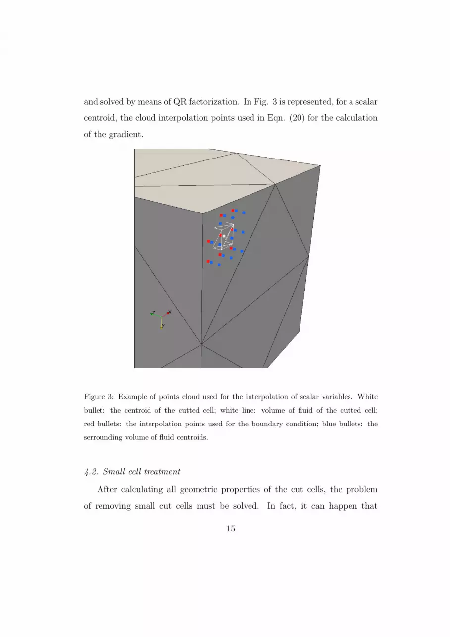
and solved by means of QR factorization. In Fig. 3 is represented, for a scalar

centroid, the cloud interpolation points used in Eqn. (20) for the calculation

of the gradient.

Figure 3: Example of points cloud used for the interpolation of scalar variables. White

bullet: the centroid of the cutted cell; white line: volume of fluid of the cutted cell;

red bullets: the interpolation points used for the boundary condition; blue bullets: the

serrounding volume of fluid centroids.

4.2. Small cell treatment

After calculating all geometric properties of the cut cells, the problem

of removing small cut cells must be solved. In fact, it can happen that

15

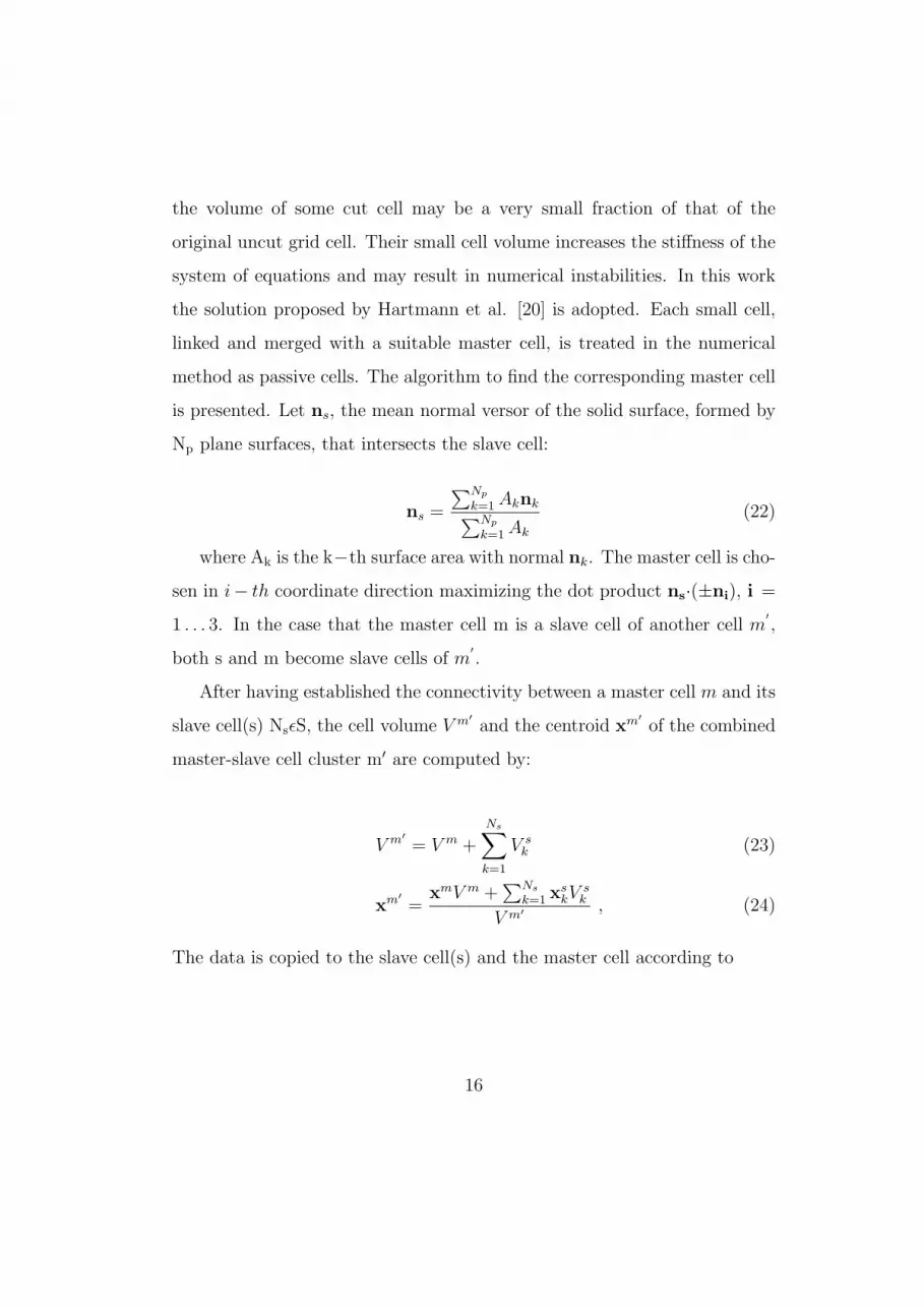
the volume of some cut cell may be a very small fraction of that of the

original uncut grid cell. Their small cell volume increases the stiffness of the

system of equations and may result in numerical instabilities. In this work

the solution proposed by Hartmann et al. [20] is adopted. Each small cell,

linked and merged with a suitable master cell, is treated in the numerical

method as passive cells. The algorithm to find the corresponding master cell

is presented. Let ns, the mean normal versor of the solid surface, formed by

Np plane surfaces, that intersects the slave cell:

ns =

∑Np

k=1 Aknk∑Np

k=1 Ak

(22)

where Ak is the k−th surface area with normal nk. The master cell is cho-

sen in i− th coordinate direction maximizing the dot product ns·(±ni), i =

1 . . . 3. In the case that the master cell m is a slave cell of another cell m′

,

both s and m become slave cells of m′

.

After having established the connectivity between a master cell m and its

slave cell(s) NsǫS, the cell volume V m′

and the centroid xm′

of the combined

master-slave cell cluster m′ are computed by:

V m′

= V m +Ns∑

k=1

V sk (23)

xm′

=xmV m +

∑Ns

k=1 xskV

sk

V m′, (24)

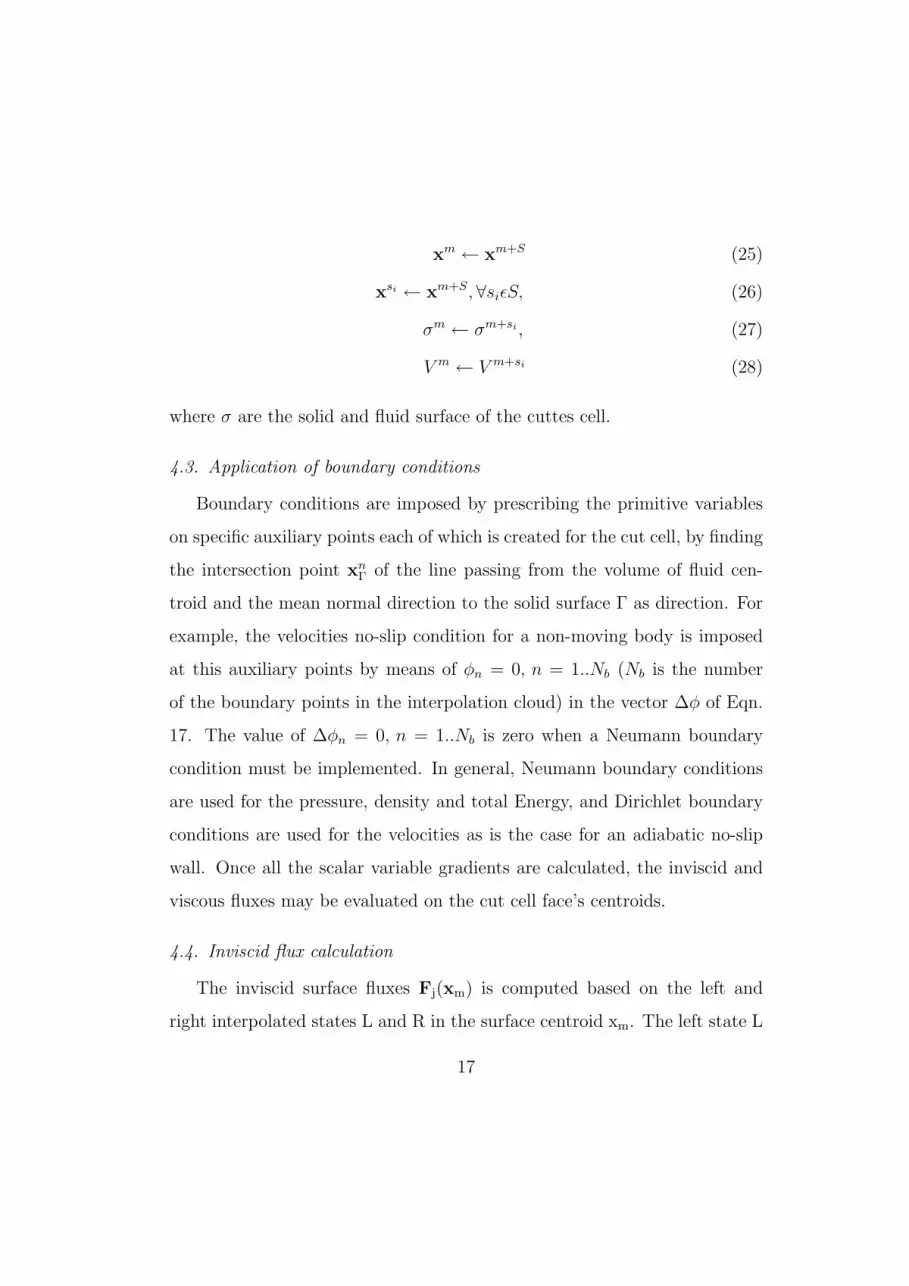
The data is copied to the slave cell(s) and the master cell according to

16

xm ← xm+S (25)

xsi ← xm+S,∀siǫS, (26)

σm ← σm+si , (27)

V m ← V m+si (28)

where σ are the solid and fluid surface of the cuttes cell.

4.3. Application of boundary conditions

Boundary conditions are imposed by prescribing the primitive variables

on specific auxiliary points each of which is created for the cut cell, by finding

the intersection point xnΓ of the line passing from the volume of fluid cen-

troid and the mean normal direction to the solid surface Γ as direction. For

example, the velocities no-slip condition for a non-moving body is imposed

at this auxiliary points by means of φn = 0, n = 1..Nb (Nb is the number

of the boundary points in the interpolation cloud) in the vector ∆φ of Eqn.

17. The value of ∆φn = 0, n = 1..Nb is zero when a Neumann boundary

condition must be implemented. In general, Neumann boundary conditions

are used for the pressure, density and total Energy, and Dirichlet boundary

conditions are used for the velocities as is the case for an adiabatic no-slip

wall. Once all the scalar variable gradients are calculated, the inviscid and

viscous fluxes may be evaluated on the cut cell face’s centroids.

4.4. Inviscid flux calculation

The inviscid surface fluxes Fj(xm) is computed based on the left and

right interpolated states L and R in the surface centroid xm. The left state L

17

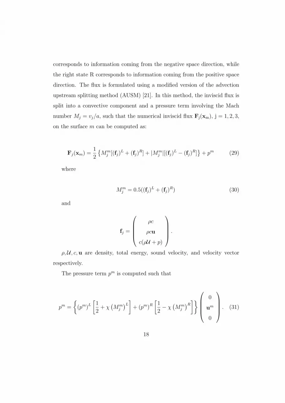
corresponds to information coming from the negative space direction, while

the right state R corresponds to information coming from the positive space

direction. The flux is formulated using a modified version of the advection

upstream splitting method (AUSM) [21]. In this method, the inviscid flux is

split into a convective component and a pressure term involving the Mach

number Mj = vj/a, such that the numerical inviscid flux Fj(xm), j = 1, 2, 3,

on the surface m can be computed as:

Fj(xm) =1

2

Mmj [(fj)

L + (fj)R] + |Mm

j |[(fj)L − (fj)

R]

+ pm (29)

where

Mmj = 0.5((fj)

L + (fj)R) (30)

and

fj =

ρc

ρcu

c(ρU + p)

.

ρ,U , c,u are density, total energy, sound velocity, and velocity vector

respectively.

The pressure term pm is computed such that

pm =

(pm)L

[

1

2+ χ

(

Mmj

)L]

+ (pm)R

[

1

2− χ

(

Mmj

)R]

0

um

0

. (31)

18

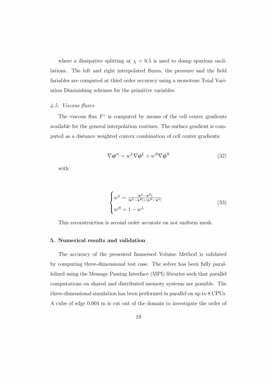
where a dissipative splitting at χ = 0.5 is used to dump spurious oscil-

lations. The left and right interpolated fluxes, the pressure and the field

fariables are computed at third order accuracy using a monotone Total Vari-

ation Diminishing schemes for the primitive variables.

4.5. Viscous fluxes

The viscous flux F v is computed by means of the cell center gradients

available for the general interpolation routines. The surface gradient is com-

puted as a distance weighted convex combination of cell center gradients:

∇φm = wL∇φL + wR∇φR (32)

with

wL = |xL−xR|

|xL−xR|+|xR−xL|

wR = 1 − wL

(33)

This reconstruction is second order accurate on not uniform mesh.

5. Numerical results and validation

The accuracy of the presented Immersed Volume Method is validated

by computing three-dimensional test case. The solver has been fully paral-

lelized using the Message Passing Interface (MPI) libraries such that parallel

computations on shared and distributed memory systems are possible. The

three-dimensional simulation has been performed in parallel on up to 8 CPUs.

A cube of edge 0.004 m is cut out of the domain to investigate the order of

19

the discretization at complex boundaries. The cube is centered in the compu-

tational domain so that a constant-valued Dirichlet boundary condition can

be specied on its boundary. The flow past a cube without visocity effect is an

appropriate validation test case, because of the presence of edges, cut cells

with internal volume and faces centroid and the absence of viscous stability

effects. The Reynolds number based on the freestream velocity is dened as

Reedge = ρuLµ∞

= 40. For the three-dimensional simulation of the ow past a

cube, a computational domain Ω: [7.5L, 7.5L]x[-0.5L, 0.5L]x[-0.5L, 0.5L] is

used. The cartesian domain contains approximately 2.0 million of cells. The

grid is refined near the cube in all directions.

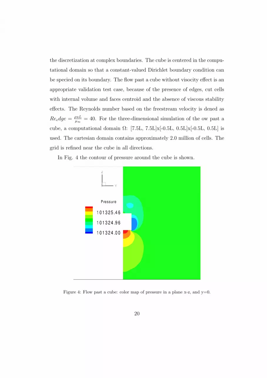
In Fig. 4 the contour of pressure around the cube is shown.

Figure 4: Flow past a cube: color map of pressure in a plane x-z, and y=0.

20

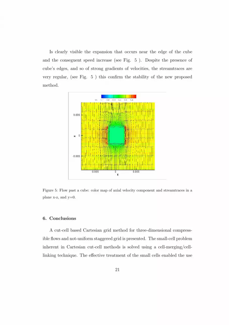
Is clearly visible the expansion that occurs near the edge of the cube

and the conseguent speed increase (see Fig. 5 ). Despite the presence of

cube’s edges, and so of strong gradients of velocities, the streamtraces are

very regular, (see Fig. 5 ) this confirm the stability of the new proposed

method.

Figure 5: Flow past a cube: color map of axial velocity component and streamtraces in a

plane x-z, and y=0.

6. Conclusions

A cut-cell based Cartesian grid method for three-dimensional compress-

ible flows and not-uniform staggered grid is presented. The small-cell problem

inherent in Cartesian cut-cell methods is solved using a cell-merging/cell-

linking technique. The effective treatment of the small cells enabled the use

21

of rather large CFL numbers in simulations. The accuracy of the viscous

fluxes is second order. Along with this extension, the solver is currently be-

ing extended for combustion problems and heat transfer between the solid

and the fluid flow.

References

[1] S. Nagarajan, S.K. Lele, J.H. Ferziger, A robust high-order compact

method for large eddy simulation, J. Comput. Phys. 191, (2003) 563-

582.

[2] D.A. Kopriva, A staggered-grid multidomain spectral method for the

compressible NavierStokes equations, J. Comput. Phys. 143 (1998) 125.

[3] G.S. Djambazov, C.-H. Lai, K.A. Pericleous, Staggered-mesh computa-

tion for aerodynamic sound, AIAA J. 38 (2000) 16.

[4] E.A. Fadlun, R. Verzicco, P. Orlandi, J. Mohd-Yusof, Combined

immersed-boundary finite-difference methods for three-dimensional

complex flow simulations, J. Comput. Phys. 161 (2000) 35-60.

[5] J. Mohd-Yusof, Combined immersed boundary/B-splines methods for

simulations of flows in complex geometries, in: Center for Turbulence

Research Briefs, NASA Ames/Stanford University, 1997.

[6] F. Muldoon, S. Acharya, A divergence free interpolation scheme for the

immersed boundary method, Int. J. Numer. Method Fluid 56 (2008)

1845-1884.

22

[7] S. Kang, G. Iaccarino, P. Moin, Accurate immersed boundary recon-

stractions for viscous flow simulations, AIAA J. 47 (7) (2009) 1750-1760.

[8] D. Clarke, M. Salas, H. Hassan, Euler calculations for multi-elements

airfoils using Cartesian grids, AIAA J. 24 (3) (1986) 353-358.

[9] M.J. Berger, R.J. Leveque, Stable boundary condition for cartesian grid

calculations, Computer System in Engineering 1 (1990) 305-311.

[10] H. Johansen, P. Colella, A cartesian grid embedded boundary method

for Poisson’s equation on irregular domains, J. Comput. Phys. 147 (1998)

60-85.

[11] M. Mayer, A. Devesa, X.Y. Hu, N.A. Adams, A conservative immersed

interface method for Large-Eddy Simulation of incompressible flows, J.

Comput. Phys. 229 (2010) 6300-6317.

[12] X.Y. Hu, B.C. Khoo, N.A. Adams, F.L. Huang, A conservative interface

method for compressible flows, J. Comput. Phys. 219 (2006) 553-578.

[13] M.H. Chung, Cartesian cut cell approach for simulating incompressible

flows with rigid bodies of arbitrary shape, Comput. Fluid 35 (2006)

607-623.

[14] Y. Cheny, O. Botella, The LS-STAG method: A new immersed/level-set

method for the computation of incompressible viscous flows in complex

moving geometries with good conservation properties, J. Comput. Phys.

229 (2010) 1043-1076.

23

[15] F.H. Harlow, J.E. Welch, Numerical calculation of time-dependent vis-

cous incompressible flow of fluid with free surfaces, Phys. Fluid 8 (1965)

2181-2189.

[16] Yang G., Causon D.M., Ingram D.M., Saunders R., Batten P., A Carte-

sian cut cell method for compressible flows part B: moving body prob-

lems. Aeronautical Journal 101 (1997) 57-65.

[17] Chiang Y., Van Leer B., Powell K.G., Simulation of unsteady inviscid

flow on an adaptively refined Cartesian grid, AIAA Paper (1992) 92-

0443-CP.

[18] M.J. Aftosmis, M.J. Berger, J.E. Melton, Robust and efficient cartesian

mesh generation for component based geometry, Tech. Report AIAA-

97-0196, US Air Force Wright Laboratory, (1997).

[19] T. Moller, A Fast Triangle-Triangle Intersection Test, Journal of Graph-

ics Tools, 2(2), 1997.

[20] D. Hartmann, M. Meinke, W. Schrder, An adaptive multilevel multigrid

formulation for Cartesian hierarchical grid methods, Comput. Fluids 37

(2008)

[21] M.S. Liou, C.J. Steen Jr., A new ux splitting scheme, J. Comput. Phys.

107 (1993) 2339.

[22] J.C. Mandal, S.P. Rao, High resolution finite volume computations on

unstructured grids using solution dependent weighted least square gra-

dients, Comput. Fluids, 2010.

24

[23] J.C. Mandal, Subramanian J., On the link between weighted least-

squares and limiters usedin higher-order reconstructions for finite

volume computations of hyperbolic equations, Appl Numer Math,

2008;58:705-25.

25