An analytical relationship for weathering induced slope retrogression: a benchmark

RIVISTA ITALIANA DI GEOTECNICA 2/2005

An analytical relationship for weathering induced slope retrogression: a benchmark

Stefano Utili*

SummaryIn this paper the evolution of slopes subjected to weathering has been studied by the limit analysis upper bound

method. Slopes subjected to weathering undergo a series of landslides, occurring at successive times, which cause the pro-gressive retrogression of the slope front. The discrete succession of failures has been modelled taking into account the dif-ferent geometry assumed by slopes after each landslide. Soil has been modelled as a Coulomb material (c, φ). Weatheringhas been modelled by assuming a uniform cohesion decrease within slopes whereas the friction angle remains constant. Ananalytical solution was obtained which gives the geometry of the failure surface and the soil mechanics properties at theonset of each landslide.

1. Introduction

Civil structures (e. g. roads, railways, buildings,landfills) are often located near slopes subjected toweathering. It is important to model suitably the re-trogression of the slope front in order to establish ifthe structure will be reached by the retrogressiveslope front during its design life (see Fig. 1) in orderto prevent costly accidents and human life losses.Moreover, if reliable predictions about the amountof the slope retrogression are obtained, it will bepossible to build new structures in areas previouslynot considered suitable because of lack of informa-tion on slope behaviour.

From an historical point of view, the first modelsaimed at describing the evolution of natural slopescome from geomorphology and geology. Slope evo-lution models were developed in 1866 thanks toFisher’s work [FISHER, 1866] later by [BAKKER & LE

HEUX, 1947], [KIRKBY, 1987], and others. Thesemodels have been conceived to describe the evolu-tion of natural slopes that occurred in the past(thousands of years). They do not consider a succes-sion of discrete events (landslides) but a continuouserosive process. The slope profiles achieved bythese models are mean profiles averaged over time.

In this paper, a model capable of making quan-titative predictions about the future evolution of na-tural slopes is described. Since the evolution of na-tural slopes is governed by single successive landsli-des occurring at different times, this model explici-tly takes into account the changes of geometry un-dergone by slopes.

* Philosophy Doctor, Dipartimento di Ingegneria Strutturale, Politecnico di Milano, Italy.

Fig. 1 – Photographs of steep slopes in weakly-cementedsand. a) Mogàn, Gran Canaria; urban development at thebase of a slope (after [DELGADO, 1991]. b) Daly City (Cali-fornia, US); urban development on the top of a slope [af-ter CLOUGH et al., 1981].Fig. 1 – Fotografie di pendii scoscesi in sabbia debolmente cementata. a) Mogàn, Gran Canaria; cittadina ai piedi di un pendio (da [DELGADO, 1991]. b) Daly City (California, US); cittadina situata sulla sommità di un pendio [da CLOUGH et al., 1981].

a)

b)

10 UTILI

RIVISTA ITALIANA DI GEOTECNICA

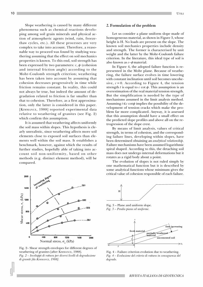
Slope weathering is caused by many differentphenomena such as chemical reactions develo-ping among soil grain minerals and physical ac-tion of atmospheric agents (wind, rain, freeze-thaw cycles, etc.). All these processes are verycomplex to take into account. Therefore, a reaso-nable way to proceed was found by studying wea-thering assuming that the effect on soil mechanicsproperties is known. To this end, soil strength hasbeen expressed by two parameters: c, φ (cohesionand internal friction angle) according to theMohr-Coulomb strength criterion; weatheringhas been taken into account by assuming thatcohesion decreases progressively in time whilefriction remains constant. In reality, this couldnot always be true, but indeed the amount of de-gradation related to friction is far smaller thanthat to cohesion. Therefore, as a first approxima-tion, only the latter is considered in this paper.[KIMMANCE, 1988] reported experimental datarelative to weathering of granites (see Fig. 2)which confirm this assumption.

It is assumed that weathering affects uniformlythe soil mass within slopes. This hypothesis is cle-arly unrealistic, since weathering affects more soilelements close to exposed soil surfaces than ele-ments well within the soil mass. It establishes abenchmark, however, against which the results offurther studies, hopefully able of taking into ac-count soil non-uniformity, based on othermethods (e.g. distinct element method), will becompared.

2. Formulation of the problem

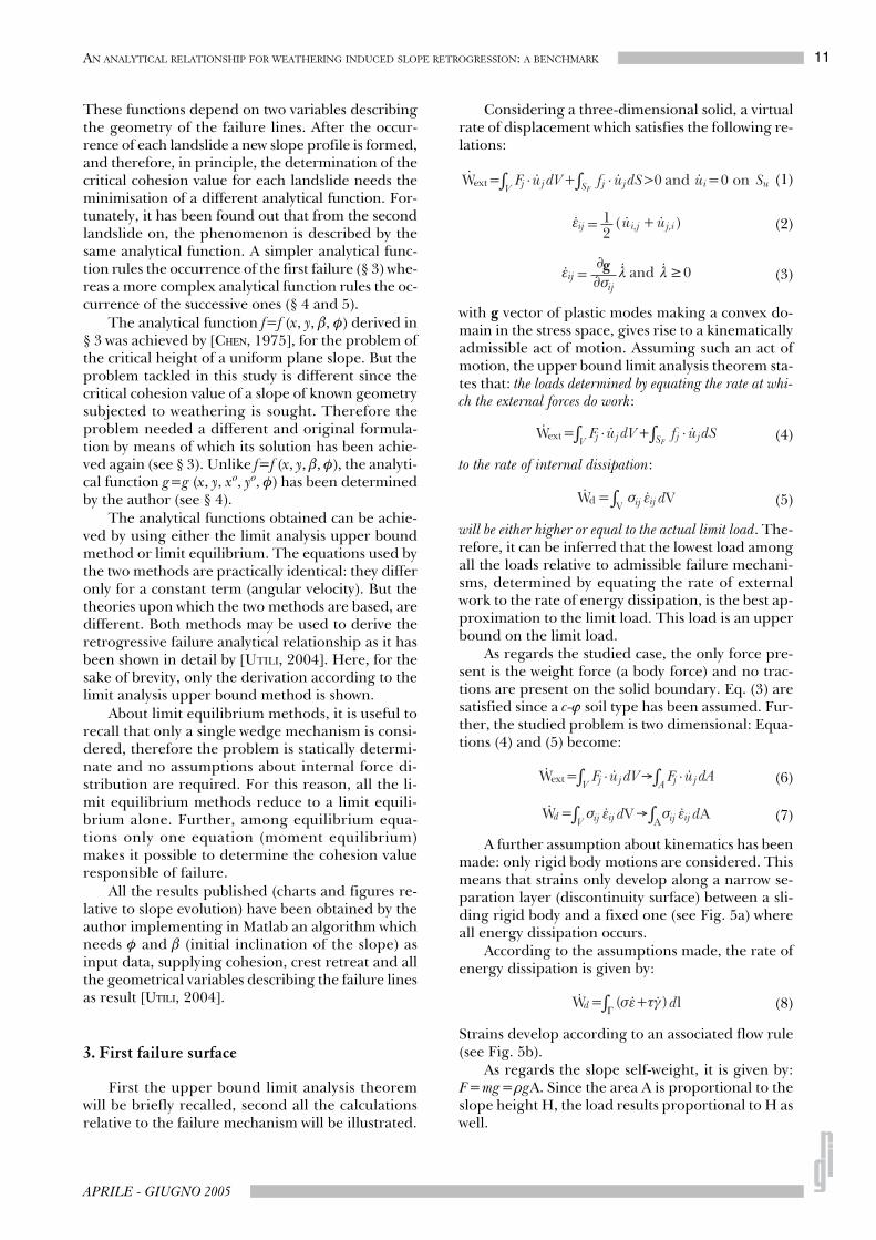
Let us consider a plane uniform slope made ofhomogeneous material, as shown in Figure 3, whoseheight is H. No loads are present on the slope. Theknown soil mechanics properties include densityand strength. The former is characterised by unitweight and the latter by the Mohr-Coulomb failurecriterion. In the literature, this ideal type of soil isalso known as c–φ material.

In Figure 4, the adopted failure function is re-presented in the Mohr plane. Because of weathe-ring, the failure surface evolves in time loweringwith constant inclination until soil becomes uncohe-sive, c = 0. According to Figure 4, the tensionstrength t is equal to c cot φ. This assumption is anoverestimation of the real material tension strength.But the simplification is needed by the type ofmechanisms assumed in the limit analysis method.Assuming t≤c cotφ implies the possibility of the de-velopment of tension cracks which make the pro-blem far more complicated. Anyway, it is assessedthat this assumption should have a small effect onthe predicted slope profiles and above all on the re-trogression of the slope crest.

By means of limit analysis, values of criticalstrength, in terms of cohesion, and the correspond-ing failure lines, developing within slopes, havebeen determined obtaining an analytical relationship.Failure mechanisms have been assumed logarithmicspiral shaped. According to this, the detaching soilmass does not undergo internal deformations but itrotates as a rigid body about a point.

The evolution of slopes is not ruled simply byone mathematical function but it is described bysome analytical functions whose minimum gives thecritical value of cohesion responsible of each failure.

Fig. 2– Shear strength envelopes for different degrees ofweathering of granites [after KIMMANCE, 1988].Fig. 2 – Inviluppi di rottura per diversi livelli di degradazione di graniti [da KIMMANCE, 1988].

Fig. 3 – Plane and uniform slope.Fig. 3 – Pendio piano ed uniforme.

Fig. 4 – Failure criterion evolution due to weathering.Fig. 4 – Evoluzione del criterio di rottura in conseguenza del degrado.

11AN ANALYTICAL RELATIONSHIP FOR WEATHERING INDUCED SLOPE RETROGRESSION: A BENCHMARK

APRILE - GIUGNO 2005

These functions depend on two variables describingthe geometry of the failure lines. After the occur-rence of each landslide a new slope profile is formed,and therefore, in principle, the determination of thecritical cohesion value for each landslide needs theminimisation of a different analytical function. For-tunately, it has been found out that from the secondlandslide on, the phenomenon is described by thesame analytical function. A simpler analytical func-tion rules the occurrence of the first failure (§ 3) whe-reas a more complex analytical function rules the oc-currence of the successive ones (§ 4 and 5).

The analytical function f=f (x, y, β, φ) derived in§ 3 was achieved by [CHEN, 1975], for the problem ofthe critical height of a uniform plane slope. But theproblem tackled in this study is different since thecritical cohesion value of a slope of known geometrysubjected to weathering is sought. Therefore theproblem needed a different and original formula-tion by means of which its solution has been achie-ved again (see § 3). Unlike f=f (x, y, β, φ), the analyti-cal function g=g (x, y, xo, yo, φ) has been determinedby the author (see § 4).

The analytical functions obtained can be achie-ved by using either the limit analysis upper boundmethod or limit equilibrium. The equations used bythe two methods are practically identical: they differonly for a constant term (angular velocity). But thetheories upon which the two methods are based, aredifferent. Both methods may be used to derive theretrogressive failure analytical relationship as it hasbeen shown in detail by [UTILI, 2004]. Here, for thesake of brevity, only the derivation according to thelimit analysis upper bound method is shown.

About limit equilibrium methods, it is useful torecall that only a single wedge mechanism is consi-dered, therefore the problem is statically determi-nate and no assumptions about internal force di-stribution are required. For this reason, all the li-mit equilibrium methods reduce to a limit equili-brium alone. Further, among equilibrium equa-tions only one equation (moment equilibrium)makes it possible to determine the cohesion valueresponsible of failure.

All the results published (charts and figures re-lative to slope evolution) have been obtained by theauthor implementing in Matlab an algorithm whichneeds φ and β (initial inclination of the slope) asinput data, supplying cohesion, crest retreat and allthe geometrical variables describing the failure linesas result [UTILI, 2004].

3. First failure surface

First the upper bound limit analysis theoremwill be briefly recalled, second all the calculationsrelative to the failure mechanism will be illustrated.

Considering a three-dimensional solid, a virtualrate of displacement which satisfies the following re-lations:

(1)

(2)

(3)

with g vector of plastic modes making a convex do-main in the stress space, gives rise to a kinematicallyadmissible act of motion. Assuming such an act ofmotion, the upper bound limit analysis theorem sta-tes that: the loads determined by equating the rate at whi-ch the external forces do work:

(4)

to the rate of internal dissipation:

(5)

will be either higher or equal to the actual limit load. The-refore, it can be inferred that the lowest load amongall the loads relative to admissible failure mechani-sms, determined by equating the rate of externalwork to the rate of energy dissipation, is the best ap-proximation to the limit load. This load is an upperbound on the limit load.

As regards the studied case, the only force pre-sent is the weight force (a body force) and no trac-tions are present on the solid boundary. Eq. (3) aresatisfied since a c-ϕ soil type has been assumed. Fur-ther, the studied problem is two dimensional: Equa-tions (4) and (5) become:

(6)

(7)

A further assumption about kinematics has beenmade: only rigid body motions are considered. Thismeans that strains only develop along a narrow se-paration layer (discontinuity surface) between a sli-ding rigid body and a fixed one (see Fig. 5a) whereall energy dissipation occurs.

According to the assumptions made, the rate ofenergy dissipation is given by:

(8)

Strains develop according to an associated flow rule(see Fig. 5b).

As regards the slope self-weight, it is given by:F=mg=ρgA. Since the area A is proportional to theslope height H, the load results proportional to H aswell.

12 UTILI


Finally, the energy balance equation:

(9)

makes it possible to determine a function c = c(considered mechanisms) by which the most criti-cal mechanism can be determined. The maximumof this function gives an upper bound on the limitvalue.

3.1. Determination of the analytical solution

The notation used in the following has beenadopted according to these criteria: lower-case let-ters for angles and upper-case letters for Cartesianco-ordinates; plain letters for scalar quantities andbold letters for vectors; the letter X for the horizon-tal direction and Y for the vertical one.

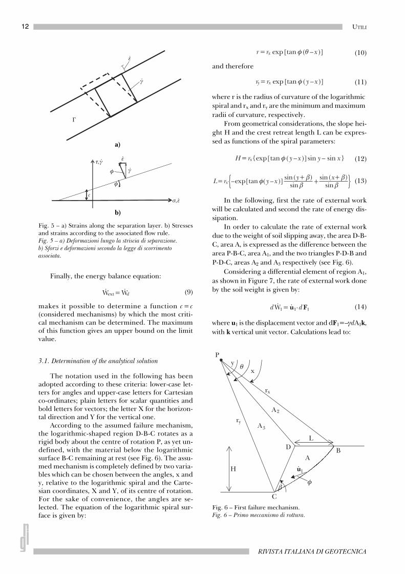
According to the assumed failure mechanism,the logarithmic-shaped region D-B-C rotates as arigid body about the centre of rotation P, as yet un-defined, with the material below the logarithmicsurface B-C remaining at rest (see Fig. 6). The assu-med mechanism is completely defined by two varia-bles which can be chosen between the angles, x andy, relative to the logarithmic spiral and the Carte-sian coordinates, X and Y, of its centre of rotation.For the sake of convenience, the angles are se-lected. The equation of the logarithmic spiral sur-face is given by:

(10)

and therefore

(11)

where r is the radius of curvature of the logarithmic spiral and rx and ry are the minimum and maximum radii of curvature, respectively.

From geometrical considerations, the slope hei-ght H and the crest retreat length L can be expres-sed as functions of the spiral parameters:

(12)

(13)

In the following, first the rate of external workwill be calculated and second the rate of energy dis-sipation.

In order to calculate the rate of external workdue to the weight of soil slipping away, the area D-B-C, area A, is expressed as the difference between thearea P-B-C, area A1, and the two triangles P-D-B andP-D-C, areas A2 and A3 respectively (see Fig. 6).

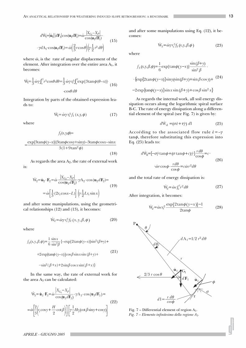
Considering a differential element of region A1,as shown in Figure 7, the rate of external work doneby the soil weight is given by:

(14)

where u1 is the displacement vector and dF1=–γdA1k,with k vertical unit vector. Calculations lead to:

Fig. 5 – a) Strains along the separation layer. b) Stressesand strains according to the associated flow rule.Fig. 5 – a) Deformazioni lungo la striscia di separazione. b) Sforzi e deformazioni secondo la legge di scorrimento associata.

b)

a)

Fig. 6 – First failure mechanism.Fig. 6 – Primo meccanismo di rottura.



(15)

where ·ω, is the rate of angular displacement of theelement. After integration over the entire area A1, itbecomes:

(16)

Integration by parts of the obtained expression lea-ds to:

(17)

where

(18)

As regards the area A2, the rate of external workis:

(19)

and after some manipulations, using the geometri-cal relationships (12) and (13), it becomes:

(20)

where

(21)

In the same way, the rate of external work forthe area A3 can be calculated:

(22)

and after some manipulations using Eq. (12), it be-comes:

(23)

where

(24)

As regards the internal work, all soil energy dis-sipation occurs along the logarithmic spiral surfaceB-C. The rate of energy dissipation along a differen-tial element of the spiral (see Fig. 7) is given by:

(25)

According to the associated flow rule ·ε=–γtanφ,

·therefore substituting this expression into

Eq. (25) leads to:

(26)

and the total rate of energy dissipation is:

(27)

After integration, it becomes:

(28)

Fig. 7 – Differential element of region A1.Fig. 7 – Elemento infinitesimo della regione A1.

14 UTILI


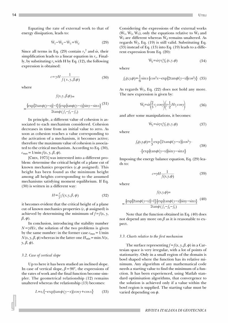
Equating the rate of external work to that ofenergy dissipation, leads to:

(29)

Since all terms in Eq. (29) contain rx2 and ·ω, their

simplification leads to a linear equation in rx. Final-ly, by substituting rx with H by Eq. (12), the followingexpression is obtained:

(30)

where

(31)

In principle, a different value of cohesion is as-sociated to each mechanism considered. Cohesiondecreases in time from an initial value to zero. Assoon as cohesion reaches a value corresponding tothe activation of a mechanism, it becomes active;therefore the maximum value of cohesion is associa-ted to the critical mechanism. According to Eq. (30),cmax=1/min f(x, y, β, φ).

[CHEN, 1975] was interested into a different pro-blem: determine the critical height of a plane cut ofknown mechanics properties (c,φ assigned). Thisheight has been found as the minimum heightamong all heights corresponding to the assumedmechanisms satisfying moment equilibrium. If Eq.(30) is written in a different way:

(32)

it becomes evident that the critical height of a planecut of known mechanics properties (c, φ assigned) isachieved by determining the minimum of f=f(x, y,β, φ).

In conclusion, introducing the stability numberN=γH/c, the solution of the two problems is givenby the same number: in the former case cmax=1/minN(x, y, β, φ) whereas in the latter one Hmin=min N(x,y, β, φ).

3.2. Case of vertical slope

Up to here it has been studied an inclined slope.In case of vertical slope, β=90°, the expressions ofthe rates of work and the final function become sim-pler. The geometrical relationship (12) remainsunaltered whereas the relationship (13) becomes:

(33)

Considering the expressions of the external works(W1,

· W2,· W3),

· only the equations relative to W2· and

W3· are different whereas Wd

· remains unaltered. Asregards W2,

· Eq. (19) is still valid. Substituting Eq.(33) instead of Eq. (13) into Eq. (19) leads to a diffe-rent expression from Eq. (20):

(34)

where

(35)

As regards W3,· Eq. (22) does not hold any more.The new expression is given by:

(36)

and after some manipulations, it becomes:

(37)

where

(38)

Imposing the energy balance equation, Eq. (29) lea-ds to:

(39)

where

(40)

Note that the function obtained in Eq. (40) doesnot depend any more on β as it is reasonable to ex-pect.

3.3. Charts relative to the first mechanism

The surface representing f=f(x, y, β, φ) in a Car-tesian space is very irregular, with a lot of points ofstationarity. Only in a small region of the domain isbowl shaped where the function has its relative mi-nimum. Any algorithm of any mathematical codeneeds a starting value to find the minimum of a fun-ction. It has been experienced, using Matlab stan-dard optimisation algorithms, that convergence tothe solution is achieved only if a value within thebowl region is supplied. The starting value must bevaried depending on φ.



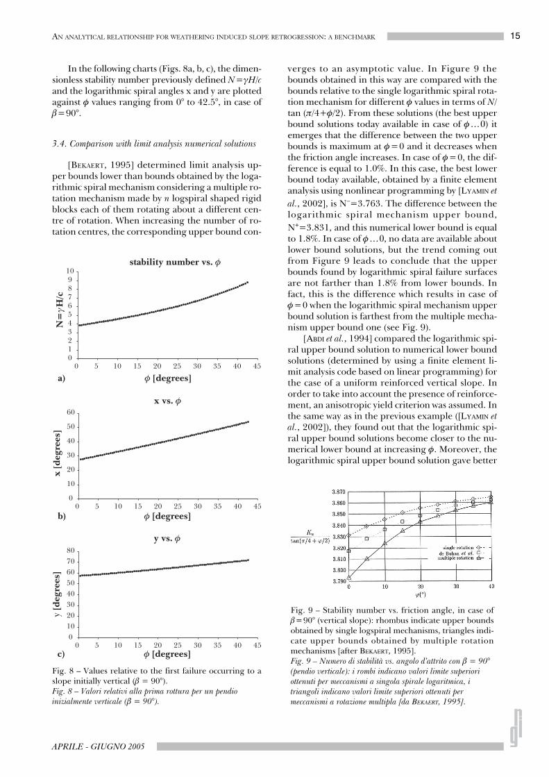
In the following charts (Figs. 8a, b, c), the dimen-sionless stability number previously defined N=γH/cand the logarithmic spiral angles x and y are plottedagainst φ values ranging from 0° to 42.5°, in case ofβ=90°.

3.4. Comparison with limit analysis numerical solutions

[BEKAERT, 1995] determined limit analysis up-per bounds lower than bounds obtained by the loga-rithmic spiral mechanism considering a multiple ro-tation mechanism made by n logspiral shaped rigidblocks each of them rotating about a different cen-tre of rotation. When increasing the number of ro-tation centres, the corresponding upper bound con-

verges to an asymptotic value. In Figure 9 thebounds obtained in this way are compared with thebounds relative to the single logarithmic spiral rota-tion mechanism for different φ values in terms of N/tan (π/4+φ/2). From these solutions (the best upperbound solutions today available in case of φ…0) itemerges that the difference between the two upperbounds is maximum at φ=0 and it decreases whenthe friction angle increases. In case of φ=0, the dif-ference is equal to 1.0%. In this case, the best lowerbound today available, obtained by a finite elementanalysis using nonlinear programming by [LYAMIN etal., 2002], is N–=3.763. The difference between thelogarithmic spiral mechanism upper bound,N+=3.831, and this numerical lower bound is equalto 1.8%. In case of φ…0, no data are available aboutlower bound solutions, but the trend coming outfrom Figure 9 leads to conclude that the upperbounds found by logarithmic spiral failure surfacesare not farther than 1.8% from lower bounds. Infact, this is the difference which results in case ofφ=0 when the logarithmic spiral mechanism upperbound solution is farthest from the multiple mecha-nism upper bound one (see Fig. 9).

[ABDI et al., 1994] compared the logarithmic spi-ral upper bound solution to numerical lower boundsolutions (determined by using a finite element li-mit analysis code based on linear programming) forthe case of a uniform reinforced vertical slope. Inorder to take into account the presence of reinforce-ment, an anisotropic yield criterion was assumed. Inthe same way as in the previous example ([LYAMIN etal., 2002]), they found out that the logarithmic spi-ral upper bound solutions become closer to the nu-merical lower bound at increasing φ. Moreover, thelogarithmic spiral upper bound solution gave better

Fig. 8 – Values relative to the first failure occurring to aslope initially vertical (β = 90°).Fig. 8 – Valori relativi alla prima rottura per un pendio inizialmente verticale (β = 90°).

Fig. 9 – Stability number vs. friction angle, in case ofβ=90° (vertical slope): rhombus indicate upper boundsobtained by single logspiral mechanisms, triangles indi-cate upper bounds obtained by multiple rotationmechanisms [after BEKAERT, 1995].Fig. 9 – Numero di stabilità vs. angolo d’attrito con β = 90° (pendio verticale): i rombi indicano valori limite superiori ottenuti per meccanismi a singola spirale logaritmica, i triangoli indicano valori limite superiori ottenuti per meccanismi a rotazione multipla [da BEKAERT, 1995].

16 UTILI


results than the numerical upper bound solutionsachieved by the FE limit analysis code.

3.5. Influence of dilatancy on limit load

Real frictional-cohesive soils do not obey thenormality rule. Soft rocks, overconsolidated clays,cemented sands are usually characterised by a dila-tion angle smaller than the friction angle. Unfortu-nately, the limit theorems are not applicable to ma-terials obeying a nonassociated flow rule. Accor-ding to a Chen’s upper bound theorem [CHEN,1975], the collapse loads for a material with nonas-sociated flow rule are smaller than those obtainedfor the same material when an associated flow ruleis assumed. However, it can be argued that the flowrule should not have large influence on the limitload when the problem is little constrained in a ki-nematic sense.

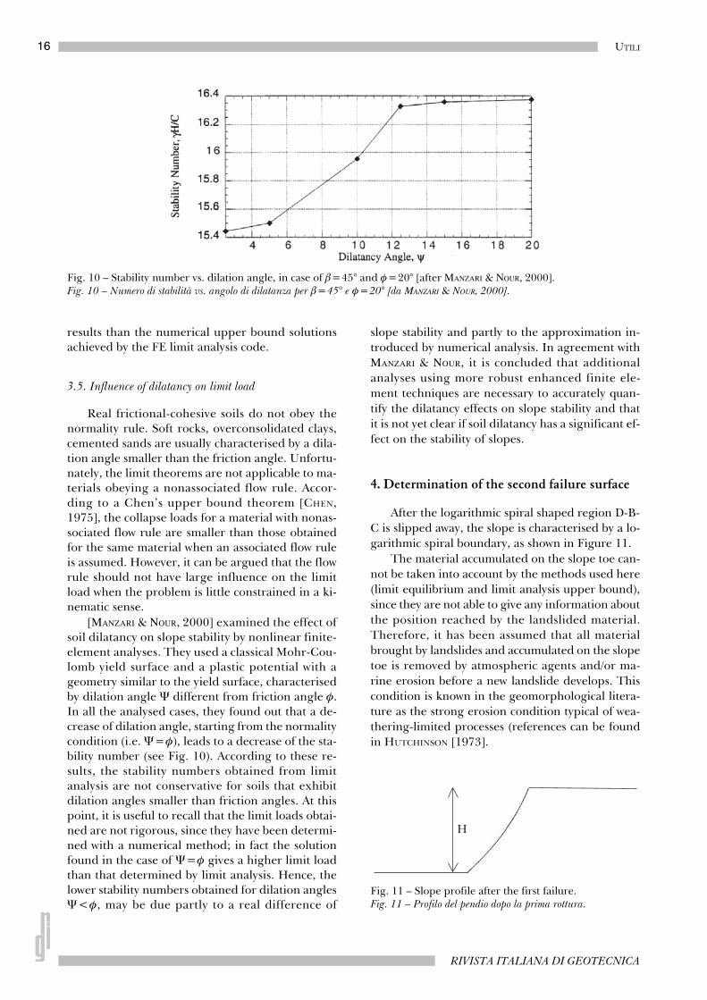
[MANZARI & NOUR, 2000] examined the effect ofsoil dilatancy on slope stability by nonlinear finite-element analyses. They used a classical Mohr-Cou-lomb yield surface and a plastic potential with ageometry similar to the yield surface, characterisedby dilation angle Ψ different from friction angle φ.In all the analysed cases, they found out that a de-crease of dilation angle, starting from the normalitycondition (i.e. Ψ=φ), leads to a decrease of the sta-bility number (see Fig. 10). According to these re-sults, the stability numbers obtained from limitanalysis are not conservative for soils that exhibitdilation angles smaller than friction angles. At thispoint, it is useful to recall that the limit loads obtai-ned are not rigorous, since they have been determi-ned with a numerical method; in fact the solutionfound in the case of Ψ=φ gives a higher limit loadthan that determined by limit analysis. Hence, thelower stability numbers obtained for dilation anglesΨ<φ, may be due partly to a real difference of

slope stability and partly to the approximation in-troduced by numerical analysis. In agreement withMANZARI & NOUR, it is concluded that additionalanalyses using more robust enhanced finite ele-ment techniques are necessary to accurately quan-tify the dilatancy effects on slope stability and thatit is not yet clear if soil dilatancy has a significant ef-fect on the stability of slopes.

4. Determination of the second failure surface

After the logarithmic spiral shaped region D-B-C is slipped away, the slope is characterised by a lo-garithmic spiral boundary, as shown in Figure 11.

The material accumulated on the slope toe can-not be taken into account by the methods used here(limit equilibrium and limit analysis upper bound),since they are not able to give any information aboutthe position reached by the landslided material.Therefore, it has been assumed that all materialbrought by landslides and accumulated on the slopetoe is removed by atmospheric agents and/or ma-rine erosion before a new landslide develops. Thiscondition is known in the geomorphological litera-ture as the strong erosion condition typical of wea-thering-limited processes (references can be foundin HUTCHINSON [1973].

Fig. 10 – Stability number vs. dilation angle, in case of β=45° and φ=20° [after MANZARI & NOUR, 2000].Fig. 10 – Numero di stabilità vs. angolo di dilatanza per β=45° e φ=20° [da MANZARI & NOUR, 2000].

Fig. 11 – Slope profile after the first failure.Fig. 11 – Profilo del pendio dopo la prima rottura.



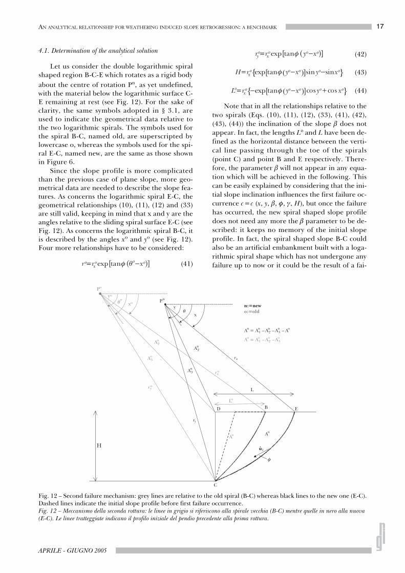
4.1. Determination of the analytical solution

Let us consider the double logarithmic spiralshaped region B-C-E which rotates as a rigid bodyabout the centre of rotation Pn, as yet undefined,with the material below the logarithmic surface C-E remaining at rest (see Fig. 12). For the sake ofclarity, the same symbols adopted in § 3.1, areused to indicate the geometrical data relative tothe two logarithmic spirals. The symbols used forthe spiral B-C, named old, are superscripted bylowercase o, whereas the symbols used for the spi-ral E-C, named new, are the same as those shownin Figure 6.

Since the slope profile is more complicatedthan the previous case of plane slope, more geo-metrical data are needed to describe the slope fea-tures. As concerns the logarithmic spiral E-C, thegeometrical relationships (10), (11), (12) and (33)are still valid, keeping in mind that x and y are theangles relative to the sliding spiral surface E-C (seeFig. 12). As concerns the logarithmic spiral B-C, itis described by the angles xo and yo (see Fig. 12).Four more relationships have to be considered:

(41)

(42)

(43)

(44)

Note that in all the relationships relative to thetwo spirals (Eqs. (10), (11), (12), (33), (41), (42),(43), (44)) the inclination of the slope β does notappear. In fact, the lengths Lo and L have been de-fined as the horizontal distance between the verti-cal line passing through the toe of the spirals(point C) and point B and E respectively. There-fore, the parameter β will not appear in any equa-tion which will be achieved in the following. Thiscan be easily explained by considering that the ini-tial slope inclination influences the first failure oc-currence c=c (x, y, β, φ, γ, H), but once the failurehas occurred, the new spiral shaped slope profiledoes not need any more the β parameter to be de-scribed: it keeps no memory of the initial slopeprofile. In fact, the spiral shaped slope B-C couldalso be an artificial embankment built with a loga-rithmic spiral shape which has not undergone anyfailure up to now or it could be the result of a fai-

Fig. 12 – Second failure mechanism: grey lines are relative to the old spiral (B-C) whereas black lines to the new one (E-C).Dashed lines indicate the initial slope profile before first failure occurrence.Fig. 12 – Meccanismo della seconda rottura: le linee in grigio si riferiscono alla spirale vecchia (B-C) mentre quelle in nero alla nuova (E-C). Le linee tratteggiate indicano il profilo iniziale del pendio precedente alla prima rottura.

18 UTILI


lure of a slope featured by whatever particularshape not necessarily plane.

In order to determine the rate of external workdone by the soil slipping away, the same method asthat used in § 3.1, based on the difference of areas,has been used. The rate of work done by the doublelogarithmic spiral shaped region B-C-E, area An, isobtained as the work done by the region Pn -C-E,area A1

n, minus the work done by the regions Pn -D-E and Pn -D-C, areas A2

n and A3n respectively, minus

the work done by the region B-C-D (see Fig. 12).The last one is expressed again as the differencebetween the work done by region Po -B-C, area A1

o,and the two triangular regions Po -D-B and Po -D-C,areas A2

o and A3o respectively. Therefore the rate of

external work done by the soil weight is given by:

(45)

As regards W1n,· W2

n· and W3n,· they have the

same analytical expressions as W1,· W2

· and ·W3 appe-aring in Eqs. (17), (34) and (37) respectively.

Unfortunately, the work done by the regionsA1

o, A2o, A3

o, assumes a much more complicatedanalytical expression. Considering, at first, the re-gion A1

o, whose gravity centre is G1, the rate of ex-ternal work done by a differential element is:

(46)

Therefore the external work for the entire regionbecomes:

(47)

and after integration by parts:

(48)

From Eq. (48), it emerges that the final equili-brium equation will assume a different structurefrom that relative to the first mechanism obtained inthe previous § 3.1, since it will not contain any morerx

2 in all its terms. So in order to achieve the func-tion which has to be minimised, Eq. (48) must befurther manipulated.

Substituting Eqs. (11), (42), (12) and (43) intoEq. (48), a more convenient expression is obtained:

(49)

Considering now the region A2o, whose gravity

centre is G2, the rate of external work is:

(50)

After some manipulations and substitutingEqs. (42), (43), (44), (11) and (12) into Eq. (50),the following expression is obtained:

(51)



As regards the region A3o, whose gravity centre

is G3, the rate of external work is:

(52)

After some manipulations and substituting Eqs. (43)and (12) into Eq. (52), the following expression isobtained:

(53)

As regards the internal work, all soil energy dis-sipation occurs along the logarithmic spiral surfaceE-C. The rate of energy dissipation along this spiralneeds to be calculated in the same way as previouslydone for the first failure mechanism in § 3.1. Hence,it is given by Eq. (28):

(28)

All terms contained in the energy balance equa-tion (9) have been calculated, but in order to obtaina function in the form c=c(x, y, xo, yo, φ, γ, H) it isnecessary to develop further Eqs. (17), (20), (23) and(28) substituting H in them by Eq. (12). This leadsto:

(54)

(55)

(56)

(57)

Equating the rate of external work (Eq. 45) tothat of energy dissipation, leads to:

(58)

All terms contain ω· and H2. After their simplifica-tion and rearranging, Eq. (58) becomes:

(59)

In the following, function g=g(x, y, xo, yo, φ) hasbeen achieved from the previously obtained analyti-cal expressions referring to work rates and grou-ping all constant terms (functions of xo, yo and φ):

(60)

where

(61)

and

20 UTILI


(62)

Note that a1(xo, yo, φ) and a2(xo, yo, φ) dependonly on parameters, therefore they assume constantvalues when the minimum of g=g(x, y, xo, yo, φ) issought by Matlab algorithms.

In order to determine the failure mechanism itis necessary to find the maximum of c=c(x, y, xo, yo,φ, γ, H) obtained by the energy balance Eq. (58) re-spect to the two variables x and y. The maximum ofthis function is obtained by finding the minimum ofg=g(x, y, xo, yo, φ).

4.2. Charts relative to the second mechanism

The g=g(x, y, xo, yo, φ) function presents cha-racteristics similar to f=f(x, y, β, φ) as it is very irre-gular and only in a small part of the domain is bowlshaped (see § 3.1).

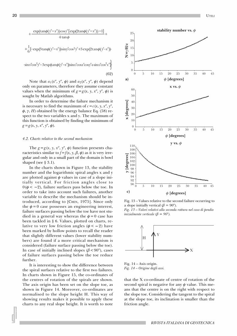
In the charts shown in Figure 13, the stabilitynumber and the logarithmic spiral angles x and yare plotted against φ values in case of a slope ini-t ial ly vertical . For frict ion angles close to0(φ< 2), failure surfaces pass below the toe. Inorder to take into account such failures, anothervariable to describe the mechanism should be in-troduced, according to [CHEN, 1975]. Since onlythe φ=0 case possesses an engineering interest,failure surfaces passing below the toe have not stu-died in a general way whereas the φ=0 case hasbeen tackled in § 6. Values, plotted on charts, re-lative to very low friction angles (φ < 2) havebeen marked by hollow points to recall the readerthat slightly different values (lower stability num-bers) are found if a more critical mechanism isconsidered (failure surface passing below the toe).In case of initially inclined slopes (β<90°), casesof failure surfaces passing below the toe reducefurther.

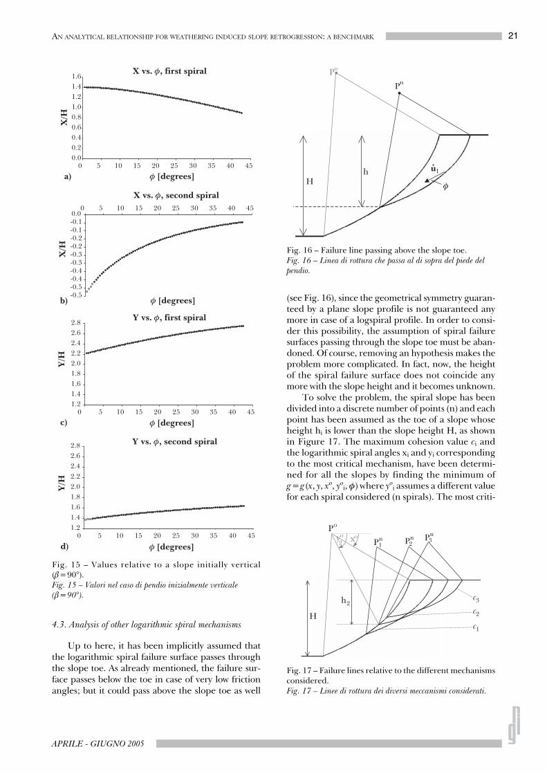
It is interesting to show the difference betweenthe spiral surfaces relative to the first two failures.In charts shown in Figure 15, the co-ordinates ofthe centres of rotation of the spirals are shown.The axis origin has been set on the slope toe, asshown in Figure 14. Moreover, co-ordinates arenormalised to the slope height H. This way ofshowing results makes it possible to apply thesecharts to any real slope height. It is worth to note

that the X co-ordinate of centre of rotation of thesecond spiral is negative for any φ value. This me-ans that the centre is on the right with respect tothe slope toe. Considering the tangent to the spiralat the slope toe, its inclination is smaller than thefriction angle.

Fig. 13 – Values relative to the second failure occurring toa slope initially vertical (β = 90°).Fig. 13 – Valori relativi alla seconda rottura nel caso di pendio inizialmente verticale (β = 90°).

Fig. 14 – Axis origin.Fig. 14 – Origine degli assi.



4.3. Analysis of other logarithmic spiral mechanisms

Up to here, it has been implicitly assumed thatthe logarithmic spiral failure surface passes throughthe slope toe. As already mentioned, the failure sur-face passes below the toe in case of very low frictionangles; but it could pass above the slope toe as well

(see Fig. 16), since the geometrical symmetry guaran-teed by a plane slope profile is not guaranteed anymore in case of a logspiral profile. In order to consi-der this possibility, the assumption of spiral failuresurfaces passing through the slope toe must be aban-doned. Of course, removing an hypothesis makes theproblem more complicated. In fact, now, the heightof the spiral failure surface does not coincide anymore with the slope height and it becomes unknown.

To solve the problem, the spiral slope has beendivided into a discrete number of points (n) and eachpoint has been assumed as the toe of a slope whoseheight hi is lower than the slope height H, as shownin Figure 17. The maximum cohesion value ci andthe logarithmic spiral angles xi and yi correspondingto the most critical mechanism, have been determi-ned for all the slopes by finding the minimum ofg=g(x, y, xo, yo

i, φ) where yoi assumes a different value

for each spiral considered (n spirals). The most criti-

Fig. 15 – Values relative to a slope initially vertical(β=90°).Fig. 15 – Valori nel caso di pendio inizialmente verticale (β=90°).

Fig. 16 – Failure line passing above the slope toe.Fig. 16 – Linea di rottura che passa al di sopra del piede del pendio.

Fig. 17 – Failure lines relative to the different mechanismsconsidered.Fig. 17 – Linee di rottura dei diversi meccanismi considerati.

22 UTILI


cal mechanism among all the n spirals is given by themechanism with the highest cohesion value.

The results obtained in case of a slope initiallyvertical (β=90°) have shown that the second failuremechanism passes through the slope toe for any va-lue of φ. This means that the charts shown in Figure13 and Figure 15 referred to a failure surface pas-sing through the slope toe, describe the actual fai-lure mechanism.

5. Determination of the successive failure surfaces

5.1. Procedure for the determination of the successive fai-lure surfaces

After the second failure has occurred, the slopeprofile is characterised again by a logarithmic spi-ral. In order to determine the third failure surfacethe same procedure used to find the second one, hasbeen used.

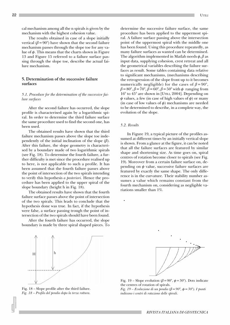
The obtained results have shown that the thirdfailure mechanism passes above the slope toe inde-pendently of the initial inclination of the slope (β).After this failure, the slope geometry is characteri-sed by a boundary made of two logarithmic spirals(see Fig. 18). To determine the fourth failure, a fur-ther difficulty is met since the procedure realised upto here, is not applicable to such a profile. It hasbeen assumed that the fourth failure passes abovethe point of intersection of the two spirals intendingto verify this hypothesis a posteriori. Hence the pro-cedure has been applied to the upper spiral of theslope boundary (height h in Fig. 18).

The obtained results have shown that the fourthfailure surface passes above the point of intersectionof the two spirals. This leads to conclude that thehypothesis done was true. In fact, if the hypothesiswere false, a surface passing trough the point of in-tersection of the two spirals should have been found.

After the fourth failure has occurred, the slopeboundary is made by three spiral shaped pieces. To

determine the successive failure surface, the sameprocedure has been applied to the uppermost spi-ral. A failure surface passing above the intersectionpoint of the uppermost spiral with the middle onehas been found. Using this procedure repeatedly, asmany failure surfaces as wanted can be determined.The algorithm implemented in Matlab needs φ, β asinput data, supplying cohesion, crest retreat and allthe geometrical variables describing the failure sur-faces as result. Some tables containing data relativeto significant mechanisms, (mechanisms describingthe retrogression of the slope front up to it becomesnumerically negligible) for the cases of β=90°,β=80°, β=70°, β=60°, β=50° with φ ranging from16° to 45° are shown in [UTILI, 2004]. Depending onφ values, a few (in case of high values of φ) or many(in case of low values of φ) mechanisms are neededto be determined to describe, in a complete way, theevolution of the slope.

5.2. Results

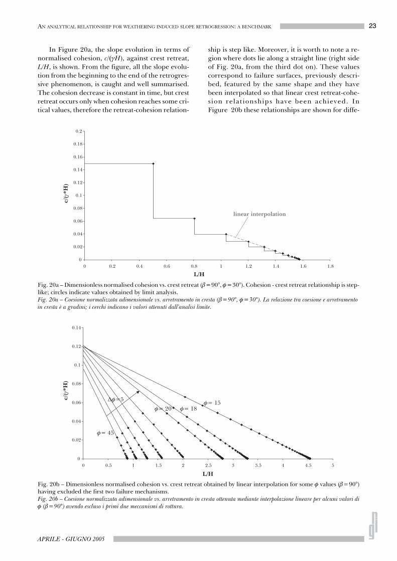
In Figure 19, a typical picture of the profiles as-sumed at different times by an initially vertical slopeis shown. From a glance at the figure, it can be notedthat all the failure surfaces are featured by similarshape and shortening size. As time goes on, spiralcentres of rotation become closer to spirals (see Fig.19). Moreover from a certain failure surface on, de-pending on φ value, successive failure surfaces arefeatured by exactly the same shape. The only diffe-rence is in the curvature. Their stability number as-sumes a value which remains constant from thefourth mechanism on, considering as negligible va-riations smaller than 1%.

Fig. 18 – Slope profile after the third failure.Fig. 18 – Profilo del pendio dopo la terza rottura.

Fig. 19 – Slope evolution (β=90°, φ=30°). Dots indicatethe centres of rotation of spirals.Fig. 19 – Evoluzione di un pendio (β=90°, φ=30°). I punti indicano i centri di rotazione delle spirali.



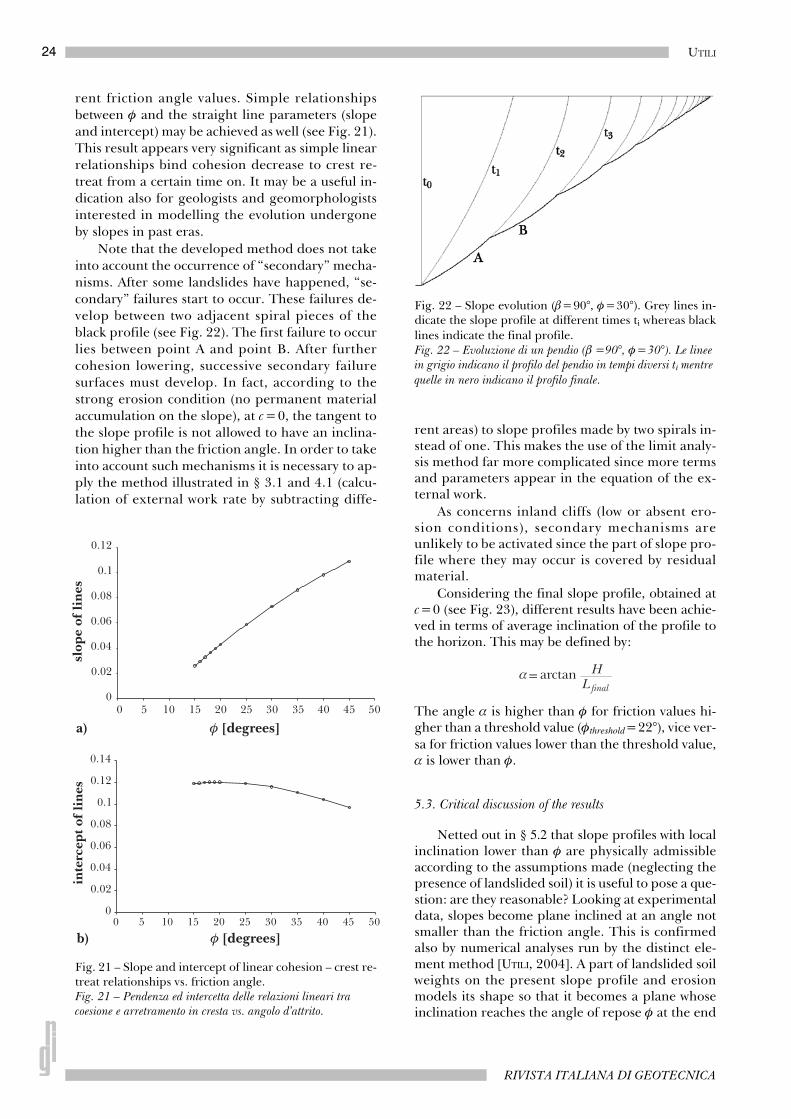
In Figure 20a, the slope evolution in terms ofnormalised cohesion, c/(γH), against crest retreat,L/H, is shown. From the figure, all the slope evolu-tion from the beginning to the end of the retrogres-sive phenomenon, is caught and well summarised.The cohesion decrease is constant in time, but crestretreat occurs only when cohesion reaches some cri-tical values, therefore the retreat-cohesion relation-

ship is step like. Moreover, it is worth to note a re-gion where dots lie along a straight line (right sideof Fig. 20a, from the third dot on). These valuescorrespond to failure surfaces, previously descri-bed, featured by the same shape and they havebeen interpolated so that linear crest retreat-cohe-sion relat ionships have been achieved. InFigure 20b these relationships are shown for diffe-

Fig. 20a – Dimensionless normalised cohesion vs. crest retreat (β=90°, φ=30°). Cohesion - crest retreat relationship is step-like; circles indicate values obtained by limit analysis.Fig. 20a – Coesione normalizzata adimensionale vs. arretramento in cresta (β=90°, φ=30°). La relazione tra coesione e arretramento in cresta è a gradini; i cerchi indicano i valori ottenuti dall’analisi limite.

Fig. 20b – Dimensionless normalised cohesion vs. crest retreat obtained by linear interpolation for some φ values (β=90°)having excluded the first two failure mechanisms.Fig. 20b – Coesione normalizzata adimensionale vs. arretramento in cresta ottenuta mediante interpolazione lineare per alcuni valori diφ (β=90°) avendo escluso i primi due meccanismi di rottura.

24 UTILI


rent friction angle values. Simple relationshipsbetween φ and the straight line parameters (slopeand intercept) may be achieved as well (see Fig. 21).This result appears very significant as simple linearrelationships bind cohesion decrease to crest re-treat from a certain time on. It may be a useful in-dication also for geologists and geomorphologistsinterested in modelling the evolution undergoneby slopes in past eras.

Note that the developed method does not takeinto account the occurrence of “secondary” mecha-nisms. After some landslides have happened, “se-condary” failures start to occur. These failures de-velop between two adjacent spiral pieces of theblack profile (see Fig. 22). The first failure to occurlies between point A and point B. After furthercohesion lowering, successive secondary failuresurfaces must develop. In fact, according to thestrong erosion condition (no permanent materialaccumulation on the slope), at c=0, the tangent tothe slope profile is not allowed to have an inclina-tion higher than the friction angle. In order to takeinto account such mechanisms it is necessary to ap-ply the method illustrated in § 3.1 and 4.1 (calcu-lation of external work rate by subtracting diffe-

rent areas) to slope profiles made by two spirals in-stead of one. This makes the use of the limit analy-sis method far more complicated since more termsand parameters appear in the equation of the ex-ternal work.

As concerns inland cliffs (low or absent ero-sion conditions), secondary mechanisms areunlikely to be activated since the part of slope pro-file where they may occur is covered by residualmaterial.

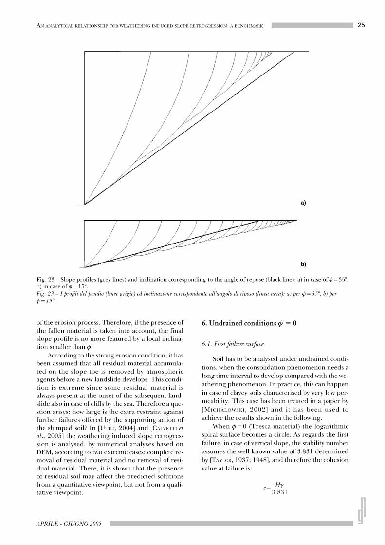
Considering the final slope profile, obtained atc=0 (see Fig. 23), different results have been achie-ved in terms of average inclination of the profile tothe horizon. This may be defined by:

The angle α is higher than φ for friction values hi-gher than a threshold value (φthreshold=22°), vice ver-sa for friction values lower than the threshold value,α is lower than φ.

5.3. Critical discussion of the results

Netted out in § 5.2 that slope profiles with localinclination lower than φ are physically admissibleaccording to the assumptions made (neglecting thepresence of landslided soil) it is useful to pose a que-stion: are they reasonable? Looking at experimentaldata, slopes become plane inclined at an angle notsmaller than the friction angle. This is confirmedalso by numerical analyses run by the distinct ele-ment method [UTILI, 2004]. A part of landslided soilweights on the present slope profile and erosionmodels its shape so that it becomes a plane whoseinclination reaches the angle of repose φ at the end

Fig. 21 – Slope and intercept of linear cohesion – crest re-treat relationships vs. friction angle.Fig. 21 – Pendenza ed intercetta delle relazioni lineari tra coesione e arretramento in cresta vs. angolo d’attrito.

Fig. 22 – Slope evolution (β=90°, φ=30°). Grey lines in-dicate the slope profile at different times ti whereas blacklines indicate the final profile.Fig. 22 – Evoluzione di un pendio (β =90°, φ=30°). Le linee in grigio indicano il profilo del pendio in tempi diversi ti mentre quelle in nero indicano il profilo finale.



of the erosion process. Therefore, if the presence ofthe fallen material is taken into account, the finalslope profile is no more featured by a local inclina-tion smaller than φ.

According to the strong erosion condition, it hasbeen assumed that all residual material accumula-ted on the slope toe is removed by atmosphericagents before a new landslide develops. This condi-tion is extreme since some residual material isalways present at the onset of the subsequent land-slide also in case of cliffs by the sea. Therefore a que-stion arises: how large is the extra restraint againstfurther failures offered by the supporting action ofthe slumped soil? In [UTILI, 2004] and [CALVETTI etal., 2005] the weathering induced slope retrogres-sion is analysed, by numerical analyses based onDEM, according to two extreme cases: complete re-moval of residual material and no removal of resi-dual material. There, it is shown that the presenceof residual soil may affect the predicted solutionsfrom a quantitative viewpoint, but not from a quali-tative viewpoint.

6. Undrained conditions φ = 0

6.1. First failure surface

Soil has to be analysed under undrained condi-tions, when the consolidation phenomenon needs along time interval to develop compared with the we-athering phenomenon. In practice, this can happenin case of clayey soils characterised by very low per-meability. This case has been treated in a paper by[MICHALOWSKI, 2002] and it has been used toachieve the results shown in the following.

When φ=0 (Tresca material) the logarithmicspiral surface becomes a circle. As regards the firstfailure, in case of vertical slope, the stability numberassumes the well known value of 3.831 determinedby [TAYLOR, 1937; 1948], and therefore the cohesionvalue at failure is:

Fig. 23 – Slope profiles (grey lines) and inclination corresponding to the angle of repose (black line): a) in case of φ=35°,b) in case of φ=15°.Fig. 23 – I profili del pendio (linee grigie) ed inclinazione corrispondente all’angolo di riposo (linea nera): a) per φ=35°, b) per φ=15°.

26 UTILI


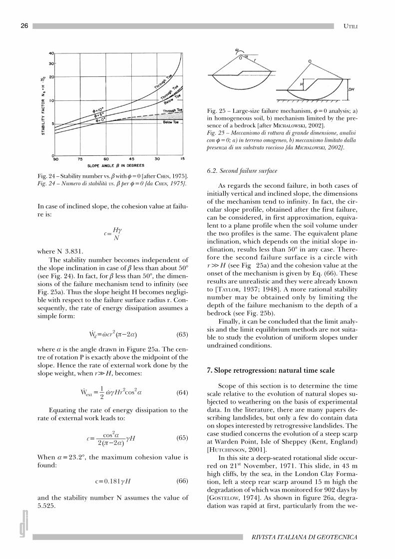
In case of inclined slope, the cohesion value at failu-re is:

where N 3.831.The stability number becomes independent of

the slope inclination in case of β less than about 50°(see Fig. 24). In fact, for β less than 50°, the dimen-sions of the failure mechanism tend to infinity (seeFig. 25a). Thus the slope height H becomes negligi-ble with respect to the failure surface radius r. Con-sequently, the rate of energy dissipation assumes asimple form:

(63)

where α is the angle drawn in Figure 25a. The cen-tre of rotation P is exactly above the midpoint of theslope. Hence the rate of external work done by theslope weight, when r>>H, becomes:

(64)

Equating the rate of energy dissipation to therate of external work leads to:

(65)

When α=23.2°, the maximum cohesion value isfound:

(66)

and the stability number N assumes the value of5.525.

6.2. Second failure surface

As regards the second failure, in both cases ofinitially vertical and inclined slope, the dimensionsof the mechanism tend to infinity. In fact, the cir-cular slope profile, obtained after the first failure,can be considered, in first approximation, equiva-lent to a plane profile when the soil volume underthe two profiles is the same. The equivalent planeinclination, which depends on the initial slope in-clination, results less than 50° in any case. There-fore the second failure surface is a circle withr>>H (see Fig 25a) and the cohesion value at theonset of the mechanism is given by Eq. (66). Theseresults are unrealistic and they were already knownto [TAYLOR, 1937; 1948]. A more rational stabilitynumber may be obtained only by limiting thedepth of the failure mechanism to the depth of abedrock (see Fig. 25b).

Finally, it can be concluded that the limit analy-sis and the limit equilibrium methods are not suita-ble to study the evolution of uniform slopes underundrained conditions.

7. Slope retrogression: natural time scale

Scope of this section is to determine the timescale relative to the evolution of natural slopes su-bjected to weathering on the basis of experimentaldata. In the literature, there are many papers de-scribing landslides, but only a few do contain dataon slopes interested by retrogressive landslides. Thecase studied concerns the evolution of a steep scarpat Warden Point, Isle of Sheppey (Kent, England)[HUTCHINSON, 2001].

In this site a deep-seated rotational slide occur-red on 21st November, 1971. This slide, in 43 mhigh cliffs, by the sea, in the London Clay Forma-tion, left a steep rear scarp around 15 m high thedegradation of which was monitored for 902 days by[GOSTELOW, 1974]. As shown in figure 26a, degra-dation was rapid at first, particularly from the we-

Fig. 24 – Stability number vs. β with φ=0 [after CHEN, 1975].Fig. 24 – Numero di stabilità vs. β per φ=0 [da CHEN, 1975].

Fig. 25 – Large-size failure mechanism, φ=0 analysis; a)in homogeneous soil, b) mechanism limited by the pre-sence of a bedrock [after MICHALOWSKI, 2002].Fig. 25 – Meccanismo di rottura di grande dimensione, analisi con φ=0; a) in terreno omogeneo, b) meccanismo limitato dalla presenza di un substrato roccioso [da MICHALOWSKI, 2002].



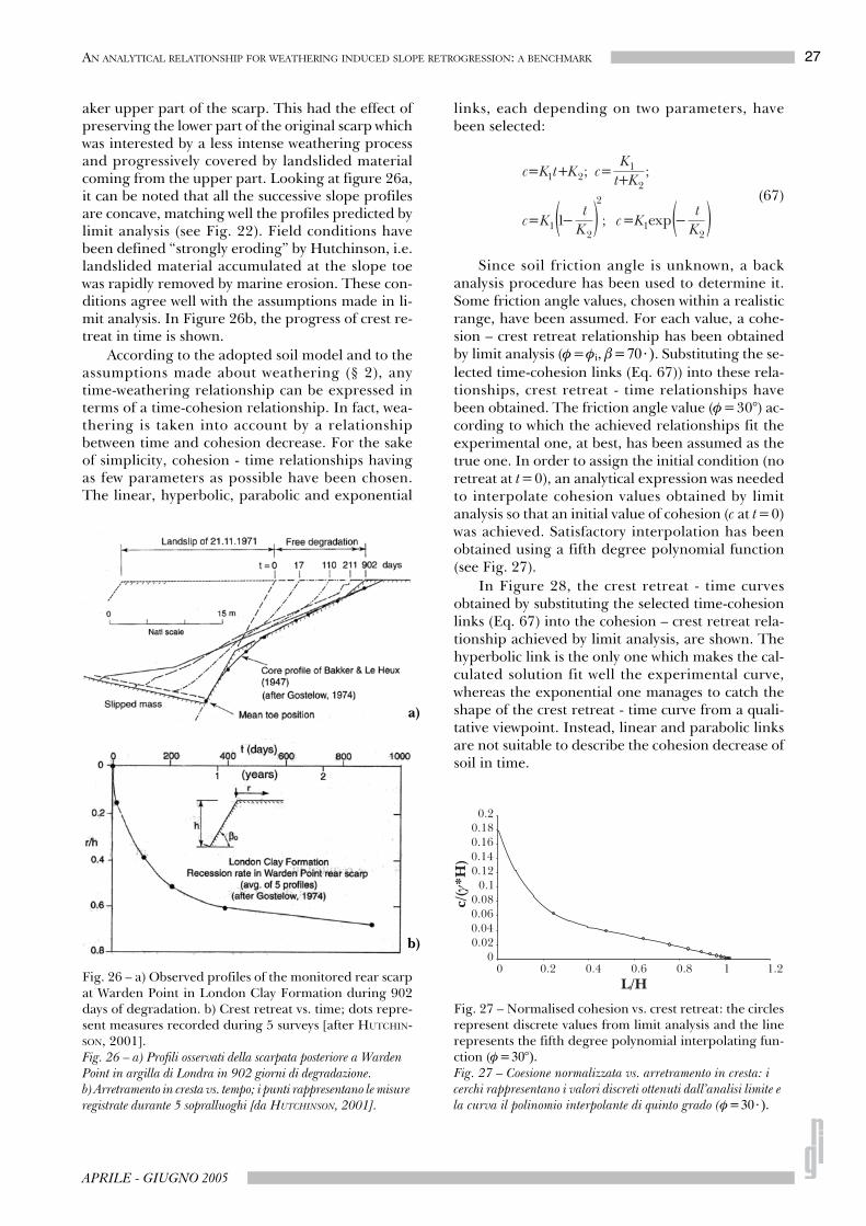
aker upper part of the scarp. This had the effect ofpreserving the lower part of the original scarp whichwas interested by a less intense weathering processand progressively covered by landslided materialcoming from the upper part. Looking at figure 26a,it can be noted that all the successive slope profilesare concave, matching well the profiles predicted bylimit analysis (see Fig. 22). Field conditions havebeen defined “strongly eroding” by Hutchinson, i.e.landslided material accumulated at the slope toewas rapidly removed by marine erosion. These con-ditions agree well with the assumptions made in li-mit analysis. In Figure 26b, the progress of crest re-treat in time is shown.

According to the adopted soil model and to theassumptions made about weathering (§ 2), anytime-weathering relationship can be expressed interms of a time-cohesion relationship. In fact, wea-thering is taken into account by a relationshipbetween time and cohesion decrease. For the sakeof simplicity, cohesion - time relationships havingas few parameters as possible have been chosen.The linear, hyperbolic, parabolic and exponential

links, each depending on two parameters, havebeen selected:

(67)

Since soil friction angle is unknown, a backanalysis procedure has been used to determine it.Some friction angle values, chosen within a realisticrange, have been assumed. For each value, a cohe-sion – crest retreat relationship has been obtainedby limit analysis (φ=φi, β=70⋅). Substituting the se-lected time-cohesion links (Eq. 67)) into these rela-tionships, crest retreat - time relationships havebeen obtained. The friction angle value (φ=30°) ac-cording to which the achieved relationships fit theexperimental one, at best, has been assumed as thetrue one. In order to assign the initial condition (noretreat at t=0), an analytical expression was neededto interpolate cohesion values obtained by limitanalysis so that an initial value of cohesion (c at t=0)was achieved. Satisfactory interpolation has beenobtained using a fifth degree polynomial function(see Fig. 27).

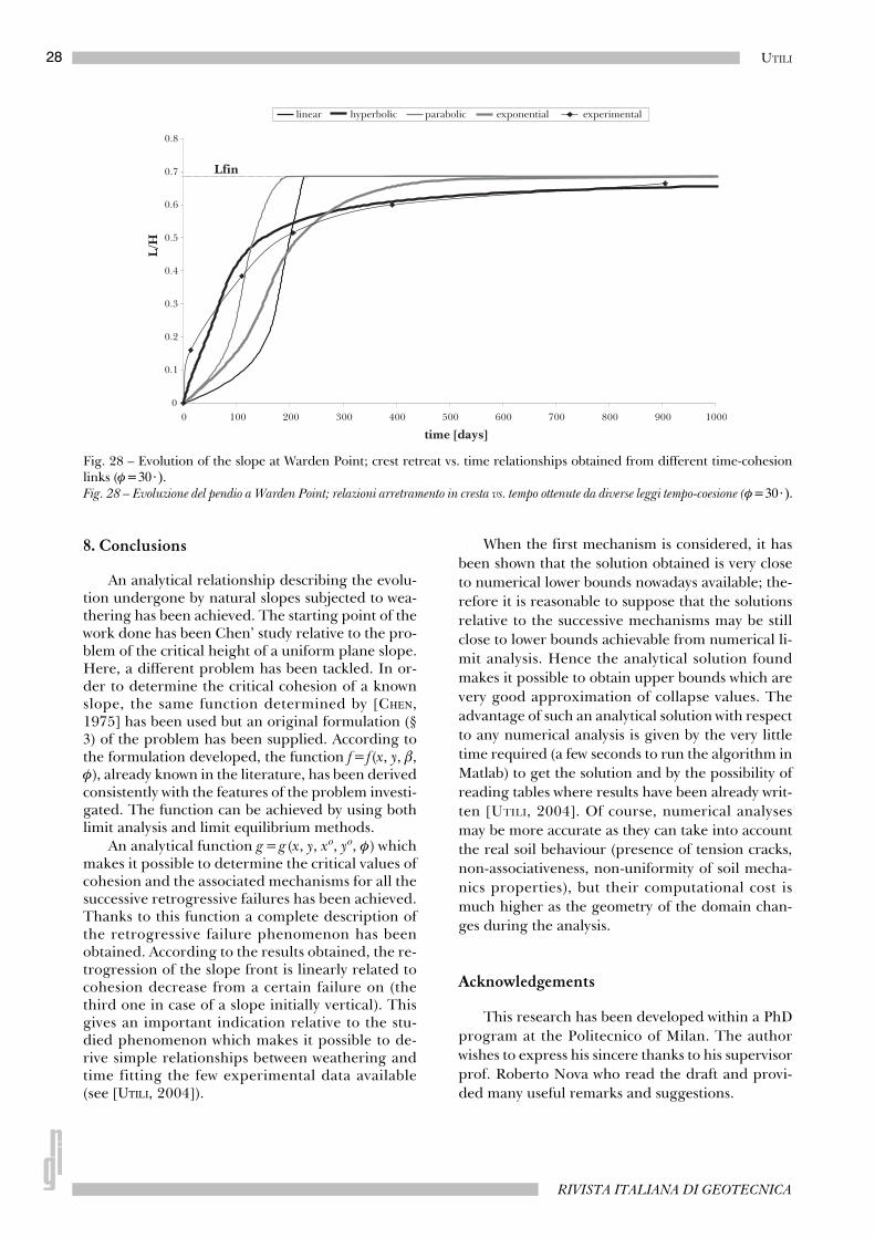
In Figure 28, the crest retreat - time curvesobtained by substituting the selected time-cohesionlinks (Eq. 67) into the cohesion – crest retreat rela-tionship achieved by limit analysis, are shown. Thehyperbolic link is the only one which makes the cal-culated solution fit well the experimental curve,whereas the exponential one manages to catch theshape of the crest retreat - time curve from a quali-tative viewpoint. Instead, linear and parabolic linksare not suitable to describe the cohesion decrease ofsoil in time.

Fig. 26 – a) Observed profiles of the monitored rear scarpat Warden Point in London Clay Formation during 902days of degradation. b) Crest retreat vs. time; dots repre-sent measures recorded during 5 surveys [after HUTCHIN-SON, 2001].Fig. 26 – a) Profili osservati della scarpata posteriore a Warden Point in argilla di Londra in 902 giorni di degradazione.b) Arretramento in cresta vs. tempo; i punti rappresentano le misure registrate durante 5 sopralluoghi [da HUTCHINSON, 2001].

b)

a)

Fig. 27 – Normalised cohesion vs. crest retreat: the circlesrepresent discrete values from limit analysis and the linerepresents the fifth degree polynomial interpolating fun-ction (φ=30°).Fig. 27 – Coesione normalizzata vs. arretramento in cresta: i cerchi rappresentano i valori discreti ottenuti dall’analisi limite e la curva il polinomio interpolante di quinto grado (φ=30⋅).

28 UTILI


8. Conclusions

An analytical relationship describing the evolu-tion undergone by natural slopes subjected to wea-thering has been achieved. The starting point of thework done has been Chen’ study relative to the pro-blem of the critical height of a uniform plane slope.Here, a different problem has been tackled. In or-der to determine the critical cohesion of a knownslope, the same function determined by [CHEN,1975] has been used but an original formulation (§3) of the problem has been supplied. According tothe formulation developed, the function f= f(x, y, β,φ), already known in the literature, has been derivedconsistently with the features of the problem investi-gated. The function can be achieved by using bothlimit analysis and limit equilibrium methods.

An analytical function g=g (x, y, xo, yo, φ) whichmakes it possible to determine the critical values ofcohesion and the associated mechanisms for all thesuccessive retrogressive failures has been achieved.Thanks to this function a complete description ofthe retrogressive failure phenomenon has beenobtained. According to the results obtained, the re-trogression of the slope front is linearly related tocohesion decrease from a certain failure on (thethird one in case of a slope initially vertical). Thisgives an important indication relative to the stu-died phenomenon which makes it possible to de-rive simple relationships between weathering andtime fitting the few experimental data available(see [UTILI, 2004]).

When the first mechanism is considered, it hasbeen shown that the solution obtained is very closeto numerical lower bounds nowadays available; the-refore it is reasonable to suppose that the solutionsrelative to the successive mechanisms may be stillclose to lower bounds achievable from numerical li-mit analysis. Hence the analytical solution foundmakes it possible to obtain upper bounds which arevery good approximation of collapse values. Theadvantage of such an analytical solution with respectto any numerical analysis is given by the very littletime required (a few seconds to run the algorithm inMatlab) to get the solution and by the possibility ofreading tables where results have been already writ-ten [UTILI, 2004]. Of course, numerical analysesmay be more accurate as they can take into accountthe real soil behaviour (presence of tension cracks,non-associativeness, non-uniformity of soil mecha-nics properties), but their computational cost ismuch higher as the geometry of the domain chan-ges during the analysis.

Acknowledgements

This research has been developed within a PhDprogram at the Politecnico of Milan. The authorwishes to express his sincere thanks to his supervisorprof. Roberto Nova who read the draft and provi-ded many useful remarks and suggestions.

Fig. 28 – Evolution of the slope at Warden Point; crest retreat vs. time relationships obtained from different time-cohesionlinks (φ=30⋅).Fig. 28 – Evoluzione del pendio a Warden Point; relazioni arretramento in cresta vs. tempo ottenute da diverse leggi tempo-coesione (φ=30⋅).



Appendix

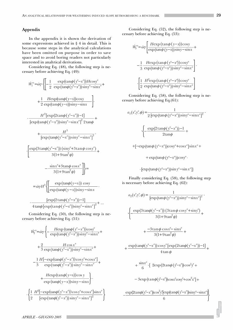
In the appendix it is shown the derivation ofsome expressions achieved in § 4 in detail. This isbecause some steps in the analytical calculationshave been omitted on purpose in order to savespace and to avoid boring readers not particularlyinterested in analytical derivations.

Considering Eq. (48), the following step is ne-cessary before achieving Eq. (49):



Considering Eq. (58), the following step is ne-cessary before achieving Eq.(61):

Finally considering Eq. (58), the following stepis necessary before achieving Eq. (62):

30 UTILI


References

ABDI R., DE BUHAN P., PASTOR J. (1994) – Calcula-tion of the critical height of a homogenized reinforcedsoil wall: a numerical approach. Int. J. Numer. Anal.Methods Geomech., 18, pp. 485-505.

BAKKER J.P., LE HEUX J.W.N. (1947) – Theory on cen-tral rectilinear recession of slopes. I & II. KoninklijkeNederlandsche Akademie van Wetenschappen,Series B, 50, pp. 959-966, pp. 1154-1162.

BEKAERT A. (1995) – Improvement of the kinematicbound for the stability of a vertical cut-off. Mech. Res.Comm., 22(6), pp. 533-540.

CALVETTI F., NOVA R., UTILI S. (2005) – On model-ling rock slope retreat by the Discrete Element Method.Proc. Powders & Grains, Stuttgart.

CHEN W. F. (1975) – Limit analysis and soil plasticity.Elsevier, Amsterdam.

FISHER O. (1866) – On the disintegration of a chalk cliff.Geol. Magazine, 3, pp. 354-356.

GOSTELOW T. P. (1974) – Slope development in stiffoverconsolidated clays. PhD. thesis. Imperial Col-lege, University of London, London.

HUTCHINSON J. N. (1973) – The response of LondonClay cliffs to differing rates of toe erosion. Geol. Appl.e Idrogeol., Bari, 7, pp. 221-239.

HUTCHINSON J. N. (2001) – Reading the ground: Mor-phology and Geology in Site Appraisal. Quarterly J.of Engrg. Geol. and Hydrogeol., 34, pp. 7-50.

KIMMANCE G.C. (1988) – Computer aided risk analysisof open pit mine slopes in kaolin mined deposits. PhD.thesis, University of London, London.

KIRKBY M.J. (1987) – General models of long-term slopeevolution through mass movement. In: AndersonM.G., Richards K.S. (Eds.), Slope Stability. Wiley,London, pp. 359-379.

LYAMIN A.V., SLOAN S.W. (2002) – Lower bound limitanalysis using nonlinear programming. Int. J. Nu-mer. Meth. Engng., 55(5), pp. 573-611.

MANZARI M.T., NOUR M.A. (2000) – Significance ofsoil dilatancy in slope stability analysis. J. Geotech. &Geoenv. Engrg., ASCE, 126(1), pp. 75-80.

MICHALOWSKI R. (2002) – Stability charts for uniformslopes. J. Geotech. & Geoenv. Engrg., ASCE,128(4), pp. 351-355.

TAYLOR D. W. (1937) – Stability of earth slopes. J. Bos-ton Soc. Civil Engineers., 24(3), pp. 197-246. Re-printed in: Contributions to soil mechanics 1925 to1940. Boston Soc. Civil Engineers, pp. 337-386.

TAYLOR D. W. (1948) – Fundamentals of soil mechanics.Wiley.

UTILI S. (2004) – Evolution of natural slopes subject toweathering: an analytical and numerical study. PhD.thesis, Politecnico di Milano, Milan, 206 pp.

Una legge analitica per l’arretramento di pendii indotto da degradazione: un benchmark

SommarioNell’articolo si illustra uno studio condotto sull’evoluzione di

pendii soggetti a degradazione con il metodo cinematico dell’analisi limite. I pendii soggetti a degradazione subiscono frane che avvengono in tempi diversi e causano il progressivo arretramento del fronte del pendio. La successione discreta dei distacchi è stata modellata tenendo conto della geometria via via assunta dai pendii dopo ciascuna frana. Si è modellato il terreno come un materiale alla Coulomb (c, φ). Per quanto riguarda la degradazione, si è ipotizzato che la coesione diminuisca uniformemente all’interno del pendio e l’angolo d’attrito rimanga costante. Si è così ottenuta una soluzione analitica che fornisce la geometria della linea di rottura e le proprietà meccaniche del suolo al momento del distacco di ciascuna frana.

Documents

An analytical relationship for weathering induced slope retrogression: a benchmark