An Analysis of Strategies for Mitigating the Sensor Network Hot Spot Problem

Strategies for Mitigating the Sensor Network HotSpot Problem

Mark Perillo, Zhao Cheng, and Wendi HeinzelmanDepartment of Electrical and Computer Engineering

University of RochesterRochester, NY 14627

Email: {perillo,zhcheng,wheinzel}@ece.rochester.edu

Abstract— In multi-hop wireless sensor networks that arecharacterized by many-to-one (convergecast) traffic patterns,problems related to energy imbalance among sensors often ap-pear. When the transmission range is fixed for nodes throughoutthe network, the amount of traffic that sensors are required toforward increases dramatically as the distance to the data sinkbecomes smaller. Thus, sensors closest to the data sink tend to dieearly, leaving areas of the network completely unmonitored andcausing network partitions. Alternatively, if all sensors transmitdirectly to the data sink, the furthest nodes from the data sinkwill die much more quickly than those close to the sink. Networklifetime can be improved to a limited extent by the use of a moreintelligent transmission power control policy that balances theenergy used in each node by requiring nodes further from thedata sink to transmit over longer distances (although not directlyto the data sink). However, transmission power control alone isnot enough to solve the hot spot problem. Rather, policies suchas data sink movement or data aggregation are necessary forthe network to operate in an energy efficient manner. Since themovement of the data sink and the deployment of an aggregatornode may be significantly more expensive than the deployment ofan ordinary microsensor node, there is a cost tradeoff involvedin both of these approaches. This paper provides an analysis ofeach of these policies for mitigating the sensor network hot spotproblem, considering energy efficiency as well as cost efficiency.

I. I NTRODUCTION

Large scale wireless sensor networks are an emerging tech-nology that have recently gained attention for their potentialuse in applications such as environmental sensing and mobiletarget tracking. Since sensors typically operate on batteries andare thus limited in their active lifetime, the problem of design-ing protocols to achieve energy efficiency to extend networklifetime has become a major concern for network designers.Much attention has been given to the reduction of unnecessaryenergy consumption of sensor nodes in areas such as hardwaredesign, collaborative signal processing, transmission powercontrol polices, and all levels of the network stack. However,reducing an individual sensor’s power consumption alone maynot always allow networks to realize their maximal potentiallifetime. In addition, it is important to maintain a balance ofpower consumption in the network so that certain nodes donot die much earlier than others, leading to unmonitored areasin the network.

Previous research has shown that because of the characteris-tics of wireless channels, multihop forwarding between a datasource and a data sink is often more energy efficient than directtransmission. Based on the power model of a specific sensornode platform, there exists an optimal transmission rangethat minimizes overall power consumption in the network.When using such a fixed transmission range in general ad hocnetworks, energy consumption is fairly balanced, especiallyin mobile networks, since the data sources and sinks aretypically assumed to be distributed throughout the area wherethe network is deployed. However, in sensor networks, wheremany applications require a many-to-one (convergecast) trafficpattern in the network, energy imbalance becomes a veryimportant issue, as a hot spot is created around the data sink, orbase station. The nodes in this hot spot are required to forwarda disproportionately high amount of traffic and typically dieat a very early stage. If we define the network lifetime asthe time when the first subregion of the environment (or asignificant portion of the environment) is left unmonitored,then the residual energy of the other sensors at this time canbe seen as wasted.

Intuition leads us to believe that the hot spot problem can besolved by varying the transmission range among nodes at dif-ferent distances to the base station so that energy consumptioncan be more evenly distributed and the lifetime of the networkcan be extended. However, this is only true to some extent,as energy balancing can only be achieved at the expense ofusing the energy resources of some nodes inefficiently [1]. Weconclude from our study that transmission power control canalleviate the hot spot problem only to a limited degree, andalternative solutions are necessary for the network to operatein a more energy efficient manner.

In this paper, we formulate the transmission range distri-bution optimization problem and analyze the limits of net-work lifetime for uniformly deployed wireless sensor net-works, which are easily obtained by using a practical energy-associated heuristic solution. However, as optimal transmissionrange distribution cannot fully solve the hot spot problem,we explore two alternative strategies: the employment ofmultiple data sink locations, implemented by using either amobile data sink or several sinks deployed during the initialnetwork deployment, and the formation of data aggregation

clusters. We investigate the effectiveness of these techniquesin combination with the optimization of transmission rangedistribution to determine their effectiveness in extending net-work lifetime. Since applying these strategies during networkdeployment may introduce extra costs, we explore the tradeoffbetween using these more advanced solutions and the cost,and we propose cost efficient suggestions for practical sensordeployments.

The rest of this paper is organized as follows. SectionII addresses related work. Section III reviews the transmis-sion power control problem and explores its effectiveness inmitigating the hot spot problem. Section IV investigates theeffectiveness and cost efficiency of data sink movement andthe deployment of multiple aggregator nodes, respectively,as alternative solutions to the hot spot problem. Section Vconcludes the paper.

II. RELATED WORK

A. Transmission Range Optimization

Early work in transmission range optimization assumedthat forwarding data packets towards a data sink over manyshort hops is more energy efficient than forwarding over afew long hops, due to the nature of wireless communication.The problem of setting transmission power to a minimallevel that will allow a network to remain connected has beenconsidered in several studies [2], [3]. Later, others noted thatbecause of the electronics overhead involved in transmittingpackets, there exists an optimal non-zero transmission range,at which power efficiency is maximized [4], [5]. The goal ofthese studies was to find a fixed network-wide transmissionrange. However, using such schemes may result in extremelyunbalanced energy consumption among the nodes in sensornetworks characterized by many-to-one traffic patterns. If wedefine sensor network lifetime as the model presented in [6],which is the network duration until the first node runs outof energy, this unbalanced energy consumption will greatlyreduce the network lifetime.

An energy efficient routing scheme was proposed in [7].The objective function of this scheme is to extend networklifetime by routing outgoing traffic intelligently. Iterative al-gorithms that are based on the formulation of the problemas a concurrent maximum flow problem are presented aswell. Our transmission range distribution problem is similarto this energy efficient routing problem in many aspects.However, we propose a heuristic scheme that can easily beimplemented rather than only providing an upper bound onnetwork lifetime for specific topologies. Also, we extend thesolution to alternative strategies rather than attempting to solvethe problem using transmission range distribution alone.

B. Sensor deployment strategies

Several sensor deployment strategies exist that can help ex-tend network lifetime. These strategies include the movementof data sinks [8], [9], [10], [11], [12], the deployment multiplebase stations [13], and the formation of data aggregationclusters [14], [15], [16]. However, some of the research related

to these strategies has primarily considered the case wherethe strategies are specifically chosen around the applicationrequirements, while the others have focused only on thefeasibility of the proposed solution while ignoring the fact thata more complex sensor deployment scheme may incur a largerfinancial cost. In this paper, not only do we investigate andcompare the performance of each strategy using general termssuch as normalized network lifetime, but we also propose somepractical sensor deployment strategies from a cost efficientperspective.

III. T RANSMISSIONPOWER CONTROL

In this section, we review our study of the transmissionrange distribution optimization problem, which is solved bydetermining how a node should distribute its outgoing datapackets over multiple distances, always using the minimumtransmission power necessary to send over each distance.Given the energy constraints and data generation rate of eachsensor node, the lifetime of the network, which we define tobe the time at which the first sensor dies, can be maximizedby using this optimal distribution. In typical sensor networkapplications, it may be true that the network can survivenode failures as long as neighboring sensors can assume thefailing nodes’ responsibilities; however, we expect neighboringsensors to exhibit similar trends and attain similar lifetimes.Thus, we consider our definition of network lifetime valid evenfor such sensor network models. We refer to this problem asa transmission range distribution optimization problem ratherthan a transmission range optimization problem because weassume that nodes may send packets over multiple transmis-sion ranges instead of setting a fixed transmission range. Inour work, we have adopted the widely used power model from[14], where the amount of energy to transmit a bit can berepresented asEbit,tx = Eelec+εdα and the amount of energyto receive a bit can be represented asEbit,rx = Eelec. Toobtain a true upper bound on network lifetime, we have madeseveral simplifications in our network model. For a descriptionof our model and assumptions, the reader is referred to [1].

In order to show the effectiveness of optimizing transmis-sion range distribution, we provide simulation results thatgive the lifetime obtained using three different solutions: theoptimal solution as found in [1], the optimal fixed transmissionrange solution and an energy-associated heuristic solution.In the second solution, we use the ideal energy efficienttransmission ranged∗ = α

√2Eelec

(α−1)ε from [4], [5], which isoptimal in the absence of the sensor network hot spot problem.The third solution is obtained using our proposed energy-associated heuristic scheme. In this scheme, we assign routingcosts to sensors to be the inverse of their residual energy. Linkcosts are set equal to a weighted sum of the energy consumedby the transmitting node and the receiving node, as given byEquation 1. Minimum cost routes are updated throughout thelifetime of the network through frequent routing updates. Inall simulations, we use values ofEelec = 50 nJ/bit andε = 100 pJ/bit/m2, resulting in a value ofd∗ = 32m.

��

��

�

��

�

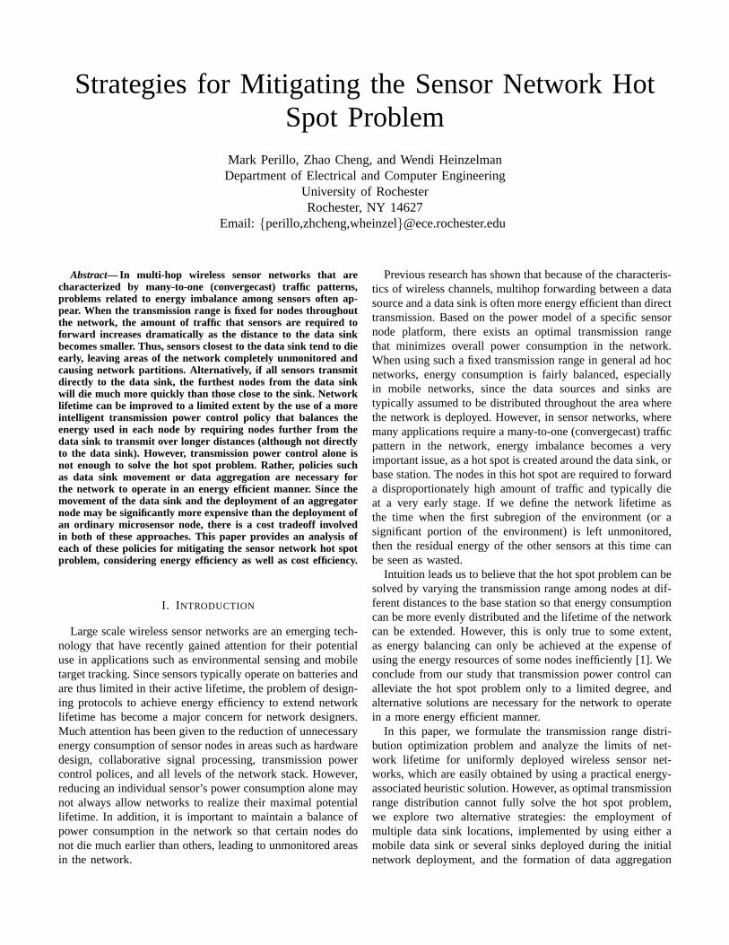
Fig. 1. One-dimensional modeling of a two-dimensional sensor field.

Clink(si, sj) =1

Eres(si)Etx,bit(si, sj) +

1Eres(sj)

Erx,bit(si, sj) (1)

For any given scenario, we can obtain the network lifetimeL and the transmission distributions using these three schemes.Let us begin with a simple scenario, a densely deployeduniform two-dimensional field, as a case study. We modeledthis deployment as a one-dimensional field with nonuniformspacing. With very dense sensor deployment, we can assumethat sensors will always send their packets within an infini-tesimally thin angle toward the data sink. Since the numberof nodesN within the distancer from the data sink satisfiesN ∝ r2 for two-dimensional networks, when mapped onto aone-dimensional space, the distance of a node to the data sinkshould be proportional to the square root of the node index,as shown in Figure 1.

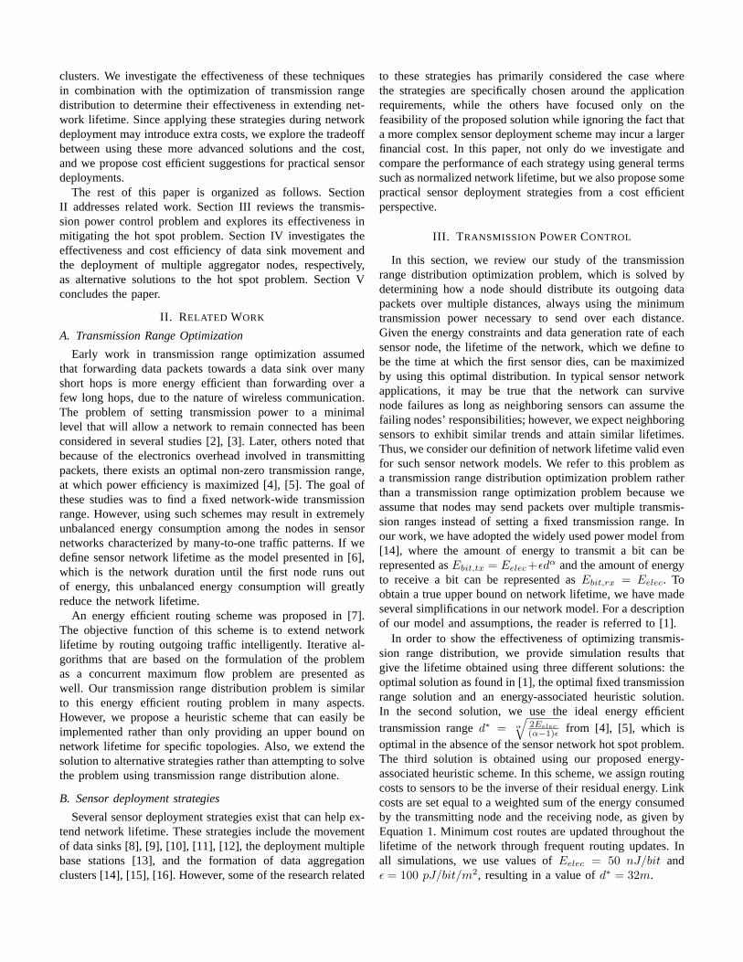
The network lifetime performance using the three schemesare shown in Figure 2. Using a fixed network-wide transmis-sion range results in a lower network lifetime, even when theoptimal fixed transmission range is used. This illustrates theimportance of varying the transmission range as a function ofa node’s location in the network. Because it incorporates twoimportant goals of lifetime maximization – power minimiza-tion and energy balancing – the energy-associated heuristicrouting scheme is able to achieve close to the lifetime obtainedthrough the optimal transmission range distribution (the dottedline almost overlaps with the solid line in Figure 2). Using thisscheme, minimum power routes are initially chosen, but asthe nodes closest to the data sink start to deplete their energyresources, they are avoided as routers. However, even in thelater stages of the network, the power minimization goal isnot completely abandoned. Eventually, the routes convergeto those that are found through the optimization, and onlya small penalty is paid for not discovering the optimality ofthese routes early enough.

While transmission range distribution optimization and ourheuristic scheme are somewhat effective in extending networklifetime compared to the scheme that uses a fixed transmissionrange, this improvement is limited because of the energyinefficiency forced on the sensors farthest from the data sinkin order to evenly distribute the energy load among the nodes.In fact, in order to achieve near-optimal network lifetimes, itis only necessary to use a fraction of the energy available inthe network. Consider the two-dimensional network used in

50 100 150 200 2500

1

2

3

4

5

6

x 106

Network radius (m)

Net

wor

k lif

etim

e (s

econ

ds)

OptimalHeuristicFixed transmission range

Fig. 2. Case study: network lifetime as a function of network radius for atwo-dimensional deployment scenario.

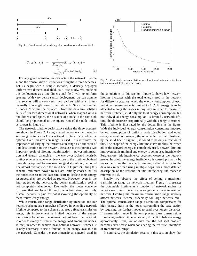
the simulations of this section. Figure 3 shows how networklifetime increases with the total energy used in the networkfor different scenarios, when the energy consumption of eachindividual sensor node is limited to1 J . If energy is to beallocated among the nodes in any way in order to maximizenetwork lifetime (i.e., if only the total energy consumption, butnot individual energy consumption, is limited), network life-time should increase proportionally with the energy consumed.This lifetime is illustrated by the dotted line in the figure.With the individual energy consumption constraints imposedby our assumption of uniform node distribution and equalenergy allocation, however, the obtainable lifetime, illustratedby the solid line in Figure 3, is found to be only a fraction ofthis. The shape of the energy-lifetime curve implies that whenall of the network energy is completely used, network lifetimeimprovement is minimal and energy is being used inefficiently.Furthermore, this inefficiency becomes worse as the networkgrows. In brief, the energy inefficiency is caused primarily bynodes far from the data sink sending traffic directly to thedata sink rather than using multiple hops. For a more detaileddescription of the reasons for this inefficiency, the reader isreferred to [1].

Finally, we observe the effect of setting a maximumtransmission range on network lifetime. Figure 4 illustratesthe obtainable lifetime as a function of network radius forvarious maximum transmission ranges in a two-dimensionalnetwork. Limiting the maximum transmission range severelyaffects network lifetime, especially for large network radii.The optimal transmission range distribution compensates forhigh energy drain in the nodes surrounding the base stationby requiring the furthest nodes to send over longer distances.If transmission range limitations prevent these transmissionsfrom being realized, it becomes very difficult to balance energyappropriately. Thus, we observe that the hot spot problembecomes even worse when considering the realistic limitationsof transmission range.

In summary, the simulation results in this section show that

0 50 100 150 2000

2

4

6

8

10

12

14

16

x 105

Total energy consumption (Joules)

Net

wor

k lif

etim

e (s

econ

ds) Individual energy limited

Total energy limited

(a)

0 50 100 150 2000

1

2

3

4

5

6

7

8

9

x 105

Total energy consumption (Joules)

Net

wor

k lif

etim

e (s

econ

ds) Individual energy limited

Total energy limited

(b)

Fig. 3. Lifetime vs. percentage of the total energy consumed in the networkfor a two-dimensional sensor field with a radius of150m and with a radiusof 250m.

50 100 150 200 2500

1

2

3

4

5

6

x 106

Network radius (m)

Net

wor

k lif

etim

e (s

econ

ds)

Transmission range=50mTransmission range=75mTransmission range=100mTransmission range=250m

Fig. 4. Network lifetime as a function of network radius for various maximumtransmission ranges in two-dimensional network deployments.

while optimizing the transmission range distribution increasesnetwork lifetime when compared to using a fixed network-wide transmission range, this optimal lifetime comes with acost of using the energy inefficiently, especially in very largenetworks. While using nonuniform deployment is the simplestsolution to the problem, this may lead to poorer sensingcapabilities in the regions farthest from the data sink. Further-more, this may be impossible in some applications. With thismotivation, we explore alternative strategies for improving thelifetime of many-to-one wireless sensor networks in the nextsection of this paper.

IV. SENSOR NETWORK DEPLOYMENT STRATEGIES

Since energy imbalance due to the many-to-one trafficpattern is the root cause of energy inefficiency and corre-sponding restricted network lifetime for sensor networks, wemust either compensate energy imbalance among the nodesin order to improve network lifetime or alter the many-to-onetraffic pattern. To compensate for the energy imbalance, wemust either assign more energy to nodes around hot spots ordeploy more nodes around hot spots. However, it may notalways be feasible to compensate for the energy imbalance byusing these solutions, especially when sensors are randomlydeployed and sensors are manufactured to be of the samecapabilities. Therefore, in this section, we focus on the lattercategory of solutions. To alter the many-to-one traffic pattern,several strategies can be applied, including mobile data sinks,multiple data sinks and clustering approaches. In addition,since alternative deployment strategies may incur extra cost,we study these strategies from the perspective of both energyefficiency and cost efficiency.

A. Normalized Lifetime

Before we discuss these specific strategies, we first definea general metric, normalized network lifetime, to describe theefficiency of a network deployment plan. In short, normalizednetwork lifetime L measures how many total bits can betransported on the network per unit of energy. For a givennetwork scenario, we are able to find the optimal lifetimeLopt. This lifetime can be arbitrarily increased by simplyincreasing the energy density in the network (either by scalingup the deployed sensor density or the average energy persensor). Also, since we assume that protocols that managethe amount of traffic sent (e.g., [17], [18], [19], [20]) may beused so that the density of active sensors does not necessarilycorrespond to the density of deployed sensors, lifetime cansimilarly be increased by decreasing the required active sensordensity. Similarly, lifetime can be increased by reducing thebit rate among active sensors. To account for these factors, thenormalized network lifetimeL is given as

L = Lopt

(Raλa

λe

)(2)

whereλa represents the density of active sensors,Ra repre-sents the average bit rate among active sensors,λe represents

the energy density of the network (we assume uniform distrib-ution of energy), andLopt is the maximum lifetime achievablewith the given parameters.

B. Strategy 1: Moving the Data Sink Location

Since intelligent transmission power control policies requireinefficient operation to maximize network lifetime, we mustsolve the hot spot problem by altering the many-to-one trafficpattern. One solution is to allow the data sink to move withinthe network. Two scenarios in which this is possible are

1) a network that employs a mobile data sink (e.g., a robot),and

2) a network in which multiple aggregator-capable nodesare deployed, only one of which collects all of the datain the network at a given time1. This can be seen as avirtual mobile data sink scenario.

These two scenarios are similar from the network routingperspective since during a given period, all data is sent toa single data sink. Although lifetime improvement is onemetric that we are interested in, we must realize that thesestrategies require extra implementation costs compared toschemes utilizing a single static sink. The extra costs maybe associated with the energy and extra hardware required tomove a data sink, or the hardware costs of deploying extra datasinks. Furthermore, there may be certain energy costs incurredby the microsensors themselves, as additional protocols areneeded to advertise the identity and location of the data sinks(however, these can be made arbitrarily small and we ignoretheir effect in this work). When exploring these schemes andthe lifetime extension that can be gained from their use, oneshould carefully consider these cost tradeoffs for practicalsensor deployment.

In addition to moving the data sink’s location, networklifetime can always be increased by simply deploying moresensors in the network. While this does not solve the hotspot problem and some data will still be sent over inefficientroutes, as shown in the previous section, at leastmoredata canbe sent. In this section, we analyze the tradeoff between thecosts associated with additional sensor deployment and thoseassociated with utilizing multiple data sinks. If the tradeoff isbalanced optimally, a desired network lifetime can be obtainedfor a minimum total cost.

1) Lifetime Improvement:To find the value ofL (given inbits per Joule) of a scheme utilizing multiple data sinks fora given number of data sink locationsNl, we ran lifetimeoptimization programs while varying the data sink locations.In these simulations, only one data sink operated at a giventime, and all of the active sensors reported to this sink duringthis time. The sensors were deployed in a two-dimensional

1This scenario may occur if an aggregator node needs a complete pictureof the network in order to make any decisions. These aggregator nodes couldconceivably collect all data in their region and forward these data to anotheraggregator node for analysis; however, this would be extremely costly for theaggregator nodes and we cannot assume that they arecompletelyunconstrainedby energy. Furthermore, unless these aggregator nodes can communicatedirectly with each other on another channel, this data will need to be forwardedbetween aggregator nodes by the ordinary microsensors in the network.

rectangular grid and were again subject to the same powermodel as in the previous section. The transmission range ofeach node was limited to75m.

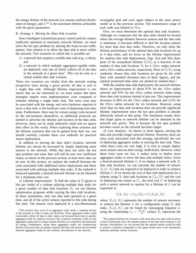
First, we must determine the optimal data sink locations.Although we conjecture that the data sinks should be locatedwhere the average distance between sensors and the data sinkis minimum, it becomes difficult to find the location patternfor more than four data sinks. Therefore, we only show thelifetime performance of the optimal data sink locations for upto 4 data sinks, and we focus on the lifetime improvementfor random data sink deployments. Figs. 5(a) and 5(b) showplots of the normalized lifetimeL(Nl) as a function of thenumber of data sink locationsNl for a 150m radius networkand a250m radius network, respectively. Plots ofL(Nl) usingrandomly chosen data sink locations are given by the solidlines with standard deviation bars in these figures, and theoptimal positioned data sinks are plotted by dashed lines.2

With the random data sink deployment, the network lifetimeshows an improvement of about 67% for the150m radiusnetwork and 91% for the250m radius network when usingthree data sink locations instead of just one. This improvementincreases to 86% for the150m radius network and 121% forthe 250m radius network for six locations. However, usingmore than six data sink locations does not provide significantlifetime improvement since the hot spot problem is alreadyeffectively solved at this point. The simulation results showthat larger gains in network lifetime can be obtained as thenetwork size grows. This is because the hot spot problembecomes worse as the network becomes larger.

2) Cost Analysis:As shown in these figures, moving thedata sink provides longer network lifetime. However, there areextra costs associated with this strategy, specifically the costof deploying aggregator nodes or moving the data sink. Thus,when these costs are very high, it is wise to simply deploymore sensors and use their energy inefficiently. However, whenthese extra costs are low, it makes sense to deploy moreaggregator nodes or move the data sink multiple times. Givena desired network lifetimeL, if we deploy a network withNl

data sink locations, we can calculate the number of sensorsNs(L,Nl) that are required to be deployed in order to achievelifetime L. If we denote the cost of data sink deployment for ascheme usingNl data sink locations asCds(Nl) and the costof deploying one sensor asCs, the total costC of deployingsuch a sensor network to operate for a lifetime ofL can beexpressed as

C(L,Nl) = Cds(Nl) + CsNs(L,Nl) (3)

whereNs(L, Nl) represents the number of sensors necessaryto achieve the lifetimeL for a configuration usingNl datasinks. Ns(L,Nl) can be found by rearranging Equation 2,using the relationshipλe = Ns∗Es

A (whereEs represents the

2The optimal lifetime for scenarios with more than four data sink locationsis hard to determine since the optimal pattern of the data sink locations is notobvious. Nevertheless, we can assume that the optimal pattern would be ableto achieve a lifetime comparable to the upper bound seen in the simulationsutilizing randomly chosen locations.

1 2 3 4 5 6 70

2

4

6

8

10

12

x 105

Number of data sink locations

Nor

mal

ized

life

time

(bits

per

Jou

le)

Network radius = 150m

Optimal placementRandom placement

(a)

1 2 3 4 5 6 70

1

2

3

4

5

6

7x 10

5


Nor

mal

ized

life

time

(bits

per

Jou

le)



(b)

Fig. 5. Normalized lifetime vs. number of data sinks deployed for networkswith a radius of150m (a) and250m (b). Increasing the number of sinklocations improves lifetime until a certain threshold is met and the hot spotproblem has effectively been solved. Much larger gains in network lifetimecan be achieved for a given number of data sink locations for a larger network,since the hot spot problem becomes worse.

initial energy of a single sensor node andA represents thearea of the network), and substitutingL for Lopt.

Ns(L, Nl) =LRaλaA

L(Nl)Es

(4)

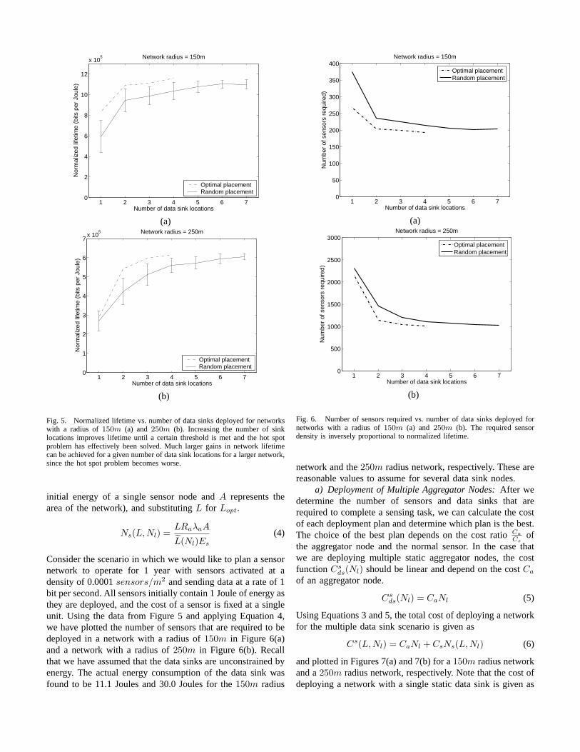
Consider the scenario in which we would like to plan a sensornetwork to operate for 1 year with sensors activated at adensity of 0.0001sensors/m2 and sending data at a rate of 1bit per second. All sensors initially contain 1 Joule of energy asthey are deployed, and the cost of a sensor is fixed at a singleunit. Using the data from Figure 5 and applying Equation 4,we have plotted the number of sensors that are required to bedeployed in a network with a radius of150m in Figure 6(a)and a network with a radius of250m in Figure 6(b). Recallthat we have assumed that the data sinks are unconstrained byenergy. The actual energy consumption of the data sink wasfound to be 11.1 Joules and 30.0 Joules for the150m radius

1 2 3 4 5 6 70

50

100

150

200

250

300

350

400


Num

ber

of s

enso

rs r

equi

red)



(a)

1 2 3 4 5 6 70

500

1000

1500

2000

2500

3000


Num

ber

of s

enso

rs r

equi

red)



(b)

Fig. 6. Number of sensors required vs. number of data sinks deployed fornetworks with a radius of150m (a) and250m (b). The required sensordensity is inversely proportional to normalized lifetime.

network and the250m radius network, respectively. These arereasonable values to assume for several data sink nodes.

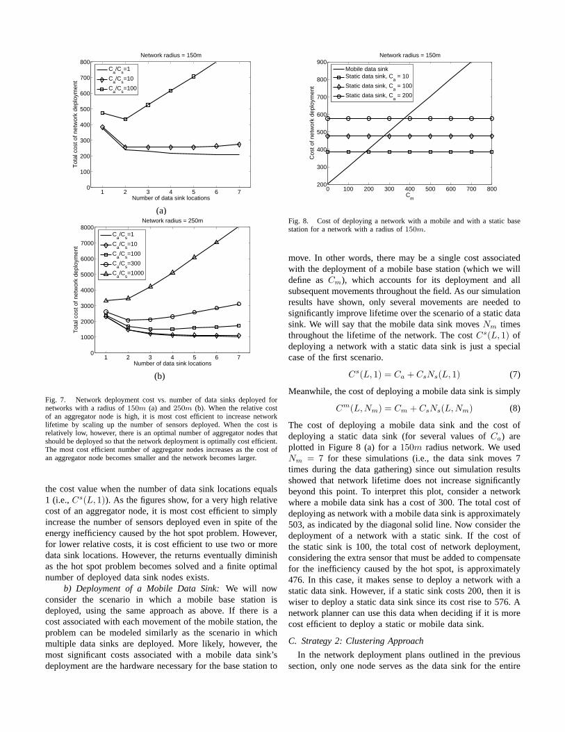
a) Deployment of Multiple Aggregator Nodes:After wedetermine the number of sensors and data sinks that arerequired to complete a sensing task, we can calculate the costof each deployment plan and determine which plan is the best.The choice of the best plan depends on the cost ratioCa

Csof

the aggregator node and the normal sensor. In the case thatwe are deploying multiple static aggregator nodes, the costfunctionCs

ds(Nl) should be linear and depend on the costCa

of an aggregator node.

Csds(Nl) = CaNl (5)

Using Equations 3 and 5, the total cost of deploying a networkfor the multiple data sink scenario is given as

Cs(L,Nl) = CaNl + CsNs(L,Nl) (6)

and plotted in Figures 7(a) and 7(b) for a150m radius networkand a250m radius network, respectively. Note that the cost ofdeploying a network with a single static data sink is given as

1 2 3 4 5 6 70

100

200

300

400

500

600

700

800


Tot

al c

ost o

f net

wor

k de

ploy

men

t


Ca/C

s=1

Ca/C

s=10

Ca/C

s=100

(a)

1 2 3 4 5 6 70

1000

2000

3000

4000

5000

6000

7000

8000


Tot

al c

ost o

f net

wor

k de

ploy

men

t


Ca/C

s=1

Ca/C

s=10

Ca/C

s=100

Ca/C

s=300

Ca/C

s=1000

(b)

Fig. 7. Network deployment cost vs. number of data sinks deployed fornetworks with a radius of150m (a) and250m (b). When the relative costof an aggregator node is high, it is most cost efficient to increase networklifetime by scaling up the number of sensors deployed. When the cost isrelatively low, however, there is an optimal number of aggregator nodes thatshould be deployed so that the network deployment is optimally cost efficient.The most cost efficient number of aggregator nodes increases as the cost ofan aggregator node becomes smaller and the network becomes larger.

the cost value when the number of data sink locations equals1 (i.e.,Cs(L, 1)). As the figures show, for a very high relativecost of an aggregator node, it is most cost efficient to simplyincrease the number of sensors deployed even in spite of theenergy inefficiency caused by the hot spot problem. However,for lower relative costs, it is cost efficient to use two or moredata sink locations. However, the returns eventually diminishas the hot spot problem becomes solved and a finite optimalnumber of deployed data sink nodes exists.

b) Deployment of a Mobile Data Sink:We will nowconsider the scenario in which a mobile base station isdeployed, using the same approach as above. If there is acost associated with each movement of the mobile station, theproblem can be modeled similarly as the scenario in whichmultiple data sinks are deployed. More likely, however, themost significant costs associated with a mobile data sink’sdeployment are the hardware necessary for the base station to

0 100 200 300 400 500 600 700 800200

300

400

500

600

700

800

900

Cm

Cos

t of n

etw

ork

depl

oym

ent


Mobile data sinkStatic data sink, C

a = 10

Static data sink, Ca = 100

Static data sink, Ca = 200

Fig. 8. Cost of deploying a network with a mobile and with a static basestation for a network with a radius of150m.

move. In other words, there may be a single cost associatedwith the deployment of a mobile base station (which we willdefine asCm), which accounts for its deployment and allsubsequent movements throughout the field. As our simulationresults have shown, only several movements are needed tosignificantly improve lifetime over the scenario of a static datasink. We will say that the mobile data sink movesNm timesthroughout the lifetime of the network. The costCs(L, 1) ofdeploying a network with a static data sink is just a specialcase of the first scenario.

Cs(L, 1) = Ca + CsNs(L, 1) (7)

Meanwhile, the cost of deploying a mobile data sink is simply

Cm(L,Nm) = Cm + CsNs(L,Nm) (8)

The cost of deploying a mobile data sink and the cost ofdeploying a static data sink (for several values ofCa) areplotted in Figure 8 (a) for a150m radius network. We usedNm = 7 for these simulations (i.e., the data sink moves 7times during the data gathering) since out simulation resultsshowed that network lifetime does not increase significantlybeyond this point. To interpret this plot, consider a networkwhere a mobile data sink has a cost of 300. The total cost ofdeploying as network with a mobile data sink is approximately503, as indicated by the diagonal solid line. Now consider thedeployment of a network with a static sink. If the cost ofthe static sink is 100, the total cost of network deployment,considering the extra sensor that must be added to compensatefor the inefficiency caused by the hot spot, is approximately476. In this case, it makes sense to deploy a network with astatic data sink. However, if a static sink costs 200, then it iswiser to deploy a static data sink since its cost rise to 576. Anetwork planner can use this data when deciding if it is morecost efficient to deploy a static or mobile data sink.

C. Strategy 2: Clustering Approach

In the network deployment plans outlined in the previoussection, only one node serves as the data sink for the entire

network at one time, even if multiple aggregator-capable nodeshave been deployed. In this section, we consider a clusteringapproach in which multiple aggregator-capable nodes aredeployed and each sink collects data from only part of thesensor network for the entire network lifetime. Such clusteringschemes have been proposed for wireless sensor networks in[14], [15], [16]. Previous work in this area deals primarilywith homogeneous networks, in which any of the deployednodes is capable of acting as cluster head. In this section, weconsider heterogeneous networks, where nodes equipped withthe capability of acting as cluster head (e.g., those with largerbatteries, more processing power and memory, and possiblya second radio to link back to a central base station) aresignificantly more expensive than ordinary microsensors. Inour model, a sensor may send its traffic to whichever clusterhead it chooses (typically, but not necessarily, the closestcluster head). The analysis methods in this section are verysimilar to those in the previous section.

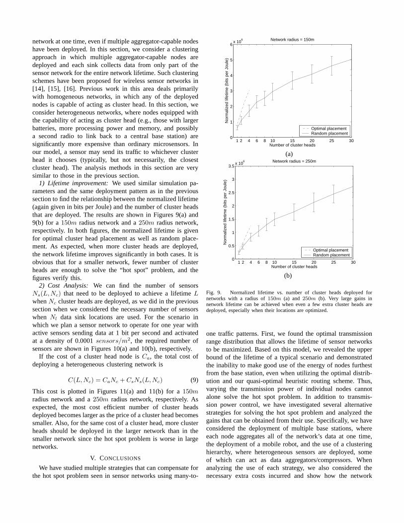
1) Lifetime improvement:We used similar simulation pa-rameters and the same deployment pattern as in the previoussection to find the relationship between the normalized lifetime(again given in bits per Joule) and the number of cluster headsthat are deployed. The results are shown in Figures 9(a) and9(b) for a150m radius network and a250m radius network,respectively. In both figures, the normalized lifetime is givenfor optimal cluster head placement as well as random place-ment. As expected, when more cluster heads are deployed,the network lifetime improves significantly in both cases. It isobvious that for a smaller network, fewer number of clusterheads are enough to solve the “hot spot” problem, and thefigures verify this.

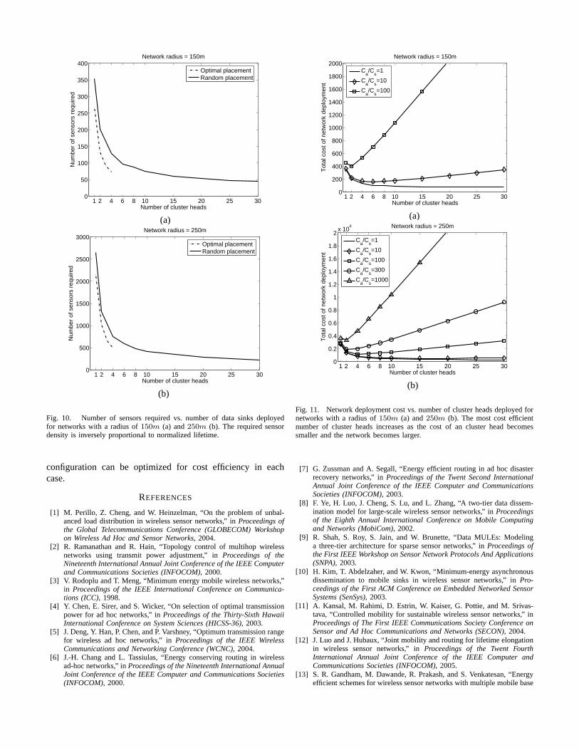
2) Cost Analysis: We can find the number of sensorsNs(L,Nc) that need to be deployed to achieve a lifetimeLwhenNc cluster heads are deployed, as we did in the previoussection when we considered the necessary number of sensorswhen Nl data sink locations are used. For the scenario inwhich we plan a sensor network to operate for one year withactive sensors sending data at 1 bit per second and activatedat a density of 0.0001sensors/m2, the required number ofsensors are shown in Figures 10(a) and 10(b), respectively.

If the cost of a cluster head node isCa, the total cost ofdeploying a heterogeneous clustering network is

C(L,Nc) = CaNc + CsNs(L,Nc) (9)

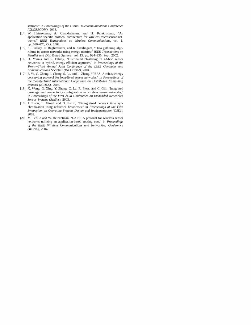
This cost is plotted in Figures 11(a) and 11(b) for a150mradius network and a250m radius network, respectively. Asexpected, the most cost efficient number of cluster headsdeployed becomes larger as the price of a cluster head becomessmaller. Also, for the same cost of a cluster head, more clusterheads should be deployed in the larger network than in thesmaller network since the hot spot problem is worse in largenetworks.

V. CONCLUSIONS

We have studied multiple strategies that can compensate forthe hot spot problem seen in sensor networks using many-to-

1 2 4 6 8 10 15 20 25 300

1

2

3

4

5

6x 10

6

Number of cluster heads

Nor

mal

ized

life

time

(bits

per

Jou

le)



(a)

1 2 4 6 8 10 15 20 25 300

0.5

1

1.5

2

2.5

3

3.5x 10

6


Nor

mal

ized

life

time

(bits

per

Jou

le)



(b)

Fig. 9. Normalized lifetime vs. number of cluster heads deployed fornetworks with a radius of150m (a) and 250m (b). Very large gains innetwork lifetime can be achieved when even a few extra cluster heads aredeployed, especially when their locations are optimized.

one traffic patterns. First, we found the optimal transmissionrange distribution that allows the lifetime of sensor networksto be maximized. Based on this model, we revealed the upperbound of the lifetime of a typical scenario and demonstratedthe inability to make good use of the energy of nodes furthestfrom the base station, even when utilizing the optimal distrib-ution and our quasi-optimal heuristic routing scheme. Thus,varying the transmission power of individual nodes cannotalone solve the hot spot problem. In addition to transmis-sion power control, we have investigated several alternativestrategies for solving the hot spot problem and analyzed thegains that can be obtained from their use. Specifically, we haveconsidered the deployment of multiple base stations, whereeach node aggregates all of the network’s data at one time,the deployment of a mobile robot, and the use of a clusteringhierarchy, where heterogeneous sensors are deployed, someof which can act as data aggregators/compressors. Whenanalyzing the use of each strategy, we also considered thenecessary extra costs incurred and show how the network

1 2 4 6 8 10 15 20 25 300

50

100

150

200

250

300

350

400


Num

ber

of s

enso

rs r

equi

red



(a)

1 2 4 6 8 10 15 20 25 300

500

1000

1500

2000

2500

3000


Num

ber

of s

enso

rs r

equi

red



(b)

Fig. 10. Number of sensors required vs. number of data sinks deployedfor networks with a radius of150m (a) and250m (b). The required sensordensity is inversely proportional to normalized lifetime.

configuration can be optimized for cost efficiency in eachcase.

REFERENCES

[1] M. Perillo, Z. Cheng, and W. Heinzelman, “On the problem of unbal-anced load distribution in wireless sensor networks,” inProceedings ofthe Global Telecommunications Conference (GLOBECOM) Workshopon Wireless Ad Hoc and Sensor Networks, 2004.

[2] R. Ramanathan and R. Hain, “Topology control of multihop wirelessnetworks using transmit power adjustment,” inProceedings of theNineteenth International Annual Joint Conference of the IEEE Computerand Communications Societies (INFOCOM), 2000.

[3] V. Rodoplu and T. Meng, “Minimum energy mobile wireless networks,”in Proceedings of the IEEE International Conference on Communica-tions (ICC), 1998.

[4] Y. Chen, E. Sirer, and S. Wicker, “On selection of optimal transmissionpower for ad hoc networks,” inProceedings of the Thirty-Sixth HawaiiInternational Conference on System Sciences (HICSS-36), 2003.

[5] J. Deng, Y. Han, P. Chen, and P. Varshney, “Optimum transmission rangefor wireless ad hoc networks,” inProceedings of the IEEE WirelessCommunications and Networking Conference (WCNC), 2004.

[6] J.-H. Chang and L. Tassiulas, “Energy conserving routing in wirelessad-hoc networks,” inProceedings of the Nineteenth International AnnualJoint Conference of the IEEE Computer and Communications Societies(INFOCOM), 2000.

1 2 4 6 8 10 15 20 25 300

200

400

600

800

1000

1200

1400

1600

1800

2000


Tot

al c

ost o

f net

wor

k de

ploy

men

t


Ca/C

s=1

Ca/C

s=10

Ca/C

s=100

(a)

1 2 4 6 8 10 15 20 25 300

0.2

0.4

0.6

0.8

1

1.2

1.4

1.6

1.8

2x 10

4


Tot

al c

ost o

f net

wor

k de

ploy

men

t


Ca/C

s=1

Ca/C

s=10

Ca/C

s=100

Ca/C

s=300

Ca/C

s=1000

(b)

Fig. 11. Network deployment cost vs. number of cluster heads deployed fornetworks with a radius of150m (a) and250m (b). The most cost efficientnumber of cluster heads increases as the cost of an cluster head becomessmaller and the network becomes larger.

[7] G. Zussman and A. Segall, “Energy efficient routing in ad hoc disasterrecovery networks,” inProceedings of the Twent Second InternationalAnnual Joint Conference of the IEEE Computer and CommunicationsSocieties (INFOCOM), 2003.

[8] F. Ye, H. Luo, J. Cheng, S. Lu, and L. Zhang, “A two-tier data dissem-ination model for large-scale wireless sensor networks,” inProceedingsof the Eighth Annual International Conference on Mobile Computingand Networks (MobiCom), 2002.

[9] R. Shah, S. Roy, S. Jain, and W. Brunette, “Data MULEs: Modelinga three-tier architecture for sparse sensor networks,” inProceedings ofthe First IEEE Workshop on Sensor Network Protocols And Applications(SNPA), 2003.

[10] H. Kim, T. Abdelzaher, and W. Kwon, “Minimum-energy asynchronousdissemination to mobile sinks in wireless sensor networks,” inPro-ceedings of the First ACM Conference on Embedded Networked SensorSystems (SenSys), 2003.

[11] A. Kansal, M. Rahimi, D. Estrin, W. Kaiser, G. Pottie, and M. Srivas-tava, “Controlled mobility for sustainable wireless sensor networks,” inProceedings of The First IEEE Communications Society Conference onSensor and Ad Hoc Communications and Networks (SECON), 2004.

[12] J. Luo and J. Hubaux, “Joint mobility and routing for lifetime elongationin wireless sensor networks,” inProceedings of the Twent FourthInternational Annual Joint Conference of the IEEE Computer andCommunications Societies (INFOCOM), 2005.

[13] S. R. Gandham, M. Dawande, R. Prakash, and S. Venkatesan, “Energyefficient schemes for wireless sensor networks with multiple mobile base

stations,” inProceedings of the Global Telecommunications Conference(GLOBECOM), 2003.

[14] W. Heinzelman, A. Chandrakasan, and H. Balakrishnan, “Anapplication-specific protocol architecture for wireless microsensor net-works,” IEEE Transactions on Wireless Communications, vol. 1,pp. 660–670, Oct. 2002.

[15] S. Lindsey, C. Raghavendra, and K. Sivalingam, “Data gathering algo-rithms in sensor networks using energy metrics,”IEEE Transactions onParallel and Distributed Systems, vol. 13, pp. 924–935, Sept. 2002.

[16] O. Younis and S. Fahmy, “Distributed clustering in ad-hoc sensornetworks: A hybrid, energy-efficient approach,” inProceedings of theTwenty-Third Annual Joint Conference of the IEEE Computer andCommunications Societies (INFOCOM), 2004.

[17] F. Ye, G. Zhong, J. Cheng, S. Lu, and L. Zhang, “PEAS: A robust energyconserving protocol for long-lived sensor networks,” inProceedings ofthe Twenty-Third International Conference on Distributed ComputingSystems (ICDCS), 2003.

[18] X. Wang, G. Xing, Y. Zhang, C. Lu, R. Pless, and C. Gill, “Integratedcoverage and connectivity configuration in wireless sensor networks,”in Proceedings of the First ACM Conference on Embedded NetworkedSensor Systems (SenSys), 2003.

[19] J. Elson, L. Girod, and D. Estrin, “Fine-grained network time syn-chronization using reference broadcasts,” inProceedings of the FifthSymposium on Operating Systems Design and Implementation (OSDI),2002.

[20] M. Perillo and W. Heinzelman, “DAPR: A protocol for wireless sensornetworks utilizing an application-based routing cost,” inProceedingsof the IEEE Wireless Communications and Networking Conference(WCNC), 2004.

Documents

An Analysis of Strategies for Mitigating the Sensor Network Hot Spot Problem