Embed Size (px)
Citation preview
Amperometric Gas Sensing
A thesis submitted for the degree of Doctor of Philosophyin Physical and Theoretical Chemistry
Linhongjia XiongSt John’s College
Trinity Term 2014
Abstract
Amperometric gas sensors are widely used for environmental and industrial monitoring.
They are sensitive and cheap but suffer from some significant limitations. The aim of
the work undertaken in this thesis is the development of ‘intelligent’ gas sensors to over-
come some of these limitations. Overall the thesis shows the value of ionic liquids as
potential solvents for gas sensors, overcoming issues of solvent volatility and providing a
wide potential range for electrochemical measurements. Methods have been developed for
sensitive amperometry, the tuning of potentials and especially proof-of-concept (patents
Publication numbers: WO2013140140 A3 and WO2014020347 A1) in respect of the intel-
ligent self-monitoring of temperature and humidity by RTIL based sensors. Designs for
practical electrodes are also proposed. The specific content is as follows.
Chapter 1 outlines the fundamental principles of electrochemistry which are of im-
portance for the reading of this thesis. Chapter 2 reviews the history and modern am-
perometric gas sensors. Limitations of present electrochemical approaches are critically
established. Micro-electrodes and Room Temperature Ionic Liquids (RTILs) are also in-
troduced in this chapter.
Chapter 4 is focused on the study of analysing chronoamperometry using the Shoup
and Szabo equation to simultaneously determine the values of concentration and diffusion
coefficient of dissolved analytes in both non-aqueous and RTIL media. A method to
optimise the chronoamperometric conditions is demonstrated. This provides an essential
experimental basis for IL based gas sensor.
Chapter 5 demonstrates how the oxidation potential of ferrocene can be tuned by
changing the anionic component of room temperature ionic liquids. This ability to tune
i
redox potentials has genetic value in gas sensing.
Chapters 6 and 7 describe two novel patented approaches to monitor the local environ-
ment for amperometric gas detection. In Chapter 6, an in-situ voltammetric ‘thermome-
ter’ is incorporated into an amperometric oxygen sensing system. The local temperature
is measured by the formal potential difference of two redox couples. A simultaneous tem-
perature and humidity sensor is reported in Chapter 7. This sensor shows advantageous
features where the temperature sensor is humidity independent and vice versa.
The Shoup and Szabo analysis (Chapter 4) requires ‘simple’ electron transfer and
as such the reduction of oxygen in wet RTILs can be complicated by dissolved water.
Chapter 8 proposes a method to stop oxygen reduction at the one electron transfer stage
under humid conditions by using phosphonium based RTILs to ‘trap’ the intermediate
superoxide ions.
Chapters 9 and 10 report the fabrication of low cost disposable electrodes of various
geometries and of different materials. The suitability of these electrode for use as working
electrodes for electrochemical experiments in aqueous, non-aqueous and RTIL media is
demonstrated. Their capability to be used as working probes for amperometric gas sensing
systems is discussed.
ii
Acknowledgements
First and foremost, I would like to express my deep gratitude to Professor Richard Comp-
ton for his patient guidance and enthusiastic encouragement throughout my D.Phil., my
Part II year and summer projects. Thank him for his great support through my difficult
time and for always understanding and trusting me.
I wish to thank all of the post-docs, especially Professor Leigh Aldous, who generously
shared his ionic liquids knowledge, Dr. Sven Ernst who always helped me, Dr. Qian Li,
who gave me good advices in both my life and projects, and Dr. Chris Batchelor-McAuley,
who was my Part II supervisor and still gave me useful advice through my D.Phil.. Also to
Dr. Blake Plowman, Dr. Wei Cheng, Dr. Kristina Tschulik and Dr. Friedrich Kaetelhoen
for always being on hand to help.
I would like to acknowledge Prof. Chris Hardacre and Dr. Sarah Norman who provided
clean and neat RTILs for my project.
Many thanks to Honeywell for funding my D.Phil. research. Great thanks go to Dr.
John Chapples, Dr. Keith Pratt, Dr. Martin Jones and Dr. Lei Xiao for their very useful
discussion and input throughout the three-year of my D.Phil and for their hospitality and
kindness during the internship in Portsmouth.
Special thanks to my ‘First Year’ friends, Ying, Emma, Min and Eddy, for precious
memories throughout the this three years. Thanks to Ying for always being there for me,
to Emma for being very sweet and kind the whole time, to Min for her companionship and
good food over the past four years and to Eddy for his endless help and patience when
I bothered him with the IT stuff. Thank every member in the RGC group for laughters
and encouragement. Thanks Patty for emergency chocolate.
I would like to thank all of my friends, especially Ivana and Hao for being are very
considerate, Y for being very supportive, NeiNei for helping me through my difficult time.
I cannot express my gratitude enough. I am sure all of you are my lifelong friends.
Finally, I would like to thank those special people in my life, my Mum, for her on-going
support, and Bin, for being extremely patient with me.
iii
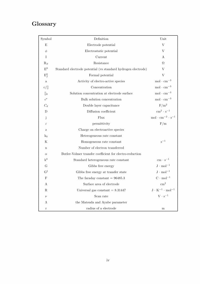
Glossary
Symbol Definition Unit
E Electrode potential V
φ Electrostatic potential V
I Current A
RS Resistance Ω
E0 Standard electrode potential (vs standard hydrogen electrode) V
E0f Formal potential V
a Activity of electro-active species mol · cm−3
c/[] Concentration mol · cm−3
[]0 Solution concentration at electrode surface mol · cm−3
c∗ Bulk solution concentration mol · cm−3
Cd Double layer capacitance F/m2
D Diffusion coefficient cm2 · s−1
j Flux mol · cm−2 · s−1
ε permittivity F/m
z Charge on electroactive species
k0 Heterogeneous rate constant
K Homogeneous rate constant s−1
n Number of electron transferred
α Butler-Volmer transfer coefficient for electro-reduction
k0 Standard heterogeneous rate constant cm · s−1
G Gibbs free energy J · mol−1
G‡ Gibbs free energy at transfer state J · mol−1
F The faraday constant = 96485.3 C · mol−1
A Surface area of electrode cm2
R Universal gas constant = 8.31447 J · K−1 · mol−1
ν Scan rate V · s−1
Λ the Matsuda and Ayabe parameter
r radius of a electrode m
iv
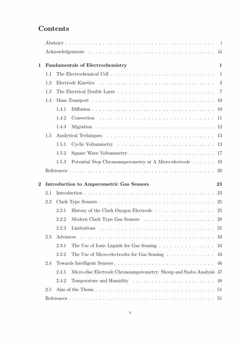
Contents
Abstract . . . . . . . . . . . . . . . . . . . . . . . . . . . . . . . . . . . . . . . . i
Acknowledgements . . . . . . . . . . . . . . . . . . . . . . . . . . . . . . . . . . iii
1 Fundamentals of Electrochemistry 1
1.1 The Electrochemical Cell . . . . . . . . . . . . . . . . . . . . . . . . . . . . 1
1.2 Electrode Kinetics . . . . . . . . . . . . . . . . . . . . . . . . . . . . . . . 3
1.3 The Electrical Double Layer . . . . . . . . . . . . . . . . . . . . . . . . . . 7
1.4 Mass Transport . . . . . . . . . . . . . . . . . . . . . . . . . . . . . . . . . 10
1.4.1 Diffusion . . . . . . . . . . . . . . . . . . . . . . . . . . . . . . . . . 10
1.4.2 Convection . . . . . . . . . . . . . . . . . . . . . . . . . . . . . . . 11
1.4.3 Migration . . . . . . . . . . . . . . . . . . . . . . . . . . . . . . . . 12
1.5 Analytical Techniques . . . . . . . . . . . . . . . . . . . . . . . . . . . . . 13
1.5.1 Cyclic Voltammetry . . . . . . . . . . . . . . . . . . . . . . . . . . 13
1.5.2 Square Wave Voltammetry . . . . . . . . . . . . . . . . . . . . . . . 17
1.5.3 Potential Step Chronoamperometry at A Micro-electrode . . . . . . 19
References . . . . . . . . . . . . . . . . . . . . . . . . . . . . . . . . . . . . . . . 20
2 Introduction to Amperometric Gas Sensors 23
2.1 Introduction . . . . . . . . . . . . . . . . . . . . . . . . . . . . . . . . . . . 23
2.2 Clark Type Sensors . . . . . . . . . . . . . . . . . . . . . . . . . . . . . . . 25
2.2.1 History of the Clark Oxygen Electrode . . . . . . . . . . . . . . . . 25
2.2.2 Modern Clark Type Gas Sensors . . . . . . . . . . . . . . . . . . . 28
2.2.3 Limitations . . . . . . . . . . . . . . . . . . . . . . . . . . . . . . . 31
2.3 Advances . . . . . . . . . . . . . . . . . . . . . . . . . . . . . . . . . . . . 33
2.3.1 The Use of Ionic Liquids for Gas Sensing . . . . . . . . . . . . . . . 34
2.3.2 The Use of Micro-electrodes for Gas Sensing . . . . . . . . . . . . . 43
2.4 Towards Intelligent Sensors . . . . . . . . . . . . . . . . . . . . . . . . . . . 46
2.4.1 Micro-disc Electrode Chronoamperometry: Shoup and Szabo Analysis 47
2.4.2 Temperature and Humidity . . . . . . . . . . . . . . . . . . . . . . 48
2.5 Aim of the Thesis . . . . . . . . . . . . . . . . . . . . . . . . . . . . . . . . 51
References . . . . . . . . . . . . . . . . . . . . . . . . . . . . . . . . . . . . . . . 51
v
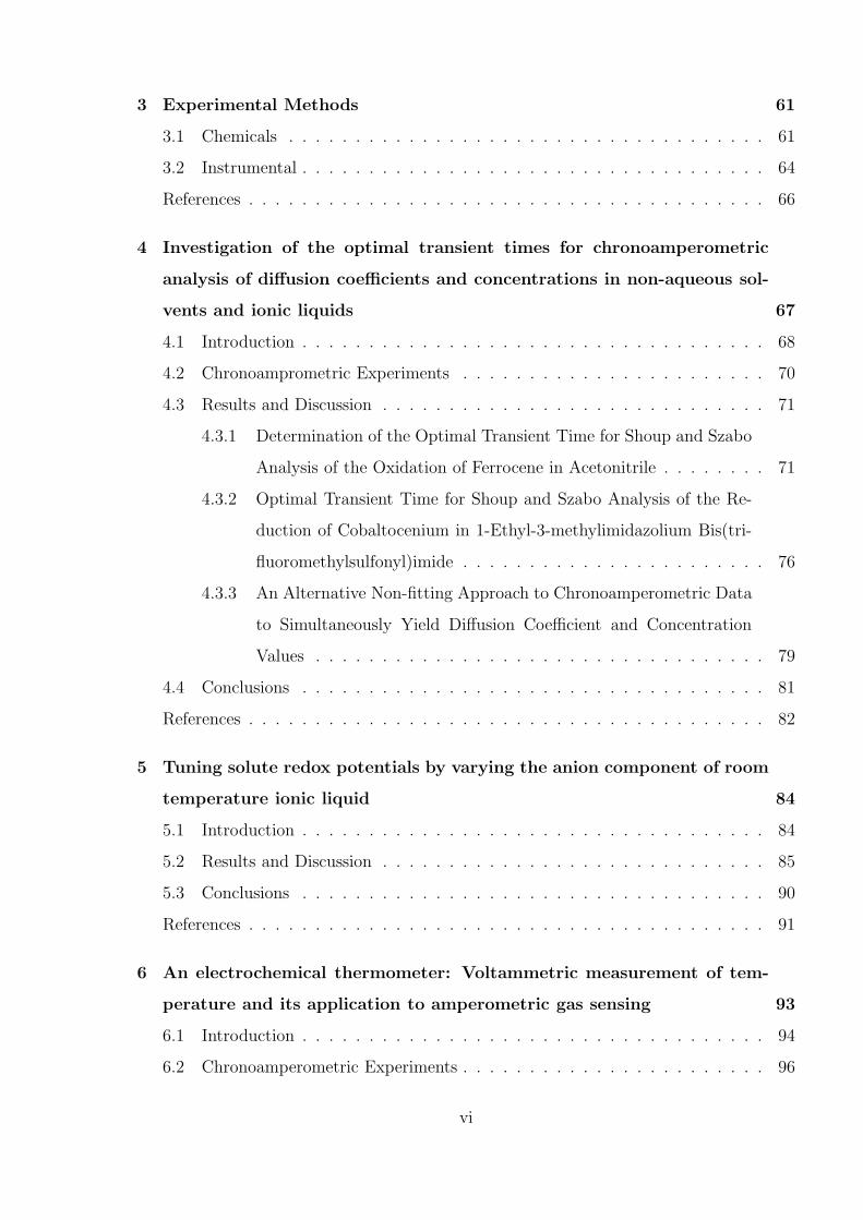
3 Experimental Methods 61
3.1 Chemicals . . . . . . . . . . . . . . . . . . . . . . . . . . . . . . . . . . . . 61
3.2 Instrumental . . . . . . . . . . . . . . . . . . . . . . . . . . . . . . . . . . . 64
References . . . . . . . . . . . . . . . . . . . . . . . . . . . . . . . . . . . . . . . 66
4 Investigation of the optimal transient times for chronoamperometric
analysis of diffusion coefficients and concentrations in non-aqueous sol-
vents and ionic liquids 67
4.1 Introduction . . . . . . . . . . . . . . . . . . . . . . . . . . . . . . . . . . . 68
4.2 Chronoamprometric Experiments . . . . . . . . . . . . . . . . . . . . . . . 70
4.3 Results and Discussion . . . . . . . . . . . . . . . . . . . . . . . . . . . . . 71
4.3.1 Determination of the Optimal Transient Time for Shoup and Szabo
Analysis of the Oxidation of Ferrocene in Acetonitrile . . . . . . . . 71
4.3.2 Optimal Transient Time for Shoup and Szabo Analysis of the Re-
duction of Cobaltocenium in 1-Ethyl-3-methylimidazolium Bis(tri-
fluoromethylsulfonyl)imide . . . . . . . . . . . . . . . . . . . . . . . 76
4.3.3 An Alternative Non-fitting Approach to Chronoamperometric Data
to Simultaneously Yield Diffusion Coefficient and Concentration
Values . . . . . . . . . . . . . . . . . . . . . . . . . . . . . . . . . . 79
4.4 Conclusions . . . . . . . . . . . . . . . . . . . . . . . . . . . . . . . . . . . 81
References . . . . . . . . . . . . . . . . . . . . . . . . . . . . . . . . . . . . . . . 82
5 Tuning solute redox potentials by varying the anion component of room
temperature ionic liquid 84
5.1 Introduction . . . . . . . . . . . . . . . . . . . . . . . . . . . . . . . . . . . 84
5.2 Results and Discussion . . . . . . . . . . . . . . . . . . . . . . . . . . . . . 85
5.3 Conclusions . . . . . . . . . . . . . . . . . . . . . . . . . . . . . . . . . . . 90
References . . . . . . . . . . . . . . . . . . . . . . . . . . . . . . . . . . . . . . . 91
6 An electrochemical thermometer: Voltammetric measurement of tem-
perature and its application to amperometric gas sensing 93
6.1 Introduction . . . . . . . . . . . . . . . . . . . . . . . . . . . . . . . . . . . 94
6.2 Chronoamperometric Experiments . . . . . . . . . . . . . . . . . . . . . . . 96
vi
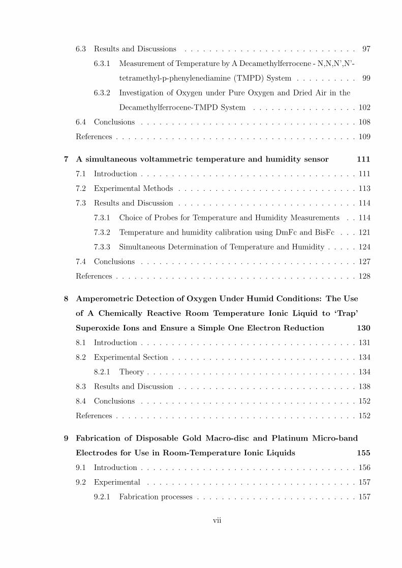
6.3 Results and Discussions . . . . . . . . . . . . . . . . . . . . . . . . . . . . 97
6.3.1 Measurement of Temperature by A Decamethylferrocene - N,N,N’,N’-
tetramethyl-p-phenylenediamine (TMPD) System . . . . . . . . . . 99
6.3.2 Investigation of Oxygen under Pure Oxygen and Dried Air in the
Decamethylferrocene-TMPD System . . . . . . . . . . . . . . . . . 102
6.4 Conclusions . . . . . . . . . . . . . . . . . . . . . . . . . . . . . . . . . . . 108
References . . . . . . . . . . . . . . . . . . . . . . . . . . . . . . . . . . . . . . . 109
7 A simultaneous voltammetric temperature and humidity sensor 111
7.1 Introduction . . . . . . . . . . . . . . . . . . . . . . . . . . . . . . . . . . . 111
7.2 Experimental Methods . . . . . . . . . . . . . . . . . . . . . . . . . . . . . 113
7.3 Results and Discussion . . . . . . . . . . . . . . . . . . . . . . . . . . . . . 114
7.3.1 Choice of Probes for Temperature and Humidity Measurements . . 114
7.3.2 Temperature and humidity calibration using DmFc and BisFc . . . 121
7.3.3 Simultaneous Determination of Temperature and Humidity . . . . . 124
7.4 Conclusions . . . . . . . . . . . . . . . . . . . . . . . . . . . . . . . . . . . 127
References . . . . . . . . . . . . . . . . . . . . . . . . . . . . . . . . . . . . . . . 128
8 Amperometric Detection of Oxygen Under Humid Conditions: The Use
of A Chemically Reactive Room Temperature Ionic Liquid to ‘Trap’
Superoxide Ions and Ensure a Simple One Electron Reduction 130
8.1 Introduction . . . . . . . . . . . . . . . . . . . . . . . . . . . . . . . . . . . 131
8.2 Experimental Section . . . . . . . . . . . . . . . . . . . . . . . . . . . . . . 134
8.2.1 Theory . . . . . . . . . . . . . . . . . . . . . . . . . . . . . . . . . . 134
8.3 Results and Discussion . . . . . . . . . . . . . . . . . . . . . . . . . . . . . 138
8.4 Conclusions . . . . . . . . . . . . . . . . . . . . . . . . . . . . . . . . . . . 152
References . . . . . . . . . . . . . . . . . . . . . . . . . . . . . . . . . . . . . . . 152
9 Fabrication of Disposable Gold Macro-disc and Platinum Micro-band
Electrodes for Use in Room-Temperature Ionic Liquids 155
9.1 Introduction . . . . . . . . . . . . . . . . . . . . . . . . . . . . . . . . . . . 156
9.2 Experimental . . . . . . . . . . . . . . . . . . . . . . . . . . . . . . . . . . 157
9.2.1 Fabrication processes . . . . . . . . . . . . . . . . . . . . . . . . . . 157
vii
9.2.2 Simulation . . . . . . . . . . . . . . . . . . . . . . . . . . . . . . . . 158
9.3 Results and Discussion . . . . . . . . . . . . . . . . . . . . . . . . . . . . . 159
9.3.1 Reproducibility of Gold Macro-disc Electrodes . . . . . . . . . . . . 159
9.3.2 The Oxidation of Ferrocene on the Gold Macro-disc Electrode Stud-
ies Using [C4mpyrr][NTf2] as Solvent . . . . . . . . . . . . . . . . . 162
9.3.3 The Platinum Micro-band Electrode in [C3mim][NTf2] . . . . . . . 162
9.3.4 Oxygen Reduction in RTILs at Gold Macro-disc and PlatinumMicro-
band Electrode . . . . . . . . . . . . . . . . . . . . . . . . . . . . . 166
9.4 Conclusions . . . . . . . . . . . . . . . . . . . . . . . . . . . . . . . . . . . 169
References . . . . . . . . . . . . . . . . . . . . . . . . . . . . . . . . . . . . . . . 170
10 Evaluation of A Simple Disposable micro-band electrode Device for Am-
perometric Gas Sensing 173
10.1 Introduction . . . . . . . . . . . . . . . . . . . . . . . . . . . . . . . . . . . 174
10.2 Electrode Fabrication . . . . . . . . . . . . . . . . . . . . . . . . . . . . . . 175
10.3 Results and Discussion . . . . . . . . . . . . . . . . . . . . . . . . . . . . . 176
10.3.1 Oxidation of Decamethylferrocene in [C3mim][NTf2] . . . . . . . . . 177
10.3.2 Oxygen Reduction in [C3mim][NTf2] . . . . . . . . . . . . . . . . . 184
10.4 Conclusions . . . . . . . . . . . . . . . . . . . . . . . . . . . . . . . . . . . 191
References . . . . . . . . . . . . . . . . . . . . . . . . . . . . . . . . . . . . . . . 192
11 Conclusions 196
viii
Chapter 1
Fundamentals of Electrochemistry
This thesis is concerned with the development of amperometric gas sensors. The first
chapter presents the theoretical fundamental electrochemistry underpinning the work re-
ported in the thesis. Fuller discussion appears in the later chapters.
1.1 The Electrochemical Cell
In an electrochemical experiment, a potential difference is applied to an electrode to
induce electron transfer.[1, 2] Consider a simple one-electron oxidation,
A(aq)
kfkb
B(aq) + e (1.1)
where A(aq) and B(aq) are electro-active species in solution and e is the electron transferred
from/to a working electrode (normally a metal or carbon electrode). It is impossible to
pass a current or measure/apply a potential difference using a single electrode; hence,
the simplest electrochemical cell includes a reference electrode as well as the (‘working’)
electrode of interest to complete a circuit. The potential is applied to the working electrode
relative to the reference electrode, and the latter is designed so that the potential at the
reference electrode is constant, provided no current is passed through it. The applied
potential is [1, 2]:
1
E = (φM − φS)working − (φM − φS)reference + IR (1.2)
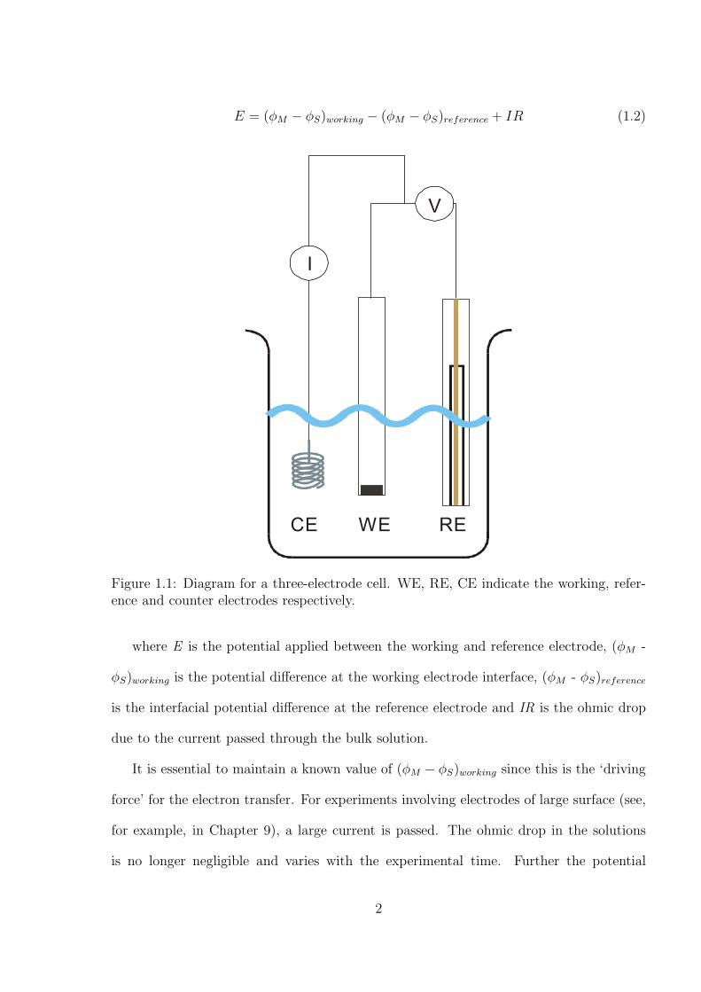
Figure 1.1: Diagram for a three-electrode cell. WE, RE, CE indicate the working, refer-ence and counter electrodes respectively.
where E is the potential applied between the working and reference electrode, (φM -
φS)working is the potential difference at the working electrode interface, (φM - φS)reference
is the interfacial potential difference at the reference electrode and IR is the ohmic drop
due to the current passed through the bulk solution.
It is essential to maintain a known value of (φM − φS)working since this is the ‘driving
force’ for the electron transfer. For experiments involving electrodes of large surface (see,
for example, in Chapter 9), a large current is passed. The ohmic drop in the solutions
is no longer negligible and varies with the experimental time. Further the potential
2
difference at the reference electrode is not constant since the large current can change
the surface and the chemical composition of the reference electrode. Consequently, the
applied potential in a two-electrode system sometimes does not reflect that applied at the
working electrode/solution interface. A third electrode, a counter electrode, is introduced
to solve this problem in which the current is only passed through the working and counter
electrodes but no current flows through the working and reference electrodes. Note that
the counter electrode is required to be highly conductive with a sufficient surface area to
ensure easy passage of electrons without limiting the electrochemical reaction. This three
electrode set-up is shown schematically in Figure 1.1. With no current passed through the
reference electrode, (φM - φS)reference becomes constant, and the value of IR falls to zero.
Therefore, changes in the applied potential, E, directly reflect changes in (φM - φS)working.
A three-electrode system is commonly applied with the use of macro-electrodes, whereas
a two-electrode system can often be employed with a micro-electrode,[3–7] but not with
a macro-electrode. Even though micro-electrodes are mainly used in this thesis, a three-
electrode set-up is utilised for all systems studied to minimise potential shifts from ohmic
drop.
The next section discusses how current generated during electrochemical process is
interpreted.
1.2 Electrode Kinetics
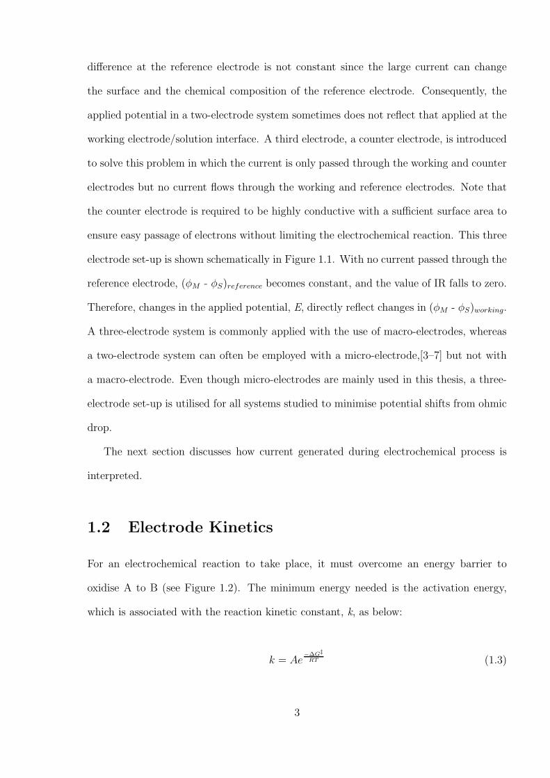
For an electrochemical reaction to take place, it must overcome an energy barrier to
oxidise A to B (see Figure 1.2). The minimum energy needed is the activation energy,
which is associated with the reaction kinetic constant, k, as below:
k = Ae−∆G‡
RT (1.3)
3
reaction coordinate
Energy
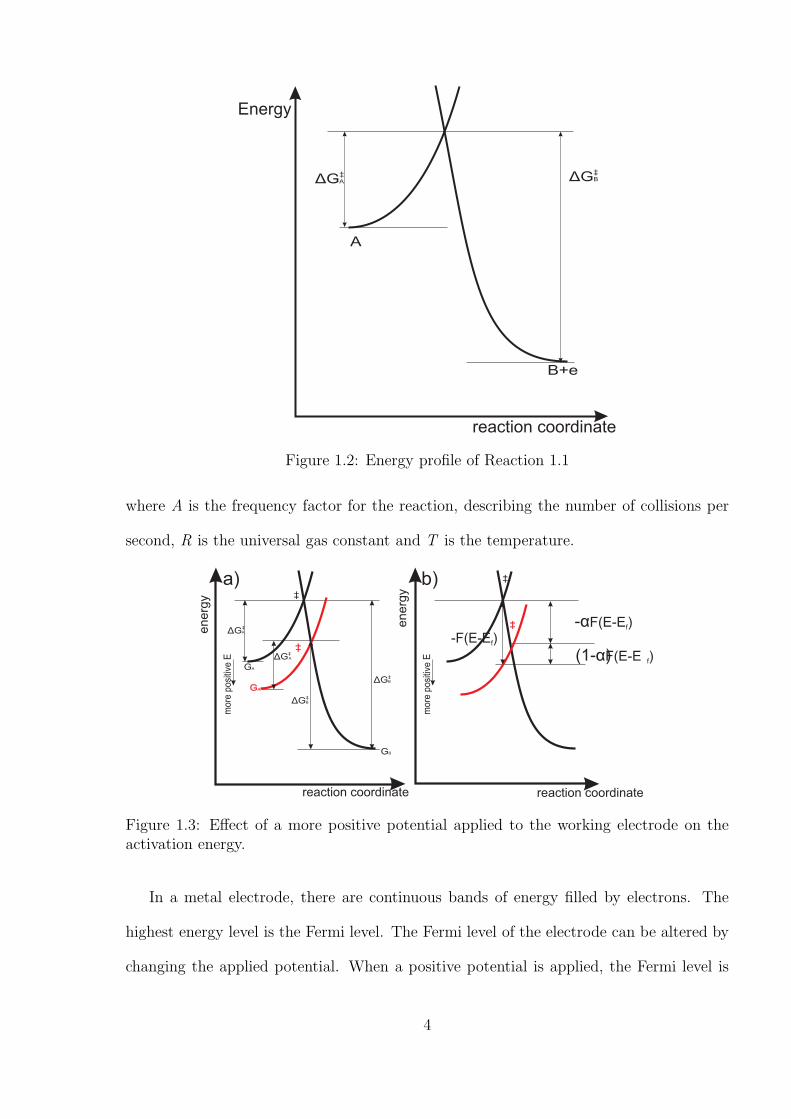
Figure 1.2: Energy profile of Reaction 1.1
where A is the frequency factor for the reaction, describing the number of collisions per
second, R is the universal gas constant and T is the temperature.
reaction coordinatereaction coordinate
en
erg
y
en
erg
y
Figure 1.3: Effect of a more positive potential applied to the working electrode on theactivation energy.
In a metal electrode, there are continuous bands of energy filled by electrons. The
highest energy level is the Fermi level. The Fermi level of the electrode can be altered by
changing the applied potential. When a positive potential is applied, the Fermi level is
4
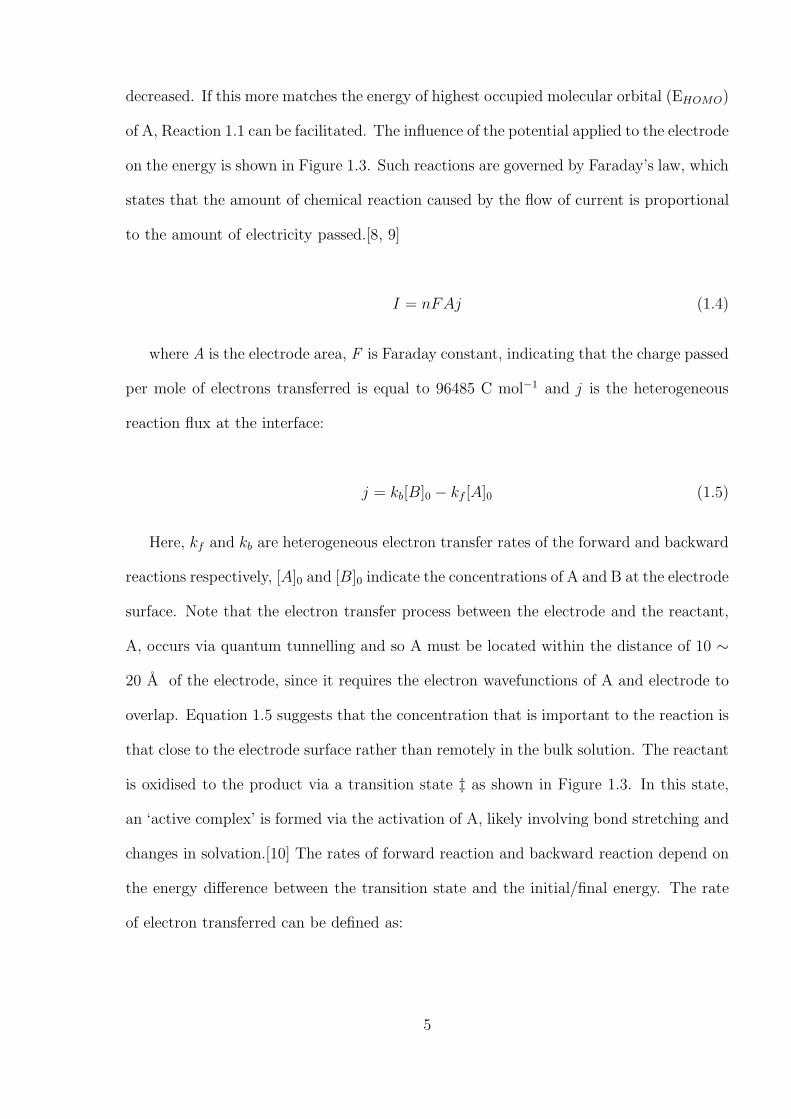
decreased. If this more matches the energy of highest occupied molecular orbital (EHOMO)
of A, Reaction 1.1 can be facilitated. The influence of the potential applied to the electrode
on the energy is shown in Figure 1.3. Such reactions are governed by Faraday’s law, which
states that the amount of chemical reaction caused by the flow of current is proportional
to the amount of electricity passed.[8, 9]
I = nFAj (1.4)
where A is the electrode area, F is Faraday constant, indicating that the charge passed
per mole of electrons transferred is equal to 96485 C mol−1 and j is the heterogeneous
reaction flux at the interface:
j = kb[B]0 − kf [A]0 (1.5)
Here, kf and kb are heterogeneous electron transfer rates of the forward and backward
reactions respectively, [A]0 and [B]0 indicate the concentrations of A and B at the electrode
surface. Note that the electron transfer process between the electrode and the reactant,
A, occurs via quantum tunnelling and so A must be located within the distance of 10 ∼
20 A of the electrode, since it requires the electron wavefunctions of A and electrode to
overlap. Equation 1.5 suggests that the concentration that is important to the reaction is
that close to the electrode surface rather than remotely in the bulk solution. The reactant
is oxidised to the product via a transition state ‡ as shown in Figure 1.3. In this state,
an ‘active complex’ is formed via the activation of A, likely involving bond stretching and
changes in solvation.[10] The rates of forward reaction and backward reaction depend on
the energy difference between the transition state and the initial/final energy. The rate
of electron transferred can be defined as:
5
kf = Afexp−(G‡ −GA)
RTand kb = Abexp
−(G‡ −GB)
RT(1.6)
The relation between the activation energy before (∆G‡0) and after the applied poten-
tial (∆G‡0) is shown in Figure 1.3 b) and can be expressed as,
∆G‡A = ∆G‡
0,A − (−α)(E −E0f ) (1.7)
∆G‡B = ∆G‡
0,B − (1− α)(E − E0f) (1.8)
Here, E − Ef is also known as the over-potential. Therefore, the reaction kinetic coeffi-
cients can be further expressed as,
kf = Afexp−∆G‡
0,A
RTexp[
(−α)(E −E0f )
RT] and kb = Abexp
−∆G‡0,B
RTexp[
(1− α)(E − E0f )
RT]
(1.9)
By assuming the oxidation reaction is at equilibrium where [A]0=[B]0 and E = E0f ,
leading to kf=kb, the reaction rate coefficient, k0, can be resolved via the Butler-Volmer
Equation as,[11]
j = k0[exp(−αF
RT(E −E0
f ))[B]0 − exp((1 − α)F
RT(E −E0
f ))[A]0] (1.10)
where k0 is the standard electrochemical rate constant and α is the transfer coefficient.
The transfer coefficient indicates the position of transition state relative to the reactants
and products, α lies in the range of 0 to 1 for one electron system. If α is close to 0,
the transition state is product-like for an oxidation, whereas if α is near 1, the transition
state is reactant-like.
The transfer coefficient can be evaluated by the following approach: An extreme over-
6
potential (E − E0) is applied at the working electrode, resulting in only oxidation or
reduction taking place. Therefore one term in Equation 1.10 can be neglected. The
current is evaluated through the use of the Tafel law:[2]
Ired = AFk0exp(−αF
RT(E −E0
f ))[B]0 and Iox = AFk0exp((1− α)F
RT(E − E0
f ))[A]0
(1.11)
Here Ired and Iox are the reduction and oxidation current respectively. Taking natural
logarithms of the above equations gives,
α = −RT
F
∂ln|Ired|∂E
and 1− α =RT
F
∂ln|Iox|∂E
(1.12)
α can be obtained via a plot of ln I against E where the gradient of this straight
line is diretly proportional to α, assuming [A]0 and [B]0 are approximately constant. The
data can be simply measured from cyclic voltmmetry (see Section 1.5.1). Despite the
simple operation of Butler-Volmer theory in modelling a variety of experimental results,
it exhibits some limitations that are likely due to the lack of physical insight. The Butler-
Volmer model suggests that the rate constant can infinitely increase when the applied
potential tends toward infinity which is physically impossible since excess energy may be
lost to heat or other forms. Therefore a better model is proposed by Marcus that provides
better physical insights into the electrochemical reactions.[12]
1.3 The Electrical Double Layer
Two types of charge transfer processeses dominate at electrodes. One type is that previ-
ously discussed in which the charge transfer across the electrode/solution interface causes
electrochemical reactions, leading to a current that follows Faraday’s law. The other pro-
7
+++++++
- +
+
+
+
+
++
+
+
+
++
Compact layer Diffuse layer Bulk solution
distance from electrode surface
ΦM
ΦS
---
-
--
-
-
--
+ -
-
-
-
-+
+
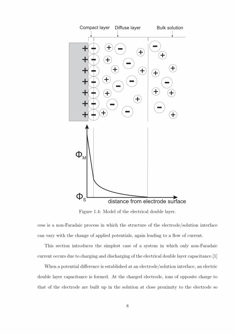
Figure 1.4: Model of the electrical double layer.
cess is a non-Faradaic process in which the structure of the electrode/solution interface
can vary with the change of applied potentials, again leading to a flow of current.
This section introduces the simplest case of a system in which only non-Faradaic
current occurs due to charging and discharging of the electrical double layer capacitance.[1]
When a potential difference is established at an electrode/solution interface, an electric
double layer capacitance is formed. At the charged electrode, ions of opposite charge to
that of the electrode are built up in the solution at close proximity to the electrode so
8
as to maintain charge neutrality. This layer partly comprises a compact layer of ions at
the electrode surface, as shown in Figure 1.4. Within the compact layer, the potential
decreases linearly with the distance away from the electrode surface. Beyond the compact
layer, a diffuse layer exists. The potential drops less rapidly in the diffuse layer, where
the ions undergo Brownian motion due to thermal forces. The charging current, I, caused
by redistribution of ions in forming the double layer is given by,
I =dQ
dt= Cd
dE
dt= CdAυ (1.13)
where Q is the charge and Cd is the double layer capacitance. Since electrode processes
take place within the double layer, it is important to compresses the diffuse layer thickness
within the electron tunnelling distance of 10 ∼ 20 A so the full drop in potential at the
electrode/solution interface is available to ‘drive’ the reaction. The diffuse thickness can
be compressed by adding an excess of salt (‘supporting electrolyte’). The Debye length
is defined as the distance in which the charged particles can screen external electric field.
By definition, the Debye length is also the double layer thickness. Its value can be shown
via the following equation:
κ−1 =
√
ε0εrkBT
2NAe2I(1.14)
where κ−1 is the Debye length, ε0 is the electric constant, εr is the permittivity of free
space, NA is the Avogadro constant, e is the elementary charge and I is the ionic strength.
Ionic strength is a measure of the concentration of ions in the solutions; it is related to
concentration via
I = 1/2
n∑
i=1
(2cz) (1.15)
where c is the concentration and z is the charge. The excess of supporting electrolytes
will increase the ionic strength via the increase of concentration. As a result of higher
ionic strength, the Debye length will decrease as will the double layer thickness. In ionic
9
liquids, the high concentration of ions ensures the desired, rapid fall-off of potential within
distance.
1.4 Mass Transport
In practice, electron transfer only occurs at a working electrode when the electro-active
species is within a few molecules distance of the electrode surface. Hence, the overall
reaction rate is governed by both the electron transfer rate for a given reaction and the
rate at which electro-active species is replenished at the electrode surface from the bulk
solution (mass transport). There are three types of mass transport: diffusion, convection
and migration.
1.4.1 Diffusion
Diffusion occurs when a concentration gradient exists in the system. When electro-active
species close to electrode surface are consumed, the concentration of the species at the
electrode decreases, forming a depletion layer (‘diffusion layer’) near the electrode surface.
The analytes are drawn to the electrode surface in order to maximise entropy. The rate
of diffusion depends on the concentration gradient as given by Fick’s first law:[13]
j = −D∂c
∂x(1.16)
where D is the diffusion coefficient, c is the concentration and x is the distance away from
the electrode. Fick’s second law is derived from Fick’s first law, via mass conservation,
and describes the rate of concentration change at point x :
∂c
∂t= D
∂2c
∂x2(1.17)
There are two types of diffusion to an electrode, linear and convergent. These two
10
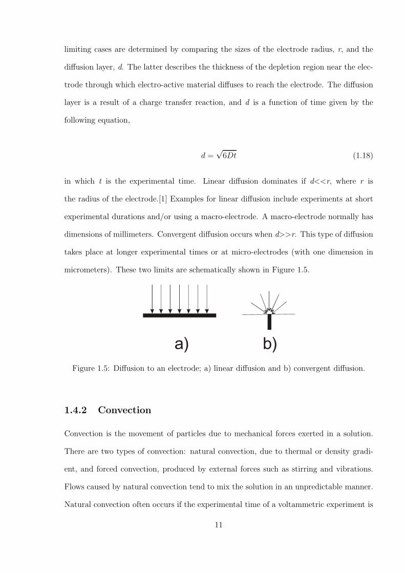
limiting cases are determined by comparing the sizes of the electrode radius, r, and the
diffusion layer, d. The latter describes the thickness of the depletion region near the elec-
trode through which electro-active material diffuses to reach the electrode. The diffusion
layer is a result of a charge transfer reaction, and d is a function of time given by the
following equation,
d =√6Dt (1.18)
in which t is the experimental time. Linear diffusion dominates if d<<r, where r is
the radius of the electrode.[1] Examples for linear diffusion include experiments at short
experimental durations and/or using a macro-electrode. A macro-electrode normally has
dimensions of millimeters. Convergent diffusion occurs when d>>r. This type of diffusion
takes place at longer experimental times or at micro-electrodes (with one dimension in
micrometers). These two limits are schematically shown in Figure 1.5.
a) b)
Figure 1.5: Diffusion to an electrode; a) linear diffusion and b) convergent diffusion.
1.4.2 Convection
Convection is the movement of particles due to mechanical forces exerted in a solution.
There are two types of convection: natural convection, due to thermal or density gradi-
ent, and forced convection, produced by external forces such as stirring and vibrations.
Flows caused by natural convection tend to mix the solution in an unpredictable manner.
Natural convection often occurs if the experimental time of a voltammetric experiment is
11
longer than ca. 10 seconds with the use of a macro-electrode.[14] Forced convection can
be introduced in a well controlled way, for example by using rotating disc or a chemical
flow cell.[1, 2, 15] The convective flux is expressed as
j = cv(x) (1.19)
Here v(x) is the solution velocity at point x.
1.4.3 Migration
Migration arises due to the motion of a charged particle down a potential gradient (electric
field).[16–19] This type of mass transport takes place for all charged species in solution
when a potential is applied to a working electrode relative to a solution, leading to a
potential gradient and resulting in a flow of charged species electro-statically attracted to
or repelled from the electrode.[20] The flux j, down a potential gradient, ∂φ∂x, is given by
the following equation:
j = − zF
RTDc
∂φ
∂x(1.20)
in which z is the charge of species migrating. To simplify the interpretation of electro-
chemistry, it is convenient to eliminate migration. This is done by adding supporting
electrolytes to the solvent. The excess salt compresses the electrical double layer (dis-
cussed in Section 1.3), and hence, the electric field is confined to a very close region to the
electrode. Consequently, mass transport to and from the electrode can be simplified to
diffusion only. For experiments in room temperature ionic liquids, the solution is already
self-supported.
High concentration of supporting electrolyte also offers several other advantages[14].
First, the solution conductivity is increased and therefore ohmic drop can be minimised.
Second, the presence of electrolyte maintains a near constant ionic strength in solution,
12
fixing the formal potentials of redox couples. Third, excess supporting electrolyte com-
presses the diffuse layer to within a distance of 10 ∼ 20 A from the electrode,[21] across
which the electron quantum tunnelling can take place (see Section 1.2).
1.5 Analytical Techniques
This section introduces the major electrochemical techniques for analysing and studying
electrochemical reactions. Information such as analyte concentrations, diffusion coeffi-
cients, and reaction rates can be obtained from voltammetry or amprometry.
1.5.1 Cyclic Voltammetry
time
po
ten
tia
l E2
E1
a) b) c)a) b)
Curr
ent /A
Potential / V
ii) ii) iii)
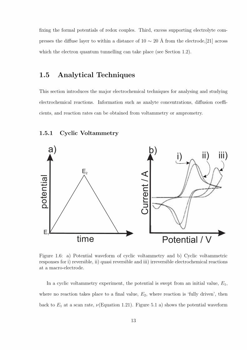
Figure 1.6: a) Potential waveform of cyclic voltammetry and b) Cyclic voltammetricresponses for i) reversible, ii) quasi reversible and iii) irreversible electrochemical reactionsat a macro-electrode.
In a cyclic voltammetry experiment, the potential is swept from an initial value, E1,
where no reaction takes place to a final value, E2, where reaction is ‘fully driven’, then
back to E1 at a scan rate, ν(Equation 1.21). Figure 5.1 a) shows the potential waveform
13
of cyclic voltammetry.
ν =∂E
∂t(1.21)
The resultant current is plotted as a function of the sweeping potential as can be seen
from Figure 5.1 b). The current - potential wave shape can be understood by considering
the rates of electron transfer and mass transport. Initially, the applied potential is less
than the oxidation potential of A (see Equation 1.1) and hence no current passes. When
the potential increases to the oxidation potential of A, electrons pass from A to the
electrode. This current is a function of the reaction rate and the concentration of A (see
Equation 1.10) since the electron transfer rate is smaller than the rate of mass transport
at this point. As potential increases further, the current reaches a peak at which the
electron rate transfer is balanced by the diffusion rate of A. At larger potentials, the
current decreases because the electron transfer is faster in comparison to mass transport.
Therefore, the rate of diffusion of A is not sufficient to replenish the material consumed
at the electrode surface. In the reverse scan, an analogous process takes place for the
reduction of B back to A.
There are two extremes of electrochemical process: ‘reversible’ and ‘irreversible’.
These limits can be explained in terms of electron kinetics, measured by standard electro-
chemicl rate constant, k0, and the rate of mass transport, measured by the mass transport
coefficient mT where
mT =D
δ(1.22)
where δ is the diffusion layer thickness, given by Equation 1.18. The experimental time
in Equation 1.18 can be related to the scan rate via,
14
t ∼ RT
Fν(1.23)
Therefore mT can be estimated from the following equation,
mT ∼√
DFν
RT(1.24)
For k0 >> mT , the process is ‘reversible’ whilst for k0 << mT , it is ‘irreversible’. The
limits of reversible and irreversible systems have been rigorously mathematically evaluated
by Matsuda and Ayabe via a parameter, Λ, where[22]:
Λ =k0
(FDν/RT )12
(1.25)
The boundaries were found to be:
Reversible Λ ≥ 15 k0 ≥ 0.3 ν12 cm · s−1 (1.26)
Irreversible Λ ≤ 10−3 k0 ≤ 2× 10⁻⁵ ν12 cm · s−1 (1.27)
These results assume the experiments at 298 K and a transfer coefficient, α, of 0.5.
These two limiting cases can also be explored via cyclic voltammetry. In the reversible
limit for one electron transfer at 298 K, the peak to peak separation (i) in Figure 5.1 b)),
∆E, is 57 mV and the peak current, ip, can be given by the Randles-Sevcık equation[23,
24].
ip,rev = 0.446FAc∗A
√
FDν
RT(1.28)
The cyclic voltammogram of irreversible limit is shown in Figure 5.1 b) iii). An
15
overpotential much larger than the formal potential is required to overcome the kinetic
barrier and to drive the electrochemical reaction.[20] Therefore, a large ∆E (> 200 mV)
is normally expected. The peak current resulting from a one-electron transfer irreversible
reaction is given by:[1, 2]
Ip,irrev = 0.496√αFA[A]
√
FDν
RT(1.29)
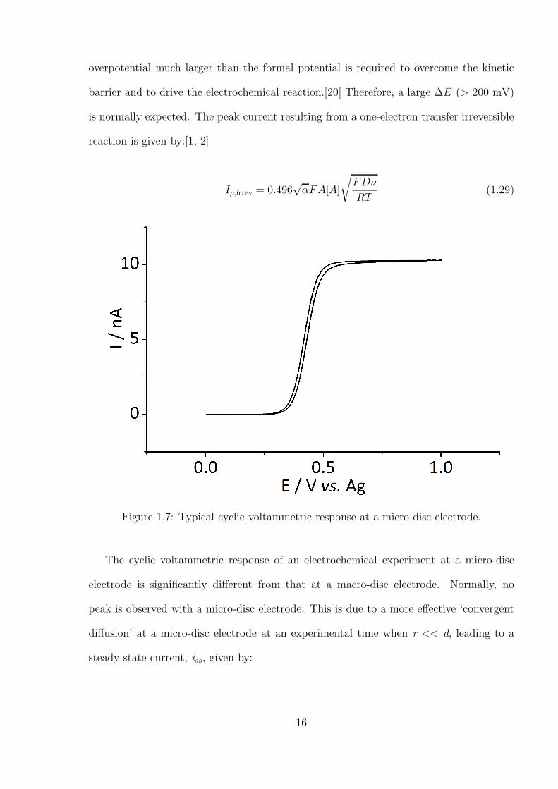
Figure 1.7: Typical cyclic voltammetric response at a micro-disc electrode.
The cyclic voltammetric response of an electrochemical experiment at a micro-disc
electrode is significantly different from that at a macro-disc electrode. Normally, no
peak is observed with a micro-disc electrode. This is due to a more effective ‘convergent
diffusion’ at a micro-disc electrode at an experimental time when r << d, leading to a
steady state current, iss, given by:
16
Iss = 4nFrDc (1.30)
However at a vary fast scan rate, a peak will appear because the linear diffusion occurs
at a short experimental time (see Equation 1.18).
1.5.2 Square Wave Voltammetry
I/ A
E/ V
ΔI
I1
I2
+ =
ΔES
ts
tp
ΔEP
1
2
a)
b)
ΔEP
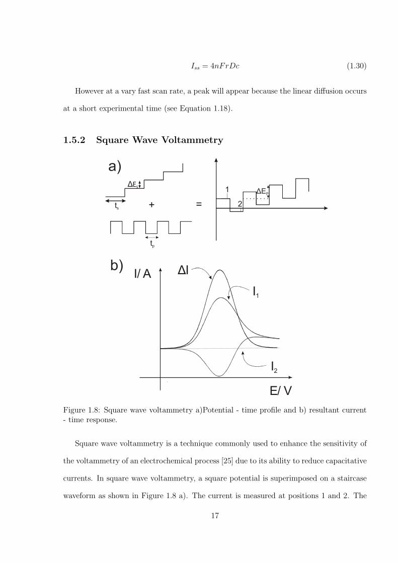
Figure 1.8: Square wave voltammetry a)Potential - time profile and b) resultant current- time response.
Square wave voltammetry is a technique commonly used to enhance the sensitivity of
the voltammetry of an electrochemical process [25] due to its ability to reduce capacitative
currents. In square wave voltammetry, a square potential is superimposed on a staircase
waveform as shown in Figure 1.8 a). The current is measured at positions 1 and 2. The
17
square wave voltammetric response is characterised by a pulse height, ∆EP , the staircase
height, ∆EP , the pulse time, tP , and the cycle period, tS. The voltage scan rate is given
by,
∆ES
2tP= f∆ES (1.31)
where ∆ES is defined in Figure 1.8 a).
Cottrellian current
Capacitative current
time
current
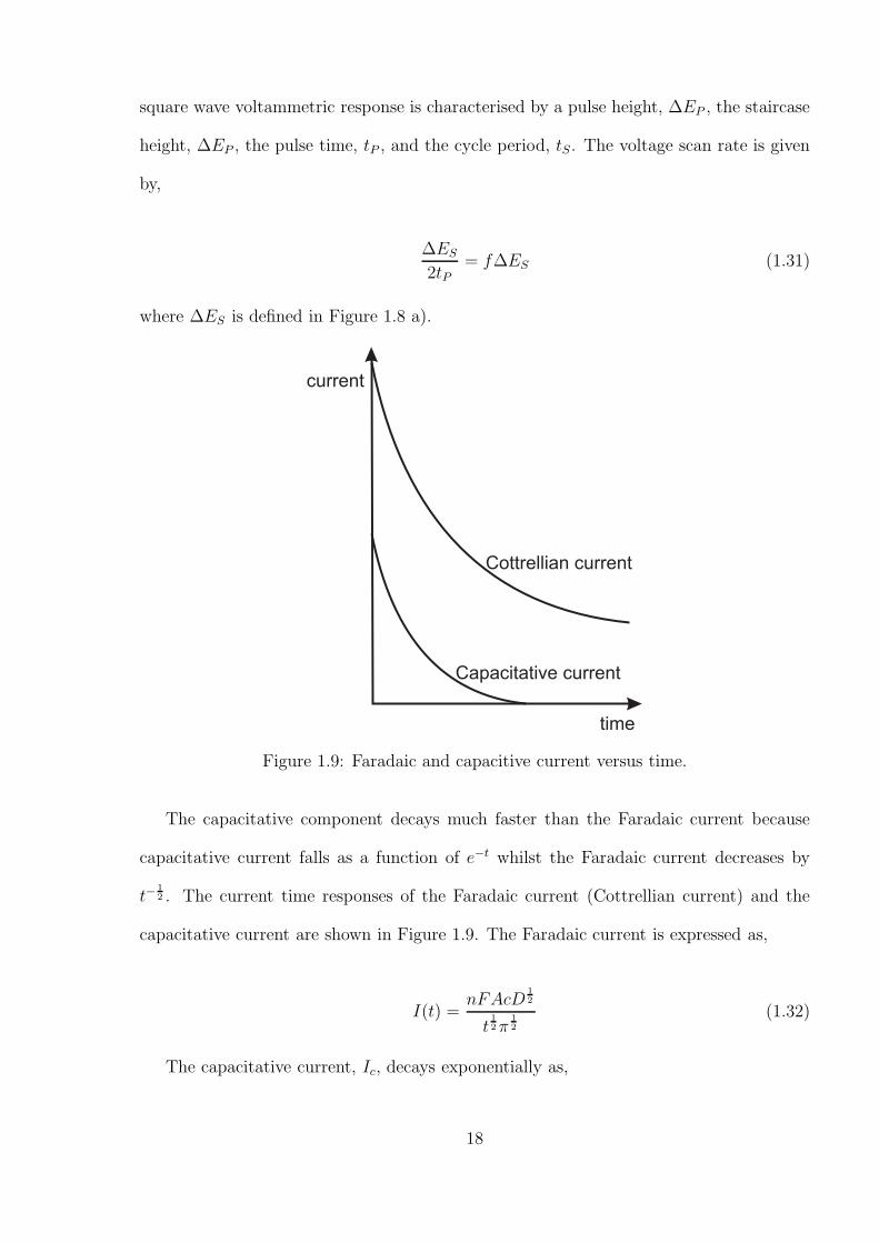
Figure 1.9: Faradaic and capacitive current versus time.
The capacitative component decays much faster than the Faradaic current because
capacitative current falls as a function of e−t whilst the Faradaic current decreases by
t−12 . The current time responses of the Faradaic current (Cottrellian current) and the
capacitative current are shown in Figure 1.9. The Faradaic current is expressed as,
I(t) =nFAcD
12
t12π
12
(1.32)
The capacitative current, Ic, decays exponentially as,
18
Ic(t) = I0exp
( −t
RCd
)
(1.33)
Here, I0 is the initial current and R is the resistance. Therefore it is possible to
minimise the capacitive contribution by sampling the current at the end of each step.
The resultant current, ∆I is the difference of I1 and I2 (see Figure 1.8 b) ) and is
plotted against applied potential as shown in Figure 1.8 b). Assuming the capacitative
currents at 1 and 2 are approximately equal, the current due to the non-Faradaic process
is reduced. Due to these features, the square wave technique provides higher sensitivity,
easily reaching detection limits of 1 × 10⁻⁸ M.
1.5.3 Potential Step Chronoamperometry at A Micro-electrode
a) b)
Time
Pote
nti
al
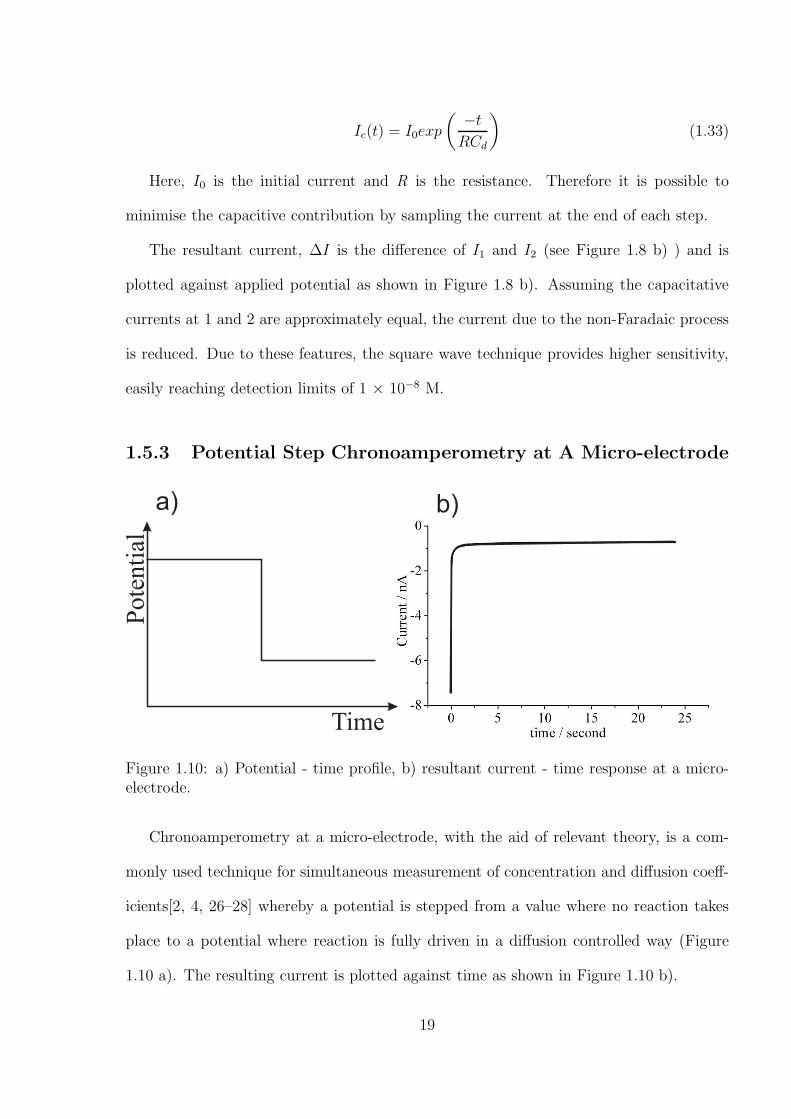
Figure 1.10: a) Potential - time profile, b) resultant current - time response at a micro-electrode.
Chronoamperometry at a micro-electrode, with the aid of relevant theory, is a com-
monly used technique for simultaneous measurement of concentration and diffusion coeff-
icients[2, 4, 26–28] whereby a potential is stepped from a value where no reaction takes
place to a potential where reaction is fully driven in a diffusion controlled way (Figure
1.10 a). The resulting current is plotted against time as shown in Figure 1.10 b).
19
The current is initially very large, resulting from a steep concentration gradient close
to the electrode surface. Then the Faradaic current decays rapidly because it is limited by
the depletion of the electro-active species near the electrode surface. Such a current-time
relationship resulting from a potential step to a planar macro electrode is described under
diffusion controlled conditions by the Cottrell equation. [1, 2, 29]
At a long experimental time, Iss is recorded at a micro-disc electrode as discussed in
Section 1.5.1.
Several numerical models have been developed to describe the chronoamperometric
responses observed at a microelectrodes.[26, 27, 30–35] The Shoup and Szabo equation is
most widely used, and has been reported to describe the current response over all time
values to within an error of 0.5 %[26]. Chapter 4 gives more details of the Shoup and
Szabo analysis. Chronoamperometry is also used in conjunction with standard addition
of analytes to observe analytical responses.[36].
References
[1] Compton, R. G.; Banks, C. E. Understanding Voltammetry ; Imperial College Press,2011, 2nd Edition.
[2] Bard, A. J.; Faulkner, L. R. Electrochemical Methods: Fundamentals and Applica-tions ; Wiley, 2001.
[3] Fleischmann, M.; Lasserre, F.; Robinson, J.; Swan, D. Journal of ElectroanalyticalChemistry and Interfacial Electrochemistry 1984, 177, 97 – 114.
[4] Rogers, E. I.; Silvester, D. S.; Poole, D. L.; Aldous, L.; Hardacre, C.; Compton, R. G.Journal of Physical Chemistry C 2008, 112, 2729–2735.
[5] Faure, M.; Pallandre, A.; Chebil, S.; Le Potier, I.; Taverna, M.; Tribollet, B.;Deslouis, C.; Haghiri-Gosnet, A.-M.; Gamby, J. Lab on a Chip - Miniaturisationfor Chemistry and Biology 2014, 14, 2800–2805.
[6] Meng, Y.; Aldous, L.; Belding, S.; Compton, R. Physical Chemistry Chemical Physics2012, 14, 5222–5228.
[7] Evans, R. G.; Klymenko, O. V.; Saddoughi, S. A.; Hardacre, C.; Compton, R. G.Journal of Physical Chemistry B 2004, 108, 7878–7886.
[8] Strong, F. C. Journal of Chemical Education 1961, 38, 98.
20
[9] Ehl, R. G.; Ihde, A. J. Journal of Chemical Education 1954, 31, 226.
[10] Atkins, P.; De Paula, J. Atkins’ Physical Chemistry ; Macmillan Higher Education,2006.
[11] Butler, J. A. V. Transactions of the Faraday Society 1924, 19, 729 – 733.
[12] Marcus, R. A.; Sutin, N. Biochimica et Biophysica Acta - Reviews on Bioenergetics1985, 811, 265–322.
[13] Fick, A. Annal. Phys. Chem. 1855, 94, 59 – 86.
[14] Bamford, C. H.; Tipper, C. F. H.; Compton, R. G. Electrode Kinetics: Principlesand Methodology: Principles and Methodology ; Comprehensive Chemical Kinetics;Elsevier Science, 1986.
[15] Montenegro, M. I.; Montenegro, I.; Queiros, A.; Daschbach, J. L.; Division, N. A. T.O. S. A. Microelectrodes: Theory and Applications: Theory and Applications ; NATOASI series / E: NATO ASI series; Springer Netherlands, 1991.
[16] Belding, S. R.; Limon-Petersen, J. G.; Dickinson, E. J. F.; Compton, R. G. Ange-wandte Chemie International Edition 2010, 49, 9242–9245.
[17] Barnes, E. O.; Wang, Y.; Limon-Petersen, J. G.; Belding, S. R.; Compton, R. G.Journal of Electroanalytical Chemistry 2011, 659, 25 – 35.
[18] Barnes, E. O.; Belding, S. R.; Compton, R. G. Journal of Electroanalytical Chemistry2011, 660, 185 – 194.
[19] Barnes, E. O.; Wang, Y.; Belding, S. R.; Compton, R. G. ChemPhysChem 2012, 13,92 – 95.
[20] Pletcher, D.; of Chemistry (Great Britain), R. S. A First Course in Electrode Pro-cesses ; A First Course in Electrode Processes; Royal Society of Chemistry, 2009.
[21] Sakata, T.; Azuma, M. Bulletin of the Chemical Society of Japan 2013, 86, 1158–1173.
[22] Matsuda, H.; Ayabe, Y. Zeitschrift fr Elektrochemie 1955, 59, 494.
[23] Randles, J. E. B. Transactions of the Faraday Society 1948, 44, 327–338.
[24] Sevcik, A. Collection of Czechoslovak Chemical Communications 1948, 13, 349–377.
[25] Xiong, L.; Batchelor-Mcauley, C.; Compton, R. G. Sensors and Actuators, B: Chem-ical 2011, 159, 251–255.
[26] Shoup, D.; Szabo, A. Journal of Electroanalytical Chemistry and Interfacial Electro-chemistry 1982, 140, 237 – 245.
[27] Klymenko, O. V.; Evans, R. G.; Hardacre, C.; Svir, I. B.; Compton, R. G. Journalof Electroanalytical Chemistry 2004, 571, 211–221.
[28] Paddon, C. A.; Silvester, D. S.; Bhatti, F. L.; Donohoe, T. J.; Compton, R. G.Electroanalysis 2007, 19, 11–22.
[29] Cottrell, F. G. Z. Physik. Chem. 1903, 42, 385 – 431.
21
[30] Heinze, J. Journal of Electroanalytical Chemistry 1981, 124, 73–86.
[31] Gavaghan, D. J.; Rollett, J. S. Journal of Electroanalytical Chemistry 1990, 295,1–14.
[32] Oldham, K. B. Journal of Electroanalytical Chemistry 1981, 122, 1–17.
[33] Aoki, K.; Osteryoung, J. Journal of Electroanalytical Chemistry 1981, 122, 19–35.
[34] Aoki, K.; Osteryoung, J. Journal of Electroanalytical Chemistry 1984, 160, 335–339.
[35] Fleischmann, M.; Pons, S. Journal of Electroanalytical Chemistry 1988, 250, 257–267.
[36] Panchompoo, J.; Aldous, L.; Downing, C.; Crossley, A.; Compton, R. G. Electroanal-ysis 2011, 23, 1568–1578.
22
Chapter 2
Introduction to Amperometric GasSensors
This chapter provides an introduction to history and recent progress in amperometric
electrochemical gas sensing. Topics covered include the use of room temperature ionic
liquids (RTILs) as solvents in gas sensors, the advantageous use of micro-electrodes rather
than macro-electrodes and membrane free devices. The work presented here has been
published in International Journal of Electrochemical Science.[1]
2.1 Introduction
Gas detection plays an important, even essential role in many areas, ranging from food
safety to environmental monitoring, with one of the best known examples being fire alarms
based on CO[2–4] detection. Quantitative measurement of gases is based on a variety of
physical or chemical principles[5]. Examples of commercialised sensors include techniques
using spectrometry[6–10], luminescence[11–15] and electrochemistry[16–20] as a basis of
sensing. Table 2.1 summaries different types of sensors and their operational principles.
Amongst the various techniques, the electrochemical approach often shows significant
advantages over the others. First and second, an electrochemical gas sensor provides high
sensitivity at low cost. Third, their compact sizes allow for high portability. Fourth,
only a small amount of energy is required to run the detector. On the other hand, the
selectivity of electrochemical sensors is rarely perfect.
23
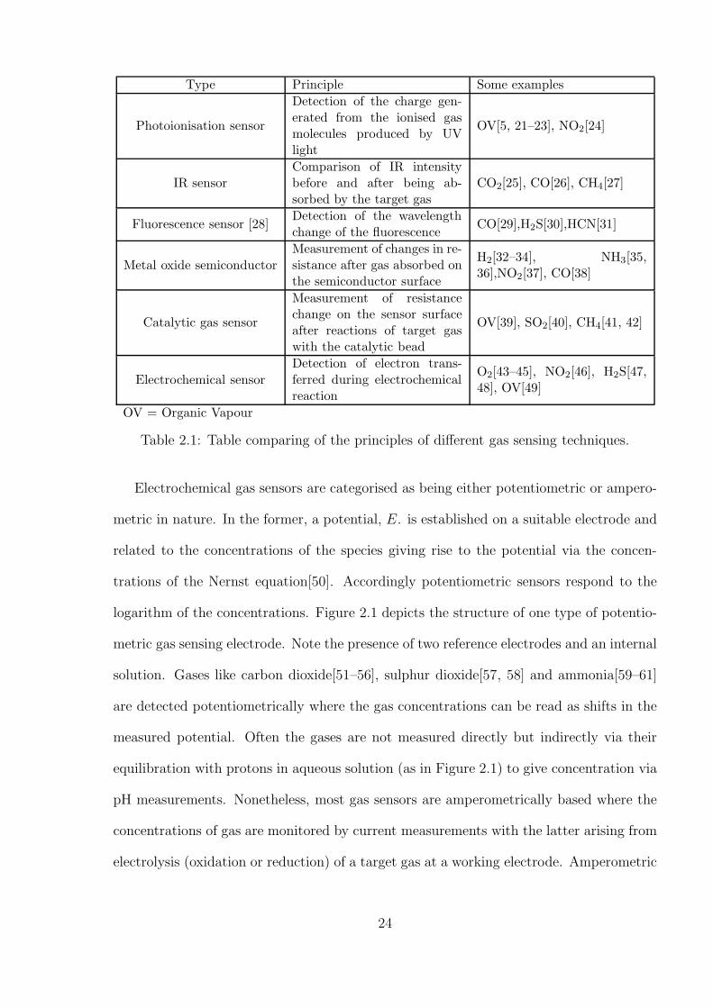
Type Principle Some examples
Photoionisation sensor
Detection of the charge gen-erated from the ionised gasmolecules produced by UVlight
OV[5, 21–23], NO2[24]
IR sensorComparison of IR intensitybefore and after being ab-sorbed by the target gas
CO2[25], CO[26], CH4[27]
Fluorescence sensor [28]Detection of the wavelengthchange of the fluorescence
CO[29],H2S[30],HCN[31]
Metal oxide semiconductor
Measurement of changes in re-sistance after gas absorbed onthe semiconductor surface
H2[32–34], NH3[35,36],NO2[37], CO[38]
Catalytic gas sensor
Measurement of resistancechange on the sensor surfaceafter reactions of target gaswith the catalytic bead
OV[39], SO2[40], CH4[41, 42]
Electrochemical sensor
Detection of electron trans-ferred during electrochemicalreaction
O2[43–45], NO2[46], H2S[47,48], OV[49]
OV = Organic Vapour
Table 2.1: Table comparing of the principles of different gas sensing techniques.
Electrochemical gas sensors are categorised as being either potentiometric or ampero-
metric in nature. In the former, a potential, E. is established on a suitable electrode and
related to the concentrations of the species giving rise to the potential via the concen-
trations of the Nernst equation[50]. Accordingly potentiometric sensors respond to the
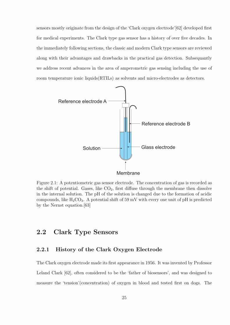
logarithm of the concentrations. Figure 2.1 depicts the structure of one type of potentio-
metric gas sensing electrode. Note the presence of two reference electrodes and an internal
solution. Gases like carbon dioxide[51–56], sulphur dioxide[57, 58] and ammonia[59–61]
are detected potentiometrically where the gas concentrations can be read as shifts in the
measured potential. Often the gases are not measured directly but indirectly via their
equilibration with protons in aqueous solution (as in Figure 2.1) to give concentration via
pH measurements. Nonetheless, most gas sensors are amperometrically based where the
concentrations of gas are monitored by current measurements with the latter arising from
electrolysis (oxidation or reduction) of a target gas at a working electrode. Amperometric
24
sensors mostly originate from the design of the ‘Clark oxygen electrode’[62] developed first
for medical experiments. The Clark type gas sensor has a history of over five decades. In
the immediately following sections, the classic and modern Clark type sensors are reviewed
along with their advantages and drawbacks in the practical gas detection. Subsequantly
we address recent advances in the area of amperometric gas sensing including the use of
room temperature ionic liquids(RTILs) as solvents and micro-electrodes as detectors.
Reference electrode A
Reference electrode B
Glass electrode
Membrane
Solution
Figure 2.1: A potentiometric gas sensor electrode. The concentration of gas is recorded asthe shift of potential. Gases, like CO2, first diffuse through the membrane then dissolvein the internal solution. The pH of the solution is changed due to the formation of acidiccompounds, like H2CO3. A potential shift of 59 mV with every one unit of pH is predictedby the Nernst equation.[63]
2.2 Clark Type Sensors
2.2.1 History of the Clark Oxygen Electrode
The Clark oxygen electrode made its first appearance in 1956. It was invented by Professor
Leland Clark [62], often considered to be the ‘father of biosensors’, and was designed to
measure the ‘tension’(concentration) of oxygen in blood and tested first on dogs. The
25
device supported the publication of another Clark invention, an oxygen generator for
cardiac surgery.[64]
The original design consisted of a power supply, a platinum cathode, a potassium
chloride-calomel anode (which was later replaced with a silver wire) and a cellophane
membrane. All the electrodes were placed inside a glass tube and were wrapped with
cotton soaked with saline solutions. The cellophane membrane was used to separate the
internal and external environment in order to avert the influence of red blood cells in
the oxygen measurements. To realise the detection, oxygen first diffuses through the
membrane and enters the internal solution. The reduction of oxygen then takes place at
the platinum cathode (see Equation 2.1) when the power supply applies a potential of 0.6
V (vs. anode) to the cathode.
O2 + 2H+ + 2e → H2O2 (2.1)
The current of the reduction of oxygen was recorded using a galvanometer. The
measured current was proportional to the concentration of O2. This linear dependence
of current on the concentration of dissolved oxygen was first discovered by Heinrich L.
Danneel[65] as long ago as the nineteenth century as part of a study on dissolved oxygen
in Nernst’s laboratory. Experiments were performed by applying - 0.2 V vs. platinum at a
platinum macro-electrode in a water solution containing dissolved oxygen. In experiments
with blood the biosensor failed since the platinum was blocked by adsorbed blood cells.[66]
Experiments were carried out by Clark to optimise experimental conditions such as
temperature, cathode voltage and choice of membrane material.[62] The current reading
was observed to increase with the temperature due to the fact that oxygen diffuses faster
at higher temperatures. The optimised voltage was within the range of 0.6 to 0.8 V
against the anode but 0.6 V was deliberately chosen to reduce blood clot formation in
vivo. It was found that the response time was largely limited by the time taken for oxygen
26
diffusion through the membrane reflecting both the diffusion coefficient and solubility of
oxygen in the membrane as compared to the aqueous electrolyte of the sensor as well as
their relative thickness. The best membrane materials in order to decrease the response
times were identified. A collection of polymers was investigated, including cellophane[62],
dialysis tubing, condom rubber, condom skin and polyethylene. The time taken to reach
steady state reading decreased in the following order:[62] condom skin > condom rubber
> polyethylene = dialysis tubing > cellophane. The best response time (∼ 20 s) was seen
with cellophane membranes. However, the cellophane membrane slowed the response time
by half as compared to what was observed without using a membrane (∼ 10 s).[62]
After the conditions were optimised, experiments for oxygen detection were carried out
on blood both in vitro and in vivo. In vivo oxygen sensing was achieved through inserting
the Clark type electrode into the aorta of a heparinised1, Nembutalized2 dog. The oxygen
responses were recorded by a galvanometer. The first experiment was performed under
different levels of oxygen where readings3 on the galvanometer of 74 and 96 indicated
partial pressure of O2 of 95 mm Hg and 700 mm Hg respectively. This design was proved
to accurately reflect the oxygen content. The sensing stability using the Clark type
electrode was determined under a constant air supply (3 hours) where identical signals
were observed throughout the experiment.[62]
The development of the Clark type oxygen electrode is deemed to be the birth of
at-point-of-care measurements. Clark cells subsequently allowed applications in gaseous
oxygen monitoring, direct blood oxygen measurements and much later even the develop-
ment of early glucose sensors.[53] This great invention has inspired numerous scientists
of later generations to develop other gas sensors using the Clark oxygen electrode as the
basis. These are discussed in the next section.
1Heparin is an anticoagulant, preventing the formation of clots within blood.2Nembutal is used as a veterinary anesthetic agent.3Full scale = 100
27
2.2.2 Modern Clark Type Gas Sensors
Data Recorder
ElectrochemicalCell
Detector Case
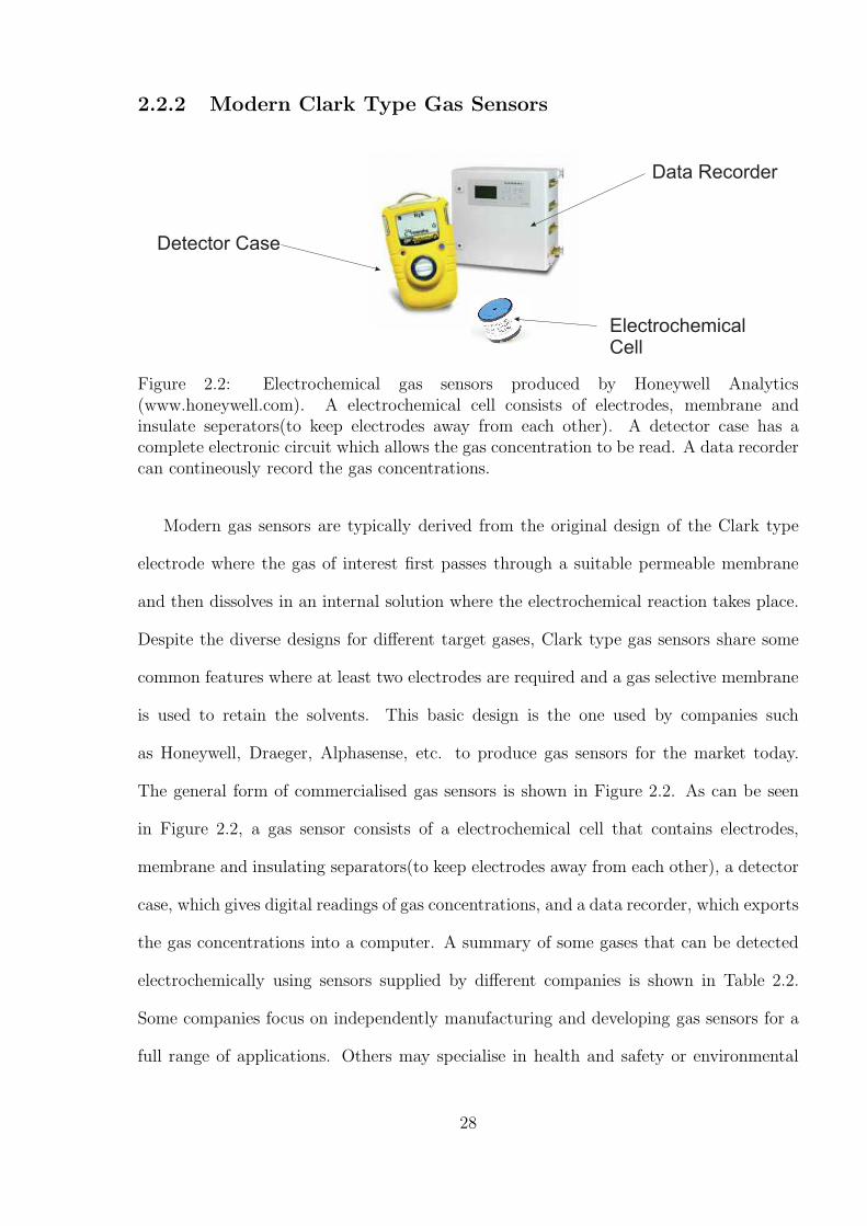
Figure 2.2: Electrochemical gas sensors produced by Honeywell Analytics(www.honeywell.com). A electrochemical cell consists of electrodes, membrane andinsulate seperators(to keep electrodes away from each other). A detector case has acomplete electronic circuit which allows the gas concentration to be read. A data recordercan contineously record the gas concentrations.
Modern gas sensors are typically derived from the original design of the Clark type
electrode where the gas of interest first passes through a suitable permeable membrane
and then dissolves in an internal solution where the electrochemical reaction takes place.
Despite the diverse designs for different target gases, Clark type gas sensors share some
common features where at least two electrodes are required and a gas selective membrane
is used to retain the solvents. This basic design is the one used by companies such
as Honeywell, Draeger, Alphasense, etc. to produce gas sensors for the market today.
The general form of commercialised gas sensors is shown in Figure 2.2. As can be seen
in Figure 2.2, a gas sensor consists of a electrochemical cell that contains electrodes,
membrane and insulating separators(to keep electrodes away from each other), a detector
case, which gives digital readings of gas concentrations, and a data recorder, which exports
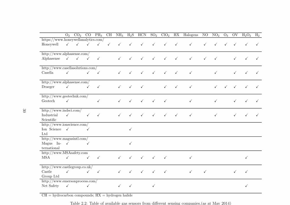
the gas concentrations into a computer. A summary of some gases that can be detected
electrochemically using sensors supplied by different companies is shown in Table 2.2.
Some companies focus on independently manufacturing and developing gas sensors for a
full range of applications. Others may specialise in health and safety or environmental
28
monitoring. The products are divided into small portable devices for field work and
larger fixed devices used, for example, in ships or in the laboratory. It is noted that
the sensors normally experience a lifetime of around 2 years, limited mainly due to the
failure of the membrane and/or loss of the solvent (see next section). More details of gas
sensing products in different companies can be found in the websites of the corresponding
companies given in Table 2.2.
The value of a gas sensor depends on four properties: selectivity, sensitivity, response
time and sensor lifetime. Selectivity allows the detection of a specific gas as other gases
are either filtered out physically or chemically. Sensitivity indicates the dependence of
the measured current on the concentration of gas. Factors influencing the sensitivity
are not restricted to the electrode but reflect the sensing environment. Response times
are also of vital importance since the sensor needs to reflect promptly the changing gas
concentrations. This is normally measured by the time taken to reach 90% of the steady
state response(t90).
The sensor lifespan is controlled by the electrode materials, solutions and membranes.
A sensor case (see Figure 2.2) lasts for a long time (> 100 years). An electrochemical
sensor normally has a shelf life of 6 months to a year. In standard sensing environments
(- 40 to 50 0C, 20 - 90 % RH, ∼ 1 atm)[67], the membrane lasts for ca. 3 years and
the sensing probe can run more than several thousand detections.4 Lifetime limiting
factors include the extreme temperature and pressures, low humidity environment and
involvement of toxic gases.[68] These directly lead to consumed or contaminated filling
solutions or electrode surfaces, resulting in electrode expiration.
4Information summarised from the user’s manuals
29
O2 CO2 CO PH3 CH NH3 H2S HCN SO2 ClO2 HX Halogens NO NO2 O3 OV H2O2 H2
https://www.honeywellanalytics.com/Honeywell X X X X X X X X X X X X X X X X X X
http://www.alphasense.com/Alphasense X X X X X X X X X X X X X X X X
http://www.casellasolutions.com/Casella X X X X X X X X X X X X X X
http://www.alphasense.com/Draeger X X X X X X X X X X X X X X
http://www.geotechuk.com/Geotech X X X X X X X X X X X X
http://www.indsci.com/IndustrialScientific
X X X X X X X X X X X X X X
http://www.ionscience.com/Ion ScienceLtd
X X X
http://www.magusintl.com/Magus In-ternational
X X X
http://www.MSAsafety.comMSA X X X X X X X X X X
http://www.castlegroup.co.uk/CastleGroup Ltd
X X X X X X X X X X X X
http://www.emersonprocess.com/Net Safety X X X X X X
CH = hydrocarbon compounds; HX = hydrogen halide
Table 2.2: Table of available gas sensors from different sensing companies.(as at May 2014)
30
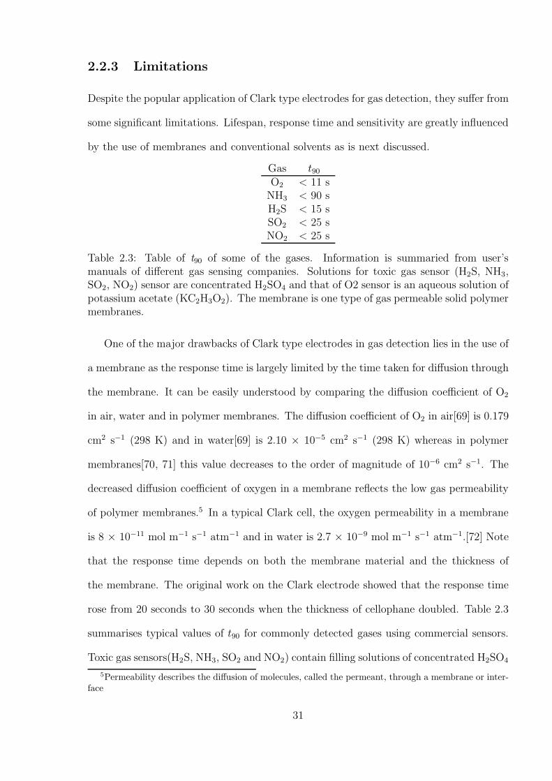
2.2.3 Limitations
Despite the popular application of Clark type electrodes for gas detection, they suffer from
some significant limitations. Lifespan, response time and sensitivity are greatly influenced
by the use of membranes and conventional solvents as is next discussed.
Gas t90O2 < 11 sNH3 < 90 sH2S < 15 sSO2 < 25 sNO2 < 25 s
Table 2.3: Table of t90 of some of the gases. Information is summaried from user’smanuals of different gas sensing companies. Solutions for toxic gas sensor (H2S, NH3,SO2, NO2) sensor are concentrated H2SO4 and that of O2 sensor is an aqueous solution ofpotassium acetate (KC2H3O2). The membrane is one type of gas permeable solid polymermembranes.
One of the major drawbacks of Clark type electrodes in gas detection lies in the use of
a membrane as the response time is largely limited by the time taken for diffusion through
the membrane. It can be easily understood by comparing the diffusion coefficient of O2
in air, water and in polymer membranes. The diffusion coefficient of O2 in air[69] is 0.179
cm2 s−1 (298 K) and in water[69] is 2.10 × 10⁻⁵ cm2 s−1 (298 K) whereas in polymer
membranes[70, 71] this value decreases to the order of magnitude of 10−6 cm2 s−1. The
decreased diffusion coefficient of oxygen in a membrane reflects the low gas permeability
of polymer membranes.5 In a typical Clark cell, the oxygen permeability in a membrane
is 8 × 10⁻¹¹ mol m−1 s−1 atm−1 and in water is 2.7 × 10⁻⁹ mol m−1 s−1 atm−1.[72] Note
that the response time depends on both the membrane material and the thickness of
the membrane. The original work on the Clark electrode showed that the response time
rose from 20 seconds to 30 seconds when the thickness of cellophane doubled. Table 2.3
summarises typical values of t90 for commonly detected gases using commercial sensors.
Toxic gas sensors(H2S, NH3, SO2 and NO2) contain filling solutions of concentrated H2SO4
5Permeability describes the diffusion of molecules, called the permeant, through a membrane or inter-face
31
whilst that of O2 sensors is an aqueous solution of potassium acetate.[73] The membrane
is one type of gas permeable solid polymer membranes. Data collected from the user
manuals of AlphaSense products show t90 of longer than 10 seconds. The prolonged
response time due to the presence of the membrane makes some sensors impractical for
real-time monitoring as the change of sensing conditions can happen within seconds or
less. Membrane dependent sensitivity is another issue. For example, work by Do et.
al.[74] demonstrates that enhanced sensitivity was achieved by using conducting polymer
membranes (polyaniline/Au/Nafion R©) as working electrodes which not only reduces the
need of a separate working electrode but also increases the sensitivity of nitrous oxide
detection from 0.33 µA ppm−1[75] to 2.28 µA ppm−1.
Conventional solvents[76] used for gas detection are prone to evaporative losses, lead-
ing eventually to sensor failure [77]. Other sensing failures may be caused by high and
low temperatures where solutions may be boiled or frozen in these environments. An
electrochemical sensor normally has a lifetime of 24 months under standard conditions
(∼ 25 0C, ∼ 60 % RH, and within 20% of ambient pressure)[67]. H2S, as a oil field gas,
is one example that requires the sensor to be operated in extreme conditions (-60 to 60
0C)[78] [79] where shorter lifetimes may be expected.
The internal solution electrolyte of commercial sensors is often composed of H2SO4/
H2O[80] as this electrolyte has a vapour pressure which most closely mirrors ‘average
ambient’ conditions. However problems still remain as stated below. First the sensing
range of the solution (-45 to 50 0C) is smaller than some real-world sensing conditions (-60
to 60 0C)[78]. Second losses of water result at humidity values lower than 60 % RH and
gains of water at humidity values higher than this value. Experiments (by AlphaSense)
in 5 M H2SO4 aqueous solution showed loss of the solution by ca. 50 % (by mass) at the
temperature of 20 0C and at a humidity ranging from 0 % to 25 % RH over 2 days. At
humidity values higher than 60 % RH, a ‘flood’ in the sensing chamber is caused where
32
the solution increased by around 100 % in mass, of water at the temperature of 20 0C and
at a humidity of 95 % RH over 2 days6. Such changes to the solvent compositions result
in the need for constant calibration of sensors. Further to this, the narrow electrochemical
windows of H2SO4/H2O (2 V) preclude useful electrochemical reactions of some gases to
be observed in this media.[81, 82]
Other limitations may be ascribed to the nature of the electrochemical process used
analytically. Due to the electron transfer process involved in the gas detection, the diffu-
sion coefficient, the number of electrons transfer and the gas concentration are all sensitive
to the environmental change. Therefore gas sensors typically are internally temperature
and/or humidity compensated.7 This is discussed in later sections.
Cross sensitivity8 of non-target gases may result in a false reading of target gas con-
centrations. Taking an O2 sensor as an example, an 6 % increase in signal is seen in the
presence of 20 % CO2. If more than 25 % CO2 is present in the system, the O2 sensor is
damaged and an enhanced O2 concentration is read, due to adsorption of CO2 into the
electrolyte(KC2H3O2)9. In addition, highly oxidising gases like chlorine, bromine, chlorine
dioxide, and ozone can also interfere with oxygen sensing as electrons transferred during
the oxygen reduction process can be possibly taken by those oxidising gases.[73] The next
section focuses on overcoming some of the discussed limitations using recent advances.
2.3 Advances
Recognising the limitations of the traditional Clark type oxygen sensors as discussed
in the previous section, we next discuss recent development aimed at overcoming these
disadvantages. The following sections introduce recent advances for gas sensing systems
6please find more details in AlphaSense Application Note ANN 1067See more details on Application notes for TGS2610 - Figaro8The sensor responds to other gases that are not filtered out and can react on the electrode.9Data collected from RAE Systems Inc Technical Note TN-152
33
from two respect: solvents and electrodes.
2.3.1 The Use of Ionic Liquids for Gas Sensing
N+
N
R'
R
[Cnmim]
N+
P+
N+N+
R
R''' R'
R''
R
R'R'''
R''
R
R'
R
tetraalkylphosphonium
tetraalkylammoniumdialkylpyrrolidinium
N-N-dialkylimidazolium N-alkylpyridinium[Pa,b,c,d]
[Na,b,c,d]
B-F
F
F
F
tetrafluoroborate
NSS
CF3F3C
O O O O
bis(trifluoromethylsulfonyl)imide
P
F
C2F5
C2F5
C2F5
tis(pentafluoroethyl)trifluorophosphate
F
F
P-
F
F
F
F
F
F
hexafluorophosphate[PF6]
[BF4][NTf2][FAP]
[Cnmpyrr]
[pyab]
S
O
O
O-
F
F
F
trifluoromethanesulfonate[OTf]
N+
dialkylpiperidinium
R1
R2
[piab]
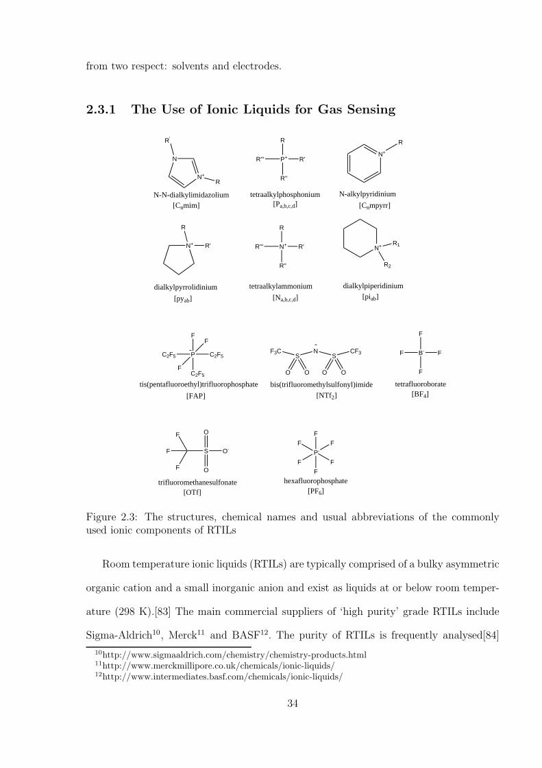
Figure 2.3: The structures, chemical names and usual abbreviations of the commonlyused ionic components of RTILs
Room temperature ionic liquids (RTILs) are typically comprised of a bulky asymmetric
organic cation and a small inorganic anion and exist as liquids at or below room temper-
ature (298 K).[83] The main commercial suppliers of ‘high purity’ grade RTILs include
Sigma-Aldrich10, Merck11 and BASF12. The purity of RTILs is frequently analysed[84]
10http://www.sigmaaldrich.com/chemistry/chemistry-products.html11http://www.merckmillipore.co.uk/chemicals/ionic-liquids/12http://www.intermediates.basf.com/chemicals/ionic-liquids/
34
using electrochemical techniques[76, 83, 85], high-performance liquid chromatography[86–
88] and X-ray photo-electron spectroscopy[89–91]. Figure 2.3 shows some commonly used
ionic cations and anions. The contrasting sizes of the ions result in poor coordination
and therefore at room temperature the materials are liquids rather than solids like NaCl.
RTILs have special properties which can offer an alternative to conventional solvents for
use in gas sensors. The following sections focus on the possible beneficial properties of
RTILs and their applications in gas detection.
Wide Electrochemical Windows
The width of the electrochemical window of a system is determined by the oxidation and
reduction potential of the supporting electrolytes or the solvents. Wider electrochem-
ical windows allow a greater range of molecules to be detected without masking from
background currents. Water has a electrochemical window of 2.4 V and acetonitrile of 5
V. However, the oxidation or reduction potentials of the constituent ions are impossible
to measure accurately as the commonly used reference electrodes in RTILs are Ag or Pt
pseudo reference electrodes which may cause potential drifts (around 5 mV). To overcome
this issue, either a stable Ag/AgNTf2 external reference electrode is made[92] or an inter-
nal reference probe, normally ferrocene(Fc) or ferrocene derivatives, is dissolved in RTILs.
The latter is commonly adopted for simplicity. The electrochemical windows are defined
as the potential corresponding to a current density13 of 1 mA cm−2. A low current density
is deliberately chosen since only small current is used in gas detection.[43, 45, 93, 94] A
number of reports indicate that the oxidation and reduction potentials of ionic liquids are
electrode material dependent[95–98]. The material dependence of electrochemical window
was studied by Zhang and Bond at Au, glassy carbon (GC) and Pt working electrodes in
[C4mim][BF4]. The magnitude of the electrochemical reduction window adhered to the
13Assuming macro-electrode behaviour (note that current density scales with the radius, not area, ofmicro-electrode)
35
electrode material sequence of Au ≈ GC > Pt while the oxidation window magnitude
followed the order Au > GC ≈ Pt.
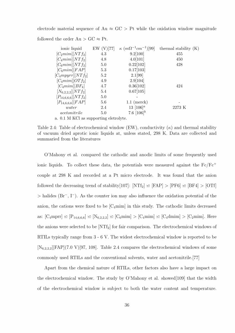
ionic liquid EW (V)[77] κ (mΩ−1cm−1)[99] thermal stability (K)[C2mim][NTf2] 4.3 9.2[100] 455[C4mim][NTf2] 4.8 4.0[101] 450[C6mim][NTf2] 5.0 0.22[102] 428[C6mim][FAP ] 5.3 0.17[103]
[C4mpyrr][NTf2] 5.2 2.1[99][C4mim][OTf2] 4.9 2.9[104][C4mim][BF4] 4.7 0.36[102] 424[N6,2,2,2][NTf2] 5.4 0.67[105][P14,6,6,6][NTf2] 5.0 -[P14,6,6,6][FAP ] 5.6 1.1 (merck) -
water 2.4 13 [106]a 2273 Kacetonitrile 5.0 7.6 [106]b
a. 0.1 M KCl as supporting eletrolyte.
Table 2.4: Table of electrochemical window (EW), conductivity (κ) and thermal stabilityof vacuum dried aprotic ionic liquids at, unless stated, 298 K. Data are collected andsummaried from the literatures
O’Mahony et al. compared the cathodic and anodic limits of some frequently used
ionic liquids. To collect these data, the potentials were measured against the Fc/Fc+
couple at 298 K and recorded at a Pt micro electrode. It was found that the anion
followed the decreasing trend of stability[107]: [NTf2] ⋍ [FAP] > [PF6] ⋍ [BF4] > [OTf]
> halides (Br−, I−). As the counter ion may also influence the oxidation potential of the
anion, the cations were fixed to be [C4mim] in this study. The cathodic limits decreased
as: [C4mprr] ⋍ [P14,6,6,6] ⋍ [N6,2,2,2] ⋍ [C6mim] > [C4mim] ⋍ [C4dmim] > [C2mim]. Here
the anions were selected to be [NTf2] for fair comparison. The electrochemical windows of
RTILs typically range from 3 - 6 V. The widest electrochemical window is reported to be
[N6,2,2,2][FAP](7.0 V)[97, 108]. Table 2.4 compares the electrochemical windows of some
commonly used RTILs and the conventional solvents, water and acetonitrile.[77]
Apart from the chemical nature of RTILs, other factors also have a large impact on
the electrochemical window. The study by O’Mahony et al. showed[109] that the width
of the electrochemical window is subject to both the water content and temperature.
36
It was found that electrochemical window decreased in the following order of ionic liq-
uid conditions: vacuum-dried > atmospheric > wet and 298 K > 318 K > 338 K. The
temperature effect is because the electron transfer rate constant increases with the tem-
perature. Hydrophobic RTILs may show less dependence on the width of electrochemical
windows when exposed to atmospheric moisture as they uptake less water as compared
to hydrophilic RTILs.[110] It was found by O’Mahony that the anion in particular affects
the level of water uptake.[107] The hydrophobicity of the anions showed the following
trend:[FAP] > [NTf2] > [PF6] > [BF4] > halides. As for cations, long carbon chains
enhance water repulsion in the solvent due to reduced polarity.[111]
Inherent Conductivity
Inherent conductivity is another important property of RTILs. It can be easily appre-
ciated since RTILs are purely composed of ions. For RTILs, the extent of conductivity
depends on the mobility of the ions composing the RTILs. The conductivity of RTILs
near 298 K normally lies in the range of 0.12 - 8 mΩ−1cm−1 which is comparable to
organic solvents containing 0.1 M tetra-n-butylammonium perchlorate (TBAP) as sup-
porting electrolyte where the values are within the range of 0.5 - 8 mΩ−1cm−1. Table
2.4 lists the conductivities of RTILs, water (0.1 M KCl as supporting electrolyte) and
acetonitrile (0.1 M TBAP as supporting electrolyte).
The large range of conductivities of RTILs reflects their structural differences. Bulky
constituent ions usually show slower movement. This is exemplified by comparing the con-
ductivity of [C2mim][NTf2], 9.2 mΩ−1cm−1, and [C6mim][NTf2], 0.22 mΩ−1cm−1. Here
an order of magnitude drop is measured when the alkyl substituted group in the imida-
zolium changes from an ethyl to a hexyl group. Another cause of a decrease in mobility,
hence conductivity, may be hydrogen bond formation.[112] The protic RTILs composed
of fluoro- (F) or oxyl- (O) substituted anions generally show low conductivity ranging
37
from 0.14 to 1.3 mΩ−1cm−1[98]. For the similar sized aprotic RTILs, the conductivities
are above 4 mΩ−1cm−1, except [[C4mim][BF4], where there may be some hydrogen bonds
due to [BF4].
The conductivity can also be changed due to the external environment. Influential
factors include temperature and the presence of additives. The variation of RTILs con-
ductivity with temperature follows the Vogel-Tammann-Fulcher(VTF) relationship with
an empirical equation[113] being
κ = AT− 12 exp[−B(T − T0)] (2.2)
From 258 K to 298 K, the conductivity of [C2mim][NTf2] increases from 1.5 to 9.2
mΩ−1cm−1.[114] The higher conductivity at increased temperature reflects the increased
mobility of the ions of RTILs. It was found that the addition of acetonitrile boosts the
conductivity of imidazolium based RTILs where the conductivity of RTILs increases by
more than 50 times with addition of just 15 % acetonitrile.[115] Similar observations were
made with other co-solvents.[116–119] The use of organic co-solvent aims to decrease the
solvent viscosity and hence to increase conductivity.
Low Volatility
The volatility of a solvent is measured by its vapour pressure. The pressure is measured
when the gas phase of the solvent is in equilibrium with its liquid phase. This property
reflects the applicability of a solvent under extreme conditions, notably high tempera-
ture and low pressure. High vapour pressure indicates the likelihood of solvent losses
under extreme environmental conditions. Compared to almost all conventional solvents,
RTILs have much lower volatility. This is evidenced by its capability for use in X-ray
Photo-electron Spectroscopy(XPS).[120] XPS is generally not applicable to liquids since
it employs ultra high vacuum (UHV) where conventional solvents evaporate. However
38
XPS is now regularly used to characterise RTILs.[121–126] The vapour pressure of pure
water[127, 128] at 298 K is 3167.73 Pa whereas that of most ionic liquids is few mPa at
298 K[129]. This significant difference reflects the much stronger inter-molecular (ionic)
forces in RTILs.
High Thermal Stability
The suitability of RTILs as solvents in gas sensing depends on the range of possible op-
eration temperatures which is defined mostly by the melting point and decomposition
temperature. Note, however, that a RTIL may also evaporate below its decomposition
temperature. Maton et al.[130] thoroughly reviewed the factors that may affect the ther-
mal stabilities, decomposition mechanisms and tools to analyse thermal decomposition
for many RTILs.
As compared to conventional solvents, RTILs often exhibit high thermal stability. This
is evidenced by the fact that RTILs remain as liquids over a large temperature range. For
example, [C4mim][NTf2] is liquid between 184 and 723 K as compared to the range of 273
K to 373 K for water at 1 atm.
The high thermal stability of RTILs is ascribed to their stable component organic
and inorganic ion structures. Decomposition of RTILs follows various mechanisms[131,
132], including nucleophilic substitution (SN1 and SN2)[133], thermal rearrangement[134],
alkene formation and dealkylation[129].
RTILs containing halides experience relatively low thermal stability as halides are
good nucleophiles and in IL media, strongly basic in nature. It is possible for halides to
react with the cations, leading to alkyl chain cleavage, at temperatures as low as 373 K.
The thermal stability of RTILs decreases with increasing nucleophilicity of the constituent
anion.
Stable products resulting from decomposition encourage thermal decomposition at
39
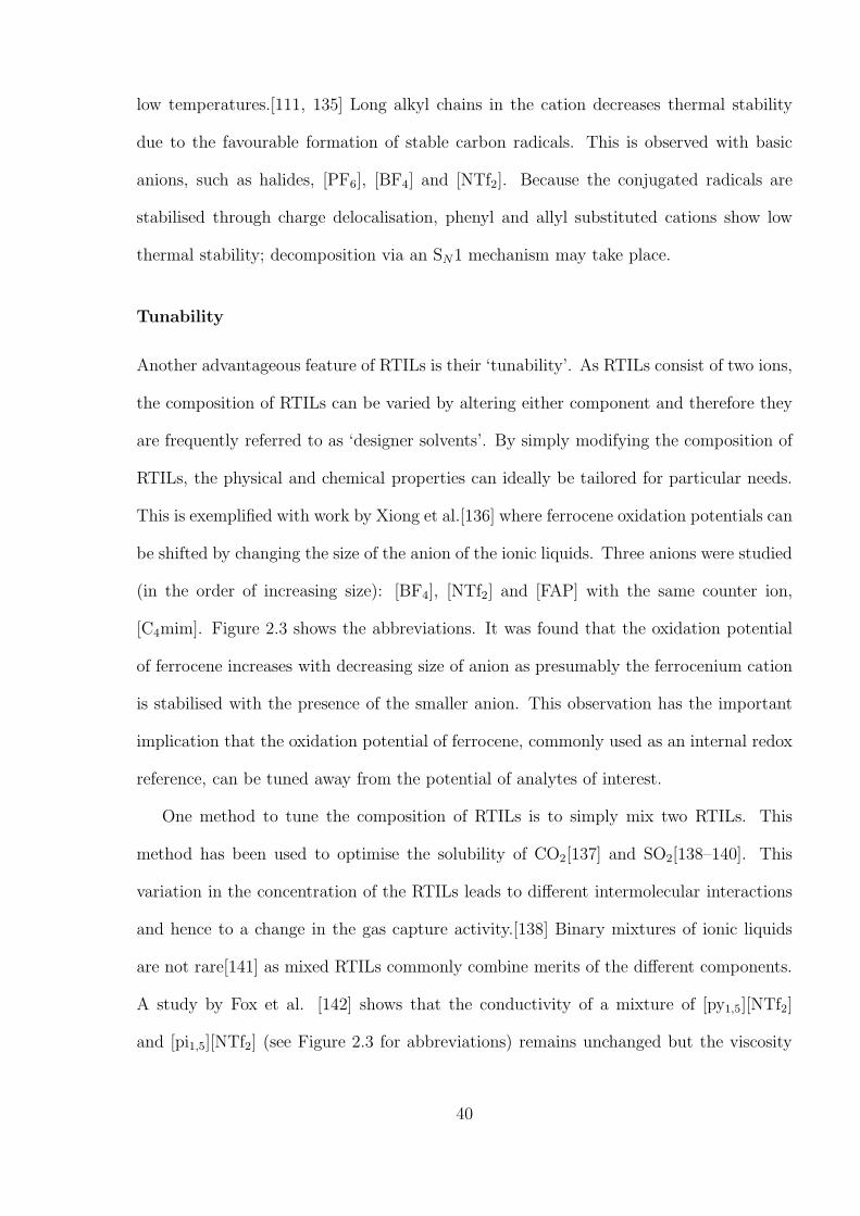
low temperatures.[111, 135] Long alkyl chains in the cation decreases thermal stability
due to the favourable formation of stable carbon radicals. This is observed with basic
anions, such as halides, [PF6], [BF4] and [NTf2]. Because the conjugated radicals are
stabilised through charge delocalisation, phenyl and allyl substituted cations show low
thermal stability; decomposition via an SN1 mechanism may take place.
Tunability
Another advantageous feature of RTILs is their ‘tunability’. As RTILs consist of two ions,
the composition of RTILs can be varied by altering either component and therefore they
are frequently referred to as ‘designer solvents’. By simply modifying the composition of
RTILs, the physical and chemical properties can ideally be tailored for particular needs.
This is exemplified with work by Xiong et al.[136] where ferrocene oxidation potentials can
be shifted by changing the size of the anion of the ionic liquids. Three anions were studied
(in the order of increasing size): [BF4], [NTf2] and [FAP] with the same counter ion,
[C4mim]. Figure 2.3 shows the abbreviations. It was found that the oxidation potential
of ferrocene increases with decreasing size of anion as presumably the ferrocenium cation
is stabilised with the presence of the smaller anion. This observation has the important
implication that the oxidation potential of ferrocene, commonly used as an internal redox
reference, can be tuned away from the potential of analytes of interest.
One method to tune the composition of RTILs is to simply mix two RTILs. This
method has been used to optimise the solubility of CO2[137] and SO2[138–140]. This
variation in the concentration of the RTILs leads to different intermolecular interactions
and hence to a change in the gas capture activity.[138] Binary mixtures of ionic liquids
are not rare[141] as mixed RTILs commonly combine merits of the different components.
A study by Fox et al. [142] shows that the conductivity of a mixture of [py1,5][NTf2]
and [pi1,5][NTf2] (see Figure 2.3 for abbreviations) remains unchanged but the viscosity
40
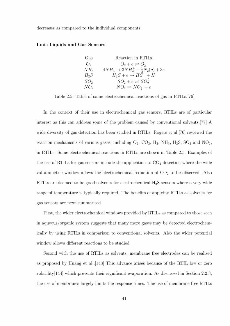
decreases as compared to the individual components.
Ionic Liquids and Gas Sensors
Gas Reaction in RTILs
O2 O2 + e O−2
NH3 4NH3 → 3NH+4 + 1
2N2(g) + 3e
H2S H2S + e → HS− +H˙
SO2 SO2 + e SO−2
NO2 NO2 NO+2 + e
Table 2.5: Table of some electrochemical reactions of gas in RTILs.[76]
In the context of their use in electrochemical gas sensors, RTILs are of particular
interest as this can address some of the problem caused by conventional solvents.[77] A
wide diversity of gas detection has been studied in RTILs. Rogers et al.[76] reviewed the
reaction mechanisms of various gases, including O2, CO2, H2, NH3, H2S, SO2 and NO2,
in RTILs. Some electrochemical reactions in RTILs are shown in Table 2.5. Examples of
the use of RTILs for gas sensors include the application to CO2 detection where the wide
voltammetric window allows the electrochemical reduction of CO2 to be observed. Also
RTILs are deemed to be good solvents for electrochemical H2S sensors where a very wide
range of temperature is typically required. The benefits of applying RTILs as solvents for
gas sensors are next summarised.
First, the wider electrochemical windows provided by RTILs as compared to those seen
in aqueous/organic system suggests that many more gases may be detected electrochem-
ically by using RTILs in comparison to conventional solvents. Also the wider potential
window allows different reactions to be studied.
Second with the use of RTILs as solvents, membrane free electrodes can be realised
as proposed by Huang et al..[143] This advance arises because of the RTIL low or zero
volatility[144] which prevents their significant evaporation. As discussed in Section 2.2.3,
the use of membranes largely limits the response times. The use of membrane free RTILs
41
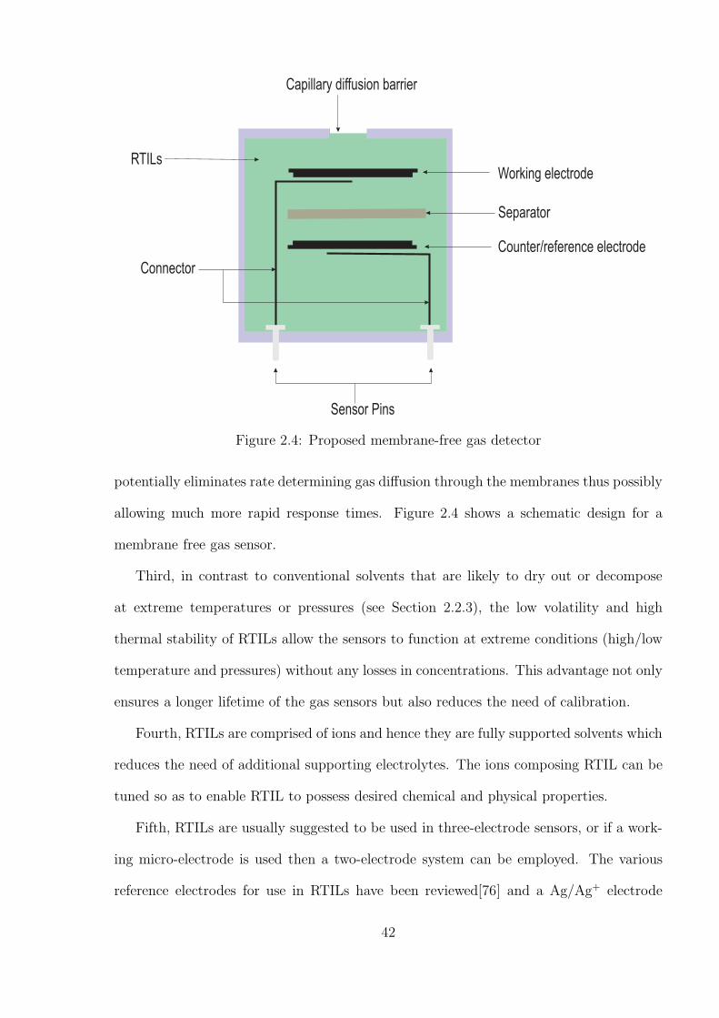
RTILs
Connector
Working electrode
Counter/reference electrode
Capillary diffusion barrier
Separator
Sensor Pins
Figure 2.4: Proposed membrane-free gas detector
potentially eliminates rate determining gas diffusion through the membranes thus possibly
allowing much more rapid response times. Figure 2.4 shows a schematic design for a
membrane free gas sensor.
Third, in contrast to conventional solvents that are likely to dry out or decompose
at extreme temperatures or pressures (see Section 2.2.3), the low volatility and high
thermal stability of RTILs allow the sensors to function at extreme conditions (high/low
temperature and pressures) without any losses in concentrations. This advantage not only
ensures a longer lifetime of the gas sensors but also reduces the need of calibration.
Fourth, RTILs are comprised of ions and hence they are fully supported solvents which
reduces the need of additional supporting electrolytes. The ions composing RTIL can be
tuned so as to enable RTIL to possess desired chemical and physical properties.
Fifth, RTILs are usually suggested to be used in three-electrode sensors, or if a work-
ing micro-electrode is used then a two-electrode system can be employed. The various
reference electrodes for use in RTILs have been reviewed[76] and a Ag/Ag+ electrode
42
developed by Meng et al.[92]. However ferrocene and its derivatives are often used as
internal redox references. Ferrocene itself has a significant volatility in RTILs solvents
so analytes such as decamethylferrocene has been proposed. The tuneability of RTILs
solvents has the benefit that the reference signal can be shifted away from the target
analyte if necessary.[145] RTIL solvents often show ohmic resistance approximating to
those seen for organic solvents in electrochemistry and as such are best studied using
micro-electrodes as working electrodes. These are discussed in the next section.
2.3.2 The Use of Micro-electrodes for Gas Sensing
A micro-electrode is defined as having at least one dimension on the micro-scale (10 to 100
µm). Due to the relatively low conductivity and high viscosity of RTILs as compared to
conventional solutions, micro-electrodes are widely employed to compensate these unde-
sired features. This is because micro-electrodes demonstrate higher mass transport rates,
better signal-to-noise ratios and lower uncompensated resistances than macro-electrodes.
These properties are detailed as below.
The diffusional regime (convergent or linear) is determined by the size of the electrode
radius, r, relative to the diffusion layer thickness, d (see Equation 1.18).[50] Within the
experimental time scale (in the regime of r << d), convergent diffusion dominates at a
micro-disc electrode as the electro-active materials are driven not only onto the electrode
surface but also to the edge of the electrode[146]. A macro-electrode, on the other hand,
experiences less effective linear diffusion (as r >> d).
Here, D is the diffusion coefficient and t is the experimental time. Convergent diffusion
dominates when r << d and linear diffusion occurs when r >> d.
The use of micro-electrodes improves the signal-to-noise ratio since noise is propor-
tional to the active electrode surface area whilst the signal depends on the total size of the
diffusional field.[50, 147] A better signal-to-noise ratio leads a lower detection limit.[73]
43
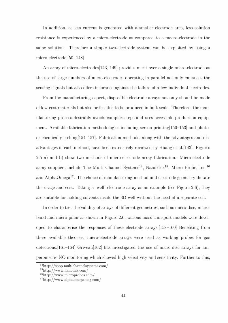
In addition, as less current is generated with a smaller electrode area, less solution
resistance is experienced by a micro-electrode as compared to a macro-electrode in the
same solution. Therefore a simple two-electrode system can be exploited by using a
micro-electrode.[50, 148]
An array of micro-electrodes[143, 149] provides merit over a single micro-electrode as
the use of large numbers of micro-electrodes operating in parallel not only enhances the
sensing signals but also offers insurance against the failure of a few individual electrodes.
From the manufacturing aspect, disposable electrode arrays not only should be made
of low-cost materials but also be feasible to be produced in bulk scale. Therefore, the man-
ufacturing process desirably avoids complex steps and uses accessible production equip-
ment. Available fabrication methodologies including screen printing[150–153] and photo-
or chemically etching[154–157]. Fabrication methods, along with the advantages and dis-
advantages of each method, have been extensively reviewed by Huang et al.[143]. Figures
2.5 a) and b) show two methods of micro-electrode array fabrication. Micro-electrode
array suppliers include The Multi Channel Systems14, NanoFlex15, Micro Probe, Inc.16
and AlphaOmega17. The choice of manufacturing method and electrode geometry dictate
the usage and cost. Taking a ‘well’ electrode array as an example (see Figure 2.6), they
are suitable for holding solvents inside the 3D well without the need of a separate cell.
In order to test the validity of arrays of different geometries, such as micro-disc, micro-
band and micro-pillar as shown in Figure 2.6, various mass transport models were devel-
oped to characterise the responses of these electrode arrays.[158–160] Benefiting from
these available theories, micro-electrode arrays were used as working probes for gas
detections.[161–164] Griveau[162] has investigated the use of micro-disc arrays for am-
perometric NO monitoring which showed high selectivity and sensitivity. Further to this,
14http://shop.multichannelsystems.com/15http://www.nanoflex.com/16http://www.microprobes.com/17http://www.alphaomega-eng.com/
44
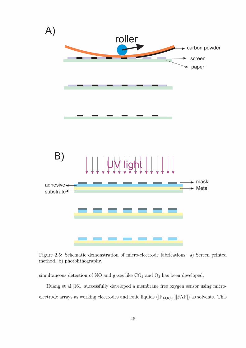
A)
B)
screen
carbon powder
roller
paper
UV light
mask
Metaladhesive
substrate
Figure 2.5: Schematic demonstration of micro-electrode fabrications. a) Screen printedmethod. b) photolithography.
simultaneous detection of NO and gases like CO2 and O2 has been developed.
Huang et al.[161] successfully developed a membrane free oxygen sensor using micro-
electrode arrays as working electrodes and ionic liquids ([P14,6,6,6][FAP]) as solvents. This
45
a) b)
c)
Figure 2.6: Different types of microarrays. a)A micro-disc electrode array. b)a micro-pillarelectrode array. c)a micro-band array (’well’ electrode array).
oxygen sensing system showed high sensitivity and most importantly, was freed from the
problem caused by the use of membranes, especially frequent calibration.
2.4 Towards Intelligent Sensors
This section discusses some influential factors in the accurate measurement of gas con-
centration including the amperometric sensing techniques and environmental influences.
46
2.4.1 Micro-disc Electrode Chronoamperometry: Shoup and Sz-
abo Analysis
Traditionally, the current generated by sensing (electrochemical) processes is used to re-
flect the concentrations of gas. However the current is not only dependent on concentra-
tion but also is a function of the number of electrons transferred during the electrochemical
process and the diffusion coefficient of target molecules. An error in determining gas con-
centration may result from the change of any of these variables. This is not rare due to the
fact that diffusion coefficients are sensitive to both temperature and humidity changes.
Hence a method that allows simultaneous determination of concentrations and diffusion
coefficients is advocated - specifically chronoamperometry has been used for this propose.
In chronoamperometry, the potential steps from a potential where no current passes to a
potential where the reaction of interest fully occurs in a diffusional controlled way. The
current is recorded as a function of time. At the short time, the current response at a
planar disc electrode follows Cottrellian behaviour (see Equation 1.20 in Chapter 1).
Whilst the current decays to zero for a macro-electrode, at longer time, a steady state
current is seen at a micro-disc electrode(See Equation 1.30 in Chapter 1).
where r is the electrode radius and all other terms are defined as above. It is evident
that at long time, current is a function of ncD12 and at short time current is a product of
ncD. Thus the parameters nc and D can be measured simultaneously through combining
the current at short and long times.
Several models [165–168] have been proposed for simulating the current-time behaviour
of chronoamperometry at micro-disc electrodes. Shoup and Szabo analysis is the most
frequently used which describes chronoamperometric responses over all time values within
an error of 0.5 % [167] (see Equation 4.1 in Chapter 4).
This equation is readily imported in data analysis software, such as Origin. Typically
the value of electrode radius, r, is fixed as known and the software then automatically
47
implements a the fitting procedure. The values of c and D are iterated until the best fit
(least difference between simulated and experimental current responses) is achieved.
Despite of the simple operation of this technique, the values of nc and D resulted from
the Shoup and Szabo analysis at different transient times can be different[169]. This is
because the Cottrellian current scales with cD12 and the steady state current is a function
of cD (for n = 1). At too short measured times, capacitative non-Faradaic currents lead to
large error whilst at long times the steady state signal dominates and many pairs of c and
D gives same steady state current. Hence, accurate values of c and D are only possible
when a ‘good’ balance between the Cottrellian current and the steady state current is
measured.
Chapter 4 investigates the optimisation of transient times for Shoup and Szabo anal-
ysis, exemplified by two systems, in order to achieve accurate results of gas systems.
2.4.2 Temperature and Humidity
Since the values of nc and D can be achieved accurately using chronoamperometry along
with Shoup and Szabo analysis, it is essential to consider other external factors on the
sensing accuracy. Due to the fact that an electrochemical gas sensor relies on the elec-
tron transfer process which is always highly sensitive to temperature and sometimes to
humidity changes, the sensing accuracy is influenced by the change of environment. The
affected parameters include the number of electron transfer, the concentration and the
diffusion coefficient of solutes. How the environment plays part in these parameters is
discussed below.
The following equilibrium is considered when a gaseous molecule is dissolved in a
solution
A(g) A(dis) (2.3)
48
where A(g) is the analyte A in gas phase and A(dis) is dissolved A. Gas solubility and
temperature normally exhibit a negative correlation[170] in ionic liquids as the Equilib-
rium 2.3 shifts to the gaseous phase at higher temperature. However this depends on the
gases and solvents studied. CO2 in [C4mim][Ac] is one of the exceptional cases, where
a possible chemical step is involved during CO2 dissolution[171, 172]. The correlation
between dissolved gas concentrations and temperature are determined by the Van’t Hoff
equation.
∂lnKeq
∂T=
∆H
RT 2(2.4)
where Keq is the equilibrium constant, ∆H is the standard enthalpy change and all other
terms are defined as above.
The diffusion coefficient of a solute in ionic liquids generally increases with tempera-
ture. This correlation can often be predicted by the Arrhenius equation:
D = D0e−EA/(RT ) (2.5)
Here, D is the diffusion coefficient and EA is the energy of activation and all other terms
are defined as before.
The influence of humidity on the solubility is due to the solubility difference as water
content of the ionic liquid changes. For example, for the pure solvents, the saturated
solubility of oxygen in water is 1.2 mM and in [P14,6,6,6][NTf2] is 7.5 mM. The solubility
of humidified oxygen in [P14,6,6,6][NTf2] ranges between these limits.[173]
The diffusion coefficient of a gas is affected by change of humidity for similar reasons.
Dissolved molecules are normally more mobile in water as compared to that in ionic
liquids. Hence humidified oxygen shows a higher diffusion coefficient than dry oxygen in
ionic liquids[173]
49
One solution to the problem caused by changed temperature and humidity is to keep
the detection system under a restrictedly stable environment where the temperature is
thermostatted and gases are pre-dried before experiment. However this is not realistic
outside of the laboratory in sensor applications. A more practical approach is to measure
the temperature and humidity of the sensing environment and correct the sensor mea-
surements accordingly. An independent temperature and humidity sensor is potentially
implantable in gas sensing systems for monitoring the change of experimental conditions.
Commercially a solid state independent temperature and humidity sensor is used to mea-
sure the temperature and humidity in sensing solutions.[174] However an external probe
may be remote from the sensing system, leading to a decreased sensitivity of temperature
and humidity measurement.
A built-in voltammetric temperature sensor incorporated into an amperometric oxygen
sensor and a simultaneous temperature and humidity detector are shown in Chapter 6
and Chapter 7 respectively.
The reaction mechanism of dissolved molecules in ionic liquids may change with hu-
midity. This is because dry protic ionic liquids are free from protons whereas water is a
good source of protons. For example, the mechanism of dissolved oxygen (in ionic liquid)
in the presence of moisture can vary from 1 and 4 electrons transferred[93, 175]. Note
that the number of electron transferred also depends on the electrode materials. The
mechanism undergone at different humidity is unpredictable thus resulting in difficult
and inaccurate measurements.
In particular the Shoup and Szabo micro-disc electrode analysis advocated above as-
sumes that the number, n, of electrons transferred is known and constant. Then c and
D are functions of humidity and temperature which can be calculated through the simul-
taneous humidity and temperature sensor. However this approach is not applicable for
mechanisms involving a slow chemical step. Taking an ECE mechanism (see Reaction
50
2.6 to 2.8) as an example, the number of electrons determined by chronoamperometry
can vary between 1 and 2 depending on the rate of Reaction 2.8. This may be moisture
sensitive and will certainly be temperature dependent.
A+ e −→ A− (2.6)
A− −→ B (2.7)
B + e −→ B− (2.8)
An alternative approach to control the reaction at a known electron transfer stage is
shown in Chapter 8.
2.5 Aim of the Thesis
This thesis aims at addressing the issues of current generation gas sensors, further develop-
ing intelligent gas sensors. The intelligent gas sensing systems will realise self-calibration
against change of the sensing environment, such as humidity and temperature. Accu-
rate measurement of gas concentration can therefore be achieved. This thesis also seeks
the fabrication of low cost electrodes and investigates their suitability in electrochemical
experiments.
References
[1] Xiong, L.; Compton, R. G. Interntional Journal of Electrochemical Science 2014,9, 7152–7181.
[2] Gutmacher, D.; Foelmli, C.; Vollenweider, W.; Hoefer, U.; Wllenstein, J. ProcediaEngineering 2011, 25, 1121 – 1124.
[3] Srivastava, S. C.; Jaiswal, R. J.; Sinha, S.; Singh, R. V. K.; Das, R. N. Journal ofMines, Metals and Fuels 1987, 35, 384–385.
[4] Sinha, A. K.; Rajwar, D. P.; Ghosh, A. K. Journal of Mines, Metals and Fuels1987, 35, 365–367.
51
[5] Barnes, S.; Old, L. T. Chemical Engineering Progress 2009, 105, 51–56.
[6] Arasaradnam, R. P.; Covington, J. A.; Harmston, C.; Nwokolo, C. U. AlimentaryPharmacology and Therapeutics 2014, 39, 780–789.
[7] Buszewski, B.; Grzywinski, D.; Ligor, T.; Stacewicz, T.; Bielecki, Z.; Wojtas, J.Bioanalysis 2013, 5, 2287–2306.
[8] Biniecka, M.; Caroli, S. TrAC - Trends in Analytical Chemistry 2011, 30, 1756–1770.
[9] Angerosa, F. European Journal of Lipid Science and Technology 2002, 104, 639–660.
[10] Dorresteijn, R. C.; De Gooijer, C. D.; Tramper, J.; Beuvery, E. C. Biotechnologyand Bioengineering 1994, 43, 149–154.
[11] Wolfbeis, O. Analytical Chemistry 2002, 74, 2663–2677.
[12] Lu, X.; Winnik, M. Chemistry of Materials 2001, 13, 3449–3463.
[13] Demas, J. N.; DeGraff, B. A.; Coleman, P. B. Analytical Chemistry 1999, 71,793A–800A.
[14] Cheung, M. C.; Yung, K. Y.; Xu, H.; Kraut, N. D.; Liu, K.; Chodavarapu, V. P.;Cartwright, A. N.; Bright, F. V. IEEE Journal on Selected Topics in QuantumElectronics 2012, 18, 1147–1159.
[15] Chu, C.-S.; Lo, Y.-L.; Sung, T.-W. Photonic Sensors 2011, 1, 234–250.
[16] Rees, N. V.; Compton, R. G. Energy and Environmental Science 2011, 4, 403–408.
[17] Korotcenkov, G.; Han, S. D.; Stetter, J. R. Chemical Reviews 2009, 109, 1402–1433.
[18] Rahman, M.; Kumar, P.; Park, D.-S.; Shim, Y.-B. Sensors 2008, 8, 118–141.
[19] Stetter, J. R.; Li, J. Chemical Reviews 2008, 108, 352–366.
[20] Knake, R.; Jacquinot, P.; Hodgson, A. W. E.; Hauser, P. C. Analytica Chimica Acta2005, 549, 1 – 9.
[21] Suresh, M.; Vasa, N. J.; Agarwal, V.; Chandapillai, J. Sensors and Actuators, B:Chemical 2014, 195, 44–51.
[22] Hori, H.; Ishimatsu, S.; Fueta, Y.; Hinoue, M.; Ishidao, T. Journal of UOEH 2013,34, 363–368.
[23] Yin, C.; Liu, S.; Li, Y.; Chen, X. Applied Mechanics and Materials 2013, 336-338,244–247.
[24] Chiorino, A.; Ghiotti, G.; Prinetto, F.; Carotta, M. C.; Gnani, D.; Martinelli, G.Sensors and Actuators, B: Chemical 1999, 58, 338–349.
[25] Golinelli, E.; Musazzi, S.; Perini, U.; Barberis, F. Lecture Notes in Electrical Engi-neering 2014, 268, 19–22.
[26] Dong, L.; Ma, W.; Zhang, L.; Yin, W.; Jia, S. Guangxue Xuebao/Acta Optica Sinica2014, 34, Article number 0130002.
52
[27] Qiao, J.-P.; Qin, J.-M.; Yan, X.-Y.; Zhang, Z.-X. Journal of Optoelectronics Laser2014, 25, 217–221.
[28] Li, C.; Shi, G. Journal of Photochemistry and Photobiology C: Photochemistry Re-views 2014, 19, 20–34.
[29] Kitiyanan, B.; Alvarez, W. E.; Harwell, J. H.; Resasco, D. E. Chemical PhysicsLetters 2000, 317, 497–503.
[30] Zhu, Q.; Aller, R. Marine Chemistry 2013, 157, 49–58.
[31] Jackson, R.; Oda, R. P.; Bhandari, R. K.; Mahon, S. B.; Brenner, M.; Rock-wood, G. A.; Logue, B. A. Analytical Chemistry 2014, 86, 1845–1852.
[32] Zakrzewska, K. Thin Solid Films 2001, 391, 229–238.
[33] Vijayalakshmi, K.; Renitta, A.; Karthick, K. Ceramics International 2014, 40,6171–6177.
[34] Gaman, V. I.; Sevast’yanov, Y. Y.; Maksimova, N. K.; Almaev, A. V.; Serge-ichenko, N. S. Russian Physics Journal 2014, 56, pp 1427–1434.
[35] Patil, J. Y.; Nadargi, D. Y.; Gurav, J. L.; Mulla, I. S.; Suryavanshi, S. S. MaterialsLetters 2014, 124, 144–147.
[36] Qi, Q.; Wang, P.-P.; Zhao, J.; Feng, L.-L.; Zhou, L.-J.; Xuan, R.-F.; Liu, Y.-P.;Li, G.-D. Sensors and Actuators, B: Chemical 2014, 194, 440–446.
[37] Kaci, S.; Keffous, A.; Hakoum, S.; Trari, M.; Mansri, O.; Menari, H. Applied SurfaceScience 2014, in press.
[38] Carotta, M. C.; Fioravanti, A.; Gherardi, S.; Malagu, C.; Sacerdoti, M.; Ghiotti, G.;Morandi, S. Sensors and Actuators, B: Chemical 2014, 194, 195–205.
[39] Gu, J.; Zhang, Y.; Jiang, J.; Li, S. Chinese Journal of Scientific Instrument 2014,35, 350–359.
[40] Darmastuti, Z.; Bur, C.; Mller, P.; Rahlin, R.; Lindqvist, N.; Andersson, M.;Schtze, A.; Spetz, A. Sensors and Actuators, B: Chemical 2014, 194, 511–520.
[41] Somov, A.; Baranov, A.; Spirjakin, D. Sensors and Actuators A: Physical 2014,210, 157 – 164.
[42] Karpova, E.; Mironov, S.; Suchkov, A.; Karelin, A.; Karpov, E.; Karpov, E. Sensorsand Actuators, B: Chemical 2014, 197, 358–363.
[43] Xiong, L.; Batchelor-McAuley, C.; Goncalves, L. M.; Rodrigues, J. A.; Comp-ton, R. G. Biosensors and Bioelectronics 2011, 26, 4198–4203.
[44] Husson-Borg, P.; Majer, V.; Costa Gomes, M. Journal of Chemical and EngineeringData 2003, 48, 480–485.
[45] Evans, R. G.; Klymenko, O. V.; Saddoughi, S. A.; Hardacre, C.; Compton, R. G.Journal of Physical Chemistry B 2004, 108, 7878–7886.
[46] Chen, W.-C.; Hsu, Y.-L.; Venkatesan, S.; Zen, J.-M. Electroanalysis 2014, 26, 565–572.
53
[47] Lawrence, N. S.; Davis, J.; Marken, F.; Jiang, L.; Jones, T. G. J.; Davies, S. N.;Compton, R. G. Sensors and Actuators, B: Chemical 2000, 69, 189–192.
[48] Lawrence, N. S.; Jiang, L.; Jones, T. G. J.; Compton, R. G. Analytical Chemistry2003, 75, 2499–2503.
[49] Sekhar, P. K.; Subramaniyam, K. ECS Electrochemistry Letters 2014, 3, B1–B4.
[50] Compton, R. G.; Banks, C. E. Understanding Voltammetry ; Imperial College Press,2011, 2nd Edition.
[51] Maj-Zurawska, M.; Hulanicki, A. Chemia Analityczna 2009, 54, 1149–1167.
[52] Xie, X.; Bakker, E. Analytical Chemistry 2013, 85, 1332–1336.
[53] Severinghaus, J. W.; Bradley, A. F. Journal of applied physiology 1958, 13, 515–520.
[54] Caflisch, C. R.; Carter, N. W. Analytical Biochemistry 1974, 60, 252–257.
[55] Cai, W. J. Analytical Chemistry 1997, 69, 5052–5058.
[56] Beyenal, H.; Davis, C. C.; Lewandowski, Z. Sensors and Actuators, B: Chemical2004, 97, 202–210.
[57] Mowery, M. D. Analytical Chemistry 1999, 71, 201–204.
[58] Ben Youssef, I.; Alem, H.; Sarry, F.; Elmazria, O.; Jimenez Rioboo, R.; Arnal-Hrault, C.; Jonquires, A. Sensors and Actuators, B: Chemical 2013, 185, 309–320.
[59] Fraticelli, Y. M.; Meyerhoff, M. E. Analytical Chemistry 1981, 53, 992–997.
[60] Meyerhoff, M. E.; Fraticelli, Y. M.; Greenberg, J. A.; Rosen, J.; Parks, S. J.; Opdy-cke, W. N. Clinical Chemistry 1982, 28, 1973–1978.
[61] Arnold, M. A. Analytica Chimica Acta 1983, 154, 33 – 39.
[62] Clark Jr., L. C.; Wolk, R.; Granger, D.; Talor, Z. Journal of applied physiology1953, 6, 189–193.
[63] Compton, R. G.; Sanders, G. H. W. Electrode Potentials ; OCP Series; OUP Oxford,1996.
[64] Clark Jr., L. C.; Gollan, F.; Gupta, V. B. Science 1950, 111, 85–87.
[65] Danneel, H. L. Zeitschrift Elektrochemie 1897, 4, 227–242.
[66] Severinghaus, J. W.; Astrup, P. B. Journal of Clinical Monitoring 1986, 2, 125–139.
[67] Moseley, P.; Norris, J.; Williams, D. Techniques and mechanisms in gas sensing ;The Adam Hilger series on sensors; Adam Hilger, 1991.
[68] Goswami, A.; Cooper, R. Anaesthesia & Intensive Care Medicine 2011, 12, 568 –573.
[69] Cussler, E. L. Diffusion: Mass Transfer in Fluid Systems ; Cambridge series inchemical engineering; Cambridge University Press, 1997.
[70] Evans, N. T. S.; Quinton, T. H. Respiration Physiology 1978, 35, 89 – 99.
54
[71] Haug, A. T.; White, R. E. Journal of the Electrochemical Society 2000, 147, 980–983.
[72] Hahn, C. Analyst 1998, 123, 57R–86R.
[73] Wang, J. Analytical Electrochemistry ; Wiley, 2006.
[74] Do, J. S.; Chang, W. B. Sensors and Actuators B: Chemical 2001, 72, 101 – 107.
[75] Do, J.-S.; Shieh, R.-Y. Sensors and Actuators B: Chemical 1996, 37, 19 – 26.
[76] Rogers, E. I.; O’Mahony, A. M.; Aldous, L.; Compton, R. G. Amperometric gasdetection using room temperature ionic liquid solvents. 2010.
[77] Barrosse-Antle, L. E.; Bond, A. M.; Compton, R. G.; O’Mahony, A. M.;Rogers, E. I.; Silvester, D. S. Chemistry - An Asian Journal 2010, 5, 202–230.
[78] O’Mahony, A. M.; Compton, R. G. Electroanalysis 2010, 22, 2313–2322.
[79] Koschel, D.; Coxam, J.-Y.; Majer, V. Industrial and Engineering Chemistry Re-search 2007, 46, 1421–1430.
[80] Silvester, D. S.; Compton, R. G. Zeitschrift fur Physikalische Chemie 2006, 220,1247–1274.
[81] Najdeker, E.; Bishop, E. Journal of Electroanalytical Chemistry 1973, 41, 79–87.
[82] Ramasubramanian, N. Journal of Electroanalytical Chemistry 1975, 64, 21–37.
[83] Buzzeo, M. C.; Evans, R. G.; Compton, R. G. ChemPhysChem 2004, 5, 1106–1120.
[84] Stark, A.; Behrend, P.; Braun, O.; Muller, A.; Ranke, J.; Ondruschka, B.; Jas-torff, B. Green Chem. 2008, 10, 1152–1161.
[85] Schroder, U.; Wadhawan, J.; Compton, R. G.; Marken, F.; Suarez, P. A. Z.; Con-sorti, C. S.; De Souza, R. F.; Dupont, J. New Journal of Chemistry 2000, 24,1009–1015.
[86] Stepnowski, P.; Mller, A.; Behrend, P.; Ranke, J.; Hoffmann, J.; Jastorff, B. Journalof Chromatography A 2003, 993, 173–178.
[87] Stepnowski, P.; Nichthauser, J.; Mrozik, W.; Buszewski, B. Analytical and Bioana-lytical Chemistry 2006, 385, 1483–1491.
[88] Le Rouzo, G.; Lamouroux, C.; Bresson, C.; Guichard, A.; Moisy, P.; Moutiers, G.Journal of Chromatography A 2007, 1164, 139–144.
[89] Kim, K.-S.; Choi, S.; Demberelnyamba, D.; Lee, H.; Oh, J.; Lee, B.-B.; Mun, S.-J.Chemical Communications 2004, 10, 828–829.
[90] Forsyth, S.; Golding, J.; MacFarlane, D.; Forsyth, M. Electrochimica Acta 2001,46, 1753–1757.
[91] Matsumoto, H.; Kageyama, H.; Miyazaki, Y. Chemistry Letters 2001, 182–183.
[92] Meng, Y.; Aldous, L.; Belding, S.; Compton, R. Physical Chemistry ChemicalPhysics 2012, 14, 5222–5228.
55
[93] Buzzeo, M. C.; Klymenko, O. V.; Wadhawan, J. D.; Hardacre, C.; Seddon, K. R.;Compton, R. G. Journal of Physical Chemistry A 2003, 107, 8872–8878.
[94] Huang, X. J.; Rogers, E. I.; Hardacre, C.; Compton, R. G. The Journal of PhysicalChemistry B 2009, 113, 8953–8959.
[95] Rogers, E. I.; Sljukic, B.; Hardacre, C.; Compton, R. G. Journal of Chemical andEngineering Data 2009, 54, 2049–2053.
[96] Suarez, P.; Consorti, C.; De Souza, R.; Dupont, J.; Gonalves, R. Journal of theBrazilian Chemical Society 2002, 13, 106–109.
[97] Howlett, P. C.; Izgorodina, E. I.; Forsyth, M.; MacFarlane, D. R. Zeitschrift furPhysikalische Chemie 2006, 220, 1483–1498.
[98] Zhao, C.; Burrell, G.; Torriero, A.; Separovic, F.; Dunlop, N.; MacFarlane, D.;Bond, A. Journal of Physical Chemistry B 2008, 112, 6923–6936.
[99] Buzzeo, M. C.; Hardacre, C.; Compton, R. G. Analytical Chemistry 2004, 76,4583–4588.
[100] Hui, N.; MinQiang, H.; QingQing, M.; YuanHui, L.; DeZhong, Y.; BuXing, H.SCIENCE CHINA Chemistry 2012, 55, 1509.
[101] Vranes, M.; Dozic, S.; Djeric, V.; Gadzuric, S. Journal of Chemical & EngineeringData 2012, 57, 1072–1077.
[102] Hunger, J.; Stoppa, A.; Schrdle, S.; Hefter, G.; Buchner, R. ChemPhysChem 2009,10, 723–733.
[103] Li, J.-G.; Hu, Y.-F.; Ling, S.; Zhang, J.-Z. Journal of Chemical & Engineering Data2011, 56, 3068–3072.
[104] Zech, O.; Stoppa, A.; Buchner, R.; Kunz, W. Journal of Chemical & EngineeringData 2010, 55, 1774–1778.
[105] Sun, J.; Forsyth, M.; MacFarlane, D. R. The Journal of Physical Chemistry B 1998,102, 8858–8864.
[106] Lide, D. CRC Handbook of Chemistry and Physics, 85th Edition; CRC Handbookof Chemistry and Physics, 85th Ed; Taylor & Francis, 2004.
[107] O’Mahony, A. M.; Compton, R. G. Electroanalysis 2010, 22, 2313–2322.
[108] Ignat’ev, N.; Welz-Biermann, U.; Kucheryna, A.; Bissky, G.; Willner, H. Journal ofFluorine Chemistry 2005, 126, 1150–1159.
[109] O’Mahony, A. M.; Silvester, D. S.; Aldous, L.; Hardacre, C.; Compton, R. G. Journalof Chemical and Engineering Data 2008, 53, 2884–2891.
[110] Buzzeo, M. C.; Hardacre, C.; Compton, R. G. ChemPhysChem 2006, 7, 176–180.
[111] Clayden, J.; Greeves, N.; Warren, S. Organic Chemistry, 2nd edition; Oxford Uni-versity Press, 2012.
[112] Miran, M. S.; Kinoshita, H.; Yasuda, T.; Susan, M. A. B. H.; Watanabe, M. Chem-ical Communications 2011, 47, 12676–12678.
56
[113] McFarlane, D. R.; Sun, J.; Golding, J.; Meakin, P.; Forsyth, M. Electrochimica Acta2000, 45, 1271 – 1278.
[114] Schreiner, C.; Zugmann, S.; Hartl, R.; Gores, H. J. Journal of Chemical & Engi-neering Data 2010, 55, 1784–1788.
[115] Chaban, V. V.; Voroshylova, I. V.; Kalugin, O. N.; Prezhdo, O. V. Journal ofPhysical Chemistry B 2012, 116, 7719–7727.
[116] Wang, C.; Yan, P.; Xing, H.; Jin, C.; Xiao, J.-X. Journal of Chemical & EngineeringData 2010, 55, 1994–1999.
[117] Fitchett, B.; Knepp, T.; Conboy, J. Journal of the Electrochemical Society 2004,151, E219–E225.
[118] Beter-Roga, M.; Hunger, J.; Stoppa, A.; Buchner, R. Journal of Chemical andEngineering Data 2010, 55, 1799–1803.
[119] Stoppa, A.; Hunger, J.; Buchner, R. Journal of Chemical and Engineering Data2009, 54, 472–479.
[120] Silvester, D. S.; Broder, T. L.; Aldous, L.; Hardacre, C.; Crossley, A.; Comp-ton, R. G. The Analyst 2007, 132, 196–198.
[121] Caporali, S.; Bardi, U.; Lavacchi, A. Journal of Electron Spectroscopy and RelatedPhenomena 2006, 151, 4–8.
[122] Fortunato, R.; Afonso, C.; Benavente, J.; Rodriguez-Castelln, E.; Crespo, J. Journalof Membrane Science 2005, 256, 216–223.
[123] Gottfried, J.; Maier, F.; Rossa, J.; Gerhard, D.; Schulz, P.; Wasserscheid, P.; Stein-rck, H.-P. Zeitschrift fur Physikalische Chemie 2006, 220, 1439–1453.
[124] Hfft, O.; Bahr, S.; Himmerlich, M.; Krischok, S.; Schaefer, J. A.; Kempter, V.Langmuir 2006, 22, 7120–7123.
[125] Smith, E. F.; Rutten, F. J. M.; Villar-Garcia, I. J.; Briggs, D.; Licence, P. Langmuir2006, 22, 9386–9392.
[126] Smith, E. F.; Villar Garcia, I. J.; Briggs, D.; Licence, P. Chemical Communications2005, 5633–5635.
[127] Tunnell, G. World distribution of atmospheric water vapour pressure; Geophysicalmemoirs; H.M. Stationery Office, 1958.
[128] Nesmeianov, A. N. Vapor pressure of the chemical elements ; Elsevier Pub. Co.,1963.
[129] Chowdhury, A.; Thynell, S. T. Thermochimica Acta 2006, 443, 159 – 172.
[130] Maton, C.; De Vos, N.; Stevens, C. V. Chemical Society Reviews 2013, 42, 5963–5977.
[131] Pletcher, D.; of Chemistry (Great Britain), R. S. A First Course in Electrode Pro-cesses ; A First Course in Electrode Processes; Royal Society of Chemistry, 2009.
[132] Rieger, P. H. Electrochemistry ; Schaum’s Outlines; Springer Netherlands, 1994.
57
[133] Chan, B. K. M.; Chang, N.; Grimmett, M. R. Australian Journal of Chemistry1977, 9, 2005 – 2013.
[134] Dessiaterik, Y.; Baer, T.; Miller, R. E. Journal of Physical Chemistry A 2006, 110,1500–1505.
[135] Atkins, P.; De Paula, J. Atkins’ Physical Chemistry ; Macmillan Higher Education,2006.
[136] Xiong, L.; Fletcher, A. M.; Davies, S. G.; Norman, S. E.; Hardacre, C.; Comp-ton, R. G. Chemical Communications 2012, 48, 5784–5786.
[137] Wang, C.; Guo, Y.; Zhu, X.; Cui, G.; Li, H.; Dai, S. Chemical Communications2012, 48, 6526–6528.
[138] Cui, G.; Lin, W.; Ding, F.; Luo, X.; He, X.; Li, H.; Wang, C. Green Chemistry2014, 16, 1211–1216.
[139] Cui, G.; Zheng, J.; Luo, X.; Lin, W.; Ding, F.; Li, H.; Wang, C. Angewandte Chemie- International Edition 2013, 52, 10620–10624.
[140] Wang, C.; Cui, G.; Luo, X.; Xu, Y.; Li, H.; Dai, S. Journal of the American ChemicalSociety 2011, 133, 11916–11919.
[141] Brussel, M.; Brehm, M.; Pensado, A. S.; Malberg, F.; Ramzan, M.; Stark, A.;Kirchner, B. Phys. Chem. Chem. Phys. 2012, 14, 13204–13215.
[142] Fox, E. T.; Paillard, E.; Borodin, O.; Henderson, W. A. Journal of Physical Chem-istry C 2013, 117, 78–84.
[143] Huang, X.-J.; Aldous, L.; OMahony, A. M.; del Campo, F. J.; Compton, R. G.Analytical Chemistry 2010, 82, 5238–5245.
[144] Faridbod, F.; Mohammad Reza Ganjali, M. R.; Norouzi, P.; Riahi, S.; Rashedi, H.Application of Room Temperature Ionic Liquids in Electrochemical Sensors andBiosensors ; InTech, 2011.
[145] Xiong, L.; Batchelor-Mcauley, C.; Ward, K. R.; Downing, C.; Hartshorne, R. S.;Lawrence, N. S.; Compton, R. G. Journal of Electroanalytical Chemistry 2011,661, 144–149.
[146] Cope, D. K.; Tallman, D. E. Journal of Electroanalytical Chemistry and InterfacialElectrochemistry 1985, 188, 21 – 31.
[147] Weber, S. G. Analytical Chemistry 1989, 61, 295–302.
[148] Bard, A. J.; Faulkner, L. R. Electrochemical Methods: Fundamentals and Applica-tions ; Wiley, 2001.
[149] Ordeig, O.; Del Campo, J.; Munoz, F. X.; Banks, C. E.; Compton, R. G. Electro-analysis 2007, 19, 1973–1986.
[150] Dias, A. C. M. S.; Gomes-Filho, S. L. R.; Silva, M. M. S.; Dutra, R. F. BiosensBioelectron 2013, 44, 216–221.
[151] Kanyong, P.; Pemberton, R. M.; Jackson, S. K.; Hart, J. P. Anal. Biochem. 2013,435, 114–119.
58
[152] Xuan Viet, N.; Chikae, M.; Ukita, Y.; Maehashi, K.; Matsumoto, K.; Tamiya, E.;Hung Viet, P.; Takamura, Y. Biosensors and Bioelectronics 2013, 42, 592–597.
[153] Thiyagarajan, N.; Chang, J.-L.; Senthilkumar, K.; Zen, J.-M. ElectrochemistryCommunications 2014, 38, 86–90.
[154] Prehn, R.; Abad, L.; Snchez-Molas, D.; Duch, M.; Sabat, N.; Del Campo, F. J.;Muoz, F. X.; Compton, R. G. Journal of Electroanalytical Chemistry 2011, 662,361–370.
[155] Wang, T.-J.; Huang, C.-F.; Wang, W.-S.; Wei, P.-K. IEEE JOURNAL OF LIGHT-WAVe TECHNOLOGY 2004, 22, 1764–1771.
[156] Davies, T. J.; Ward-Jones, S.; Banks, C. E.; del Campo, J.; Mas, R.; Muoz, F. X.;Compton, R. G. Journal of Electroanalytical Chemistry 2005, 585, 51 – 62.
[157] Lee, H.; Shin, H.; Jeong, Y.; Moon, J.; Lee, M. Appl. Phys. Lett. 2009, 95, p.071104–1 – p.071104–3.
[158] Sequeira, C. A. C.; Santos, D. M. F. Zeitschrift fur Physikalische Chemie 2010,224, 1297–1336.
[159] Ward, K. R.; Xiong, L.; Lawrence, N. S.; Hartshorne, R. S.; Compton, R. G. Journalof Electroanalytical Chemistry 2013, 702, 15 – 24.
[160] Tomk, P. Sensors (Switzerland) 2013, 13, 13659–13684.
[161] Huang, X.-J.; Aldous, L.; OMahony, A. M.; del Campo, F. J.; Compton, R. G.Analytical Chemistry 2010, 82, 5238–5245.
[162] Griveau, S.; Bedioui, F. Analytical and Bioanalytical Chemistry 2013, 405, 3475–3488.
[163] Chen, R.; Li, Y.; Huo, K.; Chu, P. K. RSC Adv. 2013, 3, 18698–18715.
[164] George, P. M.; Muthuswamy, J.; Currie, J.; Thakor, N. V.; Paranjape, M. BiomedicalMicrodevices 2001, 3, 307–313.
[165] Fleischmann, M.; Pons, S. Journal of Electroanalytical Chemistry 1988, 250, 257–267.
[166] Klymenko, O. V.; Evans, R. G.; Hardacre, C.; Svir, I. B.; Compton, R. G. Journalof Electroanalytical Chemistry 2004, 571, 211–221.
[167] Shoup, D.; Szabo, A. Journal of Electroanalytical Chemistry and Interfacial Elec-trochemistry 1982, 140, 237 – 245.
[168] Heinze, J. Journal of Electroanalytical Chemistry 1981, 124, 73–86.
[169] Xiong, L.; Aldous, L.; Henstridge, M. C.; Compton, R. G. Analytical Methods 2012,4, 371–376.
[170] Moore, J.; Stanitski, C.; Jurs, P. Principles of Chemistry: The Molecular Science;Available Titles OWL Series; Cengage Learning, 2009.
[171] Li, P.; Henstridge, M. C.; Xiong, L.; Compton, R. G. Electroanalysis 2013, 25,2268–2274.
59

[172] Zhang, J.; Zhang, S.; Dong, K.; Zhang, Y.; Shen, Y.; Lv, X. Chemistry - A EuropeanJournal 2006, 12, 4021–4026.
[173] Xiong, L.; Barnes, E.; Compton, R. Sensors and Actuators, B: Chemical 2014, 200,157–166.
[174] Courbat, J.; Kim, Y. B.; Briand, D.; De Rooij, N. F. Inkjet printing on paper forthe realization of humidity and temperature sensors. 2011.
[175] Rogers, E. I.; Huang, X. J.; Dickinson, E. J. F.; Hardacre, C.; Compton, R. G.Journal of Physical Chemistry C 2009, 113, 17811–17823.
60
Chapter 3
Experimental Methods
This chapter outlines all chemical reagents and room temperature ionic liquids used
throughout this thesis, and the general electrochemical cell set-ups together with their
configurations. Details of individual experimental procedure are given in the relevant
chapters.
3.1 Chemicals
The name and abbreviation of chemical used throughout the this thesis are listed in Ta-
ble 3.1. 1-propyl-3-methylimidazolium bis(trifluoromethylsulfonyl)imide and 1-(2-meth-
oxyethyl)-1-methylpyrrolidinium tris(pentafluoroethyl)trifluorophosphate were kindly do-
nated by Dr. Sarah Norman and Prof. Christopher Hardacre from Queen’s University
Ionic Liquids Laboratory, Belfast. The synthesis methods were provided by Sarah. 1,2-di-
ferrocenylethylene was synthesed by Dr. Ai Fletcher from Prof. Stephen Davies’ Group.
The method of synthesis was provided by Ai.
61
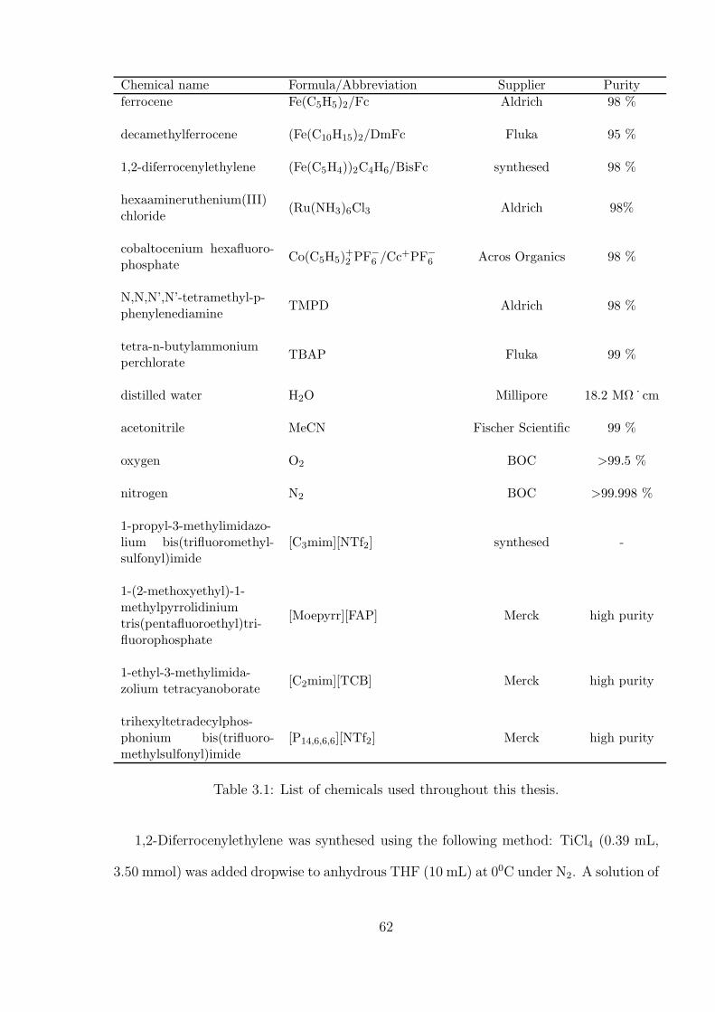
Chemical name Formula/Abbreviation Supplier Purity
ferrocene Fe(C5H5)2/Fc Aldrich 98 %
decamethylferrocene (Fe(C10H15)2/DmFc Fluka 95 %
1,2-diferrocenylethylene (Fe(C5H4))2C4H6/BisFc synthesed 98 %
hexaamineruthenium(III)chloride
(Ru(NH3)6Cl3 Aldrich 98%
cobaltocenium hexafluoro-phosphate
Co(C5H5)+2 PF
−6 /Cc
+PF−6 Acros Organics 98 %
N,N,N’,N’-tetramethyl-p-phenylenediamine
TMPD Aldrich 98 %
tetra-n-butylammoniumperchlorate
TBAP Fluka 99 %
distilled water H2O Millipore 18.2 MΩ ˙ cm
acetonitrile MeCN Fischer Scientific 99 %
oxygen O2 BOC >99.5 %
nitrogen N2 BOC >99.998 %
1-propyl-3-methylimidazo-lium bis(trifluoromethyl-sulfonyl)imide
[C3mim][NTf2] synthesed -
1-(2-methoxyethyl)-1-methylpyrrolidiniumtris(pentafluoroethyl)tri-fluorophosphate
[Moepyrr][FAP] Merck high purity
1-ethyl-3-methylimida-zolium tetracyanoborate
[C2mim][TCB] Merck high purity
trihexyltetradecylphos-phonium bis(trifluoro-methylsulfonyl)imide
[P14,6,6,6][NTf2] Merck high purity
Table 3.1: List of chemicals used throughout this thesis.
1,2-Diferrocenylethylene was synthesed using the following method: TiCl4 (0.39 mL,
3.50 mmol) was added dropwise to anhydrous THF (10 mL) at 00C under N2. A solution of
62
ferrocenecarboxaldehyde (500 mg, 2.34 mmol) in anhydrous THF (5 mL) and Zn powder
(300 mg, 4.59 mmol) were sequentially added to the yellow solution at 0C. The resultant
black suspension was heated at reflux for four hours. After cooling, the mixture was
poured onto ice water (50 mL), and sat. aq. NaHCO3 (30 mL) was added. The resultant
mixture was extracted with CH2Cl2 (3 × 30 mL). The organics were dried over MgSO4
and concentrated in vacuo to give the title compound (340 mg, 73 %) as a dark orange
solid; δH (400 MHz, CDCl3) 4.18 (10H, s, Cp), 4.33 (4H, s, Cp), 4.55 (4H, s, Cp), 6.18
(2H, s, CH=CH).
Synthesis of 1-methyl-3-propylimidazolium chloride and 1-methyl-3-propylimidazolium
bis(trifluoromethyl)sulfonylimide is provided as follow: N-methylimidazole (99 %) and 1-
chloropropane (98 %) were purchased from Sigma-Aldrich. All solvents used were HPLC
grade purchased from Riedel de Haen. Lithium bis-(trifluoromethyl)sulfonylimide was
purchased from 3M.
Synthesis of 1-methyl-3-propylimidazolium chloride:
A mixture of 1-methylimidazole (99 % Sigma-Aldrich, 41.05 g, 0.5 mol) and 1-chloro-
propane (98 % Sigma-Aldrich 59.91 g, 0.75 mol) was placed in a Parr autoclave sealed
reaction vessel along with 30 cm3 of HPLC grade acetonitrile. The reaction mixture was
heated up to 343 K and then held at this temperature for 24 h with stirring at 500 rpm.
After cooling of the reaction mixture the acetonitrile was removed under vacuum. The
highly viscous yellow product was recrystallised from acetonitrile/ethyl acetate mixture
to afford an off-white solid, 78 % yield. The pure product was characterized by 1H NMR
spectroscopy using a Bruker Avance machine
1H-NMR (300 MHz, DMSO-d6): δ (ppm) = 0.83 (3H, t, J = 7.4 Hz, CH3), 1.81 (2 H,
m, CH2), 3.86 (3H, s, N-CH3), 4.18 (2H, t, J = 7.1 Hz, N-CH2), 7.75 (1 H, s), 7.83 (1 H,
s), 9.32 (1 H, s);
Synthesis of 1-methyl-3-propylimidazolium bis(trifluoromethyl)sulfonylimide:
63
A solution of lithium bis(trifluoromethyl)sulfonylimide (143.55 g g, 0.5 mol) in dis-
tilled water (300 cm3) was added drop-wise to a rapidly stirred solution of 1-Methyl-3-
propylimidazolium chloride (78.4 g, 0.49 mmol) in dichloromethane (200 cm3) and allowed
to stir under ambient conditions overnight. The organic layer was then extracted and
washed with distilled water (100 cm3) repeatedly five times. The organic layer was then
dried in vacuo to give the product as an off-white liquid in <98 % yield which was found
to contain <0.10 wt% water, determined by Karl-Fischer analysis, and <15 ppm halide,
determined by suppressed ion chromatography.[1]
1H-NMR (400 MHz, DMSO-d6): δ (ppm) = 0.84 (3 H, t, J = 7.4 Hz, CH3), 1.75 (2
H, m, CH2), 3.79 (3 H, s, N-CH3), 4.10 (2 H, t, J = 7.1 Hz, N-CH2), 7.68 (1 H, s), 7.74
(1 H,s), 9.01 (1 H, s).
3.2 Instrumental
All electrochemical experiments were performed using a computer-controlled PGSTAT30-
Autolab potentiostat (Eco-Chemie, Netherlands). For experiments in aqueous and organic
systems, solutions were housed in a sealed glass vial, with a three-electrode arrangement
consisting of a Pt working micro-disc electrode, a silver wire reference electrode and Pt
coil wire counter electrode. The platinum microdisk working electrodes were polished on
soft lapping pads (Kemet Ltd., UK) using alumina powders (Buehler, IL) of sizes 1.0, 0.3
mm and 0.05 mm. The electrode diameters were calibrated electrochemically by analysing
the steady-state voltammetry of a 2 mM solution of ferrocene in MeCN containing 0.1 M
TBAP, using a diffusion coefficient for ferrocene of 2.30 × 10⁻⁹ m2 s−1[2] at 298 K.(See
more details in Chapter 4) For experiments with laminated electrodes (see Chapter 9 and
Chapter 10) the sealed sample vial is used.
The experiments involving ionic liquids and micro-disc electtrodes were studied using
a three-electrode arrangement, consisting of a platinum working electrode and two 0.5 mm
64
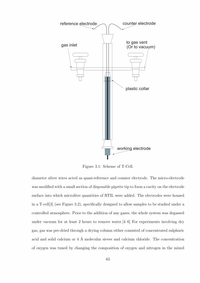
gas inletto gas vent(Or to vacuum)
working electrode
reference electrode counter electrode
plastic collar
Figure 3.1: Scheme of T-Cell.
diameter silver wires acted as quasi-reference and counter electrode. The micro-electrode
was modified with a small section of disposable pipette tip to form a cavity on the electrode
surface into which microlitre quantities of RTIL were added. The electrodes were housed
in a T-cell[3] (see Figure 3.2), specifically designed to allow samples to be studied under a
controlled atmosphere. Prior to the addition of any gases, the whole system was degassed
under vacuum for at least 2 hours to remove water.[4–6] For experiments involving dry
gas, gas was pre-dried through a drying column either consisted of concentrated sulphuric
acid and solid calcium or 4 A molecular sieves and calcium chloride. The concentration
of oxygen was tuned by changing the composition of oxygen and nitrogen in the mixed
65
gas. Before the gas measurements, gas was run for 30 minutes to ensure equilibrium
was established. For experiments excluding gases, the ionic liquid was constantly purged
under vacuum during experimental analysis. All experiments were performed inside a
thermostatted box (previously described by Evans et al.)[3] which also functioned as a
Faraday cage. The temperature was maintained at 298 (±0.5) K.
References
[1] Villagran, C.; Banks, C. E.; Hardacre, C.; Compton, R. G. Analytical Chemistry 2004,76, 1998–2003.
[2] Rogers, E. I.; Silvester, D. S.; Poole, D. L.; Aldous, L.; Hardacre, C.; Compton, R. G.Journal of Physical Chemistry C 2008, 112, 2729–2735.
[3] Evans, R. G.; Klymenko, O. V.; Saddoughi, S. A.; Hardacre, C.; Compton, R. G. J.Phys. Chem. B 2004, 108, 7878–7886.
[4] Gavaghan, D. J.; Rollett, J. S. Journal of Electroanalytical Chemistry 1990, 295, 1–14.
[5] Fleischmann, M.; Pons, S. Journal of Electroanalytical Chemistry 1988, 250, 257–267.
[6] Aoki, K.; Osteryoung, J. Journal of Electroanalytical Chemistry 1984, 160, 335–339.
66
Chapter 4
Investigation of the optimal transienttimes for chronoamperometricanalysis of diffusion coefficients andconcentrations in non-aqueoussolvents and ionic liquids
This chapter investigates the optimal transient times for chronoamperometric exper-
iments in order to simultaneously determine accurate values of concentration (c) and
diffusion coefficient (D), or alternatively the number of electrons passed (n) providing c
is known. This is achieved by the analysis of the current-time transients resulting from
potential steps for the oxidation of ferrocene in acetonitrile and the reduction of cobal-
tocenium in 1-ethyl-3-methylimidazolium bis(trifluoromethylsulfonyl)imide. The analysis
is based upon Shoup and Szabo approximation, which has been reported to describe the
current response over all time values to within an error of 0.5 % [D. Shoup and A. Szabo,
Journal of Electroanalytical Chemistry, 1982, 140, 237-245]. The error is quantified by
comparing the resulting chronoamperometric data with simulation at all transient times.
In addition, an alternative simple approach to the simultaneous determination of nc and
D values is proposed by independently investigating the short and long time regimes of
chronoamperometric transients. The chronoamperometry of hydrazine is investigated as
a multielectron example process. The work presented in this chapter has been published
67
in Analytical Methods [1].
4.1 Introduction
Electrochemistry is a powerful technique, by which a vast range of physical parameters
can be extracted from the system of interest[2–4]. Arguably the simplest electro-analytical
techniques are based on potential steps, where a system is stepped from a potential where
no detectable Faradaic current is passing to a potential where the oxidation or reduc-
tion process of interest occurs, often under diffusion control. The potential is applied,
current flows through the system and the resulting plot of current vs. time (or chronoam-
perometric transient) can be related to a range of physical parameters. This has been
used to simultaneously measure concentration and diffusion coefficients,[2, 5–10] and is
commonly used in electroanalytical investigations with the current measured during the
standard addition of an analyte.[11] The current-time relationship resulting from poten-
tial step to a planar macro electrode described by the Cottrell equation (see Equation
1.32 in Chapter 1) where often up to three variables, n, c and D, involved in this equation
are unknown when studying a redox reaction in an n-electron-transfer system. There-
fore, it is beneficial to find an alternative approach that is able to determine (nc) and
D values simultaneously. One simple approach utilises potential step chronoamperom-
etry at a micro-electrode. Micro-electrodes are widely employed, and demonstrate high
mass transport rates, good signal-to-noise ratios and low uncompensated resistances.[2, 3]
These features are potentially beneficial when performing electrochemistry in non-aqueous
environments, and especially when operating in room temperature ionic liquids (RTILs),
due to the relatively low conductivity and high viscosity of these solvents when compared
to aqueous systems.[12]
Several numerical models have been developed to describe the chronoamperometric re-
sponses (or current-time transients) observed at micro-electrodes.[6, 9, 13–18] The Shoup
68
and Szabo equation has been widely used, and has been reported to describe the current
response over all time values to within an error of 0.5 %.[9] For an n electrons process,
the chronoamperometric response at a micro-electrode can be described as
i = 4nFrDcf(t) (4.1)
where
f(t) = 0.7854 + 0.8862
√
r2
4Dt+ 0.2146exp(−0.7823
√
r2
4Dt) (4.2)
Note that Equation 4.2 was derived using simulation and as such applies to all solvents
regardless of their viscosity.
It has been demonstrated that combining experimental chronoamperometry with fit-
ting of the results to the Shoup and Szabo equation results in a powerful electroanalytical
technique, facilitating the simultaneous determination of both the product (nc) and the
diffusion coefficient (D) of electroactive analytes.[5, 7] This is possible because at short
times the response is Cottrellian and depends on ncD12 whereas at long times the steady
state current (see Equation 1.30 in Chapter 1) is recorded, which scales with ncD. Ac-
cordingly, it is possible to analyse the transient to give (nc) and D.
As noted above, at long transient times the current approaches a steady state value
where ncD is constant.[10] Therefore attempts to simultaneously determine nc and D
using chronoamperometric transients recorded over very large time ranges are likely to
yield apparent acceptable agreement between experiment and simulation over a wide
range of pairs of nc and D values; that is by using too long a measured time, a large
error can be introduced during quantifications. Alternatively, transients recorded at very
short time values will experience additional non-Faradaic current, e.g. from double layer
charging and thus inflate estimates of D and nc. There therefore likely exists an optimal
time range for chronoamperometric transients, resulting in the smallest combined error
69
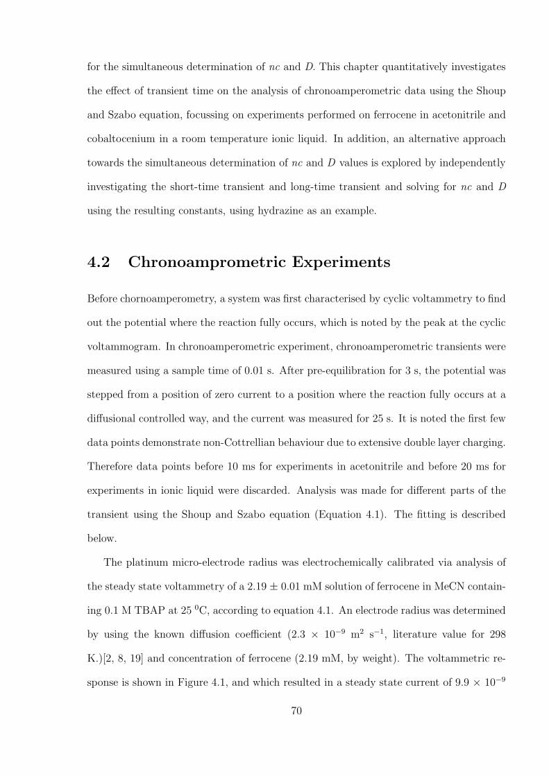
for the simultaneous determination of nc and D. This chapter quantitatively investigates
the effect of transient time on the analysis of chronoamperometric data using the Shoup
and Szabo equation, focussing on experiments performed on ferrocene in acetonitrile and
cobaltocenium in a room temperature ionic liquid. In addition, an alternative approach
towards the simultaneous determination of nc and D values is explored by independently
investigating the short-time transient and long-time transient and solving for nc and D
using the resulting constants, using hydrazine as an example.
4.2 Chronoamprometric Experiments
Before chornoamperometry, a system was first characterised by cyclic voltammetry to find
out the potential where the reaction fully occurs, which is noted by the peak at the cyclic
voltammogram. In chronoamperometric experiment, chronoamperometric transients were
measured using a sample time of 0.01 s. After pre-equilibration for 3 s, the potential was
stepped from a position of zero current to a position where the reaction fully occurs at a
diffusional controlled way, and the current was measured for 25 s. It is noted the first few
data points demonstrate non-Cottrellian behaviour due to extensive double layer charging.
Therefore data points before 10 ms for experiments in acetonitrile and before 20 ms for
experiments in ionic liquid were discarded. Analysis was made for different parts of the
transient using the Shoup and Szabo equation (Equation 4.1). The fitting is described
below.
The platinum micro-electrode radius was electrochemically calibrated via analysis of
the steady state voltammetry of a 2.19 ± 0.01 mM solution of ferrocene in MeCN contain-
ing 0.1 M TBAP at 25 0C, according to equation 4.1. An electrode radius was determined
by using the known diffusion coefficient (2.3 × 10⁻⁹ m2 s−1, literature value for 298
K.)[2, 8, 19] and concentration of ferrocene (2.19 mM, by weight). The voltammetric re-
sponse is shown in Figure 4.1, and which resulted in a steady state current of 9.9 × 10⁻⁹
70
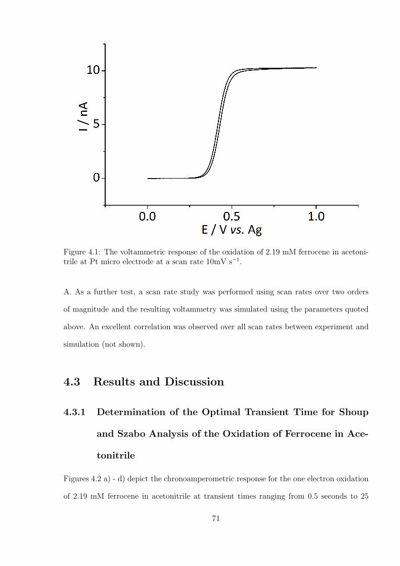
Figure 4.1: The voltammetric response of the oxidation of 2.19 mM ferrocene in acetoni-trile at Pt micro electrode at a scan rate 10mV s−1.
A. As a further test, a scan rate study was performed using scan rates over two orders
of magnitude and the resulting voltammetry was simulated using the parameters quoted
above. An excellent correlation was observed over all scan rates between experiment and
simulation (not shown).
4.3 Results and Discussion
4.3.1 Determination of the Optimal Transient Time for Shoup
and Szabo Analysis of the Oxidation of Ferrocene in Ace-
tonitrile
Figures 4.2 a) - d) depict the chronoamperometric response for the one electron oxidation
of 2.19 mM ferrocene in acetonitrile at transient times ranging from 0.5 seconds to 25
71
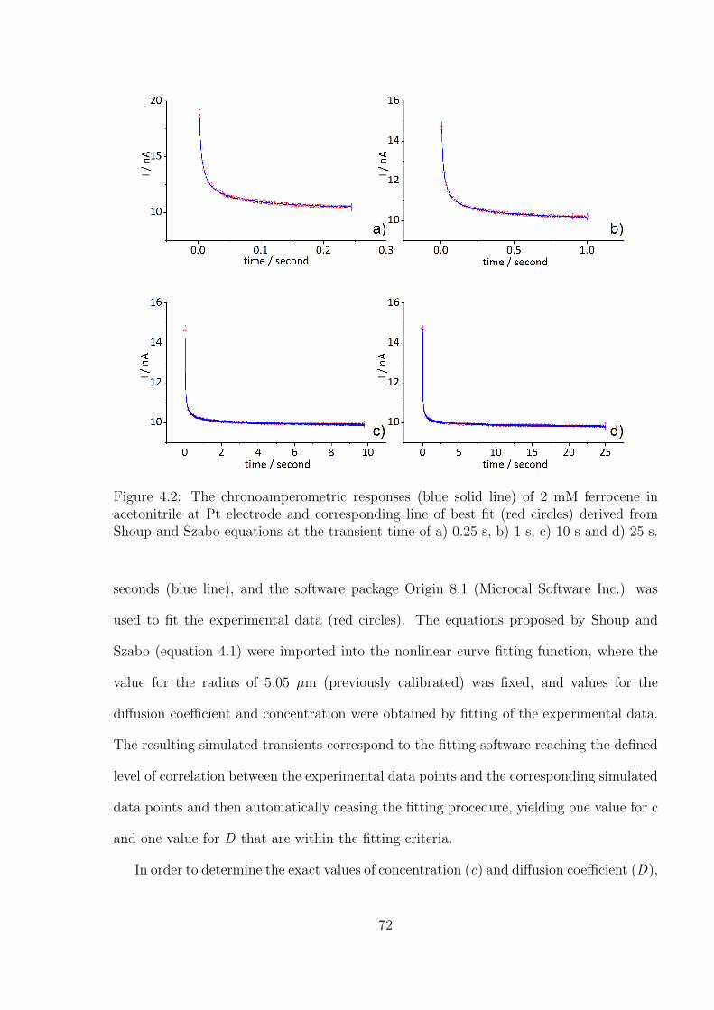
Figure 4.2: The chronoamperometric responses (blue solid line) of 2 mM ferrocene inacetonitrile at Pt electrode and corresponding line of best fit (red circles) derived fromShoup and Szabo equations at the transient time of a) 0.25 s, b) 1 s, c) 10 s and d) 25 s.
seconds (blue line), and the software package Origin 8.1 (Microcal Software Inc.) was
used to fit the experimental data (red circles). The equations proposed by Shoup and
Szabo (equation 4.1) were imported into the nonlinear curve fitting function, where the
value for the radius of 5.05 µm (previously calibrated) was fixed, and values for the
diffusion coefficient and concentration were obtained by fitting of the experimental data.
The resulting simulated transients correspond to the fitting software reaching the defined
level of correlation between the experimental data points and the corresponding simulated
data points and then automatically ceasing the fitting procedure, yielding one value for c
and one value for D that are within the fitting criteria.
In order to determine the exact values of concentration (c) and diffusion coefficient (D),
72
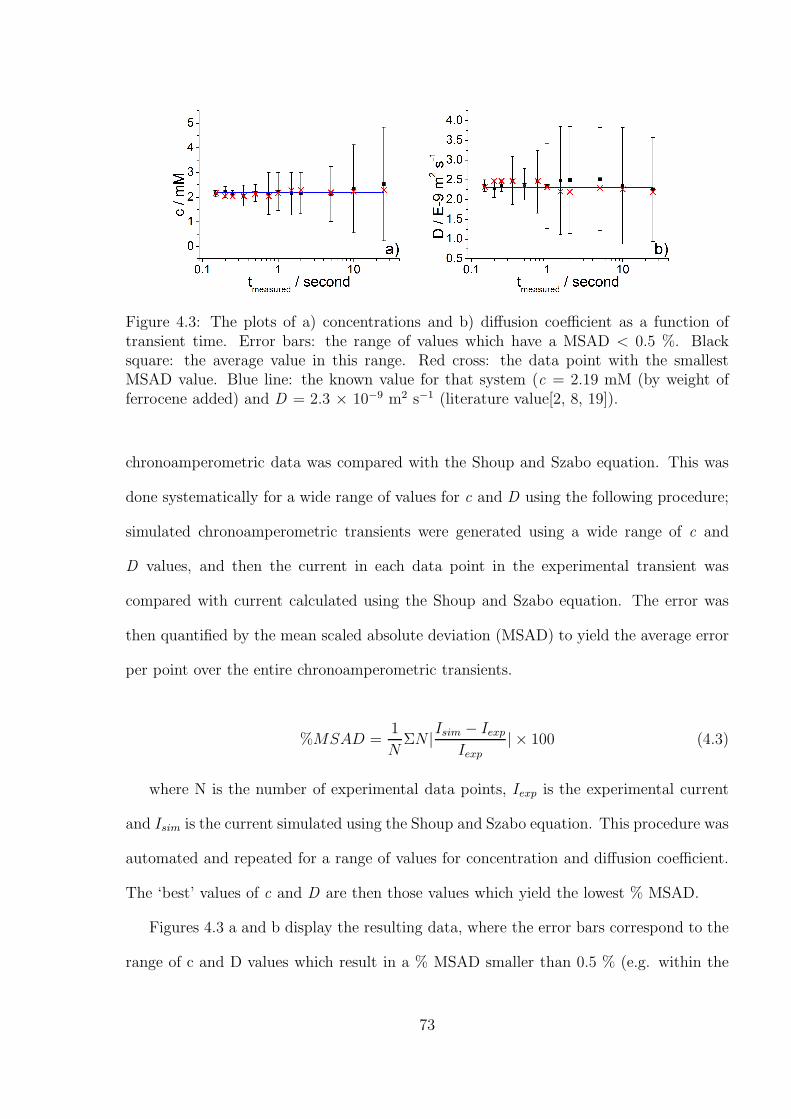
Figure 4.3: The plots of a) concentrations and b) diffusion coefficient as a function oftransient time. Error bars: the range of values which have a MSAD < 0.5 %. Blacksquare: the average value in this range. Red cross: the data point with the smallestMSAD value. Blue line: the known value for that system (c = 2.19 mM (by weight offerrocene added) and D = 2.3 × 10⁻⁹ m2 s−1 (literature value[2, 8, 19]).
chronoamperometric data was compared with the Shoup and Szabo equation. This was
done systematically for a wide range of values for c and D using the following procedure;
simulated chronoamperometric transients were generated using a wide range of c and
D values, and then the current in each data point in the experimental transient was
compared with current calculated using the Shoup and Szabo equation. The error was
then quantified by the mean scaled absolute deviation (MSAD) to yield the average error
per point over the entire chronoamperometric transients.
%MSAD =1
NΣN |Isim − Iexp
Iexp| × 100 (4.3)
where N is the number of experimental data points, Iexp is the experimental current
and Isim is the current simulated using the Shoup and Szabo equation. This procedure was
automated and repeated for a range of values for concentration and diffusion coefficient.
The ‘best’ values of c and D are then those values which yield the lowest % MSAD.
Figures 4.3 a and b display the resulting data, where the error bars correspond to the
range of c and D values which result in a % MSAD smaller than 0.5 % (e.g. within the
73
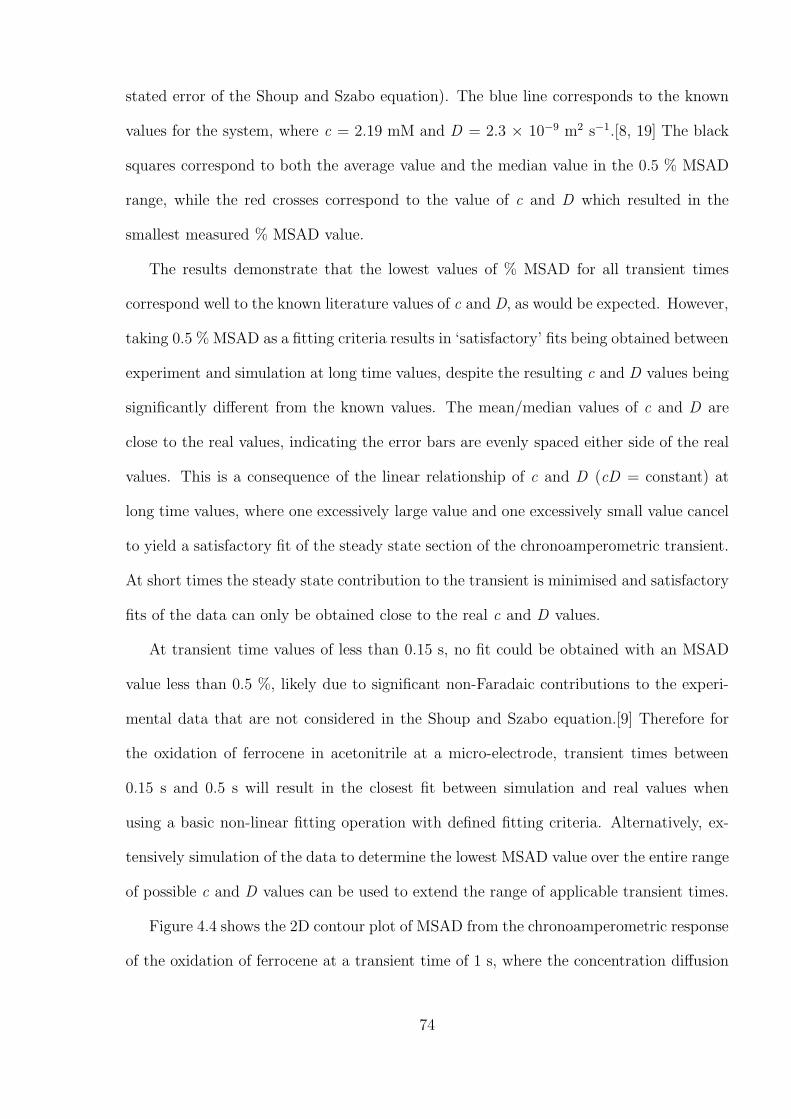
stated error of the Shoup and Szabo equation). The blue line corresponds to the known
values for the system, where c = 2.19 mM and D = 2.3 × 10⁻⁹ m2 s−1.[8, 19] The black
squares correspond to both the average value and the median value in the 0.5 % MSAD
range, while the red crosses correspond to the value of c and D which resulted in the
smallest measured % MSAD value.
The results demonstrate that the lowest values of % MSAD for all transient times
correspond well to the known literature values of c and D, as would be expected. However,
taking 0.5 % MSAD as a fitting criteria results in ‘satisfactory’ fits being obtained between
experiment and simulation at long time values, despite the resulting c and D values being
significantly different from the known values. The mean/median values of c and D are
close to the real values, indicating the error bars are evenly spaced either side of the real
values. This is a consequence of the linear relationship of c and D (cD = constant) at
long time values, where one excessively large value and one excessively small value cancel
to yield a satisfactory fit of the steady state section of the chronoamperometric transient.
At short times the steady state contribution to the transient is minimised and satisfactory
fits of the data can only be obtained close to the real c and D values.
At transient time values of less than 0.15 s, no fit could be obtained with an MSAD
value less than 0.5 %, likely due to significant non-Faradaic contributions to the experi-
mental data that are not considered in the Shoup and Szabo equation.[9] Therefore for
the oxidation of ferrocene in acetonitrile at a micro-electrode, transient times between
0.15 s and 0.5 s will result in the closest fit between simulation and real values when
using a basic non-linear fitting operation with defined fitting criteria. Alternatively, ex-
tensively simulation of the data to determine the lowest MSAD value over the entire range
of possible c and D values can be used to extend the range of applicable transient times.
Figure 4.4 shows the 2D contour plot of MSAD from the chronoamperometric response
of the oxidation of ferrocene at a transient time of 1 s, where the concentration diffusion
74
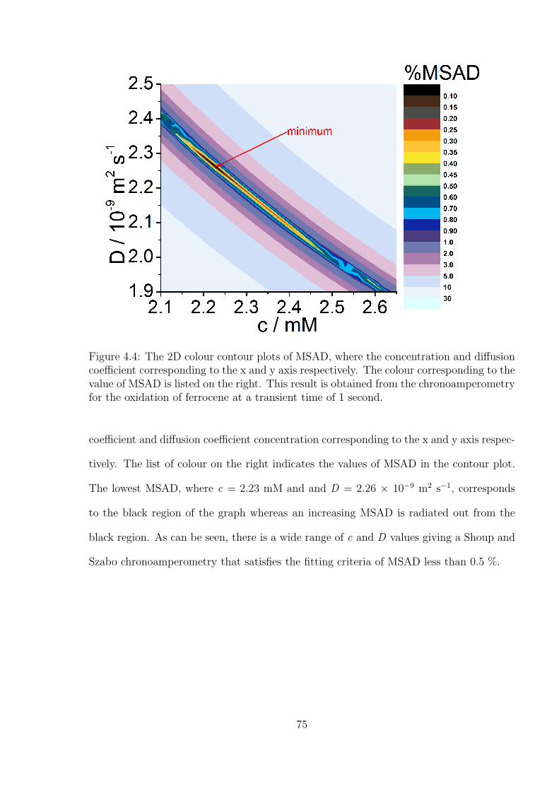
Figure 4.4: The 2D colour contour plots of MSAD, where the concentration and diffusioncoefficient corresponding to the x and y axis respectively. The colour corresponding to thevalue of MSAD is listed on the right. This result is obtained from the chronoamperometryfor the oxidation of ferrocene at a transient time of 1 second.
coefficient and diffusion coefficient concentration corresponding to the x and y axis respec-
tively. The list of colour on the right indicates the values of MSAD in the contour plot.
The lowest MSAD, where c = 2.23 mM and and D = 2.26 × 10⁻⁹ m2 s−1, corresponds
to the black region of the graph whereas an increasing MSAD is radiated out from the
black region. As can be seen, there is a wide range of c and D values giving a Shoup and
Szabo chronoamperometry that satisfies the fitting criteria of MSAD less than 0.5 %.
75
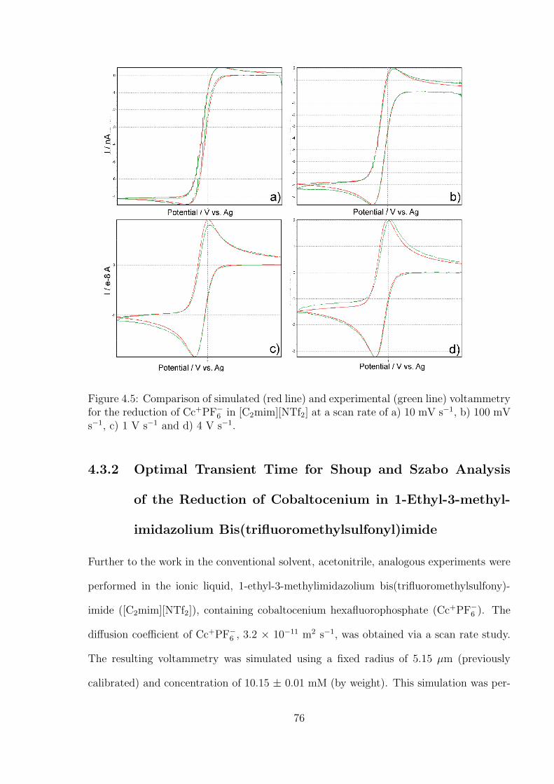
Figure 4.5: Comparison of simulated (red line) and experimental (green line) voltammetryfor the reduction of Cc+PF−
6 in [C2mim][NTf2] at a scan rate of a) 10 mV s−1, b) 100 mVs−1, c) 1 V s−1 and d) 4 V s−1.
4.3.2 Optimal Transient Time for Shoup and Szabo Analysis
of the Reduction of Cobaltocenium in 1-Ethyl-3-methyl-
imidazolium Bis(trifluoromethylsulfonyl)imide
Further to the work in the conventional solvent, acetonitrile, analogous experiments were
performed in the ionic liquid, 1-ethyl-3-methylimidazolium bis(trifluoromethylsulfony)-
imide ([C2mim][NTf2]), containing cobaltocenium hexafluorophosphate (Cc+PF−6 ). The
diffusion coefficient of Cc+PF−6 , 3.2 × 10⁻¹¹ m2 s−1, was obtained via a scan rate study.
The resulting voltammetry was simulated using a fixed radius of 5.15 µm (previously
calibrated) and concentration of 10.15 ± 0.01 mM (by weight). This simulation was per-
76
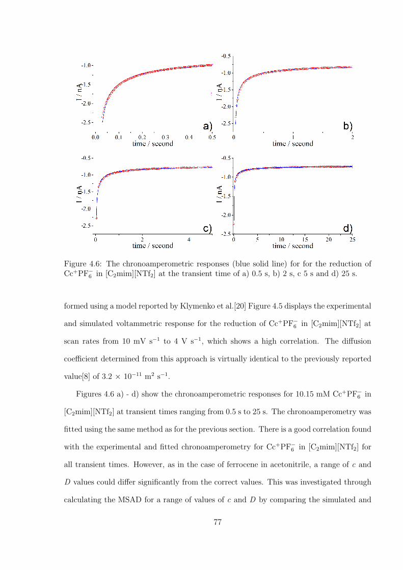
Figure 4.6: The chronoamperometric responses (blue solid line) for for the reduction ofCc+PF−
6 in [C2mim][NTf2] at the transient time of a) 0.5 s, b) 2 s, c 5 s and d) 25 s.
formed using a model reported by Klymenko et al.[20] Figure 4.5 displays the experimental
and simulated voltammetric response for the reduction of Cc+PF−6 in [C2mim][NTf2] at
scan rates from 10 mV s−1 to 4 V s−1, which shows a high correlation. The diffusion
coefficient determined from this approach is virtually identical to the previously reported
value[8] of 3.2 × 10⁻¹¹ m2 s−1.
Figures 4.6 a) - d) show the chronoamperometric responses for 10.15 mM Cc+PF−6 in
[C2mim][NTf2] at transient times ranging from 0.5 s to 25 s. The chronoamperometry was
fitted using the same method as for the previous section. There is a good correlation found
with the experimental and fitted chronoamperometry for Cc+PF−6 in [C2mim][NTf2] for
all transient times. However, as in the case of ferrocene in acetonitrile, a range of c and
D values could differ significantly from the correct values. This was investigated through
calculating the MSAD for a range of values of c and D by comparing the simulated and
77
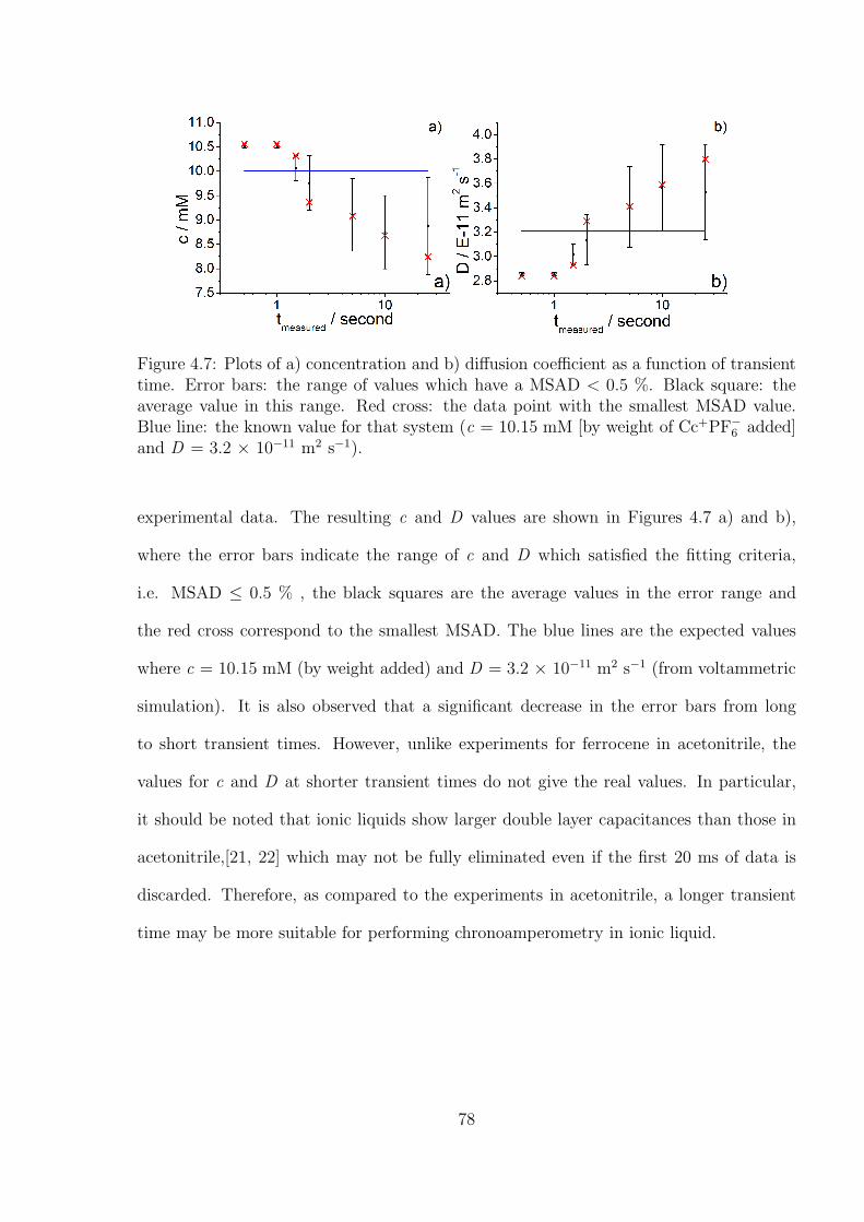
Figure 4.7: Plots of a) concentration and b) diffusion coefficient as a function of transienttime. Error bars: the range of values which have a MSAD < 0.5 %. Black square: theaverage value in this range. Red cross: the data point with the smallest MSAD value.Blue line: the known value for that system (c = 10.15 mM [by weight of Cc+PF−
6 added]and D = 3.2 × 10⁻¹¹ m2 s−1).
experimental data. The resulting c and D values are shown in Figures 4.7 a) and b),
where the error bars indicate the range of c and D which satisfied the fitting criteria,
i.e. MSAD ≤ 0.5 % , the black squares are the average values in the error range and
the red cross correspond to the smallest MSAD. The blue lines are the expected values
where c = 10.15 mM (by weight added) and D = 3.2 × 10⁻¹¹ m2 s−1 (from voltammetric
simulation). It is also observed that a significant decrease in the error bars from long
to short transient times. However, unlike experiments for ferrocene in acetonitrile, the
values for c and D at shorter transient times do not give the real values. In particular,
it should be noted that ionic liquids show larger double layer capacitances than those in
acetonitrile,[21, 22] which may not be fully eliminated even if the first 20 ms of data is
discarded. Therefore, as compared to the experiments in acetonitrile, a longer transient
time may be more suitable for performing chronoamperometry in ionic liquid.
78
4.3.3 An Alternative Non-fitting Approach to Chronoampero-
metric Data to Simultaneously Yield Diffusion Coefficient
and Concentration Values
The data presented in the previous two sections have highlighted the importance of obtain-
ing a balance between ‘short time’ data (e.g. time scales relevant to analysis using the
Cottrell equation) and ‘long time’ data (e.g. steady-state, diffusion-controlled data) when
analysing entire transients. Alternatively, these two defined regimes observed during
chronoamperometric experiments at micro-electrodes could be analysed separately, since
the Cottrell equation (Equation 1.32 in Chapter 1) can be rearranged to give
cD12 = constant1 (4.4)
where constant1 is a function of nFA− 12 and the gradient obtained by a plot of I vs
t12 , while the steady state limiting current at long time values (Equation 1.30) can be
rearranged to give
cD = constant2 (4.5)
and the two known constants can then be solved to yield
D12 =
constant2constant1
(4.6)
and ultimately give simultaneous quantification of both nc and D values.
As proof of principle, the data presented for the reduction of Cc+PF−6 in [C2mim][NTf2]
was analysed using this technique. The Cottrell plot obtained for the chronoamperometric
response of 10.15 mM cobaltocenium in [C2mim][NTf2] at a 5.15 µm Pt micro-electrode
gave a gradient of 2.62 × 10⁻¹⁰ A s12 . Solving the data by using the steady state current
79
(current at t = 5 s) and the gradient obtained by the Cottrell plot yielded a D value
of 3.2 × 10⁻¹¹ m2 s−1, which when substituted into either the Cottrell equation or the
steady state current equation yielded a c value of 10.19 mM. These values are in good
agreement with those obtained by the full simulation of the entire chronoamperometric
transient using the Shoup and Szabo equation, which gave D = 3.2× 10⁻¹¹ m2 s−1 and c
= 10.15 mM. The above data demonstrates the applicability of this technique towards the
determination of c and D when n = 1. Alternatively, this technique should be applicable
for multielectron processes, providing a sufficient overpotential is applied such that kinetic
factors are not limiting. Hydrazine, N2H4, is well known to be oxidised in a four electron
process[23], e.g.
N2H4 → N2 + 4H+ + 4e− (4.7)
The voltammetry of hydrazine at Pt micro-electrodes has previously been described
in detail.[23] Figure 4.8 displays a chronoamperogram recorded by stepping to + 1.0 V
(vs. SCE) for 10.0 mM hydrazine in a 1 M sodium acetate buffer (pH 4.8) at a 13.8 µm
radius Pt micro-electrode. The resulting Shoup and Szabo simulation (overlaid) gave D
= 9.2 × 10⁻¹⁰ m2 s−1 and nc = 38.1 mM (expected value 40.0 mM). Cottrell analysis
of the chronoamperogram yielded a gradient of 3.92 × 10⁻⁸ A s12 , which when solved as
above in combination with the steady state current recorded at t = 4 s (0.196 µA) gave
D = 9.35 × 10⁻¹⁰ m2 s−1 and nc = 39.4 mM, highlighting that both techniques are in
good agreement with the expected values.
The above results therefore demonstrate that separately investigating the short and
long time regimes of chronoamperometric transients obtained at micro-electrodes can
yield simultaneous values of c and D, or alternatively number of electrons passed (a
‘chronocoulometri’ measurement) providing c is known. The data analysis involved is
significantly more simple than the rigorous numerical analysis required for full analysis of
80
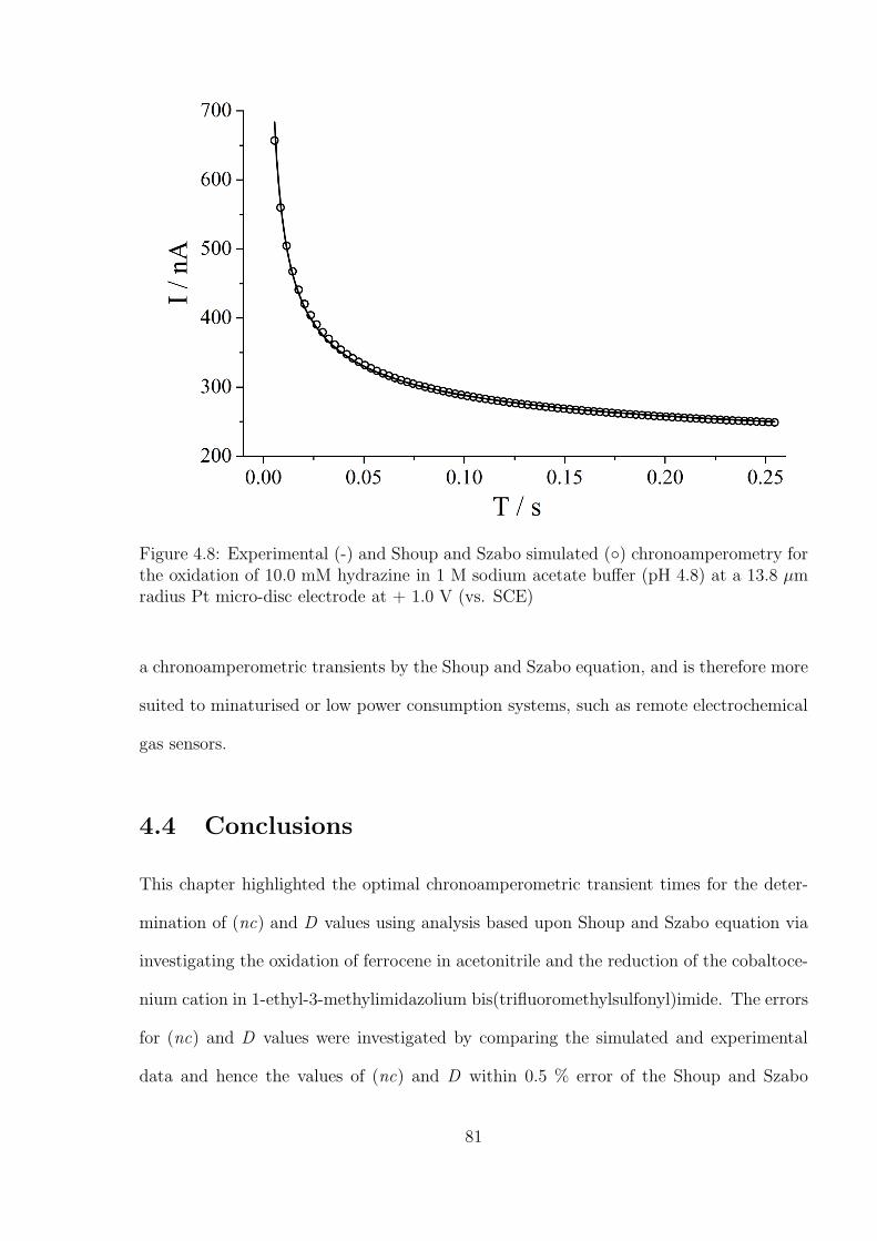
Figure 4.8: Experimental (-) and Shoup and Szabo simulated () chronoamperometry forthe oxidation of 10.0 mM hydrazine in 1 M sodium acetate buffer (pH 4.8) at a 13.8 µmradius Pt micro-disc electrode at + 1.0 V (vs. SCE)
a chronoamperometric transients by the Shoup and Szabo equation, and is therefore more
suited to minaturised or low power consumption systems, such as remote electrochemical
gas sensors.
4.4 Conclusions
This chapter highlighted the optimal chronoamperometric transient times for the deter-
mination of (nc) and D values using analysis based upon Shoup and Szabo equation via
investigating the oxidation of ferrocene in acetonitrile and the reduction of the cobaltoce-
nium cation in 1-ethyl-3-methylimidazolium bis(trifluoromethylsulfonyl)imide. The errors
for (nc) and D values were investigated by comparing the simulated and experimental
data and hence the values of (nc) and D within 0.5 % error of the Shoup and Szabo
81
equation were presented at all transient times. It was found that for the oxidation of
ferrocene in acetonitrile the more promising results are given at transient times between
0.15 s and 0.5 s whereas for the experiments in ionic liquid a longer transient time is
needed. In addition, a simple method to obtain (nc) and D values simultaneously using
the analysis of long and short time regimes of chronoamperometric transients has been
demonstrated, taking hydrazine as a multi-electron example. The next chapter looks into
the tuneability property of RTILs through the study of how the formal potentials of fer-
rocene, a commonly used internal reference for RTILs, and its derivatives can be tuned
by changing the composition of RTILs.
References
[1] Xiong, L.; Aldous, L.; Henstridge, M. C.; Compton, R. G. Analytical Methods 2012,4, 371–376.
[2] Bard, A. J.; Faulkner, L. R. Electrochemical Methods: Fundamentals and Applica-tions ; Wiley, 2001.
[3] Compton, R. G.; Banks, C. E. Understanding Voltammetry ; Imperial College Press,2011, 2nd Edition.
[4] Wang, J. Analytical Electrochemistry ; Wiley-VCH, New York, 1994.
[5] Paddon, C. A.; Silvester, D. S.; Bhatti, F. L.; Donohoe, T. J.; Compton, R. G.Electroanalysis 2007, 19, 11–22.
[6] Klymenko, O. V.; Evans, R. G.; Hardacre, C.; Svir, I. B.; Compton, R. G. Journalof Electroanalytical Chemistry 2004, 571, 211–221.
[7] Haruko, I. Journal of Electroanalytical Chemistry 2005, 577, 55–58.
[8] Rogers, E. I.; Silvester, D. S.; Poole, D. L.; Aldous, L.; Hardacre, C.; Compton, R. G.Journal of Physical Chemistry C 2008, 112, 2729–2735.
[9] Shoup, D.; Szabo, A. Journal of Electroanalytical Chemistry 1982, 140, 237–245.
[10] Evans, R. G.; Klymenko, O. V.; Hardacre, C.; Seddon, K. R.; Compton, R. G. Journalof Electroanalytical Chemistry 2003, 556, 179–188.
[11] Panchompoo, J.; Aldous, L.; Downing, C.; Crossley, A.; Compton, R. G. Electroanal-ysis 2011, 23, 1568–1578.
[12] Buzzeo, M. C.; Evans, R. G.; Compton, R. G. ChemPhysChem 2004, 5, 1106–1120.
[13] Heinze, J. Journal of Electroanalytical Chemistry 1981, 124, 73–86.
82
[14] Gavaghan, D. J.; Rollett, J. S. Journal of Electroanalytical Chemistry 1990, 295,1–14.
[15] Oldham, K. B. Journal of Electroanalytical Chemistry 1981, 122, 1–17.
[16] Aoki, K.; Osteryoung, J. Journal of Electroanalytical Chemistry 1981, 122, 19–35.
[17] Aoki, K.; Osteryoung, J. Journal of Electroanalytical Chemistry 1984, 160, 335–339.
[18] Fleischmann, M.; Pons, S. Journal of Electroanalytical Chemistry 1988, 250, 257–267.
[19] Sharp, M. Electrochimica Acta 1983, 28, 301–308.
[20] Klymenko, O. V.; Gavaghan, D. J.; Harriman, K. E.; Compton, R. G. Journal ofElectroanalytical Chemistry 2002, 531, 25–31.
[21] Yasui, Y.; Kitazumi, Y.; Mizunuma, H.; Nishi, N.; Kakiuchi, T. ElectrochemistryCommunications 2010, 12, 1479–1482.
[22] Fedorov, M. V.; Kornyshev, A. A. Journal of Physical Chemistry B 2008, 112,11868–11872.
[23] Aldous, L.; Compton, R. G. Physical Chemistry Chemical Physics 2011, 13, 5279–5287.
83
Chapter 5
Tuning solute redox potentials byvarying the anion component ofroom temperature ionic liquid
The electrode potentials for the two one electron oxidations of 1,2-diferrocenylethylene
(BisFc) were studied relative to that of the one electrode oxidation of decamethylferrocene
(DmFc) in a variety of RTILs. The difference in these potentials was found to be very
sensitive to the anion component of the ionic liquid showing the scope of these solutes as
‘designer media’ to tune the thermodynamic properties of solutes dissolved in them. The
work presented in this chapter has been published in Chemical Communications.[1]
5.1 Introduction
Chapter 2 introduces the advantageous properties of RTILs such as wide electrochemical
window, high viscosity, low volatility, inherent conductivity and high thermal stability.[2]
Due to all these properties and especially their low volatility, RTILs are considered as
environmentally friendly solvents and are easy to recycle. Consequently, RTILs find in-
creasing uses nowadays, ranging from fundamental studies to analytical applications.[3–5]
As also shown in Chapter 2, RTILs can be also thought of as ‘designer solvents’ due to
the fact that they consist of two components (anion and cation) which can be system-
atically varied and hence they can be tailored to possess different physical or chemical
84
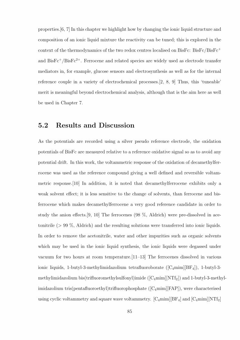
properties.[6, 7] In this chapter we highlight how by changing the ionic liquid structure and
composition of an ionic liquid mixture the reactivity can be tuned; this is explored in the
context of the thermodynamics of the two redox centres localised on BisFc: BisFc/BisFc+
and BisFc+/BisFc2+. Ferrocene and related species are widely used as electrode transfer
mediators in, for example, glucose sensors and electrosynthesis as well as for the internal
reference couple in a variety of electrochemical processes.[2, 8, 9] Thus, this ‘tuneable’
merit is meaningful beyond electrochemical analysis, although that is the aim here as well
be used in Chapter 7.
5.2 Results and Discussion
As the potentials are recorded using a silver pseudo reference electrode, the oxidation
potentials of BisFc are measured relative to a reference oxidative signal so as to avoid any
potential drift. In this work, the voltammetric response of the oxidation of decamethylfer-
rocene was used as the reference compound giving a well defined and reversible voltam-
metric response.[10] In addition, it is noted that decamethylferrocene exhibits only a
weak solvent effect; it is less sensitive to the change of solvents, than ferrocene and bis-
ferrocene which makes decamethylferrocene a very good reference candidate in order to
study the anion effects.[9, 10] The ferrocenes (98 %, Aldrich) were pre-dissolved in ace-
tonitrile (> 99 %, Aldrich) and the resulting solutions were transferred into ionic liquids.
In order to remove the acetonitrile, water and other impurities such as organic solvents
which may be used in the ionic liquid synthesis, the ionic liquids were degassed under
vacuum for two hours at room temperature.[11–13] The ferrocenes dissolved in various
ionic liquids, 1-butyl-3-methylimidazolium tetrafluoroborate ([C4mim][BF4]), 1-butyl-3-
methylimidazolium bis(trifluoromethylsulfonyl)imide ([C4mim][NTf2]) and 1-butyl-3-methyl-
imidazolium tris(pentafluoroethyl)trifluorophosphate ([C4mim][FAP]), were characterised
using cyclic voltammetry and square wave voltammetry. [C4mim][BF4] and [C4mim][NTf2]
85
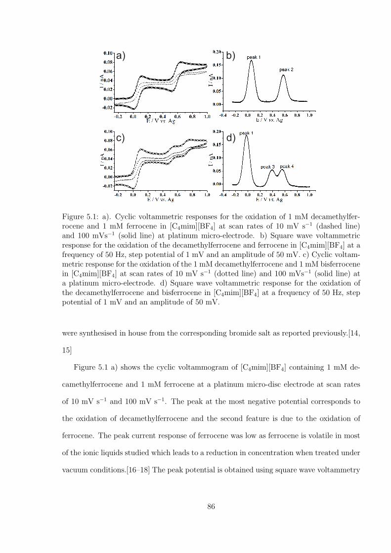
a)
c)
b)
d)
Figure 5.1: a). Cyclic voltammetric responses for the oxidation of 1 mM decamethylfer-rocene and 1 mM ferrocene in [C4mim][BF4] at scan rates of 10 mV s−1 (dashed line)and 100 mVs−1 (solid line) at platinum micro-electrode. b) Square wave voltammetricresponse for the oxidation of the decamethylferrocene and ferrocene in [C4mim][BF4] at afrequency of 50 Hz, step potential of 1 mV and an amplitude of 50 mV. c) Cyclic voltam-metric response for the oxidation of the 1 mM decamethylferrocene and 1 mM bisferrocenein [C4mim][BF4] at scan rates of 10 mV s−1 (dotted line) and 100 mVs−1 (solid line) ata platinum micro-electrode. d) Square wave voltammetric response for the oxidation ofthe decamethylferrocene and bisferrocene in [C4mim][BF4] at a frequency of 50 Hz, steppotential of 1 mV and an amplitude of 50 mV.
were synthesised in house from the corresponding bromide salt as reported previously.[14,
15]
Figure 5.1 a) shows the cyclic voltammogram of [C4mim][BF4] containing 1 mM de-
camethylferrocene and 1 mM ferrocene at a platinum micro-disc electrode at scan rates
of 10 mV s−1 and 100 mV s−1. The peak at the most negative potential corresponds to
the oxidation of decamethylferrocene and the second feature is due to the oxidation of
ferrocene. The peak current response of ferrocene was low as ferrocene is volatile in most
of the ionic liquids studied which leads to a reduction in concentration when treated under
vacuum conditions.[16–18] The peak potential is obtained using square wave voltammetry
86
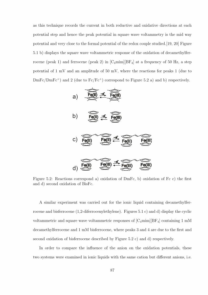
as this technique records the current in both reductive and oxidative directions at each
potential step and hence the peak potential in square wave voltammetry is the mid way
potential and very close to the formal potential of the redox couple studied.[19, 20] Figure
5.1 b) displays the square wave voltammetric response of the oxidation of decamethylfer-
rocene (peak 1) and ferrocene (peak 2) in [C4mim][BF4] at a frequency of 50 Hz, a step
potential of 1 mV and an amplitude of 50 mV, where the reactions for peaks 1 (due to
DmFc/DmFc+) and 2 (due to Fc/Fc+) correspond to Figure 5.2 a) and b) respectively.
a)
b)
c)
d)
Figure 5.2: Reactions correspond a) oxidation of DmFc, b) oxidation of Fc c) the firstand d) second oxidation of BisFc.
A similar experiment was carried out for the ionic liquid containing decamethylfer-
rocene and bisferrocene (1,2-diferrocenylethylene). Figures 5.1 c) and d) display the cyclic
voltammetric and square wave voltammetric responses of [C4mim][BF4] containing 1 mM
decamethylferrocene and 1 mM bisferrocene, where peaks 3 and 4 are due to the first and
second oxidation of bisferrocene described by Figure 5.2 c) and d) respectively.
In order to compare the influence of the anion on the oxidation potentials, these
two systems were examined in ionic liquids with the same cation but different anions, i.e.
87
[C4mim][BF4], [C4mim][NTf2] and [C4mim][FAP]. In the following work the peak potential
difference is measured as a function of the volume of the ionic liquid anion. The molecular
volumes, V([BF4]−) = 0.089 nm3, V([NTf2]
−)= 0.262 nm3 and V([FAP]−)= 0.375 nm3,
were estimated using a group contribution model as a function of temperature.[21]
a)
c)
b)
Figure 5.3: (a) Comparison of the plots of peak potential difference, ∆E of decamethyl-ferrocene and ferrocene (solid line) with that of the oxidation of decamethylferrocene andfirst oxidation of bisferrocene (dashed line) against the molecular volume of the anion inthe ionic liquid. (b) Peak potential difference of the oxidation of decamethylferrocene andsecond oxidation of bisferrocene as a function of molecular volume of ionic liquid anion.(c) Peak potential difference of oxidation of the first and second oxidation of bisferroceneas a function of molecular volume (V) of ionic liquid anion.
Figure 5.3 a) compares peak potential difference, ∆E, of peaks 1 and 2 with peaks 1
and 3 as a function of the molecular volume of ionic liquid anion, where clear linear corre-
lations (R2 > 0.99) were obtained. These peak potential differences between decamethyl-
ferrocene and ferrocene, 0.575, 0.528 and 0.469 V in [C4mim][BF4], [C4mim][NTf2] and
[C4mim][FAP] respectively, are comparable to those observed by Torriero et al., who re-
ported potential differences of 0.575, 0.513 and 0.478 V for the same anions. As can
be seen from both plots, the potential difference increases with the size of anion as the
88
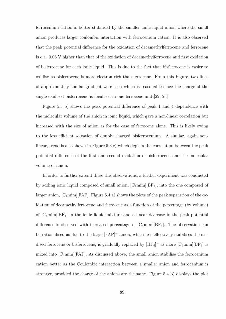
ferrocenium cation is better stabilised by the smaller ionic liquid anion where the small
anion produces larger coulombic interaction with ferrocenium cation. It is also observed
that the peak potential difference for the oxidation of decamethylferrocene and ferrocene
is c.a. 0.06 V higher than that of the oxidation of decamethylferrocene and first oxidation
of bisferrocene for each ionic liquid. This is due to the fact that bisferrocene is easier to
oxidise as bisferrocene is more electron rich than ferrocene. From this Figure, two lines
of approximately similar gradient were seen which is reasonable since the charge of the
single oxidised bisferrocene is localised in one ferrocene unit.[22, 23]
Figure 5.3 b) shows the peak potential difference of peak 1 and 4 dependence with
the molecular volume of the anion in ionic liquid, which gave a non-linear correlation but
increased with the size of anion as for the case of ferrocene alone. This is likely owing
to the less efficient solvation of doubly charged bisferrocenium. A similar, again non-
linear, trend is also shown in Figure 5.3 c) which depicts the correlation between the peak
potential difference of the first and second oxidation of bisferrocene and the molecular
volume of anion.
In order to further extend these this observations, a further experiment was conducted
by adding ionic liquid composed of small anion, [C4mim][BF4], into the one composed of
larger anion, [C4mim][FAP]. Figure 5.4 a) shows the plots of the peak separation of the ox-
idation of decamethylferrocene and ferrocene as a function of the percentage (by volume)
of [C4mim][BF4] in the ionic liquid mixture and a linear decrease in the peak potential
difference is observed with increased percentage of [C4mim][BF4]. The observation can
be rationalised as due to the large [FAP]− anion, which less effectively stabilises the oxi-
dised ferrocene or bisferrocene, is gradually replaced by [BF4]− as more [C4mim][BF4] is
mixed into [C4mim][FAP]. As discussed above, the small anion stabilise the ferrocenium
cation better as the Coulombic interaction between a smaller anion and ferrocenium is
stronger, provided the charge of the anions are the same. Figure 5.4 b) displays the plot
89
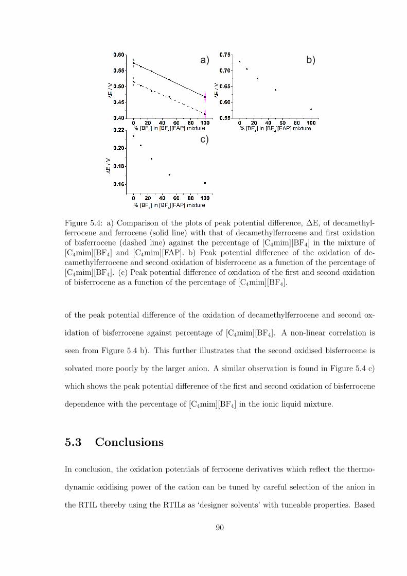
a)
c)
b)
Figure 5.4: a) Comparison of the plots of peak potential difference, ∆E, of decamethyl-ferrocene and ferrocene (solid line) with that of decamethylferrocene and first oxidationof bisferrocene (dashed line) against the percentage of [C4mim][BF4] in the mixture of[C4mim][BF4] and [C4mim][FAP]. b) Peak potential difference of the oxidation of de-camethylferrocene and second oxidation of bisferrocene as a function of the percentage of[C4mim][BF4]. (c) Peak potential difference of oxidation of the first and second oxidationof bisferrocene as a function of the percentage of [C4mim][BF4].
of the peak potential difference of the oxidation of decamethylferrocene and second ox-
idation of bisferrocene against percentage of [C4mim][BF4]. A non-linear correlation is
seen from Figure 5.4 b). This further illustrates that the second oxidised bisferrocene is
solvated more poorly by the larger anion. A similar observation is found in Figure 5.4 c)
which shows the peak potential difference of the first and second oxidation of bisferrocene
dependence with the percentage of [C4mim][BF4] in the ionic liquid mixture.
5.3 Conclusions
In conclusion, the oxidation potentials of ferrocene derivatives which reflect the thermo-
dynamic oxidising power of the cation can be tuned by careful selection of the anion in
the RTIL thereby using the RTILs as ‘designer solvents’ with tuneable properties. Based
90
upon fundamental studies on the analytical technique and the solvents property, elec-
trochemical sensors and sensing electrodes were developed as discussed in the following
chapters.
References
[1] Xiong, L.; Fletcher, A. M.; Davies, S. G.; Norman, S. E.; Hardacre, C.; Comp-ton, R. G. Chemical Communications 2012, 48, 5784–5786.
[2] Barrosse-Antle, L. E.; Bond, A. M.; Compton, R. G.; O’Mahony, A. M.; Rogers, E. I.;Silvester, D. S. Chemistry - An Asian Journal 2010, 5, 202–230.
[3] Buzzeo, M. C.; Hardacre, C.; Compton, R. G. Analytical Chemistry 2004, 76, 4583–4588.
[4] Rogers, E. I.; Huang, X.-J.; Dickinson, E. J. F.; Hardacre, C.; Compton, R. G.Journal of Physical Chemistry C 2009, 113, 17811–17823.
[5] Cui, G.; Wang, C.; Zheng, J.; Guo, Y.; Luo, X.; Li, H. Chemical Communications2012, 48, 2633–2635.
[6] Abbott, A. P.; Frisch, G.; Garrett, H.; Hartley, J. Chemical Communications 2011,47, 11876–11878.
[7] Lee, S.-G. Chemical Communications 2006, 1049–1063.
[8] Rogers, E. I.; Silvester, D. S.; Poole, D. L.; Aldous, L.; Hardacre, C.; Compton, R. G.Journal of Physical Chemistry C 2008, 112, 2729–2735.
[9] Torriero, A. A. J.; Howlett, P. C. Electrochemistry Communications 2012, 16, 84–87.
[10] Aranzaes, J. R.; Daniel, M.-C.; Astruc, D. Canadian Journal of Chemistry 2006, 84,288–299.
[11] O’Mahony, A. M.; Silvester, D. S.; Aldous, L.; Hardacre, C.; Compton, R. G. Journalof Chemical and Engineering Data 2008, 53, 2884–2891.
[12] Seddon, K. R.; Stark, A.; Torres, M.-J. Pure and Applied Chemistry 2000, 72, 2275–2287.
[13] Buzzeo, M.; Evans, R. G.; Compton, R. G. ChemPhysChem 2004, 5, 1106–1120.
[14] Ngo, H. L.; LeCompte, K.; Hargens, L.; McEwen, A. B. Thermochimica Acta 2000,357-358, 97–102.
[15] Bonhote, P.; Dias, A.-P.; Papageorgiou, N.; Kalyanasundaram, K.; Grtzel, M. Inor-ganic Chemistry 1996, 35, 1168–1178.
[16] Fu, C.; Aldous, L.; Dickinson, E. J. F.; Manan, N. S. A.; Compton, R. G. ChemicalCommunications 2011, 47, 7083–7085.
91
[17] Fu, C.; Aldous, L.; Dickinson, E. J. F.; Manan, N. S. A.; Compton, R. G. NewJournal of Chemistry 2012, 36, 774–780.
[18] Fu, C.; Aldous, L.; Dickinson, E. J. F.; Manan, N. S. A.; Compton, R. G.ChemPhysChem 2011, 12, 1708–1713.
[19] Compton, R. G.; Banks, C. E. Understanding Voltammetry ; Imperial College Press,2011, 2nd Edition.
[20] Bard, A. J.; Faulkner, L. R. Electrochemical Methods: Fundamentals and Applica-tions ; Wiley, 2001.
[21] Jacquemin, J.; Ge, R.; Nancarrow, P.; Rooney, D. W.; Costa Gomes, M. F.;Padua, A. A. H.; Hardacre, C. Journal of Chemical and Engineering Data 2008,53, 716–726.
[22] Zhang, Q.; Song, W.-L.; Showkot Hossain, A.; Liu, Z.-D.; Hu, G.-J.; Tian, Y.-P.;Wu, J.-Y.; Jin, B.-K.; Zhou, H.-P.; Yang, J.-X.; Zhang, S.-Y. Dalton Transactions2011, 40, 3510–3516.
[23] Arima, V.; Iurlo, M.; Zoli, L.; Kumar, S.; Piacenza, M.; Della Sala, F.; Matino, F.;Maruccio, G.; Rinaldi, R.; Paolucci, F.; Marcaccio, M.; Cozzi, P. G.; Bramanti, A. P.Nanoscale 2012, 4, 813–823.
92
Chapter 6
An electrochemical thermometer:Voltammetric measurement oftemperature and its application toamperometric gas sensing
Understanding the analytical technique and RTIL property is essential for improving
sensor design. This chapter demonstrates a temperature sensing system incorporated
into an amperometric oxygen sensor. In the first part of this work, we introduce temper-
ature sensing systems based upon voltammetric responses of both single molecule (1,2-
diferrocenyleththylene, bisferrocene, in 1-propyl-3-methylimidazolium bistrifluoromethyl-
sulfonylimide) and two independent molecules (decamethylferrocene and N,N,N’,N’-tetra-
methyl-p-phenylenediamine in 1-ethyl-3-methylimidazolium tetracyanoborate) respectively.
In both systems, the difference of formal potentials of two redox centres was measured as
a function of temperature. The former was recorded as the peak difference in square wave
voltammetry with the peak potential difference increases linearly with the increasing tem-
perature. In order to show proof-of-concept of voltammetric temperature measurement
in relation to a gas sensor, the latter system was investigated in the presence of oxygen,
where the concentration and diffusion coefficient of oxygen varied with temperature, as
well as the peak difference discussed previously, were studied in the presence of pure oxy-
93
gen and dried air using chronoamperometry. A negligible variation of concentration of
oxygen from both sources with temperature over the range 298 K to 318 K is demon-
strated. These results obtained from pure oxygen and dried air were compared and a c.a.
79 % drop of cathodic signal from pure oxygen to dried air was found which is consistent
with the percentage of oxygen in air. The diffusion coefficient of oxygen was related to
temperature using an Arrhenius plot , yielding a linear graph with high correlation. All
experiments gave a high reproducibility. The work presented here has been published in
the Analyst [1].
6.1 Introduction
The attraction of electrochemical sensors is discussed in Chapter 2. For all types of
electrochemical sensors, the detection depends on a Faradaic electron transfer event at a
solute-electrode interface driven by an applied potential and the resulting current gives
the sought analytical signal. Electrode processes are highly sensitive to temperature
because of thermodynamic (formal potential) and kinetic (electrochemical rate constant,
diffusion coefficient) features. The temperature dependent gas detection are detailed in
Section 2.4.2 in Chapter 2. That said it is not always possible to deploy many practical
amperometric sensors under thermostatted conditions. It is desirable in some situations
to build-in a voltammetric measurement of the operating temperature - measured at the
electrodes solution interface - so as to provide a validity and/or accuracy check. In this
chapter we propose the use of a molecule containing two redox centres with different
formal potentials which gives rise to two distinct voltammetric signals:
(A−B)− e− (A+ −B), E0f,a (6.1)
94
(A+ − B)− e− (A+ − B+), E0f,b (6.2)
which may be oxidative (as above) or reductive in character. If the electron trans-
fers are fast (relative to prevalent mass transport) then the observed voltammetry will
be electrochemically reversible in character and the temperature dependence of the two
formal potentials, Ef,a and Ef,b, will be related to the entropy change associated with the
electrochemical process via,
F(∂E0
f )
∂T= ∆S (6.3)
If the temperature dependence of the two formal potentials is different then the two
voltammetric peaks will not only appear at different potentials at two different temper-
atures but the difference in the potentials of the two peaks, Ef,a − Ef,b, for reversible
electron transfer, will also vary with temperature. Accordingly the measurement of the
difference of the two voltammetric peak potentials allows the measurement of tempera-
ture. In the following we will show that this difference can be measured with sufficient
accuracy to realise the reliable measurement of temperature. In particular, we study the
system
A− B ≡ Cp− Fe− C5H4 − (CH = CH)−H4C5 − Fe− Cp (6.4)
on a room temperature ionic liquid solvent (RTIL) and show that the value of (∂Ef,a/∂T−
∂Ef,b/∂T ) = 0.198mV/K over the temperature range of 298 K to 318 K. Note that the
benefits in the use of RTILs for solvents in gas sensing has been discussed elsewhere.[14]
We further study a system where the different molecules, A and B are used for an equiv-
95
alent measurement,
A− e− A+ E0f,a (6.5)
B − e− B+ E0f,b (6.6)
and consider the molecules decamethylferrocene and N,N,N’,N’-tetramethylphenylene-
diamine again in a room temperature ionic liquid solvent. In these cases much larger dif-
ference in the temperature coefficients of the peak potential are seen. The latter system
is used to calibrate the temperature in a series of experiments in which the chronoamper-
ometry of the one electron reduction of oxygen to superoxide in the RTIL,
O2 + e− O−2 (6.7)
is studied so as to find the solubility of the gas and the diffusion coefficient of O2 as
a function of temperature, thus providing proof-of-concept of measurement scenarios in
amperometric gas sensors, and providing proof-of-concept of the use of a voltammetric
thermometer.
6.2 Chronoamperometric Experiments
The chronoamperometric experiments adopted the methods described in Chapter 4 Sec-
tion 4.2. Due to the fact that this experiment was carried out at different system, a longer
pre-equilibration time, 300 s, is needed to reach oxygen saturation in ionic liquids. The
following methods were applied. Chronoamperometric transients were recorded using a
sample time of 0.001 s. The potential was stepped from 0 V vs. Ag to -2.0 V vs. Ag,
and the current was measured for 0.5 s. To obtain concentration and diffusion coefficient
of oxygen, the Shoup and Szabo equation (see Equation 4.1 in Chapter 4) was used to fit
96
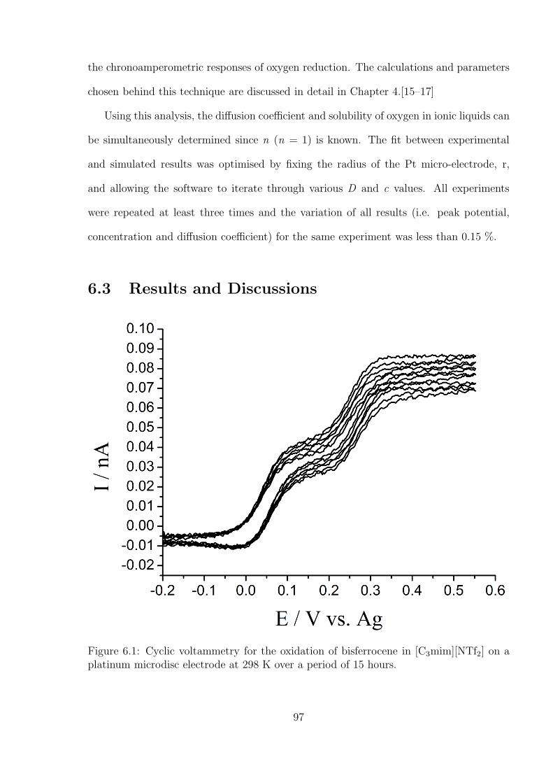
the chronoamperometric responses of oxygen reduction. The calculations and parameters
chosen behind this technique are discussed in detail in Chapter 4.[15–17]
Using this analysis, the diffusion coefficient and solubility of oxygen in ionic liquids can
be simultaneously determined since n (n = 1) is known. The fit between experimental
and simulated results was optimised by fixing the radius of the Pt micro-electrode, r,
and allowing the software to iterate through various D and c values. All experiments
were repeated at least three times and the variation of all results (i.e. peak potential,
concentration and diffusion coefficient) for the same experiment was less than 0.15 %.
6.3 Results and Discussions
Figure 6.1: Cyclic voltammetry for the oxidation of bisferrocene in [C3mim][NTf2] on aplatinum microdisc electrode at 298 K over a period of 15 hours.
97
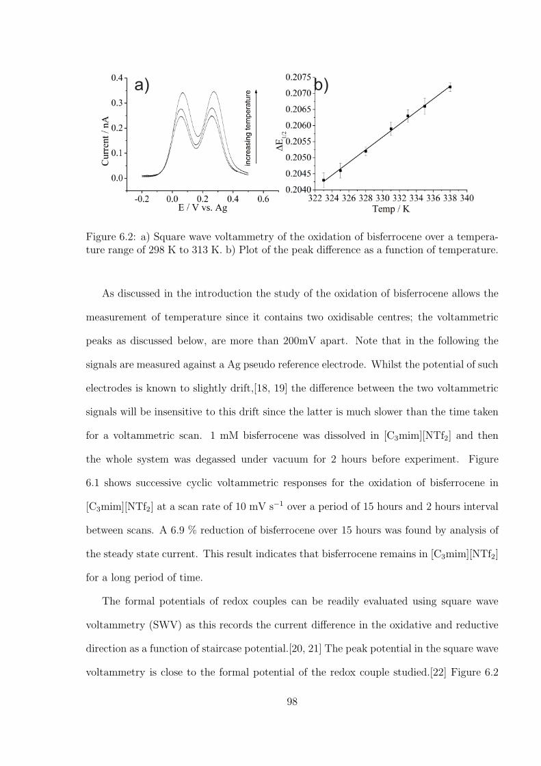
a) b)
Figure 6.2: a) Square wave voltammetry of the oxidation of bisferrocene over a tempera-ture range of 298 K to 313 K. b) Plot of the peak difference as a function of temperature.
As discussed in the introduction the study of the oxidation of bisferrocene allows the
measurement of temperature since it contains two oxidisable centres; the voltammetric
peaks as discussed below, are more than 200mV apart. Note that in the following the
signals are measured against a Ag pseudo reference electrode. Whilst the potential of such
electrodes is known to slightly drift,[18, 19] the difference between the two voltammetric
signals will be insensitive to this drift since the latter is much slower than the time taken
for a voltammetric scan. 1 mM bisferrocene was dissolved in [C3mim][NTf2] and then
the whole system was degassed under vacuum for 2 hours before experiment. Figure
6.1 shows successive cyclic voltammetric responses for the oxidation of bisferrocene in
[C3mim][NTf2] at a scan rate of 10 mV s−1 over a period of 15 hours and 2 hours interval
between scans. A 6.9 % reduction of bisferrocene over 15 hours was found by analysis of
the steady state current. This result indicates that bisferrocene remains in [C3mim][NTf2]
for a long period of time.
The formal potentials of redox couples can be readily evaluated using square wave
voltammetry (SWV) as this records the current difference in the oxidative and reductive
direction as a function of staircase potential.[20, 21] The peak potential in the square wave
voltammetry is close to the formal potential of the redox couple studied.[22] Figure 6.2
98
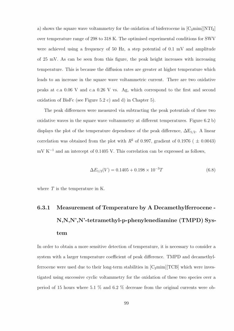
a) shows the square wave voltammetry for the oxidation of bisferrocene in [C3mim][NTf2]
over temperature range of 298 to 318 K. The optimised experimental conditions for SWV
were achieved using a frequency of 50 Hz, a step potential of 0.1 mV and amplitude
of 25 mV. As can be seen from this figure, the peak height increases with increasing
temperature. This is because the diffusion rates are greater at higher temperature which
leads to an increase in the square wave voltammetric current. There are two oxidative
peaks at c.a 0.06 V and c.a 0.26 V vs. Ag, which correspond to the first and second
oxidation of BisFc (see Figure 5.2 c) and d) in Chapter 5).
The peak differences were measured via subtracting the peak potentials of these two
oxidative waves in the square wave voltammetry at different temperatures. Figure 6.2 b)
displays the plot of the temperature dependence of the peak difference, ∆E1/2. A linear
correlation was obtained from the plot with R2 of 0.997, gradient of 0.1976 ( ± 0.0043)
mV K−1 and an intercept of 0.1405 V. This correlation can be expressed as follows,
∆E1/2(V ) = 0.1405 + 0.198× 10⁻³T (6.8)
where T is the temperature in K.
6.3.1 Measurement of Temperature by A Decamethylferrocene -
N,N,N’,N’-tetramethyl-p-phenylenediamine (TMPD) Sys-
tem
In order to obtain a more sensitive detection of temperature, it is necessary to consider a
system with a larger temperature coefficient of peak difference. TMPD and decamethyl-
ferrocene were used due to their long-term stabilities in [C2mim][TCB] which were inves-
tigated using successive cyclic voltammetry for the oxidation of these two species over a
period of 15 hours where 5.1 % and 6.2 % decrease from the original currents were ob-
99
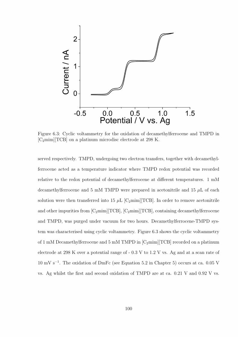
Figure 6.3: Cyclic voltammetry for the oxidation of decamethylferrocene and TMPD in[C2mim][TCB] on a platinum microdisc electrode at 298 K.
served respectively. TMPD, undergoing two electron transfers, together with decamethyl-
ferrocene acted as a temperature indicator where TMPD redox potential was recorded
relative to the redox potential of decamethylferrocene at different temperatures. 1 mM
decamethylferrocene and 5 mM TMPD were prepared in acetonitrile and 15 µL of each
solution were then transferred into 15 µL [C2mim][TCB]. In order to remove acetonitrile
and other impurities from [C2mim][TCB], [C2mim][TCB], containing decamethylferrocene
and TMPD, was purged under vacuum for two hours. Decamethylferrocene-TMPD sys-
tem was characterised using cyclic voltammetry. Figure 6.3 shows the cyclic voltammetry
of 1 mM Decamethylferrocene and 5 mM TMPD in [C2mim][TCB] recorded on a platinum
electrode at 298 K over a potential range of - 0.3 V to 1.2 V vs. Ag and at a scan rate of
10 mV s−1. The oxidation of DmFc (see Equation 5.2 in Chapter 5) occurs at ca. 0.05 V
vs. Ag whilst the first and second oxidation of TMPD are at ca. 0.21 V and 0.92 V vs.
100
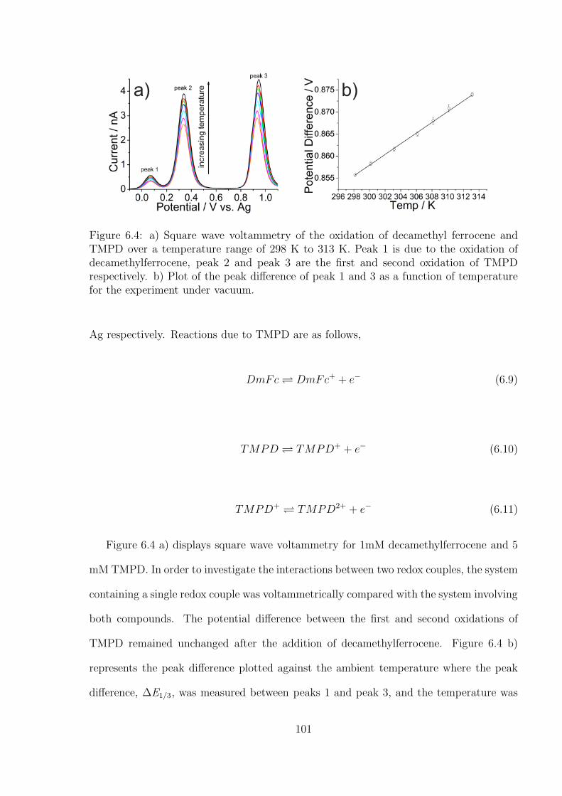
a) b)
Figure 6.4: a) Square wave voltammetry of the oxidation of decamethyl ferrocene andTMPD over a temperature range of 298 K to 313 K. Peak 1 is due to the oxidation ofdecamethylferrocene, peak 2 and peak 3 are the first and second oxidation of TMPDrespectively. b) Plot of the peak difference of peak 1 and 3 as a function of temperaturefor the experiment under vacuum.
Ag respectively. Reactions due to TMPD are as follows,
DmFc DmFc+ + e− (6.9)
TMPD TMPD+ + e− (6.10)
TMPD+ TMPD2+ + e− (6.11)
Figure 6.4 a) displays square wave voltammetry for 1mM decamethylferrocene and 5
mM TMPD. In order to investigate the interactions between two redox couples, the system
containing a single redox couple was voltammetrically compared with the system involving
both compounds. The potential difference between the first and second oxidations of
TMPD remained unchanged after the addition of decamethylferrocene. Figure 6.4 b)
represents the peak difference plotted against the ambient temperature where the peak
difference, ∆E1/3, was measured between peaks 1 and peak 3, and the temperature was
101
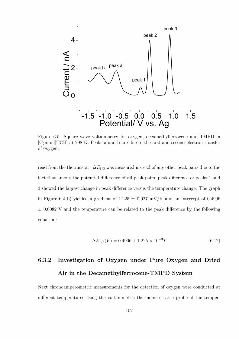
Figure 6.5: Square wave voltammetry for oxygen, decamethylferrocene and TMPD in[C2mim][TCB] at 298 K. Peaks a and b are due to the first and second electron transferof oxygen.
read from the thermostat. ∆E1/3 was measured instead of any other peak pairs due to the
fact that among the potential difference of all peak pairs, peak difference of peaks 1 and
3 showed the largest change in peak difference versus the temperature change. The graph
in Figure 6.4 b) yielded a gradient of 1.225 ± 0.027 mV/K and an intercept of 0.4906
± 0.0082 V and the temperature can be related to the peak difference by the following
equation:
∆E1/3(V ) = 0.4906 + 1.225× 10⁻³T (6.12)
6.3.2 Investigation of Oxygen under Pure Oxygen and Dried
Air in the Decamethylferrocene-TMPD System
Next chronoamperometric measurements for the detection of oxygen were conducted at
different temperatures using the voltammetric thermometer as a probe of the temper-
102
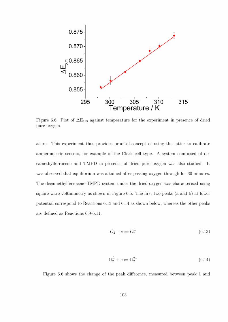
Figure 6.6: Plot of ∆E1/3 against temperature for the experiment in presence of driedpure oxygen.
ature. This experiment thus provides proof-of-concept of using the latter to calibrate
amperometric sensors, for example of the Clark cell type. A system composed of de-
camethylferrocene and TMPD in presence of dried pure oxygen was also studied. It
was observed that equilibrium was attained after passing oxygen through for 30 minutes.
The decamethylferrocene-TMPD system under the dried oxygen was characterised using
square wave voltammetry as shown in Figure 6.5. The first two peaks (a and b) at lower
potential correspond to Reactions 6.13 and 6.14 as shown below, whereas the other peaks
are defined as Reactions 6.9-6.11.
O2 + e O−2 (6.13)
O−2 + e O2−
2 (6.14)
Figure 6.6 shows the change of the peak difference, measured between peak 1 and
103
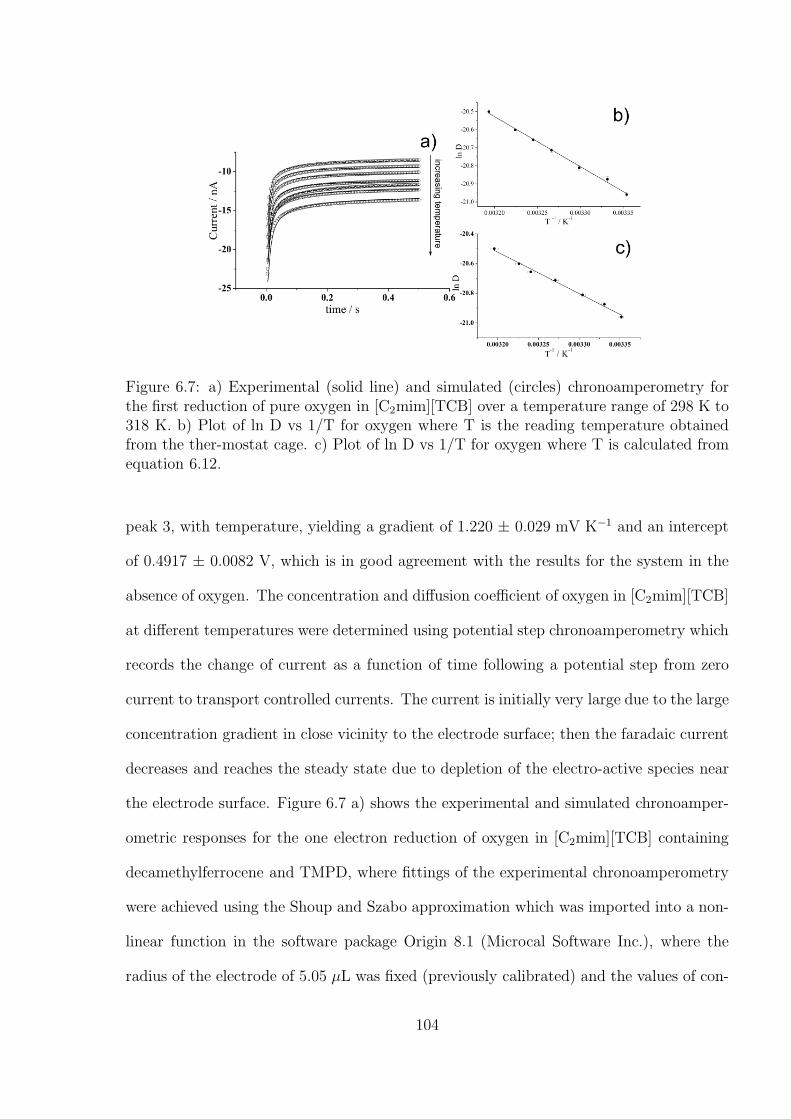
Figure 6.7: a) Experimental (solid line) and simulated (circles) chronoamperometry forthe first reduction of pure oxygen in [C2mim][TCB] over a temperature range of 298 K to318 K. b) Plot of ln D vs 1/T for oxygen where T is the reading temperature obtainedfrom the ther-mostat cage. c) Plot of ln D vs 1/T for oxygen where T is calculated fromequation 6.12.
peak 3, with temperature, yielding a gradient of 1.220 ± 0.029 mV K−1 and an intercept
of 0.4917 ± 0.0082 V, which is in good agreement with the results for the system in the
absence of oxygen. The concentration and diffusion coefficient of oxygen in [C2mim][TCB]
at different temperatures were determined using potential step chronoamperometry which
records the change of current as a function of time following a potential step from zero
current to transport controlled currents. The current is initially very large due to the large
concentration gradient in close vicinity to the electrode surface; then the faradaic current
decreases and reaches the steady state due to depletion of the electro-active species near
the electrode surface. Figure 6.7 a) shows the experimental and simulated chronoamper-
ometric responses for the one electron reduction of oxygen in [C2mim][TCB] containing
decamethylferrocene and TMPD, where fittings of the experimental chronoamperometry
were achieved using the Shoup and Szabo approximation which was imported into a non-
linear function in the software package Origin 8.1 (Microcal Software Inc.), where the
radius of the electrode of 5.05 µL was fixed (previously calibrated) and the values of con-
104
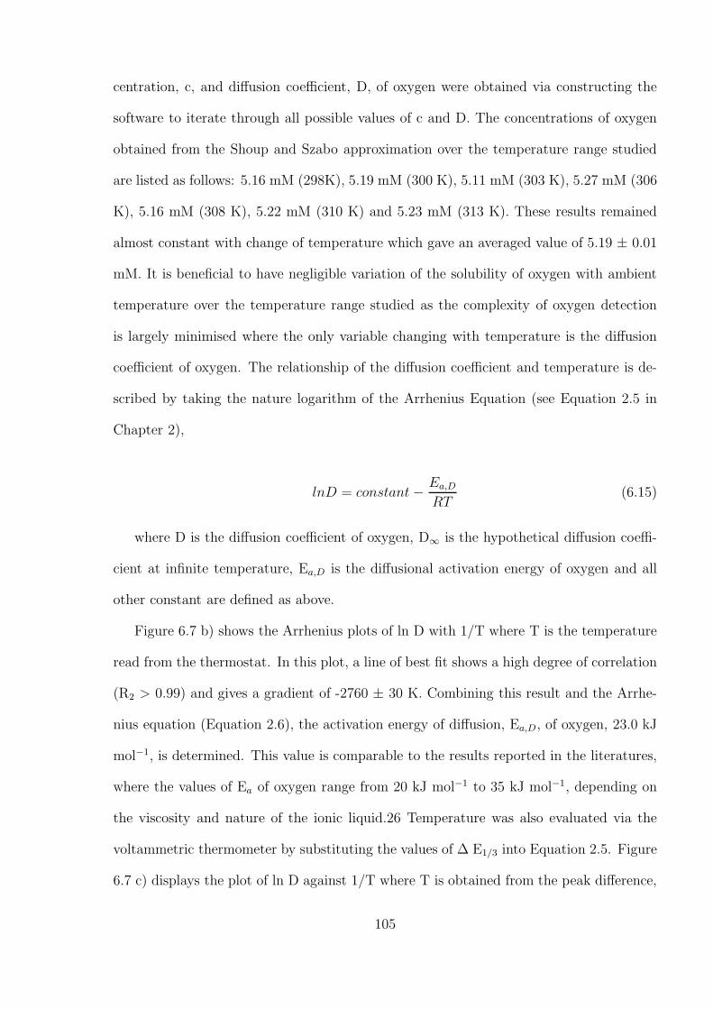
centration, c, and diffusion coefficient, D, of oxygen were obtained via constructing the
software to iterate through all possible values of c and D. The concentrations of oxygen
obtained from the Shoup and Szabo approximation over the temperature range studied
are listed as follows: 5.16 mM (298K), 5.19 mM (300 K), 5.11 mM (303 K), 5.27 mM (306
K), 5.16 mM (308 K), 5.22 mM (310 K) and 5.23 mM (313 K). These results remained
almost constant with change of temperature which gave an averaged value of 5.19 ± 0.01
mM. It is beneficial to have negligible variation of the solubility of oxygen with ambient
temperature over the temperature range studied as the complexity of oxygen detection
is largely minimised where the only variable changing with temperature is the diffusion
coefficient of oxygen. The relationship of the diffusion coefficient and temperature is de-
scribed by taking the nature logarithm of the Arrhenius Equation (see Equation 2.5 in
Chapter 2),
lnD = constant− Ea,D
RT(6.15)
where D is the diffusion coefficient of oxygen, D∞ is the hypothetical diffusion coeffi-
cient at infinite temperature, Ea,D is the diffusional activation energy of oxygen and all
other constant are defined as above.
Figure 6.7 b) shows the Arrhenius plots of ln D with 1/T where T is the temperature
read from the thermostat. In this plot, a line of best fit shows a high degree of correlation
(R2 > 0.99) and gives a gradient of -2760 ± 30 K. Combining this result and the Arrhe-
nius equation (Equation 2.6), the activation energy of diffusion, Ea,D, of oxygen, 23.0 kJ
mol−1, is determined. This value is comparable to the results reported in the literatures,
where the values of Ea of oxygen range from 20 kJ mol−1 to 35 kJ mol−1, depending on
the viscosity and nature of the ionic liquid.26 Temperature was also evaluated via the
voltammetric thermometer by substituting the values of ∆ E1/3 into Equation 2.5. Figure
6.7 c) displays the plot of ln D against 1/T where T is obtained from the peak difference,
105
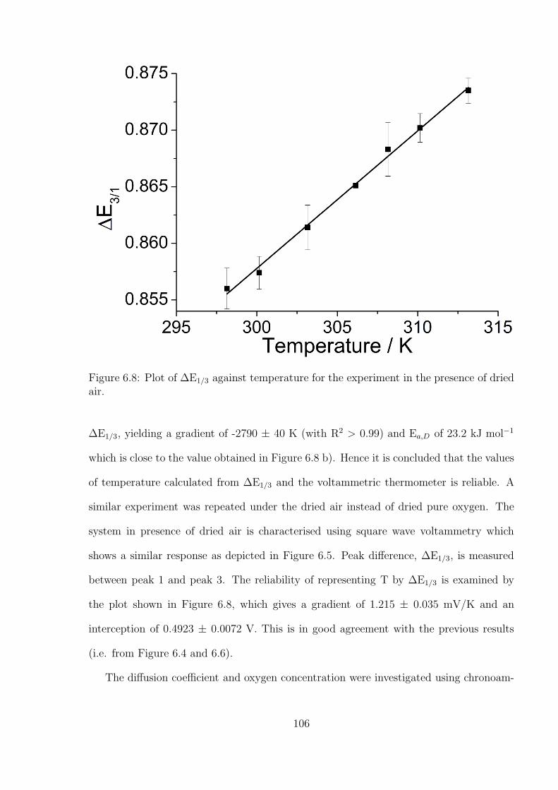
Figure 6.8: Plot of ∆E1/3 against temperature for the experiment in the presence of driedair.
∆E1/3, yielding a gradient of -2790 ± 40 K (with R2 > 0.99) and Ea,D of 23.2 kJ mol−1
which is close to the value obtained in Figure 6.8 b). Hence it is concluded that the values
of temperature calculated from ∆E1/3 and the voltammetric thermometer is reliable. A
similar experiment was repeated under the dried air instead of dried pure oxygen. The
system in presence of dried air is characterised using square wave voltammetry which
shows a similar response as depicted in Figure 6.5. Peak difference, ∆E1/3, is measured
between peak 1 and peak 3. The reliability of representing T by ∆E1/3 is examined by
the plot shown in Figure 6.8, which gives a gradient of 1.215 ± 0.035 mV/K and an
interception of 0.4923 ± 0.0072 V. This is in good agreement with the previous results
(i.e. from Figure 6.4 and 6.6).
The diffusion coefficient and oxygen concentration were investigated using chronoam-
106
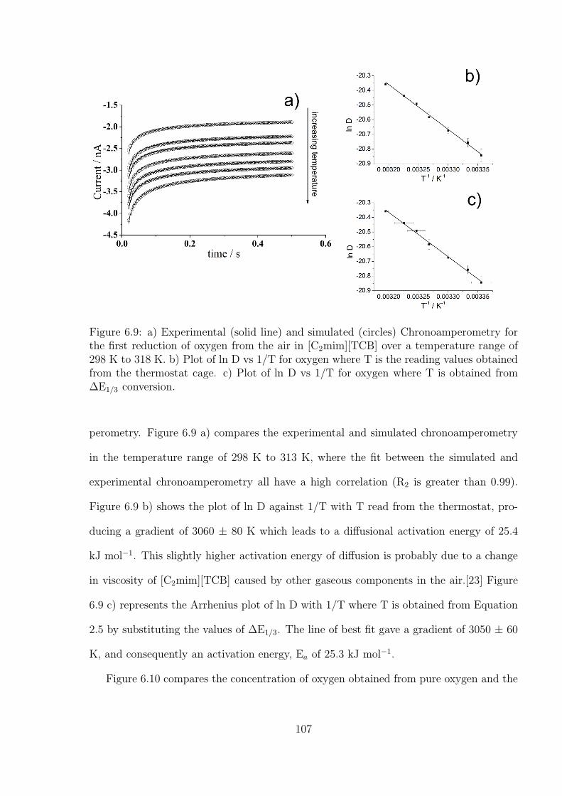
Figure 6.9: a) Experimental (solid line) and simulated (circles) Chronoamperometry forthe first reduction of oxygen from the air in [C2mim][TCB] over a temperature range of298 K to 318 K. b) Plot of ln D vs 1/T for oxygen where T is the reading values obtainedfrom the thermostat cage. c) Plot of ln D vs 1/T for oxygen where T is obtained from∆E1/3 conversion.
perometry. Figure 6.9 a) compares the experimental and simulated chronoamperometry
in the temperature range of 298 K to 313 K, where the fit between the simulated and
experimental chronoamperometry all have a high correlation (R2 is greater than 0.99).
Figure 6.9 b) shows the plot of ln D against 1/T with T read from the thermostat, pro-
ducing a gradient of 3060 ± 80 K which leads to a diffusional activation energy of 25.4
kJ mol−1. This slightly higher activation energy of diffusion is probably due to a change
in viscosity of [C2mim][TCB] caused by other gaseous components in the air.[23] Figure
6.9 c) represents the Arrhenius plot of ln D with 1/T where T is obtained from Equation
2.5 by substituting the values of ∆E1/3. The line of best fit gave a gradient of 3050 ± 60
K, and consequently an activation energy, Ea of 25.3 kJ mol−1.
Figure 6.10 compares the concentration of oxygen obtained from pure oxygen and the
107
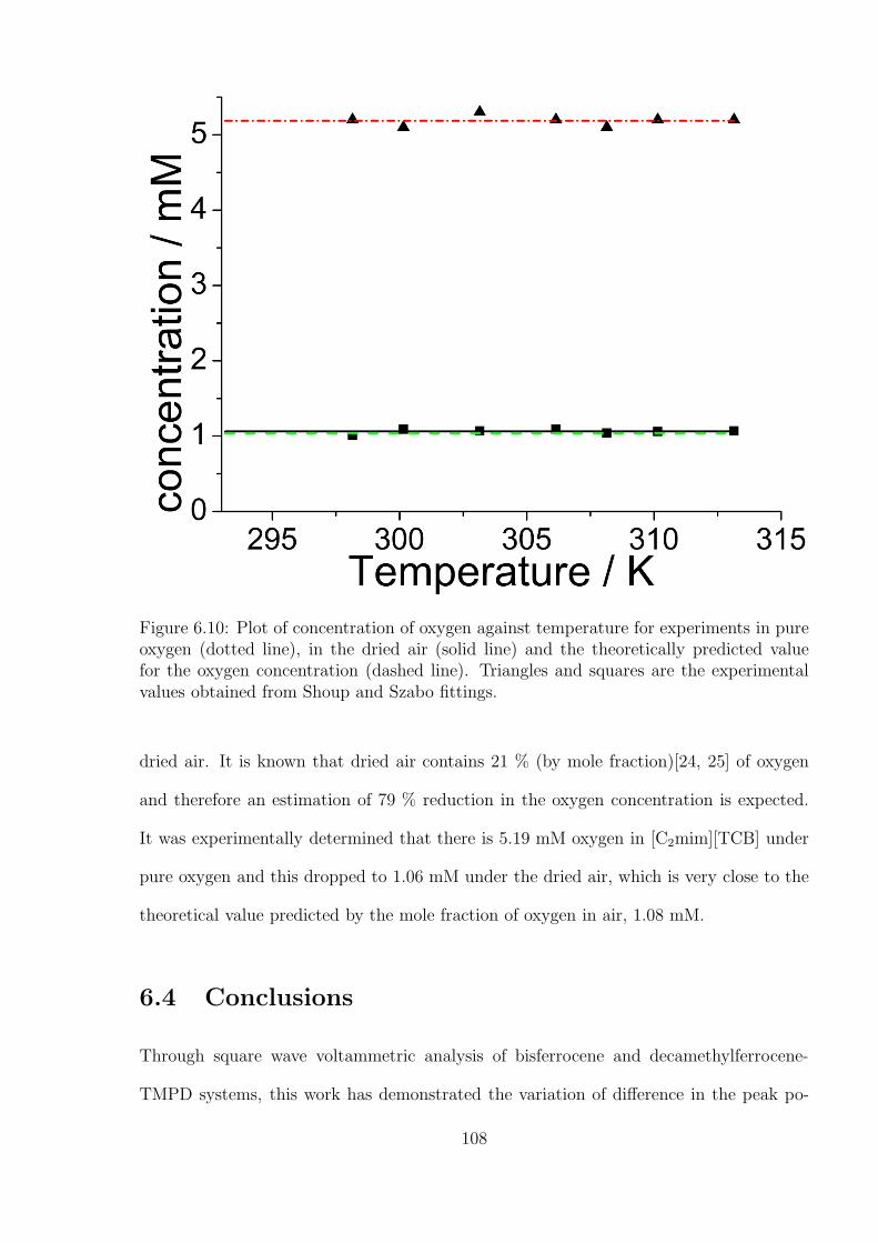
Figure 6.10: Plot of concentration of oxygen against temperature for experiments in pureoxygen (dotted line), in the dried air (solid line) and the theoretically predicted valuefor the oxygen concentration (dashed line). Triangles and squares are the experimentalvalues obtained from Shoup and Szabo fittings.
dried air. It is known that dried air contains 21 % (by mole fraction)[24, 25] of oxygen
and therefore an estimation of 79 % reduction in the oxygen concentration is expected.
It was experimentally determined that there is 5.19 mM oxygen in [C2mim][TCB] under
pure oxygen and this dropped to 1.06 mM under the dried air, which is very close to the
theoretical value predicted by the mole fraction of oxygen in air, 1.08 mM.
6.4 Conclusions
Through square wave voltammetric analysis of bisferrocene and decamethylferrocene-
TMPD systems, this work has demonstrated the variation of difference in the peak po-
108
tentials for two redox centres with temperature, which showed temperature coefficients
of 0.20 mV K−1 and 1.20 mV K−1 respectively. This temperature sensing system has
been incorporated into a model oxygen sensor via investigating the latter system in the
presence of oxygen either as pure oxygen or in dried air. It has been observed that the
solubility of oxygen does not vary with temperature over the temperature range studied
and c.a. 79 % reduction of oxygen concentration from pure oxygen to dried air is in
close agreement with the oxygen composition in air. Diffusion coefficient of oxygen has
been studied as a function of temperature via an Arrhenius plot, which can be further
related to the peak difference discussed previously. All experiments have presented high
reproducibility and a correlation of more than 0.99 has indicated a high sensitivity to-
wards sensing temperature. Further to this design, the next chapter shows a simultaneous
humidity and temperature sensor.
References
[1] Xiong, L.; Fletcher, A. M.; Ernst, S.; Davies, S. G.; Compton, R. G. The Analyst2012, 137, 2567–2573.
[2] Hanrahan, G.; Patil, D.; Wang, J. Journal of Environmental Monitoring 2004, 6,657–664.
[3] Wang, J. Analytical Electrochemistry ; Wiley-VCH, New York, 1994.
[4] Metters, J.; Kadara, R.; Banks, C. Analyst 2011, 136, 1067–1076.
[5] Heller, A.; Feldman, B. Chemical Reviews 2008, 108, 2482–2505.
[6] Clark Jr., L. C.; Lyons, C. Annals of the New York Academy of Sciences 1962, 102,29–45.
[7] Clark Jr., L. C. Transactions - American Society for Artificial Internal Organs 1956,2, 41–48.
[8] Tierney, M. J.; Kim, H.-O. L. Analytical Chemistry 1993, 65, 3435–3440.
[9] Horn, J. J.; McCreedy, T.; Wadhawan, J. Analytical Methods 2010, 2, 1346–1354.
[10] Compton, R. G.; Northing, R. J. Journal of the Chemical Society, Faraday Transac-tions 1990, 86, 1077–1081.
109

[11] Nei, L.; Compton, R. G. Sensors and Actuators, B: Chemical 1996, 30, 83–87.
[12] Lawrence, N. S.; Jiang, L.; Jones, T. G. J.; Compton, R. G. Analytical Chemistry2003, 75, 2499–2503.
[13] Chevallier, F. G.; Davies, T. J.; Klymenko, O. V.; Jiang, L.; Jones, T. G. J.; Comp-ton, R. G. Journal of Electroanalytical Chemistry 2005, 577, 211–221.
[14] Buzzeo, M. C.; Evans, R. G.; Compton, R. G. ChemPhysChem 2004, 5, 1106–1120.
[15] Paddon, C. A.; Silvester, D. S.; Bhatti, F. L.; Donohoe, T. J.; Compton, R. G.Electroanalysis 2007, 19, 11–22.
[16] Xiong, L.; Aldous, L.; Henstridge, M. C.; Compton, R. G. Analytical Methods 2012,4, 371–376.
[17] Klymenko, O. V.; Evans, R. G.; Hardacre, C.; Svir, I. B.; Compton, R. G. Journalof Electroanalytical Chemistry 2004, 571, 211–221.
[18] Rogers, E. I.; Silvester, D. S.; Poole, D. L.; Aldous, L.; Hardacre, C.; Compton, R. G.Journal of Physical Chemistry C 2008, 112, 2729–2735.
[19] Bott, A. W. Current Separations 1995, 14, 64–68.
[20] Compton, R. G.; Banks, C. E. Understanding Voltammetry ; Imperial College Press,2011, 2nd Edition.
[21] Bard, A. J.; Faulkner, L. R. Electrochemical Methods: Fundamentals and Applica-tions ; Wiley, 2001.
[22] Brett, C. M. A.; Brett, A. M. O. Electrochemistry: Principles, Methods, and Appli-cations ; Oxford Science Publications; Oxford University Press, Incorporated, 1993.
[23] Barrosse-Antle, L. E.; Aldous, L.; Hardacre, C.; Bond, A. M.; Compton, R. G.Journal of Physical Chemistry C 2009, 113, 7750–7754.
[24] Jacob, D. Introduction to Atmospheric Chemistry ; Princeton University Press, 1999.
[25] Levine, I. N. Physical Chemistry (Sie); McGraw-Hill Education (India) Pvt Limited,2007.
110
Chapter 7
A simultaneous voltammetrictemperature and humidity sensor
This chapter reports the simultaneous measurement of temperature and humidity by
analysing the square wave voltammetric responses of two ferrocene derivatives, DmFc
and BisFc in 1-(2-methoxyethyl)-1-methyl-pyrrolidinium tris(pentafluoroethyl)trifluoro-
phosphate ([Moepyrr][FAP]). These two molecules produce three peaks in square wave
voltammetry. Through study of the peak potentials of BisFc/BisFc+ (vs. DmFc/DmFc+)
and BisFc+/BisFc2+ (vs. DmFc/DmFc+) over a temperature range of 298 K to 318 K
and humidity range of 1 % to 50 % using square wave voltammetry, the temperature
and humidity dependences of the relative peak potentials were investigated. A reliable
method to calculate the humidity and temperature based on the voltammetric experiment
is characterised and demonstrated. The work presented here has been published in the
Analyst.[1]
7.1 Introduction
Chapter 6 demonstrated how temperature changes influence the sensing system and pro-
posed an in situ voltammetric thermometer to accurately calibrate the local temperature
at the electrode. Apart from the impact of temperature on the sensing system, the sensi-
tivity and accuracy of electrochemical sensors may also be affected by humidity due to the
nature of electron transfer and mass transport. Changes of the temperature or humidity
111
in the surroundings are important to monitor not only in their own right but also because
they can indirectly influence the measurement of other properties including the quantifi-
cation of chemical species. One approach to this problem is to build independent sensors
to monitor the temperature and humidity into other analytical probes. The benefits of
this approach are expected to be high in the area of gas sensing.
In this chapter, we propose a method to direct detect temperature and humidity at the
electrode solution interface, providing electrochemical temperature and humidity sensing
in their own right or, more likely, a sensing approach for immediate integration with other
voltammetric sensing. This proposed sensor is voltammetrically based and measures the
temperature and humidity via formal potentials. The formal potential dependence on
temperature is related to the entropy change of the redox process in an electrochemical
reaction,[2] and a temperature sensor has been developed according to this principle.[3]
Building on our success in monitoring temperature using differences in formal potentials
of two redox couples, we now develop this method in the current work to simultaneously
measure the two quantities, temperature and humidity. This requires two independent
formal potential measurements to be made. Furthermore, to simplify ease of measurement,
efforts are made to select species such that the temperature dependent pair is humidity
independent and vice versa. Chapter 5 has shown that change in solvation leads to changes
in the formal potential,[4] in part under using DmFc and BisFc in a room temperature
ionic liquid (RTIL). RTILs are purely composed of ions and exists as a liquid around room
temperature; their benefits in electrochemistry have been frequently disscussed. Literature
studies also demonstrate the influence of solvent humidity on solvation properties.[5, 6]
1-(2-Methoxyethyl)-1-methyl-pyrrolidinium tris(pentafluoroethyl)trifluorophosphate, is
a highly viscous RTIL, and its conductivity and viscosity change dramatically with the
humidity.[4] This is explored utilised in the work described below.
112
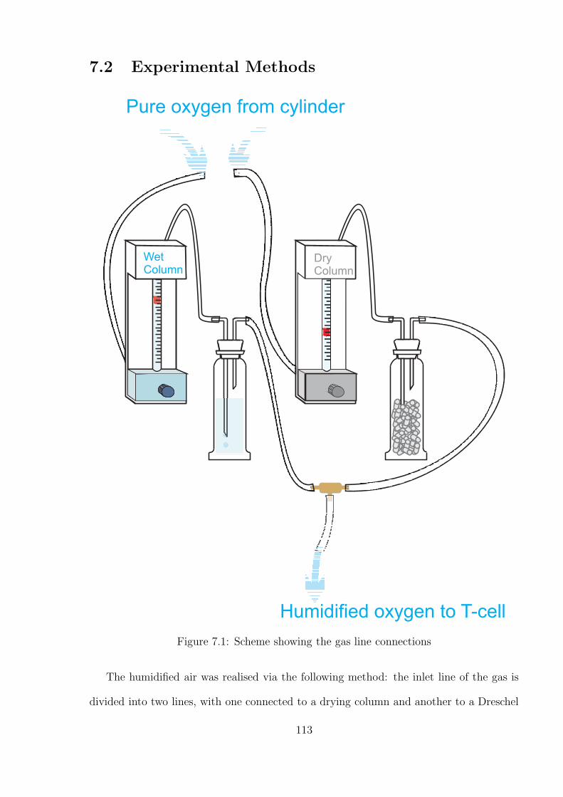
7.2 Experimental Methods
WetColumn
DryColumn
Pure oxygen from cylinder
Humidified oxygen to T-cell
Figure 7.1: Scheme showing the gas line connections
The humidified air was realised via the following method: the inlet line of the gas is
divided into two lines, with one connected to a drying column and another to a Dreschel
113
bottle which is filled with deionised water. These two lines then emerge into a common
outlet line, which allows the gas to flow into the T-cell. The humidity is controlled by the
flow meters in the dry and wet line respectively. The line connection is shown in Figure
7.1. The drying column consists of concentrated silica and solid calcium chloride. Before
the electrochemical measurements, gas was run for at least 15 hours to ensure equilibrium
was established. For experiments excluding gases, the ionic liquid was constantly purged
under vacuum during experimental analysis. The values of humidity were recorded using
an ADC-16 pico-logger (Honeywell, UK). The relative humidity, RH%, is described using
the equation below,[7]
RH(%) =ewe∗w
× 100 (7.1)
where ew is the partial pressure of water vapour (H2O) in the mixture and e∗w is the
saturated vapour pressure of water at a prescribed temperature. The variation of humidity
during an experiment was no more than 1 % RH. All experiments were repeated at least
three times and the variation of all results (i.e. peak potential) for the same experiment
was less than 3 mV which was calculated using standard deviations from at least three
sets of experiments under the same experimental conditions.
7.3 Results and Discussion
7.3.1 Choice of Probes for Temperature and Humidity Mea-
surements
In this paper, we study the following oxidative redox reactions in different ionic liquids.
DmFc DmFc+ + e (7.2)
114
Cp−Fe−C5H4−(CH = CH)−H4C5−Fe−Cp Cp−Fe+−C5H4−(CH = CH)−H4C5−Fe−Cp+e
(7.3)
Cp−Fe+−C5H4−(CH = CH)−H4C5−Fe−Cp Cp−Fe+−C5H4−(CH = CH)−H4C5−Fe+−Cp+e
(7.4)
Fc Fc+ + e (7.5)
where Fc is ferrocene, DmFc is DmFc and each redox reaction is associated with a
formal potential Ef,1, Ef,2, Ef,3 and Ef,4 respectively. See also Figure 5.2 for structures.
The following differences in formal potential are investigated adopting the notations given,
∆E1/2 = Ef,2 −Ef,1 (7.6)
∆E1/3 = Ef,3 −Ef,1 (7.7)
∆E2/3 = Ef,3 −Ef,2 (7.8)
∆E1/4 = Ef,4 −Ef,1 (7.9)
In the experiments to be reported, the peak potential difference of two redox centres is
measured to avoid the need for a stable reference electrode[3] and hence the choice of redox
probes is critical. DmFc shows many interesting electrochemical properties as compared to
other ferrocene derivatives, one of which as being relative insensitive to solute composition
makes it a very useful redox standard,[8] especially in the present humidity study. On
the other hand, previous work indicates that the first and second oxidation potential of
BisFc can be tuned by varying the anion component of ionic liquid.[4] As the change in
humidity alters the composition of ionic liquid the peak potential differences of BisFc
and DmFc may allow us to measure the humidity of air. These systems were accordingly
115
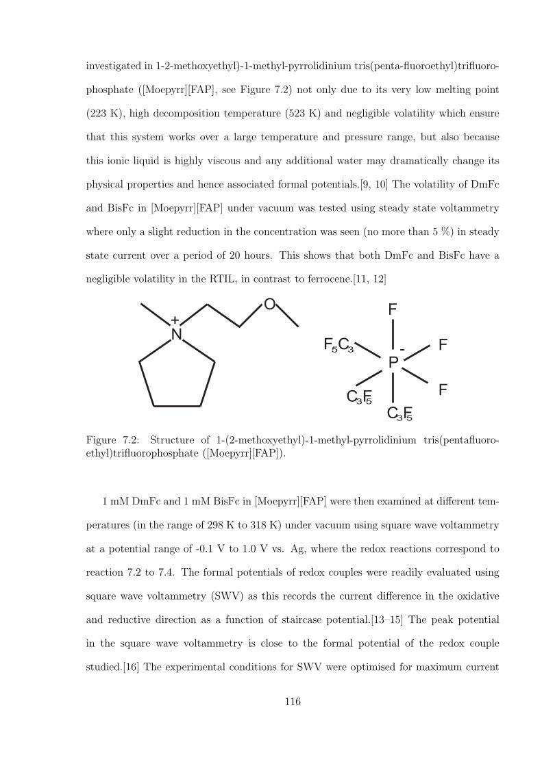
investigated in 1-2-methoxyethyl)-1-methyl-pyrrolidinium tris(penta-fluoroethyl)trifluoro-
phosphate ([Moepyrr][FAP], see Figure 7.2) not only due to its very low melting point
(223 K), high decomposition temperature (523 K) and negligible volatility which ensure
that this system works over a large temperature and pressure range, but also because
this ionic liquid is highly viscous and any additional water may dramatically change its
physical properties and hence associated formal potentials.[9, 10] The volatility of DmFc
and BisFc in [Moepyrr][FAP] under vacuum was tested using steady state voltammetry
where only a slight reduction in the concentration was seen (no more than 5 %) in steady
state current over a period of 20 hours. This shows that both DmFc and BisFc have a
negligible volatility in the RTIL, in contrast to ferrocene.[11, 12]
N+
O
P-
F
F
F
C F3 5
C F3 5
F C5 3
Figure 7.2: Structure of 1-(2-methoxyethyl)-1-methyl-pyrrolidinium tris(pentafluoro-ethyl)trifluorophosphate ([Moepyrr][FAP]).
1 mM DmFc and 1 mM BisFc in [Moepyrr][FAP] were then examined at different tem-
peratures (in the range of 298 K to 318 K) under vacuum using square wave voltammetry
at a potential range of -0.1 V to 1.0 V vs. Ag, where the redox reactions correspond to
reaction 7.2 to 7.4. The formal potentials of redox couples were readily evaluated using
square wave voltammetry (SWV) as this records the current difference in the oxidative
and reductive direction as a function of staircase potential.[13–15] The peak potential
in the square wave voltammetry is close to the formal potential of the redox couple
studied.[16] The experimental conditions for SWV were optimised for maximum current
116
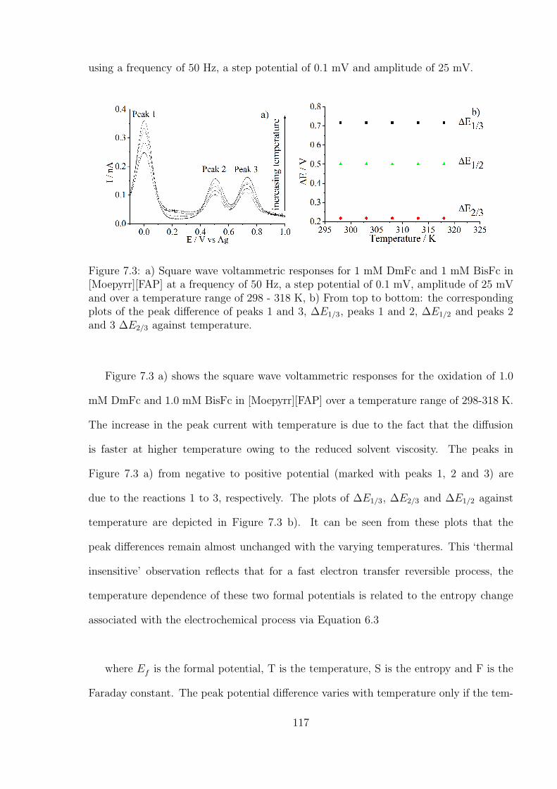
using a frequency of 50 Hz, a step potential of 0.1 mV and amplitude of 25 mV.
Figure 7.3: a) Square wave voltammetric responses for 1 mM DmFc and 1 mM BisFc in[Moepyrr][FAP] at a frequency of 50 Hz, a step potential of 0.1 mV, amplitude of 25 mVand over a temperature range of 298 - 318 K, b) From top to bottom: the correspondingplots of the peak difference of peaks 1 and 3, ∆E1/3, peaks 1 and 2, ∆E1/2 and peaks 2and 3 ∆E2/3 against temperature.
Figure 7.3 a) shows the square wave voltammetric responses for the oxidation of 1.0
mM DmFc and 1.0 mM BisFc in [Moepyrr][FAP] over a temperature range of 298-318 K.
The increase in the peak current with temperature is due to the fact that the diffusion
is faster at higher temperature owing to the reduced solvent viscosity. The peaks in
Figure 7.3 a) from negative to positive potential (marked with peaks 1, 2 and 3) are
due to the reactions 1 to 3, respectively. The plots of ∆E1/3, ∆E2/3 and ∆E1/2 against
temperature are depicted in Figure 7.3 b). It can be seen from these plots that the
peak differences remain almost unchanged with the varying temperatures. This ‘thermal
insensitive’ observation reflects that for a fast electron transfer reversible process, the
temperature dependence of these two formal potentials is related to the entropy change
associated with the electrochemical process via Equation 6.3
where Ef is the formal potential, T is the temperature, S is the entropy and F is the
Faraday constant. The peak potential difference varies with temperature only if the tem-
117
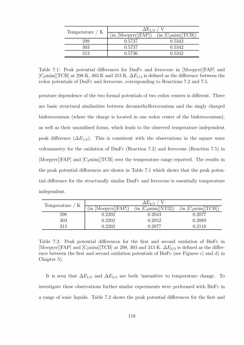
Temperature / K∆E1/4 / V
(in [Moepyrr][FAP]) (in [C2mim][TCB])298 0.5737 0.5342303 0.5737 0.5342313 0.5736 0.5342
Table 7.1: Peak potential differences for DmFc and ferrocene in [Moepyrr][FAP] and[C2mim][TCB] at 298 K, 303 K and 313 K. ∆E1/4 is defined as the difference between theredox potentials of DmFc and ferrocene, corresponding to Reactions 7.2 and 7.5.
perature dependence of the two formal potentials of two redox centres is different. There
are basic structural similarities between decamethylferrocenium and the singly charged
bisferrocenium (where the charge is located in one redox center of the bisferrocenium),
as well as their unoxidised forms, which leads to the observed temperature independent
peak difference (∆E1/2). This is consistent with the observations in the square wave
voltammetry for the oxidation of DmFc (Reaction 7.2) and ferrocene (Reaction 7.5) in
[Moepyrr][FAP] and [C2mim][TCB] over the temperature range reported. The results in
the peak potential differences are shown in Table 7.1 which shows that the peak poten-
tial difference for the structurally similar DmFc and ferrocene is essentially temperature
independent.
Temperature / K∆E2/3 / V
(in [Moepyrr][FAP]) (in [C3mim][NTf2]) (in [C2mim][TCB])298 0.2202 0.2043 0.2077303 0.2202 0.2052 0.2089313 0.2202 0.2077 0.2110
Table 7.2: Peak potential differences for the first and second oxidation of BisFc in[Moepyrr][FAP] and [C2mim][TCB] at 298, 303 and 313 K. ∆E2/3 is defined as the differ-ence between the first and second oxidation potentials of BisFc (see Figures c) and d) inChapter 5).
It is seen that ∆E1/3 and ∆E2/3 are both ‘insensitive to temperature change. To
investigate these observations further similar experiments were performed with BisFc in
a range of ionic liquids. Table 7.2 shows the peak potential differences for the first and
118
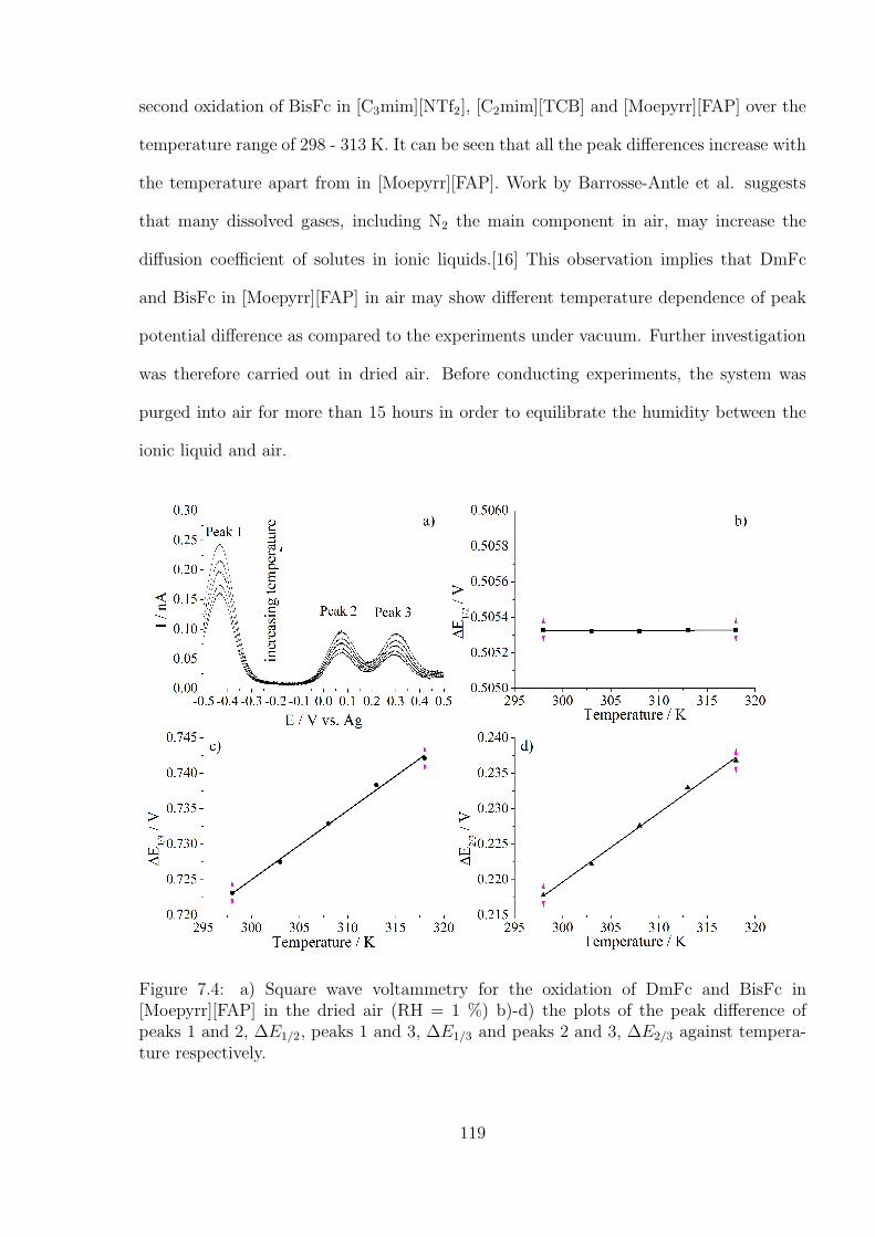
second oxidation of BisFc in [C3mim][NTf2], [C2mim][TCB] and [Moepyrr][FAP] over the
temperature range of 298 - 313 K. It can be seen that all the peak differences increase with
the temperature apart from in [Moepyrr][FAP]. Work by Barrosse-Antle et al. suggests
that many dissolved gases, including N2 the main component in air, may increase the
diffusion coefficient of solutes in ionic liquids.[16] This observation implies that DmFc
and BisFc in [Moepyrr][FAP] in air may show different temperature dependence of peak
potential difference as compared to the experiments under vacuum. Further investigation
was therefore carried out in dried air. Before conducting experiments, the system was
purged into air for more than 15 hours in order to equilibrate the humidity between the
ionic liquid and air.
Figure 7.4: a) Square wave voltammetry for the oxidation of DmFc and BisFc in[Moepyrr][FAP] in the dried air (RH = 1 %) b)-d) the plots of the peak difference ofpeaks 1 and 2, ∆E1/2, peaks 1 and 3, ∆E1/3 and peaks 2 and 3, ∆E2/3 against tempera-ture respectively.
119
Figure 7.4 a) shows the square wave voltammetry for the oxidation of DmFc (peak
1) and BisFc (peaks 2 and 3) in [Moepyrr][FAP] under dried air (RH = 1 %). The
corresponding plot of peak potential difference against temperature, between peaks 1 and
2, ∆E1/2, is displayed in Figure 7.4 b). It is again observed that ∆E1/2 is insensitive to
temperature change, where the equation for the line of best fit is given as below,
∆E1/2(V ) = 0.5053 + 2× 10⁻⁷T (7.10)
where, T is the temperature in K. Figure 7.4 c) depicts the peak potential difference
∆E1/3, measured between peak 1 and peak 3, as a function of temperature where a linear
increase with temperature is seen. This temperature dependent peak potential difference
can be described by the following equation,
∆E1/3(V ) = 0.4327 + 0.9744× 10⁻³T (7.11)
A similar observation is made with the temperature relationship of peak potential
difference between peak 2 and peak 3, of ∆E2/3, which is shown in Figure 7.4 d). This
linear relation is given below,
∆E2/3(V ) = −0.0726 + 0.9742× 10⁻³T (7.12)
Since ∆E1/3 has better defined peak to peak separations at each temperature, this
term is used to measure temperature below.
120
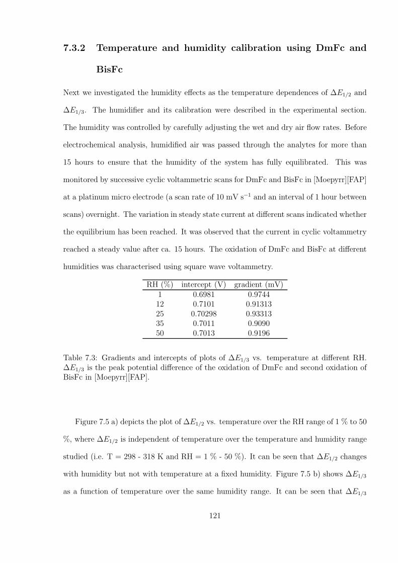
7.3.2 Temperature and humidity calibration using DmFc and
BisFc
Next we investigated the humidity effects as the temperature dependences of ∆E1/2 and
∆E1/3. The humidifier and its calibration were described in the experimental section.
The humidity was controlled by carefully adjusting the wet and dry air flow rates. Before
electrochemical analysis, humidified air was passed through the analytes for more than
15 hours to ensure that the humidity of the system has fully equilibrated. This was
monitored by successive cyclic voltammetric scans for DmFc and BisFc in [Moepyrr][FAP]
at a platinum micro electrode (a scan rate of 10 mV s−1 and an interval of 1 hour between
scans) overnight. The variation in steady state current at different scans indicated whether
the equilibrium has been reached. It was observed that the current in cyclic voltammetry
reached a steady value after ca. 15 hours. The oxidation of DmFc and BisFc at different
humidities was characterised using square wave voltammetry.
RH (%) intercept (V) gradient (mV)1 0.6981 0.974412 0.7101 0.9131325 0.70298 0.9331335 0.7011 0.909050 0.7013 0.9196
Table 7.3: Gradients and intercepts of plots of ∆E1/3 vs. temperature at different RH.∆E1/3 is the peak potential difference of the oxidation of DmFc and second oxidation ofBisFc in [Moepyrr][FAP].
Figure 7.5 a) depicts the plot of ∆E1/2 vs. temperature over the RH range of 1 % to 50
%, where ∆E1/2 is independent of temperature over the temperature and humidity range
studied (i.e. T = 298 - 318 K and RH = 1 % - 50 %). It can be seen that ∆E1/2 changes
with humidity but not with temperature at a fixed humidity. Figure 7.5 b) shows ∆E1/3
as a function of temperature over the same humidity range. It can be seen that ∆E1/3
121
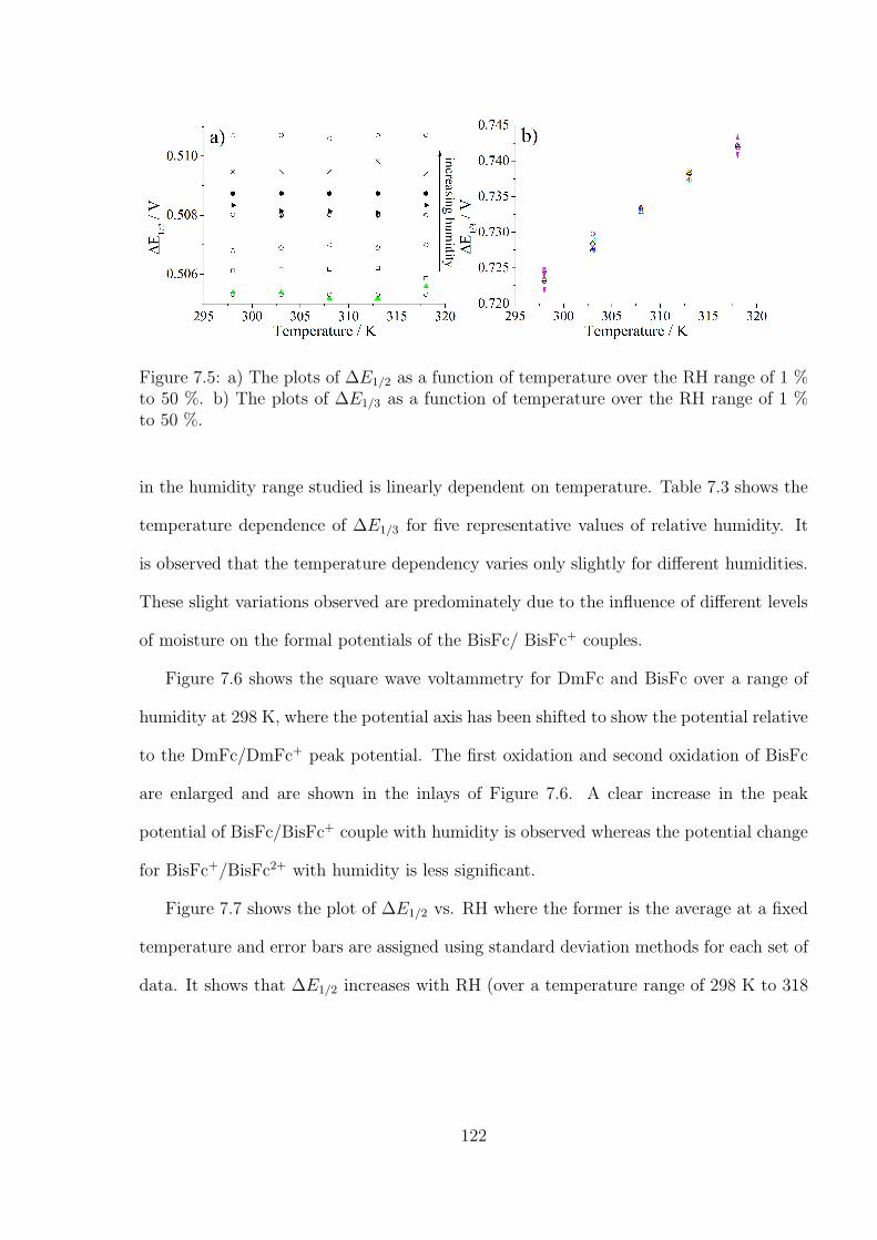
Figure 7.5: a) The plots of ∆E1/2 as a function of temperature over the RH range of 1 %to 50 %. b) The plots of ∆E1/3 as a function of temperature over the RH range of 1 %to 50 %.
in the humidity range studied is linearly dependent on temperature. Table 7.3 shows the
temperature dependence of ∆E1/3 for five representative values of relative humidity. It
is observed that the temperature dependency varies only slightly for different humidities.
These slight variations observed are predominately due to the influence of different levels
of moisture on the formal potentials of the BisFc/ BisFc+ couples.
Figure 7.6 shows the square wave voltammetry for DmFc and BisFc over a range of
humidity at 298 K, where the potential axis has been shifted to show the potential relative
to the DmFc/DmFc+ peak potential. The first oxidation and second oxidation of BisFc
are enlarged and are shown in the inlays of Figure 7.6. A clear increase in the peak
potential of BisFc/BisFc+ couple with humidity is observed whereas the potential change
for BisFc+/BisFc2+ with humidity is less significant.
Figure 7.7 shows the plot of ∆E1/2 vs. RH where the former is the average at a fixed
temperature and error bars are assigned using standard deviation methods for each set of
data. It shows that ∆E1/2 increases with RH (over a temperature range of 298 K to 318
122
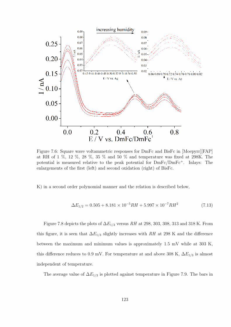
Figure 7.6: Square wave voltammetric responses for DmFc and BisFc in [Moepyrr][FAP]at RH of 1 %, 12 %, 28 %, 35 % and 50 % and temperature was fixed at 298K. Thepotential is measured relative to the peak potential for DmFc/DmFc+. Inlays: Theenlargements of the first (left) and second oxidation (right) of BisFc.
K) in a second order polynomial manner and the relation is described below,
∆E1/2 = 0.505 + 8.181× 10⁻⁵RH + 5.997× 10⁻⁷RH2 (7.13)
Figure 7.8 depicts the plots of ∆E1/3 versus RH at 298, 303, 308, 313 and 318 K. From
this figure, it is seen that ∆E1/3 slightly increases with RH at 298 K and the difference
between the maximum and minimum values is approximately 1.5 mV while at 303 K,
this difference reduces to 0.9 mV. For temperature at and above 308 K, ∆E1/3 is almost
independent of temperature.
The average value of ∆E1/3 is plotted against temperature in Figure 7.9. The bars in
123
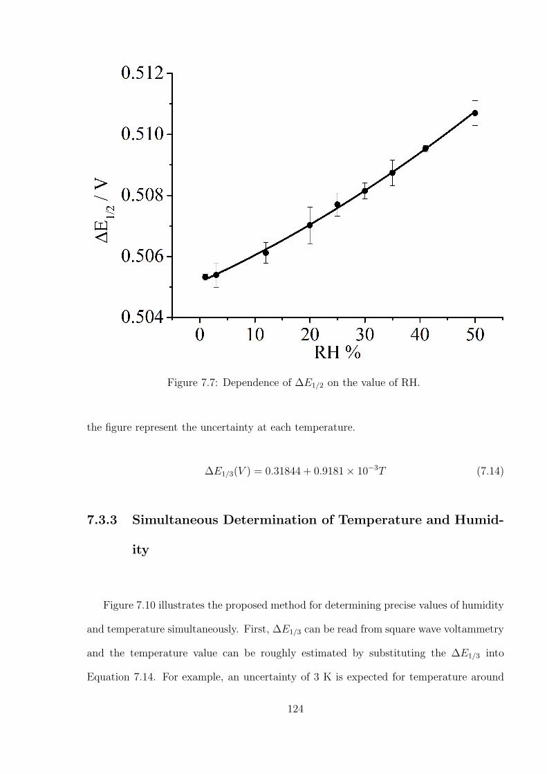
Figure 7.7: Dependence of ∆E1/2 on the value of RH.
the figure represent the uncertainty at each temperature.
∆E1/3(V ) = 0.31844 + 0.9181× 10⁻³T (7.14)
7.3.3 Simultaneous Determination of Temperature and Humid-
ity
Figure 7.10 illustrates the proposed method for determining precise values of humidity
and temperature simultaneously. First, ∆E1/3 can be read from square wave voltammetry
and the temperature value can be roughly estimated by substituting the ∆E1/3 into
Equation 7.14. For example, an uncertainty of 3 K is expected for temperature around
124
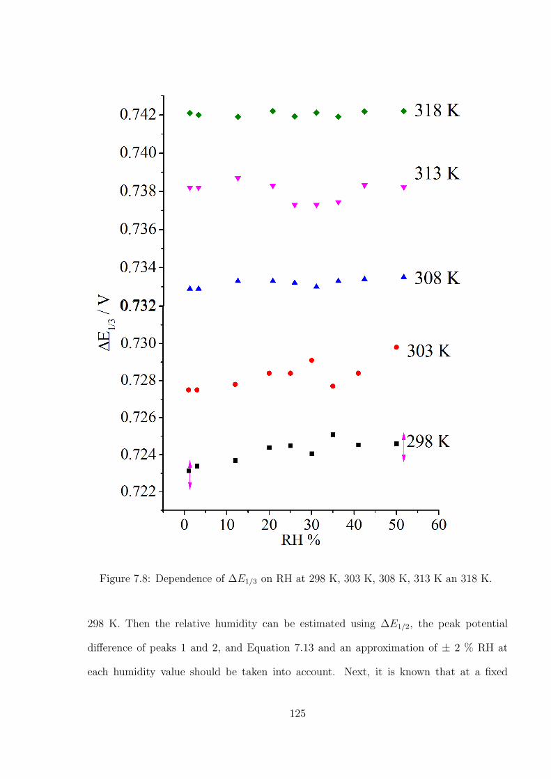
Figure 7.8: Dependence of ∆E1/3 on RH at 298 K, 303 K, 308 K, 313 K an 318 K.
298 K. Then the relative humidity can be estimated using ∆E1/2, the peak potential
difference of peaks 1 and 2, and Equation 7.13 and an approximation of ± 2 % RH at
each humidity value should be taken into account. Next, it is known that at a fixed
125
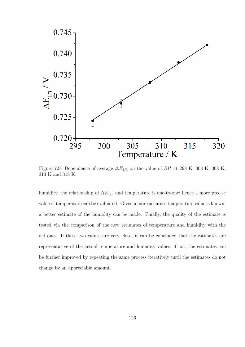
Figure 7.9: Dependence of average ∆E1/3 on the value of RH at 298 K, 303 K, 308 K,313 K and 318 K.
humidity, the relationship of ∆E1/3 and temperature is one-to-one; hence a more precise
value of temperature can be evaluated. Given a more accurate temperature value is known,
a better estimate of the humidity can be made. Finally, the quality of the estimate is
tested via the comparison of the new estimates of temperature and humidity with the
old ones. If these two values are very close, it can be concluded that the estimates are
representative of the actual temperature and humidity values; if not, the estimates can
be further improved by repeating the same process iteratively until the estimates do not
change by an appreciable amount.
126
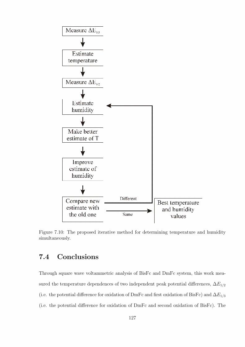
Figure 7.10: The proposed iterative method for determining temperature and humiditysimultaneously.
7.4 Conclusions
Through square wave voltammetric analysis of BisFc and DmFc system, this work mea-
sured the temperature dependences of two independent peak potential differences, ∆E1/2
(i.e. the potential difference for oxidation of DmFc and first oxidation of BisFc) and ∆E1/3
(i.e. the potential difference for oxidation of DmFc and second oxidation of BisFc). The
127
former is temperature insensitive and the other has a temperature coefficient of 0.92 mV
K−1. The humidity effects of these two independent pairs over the temperature range of
298 K to 318 K have been investigated. It has observed that the peak potential difference
between DmFc/DmFc+ and BisFc/BisFc+ is humidity dependent and the peak potential
differences of other pairs are less influenced by humidity change. A method for finding
accurate values of humidity and temperature has been proposed. Even it is possible to
measure the humidity and temperature in the RTILs using the method introduced in this
chapter, oxygen reduction mechanism in humid condition is complex and unpredictable.
Next chapter introduces a method to ‘trap’ oxygen reduction at one electron stage.
References
[1] Xiong, L.; Fletcher, A. M.; Davies, S. G.; Norman, S. E.; Hardacre, C.; Comp-ton, R. G. The Analyst 2012, 137, 4951–4957.
[2] Atkins, P.; De Paula, J. Atkins’ Physical Chemistry ; Macmillan Higher Education,2006.
[3] Xiong, L.; Fletcher, A. M.; Ernst, S.; Davies, S. G.; Compton, R. G. Analyst 2012,137, 2567–2573.
[4] Xiong, L.; Fletcher, A. M.; Davies, S. G.; Norman, S. E.; Hardacre, C.; Comp-ton, R. G. Chemical Communications 2012, 48, 5784–5786.
[5] Buzzeo, M. C.; Evans, R. G.; Compton, R. G. ChemPhysChem 2004, 5, 1106–1120.
[6] Barrosse-Antle, L. E.; Bond, A. M.; Compton, R. G.; O’Mahony, A. M.; Rogers, E. I.;Silvester, D. S. Chemistry - An Asian Journal 2010, 5, 202–230.
[7] Green, D.; Perry, R. Perry’s Chemical Engineers’ Handbook, Eighth Edition; McGrawHill professional; McGraw-Hill Education, 2007.
[8] Noviandri, I.; Brown, K. N.; Fleming, D. S.; Gulyas, P. T.; Lay, P. A.; Masters, A. F.;Phillips, L. Journal of Physical Chemistry B 1999, 103, 6713–6722.
[9] Ignat’ev, N.; Welz-Biermann, U.; Kucheryna, A.; Bissky, G.; Willner, H. Journal ofFluorine Chemistry 2005, 126, 1150–1159.
[10] Wang, Z.; Fu, L.; Xu, H.; Shang, Y.; Zhang, L.; Zhang, J. Journal of Chemical andEngineering Data 2012, 57, 1057–1063.
[11] Fu, C.; Aldous, L.; Dickinson, E.; Manan, N.; Compton, R. ChemPhysChem 2011,12, 1708–1713.
128

[12] Fu, C.; Aldous, L.; Dickinson, E.; Manan, N.; Compton, R. New Journal of Chemistry2012, 36, 774–780.
[13] Compton, R. G.; Banks, C. E. Understanding Voltammetry ; Imperial College Press,2011, 2nd Edition.
[14] Bard, A. J.; Faulkner, L. R. Electrochemical Methods: Fundamentals and Applica-tions ; Wiley, 2001.
[15] Molina, A.; Gonzalez, J.; Laborda, E.; Li, Q.; Batchelor-McAuley, C.; Comp-ton, R. G. Journal of Physical Chemistry C 2012, 116, 1070–1079.
[16] Brett, C. M. A.; Brett, A. M. O. Electrochemistry: Principles, Methods, and Appli-cations ; Oxford Science Publications; Oxford University Press, Incorporated, 1993.
129
Chapter 8
Amperometric Detection of OxygenUnder Humid Conditions: The Useof A Chemically Reactive RoomTemperature Ionic Liquid to ‘Trap’Superoxide Ions and Ensure aSimple One Electron Reduction
Last two chapters showed the sensors to monitor temperature and humidity at electrode.
However issues still remain under humid conditions as the mechanism of gas like oxygen
are highly sensitive to the presence of water especially when the amperometric detection
of oxygen via Clark cell type devices uses Room Temperature Ionic Liquids (RTILs) as
electrochemical solvents. The number of electrons transferred in the electrode reaction
varies between one and two as a function of the humidity. This chapter reports that the
problem can be avoided through the use of phosphonium cation based ionic liquids in
which the alkyl group of the phosphonium cation has acidic protons which are rapidly ab-
stracted by superoxide ions. Thus the reduction of O2 is to be trapped at the one electron
level on the micro-electrode voltammetric timescale, allowing the amperometric detection
of oxygen under humid conditions to be quantitatively viable. The work presented here
has been published in the Sensors and Actuators B.[1]
130
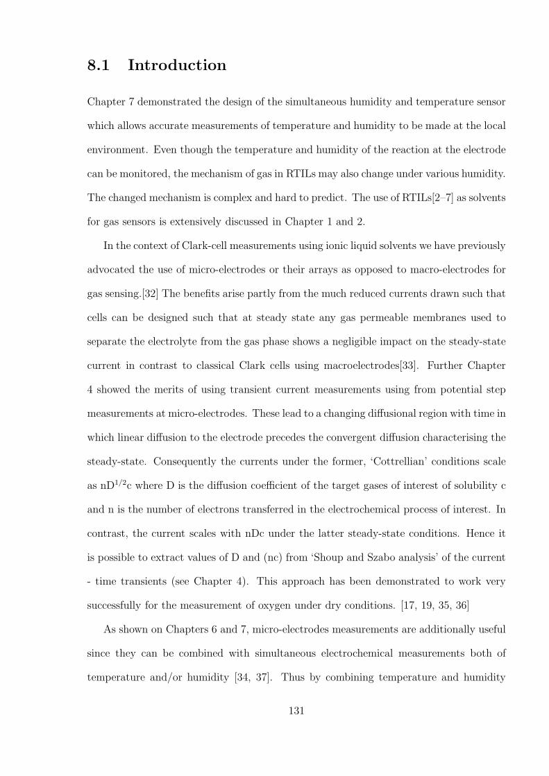
8.1 Introduction
Chapter 7 demonstrated the design of the simultaneous humidity and temperature sensor
which allows accurate measurements of temperature and humidity to be made at the local
environment. Even though the temperature and humidity of the reaction at the electrode
can be monitored, the mechanism of gas in RTILs may also change under various humidity.
The changed mechanism is complex and hard to predict. The use of RTILs[2–7] as solvents
for gas sensors is extensively discussed in Chapter 1 and 2.
In the context of Clark-cell measurements using ionic liquid solvents we have previously
advocated the use of micro-electrodes or their arrays as opposed to macro-electrodes for
gas sensing.[32] The benefits arise partly from the much reduced currents drawn such that
cells can be designed such that at steady state any gas permeable membranes used to
separate the electrolyte from the gas phase shows a negligible impact on the steady-state
current in contrast to classical Clark cells using macroelectrodes[33]. Further Chapter
4 showed the merits of using transient current measurements using from potential step
measurements at micro-electrodes. These lead to a changing diffusional region with time in
which linear diffusion to the electrode precedes the convergent diffusion characterising the
steady-state. Consequently the currents under the former, ‘Cottrellian’ conditions scale
as nD1/2c where D is the diffusion coefficient of the target gases of interest of solubility c
and n is the number of electrons transferred in the electrochemical process of interest. In
contrast, the current scales with nDc under the latter steady-state conditions. Hence it
is possible to extract values of D and (nc) from ‘Shoup and Szabo analysis’ of the current
- time transients (see Chapter 4). This approach has been demonstrated to work very
successfully for the measurement of oxygen under dry conditions. [17, 19, 35, 36]
As shown on Chapters 6 and 7, micro-electrodes measurements are additionally useful
since they can be combined with simultaneous electrochemical measurements both of
temperature and/or humidity [34, 37]. Thus by combining temperature and humidity
131
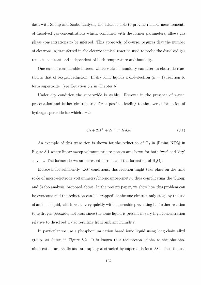
data with Shoup and Szabo analysis, the latter is able to provide reliable measurements
of dissolved gas concentrations which, combined with the former parameters, allows gas
phase concentrations to be inferred. This approach, of course, requires that the number
of electrons, n, transferred in the electrochemical reaction used to probe the dissolved gas
remains constant and independent of both temperature and humidity.
One case of considerable interest where variable humidity can alter an electrode reac-
tion is that of oxygen reduction. In dry ionic liquids a one-electron (n = 1) reaction to
form superoxide. (see Equation 6.7 in Chapter 6)
Under dry condition the superoxide is stable. However in the presence of water,
protonation and futher electron transfer is possible leading to the overall formation of
hydrogen peroxide for which n=2:
O2 + 2H+ + 2e− H2O2 (8.1)
An example of this transition is shown for the reduction of O2 in [Pmim][NTf2] in
Figure 8.1 where linear sweep voltammetric responses are shown for both ‘wet’ and ‘dry’
solvent. The former shows an increased current and the formation of H2O2.
Moreover for sufficiently ‘wet’ conditions, this reaction might take place on the time
scale of micro-electrode voltammetry/chronoamperometry, thus complicating the ‘Shoup
and Szabo analysis’ proposed above. In the present paper, we show how this problem can
be overcome and the reduction can be ‘trapped’ at the one electron only stage by the use
of an ionic liquid, which reacts very quickly with superoxide preventing its further reaction
to hydrogen peroxide, not least since the ionic liquid is present in very high concentration
relative to dissolved water resulting from ambient humidity.
In particular we use a phosphonium cation based ionic liquid using long chain alkyl
groups as shown in Figure 8.2. It is known that the protons alpha to the phospho-
nium cation are acidic and are rapidly abstracted by superoxide ions [38]. Thus the use
132
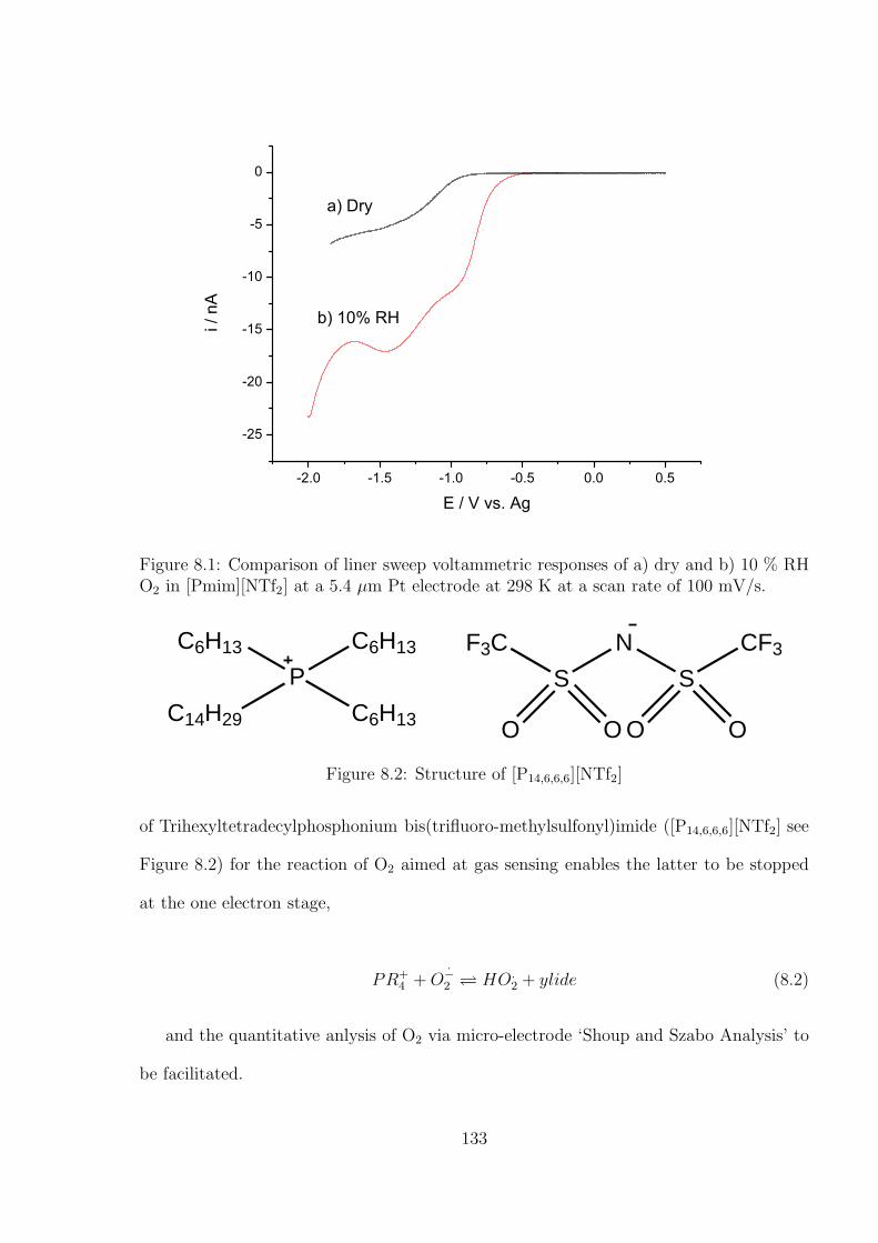
-2.0 -1.5 -1.0 -0.5 0.0 0.5
-25
-20
-15
-10
-5
0
b) 10% RHi / n
A
E / V vs. Ag
a) Dry
Figure 8.1: Comparison of liner sweep voltammetric responses of a) dry and b) 10 % RHO2 in [Pmim][NTf2] at a 5.4 µm Pt electrode at 298 K at a scan rate of 100 mV/s.
P
C6H13 C6H13
C6H13C14H29
N
SS
CF3F3C
O O O O
Figure 8.2: Structure of [P14,6,6,6][NTf2]
of Trihexyltetradecylphosphonium bis(trifluoro-methylsulfonyl)imide ([P14,6,6,6][NTf2] see
Figure 8.2) for the reaction of O2 aimed at gas sensing enables the latter to be stopped
at the one electron stage,
PR+4 +O−
2 HO.2 + ylide (8.2)
and the quantitative anlysis of O2 via micro-electrode ‘Shoup and Szabo Analysis’ to
be facilitated.
133
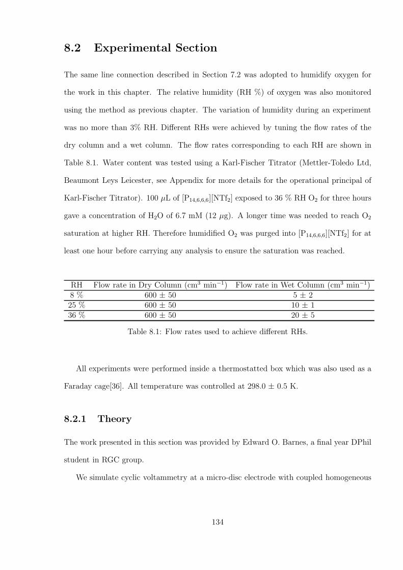
8.2 Experimental Section
The same line connection described in Section 7.2 was adopted to humidify oxygen for
the work in this chapter. The relative humidity (RH %) of oxygen was also monitored
using the method as previous chapter. The variation of humidity during an experiment
was no more than 3% RH. Different RHs were achieved by tuning the flow rates of the
dry column and a wet column. The flow rates corresponding to each RH are shown in
Table 8.1. Water content was tested using a Karl-Fischer Titrator (Mettler-Toledo Ltd,
Beaumont Leys Leicester, see Appendix for more details for the operational principal of
Karl-Fischer Titrator). 100 µL of [P14,6,6,6][NTf2] exposed to 36 % RH O2 for three hours
gave a concentration of H2O of 6.7 mM (12 µg). A longer time was needed to reach O2
saturation at higher RH. Therefore humidified O2 was purged into [P14,6,6,6][NTf2] for at
least one hour before carrying any analysis to ensure the saturation was reached.
RH Flow rate in Dry Column (cm3 min−1) Flow rate in Wet Column (cm3 min−1)8 % 600 ± 50 5 ± 225 % 600 ± 50 10 ± 136 % 600 ± 50 20 ± 5
Table 8.1: Flow rates used to achieve different RHs.
All experiments were performed inside a thermostatted box which was also used as a
Faraday cage[36]. All temperature was controlled at 298.0 ± 0.5 K.
8.2.1 Theory
The work presented in this section was provided by Edward O. Barnes, a final year DPhil
student in RGC group.
We simulate cyclic voltammetry at a micro-disc electrode with coupled homogeneous
134
kinetics according to the following mechanism:
A + e− B (8.3)
B → X (8.4)
X− e− Z (8.5)
The use of an ionic liquid solvent is assumed to suppress migration effect to ensure a
diffusion only problem. The dependence of the three concentrations on time is given by:
∂cA∂t
= DA
(
∂c2A∂r2
+∂c2A∂z2
+1
r
∂cA∂r
)
(8.6)
∂cB∂t
= DB
(
∂c2B∂r2
+∂c2B∂z2
+1
r
∂cB∂r
)
− kcB (8.7)
∂cX∂t
= DX
(
∂c2X∂r2
+∂c2X∂z2
+1
r
∂cX∂r
)
+ kcB (8.8)
∂cZ∂t
= DZ
(
∂c2Z∂r2
+∂c2Z∂z2
+1
r
∂cZ∂r
)
(8.9)
where k is the fastest rate constant for reaction 2.3. All symbols are defined in Table
8.2. The chemical step is assumed to be pseudo first order and irreversible. For the
reaction of O.−2 via an ionic liquid solvent the ionic liquid cation is present in large excess
so this is a good assumption. These mass transport equations are solved subject to
boundary conditions at the electrode surface and in bulk solution. At the electrode
surface, Butler-Volmer kinetics are employed. For each i/j couple (where i is the oxidised
species):
Di
(
∂ci∂z
)
z=0
= k0
(
c0i exp
[
−α(
E − E
f
)
RT
]
− c0j exp
[
β(
E − E
f
)
RT
])
(8.10)
135
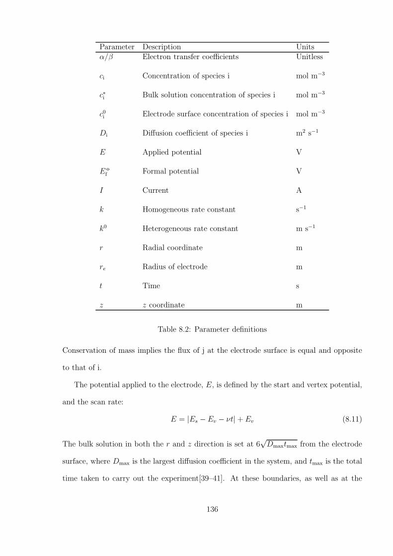
Parameter Description Unitsα/β Electron transfer coefficients Unitless
ci Concentration of species i mol m−3
c∗i Bulk solution concentration of species i mol m−3
c0i Electrode surface concentration of species i mol m−3
Di Diffusion coefficient of species i m2 s−1
E Applied potential V
E
f Formal potential V
I Current A
k Homogeneous rate constant s−1
k0 Heterogeneous rate constant m s−1
r Radial coordinate m
re Radius of electrode m
t Time s
z z coordinate m
Table 8.2: Parameter definitions
Conservation of mass implies the flux of j at the electrode surface is equal and opposite
to that of i.
The potential applied to the electrode, E, is defined by the start and vertex potential,
and the scan rate:
E = |Es −Ev − νt| + Ev (8.11)
The bulk solution in both the r and z direction is set at 6√Dmaxtmax from the electrode
surface, where Dmax is the largest diffusion coefficient in the system, and tmax is the total
time taken to carry out the experiment[39–41]. At these boundaries, as well as at the
136
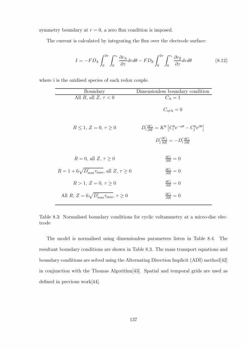
symmetry boundary at r = 0, a zero flux condition is imposed.
The current is calculated by integrating the flux over the electrode surface:
I = −FDA
∫ 2π
0
∫ re
0
∂cA∂z
drdθ − FDZ
∫ 2π
0
∫ re
0
∂cZ∂z
drdθ (8.12)
where i is the oxidised species of each redox couple.
Boundary Dimensionless boundary conditionAll R, all Z, τ < 0 CA = 1
Ci 6=A = 0
R ≤ 1, Z = 0, τ ≥ 0 D′
i∂Ci
∂R= K0
[
C0i e
−αθ − C0j e
βθ]
D′
j∂Cj
∂R= −D
′
i∂Ci
∂R
R = 0, all Z, τ ≥ 0 ∂Ci
∂R= 0
R = 1 + 6√
D′
maxτmax, all Z, τ ≥ 0 ∂Ci
∂R= 0
R > 1, Z = 0, τ ≥ 0 ∂Ci
∂R= 0
All R, Z = 6√
D′
maxτmax, τ ≥ 0 ∂Ci
∂R= 0
Table 8.3: Normalised boundary conditions for cyclic voltammetry at a micro-disc elec-trode
The model is normalised using dimensionless parameters listen in Table 8.4. The
resultant boundary conditions are shown in Table 8.3. The mass transport equations and
boundary conditions are solved using the Alternating Direction Implicit (ADI) method[42]
in conjunction with the Thomas Algorithm[43]. Spatial and temporal grids are used as
defined in previous work[44].
137
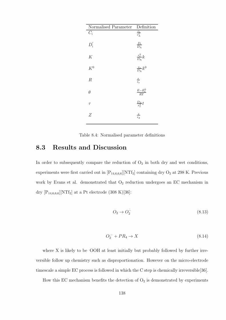
Normalised Parameter DefinitionCi
cic∗A
D′
iDi
DA
K r2eDA
k
K0 rsDA
k0
R rrs
θE−E0
f
RT
τ DA
r2st
Z zrd
Table 8.4: Normalised parameter definitions
8.3 Results and Discussion
In order to subsequently compare the reduction of O2 in both dry and wet conditions,
experiments were first carried out in [P14,6,6,6][NTf2] containing dry O2 at 298 K. Previous
work by Evans et al. demonstrated that O2 reduction undergoes an EC mechanism in
dry [P14,6,6,6][NTf2] at a Pt electrode (308 K)[36]:
O2 → O−2 (8.13)
O.−2 + PR4 → X (8.14)
where X is likely to be .OOH at least initially but probably followed by further irre-
versible follow up chemistry such as disproportionation. However on the micro-electrode
timescale a simple EC process is followed in which the C step is chemically irreversible[36].
How this EC mechanism benefits the detection of O2 is demonstrated by experiments
138
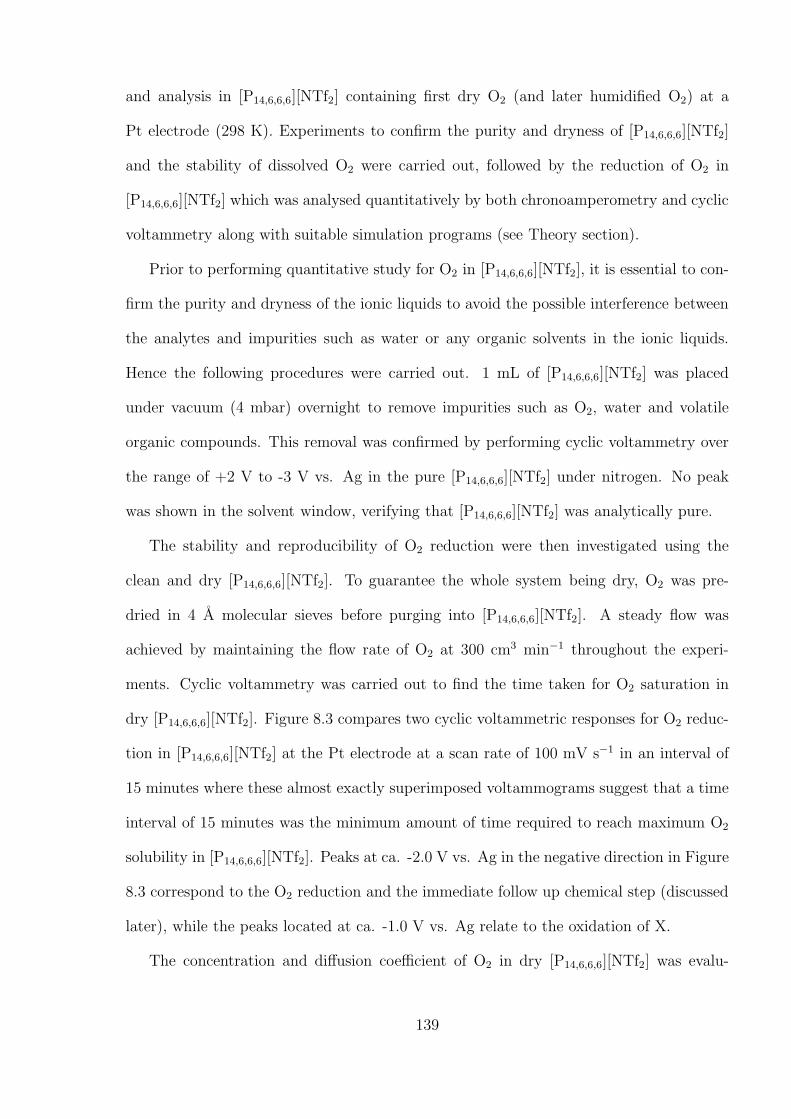
and analysis in [P14,6,6,6][NTf2] containing first dry O2 (and later humidified O2) at a
Pt electrode (298 K). Experiments to confirm the purity and dryness of [P14,6,6,6][NTf2]
and the stability of dissolved O2 were carried out, followed by the reduction of O2 in
[P14,6,6,6][NTf2] which was analysed quantitatively by both chronoamperometry and cyclic
voltammetry along with suitable simulation programs (see Theory section).
Prior to performing quantitative study for O2 in [P14,6,6,6][NTf2], it is essential to con-
firm the purity and dryness of the ionic liquids to avoid the possible interference between
the analytes and impurities such as water or any organic solvents in the ionic liquids.
Hence the following procedures were carried out. 1 mL of [P14,6,6,6][NTf2] was placed
under vacuum (4 mbar) overnight to remove impurities such as O2, water and volatile
organic compounds. This removal was confirmed by performing cyclic voltammetry over
the range of +2 V to -3 V vs. Ag in the pure [P14,6,6,6][NTf2] under nitrogen. No peak
was shown in the solvent window, verifying that [P14,6,6,6][NTf2] was analytically pure.
The stability and reproducibility of O2 reduction were then investigated using the
clean and dry [P14,6,6,6][NTf2]. To guarantee the whole system being dry, O2 was pre-
dried in 4 A molecular sieves before purging into [P14,6,6,6][NTf2]. A steady flow was
achieved by maintaining the flow rate of O2 at 300 cm3 min−1 throughout the experi-
ments. Cyclic voltammetry was carried out to find the time taken for O2 saturation in
dry [P14,6,6,6][NTf2]. Figure 8.3 compares two cyclic voltammetric responses for O2 reduc-
tion in [P14,6,6,6][NTf2] at the Pt electrode at a scan rate of 100 mV s−1 in an interval of
15 minutes where these almost exactly superimposed voltammograms suggest that a time
interval of 15 minutes was the minimum amount of time required to reach maximum O2
solubility in [P14,6,6,6][NTf2]. Peaks at ca. -2.0 V vs. Ag in the negative direction in Figure
8.3 correspond to the O2 reduction and the immediate follow up chemical step (discussed
later), while the peaks located at ca. -1.0 V vs. Ag relate to the oxidation of X.
The concentration and diffusion coefficient of O2 in dry [P14,6,6,6][NTf2] was evalu-
139
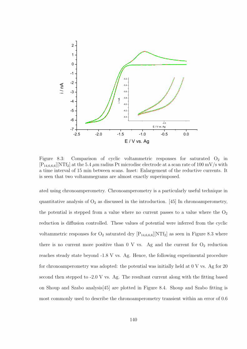
-2.5 -2.0 -1.5 -1.0 -0.5 0.0-7
-6
-5
-4
-3
-2
-1
0
1
2
-2.0
-6.4
-6.2
-6.0
-5.8
-5.6
-5.4
-5.2
i / n
A
E / V vs. Ag
i / n
A
E / V vs. Ag
Figure 8.3: Comparison of cyclic voltammetric responses for saturated O2 in[P14,6,6,6][NTf2] at the 5.4 µm radius Pt microdisc electrode at a scan rate of 100 mV/s witha time interval of 15 min between scans. Inset: Enlargement of the reductive currents. Itis seen that two voltammegrams are almost exactly superimposed.
ated using chronoamperometry. Chronoamperometry is a particularly useful technique in
quantitative analysis of O2 as discussed in the introduction. [45] In chronoamperometry,
the potential is stepped from a value where no current passes to a value where the O2
reduction is diffusion controlled. These values of potential were inferred from the cyclic
voltammetric responses for O2 saturated dry [P14,6,6,6][NTf2] as seen in Figure 8.3 where
there is no current more positive than 0 V vs. Ag and the current for O2 reduction
reaches steady state beyond -1.8 V vs. Ag. Hence, the following experimental procedure
for chronoamperometry was adopted: the potential was initially held at 0 V vs. Ag for 20
second then stepped to -2.0 V vs. Ag. The resultant current along with the fitting based
on Shoup and Szabo analysis[45] are plotted in Figure 8.4. Shoup and Szabo fitting is
most commonly used to describe the chronoamperometry transient within an error of 0.6
140
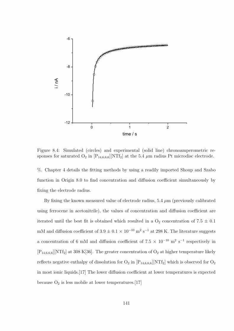
0 1 2-12
-10
-8
-6
i / n
A
time / s
Figure 8.4: Simulated (circles) and experimental (solid line) chronoamperometric re-sponses for saturated O2 in [P14,6,6,6][NTf2] at the 5.4 µm radius Pt microdisc electrode.
%. Chapter 4 details the fitting methods by using a readily imported Shoup and Szabo
function in Origin 8.0 to find concentration and diffusion coefficient simultaneously by
fixing the electrode radius.
By fixing the known measured value of electrode radius, 5.4 µm (previously calibrated
using ferrocene in acetonitrile), the values of concentration and diffusion coefficient are
iterated until the best fit is obtained which resulted in a O2 concentration of 7.5 ± 0.1
mM and diffusion coefficient of 3.9 ± 0.1 × 10⁻¹⁰ m2 s−1 at 298 K. The literature suggests
a concentration of 6 mM and diffusion coefficient of 7.5 × 10⁻¹⁰ m2 s−1 respectively in
[P14,6,6,6][NTf2] at 308 K[36]. The greater concentration of O2 at higher temperature likely
reflects negative enthalpy of dissolution for O2 in [P14,6,6,6][NTf2] which is observed for O2
in most ionic liquids.[17] The lower diffusion coefficient at lower temperatures is expected
because O2 is less mobile at lower temperatures.[17]
141
-3 -2 -1 0
-6
-4
-2
0
2
4
i / n
A
E / V vs. Ag-3 -2 -1 0
-8
-6
-4
-2
0
2
4
i / n
A
E / V vs. Ag
-3 -2 -1 0
-6
-4
-2
0
2
4
i / n
A
E / V vs. Ag-3.0 -2.5 -2.0 -1.5 -1.0 -0.5 0.0
-6
-4
-2
0
2
4
i / n
A
E / V vs. Ag-3 -2 -1 0
-6
-4
-2
0
2
4
i / n
A
E / V vs. Ag
a) b)
e)d)
c)
Figure 8.5: Simulated (circles) and experimental (solid lines) data for dry O2 in[P14,6,6,6][NTf2] at the 5.4 µm radius Pt microdisc electrode at 298 K at scan rates ofa) 100 mV s−1, b) 200 mV s−1, c) 300 mV s−1, d) 400 mV s−1 and e) 500 mV s−1.
The values of concentration and diffusion coefficient of O2 were further examined
through simulating the cyclic voltammetry for O2 in [P14,6,6,6][NTf2] with the EC mecha-
nism program reported alone. Figures 8.5 a) to e) show cyclic voltammetric responses for
dry O2 in [P14,6,6,6][NTf2] over the scan rate range of 100 mV s−1 to 500 mV s−1 at 298
K. To simulate the back peak of the cyclic voltammetry, the oxidation of X is considered:
X − e → product (8.15)
which shows an excellent fit between the simulated and experimental data. Parameters
used for simulation are listed in Table 8.5. Symbols are defined as follows: D is the
diffusion coefficient; c is the concentration of oxygen; k0,1 and k0,2 are heterogeneous rate
constant for the reductions 8.13 and 8.15 respectively; k is the homogeneous rate constant
142
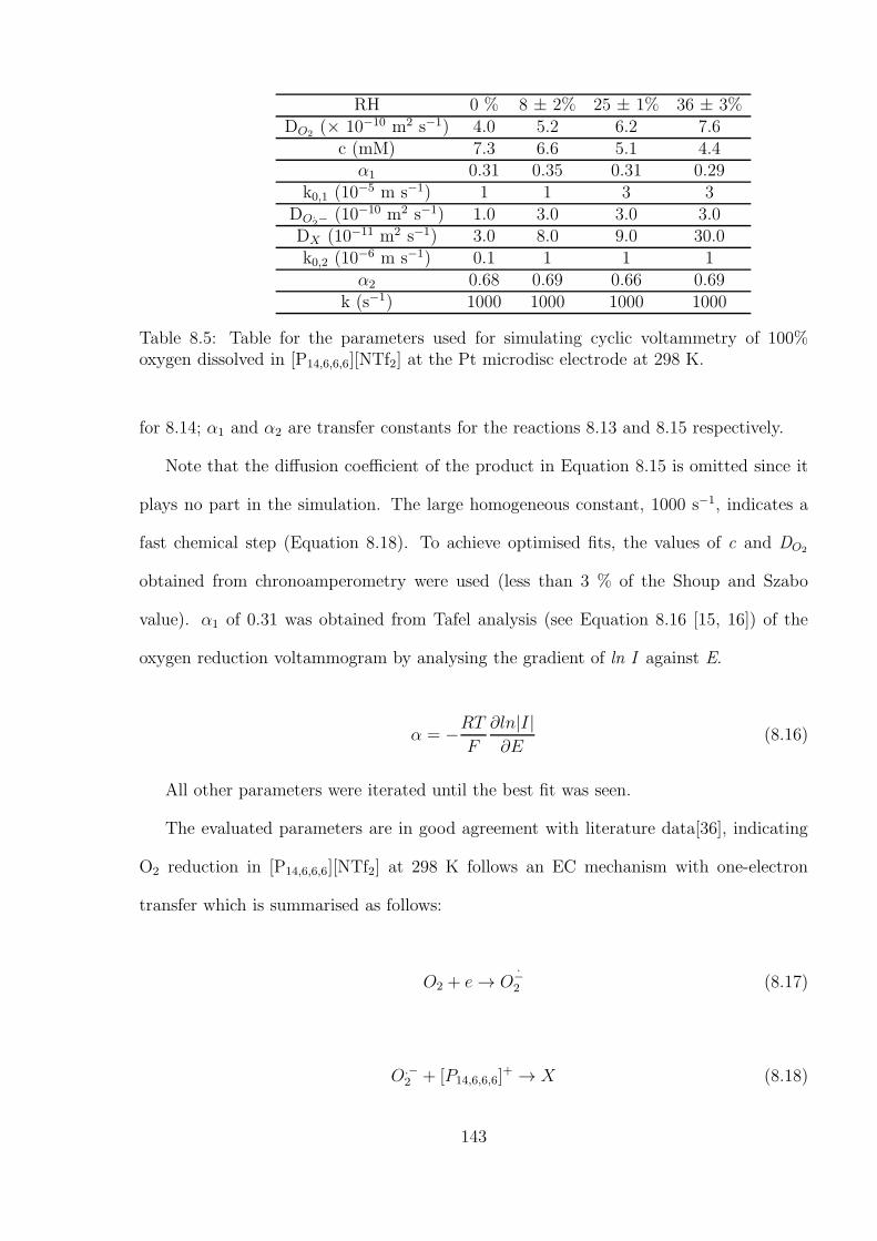
RH 0 % 8 ± 2% 25 ± 1% 36 ± 3%DO2
(× 10−10 m2 s−1) 4.0 5.2 6.2 7.6c (mM) 7.3 6.6 5.1 4.4
α1 0.31 0.35 0.31 0.29k0,1 (10−5 m s−1) 1 1 3 3
DO.2−
(10−10 m2 s−1) 1.0 3.0 3.0 3.0DX (10−11 m2 s−1) 3.0 8.0 9.0 30.0k0,2 (10−6 m s−1) 0.1 1 1 1
α2 0.68 0.69 0.66 0.69k (s−1) 1000 1000 1000 1000
Table 8.5: Table for the parameters used for simulating cyclic voltammetry of 100%oxygen dissolved in [P14,6,6,6][NTf2] at the Pt microdisc electrode at 298 K.
for 8.14; α1 and α2 are transfer constants for the reactions 8.13 and 8.15 respectively.
Note that the diffusion coefficient of the product in Equation 8.15 is omitted since it
plays no part in the simulation. The large homogeneous constant, 1000 s−1, indicates a
fast chemical step (Equation 8.18). To achieve optimised fits, the values of c and DO2
obtained from chronoamperometry were used (less than 3 % of the Shoup and Szabo
value). α1 of 0.31 was obtained from Tafel analysis (see Equation 8.16 [15, 16]) of the
oxygen reduction voltammogram by analysing the gradient of ln I against E.
α = −RT
F
∂ln|I|∂E
(8.16)
All other parameters were iterated until the best fit was seen.
The evaluated parameters are in good agreement with literature data[36], indicating
O2 reduction in [P14,6,6,6][NTf2] at 298 K follows an EC mechanism with one-electron
transfer which is summarised as follows:
O2 + e → O−2 (8.17)
O.−2 + [P14,6,6,6]
+ → X (8.18)
143
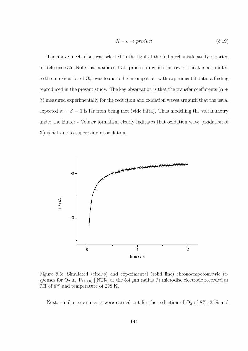
X − e → product (8.19)
The above mechanism was selected in the light of the full mechanistic study reported
in Reference 35. Note that a simple ECE process in which the reverse peak is attributed
to the re-oxidation of O.−2 was found to be incompatible with experimental data, a finding
reproduced in the present study. The key observation is that the transfer coefficients (α +
β) measured experimentally for the reduction and oxidation waves are such that the usual
expected α + β = 1 is far from being met (vide infra). Thus modelling the voltammetry
under the Butler - Volmer formalism clearly indicates that oxidation wave (oxidation of
X) is not due to superoxide re-oxidation.
0 1 2
-10
-8
i / n
A
time / s
Figure 8.6: Simulated (circles) and experimental (solid line) chronoamperometric re-sponses for O2 in [P14,6,6,6][NTf2] at the 5.4 µm radius Pt microdisc electrode recorded atRH of 8% and temperature of 298 K.
Next, similar experiments were carried out for the reduction of O2 of 8%, 25% and
144
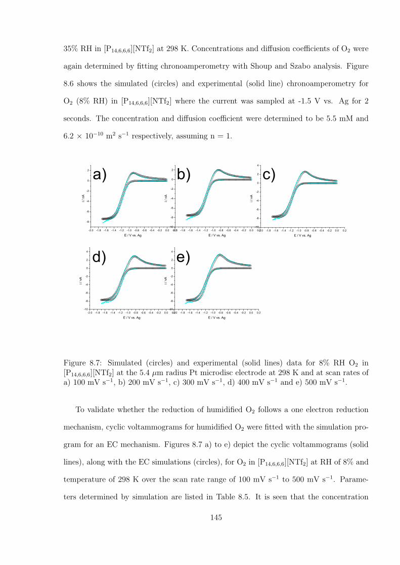
35% RH in [P14,6,6,6][NTf2] at 298 K. Concentrations and diffusion coefficients of O2 were
again determined by fitting chronoamperometry with Shoup and Szabo analysis. Figure
8.6 shows the simulated (circles) and experimental (solid line) chronoamperometry for
O2 (8% RH) in [P14,6,6,6][NTf2] where the current was sampled at -1.5 V vs. Ag for 2
seconds. The concentration and diffusion coefficient were determined to be 5.5 mM and
6.2 × 10⁻¹⁰ m2 s−1 respectively, assuming n = 1.
-2.0 -1.8 -1.6 -1.4 -1.2 -1.0 -0.8 -0.6 -0.4 -0.2 0.0 0.2-10
-8
-6
-4
-2
0
2
4
i / n
A
E / V vs. Ag-2.0 -1.8 -1.6 -1.4 -1.2 -1.0 -0.8 -0.6 -0.4 -0.2 0.0 0.2
-10
-8
-6
-4
-2
0
2
4
i / n
A
E / V vs. Ag
-2.0 -1.8 -1.6 -1.4 -1.2 -1.0 -0.8 -0.6 -0.4 -0.2 0.0 0.2-10
-8
-6
-4
-2
0
2
4
i / n
A
E / V vs. Ag-2.0 -1.8 -1.6 -1.4 -1.2 -1.0 -0.8 -0.6 -0.4 -0.2 0.0 0.2
-10
-8
-6
-4
-2
0
2
i / n
A
E / V vs. Ag-2.0 -1.8 -1.6 -1.4 -1.2 -1.0 -0.8 -0.6 -0.4 -0.2 0.0 0.2
-8
-6
-4
-2
0
2
i / n
A
E / V vs. Ag
a) b) c)
e)d)
Figure 8.7: Simulated (circles) and experimental (solid lines) data for 8% RH O2 in[P14,6,6,6][NTf2] at the 5.4 µm radius Pt microdisc electrode at 298 K and at scan rates ofa) 100 mV s−1, b) 200 mV s−1, c) 300 mV s−1, d) 400 mV s−1 and e) 500 mV s−1.
To validate whether the reduction of humidified O2 follows a one electron reduction
mechanism, cyclic voltammograms for humidified O2 were fitted with the simulation pro-
gram for an EC mechanism. Figures 8.7 a) to e) depict the cyclic voltammograms (solid
lines), along with the EC simulations (circles), for O2 in [P14,6,6,6][NTf2] at RH of 8% and
temperature of 298 K over the scan rate range of 100 mV s−1 to 500 mV s−1. Parame-
ters determined by simulation are listed in Table 8.5. It is seen that the concentration
145
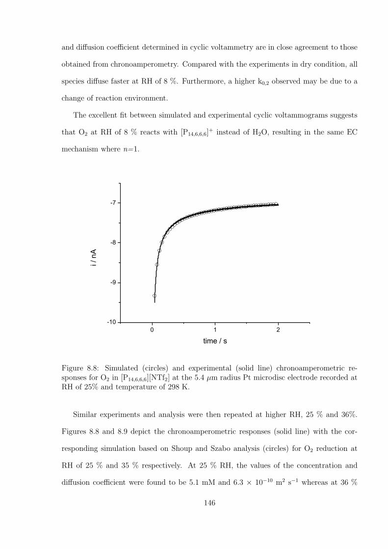
and diffusion coefficient determined in cyclic voltammetry are in close agreement to those
obtained from chronoamperometry. Compared with the experiments in dry condition, all
species diffuse faster at RH of 8 %. Furthermore, a higher k0,2 observed may be due to a
change of reaction environment.
The excellent fit between simulated and experimental cyclic voltammograms suggests
that O2 at RH of 8 % reacts with [P14,6,6,6]+ instead of H2O, resulting in the same EC
mechanism where n=1.
0 1 2-10
-9
-8
-7
i / n
A
time / s
Figure 8.8: Simulated (circles) and experimental (solid line) chronoamperometric re-sponses for O2 in [P14,6,6,6][NTf2] at the 5.4 µm radius Pt microdisc electrode recorded atRH of 25% and temperature of 298 K.
Similar experiments and analysis were then repeated at higher RH, 25 % and 36%.
Figures 8.8 and 8.9 depict the chronoamperometric responses (solid line) with the cor-
responding simulation based on Shoup and Szabo analysis (circles) for O2 reduction at
RH of 25 % and 35 % respectively. At 25 % RH, the values of the concentration and
diffusion coefficient were found to be 5.1 mM and 6.3 × 10⁻¹⁰ m2 s−1 whereas at 36 %
146
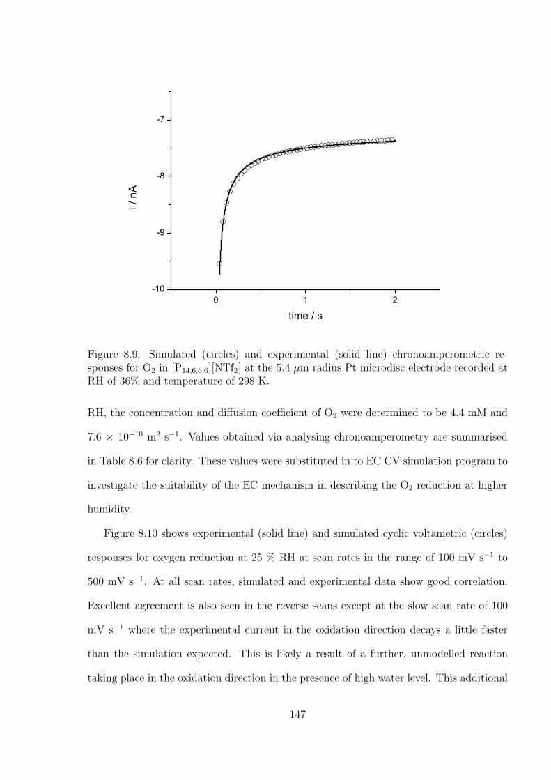
0 1 2-10
-9
-8
-7i /
nA
time / s
Figure 8.9: Simulated (circles) and experimental (solid line) chronoamperometric re-sponses for O2 in [P14,6,6,6][NTf2] at the 5.4 µm radius Pt microdisc electrode recorded atRH of 36% and temperature of 298 K.
RH, the concentration and diffusion coefficient of O2 were determined to be 4.4 mM and
7.6 × 10⁻¹⁰ m2 s−1. Values obtained via analysing chronoamperometry are summarised
in Table 8.6 for clarity. These values were substituted in to EC CV simulation program to
investigate the suitability of the EC mechanism in describing the O2 reduction at higher
humidity.
Figure 8.10 shows experimental (solid line) and simulated cyclic voltametric (circles)
responses for oxygen reduction at 25 % RH at scan rates in the range of 100 mV s−1 to
500 mV s−1. At all scan rates, simulated and experimental data show good correlation.
Excellent agreement is also seen in the reverse scans except at the slow scan rate of 100
mV s−1 where the experimental current in the oxidation direction decays a little faster
than the simulation expected. This is likely a result of a further, unmodelled reaction
taking place in the oxidation direction in the presence of high water level. This additional
147
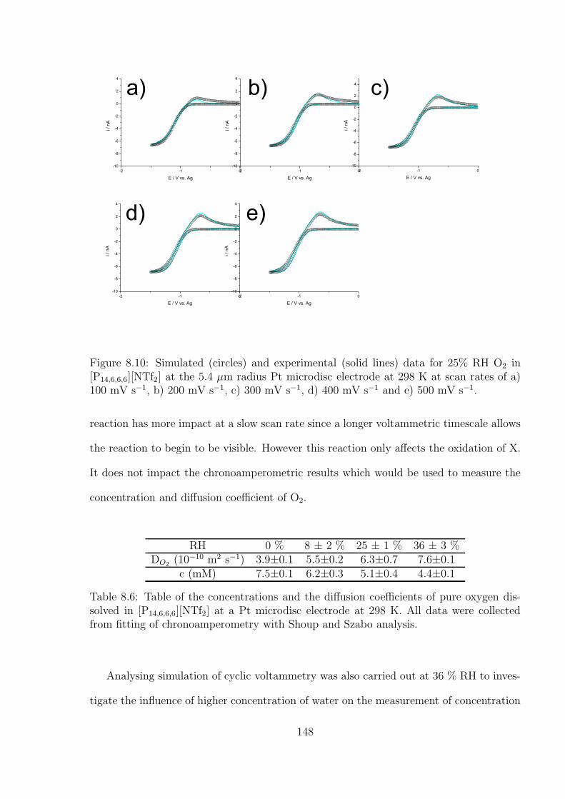
-2 -1 0-10
-8
-6
-4
-2
0
2
4
i / n
A
E / V vs. Ag-2 -1 0
-10
-8
-6
-4
-2
0
2
4
i / n
A
E / V vs. Ag
-2 -1 0-10
-8
-6
-4
-2
0
2
4
i / n
A
E / V vs. Ag-2 -1 0
-10
-8
-6
-4
-2
0
2
4
i / n
A
E / V vs. Ag-2 -1 0
-10
-8
-6
-4
-2
0
2
4
i / n
A
E / V vs. Ag
a) b) c)
e)d)
Figure 8.10: Simulated (circles) and experimental (solid lines) data for 25% RH O2 in[P14,6,6,6][NTf2] at the 5.4 µm radius Pt microdisc electrode at 298 K at scan rates of a)100 mV s−1, b) 200 mV s−1, c) 300 mV s−1, d) 400 mV s−1 and e) 500 mV s−1.
reaction has more impact at a slow scan rate since a longer voltammetric timescale allows
the reaction to begin to be visible. However this reaction only affects the oxidation of X.
It does not impact the chronoamperometric results which would be used to measure the
concentration and diffusion coefficient of O2.
RH 0 % 8 ± 2 % 25 ± 1 % 36 ± 3 %DO2
(10−10 m2 s−1) 3.9±0.1 5.5±0.2 6.3±0.7 7.6±0.1c (mM) 7.5±0.1 6.2±0.3 5.1±0.4 4.4±0.1
Table 8.6: Table of the concentrations and the diffusion coefficients of pure oxygen dis-solved in [P14,6,6,6][NTf2] at a Pt microdisc electrode at 298 K. All data were collectedfrom fitting of chronoamperometry with Shoup and Szabo analysis.
Analysing simulation of cyclic voltammetry was also carried out at 36 % RH to inves-
tigate the influence of higher concentration of water on the measurement of concentration
148
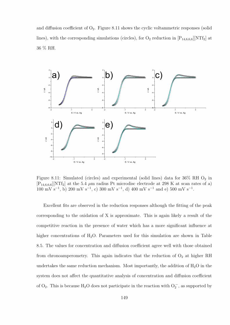
and diffusion coefficient of O2. Figure 8.11 shows the cyclic voltammetric responses (solid
lines), with the corresponding simulations (circles), for O2 reduction in [P14,6,6,6][NTf2] at
36 % RH.
-2 -1 0
-8
-6
-4
-2
0
2
i / n
A
E / V vs. Ag-2 -1 0
-10
-8
-6
-4
-2
0
2
i / n
A
E / V vs. Ag
-2 -1 0-8
-6
-4
-2
0
2
i / n
A
E / V vs. Ag-2 -1 0
-8
-6
-4
-2
0
2
i / n
A
E / V vs. Ag-2 -1 0
-8
-6
-4
-2
0
2
i / n
A
E / V vs. Ag
a) b) c)
e)d)
Figure 8.11: Simulated (circles) and experimental (solid lines) data for 36% RH O2 in[P14,6,6,6][NTf2] at the 5.4 µm radius Pt microdisc electrode at 298 K at scan rates of a)100 mV s−1, b) 200 mV s−1, c) 300 mV s−1, d) 400 mV s−1 and e) 500 mV s−1.
Excellent fits are observed in the reduction responses although the fitting of the peak
corresponding to the oxidation of X is approximate. This is again likely a result of the
competitive reaction in the presence of water which has a more significant influence at
higher concentrations of H2O. Parameters used for this simulation are shown in Table
8.5. The values for concentration and diffusion coefficient agree well with those obtained
from chronoamperometry. This again indicates that the reduction of O2 at higher RH
undertakes the same reduction mechanism. Most importantly, the addition of H2O in the
system does not affect the quantitative analysis of concentration and diffusion coefficient
of O2. This is because H2O does not participate in the reaction with O.−2 , as supported by
149
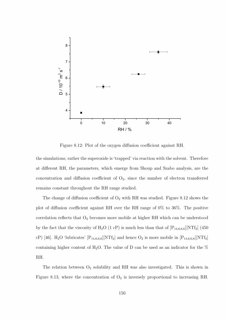
0 10 20 30 40
4
5
6
7
8
D /
10-1
0 m2 s
-1
RH / %
Figure 8.12: Plot of the oxygen diffusion coefficient against RH.
the simulations; rather the superoxide is ‘trapped’ via reaction with the solvent. Therefore
at different RH, the parameters, which emerge from Shoup and Szabo analysis, are the
concentration and diffusion coefficient of O2, since the number of electron transferred
remains constant throughout the RH range studied.
The change of diffusion coefficient of O2 with RH was studied. Figure 8.12 shows the
plot of diffusion coefficient against RH over the RH range of 0% to 36%. The positive
correlation reflects that O2 becomes more mobile at higher RH which can be understood
by the fact that the viscosity of H2O (1 cP) is much less than that of [P14,6,6,6][NTf2] (450
cP) [46]. H2O ‘lubricates’ [P14,6,6,6][NTf2] and hence O2 is more mobile in [P14,6,6,6][NTf2]
containing higher content of H2O. The value of D can be used as an indicator for the %
RH.
The relation between O2 solubility and RH was also investigated. This is shown in
Figure 8.13, where the concentration of O2 is inversely proportional to increasing RH.
150
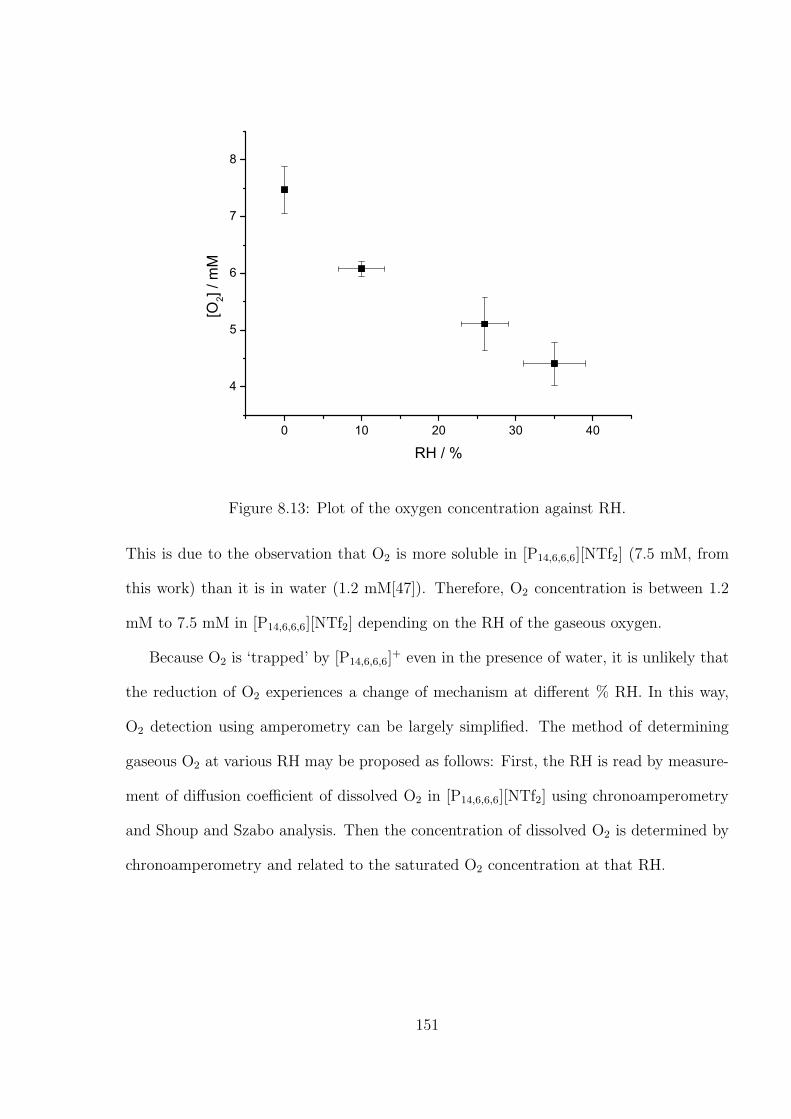
0 10 20 30 40
4
5
6
7
8
[O2]
/ mM
RH / %
Figure 8.13: Plot of the oxygen concentration against RH.
This is due to the observation that O2 is more soluble in [P14,6,6,6][NTf2] (7.5 mM, from
this work) than it is in water (1.2 mM[47]). Therefore, O2 concentration is between 1.2
mM to 7.5 mM in [P14,6,6,6][NTf2] depending on the RH of the gaseous oxygen.
Because O2 is ‘trapped’ by [P14,6,6,6]+ even in the presence of water, it is unlikely that
the reduction of O2 experiences a change of mechanism at different % RH. In this way,
O2 detection using amperometry can be largely simplified. The method of determining
gaseous O2 at various RH may be proposed as follows: First, the RH is read by measure-
ment of diffusion coefficient of dissolved O2 in [P14,6,6,6][NTf2] using chronoamperometry
and Shoup and Szabo analysis. Then the concentration of dissolved O2 is determined by
chronoamperometry and related to the saturated O2 concentration at that RH.
151
8.4 Conclusions
The reduction of O2 in [P14,6,6,6][NTf2] over the RH range of 0 % to 36 % has been
demonstrated. The concentrations and diffusion coefficients of O2 at different RHs have
been determined by fitting chronoamperometry with Shoup and Szabo analysis. Cyclic
voltammetry showed that the reduction of O2 follows a simple one electron EC mechanism
over the RH range of 0 % to 36 % where the superoxide is ‘trapped’ via reaction with
the phosphonium cation. In addition to gas sensor development described in Chapter 6
to Chapter 8 for providing more accurate results by monitoring the local environment for
gas detection and simplifying sensing reactions, Chapters 9 and 10 demonstrate low cost
home-made electrodes for both general electrochemical reactions and gas sensing systems.
References
[1] Xiong, L.; Barnes, E. O.; Compton, R. G. Sensors and Actuators, B: Chemical 2014,200, 157–166.
[2] Silvester, D. Analyst 2011, 136, 4871–4882.
[3] Shiddiky, M.; Torriero, A. Biosensors and Bioelectronics 2011, 26, 1775–1787.
[4] Hasanzadeh, M.; Shadjou, N.; Eskandani, M.; Guardia, M. TrAC - Trends in Ana-lytical Chemistry 2012, 41, 58–74.
[5] Faridbod, F.; Mohammad Reza Ganjali, M. R.; Norouzi, P.; Riahi, S.; Rashedi, H.Application of Room Temperature Ionic Liquids in Electrochemical Sensors andBiosensors ; InTech, 2011.
[6] Evans, R. G.; Klymenko, O. V.; Price, P. D.; Davies, S. G.; Hardacre, C.; Comp-ton, R. G. ChemPhysChem 2005, 6, 526–533.
[7] Silvester, D. S.; Compton, R. G. Zeitschrift fur Physikalische Chemie 2006, 220,1247–1274.
[8] Clark Jr., L.; Wolk, R.; Granger, D.; Talor, Z. Journal of applied physiology 1953,6, 189–193.
[9] Barrosse-Antle, L. E.; Bond, A. M.; Compton, R. G.; O’Mahony, A. M.; Rogers, E. I.;Silvester, D. S. Chemistry - An Asian Journal 2010, 5, 202–230.
[10] Huang, X.-J.; Aldous, L.; OMahony, A. M.; del Campo, F. J.; Compton, R. G.Analytical Chemistry 2010, 82, 5238–5245.
152
[11] Matsumoto, K.; Hagiwara, R.; Ito, Y. Electrochemical and Solid-State Letters 2004,7, E41–E44.
[12] Buzzeo, M. C.; Hardacre, C.; Compton, R. G. ChemPhysChem 2006, 7, 176–180.
[13] Zein El Abedin, S.; Endres, F. ChemPhysChem 2006, 7, 58–61.
[14] Lipsztajn, M.; Osteryoung, R. A. Journal of the Electrochemical Society 1983, 130,11–13.
[15] Compton, R. G.; Banks, C. E. Understanding Voltammetry ; Imperial College Press,2011, 2nd Edition.
[16] Bard, A. J.; Faulkner, L. R. Electrochemical Methods: Fundamentals and Applica-tions ; Wiley, 2001.
[17] Huang, X. J.; Rogers, E. I.; Hardacre, C.; Compton, R. G. The Journal of PhysicalChemistry B 2009, 113, 8953–8959.
[18] Xiong, L.; Lowinsohn, D.; Ward, K. R.; Compton, R. G. Analyst 2013, 138, 5444–5452.
[19] Xiong, L.; Fletcher, A. M.; Ernst, S.; Davies, S. G.; Compton, R. G. Analyst 2012,137, 2567–2573.
[20] Wang, Z.; Lin, P.; Baker, G. A.; Stetter, J.; Zeng, X. Analytical Chemistry 2011, 83,7066–7073.
[21] Barnes, A. S.; Rogers, E. I.; Streeter, I.; Aldous, L.; Hardacre, C.; Wildgoose, G. G.;Compton, R. G. The Journal of Physical Chemistry C 2008, 112, 13709–13715.
[22] Zhao, C.; Bond, A. M.; Compton, R. G.; O’Mahony, A. M.; Rogers, E. I. AnalyticalChemistry 2010, 82, 3856–3861.
[23] Murakawa, Y.; Hara, M.; Oguchi, H.; Hamate, Y.; Kuwano, H. Microsystem Tech-nologies 2013, 19, 1255–1259.
[24] Jalili, A. H.; Rahmati-Rostami, M.; Ghotbi, C.; Hosseini-Jenab, M.; Ahmadi, A. N.Journal of Chemical & Engineering Data 2009, 54, 1844–1849.
[25] O’Mahony, A. M.; Compton, R. G. Electroanalysis 2010, 22, 2313–2322.
[26] Villagran, C.; Banks, C. E.; Hardacre, C.; Compton, R. G. Anal. Chem. 2004, 76,1998–2003.
[27] Ng, S. R.; Guo, C. X.; Li, C. M. Electroanalysis 2011, 23, 442–448.
[28] Peng, Y.; Ji, Y.; Zheng, D.; Hu, S. Sensors and Actuators B: Chemical 2009, 137,656 – 661.
[29] Toniolo, R.; Dossi, N.; Pizzariello, A.; Doherty, A. P.; Bontempelli, G. Electroanalysis2012, 24, 865–871.
[30] Silvester, D. S.; Ward, K. R.; Aldous, L.; Hardacre, C.; Compton, R. G. Journal ofElectroanalytical Chemistry 2008, 618, 53–60.
153
[31] Ji, X.; Banks, C. E.; Silvester, D. S.; Aldous, L.; Hardacre, C.; Compton, R. G.Electroanalysis 2007, 19, 2194–2201.
[32] Buzzeo, M. C.; Hardacre, C.; Compton, R. G. Anal. Chem. 2004, 76, 4583–4588.
[33] Kudera, M.; Hill, H. A. O.; Dobson, P. J.; Leigh, P. A.; McIntire, W. S. Sensors2001, 1, 18–28.
[34] Xiong, L.; Fletcher, A. M.; Davies, S. G.; Norman, S. E.; Hardacre, C.; Comp-ton, R. G. The Analyst 2012, 137, 4951–4957.
[35] Buzzeo, M. C.; Klymenko, O. V.; Wadhawan, J. D.; Hardacre, C.; Seddon, K. R.;Compton, R. G. Journal of Physical Chemistry A 2003, 107, 8872–8878.
[36] Evans, R. G.; Klymenko, O. V.; Saddoughi, S. A.; Hardacre, C.; Compton, R. G. J.Phys. Chem. B 2004, 108, 7878–7886.
[37] Xiong, L.; Aldous, L.; Henstridge, M. C.; Compton, R. G. Analytical Methods 2012,4, 371–376.
[38] Clayden, J.; Greeves, N.; Warren, S. Organic Chemistry, 2nd edition; Oxford Uni-versity Press, 2012.
[39] Gavaghan, D. J. J. Electroanal. Chem. 1998, 456, 1–12.
[40] Gavaghan, D. J. J. Electroanal. Chem. 1998, 456, 13–23.
[41] Gavaghan, D. J. J. Electroanal. Chem. 1998, 456, 25–35.
[42] Britz, D. Digital Simulation in Electrochemistry ; Springer-Verlag: Heidelberg, 2005.
[43] Press, W. H., Teukolsky, S. A., Vetterling, W. T., Flannery, B. P., Eds. NumericalRecipes: The Art of Scientific Computing ; Cambridge University Press, 2007.
[44] Molina, A.; Gonzalez, J.; Barnes, E. O.; Compton, R. G. J. Phys. Chem. C 2014,118, 346–356.
[45] Shoup, D.; Szabo, A. Journal of Electroanalytical Chemistry and Interfacial Electro-chemistry 1982, 140, 237 – 245.
[46] Del Sesto, R.; Corley, C.; Robertson, A.; Wilkes, J. Journal of Organometallic Chem-istry 2005, 690, 2536–2542.
[47] Association, A. P. H. Standard methods for the examination of water and wastewa-ter, 18th ed ; American Public Health Association (APHA), American Water WorksAssociation (AWWA) & Water Environment Federation (WEF), 2001.
154
Chapter 9
Fabrication of Disposable GoldMacro-disc and PlatinumMicro-band Electrodes for Use inRoom-Temperature Ionic Liquids
The last two chapters focus on electrode development. This chapter introduces a sim-
ple and facile methodology for constructing gold macro-disc and platinum micro-band
for use in room temperature ionic liquids(RTILs). To validate the use of gold macro-
disc electrodes, the voltammetry of Ru(NH3)3+6 is studied in 0.1 M aqueous KCl. The
Randles-Sevcık equation is used to calculate the diffusion coefficient of Ru(NH3)3+6 , giv-
ing excellent agreement with literature values, suggesting the gold macro-disc electrode
is capable of performing quantitative electroanalysis in aqueous media. Gold macro-
disc electrodes are used to study oxidation of ferrocene in N-butyl-N-methylpyrrolidinium
bis(fluoromethylsulfonyl)imide ([C4mpyrr][NTf2]) using cyclic voltammetry. A diffusion
coefficient of ferrocene, (2.43 ± 0.07) ×10−11 m2 s−1, is obtained. This value is very
close to the literature value, indicating the good performance of gold electrode in RTILs.
Platinum micro-bands electrodes are tested in 1-propyl-3-methylimidazolium bis-trifluoro-
methylsulfonylimide ([C3mim][NTf2]) containing DmFc. Diffusion coefficients and elec-
tron transfer rate are obtained by fitting relevant simulations into the experimental data.
For comparison, analogous experiments and analysis are performed on a commercial plat-
155
inum micro-disc, where the results obtained from both micro-disc and micro-band agree
well, further suggesting the platinum micro-band electrode is suitable to be used in RTILs.
Last gold macro-disc and platinum micro-disc electrodes are used for oxygen detection.
Gold macro-disc electrodes are used to find the peak currents of oxygen at each volume
percentage analysed. Platinum micro-band electrodes showed steady-state currents of
different volumes of oxygen. These two results are compared which resulted in excellent
agreement. This is further confirmed by studying Henry’s law constants obtained from
both electrodes. The excellent behaviour of these two fabricated electrodes suggests they
are suitable for quantitative measurements and practicable for real world applications.
The work presented here has been published in the Analyst.[1]
9.1 Introduction
Work on the improvement of gas detection accuracy under various thermal and humid
condition is shown in Chapters 6 to 8, based upon the fundamental studies of the analytical
techniques in Chapter 4 and the interesting property of room temperature ionic liquids
in Chapter 5. Beside optimisation of accuracy of the gas sensing systems, gas sensors to
be produced in the manufacture, especially in large scale production, requires low cost
and high reproducibility. Hence low cost and easily fabricated disposable electrodes are
desired which is the main focus in the following chapters.
From literatures, not only have electrodes of different geometries and materials been
investigated, but also methods of construction have been developed. The most impor-
tant examples include screen printed[2–4], photo- or chemically etched[5–8] and glass
sealed electrodes[9–12]. Despite the success in the manufacture of various electrodes,
numerous challenges still exist. The cost of fabrication processes is normally high aris-
ing from the use of expensive machines or insulators. The electrode surface may result
in unreliable voltammetric responses since the surface may only be partially exposed in
156
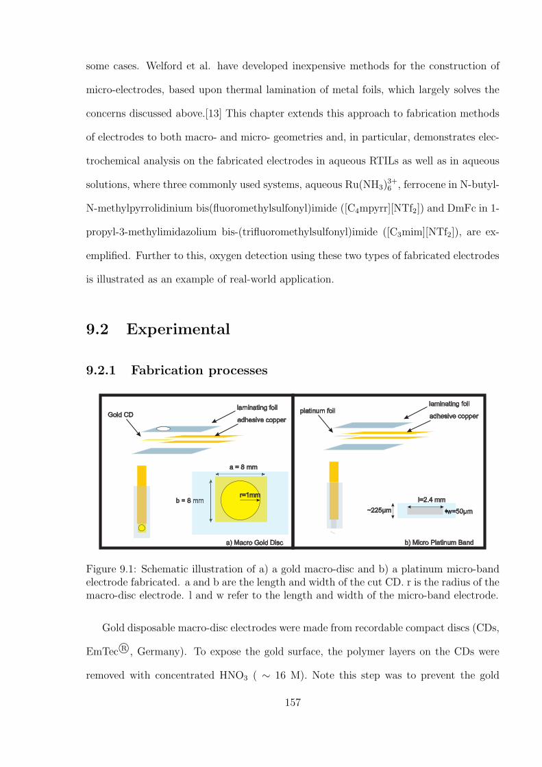
some cases. Welford et al. have developed inexpensive methods for the construction of
micro-electrodes, based upon thermal lamination of metal foils, which largely solves the
concerns discussed above.[13] This chapter extends this approach to fabrication methods
of electrodes to both macro- and micro- geometries and, in particular, demonstrates elec-
trochemical analysis on the fabricated electrodes in aqueous RTILs as well as in aqueous
solutions, where three commonly used systems, aqueous Ru(NH3)3+6 , ferrocene in N-butyl-
N-methylpyrrolidinium bis(fluoromethylsulfonyl)imide ([C4mpyrr][NTf2]) and DmFc in 1-
propyl-3-methylimidazolium bis-(trifluoromethylsulfonyl)imide ([C3mim][NTf2]), are ex-
emplified. Further to this, oxygen detection using these two types of fabricated electrodes
is illustrated as an example of real-world application.
9.2 Experimental
9.2.1 Fabrication processes
a = 8 mm
b = 8 mm
laminating foil
adhesive copperplatinum foil
b) Micro Platinum Band
w=50 mμ
l=2.4 mm
~225 mμ
r=1mm
laminating foil
adhesive copperGold CD
a) Macro Gold Disc
Figure 9.1: Schematic illustration of a) a gold macro-disc and b) a platinum micro-bandelectrode fabricated. a and b are the length and width of the cut CD. r is the radius of themacro-disc electrode. l and w refer to the length and width of the micro-band electrode.
Gold disposable macro-disc electrodes were made from recordable compact discs (CDs,
EmTec R©, Germany). To expose the gold surface, the polymer layers on the CDs were
removed with concentrated HNO3 ( ∼ 16 M). Note this step was to prevent the gold
157
surface from distortion when cutting which happens if the polymer is not removed. Figure
9.1 shows the schemes of electrode fabrication[14]. Both gold macro-disc electrodes and
platinum micro-band electrodes were prepared by thermal lamination of a piece of CD
(width × length = 8 mm × 8 mm) or platinum foil (width = 50 µm, Buckbee Mears Co.,
St. Paul, US). Electrical connection to the foil is previously established by using a piece of
copper foil with a conductive adhesive on one side (3 M Scotch brand electrical tape No.
1739-7). Gold macro-disc electrodes were exposed by punching a hole (r = 1 mm) on one
page of laminating foil prior to lamination and platinum micro-band electrode surfaces
were exposed by simply cutting the lamination normal to the foil with scissors[13].
The fabricated electrodes showed high stability over a period of three months by
repeatedly performing experiments (at least 30 scans per day) of Ru(NH3)3+6 in water or
DmFc in [C3mim][NTf2] over a period of one month; only a slight change in peak current,
ca. 3 %, was seen. These fabricated electrodes can be stored in a dry place and can be
reused straight away once needed. The variation of different fabricated gold macro-disc
or platinum micro-band electrodes was less than ± 2.5 %.
Experimental results were collected from more than five different gold macro-disc or
platinum micro-band electrodes, where the variations in peak current of cyclic voltamme-
try analysed for the same experiment at different electrodes were not more than ± 2.5 %
(analysed by standard deviation). This chapter shows representative results.
9.2.2 Simulation
All simulated results presented herein were generated by simulation packages developed in-
house by Dr. Kristopher Ward, fomally a PhD student in RGC group. Simulations of mi-
cro electrodes use a well established model developed by Klymenko et al.[15].Simulations
of micro-band electrodes use the 2D alternating direction implicit method.[16]
158
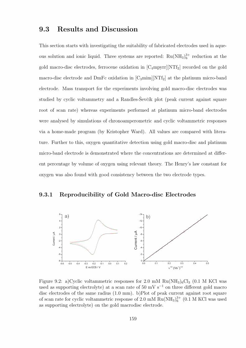
9.3 Results and Discussion
This section starts with investigating the suitability of fabricated electrodes used in aque-
ous solution and ionic liquid. Three systems are reported: Ru(NH3)3+6 reduction at the
gold macro-disc electrodes, ferrocene oxidation in [C4mpyrr][NTf2] recorded on the gold
macro-disc electrode and DmFc oxidation in [C3mim][NTf2] at the platinum micro-band
electrode. Mass transport for the experiments involving gold macro-disc electrodes was
studied by cyclic voltammetry and a Randles-Sevcık plot (peak current against square
root of scan rate) whereas experiments performed at platinum micro-band electrodes
were analysed by simulations of chronoamperometric and cyclic voltammetric responses
via a home-made program (by Kristopher Ward). All values are compared with litera-
ture. Further to this, oxygen quantitative detection using gold macro-disc and platinum
micro-band electrode is demonstrated where the concentrations are determined at differ-
ent percentage by volume of oxygen using relevant theory. The Henry’s law constant for
oxygen was also found with good consistency between the two electrode types.
9.3.1 Reproducibility of Gold Macro-disc Electrodes
-0.6 -0.5 -0.4 -0.3 -0.2 -0.1 0.0 0.1 0.2
-8
-6
-4
-2
0
2
4
6
Cu
rren
t/
mA
E vs ECS / V
0.0 0.1 0.2 0.3 0.4 0.5
0
-2
-4
-6
-8
-10
-12
-14
Cu
rre
nt
/m
A
n1/2
(Vs-1)
1/2
a) b)
Figure 9.2: a)Cyclic voltammetric responses for 2.0 mM Ru(NH3)6Cl3 (0.1 M KCl wasused as supporting electrolyte) at a scan rate of 50 mV s−1 on three different gold macrodisc electrodes of the same radius (1.0 mm). b)Plot of peak current against root squareof scan rate for cyclic voltammetric response of 2.0 mM Ru(NH3)
3+6 (0.1 M KCl was used
as supporting electrolyte) on the gold macrodisc electrode.
159
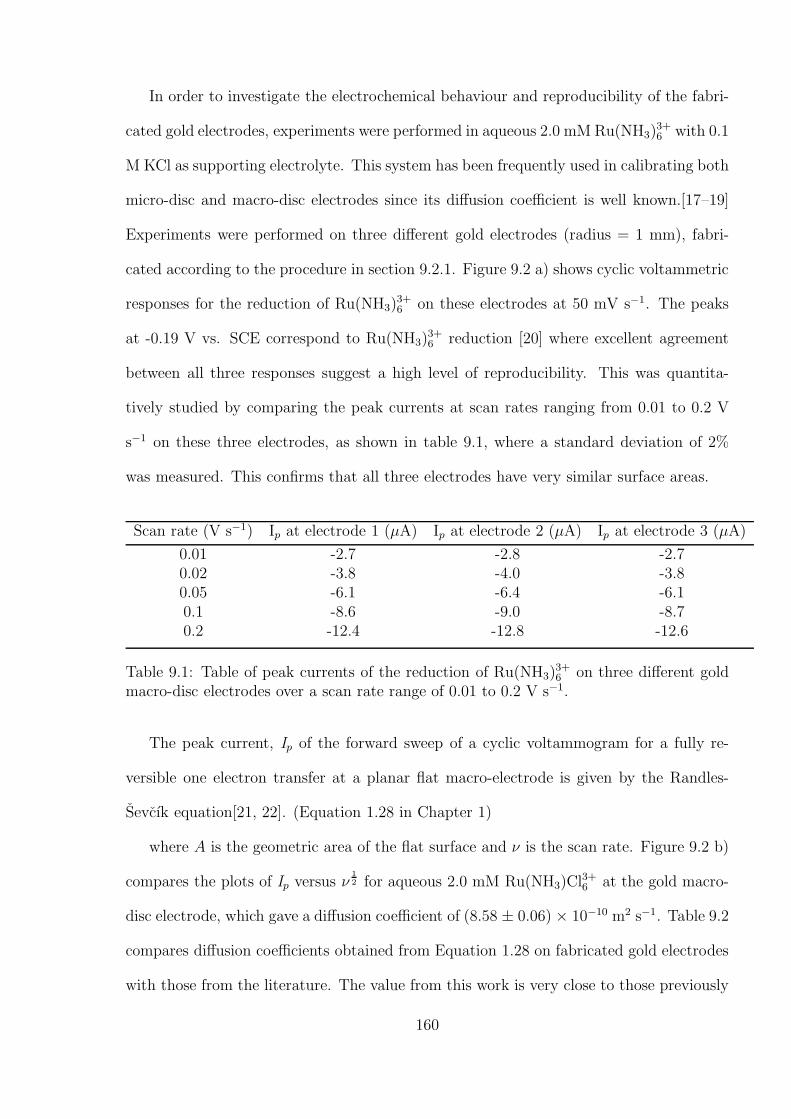
In order to investigate the electrochemical behaviour and reproducibility of the fabri-
cated gold electrodes, experiments were performed in aqueous 2.0 mM Ru(NH3)3+6 with 0.1
M KCl as supporting electrolyte. This system has been frequently used in calibrating both
micro-disc and macro-disc electrodes since its diffusion coefficient is well known.[17–19]
Experiments were performed on three different gold electrodes (radius = 1 mm), fabri-
cated according to the procedure in section 9.2.1. Figure 9.2 a) shows cyclic voltammetric
responses for the reduction of Ru(NH3)3+6 on these electrodes at 50 mV s−1. The peaks
at -0.19 V vs. SCE correspond to Ru(NH3)3+6 reduction [20] where excellent agreement
between all three responses suggest a high level of reproducibility. This was quantita-
tively studied by comparing the peak currents at scan rates ranging from 0.01 to 0.2 V
s−1 on these three electrodes, as shown in table 9.1, where a standard deviation of 2%
was measured. This confirms that all three electrodes have very similar surface areas.
Scan rate (V s−1) Ip at electrode 1 (µA) Ip at electrode 2 (µA) Ip at electrode 3 (µA)
0.01 -2.7 -2.8 -2.70.02 -3.8 -4.0 -3.80.05 -6.1 -6.4 -6.10.1 -8.6 -9.0 -8.70.2 -12.4 -12.8 -12.6
Table 9.1: Table of peak currents of the reduction of Ru(NH3)3+6 on three different gold
macro-disc electrodes over a scan rate range of 0.01 to 0.2 V s−1.
The peak current, Ip of the forward sweep of a cyclic voltammogram for a fully re-
versible one electron transfer at a planar flat macro-electrode is given by the Randles-
Sevcık equation[21, 22]. (Equation 1.28 in Chapter 1)
where A is the geometric area of the flat surface and ν is the scan rate. Figure 9.2 b)
compares the plots of Ip versus ν12 for aqueous 2.0 mM Ru(NH3)Cl
3+6 at the gold macro-
disc electrode, which gave a diffusion coefficient of (8.58 ± 0.06) × 10−10 m2 s−1. Table 9.2
compares diffusion coefficients obtained from Equation 1.28 on fabricated gold electrodes
with those from the literature. The value from this work is very close to those previously
160
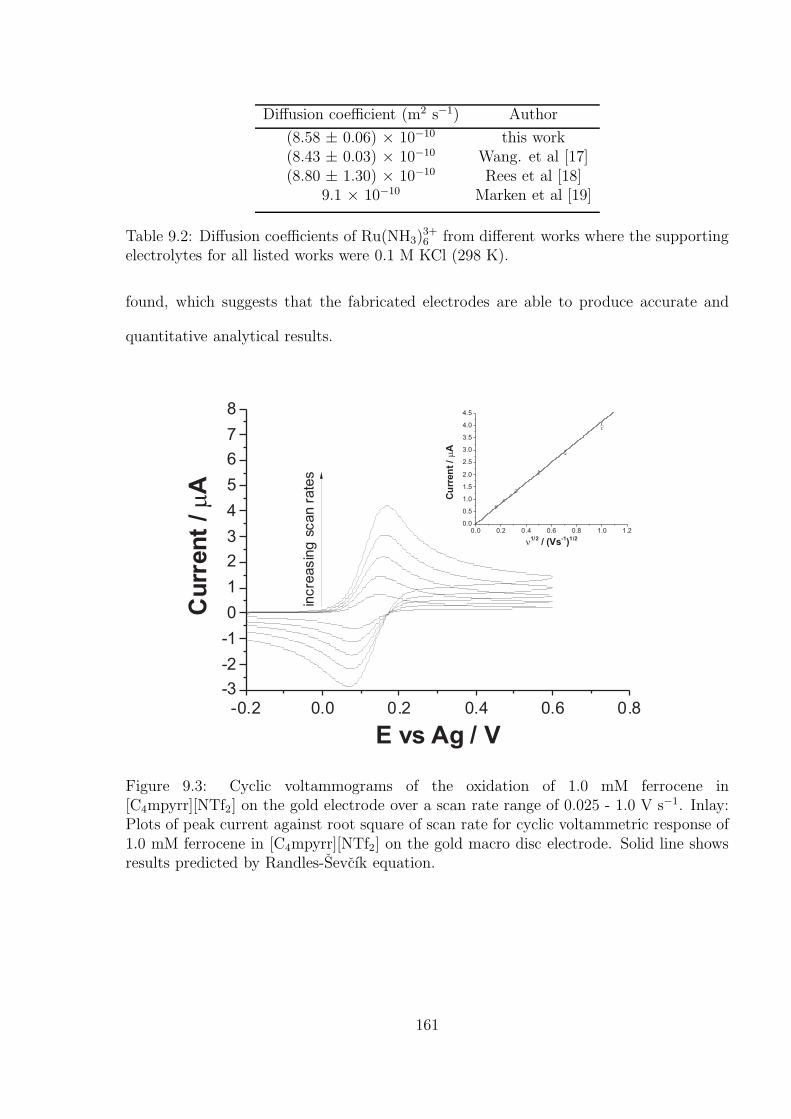
Diffusion coefficient (m2 s−1) Author
(8.58 ± 0.06) × 10−10 this work(8.43 ± 0.03) × 10−10 Wang. et al [17](8.80 ± 1.30) × 10−10 Rees et al [18]
9.1 × 10⁻¹⁰ Marken et al [19]
Table 9.2: Diffusion coefficients of Ru(NH3)3+6 from different works where the supporting
electrolytes for all listed works were 0.1 M KCl (298 K).
found, which suggests that the fabricated electrodes are able to produce accurate and
quantitative analytical results.
0.0 0.2 0.4 0.6 0.8 1.0 1.20.0
0.5
1.0
1.5
2.0
2.5
3.0
3.5
4.0
4.5
Cu
rren
t/
mA
n1/2
/ (Vs-1)1/2
-0.2 0.0 0.2 0.4 0.6 0.8-3
-2
-1
0
1
2
3
4
5
6
7
8
Cu
rren
t/
mA
E vs Ag / V
incre
asin
gsc
an
rate
s
Figure 9.3: Cyclic voltammograms of the oxidation of 1.0 mM ferrocene in[C4mpyrr][NTf2] on the gold electrode over a scan rate range of 0.025 - 1.0 V s−1. Inlay:Plots of peak current against root square of scan rate for cyclic voltammetric response of1.0 mM ferrocene in [C4mpyrr][NTf2] on the gold macro disc electrode. Solid line showsresults predicted by Randles-Sevcık equation.
161
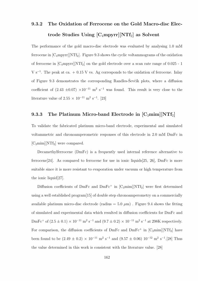
9.3.2 The Oxidation of Ferrocene on the Gold Macro-disc Elec-
trode Studies Using [C4mpyrr][NTf2] as Solvent
The performance of the gold macro-disc electrode was evaluated by analysing 1.0 mM
ferrocene in [C4mpyrr][NTf2]. Figure 9.3 shows the cyclic voltammograms of the oxidation
of ferrocene in [C4mpyrr][NTf2] on the gold electrode over a scan rate range of 0.025 - 1
V s−1. The peak at ca. + 0.15 V vs. Ag corresponds to the oxidation of ferrocene. Inlay
of Figure 9.3 demonstrates the corresponding Randles-Sevcık plots, where a diffusion
coefficient of (2.43 ±0.07) ×10−11 m2 s−1 was found. This result is very close to the
literature value of 2.55 × 10⁻¹¹ m2 s−1. [23]
9.3.3 The Platinum Micro-band Electrode in [C3mim][NTf2]
To validate the fabricated platinum micro-band electrode, experimental and simulated
voltammetric and chronoamperometric responses of this electrode in 2.0 mM DmFc in
[C3mim][NTf2] were compared.
Decamethylferrocene (DmFc) is a frequently used internal reference alternative to
ferrocene[24]. As compared to ferrocene for use in ionic liquids[25, 26], DmFc is more
suitable since it is more resistant to evaporation under vacuum or high temperature from
the ionic liquid[27].
Diffusion coefficients of DmFc and DmFc+ in [C3mim][NTf2] were first determined
using a well established program[15] of double step chronoamperometry on a commercially
available platinum micro-disc electrode (radius = 5.0 µm) . Figure 9.4 shows the fitting
of simulated and experimental data which resulted in diffusion coefficients for DmFc and
DmFc+ of (2.5 ± 0.1) × 10−11 m2 s−1 and (9.7 ± 0.2) × 10−11 m2 s−1 at 298K respectively.
For comparison, the diffusion coefficients of DmFc and DmFc+ in [C3mim][NTf2] have
been found to be (2.49 ± 0.2) × 10−11 m2 s−1 and (9.57 ± 0.06) 10−12 m2 s−1.[28] Thus
the value determined in this work is consistent with the literature value. [28]
162
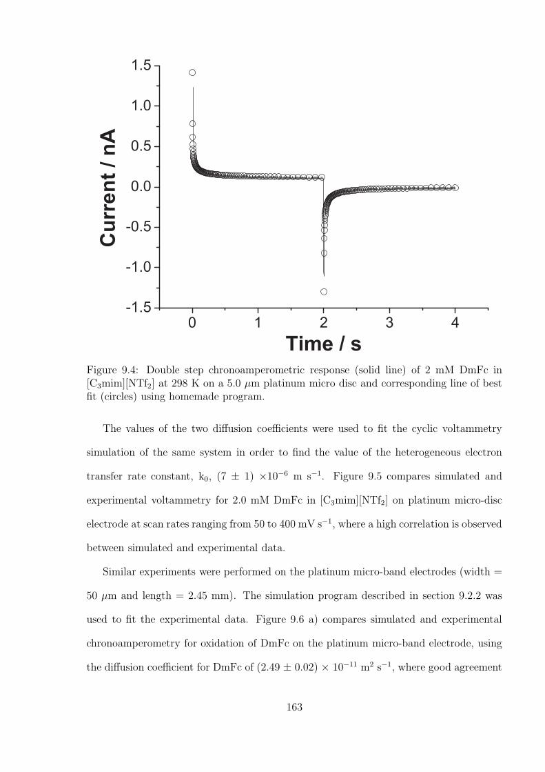
Figure 9.4: Double step chronoamperometric response (solid line) of 2 mM DmFc in[C3mim][NTf2] at 298 K on a 5.0 µm platinum micro disc and corresponding line of bestfit (circles) using homemade program.
The values of the two diffusion coefficients were used to fit the cyclic voltammetry
simulation of the same system in order to find the value of the heterogeneous electron
transfer rate constant, k0, (7 ± 1) ×10−6 m s−1. Figure 9.5 compares simulated and
experimental voltammetry for 2.0 mM DmFc in [C3mim][NTf2] on platinum micro-disc
electrode at scan rates ranging from 50 to 400 mV s−1, where a high correlation is observed
between simulated and experimental data.
Similar experiments were performed on the platinum micro-band electrodes (width =
50 µm and length = 2.45 mm). The simulation program described in section 9.2.2 was
used to fit the experimental data. Figure 9.6 a) compares simulated and experimental
chronoamperometry for oxidation of DmFc on the platinum micro-band electrode, using
the diffusion coefficient for DmFc of (2.49 ± 0.02) × 10−11 m2 s−1, where good agreement
163
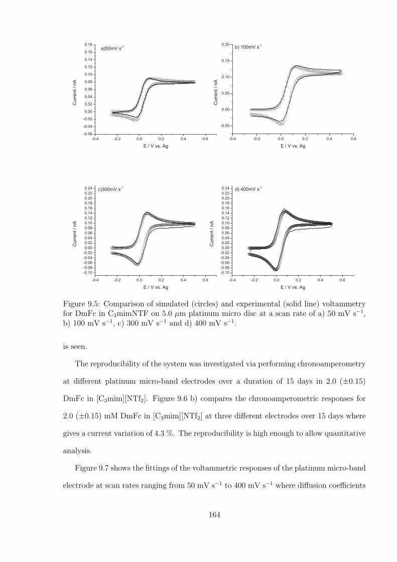
Figure 9.5: Comparison of simulated (circles) and experimental (solid line) voltammetryfor DmFc in C3mimNTF on 5.0 µm platinum micro disc at a scan rate of a) 50 mV s−1,b) 100 mV s−1, c) 300 mV s−1 and d) 400 mV s−1.
is seen.
The reproducibility of the system was investigated via performing chronoamperometry
at different platinum micro-band electrodes over a duration of 15 days in 2.0 (±0.15)
DmFc in [C3mim][NTf2]. Figure 9.6 b) compares the chronoamperometric responses for
2.0 (±0.15) mM DmFc in [C3mim][NTf2] at three different electrodes over 15 days where
gives a current variation of 4.3 %. The reproducibility is high enough to allow quantitative
analysis.
Figure 9.7 shows the fittings of the voltammetric responses of the platinum micro-band
electrode at scan rates ranging from 50 mV s−1 to 400 mV s−1 where diffusion coefficients
164
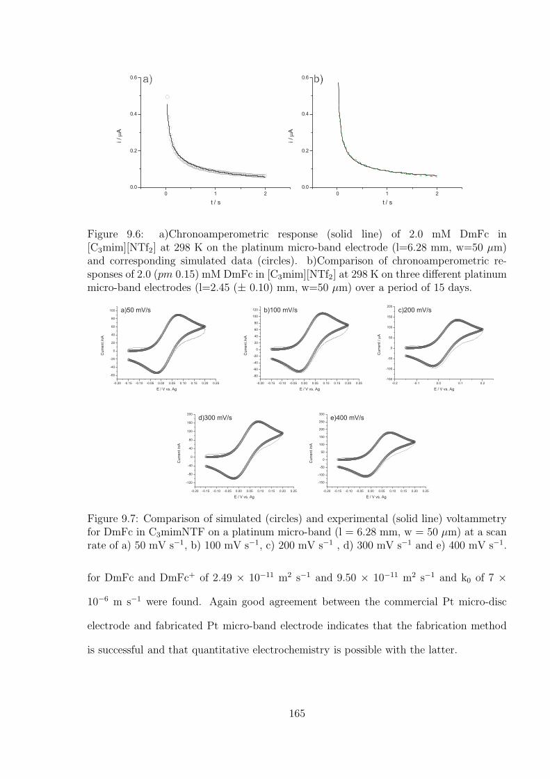
0 1 2
0.0
0.2
0.4
0.6
i/m
A
t / s
0 1 2
0.0
0.2
0.4
0.6
i/m
A
t / s
a) b)
Figure 9.6: a)Chronoamperometric response (solid line) of 2.0 mM DmFc in[C3mim][NTf2] at 298 K on the platinum micro-band electrode (l=6.28 mm, w=50 µm)and corresponding simulated data (circles). b)Comparison of chronoamperometric re-sponses of 2.0 (pm 0.15) mM DmFc in [C3mim][NTf2] at 298 K on three different platinummicro-band electrodes (l=2.45 (± 0.10) mm, w=50 µm) over a period of 15 days.
Figure 9.7: Comparison of simulated (circles) and experimental (solid line) voltammetryfor DmFc in C3mimNTF on a platinum micro-band (l = 6.28 mm, w = 50 µm) at a scanrate of a) 50 mV s−1, b) 100 mV s−1, c) 200 mV s−1 , d) 300 mV s−1 and e) 400 mV s−1.
for DmFc and DmFc+ of 2.49 × 10⁻¹¹ m2 s−1 and 9.50 × 10⁻¹¹ m2 s−1 and k0 of 7 ×
10−6 m s−1 were found. Again good agreement between the commercial Pt micro-disc
electrode and fabricated Pt micro-band electrode indicates that the fabrication method
is successful and that quantitative electrochemistry is possible with the latter.
165
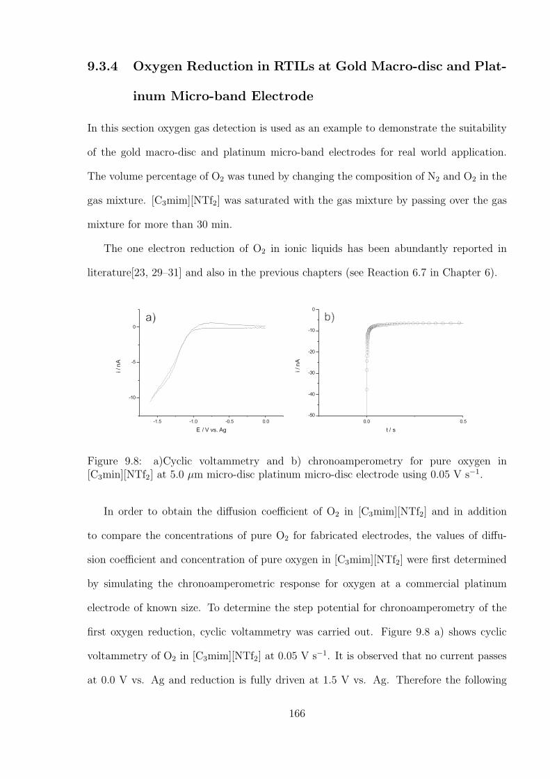
9.3.4 Oxygen Reduction in RTILs at Gold Macro-disc and Plat-
inum Micro-band Electrode
In this section oxygen gas detection is used as an example to demonstrate the suitability
of the gold macro-disc and platinum micro-band electrodes for real world application.
The volume percentage of O2 was tuned by changing the composition of N2 and O2 in the
gas mixture. [C3mim][NTf2] was saturated with the gas mixture by passing over the gas
mixture for more than 30 min.
The one electron reduction of O2 in ionic liquids has been abundantly reported in
literature[23, 29–31] and also in the previous chapters (see Reaction 6.7 in Chapter 6).
-1.5 -1.0 -0.5 0.0
-10
-5
0
i/n
A
E / V vs. Ag
0.0 0.5
-50
-40
-30
-20
-10
0
i/n
A
t / s
a) b)
Figure 9.8: a)Cyclic voltammetry and b) chronoamperometry for pure oxygen in[C3min][NTf2] at 5.0 µm micro-disc platinum micro-disc electrode using 0.05 V s−1.
In order to obtain the diffusion coefficient of O2 in [C3mim][NTf2] and in addition
to compare the concentrations of pure O2 for fabricated electrodes, the values of diffu-
sion coefficient and concentration of pure oxygen in [C3mim][NTf2] were first determined
by simulating the chronoamperometric response for oxygen at a commercial platinum
electrode of known size. To determine the step potential for chronoamperometry of the
first oxygen reduction, cyclic voltammetry was carried out. Figure 9.8 a) shows cyclic
voltammetry of O2 in [C3mim][NTf2] at 0.05 V s−1. It is observed that no current passes
at 0.0 V vs. Ag and reduction is fully driven at 1.5 V vs. Ag. Therefore the following
166
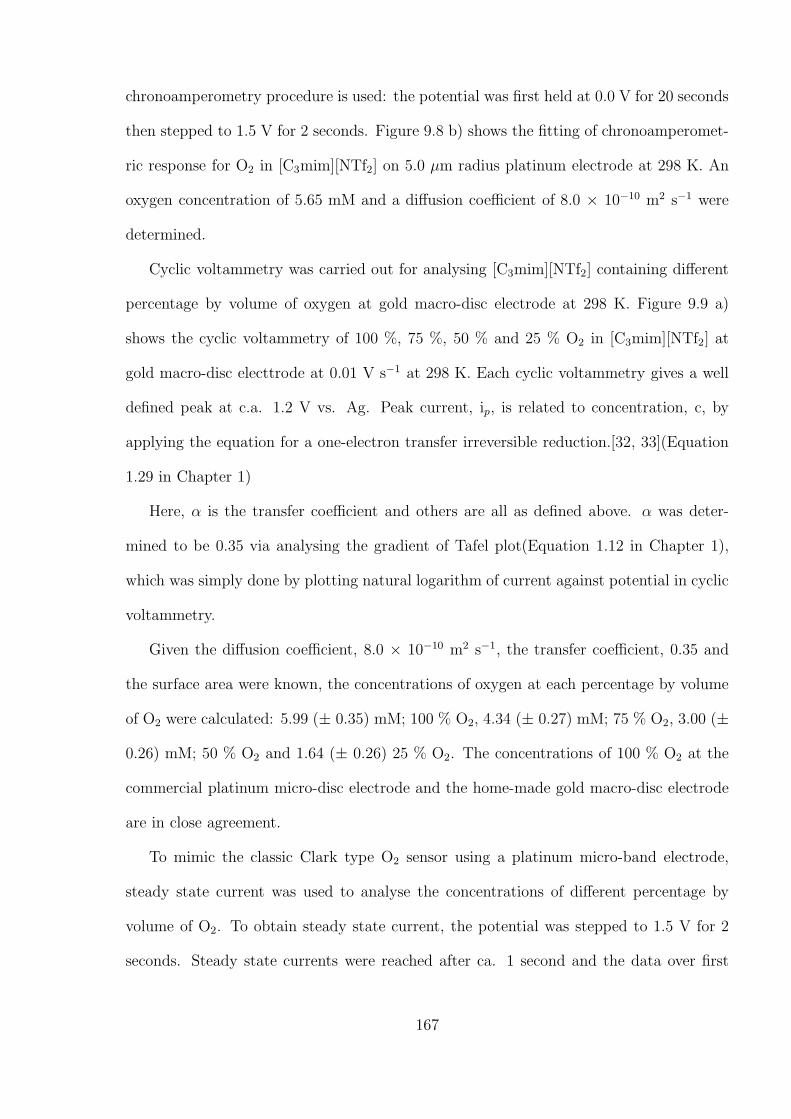
chronoamperometry procedure is used: the potential was first held at 0.0 V for 20 seconds
then stepped to 1.5 V for 2 seconds. Figure 9.8 b) shows the fitting of chronoamperomet-
ric response for O2 in [C3mim][NTf2] on 5.0 µm radius platinum electrode at 298 K. An
oxygen concentration of 5.65 mM and a diffusion coefficient of 8.0 × 10⁻¹⁰ m2 s−1 were
determined.
Cyclic voltammetry was carried out for analysing [C3mim][NTf2] containing different
percentage by volume of oxygen at gold macro-disc electrode at 298 K. Figure 9.9 a)
shows the cyclic voltammetry of 100 %, 75 %, 50 % and 25 % O2 in [C3mim][NTf2] at
gold macro-disc electtrode at 0.01 V s−1 at 298 K. Each cyclic voltammetry gives a well
defined peak at c.a. 1.2 V vs. Ag. Peak current, ip, is related to concentration, c, by
applying the equation for a one-electron transfer irreversible reduction.[32, 33](Equation
1.29 in Chapter 1)
Here, α is the transfer coefficient and others are all as defined above. α was deter-
mined to be 0.35 via analysing the gradient of Tafel plot(Equation 1.12 in Chapter 1),
which was simply done by plotting natural logarithm of current against potential in cyclic
voltammetry.
Given the diffusion coefficient, 8.0 × 10⁻¹⁰ m2 s−1, the transfer coefficient, 0.35 and
the surface area were known, the concentrations of oxygen at each percentage by volume
of O2 were calculated: 5.99 (± 0.35) mM; 100 % O2, 4.34 (± 0.27) mM; 75 % O2, 3.00 (±
0.26) mM; 50 % O2 and 1.64 (± 0.26) 25 % O2. The concentrations of 100 % O2 at the
commercial platinum micro-disc electrode and the home-made gold macro-disc electrode
are in close agreement.
To mimic the classic Clark type O2 sensor using a platinum micro-band electrode,
steady state current was used to analyse the concentrations of different percentage by
volume of O2. To obtain steady state current, the potential was stepped to 1.5 V for 2
seconds. Steady state currents were reached after ca. 1 second and the data over first
167
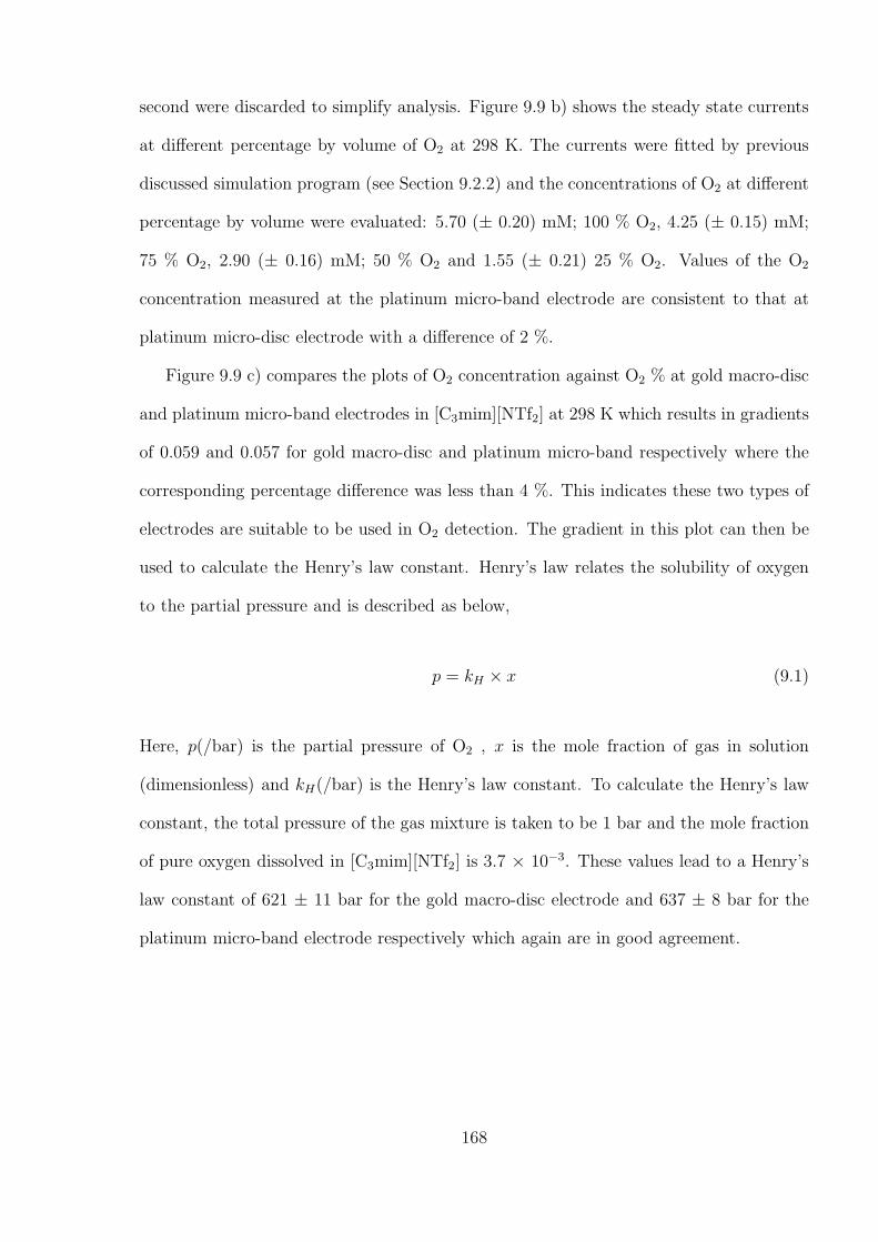
second were discarded to simplify analysis. Figure 9.9 b) shows the steady state currents
at different percentage by volume of O2 at 298 K. The currents were fitted by previous
discussed simulation program (see Section 9.2.2) and the concentrations of O2 at different
percentage by volume were evaluated: 5.70 (± 0.20) mM; 100 % O2, 4.25 (± 0.15) mM;
75 % O2, 2.90 (± 0.16) mM; 50 % O2 and 1.55 (± 0.21) 25 % O2. Values of the O2
concentration measured at the platinum micro-band electrode are consistent to that at
platinum micro-disc electrode with a difference of 2 %.
Figure 9.9 c) compares the plots of O2 concentration against O2 % at gold macro-disc
and platinum micro-band electrodes in [C3mim][NTf2] at 298 K which results in gradients
of 0.059 and 0.057 for gold macro-disc and platinum micro-band respectively where the
corresponding percentage difference was less than 4 %. This indicates these two types of
electrodes are suitable to be used in O2 detection. The gradient in this plot can then be
used to calculate the Henry’s law constant. Henry’s law relates the solubility of oxygen
to the partial pressure and is described as below,
p = kH × x (9.1)
Here, p(/bar) is the partial pressure of O2 , x is the mole fraction of gas in solution
(dimensionless) and kH(/bar) is the Henry’s law constant. To calculate the Henry’s law
constant, the total pressure of the gas mixture is taken to be 1 bar and the mole fraction
of pure oxygen dissolved in [C3mim][NTf2] is 3.7 × 10⁻³. These values lead to a Henry’s
law constant of 621 ± 11 bar for the gold macro-disc electrode and 637 ± 8 bar for the
platinum micro-band electrode respectively which again are in good agreement.
168
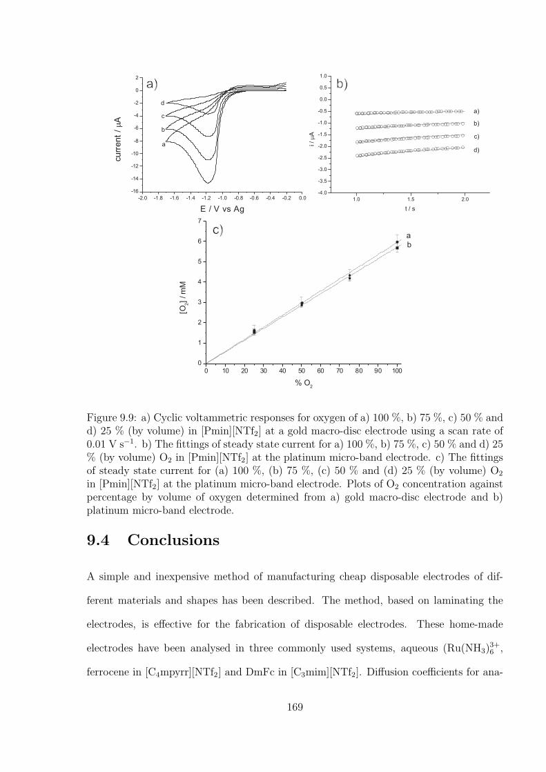
0 10 20 30 40 50 60 70 80 90 100
0
1
2
3
4
5
6
7
[O2]
/m
M
% O2
ab
-2.0 -1.8 -1.6 -1.4 -1.2 -1.0 -0.8 -0.6 -0.4 -0.2 0.0
-16
-14
-12
-10
-8
-6
-4
-2
0
2
curr
ent
/mA
E / V vs Ag
d
a
b
c
a) b)
c)
Figure 9.9: a) Cyclic voltammetric responses for oxygen of a) 100 %, b) 75 %, c) 50 % andd) 25 % (by volume) in [Pmin][NTf2] at a gold macro-disc electrode using a scan rate of0.01 V s−1. b) The fittings of steady state current for a) 100 %, b) 75 %, c) 50 % and d) 25% (by volume) O2 in [Pmin][NTf2] at the platinum micro-band electrode. c) The fittingsof steady state current for (a) 100 %, (b) 75 %, (c) 50 % and (d) 25 % (by volume) O2
in [Pmin][NTf2] at the platinum micro-band electrode. Plots of O2 concentration againstpercentage by volume of oxygen determined from a) gold macro-disc electrode and b)platinum micro-band electrode.
9.4 Conclusions
A simple and inexpensive method of manufacturing cheap disposable electrodes of dif-
ferent materials and shapes has been described. The method, based on laminating the
electrodes, is effective for the fabrication of disposable electrodes. These home-made
electrodes have been analysed in three commonly used systems, aqueous (Ru(NH3)3+6 ,
ferrocene in [C4mpyrr][NTf2] and DmFc in [C3mim][NTf2]. Diffusion coefficients for ana-
169
lytes at each experiment have been evaluated using relevant theory or simulations. These
values have been either compared with literature values, or values collected from an com-
mercially available electrode of known size. In all cases, very good agreement has been
found. This suggests the home made electrodes are suitable for use in both ionic liquids
and aqueous solution, and may be made to both macro and micro scale. Further these two
types of electrode have been studied for use in oxygen detection. Values of dissolved pure
oxygen concentrations in [C3mim][NTf2] at a commercial platinum micro-disc electrode
has been compared and good agreement found. The concentrations of oxygen have been
determined at different % (by volume) at both gold macro-disc and platinum micro-band
electrodes. Less than 4 % difference in oxygen concentration has been found, suggesting
both electrodes are suitable for use in oxygen detection. In addition, the Henry’s law
constants of oxygen obtained from both electrodes agree very well.
References
[1] Xiong, L.; Lowinsohn, D.; Ward, K. R.; Compton, R. G. Analyst 2013, 138, 5444–5452.
[2] Dias, A. C. M. S.; Gomes-Filho, S. L. R.; Silva, M. M. S.; Dutra, R. F. Biosensorsand Bioelectronics 2013, 44, 216–221.
[3] Kanyong, P.; Pemberton, R. M.; Jackson, S. K.; Hart, J. P. Analytical Biochemistry2013, 435, 114–119, cited By (since 1996) 0; Article in Press.
[4] Xuan Viet, N.; Chikae, M.; Ukita, Y.; Maehashi, K.; Matsumoto, K.; Tamiya, E.;Hung Viet, P.; Takamura, Y. Biosensors and Bioelectronics 2013, 42, 592–597, citedB.
[5] Prehn, R.; Abad, L.; Snchez-Molas, D.; Duch, M.; Sabat, N.; Del Campo, F. J.;Muoz, F. X.; Compton, R. G. Journal of Electroanalytical Chemistry 2011, 662,361–370.
[6] Wang, T.-J.; Huang, C.-F.; Wang, W.-S.; Wei, P.-K. IEEE JOURNAL OF LIGHT-WAVE TECHNOLOGY 2004, 22, 1764–1771.
[7] Davies, T. J.; Ward-Jones, S.; Banks, C. E.; del Campo, J.; Mas, R.; Muoz, F. X.;Compton, R. G. Journal of Electroanalytical Chemistry 2005, 585, 51 – 62.
[8] Lee, H.; Shin, H.; Jeong, Y.; Moon, J.; Lee, M. Applied Physics Letters 2009, 95,p071104.
170
[9] Koppenol, M.; Cooper, J. B.; Bond, A. M. American Laboratory 1994, 26, 25–29.
[10] Shao, Y.; Mirkin, M.; Fish, G.; Kokotov, S.; Palanker, D.; Lewis, A. AnalyticalChemistry 1997, 69, 1627–1634.
[11] Kovach, P. M.; Caudill, W. L.; Peters, D. G.; Wightman, R. M. Journal of Electro-analytical Chemistry 1985, 185, 285–295.
[12] Shea, T. V.; Bard, A. J. Analytical Chemistry 1987, 59, 2101–2111.
[13] Welford, P. J.; Freeman, J.; Wilkins, S. J.; Wadhawan, J. D.; Hahn, C. E. W.;Compton, R. G. Analytical Chemistry 2001, 73, 6088–6092.
[14] Angnes, L.; Richter, E. M.; Augelli, M. A.; Kume, G. H. Analytical Chemistry 2000,72, 5503–5506.
[15] Klymenko, O. V.; Evans, R. G.; Hardacre, C.; Svir, I. B.; Compton, R. G. Journalof Electroanalytical Chemistry 2004, 571, 211–221.
[16] Alden, J. A.; Compton, R. G. Journal of Electroanalytical Chemistry 1996, 402,1–10.
[17] Wang, Y.; Limon-Petersen, J. G.; Compton, R. G. Journal of Electroanalytical Chem-istry 2011, 652, 13–17.
[18] Banks, C. E.; Rees, N. V.; Compton, R. G. Journal of Electroanalytical Chemistry2002, 535, 41–47.
[19] Marken, F.; Eklund, J. C.; Compton, R. G. Journal of Electroanalytical Chemistry1995, 395, 335–339.
[20] Banks, C. E.; Compton, R. G.; Fisher, A. C.; Henley, I. E. Physical ChemistryChemical Physics 2004, 6, 3147–3152.
[21] Randles, J. E. B. Transactions of the Faraday Society 1948, 44, 327–338.
[22] Sevcik, A. Collection of Czechoslovak Chemical Communications 1948, 13, 349–377.
[23] Rogers, E. I.; Silvester, D. S.; Poole, D. L.; Aldous, L.; Hardacre, C.; Compton, R. G.Journal of Physical Chemistry C 2008, 112, 2729–2735.
[24] Noviandri, I.; Brown, K. N.; Fleming, D. S.; Gulyas, P. T.; Lay, P. A.; Masters, A. F.;Phillips, L. The Journal of Physical Chemistry B 1999, 103, 6713–6722.
[25] Fu, C.; Aldous, L.; Dickinson, E. J. F.; Manan, N. S. A.; Compton, R. G.ChemPhysChem 2011, 12, 1708–1713.
[26] Vorotyntsev, M. A.; Zinovyeva, V. A.; Konev, D. V.; Picquet, M.; Gaillon, L.;Rizzi, C. Journal of Physical Chemistry B 2009, 113, 1085–1099.
[27] Xiong, L.; Fletcher, A. M.; Davies, S. G.; Norman, S. E.; Hardacre, C.; Comp-ton, R. G. Analyst 2012, 137, 4951–4957.
[28] Barnes, E. O.; Xiong, L.; Ward, K. R.; Compton, R. G. Journal of ElectroanalyticalChemistry 2013, –.
171

[29] Evans, R. G.; Klymenko, O. V.; Saddoughi, S. A.; Hardacre, C.; Compton, R. G.Journal of Physical Chemistry B 2004, 108, 7878–7886.
[30] Huang, X. J.; Rogers, E. I.; Hardacre, C.; Compton, R. G. The Journal of PhysicalChemistry B 2009, 113, 8953–8959.
[31] Switzer, E. E.; Zeller, R.; Chen, Q.; Sieradzki, K.; Buttry, D. A.; Friesen, C. TheJournal of Physical Chemistry C 2013, 117, 8683–8690.
[32] Compton, R. G.; Banks, C. E. Understanding Voltammetry ; Imperial College Press,2011, 2nd Edition.
[33] Bard, A.; Faulkner, L. Electrochemical Methods: Fundamentals and Applications ;Wiley, 2001.
172
Chapter 10
Evaluation of A Simple Disposablemicro-band electrode Device forAmperometric Gas Sensing
Following the success of previous work on the use of laminated macro-disc and micro-
band electrodes for electrochemical experiments, including in aqueous, non-aqueous and
RTIL systems, this chapter further demonstrates the home-made laminated Pt (6.3 mm
× 50 µm) and Cu (6.3 mm × 30 µm) annular micro-band electrodes for use in room
temperature ionic liquids (RTILs) and proposes their use for amperometric gas sensing.
The suitability of micro-band electrodes for use in electrochemical analysis was examined
in experiments on two systems. The first system studied to validate the electrochemical
responses of the annular micro-band electrode was decamethylferrocene (DmFc), as a
stable internal reference probe commonly used in ionic liquids, in [C3mim][NTf2], where
the diffusion coefficients of DmFc and DmFc+ and the standard electron rate constant
for the DmFc/DmFc+ couple were determined through fitting chronoamperometric and
cyclic voltammetric responses with relevant simulations.These values are independently
compared with those collected from a commercially available Pt microdisc electrode with
excellent agreement. The second system focuses on O2 reduction in [C3mim][NTf2], which
is used as a model for gas sensing. The diffusion coefficients of O2 and O−2 and the
electron transfer rate constant were again obtained using chronoamperometry and cyclic
173
voltammetry, along with simulations. Results determined from the micro-bands are again
consistent to those evaluated from the Pt microdisc electrode when compared these results
from home-made micro-band and commercially available microdisc electrodes. These
observations indicate that the fabricated annular micro-band electrodes are suitable for
quantitative measurements. Further the successful use of the Cu electrodes in the O2
system suggests a cheap disposable sensor for gas detection. This work has been published
in Sensors and Actuators B.[1]
10.1 Introduction
The previous chapter discussed the use of laminated electrodes as working electrodes in
electrochemical experiments in various solvent media. This chapter is concerned with
the home-made electrode in room temperature ionic liquids. The benefits of RTILs as
solvents for gas sensors as compared to conventional solvents have been discussed earlier
in the thesis. Chapter 2 introduced the possible design of membrane free gas sensors
through combining room temperature ionic liquids as solvents and laminated electrodes
as sensing probes. Huang et al.[1] successfully developed a membrane free oxygen sensor
using micro-electrode arrays as working electrodes and ionic liquids([P14,6,6,6][FAP]) as
solvents. This oxygen sensing system showed high sensitivity and most importantly, was
freed from the problem caused by the use of membranes, especially frequent calibration.
In this chapter a design for a gas sensor is proposed which utilises micro-band elec-
trodes and RTIL solvents. The aim of this work is to validate the use of such electrodes
for gas sensing in RTIL media and to show that such electrodes are easily fabricated to
the extent that practical disposable electrodes could be readily envisaged.
The use of chronoamperometry to measure gas concentrations and diffusion coeffi-
cients in this type of electrode is established by conducting O2 detection using the RTIL
[C3mim][NTf2]. Two additional observations to be reported are first that the solubility of
174
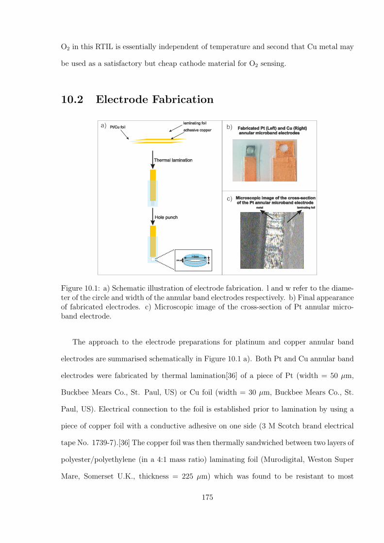
O2 in this RTIL is essentially independent of temperature and second that Cu metal may
be used as a satisfactory but cheap cathode material for O2 sensing.
10.2 Electrode Fabrication
Thermal lamination
Hole punch
laminating foil
adhesive copperPt/Cu foil
w225 mμ
l=2mm
a) b) Fabricated Pt (Left) and Cu (Right)annular microband electrodes
Microscopic image of the cross-sectionof the Pt annular microband electrode
c)
metal laminating foil
Figure 10.1: a) Schematic illustration of electrode fabrication. l and w refer to the diame-ter of the circle and width of the annular band electrodes respectively. b) Final appearanceof fabricated electrodes. c) Microscopic image of the cross-section of Pt annular micro-band electrode.
The approach to the electrode preparations for platinum and copper annular band
electrodes are summarised schematically in Figure 10.1 a). Both Pt and Cu annular band
electrodes were fabricated by thermal lamination[36] of a piece of Pt (width = 50 µm,
Buckbee Mears Co., St. Paul, US) or Cu foil (width = 30 µm, Buckbee Mears Co., St.
Paul, US). Electrical connection to the foil is established prior to lamination by using a
piece of copper foil with a conductive adhesive on one side (3 M Scotch brand electrical
tape No. 1739-7).[36] The copper foil was then thermally sandwiched between two layers of
polyester/polyethylene (in a 4:1 mass ratio) laminating foil (Murodigital, Weston Super
Mare, Somerset U.K., thickness = 225 µm) which was found to be resistant to most
175
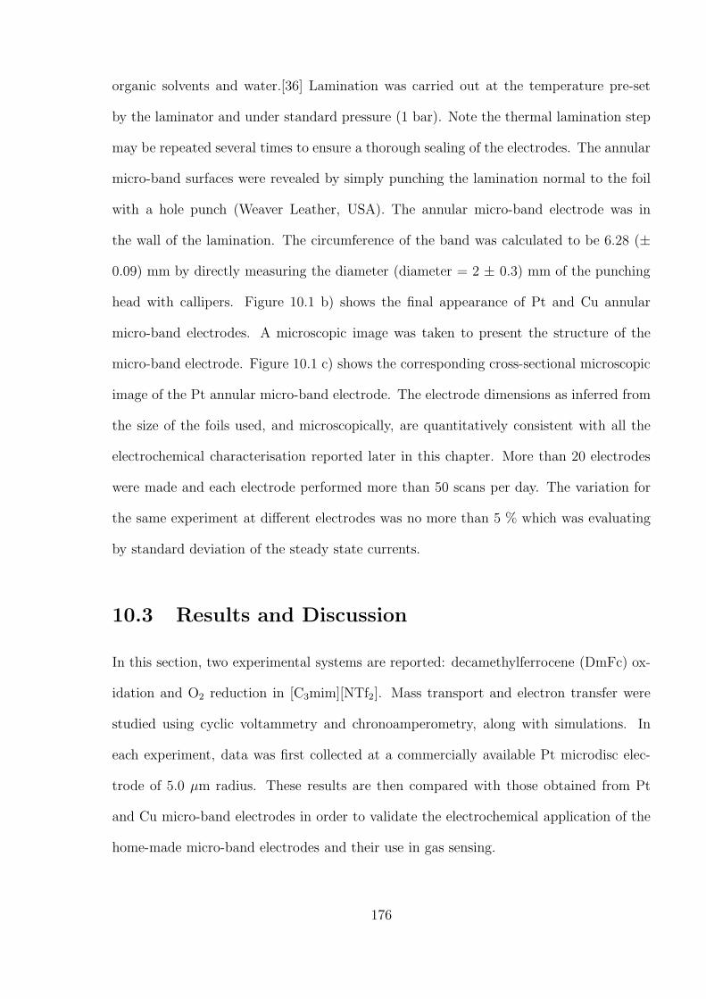
organic solvents and water.[36] Lamination was carried out at the temperature pre-set
by the laminator and under standard pressure (1 bar). Note the thermal lamination step
may be repeated several times to ensure a thorough sealing of the electrodes. The annular
micro-band surfaces were revealed by simply punching the lamination normal to the foil
with a hole punch (Weaver Leather, USA). The annular micro-band electrode was in
the wall of the lamination. The circumference of the band was calculated to be 6.28 (±
0.09) mm by directly measuring the diameter (diameter = 2 ± 0.3) mm of the punching
head with callipers. Figure 10.1 b) shows the final appearance of Pt and Cu annular
micro-band electrodes. A microscopic image was taken to present the structure of the
micro-band electrode. Figure 10.1 c) shows the corresponding cross-sectional microscopic
image of the Pt annular micro-band electrode. The electrode dimensions as inferred from
the size of the foils used, and microscopically, are quantitatively consistent with all the
electrochemical characterisation reported later in this chapter. More than 20 electrodes
were made and each electrode performed more than 50 scans per day. The variation for
the same experiment at different electrodes was no more than 5 % which was evaluating
by standard deviation of the steady state currents.
10.3 Results and Discussion
In this section, two experimental systems are reported: decamethylferrocene (DmFc) ox-
idation and O2 reduction in [C3mim][NTf2]. Mass transport and electron transfer were
studied using cyclic voltammetry and chronoamperometry, along with simulations. In
each experiment, data was first collected at a commercially available Pt microdisc elec-
trode of 5.0 µm radius. These results are then compared with those obtained from Pt
and Cu micro-band electrodes in order to validate the electrochemical application of the
home-made micro-band electrodes and their use in gas sensing.
176
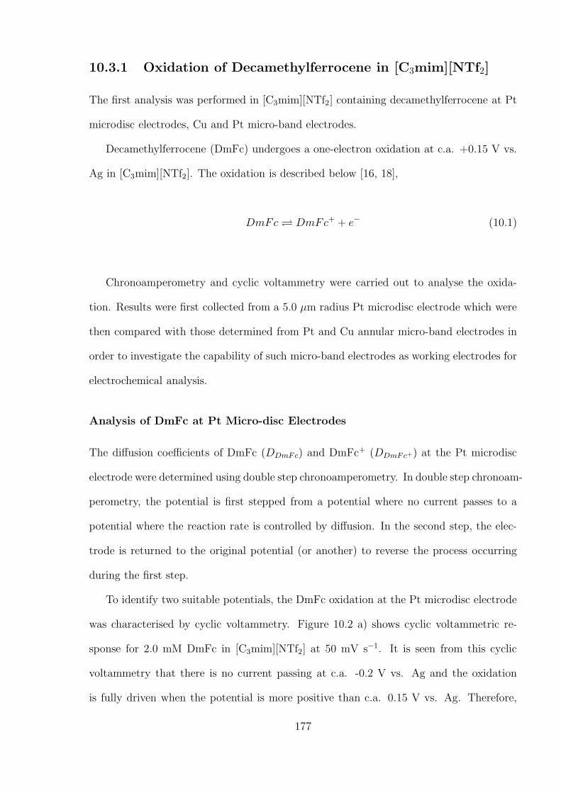
10.3.1 Oxidation of Decamethylferrocene in [C3mim][NTf2]
The first analysis was performed in [C3mim][NTf2] containing decamethylferrocene at Pt
microdisc electrodes, Cu and Pt micro-band electrodes.
Decamethylferrocene (DmFc) undergoes a one-electron oxidation at c.a. +0.15 V vs.
Ag in [C3mim][NTf2]. The oxidation is described below [16, 18],
DmFc DmFc+ + e− (10.1)
Chronoamperometry and cyclic voltammetry were carried out to analyse the oxida-
tion. Results were first collected from a 5.0 µm radius Pt microdisc electrode which were
then compared with those determined from Pt and Cu annular micro-band electrodes in
order to investigate the capability of such micro-band electrodes as working electrodes for
electrochemical analysis.
Analysis of DmFc at Pt Micro-disc Electrodes
The diffusion coefficients of DmFc (DDmFc) and DmFc+ (DDmFc+) at the Pt microdisc
electrode were determined using double step chronoamperometry. In double step chronoam-
perometry, the potential is first stepped from a potential where no current passes to a
potential where the reaction rate is controlled by diffusion. In the second step, the elec-
trode is returned to the original potential (or another) to reverse the process occurring
during the first step.
To identify two suitable potentials, the DmFc oxidation at the Pt microdisc electrode
was characterised by cyclic voltammetry. Figure 10.2 a) shows cyclic voltammetric re-
sponse for 2.0 mM DmFc in [C3mim][NTf2] at 50 mV s−1. It is seen from this cyclic
voltammetry that there is no current passing at c.a. -0.2 V vs. Ag and the oxidation
is fully driven when the potential is more positive than c.a. 0.15 V vs. Ag. Therefore,
177
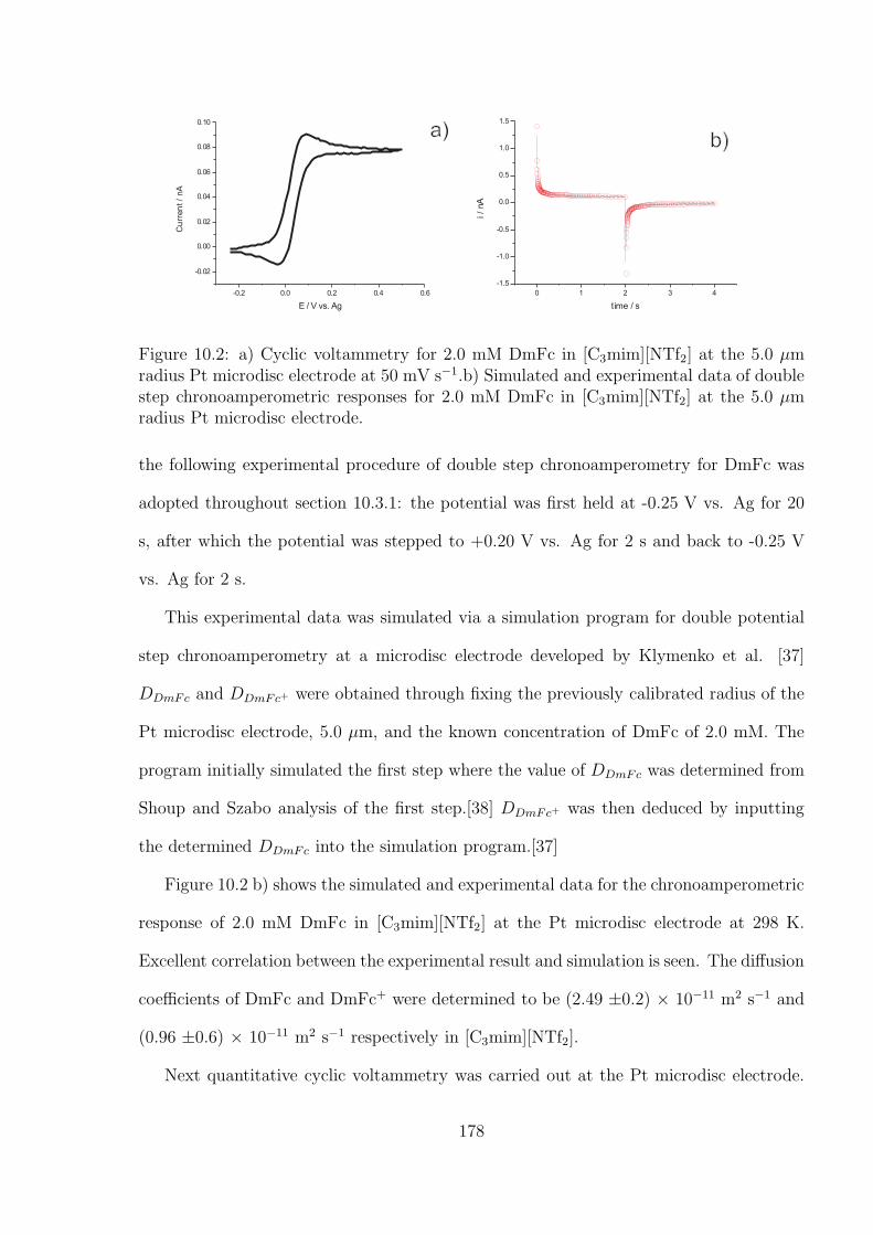
-0.2 0.0 0.2 0.4 0.6
-0.02
0.00
0.02
0.04
0.06
0.08
0.10
Cu
rren
t/
nA
E / V vs. Ag
0 1 2 3 4
-1.5
-1.0
-0.5
0.0
0.5
1.0
1.5
i/
nA
time / s
a)b)
Figure 10.2: a) Cyclic voltammetry for 2.0 mM DmFc in [C3mim][NTf2] at the 5.0 µmradius Pt microdisc electrode at 50 mV s−1.b) Simulated and experimental data of doublestep chronoamperometric responses for 2.0 mM DmFc in [C3mim][NTf2] at the 5.0 µmradius Pt microdisc electrode.
the following experimental procedure of double step chronoamperometry for DmFc was
adopted throughout section 10.3.1: the potential was first held at -0.25 V vs. Ag for 20
s, after which the potential was stepped to +0.20 V vs. Ag for 2 s and back to -0.25 V
vs. Ag for 2 s.
This experimental data was simulated via a simulation program for double potential
step chronoamperometry at a microdisc electrode developed by Klymenko et al. [37]
DDmFc and DDmFc+ were obtained through fixing the previously calibrated radius of the
Pt microdisc electrode, 5.0 µm, and the known concentration of DmFc of 2.0 mM. The
program initially simulated the first step where the value of DDmFc was determined from
Shoup and Szabo analysis of the first step.[38] DDmFc+ was then deduced by inputting
the determined DDmFc into the simulation program.[37]
Figure 10.2 b) shows the simulated and experimental data for the chronoamperometric
response of 2.0 mM DmFc in [C3mim][NTf2] at the Pt microdisc electrode at 298 K.
Excellent correlation between the experimental result and simulation is seen. The diffusion
coefficients of DmFc and DmFc+ were determined to be (2.49 ±0.2) × 10−11 m2 s−1 and
(0.96 ±0.6) × 10−11 m2 s−1 respectively in [C3mim][NTf2].
Next quantitative cyclic voltammetry was carried out at the Pt microdisc electrode.
178
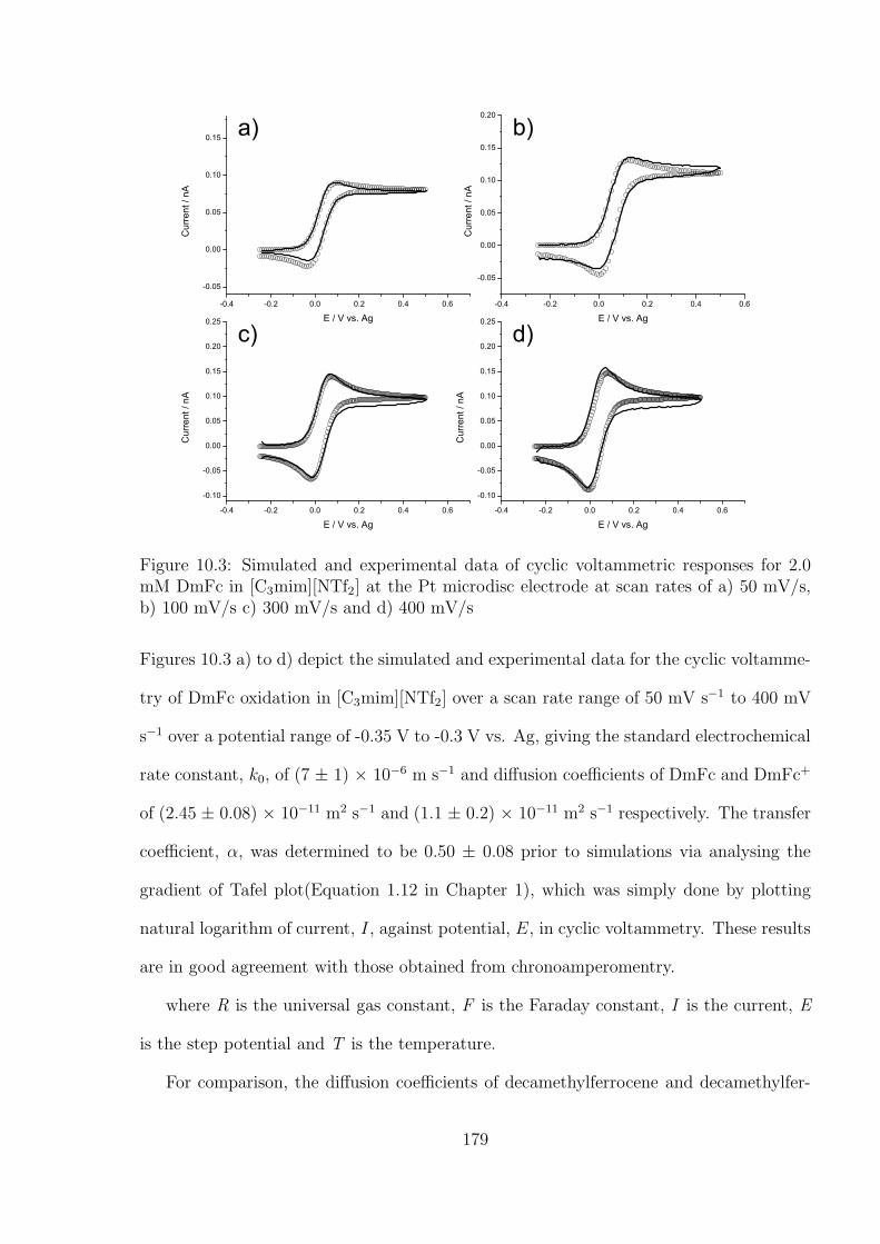
-0.4 -0.2 0.0 0.2 0.4 0.6
-0.05
0.00
0.05
0.10
0.15
0.20
b)
Cur
rent
/ nA
E / V vs. Ag-0.4 -0.2 0.0 0.2 0.4 0.6
-0.05
0.00
0.05
0.10
0.15 a)
Cur
rent
/ nA
E / V vs. Ag
-0.4 -0.2 0.0 0.2 0.4 0.6
-0.10
-0.05
0.00
0.05
0.10
0.15
0.20
0.25
Cur
rent
/ nA
E / V vs. Ag
d)
-0.4 -0.2 0.0 0.2 0.4 0.6
-0.10
-0.05
0.00
0.05
0.10
0.15
0.20
0.25
c)
Cur
rent
/ nA
E / V vs. Ag
Figure 10.3: Simulated and experimental data of cyclic voltammetric responses for 2.0mM DmFc in [C3mim][NTf2] at the Pt microdisc electrode at scan rates of a) 50 mV/s,b) 100 mV/s c) 300 mV/s and d) 400 mV/s
Figures 10.3 a) to d) depict the simulated and experimental data for the cyclic voltamme-
try of DmFc oxidation in [C3mim][NTf2] over a scan rate range of 50 mV s−1 to 400 mV
s−1 over a potential range of -0.35 V to -0.3 V vs. Ag, giving the standard electrochemical
rate constant, k0, of (7 ± 1) × 10−6 m s−1 and diffusion coefficients of DmFc and DmFc+
of (2.45 ± 0.08) × 10−11 m2 s−1 and (1.1 ± 0.2) × 10−11 m2 s−1 respectively. The transfer
coefficient, α, was determined to be 0.50 ± 0.08 prior to simulations via analysing the
gradient of Tafel plot(Equation 1.12 in Chapter 1), which was simply done by plotting
natural logarithm of current, I, against potential, E, in cyclic voltammetry. These results
are in good agreement with those obtained from chronoamperomentry.
where R is the universal gas constant, F is the Faraday constant, I is the current, E
is the step potential and T is the temperature.
For comparison, the diffusion coefficients of decamethylferrocene and decamethylfer-
179
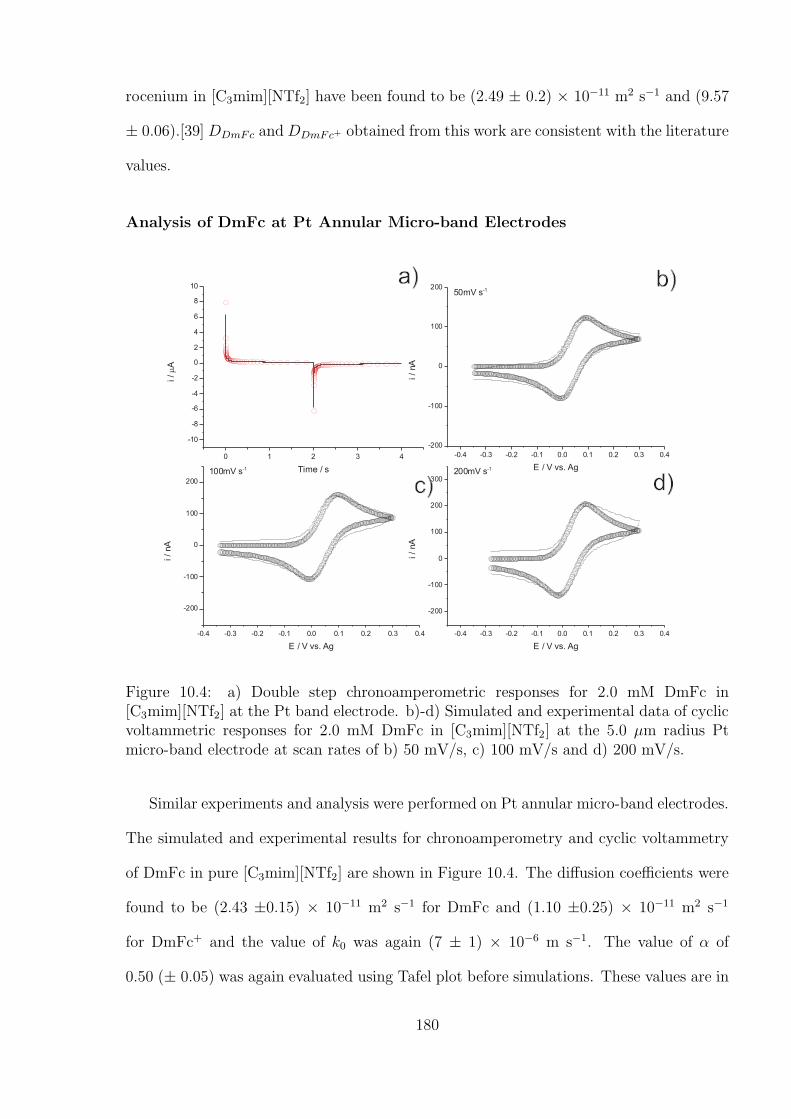
rocenium in [C3mim][NTf2] have been found to be (2.49 ± 0.2) × 10−11 m2 s−1 and (9.57
± 0.06).[39] DDmFc andDDmFc+ obtained from this work are consistent with the literature
values.
Analysis of DmFc at Pt Annular Micro-band Electrodes
-0.4 -0.3 -0.2 -0.1 0.0 0.1 0.2 0.3 0.4
-200
-100
0
100
20050mV s-1
i/
nA
E / V vs. Ag
-0.4 -0.3 -0.2 -0.1 0.0 0.1 0.2 0.3 0.4
-200
-100
0
100
200
100mV s-1
i/
nA
E / V vs. Ag
-0.4 -0.3 -0.2 -0.1 0.0 0.1 0.2 0.3 0.4
-200
-100
0
100
200
300200mV s-1
i/
nA
E / V vs. Ag
a) b)
c)
0 1 2 3 4
-10
-8
-6
-4
-2
0
2
4
6
8
10
i/m
A
Time / s
d)
Figure 10.4: a) Double step chronoamperometric responses for 2.0 mM DmFc in[C3mim][NTf2] at the Pt band electrode. b)-d) Simulated and experimental data of cyclicvoltammetric responses for 2.0 mM DmFc in [C3mim][NTf2] at the 5.0 µm radius Ptmicro-band electrode at scan rates of b) 50 mV/s, c) 100 mV/s and d) 200 mV/s.
Similar experiments and analysis were performed on Pt annular micro-band electrodes.
The simulated and experimental results for chronoamperometry and cyclic voltammetry
of DmFc in pure [C3mim][NTf2] are shown in Figure 10.4. The diffusion coefficients were
found to be (2.43 ±0.15) × 10−11 m2 s−1 for DmFc and (1.10 ±0.25) × 10−11 m2 s−1
for DmFc+ and the value of k0 was again (7 ± 1) × 10−6 m s−1. The value of α of
0.50 (± 0.05) was again evaluated using Tafel plot before simulations. These values are in
180
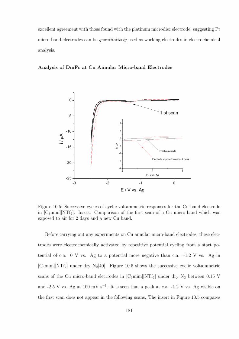
excellent agreement with those found with the platinum microdisc electrode, suggesting Pt
micro-band electrodes can be quantitatively used as working electrodes in electrochemical
analysis.
Analysis of DmFc at Cu Annular Micro-band Electrodes
-3 -2 -1 0-25
-20
-15
-10
-5
0
-2 -1 0-4
-3
-2
-1
0
1
2
Electrode exposed to air for 2 days
i /
A
E / V vs. Ag
Fresh electrode
i /
A
E / V vs. Ag
1 st scan
Figure 10.5: Successive cycles of cyclic voltammetric responses for the Cu band electrodein [C3mim][NTf2]. Insert: Comparison of the first scan of a Cu micro-band which wasexposed to air for 2 days and a new Cu band.
Before carrying out any experiments on Cu annular micro-band electrodes, these elec-
trodes were electrochemically activated by repetitive potential cycling from a start po-
tential of c.a. 0 V vs. Ag to a potential more negative than c.a. -1.2 V vs. Ag in
[C3mim][NTf2] under dry N2[40]. Figure 10.5 shows the successive cyclic voltammetric
scans of the Cu micro-band electrodes in [C3mim][NTf2] under dry N2 between 0.15 V
and -2.5 V vs. Ag at 100 mV s−1. It is seen that a peak at c.a. -1.2 V vs. Ag visible on
the first scan does not appear in the following scans. The insert in Figure 10.5 compares
181
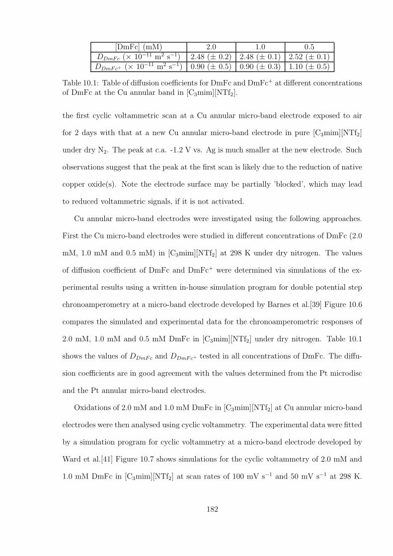
[DmFc] (mM) 2.0 1.0 0.5DDmFc (× 10−11 m2 s−1) 2.48 (± 0.2) 2.48 (± 0.1) 2.52 (± 0.1)DDmFc+ (× 10−11 m2 s−1) 0.90 (± 0.5) 0.90 (± 0.3) 1.10 (± 0.5)
Table 10.1: Table of diffusion coefficients for DmFc and DmFc+ at different concentrationsof DmFc at the Cu annular band in [C3mim][NTf2].
the first cyclic voltammetric scan at a Cu annular micro-band electrode exposed to air
for 2 days with that at a new Cu annular micro-band electrode in pure [C3mim][NTf2]
under dry N2. The peak at c.a. -1.2 V vs. Ag is much smaller at the new electrode. Such
observations suggest that the peak at the first scan is likely due to the reduction of native
copper oxide(s). Note the electrode surface may be partially ’blocked’, which may lead
to reduced voltammetric signals, if it is not activated.
Cu annular micro-band electrodes were investigated using the following approaches.
First the Cu micro-band electrodes were studied in different concentrations of DmFc (2.0
mM, 1.0 mM and 0.5 mM) in [C3mim][NTf2] at 298 K under dry nitrogen. The values
of diffusion coefficient of DmFc and DmFc+ were determined via simulations of the ex-
perimental results using a written in-house simulation program for double potential step
chronoamperometry at a micro-band electrode developed by Barnes et al.[39] Figure 10.6
compares the simulated and experimental data for the chronoamperometric responses of
2.0 mM, 1.0 mM and 0.5 mM DmFc in [C3mim][NTf2] under dry nitrogen. Table 10.1
shows the values of DDmFc and DDmFc+ tested in all concentrations of DmFc. The diffu-
sion coefficients are in good agreement with the values determined from the Pt microdisc
and the Pt annular micro-band electrodes.
Oxidations of 2.0 mM and 1.0 mM DmFc in [C3mim][NTf2] at Cu annular micro-band
electrodes were then analysed using cyclic voltammetry. The experimental data were fitted
by a simulation program for cyclic voltammetry at a micro-band electrode developed by
Ward et al.[41] Figure 10.7 shows simulations for the cyclic voltammetry of 2.0 mM and
1.0 mM DmFc in [C3mim][NTf2] at scan rates of 100 mV s−1 and 50 mV s−1 at 298 K.
182
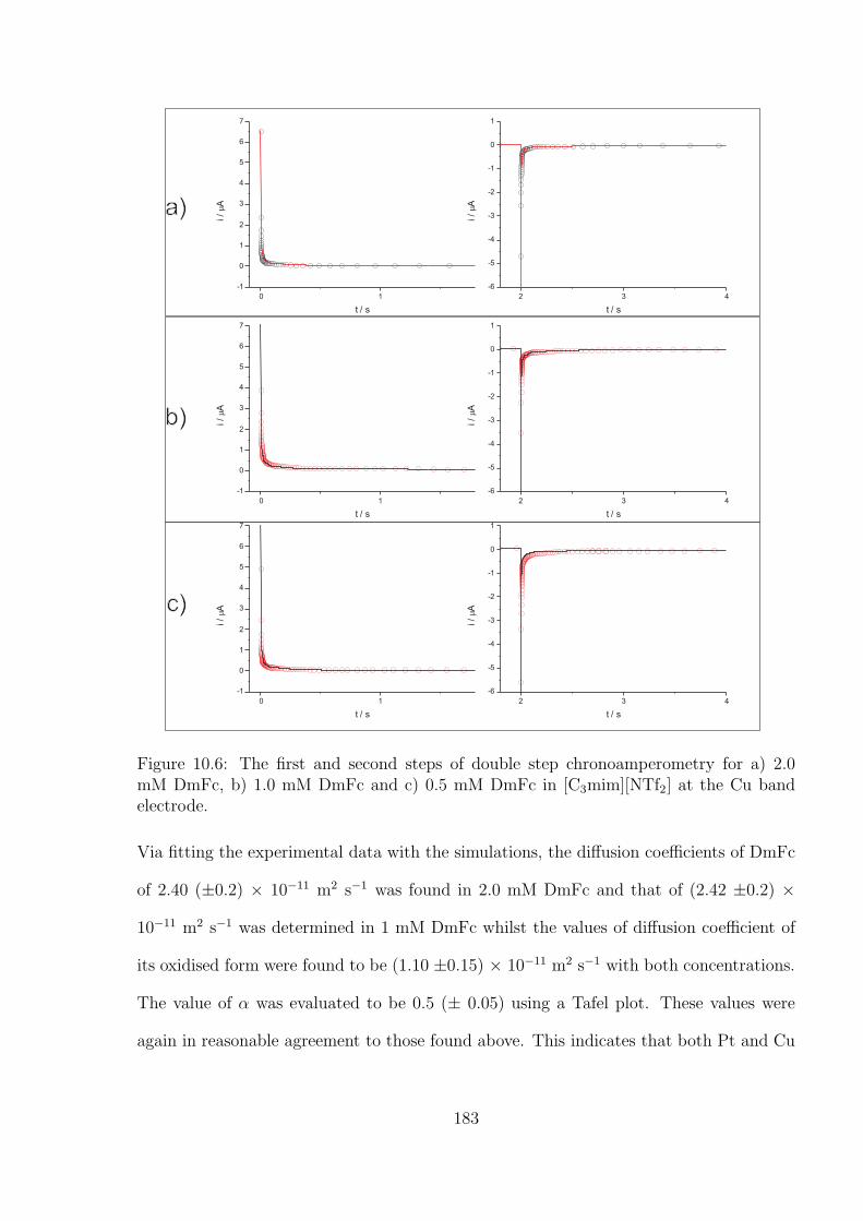
0 1
-1
0
1
2
3
4
5
6
7
i/
mA
t / s
0 1
-1
0
1
2
3
4
5
6
7
i/
mA
t / s
0 1
-1
0
1
2
3
4
5
6
7
i/
mA
t / s
2 3 4
-6
-5
-4
-3
-2
-1
0
1
i/
mA
t / s
2 3 4
-6
-5
-4
-3
-2
-1
0
1
i/
mA
t / s
2 3 4
-6
-5
-4
-3
-2
-1
0
1
i/
mA
t / s
a)
b)
c)
Figure 10.6: The first and second steps of double step chronoamperometry for a) 2.0mM DmFc, b) 1.0 mM DmFc and c) 0.5 mM DmFc in [C3mim][NTf2] at the Cu bandelectrode.
Via fitting the experimental data with the simulations, the diffusion coefficients of DmFc
of 2.40 (±0.2) × 10−11 m2 s−1 was found in 2.0 mM DmFc and that of (2.42 ±0.2) ×
10−11 m2 s−1 was determined in 1 mM DmFc whilst the values of diffusion coefficient of
its oxidised form were found to be (1.10 ±0.15) × 10−11 m2 s−1 with both concentrations.
The value of α was evaluated to be 0.5 (± 0.05) using a Tafel plot. These values were
again in reasonable agreement to those found above. This indicates that both Pt and Cu
183
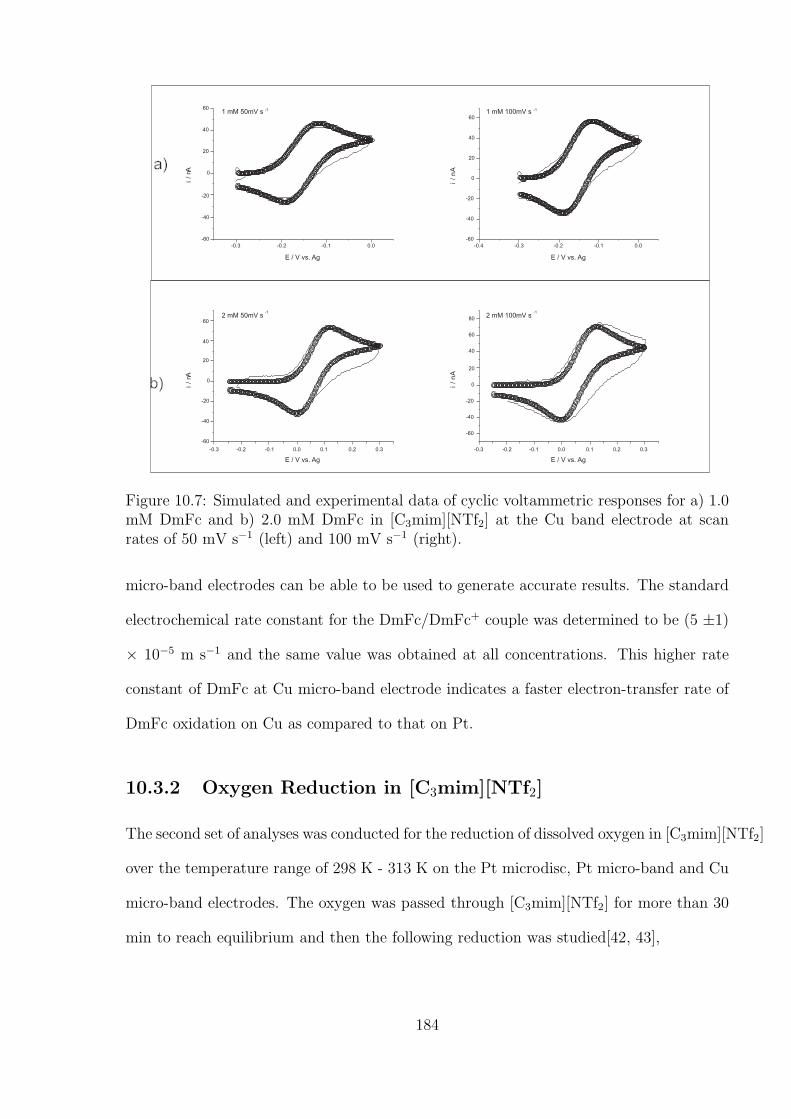
a)
b)
-0.3 -0.2 -0.1 0.0 0.1 0.2 0.3
-60
-40
-20
0
20
40
60
802 mM 100mV s
-1
i/
nA
E / V vs. Ag
-0.3 -0.2 -0.1 0.0 0.1 0.2 0.3
-60
-40
-20
0
20
40
602 mM 50mV s
-1
i/
nA
E / V vs. Ag
-0.4 -0.3 -0.2 -0.1 0.0
-60
-40
-20
0
20
40
60
i/
nA
E / V vs. Ag
1 mM 100mV s -1
-0.3 -0.2 -0.1 0.0
-60
-40
-20
0
20
40
601 mM 50mV s -1
i/
nA
E / V vs. Ag
Figure 10.7: Simulated and experimental data of cyclic voltammetric responses for a) 1.0mM DmFc and b) 2.0 mM DmFc in [C3mim][NTf2] at the Cu band electrode at scanrates of 50 mV s−1 (left) and 100 mV s−1 (right).
micro-band electrodes can be able to be used to generate accurate results. The standard
electrochemical rate constant for the DmFc/DmFc+ couple was determined to be (5 ±1)
× 10−5 m s−1 and the same value was obtained at all concentrations. This higher rate
constant of DmFc at Cu micro-band electrode indicates a faster electron-transfer rate of
DmFc oxidation on Cu as compared to that on Pt.
10.3.2 Oxygen Reduction in [C3mim][NTf2]
The second set of analyses was conducted for the reduction of dissolved oxygen in [C3mim][NTf2]
over the temperature range of 298 K - 313 K on the Pt microdisc, Pt micro-band and Cu
micro-band electrodes. The oxygen was passed through [C3mim][NTf2] for more than 30
min to reach equilibrium and then the following reduction was studied[42, 43],
184
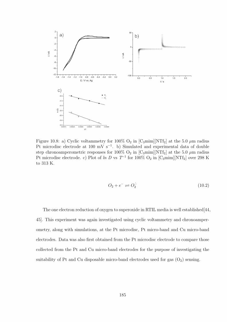
-1.8 -1.6 -1.4 -1.2 -1.0 -0.8 -0.6 -0.4 -0.2 0.0 0.2
-12
-10
-8
-6
-4
-2
0
2
i/n
A
E / V vs. Ag
0.00315 0.00320 0.00325 0.00330 0.00335 0.00340
-23.5
-23.0
-22.5
-22.0
-21.5
-21.0
-20.5O
2
O.-
2
ln(D
)
1/T
0.0 0.5 1.0 1.5 2.0
-100
-50
0
50
i/
nA
t / s
a) b)
c)
Figure 10.8: a) Cyclic voltammetry for 100% O2 in [C3mim][NTf2] at the 5.0 µm radiusPt microdisc electrode at 100 mV s−1. b) Simulated and experimental data of doublestep chronoamperometric responses for 100% O2 in [C3mim][NTf2] at the 5.0 µm radiusPt microdisc electrode. c) Plot of ln D vs T−1 for 100% O2 in [C3mim][NTf2] over 298 Kto 313 K.
O2 + e− O−2 (10.2)
The one electron reduction of oxygen to superoxide in RTIL media is well established[44,
45]. This experiment was again investigated using cyclic voltammetry and chronoamper-
ometry, along with simulations, at the Pt microdisc, Pt micro-band and Cu micro-band
electrodes. Data was also first obtained from the Pt microdisc electrode to compare those
collected from the Pt and Cu micro-band electrodes for the purpose of investigating the
suitability of Pt and Cu disposable micro-band electrodes used for gas (O2) sensing.
185
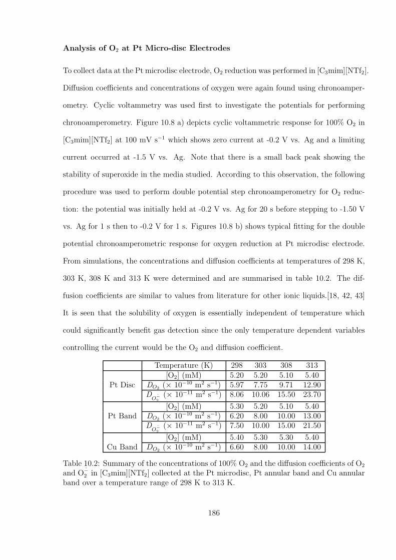
Analysis of O2 at Pt Micro-disc Electrodes
To collect data at the Pt microdisc electrode, O2 reduction was performed in [C3mim][NTf2].
Diffusion coefficients and concentrations of oxygen were again found using chronoamper-
ometry. Cyclic voltammetry was used first to investigate the potentials for performing
chronoamperometry. Figure 10.8 a) depicts cyclic voltammetric response for 100% O2 in
[C3mim][NTf2] at 100 mV s−1 which shows zero current at -0.2 V vs. Ag and a limiting
current occurred at -1.5 V vs. Ag. Note that there is a small back peak showing the
stability of superoxide in the media studied. According to this observation, the following
procedure was used to perform double potential step chronoamperometry for O2 reduc-
tion: the potential was initially held at -0.2 V vs. Ag for 20 s before stepping to -1.50 V
vs. Ag for 1 s then to -0.2 V for 1 s. Figures 10.8 b) shows typical fitting for the double
potential chronoamperometric response for oxygen reduction at Pt microdisc electrode.
From simulations, the concentrations and diffusion coefficients at temperatures of 298 K,
303 K, 308 K and 313 K were determined and are summarised in table 10.2. The dif-
fusion coefficients are similar to values from literature for other ionic liquids.[18, 42, 43]
It is seen that the solubility of oxygen is essentially independent of temperature which
could significantly benefit gas detection since the only temperature dependent variables
controlling the current would be the O2 and diffusion coefficient.
Temperature (K) 298 303 308 313[O2] (mM) 5.20 5.20 5.10 5.40
Pt Disc DO2(× 10−10 m2 s−1) 5.97 7.75 9.71 12.90
DO−
2
(× 10−11 m2 s−1) 8.06 10.06 15.50 23.70
[O2] (mM) 5.30 5.20 5.10 5.40Pt Band DO2
(× 10−10 m2 s−1) 6.20 8.00 10.00 13.00D
O−2
(× 10−11 m2 s−1) 7.50 10.00 15.00 21.50
[O2] (mM) 5.40 5.30 5.30 5.40Cu Band DO2
(× 10−10 m2 s−1) 6.60 8.00 10.00 14.00
Table 10.2: Summary of the concentrations of 100% O2 and the diffusion coefficients of O2
and O−2 in [C3mim][NTf2] collected at the Pt microdisc, Pt annular band and Cu annular
band over a temperature range of 298 K to 313 K.
186
The diffusion coefficient is related to temperature by the Arrhenius equation[46–48]
lnD = constant− ED,a
RT(10.3)
where D is the diffusion coefficient, ED,a is the activation energy of diffusion in J mol−1,
R is the universal gas constant, 8.31 J K−1 mol−1, and T is the temperature in K.
Figure 10.8 c) shows Arrhrenius plots of O2 (squares) and O−2 (circles) over 298 K to
313 K, which give the diffusion activation energies (ED,a) of (38.2 ±0.6) kJ mol−1 and
(54 ± 1) kJ mol−1 for O2 and O−2 respectively. The larger activation energy for O−
2 as
compared to that for O2 is due to the fact that charged species are harder to diffuse
through ionic solvents than the neutral ones because of their coulombic interaction with
other ions.
Analysis of O2 at Pt Annular Micro-band Electrodes
The same analysis was repeated with Pt annular micro-band electrodes. Typical double
potential step chronoamperometric responses, along with simulations, for oxygen reduc-
tion at the Pt annular micro-band electrode are shown in Figures 10.9 a) and b). A good
fit is observed between the simulated and experimental data. The corresponding Arrhe-
nius plots for O2 and O−2 are shown in figure 10.9 c). Diffusion activation energies of (37.9
± 0.9) kJ mol−1 and (53 ± 5) kJ mol−1 for O2 and O−2 respectively were determined.
These values are very close to what were found on the Pt microdisc electrode, suggesting
that Pt micro-band electrodes again have performed excellently for gas sensing.
Analysis of O2 at Cu annular micro-band electrodes
To validate the use of Cu electrodes for oxygen detection, experiments were performed
in 100%, 50% and 25% O2 (by volume). The other part of the gas mixture was N2.
To fully dissolve(saturate) the gas mixture in [C3mim][NTf2], the gas was passed over
187
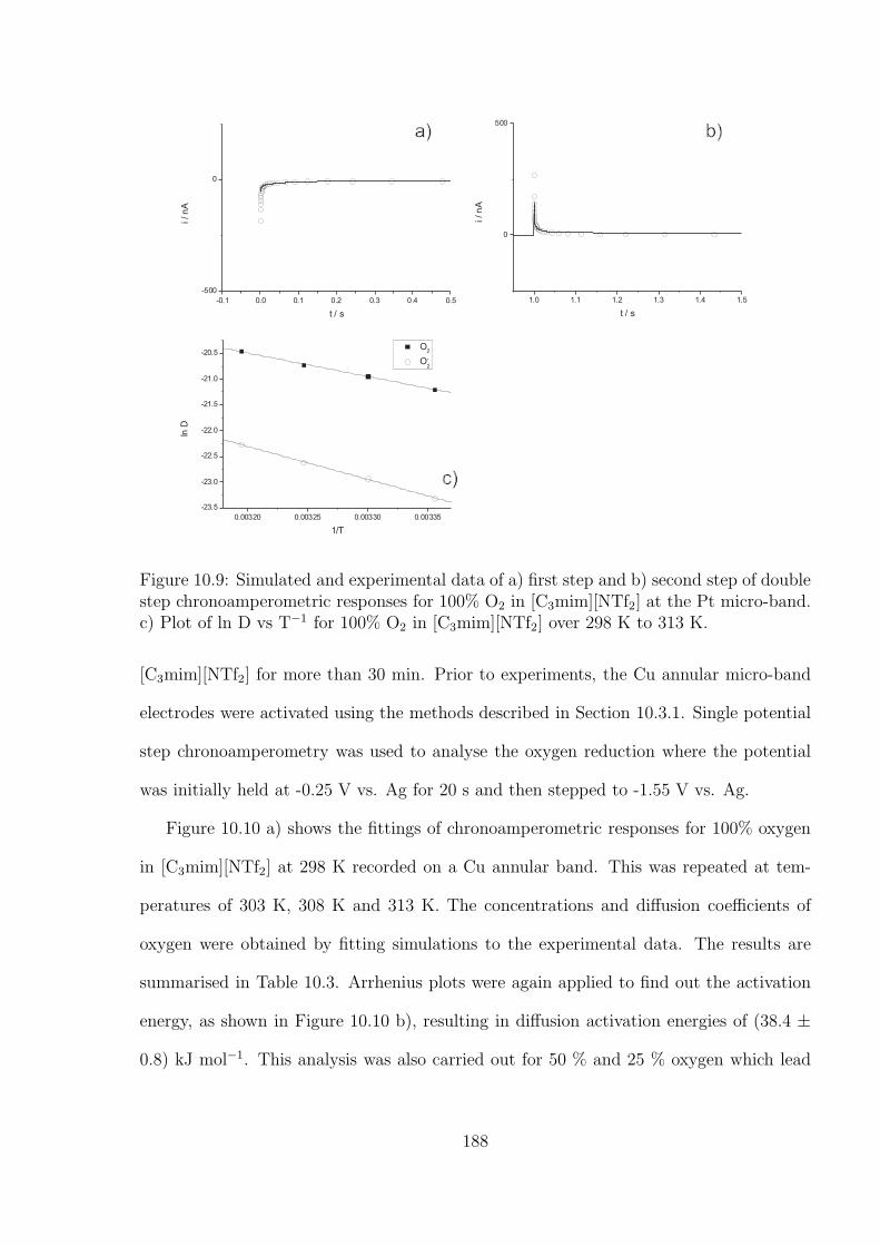
-0.1 0.0 0.1 0.2 0.3 0.4 0.5
-500
0i/n
A
t / s
1.0 1.1 1.2 1.3 1.4 1.5
0
500
i/n
A
t / s
0.00320 0.00325 0.00330 0.00335
-23.5
-23.0
-22.5
-22.0
-21.5
-21.0
-20.5
lnD
1/T
O2
O-
2
a) b)
c)
Figure 10.9: Simulated and experimental data of a) first step and b) second step of doublestep chronoamperometric responses for 100% O2 in [C3mim][NTf2] at the Pt micro-band.c) Plot of ln D vs T−1 for 100% O2 in [C3mim][NTf2] over 298 K to 313 K.
[C3mim][NTf2] for more than 30 min. Prior to experiments, the Cu annular micro-band
electrodes were activated using the methods described in Section 10.3.1. Single potential
step chronoamperometry was used to analyse the oxygen reduction where the potential
was initially held at -0.25 V vs. Ag for 20 s and then stepped to -1.55 V vs. Ag.
Figure 10.10 a) shows the fittings of chronoamperometric responses for 100% oxygen
in [C3mim][NTf2] at 298 K recorded on a Cu annular band. This was repeated at tem-
peratures of 303 K, 308 K and 313 K. The concentrations and diffusion coefficients of
oxygen were obtained by fitting simulations to the experimental data. The results are
summarised in Table 10.3. Arrhenius plots were again applied to find out the activation
energy, as shown in Figure 10.10 b), resulting in diffusion activation energies of (38.4 ±
0.8) kJ mol−1. This analysis was also carried out for 50 % and 25 % oxygen which lead
188
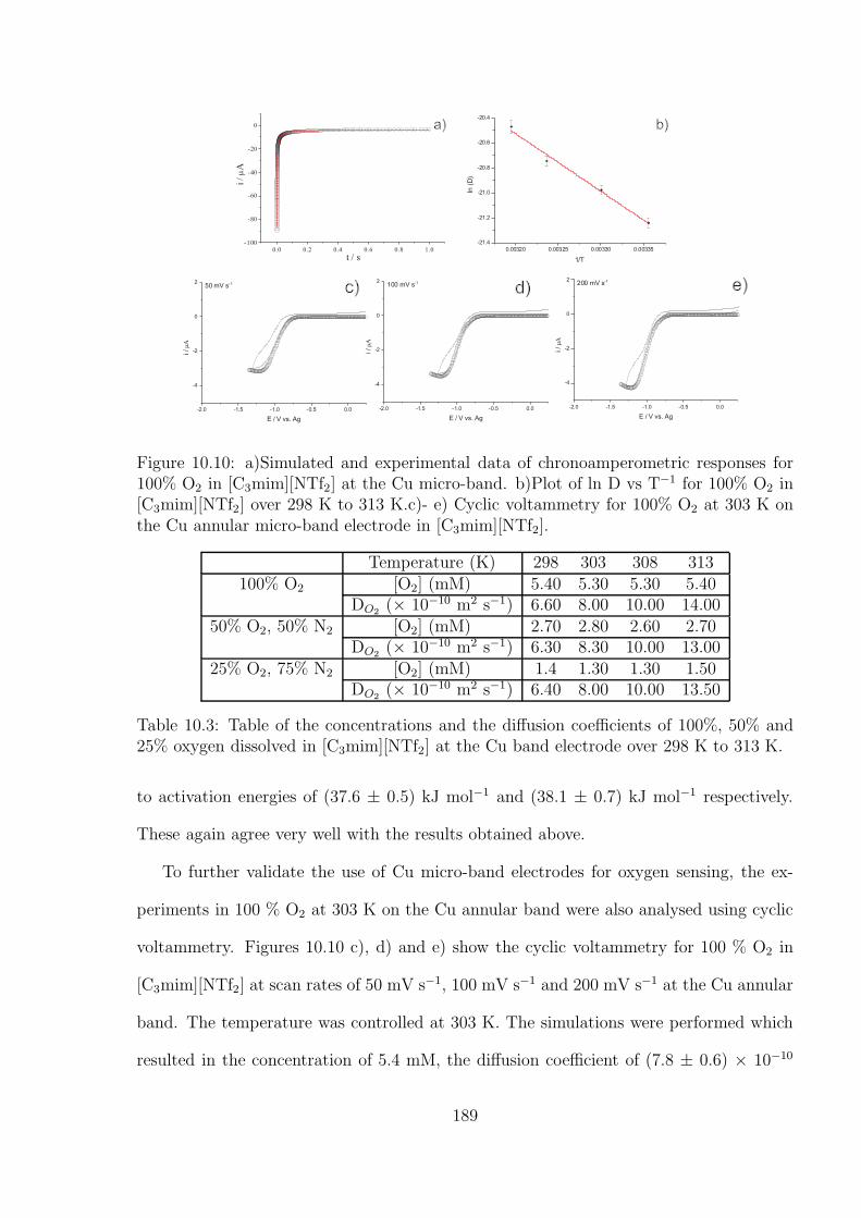
a) b)
0.00320 0.00325 0.00330 0.00335
-21.4
-21.2
-21.0
-20.8
-20.6
-20.4
ln(D
)
1/T
0.0 0.2 0.4 0.6 0.8 1.0
-100
-80
-60
-40
-20
0
i/
mA
t / s
-2.0 -1.5 -1.0 -0.5 0.0
-4
-2
0
2100 mV s-1
i/mA
E / V vs. Ag
-2.0 -1.5 -1.0 -0.5 0.0
-4
-2
0
250 mV s-1
i/mA
E / V vs. Ag
-2.0 -1.5 -1.0 -0.5 0.0
-4
-2
0
2
i/mA
E / V vs. Ag
200 mV s-1
c) d) e)
Figure 10.10: a)Simulated and experimental data of chronoamperometric responses for100% O2 in [C3mim][NTf2] at the Cu micro-band. b)Plot of ln D vs T−1 for 100% O2 in[C3mim][NTf2] over 298 K to 313 K.c)- e) Cyclic voltammetry for 100% O2 at 303 K onthe Cu annular micro-band electrode in [C3mim][NTf2].
Temperature (K) 298 303 308 313100% O2 [O2] (mM) 5.40 5.30 5.30 5.40
DO2(× 10−10 m2 s−1) 6.60 8.00 10.00 14.00
50% O2, 50% N2 [O2] (mM) 2.70 2.80 2.60 2.70DO2
(× 10−10 m2 s−1) 6.30 8.30 10.00 13.0025% O2, 75% N2 [O2] (mM) 1.4 1.30 1.30 1.50
DO2(× 10−10 m2 s−1) 6.40 8.00 10.00 13.50
Table 10.3: Table of the concentrations and the diffusion coefficients of 100%, 50% and25% oxygen dissolved in [C3mim][NTf2] at the Cu band electrode over 298 K to 313 K.
to activation energies of (37.6 ± 0.5) kJ mol−1 and (38.1 ± 0.7) kJ mol−1 respectively.
These again agree very well with the results obtained above.
To further validate the use of Cu micro-band electrodes for oxygen sensing, the ex-
periments in 100 % O2 at 303 K on the Cu annular band were also analysed using cyclic
voltammetry. Figures 10.10 c), d) and e) show the cyclic voltammetry for 100 % O2 in
[C3mim][NTf2] at scan rates of 50 mV s−1, 100 mV s−1 and 200 mV s−1 at the Cu annular
band. The temperature was controlled at 303 K. The simulations were performed which
resulted in the concentration of 5.4 mM, the diffusion coefficient of (7.8 ± 0.6) × 10−10
189
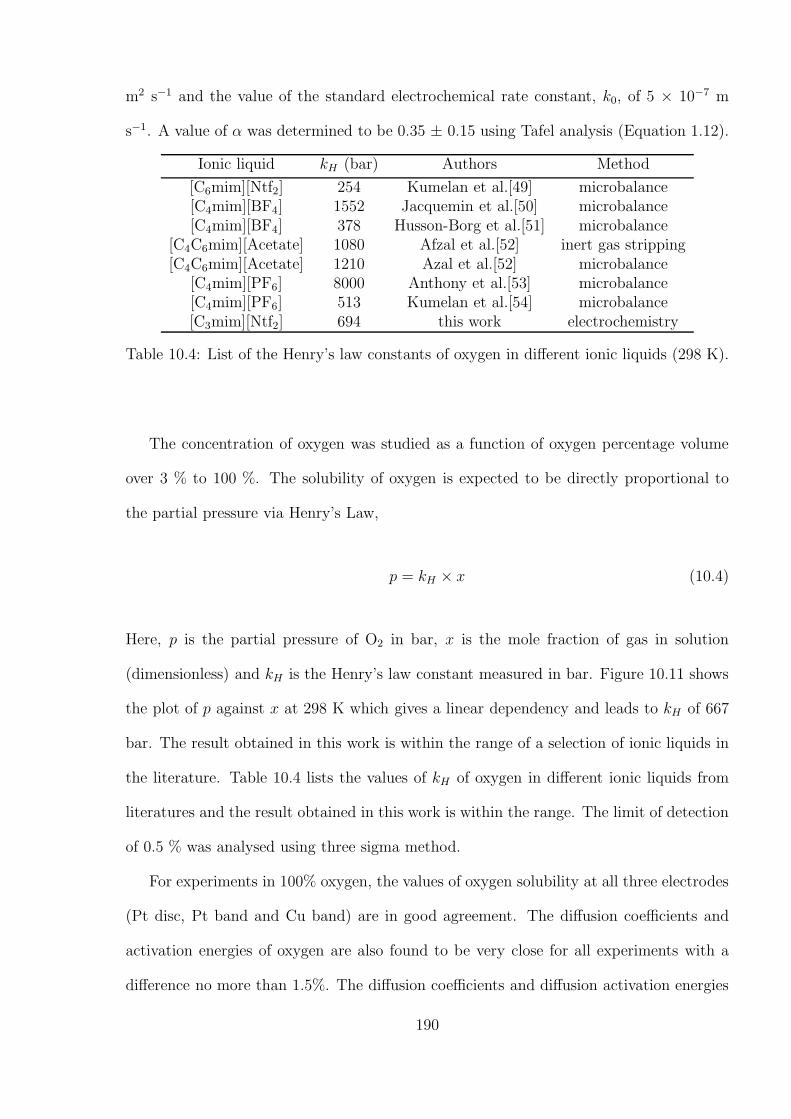
m2 s−1 and the value of the standard electrochemical rate constant, k0, of 5 × 10⁻⁷ m
s−1. A value of α was determined to be 0.35 ± 0.15 using Tafel analysis (Equation 1.12).
Ionic liquid kH (bar) Authors Method
[C6mim][Ntf2] 254 Kumelan et al.[49] microbalance[C4mim][BF4] 1552 Jacquemin et al.[50] microbalance[C4mim][BF4] 378 Husson-Borg et al.[51] microbalance
[C4C6mim][Acetate] 1080 Afzal et al.[52] inert gas stripping[C4C6mim][Acetate] 1210 Azal et al.[52] microbalance
[C4mim][PF6] 8000 Anthony et al.[53] microbalance[C4mim][PF6] 513 Kumelan et al.[54] microbalance[C3mim][Ntf2] 694 this work electrochemistry
Table 10.4: List of the Henry’s law constants of oxygen in different ionic liquids (298 K).
The concentration of oxygen was studied as a function of oxygen percentage volume
over 3 % to 100 %. The solubility of oxygen is expected to be directly proportional to
the partial pressure via Henry’s Law,
p = kH × x (10.4)
Here, p is the partial pressure of O2 in bar, x is the mole fraction of gas in solution
(dimensionless) and kH is the Henry’s law constant measured in bar. Figure 10.11 shows
the plot of p against x at 298 K which gives a linear dependency and leads to kH of 667
bar. The result obtained in this work is within the range of a selection of ionic liquids in
the literature. Table 10.4 lists the values of kH of oxygen in different ionic liquids from
literatures and the result obtained in this work is within the range. The limit of detection
of 0.5 % was analysed using three sigma method.
For experiments in 100% oxygen, the values of oxygen solubility at all three electrodes
(Pt disc, Pt band and Cu band) are in good agreement. The diffusion coefficients and
activation energies of oxygen are also found to be very close for all experiments with a
difference no more than 1.5%. The diffusion coefficients and diffusion activation energies
190
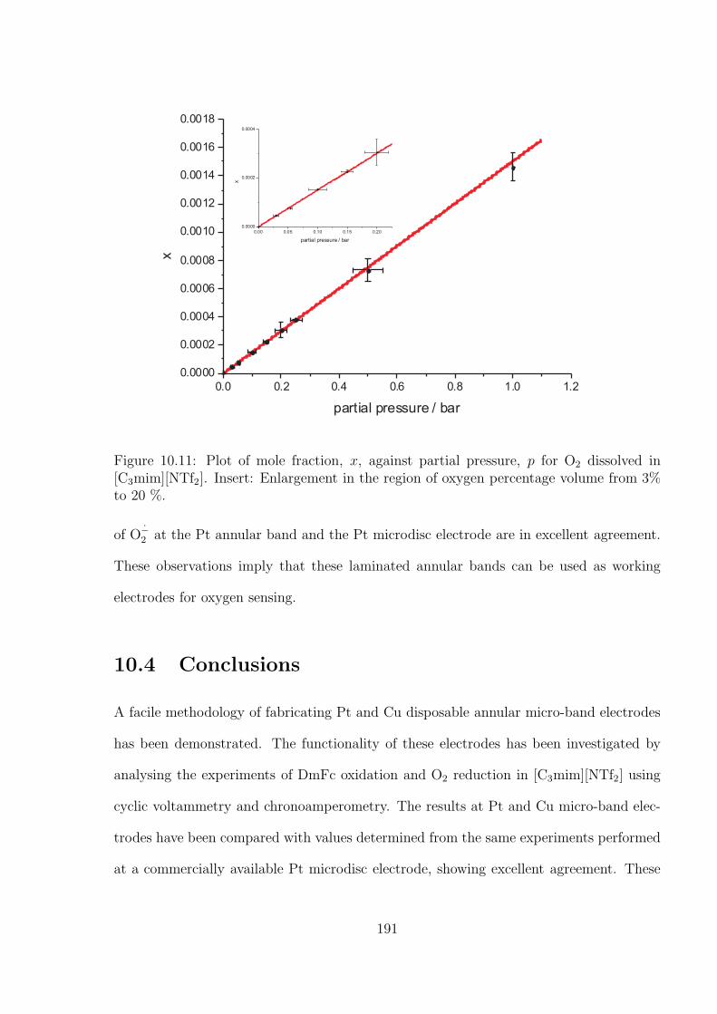
0.0 0.2 0.4 0.6 0.8 1.0 1.2
0.0000
0.0002
0.0004
0.0006
0.0008
0.0010
0.0012
0.0014
0.0016
0.0018
x
partial pressure / bar
0.00 0.05 0.10 0.15 0.20
0.0000
0.0002
0.0004
xpartial pressure / bar
Figure 10.11: Plot of mole fraction, x, against partial pressure, p for O2 dissolved in[C3mim][NTf2]. Insert: Enlargement in the region of oxygen percentage volume from 3%to 20 %.
of O−2 at the Pt annular band and the Pt microdisc electrode are in excellent agreement.
These observations imply that these laminated annular bands can be used as working
electrodes for oxygen sensing.
10.4 Conclusions
A facile methodology of fabricating Pt and Cu disposable annular micro-band electrodes
has been demonstrated. The functionality of these electrodes has been investigated by
analysing the experiments of DmFc oxidation and O2 reduction in [C3mim][NTf2] using
cyclic voltammetry and chronoamperometry. The results at Pt and Cu micro-band elec-
trodes have been compared with values determined from the same experiments performed
at a commercially available Pt microdisc electrode, showing excellent agreement. These
191
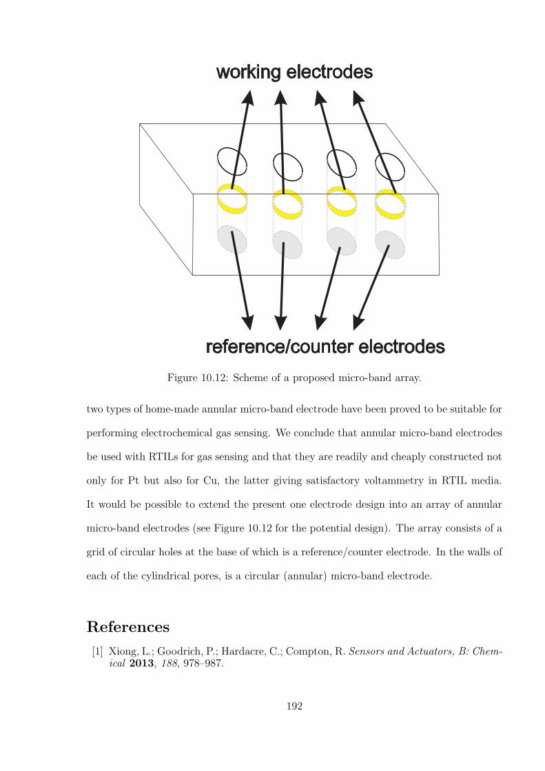
reference/counter electrodes
working electrodes
Figure 10.12: Scheme of a proposed micro-band array.
two types of home-made annular micro-band electrode have been proved to be suitable for
performing electrochemical gas sensing. We conclude that annular micro-band electrodes
be used with RTILs for gas sensing and that they are readily and cheaply constructed not
only for Pt but also for Cu, the latter giving satisfactory voltammetry in RTIL media.
It would be possible to extend the present one electrode design into an array of annular
micro-band electrodes (see Figure 10.12 for the potential design). The array consists of a
grid of circular holes at the base of which is a reference/counter electrode. In the walls of
each of the cylindrical pores, is a circular (annular) micro-band electrode.
References
[1] Xiong, L.; Goodrich, P.; Hardacre, C.; Compton, R. Sensors and Actuators, B: Chem-ical 2013, 188, 978–987.
192
[2] Clark Jr., L. C.; Wolk, R.; Granger, D.; Talor, Z. Journal of applied physiology 1953,6, 189–193.
[3] Bakker, E.; Telting-Diaz, M. Analytical Chemistry 2002, 74, 2781–2800.
[4] Knake, R.; Guchardi, R.; Hauser, P. Analytica Chimica Acta 2003, 475, 17–25.
[5] Hammond, M.; Johnson, K.; Rose-Pehrsson, S.; Ziegler, J.; Walker, H.; Caudy, K.;Gary, D.; Tillett, D. Sensors and Actuators, B: Chemical 2006, 116, 135–144.
[6] Kealy, J.; Bennett, R.; Lowry, J. Journal of Neuroscience Methods 2013, 215, 110–120.
[7] Roberts, T. J.; Braban, C. F.; Oppenheimer, C.; Martin, R. S.; Freshwater, R. A.;Dawson, D. H.; Griffiths, P. T.; Cox, R. A.; Saffell, J. R.; Jones, R. L. ChemicalGeology 2012, 332-333, 74–91.
[8] Al-Heuseen, K.; Hashim, M. R. Sensors and Actuators, B: Chemical 2012, 163,159–164.
[9] Lawrence, N. S.; Jiang, L.; Jones, T. G. J.; Compton, R. G. Analytical Chemistry2003, 75, 2499–2503.
[10] Lawrence, N. S.; Jiang, L.; Jones, T. G. J.; Compton, R. G. Analytical Chemistry2003, 75, 2054–2059.
[11] Buzzeo, M. C.; Hardacre, C.; Compton, R. G. Analytical Chemistry 2004, 76, 4583–4588.
[12] Buzzeo, M. C.; Evans, R. G.; Compton, R. G. ChemPhysChem 2004, 5, 1106–1120.
[13] Silvester, D. S.; Compton, R. G. Zeitschrift fur Physikalische Chemie 2006, 220,1247–1274.
[14] Faridbod, F.; Mohammad Reza Ganjali, M. R.; Norouzi, P.; Riahi, S.; Rashedi, H.Application of Room Temperature Ionic Liquids in Electrochemical Sensors andBiosensors ; InTech, 2011.
[15] Barrosse-Antle, L. E.; Bond, A. M.; Compton, R. G.; O’Mahony, A. M.; Rogers, E. I.;Silvester, D. S. Chemistry - An Asian Journal 2010, 5, 202–230.
[16] Xiong, L.; Fletcher, A. M.; Ernst, S.; Davies, S. G.; Compton, R. G. The Analyst2012, 137, 2567–2573.
[17] Xiong, L.; Fletcher, A. M.; Davies, S. G.; Norman, S. E.; Hardacre, C.; Comp-ton, R. G. The Analyst 2012, 137, 4951–4957.
[18] Buzzeo, M. C.; Klymenko, O. V.; Wadhawan, J. D.; Hardacre, C.; Seddon, K. R.;Compton, R. G. Journal of Physical Chemistry A 2003, 107, 8872–8878.
[19] Dias, A. C. M. S.; Gomes-Filho, S. L. R.; Silva, M. M. S.; Dutra, R. F. BiosensBioelectron 2013, 44, 216–221.
[20] Kanyong, P.; Pemberton, R. M.; Jackson, S. K.; Hart, J. P. Anal. Biochem. 2013,435, 114–119.
193
[21] Xuan Viet, N.; Chikae, M.; Ukita, Y.; Maehashi, K.; Matsumoto, K.; Tamiya, E.;Hung Viet, P.; Takamura, Y. Biosensors and Bioelectronics 2013, 42, 592–597.
[22] Prehn, R.; Abad, L.; Snchez-Molas, D.; Duch, M.; Sabat, N.; Del Campo, F. J.;Muoz, F. X.; Compton, R. G. Journal of Electroanalytical Chemistry 2011, 662,361–370.
[23] Wang, T.-J.; Huang, C.-F.; Wang, W.-S.; Wei, P.-K. IEEE JOURNAL OF LIGHT-WAVe TECHNOLOGY 2004, 22, 1764–1771.
[24] Davies, T. J.; Ward-Jones, S.; Banks, C. E.; del Campo, J.; Mas, R.; Muoz, F. X.;Compton, R. G. Journal of Electroanalytical Chemistry 2005, 585, 51 – 62.
[25] Lee, H.; Shin, H.; Jeong, Y.; Moon, J.; Lee, M. Appl. Phys. Lett. 2009, 95, p.071104–1 – p.071104–3.
[26] Koppenol, M.; Cooper, J. B.; Bond, A. M. American Laboratory 1994, 26, 25–29.
[27] Shao, Y.; Mirkin, M.; Fish, G.; Kokotov, S.; Palanker, D.; Lewis, A. AnalyticalChemistry 1997, 69, 1627–1634.
[28] Kovach, P. M.; Caudill, W. L.; Peters, D. G.; Wightman, R. M. Journal of Electro-analytical Chemistry 1985, 185, 285–295.
[29] Shea, T. V.; Bard, A. J. Analytical Chemistry 1987, 59, 2101–2111.
[30] Rajantie, H.; Strutwolf, J.; Williams, D. Journal of Electroanalytical Chemistry 2001,500, 108–120.
[31] Tomk, P.; Jursa, S.; Bustin, D.; Tvaroek, V. Chemicke Listy 1998, 92, 631–632.
[32] Freeman, N.; Sultana, R.; Reza, N.; Woodvine, H.; Terry, J.; Walton, A.; Brady, C.;Schmueser, I.; Mount, A. Physical Chemistry Chemical Physics 2013, 15, 8112–8118.
[33] Tsunozaki, K.; Einaga, Y.; Rao, T.; Fujishima, A. Chemistry Letters 2002, 502–503.
[34] Farrington, A.; Jagota, N.; Slater, J. Analyst 1994, 119, 233–238.
[35] Guiseppi-Elie, A.; Brahim, S.; Slaughter, G.; Ward, K. IEEE Sensors Journal 2005,5, 345–355.
[36] Welford, P. J.; Freeman, J.; Wilkins, S. J.; Wadhawan, J. D.; Hahn, C. E. W.;Compton, R. G. Analytical Chemistry 2001, 73, 6088–6092.
[37] Klymenko, O. V.; Evans, R. G.; Hardacre, C.; Svir, I. B.; Compton, R. G. Journalof Electroanalytical Chemistry 2004, 571, 211–221.
[38] Shoup, D.; Szabo, A. Journal of Electroanalytical Chemistry and Interfacial Electro-chemistry 1982, 140, 237 – 245.
[39] Barnes, E. O.; Xiong, L.; Ward, K. R.; Compton, R. G. Journal of ElectroanalyticalChemistry 2013, 701, 59 – 68.
[40] Reyter, D.; Odziemkowski, M.; B’langer, D.; Ro, L. Journal of the ElectrochemicalSociety 2007, 154, 36 – 44.
194
[41] Ward, K. R.; Xiong, L.; Lawrence, N. S.; Hartshorne, R. S.; Compton, R. G. Journalof Electroanalytical Chemistry 2013, 702, 15 – 24.
[42] Rogers, E. I.; Huang, X. J.; Dickinson, E. J. F.; Hardacre, C.; Compton, R. G.Journal of Physical Chemistry C 2009, 113, 17811–17823.
[43] Huang, X. J.; Rogers, E. I.; Hardacre, C.; Compton, R. G. The Journal of PhysicalChemistry B 2009, 113, 8953–8959.
[44] Switzer, E. E.; Zeller, R.; Chen, Q.; Sieradzki, K.; Buttry, D. A.; Friesen, C. TheJournal of Physical Chemistry C 2013, 117, 8683–8690.
[45] Evans, R. G.; Klymenko, O. V.; Saddoughi, S. A.; Hardacre, C.; Compton, R. G. J.Phys. Chem. B 2004, 108, 7878–7886.
[46] Compton, R. G.; Banks, C. E. Understanding Voltammetry ; Imperial College Press,2011, 2nd Edition.
[47] Bard, A. J.; Faulkner, L. R. Electrochemical Methods: Fundamentals and Applica-tions ; Wiley, 2001.
[48] Russell, J.; Cohn, R. Arrhenius Equation; Book on Demand, 2012.
[49] Kumelan, J.; Kamps, . P. S.; Tuma, D.; Maurer, G. Journal of Chemical and Engi-neering Data 2009, 54, 966–971.
[50] Jacquemin, J.; Gomes, M. F. C.; Husson, P.; Majer, V. The Journal of ChemicalThermodynamics 2006, 38, 490 – 502.
[51] Husson-Borg, P.; Majer, V.; Costa Gomes, M. Journal of Chemical and EngineeringData 2003, 48, 480–485.
[52] Afzal, W.; Yoo, B.; Prausnitz, J. Industrial and Engineering Chemistry Research2012, 51, 4433–4439.
[53] Anthony, J. L.; Maginn, E. J.; Brennecke, J. F. Journal of Physical Chemistry B2002, 106, 7315–7320.
[54] Kumelan, J.; Kamps, A. P.-S.; Urukova, I.; Tuma, D.; Maurer, G. The Journal ofChemical Thermodynamics 2005, 37, 595 – 602.
195
Chapter 11
Conclusions
This thesis aimed at improving present generation gas sensors. As discussed in Chapter 2
these suffer from some significant limitations. First the lifetime of the sensor is limited by
solution evaporation as the sensor is normally exposed to different humidity levels with
electrolyte loss under dry conditions. Second the solvents in the sensor provide restrictions
to the high and low temperature and pressure limits on the range of operation. Third
the presence of a membrane to retain the electrolyte increases the response time of the
sensor. Finally, calibration of gas sensors against temperature and humidity is required.
To address the problems due to the use of conventional solvents, RTILs were em-
ployed throughout the thesis. The benefits of RTILs were discussed in Chapter 2. To
compensate some undesired features of RTILs, like high viscosity and low conductivity,
micro-electrodes were used as working probes.
To improve the accuracy of gas detection, a method to obtain optimised chronoam-
perometry for Shoup and Szabo analysis was reported in Chapter 4. The ‘best’ transient
times were found to be dependent on the electrochemical systems. This work enabled the
simultaneous and accurate determination of the concentration and diffusion coefficient of
analyte, improved the accuracy of gas sensors and underpinned all the subsequent work.
The properties of RTILs have been further investigated in Chapter 5 where the tune-
ability of RTILs was studied. Control of the oxidation potential of ferrocene was realised
by changing the size of the anion of the ionic liquids. This observation has important
196
implications for sensors in that the oxidation potential of ferrocene, commonly used as
an internal redox reference, can be tuned away from the potential of analytes of interest.
Further, work in this chapter provided a key basis for Chapter 7.
Two self-calibrating (‘intelligent’) systems have been developed to eliminate the need
of constant calibration of gas sensors against temperature and humidity. Work presented
in Chapter 6 proposed a built-in voltammetric temperature sensor incorporated into an
amperometric oxygen sensor. This patented sensor was shown to be capable of providing
a real-time temperature for amperometric oxygen sensing systems at the electrode surface
for both air and dry oxygen analytes.
A simultaneous temperature and humidity sensor has also been designed. This sen-
sor provides a simple measurement towards humidity and temperature, giving humidity
insensitive temperature measurement and vice versa. An iterative scheme to determine si-
multaneous values of temperature and humidity was proposed (see Figure 7.10 in Chapter
7) and again patented.
Gas detection under wet conditions may undergo complicated redox mechanism which
cannot be resolved by Shoup and Szabo analysis. Chapter 8 demonstrated a method
to prevent the influence of water on the mechanism of oxygen reduction by ‘trapping’
superoxide ions using a phosphonium based ionic liquid. This method largely simplifies
oxygen detection through forcing oxygen reduction to stop at the one electron transfer
stage which allows the Shoup and Szabo analysis to determine the concentration and
diffusion coefficient of oxygen.
A methodology for the reliable fabrication of cheap disposable electrodes of different
geometries and materials was validated. The suitability of these electrodes to be used as
working electrodes for electrochemical experiments in water, acetonitrile and ionic liquid
media was shown. The electrodes demonstrated high capability toward oxygen sensing
with high reproducibility. The cheap laminated annular micro-band electrodes may be
197

potentially used as both electrodes and solvent containers for gas detection.
Overall this thesis has shown that RTILs can offer many advantages in gas sensors
and reports developments which go a long way towards the realisation of intelligent gas
sensors.
198


