Alcohol Price and Intoxication in College Bars

Ryan J. O’Mara, Dennis L. Thombs, Alexander C. Wagenaar, Matthew E. Rossheim,Michele L. Merves, Wei Hou, Virginia J. Dodd, Steven B. Pokorny, Robert M. Weiler,

and Bruce A. Goldberger

Background: Many population studies find that alcohol prices are inversely related to alcohol

consumption and alcohol-related problems, including among college students and young adults.

Yet, little is known about the ‘‘micro-level’’ effects of alcohol price on the behavior of individual

consumers in natural drinking settings such as college bars. Therefore, we assessed patron’s cost

per gram of ethanol consumed at on-premise drinking establishments and its association with

intoxication upon leaving an establishment.

Methods: On 4 consecutive nights during April 2008, data were collected from 804 patrons

exiting 7 on-premise establishments in a bar district located adjacent to a large university campus

in the southeastern United States. Anonymous interview and survey data were collected as well as

breath alcohol concentration (BrAC) readings. We calculated each patron’s expenditures per unit

of ethanol consumed based on self-reported information regarding the type, size, number, and

cost of consumed drinks.

Results: A multivariable model revealed that a 10-cent increase in cost per gram of ethanol at

on-premise establishments was associated with a 30% reduction in the risk of exiting an establish-

ment intoxicated (i.e., BrAC ‡ 0.08 g ⁄ 210 l).

Conclusions: The results are consistent with economic theory and population-level research

regarding the price elasticity of alcoholic beverages, which show that increases in alcohol prices

are accompanied by less alcohol consumption. These findings suggest that stricter regulation of

the drink discounting practices of on-premise drinking establishments would be an effective strat-

egy for reducing the intoxication levels of exiting patrons.

Key Words: Alcohol, Price, Intoxication, College Bars.

A LCOHOL MISUSE IS a common problem in the

American college student population (Hingson et al.,

2005). About 44% of undergraduates engage in heavy epi-

sodic drinking on a bi-weekly basis (Wechsler et al., 2002).

Problems associated with heavy drinking among this popula-

tion constitute a substantial public health and social burden

in the United States. Annually, alcohol use among college stu-

dents is associated with roughly 1,400 deaths (Hingson et al.,

2002). Additionally, each year alcohol use is associated with

approximately 500,000 injuries, more than 600,000 assaults,

70,000 reported incidents of sexual assault or date rape, and

400,000 incidents of unprotected sex (Hingson et al., 2002).

Numerous studies have examined the association between

alcoholic beverage prices (or taxes) and various indices of

alcohol sales, drinking, and alcohol-related problems.

A recent systematic review and meta-analysis summarized

over a hundred studies and over a thousand estimates of the

effect of alcohol tax and price levels on drinking. Results dem-

onstrated the remarkable consistency of observed effects

across studies of diverse populations using varied methods

(Wagenaar et al., 2009). In general, a relationship between

alcohol prices ⁄ taxes and consumption is found among teens,

young adults, the general adult population, and both heavy

and moderate drinkers. Some investigators have concluded

that the effect of price is especially pronounced among college

students and young adults, who may have less disposable

income than older populations (Chaloupka and Wechsler,

1996; Chaloupka et al., 2002; Kuo et al., 2003; Osterberg,

1995). Moreover, several studies have documented the associ-

ation between increases in alcohol taxes (and therefore prices)

and decreases in the diverse health and social problems associ-

ated with drinking. For example, a recent controlled time-

series evaluation of effects of 2 alcohol tax increases in

Alaska found a reduction in the rate of alcohol-related disease

mortality of 29% after the first tax increase and 11% after the

second increase (Wagenaar et al., in press).

From the Department of Health Education and Behavior (RJO,

VJD, SBP, RMW), University of Florida, Department of Behavioral

Science and Community Health (DLT), University of Florida,

Department of Epidemiology and Health Policy Research (ACW,

WH), University of Florida, Department of Economics (MER),

University of Florida, Department of Pathology, Immunology and

Laboratory Medicine (MLM), University of Florida, Department of

Pathology, Immunology and Laboratory Medicine and Department of

Psychiatry (BAG), University of Florida, Florida.

Received for publication March 30, 2009; accepted June 26, 2009.

Reprint requests: Ryan J. O’Mara, MS, Department of Health

Education and Behavior, University of Florida, P.O. Box 118210,

Gainesville, FL 32611-8210; Fax: 352-392-1909; E-mail: ryan.j.omara@

gmail.com

This project was supported by funds from the Office of the President at

the University of Florida.

Copyright Ó 2009 by the Research Society on Alcoholism.

DOI: 10.1111/j.1530-0277.2009.01036.x

Alcoholism: Clinical and Experimental Research Vol. 33, No. 11November 2009

Alcohol Clin Exp Res, Vol 33, No 11, 2009: pp 1973–1980 1973

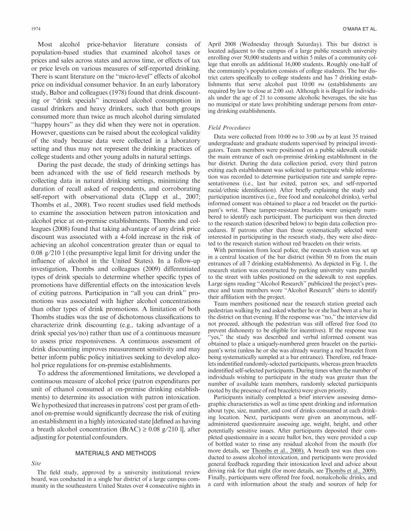
Most alcohol price-behavior literature consists of

population-based studies that examined alcohol taxes or

prices and sales across states and across time, or effects of tax

or price levels on various measures of self-reported drinking.

There is scant literature on the ‘‘micro-level’’ effects of alcohol

price on individual consumer behavior. In an early laboratory

study, Babor and colleagues (1978) found that drink discount-

ing or ‘‘drink specials’’ increased alcohol consumption in

casual drinkers and heavy drinkers, such that both groups

consumed more than twice as much alcohol during simulated

‘‘happy hours’’ as they did when they were not in operation.

However, questions can be raised about the ecological validity

of the study because data were collected in a laboratory

setting and thus may not represent the drinking practices of

college students and other young adults in natural settings.

During the past decade, the study of drinking settings has

been advanced with the use of field research methods by

collecting data in natural drinking settings, minimizing the

duration of recall asked of respondents, and corroborating

self-report with observational data (Clapp et al., 2007;

Thombs et al., 2008). Two recent studies used field methods

to examine the association between patron intoxication and

alcohol price at on-premise establishments. Thombs and col-

leagues (2008) found that taking advantage of any drink price

discount was associated with a 4-fold increase in the risk of

achieving an alcohol concentration greater than or equal to

0.08 g ⁄210 l (the presumptive legal limit for driving under the

influence of alcohol in the United States). In a follow-up

investigation, Thombs and colleagues (2009) differentiated

types of drink specials to determine whether specific types of

promotions have differential effects on the intoxication levels

of exiting patrons. Participation in ‘‘all you can drink’’ pro-

motions was associated with higher alcohol concentrations

than other types of drink promotions. A limitation of both

Thombs studies was the use of dichotomous classifications to

characterize drink discounting (e.g., taking advantage of a

drink special yes ⁄no) rather than use of a continuous measure

to assess price responsiveness. A continuous assessment of

drink discounting improves measurement sensitivity and may

better inform public policy initiatives seeking to develop alco-

hol price regulations for on-premise establishments.

To address the aforementioned limitations, we developed a

continuous measure of alcohol price (patron expenditures per

unit of ethanol consumed at on-premise drinking establish-

ments) to determine its association with patron intoxication.

Wehypothesized that increases inpatrons’ cost per gramof eth-

anol on-premise would significantly decrease the risk of exiting

an establishment in a highly intoxicated state [defined as having

a breath alcohol concentration (BrAC) ‡ 0.08 g ⁄210 l], after

adjusting for potential confounders.

MATERIALS AND METHODS

Site

The field study, approved by a university institutional reviewboard, was conducted in a single bar district of a large campus com-munity in the southeastern United States over 4 consecutive nights in

April 2008 (Wednesday through Saturday). This bar district islocated adjacent to the campus of a large public research universityenrolling over 50,000 students and within 5 miles of a community col-lege that enrolls an additional 16,000 students. Roughly one-half ofthe community’s population consists of college students. The bar dis-trict caters specifically to college students and has 7 drinking estab-lishments that serve alcohol past 10:00 pm (establishments arerequired by law to close at 2:00 am). Although it is illegal for individu-als under the age of 21 to consume alcoholic beverages, the site hasno municipal or state laws prohibiting underage persons from enter-ing drinking establishments.

Field Procedures

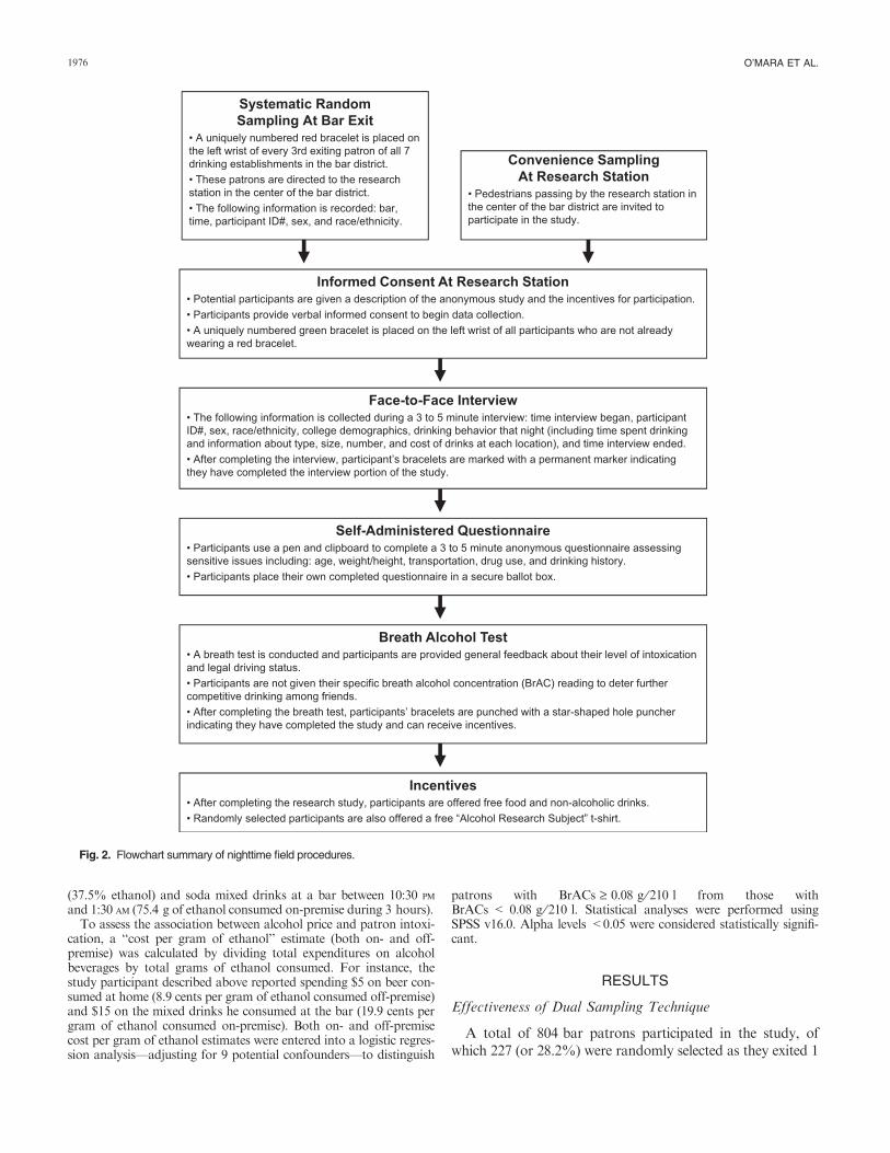
Data were collected from 10:00 pm to 3:00 am by at least 35 trainedundergraduate and graduate students supervised by principal investi-gators. Team members were positioned on a public sidewalk outsidethe main entrance of each on-premise drinking establishment in thebar district. During the data collection period, every third patronexiting each establishment was solicited to participate while informa-tion was recorded to determine participation rate and sample repre-sentativeness (i.e., last bar exited, patron sex, and self-reportedracial ⁄ ethnic identification). After briefly explaining the study andparticipation incentives (i.e., free food and nonalcohol drinks), verbalinformed consent was obtained to place a red bracelet on the partici-pant’s wrist. These tamper-resistant bracelets were uniquely num-bered to identify each participant. The participant was then directedto the research station (described below) to begin data collection pro-cedures. If patrons other than those systematically selected wereinterested in participating in the research study, they were also direc-ted to the research station without red bracelets on their wrists.With permission from local police, the research station was set up

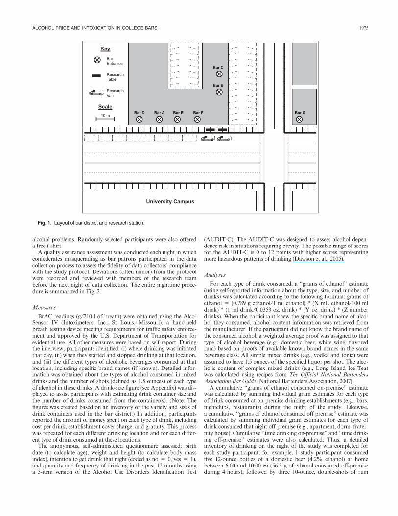
in a central location of the bar district (within 50 m from the mainentrances of all 7 drinking establishments). As depicted in Fig. 1, theresearch station was constructed by parking university vans parallelto the street with tables positioned on the sidewalk to rest supplies.Large signs reading ‘‘Alcohol Research’’ publicized the project’s pres-ence and team members wore ‘‘Alcohol Research’’ shirts to identifytheir affiliation with the project.Team members positioned near the research station greeted each

pedestrianwalking by and askedwhether he or she had been at a bar inthe district on that evening. If the response was ‘‘no,’’ the interview didnot proceed, although the pedestrian was still offered free food (toprevent dishonesty to be eligible for incentives). If the response was‘‘yes,’’ the study was described and verbal informed consent wasobtained to place a uniquely-numbered green bracelet on the partici-pant’s wrist (unless he or she was already wearing a red bracelet frombeing systematically sampled at a bar entrance). Therefore, red brace-lets indentified randomly-selected participants,whereas greenbraceletsindentified self-selected participants.During timeswhen the number ofindividuals wishing to participate in the study was greater than thenumber of available team members, randomly selected participants(notedby the presence of red bracelets)were given priority.Participants initially completed a brief interview assessing demo-

graphic characteristics as well as time spent drinking and informationabout type, size, number, and cost of drinks consumed at each drink-ing location. Next, participants were given an anonymous, self-administered questionnaire assessing age, weight, height, and otherpotentially sensitive issues. After participants deposited their com-pleted questionnaire in a secure ballot box, they were provided a cupof bottled water to rinse any residual alcohol from the mouth (formore details, see Thombs et al., 2008). A breath test was then con-ducted to assess alcohol intoxication, and participants were providedgeneral feedback regarding their intoxication level and advice aboutdriving risk for that night (for more details, see Thombs et al., 2009).Finally, participants were offered free food, nonalcoholic drinks, anda card with information about the study and sources of help for

1974 O’MARA ET AL.

alcohol problems. Randomly-selected participants were also offereda free t-shirt.A quality assurance assessment was conducted each night in which

confederates masquerading as bar patrons participated in the datacollection process to assess the fidelity of data collectors’ compliancewith the study protocol. Deviations (often minor) from the protocolwere recorded and reviewed with members of the research teambefore the next night of data collection. The entire nighttime proce-dure is summarized in Fig. 2.

Measures

BrAC readings (g ⁄210 l of breath) were obtained using the Alco-Sensor IV (Intoximeters, Inc., St Louis, Missouri), a hand-heldbreath testing device meeting requirements for traffic safety enforce-ment and approved by the U.S. Department of Transportation forevidential use. All other measures were based on self-report. Duringthe interview, participants identified: (i) where drinking was initiatedthat day, (ii) when they started and stopped drinking at that location,and (iii) the different types of alcoholic beverages consumed at thatlocation, including specific brand names (if known). Detailed infor-mation was obtained about the types of alcohol consumed in mixeddrinks and the number of shots (defined as 1.5 ounces) of each typeof alcohol in these drinks. A drink-size figure (see Appendix) was dis-played to assist participants with estimating drink container size andthe number of drinks consumed from the container(s). (Note: Thefigures was created based on an inventory of the variety and sizes ofdrink containers used in the bar district.) In addition, participantsreported the amount of money spent on each type of drink, includingcost per drink, establishment cover charge, and gratuity. This processwas repeated for each different drinking location and for each differ-ent type of drink consumed at these locations.The anonymous, self-administered questionnaire assessed: birth

date (to calculate age), weight and height (to calculate body massindex), intention to get drunk that night (coded as no = 0, yes = 1),and quantity and frequency of drinking in the past 12 months usinga 3-item version of the Alcohol Use Disorders Identification Test

(AUDIT-C). The AUDIT-C was designed to assess alcohol depen-dence risk in situations requiring brevity. The possible range of scoresfor the AUDIT-C is 0 to 12 points with higher scores representingmore hazardous patterns of drinking (Dawson et al., 2005).

Analyses

For each type of drink consumed, a ‘‘grams of ethanol’’ estimate(using self-reported information about the type, size, and number ofdrinks) was calculated according to the following formula: grams ofethanol = (0.789 g ethanol ⁄1 ml ethanol) * (X mL ethanol ⁄100 mldrink) * (1 ml drink ⁄0.0353 oz. drink) * (Y oz. drink) * (Z numberdrinks). When the participant knew the specific brand name of alco-hol they consumed, alcohol content information was retrieved fromthe manufacturer. If the participant did not know the brand name ofthe consumed alcohol, a weighted average proof was assigned to thattype of alcohol beverage (e.g., domestic beer, white wine, flavoredrum) based on proofs of available known brand names in the samebeverage class. All simple mixed drinks (e.g., vodka and tonic) wereassumed to have 1.5 ounces of the specified liquor per shot. The alco-holic content of complex mixed drinks (e.g., Long Island Ice Tea)was calculated using recipes from The Official National BartendersAssociation Bar Guide (National Bartenders Association, 2007).A cumulative ‘‘grams of ethanol consumed on-premise’’ estimate

was calculated by summing individual gram estimates for each typeof drink consumed at on-premise drinking establishments (e.g., bars,nightclubs, restaurants) during the night of the study. Likewise,a cumulative ‘‘grams of ethanol consumed off premise’’ estimate wascalculated by summing individual gram estimates for each type ofdrink consumed that night off-premise (e.g., apartment, dorm, frater-nity house). Cumulative ‘‘time drinking on-premise’’ and ‘‘time drink-ing off-premise’’ estimates were also calculated. Thus, a detailedinventory of drinking on the night of the study was completed foreach study participant, for example, 1 study participant consumedfive 12-ounce bottles of a domestic beer (4.2% ethanol) at homebetween 6:00 and 10:00 pm (56.3 g of ethanol consumed off-premiseduring 4 hours), followed by three 10-ounce, double-shots of rum

Fig. 1. Layout of bar district and research station.

ALCOHOL PRICE AND INTOXICATION IN COLLEGE BARS 1975

(37.5% ethanol) and soda mixed drinks at a bar between 10:30 pm

and 1:30 am (75.4 g of ethanol consumed on-premise during 3 hours).To assess the association between alcohol price and patron intoxi-

cation, a ‘‘cost per gram of ethanol’’ estimate (both on- and off-premise) was calculated by dividing total expenditures on alcoholbeverages by total grams of ethanol consumed. For instance, thestudy participant described above reported spending $5 on beer con-sumed at home (8.9 cents per gram of ethanol consumed off-premise)and $15 on the mixed drinks he consumed at the bar (19.9 cents pergram of ethanol consumed on-premise). Both on- and off-premisecost per gram of ethanol estimates were entered into a logistic regres-sion analysis—adjusting for 9 potential confounders—to distinguish

patrons with BrACs ‡ 0.08 g ⁄210 l from those withBrACs < 0.08 g ⁄210 l. Statistical analyses were performed usingSPSS v16.0. Alpha levels <0.05 were considered statistically signifi-cant.

RESULTS

Effectiveness of Dual Sampling Technique

A total of 804 bar patrons participated in the study, of

which 227 (or 28.2%) were randomly selected as they exited 1

Fig. 2. Flowchart summary of nighttime field procedures.

1976 O’MARA ET AL.

of the 7 establishments in the bar district (the remaining 577

participants self-selected into the study). Table 1 summarizes

characteristics of the randomly selected participants, self-

selected participants, and total participants. Chi-square

analyses indicated that there were no statistically significant

differences between the randomly and self-selected partici-

pants on sex [v2(1, 797) = 0.714, p = 0.398], race ⁄ethnicity

[v2(4, 802) = 0.728, p = 0.948], and last bar exited [v2(6,

710) = 10.746, p = 0.097]. In addition, the 2 participant

groups did not differ on age [t(714) = )1.374, p = 0.170]

and BrAC [t(738) = 0.892, p = 0.373].

The random sampling procedure solicited participation

from 687 patrons as they exited the establishments from 10:00

pm to 2:00 am. As noted, this effort led to the successful

recruitment of 227 patrons (or 33.0%). There were no sex

[v2(1, 629) = 0.202, p = 0.653] or race ⁄ethnicity [v2(4, 637)

= 1.252, p = 0.870] differences between these participants

and the 460 solicited nonparticipants. There was a significant

difference between these 2 groups on last bar exited [v2(6,

658) = 26.938, p < 0.0001], which was likely due to the

varying physical proximity of the research station to some

bars. Figure 1 shows that the research station was most clo-

sely located to Bars E and F, from which the yield of ran-

domly selected participants was the greatest. Results of these

analyses provided no reason to believe the sampling proce-

dure produced a biased sample of patrons. Thus, data from

the randomly- and self-selected participants were combined

for analyses.

Participants were included in price and intoxication analy-

ses if they completed all phases of data collection and

reported: (i) being of legal drinking age, i.e., 21 years or older;

(ii) consuming alcohol at an establishment in the targeted bar

district that night; (iii) paying for their own cover charges and

alcohol beverages at establishments, i.e., not receiving cover

or drinks purchased by other patrons; (iv) not having partici-

pated in the study on a previous night; and (v) responding to

all interview and survey questions in an accurate and honest

manner. Analyses were limited to these patrons because they

are the primary customer base who can legally and directly

purchase their alcohol supply from on-premise establish-

ments. Among the 804 participants, 501 (62.3%) met the eligi-

bility criteria. Table 2 summarizes the on- and off-premise

drinking behavior and expenditures of these patrons.

Validation of the Grams of Ethanol Consumed Measure

In the sample of eligible patrons (n = 501), the mean

BrAC was 0.086 g ⁄210 l (SD = 0.045). The Kolmogorov–

Smirnov test revealed that the distribution of BrAC readings

did not significantly deviate from a normal distribution

(p = 0.392). Therefore, a multiple linear regression analysis

was conducted in which a continuous measure of BrAC was

treated as a dependent variable [F (2, 497) = 92.18,

p < 0.0001, R2 = 0.27]. Model checking showed that collin-

earity was not present in the predictor set (variation inflation

indicators were <2.0). Total grams of ethanol consumed

(b = 0.39, p < 0.0001) had a significant association with

BrAC after adjusting for the effects of total number of drinks

consumed (b = 0.13, p < 0.03), indicating that the estimated

grams of ethanol variable provided a stronger predictor of

alcohol intoxication than the standard number of drinks mea-

sure. Therefore, subsequent analyses of alcohol price used

‘‘cost per gram of ethanol’’ rather than cost per drink.

Association Between Alcohol Price and Patron Intoxication

Fixed and random effects (Subramanian et al., 2003) of

drinking establishment were tested in 2 preliminary logistic

regression models. As fixed effects, only 1 establishment had a

statistically significant association (p = 0.030) with BrAC

level. As random effects, 4 establishments were not statisti-

cally significant and 3 could not be estimated due to the data

and the complexity of the binary outcome model (i.e., some

matrices were not positive definite). In addition, treating

drinking establishment as either a fixed effect or a random

effect did not alter the statistical significance of any of the

Table 1. Participant Characteristics

Samplecharacteristics

Randomlyselected

participants(n = 227)

Self-selectedparticipants(n = 577)

Totalparticipants(n = 804)

Sex% Male 59.3 62.5 61.6% Female 40.7 37.5 38.4

Race ⁄ ethnicity% White 81.4 80.2 81.0% Hispanic 8.9 8.4 8.7% Black 2.3 3.1 2.5% Asian 3.0 3.1 3.0% Other 4.5 5.2 4.7

Last bar exited% Bar A 13.6 11.7 12.3% Bar B 6.1 6.6 6.5% Bar C 6.6 6.8 6.8% Bar D 22.7 20.5 21.1% Bar E 11.6 20.7 18.2% Bar F 16.7 17.4 17.2% Bar G 22.7 13.2 18.0

OtherMean age (years) 22.9 22.6 22.7Mean BrAC (g ⁄ 210 l) 0.077 0.080 0.080

Table 2. Descriptive Statistics for Legal Age Bar Patrons Who PurchasedTheir Own Alcohol Beverages (n = 501)

VariableOn-premisemean (SD)

Off-premisemean (SD)

Total mean(SD)

Hours drinking 2.4 (1.6) 0.8 (1.5) 3.2 (2.1)Number of drinksconsumed

4.9 (3.1) 1.6 (2.7) 6.6 (4.2)

Grams of ethanolconsumed

78.0 (55.3) 27.3 (48.5) 105.3 (71.6)

Expenditures onalcohol beverages

$11.7 (9.6) $1.4 (4.2) $13.1 (10.4)

Cost per gram ofethanol

$0.192 (0.147) $0.030 (0.105) $0.157 (0.122)

ALCOHOL PRICE AND INTOXICATION IN COLLEGE BARS 1977

covariates in the model. Consequently, we did not include

establishment as a nested random effect in subsequent

analyses.

A multivariable logistic regression analysis was then con-

ducted to test the study hypothesis, i.e., to distinguish patrons

with BrACs ‡ 0.08 g ⁄210 l from those with BrACs <

0.08 g ⁄210 l. In addition to cost per gram of ethanol con-

sumed at on-premise drinking establishments, 10 other vari-

ables were entered into the model to account for alternative

explanations of BrAC after leaving an establishment. Among

432 participants who provided complete data (a listwise dele-

tion of cases with missing values resulted in 68 cases being

excluded from the analysis), 209 (or 48.4%) had BrAC read-

ings less than the 0.08 g ⁄210 l cutoff. Peduzzi and colleagues

(1996) recommend in the smaller of the 2 groups in logistic

regression analysis, that there be at least 10 cases per variable

to reduce the possibility of an invalid model. Thus, the

case-to-variable ratio of 19 in the logistic model (209 ⁄11) was

substantially greater than the threshold needed to establish

statistical conclusion validity.

As shown in Table 3, the predictor set accounted for a sig-

nificant amount of variance in BrAC defined by the 0.08 g ⁄

210 l cutting score [model chi-square (11, 432) = 115.19,

p < 0.0001]. The Nagelkerke pseudo-R2 statistic indicated

that an estimated 31.2% of the variance in intoxication level

could be explained by the predictor set. In support of the

study hypothesis, the results indicated that increases in cost

per gram of ethanol on-premise significantly reduced the odds

of leaving a bar intoxicated (BrAC ‡ 0.08 g ⁄210 l), after

adjusting for confounding effects. A 10 cent increase in cost

per gram of ethanol on-premise was associated with a 30%

reduction in the risk of having a BrAC ‡ 0.08 g ⁄210 l.

Practical Illustration of Patrons’ Price Responsiveness

Table 4 displays the mean cost per gram of ethanol on-

premise for six BrAC groups: (i) 0.000 to 0.019, (ii) 0.020 to

0.049, (iii) 0.050 to 0.079, (iv) 0.080 to 0.119, (v) 0.120 to

0.159, and (vi) 0.160 to 0.199 g ⁄210 l. To aid interpretations,

each groups’ mean cost per gram of ethanol was also con-

verted to the cost of a standard drink—defined as any drink

that contains approximately 14 g of pure ethanol, for example

(i) 12-ounce, 10-proof beer, (ii) 1.5-ounce, 80-proof liquor, or

(iii) 5-ounce, 24 proof wine. Results from a 1-way ANOVA

revealed significant BrAC group differences in cost per gram

of ethanol, F(5,490) = 10.813, p < .0001. Post hoc analyses

(Student-Newman-Keuls) indicated that the mean cost per

gram of ethanol was significantly higher in the first BrAC

group (0.000 to 0.019 g ⁄210 l) compared with the other 5

groups. In addition, the mean cost per gram of ethanol was

significantly higher in the second and third BrAC groups

(0.020 to 0.049, 0.050 to 0.079 g ⁄210 l) compared to the

fourth, fifth, and sixth groups (0.080 to 0.119, 0.120 to 0.159,

0.160 to 0.199 g ⁄210 l).

DISCUSSION

This study examined the association between alcohol price

and patron intoxication at on-premise drinking establish-

ments. We hypothesized that increases in patrons’ cost per

gram of ethanol consumed on-premise would significantly

decrease the risk of exiting an establishment intoxicated (i.e.,

BrAC ‡ 0.08 g ⁄210 l), after adjusting for confounders includ-

ing intention to get drunk and AUDIT-C score (the latter

representing the existing pattern of patron alcohol use). In

support of this hypothesis, we found that a 10 cent increase in

cost per gram of ethanol was associated with a 30% reduction

in the risk of having a BrAC ‡ 0.08 g ⁄210 l. Applied to con-

ventional serving practices, a 10-cent increased cost per gram

Table 3. Multivariable Logistic Regression Analysis of Drinking Variables Associated With High Intoxication (BrAC ‡ 0.080 g ⁄210 l) Among Patrons ExitingOn-Premise Drinking Establishments in a College Bar District (n = 432)

Variable OR (95% CI) p

BrAC < 0.080 g ⁄ 210 l(n = 209)

BrAC ‡ 0.080 g ⁄ 210 l(n = 223)

Number of drinks consumed on-premise 1.24 (1.13–1.36) <0.001 M = 3.89 (SD = 2.50) M = 5.74 (SD = 3.34)Cost per gram of ethanol on-premise 0.97 (0.95–0.99) <0.001 M = $0.229 (SD = $0.170) M = $0.160 (SD = $0.117)Hours drinking on-premise 1.31 (1.11–1.56) 0.002 M = 1.95 (SD = 1.19) M = 2.73 (SD = 1.79)Number of drinks consumed off-premise 1.19 (1.04–1.35) 0.009 M = 1.11 (SD = 2.14) M = 2.11 (SD = 3.07)Female 1.89 (1.13–3.17) 0.016 Female = 35.7% Female = 37.5%Hours drinking off-premise 1.24 (1.00–1.55) 0.050 M = 0.51 (SD = 1.11) M = 1.03 (SD = 1.76)Intention to get drunk 1.52 (0.95–2.41) ns — —Minutes between last drink and breath test 1.36 (0.86–2.15) ns — —AUDIT-C score 1.07 (0.98–1.18) ns — —Body mass index 0.97 (0.91–1.05) ns — —Cost per gram of ethanol off-premise 1.00 (0.98–1.02) ns — —

Table 4. Mean Cost Per Gram of Ethanol Consumed at On-PremiseDrinking Establishments for Six BrAC Groups

BrAC group(g ⁄ 210 l)

Mean cost pergram of ethanol

Equivalent cost of astandard drink

(i.e., 14 g of ethanol)

0.000–0.019 $0.317 $4.440.020–0.049 $0.227 $3.180.050–0.079 $0.217 $3.040.080–0.119 $0.165 $2.310.120–0.159 $0.150 $2.100.160–0.199 $0.129 $1.81

1978 O’MARA ET AL.

of ethanol translates to a $1.40 price increase on a standard

drink ($0.10 · 14 grams of pure ethanol in a standard drink).

Further analyses suggested an inverse dose–responsive rela-

tionship between alcohol price and patron intoxication. For

example, patrons with BrACs ranging between 0.000 and

0.019 g ⁄210 l spent (on average) 31.7 cents per gram of ethanol

consumed at on-premise establishments (about $4.44 per

standard drink) versus patrons with BrACs ranging

between 0.160 and 0.199 g ⁄210 l, who spent (on average)

12.9 cents per gram of ethanol (about $1.81 per standard

drink). This corroborates previous research by Thombs

and colleagues (2009) who found that the ‘‘all you can

drink’’ promotion may be the specific drink special most

likely to result in excessive drinking because the unit price

of ethanol decreases with each successive drink.

This is the first known investigation to document that

increases in alcohol price at on-premise establishments can be

linked to lower intoxication levels among patrons. These

‘‘micro-level’’ findings corroborate population-based econo-

metric research and theory of the price elasticity of alcoholic

beverages, which hold that customers respond to increased

alcohol prices by purchasing and consuming less alcohol

(Chaloupka et al., 2002). Lower alcohol consumption and

intoxication among patrons may consequently reduce the risk

of problems that have been attributed to on-premise establish-

ments such as fighting (Forsyth, 2008), injuries (Luke et al.,

2002), and alcohol-impaired driving (Grube and Stewart,

2004; Gruenewald et al., 2002; Usdan et al., 2005).

Lastly, these findings demonstrate that even slight increases

in alcohol price at on-premise establishments are associated

with decreases in patron intoxication after leaving a bar, sug-

gesting that raising alcoholic beverage prices by tax increases

and stricter regulation of drink discounting practices could

have a substantial public health benefit. Although the data

were collected in only 1 campus community, these results sug-

gest that alcohol price should be a priority focus of policy

development and regulation aimed at improving the serving

practices of drinking establishments that cater to young

adults. More specifically, stricter regulation of on-premise

drink discounting promotions may be warranted.

Strengths and Limitations

Themajor strengthof this investigationwasourfieldmethods,

which collected data in a natural drinking setting, mini-

mized the duration of recall asked of respondents, and

corroborated self-reported alcohol consumption with an

objective measurement of intoxication. An additional

strength was the use of a ‘‘grams of ethanol’’ measure to

estimate alcohol consumption rather than the standard

‘‘number of drinks’’ measure—as drinks contain substan-

tially varying amounts of ethanol. The findings presented

here may have greater ecological validity than those

obtained from studies that rely exclusively on retrospec-

tive self-report survey data collected from sober college

students in nondrinking settings (Christie et al., 2001) or

from protocols using laboratory settings (Babor et al.,

1978). Moreover, the event-specific analyses of price

responsiveness at the individual (patron) level augment

analyses done at the population-level and serve to counter

layperson arguments which may contend that population

studies do not apply to the drinking practices of typical

consumers.

Although there is uncertainty about the sample’s ability to

represent patron characteristics that exist in the broad range

of campus communities, we believe the obtained sample rep-

resents the population of bar patrons in the targeted bar dis-

trict. A total of 71.8% of the participants self-selected into the

study (the remainder were randomly selected). Yet, there were

no significant differences between those self-selected and those

randomly selected with respect to demographic and relevant

drinking variables. Another sampling concern might be that

the participation rate among the randomly recruited partici-

pants was only 33.0%. However, we found no statistically sig-

nificant demographic differences between randomly selected

bar patrons who participated in data collection and randomly

selected bar patrons who chose not to participate. Further-

more, as Krosnick (1999) has pointed out, nonparticipation is

often related to factors that have no bearing on the research

questions of a study and thus do not necessarily produce sam-

pling error. For example, we collected information about

motives for nonparticipation and found that the most fre-

quently cited reasons were as follows: (i) leaving the bar in a

direction that did not take them past the research station,

(ii) not interested in the incentives, e.g., not hungry, and

(iii) wanting to leave quickly. Therefore, nonparticipation

may not have been related to alcohol consumption.

Suggestions for Future Field Research in Bar Districts

Future field research of patron drinking behavior and price

responsiveness should: (i) collect all data as close as possible

to establishment entrances, (ii) consolidate data collection pro-

cedures to 5 to 10 minutes, (iii) increase the variety of incen-

tives, and (iv) anticipate weather, crowding, and other factors

that might preclude participation. Consideration should be

given to research designs that plot changing intoxication levels

over the course of a night while minimizing unwanted testing

effects. In addition, protocols should emphasize the use of

objective measures whenever possible (e.g., direct observation,

expenditure receipts, biological samples). Finally, there is a

need to replicate the findings of this study in a broader sample

of bar districts of different types using field research methods

similar to those used in this investigation.

ACKNOWLEDGMENTS

This project was supported by funds from the Office of the

President at the University of Florida and volunteer field

research assistants from the Student Safety Research Collo-

quium at the University of Florida. The following persons are

acknowledged for their contributions to this research project:

ALCOHOL PRICE AND INTOXICATION IN COLLEGE BARS 1979

Sara Gullet, Tommy Huang, Altina Fenelon, Rick Ligon,

Petey Bingham, Neil Deochand, Gloria Longin, Jordan

Miller, Christopher Massicot, Henry Lewis, Kevin Clark,

Chelsea Kim, Diana Chu, Chung-Bang Weng, Laura

Haderxhanaj, Jennifer Reingle, Amanda Hilton, Miranda

Tsukamoto, Ashley Martinovich, Joseph Everette, Amanda

Hecker,DavidMendoza,LaRhondaWalker,SebastianEstades,

Casey Head, Justine Bronson, Justin Alfonso, Jennifer

Aranda, Daniel Gierbolini, Greg Feldman, Joshua

McCarty, Samantha Carino, Ashley Voight, Donielle

Rouse, Isabella Mays, Mia Lopez, Nikki Farides, Benita

Chilampath, Hillary Kener, Jessie Lazarchik, Nina

Dawson, Amara Huda, Renee Ryals, Shenae Samuels,

Mekailah Simpson, Brian Min, Amanda Negron, Daniel

Hunter, Devonne Collins, Ashlee Lovejoy, Amber Mann,

Kailyn Kruger, Devon Grimme, Sara Johnson, Marilee

Leon, Lindsey Teague, Shelly Taylor, India Van Horn,

Eric Busch, Kathryn Bello, Jaime Chakkala, Daniel

Fisher, Elizabeth Hernandez, Ian Galloway, Lindsay

Keller, Ashley Johnson, Anthony Lawson, Lorna Lopez,

Evan Ratchford, Meghan Speicher-Harris, and Tiffany

Walker.

REFERENCES

Babor TF, Mendelson JH, Greenberg I, Kuehnle J (1978) Experimental analy-

sis of the ‘happy hour’: effects of purchase price on alcohol consumption.

Psychopharmocology 58:35–41.

Chaloupka FJ, Grossman M, Saffer H (2002) The effects of price on alcohol

consumption and alcohol related problems. Alcohol Res Health 26:22–34.

Chaloupka FJ, Wechsler H (1996) Binge drinking in college: the impact of

price, availability and alcohol control policies. Contemp Econ Policy

14:112–124.

Christie J, Fisher D, Kozup JC, Smith S, Burton S, Creyer EH (2001) The

effects of bar- sponsored alcohol beverage promotions across binge and

nonbinge drinkers. J Public Policy Market 20:240–253.

Clapp JD, Holmes MR, Reed MB, Shillington AM, Freisthler B (2007) Mea-

suring college students’ alcohol consumption in natural drinking environ-

ments: field methodologies for bars and parties. Eval Rev 31:469–489.

Dawson DA, Grant BF, Stinson FS, Zhou Y (2005) Effectiveness of the

derived Alcohol Use Disorders Identification Test (AUDIT-C) in screening

for alcohol use disorders and risk drinking in the US general population.

Alcohol Clin Exp Res 29:844–854.

Forsyth AJM (2008) Banning glassware from nightclubs in Glascow (Scot-

land): observed impacts, compliance and patrons’ views. Alcohol Alcohol

43:111–117.

Grube JW, Stewart K (2004) Preventing impaired driving using alcohol policy.

Traffic Inj Prev 5:199–207.

Gruenewald PJ, Johnson FW, Treno AJ (2002) Outlets, drinking and driving:

a multilevel analysis of availability. J Stud Alcohol 63:460–468.

Hingson R, Heeren T, Winter M, Wechsler H (2005) Magnitude of alcohol-

related mortality and morbidity among U.S. college students ages 18–24:

changes from 1998–2001. Annu Rev Public Health 26:259–279.

Hingson RW, Heeren T, Zakocs RC, Kopstein A, Wechsler H (2002) Magni-

tude of alcohol-related mortality and morbidity among U.S. college students

ages 18–24. J Stud Alcohol 63:136–144.

Krosnick JA (1999) Survey research. Annu Rev Psychol 50:537–567.

Kuo M, Wechsler H, Greenberg P, Lee H (2003) The marketing of alcohol to

college students: the role of low prices and special promotions. Am J Prev

Med 25:204–211.

Luke LC, Dewar C, Bailey M, McGreevy D, Burdett-Smith P (2002) A little

nightclub medicine: the healthcare implications of clubbing. Emerg Med J

19:542–545.

National Bartenders Association (2007) The Official National Bartenders

Association Bar Guide. Cliff Road Books, Lakeville, CT.

Osterberg E (1995) Do alcohol prices affect consumption and related prob-

lems? in Alcohol and Public Policy: Evidence and Issues (Holder HD,

Edwards G eds), pp 145–163. Oxford University Press, New York.

Peduzzi P, Concato J, Kemper E, Holford TR, Feinstein AR (1996) A simula-

tion study of the number of events per variable in logistic regression analy-

sis. J Clin Epidemiol 49:1373–1379.

Subramanian SV, Jones K, Duncan C (2003) Multilevel methods for public

health research, in Neighborhoods and Health (Kawachi I, Berkman LF

eds), pp 65–111. Oxford University Press, New York.

Thombs DL, Dodd V, Pokorny SB, Omli MR, O’Mara R, Webb MC, Lacaci

DM, Werch C (2008) Drink specials and the intoxication levels of patrons

exiting college bars. Am J Health Behav 32:411–419.

Thombs DL, O’Mara R, Dodd VJ, Hou W, Merves ML, Weiler RM,

Pokorny SB, Goldberger BA, Reingle J, Werch C (2009) A field study of

bar-sponsored drink specials and their associations with patron intoxica-

tion. J Stud Alcohol Drugs 70:206–214.

Usdan SL, Moore CG, Schumacher JE, Talbott LL (2005) Drinking locations

prior to impaired driving among college students: implications for preven-

tion. J Am Coll Health 54:69–75.

Wagenaar AC, Salois MJ, Komro KA (2009) Effects of beverage alcohol price

and tax levels on drinking: a meta-analysis of 1003 estimates from 112 stud-

ies. Addiction 104:179–190.

Wagenaar AC, Maldonado-Molina MM, PhD, Wagenaar BH (in press)

Effects of alcohol tax increases on alcohol-related disease mortality in

Alaska: time-series analyses from 1976 to 2004. Am J Public Health.

Wechsler H, Lee JE, Kuo M, Seibring M, Nelson TF, Lee H (2002) Trends in

college binge drinking during a period of increased prevention efforts. Find-

ings from 4 Harvard School of Public Health College Alcohol Study sur-

veys: 1993-2001. J Am Coll Health 50:203–217.

SUPPORTING INFORMATION

Additional Supporting Information may be found in the

online version of this article:

Appendix. Drink size figure used to obtain participant esti-

matesofbeveragecontainer sizes theyused toconsumealcohol.

Please note: Wiley-Blackwell is not responsible for the con-

tent or functionality of any supporting information supplied

by the authors. Any queries (other than missing material)

should be directed to the corresponding author for the article

1980 O’MARA ET AL.