AGE, RETIREMENT AND EXPENDITURE PATTERNS: AN ECONOMETRIC STUDY OF

Research Institute for Quantitative Studies in Economics and Population

Faculty of Social Sciences, McMaster University

Hamilton, Ontario, Canada

L8S 4M4

AGE, RETIREMENT AND EXPENDITURE PATTERNS:

AN ECONOMETRIC STUDY OF

OLDER CANADIAN HOUSEHOLDS

Frank T. Denton

Dean C. Mountain

Byron G. Spencer

QSEP Research Report No. 375

October 2002

The authors are QSEP Research Associates. Frank Denton and Byron Spencer are faculty

members of the McMaster Department of Economics. Dean Mountain is a faculty member

of the McMaster Michael G. DeGroote School of Business and an associate member of the

Department of Economics.

This report is cross-listed as No. 82 in the McMaster University SEDAP Research Paper

Series.

The Research Institute for Quantitative Studies in Economics and Population (QSEP) is an

interdisciplinary institute established at McMaster University to encourage and facilitate

theoretical and empirical studies in economics, population, and related fields. For further

information about QSEP and other reports in this series, see our web site

http://socserv2.mcmaster.ca/~qsep. The Research Report series provides a vehicle for

distributing the results of studies undertaken by QSEP associates. Authors take full

responsibility for all expressions of opinion.

September 2002

ABSTRACT

AGE, RETIREMENT AND EXPENDITURE PATTERNS : AN ECONOMETRIC STUDY

OF OLDER CANADIAN HOUSEHOLDS

Frank T. Denton, Dean C. Mountain and Byron G. Spencer

McMaster University

The paper explores the allocation of consumption expenditure by the older population among

different categories of goods and services, and how expenditure patterns change with age within

that population. Of particular interest is whether observed differences between pre-retirement and

post-retirement patterns are a consequence of changes in “tastes” or reductions in income. An

adapted form of the Deaton and Muellbauer Almost Ideal Demand System is estimated with data

from six Family Expenditure Surveys and used to investigate that question. The findings suggest

that observed changes in budget allocations are most closely related to reductions in income.

1We acknowledge with appreciation the help of Christine Feaver, who did the

calculations reported in this paper. The work underlying the paper was carried out as part of the

SEDAP (Social and Economic Dimensions of an Aging Population) Research Program supported

by the Social Sciences and Humanities Research Council of Canada, Statistics Canada and the

Canadian Institute for Health Information.

-1-

September 2002

AGE, RETIREMENT AND EXPENDITURE PATTERNS : AN ECONOMETRIC STUDY

OF OLDER CANADIAN HOUSEHOLDS1

Frank T. Denton, Dean C. Mountain and Byron G. Spencer

McMaster University

1. INTRODUCTION

The widespread recognition of the importance of population aging for the economy has

generated new interest in how people manage their resources in later life. One can think of three

broad aspects of household resource management that are of interest: patterns of saving and the

use of wealth, reflecting choices between current consumption, on the one hand, and future

consumption or bequests, on the other; leisure/work choices, as indicated by labour force

participation rates; and the allocation of current consumption expenditure among different

categories of goods and services. The allocation of current consumption expenditure is the

subject of this paper. In particular, the paper is concerned with how the expenditure patterns of

households in the range 50 and older vary as age increases, and how they are affected by the

transition from work to retirement. A question of special interest is whether observed differences

between pre-retirement and post-retirement expenditure patterns are a consequence of age-related

-2-

changes in “tastes” or of reductions in income.

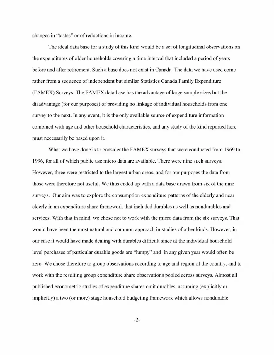
The ideal data base for a study of this kind would be a set of longitudinal observations on

the expenditures of older households covering a time interval that included a period of years

before and after retirement. Such a base does not exist in Canada. The data we have used come

rather from a sequence of independent but similar Statistics Canada Family Expenditure

(FAMEX) Surveys. The FAMEX data base has the advantage of large sample sizes but the

disadvantage (for our purposes) of providing no linkage of individual households from one

survey to the next. In any event, it is the only available source of expenditure information

combined with age and other household characteristics, and any study of the kind reported here

must necessarily be based upon it.

What we have done is to consider the FAMEX surveys that were conducted from 1969 to

1996, for all of which public use micro data are available. There were nine such surveys.

However, three were restricted to the largest urban areas, and for our purposes the data from

those were therefore not useful. We thus ended up with a data base drawn from six of the nine

surveys. Our aim was to explore the consumption expenditure patterns of the elderly and near

elderly in an expenditure share framework that included durables as well as nondurables and

services. With that in mind, we chose not to work with the micro data from the six surveys. That

would have been the most natural and common approach in studies of other kinds. However, in

our case it would have made dealing with durables difficult since at the individual household

level purchases of particular durable goods are “lumpy” and in any given year would often be

zero. We chose therefore to group observations according to age and region of the country, and to

work with the resulting group expenditure share observations pooled across surveys. Almost all

published econometric studies of expenditure shares omit durables, assuming (explicitly or

implicitly) a two (or more) stage household budgeting framework which allows nondurable

-3-

goods and services to be dealt with, while ignoring durable goods altogether. We ourselves

followed that practice in a study based on Canadian time series (Denton, Mountain and Spencer,

1999; see also the other studies cited in Table 6 of that paper, in all of which the same was done).

But omitting durables in the present study was not a reasonable option for us. A comprehensive

view of expenditure was required, and while the use of grouped data was a theoretically

imperfect solution to the “lumpiness” problem, it allowed us to deal with the full range of

household expenditure categories and made it straightforward to apply a standard type of share

equation model.

We provide further discussion of the use of grouped data and the issue of durables below.

To make more homogeneous the subject of analysis we confine our attention to households with

husband and wife both present; we discuss that below, and other aspects of the data we have

used. Among the other matters discussed are the treatment of price indexes in a share equation

model when spatial (regional) price level differences have to be taken into account, as well as

changes through time, and of course the details of the model used in the study.

The model is a standard linear form of the Deaton and Muellbauer (1980) Almost Ideal

Demand System, adapted to suit the requirements of our analysis. It is estimated using the

grouped share observations from the six surveys. We present it, subject it to a number of

hypothesis tests, and use it to simulate the expenditure patterns of older households in their pre-

retirement and post-retirement years under alternative assumptions about income replacement

rates at retirement.

2. DATA SOURCES AND RESTRICTIONS

The six FAMEX surveys from which our expenditure information is drawn are for the

years 1969, 1978, 1982, 1986, 1992, and 1996. The surveys were not exactly the same in

-4-

coverage and definitions but after a careful examination and comparison of their documentation

we judged them to be close enough to permit us to extract a reasonably consistent data base. We

wished to have a relatively homogeneous sample of older households to work with in terms of

composition and type of residential environment. That plus the requirement of consistency of

coverage across the surveys suggested restricting the sample to husband-and-wife households

living in urban centres of 30,000 or more population (with or without others present in the

household), and with husband aged 50 or more. We considered instead using the average age of

husband and wife but that would have complicated the analysis greatly by making it difficult to

create five-year age groups for matching with other variables. Also, because we were dealing

with older households in roughly the last three decades of the 20th century it seemed likely that

retirement decisions for those households would have been more closely linked to husband’s

rather wife’s age. Hence the choice of the former.

The FAMEX surveys provide considerable detail in terms of expenditure categories.

However, our interest is in a broad rather than detailed assessment of the expenditure behaviour

of older households. In view of that, and the consideration that minor differences from survey to

survey in the definitions of categories were less likely to be a problem at more aggregated levels,

we chose ten categories to work with: food at home; food from restaurants; shelter; household

furnishing and operation; clothing; transportation; health and personal care; recreation; tobacco;

and alcohol. All of the analysis in the paper relates to those ten categories, cross-classified by age

and region of the country. Five-year age groups are identified for ages 50 to 74. Beyond that the

survey data do not provide any breakdown and it is necessary therefore to treat ages 75 and over

as a single group.

Price indexes are required also for our model. The basic source for those is an

unpublished set of annual time series of current and constant dollar expenditures, by province,

-5-

compiled for purposes of the provincial income and expenditure accounts and furnished to us by

Statistics Canada. We combined the Atlantic Provinces and Prairie Provinces to obtain regional

aggregates, along with Quebec, Ontario, and British Columbia, making five regions in total.

Although the expenditure categories are somewhat different from the FAMEX ones they were

available at a sufficiently fine level to permit us to make a close and detailed match, combine the

matched categories to form a set of ten corresponding to the ten expenditure categories noted

above, and then calculate the implicit price indexes for those categories by dividing current by

constant dollar totals. (We were able to do that back to 1971; for 1970 and 1969 we had only

national price indexes to work with and we used the changes in those to project the regional

indexes back two years.)

A potential alternative to using the indexes calculated from the provincial accounts

expenditure series was to use the provincial index components of the Consumer Price Index.

However, the provincial accounts indexes were available in full detail for all regions, on a

consistent and comprehensive definitional basis for the whole of the period of interest to us,

whereas the CPI components were not . Also, the price deflators for the provincial accounts are

implicitly derived from the same underlying survey data as the CPI indexes to the extent that the

two sets have similar definitions and coverage, but are somewhat broader in scope since they

must conform with accepted and comprehensive national accounting definitions. In sum, they

were more appropriate and useful for our purposes.

The indexes derived from the provincial accounts series measure only changes through

time. Our model requires that interregional as well as time differences in price levels be allowed

for. However, as we discuss later, such allowance can be made by an appropriate specification of

the model, and the use of a geometric rather than an arithmetic aggregator function in converting

the individual expenditure category indexes into an overall index.

-6-

3. THE HOUSEHOLD BUDGET AT OLDER AGES: A QUICK LOOK AT THE DATA

To set the stage for the subsequent analysis we begin by taking a quick look at the budget

patterns of older households, based simply on the all-Canada percentages spent on the ten

expenditure categories averaged over all six of the FAMEX surveys from which our data are

drawn. The percentages are shown in Table 1 for the six age groups of concern and there are

clear patterns of variation evidenced within the table.

The first clear pattern is the consistent rise with age in the percentage spent on food at

home, offset, but only partially, by a corresponding decrease in the percentage spent on food

from restaurants; adding the two categories together, the food percentage increases from 20.9 at

ages 50-54 to 24.7 at ages 75 and over. The budget share of shelter increases consistently also

over the same age range, from 18.2 to 27.8 percent. Thus in total the combined share of food and

shelter increases from 39.1 to 52.5 percent of the household budget. In round numbers, the

average husband/wife household spends about two-fifths of its budget on food and shelter when

the husband is in his early 50s ( which in most cases means before retirement) but more than half

when he is 75 or older. Other patterns include declines in the expenditure shares of clothing,

recreation, tobacco, and alcohol, sharp declines in the transportation share at the oldest ages, and

some increase in the health and personal care share at those ages too. (Note though that health

costs funded through public insurance plans are by definition not included in household

expenditure.) Table 1 and the foregoing discussion are merely descriptive. It remains to be seen

whether the patterns reflect changes in “tastes” that come with age or changes in household

purchasing power, which also may come with age.

4. A MODEL OF THE EXPENDITURE SYSTEM FOR OLDER HOUSEHOLDS

The instrument for analyzing the expenditure patterns of older households is a variant of

-7-

the Deaton/Muellbauer Almost Ideal Demand System model fitted to the observed regional/age

group means from six FAMEX surveys, representing a total of 180 group observations. (The total

number of underlying sample observations from the six surveys is approximately 10,100.) The

model is of the form

(1) S x P P R Aiart i art rt ij jrt ir r ia a

arj

= + + + +∑∑∑β γ δ θln( / ) ln* λ εi art iartZ +

where is total household expenditure, is the proportion spent on a particular category ofx S

expenditure, is a category-specific price index, is a geometrically weighted compositeP P*

price index (defined below), and are binary dummy variables denoting region and ageR A

group, is a vector of other explanatory variables, is a random error, and the Greek symbolsZ ε

are parameters. Expenditure categories are indexed by = 1, ..., 10 (or alternatively by j, wherei

necessary), age groups by = 1, ..., 6, regions by = 1, ..., 5, and survey years by = 1969,a r t

1978, 1982, 1986, 1992, 1996. The complete model, consisting of ten equations, is subject to an

adding-up restriction (since the shares must sum to 1). In addition, symmetry and homogeneity

restrictions are imposed on the and parameters. The model of course has its roots in microβ γ

utility maximization theory and can be assumed to apply to aggregate observations only as a

convenient approximation. (For a somewhat reassuring evaluation of aggregation error, though,

see Denton and Mountain, 2001.) The incorporation of the symmetry and homogeneity

restrictions should be viewed as a device for imposing some discipline on the model in

estimation (given the relatively small number of group observations), rather than as having a firm

grounding in consumer optimization theory when applied to aggregate data. The model is

estimated as a restricted seemingly unrelated regression equation (SURE) system. One of the

equations is dropped in estimation because of the singularity arising from the adding-up

-8-

restriction. In addition, one of the regional dummy variables is dropped in each equation to avoid

obvious other singularities.

We report below an evaluation of the complete fitted model and its various estimated

parameters, based on standard criteria. From the point of view of the way in which the model is

to be used subsequently though, the most important considerations are income effects (strictly

speaking, the effects of total expenditure), as represented by the coefficients and derivedβ

income elasticities, and age group effects, as represented by the coefficients. Variables otherθ

than (real) income and age group are essentially for control purposes.

4. PRICE INDEXES

The treatment of price indexes calls for special attention. The ten individual variablesP

are time-based indexes rather than indexes based on both time and region, as the correct theory

underlying the model obviously requires. However, the use of indexes based only on time is in

fact appropriate, in accordance with the following argument. Let be an index based on bothP

time and region. Then and can be thought of as defined (in log form) byP P

(2) ln ln( / )P p pjrt jrt jro

=

(3) ln ln( / ) lnP p p P kjrt jrt j jrt jr

= = +00

where is the category price per unit in a given region and year, the region index base is ,p r = 0

the time (year) base is , and is a constant with respect to time.t = 0 k p pjr jr j

= ln( / )0 00

Hence and the term is implicitly absorbed by , theγ γ γij jrt ij jrt ij jr

P P kln ln= + γij jrk δ

ir rR

-9-

regional constant term in equation (1).

A similar argument applies to the composite price index. in equation (1) is aP*

geometrically weighted time-based index defined by

(4) ln ln*

P w Prt jr jrt

j

= ∑ 0

where is the expenditure weight for region in the base year; is defined in the samewjr0

r w

way as but represents the aggregate expenditure proportion over all age groups combined,S

rather than an age-group-specific proportion. Thus households in a given region are assumed to

face the same composite price index, regardless of age, just as they do with the individual

category-specific price indexes. An alternative would be to define a separate composite index for

each age group in each region by using age-group-specific expenditure weights, and the argument

that follows could be adapted easily to accommodate that kind of index. However, there is strong

evidence to indicate that using age-group-specific weights would make little difference, based on

experimental calculations with the Consumer Price Index (Denton and Spencer, 2000), and we

have elected to use combined regional weights instead.

Extending the earlier argument, let be a composite index based on both time andP*

region. Then

(5) ln ln ln* *

P w P P Krt jro

j

rt rt r= = +∑

where , a constant over time. If is replaced by in equation (1) the firstK w kr jr jr

j

= ∑ 0P

*P

*

-10-

term on the right side of that equation can be written as

(6) β β βi art rt i art i rtx P x P( / ) ln ln* *= − = β β β

i art i rt i rx P Kln ln

*− −

Thus when is used instead of the term can be thought of too as incorporated in theP*

P* β

i rK

regional constant term.

5. OTHER VARIABLES

The variables in equation (1) other than total expenditure, the price indexes, and the age

and regional dummies – the elements of the vector, that is – include three dummies to allowZ

for the exclusion of particular cities in two of the six surveys, a trend variable to pick up longer-

term shifts over the period covered by the surveys (YEAR = survey year), a variable representing

the “degree of retirement” (ERNR = ratio of earned income to total income, where earned

income is defined as wages and salaries plus income from self-employment), and a variable

representing household size (NMEM = number of members of the household). The variables to

allow for the exclusion of cities are as follows: R1_92 to allow for the exclusion of

Charlottetown and Corner Brook from the Atlantic Region in the 1992 survey; R4_92 to allow

for the exclusion of Brandon from the Prairie Region in the same survey; and R1_96 to allow for

the exclusion of Charlottetown and St. John’s from the Atlantic Region in the 1996 survey.

We experimented with two other variables but did not include them in the final version

of the model. The first was a lagged dependent variable, defined as . Viewing anSi a r t, , ,− −5 5

expenditure share as associated with a cohort (strictly, a pseudo-cohort), this variable represents

the average category share of a cohort of age in region in year five years earlier, whenith

a r t

it was five years younger. (The five-year lagged cohort shares were obtained by interpolation,

-11-

where necessary. The 1969 survey was dropped to allow calculation of the initial lagged S

values.) While the inclusion of a cohort lagged variable of this kind seemed reasonable on

theoretical grounds it proved to have no acceptable statistical significance and was dropped.

The other variable that we experimented with was intended to deal with the possible

effects of age-dependent selection bias. Our sample of 180 grouped observations pertains to older

husband/wife households and a concern was that there might be relevant but unobservable age-

dependent characteristics. That is to say, the fact that husbands and wives at the oldest ages must

have both survived in order to be in our sample might imply unobservable characteristics that

were different, on average, from those of the younger households in our sample age range. The

proportion of husband/wife households declines with age, reflecting the effects of mortality and

widowhood. Since husband’s age defines the age of a household for our purposes we calculated

from the survey data, by age group and region, the ratio of men currently married to the total of

all men who had ever been married and used that to pick up possible selection effects. Again,

though, the variable proved to have no acceptable statistical significance and we dropped it.

6. ON THE TREATMENT OF DURABLE GOODS

As noted, the observations are expenditure shares of an average household for givenS

expenditure categories in a given age group, region and survey year. They thus cover services,

nondurable goods and durable goods. The categories in which durable goods are most prominent

are household furnishing and operation (which includes furniture and household appliances) and

transportation (which includes automobile purchases). However, many goods classified

elsewhere also have durability; indeed, virtually all goods are durable in some degree (even food,

especially food purchased for freezer storage). Clothing has obvious durability, although it is

classified as nondurable, and the same can be said of jewelry and other goods. Owner occupied

-12-

dwellings are not treated as durables though, but rather are converted to flows of service

purchases by the use of imputed rental prices. In any event, while it is necessary for our purposes

to depart from the common practice in consumer demand studies of excluding goods explicitly

classified as durable it is worth noting that the distinction between durable and nondurable goods

is somewhat arbitrary.

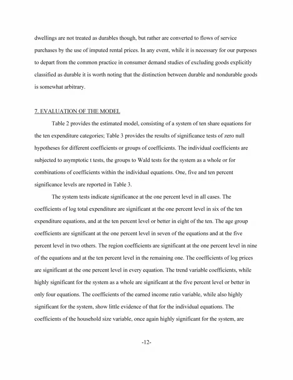
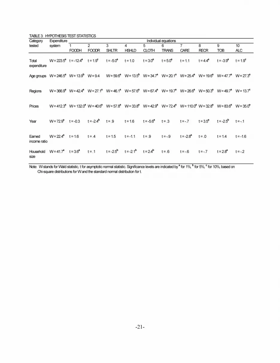
7. EVALUATION OF THE MODEL

Table 2 provides the estimated model, consisting of a system of ten share equations for

the ten expenditure categories; Table 3 provides the results of significance tests of zero null

hypotheses for different coefficients or groups of coefficients. The individual coefficients are

subjected to asymptotic t tests, the groups to Wald tests for the system as a whole or for

combinations of coefficients within the individual equations. One, five and ten percent

significance levels are reported in Table 3.

The system tests indicate significance at the one percent level in all cases. The

coefficients of log total expenditure are significant at the one percent level in six of the ten

expenditure equations, and at the ten percent level or better in eight of the ten. The age group

coefficients are significant at the one percent level in seven of the equations and at the five

percent level in two others. The region coefficients are significant at the one percent level in nine

of the equations and at the ten percent level in the remaining one. The coefficients of log prices

are significant at the one percent level in every equation. The trend variable coefficients, while

highly significant for the system as a whole are significant at the five percent level or better in

only four equations. The coefficients of the earned income ratio variable, while also highly

significant for the system, show little evidence of that for the individual equations. The

coefficients of the household size variable, once again highly significant for the system, are

-13-

significant at the five percent level or better in half of the expenditure equations. Overall, our

assessment is that the model performs rather well.

8. EXPENDITURE ELASTICITIES AT DIFFERENT AGES

We are particularly interested in how income – more precisely, total expenditure –

affects the budget shares for different categories of goods and services at different ages. With that

in mind we derived total expenditure elasticities for the six older age groups on which we are

focusing in this paper, calculated in each case at mean values of all variables to obtain all-

Canada, averages. The elasticities (calculated as ) are reported in Table 4, together1+ βi iaS/

with standard errors calculated by Monte Carlo procedures (since the elasticities are nonlinear

functions of the estimated coefficients of the model; see Krinsky and Robb, 1986).

The sixty elasticities in Table 4 are positive, with only one exception (which can be

discounted since the standard error is considerably greater than the elasticity estimate). The

highest elasticities at every age are those for recreation, transportation, alcohol, clothing, food

from restaurants, and health and personal care, all of which are greater than 1. The lowest ones

are those for food at home, tobacco, and shelter, which are well below 1. The final category,

household furnishing and operation, has an elasticity only slightly higher than 1 at every age. The

relative positions of the categories seem generally to be reasonable in light of prior expectations.

There are no gross reversals as age increases – no switches between “greater than” and

“less than” unity. However there are some obvious patterns of change. Most notable is that food

at home and shelter, which are inelastic, become less so as age increases, while the elastic

categories become more so, a pattern made arithmetically possible by the increasing expenditure

shares of the food at home and shelter categories (see Table 1; given the expenditure elasticity

formula, any change can result only from a change in share). Whether this pattern is a function of

-14-

age, as such, or of declines in total expenditure associated with retirement has yet to be

determined.

9. PRE-RETIREMENT AND POST-RETIREMENT SIMULATIONS

We have simulated the expenditure patterns of households before and after retirement, as

follows. Retirement is assumed to occur at age 65 by setting the earned income ratio variable

(EARNR) to zero at that age. The calculations are for a two-person husband/wife household

living in Ontario; the dummy variables for all other regions are therefore set to zero, and the

household size variable (NMEM) to 2. Also, the trend variable (YEAR) is set to 1992.

Alternative assumptions are made about total household expenditure, or income as we shall call

it here, for convenience. In particular, various simulations were carried out assuming high,

median, and low income levels for a household at ages below 65, where high was taken to be the

3rd quartile level of total expenditure for each of the below-65 age groups in Ontario, as

calculated from the 1992 FAMEX survey data, and low was taken to be the first quartile level.

Borrowing a term from the pension literature, a “replacement rate” (RR) was then set at

alternative levels, depending on the particular simulation, and applied to pre-retirement (real)

income to establish the household’s post-retirement (real) income for the age groups 65-69, 70-

74, and 75 and over. The alternative replacement rates experimented with were 50, 70, and 100

percent. The expenditure patterns were generated by the model for each of the six age groups,

from 50-54 to 75 and over, under all nine combinations of income levels and replacement rates.

Results for five of the combinations are shown in Table 5. The patterns exhibited by the results in

the table are representative of the larger set of simulation results; reporting results for only the

five is for the purpose of conserving space. Also, it should be noted that the intention was not to

mimic actual pension plans, public or private, but simply to indicate in a more or less realistic

-15-

way how changes in income level at retirement might affect a household’s budget allocations.

Incorporation of actual pension plan and other income source details would have required

assumptions about the type of inflation indexing built into private pension plans (and hence rates

of inflation), the assessment of income tax, and other matters, and would have made the

simulation unnecessarily complicated for our purposes.

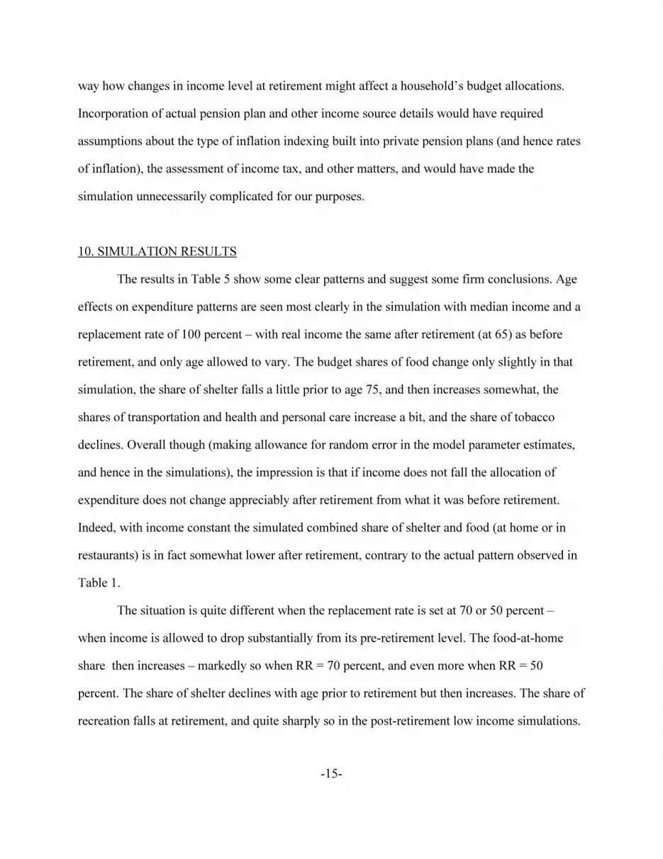
10. SIMULATION RESULTS

The results in Table 5 show some clear patterns and suggest some firm conclusions. Age

effects on expenditure patterns are seen most clearly in the simulation with median income and a

replacement rate of 100 percent – with real income the same after retirement (at 65) as before

retirement, and only age allowed to vary. The budget shares of food change only slightly in that

simulation, the share of shelter falls a little prior to age 75, and then increases somewhat, the

shares of transportation and health and personal care increase a bit, and the share of tobacco

declines. Overall though (making allowance for random error in the model parameter estimates,

and hence in the simulations), the impression is that if income does not fall the allocation of

expenditure does not change appreciably after retirement from what it was before retirement.

Indeed, with income constant the simulated combined share of shelter and food (at home or in

restaurants) is in fact somewhat lower after retirement, contrary to the actual pattern observed in

Table 1.

The situation is quite different when the replacement rate is set at 70 or 50 percent –

when income is allowed to drop substantially from its pre-retirement level. The food-at-home

share then increases – markedly so when RR = 70 percent, and even more when RR = 50

percent. The share of shelter declines with age prior to retirement but then increases. The share of

recreation falls at retirement, and quite sharply so in the post-retirement low income simulations.

-16-

The share of clothing also declines. The most pronounced differences among the simulation

results occur at the oldest ages. Comparing the extremes in the table, for the high income

simulation with RR = 70 percent food at home and shelter combined account for 34.7 percent of

total expenditure in the 50-54 age group, 38.8 percent in the 75 and older group; for the low

income simulation with RR = 50 percent the comparable shares are 45.3 and 57.0.

The overall conclusion would seem to be that age alone does not induce the kinds of

changes in expenditure patterns that one sees in the actual data after age 65, and if anything may

result in some shifts in the opposite direction. On the whole, changes in “tastes” seem to play a

rather minor role; most of the major differences that are observed among the age groups are a

consequence of declines in income after retirement.

11. SUMMARY AND CONCLUSION

We have examined the expenditure patterns of older husband/wife households in larger

urban areas using a model fitted to data grouped by age and region from six FAMEX surveys

carried out in the period 1969-1996. The model, an adapted version of the Deaton/Muellbauer

Almost Ideal Demand System, encompasses all categories of consumer expenditure, including

expenditures on durable goods, and performs well by conventional criteria. Group expenditure

shares averaged over the six surveys show clear patterns of change with advancing age –

especially a rise in the food-at-home and shelter shares – and elasticities calculated from the

model parameters also show clear age-related patterns. We used the model to investigate whether

those patterns are a consequence of age as such, or of lower income levels after retirement, by

simulating household budget allocations for a hypothetical household with full retirement from

the labour force at age 65 and alternative income levels before retirement and alternative income

replacement rates after retirement. The evidence provided by the simulation results indicates that

-17-

changes in budget allocations observed in survey data are most closely related to declines in

income rather than to changes in “tastes” associated with age.

REFERENCES

Deaton, A. S., and Muellbauer, J. (1980), “An Almost Ideal Demand System,” American

Economic Review, 70, 312-326.

Denton, F. T., and Mountain, D. C. (2001), “Income Distribution and

Aggregation/Disaggregation Biases in the Measurement of Consumer Demand Elasticities,”

Economics Letters, 73, 21-28.

Denton, F. T., Mountain, D. C., and Spencer, B. G. (1999), “Age, Trend, and Cohort Effects in a

Macro Model of Canadian Expenditure Patterns,” Journal of Business and Economic Statistics,

17, 430-443.

Denton, F. T., and Spencer, B. G. (2000), “How Well Does the CPI Serve as an Index of Inflation

for Older Age Groups?,” in F. T. Denton, D. A. Fretz, and B. G. Spencer (eds.), Independence

and Economic Security in Old Age, Vancouver: University of British Columbia Press.

Krinsky, L., and Robb, A. L. (1986), “On Approximating the Statistical Properties of

Elasticities,” Review of Economics and Statistics, 68, 715-719.

-18-

TABLE 1: EXPENDITURE SHARES, OLDER HUSBAND/WIFE HOUSEHOLDS IN LARGER URBAN

AREAS, BY AGE GROUP: ALL-CANADA, ALL-SURVEY AVERAGES

Description Symbol 50-54 55-59 60-64 65-69 70-74 75+

Food at home FOODH 16.0 16.5 17.6 18.0 20.7 21.9

Food from restaurants FOODR 4.9 4.8 4.4 4.0 3.6 2.8

Shelter SHLTR 18.2 18.3 19.5 20.5 22.6 27.8

Household furnishing and operation HSHLD 9.7 9.7 9.7 9.9 10.0 10.4

Clothing CLOTH 9.5 8.8 8.3 7.4 6.7 6.1

Transportation TRANS 19.7 19.9 19.2 19.7 17.5 13.9

Health and personal care CARE 5.8 6.0 6.4 6.2 6.5 7.5

Recreation RECR 11.8 11.3 10.3 10.3 8.7 7.0

Tobacco TOB 2.1 2.2 2.0 1.8 1.7 1.2

Alcohol ALC 2.5 2.6 2.5 2.2 2.1 1.5

Total EXCON 100.0 100.0 100.0 100.0 100.0 100.0

Note: The averages are all-Canada percentages based on weighted sample data, averaged over the FAMEX

surveys carried out in 1969, 1978, 1982, 1986, 1992, and 1996.

Age Group

%

Expenditure Category

-19-

TABLE 2: THE ESTIMATED EXPENDITURE SYSTEM

Variable Scaling

name factor 1 2 3 4 5 6 7 8 9 10

FOODH FOODR SHLTR HSHLD CLOTH TRANS CARE RECR TOB ALC

Total Expenditure

LNEXCON 10-1

-1.3304 0.1286 -0.9243 0.0943 0.2292 1.1551 0.0947 0.6182 -0.1523 0.0869

(0.1073) (0.0673) (0.1835) (0.0989) (0.0759) (0.2289) (0.0842) (0.1396) (0.0390) (0.0448)

Age groups

A1 100

1.7221 2.1630 -0.1765 -2.2081 4.9693 -1.6135 0.8267 -5.8140 1.1215 0.0096

(1.0620) (0.9337) (1.6120) (1.4120) (0.9391) (1.7570) (1.1250) (1.5510) (0.3945) (0.5921)

A2 100

1.7234 2.1635 -0.1933 -2.2154 4.9700 -1.5954 0.8266 -5.8147 1.1257 0.0096

(1.0610) (0.9335) (1.6110) (1.4120) (0.9388) (1.7550) (1.1250) (1.5500) (0.3942) (0.5920)

A3 100

1.7233 2.1631 -0.2109 -2.2195 4.9750 -1.5800 0.8265 -5.8148 1.1263 0.0110

(1.0610) (0.9333) (1.6100) (1.4120) (0.9383) (1.7530) (1.1250) (1.5490) (0.3938) (0.5918)

A4 100

1.7247 2.1611 -0.2027 -2.2236 4.9737 -1.5694 0.8161 -5.8114 1.1257 0.0058

(1.0600) (0.9330) (1.6080) (1.4110) (0.9378) (1.7500) (1.1240) (1.5480) (0.3933) (0.5915)

A5 100

1.7335 2.1608 -0.2000 -2.2275 4.9757 -1.5721 0.8160 -5.8162 1.1243 0.0055

(1.0590) (0.9327) (1.6070) (1.4110) (0.9374) (1.7470) (1.1240) (1.5480) (0.3930) (0.5913)

A6 100

1.7256 2.1564 -0.1658 -2.2222 4.9774 -1.5902 0.8247 -5.8225 1.1176 -0.0010

(1.0590) (0.9326) (1.6060) (1.4100) (0.9371) (1.7450) (1.1240) (1.5470) (0.3927) (0.5912)

Regions

R1 10-2

-0.3661 -0.0205 -1.9654 -0.1770 -0.3093 2.0118 1.5312 -0.3507 0.2564 -0.6105

(0.5037) (0.4812) (0.8218) (0.6508) (0.4038) (0.9935) (0.5060) (0.6840) (0.1831) (0.2719)

R2 10-2

1.1459 0.4299 -0.3926 -1.1965 1.3168 -1.0702 1.1883 -1.8952 0.6520 -0.1784

(0.3401) (0.2710) (0.5889) (0.3859) (0.2672) (0.7431) (0.3099) (0.4738) (0.1322) (0.1667)

R4 10-2

-0.5759 0.4706 -3.1846 -0.2656 0.3309 1.4690 1.2719 1.0422 -0.1504 -0.4080

(0.3274) (0.2396) (0.5692) (0.3542) (0.2516) (0.7294) (0.2831) (0.4436) (0.1285) (0.1528)

R5 10-2

-0.2695 0.3431 -1.5032 0.5659 -0.4425 0.5987 1.3056 0.1336 -0.2141 -0.5176

(0.3514) (0.2628) (0.5952) (0.4216) (0.2783) (0.7932) (0.3168) (0.4804) (0.1345) (0.1711)

R1_92 10-2

-0.0189 -0.9138 -1.0032 1.9366 0.1646 -1.1850 -0.6230 1.1088 -0.0188 0.5527

(0.6048) (0.4781) (1.0660) (0.6512) (0.4684) (1.3900) (0.5383) (0.8382) (0.2411) (0.2861)

R1_96 10-2

-0.5139 -0.4267 -0.6668 1.4890 0.7193 -0.4984 0.1253 -0.2427 -0.1174 0.1323

(0.6656) (0.5039) (1.1810) (0.6911) (0.5164) (1.4950) (0.5852) (0.9848) (0.2672) (0.3126)

R4_92 10-2

-0.8199 -0.1625 -0.0890 0.9311 -0.0949 -0.9472 -0.0909 0.6309 0.3594 0.2830

(0.5580) (0.3607) (1.0090) (0.5283) (0.4228) (1.3290) (0.4514) (0.7786) (0.2331) (0.2399)


-20-

TABLE 2: THE ESTIMATED EXPENDITURE SYSTEM (continued)

Variable Scaling

name factor 1 2 3 4 5 6 7 8 9 10


Prices

LNP1 10-1

-1.0091 -0.0893 -1.3997 0.3135 0.4699 1.0611 -0.0745 0.8027 -0.3089 0.2343

(0.2958) (0.2221) (0.2838) (0.3292) (0.1891) (0.2831) (0.2432) (0.2617) (0.0585) (0.1381)

LNP2 10-1

-0.0893 0.6403 -0.2611 -0.1650 -0.6210 -0.2443 0.7708 0.1788 0.0494 -0.2586

(0.2221) (0.3049) (0.2506) (0.3214) (0.1846) (0.2016) (0.2578) (0.2381) (0.0519) (0.1463)

LNP3 10-1

-1.3997 -0.2611 0.1306 0.6485 0.3865 2.0764 -0.9465 -0.7845 0.0752 -0.7793

(0.2838) (0.2506) (0.5406) (0.3356) (0.2286) (0.4275) (0.2951) (0.3861) (0.0917) (0.1521)

LNP4 10-1

0.3135 -0.1650 0.6485 0.5905 -0.1501 -0.2389 -1.3826 0.3035 0.0153 0.0652

(0.3292) (0.3214) (0.3356) (0.6259) (0.2800) (0.3001) (0.3788) (0.3433) (0.0737) (0.2094)

LNP5 10-1

0.4699 -0.6210 0.3865 -0.1501 -0.5712 0.0178 0.8111 -0.3277 0.1236 -0.1389

(0.1891) (0.1846) (0.2286) (0.2800) (0.2221) (0.2096) (0.2202) (0.2403) (0.0505) (0.1216)

LNP6 10-1

1.0611 -0.2443 2.0764 -0.2389 0.0178 -1.3376 0.5608 -1.8145 0.1472 -0.2279

(0.2831) (0.2016) (0.4275) (0.3001) (0.2096) (0.6542) (0.2577) (0.3775) (0.0931) (0.1388)LNP7 10

-1-0.0745 0.7708 -0.9465 -1.3826 0.8111 0.5608 -1.0015 0.7577 -0.0106 0.5152

(0.2432) (0.2578) (0.2951) (0.3788) (0.2202) (0.2577) (0.4345) (0.2895) (0.0641) (0.1918)

LNP8 10-1

0.8027 0.1788 -0.7845 0.3035 -0.3277 -1.8145 0.7577 1.0186 -0.1787 0.0441

(0.2617) (0.2381) (0.3861) (0.3433) (0.2403) (0.3775) (0.2895) (0.5109) (0.0837) (0.1549)

LNP9 10-1

-0.3089 0.0494 0.0752 0.0153 0.1236 0.1472 -0.0106 -0.1787 0.1095 -0.0219

(0.0585) (0.0519) (0.0917) (0.0737) (0.0505) (0.0931) (0.0641) (0.0837) (0.0255) (0.0374)

LNP10 10-1

0.2343 -0.2586 0.0746 0.0652 -0.1389 -0.2279 0.5152 0.0441 -0.0219 -0.2861

(0.1381) (0.1463) (0.1521) (0.2094) (0.1216) (0.1388) (0.1918) (0.1549) (0.0374) (0.1391)

Year

YEAR 10-3

-0.1392 -1.1313 0.7229 1.1382 -2.6036 0.2919 -0.4217 2.6663 -0.4885 -0.0350

(0.5245) (0.4674) (0.7995) (0.7052) (0.4678) (0.8473) (0.5627) (0.7726) (0.1935) (0.2957)

Earned income ratio

EARNR 10-2

2.1360 0.3815 3.8505 -1.3846 0.8949 -2.8804 -3.0134 0.0922 0.8192 -0.8960

(1.3640) (0.8613) (2.5100) (1.2650) (1.0190) (3.3220) (1.0760) (1.9020) (0.5720) (0.5712)

Household size

NMEM 10-2

2.8457 0.0381 -3.5781 -1.6001 1.4411 1.1768 -0.3802 -0.8051 0.9207 -0.0588

(0.8013) (0.5109) (1.4420) (0.7480) (0.5979) (1.8950) (0.6395) (1.1040) (0.3284) (0.3385)

Note: Figures in parentheses are standard errors. The coefficients in any row (and the corresponding standard errors) should be multiplied

by the scaling factor for that row. LN in a variable symbol indicates logarithm.


-21-

TABLE 3: HYPOTHESIS TEST STATISTICS

Category Expenditure

tested system 1 2 3 4 5 6 7 8 9 10


Total W = 223.5a

t = -12.4a

t = 1.9c

t = -5.0a

t = 1.0 t = 3.0a

t = 5.0a

t = 1.1 t = 4.4a

t = -3.9a

t = 1.9c

expenditure

Age groups W = 246.5a

W = 13.9b

W = 9.4 W = 59.6a

W = 13.5b

W = 34.7a

W = 20.1a

W = 25.4a

W = 19.6a

W = 47.7a

W = 27.3a

Regions W = 366.9a

W = 42.4a

W = 27.1a

W = 46.1a

W = 57.6a

W = 67.4a

W = 19.7a

W = 26.6a

W = 50.3a

W = 49.7a

W = 13.7c

Prices W = 412.3a

W = 132.0a

W = 40.6a

W = 57.8a

W = 33.8a

W = 42.9a

W = 72.4a

W = 110.0a

W = 32.8a

W = 83.6a

W = 35.0a

Year W = 72.9a

t = -0.3 t = -2.4b

t = .9 t = 1.6 t = -5.6a

t = .3 t = -.7 t = 3.5a

t = -2.5b

t = -.1

Earned W = 22.4a

t = 1.6 t = .4 t = 1.5 t = -1.1 t = .9 t = -.9 t = -2.8a

t = .0 t = 1.4 t = -1.6

income ratio

Household W = 41.7a

t = 3.6a

t = .1 t = -2.5b

t = -2.1b

t = 2.4b

t = .6 t = -.6 t = -.7 t = 2.8a

t = -.2

size

Note: W stands for Wald statistic, t for asymptotic normal statistic. Significance levels are indicated by a for 1%,

b for 5%,

c for 10%, based on

Chi-square distributions for W and the standard normal distribution for t.

Individual equations

-22-

TABLE 4: EXPENDITURE ELASTICITIES, OLDER HUSBAND/WIFE HOUSEHOLDS IN LARGER URBAN AREAS, BY AGE GROUP:

ALL-CANADA, ALL-SURVEY AVERAGES

Age

group 1 2 3 4 5 6 7 8 9 10


Expenditure elasticities

50-54 0.117 1.260 0.497 1.093 1.259 1.566 1.169 1.499 0.237 1.384

(0.071) (0.149) (0.122) (0.103) (0.102) (0.167) (0.161) (0.144) (0.309) (0.212)

55-59 0.135 1.267 0.508 1.094 1.285 1.558 1.161 1.517 0.296 1.386

(0.070) (0.153) (0.119) (0.104) (0.113) (0.164) (0.154) (0.149) (0.284) (0.216)

60-64 0.195 1.289 0.521 1.093 1.305 1.572 1.149 1.560 0.263 1.361

(0.064) (0.166) (0.116) (0.102) (0.121) (0.168) (0.143) (0.162) (0.296) (0.200)

65-69 0.219 1.322 0.545 1.092 1.344 1.555 1.153 1.573 0.155 1.416

(0.064) (0.184) (0.111) (0.101) (0.136) (0.162) (0.145) (0.165) (0.346) (0.230)

70-74 0.322 1.352 0.583 1.093 1.379 1.616 1.143 1.665 0.093 1.425

(0.055) (0.201) (0.101) (0.102) (0.149) (0.180) (0.137) (0.190) (0.371) (0.234)

75+ 0.365 1.438 0.663 1.088 1.411 1.781 1.125 1.824 -0.306 1.670

(0.052) (0.250) (0.082) (0.096) (0.161) (0.228) (0.119) (0.235) (0.560) (0.370)

Note: The elasticities are evaluated for each age group at the group's values of ln x, ln P*, etc. Figures in parentheses are standard errors.


-23-

TABLE 5: SIMULATED EXPENDITURE PATTERNS,OLDER HUSBAND/WIFE HOUSEHOLDS RETIRING

AT 65 WITH ALTERNATIVE INCOME LEVELS AND REPLACEMENT RATES: ONTARIO, 1992

Income Total

characteristics expenditure 1 2 3 4 5 6 7 8 9 10

and age group (1992 $) FOODH FOODR SHLTR HSHLD CLOTH TRANS CARE RECR TOB ALC

High income, RR = 70%

Ages 50-54 42,051 10.4 5.1 24.3 11.5 6.4 19.5 5.3 14.0 1.2 2.3

Ages 55-59 42,051 10.6 5.1 22.6 10.8 6.5 21.3 5.3 13.9 1.6 2.3

Ages 60-64 42,051 10.6 5.1 20.8 10.4 7.0 22.9 5.3 13.9 1.7 2.5

Ages 65-69 29,436 13.5 4.1 21.5 10.9 5.2 22.4 6.6 12.0 1.4 2.4

Ages 70-74 29,436 14.4 4.0 21.7 10.5 5.4 22.1 6.6 11.5 1.3 2.4

Ages 75+ 29,436 13.6 3.6 25.2 11.0 5.6 20.3 7.5 10.9 0.6 1.7

Median income, RR = 100%

Ages 50-54 34,329 13.1 4.8 26.1 11.3 5.9 17.2 5.1 12.8 1.5 2.1

Ages 55-59 34,329 13.3 4.8 24.5 10.6 6.0 19.0 5.1 12.7 1.9 2.1

Ages 60-64 34,329 13.3 4.8 22.7 10.2 6.5 20.5 5.1 12.7 2.0 2.3

Ages 65-69 34,329 11.5 4.3 20.0 11.0 5.6 24.2 6.7 12.9 1.2 2.6

Ages 70-74 34,329 12.4 4.2 20.3 10.6 5.8 23.9 6.7 12.5 1.1 2.5

Ages 75+ 34,329 11.6 3.8 23.7 11.2 5.9 22.1 7.6 11.8 0.4 1.9


Ages 50-54 34,329 13.1 4.8 26.1 11.3 5.9 17.2 5.1 12.8 1.5 2.1

Ages 55-59 34,329 13.3 4.8 24.5 10.6 6.0 19.0 5.1 12.7 1.9 2.1

Ages 60-64 34,329 13.3 4.8 22.7 10.2 6.5 20.5 5.1 12.7 2.0 2.3

Ages 65-69 24,030 16.2 3.8 23.3 10.7 4.7 20.1 6.4 10.7 1.7 2.3

Ages 70-74 24,030 17.1 3.8 23.6 10.3 4.9 19.8 6.4 10.3 1.6 2.2

Ages 75+ 24,030 16.3 3.3 27.0 10.8 5.1 18.0 7.3 9.6 0.9 1.6


Ages 50-54 34,329 13.1 4.8 26.1 11.3 5.9 17.2 5.1 12.8 1.5 2.1

Ages 55-59 34,329 13.3 4.8 24.5 10.6 6.0 19.0 5.1 12.7 1.9 2.1

Ages 60-64 34,329 13.3 4.8 22.7 10.2 6.5 20.5 5.1 12.7 2.0 2.3

Ages 65-69 17,164 20.7 3.4 26.4 10.4 4.0 16.2 6.1 8.7 2.3 2.0

Ages 70-74 17,164 21.6 3.3 26.7 10.0 4.2 15.9 6.1 8.2 2.1 1.9

Ages 75+ 17,164 20.8 2.9 30.1 10.5 4.3 14.1 6.9 7.5 1.4 1.3

Low income, RR = 50%

Ages 50-54 26,276 16.7 4.5 28.6 11.1 5.3 14.1 4.8 11.1 1.9 1.9

Ages 55-59 26,276 16.8 4.5 26.9 10.3 5.4 15.9 4.8 11.0 2.3 1.9

Ages 60-64 26,276 16.8 4.5 25.2 9.9 5.9 17.4 4.8 11.0 2.4 2.0

Ages 65-69 13,138 24.3 3.0 28.9 10.1 3.4 13.1 5.8 7.0 2.7 1.7

Ages 70-74 13,138 25.1 3.0 29.2 9.7 3.6 12.8 5.8 6.5 2.5 1.7

Ages 75+ 13,138 24.4 2.6 32.6 10.3 3.7 11.0 6.7 5.9 1.9 1.0

Note: RR stands for income replacement rate at retirement. High income is defined as the 3rd quartile in

Ontario in 1992, median income as the 2nd quartile, and low income as the 1st quartile.

Expenditure categories (% shares)

QSEP RESEARCH REPORTS - Recent Releases

Number Title Author(s)

-24-

No. 351: Describing Disability among High and Low Income Status

Older Adults in Canada

P. Raina

M. Wong

L.W. Chambers

M. Denton

A. Gafni

No. 352: Some Demographic Consequences of Revising the

Definition of #Old& to Reflect Future Changes in Life Table

Probabilities

F.T. Denton

B.G. Spencer

No. 353: The Correlation Between Husband’s and Wife’s

Education: Canada, 1971-1996

L. Magee

J. Burbidge

L. Robb

No. 354: The Effect of Marginal Tax Rates on Taxable Income: A

Panel Study of the 1988 Tax Flattening in Canada

M.-A. Sillamaa

M.R. Veall

No. 355: Population Change and the Requirements for Physicians:

The Case of Ontario

F.T. Denton

A. Gafni

B.G. Spencer

No. 356: 2 ½ Proposals to Save Social Security D. Fretz

M.R. Veall

No. 357: The Consequences of Caregiving: Does Employment Make

A Difference?

C.L. Kemp

C.J. Rosenthal

No. 358: Exploring the Effects of Population Change on the Costs

of Physician Services

F.T. Denton

A. Gafni

B.G. Spencer

No. 359: Reflexive Planning for Later Life: A Conceptual Model

and Evidence from Canada

M.A. Denton

S. French

A. Gafni

A. Joshi

C. Rosenthal

S. Webb

No. 360: Time Series Properties and Stochastic Forecasts: Some

Econometrics of Mortality from The Canadian Laboratory

F.T. Denton

C.H. Feaver

B.G. Spencer

No. 361: Linear Public Goods Experiments: A Meta-Analysis J. Zelmer



-25-

No. 362: The Timing and Duration of Women's Life Course Events:

A Study of Mothers With At Least Two Children

K.M. Kobayashi

A. Martin-Matthews

C.J. Rosenthal

S. Matthews

No. 363: Age-Gapped and Age-Condensed Lineages: Patterns of

Intergenerational Age Structure among Canadian Families

A. Martin-Matthews

K.M. Kobayashi

C.J. Rosenthal

S.H. Matthews

No. 364: The Education Premium in Canada and the United States J.B. Burbidge

L. Magee

A.L. Robb

No. 365: Student Enrolment and Faculty Recruitment in Ontario:

The Double Cohort, the Baby Boom Echo, and the Aging

of University Faculty

B.G. Spencer

No. 366: The Economic Well-Being of Older Women Who Become

Divorced or Separated in Mid and Later Life

S. Davies

M. Denton

No. 367: Alternative Pasts, Possible Futures: A “What If” Study of

the Effects of Fertility on the Canadian Population and

Labour Force

F.T. Denton

C.H. Feaver

B.G. Spencer

No. 368: Baby-Boom Aging and Average Living Standards W. Scarth

M. Souare

No. 369: The Impact of Reference Pricing of Cardiovascular Drugs

on Health Care Costs and Health Outcomes: Evidence

from British Columbia – Volume I: Summary

P.V. Grootendorst

L.R. Dolovich

A.M. Holbrooke

A.R. Levy

B.J. O'Brien



from British Columbia – Volume II: Technical Report

P.V. Grootendorst

L.R. Dolovich

A.M. Holbrooke

A.R. Levy

B.J. O'Brien



from British Columbia – Volume III: ACE and CCB

Literature Review

L.R. Dolovich

A.M. Holbrook

M. Woodruff



-26-

No. 372: Do Drug Plans Matter? Effects of Drug Plan Eligibility on

Drug Use Among the Elderly, Social Assistance Recipients

and the General Population

P. Grootendorst

M. Levine

No. 373: Student Enrolment and Faculty Recruitment in Ontario:

The Double Cohort, the Baby Boom Echo, and the Aging

of University Faculty

B.G. Spencer

No. 374: Aggregation Effects on Price and Expenditure Elasticities

in a Quadratic Almost Ideal Demand System

F.T. Denton

D.C. Mountain

No. 375: Age, Retirement and Expenditure Patterns: An

Econometric Study of Older Canadian Households

F.T. Denton

D.C. Mountain

B.G. Spencer

Documents

AGE, RETIREMENT AND EXPENDITURE PATTERNS: AN ECONOMETRIC STUDY OF