ARTICLE

Received 11 Apr 2014 | Accepted 21 Oct 2014 | Published 26 Nov 2014

Afforestation or intense pasturing improve theecological and economic value of abandonedtropical farmlandsThomas Knoke1, Jorg Bendix2, Perdita Pohle3, Ute Hamer4,w, Patrick Hildebrandt1, Kristin Roos5, Andres Gerique3,

Marıa L. Sandoval6, Lutz Breuer7, Alexander Tischer4, Brenner Silva2, Baltazar Calvas1, Nikolay Aguirre8,

Luz M. Castro9, David Windhorst7, Michael Weber1, Bernd Stimm1, Sven Gunter10,w, Ximena Palomeque1,

Julio Mora1, Reinhard Mosandl1 & Erwin Beck5

Increasing demands for livelihood resources in tropical rural areas have led to progressive

clearing of biodiverse natural forests. Restoration of abandoned farmlands could counter

this process. However, as aims and modes of restoration differ in their ecological and

socio-economic value, the assessment of achievable ecosystem functions and benefits

requires holistic investigation. Here we combine the results from multidisciplinary research

for a unique assessment based on a normalization of 23 ecological, economic and social

indicators for four restoration options in the tropical Andes of Ecuador. A comparison of the

outcomes among afforestation with native alder or exotic pine, pasture restoration with either

low-input or intense management and the abandoned status quo shows that both variants of

afforestation and intense pasture use improve the ecological value, but low-input pasture

does not. Economic indicators favour either afforestation or intense pasturing. Both Mestizo

and indigenous Saraguro settlers are more inclined to opt for afforestation.

DOI: 10.1038/ncomms6612 OPEN

1 TUM School of Life Sciences Weihenstephan, Technische Universitat Munchen, 85354 Freising, Germany. 2 Laboratory for Climatology and Remote Sensing(LCRS), Faculty of Geography, University of Marburg, 35032 Marburg, Germany. 3 Institute of Geography, University of Erlangen-Nurnberg, 91058 Erlangen,Germany. 4 Institute of Soil Science and Site Ecology, Dresden University of Technology, 01737 Tharandt, Germany. 5 Department of Plant Physiology andBayreuth Centre of Ecology and Environmental Research, University of Bayreuth, 95440 Bayreuth, Germany. 6 Departamento de Desarrollo Ambiente yterritorio, Facultad Latinoamericana de Ciencias Sociales, FLACSO, 170516 Quito, Ecuador. 7 Institute for Landscape Ecology and Resources Management,Justus Liebig University Giessen, 35392 Giessen, Germany. 8 Biodiversity, Forestry and Ecosystem Services Research Program, National University of Loja,110101 Loja, Ecuador. 9 Departamento de Economıa, Universidad Tecnica Particular de Loja, 1101608 Loja, Ecuador. 10 Tropical Agricultural Research and HigherEducation Center (CATIE), 7170 Turrialba-Cartago, Costa Rica. w Present address: Institute of Landscape Ecology, University of Muenster, 48149 Munster,Germany (U.H.) Thunen-Institut, 21031 Hamburg, Germany (S.G.). Correspondence and requests for materials should be addressed to T.K. (email:knoke@forst.wzw.tum.de).

NATURE COMMUNICATIONS | 5:5612 | DOI: 10.1038/ncomms6612 | www.nature.com/naturecommunications 1

& 2014 Macmillan Publishers Limited. All rights reserved.

Decreasing agricultural yields and increasing national andglobal competition1,2 force farmers to abandon lessproductive lands and either clear more pristine forest

for agriculture or give up agriculture as the basis of theirlivelihoods. Reclaiming abandoned areas to resume production israrely considered a worthwhile alternative. Field et al.3 estimatedthat 386 M ha of abandoned lands worldwide have the potentialfor renewed productive use.

Re-utilization could not only mitigate the increasing pressureson natural forest, but could also help to alleviate poverty byimproving food security4, to promote rural socio-economicdevelopment5 and to lower rural outmigration. Sustainabilityresearch must, therefore, investigate strategies to recoverabandoned lands6.

Existing approaches to the problem of restoration have largelybeen focused on afforestation attempts and either theirecological7, economic8 or social9 consequences. A more holistic,but thus far unrealized, ideal of research into the benefits humansreceive from ecosystems should provide biophysically realisticecosystem data and models, consider local trade-offs, recognizeoff-site effects and involve stakeholders10. Moreover, to promotesustainable future land use, not only afforestation but alsorestoration of agricultural potential should be considered.Consequently, scientifically responsible decision supportrequires multidisciplinary long-term research that supportsreliable parameterization of customized models.

Although benefit-specific ecosystem services are generallynarrowly defined as components of nature that are directlyenjoyed, consumed or used as final products and services11, weuse a broader approach to assess the capacity of natural processesand components of restoration options to provide goods andservices12. Our ecological indicators thus quantify ecosystemfunctions. Following the classification by Boyd and Banzhaf11,our socio-economic indicators are estimates of the benefitsfarmers may obtain from each restoration option.

In the tropical Andes of southern Ecuador, clearing of naturalforest commonly follows the abandonment of pastures and thusrepresents a widespread example of unsustainable land use13,14.This practice occurs mostly in tropical mountain regionsbeginning at 1,500 m altitude and continuing up to the treeline15–17, in Latin America and also elsewhere18,19. In our studyarea, abandoned pastures have already grown to 35% of the totalpasture area20. One major reason for this adverse development isthe invasion of weeds—mainly tropical bracken fern, which isresistant to burning—the most common local weed controltool21. The use of fire begins with the clearing of the natural forestand is regularly applied thereafter for weed control and pasturerejuvenation. In this topographically diverse landscape withhighly fragmented vegetation, productive alternatives to leavingareas abandoned are of utmost ecological and socio-economicimportance22. This applies particularly to southern Ecuadorwhere the native mountain forests contribute significantly to the

outstanding biodiversity23 (Supplementary Methods). In thepresent work, we evaluate four different options forreintegrating abandoned pastures into the production process.The results of experiments—some running as long as 15 years—show that both afforestation13 and restoration of pasture24

(‘repasturization’) are feasible alternatives to leaving landabandoned. However, these results also suggest that largefinancial inputs as compared with the business-as-usual (BAU)option—pasturing after clearing of natural forest—are necessaryto establish the restoration options.

The use of appropriate indicators is pivotal to answeringpolicy-relevant questions concerning the potential benefits thatpeople may obtain from ecosystems25. The establishment ofstandardized methods allows comparisons of ecosystem functionsand benefits if they are adjusted for location and to addressspecific problems. However, the integration of multiple functionsand benefits into a general assessment is still problematic and arerelatively uncommon in the literature25. Our novel evaluationapproach to quantifying and assessing the ecosystem functionsand benefits of different land-use options is an attempt to solvethese problems. It uses normalized indicators to make variousecosystem functions and benefits comparable, which, in thisstudy, proves itself to be a robust method even under rigoroussensitivity assessments. We show that averaged ecological andsocio-economic indicators are highly positively correlated.Afforestation ranks highest both from the ecological and thesocio-economic points of view, followed by repasturization withsubsequent intense pasturing. However, the options for landrestoration provide relatively low short-term socio-economicbenefits for farmers when compared with the BAU land use(pasturing after forest clearing). Because of this, to successfullypromote restoration options as a way to relieve the pressure onbiodiverse natural forests, a compensation amount of up to US$180 ha� 1 per year may be necessary.

ResultsAssessing ecosystem functions and benefits. We will first pre-sent our approach for assessing multiple ecosystem functions andbenefits of five land-use options (Table 1). Next, we justify theselected indicators and briefly illustrate the process of assessingthe various restoration options using data from our study area.Each indictor subsection concludes with highlighting the resultsof general importance for that indicator.

We use 23 indicators to characterize four key elements of‘Ecological Functions’ and four key elements of ‘Socio-economicBenefits’ (Table 2), to thoroughly assess the potential ecosystemfunctions and benefits provided by the land-use optionsinvestigated. The indicators include supporting (biomass produc-tion and soil quality) and regulating functions (carbon, climateand hydrology), as well as provisioning (timber and food) andsocial benefits (acceptance by the local people), and are meant to

Table 1 | Characterization of the land-use options investigated.

Land-use option Land preparation Establishment Management

Abandoned pastures: leaving areas abandoned None None NoneAlnus: afforestation with native Alnus acuminataPinus: afforestation with exotic Pinus patula

Initial removal of weeds(bracken)

1,111 Trees perhectare

Weed control in years 1 and 2, 2 thinningcampaigns (years 12 and 16)

Low-input pastures: repasturization with low-inputmanagement after mechanical weed control

1 Year with 4 recurrentcuttings of bracken

32,400 Grassplantlets perhectare

1 Weed control/year2 Grazing rounds/year

Intense pastures: repasturization with intensemanagement after chemical weed control

9 Months with 3 recurrentherbicide applications

As above 3 Grazing rounds/year3 Fertilization campaigns/year

ARTICLE NATURE COMMUNICATIONS | DOI: 10.1038/ncomms6612

2 NATURE COMMUNICATIONS | 5:5612 | DOI: 10.1038/ncomms6612 | www.nature.com/naturecommunications

& 2014 Macmillan Publishers Limited. All rights reserved.

represent a comprehensive set of indicators of the potentialcapacity for the various restoration options to generate benefitsfrom ecosystems26.

Social acceptance serves here as an indicator of the culturalbenefit, for example, the compatibility with traditional liveli-hoods, as well as their contribution to landscape aesthetics orpreserving cultural heritage. Although people often consider bothprovisioning and regulating functions when expressing theirpreferences, they also tend to include intangible values of landuse, which are largely determined by tradition, experience andpersonal preference. However, as intangible cultural values areimpossible to measure in ecological units, social acceptance canbe used as a meaningful proxy for cultural ecosystem benefits,which are often ignored in existing approaches to assessingecosystem services27.

We normalized every indicator by considering the relativeposition of each value in the range between the real minimum(referred to as 0%) and real maximum values (100%) (‘min–maxnormalization’) to obtain a unitary performance index, Pi. Theminimum is considered to be the least and the maximum themost desirable value. Other approaches have used a hypotheticalindicator value of zero as the minimum28,29, although zero israrely included in the set of possible results. For example, asplants always store carbon, assigning a value of zero carbon toany kind of vegetation is not realistic. Moreover, our min–maxnormalization allows us to use indicators for which negativevalues are possible (for example, economic indicators). Tocombine indicators into a higher-ranked category—the keyelement index Pk—we averaged the Pi values. We then formedthe ecological and socio-economic index value of each land-useoption, WPo, by calculating the average of its Pk indices. Weapplied the ‘more is better’ principle for most indicators.However, for ‘overland flow’ and ‘payback period’, the ‘less isbetter’ principle was used. This means that applying our schemerequires some local experience to form a meaningful assessmentof each indicator.

Finally, we use sensitivity scenarios to test the robustness of ourassessment approach. In one scenario, we account for the size ofthe differences by weighting the indicator values by their relativerange of variation (objective weighting), because through ournormalization, even small differences in indicator values are

scaled between 0 and 100%. In another scenario, we test theimpact of uncertainty by using both pessimistic and optimisticestimates (based on 95% confidence limits). After the pessimisticand optimistic indicators are normalized to create performanceindices, their range is used to evaluate the robustness of ourassessment system. The results of the uncertainty analyses aredescribed in ‘Synopsis and sensitivity of indices’.

Ecological indicators. Carbon relationships characterize theuptake and accumulation of carbon—a primary ecosystemfunction that is a pivotal part of provisioning (for example, fodderfor cattle or timber), regulating (storage of atmospheric carbon)and life supporting (organic matter to improve soil quality)ecosystem services. We use three indicators for this assessment:biomass production, whole plant-cover carbon accumulation andsoil organic carbon (Table 3 and Supplementary Tables 1 and 2).Carbon relationships for abandoned pastures assume equilibriumbetween production and death of bracken leaves and rhizomes30.For the tree plantations (Alnus or Pinus, see SupplementaryMethods and Supplementary Tables 3 and 4), average values forbiomass production over a 20-year period are computed, whichaccount for losses from thinning and mortality.

Annual biomass production of bracken fern on abandonedpastures is the second highest among the options investigated.Thus, owing to the combination of the carbon present in thisbiomass and the organic carbon of the soil, abandoned areas rankintermediate in terms of total C-sequestration. The annual (20-year average) biomass production in the tree plantations isrelatively low (see Supplementary Methods and SupplementaryFig. 1 for discussion). The corresponding average total carbonstocks in planta are slightly lower than those in the abandonedareas. However, when carbon in the accumulating litter layer isconsidered (Supplementary Table 3), total carbon sequestrationin the tree plantations is in the same range as that calculated forabandoned pastures (Table 3). In both pasture types, Setaria isplanted after bracken control. A nearly homogeneous grasscanopy has been achieved after 1.5 years. In the ‘low-input’variant, nutrient shortage strongly limits growth, even beforeweeds come up. After two rounds of (simulated) grazing,equilibrium biomass production is established with an above-

Table 2 | Categories, key elements and associated indicators, data sources.

Categories Key elements Indicators Data source

Ecologicalfunctions

Carbonrelationships

Biomass production, carbon in planta,soil organic carbon

Afforestation: statistical regression models, parametersestimated from field data; pastures and abandoned pastures:field data plus process-based model for annual below-groundbiomass production

Climate regulation Evapotranspiration, momentum flux Process-based models, most model parameters estimated fromfield data

Hydrologicalregulation

Surface flow, groundwater recharge, area-specific discharge

Soil quality pH, soil organic carbon, base saturation, carbonin microbial biomass, C-mineralization,N-mineralization, PO4-P

Field data

Socio-economicbenefits

Net present valuePayback period

5% and 8% discount rates Evaluation of timber and cattle products with market prices andcosts (obtained from household surveys supplemented by data ofthe Food and Agriculture Organization of the United Nations)

SaraguropreferenceMestizopreference foreach land-useoption

Saraguros asked with and without theoption of subsidiesMestizos asked with and without theoption of subsidies

Standardized questionnaires

NATURE COMMUNICATIONS | DOI: 10.1038/ncomms6612 ARTICLE

NATURE COMMUNICATIONS | 5:5612 | DOI: 10.1038/ncomms6612 | www.nature.com/naturecommunications 3

& 2014 Macmillan Publishers Limited. All rights reserved.

to below-ground average ratio of 0.05. Owing to the very low Ccontent in the standing above-ground biomass, C-sequestrationpotential in low-input pasture is the lowest of all the land-useoptions investigated. In contrast, fertilization of pastures in thehigh-input alternative results in an almost two-fold (over low-input pasture) and in some cases even a six-fold increase (overtree plantations) in above-ground biomass production. All of thegrass leaf biomass except the basal 20 cm is removed in each ofthe three (simulated) grazing rounds.

The annual biomass production differs among the fiveecosystem alternatives by a factor of 6.5 and plant-bound carbonby a factor of 2.6. The amount of carbon sequestered by each issimilar (DB20%) due to the soil-bound fraction, which is high inall options. Because of high annual biomass production, theindices for ‘Carbon relationships’ are high for intense pasturing,moderate for both abandoned land and Pinus plantation, and lowfor low-input pasture and Alnus plantation.

Climate regulation is another important function of ecosys-tems, and the type and structure of the ecosystem directlyinfluences the nature of surface–atmosphere exchanges. Thus,large-scale land-use changes elicit changes in both microclimateand the climate regulation function of an ecosystem31. The maindrivers of this are changes in energy balance, surface roughnessand evapotranspiration (ET), all of which link atmospheric tohydrological functions32. Here we calculate water andmomentum fluxes (turbulence production, an important land–atmosphere feedback parameter) for a 20-year period using thecoupled SoBraCo—catchment modelling framework (CMF)33

(see Methods and Supplementary Methods), to derive indicatorsfor the intensity of surface–atmosphere exchanges.

The main components of microclimate, ET and turbulenceproduction (M-flux, or the sum of zonal and meridionalmomentum fluxes) differ among the various land-use options(Table 4).

We find ET, the majority of which is plant transpiration,to be similar in the two types of tree plantation and significantlyhigher here than in the abandoned area. Periodic removal ofbiomass from the active pasture options leads to a decrease intranspiration, resulting in an overall ET lower than that in thetree plantations, but still higher than that of the abandonedpasture. Turbulence production is very high in tree plantations,whereas re-established pasture performs similarly to abandonedpasture.

Altogether, the tree plantations mimic the climate regulationfunction of a natural forest better than the options without trees.Afforestation with the broadleaf Alnus is even more effective inthis regard than with Pinus.

Hydrological regulation performances of the various restora-tion options are crucial elements in assessing their potential formitigating the adverse effects of water (such as erosion) but alsoin controlling the quantitative supply of water. We simulatebelow-ground water cycles using the well tested CMF34 (seeMethods, Supplementary Methods and Supplementary Tables 5and 6). Similar to the ambiguous effects that ecohydraulicprocesses can have on hydrological ecosystem services25, theinvestigated indicators might have a positive or a negative effect.For example, discharge (water volume) is a resource forhydropower35, and water that quickly leaves a system viaoverland flow and seepage prevents soils from becomingwaterlogged. Therefore, rapid movement of water through thesystem can be considered positive. In contrast, seepage flow canalso leach nutrients and overland flow can cause erosion, resultingin a negative effect from this indicator. To make our assessmentmore easily transferrable to sites with different objectives (highdischarge or minimizing leaching/erosion), we calculate twoseparate indicators. The first indicator (Pk1) combines a positiveeffect (discharge) and a negative effect (overland flow), while thesecond (Pk2) considers both factors to be negative (Table 5).

Table 3 | Rating of the key element ‘Carbon relationships’ (indicator value±s.e.m.)*.

Land-use option Annual biomass production Carbon stocks Carbon relationships

(Mg ha� 1 per year) Pi Carbon in plantaw Soil organic carbonz Total carbon Pk

(Mg ha� 1) Pi (Mg ha� 1) Pi (Mg ha� 1) Pi

Abandoned pastures 31.8±4.8 57 33.0±2.9 100 87.3±5.3 0 120.3±6.9 85 52Alnus 7.7±0.6 0 24.5±2.3 58 91.7±6.8 49 116.2±7.2 63 36Pinus 8.9±0.4 3 29.6±1.4 83 93.5±4.6 69 123.1±4.8 100 52Low-input pastures 26.5±4.4 44 12.5±1.2 0 91.8±4.9 50 104.4±6.5 0 32Intense pastures 50.0±2.3 100 25.8±3.4 65 96.3±5.1 100 122.2±5.5 95 88

*Estimates for tree plantations from statistical-based regression models parameterized with field data; for pastures, all data from field measurements except annual below-ground biomass production,which was estimated by the process-based model SoBraCo33, with parameters derived from field data.wAveraged over a 20-year period.zOrganic layer and mineral top soil (0–20 cm depth).

Table 4 | Rating of the key element ‘Climate regulation’ (indicator value±s.e.m.)*.

Land-use option ET MF Pk

(mm) Pi (kg m� 1 s� 2) Pi

Abandoned pastures 928±3.80 0 0.018±0.00028 0 0Alnus 1,597±4.10 100 0.285±0.01560 97 99Pinus 1,410±1.12 72 0.294±0.00038 100 86Low-input pastures 1,186±5.81 39 0.023±0.00003 2 21Intense pastures 1,167±5.10 36 0.026±0.00040 3 20

CMF, catchment modelling framework; ET, evapotranspiration; MF, momentum flux.*ET and MF are simulated with the coupled SoBraCo-CMF model33. The model is forced with data of a micrometeorological station33. Optical and physiological as well as soil model parameters arederived from field observations presented in Bendix et al.56, Silva et al.33 and from literature (for more details, refer to Supplementary Table 12 and Table 2 in Silva et al.33).

ARTICLE NATURE COMMUNICATIONS | DOI: 10.1038/ncomms6612

4 NATURE COMMUNICATIONS | 5:5612 | DOI: 10.1038/ncomms6612 | www.nature.com/naturecommunications

& 2014 Macmillan Publishers Limited. All rights reserved.

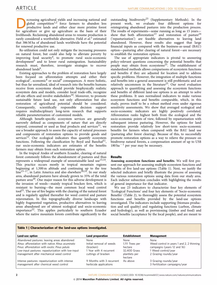
Annual interception is low for pasture but high for abandonedpasture and Pinus. Water returned to the atmosphere throughET dominates the water relations in the tree plantations,while discharge driven by groundwater recharge is the mainhydrological component of both active and abandoned pasture.The amount of water infiltrating the soil is offset by planttranspiration, and thus its total share is lower in the treeplantations. The fraction of overland flow is dependent onsteepness of slope, level of soil compaction and vegetation cover.Steepness of slope remains constant in the model, but the othertwo factors are allowed to vary. The results for overland flowrange between 2 and 4% of precipitation, thus representing only aminor fraction.

If a large amount of discharge is desired (Pk1), Pinus proves tobe the best option, followed by abandoned pasture, Alnus, and thetwo active pasture options. In the second case (Pk2), the ecologicalindex value of the tree plantations increases considerably. Thus,ranking can also depend on location. On steep slopes with soilswith high levels of conductivity water retention is more desirable,whereas on flatter ground with compacted soil discharge is moreimportant.

Soil quality is essential in maintaining the long-termproductivity, and thus the sustainability, of the provisioningservices of our restoration options. The chosen indicators(Table 6 and Supplementary Table 7) are well known to vary inresponse to land-use change36, to support plant productivity37

and to contribute to soil biodiversity38.The dominant soil types in the research area are Haplic or Folic

Cambisols, and Mollic Cambic Umbrisols36. Burning the originalforest fertilizes the mineral top soil, raises its pH and results insoils with higher contents of both organic carbon and totalnitrogen, but extremely low phosphate availability39. The burntlitter layer slowly regenerates in tree plantations but not on

pasture. Regarding the assessment of soil quality, we focus hereon sustainable plant productivity40 (Table 6).

The soil quality determined for the various land-use optionsallows for a ranking, although two of the seven indicators—C-and N-mineralization rates—differ only moderately among thealternatives. Still, they are important here and in possible otherapplications of our assessment approach, as they are associatedwith different microbial communities40. Intense pasturingproduces the best soils, with high organic carbon content, highmicrobial biomass and nitrogen mineralization rates, as well ashigh phosphate content. The relatively acidic pH in this variantresults from artificial fertilization. The soil on abandoned pastureis inferior, and in its overall quality, similar to that under Alnusand low-input pasture. Afforestation with Pinus decreases the soilquality dramatically due to acidification and the concomitantdecline in base saturation, soil organic and microbial carboncontent. However, due to the acidic pH, availability of phosphateincreases. As Alnus is able to fix nitrogen41, which improves mostof the soil quality indicators, the soil under Alnus may get betterwith time.

Socio-economic indicators. Economic investigations of therestoration options are imperative for analysing the likelihoodthat they will actually be implemented. Thus, we assess benefitsfrom timber or food production based on their simulated marketvalue (household data are given in Supplementary Data 1 andSupplementary Table 8). The analysis of the BAU land-use option(pasturing after forest clearing) provides data for comparison. Weuse the net present value (NPV, Supplementary Methods) to rankthe benefits of each option from an economic perspective.

The NPV (calculated using a 5% discount rate) of the activeland-use alternatives ranges from US$ 127 (low-input pasture) toUS$ 1,435 ha� 1 (Alnus), which is in accordance with results from

Table 5 | Rating of the key element ‘Hydrological regulation’ (indicator value±s.e.m.)*.

Land-use option Overland flow Area-specific discharge Pk1 Pk2

(mm per year) Pi (mm per year) Pi(þ ) Pi(� )

Abandoned pastures 75±3.74 4 927±6.90 100 0 52 2Alnus 38±0.84 81 283±3.95 0 100 41 91Pinus 29±1.48 100 471±2.7 29 71 65 86Low-input pastures 75±2.81 3 677±6.97 61 39 32 22Intense pastures 77±2.93 0 695±6.11 64 36 32 18

CMF, catchment modelling framework.*Reported values are based on process-based model simulated data from the coupled CMF-SoBraCo setup adapted to the local land-use option and forced by local climate data (see Table 4).

Table 6 | Rating of the key element ‘Soil quality’ (indicator value±s.e.m.; Pi in parentheses)*.

Land-useoption

pHw SOC (%) BS (%) MBC(mg kg� 1)

C-min (g CO2-Cper kg SOC)

N-minz (mg Nkg� 1per day)

PO4-P(mg kg� 1)

Pk

Abandonedpastures

4.5±0.09 (98) 9.5±0.18 (55) 11.5±2.64 (21) 1,088±51 (65) 3.9±0.18 (100) 2.3±0.27 (65) 0.5±0.09 (0) 58

Alnus 4.3±0.04 (89) 7.9±0.67 (22) 30.4±1.79 (100) 1,065±80 (63) 3.1±0.13 (0) 2.7±0.49 (85) 1.3±0.22 (15) 53Pinus 3.6±0.13 (0) 6.8±0.76 (0) 6.4±1.21 (0) 576±75 (0) 3.7±0.49 (75) 1.9±0.31 (45) 5.8±1.21 (96) 31Low-inputpastures

4.5±0.18 (100) 10.6±0.58 (76) 16.9±1.30 (44) 1,065±102 (63) 3.5±0.31 (50) 1.0±0.22 (0) 0.6±0.13 (2) 48

Intensepastures

4.1±0.09 (78) 11.7±0.40 (100) 11.9±1.30 (23) 1,359±65 (100) 3.2±0.27 (13) 3.0±1.12 (100) 6.0±1.79 (100) 73

BS, base saturation; C-min, carbon mineralization; MBC, carbon in microbial biomass; N-min, Nitrogen mineralization; SOC, soil organic carbon.*Field data, SOC, BS, MBC, C-min; n¼ 5.wPi calculated as delog pH based on a higher precision than indicated in the Table to obtain a higher ecological significance than the commonly used pH shown in the Table.zN-min: data shown is only for 0–5 cm soil depth.

NATURE COMMUNICATIONS | DOI: 10.1038/ncomms6612 ARTICLE

NATURE COMMUNICATIONS | 5:5612 | DOI: 10.1038/ncomms6612 | www.nature.com/naturecommunications 5

& 2014 Macmillan Publishers Limited. All rights reserved.

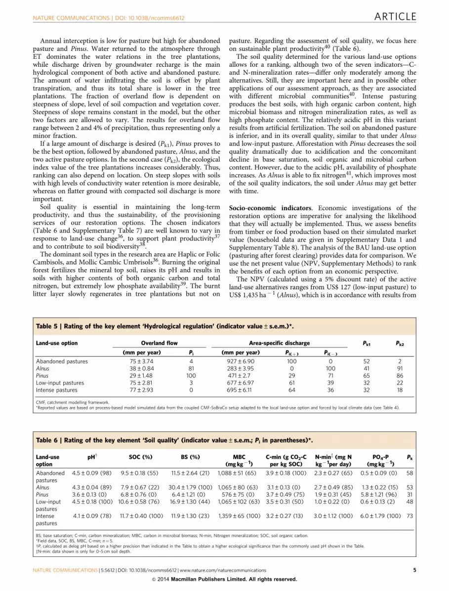
previous studies42. Payback periods from 10 (intense pasture) to18 years (low-input pasturing) are required to recoup initialinvestment costs (Table 7). Among the pasture options, theintense variant is best in economic terms, with an NPV of US$1,060 ha� 1. To simulate a greater preference for immediate netrevenues with low initial costs, an 8% discount rate is also tested.In this case, the relative position of leaving land abandonedimproves, as the NPVs of the active management alternativesdecrease under these conditions. Intense pasture (13 years) andafforestation (16 years), however, still break even within the timespan considered.

The land-use variants differ widely in the distribution of netrevenues over the 20-year time period. For both afforestationoptions, we find only 3 years with positive, albeit high, netrevenues (Supplementary Table 9), while the pasture optionsgenerate positive net revenues in 18 years. Owing to theconcentration of net revenues in only 3 years, the diversificationof annual market and production risks in the afforestationoptions is not comparable to that of the pasture options, forwhich the ‘averaging effect’ is much stronger. The uncertainty ofthe intense pasture’s NPV is thus only around 50% of that of thetree plantations.

From a farmer’s perspective, all restoration options must becompared with the BAU option of land use in the study region43

(explained in Supplementary Methods). All restoration optionstested are less favourable from an economic point of view thanBAU, for which the NPV (US$ 1,435 and 1,765 ha� 1 at 8% and5% discount rates) is always higher than that of the best restorationoption. The annualized differences between the NPVs (8%discount rate) of BAU and the restoration scenarios are US$87±52 ha� 1 per year (Alnus as reference) or US$ 100±40 ha� 1

per year (intense pasture as reference). These amounts suggest theorder of magnitude of the financial transfers that might be requiredto convince farmers to establish one or more restoration options.

Social preference in the context of this method representsinformation beyond that contained in the economic indicators. Inaddition to the tangible values reported above, people tend toimplicitly include intangible cultural values when expressingtheir preference for land-use options. Thus, the success ofrecommendations regarding land use depends largely on thisindicator, as farmers must evaluate whether a particular optionfits not only into their overall economic, but also into theirhousehold and socio-cultural situations44.

Using standardized questionnaires (Supplementary Methods),we asked Mestizo and Saraguro farmers about their preferencesand find an inclination towards afforestation (Table 8 andSupplementary Table 10). Farmers of both ethnic groups list ‘lackof timber’ and ‘shortage of labour’ as the main reasons for thispreference. Without the benefit of subsidies, farmers of bothethnic groups prefer Alnus over Pinus; however, given thepossibility of external subsidies, the Mestizos show a slightpreference for Pinus. With respect to repasturization, low-inputpasture appears to be more attractive than the intense option.Concerns about adverse ecological effects and the costs forfertilizer are the main reasons given by Mestizos for preferringlow-input pasturing: more than one fourth of Mestizosinterviewed (10 out of 37) believe that agrochemicals damageor ‘sterilize’ the soil. The Saraguros, however, state a higherpreference for intense pasture if subsidies are available, butnevertheless consider reforestation with Alnus to be the bestoption.

The interviews show a clear preference for tree plantations.Interestingly, leaving areas abandoned is not favoured at all.Farmers express willingness to re-utilize abandoned areas but areless ready to invest high upfront costs or substantial labour to doso. Differences in the acceptance level even among differentethnic groups support the necessity and usefulness of thisindicator, especially when applied in other regions.

Table 7 | Rating of the ‘Economic’ key elements (indicator value±s.e.m.)*.

Land-use option Net present value for discount rate: Payback period for discount rate:

5% (US$ ha� 1) Pi 8% (US$ ha� 1) Pi Pk 5% (years) Pi 8% (years) Pi Pk

Abandoned pastures 0±0 0 0±0 20 10 0±0 100 0±0 100 100Alnus 1,435±649 100 619±394 100 100 16±3 11 16±4 50 30.5Pinus 1,322±586 92 561±373 93 92.5 16±3 11 16±4 50 30.5Low-input pastures 127±146 9 � 156±129 0 4.5 18±6 0 32±4 0 0Intense pastures 1,060±264 74 485±234 83 78.5 10±2 44 13±4 59 51.5

*Product (timber, milk and meat) quantities estimated based on tree and grass biomass predictions, and possible number of cattle calculated from simulated grazing rounds plus measured nutrition valueof grass; local timber prices and harvesting costs, and prices and costs for milk and meat production contained in Supplementary Data 1; uncertainty from Monte-Carlo simulations, coefficients ofvariation43 from FAO time series data for prices and productivities, as well as from simulated fire risks based on remote sensing data.

Table 8 | Rating of the key elements for ‘Social preference’; ‘answers’ refer to number of respondents who rate an option as bestor second best (indicator value±s.e.m.)*.

Preferred land-use option Saraguros (22 interviews) Mestizos (37 interviews)

Without subsidy With subsidy Pk Without subsidy With subsidy Pk

Answers Pi Answers Pi Answers Pi Answers Pi

Abandoned pastures 4±1.9 0 0±0 0 0 5±2.1 0 0±0 0 0Alnus 14±3.0 100 19±3.1 100 100 19±3.6 100 16±3.4 94 97Pinus 12±2.9 80 9±2.6 47 63.5 15±3.4 71 17±3.5 100 86Low-input pastures 5±2.1 10 3±1.7 16 13 12±3.1 50 14±3.2 82 66Intense pastures 4±1.9 0 8±2.5 42 21 12±3.1 50 10±2.9 59 55

*Field data from standardized interviews.

ARTICLE NATURE COMMUNICATIONS | DOI: 10.1038/ncomms6612

6 NATURE COMMUNICATIONS | 5:5612 | DOI: 10.1038/ncomms6612 | www.nature.com/naturecommunications

& 2014 Macmillan Publishers Limited. All rights reserved.

Synopsis and sensitivity of indices. To gain more insight into thepossible trade-offs between ecological and socio-economic eco-system indices, and to support science-based decision making, weanalyse the correlation between the average ecological and socio-economic key elements (Fig. 1).

Spanning considerable ranges, the ecological and socio-economic indicators are strongly positively correlated and showa low degree of trade-off—þ 0.99 with high water retention, andþ 0.94 with high discharge considered most desirable. Leavingareas abandoned and low-input pasture both appear less efficientthan the other options. Ranking by the ecological indices aloneplaces afforestation on top, irrespective of the hydrological keyelement used (Fig. 2a).

Alnus plantations rank slightly higher than Pinus plantations,followed by intense pasture. Afforestation and intense pastureboth rank higher than the original state of ‘abandoned pasture’.Low-input pasture is ecologically equal to abandoned pasturewhen water retention is assessed as positive, but falls short whenwater discharge is more desirable.

The economic results (Fig. 2b) are supported by the analysis ofthe preferences obtained from the household survey, which showan affinity for afforestation among all respondents.

Sensitivity analysis (Supplementary Tables 11–21) shows ourranking to be sufficiently robust in this context and provide anindication of how this ranking might be affected by subjectiveweighting of key elements (Supplementary Fig. 2). The ranking

remains the same when we account for the size of the differencesby applying equation (3) (see Methods) in an attempt to preventoverestimation of small differences (Supplementary Fig. 2a).However, with this type of weighting, the ecological indicatorsdistinguish less clearly among the restoration options. Althoughsome ecological differences may be considered small (for examplein N-mineralization), their importance may be high. Suchdifferences are scaled appropriately with our approach. Anotheradvantage is its relatively high immunity against uncertainty. Bycalculating the relative position of the indicator values in therange between their maximum and minimum, we obtain robustrankings that are largely unaffected by indicator uncertainty (seebelow). When using the 95% confidence limits to representpessimistic and optimistic indicator estimates and account foruncertainties (according to equation (4) in Methods), some land-use options change their rank position, but only for singleindicators. One example of this is the option pair Alnus andintense pasture, which trade positions between ranks 1 and 3 forthe indicator NPV (8%) depending on whether the analysis isbased on optimistic or pessimistic assumptions (SupplementaryTable 20). However, where process-based model results con-tribute to the assessment, the individual (Pi) and integrated (Pk)indicator assessment scheme are very robust (SupplementaryTables 15–18). In sum, we do not see any significant overallvariation in the average normalized indicators (SupplementaryFig. 2b,c). Only under pessimistic assumptions does thecorrelation between socio-economic and ecological indicators,and significance levels weaken (Supplementary Fig. 2c andSupplementary Table 22). Given the generally high level ofrobustness of our ranking system, we conclude that both ournormalization procedure and assessment approach are reliable.

0

20

40

60

80

100

0 20 40 60 80 100

Ave

rage

eco

nom

ic/s

ocia

l ind

icat

ors WP

socioe

cono

mic

Average ecological indicators WPecology

Abandoned pasturesAlnus plantationsPinus plantationsLow-input pastureIntense pasture

Figure 1 | Ecological versus socio-economic index values. Average of key

element—Pk—indices of the five investigated options of land use if water

retention is considered positive. Error bars (whiskers) indicate±s.e.m.,

coefficient of correlation is r¼0.99 (tr¼ 11.77; pto0.001); the statistic of a

Kruskal–Wallis one-way analysis of variance is H¼ 13.4 (pHo0.01) for

differences between overall average index values (n¼ 8 key elements for

each land-use option). A priori hypotheses about differences between single

land-use options or groups of land-use options are tested as statistical

contrasts using rank transformed data with: Ab, abandoned pastures; A,

Alnus; P, Pinus; L, low-input pastures; I, intense pastures. Contrast 1,

associated with the hypothesis (Aþ Pþ Lþ I)/44Ab, tests if restoration

options on average improve ecological and socio-economic values, and

results in a significant tc1¼ 2.3 (pc1o0.025). Contrast 2, associated with

the hypothesis (Aþ P)/24(Iþ L)/2, tests if afforestations perform better

than pasture, and results in a significant tc2¼ 3.1 (pc2o0.025). Contrast 3

focuses on the hypothesis A4P and tests if Alnus outperforms Pinus, and

results in a nonsignificant tc3¼0.9. Contrast 4, associated with the

hypothesis I4L, tests if intense pastures perform better than low-input

pastures, and results in a weakly significant tc4¼ 1.6 (pc4o0.100)

(Supplementary Table 22).

36 36 52 52 52 52 32 32

98 98 86 86 19 19

88 88 20 20

91 85

18

21

4165

32

52 32

52

52

3131

7070

58

5848 48

0

50

100

150

200

250

300

350

Alnusplantations

Pinusplantations

Intensepastures

Abandonedpastures

Low-inputpastures

Cum

ulat

ive

indi

cato

rs p

k

Soil Hydrology Pk1 Hydrology Pk2

Climate Carbon relationships

113 105 8913 4

31 31 52

100

8652 21

12

84

7648

60

0

50

100

150

200

250

300

350

Alnusplantations

Pinusplantations

Intensepastures

Abandonedpastures

Low-inputpastures

Cum

ulat

ive

indi

cato

rs p

k Preference Mestizos Preference Saraguros

Payback period Net present value

a

b

Figure 2 | Accumulated index values. (a) Summed index values on

ecological indicators are shown for the five land-use options with Pk1:

discharge considered positive (left columns) and Pk2: water retention

preferred (right columns). (b) Summed index values on socio-economic

indicators for the five land-use options are depicted. Preferences distinguish

between indigenous Saraguro and Mestizo settlers. With payback periods,

we measure how long settlers will need to receive their money invested back

and the NPV is the sum of all appropriately discounted net revenues.

NATURE COMMUNICATIONS | DOI: 10.1038/ncomms6612 ARTICLE

NATURE COMMUNICATIONS | 5:5612 | DOI: 10.1038/ncomms6612 | www.nature.com/naturecommunications 7

& 2014 Macmillan Publishers Limited. All rights reserved.

DiscussionAssessing the potential for the provision of ecosystem functionsand benefits from various restoration options using normalizedecological and socio-economic indicators is a novel approach inscience-directed decision support. It is clear that any suchassessment is context specific and dependent on the particularobjectives of the decision makers in a given ecological and socio-economic context. Nevertheless, our study shows that the oftenignored socio-economic indicators are essential components of acomprehensive assessment approach to guide the way to a possibleimplementation of desirable land-use options. Their extremelystrong correlation with ecological indicators does, however, notnecessarily mean that a cause–response relationship exists. Itrather indicates that trade-offs between average indicators are low.Thus, to avoid assessing the consequences of restoration optionsoverly optimistic, it is important to quantify the short-term socio-economic trade-offs when compared with BAU. Given thispremises and combined with a thorough analysis of uncertainties,both the indicator system and the normalization proceduredeveloped in our study are useful for comprehensive evaluationsof ecosystem functions and benefits in other study regions.

The choice and quality of indicators are crucial issues. Forexample, our quantitative hydrological indicators showed realisticresults when compared with other studies45,46. However, waterquality could also be an important indicator25, as intense pasturerequires the use of herbicides and inorganic fertilizer, some ofwhich could end up in rivers and groundwater. This problem canbe mitigated by proper handling, that is, application of anyagrochemical only under suitable weather conditions. As overlandflow is generally low (2–4% of precipitation), the volume of waterfor direct downhill transport of the chemicals is also small,reducing the risk of displacement. In fact, our observations of thecontrol plots located down slope from herbicide-treated plots didnot show any herbicide effect. Carryover effects of any of theherbicides applied via the soil to the subsequent pasture were alsonot observed24. A similar consideration applies to fertilizertreatment, as the poor soils act as strong nutrient sinks.Nevertheless, some leaching of nitrate cannot be completelyruled out, although we did not observe a statistically significantfertilization effect in reference plots situated down slope.

In contrast to other authors28, we did not use biodiversity as anindicator in our study, as it is very low in the options investigatedand—even on long-abandoned pasture—is not at all comparableto that of the pristine forest. Stable shrubby vegetation madeup of bracken and several prolific roadside species formed aclosed canopy21, which can persist for decades (SupplementaryMethods). Species richness of selected other groups of organismssuch as birds and moths is also low compared with that found inpristine forests. Thus, the anthropogenic landscapes flankingforests are merely sinks for such species, mainly due to a shortageof food resources, nesting sites and other ecological factorsnecessary to provide suitable habitats. Consequently, the land-useoptions considered here represent ‘novel ecosystems’ that areexpected to persist, rather than merely being an interim stage inthe process of returning to a near-natural forest47–49. Naturalgrassland suitable for use as pasture does not occur in theresearch area and thus introduced grass species (Setariasphacelata and Melinis minutiflora) are used. Someaccompanying herbs, grasses and shrubs are indigenous, butmost are cosmopolitans50, resulting in limited phytodiversity.Every hectare of natural vegetation—dense forest up to2,800 m asl and shrub paramo above the tree line51—that is notcleared for production of short-lived pastures preserves muchmore of the biological diversity than pasture, afforested areas orabandoned lands can maintain.

Still, some barriers must be overcome to implement theadvantageous restoration options, as all of them impose short-term economic trade-offs. The quantified trade-off of US$ 87 inopportunity costs resulting from afforestation with Alnus, or theUS$ 100 ha� 1 per year costs incurred when intense pasture isimplemented are, however, subject to a high level of uncertainty. Ifwe use the upper 95% confidence limit of the estimated costs toinclude the possible compensation amounts demanded with a0.975 probability, we end up with approximately US$ 180 ha� 1

per year to be transferred to farmers. Spending this money couldbe worthwhile, given the amount of CO2 emissions42 and losses ofbiodiversity, which could be avoided, and the other ecologicalbenefits, which could be achieved if farmers were to re-utilize theirabandoned lands rather than clearing natural forest. In our studyarea, the preservation of natural forests may prevent the emissionof 272 Mg CO2 per hectare43. Consequently, a moderate price forCO2 emission allowances of US$ 7.5 per Mg would result in a NPVof US$ 2,040 ha� 1, which is equivalent to an annualized paymentof US$ 208 over a 20-year period (based on an 8% discount rate).Carbon markets could, thus, possibly cover the compensationamounts needed to convince famers to choose restoration options.

However, to improve conservation efficiency, transfers tolandowners as rewards for conserving their forests—for example,under the REDDþ mechanism52 or other national programmessuch as the Ecuadorian ‘Socio Bosque’53—should be madeconditional on the implementation of restoration activities onabandoned land, considering also agricultural options in thefuture54. In regions with chaotic property rights regimes, as in ourstudy area44, the implementation of the restoration options couldalso be supported by offering property rights contracts (possiblycoupled with additional financial compensation). The size of theabandoned area, its accessibility and distance to the farm mustalso be considered in recommendations, as the advantages ofafforestation increase with distance to farm, whereas those ofintense pasture increase with increasing accessibility.

As a general conclusion, it appears important for farmers toreceive appropriate education and financial support to highlightand strengthen the link between more long-term economicthinking and ecological considerations. Our study shows thatpreference analyses are crucial parts of studies on ecosystemfunctions and benefits. The preference expressed by the majorityof subsistence farmers for restoring abandoned pasture areasthrough afforestation demonstrates that implementation of thisoption is realistic. Farmers could benefit from more moderateupfront costs, the lack of a need for further inputs of labour untilthinning and harvest activities take place and flexibility withrespect to the timber market, which ultimately results in areduction in risk54. Pinus could be used as a nurse-tree species tofacilitate regeneration of useful native trees. Restoration ofabandoned pasture for intensive re-use may be more attractiveon medium to large farms (50–100 ha), which are alreadyintegrated into agricultural markets and can afford higherupfront investments. The implementation of intense pasturingwill require a higher level of input from consulting experts.Similar conclusions will be valid for other tropical mountainregions, from 1,500 m altitude up to the tree line.

As evidenced by the short-term economic trade-offs inherentto each of the restoration options, a farmer’s decision to afforest,re-cultivate pasture or leave areas abandoned depends—inaddition to available labour capacity—on the availability ofaffordable financial support from government programmes orcredit institutions. Studies such as ours can help raise awarenessabout possibilities for recultivating abandoned land, thusenhancing the effectiveness of incentive programmes, whichcould ultimately relieve pressure on natural ecosystems42.

ARTICLE NATURE COMMUNICATIONS | DOI: 10.1038/ncomms6612

8 NATURE COMMUNICATIONS | 5:5612 | DOI: 10.1038/ncomms6612 | www.nature.com/naturecommunications

& 2014 Macmillan Publishers Limited. All rights reserved.

MethodsLand-use options and period considered. We investigate two variants each ofafforestation and pasture restoration as feasible options with respect to their eco-logical value, their economic benefits and the preferences for each option amongboth Mestizo and indigenous Saraguro farmers. A former pasture area that hasbeen abandoned for 14 years is our reference. We consider a 20-year period to be ameaningful time span for the study, as it represents the common rotation time fortree plantations in the region.

Data. The present work synthesizes the findings of a multi-disciplinary researchinitiative that started ecosystem studies in southern Ecuador in 1998. Since then, asolid knowledge base has accumulated with data that is used in this study. Modelsparameterized with field data are used to obtain the results for some indicators overthe 20-year period during which we assume nearly constant environmental con-ditions. Other indicators were either measured directly in the field or obtainedfrom interviews. Field data for carbon relationships and soil quality has beenobtained from previous peer-reviewed work carried out by members of the multi-disciplinary research team24,30,31,36,40,55–57. Model-based indicators have beenestimated with models published in peer-reviewed journals, which have beendeveloped for or adapted to the study region. Model estimates includeclimatic32,36,55, hydrological34,46,58 and economic42,43,59 approaches. Onlyoccasionally have models from other literature been used to complement ourdata60,61. The results of the interviews (Supplementary Table 10) to obtain data onthe social preferences have not been published in peer-reviewed journals before.Details, as well as an assessment of the methods are presented in SupplementaryMethods.

Research area. The research area62 is located in the eastern range of the tropicalAndes of southern Ecuador (3�580300 0 S and 79�40250 0 W). Our experimental siteswere established on areas with a 35� slope located between 1,800 and 2,100 m asl,and covering a total area of abandoned pasture of 150 ha. Analysis of aerialphotographs shows that forest clearing has been occurring since the 1960s, andpasture farming has been done for about the last 35 years. Because of heavyinfestation by weeds—mostly bracken fern—many pastures were abandoned about15 years ago.

Normalization of indicators and statistical analyses. Unitary performanceindices are calculated for each indicator (Pi) and for each of the key elements (Pk).Pi (equation (1)) reflects the relative position of a land-use option in the achievablerange. Ri is the indicator value, i the land-use option, Rmin the least desirable andRmax is the most desirable value for the indicator.

Pi ¼Ri�Rmin

Rmax �Rmin� 100 ð1Þ

As equation (1) might result in inflation of small differences through itsnormalization approach, we impose an objective weighting factor, wd, proportionalto the maximum achievable difference to test the robustness of our Pi. Specifically,we use the total range of variation divided by the indicator’s maximum as theweight, wd, to account for the relative size of the maximum achievable differenceand to see how our results change through this type of weighting (equation (2)).

Pi ¼Ri�Rmin

Rmax �Rmin� wd � 100 with : wd ¼

Rmax �Rmin

Rmaxð2Þ

Adjusted according to equation (2), equation (1) then simplifies to equation (3):

Pi ¼Ri�Rmin

Rmax� 100 ð3Þ

Although equation (3) constitutes a weighting of the normalized indicators, wealso conduct sensitivity studies in which we test scenarios using either pessimisticor optimistic estimates for our indicators to identify possible impacts ofuncertainty. To obtain the pessimistic and optimistic estimates, 95% confidencelimits for the estimated indicators are used. The interpretation of a confidence limitas pessimistic or optimistic depends on what is desirable. If a high indicator value isdesired (for example NPV), the lower confidence limit is considered to be thepessimistic (near worst-case) estimate. If instead a low indicator value is preferable(for example, payback period), the upper confidence limit is considered pessimistic(equation (4)).

Ri;opt;pess ¼ Ri � ta¼1� 0:95;df � SEMi ð4Þ

SEMSamplei ¼ SDiffiffiffi

np ð5Þ

SEMSample Interviewsi ¼ n �

ffiffiffiffiffiffiffiffiffiffiffiffiffiffiffiffiffiffiffiffiffiffiffiffiffiffiffipi � 1� pið Þ=n

pð6Þ

SEMMonte Carloi ¼ SDSimulated Mean

i ð7ÞHere, SEMi is the uncertainty associated with the estimated mean indicator

value for restoration option i, commonly understood as the s.d. of the mean andta¼ 1� 0.95,df is a number obtained from a Student’s t-distribution, which is used toform a 95% confidence limit depending on the degrees of freedom, df. For indicator

values derived from sampling, we obtain SEMi by dividing SDi (the s.d. amongindividual samples) by the square root of n (number of samples) (equation 5). Forthe interview data, the SEMi

Sample_Interviews (equation (6)) is the s.e. of the numberof answers where a restoration option is chosen as the best or second bestalternative. Here, n is the sum of all responses of ‘best’ or ‘second best’, and p is therelative frequency of the responses ‘best’ and ‘second best’ for that restorationoption. In detail, p is the number of ‘bests’ and ‘second bests’ for option i divided byn—the sum of all answers for a given indicator naming these categories. For themodel estimates, SEMi

Monte_Carlo is computed directly as the standard deviation,SDi

Simulated_Mean, of the mean values derived from the simulated repetitions(equation 7). Finally, normalization of either Ropt or Rpess is carried out accordingto equation (1).

Pk (equation 8) is the average of all (weighted or not weighted) Pi values, whichcontribute to a particular key element (ni is the respective number of indicators).

Pk ¼1ni

X

i

Pi ð8Þ

The ecological and socio-economic average of index values for each of the land-use options are determined by average performance indices (equation 9) (weightedor not weighted), where o is the land-use option, c the category, nk is the number ofkey elements and wsub is a subjective weighting factor.

WPco ¼

1nk

X

k

wsub � Pk ð9Þ

wsub is set equal to 1 for standard analyses. For specific scenarios, however, we testsubjective weighting factors to favour preferred key elements.

We compute Pearson correlations between ecological and socio-economicindicators for Pk values and associated t- and p-values (Fig. 1 and SupplementaryFig. 2). Given our—through normalization—truncated distributions of Pi indexvalues, non-parametric Kruskal–Wallis analyses of variance served to test theimpact of land-use options on the average Pk (nk¼ 8 for each option). Associatedwith a one-way analysis of variance for rank-transformed data, contrasts based ona priori formulated hypotheses are computed finally to distinguish between theland-use options investigated (Supplementary Table 22).

Biomass production and carbon content. On the abandoned areas (controlplots), above-ground plant biomass (bracken leaves) was harvested individuallyfrom four 25-m2 plots and dried for further analysis, while below-ground biomasswas estimated from roots and rhizomes extracted from soil cores (40 cm deep, 6 cmdiameter, n¼ 3 per plot). Aliquots of the dried plant material were analysed in aCNS-Analyser (vario EL III/elementar, Heraeus). Production of above-groundbiomass was determined based on the amount of standing biomass and the lifespan of the bracken leaves30. Below-ground biomass production was estimatedusing the SoBraCo-model33. On the pastures, biomass production and totalbiomass were determined using 4� 4 m plots with four repetitions per optionduring the second year of pasture management after complete removal of theharvest from the first year. Grazing was simulated by cutting the grasses andleaving a basal layer of 20 cm. At the end of the year, the grass was completelyharvested. For calculation of the standing crop, see Supplementary Methods.Below-ground biomass was determined and root biomass production wasestimated as described above, with cores taken below, near and between grass tufts.SEM was calculated according to equation (5). Based on data from theexperimental plots as described in Gunter et al.63, growth of the Pinus and Alnustrees over 20 years was calculated. This was done using regression curves tocorrelate dbh (diameter at breast height) and height with the independent variablesage and tree density. Tree density is based on an initial density of 1,111 trees perhectare and an observed annual mortality rate of 2%. To establish the regressioncurves, Pinus was recorded on two sites with 16 plots each (32 plots of10.8� 10.8 m, all 6 years old) and on one site with two circular plots (radius 20 m,1,256 m2, 25 years old). Data for Alnus was measured on two sites, one with 14 andthe other with 16 plots (30 plots 10.8� 10.8 m, 7 years old) and one site with 10plots (size on average 777 m2, 8 years old). Above-ground biomass and carboncontent are estimated using both allometric equations and information adoptedfrom the literature (Supplementary Methods). Uncertainty is modelled by means ofMonte-Carlo (MC) simulation (3,000 repetitions for each afforestation option),where the coefficients of regression models are considered random. Regressioncoefficients as means, and their uncertainties, in the form of their s.e. allow us todraw randomly fluctuating coefficients for each simulation run to predict forestgrowth. The calculation of SEM refers to equation (7).

Climate. The Soil-Vegetation-Atmosphere Transfer model and the vegetationgrowth model SoBraCo33 are used to assess changes in the climate regulationfunction of the land-use options. SoBraCo is a derivative of the properly validatedcommunity land model (CLM, see Lawrence et al.64 and Bonan et al.65). The maindifference between SoBraCo and CLM is that in SoBraCo, the calculations used inCLM for some atmospheric variables are replaced by direct forcing withobservational data from a specifically designed micro-meteorological station for anaverage reference year (2008; refer to Supplementary Methods). Hourlyenvironmental forcing data for the 20-year modelling period is generated using thereference period for the forcing variables (solar irradiation, air temperature, relative

NATURE COMMUNICATIONS | DOI: 10.1038/ncomms6612 ARTICLE

NATURE COMMUNICATIONS | 5:5612 | DOI: 10.1038/ncomms6612 | www.nature.com/naturecommunications 9

& 2014 Macmillan Publishers Limited. All rights reserved.

humidity, wind speed, rainfall, soil water content and soil temperature) andcontinually re-applying the annual data set over the entire period. Required plant-specific model parameters are derived from measurements at both leaf and rootlevels at the study site and from data available from the literature (for more details,refer to Supplementary Methods and Supplementary Table 12). CMF is directlycoupled with the SoBraCo-model using a Python interface58.

Time series of leaf area indices (LAIs) and vegetation height used for parameterforcing for the coupled model over the 20-year period are calculated using fieldmeasurements (Supplementary Fig. 1). For Pinus, LAI is estimated based on dbh60.For Alnus, observed leaf numbers from experimental plots and mean leaf area61 areused to estimate the mean allometric leaf area (LAallom) per tree, asLAallom¼ EXP(� 0.22þ 1.297� ln(dbh)). LAallom and the actual number of trees isused to scale LAI up to the plantation level. LAI for grass and bracken are directlyderived from LAI field measurements56. Uncertainty analysis (for climate andhydrology) of the coupled SoBraCo-CMF model framework is conducted forforcing variable and parameter uncertainties of climate and hydrological indicators,the latter with the help of more than 3,000 MC simulation runs and subsequentcalculation of the SEM using equation (7). Based on sensitivity studies and aliterature survey, eight (SoBraCo)þ two (CMF) model parameters shown to havethe biggest influence on model output are chosen (see Supplementary Methods).Most parameters and the form of their probability density functions are based onfield observations (for parameters and sources, see Supplementary Tables 12 and13). The robustness of the integral rating scheme (Pk) regarding climate andhydrological indicators is tested by comparing the range of the Pi gradingconsidering forcing variable uncertainty (Supplementary Tables 17 and 18). Ascenario using 95% limits for the indicator values (following from equation (4))derived from the MC analysis (parameter uncertainty) has also been tested(Supplementary Tables 15 and 16).

Hydrology. The CMF34 is used to simulate hydrological processes in a one-dimensional soil column and to quantify water fluxes. This model effectively meetsthe challenges and provides the opportunities called for in hydrological models tosupport decision making outlined by Guswa et al.66 Similar to the finite volumemethod used by Qu and Duffy67, CMF discretises the soil column into soil layersserving as water storages. We use the Richards equation to simulate water fluxbetween cells. Eight soil layers of increasing thickness from the top downwards,each with unique hydraulic properties, are summed to reach a total column depthof 1 m. Water leaving the soil column is routed to the ground water using aDirichlet boundary condition with a constant negative pressure. An average slopesimilar to the slope occurring at the site is used. The CMF water balance is asfollows: Dstorage¼ rainfall—ET—overland flow—ground water seepage.Groundwater seepage plus overland flow is summed to derive the area-specificdischarge. Saturated hydraulic conductivity (ksat) for the scenarios is adapted inaccordance with local measurements for pasture and forested sites presented byHuwe et al.57 To account for the highly conductive litter layer and roots that createadditional pore space, the ksat values of the three top soil layers are increased. ETand throughfall are calculated using the SoBraCo-model33, which shows realisticresults. For example, the rate of throughfall forwarded to the hydrological model bythe plant growth model SoBraCo is well within the range found in other studies inadjacent tropical mountainous rainforest sites45 (between 88% and 97% ofprecipitation). Saturated soil depth is set to � 2 m below soil surface to initializethe model and provide uniform initial conditions. To emphasize the impact ofvegetation type, uniform parameters for soil are used for all of the land-use options(Supplementary Methods). Overland flow is simulated as saturation excess. For theanalysis of uncertainty, refer to the key element ‘Climate’.

Soils. The quantification of our ecosystem function is based solely on empiricaldata measured on five plots in 2011. Soil samples were taken with an auger(diameter: 6 cm). A pooled soil sample of six replicates per plot was analysed forthe 0–5 and 5–10 cm depth intervals. Soil organic carbon and total nitrogen (N)were quantified using a CNS-Analyzer (vario EL III/elementar, Heraeus). Freshsamples were used for all other measurements, but the data were calculated for dryweight (105 �C). Plant available PO4-P was determined by the Bray-P method68

and the chloroform-fumigation extraction method was used69 for microbialcarbon. Gross N mineralization was measured by the 15N-isotope pool dilutionmethod and soil organic carbon mineralization by CO2 evolution during 14 days ofincubation70. Soil pH was determined in deionized water. Soil data were gatheredfor restored pasture beginning 2 years after re-establishment and for treeplantations in the oldest existing plots. Calculation of SEM refers to equation (5).

Economics. The modelled (afforestation) or measured (pasture) biomass pro-duction in the form of either timber volume (afforestation) or fodder for a specificnumber of cattle (pasture) forms the ecological data to be evaluated using localprices and costs. Local historical timber prices and harvesting expenses, reported inSupplementary Data 1, were applied to the afforestation areas to estimate the netrevenues from timber production (see Supplementary Table 4 for biophysicaltimber production and 18 for financial household data). For pasture, extrapolationof simulated grazing generates expected fodder yield, and the number of cattle thatcan be fed is computed based on the measured nutrient value of the grass. Milk andmeat yield, as well as corresponding prices and costs are given in Supplementary

Data 1. The distribution of net revenues over the 20-year time period forms thebasis for economic valuation (Supplementary Table 9). The sum of all discountednet revenues (NPV) is used to evaluate the economic returns from the variousland-use options and discounting based on discount rates of 5 or 8%. Paybackperiods are calculated based on discounted net revenues (Supplementary Methods).For the scenario ‘pasturing after forest clearing’ (BAU), upfront net returns fromforest clearing and pasture establishment were obtained from Knoke et al.43 andcombined with subsequent net revenues from low-input pasture management(Supplementary Table 9). Uncertainty is modelled by means of MC simulation(3,000 repetitions for each restoration option) for the annual net revenues used tocalculate NPV and payback periods. Here, net revenues are drawn as randomvariables for every single year of the 20-year period considered from a normaldistribution with the previously estimated expected net revenue as the mean andthe s.d. indicated in Supplementary Table 9. After completing the annualsimulation of net revenues over the entire 20-year period, a random NPV andpayback period are computed for all iterations and SEM is calculated according toequation (7). Year-to-year correlation is set to zero. This appears reasonable,because average year-to-year correlation of revenues (average price obtained timesquantity produced) for 10 South American countries was 0.04±0.21 according to adata set used by Knoke et al.59 Uncertainty coefficients for the land-use options inthe study area are derived from coefficients of variation published in an earlieranalysis43 in our study area. The coefficients of variation reflect compounded s.d. ofprices and productivities from Food and Agriculture Organization of UnitedNations time series data, as well as s.d. caused by failure due to fire (coefficients inSupplementary Table 9).

Social assessment. The preferences of Saraguro and Mestizo farmers for the fiveproposed land-use options were determined using a standardized questionnaire(Supplementary Methods). This includes questions regarding the land-use pre-ferences of the farmers and their arguments for preferring particular land-useoptions, as well as information about household composition, ownership ofabandoned land and reasons for its abandonment. Two scenarios are tested—onein which farmers reclaim the abandoned areas using their own means (withoutsubsidies) and a second in which farmers receive financial support for major inputsfrom external agencies (with subsidies).

References1. Garcıa-Barrios, L. et al. Neotropical forest conservation, agricultural

intensification, and rural out-migration: The Mexican experience. BioScience59, 863–873 (2009).

2. Lambin, E. F. & Meyfroidt, P. Global land use change, economic globalization,and the looming land scarcity. Proc. Natl Acad. Sci. USA 106, 3465–3472 (2011).

3. Field, C. B., Campbell, J. E. & Lobell, D. B. Biomass energy: the scale of thepotential resource. Trends Ecol. Evol. 23, 65–72 (2007).

4. Tscharntke, T. et al. Global food security, biodiversity conservation and thefuture of agricultural intensification. Biol. Conserv. 151, 53–59 (2012).

5. Aronson, J. et al. Are socioeconomic benefits of restoration adequatelyquantified? a meta-analysis of recent papers (2000–2008) in restoration ecologyand 12 other scientific journals. Restor. Ecol. 18, 143–154 (2010).

6. DeFries, R. & Rosenzweig, C. Toward a whole-landscape approach forsustainable land use in the tropics. Proc. Natl Acad. Sci. USA 107, 19627–19632(2010).

7. Silver, W. L., Kueppers, L. M., Lugo, A. E., Ostertag, R. & Matzek, V. Carbonsequestration and plant community dynamics following reforestation oftropical pasture. Ecol. Appl. 14, 1115–1127 (2004).

8. Larsson, S. & Nilsson, C. A remote sensing methodology to assess the costs ofpreparing abandoned farmland for energy crop cultivation in northern Sweden.Biomass Bioenerg. 28, 1–6 (2005).

9. Aronson, J. & Alexander, S. Ecosystem restoration is now a global priority:Time to roll up our sleeves. Restor. Ecol. 21, 293–296 (2013).

10. Seppelt, R., Dormann, C. F., Eppink, F. V., Lautenbach, S. & Schmidt, S. Aquantitative review of ecosystem service studies: approaches, shortcomings andthe road ahead. J. Appl. Ecol. 48, 630–636 (2011).

11. Boyd, J. & Banzhaf, S. What are ecosystem services? The need for standardizedenvironmental units. Ecol. Econ. 63, 616–626 (2007).

12. Groot, R. S., de, Wilson, M. A. & Boumans, R. M. J. A typology for theclassification, description and valuation of ecosystem functions, goods andservices. Ecol. Econ. 41, 393–408 (2002).

13. Aguirre, N., Palomeque, C., Weber, M., Stimm, B. & Gunter, S. in Silviculture inthe Tropics (eds Gunter, S., Weber, M., Stimm, B. & Mosandl, R.) 513–526(Springer, 2011).

14. Gottlicher et al. Landcover classification in the Andes of southern Ecuadorusing Landsat ETMþ data as a basis for SVAT modelling. Int. J. Remote Sens.30, 1867–1886 (2009).

15. Ellenberg, H. Man’s influence on tropical mountain ecosystems in SouthAmerica. J. Ecol. 67, 401–416 (1979).

16. Lauer, W. Human development and environment in the Andes: a geoecologicaloverview. Mt. Res. Dev. 13, 157–166 (1993).

ARTICLE NATURE COMMUNICATIONS | DOI: 10.1038/ncomms6612

10 NATURE COMMUNICATIONS | 5:5612 | DOI: 10.1038/ncomms6612 | www.nature.com/naturecommunications

& 2014 Macmillan Publishers Limited. All rights reserved.

17. Sarmiento, F. O. Arrested succession in pastures hinders regeneration ofTropandean forests and shreds mountain landscapes. Environ. Conserv. 1,14–23 (1997).

18. Ruddle, K. Problems of resource use in humid tropical high mountains. Frankf.Beitr. Didaktik Geogr. 5, 185–196 (1981).

19. Harden, C. P. Interrelationships between land abandonment and landdegradation: a case from the Ecuadorian Andes. Mt. Res. Dev. 16, 274–280 (1996).

20. Curatola Fernandez, G. F., Silva, B., Gawlik, J., Thies, B. & Bendix, J.Bracken fern frond status classification in the Andes of southern Ecuador:combining multispectral satellite data and field spectroscopy. Int. J. RemoteSens. 34, 7020–7037 (2013).

21. Hartig, K. & Beck, E. The bracken fern (Pteridium arachnoideum (Kaulf.)Maxon) dilemma in the Andes of Southern Ecuador. Ecotropica 9, 3–13 (2003).

22. Knoke, T., Stimm, B. & Weber, M. Tropical farmers need productivealternatives. Nature 452, 934 (2008).

23. Beck, E. & Richter, M. in The Tropical Mountain Forest: Biodiversity andEcology Series 2 (eds Gradstein, S. R., Homeier, J. & Gansert, D.) 195–217(Universitatsverlag Gottingen, 2008).

24. Roos, K., Rodel, H. G. & Beck, E. Short- and long-term effects of weed controlon pastures infested with Pteridium arachnoideum and an attempt to regenerateabandoned pastures in South Ecuador. Weed Res. 51, 165–176 (2011).

25. Brauman, K. A., Daily, G. C., Ka’eo Duarte, T. & Mooney, H. A. The Natureand value of ecosystem services: an overview highlighting hydrologic services.Annu. Rev. Environ. Resour. 32, 67–98 (2007).

26. Millennium Ecosystem Assessment. Ecosystems and Human Well-being:Synthesis (Island Press, r 2005 World Resources Institute, 2005).

27. Daniel, T. C. et al. Contributions of cultural services to the ecosystem servicesagenda. Proc. Natl Acad. Sci. USA 109, 8812–8819 (2012).

28. Nelson, E. et al. Modeling multiple ecosystem services, biodiversityconservation, commodity production, and tradeoffs at landscape scales. Front.Ecol. Environ. 7, 4–11 (2009).

29. Goldstein, J. H. et al. Integrating ecosystem-service trade-offs into land-usedecisions. Proc. Natl Acad. Sci. USA 109, 7565–7570 (2012).

30. Roos, K., Rollenbeck, R., Peters, T., Bendix, J. & Beck, E. Growth of tropicalbracken (Pteridium arachnoideum): response to weather variations andburning. Invasive Plant Sci. Manag. 3, 402–411 (2010).

31. Fries, A., Rollenbeck, R., Nau�, T., Peters, T. & Bendix, J. Near surface airhumidity in a megadiverse Andean mountain ecosystem of southern Ecuadorand its regionalization. Agric. For. Meteorol. 152, 17–30 (2011).

32. Gholz, H. L., Ewel, K. C. & Teskey, R. O. Water and forest productivity. ForestEcol. Manag. 30, 1–18 (1990).

33. Silva, B. S. G. et al. Simulating canopy photosynthesis for two competingspecies of an anthropogenic grassland community in the Andes of southernEcuador. Ecol. Model. 239, 14–26 (2012).

34. Kraft, P., Vache, K. B., Frede, H. -G. & Breuer, L. CMF: a hydrologicalprogramming language extension for integrated catchment models. Environ.Model. Softw. 26, 828–830 (2011).

35. Keeler, B. L. et al. Linking water quality and well-being for improvedassessment and valuation of ecosystem services. Proc. Natl Acad. Sci. USA 109,18619–18624 (2012).

36. Hamer, U., Potthast, K., Burneo, J. & Makeschin, F. Nutrient stocks andphosphorus fractions in mountain soils of Southern Ecuador after conversionof forest to pasture. Biogeochemistry 112, 495–510 (2013).

37. Andrews, S. S., Karlen, D. L. & Cambardella, C. A. The soil managementassessment framework: a quantitative soil quality evaluation method. Soil Sci.Soc. Am. J. 68, 1945–1962 (2004).

38. Pulleman, M. et al. Soil biodiversity, biological indicators and soil ecosystemservices—an overview of European approaches. Curr. Opin. Environ. Sustain 4,529–538 (2012).

39. Makeschin, F., Haubrich, F., Abiy, M., Burneo, J. I. & Klinger, T. in Gradients ina Tropical Mountain Ecosystem in Ecuador (eds Beck, E., Bendix, J., Kottke, I.,Makeschin, F. & Mosandl, R.) Ecological Studies 198, 397–408 (Springer, 2008).

40. Hamer, U., Potthast, K. & Makeschin, F. Urea fertilisation affected soil organicmatter dynamics and microbial community structure in pasture soils ofSouthern Ecuador. Appl. Soil Ecol. 43, 226–233 (2009).

41. Caru, M., Becerra, A., Sepulveda, D. & Cabello, A. Isolation of infective andeffective Frankia strains from root nodules of Alnus acuminata (Betulaceae).World J. Microbiol. Biotechnol. 16, 647–651 (2000).

42. Knoke, T., Calvas, B., Ochoa, W. S., Onyekwelu, J. & Griess, V. C. Foodproduction and climate protection—What abandoned lands can do to preservenatural forests. Glob. Environ. Change 23, 1064–1072 (2013).

43. Knoke, T. et al. Effectiveness and distributional impacts of payments forreduced carbon emissions from deforestation. Erdkunde 63, 365–384 (2009).

44. Pohle, P., Gerique, A., Park, M. & Lopez Sandoval, M. F. in Tropical Rainforestsand Agroforests Under Global Change (eds Tscharntke, T. et al.) 477–503(Springer, 2010).

45. Bruijnzeel, L., Mulligan, M. & Scatena, F. N. Hydrometeorology of tropicalmontane cloud forests: emerging patterns. Hydrol. Proc. 25, 465–498 (2011).

46. Windhorst, D., Kraft, P., Timbe, E., Frede, H.-G. & Breuer, L. Stable waterisotope tracing through hydrological models for disentangling runoffgeneration processes at the hillslope scale. Hydrol. Earth Syst. Sci. Discuss 11,5179–5216 (2014).

47. Paulsch, D. & Muller-Hohenstein, K. in Gradients in a Tropical MountainEcosystem of Ecuador (eds Beck, E., Bendix, J., Kottke, I., Makeschin, F. &Mosandl, R.) Ecological Studies 198, 149–156 (Springer, 2008).

48. Turner, I. M. Species loss in fragments of tropical rain forest: A review of theevidence. J. Appl. Ecol. 33, 200–209 (1996).

49. Hilt, N. & Fiedler, K. in Gradients in a Tropical Mountain Ecosystem of Ecuador(eds Beck, E., Bendix, J., Kottke, I., Makeschin, F. & Mosandl, R.) EcologicalStudies 198, 443–149 (Springer, 2008).

50. Homeier, J. et al. in Ecosystem Services, Biodiversity and Environmental Changein a Tropical Mountain Ecosystem of South Ecuador (eds Bendix, J. et al.)Ecological Studies 221, 93–106 (Springer, 2013).

51. Richter, M., Diertl, K. H., Emck, P., Peters, T. & Beck, E. Reasons for anoutstanding plant diversity in the tropical Andes of southern Ecuador.Landscape Online 12 (2009).

52. Pirard, R. & Belna, K. Agriculture and deforestation: is REDDþ rooted inevidence? For. Policy Econ. 21, 62–70 (2012).

53. de Koning, F. et al. Bridging the gap between forest conservation and povertyalleviation: the Ecuadorian Socio Bosque program. Environ. Sci. Policy 14,531–542.

54. Knoke, T., Roman Cuesta, R. M., Weber, M. & Haber, W. How can climatepolicy benefit from comprehensive land-use approaches? Front. Ecol. Environ.10, 438–445 (2012).

55. Potthast, K., Hamer, U. & Makeschin, F. In an Ecuadorian pasture soil thegrowth of Setaria sphacelata, but not of soil microorganisms, is co-limited by Nand P. Appl. Soil Ecol. 62, 103–114 (2012).

56. Bendix, J. et al. Model parameterization to simulate and compare the PARabsorption potential of two competing plant species. Int. J. Biometeorol. 54,283–295 (2010).

57. Huwe, B., Zimmermann, B., Zeilinger, J., Quizhpe, M. & Elsenbeer, H. inGradients in a Tropical Mountain Ecosystem in Ecuador (eds Beck, E., Bendix,J., Kottke, I., Makeschin, F. & Mosandl, R.) Ecological Studies 198, 375–386(Springer, 2008).

58. Windhorst, D. et al.in Ecosystem Services, Biodiversity and EnvironmentalChange in a Tropical Mountain Ecosystem of South Ecuador (eds Bendix, J.et al.) Ecological Studies 221, 275–286 (Springer, 2013).

59. Knoke, T., Steinbeis, O. E., Bosch, M., Roman Cuesta, R. M. & Burkhardt, T.Cost-effective compensation to avoid carbon emissions from forest loss: anapproach to consider price–quantity effects and risk-aversion. Ecol. Econ. 70,1139–1153 (2011).

60. Aguirre-Salado, C. A. et al. Mapping Leaf Area Index and canopy cover usinghemispherical photography and spot 5 HGR data regression and K-NN.Agrociencia 45, 105–119 (2011).

61. Cabezas-Gutierrez, M. et al. Un modelo para la estimacion del area foliar entres especies forestales de forma no destructiva. Colombia Revista U.D.C.AActualidad & Divulgacion Cientıfica 12, 131–140 (2009).

62. Beck, E. et al. in Gradients in a Tropical Mountain Ecosystem in Ecuador (edsBeck, E., Bendix, J., Kottke, I., Makeschin, F. & Mosandl, R.) Ecological Studies198, 1–13 (Springer, 2008).

63. Gunter, S. et al. Determinants for successful reforestation of abandonedpastures in the Andes: soil conditions and vegetation cover. Forest Ecol. Manag.258, 81–91 (2009).

64. Lawrence, D. M. et al. Parameterization improvements and functional andstructural advances in version 4 of the community land model. J. Adv. Model.Earth Syst. 3 Art. 2011MS000045 (2011).

65. Bonan, G. B. et al. Improving canopy processes in the Community Land Modelversion 4 (CLM4) using global flux fields empirically inferred from FLUXNETdata. J. Geophys. Res. 116, G02014 (2011).

66. Guswa, A. J. et al. Ecosystem services: challenges and opportunities forhydrologic modeling to support decision making. Water. Resour. Res 50,4535–4544 (2014).

67. Qu, Y. & Duffy, C. J. A semidiscrete finite volume formulation for multiprocesswatershed simulation. Water Resour. Res. 43, W08419 (2007).

68. Bray, R. H. & Kurtz, L. T. Determination of total, organic and available forms ofphosphorus in soils. Soil Sci. 59, 39–45 (1945).

69. Vance, E. D., Brookes, P. C. & Jenkinson, D. S. An extraction methodfor measuring soil microbial biomass C. Soil Biol. Biochem. 19, 703–707 (1987).

70. Hamer, U., Makeschin, F., Stadler, J. & Klotz, S. Soil organic matter andmicrobial community structure in set-aside and intensively managed arablesoils in NE-Saxony, Germany. Appl. Soil Ecol. 40, 465–475 (2008).

AcknowledgementsWe thank the German Research Foundation (DFG) for financing the study (ResearchUnits 402 and 816), Naturaleza y Cultura Internacional (Loja, San Diego) for support,our Ecuadorian partner Universities (UTPL, UNL Loja) for outstanding cooperation,

NATURE COMMUNICATIONS | DOI: 10.1038/ncomms6612 ARTICLE

NATURE COMMUNICATIONS | 5:5612 | DOI: 10.1038/ncomms6612 | www.nature.com/naturecommunications 11

& 2014 Macmillan Publishers Limited. All rights reserved.

the Ecuadorian Ministerio del Ambiente for granting research permits, theEcuadorian Weather Service (INAMHI) for providing data from the stations Loja andSan Ramon, and the staff of the Estacion Cientıfica San Francisco and many studentsand workers for their support. We also thank the farmers of Imbana, Los Guabos,El Tibio and Sabanilla for their contribution to this study. Finally, we are grateful toLaura Carlson for language editing.

Author contributionsT.K., E.B., J.B., P.P., L.B., R.M., M.W., B.S., S.G. and N.A. designed research and wrotethe paper; P.H., U.H., A.G., M.L.S., K.R., A.T., B.S., B.C., L.M.C., D.W., X.P. and J.M.analysed data and performed research.

Additional informationSupplementary Information accompanies this paper at http://www.nature.com/naturecommunications

Competing financial interests: The authors declare no competing financial interests.

Reprints and permission information is available online at http://npg.nature.com/reprintsandpermissions/

How to cite this article: Knoke, T. et al. Afforestation or intense pasturing improve theecological and economic value of abandoned tropical farmlands. Nat. Commun. 5:5612doi: 10.1038/ncomms6612 (2014).

This work is licensed under a Creative Commons Attribution 4.0International License. The images or other third party material in this

article are included in the article’s Creative Commons license, unless indicated otherwisein the credit line; if the material is not included under the Creative Commons license,users will need to obtain permission from the license holder to reproduce the material.To view a copy of this license, visit http://creativecommons.org/licenses/by/4.0/

ARTICLE NATURE COMMUNICATIONS | DOI: 10.1038/ncomms6612

12 NATURE COMMUNICATIONS | 5:5612 | DOI: 10.1038/ncomms6612 | www.nature.com/naturecommunications

& 2014 Macmillan Publishers Limited. All rights reserved.

1

1

Supplementary Figure 1. LAI story line data for each land-use option used to force model 2

parameters. Fluctuations in pasture and tree plantation scenarios represent grazing a timber 3

extraction. LAI on abandoned pastures is kept constant over the 20-year period. 4

2

5

6

Supplementary Figure 2. Average of ecological and socio-economic index values (±SEMWP) 7

under various sensitivity scenarios. ρ is the coefficient of correlation between average index 8

values with t statistic and p-value. H is the Kruskal-Wallis statistic for differences in overall 9

index means of land-use options with p-value (n=8 key elements) a. Indicator values are 10

weighted with their relative range of variation according to Eq. (3) in Materials and Methods 11

(main text). b. Indicator values are estimated optimistically based on 95% confidence limits 12

according to Eq. (4) c. Indicator values are computed pessimistically based on 95% 13

confidence limits according to Eq. (4). d. Key element “Soil quality” is given a very high 14

subjective weight, wsub, of 5 instead of 1 to express a strong preference for food production, 15

while all other key elements have a weight of 1, given Eq. (9). This puts intense pasture at 16

first place for the ecological assessment. See Supplementary Table 22 for statistical 17

contrasts between single land-use options. 18

b a

c d

ρ=0.98 tρ=9.17 pt<0.005 H=12.2 pH<0.025

ρ=0.98 tρ=9.28 pt<0.005 H=12.7 pH<0.025

ρ=0.85 tρ=2.84 pt<0.1 H=12.3 pH<0.025

ρ=0.74 tρ=1.68 n.s. H=9.52 pH<0.05

3

Supplementary Table 1. Total yield (DM) and fodder quality of Setaria pastures after 19

restoration and improvement through fertilisation. 20

Treatment Biomass yield

[kg ha-1

y-1

]

Content

[g kg-1

DM]

Crude protein

P Ca N

Restored pasture

Low-input pastures 1,240 38.2 0.69 2.21 6.12

Intense pastures 6,640 37.8 0.93 1.79 6.05

Long standing pastures* with various fertilisers applied

Control 9,020 83.5 1.76 4.31 13.36

Urea 9,750 91.3 1.51 4.17 14.61

Rock phosphate 9,120 85.5 2.49 4.90 13.68

Urea + rock phosphate 11,190 79.3 2.08 4.61 12.68

*Data adopted from Potthast et al.1 21

22

Supplementary Table 2. Partitioning of biomass production (mean ± SEM) between 23

above- and below-ground fractions for each of the five land-use options calculated on 24

a per-year basis. Coefficient of variation for above ground biomass in parentheses. 25

Land-use option

Biomass production [Mg ha

-1 y

-1]

Above ground Above ground

(with grazing) Below ground* Total**

Abandoned pastures 9.2 ± 1.4

(0.15) - 22.6 31.8 ± 4.8

Alnus plantations 6.1 - 1.6 7.7 ± 0.6

Pinus plantations 7.1 - 1.8 8.9 ± 0.4

Low-input pastures 1.2 ± 0.2

(0.17) 0.8 ± 0.1 25.3 26.5 ± 4.4

Intense pastures 6.6 ± 0.3

(0.05) 5.2 ± 0.3 43.4 50.0 ± 2.3

26 *No SEM available for simulated values. 27 28 **To obtain SEM for the total biomass production, the measured coefficient of variation of above ground biomass 29 production was used for the pasture options and for afforestation it was obtained through Monte-Carlo simulation 30 (see Material and Methods main text). 31

4

Supplementary Table 3. Standing crop (mean ± SEM) and carbon stocks in each of the five land-use options calculated on a per-year 32

basis. Where not otherwise mentioned: Data from field measurements. 33

34 35 36 37 38 39 40 41 42 43 44 45 46 47 48 49 50 51 52 53 54 55 56 57 58 59

60 61 62 *Averages computed over the entire production period (20 y). 63 **Calculated with a root:shoot ratio of 0.205 ± 0.036 (median, SEM) for tropical/subtropical moist forest/plantations according to Mokany et al.

2 64 ***SEM obtained through Monte-Carlo simulation (see Material and Methods main text). 65 Analysed with a Vario EL III/elementar analyser (Heraeus) 66 ##

Acosta-Mireles et al. 3 67

Land-use Option

Biomass average standing crop [Mg ha

-1]

C-content in roots and rhizomes

[%]

Average carbon stock

[Mg/ha]

Above ground

Below ground

Total Above ground

Below ground

Above ground

Root & Rhizome

Carbon in planta

Org. layer

SOC Total

Abandoned pastures

6.1 ± 0.9 69.9 ± 6.7 76.0 ± 7.6 49 43 3.0 ± 0.4 30.0 33.0 ± 2.9 - 87.3 ±5.3 120.3

Alnus plantations*

40.7 8.3** 49.1 50 50 20.4 4.2 24.5

± 2.4*** 7.9 ± 0.3 83.8 ± 6.8 116.3

Pinus plantations*

49.1 10.1** 59.2 50##

50##

24.6 5.0 29.6

± 1.5*** 13.0 ± 1.1 80.5 ± 4.6 122.7

Low-input pastures

0.7 ± 0.1 29.9 ± 3.0 30.6 ± 3.1 44 41 0.3 ± 0.1 12.2 12.5 ± 1.2 - 91.8 ±4.9 104.4

Intense pastures

3.0 ± 0.1 59.9 ± 8.3 62.1 ± 8.4 44 41 1.3 ± 0.1 24.5 25.8 ± 3.4 - 96.3 ±5.1 122.8

5

Supplementary Table 4. Stand characteristics for Alnus acuminata and Pinus patula obtained from a statistical based model (see 68

material and Methods main text). Thinnings after 12 and 16 years with 40% of Nr removed each time; mortality rate = 2% of Nr. 69

Nr = number of remaining trees; Nd = cumulative number of dead trees; Dbh = mean diameter at breast height Ba = basal area; ht = mean total height; vt= total 70

volume without bark; vc = commercial volume without bark; bma = above-ground biomass; bmb = below-ground biomass; bmt = total biomass; C = carbon 71

sequestration; LAI = leaf area index; Nrm = number of trees removed.72

Standing crop Removed crop

Age Nr Nd Dbh [cm]

Ba [m²ha

-1]

ht [m] vt [m³ ha

-1]

vc

[m³ ha-1]

bma [Mg ha

-1]

bmb

[Mg ha-1]

bmt

[Mg ha-1]

C [Mg ha

-1]

LAI Nrm vt vc

Aln

us

0 1111 0 0.00 0.00 0.00 0.00 0.00 0.00 0.00 0.00 0.00 0.00 0 0.00 0.00

4 1025 86 6.22 3.12 5.50 8.86 2.16 7.11 1.46 8.57 4.28 0.88 0 0.00 0.00

8 945 166 14.88 16.45 9.64 81.29 28.97 45.85 9.40 55.25 27.62 2.52 0 0.00 0.00

12 516 239 20.94 17.77 12.01 109.10 45.08 53.60 10.99 64.58 32.29 2.14 356 49.83 9.62

16 282 279 25.55 14.45 13.65 100.60 45.32 45.60 9.35 54.95 27.47 1.51 194 49.74 10.61

20 260 301 28.44 16.50 14.63 122.99 58.04 53.39 10.95 64.34 32.17 1.60 260 91.39 20.53

Pin

us

0 1111 0 0.00 0.00 0.00 0.00 0.00 0.00 0.00 0.00 0.00 0.00 0 0.00 0.00

4 1025 86 9.18 6.78 7.31 18.67 0.00 17.23 3.53 20.77 10.38 1.96 0 0.00 0.00

8 945 166 16.30 19.73 10.82 81.71 12.11 55.68 11.41 67.10 33.55 5.99 0 0.00 0.00

12 516 239 21.01 17.89 13.86 95.69 58.23 61.57 12.62 74.19 37.09 4.51 356 43.55 6.60

16 282 279 24.52 13.30 16.33 84.26 63.72 53.03 10.87 63.90 31.95 2.85 194 41.09 12.39

20 260 301 26.87 14.73 17.34 99.34 81.04 61.98 12.71 74.68 37.34 2.82 260 72.68 25.93

6

Supplementary Table 5. Soil parameterisation and saturated hydraulic conductivity 73

(ksat) for CMF. Soil texture was parameterised identically for all land-use types. 74

Soil layer

Depth

[cm]

Texture

[%]

ksat

[m d-1

]

Sand Clay Silt Pasture

scenarios Afforestation

scenarios

1 0.0-1.5 28.8 31.9 39.3 20.0 40.0

2 1.5-4.0 28.8 31.9 39.3 8.0 16.0

3 4.0-8.0 28.8 31.9 39.3 4.0 8.0

4 8.0-14.5 27.4 27.2 45.4 0.056 0.100

5 14.5-25.5 28.2 27.5 44.3 0.056 0.100

6 25.5-43.5 20.0 22.6 57.4 0.056 0.056

7 43.5-73.0 27.6 17.6 54.8 0.056 0.056

8 73.0-100.0 29.1 12.1 58.8 0.056 0.032

75

Supplementary Table 6. Simulated hydrological fluxes of the land-use options 76

investigated, calculated using the coupled CMF – SoBraCo model. Both models are 77

parameterised using actual field data. Identical precipitation inputs (1,892 mm y-1) are 78

assumed for all land-use systems. 79

Land-use Option

Evapo-transpiration

[mm y-1]

Interception

[mm y-1]

Overland flow

[mm y-1]

Groundwater

recharge

[mm y-1]

Area-specific discharge

[mm y-1]

Abandoned pastures

928 181 75 852 927

Alnus plantations

1,597 143 38 245 283

Pinus plantations

1,410 228 29 442 471

Low-input pastures

1,186 66 75 602 677

Intense pastures

1,167 66 77 618 695

80

81 82 83 84 85 86 87 88 89 90

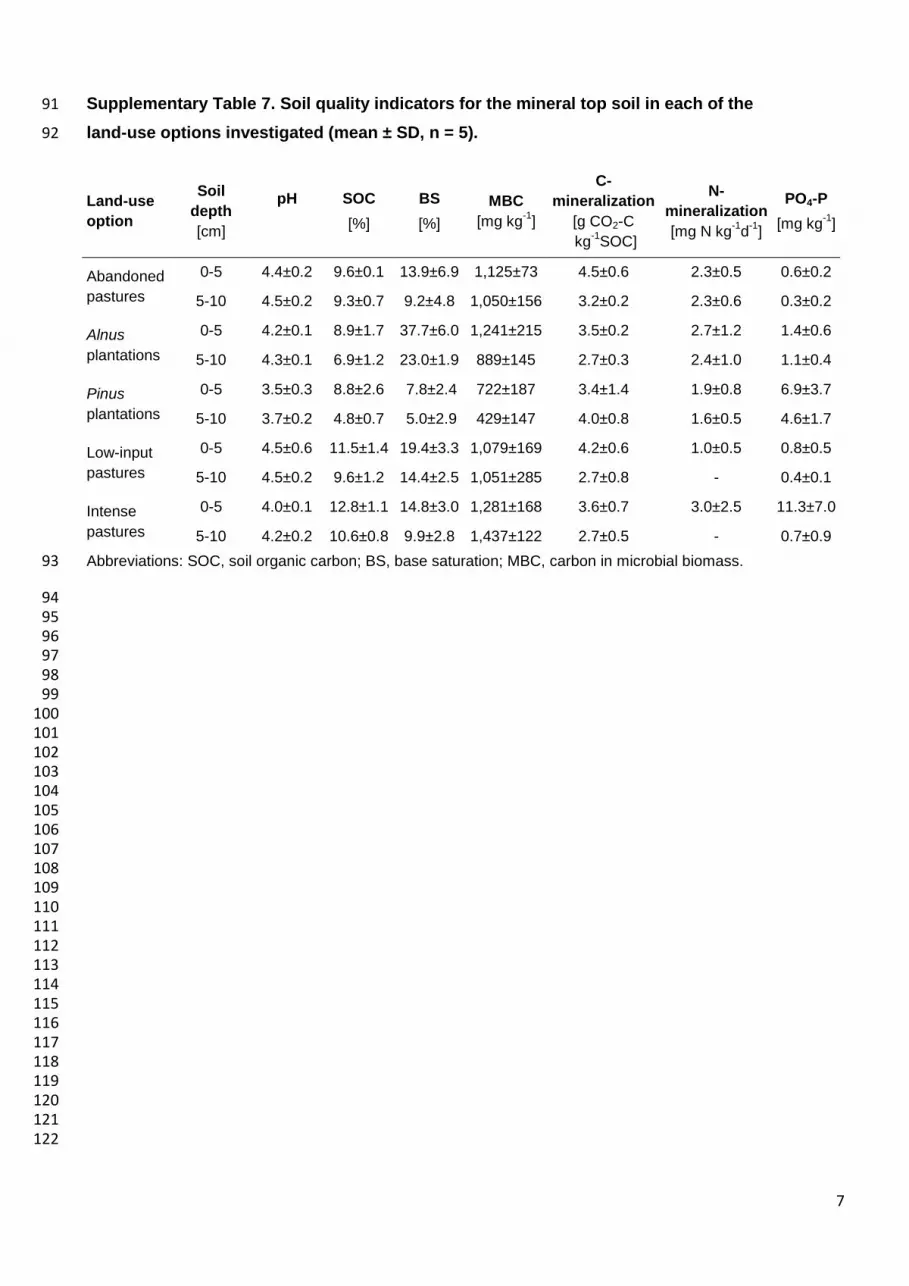
7

Supplementary Table 7. Soil quality indicators for the mineral top soil in each of the 91

land-use options investigated (mean ± SD, n = 5). 92

Land-use

option

Soil

depth

[cm]

pH

SOC

[%]

BS

[%]

MBC

[mg kg-1

]

C-

mineralization

[g CO2-C

kg-1

SOC]

N-

mineralization

[mg N kg-1

d-1

]

PO4-P

[mg kg-1

]

Abandoned

pastures

0-5 4.4±0.2 9.6±0.1 13.9±6.9 1,125±73 4.5±0.6 2.3±0.5 0.6±0.2

5-10 4.5±0.2 9.3±0.7 9.2±4.8 1,050±156 3.2±0.2 2.3±0.6 0.3±0.2

Alnus

plantations

0-5 4.2±0.1 8.9±1.7 37.7±6.0 1,241±215 3.5±0.2 2.7±1.2 1.4±0.6

5-10 4.3±0.1 6.9±1.2 23.0±1.9 889±145 2.7±0.3 2.4±1.0 1.1±0.4

Pinus

plantations

0-5 3.5±0.3 8.8±2.6 7.8±2.4 722±187 3.4±1.4 1.9±0.8 6.9±3.7

5-10 3.7±0.2 4.8±0.7 5.0±2.9 429±147 4.0±0.8 1.6±0.5 4.6±1.7

Low-input

pastures

0-5 4.5±0.6 11.5±1.4 19.4±3.3 1,079±169 4.2±0.6 1.0±0.5 0.8±0.5

5-10 4.5±0.2 9.6±1.2 14.4±2.5 1,051±285 2.7±0.8 - 0.4±0.1

Intense

pastures

0-5 4.0±0.1 12.8±1.1 14.8±3.0 1,281±168 3.6±0.7 3.0±2.5 11.3±7.0

5-10 4.2±0.2 10.6±0.8 9.9±2.8 1,437±122 2.7±0.5 - 0.7±0.9

Abbreviations: SOC, soil organic carbon; BS, base saturation; MBC, carbon in microbial biomass. 93

94 95 96 97 98 99 100 101 102 103 104 105 106 107 108 109 110 111 112 113 114 115 116 117 118 119 120 121 122

8

Supplementary Table 8. Financial coefficients used in the evaluation of each of the land-use 123 options investigated. 124

Afforesta-

tion

Alternative Time [d ha

-1 y

-1]

Material [US$ ha

-1]

Year Explanation

Site preparation

Both 5 30 0 Marking, distribution of plants removal of bracken; tools

Planting Alnus 7 333 0 Plant density=1,111 N ha-1

; planting=7 d ha

-1; plants (incl. transport)=0.3 US$ plant

-1

Pinus 7 300 0 Plant density=1,111 N ha-1

; planting=7 d ha

-1; plants (incl. transport)=0.27 US$

plant-1

Infrastructure Both 6 0 Installation of fire breaks and extraction lines

Maintenance Both 4 1-20 Maintenance of fire breaks and extraction lines

Production Costs Revenues

Both 26.2 (7) 61.73 (24) 12, 16, 20 US$ m-³ for saw timber (fuel wood)

Pasture Alternative Time [d ha

-1 y

-1]

Material [US$ ha

-1]

Year Explanation

Site preparation

Low-input 8 20 0-1 Mechanical removal of bracken (4 applications); tools

Intense 7 60 0 Chemical removal of bracken (3 applications); tools (herbicide =60US$

ha-1

)

Planting Both 45 240 0 Plant density = 32,400 N ha-1

; plant collection=20d ha

-1; plant transport

=100US$ ha-1

; planting =25d ha-1

;

Infrastructure Both 1.2 84 1,6,11,16 Material and installation of fences

Maintenance Low-input 10.4 2-20 Veterinary = 13US$ cow-1

y-1

Intense 20.8 2-20 Veterinary = 13US$ cow-1

y-1

Fertilisation Intense 4 400 0 Distribution; Fertiliser=400 US$ ha-1

application

-1

Intense 4 73 1-20 Distribution; Fertiliser=34 US$ ha-1

application

-1 (Urea 46%) + 39 US$ ha

-1

application-1

(rock phosphate)

Production Costs

milking

[US$ ha-1

]

Revenues

meat [US$ kg-1

]

milk [US$ l-1

]

Low-input 13 1.9/0.34 2-20 0.4 cows ha-1

; production period=200d ha-1

y

-1; milk quantity=4.5 l cow

-1 d

-1; meat

quantity=220 kg cow-1

y-1

; milking=6.3 d cow

-1 y

-1

Intense 34 1.9/0.34 1.5-20 1.1 cows ha-1

; production period =200d ha-1

y

-1; milk quantity=4.5 l cow

-1 d

-1; meat

quantity=220 kg cow-1

y-1

; milking=6.3 d cow

-1 y

-1

125 126

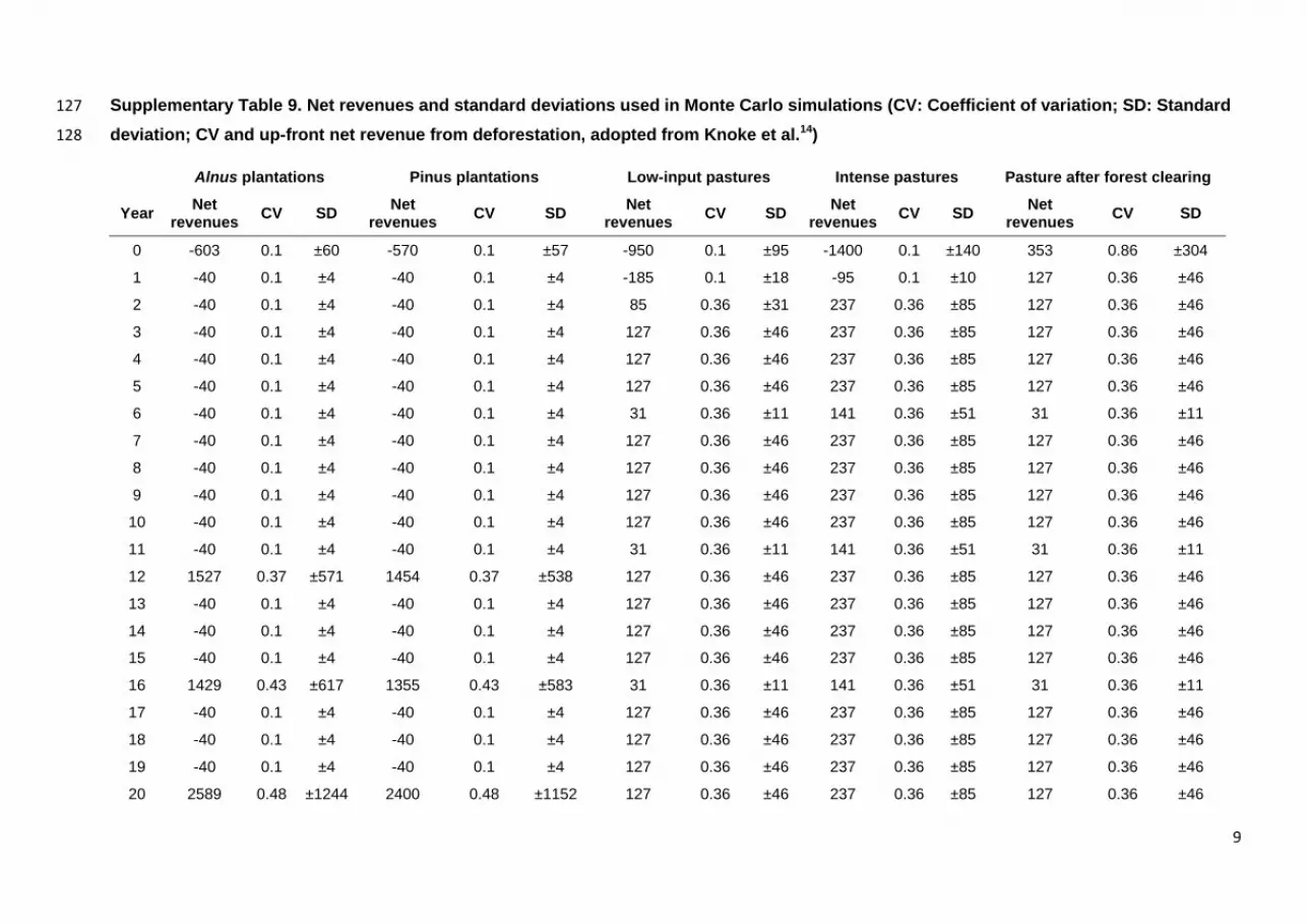
9

Supplementary Table 9. Net revenues and standard deviations used in Monte Carlo simulations (CV: Coefficient of variation; SD: Standard 127

deviation; CV and up-front net revenue from deforestation, adopted from Knoke et al.14) 128

Alnus plantations Pinus plantations Low-input pastures Intense pastures Pasture after forest clearing

Year Net

revenues CV SD

Net revenues

CV SD Net

revenues CV SD

Net revenues

CV SD Net

revenues CV SD

0 -603 0.1 ±60 -570 0.1 ±57 -950 0.1 ±95 -1400 0.1 ±140 353 0.86 ±304

1 -40 0.1 ±4 -40 0.1 ±4 -185 0.1 ±18 -95 0.1 ±10 127 0.36 ±46

2 -40 0.1 ±4 -40 0.1 ±4 85 0.36 ±31 237 0.36 ±85 127 0.36 ±46

3 -40 0.1 ±4 -40 0.1 ±4 127 0.36 ±46 237 0.36 ±85 127 0.36 ±46

4 -40 0.1 ±4 -40 0.1 ±4 127 0.36 ±46 237 0.36 ±85 127 0.36 ±46

5 -40 0.1 ±4 -40 0.1 ±4 127 0.36 ±46 237 0.36 ±85 127 0.36 ±46

6 -40 0.1 ±4 -40 0.1 ±4 31 0.36 ±11 141 0.36 ±51 31 0.36 ±11

7 -40 0.1 ±4 -40 0.1 ±4 127 0.36 ±46 237 0.36 ±85 127 0.36 ±46

8 -40 0.1 ±4 -40 0.1 ±4 127 0.36 ±46 237 0.36 ±85 127 0.36 ±46

9 -40 0.1 ±4 -40 0.1 ±4 127 0.36 ±46 237 0.36 ±85 127 0.36 ±46

10 -40 0.1 ±4 -40 0.1 ±4 127 0.36 ±46 237 0.36 ±85 127 0.36 ±46

11 -40 0.1 ±4 -40 0.1 ±4 31 0.36 ±11 141 0.36 ±51 31 0.36 ±11

12 1527 0.37 ±571 1454 0.37 ±538 127 0.36 ±46 237 0.36 ±85 127 0.36 ±46

13 -40 0.1 ±4 -40 0.1 ±4 127 0.36 ±46 237 0.36 ±85 127 0.36 ±46

14 -40 0.1 ±4 -40 0.1 ±4 127 0.36 ±46 237 0.36 ±85 127 0.36 ±46

15 -40 0.1 ±4 -40 0.1 ±4 127 0.36 ±46 237 0.36 ±85 127 0.36 ±46

16 1429 0.43 ±617 1355 0.43 ±583 31 0.36 ±11 141 0.36 ±51 31 0.36 ±11

17 -40 0.1 ±4 -40 0.1 ±4 127 0.36 ±46 237 0.36 ±85 127 0.36 ±46

18 -40 0.1 ±4 -40 0.1 ±4 127 0.36 ±46 237 0.36 ±85 127 0.36 ±46

19 -40 0.1 ±4 -40 0.1 ±4 127 0.36 ±46 237 0.36 ±85 127 0.36 ±46

20 2589 0.48 ±1244 2400 0.48 ±1152 127 0.36 ±46 237 0.36 ±85 127 0.36 ±46

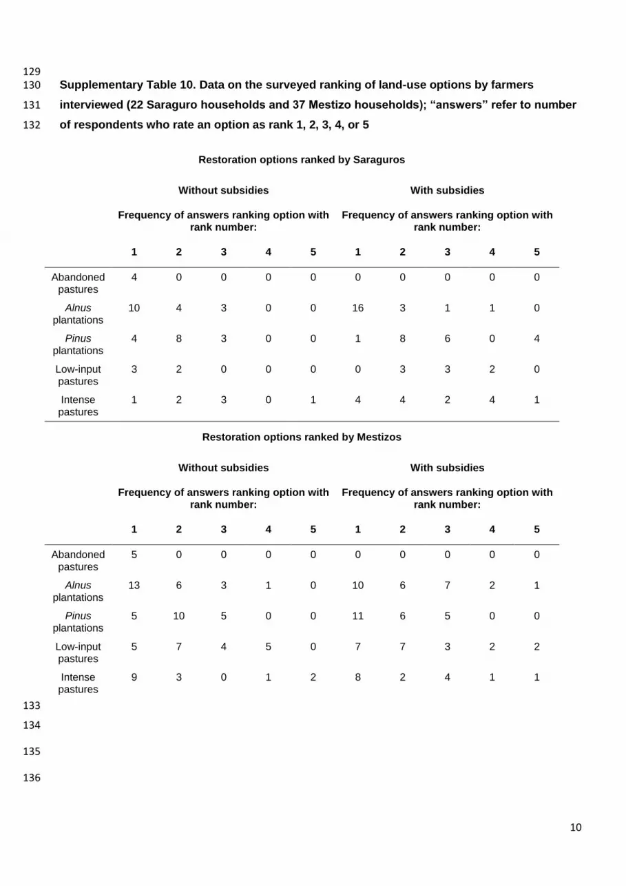
10

129 Supplementary Table 10. Data on the surveyed ranking of land-use options by farmers 130

interviewed (22 Saraguro households and 37 Mestizo households); “answers” refer to number 131

of respondents who rate an option as rank 1, 2, 3, 4, or 5 132

Restoration options ranked by Saraguros

Without subsidies With subsidies

Frequency of answers ranking option with

rank number: Frequency of answers ranking option with

rank number:

1 2 3 4 5 1 2 3 4 5

Abandoned pastures

4 0 0 0 0 0 0 0 0 0

Alnus plantations

10 4 3 0 0 16 3 1 1 0

Pinus plantations

4 8 3 0 0 1 8 6 0 4

Low-input pastures

3 2 0 0 0 0 3 3 2 0

Intense pastures

1 2 3 0 1 4 4 2 4 1

Restoration options ranked by Mestizos

Without subsidies With subsidies

Frequency of answers ranking option with

rank number: Frequency of answers ranking option with

rank number:

1 2 3 4 5 1 2 3 4 5

Abandoned pastures

5 0 0 0 0 0 0 0 0 0

Alnus plantations

13 6 3 1 0 10 6 7 2 1

Pinus plantations

5 10 5 0 0 11 6 5 0 0

Low-input pastures

5 7 4 5 0 7 7 3 2 2

Intense pastures

9 3 0 1 2 8 2 4 1 1

133

134

135

136

11

Supplementary Table 11. Difference between climatic and hydrologic indicator means 137

obtained from two model runs - one with 0 and one with 10 years spin-up time. 138

Parameterisation, forcing and indicator units are the same as those presented in 139

Tables 4 and 5 in the main text. 140

Option Evapo-

transpiration Turbulence Overland flow Area-specific discharge

Abandoned pastures

0 0 -2 1

Alnus plantations 0 0 2 -2

Pinus plantations 0 0 0 0

Low-input pastures 0 0 0 0

Intense pastures 0 0 0 0

141

12

Supplementary Table 12. Most important model parameters in terms of parameter 142

uncertainty, indicated by their expected maximum deviation from mean (span ±), for 143

each of the plants characterizing the land-use options simulated using the SoBraCo model. 144

Table refers to parameters as described in Bendix et al.6 and Silva et al.46. PDF: probability 145

density function. NIR: Near infrared. 146

SoBrCoMo

Plant Parameter PDF Form Mean Span (±%)

Source of model data

Bracken, abandoned pastures

Leaf albedo NIR Triangular 0.475 10 Göttlicher et al.4

Maximum carboxylation rate 68.8

Silva et al.5 Quantum efficiency 0.048

Root coefficient a 3

Root coefficient b 3

Leaf dimension* Uniform 0.030 5

Destructive measurements from

1m2 vegetation surface (n=3; values obtained:

0.025, 0.025, 0.026)

Displacement height 0.7

LAI Scenario

forcing Bendix et al.6

Setaria, active pastures

Leaf albedo NIR Triangular 0.40 10 Göttlicher et al.4

Maximum carboxylation rate 29.2 Silva et al.5

Quantum efficiency 0.50

Root coefficient a 33.0

Root coefficient b 9

Leaf dimension* Uniform 0.020 5

Destructive measurements from

1m2 vegetation surface (n=3; values obtained:

0.022, 0.017, 0.019)

Displacement height 0.55

LAI Scenario

forcing Bendix et al.6

Alnus plantations

Leaf albedo NIR Triangular 50.3 10 Göttlicher et al.4

Maximum carboxylation rate 40 Oleson and Dai7

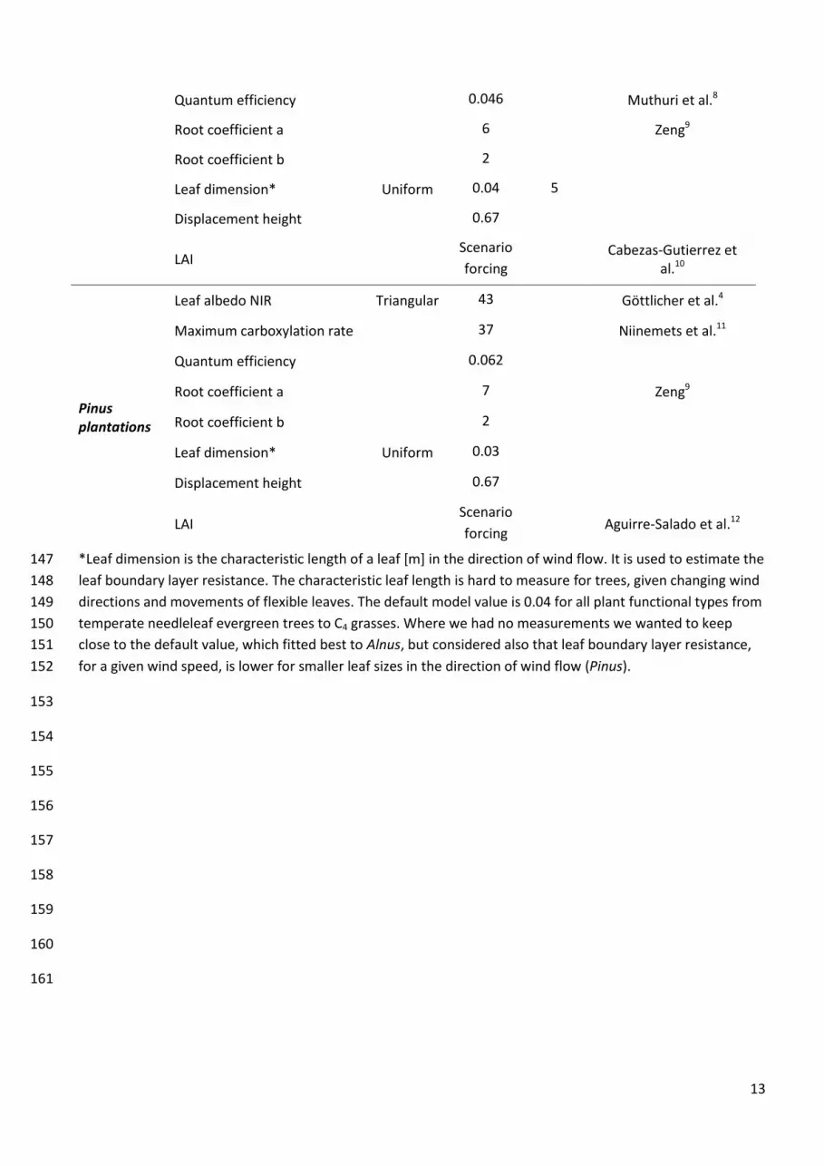
13

Quantum efficiency 0.046 Muthuri et al.8

Root coefficient a 6 Zeng9

Root coefficient b 2

Leaf dimension* Uniform 0.04 5

Displacement height 0.67

LAI Scenario

forcing

Cabezas-Gutierrez et al.10

Pinus plantations

Leaf albedo NIR Triangular 43 Göttlicher et al.4

Maximum carboxylation rate 37 Niinemets et al.11

Quantum efficiency 0.062

Root coefficient a 7 Zeng9

Root coefficient b 2

Leaf dimension* Uniform 0.03

Displacement height 0.67

LAI Scenario

forcing Aguirre-Salado et al.12

*Leaf dimension is the characteristic length of a leaf [m] in the direction of wind flow. It is used to estimate the 147

leaf boundary layer resistance. The characteristic leaf length is hard to measure for trees, given changing wind 148

directions and movements of flexible leaves. The default model value is 0.04 for all plant functional types from 149

temperate needleleaf evergreen trees to C4 grasses. Where we had no measurements we wanted to keep 150

close to the default value, which fitted best to Alnus, but considered also that leaf boundary layer resistance, 151

for a given wind speed, is lower for smaller leaf sizes in the direction of wind flow (Pinus). 152

153

154

155

156

157

158

159

160

161

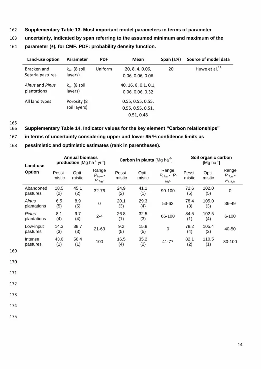
14

Supplementary Table 13. Most important model parameters in terms of parameter 162

uncertainty, indicated by span referring to the assumed minimum and maximum of the 163

parameter (±), for CMF. PDF: probability density function. 164

Land-use option Parameter PDF Mean Span (±%) Source of model data

Bracken and Setaria pastures

ksat (8 soil layers)

Uniform 20, 8, 4, 0.06,

0.06, 0.06, 0.06

20 Huwe et al.13

Alnus and Pinus plantations

ksat (8 soil layers)

40, 16, 8, 0.1, 0.1,

0.06, 0.06, 0.32

All land types Porosity (8 soil layers)

0.55, 0.55, 0.55,

0.55, 0.55, 0.51,

0.51, 0.48

165 Supplementary Table 14. Indicator values for the key element “Carbon relationships” 166

in terms of uncertainty considering upper and lower 95 % confidence limits as 167

pessimistic and optimistic estimates (rank in parentheses). 168

Land-use

Option

Annual biomass production [Mg ha

-1 yr

-1]

Carbon in planta [Mg ha-1

] Soil organic carbon

[Mg ha-1

]

Pessi-mistic

Opti-mistic

Range Pi low - Pi high

Pessi-mistic

Opti-mistic

Range Pi low - Pi

high

Pessi-mistic

Opti-mistic

Range Pi low - Pi high

Abandoned pastures

18.5 (2)

45.1 (2)

32-76 24.9 (2)

41.1 (1)

90-100 72.6 (5)

102.0 (5)

0

Alnus plantations

6.5 (5)

8.9 (5)

0 20.1 (3)

29.3 (4)

53-62 78.4 (3)

105.0 (3)

36-49

Pinus plantations

8.1 (4)

9.7 (4)

2-4 26.8 (1)

32.5 (3)

66-100 84.5 (1)

102.5 (4)

6-100

Low-input pastures

14.3 (3)

38.7 (3)

21-63 9.2 (5)

15.8 (5)

0 78.2 (4)

105.4 (2)

40-50

Intense pastures

43.6 (1)

56.4 (1)

100 16.5 (4)

35.2 (2)

41-77 82.1 (2)

110.5 (1)

80-100

169

170

171

172

173

174

175

15

Supplementary Table 15. Indicator values for the key element “Climate regulation” in 176

terms of parameter uncertainty after 3,216 Monte-Carlo (MC) simulation runs considering 177

upper and lower 95 % confidence limits as pessimistic and optimistic estimates (rank in 178

parentheses). 179

Land-use

Option Evapo-transpiration (ET) [mm]

Momentum flux [kg m

-1 sec

-2]

Pessimistic Optimistic Range Pi low - Pi high

Pessimistic Optimistic Range Pi low - Pi high

Abandoned pastures

921 (5) 936 (5) 0-0 0.0174 (5) 0.0184 (5) 0-0

Alnus plantations

1589 (1) 1600 (1) 100-100 0.2544 (2) 0.3156 (1) 86-100

Pinus plantations

1407 (2) 1415 (2) 71-73 0.2932 (1) 0.2947 (2) 93-100

Low-input pastures

1175 (3) 1197 (3) 38-39 0.0229 (4) 0.0231 (4) 2-2

Intense pastures

1157 (4) 1177 (4) 35-36 0.0252 (3) 0.0268 (3) 3-3

180

181

182 Supplementary Table 16. Indicator values for the key element “Hydrological regulation” 183

(considering high area specific discharge as negative) in terms of parameter uncertainty 184

after 3,216 Monte-Carlo (MC) simulation runs considering upper and lower 95 % confidence 185

limits as pessimistic and optimistic estimates (rank in parentheses). 186

Land-use

Option Overland flow [mm y

-1]

Area specific discharge [mm y

-1]

Pessimistic Optimistic Range Pi low - Pi high

Pessimistic Optimistic Range Pi low - Pi high

Abandoned pastures

82 (4) 68 (3) 1-8 941 (5) 913 (5) 0-0

Alnus plantations

40 (2) 36 (2) 77-85 291 (1) 275 (1) 100-100

Pinus plantations

32 (1) 26 (1) 100-100 476 (2) 465 (2) 70-71

Low-input pastures

81 (3) 69 (4) 4-4 691 (4) 663 (4) 38-39

Intense pastures

83 (5) 71 (5) 0-0 707 (3) 683 (3) 36-36

187

188

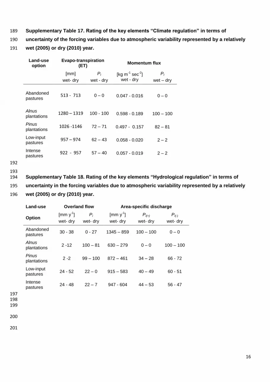
16

Supplementary Table 17. Rating of the key elements “Climate regulation” in terms of 189

uncertainty of the forcing variables due to atmospheric variability represented by a relatively 190

wet (2005) or dry (2010) year. 191

Land-use option

Evapo-transpiration (ET)

Momentum flux

[mm]

wet- dry

PI

wet - dry

[kg m-1

sec-2

] wet - dry

PI

wet – dry

Abandoned pastures

513 - 713 0 – 0

0.047 - 0.016

0 – 0

Alnus plantations

1280 – 1319 100 - 100 0.598 - 0.189 100 – 100

Pinus plantations

1026 -1146 72 – 71 0.497 - 0.157 82 – 81

Low-input pastures

957 – 974 62 – 43 0.058 - 0.020 2 – 2

Intense pastures

922 - 957 57 – 40 0.057 - 0.019 2 – 2

192

193 Supplementary Table 18. Rating of the key elements “Hydrological regulation” in terms of 194

uncertainty in the forcing variables due to atmospheric variability represented by a relatively 195

wet (2005) or dry (2010) year. 196

Land-use Overland flow Area-specific discharge

Option [mm y

-1]

wet- dry

Pi

wet- dry

[mm y-1

]

wet- dry

Pi(+)

wet- dry

Pi(-)

wet- dry

Abandoned pastures

30 - 38 0 - 27 1345 – 859 100 – 100 0 – 0

Alnus plantations

2 -12 100 – 81 630 – 279 0 – 0 100 – 100

Pinus plantations

2 -2 99 – 100 872 – 461 34 – 28 66 - 72

Low-input pastures

24 - 52 22 – 0 915 – 583 40 – 49 60 - 51

Intense pastures

24 - 48 22 – 7 947 - 604 44 – 53 56 - 47

197 198 199

200

201

17

Supplementary Table 19. Range of index values (Pi) for the key element “Soil quality” 202

when upper and lower 95 % confidence limits as pessimistic and optimistic estimates are 203

used to estimate indicator values. 204

Land-use option

pH

SOC

[%]

BS

[%]

MBC [mg kg

-1]

C- mineralization

[g CO2-C kg

-1SOC]

N-minerali-zation [mg N

kg-1

d-1

]

PO4-P

[mg kg-1

]

Abandoned pastures

93 -100 30 -72 6 - 34 59 - 71 61 - 100 33 - 100 0 - 0

Alnus plantations

73 - 98 22 - 23 100 - 100 59 - 66 0 – 33 55 - 89 11 - 19

Pinus plantations

0 - 0 0 - 0 0 - 0 0 - 0 0 – 100 26 - 66 83 – 100

Low-input pastures

92 - 100 73 - 74 42 - 46 52 - 74 26 – 57 0 - 21 0 – 2

Intense pastures

66 - 83 100 - 100 22 - 23 100-100 7 – 30 0 - 100 47 – 100

18

Supplementary Table 20. Indicator values for the economic key elements for an assumed 205

discount rate of 8% in terms of uncertainty of the coefficients used in the economic 206

calculation after 3,000 MC simulation runs considering upper and lower 95 % confidence 207

limits as pessimistic and optimistic estimates (rank in parentheses). 208

Land-use

option

NPV (Euro/ha) Payback period (years)

Pessimistic Optimistic Range Pi low - Pi high

Pessimistic Optimistic Range Pi low - Pi high

Abandoned pastures

0 (2) 0 (5) 3-53 0 (1) 0 (1) 100-100

Alnus plantations

-153 (3) 1397 (1) 59-100 24 (3) 8 (3) 40-66

Pinus plantations

-170 (4) 1308 (2) 55-94 24 (3) 8 (3) 40-66

Low-input pastures

-409 (5) 113 (4) 0-0 40 (5) 24 (5) 0-0

Intense pastures

26 (1) 924 (3) 66-100 21 (2) 5 (2) 48-79

209 210 Supplementary Table 21. Indicator values for the “Social preference” (example without 211

subsidy) key elements considering upper and lower 95 % confidence limits as 212

pessimistic and optimistic estimates (rank in parentheses). Answers refer to number of 213

respondents who rate an option as best or second best 214

Land-use

option

Answers Saraguros Answers Mestizos

Pessimistic Optimistic Range Pi low - Pi high

Pessimistic Optimistic Range Pi low - Pi high

Abandoned pastures

0 (4) 8 (4) 0-0 1 (5) 9 (5) 0-0

Alnus plantations

8 (1) 20 (1) 100-100 12 (1) 26 (1) 100-100

Pinus plantations

6 (2) 18 (2) 77-82 8 (2) 22 (2) 40-66

Low-input pastures

1 (3) 9 (3) 8-11 6 (3) 18 (3) 45-53

Intense pastures

0 (4) 8 (4) 0-0 6 (3) 18 (3) 45-53

215 216

217 218 219

220 221

19

Supplementary Table 22. t- and p-values (in parentheses) for statistical contrasts 222

between land-use options tested in conjunction with a one-way ANOVA on rank-223

transformed data. Abbreviations: Ab=abandoned pastures, A=Alnus, P=Pinus, L=low-224

input pastures, and I=intense pastures. Standardised differences (t-values) associated 225

with p-values <= 0.10 considered significant (indicated in bold). Contrast 1 ( -4 I 1 I 1 I 1 I 226

1 ), contrast 2 ( 0 I 1 I 1 I -1 I -1 ), contrast 3 ( 0 I 1 I -1 I 0 I 0 ), and contrast 4 ( 0 I 0 I 0 I -1 I 227

1), respectively, indicate that: 1. All restoration options on average improve the 228

ecological and socio-economic index values significantly, 2. afforestations perform 229

significantly better than pasturing options, 3. Alnus does not differ significantly from 230

Pinus, and 4. intense pasture is better than low-input pasture on a significance level of at 231

least α<0.1 in most scenarios (n.s.: not significant). 232

t-values and associated p-values in parentheses for five scenarios tested:

Contrast

Scenario tested in main text

Index values weighted with relative range of maximum

variation (a. in Supplementary

Figure 1)

Optimistic index values

(b. in Supplementary

Figure 1)

Pessimistic index values

(c. in Supplementary

Figure 1)

Subjectively weighted index

values (d. in Supplementary

Figure 1)

1. (A+P+L+I)/4 > Ab 2.3

(<0.025) 2.4

(<0.025) 2.6

(<0.025) 1.5

(<0.100) 1.9

(<0.050)

2. (A+P)/2 > (L+I)/2 3.1

(<0.025) 2.6

(<0.025) 2.7

(<0.025) 3.3

(<0.025) 2.4

(<0.025)

3. A > P 0.9

(n.s.) 0.5

(n.s.) 0.9

(n.s.) 1.0

(n.s.) 0.7

(n.s.)

4. L < I 1.6

(<0.100) 1.9

(<0.050) 1.4

(<0.100) 1.6

(<0.100) 1.1

(n.s.)

233

20

Supplementary Methods 234

1. Background information on research area 235

2. Land-use options investigated 236

2.1. Leaving areas abandoned 237

2.2. Afforestation 238

2.3. Pasture use 239

3. Indicators evaluated 240

3.1. Ecological 241

3.1.1. Biomass production and carbon-sequestration 242

3.1.2. Climate and water indicators 243

3.1.3. Soil quality 244

3.2. Economic 245

3.3. Social 246

247

1. Background information on research area 248

The research area is in the catchment area and valley of the Rio San Francisco (1,000-249

2,800 m a.s.l.) which is a deeply incised valley in the very humid eastern range 250

“Cordillera oriental” of the Andes in southern Ecuador15. As such, it is representative of 251

the biogeographical and socio-economic setting of the eastern escarpment of the 252

tropical Andes. 253

Climate. Air temperature in the forest-to-pasture conversion zone of the San Francisco 254

Valley is generally <16°C16. The area is characterized by very humid conditions year-255

round, with annual rainfall exceeding 1,800 mm (up to 6,000 mm y-1 including occult 256

precipitation at 3,200 m asl) and without any pronounced dry season17. This is caused 257

by a very high perennial cloud frequency of around 80%18. Inter-annual variability 258

depends largely on the ENSO (El Niño / Southern Oscillation) cycle19,20, which seems to 259

have changed slightly since 200021. 260

Soils. Most soils in the deforestation areas are Dystrudept soils. These soils are 261

frequently characterised by hydromorphic properties due to humid conditions, as well as 262

by acidic pH values, enhanced soil moisture, a well-established organic layer and a 263

poor nutrient situation (high C/N ratio, N and P deficiencies)22-24. 264

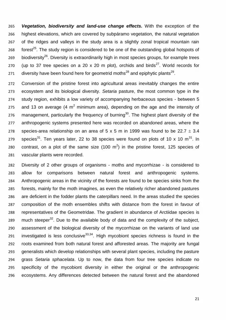
21

Vegetation, biodiversity and land-use change effects. With the exception of the 265

highest elevations, which are covered by subpáramo vegetation, the natural vegetation 266

of the ridges and valleys in the study area is a slightly zonal tropical mountain rain 267

forest25. The study region is considered to be one of the outstanding global hotspots of 268

biodiversity26. Diversity is extraordinarily high in most species groups, for example trees 269

(up to 37 tree species on a 20 x 20 m plot), orchids and birds27. World records for 270

diversity have been found here for geometrid moths28 and epiphytic plants29. 271

Conversion of the pristine forest into agricultural areas inevitably changes the entire 272

ecosystem and its biological diversity. Setaria pasture, the most common type in the 273

study region, exhibits a low variety of accompanying herbaceous species - between 5 274

and 13 on average (4 m2 minimum area), depending on the age and the intensity of 275

management, particularly the frequency of burning30. The highest plant diversity of the 276

anthropogenic systems presented here was recorded on abandoned areas, where the 277

species-area relationship on an area of 5 x 5 m in 1999 was found to be 22.7 3.4 278

species31. Ten years later, 22 to 38 species were found on plots of 10 x 10 m31. In 279

contrast, on a plot of the same size (100 m2) in the pristine forest, 125 species of 280

vascular plants were recorded. 281

Diversity of 2 other groups of organisms - moths and mycorrhizae - is considered to 282

allow for comparisons between natural forest and anthropogenic systems. 283

Anthropogenic areas in the vicinity of the forests are found to be species sinks from the 284

forests, mainly for the moth imagines, as even the relatively richer abandoned pastures 285

are deficient in the fodder plants the caterpillars need. In the areas studied the species 286

composition of the moth ensembles shifts with distance from the forest in favour of 287

representatives of the Geometridae. The gradient in abundance of Arctiidae species is 288

much steeper32. Due to the available body of data and the complexity of the subject, 289

assessment of the biological diversity of the mycorrhizae on the variants of land use 290

investigated is less conclusive33,34. High mycobiont species richness is found in the 291

roots examined from both natural forest and afforested areas. The majority are fungal 292

generalists which develop relationships with several plant species, including the pasture 293

grass Setaria sphacelata. Up to now, the data from four tree species indicate no 294

specificity of the mycobiont diversity in either the original or the anthropogenic 295

ecosystems. Any differences detected between the natural forest and the abandoned 296

22

pastures are difficult to assess because they may be due purely to inherent differences 297

in the two types of habitats, or simply to plant age. 298

In summary, clearing of the forest for agricultural land use causes an extraordinary 299

decline in vascular plant and moth diversity, which may or may not be paralleled by soil 300

fungal diversity. After areas are abandoned, plant diversity increases a little, but 301

remains far below that of the pristine forest. Moth diversity still relies on migration rather 302

than on the establishment of unique populations. Fungal diversity remains rich in the 303

anthropogenic systems, particularly in afforested areas, where it is comparable to that in 304

natural forest. 305

Land-use change and non-sustainable pasture management. From the valley floor 306

upwards, the forest has been cleared by slash and burn for agricultural purposes - 307

mostly pasture. The most common pasture grasses used are introduced species such 308

as Setaria sphacelata (which is planted manually) or Melinis minutiflora, both of which 309

are native to south and central Africa. In the core research area of 120 km2, around 310

35% of areas that have been converted to pasture are no longer used because of 311

infestation by weeds35. 312

The nutritive value of the grasses commonly used here is rather low, and therefore, the 313

majority of pastures are overgrazed. This sets in motion a vicious cycle, as weeds 314

eventually overgrow the non-native pasture grasses. Bracken fern (Pteridium 315

arachnoideum and Pt. caudatum) is the most problematic weed handicapping 316

agriculture in tropical mountains. Fire is commonly used by the local farmers to 317

rejuvenate pastures and remove weeds. However, tropical bracken and other 318

aggressive weeds have proven to be fire-resistant, and therefore, in the long run, 319

burning favours the weeds and eventually leads to abandonment of the pasture36. At 320

this stage, the weeds form a closed canopy, which prevents return of the natural 321

forest30. 322

The farmers. Most of the farmers in the area are Mestizos, a term generally used to 323

indicate people of mixed Spanish and indigenous descent. Neighbouring valleys are 324

also inhabited by indigenous Saraguros - Quechua-speaking Indians who traditionally 325

inhabited the Andean uplands of southern Ecuador. Farmers of both ethnic groups are 326

colonists who arrived in the study area during the 20th century. As agro-pastoralists37,38, 327

they participate in both a market economy (cattle ranching for cheese, milk and meat 328

production) and a subsistence economy (crop production, horticulture and cattle 329

23

ranching for subsistence needs). Cattle ranching is the most important market activity, 330

and from the farmers’ point of view, the most profitable. The main product drawn from 331

cattle ranching is cheese (quesillo - an unsalted fresh white cheese), which is sold in the 332

local markets. Only farmers who have good access to roads can sell milk to regional 333

producers of dairy products. Despite both ethnic groups practicing a similar land-use 334

system, Saraguros derive more income from cattle ranching than Mestizos and 335

Mestizos have higher off-farm incomes (employment, remittances) than Saraguros37,38. 336

Migration of farmers is an important phenomenon. According to the census of 2010, 337

from 1,324 persons born in the study area (Imbana, Sabanilla), 335 were registered in 338

other regions in the country and, of these, 249 lived in urban areas. Population has 339

decreased by around 6% (from 1,807 to 1,710 people) since the previous census in 340

2001; also, the percentage of the population economically active in agriculture 341

decreased from 83% in 2001 to 65% in 201039. These trends are mainly due to the lack 342

of agricultural labour in the region and the opportunity for wage labour elsewhere. 343

344

2. Land-use options investigated 345

2.1. Leaving areas abandoned 346

Abandoned areas are usually covered by bracken fern (Pteridium arachnoideum (Kaulf.) 347

Maxon and Pt. caudatum (L.) Maxon) interspersed with quickly reproducing shrubs. Fire 348

usually kills the above-ground parts of this vegetation, but the plants can readily re-349

sprout from subterranean buds, such as the short lateral rhizomes of the bracken fern. 350

This type of fire-resistant plant community with a high potential for propagation is 351

encountered in many abandoned farming areas of the southern Ecuadorian Andes, and 352

can be considered a type of “novel ecosystem”40 resulting from human activities. It 353

forms our reference as a typical widespread ecosystem in the southern Ecuadorian 354

Andes (phytosociological details in Hartig & Beck30). 355

2.2. Afforestation 356

Afforestation with native Andean alder (Alnus acuminata). This option is based on 357

data from an afforestation experiment consisting of afforestation plots (10.8 x 10.8 m), 358

with 6 repetitions each41. Bracken leaves were removed manually and saplings up to 359

0.5 m tall were planted. Any regrowth of bracken was removed in the same way during 360

the following 2 years. Modelling of future growth was based on this experimental data, 361

24

using an annual mortality rate of 2 % of the number of trees per hectare and the 362

commonly used seedling distance of 3 m x 3 m. The harvest regime began after 12 363

years with an initial thinning of 40% of the number of trees per hectare followed by a 364

second thinning of the same intensity 16 years after the initial planting. The final harvest 365

of crop trees was simulated after 20 years. 366

Afforestation with exotic Pinus patula. Pinus patula or Eucalyptus saligna are 367

commonly used for afforestation in southern Ecuador. Here, we considered Pinus patula 368

as a fast-growing, exotic alternative to alder. The calculations used were based on data 369

from the previously mentioned reforestation experiment where Pinus was also planted, 370

and the same protocol was used, including tree density, mortality rate and harvest 371

regime. 372

373

2.3. Pasture 374

The total area of repasturisation was 4,500 m2, and was subdivided into 4 x 4 m plots. 375

Each treatment was investigated in 4 parallels to average possible variations in site 376

quality. The procedures used for weed removal and planting of grass are described in 377

Roos et al.42. 378

Weed removal and low-input pasture. Pasture rehabilitation42 proved successful 379

when three consecutive steps were followed: i) Bracken control by repetitive cutting of 380

the leaves during 1 year. Four such cutting campaigns were sufficient. ii) After a short 381

fallow period, the common pasture grass, Setaria sphacelata, was purchased from local 382

farmers and planted manually at the customary density (32,400 plantlets x ha-1). 383

Planting of 1 ha required approximately 1 month. After approximately one and half 384

years, the grass had reached a cover percentage of more than 70% and grazing could 385

begin. iii) Grazing was simulated by cutting the grass to a residual height of 20 cm. 386

Regrown bracken fronds were kept in check by simulating trampling by cattle. Two 387

grazing rounds per year were thought to represent a compromise between sustainable 388

and maximal grass yields, and were expected to result in sufficient trampling to prevent 389

recovery of bracken. 390

Weed removal and intense pasture use. This option paralleled low-input pasture, but 391

bracken removal was accomplished by spraying a common herbicide (“Combo”: 392

picloram: 960 g a.i. ha-1 and metsulfuron methyl: 2,400 g a.i. ha-1; Dow Agro Science) 393

25

three times (within nine months) and subsequent application of chemical fertiliser. The 394

results obtained during two years of pasture fertilisation and grazing revealed co-395

limitation of productivity by levels of both N and P, with the latter being particularly 396

important. Fertilisation with NPK (150 kg N, 86 kg P, and 107 kg K ha-1 y-1) did not 397

change the nutritive value of the pasture grass, but increased its growth and biomass 398

production significantly (Supplementary Table 1). Three grazing rounds per year were 399

simulated, with a higher number of cattle than in the low-input option to insure sufficient 400

trampling of the fern. High yields have been achieved on long-standing pasture on 401

favourable sites using a fertilisation protocol to replace the nutrients removed by grazing 402

(50 kg N and 10 kg P ha-1 y-1; 1.25-fold increase from 9.02 Mg DM ha-1 y-1 to 11.2 Mg 403

DM ha-1 y-1)1,43. In these cases, the levels of protein, N, P and Ca were also much 404

higher than in our research pastures (Supplementary Table 1). According to the 405

National Research Council44, about 0.89 kg crude protein per day is required by highly 406

productive mature dairy cattle. The daily requirements of cattle for P (10 g to 28 g) and 407

Ca (14 g to 56 g) vary strongly depending on such factors as breed, current body weight 408

and lactation status. In the research area, only a small percentage of the cattle are dairy 409

cows, and breeding of calves is very common. Therefore the number of possible cattle 410

is higher than calculated from the nutritive value assumed to be necessary for dairy 411

cattle. For the low-input pasture management option modelled here, 0.4 head of cattle 412

per hectare were assumed, and for the intense pasture, 1.1 head. These are still 413

modest assumptions, because on high yielding pasture twice as many cattle could be 414

maintained. 415

416

3. Indicators evaluated 417

3.1. Ecological 418

3.1.1. Biomass production and carbon sequestration 419

The data used for the evaluation of the carbon relationships of the 5 land-use options 420

are presented in Supplementary Tables 2 and 3. Average carbon stocks (“Carbon in 421

planta”) are calculated individually for above- and below-ground biomass 422

(Supplementary Table 3) and average standing crop data, which is common practice in 423

carbon assessment for of ecosystems45. Total carbon stocks in the above- and below-424

ground biomass, and in the top 20 cm soil layer are used to assess the carbon balances 425

of the various land-use options. When equilibria are considered (abandoned area, 426

pasture), constant carbon stocks are assumed to take into account smaller fluctuations 427

26

due to weather conditions46. In the afforestation options, carbon stocks increase with 428

tree growth but decrease after thinning. 429

Abandoned areas. Bracken leaf is assumed to have an average lifetime of 8 months47. 430

Thus, annual aboveground biomass production is estimated as standing crop volume 431

times 12/8, and is equal to 9.15 Mg ha-1 y-1. Because the lifetime of the below-ground 432

bracken organs (rhizomes and roots) is difficult to measure, an average value of 22.6 433

Mg ha-1 y-1 for bracken below-ground biomass production is estimated using the 434

SoBraCo-Model46. 435

Pinus and Alnus plantations. Volume equations obtained from the literature are used 436

to calculate both the standing and the commercial timber volume for A. acuminata48 and 437

P. patula49. Based on the number of trees per hectare (N), the diameter at 1.3 m height 438

(dbh), and the mean total height (ht), estimated regression curves are as follows: 439

dbhAlnus = 1.516 – 1.778 ln(N) + 12.287 ln(age) 440

dbhPinus = 1.803 – 0.969 ln(N) + 10.165 ln(age) 441

htAlnus = EXP(5.132 + 0.644 ln(dbh)) 442

htPinus = 1282.369 + 249.983 ln(dbh) – 214.119 ln(N) + 273.475 ln(age); 443

dbh = mean diameter at breast height [cm], N = number of trees/hectare, age = age of 444

plantation [years], ht = mean height of trees [cm]. 445

Above-ground biomass is calculated using the equation developed by Figueroa-Navarro 446

et al.50 for P. patula and that from Acosta-Mireles et al.3 for A. acuminata. Below-ground 447

biomass is estimated based on a shoot : root ratio of 1:0.2052. The concentration of 448

carbon for both species in litter and in timber is around 50 %. Therefore, the rate of 449

carbon sequestration is calculated as half of the corresponding biomass. For the leaf 450

area indices (LAI) methods used, see Materials and Methods, chapter Climate. The 451

resulting stand characteristics for afforestation with A. acuminata and P. patula are 452

shown in Supplementary Table 4. These figures take both thinnings and mortality into 453

account. 454

Low-input and intense pasture. In the grazing simulation, above-ground biomass was 455

harvested and both fresh and dry weights determined. This material is included in the 456

calculation of annual biomass production. Below-ground biomass production is 457

calculated using the SoBraCo-model parameterised with adjusted LAI and vegetation 458

height data collected during the second management year. Average standing above-459

27

ground crop is calculated, accounting for the material extracted by simulated grazing. 460

Grass biomass from 0 to 20 cm in height is added to this amount to account for the 461

material not removed in the grazing simulation. Below-ground average standing crop 462

was analysed from soil cores, as described in Material and Methods. Uncertainty from 463

using 95 % confidence limits of indicators to estimate indices is reported in 464

Supplementary Table 5. 465

3.1.2. Climate and water indicators 466

Comprehensive validation of the SVAT and vegetation growth model CLM (Community 467

Land Model), which is the numerical basis of SoBraCoMo46, reveals that the uncertainty 468

of GPP and ET simulations for all plant functional types lies well within the uncertainty of 469

FLUXNET‐based validation estimates (e.g. Bonan et al.51). In the current study, the 470

simulations are forced using data from an average meteorological year (2008) as 471

measured at a specifically designed micrometeorological station onsite (lat.: 3.96427°S, 472

long: 79.07689°W, 2109 m a.s.l.)46. The measurements used are solar irradiation, air 473

temperature (0.5 and 2 m), relative humidity (0.5 and 2 m), leaf temperature (sunlit and 474

shaded), wind speed, rainfall, soil water content and soil temperature. The year 2008 475

was selected as a typical year for the area based on data collected between 1981 and 476

2010 at the INAMHI (Ecuadorian Weather Service) station Loja La Argelia (lat.: 477

4.03055°S, long: 79.19944°W, 2160 m a.s.l.). This is the only long-term data set 478

available (temperature and rainfall only) for the wider study area. Average temperature 479

and monthly total rainfall for 2008 (15.9°C, 115 mm/month) are similar to long-term 480

averages (16.0°C with SD of ±0.8°C; 78.1 mm/month with SD of ±48.9 mm/month). The 481

annual time series used for model forcing consists of hourly aggregated meteorological 482

variables and is applied repeatedly for the entire 20-year period. 483

Required plant-specific model parameters are derived either from measurements at leaf 484

and root levels in the study site, or from data available from the literature (for further 485

details refer to Silva et al.46, Supplementary Table 12 and Potthast et al.52 for soil 486

parameters). The parameters derived are leaf area index, leaf tilt angle, leaf reflectance 487

and transmittance, quantum yield, carboxylation rate of sunlit/shade leaves, Q10 488

temperature coefficient, entropy factor, deactivation energy, dark respiration at 25°C of 489

sunlit/shaded leaves, activation energy for respiration, vertical density of root 490

distribution, root/rhizome biomass, root/rhizome C:N ratio and CO2 to biomass 491

conversion factor. 492

28

In the coupled model framework (see next para), the SoBraCoMo calculates the main 493

water and momentum fluxes between the canopy and the atmosphere, which are 494

important for assessing land-use change effects on climate regulation functions. The 495

variables considered for the climatic assessment are (i) evapotranspiration and (ii) 496

turbulence production, with the latter expressed as the sum of zonal and meridional 497

momentum fluxes. With regard to carbon and biomass estimates, the model also 498

computes net canopy photosynthesis, based on the “two-big-leaf” approach. Validation 499

with porometer observations showed a high level of accuracy for the model results, with 500

deviations between simulated and observed leaf net assimilation of less than 5%46. 501

The Catchment Modelling Framework (CMF53) is a state-of-the-art programming library 502

used to create hydrological models which are highly modular and connectible to other 503

models. Due to its modular structure, it is suitable for simulating a wide variety of 504

hydrological conditions and has proven to provide reliable results in complex, 505

intrinsically coupled modelling systems54,55. Eight soil layers of increasing thicknesses 506

from the top downwards are summed to reach a total column depth of 1 m 507

(Supplementary Table 5). The movement of soil water within each layer is simulated 508

using the Richards equation. Water leaving the soil column is directed to the ground 509

water using a Dirichlet boundary condition with a constant negative pressure. Slope in 510

the study area is considered using a hydraulic gradient suitable for a slope of 10%. 511

It should be stressed that CMF is directly coupled with the SoBraCo-model using a 512

Python interface56. Atmospheric variables are computed using SoBraCoMo, while soil 513

and surface hydrology are determined using CMF. The setup described in the main 514

section, the discretisation of the 1D soil column and the soil properties are all presented 515

in Supplementary Table 5. The water fluxes generated by the model and presented in 516

Supplementary Table 6 account for more than 98% of the incoming precipitation (all 517

intercepted water evaporates, and is, therefore, included in the evapotranspiration 518

figures). The remainder (less than 2%) can be attributed to storage changes and minor 519

rounding errors. 520

The spin-up time of the coupled SoBraCo-CMF model was initially set to 0. However, 521

because some previous work57 has shown a potential influence of the spin-up time on 522

model results, we compare the results from runs using 0 and 10 years of spin-up time. 523

The outcome of this comparison presented in Supplementary Table 11 shows either no 524

29

(climatic indicators) or non-relevant (hydrologic indicators) differences in the model 525

outputs. 526

Model output uncertainty analysis of the coupled SoBraCo-CMF model framework with 527

regard to parameter uncertainty is conducted using the Monte Carlo (MC) technique, as 528

proposed by Veerbeeck et al.58 for SVAT-type models. 529

Parameter uncertainty analysis is normally based on a model sensitivity study to unveil 530

the model parameters to which the model output is most sensitive. A one-at-a-time 531

sensitivity analysis of the CLM model for the study area59 revealed sensitive model 532

parameters similar to those found for the FORUG model evaluated by Veerbeck et al.58. 533

Based on this evaluation, the parameters displayed in Supplementary Table 12 are 534

used in the parameter uncertainty analysis conducted in this study. Most are related to 535

photosynthesis and plant water regulation. The two most sensitive CMF parameters - 536

porosity and saturated hydrologic conductivity (ksat) - are shown in Supplementary Table 537

13. The form of the probability density functions (PDFs) of the model parameters and 538

the percentage deviation from the mean used for the MC analysis are chosen as either 539

uniform or triangular, based on analysis of the field data and the PDF types used by 540

Veerbeeck et al.58. The mean values of the parameters are derived from sources 541

indicated in Supplementary Tables 12 and 13. 542

It should be stressed that one of the most sensitive parameters - the Leaf Area Index 543

(LAI) – is a forcing parameter in our study which is allowed to change over time based 544

on the individual management story lines of each of our land use options. While mean 545

LAI is generally based on observational data in the field (refer to Supplementary Table 546

12), here it is modified according to activities undertaken during the 20-year model run 547

in a particular management option (e.g. timber extraction, grazing), as defined by the 548

requirements of the economic assessment (Supplementary Fig. 1). For tree plantations, 549

the LAI scenarios are certainly very conservative. In the first years, when trees have not 550

yet formed a closed canopy (achieved after 3 to 6 years), no LAI and thus, no 551

production of biomass is modelled, although production levels similar to those in the 552

abandoned pastures are to be expected. We are aware that this leads to an 553

underestimation of the performance of the afforestation areas, but accept this. Thus, the 554

better performances obtained for the afforestation options represent conservative 555

estimates and underline the robustness of our assessment. In the MC analysis, the PDF 556

form and relative deviation (in %), shown in Supplementary Table 13 are applied to the 557

30

respective mean LAI scenario value at each time step t as shown in Supplementary Fig. 558

1. 559

To properly analyse the output variance of the model, we include more than 3,000 560

simulation runs into the MC analysis. To analyse the robustness of the assessment 561

scheme, the SEM output of all simulation runs is extracted and the 95 % confidence 562

limits are computed for the climatic and hydrological indicators, to calculate the 563

pessimistic and optimistic scenarios. The results for the climate indicators point to a 564

general robustness of the assessment scheme. Only for the indicator momentum flux, 565

Alnus and Pinus change rank position, but by leaving the afforestation options in the two 566

top positions (Supplementary Table 15). With regard to the hydrological ratings, small 567

changes in the overland flow are observed (Supplementary Table 16). While the first 568

and second ranks remained the same for Pinus and Alnus, changes occur only in one 569

case for the indicator overland flow which is characterized by very small differences in 570

mean values. Here, the third best option is now low-input pasture changing rank 571

position with abandoned pasture. However, no change is found for the area-specific 572

discharge. The integrated Pk rankings do neither change for the “less is better” option 573

nor for the “more is better option”. 574

To assess the uncertainty of the final model output, given input (forcing) variable 575

uncertainty with regard to atmospheric variability, we simulate the two most extreme 576

meteorological years observed in the study area between 1998 and 2011 - the relatively 577

dry year in 2010 (annual total of rainfall 1582 mm; anomaly = -338 mm = -1.8 SEM) and 578

the wet year in 2005 (annual total of rainfall 2135 mm; anomaly = +165 mm = 579

+0.9SEM). Considering the simulated climatic indicators for our assessment scheme 580

(Supplementary Table 17) the simulations during relatively dry and wet years do not 581

change the integrated ranking Pk based on the climate indicators. With regard to the 582

hydrological indicators, no relevant shift in the integrated assessment for either the 583

“more is better” or the “less is better” option becomes visible (Supplementary Table 18). 584

Only the low-input and intense pasture options changed rank position. 585

In summary, the integrated assessment scheme for climatic and hydrological indicators 586

proves to be very robust against parameter uncertainties and oscillations in forcing 587

variables. 588

589

590

31

3.1.3. Soil quality 591

The soil quality indicators for plant growth presented in Supplementary Table 7 are well 592

known I) to vary in response to land-use change43, II) to support plant productivity60 and 593

III) to contribute to soil biodiversity61. The variation of indices when using 95 % 594

confidence limits is reported in Supplementary Table 19. 595

596

3.2. Economic 597

We use state-of-the-art methods - net present value (NPV) and payback periods - to 598

evaluate the economic attractiveness of each of the land-use options62, as well as the 599

cost:benefit ratios of nature conservation63. The net present values (NPVi) and payback 600

periods (PBTi) for each land-use option are computed as follows: 601

)20,...,1,0(

)100

1(

0

subject to

*t

0t

,

*

0

,

Tt

dq

qr

tPBT

qrNPV

t

ti

i

T

t

t

tii

(1) 602

where t is a point in time; T is the period of 20 years; ri,t is the net revenue of option, i, at 603

time, t; q is the discount factor, d is the discount rate (either 5 or 8 %); and t* indicates 604

the payback period, defined as the time needed until cumulative discounted net 605

revenues cover the up-front costs. 606

The results obtained are a good fit to the range of values achieved in other studies64. 607

We concentrate on provisioning services when investigating the potential value of a 608

land-use option, as financial consequences are crucial drivers of land-use decisions65. 609

As labour plays an important role in both forestry and agriculture, a daily wage of 10 610

US$ is assumed. In the case of afforestation, the harvestable volume (m³ ha-1 without 611

bark) of commercial and non-commercial timber is the production quantity of saw timber 612

and fuel wood respectively (Supplementary Table 8). Costs for site preparation and 613

planting are also taken into account (603 US$ ha-1 for A. acuminata, and 570 US$ ha-1 614

for P. patula). These costs include marking, distribution of saplings, removal of bracken, 615

seedling prices (A. acuminata: 0.3 US$; P. patula: 0.27 US$ per seedling), labour used 616

32

for planting, and tools. In addition, expenses for the installation (60 US$ ha-1) and 617

annual maintenance (40 US$ ha-1) of fire breaks and extraction lines are considered. 618

Revenues minus these costs are calculated with respect to both the quantity and quality 619

of timber extracted (costs: 26.7 US$ m-³ for saw timber and 7 US$ m-³ for fuel wood; 620

revenues: 61.73 US$ m-³ for saw timber and 24 US$ m-³ for fuel wood; Supplementary 621

Table 8). 622

For pasture, economic data originate either from field experiments, from household 623

surveys (Supplementary Table 8), or from the Statistics homepage of the Food and 624

Agriculture Organization (faostat.fao.orgs). The production of milk and meat is based on 625

the number of cows per hectare (low-input: 0.4 cows ha-1; intense: 1.1 cows ha-1), and 626

allows for a minimum pasture preparation phase of either 24 (low input pasture use) or 627

18 (intense pasture) months. Expenses for site preparation and planting sum to 950 628

US$ ha-1 for low-input and 1,400 US$ ha-1 for intense pasture. Costs included in these 629

figures are labour for mechanical (low-input) or chemical (intense) bracken removal, 630

tools, purchase, transport and planting of mother tussocks (32,400 ha-1) and, in the 631

case of intense pasture, fertilisation. While the purchase price of cows is excluded from 632

the expenditures considered, costs for infrastructure such as fencing (year 1; 6; 11; 16), 633

as well as expenses for veterinary care (13 US$ cow-1 y-1) are also calculated. 634

Assuming a proportion of cows for milk production and cows for meat production of 1:1, 635

production costs (costs for milking: 13 US$ ha-1 for low-input and 34 US$ ha-1 for 636

intense pasture) versus revenues (0.34 US$ l-1 for milk and 1.9 US$ kg-1 for meat are 637

calculated (Supplementary Table 8). Finally, discounted returns (5% and 8%) and 638

payback periods are calculated for all options. 639

To obtain a reference scenario, we also simulate the economic coefficients of the 640

currently prevailing form of land-use in the study region, which is low-input pasture after 641

forest clearing (BAU scenario). Here, farmers clear forest areas up front and may sell at 642

least part of the standing timber. According to Knoke et al.14. 42.6 cubic meters of 643

merchantable timber (dbh larger than 40 cms) can be expected from a typical forest in 644

the study area, of which 50% remains after processing. After subtracting harvesting 645

costs and expenses for pasture establishment, the farmer still receives positive net 646

revenues of US$ 378 ha-1 (Supplementary Table 9). From year 2 onwards, the same 647

net revenues are considered as those assumed for low-input pasture. 648

33

The coefficients used for the Monte-Carlo simulations are adopted from Knoke et al.14 649

and are presented in Supplementary Table 9 (see also Material and Methods in main 650

text). The impact of uncertainty on the index values is contained in Supplementary 651

Table 20. 652

653

3.3. Social 654

We performed preference analysis - a standard interview method used to quantify 655

farmers’ subjective valuation of various land-use alternatives66-68. Our results show that 656

farmers’ preferences are influenced by characteristics of both the farm and the farmer 657

and by the personal costs and benefits that farmers expect. The interviews took place in 658

October and November of 2011 in El Tibio (Saraguro community), Los Guabos (Mestizo 659

community), and along the road known as Loja-Zamora (scattered Mestizo farms). Of 660

the 60 interviews, 59 could be used for the ranking procedure, 37 of which were with 661

Mestizo and 22 with Saraguro farmers. The preferences are ranked from 1 (best option) 662

to 5 (lowest rank). Two scenarios are then tested - one in which farmers rehabilitate the 663

abandoned areas using their own means (without subsidies) and a second in which 664

farmers receive financial support for major inputs (e.g. seedlings, fertiliser, labour) from 665

external agencies (with subsidies). Performance indices (Pi) are calculated from Ri 666

values which represent the total number of responses indicating a specific option as 667

either the best or the second best alternative (see Table 8 in main text). For the 668

variation of indices under uncertainty refer to Supplementary Table 21. 669

670

34

Supplementary References 671

1. Potthast, K., Hamer, U. & Makeschin, F. Land-use change in a tropical mountain 672

rainforest region of southern Ecuador affects soil microorganisms and nutrient cycling. 673

Biogeochemistry 111, 151-167 (2012). 674

2. Mokany, K., Raison, R. J. & Prokushkin, A. S. Critical analysis of root : shoot ratios in 675

terrestrial biomes. Glob. Change Biol. 12, 84-96 (2006). 676

3. Acosta-Mireles, M., et al. Aboveground biomass estimation by means of allometric 677

relationships in six hardwood species in Oaxaca, Mexico. Agrociencia 36, 725-736 678

(2002). 679

4. Göttlicher, D., Albert, J., Nauß, T. & Bendix, J. Optical properties of selected plants from 680

a tropical mountain ecosystem - Traits for Plant Functional Types to parameterize a land 681

surface model. Ecol. Model. 222, 493-502 (2011). 682

5. Silva B., et al. in: Ecosystem Services, Biodiversity and Environmental Change in a 683

Tropical Mountain Ecosystem of South Ecuador (eds Bendix, J., et al.) Ecological 684

Studies 221, 331-342 (Springer, 2013). 685

6. Bendix, J., et al. Model parameterization to simulate and compare the PAR absorption 686

potential of two competing plant species. Int. J. Biometeorol. 54, 283-295 (2010). 687

7. Oleson, K., Y. Dai, et al. Technical Description of the Community Land Model (CLM). 688

NCAR Technical Note NCAR/TN-461+STR, DOI: 10.5065/D6N877R0 (2004). 689

8. Muthuri, C.W., Ong, C.K., Black, C.R., Ngumi, V.W. & Mati, B.M. Tree and crop 690

productivity in Grevillea, Alnus and Paulownia-based agroforestry systems in semi-arid 691

Kenya. For, Ecol. Manage. 212, 23–39 (2005) 692

9. Zeng, X. Global vegetation root distribution for land modeling. J. Hydrometeor. 2, 525-693

530 (2001). 694

10. Cabezas-Gutierrez, M., et al. Un modelo para la estimación del área foliar en tres 695

especies forestales de forma no destructiva. Colombia Revista U.D.C.A Actualidad & 696

Divulgación Científica 12,131-140 (2009). 697

11. Niinemets, U., Lukjanova, A., Turnbull, M. H. & Sparrow, A. D. Plasticity in mesophyll 698

volume fraction modulates light-acclimation in needle photosynthesis in two pines. Tree 699

Physiol. 27, 1137-1151 (2007). 700

12. Aguirre-Salado, C.A., et al. Mapping Leaf Area Index and canopy cover using 701

hemispherical photography and spot 5 HGR data regression and K-NN. Agrociencia 702

45,105-119 (2011). 703

13. Huwe, B., Zimmermann, B., Zeilinger, J., Quizhpe, M. & Elsenbeer, H. in Gradients in a 704

Tropical Mountain Ecosystem in Ecuador (eds Beck, E., Bendix, J., Kottke, I., 705

Makeschin, F., & Mosandl, R.) Ecological Studies 198, 375-386 (Springer, 2008). 706

14. Knoke, T., et al. Effectiveness and distributional impacts of payments for reduced carbon 707

emissions from deforestation. Erdkunde 63, 365-384 (2009). 708

15. Bendix, J. & Beck, E. Spatial aspects of ecosystem research in a biodiversity hot spot of 709

southern Ecuador – an introduction. Erdkunde 63, 305-308 (2009). 710

35

16. Bendix. J., et al. in Gradients in a Tropical Mountain Ecosystem in Ecuador (eds Beck, 711

E., Bendix, J., Kottke, I., Makeschin, F., & Mosandl, R.) Ecological Studies 198, 281-290 712

(Springer, 2008). 713

17. Rollenbeck, R. & Bendix, J. Rainfall distribution in the Andes of southern Ecuador 714

derived from blending weather radar data and meteorological field observations. Atmos. 715

Res. 99, 277–289 (2011). 716

18. Bendix, J., Rollenbeck, R., Göttlicher, D. & Cermak, J. Cloud occurrence and cloud 717

properties in Ecuador. Clim. Res. 30, 133-147 (2006). 718

19. Bendix, J. Precipitation dynamics in Ecuador and Northern Peru during the 1991/92 El 719

Niño - A Remote Sensing perspective. Int. J. Remote Sens. 21, 533-548 (2000a). 720

20. Bendix, J. A comparative analysis of the major El Niño events in Ecuador and Peru over 721

the last two decades. Zbl. Geol. Paläontol. (Teil I. H. 7/8), 1119-1131 (2000b). 722

21. Bendix, J. et al. El Niño meets La Niña – anomalous rainfall patterns in the "traditional" 723

El Niño region of southern Ecuador. Erdkunde 65, 151-167 (2011). 724

22. Schrumpf, M., Guggenberger, G., Valarezo, C. & Zech, W. Tropical montane rain forest 725

soils. Development and nutrient status along an altitudinal gradient in the southern 726

Ecuadorian Andes. Erde 132, 43–59 (2001). 727

23. Iost, S., Makeschin, F., Abiy, M. & Haubrich, F. in Gradients in a Tropical Mountain 728

Ecosystem in Ecuador (eds Beck, E., Bendix, J., Kottke, I., Makeschin, F., Mosandl, R.) 729

Ecological Studies 198, 217-228 (Springer, 2008). 730

24. Moser, G., Röderstein, M., Soethe, N., Hertel, D. & Leuschner, C. in Gradients in a 731

Tropical Mountain Ecosystem in Ecuador (eds Beck, E., Bendix, J., Kottke, I., 732

Makeschin, F., & Mosandl, R.) Ecological Studies 198, 229-242 (Springer, 2008). 733

25. Homeier, J., Werner, F. A., Gradstein, S. R., Breckle, S.-W. & Richter, M. in Gradients in 734

a Tropical Mountain Ecosystem in Ecuador (eds Beck, E., Bendix, J., Kottke, I., 735

Makeschin, F., & Mosandl, R.) Ecological Studies 198, 87-100 (Springer, 2008). 736

26. Barthlott, W., Lauer, W. & Placke, A. Global Distribution of Species Diversity in vascular 737

Plants: Towards a World map of phytodiversity. Erdkunde 50, 317-328 (1996). 738

27. Liede-Schumann, S. & Breckle, S.-W. Provisional Checklists of flora and fauna of the 739

San Francisco Valleys and its surroundings. Ecotropical Monographs, No. 4 Society of 740

Tropical Ecology (2008). 741

28. Brehm G. & Fiedler, K. Diversity and community structure of geometrid moths of 742

disturbed habitat in a montane area in the Ecuadorian Andes. J Res Lepidoptera 38, 1-743

14 (2005). 744

29. Werner, F. A., Homeier, J. & Gradstein, S. Diversity of vascular epiphytes on isolated 745

remnant trees in the montane forest belt of southern Ecuador. Ecotropica 11, 21-40 746

(2005). 747

30. Hartig, K. & Beck, E. The bracken fern (Pteridium arachnoideum (Kaulf.) Maxon) 748

dilemma in the Andes of Southern Ecuador. Ecotropica 9, 3-13 (2003). 749

31. Homeier, J., et al. in Ecosystem Services, Biodiversity and Environmental Change in a 750

Tropical Mountain Ecosystem of South Ecuador (eds Bendix, J., et al.) Ecological 751

Studies 221, 93-106 (Springer, 2013). 752

36

32. Fiedler, K., Hilt, N., Brehm, G. & Schulze, C. H. in Stability of Tropical Rain Forest 753

Margins (eds Tscharntke, T., Leuschner, C., Zeller, M., Guhardja, E. & Didin, A.) 39-60 754

(Springer, 2007). 755

33. Haug, I., et al. Species-rich but distinct arbuscular mycorrhizal communities in 756

reforestation plots on degraded pastures and in neighboring pristine tropical mountain 757

forest. Trop. Ecol. 51, 125-148 (2010). 758

34. Haug, I., Setaro, S. & Suárez, J. P. Reforestation sites show similar and nested AMF 759

communities to an adjacent pristine forest in a tropical mountain area of South Ecuador. 760

PLOS ONE 8, DOI: 10.1371/journal.pone.0063524 (2013). 761

35. Curatola Fernández, G. F., Silva, B., Gawlik, J., Thies, B. & Bendix, J. Bracken fern 762

frond status classification in the Andes of southern Ecuador: combining multispectral 763

satellite data and field spectroscopy. Int. J. Remote Sens. 34, 7020-7037 (2013). 764

36. Beck, E., et al. in Ecosystem Services, Biodiversity and Environmental Change in a 765

Tropical Mountain Ecosystem of South Ecuador (eds Bendix, J., et al.) Ecological 766

Studies 221, 355-370 (Springer, 2013). 767

37. Pohle, P., Gerique, A., Park, M. & López Sandoval, M. F. in: Tropical Rainforests and 768

Agroforests Under Global Change (eds Tscharntke, T., et al.) 477-503 (Springer , 2010). 769

38. Pohle, P., Gerique, A., López, M.F. & Spohner, R. in Ecosystem Services, Biodiversity 770

and Environmental Change in a Tropical Mountain Ecosystem of South Ecuador (eds 771

Bendix, J., et al.) Ecological Studies 221, 219-234 (Springer, 2013). 772

39. INEC-REDATAM. Censo de Población y Vivienda. Sistema Integrado de Consultas 773

[Census of population and housing. Integrated system of queries]. Retrieved from 774

http://redatam.inec.gob.ec/cgibin/RpWebEngine.exe/PortalAction? 775

&MODE=MAIN&BASE=CPV2010&MAIN=WebServerMain.inl (10.11.2013). Spanish 776

(2001-2010). 777

40. Ellis, E. C. Anthropogenic transformation of the terrestrial biosphere. Phil. Trans. R. Soc. 778

A 369, 1010-1035 (2011). 779

41. Aguirre, N., Palomeque, X., Weber, M., Stimm, B., Günter, S. in Silviculture in the 780

Tropics (eds Günter, S., Weber, M., Stimm, B. & Mosandl, R.) Tropical Forestry 8, 513-781

524 (Springer, 2011). 782

42. Roos, K., Rödel, H. G. & Beck, E. Short- and long-term effects of weed control on 783

pastures infested with Pteridium arachnoideum and an attempt to regenerate 784

abandoned pastures in South Ecuador. Weed Res. 51, 165-176 (2011). 785

43. Hamer, U., Potthast, K., Burneo, J. & Makeschin, F. Nutrient stocks and phosphorus 786

fractions in mountain soils of Southern Ecuador after conversion of forest to pasture. 787

Biogeochemistry 112, 495-510 (2013). 788

44. National Research Council. Nutrient Requirements of Dairy Cattle. Washington, DC: The 789

National Academies Press (2001). 790

45. Masera, O. R., et al. Modeling carbon sequestration in afforestation, agroforestry and 791

forest management projects: the CO2FIX V.2 approach. Ecol. Model. 164, 177-199 792

(2003). 793

37

46. Silva, B. S. G., et al. Simulating canopy photosynthesis for two competing species of an 794

anthropogenic grassland community in the Andes of southern Ecuador. Ecol. Mod. 239, 795

14–26 (2012). 796

47. Roos, K., Rollenbeck, R., Peters, T., Bendix, J. & Beck, E. Growth of tropical bracken 797

(Pteridium arachnoideum): Response to weather variations and burning. Invasive Plant 798

Sci. Manage. 3, 402-411 (2010). 799

48. Segura, M., et al. Respuesta a la fertilización con P en plantaciones de Jaúl (Alnus 800

acuminata) en andisoles de la cuenca del río Virilla, Costa Rica [Effect of P fertilization 801

on the growth of Alnus acuminata plantations at Andisols of the Virilla river watershed, 802

Costa Rica]. Agronomia Costarricense 29, 121-134. Spanish (2005). 803

49. Valdez Lazalde, J.R. & Lynch, D. K. Merchantable and total volume equations for 804

thinned natural stands of Patula Pine in Puebla, Mexico. Agrociencia 34, 747-758 805

(2000). 806

50. Figueroa-Navarro, C. M., et al. Biomass estimation on a managed Pinus patula Schltdl. 807

et Cham. forest at Zacualtipan, Hidalgo State. Revista Mexicana de Ciencias Forestales 808

1, 95-104 (2010). 809

51. Bonan, G. B., et al. Improving canopy processes in the Community Land Model version 810

4 (CLM4) using global flux fields empirically inferred from FLUXNET data. J. Geophys. 811

Res. 116, G02014, doi:10.1029/2010JG001593 (2011). 812

52. Potthast, K., Hamer, U., Makeschin, F. Impact of litter quality on mineralization 813

processes in managed and abandoned pasture soils in Southern Ecuador. Soil 814

Biol. Biochem. 42, 56–64 (2010). 815

53. Kraft, P., Vaché, K. B., Frede, H.-G. & Breuer, L. CMF: A Hydrological Programming 816

Language Extension For Integrated Catchment Models. Environmental Modelling & 817

Software 26, 828-830 (2011). 818

54. Kraft, P., Multsch, S., Vaché, K., Frede, H.-G. & Breuer, L. Using Python as a coupling 819

platform for integrated catchment models. Adv. Geosci. 27, 51–56 (2010). 820

55. Haas, E., et al. LandscapeDNDC: a process model for simulation of biosphere–821

atmosphere–hydrosphere exchange processes at site and regional scale. Landsc. Ecol. 822

28, 615-636 (2013). 823

56. Windhorst, D., et al. in Ecosystem Services, Biodiversity and Environmental Change in a 824

Tropical Mountain Ecosystem of South Ecuador (eds Bendix, J., et al.) Ecological 825

Studies 221, 275-286 (Springer, 2013). 826

57. Yang, Z.-L., Dickinson, R.E., Henderson-Sellers, A. & Pitman, A.J. Preliminary study of 827

spin-up processes in land surface models with the first stage data of project for 828

intercomparisons of land-surface parameterization schemes phase 1(a). J. Geophys. 829

Res. D8 100, 16, 553-578 (1995). 830

58. Veerbeck, H., Samson, R., Verdonck, F. & Lemeur, R. Parameter sensitivity and 831

uncertainty of the forest carbon flux model FORUG: a Monte Carlo analysis. Tree 832

Physiology 26, 807–817 (2006). 833

59. Göttlicher, D. Plant functional types for land surface modelling in South Ecuador - Spatial 834

delineation, sensitivity and parameter determination. PhD thesis, Faculty of Geography, 835

38

University of Marburg, 123 pp (2010). (http://archiv.ub.uni-marburg.de/diss/z2011/0061/, 836

access: 13 July 2014). 837

60. Andrews, S. S., Karlen, D. L. & Cambardella, C. A. The soil management assessment 838

framework: A quantitative soil quality evaluation method. Soil Sci. Soc. Am. J. 68, 1945-839

1962 (2004). 840

61. Pulleman, M., et al. Soil biodiversity, biological indicators and soil ecosystem services - 841

an overview of European approaches. Curr. Opin. Environ. Sustain 4, 529-538 (2012). 842

62. Cubbage, F., et al. Investment returns for selected plantation and native forests in South 843

America and the Southern United States. New. For. 33, 237–255 (2007). 844

63. Balmford, A., et al. Economic reasons for conserving wild nature. Science 297, 950-953 845

(2002). 846

64. Knoke, T., Steinbeis, O. E., Bösch, M., Román Cuesta, R. M. & Burkhardt, T. Cost-847

effective compensation to avoid carbon emissions from forest loss: An approach to 848

consider price–quantity effects and risk-aversion. Ecol. Econ. 70, 1139-1153 (2011). 849

65. Lambin, E. F., et al. The causes of land-use and land-cover change: moving beyond the 850

myths. Glob. Environ. Change 11, 261-269 (2001). 851

66. Batz, F.-J., Janssen, W. & Peters, K. J. Predicting technology adoption to improve 852

research priority-setting. Agricult Econ. 28, 151-164 (2003). 853

67. Bekele, W. Analysis of Farmers’ Preferences for Development Intervention Programs: A 854

Case Study of Subsistence Farmers from East Ethiopian Highlands. Afr. Dev. Rev. 18, 855

183-204 (2006). 856

68. Hernández-Hernández, R. M., et al. La integración del conocimiento local y científico en 857

el manejo sostenible de suelos en agroecosistemas de sabanas. (The integration of 858

local and scientific knowledge in the sustainable management of soils in savannah 859

agroecosystems). Interciencia 36, 104-112 (2011). 860

861