Embed Size (px)
Citation preview
UNIVERSIDADE*DE*LISBOA*
FACULDADE*DE*CIÊNCIAS*
DEPARTAMENTO*DE*BIOLOGIA*ANIMAL*
*
*
*
*
Rewilding*abandoned*landscapes*in*Europe:*Biodiversity*impact*and*contribution*to*human*wellJbeing*
Laetitia*Marie*Lucie*Navarro*
DOUTORAMENTO*EM*BIOLOGIA**
ESPECIALIDADE*DE*BIOLOGIA*DA*CONSERVAÇÃO
2014*

* *

* *

UNIVERSIDADE*DE*LISBOA*
FACULDADE*DE*CIÊNCIAS*
DEPARTAMENTO*DE*BIOLOGIA*ANIMAL*
*
*
*
*
Rewilding*abandoned*landscapes*in*Europe:*Biodiversity*impact*and*contribution*to*human*wellJbeing*
Laetitia*Marie*Lucie*Navarro*
Tese*orientada*pelo*Professor*Doutor*Henrique*Miguel*Pereira,*especialmente*elaborada*para*a*obtenção*do*grau*de*doutor*em*
Biologia*(Especialidade*de*Biologia*da*Conservação)*
2014*


*


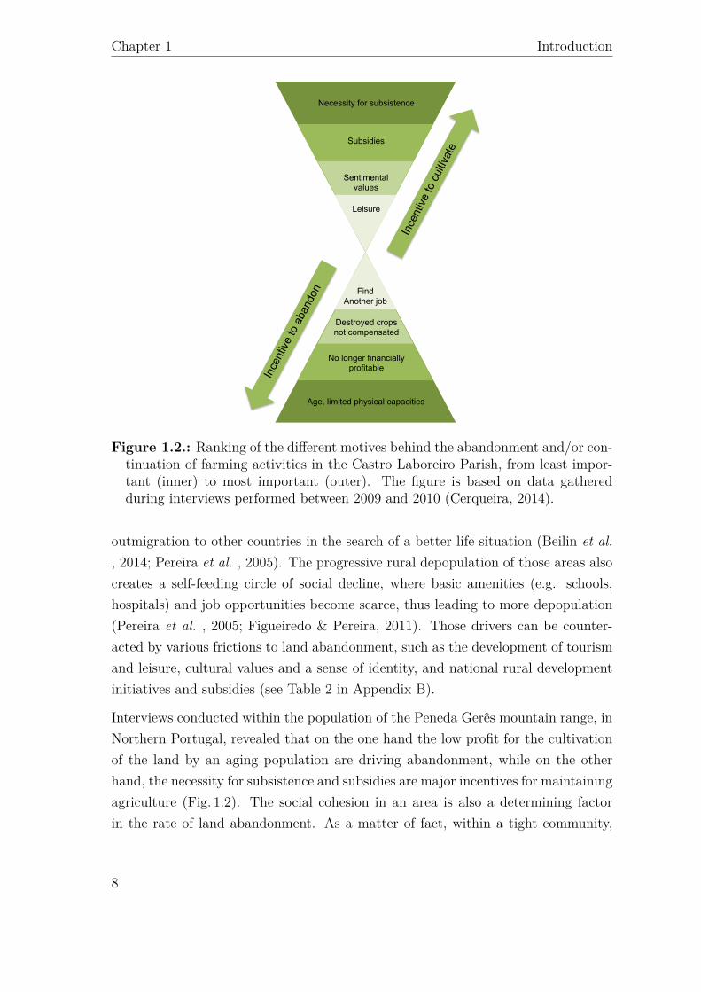
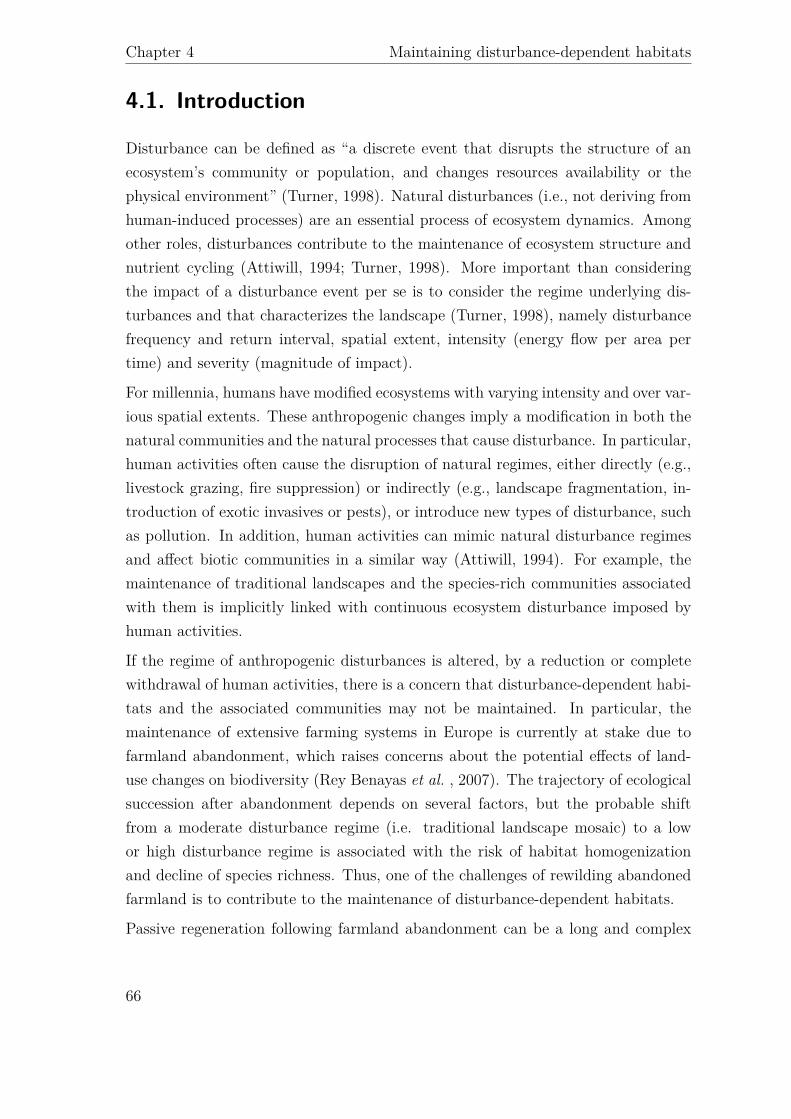
Ince
ntiv
e to
cul
tivat
e
Necessity for subsistence
Subsidies
Sentimental values
Leisure
Age, limited physical capacities
Destroyed crops not compensated
No longer financially profitable
Find Another job
Ince
ntiv
e to
aba
ndon


!
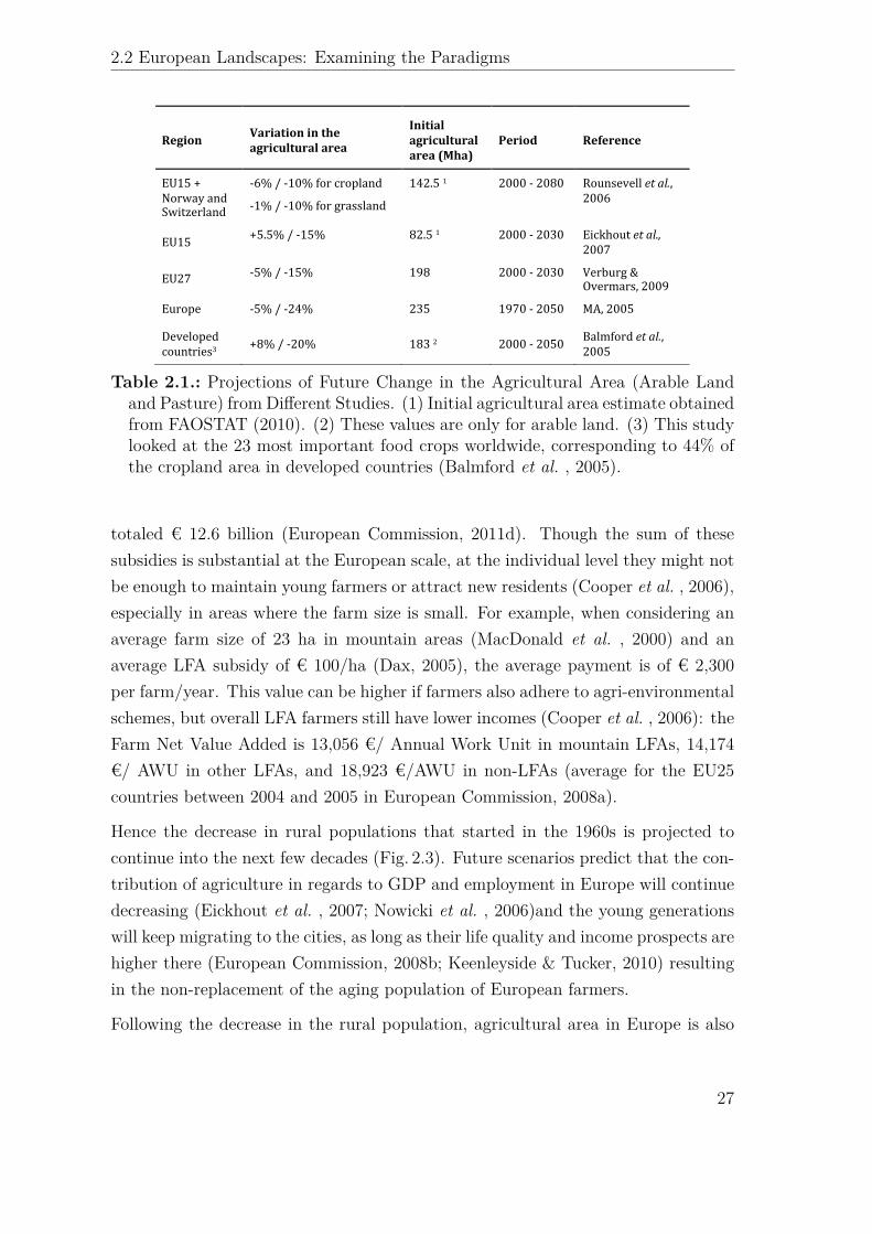
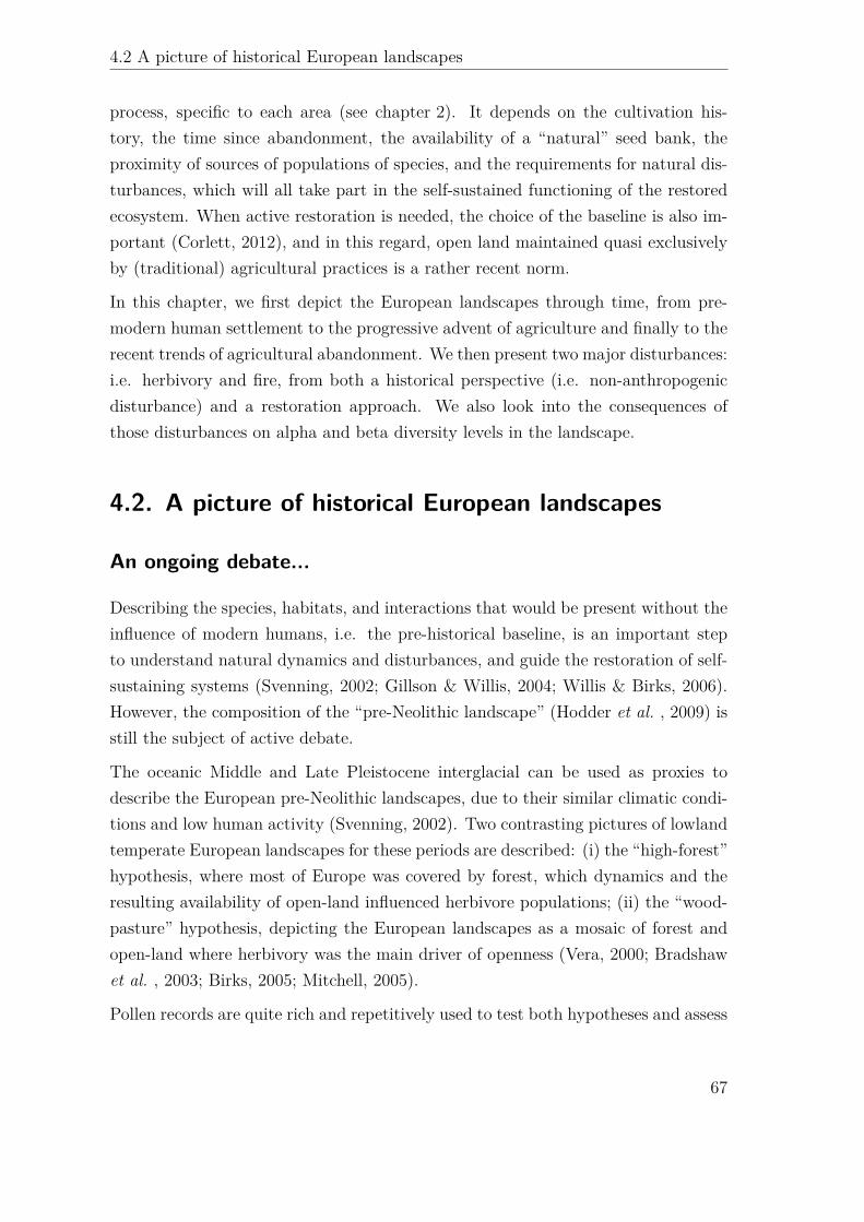
Region' Variation'in'the'agricultural'area'
Initial'agricultural'area'(Mha)'
Period' Reference'
EU15!+!Norway!and!Switzerland!
56%!/!510%!for!cropland!!
51%!/!510%!for!grassland!
142.5!1! 2000!5!2080! Rounsevell!et#al.,!2006!
EU15! +5.5%!/!515%!!! 82.5!1! 2000!5!2030! Eickhout!et#al.,!2007!
EU27! 55%!/!515%! 198! 2000!5!2030! Verburg!&!Overmars,!2009!
Europe! 55%!/!524%! 235! 1970!5!2050! MA,!2005!
Developed!countries3! +8%!/!520%! 183!2! 2000!5!2050! Balmford!et#al.,!
2005!

ε
λ
A = T − F
dF
dt= εF
(1− F
T
)− λRF
F = 0 F = Tε (ε−Rλ)
Rλ > ε
F = 0
ε > Rλ F = Tε (ε−Rλ)
ε
λ
F = T
dFi
dt= εiFi
(1− Fi
Ti
)− λiNFi
dFb
dt= εbFb
(1− Fb
Tb
)− (λbSS + λbNN)Fb
Fi = 0 Fi =Tiεi−RTiλi+STiλi
εi
Fb = 0
Fi =Tb(εb−RλbN+SλbN−SλbS)
εb
S +N = R
dS
dt= f
(S
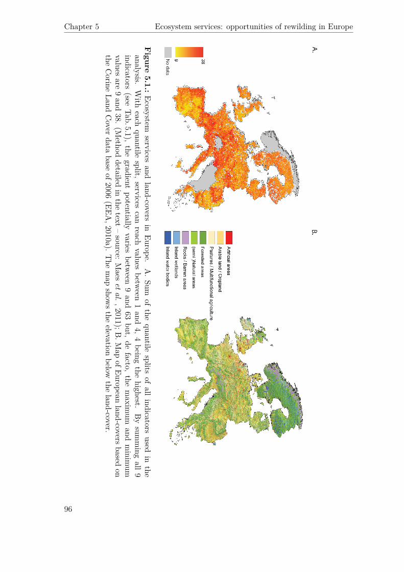
R
)
f
CDF(SR
)
SR
CDF
(S
R
)=
1
1 +(
µ− SR
δ
)
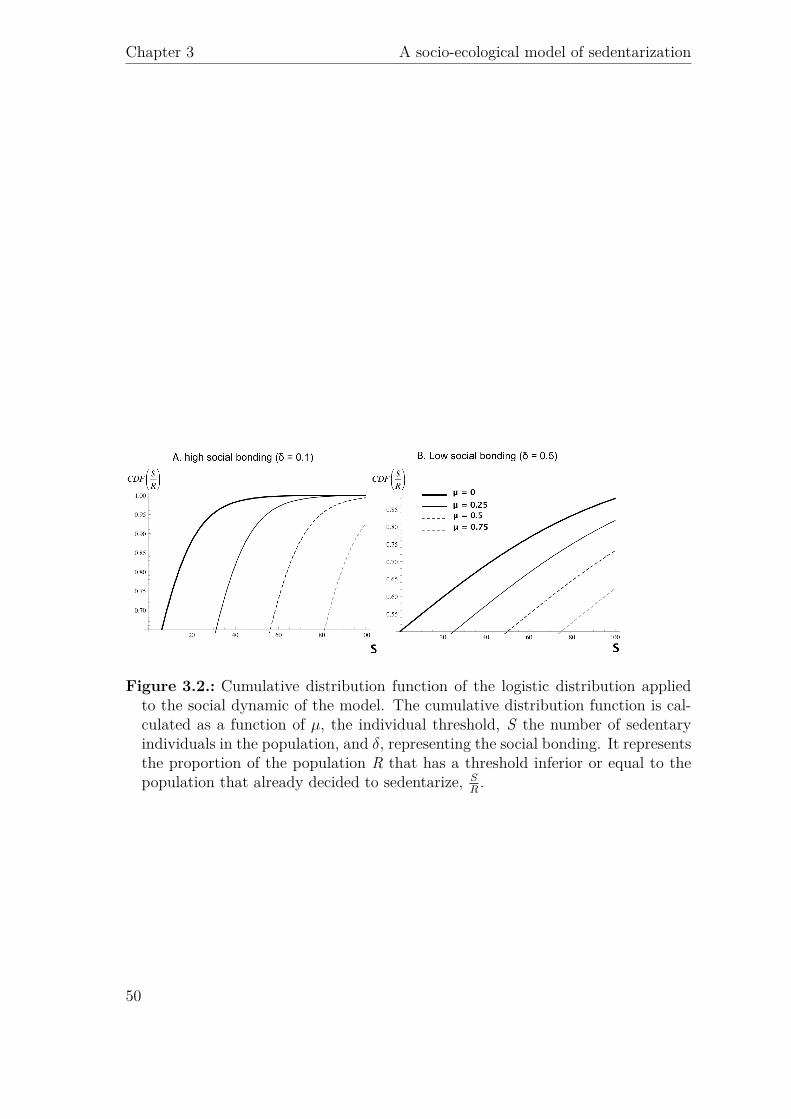
µ δ
δ > 0
δ
µ
δ
µ > 0.5
ω
SR CDF
(SR
)
SR
dS
dt= ω ×
[CDF
(S
R
)− S
R
]×R = ω
⎛
⎝ R
1 +(µ− S
R)δ
− S
⎞
⎠
δ S
µ
δ µ
S = R
µ S = 0
µ
S < R2
S = 0 S > R2
µδ
SR
S = R
δ
µ
Axhx Ax
hx
UN
σ
UN =Aihi
R− S+ (1− c)
Abhb
R+ σ
US =Abhb
R+ σ
µ
µ = 0.5 UN = US
µ =AihiR−S + (1−c)Abhb
R + σ
2(AbhbR + σ
)
dS
dt= ω
⎡
⎢⎢⎢⎢⎢⎣
R
1 +
⎡
⎣AihiR−S +(1−c)
AbhbR +σ
2
!AbhbR +σ
" − SR
⎤
⎦
δ
− S
⎤
⎥⎥⎥⎥⎥⎦
hb
δ = 0.1 δ = 0.5
δ = 0.1δ = 0.5 Ai Ab
hi σ = 1 ω = 1
Ai Ab
R− S
Ai Ab
(Ti − Fi) (Tb − Fb)
dFi
dt= εiFi
(1− Fi
Ti
)− λi (R− S)Fi
dFb
dt= εbFb
(1− Fb
Tb
)− (λbSS + λbN (R− S))Fb
dS
dt= ω
⎡
⎢⎢⎢⎢⎢⎢⎣
R
1 +
⎡
⎢⎣(Ti−Fi)hi
R−S +(1−c)(Tb−Fb)hb
R +σ
2
#(Tb−Fb)hb
R +σ
$ − SR
⎤
⎥⎦
δ
− S
⎤
⎥⎥⎥⎥⎥⎥⎦
Fb Fi
δ = 0.1
δ = 0.5 ε = 0.1
ε = 4
hb = 1 hb = 3
Fi ≈ 0 Fb ≈ 0 S ≈ 0
Fb =Tb(εb−RλbN+SλbN−SλbS)
εbFi =
Tiεi−RTiλi+STiλiεi
S ≈ 100
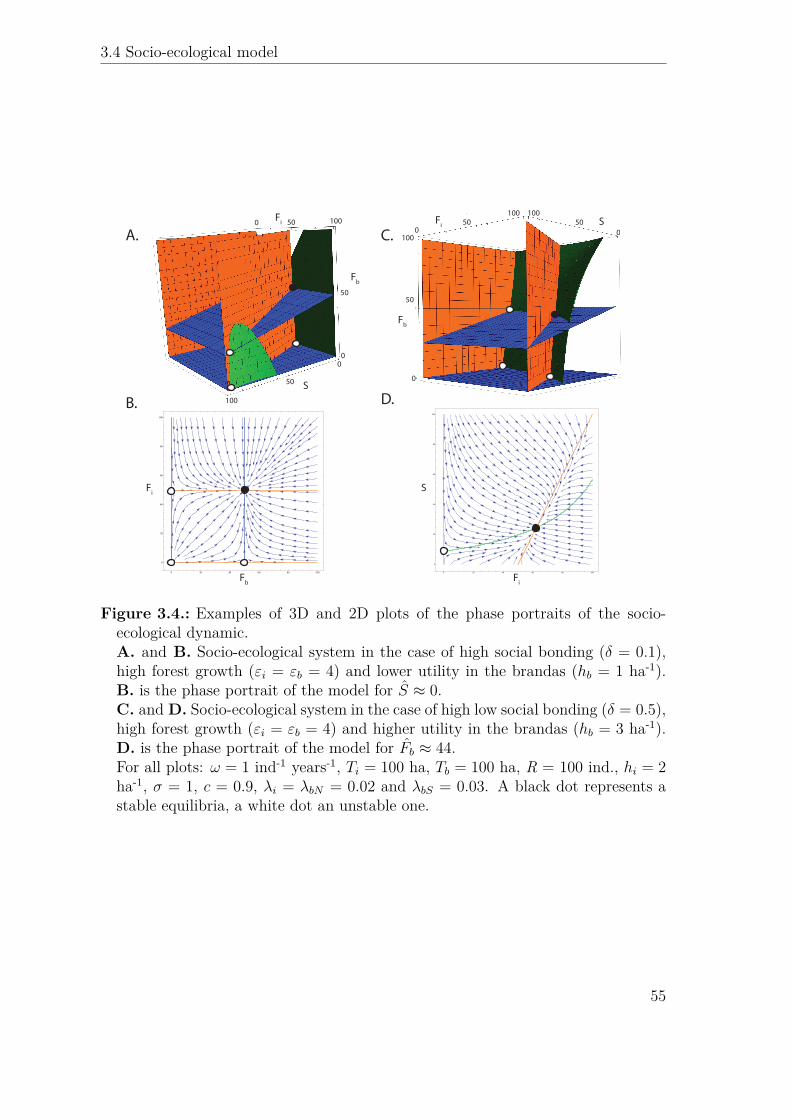
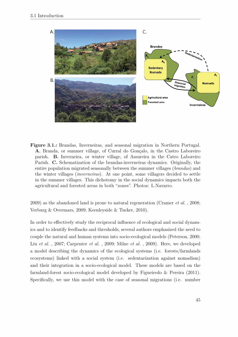
A.
B.
C.
D.
Fi 500 100
Fb50
50
00
100
S
Fi
Fb Fi
S
100
50
0
Fb
100 10050
0S50
0Fi S
0 20 40 60 80 100
0
20
40
60
80
100
0 20 40 60 80 100
0
20
40
60
80
100
δ = 0.1εi = εb = 4 hb = 1
S ≈ 0δ = 0.5
εi = εb = 4 hb = 3Fb ≈ 44
ω = 1 Ti = 100 Tb = 100 hi = 2σ = 1 c = 0.9 λi = λbN = 0.02 λbS = 0.03
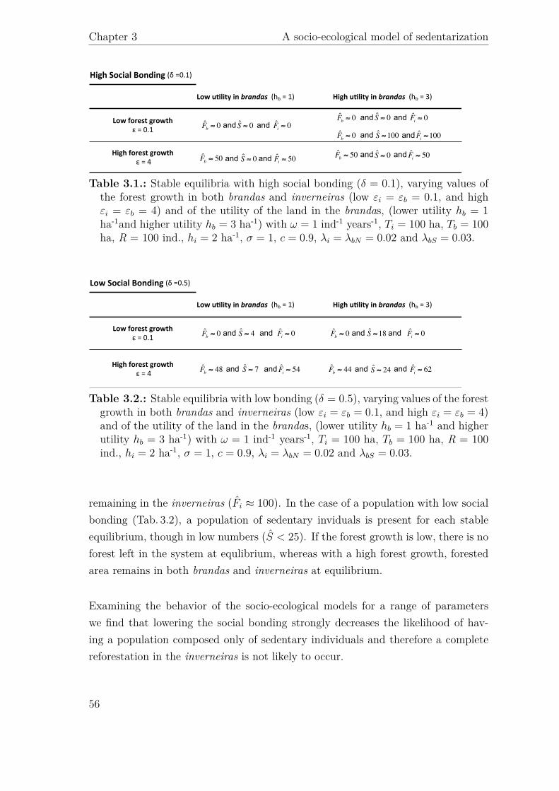
High%Social%Bonding%(δ#=0.1)#
Low%u1lity%in%brandas%%(hb#=#1)# High%u1lity%in%brandas%%(hb#=#3)#
Low%forest%growth%%ε#=#0.1#
High%forest%growth%#ε#=#4#
Fb ≈ 0 and S ≈ 0 and Fi ≈ 0
Fb ≈ 50 and S ≈ 0 and Fi ≈ 50
Fb ≈ 0 and and
Fb ≈ 0 and and
Fb ≈ 50 and and
S ≈ 0
S ≈ 0
S ≈100
Fi ≈ 0
Fi ≈100
Fi ≈ 50
δ = 0.1εi = εb = 0.1
εi = εb = 4 hb = 1hb = 3 ω = 1 Ti = 100 Tb = 100
hi = 2 σ = 1 c = 0.9 λi = λbN = 0.02 λbS = 0.03
Low$Social$Bonding$(δ#=0.5)#
Low$u/lity$in$brandas$$(hb#=#1)# High$u/lity$in$brandas$$(hb#=#3)#
Low$forest$growth$$ε#=#0.1#
High$forest$growth$#ε#=#4#
Fb ≈ 0 and and
Fb ≈ 48 and and
Fb ≈ 0 and and
Fb ≈ 44 and and
Fi ≈ 0
Fi ≈ 54
Fi ≈ 0
Fi ≈ 62S ≈ 7
S ≈ 4 S ≈18
S ≈ 24
δ = 0.5εi = εb = 0.1 εi = εb = 4
hb = 1hb = 3 ω = 1 Ti = 100 Tb = 100
hi = 2 σ = 1 c = 0.9 λi = λbN = 0.02 λbS = 0.03
Fi ≈ 100
S < 25
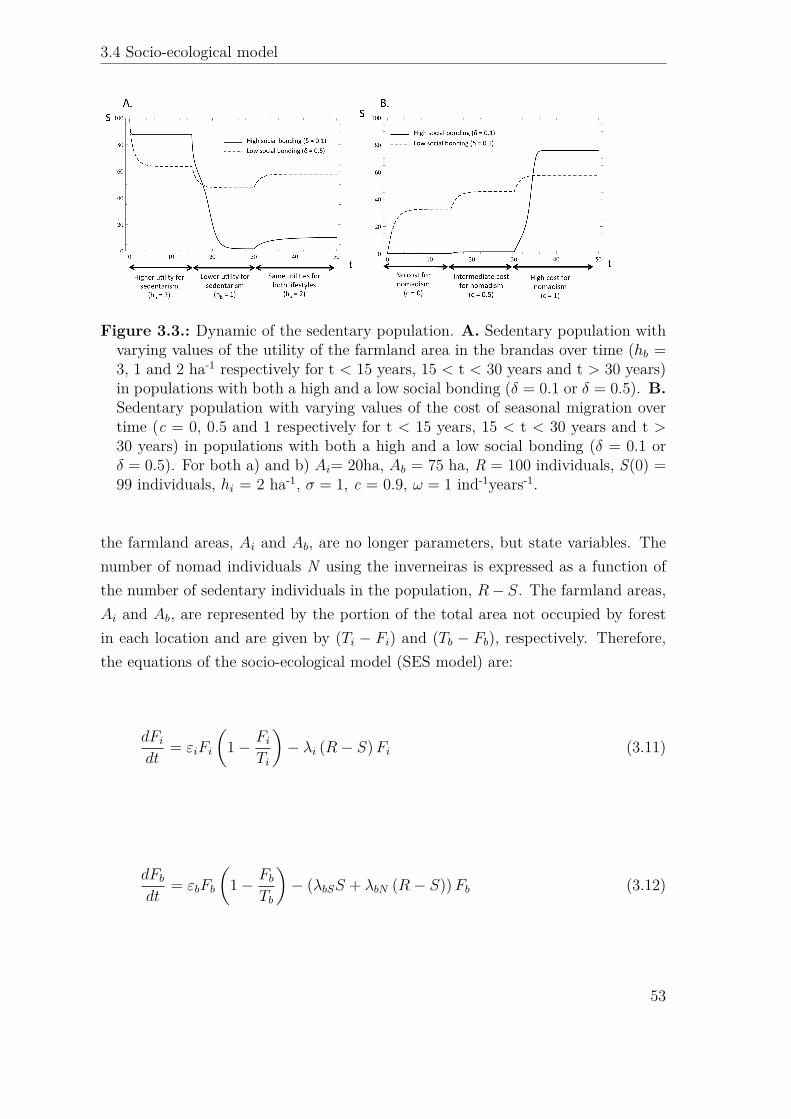
hb
hi
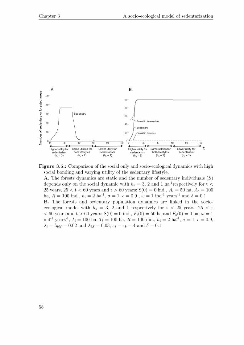
t Higher utility for sedentarism
(hb = 3)
Lower utility for sedentarism
(hb = 1)
Same utilities for both lifestyles
(hb = 2)
B.
Sedentary
Forest in brandas
Forest in inverneiras
A.
Nu
mb
er
of se
de
nta
ry o
r fo
reste
d a
rea
s
Sedentary
Higher utility for sedentarism
(hb = 3)
Lower utility for sedentarism
(hb = 1)
Same utilities for both lifestyles
(hb = 2)
100
80
60
40
20
00 20 40 60 80 100
100
80
60
40
20
00 20 40 60 80 100
hb
Ai Ab
hi = 2 σ = 1 c = 0.9 ω = 1 δ = 0.1
hb
Fi(0) = 50 Fb(0) = 0 ω = 1Ti = 100 Tb = 100 hi = 2 σ = 1 c = 0.9
λi = λbN = 0.02 λbS = 0.03 εi = εb = 4 δ = 0.1

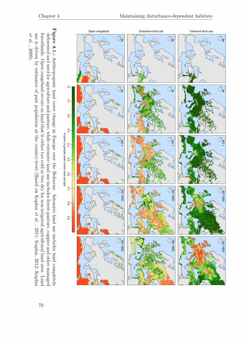
8k
Intensive land use
3k
AD
1A
D 1
50
0A
D 1
85
0
8k
Extensive land use
3k
AD
1A
D 1
50
0A
D 1
85
0
8k
Open rangeland
3k
AD
1A
D 1
50
0A
D 1
85
0
>0
0.1
0.2
0.3
0.4
0.5
0.6
0.7
0.8
0.9
Fra
ction o
f grid
cell u
nder h
um
an la
nd u
se typ
e
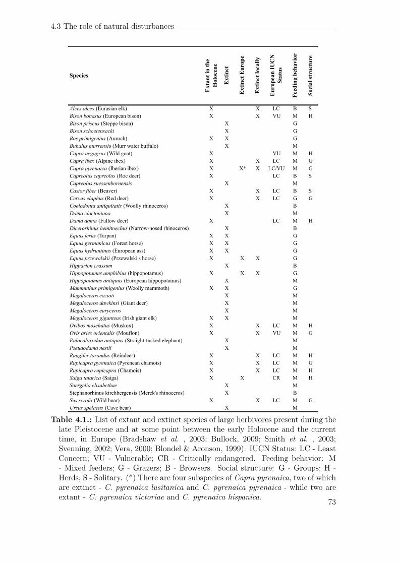
Species
Ext
ant i
n th
e H
oloc
ene
Ext
inct
Ext
inct
Eur
ope
Ext
inct
loca
lly
Eur
opea
n IU
CN
St
atus
Feed
ing
beha
vior
Soci
al st
ruct
ure
Alces alces (Eurasian elk) X X LC B SBison bonasus (European bison) X X VU M HBison priscus (Steppe bison) X GBison schoetensacki X GBos primigenius (Auroch) X X GBubalus murrensis (Murr water buffalo) X MCapra aegagrus (Wild goat) X VU M HCapra ibex (Alpine ibex) X X LC M GCapra pyrenaica (Iberian ibex) X X* X LC/VU M GCapreolus capreolus (Roe deer) X LC B SCapreolus suessenbornensis X MCastor fiber (Beaver) X X LC B SCervus elaphus (Red deer) X X LC G GCoelodonta antiquitatis (Woolly rhinoceros) X BDama clactoniana X MDama dama (Fallow deer) X LC M HDicerorhinus hemitoechus (Narrow-nosed rhinoceros) X BEquus ferus (Tarpan) X X GEquus germanicus (Forest horse) X X GEquus hydruntinus (European ass) X X GEquus przewalskii (Przewalski's horse) X X X GHipparion crassum X BHippopotamus amphibius (hippopotamus) X X X GHippopotamus antiquus (European hippopotamus) X MMammuthus primigenius (Woolly mammoth) X X GMegaloceros cazioti X MMegaloceros dawkinsi (Giant deer) X MMegaloceros euryceros X MMegaloceros giganteus (Irish giant elk) X X MOvibos moschatus (Muskox) X X LC M HOvis aries orientalis (Mouflon) X X VU M GPalaeoloxodon antiquus (Straight-tusked elephant) X MPseudodama nestii X MRangifer tarandus (Reindeer) X X LC M HRupicapra pyrenaica (Pyrenean chamois) X X LC M GRupicapra rupicapra (Chamois) X X LC M HSaiga tatarica (Saiga) X X CR M HSoergelia elisabethae X MStephanorhinus kirchbergensis (Merck's rhinoceros) X BSus scrofa (Wild boar) X X LC M GUrsus spelaeus (Cave bear) X M
α
α
β
γ
Legislation
Conservation measures (including
reintroductions)
Reduced human pressure (e.g. land
abandonment, decreased hunting)
Change in environmental
conditions
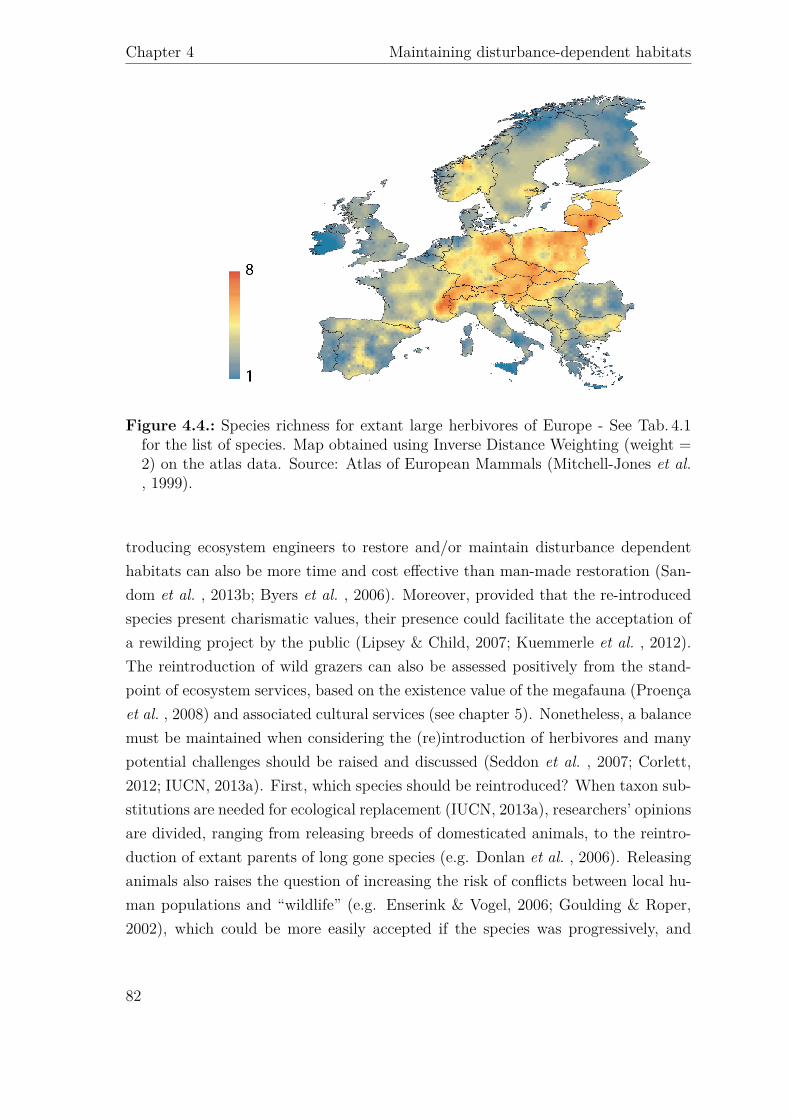
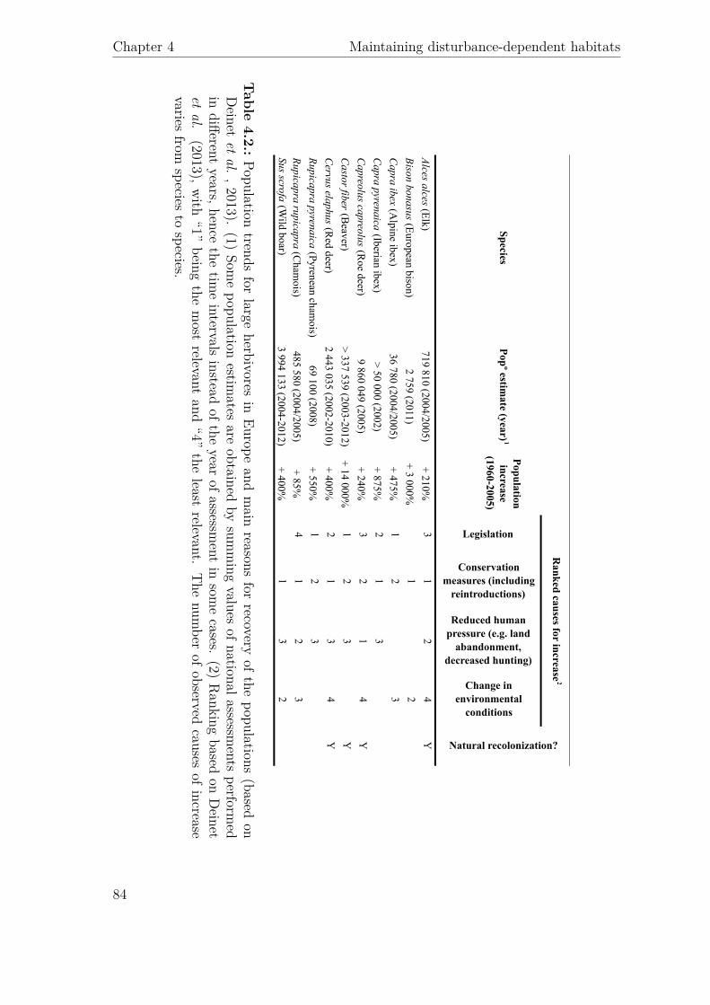
Alces alces (Elk)719 810 (2004/2005)
+ 210%3
12
4Y
Bison bonasus (European bison)2 759 (2011)
+ 3 000%1
2
Capra ibex (A
lpine ibex)36 780 (2004/2005)
+ 475%1
23
Capra pyrenaica (Iberian ibex)
> 50 000 (2002)+ 875%
21
3
Capreolus capreolus (R
oe deer)9 860 049 (2005)
+ 240%3
21
4Y
Castor fiber (B
eaver)> 337 539 (2003-2012)
+ 14 000%1
23
Y
Cervus elaphus (R
ed deer)2 443 035 (2002-2010)
+ 400%2
13
4Y
Rupicapra pyrenaica (Pyrenean chamois)
69 100 (2008)+ 550%
12
3
Rupicapra rupicapra (Cham
ois)485 580 (2004/2005)
+ 85%4
12
3Sus scrofa (W
ild boar)3 994 133 (2004-2012)
+ 400%1
32
SpeciesPopº estim
ate (year)1
Population increase
(1960-2005)
Ranked causes for increase
2
Natural recolonization?

Agric
ultural*
Area
To
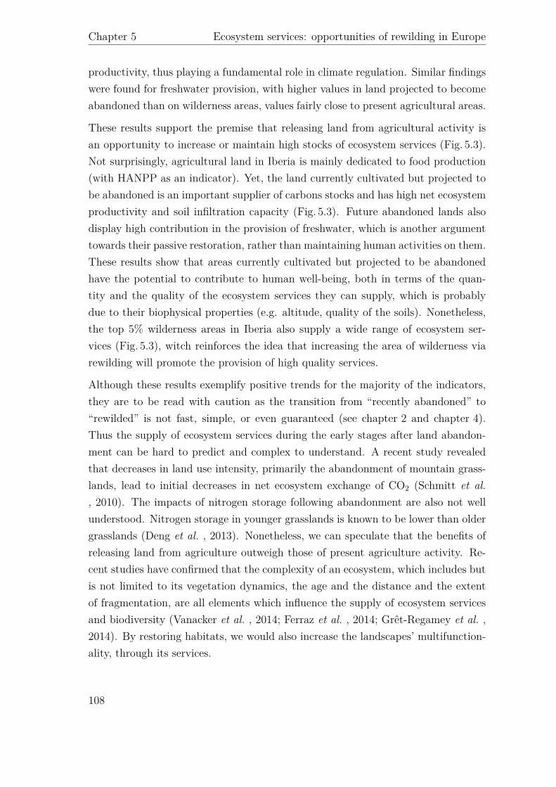
p*5%
*high*
wild
erne
ss
Projected**
to*be*
aban
done
d p*value*
Category
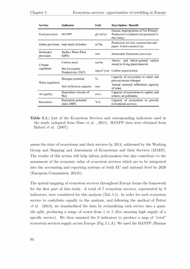
Service
Indicator
Unit
Mean*pe
r*km
2 *(sem)
Provisionn
ing
Food
$prod
uc)o
n HA
NPP
gC/m
2/yr
279.03$$
(0.21)
224.12$
(2.65)
271.15$
$(2.91)
<.0001$(*
**)
Timbe
r total$stock
m
3 /ha
0.81E+05$
$(0.21E+03)
2.10$E+05$
$(1.67E+03)
1.34E+05$
$(1.68E+03)
0.23$(N
S)
Freshw
ater
Surface$water$flow
mm
151.05$
$(0.15)
156.08$
(0.58)
244.77$
$(1.61)
<.0001$(*
**)
RegulaFo
n*an
d*Mainten
ance
Clim
ate$
regula)o
n
Carbon
$stock
ton/ha
24.82$
$(0.06)
63.19$
$(0.30)
74.81$
$(0.49)
<.0001$(*
**)
Net$Ecosystem
$Prod
uc)vity
$(NEP)
mg/m
2 /yr
5.13E+05$
$(0.34E+03)
6.99$E+05$
(1.75E+03)
7.36E+05$
$(1.92E+03)
<.0001$(*
**)
Water$
regula)o
n
Nitrogen
$reten)
on
%
2.69$
$(.00
) 3.04$
(.01)
2.46$
$(.02
) <.0001$(*
**)
Soil$infiltra)
on$
capacity
mm
9.61$
$(0.02)
15.99$$
(0.11)
32.15$
$(0.23)
0.0006$(*
**)
Air$q
uality
Depo
si)on
$velocity
$of$Nox
cm
/s$
0.07$
$(0.00)
0.42$
$(0.00)
0.28$
$(0.01)
<.0001$(*
**)
Cultu
ral
Recrea)o
n Re
crea)o
nal$
Poten)
al$Inde
x$(RPI)
N/A
0.22$$
(2E\04
) 0.43$
$(11E\04)
0.26$
$(17E\04)
<.0001$(*
**)


Category Name Management type DetailNumber
(%)
Total Area in km2
(%)
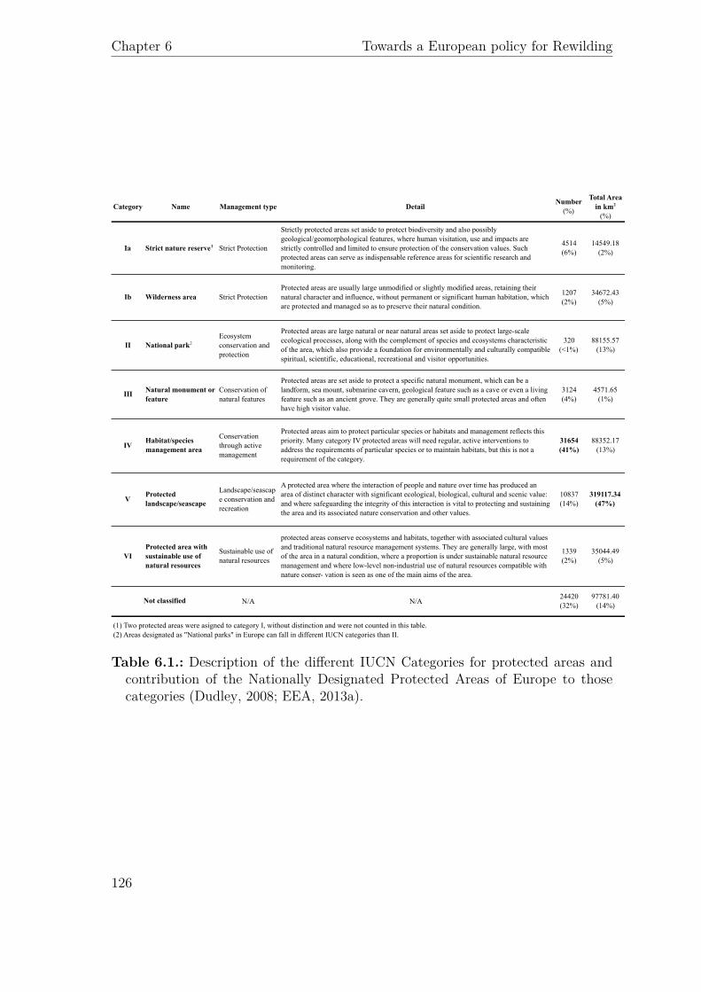
Ia Strict nature reserve1 Strict Protection
Strictly protected areas set aside to protect biodiversity and also possibly geological/geomorphological features, where human visitation, use and impacts are strictly controlled and limited to ensure protection of the conservation values. Such protected areas can serve as indispensable reference areas for scientific research and monitoring.
4514(6%)
14549.18(2%)
Ib Wilderness area Strict ProtectionProtected areas are usually large unmodified or slightly modified areas, retaining their natural character and influence, without permanent or significant human habitation, which are protected and managed so as to preserve their natural condition.
1207(2%)
34672.43(5%)
II National park2Ecosystem conservation and protection
Protected areas are large natural or near natural areas set aside to protect large-scale ecological processes, along with the complement of species and ecosystems characteristic of the area, which also provide a foundation for environmentally and culturally compatible spiritual, scientific, educational, recreational and visitor opportunities.
320(<1%)
88155.57(13%)
III Natural monument or feature
Conservation of natural features
Protected areas are set aside to protect a specific natural monument, which can be a landform, sea mount, submarine cavern, geological feature such as a cave or even a living feature such as an ancient grove. They are generally quite small protected areas and often have high visitor value.
3124(4%)
4571.65 (1%)
IVHabitat/species management area
Conservation through active management
Protected areas aim to protect particular species or habitats and management reflects this priority. Many category IV protected areas will need regular, active interventions to address the requirements of particular species or to maintain habitats, but this is not a requirement of the category.
31654(41%)
88352.17(13%)
VProtected landscape/seascape
Landscape/seascape conservation and recreation
A protected area where the interaction of people and nature over time has produced an area of distinct character with significant ecological, biological, cultural and scenic value: and where safeguarding the integrity of this interaction is vital to protecting and sustaining the area and its associated nature conservation and other values.
10837(14%)
319117.34(47%)
VIProtected area with sustainable use of natural resources
Sustainable use of natural resources
protected areas conserve ecosystems and habitats, together with associated cultural values and traditional natural resource management systems. They are generally large, with most of the area in a natural condition, where a proportion is under sustainable natural resource management and where low-level non-industrial use of natural resources compatible with nature conser- vation is seen as one of the main aims of the area.
1339(2%)
35044.49(5%)
N/A N/A24420(32%)
97781.40 (14%)
(1) Two protected areas were asigned to category I, without distinction and were not counted in this table.
Not classified
(2) Areas designated as "National parks" in Europe can fall in different IUCN categories than II.
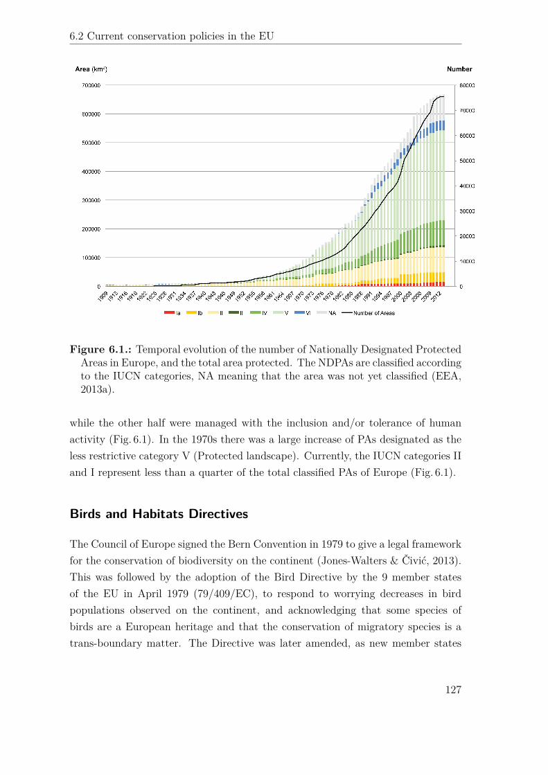
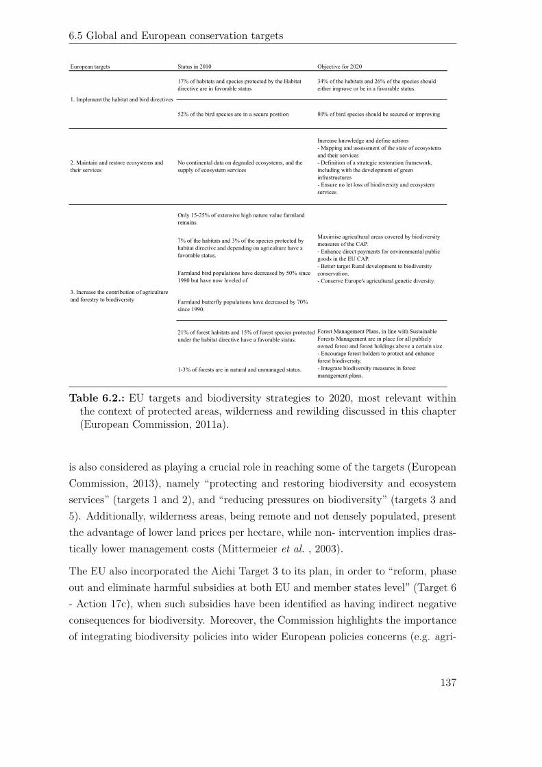
European targets Status in 2010 Objective for 2020
17% of habitats and species protected by the Habitat directive are in favorable status
34% of the habitats and 26% of the species should either improve or be in a favorable status.
52% of the bird species are in a secure position 80% of bird species should be secured or improving
2. Maintain and restore ecosystems and their services
No continental data on degraded ecosystems, and the supply of ecosystem services
Increase knowledge and define actions - Mapping and assessment of the state of ecosystems and their services- Definition of a strategic restoration framework, including with the development of green infrastructures- Ensure no let loss of biodiversity and ecosystem services
Only 15-25% of extensive high nature value farmland remains.
7% of the habitats and 3% of the species protected by habitat directive and depending on agriculture have a favorable status.
Farmland bird populations have decreased by 50% since 1980 but have now leveled of
Farmland butterfly populations have decreased by 70% since 1990.
21% of forest habitats and 15% of forest species protected under the habitat directive have a favorable status.
1-3% of forests are in natural and unmanaged status.
3. Increase the contribution of agriculture and forestry to biodiversity
1. Implement the habitat and bird directives
Maximise agricultural areas covered by biodiversity measures of the CAP.- Enhance direct payments for environmental public goods in the EU CAP.- Better target Rural development to biodiversity conservation.- Conserve Europe's agricultural genetic diversity.
Forest Management Plans, in line with Sustainable Forests Management are in place for all publicly owned forest and forest holdings above a certain size.- Encourage forest holders to protect and enhance forest biodiversity.- Integrate biodiversity measures in forest management plans.

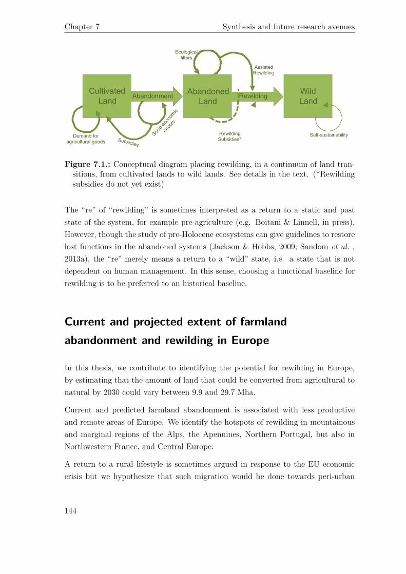
Ecological filters
Self-sustainability
Assisted Rewilding
Rewilding Subsidies* Subsidies
Demand for agricultural goods
Socio-
econ
omic
drive
rs
Cultivated Land
Abandoned Land
Wild Land
Abandonment Rewilding


EG37CH02-Pereira ARI 5 October 2012 14:37
Global Biodiversity Change:The Bad, the Good, andthe UnknownHenrique Miguel Pereira, Laetitia Marie Navarro,and Ines Santos MartinsCentro de Biologia Ambiental, Faculdade de Ciencias da Universidade de Lisboa,Campo Grande, 1749-016 Lisboa, Portugal; email: [email protected], [email protected],[email protected]
Annu. Rev. Environ. Resour. 2012. 37:25–50
First published online as a Review in Advance onAugust 28, 2012
The Annual Review of Environment and Resourcesis online at environ.annualreviews.org
This article’s doi:10.1146/annurev-environ-042911-093511
Copyright c⃝ 2012 by Annual Reviews.All rights reserved
1543-5938/12/1121-0025$20.00
Keywordsextinctions, species, abundance, range, land-use, climate
AbstractGlobal biodiversity change is one of the most pressing environmental is-sues of our time. Here, we review current scientific knowledge on globalbiodiversity change and identify the main knowledge gaps. We discusstwo components of biodiversity change—biodiversity alterations andbiodiversity loss—across four dimensions of biodiversity: species extinc-tions, species abundances, species distributions, and genetic diversity.We briefly review the impacts that modern humans and their ancestorshave had on biodiversity and discuss the recent declines and alterationsin biodiversity. We analyze the direct pressures on biodiversity change:habitat change, overexploitation, exotic species, pollution, and climatechange. We discuss the underlying causes, such as demographic growthand resource use, and review existing scenario projections. We identifysuccesses and impending opportunities in biodiversity policy and man-agement, and highlight gaps in biodiversity monitoring and models.Finally, we discuss how the ecosystem services framework can be usedto identify undesirable biodiversity change and allocate conservationefforts.
25
Ann
u. R
ev. E
nviro
n. R
esou
rc. 2
012.
37:2
5-50
. Dow
nloa
ded
from
ww
w.a
nnua
lrevi
ews.o
rgby
200
.0.2
9.76
on
10/1
8/12
. For
per
sona
l use
onl
y.

EG37CH02-Pereira ARI 5 October 2012 14:37
Contents1. INTRODUCTION . . . . . . . . . . . . . . . . 262. GLOBAL BIODIVERSITY
CHANGE: ALTERATIONSAND LOSSES . . . . . . . . . . . . . . . . . . . . 27
3. A BRIEF HISTORICALPERSPECTIVE ON GLOBALBIODIVERSITY CHANGE:FROM THE ICE AGE TO THEINDUSTRIAL REVOLUTION . . . 28
4. RECENT TRENDS IN GLOBALBIODIVERSITY CHANGE . . . . . . . 304.1. Species Extinctions and
Extinction Risk . . . . . . . . . . . . . . . . . 304.2. Changes in Species Abundances
and Community Structure . . . . . . . 324.3. Shifts in the Distribution of
Species and Communities . . . . . . . 344.4. Genetic Diversity in
Domesticated andWild Species . . . . . . . . . . . . . . . . . . . 35
5. UNDERSTANDING THEDIRECT PRESSURES . . . . . . . . . . . . 365.1. Habitat Change and
Degradation . . . . . . . . . . . . . . . . . . . . 365.2. Overexploitation . . . . . . . . . . . . . . . 375.3. Pollution . . . . . . . . . . . . . . . . . . . . . . 375.4. Introduction of Exotic Species
and Invasions . . . . . . . . . . . . . . . . . . . 385.5. Climate Change . . . . . . . . . . . . . . . 38
6. EXPLORING THEUNDERLYING CAUSES WITHSCENARIO MODELS . . . . . . . . . . . . 39
7. A BIT OF GOOD NEWSFOR A CHANGE . . . . . . . . . . . . . . . . . 39
8. MAJOR GAPS IN OURUNDERSTANDING OFGLOBAL BIODIVERSITYCHANGE . . . . . . . . . . . . . . . . . . . . . . . . 41
9. IS ALL BIODIVERSITY CHANGEEQUALLY BAD? . . . . . . . . . . . . . . . . . 42
1. INTRODUCTIONBiodiversity is the sum of all “plants, animals,fungi, and microorganisms on Earth, their
genotypic and phenotypic variation, and thecommunities and ecosystems of which theyare a part” (1, p. 138), or simply stated, life onEarth (2). Biodiversity is multidimensional, andno single measure of biodiversity can captureall its dimensions (3). Biodiversity provides thefoundation for ecosystem services, includingnutrient cycling, climate regulation, foodproduction, and the regulation of the watercycle, and it is therefore intimately linked withhuman well-being (2, 4, 5). This foundation isnow becoming endangered as the human foot-print on the planet increases and biodiversitydeclines. Species are becoming extinct at rateshigher than in the fossil record of the past fewmillion years, including the peak extinctionrate owing to the megafauna disappearance atthe end of the Pleistocene (6). Several otherdimensions of biodiversity are also declining,such as the extent of tropical forests and themean abundance of wild bird species (7, 8).The human appropriation of Earth’s naturalresources is not only leading to biodiversityloss but also to large alterations of biodiversitydistribution, composition, and abundance.
Here, we review our current understandingof global biodiversity change and its underlyingdrivers. We start by scoping our definition ofglobal biodiversity change, which includes bothbiodiversity loss and biodiversity alterations.Next, we briefly review human-induced globalbiodiversity change since the last ice age tothe Industrial Revolution. This provides ahistorical background for our discussion ofrecent biodiversity change, which is organizedinto four biodiversity dimensions: species ex-tinctions, species abundances and communitystructure, species ranges, and genetic diversity.These dimensions are not by any means exhaus-tive but aim at being representative. We focuson terrestrial ecosystems, but we also give ex-amples for freshwater and marine ecosystems.Next, we examine the direct drivers of biodiver-sity change: habitat change, overexploitation,pollution, biotic exchange, and climate change.Some of these drivers could also be considereddimensions of biodiversity, such as the changein quality of a habitat or biotic exchanges, but
26 Pereira · Navarro · Martins
Ann
u. R
ev. E
nviro
n. R
esou
rc. 2
012.
37:2
5-50
. Dow
nloa
ded
from
ww
w.a
nnua
lrevi
ews.o
rgby
200
.0.2
9.76
on
10/1
8/12
. For
per
sona
l use
onl
y.
EG37CH02-Pereira ARI 5 October 2012 14:37
for simplicity, we treat them only in the driverssection. We discuss how these drivers mightevolve in the next few decades by reviewingexisting social-ecological scenarios and theprojections for indirect drivers, such as popula-tion growth, consumption patterns, and energyuse. Although much of the news related to bio-diversity change is worrying, we also provide anoverview of future opportunities for reversingbiodiversity declines and increasing biodiver-sity at the local level, as well as review some re-cent successes in biodiversity conservation. Thenext section discusses the gaps in our under-standing of global biodiversity change, both inobservations and modeling. We conclude withsome thoughts on the nature of biodiversitychange and the need to focus our managementefforts on detrimental biodiversity change.
2. GLOBAL BIODIVERSITYCHANGE: ALTERATIONSAND LOSSESMany organisms modify the environmentand as a result increase their fitness or affectresource availability to other species, processesknown as niche construction of ecosystemengineering (9). Humans and their hominidancestors are no exception; they have beenmodifying ecosystems throughout history toimprove food availability and decrease thesuccess of their ecological competitors. Whatis truly exceptional about humans is the scaleat which they have been able to modify ecosys-tems. The total industrial fixation of nitrogen(mainly for fertilizer production) togetherwith biological fixation in crops, and nitrogenmobilized during fossil-fuel combustion, isgreater than the nitrogen fixed by all naturalprocesses together (10). Humans currentlyharvest about 15% of global terrestrial netprimary production, using about six times morenet primary production than was used by theextinct Pleistocene community of megaherbi-vores (11). More than 35–40% of the world’sforests and other natural ice-free habitats havebeen converted to cropland and pasture (12,13), a value that increases to about 70% in some
Biodiversity: the sumof all organisms onEarth, their variation,and the ecosystems ofwhich they are a part
Biodiversity loss: thelocal or globalextinction of an alleleor species
Drivers: direct orindirect pressures onbiodiversity thatinduce a change (eithernegative or positive)
Biodiversityalterations:human-inducedchanges that lead tomodifications ofcommunity structureor to shifts in speciesdistributions
Scenarios: plausiblestories about how thefuture may unfold,often associated withquantitativeprojections
biomes, such as Mediterranean forests (2). Overhalf of the world’s large river systems have beenaffected by dams (14), and 40% of the ocean isstrongly affected by multiple drivers (15). Someof these impacts do not target specific species,such as altering the nitrogen cycle or land-usechange, but may favor some functional groups.Other actions are directed at specific species orat least aim directly at some functional groups,such as hunting, fishing, and timber logging.
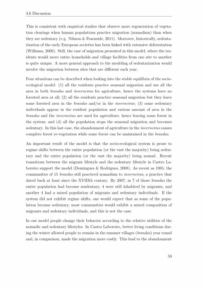
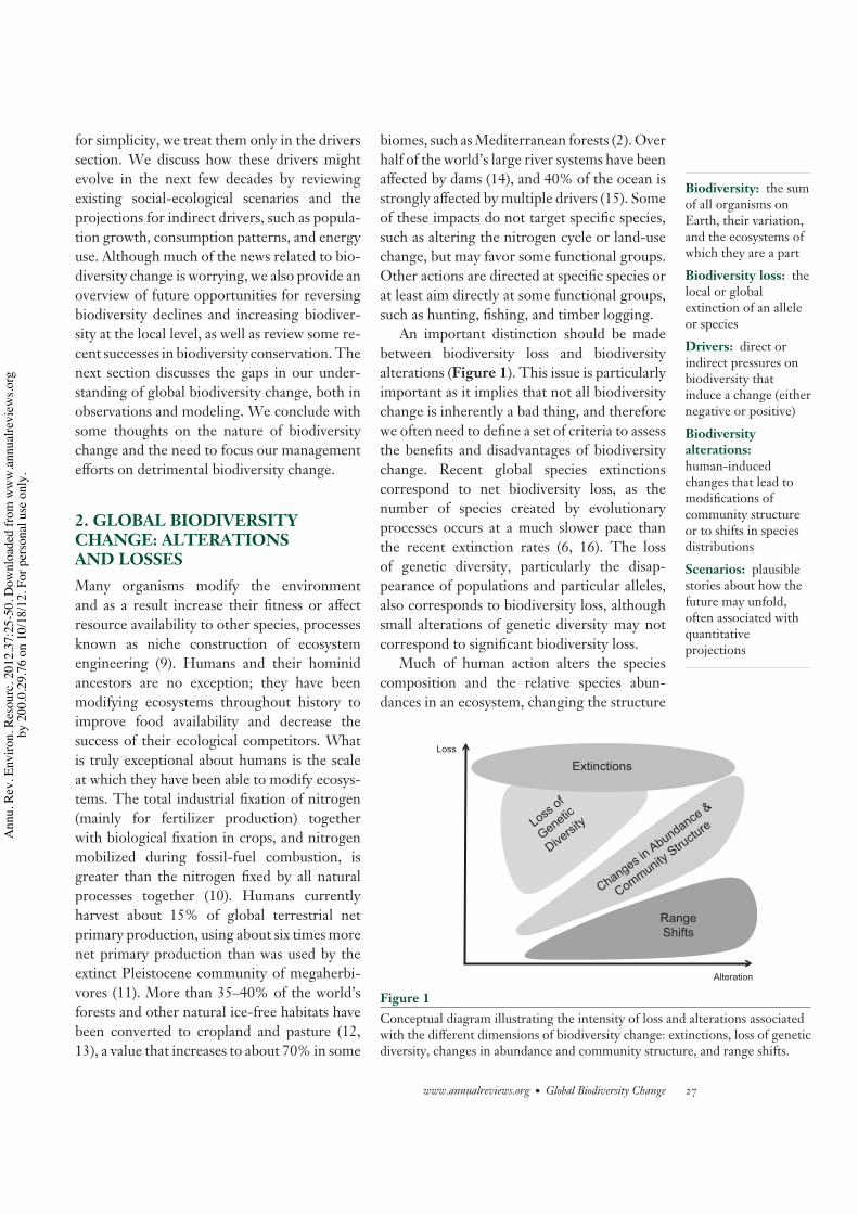
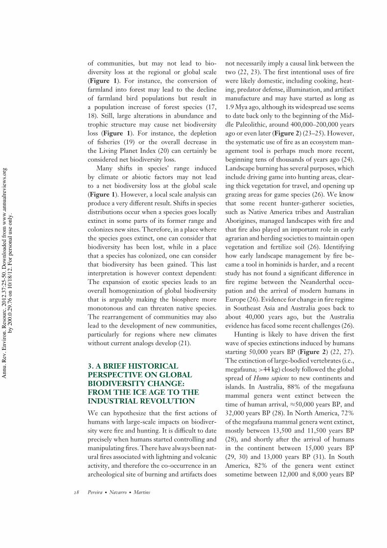
An important distinction should be madebetween biodiversity loss and biodiversityalterations (Figure 1). This issue is particularlyimportant as it implies that not all biodiversitychange is inherently a bad thing, and thereforewe often need to define a set of criteria to assessthe benefits and disadvantages of biodiversitychange. Recent global species extinctionscorrespond to net biodiversity loss, as thenumber of species created by evolutionaryprocesses occurs at a much slower pace thanthe recent extinction rates (6, 16). The lossof genetic diversity, particularly the disap-pearance of populations and particular alleles,also corresponds to biodiversity loss, althoughsmall alterations of genetic diversity may notcorrespond to significant biodiversity loss.
Much of human action alters the speciescomposition and the relative species abun-dances in an ecosystem, changing the structure
Extinctions
Alteration
Loss
Range Shifts
Figure 1Conceptual diagram illustrating the intensity of loss and alterations associatedwith the different dimensions of biodiversity change: extinctions, loss of geneticdiversity, changes in abundance and community structure, and range shifts.
www.annualreviews.org • Global Biodiversity Change 27
Ann
u. R
ev. E
nviro
n. R
esou
rc. 2
012.
37:2
5-50
. Dow
nloa
ded
from
ww
w.a
nnua
lrevi
ews.o
rgby
200
.0.2
9.76
on
10/1
8/12
. For
per
sona
l use
onl
y.
EG37CH02-Pereira ARI 5 October 2012 14:37
of communities, but may not lead to bio-diversity loss at the regional or global scale(Figure 1). For instance, the conversion offarmland into forest may lead to the declineof farmland bird populations but result ina population increase of forest species (17,18). Still, large alterations in abundance andtrophic structure may cause net biodiversityloss (Figure 1). For instance, the depletionof fisheries (19) or the overall decrease inthe Living Planet Index (20) can certainly beconsidered net biodiversity loss.
Many shifts in species’ range inducedby climate or abiotic factors may not leadto a net biodiversity loss at the global scale(Figure 1). However, a local scale analysis canproduce a very different result. Shifts in speciesdistributions occur when a species goes locallyextinct in some parts of its former range andcolonizes new sites. Therefore, in a place wherethe species goes extinct, one can consider thatbiodiversity has been lost, while in a placethat a species has colonized, one can considerthat biodiversity has been gained. This lastinterpretation is however context dependent:The expansion of exotic species leads to anoverall homogenization of global biodiversitythat is arguably making the biosphere moremonotonous and can threaten native species.The rearrangement of communities may alsolead to the development of new communities,particularly for regions where new climateswithout current analogs develop (21).
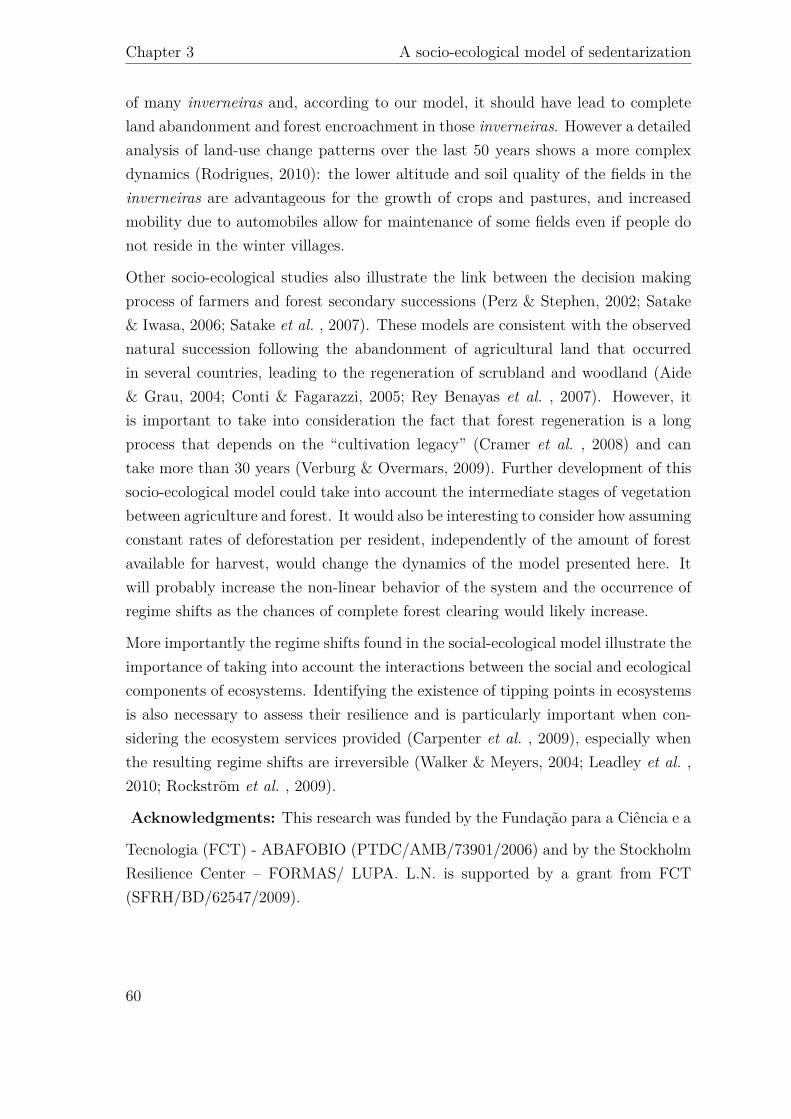
3. A BRIEF HISTORICALPERSPECTIVE ON GLOBALBIODIVERSITY CHANGE:FROM THE ICE AGE TO THEINDUSTRIAL REVOLUTIONWe can hypothesize that the first actions ofhumans with large-scale impacts on biodiver-sity were fire and hunting. It is difficult to dateprecisely when humans started controlling andmanipulating fires. There have always been nat-ural fires associated with lightning and volcanicactivity, and therefore the co-occurrence in anarcheological site of burning and artifacts does
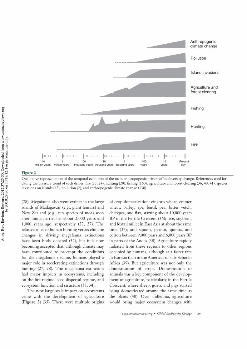
not necessarily imply a causal link between thetwo (22, 23). The first intentional uses of firewere likely domestic, including cooking, heat-ing, predator defense, illumination, and artifactmanufacture and may have started as long as1.9 Mya ago, although its widespread use seemsto date back only to the beginning of the Mid-dle Paleolithic, around 400,000–200,000 yearsago or even later (Figure 2) (23–25). However,the systematic use of fire as an ecosystem man-agement tool is perhaps much more recent,beginning tens of thousands of years ago (24).Landscape burning has several purposes, whichinclude driving game into hunting areas, clear-ing thick vegetation for travel, and opening upgrazing areas for game species (26). We knowthat some recent hunter-gatherer societies,such as Native America tribes and AustralianAborigines, managed landscapes with fire andthat fire also played an important role in earlyagrarian and herding societies to maintain openvegetation and fertilize soil (26). Identifyinghow early landscape management by fire be-came a tool in hominids is harder, and a recentstudy has not found a significant difference infire regime between the Neanderthal occu-pation and the arrival of modern humans inEurope (26). Evidence for change in fire regimein Southeast Asia and Australia goes back toabout 40,000 years ago, but the Australiaevidence has faced some recent challenges (26).
Hunting is likely to have driven the firstwave of species extinctions induced by humansstarting 50,000 years BP (Figure 2) (22, 27).The extinction of large-bodied vertebrates (i.e.,megafauna; >44 kg) closely followed the globalspread of Homo sapiens to new continents andislands. In Australia, 88% of the megafaunamammal genera went extinct between thetime of human arrival, ≈50,000 years BP, and32,000 years BP (28). In North America, 72%of the megafauna mammal genera went extinct,mostly between 13,500 and 11,500 years BP(28), and shortly after the arrival of humansin the continent between 15,000 years BP(29, 30) and 13,000 years BP (31). In SouthAmerica, 82% of the genera went extinctsometime between 12,000 and 8,000 years BP
28 Pereira · Navarro · Martins
Ann
u. R
ev. E
nviro
n. R
esou
rc. 2
012.
37:2
5-50
. Dow
nloa
ded
from
ww
w.a
nnua
lrevi
ews.o
rgby
200
.0.2
9.76
on
10/1
8/12
. For
per
sona
l use
onl
y.
EG37CH02-Pereira ARI 5 October 2012 14:37
Island invasions
Agriculture and forest clearing
Fishing
Hunting
Fire
Pollution
Anthropogenic climate change
10million years
1 million years
100 thousand years
10 thousand years
1 thousand years
100years
10years
Present day
Presentday
Figure 2Qualitative representation of the temporal evolution of the main anthropogenic drivers of biodiversity change. References used fordating the pressure trend of each driver: fire (23, 24), hunting (28), fishing (160), agriculture and forest clearing (36, 40, 41), speciesinvasions on islands (42), pollution (2), and anthropogenic climate change (138).
(28). Megafauna also went extinct in the largeislands of Madagascar (e.g., giant lemurs) andNew Zealand (e.g., ten species of moa) soonafter human arrival at about 2,000 years and1,000 years ago, respectively (22, 27). Therelative roles of human hunting versus climaticchanges in driving megafauna extinctionshave been hotly debated (32), but it is nowbecoming accepted that, although climate mayhave contributed to preempt the conditionsfor the megafauna decline, humans played amajor role in accelerating extinctions throughhunting (27, 28). The megafauna extinctionhad major impacts in ecosystems, includingon the fire regime, seed dispersal regime, andecosystem function and structure (33, 34).
The next large-scale impact on ecosystemscame with the development of agriculture(Figure 2) (35). There were multiple origins
of crop domestication: einkorn wheat, emmerwheat, barley, rye, lentil, pea, bitter vetch,chickpea, and flax, starting about 10,000 yearsBP in the Fertile Crescent (36); rice, soybean,and foxtail millet in East Asia at about the sametime (37); and squash, peanut, quinoa, andcotton between 9,000 years and 6,000 years BPin parts of the Andes (38). Agriculture rapidlyradiated from these regions to other regionsoccupied by humans, although at a faster ratein Eurasia than in the Americas or sub-SaharanAfrica (39). But agriculture was not only thedomestication of crops. Domestication ofanimals was a key component of the develop-ment of agriculture, particularly in the FertileCrescent, where sheep, goats, and pigs startedbeing domesticated around the same time asthe plants (40). Over millennia, agriculturewould bring major ecosystem changes with
www.annualreviews.org • Global Biodiversity Change 29
Ann
u. R
ev. E
nviro
n. R
esou
rc. 2
012.
37:2
5-50
. Dow
nloa
ded
from
ww
w.a
nnua
lrevi
ews.o
rgby
200
.0.2
9.76
on
10/1
8/12
. For
per
sona
l use
onl
y.
EG37CH02-Pereira ARI 5 October 2012 14:37
IUCN: InternationalUnion forConservation ofNature
the deforestation of large areas, changes infire regime, the appropriation of primaryproductivity by humans, and the replacementof wild herbivores by domestic grazers (11, 28,41). In Europe, by 3,000 years BP, perhaps asmuch as 30% of the usable land for crops andpasture had already been cleared (41), a patternthat would continue to intensify over thefollowing centuries, only briefly interruptedby the Dark Ages (AD 500–700) and the blackdeath (AD 1350). At the beginning of theIndustrial Revolution, at around AD 1850, theusable land cleared for agriculture in Europemay have reached a peak of about 80% (41),much higher than what is currently observed.
The most recent wave of extinctions beforethe Industrial Revolution occurred in islandsand was likely associated with the expansionof global trade via maritime routes (Figure 2).Between AD 1500 and 1800, all documentedextinctions occurred on islands (42). Bird ex-tinctions are particularly well documented forthat period. The major drivers of bird extinc-tions have been, by decreasing order of impor-tance, invasive species, overexploitation, andhabitat loss (42). The effects of invasive species,such as cats, rats, and goats, included both directpredation upon the native birds or the degrada-tion of their habitats (43).
4. RECENT TRENDS IN GLOBALBIODIVERSITY CHANGEIn this section, we review what is known aboutglobal biodiversity change since the IndustrialRevolution (mid-nineteenth century onward).Much of the emphasis is on very recent changesin the past 40 years, as some of the data are onlyavailable for that period. We divide our analysisinto four different dimensions of biodiversitychange that have different scores in the loss andalteration axes (Figure 1).
4.1. Species Extinctionsand Extinction RiskDuring the twentieth century, there were ap-proximately 100 extinctions of birds, mammals,
and amphibians (16). Considering that thereare approximately 21,000 species described inthese groups, this yields a rate of 48 extinctionsper million species years (E/MSY), about 20 to40 times greater than the average extinctionrate for the Cenozoic fossil record of 1–2E/MSY (6). Unfortunately, much less isknown for other taxonomic groups and fororganisms inhabiting the marine (44) andfreshwater realms (45). In the very recentperiod of 1984–2004, the International Unionfor Conservation of Nature (IUCN) recorded27 extinctions (42). Approximately half ofthese extinctions have occurred on continents,suggesting that recent extinctions are no longermostly restricted to oceanic islands. Twelve ofthe extinct species were flowering plants, fol-lowed by eight amphibians and six bird species.Habitat loss is thought to have played a rolein 13 of these extinctions, followed by invasiveexotics and disease (particularly the amphibiandisease chytridiomycosis). Habitat loss seemstherefore to be playing a much larger role invery recent extinctions than in previous cen-turies, and disease is emerging as a new threat(42).
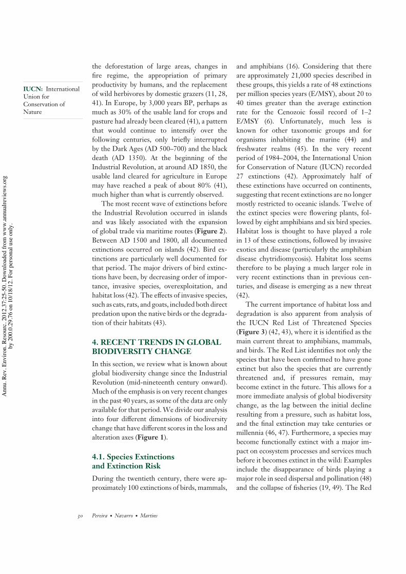
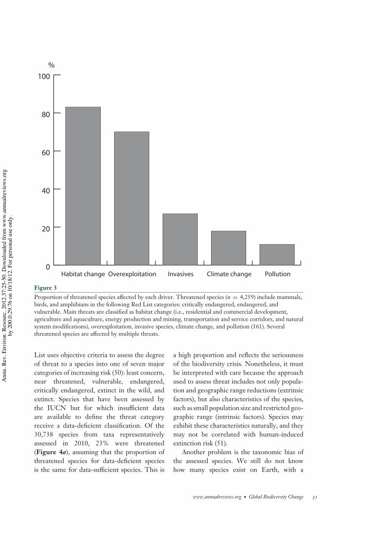
The current importance of habitat loss anddegradation is also apparent from analysis ofthe IUCN Red List of Threatened Species(Figure 3) (42, 43), where it is identified as themain current threat to amphibians, mammals,and birds. The Red List identifies not only thespecies that have been confirmed to have goneextinct but also the species that are currentlythreatened and, if pressures remain, maybecome extinct in the future. This allows for amore immediate analysis of global biodiversitychange, as the lag between the initial declineresulting from a pressure, such as habitat loss,and the final extinction may take centuries ormillennia (46, 47). Furthermore, a species maybecome functionally extinct with a major im-pact on ecosystem processes and services muchbefore it becomes extinct in the wild: Examplesinclude the disappearance of birds playing amajor role in seed dispersal and pollination (48)and the collapse of fisheries (19, 49). The Red
30 Pereira · Navarro · Martins
Ann
u. R
ev. E
nviro
n. R
esou
rc. 2
012.
37:2
5-50
. Dow
nloa
ded
from
ww
w.a
nnua
lrevi
ews.o
rgby
200
.0.2
9.76
on
10/1
8/12
. For
per
sona
l use
onl
y.
EG37CH02-Pereira ARI 5 October 2012 14:37
0
20
40
60
80
100
PollutionClimate changeInvasivesOverexploitationHabitat change
%
Figure 3Proportion of threatened species affected by each driver. Threatened species (n = 4,259) include mammals,birds, and amphibians in the following Red List categories: critically endangered, endangered, andvulnerable. Main threats are classified as habitat change (i.e., residential and commercial development,agriculture and aquaculture, energy production and mining, transportation and service corridors, and naturalsystem modifications), overexploitation, invasive species, climate change, and pollution (161). Severalthreatened species are affected by multiple threats.
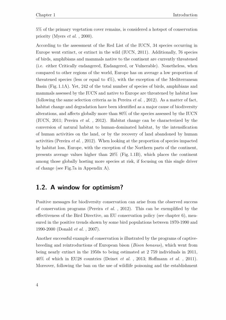
List uses objective criteria to assess the degreeof threat to a species into one of seven majorcategories of increasing risk (50): least concern,near threatened, vulnerable, endangered,critically endangered, extinct in the wild, andextinct. Species that have been assessed bythe IUCN but for which insufficient dataare available to define the threat categoryreceive a data-deficient classification. Of the30,738 species from taxa representativelyassessed in 2010, 23% were threatened(Figure 4a), assuming that the proportion ofthreatened species for data-deficient speciesis the same for data-sufficient species. This is
a high proportion and reflects the seriousnessof the biodiversity crisis. Nonetheless, it mustbe interpreted with care because the approachused to assess threat includes not only popula-tion and geographic range reductions (extrinsicfactors), but also characteristics of the species,such as small population size and restricted geo-graphic range (intrinsic factors). Species mayexhibit these characteristics naturally, and theymay not be correlated with human-inducedextinction risk (51).
Another problem is the taxonomic bias ofthe assessed species. We still do not knowhow many species exist on Earth, with a
www.annualreviews.org • Global Biodiversity Change 31
Ann
u. R
ev. E
nviro
n. R
esou
rc. 2
012.
37:2
5-50
. Dow
nloa
ded
from
ww
w.a
nnua
lrevi
ews.o
rgby
200
.0.2
9.76
on
10/1
8/12
. For
per
sona
l use
onl
y.
EG37CH02-Pereira ARI 5 October 2012 14:37
recent estimate placing the total number ofspecies at 7.4 to 10 million (52). Of these, onlyaround 1.7 million species have been described(Figure 4a) (16, 43). Systematic global RedList assessments have been carried out for onlya few taxonomic groups, and the proportion ofspecies assessed in each group is very differentfrom its representation in global biodiversity(Figure 4a). It is virtually impossible to assessthe extinction risk of all taxa. Instead, in thepast few years, the IUCN has developed arandomized sampling approach to expand itsassessment to more taxonomic groups (53).
Still, the overall pattern emerging from theRed List assessments is that amphibians (41%threatened) and cycads (63% threatened) arethe most threatened groups, and birds are theleast threatened group (13% threatened) (54).The generally low mobility and small ranges ofamphibians and cycads may contribute to thisvulnerability, but one might also ask if our bet-ter knowledge of bird species has contributedto their lower assessment of threat.
Most of the threatened terrestrial verte-brates occur in tropical regions (Figure 5b), fol-lowing the latitudinal trends in the species rich-ness of this group (Figure 5a). A very differentmap is obtained by looking at the relative pro-portion of threatened species in each grid cell(Figure 5c). Incidence of threatened species ishigh in much of Asia (except the North), theSahara, the Andes, Madagascar, the Caribbean,New Zealand, and other islands. Areas of highspecies diversity and moderate to high inci-dence of threatened species include the Indo-Malayan region (particularly Southeast Asia),the Andes, Central America, the Brazilian Cer-rado and Atlantic Forest, and some localizedareas of sub-Saharan Africa (Figure 6). Theseare regions with restricted-range species (42,55), and most have undergone rapid forest loss(56, 57).
The pattern for threatened marine verte-brates (cartilaginous fish) is somewhat similar,with higher occurrence of threatened species inthe tropics, but there is also a strong coastal sig-nal, with both of these regions having higherspecies richness (54). When one controls for
the species richness effect, high incidence ofthreatened species is still found at coastal ar-eas (54). This pattern agrees with the higherhuman pressure on coastal regions, particularlythat associated with fishing activities (15).
The Red List status gives us a snapshot ofwhat is happening to biodiversity at a giventime. However, we are also interested in under-standing the trends in biodiversity. The RedList Index compares the proportion of speciesin the different threat categories over time (43,54, 58). A key component of developing theRed List Index is the identification of speciesthat have changed status not because moreinformation became available but because theconservation situation of the species changed,i.e., genuine changes (43). Red List Indiceshave been calculated for birds (1988–2008),mammals (1996–2008), amphibians (1996–2008), and corals (1996–2008) (8, 54, 59). In allcases, the Red List Index shows an increase inthe proportion of threatened species, and thisincrease is especially pronounced for coralsowing to the large-scale bleaching event of1996–1998. It is important to understand thata flat (or unchanging) Red List Index means, intheory, that species are still declining toward ex-tinction, as the maintenance of a given categoryof threat indicates that a species population sizeor geographic range continues to decline at thesame rate (60). This contrasts with the meanpopulation abundance indices discussed in thenext section, where a constant value meansthe maintenance of the relative extinction risk.However, the fact that the risk assessmentincludes both population/range size andpopulation/range change can blur thisdistinction.
4.2. Changes in Species Abundancesand Community StructureChanges in extinction risk status can be slowand do not capture important alterations ofecosystem function that can occur when speciesabundances change (61, 62). In the past decade,several indicators have been developed toassess the population abundance dimension of
32 Pereira · Navarro · Martins
Ann
u. R
ev. E
nviro
n. R
esou
rc. 2
012.
37:2
5-50
. Dow
nloa
ded
from
ww
w.a
nnua
lrevi
ews.o
rgby
200
.0.2
9.76
on
10/1
8/12
. For
per
sona
l use
onl
y.
EG37CH02-Pereira ARI 5 October 2012 14:37
biodiversity (Figure 4b), including the LivingPlanet Index (LPI) (20, 63), the EuropeanCommon Farmland Bird Indicator (64), theWild Bird Index (WBI) (covering NorthAmerica and Europe) (8), and the EuropeanButterfly Indicator for Grassland Species (65).Most of the data in these indicators comes fromextensive observation networks of volunteers(66), and they portray one of the most immedi-ate and detailed pictures of global biodiversitychange. The idea in each of the indicators is toobtain the average population trend across a setof species and their populations. For example,the LPI includes 7,190 vertebrate populationsfrom 2,301 species across the marine, fresh-water, and terrestrial realms (8). The LPI fora given year is based on the geometric meanacross all populations of the relative abundanceindices between that year and the previous year(i.e., N t
N t−1). That geometric mean is then mul-
tiplied by the value of the LPI in the previousyear to give the final index value for that year,starting in 1970 with the value 1 (or 100%).The geometric mean of relative abundanceindices has nice statistical properties, partic-ularly when based on common species, and isable to detect overall abundance and evennessdecreases and, to some extent, species richnessdecreases (67, 68). The geometric mean isequal to one when the halving of the density ofa species is compensated by a doubling of thedensity of another species. The other indicatorsmentioned above follow similar approaches.
Overall, the pattern that emerges from allof these indicators is of global or regionaldeclines of species abundances, despite someyear-to-year fluctuations of some indicators(Figure 4b). The LPI has declined from 1970 to2006 by 31% (8), the WBI for habitat specialistshas declined from 1980 to 2007 by 2.6% (8), theEuropean Common Farmland Bird Indicatordeclined from 1980 to 2006 by 49% (69), andthe European Butterfly Indicator for GrasslandSpecies declined from 1990 to 2009 by 70%(based on a best-fit line) (65). These numberspaint a depressing figure and are in some caseslarge enough to suggest that ecosystem pro-cesses and services are being modified (70, 71).
LPI: Living PlanetIndex
Biodiversityindicator: a metricused to assess the rateand intensity ofbiodiversity change
However, they must be interpreted with somecaution as the spatial and taxonomic coverageof these indicators is limited (72). Furthermore,a finer analysis of these indicators can tell somecontrasting stories. The tropical terrestrial LPIhas declined, but the temperate terrestrial LPIhas increased (20). One possible explanation isthat, although tropical ecosystems are now un-dergoing fast and detrimental land-use changeand overexploitation (2), these drivers peakedin temperate regions much before 1970 andare now decreasing as a consequence of farm-land abandonment, greater species protection,and conservation actions. This has favored thereturn of large mammals (those that survivedthe earlier extinction wave) and other species insome temperate regions (17, 73). Still, the samehabitat changes that have benefited large mam-mals are thought to contribute to the declineof farmland birds and grassland butterflies, al-though agricultural intensification is likely toplay a major role too (64, 65). There are ma-jor geographic differences in the marine LPI,with strong decreases in the Indian Ocean andSouthern Ocean and increases elsewhere (20).Similarly, although the terrestrial species in theWild Bird Index have declined by 16%, the wet-land species have increased by 40%. This lastcase also illustrates the problem of spatial cov-erage: The Waterbird Population Status Index,with global coverage and measuring the pro-portion of monitored shorebird populations,declined 18% from 1985 to 2005 (8). We dis-cuss biodiversity change uncertainties associ-ated with spatial coverage in detail in Section 6.
In the marine realm, much of the existingdata come from fisheries, which have influ-enced the development of marine biodiversityindicators. The Marine Trophic Index (MTI)measures the mean trophic level of fish landings(74). The MTI declined globally in the 1960sand in the 1980s, and it increased in the early1970s and since the 1990s (8, 75). Declines havebeen attributed to overfishing of large species,leading to shifting fishing efforts to smallerspecies at lower trophic levels. Recent increaseshave been attributed to the spatial expansion ofthe fishing effort (8, 76). The sensitivity of the
www.annualreviews.org • Global Biodiversity Change 33
Ann
u. R
ev. E
nviro
n. R
esou
rc. 2
012.
37:2
5-50
. Dow
nloa
ded
from
ww
w.a
nnua
lrevi
ews.o
rgby
200
.0.2
9.76
on
10/1
8/12
. For
per
sona
l use
onl
y.
EG37CH02-Pereira ARI 5 October 2012 14:37
MTI to changes in the spatial distributionof fishing effort has led to the search foralternative measures of species abundancechanges in the oceans. One such measure isthe proportion of fish stocks not fully exploitedor depleted (Figure 4b). For the fisheriesthat have been assessed, this proportion hasdecreased to half since 1974, and currently,only 21% of the stocks are not fully exploitedor depleted (8, but see Reference 19 for analternative estimate). Although the MTI andthe proportion of fully exploited stocks giveus a measure of the capacity of the ecosystemto provide a service, they may not reflect theoverall state of biodiversity in those systems, asmany species are not targeted by fishing.
Coastal habitats have been undergoing par-ticularly high human pressure (77), and coralreefs, one of the most biologically diverse andproductive systems on the planet, are particu-larly vulnerable because of their sensitivity toclimate change and other pressures (78, 79).One measure of the community structure ofcoral reefs is hard-coral live cover (80, 81).Hard-coral live cover had a marked declinedin the late 1970s in the Caribbean, followingthe white band disease outbreak, but has re-mained steady since the mid-1980s, althoughother community changes have been observed,including an increase in macroalgae cover inthe late 1980s (Figure 4b) (81). In the Indo-Pacific live hard-coral cover has declined sincethe 1980s, and particularly from 1997 to 2004(80), and in 2003, coral cover averaged 22.1%, avalue much lower than the historic baseline es-timates of >50% cover. The bleaching event of1996–1998 has had major impact, but disease,sedimentation from coastal development, anddestructive fishing practices have also played arole.
4.3. Shifts in the Distributionof Species and CommunitiesClimate change and other ecosystem changedrivers may cause alterations in species distri-butions (3, 82, 83). The alteration of a species
distribution can be decomposed into two majoraspects: directional shifts in the distribution(3) and changes in the size of the distribution(84). Directional shifts have been measuredusing species distribution centroids (3) orrange limits (85). Recently, a new measurefor directional shifts has been proposed, theCommunity Temperature Index, which trackshow the composition of communities at eachsite changes toward high-temperature dwellingspecies (86). Changes in the size of the speciesdistribution are likely to be correlated withoverall changes in species abundance (87, 88);however, directional shifts in the distribu-tion may go undetected if only total speciesabundances are tracked.
An early meta-analysis of birds (UnitedKingdom), butterflies (Sweden), and alpineherbs (Switzerland) suggested that specieswere moving their range limits poleward at anaverage rate of 0.61 km/year (Figure 4c) (85),providing evidence of climate change impactson species distributions. Another study analyz-ing northern limit shifts across 16 taxonomicgroups in the United Kingdom found averageshifts of 1.2–2.5 km/year (Figure 4c) (89).More recently, an assessment of distributionshifts for birds and butterflies in Europe,using the Community Temperature Index, hasfound rates of 2.1 and 6.3 km/year, respectively(Figure 4c) (90). The one order of magnitudedifference between the lowest estimate of rangeshifts and the highest estimate may be causedby the different methods used, the differentregions, and the different taxa analyzed. Theintervals of species shift rates are consistentwith those of the velocities of isotherms from1960 to 2009 in land surfaces (median of2.7 km/year) and oceans (2.2 km/year), whichexhibit large spatial variations, with some re-gions exhibiting no significant shifts and othersshifting at rates higher than 10 km/year (91).
Average shifts may hide substantial variationin individual species responses, as some speciesmaintain their previous ranges, others movetoward the poles (i.e., North in the North-ern Hemisphere), and yet others move in
34 Pereira · Navarro · Martins
Ann
u. R
ev. E
nviro
n. R
esou
rc. 2
012.
37:2
5-50
. Dow
nloa
ded
from
ww
w.a
nnua
lrevi
ews.o
rgby
200
.0.2
9.76
on
10/1
8/12
. For
per
sona
l use
onl
y.
EG37CH02-Pereira ARI 5 October 2012 14:37
unexpected directions (83, 92). For instance,in the North Sea, the varying responses ofdifferent species (Figure 4c ) led to a nonsignif-icant change in the mean latitude of speciesranges from 1980 to 2004, although mostspecies assemblages tracked yearly fluctuationsin climate with mean latitudinal shifts of 10–70 km/◦C (83). Some species assemblages, suchas warm-water specialists, exhibited significantoverall shifts during these 25 years, movingnorthward at a rate of 4 km/year (83).
Species can also adapt to climate change byshifts in elevation (85, 92) or depth (83), shiftinglife history traits in time (93), or by adapting tothe new conditions in their local range throughphenotypic plasticity or microevolution (94).
4.4. Genetic Diversity inDomesticated and Wild SpeciesOf the four biodiversity dimensions analyzedhere, we have the least information at theglobal level for changes in genetic diversity.Studies of loss of genetic diversity can beclassified into two categories: studies of geneticdiversity of domesticated species and studiesof genetic diversity of wild species. Studies ofdomesticated species can further be dividedinto plant genetic resources (95) and animalgenetic resources (96).
Over the past few decades, the worldwideadoption of modern crop varieties adapted tohigh-input systems has led to the reduction inthe area farmed with local crop varieties (95).This change in agricultural practices has raisedconcerns: For instance in China, the numberof rice breeds in production is reported to havedeclined since the 1950s from 46,000 to 1,000,and most of the 10,000 traditional corn breedsare no longer in production (97). Still, there aremany farm communities that, although exposedto modern varieties, choose to maintain, at leastin portions of the farm, traditional varieties(98). The picture of allelic diversity change isalso complex. Although some studies reportdeclines in allelic diversity of modern varietiesover the past few decades (99), a meta-analysis
of 44 studies has found no significant overalltrend (100). Another concern is the status ofthe crops’ wild relatives, which are under thesame threats as other aspects of biodiversity,and recently a system of priority areas fortheir conservation in situ has been proposed(95).
Of the about 7,600 animal breeds (among36 domesticated mammal and bird species) reg-istered in the UN Food and Agriculture Or-ganization’s Global Databank, 20% are clas-sified as being at risk, and a further 9% havebecome extinct (Figure 4d ) (96). Over the pastdecades, a similar phenomena to what happenedwith the crop varieties is occurring with the an-imal breeds: Local animal breeds are being re-placed by widely used and high-output breedsmore adapted to intensive animal productionsystems (7).
Less is known about the loss of geneticdiversity in wild populations. One study hasestimated that about 16 million populations arebeing lost annually, on the basis of an estimateof 220 populations per species derived froma review of population genetic studies and anassumption of linearity between tropical defor-estation and population extinction rates (101).This is a very indirect estimate, and to ourknowledge, it has not been confirmed indepen-dently. Other studies have looked at patternsof genetic diversity in populations impacted byhumans (102, 103). A meta-analysis of popula-tion genetics studies found decreases in geneticdiversity in animal and plant populationsunder pressure of habitat fragmentation andno consistent signal for populations affectedby hunting or fishing, but found diversityincreases in populations affected by pollution(103). Another meta-analysis, targeted onlyat mammals, found significant lower geneticdiversity in mammalian populations that haveexperienced a reduction in population sizeor range or a population bottleneck (102). Ina rare longitudinal study, Lage & Kornfield(104) looked at the genetic diversity in apopulation of the Atlantic salmon (Salmo salar)using samples from 1963 to 2001. They found
www.annualreviews.org • Global Biodiversity Change 35
Ann
u. R
ev. E
nviro
n. R
esou
rc. 2
012.
37:2
5-50
. Dow
nloa
ded
from
ww
w.a
nnua
lrevi
ews.o
rgby
200
.0.2
9.76
on
10/1
8/12
. For
per
sona
l use
onl
y.
EG37CH02-Pereira ARI 5 October 2012 14:37
that genetic diversity declined during thisperiod, closely following population declines.
5. UNDERSTANDING THEDIRECT PRESSURESWe now examine five major categories of globalbiodiversity change pressures. For three ofthose, habitat change, pollution, and climatechange, global models of their impacts are avail-able, and we make comparisons between theterrestrial spatial pattern of the driver and theimpacts on species extinction risk (Figure 7).Note, however, that the current biodiversityimpacts of land-use change are much greaterthan the impacts of the other two drivers(Figure 3).
5.1. Habitat Change and DegradationHabitat change and habitat degradation arecurrently the major drivers of global biodiver-sity change (Figure 3). In terrestrial systems,land-use change dynamics can be broadly classi-fied into three categories: conversion of naturalhabitats to human-dominated habitats, inten-sification of human use of human-dominatedhabitats, and recovery of natural vegetation andforest in areas that have been previously clearedby humans. Not all species respond equally tohabitat changes (105–107): When forest is con-verted to agriculture and pastures, some speciesmay increase in abundance, whereas otherspecies, particularly habitat specialists (108,109), can decline or even go locally extinct.
Although the three types of land change dy-namics occur in most world regions, the relativeimportance of each one has a strong latitudinalpattern (Figure 7b) (2, 110): Most conversionof natural to human-dominated habitats isoccurring in tropical forests (111); agriculturalintensification started in the developed regionsbut is rapidly expanding to the rest of the world(not represented in Figure 7b) (112); most re-covery of natural and forest vegetation is occur-ring in temperate regions in Europe and NorthAmerica (17) (Figure 7b). A net forest loss ofabout 42,000 km2 per year (111) in tropical
regions is partially balanced by a net forestgain of 8,700 km2 per year in Europe (110).However, part of the net forest gain is the resultof new forest plantations, often with exoticspecies, which often have lower biodiversitythan natural forests (113). Fire plays a majorrole in many regions in the conversion of forestto agriculture but also in maintaining openlandscapes.
As expected, there is an agreement betweenthe spatial distribution of areas of naturalhabitat being converted to agriculture and thedistribution of species affected by habitat loss(Figure 7a,b), including in Madagascar, someareas of sub-Saharan Africa, Brazil’s AtlanticForest, the Middle East, and Southeast Asia.Forest loss in Southeast Asia is not wellcaptured in our land-use change map but hasbeen reported in other studies (57). There aresome regions where there is a high proportionof species affected by habitat loss where mostland-use change already occurred in the past(much of Europe), and regions where specieshave been affected by habitat loss not capturedin our analysis (e.g., the Sahara).
River systems have been deeply altered byimpoundments and diversions to meet water,energy, and transportation needs of a growinghuman population (14). Today, there are morethan 45,000 large dams (>15 m in height)worldwide (14). Dams have upstream impacts,where lotic systems are changed into lenticsystems, and downstream impacts, where thetiming, magnitude, and temperature of waterflow is changed (45). Dams are also responsiblefor the fragmentation of river systems, asthey hamper or even block the dispersal andmigration of organisms (14). Furthermore,water resource development by impoundmentsand diversions has high spatial overlap withother pressures in freshwater ecosystems,such as pollution and catchment disturbanceby cropland (114). Other important habitatchanges in freshwater ecosystems includethe loss of wetlands owing to drainage forconversion to agriculture or urbanization,overextraction of groundwater (45), and theexcavation of river sand (115).
36 Pereira · Navarro · Martins
Ann
u. R
ev. E
nviro
n. R
esou
rc. 2
012.
37:2
5-50
. Dow
nloa
ded
from
ww
w.a
nnua
lrevi
ews.o
rgby
200
.0.2
9.76
on
10/1
8/12
. For
per
sona
l use
onl
y.
EG37CH02-Pereira ARI 5 October 2012 14:37
Marine habitats are also being affected byhuman activities, particularly by destructivefishing practices, such as trawling and dynamit-ing (116). Coastal habitats and wetlands havebeen affected mostly by urbanization, aqua-culture development, and coastal engineeringworks (15, 77).
5.2. OverexploitationOverexploitation is the major driver of bio-diversity loss in the oceans (2, 19). Capturefisheries production increased for much of thetwentieth century but has reached a plateausince the mid-1980s at around 70–80 milliontons annually, despite continuing increasesin global fishing effort levels (117, 118). Theglobal landings would have likely declinedexcept for the spatial expansion of the fishingeffort toward deeper and further offshorewaters. By the mid-1960s, most fully exploitedor overexploited fisheries were located incoastal areas of the Northern Hemisphere. Bythe 1980s, fishing efforts were having an impacton regions much farther away from the coast,in the middle of the northern and southernAtlantic Oceans. One decade later, the spatialexpansion of the fisheries had reached muchof the world’s oceans, with only some parts ofthe Indian Ocean, the Pacific Ocean, and theAntarctic ocean not having reached maximumhistorical catches (116).
In terrestrial systems, hunting is a majorconcern in tropical savannahs and forests (2).Large birds and mammals are targeted fortheir meat and charismatic species for their or-naments and alleged medicinal purposes (108,111). Wild-meat harvest has been estimated at67–164 thousand tons in the Brazilian Amazonand 1–3.4 million tons in Central Africa (119).The impacts are particularly acute in SoutheastAsia and Central Africa (111). A connectionhas been established between the reductionof fish availability per capita and the increasein hunting pressure of wild meat in WestAfrica (120). Synergistic interactions betweenhunting and other drivers, such as land-use
change and disease, can also occur and causelocal extinctions (106).
5.3. PollutionEutrophication and other ecosystem changescaused by pollution are major drivers ofbiodiversity loss and alterations in both inlandwaters and coastal systems (121). River nitro-gen loads from point sources, such as domesticand industrial sewage, and nonpoint sources,such as agriculture and atmospheric deposition,increased in most world regions from 1970 to1995 but are starting to decline or are projectedto decline until 2030 in Europe and northernAsia (Russia) (122). Lakes are particularlyvulnerable to regime shifts caused by eutrophi-cation, which may be difficult to reverse (47,123). Eutrophication can lead to increasedbiomass of phytoplankton and macrophytevegetation, blooms of toxic cyanobacteria andother algae, higher incidence of fish kills, and,in the case of coral reefs, declines in coral reefhealth and loss of coral reef communities (121).
Atmospheric nitrogen deposition fromintensive agriculture and fossil-fuel combus-tion can also affect terrestrial ecosystems,particularly temperate grasslands (2). Theincrease in availability of nitrogen changes thecompetition dynamics in plant (124) and lichencommunities (125), favoring the increaseof nitrophilous species and the decline ofnitrogen-sensitive species. One study found alinear relationship between the rate of nitrogendeposition and species richness declines intemperate grasslands and estimated that, forthe levels of nitrogen deposition observed inmuch of central Europe (17 kg/ha/year), a 23%reduction of species diversity can be expected(124). Unfortunately, some high species diver-sity regions (e.g., Southeast Asia and Brazil’sAtlantic Forest) are also receiving similarlevels of nitrogen deposition (Figure 7d ),but more research is needed to identify itsimpacts (126). A visual inspection of thespatial overlap between the global patterns ofnitrogen deposition and the distribution of ver-tebrates affected by pollution shows reasonable
www.annualreviews.org • Global Biodiversity Change 37
Ann
u. R
ev. E
nviro
n. R
esou
rc. 2
012.
37:2
5-50
. Dow
nloa
ded
from
ww
w.a
nnua
lrevi
ews.o
rgby
200
.0.2
9.76
on
10/1
8/12
. For
per
sona
l use
onl
y.
EG37CH02-Pereira ARI 5 October 2012 14:37
agreement in Europe, but inspection alsoshows disagreement in other parts of theworld, such as Central Africa (Figure 7c,d ).Note, however, that there are other sources ofpollution included in the assessment of speciesextinction risk (Figure 7c) and not directlyrelated to atmospheric nitrogen deposition(Figure 7d ).
5.4. Introduction of Exotic Speciesand InvasionsOne of the major trends in global biodiver-sity change is the increased homogenization ofplant and animal diversity owing to biotic ex-change. In some cases, exotic species are able tospread beyond the places where they were in-troduced, spreading in the landscape and out-competing native species (127). Islands havebeen particularly affected by invasive species(128): Animal invasions have led to species ex-tinctions, whereas plant invasions can decreasethe abundance of native species and becomedominant in plant communities. Plant invasionsmay also affect the nutrient cycles, alter thefire regimes, and impact other ecosystem ser-vices (129, 130). A particularly serious type ofinvasions is epidemic disease. One example ischytridiomycosis, which has been decimatingamphibians in many regions of the world and isa leading cause of the global amphibian decline(131). Invasive species have also had impor-tant impacts on freshwater ecosystems, wheretheir incidence is correlated with human eco-nomic activity (132), and in marine and estu-arine ecosystems due to ballast water or hullfouling transported by ships (133).
Still, many invasive species have had moremoderate impacts on ecosystems (134), and re-cently, some ecologists have called for a moreembracing attitude toward exotic species, ar-guing that alien species should not be a prioriconsidered negative in an ecosystem but shouldbe assessed objectively for their impacts (135,136). Others have argued for active translo-cation or assisted migration of species endan-gered by climate change (137), an approach thatseems fraught with peril on the basis of our
historical experience of human introductions ofexotic species, often with the best intentions.
5.5. Climate ChangeGlobal mean surface temperature increased0.74◦C from 1906 to 2005 and is expected toincrease between 1.8◦C and 4◦C during thetwenty-first century, depending on the socio-economic scenario (138). Warming is spatiallyvery heterogeneous as it is largest in terrestrialsystems and at high northern latitudes, withrecent warming greater than 1.5◦C in some ar-eas, and least pronounced in the tropics, wheremany regions have warmed around 0.5◦C(Figure 7f ). The impacts of climate changeare already contributing to increased extinc-tion risk of species at high northern latitudes(Figure 7e). Further climate change impactsin these regions have been projected for birds(139) and for plants (46) during this century.Surprisingly, in the Cape region (South Africa)and in southeastern Australia, a high incidenceof species negatively affected by climate changehas been reported (Figure 7e), althoughthese areas are not suffering large warming(Figure 7f ). One explanation may be thatthose regions have many species particularlyvulnerable to climate change. Species withhigh vulnerability are species that have narrowclimate niches, cannot shift their ranges, orare unable to change their phenology, evolvetheir physiology, or behaviorally adapt to thenew conditions (93, 140). For instance, thelimited ability of mountaintop species to shiftin elevation has been identified as a majorclimate vulnerability (92).
For amphibians, important future climateimpacts have been projected in the northernAndes, parts of the Amazon, Central America,southern and southeastern Europe, sub-Saharan tropical Africa, and Southeast Asia(140, 141). Surprisingly, this disagrees some-what from the recent spatial patterns of in-creased extinction risk owing to climate change(Figure 7e).
In corals, most threatened and climatechange–susceptible species occur in Southeast
38 Pereira · Navarro · Martins
Ann
u. R
ev. E
nviro
n. R
esou
rc. 2
012.
37:2
5-50
. Dow
nloa
ded
from
ww
w.a
nnua
lrevi
ews.o
rgby
200
.0.2
9.76
on
10/1
8/12
. For
per
sona
l use
onl
y.
EG37CH02-Pereira ARI 5 October 2012 14:37
Asia (140). Climate change is also causingsea-level rise and threatening coastal habitats,particularly in synergy with land-use change,which may not allow coastal habitats to migrateinland (47). Marine ecosystems are also affectedby ocean acidification caused by climate change,particularly corals (79) and other marine or-ganisms that build calcium carbonate skeletons(142).
6. EXPLORING THEUNDERLYING CAUSES WITHSCENARIO MODELSUpstream from the direct pressures on biodi-versity, there are indirect drivers of biodiversitychange. Major indirect drivers for biodiversityinclude population growth, energy use andenergy production, diet, and food demand.Naturally, these drivers interact between themand with other drivers, such as technologydevelopment, socioeconomic changes, andcultural transformations (143). One way ofexploring the relationship between the indirectdrivers and global biodiversity change isthrough scenario modeling. Biodiversity sce-narios have recently been reviewed elsewhere(3). They can be developed in three steps:(a) plausible trajectories of key indirect driversare generated; (b) the trajectories are fed intomodels that project changes in direct pressures;and (c) projected pressures are used as inputsof biodiversity models. Many scenarios exploredifferent futures and how they depend on policydecisions, but scenario models can also be usedfor hindcasting, i.e., to reconstruct the past.
The human population increased from2.5 billion people in 1950 to 7 billion in2011 and can reach between 8.1 billion and10.6 billion people in 2050, depending onthe scenario (144). The increase in humanpopulation growth is being accompanied byan increase in the demand for food (with foodproduction growing faster than human popu-lation) and an increase in energy consumption(2). How much of the increase in food pro-duction needed over the next few decades willcome from intensification or from farmland
expansion to natural habitats will depend ontechnological developments, policy choices,and societal behavior. Similarly, how a growingenergy demand will be satisfied by additionalfossil-fuel consumption or by shifting energyproduction toward other sources has also beenexplored in scenarios.
Most scenarios project a decrease in forestarea by 2050 of up to 20% and in an extremecase, of more than 60% (3). Still, some sce-narios that account for policies recognizing therole of forests in CO2 sequestration and avoid-ing the impacts of land-use changes, includingconversion of forests to biofuels, project netincreases in forest area (3). Species extinctionrates will continue to be higher than in the fossilrecord. For the same modeling approach, sce-narios with lower levels of population growthand climate change result in lower estimates ofbiodiversity loss.
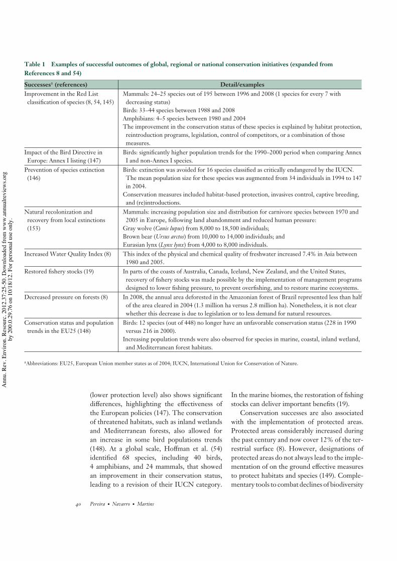
7. A BIT OF GOOD NEWSFOR A CHANGEDespite the gloomy biodiversity picture de-picted in the previous sections, there is alsosome good news about global biodiversitychange due to the reversion of the effect of adriver (e.g., forest recovery) or the successes ofconservation initiatives on the status of species(Table 1).
Measures such as habitat conservation,reintroduction programs, and legislation haveproven to be efficient in improving the statusof several species (145). One way to assessconservation successes is to identify preventedextinctions. Between 1994 and 2004, 16 birdspecies would have gone extinct if actions hadnot been undertaken to protect them (146).One example is the population of the NorfolkIsland green parrot (Cyanoramphus cookii ), verylikely to go extinct in 1994, with only fourbreeding females, which has now close to 300individuals thanks to habitat protection andcontrol of predator and competitor species.In Europe, a comparison of bird populationtrends between Birds Directive Annex I (higherprotection level) and non-Annex I species
www.annualreviews.org • Global Biodiversity Change 39
Ann
u. R
ev. E
nviro
n. R
esou
rc. 2
012.
37:2
5-50
. Dow
nloa
ded
from
ww
w.a
nnua
lrevi
ews.o
rgby
200
.0.2
9.76
on
10/1
8/12
. For
per
sona
l use
onl
y.
EG37CH02-Pereira ARI 5 October 2012 14:37
Table 1 Examples of successful outcomes of global, regional or national conservation initiatives (expanded fromReferences 8 and 54)
Successesa (references) Detail/examplesImprovement in the Red Listclassification of species (8, 54, 145)
Mammals: 24–25 species out of 195 between 1996 and 2008 (1 species for every 7 withdecreasing status)
Birds: 33–44 species between 1988 and 2008Amphibians: 4–5 species between 1980 and 2004The improvement in the conservation status of these species is explained by habitat protection,reintroduction programs, legislation, control of competitors, or a combination of thosemeasures.
Impact of the Bird Directive inEurope: Annex I listing (147)
Birds: significantly higher population trends for the 1990–2000 period when comparing AnnexI and non-Annex I species.
Prevention of species extinction(146)
Birds: extinction was avoided for 16 species classified as critically endangered by the IUCN.The mean population size for these species was augmented from 34 individuals in 1994 to 147in 2004.
Conservation measures included habitat-based protection, invasives control, captive breeding,and (re)introductions.
Natural recolonization andrecovery from local extinctions(153)
Mammals: increasing population size and distribution for carnivore species between 1970 and2005 in Europe, following land abandonment and reduced human pressure:
Gray wolve (Canis lupus) from 8,000 to 18,500 individuals;Brown bear (Ursus arctos) from 10,000 to 14,000 individuals; andEurasian lynx (Lynx lynx) from 4,000 to 8,000 individuals.
Increased Water Quality Index (8) This index of the physical and chemical quality of freshwater increased 7.4% in Asia between1980 and 2005.
Restored fishery stocks (19) In parts of the coasts of Australia, Canada, Iceland, New Zealand, and the United States,recovery of fishery stocks was made possible by the implementation of management programsdesigned to lower fishing pressure, to prevent overfishing, and to restore marine ecosystems.
Decreased pressure on forests (8) In 2008, the annual area deforested in the Amazonian forest of Brazil represented less than halfof the area cleared in 2004 (1.3 million ha versus 2.8 million ha). Nonetheless, it is not clearwhether this decrease is due to legislation or to less demand for natural resources.
Conservation status and populationtrends in the EU25 (148)
Birds: 12 species (out of 448) no longer have an unfavorable conservation status (228 in 1990versus 216 in 2000).
Increasing population trends were also observed for species in marine, coastal, inland wetland,and Mediterranean forest habitats.
aAbbreviations: EU25, European Union member states as of 2004; IUCN, International Union for Conservation of Nature.
(lower protection level) also shows significantdifferences, highlighting the effectiveness ofthe European policies (147). The conservationof threatened habitats, such as inland wetlandsand Mediterranean forests, also allowed foran increase in some bird populations trends(148). At a global scale, Hoffman et al. (54)identified 68 species, including 40 birds,4 amphibians, and 24 mammals, that showedan improvement in their conservation status,leading to a revision of their IUCN category.
In the marine biomes, the restoration of fishingstocks can deliver important benefits (19).
Conservation successes are also associatedwith the implementation of protected areas.Protected areas considerably increased duringthe past century and now cover 12% of the ter-restrial surface (8). However, designations ofprotected areas do not always lead to the imple-mentation of on the ground effective measuresto protect habitats and species (149). Comple-mentary tools to combat declines of biodiversity
40 Pereira · Navarro · Martins
Ann
u. R
ev. E
nviro
n. R
esou
rc. 2
012.
37:2
5-50
. Dow
nloa
ded
from
ww
w.a
nnua
lrevi
ews.o
rgby
200
.0.2
9.76
on
10/1
8/12
. For
per
sona
l use
onl
y.
EG37CH02-Pereira ARI 5 October 2012 14:37
outside nature reserves are agri-environmentschemes, which are policy tools with amplescope to reverse the negative trends of once-common, widespread species (150), and directpayments to conserve biodiversity (151).
In some regions of the world, a habitatconservation strategy that is emerging as asignificant opportunity is the rewilding ofabandoned areas (17). Natural revegetationin large areas has been observed in the pastand is predicted to occur in the next decades(Figure 7b), particularly on remote andmarginally productive areas (e.g., mountains)in the Northern Hemisphere where agricultureand forestry activities are being abandoned(46, 152). The subsequent reappropriationof the land by wildlife can be beneficial forvarious species that take advantage of thereduced human pressure (17): Several Euro-pean carnivores have been coming back tocountries where they were previously extinct(153). Still, natural regeneration presentscertain challenges that depend on the level ofresilience of the land (154, 155) and potentialconflicts with human populations (17).
Finally, aside from avoided extinctions andincreasing population trends, conservation suc-cesses can be measured in changes in societies’behavior regarding sustainable resource uses.The increasing public support for biodiver-sity conservation in the past few decades (156),the commitment of the Convention on Bio-logical Diversity parties to new goals for 2020(157), and the recent establishment of the In-tergovernmental Platform on Biodiversity andEcosystem Services (http://www.ipbes.net)give hope of further progress in the years tocome.
8. MAJOR GAPS IN OURUNDERSTANDING OF GLOBALBIODIVERSITY CHANGEIn this article, we reviewed the current sci-entific knowledge about the state of globalbiodiversity change. Overall, the patterns thatemerge allow us to state with confidence thatbiodiversity is being rapidly altered on land,
in rivers, and in oceans, and is being lostlocally in many regions and also globally. Someconservation actions have been successfulat mitigating or, in a few cases, reversingbiodiversity loss. However, many unknownsremain, and we still do not know the exactdimensions of the biodiversity crisis.
Some of the biodiversity indicators thatwere described in Section 4 and that were usedto assess the 2010 target of the Convention onBiological Diversity are far from being com-pletely developed (149). Very little is knownabout trends in genetic diversity, particularlyin wild species. The taxonomic coverage of theindicators and assessments is very limited: Theextinction risk of the vast majority of biodiver-sity is not known (Figure 4a), and most of thepopulation indicators are derived from verte-brate populations (Figure 4b). This is not to saythat the same conservation and research em-phasis shall be placed on all biodiversity. Peopleplace high existence values on vertebrates (158),and many important ecosystem services areassociated with vertebrates (48, 62). It is just anacknowledgment of the large gap in our taxo-nomic knowledge of global biodiversity change.More worryingly, even the available informa-tion for vertebrates is spatially very heteroge-neous (72) and is least available in regions thatare currently under pressure (Figure 8). TheGroup on Earth Observations Biodiversity Ob-servation Network (GEO BON) aims at fillingthese gaps by integrating biodiversity monitor-ing programs across the globe and promotingbiodiversity monitoring in gap regions (159).
Major gaps and uncertainties remain inmodeling global biodiversity change. In terres-trial systems, most research has been dedicatedto model climate change impacts, althoughsome work has also been done on modelingthe impacts of land-use change and, to a lesserextent, pollution. Models are lacking for theglobal spatial distribution of exploitation pres-sure and invasive species and their impacts interrestrial systems. But even for the pressuresthat have received most attention, large uncer-tainties remain: Projected extinction rates forthis century range from less than 20 E/MSY
www.annualreviews.org • Global Biodiversity Change 41
Ann
u. R
ev. E
nviro
n. R
esou
rc. 2
012.
37:2
5-50
. Dow
nloa
ded
from
ww
w.a
nnua
lrevi
ews.o
rgby
200
.0.2
9.76
on
10/1
8/12
. For
per
sona
l use
onl
y.
EG37CH02-Pereira ARI 5 October 2012 14:37
to more than 14,000 E/MSY (3). Both the lackof harmonization of modeling approaches andthe lack of knowledge of how species respondto global change contribute to this uncertainty.
9. IS ALL BIODIVERSITY CHANGEEQUALLY BAD?Our world is changing, and biodiversity is noexception. Yet, not all biodiversity change is in-herently bad, and we should avoid a static viewof conservation biology (despite its name). Themaintenance of the landscapes or the biologicalcommunities we know should not be the apriori management target. We need to assessbiodiversity change with objective criteria. Theecosystem services framework (2, 70), withthe appropriate inclusion of species existencevalues (158), is an excellent tool to assess themanagement priorities for biodiversity change.It allows us to identify not only the benefitsand costs of biodiversity alterations for humanwell-being but also to prioritize the biodiversitylosses that are more important to address.
Biodiversity alterations and losses have tobe assessed for their contribution to ecosystemprocesses, such as nutrient cycling and soilformation, and to ecosystem services, such asclimate regulation, water quality regulation,
water provisioning, timber provisioning, dis-ease and pest regulation, and cultural services.An appropriate inclusion of existence valuesis essential; people place large values on theconservation of particular species or taxonomicgroups. Therefore, not all species extinctionscan be treated equally from a utilitarian point ofview. The extinction in the wild of the virusesvariola major and variola minor, the causes ofthe deadly smallpox, was arguably a good thing.But in many more cases, the loss of biodiversityis impoverishing us and making our planetmore unequal for its human inhabitants: It isoften the poor that suffer the first negativeimpacts of biodiversity change (2).
Some biodiversity alterations, such as theconversion of the Amazon forest to agriculturalareas, may lead to tipping points in ecosystemsthat are hard to reverse (47), but the majority ofbiodiversity alterations are reversible throughmanagement. In contrast, biodiversity loss isusually irreversible: Extinction is forever, atleast with the current biotechnology level.Scientists can inform society about how bio-diversity is changing and what the likely con-sequences of those changes are for ecosystemsand for human well-being, but it is up to societyto decide what should be done about theseissues.
SUMMARY POINTS
1. Biodiversity change is composed of biodiversity loss, such as species extinctions, andbiodiversity alterations, such as species range shifts.
2. Biodiversity is changing at unprecedented rates in human history: Species are becomingextinct or closer to extinction; mean species abundances of several taxa are decreasing;species are shifting their ranges in response to climate change; and domestic and wildgenetic diversity are being lost.
3. The major direct drivers of biodiversity change are habitat change and overexploitation.Pollution, exotic species, and disease are also important drivers. Climate change is anemerging driver of biodiversity change.
4. Human population growth and human resource use are the underlying indirect driversof biodiversity change.
42 Pereira · Navarro · Martins
Ann
u. R
ev. E
nviro
n. R
esou
rc. 2
012.
37:2
5-50
. Dow
nloa
ded
from
ww
w.a
nnua
lrevi
ews.o
rgby
200
.0.2
9.76
on
10/1
8/12
. For
per
sona
l use
onl
y.
EG37CH02-Pereira ARI 5 October 2012 14:37
5. There have been some important successes in biodiversity conservation—mainly throughspecies management, protected areas, and increased societal awareness. Farmland aban-donment is an opportunity for biodiversity restoration.
6. Not all biodiversity change is bad. Biodiversity change should be assessed in relation toits consequences for ecosystem services and species existence values.
FUTURE ISSUES
1. There are major gaps in our knowledge of biodiversity change, and there is the need toimprove our biodiversity monitoring programs worldwide.
2. There are also important uncertainties and gaps in our models of global biodiversitychange.
DISCLOSURE STATEMENTThe authors are not aware of any affiliations, memberships, funding, or financial holdings thatmight be perceived as affecting the objectivity of this review.
ACKNOWLEDGMENTSThis work was supported by grants PTDC/AGR-AAM/104819/2008 and PTDC/AAC-AMB/114522/2009 from Fundacao para a Ciencia e Tecnologia (FCT). L.M.N. was supported bya PhD fellowship from FCT. We thank Stuart Butchart for providing data for Figure 4, LouiseMcRae for proving the data for Figure 8, and Thomas Merckx for comments. Finally, we thankIUCN, Birdlife International, and their experts, which over the past years compiled and madepublic data on global threat and distribution of amphibians, mammals, and birds.
LITERATURE CITED
1. Dirzo R, Raven P. 2003. Global state of biodiversity and loss. Annu. Rev. Environ. Resour. 28:137–672. Duraiappah A, Naheem S, Agardy T, Ash NJ, Cooper HD, et al. 2005. Ecosystems and Human Well-Being:
Biodiversity Synthesis. Washington, DC: World Resour. Inst.3. Pereira HM, Leadley PW, Proenca V, Alkemade R, Scharlemann JPW, et al. 2010. Scenarios for global
biodiversity in the 21st century. Science 330:1496–5024. Carpenter SR, Mooney HA, Agard J, Capistrano D, Defries RS, et al. 2009. Science for managing ecosys-
tem services: beyond the Millennium Ecosystem Assessment. Proc. Natl. Acad. Sci. USA 106(5):1305–125. The Econ. Ecosyst. Biodivers. (TEEB). 2010. Mainstreaming the Economics of Nature: A Synthesis of the
Approach, Conclusions and Recommendations of TEEB. Geneva: TEEB6. Barnosky AD, Matzke N, Tomiya S, Wogan GOU, Swartz B, et al. 2011. Has the Earth’s sixth mass
extinction already arrived? Nature 471(7336):51–577. GBO 3. 2010. Global Biodiversity Outlook 3. Montreal: Secr. Conv. Biol. Divers. 94 pp.8. Butchart SHM, Walpole M, Collen B, van Strien A, Scharlemann JPW, et al. 2010. Global biodiversity:
indicators of recent declines. Science 328(5982):1164–689. Erwin DH. 2008. Macroevolution of ecosystem engineering, niche construction and diversity. Trends
Ecol. Evol. 23(6):304–10
www.annualreviews.org • Global Biodiversity Change 43
Ann
u. R
ev. E
nviro
n. R
esou
rc. 2
012.
37:2
5-50
. Dow
nloa
ded
from
ww
w.a
nnua
lrevi
ews.o
rgby
200
.0.2
9.76
on
10/1
8/12
. For
per
sona
l use
onl
y.
EG37CH02-Pereira ARI 5 October 2012 14:37
10. Robertson GP, Vitousek PM. 2009. Nitrogen in agriculture: balancing the cost of an essential resource.Annu. Rev. Environ. Resour. 34:97–125
11. Doughty CE, Field CB. 2010. Agricultural net primary production in relation to that liberated by theextinction of Pleistocene mega-herbivores: an estimate of agricultural carrying capacity? Environ. Res.Lett. 5(4):044001
12. Foley J, DeFries R, Asner G, Barford C, Bonan G, et al. 2005. Global consequences of land use. Science309(5734):570–74
13. Klein Goldewijk K, Beusen A, Van Drecht G, Vos M. 2011. The HYDE 3.1 spatially explicit databaseof human-induced global land-use change over the past 12,000 years. Glob. Ecol. Biogeogr. 20:73–86
14. Nilsson C, Reidy CA, Dynesius M, Revenga C. 2005. Fragmentation and flow regulation of the world’slarge river systems. Science 308(5720):405–8
15. Halpern BS, Walbridge S, Selkoe KA, Kappel CV, Micheli F, et al. 2008. A global map of human impacton marine ecosystems. Science 319(5865):948–52
16. Mace GM, Masundire H, Baillie J, Ricketts TH, Brooks TM, et al. 2005. Biodiversity. See Ref. 168,pp. 77–126
17. Navarro L, Pereira HM. 2012. Rewilding abandoned landscapes in Europe. Ecosystems. 15:900–1218. Moreira F, Russo D. 2007. Modelling the impact of agricultural abandonment and wildfires on vertebrate
diversity in Mediterranean Europe. Landsc. Ecol. 22(10):1461–7619. Worm B, Hilborn R, Baum JK, Branch TA, Collie JS, et al. 2009. Rebuilding global fisheries. Science
325(5940):578–8520. Collen B, Loh J, Whitmee S, McRae L, Amin R, Baillie JEM. 2009. Monitoring change in vertebrate
abundance: the Living Planet Index. Conserv. Biol. 23(2):317–2721. Williams JW, Jackson ST, Kutzbach JE. 2007. Projected distributions of novel and disappearing climates
by 2100 AD. Proc. Natl. Acad. Sci. USA 104(14):573822. Groombridge B, Jenkins MD. 2002. World Atlas of Biodiversity. Berkeley: Univ. Calif. Press23. Roebroeks W, Villa P. 2011. On the earliest evidence for habitual use of fire in Europe. Proc. Natl. Acad.
Sci. USA 108(13):5209–1424. Bowman DMJS, Balch JK, Artaxo P, Bond WJ, Carlson JM, et al. 2009. Fire in the Earth System. Science
324(5926):481–8425. Power C. 2011. Fire: the spark that ignited human evolution. J. R. Anthropol. Inst. 17(2):409–1026. Daniau A-L, d’ Errico F, Sanchez Goni MF. 2010. Testing the hypothesis of fire use for ecosystem
management by Neanderthal and Upper Palaeolithic modern human populations. PLoS ONE 5(2):e915727. Johnson CN. 2009. Ecological consequences of Late Quaternary extinctions of megafauna. Proc. R. Soc.
B 276(1667):2509–1928. Barnosky AD. 2008. Megafauna biomass tradeoff as a driver of Quaternary and future extinctions.
Proc. Natl. Acad. Sci. USA 105(Suppl. 1):11543–4829. Goebel T, Waters MR, O’Rourke DH. 2008. The late Pleistocene dispersal of modern humans in the
Americas. Science 319(5869):1497–50230. Waters MR, Stafford TW, McDonald HG, Gustafson C, Rasmussen M, et al. 2011. Pre-Clovis mastodon
hunting 13,800 years ago at the Manis site, Washington. Science 334(6054):351–5331. Lawler A. 2011. Pre-Clovis mastodon hunters make a point. Science 334(6054):30232. Barnosky AD, Koch PL, Feranec RS, Wing SL, Shabel AB. 2004. Assessing the causes of late Pleistocene
extinctions on the continents. Science 306(5693):70–7533. Guimaraes PR, Galetti M, Jordano P. 2008. Seed dispersal anachronisms: rethinking the fruits extinct
megafauna ate. PLoS ONE 3(3):e174534. Gill JL, Williams JW, Jackson ST, Lininger KB, Robinson GS. 2009. Pleistocene megafaunal collapse,
novel plant communities, and enhanced fire regimes in North America. Science 326(5956):1100–335. Blondel J. 2006. The “design” of Mediterranean landscapes: a millennial story of humans and ecological
systems during the historic period. Hum. Ecol. 34(5):713–2936. Lev-Yadun S, Gopher A, Abbo S. 2000. The cradle of agriculture. Science 288(5471):1602–337. Jones MK, Liu X. 2009. Origins of agriculture in East Asia. Science 324(5928):730–3138. Dillehay TD, Rossen J, Andres TC, Williams DE. 2007. Preceramic adoption of peanut, squash, and
cotton in northern Peru. Science 316(5833):1890–93
44 Pereira · Navarro · Martins
Ann
u. R
ev. E
nviro
n. R
esou
rc. 2
012.
37:2
5-50
. Dow
nloa
ded
from
ww
w.a
nnua
lrevi
ews.o
rgby
200
.0.2
9.76
on
10/1
8/12
. For
per
sona
l use
onl
y.
EG37CH02-Pereira ARI 5 October 2012 14:37
39. Diamond JM. 1998. Guns, Germs and Steel: A Short History of Everybody for the Last 13,000 Years. London:Random House
40. Zeder MA, Hesse B. 2000. The initial domestication of goats (Capra hircus) in the Zagros Mountains10,000 years ago. Science 287(5461):2254–57
41. Kaplan J, Krumhardt K, Zimmermann N. 2009. The prehistoric and preindustrial deforestation ofEurope. Quat. Sci. Rev. 28(27–28):3016–34
42. Baillie JEM, Hilton-Taylor C, Stuart SN. 2004. 2004 IUCN Red List of Threatened Species. A Global SpeciesAssessment. Gland, Switz.: IUCN
43. Vie J-C, Hilton-Taylor C, Stuart SN, eds. 2009. Wildlife in a Changing World: An Analysis of the 2008IUCN Red List of Threatened Species. Gland, Switz.: IUCN
44. Dulvy NK, Sadovy Y, Reynolds J. 2003. Extinction vulnerability in marine populations. Fish Fish. 4(1):25–64
45. Finlayson CM, D’Cruz R. 2005. Inland water systems. See Ref. 168, pp. 551–8346. van Vuuren DP, Sala OE, Pereira HM. 2006. The future of vascular plant diversity under four global
scenarios. Ecol. Soc. 11(2):2547. Leadley PW, Pereira HM, Alkemade R, Fernandez-Manjarres JF, Proenca V, et al. 2010. Biodiversity
Scenarios: Projections of 21st Century Change in Biodiversity and Associated Ecosystem Services. Montreal: Secr.Conv. Biol. Divers. 132 pp.
48. Sekercioglu CH, Daily GC, Ehrlich PR. 2004. Ecosystem consequences of bird declines. Proc. Natl.Acad. Sci. USA 101(52):18042–47
49. Worm B, Barbier EB, Beaumont N, Duffy JE, Folke C, et al. 2006. Impacts of biodiversity loss on oceanecosystem services. Science 314(5800):787–90
50. IUCN Species Surviv. Comm. 2001. IUCN Red List Categories and Criteria, Version 3.1. Gland,Switz./Cambridge, UK: IUCN
51. Robbirt KM, Roberts DL, Hawkins JA. 2006. Comparing IUCN and probabilistic assessments of threat:Do IUCN Red List criteria conflate rarity and threat? Biodivers. Conserv. 15(6):1903–12
52. Mora C, Tittensor DP, Adl S, Simpson AGB, Worm B. 2011. How many species are there on Earth andin the ocean? PLoS Biol. 9(8):e1001127
53. Baillie JEM, Collen B, Amin R, Akcakaya HR, Butchart SHM, et al. 2008. Toward monitoring globalbiodiversity. Conserv. Lett. 1(1):18–26
54. Hoffmann M, Hilton-Taylor C, Angulo A, Bohm M, Brooks T, et al. 2010. The impact of conservationon the status of the world’s vertebrates. Science 330(6010):1503–9
55. Orme CDL, Davies RG, Olson VA, Thomas GH, Ding T-S, et al. 2006. Global patterns of geographicrange size in birds. PLoS Biol. 4(7):e208
56. Achard F, Eva HD, Stibig H-J, Mayaux P, Gallego J, et al. 2002. Determination of deforestation ratesof the world’s humid tropical forests. Science 297(5583):999–1002
57. Hansen MC, Stehman SV, Potapov PV, Loveland TR, Townshend JRG, et al. 2008. Humid tropicalforest clearing from 2000 to 2005 quantified by using multitemporal and multiresolution remotely senseddata. Proc. Natl. Acad. Sci. USA 105(27):9439–44
58. Butchart SHM, Stattersfield AJ, Bennun LA, Shutes SM, Akcakaya HR, et al. 2004. Measuring globaltrends in the status of biodiversity: Red List Indices for birds. PLoS Biol. 2(12):e383
59. Carpenter K, Abrar M, Aeby G, Aronson R, Banks S, et al. 2008. One-third of reef-building corals faceelevated extinction risk from climate change and local impacts. Science 321(5888):560–63
60. Butchart SHM, Stattersfield AJ, Baillie J, Bennun LA, Stuart SN, et al. 2005. Using Red List Indices tomeasure progress towards the 2010 target and beyond. Philos. Trans. R. Soc. B 360(1454):255–68
61. Balmford A, Green RE, Jenkins M. 2003. Measuring the changing state of nature. Trends Ecol. Evol.18(7):326–30
62. Pereira HM, Brummitt N, Collen B, Couvet D, Gibson C, et al. 2010. Terrestrial species monitoring.In Group on Earth Observations Biodiversity Observation Network (GEO BON) Detailed Implementation Plan.Geneva: GEO BON
63. Loh J, Green RE, Ricketts T, Lamoreux J, Jenkins M, et al. 2005. The Living Planet Index: using speciespopulation time series to track trends in biodiversity. Philos. Trans. R. Soc. B 360:289–95
www.annualreviews.org • Global Biodiversity Change 45
Ann
u. R
ev. E
nviro
n. R
esou
rc. 2
012.
37:2
5-50
. Dow
nloa
ded
from
ww
w.a
nnua
lrevi
ews.o
rgby
200
.0.2
9.76
on
10/1
8/12
. For
per
sona
l use
onl
y.
EG37CH02-Pereira ARI 5 October 2012 14:37
64. Gregory RD, van Strien A, Vorisek P, Meyling AWG, Noble DG, et al. 2005. Developing indicatorsfor European birds. Philos. Trans. R. Soc. B 360(1454):269–88
65. Van Swaay CAM, Van Strien AJ, Harpke A, Fontaine B, Stefanescu C, et al. 2010. The European ButterflyIndicator for Grassland Species. Wageningen, Neth.: De Vlinderstichting
66. Pereira HM, Cooper HD. 2006. Towards the global monitoring of biodiversity change. Trends Ecol.Evol. 21:123–29
67. Buckland ST, Magurran AE, Green RE, Fewster RM. 2005. Monitoring change in biodiversity throughcomposite indices. Philos. Trans. R. Soc. B 360(1454):243
68. van Strien AJ, Soldaat LL, Gregory RD. 2012. Desirable mathematical properties of indicators forbiodiversity change. Ecol. Indic. 14(1):202–8
69. Vorısek P, Jiguet F, van Strien A, Skorpilova J, Klvanova A, Gregory RD. 2010. Trends in abundanceand biomass of widespread European farmland birds: How much have we lost? Proc. BOU—LowlandFarmland Birds III: Delivering Solutions in an Uncertain World, Br. Ornithol. Union, March 31–April 2,2009, Univ. Leicester, UK. http://www.bou.org.uk/bouproc-net/lfb3/vorisek-etal.pdf
70. Dıaz S, Fargione J, Chapin FS, Tilman D. 2006. Biodiversity loss threatens human well-being. PLoSBiol. 4(8):e277
71. Sekercioglu CH, Schneider SH, Fay JP, Loarie SR. 2008. Climate change, elevational range shifts, andbird extinctions. Conserv. Biol. 22(1):140–50
72. Pereira HM, Belnap J, Brummitt N, Collen B, Ding H, et al. 2010. Global biodiversity monitoring.Front. Ecol. Environ. 8(9):459–60
73. Russo D. 2006. Effects of Land Abandonment on Animal Species in Europe: Conservation and ManagementImplications. Portici (Napoli), Italy: Univ. Studi Napoli Federico II. 51 pp.
74. Pauly D, Watson R. 2005. Background and interpretation of the “Marine Trophic Index” as a measureof biodiversity. Philos. Trans. R. Soc. B 360(1454):415–23
75. Pauly D, Christensen VV, Dalsgaard J, Froese R, Torres F Jr. 1998. Fishing down marine food webs.Science 279(5352):860–63
76. Bhathal B, Pauly D. 2008. “Fishing down marine food webs” and spatial expansion of coastal fisheries inIndia, 1950–2000. Fish Res. 91(1):26–34
77. Agardy T, Alder J. 2005. Coastal systems. See Ref. 168, pp. 13–4978. Hughes TP, Baird AH, Bellwood DR, Card M, Connolly SR, et al. 2003. Climate change, human
impacts, and the resilience of coral reefs. Science 301(5635):929–3379. Hoegh-Guldberg O, Mumby PJ, Hooten AJ, Steneck RS, Greenfield P, et al. 2007. Coral reefs under
rapid climate change and ocean acidification. Science 318(5857):1737–4280. Bruno JF, Selig ER. 2007. Regional decline of coral cover in the Indo-Pacific: timing, extent, and
subregional comparisons. PLoS One 2(8):e71181. Schutte VGW, Selig ER, Bruno JF. 2010. Regional spatio-temporal trends in Caribbean coral reef
benthic communities. Mar. Ecol. Prog. Ser. 402:115–2282. Fischlin A, Midgley GF, Price J, Leemans R, Gopal B, et al. 2007. Ecosystems, their properties, goods
and services. In Climate Change 2007: Impacts, Adaptation and Vulnerability. Contribution of Working GroupII to the Fourth Assessment Report of the IPCC, ed. ML Parry, OF Canziani, JP Palutikof, PJ van der Linden,CE Hanson, pp. 211–72. Cambridge, UK: Cambridge Univ. Press
83. Dulvy NK, Rogers S, Jennings S, Stelzenmuller V, Dye S, Skjoldal H. 2008. Climate change and deep-ening of the North Sea fish assemblage: a biotic indicator of warming seas. J. Appl. Ecol. 45(4):1029–39
84. Araujo MB, Pearson RG, Thuiller W, Erhard M. 2005. Validation of species-climate impact modelsunder climate change. Glob. Change Biol. 11(9):1504–13
85. Parmesan C, Yohe G. 2003. A globally coherent fingerprint of climate change impacts across naturalsystems. Nature 421(6918):37–42
86. Devictor V, Julliard R, Couvet D, Jiguet F. 2008. Birds are tracking climate warming, but not fast enough.Proc. R. Soc. B 275(1652):2743–48
87. Warren MS, Hill JK, Thomas JA, Asher J, Fox R, et al. 2001. Rapid responses of British butterflies toopposing forces of climate and habitat change. Nature 414(6859):65–69
46 Pereira · Navarro · Martins
Ann
u. R
ev. E
nviro
n. R
esou
rc. 2
012.
37:2
5-50
. Dow
nloa
ded
from
ww
w.a
nnua
lrevi
ews.o
rgby
200
.0.2
9.76
on
10/1
8/12
. For
per
sona
l use
onl
y.
EG37CH02-Pereira ARI 5 October 2012 14:37
88. Fordham DA, Resit Akcakaya H, Araujo MB, Elith J, Keith DA, et al. 2012. Plant extinction risk underclimate change: Are forecast range shifts alone a good indicator of species vulnerability to global warming?Glob. Change Biol. 18:1357–71
89. Hickling R, Roy DB, Hill JK, Fox R, Thomas CD. 2006. The distributions of a wide range of taxonomicgroups are expanding polewards. Glob. Change Biol. 12(3):450–55
90. Devictor V, van Swaay C, Brereton T, Brotons L, Chamberlain D, et al. 2012. Differences in the climaticdebts of birds and butterflies at a continental scale. Nat. Clim. Change 2(2):121–24
91. Burrows MT, Schoeman DS, Buckley LB, Moore P, Poloczanska ES, et al. 2011. The pace of shiftingclimate in marine and terrestrial ecosystems. Science 334(6056):652–55
92. Parmesan C. 2006. Ecological and evolutionary responses to recent climate change. Annu. Rev. Ecol.Evol. Syst. 37(1):637–69
93. Bellard C, Bertelsmeier C, Leadley P, Thuiller W, Courchamp F. 2012. Impacts of climate change onthe future of biodiversity. Ecol. Lett. 15:365–77
94. Dawson TP, Jackson ST, House JI, Prentice IC, Mace GM. 2011. Beyond predictions: biodiversityconservation in a changing climate. Science 332(6025):53–58
95. Food Agric. Organ. UN. 2010. The Second Report on the State of the World’s Plant Genetic Resources for Foodand Agriculture. Rome: FAO
96. Food Agric. Organ. UN. 2007. The State of the World’s Animal Genetic Resources for Food and Agriculture.Rome: FAO
97. Xu H, Tang X, Liu J, Ding H, Wu J, et al. 2009. China’s progress toward the significant reduction ofthe rate of biodiversity loss. BioScience 59(10):843–52
98. Jarvis DI, Brown AHD, Cuong PH, Collado-Panduro L, Latournerie-Moreno L, et al. 2008. A globalperspective of the richness and evenness of traditional crop-variety diversity maintained by farmingcommunities. Proc. Natl. Acad. Sci. USA 105(14):5326–31
99. Reif JC, Hamrit S, Heckenberger M, Schipprack W, Maurer HP, et al. 2005. Trends in genetic diversityamong European maize cultivars and their parental components during the past 50 years. Theor. Appl.Genet. 111(5):838–45
100. Wouw M, Hintum T, Kik C, Treuren R, Visser B. 2010. Genetic diversity trends in twentieth centurycrop cultivars: a meta analysis. Theor. Appl. Genet. 120(6):1241–52
101. Hughes JB, Daily GC, Ehrlich PR. 1997. Population diversity: its extent and extinction. Science278(5338):689–92
102. Garner A, Rachlow J, Hicks J. 2005. Patterns of genetic diversity and its loss in mammalian populations.Conserv. Biol. 19(4):1215–21
103. DiBattista JD. 2008. Patterns of genetic variation in anthropogenically impacted populations. Conserv.Genet. 9(1):141–56
104. Lage C, Kornfield I. 2006. Reduced genetic diversity and effective population size in an endangeredAtlantic salmon (Salmo salar) population from Maine, USA. Conserv. Genet. 7(1):91–104
105. Pereira HM, Daily GC. 2006. Modeling biodiversity dynamics in countryside landscapes. Ecology87(8):1877–85
106. Stork NE, Coddington JA, Colwell RK, Chazdon RL, Dick CW, et al. 2009. Vulnerability and resilienceof tropical forest species to land-use change. Conserv. Biol. 23(6):1438–47
107. Phalan B, Onial M, Balmford A, Green RE. 2011. Reconciling food production and biodiversity conser-vation: land sharing and land sparing compared. Science 333(6047):1289–91
108. Owens IPF, Bennett PM. 2000. Ecological basis of extinction risk in birds: habitat loss versus humanpersecution and introduced predators. Proc. Natl. Acad. Sci. USA 97(22):12144–48
109. Brook BW, Sodhi NS, Ng PKL. 2003. Catastrophic extinctions follow deforestation in Singapore. Nature424(6947):420–23
110. Food Agric. Organ. UN. 2010. Global Forest Resources Assessment 2010. Rome: FAO111. Wright SJ. 2010. The future of tropical forests. Ann. N.Y. Acad. Sci. 1195:1–27112. Cassman KG, Wood S, Choo P, Cooper H, Devendra C, et al. 2005. Cultivated systems. See Ref. 168,
pp. 745–94113. Proenca VM, Pereira HM, Guilherme J, Vicente L. 2010. Plant and bird diversity in natural forests and
in native and exotic plantations in NW Portugal. Acta Oecol. 36(2):219–26
www.annualreviews.org • Global Biodiversity Change 47
Ann
u. R
ev. E
nviro
n. R
esou
rc. 2
012.
37:2
5-50
. Dow
nloa
ded
from
ww
w.a
nnua
lrevi
ews.o
rgby
200
.0.2
9.76
on
10/1
8/12
. For
per
sona
l use
onl
y.
EG37CH02-Pereira ARI 5 October 2012 14:37
114. Vorosmarty C, McIntyre P, Gessner M, Dudgeon D, Prusevich A, et al. 2010. Global threats to humanwater security and river biodiversity. Nature 467(7315):555–61
115. Dudgeon D, Arthington AH, Gessner MO, Kawabata Z-I, Knowler DJ, et al. 2006. Freshwater biodi-versity: importance, threats, status and conservation challenges. Biol. Rev. 81(02):163–82
116. Pauly D, Alder J. 2005. Marine fisheries systems. See Ref. 168, pp. 477–512117. Christensen V, Aiken KA, Villanueva MC. 2007. Threats to the ocean: on the role of ecosystem ap-
proaches to fisheries. Soc. Sci. Inform. 46(1):67–86118. Food Agric. Organ. UN. 2009. The State of World Fisheries and Aquaculture 2008. Rome: FAO119. Milner-Gulland E, Bennett E. 2003. Wild meat: the bigger picture. Trends Ecol. Evol. 18(7):351–57120. Brashares JS, Arcese P, Sam MK, Coppolillo PB, Sinclair ARE, Balmford A. 2004. Bushmeat hunting,
wildlife declines, and fish supply in West Africa. Science 306(5699):1180–83121. Smith V, Schindler D. 2009. Eutrophication science: Where do we go from here? Trends Ecol. Evol.
24(4):201–7122. Bouwman AF, Van Drecht G, Knoop JM, Beusen AHW, Meinardi CR. 2005. Exploring changes in river
nitrogen export to the world’s oceans. Glob. Biogeochem. Cycles 19:GB1002123. Carpenter SR. 2003. Regime Shifts in Lake Ecosystems: Pattern and Variation. Oldendorf/Luhe, Germ.: Int.
Ecol. Inst.124. Stevens CJ, Dise NB, Mountford JO, Gowing DJ. 2004. Impact of nitrogen deposition on the species
richness of grasslands. Science 303(5665):1876–79125. Pinho P, Augusto S, Martins-Loucao MA, Pereira MJ, Soares A, et al. 2008. Causes of change in nitro-
phytic and oligotrophic lichen species in a Mediterranean climate: impact of land cover and atmosphericpollutants. Environ. Pollut. 154(3):380–89
126. Phoenix GK, Hicks WK, Cinderby S, Kuylenstierna JCI, Stock WD, et al. 2006. Atmospheric nitro-gen deposition in world biodiversity hotspots: the need for a greater global perspective in assessing Ndeposition impacts. Glob. Change Biol. 12(3):470–76
127. Theoharides KA, Dukes JS. 2007. Plant invasion across space and time: factors affecting nonindigenousspecies success during four stages of invasion. New Phytol. 176(2):256–73
128. Sax D, Gaines S. 2008. Species invasions and extinction: the future of native biodiversity on islands.Proc. Natl. Acad. Sci. USA 105:11490–97
129. Mack RN, Simberloff D, Lonsdale WM, Evans H, Clout M, Bazzaz FA. 2000. Biotic invasions: causes,epidemiology, global consequences, and control. Ecol. Appl. 10(3):689–710
130. Pejchar L, Mooney H. 2009. Invasive species, ecosystem services and human well-being. Trends Ecol.Evol. 24(9):497–504
131. Wake DB, Vredenburg VT. 2008. Are we in the midst of the sixth mass extinction? A view from theworld of amphibians. Proc. Natl. Acad. Sci. USA 105(Suppl. 1):11466–73
132. Leprieur F, Beauchard O, Blanchet S, Oberdorff T, Brosse S. 2008. Fish invasions in the world’s riversystems: when natural processes are blurred by human activities. PLOS Biol. 6(2):404–10
133. Barry SC, Hayes KR, Hewitt CL, Behrens HL, Dragsund E, Bakke SM. 2008. Ballast water risk assess-ment: principles, processes, and methods. ICES J. Mar. Sci. 65(2):121–31
134. Gurevitch J, Padilla D. 2004. Are invasive species a major cause of extinctions? Trends Ecol. Evol.19(9):470–74
135. Vince G. 2011. Conservation ecology: embracing invasives. Science 331(6023):1383–84136. Davis MA, Chew MK, Hobbs RJ, Lugo AE, Ewel JJ, et al. 2011. Don’t judge species on their origins.
Nature 474(7350):153–54137. Lawler JJ, Olden JD. 2011. Reframing the debate over assisted colonization. Front. Ecol. Environ.
9(10):569–74138. IPCC. 2007. Climate Change 2007: Synthesis Report. Contribution of Working Groups I, II and III to the
Fourth Assessment Report of the Intergovernmental Panel on Climate Change. Geneva, Switz.: IPCC. 104 pp.139. Jetz W, Wilcove DS, Dobson AP. 2007. Projected impacts of climate and land-use change on the global
diversity of birds. PLoS Biol. 5(6):e157140. Foden WB, Mace GM, Vie J-C, Angulo A, Butchart SHM, et al. 2009. Species susceptibility to climate
change impacts. See Ref. 43, pp. 77–88
48 Pereira · Navarro · Martins
Ann
u. R
ev. E
nviro
n. R
esou
rc. 2
012.
37:2
5-50
. Dow
nloa
ded
from
ww
w.a
nnua
lrevi
ews.o
rgby
200
.0.2
9.76
on
10/1
8/12
. For
per
sona
l use
onl
y.
EG37CH02-Pereira ARI 5 October 2012 14:37
141. Hof C, Araujo MB, Jetz W, Rahbek C. 2011. Additive threats from pathogens, climate and land-usechange for global amphibian diversity. Nature 480:516–19
142. Orr JC, Fabry VJ, Aumont O, Bopp L, Doney SC, et al. 2005. Anthropogenic ocean acidification overthe twenty-first century and its impact on calcifying organisms. Nature 437(7059):681–86
143. Millenn. Ecosyst. Assess. 2003. Ecosystems and Human Well-Being. A Framework for Assessment. Washing-ton, DC: Island Press
144. UN. 2011. World Population Prospects: The 2010 Revision. New York: UN145. Hoffmann M, Belant JL, Chanson JS, Cox NA, Lamoreux J, et al. 2011. The changing fates of the world’s
mammals. Philos. Trans. R. Soc. B 366(1578):2598–610146. Butchart SHM, Stattersfield AJ, Collar NJ. 2006. How many bird extinctions have we prevented?
Oryx 40(03):266–78147. Donald PF, Sanderson FJ, Burfield IJ, Bierman SM, Gregory RD, Waliczky Z. 2007. International
conservation policy delivers benefits for birds in Europe. Science 317(5839):810–13148. BirdLife Int. 2004. Birds in the European Union: A Status Assessment. Wageningen, Neth.: BirdLife Int.149. Walpole M, Almond REA, Besancon C, Butchart SHM, Campbell-Lendrum D, et al. 2009. Tracking
progress toward the 2010 biodiversity target and beyond. Science 325(5947):1503–4150. Merckx T, Feber RE, Riordan P, Townsend MC, Bourn NAD, et al. 2009. Optimizing the biodiversity
gain from agri-environment schemes. Agric. Ecosyst. Environ. 130(3–4):177–82151. Ferraro PJ, Kiss A. 2002. Direct payments to conserve biodiversity. Science 298(5599):1718–19152. Verburg PH, Overmars KP. 2009. Combining top-down and bottom-up dynamics in land use modeling:
exploring the future of abandoned farmlands in Europe with the Dyna-CLUE model. Landsc. Ecol.24:1167–81
153. Large Carniv. Initiat. Eur. (LCIE). 2004. Status and trends for large carnivores in Europe. Rep. UNEP-WCMC Project, Biodiversity Trends and Threats in Europe, Krakow, Poland
154. Cramer VA, Hobbs RJ, Standish RJ. 2008. What’s new about old fields? Land abandonment and ecosys-tem assembly. Trends Ecol. Evol. 23:104–12
155. Benayas JMR, Bullock JM, Newton AC. 2008. Creating woodland islets to reconcile ecological restora-tion, conservation, and agricultural land use. Front. Ecol. Environ. 6(6):329–36
156. Rands MRW, Adams WM, Bennun L, Butchart SHM, Clements A, et al. 2010. Biodiversity conservation:challenges beyond 2010. Science 329(5997):1298–303
157. Conv. Biol. Divers. 2010. Decision X/2. The Strategic Plan for Biodiversity 2011–2020 and the Aichi Biodi-versity Targets. Montreal, Can.: CBD. http://www.biodiv.be/convention/strategic-plan-2011-2020/
158. Proenca VM, Pereira HM, Vicente L. 2008. Organismal complexity is an indicator of species existencevalue. Front. Ecol. Environ. 6(6):298–99
159. Scholes RJ, Walters M, Turak E, Saarenmaa H, Heip CH, et al. 2012. Building a global observing systemfor biodiversity. Curr. Opin. Environ. Sustain. 4(1):139–46
160. Stringer C, Finlayson J, Barton R, Fernandez-Jalvo Y, Caceres I, et al. 2008. Neanderthal exploitationof marine mammals in Gibraltar. Proc. Natl. Acad. Sci. USA 105(38):14319
161. IUCN. 2011. IUCN Red List of Threatened Species. Version 2011.2. Gland, Switz.: IUCN.http://www.iucnredlist.org
162. Eur. Environ. Agency. 2009. Common birds in Europe—Population Index (1980 = 100). Copenhagen: Eur.Environ. Agency. http://www.eea.europa.eu/data-and-maps/figures/common-birds-in-europe-2014-population-index-1980
163. Eur. Environ. Agency. 2010. Grassland Butterflies—Population Index. Copenhagen: Eur. Environ. Agency.http://www.eea.europa.eu/data-and-maps/figures/grassland-butterflies-2014-population-index-1990
164. BirdLife Int. 2011. Distribution Maps of Birds of the World. Cambridge, UK: BirdLife Int.165. Alcamo J, van Vuuren D, Cramer W. 2005. Changes in ecosystem services and their drivers across
scenarios. In Ecosystems and Human Well-Being: Scenarios, ed. SR Carpenter, LP Prabhu, EM Bennet,MB Zurek, 2:297–373. Washington, DC: Island Press
166. Dentener FJ. 2006. Global Maps of Atmospheric Nitrogen Deposition, 1860, 1993, and 2050. Data set. OakRidge, TN: Oak Ridge Natl. Lab., Distrib. Act. Arch. Cent. http://daac.ornl.gov/
www.annualreviews.org • Global Biodiversity Change 49
Ann
u. R
ev. E
nviro
n. R
esou
rc. 2
012.
37:2
5-50
. Dow
nloa
ded
from
ww
w.a
nnua
lrevi
ews.o
rgby
200
.0.2
9.76
on
10/1
8/12
. For
per
sona
l use
onl
y.
EG37CH02-Pereira ARI 5 October 2012 14:37
167. Mitchell TD, Carter TR, Jones PD, Hulme M, New M. 2004. A comprehensive set of high-resolution gridsof monthly climate for Europe and the globe: the observed record (1901–2000) and 16 scenarios (2001–2100).Tyndall Cent. Work. Pap. 55., Tyndall Cent. Clim. Change Res., Univ. East Anglia, Norwick, UK
168. Hassan R, Scholes R, Ash N, eds. 2005. Ecosystems and Human Well-Being. Volume 1: Current State andTrends: Findings of the Condition and Trends Working Group. Millennium Ecosystem Assessment. Washington,DC: Island Press
50 Pereira · Navarro · Martins
Ann
u. R
ev. E
nviro
n. R
esou
rc. 2
012.
37:2
5-50
. Dow
nloa
ded
from
ww
w.a
nnua
lrevi
ews.o
rgby
200
.0.2
9.76
on
10/1
8/12
. For
per
sona
l use
onl
y.
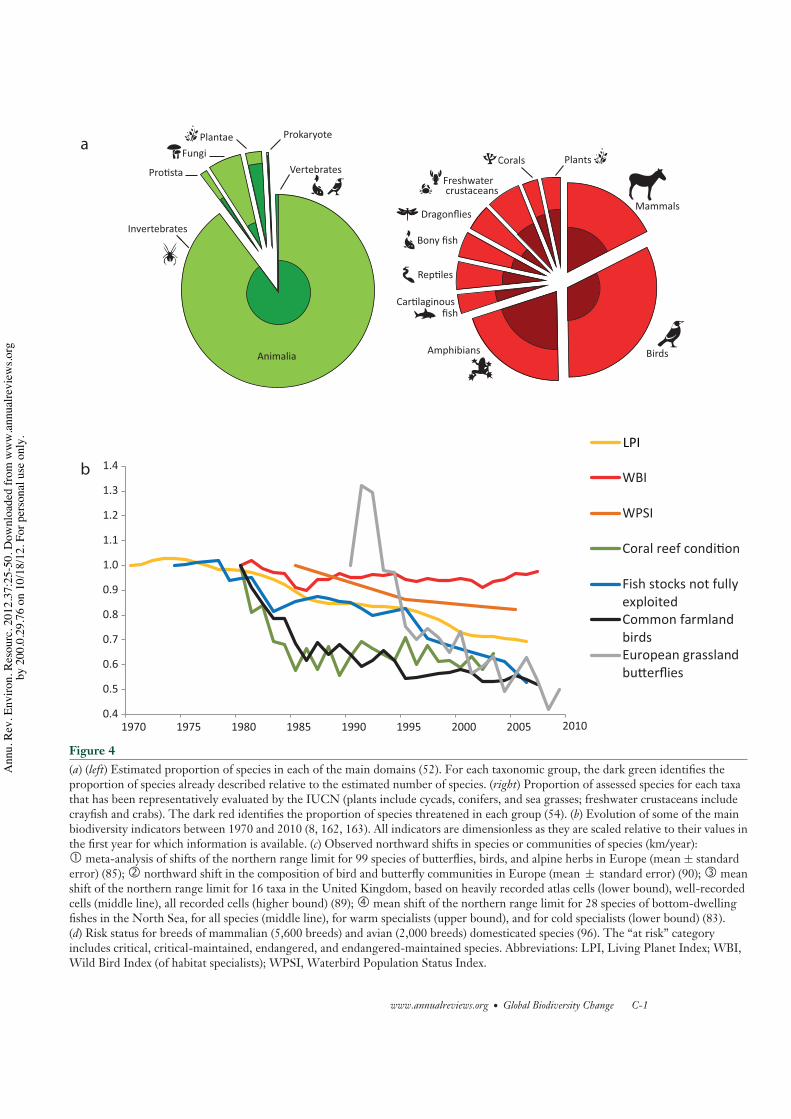
EG37CH02-Pereira ARI 5 October 2012 14:37
Plants
Mammals
Bony fish
Dragonflies
Freshwater crustaceans
Corals
BirdsAmphibians
Car!laginousfish
Rep!les
Pro!sta
FungiPlantae
Vertebrates
Prokaryote
Animalia
Invertebrates
i d
C
F
a
b
Figure 4(a) (left) Estimated proportion of species in each of the main domains (52). For each taxonomic group, the dark green identifies theproportion of species already described relative to the estimated number of species. (right) Proportion of assessed species for each taxathat has been representatively evaluated by the IUCN (plants include cycads, conifers, and sea grasses; freshwater crustaceans includecrayfish and crabs). The dark red identifies the proportion of species threatened in each group (54). (b) Evolution of some of the mainbiodiversity indicators between 1970 and 2010 (8, 162, 163). All indicators are dimensionless as they are scaled relative to their values inthe first year for which information is available. (c) Observed northward shifts in species or communities of species (km/year):! meta-analysis of shifts of the northern range limit for 99 species of butterflies, birds, and alpine herbs in Europe (mean ± standarderror) (85); " northward shift in the composition of bird and butterfly communities in Europe (mean ± standard error) (90); # meanshift of the northern range limit for 16 taxa in the United Kingdom, based on heavily recorded atlas cells (lower bound), well-recordedcells (middle line), all recorded cells (higher bound) (89); $ mean shift of the northern range limit for 28 species of bottom-dwellingfishes in the North Sea, for all species (middle line), for warm specialists (upper bound), and for cold specialists (lower bound) (83).(d) Risk status for breeds of mammalian (5,600 breeds) and avian (2,000 breeds) domesticated species (96). The “at risk” categoryincludes critical, critical-maintained, endangered, and endangered-maintained species. Abbreviations: LPI, Living Planet Index; WBI,Wild Bird Index (of habitat specialists); WPSI, Waterbird Population Status Index.
www.annualreviews.org • Global Biodiversity Change C-1
Ann
u. R
ev. E
nviro
n. R
esou
rc. 2
012.
37:2
5-50
. Dow
nloa
ded
from
ww
w.a
nnua
lrevi
ews.o
rgby
200
.0.2
9.76
on
10/1
8/12
. For
per
sona
l use
onl
y.
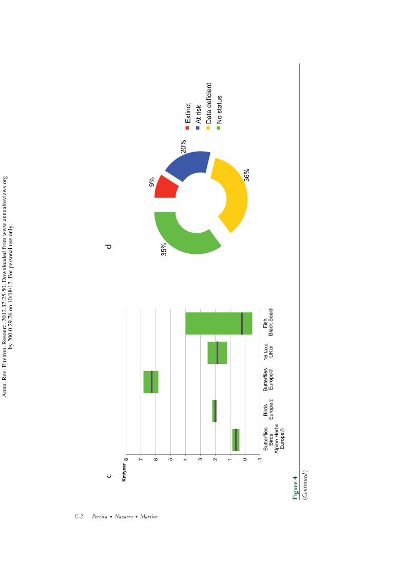
EG37CH02-Pereira ARI 5 October 2012 14:37
c
9%
20%
36%
35%
Extin
ct
At ri
sk
Dat
a de
ficie
nt
No
stat
us
d
-1 0 1 2 3 4 5 6 7 8
Km/y
ear
Butte
rflie
s Bi
rds
Alpi
ne H
erbs
Eu
rope
16 ta
xa
UK
Fish
Bl
ack
Sea
Butte
rflie
s Eu
rope
Bird
s Eu
rope
Figu
re4
(Con
tinue
d)
C-2 Pereira · Navarro · Martins
Ann
u. R
ev. E
nviro
n. R
esou
rc. 2
012.
37:2
5-50
. Dow
nloa
ded
from
ww
w.a
nnua
lrevi
ews.o
rgby
200
.0.2
9.76
on
10/1
8/12
. For
per
sona
l use
onl
y.
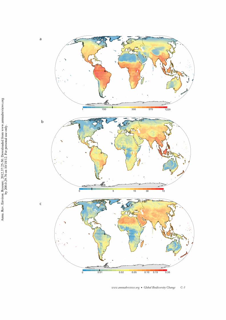
EG37CH02-Pereira ARI 5 October 2012 14:37
a
b
c
0 5 15 30 72
1 150 300 570 1229
0 0.01 0.02 0.05 0.10 0.15 0.35
www.annualreviews.org • Global Biodiversity Change C-3
Ann
u. R
ev. E
nviro
n. R
esou
rc. 2
012.
37:2
5-50
. Dow
nloa
ded
from
ww
w.a
nnua
lrevi
ews.o
rgby
200
.0.2
9.76
on
10/1
8/12
. For
per
sona
l use
onl
y.
EG37CH02-Pereira ARI 5 October 2012 14:37
←−−−−−−−−−−−−−−−−−−−−−−−−−−−−−−−−−−−−−−−−−−−−−−−−−−−−−−−−−−−−−−−−−−−−−−−−−−−−−−−−−−−−−−−−−
Figure 5Global distributions of terrestrial vertebrates and threatened species, based on species ranges for birds (n = 10,606) (164), mammals(n = 5,348), and amphibians (n = 6,248) (161). Color scales are based on geometric intervals (interval size increases at a constant ratioto the left and to the right of the black bar in the scale). Density calculations are based on grid cells of 0.48◦ × 0.48◦. (a) Speciesrichness. (b) Number of threatened species (critically endangered, endangered, or vulnerable). (c) Proportion of threatened species(number of threatened species divided by number of species in each cell).
C-4 Pereira · Navarro · Martins
Ann
u. R
ev. E
nviro
n. R
esou
rc. 2
012.
37:2
5-50
. Dow
nloa
ded
from
ww
w.a
nnua
lrevi
ews.o
rgby
200
.0.2
9.76
on
10/1
8/12
. For
per
sona
l use
onl
y.
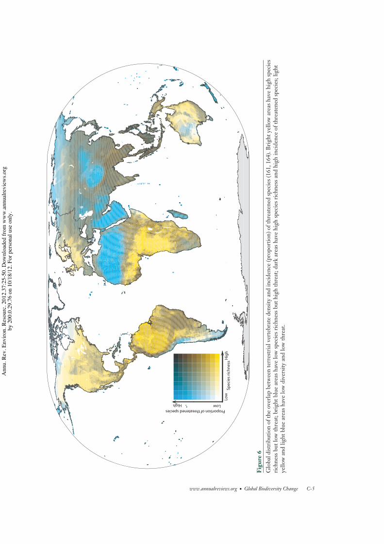
EG37CH02-Pereira ARI 5 October 2012 14:37
Spec
ies r
ichn
ess
Proportion of threatened species
Low
Low
Hig
h
High
Figu
re6
Glo
bald
istri
butio
nof
the
over
lap
betw
een
terr
estr
ialv
erte
brat
ede
nsity
and
inci
denc
e(p
ropo
rtio
n)of
thre
aten
edsp
ecie
s(16
1,16
4).B
righ
tyel
low
area
shav
ehi
ghsp
ecie
sri
chne
ssbu
tlow
thre
at;b
righ
tblu
ear
eash
ave
low
spec
iesr
ichn
essb
uthi
ghth
reat
;dar
kar
eash
ave
high
spec
iesr
ichn
essa
ndhi
ghin
cide
nce
ofth
reat
ened
spec
ies;
light
yello
wan
dlig
htbl
uear
eash
ave
low
dive
rsity
and
low
thre
at.
www.annualreviews.org • Global Biodiversity Change C-5
Ann
u. R
ev. E
nviro
n. R
esou
rc. 2
012.
37:2
5-50
. Dow
nloa
ded
from
ww
w.a
nnua
lrevi
ews.o
rgby
200
.0.2
9.76
on
10/1
8/12
. For
per
sona
l use
onl
y.
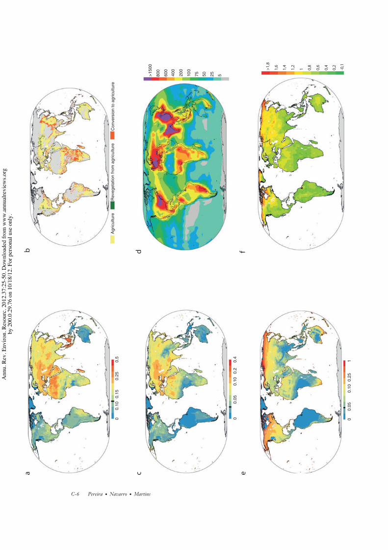
EG37CH02-Pereira ARI 5 October 2012 14:37
Agr
icul
ture
Rev
eget
atio
n fr
om a
gric
ultu
reC
onve
rsio
n to
agr
icul
ture
>150
0
5800
600
400
200
100
75 50 25
ab
cd f
e
00.
100.
150.
250.
5
00.
050.
100.
20.
4
00.
050.
100.
251
0,2
0,4
0,6
0,8
11,2
1,4
1,6
>1,8
-0,1
C-6 Pereira · Navarro · Martins
Ann
u. R
ev. E
nviro
n. R
esou
rc. 2
012.
37:2
5-50
. Dow
nloa
ded
from
ww
w.a
nnua
lrevi
ews.o
rgby
200
.0.2
9.76
on
10/1
8/12
. For
per
sona
l use
onl
y.
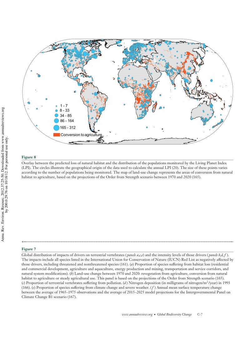
EG37CH02-Pereira ARI 5 October 2012 14:37
1 - 78 - 3334 - 8586 - 164
165 - 312
Conversion
to
agriculture
Figure 8Overlay between the predicted loss of natural habitat and the distribution of the populations monitored by the Living Planet Index(LPI). The circles illustrate the geographical origin of the data used to calculate the annual LPI (20). The size of these points variesaccording to the number of populations being monitored. The map of land-use change represents the areas of conversion from naturalhabitat to agriculture, based on the projections of the Order from Strength scenario between 1970 and 2020 (165).
←−−−−−−−−−−−−−−−−−−−−−−−−−−−−−−−−−−−−−−−−−−−−−−−−−−−−−−−−−−−−−−−−−−−−−−−−−−−−−−−−−−−−−−−−−−
Figure 7Global distribution of impacts of drivers on terrestrial vertebrates ( panels a,c,e) and the intensity levels of those drivers ( panels b,d, f ).The impacts include all species listed in the International Union for Conservation of Nature (IUCN) Red List as negatively affected bythose drivers, including threatened and nonthreatened species (161). (a) Proportion of species suffering from habitat loss (residentialand commercial development, agriculture and aquaculture, energy production and mining, transportation and service corridors, andnatural system modifications). (b) Land-use change between 1970 and 2020: revegetation from agriculture, conversion from naturalhabitat to agriculture or steady agricultural use. This panel is based on the projections of the Order from Strength scenario (165).(c) Proportion of terrestrial vertebrates suffering from pollution. (d ) Nitrogen deposition (in milligrams of nitrogen/m2/year) in 1993(166). (e) Proportion of species suffering from climate change and severe weather. ( f ) Annual mean surface temperature changebetween the average of 1965–1975 observations and the average of 2015–2025 model projections for the Intergovernmental Panel onClimate Change B1 scenario (167).
www.annualreviews.org • Global Biodiversity Change C-7
Ann
u. R
ev. E
nviro
n. R
esou
rc. 2
012.
37:2
5-50
. Dow
nloa
ded
from
ww
w.a
nnua
lrevi
ews.o
rgby
200
.0.2
9.76
on
10/1
8/12
. For
per
sona
l use
onl
y.
Land Use Policy 36 (2014) 60– 72
Contents lists available at ScienceDirect
Land Use Policy
jou rn al hom epage : www.elsev ier .com/ locate / landus epol
Analysing how drivers of agricultural land abandonment affectbiodiversity and cultural landscapes using case studies fromScandinavia, Iberia and Oceania
Ruth Beilina,∗, Regina Lindborgb,c, Marie Stenseked, Henrique Miguel Pereirae,Albert Llausàsa,f, Elin Slätmod, Yvonne Cerqueirag, Laetitia Navarroe, Patrícia Rodriguese,Nicole Reichelta, Nicola Munroh, Cibele Queirozc,e,i
a Department of Resource Management and Geography, University of Melbourne, 221 Bouverie Street, Parkville 3010, Australiab Department of Physical Geography and Quaternary Geology, Stockholm University, SE-106 91 Stockholm, Swedenc Stockholm Resilience Centre, Stockholm University, Kräftriket 2B (Roslagsvägen 101), 114 19 Stockholm, Swedend Department of Human & Economic Geography, University of Gothenburg, P.O. Box 630, SE-405 30 Göteborg, Swedene Center for Environmental Biology, Faculty of Sciences of the University of Lisbon, Edifício C2, Campo Grande, 1749-016 Lisboa, Portugalf Department of Geography & Institute of the Environment, University of Girona, Pl Ferrater Mora, 1, 17071 Girona, Spaing CIBIO, Faculty of Sciences of the University of Porto, Campus Agrário de Vairão, R. Padre Armando Quintas, 4485-661 Vairão, Portugalh Fenner School of Environment and Society, Australian National University, Building 48, Linnaeus Way, Canberra, ACT 0200, Australiai Department of Systems Ecology, Stockholm University, Svante Arrhenius väg 21 A, Frescati Backe, SE-106 91 Stockholm, Sweden
a r t i c l e i n f o
Article history:Received 28 November 2012Received in revised form 9 July 2013Accepted 11 July 2013
Keywords:Agricultural policyFarmingInterdisciplinaryLand managementLand use changeSocial drivers
a b s t r a c t
Agricultural land abandonment (ALA) is widespread in many countries of the global north. It impactsrural communities, traditional landscapes, biodiversity and ecosystem services. It is an opportunity forecosystem restoration or new landscape functions. We explored ALA in study areas in Australia, Portugaland Sweden. In each, we assessed plant species diversity, historical trajectories of land cover change;and the socioeconomic past, present and future in interviews with farmers. The ALA data was integratedand analysed by identifying the drivers of change. The relative importance of each driver and its scale ofaction was estimated, both in the past (1950–2010) and in the future (2010–2030). ALA has transformedrural landscapes in the study areas of Portugal and Sweden. It is at a much earlier stage with potential toincrease in the Australian case. We identified a set of driving forces, classified into pressures, frictions andattractors that clarify why ALA, noting its temporal and spatial scale, occurs differently in each study area.The effect of the drivers is related to social and historical contexts. Pressures and attractors encourag-ing agricultural abandonment are strongest in Portugal and Sweden. Generally more (institutionalized)frictions are in place in these European sites, intended to prevent further change, based on the bene-fits assumed for biodiversity and aesthetics. In Australia, the stimulation of driving forces to promote awell-managed abandonment of some cleared areas could be highly beneficial for biodiversity, minimallydisruptive for current dairy farming operations and would bring opportunities for alternative types ofrural development.
© 2013 Elsevier Ltd. All rights reserved.
Introduction
Land use change has implications for sustainable developmentat a global scale (Pereira et al., 2010), particularly with regard
∗ Corresponding author. Tel.: +61 9035 8273.E-mail addresses: [email protected] (R. Beilin),
[email protected] (R. Lindborg), [email protected](M. Stenseke), [email protected] (H.M. Pereira), [email protected](A. Llausàs), [email protected] (E. Slätmo), [email protected](Y. Cerqueira), [email protected] (L. Navarro), [email protected](P. Rodrigues), [email protected] (N. Reichelt), [email protected](N. Munro), [email protected] (C. Queiroz).
to feeding a growing and wealthier human population (Foleyet al., 2005). During the last 50 years there have been two mainland use trajectories affecting biodiversity and nature values inagricultural landscapes (Tilman et al., 2001). More economicallyproductive areas have been intensified, incorporated into largerassemblages particularly within developed countries (Stoate et al.,2009), whereas remote, economically unproductive farm areas areincreasingly abandoned, reforested, or included in rewilding fornature values with the creation of nature reserves or parks (Pinto-Correia, 1993; MacDonald et al., 2000; Navarro and Pereira, 2012).Although the connections between social and ecological values arerecognized as important (Folke, 2006; Carpenter et al., 2009), fewstudies integrate both social and ecological data from case studies
0264-8377/$ – see front matter © 2013 Elsevier Ltd. All rights reserved.http://dx.doi.org/10.1016/j.landusepol.2013.07.003
R. Beilin et al. / Land Use Policy 36 (2014) 60– 72 61
to examine the links between social drivers and their effect on landuse and biodiversity. Yet, the trend in land abandonment evincesconcern and/or opportunity globally but for markedly different rea-sons in various landscapes (Moreira et al., 2001a; Gellrich et al.,2007; Cramer et al., 2008; Cetinkaya, 2009).
In this study we compare case studies in Australia, Portugal andSweden. These countries have had different social-economic devel-opment during the last century, and all three experience degrees ofagricultural land abandonment (ALA). In each country we examinethe drivers of change affecting ALA and discuss effects on land useand on the social and ecological systems. In doing so, we will inte-grate what Lambin et al. (2001) refer to as local-level case studieswith regional ‘generalities’ to link to international themes of globalchange. The goals of our study are to examine: (i) which are themain drivers influencing management practices associated withagricultural land use change and abandonment in the three loca-tions; (ii) what are the temporal and spatial scales and institutionallevels framing land use change; and (iii) how have these drivers,through different land use changes, affected and will affect biolog-ical and cultural outcomes. Ultimately, this framework is intendedto enable and better support policy decisions associated with agri-cultural land abandonment.
Agricultural land abandonment
The degrees of land use change have both spatial and temporalhistoricity, associated with the decline in agricultural productivitywithin regions, across economies and in association with tech-nological and demographic changes (Beilin et al., 2011). ALA iscommonly defined qualitatively as land condition; and quantita-tively as years without agricultural use (Moravec and Zemeckis,2007, p. 5). It may be evident at a variety of scales and with dif-ferent degrees of intensity (Pinto-Correia, 1993; Burel and Baudry,1995). At the extreme, abandonment is the complete withdrawalof agricultural management from the landscape and a transition tovarious non-agricultural lands uses (Keenleyside and Tucker, 2010).In other instances there is a reduction in management intensity,e.g. conversion of croplands to pasture areas (Bielsa et al., 2005).These situations may occur at different scales (MacDonald et al.,2000); and depending on spatial and temporal scales, the outcomesof abandonment may not be permanent (Wood, 1993).
ALA is driven by a combination of different factors, rangingfrom physical constraints of the landscape to more economic andsocial drivers (Strijker, 2005; Kizos and Koulouri, 2006; Koulouriand Giourga, 2007). A combination of these drivers is generallymore pronounced in remote and isolated regions, such as moun-tain zones or marginal areas for agriculture where productivity islow, e.g. areas with shallow soil, salty soils, or poorly drained, whilemechanization is often restricted by the terrain (MacDonald et al.,2000; Gellrich and Zimmermann, 2007; Cramer et al., 2008).
The diminishing of agriculture in an area often co-varies withsocio-economic changes and has ecological consequences, whichcan differ with local land use history, climate and landscape compo-sition (Rey Benayas et al., 2007). Related socio-economic changesin remote areas are characteristically demographic, for example,declining and ageing populations. How biodiversity is affectedby different land use changes is a contested topic in conserva-tion research (Balmford et al., 2005; Matson and Vitousek, 2006;Dorrough et al., 2007; Vandermeer and Perfecto, 2007) and that istrue in relation to land abandonment (Pereira et al., 2005; Navarroand Pereira, 2012). Agricultural practises have been responsiblefor the destruction and fragmentation of many native habitatswith consequent negative impacts on biodiversity (Poschlod et al.,2005); therefore it could be expected that retiring agricultural landfrom production can be an opportunity to improve the conditionfor many species that were severely affected by native habitat
fragmentation in the past (Reidsma et al., 2006; Foster et al., 2009;Aide et al., 2012). However, decline in traditional low-intensiveagriculture often has negative effects on biodiversity at the localscale, as the moderate utilization of grasslands and forests in his-torical times were associated with high species richness in the rurallandscape of Europe (Kull and Zobel, 1991; Eriksson et al., 2002;Pykälä, 2004), leading to the concept of high nature value farmland(Halada et al., 2011).
Drivers of change
‘Driving forces’ are defined as ‘the forces that cause observedlandscape changes, i.e., they are influential processes in the evo-lutionary trajectory of the landscape’ (Bürgi et al., 2004, p. 858).The potential of the concept lies in the possibility of using drivingforces as a theoretical frame to understand and analyse changesand also, by comparing case studies, to identify common land usetrends (Eiter and Potthoff, 2007; Schneeberger et al., 2007).
In a literature review of the concept and application of drivingforces of land use change, Slätmo (2011) characterizes them intofour concepts: pressures, frictions, attractors and triggers. Pressuresare factors that are pushing for change, with long term implicationsthat put a stress on the current land use. Pressures can be dividedinto different types deriving from overarching categories such aspolitical, economic, cultural and technical. Frictions are factors thatserve to resist change: preventing, slowing down or changing thedirection of land use change. Frictions can be divided into differenttypes deriving from the same overarching categories as ‘pressures’.Attractors are associated with site conditions that attract changedue to their privileged characteristics and/or location. Triggers arefactors that spur land use change in a direct, time specific ways(e.g. the opening of a new road). Therefore, even if their impact issignificant, they are difficult to relate to long term landscape trans-formations due to their short-term nature. If a trigger persists intime, then it can be easily classified as either a friction or a pressure(e.g. increased accessibility because of the new road).
Study areas
Individual sites in each country (Australia, Portugal and Sweden)incorporated landscapes exhibiting different levels of ALA, butsharing some overall similarities. These were the impacts of globalmarkets, challenging biophysical conditions for farming and at leastone hundred years of consecutive agricultural land use.
Poowong, Australia
The Australian case study is located in the south-eastern State ofVictoria within a commutable 100 km of the capital city, Melbourne(Fig. 1). Encompassing approximately 18,000 ha of farmland pre-dominantly used for grazing dairy cows and beef cattle, the researcharea is situated north-east of a small rural township, Poowong,spanning two local government administrations. The terrain is hillyand steep, but the elevation range is limited to between 90 and300 m above sea level. The area is best described as a maritimetemperate climate, with mean maximum temperatures around24.5 ◦C in the summer and just above 13 ◦C in winter, with very rareepisodes of minimum temperatures below 0 ◦C. The area receivesa typically high annual rainfall by Australian standards, between800 mm and 1400 mm. The combination of rugged topography andduplex soil types formed from sedimentary and basalt bedrockcreates a landscape vulnerable to erosion and landslips throughwaterlogging and disturbance of vegetation cover for agricultureand forestry (Jenkin, 1970; Beilin, 2007). The study area forms partof the western section of the Strzelecki Ranges in the StrzeleckiWest Biodiversity Landscape zone. An estimated 600 people live
62 R. Beilin et al. / Land Use Policy 36 (2014) 60– 72
Fig. 1. The three countries, Australia, Portugal and Sweden, and the location of the respective study areas.
on independent holdings in the census area known as PoowongState Suburb (ABS, 2006).
Castro Laboreiro, Portugal
The Portuguese case study is located in the parish of CastroLaboreiro in the Peneda Mountain Range, in the north of the coun-try (Fig. 1). The parish covers approximately 9440 hectares withelevation ranging from 300 m to 1340 m. Located at the transitionbetween the Mediterranean and Atlantic biogeographic zones, theregion has a temperate Mediterranean climate, characterized bytemperatures varying between an average daily minimum of 0–3 ◦Cin the winter months and an average daily maximum of 22.5 ◦C inthe summer months. Precipitation exceeds 2000 mm per year, withrelatively dry summers. The geology of the area reveals a strongpresence of granite and quartzite, with thin and non-existent soilsin the steepest slopes, whereas pluvial action formed deep soilsin the valleys, nowadays intensively altered in their characteristicsdue to long human activity (ICN, 1995). The parish is in the Peneda-Gerês National Park and is part of the Natura 2000, the EuropeanUnion protected area network. Over the last 50 years the popula-tion in mountain regions of Portugal has declined significantly andsteadily (Pereira et al., 2005; Aguiar et al., 2009), and today CastroLaboreiro is inhabited by about 540 residents (INE, 2011). The rig-orous winter and the orography of the parish led to the seasonalmigration from summer villages (brandas) in the plateau to wintervillages (inverneiras) in the valley. The parish consists of 15 bran-das, 18 inverneiras and 8 fixed villages. The traditional migration ofthe local residents has steadily decreased since the early 1980s andnow occurs only in a couple of villages. Farmers receive subsidiesto maintain traditional farming and pastoral activities.
Hållnäs, Sweden
The Swedish study area (Hållnäs) is a peninsula in SouthernBothnian, situated in south-central Sweden in Uppland County(Fig. 1). The size of the parish is 25,000 ha. Hållnäs is located inan area affected by isostatic land-uplift (0.6 m/100 years), implyingsignificant environmental changes in a relatively short time span.
Currently the study area is within a range of 10–25 m above the sealevel. In spite of the high northern latitude of Sweden, the climatecan be classified as warm summer, with July being the warmestmonth (average maximum temperature of 21 ◦C), and January thecoldest (with an average minimum of −8 ◦C), with freezing spellsover consecutive days. Rainfall is higher during the summer monthsof the year (up to 60 mm/day), while less abundant in winter (up to25 mm/day), averaging around 530 mm annually. Soils are nutrientpoor, and cover a subsoil rich in calcium carbonate and bases. Natu-ral values on the peninsula are to a large extent related to the upliftprocess. There are fourteen Natura 2000 areas and seven naturereserves encompassing shores, wetlands and coniferous forests onlime-rich soils (Naturvårdsverket, 2012). A large amount of thesemi-natural pastures are acknowledged for their high biodiver-sity and receive subsidies to maintain traditional management. Themixed landscape is of interest for ecological protection because ofthe mosaic structure formed by forest, marsh and agricultural use(Tierps kommun, 1991). There are 1200 inhabitants in Hållnäs andapproximately 70 agricultural enterprises (Tierps kommun, 1991).
Methods
In each country ecological and social data was collected andanalysed, initially by country and then in comparative tables andtexts. In the first stage, plant diversity data was gathered for thethree study sites (section “Comparison of vegetation data”). Sec-ondly, land cover change maps were generated for three key datesin the landscape evolution process (section “Mapping land usechange”). Finally semi-structured interviews were conducted withthe farmers and landholders managing the landscape to collecttheir landscape stories, gather their views on land use or aban-donment, understand how they manage their businesses and howthey plan to develop their activities in the future (section “Socialdata: interviews”). The results for each stage were integrated anddiscussed among the project researchers in a seminar (2010) to cre-ate a matrix synthesizing the main outcomes and identifying thesocial and environmental drivers involved (section “Integration ofdata and production of results”).
R. Beilin et al. / Land Use Policy 36 (2014) 60– 72 63
Comparison of vegetation data
To get a general understanding of how different land useshave affected flora in the different countries, we compared ear-lier published data on plant diversity from each study site. Becauseof different historical and current agricultural management tra-ditions, a perfect match between the land cover/use betweencountries was not possible. However, we were able to compare thedifferent land covers in terms of the gradient in land use intensityand abandonment of the agricultural use. In Australia, the three keyvegetation types of interest were the remnant temperate rainfor-est (mixture of wet and dry coastal forest types, severely reducedin cover, but considered to have a high value for biodiversity),revegetation (newly established vegetation through planting localindigenous only species), and fields (the cleared landscape, usu-ally grazed and locally denominated paddocks) (cf. Munro et al.,2009). In Portugal, the land uses were agricultural fields (mostlysemi-natural pastures and hay fields, but also some crop fields),scrubland and oak forest fragments (cf. Proenc a and Pereira, 2013).In Sweden, the key land uses were categorized as field, wooded pas-ture (grazed semi-natural pastures) and coniferous forests (mixedconiferous and deciduous forests used in low intensity forestry) (cf.Lindborg et al., 2008). The number of plant species in each studysite is given only as reference, as the field sampling method usedto measure species diversity differed between sites. However, theproportion of species occurring in each habitat is informative aswell as the proportion of native and exotic plant species.
Mapping land use change
To estimate land use change over time, land use maps were cre-ated for each of the three study sites. Three distinct time periodswere analysed in the geographic information system ArcMap v.9.1(ESRI, 2005). The dates were chosen to illustrate key periods in thehistory of landscape use in each country, and to correlate with theavailability of data. In each time period the major land covers wereidentified, mapped and the area was calculated. These data werethen used to build land cover transition matrices for each site.
In the Australian study site (Poowong), pre-European (1840s)vegetation extent was presumed to be 100% cover (KDHS, 1998).Vegetation clearance peaked in approximately 1970, with somerevegetation since that time. Revegetation and remnant vegetationwere mapped from government department sourced aerial photog-raphy. Proportions of different vegetation types in the landscapecould be determined for 1970 and 2006.
In both Portugal and Sweden all three time periods used werebased on maps and aerial photographs from the last 60 years. InCastro Laboreiro, Portugal, landscape characterization was madethrough field reconnaissance and photo interpretation for the years1960, 1990 and 2007 (Rodrigues, 2010). A regressive updating tech-nique was used for the interpretation of the changes in the land use(Bender et al., 2005). The three time layers for the Swedish studycase Hållnäs were from 1959, 1979 and 2010. The current and his-torical land use in Hållnäs was documented through cadastral mapsanalysing both the current landscape and the landscape from 1950and 1970.
Social data: interviews
We carried out 1–2 h semi-structured interviews. The contentsvaried across study sites according to the interests of each researchteam, but a common set of questions was agreed to provide a com-mon basis for the research presented here. This shared section of theinterview inquired about social data across three time zones: 1950sto the present; the present (which was 2010/11); and 2010–2030.Questions regarded socio-economic and demographic data,
including quality of life; determining the reasons for present culti-vation or the discontinuation of agricultural activity and changes tosubsistence/production strategies; perception of landscape changein the last 50 years and services provided by agro-ecosystems; andfuture perspectives.
AustraliaEleven rural properties from the research area were visited with
18 landholders responding the interviews as individuals, familygroups or in partnerships. Ten females and eight males between30+ and 80+ years participated. Landholders were recruited froma local community-based natural resource management orga-nization (e.g. Landcare) and a community activist associationusing non-probability convenience and opportunistic sampling.The average size hill farm was 106 ha, which is smaller than theaverage plains-based South Gippsland dairy farm (138 ha) andnorthern Victorian dairy farm (160 ha). Some farms have consol-idated to grow larger; and this expansion is not necessarily as onesingle property but rather a series of land titles that are owned orleased around the district, operating as one agribusiness. The vastmajority of rural properties were considered farms with only oneperson viewing their land as a rural residential property, whetheror not they derived their main income from the ‘farm’. Three inter-viewees did not classify themselves as farmers and were eitherretired or employed in non-farming work. All the intervieweesresided in Farming Zones as designated in local planning schemes.
PortugalAfter a primary informant provided a list of potential respon-
dents, twenty-seven interviews were undertaken. The respondentsconsisted of 8 men and 19 woman, average age 59 (about 62% ofthe resident population are women according to the 2011 census).Nearly all of the respondents have resided in Castro Laboreiro for50 years or more. More than half of the respondents were full timefarmers, a third were retired farmers, of which one in three stillmaintains some type of agricultural activity (often for leisure) anda few of them were part-time farmers with a secondary job. Abouthalf of the sample own less than 4 ha of land, and each owner hasland scattered across a number of properties (4–6 fields) with anaverage field size of 0.4–0.8 ha. Of the total sample, almost a half ofthe households consisted of only 1 person and none of the house-holds had children working in the area. Only 3 respondents wereconsidered large-scale farmers, based on the number of livestock(>50 head of cattle). All respondents were landowners, and only asmall fraction additionally rent or work neighbouring private landfor free, although most use common land. Income from farmingis mainly derived from subsidies for livestock and for maintainingpastures clear of scrubland. None of the respondents acknowledgedmonetary return from cultivating their land. (Production is for sub-sistence only.)
SwedenNine interviews with small-scale land owners were conducted
within the selected study area on Hållnäs peninsula. Farmers wereselected from a list compiled by the Swedish Board of Agricul-ture. The participants are primarily men around 50 years, exceptone man around 90 years and one female around 50 years. Dur-ing three of the interviews other family members such as a partnerand children were present in the discussion. The size of the prop-erties varied between 5 and 30 hectares of farmland. Land useand farming practices are small scale livestock keeping and hayor ensilage production. These are the typical agricultural activitiesin the area. Of the nine interviews, a majority of five farmers wereleisure or hobby farmers, three were retired and one was a fulltimefarmer. Most of the adult inhabitants, including the active farmers,are today working outside the parish or are pensioners. Income
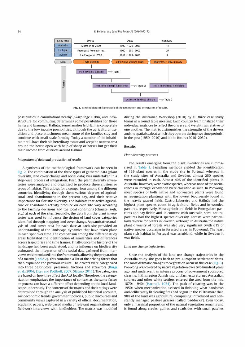
64 R. Beilin et al. / Land Use Policy 36 (2014) 60– 72
Fig. 2. Methodological framework of the generation and integration of results.
possibilities in conurbations nearby (Skärplinge 10 km) and infra-structure for commuting determines some possibilities for thoseliving and farming in Hållnäs. Some families left Hållnäs completelydue to the low income possibilities, although the agricultural tra-dition and place attachment mean some of the families stay andcontinue with small-scale farming. Today a number of the inhabi-tants still have their old hereditary estate and keep the nearest areaaround the house open with help of sheep or horses but get theirmain income from districts around Hållnäs.
Integration of data and production of results
A synthesis of the methodological framework can be seen inFig. 2. The combination of the three types of gathered data (plantdiversity, land cover change and social data) was undertaken in astep-wise process of integration. First, the plant diversity inven-tories were analysed and organized to produce three clusters ortypes of habitat. This allows for a comparison among the differentcountries, identifying through them various degrees of agricul-tural land abandonment in the present day, and their relativeimportance for floristic diversity. The habitats that active agricul-ture or abandoned activity produce on each site vary accordingto the farming decisions and the local conditions (climate, soils,etc.) at each of the sites. Secondly, the data from the plant inven-tories was used to influence the design of land cover categoriesidentified through mapping land cover change. A quantitative anal-ysis of land cover area for each date at each site provided anunderstanding of the landscape dynamics that have taken placein each spot over time. The comparison among the different studyareas facilitated the identification of similarities and differencesacross trajectories and time frames. Finally, once the history of thelandscape had been understood, and its influence on biodiversityestimated, the integration of the social data gathered from inter-views was introduced into the framework, allowing the preparationof a matrix (Table 2). This contained a list of the driving forces thatthen explained the previous results. The drivers were categorizedinto three descriptors: pressures, frictions and attractors (Bürgiet al., 2004; Eiter and Potthoff, 2007; Slätmo, 2011). The categoriesare based on how they affect the ALA locally. Therefore, the catego-rization emphasizes the importance of context as the same factoror process can have a different effect depending on the local land-scape under study. The contents of the matrix and their ratings weredetermined through the analysis of published historical accounts,socioeconomic trends, government policies, public discourses andcommunity views captured in a variety of official documentation,academic papers, web-based media of relevant organizations andfieldwork interviews with landholders. The matrix was modified
during the Australian Workshop (2010) by all three case studyteams in a round table meeting. Each country team finalized theirindividual matrices to reflect the drivers and weightings relative toone another. The matrix distinguishes the strengths of the driversand the spatial scale at which they operate during two time periods:in the past (1950–2010) and in the future (2010–2030).
Results
Plant diversity patterns
The results emerging from the plant inventories are summa-rized in Table 1. Sampling methods yielded the identificationof 139 plant species in the study site in Portugal whereas inthe study sites of Australia and Sweden, almost 250 specieswere recorded in each. Almost 40% of the identified plants inAustralia, however, were exotic species, whereas none of the occur-rences in Portugal or Sweden were classified as such. In Poowong,most species of both native and non-native plants were foundin revegetation plantings with the lowest biodiversity found inthe heavily grazed fields. Castro Laboreiro and Hållnäs had thehighest plant species count in agricultural fields and in woodedpastures, respectively. Most agricultural fields in Portugal are pas-tures and hay fields; and, in contrast with Australia, semi-naturalpastures had the highest species diversity. Forests were particu-larly diverse for plants in Sweden, although in Australia the nativeplant diversity of forests was also very significant (with 61% ofnative species occurring in forested areas in Poowong). The leastplant rich habitat in Portugal was scrubland, while in Sweden itwas fields.
Land use change trajectories
Since the analysis of the land use change trajectories in theAustralia study site goes back to pre-European settlement dates,the most dramatic changes to vegetation occur in this case (Fig. 3).Poowong was covered by native vegetation over two hundred yearsago, and underwent an intense process of government sponsoredclearing. In this region Danish migrant farmers, returned Australiansoldiers and other white settlers entered the area from the mid1870s–1940s (Hartnell, 1974). The peak of clearing was in the1950s when mechanization assisted in finishing what handsawsand deliberately lit clearing fires had begun. In the 1970s more than90% of the land was agriculture, comprising introduced and con-stantly managed pasture grasses (called ‘paddocks’). Even today,only a marginal proportion of the natural vegetation remains andis found along creeks, gullies and roadsides with small patches
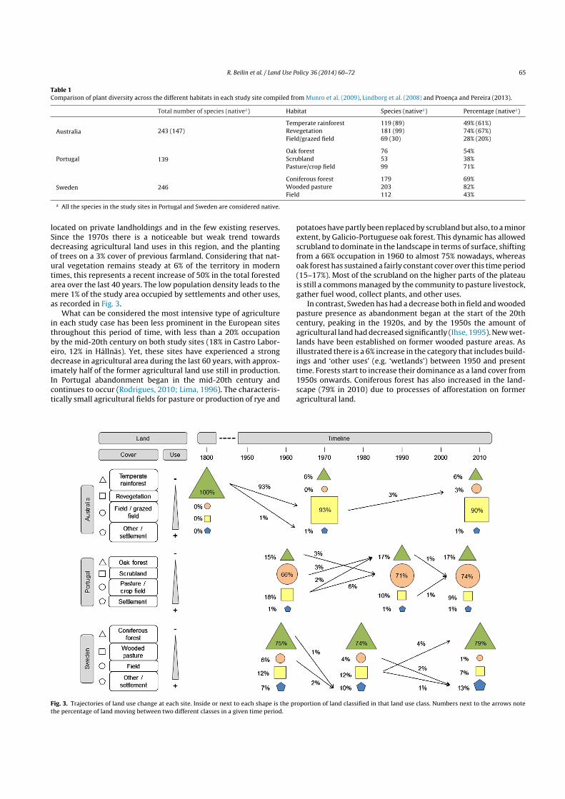
R. Beilin et al. / Land Use Policy 36 (2014) 60– 72 65
Table 1Comparison of plant diversity across the different habitats in each study site compiled from Munro et al. (2009), Lindborg et al. (2008) and Proenc a and Pereira (2013).
Total number of species (nativea) Habitat Species (nativea) Percentage (nativea)
Australia 243 (147)Temperate rainforest 119 (89) 49% (61%)Revegetation 181 (99) 74% (67%)Field/grazed field 69 (30) 28% (20%)
Portugal 139Oak forest 76 54%Scrubland 53 38%Pasture/crop field 99 71%
Sweden 246Coniferous forest 179 69%Wooded pasture 203 82%Field 112 43%
a All the species in the study sites in Portugal and Sweden are considered native.
located on private landholdings and in the few existing reserves.Since the 1970s there is a noticeable but weak trend towardsdecreasing agricultural land uses in this region, and the plantingof trees on a 3% cover of previous farmland. Considering that nat-ural vegetation remains steady at 6% of the territory in moderntimes, this represents a recent increase of 50% in the total forestedarea over the last 40 years. The low population density leads to themere 1% of the study area occupied by settlements and other uses,as recorded in Fig. 3.
What can be considered the most intensive type of agriculturein each study case has been less prominent in the European sitesthroughout this period of time, with less than a 20% occupationby the mid-20th century on both study sites (18% in Castro Labor-eiro, 12% in Hållnäs). Yet, these sites have experienced a strongdecrease in agricultural area during the last 60 years, with approx-imately half of the former agricultural land use still in production.In Portugal abandonment began in the mid-20th century andcontinues to occur (Rodrigues, 2010; Lima, 1996). The characteris-tically small agricultural fields for pasture or production of rye and
potatoes have partly been replaced by scrubland but also, to a minorextent, by Galicio-Portuguese oak forest. This dynamic has allowedscrubland to dominate in the landscape in terms of surface, shiftingfrom a 66% occupation in 1960 to almost 75% nowadays, whereasoak forest has sustained a fairly constant cover over this time period(15–17%). Most of the scrubland on the higher parts of the plateauis still a commons managed by the community to pasture livestock,gather fuel wood, collect plants, and other uses.
In contrast, Sweden has had a decrease both in field and woodedpasture presence as abandonment began at the start of the 20thcentury, peaking in the 1920s, and by the 1950s the amount ofagricultural land had decreased significantly (Ihse, 1995). New wet-lands have been established on former wooded pasture areas. Asillustrated there is a 6% increase in the category that includes build-ings and ‘other uses’ (e.g. ‘wetlands’) between 1950 and presenttime. Forests start to increase their dominance as a land cover from1950s onwards. Coniferous forest has also increased in the land-scape (79% in 2010) due to processes of afforestation on formeragricultural land.
Fig. 3. Trajectories of land use change at each site. Inside or next to each shape is the proportion of land classified in that land use class. Numbers next to the arrows notethe percentage of land moving between two different classes in a given time period.
66 R. Beilin et al. / Land Use Policy 36 (2014) 60– 72
The socio-economical landscape
Interview data provided context for the quantitative findings,in particular clarifying how the socio-economic systems operate ateach site.
As a social phenomenon, ALA is least common in Australia,where farmers in the Poowong study area still rely on the long-running activity of dairy farming as a main source of income.Despite a dramatic reduction in the number of businesses in thearea during the last three decades of the 20th century (ABS, 1998),the community is still dependant on dairy farming enterpriseswhich are supported by continuing investment in export orienteddairy processing in the region. However, the interviews identifieda number of factors currently affecting and transforming this situ-ation: climate change, increasing costs in agricultural inputs, landdegradation and volatile milk prices in domestic and global mar-kets. These are creating a fragile operating environment for 21stcentury dairy farmers. In addition, the ageing of current familyfarm managers, and a lack of family succession in these agribusi-nesses, brings the longer term viability of dairying into question.Funding to assist in addressing common natural resource manage-ment issues has come from both State and Federal sources over theyears and is currently associated with private landowner manage-ment of watersheds/catchments and conservation on individual’sland (e.g. market-based instruments such as EcoTender). This par-allels similar activities for group extension services and communityorganizations (e.g. Landcare, Greening Australia, Trees on Farms).
In the Portuguese case, changes in the social arena have beencoupled with the changes observed in the land cover changeanalysis. Key influences on the abandonment dynamics includehigh rates of migration out of rural areas after World War II tosecure employment, state policies appropriating common land forafforestation, and Portugal’s entrance into the European Union.These increased pressure on local farming enterprises to com-pete with farms operating at greater economies of scale. ALA ismostly perceived in areas which are characterized by biophysicalconstraints such as poor soils, steep slopes, harsh climate and iso-lation. (Castro Laboreiro is located 100 km and extremely windingroads away from the nearest city, Braga.) The traditional mountainfarming systems are now facing a collapse. As a consequence ofincreased agricultural abandonment, scrubland and forest (Galicio-Portuguese oak forest) have increased, and the particular increaseof highly flammable shrub areas has escalated the risks of fire occur-rence (Moreira et al., 2001b). The main forms of income in theparish are retirement pensions, subsidies for agro-pastoral activ-ities, and most recently, tourism (e.g. lodging and restaurants).Castro Laboreiro is a European Union Less Favoured Area (an areawhere agricultural production or activity is more difficult becauseof natural handicaps), and therefore farmers benefit from spe-cial subsidies. Furthermore, the landscape mosaic is classed asbeing of high nature value farmland and farmers can benefit fromagri-environmental payments aimed at maintaining such habitats.Meanwhile, the potential benefits of oak forest regeneration to bio-diversity and local ecosystem services are not acknowledged by thecurrent policies, which are mainly focused on the prevention of ALA.
Biophysical conditions have had an influence on the humanactivities in the Swedish case area and their viability over time.Agriculture has low productivity here and living solely on farm-ing has traditionally been difficult due to harsh climate, poor soilsand small parcels. Farming activities have declined since the 1950sand today, primarily livestock keeping and hay production remain.The majority of the population does not have a working farm andthose who have are mainly ‘leisure farmers’, keeping the land openwhile working outside the parish for an income. This situationindicates that the landowners in Hållnäs have other motives fordecisions about land use than landowners who survive on farming.
Challenges for the future of agricultural activity in Hållnäs relateto the surplus of agricultural land, from a European Union per-spective; while small units and relatively poor soil quality makeit difficult to develop economically viable agricultural businessesin the parish. This makes alternative working opportunities crucialfor continued farming. Workplaces within commuting distance aretherefore essential in order to keep active the small-scale farminglifestyle as a part-time or hobby activity. On the other hand, sub-sidies are aiding small farm units, opportunities arise in the fieldof summer tourism and leisure residents are believed to positivelyinfluence the future sustainability of the community, culminatingin the preference for a mosaic landscape (Stenseke, 2009).
Drivers of land use change
The drivers that have been identified for ALA for the variousareas were then categorized into pressures, frictions and attractors(Table 2). Triggers for ALA (for example, the post WWII reconstruc-tion that led to a rural exodus from Castro Laboreiro, before thetimeline of this study) undoubtedly manifest as pressures or fric-tions within other time frames (as apparent in the ongoing declinein population).
Ongoing pressures from global market forces have been impor-tant in all three study sites, emphasizing the impact of internationalscale on local outcomes. The three areas are somewhat aligned withregard to historical pressures related to the expansion of state-owned forestry and a sense of remoteness, driven mainly at thelocal level. Remoteness, surprisingly, does not seem equally corre-lated with a relative decline of infrastructural accessibility, or therelative decline of working opportunities, or a diminishing levelof public and commercial service for the three study areas. Thesefactors are only important for future agricultural land use in Cas-tro Laboreiro and Hållnäs. In Poowong pressures of reforestationand a sense of remoteness have historically had some influence onland use change dynamics locally, but these will be less relevantin the future as the area experiences the influence of urbanizationpressures from an expanding metropolitan population. In contrast,in Castro Laboreiro and Hållnäs re-afforestation and remotenesshave and are contributing significantly to ALA. Nature conservationregulations promoted at the local level are gaining momentum inAustralia, but they remain a pressure for agricultural land aban-donment in the Portuguese case study and less prominently in theSwedish case. It is also important to note that some pressures inter-act, creating positive feedback. For instance, the relative declineof working opportunities leads to out-migration which leads to adiminishing level of public and commercial service which in turnsleads to further migration and further decreases in the level ofpublic and commercial services (Figueiredo and Pereira, 2011).
In the past, frictions preventing the abandonment of agriculturalland have appeared or have been put in place in the three studyareas, mainly from the national level, but some of them are increas-ingly coming from the local governments and communities. In thefuture, however, the general trend indicates that there will be anincrease in the influence of such driving forces, but not in relation tocommunity cohesiveness and farming identity among land owners(i.e. the degree to which citizens are committed to the prosperity ofthe community and to which land owners are committed to ongo-ing farming). These latter are expected to act less as a friction to ALAin Portugal and Sweden, but is likely to remain an important socialdriver in Australia. State and regional campaigns for rural devel-opment will also be important local frictions in Australia, whereasin Europe though equally determining, emanate from the nationallevel. Official funding and subsidies for land management, tourismand second home owners represent more obvious differences, asfrictions within the study areas. Their influence has been and willbe limited in the Australian case. They have been important drivers
R. Beilin et al. / Land Use Policy 36 (2014) 60– 72 67
Table 2Drivers of land use change identified in the study areas along two time periods (past: 1950–2010, future: 2010–2030). More influential drivers are given a higher numberof + (from 1 to 3) and 0 for nil influence, whereas the scale of their influence is divided into three levels according to the classification: I = international, N = national, andL = local.
Driving forces to agricultural land use change Of specificimportance inPoowong
Of specificimportance inCastro Laboreiro
Of specificimportance inHållnäs
Past Future Past Future Past Future
Pressures to abandon agriculturalpractices on the land
Market driven changes in economic conditions for farming + I ++ I ++ I +++ I +++I/L + I/LExpansion of forest land owned by companies/state ++ L + L ++ N 0 L/N ++ L + LDiminishing level of public and commercial service 0 0 ++ L ++ L + L ++ LRelative decline of working opportunities + L 0 +++L +++ L +++ L ++ LRelative decline of infrastructural accessibility + L 0 ++ L + L ++ L +++ LIncreased nature conservation regulations 0 ++ L + N + N ++ N + NFeeling of continuing remoteness ++ L + L ++ L ++ L + L + L
Frictions to abandon agriculturalpractices on land
Cohesiveness and the farming identity among land owners ++ L ++ L +++L + L ++ L + LOfficial funding and subsidies for land management + N + N ++ N +++ N ++ N +++ NState campaigns for rural development ++ L ++ L + N ++ N + N ++ NTourism and secondary home owners 0 + N/L +N/L ++ N/L + N/L +++N/LAppreciation of natural and cultural values + L ++ N/L + N ++ N + N ++ N
Attractors for abandonment ofagricultural practices on the land
Physical conditions for cultivating 0 0 +++L +++ L +++ L + LPhysical conditions for livestock keeping + L 0 +++L ++ L + L 0
in the past in the Portuguese and Swedish areas. Further, they areexpected to play an even more prominent role there in preventingALA in the future.
Attractors for abandonment include the physical conditionsin the Swedish and the Portuguese cases areas, which are lessfavourable, and that has underpinned their abandonment. In north-ern Portugal, this is likely to continue, while in Hållnäs, thedevelopment has gone so far, that the remaining lands are now,in the main, managed by leisure farmers, and there are therefore,other motives than that of economic revenues keeping them in agri-cultural practice for the future. In Poowong, there are currentlyfavourable climatic and soil conditions for commercial cattle graz-ing (understood as a complementary use to dairying); therefore,the biophysical conditions are not expected to attract considerableALA.
Discussion
Comparison of the three study cases
Comparative studies offer the opportunity to analyse similar-ities and differences between study areas (George and Bennett,2005). The integrative results provide a global connectivity; con-textualizing the findings in an interesting and more useful way thanwould be the case if they had remained within the boundaries oftheir own disciplines (Redman et al., 2004). In this case, there isopportunity to compare landscape trajectories in three areas that,due to their diverse biophysical features, but not least due to theirparticular socioeconomic and cultural environments, have under-gone substantially different transformations over time. Swedishand Portuguese agricultural landscapes have been cultivated overa much longer time than the Australian landscapes (see section“Land use change trajectories”; Meeus et al., 1990; Powell, 1996).This is clearly noticeable when dynamics of agricultural land aban-donment are contrasted. Whereas the proportions of land uses inthe landscape in the European study cases seem relatively stableover the period of time for which data has been recorded, dramaticland use change has occurred in the Australian case study over asomewhat longer period of time, despite a shorter period of cultiva-tion overall. The rural areas of Castro Laboreiro and Hållnäs are theresult of a much longer history of profound agricultural landscapemanagement.
In Europe social drivers have played an important role in stimu-lating modifications to these landscapes. A number of local decisionfactors need to be considered as farmers (as the main stakeholdersresponsible for the modification of the agricultural landscape) orga-nize land management. Albeit to very different degrees, all threestudy areas have attracted some abandonment of cultivation orlivestock keeping due to challenging physical conditions. In thelast 60 years, factors like the sense of remoteness or the declineof infrastructural accessibility and working opportunities associ-ated with their peripheral locations have pressed many farmers togive up farming, abandoning their cultivation or grazing. Finally,frictions coming from the local or the national level such as thoseassociated with maintaining or stimulating cohesiveness and thefarming identity among land owners through direct or indirectstate campaigns for rural development (sometimes coupled withofficial funding or subsidies) have attempted to counter ALA. Ineffect, mainly in Europe, attention has turned to emphasizing anappreciation of natural and cultural values across the case sites.The development of conservation values across formerly produc-tion landscapes has played a part in preventing some abandonment,or at least diminishing its prominence, due to subsidies, land stew-ardship programs, and agri-tourism initiatives.
In Table 2 we have synthesized the driving forces of agriculturalland use change, offering an estimation of their relative impor-tance towards land use change and noticing the scale at whichthey occur. When these results are compared to the landscape tra-jectories presented in the section “Land use change trajectories”,a correlation between the intensity of land use change in the lastdecades and the relative importance of the driving forces becomesapparent. In the last 40 years, only a 3% of agricultural land hasreverted to forested areas in Poowong (mostly framed as being inte-grated into the farming system/lifestyle of the property), whereasin a slightly longer period of time, the changes indicating ALA inCastro Laboreiro and Hållnäs account for approximately 10% inabsolute terms. In this same time scale, pressures and attractorsof abandonment have been deemed to be of much less impor-tance in the Australian case study, whereas the matrix reveals amuch stronger effect of such drivers in the Swedish and Portuguesesites. Again, physical conditions play a role in determining suchdynamics. Poowong offers the most suitable biophysical conditionsfor farming; but most of its drivers are social in origin. Excludingmarket driven changes in economic conditions for farming, whichaffect the three study sites with similar intensity as WTO members,
68 R. Beilin et al. / Land Use Policy 36 (2014) 60– 72
yet with different effects (Dibden et al., 2009; Hamblin, 2009), allother pressures have been stronger in Europe. Furthermore, bothisolation (relative to local markets, access to infrastructure andservices) and ageing demographics are also more of an issue inSweden and especially in Portugal than they are in the Australiancase. Nonetheless, if the differences in the mapped trends of ALAare not even more marked, this might be due to the fact that fric-tions preventing the abandonment of agricultural practices havealso been stronger in the European sites than they have been inOceania. This might be related to the fact that in the Swedish andPortuguese case studies, a multifunctional rural transition has pro-vided an increased balance between the economic, the social andthe environmental capital, resulting in what Wilson (2010) char-acterizes as a strong multifunctionality leading to a reinforcementof the resilience of these local communities in a post-productivistera. The multi-functionality of mosaic rural landscapes made ofcropping fields or semi-natural grasslands, hedgerows or patchesof trees and masses of tree cover has set the basis for nationalsupport plans and subsidies, state campaigns for rural develop-ment and an increased appreciation and interest in preserving andenjoying their recreational values. This is evidenced by Swedishfarmers, albeit uneconomically, who keep managing their lands fortheir aesthetic value, or when the heirs of emigrants from CastroLaboreiro locate their second home in the parish, or with the emer-gence of agri-tourism in these same areas (Granvik et al., 2012).By contrast, in Australia there have been several State Govern-ment attempts to support farmers to abandon agriculture on theinitially cleared eastern slopes of the Strzelecki Bioregion for treeplantations, and afforestation has been promoted in the pursuitof environmental enhancements such as erosion prevention andhydrology management (Cary and Roberts, 2011). Even if their suc-cess has been limited (only a 3% of the land has changed use fromagriculture to trees in 40 years), it contributes to biodiversity con-servation as it matures. Therefore, the landscape in the Australiancase study exhibits a rather weak multifunctionality, in which com-modity farming, called ‘productivist agriculture’ by Holmes (2006),and simply, ‘production’ landscapes by Barr (2005), dominate socialand environmental concerns.
Integrating ecological and sociological data
By integrating sociological data with plant inventories gener-ated in the study areas we are able to link some of the processesoccurring on the landscape and related to agricultural land aban-donment with the impacts that these dynamics might have onbiodiversity. The climate and geomorphologic conditions, however,differ between areas hence it is difficult to draw strong conclusionsbased on the observed differences in the richness and diversity ofplant species among study sites. However, within sites, changesassociated with altered management can be examined. Interme-diate intensified agriculture often holds the highest biodiversitycompared to highly intensified or abandoned areas (Tscharntkeet al., 2005). Difference within countries shows that manage-ment intensity partly explains differences in species richness as‘field’ in Portugal and ‘wooded pasture’ in Sweden (both represent-ing intermediate intensity) had the highest richness compared torevegetated areas in Australia. Specific for the Australian case is thedistinction between native and exotic plants, where the longer his-tory of landscape transformation occurring in the European studysites has made this distinction much more difficult for the naturalsciences (Kornas, 1990). Much of the Australian biodiversity, andeven more so the native one, is recorded in the remnants of origi-nal forests (89 out of 147 native species are present). Even if suchremnants account for only 6% of the study area, these figures provehow valuable these patches are for the conservation of native flora.Land abandonment processes in Portugal and Sweden are further
strengthening the presence of land uses that are already dominantin the landscape, as scrubland in Castro Laboreiro (74% in 2007) andconiferous forest in Hållnäs (79% in 2010). This diminishes diversityin the landscape, and is detrimental to plant species which occur inagricultural fields and pastures.
The distinction of the situation in Australia and the situa-tion in Portugal and Sweden leads to an important observation.In the European case studies, social forces are driving the land-scape towards land abandonment processes that by reducing itsdiversity of uses are diminishing its potential value for biodi-versity associated with high-natural value farmland. In Australia,factors facilitating further abandonment of fields and promotingtheir transition towards the creation of forested habitat wouldincrease opportunities for species to establish themselves in therural landscape. Thus, current ecological communities would bestrengthened by not only increasing the total habitat availabilitybut also through an improvement of its overall connectivity (Fahriget al., 2011). The policies in Portugal and Sweden are transitioningtheir rural landscapes from just agricultural production systemsto multifunctional systems. Even if their attractors for ALA arestronger than in Australia and their pressures to abandon land aredeemed more influential, prominent frictions exist or have been putin place at the local or national levels to prevent such undesirablechange, with support from most of these communities (Renwicket al., 2013). By contrast, in Australia, where a certain degree ofALA would be beneficial for biodiversity if adequately managed,pressures and attractors are less influential, and some frictions, ori-entated towards sustaining the intensification of agricultural landuses to ultimately increase commercial productivity, are preven-ting this change from taking place. This makes farming activity inAustralia very dependent on its capacity to produce food to satisfyexports markets; and at the same time prevents indigenous speciesfrom inhabiting larger, less fragmented habitat, reducing the func-tional resilience of both entities to eventual changes. In Europe,due to a somewhat larger equity of land uses in the landscape andespecially due to a number of frictions preventing sudden ALA fromoccurring, the stability of the traditional agricultural landscape andhence the resilience of the species, populations and communitiesinhabiting it, is increased. Yet, long term processes of ALA, andthe threats they pose on biodiversity, have not been completelyprevented either in Sweden or Portugal.
A scalar analysis of these dynamics also provides some inter-esting insights to explain the substantially different outcomes inrelatively similar study areas. In fact, one could argue that, follow-ing a conception of scale based on size considerations only, andoperating as pre-given nested hierarchical levels, the three studyareas and the processes taking place in them look very similarindeed (Jonas, 2006). In this sense, each covers a similar size ofterritory, produces a similar type of commodity for which globaldemand and markets exist, is regulated according to the policiesof a state, and is managed at the local level by a group of strug-gling farmers who see how their average age increases while thenumber of viable farm businesses decreases. This description fitscomfortably with the germinal framework envisaged by Taylor(1982), building on Wallerstein’s world systems theory, character-ized by the presence of a global scale at which the world economyoperates, a nation state scale at which ideology is expressed and,finally, a local scale where daily experience happens and individualscan feel the consequences of arrangements coming from the supe-rior scales. For a long time, this three-level framework has heavilyinfluenced the widespread vision that the important decisions onhigher levels in the hierarchy are the ones with higher causal powerto explain processes observed at the lower level (Marston et al.,2005). Furthermore, it has contributed to the conception of a dual-ity between a global level which imposes its preferences – usuallyof an economical nature – and a local level which receives its
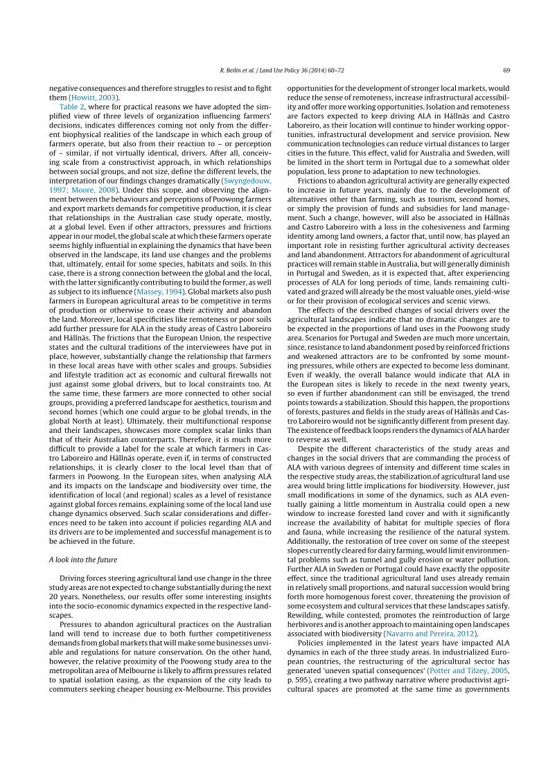
R. Beilin et al. / Land Use Policy 36 (2014) 60– 72 69
negative consequences and therefore struggles to resist and to fightthem (Howitt, 2003).
Table 2, where for practical reasons we have adopted the sim-plified view of three levels of organization influencing farmers’decisions, indicates differences coming not only from the differ-ent biophysical realities of the landscape in which each group offarmers operate, but also from their reaction to – or perceptionof – similar, if not virtually identical, drivers. After all, conceiv-ing scale from a constructivist approach, in which relationshipsbetween social groups, and not size, define the different levels, theinterpretation of our findings changes dramatically (Swyngedouw,1997; Moore, 2008). Under this scope, and observing the align-ment between the behaviours and perceptions of Poowong farmersand export markets demands for competitive production, it is clearthat relationships in the Australian case study operate, mostly,at a global level. Even if other attractors, pressures and frictionsappear in our model, the global scale at which these farmers operateseems highly influential in explaining the dynamics that have beenobserved in the landscape, its land use changes and the problemsthat, ultimately, entail for some species, habitats and soils. In thiscase, there is a strong connection between the global and the local,with the latter significantly contributing to build the former, as wellas subject to its influence (Massey, 1994). Global markets also pushfarmers in European agricultural areas to be competitive in termsof production or otherwise to cease their activity and abandonthe land. Moreover, local specificities like remoteness or poor soilsadd further pressure for ALA in the study areas of Castro Laboreiroand Hållnäs. The frictions that the European Union, the respectivestates and the cultural traditions of the interviewees have put inplace, however, substantially change the relationship that farmersin these local areas have with other scales and groups. Subsidiesand lifestyle tradition act as economic and cultural firewalls notjust against some global drivers, but to local constraints too. Atthe same time, these farmers are more connected to other socialgroups, providing a preferred landscape for aesthetics, tourism andsecond homes (which one could argue to be global trends, in theglobal North at least). Ultimately, their multifunctional responseand their landscapes, showcases more complex scalar links thanthat of their Australian counterparts. Therefore, it is much moredifficult to provide a label for the scale at which farmers in Cas-tro Laboreiro and Hållnäs operate, even if, in terms of constructedrelationships, it is clearly closer to the local level than that offarmers in Poowong. In the European sites, when analysing ALAand its impacts on the landscape and biodiversity over time, theidentification of local (and regional) scales as a level of resistanceagainst global forces remains, explaining some of the local land usechange dynamics observed. Such scalar considerations and differ-ences need to be taken into account if policies regarding ALA andits drivers are to be implemented and successful management is tobe achieved in the future.
A look into the future
Driving forces steering agricultural land use change in the threestudy areas are not expected to change substantially during the next20 years. Nonetheless, our results offer some interesting insightsinto the socio-economic dynamics expected in the respective land-scapes.
Pressures to abandon agricultural practices on the Australianland will tend to increase due to both further competitivenessdemands from global markets that will make some businesses unvi-able and regulations for nature conservation. On the other hand,however, the relative proximity of the Poowong study area to themetropolitan area of Melbourne is likely to affirm pressures relatedto spatial isolation easing, as the expansion of the city leads tocommuters seeking cheaper housing ex-Melbourne. This provides
opportunities for the development of stronger local markets, wouldreduce the sense of remoteness, increase infrastructural accessibil-ity and offer more working opportunities. Isolation and remotenessare factors expected to keep driving ALA in Hållnäs and CastroLaboreiro, as their location will continue to hinder working oppor-tunities, infrastructural development and service provision. Newcommunication technologies can reduce virtual distances to largercities in the future. This effect, valid for Australia and Sweden, willbe limited in the short term in Portugal due to a somewhat olderpopulation, less prone to adaptation to new technologies.
Frictions to abandon agricultural activity are generally expectedto increase in future years, mainly due to the development ofalternatives other than farming, such as tourism, second homes,or simply the provision of funds and subsidies for land manage-ment. Such a change, however, will also be associated in Hållnäsand Castro Laboreiro with a loss in the cohesiveness and farmingidentity among land owners, a factor that, until now, has played animportant role in resisting further agricultural activity decreasesand land abandonment. Attractors for abandonment of agriculturalpractices will remain stable in Australia, but will generally diminishin Portugal and Sweden, as it is expected that, after experiencingprocesses of ALA for long periods of time, lands remaining culti-vated and grazed will already be the most valuable ones, yield-wiseor for their provision of ecological services and scenic views.
The effects of the described changes of social drivers over theagricultural landscapes indicate that no dramatic changes are tobe expected in the proportions of land uses in the Poowong studyarea. Scenarios for Portugal and Sweden are much more uncertain,since, resistance to land abandonment posed by reinforced frictionsand weakened attractors are to be confronted by some mount-ing pressures, while others are expected to become less dominant.Even if weakly, the overall balance would indicate that ALA inthe European sites is likely to recede in the next twenty years,so even if further abandonment can still be envisaged, the trendpoints towards a stabilization. Should this happen, the proportionsof forests, pastures and fields in the study areas of Hållnäs and Cas-tro Laboreiro would not be significantly different from present day.The existence of feedback loops renders the dynamics of ALA harderto reverse as well.
Despite the different characteristics of the study areas andchanges in the social drivers that are commanding the process ofALA with various degrees of intensity and different time scales inthe respective study areas, the stabilization.of agricultural land usearea would bring little implications for biodiversity. However, justsmall modifications in some of the dynamics, such as ALA even-tually gaining a little momentum in Australia could open a newwindow to increase forested land cover and with it significantlyincrease the availability of habitat for multiple species of floraand fauna, while increasing the resilience of the natural system.Additionally, the restoration of tree cover on some of the steepestslopes currently cleared for dairy farming, would limit environmen-tal problems such as tunnel and gully erosion or water pollution.Further ALA in Sweden or Portugal could have exactly the oppositeeffect, since the traditional agricultural land uses already remainin relatively small proportions, and natural succession would bringforth more homogenous forest cover, threatening the provision ofsome ecosystem and cultural services that these landscapes satisfy.Rewilding, while contested, promotes the reintroduction of largeherbivores and is another approach to maintaining open landscapesassociated with biodiversity (Navarro and Pereira, 2012).
Policies implemented in the latest years have impacted ALAdynamics in each of the three study areas. In industrialized Euro-pean countries, the restructuring of the agricultural sector hasgenerated ‘uneven spatial consequences’ (Potter and Tilzey, 2005,p. 595), creating a two pathway narrative where productivist agri-cultural spaces are promoted at the same time as governments
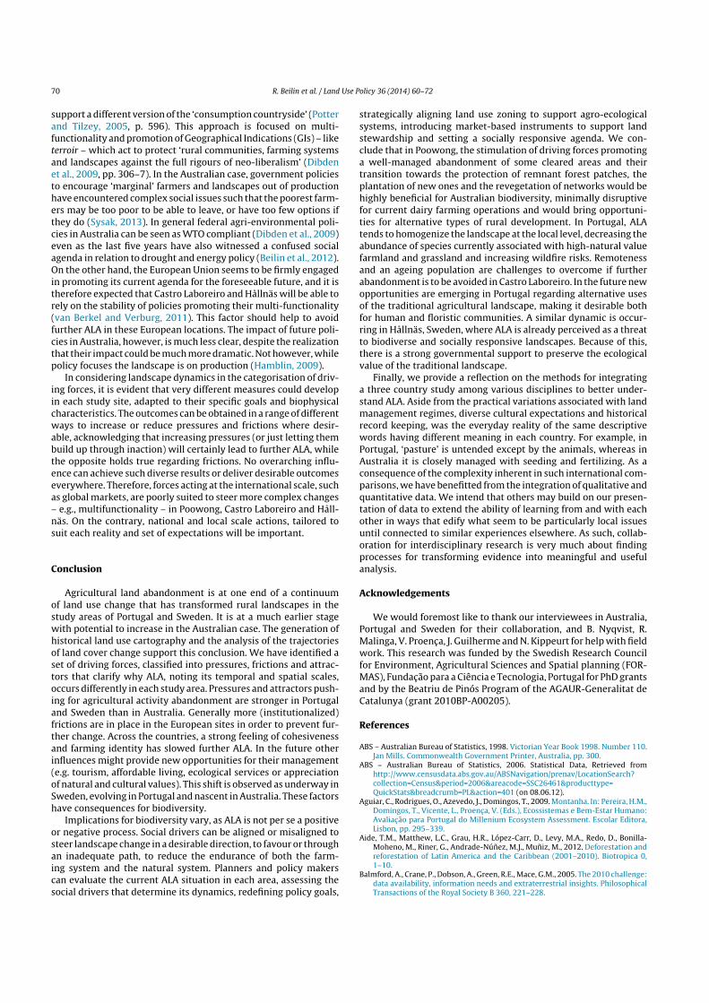
70 R. Beilin et al. / Land Use Policy 36 (2014) 60– 72
support a different version of the ‘consumption countryside’ (Potterand Tilzey, 2005, p. 596). This approach is focused on multi-functionality and promotion of Geographical Indications (GIs) – liketerroir – which act to protect ‘rural communities, farming systemsand landscapes against the full rigours of neo-liberalism’ (Dibdenet al., 2009, pp. 306–7). In the Australian case, government policiesto encourage ‘marginal’ farmers and landscapes out of productionhave encountered complex social issues such that the poorest farm-ers may be too poor to be able to leave, or have too few options ifthey do (Sysak, 2013). In general federal agri-environmental poli-cies in Australia can be seen as WTO compliant (Dibden et al., 2009)even as the last five years have also witnessed a confused socialagenda in relation to drought and energy policy (Beilin et al., 2012).On the other hand, the European Union seems to be firmly engagedin promoting its current agenda for the foreseeable future, and it istherefore expected that Castro Laboreiro and Hållnäs will be able torely on the stability of policies promoting their multi-functionality(van Berkel and Verburg, 2011). This factor should help to avoidfurther ALA in these European locations. The impact of future poli-cies in Australia, however, is much less clear, despite the realizationthat their impact could be much more dramatic. Not however, whilepolicy focuses the landscape is on production (Hamblin, 2009).
In considering landscape dynamics in the categorisation of driv-ing forces, it is evident that very different measures could developin each study site, adapted to their specific goals and biophysicalcharacteristics. The outcomes can be obtained in a range of differentways to increase or reduce pressures and frictions where desir-able, acknowledging that increasing pressures (or just letting thembuild up through inaction) will certainly lead to further ALA, whilethe opposite holds true regarding frictions. No overarching influ-ence can achieve such diverse results or deliver desirable outcomeseverywhere. Therefore, forces acting at the international scale, suchas global markets, are poorly suited to steer more complex changes– e.g., multifunctionality – in Poowong, Castro Laboreiro and Håll-näs. On the contrary, national and local scale actions, tailored tosuit each reality and set of expectations will be important.
Conclusion
Agricultural land abandonment is at one end of a continuumof land use change that has transformed rural landscapes in thestudy areas of Portugal and Sweden. It is at a much earlier stagewith potential to increase in the Australian case. The generation ofhistorical land use cartography and the analysis of the trajectoriesof land cover change support this conclusion. We have identified aset of driving forces, classified into pressures, frictions and attrac-tors that clarify why ALA, noting its temporal and spatial scales,occurs differently in each study area. Pressures and attractors push-ing for agricultural activity abandonment are stronger in Portugaland Sweden than in Australia. Generally more (institutionalized)frictions are in place in the European sites in order to prevent fur-ther change. Across the countries, a strong feeling of cohesivenessand farming identity has slowed further ALA. In the future otherinfluences might provide new opportunities for their management(e.g. tourism, affordable living, ecological services or appreciationof natural and cultural values). This shift is observed as underway inSweden, evolving in Portugal and nascent in Australia. These factorshave consequences for biodiversity.
Implications for biodiversity vary, as ALA is not per se a positiveor negative process. Social drivers can be aligned or misaligned tosteer landscape change in a desirable direction, to favour or throughan inadequate path, to reduce the endurance of both the farm-ing system and the natural system. Planners and policy makerscan evaluate the current ALA situation in each area, assessing thesocial drivers that determine its dynamics, redefining policy goals,
strategically aligning land use zoning to support agro-ecologicalsystems, introducing market-based instruments to support landstewardship and setting a socially responsive agenda. We con-clude that in Poowong, the stimulation of driving forces promotinga well-managed abandonment of some cleared areas and theirtransition towards the protection of remnant forest patches, theplantation of new ones and the revegetation of networks would behighly beneficial for Australian biodiversity, minimally disruptivefor current dairy farming operations and would bring opportuni-ties for alternative types of rural development. In Portugal, ALAtends to homogenize the landscape at the local level, decreasing theabundance of species currently associated with high-natural valuefarmland and grassland and increasing wildfire risks. Remotenessand an ageing population are challenges to overcome if furtherabandonment is to be avoided in Castro Laboreiro. In the future newopportunities are emerging in Portugal regarding alternative usesof the traditional agricultural landscape, making it desirable bothfor human and floristic communities. A similar dynamic is occur-ring in Hållnäs, Sweden, where ALA is already perceived as a threatto biodiverse and socially responsive landscapes. Because of this,there is a strong governmental support to preserve the ecologicalvalue of the traditional landscape.
Finally, we provide a reflection on the methods for integratinga three country study among various disciplines to better under-stand ALA. Aside from the practical variations associated with landmanagement regimes, diverse cultural expectations and historicalrecord keeping, was the everyday reality of the same descriptivewords having different meaning in each country. For example, inPortugal, ‘pasture’ is untended except by the animals, whereas inAustralia it is closely managed with seeding and fertilizing. As aconsequence of the complexity inherent in such international com-parisons, we have benefitted from the integration of qualitative andquantitative data. We intend that others may build on our presen-tation of data to extend the ability of learning from and with eachother in ways that edify what seem to be particularly local issuesuntil connected to similar experiences elsewhere. As such, collab-oration for interdisciplinary research is very much about findingprocesses for transforming evidence into meaningful and usefulanalysis.
Acknowledgements
We would foremost like to thank our interviewees in Australia,Portugal and Sweden for their collaboration, and B. Nyqvist, R.Malinga, V. Proenc a, J. Guilherme and N. Kippeurt for help with fieldwork. This research was funded by the Swedish Research Councilfor Environment, Agricultural Sciences and Spatial planning (FOR-MAS), Fundac ão para a Ciência e Tecnologia, Portugal for PhD grantsand by the Beatriu de Pinós Program of the AGAUR-Generalitat deCatalunya (grant 2010BP-A00205).
References
ABS – Australian Bureau of Statistics, 1998. Victorian Year Book 1998. Number 110.Jan Mills. Commonwealth Government Printer, Australia, pp. 300.
ABS – Australian Bureau of Statistics, 2006. Statistical Data, Retrieved fromhttp://www.censusdata.abs.gov.au/ABSNavigation/prenav/LocationSearch?collection=Census&period=2006&areacode=SSC26461&producttype=QuickStats&breadcrumb=PL&action=401 (on 08.06.12).
Aguiar, C., Rodrigues, O., Azevedo, J., Domingos, T., 2009. Montanha. In: Pereira, H.M.,Domingos, T., Vicente, L., Proenc a, V. (Eds.), Ecossistemas e Bem-Estar Humano:Avaliac ão para Portugal do Millenium Ecosystem Assessment. Escolar Editora,Lisbon, pp. 295–339.
Aide, T.M., Matthew, L.C., Grau, H.R., López-Carr, D., Levy, M.A., Redo, D., Bonilla-Moheno, M., Riner, G., Andrade-Núnez, M.J., Muniz, M., 2012. Deforestation andreforestation of Latin America and the Caribbean (2001–2010). Biotropica 0,1–10.
Balmford, A., Crane, P., Dobson, A., Green, R.E., Mace, G.M., 2005. The 2010 challenge:data availability, information needs and extraterrestrial insights. PhilosophicalTransactions of the Royal Society B 360, 221–228.
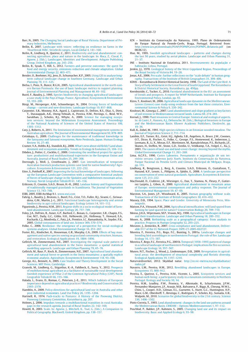
R. Beilin et al. / Land Use Policy 36 (2014) 60– 72 71
Barr, N., 2005. The Changing Social Landscape of Rural Victoria. Department of Pri-mary Industries, Melbourne.
Beilin, R., 2007. Landscape with voices: reflecting on resilience on farms in the‘Heartbreak Hills’, Strzelecki ranges. Local-Global 4, 141–160.
Beilin, R., Lindborg, R., Queiroz, C., 2011. Biodiversity and land abandonment: con-necting agriculture, place and nature in the landscape. In: Roca, Z., Claval, P.,Agnew, J. (Eds.), Landscapes, Identities and Development. Ashgate PublishingGroup, United Kingdom, pp. 243–256.
Beilin, R., Sysak, T., Hill, S., 2012. Farmers and perverse outcomes: the quest forfood and energy security, emissions reduction and climate adaptation. GlobalEnvironmental Change 22, 463–471.
Bender, O., Boehmer, H.J., Jens, D., Schumacher, K.P., 2005. Using GIS to analyse long-term cultural landscape change in Southern Germany. Landscape and UrbanPlanning 70, 111–125.
Bielsa, I., Pons, X., Bunce, R.G.H., 2005. Agricultural abandonment in the north east-ern Iberian Peninsula: the use of basic landscape metrics to support planning.Journal of Environmental Planning and Management 48, 85–102.
Burel, F., Baudry, J., 1995. Species biodiversity in changing agricultural landscapes:a case study in the Pays d’Auge, France. Agriculture, Ecosystems & Environment55, 193–200.
Bürgi, M., Hersperger, A.M., Schneeberger, N., 2004. Driving forces of landscapechange – current and new directions. Landscape Ecology 19, 857–868.
Carpenter, S.R., Mooney, H.A., Agard, J., Capistrano, D., Defries, R.S., Díaz, S., Dietz,T., Duraiappah, A.K., Oteng-Yeboah, A., Pereira, H.M., Perrings, C., Reid, W.V.,Sarukhan, J., Scholes, R.J., Whyte, A., 2009. Science for managing ecosys-tem services: beyond the Millennium Ecosystem Assessment. Proceedingsof the National Academy of Sciences of the United States of America 106,1305–1312.
Cary, J., Roberts, A., 2011. The limitations of environmental management systems inAustralian agriculture. The Journal of Environmental Management 92, 878–885.
Cetinkaya, G., 2009. Challenges for the maintenance of traditional knowledge inthe Satoyama and Satoumi ecosystems, Noto Peninsula, Japan. Human EcologyReview 16, 27–40.
Cramer, V.A., Hobbs, R.J., Standish, R.J., 2008. What’s new about old fields? Land aban-donment and ecosystem assembly. Trends in Ecology & Evolution 23, 104–112.
Dibden, J., Potter, C., Cocklin, C., 2009. Contesting the neoliberal project for agricul-ture: productivist and multifunctional trajectories in the European Union andAustralia. Journal of Rural Studies 25, 299–308.
Dorrough, J., Moll, J., Crosthwaite, J., 2007. Can intensification of temperateAustralian livestock production systems save land for native biodiversity? Agri-culture, Ecosystems & Environment 121, 222–232.
Eiter, S., Potthoff, K., 2007. Improving the factual knowledge of landscapes: followingup the European Landscape Convention with a comparative historical analysisof forces of landscape change in the Sjodalen and Stølsheimen mountain areas,Norway. Norsk Geografisk Tidsskrift 61, 145–156.
Eriksson, O., Cousins, S.A.O., Bruun, H.-H., 2002. Landuse history and fragmentationof traditionally managed grasslands in Scandinavia. The Journal of VegetationScience 13, 743–748.
ESRI, 2005. ESRI ArcMap 9.1. www.esri.comFahrig, L., Baudry, J., Brotons, L., Burel, F.G., Crist, T.O., Fuller, R.J., Sirami, C., Siriwar-
dena, G.M., Martin, J.-L., 2011. Functional landscape heterogeneity and animalbiodiversity in agri-cultural landscapes. Ecology Letters 14, 101–112.
Figueiredo, J., Pereira, H.M., 2011. Regime shifts in a socio-ecological model of farm-land abandonment. Landscape Ecology 26, 737–749.
Foley, J.A., DeFries, R., Asner, G.P., Barford, C., Bonan, G., Carpenter, S.R., Chapin, F.S.,Coe, M.T., Daily, G.C., Gibbs, H.K., Helkowski, J.H., Holloway, T., Howard, E.A.,Kucharik, C.J., Monfreda, C., Patz, J.A., Prentice, I.C., Ramankutty, N., Snyder, P.K.,2005. Global consequences of land use. Science 309, 570–574.
Folke, C., 2006. Resilience: the emergence of a perspective for social–ecologicalsystems analyses. Global Environmental Change 16, 253–267.
Foster, B.L., Kindscher, K., Houseman, G.R., Murphy, C.A., 2009. Effects of hay man-agement and native species sowing on grassland community structure, biomass,and restoration. Ecological Applications 19, 1884–1896.
Gellrich, M., Zimmermann, N.E., 2007. Investigating the regional scale pattern ofagricultural land abandonment in the Swiss mountains: a spatial statisticalmodelling approach. Landscape and Urban Planning 79, 65–76.
Gellrich, M., Baur, P., Koch, B., Zimmermann, N.E., 2007. Agricultural land abandon-ment and natural forest re-growth in the Swiss mountains: a spatially expliciteconomic analysis. Agriculture, Ecosystems & Environment 118, 93–108.
George, A.L., Bennett, A., 2005. Case Studies and Theory Development in the SocialSciences. MIT Press, Cambridge.
Granvik, M., Lindberg, G., Stigzelius, K.-A., Fahlbeck, E., Surry, Y., 2012. Prospectsof multifunctional agriculture as a facilitator of sustainable rural development:Swedish experience of Pillar 2 of the Common Agricultural Policy (CAP). NorskGeografisk Tidsskrift 66, 155–166.
Halada, L., Evans, D., Romao, C., Petersen, J.-E., 2011. Which habitats of Europeanimportance depend on agricultural practices? Biodiversity and Conservation 20,2365–2378.
Hamblin, A., 2009. Policy directions for agricultural land use in Australia and otherpost-industrial economies. Land Use Policy 26, 1195–1204.
Hartnell, R., 1974. Pack-tracks to Pastures: A History of the Poowong District.Poowong Centenary Committee, Korumburra, pp. 207.
Holmes, J., 2006. Impulses towards a multifunctional transition in rural Australia:gaps in the research agenda. Journal of Rural Studies 22, 142–160.
Howitt, R., 2003. Scale. In: Agnew, J., Mitchell, K., Toal, G. (Eds.), A Companion toPolitical Geography. Blackwell, United Kingdom, pp. 138–157.
ICN – Instituto da Conservac ão da Natureza, 1995. Plano de Ordenamentodo Parque Natural da Penede-Gerês, Braga, Portugal. Retrieved from:http://www.icn.pt/downloads/POAP/POPNPGeres/POPNPG Relatorio.pdf (on08.06.12).
Ihse, M., 1995. Swedish agricultural landscapes – patterns and changes duringthe last 50 years, studied by aerial photos. Landscape and Urban Planning 31,21–37.
INE – Instituto Nacional de Estatística, 2011. Recenseamento da populac ão ehabitac ão, Lisboa, Portugal.
Jenkin, J.J., 1970. Geological history of the West Gippsland Region. Proceedings ofthe Royal Society of Victoria 84, 19–28.
Jonas, A.E., 2006. Pro scale: further reflections on the “scale debate” in human geog-raphy. Transactions of the Institute of British Geographers 31, 399–406.
KDHS – Korumburra & District Historical Society, 1998. The Land of the Lyre Bird: AStory of Early Settlement in the Great Forest of South Gippsland. The Korumburra& District Historical Society, Korumburra, pp. 450pp.
Keenleyside, C., Tucker, G., 2010. Farmland abandonment in the EU: an assessmentof trends and prospects. A report for WWF Netherlands. Institute for EuropeanEnvironmental Policy, London, pp. 93.
Kizos, T., Koulouri, M., 2006. Agricultural landscape dynamics in the Mediterranean:Lesvos (Greece) case study using evidence from the last three centuries. Envi-ronmental Science & Policy 9, 330–342.
Koulouri, M., Giourga, C., 2007. Land abandonment and slope gradient as key factorsof soil erosion in Mediterranean terraced lands. Catena 69, 274–281.
Kornas, J., 1990. Plant invasions in Central Europe: historical and ecological aspects.In: di Castri, F., Hansen, A.J., Debussche, M. (Eds.), Biological Invasions in Europeand the Mediterranean Basin. Kluwer Academic Publishers, Dordrecht, pp.19–36.
Kull, K., Zobel, M., 1991. High species richness in an Estonian wooded meadow. TheJournal of Vegetation Science 2, 711–714.
Lambin, E.F., Turner, B.L., Geist, H.J., Agbola, S.B., Angelsen, A., Bruce, J.W., Coomes,O.T., Dirzo, R., Fischer, G., Folke, C., George, P.S., Homewood, K., Imbernon, J.,Leemans, R., Li, X., Moran, E.F., Mortimore, M., Ramakrishnan, P.S., Richards, J.F.,Skanes, H., Steffen, W., Stone, G.D., Svedin, U., Veldkamp, T.A., Volgel, C., Xu, J.,2001. The causes of land-use and land-cover change: moving beyond the myths.Global Environmental Change 11, 261–269.
Lima, A.C.P.S., 1996. Castro Laboreiro. Povoamento e organizac ão de um ter-ritório serrano. Cadernos Juríz Xurés. Instituto da Conservac ão da Natureza,Parque Nacional da Peneda Gerês and Câmara Municipal de Melgac o, Braga,pp. 155.
Lindborg, R., Bengtsson, J., Berg, Å., Cousins, S.A.O., Eriksson, O., Gustafsson, T.,Hasund, K.P., Lenoir, L., Pihlgren, A., Sjödin, E., 2008. A landscape perspectiveon conservation of semi-natural grasslands. Agriculture, Ecosystems & Environ-ment 125, 213–222.
MacDonald, D., Crabtree, J.R., Wiesinger, G., Dax, T., Stamou, N., Fleury, P., Gutier-rez Lazpita, J., Gibon, A., 2000. Agricultural abandonment in mountain areasof Europe: environmental consequences and policy response. The Journal ofEnvironmental Management 59, 47–69.
Marston, S.A., Jones, J.P., Woodward, K., 2005. Human geography without scale.Transactions of the Institute of British Geographers 30, 416–432.
Massey, D.B., 1994. Space, Place and Gender. University of Minnesota Press, Min-neapolis.
Matson, P.A., Vitousek, P.M., 2006. Agricultural intensification: will land spared fromfarming be land spared for nature? Conservation Biology 20, 709–710.
Meeus, J.H.A., Wijermans, M.P., Vroom, M.J., 1990. Agricultural landscapes in Europeand their transformation. Landscape and Urban Planning 18, 289–352.
Moore, A., 2008. Rethinking scale as a geographical category: from analysis topractice. Progress in Human Geography 32, 203–225.
Moravec, J., Zemeckis, R., 2007. Cross compliance and land abandonment, Deliver-able D17 of the CC Network Project, SSPE-CT-2005-022727.
Moreira, F., Ferreira, P.G., Rego, F.C., Bunting, S., 2001a. Landscape changes andbreeding bird assemblages in northwestern Portugal: the role of fire. LandscapeEcology 16, 175–187.
Moreira, F., Rego, F.C., Ferreira, P.G., 2001b. Temporal (1958–1995) pattern of changein a cultural landscape of northwestern Portugal: implications for fire occurence.Landscape Ecology 16, 557–567.
Munro, N.T., Fischer, J., Wood, J., Lindenmayer, D.B., 2009. Revegetation in agricul-tural areas: the development of structural complexity and floristic diversity.Ecological Applications 19, 1197–1210.
Naturvårdsverket, 2012. Skyddad natur. http://sn.vic-metria.nu/skyddadnatur/index.jsf
Navarro, L.M., Pereira, H.M., 2012. Rewilding abandoned landscapes in Europe.Ecosystems 15, 900–912.
Pereira, E., Queiroz, C., Pereira, H.M., Vicente, L., 2005. Ecosystem services andhuman well-being: a participatory study in a mountain community in NorthernPortugal. Ecology and Society 10, 14.
Pereira, H.M., Leadley, P.W., Proenca, V., Alkemade, R., Scharlemann, J.P.W.,Fernandez-Manjarres, J.F., Araujo, M.B., Balvanera, P., Biggs, R., Cheung, W.W.L.,Chini, L., Cooper, H.D., Gilman, E.L., Guenette, S., Hurtt, G.C., Huntington, H.P.,Mace, G.M., Oberdorff, T., Revenga, C., Rodrigues, P., Scholes, R.J., Sumaila, U.R.,Walpole, M., 2010. Scenarios for global biodiversity in the 21st century. Science330, 1496–1502.
Pinto-Correia, T., 1993. Land abandonment: changes in the land use patterns aroundthe Mediterranean Basin. CIHEAM – Options Mediterraneennes 1, 97–112.
Poschlod, P., Bakker, J.P., Kahmen, S., 2005. Changing land use and its impact onbiodiversity. Basic and Applied Ecology 6, 93–98.
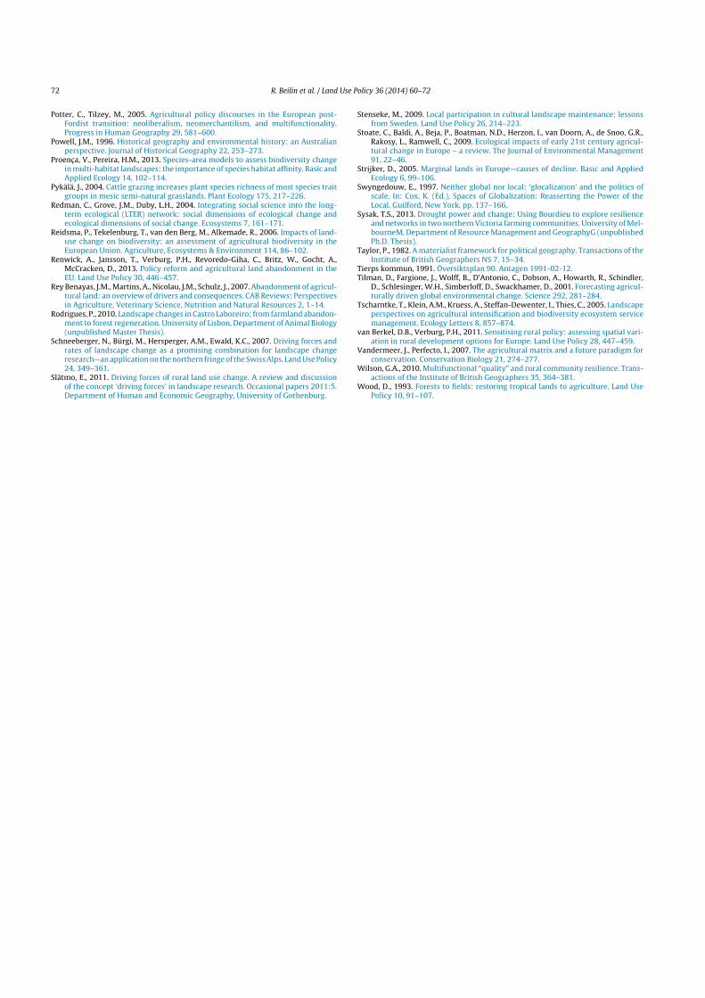
72 R. Beilin et al. / Land Use Policy 36 (2014) 60– 72
Potter, C., Tilzey, M., 2005. Agricultural policy discourses in the European post-Fordist transition: neoliberalism, neomerchantilism, and multifunctionality.Progress in Human Geography 29, 581–600.
Powell, J.M., 1996. Historical geography and environmental history: an Australianperspective. Journal of Historical Geography 22, 253–273.
Proenc a, V., Pereira, H.M., 2013. Species-area models to assess biodiversity changein multi-habitat landscapes: the importance of species habitat affinity. Basic andApplied Ecology 14, 102–114.
Pykälä, J., 2004. Cattle grazing increases plant species richness of most species traitgroups in mesic semi-natural grasslands. Plant Ecology 175, 217–226.
Redman, C., Grove, J.M., Duby, L.H., 2004. Integrating social science into the long-term ecological (LTER) network: social dimensions of ecological change andecological dimensions of social change. Ecosystems 7, 161–171.
Reidsma, P., Tekelenburg, T., van den Berg, M., Alkemade, R., 2006. Impacts of land-use change on biodiversity: an assessment of agricultural biodiversity in theEuropean Union. Agriculture, Ecosystems & Environment 114, 86–102.
Renwick, A., Jansson, T., Verburg, P.H., Revoredo-Giha, C., Britz, W., Gocht, A.,McCracken, D., 2013. Policy reform and agricultural land abandonment in theEU. Land Use Policy 30, 446–457.
Rey Benayas, J.M., Martins, A., Nicolau, J.M., Schulz, J., 2007. Abandonment of agricul-tural land: an overview of drivers and consequences. CAB Reviews: Perspectivesin Agriculture, Veterinary Science, Nutrition and Natural Resources 2, 1–14.
Rodrigues, P., 2010. Landscape changes in Castro Laboreiro: from farmland abandon-ment to forest regeneration. University of Lisbon, Department of Animal Biology(unpublished Master Thesis).
Schneeberger, N., Bürgi, M., Hersperger, A.M., Ewald, K.C., 2007. Driving forces andrates of landscape change as a promising combination for landscape changeresearch—an application on the northern fringe of the Swiss Alps. Land Use Policy24, 349–361.
Slätmo, E., 2011. Driving forces of rural land use change. A review and discussionof the concept ‘driving forces’ in landscape research. Occasional papers 2011:5.Department of Human and Economic Geography, University of Gothenburg.
Stenseke, M., 2009. Local participation in cultural landscape maintenance: lessonsfrom Sweden. Land Use Policy 26, 214–223.
Stoate, C., Baldi, A., Beja, P., Boatman, N.D., Herzon, I., van Doorn, A., de Snoo, G.R.,Rakosy, L., Ramwell, C., 2009. Ecological impacts of early 21st century agricul-tural change in Europe – a review. The Journal of Environmental Management91, 22–46.
Strijker, D., 2005. Marginal lands in Europe—causes of decline. Basic and AppliedEcology 6, 99–106.
Swyngedouw, E., 1997. Neither global nor local: ‘glocalization’ and the politics ofscale. In: Cox, K. (Ed.), Spaces of Globalization: Reasserting the Power of theLocal. Guilford, New York, pp. 137–166.
Sysak, T.S., 2013. Drought power and change: Using Bourdieu to explore resilienceand networks in two northern Victoria farming communities. University of Mel-bourneM, Department of Resource Management and GeographyG (unpublishedPh.D. Thesis).
Taylor, P., 1982. A materialist framework for political geography. Transactions of theInstitute of British Geographers NS 7, 15–34.
Tierps kommun, 1991. Översiktsplan 90. Antagen 1991-02-12.Tilman, D., Fargione, J., Wolff, B., D’Antonio, C., Dobson, A., Howarth, R., Schindler,
D., Schlesinger, W.H., Simberloff, D., Swackhamer, D., 2001. Forecasting agricul-turally driven global environmental change. Science 292, 281–284.
Tscharntke, T., Klein, A.M., Kruess, A., Steffan-Dewenter, I., Thies, C., 2005. Landscapeperspectives on agricultural intensification and biodiversity ecosystem servicemanagement. Ecology Letters 8, 857–874.
van Berkel, D.B., Verburg, P.H., 2011. Sensitising rural policy: assessing spatial vari-ation in rural development options for Europe. Land Use Policy 28, 447–459.
Vandermeer, J., Perfecto, I., 2007. The agricultural matrix and a future paradigm forconservation. Conservation Biology 21, 274–277.
Wilson, G.A., 2010. Multifunctional “quality” and rural community resilience. Trans-actions of the Institute of British Geographers 35, 364–381.
Wood, D., 1993. Forests to fields: restoring tropical lands to agriculture. Land UsePolicy 10, 91–107.
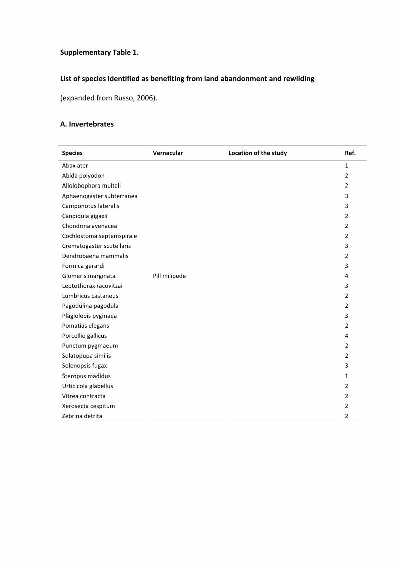
Supplementary,Table,1.,,
List,of,species,identified,as,benefiting,from,land,abandonment,and,rewilding,
(expanded(from(Russo,(2006).(
A.,Invertebrates!
Species, Vernacular, Location,of,the,study, Ref.,
Abax(ater( (( (( 1(
Abida(polyodon(( (
2(
Allolobophora(multali(( (
2(
Aphaenogaster(subterranea(( (
3(
Camponotus(lateralis(( (
3(
Candidula(gigaxii(( (
2(
Chondrina(avenacea(( (
2(
Cochlostoma(septemspirale(( (
2(
Crematogaster(scutellaris(( (
3(
Dendrobaena(mammalis(( (
2(
Formica(gerardi((( (
3(
Glomeris(marginata( Pill(milipede((
4(
Leptothorax(racovitzai(( (
3(
Lumbricus(castaneus(( (
2(
Pagodulina(pagodula(( (
2(
Plagiolepis(pygmaea(( (
3(
Pomatias(elegans(( (
2(
Porcellio(gallicus(( (
4(
Punctum(pygmaeum(( (
2(
Solatopupa(similis(( (
2(
Solenopsis(fugax(( (
3(
Steropus(madidus(( (
1(
Urticicola(glabellus(( (
2(
Vitrea(contracta(( (
2(
Xerosecta(cespitum(( (
2(
Zebrina(detrita( (( (( 2(
!
!
!
!
!
,
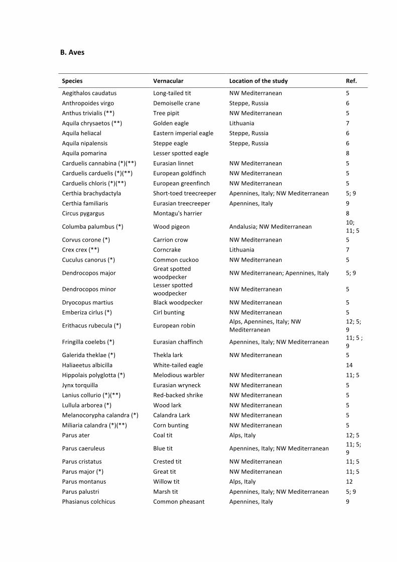
B.,Aves,
Species( Vernacular( Location,of,the,study( Ref.(
Aegithalos(caudatus( LongOtailed(tit( NW(Mediterranean( 5(
Anthropoides(virgo( Demoiselle(crane( Steppe,(Russia( 6(
Anthus(trivialis((**)( Tree(pipit( NW(Mediterranean( 5(
Aquila(chrysaetos((**)( Golden(eagle( Lithuania( 7(
Aquila(heliacal( Eastern(imperial(eagle( Steppe,(Russia( 6(
Aquila(nipalensis( Steppe(eagle( Steppe,(Russia( 6(
Aquila(pomarina( Lesser(spotted(eagle((
8(
Carduelis(cannabina((*)(**)( Eurasian(linnet( NW(Mediterranean( 5(
Carduelis(carduelis((*)(**)( European(goldfinch( NW(Mediterranean( 5(
Carduelis(chloris((*)(**)( European(greenfinch( NW(Mediterranean( 5(
Certhia(brachydactyla( ShortOtoed(treecreeper( Apennines,(Italy;(NW(Mediterranean( 5;(9(
Certhia(familiaris( Eurasian(treecreeper( Apennines,(Italy( 9(
Circus(pygargus( Montagu's(harrier((
8(
Columba(palumbus((*)( Wood(pigeon( Andalusia;(NW(Mediterranean(10;(
11;(5(
Corvus(corone((*)( Carrion(crow( NW(Mediterranean( 5(
Crex(crex((**)( Corncrake( Lithuania( 7(
Cuculus(canorus((*)( Common(cuckoo( NW(Mediterranean( 5(
Dendrocopos(major(Great(spotted(
woodpecker(NW(Mediterranean;(Apennines,(Italy( 5;(9(
Dendrocopos(minor(Lesser(spotted(
woodpecker(NW(Mediterranean( 5(
Dryocopus(martius( Black(woodpecker( NW(Mediterranean( 5(
Emberiza(cirlus((*)( Cirl(bunting( NW(Mediterranean( 5(
Erithacus(rubecula((*)( European(robin(Alps,(Apennines,(Italy;(NW(
Mediterranean(
12;(5;(
9(
Fringilla(coelebs((*)( Eurasian(chaffinch( Apennines,(Italy;(NW(Mediterranean(11;(5(;(
9(
Galerida(theklae((*)( Thekla(lark( NW(Mediterranean( 5(
Haliaeetus(albicilla( WhiteOtailed(eagle((
14(
Hippolais(polyglotta((*)( Melodious(warbler( NW(Mediterranean( 11;(5(
Jynx(torquilla( Eurasian(wryneck( NW(Mediterranean( 5(
Lanius(collurio((*)(**)( RedObacked(shrike( NW(Mediterranean( 5(
Lullula(arborea((*)( Wood(lark( NW(Mediterranean( 5(
Melanocorypha(calandra((*)( Calandra(Lark( NW(Mediterranean( 5(
Miliaria(calandra((*)(**)( Corn(bunting( NW(Mediterranean( 5(
Parus(ater( Coal(tit( Alps,(Italy( 12;(5(
Parus(caeruleus( Blue(tit( Apennines,(Italy;(NW(Mediterranean(11;(5;(
9(
Parus(cristatus( Crested(tit( NW(Mediterranean( 11;(5(
Parus(major((*)( Great(tit( NW(Mediterranean( 11;(5(
Parus(montanus( Willow(tit( Alps,(Italy( 12(
Parus(palustri( Marsh(tit( Apennines,(Italy;(NW(Mediterranean( 5;(9(
Phasianus(colchicus( Common(pheasant( Apennines,(Italy( 9(
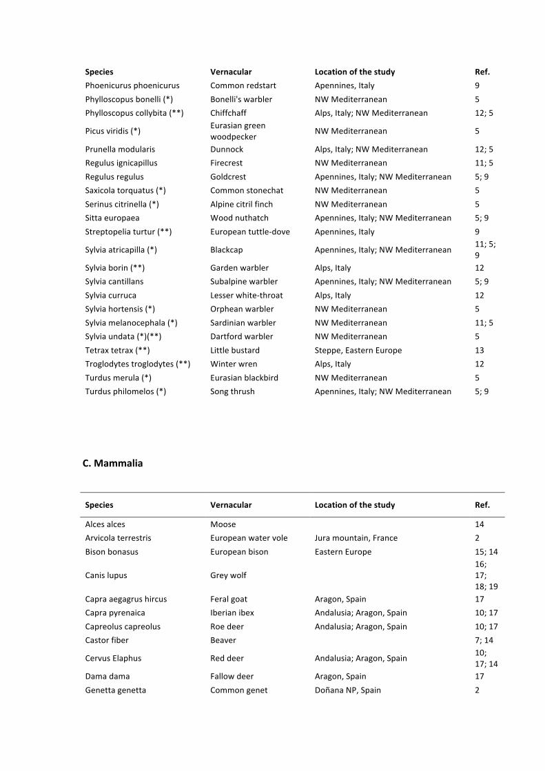
Species( Vernacular( Location,of,the,study( Ref.(Phoenicurus(phoenicurus( Common(redstart( Apennines,(Italy( 9(
Phylloscopus(bonelli((*)( Bonelli's(warbler( NW(Mediterranean( 5(
Phylloscopus(collybita((**)( Chiffchaff( Alps,(Italy;(NW(Mediterranean( 12;(5(
Picus(viridis((*)(Eurasian(green(
woodpecker(NW(Mediterranean( 5(
Prunella(modularis( Dunnock( Alps,(Italy;(NW(Mediterranean( 12;(5(
Regulus(ignicapillus( Firecrest( NW(Mediterranean( 11;(5(
Regulus(regulus( Goldcrest( Apennines,(Italy;(NW(Mediterranean( 5;(9(
Saxicola(torquatus((*)( Common(stonechat( NW(Mediterranean( 5(
Serinus(citrinella((*)( Alpine(citril(finch( NW(Mediterranean( 5(
Sitta(europaea( Wood(nuthatch( Apennines,(Italy;(NW(Mediterranean( 5;(9(
Streptopelia(turtur((**)( European(tuttleOdove( Apennines,(Italy( 9(
Sylvia(atricapilla((*)( Blackcap( Apennines,(Italy;(NW(Mediterranean(11;(5;(
9(
Sylvia(borin((**)( Garden(warbler( Alps,(Italy( 12(
Sylvia(cantillans( Subalpine(warbler( Apennines,(Italy;(NW(Mediterranean( 5;(9(
Sylvia(curruca( Lesser(whiteOthroat( Alps,(Italy( 12(
Sylvia(hortensis((*)( Orphean(warbler( NW(Mediterranean( 5(
Sylvia(melanocephala((*)( Sardinian(warbler( NW(Mediterranean( 11;(5(
Sylvia(undata((*)(**)( Dartford(warbler( NW(Mediterranean( 5(
Tetrax(tetrax((**)( Little(bustard( Steppe,(Eastern(Europe( 13(
Troglodytes(troglodytes((**)( Winter(wren( Alps,(Italy( 12(
Turdus(merula((*)( Eurasian(blackbird( NW(Mediterranean( 5(
Turdus(philomelos((*)( Song(thrush( Apennines,(Italy;(NW(Mediterranean( 5;(9(
!
,
C.,Mammalia,
Species( Vernacular( Location,of,the,study( Ref.(
Alces(alces( Moose( (( 14(
Arvicola(terrestris( European(water(vole( Jura(mountain,(France( 2(
Bison(bonasus( European(bison( Eastern(Europe( 15;(14(
Canis(lupus( Grey(wolf((
16;(
17;(
18;(19(
Capra(aegagrus(hircus( Feral(goat( Aragon,(Spain( 17(
Capra(pyrenaica( Iberian(ibex( Andalusia;(Aragon,(Spain( 10;(17(
Capreolus(capreolus( Roe(deer( Andalusia;(Aragon,(Spain( 10;(17(
Castor(fiber( Beaver((
7;(14(
Cervus(Elaphus( Red(deer( Andalusia;(Aragon,(Spain(10;(
17;(14(
Dama(dama( Fallow(deer( Aragon,(Spain( 17(
Genetta(genetta( Common(genet( Doñana(NP,(Spain( 2(
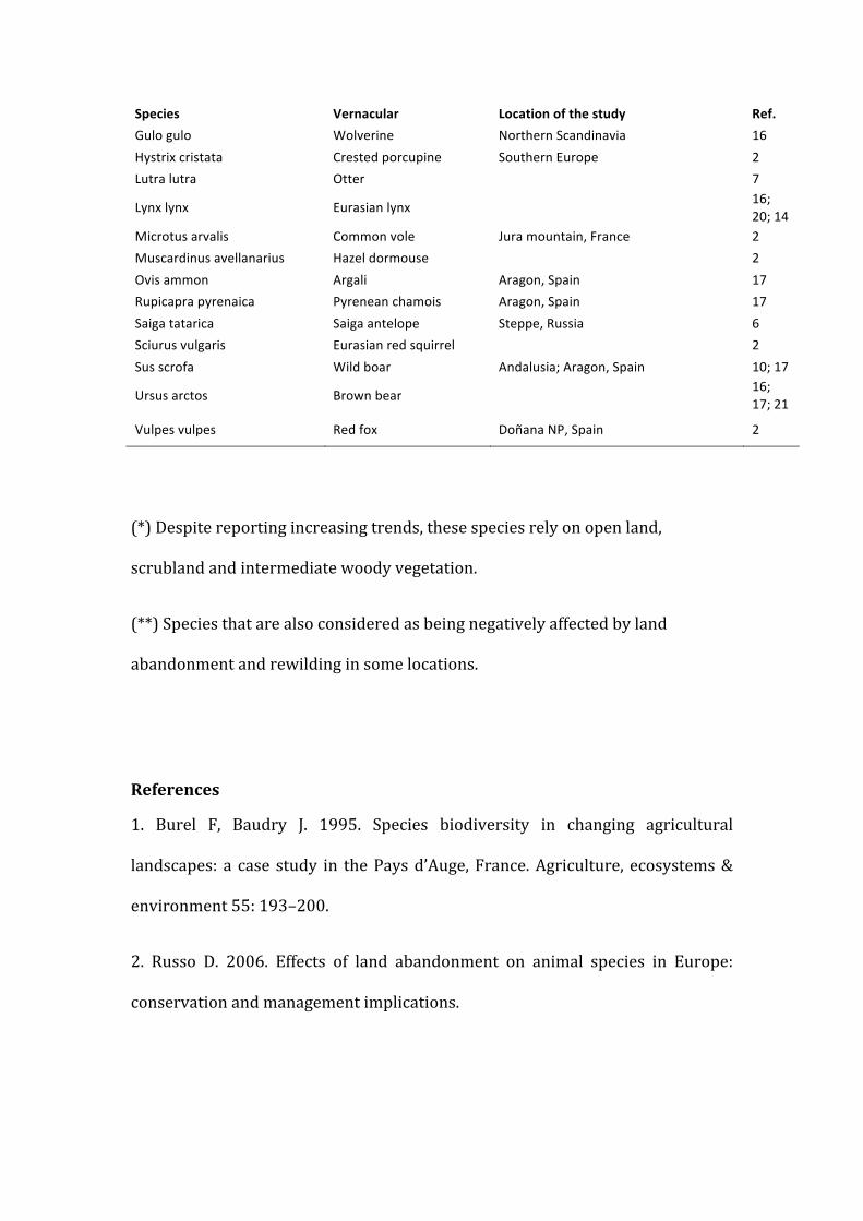
Species( Vernacular( Location,of,the,study( Ref.(Gulo(gulo( Wolverine( Northern(Scandinavia( 16(
Hystrix(cristata( Crested(porcupine( Southern(Europe( 2(
Lutra(lutra( Otter((
7(
Lynx(lynx( Eurasian(lynx((
16;(
20;(14(
Microtus(arvalis( Common(vole( Jura(mountain,(France( 2(
Muscardinus(avellanarius( Hazel(dormouse((
2(
Ovis(ammon( Argali( Aragon,(Spain( 17(
Rupicapra(pyrenaica( Pyrenean(chamois( Aragon,(Spain( 17(
Saiga(tatarica( Saiga(antelope( Steppe,(Russia( 6(
Sciurus(vulgaris( Eurasian(red(squirrel((
2(
Sus(scrofa( Wild(boar( Andalusia;(Aragon,(Spain( 10;(17(
Ursus(arctos( Brown(bear((
16;(
17;(21(
Vulpes(vulpes( Red(fox( Doñana(NP,(Spain( 2(
!
!
(*)!Despite!reporting!increasing!trends,!these!species!rely!on!open!land,!
scrubland!and!intermediate!woody!vegetation.!!
(**)!Species!that!are!also!considered!as!being!negatively!affected!by!land!
abandonment!and!rewilding!in!some!locations.!
!
!
References!
1.! Burel! F,! Baudry! J.! 1995.! Species! biodiversity! in! changing! agricultural!
landscapes:! a! case! study! in! the!Pays!d’Auge,!France.!Agriculture,! ecosystems!&!
environment!55:!193–200.!
2.! Russo! D.! 2006.! Effects! of! land! abandonment! on! animal! species! in! Europe:!
conservation!and!management!implications.!
3.!Gomez!C,!Casellas!D,!Oliveras!J,!Bas!JM.!2003.!Structure!of!groundUforaging!ant!
assemblages! in!relation! to! landUuse!change! in! the!northwestern!Mediterranean!
region.!Biodiversity!and!Conservation!12:!2135U2146.!
4.! David! JF,! Devernay! S,! Loucougaray! G,! Floc’h! EL.! 1999.! Belowground!
biodiversity!in!a!Mediterranean!landscape:!relationships!between!saprophagous!
macroarthropod! communities! and! vegetation! structure.! Biodiversity! and!
Conservation!8:!753–767.!
5.! Sirami! C,! Brotons! L,! Burfield! I,! Fonderflick! J,! Martin! JL.! 2008.! Is! land!
abandonment!having!an! impact!on!biodiversity?!A!metaUanalytical!approach! to!
bird! distribution! changes! in! the! northUwestern! Mediterranean.! Biological!
Conservation!141:!450–459.!
6.!Hölzel!N,!Haub!C,!Ingelfinger!MP,!Otte!A,!Pilipenko!VN.!2002!The!return!of!the!
steppe! largeUscale! restoration! of! degraded! land! in! southern! Russia! during! the!
postUSoviet!era.!Journal!for!Nature!Conservation!10:!75–85.!
7.! Kull! T,! Pencheva! V,! Petrovic! F,! Elias! P,! Henle! K,! Balciauskas! L,! Kopacz! M,!
Zajickova!Z,!Stoianovici!V.!2004.!Agricultural!landscapes.!Young!J,!Halada!L,!Kull!
T,! Kuzniar! A,! Tartes! U,! Uzunov! Y,! Watt! A,! editors.! Conflicts! between! human!
activities! and! the! conservation! of! biodiversity! in! agricultural! landscapes,!
grasslands,! forests,! wetlands! and! uplands! in! the! acceding! and! candidate!
countries.!p10U20.!
8.!Pointereau!P,!Coulon!F,!Lambotte!M,!Stuczynski!T,!Sanchez!Ortega!V,!Del!Rio!A.!
2008.! Analysis! of! Farmland! Abandonment! and! the! Extent! and! Location! of!
Agricultural!Areas!that!are!Actually!Abandoned!or!are!in!Risk!to!be!Abandoned.!
European!Commission!U!JRC!U!Institute!for!Environment!and!Sustainability.!
9.! TelliniUFlorenzano! G.! 2004.! Birds! as! indicators! of! recent! environmental!
changes! in! the! Apennines! (Foreste! Casentinesi! National! Park,! central! Italy).!
Italian!Journal!of!Zoology!71:!317–324.!
10.!DelibesUMateos!M,!Farfán!MÁ,!Olivero!J,!Márquez!AL,!Vargas!JM.!2009.!LongU
Term! Changes! in! Game! Species! Over! a! Long! Period! of! Transformation! in! the!
Iberian!Mediterranean!Landscape.!Environmental!Management!43:!1256U1268.!
11.! Preiss! E,! Martin! JL,! Debussche! M.! 1997.! Rural! depopulation! and! recent!
landscape! changes! in! a! Mediterranean! region:! consequences! to! the! breeding!
avifauna.!Landscape!Ecology!12:!51–61.!
12.!Laiolo!P,!Dondero!F,!Ciliento!E,!Rolando!A.!2004.!Consequences!of!pastoral!
abandonment! for! the! structure! and! diversity! of! the! alpine! avifauna.! Journal! of!
Applied!Ecology!41:!294–304.!
13.!Hölzel!N,!Haub!C,!Ingelfinger!M!P,!Otte!A,!Pilipenko!V!N.!2002.!The!Return!of!
the!Steppe!LargeUscale!Restoration!of!Degraded!Land!in!Southern!Russia!During!
the!postUSoviet!Era.!Journal!for!Nature!Conservation!10!(2):!75–85.!
14.! Sylven! M,! Wijnberg! B,! Schepers! F,! Teunissen! T.! 2010! Rewilding! Europe! U!
Bringing!the!variety!of!life!back!to!Europe’s!abandoned!lands.!WWF.!
15.! Kuemmerle! T,! Perzanowski! K,! Chaskovskyy! O,! Ostapowicz! K,! Halada! L,!
Bashta!AT,!Kruhlov! I,!Hostert!P,!Waller!DM,!Radeloff!VC.!2010.!European!bison!
habitat!in!the!Carpathian!Mountains.!Biological!Conservation!143:!908–916.!
16.!Enserink!M,!Vogel!G.!2006.!The!carnivore!comeback.!Science!314:!746U749.!
17.!Gortázar!C,!Herrero!J,!Villafuerte!R,!Marco!J.!2000.!Historical!examination!of!
the!status!of!large!mammals!in!Aragon,!Spain.!Mammalia!64:!411–422.!
18.!Breitenmoser!U.!1998.!Large!predators!in!the!Alps:!the!fall!and!rise!of!man’s!
competitors.!Biological!Conservation!83:!279–289.!
19.!!Boitani!L.!2000.!Action!plan!for!the!conservation!of!the!wolves!(Canis!lupus)!
in!Europe.!Nature!and!environment,!No.!113.!Council!of!Europe!Publishing.!84p.!
20.!LCIE.!2004.!Status!and!Trends!for!Large!Carnivores!in!Europe.!UNEPUWCMC.!
21.! Swenson! JE,! Gerstl! N,! Dahle! B,! Zedrosser! A.! 2000.! Action! Plan! for! the!
conservation! of! the! Brown! Bear! (Ursus! arctos)! in! Europe.! Nature! and!
environment,!No.!114.!Council!of!Europe!Publishing.!68p.!
!
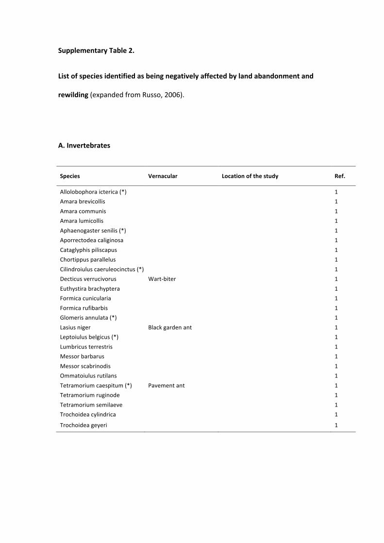
Supplementary,Table,2.,,
List,of,species,identified,as,being,negatively,affected,by,land,abandonment,and,
rewilding,(expanded(from(Russo,(2006).(
(
A.,Invertebrates,
Species, Vernacular, Location,of,the,study, Ref.,
Allolobophora(icterica((*)( (( (( 1(Amara(brevicollis(
( (1(
Amara(communis(( (
1(Amara(lumicollis((
( (1(
Aphaenogaster(senilis((*)(( (
1(Aporrectodea(caliginosa(
( (1(
Cataglyphis(piliscapus(( (
1(Chortippus(parallelus(
( (1(
Cilindroiulus(caeruleocinctus((*)((
1(Decticus(verrucivorus( WartEbiter(
(1(
Euthystira(brachyptera(( (
1(Formica(cunicularia((
( (1(
Formica(rufibarbis(( (
1(Glomeris(annulata((*)((
( (1(
Lasius(niger( Black(garden(ant((
1(Leptoiulus(belgicus((*)(
( (1(
Lumbricus(terrestris((( (
1(Messor(barbarus((
( (1(
Messor(scabrinodis(( (
1(Ommatoiulus(rutilans(
( (1(
Tetramorium(caespitum((*)( Pavement(ant((
1(Tetramorium(ruginode(
( (1(
Tetramorium(semilaeve(( (
1(Trochoidea(cylindrica(
( (1(
Trochoidea(geyeri( (( (( 1(
!
,
,
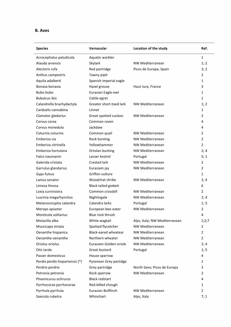
B.,Aves,
Species, Vernacular, Location,of,the,study, Ref.,
Acrocephalus(paludicola( Aquatic(warbler( (( 1(Alauda(arvensis( Skylark( NW(Mediterranean( 1;(2(Alectoris(rufa( Red(partridge( Picos(de(Europa,(Spain( 3;(2(Anthus(campestris(( Tawny(pipit(
(2(
Aquila(adalberti( Spanish(imperial(eagle((
1(Bonasa(bonasia( Hazel(grouse( Haut(Jura,(France( 3(Bubo(bubo( Eurasian(EagleEowl(
(1(
Bubulcus(ibis( Cattle(egret((
1(Calandrella(brachydactyla( Greater(shortEtoed(lark( NW(Mediterranean( 1;(2(Carduelis(cannabina( Linnet(
(1(
Clamator(gladarius( Great(spotted(cuckoo( NW(Mediterranean( 2(Corvus(corax( Common(raven(
(4(
Corvus(monedula( Jackdaw((
4(Coturnix(coturnix( Common(quail( NW(Mediterranean( 2(Emberiza(cia( Rock(bunting( NW(Mediterranean( 2(Emberiza(citrinella( Yellowhammer( NW(Mediterranean( 2(Emberiza(hortulana( Ortolan(bunting( NW(Mediterranean( 2;(4(Falco(naumanni( Lesser(kestrel( Portugal( 5;(1(Galerida(cristata( Crested(lark( NW(Mediterranean( 2(Garrulus(glandarius( Eurasiam(jay( NW(Mediterranean( 2(Gyps(fulvus(( Griffon(vulture(
(1(
Lanius(senator( Woodchat(shrike( NW(Mediterranean( 2;(4(Limosa(limosa( Black(tailed(godwit(
(6(
Loxia(curvirostra( Common(crossbill( NW(Mediterranean( 2(Luscinia(megarhynchos( Nightingale( NW(Mediterranean( 2;(4(Melanocorypha(calandra( Calandra(larks( Portugal( 1;(5(Merops(apiaster( European(beeEeater( NW(Mediterranean( 2(Monticola(solitarius( Blue(rock(thrush(
(4(
Motacilla(alba( White(wagtail( Alps,(Italy;(NW(Mediterranean( 1;2;7(Muscicapa(striata( Spotted(flycatcher( NW(Mediterranean( 2(Oenanthe(hispanica( BlackEeared(wheatear( NW(Mediterranean( 2(Oenanthe(oenanthe( Northern(wheater( NW(Mediterranean( 2(Oriolus(oriolus( Eurasiam(Golden(oriole( NW(Mediterranean( 2;(4(Otis(tarda( Great(bustard( Portugal( 1;(5(Passer(domesticus( House(sparrow(
(4(
Perdix(perdix(hispaniensis((*)( Pyrenean(Grey(partidge((
1(Perdrix(perdrix( Grey(partridge( North(Savo;(Picos(de(Europa( 3(Petronia(petronia( Rock(sparrow( NW(Mediterranean( 2(Phoenicurus(ochruros( Black(redstart(
(4(
Pyrrhocorax(pyrrhocorax( RedEbilled(chough((
1(Pyrrhula(pyrrhula( Eurasian(Bullfinch( NW(Mediterranean( 2(Saxicola(rubetra( Whinchart( Alps,(Italy( 7;(1(
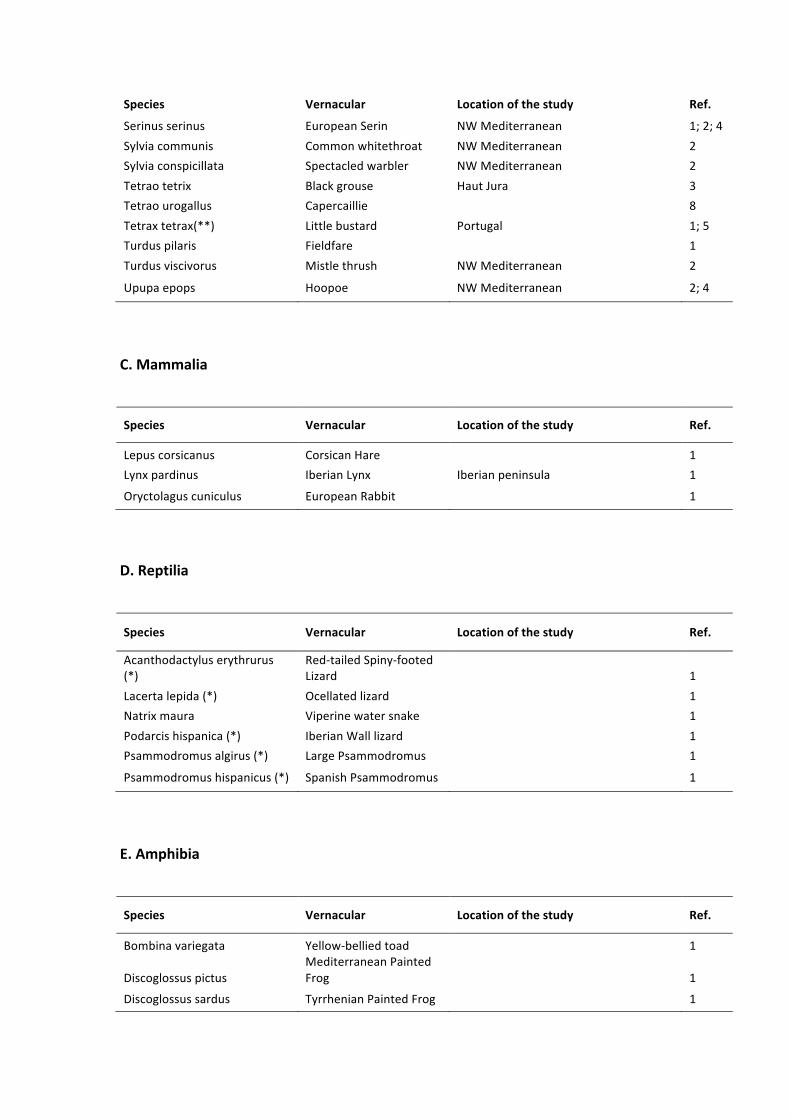
Species, Vernacular, Location,of,the,study, Ref.,
Serinus(serinus( European(Serin( NW(Mediterranean( 1;(2;(4(Sylvia(communis( Common(whitethroat( NW(Mediterranean( 2(Sylvia(conspicillata( Spectacled(warbler( NW(Mediterranean( 2(Tetrao(tetrix( Black(grouse( Haut(Jura( 3(Tetrao(urogallus( Capercaillie(
(8(
Tetrax(tetrax(**)( Little(bustard( Portugal( 1;(5(Turdus(pilaris( Fieldfare(
(1(
Turdus(viscivorus( Mistle(thrush( NW(Mediterranean( 2(
Upupa(epops( Hoopoe( NW(Mediterranean( 2;(4(
,
C.,Mammalia,
Species, Vernacular, Location,of,the,study, Ref.,
Lepus(corsicanus( Corsican(Hare( (( 1(Lynx(pardinus( Iberian(Lynx( Iberian(peninsula( 1(
Oryctolagus(cuniculus( European(Rabbit( (( 1(
!
D.,Reptilia,
Species, Vernacular, Location,of,the,study, Ref.,
Acanthodactylus(erythrurus((*)(
RedEtailed(SpinyEfooted(Lizard(
(1(
Lacerta(lepida((*)( Ocellated(lizard((
1(Natrix(maura( Viperine(water(snake(
(1(
Podarcis(hispanica((*)( Iberian(Wall(lizard((
1(Psammodromus(algirus((*)( Large(Psammodromus(
(1(
Psammodromus(hispanicus((*)(( Spanish(Psammodromus( ( 1(
,
E.,Amphibia,
Species, Vernacular, Location,of,the,study, Ref.,
Bombina(variegata( YellowEbellied(toad( (( 1(
Discoglossus(pictus(Mediterranean(Painted(Frog(
(1(
Discoglossus(sardus( Tyrrhenian(Painted(Frog( (( 1(
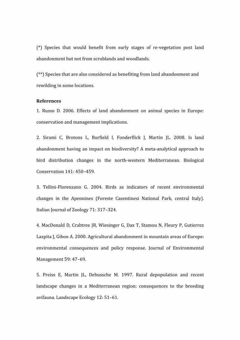
,
(*)! Species! that! would! benefit! from! early! stages! of! re:vegetation! post! land!
abandonment!but!not!from!scrublands!and!woodlands.!
(**)!Species!that!are!also!considered!as!benefiting!from!land!abandonment!and!
rewilding!in!some!locations.!
References(
1.! Russo! D.! 2006.! Effects! of! land! abandonment! on! animal! species! in! Europe:!
conservation!and!management!implications.!
2.! Sirami! C,! Brotons! L,! Burfield! I,! Fonderflick! J,! Martin! JL.! 2008.! Is! land!
abandonment!having!an! impact!on!biodiversity?!A!meta:analytical!approach! to!
bird! distribution! changes! in! the! north:western! Mediterranean.! Biological!
Conservation!141:!450–459.!
3.! Tellini:Florenzano! G.! 2004.! Birds! as! indicators! of! recent! environmental!
changes! in! the! Apennines! (Foreste! Casentinesi! National! Park,! central! Italy).!
Italian!Journal!of!Zoology!71:!317–324.!
4.!MacDonald!D,!Crabtree!JR,!Wiesinger!G,!Dax!T,!Stamou!N,!Fleury!P,!Gutierrez!
Lazpita!J,!Gibon!A.!2000.!Agricultural!abandonment!in!mountain!areas!of!Europe:!
environmental! consequences! and! policy! response.! Journal! of! Environmental!
Management!59:!47–69.!
5.! Preiss! E,! Martin! JL,! Debussche! M.! 1997.! Rural! depopulation! and! recent!
landscape! changes! in! a! Mediterranean! region:! consequences! to! the! breeding!
avifauna.!Landscape!Ecology!12:!51–61.!
6.! Stoate! C,! Báldi! A,! Beja! P,! Boatman!ND,!Herzon! I,! Van!Doorn!A,!De! Snoo!GR,!
Rakosy!L,!Ramwell!C.!2009.!Ecological!impacts!of!early!21st!century!agricultural!
change!in!Europe:A!review.!Journal!of!environmental!management!91:!22–46.!
7.!Pointereau!P,!Coulon!F,!Lambotte!M,!Stuczynski!T,!Sanchez!Ortega!V,!Del!Rio!A.!
2008.! Analysis! of! Farmland! Abandonment! and! the! Extent! and! Location! of!
Agricultural!Areas!that!are!Actually!Abandoned!or!are!in!Risk!to!be!Abandoned.!
European!Commission!:!JRC!:!Institute!for!Environment!and!Sustainability.!
8.! Laiolo! P,! Dondero! F,! Ciliento! E,! Rolando! A.! 2004.! Consequences! of! pastoral!
abandonment! for! the! structure! and! diversity! of! the! alpine! avifauna.! Journal! of!
Applied!Ecology!41:!294–304.!
9.!Gortázar!C,!Herrero! J,!Villafuerte!R,!Marco! J.! 2000.!Historical! examination!of!
the!status!of!large!mammals!in!Aragon,!Spain.!Mammalia!64:!411–422.!
!
,

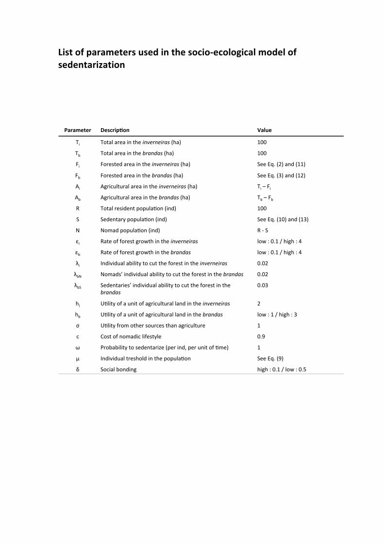
List%of%parameters%used%in%the%socio2ecological%model%of%sedentarization%
!
!
!
!
Parameter' Descrip-on' Value'
Ti#
Total#area#in#the#inverneiras((ha)# 100#
Tb#
Total#area#in#the#brandas((ha)( 100##
Fi#
Forested#area#in#the#inverneiras((ha)( See#Eq.#(2)#and#(11)#
Fb#
Forested#area#in#the#brandas((ha)( See#Eq.#(3)#and#(12)#
Ai#
Agricultural#area#in#the#inverneiras((ha)( Ti#–#F
i##
Ab#
Agricultural#area#in#the#brandas((ha)( Tb#–#F
b##
R# Total#resident#populaAon#(ind)# 100##
S# Sedentary#populaAon#(ind)# See#Eq.#(10)#and#(13)#
N# Nomad#populaAon#(ind)# R#E#S#
εi#
Rate#of#forest#growth#in#the#inverneiras( low#:#0.1#/#high#:#4#
εb#
Rate#of#forest#growth#in#the#brandas( low#:#0.1#/#high#:#4#
λi#
Individual#ability#to#cut#the#forest#in#the#inverneiras( 0.02#
λbN#
Nomads’#individual#ability#to#cut#the#forest#in#the#brandas( 0.02#
λbS#
Sedentaries’#individual#ability#to#cut#the#forest#in#the#
brandas(0.03#
hi#
UAlity#of#a#unit#of#agricultural#land#in#the#inverneiras( 2#
hb#
UAlity#of#a#unit#of#agricultural#land#in#the#brandas( low#:#1#/#high#:#3#
σ# UAlity#from#other#sources#than#agriculture# 1#
c# Cost#of#nomadic#lifestyle# 0.9#
ω# Probability#to#sedentarize#(per#ind,#per#unit#of#Ame)# 1##
μ# Individual#treshold#in#the#populaAon# See#Eq.#(9)#
δ# Social#bonding# high#:#0.1#/#low#:#0.5#