Embed Size (px)
Citation preview


ADVANCES IN BIOMEDICAL
ENGINEERING

This page intentionally left blank

ADVANCES IN BIOMEDICAL
ENGINEERING
Editor
PASCAL VERDONCK
Amsterdam • Boston • Heidelberg • London • New York • Oxford
Paris • San Diego • San Francisco • Singapore • Sydney • Tokyo
Elsevier
Radarweg 29, PO Box 211, 1000 AE Amsterdam, The Netherlands
Linacre House, Jordan Hill, Oxford OX2 8DP, UK
First edition 2009
Copyright � 2009 Elsevier B.V. All rights reserved
No part of this publication may be reproduced, stored in a retrieval system
or transmitted in any form or by any means electronic, mechanical, photocopying,
recording or otherwise without the prior written permission of the publisher
Permissions may be sought directly from Elsevier’s Science & Technology Rights
Department in Oxford, UK: phone (+44) (0) 1865 843830; fax (+44) (0) 1865 853333;
email: [email protected]. Alternatively you can submit your request online by
visiting the Elsevier web site at http://elsevier.com/locate/permissions, and selecting
Obtaining permission to use Elsevier material
Notice
No responsibility is assumed by the publisher for any injury and/or damage to persons
or property as a matter of products liability, negligence or otherwise, or from any use or
operation of any methods, products, instructions or ideas contained in the material
herein. Because of rapid advances in the medical sciences, in particular, independent
verification of diagnoses and drug dosages should be made
British Library Cataloguing in Publication Data
A catalogue record for this book is available from the British Library
Library of Congress Cataloging-in-Publication Data
A catalog record for this book is available from the Library of Congress
ISBN: 978-0-444-53075-2
For information on all Elsevier publications
visit our web site at books.elsevier.com
Printed and bound in Hungary
08 09 10 10 9 8 7 6 5 4 3 2 1
Working together to grow libraries in developing countries
www.elsevier.com | www.bookaid.org | www.sabre.org

CONTENTS
Preface ix
List of Contributors xi
1 Review of Research in Cardiovascular Devices 1Zbigniew Nawrat
1 Introduction 22 The Heart Diseases 83 The Cardiovascular Devices in Open-Heart Surgery 8
3.1 Blood Pumps 93.2 Valve Prostheses 233.3 Heart Pacemaker 34
4 The Minimally Invasive Cardiology Tools 345 The Technology for Atrial Fibrillation 386 Minimally Invasive Surgery 39
6.1 The Classical Thoracoscopic Tools 406.2 The Surgical Robots 436.3 Blood Pumps – MIS Application Study 49
7 The Minimally Invasive Valve Implantation 538 Support Technology for Surgery Planning 539 Conclusions 57
2 Biomechanical Modeling of Stents: Survey 1997–2007 61Matthieu De Beule
1 Introduction 622 Finite Element Modeling of Stents 63
2.1 Finite element basics 632.2 Geometrical design and approximation 642.3 Material properties 652.4 Loading and boundary conditions 662.5 Finite element stent design 662.6 Effective use of FEA 68
3 Survey of the State of the Art in Stent Modeling: 1997–2007 683.1 Neglect of the balloon 693.2 Cylindrical balloon 743.3 Folded balloon 783.4 Summary 81
4 Alternative methods for biomechanical modeling of stents 844.1 FEM – Prolapse, flexibility and strut micromechanics 844.2 FEM – Self-expandable stents 854.3 CFD–drug elution and immersed FEM 87
v
5 Future Prospects 886 Conclusion 88
3 Signal Extraction in Multisensor Biomedical Recordings 95Vicente Zarzoso, Ronald Phlypo, Olivier Meste, and Pierre Comon
1 Introduction 961.1 Aim and scope of the chapter 961.2 Mathematical notations 97
2 Genesis of Biomedical Signals 982.1 A biomedical source model 982.2 Cardiac signals 1012.3 Brain signals 105
3 Multi-Reference Optimal Wiener Filtering 1093.1 Non-invasive fetal ECG extraction 1093.2 Optimal Wiener filtering 1103.3 Adaptive noise cancellation 1123.4 Results 113
4 Spatio-Temporal Cancellation 1154.1 Atrial activity extraction in atrial fibrillation 1154.2 Spatio-temporal cancellation of the QRST complex in AF episodes 117
5 Blind Source Separation (BSS) 1235.1 The isolation of interictal epileptic discharges in the EEG 1235.2 Modeling and assumptions 1255.3 Inherent indeterminacies 1275.4 Statistical independence, higher-order statistics and
non-Gaussianity 1275.5 Independent component analysis 1295.6 Algorithms 1315.7 Results 1335.8 Incorporating prior information into the separation model 1365.9 Independent subspaces 1385.10 Softening the stationarity constraint 1385.11 Revealing more sources than sensor signals 138
6 Summary, Conclusions and Outlook 139
4 Fluorescence Lifetime Spectroscopy and Imaging of Visible FluorescentProteins 145Ankur Jain, Christian Blum, and Vinod Subramaniam
1 Introduction 1462 Introduction to Fluorescence 146
2.1 Interaction of light with matter 1462.2 The Jab�onski diagram 1472.3 Fluorescence parameters 151
vi Contents
2.4 Fluorescence lifetime 1512.5 Measurement of fluorescence lifetime 1532.6 Fluorescence anisotropy and polarization 1552.7 Factors affecting fluorescence 157
3 Fluorophores and Fluorescent Proteins 1603.1 Green fluorescent protein 1613.2 Red fluorescent protein 165
4 Applications of VFPs 1664.1 Lifetime spectroscopy and imaging of VFPs 167
5 Concluding Remarks 170
5 Monte Carlo Simulations in Nuclear Medicine Imaging 175Steven Staelens and Irene Buvat
1 Introduction 1762 Nuclear Medicine Imaging 176
2.1 Single photon imaging 1772.2 Positron emission tomography 1782.3 Emission tomography in small animal imaging 1792.4 Reconstruction 179
3 The MC Method 1803.1 Random numbers 1803.2 Sampling methods 1813.3 Photon transport modeling 1823.4 Scoring 183
4 Relevance of Accurate MC Simulations in Nuclear Medicine 1844.1 Studying detector design 1844.2 Analysing quantification issues 1844.3 Correction methods for image degradations 1854.4 Detection tasks using MC simulations 1864.5 Applications in other domains 186
5 Available MC Simulators 1876 Gate 188
6.1 Basic features 1886.2 GATE: Time management 1926.3 GATE: Digitization 193
7 Efficiency-Accuracy Trade-Off 1947.1 Accuracy and validation 1947.2 Calculation time 194
8 Case Studies 1958.1 Case study I: TOF-PET 1958.2 Case study II: Assessment of PVE correction 1968.3 Case study III: MC-based reconstruction 197
9 Future Prospects 20010 Conclusion 200
Contents vii

6 Biomedical Visualization 209Chris R. Johnson and Xavier Tricoche
1 Introduction 2102 Scalar Field Visualization 211
2.1 Direct volume rendering 2112.2 Isosurface extraction 2202.3 Time-dependent scalar field visualization 222
3 Vector Field Visualization 2233.1 Vector field methods in scientific visualization 2243.2 Streamline-based techniques 2253.3 Stream surfaces 2263.4 Texture representations 2293.5 Topology 232
4 Tensor Field Visualization 2344.1 Anisotropy and tensor invariants 2354.2 Color coding of major eigenvector orientation 2364.3 Tensor glyphs 2364.4 Fiber tractography 2394.5 Volume rendering 2414.6 White matter segmentation using tensor invariants 244
5 Multi-field Visualization 2456 Error and Uncertainty Visualization 2507 Visualization Software 254
7.1 SCIRun/BioPSE visualization tools 2557.2 map3d 258
8 Summary and Conclusion 263
Index 273
viii Contents

PREFACE
The aim of this book is to bridge the interdisciplinary gap in biomedical engineeringeducation. No single medical device has ever been developed without an extensiveinterdisciplinary collaboration but, nevertheless, a wide gap still exists betweendifferent themes like biomaterials, biomechanics, extracorporeal circulation research,nanotechnology, and safety and regulations.We have to evitate that, due to the growing complexity, we only gather with and
communicate in our own expert groups with their specific research topics.Therefore it is, in my opinion, extremely important that a high quality bookis available to cover these interdisciplinary islands by bringing representative researchgroups together. The aim of this book is a top review of current research advances inbiomedical engineering but on an educational level, so it is also useful for teachingmaster’s students, Ph.D. students, and professionals. Each chapter is complementaryto reviews in specific scientific journals. The topics range from visualizationtechnology and biosignal and imaging analysis over biomechanics and artificialorgans to nanotechnology and biophotonics and cardiovascular medical devices.I thank all authors for their support and I sincerely hope this book will contribute tobetter engineering for health.
Prof. Pascal VerdonckDecember 2007
ix

This page intentionally left blank
LIST oF CONTRIBUTORS
C. BlumBiophysical Engineering Group, Institute for Biomedical Technology and MESA+
Institute for Nanotechnology, University of Twente, PO Box 217, 7500AEEnschede, The Netherlands
I. BuvatINSERM U678 UPMC, CHU Pitie-Salpetriere, F-75634 Paris, France
P. ComonLaboratoire I3S, UNSA-CNRS, Les Algorithmes, Euclide-B, BP 121, 2000Route, des Lucioles, 06903 Sophia Antipolis Cedex, France
M. De BeuleBiophysical Engineering Group, Institute for Biomedical Technology and MESA+
Institute for Nanotechnology, University of Twente, PO Box 217, 7500AEEnschede, The Netherlands
A. JainBiophysical Engineering Group, Institute for Biomedical Technology and MESA+
Institute for Nanotechnology, University of Twente, PO Box 217, 7500AEEnschede, The Netherlands; Department of Biotechnology, Indian Institute ofTechnology Kharagpur, Kharagpur, India
C.R. JohnsonScientific Computing and Imaging Institute, University of Utah, Salt Lake City,UT 84112, USA
O. MesteLaboratoire I3S, UNSA-CNRS, Les Algorithmes, Euclide-B, BP 121, 2000Route, des Lucioles, 06903 Sophia Antipolis Cedex, France
Z. NawratFoundation for Cardiac Surgery Development & Medical University of Silesia,Poland
R. PhlypoBiophysical Engineering Group, Institute for Biomedical Technology and MESA+
Institute for Nanotechnology, University of Twente, PO Box 217, 7500AEEnschede, The Netherlands
S. StaelensBiophysical Engineering Group, Institute for Biomedical Technology and MESA+
Institute for Nanotechnology, University of Twente, PO Box 217, 7500AEEnschede, The Netherlands
xi

V. SubramaniamBiophysical Engineering Group, Institute for Biomedical Technology and MESA+
Institute for Nanotechnology, University of Twente, PO Box 217, 7500AEEnschede, The Netherlands
X. TricocheScientific Computing and Imaging Institute, University of Utah, Salt Lake City,UT 84112, USA
V. ZarzosoLaboratoire I3S, UNSA-CNRS, Les Algorithmes, Euclide-B, BP 121, 2000Route, des Lucioles, 06903 Sophia Antipolis Cedex, France
xii List of Contributors
Advances in Biomedical Engineering � 2009 Elsevier B.V.
ISBN 978-0-444-53075-2 All rights reserved.
1
C H A P T E R 1
REVIEW OF RESEARCH IN CARDIOVASCULARDEVICES
Zbigniew Nawrat
Contents
1. Introduction 22. The Heart Diseases 8
3. The Cardiovascular Devices in Open-Heart Surgery 83.1. Blood Pumps 93.2. Valve Prostheses 23
3.3. Heart Pacemaker 344. The Minimally Invasive Cardiology Tools 345. The Technology for Atrial Fibrillation 386. Minimally Invasive Surgery 39
6.1. The Classical Thoracoscopic Tools 406.2. The Surgical Robots 436.3. Blood Pumps – MIS Application Study 49
7. The Minimally Invasive Valve Implantation 538. Support Technology for Surgery Planning 539. Conclusions 57
Acknowledgments 58References 58
Abstract
An explosion in multidisciplinary research, combining mechanical, chemical, and elec-trical engineering with physiology and medicine, during the 1960s created huge advances
in modern health care. In cardiovascular therapy, lifesaving implantable defibrillators,ventricular assist devices, catheter-based ablation devices, vascular stent technology,and cell and tissue engineering technologies have been introduced. The latest and
leading technology presents robots intended to keep the surgeon in the most comfor-table, dexterous, and ergonomic position during the entire procedure. The branch of themedical and rehabilitation robotics includes the manipulators and robots providingsurgery, therapy, prosthetics, and rehabilitation. This chapter provides an overview of
research in cardiac surgery devices.
Keywords: Heart prostheses, valve prostheses, blood pumps, stents, training and expertsystems, surgical tools, medical robots, biomaterials
1. INTRODUCTION
Remarkable advances in biomedical engineering create new possibilities of helpfor people with heart diseases. This chapter provides an overview of research incardiac surgery devices. An explosion in multidisciplinary research, combiningmechanical, chemical, and electrical engineering with physiology and medicine,during the 1960s created huge advances in modern health care. This decade openednew possibilities in aerospace traveling and in human body organ replacement. Homosapiens after World War II trauma became not only the hero of mind and progress butalso the creator of the culture of freedom. Computed tomographic (CT) scanningwas developed at EMI Research Laboratories (Hayes, Middlesex, England) funded inpart by the success of EMI’s Beatles records. Modern medical imaging techniquessuch as CT, nuclear magnetic resonance (NMR), and ultrasonic imaging enable thesurgeon to have a very precise representation of internal anatomy as preoperativescans. It creates possibilities of realizing new intervention methods, for instance, thevery popular bypass surgery. It was a revolution in disease diagnosis and generally inmedicine. In cardiovascular therapy, lifesaving implantable defibrillators, ventricularassist devices (VADs), catheter-based ablation devices, vascular stent technology, andcell and tissue engineering technologies have been introduced.
Currently, the number of people on Earth is more than 6 billion: increasinglylesser number of living organisms and about million increasingly more “intelligent”robots accompany them.
Robotics, a technical discipline, deals with the synthesis of certain functions ofthe human using some mechanisms, sensors, actuators, and computers. Amongmany types of robotics is the medical and rehabilitation robotics – the latest butrapidly developing branch at present, which includes the manipulators and robotsproviding surgery, therapy, prosthetics, and rehabilitation. They help fight paresesin humans and can also fulfill the role of a patient’s assistant. Rehabilitationmanipulators can be steered using ergonomic user interfaces – e.g., the head, thechin, and eye movements. The “nurse” robots for patients and physically chal-lenged persons’ service are being developed very quickly. Partially or fully roboticdevices help in almost all life actions, such as person moving or consuming meals,simple mechanical devices, science education, and entertainment activities. Help-Mate, an already existing robot-nurse, moving on the hospital corridors and roomsdelivers meals, helps find the right way, etc.
On the one hand, robots are created that resemble the human body in appearance(humanoids), able to direct care; on the other hand, robotic devices are constructed –telemanipulators – controlled by the human tools allowing to improve the precisionof human tasks. Robots such as ISAC (Highbrow Soft Arm Control) or HelpMatecan replace several functions of the nurse, who will give information, help find theway, bring the medicines and the meal. In case of lack of qualified staff, to providecare for hospice patients at home, these robots will be of irreplaceable help.
Robotic surgery was born out of microsurgery and endoscopic experience. Mini-mally invasive interventions require a multitude of technical devices: cameras, lightsources, special tools (offering the mechanical efficiency and tissue coagulation for
2 Zbigniew Nawrat
preventing bleeding), and insufflations (thanks to advances in computer engineering,electronics, optics, materials, and miniaturization). The mobility of instruments isdecreased [from seven, natural for human arm, to four degrees of freedom (DOFs)]due to the invariant point of insertion through the patient’s body wall. Across theworld, physicians and engineers are working together toward developing increasinglyeffective instruments to enable surgery using the latest technology. The leadingtechnology presents robots intended to keep the surgeon in the most comfortable,dexterous, and ergonomic position during the entire procedure. The surgery iscomplex and requires precise control of position and force. The basic advantages ofminimally invasive robot-aided surgery are safe, reliable, and repeatable operativeresults with less patient pain, trauma, and recovery time. Conventional open-heartsurgery requires full median sternotomy, which means cracking of sternum, compro-mising pulmonary function, and considerable loss of blood.
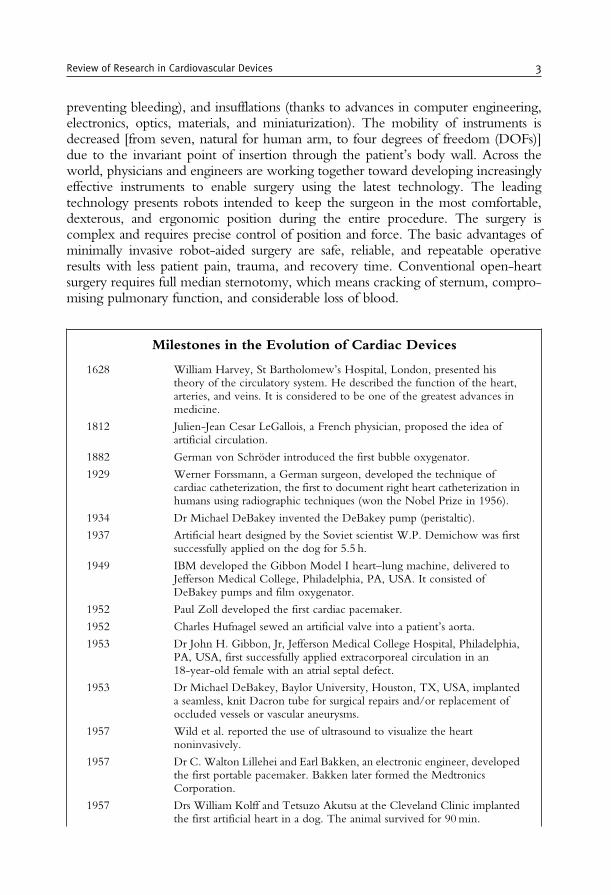
Milestones in the Evolution of Cardiac Devices
1628 William Harvey, St Bartholomew’s Hospital, London, presented histheory of the circulatory system. He described the function of the heart,arteries, and veins. It is considered to be one of the greatest advances inmedicine.
1812 Julien-Jean Cesar LeGallois, a French physician, proposed the idea ofartificial circulation.
1882 German von Schroder introduced the first bubble oxygenator.
1929 Werner Forssmann, a German surgeon, developed the technique ofcardiac catheterization, the first to document right heart catheterization inhumans using radiographic techniques (won the Nobel Prize in 1956).
1934 Dr Michael DeBakey invented the DeBakey pump (peristaltic).
1937 Artificial heart designed by the Soviet scientist W.P. Demichow was firstsuccessfully applied on the dog for 5.5 h.
1949 IBM developed the Gibbon Model I heart–lung machine, delivered toJefferson Medical College, Philadelphia, PA, USA. It consisted ofDeBakey pumps and film oxygenator.
1952 Paul Zoll developed the first cardiac pacemaker.
1952 Charles Hufnagel sewed an artificial valve into a patient’s aorta.
1953 Dr John H. Gibbon, Jr, Jefferson Medical College Hospital, Philadelphia,PA, USA, first successfully applied extracorporeal circulation in an18-year-old female with an atrial septal defect.
1953 Dr Michael DeBakey, Baylor University, Houston, TX, USA, implanteda seamless, knit Dacron tube for surgical repairs and/or replacement ofoccluded vessels or vascular aneurysms.
1957 Wild et al. reported the use of ultrasound to visualize the heartnoninvasively.
1957 Dr C. Walton Lillehei and Earl Bakken, an electronic engineer, developedthe first portable pacemaker. Bakken later formed the MedtronicsCorporation.
1957 Drs William Kolff and Tetsuzo Akutsu at the Cleveland Clinic implantedthe first artificial heart in a dog. The animal survived for 90min.
Review of Research in Cardiovascular Devices 3
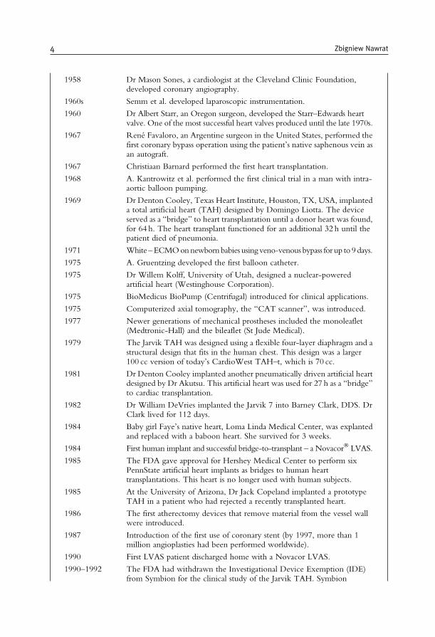
1958 Dr Mason Sones, a cardiologist at the Cleveland Clinic Foundation,developed coronary angiography.
1960s Semm et al. developed laparoscopic instrumentation.
1960 Dr Albert Starr, an Oregon surgeon, developed the Starr–Edwards heartvalve. One of the most successful heart valves produced until the late 1970s.
1967 Rene Favaloro, an Argentine surgeon in the United States, performed thefirst coronary bypass operation using the patient’s native saphenous vein asan autograft.
1967 Christiaan Barnard performed the first heart transplantation.
1968 A. Kantrowitz et al. performed the first clinical trial in a man with intra-aortic balloon pumping.
1969 Dr Denton Cooley, Texas Heart Institute, Houston, TX, USA, implanteda total artificial heart (TAH) designed by Domingo Liotta. The deviceserved as a “bridge” to heart transplantation until a donor heart was found,for 64 h. The heart transplant functioned for an additional 32 h until thepatient died of pneumonia.
1971 White –ECMOonnewborn babies using veno-venous bypass for up to 9 days.
1975 A. Gruentzing developed the first balloon catheter.
1975 Dr Willem Kolff, University of Utah, designed a nuclear-poweredartificial heart (Westinghouse Corporation).
1975 BioMedicus BioPump (Centrifugal) introduced for clinical applications.
1975 Computerized axial tomography, the “CAT scanner”, was introduced.
1977 Newer generations of mechanical prostheses included the monoleaflet(Medtronic-Hall) and the bileaflet (St Jude Medical).
1979 The Jarvik TAH was designed using a flexible four-layer diaphragm and astructural design that fits in the human chest. This design was a larger100 cc version of today’s CardioWest TAH–t, which is 70 cc.
1981 Dr Denton Cooley implanted another pneumatically driven artificial heartdesigned by Dr Akutsu. This artificial heart was used for 27 h as a “bridge”to cardiac transplantation.
1982 Dr William DeVries implanted the Jarvik 7 into Barney Clark, DDS. DrClark lived for 112 days.
1984 Baby girl Faye’s native heart, Loma Linda Medical Center, was explantedand replaced with a baboon heart. She survived for 3 weeks.
1984 First human implant and successful bridge-to-transplant – a Novacor� LVAS.
1985 The FDA gave approval for Hershey Medical Center to perform sixPennState artificial heart implants as bridges to human hearttransplantations. This heart is no longer used with human subjects.
1985 At the University of Arizona, Dr Jack Copeland implanted a prototypeTAH in a patient who had rejected a recently transplanted heart.
1986 The first atherectomy devices that remove material from the vessel wallwere introduced.
1987 Introduction of the first use of coronary stent (by 1997, more than 1million angioplasties had been performed worldwide).
1990 First LVAS patient discharged home with a Novacor LVAS.
1990–1992 The FDA had withdrawn the Investigational Device Exemption (IDE)from Symbion for the clinical study of the Jarvik TAH. Symbion
4 Zbigniew Nawrat
subsequently donated the TAH technology to University Medical Center(UMC), Tucson, AZ, USA, which reincorporated the company andrenamed it CardioWest.
1994 First FDA-approved robot for assisting surgery [automated endoscopicsystem for optimal positioning (AESOP) produced by Computer Motion(CM; Goleta, CA, USA)].
1994 FDA approved the pneumatically driven HeartMate� LVAD (ThoratecCorporation, Burlington, MA, USA) for bridge to transplantation (thefirst pump with textured blood-contacting surfaces).
1994 HeartMate LVAS has been approved as a bridge to cardiac transplantation.
1996 REMATCH Trial (Randomized Evaluation of Mechanical Assistance forthe Treatment of Congestive Heart failure, E. Rose principal investigator)initiated with HeartMate� VE (Thoratec Corp.). Results published in2002 showed mortality reduction of 50% at 1 year as compared to patientsreceiving optimal medical therapy.
1998 Simultaneous FDA approval of HeartMate VE (Thoratec Corporation,Burlington, MA, USA) and Novacor LVAS (World Heart Corporation,Ontario, Canada), electrically powered, wearable assist systems for bridgeto transplantation, utilized in more than 4000 procedures to 2002. Tillnow, we can estimate 4500 HeartMate XVE, more than 440 IVAD(Implantable Ventricular Assist Device) and more than 1700 Novacor inthis kind of blood pump.
1998 First clinical application of next-generation continuous-flow assist devices.DeBakey (MicroMed Inc.) axial-flow pump implanted by R. Hetzer,G. Noon, and M. DeBakey.
1998 Carpentier and Loulmet performed first in the world endoscopicoperation of single bypass graft between left internal thoracic artery andleft anterior descending (LITA–LAD) and first operation inside the heart –mitral valve plastic and atrial septal defect closure was performed usingsurgical robot da Vinci (Intuitive Surgical, Sunnyvale, CA, USA).
1998 Mohr and Falk bypass surgery and mitral valve repairs in near endoscopictechnique (da Vinci).
1999 First clinical application of a totally implantable circulatory supportsystem. LionHeart LVAS implanted in a 67 year-old male recipient byR. Koerfer and W. Pae.
1999 D. Boyd first totally endoscopic coronary artery bypass graft (E-CABG)using Zeus robot (Computer Motion, CA, USA, currently intuitivesurgical, not in the market).
2000 Physicians in HoustonUS have realised the implantation and have got the firstpatient in the clinical investigation of the Jarvik 2000 Heart. Jarvik Heart, Inc.and the Texas Heart Institute began developing the Jarvik 2000Heart in 1988.
2000 THI was granted permission by the Food and Drug Administration toevaluate the Jarvik 2000 Heart as a bridge to transplantation in five patients.
2000 The FDA gave permission to extend the study. Patients havebeen sustained for more than 400 days with this device. (http://www.texasheartinstitute.org/Research/Devices/j2000.cfm).
2001 The AbioCor was implanted in Robert Tools by cardiac surgeons LamanGray and Robert Dowling on July 2, 2001, at Jewish Hospital inLouisville, Kentucky. L. Robert Tools aged 59 years with the artificialheart survived 5 months. He died because of the blood clot.
Review of Research in Cardiovascular Devices 5

2001 Doctors Laman Gray and Robert Dowling in Louisville (KY, USA)implanted the first autonomic artificial heart – AbioCor (Abiomed, Inc.,Danvers, MA, USA). The FDA approved the Abiocor for commercialapproval under a Humanitarian Device Exemption in September, 2006.ABIOMED is also working on the next generation implantablereplacement heart, the AbioCor II. Incorporating technology both fromABIOMED and Penn State, the AbioCor II is smaller and is beingdesigned with a goal of 5-year reliability. The BVS 5000 was the firstextracorporeal, or outside the body, ventricular assist device on the marketand is still the most widely used bridge to recovery device with systemslocated in more than 700 institutions throughout the world. Abiomed alsooffers the Impella 2.5 – a minimally invasive, percutaneous ventricularassist device that allows the heart to rest and recover(http://www.abiomed.com/products/faqs.cfm).
2001 Drs Laman Gray and Robert Dowling in Louisville (KY, USA) implanted thefirst autonomic artificial heart –AbioCor (Abiomed Inc.,Danvers,MA,USA).
2001 The first transatlantic telesurgery – Lindbergh operation – surgeon fromNew York operated patients in Strasburg using Zeus� system.
2001 The first full implantable TAH Lion Heart (the Texas Heart Institute inHouston, Abiomed in Danvers, US) was used. The first-ever humanimplant of the LionHeartTM left ventricular assist system took placeOctober 26, 1999 at the Hearzzentrum NRW in Bad Oeynhausen,Germany. Eight patients have lived with the device for more than 1 year,and four patients have lived with the device for more than 2 years. TheFood and Drug Administration approved the first series of US clinicaltrials for the Arrow LionHeartTM heart assist device in February 2001.Penn State Milton S. Hershey Medical Center implanted the device in thefirst US patient later that month (http://www.hmc.psu.edu/lionheart/clinical/index.htm).
2001 The first totally implantable TAH LionHeart (the Texas Heart Institute inHouston, TX, USA; Abiomed in Danvers, MA, USA) was used.
2002 FDAapproved theHeartMateVELVADfor permanent use (ThoratecCorp.).
2002 Novacor LVAS became the first implanted heart assist device to support asingle patient for longer than 5 years.
2002 The first percutaneous aortic valve replacement was performed by AlainCribier in April of 2002 [xxxx]. To
2004 The CardioWest TAH-t becomes the world’s first and only FDA-approved temporary total artificial heart (TAH-t). The indication for useis as a bridge to transplant in cardiac transplant patients at risk of imminentdeath from nonreversible biventricular failure. SynCardia Systems, Inc.(Tucson, AZ, USA) is the manufacturer of the CardioWestTM TAH-t.It is the only FDA- and CE-approved TAH-t in the world. It is designedfor severely ill patients with end-stage biventricular failure. The TAH-tserves as a bridge to human heart transplant for transplant eligible patientswho are within days or even hours of death. A New England Journalof Medicine paper published on August 26, 2004 (NEJM 2004; 351:859–867), states that in the pivotal clinical study of the TAH-t, the 1-yearsurvival rate for patients receiving the CardioWest TAH-t was 70% versus31% for control patients who did not receive the device. One-year and5-year survival rates after transplantation among patients who had receiveda TAH-t as a bridge to human heart transplant were 86% and 64%. Thehighest bridge to human heart transplant rate of any heart device is 79%
6 Zbigniew Nawrat
(New England Journal of Medicine 2004; 351: 859–867). Over 715implants account for more than 125 patient years on the TAH-t(http://www.syncardia.com).
2005 A total of about 3000 cardiac procedures were performed worldwideusing the da Vinci system. This includes totally endoscopic coronaryartery bypass grafting (TECAB), mitral valve repair (MVR) procedures,ASD closure, and cardiac tissue ablation for atrial fibrillation.
2006 The next-generation pulsatile VAD, the Novacor II, entered a key phaseof animal testing with the first chronic animal implant.
2006 The FDA approved the first totally implantable TAH – developed byAbioCor – for people who are not eligible for heart transplantation andwho are unlikely to live more than a month without intervention.
2006 Have experience with human implantation: Edwards Lifesciences (>100patients) and CoreValve (>70 patients). (www.touchbriefings.com/pdf/2046/Babaliaros.pdf)
2006 US FDA approval to start pilot clinical trial for Impella 2.5 (Abiomed,Inc., Danvers, MA, USA). To date the Impella 2.5 has been used tosupport over 500 patients during high-risk PCI, post PCI, and withAMI with low cardiac output.
2007 More than 4,500 in 186 centers advanced heart failure patients worldwidehave been implanted with the HeartMate XVE. Longest duration ofsupport (ongoing patient on one device): 1,854 days, age range: 8–74(average 51). The REMATCH (Randomized Evaluation of MechanicalAssistance for the Treatment of Congestive Heart Failure) clinical trialdemonstrated an 81% improvement in two-year survival among patientsreceiving HeartMate XVE versus optimal medical management. ADestination Therapy study following the REMATCH trial demonstratedan additional 17% improvement (61% vs. 52%) in one-year survival ofpatients receiving the HeartMate XVE, with an implication for theappropriate selection of candidates and timing of VAD implantation.
2008 State of art in 2008, based on the experience almost 20–30 years showsamong others:
– future of long-term heart support methods will be connected withrotary pumps, the stop of activity in pulsating pump technology isobserved (rotary pumps are smaller and comfortable in the implantationespecially it is possible introduce mini invasive surgical methods)
– the mono-leaflet disk valve are applied more and more seldom (theyrequire during the implantation the definite orientation in the heart) inthe comparison with bi-leaflet
– the new kind of biological valve prostheses based on tissue engineeringmethod get into the clinical experiment
– the multiple companies have engineered percutaneous heart valves(PHV), primarily for aortic stenosis
2008 There have been 867 unit shipments worldwide – 647 in the United States,148 in Europe and 72 in the rest of the world ( http://www.intuitivesurgical.com). Devices for “robotic surgery” are designedto perform entirely autonomous movements after being programmedby a surgeon. The da Vinci Surgical System is a computer-enhancedsystem that interposes a computer between the surgeon’s hands andthe tips of microinstruments. The system replicates the surgeon’smovements in real time.
Review of Research in Cardiovascular Devices 7
2. THE HEART DISEASES
The human biological heart has two sets of pumping chambers. The right atriumreceives oxygen-depleted blood from the body,which is pumped into the lungs throughthe right ventricle. The left atrium receives aerated blood from the lungs, which ispumped out to the body through the left ventricle. With each heart beat, the ventriclescontract together. The valves control the direction of blood flow through the heart.
Congestive heart failure, a condition in which the heart is unable to pump theblood effectively throughout the body, is one of the leading causes of death. Thisdisease is caused by sudden damage from heart attacks, deterioration from viralinfections, valve malfunctions, high blood pressure, and other problems. Althoughmedication and surgical techniques can help control symptoms, the only cure forheart failure is heart transplantation. Artificial hearts and pump assist devices havethus been developed as potential alternatives.
Ischemic heart disease is caused by progressive atherosclerosis with increasing occlu-sion of coronary arteries resulting in a reduction in coronary blood flow. Blood flow canbe further decreased by superimposed events such as vasospasm, thrombosis, or circula-tory changes leading to hypoperfusion. Myocardial infarction (MI) is the rapid develop-ment of myocardial necrosis caused by a critical imbalance between the oxygen supplyand the oxygen demand of the myocardium. Coronary artery bypass grafts (CABGs) areimplanted in patients with stenosed coronary arteries to support myocardial blood flow.
Valvular heart disease is a life-threatening disease that affects millions of peopleworldwide and leads to valve repairs and/or replacements.
In theUSA andEurope alone,withmore than 600million inhabitants andmore than6million patients with heart failure, the prevalence of advanced heart failure, constituting1–10% of the heart failure population, is estimated to total between 60,000 and 600,000patients. More than 700,000 Americans die each year from heart failure, making it thenumber one cause of death in the U.S., as well as worldwide. About half of these aresudden cardiac deaths, which occur so quickly that there is not enough time forintervention with a cardiac assist or replacement device. For the remaining half, hearttransplantation is one of the few options available today. Though hundreds of thousandsare in need, only about 2,000 people in theU.S.will be able to receive donor hearts everyyear. This consistent shortage in the supply of donor hearts in the U.S. demonstrates theneed for an alternative to heart transplantation. The total potential market for the artificialheart is more than 100,000 people in the U.S. each year. (http://www.abiomed.com).
3. THE CARDIOVASCULAR DEVICES IN OPEN-HEART SURGERY
Cardiac surgery is surgery on the heart and/or great vessels. This surgery is acomplex procedure requiring precise control of position and force. Conventionalopen-heart surgery requires full median sternotomy, which means cracking ofsternum, compromising pulmonary function, and considerable loss of blood.
8 Zbigniew Nawrat
The repair of intracardiac defects requires a bloodless and motionless environ-ment, which means that the heart should be stopped and drained of blood. Hence,the patient requires the function of the heart and lungs provided by an artificialmethod.
Modern heart–lung machines can perform a number of other tasks required fora safe open-heart operation. This system preserves the patient’s own bloodthroughout the operation and the patient’s body temperature can be controlledby selectively cooling or heating the blood as it flows through the heart–lungmachine. Medications and anesthetic drugs can be administered via separate con-nections. The disadvantages include the formation of small blood clots, whichincrease the risk of stroke, pulmonary complications, and renal complications.The machine can also trigger an inflammatory process that can damage many ofthe body’s systems and organs. Those risks push today’s biomedical engineers toimprove the heart–lung machine and oxygenator, while surgeons are developingadvances that would eliminate the need for the machine altogether. One suchadvance is minimally invasive surgery (MIS).
The surgeons have begun to perform “off-pump bypass surgery” – coronaryartery bypass surgery without the aforementioned cardiopulmonary bypass. Thesurgeons operate on the beating heart stabilized to provide an (almost) still workarea. One of the greatest challenges in beating-heart surgery is the difficulty ofsuturing or sewing on a beating heart. A stabilization system makes it possible forthe surgeon to work on the patient’s beating heart carefully and, in the vast majorityof cases, eliminates the need for the heart–lung machine.
3.1. Blood Pumps
The human heart is a pump that is made of muscle tissue. A special group of cellscalled the sinus node is located in the right atrium. The sinus node generateselectrical stimuli that make the heart contract and pump out blood. The normalhuman heart beats about 75 times per minute (i.e., about 40 million times a year) –i.e., the heart pumps 5 l of blood per minute. The normal systemic blood pressure is120/80mmHg. The mechanical power (calculated by multiplying the pressure bythe flow rate) of the human heart is about 1.3W. However, to provide thismechanical power, the heart requires 10 times much higher rate of energy turn-over, owing to its low mechanical efficiency (less than 10%).
However, the development in biotechnology can open the opportunity fortissue engineering (a branch of biotechnology) – a prospect of saving people withextremely complex or irreversible failure heart will still be realized using mechan-ical heart support devices.
During the last half-century, various blood pumps were introduced intoclinical practice, which can partially support or replace the heart during open-heart surgery or considerably for a longer time period until heart recovers oruntil transplantation is performed. Several millions of people owe their healthand lives to these devices. According to the American Heart Association, anestimated 5 million Americans are living with heart failure and more than
Review of Research in Cardiovascular Devices 9
400,000 new cases are diagnosed every year. About 50% of all patients diewithin 5 years.
The first operation on a beating heart was performed by Gibbon in 1953 using aperistaltic pump. Since then, there has been rapid development in mechanical assistdevices, leading to the realization of today’s mechanical aid system for bloodcirculation, based on the requirements using the following:
• intra-aortic balloon pump (IABP)• continuous blood flow devices – roll and centrifugal rotary pumps• pulsating flow blood pumps – pneumatic or electro-control membrane pumps
The assumed time of blood pump using in the organism influences the con-struction and material used in its design. According to this criterion, the pumps canbe divided into following categories:
• short-term (during the operation or in sudden rescue operations)• medium-term – over several weeks or months (as a bridge to hearttransplantation or treatment)
• long-term – several years (already at present) and permanently (in the intention)(as the target therapy)
The extracorporeal circulation (perfusion) and the controlled stopping of heartaction make it possible to perform the open-heart operation. The peristaltic pumpsare in common use, where the turning roll locally tightens the silicon drain to movea suitable volume of the blood. The disadvantages of this procedure, such as thedamage to blood components, are eliminated or reduced by pump construction andmaterial improvement. The patients with both heart and lung failure are assisted bythe system consisting of pump and oxygenator. The method of time oxygenation(supply oxygen to the blood) for extracorporeal blood – extracorporeal membraneoxygenation (ECMO) – was applied the first time in 1972 by Hill. The bloodpump, membrane oxygenator, heat exchanger, and a system of cannulas (tubes) forpatient’s vascular system connection are the elements of the system. Inner surface ofall these parts are covered with heparin. The Extracorporeal Life Support Organi-zation Registry has collected (since 1989) data on more than 30,000 patients, mostof whom have been neonates with respiratory failure [7]. The currently availablecentrifugal pump VADs are BioMedicus BioPump (Medtronic, Minneapolis, MN,USA), CentriMag� (Levitronix, Zurich, Switzerland), RotaFlow� (Jostra, Hirrlin-gen, Germany), and Capiox� (Terumo, Ann Arbor, MI, USA). These pumps havebeen available since 1989 to support neonates and older children with postoperativecardiac failure but competent lung function.
Centrifugal pumps benefit from the physical phenomena (centrifugal, inertiaforce) of blood acceleration during temporal rotational movement. These pumpsconsist of a driving unit and an acrylic head driven by a magnetic couple. Input andoutput blood flow channels are perpendicular to each other. The output velocity ofthe blood on the conical rotor depends on the input rotary speed, preload, andafterload. Based on vortex technology, these pumps use turbine spins of10,000–20,000 rpm to create a flow of 5–6 l/min and have generally been appliedfor temporary assistance of stunned myocardium of the left ventricle. The
10 Zbigniew Nawrat
construction of working pump and its environment conditions influence the bloodhemolysis during its use. According to the results of in vitro experiment, with thepump working as VAD and extracorporeal circulation (CPB and ECMO), the useof the pump as VAD caused the least degree of hemolysis, and the hemolysis ofpumps in the time to ECMO strongly depends on the kind of oxygenator used.Pumps with the conical rotor caused a greater degree of hemolysis working withsmall flows and large pressures (ECMO). On the contrary, a lesser degree ofhemolysis was observed for pumps with the flat rotor, regardless of its purpose.
The intra-aortic balloon was introduced as a tool for coronary circulation assis-tance in works of Maulopulos, Topaz, and Kolff in 1960. In 1968, Kantrowitz wasthe first to prove the clinical effectiveness of intra-aortic counterpulsation. Itbecame the classic method in the 1970s, thanks to Datascope Company for itsfirst device (System 80) for their clinical applications. The balloon (30–40 ml)placed in the aorta, synchronically with the heart, is filled up and emptied byraising the diastolic pressure and the perfusion of coronary arteries. As a result, themyocardial contractibility is improved, and hence, the cardiac output is bigger. Thisis one of the basic devices in cardiosurgery units. The balloon, rolled up on acatheter, is introduced through the artery. Kantrowitz introduced to cardiosurgeryalso another type of pump called the aortic patch, which has been in clinical use formany years, and uses the natural localization of heart valve. The balloon, which issewn to cut the descending aorta, is connected through the skin with the pneumaticdriver unit. The aortic blood flow is improved by the pulsate balloon filling and theaortic valve blocked the backflow to the ventricle.
New constructions of TAHs and VADs offer new hope for millions of heartpatients whose life expectancy is greatly reduced because the number of patientswaiting for a transplant far exceeds the donated hearts available. An artificial heart orVAD is made of metal (typically titanium–aluminum–vanadium alloy), plastic,ceramic, and animal parts (valve bioprostheses). A blood-contacting diaphragmwithin the pump is made from a special type of polyurethane that may also betextured to provide blood cell adherence.
The VAD (Figure 1) is an extracorporeal pneumatic blood pump, inventedto assist a failure left or right ventricle, or the whole heart until it recovers oruntil a replacement by transplantation is performed. A mechanical heart assist isused to support the heart during failure caused by the ischemia of the heartmuscle, the small cardiac output, cardiomyopathy, or heart valve diseases. Therole of these aid pumps is to support the life function of the brain and otherorgans and heart treatment (thanks to the devices that partly take over its role)by improving hemodynamic conditions. It is fitted with inflow and outflowcannulas for connecting the VAD with heart and vascular system in parallelwith the biological heart ventricle being assisted. The VAD consist one or twoventricles placed outside the body (failing heart is left in place) connected tothe control unit.
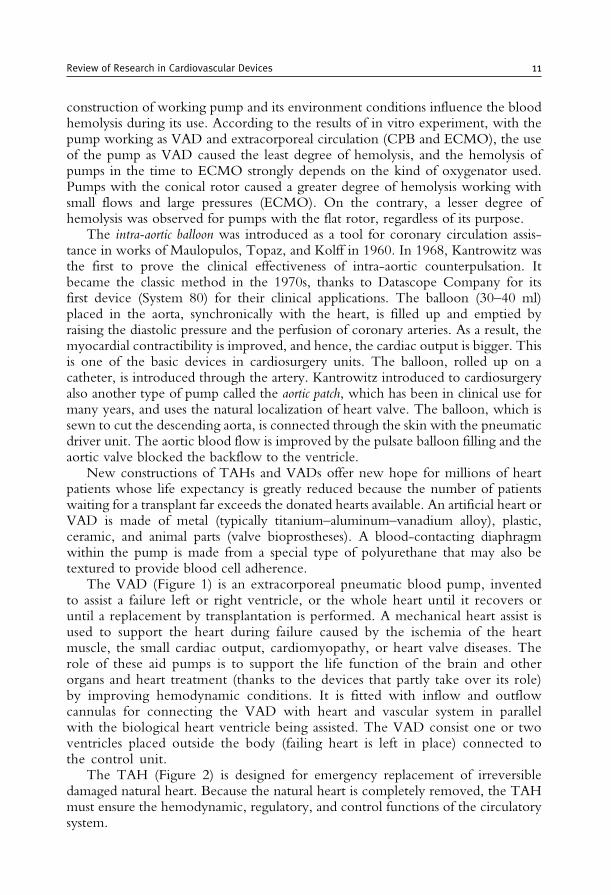
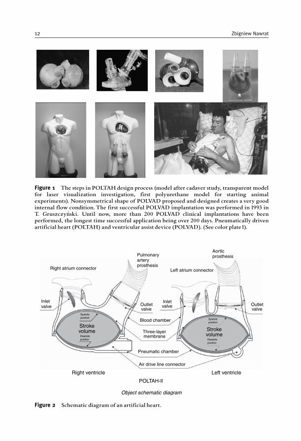
The TAH (Figure 2) is designed for emergency replacement of irreversibledamaged natural heart. Because the natural heart is completely removed, the TAHmust ensure the hemodynamic, regulatory, and control functions of the circulatorysystem.
Review of Research in Cardiovascular Devices 11
Aorticprosthesis
Left atrium connector
Pulmonaryarteryprosthesis
Right atrium connector
Inletvalve
Strokevolume
Outletvalve
Outletvalve
Inletvalve
Blood chamber
Three-layermembrane
Pneumatic chamber
Air drive line connector
Right ventricle Left ventricle
POLTAH-ll
Object schematic diagram
Systolicposition
Diastolicposition
Strokevolume
Systolicposition
Diastolicposition
Figure 2 Schematic diagram of an artificial heart.
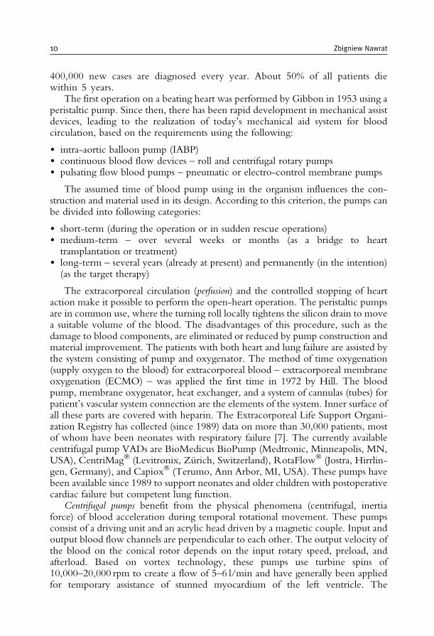
Figure 1 The steps in POLTAH design process (model after cadaver study, transparent modelfor laser visualization investigation, first polyurethane model for starting animalexperiments). Nonsymmetrical shape of POLVAD proposed and designed creates a very goodinternal flow condition.The first successful POLVAD implantation was performed in 1993 inT. Gruszczyn¤ ski. Until now, more than 200 POLVAD clinical implantations have beenperformed, the longest time successful application being over 200 days. Pneumatically drivenartificial heart (POLTAH) and ventricular assist device (POLVAD). (See color plate1).
12 Zbigniew Nawrat
If the total replacement artificial heart is to mimic the function of the naturalhuman heart, it meet the following requirements [1]:
1. Two separate pumps duplicating the left and the right heart2. Output range of 5–10 l/min from each side3. Aortic arterial pressure range of 120–180mmHg4. Pulmonary arterial pressure range of 20–80mmHg5. Physical dimensions permitting easy surgical insertion within the pericardium6. Low weight to minimize restraints7. A minimum of noise and vibration8. A heat output of less than 25W9. A low degree of hemolysis
10. Inert to body chemicals
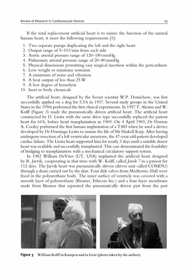
The artificial heart, designed by the Soviet scientist W.P. Demichow, was firstsuccessfully applied on a dog for 5.5 h in 1937. Several study groups in the UnitedStates in the 1950s performed the first clinical experiments. In 1957 T. Akutsu andW.Kolff (Figure 3) made the pneumatically driven artificial heart. The artificial heartconstructed by D. Liotta with the same drive type successfully replaced the patientheart for 64 h, before heart transplantation in 1969. On 4 April 1969, Dr DentonA. Cooley performed the first human implantation of a TAH when he used a devicedeveloped by Dr Domingo Liotta to sustain the life of Mr Haskell Karp. After havingundergone resection of a left ventricular aneurysm, the 47-year-old patient developedcardiac failure. The Liotta heart supported him for nearly 3 days until a suitable donorheart was available and successfully transplanted. This case demonstrated the feasibilityof bridging to transplantation with a mechanical circulatory support system.
In 1982 William DeVries (UT, USA) implanted the artificial heart designedby R. Jarvik, cooperating in that time with W. Kolff, called Jarvik 7 in a patient for112 days. The Jarvik heart was pneumatically driven (driver unit called COMDU)through a drain carried out by the skin. Four disk valves from Medtronic-Hall werefixed in the polyurethane body. The inner surface of ventricle was covered with asmooth layer of polyurethane (Biomer, Ethicon Inc.) and a four-layer membranemade from Biomer that separated the pneumatically driven part from the part
Figure 3 WilliamKolff in Kampen and in Gent (photo taken by the author).
Review of Research in Cardiovascular Devices 13
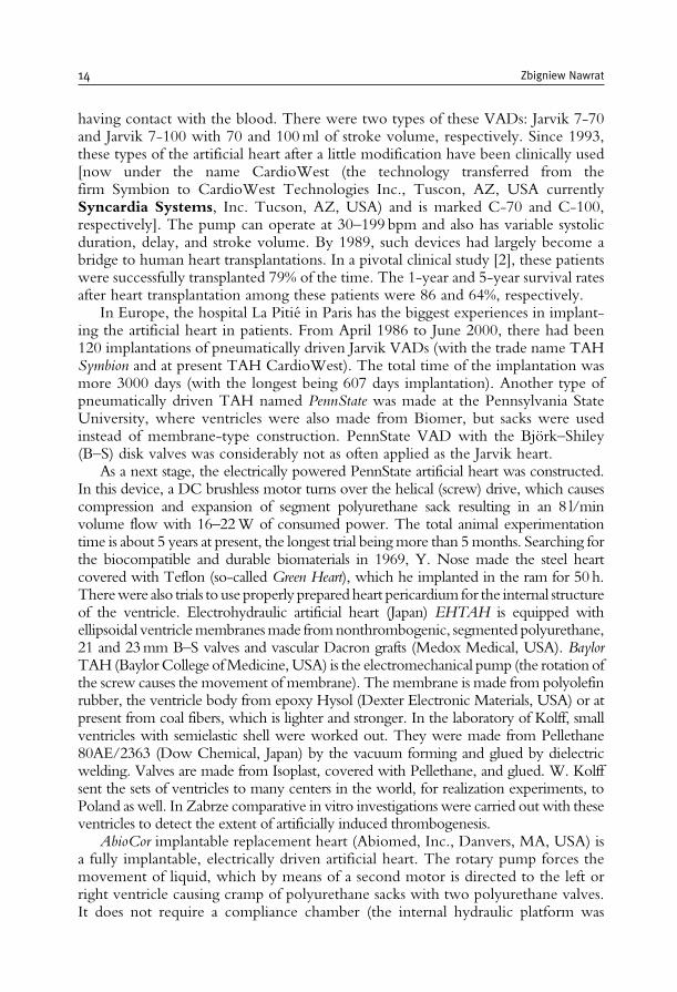
having contact with the blood. There were two types of these VADs: Jarvik 7-70and Jarvik 7-100 with 70 and 100ml of stroke volume, respectively. Since 1993,these types of the artificial heart after a little modification have been clinically used[now under the name CardioWest (the technology transferred from thefirm Symbion to CardioWest Technologies Inc., Tuscon, AZ, USA currentlySyncardia Systems, Inc. Tucson, AZ, USA) and is marked C-70 and C-100,respectively]. The pump can operate at 30–199 bpm and also has variable systolicduration, delay, and stroke volume. By 1989, such devices had largely become abridge to human heart transplantations. In a pivotal clinical study [2], these patientswere successfully transplanted 79% of the time. The 1-year and 5-year survival ratesafter heart transplantation among these patients were 86 and 64%, respectively.
In Europe, the hospital La Pitie in Paris has the biggest experiences in implant-ing the artificial heart in patients. From April 1986 to June 2000, there had been120 implantations of pneumatically driven Jarvik VADs (with the trade name TAHSymbion and at present TAH CardioWest). The total time of the implantation wasmore 3000 days (with the longest being 607 days implantation). Another type ofpneumatically driven TAH named PennState was made at the Pennsylvania StateUniversity, where ventricles were also made from Biomer, but sacks were usedinstead of membrane-type construction. PennState VAD with the Bjork–Shiley(B–S) disk valves was considerably not as often applied as the Jarvik heart.
As a next stage, the electrically powered PennState artificial heart was constructed.In this device, a DC brushless motor turns over the helical (screw) drive, which causescompression and expansion of segment polyurethane sack resulting in an 8 l/minvolume flow with 16–22W of consumed power. The total animal experimentationtime is about 5 years at present, the longest trial beingmore than 5months. Searching forthe biocompatible and durable biomaterials in 1969, Y. Nose made the steel heartcovered with Teflon (so-called Green Heart), which he implanted in the ram for 50h.Therewere also trials to use properly preparedheart pericardium for the internal structureof the ventricle. Electrohydraulic artificial heart (Japan) EHTAH is equipped withellipsoidal ventriclemembranesmade fromnonthrombogenic, segmented polyurethane,21 and 23mm B–S valves and vascular Dacron grafts (Medox Medical, USA). BaylorTAH (BaylorCollege ofMedicine,USA) is the electromechanical pump (the rotation ofthe screw causes the movement of membrane). The membrane is made from polyolefinrubber, the ventricle body from epoxy Hysol (Dexter Electronic Materials, USA) or atpresent from coal fibers, which is lighter and stronger. In the laboratory of Kolff, smallventricles with semielastic shell were worked out. They were made from Pellethane80AE/2363 (Dow Chemical, Japan) by the vacuum forming and glued by dielectricwelding. Valves are made from Isoplast, covered with Pellethane, and glued. W. Kolffsent the sets of ventricles to many centers in the world, for realization experiments, toPoland as well. In Zabrze comparative in vitro investigations were carried out with theseventricles to detect the extent of artificially induced thrombogenesis.
AbioCor implantable replacement heart (Abiomed, Inc., Danvers, MA, USA) isa fully implantable, electrically driven artificial heart. The rotary pump forces themovement of liquid, which by means of a second motor is directed to the left orright ventricle causing cramp of polyurethane sacks with two polyurethane valves.It does not require a compliance chamber (the internal hydraulic platform was
14 Zbigniew Nawrat
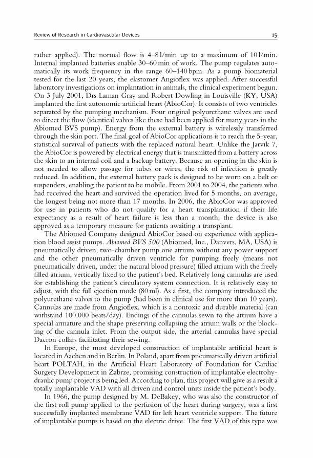
rather applied). The normal flow is 4–8 l/min up to a maximum of 10 l/min.Internal implanted batteries enable 30–60min of work. The pump regulates auto-matically its work frequency in the range 60–140 bpm. As a pump biomaterialtested for the last 20 years, the elastomer Angioflex was applied. After successfullaboratory investigations on implantation in animals, the clinical experiment begun.On 3 July 2001, Drs Laman Gray and Robert Dowling in Louisville (KY, USA)implanted the first autonomic artificial heart (AbioCor). It consists of two ventriclesseparated by the pumping mechanism. Four original polyurethane valves are usedto direct the flow (identical valves like these had been applied for many years in theAbiomed BVS pump). Energy from the external battery is wirelessly transferredthrough the skin port. The final goal of AbioCor applications is to reach the 5-year,statistical survival of patients with the replaced natural heart. Unlike the Jarvik 7,the AbioCor is powered by electrical energy that is transmitted from a battery acrossthe skin to an internal coil and a backup battery. Because an opening in the skin isnot needed to allow passage for tubes or wires, the risk of infection is greatlyreduced. In addition, the external battery pack is designed to be worn on a belt orsuspenders, enabling the patient to be mobile. From 2001 to 2004, the patients whohad received the heart and survived the operation lived for 5 months, on average,the longest being not more than 17 months. In 2006, the AbioCor was approvedfor use in patients who do not qualify for a heart transplantation if their lifeexpectancy as a result of heart failure is less than a month; the device is alsoapproved as a temporary measure for patients awaiting a transplant.
The Abiomed Company designed AbioCor based on experience with applica-tion blood assist pumps. Abiomed BVS 500 (Abiomed, Inc., Danvers, MA, USA) ispneumatically driven, two-chamber pump one atrium without any power supportand the other pneumatically driven ventricle for pumping freely (means notpneumatically driven, under the natural blood pressure) filled atrium with the freelyfilled atrium, vertically fixed to the patient’s bed. Relatively long cannulas are usedfor establishing the patient’s circulatory system connection. It is relatively easy toadjust, with the full ejection mode (80ml). As a first, the company introduced thepolyurethane valves to the pump (had been in clinical use for more than 10 years).Cannulas are made from Angioflex, which is a nontoxic and durable material (canwithstand 100,000 beats/day). Endings of the cannulas sewn to the atrium have aspecial armature and the shape preserving collapsing the atrium walls or the block-ing of the cannula inlet. From the output side, the arterial cannulas have specialDacron collars facilitating their sewing.
In Europe, the most developed construction of implantable artificial heart islocated in Aachen and in Berlin. In Poland, apart from pneumatically driven artificialheart POLTAH, in the Artificial Heart Laboratory of Foundation for CardiacSurgery Development in Zabrze, promising construction of implantable electrohy-draulic pump project is being led. According to plan, this project will give as a result atotally implantable VAD with all driven and control units inside the patient’s body.
In 1966, the pump designed by M. DeBakey, who was also the constructor ofthe first roll pump applied to the perfusion of the heart during surgery, was a firstsuccessfully implanted membrane VAD for left heart ventricle support. The futureof implantable pumps is based on the electric drive. The first VAD of this type was
Review of Research in Cardiovascular Devices 15
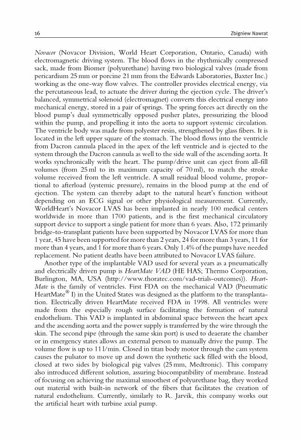
Novacor (Novacor Division, World Heart Corporation, Ontario, Canada) withelectromagnetic driving system. The blood flows in the rhythmically compressedsack, made from Biomer (polyurethane) having two biological valves (made frompericardium 25mm or porcine 21mm from the Edwards Laboratories, Baxter Inc.)working as the one-way flow valves. The controller provides electrical energy, viathe percutaneous lead, to actuate the driver during the ejection cycle. The driver’sbalanced, symmetrical solenoid (electromagnet) converts this electrical energy intomechanical energy, stored in a pair of springs. The spring forces act directly on theblood pump’s dual symmetrically opposed pusher plates, pressurizing the bloodwithin the pump, and propelling it into the aorta to support systemic circulation.The ventricle body was made from polyester resin, strengthened by glass fibers. It islocated in the left upper square of the stomach. The blood flows into the ventriclefrom Dacron cannula placed in the apex of the left ventricle and is ejected to thesystem through the Dacron cannula as well to the side wall of the ascending aorta. Itworks synchronically with the heart. The pump/drive unit can eject from all-fillvolumes (from 25ml to its maximum capacity of 70ml), to match the strokevolume received from the left ventricle. A small residual blood volume, propor-tional to afterload (systemic pressure), remains in the blood pump at the end ofejection. The system can thereby adapt to the natural heart’s function withoutdepending on an ECG signal or other physiological measurement. Currently,WorldHeart’s Novacor LVAS has been implanted in nearly 100 medical centersworldwide in more than 1700 patients, and is the first mechanical circulatorysupport device to support a single patient for more than 6 years. Also, 172 primarilybridge-to-transplant patients have been supported by Novacor LVAS for more than1 year, 45 have been supported for more than 2 years, 24 for more than 3 years, 11 formore than 4 years, and 1 for more than 6 years. Only 1.4% of the pumps have neededreplacement. No patient deaths have been attributed to Novacor LVAS failure.
Another type of the implantable VAD used for several years as a pneumaticallyand electrically driven pump is HeartMate VAD (HE HAS; Thermo Corporation,Burlington, MA, USA (http://www.thoratec.com/vad-trials-outcomes)). Heart-Mate is the family of ventricles. First FDA on the mechanical VAD (PneumaticHeartMate� I) in the United States was designed as the platform to the transplanta-tion. Electrically driven HeartMate received FDA in 1998. All ventricles weremade from the especially rough surface facilitating the formation of naturalendothelium. This VAD is implanted in abdominal space between the heart apexand the ascending aorta and the power supply is transferred by the wire through theskin. The second pipe (through the same skin port) is used to deaerate the chamberor in emergency states allows an external person to manually drive the pump. Thevolume flow is up to 11 l/min. Closed in titan body motor through the cam systemcauses the pulsator to move up and down the synthetic sack filled with the blood,closed at two sides by biological pig valves (25mm, Medtronic). This companyalso introduced different solution, assuring biocompatibility of membrane. Insteadof focusing on achieving the maximal smoothest of polyurethane bag, they workedout material with built-in network of the fibers that facilitates the creation ofnatural endothelium. Currently, similarly to R. Jarvik, this company works outthe artificial heart with turbine axial pump.
16 Zbigniew Nawrat
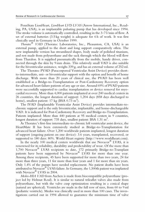
PennState LionHeart, LionHeart LVD LVAS (Arrow International, Inc., Read-ing, PA, USA), is an implantable pulsating pump that has developed since 1994.The stroke volume is automatically controlled, resulting in the 3–7 l/min of flow. Aset of external batteries (3.5 kg weight) is adequate for 6 h of work. It was firstclinically used in Germany in October 1999.
Thoratec� VAD (Thoratec Laboratories, Inc., Pleasanton, CA, USA) is anexternal pump, applied to the short and long support comparatively often. Thenew implantable version has streamlined shapes, body made of polished titanium,and rest made from polyurethane and the sack through which the blood will flowfrom Tharalon. It is supplied pneumatically from the mobile, handy driver, con-nected through the skin by 9mm drain. This relatively small VAD is also suitablefor the biventricular assistance, weighs 339 g, and has an external volume of 252ml.
The Thoratec PVAD (Paracorporeal Ventricular Assist Device) provides short-to-intermediate, uni- or biventricular support with the option and benefit of homedischarge. With more than 20 years of clinical use, the PVAD has been wellestablished as a Bridge-to-Transplantation or Post-Cardiotomy Recovery optionfor advanced heart failure patients of any age or size. Around 69% of PVAD patientswere successfully supported to cardiac transplantation or device removal for myo-cardial recovery. More than 4,000 patients implanted at over 240 medical centers in26 countries, the longest duration of support: 1,204 days (858 days discharged tohome), smallest patient: 17 kg (BSA 0.73 m2).
The IVAD (Implantable Ventricular Assist Device) provides intermediate-to-chronic support and is the only biventricular, implantable, and home-dischargeableVAD. It is indicated for Post-Cardiotomy Recovery and Bridge-to-Transplantation.Patients implanted: More than 440 patients at 95 medical centers in 9 countries,longest duration of support: 735 days, smallest patient: BSA 1.31 m2.
As Thoratec’s first-line intermediate-to-chronic left ventricular assist device, theHeartMate II has been extensively studied as Bridge-to-Transplantation foradvanced heart failure. Over 1,200 worldwide patients implanted, longest durationof support (ongoing patient on one device): 3.6 years, transplanted, recovered, orsupported to 180 days: 80%. World Heart registry (http://www.worldheart.com).
In the nearly 100 medical centers worldwide that use Novacor� LVAS, it isrenowned for its reliability, durability and predictability of wear. Of the more than1,700 Novacor� LVAS recipients to date, 172 primarily Bridge-to-Transplantpatients have been supported by Novacor� LVAS for more than one year.Among these recipients, 45 have been supported for more than two years, 24 formore than three years, 11 for more than four years and 1 for more than six years.Only 1.4% of the pumps have needed replacement. No patient deaths have beenattributed to Novacor� LVAS failure. In Germany, the 1,500th patient was implantedwith Novacor� LVAS in 2004.
Medos-HIA VAD from Aachen is made from biocompatible polyurethane (pro-ject led by Helmut Reul). It is similar to natural trileaflet valves also made frompolyurethane, but with the valve cusp optimization resulting in a conical shape(natural are spherical). Ventricles are made in the full row of sizes, from 60 to 9ml(pediatric ventricle). Medos was clinically used in more than 100 cases. The inves-tigations carried out in 1994 allowed to guarantee the minimum time of valve
Review of Research in Cardiovascular Devices 17
functioning of half-year (18 million of cycles). Since 1990, in Aachen, the HIA TAHhas been developed, which is based on electromechanical driving unit. The inclina-tion of the plate onwhich themembrane is fixed about 2 cm allows to reach the 65mlstroke volume. Brushless motor rotates in only one direction (similar to the case ofHeartMate, but the construction of the cam unit is different). The pump allows toreach above 10 l/min (with the frequency of 140 bpm under physiologicalconditions).
HeartSaver VAD (WorldHeart Corporation, Ottawa, ON, Canada) is thepulsate pump with hydraulic drive (project led by Tofy Mussivand). In 2000, itwas almost ready for the starting of clinical experiments. Different types wereprepared: the axial pumps for continuous flow and VADs and TAHs for pulsatingpumps. All models are driven electrohydraulically (rotor). The external volume ofthe VAD is approximately 530ml, the membrane is made from smooth polyur-ethane, and Medtronic-Hall mechanical valves are used, which according to planwill be replaced with the less thrombogenic biological Carpentier–Edwards valves.The working liquid in this pump is the silicon oil, which is currently not in use.
Berlin Heart is a series of external, pneumatically driven, ventricle assist devices,with the 50, 60, or 80ml ejection, equipped with B–S mechanical valves or thepolyurethane valves. Berlin Heart VADs have comfortable silicone cannulas withthe wire armature, which renders cannulas a suitable shape. This type of VADs hadbeen successfully in vitro tested for 5 years (more than 210 million cycles), mainlyin Berlin. Berlin Heart VAD was used in Poland by Z. Religa’s team in firstsuccessful mechanical support of heart as a bridge to transplantation.
The pneumatically driven membrane-type Polish ventricle assist devicesPOLVAD (U-shaped) and artificial heart POLTAH (spherical) were developed inZabrze, Poland. Until now, more than 200 VAD implantations have been per-formed. First successful bridge to transplantation was constructed by Z. Religa’steam. The implantation of BVAD produced by Berlin Heart LVAD was performedin May 1991. The patient T. Gruszczynski was awaiting heart transplantation. After11 days of support, the heart transplantation was performed and patient returnedhome. Unfortunately, rejection occurred and the patient needed a second, newheart. In the meantime, author (physicist) designed and B. Stolarzewicz (chemist)performed a new Polish ventricular assist pump named POLVAD. After tests,POLVAD was ready for clinical applications. It happened that the first patient touse POLVAD was the same patient T. Gruszczynski (the heart was rejected after2 years). Fortunately, the POLVAD worked very well, and after 21 days, the hearttransplantation was performed. Unfortunately, the patient died during surgery(second heart transplantation).
In pulsate blood pumps, the part producing mechanical energy is separated fromthe blood by a biocompatible and durable membrane. Membrane-type VADs haveit fixed to the hard or half-elastic body. They divide the artificial chamber in twoalmost even parts. However, in the ventricle with sack, the membrane is shapedinto this bag hung in stiff chamber. The artificial ventricles can be driven pneuma-tically, hydraulically, or electromechanically. The trials of the nuclear power sourceintroduction failed. The VADs are used for supporting patient’s life as a bridge totransplantation or to natural heart recovery. At the end of this procedure, the
18 Zbigniew Nawrat
cannulas connecting VAD to the patient’s circulatory system are operationallyremoved. The TAHs are used in these cases, when heart transplantation is theonly rescue for the patient or as a target therapy.
Distinct from abovedescribed pulsate pumps, the Jarvik 2000 and MicroMed–DeBakey are the currently used implantable axial pumps with continuous flow.The first axial flow pump to be introduced into clinical practice for intermediate tolong-term treatment of end-stage heart failure in adults was the DeBakey VAD�.MicroMed–DeBakey VAD is the rotor, axial pump (flow up to 5 l/min), connectedby the cable through the skin to the driver unit held on the patient’s belt. It isimplanted between the heart apex and aorta (ascending or descending). TheDeBakey VAD is 30mm� 76mm, weighs 93 g, and is approximately 1/10th thesize of pulsatile products on the market. In 2000, the first successful usage wasperformed in Vienna.
Jarvik 2000 is a small (2.5/5.5 cm) rotor pump (the electromagnetic rotorcovered by titanium layer). It fits directly into the left ventricle, which mayeliminate problems with clotting. The outflow graft connects to the descendingaorta. The device itself is nonpulsatile, but the natural heart continues to beat andprovides a pulse. The rotor has ceramic bearings, which are washed by the blood(smearing and the receipt of warmth). The angular velocity of 9000–16,000 rpmensures 3–6 l/min of output flow with the aortic pressure of 80mmHg and powerconsumption of 4–10W. The system is powered by external batteries remotelythrough skin using electromagnetic field created by a set of coupled coins or usingthe wire carried out through the “port” in the skull safety plugged with thepyrolytic carbon. On 25 April 2000, physicians in Houston, TX, USA, haverealized the implantation and introduced the first patient in the clinical investigationof the Jarvik 2000. For lifetime use, the Jarvik 2000 has also had provensuccessful in treating a target population of patients suffering from chronicheart failure due to a prior heart attack or cardiomyopathy. Many have beenrehabilitated to a dramatically improved life at home, and in some cases patientshave even returned to work. So far, the Jarvik 2000 FlowMaker� has been usedto treat more than 200 patients in the United States, Europe, and Asia. Ofthose, roughly 79% received the Jarvik 2000 as a bridge to transplantation and21% as a permanent implant, with a number of patients in each group beingterminally ill, near-death cases. Nearly 70% of those patients were supportedsuccessfully. Several surgeons reports have described placement of continuousflow devices without cardiopulmonary bypass. Frazier described a patient inwhom he placed this pump while briefly fibrillating the heart and placement ofthe Jarvik 2000 with an anterior, intraperitoneal approach without bypass. Thistechnique is attractive in reoperative situations.
The University of Pittsburgh–Thermo Cardiosystems HeartMate� II is an axialrotary pump with the stone bearing with a volume of 89ml, weighs 350 g, andthe estimated time of use is 5–7 years. As intermediate-to-chronic left ventricularassist device, the HeartMate II (now Thoratec’s) has been extensively studied asBridge-to-Transplantation for advanced heart failure. Over 1,200 worldwide patientsimplanted, longest duration of support (ongoing patient on one device): 3.6 years,transplanted, recovered, or supported to 180 days: 80%. The third-generation,
Review of Research in Cardiovascular Devices 19

HeartMate III, will be the centrifugal pump with the rotor levitating in the magneticfield (without mechanical bearings).
There have been several scientific groups working in the field of artificial heartin Japan, Australia, Austria, Argentina, France, Germany, Poland, Czech Republic,Russia, and so on. But from the market point of view, there is not easy business.Currently, the strongest company offering the wide range of products in the area ofblood pumps is Thoratec. Thoratec Corporation is engaged in the research, devel-opment, manufacturing, and marketing of medical devices for circulatory support,vascular graft, blood coagulation, and skin incision applications. The ThoratecVAD system is the device that is approved for left, right, or total heart supportand that can be used both as a bridge to transplantation and for recovery from open-heart surgery. More than 4300 of these devices have been used in the treatment ofover 2800 patients worldwide. With the introduction of the Implantable Ventri-cular Assist Device (IVAD
TM
), Thoratec delivers the first and only implantableVADs for left, right, and biventricular support for bridge to transplantation andfor postcardiotomy recovery. The HeartMate� XVE Left Ventricular Assist System(LVAS) is now FDA approved as a long-term permanent implant, called destinationtherapy. In addition, the accompanying Thoratec TLC-II� Portable VAD Driverprovides hospitals with the first mobile system that allows these univentricular orbiventricular VAD patients to be discharged home to await cardiac transplantationor myocardial recovery. The company is also a leader in implantable LVADs. Itsair-driven and electric HeartMate LVAD, which has been implanted in more than4100 patients worldwide, are implanted alongside the natural heart and take overthe pumping function of the left ventricle for patients whose hearts are toodamaged or diseased to produce adequate blood flow.
WorldHeart is a developer of mechanical circulatory support systems (e.g., Nova-cor) with leading next-generation technologies. The Levacor is a next-generationrotary VAD. It is the only bearingless, fully magnetically levitated implantable cen-trifugal rotary pump with clinical experience. An advanced, continuous-flow pump,the Levacor uses magnetic levitation to fully suspend the spinning rotor, its onlymoving part, inside a compact housing.
WorldHeart’s Novacor II LVAS is a next-generation, pulsatile VAD. It can befully implanted without a volume displacement chamber, thereby reducing the riskof complications by eliminating the need to perforate the skin. The operation of thepump drive unit is very interesting. When the pusher plate is driven to the right(pumping stroke), the prechamber expands, filling from the left ventricle. Simulta-neously, the pumping chamber is compressed, ejecting blood into the body. Whenthe pusher plate returns to the left (transfer stroke), the prechamber is compressedwhile the pumping chamber expands; blood transfers from the prechamber to thepumping chamber, with no inflow or outflow. Because the total volume of thetwo chambers remains constant as one fills and the other empties, the system canoperate without a volume compensator or venting through the skin. WorldHeart’sNovacor II LVAS is not currently available. In 2005, WorldHeart conducted thefirst animal implant of the Novacor II LVAS – ahead of schedule. WorldHeartCompany currently focuses on new products – especially for pediatric patients. ThePediaFlow VAD is an implantable, magnetically levitated blood pump based on
20 Zbigniew Nawrat
WorldHeart’s proprietary rotary VAD MagLevTM technology. In its pediatricconfiguration, the device is designed to provide a flow rate from 0.3 to 1.5 l/min.The PediaFlow VAD is being developed to provide medium-term (less than 1 year)implantable circulatory support to patients from birth to 2 years of age with congenitalor acquired heart disease.
Pneumatic pulsatile VADs have been available in pediatric sizes since 1992. AtHerzzentrum Berlin, VADs are used lasting from several days to 14 months in70 infants and children with myocarditis and cardiomyopathy, leading to a notablerise in survival in the past 5 years. It is possible to discharge 78% of the infants under1 year old [3].
Several types of VADs have been used in children and adolescents whose bodysurface area is greater than 1.2m2 – that is, generally in children older than 5 years.The Thoratec VADs (Thoratec Laboratories, Inc.) have been available since theearly 1980s for adult use, but they can also be implanted in older children andadolescents. Several other adult-size VADs, such as the Novacor (Baxter HealthcareCorporation, Irvine, CA, USA), have been applied in adolescents, and a version ofthe axial flow DeBakey VAD (MicroMed Technology Inc., The Woodlands, TX,USA) has been developed that is suitable for use in children and has been implantedin several patients. Two miniaturized extracorporeal, pneumatically driven VADsdesigned specifically for smaller children and infants have been introduced inEurope so far: the Berlin Heart Excor� (Berlin Heart AG, Berlin, Germany) in1992 and the Medos HIA device (Medos Medizintechnik AG, Stolberg, Germany)in 1994. The first reported implantation of a Medos VAD as a bridge to transplan-tation in a child took place in 1994. Only the extracorporeal, pneumatically drivenBerlin Heart Excor and the Medos HIA pulsatile systems have so far provensuccessful in children of all ages. The pediatric version of the Berlin Heart ExcorVAD is mounted with trileaflet polyurethane valves and is available with pump sizesof 10, 25, 30, 50, 60, and 80ml. The 10-ml pumps are suitable for neonates andinfants with body weight of up to 9 kg (body surface area 0.43m2), and the 25 and30ml pumps can be used in children up to the age of 7 years (weight 30 kg and bodysurface area of about 0.95m2); adult-sized pumps can be implanted in older children.The adult pump has a stroke volume of 80ml and tilting disk valves. Pediatric-sizedpumps are suitable for children with a body weight of 3–9 kg. This pump has a strokevolume of 10ml and polyurethane trileaflet valves [3].
Several other pulsatile devices developed for the adult population are used inschool-aged children: the HeartMate I (Thoratec Laboratories, Inc.), Toyobo(National Cardiovascular Center Tokyo, Japan), Abiomed� BVS 5000 (AbiomedInc., Delaware, MA, USA), and Novacor (World Heart Corporation, Ontario,Canada). Two continuous flow rotary VADs that use axial flow or centrifugal flow –the Incor� VAD (Berlin Heart) and the DeBakey VAD – have been introducedinto routine clinical care. Some further devices are still being subjected to clinical trials:Jarvik 2000 (Jarvik, New York, NY, USA), HeartMate II, Duraheart� (TerumoKabushiki Kaisha Corporation, Shibuya-ku, Japan), VentrAssist (Ventracor, Chats-wood, NSW, Australia), and CorAid� (Cleveland Clinic, Cleveland, OH, USA) [3].
The Incor device (Berlin Heart AG) is 146mm long and 30mm wide andweighs 200 g. MicroMed modified the adult pump to fit children and in 2004
Review of Research in Cardiovascular Devices 21
received FDA humanitarian device exemption status, enabling implantation of theDeBakey VAD Child pump for persons, aged 5–16, awaiting heart transplantation.
Berlin Heart AG products are Incor, Excor cannulas, and driving units. In June2002, the worldwide first implantation of the Incor device took place in theGerman Heart Center DHZB. By July 2005, no less than 300 Incor devices hadbeen implanted (two patients have been living with the device for 3 years). Excor isan extracorporeal, pulsatile VAD. Various types and sizes of blood pumps and awide range of cannulas allow us to meet all clinical needs and treat all patients,regardless of their age.
The VentrAssist, which is made by the Australian company Ventracor, has amoving part – a hydrodynamically suspended impeller. It has been designed to haveno wearing parts or cause blood damage. It weighs just 298 g and measures 60mmin diameter, making it suitable for both children and adults. VentrAssist also has anadvantage over its one competitor, Incor made by the German company BerlinHeart. The VentrAssist is less likely to damage red blood cells because it moves theblood more slowly with a bigger impeller.
The term VAD has been applied to a wide variety of mechanical circulatorysupport systems designed to unload the heart and provide adequate perfusion of theorgans.
Short-term circulatory support with an LVAD may be indicated for patientswith end-stage heart failure (of any etiology) who are awaiting a donor heart fortransplantation, and for patients with a severe acute heart failure syndrome fromwhich myocardial recovery is anticipated (such as acute myocarditis). An LVAD issometimes used if weaning from cardiopulmonary bypass after cardiac surgery fails.In the active arm of a nonrandomized controlled study, 78% (32/41) of patientssurvived for a mean of 215 days with LVAD support. In another comparative study,81% (13/16) of patients survived to transplantation (duration of support not stated).One case series showed that at 30 days of bridging to transplantation with anLVAD, survival was 83%, falling to 19% after 24 months’ support.
In a nonrandomized controlled trial, posttransplant survival of patients bridgedon LVAD support was 66% (21/32) at 41 months, compared with 67% (98/146) ofpatients at 36 months who had a transplant without circulatory support, althoughpatients in the latter group were significantly older. One case series of 243 patientsin whom LVADs were used to bridge to transplantation reported actuarial post-transplant survival of 91% at 1 year, 70% at 5 years, and 40% at 10 years. Resultsfrom case series included in a systematic review showed that between 60% (12/20)and 83% (5/6) of patients survived to transplantation or were still alive awaitingtransplantation on LVAD support. Of the total cases of bridge to recovery reported,58% (7/12) of patients survived to final follow-up; successful explantation of thedevice or weaning from support was achieved in all these patients [4].
The randomized controlled study showed a reduction of 48% in the risk ofdeath from any cause in the group that received left VADs as compared with themedical therapy group [relative risk 0.52; 95% confidence interval (CI) 0.34–0.78;P= 0.001]. Randomly assigned 129 patients with end-stage heart failure wereineligible for cardiac transplantation to receive a left VAD (68 patients) or optimalmedical management (class IV heart failure). The rates of survival at 1 year were
22 Zbigniew Nawrat
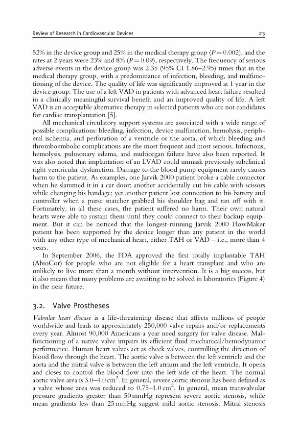
52% in the device group and 25% in the medical therapy group (P= 0.002), and therates at 2 years were 23% and 8% (P= 0.09), respectively. The frequency of seriousadverse events in the device group was 2.35 (95% CI 1.86–2.95) times that in themedical therapy group, with a predominance of infection, bleeding, and malfunc-tioning of the device. The quality of life was significantly improved at 1 year in thedevice group. The use of a left VAD in patients with advanced heart failure resultedin a clinically meaningful survival benefit and an improved quality of life. A leftVAD is an acceptable alternative therapy in selected patients who are not candidatesfor cardiac transplantation [5].
All mechanical circulatory support systems are associated with a wide range ofpossible complications: bleeding, infection, device malfunction, hemolysis, periph-eral ischemia, and perforation of a ventricle or the aorta, of which bleeding andthromboembolic complications are the most frequent and most serious. Infections,hemolysis, pulmonary edema, and multiorgan failure have also been reported. Itwas also noted that implantation of an LVAD could unmask previously subclinicalright ventricular dysfunction. Damage to the blood pump equipment rarely causesharm to the patient. As examples, one Jarvik 2000 patient broke a cable connectorwhen he slammed it in a car door; another accidentally cut his cable with scissorswhile changing his bandage; yet another patient lost connection to his battery andcontroller when a purse snatcher grabbed his shoulder bag and ran off with it.Fortunately, in all these cases, the patient suffered no harm. Their own naturalhearts were able to sustain them until they could connect to their backup equip-ment. But it can be noticed that the longest-running Jarvik 2000 FlowMakerpatient has been supported by the device longer than any patient in the worldwith any other type of mechanical heart, either TAH or VAD – i.e., more than 4years.
In September 2006, the FDA approved the first totally implantable TAH(AbioCor) for people who are not eligible for a heart transplant and who areunlikely to live more than a month without intervention. It is a big success, butit also means that many problems are awaiting to be solved in laboratories (Figure 4)in the near future.
3.2. Valve Prostheses
Valvular heart disease is a life-threatening disease that affects millions of peopleworldwide and leads to approximately 250,000 valve repairs and/or replacementsevery year. Almost 90,000 Americans a year need surgery for valve disease. Mal-functioning of a native valve impairs its efficient fluid mechanical/hemodynamicperformance. Human heart valves act as check valves, controlling the direction ofblood flow through the heart. The aortic valve is between the left ventricle and theaorta and the mitral valve is between the left atrium and the left ventricle. It opensand closes to control the blood flow into the left side of the heart. The normalaortic valve area is 3.0–4.0 cm2. In general, severe aortic stenosis has been defined asa valve whose area was reduced to 0.75–1.0 cm2. In general, mean transvalvularpressure gradients greater than 50mmHg represent severe aortic stenosis, whilemean gradients less than 25mmHg suggest mild aortic stenosis. Mitral stenosis
Review of Research in Cardiovascular Devices 23
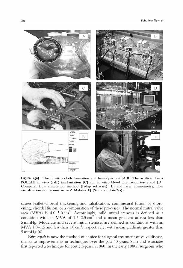
causes leaflet/chordal thickening and calcification, commissural fusion or short-ening, chordal fusion, or a combination of these processes. The normal mitral valvearea (MVA) is 4.0–5.0 cm2. Accordingly, mild mitral stenosis is defined as acondition with an MVA of 1.5–2.5 cm2 and a mean gradient at rest less than5mmHg. Moderate and severe mitral stenoses are defined as conditions with anMVA 1.0–1.5 and less than 1.0 cm2, respectively, with mean gradients greater than5mmHg [6].
Valve repair is now the method of choice for surgical treatment of valve disease,thanks to improvements in techniques over the past 40 years. Starr and associatesfirst reported a technique for aortic repair in 1960. In the early 1980s, surgeons who
Figure 4(a) The in vitro cloth formation and hemolysis test [A,B]. The artificial heartPOLTAH in vivo (calf ) implantation [C] and in vitro blood circulation test stand [D].Computer flow simulation method (Fidap software) [E] and laser anemometry, flowvisualization stand (constructor Z.Małota) [F]. (See color plate 2(a)).
24 Zbigniew Nawrat
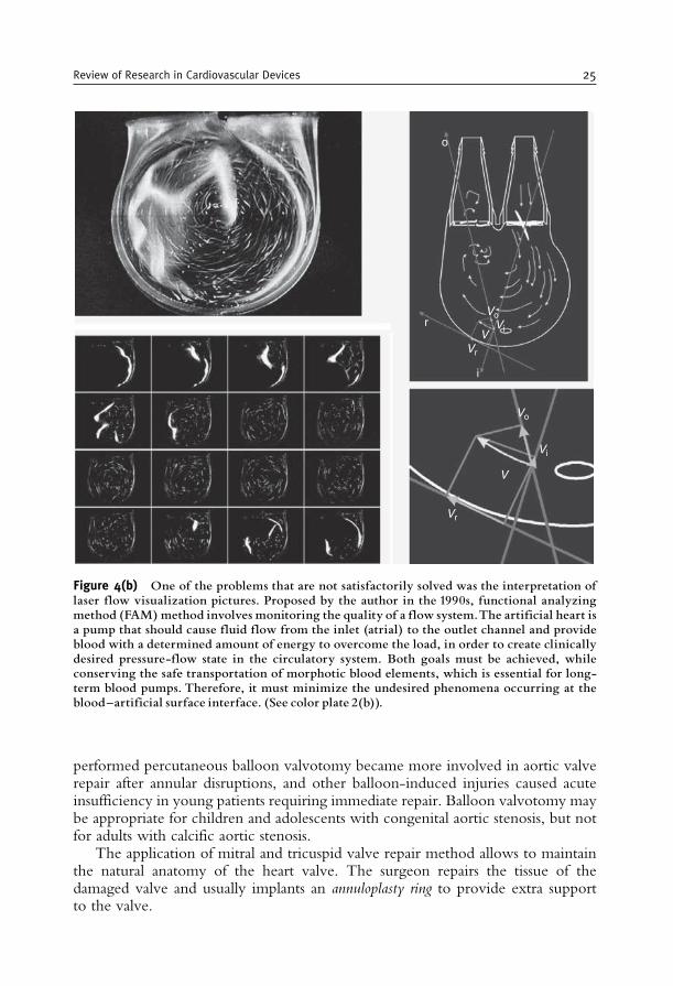
performed percutaneous balloon valvotomy became more involved in aortic valverepair after annular disruptions, and other balloon-induced injuries caused acuteinsufficiency in young patients requiring immediate repair. Balloon valvotomy maybe appropriate for children and adolescents with congenital aortic stenosis, but notfor adults with calcific aortic stenosis.
The application of mitral and tricuspid valve repair method allows to maintainthe natural anatomy of the heart valve. The surgeon repairs the tissue of thedamaged valve and usually implants an annuloplasty ring to provide extra supportto the valve.
o
r
i
Vr
Vr
Vi
Vi
Vo
Vo
V
V
Figure 4(b) One of the problems that are not satisfactorily solved was the interpretation oflaser flow visualization pictures. Proposed by the author in the 1990s, functional analyzingmethod (FAM) method involves monitoring the quality of a flow system.The artificial heart isa pump that should cause fluid flow from the inlet (atrial) to the outlet channel and provideblood with a determined amount of energy to overcome the load, in order to create clinicallydesired pressure-flow state in the circulatory system. Both goals must be achieved, whileconserving the safe transportation of morphotic blood elements, which is essential for long-term blood pumps. Therefore, it must minimize the undesired phenomena occurring at theblood^artificial surface interface. (See color plate 2(b)).
Review of Research in Cardiovascular Devices 25
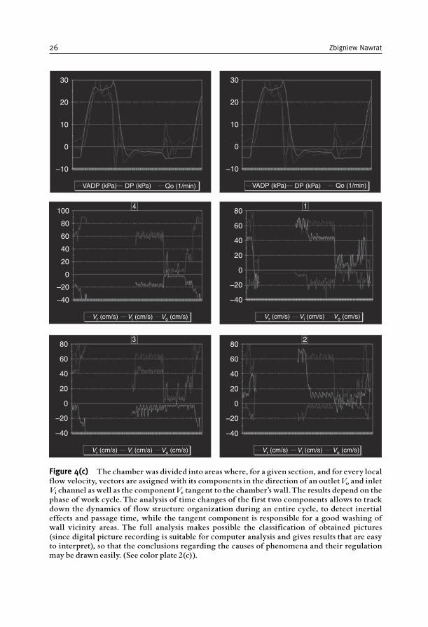
30
20
10
0
–10
VADP (kPa)
Vr (cm/s) Vi (cm/s) Vo (cm/s) Vr (cm/s) Vi (cm/s) Vo (cm/s)
Vr (cm/s) Vi (cm/s) Vo (cm/s) Vr (cm/s) Vi (cm/s) Vo (cm/s)
VADP (kPa)DP (kPa) DP (kPa)Qo (1/min) Qo (1/min)
100
80
60
40
20
0
–20
–40
801
23
4
60
40
20
0
–20
–40
80
60
40
20
0
–20
–40
80
60
40
20
0
–20
–40
30
20
10
0
–10
Figure 4(c) The chamber was divided into areas where, for a given section, and for every localflow velocity, vectors are assigned with its components in the direction of an outletVo and inletVi channel as well as the componentVr tangent to the chamber’s wall.The results depend on thephase of work cycle.The analysis of time changes of the first two components allows to trackdown the dynamics of flow structure organization during an entire cycle, to detect inertialeffects and passage time, while the tangent component is responsible for a good washing ofwall vicinity areas. The full analysis makes possible the classification of obtained pictures(since digital picture recording is suitable for computer analysis and gives results that are easyto interpret), so that the conclusions regarding the causes of phenomena and their regulationmay be drawn easily. (See color plate 2(c)).
26 Zbigniew Nawrat
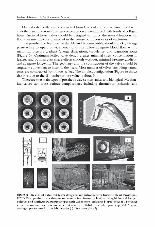
Natural valve leaflets are constructed from layers of connective tissue lined withendothelium. The zones of stress concentration are reinforced with bands of collagenfibers. Artificial heart valves should be designed to mimic the natural function andflow dynamics that are optimized in the course of million years of evolution.
The prosthetic valve must be durable and biocompatible, should quickly changephase (close to open, or vice versa), and must allow adequate blood flow with aminimum pressure gradient (energy dissipation), turbulence, and stagnation zones(Figure 5). Optimum leaflet valve design creates minimal stress concentration inleaflets, and optimal cusp shape effects smooth washout, minimal pressure gradient,and adequate longevity. The geometry and the construction of the valve should besurgically convenient to insert in the heart. Most number of valves, including naturalones, are constructed from three leaflets. The simplest configuration (Figure 6) showsthat it is due to the � number whose value is about 3.
There are two main types of prosthetic valves: mechanical and biological. Mechan-ical valves can cause various complications, including thrombosis, ischemia, and
a
b c
Figure 5 Results of valve test tester designed and introduced in Institute Heart Prostheses,FCSD.The opening area valve test and comparison in one cycle of working biological Religa,Polcryo, and synthetic Polpu prototypes with Carpentier^Edwards bioprotheses (a).The laservisualization and laser anemometer test results of Polish disk valve prototype (b). Severaltesting apparatus used in our laboratories (c). (See color plate 3).
Review of Research in Cardiovascular Devices 27
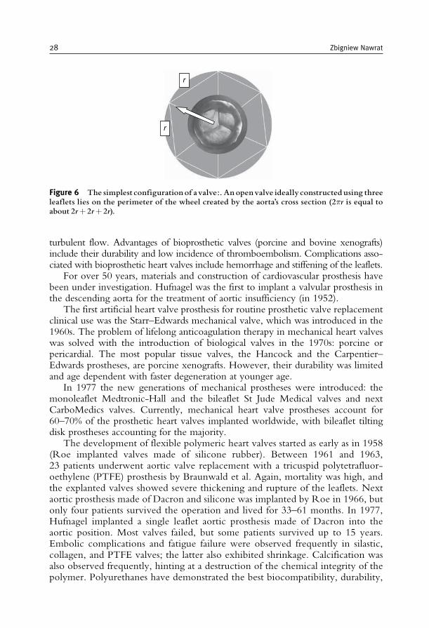
turbulent flow. Advantages of bioprosthetic valves (porcine and bovine xenografts)include their durability and low incidence of thromboembolism. Complications asso-ciated with bioprosthetic heart valves include hemorrhage and stiffening of the leaflets.
For over 50 years, materials and construction of cardiovascular prosthesis havebeen under investigation. Hufnagel was the first to implant a valvular prosthesis inthe descending aorta for the treatment of aortic insufficiency (in 1952).
The first artificial heart valve prosthesis for routine prosthetic valve replacementclinical use was the Starr–Edwards mechanical valve, which was introduced in the1960s. The problem of lifelong anticoagulation therapy in mechanical heart valveswas solved with the introduction of biological valves in the 1970s: porcine orpericardial. The most popular tissue valves, the Hancock and the Carpentier–Edwards prostheses, are porcine xenografts. However, their durability was limitedand age dependent with faster degeneration at younger age.
In 1977 the new generations of mechanical prostheses were introduced: themonoleaflet Medtronic-Hall and the bileaflet St Jude Medical valves and nextCarboMedics valves. Currently, mechanical heart valve prostheses account for60–70% of the prosthetic heart valves implanted worldwide, with bileaflet tiltingdisk prostheses accounting for the majority.
The development of flexible polymeric heart valves started as early as in 1958(Roe implanted valves made of silicone rubber). Between 1961 and 1963,23 patients underwent aortic valve replacement with a tricuspid polytetrafluor-oethylene (PTFE) prosthesis by Braunwald et al. Again, mortality was high, andthe explanted valves showed severe thickening and rupture of the leaflets. Nextaortic prosthesis made of Dacron and silicone was implanted by Roe in 1966, butonly four patients survived the operation and lived for 33–61 months. In 1977,Hufnagel implanted a single leaflet aortic prosthesis made of Dacron into theaortic position. Most valves failed, but some patients survived up to 15 years.Embolic complications and fatigue failure were observed frequently in silastic,collagen, and PTFE valves; the latter also exhibited shrinkage. Calcification wasalso observed frequently, hinting at a destruction of the chemical integrity of thepolymer. Polyurethanes have demonstrated the best biocompatibility, durability,
r
r
Figure 6 The simplest configuration of avalve:. An openvalve ideally constructed using threeleaflets lies on the perimeter of the wheel created by the aorta’s cross section (2�r is equal toabout 2rþ 2rþ 2r).
28 Zbigniew Nawrat
and resistance to thromboembolism among all polymers and are, therefore, alsoused for a variety of medical devices [7].
Currently, some polymeric valves have proven efficacious in assist devices(Abiomed, Medos, and Berlin Heart). However, so far no flexible polymericheart valve has proven durability for long-term implantation.
All mechanical valves are made up of an orifice ring and occluders, either one ortwo leaflets through which blood flows through the heart in a forward direction.Because of susceptibility to thromboembolic events, mechanical devices are used ina lifelong anticoagulation therapy (using agents such as Heparin, Warfarin, orCoumadin that delay the clotting of blood, which can cause a heart attack orstroke). The abovementioned drawbacks are minimized or eliminated when bio-prostheses are implanted.
Tissue valves (bioprosthetic valves) are made of human or animal tissue. Thereare three types of tissue valves: pig tissue (porcine), cow tissue (bovine), and humantissue (e.g., aortic or pulmonary valves obtained from human cadavers), or auto-grafts (e.g., the patient’s own pulmonary valve, pericardium, or fascia lata). Homo-graft aortic or pulmonary valves (and associated portions of aortic or pulmonaryroot) obtained from human cadavers are cryopreserved and implanted directly inplace without a synthetic frame.
Heterograft tissue valves for aortic or mitral valve replacement (MVR) are madefrom natural, animal tissue (porcine aortic valve or bovine pericardium) fixed,usually in dilute glutaraldehyde (GA) and mounted on a synthetic stent – a semirigidframe comprising a base ring and struts.
The technically more difficult to implant, similar to the homograft valve,porcine stentless valve is used only for aortic valve replacement.
The mechanical valves are made from Stellite 21, Haynes 25, Titanium (thehousing/strut), Delrin, pyrolytic carbon, carbon/Delrin composite, and an ultra-high-molecular polyethylene (UHMPE) (the leaflet).
In bioprostheses, leaflets are made from porcine aortic valve or porcine peri-cardial tissue fixed by stabilized GA mounted on stents (polypropylene stentcovered with Dacron and Elgiloy wire and nylon support band covered withpolyester and Teflon cloth).
The sewing ring is made from Dacron and soft silicone rubber insert coveredwith porous, seamless Teflon cloth or PTFE fabric over silicone rubber filter.
The physical properties of material, valve geometry, stress–strain distribution inleaflets, and the local pressure and flow values near the valve influence the risk ofvalve failure and can cause damage to the blood components. Dangerous for bloodlocal space are associated with shear velocities and shear stress reaching criticalvalues for morphotic blood elements. For soft (biological) valve durability, the stresson leaflets is the most important factor, which lead to calcifications and, as a result,valve damage.
The global geometry of valve is enforced by the fit criteria and is characteristicof physical nature of work. The biological valve design made from donors (humansor animals) is limited by anatomical valve tissue and heart geometry.
The use of xenograft and allograft biomaterials has typically required chemicalor physical pretreatment aimed at preserving and sterilizing the materials and
Review of Research in Cardiovascular Devices 29
reducing the immunogenicity of the tissue. Multiple chemical and physical cross-linking techniques have been explored to stabilize the collagen-based structure ofthe tissue, maintaining its mechanical integrity and natural compliance. Bioproth-eses are mainly prepared from animal structures, e.g., valves or pericardium,composed primarily of collagen. The main advantage of xenogenic bioprothesesis their structural similarity to human tissues. However, in order to improveprosthesis durability reflected by the enhanced resistance to enzymatic degradationand reduced immunogenicity, animal tissues must be chemically or physicallypretreated (fixed). Fixation procedures are connected with crosslinking of tissueproteins. Among chemical methods of crosslinking, the most commonly accepted istreatment with GA. This five-carbon bifunctional aldehyde reacts with free aminogroups of proteins – mainly "-amino groups of collagen lysyl residues – forminginter- or intrachain crosslinks. Prostheses obtained after tissue treatment with GAreveal remarkable reduction in immunogenicity and sensitivity to in vivodegradation.
Patients with mechanical valves require long-term anticoagulant therapy owingto the risk of thromboembolic complications. Reports of strut failure, materialerosion, and leaflet escapes as well as pitting (cavitations) and erosion of valve leafletand housing have resulted in numerous investigations on the closing dynamics ofmechanical valves and the pressure distribution on the leaflets and impact forcesbetween the leaflets and guiding struts. This requires the flow through the clearancebetween the leaflet and the housing in closing position influencing the hemolysisand thrombus initiation.
The valve-related problems are as follows:
• Mechanical valves: thromboembolism, structural failure, red blood cell and plateletdestruction, tissue overgrowth, damage to endothelial lining, para/perivalvularleakage, tearing of sutures, infection
• Bioprosthetic valves: tissue calcification, leaflet rupture, para/perivalvular leakage,infection
The cause of valve failure can be related to the valve components (Figure 7).The probability of survival 5 and 10 years following heart valve replacement is
approximately 70 and 50%, respectively. Prosthesis-associated complications oftenlead to reoperation such that replacements currently account for 15–25% of allvalve operations. Thrombotic deposits may form on heart valve prostheses, which ismore likely to occur in mechanical heart valves which are more thrombogenic thantissue valves. Hemorrhage rates are higher in patients with mechanical valves in theaortic site than in patients with aortic tissue valves. However, these rates are similarfor mechanical and tissue valves in the mitral location. Rates of infection (1–6%) donot differ significantly between tissue and mechanical prostheses. In tissue valves,infection may be localized in the vicinity of the sewing ring. However, the cuspsmay also be a focus of infection [6].
From the early generation of heart valves, only the Starr–Edwards ball valvedesign remains in clinical use today. Currently available mechanical valves havebeen designed with a lower profile and a more effective orifice area, to improvehemodynamics.
30 Zbigniew Nawrat
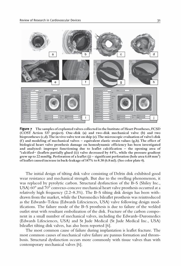
The initial design of tilting disk valve consisting of Delrin disk exhibited goodwear resistance and mechanical strength. But due to the swelling phenomenon, itwas replaced by pyrolytic carbon. Structural dysfunction of the B–S (Shiley Inc.,USA) 60� and 70� convexo-concave mechanical heart valve prosthesis occurred at arelatively high frequency (2.2–8.3%). The B–S tilting disk design has been with-drawn from the market, while the Duromedics bileaflet prosthesis was reintroducedas the Edwards–Tekna (Edwards Lifesciences, USA) valve following design mod-ifications. The failure mode of the B–S prosthesis is due to failure of the weldedoutlet strut with resultant embolization of the disk. Fracture of the carbon compo-nent in a small number of mechanical valves, including the Edwards–Duromedics(Edwards Lifesciences, USA) and St Jude Medical (St Jude Medical Inc., USA)bileaflet tilting disk valves, has also been reported [6].
The most common cause of failure during implantation is leaflet fracture. Themost common causes of mechanical valve failure are pannus formation and throm-bosis. Structural dysfunction occurs more commonly with tissue valves than withcontemporary mechanical valves [6].
a b c d
f g he
i j
Figure 7 The samples of explanted valves collected in the Institute of Heart Prostheses, FCSD(COST Action 537 project). One-disk (a) and two-disk mechanical valve (b) and twobioprostheses (c,d).The in vivo valve test on ship (e).The microscopic evaluation of valve’s disk(f ) and modeling of mechanical valves ^ equivalent elastic strain values (g,h). The effect ofbiological heart valve prosthesis damage on hemodynamic efficiency has been investigatedand analyzed: improper functioning due to leaflet calcification ^ the opening area of‘‘calcified” (leaflets partially glued (i)) valve decreased by 44%, while the pressure gradientgrew up to 22mmHg. Perforation of a leaflet (j) ^ significant perforation (hole area 6.68mm2)of leaflet caused increase in back-leakage of 147% to 8.38 (6.8ml). (See color plate 4).
Review of Research in Cardiovascular Devices 31
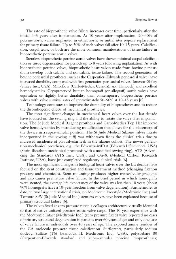
The rate of bioprosthetic valve failure increases over time, particularly after theinitial 4–5 years after implantation. At 10 years after implantation, 20–40% ofporcine aortic valves implanted in either aortic or mitral sites require replacementfor primary tissue failure. Up to 50% of such valves fail after 10–15 years. Calcifica-tion, cuspal tears, or both are the most common manifestations of tissue failure inbioprosthetic porcine aortic valves.
Stentless bioprosthetic porcine aortic valves have shown minimal cuspal calcifica-tion or tissue degeneration for periods up to 8 years following implantation. As withbioprosthetic porcine valves, bioprosthetic heart valves made from bovine pericar-dium develop both calcific and noncalcific tissue failure. The second generation ofbovine pericardial prostheses, such as the Carpentier–Edwards pericardial valve, haveincreased durability compared with first-generation pericardial valves [Ionescu–Shiley(Shiley Inc., USA), Mitroflow (CarboMedics, Canada), and Hancock] and excellenthemodynamics. Cryopreserved human homograft (or allograft) aortic valves haveequivalent or slightly better durability than contemporary bioprosthetic porcinevalves with valve survival rates of approximately 50–90% at 10–15 years [6].
Technology continues to improve the durability of bioprostheses and to reducethe thrombogenic effects of mechanical prostheses.
The most significant changes in mechanical heart valves over the last decadehave focused on the sewing ring and the ability to rotate the valve after implanta-tion. The St Jude Medical Regent prosthesis and CarboMedics Top Hat improvevalve hemodynamics by introducing modification that allows for the placement ofthe device in a supra-annular position. The St Jude Medical Silzone (silver nitrateincorporated in the sewing cuff) was withdrawn from the clinical trials due toincreased incidence of paravalvular leak in the silzone cohort. The newer genera-tion mechanical prostheses, e.g., the Edwards–MIRA (Edwards Lifesciences, USA)(Sorin Bicarbon mechanical prosthesis with a modified sewing ring), ATS (Advan-cing the Standard) (ATS Inc., USA), and On-X (Medical Carbon ResearchInstitute, USA), have just completed regulatory clinical trials [6].
The most significant changes in biological heart valves over the last decade havefocused on the stent construction and tissue treatment method (changing fixationpressure and chemicals). Stent mounting produces higher transvalvular gradientsand also causes premature valve failure. In the brief period in which homograftswere stented, the average life expectancy of the valve was less than 10 years (about90% homografts have a 10-year freedom from valve degeneration). Furthermore, todate, in two large international trials, no Medtronic Freestyle (Medtronic Inc.) andToronto SPV (St Jude Medical Inc.) stentless valves have been explanted because ofprimary structural failure [6].
The valves fixed at zero pressure retain a collagen architecture virtually identicalto that of native unfixed porcine aortic valve cusps. The 10-year experience withthe Medtronic Intact (Medtronic Inc.) (zero pressure fixed) valve reported no casesof primary structural degeneration in patients over 60 years of age and only one caseof valve failure in individuals over 40 years of age. The exposed amine residues ofthe GA molecule promote tissue calcification. Surfactants, particularly sodiumdodecyl sulfate (T6) (Hancock II, Medtronic Inc., USA), polysorbate 80(Carpentier–Edwards standard and supra-annular porcine bioprostheses;
32 Zbigniew Nawrat
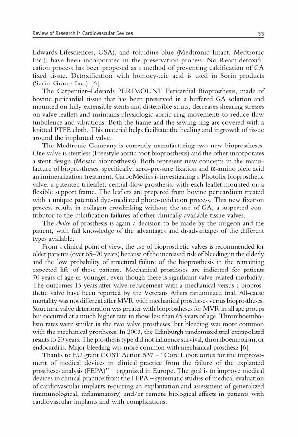
Edwards Lifesciences, USA), and toluidine blue (Medtronic Intact, MedtronicInc.), have been incorporated in the preservation process. No-React detoxifi-cation process has been proposed as a method of preventing calcification of GAfixed tissue. Detoxification with homocysteic acid is used in Sorin products(Sorin Group Inc.) [6].
The Carpentier–Edwards PERIMOUNT Pericardial Bioprosthesis, made ofbovine pericardial tissue that has been preserved in a buffered GA solution andmounted on fully extensible stents and distensible struts, decreases shearing stresseson valve leaflets and maintains physiologic aortic ring movements to reduce flowturbulence and vibrations. Both the frame and the sewing ring are covered with aknitted PTFE cloth. This material helps facilitate the healing and ingrowth of tissuearound the implanted valve.
The Medtronic Company is currently manufacturing two new bioprostheses.One valve is stentless (Freestyle aortic root bioprosthesis) and the other incorporatesa stent design (Mosaic bioprosthesis). Both represent new concepts in the manu-facture of bioprostheses, specifically, zero-pressure fixation and a-amino oleic acidantimineralization treatment. CarboMedics is investigating a Photofix bioprostheticvalve: a patented trileaflet, central-flow prosthesis, with each leaflet mounted on aflexible support frame. The leaflets are prepared from bovine pericardium treatedwith a unique patented dye-mediated photo-oxidation process. This new fixationprocess results in collagen crosslinking without the use of GA, a suspected con-tributor to the calcification failures of other clinically available tissue valves.
The choice of prosthesis is again a decision to be made by the surgeon and thepatient, with full knowledge of the advantages and disadvantages of the differenttypes available.
From a clinical point of view, the use of bioprosthetic valves is recommended forolder patients (over 65–70 years) because of the increased risk of bleeding in the elderlyand the low probability of structural failure of the bioprosthesis in the remainingexpected life of these patients. Mechanical prostheses are indicated for patients70 years of age or younger, even though there is significant valve-related morbidity.The outcomes 15 years after valve replacement with a mechanical versus a biopros-thetic valve have been reported by the Veterans Affairs randomized trial. All-causemortality was not different afterMVRwith mechanical prostheses versus bioprostheses.Structural valve deterioration was greater with bioprostheses for MVR in all age groupsbut occurred at a much higher rate in those less than 65 years of age. Thromboembo-lism rates were similar in the two valve prostheses, but bleeding was more commonwith the mechanical prostheses. In 2003, the Edinburgh randomized trial extrapolatedresults to 20 years. The prosthesis type did not influence survival, thromboembolism, orendocarditis. Major bleeding was more common with mechanical prosthesis [6].
Thanks to EU grant COST Action 537 – “Core Laboratories for the improve-ment of medical devices in clinical practice from the failure of the explantedprostheses analysis (FEPA)” – organized in Europe. The goal is to improve medicaldevices in clinical practice from the FEPA – systematic studies of medical evaluationof cardiovascular implants requiring an explantation and assessment of generalized(immunological, inflammatory) and/or remote biological effects in patients withcardiovascular implants and with complications.
Review of Research in Cardiovascular Devices 33
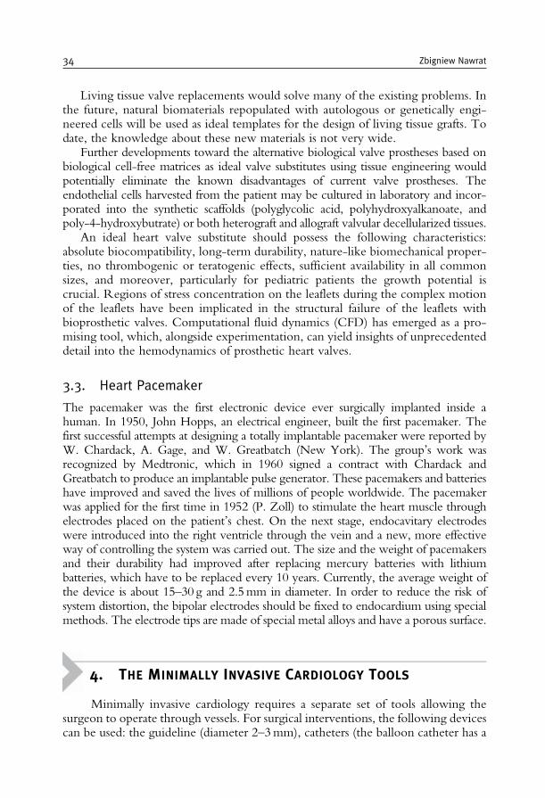
Living tissue valve replacements would solve many of the existing problems. Inthe future, natural biomaterials repopulated with autologous or genetically engi-neered cells will be used as ideal templates for the design of living tissue grafts. Todate, the knowledge about these new materials is not very wide.
Further developments toward the alternative biological valve prostheses based onbiological cell-free matrices as ideal valve substitutes using tissue engineering wouldpotentially eliminate the known disadvantages of current valve prostheses. Theendothelial cells harvested from the patient may be cultured in laboratory and incor-porated into the synthetic scaffolds (polyglycolic acid, polyhydroxyalkanoate, andpoly-4-hydroxybutrate) or both heterograft and allograft valvular decellularized tissues.
An ideal heart valve substitute should possess the following characteristics:absolute biocompatibility, long-term durability, nature-like biomechanical proper-ties, no thrombogenic or teratogenic effects, sufficient availability in all commonsizes, and moreover, particularly for pediatric patients the growth potential iscrucial. Regions of stress concentration on the leaflets during the complex motionof the leaflets have been implicated in the structural failure of the leaflets withbioprosthetic valves. Computational fluid dynamics (CFD) has emerged as a pro-mising tool, which, alongside experimentation, can yield insights of unprecedenteddetail into the hemodynamics of prosthetic heart valves.
3.3. Heart Pacemaker
The pacemaker was the first electronic device ever surgically implanted inside ahuman. In 1950, John Hopps, an electrical engineer, built the first pacemaker. Thefirst successful attempts at designing a totally implantable pacemaker were reported byW. Chardack, A. Gage, and W. Greatbatch (New York). The group’s work wasrecognized by Medtronic, which in 1960 signed a contract with Chardack andGreatbatch to produce an implantable pulse generator. These pacemakers and batterieshave improved and saved the lives of millions of people worldwide. The pacemakerwas applied for the first time in 1952 (P. Zoll) to stimulate the heart muscle throughelectrodes placed on the patient’s chest. On the next stage, endocavitary electrodeswere introduced into the right ventricle through the vein and a new, more effectiveway of controlling the system was carried out. The size and the weight of pacemakersand their durability had improved after replacing mercury batteries with lithiumbatteries, which have to be replaced every 10 years. Currently, the average weight ofthe device is about 15–30 g and 2.5mm in diameter. In order to reduce the risk ofsystem distortion, the bipolar electrodes should be fixed to endocardium using specialmethods. The electrode tips are made of special metal alloys and have a porous surface.
4. THE MINIMALLY INVASIVE CARDIOLOGY TOOLS
Minimally invasive cardiology requires a separate set of tools allowing thesurgeon to operate through vessels. For surgical interventions, the following devicescan be used: the guideline (diameter 2–3mm), catheters (the balloon catheter has a
34 Zbigniew Nawrat
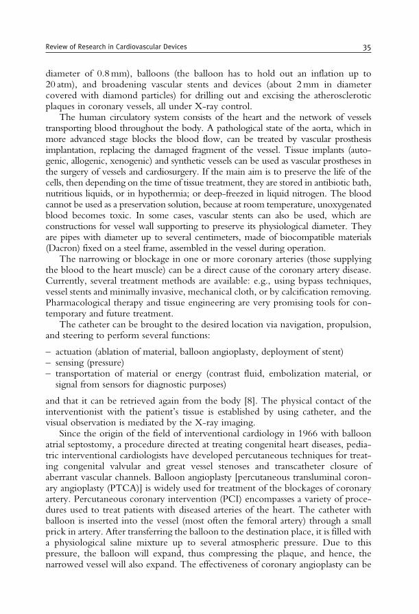
diameter of 0.8mm), balloons (the balloon has to hold out an inflation up to20 atm), and broadening vascular stents and devices (about 2mm in diametercovered with diamond particles) for drilling out and excising the atheroscleroticplaques in coronary vessels, all under X-ray control.
The human circulatory system consists of the heart and the network of vesselstransporting blood throughout the body. A pathological state of the aorta, which inmore advanced stage blocks the blood flow, can be treated by vascular prosthesisimplantation, replacing the damaged fragment of the vessel. Tissue implants (auto-genic, allogenic, xenogenic) and synthetic vessels can be used as vascular prostheses inthe surgery of vessels and cardiosurgery. If the main aim is to preserve the life of thecells, then depending on the time of tissue treatment, they are stored in antibiotic bath,nutritious liquids, or in hypothermia; or deep-freezed in liquid nitrogen. The bloodcannot be used as a preservation solution, because at room temperature, unoxygenatedblood becomes toxic. In some cases, vascular stents can also be used, which areconstructions for vessel wall supporting to preserve its physiological diameter. Theyare pipes with diameter up to several centimeters, made of biocompatible materials(Dacron) fixed on a steel frame, assembled in the vessel during operation.
The narrowing or blockage in one or more coronary arteries (those supplyingthe blood to the heart muscle) can be a direct cause of the coronary artery disease.Currently, several treatment methods are available: e.g., using bypass techniques,vessel stents and minimally invasive, mechanical cloth, or by calcification removing.Pharmacological therapy and tissue engineering are very promising tools for con-temporary and future treatment.
The catheter can be brought to the desired location via navigation, propulsion,and steering to perform several functions:
– actuation (ablation of material, balloon angioplasty, deployment of stent)– sensing (pressure)– transportation of material or energy (contrast fluid, embolization material, orsignal from sensors for diagnostic purposes)
and that it can be retrieved again from the body [8]. The physical contact of theinterventionist with the patient’s tissue is established by using catheter, and thevisual observation is mediated by the X-ray imaging.
Since the origin of the field of interventional cardiology in 1966 with balloonatrial septostomy, a procedure directed at treating congenital heart diseases, pedia-tric interventional cardiologists have developed percutaneous techniques for treat-ing congenital valvular and great vessel stenoses and transcatheter closure ofaberrant vascular channels. Balloon angioplasty [percutaneous transluminal coron-ary angioplasty (PTCA)] is widely used for treatment of the blockages of coronaryartery. Percutaneous coronary intervention (PCI) encompasses a variety of proce-dures used to treat patients with diseased arteries of the heart. The catheter withballoon is inserted into the vessel (most often the femoral artery) through a smallprick in artery. After transferring the balloon to the destination place, it is filled witha physiological saline mixture up to several atmospheric pressure. Due to thispressure, the balloon will expand, thus compressing the plaque, and hence, thenarrowed vessel will also expand. The effectiveness of coronary angioplasty can be
Review of Research in Cardiovascular Devices 35
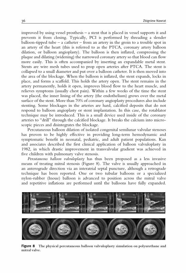
improved by using vessel prosthesis – a stent that is placed in vessel supports it andprevents it from closing. Typically, PCI is performed by threading a slenderballoon-tipped tube – a catheter – from an artery in the groin to a trouble spot inan artery of the heart (this is referred to as the PTCA, coronary artery balloondilation, or balloon angioplasty). The balloon is then inflated, compressing theplaque and dilating (widening) the narrowed coronary artery so that blood can flowmore easily. This is often accompanied by inserting an expandable metal stent.Stents are wire mesh tubes used to prop open arteries after PTCA. The stent iscollapsed to a small diameter and put over a balloon catheter. It is then moved intothe area of the blockage. When the balloon is inflated, the stent expands, locks inplace, and forms a scaffold. This holds the artery open. The stent remains in theartery permanently, holds it open, improves blood flow to the heart muscle, andrelieves symptoms (usually chest pain). Within a few weeks of the time the stentwas placed, the inner lining of the artery (the endothelium) grows over the metalsurface of the stent. More than 70% of coronary angioplasty procedures also includestenting. Some blockages in the arteries are hard, calcified deposits that do notrespond to balloon angioplasty or stent implantation. In this case, the rotablatortechnique may be introduced. This is a small device used inside of the coronaryarteries to “drill” through the calcified blockage. It breaks the calcium into micro-scopic pieces and disintegrates the blockage.
Percutaneous balloon dilation of isolated congenital semilunar valvular stenoseshas proven to be highly effective in providing long-term hemodynamic andsymptomatic benefit in neonatal, pediatric, and adult patient populations. Kanand associates described the first clinical application of balloon valvuloplasty in1982, in which drastic improvement in transvalvular gradient was achieved infive children with pulmonary valve stenosis.
Percutaneous balloon valvuloplasty has thus been proposed as a less invasivemeans of treating mitral stenosis (Figure 8). The valve is usually approached inan anterograde direction via an interatrial septal puncture, although a retrogradetechnique has been reported. One or two tubular balloons or a specializednylon-rubber (Inoue) balloon is advanced to position across the mitral valveand repetitive inflations are performed until the balloons have fully expanded.
Figure 8 The physical percutaneous balloon valvuloplasty simulation on polyurethane andmitral valve.
36 Zbigniew Nawrat
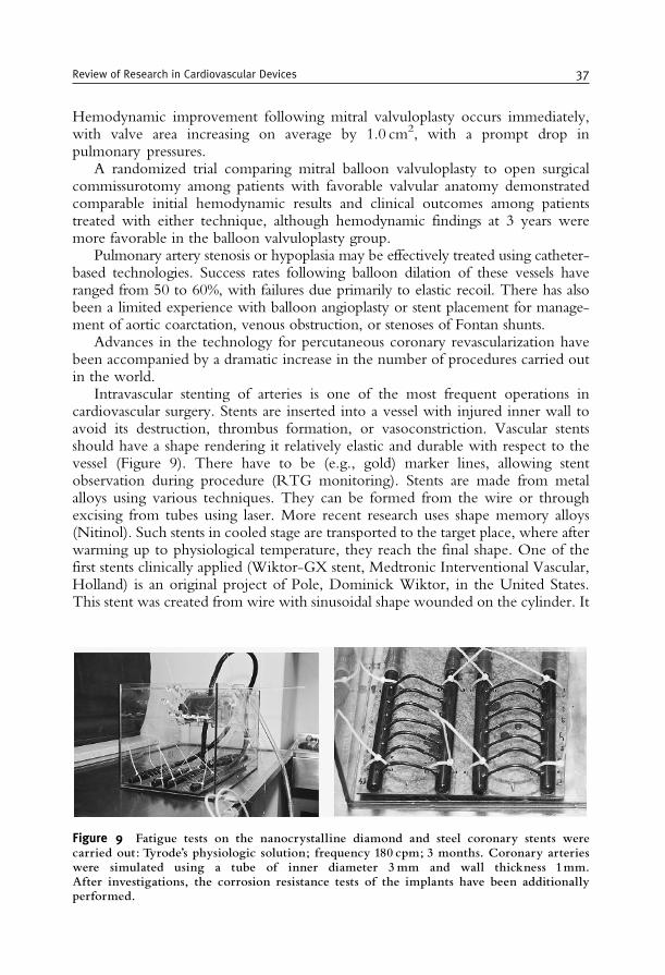
Hemodynamic improvement following mitral valvuloplasty occurs immediately,with valve area increasing on average by 1.0 cm2, with a prompt drop inpulmonary pressures.
A randomized trial comparing mitral balloon valvuloplasty to open surgicalcommissurotomy among patients with favorable valvular anatomy demonstratedcomparable initial hemodynamic results and clinical outcomes among patientstreated with either technique, although hemodynamic findings at 3 years weremore favorable in the balloon valvuloplasty group.
Pulmonary artery stenosis or hypoplasia may be effectively treated using catheter-based technologies. Success rates following balloon dilation of these vessels haveranged from 50 to 60%, with failures due primarily to elastic recoil. There has alsobeen a limited experience with balloon angioplasty or stent placement for manage-ment of aortic coarctation, venous obstruction, or stenoses of Fontan shunts.
Advances in the technology for percutaneous coronary revascularization havebeen accompanied by a dramatic increase in the number of procedures carried outin the world.
Intravascular stenting of arteries is one of the most frequent operations incardiovascular surgery. Stents are inserted into a vessel with injured inner wall toavoid its destruction, thrombus formation, or vasoconstriction. Vascular stentsshould have a shape rendering it relatively elastic and durable with respect to thevessel (Figure 9). There have to be (e.g., gold) marker lines, allowing stentobservation during procedure (RTG monitoring). Stents are made from metalalloys using various techniques. They can be formed from the wire or throughexcising from tubes using laser. More recent research uses shape memory alloys(Nitinol). Such stents in cooled stage are transported to the target place, where afterwarming up to physiological temperature, they reach the final shape. One of thefirst stents clinically applied (Wiktor-GX stent, Medtronic Interventional Vascular,Holland) is an original project of Pole, Dominick Wiktor, in the United States.This stent was created from wire with sinusoidal shape wounded on the cylinder. It
Figure 9 Fatigue tests on the nanocrystalline diamond and steel coronary stents werecarried out: Tyrode’s physiologic solution; frequency 180 cpm; 3 months. Coronary arterieswere simulated using a tube of inner diameter 3mm and wall thickness 1mm.After investigations, the corrosion resistance tests of the implants have been additionallyperformed.
Review of Research in Cardiovascular Devices 37
is made from tantalum, instead of steel, because of its better contrast in RTGvisualization and the electronegative surface improving thromboresistance of thestent. The first clinical implantation of stent was performed in 1989. The materialsused for the construction of these stents have changed dramatically over the past10 years. Unfortunately, metal stents induce thrombus formation. Stent biocom-patibility can be enhanced by either modifying the metal surface of the implant orapplying biocompatible coatings. To improve its biocompatibility and to preventthe closing of renewed vessel, the surface of stents is covered with heparin. Stentingprocedures can also be connected with genetic therapy by covering its surface by alayer of polymer, which when placed into the vessel wall releases the geneticmaterial, which blocks the cell growth. In Poland, the multidisciplinary teamworks on original vascular stents covered with a layer of nanocrystalline diamond.
Currently, multiple research projects are focused on the design of a stent withbetter radiopacity, reduced stent–vessel wall contact area, and improved elasticity,and thrombogenic effects are lowered when the stent is coated with the properantithrombotic substances. The problem that plagues about one-third of patientswho receive angioplasty with or without stents is “restenosis” – the recurrence ofthe narrowing of the blood vessel. The new drug-coated stents release a medicationthat blocks this scarring process.
Novel technologies will be introduced and developed, directed at the efficientremoval or modification of arterial plaques with minimal arterial trauma or atsite-specific drug delivery to inhibit thrombosis and restenosis. Concurrently,intravascular ultrasound and angioscopy will be further refined and integratedinto revascularization devices, allowing precise guidance and optimization of pla-que ablation or remodeling while limiting associated coronary injury. Finally,understanding of the vascular biology of percutaneous revascularization, thrombo-sis, and restenosis will be improved, leading to pharmacological therapies designedto ameliorate adverse thrombotic, proliferative, and remodeling responses.
5. THE TECHNOLOGY FOR ATRIAL FIBRILLATION
The evolving technologies for ablation of atrial fibrillation include radiofrequency, cryotherapy, microwave, laser, and ultrasound. The efforts directed atisolating and ablating percutaneous catheter pulmonary vein have essentially beenabandoned because of the extensive length of procedures and the high incidence ofpulmonary vein stenosis. The newer technologies have been developed to createtransmural lesions during cardiac surgery [6].
Radiofrequency used in ablation: Radio frequency corresponds to the frequency ofunmodulated alternating current delivered in the range of 0.5–1.0MHz betweentwo electrodes, one located on the endocardial surface and the other on the skin. Itsheating effect produces homogeneous lesions that measure a few millimeters indiameter and depth. It has been demonstrated that reliable and effective ablation isperformed at 70�C for 60 s. The goal temperature should never be set at more than95�C to avoid potential tissue disruption.
38 Zbigniew Nawrat
Cryoablation: Cryoablation has an excellent clinical safety record, although its usein atrial fibrillation surgery has been limited to creating spot lesions over the tricuspidand mitral valve annuli. The salient features of the procedure are rapid freezing, andslow thawing with repeated freeze–thaw cycles. The coldest temperature (the primedeterminant of cell death) may range from –50�C to –150�C and the application timecan vary between 0.5 and 5min, depending on the area of application.
Laser ablation: The laser lesion formation is thermal through photon absorptionat the surface, with deeper myocardial sites heated through passive conduction. Thewavelength chosen for good penetration is 980 nm (using a 980-nm diode laser).This wavelength ablates tissue with absorption of actual laser energy as deep as4mm into the tissue and further ablation by conductive heating mechanisms. Thelesion times are for 36 s utilizing 5W/cm, but ablation cannot be longer than 5 cm.
Microwave ablation: The electromagnetic microwaves occur at 2.45GHz togenerate frictional heating by induction of dielectric ionic movements. The micro-wave device can provide a range of 40–45W of power for 20–30 s, generating aconsistent 3–6mm lesion depth sufficient to produce transmural ablation.
Ultrasound ablation: This technology uses an ultrasound transducer to delivermechanical pressure waves at high frequency. The tissue destruction is thermal andlesion depth corresponds to vibrational frequency. The ultrasound wave emittedfrom the transducer travels through tissue causing compression, refraction, andparticle movement, resulting in kinetic energy and heat [6].
6. MINIMALLY INVASIVE SURGERY
Minimally invasive surgery, a keyhole surgery, is an operation technique inwhich access to the inside of the patient’s body is achieved via small incisions. Thelong rigid instruments inserted via trocars can be used to move, retract, and cuttissue in abdomen (laparoscopy), chest (thoracoscopy), blood vessels (angioscopy),gastrointestinal tract (colonoscopy), uterus (hysteroscopy), and joints (arthero-scopy). Insufflation of the body cavity may be carded out and maintained by sealson the trocar port, which allow tool manipulation without excessive loss ofinsufflation gas [8]. The trocars may be sized to provide ports of differing sizes,typically of about 5–11mm diameter. Currently, tools such as retractors, forceps,graspers, suture needles, scissors, different types of knives, laser incision instruments,and specimen bags are available. A video camera is generally operated through atrocar port for visualization and control of the procedures in the cavity. High-definition video cameras and monitors are then attached to the camera and asurgical team can obtain a clear picture of the affected internal area withoutresorting to radical, disfiguring surgical incisions to physically open the patient.Another benefit of laparoscopic surgery is the significantly reduced recovery time,when compared to standard surgical procedures, due to the minuscule size of thescalpel incisions and avoidance of the massive internal traumatization known instandard surgical procedures.
Review of Research in Cardiovascular Devices 39
Due to fixed entry points of the instruments in the abdominal wall, the DOF isreduced, and the movements are mirrored and scaled. The coupling betweenobservation and manipulation, the hand–eye coordination is disturbed, tactileinformation about tissue properties partially, due to friction and the poor ergo-nomic design of instruments, lost. The future is open for semiautomatic tools forMIS. As an example, Medtronic, Inc., has introduced the world’s first minimallyinvasive epicardial lead placement tool. The Medtronic Model 10626 EpicardialLead Implant Tool allows for perpendicular alignment to the heart from differentangle approaches. The tool furthers the trend moving away from invasive sternot-omy procedures. Laparoscopy reduces patient trauma, but eliminates the surgeon’sability to directly view and touch the surgical environment. This is reason that thesurgeon introduced the small-incision surgery when they have a direct view of thetissue.
The rapid development and growing interest in MIS methods impelled creationof modern, complicated tools: cardiosurgical robots.
6.1. The Classical Thoracoscopic Tools
Laparoscopic or thoracoscopic surgery requires that surgeons perform complexprocedures using a standardized set of tools. For laparoscopic procedures, specialsewing devices, ligating instruments, knot pushers, clips, and clip appliers have beendeveloped. The clamp is an essential tool for stopping or controlling blood flow toan organ during surgery. There is a need for a secure and easy method of suturing inlaparoscopic surgery. Laparoscopic suturing can be performed with a suture, usingautomatic sewing devices or clips. When a surgeon wants to suture laparoscopicallyin the traditional way by using a Roeder knot for instance, the tying of the knotrequires some expertise and makes the procedure more complicated and time-consuming. The vascular clips provide a very easy (and secure) method of stoppingblood flow while performing procedures on vessels. The locking forceps allowseasy, precise, and secure grasping of the surgical clips. The risky point of a clip is theopen end of its U-shaped design, which makes it possible for the clip to slip off.Sutures avoid this risk by totally enclosing the structure to be occluded. Knottinginstruments require a two-forcep technique, whereas sewing devices require onlyone working channel.
There has been a tremendous interest in the development of anastomotic devicesfor coronary surgery. Coronary artery disease is a major health problem worldwide,with approximately 850,000 bypass procedures being performed every year. Thecurrent methods of coronary bypass surgery can be time-consuming and technicallydifficult especially when minimally invasive instruments for suturing the bloodvessels (the connection is called anastomosis) are used. Alexis Carrel, who manyconsider the father of anastamoses, received a Nobel Prize for the suturing of bloodvessels about 100 years ago. More than 5 million vascular anastomoses areperformed annually in the world and more than 70% often are on the CABGmarket [9].
The requirements of anastomotic devices include reproducibility, ease of use,and a short anastomotic time (less than1min). The anastomotic device ideally
40 Zbigniew Nawrat
would work with either vein or artery and so the proximal or distal order ofanastomoses should be interchangeable. The device should facilitate a wide rangeof surgical access points and should have patency comparable to that of hand-sewntechniques [9].
There are manual and automatic anastomotic devices. The manual proximalanastomotic devices Heartstring Aortic Occluder
TM
from Guidant (that acts as anumbrella inside an aortotomy) and the Enclose
TM
device from Novare Medical(require a separate insertion through the aorta) create a dry area for conventionalsuturing in aortotomies.
The SymmetryTM
Bypass System Aortic Connector is the first in a line ofsutureless anastomoses devices for CABG developed by St Jude Medical, Inc.,Cardiac Surgery Division – Anastomotic Technology Group (ATG), formerlyVascular Science, Inc. (VSI). There have been more than 50,000 implantsperformed.
CardioVationsTM
has released the CorlinkTM
proximal device in Europe. This is aNitinol-based stent device. The major difference in comparison with Symmetry isthat the Corlink device sits outside of the vein graft wall and the Symmetry devicelies inside the vein graft wall.
The PassportTM
automatic proximal device consists of an integrated system thatperforms the aortotomy, delivers the graft to the aorta, and deploys a stainless-steelconnector end-to-side the graft using a delivery device. The stainless-steel stent(more rigid than Nitinol) creates a widely patented anastomosis.
Another proximal anastomotic device is the Magnaport from Ventrica. This isalso a one-step anastomotic device using rare earth magnets.
Coalescent SurgicalTM
has developed an automatic proximal anastomotic device,called the Spyder� based on their proprietary Nitinol (nickel–titanium) cliptechnology.
The first distal device to market (launched in 2000) was the manual CoalescentU-CLIP
TM
. This is a self-closing, penetrating device with bailout. The U-CLIPdevice is designed to provide an alternative to conventional suture and surgicalclips in a variety of applications including anastomosis creation and tissueapproximation. The device consists of a self-closing surgical clip attached to aconventional surgical needle by a flexible member. U-CLIP device placement iseasy and requires only standard surgical instrumentation. The self-closing clipeliminates the requirement for knot-tying and suture management. A fresh, sharpneedle is provided with each clip. The clip is easily removed. The U-CLIPanastomotic device technology consistently facilitates the interrupted techniquein both on-pump (or surgery performed with a cardiopulmonary bypassmachine) and off-pump (also known as beating-heart, CABG procedures).Independent core laboratory analysis demonstrated that the left internal mam-mary artery to the left anterior descending coronary artery (LIMA to LADA)anastomoses created with the U-CLIP anastomotic device were 100% perfectlypatented at 6 months [9].
The Spyder device provides fast, automated proximal anastomotic connectionby simultaneous delivery of six U-CLIP devices without the use of a side-bitingclamp or second manipulation of the aorta. The JoMed Solem connector consists
Review of Research in Cardiovascular Devices 41
of a stented “T”-shaped PTFE graft connected to the internal mammary artery. TheSt Jude distal connector consists of a stent that is deployed with a balloon using a side-to-side technique to create a distal coronary anastomosis. The Converge Medical deviceconsists of outer and inner Nitinol couplers that are placed on the vein graft. Thisdevice allows for an angled anastomosis and creates elliptical interface. MagneticVascular Positioner (MVP), developed by Ventrica (received CE Mark approval inFebruary 2002), uses magnetic attraction to form an instantaneous self-aligning, self-sealing connection between two blood vessels. The elliptical magnets are placed insidethe conduit and native vessel. The MVP device connects the “bypass graft” to thecoronary artery in seconds, and is designed to be used in the distal, or smallest, portionof the coronary arteries.
Anastomotic devices in OPCAB may play their most important role in theproximal anastomosis. The major meta-analyses reveal the significant benefits ofperforming OPCAB (off-pump coronary artery bypass) over CCABG (conven-tional coronary artery bypass) for certain patient populations requiring myocardialrevascularization procedures. The technology has potential benefits as a replace-ment for sutures due to shorter procedure times, uniform and repeatable connec-tions, and the potential to allow for significantly smaller incisions. This would allowproximal anastomoses to be performed with minimal aortic manipulation, whichmay result in a lower rate of intra- and postoperative embolism. An automateddistal device could facilitate lateral wall grafting in OPCAB. In total endoscopiccoronary artery bypass (TECAB), a distal automatic device could be critical inevolving the endoscopic procedure. Currently, the Ventrica device is being mod-ified for deployment in a robotic environment. Finally, in multivessel TECABprocedures, distal anastomotic devices are predicted to make a major contribution.Most minimally invasive procedures in the future will be facilitated by an auto-mated anastomotic device. The automated anastomotic device will level the playingfield and allow for more surgeons to perform more perfect anastomoses. Wolfconcluded that with continued evolution of these devices, it is easy to anticipatethat in the near future the majority of anastomoses may be performed with a manualor automatic device as opposed to the current conventional suture technique [9].The leaders of clinical trials of these new methods are Randall K. Wolf andVolkmar Falk, MD.
Since 1997, Medtronic has been a pioneer in minimally invasive, beating-heartsurgery with the introduction of the Octopus tissue stabilizer system and its familyof products, and most recently with the release of the Starfish2 heart positioner.
In traditional open-heart surgery, the heart is stopped and an artificial pump isused to maintain blood circulation. This is highly traumatic as the blood flow isrerouted through a machine. Many patients with coronary heart disease undergoopen-heart operations, especially bypass surgery. These are traditionally performedwith a heart–lung machine. The machine serves as a substitute for the patient’s ownbeating heart and lungs, allowing the organs to function while surgeons operate ona “still” heart.
Endoscopic surgery in a major cavity in the body requires space for manipula-tion and local cardiac wall immobilization for coronary artery grafting on theworking heart. One of the revolutionary instrument used in beating-heart surgery
42 Zbigniew Nawrat
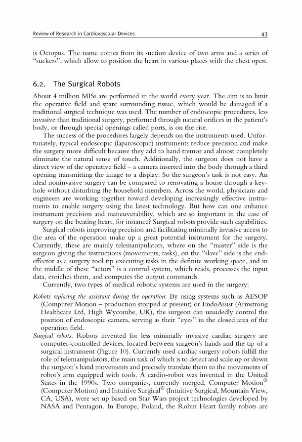
is Octopus. The name comes from its suction device of two arms and a series of“suckers”, which allow to position the heart in various places with the chest open.
6.2. The Surgical Robots
About 4 million MISs are performed in the world every year. The aim is to limitthe operative field and spare surrounding tissue, which would be damaged if atraditional surgical technique was used. The number of endoscopic procedures, lessinvasive than traditional surgery, performed through natural orifices in the patient’sbody, or through special openings called ports, is on the rise.
The success of the procedures largely depends on the instruments used. Unfor-tunately, typical endoscopic (laparoscopic) instruments reduce precision and makethe surgery more difficult because they add to hand tremor and almost completelyeliminate the natural sense of touch. Additionally, the surgeon does not have adirect view of the operative field – a camera inserted into the body through a thirdopening transmitting the image to a display. So the surgeon’s task is not easy. Anideal noninvasive surgery can be compared to renovating a house through a key-hole without disturbing the household members. Across the world, physicians andengineers are working together toward developing increasingly effective instru-ments to enable surgery using the latest technology. But how can one enhanceinstrument precision and maneuverability, which are so important in the case ofsurgery on the beating heart, for instance? Surgical robots provide such capabilities.
Surgical robots improving precision and facilitating minimally invasive access tothe area of the operation make up a great potential instrument for the surgery.Currently, these are mainly telemanipulators, where on the “master” side is thesurgeon giving the instructions (movements, tasks), on the “slave” side is the end-effector as a surgery tool tip executing tasks in the definite working space, and inthe middle of these “actors” is a control system, which reads, processes the inputdata, enriches them, and computes the output commands.
Currently, two types of medical robotic systems are used in the surgery:
Robots replacing the assistant during the operation: By using systems such as AESOP(Computer Motion – production stopped at present) or EndoAssist (ArmstrongHealthcare Ltd, High Wycombe, UK), the surgeon can unaidedly control theposition of endoscopic camera, serving as their “eyes” in the closed area of theoperation field.
Surgical robots: Robots invented for less minimally invasive cardiac surgery arecomputer-controlled devices, located between surgeon’s hands and the tip of asurgical instrument (Figure 10). Currently used cardiac surgery robots fulfill therole of telemanipulators, the main task of which is to detect and scale up or downthe surgeon’s hand movements and precisely translate them to the movements ofrobot’s arm equipped with tools. A cardio-robot was invented in the UnitedStates in the 1990s. Two companies, currently merged, Computer Motion�
(Computer Motion) and Intuitive Surgical� (Intuitive Surgical, Mountain View,CA, USA), were set up based on Star Wars project technologies developed byNASA and Pentagon. In Europe, Poland, the Robin Heart family robots are
Review of Research in Cardiovascular Devices 43
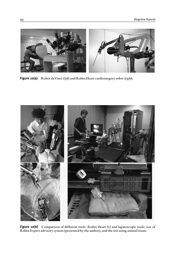
Figure 10(a) Robot daVinci (left) andRobin Heart cardiosurgery robot (right).
Figure 10(b) Comparison of different tools: Robin Heart 0,1 and laparoscopic tools; test ofRobin Expert advisory system (presented by the author); and the test using animal tissue.
44 Zbigniew Nawrat
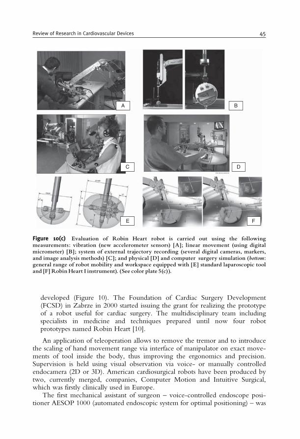
developed (Figure 10). The Foundation of Cardiac Surgery Development(FCSD) in Zabrze in 2000 started issuing the grant for realizing the prototypeof a robot useful for cardiac surgery. The multidisciplinary team includingspecialists in medicine and techniques prepared until now four robotprototypes named Robin Heart [10].
An application of teleoperation allows to remove the tremor and to introducethe scaling of hand movement range via interface of manipulator on exact move-ments of tool inside the body, thus improving the ergonomics and precision.Supervision is held using visual observation via voice- or manually controlledendocamera (2D or 3D). American cardiosurgical robots have been produced bytwo, currently merged, companies, Computer Motion and Intuitive Surgical,which was firstly clinically used in Europe.
The first mechanical assistant of surgeon – voice-controlled endoscope posi-tioner AESOP 1000 (automated endoscopic system for optimal positioning) – was
A B
C D
E F
Figure 10(c) Evaluation of Robin Heart robot is carried out using the followingmeasurements: vibration (new accelerometer sensors) [A]; linear movement (using digitalmicrometer) [B]; system of external trajectory recording (several digital cameras, markers,and image analysis methods) [C]; and physical [D] and computer surgery simulation (bottom:general range of robot mobility and workspace equipped with [E] standard laparoscopic tooland [F] Robin Heart I instrument). (See color plate 5(c)).
Review of Research in Cardiovascular Devices 45
introduced by firm CM in 1994. In January–May 1998, a French team in Paris anda German group from Leipzig performed using da Vinci (Figure 10a) (IS) tele-manipulator the first endoscopic operation of single coronary bypass and mitralvalvuloplasty. About 1000 surgical and endocamera robots were installed in clinics;to date, more than 130,000 minimally invasive procedures, across a wide range ofsurgical applications such as general surgery, gynecology, spinal, urology, andcardiothoracic surgery, have been performed in several counters (also in Poland,Katowice) [11].
In 1999, the Zeus surgical system made history in the world’s first robot-assistedbeating-heart bypass surgery, by Douglas Boyd, MD. In 2001, the first transatlantictelesurgical procedure was performed using the Zeus system. The doctors in NewYork removed a gallbladder of a 68-year-old patient in Strasbourg, France, and theprocedure was successful with no complications.
In traditional laparoscopic surgery, the operating surgeon does not have directvisual control of the operative field due to manual camera control by an assistant.Ideally, the surgeon should have full control of operative instruments and theoperative field. Camera holders should return camera control to the surgeon andstabilize the visual field during minimally invasive procedures. The active andpassive camera holders offer the surgeon an alternative and better tool to controlthe operating surgeon’s direct visual field. One of the first, active teleoperatedrobots introduced into clinical practice was produced by Computer Motion (US)Company. Currently, more than 1500 of Computer Motion’s robotic systems(AESOP, Zeus) are in use worldwide in 900 hospitals by more than 3000 surgeonsin 32 countries. The Zeus system consists of three robotic arms mounted onto anoperating table. Two arms hold surgical instruments, and the third arm holds andpositions the endoscope via voice control. All three arms are connected to a masterconsole where the surgeon telemanipulates the arms. The handles used to controlthe movement of the surgical instruments are similar to the instruments used inconventional surgery. The surgeon’s manual movements are filtered and scaled forthe slave instruments to perform precise microsurgery. The Zeus system can beused in combination with an independent 3D visualization system (AESOP). Morethan 300,000 surgical procedures have been performed with Computer Motion’srobotic systems assistance. The AESOP system is both CE marked and FDAapproved and has been used in more than 100,000 laparoscopic and endoscopicprocedures. The duration of several types of endoscopic surgery was reportedlyfaster using the AESOP; voice control was considered to be more efficient andfaster than either the foot or hand control.
The disadvantages for the AESOP include the constant voice commands, whichmay be distracting. In addition, the voice control is slower compared to the rapidcamera movements achieved by an experienced assistant. The AESOP is intendedto facilitate solo-surgeon laparoscopic procedures; however, the surgeon may stillneed an assistant to control the fourth laparoscopic port. The Intuitive Surgical Inc.(US) da Vinci telemanipulator consists of three or four robotic arms in one set fixedon one common column, placed near the operating table.
In contrast to the AESOP system, da Vinci arm for camera holding is integratedwith all robotic arms. Today approximately 400 da Vinci systems have been
46 Zbigniew Nawrat
installed worldwide, and its applications have been described in thousands ofscientific publications and presentations. It is CE marked and FDA approved andused in more than 300 hospitals in America and Europe. The da Vinci was used inat least 16,000 procedures in 2004 and sells for about $1.3 million.
In Europe, the Armstrong Healthcare Ltd (UK) produced telemanipulatorEndoAssist. A robot system EndoAssist holds a conventional laparoscopic telescopeand camera, coordinated by the surgeon’s head movements. EndoAssist (CEmarked and approved by FDA) has also been used in telesurgical applicationswith control via a joystick communicating with the robot over a telephone line.About 30 systems installed worldwide now has been used in several thousandclinical procedures.
The future of robotic surgery has significant potential that has been proven inmany clinical applications. The procedure completed without the need for anadditional assistant is called a “solo surgery”. Robotic assistance has enabled a solosurgery approach. The basic principle of manipulator construction is that of a serialarchitecture of joints and links with a fixed remote center in the corporeal wall. Forinstance, the da Vinci robot have seven DOFs: three (yaw, pitch, and insertion)have surgical manipulators provide motion coupling to the end-effector, anexchangeable instrument that adds four DOFs (roll, pitch, yaw, and grip) bymeans of a cable-driven mechanical wrist. The surgeon controls the movementsof tools via a human machine. The slave is capable of detecting force feedback(tissue contact, collision of manipulator) greater than 2.2N. Scaling is useful in therange from 1:1 to 10:1, in combination with tremor filtering greater than 6Hz [12].
The computer and laboratory tests are required to design a new, smart surgeryrobot and expanding its applications to the field of medicine. The 3D computersimulation and physical modeling will continue to be supported on Polish grants.
The use of conventional endoscopic instruments allows a limited range ofmotion by the trocars through which the instruments are introduced and byreduction to only four DOFs for tools. Long and rigid instruments are harder tocontrol and amplify tremor.
Six DOFs are required to perform a free motion. For instance, suturingperpendicular to the four-DOF tool’s shape becomes impossible. The studyshows that using four-DOF robot (Zeus system, Computer Motion) the 1.5mmtube anastomosis was performed in 46min compared to only 12min performed bysix-DOF robots (da Vinci). Endoscopic tissue manipulation and suturing usingfour-DOF instrumentation requires skill and training.
Cardiac surgery is carried out on soft tissues. Results obtained from surgicalaction analysis allowed to determine the maximum values of forces needed fortypical procedures performed in heart area, using different types of tools. This canbe the basis for cardiac surgery robot design assumption, in the field connected withcontrolling of robot tool movements. The penetration of soft tissue involves actionssuch as cutting, slicing, inserting a needle, and knotting. The difficulty with softtissue is that it deforms and changes shape. The map of force resistance duringpricking for left and right heart chamber was obtained (i.e., the basic mechanicalproperties of typical surgical actions; from the FCSD). For example, the maximalforce value for surgical needle Prolene 3/0 during pricking through papillary
Review of Research in Cardiovascular Devices 47
muscle reached the 150G, the measured load value equaled 200G (2 cm depth)during scalpel cutting procedure for the left ventricle (the mitral valve ring), and upto 200G with 0.1mm/s test speed for sewing tests – the knot-tying using Proleneneedle.
One of the limitations of current surgical robots used in surgery is the lack ofhaptic feedback. Although current surgical robots improve surgeon dexterity,decrease tremor, and improve visualization, they lack the necessary fidelity tohelp a surgeon characterize tissue properties for improving diagnostic capabilities.Many research groups focus on the development of tools and software that willallow haptic feedback to be integrated in a robot-assisted surgical procedure.
The surgeon needs assistants of next robot arm during operation mainly forstabilization of the heart (beating-heart bypass grafting) or another tissue. Severaltrials using two da Vinci consoles delivered good results. In response, the ISprepared the da Vinci S model with four arms.
The devices providing an “inside equipment store” for the surgeon are alsoneeded. A self-sufficient Cargo Module was developed as a transportation anddepot device by Dresden group. With the Assist Module, the surgical equipment,tissue, and vessels can be positioned on a desired place in the operating field. Thismodule provides the surgeon an “assistant” inside the closed chest.
Potential applications of robotics in cardiac surgery includes aortic valve repla-cement (standard or percutaneous technology); tricuspid valve repair; descendingthoracic aortic surgery; transmyocardial laser revascularization; ventricular septaldefect, patent ductus arteriosus, coarctation; and intramyocardial delivery platformfor biological agents such as stem cells, molecular therapeutics, genetic vectors, andAORobAS (Artificial Organs Robotically Assisted Surgery).
In the Institute of Heart Prostheses, FCSD, surgeries related to artificial organ(AO) implantation are performed. Our future plans, AORobAS, include carryingout a robotically assisted less invasive procedures to implant pumps and valves.
The da Vinci system is therefore the only surgical telemanipulator that iscurrently clinically being used. Due to the actual range of the system acceptance,the number of endoscopic cardiac procedures performed in 2005 worldwide(reported in a company-based registry) was 2984 and it increased steadily. Thisincludes TECAB procedures or small access single- or multivessel coronary arterybypass procedures with endoscopic uni- or bilateral ITA harvest (1784 procedures).The number of MVR increased to about 450 cases in 2004, to more than 600 in2005, to 850 in the first 10 months of 2006 (reported in a company-basedregistry) [13].
The number of procedures performed may increase due to development of andimprovement in facilitating anastomotic devices (MVP magnetic coupling device)and augmented reality with preoperative planning and intraoperative navigation.Based on the preoperation cardiac surgery simulation results, the optimization ofcardiac surgery procedures can be achieved.
The effectiveness and expansion of robot’s application fields requires searchingthe most effective cardiac robots in the wide application range, building thestrategy of its usage, simulating the operation results, and creating the knowledgebase supporting the robot’s arm navigation and cardiac surgeon decision
48 Zbigniew Nawrat
making, and studying image processing methods for optimal robot’s armnavigation [13].
6.3. Blood Pumps – MIS Application Study
The use of the mechanical circulatory support systems (TAHs and VADs) hasevolved significantly over the last 30 years, with more than 10,000 patients beingsupported by these devices (TAH 2%). The devices have evolved from extracor-poreal devices (such as Jarvik 7, Thoratec, Abiomed systems), driven by largepneumatic consoles, to electrically driven partially implantable devices with por-table controllers carried by the patient (such as Novacor, HeartMate).
The future prospects of the mechanical circulatory support clearly lie in threemajor areas:
1. active left ventricular pump system, which supports and stabilizes the heart inextremely critical situations (e.g., acute heart attack), and can be implanted for aperiod of up to 5 days (e.g., Impella� Acute)
2. devices as a bridge to recovery (e.g., pulsatile pumps: Novacor, HeartMate;rotary pumps: MicroMed, Jarvik-Heart, Nimbus-HeartMate II)
3. devices as an alternative to the cardiac transplantation and conventional therapy(e.g., destination therapy : LionHeart, AbioCor TAH)
6.3.1. Minimally invasive VAD implantationDr J. Donald Hill of the California Pacific Medical Center (San Francisco, CA,USA) has successfully performed the less invasive Thoratec LVAD surgery onseveral patients.
The patient is placed on the cardiopulmonary bypass using the right or leftfemoral artery or vein. The VAD cannulation system is placed in the left ventricularapex (VAD inflow) and the ascending aorta (VAD outflow), using two separateincisions. The procedure offers the following advantages: no sternotomy, easierreoperation, less blood use, reduced risk of sensitization, and it is psychologicallymore acceptable (according to Dr Hill, the Thoratec Laboratories).
General steps in VAD implantation are as follows: anesthesia is administered tothe patient; preparing the operating area – cardiopulmonary bypass (if required) andlung deflation; choosing the exit site for LVAD – depending on the need of LVADalone or of BiVAD, one or two outflow and inflow grafts will be necessary; aorticand pulmonary artery anastomoses performed; left and right ventricular apical oratrial cannulation performed; connecting the VAD to the cannulas, deaerating theVAD; gradually discontinue cardiopulmonary bypass and allow the VAD to run in“fill-to-empty” mode; completing surgery.
Our plans include carrying out robotically assisted less invasive procedures toimplant VADs (Figure 11), TAHs, valves, and vessel prostheses. The rapid evolutionof MIS techniques for heart prostheses will have implications for designing and con-struction of heart prostheses. Our team works on the designing of heart pumps andvalves particularly for robot and MIS applications and special tools of robot are beingconstructed. I am sure that this is the future of this domain of biomedical engineering.
Review of Research in Cardiovascular Devices 49
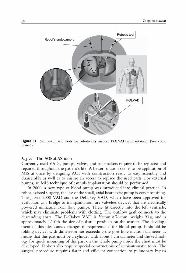
6.3.2. The AORobAS ideaCurrently used VADs, pumps, valves, and pacemakers require to be replaced andrepaired throughout the patient’s life. A better solution seems to be application ofMIS at once by designing AOs with construction ready to easy assembly anddisassembly as well as to ensure an access to replace the used parts. For externalpumps, an MIS technique of cannula implantation should be performed.
In 2000, a new type of blood pump was introduced into clinical practice. Inrobot-assisted surgery, the use of the small, axial heart assist pump is very promising.The Jarvik 2000 VAD and the DeBakey VAD, which have been approved forevaluation as a bridge to transplantation, are valveless devices that are electricallypowered miniature axial flow pumps. These fit directly into the left ventricle,which may eliminate problems with clotting. The outflow graft connects to thedescending aorta. The DeBakey VAD is 30mm� 76mm, weighs 93 g, and isapproximately 1/10th the size of pulsatile products on the market. The develop-ment of this idea causes changes in requirements for blood pump. It should befolding device, with dimension not exceeding the port hole incision diameter. Itmeans that this part must be a cylinder with about 1 cm diameter and the technol-ogy for quick mounting of this part on the whole pump inside the chest must bedeveloped. Robots also require special constructions of semiautomatic tools. Thesurgical procedure requires faster and efficient connection to pulmonary bypass
Robot’s tool
Robot’s endocamera
POLVAD
Figure 11 Semiautomatic tools for robotically assisted POLVAD implantation. (See colorplate 6).
50 Zbigniew Nawrat
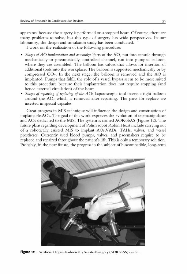
apparatus, because the surgery is performed on a stopped heart. Of course, there aremany problems to solve, but this type of surgery has wide perspectives. In ourlaboratory, the design and simulation study has been conducted.
I work on the realization of the following procedure:
• Stages of AO implantation and assembly: Parts of the AO, put into capsule throughmechanically or pneumatically controlled channel, run into pumped balloon,where they are assembled. The balloon has valves that allows for insertion ofadditional tools into the workplace. The balloon is supported mechanically or bycompressed CO2. In the next stage, the balloon is removed and the AO isimplanted. Pumps that fulfill the role of a vessel bypass seem to be most suitedto this procedure because their implantation does not require stopping (andhence external circulation) of the heart.
• Stages of repairing of replacing of the AO: Laparoscopic tool inserts a tight balloonaround the AO, which is removed after repairing. The parts for replace areinserted in special capsules.
Great progress in MIS technique will influence the design and construction ofimplantable AOs. The goal of this work expresses the evolution of telemanipulatorand AOs dedicated to the MIS. The system is named AORobAS (Figure 12). Thefuture plans regarding development of Polish robot Robin Heart include carrying outof a robotically assisted MIS to implant AOs,VADs, TAHs, valves, and vesselprostheses. Currently used blood pumps, valves, and pacemakers require to bereplaced and repaired throughout the patient’s life. This is only a temporary solution.Probably, in the near future, the progress in the subject of biocompatible, long-term
Figure 12 ArtificialOrgansRoboticallyAssisted Surgery (AORobAS) system.
Review of Research in Cardiovascular Devices 51
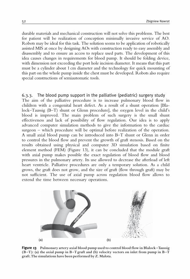
durable materials and mechanical construction will not solve this problems. The bestfor patient will be realization of conception minimally invasive service of AO.Robots may be ideal for this task. The solution seems to be application of roboticallyassisted MIS at once by designing AOs with construction ready to easy assembly anddisassembly and to ensure an access to replace used parts. The development of thisidea causes changes in requirements for blood pump. It should be folding device,with dimension not exceeding the port hole incision diameter. It means that this partmust be a cylinder about 1 cm diameter and the technology for quick mounting ofthis part on the whole pump inside the chest must be developed. Robots also requirespecial constructions of semiautomatic tools.
6.3.3. The blood pump support in the palliative (pediatric) surgery studyThe aim of the palliative procedure is to increase pulmonary blood flow inchildren with a congenital heart defect. As a result of a shunt operation [Bla-lock–Taussig (B–T) shunt or Glenn procedure], the oxygen level in the child’sblood is improved. The main problem of such surgery is the small shunteffectiveness and lack of possibility of flow regulation. Our idea is to applyadvanced computer simulation methods to give the information to the cardiacsurgeon – which procedure will be optimal before realization of the operation.A small axial blood pump can be introduced into B–T shunt or Glenn in orderto control the blood flow and prevent the growth of graft stenosis. Based on theresults obtained using physical and computer 3D simulation based on finiteelement method (FEM) (Figure 13), it can be concluded that the module graftwith axial pump makes possible the exact regulation of blood flow and bloodpressures in the pulmonary artery. Its use allowed to decrease the afterload of leftheart ventricle. Palliative procedures are only a temporary solution. As a childgrows, the graft does not grow, and the size of graft (flow through graft) may benot sufficient. The use of axial pump across regulation blood flow allows toextend the time between necessary operations.
(a) (b)
Figure 13 Pulmonary artery axial blood pump used to control blood flow in Blalock^Taussig(B^T): (a) the axial pump in B^Tgraft and (b) velocity vectors on inlet from pump in B^Tgraft.The simulations have been performed by Z.Małota.
52 Zbigniew Nawrat
7. THE MINIMALLY INVASIVE VALVE IMPLANTATION
Percutaneous (pulmonary and aortic) valve replacement has recentlyopened new perspectives on transcatheter replacement of cardiac valves. Typi-cally, a bioprosthetic valve is dissected and sutured into an autoexpandableNitinol stent (which has an initial aortic diameter, for instance, 25 mm) ormounted within a balloon-expandable stent. It has been used in patients who areat high risk for valve replacement surgery. Percutaneous valve repair is also beingdeveloped for mitral regurgitation. Direct leaflet repair and percutaneousannuloplasty are being employed in clinical trials. All the percutaneousapproaches are based on existing surgical techniques and offer less invasivealternatives. This marked the beginning of the era of percutaneous valvetherapy, and ongoing trials will define the clinical role for these new therapeuticmodalities. Percutaneous catheter-based systems for the treatment of valvularheart disease have been designed and studied in animal models for severalyears. Bonhoeffer et al. were the first to perform percutaneous implantationsof artificial valves, using a bovine jugular vein valve mounted within a stent, inchildren with right ventricle to pulmonary prosthetic conduits. The first humancase report of percutaneous transcatheter implantation of an aortic valve pros-thesis for calcific aortic stenosis appeared in 2002 [14].
A percutaneously implanted heart valve (PHV) composed of three bovinepericardial leaflets mounted within a balloon-expandable stent was developed(Percutaneous Valve Technologies, Inc.). Using an antegrade transseptal approach,the PHV was successfully implanted within the diseased native aortic valve, withaccurate and stable PHV positioning, without impairing the coronary artery bloodflow or the mitral valve function, and a with no mild paravalvular aortic regurgita-tion. Immediately and at 48 h after implantation, valve functioning was excellent,resulting in a marked hemodynamic improvement. Nonsurgical implantation of aprosthetic heart valve can be successfully achieved with immediate and midtermhemodynamic and clinical improvement.
8. SUPPORT TECHNOLOGY FOR SURGERY PLANNING
Modern medical imaging techniques such as CT, NMR, and ultrasonicimaging enable the surgeon to have a very precise representation of internalanatomy as preoperative scans.
For surgery robots (telemanipulators), the following distinct phases can berealized:
– Preoperative planning: The optimal strategy is defined using the 3D computermodel.
– Robot-assisted intervention: A calibration routine brings robot, patient, and imagesystem to a common frame of reference, for example, using anatomical (orartificial) landmarks.
Review of Research in Cardiovascular Devices 53

– Feedback and replanning: The robot starts to operate under the supervision ofsurgeon. Sensor information ensures that the anatomy is as expected and storedby a model in computer. If deviations occur, the surgeon asks for a revisedstrategy, or for permission to continue.
Computer flow simulation method is important for diagnosing the heart diseasedevelopment, for optimizing the surgery for a particular patient, and for long-termfunctioning of graft prognosis. During simulation, the input data (biochemical data,diagnostic data, geometrical data, biophysical data) are transformed into test outputdata (the hemodynamic pressure and flows or another characterization of biologicalobject modified by surgery).
Remote-control manipulators are proposed for cardiac surgery using a computer-based advisory system. Information in a prepared database (an online expert system)may be of help to a surgeon in decision making. The first step is to simulate therobot-assisted surgery using both computer and physical models of a particularoperation type. Based on the preoperation cardiac surgery simulation results, theoptimization of the procedures can be achieved.
The main issues of computer simulation support to surgery robots are as follows:
1. The operation planning: Based on diagnostic data (images, pressure and flowsignals, etc.), computer and physical models can be created. In vitrosimulations performed on them may be used to find the optimal way ofoperation (the joint point localization, the graft selection). A prepared reportcan be presented to the surgeon as a hint for robot choreography planning. Thisstage should also include input port localization on patient skin, the type oftools, and the way of removing and preparing the graft branch.
2. Advisory and control system: During the operation, diagnostic images or simulationresults from various sources can be called by surgeon and superimposed on thereal operating image.
The introduction of robots to cardiac surgery created the possibility of directand practical use of simulation results of surgical procedures in the robot informa-tion system.
Surgical planning and augmented reality are likely to enhance robotic surgery inthe future. The interesting case of applying preoperatively in robotically assistedcardiac surgery planning, intraoperative registration, and augmented reality wasperformed by Falk et al. [15]. The regions of interest (i.e., the heart, ribs, coron-aries, ITA) were segmented semiautomatically to create a virtual model of theanimal. In this model, the target regions of the total endoscopic bypass procedurealong with the ITA and anastomotic area were defined. Algorithms for assessingvisibility, dexterity, and collision avoidance were developed after defining nonadmis-sible areas using the virtual model of the manipulator. Intraoperatively, registrationof the animal and the telemanipulator was performed using encoder data of thetelemanipulator by pointing to the fiducial points. After pericardiotomy, thereconstructed coronary tree was projected onto the videoscopic image using asemiautomatic alignment procedure. In dogs, the total endoscopic bypass proce-dure was successful on the beating heart.
54 Zbigniew Nawrat
For medical applications, matching procedures between diagnostic images andoff-line intervention planning and real execution are very important. Many pro-blems still remain for soft tissue surgery where deformations may occur. Thenavigation and guidance of the instruments highly depends on the surgeon’s skillwho has to combine their intraoperative views with the information extracted fromthe preoperative images.
Several scientific groups work on computer method for preparing quasi-stationaryview. The da Vinci robot uses a two-camera endoscope that feeds images to thesurgeon’s viewer. Images from the left and right cameras are fed to each of thesurgeon’s eyes separately, providing a 3D view of the tissue being operated on.The Mylonas system exploits this principle by fitting an infrared eye tracker to theviewer. This ensures that each eye detects precisely where the surgeon is looking,and then calculates the distance to the point their gaze is fixed upon usingtriangulation. The software first constructs a 3D model of the heart by trackingthe surgeon’s eyes as they move over the organ. Then it creates a real-time movingimage by recording the changes in the surgeon’s focal point as the heart beats. Theendoscope is calibrated to move forward and backward in time with this image,thus making the heart to appear stationary to the surgeon viewing it through thetwo cameras. The surgical instruments are also calibrated to move in synchronywith the beating heart, removing the need to constantly move them back andforward, and allowing the surgeon to concentrate on performing the operation.The software has so far been tested only on an artificial silicone heart using arobotic arm.
According to surgeons and device executives, surgeon training is the key tothe future success of the robotics industry. Because modern surgery is verychallenging, the surgeon training will become comparable to fighter pilot trainingwhile the robotic systems are having a huge impact on surgical education,and, without doubt, will be integrated into surgeons’ future education process.Currently for clinical use of the da Vinci surgical system, the FDA requires a2-day training course to understand the setup, maintenance, and applications ofthe surgical system, in addition to animated laboratory training. The devicemanufacturers have training programs in place to advance the skill sets of bothnew and experienced surgeons.
Both the virtual (Figure 14) and the real station are used for MIS education. Asexamples, commercial products include LapTrainer z SimuVision (Simulab Inc.,Seattle, WA, USA; www.simulab.com), ProMIS (Haptica Inc., Boston, MA, USA;www.haptica.com), Laparoscopic Surgical Workstation and Virtual LaparoscopicInterface (Immersion Inc., Gaithersburg,MD,USA;www.immersion.com), Phantomdevices (SensAble Technologies Inc., Woburn, MA, USA; www.sensable.com),Xitact LS500 Laparoscopy Simulator (Xitact S.A., Lausanne, Switzerland;www.entice.com), Lapmentor (Simbionix Inc., Cleveland, OH, USA; www.simbionix.com); Surgical Education Platform (SEP) (SimSurgery, Oslo, Norway;www.simsurgery.no;www.meti.com), LapSim (Surgical Science Ltd, Gothenburg,Sweden; www.surgical-science.com), Procedus MIST (Mentice AB,Gothenburg, Sweden; www.mentice.com), EndoTower (Verefi Technologies Inc.,Elizabethtown, PA, USA; www.verefi.com), Reachi Laparoscopic Trainer (Reachin
Review of Research in Cardiovascular Devices 55
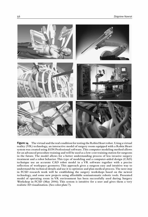
Figure 14 The virtual and the real condition for testing theRobinHeart robot.Using avirtualreality (VR) technology, an interactive model of surgery room equipped with a Robin Heartsystemwas created using EON Professional software.This computer modeling method allowsfor an advanced procedure training and will be used as a low-cost training station for surgeonsin the future. The model allows for a better understanding process of less invasive surgerytreatment and a robot behavior. This type of modeling and a computer-aided design (CAD)technique use an accurate CAD robot model in a VR software together with a precisereflection of workspace geometry. This approach gives a surgeon easy and intuitive way tounderstand the technical details and use it to optimize and plan medical process.The next stepin FCSD research work will be establishing the surgery workshops based on the newesttechnology, and some new projects using affordable semiautomatic robotic tools. Presentedmodel of operating room in VR environment has been successfully used during SurgeryWorkshop in FCSD (May 2006). This system is intuitive for a user and gives them a veryrealistic 3D visualization. (See color plate 7).
56 Zbigniew Nawrat
Technologies AB, Stockholm, Sweden; www.reachin.se), Vest System (VirtualEndoscopic Surgical Trainer; Select-IT VEST Systems AG, Bremen, Germany;www.select-it.de), and Simendo (Simulator for endoscopy; DeltaTech, Delft, Neth-erlands; www.simendo.nl).
9. CONCLUSIONS
Notable achievements in cardiovascular research and devices that are cur-rently under investigation and expected in the near future are listed below:
1. New pediatric devices, such as the axial-flow pumps and small-diameter valveprostheses, have been introduced, and some are under construction. As thedevices become more and more reliable, mechanical circulatory support willplay an increasingly important role, not only for rescue therapy but also for safetreatment of the most complex congenital heart diseases, not only with the aimof bridging to cardiac recovery or transplantation but, eventually, as a permanentsolution.
2. The effective miniature blood pumps have been commonly used in minimallyinvasive cardiology. Transported to the destination place through the arteries,the smart pump mainly for short-term heart support can play an important rolein an emergency.
3. New types of devices create possibilities of pump and blood oxygenationintroduction into clinical practice. The idea is not new, but thanks to newmaterials (durable, semiconductive silicon membranes) that are being rapidlydeveloped.
4. New “biomechanical” valves and vessels completely synthetic/artificial, butflexible and durable, will be introduced. The development of small-calibervascular grafts is very important for bypass and graft surgery.
5. A significant improvement in technical support for preplanning and controlsurgical interventions, including telemedicine technology, will be observed.
6. Bioartificial myocardial grafts will be introduced in which perfusion by amacroscopic core vessel will be applicable.
7. Improved cell-culture techniques may render human aortic myofibroblasts anative tissue-like structure.
8. Tissue-engineered bioprosthethic valves will be commonly used in clinics.
As the field of surgery robots controlled by surgeons expands, the economicalcost is expected to reduce, which will allow surgeons to more commonly useteleoperation in situations that warrants professional staff assistance such as wars,epidemics, and space trips. The situation of “no contact” between the medicalpersonnel and the patient will reduce the risk of loss of health because of theinfection(s) from the side of the operating staff.
It is most probable that contemporary telemanipulators will be replacedby adaptive robots in the near future. Currently, the trials of shifting from passiveto active systems can be seen. To be clear, let’s define the basic concepts:
Review of Research in Cardiovascular Devices 57
Teleoperators are remotely controlled by operator robot transferring on distancemotoric and sensoric functions, whereas adaptive robots have more advanced controlsystem with sensoric and learning abilities. However, creating the next-generation“intelligent” robots is a true challenge. These robots must be able to work unaidedly invarious environments, gathering information from their senses. Optimization of theirbehavior and the effectiveness of given task realization will depend on “self-learningcontrol algorithm”, which will more resemble systems based on “instincts” in relationto living creatures and contact with surroundings by means of “senses”, zoom, touchsensors (inductive, supersonic, optical, pneumatic, and microwave). I am convincedthat theywill not be similar to contemporary cardiosurgical robots, but theywill be ableto replace them considerably. Probably, they will bemicrorobots that are able to reach,e.g., a given human internal diseased organ (e.g., the heart).
ACKNOWLEDGMENTS
This chapter has been illustrated with the experimental data obtained in theInstitute of Heart Prostheses, FCSD, Zabrze. The research was supported by thePolish State Committee for Scientific Research and Foundation. The authorthanks his numerous collaborators, including R. Kustosz, M. Kozlak, P. Kostka,Z. Małota, L. Podsedkowski, Z. Religa, and M. Jakubowski (special thanks forexcellent photography), who prepared the artwork of this chapter.
REFERENCES
[1] Morris D., Couves C. Experiences with a sac-type artificial heart. Can Med Assoc J1971;105:483–487.
[2] Copeland J.G., Smith R.G., Arabia F.A., et al. For the CardioWest Total Artifical HeartInvestigators. Cardiac replacement with a total artificial heart as a bridge to transplantation.N Engl J Med 2004;351:859–867.
[3] Hetzer R., Stiller B. Technology insight: Use of ventricular assist devices in children. Nat ClinPract Cardiovasc Med 2006;3:377–386.
[4] Short-term circulatory support with left ventricular assist devices as a bridge to cardiac trans-plantation or recovery. National Institute for Health and Clinical Excellence, June 2006; ISBN1-84629-233-6. Available from: www.nice.org.uk/ip059overview.
[5] Rose E., Gelijns A., Moskowitz A., et al.; from the Randomized Evaluation of MechanicalAssistance for the Treatment of Congestive Heart Failure (REMATCH) Study Group. Long-term use of a left ventricular assist device for end-stage heart failure. N Engl J Med2001;345(20):1435–1443.
[6] Jamieson E. Cartier P., Allard M., et al.; Primary Panel Members. Surgical management ofvalvular heart disease 2004. Can J Cardiol 2004;20(Suppl. E):7E–120E.
[7] Daebritz S., Sachweh J., Hermanns B., et al. Introduction of a flexible polymeric heart valveprosthesis with special design for mitral position. Circulation 2003;108:II–134.
[8] Dankleman J., Grimbergen C.A., Stassen H.G. Engineering for Patient Safety. Issues in MinimallyInvasive Procedures. 2005; Lawrence Erlbaum Associates: London.
[9] Wolf R. Anastomotic devices for coronary surgery. CTSNet, 14 January 2005. Available from:www.ctsnet.org/sections/innovation/minimallyinvasive/articles/article-9.html.
58 Zbigniew Nawrat

[10] Nawrat Z. Perspectives of computer and robot assisted surgery for heart assist pump implanta-tion. Planning for robotically assisted surgery. Lecture Notes of the ICB Seminars. Assessment andMechanical Support of Heart and Lungs (eds M. Darowski, G. Ferrari), Warsaw 2001:130–150.
[11] Nawrat Z., Kostka P. The Robin Heart Vision, telemanipulator for camera holding preliminarytest results. J Autom Mobile Rob Intell Syst 2007;1(1):str.48–53.
[12] Falk V., McLoughin J., Guthart G., Salisbury JK., Walther T., Mohr FW. Dexterity enhance-ment in endoscopic surgery by a computer-controlled mechanical wrist. Minim Invasive TherapyAllied Tech 1999;8:235–242.
[13] Jacobs S., Falk V., Holzhey D., Mohr F.W. Perspectives in endoscopic cardiac surgery. CompBiol Med 2007;37(10):1374–1376 (Epub 20 December 2006; doi: 10.1016/j.compbiomed.2006.11.007).
[14] Bauer F., Derumeaux G., Anselme F., et al. Percutaneous transcatheter implantation of an aorticvalve prosthesis for calcific aortic stenosis: First human case description. Circulation2002;106:3006–3008.
[15] Falk V.D., Mourgues F., Adhami L., et al. Cardio navigation: Planning, simulation, andaugmented reality in robotic assisted endoscopic bypass grafting. Ann Thorac Surg2005;79:2040–2047.
Review of Research in Cardiovascular Devices 59

This page intentionally left blank
C H A P T E R 2
BIOMECHANICAL MODELING OF STENTS:SURVEY 1997–2007
Matthieu De Beule
Contents
1. Introduction 622. Finite Element Modeling of Stents 63
2.1. Finite element basics 63
2.2. Geometrical design and approximation 642.3. Material properties 652.4. Loading and boundary conditions 66
2.5. Finite element stent design 662.6. Effective use of FEA 68
3. Survey of the State of the Art in Stent Modeling: 1997–2007 683.1. Neglect of the balloon 69
3.2. Cylindrical balloon 743.3. Folded balloon 783.4. Summary 81
4. Alternative methods for biomechanical modeling of stents 844.1. FEM – Prolapse, flexibility, and strut micromechanics 844.2. FEM – Self-expandable stents 85
4.3. CFD–drug elution and immersed FEM 875. Future Prospects 886. Conclusion 88
Acknowledgments 89References 89
Abstract
The aim of this chapter is to provide an educational review on finite element modeling ofstents. First, the basic principles of stent modeling are briefly described, followed by a survey
regarding state of the art solid mechanical computational models of balloon-expandablestents. This review is organized chronologically according to the applied stent expansionmethodology: (1) neglecting the presence of the balloon, (2) assuming it to have a cylindricalshape, or (3) taking the actual folded shape of the balloon into account. Subsequently,
alternative methodologies to study the (bio)mechanical behavior of stents are described,and to conclude, future prospects for stent modeling are briefly addressed.
Keywords: Finite Element Method, stent, expansion methodology, validation
Advances in Biomedical Engineering � 2009 Elsevier B.V.
ISBN 978-0-444-53075-2 All rights reserved.
61
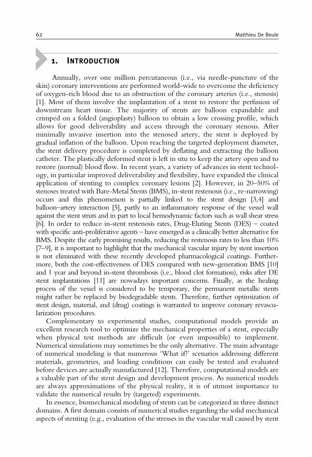
1. INTRODUCTION
Annually, over one million percutaneous (i.e., via needle-puncture of theskin) coronary interventions are performed world-wide to overcome the deficiencyof oxygen-rich blood due to an obstruction of the coronary arteries (i.e., stenosis)[1]. Most of them involve the implantation of a stent to restore the perfusion ofdownstream heart tissue. The majority of stents are balloon expandable andcrimped on a folded (angioplasty) balloon to obtain a low crossing profile, whichallows for good deliverability and access through the coronary stenosis. Afterminimally invasive insertion into the stenosed artery, the stent is deployed bygradual inflation of the balloon. Upon reaching the targeted deployment diameter,the stent delivery procedure is completed by deflating and extracting the ballooncatheter. The plastically deformed stent is left in situ to keep the artery open and torestore (normal) blood flow. In recent years, a variety of advances in stent technol-ogy, in particular improved deliverability and flexibility, have expanded the clinicalapplication of stenting to complex coronary lesions [2]. However, in 20–50% ofstenoses treated with Bare-Metal Stents (BMS), in-stent restenosis (i.e., re-narrowing)occurs and this phenomenon is partially linked to the stent design [3,4] andballoon–artery interaction [5], partly to an inflammatory response of the vessel wallagainst the stent struts and in part to local hemodynamic factors such as wall shear stress[6]. In order to reduce in-stent restenosis rates, Drug-Eluting Stents (DES) – coatedwith specific anti-proliferative agents – have emerged as a clinically better alternative forBMS. Despite the early promising results, reducing the restenosis rates to less than 10%[7–9], it is important to highlight that the mechanical vascular injury by stent insertionis not eliminated with these recently developed pharmacological coatings. Further-more, both the cost-effectiveness of DES compared with new-generation BMS [10]and 1 year and beyond in-stent thrombosis (i.e., blood clot formation), risks after DEstent implantations [11] are nowadays important concerns. Finally, as the healingprocess of the vessel is considered to be temporary, the permanent metallic stentsmight rather be replaced by biodegradable stents. Therefore, further optimization ofstent design, material, and (drug) coatings is warranted to improve coronary revascu-larization procedures.
Complementary to experimental studies, computational models provide anexcellent research tool to optimize the mechanical properties of a stent, especiallywhen physical test methods are difficult (or even impossible) to implement.Numerical simulations may sometimes be the only alternative. The main advantageof numerical modeling is that numerous ‘What if?’ scenarios addressing differentmaterials, geometries, and loading conditions can easily be tested and evaluatedbefore devices are actually manufactured [12]. Therefore, computational models area valuable part of the stent design and development process. As numerical modelsare always approximations of the physical reality, it is of utmost importance tovalidate the numerical results by (targeted) experiments.
In essence, biomechanical modeling of stents can be categorized in three distinctdomains. A first domain consists of numerical studies regarding the solid mechanicalaspects of stenting (e.g., evaluation of the stresses in the vascular wall caused by stent
62 Matthieu De Beule
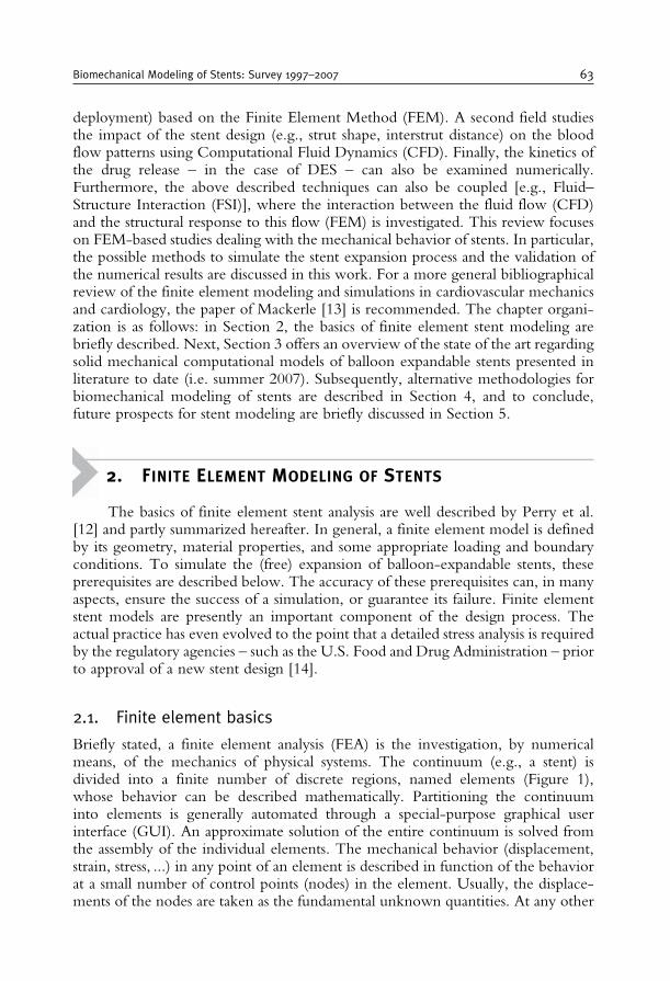
deployment) based on the Finite Element Method (FEM). A second field studiesthe impact of the stent design (e.g., strut shape, interstrut distance) on the bloodflow patterns using Computational Fluid Dynamics (CFD). Finally, the kinetics ofthe drug release – in the case of DES – can also be examined numerically.Furthermore, the above described techniques can also be coupled [e.g., Fluid–Structure Interaction (FSI)], where the interaction between the fluid flow (CFD)and the structural response to this flow (FEM) is investigated. This review focuseson FEM-based studies dealing with the mechanical behavior of stents. In particular,the possible methods to simulate the stent expansion process and the validation ofthe numerical results are discussed in this work. For a more general bibliographicalreview of the finite element modeling and simulations in cardiovascular mechanicsand cardiology, the paper of Mackerle [13] is recommended. The chapter organi-zation is as follows: in Section 2, the basics of finite element stent modeling arebriefly described. Next, Section 3 offers an overview of the state of the art regardingsolid mechanical computational models of balloon expandable stents presented inliterature to date (i.e. summer 2007). Subsequently, alternative methodologies forbiomechanical modeling of stents are described in Section 4, and to conclude,future prospects for stent modeling are briefly discussed in Section 5.
2. FINITE ELEMENT MODELING OF STENTS
The basics of finite element stent analysis are well described by Perry et al.[12] and partly summarized hereafter. In general, a finite element model is definedby its geometry, material properties, and some appropriate loading and boundaryconditions. To simulate the (free) expansion of balloon-expandable stents, theseprerequisites are described below. The accuracy of these prerequisites can, in manyaspects, ensure the success of a simulation, or guarantee its failure. Finite elementstent models are presently an important component of the design process. Theactual practice has even evolved to the point that a detailed stress analysis is requiredby the regulatory agencies – such as the U.S. Food and Drug Administration – priorto approval of a new stent design [14].
2.1. Finite element basics
Briefly stated, a finite element analysis (FEA) is the investigation, by numericalmeans, of the mechanics of physical systems. The continuum (e.g., a stent) isdivided into a finite number of discrete regions, named elements (Figure 1),whose behavior can be described mathematically. Partitioning the continuuminto elements is generally automated through a special-purpose graphical userinterface (GUI). An approximate solution of the entire continuum is solved fromthe assembly of the individual elements. The mechanical behavior (displacement,strain, stress, ...) in any point of an element is described in function of the behaviorat a small number of control points (nodes) in the element. Usually, the displace-ments of the nodes are taken as the fundamental unknown quantities. At any other
Biomechanical Modeling of Stents: Survey 1997–2007 63
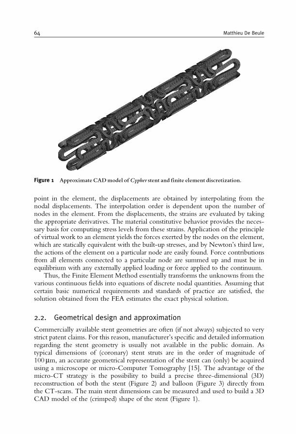
point in the element, the displacements are obtained by interpolating from thenodal displacements. The interpolation order is dependent upon the number ofnodes in the element. From the displacements, the strains are evaluated by takingthe appropriate derivatives. The material constitutive behavior provides the neces-sary basis for computing stress levels from these strains. Application of the principleof virtual work to an element yields the forces exerted by the nodes on the element,which are statically equivalent with the built-up stresses, and by Newton’s third law,the actions of the element on a particular node are easily found. Force contributionsfrom all elements connected to a particular node are summed up and must be inequilibrium with any externally applied loading or force applied to the continuum.
Thus, the Finite Element Method essentially transforms the unknowns from thevarious continuous fields into equations of discrete nodal quantities. Assuming thatcertain basic numerical requirements and standards of practice are satisfied, thesolution obtained from the FEA estimates the exact physical solution.
2.2. Geometrical design and approximation
Commercially available stent geometries are often (if not always) subjected to verystrict patent claims. For this reason, manufacturer’s specific and detailed informationregarding the stent geometry is usually not available in the public domain. Astypical dimensions of (coronary) stent struts are in the order of magnitude of100mm, an accurate geometrical representation of the stent can (only) be acquiredusing a microscope or micro-Computer Tomography [15]. The advantage of themicro-CT strategy is the possibility to build a precise three-dimensional (3D)reconstruction of both the stent (Figure 2) and balloon (Figure 3) directly fromthe CT-scans. The main stent dimensions can be measured and used to build a 3DCAD model of the (crimped) shape of the stent (Figure 1).
Figure 1 Approximate CADmodel ofCypher stent and finite element discretization.
64 Matthieu De Beule
2.3. Material properties
Angioplasty balloons are generally manufactured from either PolyEthyleneTerephthalate (PET) or Polyamide (nylon) [16]. PET balloons are usually strongerand have a lower compliance than nylon balloons. Based on in vitro testing, thechange in balloon diameter as a function of inflation pressure is determined by themanufacturer and summarized in a compliance chart in the directions for use. Ifneither the balloon constitutive material behavior is known, nor experimentaltensile tests can be performed; the constitutive law can be derived from thecompliance data based on thin shell membrane theory [17].
Figure 2 CT-Image reconstruction ofCypher stent.
Figure 3 CT-Image reconstruction of tri-folded angioplasty balloon.
Biomechanical Modeling of Stents: Survey 1997–2007 65
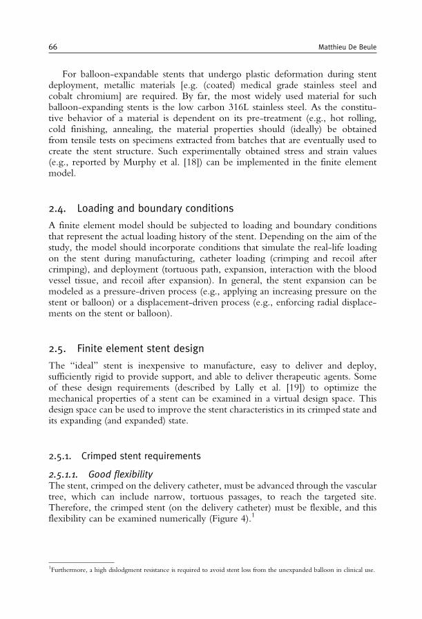
For balloon-expandable stents that undergo plastic deformation during stentdeployment, metallic materials [e.g. (coated) medical grade stainless steel andcobalt chromium] are required. By far, the most widely used material for suchballoon-expanding stents is the low carbon 316L stainless steel. As the constitu-tive behavior of a material is dependent on its pre-treatment (e.g., hot rolling,cold finishing, annealing, the material properties should (ideally) be obtainedfrom tensile tests on specimens extracted from batches that are eventually used tocreate the stent structure. Such experimentally obtained stress and strain values(e.g., reported by Murphy et al. [18]) can be implemented in the finite elementmodel.
2.4. Loading and boundary conditions
A finite element model should be subjected to loading and boundary conditionsthat represent the actual loading history of the stent. Depending on the aim of thestudy, the model should incorporate conditions that simulate the real-life loadingon the stent during manufacturing, catheter loading (crimping and recoil aftercrimping), and deployment (tortuous path, expansion, interaction with the bloodvessel tissue, and recoil after expansion). In general, the stent expansion can bemodeled as a pressure-driven process (e.g., applying an increasing pressure on thestent or balloon) or a displacement-driven process (e.g., enforcing radial displace-ments on the stent or balloon).
2.5. Finite element stent design
The “ideal’’ stent is inexpensive to manufacture, easy to deliver and deploy,sufficiently rigid to provide support, and able to deliver therapeutic agents. Someof these design requirements (described by Lally et al. [19]) to optimize themechanical properties of a stent can be examined in a virtual design space. Thisdesign space can be used to improve the stent characteristics in its crimped state andits expanding (and expanded) state.
2.5.1. Crimped stent requirements
2.5.1.1. Good flexibilityThe stent, crimped on the delivery catheter, must be advanced through the vasculartree, which can include narrow, tortuous passages, to reach the targeted site.Therefore, the crimped stent (on the delivery catheter) must be flexible, and thisflexibility can be examined numerically (Figure 4).1
1Furthermore, a high dislodgment resistance is required to avoid stent loss from the unexpanded balloon in clinical use.
66 Matthieu De Beule
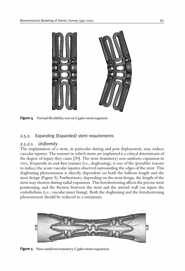
2.5.2. Expanding (Expanded) stent requirements
2.5.2.1. UniformityThe implantation of a stent, in particular during and post deployment, may inducevascular injuries. The manner in which stents are implanted is a critical determinant ofthe degree of injury they cause [20]. The stent (transitory) non-uniform expansion invivo, frequently in end-first manner (i.e., dogboning), is one of the (possible) reasonsto induce the acute vascular injuries observed surrounding the edges of the stent. Thisdogboning phenomenon is directly dependent on both the balloon length and thestent design (Figure 5). Furthermore, depending on the stent design, the length of thestent may shorten during radial expansion. This foreshortening affects the precise stentpositioning, and the friction between the stent and the arterial wall can injure theendothelium (i.e., vascular inner lining). Both the dogboning and the foreshorteningphenomenon should be reduced to a minimum.
Figure 5 Non-uniform transitoryCypher stent expansion.
Figure 4 Virtual flexibility test onCypher stent segment.
Biomechanical Modeling of Stents: Survey 1997–2007 67

2.5.2.2. High radial strengthA stent should be designed as a mechanical scaffold to support the vessel lumen byminimizing post-stenting vessel recoil. The required radial support is both designand material dependent.
2.5.2.3. Low elastic recoilTo achieve a final lumen diameter consistent with the targeted vessel diameter,knowledge of the degree of elastic radial recoil of the stent must be factored into theexpansion of the stent during deployment. To minimize the “inevitable’’ over-expansion, the material and design-dependent radial recoil should be reduced to theabsolute minimum. In addition to foreshortening, undesirable shearing along thearterial walls may also be caused by longitudinal recoil after the balloon is deflated,and this phenomenon should be minimized.
2.5.2.4. Good FlexibilityThe expanded stent must conform to the tortuous vessel geometry and should notstraighten the vessel, as that would induce significant injuries to the vessel wall.
2.5.2.5. Optimal ScaffoldingTo ensure vessel tissue not to prolapse between the stent struts, the stent shouldprovide optimum (uniform) vessel coverage. In addition, a uniform strut distributionis beneficial to avoid local drug concentration and gradients in DES [21]. However, alow artery–stent contact surface area should also be maintained, because the body-foreign material of the stent can initiate an aggressive thrombotic response.
2.6. Effective use of FEA
The correlation between the finite element approximations and the physical reality isdirectly related to the ability of the scientist to accurately define the geometry, materialbehavior and loading environment of the device. While simplifying assumptions areoften (if not always) inevitable, there is a risk that significant simplifications canconsiderably alter the problem. Therefore, the influence of the simplifications on thesolution of the original problem must always be evaluated. Consequently, the numer-ical results should be validated by (targeted) experiments under similar conditions.
3. SURVEY OF THE STATE OF THE ART IN STENT MODELING:1997–2007
When reviewing literature regarding finite element models of the (free)expansion of balloon-expandable stents, there are three possible ways reported tosimulate the inflation of the balloon: neglecting the presence of the balloon,assuming it to have a cylindrical shape or taking the actual folded shape of the
68 Matthieu De Beule
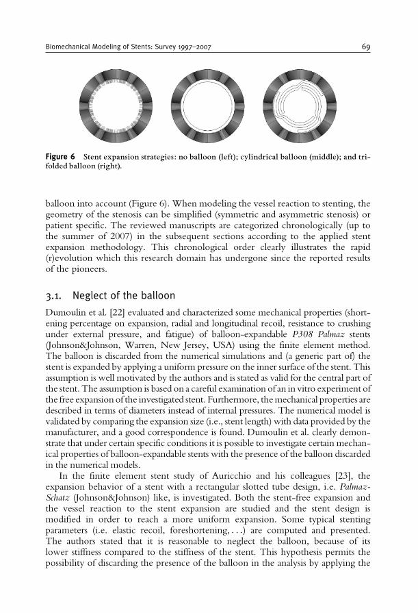
balloon into account (Figure 6). When modeling the vessel reaction to stenting, thegeometry of the stenosis can be simplified (symmetric and asymmetric stenosis) orpatient specific. The reviewed manuscripts are categorized chronologically (up tothe summer of 2007) in the subsequent sections according to the applied stentexpansion methodology. This chronological order clearly illustrates the rapid(r)evolution which this research domain has undergone since the reported resultsof the pioneers.
3.1. Neglect of the balloon
Dumoulin et al. [22] evaluated and characterized some mechanical properties (short-ening percentage on expansion, radial and longitudinal recoil, resistance to crushingunder external pressure, and fatigue) of balloon-expandable P308 Palmaz stents(Johnson&Johnson, Warren, New Jersey, USA) using the finite element method.The balloon is discarded from the numerical simulations and (a generic part of) thestent is expanded by applying a uniform pressure on the inner surface of the stent. Thisassumption is well motivated by the authors and is stated as valid for the central part ofthe stent. The assumption is based on a careful examination of an in vitro experiment ofthe free expansion of the investigated stent. Furthermore, themechanical properties aredescribed in terms of diameters instead of internal pressures. The numerical model isvalidated by comparing the expansion size (i.e., stent length) with data provided by themanufacturer, and a good correspondence is found. Dumoulin et al. clearly demon-strate that under certain specific conditions it is possible to investigate certain mechan-ical properties of balloon-expandable stents with the presence of the balloon discardedin the numerical models.
In the finite element stent study of Auricchio and his colleagues [23], theexpansion behavior of a stent with a rectangular slotted tube design, i.e. Palmaz-Schatz (Johnson&Johnson) like, is investigated. Both the stent-free expansion andthe vessel reaction to the stent expansion are studied and the stent design ismodified in order to reach a more uniform expansion. Some typical stentingparameters (i.e. elastic recoil, foreshortening, . . .) are computed and presented.The authors stated that it is reasonable to neglect the balloon, because of itslower stiffness compared to the stiffness of the stent. This hypothesis permits thepossibility of discarding the presence of the balloon in the analysis by applying the
Figure 6 Stent expansion strategies: no balloon (left); cylindrical balloon (middle); and tri-folded balloon (right).
Biomechanical Modeling of Stents: Survey 1997–2007 69

internal pressure, which normally acts on the balloon, directly to the inner surfaceof the stent. Hence, the stent is loaded by an internal uniform radial pressurevarying linearly from 0 to 1.3MPa (inflation) and then again linearly back to 0(deflation). The numerical results for some mechanical properties (elastic recoil,foreshortening, metal-artery ratio) correspond with values available in literature forthe non-modified stent design. Though, the validation of the stent expansionbehavior is rather limited. To investigate the revascularization, a symmetric 3Dmodel of the plaque and artery is developed. The idealized “symmetric stenosis’’ ischaracterized by a straight artery segment and a plaque with a parabolic longitudinalprofile and the constitutive material behavior is adopted from literature. Thispioneering work clearly shows the enormous potential of the finite elementmethod in this research domain, both on stent design and on procedural level.
In the same period, Etave et al. [24] used a finite element analysis to determine the“exact’’ mechanical characteristics of tubular (Palmaz-Schatz, Johnson&Johnson) andcoil (Freedom, Global Therapeutics Inc.) stents. Seven mechanical properties werestudied numerically with determination of (1) stent deployment pressure, (2) intrinsicelastic recoil of the material used, (3) resistance of the stent to external compressiveforces, (4) stent foreshortening, (5) stent coverage area, (6) stent flexibility, and (7) thestress maps. The balloon is ignored in the numerical simulations and the stents were
Figure 7 Pressure-driven Cypher stent expansion (neglect of the balloon). Top: no pressure;Middle: low pressure range; and Bottom: high pressure range.
70 Matthieu De Beule
expanded by a radial displacement-driven process, forcing the stent to expand as acylinder during the complete expansion (i.e., dogboning is excluded from the analysis).This numerical study shows the possibility of studying several important mechanicalcharacteristics of different stent designs, but no experimental validationof thenumericalresults is reported.
Migliavacca et al. [25] investigated the mechanical behavior of coronary stents bymeans of the finite element method. Finite element analyses were applied (1) tounderstand the effects of different geometrical parameters (thickness, metal-to-arterysurface ratio, longitudinal and radial cut lengths of a Palmaz-Schatz-like stent) of atypical diamond-shaped coronary stent on the device mechanical performance, (2) tocompare the response of different actual stent models (Multi-Link Tetra, Guidant andCarbostent, Sorin Biomedica) when loaded by internal pressure, and (3) to collectsuggestions for optimizing the device shape and performance. The presence of theballoon is discarded in the analysis, and the internal pressure on the balloon is directlyapplied to the inner surface of the stent corresponding with the expansion strategyproposed by Auricchio et al. [23]. The introduction of new-generation stent geome-tries opens the door to study stent designs currently used in the clinical practice.Experimental evidence of the numerical results would certainly create a more solidbase for the proposed design optimization.
More recently, McGarry et al. [26] examined the mechanical behavior of astainless steel balloon-expandable stent design using computational micromechanicsin the context of the finite element method. Stent deployment and cardiac pulsingloading conditions were considered. As the typical dimensions of stent struts (e.g.,100mm for coronary stents) are of a similar order of magnitude as the average grainsize in stainless steel (i.e., 25mm), continuum approaches relying on macroscopicmaterial properties may be regarded as somewhat questionable, and alternativenumerical analysis, based on crystal plasticity for example, may need to be used.McGarry and colleagues used classical phenomenological plasticity theory (J2 flowtheory) and physically based crystal plasticity theory to describe the stent materialbehavior. Important stent deployment characteristics such as recoil and foreshor-tening were determined using a two-dimensional (2D) model of a unit cell (i.e.,characteristic pattern, which is repeated both circumferentially and longitudinally)of theNIR stent (Medinol/Boston Scientific). The deployment of the 2D unit stentcell was modeled using applied displacements. Furthermore, elementary fatiguefactors of safety were determined by plotting Goodman diagrams to compare bothmaterial models, leading to a lower (and thus conservative) factor of safety for theclassical plasticity theory in comparison with the crystal plasticity model. Thenumerical results in terms of average hydrostatic stresses are in the correct orderof magnitude relative to experimental data reported in literature. McGarry et al.clearly demonstrate that under specific conditions it is possible to investigate certainmechanical properties of balloon-expandable stents (e.g., recoil, foreshortening,etcetera) with the presence of the balloon discarded in the numerical models.Nevertheless (experimentally validated), full 3D stent modeling should be per-formed in order to improve the accuracy according to McGarry and colleagues.
Gu and his colleagues [27] performed finite element analyses of covered microstents(i.e., baremetal stentswith ultra-thin tubular coverings to treat for examplewide-necked
Biomechanical Modeling of Stents: Survey 1997–2007 71
intracranial aneurysms) to assist in the design of stent coverings and to select materials forthe cover in 2005. The primary objective of this study was to determine the mechanicalproperties of the covered microstent (e.g., longitudinal shortening, elastic recoil.) andinvestigate the effects of the covering on the mechanical behavior of the stent (e.g.,deployment pressure vs. covering thickness). Careful observation of in vivo stentingexperiments showed an almost uniformly inflated balloon except at its two ends, and thecentral portion of the stent is expanded by the uniformly inflated part of the balloon.Therefore, the authors decided to expand the stents in the model by a uniform internalpressure that was applied in small increments on the internal surface of the coveredmicrostent. During loading, pressure was increased until the final diameter of the stentreached a certain value and then the pressure was decreased to study recoil. Although asimple non-specified in vitro experiment was performed to study the expansion of thestent, surprisingly no quantitative validation of the numerical results was presented interms of the recorded deployment pressure-diameter data.Consequently, the accuracy ofthe proposed methodology has not been confirmed quantitatively.
A computational methodology that allows a set of stent parameters to be varied,with the aim of evaluating the difference in the mechanical environment within thearterial wall before and after angioplasty with stenting is proposed in the sameperiod by Holzapfel et al. [28]. This methodology is applied to an image-based 3Dgeometrical model of a postmortem specimen of a human iliac artery with astenosis. 3D stent models are parameterized in order to enable new designs to begenerated simply with regard to variations in their geometric structure. Thefollowing parameters are altered to analyze their inter-relationship: (1) the type ofstent cells, similar to three commercial products (Multi-Link Tetra, Guidant;Niroyal-Elite, Boston Scientific and Inflow-Gold-Flex, InFlow Dynamics), (2) the geometryof stent struts, and (3) the radial mismatch between the smallest lumen diameter inthe stenosis and the expanded stent diameter (nominal stent diameter). Further-more, the numerical simulations allowed to characterize the following indicators:(1) the change of the intimal pressure caused by the struts of the stent, (2) the stresschange within the arterial wall caused by the stent, and (3) the luminal change dueto angioplasty. The obtained numerical results are interpreted in terms of restenosisrates reported in clinical studies. This approach allows the analysis of the 3Dinteraction between the stent models and patient specific wall models, the quanti-fication of change in the mechanical environment which occurs during stentplacement, and the comparison of effects of different parameters to identify optimalstent designs. In the numerical simulations, the balloon is ignored and the (deforma-tion dependent) pressure load is applied directly on the stent struts. This groundbreaking work combines parametric modeling of new stent designs with the possi-bility to study the interaction of these designs with a patient-specific stenosis
In the same year, Lally et al. [29] analyzed the stress levels within a symmetricatherosclerotic artery provoked by two different stent designs (S7, Medtronic AVEandNIR, Boston Scientific). These stress levels are linked to possible vascular injuryand thus, to the degree of restenosis reported in clinical studies. The developedmethodology consists of two steps: firstly, the vessel was expanded to a diametergreater than that of the “idealized’’ expanded stent by applying a sufficient internalpressure to the vessel, and secondly, the pressure on the inner lumen of the artery
72 Matthieu De Beule
was gradually reduced. The arterial tissue material model was determined by datafrom uniaxial and equibiaxial tension tests of human femoral arterial tissue. Thehyperelastic constitutive model used to characterize the plaque tissue was deter-mined by fitting to published data for human calcified plaques. Due to the elasticnature of the hyperelastic arterial tissue the vessel contracted around the scaffoldingstent. The major limitation of the proposed methodology is the absence of the stentexpansion process. Therefore, the influence of the stenosis on the stent expansionand the influence of the shear force during the expansion remain unstudied.
Migliavacca et al. [30] applied the finite element method to study the mechanicalbehavior of a new generation coronary stent (BXVelocity, Cordis). The results from thecomputationswerecomparedwith those froma laboratoryexperiment in termsof radialexpansion and elastic recoil. Furthermore,Migliavacca and his colleagues were the firstto compare the complianceof the stent in their simulationswith the compliance chart ofthemanufacturer. The presence of the balloon is discarded in the analysis and a uniformlinearly increasing radial pressurewas applied to the internal surfaceof the stent tomimicthe free expansion of the stent. In addition, to investigate the mechanical properties ofthe stent after the load removal, the stent was unloaded decreasing the internal pressureback to zero. The authors state that the absence of any balloonmodel is the real decisiveelement in interpreting the discrepancies between the experimental and the computa-tional tests. Therefore, the development of more realistic computational modelsaccounting for the presence of the balloon (in its actual folded shape) is required.
In order to reduce the dogboning to a minimum, De Beule and his colleagues [31]exploited the finite element method to investigate and compare the expansion ofdifferent designs of a first-generation Palmaz-Schatz stent. The stent expansion isstudied by applying a uniformly distributed internal pressure directly to the innersurface of the stent as proposed by Auricchio et al. [23]. The dogboning effect evenvanished when altering the original symmetric stent design to an asymmetric design.Thus taking asymmetry into account in the design seems very promising, at least from adogboning point of view. However, no experimental validation of the numericalresults has been performed and the authors acknowledge that more realistic balloon–stent interactions should be taken into account in future studies as the stent expansionbehavior might be governed by the unfolding and expansion of the balloon [32,33].
Finally, Bedoya and co-workers [34] numerically studied the effects of stentdesign parameters on the stress field induced in the normal artery wall and the radialdisplacement achieved by the stent during systole and diastole in the same year.Each stent was positioned in a straight homogeneous cylindrical artery model withnon-linear hyperelastic mechanical properties. These mechanical properties wereobtained from pressure-diameter and force-elongation tests on a porcine arteryspecimen. The study indicated that stent designs (consisting of concentric rings ofsinusoid like curves linked by straight bars of various lengths) incorporating largeaxial strut spacing, blunted corners at bends, and high axial ring segment amplitudesexposed smaller regions of the artery to high stresses, while maintaining an adequateradial displacement. The results of this interesting study may have limited applic-ability to the considered stent design. Timmins et al. [35] extended the work ofBedoya et al. [34] by developing an algorithm to optimize stent design, allowing forconsideration of wall stress, lumen gain and cyclic deflection. The stent strut
Biomechanical Modeling of Stents: Survey 1997–2007 73

configuration was refined, via varying specific design parameters, to optimize stentperformance. This interesting study demonstrates the feasibility of medical devicedesign optimization under complex circumstances. Analogous to the methodologydeveloped by Lally and her colleagues [29], the stent expansion process is not takeninto account in both studies and the stent was initially a straight cylinder with aconstant diameter (larger than the systolic arterial diameter). Therefore, the pro-posed design guidelines might alter when studying the real expansion in a patientspecific stenosis, a logical topic for further investigation.
3.2. Cylindrical balloon
Prior to the millennium, in 1999, Rogers et al. [5] were the first to report an innovativeexperimental and numerical study on the balloon-artery interactions during stent place-ment, hypothesizing that balloon-artery interaction is a mechanism of vascular injuryduring stent deployment. Therefore, a two-dimensional finite element model was madeto investigate howballoon-artery contact stress and area depend on stent-strut geometry,balloon compliance, and inflation pressure. The model assumed a linear elastic balloonmembrane under pressure loading conditions to study balloon extrusion between struts.
Figure 8 Displacement drivenCypher stent expansion (cylindrical balloon).
74 Matthieu De Beule
The constitutive behavior of the arterialwallwas also considered to be linear elastic, basedon previously published studies. The study demonstrates the influence of ballooncompliance, stent geometry, and pressure load on contact pressure and surface.
One year later, Holzapfel et al. [36] studied the solid mechanics of angioplasty withand without stenting to provide essential insight into the mechanisms of angioplastysuch as overstretching the disease-free tissue, plaque disruption or dissection, redis-tribution inside thewall, and lipid extrusion.MagneticResonance Imaging (MRI)wasused to obtain accurate geometrical data for the vessel wall and plaque architecture andto identify different types of soft (biological) tissues and calcifications. New experi-mental results showing strong non-linearity and anisotropy were presented based on asample of a human iliac artery with eccentric stenosis. The numerical model – to studyboth angioplasty procedures with and without the Palmaz-Schatz stent (Johnson&-Johnson) – assumed a cylindrical balloon with pressure loading in the balloon. Theirnon-linear numerical analysis showed that for this type of stenosis, with the presence ofa complete collagenous cap, the disease-free segments of the vessel wall were over-stretched, i.e., loaded beyond the elastic limit, while the plaque region was relativelyunstretched. This (over)stretch leads to gains of the cross-sectional lumen area, whichturns out to be a major mechanism of angioplasty for this type of stenosis as alsosuggested by other scientists. Subsequently, Holzapfel and his colleagues [37] analyzedthe 3D stress states of the investigated artery during balloon expansion and stentdeployment. Changes of 3D stress state due to model simplifications, which arecharacterized by neglecting axial in situ prestretch, assuming plane strain states andisotropic material responses, were studied. These simplifications lead to maximumstress deviations of up to 600% and are thus in general inappropriate. The (fully inflated)balloon is modeled as a rigid cylinder-shaped structure, and both the balloon inflationand the stent expansion are modeled as displacement-driven processes. The authorsstate that the assumption of a rigid cylinder is justified by the fact that fully inflatedangioplasty balloons behave as non-compliant tubular structures, though this assump-tion has not been validated. The work byHolzapfel and his colleagues is groundbreak-ing on the basis of the simulation of the stenosed artery, taking into account realisticnon-linear, anisotropic, and eccentric characteristics.
Recently, Liang and co-workers [38] investigated the biomechanical character-istics of intracoronary stent implantation by developing a 3D model of the completestenting system and self-defined constitutive models for the plaque, the arterial wall,and the balloon. The stress concentrations in the contacting areas between stent andplaque, and the recoil ratios were examined. The artery and plaque were modeledas two symmetrical concentric cylindrical tubes. Due to the model symmetry, onlya 120� segment was considered in this work. Uniaxial and biaxial experiments onhuman arteries were used to develop a hyperelastic constitutive model for theartery. In order to characterize the non-recoverable deformations of the interliningbetween plaques and arteries, a visco-plastic material model was established for theplaque. The authors state that this is a clearly limiting and somewhat unrealisticassumption due to the lack of experimental data. The balloon was modeled as acylindrical plane with a fictitiously adopted hyperelastic material model in order totry to capture the unfolding of the balloon. This is an interesting approximativemethodology, but unfortunately not validated.
Biomechanical Modeling of Stents: Survey 1997–2007 75
Even more recently, Ballyk [39] evaluated the impact of stent oversizing onresultant arterial wall stress concentrations and examined the concept of a “stressthreshold’’ for neointimal hyperplasia development in 2006. A 3D large-strainhyperelastic numerical model was used to examine the non-linear isotropic beha-vior of a 6mm diameter straight cylindrical artery during stent deployment. In afashion similar to that used by Holzapfel et al. [36], a Palmaz-Schatz stent wasdeployed to a diameter 30% greater than that of the native artery by a displacement-driven process. Ballyk found that the order in which location-specific peak stressesexceeded a predetermined stress threshold was constant: the threshold was firstsurpassed at the stent ends, followed by the stent cross-links, then the stent struts,and finally the bare (non-stent-covered) area between the stent struts. According toseveral (experimental) studies, these locations corresponded to the most commonlocations of intimal proliferation after stent deployment. Furthermore, an expo-nential relationship between peak stress concentration and percent stent inflationwas formulated. These considerations provide a rationale for a stent design strategyaimed at minimizing vascular injury by optimizing rather than maximizing ballooninflation pressure and diameter. This interesting study is mainly limited by theabsence of a realistic balloon, which will induce additional vessel stresses whenprotruding the bare (non-stent-covered) area between the stent struts (as shown byRogers et al. [5]) and might also have an impact on the order in which the thresholdis exceeded by the peak stresses. These findings could be supported by targeted(e.g., in vitro) experiments.
Also in 2006, a new methodology for quantitatively predicting the fatigue life ofcobalt-chromium stents was presented by Marrey et al. [40]. In addition, fracturemechanics analysis is used to evaluate the role of pre-existing microstructural flaws.Therefore, the severity of such flaws observed on expanded stents are assessedquantitatively in terms of the propensity of the flaw to propagate and lead to invivo failure of the stent when subjected to cyclic systolic/diastolic pressure loadswithin the implanted artery. The loading on the stents was modeled in terms of fourdiscrete phases that are experienced in service, namely (1) assembly onto theballoon catheter (i.e., crimping), (2) balloon-inflation, (3) recoil, and (4) physiolo-gical loading within the artery. At the end of the crimping phase, a semi-rigidexpansion cylinder was used to expand the stent into a hyperelastic tube, simulatingthe controlled inflation of the balloon. The symmetric hyperelastic tube repre-sented the section of the coronary artery into which the stent is implanted. Thematerial constants of the hyperelastic tube were numerically calibrated to exhibit aphysiologically relevant coronary arterial distension. Marrey et al. clearly demon-strate that under certain specific conditions it is possible to investigate the mechan-ical properties of balloon-expandable stents with the presence of the actual foldedballoon shape discarded in the numerical models.
In the same period, an interesting comparison of element technologies formodeling stent expansion was published by Hall and Kasper [41]. The computa-tional efficiency and results achieved using continuum solid, shell, and beamelements are compared, and the study shows that all of the element formulationsprovide (asymptotically) a similar response in the context of stent deploymentsimulations. Among the element choices, the beam formulation is computationally
76 Matthieu De Beule
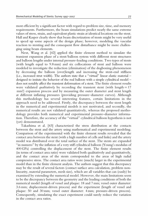
most efficient by a significant factor with regard to problem size, time, and memoryrequirements. Furthermore, the beam simulations predict nearly the same extremevalues of stress, strain, and equivalent plastic strain at identical locations on the stent.Hall and Kasper clearly show that beam discretization of stents might be very usefulto speed up some aspects of the design phase; however, modeling the vascularreaction to stenting and the consequent flow disturbance might be more challen-ging using beam elements.
Next, Wang et al. [42] applied the finite element method to simulate thetransient expansion phase of a stent/balloon system with different stent structuresand balloon lengths under internal pressure-loading conditions. Two types of stents(with length equal to 9.8mm) and six collocations of stent and balloon weremodeled to investigate the reduction (elimination) of the dogboning phenomenonby decreasing the balloon (over)length and increasing the stent-end stiffness(i.e., increased strut width). The authors state that a “virtual’’ linear elastic material –designed to imitate the behavior of the real balloon with a simple cylindrical model –does not notably affect the transient deformation of a stent. The finite element resultswere validated qualitatively by recording the transient stent (with length= 17mm!) expansion process and by measuring the outer diameter and stent lengthat different inflating pressures (providing pressure–diameter curves). Althoughthis methodology has several interesting features, certain limitations in theapproach need to be addressed. Firstly, the discrepancy between the stent lengthin the numerical and experimental models is not motivated, and secondly, thenumerical results are not validated quantitatively, whereas the proposed metho-dology provides both numerical and experimental pressure–diameter informa-tion. Therefore, the accuracy of the “virtual’’ cylindrical balloon hypothesis is not(yet) demonstrated.
Takashima et al. [43] characterized the stress distribution at the contactsbetween the stent and the artery using mathematical and experimental modeling.Comparison of the experimental with the finite element results revealed that thecontact area between the stent (with a high number of cells and links) and the arterymodel was distributed over the total surface of the stent. The stents are expanded“in numero’’ by the inflation of a very stiff cylindrical balloon (Young’s modulus of400GPa) controlling the displacement of the stent. The finite element results(in terms of contact area ratio) were validated both qualitatively and quantitatively,and the contact areas of the stents corresponded to the areas of high radialcompressive stress. The contact area ratios were (much) larger in the experimentalmodel than in the finite element analysis. The authors suggest that this discrepancymay be the result of several factors (contact surface area calculation, problem non-linearity, material parameters, mesh size), which are all variables that can (easily) beexamined by extending the numerical model. However, the main limitations seemto be the discrepancy between the geometry and the loading conditions of both thenumerical model (length of vessel and plaque: 18 and 7mm; vessel outer diameter:3.6mm; displacement-driven process) and the experiment (length of vessel andplaque: 50 and 30mm; vessel outer diameter: 4mm; pressure-driven process).Consequently, simulating the exact experiment could surely reduce the variationin the contact area ratios.
Biomechanical Modeling of Stents: Survey 1997–2007 77
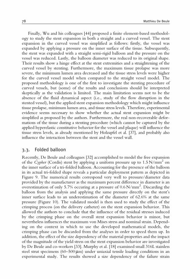
Finally, Wu and his colleagues [44] proposed a finite element-based methodol-ogy to study the stent expansion in both a straight and a curved vessel. The stentexpansion in the curved vessel was simplified as follows: firstly, the vessel wasexpanded by applying a pressure on the inner surface of the tissue. Subsequently,the stent was expanded with a straight semi-rigid balloon and the pressure on thevessel was reduced. Lastly, the balloon diameter was reduced to its original shape.Their results show a hinge effect at the stent extremities and a straightening of thecurved vessel by stenting. Furthermore, the maximum tissue prolapse was moresevere, the minimum lumen area decreased and the tissue stress levels were higherfor the curved vessel model when compared to the straight vessel model. Theproposed methodology is one of the first to investigate the stenting procedure ofcurved vessels, but (some) of the results and conclusions should be interpretedskeptically as the validation is limited. The main limitation seems not to be theabsence of the fluid dynamical aspect (i.e., study of the flow disruption in thestented vessel), but the applied stent expansion methodology which might influencetissue prolapse, minimum lumen area, and tissue stress levels. Therefore, experimentalevidence seems necessary to show whether the actual stent expansion might besimplified as proposed by the authors. Furthermore, the real non-recoverable defor-mations of the tissue during a stenting procedure (which cannot be captured by theapplied hyperelastic constitutive behavior for the vessel and plaque) will influence thetissue stress levels, as already mentioned by Holzapfel et al. [37], and probably alsoinfluence the interaction between the stent and the vessel wall.
3.3. Folded balloon
Recently, De Beule and colleagues [32] accomplished to model the free expansionof the Cypher (Cordis) stent by applying a uniform pressure up to 1.5N/mm2 onthe inner surface of a tri-folded balloon. Accounting for the presence of the balloonin its actual tri-folded shape reveals a particular deployment pattern as depicted inFigure 9. The numerical results correspond very well to pressure/diameter dataprovided by the manufacturer as the maximum percent difference in diameter is anoverestimation of only 5.7% occuring at a pressure of 0.6N/mm2. Discarding theballoon from the analysis and applying the same pressure directly on the stent’sinner surface leads to an underestimation of the diameter of 62.6% at the samepressure (Figure 10). The validated model is then used to study the effect of thecrimping process (on the delivery catheter) on the stent expansion behavior. Thisallowed the authors to conclude that the influence of the residual stresses inducedby the crimping phase on the overall stent expansion behavior is minor, butnevertheless influences the maximum von Mises stress and nominal strain. Depend-ing on the context in which to use the developed mathematical models, thecrimping phase can be discarded from the analyses in order to speed them up. Inaddition, the effect of the size dependency of the material properties and the impactof the magnitude of the yield stress on the stent expansion behavior are investigatedby De Beule and co-workers [33]. Murphy et al. [18] examined small 316L stainlesssteel strut specimens (60–500mm) under uniaxial tensile loading conditions in anexperimental study. The results showed a size dependency of the failure strain
78 Matthieu De Beule
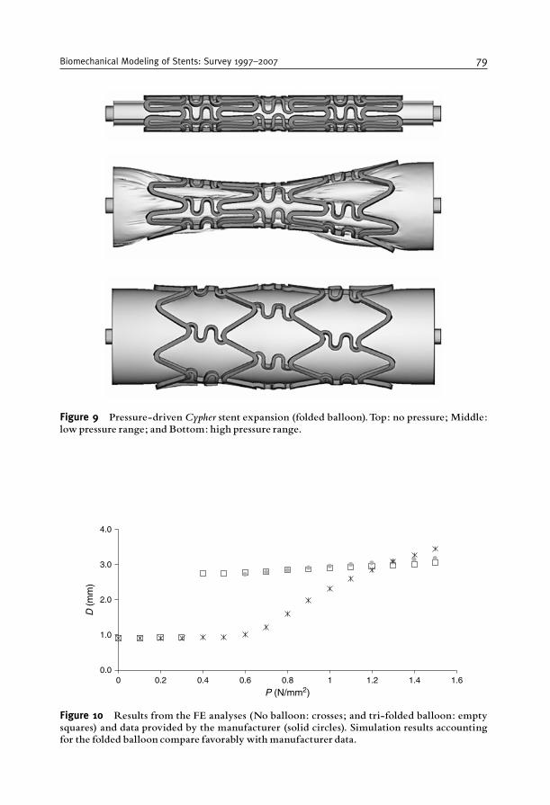
4.0
3.0
2.0
1.0
0.00 0.2 0.4 0.6
D (
mm
)
0.8
P (N/mm2)1 1.2 1.4 1.6
Figure 10 Results from the FE analyses (No balloon: crosses; and tri-folded balloon: emptysquares) and data provided by the manufacturer (solid circles). Simulation results accountingfor the folded balloon compare favorably with manufacturer data.
Figure 9 Pressure-driven Cypher stent expansion (folded balloon).Top: no pressure; Middle:low pressure range; and Bottom: high pressure range.
Biomechanical Modeling of Stents: Survey 1997–2007 79
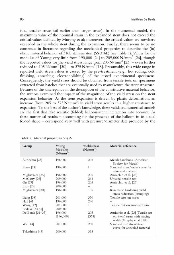
(i.e., smaller struts fail earlier than larger struts). In the numerical model, themaximum value of the nominal strain in the expanded stent does not exceed thecritical values defined by Murphy et al; moreover, the critical values are nowhereexceeded in the whole stent during the expansion. Finally, there seems to be noconsensus in literature regarding the mechanical properties to describe the (in)elastic material behavior of 316L stainless steel (SS 316L) (see Table 1). Values for themodulus of Young vary little from 190,000 [24] to 209,000N/mm2 [26], thoughthe reported values for the yield stress range from 205N/mm2 [23] – even furtherreduced to 105N/mm2 [30] – to 375N/mm2 [18]. Presumably, this wide range inreported yield stress values is caused by the pre-treatment (e.g., hot rolling, coldfinishing, annealing, electropolishing) of the tested experimental specimens.Consequently, the yield stress should be obtained from tensile tests on specimensextracted from batches that are eventually used to manufacture the stent structure.Because of this discrepancy in the description of the constitutive material behavior,the authors examined the impact of the magnitude of the yield stress on the stentexpansion behavior. As the stent expansion is driven by plastic deformation, anincrease (from 205 to 375N/mm2) in yield stress results in a higher resistance toexpansion. To the best of the author’s knowledge, these validated numerical modelsare the first that take realistic (folded) balloon–stent interaction into account. Asthese numerical results – accounting for the presence of the balloon in its actualfolded shape – correspond very well with pressure/diameter data provided by the
Table 1 Material properties SS316L
Group YoungModulus(N/mm2)
Yield stress(N/mm2)
Material reference
Auricchio [23] 196,000 205 Metals handbook (AmericanSociety for Metals)
Etave [24] 190,000 ? Standard stress/strain curve forannealed material
Migliavacca [25] 196,000 205 Auricchio et al. [23]McGarry [26] 209,000 264 Uniaxial tensile testGu [27] 196,000 205 Auricchio et al. [23]Lally [29] 200,000 – –Migliavacca [30] 196,000 105 Kinematic hardening yield
stress reduction (crimping)Liang [38] 201,000 330 Tensile tests on wiresHall [41] 196,000 290 –Wang [42] 201,000 ? Tensile test on annealed wireBedoya [34,35] 200,000 – –De Beule [31–33] 196,000
[196,000]205[375]
Auricchio et al. [23] [Tensile teston (stent) struts with varyingwidth (Murphy et al. [18])]
Wu [44] 201,000 280 Standard true stress/straincurve for annealed material
Takashima [43] 200,000 315 –
80 Matthieu De Beule
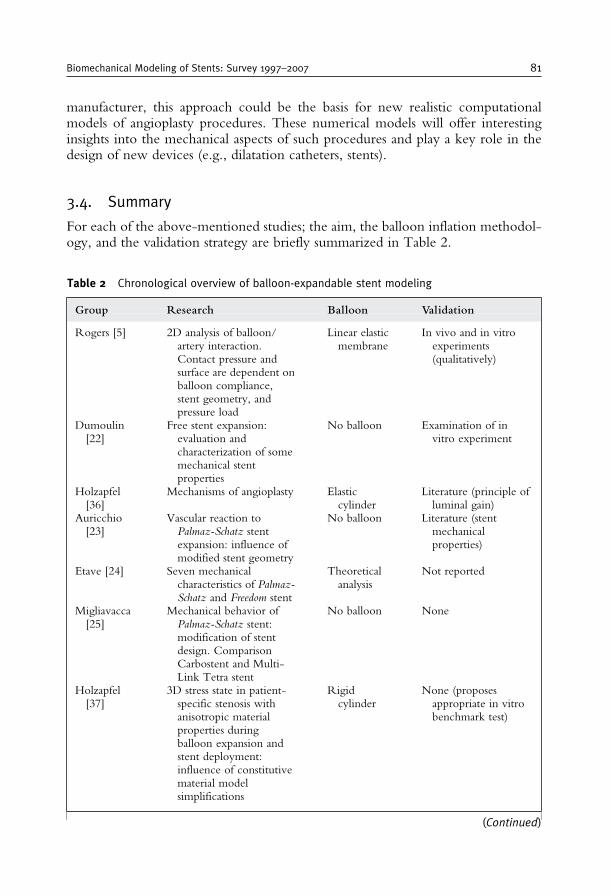
manufacturer, this approach could be the basis for new realistic computationalmodels of angioplasty procedures. These numerical models will offer interestinginsights into the mechanical aspects of such procedures and play a key role in thedesign of new devices (e.g., dilatation catheters, stents).
3.4. Summary
For each of the above-mentioned studies; the aim, the balloon inflation methodol-ogy, and the validation strategy are briefly summarized in Table 2.
Table 2 Chronological overview of balloon-expandable stent modeling
Group Research Balloon Validation
Rogers [5] 2D analysis of balloon/artery interaction.Contact pressure andsurface are dependent onballoon compliance,stent geometry, andpressure load
Linear elasticmembrane
In vivo and in vitroexperiments(qualitatively)
Dumoulin[22]
Free stent expansion:evaluation andcharacterization of somemechanical stentproperties
No balloon Examination of invitro experiment
Holzapfel[36]
Mechanisms of angioplasty Elasticcylinder
Literature (principle ofluminal gain)
Auricchio[23]
Vascular reaction toPalmaz-Schatz stentexpansion: influence ofmodified stent geometry
No balloon Literature (stentmechanicalproperties)
Etave [24] Seven mechanicalcharacteristics of Palmaz-Schatz and Freedom stent
Theoreticalanalysis
Not reported
Migliavacca[25]
Mechanical behavior ofPalmaz-Schatz stent:modification of stentdesign. ComparisonCarbostent and Multi-Link Tetra stent
No balloon None
Holzapfel[37]
3D stress state in patient-specific stenosis withanisotropic materialproperties duringballoon expansion andstent deployment:influence of constitutivematerial modelsimplifications
Rigidcylinder
None (proposesappropriate in vitrobenchmark test)
(Continued)
Biomechanical Modeling of Stents: Survey 1997–2007 81
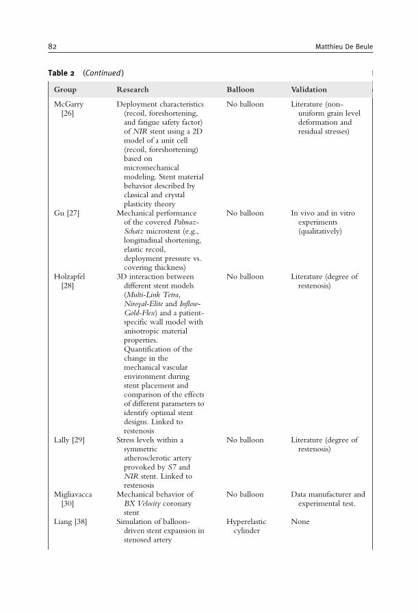
Table 2 (Continued )
Group Research Balloon Validation
McGarry[26]
Deployment characteristics(recoil, foreshortening,and fatigue safety factor)of NIR stent using a 2Dmodel of a unit cell(recoil, foreshortening)based onmicromechanicalmodeling. Stent materialbehavior described byclassical and crystalplasticity theory
No balloon Literature (non-uniform grain leveldeformation andresidual stresses)
Gu [27] Mechanical performanceof the covered Palmaz-Schatz microstent (e.g.,longitudinal shortening,elastic recoil,deployment pressure vs.covering thickness)
No balloon In vivo and in vitroexperiments(qualitatively)
Holzapfel[28]
3D interaction betweendifferent stent models(Multi-Link Tetra,Niroyal-Elite and Inflow-Gold-Flex) and a patient-specific wall model withanisotropic materialproperties.Quantification of thechange in themechanical vascularenvironment duringstent placement andcomparison of the effectsof different parameters toidentify optimal stentdesigns. Linked torestenosis
No balloon Literature (degree ofrestenosis)
Lally [29] Stress levels within asymmetricatherosclerotic arteryprovoked by S7 andNIR stent. Linked torestenosis
No balloon Literature (degree ofrestenosis)
Migliavacca[30]
Mechanical behavior ofBX Velocity coronarystent
No balloon Data manufacturer andexperimental test.
Liang [38] Simulation of balloon-driven stent expansion instenosed artery
Hyperelasticcylinder
None
82 Matthieu De Beule
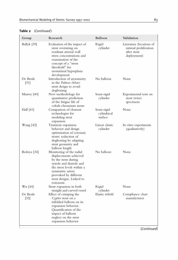
Table 2 (Continued )
Group Research Balloon Validation
Ballyk [39] Evaluation of the impact ofstent oversizing onresultant arterial wallstress concentrations andexamination of theconcept of a “stressthreshold’’ forneointimal hyperplasiadevelopment
Rigidcylinder
Literature (locations ofintimal proliferationafter stentdeployment)
De Beule[31]
Introduction of asymmetryin the Palmaz-Schatzstent design to avoiddogboning
No balloon None
Marrey [40] New methodology forquantitative predictionof the fatigue life ofcobalt-chromium stents
Semi-rigidcylinder
Experimental tests onstent (wire)specimens
Hall [41] Comparison of elementtechnologies formodeling stentexpansion
Semi-rigidcylindricalsurface
None
Wang [42] Transient expansionbehavior and designoptimization of coronarystents: reduction ofdogboning by adaptingstent geometry andballoon length
Linear elasticcylinder
In vitro experiments(qualitatively)
Bedoya [34] Monitoring of the radialdisplacements achievedby the stent duringsystole and diastole andthe stress levels within asymmetric arteryprovoked by differentstent designs. Linked torestenosis
No balloon None
Wu [44] Stent expansion in bothstraight and curved vessel
Rigidcylinder
None
De Beule[32]
Effect of crimping theCypher stent on atrifolded balloon on itsexpansion behavior.Quantification of theimpact of balloonneglect on the stentexpansion behavior
Elastic trifold Compliance chartmanufacturer
(Continued)
Biomechanical Modeling of Stents: Survey 1997–2007 83
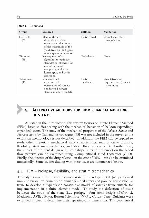
4. ALTERNATIVE METHODS FOR BIOMECHANICAL MODELING
OF STENTS
As stated in the introduction, this review focuses on Finite Element Method(FEM)-based studies dealing with the mechanical behavior of (balloon expanding/expanded) stents. The study of the mechanical properties of the Palmaz-Schatz andFreedom stents by Tan and his colleagues [45] was not included in the survey as theexpansion methodology is not described. In addition, the FEM can be applied tostudy other important mechanical stent characteristics, such as tissue prolapse,flexibility, strut micromechanics, and also self-expandable stents. Furthermore,the impact of the stent design (e.g., strut shape, interstrut distance) on the bloodflow patterns can be examined using Computational Fluid Dynamics (CFD).Finally, the kinetics of the drug release – in the case of DES – can also be examinednumerically. Some studies dealing with these issues are summarized below.
4.1. FEM – Prolapse, flexibility, and strut micromechanics
To analyze tissue prolapse in cardiovascular stents, Prendergast et al. [46] performeduni- and biaxial experiments on human femoral artery and porcine aortic vasculartissue to develop a hyperelastic constitutive model of vascular tissue suitable forimplementation in a finite element model. To study the deflection of tissuebetween the struts of the stent (i.e., prolapse), four stent designs (BeStent 2,Medtronic AVE; Niroyal, Boston Scientific; Velocity, Cordis; Tetra, Guidant) wereexpanded in vitro to determine their repeating-unit dimensions. This geometrical
Table 2 (Continued )
Group Research Balloon Validation
De Beule[33]
Effect of the sizedependency of thematerial and the impactof the magnitude of theyield stress on the Cypherstent expansion behavior
Elastic trifold Compliance chartmanufacturer
Timmins[35]
Development of analgorithm to optimizestent design, allowing forconsideration ofcompeting wall stress,lumen gain, and cyclicdeflection
No balloon None
Takashima[43]
Simulation andexperimentalobservation of contactconditions betweenstents and artery models.
Elasticcylinder
Qualitative andquantitative (contactarea ratio)
84 Matthieu De Beule

information was used to generate a finite element model of the vascular tissuesupported within a repeating unit of the stent. This methodology is proposed as away to compare stents relative to their potential for restenosis and as a basis for abiomechanical design of a stent repeating-unit that would minimize restenosis. Thestent measurements were obtained by taking pictures of the fully expanded stentunder a microscope and the images were then projected onto a 3.5mm cylinder todefine the geometry of one repeating unit of each stent design. Consequently, theblood vessel is modeled as a symmetric concentric cylindrical tube. The mostimportant simplification made by the authors is that the prolapse is not investigatedby taking the stent expansion process into account. Furthermore, the effect on theprolapse of taking a realistic (patient-specific) artery with a stenosis into account isnot (yet) examined.
Both Petrini and her colleagues [47] and Mori and Saito [48] explored theadvantages of the finite element method in order to investigate stent performance interms of flexibility. Petrini et al. considered two 3D models resembling two new-generation coronary stents (BX Velocity, Cordis and Carbostent, Sorin Biomedica),both in the expanded and in the unexpanded configuration. The main limitationsof the work are the absence of an experimental validation and the absence of thedelivery system during the flexibility analysis in the unexpanded configuration.Mori and Saito applied the four-points bending test to evaluate stent flexibility, andemployed the finite element method to assess the effect of stent structure onflexibility in stents with differing link structures under compressive loading condi-tions. The flexibility predicted from their simplified 2D finite element analysiscorrelated with the bending stiffness of the stents. The main limitation of thisstudy is that the flexibility is examined only in the stent’s expanded configuration,where the stent also should possess flexibility for maneuverability through tortuousvasculature to the site of occlusion in the unexpanded configuration.
The use of finite element analysis to predict the mechanical failure of stent strutswas investigated by Savage et al. [49]. A 2D computational micromechanicsapproach was considered involving an explicit representation of the grain structurein the steel struts to accurately represent the constitutive behavior of the material, asquestion arises as to the suitability of using bulk material properties at the size scaleof stent struts. The predictions of the failure strains in virtual uniaxial tensile tests onstrut specimens are in good qualitative agreement with the experimental results ofMurphy and his colleagues [18], i.e., the observation of a similar trend in thevariation of the failure strain with strut thickness. In order to produce betterquantitative results, full 3D models and models with an explicit damage mechanismseem necessary before even thinking of studying the (micro)mechanical behavior ofentire stents in their natural environment. Furthermore, these extended modelsmight require very high computational times as already stated by the authors.
4.2. FEM – Self-expandable stents
The first one to report a numerical study on the behavior of self-expandable stentstructures was Whitcher [50], who estimated the in vivo structural behavior andfatigue properties of nitinol stents. Migliavacca and colleagues [51] analyzed the
Biomechanical Modeling of Stents: Survey 1997–2007 85
stress state induced on the vascular wall, by the expansion of both balloon- and self-expandable stents using the finite element method, as the modified mechanicalstress state is in part responsible for the restenosis process. Comparing the stainlesssteel balloon expandable stent with the shape memory alloy (Nitinol) self-expandableone, the latter induces lower stresses, but on the other hand, its lower stiffnessinduces a lower capability to restore artery lumen and to counteract arterial elasticrecoil. However, because of the strong dependency of the material properties onthe shape memory alloy composition and thermomechanical treatment, this studydoes not make any attempt to give quantitative indications. In a more generalcomputational study of the shape memory alloy (SMA) behavior in biomedicalapplications, Petrini and her colleagues [52] performed an experimental and virtualstent crush test. Again, the exact knowledge of the real characteristic materialparameters is missing, but the observed agreement between the experimental andthe numerical results is encouraging and shows the capability of the implementedmaterial model to describe the fully 3D behavior of SMA devices. A noveland interesting concept of progressively expanding shape memory stents was proposedand studied by Theriault et al. [53]. To prevent restenosis caused by intimalhyperplasia, related to arterial wall injury due to the violent penetration of thestent structure, this study proposes a nitinol self-expanding stent with a progressiveexpansion system activated by the creep effect of polyethylene rings. This devicewill impose a smooth and gradual contact between the stent and the endothelium,giving the artery the opportunity to adapt to the presence of the device. A modelingstrategy was proposed to obtain the final geometry of the stent laser cut from a smalltube and to examine the behavior of the prosthesis during surgery and over the 4weeks following the operation. The numerical results demonstrate that a compro-mise can be reached between a limited expansion prior to the inflation of anexpandable balloon and a significant expansion by creep of the polymer rings.However, experimental validation of the mechanical behavior of the prosthesis ismissing and the interaction of the device with a (patient specific) stenosis has not yetbeen investigated. In a virtual study by Wu and colleagues [54], two superelasticstents were delivered into a stenotic carotid bifurcation through a sheath and self-expanded in the internal and common carotid artery. The stent with shorter strutshad less malapposition areas, a higher luminal gain, caused more tortuosity changesand induced higher maximum vessel stresses. The actual stent release from thecatheter is simplified by assuming a uniform diameter increase of the sheath andcontact between the stent struts during compression of the stent in the sheath isneglected. Furthermore, only one kind of nitinol material properties was modeled,whereas the actual (and highly adaptable) nitinol properties can influence the stentmechanical properties greatly. The above-mentioned assumptions can (only) bejustified through a missing targeted experimental validation.
As summarized above, the studies in engineering literature dedicated to theanalysis of the mechanical properties of nitinol self-expanding stents and to theirinteraction with the vessel wall focus on tubular stents. In contrast, the number ofvirtual studies related to wire stents is rather limited. This is surprising because ofthe wide application field of these devices [55–58]. Jedwab and Clerc [59] devel-oped an experimentally validated theoretical model of a self-expanding metallic
86 Matthieu De Beule
wire stent with the aim of predicting the various mechanical properties of the stent.Wang and Ravi-Chandar [60,61] developed a mathematically rigorous model,based on the theory of slender rods, that describes the response to internal andexternal loading conditions of a metallic braided wire stent, and the obtained resultswere validated with experimental data. In addition, Canic et al. [62] performed ananalytical study in order to analyze the mechanical properties of two bare-metalbraided stent grafts and to compare their response to hemodynamic forces. Further-more, Brand and his colleagues [63] developed an analytical approach for themechanical interaction of the self-expanding Cardiocoil (Medtronic InStent) stentwith the stenosed artery. All these studies show good results, but at the same time,they demonstrate the necessity to build complex analytical models to examine themechanical behavior of wire stents. Furthermore, these analytical models seemchallenging to analyze the expansion of wire stents in patient-specific anatomicalgeometries and seem unable to capture the mechanical behavior of innovativebioabsorbable braided stents [64]. In an attempt to partially justify the lack of finiteelement-based wire stent studies, one should consider the complexity of buildingthe geometrical model of such a wire stent using classical CAD methodologies andsubsequent (numerical) analysis of this family of stents.
4.3. CFD–drug elution and immersed FEM
Frank and his colleagues [65] have given a brief overview of Computational FluidDynamics (CFD) research studies dealing with stent design. CFD approaches arewell suited for obtaining detailed information on stent flow patterns, and the strongdependence of flow stagnation (possibly related to restenosis) on stent-strut spacinghas been clearly demonstrated. He and co-workers [66] examined detailed flowcharacteristics by estimating the Wall Shear Stress (WSS) in the near-strut region ofrealistic stent designs using 3D CFD. Their results also indicated that stent design iscrucial in determining the fluid mechanical environment in an artery. The results ofthe 3D CFD study of LaDisa et al. [67] supported the hypothesis that circumfer-ential vascular deformation after stent implantation imparts distinctive alterations inWSS that are not detected by using a standard circular model of the vascular crosssection. In addition, Benard and his colleagues [68] investigated the effects of blood(rheological) properties on changes in intra-stent flow with a 3D CFD model.Balakrishnan et al. [69] coupled computational fluid dynamics and a mass transfermodel to predict drug deposition for single and overlapping drug-eluting stents.The simulations correlated with in vivo effects and revealed that drug depositionoccurs not only beneath regions of arterial contact with the stent strut, but surpris-ingly also beneath standing drug pools created by strut disruption of flow. Toconclude, the mechanical behavior of stents during and after implantation werestudied by Gay et al. [70] using a fluid–structure interaction computational tech-nique. This complex fluid and deformable structure interaction problem wastackled using an immersed finite element method (IFEM) and allows to study theflow patterns during the deployment of a stent. However, the proposed modelingstrategy is not (yet) validated, and the effect of realistic stent expansion by balloonunfolding on the flow patterns remains unknown.
Biomechanical Modeling of Stents: Survey 1997–2007 87
5. FUTURE PROSPECTS
Future developments in stent modeling will most likely include further integra-tion of innovative (braided and tubular) stent designs and materials in realistic patient-specific stenosis models. Such integrated models may even further raise its share in thestent design phase and eventually enter the clinical practice to optimize the coronaryrevascularization procedure for a specific patient (e.g., as a presurgical planning tool).
In the “hunt’’ for the ideal stent, new stent materials [e.g., cobalt-chromium,superelastic shape-memory alloys, (biodegradable) polymers, magnesium.] areemerging. Each of these materials has a specific constitutive behavior and conse-quently requires a specific innovative stent design. These inventive stent designsand materials can and will further be tested and evaluated “in numero’’ [40,52,71].
The current (r)evolution in medical imaging, providing scientists with even moredetailed and accurate geometrical information for the vessel wall and plaque architec-ture, in combination with new insights into the constitutive material behavior of soft(biological) tissues and calcifications will allow further optimization of the strategyproposed byHolzapfel and his colleagues [36]. In addition, the recent advances in bothimage reconstruction, allowing to transfer these detailed medical images and materialdata into an accurate mathematical model, and simulation tools (e.g., complex contactdefinitions [32,33]) will only speed-up this optimization. Furthermore, validation ofthese numerical resultswith innovative (targeted) experiments [43]will only encouragethe use of the “in numero’’ strategy. Therefore, the idea of a surgeon implanting apatient-specific stent, selected by means of a numerical presurgical planning tool, nolonger seems science fiction.
6. CONCLUSION
From this review, it is obvious that the finite element method offers numerouspossibilities in the optimization of (coronary) revascularization procedures. The appli-cation of such a numerical approach in this specific biomechanical research domain isquite recent (1997) and has known an enormous evolution the last few years.Undoubtedly, all previously mentioned papers have contributed to the current levelof understanding the mechanics of both stent designs and angioplasty procedures, andthe quality of these studies should be evaluated taking into account the availableprescience and computational facilities (at the moment of publication). In the earlyyears, numerical simulations were based on Palmaz–Schatz (Johnson & Johnson)-likestents and simplified symmetrical stenosed arteries, mainly due to their straightforwardgeometry (e.g., the pioneering study published by Auricchio [23]). Furthermore, thePalmaz–Schatz stent was the only stent used in a multitude of large clinical studies atthat time. Since then this numerical (r)evolution has been characterized by someimportant milestones, such as (i) the introduction of patient-specific stenosis modelsby Holzapfel and coworkers in 2000 [36], (ii) the introduction of next generation stentgeometries by Migliavacca et al. in 2002 [25] and the introduction of stent design-optimization techniques by Timmins and his colleagues [35].
88 Matthieu De Beule
An astonishing observed fact in numerous studies is the lack of experimentalevidence for the obtained numerical results, creating a missing-link with reality andprovoking an (understandable) skepticism with respect to numerical models and tothe conclusions drawn from them. The little validation that is performed is oftenmerely qualitative, and thus not always applicable to interpret and verify thenumerical results. The only consistent quantitative validation regarding the stent-free expansion is from Migliavacca et al. [30], showing the considerable discrepancybetween numerical results and reality when discarding the presence of the balloon.Regarding the vascular reaction to stent deployment, it should be nuanced thatmeasuring the — by the stent (expansion) induced — stresses in the vessel wall inan experimental setup is a huge challenge. For such specific numerical studies, itmakes sense to compare the results with clinical findings in literature (e.g., restenosisrates). Nevertheless, caution should be paid to the adopted methodology of thecited clinical trials (i.e., investigated stent designs, patient recruitment), and speci-fically designed new clinical follow-ups could be required for thorough validationof the developed hypotheses from the numerical results. In addition, it should befeasible to examine the deployment characteristics of a stent using, for example, X-ray (Nano) Microtomography [72]. Furthermore, the impact of the assumptionsthat were made (e.g., balloon neglect or simplification, applied constitutive materialmodels), on the obtained results should be investigated thoroughly, as alreadyindicated by Holzapfel et al. [37].
The reported different methodologies to model the free expansion of a balloon-expandable stent should be evaluated and compared to assess the optimal freeexpansion methodology for finite element-based stent design. Such a comparisoncan help define the context in which neglecting the folded shape of the balloon isacceptable.
ACKNOWLEDGMENTS
The author gratefully acknowledges the valuable support and assistance fromRudy Van Impe (Ph.D.), Pascal Verdonck (Ph.D.), Benedict Verhegghe (Ph.D.),Patrick Segers (Ph.D.), Stephane Carlier (MD, Ph.D.), Peter Mortier, Denis VanLoo, and Bert Masschaele (Ph.D.).
REFERENCES
[1] A. H. Association, Heart Disease and Stroke Statistics – 2007 Update, Dallas, TX: AmericanHeart Association (2007) 1–43.
[2] D. E. Kandzari, J. E. Tcheng, J. P. Zidar, Coronary artery stents: evaluating new designs forcontemporary percutaneous intervention, Catherization and Cardiovascular Interventions 56 (4)(2002) 562–576.
[3] A. Kastrati, J. Mehilli, J. Dirschinger, J. Pache, K. Ulm, H. Schuhlen, M. Seyfarth, C. Schmitt,R. Blasini, F. J. Neumann, A. Schomig, Restenosis after coronary placement of various stenttypes, Am J Cardiol 87 (1) (2001) 34–39.
Biomechanical Modeling of Stents: Survey 1997–2007 89

[4] A. C. Morton, D. Crossman, J. Gunn, The influence of physical stent parameters upon rest-enosis, Pathol Biol (Paris) 52 (4) (2004) 196–205.
[5] C. Rogers, D. Y. Tseng, J. C. Squire, E. R. Edelman, Balloon-artery interactions during stentplacement: a finite element analysis approach to pressure, compliance, and stent design ascontributors to vascular injury, Circ Res 84 (4) (1999) 378–383.
[6] R. Mongrain, J. Rodes-Cabau, Role of shear stress in atherosclerosis and restenosis aftercoronary stent implantation, Rev Esp Cardiol 59 (1) (2006) 1–4.
[7] M.-C. Morice, P. W. Serruys, J. E. Sousa, J. Fajadet, E. Ban Hayashi, M. Perin, A. Colombo,G. Schuler, P. Barragan, G. Guagliumi, F. Molnar, R. Falotico, A randomized comparison of asirolimus-eluting stent with a standard stent for coronary revascularization, N Engl J Med 346(23) (2002) 1773–1780.
[8] J. E. Sousa, M. A. Costa, A. Abizaid, F. Feres, A. C. Seixas, L. F. Tanajura, L. A. Mattos,R. Falotico, J. Jaeger, J. J. Popma, P. W. Serruys, A. G. M. R. Sousa, Four-year angiographicand intravascular ultrasound follow-up of patients treated with sirolimus-eluting stents, Circulation111 (18) (2005) 2326–2329.
[9] P. W. Serruys, M. J. B. Kutryk, A. T. L. Ong, Coronary-artery stents, N Engl J Med 354 (5)(2006) 483–495.
[10] C. Kaiser, H. P. Brunner-La Rocca, P. T. Buser, P. O. Bonetti, S. Osswald, A. Linka,A. Bernheim, A. Zutter, M. Zellweger, L. Grize, M. E. Pfisterer, Incremental cost-effectivenessof drug-eluting stents compared with a third-generation bare-metal stent in a real-world setting:randomised Basel Stent Kosten Effektivitats Trial (BASKET), Lancet 366 (9489) (2005) 921–929.
[11] R. Virmani, G. Guagliumi, A. Farb, G. Musumeci, N. Grieco, T. Motta, L. Mihalcsik,M. Tespili, O. Valsecchi, F. D. Kolodgie, Localized hypersensitivity and late coronary throm-bosis secondary to a sirolimus-eluting stent: should we be cautious? Circulation 109 (6) (2004)701–705.
[12] M. Perry, S. Oktay, J. C. Muskivitch, Finite element analysis and fatigue of stents, MinimInvasive Ther Allied Technol 11 (4) (2002) 165–171.
[13] J. Mackerle, Finite element modelling and simulations in cardiovascular mechanics and cardiol-ogy: a bibliography 1993–2004, Comput Methods Biomech Biomed Engin 8 (2) (2005) 59–81.
[14] FDA Center for Devices and Radiological Health, Non Clinical Tests and RecommendedLabeling for Intravascular Stents and Associated Delivery Systems – Guidance for Industry andFDA Staff (2005) 1–48.
[15] UGCT, http://www.UGCT.UGent.be.[16] M. Saab, Applications of high-pressure balloons in the medical device industry, Medical Device &
Diagnostic Industry Magazine, NH, USA (1999).[17] S. Timoshenko, Strength of Materials (Part I: Elementary Theory and Problems), Van Nostrand
Reinhold, New York, p. 45, Chap. 2 (1955).[18] B. P. Murphy, P. Savage, P. E. McHugh, D. F. Quinn, The stress-strain behavior of coronary
stent struts is size dependent, Ann Biomed Eng 31 (6) (2003) 686–691.[19] C. Lally, P. Prendergast, D. Kelly, Stents, Wiley Encyclopaedia of Biomedical Engineering, John
Wiley & Sons 2007.[20] J. Squire, Dynamics of endovascular stent expansion, Ph.D. thesis, Massachusetts Institute of
Technology, US (2000).[21] H. Takebayashi, G. S. Mintz, S. G. Carlier, Y. Kobayashi, K. Fujii, T. Yasuda, R. A. Costa,
I. Moussa, G. D. Dangas, R. Mehran, A. J. Lansky, E. Kreps, M. B. Collins, A. Colombo,G. W. Stone, M. B. Leon, J. W. Moses, Nonuniform strut distribution correlates with moreneointimal hyperplasia after sirolimus-eluting stent implantation, Circulation 110 (22) (2004)3430–3434.
[22] C. Dumoulin, B. Cochelin, Mechanical behaviour modelling of balloon-expandable stents,J Biomech 33 (11) (2000) 1461–1470.
[23] F. Auricchio, M. Di Loreto, E. Sacco, Finite element analysis of a stenotic artery revasculariza-tion through a stent insertion, Comput Methods Biomech Biomed Engin 4 (2001) 249–263.
[24] F. Etave, G. Finet, M. Boivin, J. C. Boyer, G. Rioufol, G. Thollet, Mechanical propertiesof coronary stents determined by using finite element analysis, J Biomech 34 (8) (2001)1065–1075.
90 Matthieu De Beule
[25] F. Migliavacca, L. Petrini, M. Colombo, F. Auricchio, R. Pietrabissa, Mechanical behavior ofcoronary stents investigated through the finite element method, J Biomech 35 (6) (2002) 803–811.
[26] J. McGarry, B. O’Donnell, P. McHugh, J. G. McGarry, Analysis of the mechanical performanceof a cardiovascular stent design based on micromechanical modelling, CompMater Sci 31 (2004)421–438.
[27] L. Gu, S. Santra, R. A. Mericle, A. V. Kumar, Finite element analysis of covered microstents,J Biomech 38 (6) (2005) 1221–1227.
[28] G. A. Holzapfel, M. Stadler, T. C. Gasser, Changes in the mechanical environment of stenoticarteries during interaction with stents: computational assessment of parametric stent designs,J Biomech Eng 127 (1) (2005) 166–180.
[29] C. Lally, F. Dolan, P. J. Prendergast, Cardiovascular stent design and vessel stresses: a finiteelement analysis, J Biomech 38 (8) (2005) 1574–1581.
[30] F. Migliavacca, L. Petrini, V. Montanari, I. Quagliana, F. Auricchio, G. Dubini, A predictivestudy of the mechanical behaviour of coronary stents by computer modelling, Med Eng Phys 27(1) (2005) 13–18.
[31] M. De Beule, R. Van Impe, B. Verhegghe, P. Segers, P. Verdonck, Finite element analysis andstent design: reduction of dogboning, Technol Health Care 14 (4–5) (2006) 233–241.
[32] M. De Beule, P. Mortier, R. Van Impe, B. Verhegghe, P. Segers, P. Verdonck, Plasticity in themechanical behaviour of cardiovascular stents during stent preparation (crimping) and placement(expansion), Key Eng Mater 340–341 (2007) 847–852.
[33] M. De Beule, P. Mortier, J. Belis, R. Van Impe, B. Verhegghe, P. Verdonck, Plasticity as alifesaver in the design of cardiovascular stents, Key Eng Mater 340–341 (2007) 841–846.
[34] J. Bedoya, C. A. Meyer, L. H. Timmins, M. R. Moreno, J. E. Moore, Effects of stent designparameters on normal artery wall mechanics, J Biomech Eng 128 (5) (2006) 757–765.
[35] L. H. Timmins, M. R. Moreno, C. A. Meyer, J. C. Criscione, A. Rachev, J. E. J. Moore,Stented artery biomechanics and device design optimization, Med Biol Eng Comput 45 (5)(2007) 505–513.
[36] G. A. Holzapfel, C. A. J. Schulze-Bauer, M. Stadler, Mechanics of angioplasty: wall, balloon andstent, Mechanics in Biology – AMD-Vol. 242 and BED-Vol. 46 (2000) 141–156.
[37] G. A. Holzapfel, M. Stadler, C. A. J. Schulze-Bauer, A layer-specific three-dimensional modelfor the simulation of balloon angioplasty using magnetic resonance imaging and mechanicaltesting, Ann Biomed Eng 30 (6) (2002) 753–767.
[38] D. K. Liang, D. Z. Yang, M. Qi, W. Q. Wang, Finite element analysis of the implantation of aballoon-expandable stent in a stenosed artery, Int J Cardiol 104 (3) (2005) 314–318.
[39] P. D. Ballyk, Intramural stress increases exponentially with stent diameter: a stress threshold forneointimal hyperplasia, J Vasc Interv Radiol 17 (7) (2006) 1139–1145.
[40] R. V. Marrey, R. Burgermeister, R. B. Grishaber, R. O. Ritchie, Fatigue and life prediction forcobalt-chromium stents: a fracture mechanics analysis, Biomaterials 27 (9) (2006) 1988–2000.
[41] G. J. Hall, E. P. Kasper, Comparison of element technologies for modeling stent expansion,J Biomech Eng 128 (5) (2006) 751–756.
[42] W.-Q. Wang, D.-K. Liang, D.-Z. Yang, M. Qi, Analysis of the transient expansion behaviorand design optimization of coronary stents by finite element method, J Biomech 39 (1) (2006)21–32.
[43] K. Takashima, T. Kitou, K. Mori, K. Ikeuchi, Simulation and experimental observation ofcontact conditions between stents and artery models, Med Eng Phys 29 (3) (2007) 326–335.
[44] W. Wu, W.-Q. Wang, D.-Z. Yang, M. Qi, Stent expansion in curved vessel andtheir interactions: a finite element analysis, J Biomech, doi:10.1016/j.jbiomech.2006.11.009(2007).
[45] L. B. Tan, D. C. Webb, K. Kormi, S. T. Al-Hassani, A method for investigating the mechanicalproperties of intracoronary stents using finite element numerical simulation, Int J Cardiol 78 (1)(2001) 51–67.
[46] P. J. Prendergast, C. Lally, S. Daly, A. J. Reid, T. C. Lee, D. Quinn, F. Dolan, Analysis ofprolapse in cardiovascular stents: a constitutive equation for vascular tissue and finite-elementmodelling, J Biomech Eng 125 (5) (2003) 692–699.
Biomechanical Modeling of Stents: Survey 1997–2007 91
[47] L. Petrini, F. Migliavacca, F. Auricchio, G. Dubini, Numerical investigation of the intravascularcoronary stent flexibility, J Biomech 37 (4) (2004) 495–501.
[48] K. Mori, T. Saito, Effects of stent structure on stent flexibility measurements, Ann Biomed Eng33 (6) (2005) 733–742.
[49] P. Savage, B. P. O’Donnell, P. E. McHugh, B. P. Murphy, D. F. Quinn, Coronary stent strutsize dependent stress-strain response investigated using micromechanical finite element models,Ann Biomed Eng 32 (2) (2004) 202–211.
[50] F. Whitcher, Simulation of in vivo loading conditions of nitinol vascular stent structures,Comput Struct 64 (5/6) (1997) 1005–1011.
[51] F. Migliavacca, L. Petrini, P. Massarotti, S. Schievano, F. Auricchio, G. Dubini, Stainless andshape memory alloy coronary stents: a computational study on the interaction with the vascularwall, Biomech Model Mechanobiol 2 (4) (2004) 205–217.
[52] L. Petrini, F. Migliavacca, P. Massarotti, S. Schievano, G. Dubini, F. Auricchio, Computationalstudies of shape memory alloy behavior in biomedical applications, J Biomech Eng 127 (4)(2005) 716–725.
[53] P. Theriault, P. Terriault, V. Brailovski, R. Gallo, Finite element modeling of a progressivelyexpanding shape memory stent, J Biomech 39 (15) (2006) 2837–2844.
[54] W. Wu, M. Qi, X. Liu, D. Yang, W. Wang, Delivery and release of nitinol stent in carotidartery and their interactions: a finite element analysis, J Biomech, doi:10.1016/j.jbio-mech.2007.02.024 (2007).
[55] R. Morgan, A. Adam, Use of metallic stents and balloons in the esophagus and gastrointestinaltract, J Vasc Interv Radiol 12 (3) (2001) 283–297.
[56] A. R. Assali, S. Sdringola, A. Moustapha, M. Rihner, A. E. Denktas, M. A. Lefkowitz, M.Campbell, R. W. Smalling, Endovascular repair of traumatic pseudoaneurysm by uncoveredself-expandable stenting with or without transstent coiling of the aneurysm cavity, CatheterCardiovasc Interv 53 (2) (2001) 253–258.
[57] E. M. Walser, B. Robinson, S. A. Raza, O. S. Ozkan, E. Ustuner, J. Zwischenberger, Clinicaloutcomes with airway stents for proximal versus distal malignant tracheobronchial obstructions, JVasc Interv Radiol 15 (5) (2004) 471–477.
[58] S. Resnick, V. Rome, R. Vogelzang, Use of a partially deployed wallstent to act as an inferiorvena cava filtration device during coil embolization of a high-flow arteriovenous fistula, J VascInterv Radiol 17 (2 Pt 1) (2006) 369–372.
[59] M. R. Jedwab, C. O. Clerc, A study of the geometrical and mechanical properties of a self-expanding metallic stent–theory and experiment, J Appl Biomater 4 (1) (1993) 77–85.
[60] R. Wang, K. Ravi-Chandar, Mechanical response of a metallic aortic stent – Part I: Pressure-diameter relationship, J Appl Mech 71 (2004) 697–705.
[61] R. Wang, K. Ravi-Chandar, Mechanical response of a metallic aortic stent – Part II: A beam onelastic foundation model, J Appl Mech 71 (2004) 706–712.
[62] S. Canic, K. Ravi-Chandar, Z. Krajcer, D. Mirkovic, S. Lapin, Mathematical model analysis ofWallstent and AneuRx – dynamic responses of bare-metal endoprosthesis compared with thoseof stent-graft, Tex Heart I J 32 (4) (2005) 502–506.
[63] M. Brand, M. Ryvkin, S. Einav, L. Slepyan, The cardiocoil stent-artery interaction, J BiomechEng 127 (2) (2005) 337–344.
[64] J.-P. Nuutinen, C. Clerc, P. Tormala, Theoretical and experimental evaluation of the radialforce of self-expanding braided bioabsorbable stents, J Biomater Sci Polym Ed 14 (7) (2003)677–687.
[65] A. O. Frank, P. W. Walsh, J. E. J. Moore, Computational fluid dynamics and stent design, ArtifOrgans 26 (7) (2002) 614–621.
[66] Y. He, N. Duraiswamy, A. O. Frank, J. E. J. Moore, Blood flow in stented arteries: aparametric comparison of strut design patterns in three dimensions, J Biomech Eng 127 (4)(2005) 637–647.
[67] J. F. J. LaDisa, L. E. Olson, I. Guler, D. A. Hettrick, J. R. Kersten, D. C. Warltier, P. S. Pagel,Circumferential vascular deformation after stent implantation alters wall shear stress evaluatedwith time-dependent 3D computational fluid dynamics models, J Appl Physiol 98 (3) (2005)947–957.
92 Matthieu De Beule

[68] N. Benard, R. Perrault, D. Coisne, Computational approach to estimating the effects of bloodproperties on changes in intra-stent flow, Ann Biomed Eng 34 (8) (2006) 1259–1271.
[69] B. Balakrishnan, A. R. Tzafriri, P. Seifert, A. Groothuis, C. Rogers, E. R. Edelman, Strutposition, blood flow, and drug deposition: implications for single and overlapping drug-elutingstents, Circulation 111 (22) (2005) 2958–2965.
[70] M. Gay, L. Zhang, W. K. Liu, Stent modeling using immersed finite element method, ComputMethods Appl Mech Eng 195 (2006) 4358–4370.
[71] H. Muller, Development of metallic bioabsorbable intravascular implants, ESVB 2005, NewTechnologies in vascular biomaterials – Fundamentals about stents; eds. Chafke, N. and Durand,B. and Kretz, J. G. (2005).
[72] Stent-Research-Unit, http://www.stent-IBiTech.UGent.be.
Biomechanical Modeling of Stents: Survey 1997–2007 93

This page intentionally left blank

C H A P T E R 3
SIGNAL EXTRACTION IN MULTISENSOR
BIOMEDICAL RECORDINGS
Vicente Zarzoso, Ronald Phlypo, Olivier Meste, and Pierre Comon
Contents
1. Introduction 961.1. Aim and scope of the chapter 96
1.2. Mathematical notations 972. Genesis of Biomedical Signals 98
2.1. A biomedical source model 98
2.2. Cardiac signals 1012.3. Brain signals 105
3. Multi-Reference Optimal Wiener Filtering 1093.1. Non-invasive fetal ECG extraction 109
3.2. Optimal Wiener filtering 1103.3. Adaptive noise cancellation 1123.4. Results 113
4. Spatio-Temporal Cancellation 1154.1. Atrial activity extraction in atrial fibrillation 1154.2. Spatio-temporal cancellation of the QRST complex in AF episodes 117
5. Blind Source Separation (BSS) 1235.1. The isolation of interictal epileptic discharges in the EEG 1235.2. Modeling and assumptions 125
5.3. Inherent indeterminacies 1275.4. Statistical independence, higher-order statistics and non-Gaussianity 1275.5. Independent component analysis 1295.6. Algorithms 131
5.7. Results 1335.8. Incorporating prior information into the separation model 1365.9. Independent subspaces 138
5.10. Softening the stationarity constraint 1385.11. Revealing more sources than sensor signals 138
6. Summary, Conclusions and Outlook 139
Acknowledgments 140References 141
Advances in Biomedical Engineering � 2009 Elsevier B.V.
ISBN 978-0-444-53075-2 All rights reserved.
95
Abstract
A wide variety of biomedical problems require the extraction of signals of interest fromrecordings corrupted by other physiological activity signals, noise and interference. The taskis facilitated when multiple sensors on different locations record simultaneously the biome-dical phenomenon under examination. This chapter provides an overview of signal proces-
sing techniques to extract the signal(s) of interest and cancel the interference byexploiting the spatial diversity available in the multisensor measurements. The focus is onthree different approaches, namely, multi-reference optimal Wiener filtering, spatio-temporal
cancellation and blind source separation. The working assumptions and main algorithmicimplementations of these techniques are discussed, and their usefulness is demonstratedon real recordings issued from various biomedical signal processing problems.
Keywords: array signal processing, blind source separation, electroencephalogram,electrocardiogram, higher-order statistics, independent component analysis, multisensormeasurements, optimal Wiener filtering, principal component analysis, second-orderstatistics, spatial diversity, synchronized averaging
1. INTRODUCTION
1.1. Aim and scope of the chapter
Physiological phenomena are typically associated with measurable variations ofphysical magnitudes such as electric potential, giving rise to biomedical signals. Never-theless, the measurement of signals of physiological or clinical interest is often hinderedby other biomedical activities, noise and interference. In recordings taken from themother’s skin during pregnancy, the electrical activity from the fetal heartbeat can bemasked by the stronger maternal cardiac activity. In electrocardiogram (ECG) record-ings from atrial fibrillation sufferers, the electrical activity from the atria appears mixedwith that from the ventricles. In electroencephalogram (EEG) recordings fromepileptic patients, epileptic discharges and the brain’s background activity contributesimultaneously to the signals measured by scalp electrodes, and can be furthercorrupted by artifacts such as eye blinks or body movements.
These and many other similar scenarios call for signal processing techniquesto extract the desired signal – the fetal heartbeat, the atrial activity, the epileptic-related brain source, etc. – from the artifact-corrupted measurements. Traditionaltechniques such as frequency filtering or synchronized averaging and subtrac-tion can be used to process the output of a single sensor. However, in manyapplications multiple sensors at different locations are available to record simulta-neously the physiological phenomenon under analysis. The spatial diversity of themultisensor recordings can then be exploited to significantly improve the signalextraction and interference cancellation performance. In particular, the proper useof spatial diversity allows the separation of signals with overlapping frequencyspectra. The main idea is to combine judiciously the multisensor observations, anoperation known as spatial filtering, in order to estimate the signal of interestdirectly, or indirectly by first estimating and then cancelling the interference.Specific approaches differ in the manner in which spatial filters are designed.
96 Vicente Zarzoso et al.
Designs can be based on elaborate signal models trying to explain accurately thephysiological phenomena under study, or simpler models sacrificing precision formathematical tractability.
Three spatial filtering approaches are surveyed in this chapter. The first approach(Section 3) is arguably the most classical and consists of the application of optimalWiener’s filter to the scenario of multiple reference signals [1]. The technique assumesthe availability of some observations containing information correlated with theartifact, but uncorrelated with the desired signal. The interference present in thecorrupted sensor output is estimated by filtering these artifact-correlated recordings.The desired signal is finally obtained by subtracting the estimated interference. Thistechnique exploits the often plausible assumption of uncorrelation between the desiredsignal and the artifacts and relies on the second-order statistics of the data.
The second approach, referred to as spatio-temporal cancellation (Section 4), can beconsidered as an extension of the conventional synchronized averaging and subtractiontechnique to the multisensor case [2]. This approach constructs a spatial template of theinterfering waveforms by first detecting their occurrence in the recording of each lead.By relying on the repetitive character of the interference, synchronized averaging helpsremove other activity, such as the desired signal, uncorrelated with the interferingwaveform. Before subtraction, the estimated template is optimally scaled in amplitudeand aligned in time to every occurrence in the recordings.
Blind Source Separation (BSS), a rather general array processing approach notlimited to biomedical applications, is addressed at the end of this chapter (Section 5).In this recent technique [3–6], the observed signals are considered as unknown linearmixtures of some unknown sources representing the underlying biological activity.The source waveforms can be estimated at the separator output by spatial filtersrecovering a known property of the sources such as mutual independence. Measuringthese properties typically involves statistical information at orders higher than two(higher-order statistics). By isolating the estimated sources of interest and their corre-sponding mixing coefficients, the contributions of the desired biomedical activity tothe recordings can be easily reconstructed free from noise and interference. BSS can beseen as a generalization ofWiener’s noise cancelling approach without pure references.
For didactic purposes, each approach is first motivated by one of the biomedicalproblems briefly presented at the beginning of this chapter. The mathematicaldetails of the signal processing techniques are then developed and illustrated byapplication results on real recordings. A summary and some concluding remarks onthe perspectives and further applications of the presented techniques (Section 6)bring the chapter to an end.
First, Section 2 addresses the modeling of the biomedical signals considered inthis chapter. The signal processing techniques developed in Sections 3–5 are basedon these models.
1.2. Mathematical notations
Throughout the rest of the chapter, scalars, vectors, and matrices are represented bylightface (a, A), boldface lowercase (a) and boldface uppercase (A) letters, respec-tively. In is the n� n identity matrix. Notation kak denotes the Euclidean norm of
Signal Extraction in Multisensor Biomedical Recordings 97
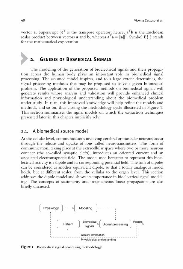
vector a. Superscript (�)T is the transpose operator; hence, aTb is the Euclideanscalar product between vectors a and b, whereas aTa= kak2. Symbol Ef�g standsfor the mathematical expectation.
2. GENESIS OF BIOMEDICAL SIGNALS
The modeling of the generation of bioelectrical signals and their propaga-tion across the human body plays an important role in biomedical signalprocessing. The assumed model inspires, and to a large extent determines, thesignal processing methods that may be proposed to solve a given biomedicalproblem. The application of the proposed methods on biomedical signals willgenerate results whose analysis and validation will provide enhanced clinicalinformation and physiological understanding about the biomedical problemunder study. In turn, this improved knowledge will help refine the models andmethods, and so on, thus closing the methodology cycle illustrated in Figure 1.This section summarizes the signal models on which the extraction techniquespresented later in this chapter implicitly rely.
2.1. A biomedical source model
At the cellular level, communications involving cerebral or muscular neurons occurthrough the release and uptake of ions called neurotransmitters. This form ofcommunication, taking place at the extracellular space where two or more neuronsconnect (the so-called synaptic clefts), introduces an oriented current and anassociated electromagnetic field. The model used hereafter to represent this bioe-lectrical activity is a dipole and its corresponding potential field. The sum of dipolescan be considered as another equivalent dipole, so that a totally analogous modelholds, but at different scales, from the cellular to the organ level. This sectionaddresses the dipole model and shows its importance in bioelectrical signal model-ing. The concepts of stationarity and instantaneous linear propagation are alsobriefly discussed.
Patient
Modeling
Biomedical
signalsSignal processing
Physiology
Results
Clinical information
Physiological understanding
Figure 1 Biomedical signal processingmethodology.
98 Vicente Zarzoso et al.
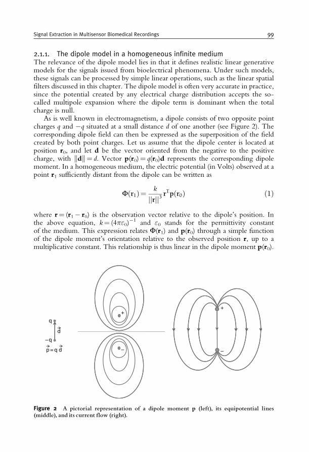
2.1.1. The dipole model in a homogeneous infinite mediumThe relevance of the dipole model lies in that it defines realistic linear generativemodels for the signals issued from bioelectrical phenomena. Under such models,these signals can be processed by simple linear operations, such as the linear spatialfilters discussed in this chapter. The dipole model is often very accurate in practice,since the potential created by any electrical charge distribution accepts the so-called multipole expansion where the dipole term is dominant when the totalcharge is null.
As is well known in electromagnetism, a dipole consists of two opposite pointcharges q and �q situated at a small distance d of one another (see Figure 2). Thecorresponding dipole field can then be expressed as the superposition of the fieldcreated by both point charges. Let us assume that the dipole center is located atposition r0, and let d be the vector oriented from the negative to the positivecharge, with kdk= d. Vector p(r0)= q(r0)d represents the corresponding dipolemoment. In a homogeneous medium, the electric potential (in Volts) observed at apoint r1 sufficiently distant from the dipole can be written as
Fðr1Þ= k
jjrjj3 rTpðr0Þ ð1Þ
where r= (r1� r0) is the observation vector relative to the dipole’s position. Inthe above equation, k= (4�"0)
�1 and "0 stands for the permittivity constantof the medium. This expression relates F(r1) and p(r0) through a simple functionof the dipole moment’s orientation relative to the observed position r, up to amultiplicative constant. This relationship is thus linear in the dipole moment p(r0).
p = q d
– q
q
d
– –
++
Figure 2 A pictorial representation of a dipole moment p (left), its equipotential lines(middle), and its current flow (right).
Signal Extraction in Multisensor Biomedical Recordings 99
Equation (1) can be rewritten to obtain F(r1) as a function of the electricalcharge q(r0) under the constraint that d and r are fixed:
Fðr1Þ= cðjjrjj; kÞrTpðr0Þ= cðjjrjj; kÞðrTdÞqðr0Þ= hðr; d; kÞqðr0Þ: ð2ÞThe potential at point r1 is then expressed as a linear function of the electrical chargeq(r0) if the dipole’s orientation d and its position r relative to the measurement pointare held fixed. These stationary conditions thus result in an instantaneous linearrelationship between the charge distribution and the generated potential. Likewise,under these conditions, the electric potential generated by a dipole distributionp(r0
i )= q(r0i )di, 1� i�M, is given by F(r1)=�i= 1
M h(ri, di, k) q(r0i ), with
ri= (r1� r0i ).
2.1.2. The dipole in a heterogeneous mediumMost bioelectrical media are not homogeneous, and thus the simple relationbetween F and q does not hold for all r1 and r0. However, it is possible to de-compose the total medium into piecewise homogeneous volumes (PHVs). EachPHV can be considered as a closed volume of a bioelectrical medium with quasi-homogeneous electrical properties (such as a single "0 for the whole volume). Forthe PHV which encloses the dipole, the potentials can be calculated at its volumesurface. This charged surface can then be seen as an ensemble of dipoles which, inturn, can be enclosed by another volume. The simple analytical relation betweenthe potential and the charge distribution of Eq. (1) no longer exists but for a fixeddipole and a fixed observation vector, Eq. (2) still holds, even if we cross theboundaries of homogeneity. The proof of this linear relation, which is omitted heredue to lack of space, can be found in Gulrajani [7]. Since the analytical model thatwould result from this nested structure of PHVs does not have a straightforwardsolution, an appropriate h for each r, d, and k can be obtained using numericalmodels based on sampled 3D spaces [8].
2.1.3. Not everything is a dipole: more realistic modelsHowever, not all bioelectrical activity can be modeled accurately by considering asingle dipole and its potential field. In some cases, a dipole layer or a multi-dipoleconfiguration would be more suitable approximations. More elaborate modelsproposed in the literature range from coupled dipoles [9] to distributed sourcemodels [10], including dipole lines and dipole surfaces/volumes.
On the other hand, the currents generated in the synaptic clefts do not directlyreflect as such at the cutaneous electrodes used for measuring biopotentials.A sufficiently high magnitude with respect to the noise (e.g., the quantizationnoise introduced by any digital system, the background noise, etc.) demands thesimultaneous firing of groups of neurons. If the group of neurons are assumed tofire synchronously at fixed positions and with fixed orientations, the activity of theensemble can be modeled by a single dipole in the far-field approximation (seeSection 2.1.1).
100 Vicente Zarzoso et al.
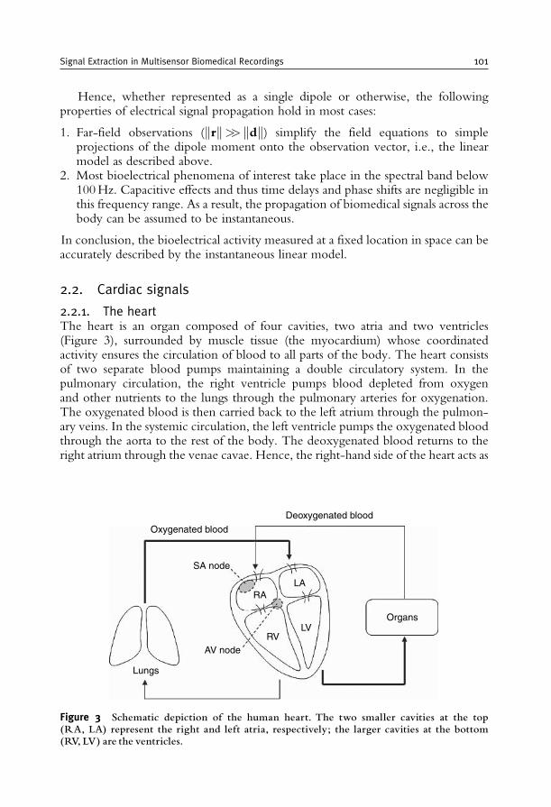
Hence, whether represented as a single dipole or otherwise, the followingproperties of electrical signal propagation hold in most cases:
1. Far-field observations (krk>> kdk) simplify the field equations to simpleprojections of the dipole moment onto the observation vector, i.e., the linearmodel as described above.
2. Most bioelectrical phenomena of interest take place in the spectral band below100Hz. Capacitive effects and thus time delays and phase shifts are negligible inthis frequency range. As a result, the propagation of biomedical signals across thebody can be assumed to be instantaneous.
In conclusion, the bioelectrical activity measured at a fixed location in space can beaccurately described by the instantaneous linear model.
2.2. Cardiac signals
2.2.1. The heartThe heart is an organ composed of four cavities, two atria and two ventricles(Figure 3), surrounded by muscle tissue (the myocardium) whose coordinatedactivity ensures the circulation of blood to all parts of the body. The heart consistsof two separate blood pumps maintaining a double circulatory system. In thepulmonary circulation, the right ventricle pumps blood depleted from oxygenand other nutrients to the lungs through the pulmonary arteries for oxygenation.The oxygenated blood is then carried back to the left atrium through the pulmon-ary veins. In the systemic circulation, the left ventricle pumps the oxygenated bloodthrough the aorta to the rest of the body. The deoxygenated blood returns to theright atrium through the venae cavae. Hence, the right-hand side of the heart acts as
Oxygenated blood
Deoxygenated blood
Organs
LA
LVRV
RA
AV node
Lungs
SA node
Figure 3 Schematic depiction of the human heart. The two smaller cavities at the top(RA, LA) represent the right and left atria, respectively; the larger cavities at the bottom(RV, LV) are the ventricles.
Signal Extraction in Multisensor Biomedical Recordings 101
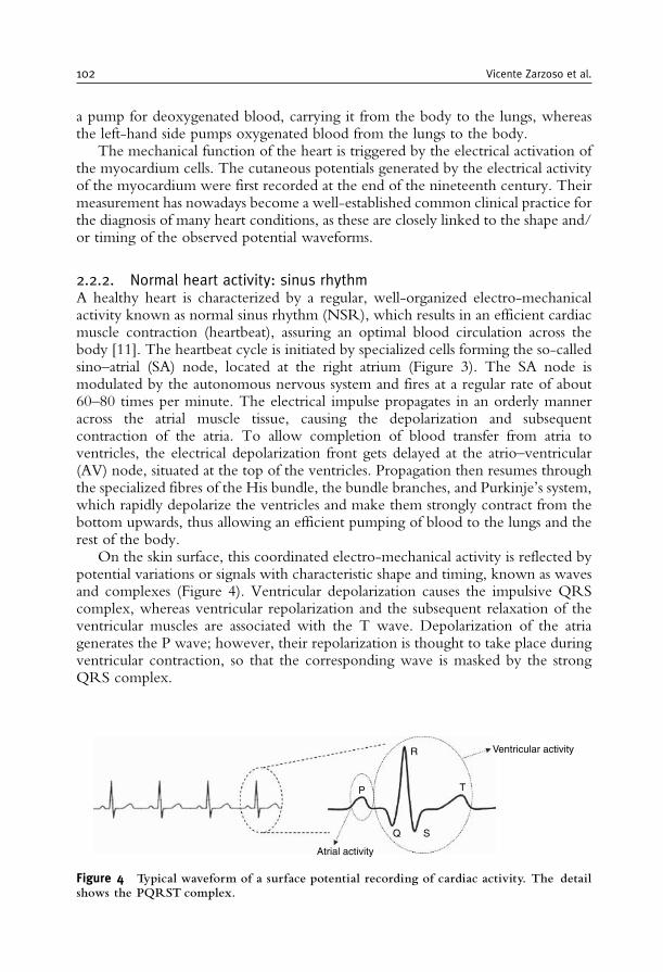
a pump for deoxygenated blood, carrying it from the body to the lungs, whereasthe left-hand side pumps oxygenated blood from the lungs to the body.
The mechanical function of the heart is triggered by the electrical activation ofthe myocardium cells. The cutaneous potentials generated by the electrical activityof the myocardium were first recorded at the end of the nineteenth century. Theirmeasurement has nowadays become a well-established common clinical practice forthe diagnosis of many heart conditions, as these are closely linked to the shape and/or timing of the observed potential waveforms.
2.2.2. Normal heart activity: sinus rhythmA healthy heart is characterized by a regular, well-organized electro-mechanicalactivity known as normal sinus rhythm (NSR), which results in an efficient cardiacmuscle contraction (heartbeat), assuring an optimal blood circulation across thebody [11]. The heartbeat cycle is initiated by specialized cells forming the so-calledsino–atrial (SA) node, located at the right atrium (Figure 3). The SA node ismodulated by the autonomous nervous system and fires at a regular rate of about60–80 times per minute. The electrical impulse propagates in an orderly manneracross the atrial muscle tissue, causing the depolarization and subsequentcontraction of the atria. To allow completion of blood transfer from atria toventricles, the electrical depolarization front gets delayed at the atrio–ventricular(AV) node, situated at the top of the ventricles. Propagation then resumes throughthe specialized fibres of the His bundle, the bundle branches, and Purkinje’s system,which rapidly depolarize the ventricles and make them strongly contract from thebottom upwards, thus allowing an efficient pumping of blood to the lungs and therest of the body.
On the skin surface, this coordinated electro-mechanical activity is reflected bypotential variations or signals with characteristic shape and timing, known as wavesand complexes (Figure 4). Ventricular depolarization causes the impulsive QRScomplex, whereas ventricular repolarization and the subsequent relaxation of theventricular muscles are associated with the T wave. Depolarization of the atriagenerates the P wave; however, their repolarization is thought to take place duringventricular contraction, so that the corresponding wave is masked by the strongQRS complex.
Ventricular activity
T
SQ
P
Atrial activity
R
Figure 4 Typical waveform of a surface potential recording of cardiac activity. The detailshows the PQRST complex.
102 Vicente Zarzoso et al.
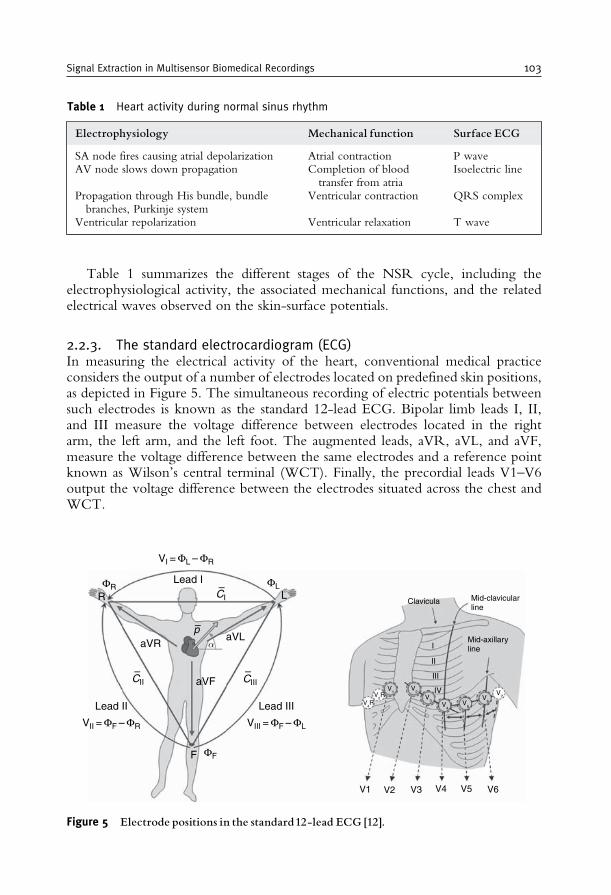
Table 1 summarizes the different stages of the NSR cycle, including theelectrophysiological activity, the associated mechanical functions, and the relatedelectrical waves observed on the skin-surface potentials.
2.2.3. The standard electrocardiogram (ECG)In measuring the electrical activity of the heart, conventional medical practiceconsiders the output of a number of electrodes located on predefined skin positions,as depicted in Figure 5. The simultaneous recording of electric potentials betweensuch electrodes is known as the standard 12-lead ECG. Bipolar limb leads I, II,and III measure the voltage difference between electrodes located in the rightarm, the left arm, and the left foot. The augmented leads, aVR, aVL, and aVF,measure the voltage difference between the same electrodes and a reference pointknown as Wilson’s central terminal (WCT). Finally, the precordial leads V1–V6output the voltage difference between the electrodes situated across the chest andWCT.
Table 1 Heart activity during normal sinus rhythm
Electrophysiology Mechanical function Surface ECG
SA node fires causing atrial depolarization Atrial contraction P waveAV node slows down propagation Completion of blood
transfer from atriaIsoelectric line
Propagation through His bundle, bundlebranches, Purkinje system
Ventricular contraction QRS complex
Ventricular repolarization Ventricular relaxation T wave
F
R
Lead II Lead III
Lead I
LClavicula
I
III
IV
V1
V4R
V2R
V1
V2
V3
V4
V5
V6
V7
V2 V3 V4 V5 V6
II
Mid-clavicularline
Mid-axillarylineaVR
– –
–
–
aVF
VIII = ΦF – ΦLVII = ΦF – ΦR
VI = ΦL – ΦR
aVL
CII
α
CIII
CI
p
ΦR
ΦF
ΦL
Figure 5 Electrode positions in the standard12-lead ECG [12].
Signal Extraction in Multisensor Biomedical Recordings 103
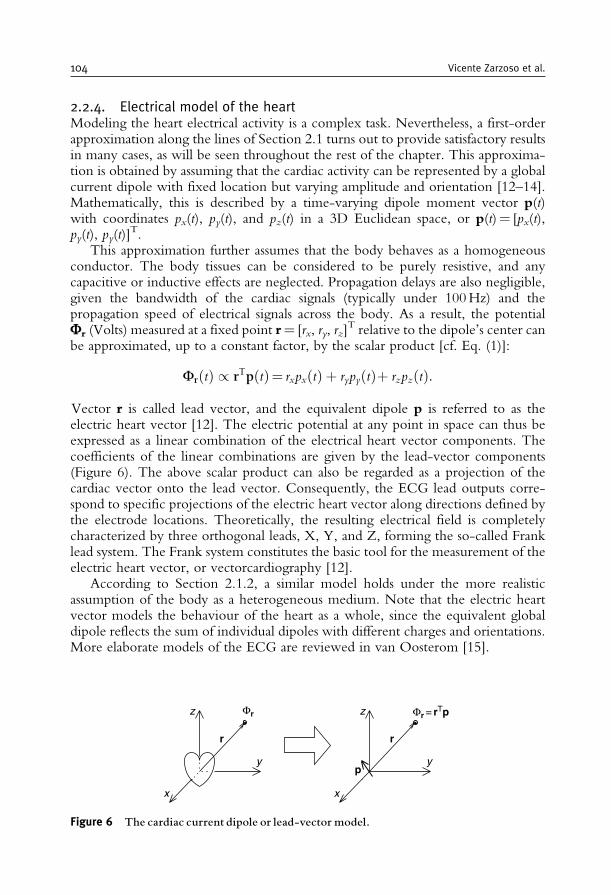
2.2.4. Electrical model of the heartModeling the heart electrical activity is a complex task. Nevertheless, a first-orderapproximation along the lines of Section 2.1 turns out to provide satisfactory resultsin many cases, as will be seen throughout the rest of the chapter. This approxima-tion is obtained by assuming that the cardiac activity can be represented by a globalcurrent dipole with fixed location but varying amplitude and orientation [12–14].Mathematically, this is described by a time-varying dipole moment vector p(t)with coordinates px(t), py(t), and pz(t) in a 3D Euclidean space, or p(t)= [px(t),py(t), py(t)]
T.This approximation further assumes that the body behaves as a homogeneous
conductor. The body tissues can be considered to be purely resistive, and anycapacitive or inductive effects are neglected. Propagation delays are also negligible,given the bandwidth of the cardiac signals (typically under 100Hz) and thepropagation speed of electrical signals across the body. As a result, the potentialFr (Volts) measured at a fixed point r= [rx, ry, rz]
T relative to the dipole’s center canbe approximated, up to a constant factor, by the scalar product [cf. Eq. (1)]:
FrðtÞ / rTpðtÞ= rxpxðtÞ þ rypyðtÞþ rzpzðtÞ:
Vector r is called lead vector, and the equivalent dipole p is referred to as theelectric heart vector [12]. The electric potential at any point in space can thus beexpressed as a linear combination of the electrical heart vector components. Thecoefficients of the linear combinations are given by the lead-vector components(Figure 6). The above scalar product can also be regarded as a projection of thecardiac vector onto the lead vector. Consequently, the ECG lead outputs corre-spond to specific projections of the electric heart vector along directions defined bythe electrode locations. Theoretically, the resulting electrical field is completelycharacterized by three orthogonal leads, X, Y, and Z, forming the so-called Franklead system. The Frank system constitutes the basic tool for the measurement of theelectric heart vector, or vectorcardiography [12].
According to Section 2.1.2, a similar model holds under the more realisticassumption of the body as a heterogeneous medium. Note that the electric heartvector models the behaviour of the heart as a whole, since the equivalent globaldipole reflects the sum of individual dipoles with different charges and orientations.More elaborate models of the ECG are reviewed in van Oosterom [15].
Φr = rTp
r
p
Φr
r
y
x
z
y
z
x
Figure 6 The cardiac current dipole or lead-vector model.
104 Vicente Zarzoso et al.
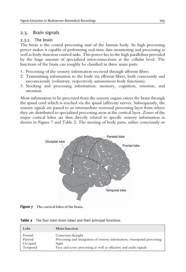
2.3. Brain signals
2.3.1. The brainThe brain is the central processing unit of the human body. Its high processingpower makes it capable of performing real-time data monitoring and processing aswell as body-function control tasks. This power lies in the high parallelism providedby the huge amount of specialized interconnections at the cellular level. Thefunctions of the brain can roughly be classified in three main parts:
1. Processing of the sensory information received through afferent fibres.2. Transmitting information to the body via efferent fibres, both consciously and
unconsciously (voluntary, respectively autonomous body functions).3. Stocking and processing information: memory, cognition, emotion, and
attention.
Most information to be processed from the sensory organs enters the brain throughthe spinal cord which is reached via the spinal (afferent) nerves. Subsequently, thesensory signals are passed to an intermediate neuronal processing layer from wherethey are distributed to specialized processing areas at the cortical layer. Zones of themajor cortical lobes are thus directly related to specific sensory information asshown in Figure 7 and Table 2. The steering of body parts, either consciously or
Occipital lobe
Parietal lobe
Frontal lobe
Temporal lobe
Figure 7 The cortical lobes of the brain.
Table 2 The four main brain lobes and their principal functions
Lobe Main function
Frontal Conscious thoughtParietal Processing and integration of sensory information; visuospatial processingOccipital SightTemporal Face and scene processing as well as olfactory and audio signals
Signal Extraction in Multisensor Biomedical Recordings 105
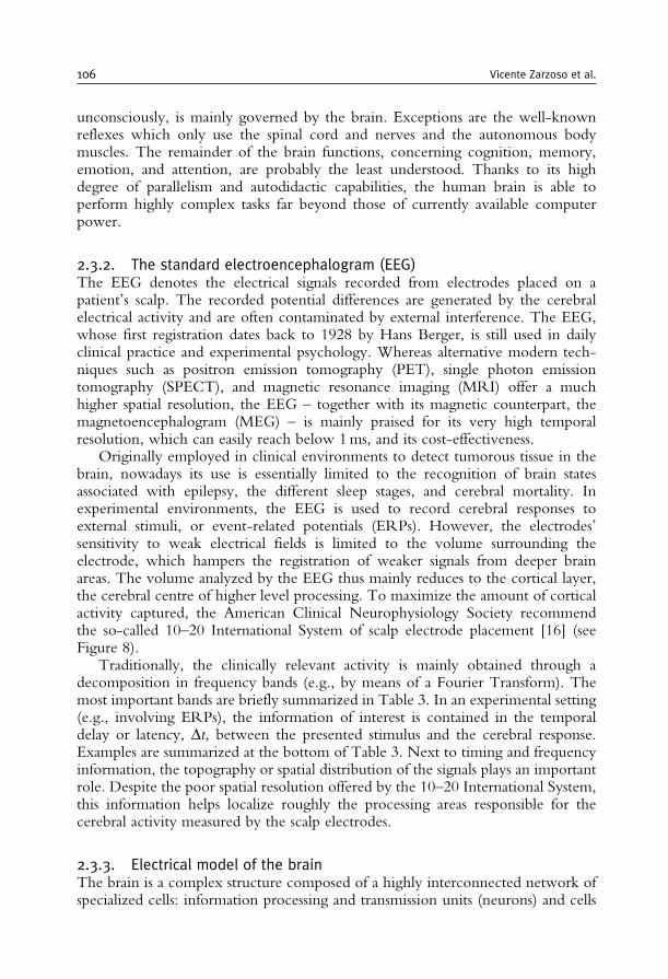
unconsciously, is mainly governed by the brain. Exceptions are the well-knownreflexes which only use the spinal cord and nerves and the autonomous bodymuscles. The remainder of the brain functions, concerning cognition, memory,emotion, and attention, are probably the least understood. Thanks to its highdegree of parallelism and autodidactic capabilities, the human brain is able toperform highly complex tasks far beyond those of currently available computerpower.
2.3.2. The standard electroencephalogram (EEG)The EEG denotes the electrical signals recorded from electrodes placed on apatient’s scalp. The recorded potential differences are generated by the cerebralelectrical activity and are often contaminated by external interference. The EEG,whose first registration dates back to 1928 by Hans Berger, is still used in dailyclinical practice and experimental psychology. Whereas alternative modern tech-niques such as positron emission tomography (PET), single photon emissiontomography (SPECT), and magnetic resonance imaging (MRI) offer a muchhigher spatial resolution, the EEG – together with its magnetic counterpart, themagnetoencephalogram (MEG) – is mainly praised for its very high temporalresolution, which can easily reach below 1ms, and its cost-effectiveness.
Originally employed in clinical environments to detect tumorous tissue in thebrain, nowadays its use is essentially limited to the recognition of brain statesassociated with epilepsy, the different sleep stages, and cerebral mortality. Inexperimental environments, the EEG is used to record cerebral responses toexternal stimuli, or event-related potentials (ERPs). However, the electrodes’sensitivity to weak electrical fields is limited to the volume surrounding theelectrode, which hampers the registration of weaker signals from deeper brainareas. The volume analyzed by the EEG thus mainly reduces to the cortical layer,the cerebral centre of higher level processing. To maximize the amount of corticalactivity captured, the American Clinical Neurophysiology Society recommendthe so-called 10–20 International System of scalp electrode placement [16] (seeFigure 8).
Traditionally, the clinically relevant activity is mainly obtained through adecomposition in frequency bands (e.g., by means of a Fourier Transform). Themost important bands are briefly summarized in Table 3. In an experimental setting(e.g., involving ERPs), the information of interest is contained in the temporaldelay or latency, Dt, between the presented stimulus and the cerebral response.Examples are summarized at the bottom of Table 3. Next to timing and frequencyinformation, the topography or spatial distribution of the signals plays an importantrole. Despite the poor spatial resolution offered by the 10–20 International System,this information helps localize roughly the processing areas responsible for thecerebral activity measured by the scalp electrodes.
2.3.3. Electrical model of the brainThe brain is a complex structure composed of a highly interconnected network ofspecialized cells: information processing and transmission units (neurons) and cells
106 Vicente Zarzoso et al.
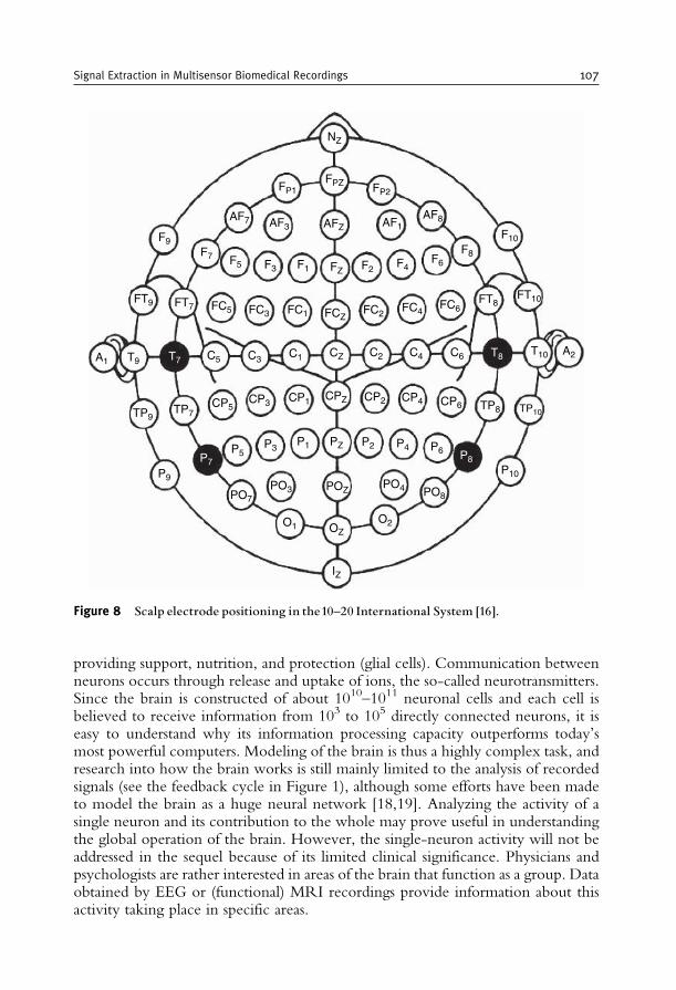
providing support, nutrition, and protection (glial cells). Communication betweenneurons occurs through release and uptake of ions, the so-called neurotransmitters.Since the brain is constructed of about 1010–1011 neuronal cells and each cell isbelieved to receive information from 103 to 105 directly connected neurons, it iseasy to understand why its information processing capacity outperforms today’smost powerful computers. Modeling of the brain is thus a highly complex task, andresearch into how the brain works is still mainly limited to the analysis of recordedsignals (see the feedback cycle in Figure 1), although some efforts have been madeto model the brain as a huge neural network [18,19]. Analyzing the activity of asingle neuron and its contribution to the whole may prove useful in understandingthe global operation of the brain. However, the single-neuron activity will not beaddressed in the sequel because of its limited clinical significance. Physicians andpsychologists are rather interested in areas of the brain that function as a group. Dataobtained by EEG or (functional) MRI recordings provide information about thisactivity taking place in specific areas.
NZ
F9F7
FT7 FC5
CP5
P5P3
P1 PZ P2 P4 P6
PO8PO4POZPO3PO7
O1 OZ
IZ
O2
P10
P8
CP3 CP1 CPZ CP2 CP4 CP6 TP8 TP10
FC3 FC1
FT9
F5 F3 F1
AF7 AF3 AFZ AF1AF8
F10F8F6F4F2FZ
FP1 FP2FPZ
FCZFC2
FC4FC6
C6C4C2CZC1C3C5
FT8FT10
T10T8T7T9
TP9
P9
P7
TP7
A1A2
Figure 8 Scalp electrode positioning in the10^20 International System [16].
Signal Extraction in Multisensor Biomedical Recordings 107
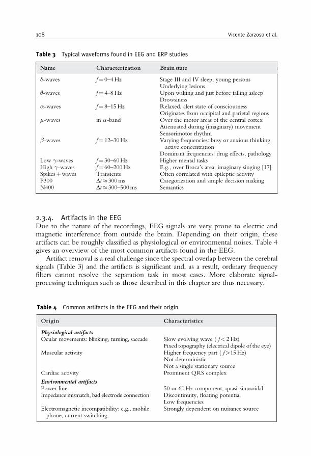
2.3.4. Artifacts in the EEGDue to the nature of the recordings, EEG signals are very prone to electric andmagnetic interference from outside the brain. Depending on their origin, theseartifacts can be roughly classified as physiological or environmental noises. Table 4gives an overview of the most common artifacts found in the EEG.
Artifact removal is a real challenge since the spectral overlap between the cerebralsignals (Table 3) and the artifacts is significant and, as a result, ordinary frequencyfilters cannot resolve the separation task in most cases. More elaborate signal-processing techniques such as those described in this chapter are thus necessary.
Table 3 Typical waveforms found in EEG and ERP studies
Name Characterization Brain state
�-waves f= 0–4Hz Stage III and IV sleep, young personsUnderlying lesions
�-waves f= 4–8Hz Upon waking and just before falling asleepDrowsiness
�-waves f= 8–15Hz Relaxed, alert state of consciousnessOriginates from occipital and parietal regions
�-waves in �-band Over the motor areas of the central cortexAttenuated during (imaginary) movementSensorimotor rhythm
�-waves f= 12–30Hz Varying frequencies: busy or anxious thinking,active concentration
Dominant frequencies: drug effects, pathologyLow �-waves f= 30–60Hz Higher mental tasksHigh �-waves f= 60–200Hz E.g., over Broca’s area: imaginary singing [17]Spikesþwaves Transients Often correlated with epileptic activityP300 Dt� 300ms Categorization and simple decision makingN400 Dt� 300–500ms Semantics
Table 4 Common artifacts in the EEG and their origin
Origin Characteristics
Physiological artifactsOcular movements: blinking, turning, saccade Slow evolving wave ( f< 2Hz)
Fixed topography (electrical dipole of the eye)Muscular activity Higher frequency part ( f>15Hz)
Not deterministicNot a single stationary source
Cardiac activity Prominent QRS complex
Environmental artifactsPower line 50 or 60Hz component, quasi-sinusoidalImpedance mismatch, bad electrode connection Discontinuity, floating potential
Low frequenciesElectromagnetic incompatibility: e.g., mobilephone, current switching
Strongly dependent on nuisance source
108 Vicente Zarzoso et al.
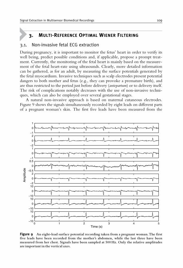
3. MULTI-REFERENCE OPTIMAL WIENER FILTERING
3.1. Non-invasive fetal ECG extraction
During pregnancy, it is important to monitor the fetus’ heart in order to verify itswell being, predict possible conditions and, if applicable, propose a prompt treat-ment. Currently, the monitoring of the fetal heart is mainly based on the measure-ment of the fetal heart-rate using ultrasounds. Clearly, more detailed informationcan be gathered, as for an adult, by measuring the surface potentials generated bythe fetal myocardium. Invasive techniques such as scalp electrodes present potentialdangers to both mother and fetus (e.g., they can provoke a premature birth), andare thus restricted to the period just before delivery (antepartum) or to delivery itself.The risk of complications notably decreases with the use of non-invasive techni-ques, which can also be employed over several gestational stages.
A natural non-invasive approach is based on maternal cutaneous electrodes.Figure 9 shows the signals simultaneously recorded by eight leads on different partsof a pregnant woman’s skin. The first five leads have been measured from the
Am
plitu
de
−1
0
1
−2
0
2
−1
0
1
−0.5
0
0.5
−2
0
2
−10
0
10
−10
0
10
0 1 2 3 4 5−10
0
10
Time (s)
Figure 9 An eight-lead surface potential recording taken from a pregnant woman.The firstfive leads have been recorded from the mother’s abdomen, while the last three have beenmeasured from her chest. Signals have been sampled at 500Hz. Only the relative amplitudesare important in the vertical axes.
Signal Extraction in Multisensor Biomedical Recordings 109
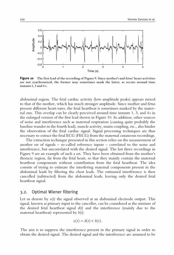
abdominal region. The fetal cardiac activity (low-amplitude peaks) appears mixedto that of the mother, which has much stronger amplitude. Since mother and fetuspresent different heart-rates, the fetal heartbeat is sometimes masked by the mater-nal one. This overlap can be clearly perceived around time instants 1, 3, and 4 s inthe enlarged version of the first lead shown in Figure 10. In addition, other sourcesof noise and interference such as maternal respiration (causing quite probably thebaseline wander in the fourth lead), muscle activity, mains coupling, etc., also hinderthe observation of the fetal cardiac signal. Signal processing techniques are thusnecessary to extract the fetal ECG (FECG) from the maternal cutaneous recordings.
The extraction technique presented in this section relies on the measurement ofanother set of signals – so-called reference inputs – correlated to the noise andinterference, but uncorrelated with the desired signal. The last three recordings inFigure 9 are an example of such a set. They have been obtained from the mother’sthoracic region, far from the fetal heart, so that they mainly contain the maternalheartbeat components without contribution from the fetal heartbeat. The ideaconsists of trying to estimate the interfering maternal components present in theabdominal leads by filtering the chest leads. The estimated interference is thencancelled (subtracted) from the abdominal leads, leaving only the desired fetalheartbeat signal.
3.2. Optimal Wiener filtering
Let us denote by x(t) the signal observed at an abdominal electrode output. Thissignal, known as primary input to the canceller, can be considered as the mixture ofthe desired fetal heartbeat signal d(t) and the interference (mainly due to thematernal heartbeat) represented by b(t):
xðtÞ= dðtÞþ bðtÞ:The aim is to suppress the interference present in the primary signal in order toobtain the desired signal. The desired signal and the interference are assumed to be
0 1 2 3 4 5−0.6
−0.4
−0.2
0
0.2
0.4
0.6
Time (s)
Am
plitu
de
Figure 10 The first lead of the recording of Figure 9. Since mother’s and fetus’ heart activitiesare not synchronized, the former may sometimes mask the latter, as occurs around timeinstants 1, 3 and 4 s.
110 Vicente Zarzoso et al.
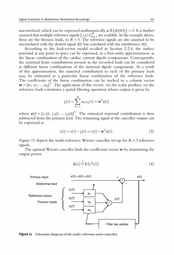
uncorrelated, which can be expressed mathematically as Efd(t)b(t)g= 0. It is furtherassumed that multiple reference signals zk tð Þf gRk¼1 are available. In the example above,these are the thoracic leads, so R= 3. The reference signals are also assumed to beuncorrelated with the desired signal d(t) but correlated with the interference b(t).
According to the lead-vector model recalled in Section 2.2.4, the surfacepotential at any point in space can be expressed, in a first-order approximation, asthe linear combination of the cardiac current dipole components. Consequently,the maternal heart contributions present in the recorded leads can be consideredas different linear combinations of the maternal dipole components. As a resultof this approximation, the maternal contribution to each of the primary leadsmay be estimated as a particular linear combination of the reference leads.The coefficients of the linear combination can be stacked in a column vectorw= [w1 w2 . . .wR]
T. The application of this vector, via the scalar product, on thereference leads constitutes a spatial filtering operation whose output is given by
yðtÞ=XRk=1
wkzkðtÞ=wTzðtÞ
where z(t)= [z1(t) z2(t) . . . zR(t)]T. The estimated maternal contribution is then
subtracted from the primary lead. The remaining signal at the canceller output canbe expressed as
sðtÞ= xðtÞ�yðtÞ= xðtÞ�wTzðtÞ: ð3Þ
Figure 11 depicts the multi-reference Wiener canceller set-up for R= 3 referencesignals.
The optimal Wiener canceller finds the coefficient vector w by minimizing theoutput power
cðsÞ¼4 Efs2ðtÞg: ð4Þ
Primary input:
Abdominal lead
Reference inputs:
Thoracic leads
Filter tap update
x (t ) = d (t ) + b (t )
z1(t )
y (t )
s (t )
+
++
–
w1
w2
w3
z2(t )
z3(t )
Figure 11 Schematic diagram of the multi-reference noise canceller.
Signal Extraction in Multisensor Biomedical Recordings 111
To understand why this criterion provides the desired results under the workingassumptions, one may expand the canceller output power as
Efs2ðtÞg=Ef½dðtÞþbðtÞ � yðtÞ�2g=Ef½bðtÞ � yðtÞ�2g þ Efd2ðtÞg:The uncorrelation of d(t) with both b(t) and z(t) [and hence with y(t)] has beeninvoked to arrive at the last equality. Consequently, minimizing c(s) is equivalentto making the spatial filter output y(t) as close as possible, in the mean square errorsense, to the interference b(t). In turn, since [s(t)�d(t)]= [b(t)�y(t)], making y(t)close to b(t) is tantamount to minimizing the difference between the cancelleroutput s(t) and the desired signal d(t).
The minimization of c(s) is carried out with respect to the spatial filtercoefficients stored in vector w. The gradient of c(w) is given by
rcðwÞ=�2EfsðtÞzðtÞg ð5Þand is null at the optimal solution. Hence, the second-order statistical informationcontained in the reference signals is ‘‘exhausted’’ by the optimal spatial filter, as itdecorrelates them with the canceller output.
Combining Eqs (3) and (5), the so-called optimal Wiener–Hopf solution isreadily obtained as
wopt =R�1zz rxz ð6Þ
where Rzz=Efz(t)z(t)Tg is the reference-signal covariance matrix, and rxz=Efx(t)z(t)g represents the cross-correlation vector between the primary lead andthe reference inputs.
In practice, mathematical expectations are replaced by their sample estimates.Assuming that signal blocks of T samples are available, we can approximate:
Rzz � 1
T
XT�1n=0
zðnTsÞzðnTsÞT rxz � 1
T
XT�1n=0
xðnTsÞzðnTsÞ ð7Þ
where Ts denotes the sampling period.
3.3. Adaptive noise cancellation
Obtaining the optimal Wiener–Hopf filter requires the solution of the linear system (6),which can be found off-line by standard linear algebra routines. Off-line algorithmsconverge after a finite number of iterations executed over the entire availabledata (the block of samples in the recording). Alternatively, the solution to Eq. (6)can be computed on-line. On-line algorithms involve an explicit recursion overtime, either sample by sample (sample-wise) or over consecutive signal blocks(block-wise). As opposed to off-line algorithms, the number of iterations necessaryfor convergence may not be bounded, particularly in the presence of non-stationarities.The simplest adaptive algorithm consists of descending the surface of criterion (4) by
112 Vicente Zarzoso et al.
moving the filter vector in small steps along the direction opposite to the gradient. Inthis gradient-descent implementation, the spatial filter weights are updated as
wðkþ 1Þ=wðkÞ � �rcðwðkÞÞ: ð8ÞOnce the steady-state is reached, the update term in Eq. (8) causes oscillations of thespatial filter coefficients around the optimal solutionwopt (6), a phenomenon known asmisadjustment. The choice of parameter �, referred to as adaption coefficient or stepsize, establishes a well-known trade-off between convergence speed and accuracy:� should be chosen small enough to prevent divergence and to obtain an accuratefinal solution (low misadjustment), but large enough to avoid slow convergence.
Alternative implementations differ in how gradient (5) is estimated in updaterule (8). Batch, block, or windowed methods estimate the gradient by averagingover the observation window samples, as in Eq. (7). Stochastic methods drop theexpectation operation altogether and use a one-sample approximation of thegradient, as in the conventional least mean squares (LMS) algorithm [20]. Thisyields Widrow’s multi-reference adaptive noise cancelling method [1]:
wðkþ 1Þ=wðkÞ � �0½xðkTsÞ � wðkÞTzðkTsÞ�zðkTsÞ ð9Þ
with �0 = 2�. This rough approximation of the gradient generally leads to slowerconvergence and increased misadjustment relative to the block-gradient implemen-tation. Common belief states that the one-sample algorithm presents improvedtracking capabilities. As a matter of fact, better performance can be expected fromthe block algorithm if the signals remain stationary over the observation window.
The above development can easily be generalized to the use of spatio-temporalfilters, as in Widrow’s pioneering contribution [1]. Each reference input is con-volved with the impulse response of a P th-order finite impulse response filter, withP> 0, before adding the outputs to form interference estimate y(t). However, theheart-dipole model of Section 2.2.4 suggests that P= 0 suffices for the applicationin hand, thus reducing the required processing of the reference inputs to a purelyspatial filtering operation.
3.4. Results
The multi-reference optimal Wiener spatial filtering method reviewed in Section 3.2is applied in turn to each of the five primary (abdominal) inputs of the recording shownin Figure 9. The last three signals, recorded from the thoracic electrodes, are employedas reference inputs to the canceller (R= 3). The resulting output signals are representedby the dark lines of Figure 12; for comparison, the outputs are superimposed to theoriginal primary inputs plotted in a lighter line. The canceller is successful in that itconsiderably reduces the maternal ECG interference from all abdominal leads.Nevertheless, residual maternal peaks remain in the time waveforms. FECG contribu-tions are clearly visible in the first three outputs, although the second and third signalsare rather noisy. The fetal heartbeat peaks can hardly be perceived over the noisecomponents in the output signal from the fourth and fifth abdominal leads.
Signal Extraction in Multisensor Biomedical Recordings 113
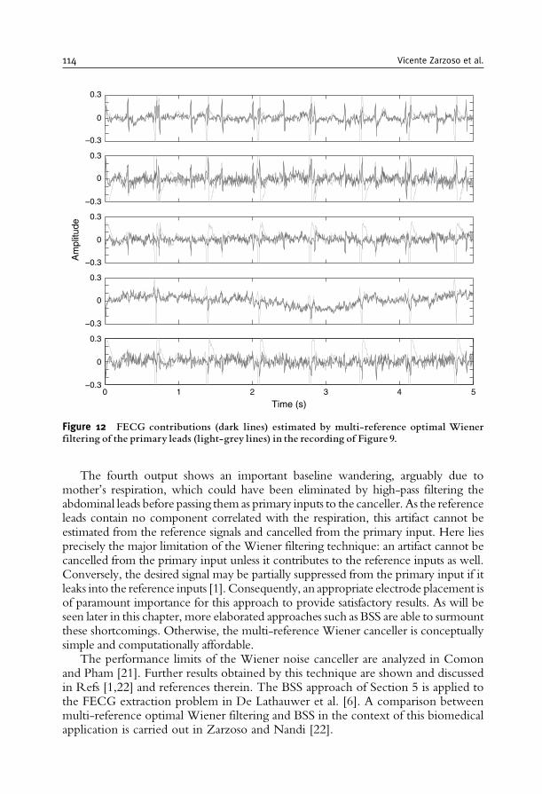
The fourth output shows an important baseline wandering, arguably due tomother’s respiration, which could have been eliminated by high-pass filtering theabdominal leads before passing them as primary inputs to the canceller. As the referenceleads contain no component correlated with the respiration, this artifact cannot beestimated from the reference signals and cancelled from the primary input. Here liesprecisely the major limitation of the Wiener filtering technique: an artifact cannot becancelled from the primary input unless it contributes to the reference inputs as well.Conversely, the desired signal may be partially suppressed from the primary input if itleaks into the reference inputs [1]. Consequently, an appropriate electrode placement isof paramount importance for this approach to provide satisfactory results. As will beseen later in this chapter, more elaborated approaches such as BSS are able to surmountthese shortcomings. Otherwise, the multi-reference Wiener canceller is conceptuallysimple and computationally affordable.
The performance limits of the Wiener noise canceller are analyzed in Comonand Pham [21]. Further results obtained by this technique are shown and discussedin Refs [1,22] and references therein. The BSS approach of Section 5 is applied tothe FECG extraction problem in De Lathauwer et al. [6]. A comparison betweenmulti-reference optimal Wiener filtering and BSS in the context of this biomedicalapplication is carried out in Zarzoso and Nandi [22].
Am
plitu
de
0 1 2 3 4 5
Time (s)
−0.3
0
0.3
−0.3
0
0.3
−0.3
0
0.3
−0.3
0
0.3
−0.3
0
0.3
Figure 12 FECG contributions (dark lines) estimated by multi-reference optimal Wienerfiltering of the primary leads (light-grey lines) in the recording of Figure 9.
114 Vicente Zarzoso et al.
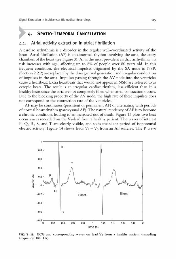
4. SPATIO-TEMPORAL CANCELLATION
4.1. Atrial activity extraction in atrial fibrillation
A cardiac arrhythmia is a disorder in the regular well-coordinated activity of theheart. Atrial fibrillation (AF) is an abnormal rhythm involving the atria, the entrychambers of the heart (see Figure 3). AF is the most prevalent cardiac arrhythmia; itsrisk increases with age, affecting up to 8% of people over 80 years old. In thisfrequent condition, the electrical impulses originated by the SA node in NSR(Section 2.2.2) are replaced by the disorganized generation and irregular conductionof impulses in the atria. Impulses passing through the AV node into the ventriclescause a heartbeat. Extra heartbeats that would not appear in NSR are referred to asectopic beats. The result is an irregular cardiac rhythm, less efficient than in ahealthy heart since the atria are not completely filled when atrial contraction occurs.Due to the blocking property of the AV node, the high rate of these impulses doesnot correspond to the contraction rate of the ventricles.
AF may be continuous (persistent or permanent AF) or alternating with periodsof normal heart rhythm (paroxysmal AF). The natural tendency of AF is to becomea chronic condition, leading to an increased risk of death. Figure 13 plots two beatoccurrences recorded on the V2-lead from a healthy patient. The waves of interestP, Q, R, S, and T are clearly visible, and so is the silent period of isopotentialelectric activity. Figure 14 shows leads V1�V3 from an AF sufferer. The P wave
0 0.2 0.4 0.6 0.8 1 1.2 1.4 1.6 1.8 2−0.8
−0.6
−0.4
−0.2
0
0.2
0.4
0.6
0.8
1
Time (s)
Am
plitu
de P
Q
R
S
T
Silent Silent
Figure 13 ECG and corresponding waves on lead V2 from a healthy patient (samplingfrequency: 1000 Hz).
Signal Extraction in Multisensor Biomedical Recordings 115
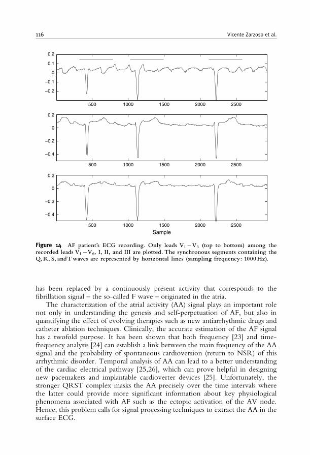
has been replaced by a continuously present activity that corresponds to thefibrillation signal – the so-called F wave – originated in the atria.
The characterization of the atrial activity (AA) signal plays an important rolenot only in understanding the genesis and self-perpetuation of AF, but also inquantifying the effect of evolving therapies such as new antiarrhythmic drugs andcatheter ablation techniques. Clinically, the accurate estimation of the AF signalhas a twofold purpose. It has been shown that both frequency [23] and time-frequency analysis [24] can establish a link between the main frequency of the AAsignal and the probability of spontaneous cardioversion (return to NSR) of thisarrhythmic disorder. Temporal analysis of AA can lead to a better understandingof the cardiac electrical pathway [25,26], which can prove helpful in designingnew pacemakers and implantable cardioverter devices [25]. Unfortunately, thestronger QRST complex masks the AA precisely over the time intervals wherethe latter could provide more significant information about key physiologicalphenomena associated with AF such as the ectopic activation of the AV node.Hence, this problem calls for signal processing techniques to extract the AA in thesurface ECG.
500 1000 1500 2000 2500
−0.2
−0.1
0
0.1
0.2
500 1000 1500 2000 2500
−0.4
−0.2
0
0.2
500 1000 1500 2000 2500
−0.4
−0.2
0
0.2
Sample
Figure 14 AF patient’s ECG recording. Only leads V1�V3 (top to bottom) among therecorded leads V1�V6, I, II, and III are plotted. The synchronous segments containing theQ,R, S, andTwaves are represented by horizontal lines (sampling frequency: 1000Hz).
116 Vicente Zarzoso et al.
4.2. Spatio-temporal cancellation of the QRST complexin AF episodes
Among the possible extraction techniques, spatio-temporal cancellation is a genericmethodology based on a model for the propagation of electrical signal from theheart to the leads on the body surface. Temporal information is also taken intoaccount by this model. The method is usually expressed in the sampled-timedomain and requires judiciously placed electrodes on the torso in order to compriseall the information contained in the cardiac electrical field. Theoretically, ortho-gonal leads X, Y, and Z should be sufficient to completely characterize this field(Section 2.2.4). The method relies on the estimation of the time occurrence ofventricular activity (VA) allowing the segmentation and synchronization of thewave of interest, i.e., the identification of Q, R, S, and T wave segments. Timesynchronization is not critical since a realignment step can be added to the globalprocess. Such a step will not be dealt with in the sequel.
In the presence of AF, each lead exhibits a mixture of consecutive transientsignals (the Q, R, S, and T waves of VA) added to the AA spread over time. Thelatter is no longer a transient signal, as opposed to the P wave in NSR (seeFigure 14). The AA in AF is assumed to be spectrally stationary at least over onebeat and can be approximated by a sawtooth-shaped periodic signal. In thesampled-time domain, the ith beat segmented in a given lead is represented by acolumn vector made up of N samples:
xi= ½xi ð0Þ xi ðTs Þ . . . xi ððN � 1ÞTs Þ �T: ð10ÞNote the column-wise arrangement of samples in the framework of spatiotemporalor temporal cancellation, in contrast with the row-wise sample placement in BSSapproaches (see Section 5). For the sake of consistency with the literature on thetopic, this section will adhere to the column-wise arrangement of Eq. (10).
The essential idea behind spatio-temporal cancellation is to obtain an estimate ofthe average VA, and then subtract it, after appropriate scaling and time shift, fromthe actual beats observed in the lead outputs. Specific methods are detailednext. Their differences lie in the manner in which the average VA is modeledand estimated, as well as in how it is fitted to the observed signals before subtrac-tion. A common implicit assumption is the uncorrelation between AA and VA.
4.2.1. Single-lead processingRecording the ECG with a multilead system allows the best characterization of theoverall cardiac electrical activity. However, only few leads may be available in someparticular cases. The paroxysmal stage of AF recorded by a Holter system is a typicalexample. An attempt to deal with the single-lead case is made in Castells et al. [27].The proposed method assumes that, in the aligned (e.g., on the R peak) observedbeats, the vectors of sampled VA lie on a subspace orthogonal to that associatedwith the AA vectors. This orthogonality is a direct consequence of the assumeduncorrelation between AA and VA. The corresponding subspaces are spanned bysome sampled-time basis functions (or source vectors) estimated by the Principal
Signal Extraction in Multisensor Biomedical Recordings 117
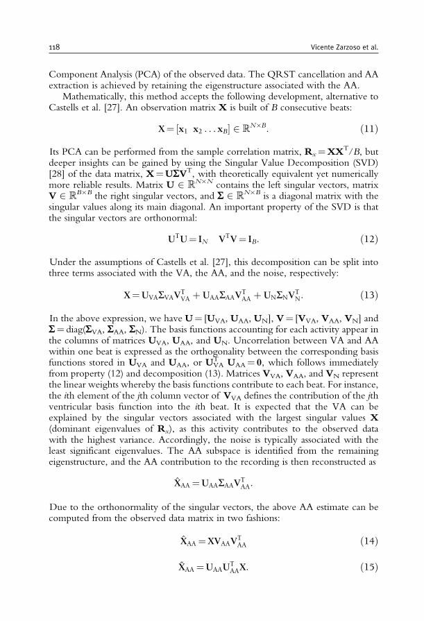
Component Analysis (PCA) of the observed data. The QRST cancellation and AAextraction is achieved by retaining the eigenstructure associated with the AA.
Mathematically, this method accepts the following development, alternative toCastells et al. [27]. An observation matrix X is built of B consecutive beats:
X= ½x1 x2 . . . xB� 2 RN�B: ð11Þ
Its PCA can be performed from the sample correlation matrix, Rx=XXT/B, butdeeper insights can be gained by using the Singular Value Decomposition (SVD)[28] of the data matrix, X=USVT, with theoretically equivalent yet numericallymore reliable results. Matrix U 2 R
N�N contains the left singular vectors, matrixV 2 R
B�B the right singular vectors, and S 2 RN�B is a diagonal matrix with the
singular values along its main diagonal. An important property of the SVD is thatthe singular vectors are orthonormal:
UTU= IN VTV= IB: ð12Þ
Under the assumptions of Castells et al. [27], this decomposition can be split intothree terms associated with the VA, the AA, and the noise, respectively:
X=UVASVAVTVA þ UAASAAV
TAA þ UNSNV
TN: ð13Þ
In the above expression, we have U= [UVA, UAA, UN], V= [VVA, VAA, VN] andS= diag(SVA, SAA, SN). The basis functions accounting for each activity appear inthe columns of matrices UVA, UAA, and UN. Uncorrelation between VA and AAwithin one beat is expressed as the orthogonality between the corresponding basisfunctions stored in UVA and UAA, or UVA
T UAA= 0, which follows immediatelyfrom property (12) and decomposition (13). Matrices VVA, VAA, and VN representthe linear weights whereby the basis functions contribute to each beat. For instance,the ith element of the jth column vector of VVA defines the contribution of the jthventricular basis function into the ith beat. It is expected that the VA can beexplained by the singular vectors associated with the largest singular values X(dominant eigenvalues of Rx), as this activity contributes to the observed datawith the highest variance. Accordingly, the noise is typically associated with theleast significant eigenvalues. The AA subspace is identified from the remainingeigenstructure, and the AA contribution to the recording is then reconstructed as
XAA=UAASAAVTAA:
Due to the orthonormality of the singular vectors, the above AA estimate can becomputed from the observed data matrix in two fashions:
XAA=XVAAVTAA ð14Þ
XAA =UAAUTAAX: ð15Þ
118 Vicente Zarzoso et al.
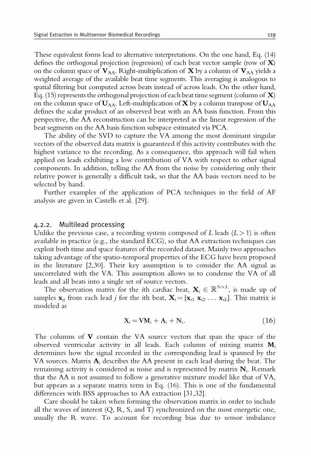
These equivalent forms lead to alternative interpretations. On the one hand, Eq. (14)defines the orthogonal projection (regression) of each beat vector sample (row of X)on the column space of VAA. Right-multiplication of X by a column of VAA yields aweighted average of the available beat time segments. This averaging is analogous tospatial filtering but computed across beats instead of across leads. On the other hand,Eq. (15) represents the orthogonal projection of each beat time segment (columnof X)on the column space ofUAA. Left-multiplication ofX by a column transpose ofUAA
defines the scalar product of an observed beat with an AA basis function. From thisperspective, the AA reconstruction can be interpreted as the linear regression of thebeat segments on the AA basis function subspace estimated via PCA.
The ability of the SVD to capture the VA among the most dominant singularvectors of the observed data matrix is guaranteed if this activity contributes with thehighest variance to the recording. As a consequence, this approach will fail whenapplied on leads exhibiting a low contribution of VA with respect to other signalcomponents. In addition, telling the AA from the noise by considering only theirrelative power is generally a difficult task, so that the AA basis vectors need to beselected by hand.
Further examples of the application of PCA techniques in the field of AFanalysis are given in Castells et al. [29].
4.2.2. Multilead processingUnlike the previous case, a recording system composed of L leads (L> 1) is oftenavailable in practice (e.g., the standard ECG), so that AA extraction techniques canexploit both time and space features of the recorded dataset. Mainly two approachestaking advantage of the spatio-temporal properties of the ECG have been proposedin the literature [2,30]. Their key assumption is to consider the AA signal asuncorrelated with the VA. This assumption allows us to condense the VA of allleads and all beats into a single set of source vectors.
The observation matrix for the ith cardiac beat, Xi 2 RN�L, is made up of
samples xij from each lead j for the ith beat, Xi= [xi1 xi2 . . . xiL]. This matrix ismodeled as
Xi=VMi þ Ai þNi: ð16ÞThe columns of V contain the VA source vectors that span the space of theobserved ventricular activity in all leads. Each column of mixing matrix Mi
determines how the signal recorded in the corresponding lead is spanned by theVA sources. Matrix Ai describes the AA present in each lead during the beat. Theremaining activity is considered as noise and is represented by matrix Ni. Remarkthat the AA is not assumed to follow a generative mixture model like that of VA,but appears as a separate matrix term in Eq. (16). This is one of the fundamentaldifferences with BSS approaches to AA extraction [31,32].
Care should be taken when forming the observation matrix in order to includeall the waves of interest (Q, R, S, and T) synchronized on the most energetic one,usually the R wave. To account for recording bias due to sensor imbalance
Signal Extraction in Multisensor Biomedical Recordings 119
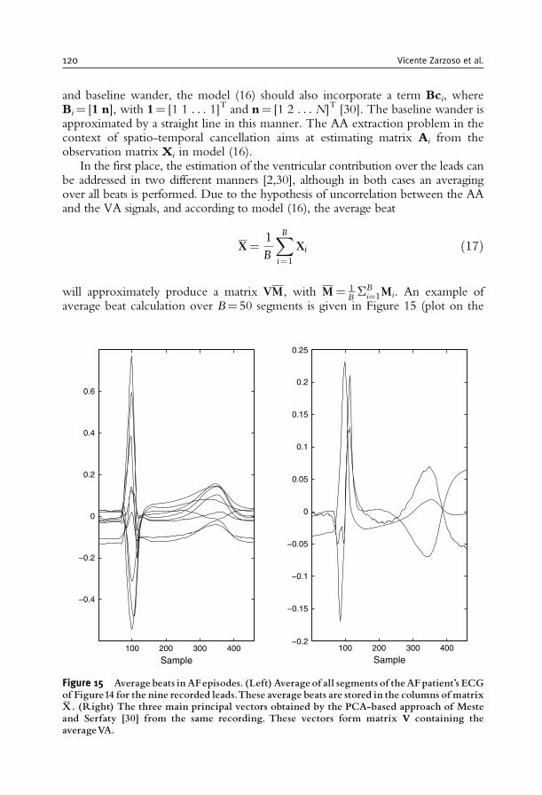
and baseline wander, the model (16) should also incorporate a term Bci, whereBi= [1 n], with 1= [1 1 . . . 1]T and n= [1 2 . . . N]T [30]. The baseline wander isapproximated by a straight line in this manner. The AA extraction problem in thecontext of spatio-temporal cancellation aims at estimating matrix Ai from theobservation matrix Xi in model (16).
In the first place, the estimation of the ventricular contribution over the leads canbe addressed in two different manners [2,30], although in both cases an averagingover all beats is performed. Due to the hypothesis of uncorrelation between the AAand the VA signals, and according to model (16), the average beat
X=1
B
XBi=1
Xi ð17Þ
will approximately produce a matrix VM, with M= 1B�B
i=1Mi. An example ofaverage beat calculation over B= 50 segments is given in Figure 15 (plot on the
100 200 300 400
−0.4
−0.2
0
0.2
0.4
0.6
Sample100 200 300 400
−0.2
−0.15
−0.1
−0.05
0
0.05
0.1
0.15
0.2
0.25
Sample
Figure 15 Average beats inAFepisodes. (Left)Average of all segments of theAFpatient’s ECGof Figure14 for the nine recorded leads.These average beats are stored in the columns of matrixX� . (Right) The three main principal vectors obtained by the PCA-based approach of Mesteand Serfaty [30] from the same recording. These vectors form matrix V containing theaverageVA.
120 Vicente Zarzoso et al.
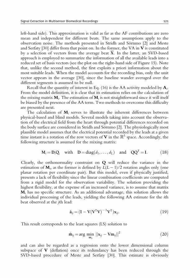
left-hand side). This approximation is valid as far as the AF contributions are zeromean and independent for different beats. The same assumptions apply to theobservation noise. The methods presented in Stridh and Sornmo [2] and Mesteand Serfaty [30] differ from that point on. In the former, the VA in V is constitutedby a selection of vectors from the average beat X. In the latter, an SVD-basedapproach is employed to summarize the information of all the available leads into areduced set of basis vectors (see the plot on the right-hand side of Figure 15). Notethat, unlike the second method, the first exploits a priori information about themost suitable leads. When the model accounts for the recording bias, only the unitvector appears in the average [30], since the baseline wander averaged over thedifferent segments is assumed to be null.
Recall that the quantity of interest in Eq. (16) is the AA activity modeled by Ai.From the model definition, it is clear that its estimation relies on the calculation ofthe mixing matrixMi. The estimation ofMi is not straightforward since it will itselfbe biased by the presence of the AA term. Two methods to overcome this difficultyare presented next.
The calculation of Mi serves to illustrate the inherent differences betweenphysical-based and blind models. Several models taking into account the observa-tion of the electrical field from the heart through potential differences recorded onthe body surface are considered in Stridh and Sornmo [2]. The physiologically mostplausible model assumes that the electrical potential recorded by the leads at a giventime instant is a rotation of the row vectors of V in the RL space. Accordingly, thefollowing structure is assumed for the mixing matrix:
Mi =DiQi with D= diagðd1; . . . ; dLÞ and QQT= I: ð18Þ
Clearly, the orthonormality constraint on Q will reduce the variance in theestimation of Mi, as the former is defined by L(L� 1)/2 rotation angles only (oneplanar rotation per coordinate pair). But this model, even if physically justified,presents a lack of flexibility since the linear combination coefficients are computedfrom a rigid model for the observation variability. The solution providing thehighest flexibility, at the expense of an increased variance, is to assume that matrixMi has no specific structure. As an additional advantage, this solution allows theindividual processing of the leads, yielding the following AA estimate for the ithbeat observed at the jth lead:
aij = ðI� VðVTVÞ�1VTÞxij: ð19Þ
This result corresponds to the least squares (LS) solution to
mij = arg minmij
jjxij � Vmijjj2 ð20Þ
and can also be regarded as a regression onto the lower dimensional columnsubspace of V (deflation) once its redundancy has been reduced through theSVD-based procedure of Meste and Serfaty [30]. This estimate is obviously
Signal Extraction in Multisensor Biomedical Recordings 121
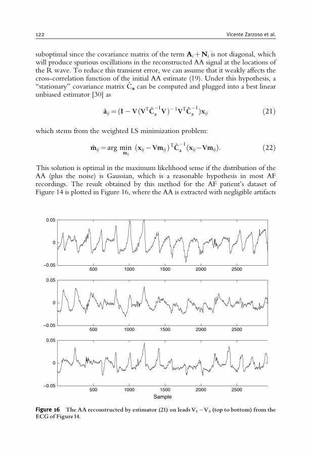
suboptimal since the covariance matrix of the term AiþNi is not diagonal, whichwill produce spurious oscillations in the reconstructed AA signal at the locations ofthe R wave. To reduce this transient error, we can assume that it weakly affects thecross-correlation function of the initial AA estimate (19). Under this hypothesis, a‘‘stationary’’ covariance matrix Ca can be computed and plugged into a best linearunbiased estimator [30] as
aij = ðI� VðVTC�1
a V�1VTC�1
a Þxij ð21Þ
which stems from the weighted LS minimization problem:
mij = arg minmij
ðxij �Vmij ÞTC�1
a ðxij�VmijÞ: ð22Þ
This solution is optimal in the maximum likelihood sense if the distribution of theAA (plus the noise) is Gaussian, which is a reasonable hypothesis in most AFrecordings. The result obtained by this method for the AF patient’s dataset ofFigure 14 is plotted in Figure 16, where the AA is extracted with negligible artifacts
500 1000 1500 2000 2500−0.05
0
0.05
500 1000 1500 2000 2500−0.05
0
0.05
500 1000 1500 2000 2500−0.05
0
0.05
Sample
Figure 16 The AA reconstructed by estimator (21) on leadsV1�V3 (top to bottom) from theECG of Figure14.
122 Vicente Zarzoso et al.
and in agreement with the AA visible in the original recording. An alternative toAA covariance matrix estimation is proposed in Stridh and Sornmo [2], where theAA in the TQ interval, i.e., the ventricular silent segment (see Figure 13), is linearlyapproximated in the QT interval assuming a repetitive constant pattern.
4.2.3. A simple alternative: average beat subtraction (ABS)The traditional ABS method neglects the spatial properties of multisensor cardiacsignal recordings. The synchronous averaged beat X in Eq. (17) is employed as areference [33] and is optimally shifted in time before being subtracted from eachobserved beat. The original method can be extended to the multilead case bysolving the minimization problem [2]:
�i = arg min�i
jjXi � X�ijj2F ð23Þ
where (.)� stands for the �-sample delay operator. This formulation based on theFrobenius norm can be seen as the minimization of the sum of individual Euclideannorms over all leads, that is,
�i= argmin�i
XLj = 1
jjxij � xj�ijj2 = arg max�i
XLj=1
xTijxj�i ð24Þ
where xj denotes the jth column of the average beat X, i.e., the average beat ofthe jth lead. The scalar product in Eq. (24) can be considered as an approximationof the cross-correlation function of the observed signal and the average beat in thecorresponding leads at lag �i. Once the optimum delay is estimated, the AA in eachlead is obtained by the subtraction:
aij = xij � xj�i ð25Þ
Note that, at each beat, this method does not seek a delay for each lead, but finds theoptimal delay over all leads. This option yields more accurate results under thesensible assumption of negligible propagation delays between the leads (Section2.2.4). The technique can be simply improved by scaling the average beat as aixj�i .In such a case, the amplitude factor ai needs to be incorporated into Eq. (24) and itsoptimal value estimated accordingly.
5. BLIND SOURCE SEPARATION (BSS)
5.1. The isolation of interictal epileptic discharges in the EEG
About 0.5–1% of the population suffers from epilepsy, a neurological disorderassociated with recurrent unprovoked seizures. These seizures are often linked withcognitive absences or state alterations, tonic or clonic movements or convulsions.
Signal Extraction in Multisensor Biomedical Recordings 123
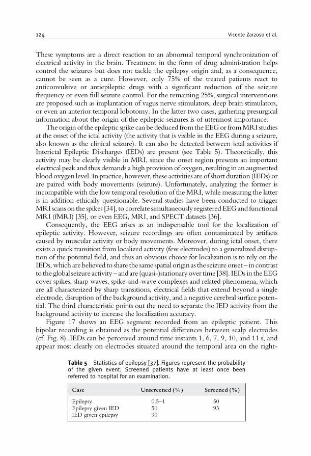
These symptoms are a direct reaction to an abnormal temporal synchronization ofelectrical activity in the brain. Treatment in the form of drug administration helpscontrol the seizures but does not tackle the epilepsy origin and, as a consequence,cannot be seen as a cure. However, only 75% of the treated patients react toanticonvulsive or antiepileptic drugs with a significant reduction of the seizurefrequency or even full seizure control. For the remaining 25%, surgical interventionsare proposed such as implantation of vagus nerve stimulators, deep brain stimulators,or even an anterior temporal lobotomy. In the latter two cases, gathering presurgicalinformation about the origin of the epileptic seizures is of uttermost importance.
The origin of the epileptic spike can be deduced from theEEGor fromMRI studiesat the onset of the ictal activity (the activity that is visible in the EEG during a seizure,also known as the clinical seizure). It can also be detected between ictal activities ifInterictal Epileptic Discharges (IEDs) are present (see Table 5). Theoretically, thisactivity may be clearly visible in MRI, since the onset region presents an importantelectrical peak and thus demands a high provision of oxygen, resulting in an augmentedblood oxygen level. In practice, however, these activities are of short duration (IEDs) orare paired with body movements (seizure). Unfortunately, analyzing the former isincompatible with the low temporal resolution of the MRI, while measuring the latteris in addition ethically questionable. Several studies have been conducted to triggerMRI scans on the spikes [34], to correlate simultaneously registered EEGand functionalMRI (fMRI) [35], or even EEG, MRI, and SPECT datasets [36].
Consequently, the EEG arises as an indispensable tool for the localization ofepileptic activity. However, seizure recordings are often contaminated by artifactscaused by muscular activity or body movements. Moreover, during ictal onset, thereexists a quick transition from localized activity (few electrodes) to a generalized disrup-tion of the potential field, and thus an obvious choice for localization is to rely on theIEDs,which are believed to share the same spatial origin as the seizure onset – in contrastto the global seizure activity – and are (quasi-)stationary over time [38]. IEDs in theEEGcover spikes, sharp waves, spike-and-wave complexes and related phenomena, whichare all characterized by sharp transitions, electrical fields that extend beyond a singleelectrode, disruption of the background activity, and a negative cerebral surface poten-tial. The third characteristic points out the need to separate the IED activity from thebackground activity to increase the localization accuracy.
Figure 17 shows an EEG segment recorded from an epileptic patient. Thisbipolar recording is obtained as the potential differences between scalp electrodes(cf. Fig. 8). IEDs can be perceived around time instants 1, 6, 7, 9, 10, and 11 s, andappear most clearly on electrodes situated around the temporal area on the right-
Table 5 Statistics of epilepsy [37]. Figures represent the probabilityof the given event. Screened patients have at least once beenreferred to hospital for an examination.
Case Unscreened (%) Screened (%)
Epilepsy 0.5–1 50Epilepsy given IED 50 93IED given epilepsy 90
124 Vicente Zarzoso et al.
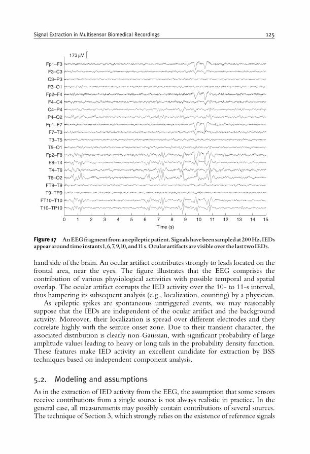
hand side of the brain. An ocular artifact contributes strongly to leads located on thefrontal area, near the eyes. The figure illustrates that the EEG comprises thecontribution of various physiological activities with possible temporal and spatialoverlap. The ocular artifact corrupts the IED activity over the 10- to 11-s interval,thus hampering its subsequent analysis (e.g., localization, counting) by a physician.
As epileptic spikes are spontaneous untriggered events, we may reasonablysuppose that the IEDs are independent of the ocular artifact and the backgroundactivity. Moreover, their localization is spread over different electrodes and theycorrelate highly with the seizure onset zone. Due to their transient character, theassociated distribution is clearly non-Gaussian, with significant probability of largeamplitude values leading to heavy or long tails in the probability density function.These features make IED activity an excellent candidate for extraction by BSStechniques based on independent component analysis.
5.2. Modeling and assumptions
As in the extraction of IED activity from the EEG, the assumption that some sensorsreceive contributions from a single source is not always realistic in practice. In thegeneral case, all measurements may possibly contain contributions of several sources.The technique of Section 3, which strongly relies on the existence of reference signals
T10–TP10
FT10–T10
T9–TP9
FT9–T9
T6–O2
T4–T6
F8–T4
Fp2–F8
T5–O1
T3–T5
F7–T3
Fp1–F7
P4–O2
C4–P4
F4–C4
Fp2–F4
P3–O1
C3–P3
F3–C3
Fp1–F3
173 μV
Time (s)
0 1 2 3 4 5 6 7 8 9 10 11 12 13 14 15
Figure 17 AnEEGfragmentfromanepilepticpatient.Signalshavebeensampledat200Hz.IEDsappeararoundtime instants1,6,7,9,10, and11s.Ocularartifacts arevisibleover the last twoIEDs.
Signal Extraction in Multisensor Biomedical Recordings 125
free from the source of interest, may yield poor results in such scenarios. Similarly, thespatio-temporal cancellation approach of Section 4 becomes inadequate in situationswhere a quasi-periodic source such as the VA is not encountered.
These remarks motivate the simplest instance of the BSS problem, where thesensor signals follow the linear instantaneous statistical model:
xðtÞ=AsðtÞ: ð26Þ
The components of vector x(t)= [x1(t) x2(t) . . . xL(t)]T denote the L signals recorded,
whereas the components of vector s(t)= [s1(t) s2(t) . . . sM(t)]T are the M unknown
sources. A is an unknown L�Mmixing matrix reflecting how the sources contributeto the sensors. Because it is not known in advance whether some sensors receivecontributions from a reduced number of sources or not, matrix A has no knownstructure or sparsity pattern. The above model can also be decomposed as
xðtÞ=XMm = 1
amsmðtÞ ð27Þ
where am is the mth column vector of A. This equation signifies that each sourcecontributes to the sensors through the projection of its amplitude on the associatedcolumn of the mixing matrix.
The goal of BSS is to estimate the realizations of source vector s(t) from thecorresponding realizations of observed vector x(t). To this end, anM�L separatingmatrix filter B is built such that its outputs
yðtÞ=BxðtÞ ð28Þare estimates of the sources. Note that the ith row of B defines a spatial filter actingon the sensor output x(t) to produce the separator output yi(t), the ith componentof vector y(t).
In order to solve this problem, additional assumptions are necessary. Dependingon the assumptions, the BSS problem is of variable difficulty and can be solvedmore or less easily. We shall limit our scope to the following:
A1. Matrix A is of full rank M, and there are at least as many sensors as sources(L�M).
A2. Sources sm(t) are mutually statistically independent.A3. At least (M� 1) sources are non-Gaussian, in the sense that they admit a non-
zero finite cumulant of order four.
Under assumption A1, Eq. (26) models a so-called overdetermined mixture,where the available spatial diversity is sufficient to recover the sources byapplying a linear transformation on the observed data. Indeed, the sources scan be recovered by a linear oblique projection of the observation vector xonto the columns of A. This projection is carried out by separating matrix Bin Eq. (28). Assumptions A2–A3 allow the design of BSS techniques exploitingthe property of statistical independence between the sources. This is an impor-tant property, as it is plausible in numerous applications and leads to
126 Vicente Zarzoso et al.
computationally efficient practical BSS algorithms such as that presented inSection 5.6. Independence can be seen as a generalization of conventionalsecond-order uncorrelation, the property exploited by the extraction techni-ques of Sections 3–4. Section 5.4 will explain in more detail the concept ofindependence (assumption A2), together with its connection with cumulants andnon-Gaussianity (assumption A3).
5.3. Inherent indeterminacies
It is clear that if the components of s(t) undergo an arbitrary permutation(re-ordering), assumptions A1–A3 are still fulfilled and the observation x(t) inEq. (26) is not altered as long as the columns of A are re-arranged accordingly.The same result holds if a source is scaled by a constant factor � and thecorresponding mixing matrix column by 1/�. These simple remarks show thatthere are inherent indeterminacies in the BSS problem if addressed underassumptions A1–A3: the source signals and the mixing matrix columns can beestimated up to permutation and scale ambiguities. Conversely, it can be shownthat these three assumptions are sufficient to establish identifiability of matrix Aup to the above ambiguities and to estimate matrix B [3]. Note that they arenot necessary, for other assumptions such as non-stationarity or colorness (timecoherence) of the sources also allow identifiability under certain circumstances;see [39] and references therein.
Our goal is thus to estimate one representative (A, s(t)) of a whole equivalenceclass of solutions. Note that the number of solutions may be reduced to a finitenumber by imposing each estimated source to have unit variance. The remainingindeterminacy eventually reduces to sign and permutation.
As time coherence will be ignored in the sequel, all pertinent informationis contained in the probability distribution of the processed signals, whosesamples are considered as realizations of random variables. Consequently, thetime dependency denoted by index t becomes irrelevant and will be dropped forconvenience.
5.4. Statistical independence, higher-order statisticsand non-Gaussianity
The components of random vector s2RM are said to be independent if and only if
their joint probability density function can be decomposed as the product of theirmarginal densities:
psðsÞ=YMm=1
psmðsmÞ: ð29Þ
Dealing with probability distributions is usually hard. Instead, independence caneasily be measured using statistical parameters known as cumulants [40,41]. The
Signal Extraction in Multisensor Biomedical Recordings 127
cumulants of random vector s, denoted by Cs,ijk. . . = cum(si, sj, sk,. . .), where si isthe ith component of s, are defined as the coefficients of the Taylor expansion of itssecond characteristic function �(w)= log Efexp( jwTs)g, where j is the imaginaryunit. Omitting mathematical details beyond our scope, it will suffice to mentionhere that the cumulants are linked to the moments through relationships that areoften non-linear. For zero-mean variables, we have the following expressions for thecumulants up to fourth order:
� order 1: Cs;i =Efsig= 0
� order 2: Cs;ij =Efsisjg� order 3: Cs;ijk =Efsisjskg� order 4: Cs;ijk‘ =Efsisjsks‘g�Efsisjgfsks‘g�EfsiskgEfsjs‘g
�Efsis‘gEfsjskg:
ð30Þ
Cumulants are said to be marginal if they involve a single component of s, whilecross-cumulants involve more than one component. The second-order cross-cumulant is the conventional covariance. Cumulants of order higher than twoare referred to as higher-order cumulants and, along with the higher-ordermoments, constitute the higher-order statistics (HOS). The normalized fourth-order marginal cumulant,Cs;iiii=C
2s;ii, is also called kurtosis.
The cross-cumulants of a random vector with independent components arenull at all orders. Full independence is too stringent an assumption and is indeed notnecessary in practice to accomplish the separation. The concept can be relaxedby defining independence at order r, which only requires null cross-cumulantsup to that order. In particular, independence at order 2 reduces to the classicalsecond-order uncorrelation. Note that higher-order independence is a stricterproperty as it implies, in particular, second-order uncorrelation, whereas theconverse is not true: uncorrelated signals may not necessarily be independent.The term ‘higher-order’ will be omitted in the sequel when talking about inde-pendence, as will be ‘second-order’ when referring to uncorrelation. As will beseen later (Section 5.5.1), decorrelating the observations (i.e., making them uncor-related at the separator output) is generally insufficient to achieve the separation ifthe temporal coherence of the sources is not (or cannot be) exploited.
All the higher-order cumulants of a Gaussian random variable are zero, sothat these statistical parameters arise as natural measures of non-Gaussianity.From the connection between independence and cumulants just recalled, itfollows that imposing uncorrelation on Gaussian variables renders them inde-pendent without enforcing any constraints involving HOS. As a result, recover-ing the property of independence is insufficient to separate these type of signals[3]. Indeed, independence-exploiting techniques are unable to perform a com-plete separation if more than one source is Gaussian; hence, the need forassumption A3. HOS-based methods can separate the non-Gaussian sources,while the Gaussian sources will remain mixed at the separator output. Thislimitation will be illustrated in Section 5.5.2 with the particular separationcriterion of [3] (see also Section 5.9).
128 Vicente Zarzoso et al.
5.5. Independent component analysis
It is possible to estimate the source signals by first identifying the mixing matrix(blind identification) before inverting the mixture. More common in biomedicalapplications are inverse approaches. These are formulated as the maximization of aso-called contrast criterion and are thus expected to be more robust to additivenoise than blind identification approaches. Inverse approaches look for a separatingmatrix B such as to maximize a contrast �(B). A contrast is a function measuring aknown property of the sources. From this perspective, BSS is approached as aproperty recovery problem: recover the source waveforms by recovering the sourceproperty. The maximization of a contrast function guarantees the separation, so thatthe contrast is said to discriminate among the sources having that property.
If source and noise distributions are known, one can rely on the MaximumLikelihood (ML) principle. Otherwise, one can use a contrast measuring thestatistical independence between the components of the separator output (28).The maximization of statistical independence gives rise to the Independent Compo-nent Analysis (ICA) of the observed data [3]. The most natural criterion for ICA isthe Mutual Information (MI):
¡MIðBÞ=ZpyðuÞlog pyðuÞ
Pm pymðumÞdu: ð31Þ
According to the definition of independence expressed by Eq. (29), the abovecriterion is null if and only if the separator output is made up of independentcomponents. The MI involves probability densities that are unknown; this isdifficult to handle even if they can be estimated, especially in large dimensions.Moreover, maximizing Eq. (31) with respect to B can only be done iteratively[42], which may raise problems due to the multimodality of the likelihoodfunction, in addition to the huge computational complexity. These shortcomingsexplain why several other more practical criteria have been proposed in theliterature. Many of these alternative criteria capitalize on the ability of cumulantsto measure independence (Section 5.4). The kurtosis-based contrast [3], whichis probably the most widely used, will be presented in Section 5.5.2. Let usfirst point out the inability of second-order techniques to accomplish theseparation.
5.5.1. Principal component analysis (PCA)Since it is desired to obtain independent components ym, 1�m�M, in particularthey must also be uncorrelated (Section 5.4). An efficient technique to obtainuncorrelated variables via a linear transformation is PCA.
For simplicity and without restricting the generality, assume that vector x iszero-mean, and denote Rx=EfxxTg its covariance matrix. Then there exists anM�L full rank matrix W such that
WRxWT= IM : ð32Þ
Signal Extraction in Multisensor Biomedical Recordings 129
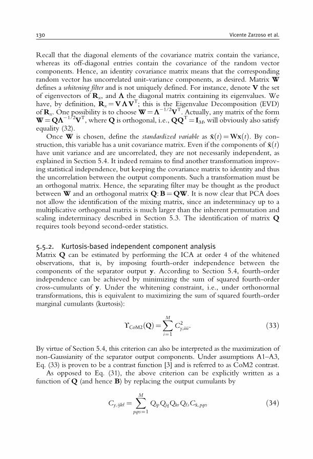
Recall that the diagonal elements of the covariance matrix contain the variance,whereas its off-diagonal entries contain the covariance of the random vectorcomponents. Hence, an identity covariance matrix means that the correspondingrandom vector has uncorrelated unit-variance components, as desired. Matrix Wdefines a whitening filter and is not uniquely defined. For instance, denote V the setof eigenvectors of Rx, and L the diagonal matrix containing its eigenvalues. Wehave, by definition, Rx=VLVT; this is the Eigenvalue Decomposition (EVD)of Rx. One possibility is to choose W=L�1/2VT. Actually, any matrix of the formW=QL�1/2VT, whereQ is orthogonal, i.e.,QQT= IM, will obviously also satisfyequality (32).
Once W is chosen, define the standardized variable as xðtÞ=WxðtÞ. By con-struction, this variable has a unit covariance matrix. Even if the components of xðtÞhave unit variance and are uncorrelated, they are not necessarily independent, asexplained in Section 5.4. It indeed remains to find another transformation improv-ing statistical independence, but keeping the covariance matrix to identity and thusthe uncorrelation between the output components. Such a transformation must bean orthogonal matrix. Hence, the separating filter may be thought as the productbetween W and an orthogonal matrix Q:B=QW. It is now clear that PCA doesnot allow the identification of the mixing matrix, since an indeterminacy up to amultiplicative orthogonal matrix is much larger than the inherent permutation andscaling indeterminacy described in Section 5.3. The identification of matrix Qrequires tools beyond second-order statistics.
5.5.2. Kurtosis-based independent component analysisMatrix Q can be estimated by performing the ICA at order 4 of the whitenedobservations, that is, by imposing fourth-order independence between thecomponents of the separator output y. According to Section 5.4, fourth-orderindependence can be achieved by minimizing the sum of squared fourth-ordercross-cumulants of y. Under the whitening constraint, i.e., under orthonormaltransformations, this is equivalent to maximizing the sum of squared fourth-ordermarginal cumulants (kurtosis):
¡CoM2ðQÞ=XMi=1
C2y;iiii: ð33Þ
By virtue of Section 5.4, this criterion can also be interpreted as the maximization ofnon-Gaussianity of the separator output components. Under assumptions A1–A3,Eq. (33) is proven to be a contrast function [3] and is referred to as CoM2 contrast.
As opposed to Eq. (31), the above criterion can be explicitly written as afunction of Q (and hence B) by replacing the output cumulants by
Cy; ijk‘=XMpqrs=1
QipQjqQkrQ‘sCx; pqrs ð34Þ
130 Vicente Zarzoso et al.
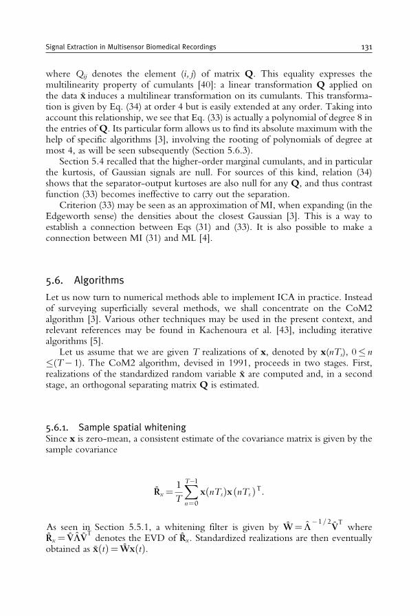
where Qij denotes the element (i, j) of matrix Q. This equality expresses themultilinearity property of cumulants [40]: a linear transformation Q applied onthe data x induces a multilinear transformation on its cumulants. This transforma-tion is given by Eq. (34) at order 4 but is easily extended at any order. Taking intoaccount this relationship, we see that Eq. (33) is actually a polynomial of degree 8 inthe entries ofQ. Its particular form allows us to find its absolute maximum with thehelp of specific algorithms [3], involving the rooting of polynomials of degree atmost 4, as will be seen subsequently (Section 5.6.3).
Section 5.4 recalled that the higher-order marginal cumulants, and in particularthe kurtosis, of Gaussian signals are null. For sources of this kind, relation (34)shows that the separator-output kurtoses are also null for any Q, and thus contrastfunction (33) becomes ineffective to carry out the separation.
Criterion (33) may be seen as an approximation of MI, when expanding (in theEdgeworth sense) the densities about the closest Gaussian [3]. This is a way toestablish a connection between Eqs (31) and (33). It is also possible to make aconnection between MI (31) and ML [4].
5.6. Algorithms
Let us now turn to numerical methods able to implement ICA in practice. Insteadof surveying superficially several methods, we shall concentrate on the CoM2algorithm [3]. Various other techniques may be used in the present context, andrelevant references may be found in Kachenoura et al. [43], including iterativealgorithms [5].
Let us assume that we are given T realizations of x, denoted by x(nTs), 0� n�(T� 1). The CoM2 algorithm, devised in 1991, proceeds in two stages. First,realizations of the standardized random variable x are computed and, in a secondstage, an orthogonal separating matrix Q is estimated.
5.6.1. Sample spatial whiteningSince x is zero-mean, a consistent estimate of the covariance matrix is given by thesample covariance
Rx=1
T
XT�1n=0
xðnTsÞxðnTs ÞT:
As seen in Section 5.5.1, a whitening filter is given by W= L�1=2VTwhere
Rx= VLVTdenotes the EVD of Rx. Standardized realizations are then eventually
obtained as xðtÞ= WxðtÞ.
Signal Extraction in Multisensor Biomedical Recordings 131
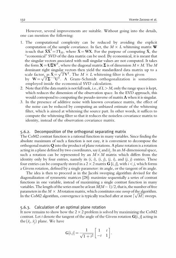
However, several improvements are suitable. Without going into the details,one can mention the following:
1. The computational complexity can be reduced by avoiding the explicitcomputation of the sample covariance. In fact, the M � L whitening matrix Wis such that XX
T=TIM , where X=WX. For the purpose of computing X, the
‘‘economical’’ SVD of the data matrix can be used. By economical, it is meant thatthe singular vectors associated with null singular values are not computed. It takesthe formX=USVT, where the diagonal matrix S is of dimensionM�M. TheMdominant right singular vectors then yield the standardized data matrix up to ascale factor, as X=
ffiffiffiffiT
pVT. The M � L whitening filter is then given
by W=ffiffiffiffiT
pS�1UT. A Gram–Schmidt orthogonalization is sometimes
employed inside the economical SVD calculation.2. Note that if the datamatrix is not full rank, i.e., ifL>M, only the range space is kept,
which reduces the dimension of the observation space. In the EVD approach, thiswould correspond to computing the pseudo-inverse of matrixLwhen it is singular.
3. In the presence of additive noise with known covariance matrix, the effect ofthe noise can be reduced by computing an unbiased estimate of the whiteningfilter, which is aimed at whitening the source part. In other words, it suffices tocompute the whitening filter so that it reduces the noiseless covariance matrix toidentity, instead of the observation covariance matrix.
5.6.2. Decomposition of the orthogonal separating matrixThe CoM2 contrast function is a rational function in many variables. Since finding theabsolute maximum of such a function is not easy, it is convenient to decompose theorthogonalmatrixQ into the product of plane rotations. A plane rotation is a rotationacting in a plane defined by two coordinates, say xi and xj. In anM-dimensional space,such a rotation can be represented by an M�M matrix which differs from theidentity only by four entries, namely its (i, i), (i, j), (j, i), and (j, j) entries. Thesefour entries can be compactly stored in a 2� 2matrixG [i, j], with i< j, which formsa Givens rotation, defined by a single parameter: its angle, or the tangent of its angle.
The idea is then to proceed as in the Jacobi sweeping algorithm devised for thediagonalization of symmetric matrices [28]: maximize sequentially a series of contrastfunctions in one variable, instead of maximizing a single contrast function in manyvariables. The length of the seriesmust be at leastM(M� 1)/2, that is, the number of freeparameters in theM � M rotationmatrix,which constitutes one sweep of the algorithm.In the CoM2 algorithm, convergence is typically reached after at most d ffiffiffiffiffi
Mp e sweeps.
5.6.3. Calculation of an optimal plane rotationIt now remains to show how the 2� 2 problem is solved by maximizing the CoM2contrast. Let t denote the tangent of the angle of the Givens rotationG[i, j] acting intheðxi; xjÞ plane. We have
G½i; j�= 1ffiffiffiffiffiffiffiffiffiffiffiffi1þ t2
p 1 t
�t 1
� �:
132 Vicente Zarzoso et al.

The contrast criterion �CoM2 defined in Eq. (33) turns out to be a rational functionin t of degree 8, as shown by the multilinearity property (34). It has been proven inComon [3] that, because of its particular form, all stationary values of this contrastcriterion can be found by rooting a polynomial of degree 4, which can be done inan entirely algebraic (non-iterative) manner. By plugging back these values in thecontrast expression, we are able to select the absolute maximum of �CoM2, within afinite number of operations. Since 1992, the source code of this algorithm can bedownloaded from www.i3s.unice.fr/pcomon.
The coefficients of the above rational function involve sample cumulants of thepairðxi; xjÞ, or of the pair (yi, yj) previously computed. Sample cumulants can beestimated from sample moments either in a batch manner, by averaging over the Trealizations in the available signal block, or recursively (on-line) if a real-timeimplementation is preferred.
5.7. Results
We apply the CoM2 cumulant-based BSS algorithm of Comon [3] (summarized inSection 5.6) to the interictal EEG fragment shown in Figure 17. The algorithmseparates the measurements into the maximally independent sources of Figure 18.
0 1 2 3 4 5 6 7
Time (s)
8 9 10 11 12 13 14 15
1
2
3
4
5
6
7
8
9
10
11
12
13
14
15
16
17
18
Figure 18 Brain signal extraction in the EEG: decomposition of the EEG fragment ofFigure 17 into its source signals by the CoM2 algorithm of [3] (Section 5.6). Sources 2 and 3represent the ocular artifact. Amplitudes are normalized to yield unit power sources.
Signal Extraction in Multisensor Biomedical Recordings 133
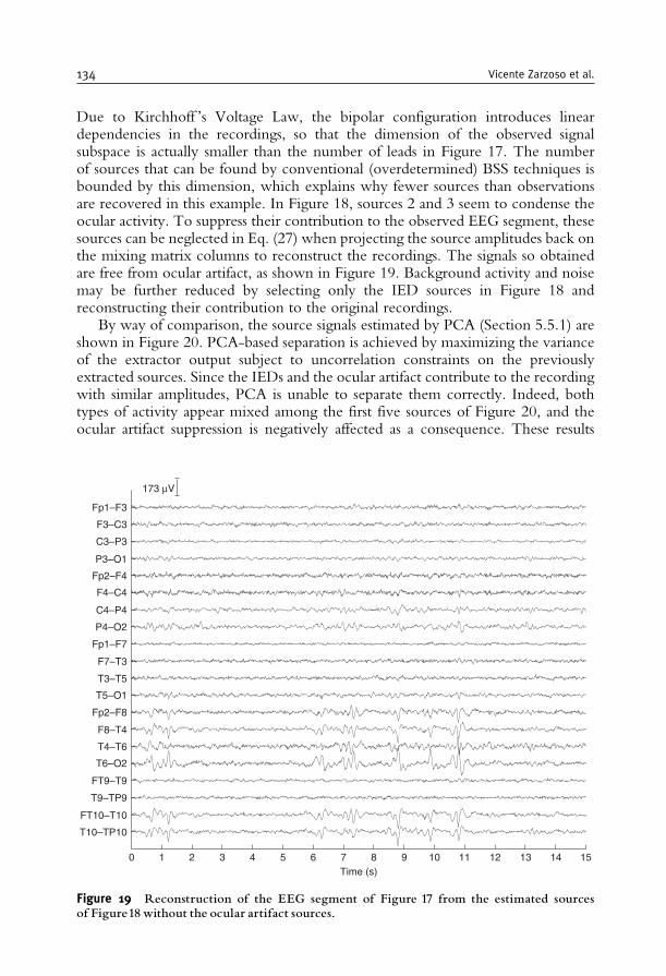
Due to Kirchhoff ’s Voltage Law, the bipolar configuration introduces lineardependencies in the recordings, so that the dimension of the observed signalsubspace is actually smaller than the number of leads in Figure 17. The numberof sources that can be found by conventional (overdetermined) BSS techniques isbounded by this dimension, which explains why fewer sources than observationsare recovered in this example. In Figure 18, sources 2 and 3 seem to condense theocular activity. To suppress their contribution to the observed EEG segment, thesesources can be neglected in Eq. (27) when projecting the source amplitudes back onthe mixing matrix columns to reconstruct the recordings. The signals so obtainedare free from ocular artifact, as shown in Figure 19. Background activity and noisemay be further reduced by selecting only the IED sources in Figure 18 andreconstructing their contribution to the original recordings.
By way of comparison, the source signals estimated by PCA (Section 5.5.1) areshown in Figure 20. PCA-based separation is achieved by maximizing the varianceof the extractor output subject to uncorrelation constraints on the previouslyextracted sources. Since the IEDs and the ocular artifact contribute to the recordingwith similar amplitudes, PCA is unable to separate them correctly. Indeed, bothtypes of activity appear mixed among the first five sources of Figure 20, and theocular artifact suppression is negatively affected as a consequence. These results
Time (s)0
T10–TP10
FT10–T10
T9–TP9
FT9–T9
T6–O2
T4–T6
F8–T4
Fp2–F8
T5–O1
T3–T5
F7–T3
Fp1–F7
P4–O2
C4–P4
F4–C4
Fp2–F4
P3–O1
C3–P3
F3–C3
Fp1–F3
1 2 3 4 5 6 7 8 9 10 11 12 13 14 15
173 μV
Figure 19 Reconstruction of the EEG segment of Figure 17 from the estimated sourcesof Figure18 without the ocular artifact sources.
134 Vicente Zarzoso et al.
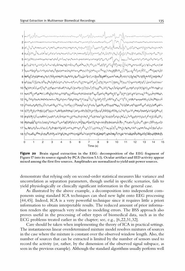
demonstrate that relying only on second-order statistical measures like variance anduncorrelation as separation parameters, though useful in specific scenarios, fails toyield physiologically or clinically significant information in the general case.
As illustrated by the above example, a decomposition into independent com-ponents using standard ICA techniques can shed new light onto EEG processing[44,45]. Indeed, ICA is a very powerful technique since it requires little a prioriinformation to obtain interpretable results. The reduced amount of prior informa-tion renders the approach very robust to modeling errors. The BSS approach alsoproves useful in the processing of other types of biomedical data, such as in theECG problems treated earlier in the chapter; see, e.g., [6,22,31,32].
Care should be taken when implementing the theory of ICA in practical settings.The instantaneous linear overdetermined mixture model resolves mixtures of sourcesin the case where the mixture is constant over the observed window length. Also, thenumber of sources that can be extracted is limited by the number of sensors used torecord the activity (or, rather, by the dimension of the observed signal subspace, asseen in the previous example). Although the standard algorithms usually perform well
18
17
16
15
14
13
12
11
10
9
8
7
6
5
4
3
2
1
0 1 2 3 4 5 6 7Time (s)
8 9 10 11 12 13 14 15
Figure 20 Brain signal extraction in the EEG: decomposition of the EEG fragment ofFigure17 into its source signals by PCA (Section 5.5.1). Ocular artifact and IED activity appearmixed among the first five sources. Amplitudes are normalized to yield unit power sources.
Signal Extraction in Multisensor Biomedical Recordings 135
and provide useful clinical and physiological information, more advanced methodscircumventing the above limitations can be developed by replacing, altering or addingassumptions to the separation criteria. In what follows, we briefly summarize somepromising developments adding on the capabilities of classical ICA in multisensorbiomedical data analysis. This overview does not pretend to be exhaustive.
5.8. Incorporating prior information into the separation model
The above-mentioned techniques for BSS make little to no use of prior knowledgeof the source signals except for assumptions A1–A3 concerning their statisticalindependence and non-Gaussian character. By inserting some prior knowledgeinto the objective of ICA, the standard ambiguities mentioned in Section 5.3 canbe alleviated while improving the performance of the resulting techniques. Recentmethods have been proposed by inserting priors into the ICA contrast and/or intothe ICA-updating algorithm. The following sections shortly highlight some inter-esting contributions to this topic.
5.8.1. Temporal referenceThe use of a reference signal in conjunction with independence has been proposedin Adib et al. [46]. The method in Lu and Rajapakse [47] is based on the so-calledFastICA algorithm [5,48], but includes a Lagrangian term measuring the distance tothe reference. The method is reminiscent of the optimal Wiener filtering techniqueof Section 3 in the exploitation of a reference signal. Its major drawback is preciselythe generation of that signal, ideally the source of interest and thus not available apriori. The major advantage of ICA with reference signal is the reduction incomputational cost, as a full decomposition with a posteriori selection is reducedinto a single signal extraction. Since only the source of interest will be found at theseparator output, the permutation ambiguity inherent to classical implementationsof ICA is alleviated or even avoided.
5.8.2. Spatial referenceIn a given source separation problem, the contribution of a source signal to the sensorsis determined by the mixing matrix column associated with that source, as signifiedmathematically by Eq. (27). A spatial map quantifies the typical configuration of thiscontribution. In biomedical signal processing, the idea of exploiting a source spatialmap seems more practical than using a reference signal, as much more a prioriinformation is available for spatial maps than for time variations [49,50]. Since manyprocesses captured by a multisensor recording system display a rather fixed and knowntopography, this information can be readily incorporated into ICA contrasts. Thisyields source separation techniques with spatial maps adapted to epileptic spikes [49]and artifacts [51], among others, thus simplifying the identification of these activities.
In the context of ocular artifact suppression in the EEG, the benefits ofexploiting a spatial reference are illustrated in Figure 21. The top plot shows anEEG recording clearly corrupted by eye blinks. The application of the signalextraction method of Phlypo et al. [51], based on a library of spatial maps adapted
136 Vicente Zarzoso et al.
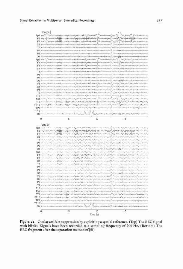
OzTP10TP9
FT10FT9FpzT10T9PzCzFzO2P4P8T8C4F8F4
Fp2O1P3P7T7C3F7F3
Fp1200 μV
OzTP10TP9
FT10FT9FpzT10T9PzCzFzO2P4P8T8C4F8F4
Fp2O1P3P7T7C3F7F3
Fp1200 μV
Time (s)
0 5 10 15
0 5 10 15
Figure 21 Ocular artifact suppression by exploiting a spatial reference. (Top) The EEG signalwith blinks. Signals have been recorded at a sampling frequency of 200 Hz. (Bottom) TheEEG fragment after the separation method of [51].
Signal Extraction in Multisensor Biomedical Recordings 137
to ocular artifacts, yields the corrected EEG fragment shown in the bottom plot.Since the muscular activity around the 10th second and the spiking activity justbefore the 15th second have spatial distributions different from that of the ocularartifact, they are not affected by the extraction filter.
5.9. Independent subspaces
Recently, the trend to step forward from ICA techniques toward IndependentSubspace Analysis (ISA) has gained increasing attention in the signal processingcommunity. The idea of ISA, originally proposed in Comon [52, p. 125], has beenfurther developed in [53] or [54], among others. This trend goes hand in hand withthe dependent component analysis method, that takes prior information about therelation between components to solve the linearmixture system. Left to explore is theinfluence these novel techniques would have on biomedical signal processing. Sincethe activity in the three orthogonal axes of the electric heart vector (Section 2.2.4) istemporally dependent, it could reasonably be captured in a three-dimensional mea-surement subspace, rather than being compressed into a single component. The sameobservation holds for dependent brain activities (see Section 5.1). Subspace analysisor dependent component analysis could help find coherence between the activities ofmultiple or spread brain areas.
5.10. Softening the stationarity constraint
If the mixing matrix is constant over a time period, the stationarity of thesources is not mandatory. In fact, when using sample statistics such as momentor cumulants, one actually averages them over the period. What is thenimportant is that these average values should be non-zero, and in particularthe underlying source average statistics. Attempts have been made to soften (orentirely discard) the stationary conditions by using, among others, statemachines [55] or the ML principle [56]. A similar attempt is made by thealgorithm of Phlypo et al. [51] through the combination of short-time andlong-term statistics. Another point of view is to exploit independence in thespectral domain. Instead of the ordinary frequency transforms with fixed bases,there is a tendency to use methods that adapt the spectral basis to the data inhand, either through decorrelation [57] or by using HOS as in ICA [58], aredrawing increasing interest. Note that many works exploit non-stationarity ofthe sources when the mixture is constant [56]. In that case, having non-stationary sources is an advantage, not a drawback.
5.11. Revealing more sources than sensor signals
Mixtures having fewer sensors than sources are referred to as underdeterminedsince 1999 [59]. The difficulty when considering underdetermined mixtures liesin the non-invertibility of the mixing matrix A, since it is no longer full-columnrank. As a result, the sources s cannot be exactly recovered by a linear projectionof the observation vector x onto the columns of A. The problem of extracting the
138 Vicente Zarzoso et al.
sources in underdetermined mixtures can be addressed by three main approaches:(1) build a non-linear extractor [59], possibly based on a Maximum A Posterioriestimator (well-matched to the case of discrete sources); (2) exploit a possiblesource sparseness [60,61], whereby only a few sources are assumed to be activesimultaneously in the observation window; (3) exploit possible additional diver-sities by storing the recorded information in a high-dimensional array (a matrixwith more than two dimensions, e.g., a cube-like data structure) and performingits decomposition [62]. This last option, and perhaps also the use of sparsity inspecific scenarios, would appear as the most promising in biomedical applications.On the other hand, if one is only interested in detecting the number of sources oridentifying the mixture (e.g., for source localization), decomposing the cumulanttensor [63] or the characteristic function [64] suffices, and weaker assumptionsapply.
6. SUMMARY, CONCLUSIONS AND OUTLOOK
The extraction of signals of interest from measurements corrupted by noise andinterference is a fundamental problem arising in a wide variety of domains. Inbiomedicine, a successful signal extraction can help the physician diagnose andunderstand a pathologic condition. The signal extraction techniques presented inthis chapter rely on the availability of multiple spatially separated sensors recordingsimultaneously the biomedical activity under study. Exploiting the spatial dimensionbrought about by multisensor measurements gives rise to the concept of spatialfiltering, and enables powerful signal processing approaches with capabilities reachingfar beyond conventional single-channel frequency filters. Specific methods dependon the particular problem in hand, its model and its constraints. Our purpose hasbeen to provide the reader with an overview of some existing signal extraction tools.
Approximating the bioelectrical activity by equivalent current dipoles leadsto the definition of signal models in which sources and observations are linearlyrelated. As a result, signal extraction can be carried out by linear processing,namely, the appropriate weighted average of the measured signals. The techniquesaddressed in this chapter aim at finding the weights or coefficients of the extractingspatial filter by exploiting specific properties of the signals of interest. Such weightsare optimal under specific assumptions and extraction criteria. Classical Wienerfiltering and spatio-temporal cancellation exploit the uncorrelation between thesignal of interest and the interference. Uncorrelation is measured usingsecond-order statistics (covariance). The former method relies on reference signalscorrelated with the interference but uncorrelated with the desired signal, whichdemands a careful electrode placement. The latter technique assumes the repeti-tive character of the interference. BSS is a more general approach capable of dealingwith (practically) arbitrary electrode location. The use of statistical independence,a property stronger than uncorrelation and measured using HOS (cumulants),enables the extraction of any type of sources as long as they are non-Gaussian.Even if the relationship between bioelectrical sources and observations is
Signal Extraction in Multisensor Biomedical Recordings 139
actually more involved than a simple equivalent dipole, these techniques are oftenable to extract physiologically meaningful and clinically relevant sources.
Each of these signal processing tools has been introduced in the context ofa suitable biomedical application, but could also be adapted and applied to theother problems addressed in this chapter. Some comparisons can be found in[6,22,43,65], among other works. Although our focus has been on bioelectricalrecordings (ECG, EEG), signals conveying genetic (DNA), chemical, or other kindof biomedical information can also be processed by these techniques. Likewise, themethods are readily applicable, with possible modifications, in other fields such astelecommunications (see, e.g., [39,66–69] and references therein).
Many open problems remain to be tackled in the area of signal extraction inmultisensor biomedical recordings. A fundamental question concerns the rela-tionship between the sources estimated by signal extraction methods and theactual sources of underlying physiological activity. As discussed at the end ofthe previous section, the applicability of existing techniques needs to beextended to more challenging environments such as underdetermined scenarios,and their performance improved by incorporating prior information into theextraction criteria. Multimodal processing is emerging as another promisingavenue of research. Signals simultaneously acquired in different modalities(EEG and MEG, EEG and fMRI, PET and SPECT, etc.) can be analyzedsequentially or in parallel to perform mutual validation or to increase theinformation provided separately by each modality. The potential benefits aremany-fold. For instance, the combination of EEG and fMRI can improve bothtemporal (with respect to fMRI) and spatial (with respect to EEG) resolution,while PET and SPECT can provide information about both anatomical struc-tures and functional behaviour. Recording multimodal measurements, e.g., anEEG in a high magnetic field such as an MRI scanner represents an interestingtechnical problem in itself. Designing novel signal processing algorithms fullyexploiting the information available in the recorded modalities constitutes anexciting research challenge likely to draw the attention of the biomedical signalprocessing community over the next decades.
ACKNOWLEDGMENTS
This work has been partly supported by contract ‘‘DECOTES’’ (D6-BLAN-0074-01) from Agence National de la Recherche. Most of Figure 5has been reproduced with permission from the Web edition of Malmivuo andPlonsey [12]. The ECG recording of Figure 9 has been kindly provided by L.De Lathauwer, D. Callaerts, and J. Vandewalle, from K. U. Leuven, Belgium.The ECG recordings of Figures 13 and 14 are courtesy of the Signal ProcessingGroup, Lund University, Sweden. The EEG data of Figures 17 and 21 (top) aredue to P. Boon from the Laboratory for Clinical and Experimental Neurology,Ghent University Hospital, Belgium.
140 Vicente Zarzoso et al.
REFERENCES
[1] B. Widrow, J. R. Glover, J. M. McCool, et al., Adaptive noise cancelling: principles andapplications, Proceedings of the IEEE 63 (12) (1975) 1692–1716.
[2] M. Stridh, L. Sornmo, Spatiotemporal QRST cancellation techniques for analysis of atrialfibrillation, IEEE Transactions on Biomedical Engineering 48 (1) (2001) 105–111.
[3] P. Comon, Independent component analysis, a new concept? Signal Processing 36 (3) (1994)287–314, Special Issue on Higher-Order Statistics.
[4] J.-F. Cardoso, Blind signal separation: statistical principles, Proceedings of the IEEE 86 (10)(1998) 2009–2025.
[5] A. Hyvarinen, J. Karhunen, E. Oja, Independent Component Analysis, John Wiley & Sons,New York, 2001.
[6] L. De Lathauwer, B. De Moor, J. Vandewalle, Fetal electrocardiogram extraction by blindsource subspace separation, IEEE Transactions on Biomedical Engineering 47 (5) (2000)567–572, Special Topic Section on Advances in Statistical Signal Processing for Biomedicine.
[7] R. Gulrajani, Bioelectricity and Bioelectromagnetism, John Wiley & Sons, New York, 1998.[8] H. Hallez, B. Vanrumste, R. Grech, J. Muscat, Y. D’Asseler, W. D. Clercq, A. Vergult, K. P.
Camilleri, S. G. Fabri, R. Van de Walle, S. Van Huffel, I. Lemahieu, Review on solving theforward problem in EEG source analysis, Journal of Neuroengineering and Rehabilitation4 (46), (November 2007) doi:10.1186/1743-0003-4-46, 29 pages.
[9] F. Bijmaa, J. C. deMunck, K. B. Bockerb,H.M.Huizengac,R.M.Heethaard, The coupled dipolemodel: an integrated model for multiple MEG/EEG data sets, Neuroimage 23 (3) (2004) 890–904.
[10] R. Pascual-Marqui, C. Michel, D. Lehmann, Low resolution electromagnetic tomography:a new method for localizing electrical activity in the brain, International Journal of Psychophy-siology 18 (1994) 49–65.
[11] R. M. Rangayyan, Biomedical Signal Analysis. A Case-Study Approach, John Wiley & Sons,Inc., New York, 2002.
[12] J. Malmivuo, R. Plonsey, Bioelectromagnetism: Principles and Applications, Oxford UniversityPress, New York, 1995.
[13] R. Plonsey, Bioelectric Phenomena, McGraw-Hill, New York, 1969.[14] R. Plonsey, R. C. Barr, Bioelectricity: A Quantitative Approach, 2nd Edition, Kluwer
Academic Publishers, New York, 2000.[15] A. van Oosterom, Beyond the dipole: modeling the genesis of the electrocardiogram, in: Schalij,
Janse, van Oosterom, Wellens, van der Wal (Eds.), Einthoven 2002: 100 Years of Electrocar-diography, The Einthoven Foundation, Leiden, The Netherlands, 2002, Ch. 2, pp. 7–15.
[16] American Clinical Neurophysiology Society, Guideline 5: Guidelines for standard electrodeposition nomenclature https://www.acns.org//pdfs/ACFDD46.pdf (2006).
[17] A. Gunji, R. Ishii, W. Chau, R. Kakigi, C. Pantev, Rhythmic brain activities related to singingin humans, NeuroImage 34 (2007) 426–434.
[18] D. J. Amit, Modeling Brain Function, Cambridge University Press, Cambridge, UK, 1992.[19] P. Robinson, C. Rennie, D. Rowe, S. O’Connor, E. Gordon, Multiscale brain modelling,
Philosophical Transactions of the Royal Society of London B 360 (2005) 1043–1050.[20] G. O. Glentis, K. Berberidis, S. Theodoridis, Efficient least squares adaptive algorithms for FIR
transversal filtering, IEEE Signal Processing Magazine 16 (4) (1999) 13–41.[21] P. Comon, D. T. Pham, An error bound for a noise canceller, IEEE Transactions on Acoustics,
Speech and Signal Processing 37 (10) (1989) 1513–1517.[22] V. Zarzoso, A. K. Nandi, Noninvasive fetal electrocardiogram extraction: blind separation
versus adaptive noise cancellation, IEEETransactions onBiomedical Engineering 48 (1) (2001) 12–18.[23] P. Langley, J. Bourke, A. Murray, Frequency analysis of atrial fibrillation, IEEE Computer
Society Press, Proc. Computers in Cardiology, Vol. 27, Boston, Massachusetts, 2000, 269–272.[24] M. Stridth, L. Sornmo, Characterization of atrial fibrillation using the surface ECG: time-
dependent spectral properties, IEEE Transactions on Biomedical Engineering 48 (1) (2001) 19–27.[25] J. Lian, D. Mussig, V. Lang, Computer modeling of ventricular rhythm during atrial fibrillation
and ventricular pacing, IEEE Transactions on Biomedical Engineering 53 (8) (2006) 1512–1520.
Signal Extraction in Multisensor Biomedical Recordings 141
[26] P. Bonizzi, O. Meste, V. Zarzoso, Atrio-ventricular junction behaviour during atrial fibrillation,IEEE Computer Society Press, Proc. Computers in Cardiology, Vol. 34, Durham, NorthCarolina, 2007, pp. 561–564.
[27] F. Castells, C. Mora, J. J. Rieta, D. Moratal-Perez, J. Millet, Estimation of atrial fibrillatory wavefrom single-lead atrial fibrillation electrocardiograms using principal component analysisconcepts, Medical and Biological Engineering and Computing 43 (5) (2005) 557–560.
[28] G. H. Golub, C. F. Van Loan, Matrix Computations, 3rd Edition, The Johns HopkinsUniversity Press, 1996.
[29] F. Castells, P. Laguna, L. Sornmo, A. Bollmann, J. Millet Roig, Principal component analysis inECG signal processing, EURASIP Journal on Advances in Signal Processing (2007),doi:10.1155/2007/74580, 21 pages.
[30] O. Meste, N. Serfaty, QRST cancellation using Bayesian estimation for the auricular fibrillationanalysis, in: Proceedings of the 27th Annual International Conference of the IEEE Engineeringin Medicine and Biology Society, Shanghai, China, 2005, pp. 7083–7086.
[31] J. J. Rieta, F. Castells, C. Sanchez, V. Zarzoso, J. Millet, Atrial activity extraction for atrialfibrillation analysis using blind source separation, IEEE Transactions on Biomedical Engineering51 (7) (2004) 1176–1186.
[32] F. Castells, J. J. Rieta, J. Millet, V. Zarzoso, Spatiotemporal blind source separation approach toatrial activity estimation in atrial tachyarrhythmias, IEEE Transactions on Biomedical Engineer-ing 52 (2) (2005) 258–267.
[33] J. Slocum, E. Byrom, L. McCarthy, A. Sahakian, S. Swiryn, Computer detection ofatrioventricular dissociation from the surface electrocardiogram during wide QRS tachycardia,Circulation 72 (1985) 1028–1036.
[34] G. Beltramello, P. Manganotti, G. Zanette, C. Miniussi, A. Marravita, E. Santorum, A. Polo,C. Marzi, A. Fiaschi, B. Bernardina, Coregistration of EEG and fMRI in rolandic epilepsy withevoked spikes by peripheral tapping stimulation, Electroencephalography and Clinical Neuro-physiology 103 (1) (1997) 83.
[35] X. D. Tiege, H. Laufs, S. G. Boyd,W. Harkness, P. J. Allen, C. A. Clark, A. Connelly, J. H. Cross,EEG-fMRI in children with pharmacoresistant focal epilepsy, Epilepsia 48 (2) (2007) 385–389.
[36] E. L. So, Integration of EEG, MRI, and SPECT in localizing the seizure focus for epilepsysurgery, Epilepsia 41 (Suppl 3) (2000) S48–S54.
[37] J. M. Stern, J. Engel Jr., Atlas of EEG Patterns, Lippincott, Williams & Wilkins, Hagerstown,Maryland, 2004.
[38] L. Tang, M. Mantle, P. Ferrari, H. Schiffbauer, H. A. Rowley, N. M. Barbaro, M. S. Berger, T.P. L. Roberts, Consistency of interictal and ictal onset localization using magnetoencephalo-graphy in patients with partial epilepsy, Journal of Neurosurgery 98 (4) (2003) 837–845.
[39] P. Comon, C. Jutten, Separation de sources: concepts de base et analyse en composantesindependantes, Vol. 1 of Collection IC2, Hermes, 2007, ISBN 978-2-7462-1517-7.
[40] P. McCullagh, Tensor Methods in Statistics, Monographs on Statistics and Applied Probability,Chapman and Hall, London, 1987.
[41] A. Stuart, J. K. Ord, Kendall’s Advanced Theory of Statistics, 6th Edition, Vol. I, EdwardArnold, London, 1994.
[42] D. T. Pham, P. Garat, Blind separation of mixture of independent sources through a quasi-maximum likelihood approach, IEEE Transactions on Signal Processing 45 (7) (1997) 1712–1725.
[43] A. Kachenoura, L. Albera, L. Senhadji, P. Comon, ICA: a potential tool for BCI systems, IEEESignal Processing Magazine 25 (1) (2008), Special Issue on Brain-Computer Interfaces 57–68.
[44] S. Makeig, A. J. Bell, T.-P. Jung, T. J. Sejnowski, Independent component analysis of electroence-phalographicdata, in:Advances inNeural InformationProcessingSystems (NIPS)Foundation,Vol. 8,1996, pp. 145–151.
[45] A. Delorme, S. Makeig, EEGLAB: an open source toolbox for analysis of single trial EEGdynamics, Journal of Neuroscience Methods 134 (2004) 9–21.
[46] A. Adib, E. Moreau, D. Aboutajdine, Source separation contrasts using a reference signal, IEEESignal Processing Letters 11 (3) (2004) 312–315.
[47] W. Lu, J. C. Rajapakse, Approach and applications of constrained ICA, IEEE Transactions onNeural Networks 16 (1) (2005) 203–212.
142 Vicente Zarzoso et al.
[48] A. Hyvarinen, E. Oja, A fast fixed-point algorithm for independent component analysis, NeuralComputation 9 (7) (1997) 1483–1492.
[49] N. Ille, P. Berg, M. Scherg, Artifact correction of the ongoing EEG using spatial filters based onartifact and brain signal topographies, Journal of Clinical Neurophysiology 19 (2) (2002) 113–124.
[50] C. W. Hesse, C. J. James, The FastICA algorithm with spatial constraints, IEEE Signal Proces-sing Letters 12 (11) (2005) 792–795.
[51] R. Phlypo, Y. D’Asseler, I. Lemahieu, Removing ocular movement artefacts by a jointsmoothened subspace estimator (JSSE), Computational Intelligence and Neuroscience, 2007doi: 10.1155/2007/75079.
[52] P. Comon, Supervised classification, a probabilistic approach, in: Verleysen (Ed.), ESANN-EuropeanSymposium on Artificial Neural Networks, D facto Publ., Brussels, 1995, pp. 111–128, invited.
[53] J.-F. Cardoso, Multidimensional independent component analysis, in: Proc. ICASSP-98, 23rd IEEEInternational Conference on Acoustics, Speech and Signal Processing, Seattle, 1998, pp. 1941–1944.
[54] F. Theis, Blind signal separation into groups of dependent signals using block diagonalization,in: Proc. ISCAS-2005, IEEE International Symposium on Circuits and Systems, Kobe, Japan,1995, pp. 5878–5881.
[55] J.-I. Hirayama, S.-I. Maeda, S. Ishii, Markov and semi-Markov switching of source appearancesfor nonstationary independent component analysis, IEEE Transactions on Neural Networks18 (5) (2007) 1326–1342.
[56] D.-T. Pham, J.-F. Cardoso, Blind separation of instantaneous mixtures of non stationary sources,IEEE Transactions on Signal Processing 49 (9) (2001) 1837–1848.
[57] R. Phlypo, Y. D’Asseler, I. Lemahieu, Extracting common spectral features by multichannelfiltering using circulant matrices, in: Proc. ISSPA-2007, 9th International Symposium on SignalProcession and its Applications, Sharjah, United Arab Emirates, 2007.
[58] M. Davies, C. James, S. Wang, Space-time ICA and EM brain signals, in: M. Davies, C. James,S. Abdallah, M. Plumbley (Eds.), Proc. ICA-2007, 7th International Conference on Indepen-dent Component Analysis and Source Separation, Lecture Notes on Computer Science(LNCS 4666), London, UK, 2007, pp. 577–584.
[59] P. Comon, O. Grellier, Non linear inversion of underdetermined mixtures, in: Proc. ICA-99,1st International Workshop on Independent Component Analysis and Blind Source Separation,Aussois, France, 1999, pp. 461–465.
[60] P. Bofill, M. Zibulevsky, Underdetermined blind source separation using sparse representation,Signal Processing 81 (11) (2001) 2353–2362.
[61] R. Gribonval, Sparse decomposition of stereo signals with matching pursuit and application toblind separation of more than two sources from a stereo mixture, in: Proc. ICASSP-2002, 27thIEEE International Conference on Acoustics, Speech and Signal Processing, Vol. III, Orlando,Florida, 2002, pp. 3057–3060.
[62] N. D. Sidiropoulos, R. Bro, G. B. Giannakis, Parallel factor analysis in sensor array processing,IEEE Transactions on Signal Processing 48 (8) (2000) 2377–2388.
[63] L. Albera, A. Ferreol, P. Comon, P. Chevalier, Blind identification of overcomplete mixtures ofsources (BIOME), Linear Algebra and its Applications 391 (2004) 1–30.
[64] P. Comon, M. Rajih, Blind identification of under-determined mixtures based on the char-acteristic function, Signal Processing 86 (9) (2006) 2271–2281.
[65] P. Langley, M. Stridh, J. J. Rieta, J. Millet, L. Sornmo, A. Murray, Comparison of atrial signalextraction algorithms in 12-lead ECGs with atrial fibrillation, IEEE Transactions on BiomedicalEngineering 53 (2) (2006) 343–346.
[66] N. Delfosse, P. Loubaton, Adaptive blind separation of independent sources: a deflationapproach, Signal Processing 45 (1) (1995) 59–83.
[67] L. Castedo, C. Escudero, A. Dapena, A blind signal separation method for multiuser commu-nications, IEEE Transactions on Signal Processing 45 (5) (1997) 1343–1348.
[68] S. Houcke, A. Chevreuil, P. Loubaton, Blind source separation of a mixture of communicationsources emitting at various baud-rates, Transactions of IEICE E86-A (3) (2003) 564–572.
[69] M. E. Davies, C. J. James, S. A. Abdallah, M. D. Plumbley (Eds.), Proc. ICA-2007, 7thInternational Conference on Independent Component Analysis and Signal Separation, Vol. 7of Lecture Notes in Computer Science (LNCS 4666), Springer, London, UK, 2007.
Signal Extraction in Multisensor Biomedical Recordings 143

This page intentionally left blank
C H A P T E R 4
FLUORESCENCE LIFETIME SPECTROSCOPY AND
IMAGING OF VISIBLE FLUORESCENT PROTEINS
Ankur Jain, Christian Blum, and Vinod Subramaniam
Contents
1. Introduction 1462. Introduction to Fluorescence 146
2.1. Interaction of light with matter 1462.2. The Jabłonski diagram 1472.3. Fluorescence parameters 151
2.4. Fluorescence lifetime 1512.5. Measurement of fluorescence lifetime 1532.6. Fluorescence anisotropy and polarization 1552.7. Factors affecting fluorescence 157
3. Fluorophores and Fluorescent Proteins 1603.1. Green fluorescent protein 1613.2. Red fluorescent protein 165
4. Applications of VFPs 1664.1. Lifetime spectroscopy and imaging of VFPs 167
5. Concluding Remarks 170
References 170
Abstract
The excited state lifetime of a fluorophore is a fundamental parameter that reports
sensitively on the fluorophore nanoenvironment and on interactions between the fluor-ophore and other molecules. When coupled with the spatial resolution inherent toimaging techniques, fluorescence lifetime spectroscopy provides information about thespatial distributions of the molecules and the dynamics of related processes. In combi-
nation with genetically encodable visible fluorescent protein fluorophores, fluorescencelifetime imaging enables the real-time visualization of dynamic biological interactions inthe complex context of the living cell. This chapter provides an introduction to fluores-
cence spectroscopy with an emphasis on fluorescence lifetimes and to the use of visiblefluorescent proteins and fluorescence lifetime microspectroscopy for biophotonicsapplications.
Keywords: fluorescence, fluorescence lifetime imaging, FRET, GFP, protein localization,photophysics
Advances in Biomedical Engineering � 2009 Elsevier B.V.
ISBN 978-0-444-53075-2 All rights reserved.
145
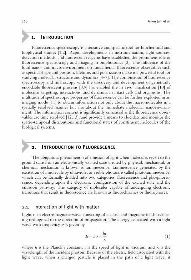
1. INTRODUCTION
Fluorescence spectroscopy is a sensitive and specific tool for biochemical andbiophysical studies [1,2]. Rapid developments in instrumentation, light sources,detection methods, and fluorescent reagents have established the prominent role offluorescence spectroscopy and imaging in biophotonics [3]. The influence of thelocal nano- and microenvironment on fundamental fluorescence observables suchas spectral shape and position, lifetime, and polarization make it a powerful tool forstudying molecular structure and dynamics [4–7]. The combination of fluorescencespectroscopy and microscopy with the discovery and development of geneticallyencodable fluorescent proteins [8,9] has enabled the in vivo visualization [10] ofmolecular targeting, interactions, and dynamics in intact cells and organisms. Themultitude of spectroscopic properties of fluorescence can be further exploited in animaging mode [11] to obtain information not only about the macromolecules in aspatially resolved manner but also about the immediate molecular nanoenviron-ment. The information content is significantly enhanced as the fluorescence obser-vables are time resolved [12,13], and provide a means to elucidate and monitor thespatio-temporal distributions and functional states of constituent molecules of thebiological systems.
2. INTRODUCTION TO FLUORESCENCE
The ubiquitous phenomenon of emission of light when molecules revert to theground state from an electronically excited state created by physical, mechanical, orchemical mechanism is known as luminescence. Luminescence generated by theexcitation of a molecule by ultraviolet or visible photons is called photoluminescence,which can be formally divided into two categories, fluorescence and phosphores-cence, depending upon the electronic configuration of the excited state and theemission pathway. The category of molecules capable of undergoing electronictransitions that result in fluorescence are known as fluorochromes or fluorophores.
2.1. Interaction of light with matter
Light is an electromagnetic wave consisting of electric and magnetic fields oscillat-ing orthogonal to the direction of propagation. The energy associated with a lightwave with frequency is given by
E= h=hc
lð1Þ
where h is the Planck’s constant, c is the speed of light in vacuum, and l is thewavelength of the incident photon. Because of the electric field associated with thelight wave, when a charged particle is placed in the path of a light wave, it
146 Ankur Jain et al.
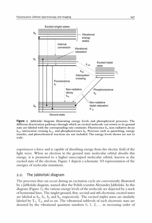
experiences a force and is capable of absorbing energy from the electric field of thelight wave. When an electron in the ground state molecular orbital absorbs thisenergy, it is promoted to a higher unoccupied molecular orbital, known as theexcited state of the electron. Figure 1 depicts a schematic 1D representation of theenergies of molecular transitions.
2.2. The Jabłonski diagram
The processes that can occur during an excitation cycle are conveniently illustratedby a Jabłonski diagram, named after the Polish scientist Alexander Jabłonski. In thisdiagram (Figure 1), the various energy levels of the molecule are depicted by a stackof horizontal lines. The singlet ground, first, second and nth electronic excited statesare labeled as S0, S1, S2 and Sn, respectively. The excited triplet states are similarlylabeled by T1, T2, and so on. The vibrational sublevels of each electronic state aredenoted by the vibrational quantum numbers 0, 1, 2, . . . in increasing order of
k isc
k r
k -isc
Ground state
Excited singlet states
Excited tripletstate
S2
S1
S0
T1
Vibrationalenergystates
Internalconversion
Intersystemcrossing
Non-radiativedecayk nr
Phosphorecencek p
Fluorescence
Non-radiativetriplet relaxationk ′ nr
Vibrationalrelaxation
Figure 1 Jabłon¤ ski diagram illustrating energy levels and photophysical processes. Thedifferent deactivation pathways through which an excited molecule can return to its groundstate are labeled with the corresponding rate constants: Fluorescence kr, non-radiative decayknr, intersystem crossing kisc, and phosphorescence kp. Processes such as quenching, energytransfer, and photochemical reactions are not included. The energy levels shown are not toscale.
Fluorescence Lifetime Spectroscopy and Imaging 147
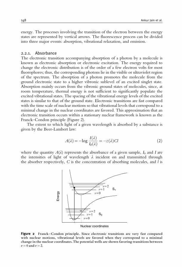
energy. The processes involving the transition of the electron between the energystates are represented by vertical arrows. The fluorescence process can be dividedinto three major events: absorption, vibrational relaxation, and emission.
2.2.1. AbsorbanceThe electronic transition accompanying absorption of a photon by a molecule isknown as electronic absorption or electronic excitation. The energy required tochange the electronic distribution is of the order of a few electron volts for mostfluorophores; thus, the corresponding photons lie in the visible or ultraviolet regionof the spectrum. The absorption of a photon promotes the molecule from theground electronic state to a higher vibronic sublevel of an excited singlet state.Absorption mainly occurs from the vibronic ground states of molecules, since, atroom temperature, thermal energy is not sufficient to significantly populate theexcited vibrational states. The spacing of the vibrational energy levels of the excitedstates is similar to that of the ground state. Electronic transitions are fast comparedwith the time scale of nuclear motions so that vibrational levels that correspond to aminimal change in the nuclear coordinates are favored. This approximation that anelectronic transition occurs within a stationary nuclear framework is known as theFranck–Condon principle (Figure 2).
The extent to which light of a given wavelength is absorbed by a substance isgiven by the Beer-Lambert law:
A lð Þ=�logI lð ÞI0 lð Þ =�" lð ÞCl ð2Þ
where the quantity A(l) represents the absorbance of a given sample, I0 and I arethe intensities of light of wavelength l incident on and transmitted throughthe absorber respectively, C is the concentration of absorbing molecules, and l is
S1
S0
ν = 2ν = 1
ν = 2ν = 1
ν = 0
Ene
rgy
Nuclear coordinates
ν = 0
Figure 2 Franck^Condon principle. Since electronic transitions are very fast comparedwith nuclear motions, vibrational levels are favored when they correspond to a minimalchange in the nuclear coordinates.The potential wells are shown favoring transitions betweenv= 0 and v= 2.
148 Ankur Jain et al.
the path length of light through the sample. "(l) is a molecular constant under agiven set of physical conditions and solvent, related to the electronic transitiondipole moment, and is called the molar extinction coefficient of the sample. Agraphical representation of the absorbance of a species as a function of wavelengthor frequency is known as the absorption spectrum. Regions of the spectrum wherethe intensity of absorbed light is high are known as absorption bands. Spectrallybroad absorption bands are a consequence of closely spaced vibrational energylevels together with the thermal motion that enables a range of photon energiesto cause a particular transition.
2.2.2. Non-radiative relaxation processesThe absorption of a photon leaves a molecule in one of the possible highervibrational states of one of its electronically excited states. Excess vibrational energyis dissipated as heat by a process termed as internal conversion and the molecule relaxesto the ground vibrational level of the first excited singlet state within a fewpicoseconds, an effect known as vibrational relaxation. As the time required forinternal conversion is typically much less than that for fluorescence emission, thefollowing transition occurs from the lowest vibrational sublevel of the lowestexcited state.
The primary mechanism of relaxation of excited non-emitting molecules isradiationless decay, in which the excess energy is transferred into the vibration,rotation, and translation of the surrounding molecules. The excitation energy isthus dissipated as heat, and the molecule returns to the ground electronic state.
The electrons in the excited singlet state S1 can also undergo intersystem crossing,a non-radiative transition between states of different spin multiplicity. A transitionto the triplet state T1 is usually followed by another radiative (phosphorescence) ornon-radiative deactivation. In addition, a molecule in its excited state can non-radiatively transfer its excitation energy to other molecules, either by collision, aprocess known as dynamic quenching, or by resonance energy transfer.
2.2.3. Radiative relaxation of electronically excited moleculesMolecules that do not possess effective non-radiative decay channels can dissipatetheir excitation energy upon radiation of a photon. Depending on the electronicnature of the excited state, one can distinguish between fluorescence andphosphorescence.
2.2.3.1. FluorescenceThe processes of internal conversion and vibrational relaxation leave the electro-nically excited molecule in the lowest vibrational sublevels of the first singletexcited state. If subsequent relaxation to the ground electronic state is accom-panied by the emission of a photon, the process is formally known as fluores-cence. An excited molecule capable of fluorescence typically stays in the lowestexcited singlet state S1 for a period of several nanoseconds before finally relaxingto the ground state. Internal conversion and vibrational relaxation are responsible
Fluorescence Lifetime Spectroscopy and Imaging 149
for the emitted photon having lower energy than the incident photon. This shiftto a longer wavelength is a phenomenon known as the Stokes shift. The Stokesshift is essential for the sensitivity of fluorescence detection because it allowseffective separation of the fluorescence emission signal from Rayleigh-scatteredexcitation light. As emission occurs from the lowest vibrational sublevel of firstexcited singlet state, the emission spectra are, in general, independent of excita-tion wavelength.
Emission spectra are usually mirror symmetric to the lowest energy absorp-tion band. This symmetry is a result of relaxation to the vibrationally excitedstates of the electronic ground state S0, and the similarities of the vibrationalenergy levels of S0 and S1. According to the Franck–Condon principle, allelectronic transitions are vertical (Figure 2) that is, they occur without changein the position of the nuclei. Thus, the various transition probabilities (Franck–Condon factors) are similar and lead to the symmetric nature of the absorptionand emission spectra.
2.2.3.2. PhosphorescenceThe emission of a photon from the excited triplet state T1 is defined as phosphores-cence. The phosphorescence spectrum is generally shifted to longer wavelengthsrelative to the fluorescence spectrum. Although transitions between states of differentspin multiplicity are strictly forbidden, singlet states occasionally have some tripletcharacter due to mixing of the singlet and triplet wavefunctions, thus relaxing thisselection rule. Nevertheless, the probability for such a transition remains very small,and as a consequence, the triplet–singlet transition is very long-lived and results inphosphorescence lifetimes on the order of milliseconds to a few seconds.
2.2.3.3. Delayed fluorescenceOccasionally, in rigid and viscous media at very low temperature, another long-lived emission band is observed at a frequency corresponding to that of fluorescencebut with a decay time similar to phosphorescence. This phenomenon is known asdelayed fluorescence and is a consequence of thermal excitation of the moleculefrom the first excited triplet state back to the first excited singlet state, followed byfluorescence emission.
2.2.4. Timescales of various fluorescence processesThe various relaxation processes of an excited molecule occur on timescalesdiffering by several orders of magnitude; characteristic rate constants and timescalesare summarized in Table 1 [1]. The initial absorption of a quantum of energy takesplace within a few femtoseconds. The vibrational relaxation takes place in less thana few picoseconds. The final emission of a longer wavelength photon from the firstexcited singlet state, that is, fluorescence emission, occurs in a relatively longer timeperiod (several nanoseconds), whereas phosphorescence lifetimes can range fromseveral milliseconds to a few seconds. The excited state lifetime is further influencedby processes such as quenching, energy transfer, and intersystem crossing, whichprovide for alternative decay pathways.
150 Ankur Jain et al.
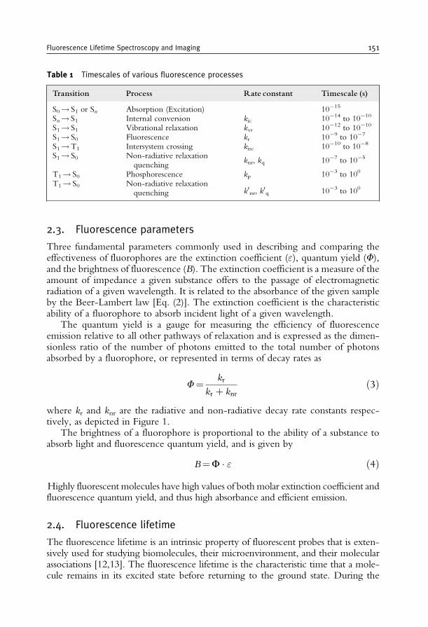
2.3. Fluorescence parameters
Three fundamental parameters commonly used in describing and comparing theeffectiveness of fluorophores are the extinction coefficient ("), quantum yield (F),and the brightness of fluorescence (B). The extinction coefficient is a measure of theamount of impedance a given substance offers to the passage of electromagneticradiation of a given wavelength. It is related to the absorbance of the given sampleby the Beer-Lambert law [Eq. (2)]. The extinction coefficient is the characteristicability of a fluorophore to absorb incident light of a given wavelength.
The quantum yield is a gauge for measuring the efficiency of fluorescenceemission relative to all other pathways of relaxation and is expressed as the dimen-sionless ratio of the number of photons emitted to the total number of photonsabsorbed by a fluorophore, or represented in terms of decay rates as
F=kr
kr þ knrð3Þ
where kr and knr are the radiative and non-radiative decay rate constants respec-tively, as depicted in Figure 1.
The brightness of a fluorophore is proportional to the ability of a substance toabsorb light and fluorescence quantum yield, and is given by
B=F � " ð4ÞHighly fluorescent molecules have high values of both molar extinction coefficient andfluorescence quantum yield, and thus high absorbance and efficient emission.
2.4. Fluorescence lifetime
The fluorescence lifetime is an intrinsic property of fluorescent probes that is exten-sively used for studying biomolecules, their microenvironment, and their molecularassociations [12,13]. The fluorescence lifetime is the characteristic time that a mole-cule remains in its excited state before returning to the ground state. During the
Table 1 Timescales of various fluorescence processes
Transition Process Rate constant Timescale (s)
S0! S1 or Sn Absorption (Excitation) 10�15
Sn! S1 Internal conversion kic 10�14 to 10�10
S1! S1 Vibrational relaxation kvr 10�12 to 10�10
S1! S0 Fluorescence kr 10�9 to 10�7
S1!T1 Intersystem crossing kisc 10�10 to 10�8
S1! S0 Non-radiative relaxationquenching
knr, kq 10�7 to 10�5
T1! S0 Phosphorescence kp 10�3 to 100
T1! S0 Non-radiative relaxationquenching k0nr, k0q 10�3 to 100
Fluorescence Lifetime Spectroscopy and Imaging 151
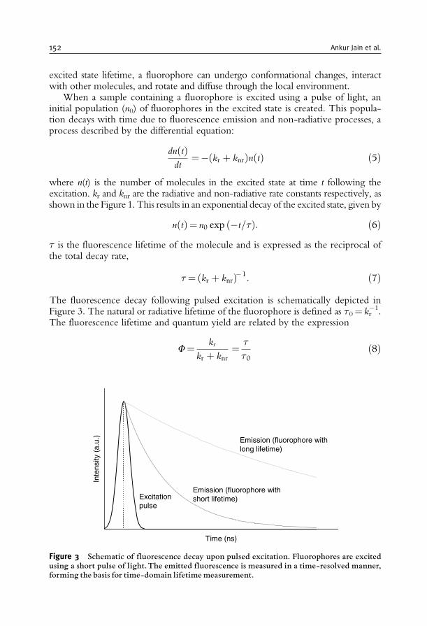
excited state lifetime, a fluorophore can undergo conformational changes, interactwith other molecules, and rotate and diffuse through the local environment.
When a sample containing a fluorophore is excited using a pulse of light, aninitial population (n0) of fluorophores in the excited state is created. This popula-tion decays with time due to fluorescence emission and non-radiative processes, aprocess described by the differential equation:
dn tð Þdt
=� kr þ knrð Þn tð Þ ð5Þ
where n(t) is the number of molecules in the excited state at time t following theexcitation. kr and knr are the radiative and non-radiative rate constants respectively, asshown in the Figure 1. This results in an exponential decay of the excited state, given by
n tð Þ= n0 exp �t=ð Þ: ð6Þ is the fluorescence lifetime of the molecule and is expressed as the reciprocal ofthe total decay rate,
= kr þ knrð Þ�1: ð7Þ
The fluorescence decay following pulsed excitation is schematically depicted inFigure 3. The natural or radiative lifetime of the fluorophore is defined as 0= kr
�1.The fluorescence lifetime and quantum yield are related by the expression
F=kr
kr þ knr=
0ð8Þ
Time (ns)
Inte
nsity
(a.
u.)
Emission (fluorophore withlong lifetime)
Emission (fluorophore withshort lifetime)Excitation
pulse
Figure 3 Schematic of fluorescence decay upon pulsed excitation. Fluorophores are excitedusing a short pulse of light.The emitted fluorescence is measured in a time-resolved manner,forming the basis for time-domain lifetime measurement.
152 Ankur Jain et al.
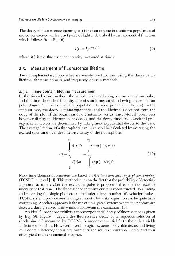
The decay of fluorescence intensity as a function of time in a uniform population ofmolecules excited with a brief pulse of light is described by an exponential functionwhich follows from Eq. (6):
I tð Þ= I0e� t=ð Þ ð9Þ
where I(t) is the fluorescence intensity measured at time t.
2.5. Measurement of fluorescence lifetime
Two complementary approaches are widely used for measuring the fluorescencelifetime, the time-domain, and frequency-domain methods.
2.5.1. Time-domain lifetime measurementIn the time-domain method, the sample is excited using a short excitation pulse,and the time-dependent intensity of emission is measured following the excitationpulse (Figure 3). The excited state population decays exponentially (Eq. (6)). In thesimplest case, the decay is monoexponential and the lifetime is deduced from theslope of the plot of the logarithm of the intensity versus time. Most fluorophoreshowever display multicomponent decays, and the decay times and associated pre-exponential factors are determined by fitting multiexponential decays to the data.The average lifetime of a fluorophore can in general be calculated by averaging theexcited state time over the intensity decay of the fluorophore:
hti=
ð1
0
tIðtÞdt
ð1
0
IðtÞdt=
ð1
0
t exp ð�t=Þdt
ð1
0
exp ð�t=Þdtð10Þ
Most time-domain fluorimeters are based on the time-correlated single photon counting(TCSPC)method [14]. This method relies on the fact that the probability of detectinga photon at time t after the excitation pulse is proportional to the fluorescenceintensity at that time. The fluorescence intensity curve is reconstructed after timingand recording the single photons emitted after a large number of excitation pulses.TCSPC systems provide outstanding sensitivity, but data acquisition can be quite timeconsuming. Another approach is the use of time-gated systems where the photons aredetected during a fixed time window following the excitation [15].
An ideal fluorophore exhibits a monoexponential decay of fluorescence as givenby Eq. (9). Figure 4 depicts the fluorescence decay of an aqueous solution ofrhodamine 6G measured by TCSPC. A monoexponential fit to these data yieldsa lifetime of4.1 ns. However, most biological systems like viable tissues and livingcells contain heterogeneous environments and multiple emitting species and thusoften yield multiexponential lifetimes.
Fluorescence Lifetime Spectroscopy and Imaging 153
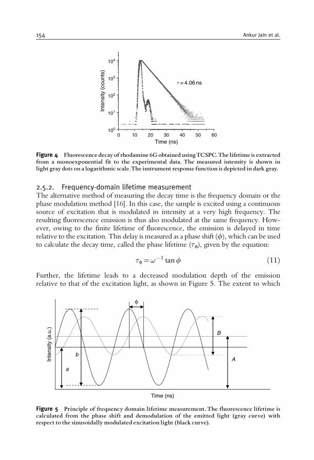
2.5.2. Frequency-domain lifetime measurementThe alternative method of measuring the decay time is the frequency domain or thephase modulation method [16]. In this case, the sample is excited using a continuoussource of excitation that is modulated in intensity at a very high frequency. Theresulting fluorescence emission is thus also modulated at the same frequency. How-ever, owing to the finite lifetime of fluorescence, the emission is delayed in timerelative to the excitation. This delay is measured as a phase shift (f), which can be usedto calculate the decay time, called the phase lifetime (f), given by the equation:
f =!�1 tanf ð11ÞFurther, the lifetime leads to a decreased modulation depth of the emissionrelative to that of the excitation light, as shown in Figure 5. The extent to which
0 10 20 30 40 50 60100
101
102
103
104
τ = 4.06 ns
Inte
nsity
(co
unts
)
Time (ns)
Figure 4 Fluorescence decayof rhodamine 6G obtained usingTCSPC.The lifetime is extractedfrom a monoexponential fit to the experimental data. The measured intensity is shown inlight graydots on a logarithmic scale.The instrument response function is depicted in dark gray.
Time (ns)
Inte
nsity
(a.
u.)
B
A
a
b
φ
Figure 5 Principle of frequency domain lifetime measurement.The fluorescence lifetime iscalculated from the phase shift and demodulation of the emitted light (gray curve) withrespect to the sinusoidally modulated excitation light (black curve).
154 Ankur Jain et al.
this occurs depends upon the decay time of the fluorophore and the modulationfrequency. The demodulation factor, m, is given by
m=B=A
b=að12Þ
where b/a is the modulation of the excitation light and B/A, for the emitted light(Figure 5). The lifetime calculated from the demodulation is called the modulationlifetime (m) and is given by
m =1
!
1
m2� 1
� �1=2ð13Þ
For monoexponential decays, the phase and modulation lifetimes correspond.A difference in the phase and modulation lifetimes is indicative of multiexponentialfluorescence decay or excited state interactions of the fluorophore. Frequencydomain lifetime determination is particularly suited for wide-field illuminationstrategies and spatially-resolved fluorescence lifetime imaging [17].
2.6. Fluorescence anisotropy and polarization
The interaction of the exciting light with the molecule can be described as theinteraction of the electric field component of the light with the relevant transitiondipole moment of the molecule. For excitation by linearly polarized light, fluor-ophores whose transition moments are aligned parallel to the electric field vector ofthe excitation light preferentially absorb photons, a process known as photoselec-tion. This selective excitation results in a partially oriented population of excitedfluorophores and thus in a partially polarized emission. The extent of fluorescencepolarization is determined by the parameter anisotropy r, given by
r =Ik � I?Ik þ 2I?
ð14Þ
where Ik and I? are the intensities of vertically (k) and horizontally (?) polarizedemission, measured relative to the polarization of the excitation light. The limitinganisotropy, r0, for a randomly oriented molecule upon excitation by linearlypolarized light under one photon excitation conditions, is given by
r0 = 0:6 cos 2� � 0:2 ð15Þwhere � is the angle by which the absorption and emission transition dipolemoments of the fluorophore are displaced relative to each other. It follows thatthe theoretical anisotropy maximum for collinear absorption and emission transi-tion dipole moments is 0.4.
When the emission and excitation transition dipole moments are non-collinear,there will be some depolarization even when the molecules are fixed (Eq. (15)).
Fluorescence Lifetime Spectroscopy and Imaging 155
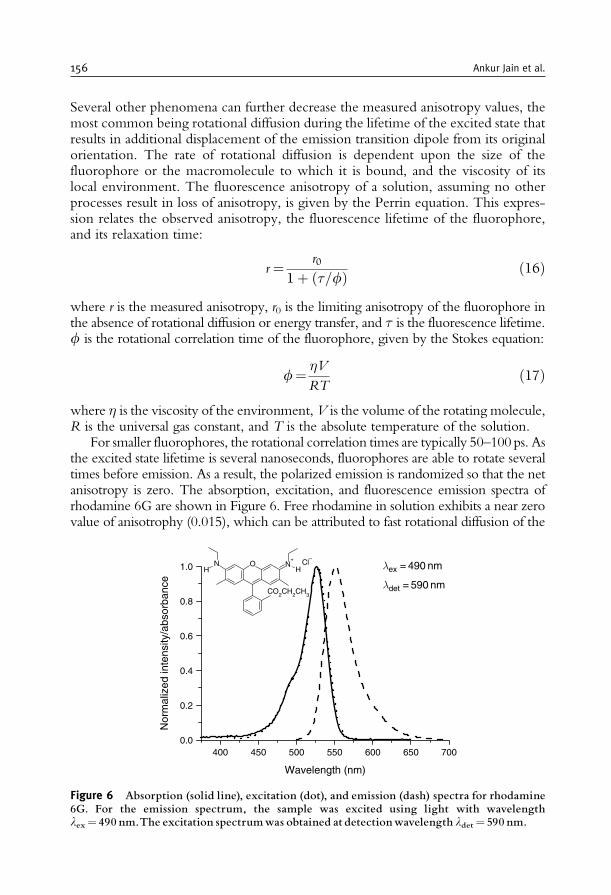
Several other phenomena can further decrease the measured anisotropy values, themost common being rotational diffusion during the lifetime of the excited state thatresults in additional displacement of the emission transition dipole from its originalorientation. The rate of rotational diffusion is dependent upon the size of thefluorophore or the macromolecule to which it is bound, and the viscosity of itslocal environment. The fluorescence anisotropy of a solution, assuming no otherprocesses result in loss of anisotropy, is given by the Perrin equation. This expres-sion relates the observed anisotropy, the fluorescence lifetime of the fluorophore,and its relaxation time:
r =r0
1þ =fð Þ ð16Þ
where r is the measured anisotropy, r0 is the limiting anisotropy of the fluorophore inthe absence of rotational diffusion or energy transfer, and is the fluorescence lifetime.f is the rotational correlation time of the fluorophore, given by the Stokes equation:
f=�V
RTð17Þ
where � is the viscosity of the environment, V is the volume of the rotating molecule,R is the universal gas constant, and T is the absolute temperature of the solution.
For smaller fluorophores, the rotational correlation times are typically 50–100ps. Asthe excited state lifetime is several nanoseconds, fluorophores are able to rotate severaltimes before emission. As a result, the polarized emission is randomized so that the netanisotropy is zero. The absorption, excitation, and fluorescence emission spectra ofrhodamine 6G are shown in Figure 6. Free rhodamine in solution exhibits a near zerovalue of anisotrophy (0.015), which can be attributed to fast rotational diffusion of the
400 450 500 550 600 650 7000.0
0.2
0.4
0.6
0.8
1.0 ONH
N+
H
CO2CH2CH3
λ ex = 490 nm
λ det = 590 nm
Nor
mal
ized
inte
nsity
/abs
orba
nce
Wavelength (nm)
Cl–+
Figure 6 Absorption (solid line), excitation (dot), and emission (dash) spectra for rhodamine6G. For the emission spectrum, the sample was excited using light with wavelengthlex= 490 nm.The excitation spectrumwas obtained at detectionwavelength ldet= 590 nm.
156 Ankur Jain et al.
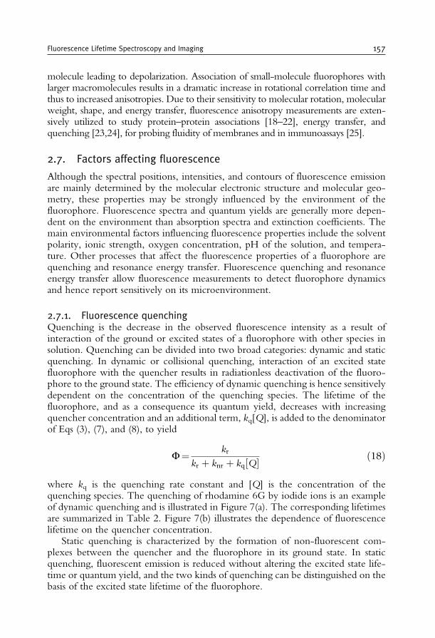
molecule leading to depolarization. Association of small-molecule fluorophores withlarger macromolecules results in a dramatic increase in rotational correlation time andthus to increased anisotropies. Due to their sensitivity to molecular rotation, molecularweight, shape, and energy transfer, fluorescence anisotropy measurements are exten-sively utilized to study protein–protein associations [18–22], energy transfer, andquenching [23,24], for probing fluidity of membranes and in immunoassays [25].
2.7. Factors affecting fluorescence
Although the spectral positions, intensities, and contours of fluorescence emissionare mainly determined by the molecular electronic structure and molecular geo-metry, these properties may be strongly influenced by the environment of thefluorophore. Fluorescence spectra and quantum yields are generally more depen-dent on the environment than absorption spectra and extinction coefficients. Themain environmental factors influencing fluorescence properties include the solventpolarity, ionic strength, oxygen concentration, pH of the solution, and tempera-ture. Other processes that affect the fluorescence properties of a fluorophore arequenching and resonance energy transfer. Fluorescence quenching and resonanceenergy transfer allow fluorescence measurements to detect fluorophore dynamicsand hence report sensitively on its microenvironment.
2.7.1. Fluorescence quenchingQuenching is the decrease in the observed fluorescence intensity as a result ofinteraction of the ground or excited states of a fluorophore with other species insolution. Quenching can be divided into two broad categories: dynamic and staticquenching. In dynamic or collisional quenching, interaction of an excited statefluorophore with the quencher results in radiationless deactivation of the fluoro-phore to the ground state. The efficiency of dynamic quenching is hence sensitivelydependent on the concentration of the quenching species. The lifetime of thefluorophore, and as a consequence its quantum yield, decreases with increasingquencher concentration and an additional term, kq[Q], is added to the denominatorof Eqs (3), (7), and (8), to yield
F=kr
kr þ knr þ kq Q½ � ð18Þ
where kq is the quenching rate constant and [Q] is the concentration of thequenching species. The quenching of rhodamine 6G by iodide ions is an exampleof dynamic quenching and is illustrated in Figure 7(a). The corresponding lifetimesare summarized in Table 2. Figure 7(b) illustrates the dependence of fluorescencelifetime on the quencher concentration.
Static quenching is characterized by the formation of non-fluorescent com-plexes between the quencher and the fluorophore in its ground state. In staticquenching, fluorescent emission is reduced without altering the excited state life-time or quantum yield, and the two kinds of quenching can be distinguished on thebasis of the excited state lifetime of the fluorophore.
Fluorescence Lifetime Spectroscopy and Imaging 157
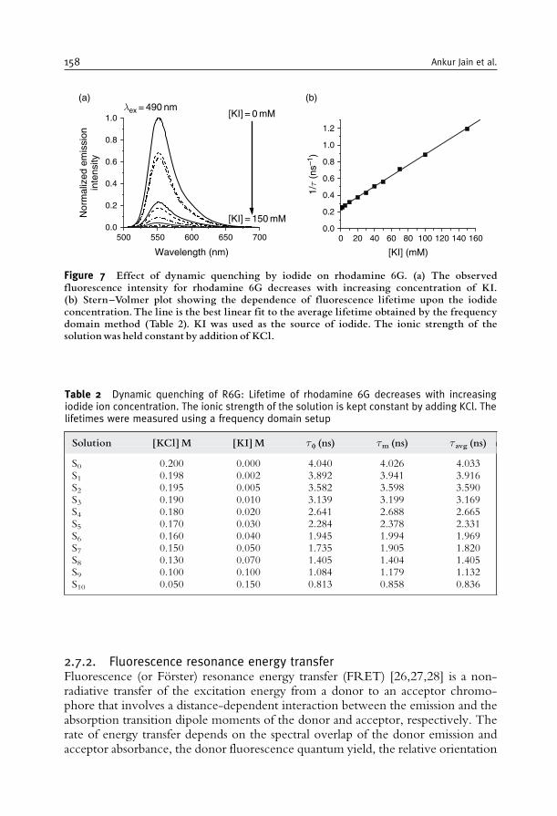
2.7.2. Fluorescence resonance energy transferFluorescence (or Forster) resonance energy transfer (FRET) [26,27,28] is a non-radiative transfer of the excitation energy from a donor to an acceptor chromo-phore that involves a distance-dependent interaction between the emission and theabsorption transition dipole moments of the donor and acceptor, respectively. Therate of energy transfer depends on the spectral overlap of the donor emission andacceptor absorbance, the donor fluorescence quantum yield, the relative orientation
500 550 600 650 7000.0
0.2
0.4
0.6
0.8
1.0
Nor
mal
ized
em
issi
onin
tens
ity
Wavelength (nm)
(a)λ ex = 490 nm
[KI] = 0 mM
[KI] = 150 mM
0 20 40 60 80 100 120 140 1600.0
0.2
0.4
0.6
0.8
1.0
1.2
1/τ
(ns–1
)
(b)
[KI] (mM)
Figure 7 Effect of dynamic quenching by iodide on rhodamine 6G. (a) The observedfluorescence intensity for rhodamine 6G decreases with increasing concentration of KI.(b) Stern^Volmer plot showing the dependence of fluorescence lifetime upon the iodideconcentration.The line is the best linear fit to the average lifetime obtained by the frequencydomain method (Table 2). KI was used as the source of iodide. The ionic strength of thesolutionwas held constant by addition of KCl.
Table 2 Dynamic quenching of R6G: Lifetime of rhodamine 6G decreases with increasingiodide ion concentration. The ionic strength of the solution is kept constant by adding KCl. Thelifetimes were measured using a frequency domain setup
Solution [KCl]M [KI]M f (ns) m (ns) avg (ns)
S0 0.200 0.000 4.040 4.026 4.033S1 0.198 0.002 3.892 3.941 3.916S2 0.195 0.005 3.582 3.598 3.590S3 0.190 0.010 3.139 3.199 3.169S4 0.180 0.020 2.641 2.688 2.665S5 0.170 0.030 2.284 2.378 2.331S6 0.160 0.040 1.945 1.994 1.969S7 0.150 0.050 1.735 1.905 1.820S8 0.130 0.070 1.405 1.404 1.405S9 0.100 0.100 1.084 1.179 1.132S10 0.050 0.150 0.813 0.858 0.836
158 Ankur Jain et al.
of their transition dipole moments, and the distance between donor and acceptormolecules. The energy transfer rate, kET, is given by
kET=1
d
R0
r
� �6
ð19Þ
where d is the decay time of the fluorophore in the absence of an acceptor, and r isthe distance between the donor and the acceptor. R0 is the Forster radius (typically2 to 9 nm) characterizing the donor/acceptor pair. It is defined as the distance atwhich the efficiency of resonance energy transfer is 50% and can be estimated as
R0 in nmð Þ= 979 �2n4F0J� �1=6 ð20Þ
where n is the refractive index of the medium, F0 is the fluorescence quantum yieldof the donor, J is the spectral overlap integral, and �2 is the orientation factor. Theoverlap integral, J, expresses the extent of overlap between the donor emission andthe acceptor absorption.
J =
ð10
FD lð Þ"A lð Þl4dl ð21Þ
where FD(l) is the normalized fluorescence spectrum of the donor and "A(l) is themolar extinction coefficient of the acceptor as a function of wavelength, l. The rate ofenergy transfer varies linearly with the overlap integral [29]. A large value of overlapintegral ensures high sensitivity for imaging and sensing as well as high selectivity.
Resonance energy transfer provides an additional deactivation pathway for theexcited fluorophore and results in reduced excited state lifetime of the donorfluorophore. The Forster distances are comparable to the size of biological macro-molecules, and thus, FRET is extensively used as a ‘‘spectroscopic ruler’’ formeasuring distances between sites on interacting proteins [30–36].
The magnitude of kET can be determined from the efficiency of energy transfer,ET, using the relation
kET =1
d
ET
1� ET
� �ð22Þ
and ET can be determined experimentally by measuring the decrease in theintensity F or the lifetime of the donor in the presence of the acceptor,
ET= 1� F
Fd= 1�
d: ð23Þ
Hence, the change in observed fluorescence intensity or the excited state lifetime ofthe donor fluorophore, due to resonance energy transfer, can be used to determinethe distance between the donor acceptor pair. However, the distances so estimatedare also influenced by the orientation factor, �2, which depends on the relative
Fluorescence Lifetime Spectroscopy and Imaging 159
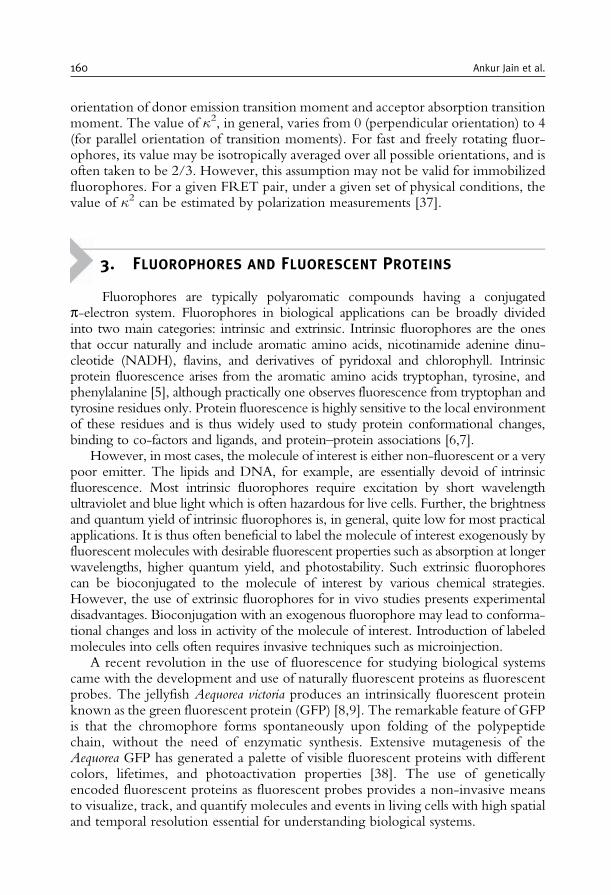
orientation of donor emission transition moment and acceptor absorption transitionmoment. The value of �2, in general, varies from 0 (perpendicular orientation) to 4(for parallel orientation of transition moments). For fast and freely rotating fluor-ophores, its value may be isotropically averaged over all possible orientations, and isoften taken to be 2/3. However, this assumption may not be valid for immobilizedfluorophores. For a given FRET pair, under a given set of physical conditions, thevalue of �2 can be estimated by polarization measurements [37].
3. FLUOROPHORES AND FLUORESCENT PROTEINS
Fluorophores are typically polyaromatic compounds having a conjugatedp-electron system. Fluorophores in biological applications can be broadly dividedinto two main categories: intrinsic and extrinsic. Intrinsic fluorophores are the onesthat occur naturally and include aromatic amino acids, nicotinamide adenine dinu-cleotide (NADH), flavins, and derivatives of pyridoxal and chlorophyll. Intrinsicprotein fluorescence arises from the aromatic amino acids tryptophan, tyrosine, andphenylalanine [5], although practically one observes fluorescence from tryptophan andtyrosine residues only. Protein fluorescence is highly sensitive to the local environmentof these residues and is thus widely used to study protein conformational changes,binding to co-factors and ligands, and protein–protein associations [6,7].
However, in most cases, the molecule of interest is either non-fluorescent or a verypoor emitter. The lipids and DNA, for example, are essentially devoid of intrinsicfluorescence. Most intrinsic fluorophores require excitation by short wavelengthultraviolet and blue light which is often hazardous for live cells. Further, the brightnessand quantum yield of intrinsic fluorophores is, in general, quite low for most practicalapplications. It is thus often beneficial to label the molecule of interest exogenously byfluorescent molecules with desirable fluorescent properties such as absorption at longerwavelengths, higher quantum yield, and photostability. Such extrinsic fluorophorescan be bioconjugated to the molecule of interest by various chemical strategies.However, the use of extrinsic fluorophores for in vivo studies presents experimentaldisadvantages. Bioconjugation with an exogenous fluorophore may lead to conforma-tional changes and loss in activity of the molecule of interest. Introduction of labeledmolecules into cells often requires invasive techniques such as microinjection.
A recent revolution in the use of fluorescence for studying biological systemscame with the development and use of naturally fluorescent proteins as fluorescentprobes. The jellyfish Aequorea victoria produces an intrinsically fluorescent proteinknown as the green fluorescent protein (GFP) [8,9]. The remarkable feature of GFPis that the chromophore forms spontaneously upon folding of the polypeptidechain, without the need of enzymatic synthesis. Extensive mutagenesis of theAequorea GFP has generated a palette of visible fluorescent proteins with differentcolors, lifetimes, and photoactivation properties [38]. The use of geneticallyencoded fluorescent proteins as fluorescent probes provides a non-invasive meansto visualize, track, and quantify molecules and events in living cells with high spatialand temporal resolution essential for understanding biological systems.
160 Ankur Jain et al.
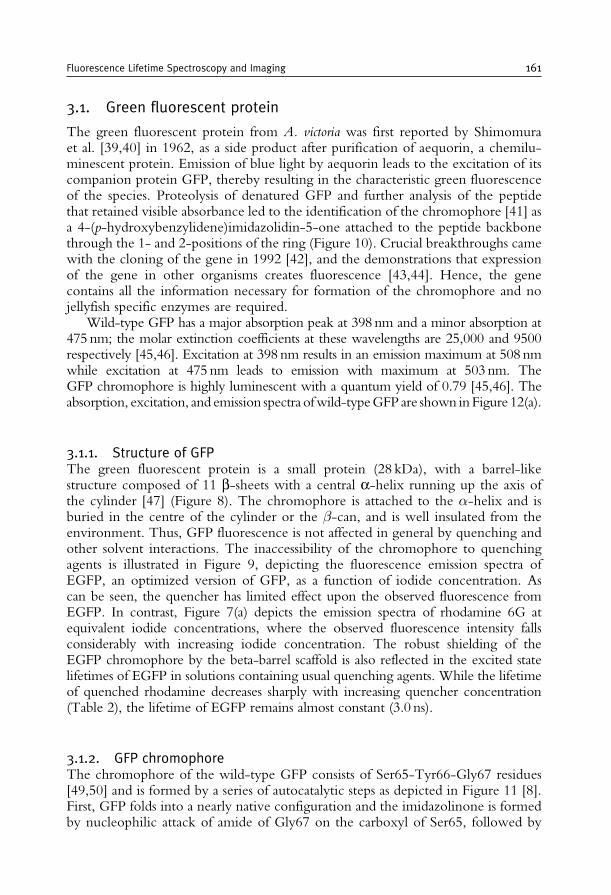
3.1. Green fluorescent protein
The green fluorescent protein from A. victoria was first reported by Shimomuraet al. [39,40] in 1962, as a side product after purification of aequorin, a chemilu-minescent protein. Emission of blue light by aequorin leads to the excitation of itscompanion protein GFP, thereby resulting in the characteristic green fluorescenceof the species. Proteolysis of denatured GFP and further analysis of the peptidethat retained visible absorbance led to the identification of the chromophore [41] asa 4-(p-hydroxybenzylidene)imidazolidin-5-one attached to the peptide backbonethrough the 1- and 2-positions of the ring (Figure 10). Crucial breakthroughs camewith the cloning of the gene in 1992 [42], and the demonstrations that expressionof the gene in other organisms creates fluorescence [43,44]. Hence, the genecontains all the information necessary for formation of the chromophore and nojellyfish specific enzymes are required.
Wild-type GFP has a major absorption peak at 398 nm and a minor absorption at475 nm; the molar extinction coefficients at these wavelengths are 25,000 and 9500respectively [45,46]. Excitation at 398 nm results in an emission maximum at 508 nmwhile excitation at 475 nm leads to emission with maximum at 503 nm. TheGFP chromophore is highly luminescent with a quantum yield of 0.79 [45,46]. Theabsorption, excitation, and emission spectra ofwild-typeGFPare shown inFigure 12(a).
3.1.1. Structure of GFPThe green fluorescent protein is a small protein (28 kDa), with a barrel-likestructure composed of 11 b-sheets with a central a-helix running up the axis ofthe cylinder [47] (Figure 8). The chromophore is attached to the �-helix and isburied in the centre of the cylinder or the �-can, and is well insulated from theenvironment. Thus, GFP fluorescence is not affected in general by quenching andother solvent interactions. The inaccessibility of the chromophore to quenchingagents is illustrated in Figure 9, depicting the fluorescence emission spectra ofEGFP, an optimized version of GFP, as a function of iodide concentration. Ascan be seen, the quencher has limited effect upon the observed fluorescence fromEGFP. In contrast, Figure 7(a) depicts the emission spectra of rhodamine 6G atequivalent iodide concentrations, where the observed fluorescence intensity fallsconsiderably with increasing iodide concentration. The robust shielding of theEGFP chromophore by the beta-barrel scaffold is also reflected in the excited statelifetimes of EGFP in solutions containing usual quenching agents. While the lifetimeof quenched rhodamine decreases sharply with increasing quencher concentration(Table 2), the lifetime of EGFP remains almost constant (3.0 ns).
3.1.2. GFP chromophoreThe chromophore of the wild-type GFP consists of Ser65-Tyr66-Gly67 residues[49,50] and is formed by a series of autocatalytic steps as depicted in Figure 11 [8].First, GFP folds into a nearly native configuration and the imidazolinone is formedby nucleophilic attack of amide of Gly67 on the carboxyl of Ser65, followed by
Fluorescence Lifetime Spectroscopy and Imaging 161
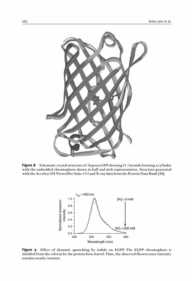
Figure 8 Schematic crystal structure ofAequoreaGFP showing11 � strands forming a cylinderwith the embedded chromophore shown in ball and stick representation. Structure generatedwith theAccelrys DSViewerPro Suite v5.1andX-ray data from the Protein Data Bank [48].
450 500 550 6000.0
0.2
0.4
0.6
0.8
1.0
λ ex = 450 nm
Nor
mal
ized
em
issi
onin
tens
ity
Wavelength (nm)
[KI] = 200 mM
[KI] = 0 mM
Figure 9 Effect of dynamic quenching by iodide on EGFP. The EGFP chromophore isshielded from the solvent by the protein beta-barrel.Thus, the observed fluorescence intensityremains nearly constant.
162 Ankur Jain et al.
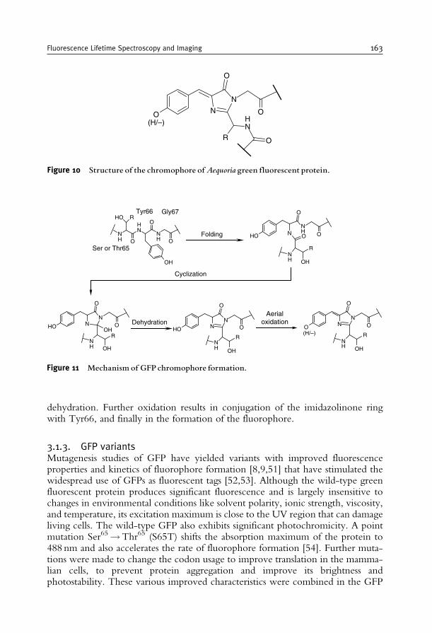
dehydration. Further oxidation results in conjugation of the imidazolinone ringwith Tyr66, and finally in the formation of the fluorophore.
3.1.3. GFP variantsMutagenesis studies of GFP have yielded variants with improved fluorescenceproperties and kinetics of fluorophore formation [8,9,51] that have stimulated thewidespread use of GFPs as fluorescent tags [52,53]. Although the wild-type greenfluorescent protein produces significant fluorescence and is largely insensitive tochanges in environmental conditions like solvent polarity, ionic strength, viscosity,and temperature, its excitation maximum is close to the UV region that can damageliving cells. The wild-type GFP also exhibits significant photochromicity. A pointmutation Ser65!Thr65 (S65T) shifts the absorption maximum of the protein to488 nm and also accelerates the rate of fluorophore formation [54]. Further muta-tions were made to change the codon usage to improve translation in the mamma-lian cells, to prevent protein aggregation and improve its brightness andphotostability. These various improved characteristics were combined in the GFP
N
N
O
RNH
O
O
O(H/–)
Figure 10 Structure of the chromophore ofAequoriagreen fluorescent protein.
NH
NH
HO R
ONH
O
O
OH
HO NNH
O
OO
NH
R
OH
HO NN
O
OOH
RNH OH
HO NN
O
O
NH
R
OH
NN
O
O
NH
R
OH
Ser or Thr65
Tyr66 Gly67
(H/–)
Cyclization
DehydrationAerial
oxidation
Folding
O
Figure 11 Mechanism of GFP chromophore formation.
Fluorescence Lifetime Spectroscopy and Imaging 163

variant known as enhanced GFP (EGFP), which is among the most commonly usedGFP variants in cell biology [52]. Further improvements led to the development ofnumerous mutants with differing absorbance and emission spectra allowing simul-taneous visualization of distinct fluorescent proteins in a cell. Various spectral
300 350 400 450 500 550 6000.0
0.2
0.4
0.6
0.8
1.0(a) Wild-type GFP λ ex = 380 nm
λ det = 560 nm
Nor
mal
ized
inte
nsity
Wavelength (nm)
300 350 400 450 500 550 6000.0
0.2
0.4
0.6
0.8
1.0(c) Red-shifted GFP λ ex = 470 nm
λ det = 530 nm
Nor
mal
ized
inte
nsity
Wavelength (nm)
300 350 400 450 500 550 6000.0
0.2
0.4
0.6
0.8
1.0(e) EYFP λ ex = 490 nm
λ det = 560 nm
Nor
mal
ized
inte
nsity
Wavelength (nm)
300 350 400 450 500 550 6000.0
0.2
0.4
0.6
0.8
1.0(b) EGFP λ ex = 450 nm
λ det = 530 nm
Nor
mal
ized
inte
nsity
Wavelength (nm)
300 350 400 450 500 550 6000.0
0.2
0.4
0.6
0.8
1.0(d) EBFP λ ex = 320 nm
λ det = 490 nm
Nor
mal
ized
inte
nsity
Wavelength (nm)
300 350 400 450 500 550 6000.0
0.2
0.4
0.6
0.8
1.0(f) Cerulean λ ex = 420 nm
λ det = 490 nm
Nor
mal
ized
inte
nsity
Wavelength (nm)
Figure 12 Absorption (black solid), excitation (black dotted) and emission spectra (gray) ofVFPs: (a) wild-type GFP, (b) EGFP, (c) red-shifted GFP (RSGFP) (d) EBFP, (e) EYFP, and(f ) Cerulean. Protein solutions at a concentration 1.5mM were prepared in 100mM Trisbuffer containing100mMNaCl at pH 8.5.The fluorescence excitation and emission spectraweredetermined at room temperature (22�C) with a Varian Cary Eclipse spectrofluorometer.The excitationwavelength for emission spectra (lex) and the detectionwavelength for excitationspectra (ldet) are mentioned on the top right corner of the figures (a)^(f ).
164 Ankur Jain et al.
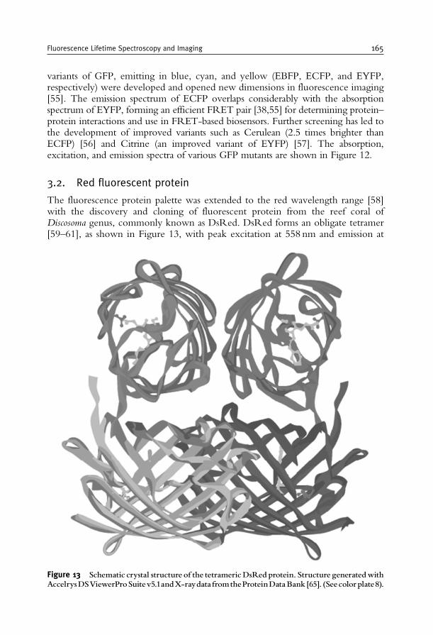
variants of GFP, emitting in blue, cyan, and yellow (EBFP, ECFP, and EYFP,respectively) were developed and opened new dimensions in fluorescence imaging[55]. The emission spectrum of ECFP overlaps considerably with the absorptionspectrum of EYFP, forming an efficient FRET pair [38,55] for determining protein–protein interactions and use in FRET-based biosensors. Further screening has led tothe development of improved variants such as Cerulean (2.5 times brighter thanECFP) [56] and Citrine (an improved variant of EYFP) [57]. The absorption,excitation, and emission spectra of various GFP mutants are shown in Figure 12.
3.2. Red fluorescent protein
The fluorescence protein palette was extended to the red wavelength range [58]with the discovery and cloning of fluorescent protein from the reef coral ofDiscosoma genus, commonly known as DsRed. DsRed forms an obligate tetramer[59–61], as shown in Figure 13, with peak excitation at 558 nm and emission at
Figure 13 Schematic crystal structure of the tetramericDsRed protein. Structure generatedwithAccelrysDSViewerProSuitev5.1andX-raydatafromtheProteinDataBank[65]. (Seecolorplate8).
Fluorescence Lifetime Spectroscopy and Imaging 165
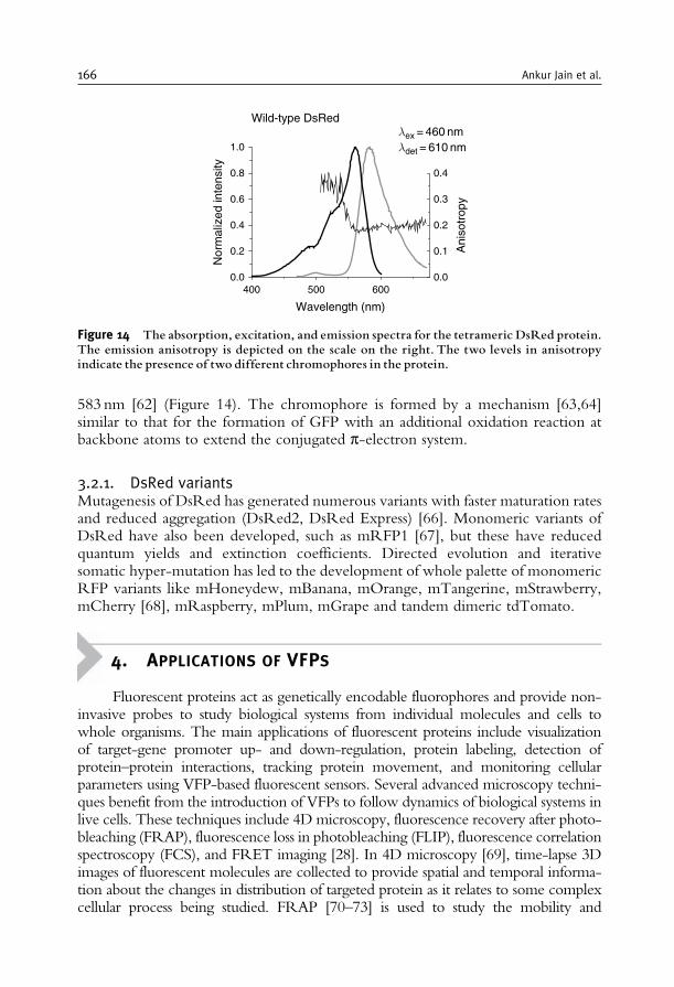
583 nm [62] (Figure 14). The chromophore is formed by a mechanism [63,64]similar to that for the formation of GFP with an additional oxidation reaction atbackbone atoms to extend the conjugated p-electron system.
3.2.1. DsRed variantsMutagenesis of DsRed has generated numerous variants with faster maturation ratesand reduced aggregation (DsRed2, DsRed Express) [66]. Monomeric variants ofDsRed have also been developed, such as mRFP1 [67], but these have reducedquantum yields and extinction coefficients. Directed evolution and iterativesomatic hyper-mutation has led to the development of whole palette of monomericRFP variants like mHoneydew, mBanana, mOrange, mTangerine, mStrawberry,mCherry [68], mRaspberry, mPlum, mGrape and tandem dimeric tdTomato.
4. APPLICATIONS OF VFPS
Fluorescent proteins act as genetically encodable fluorophores and provide non-invasive probes to study biological systems from individual molecules and cells towhole organisms. The main applications of fluorescent proteins include visualizationof target-gene promoter up- and down-regulation, protein labeling, detection ofprotein–protein interactions, tracking protein movement, and monitoring cellularparameters using VFP-based fluorescent sensors. Several advanced microscopy techni-ques benefit from the introduction of VFPs to follow dynamics of biological systems inlive cells. These techniques include 4D microscopy, fluorescence recovery after photo-bleaching (FRAP), fluorescence loss in photobleaching (FLIP), fluorescence correlationspectroscopy (FCS), and FRET imaging [28]. In 4D microscopy [69], time-lapse 3Dimages of fluorescent molecules are collected to provide spatial and temporal informa-tion about the changes in distribution of targeted protein as it relates to some complexcellular process being studied. FRAP [70–73] is used to study the mobility and
400 500 6000.0
0.2
0.4
0.6
0.8
1.0
Wild-type DsRedλ ex = 460 nmλ det = 610 nm
Ani
sotr
opy
Nor
mal
ized
inte
nsity
Wavelength (nm)
0.0
0.1
0.2
0.3
0.4
Figure 14 The absorption, excitation, and emission spectra for the tetrameric DsRed protein.The emission anisotropy is depicted on the scale on the right. The two levels in anisotropyindicate the presence of two different chromophores in the protein.
166 Ankur Jain et al.
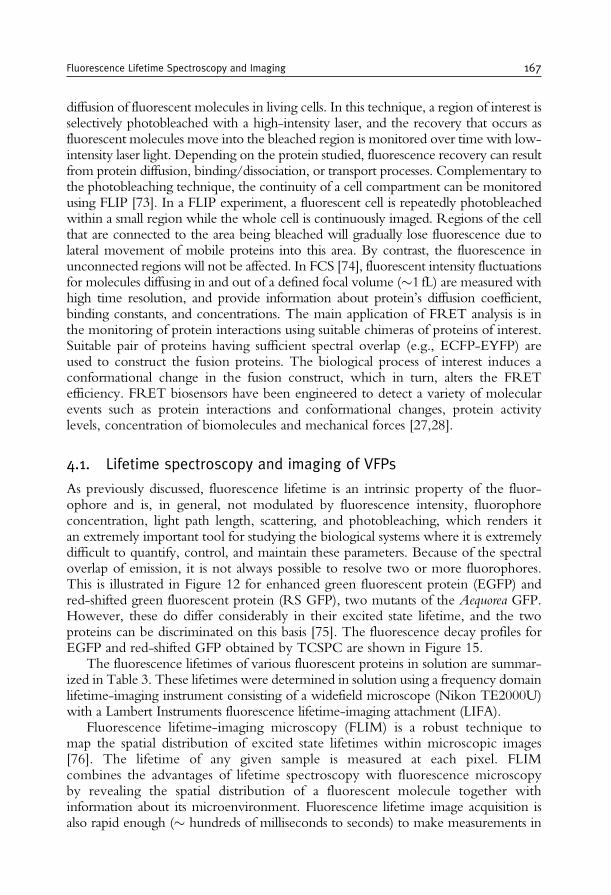
diffusion of fluorescent molecules in living cells. In this technique, a region of interest isselectively photobleached with a high-intensity laser, and the recovery that occurs asfluorescent molecules move into the bleached region is monitored over time with low-intensity laser light. Depending on the protein studied, fluorescence recovery can resultfrom protein diffusion, binding/dissociation, or transport processes. Complementary tothe photobleaching technique, the continuity of a cell compartment can be monitoredusing FLIP [73]. In a FLIP experiment, a fluorescent cell is repeatedly photobleachedwithin a small region while the whole cell is continuously imaged. Regions of the cellthat are connected to the area being bleached will gradually lose fluorescence due tolateral movement of mobile proteins into this area. By contrast, the fluorescence inunconnected regions will not be affected. In FCS [74], fluorescent intensity fluctuationsfor molecules diffusing in and out of a defined focal volume (1 fL) are measured withhigh time resolution, and provide information about protein’s diffusion coefficient,binding constants, and concentrations. The main application of FRET analysis is inthe monitoring of protein interactions using suitable chimeras of proteins of interest.Suitable pair of proteins having sufficient spectral overlap (e.g., ECFP-EYFP) areused to construct the fusion proteins. The biological process of interest induces aconformational change in the fusion construct, which in turn, alters the FRETefficiency. FRET biosensors have been engineered to detect a variety of molecularevents such as protein interactions and conformational changes, protein activitylevels, concentration of biomolecules and mechanical forces [27,28].
4.1. Lifetime spectroscopy and imaging of VFPs
As previously discussed, fluorescence lifetime is an intrinsic property of the fluor-ophore and is, in general, not modulated by fluorescence intensity, fluorophoreconcentration, light path length, scattering, and photobleaching, which renders itan extremely important tool for studying the biological systems where it is extremelydifficult to quantify, control, and maintain these parameters. Because of the spectraloverlap of emission, it is not always possible to resolve two or more fluorophores.This is illustrated in Figure 12 for enhanced green fluorescent protein (EGFP) andred-shifted green fluorescent protein (RS GFP), two mutants of the Aequorea GFP.However, these do differ considerably in their excited state lifetime, and the twoproteins can be discriminated on this basis [75]. The fluorescence decay profiles forEGFP and red-shifted GFP obtained by TCSPC are shown in Figure 15.
The fluorescence lifetimes of various fluorescent proteins in solution are summar-ized in Table 3. These lifetimes were determined in solution using a frequency domainlifetime-imaging instrument consisting of a widefield microscope (Nikon TE2000U)with a Lambert Instruments fluorescence lifetime-imaging attachment (LIFA).
Fluorescence lifetime-imaging microscopy (FLIM) is a robust technique tomap the spatial distribution of excited state lifetimes within microscopic images[76]. The lifetime of any given sample is measured at each pixel. FLIMcombines the advantages of lifetime spectroscopy with fluorescence microscopyby revealing the spatial distribution of a fluorescent molecule together withinformation about its microenvironment. Fluorescence lifetime image acquisition isalso rapid enough ( hundreds of milliseconds to seconds) to make measurements in
Fluorescence Lifetime Spectroscopy and Imaging 167
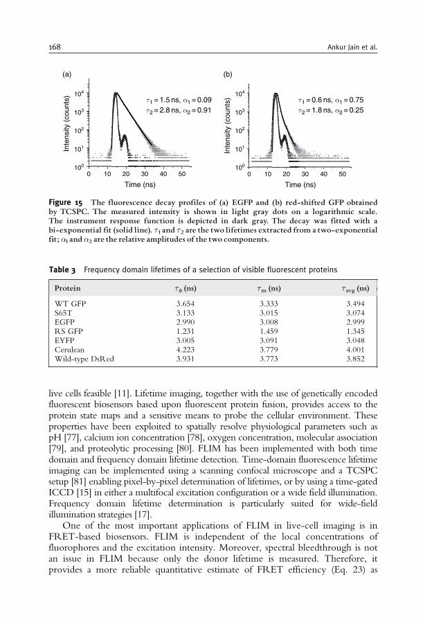
live cells feasible [11]. Lifetime imaging, together with the use of genetically encodedfluorescent biosensors based upon fluorescent protein fusion, provides access to theprotein state maps and a sensitive means to probe the cellular environment. Theseproperties have been exploited to spatially resolve physiological parameters such aspH [77], calcium ion concentration [78], oxygen concentration, molecular association[79], and proteolytic processing [80]. FLIM has been implemented with both timedomain and frequency domain lifetime detection. Time-domain fluorescence lifetimeimaging can be implemented using a scanning confocal microscope and a TCSPCsetup [81] enabling pixel-by-pixel determination of lifetimes, or by using a time-gatedICCD [15] in either a multifocal excitation configuration or a wide field illumination.Frequency domain lifetime determination is particularly suited for wide-fieldillumination strategies [17].
One of the most important applications of FLIM in live-cell imaging is inFRET-based biosensors. FLIM is independent of the local concentrations offluorophores and the excitation intensity. Moreover, spectral bleedthrough is notan issue in FLIM because only the donor lifetime is measured. Therefore, itprovides a more reliable quantitative estimate of FRET efficiency (Eq. 23) as
0 10 20 30 40 50100
101
102
103
104
Inte
nsity
(co
unts
)
Time (ns)
0 10 20 30 40 50
Time (ns)
τ1 = 1.5 ns, α1 = 0.09τ2 = 2.8 ns, α2 = 0.91
τ1 = 0.6 ns, α1 = 0.75τ2 = 1.8 ns, α2 = 0.25
(a)
100
101
102
103
104
Inte
nsity
(co
unts
)
(b)
Figure 15 The fluorescence decay profiles of (a) EGFP and (b) red-shifted GFP obtainedby TCSPC. The measured intensity is shown in light gray dots on a logarithmic scale.The instrument response function is depicted in dark gray. The decay was fitted with abi-exponential fit (solid line). 1 and 2 are the two lifetimes extracted from a two-exponentialfit; �1and �2 are the relative amplitudes of the two components.
Table 3 Frequency domain lifetimes of a selection of visible fluorescent proteins
Protein f (ns) m (ns) avg (ns)
WT GFP 3.654 3.333 3.494S65T 3.133 3.015 3.074EGFP 2.990 3.008 2.999RS GFP 1.231 1.459 1.345EYFP 3.005 3.091 3.048Cerulean 4.223 3.779 4.001Wild-type DsRed 3.931 3.773 3.852
168 Ankur Jain et al.
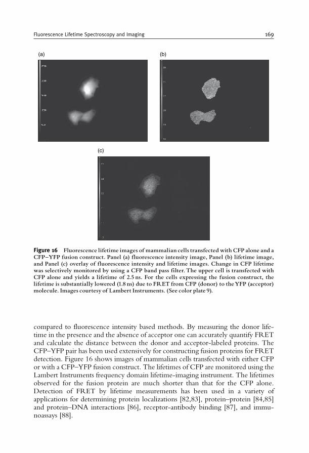
compared to fluorescence intensity based methods. By measuring the donor life-time in the presence and the absence of acceptor one can accurately quantify FRETand calculate the distance between the donor and acceptor-labeled proteins. TheCFP–YFP pair has been used extensively for constructing fusion proteins for FRETdetection. Figure 16 shows images of mammalian cells transfected with either CFPor with a CFP–YFP fusion construct. The lifetimes of CFP are monitored using theLambert Instruments frequency domain lifetime-imaging instrument. The lifetimesobserved for the fusion protein are much shorter than that for the CFP alone.Detection of FRET by lifetime measurements has been used in a variety ofapplications for determining protein localizations [82,83], protein–protein [84,85]and protein–DNA interactions [86], receptor-antibody binding [87], and immu-noassays [88].
(a) (b)
(c)
Figure 16 Fluorescence lifetime images of mammalian cells transfected with CFP alone and aCFP^YFP fusion construct. Panel (a) fluorescence intensity image, Panel (b) lifetime image,and Panel (c) overlay of fluorescence intensity and lifetime images. Change in CFP lifetimewas selectively monitored by using a CFP band pass filter. The upper cell is transfected withCFP alone and yields a lifetime of 2.5 ns. For the cells expressing the fusion construct, thelifetime is substantially lowered (1.8 ns) due to FRET from CFP (donor) to theYFP (acceptor)molecule. Images courtesy of Lambert Instruments. (See color plate 9).
Fluorescence Lifetime Spectroscopy and Imaging 169
5. CONCLUDING REMARKS
The discovery and development of fluorescent proteins as molecular tags inthe recent years has led to a revolution by allowing complex biochemical processesto be correlated with the functioning of proteins in living cells. The green fluor-escent protein from A. victoria and its various variants can be fused to virtually anyprotein of interest to analyze its spatial distribution, biochemical reactions, anddistribution in the biological systems. Lifetime spectroscopy and imaging of cellsexpressing fluorescent protein-tagged fusion constructs provides a non-invasivemeans to detect and quantify various biochemical processes in taking place in livecells and to probe the immediate nano-environment of the protein. Fluorescencelifetime of a species is independent of probe concentration and light path length:variables difficult to measure and control in live cells. Interactions, proteolyticprocessing, covalent modifications, and conformational changes can be followedin a live cell by detecting FRET between tagged proteins. Further, recent advanceslike the development and use of new fluorescent tools such as semiconductornanocrystals (quantum dots), multi-photon excitation, single molecule detectionand development of better fluorescent proteins have opened up newer dimensionsfor the application of fluorescence lifetime for studying biological systems.
REFERENCES
[1] J.R. Lakowicz, Principles of Fluorescence Spectroscopy, Second Edition, Kluwer Academic/PlenumPublishers, New York, 2002.
[2] A. Sharma and S.G. Schulman, Introduction to Fluorescence Spectroscopy, John Wiley and Sons,New York, 1999.
[3] M. Hof, V. Fidler and R. Hutterer, in Fluorescence Spectroscopy in Biology, Vol. 3 (ed. M. Hof,V. Fidler and R. Hutterer), Springer-Verlag, New York, 2005, pp. 1–29.
[4] A.P. Demchenko, in Topics in Fluorescence Spectroscopy: Biochemical Applications (ed. J.R. Lakowicz),Plenum, New York, 1991, pp. 65–112.
[5] A.P. Demchenko, Ultraviolet Spectroscopy of Proteins, Springer-Verlag, New York, 1981.[6] A. Saxena, J.B. Udgaonkar and G. Krishnamoorthy, in Fluorescence Spectroscopy in Biology, Vol. 3
(ed. M. Hof, V. Fidler and R. Hutterer), Springer-Verlag, New York, 2005, pp. 163–179.[7] M.R. Eftink, The use of fluorescence methods to monitor unfolding transitions in proteins,
Biophys. J., 1994, 66, 482–501.[8] R.Y. Tsien, The green fluorescent protein, Annu. Rev. Biochem., 1998, 67, 509–544.[9] M. Zimmer, Green fluorescent protein (GFP): application, structure and related photophysical
behavior, Chem. Rev., 2002, 102, 759–781.[10] A. Miyawaki, A. Sawano and T. Kogure, Lighting up cells: labelling proteins with fluorophores,
Nat. Cell Biol., 2003, 5, Suppl., S1–S7.[11] P.I.H. Bastiaens and A. Squire, Fluorescence lifetime imaging microscopy: spatial resolution of
biochemical processes in the cell, Trends Cell Biol., 1999, 9, 48–52.[12] J.R. Lakowicz, in Topics in Fluorescence Spectroscopy: Probe Design and Chemical Sensing (ed.
J.R. Lakowicz), Plenum, New York, 1991, pp. 1–20.[13] K. Suhling, P.M. French and D. Phillips, Time-resolved fluorescence microscopy, Photochem.
Photobiol. Sci., 2005, 4, 13–22[14] D.J.S. Birch and R.E. Imhof, in Topics in Fluorescence Spectroscopy: Techniques (ed. J.R. Lakowicz),
Plenum, New York, 1991, pp. 1–96.
170 Ankur Jain et al.
[15] H. Schneckenburger, M.H. Gschwend, R. Sailer, H.P. Mock and W.S. Strauss, Time-gatedfluorescence microscopy in cellular and molecular biology, Cell. Mol. Biol., 1998, 44,795–805.
[16] J.R. Lakowicz and I. Gryczynski, in Topics in Fluorescence Spectroscopy: Techniques (ed. J.R. Lakowicz),Plenum, New York, 1991, pp. 293–336.
[17] T.W.J. Gadella Jr, R.M. Clegg and T.M. Jovin, Fluorescence lifetime imaging microscopy:pixel-by-pixel analysis of phase-modulation data, Bioimaging, 1994, 2, 139–159.
[18] R.F. Steiner, in Topics in Fluorescence Spectroscopy: Principles (ed. J.R. Lakowicz), Plenum,New York, 1991, pp. 1–52.
[19] D.M. Jameson and S.E. Seifried, Quantification of protein-protein interactions using fluores-cence polarization, Methods, 1999, 19, 222–233.
[20] V. LeTilly and C.A. Royer, Fluorescence anisotropy assays implicate protein-protein interac-tions in regulating trp repressor DNA binding, Biochemistry, 1993, 32, 7753–7758.
[21] R.V. Weatherman and L.L. Kiessling, Fluorescence anisotropy assays reveal affinities of C- andO-glycosides for concanavalin A1, J. Org. Chem., 1996, 61, 534–538.
[22] D.M. Jameson and W.H. Sawyer, Fluorescence anisotropy applied to biomolecular interactions,Meth. Enzymol., 1995, 246, 283–300.
[23] J. Larsen, J. Andersson, T. Polıvka, J. Sly, M.J. Crossley, V. Sundstrom and E. Akesson, Energytransfer and conformational dynamics in Zn-porphyrin dendrimers, Chem. Phys. Lett., 2005,403, 205–210.
[24] Q.H. Xu, S. Wang, D. Korystov, A. Mikhailovsky, G.C. Bazan, D. Moses and A.J. Heeger, Thefluorescence resonance energy transfer (FRET) gate: a time-resolved study, Proc. Natl. Acad. Sci.U.S.A., 2005, 102, 530–535.
[25] M.S. Nasir and M.E. Jolley, Fluorescence polarization: an analytical tool for immunoassay anddrug discovery, Comb. Chem. High Throughput Screen, 1999, 2, 177–190.
[26] P. Wu and L. Brand, Resonance energy transfer: methods and applications, Anal. Biochem., 1994,218, 1–13.
[27] E.A. Jares-Erijman and T.M. Jovin, FRET imaging, Nat. Biotechnol., 2003, 21, 1387–1395.[28] A. Peyker, O. Rocks, and P.I. Bastiaens, Imaging activation of two Ras isoforms simultaneously
in a single cell, Chembiochem, 2005, 6, 78–85.[29] R.P. Haugland, J. Yguerabide and L. Stryer, Dependence of the kinetics of singlet-singlet energy
transfer on spectral overlap, Proc. Natl. Acad. Sci. U.S.A., 1969, 63, 23–30.[30] L. Stryer, Fluorescence energy transfer as a spectroscopic ruler, Annu. Rev. Biochem., 1978, 47,
819–846.[31] C.G. dos Remedios, M. Miki and J.A. Barden, Fluorescence resonance energy transfer mea-
surements of distances in actin and myosin. A critical evaluation, J. Muscle Res. Cell. Motil., 1987,8, 97–117.
[32] P.R. Selvin, The renaissance of fluorescence resonance energy transfer, Nat. Struct. Biol., 2000,7, 730–734.
[33] P.R. Selvin, Fluorescence resonance energy transfer, Meth. Enzymol., 1995, 246, 300–334.[34] C.G. dos Remedios and P.D. Moens, Fluorescence resonance energy transfer spectroscopy is a
reliable ‘‘ruler’’ for measuring structural changes in proteins. Dispelling the problem of theunknown orientation factor, J. Struct. Biol., 1995, 115, 175–185.
[35] C. Berney and G. Danuser, FRET or no FRET: a quantitative comparison, Biophys. J., 2003,84, 3992–4010.
[36] A. Periasamy, Fluorescence resonance energy transfer microscopy: a mini review, J. Biomed.Opt., 2001, 6, 287–291.
[37] R.E. Dale, J. Eisinger and W.E. Blumberg, The orientational freedom of molecular probes. Theorientation factor in intramolecular energy transfer, Biophys. J., 1979, 26, 161–193.
[38] J. Zhang, R.E. Campbell, A.Y. Ting and R.Y. Tsien, Creating new fluorescent probes for cellbiology, Nat. Rev. Mol. Cell Biol., 2002, 3, 906-918.
[39] O. Shimomura, F.H. Johnson and Y. Saiga, Extraction, purification and properties of aequorin, abioluminescent protein from the luminous hydromedusan Aequorea, J. Cell. Comp. Physiol.,1962, 59, 223–239.
[40] O. Shimomura, The discovery of aequorin and green fluorescent protein, J. Microsc., 2005, 217, 1–15.
Fluorescence Lifetime Spectroscopy and Imaging 171
[41] O. Shimomura, Structure of the chromophore of Aequorea green fluorescent protein, FEBSLett., 1979, 104, 220–222.
[42] D.C. Prasher, V.K. Eckenrode, W.W. Ward, F.G. Prendergast and M.J. Cormier, Primarystructure of the Aequorea victoria green-fluorescent protein, Gene, 1992, 111, 229–233.
[43] M. Chalfie, Y. Tu, G. Euskirchen, W.W.Ward and D.C. Prasher, Green fluorescent protein as amarker for gene expression, Science, 1994, 263, 802–805.
[44] S. Inouye and F.I. Tsuji, Aequorea green fluorescent protein: expression of the gene andfluorescence characteristics of the recombinant protein, FEBS Lett., 1994, 341, 277–280.
[45] G.H. Patterson, S.M. Knobel, W.D. Sharif, S.R. Kain and D.W. Piston, Use of the greenfluorescent protein and its mutants in quantitative fluorescence microscopy, Biophys. J., 1997,73, 2782–2790.
[46] W.W. Ward, in Green Fluorescent Protein: Properties, Applications, and Protocols, Second edition(ed. M. Chalfie and S.R. Kain), John Wiley & Sons, New York, 2005, pp. 39–65.
[47] M. Ormo, A.B. Cubitt, K. Kallio, L.A. Gross, R.Y. Tsien and S.J. Remington, Crystal structureof the Aequorea victoria green fluorescent protein, Science, 1996, 273, 1392–1395.
[48] F. Yang, L. Moss and G. Phillips, The molecular structure of green fluorescent protein,Nat. Biotechnol., 1996, 14, 1246–1251.
[49] B.G. Reid and G.C. Flynn, Chromophore formation in green fluorescent protein, Biochemistry,1997, 36, 6786–6791.
[50] R. Heim, D.C. Prasher and R.Y. Tsien, Wavelength mutations and posttranslational autoxida-tion of green fluorescent protein, Proc. Natl. Acad. Sci. U.S.A., 1994, 91, 12501–12504.
[51] A.B. Cubitt, R. Heim, S.R. Adams, A.E. Boyd, L.A. Gross and R.Y. Tsien, Understanding,improving and using green fluorescent proteins, Trends Biochem. Sci., 1995, 20, 448–455.
[52] J.A. Schmid and H. Neumeier, Evolutions in science triggered by green fluorescent protein(GFP), Chembiochem, 2005, 6, 1149–1156.
[53] J. Lippincott-Schwartz and G.H. Patterson, Development and use of fluorescent protein markersin living cells, Science, 2003, 300, 87–91.
[54] R. Heim, A.B. Cubitt and R.Y. Tsien, Improved green fluorescence,Nature, 1995, 373, 663–664.[55] P. van Roessel and A.H. Brand, Imaging into the future: visualizing gene expression and protein
interactions with fluorescent proteins, Nat. Cell Biol., 2002, 4, E15–E20.[56] M.A. Rizzo, G.H. Springer, B. Granada and D.W. Piston, An improved cyan fluorescent
protein variant useful for FRET, Nat. Biotechnol., 2004, 22, 445–449.[57] O. Griesbeck, G.S. Baird, R.E. Campbell, D.A. Zacharias and R.Y. Tsien, Reducing the
environmental sensitivity of yellow fluorescent protein, J. Biol. Chem., 2001, 276, 29188–29194.[58] M.V. Matz, A.F. Fradkov, Y.A. Labas, A.P. Savitsky, A.G. Zaraisky, M.L. Markelov and
S.A. Lukyanov, Fluorescent proteins from nonbioluminescent Anthozoa species, Nat. Biotech-nol., 1999, 17, 969–973.
[59] G.S. Baird, D.A. Zacharias and R.Y. Tsien, Biochemistry, mutagenesis, and oligomerizationof DsRed, a red fluorescent protein from coral, Proc. Natl. Acad. Sci. U.S.A., 2000, 97,11984–11989.
[60] A. Sacchetti, V. Subramaniam, T.M. Jovin and S. Alberti, Oligomerization of DsRed isrequired for the generation of a functional red fluorescent chromophore, FEBS Lett., 2002,525, 13–19.
[61] D. Yarbrough, R.M. Wachter, K. Kallio, M.V. Matz and S.J. Remington, Refined crystalstructure of DsRed, a red fluorescent protein from coral, at 2.0-A resolution, Proc. Natl. Acad.Sci. U.S.A., 2001, 98, 462–467.
[62] A.A. Heikal, S.T. Hess, G.S. Baird, R.Y. Tsien and W.W. Webb, Molecular spectroscopy anddynamics of intrinsically fluorescent proteins: coral red (dsRed) and yellow (Citrine), Proc. Natl.Acad. Sci. U.S.A., 2000, 97, 11996–12001.
[63] V.V. Verkhusha, D.M. Chudakov, N.G. Gurskaya, S. Lukyanov and K.A. Lukyanov, Commonpathway for the red chromophore formation in fluorescent proteins and chromoproteins, Chem.Biol., 2004, 11, 845–854.
[64] L.A. Gross, G.S. Baird, R.C. Hoffman, K.K. Baldridge and R.Y. Tsien, The structure of thechromophore within DsRed, a red fluorescent protein from coral, Proc. Natl. Acad. Sci. U.S.A.,2000, 97, 11990–11995.
172 Ankur Jain et al.
[65] M.A. Wall, M. Socolich and R. Ranganathan, The structural basis for red fluorescence in thetetrameric GFP homolog DsRed, Nat. Struct. Biol., 2000, 7, 1133–1138.
[66] B.J. Bevis and B.S. Glick, Rapidly maturing variants of the Discosoma red fluorescent protein(DsRed), Nat. Biotechnol., 2002, 20, 83–87.
[67] R.E. Campbell, O. Tour, A.E. Palmer, P.A. Steinbach, G.S. Baird, D.A. Zacharias and R.Y.Tsien, A monomeric red fluorescent protein, Proc. Natl. Acad. Sci. U.S.A., 2002, 99, 7877–7882.
[68] N.C. Shaner, R.E. Campbell, P.A. Steinbach, B.N. Giepmans, A.E. Palmer and R.Y. Tsien,Improved monomeric red, orange and yellow fluorescent proteins derived from Discosoma sp.red fluorescent protein, Nat. Biotechnol., 2004, 22, 1567–1572.
[69] D. Gerlich, J. Beaudouin, M. Gebhard, J. Ellenberg and R. Eils, Four-dimensional imaging andquantitative reconstruction to analyse complex spatiotemporal processes in live cells, Nat. CellBiol., 2001, 3, 852–855.
[70] D. Axelrod, D.E. Koppel, J. Schlessinger, E. Elson and W.W. Webb, Mobility measurement byanalysis of fluorescence photobleaching recovery kinetics, Biophys. J., 1976, 16, 1055–1069.
[71] R.D. Phair and T. Misteli, Kinetic modeling approaches to in vivo imaging, Nat. Rev. Mol. CellBiol., 2001, 2, 898–907.
[72] E.A. Reits and J.J. Neefjes, From fixed to FRAP: measuring protein mobility and activity inliving cells, Nat. Cell Biol., 2001, 3, E145–E147.
[73] J. Lippincott-Schwartz, E. Snapp and A. Kenworthy, Studying protein dynamics in living cells,Nat. Rev. Mol. Cell Biol., 2001, 2, 444–456.
[74] P. Schwille, Fluorescence correlation spectroscopy and its potential for intracellular applications,Cell. Biochem. Biophys., 2001, 34, 383–408.
[75] A. Volkmer, V. Subramaniam, D.J.S. Birch and T.M. Jovin, One- and two-photon excitedfluorescence lifetimes and anisotropy decays of green fluorescent proteins, Biophys. J., 2000, 78,1589–1598.
[76] E.C. van Munster and T.W.J. Gadella, Fluorescence lifetime imaging microscopy (FLIM),Adv. Biochem. Eng. Biotechnol., 2005, 95, 143–175.
[77] R. Sanders, A. Draaijer, H.C. Gerritsen, P.M. Houpt and Y.K. Levine, Quantitative pHimaging in cells using confocal fluorescence lifetime imaging microscopy, Anal. Biochem.,1995, 227, 302–308.
[78] J.R. Lakowicz, H. Szmacinski, K. Nowaczyk, W.J. Lederer, M.S. Kirby and M.L. Johnson,Fluorescence lifetime imaging of intracellular calcium in COS cells using Quin-2, Cell Calcium,1994, 15, 7–27.
[79] P.I.H. Bastiaens and T.M. Jovin, Microspectroscopic imaging tracks the intracellular processingof a signal transduction protein: fluorescent-labeled protein kinase CbI, Proc. Natl. Acad. Sci.U.S.A., 1996, 93, 8407–8412.
[80] T.W. Gadella Jr. and T.M. Jovin, Oligomerization of epidermal growth factor receptors onA431 cells studied by time-resolved fluorescence imaging microscopy. A stereochemical modelfor tyrosine kinase receptor activation, J. Cell Biol., 1995, 129, 1543–1558.
[81] W. Becker, A. Bergmann, M.A. Hink, K. Konig, K. Benndorf and C. Biskup, Fluorescencelifetime imaging by time-correlated single-photon counting, Microsc. Res. Tech., 2004, 63,58–66.
[82] J.W. Legg, C.A. Lewis, M. Parsons, T. Ng and C.M. Isacke, A novel PKC-regulatedmechanism controls CD44 ezrin association and directional cell motility, Nat. Cell Biol., 2002,4, 399–407.
[83] P.J. Verveer, F.S. Wouters, A.R. Reynolds and P.I. Bastiaens, Quantitative imaging oflateral ErbB1 receptor signal propagation in the plasma membrane, Science, 2000, 290,1567–1570.
[84] F. S. Wouters and P. I. Bastiaens, Fluorescence lifetime imaging of receptor tyrosine kinaseactivity in cells, Curr. Biol., 1999, 9, 1127–1130.
[85] A.G. Harpur, F.S. Wouters and P.I. Bastiaens, Imaging FRET between spectrally similar GFPmolecules in single cells, Nat. Biotechnol., 2001, 19, 167–169.
[86] F.G.E. Cremazy, E.M. Manders, P.I. Bastiaens, G. Kramer, G.L. Hager, E.B. van Munster, P.J.Verschure, T.W.J. Gadella Jr. and R. van Driel, Imaging in situ protein-DNA interactions in thecell nucleus using FRET–FLIM, Exp. Cell Res., 2005, 309, 390–396.
Fluorescence Lifetime Spectroscopy and Imaging 173

[87] T. Ng, M. Parsons, W.E. Hughes, J. Monypenny, D. Zicha, A. Gautreau, M. Arpin,S. Gschmeissner, P.J. Verveer, P.I. Bastiaens and P.J. Parker, Ezrin is a downstream effector oftrafficking PKC-integrin complexes involved in the control of cell motility, EMBO J., 2001, 20,2723–2741.
[88] W. Zwart, A. Griekspoor, C. Kuijl, M. Marsman, J. van Rheenen, H. Janssen, J. Calafat, M. vanHam, L. Janssen, M. van Lith, K. Jalink and J. Neefjes, Spatial separation of HLA-DM/HLA-DRinteractions within MIIC and phagosome-induced immune escape, Immunity, 2005, 22, 221–233.
174 Ankur Jain et al.
C H A P T E R 5
MONTE CARLO SIMULATIONS IN NUCLEAR
MEDICINE IMAGING
Steven Staelens and Irene Buvat
Contents
1. Introduction 1762. Nuclear Medicine Imaging 176
2.1. Single photon imaging 1772.2. Positron emission tomography 1782.3. Emission tomography in small animal imaging 179
2.4. Reconstruction 1793. The MC Method 180
3.1. Random numbers 1803.2. Sampling methods 181
3.3. Photon transport modeling 1823.4. Scoring 183
4. Relevance of Accurate MC Simulations in Nuclear Medicine 184
4.1. Studying detector design 1844.2. Analysing quantification issues 1844.3. Correction methods for image degradations 185
4.4. Detection tasks using MC simulations 1864.5. Applications in other domains 186
5. Available MC Simulators 187
6. Gate 1886.1. Basic features 1886.2. GATE: Time management 1926.3. GATE: Digitization 193
7. Efficiency-Accuracy Trade-Off 1947.1. Accuracy and validation 1947.2. Calculation time 194
8. Case Studies 1958.1. Case study I: TOF-PET 1958.2. Case study II: Assessment of PVE correction 196
8.3. Case study III: MC-based reconstruction 1979. Future Prospects 20010. Conclusion 200Acknowledgments 201
References 201
Advances in Biomedical Engineering � 2009 Elsevier B.V.
ISBN 978-0-444-53075-2 All rights reserved.
175
Abstract
The purpose of this chapter is to serve as an educational review regarding Monte Carlo (MC)simulations in Nuclear Medicine imaging complementary to reviews in specific scientificjournals. After the basics of Nuclear Medicine are briefly described, the principles of MCsimulations for modeling particle transport are presented. The major fields of applications of
MC simulations in Nuclear Medicine imaging are discussed. To better illustrate the principlesof a Monte Carlo simulator in Nuclear Medicine imaging, a recent but widely used simulationtool, GATE, is taken as an example. Finally, three case studies are presented as current
applications representative of the use of MC simulations in Nuclear Medicine imaging.
Keywords: Monte Carlo, simulation, emission tomography, SPECT, PET, tomographicreconstruction, GATE
1. INTRODUCTION
Monte Carlo (MC) simulations are a modeling tool that is increasingly used inNuclear Medicine imaging, namely in Single Photon Emission Computed Tomo-graphy (SPECT) and in Positron Emission Tomography (PET), mostly for theoptimization of detector design and of acquisition and processing protocols, andalso as part of the image formation process itself. In this chapter, we first recall thebasics of Nuclear Medicine imaging to set the context. We then present the generalprinciples of MC simulations when applied to modeling particle transport, and weexplain why accurate MC modeling is of foremost importance for various applica-tions in emission tomography. After briefly presenting the state-of-the-art regard-ing MC simulation tools appropriate for emission tomography modeling, we focuson a recent and widely used tool, GATE, to illustrate the major components of asimulator dedicated to SPECT and PET modeling, and to explain the way thesimulation of a SPECT or PET acquisition can be designed. Lastly, three typicalexamples representative of the current use of MC simulations in emission tomo-graphy are presented. Future prospects regarding MC simulations in the field ofNuclear Medicine imaging are briefly discussed.
2. NUCLEAR MEDICINE IMAGING
Nuclear medicine imaging involves the use of radioactively labeled pharma-ceuticals to diagnose and assess disease in the human body. The radiopharmaceu-tical is intravenously injected, inhaled or ingested: the choice of pharmaceuticaland route of administration depends on the disease under investigation. Position-sensitive detectors are used to detect the radiation emitted from the pharmaceutical,and so, in principle, both the temporal and spatial distribution of the pharmaceuticalwithin the body can be determined. Historically, Nuclear Medicine imaging wasthe first modality for functional imaging, i.e., giving information regarding the wayorgans work, as opposed to anatomical imaging, giving information regarding the
176 Steven Staelens and Irene Buvat
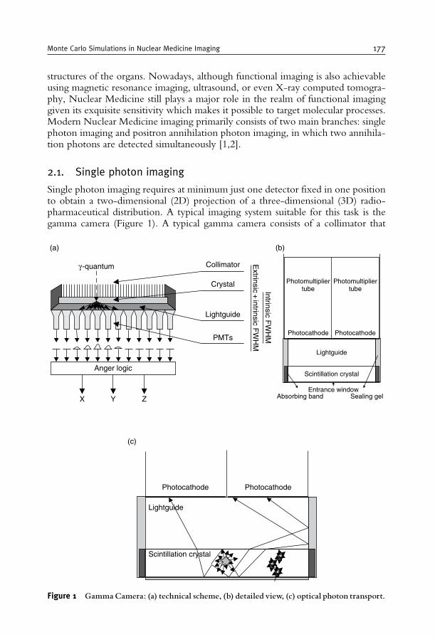
structures of the organs. Nowadays, although functional imaging is also achievableusing magnetic resonance imaging, ultrasound, or even X-ray computed tomogra-phy, Nuclear Medicine still plays a major role in the realm of functional imaginggiven its exquisite sensitivity which makes it possible to target molecular processes.Modern Nuclear Medicine imaging primarily consists of two main branches: singlephoton imaging and positron annihilation photon imaging, in which two annihila-tion photons are detected simultaneously [1,2].
2.1. Single photon imaging
Single photon imaging requires at minimum just one detector fixed in one positionto obtain a two-dimensional (2D) projection of a three-dimensional (3D) radio-pharmaceutical distribution. A typical imaging system suitable for this task is thegamma camera (Figure 1). A typical gamma camera consists of a collimator that
Anger logic
X Y Z
γ -quantum Collimator
Crystal
(a) (b)
Lightguide
PMTs
Extrinsic
+ intrinsic F
WH
M
I ntrinsic FW
HM
Scintillation crystal
Lightguide
Photocathode Photocathode
Photomultipliertube
Photomultipliertube
Absorbing band Sealing gelEntrance window
Scintillation crystal
Lightguide
Photocathode
(c)
Photocathode
Figure 1 GammaCamera: (a) technical scheme, (b) detailed view, (c) optical photon transport.
Monte Carlo Simulations in Nuclear Medicine Imaging 177
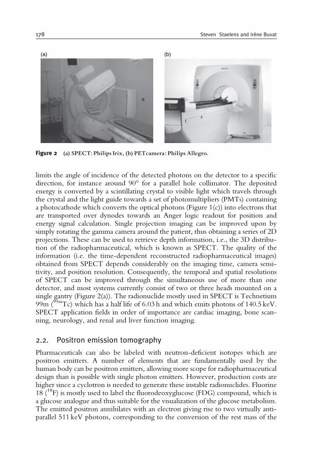
limits the angle of incidence of the detected photons on the detector to a specificdirection, for instance around 90� for a parallel hole collimator. The depositedenergy is converted by a scintillating crystal to visible light which travels throughthe crystal and the light guide towards a set of photomultipliers (PMTs) containinga photocathode which converts the optical photons (Figure 1(c)) into electrons thatare transported over dynodes towards an Anger logic readout for position andenergy signal calculation. Single projection imaging can be improved upon bysimply rotating the gamma camera around the patient, thus obtaining a series of 2Dprojections. These can be used to retrieve depth information, i.e., the 3D distribu-tion of the radiopharmaceutical, which is known as SPECT. The quality of theinformation (i.e. the time-dependent reconstructed radiopharmaceutical images)obtained from SPECT depends considerably on the imaging time, camera sensi-tivity, and position resolution. Consequently, the temporal and spatial resolutionsof SPECT can be improved through the simultaneous use of more than onedetector, and most systems currently consist of two or three heads mounted on asingle gantry (Figure 2(a)). The radionuclide mostly used in SPECT is Technetium99m (99mTc) which has a half life of 6.03 h and which emits photons of 140.5 keV.SPECT application fields in order of importance are cardiac imaging, bone scan-ning, neurology, and renal and liver function imaging.
2.2. Positron emission tomography
Pharmaceuticals can also be labeled with neutron-deficient isotopes which arepositron emitters. A number of elements that are fundamentally used by thehuman body can be positron emitters, allowing more scope for radiopharmaceuticaldesign than is possible with single photon emitters. However, production costs arehigher since a cyclotron is needed to generate these instable radionuclides. Fluorine18 (18F) is mostly used to label the fluorodeoxyglucose (FDG) compound, which isa glucose analogue and thus suitable for the visualization of the glucose metabolism.The emitted positron annihilates with an electron giving rise to two virtually anti-parallel 511 keV photons, corresponding to the conversion of the rest mass of the
(a) (b)
Figure 2 (a) SPECT: Philips Irix, (b) PETcamera: Philips Allegro.
178 Steven Staelens and Irene Buvat
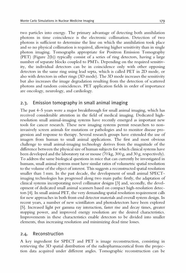
two particles into energy. The primary advantage of detecting both annihilationphotons in time coincidence is the electronic collimation. Detection of twophotons is sufficient to determine the line on which the annihilation took placeand so no physical collimation is required, allowing higher sensitivity than in singlephoton imaging. Tomographs appropriate for Positron Emission Tomography(PET) (Figure 2(b)) typically consist of a series of ring detectors, having a largenumber of separate blocks coupled to PMTs. Depending on the required sensitiv-ity, the individual detectors can be in coincidence only with other opposingdetectors in the same ring using lead septa, which is called PET in 2D mode, oralso with detectors in other rings (3D mode). The 3D mode increases the sensitivitybut also increases the image degradation resulting from the detection of scatteredphotons and random coincidences. PET application fields in order of importanceare oncology, neurology, and cardiology.
2.3. Emission tomography in small animal imaging
The past 4–5 years were a major breakthrough for small animal imaging, which hasreceived considerable attention in the field of medical imaging. Dedicated high-resolution small animal-imaging systems have recently emerged as important newtools for cancer research. These new imaging systems permit researchers to non-invasively screen animals for mutations or pathologies and to monitor disease pro-gression and response to therapy. Several research groups have extended the use ofimagers from human to small animal applications. The first and most obviouschallenge to small animal-imaging technology derives from the magnitude of thedifference between the physical size of human subjects for which clinical systems havebeen developed and the laboratory rat or mouse (70 kg, 300 g, and 30 g, respectively).To address the same biological questions in mice that can currently be investigated inhumans, small animal systems must have similar ratios of volumetric spatial resolutionto the volume of the object of interest. This suggests a reconstructed spatial resolutionsmaller than 1mm. In the past decade, the development of small animal SPECT-imaging technologies has progressed along two main paths: firstly, the adaptation ofclinical systems incorporating novel collimator designs [3] and, secondly, the devel-opment of dedicated small animal scanners based on compact high-resolution detec-tors [4]. In small animal PET, the very demanding spatial resolution requirement callsfor new approaches in both front-end detector materials and overall system design. Inrecent years, a number of new scintillators and photodetectors have been explored[5]. Increased light per gamma ray interaction, faster rise and decay times, greaterstopping power, and improved energy resolution are the desired characteristics.Improvements in these characteristics enable detectors to be divided into smallerelements, thus increasing resolution and minimizing dead time losses.
2.4. Reconstruction
A key ingredient for SPECT and PET is image reconstruction, consisting inretrieving the 3D spatial distribution of the radiopharmaceutical from the projec-tion data acquired under different angles. Tomographic reconstruction can be
Monte Carlo Simulations in Nuclear Medicine Imaging 179
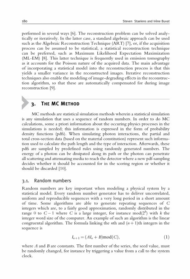
performed in several ways [6]. The reconstruction problem can be solved analy-tically or iteratively. In the latter case, a standard algebraic approach can be usedsuch as the Algebraic Reconstruction Technique (ART) [7], or, if the acquisitionprocess can be assumed to be statistical, a statistical reconstruction techniquecan be preferred, such as Maximum Likelihood Expectation Maximization(ML-EM) [8]. This latter technique is frequently used in emission tomographyas it accounts for the Poisson nature of the acquired data. The main advantageof incorporating a statistical model into the reconstruction process is that thisyields a smaller variance in the reconstructed images. Iterative reconstructiontechniques also enable the modeling of image-degrading effects in the reconstruc-tion algorithm, so that these are automatically compensated for during imagereconstruction [9].
3. THE MC METHOD
MCmethods are statistical simulation methods wherein a statistical simulationis any simulation that uses a sequence of random numbers. In order to do MCcalculations, some a priori information about the occuring physics processes in thesimulations is needed; this information is expressed in the form of probabilitydensity functions (pdfs). When simulating photon interactions, the partial andtotal cross-section data (based on the material constitution) represent such informa-tion used to calculate the path length and the type of interaction. Afterwards, thesepdfs are sampled by predefined rules using randomly generated numbers. Theenergy of a photon can be dissipated along its path or the photon can penetrateall scattering and attenuating media to reach the detector where a new pdf-samplingdecides whether it should be accounted for in the scoring region or whether itshould be discarded [10].
3.1. Random numbers
Random numbers are key important when modeling a physical system by astatistical model. Every random number generator has to deliver uncorrelated,uniform and reproducible sequences with a very long period in a short amountof time. Some algorithms are able to generate repeating sequences of Cintegers which are, to a fairly good approximation, randomly distributed in therange 0 to C� 1 where C is a large integer, for instance mod(2k) with k theinteger word size of the computer. An example of such an algorithm is the linearcongruental algorithm. The formula linking the nth and (nþ 1)th integers in thesequence is
Inþ1= ðAIn þ BÞmodðCÞ; ð1Þwhere A and B are constants. The first number of the series, the seed value, mustbe randomly changed, for instance by triggering a value from a call to the systemclock.
180 Steven Staelens and Irene Buvat

3.2. Sampling methods
To obtain a stochastic variable that follows a particular pdf, f(x), three differentsampling methods can be used.
3.2.1. The distribution function methodA cumulative distribution function F(x)=P(X� x) is constructed from the integralof f(x) over the interval [a, x] according to
FðxÞ=Z x
a
f ðx0Þdx0: ð2Þ
The variable x is then sampled by replacing F(x) in Eq. (2) with a uniformlydistributed random number in the range of [0, 1] and solving for x. This samplingmethod is used if the inverse of F(x) can be easily calculated.
3.2.2. The rejection methodPossibly there can arise some mathematical difficulties in calculating the inverse ofthe cumulative distribution function F. In such case, the rejection method can offera solution. Let f(x) be defined in the range [a, b] and let r(x) be the rejectionfunction 8 x 2 [a, b]) 0< r(x)� 1. Here r(x) is given as f *(x), being the pdf afternormalization to unity. Then, a uniform distributed value of x within the range[a, b] can be sampled from the relation
x= aþ R1ðb� aÞ; ð3Þwhere R1 is a random number in [0, 1]. A second random number R2 in [0, 1] isthen drawn to decide whether the sampled x should be accepted by checkingwhether
R2 < rðxÞ= f ðxÞ: ð4ÞIf this relation is fulfilled, then x is accepted as a properly distributed stochasticvalue, otherwise x needs to be resampled.
3.2.3. Mixed methodsWhen the previous two methods are not applicable, a mixture of the two methodsabove is used. The f(x) is written as the product of two probability distributionfunctions m(x).r(x) with r(x) acting as the rejection function defined in the previoussection. One determines an x value using the distribution function method on m(x)and applies the rejection method with that x to r(x) [11].
3.2.4. Non-analog samplingAn MC simulation involving the exact pdfs may be impractical from a computa-tional point of view, requiring unrealistic computation time to achieve reliable
Monte Carlo Simulations in Nuclear Medicine Imaging 181
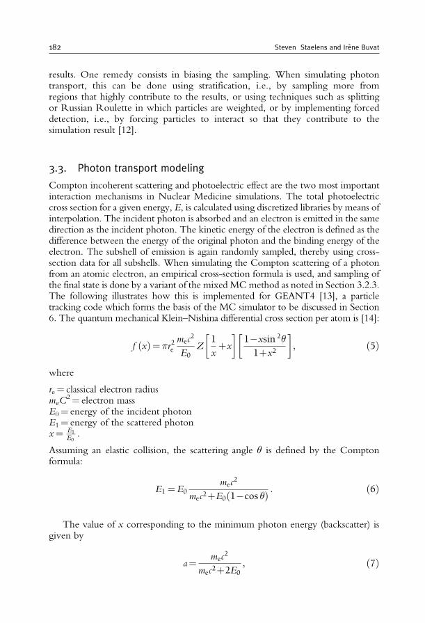
results. One remedy consists in biasing the sampling. When simulating photontransport, this can be done using stratification, i.e., by sampling more fromregions that highly contribute to the results, or using techniques such as splittingor Russian Roulette in which particles are weighted, or by implementing forceddetection, i.e., by forcing particles to interact so that they contribute to thesimulation result [12].
3.3. Photon transport modeling
Compton incoherent scattering and photoelectric effect are the two most importantinteraction mechanisms in Nuclear Medicine simulations. The total photoelectriccross section for a given energy, E, is calculated using discretized libraries by means ofinterpolation. The incident photon is absorbed and an electron is emitted in the samedirection as the incident photon. The kinetic energy of the electron is defined as thedifference between the energy of the original photon and the binding energy of theelectron. The subshell of emission is again randomly sampled, thereby using cross-section data for all subshells. When simulating the Compton scattering of a photonfrom an atomic electron, an empirical cross-section formula is used, and sampling ofthe final state is done by a variant of the mixed MCmethod as noted in Section 3.2.3.The following illustrates how this is implemented for GEANT4 [13], a particletracking code which forms the basis of the MC simulator to be discussed in Section6. The quantum mechanical Klein–Nishina differential cross section per atom is [14]:
f ðxÞ=�r2emec
2
E0Z
1
xþx
� �1�xsin 2�
1þx2
� �; ð5Þ
where
re= classical electron radiusmeC
2= electron massE0= energy of the incident photonE1= energy of the scattered photonx= E1
E0:
Assuming an elastic collision, the scattering angle � is defined by the Comptonformula:
E1 =E0mec
2
mec2þE0 1�cos �ð Þ : ð6Þ
The value of x corresponding to the minimum photon energy (backscatter) isgiven by
a=mec
2
mec2þ2E0; ð7Þ
182 Steven Staelens and Irene Buvat

hence x 2 [a, 1]. One may state that
f xð Þ» 1
xþx
� �1�xsin 2�
1þx2
� �=m xð Þ � r xð Þ= �1m1 xð Þþ�2m2 xð Þ½ � � r xð Þ; ð8Þ
where
�1 = lnð1aÞ
m1ðxÞ= 1
�1x
�2 =ð1�a2Þ
2
m2ðxÞ= x
�2:
ð9Þ
m1 and m2 are probability density functions defined on the interval [a, 1], and r(x) isset to
rðxÞ= 1�xsin 2�
1þx2
� �; ð10Þ
being the rejection function 8 x 2 [a, 1]) 0< r(x)� 1. Given a set of threerandom numbers R0,R1,R2 uniformly distributed on the interval [0, 1], the sam-pling procedure for x is the following:
(1) decide whether to sample from m1(x) or m2(x): if R1 <�1
ð�1þ�2Þ select m1(x)otherwise select m2(x),
(2) sample x from the distributions to m1 or m2:
for m1: x= aR1
for m2: x2= a2þ (1� a2)R1,
(3) calculate sin2 �= t(t� 1) where t � ð1�cos �Þ= mec2ð1�xÞE0x
,(4) test the rejection function: if r(x)�R2 accept x, otherwise go to (1).
The polar angle � is deduced from the sampled x value and in the azimuthaldirection the angular distributions of both the scattered photon and the recoilelectron are considered to be isotropic [13,14].
3.4. Scoring
A selection of relevant physical quantities such as energy, detection location andphoton interactions must be accumulated into tallies or scores. Also, an estimate ofthe statistical error as a function of the number of trials (and other quantities) mustbe determined.
Monte Carlo Simulations in Nuclear Medicine Imaging 183
4. RELEVANCE OF ACCURATE MC SIMULATIONS IN NUCLEAR
MEDICINE
MC modeling is the only possible approach for all applications where mea-surements are not feasible or where analytic models are not available due to thecomplex nature of the problem [11,15]. In addition, such modeling is a practicalapproach in nuclear medical imaging in four important application fields [10,16],presented hereafter.
4.1. Studying detector design
MC methods can assist in the development of new collimator and detector designs,evaluation of new electronics, aso. MC simulations have been extensively used toanalyze the performance of new long bore parallel collimators as well as rotating slitcollimators [17], fan beam [18], cone beam and pinhole collimators [19]. For thelatter, simulations have been performed with various aperture span angles, differenthole sizes and various materials to evaluate the penetration [20]. MC methods alsoplay an important role in new system design, for instance in the research field ofsolid-state detectors with improved energy resolution and low-noise electronics[21–23]. Similarly, in the field of PET, MC techniques have been used to study theperformance of interplane septa with varying constitution, thickness and geometry,to compare single to true coincidence event ratios in single-slice, multi-slice andopen collimator 3D configurations and to assess the effect of collimation on scatterfraction (e.g., [24–26]). MC simulations of detector responses and efficiencies are ofkey importance since the scintillation crystal is the critical component in emissiontomography [27]. Simulations also prove their usefulness in Time-of-Flight PET(TOF) design since they can be used to test several detector crystals and to simulatethe influence of timing resolution on variance reduction (e.g., [28–30]). MCmethods can also assist in the design of new detectors with depth-of-interaction(DOI) information by simulating multilayer crystals and by estimating the gain inreconstructed resolution through incorporation of DOI information [31,32].
4.2. Analysing quantification issues
The presence of the scatter, attenuation and partial volume effects in NuclearMedicine images limits the accuracy of activity estimates (i.e., what is calledquantification). Each of these degradations has a particular impact [33–35]. Scatterdoes not produce major artefacts comparable to those caused by attenuation butreduces contrast by introducing a low-frequency blur in the image. Moreover, theimpact of scatter and attenuation generally depends on the photon energy, cameraenergy resolution and energy window settings, as well as the object size and shape,detector geometry and the source distribution. Many of these parameters are non-stationary which implies a potential difficulty when developing proper scatter andattenuation correction techniques. MC calculations have been found to be power-ful tools for an in depth analysis since the user has the ability to separate the detected
184 Steven Staelens and Irene Buvat
photons according to their interaction history: primary (i.e., unscattered) events,scattered events, contribution of downscattered events, scatter in patient or detec-tor, etc. [36]. MC modeling thus enables a detailed investigation of the spatial andenergy distribution of Compton scatter: energy spectra, point-spread functions andscatter fractions can be simulated [37]. This is impossible to perform using presentexperimental techniques, even with very good energy resolution detectors.Another important application field for MC simulations in quantification is resolu-tion recovery. For instance in SPECT, distance dependent collimator response canbe subdivided into a geometric component, collimator scatter and septal penetra-tion. MC simulations can be used to determine the relative contribution of each ofthese components in specific imaging configurations [38].
In PET, the penetration of annihilation photons into the detector materialbefore interaction is a statistical process which leads to significant displacementand anisotropy of the point spread function [39,40]. Compensation for crystalpenetration is thus one of the most important issue in order to recover the spatialresolution in PET. Theoretical models for that anisotrope spatial resolution canonly be verified by MC simulations since those DOI-dependent experiments arevery hard to perform with current devices.
Finally, MC analysis has been proven useful in evaluating motion artefacts. If thesimulator is capable of using explicit timing information to synchronize decay withdetector and patient movement then degradations such as cardiac or respiratorymotions can be studied [41].
4.3. Correction methods for image degradations
The image-degrading factors (as described in the previous section) can have a largeimpact on quantitative accuracy and on clinical diagnosis and ideally all have to becorrected for to achieve optimal clinical imaging. Traditionally, this was done bypreprocessing the projection data or by postprocessing the reconstructed images.MC-simulated datasets are often used to evaluate the accuracy of these correctionmethods. For such evaluation studies, the simulated datasets must have the appro-priate statistical properties and include all detector specific imperfections. Forinstance, when evaluating a scatter correction method, MC simulations can be usedto generate scatter-free projections. Images reconstructed from scatter-free projec-tions constitute the gold standard for any scatter correction method. Nowadays, MCsimulations often form the basis of the aforementioned correction techniques sinceiterative reconstruction algorithms are able to correct for image degradations bysimulating the effect during the reconstruction. The simulations can be based onMC methods or on a combination of MC and analytical methods. These SPECTsimulators face a considerable challenge; they have to balance accuracy againstefficiency. A large variety of simulators have been proposed [42–46]. Other groupsachieve similar goals by simulating and store the system matrix [47,48]. Reconstruc-tion methods based on MC simulators have been shown to improve contrast-to-noise [49–51] and lesion detectability [52–54]. Finally, MC-generated datasets arealso used in evaluation or comparison of different reconstruction schemes, forinstance to evaluate the robustness of an algorithm to parameter variations.
Monte Carlo Simulations in Nuclear Medicine Imaging 185
4.4. Detection tasks using MC simulations
Receiver Operating Characteristic (ROC) analysis is considered as the most reliablemethod for evaluating the diagnostic ability of medical imaging techniques. Itprovides a measure of the diagnostic performance of an imaging modality byplotting the sensitivity versus the specificity for a wide and continuous range ofdecision criteria. These studies require many images (typically hundreds) so thatstatistical analysis of the detection performance can be performed. Observer studiesbased on MC-based projection data can answer a large range of problems from thesimple comparison between analytical and statistical reconstruction [55] to complexstudies on the benefits of anatomical a priori information in the reconstruction [56].Using MC simulations to generate the datasets is therefore only feasible if efficientcodes are available. Also, sharing these datasets encourages and facilitates evaluationstudies. In addition, evaluating data-processing tools developed by different groupsworldwide using the same datasets removes the evaluation biases introduced by theuse of different data. Therefore, some efforts have recently been accomplished topropose publicly available databases of MC-simulated data dedicated to evaluationstudies [57,58].
4.5. Applications in other domains
In the Nuclear Medicine field, MC simulations are also widely used in dosimetryand radiotherapy research. One application is the individual treatment planning inradionuclide or radioimmunotherapy [59] where prospective dose estimates aremade in the latter by using a tracer activity of a radiolabeled antibody to obtainbiodistribution information prior to administration of a large therapeutic activity(e.g., [60]). The MC simulations return the dose distribution calculated from thequantitative images of the tracer distribution. The clinical applicability of individualtreatment planning algorithms will depend on the time required to generate thoseabsorbed dose estimates for each individual.
MC simulations are also used for the evaluation of external beam radiotherapysetups [61]. A complete simulation model of the accelerator head, includingscatter foil or X-ray target and flattening filter, multileaf collimator, supportplates, and so on, is necessary for this purpose. In that context, hybrid devicessuch as SPECT/CT and PET/CT might allow for a better delineation of thePlanned Target Volume (PTV) on CT using the functional information providedby the registered SPECT or PET images, thus fundamentally increasing theaccuracy. Precise MC simulations should be used in the virtual treatment-plan-ning system to maintain the most precise dose estimates [62] to further improvethe treatment plan.
Another field of interest is to perform a MC-based dosimetry for brachytherapyapplications [63] to provide detailed descriptions of local doses. Hadrontherapy isalso a MC-assisted research area [64] where simulations can reproduce the beam-induced �þ emissions of the irradiated target nuclei along the beam path, toassist the design of in-beam PET systems with high sensitivity and high spatialresolution.
186 Steven Staelens and Irene Buvat

5. AVAILABLE MC SIMULATORS
Some MC simulation codes dedicated to the simulation of SPECT and PEThave been developed, such as SimSET [65] enabling SPECT and PET modeling,SIMIND [66] and SimSPECT [67] for SPECT, PETSIM [68], Eidolon [69] andSORTEO [70] for PET.
Such dedicated packages are very powerful for their specific design goal but areoften not detailed and flexible enough to enable realistic simulations of emissiontomography detector geometries. Moreover, most of them do not account for timeexplicitly, which limits their use for modeling time-dependent processes such as decay,tracer kinetics, patient and bed motion, dead time or detector orbits. To ensure highflexibility in simulation design, general purpose nuclear physics codes such as EGS4[71], GEANT4 [13,72], or MCNP [73] have also been used for SPECT and PETsimulations. The main advantages of these general purpose codes are that they arewidely used and extensively tested, they can be regarded as long-term existent as wellas supported, and they are continuously evolving and therefore use the best of currenthardware and software capabilities. There are fewer limitations on their possibleapplications than for dedicated codes, and fewer simplifying assumptions are made.For example, the processes taking place in the collimator can be thoroughly simulatedwhereas dedicated codes often use a parametric model. Also, time-dependent processescan be simulated and their non-specific design makes them appropriate to implementnon-conventional SPECT and PET cameras [16]. In the end of the 1990s, 14 codeswere used for MC simulations in SPECT and PET, among which 10 were not used byanother group than those who developed the code, and 4 were publicly released oravailable from the authors. In the early 2000, 15 codes were used among which 8 werehome-made and 7 were publicly released or available from authors [74]. This suggeststhat up to recently, there was no code that was considered as a standard for MCsimulations in emission tomography. Based on this observation, a new code, GATE[75–77], has recently been designed as an upper layer of the GEANT4 nuclear physicscode [13,72] tuned for simulating SPECT and PET acquisitions. GATE thus takesadvantage of all GEANT4 features, including well-validated physics models, basicevent-timing information, geometry modeling and visualization tools. It is written inan object-oriented language that ensures high modularity. In addition, GATE uses ascripting language making it easy for the user to design a SPECT or PET simulation.GATE has been developed as a collaboration effort of about 10 laboratories worldwide(the OpenGATE collaboration), and was publicly released in May 2004. It is nowshared by a large research community, while long-term support and maintenance is stillensured by the OpenGATE collaboration. During 2006, already more than 650individuals had subscribed to the GATE community and at the 2005 IEEE MedicalImaging Conference (the most relevant conference in this domain), GATE and/orGEANT4 were used as tool of excellence in 33% of all papers involving MCsimulations while this number was 13% for SimSET and 7% for SIMIND, respectively[74]. It is therefore expected that GATE will become the code most frequently usedfor SPECT and PET simulations. Given this explicit tendency, we will describe GATEhereafter as an example of a simulation platform.
Monte Carlo Simulations in Nuclear Medicine Imaging 187
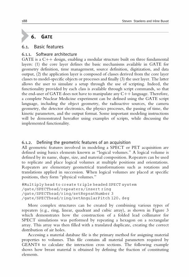
6. GATE
6.1. Basic features
6.1.1. Software architectureGATE is a Cþþ design, enabling a modular structure built on three fundamentallayers: (1) the core layer defines the basic mechanisms available in GATE forgeometry definition, time management, source definition, digitization, and dataoutput, (2) the application layer is composed of classes derived from the core layerclasses to model-specific objects or processes and finally (3) the user layer. The latterallows the user to simulate a setup through the use of scripting. Indeed, thefunctionality provided by each class is available through script commands, so thatthe end-user of GATE does not have to manipulate any Cþþ language. Therefore,a complete Nuclear Medicine experiment can be defined using the GATE scriptlanguage, including the object geometry, the radioactive sources, the camerageometry, the detector electronics, the physics processes, the passing of time, thekinetic parameters, and the output format. Some important modeling instructionswill be demonstrated hereafter using examples of scripts, while discussing theimplemented functionality.
6.1.2. Defining the geometric features of an acquisitionAll geometric features involved in modeling a SPECT or PET acquisition aredefined using basics elements known as ‘‘logical volumes.’’ A logical volume isdefined by its name, shape, size, and material composition. Repeaters can be usedto replicate and place logical volumes at multiple positions and orientations.Repeaters are elementary geometrical transformations such as rotations andtranslations applied in succession. When logical volumes are placed at specificpositions, they form ‘‘physical volumes.’’
#Multiply head to create triple headed SPECT system/gate/SPECThead/repeaters/insert ring/gate/SPECThead/ring/setRepeatNumber 3/gate/SPECThead/ring/setAngularPitch 120. deg
More complex structures can be created by combining various types ofrepeaters (e.g., ring, linear, quadrant and cubic array), as shown in Figure 3which demonstrates how the construction of a folded lead collimator forSPECT simulations was performed by repeating a hexagon on a rectangulararray. This array was then filled with a translated duplicate, creating the correctdistribution of air holes.
Accessing a material database file is the primary method for assigning materialproperties to volumes. This file contains all material parameters required byGEANT4 to calculate the interaction cross sections. The following exampleshows how breast material is obtained by defining the fraction of constitutingelements.
188 Steven Staelens and Irene Buvat
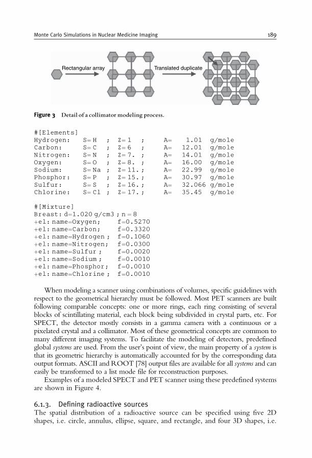
#[Elements]Hydrogen: S= H ; Z= 1 ; A= 1.01 g/moleCarbon: S= C ; Z= 6 ; A= 12.01 g/moleNitrogen: S= N ; Z= 7. ; A= 14.01 g/moleOxygen: S= O ; Z= 8. ; A= 16.00 g/moleSodium: S= Na ; Z= 11.; A= 22.99 g/molePhosphor: S= P ; Z= 15.; A= 30.97 g/moleSulfur: S= S ; Z= 16.; A= 32.066 g/moleChlorine: S= Cl ; Z= 17.; A= 35.45 g/mole
#[Mixture]Breast: d=1.020 g/cm3 ; n = 8þel: name=Oxygen; f=0.5270þel: name=Carbon; f=0.3320þel: name=Hydrogen ; f=0.1060þel: name=Nitrogen; f=0.0300þel: name=Sulfur ; f=0.0020þel: name=Sodium ; f=0.0010þel: name=Phosphor; f=0.0010þel: name=Chlorine ; f=0.0010
When modeling a scanner using combinations of volumes, specific guidelines withrespect to the geometrical hierarchy must be followed. Most PET scanners are builtfollowing comparable concepts: one or more rings, each ring consisting of severalblocks of scintillating material, each block being subdivided in crystal parts, etc. ForSPECT, the detector mostly consists in a gamma camera with a continuous or apixelated crystal and a collimator. Most of these geometrical concepts are common tomany different imaging systems. To facilitate the modeling of detectors, predefinedglobal systems are used. From the user’s point of view, the main property of a system isthat its geometric hierarchy is automatically accounted for by the corresponding dataoutput formats. ASCII and ROOT [78] output files are available for all systems and caneasily be transformed to a list mode file for reconstruction purposes.
Examples of a modeled SPECT and PET scanner using these predefined systemsare shown in Figure 4.
6.1.3. Defining radioactive sourcesThe spatial distribution of a radioactive source can be specified using five 2Dshapes, i.e. circle, annulus, ellipse, square, and rectangle, and four 3D shapes, i.e.
Rectangular array Translated duplicate
Figure 3 Detail of a collimator modeling process.
Monte Carlo Simulations in Nuclear Medicine Imaging 189
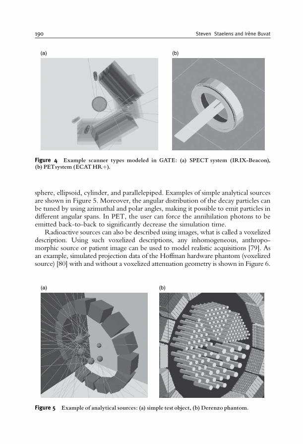
sphere, ellipsoid, cylinder, and parallelepiped. Examples of simple analytical sourcesare shown in Figure 5. Moreover, the angular distribution of the decay particles canbe tuned by using azimuthal and polar angles, making it possible to emit particles indifferent angular spans. In PET, the user can force the annihilation photons to beemitted back-to-back to significantly decrease the simulation time.
Radioactive sources can also be described using images, what is called a voxelizeddescription. Using such voxelized descriptions, any inhomogeneous, anthropo-morphic source or patient image can be used to model realistic acquisitions [79]. Asan example, simulated projection data of the Hoffman hardware phantom (voxelizedsource) [80] with and without a voxelized attenuation geometry is shown in Figure 6.
(a) (b)
Figure 4 Example scanner types modeled in GATE: (a) SPECT system (IRIX-Beacon),(b) PETsystem (ECATHRþ).
(a) (b)
Figure 5 Example of analytical sources: (a) simple test object, (b) Derenzo phantom.
190 Steven Staelens and Irene Buvat
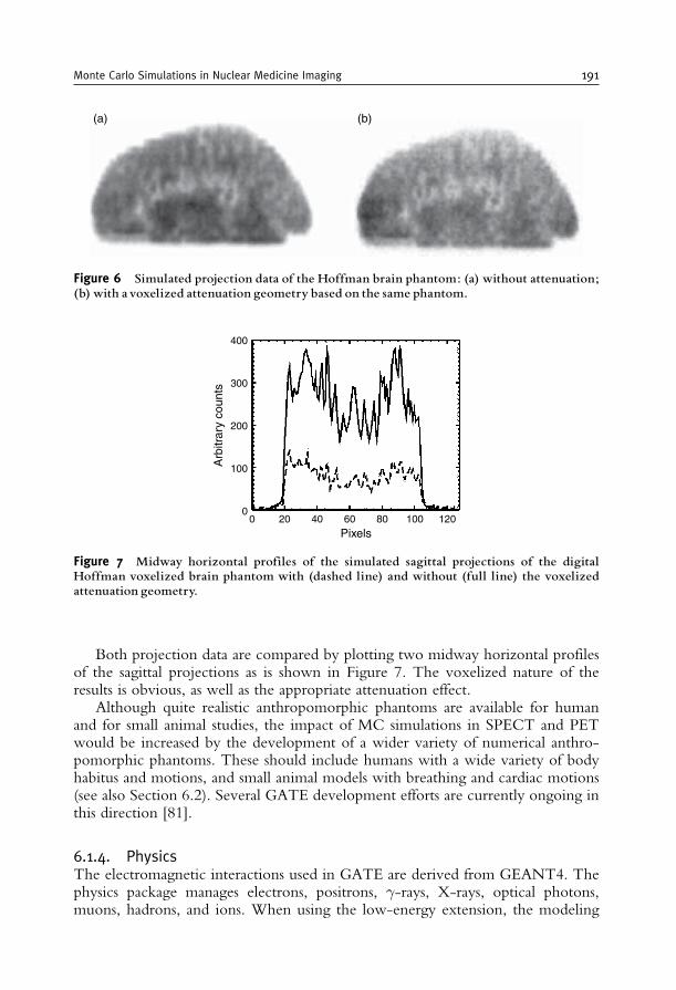
Both projection data are compared by plotting two midway horizontal profilesof the sagittal projections as is shown in Figure 7. The voxelized nature of theresults is obvious, as well as the appropriate attenuation effect.
Although quite realistic anthropomorphic phantoms are available for humanand for small animal studies, the impact of MC simulations in SPECT and PETwould be increased by the development of a wider variety of numerical anthro-pomorphic phantoms. These should include humans with a wide variety of bodyhabitus and motions, and small animal models with breathing and cardiac motions(see also Section 6.2). Several GATE development efforts are currently ongoing inthis direction [81].
6.1.4. PhysicsThe electromagnetic interactions used in GATE are derived from GEANT4. Thephysics package manages electrons, positrons, �-rays, X-rays, optical photons,muons, hadrons, and ions. When using the low-energy extension, the modeling
(a) (b)
Figure 6 Simulated projection data of the Hoffman brain phantom: (a) without attenuation;(b) with avoxelized attenuation geometry based on the same phantom.
00
100
200
300
400
Arb
itrar
y co
unts
20 40 60 12010080Pixels
Figure 7 Midway horizontal profiles of the simulated sagittal projections of the digitalHoffman voxelized brain phantom with (dashed line) and without (full line) the voxelizedattenuation geometry.
Monte Carlo Simulations in Nuclear Medicine Imaging 191
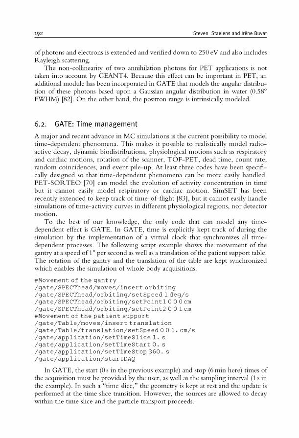
of photons and electrons is extended and verified down to 250 eV and also includesRayleigh scattering.
The non-collinearity of two annihilation photons for PET applications is nottaken into account by GEANT4. Because this effect can be important in PET, anadditional module has been incorporated in GATE that models the angular distribu-tion of these photons based upon a Gaussian angular distribution in water (0.58�FWHM) [82]. On the other hand, the positron range is intrinsically modeled.
6.2. GATE: Time management
A major and recent advance in MC simulations is the current possibility to modeltime-dependent phenomena. This makes it possible to realistically model radio-active decay, dynamic biodistributions, physiological motions such as respiratoryand cardiac motions, rotation of the scanner, TOF-PET, dead time, count rate,random coincidences, and event pile-up. At least three codes have been specifi-cally designed so that time-dependent phenomena can be more easily handled.PET-SORTEO [70] can model the evolution of activity concentration in timebut it cannot easily model respiratory or cardiac motion. SimSET has beenrecently extended to keep track of time-of-flight [83], but it cannot easily handlesimulations of time-activity curves in different physiological regions, nor detectormotion.
To the best of our knowledge, the only code that can model any time-dependent effect is GATE. In GATE, time is explicitly kept track of during thesimulation by the implementation of a virtual clock that synchronizes all time-dependent processes. The following script example shows the movement of thegantry at a speed of 1� per second as well as a translation of the patient support table.The rotation of the gantry and the translation of the table are kept synchronizedwhich enables the simulation of whole body acquisitions.
#Movement of the gantry/gate/SPECThead/moves/insert orbiting/gate/SPECThead/orbiting/setSpeed 1 deg/s/gate/SPECThead/orbiting/setPoint1 0 0 0cm/gate/SPECThead/orbiting/setPoint2 0 0 1cm#Movement of the patient support/gate/Table/moves/insert translation/gate/Table/translation/setSpeed 0 0 1.cm/s/gate/application/setTimeSlice 1. s/gate/application/setTimeStart 0. s/gate/application/setTimeStop 360. s/gate/application/startDAQ
In GATE, the start (0 s in the previous example) and stop (6min here) times ofthe acquisition must be provided by the user, as well as the sampling interval (1 s inthe example). In such a ‘‘time slice,’’ the geometry is kept at rest and the update isperformed at the time slice transition. However, the sources are allowed to decaywithin the time slice and the particle transport proceeds.
192 Steven Staelens and Irene Buvat
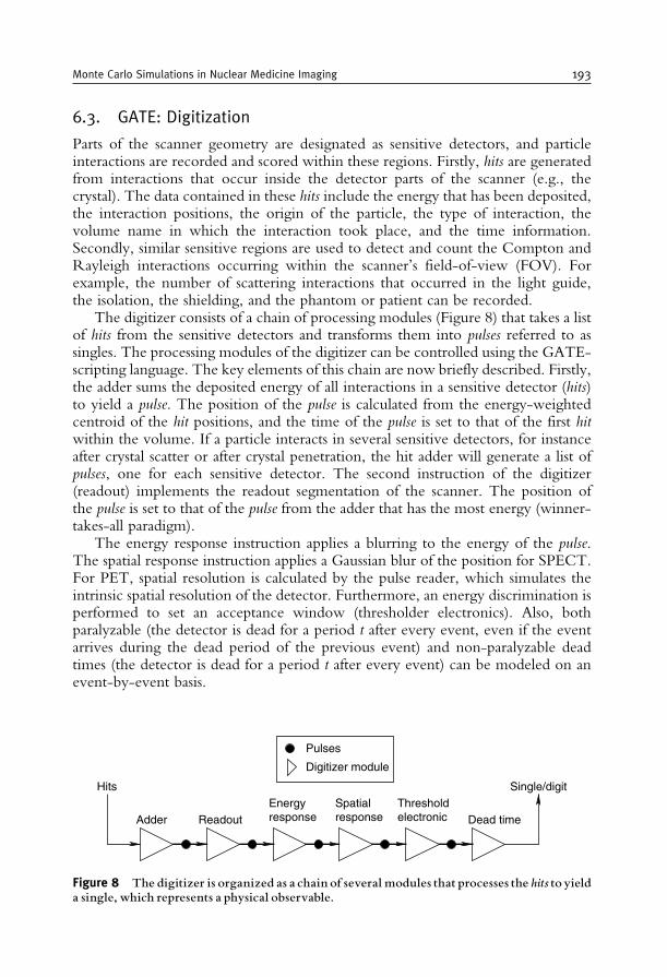
6.3. GATE: Digitization
Parts of the scanner geometry are designated as sensitive detectors, and particleinteractions are recorded and scored within these regions. Firstly, hits are generatedfrom interactions that occur inside the detector parts of the scanner (e.g., thecrystal). The data contained in these hits include the energy that has been deposited,the interaction positions, the origin of the particle, the type of interaction, thevolume name in which the interaction took place, and the time information.Secondly, similar sensitive regions are used to detect and count the Compton andRayleigh interactions occurring within the scanner’s field-of-view (FOV). Forexample, the number of scattering interactions that occurred in the light guide,the isolation, the shielding, and the phantom or patient can be recorded.
The digitizer consists of a chain of processing modules (Figure 8) that takes a listof hits from the sensitive detectors and transforms them into pulses referred to assingles. The processing modules of the digitizer can be controlled using the GATE-scripting language. The key elements of this chain are now briefly described. Firstly,the adder sums the deposited energy of all interactions in a sensitive detector (hits)to yield a pulse. The position of the pulse is calculated from the energy-weightedcentroid of the hit positions, and the time of the pulse is set to that of the first hitwithin the volume. If a particle interacts in several sensitive detectors, for instanceafter crystal scatter or after crystal penetration, the hit adder will generate a list ofpulses, one for each sensitive detector. The second instruction of the digitizer(readout) implements the readout segmentation of the scanner. The position ofthe pulse is set to that of the pulse from the adder that has the most energy (winner-takes-all paradigm).
The energy response instruction applies a blurring to the energy of the pulse.The spatial response instruction applies a Gaussian blur of the position for SPECT.For PET, spatial resolution is calculated by the pulse reader, which simulates theintrinsic spatial resolution of the detector. Furthermore, an energy discrimination isperformed to set an acceptance window (thresholder electronics). Also, bothparalyzable (the detector is dead for a period t after every event, even if the eventarrives during the dead period of the previous event) and non-paralyzable deadtimes (the detector is dead for a period t after every event) can be modeled on anevent-by-event basis.
Single/digitHits
Adder ReadoutEnergyresponse
Spatialresponse
Thresholdelectronic Dead time
Digitizer module
Pulses
Figure 8 The digitizer is organized as a chain of several modules that processes the hits to yielda single, which represents a physical observable.
Monte Carlo Simulations in Nuclear Medicine Imaging 193
Other user-defined modules can be added individually to model more specificproperties, such as the time resolution. Moreover for PET, at the end of a digitizerchain, a sorter can be added to find pairs of singles that are in coincidence(whenever the time interval between the singles is less than a user-defined coin-cidence window). Using the event number and the Compton flag, randoms andscatter coincidences can be differentiated from true coincidences. Multiple coin-cidences and auto-coincidences are also taken into account.
The optimization of the digitizer chain parameters to reproduce the behaviourof a specific scanner is very time-consuming. This is best done by comparing theresults from different sets of digitizer parameters using the same series of hits withthose of the real tomography when available. To perform this optimization, GATEoffers an operating mode named DigiGATE. In this mode, hits are read from a datafile generated by GATE and fed directly into the digitizer chain. All conditions arekept identical in the simulations including time dependencies.
7. EFFICIENCY-ACCURACY TRADE-OFF
7.1. Accuracy and validation
To model a broad range of detector geometries, there are currently two options:either use a generic simulator, such as GEANT4, EGS4 or Penelope, or use GATE,which is currently the code able to accommodate the largest number of detectorgeometries. For instance, the spherical shape of the Hi-Rez PET tomograph couldnot be accurately modeled using SimSET, but only using GATE (or anothergeneric code) [84].
The flexibility of GATE is further illustrated by the number of commercialtomographs that have been modeled in GATE, both in SPECT (e.g., AXIS [37],IRIX [85], DST-Xli [86] and Millenium VG Hawkeye [87]), in PET (e.g., ECATExact HRþ [88], Advance [89], Allegro [90], ECAT HRRT [91], Hi-Rez [84])and in small animal imaging (e.g., MicroPET P4 [92], microPET Focus 220 [93],ClearPET [94]). Moreover, GATE is the code used the most for studying proto-types (e.g., [95,96]).
How well simulations can predict the physical response of the tomograph isusually verified by comparing the simulated and empirical values of some para-meters, which can be experimentally measured and that characterize the physicalperformances [97]. The modeling of a system is then considered to be validated if itaccurately reproduces the response of the real system. The parameters of interestthat are used most often to assess the validity of a model are the spatial resolution,energy spectra, scatter fractions, sensitivity, and count rates obtained in specificconfigurations, for instance, using the NEMA phantoms [98].
7.2. Calculation time
An important issue of MC simulations is the calculation burden. The computingtime for a typical PET benchmark on a 1-GHz basis averages around 850 generated
194 Steven Staelens and Irene Buvat
and tracked events per second and 16 simulated coincidence detections per second.For SPECT, this value amounts 420 generated and tracked events per second and0.83 detections per second or 1.2 second per detection. For simulating clinicallyrealistic acquisitions, many months of computation time on one CPU are accord-ingly needed. This computational issue is most cumbersome for SPECT since thetotal number of detected counts in SPECT is less than 0.02% of the generatedevents because the collimator in front of the crystal stops most of the incomingphotons. This effect is most pronounced in high-resolution collimator variants.Secondly, every photon is tracked through every object of the experiment, and atypical Low-Energy High-Resolution (LEHR) collimator for instance consists of161120 individual air holes. Several approaches are investigated to solve thiscomputational issue both for SPECT and PET. Firstly, variance reduction techni-ques such as stratification, importance sampling and forced detection can be used[12]. Also, hybrid methods can be proposed that combine MC simulations in theobject coupled to analytical or tabulated models for the detector [99,100]. Lastly,efforts are conducted to submit simulations to a cluster of computers by distributionsoftware or by intrinsically parallelizing the code [101].
8. CASE STUDIES
Three case studies will now be discussed to illustrate the relevance of MCsimulations in emission tomography. The first case study will demonstrate the valueof using MC simulations in detector design for the optimization of TOF-PET. Thesecond case study will show an example of the use of MC simulation for theassessment of the quantitative accuracy of correction techniques in clinical data.The third case study will illustrate the use of MC simulations in image reconstruc-tion to calculate the system matrix in SPECT.
8.1. Case study I: TOF-PET
During the 1980s, different PET systems with TOF information were developed[102–109]. The TOF information leads to more accurate imaging by reducing thenoise in image data, resulting in higher image quality, shorter imaging times, andlower dose to the patient. Due to technical limitations of the TOF-capablescintillators, these systems could not compete at that time with non-TOF BGOPET scanners. Recently, new scintillators with high stopping power and high lightoutput (e.g., LSO and LaBr3) that are fast enough for TOF PET have becomeavailable. Therefore, different TOF-PET systems are under development and thefirst commercial system is available since June 2006 [110].
In PET, the time difference measurement between both photons is used todetermine whether two single photons will be stored as a coincident event. Twophotons coming from a single annihilation arrive at slightly different times depend-ing on their origin in the FOV. For a camera with a ring diameter of 90 cm, themaximum time difference for photons to reach the detectors is a few nanoseconds
Monte Carlo Simulations in Nuclear Medicine Imaging 195
and therefore accuracy of time measurement has to be only in the range of 1–2 ns.In TOF-PET, the time difference is determined as accurately as possible and thedifference is stored and used in the reconstruction. For TOF-PET, it is necessary touse a MC simulator with very accurate time tracking (accuracy of ps) of bothphotons. To get a good prediction of the system performance, it is also important tohave an accurate model of the scintillators’ rise and decay time. GATE has anexplicit modeling of time and is therefore suitable for simulation of TOF-PETscanners.
The GATE MC simulation tool has been used to model the University ofPennsylvania prototype LaBr3 TOF-PET scanner [111]. The scanner consists of648 crystals (4� 4� 30mm3) in a 90-cm diameter ring. Sixty rings cover a 25-cmaxial length for a maximum axial acceptance angle of +15�. The slice thickness is4.3mm. Based on measurements on the scanner, the energy resolution was set to6%. The spatial resolution is determined by the crystal size (4� 4mm) but also bythe fact that photopeak detection is often the result of multiple Compton interac-tions in LaBr3. The singles timing resolution was simulated at 150, 300, and 600 ps;this corresponds to coincidence timing resolutions of 212, 424, and 848 ps (or 32,64, and 128mm spatial equivalent, respectively). The TOF information decreasesthe impact of axial rebinning and lessens the needs for fine transverse angularsampling. When TOF information is ignored during reconstruction (single slicerebinning), the axial resolution worsens dramatically with radial distance due toaxial rebinning errors. When TOF information is used during rebinning, the axialresolution is fairly constant across the transverse FOV. In addition, the rebinningerror is reduced with improved timing resolution. For the simulated system theaxial resolution is about 10–11mm for 848 ps timing resolution, 6–7.5mm for424 ps, and 5–5.5mm for 212 ps. 3D listmode MLEM reconstruction results in anaxial resolution of about 4mm, independent of timing resolution. Degraded tan-gential resolution is anticipated when the data are mashed into a limited number oftransverse angles. With 848 ps timing resolution, even using 36 angles results inonly a slight loss of tangential resolution. With 424 ps timing resolution, as few as18 angles are needed, and with 212 ps resolution, 9 angles leads to only a small(<1mm) loss of tangential resolution.
The aforementioned simulations were used to develop a more efficient way ofreconstructing TOF-PET data without introduction of resolution loss [112]. TheMC method made it possible to investigate the relationship between timingresolution and angular sampling requirements in terms of rebinning and mashingwithout having to build the systems and their electronics for performing realmeasurements.
8.2. Case study II: Assessment of PVE correction
In SPECT scans of the dopaminergic system, measurements of striatal uptake areuseful for diagnosis and patient follow-up. Most radiopharmaceuticals appropriatefor studying the presynaptic transporter binding or the postsynaptic dopamine D2receptor status are labeled with 123I. Common indications are early diagnosis ofParkinson’s disease and evaluation of Parkinsonian syndromes. A more recent
196 Steven Staelens and Irene Buvat
application is the differential diagnosis between dementia with Lewy bodies (DLB)and Alzheimer’s disease (AD) in demented patients. DLB is the second mostcommon type of degenerative dementia in the elderly. As mentioned in Section4.2, MC simulations of patient data are extremely useful for assessing the accuracywith which the radiopharmaceutical uptake can be quantified, because they allowto determine absolute biases. In the study taken here as an example [113], 23patients diagnosed with DLB (10 patients) or AD (13 patients) were simulated.For these patients, processing of MC-simulated data showed that without PVEcorrection, the binding potential (BP), which characterizes the radiopharmaceuticaluptake in the striata (hence the density of dopaminergic transporters), was under-estimated by 72.4% on average in the caudate nuclei and by 57.3% on average inthe putamen. Similar to what was observed on acquired patient data, PVE correc-tion greatly affected BP values. When combined with scatter and attenuationcorrections, it yielded an averaged overestimation of BP estimates of only 13.4%in the caudate nuclei and of 16.1% in the putamen. The mean absolute differencebetween true BP and measured BP was no more than 0.9 in the caudate nuclei and0.6 in the putamen.
Accurate quantitative assessment of BP would be of great interest for detectionof pre-symptomatic cases of neurodegenerative diseases, both for a better under-standing of the degenerative process and for evaluation of neuroprotective treat-ments. However, pre-symptomatic patients are hard to recruit so using MCsimulations is an appealing solution to get the data that would be acquired insuch patients, and compare the performance of different processing protocols indetecting subtle changes in striatal uptake. In [113], SPECT scans were simulatedwith striatal uptake values mimicking pre-symptomatic cases of DLB. For thisspecifically (difficult) patient population, it was shown that DLB could be differ-entiated from AD only when PVE correction was combined with attenuation andscatter corrections (Figure 9).
In summary, MC simulations allowed these authors to conclude that only acomplete processing scheme including scatter, attenuation, and PVE correctionscould accurately estimate BP from SPECT scans of the dopaminergic system, and itbecame clear that the most important correction for accurate estimates of BP wasPVE correction. MC simulations allowed the authors to test their quantificationmethods while being sure that no segmentation or registration errors occurred.They could demonstrate that PVE correction improved the accuracy of classifica-tion of patients when pre-symptomatic DLB cases were considered. These resultssuggest that the accuracy with which preclinical cases are detected may be increasedwhen applying a complete reconstruction scheme, including scatter, attenuation,and most important, PVE corrections.
8.3. Case study III: MC-based reconstruction
The concept of using MC simulations to estimate the 3D system involved inSPECT tomographic reconstruction was proposed early [114–116] but could notbe applied in fully 3D at that time, due to impractical storage and computationtime.
Monte Carlo Simulations in Nuclear Medicine Imaging 197
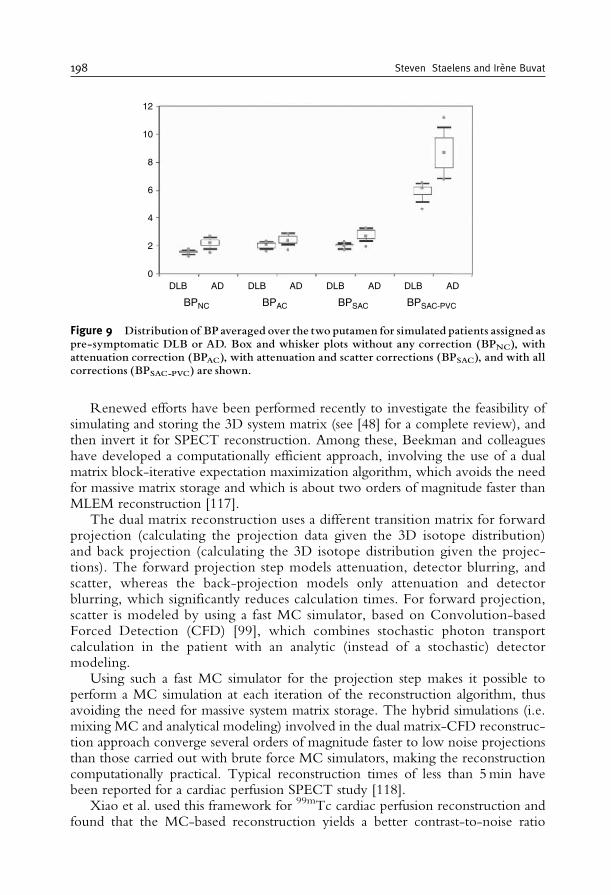
Renewed efforts have been performed recently to investigate the feasibility ofsimulating and storing the 3D system matrix (see [48] for a complete review), andthen invert it for SPECT reconstruction. Among these, Beekman and colleagueshave developed a computationally efficient approach, involving the use of a dualmatrix block-iterative expectation maximization algorithm, which avoids the needfor massive matrix storage and which is about two orders of magnitude faster thanMLEM reconstruction [117].
The dual matrix reconstruction uses a different transition matrix for forwardprojection (calculating the projection data given the 3D isotope distribution)and back projection (calculating the 3D isotope distribution given the projec-tions). The forward projection step models attenuation, detector blurring, andscatter, whereas the back-projection models only attenuation and detectorblurring, which significantly reduces calculation times. For forward projection,scatter is modeled by using a fast MC simulator, based on Convolution-basedForced Detection (CFD) [99], which combines stochastic photon transportcalculation in the patient with an analytic (instead of a stochastic) detectormodeling.
Using such a fast MC simulator for the projection step makes it possible toperform a MC simulation at each iteration of the reconstruction algorithm, thusavoiding the need for massive system matrix storage. The hybrid simulations (i.e.mixing MC and analytical modeling) involved in the dual matrix-CFD reconstruc-tion approach converge several orders of magnitude faster to low noise projectionsthan those carried out with brute force MC simulators, making the reconstructioncomputationally practical. Typical reconstruction times of less than 5min havebeen reported for a cardiac perfusion SPECT study [118].
Xiao et al. used this framework for 99mTc cardiac perfusion reconstruction andfound that the MC-based reconstruction yields a better contrast-to-noise ratio
BPNC BPAC BPSAC BPSAC-PVC
ADADDLB DLB DLB AD ADDLB0
2
4
6
8
10
12
Figure 9 Distribution of BP averaged over the two putamen for simulated patients assigned aspre-symptomatic DLB or AD. Box and whisker plots without any correction (BPNC), withattenuation correction (BPAC), with attenuation and scatter corrections (BPSAC), and with allcorrections (BPSAC-PVC) are shown.
198 Steven Staelens and Irene Buvat
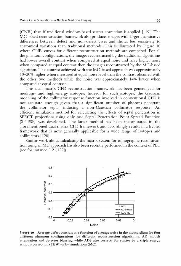
(CNR) than if traditional window-based scatter correction is applied [119]. TheMC-based reconstruction framework also produces images with larger quantitativedifferences between defect and non-defect cases and shows less sensitivity toanatomical variations than traditional methods. This is illustrated by Figure 10where CNR curves for different reconstruction methods are compared. For allthe phantom configurations, the images reconstructed by the traditional algorithmshad lower overall contrast when compared at equal noise and have higher noisewhen compared at equal contrast then the images reconstructed by the MC-basedalgorithm. The contrast achieved with the MC-based approach was approximately10–20% higher when measured at equal noise level than the contrast obtained withthe other two methods while the noise was approximately 14% lower whencompared at equal contrast.
This dual matrix-CFD reconstruction framework has been generalized formedium- and high-energy isotopes. Indeed, for such isotopes, the Gaussianmodeling of the collimator response function involved in conventional CFD isnot accurate enough given that a significant number of photons penetratethe collimator septa, inducing a non-Gaussian collimator response. Anefficient simulation method for calculating the effects of septal penetration inSPECT projections using only one Septal Penetration Point Spread Function(SP-PSF) was developed. The latter method has been incorporated in theaforementioned dual matrix CFD framework and accordingly results in a hybridframework that is now generally applicable for a wide range of isotopes andcollimators [120].
Similar work about calculating the matrix system for tomographic reconstruc-tion using an MC approach has also been recently performed in the context of PET(see for instance [121,122]).
Noise
Rel
ativ
e co
ntra
st
00.2
0.3
0.5
0.4
0.6
0.7
0.8
0.02 0.04 0.06 0.08 0.1
AD
ADS-TEWADS-MC
Figure 10 Average defect contrast as a function of average noise in the myocardium for fourdifferent phantom configurations for different reconstruction algorithms. AD modelsattenuation and detector blurring while ADS also corrects for scatter by a triple energywindow correction (TEW) or by simulations (MC).
Monte Carlo Simulations in Nuclear Medicine Imaging 199
9. FUTURE PROSPECTS
Future developments in MC simulations in the context of Nuclear Medicinewill probably include further integration of current MC tools to provide moreaccurate and powerful diagnosis and treatment systems [123].
A first integration level would consist in bridging the gap between MC calcula-tions used for SPECT and PET modeling and for dose calculation. Nowadays, MCsimulations are becoming part of the imaging process itself, when being used forcalculating the system matrix involved in tomographic reconstruction, as previouslydiscussed in the third case study. A further extension will be to also calculate thepatient-specific dose distributions using this MC approach, which can give accuratedose deposit estimates following, e.g., internal radiation [124]. Currently, whenperformed with the MC approach, dose calculations usually rely on different MCcodes than those used for modeling SPECT or PET scans. Using a single simulationframework for both tomographic reconstruction and dose calculation will facilitatethe feasibility (e.g., single coordinate system, common object description, consis-tent sampling) and the assessment of patient-specific dosimetry.
A second integration level concerns the MC modeling of dual modality imagingsystem. In the past years, the Nuclear Medicine instrumentation market has shiftedtoward dual modality imagers: SPECT-CT and PET-CT. SPECT and PET MCmodeling are currently very well mastered. MC modeling of CT devices has alsobeen described (see e.g. [125]). Integrating a MC model for the CT part of thesehybrid imagers in the same MC simulation framework as that used for SPECT andPET modeling would enable a more detailed investigation of dual modalitytechniques, such as CT-based SPECT or PET attenuation correction, or CT-based SPECT and PET partial volume correction.
Finally, MC simulations remain computationally demanding methods, whilelarge database of simulated data are ideally needed for evaluation purposes. There-fore, further progress is anticipated in implementing variance reduction techniques.Also, some laboratories endow significant funds in large computer clusters in orderto perform detection tasks based on simulated datasets. Forthcoming work will bededicated to developing distribution software for datagrid deployments or toparallellization solutions. It can also be expected that more efforts will go to thecollection of simulated data to create online repositories, that would enable sub-scribers to test their image correction and processing techniques without the needto extensively simulate or acquire the appropriate datasets.
All these expected developments should make MC simulations even morepresent in the realm of emission tomography in the future.
10. CONCLUSION
In the end of 1990s, MC simulations in emission tomography were mostlyused by research labs to assess reconstruction and correction techniques, and tostudy specific aspects of the imaging system response. It is expected that MC
200 Steven Staelens and Irene Buvat

simulations will eventually find their way to the clinics, as contributing to theSPECT or PET imaging process, and as provider of extremely realistic and stillperfectly controlled datasets for evaluation purpose. The role of MC simulations foroptimizing detector design will also increase, as simulations are becoming more andmore flexible and accurate, allowing for detailed investigation of a broad range ofdetector configurations. Overall, MC simulations will become an indispensable toolfor all involved in emission tomography.
ACKNOWLEDGMENTS
This work of S.S was supported by the Fund for Scientific Research Flanders, thework of I.B was supported by INSERM.
REFERENCES
[1] J. Sorenson, M. Phelps, Physics in Nuclear Medicine, W:B: Saunders Company; 1987:[2] Z. Cho, J. Jones, M. Singh, Foundations of Medical Imaging, John Wiley & sons Inc., 1993.[3] F. Beekman, F. van der Have, B. Vastenhouw, A. van der Linden, P. van Rijk, J. Burbach,
M. Smidt, U-SPECT-I: a novel system for submillimeter-resolution tomography withradiolabelled molecules in mice, Journal of Nuclear Medicine, 46 (2005) 1194–1200.
[4] L. Furenlid, D. Wilson, C. Yi-Chun, K. Hyunki, P. Pietraski, M. Crawford, H. Barrett,FastSPECT II: a second-generation high-resolution dynamic SPECT imager, IEEE Transac-tions on Nuclear Science, 49 (2004) 116–123.
[5] A. Chatziioannou, Molecular imaging of small animals with dedicated PET tomographs,European Journal of Nuclear Medicine, 29 (2002) 98–114.
[6] F.Natterer, F.Wubbeling,MathematicalMethods in ImageReconstruction, CambridgeUniversityPress, 2001.
[7] R. Gordon, A tutorial on ART, IEEE Transactions on Nuclear Science, 21 (1974) 78–93.[8] L. A. Shepp, Y. Vardi, Maximum likelihood reconstruction for emission tomography, IEEE
Transactions on Medical Imaging, 1 (1982) 113–122.[9] B. Tsui, E. Frey, X. Zhao, D. Lalush, R. Johnston, W. McCartney, The importance and
implementation of accurate 3D compensation methods for quantitative SPECT, Physics inMedicine and Biology, 39 (1994) 509–530.
[10] H. Zaidi, Relevance of accurate Monte Carlo modeling in nuclear medical imaging, MedicalPhysics, 26 (1999) 574–608.
[11] M. Ljungberg, S. Strand, M. King, Monte Carlo Simulations in Nuclear Medicine: Applica-tions in Diagnostic Imaging, Institute of Physics, 1998.
[12] D. Haynor, R. Harrison, T. Lewellen, The use of importance sampling techniques to improvethe efficiency of photon tracking in emission tomography simulations, Medical Physics, 18(1991) 990–1001.
[13] S. Agostinelli, J. Allison, K. Amako, J. Apostolakis, H. Araujo, P. Arce, M. Asai, D. Axen,S. Banerjee, G. Barrand, F. Behner, L. Bellagamba, J. Boudreau, L. Broglia, A. Brunengo,H. Burkhardt, S. Chauvie, J. Chuma, R. Chytracek, G. Cooperman, G. Cosmo,P. Degtyarenko, A. Dell’AcquaG. Depaola, D. Dietrich, R. Enami, A. Feliciello, C. Ferguson,H. Fesefeldt, G. Folger, F. Foppiano, A. Forti, S. Garelli, S. Giani, R. Giannitrapani, D. Gibin,J. J. G. Cadenas, I. Gonzalez, G. G. Abril, G. Greeniaus, W. Greiner, V. Grichine, A. Grossheim,S. Guatelli, P. Gumplinger, R. Hamatsu, K. Hashimoto, H. Hasui, A. Heikkinen, A. Howard,
Monte Carlo Simulations in Nuclear Medicine Imaging 201
V. Ivanchenko, A. Johnson, F. W. Jones, J. Kallenbach, N. Kanaya, M. Kawabata, Y. Kawabata,M. Kawaguti, S. Kelner, P. Kent, A. Kimura, T. Kodama,R.Kokoulin,M.Kossov, H. Kurashige,E. Lamanna, T. Lampen, V. Lara, V. Lefebure, F. Lei, M. Liendl, W. Lockman, F. Longo,S. Magni, M. Maire, E. Medernach, K. Minamimoto, P. M. de Freitas, Y. Morita,K. Murakami, M. Nagamatu, R. Nartallo, P. Nieminen, T. Nishimura, K. Ohtsubo,M. Okamura, S. O’Neale, Y. Oohata, K. Paech, J. Perl, A. Pfeiffer, M. G. Pia, F. Ranjard,A. Rybin, S. Sadilov, E. Di Salvo, G. Santin, T. Sasaki, N. Savvas, Y. Sawada, S. Scherer, S. Seil,V. Sirotenko, D. Smith, N. Starkov, H. Stoecker, J. Sulkimo, M. Takahata, S. Tanaka,E. Tcherniaev, E. S. Tehrani, M. Tropeano, P. Truscott, H. Uno, L. Urban, P. Urban,M. Verderi, A. Walkden, W. Wander, H. Weber, J. P. Wellisch, T. Wenaus, D. C. Williams,D. Wright, T. Yamada, H. Yoshida, D. Zschiesche, Geant4: a simulation toolkit, NuclearMethods and Instruments in Physics Research Section A, 506 (2003) 250–303.
[14] Geant4, http://geant4.web.cern.ch/geant4/UserDocumentation/.[15] P. Andreo, Monte Carlo techniques in medical radiation physics, Physics in Medicine and
Biology, 36 (1991) 861–920.[16] I. Buvat, I. Castiglioni, Monte Carlo simulations in SPET and PET, Quarterly Journal of
Nuclear Medicine, 46 (2002) 48–61.[17] S. Webb, D. Binnie, M. Flower, R. Ott, Monte Carlo modeling of the performace of a
rotating slit collimator for improved planar gamma camera imaging, Physics in Medicine andBiology, 37 (1992) 1095–1108.
[18] A. Cot, J. Sempau, D. Pareto, S. Bullich, J. Pavia, F. Calvino, D. Ros, Evaluation of thegeometric, scatter, and septal penetration components in fan-beam collimators using MonteCarlo simulation, IEEE Transactions on Nuclear Science, 49 (2002) 12–16.
[19] T. Song, Y. Choi, Y. Chung, J. Jung, Y. Choe, K. Lee, S. Kim, B. Kim, Optimization ofpinhole collimator for small animal SPECT using Monte Carlo simulation, IEEE Transactionson Nuclear Science, 50 (2003) 327–332.
[20] F. van der Have, F. Beekman, Photon penetration and scatter in micro-pinhole imaging: aMonte Carlo investigation, Physics in Medicine and Biology, 49 (2004) 1369–1386.
[21] D. Gagnon, G. Zeng, M. Links, J. Griesmer, C. Valentino, Design considerations for a newsolid state gammacamera: SOLSTICE, in: Proceedings of the IEEE Medical Imaging Con-ference Norfolk, USA, 2001, pp. 1156–1160.
[22] J. Griesmer, B. Kline, J. Grosholz, K. Parnham, D. Gagnon, Performance evaluation of a newCZT detector for nuclear medicine: SOLSTICE, in: Proceedings of the IEEE Medical ImagingConference Norfolk, USA, 2001, pp. 1050–1054.
[23] S. Staelens, M. Koole, S. Vandenberghe, Y. D’Asseler, I. Lemahieu, R. Van de Walle, Thegeometric transfer function for a slat collimator mounted on a strip detector, IEEE Transactionson Nuclear Science, 52 (2005) 708–714.
[24] C. Groiselle, Y. D’Asseler, J. Kolthammer, C. Matthews, S. Glick, A Monte Carlo simulationstudy to evaluate septal spacing using triple-head hybrid PET imaging, IEEE Transactions onNuclear Science, 50 (2003) 1339–1346.
[25] C. Thompson, The effect of collimation on singles rates in multi-slice PET, IEEE Transactionson Nuclear Science, 35 (1988) 598–602.
[26] S. Surti, J. Karp, G. Muehllehner, Image quality assessment of LaBr3-based whole-body 3D PETscanners: a Monte Carlo evaluation, Physics in Medicine and Biology, 49 (2004) 4593–4610.
[27] S. Surti, J. Karp, A count-rate model for PET scanners using pixelated Angerlogic detectorswith different scintillators, Physics in Medicine and Biology, 50 (2005) 5697–5715.
[28] A. Bice, T. Lewellen, R. Miyaoka, R. Harrison, D. Haynor, K. Pollard, C. Hanson,S. Gillispie, Monte Carlo simulations of BaF2 detectors used in time of flight positron emissiontomography, IEEE Transactions on Nuclear Science, 37 (1990) 696–701.
[29] S. Surti, J. Karp, G. Muehllehner, P. Raby, Investigation of lanthanum scintillators for 3-DPET, IEEE Transactions on Nuclear Science, 50 (2003) 348–354.
[30] W. Moses, Time of flight in PET revisited, IEEE Transactions on Nuclear Science, 50 (2003)1325–1330.
[31] W. Moses, S. Derenzo, Design studies for a PET detector module using a PIN photodiode tomeasure depth of interaction, IEEE Transactions on Nuclear Science, 41 (1994) 1441–1445.
202 Steven Staelens and Irene Buvat
[32] C. Lartizien, A. Reilhac, N. Costes, M. Janier, D. Sappey-Marinier, Monte Carlo simulation-based design study of a LSO-LuAP small animal PET system, IEEE Transactions on NuclearScience, 50 (2003) 1433–1438.
[33] G. El Fakhri, I. Buvat, M. Pelegrini, H. Benali, P. Almeida, B. Bendriem, A. Todd-Pokropek,R. Di Paolo, Respective roles of scatter, attenuation, depth-dependent collimator response andfinite spatial resolution in cardiac SPECT quantitation: a Monte Carlo study, European Journalof Nuclear Medicine, 26 (1999) 437–446.
[34] G. El Fakhri, I. Buvat, H. Benali, A. Todd-Pokropek, R. Di Paolo, Relative impact of scatter,collimator response, attenuation, and finite spatial resolution corrections in cardiac SPECT,Journal of Nuclear Medicine, 41 (2000) 1400–1408.
[35] M. Soret, P. Koulibaly, J. Darcourt, S. Hapdey, I. Buvat, Quantitative accuracy of dopaminergicneurotransmission imaging using 123I SPECT, Journal of Nuclear Medicine, 44 (2003) 1184–1193.
[36] H. Zaidi, K. Koral, Scatter modeling and compensation in emission tomography, EuropeanJournal of Nuclear Medicine, 31 (2004) 761–782.
[37] S. Staelens, D. Strul, S. Vandenberghe, G. Santin, M. Koole, Y. D’Asseler, I. Lemahieu,R. Van deWalle, Monte Carlo simulations of a scintillation camera using GATE: validationand application modeling, Physics in Medicine and Biology, 48 (2003) 3021–3042.
[38] A. Cot, J. Sempau, D. Pareto, S. Bullich, J. Pavia, F. Calvino, D. Ros, Study of the point spreadfunction (PSF) for 123I SPECT imaging using Monte Carlo simulation, Physics in Medicineand Biology, 49 (2004) 3125–3136.
[39] H. Huesman, E. Salmeron, J. Baker, Compensation for crystal penetration in high resolutionpositron tomography, IEEE Transactions on Nuclear Science, 36 (1989) 1100–1107.
[40] S. Staelens, Y. D’Asseler, S. Vandenberghe, M. Koole, I. Lemahieu, R. Van de Walle, A three-dimensional theoretical model incorporating spatial detection uncertainty in continuous detec-tor PET, Physics in Medicine and Biology, 49 (2004) 2337–2351.
[41] F. Lamare, M. Ledesma Carbayo, G. Kontaxakis, A. Santos, A. Turzo, Y. Bizais, C. Cheze-Le Rest, D. Visvikis, Incorporation of elastic transformations in list-mode based reconstructionfor respiratory motion correction in PET, in: Proceedings of the IEEE Medical ImagingConference, Rome, Italy, 2004, pp. M03–247.
[42] F. J. Beekman, M. A. Viergever, Fast SPECT simulation including object shape dependentscatter, IEEE Transactions on Medical Imaging, 14 (1995) 271–282.
[43] F. J. Beekman, J. M. den Harder, M. A. Viergever, P. P. van Rijk, SPECT scatter modeling innon-uniform attenuating objects, Physics in Medicine and Biology, 42 (1997) 1133–1142.
[44] E. C. Frey, B. M. W. Tsui, A new method for modelling the spatially variant object dependentscatter response function in SPECT, in: Proceedings of the IEEE Medical Imaging Conference,Anaheim, USA, 1996, pp. 1082–1086.
[45] S. R. Meikle, B. F. Hutton, D. L. Bailey, A transmission dependent method for scattercorrection in SPECT, Journal of Nuclear Medicine, 23 (1994) 360–367.
[46] S. H. M. Walrand, L. R. van Elmbt, S. Pauwels, Quantification in SPECT using an effectivemodel of the scattering, Physics in Medicine and Biology, 39 (1994) 719–734.
[47] C. E. Floyd, R. J. Jaszczak, K. L. Greer, R. E. Coleman, Inverse Monte Carlo as a unifiedreconstruction algorithm for ECT, Journal of Nuclear Medicine, 27 (1986) 1577–1585.
[48] D. Lazaro, Z. El Bitar, V. Breton, D. Hill, I. Buvat, Fully 3D Monte Carlo reconstruction inSPECT: a feasibility study, Physics in Medicine and Biology, 50 (2005) 3739–3754.
[49] F. J. Beekman, C. Kamphuis, M. A. Viergever, Improved SPECT quantitation using fullythree-dimensional iterative spatially variant scatter response compensation, IEEE Transactionson Medical Imaging, 15 (1996) 491–499.
[50] F. J. Beekman, C. Kamphuis, E. C. Frey, Scatter compensation methods in 3D iterative SPECTreconstruction: a simulation study, Physics in Medicine and Biology, 42 (1997) 1619–1632.
[51] D. Kadrmas, E. Frey, B. Tsui, Application of reconstruction-based scatter compensation toThallium-201 SPECT: implementations for reduced reconstructed noise, IEEE Transactionson Medical Imaging, 17 (1998) 325–333.
[52] T. Farncombe, H. Gifford, M. Narayanan, H. Pretorius, E. Frey, M. King, Assessment ofscatter compensation strategies for 67Ga SPECT using numerical observers and human LROCstudies, Journal of Nuclear Medicine, 45 (2004) 802–812.
Monte Carlo Simulations in Nuclear Medicine Imaging 203
[53] E. C. Frey, K. Gilland, B. M. W. Tsui, Application of task-based measures of image quality tooptimization and evaluation of three-dimensional reconstruction-based scatter compensation inmyocardial perfusion SPECT, IEEE Transactions on Medical Imaging, 21 (2002) 1040–1050.
[54] M. Narayanan, H. Pretorius, S. Dahlberg, J. Leppo, N. Botkin, J. Krasnow, W. Berndt, E. Frey,M. King, Evaluation of scatter compensation strategies and their impact on human detectionperformance Tc-99m myocardial perfusion imaging, IEEE Transactions on Nuclear Science, 50(2003) 1522–1527.
[55] G. Tourassi, E. Carey, M. Munley, Improved lesion detection in SPECT using MLEMreconstruction, IEEE Transactions on Nuclear Science, 38 (1991) 780–783.
[56] P. Bruyant, H. Gifford, G. Gindi, M. King, Numerical observer study of MAPOSEMregularization methods with anatomical priors for lesion detection in Ga-67 images, IEEETransactions on Nuclear Science, 51 (2004) 193–197.
[57] I. Castiglioni, I. Buvat, G. Rizzo, M. Gilardi, J. Feuardent, F. Fazio, A publicly accessibleMonte Carlo database for validation purposes in emission tomography, European Journal ofNuclear Medicine, 32 (2005) 1234–1239.
[58] A. Reilhac, G. Batan, C. Michel, C. Grova, J. Tohka, D. Collins, N. Costes, A. Evans, PET-SORTEO: validation and development of database of simulated PET volumes, IEEE Transac-tions on Nuclear Science, 52 (2005) 1321–1328.
[59] A. Syme, C. Kirkby, T. Riauka, B. Fallone, S. McQuarrie, Monte Carlo investigation of singlecell beta dosimetry for intraperitoneal radionuclide therapy, Physics in Medicine and Biology,49 (2004) 1959–1972.
[60] Y. Dewaraja, S. Wilderman, M. Ljungberg, K. Koral, K. Zasadny, M. Kaminiski, Accuratedosimetry in 131I radionuclide therapy using patient-specific, 3-dimensional methods for SPECTreconstruction and absorbed dose calculation, Journal of Nuclear Medicine, 46 (2005) 840–849.
[61] B. Fraass, J. Smathers, J. Deye, Summary and recommendations of a national cancer instituteworkshop on issues limiting the clinical use of Monte Carlo dose calculation algorithms formegavoltage external beam radiation therapy, Medical Physics, 30 (2003) 3206–3216.
[62] O. Chibani, X. Li, Monte Carlo dose calculations in homogeneous media and at interfaces: acomparison between GEPTS, EGSnrc, MCNP, and measurements, Medical Physics, 29 (2003)835–847.
[63] B. Reniers, F. Verhaegen, S. Vynckier, The radial dose function of low-energy brachytherapyseeds in different solid phantoms: comparison between calculations with the EGSnrc andMCNP4C Monte Carlo codes and measurements, Physics in Medicine and Biology, 49(2004) 1569–1582.
[64] S. Garelli, S. Giordano, G. Piemontese, S. Squaricia, Interactive FLUKA: a World Wide Webversion for a simulation code in protontherapy, Journal de Chimie Physique et de Physico-Chimie Biologique, 95 (1998) 767–771.
[65] R. Harrison, S. Vannoy, D. Haynor, S. Gillipsie, M. Kaplan, T. Lewellen, Preliminaryexperience with the photon generator module of a public-domain simulation system foremission tomography, in: Proceedings of the IEEE Medical Imaging Conference, San Fransico,USA, 1993, pp. 1154–1158.
[66] M. Ljungberg, S. Strand, A Monte Carlo program for the simulation of scintillation cameracharacteristics, Computer Methods and Programs in Biomedicine, 29 (1989) 257–272.
[67] J. Yanch, A. Dobrzeniecki, C. Ramanathan, R. Behrman, Physically realistic Monte Carlosimulation of source, collimator and tomographic data acquisition for emission computedtomography, Physics in Medicine and Biology, 37 (1992) 853–870.
[68] C. Thomson, J. Cantu, Y. Picard, PETSIM: Monte Carlo program simulation of all sensitivityand resolution parameters of cylindrical positron imaging systems, Physics in Medicine andBiology, 37 (1992) 731–749.
[69] H. Zaidi, A. Hermann Scheurer, C. Morel, An object-oriented Monte-Carlo simulator for 3Dcylindrical positron tomographs, Computer Methods and Programs in Biomedicine, 58 (1999)133–145.
[70] A. Reilhac, C. Lartizien, N. Costes, S. Sans, C. Comtat, R. Gunn, A. Evans, PET-SORTEO:a Monte Carlo-based simulator with high count rate capabilities, IEEE Transactions on NuclearScience, 51 (2004) 46–52.
204 Steven Staelens and Irene Buvat
[71] A. Bielajew, H. Hirayama, W. Nelson, D. Rogers, History, overview and recent improve-ments of EGS4, Tech. rep., National Research Council, Ottawa, Canada, (1994).
[72] Geant4, http://wwwasd.web.cern.ch/wwwasd/geant4/geant4.html.[73] J. Briesmeister, MCNP – a general Monte Carlo N-particle transport code, Tech. rep., Los
Alamos National Laboratory, Los Alamos, NM, USA, (1993).[74] I. Buvat, D. Lazaro, Monte Carlo simulations in emission tomography and GATE: an
overview. Nuclear Methods and Instruments in Physics Research 569 (2006) 323–329.[75] D. Strul, G. Santin, D. Lazaro, V. Breton, C. Morel, GATE (Geant4 Application for Tomo-
graphic Emission): a PET/SPECT general-purpose simulation platform, Nuclear Physics B,125C (2003) 75–79.
[76] G. Santin, D. Strul, D. Lazaro, L. Simon, M. Krieguer, M. Vieira Martins, V. Breton,C. Morel, GATE, a Geant4-based simulation platform for PET and SPECT integratingmovement and time management, IEEE Transactions on Nuclear Science, 50 (2003)1516–1521.
[77] S. Jan, G. Santin, D. Strul, S. Staelens, K. Assie, D. Autret, D. Avner, R. Barbier, M. Bardies,P. Bloomfield, D. Brasse, V. Breton, P. Bruyndonckx, I. Buvat, A. Chatziioannou, Y. Choi,Y. Chung, C. Comtat, D. Donnarieix, L. Ferrer, S. Glick, C. Groiselle, S. Kerhoas-Cavata,A. Kirov, V. Kohli, M. Koole, M. Krieguer, J. van der Laan, F. Lamare, G. Largeron,C. Lartizien, D. Lazaro, M. Maas, L. Maigne, F. Mayet, F. Melot, S. Nehmeh, E. Pennacchio,J. Perez, U. Pietrzyk, F.Rannou,M.Rey,D. Schaart, R. Schmidtlein, L. Simon, T. Song, J. Vieira,D. Visvikis, R. Van de Walle, E. Wieers, C. Morel, GATE: a simulation toolkit for PET andSPECT, Physics in Medicine and Biology, 49 (2004) 4543–4561.
[78] R. Brun, F. Rademakers, ROOT, an object oriented data analysis framework, NuclearMethods and Instruments in Physics Research Section A, 389 (1997) 81–86.
[79] S. Staelens, G. Santin, D. Strul, M. Koole, S. Vandenberghe, Y. D’Asseler, V. Breton,C. Morel, I. Lemahieu, R. Van de Walle, Monte Carlo simulations of Interfile based emissionand attenuation maps for clinical applications, Journal of Nuclear Medicine, 44 (2003) 1048.
[80] E. Hoffman, P. Cutler, W. Digby, J. Mazziota, Three dimensional phantom to simulatecerebral blood flow and metabolic images for PET, IEEE Transactions on Nuclear Science,37 (1990) 616–620.
[81] R. Taschereau, P. Chow, A. Chatziioannou, Monte Carlo simulations of dose from microCTimaging procedures in a realistic mouse phantom, Medical Physics, 33 (2006) 216–224.
[82] S. Jan, Simulateur Monte Carlo et camera a xenon liquide pour la Tomographie a Emission dePositons, Ph.D. thesis, Universite Joseph Fourier, Grenoble, France (2002).
[83] R. Harrison, S. Gillispie, A. Alessio, P. Kinahan, T. Lewellen, The effects of object size,attenuation, scatter, and random coincidences on signal to noise ratio in simulations of time-of-flight positron emission tomography, in: Proceedings of the IEEEMedical Imaging ConferencePuerto Rico, 2005, pp. 1900–1904.
[84] C. Michel, L. Eriksson, H. Rothfuss, B. Bendriem, D. I. Lazaro, Buvat, Influence of crystalmaterial on the performance of the HiRez 3D PET scanner: a Monte-Carlo study, in: IEEEMedical Imaging Symposium Conference Record, 4, (2006), p. 2007.
[85] S. Staelens, G. Santin, S. Vandenberghe, D. Strul, M. Koole, Y. D’Asseler, I. Lemahieu,R. Van de Walle, Transmission imaging with a moving point source: influence of crystalthickness and collimator type, IEEE Transactions on Nuclear Science, 52 (2005) 166–173.
[86] K. Assie, I. Gardin, P. Vera, I. Buvat, Validation of the Monte Carlo simulator GATE forIndium111 imaging, Physics in Medicine and Biology, 50 (2005) 3113–3125.
[87] D. Autret, A. Bitar, L. Ferrer, A. Lisbona, M. Bardies, Monte Carlo modeling of gammacameras for I-131 imaging in targeted radiotherapy, Cancer Biotherapy and Radio Pharma-ceuticals, 20 (2005) 77–84.
[88] S. Jan, C. Comtat, D. Strul, G. Santin, R. Trebossen, Monte Carlo simulation for the ECATEXACT HRþ system using GATE, IEEE Transactions on Nuclear Science, 52 (2005)627–633.
[89] C. Schmidtlein, A. Kirov, S. Nehmeh, Y. Erdi, J. Humm, H. Amols, L. Bidaut, A. Ganin,C. Stearns, D. McDaniel, K. Hamacher, Validation of GATE Monte Carlo simulations of theGE Advance/Discovery LS PET scanners, Medical Physics, 33 (2006) 198–208.
Monte Carlo Simulations in Nuclear Medicine Imaging 205
[90] F. Lamare, A. Turzo, Y. Bizais, C. Le Rest, D. Visvikis, Validation of a Monte Carlosimulation of the Philips Allegro/GEMINI PET systems using GATE, Physics in Medicineand Biology, 51 (2006) 943–962.
[91] F. Bataille, C. Comtat, S. Jan, R. Trebossen, Monte Carlo simulation for the ECAT HRRTusing GATE, in: Proceedings of the IEEE Medical Imaging Conference Rome, Italy, 2004,pp. 2570–2574.
[92] S. Jan, A. Chatziioannou, C. Comtat, D. Strul, G. Santin, R. Trbossen, Monte Carlo simula-tion for the microPET P4 system using GATE, Molecular Imaging and Biology, 5 (2003) , 138.
[93] S. Jan, A. Desbree, F. Pain, D. Guez, C. Comtat, H. Gurden, S. Kerhoas, P. Laniece,F. Lefebvre, R. Mastrippolito, R. Trebossen, Monte Carlo simulation of the microPETFOCUS system for small rodents imaging applications, in: Proceedings of the IEEE MedicalImaging Conference Puerto Rico, 2005, pp. 1653–1657.
[94] M. Rey, J. Vieira, J. Mosset, B. Moulin Sallanon, P. Millet, J. Loude, C. Morel,Measured and simulated specifications of the Lausanne ClearPET scanner demonstrator,in: Proceedings of the IEEE Medical Imaging Conference Puerto Rico, 2005,pp. 2070–2073.
[95] F. Rannou, V. Kohli, D. Prout, A. Chatziioannou, Investigation of OPET peformance usingGATE, a Geant4-based simulation software, IEEE Transactions on Nuclear Science, 51 (2004)2713–2717.
[96] Y. Chung, Y. Choi, G. Cho, Y. Choe, K. Lee, B. Kim, Optimization of dual layer phoswichdetector consisting of LSO and LuYAP for small animal PET, IEEE Transactions on NuclearScience, 52 (2005) 217–221.
[97] I. Buvat, I. Castiglioni, J. Feuardent, M. Gilardi, Unified description and validation of MonteCarlo simulators in PET, Physics in Medicine and Biology, 50 (2005) 329–346.
[98] National electric manufacturers association, Rosslyn, VA, NEMA standards publication NU 2-2001: Performance measurements of positron emission tomographs (2001).
[99] H. W. de Jong, E. T. P. Slijpen, F. J. Beekman, Acceleration of Monte Carlo SPECT simulationusing convolution-based forced detection, IEEETransactions onNuclear Science, 48 (2001) 58–64.
[100] X. Song, W. Segars, Y. Du, B. Tsui, E. Frey, Fast modeling of the collimator-detector responsein Monte Carlo simulation of SPECT imaging using the angular response function, Physics inMedicine and Biology, 50 (2005) 1791–1804.
[101] J. De Beenhouwer, D. Kruecker, S. Staelens, L. Ferrer, A. Chatziioannou, F. Rannou,Distributed computing platform for PET and SPECT simulations with GATE, in: Proceedingsof the IEEE Medical Imaging ConferencePuerto Rico, 2005, pp. 2437–2440.
[102] R. Allemand, C. Gresset, J. Vacher, Potential advantages of a cesium fluoride scintillator fortime-of-flight positron camera, Journal of Nuclear Medicine, 21 (1980) 153–155.
[103] N. Mullani, D. Ficke, R. Hartz, J. Markham, G. Wong, System design of a fast PET scannerutilizing time-of-flight, IEEE Transactions on Nuclear Science NS-28, 104–107.
[104] M. Ter-Pogossian, D. Ficke, M. Yamamoto, J. Hood, Super PETT I: a positron emissiontomograph utilizing photon time-of-flight information, IEEE Transactions on Medical Ima-ging MI-1 (1982), 179–192.
[105] R. Gariod, R. Allemand, E. Cormoreche, M. Laval, M. Moszynski, The LETI positrontomograph architecture and time of flight improvements, in: Proceedings of IEEE Workshopon Time-of-Flight Emission Tomography Washington University, St. Louis, USA, 1982,pp. 25–29.
[106] N. Mullani, W. Wong, R. Hartz, E. Philippe, K. Yerian, J. Gaeta, K. Gould, Preliminaryresults obtained with TOFPET-I – a whole-body time of flight positron emission tomograph,Journal of Nuclear Medicine, 24 (1983) 11–12.
[107] T. Lewellen, A. Bice, R. Harrison, M. Pencke, J. Link, Performance measurements of theSP3000/UW time-of-flight positron emission tomograph, IEEE Transactions on NuclearScience, 35 (1988) 665–669.
[108] B. Mazoyer, R. Trebossen, C. Schoukroun, B. Verrey, A. Syrota, J. Vacher, P. Lemasson,O. Monnet, A. Bouvier, J. L. Lecomte, Physical characteristics of TTV03, a new high spatialresolution time-of-flight positron tomograph, IEEE Transactions on Nuclear Science, 37(1990) 778–782.
206 Steven Staelens and Irene Buvat
[109] W.Wong, N. Mullani, E. Philippe, R. Hartz, D. Bristow, K. Yerian, J. Gaeta, N. Ketharnavaz,Performance characteristics of the University of Texas TOFPET-I PET camera, Journal ofNuclear Medicine, 25 (1984) 46–47.
[110] Philips, http://www.medical.philips.com/main/products/pet/.[111] J. Karp, A. Kuhn, A. Perkins, S. Surti, M. Werner, M. E. Daube-Witherspoon, L. Popescu,
S. Vandenberghe, G. Muehllehner, Characterization of TOF PET scanner based onlanthanum bromide, in: Proceedings of the IEEE Medical Imaging Conference Puerto Rico,2005, pp. 5.
[112] S. Vandenberghe, M. Daube-Witherspoon, R. Lewitt, J. Karp, Fast reconstruction of 3d time-of-flight PET data by axial rebinning and transverse mashing, Physics in Medicine and Biology,51 (2006) 1603–1621.
[113] M. Soret, P. Koulibaly, J. Darcourt, I. Buvat, Partial volume effect correction in SPECT forstriatal uptake measurements in patients with neurodegenerative diseases: impact upon patientclassification, European Journal of Nuclear Medicine, 33 (2006) 1062–1072.
[114] C. Floyd, R. Jaszczak, K. Greer, R. Coleman, Inverse Monte Carlo: a unified reconstructionalgorithm for ECT, Journal of Nuclear Medicine, 27 (1996) 1577–1585.
[115] E. Veklerov, J. Llacer, E. Hoffman, MLE reconstruction of a brain phantom using a MonteCarlo transition matrix and a statistical stopping rule, IEEE Transactions on Nuclear Science,35 (1988) 603–607.
[116] J. Bowsher, C. Floyd, Treatment of Compton scatter in maximum-likelihood, expectation-maximization reconstruction of SPECT images, Journal of Nuclear Medicine, 32 (1991)1285–1291.
[117] F. Beekman, H. W. de Jong, S. van Geloven, Efficient fully 3D iterative SPECT reconstructionwith Monte Carlo based scatter correction, IEEE Transactions on Medical Imaging, 21 (2002)867–877.
[118] T. C. de Wit, J. Xiao, F. J. Beekman, Monte-Carlo based statistical SPECT reconstruction:influence of number of photon tracks, IEEE Transactions on Nuclear Science, 52 (2005)1365–1369.
[119] J. Xiao, T. DeWit, S. Staelens, F. Beekman, Quantitative evaluation of 3DMonte-Carlo basedscatter correction for Tc-99m cardiac perfusion SPECT: a phantom study, Journal of NuclearMedicine, 47 (10) (2006) 1662–1669.
[120] S. Staelens, T. de Wit, F. Beekman, Ultra-fast SPECT simulation with combined convolutionbased forced detection and efficient septal penetration modeling, Journal of Nuclear Medicine,47 (2006) 198.
[121] M. Rafecas, G. Bning, B. Pichler, E. Lorenz, M. Schwaiger, S. Ziegler, Effect of noise in theprobability matrix used for statistical reconstruction of PET, IEEE Transactions on NuclearScience, 51 (2004) 149–156.
[122] S. Vandenberghe, S. Staelens, C. Byrne, E. Soares, I. Lemahieu, S. Glick, Reconstruction of2D PET data with Monte Carlo generated natural pixels, Physics in Medicine and Biology, 51(2006) 3105–3125.
[123] J. Lehmann, C. Hartmann Siantar, D. Wessol, C. Wemple, D. Nigg, J. Cogliati, T. Daly,M. Descalle, T. Flickinger, D. Pletcher, G. DeNardo, Monte Carlo treatment planning formolecular targeted radiotherapy within the MINERVA system, Physics in Medicine andBiology, 50 (2005) 947–958.
[124] E. Furhang, C. Chui, K. Kolbert, S. Larson, G. Sgouros, Monte Carlo dosimetry method forpatient-specific internal emitter therapy, Medical Physics, 24 (1997) 1163–1172.
[125] A. Colijn, W. Zbijewski, A. Sasov, F. Beekman, Experimental validation of a rapid MonteCarlo based micro-CT simulator, Physics in Medicine and Biology, 49 (2004) 4321–4333.
Monte Carlo Simulations in Nuclear Medicine Imaging 207

This page intentionally left blank
C H A P T E R 6
BIOMEDICAL VISUALIZATION
Chris R. Johnson and Xavier Tricoche
Contents
1. Introduction 2102. Scalar Field Visualization 211
2.1. Direct volume rendering 2112.2. Isosurface extraction 2202.3. Time-dependent scalar field visualization 222
3. Vector Field Visualization 2233.1. Vector field methods in scientific visualization 2243.2. Streamline-based techniques 2253.3. Stream surfaces 226
3.4. Texture representations 2293.5. Topology 232
4. Tensor Field Visualization 234
4.1. Anisotropy and tensor invariants 2354.2. Color coding of major eigenvector orientation 2364.3. Tensor glyphs 236
4.4. Fiber tractography 2394.5. Volume rendering 2414.6. White matter segmentation using tensor invariants 244
5. Multi-field Visualization 245
6. Error and Uncertainty Visualization 2507. Visualization Software 254
7.1. SCIRun/BioPSE visualization tools 255
7.2. map3d 2588. Summary and Conclusion 263Acknowledgments 264
References 264
Abstract
Computers have become indispensable to the research and the clinical practice of biome-dicine. Theirwidespreadusenowpermits themanipulation ofmassive amounts ofmeasured
data, as well as, the study of sophisticated models through numerical simulations. Therapidly growing size and complexity of the resulting information from experiments orsimulations creates a challenging demand on the tools and techniques needed to derive
knowledge and insight from thedata. Scientific visualizationoffers a very powerful approachto tackle this data analysis challenge by creating visual representations that convey salient
Advances in Biomedical Engineering � 2009 Elsevier B.V.
ISBN 978-0-444-53075-2 All rights reserved.
209
properties of large data sets and permit their effective interpretation and analysis. Thischapter presents an overview of the techniques devised by scientific visualization research
to address the specific needs of biomedical applications.
Keywords: biomedical visualization, scalar field visualization, vector field visualization,tensor field visualization, uncertainty visualization, visualization software PACS
1. INTRODUCTION
Computers are now extensively used throughout science, engineering, andmedicine. Advances in computational geometric modeling, imaging, and simulationallow researchers to build and testmodels of increasing complexity and thus to generateunprecedented amounts of data. As noted in the NIH-NSF Visualization ResearchChallenges report [1], to effectively understand and make use of the vast amounts ofinformation being produced is one of the greatest scientific challenges of thetwenty-first Century. Visualization, namely helping researchers explore measured orsimulated data to gain insight into structures and relationships within the data, will becritical in achieving this goal and is fundamental to understanding models of complexphenomena. In this chapter, we give an overview of recent research in visualization asapplied to biomedical applications, focusing on thework by researchers at the ScientificComputing and Imaging (SCI) Institute [2].
Schroeder et al. have offered the following useful definition of visualization [3]:
Scientific visualization is the formal name given to the field in computer science thatencompasses user interface, data representation and processing algorithms, visualrepresentations, and other sensory presentation such as sound or touch. The termdata visualization is another phrase to describe visualization. Data visualization isgenerally interpreted to be more general than scientific visualization, since it impliestreatment of data sources beyond the sciences and engineering. . . Another recentlyemerging term is information visualization. This field endeavors to visualize abstractinformation such as hyper-text documents on the World Wide Web, directory/filestructures on a computer, or abstract data structures.
The field of visualization is focused on creating images that convey salient informationabout underlying data and processes. In the past three decades, there has been unpre-cedented growth in computational and acquisition technologies, a growth that hasresulted in an increased ability both to sense the physical world in precise detail and tomodel and simulate complex physical phenomena. As such, visualization plays a crucialrole in our ability to comprehend such large and complex data—data which, in two,three, or more dimensions, convey insight into such diverse biomedical applications asunderstanding the bioelectric currents within the heart, characterizing white mattertracts by diffusion tensor imaging, and understandingmorphology differences betweendifferent genetic mice phenotypes, among many others.
Shown in Figure 1, the “visualization pipeline” is one method of describing theprocess of visualization. The filtering step in the pipeline involves processing raw dataand includes operations such as resampling, compression, and other image-processing
210 Chris R. Johnson and Xavier Tricoche
algorithms such as feature-preserving noise suppression. In what can be considered thecore of the visualization process, the mapping stage transforms the pre-processedfiltered data into geometric primitives along with additional visual attributes, such ascolor or opacity, determining the visual representation of the data. Rendering utilizescomputer graphics techniques to generate the final image using the geometricprimitives from the mapping process.
While the range of different biomedical visualization applications is vast, thescientific visualization research community has found it useful to characterizescientific visualization techniques using a taxonomy associated with the dimension-ality of the (bio)physical field to visualize:
• Scalar fields (temperature, voltage, density, magnitudes of vector fields, mostimage data),
• Vector fields (pressure, velocity, electric field, magnetic field), and• Tensor fields (diffusion, electrical and thermal conductivity, stress, strain,diffusion tensor image data).
We use this taxonomy to discuss the biomedical visualization techniques through-out this chapter.
2. SCALAR FIELD VISUALIZATION
Scalar data are prevalent in biomedical simulation and imaging. In biomedicalcomputing, scalar fields represent a quantity associated with a single (scalar) number,such as voltage, temperature, the magnitude of velocity. Scalar fields are among themost common datasets in scientific visualization, and thus, they have received themostresearch attention (see Hansen and Johnson [4] for an overview of scalar field visualiza-tion research). Biomedical scalar data, whether derived from simulations or gatheredexperimentally, often have both spatial and temporal components. These componentshave traditionally been visualized through different software structures. However,handling both spatial and temporal components of datawithin a single, unified softwarestructure is not only convenient butwill tend to strengthen the underlying visualizationsoftware by providing the same results whether the data is measured or computed.
2.1. Direct volume rendering
Direct volume rendering is a method of displaying 3D volumetric scalar data as 2Dimages and is probably one of the simplest ways to visualize volume data. Theindividual values in the dataset are made visible by the choice of a transfer functionthat maps the data to optical properties, like color and opacity, which are thenprojected and composited to form an image. As a tool for scientific visualization,the appeal of direct volume rendering is that no intermediate geometric information
Data Filtering Mapping Rendering Images
Figure 1 The visualization pipeline.
Biomedical Visualization 211
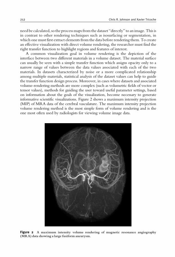
need be calculated, so the processmaps from the dataset “directly” to an image. This isin contrast to other rendering techniques such as isosurfacing or segmentation, inwhich onemust first extract elements from the data before rendering them. To createan effective visualization with direct volume rendering, the researcher must find theright transfer function to highlight regions and features of interest.
A common visualization goal in volume rendering is the depiction of theinterface between two different materials in a volume dataset. The material surfacecan usually be seen with a simple transfer function which assigns opacity only to anarrow range of values between the data values associated with each of the twomaterials. In datasets characterized by noise or a more complicated relationshipamong multiple materials, statistical analysis of the dataset values can help to guidethe transfer function design process. Moreover, in cases where datasets and associatedvolume-rendering methods are more complex (such as volumetric fields of vector ortensor values), methods for guiding the user toward useful parameter settings, basedon information about the goals of the visualization, become necessary to generateinformative scientific visualizations. Figure 2 shows a maximum intensity projection(MIP) of MRA data of the cerebral vasculature. The maximum intensity projectionvolume rendering method is the most simple form of volume rendering and is theone most often used by radiologists for viewing volume image data.
Figure 2 A maximum intensity volume rendering of magnetic resonance angiography(MRA) data showing a large fusiform aneurysm.
212 Chris R. Johnson and Xavier Tricoche
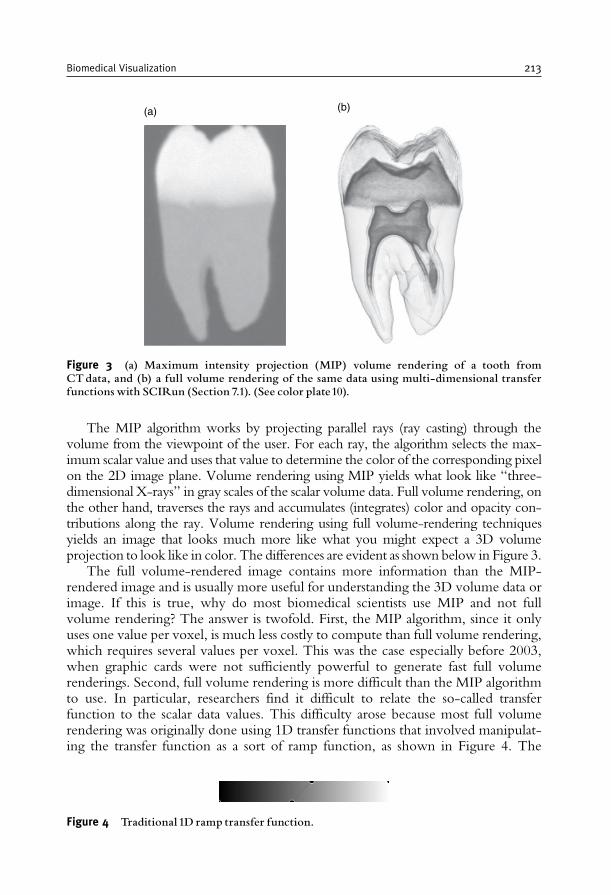
The MIP algorithm works by projecting parallel rays (ray casting) through thevolume from the viewpoint of the user. For each ray, the algorithm selects the max-imum scalar value and uses that value to determine the color of the corresponding pixelon the 2D image plane. Volume rendering using MIP yields what look like “three-dimensional X-rays” in gray scales of the scalar volume data. Full volume rendering, onthe other hand, traverses the rays and accumulates (integrates) color and opacity con-tributions along the ray. Volume rendering using full volume-rendering techniquesyields an image that looks much more like what you might expect a 3D volumeprojection to look like in color. The differences are evident as shown below in Figure 3.
The full volume-rendered image contains more information than the MIP-rendered image and is usually more useful for understanding the 3D volume data orimage. If this is true, why do most biomedical scientists use MIP and not fullvolume rendering? The answer is twofold. First, the MIP algorithm, since it onlyuses one value per voxel, is much less costly to compute than full volume rendering,which requires several values per voxel. This was the case especially before 2003,when graphic cards were not sufficiently powerful to generate fast full volumerenderings. Second, full volume rendering is more difficult than the MIP algorithmto use. In particular, researchers find it difficult to relate the so-called transferfunction to the scalar data values. This difficulty arose because most full volumerendering was originally done using 1D transfer functions that involved manipulat-ing the transfer function as a sort of ramp function, as shown in Figure 4. The
Figure 4 Traditional 1D ramp transfer function.
(a) (b)
Figure 3 (a) Maximum intensity projection (MIP) volume rendering of a tooth fromCTdata, and (b) a full volume rendering of the same data using multi-dimensional transferfunctions with SCIRun (Section 7.1). (See color plate10).
Biomedical Visualization 213
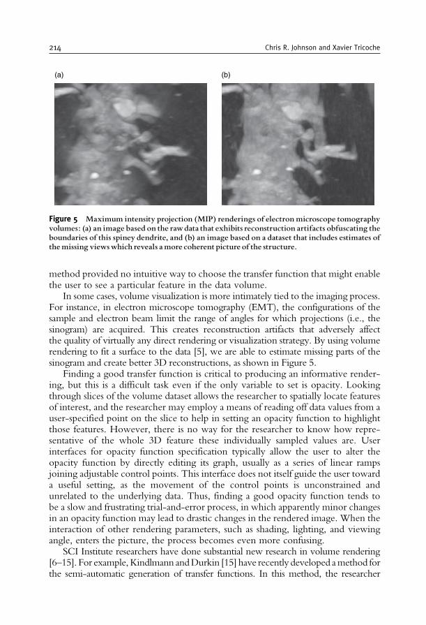
method provided no intuitive way to choose the transfer function that might enablethe user to see a particular feature in the data volume.
In some cases, volume visualization is more intimately tied to the imaging process.For instance, in electron microscope tomography (EMT), the configurations of thesample and electron beam limit the range of angles for which projections (i.e., thesinogram) are acquired. This creates reconstruction artifacts that adversely affectthe quality of virtually any direct rendering or visualization strategy. By using volumerendering to fit a surface to the data [5], we are able to estimate missing parts of thesinogram and create better 3D reconstructions, as shown in Figure 5.
Finding a good transfer function is critical to producing an informative render-ing, but this is a difficult task even if the only variable to set is opacity. Lookingthrough slices of the volume dataset allows the researcher to spatially locate featuresof interest, and the researcher may employ a means of reading off data values from auser-specified point on the slice to help in setting an opacity function to highlightthose features. However, there is no way for the researcher to know how repre-sentative of the whole 3D feature these individually sampled values are. Userinterfaces for opacity function specification typically allow the user to alter theopacity function by directly editing its graph, usually as a series of linear rampsjoining adjustable control points. This interface does not itself guide the user towarda useful setting, as the movement of the control points is unconstrained andunrelated to the underlying data. Thus, finding a good opacity function tends tobe a slow and frustrating trial-and-error process, in which apparently minor changesin an opacity function may lead to drastic changes in the rendered image. When theinteraction of other rendering parameters, such as shading, lighting, and viewingangle, enters the picture, the process becomes even more confusing.
SCI Institute researchers have done substantial new research in volume rendering[6–15]. For example,Kindlmann andDurkin [15] have recently developed amethod forthe semi-automatic generation of transfer functions. In this method, the researcher
(a) (b)
Figure 5 Maximum intensity projection (MIP) renderings of electron microscope tomographyvolumes: (a) an image based on the rawdata that exhibits reconstruction artifacts obfuscating theboundaries of this spiney dendrite, and (b) an image based on a dataset that includes estimates ofthemissing viewswhich reveals amore coherent picture of the structure.
214 Chris R. Johnson and Xavier Tricoche
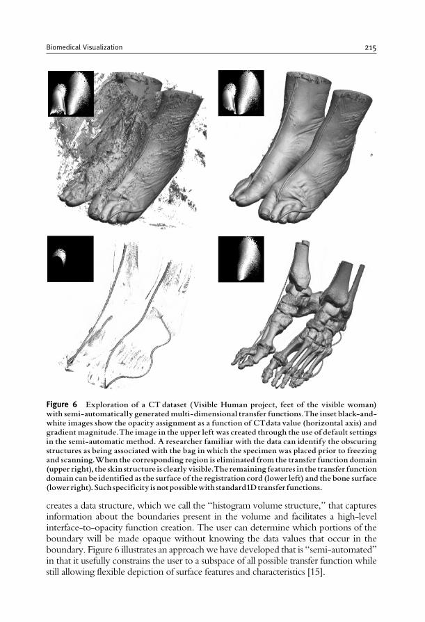
creates a data structure, which we call the “histogram volume structure,” that capturesinformation about the boundaries present in the volume and facilitates a high-levelinterface-to-opacity function creation. The user can determine which portions of theboundary will be made opaque without knowing the data values that occur in theboundary. Figure 6 illustrates an approachwe have developed that is “semi-automated”in that it usefully constrains the user to a subspace of all possible transfer function whilestill allowing flexible depiction of surface features and characteristics [15].
Figure 6 Exploration of a CT dataset (Visible Human project, feet of the visible woman)with semi-automatically generatedmulti-dimensional transfer functions.The inset black-and-white images show the opacity assignment as a function of CTdata value (horizontal axis) andgradient magnitude.The image in the upper left was created through the use of default settingsin the semi-automatic method. A researcher familiar with the data can identify the obscuringstructures as being associated with the bag in which the specimen was placed prior to freezingand scanning.When the corresponding region is eliminated from the transfer function domain(upper right), the skin structure is clearly visible.The remaining features in the transfer functiondomain can be identified as the surface of the registration cord (lower left) and the bone surface(lower right). Such specificity is notpossiblewith standard1Dtransfer functions.
Biomedical Visualization 215
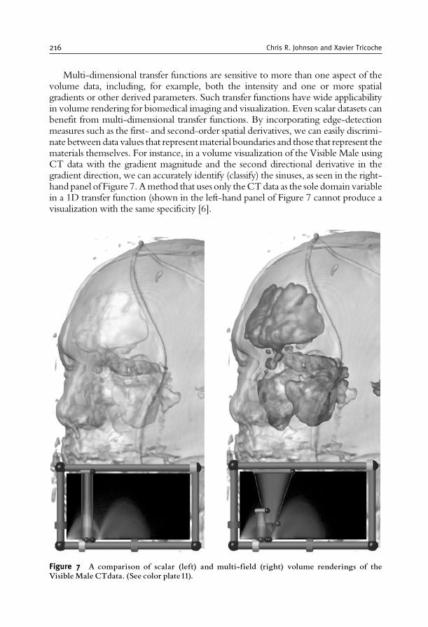
Multi-dimensional transfer functions are sensitive to more than one aspect of thevolume data, including, for example, both the intensity and one or more spatialgradients or other derived parameters. Such transfer functions have wide applicabilityin volume rendering for biomedical imaging and visualization. Even scalar datasets canbenefit from multi-dimensional transfer functions. By incorporating edge-detectionmeasures such as the first- and second-order spatial derivatives, we can easily discrimi-nate between data values that representmaterial boundaries and those that represent thematerials themselves. For instance, in a volume visualization of the Visible Male usingCT data with the gradient magnitude and the second directional derivative in thegradient direction, we can accurately identify (classify) the sinuses, as seen in the right-hand panel of Figure 7.Amethod that uses only theCTdata as the sole domain variablein a 1D transfer function (shown in the left-hand panel of Figure 7 cannot produce avisualization with the same specificity [6].
Figure 7 A comparison of scalar (left) and multi-field (right) volume renderings of theVisibleMale CTdata. (See color plate11).
216 Chris R. Johnson and Xavier Tricoche
Multi-dimensional transfer functions are also valuable for more general cases inwhich the data come from multiple variables in a physical simulation or multiplemedical-imaging modalities. In such a case, the transfer function allows one toidentify phenomena or features that can be described or classified based only on thebasis of unique combinations of data values. Medical imaging can also benefit frommulti-dimensional transfer functions when features of interest are not adequatelydescribed by any one imaging modality. For instance, CT imaging captures varia-tions in bone structure but does not differentiate soft tissues well, whereas MRimaging differentiates soft tissue well and bone very poorly. By visualizing a co-registered CT and MRI dataset simultaneously, one can visualize features of interestin the soft tissue along with important bone landmarks.
To resolve the complexities inherent in a user interface for multi-dimensional transfer functions, we introduced a set of direct manipulationwidgets that make finding and experimenting with transfer functions an intui-tive, efficient, and informative process. To achieve interactive response, weexploited the fast rendering capabilities of modern graphics hardware, especially3D texture memory and pixel texturing operations. Together, the widgets andthe hardware form the basis for new interaction modes that guide the usertoward transfer function settings appropriate for their visualization and dataexploration interests [10,16,17].
The generalization of direct volume rendering to multi-valued fields presents atleast two research challenges on which future work can focus, the first involvingsurface shading and the second involving the efficient evaluation of multi-dimensional transfer functions. Crucial to successful volume rendering is thecalculation from the original data of the spatial gradients with which shading andsurface rendering will be performed. In scalar data, the gradient has a simplemathematical definition and computation. In multi-valued fields, however, thegeneralization of the gradient is matrix-valued, and the surface orientation is repre-sented as an eigenvector of this matrix. Current volume-rendering methods makelittle use of this information because it is computationally expensive, although advancesin the abilities of GPUs increasingly support these calculations at interactive rates.
As described above, multi-dimensional transfer functions permit the visualiza-tion of structure based on combinations of values within the constituent fields. Asthe number of fields increases, simple implementations of multi-dimensional trans-fer functions become unwieldy. This observation motivated us to investigateanalytic expressions for transfer function representation [7]. We have introduceda flexible framework for classifying and rendering multi-field datasets using transferfunctions based on Gaussian primitives. We show in the paper that Gaussian transferfunctions have a number of key features: they allow for selective classification ofnarrow features, can be efficiently computed on the graphics hardware, and theirintegral along a line segment has, under very limited assumptions, a closed-formanalytic solution. Hence, they obviate the need for large precomputed lookuptables and are very memory efficient.
We expect this approach to have a large impact on the qualitative and quanti-tative value of volume rendering and become a significant tool for biomedicalresearchers. An example is shown in Figure 8.
Biomedical Visualization 217
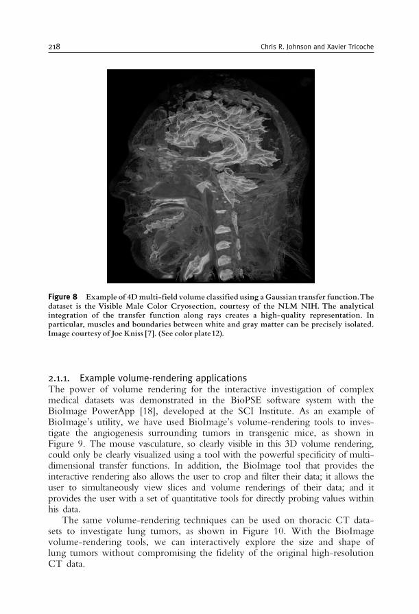
2.1.1. Example volume-rendering applicationsThe power of volume rendering for the interactive investigation of complexmedical datasets was demonstrated in the BioPSE software system with theBioImage PowerApp [18], developed at the SCI Institute. As an example ofBioImage’s utility, we have used BioImage’s volume-rendering tools to inves-tigate the angiogenesis surrounding tumors in transgenic mice, as shown inFigure 9. The mouse vasculature, so clearly visible in this 3D volume rendering,could only be clearly visualized using a tool with the powerful specificity of multi-dimensional transfer functions. In addition, the BioImage tool that provides theinteractive rendering also allows the user to crop and filter their data; it allows theuser to simultaneously view slices and volume renderings of their data; and itprovides the user with a set of quantitative tools for directly probing values withinhis data.
The same volume-rendering techniques can be used on thoracic CT data-sets to investigate lung tumors, as shown in Figure 10. With the BioImagevolume-rendering tools, we can interactively explore the size and shape oflung tumors without compromising the fidelity of the original high-resolutionCT data.
Figure 8 Example of 4Dmulti-field volume classified using a Gaussian transfer function.Thedataset is the Visible Male Color Cryosection, courtesy of the NLM NIH. The analyticalintegration of the transfer function along rays creates a high-quality representation. Inparticular, muscles and boundaries between white and gray matter can be precisely isolated.Image courtesy of Joe Kniss [7]. (See color plate12).
218 Chris R. Johnson and Xavier Tricoche
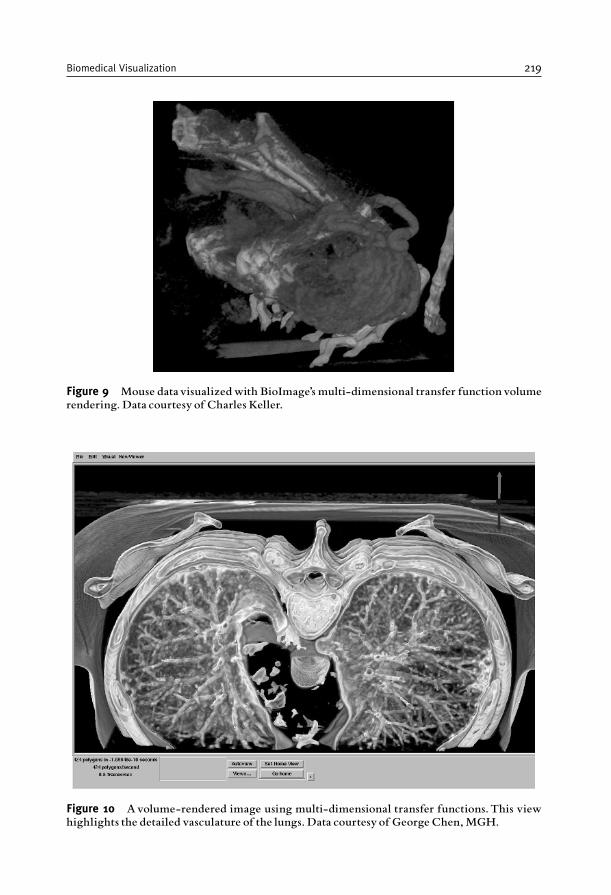
Figure 9 Mouse datavisualizedwith BioImage’s multi-dimensional transfer function volumerendering. Data courtesy of Charles Keller.
Figure 10 Avolume-rendered image using multi-dimensional transfer functions.This viewhighlights the detailed vasculature of the lungs. Data courtesy of George Chen,MGH.
Biomedical Visualization 219

2.2. Isosurface extraction
Isosurface extraction is a powerful tool for investigating volumetric scalar fields. Anisosurface in a scalar volume is a surface on which the data value is constant,separating regions of higher and lower value. Given the physical or biologicalsignificance of the data value (i.e., radio-opacity, dye concentration, fluorescencelevel), the position of an isosurface, as well as its relation to other neighboringisosurfaces, can provide clues to the underlying structure of the scalar field. Inbiomedical imaging applications, isosurfaces permit the extraction of particularanatomical structures and tissues; however, these isosurfaces are typically static innature. A more dynamic use of isosurfaces can provide better visualization ofcomplex space- or time-dependent behaviors in many scientific applications.
Within the last 15 years, isosurface extraction methods have advanced signifi-cantly, from an off-line, single-surface extraction process into an interactive,exploratory visualization tool. Interactivity is especially important in exploratoryvisualization where the user has no a priori knowledge of any underlying structuresin the data. A typical data exploration session therefore requires the researcher tomake many isovalue changes in search of interesting features. In addition, it ishelpful to provide global views (to place an isosurface in the context of the entiredataset) and detailed views of small sections of interest. Maintaining interactivitywhile meeting these visualization goals is especially challenging for large datasetsand complex isosurface geometry.
The Marching Cubes [19,20] method, introduced in 1986, was the first practicaland most successful isosurface extraction algorithm. Its simplicity has made it thede facto standard extraction method even to this date. The Marching Cubes algo-rithm demonstrated that isosurface extraction can be reduced, using a divide andconquer approach, to solving a local triangulation problem. In addition, themarching cubes method proposed a simple and efficient local triangulation schemethat uses a lookup table. Subsequently, researchers created methods for acceleratingthe search phase for isosurface extraction [21–25] all of which have a complexityof O(n), where n is the number of voxels in the volume. We introduced thespan space [26] as a means for mapping the search onto a 2D space and then usedit to create a near optimal isosurface extraction (NOISE) algorithm that has a timecomplexity of O
ffiffiffin
p þ kð Þ, where k is the size of the isosurface. Cignoni et al. [27]employed another decomposition of the span space leading to a search method withoptimal time complexity ofO(log nþ k), albeit with larger storage requirements. Inaddition, Bajaj et al. introduced the contour spectrum, which provides a fastisosurface algorithm and a user interface component that improves qualitativeuser interaction and provides real-time exact quantification in the visualization ofisocontours [28,29].
We improved further on these isosurface extraction methods by using a differ-ent visibility testing approach and virtual buffer rendering to achieve a real-time,view-dependent isosurface extraction [30–33]. We also presented a progressivehardware-assisted isosurface extraction (PHASE) that is suitable for remote visua-lization, i.e., when the data and display device reside on separate computers. Thisapproach works by reusing, when a view point is changed, the information and
220 Chris R. Johnson and Xavier Tricoche
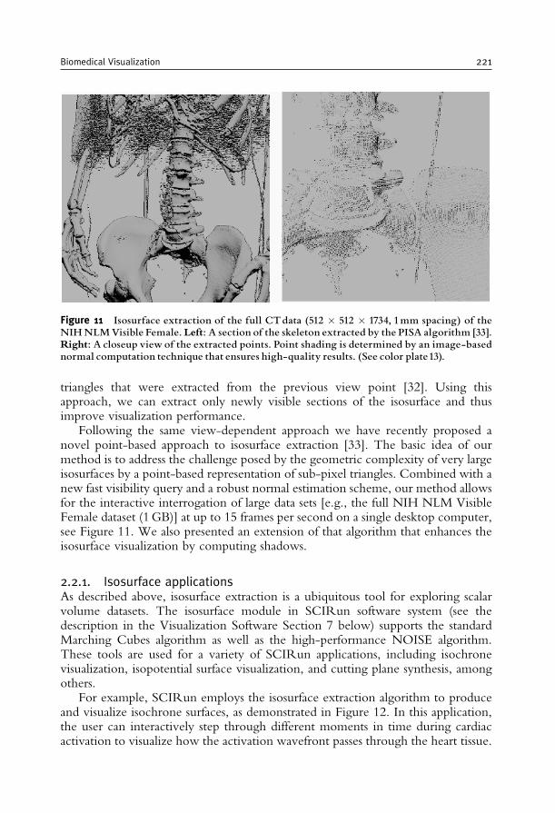
triangles that were extracted from the previous view point [32]. Using thisapproach, we can extract only newly visible sections of the isosurface and thusimprove visualization performance.
Following the same view-dependent approach we have recently proposed anovel point-based approach to isosurface extraction [33]. The basic idea of ourmethod is to address the challenge posed by the geometric complexity of very largeisosurfaces by a point-based representation of sub-pixel triangles. Combined with anew fast visibility query and a robust normal estimation scheme, our method allowsfor the interactive interrogation of large data sets [e.g., the full NIH NLM VisibleFemale dataset (1GB)] at up to 15 frames per second on a single desktop computer,see Figure 11. We also presented an extension of that algorithm that enhances theisosurface visualization by computing shadows.
2.2.1. Isosurface applicationsAs described above, isosurface extraction is a ubiquitous tool for exploring scalarvolume datasets. The isosurface module in SCIRun software system (see thedescription in the Visualization Software Section 7 below) supports the standardMarching Cubes algorithm as well as the high-performance NOISE algorithm.These tools are used for a variety of SCIRun applications, including isochronevisualization, isopotential surface visualization, and cutting plane synthesis, amongothers.
For example, SCIRun employs the isosurface extraction algorithm to produceand visualize isochrone surfaces, as demonstrated in Figure 12. In this application,the user can interactively step through different moments in time during cardiacactivation to visualize how the activation wavefront passes through the heart tissue.
Figure 11 Isosurface extraction of the full CTdata (512 � 512 � 1734, 1mm spacing) of theNIHNLMVisible Female. Left: A section of the skeleton extracted by the PISA algorithm [33].Right: A closeup view of the extracted points. Point shading is determined by an image-basednormal computation technique that ensures high-quality results. (See color plate13).
Biomedical Visualization 221
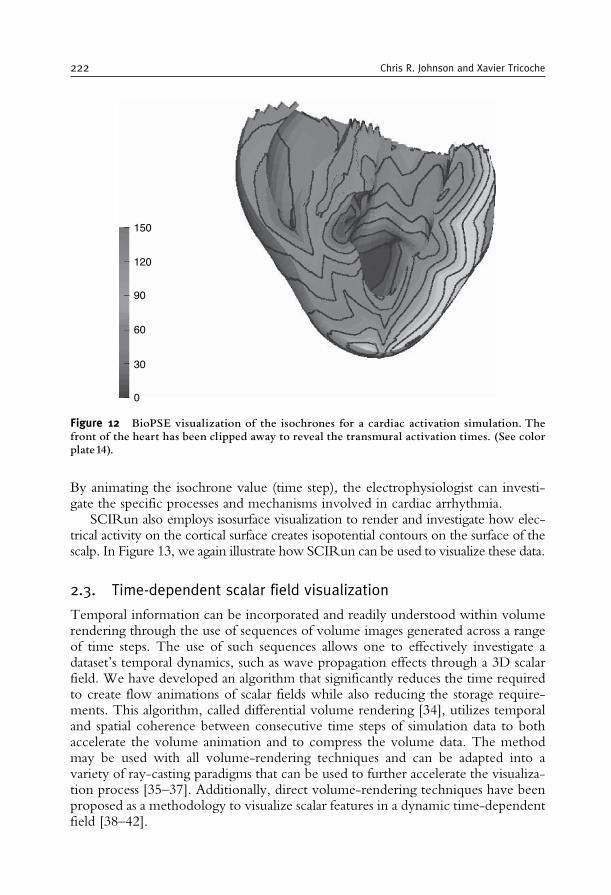
By animating the isochrone value (time step), the electrophysiologist can investi-gate the specific processes and mechanisms involved in cardiac arrhythmia.
SCIRun also employs isosurface visualization to render and investigate how elec-trical activity on the cortical surface creates isopotential contours on the surface of thescalp. In Figure 13, we again illustrate how SCIRun can be used to visualize these data.
2.3. Time-dependent scalar field visualization
Temporal information can be incorporated and readily understood within volumerendering through the use of sequences of volume images generated across a rangeof time steps. The use of such sequences allows one to effectively investigate adataset’s temporal dynamics, such as wave propagation effects through a 3D scalarfield. We have developed an algorithm that significantly reduces the time requiredto create flow animations of scalar fields while also reducing the storage require-ments. This algorithm, called differential volume rendering [34], utilizes temporaland spatial coherence between consecutive time steps of simulation data to bothaccelerate the volume animation and to compress the volume data. The methodmay be used with all volume-rendering techniques and can be adapted into avariety of ray-casting paradigms that can be used to further accelerate the visualiza-tion process [35–37]. Additionally, direct volume-rendering techniques have beenproposed as a methodology to visualize scalar features in a dynamic time-dependentfield [38–42].
0
30
60
90
120
150
Figure 12 BioPSE visualization of the isochrones for a cardiac activation simulation. Thefront of the heart has been clipped away to reveal the transmural activation times. (See colorplate14).
222 Chris R. Johnson and Xavier Tricoche
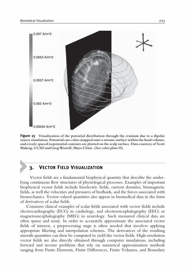
3. VECTOR FIELD VISUALIZATION
Vector fields are a fundamental biophysical quantity that describe the under-lying continuous flow structures of physiological processes. Examples of importantbiophysical vector fields include bioelectric fields, current densities, biomagneticfields, as well the velocities and pressures of biofluids, and the forces associated withbiomechanics. Vector-valued quantities also appear in biomedical data in the formof derivatives of scalar fields.
Common clinical examples of scalar fields associated with vector fields includeelectrocardiography (ECG) in cardiology, and electroencephalography (EEG) ormagnetoancephalography (MEG) in neurology. Such measured clinical data areoften sparse and noisy. In order to accurately approximate the associated vectorfields of interest, a preprocessing stage is often needed that involves applyingappropriate filtering and interpolation schemes. The derivatives of the resultingsmooth quantities can then be computed to yield the vector fields. High-resolutionvector fields are also directly obtained through computer simulations, includingforward and inverse problems that rely on numerical approximation methodsranging from Finite Elements, Finite Differences, Finite Volumes, and Boundary
0.007 A/m^2
0.0053 A/m^2
0.0037 A/m^2
0.002 A/m^2
0.00034 A/m^2
Figure 13 Visualization of the potential distribution through the cranium due to a dipolarsource simulation. Potentials are color-mapped onto a stream-surface within the head volume,and evenly spaced isopotential contours are plotted on the scalp surface. Data courtesy of ScottMakeig, UCSD and GregWorrell, Mayo Clinic. (See color plate15).
Biomedical Visualization 223
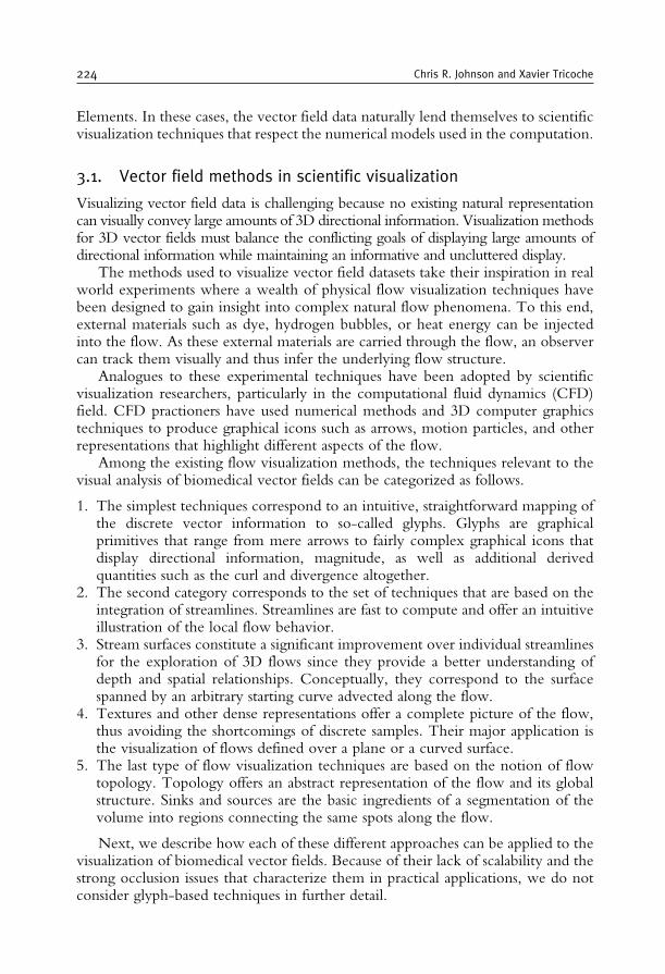
Elements. In these cases, the vector field data naturally lend themselves to scientificvisualization techniques that respect the numerical models used in the computation.
3.1. Vector field methods in scientific visualization
Visualizing vector field data is challenging because no existing natural representationcan visually convey large amounts of 3D directional information. Visualization methodsfor 3D vector fields must balance the conflicting goals of displaying large amounts ofdirectional information while maintaining an informative and uncluttered display.
The methods used to visualize vector field datasets take their inspiration in realworld experiments where a wealth of physical flow visualization techniques havebeen designed to gain insight into complex natural flow phenomena. To this end,external materials such as dye, hydrogen bubbles, or heat energy can be injectedinto the flow. As these external materials are carried through the flow, an observercan track them visually and thus infer the underlying flow structure.
Analogues to these experimental techniques have been adopted by scientificvisualization researchers, particularly in the computational fluid dynamics (CFD)field. CFD practioners have used numerical methods and 3D computer graphicstechniques to produce graphical icons such as arrows, motion particles, and otherrepresentations that highlight different aspects of the flow.
Among the existing flow visualization methods, the techniques relevant to thevisual analysis of biomedical vector fields can be categorized as follows.
1. The simplest techniques correspond to an intuitive, straightforward mapping ofthe discrete vector information to so-called glyphs. Glyphs are graphicalprimitives that range from mere arrows to fairly complex graphical icons thatdisplay directional information, magnitude, as well as additional derivedquantities such as the curl and divergence altogether.
2. The second category corresponds to the set of techniques that are based on theintegration of streamlines. Streamlines are fast to compute and offer an intuitiveillustration of the local flow behavior.
3. Stream surfaces constitute a significant improvement over individual streamlinesfor the exploration of 3D flows since they provide a better understanding ofdepth and spatial relationships. Conceptually, they correspond to the surfacespanned by an arbitrary starting curve advected along the flow.
4. Textures and other dense representations offer a complete picture of the flow,thus avoiding the shortcomings of discrete samples. Their major application isthe visualization of flows defined over a plane or a curved surface.
5. The last type of flow visualization techniques are based on the notion of flowtopology. Topology offers an abstract representation of the flow and its globalstructure. Sinks and sources are the basic ingredients of a segmentation of thevolume into regions connecting the same spots along the flow.
Next, we describe how each of these different approaches can be applied to thevisualization of biomedical vector fields. Because of their lack of scalability and thestrong occlusion issues that characterize them in practical applications, we do notconsider glyph-based techniques in further detail.
224 Chris R. Johnson and Xavier Tricoche
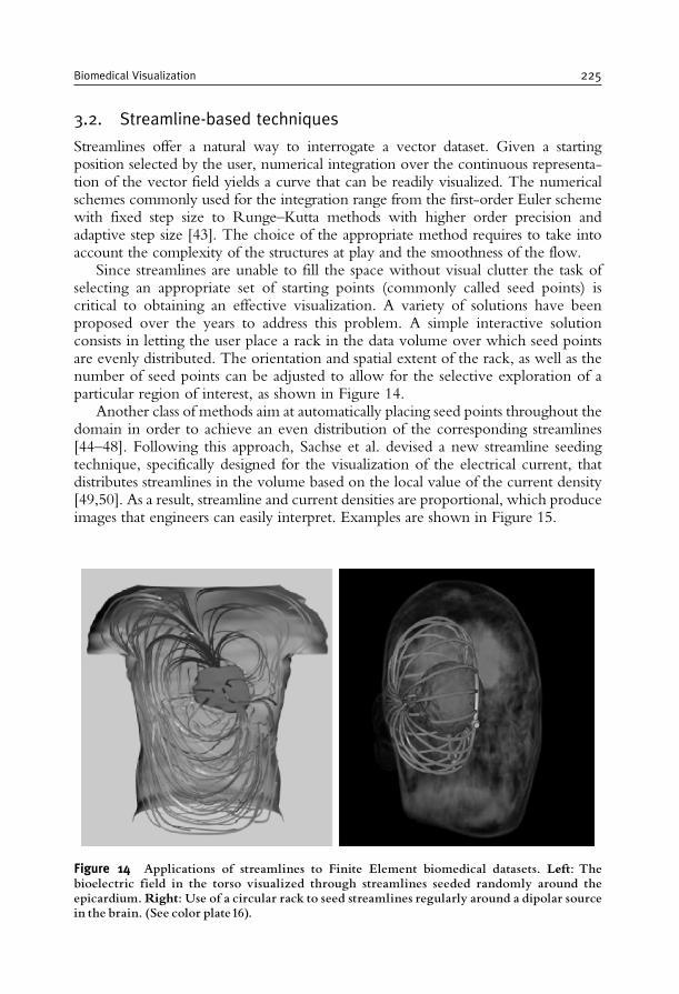
3.2. Streamline-based techniques
Streamlines offer a natural way to interrogate a vector dataset. Given a startingposition selected by the user, numerical integration over the continuous representa-tion of the vector field yields a curve that can be readily visualized. The numericalschemes commonly used for the integration range from the first-order Euler schemewith fixed step size to Runge–Kutta methods with higher order precision andadaptive step size [43]. The choice of the appropriate method requires to take intoaccount the complexity of the structures at play and the smoothness of the flow.
Since streamlines are unable to fill the space without visual clutter the task ofselecting an appropriate set of starting points (commonly called seed points) iscritical to obtaining an effective visualization. A variety of solutions have beenproposed over the years to address this problem. A simple interactive solutionconsists in letting the user place a rack in the data volume over which seed pointsare evenly distributed. The orientation and spatial extent of the rack, as well as thenumber of seed points can be adjusted to allow for the selective exploration of aparticular region of interest, as shown in Figure 14.
Another class of methods aim at automatically placing seed points throughout thedomain in order to achieve an even distribution of the corresponding streamlines[44–48]. Following this approach, Sachse et al. devised a new streamline seedingtechnique, specifically designed for the visualization of the electrical current, thatdistributes streamlines in the volume based on the local value of the current density[49,50]. As a result, streamline and current densities are proportional, which produceimages that engineers can easily interpret. Examples are shown in Figure 15.
Figure 14 Applications of streamlines to Finite Element biomedical datasets. Left: Thebioelectric field in the torso visualized through streamlines seeded randomly around theepicardium.Right: Use of a circular rack to seed streamlines regularly around a dipolar sourcein the brain. (See color plate16).
Biomedical Visualization 225
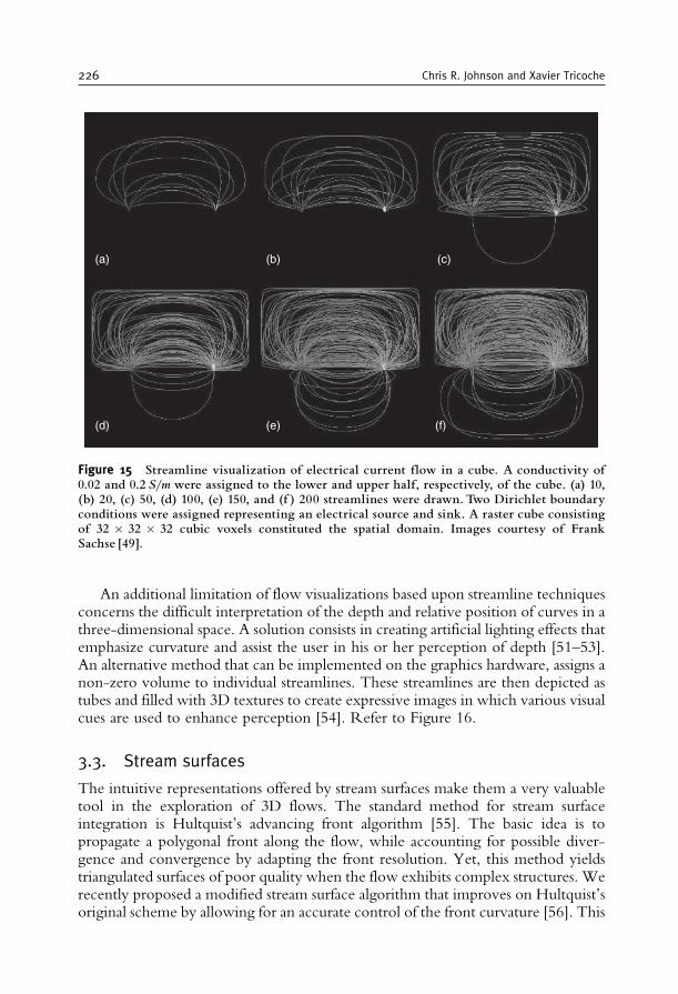
An additional limitation of flow visualizations based upon streamline techniquesconcerns the difficult interpretation of the depth and relative position of curves in athree-dimensional space. A solution consists in creating artificial lighting effects thatemphasize curvature and assist the user in his or her perception of depth [51–53].An alternative method that can be implemented on the graphics hardware, assigns anon-zero volume to individual streamlines. These streamlines are then depicted astubes and filled with 3D textures to create expressive images in which various visualcues are used to enhance perception [54]. Refer to Figure 16.
3.3. Stream surfaces
The intuitive representations offered by stream surfaces make them a very valuabletool in the exploration of 3D flows. The standard method for stream surfaceintegration is Hultquist’s advancing front algorithm [55]. The basic idea is topropagate a polygonal front along the flow, while accounting for possible diver-gence and convergence by adapting the front resolution. Yet, this method yieldstriangulated surfaces of poor quality when the flow exhibits complex structures. Werecently proposed a modified stream surface algorithm that improves on Hultquist’soriginal scheme by allowing for an accurate control of the front curvature [56]. This
(a) (b) (c)
(d) (e) (f)
Figure 15 Streamline visualization of electrical current flow in a cube. A conductivity of0.02 and 0.2 S/m were assigned to the lower and upper half, respectively, of the cube. (a) 10,(b) 20, (c) 50, (d) 100, (e) 150, and (f ) 200 streamlines were drawn. Two Dirichlet boundaryconditions were assigned representing an electrical source and sink. A raster cube consistingof 32 � 32 � 32 cubic voxels constituted the spatial domain. Images courtesy of FrankSachse [49].
226 Chris R. Johnson and Xavier Tricoche
method creates smooth, high-quality surfaces, even for very intricate flow patterns.We applied stream surfaces to the visualization of the cardiothoracic currentobtained through a Finite Elements simulation [49]. Specifically, stream surfaceswere shown to permit insight into the interconnection of different regions of theepicardium through the bioelectric current inside the thorax. An illustration isshown in Figure 17.
A similar approach was used to visualize the return current in a high-resolutionsimulation of a realistic head model. In this case, stream surfaces proved instrumentalin assessing the impact of various models of the white matter anisotropy on thecurrent pattern and its interconnection with anatomical structures, see Figure 18 andSection 5.1.
Despite their esthetic appeal and the effective visualizations they yield, streamsurfaces share with streamlines the limitation induced by their reliance on a carefulseeding. Here, the seeding task consists in selecting a starting curve such that theresulting surface will exhibit the characteristic patterns of important flow structures.As with streamlines, this task can be tedious. In the case of the bioelectric current,flow structures can be defined in terms of interconnections between zones of inflowand outflow on surface enclosing dipolar sources. This is the solution that weapplied in Figures 17 and 18. To visualize the cardiothoracic current isocontours of
Figure 16 An extension of streamline-based Flow Visualization. The image shows acombination of streamlines and 3D textures in the visualization of a tornado data set.Texturespermit to embed additional information and ease the interpretation of the spatial context.From Li et al. [54].
Biomedical Visualization 227
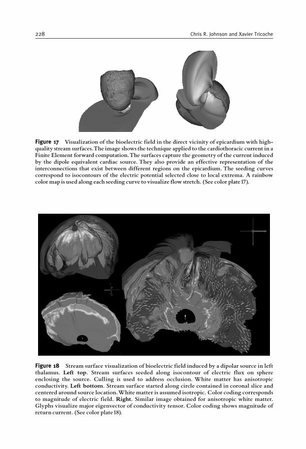
Figure 17 Visualization of the bioelectric field in the direct vicinity of epicardium with high-quality stream surfaces.The image shows the technique applied to the cardiothoracic current in aFinite Element forward computation.The surfaces capture the geometry of the current inducedby the dipole equivalent cardiac source. They also provide an effective representation of theinterconnections that exist between different regions on the epicardium. The seeding curvescorrespond to isocontours of the electric potential selected close to local extrema. A rainbowcolor map is used along each seeding curve tovisualize flow stretch. (See color plate17).
Figure 18 Stream surface visualization of bioelectric field induced by a dipolar source in leftthalamus. Left top. Stream surfaces seeded along isocontour of electric flux on sphereenclosing the source. Culling is used to address occlusion. White matter has anisotropicconductivity. Left bottom. Stream surface started along circle contained in coronal slice andcentered around source location.White matter is assumed isotropic. Color coding correspondsto magnitude of electric field. Right. Similar image obtained for anisotropic white matter.Glyphs visualize major eigenvector of conductivity tensor. Color coding shows magnitude ofreturn current. (See color plate18).
228 Chris R. Johnson and Xavier Tricoche
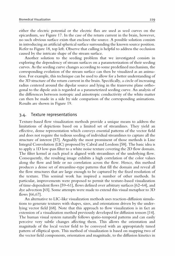
either the electric potential or the electric flux are used as seed curves on theepicardium, see Figure 17. In the case of the return current in the brain, however,no such obvious surface exists that encloses the source. A possible solution consistsin introducing an artificial spherical surface surrounding the known source position.Refer to Figure 18, top left. Observe that culling is helpful to address the occlusioncaused by the intricate shape of the stream surface.
Another solution to the seeding problem that we investigated consists inexploring the dependency of stream surfaces on a parameterization of their seedingcurves. As the seeding curve changes according to some predefined mechanism, thecorresponding evolution of the stream surface can then be visualized as an anima-tion. For example, this technique can be used to allow for a better understanding ofthe 3D structure of the return current in the brain. Specifically, a circle of increasingradius centered around the dipolar source and lying in the transverse plane ortho-gonal to the dipole axis is regarded as a parameterized seeding curve. An analysis ofthe differences between isotropic and anisotropic conductivity of the white mattercan then be made in a side by side comparison of the corresponding animations.Results are shown in Figure 19.
3.4. Texture representations
Texture-based flow visualization methods provide a unique means to address thelimitations of depictions based on a limited set of streamlines. They yield aneffective, dense representation which conveys essential patterns of the vector fieldand does not require the tedious seeding of individual streamlines to capture all thestructure of interest [57]. Arguably the most prominent of those methods is LineIntegral Convolution (LIC) proposed by Cabral and Leedom [58]. The basic idea isto apply a 1D low-pass filter to a white noise texture covering the 2D flow domain.The filter kernel at each pixel is aligned with streamlines of the underlying flow.Consequently, the resulting image exhibits a high correlation of the color valuesalong the flow and little or no correlation across the flow. Hence, this methodproduces a dense set of streamline-type patterns that fill the domain and reveal allthe flow structures that are large enough to be captured by the fixed resolution ofthe texture. This seminal work has inspired a number of other methods. Inparticular, improvements were proposed to permit the texture-based visualizationof time-dependent flows [59–61], flows defined over arbitrary surfaces [62–64], anddye advection [65]. Some attempts were made to extend this visual metaphor to 3Dflows [66,67].
An alternative to LIC-like visualization methods uses reaction-diffusion simula-tions to generate textures with shapes, sizes, and orientations driven by the under-lying vector field [68]. Note that this approach to flow visualization is in fact anextension of a visualization method previously developed for diffusion tensors [14].The human visual system naturally follows spatio-temporal patterns and can easilyperceive very subtle changes affecting them. This allows the orientation andmagnitude of the local vector field to be conveyed with an appropriately tunedpattern of elliptical spots. This method of visualization is based on mapping two ofthe vector field components, orientation and magnitude, to the diffusion kinetics in
Biomedical Visualization 229
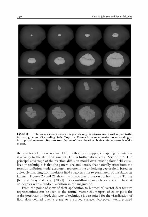
the reaction-diffusion system. Our method also supports mapping orientationuncertainty to the diffusion kinetics. This is further discussed in Section 5.2. Theprincipal advantage of the reaction-diffusion model over existing flow field visua-lization techniques is that the pattern size and density that naturally arises from thereaction-diffusion model accurately represents the underlying vector field, based ona flexible mapping from multiple field characteristics to parameters of the diffusionkinetics. Figures 20 and 21 show the anisotropic diffusion applied to the Turing[69] and Gray and Scott [70,71] reaction-diffusion models for a vector field at45 degrees with a random variation in the magnitude.
From the point of view of their application to biomedical vector data texturerepresentations can be seen as the natural vector counterpart of color plots forscalar potentials. Indeed, this type of technique is best suited for the visualization offlow data defined over a plane or a curved surface. Moreover, texture-based
Figure 19 Evolution of a stream surface integrated along the return currentwith respect to theincreasing radius of its seeding circle. Top row. Frames from an animation corresponding toisotropic white matter. Bottom row. Frames of the animation obtained for anisotropic whitematter.
230 Chris R. Johnson and Xavier Tricoche
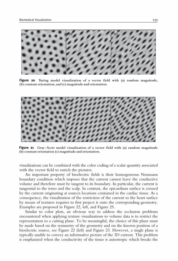
visualizations can be combined with the color coding of a scalar quantity associatedwith the vector field to enrich the pictures.
An important property of bioelectric fields is their homogeneous Neumannboundary condition which imposes that the current cannot leave the conductivevolume and therefore must be tangent to its boundary. In particular, the current istangential to the torso and the scalp. In contrast, the epicardium surface is crossedby the current originating at sources locations contained in the cardiac tissue. As aconsequence, the visualization of the restriction of the current to the heart surfaceby means of textures requires to first project it onto the corresponding geometry.Examples are proposed in Figure 22, left, and Figure 25.
Similar to color plots, an obvious way to address the occlusion problemsencountered when applying texture visualizations to volume data is to restrict therepresentation to a cutting plane. To be meaningful, the choice of this plane mustbe made based on the symmetry of the geometry and on the known position of abioelectric source, see Figure 22 (left) and Figure 23. However, a single plane istypically unable to convey an informative picture of the 3D current. This problemis emphasized when the conductivity of the tissue is anisotropic which breaks the
(a) (b) (c)
Figure 20 Turing model visualization of a vector field with (a) random magnitude,(b) constant orientation, and (c) magnitude and orientation.
(a) (b) (c)
Figure 21 Gray^Scott model visualization of a vector field with (a) random magnitude(b) constant orientation (c) magnitude and orientation.
Biomedical Visualization 231
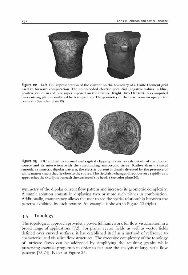
symmetry of the dipolar current flow pattern and increases its geometric complexity.A simple solution consists in displaying two or more such planes in combination.Additionally, transparency allows the user to see the spatial relationship between thepatterns exhibited by each texture. An example is shown in Figure 22 (right).
3.5. Topology
The topological approach provides a powerful framework for flow visualization in abroad range of applications [72]. For planar vector fields, as well as vector fieldsdefined over curved surfaces, it has established itself as a method of reference tocharacterize and visualize flow structures. The excessive complexity of the topologyof intricate flows can be addressed by simplifying the resulting graphs whilepreserving essential properties in order to facilitate the analysis of large-scale flowpatterns [73,74]. Refer to Figure 24.
Figure 22 Left. LIC representation of the current on the boundary of a Finite Element gridused in forward computation. The color-coded electric potential (negative values in blue,positive values in red) are superimposed on the texture. Right. Two LIC textures computedover cutting planes combined by transparency.The geometry of the heart remains opaque forcontext. (See color plate19).
Figure 23 LIC applied to coronal and sagittal clipping planes reveals details of the dipolarsource and its interaction with the surrounding anisotropic tissue. Rather than a typicalsmooth, symmetric dipolar pattern, the electric current is clearly diverted by the presence ofwhite matter tracts that lie close to the source.The field also changes direction very rapidly as itapproaches the skull just beneath the surface of the head. (See color plate 20).
232 Chris R. Johnson and Xavier Tricoche
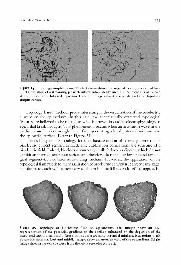
Topology-based methods prove interesting in the visualization of the bioelectriccurrent on the epicardium. In this case, the automatically extracted topologicalfeatures are believed to be related to what is known in cardiac electrophysiology asepicardial breakthroughs. This phenomenon occurs when an activation wave in thecardiac tissue breaks through the surface, generating a local potential minimum inthe epicardial surface. Refer to Figure 25.
The usability of 3D topology for the characterization of salient patterns of thebioelectric current remains limited. The explanation comes from the structure of abioelectric field. Indeed, bioelectric sources typically behave as dipoles, which do notexhibit an intrinsic separation surface and therefore do not allow for a natural topolo-gical segmentation of their surrounding medium. However, the application of thetopological framework to the visualization of bioelectric activity is at a very early stage,and future research will be necessary to determine the full potential of this approach.
Figure 24 Topology simplification.The left image shows the original topology obtained for aCFD simulation of a streaming jet with inflow into a steady medium. Numerous small-scalestructures lead to a cluttered depiction.The right image shows the same data set after topologysimplification.
Figure 25 Topology of bioelectric field on epicardium. The images show an LICrepresentation of the potential gradient on the surface enhanced by the depiction of theassociated topological graph. Green points correspond to potential minima, blue points markpotentials maxima. Left and middle images show an anterior view of the epicardium. Rightimage shows aviewof the torso from the left. (See color plate 21).
Biomedical Visualization 233
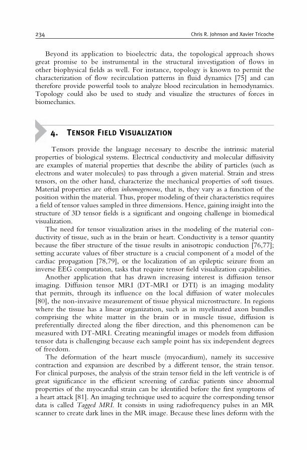
Beyond its application to bioelectric data, the topological approach showsgreat promise to be instrumental in the structural investigation of flows inother biophysical fields as well. For instance, topology is known to permit thecharacterization of flow recirculation patterns in fluid dynamics [75] and cantherefore provide powerful tools to analyze blood recirculation in hemodynamics.Topology could also be used to study and visualize the structures of forces inbiomechanics.
4. TENSOR FIELD VISUALIZATION
Tensors provide the language necessary to describe the intrinsic materialproperties of biological systems. Electrical conductivity and molecular diffusivityare examples of material properties that describe the ability of particles (such aselectrons and water molecules) to pass through a given material. Strain and stresstensors, on the other hand, characterize the mechanical properties of soft tissues.Material properties are often inhomogeneous, that is, they vary as a function of theposition within the material. Thus, proper modeling of their characteristics requiresa field of tensor values sampled in three dimensions. Hence, gaining insight into thestructure of 3D tensor fields is a significant and ongoing challenge in biomedicalvisualization.
The need for tensor visualization arises in the modeling of the material con-ductivity of tissue, such as in the brain or heart. Conductivity is a tensor quantitybecause the fiber structure of the tissue results in anisotropic conduction [76,77];setting accurate values of fiber structure is a crucial component of a model of thecardiac propagation [78,79], or the localization of an epileptic seizure from aninverse EEG computation, tasks that require tensor field visualization capabilities.
Another application that has drawn increasing interest is diffusion tensorimaging. Diffusion tensor MRI (DT-MRI or DTI) is an imaging modalitythat permits, through its influence on the local diffusion of water molecules[80], the non-invasive measurement of tissue physical microstructure. In regionswhere the tissue has a linear organization, such as in myelinated axon bundlescomprising the white matter in the brain or in muscle tissue, diffusion ispreferentially directed along the fiber direction, and this phenomenon can bemeasured with DT-MRI. Creating meaningful images or models from diffusiontensor data is challenging because each sample point has six independent degreesof freedom.
The deformation of the heart muscle (myocardium), namely its successivecontraction and expansion are described by a different tensor, the strain tensor.For clinical purposes, the analysis of the strain tensor field in the left ventricle is ofgreat significance in the efficient screening of cardiac patients since abnormalproperties of the myocardial strain can be identified before the first symptoms ofa heart attack [81]. An imaging technique used to acquire the corresponding tensordata is called Tagged MRI. It consists in using radiofrequency pulses in an MRscanner to create dark lines in the MR image. Because these lines deform with the
234 Chris R. Johnson and Xavier Tricoche
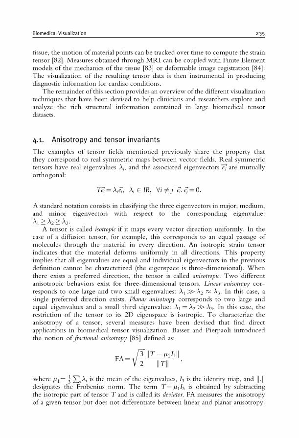
tissue, the motion of material points can be tracked over time to compute the straintensor [82]. Measures obtained through MRI can be coupled with Finite Elementmodels of the mechanics of the tissue [83] or deformable image registration [84].The visualization of the resulting tensor data is then instrumental in producingdiagnostic information for cardiac conditions.
The remainder of this section provides an overview of the different visualizationtechniques that have been devised to help clinicians and researchers explore andanalyze the rich structural information contained in large biomedical tensordatasets.
4.1. Anisotropy and tensor invariants
The examples of tensor fields mentioned previously share the property thatthey correspond to real symmetric maps between vector fields. Real symmetrictensors have real eigenvalues i, and the associated eigenvectors e!i are mutuallyorthogonal:
Te~i= ie~i; i 2 IR; 8i 6¼ j e~i: e~j = 0:
A standard notation consists in classifying the three eigenvectors in major, medium,and minor eigenvectors with respect to the corresponding eigenvalue: 1� 2� 3.
A tensor is called isotropic if it maps every vector direction uniformly. In thecase of a diffusion tensor, for example, this corresponds to an equal passage ofmolecules through the material in every direction. An isotropic strain tensorindicates that the material deforms uniformly in all directions. This propertyimplies that all eigenvalues are equal and individual eigenvectors in the previousdefinition cannot be characterized (the eigenspace is three-dimensional). Whenthere exists a preferred direction, the tensor is called anisotropic. Two differentanisotropic behaviors exist for three-dimensional tensors. Linear anisotropy cor-responds to one large and two small eigenvalues: 1>> 2 � 3. In this case, asingle preferred direction exists. Planar anisotropy corresponds to two large andequal eigenvalues and a small third eigenvalue: 1= 2>> 3. In this case, therestriction of the tensor to its 2D eigenspace is isotropic. To characterize theanisotropy of a tensor, several measures have been devised that find directapplications in biomedical tensor visualization. Basser and Pierpaoli introducedthe notion of fractional anisotropy [85] defined as:
FA=
ffiffiffiffiffi3
2
rkT � �1I3k
kTk ;
where �1=13
Pi i is the mean of the eigenvalues, I3 is the identity map, and k.k
designates the Frobenius norm. The term T� m1I3 is obtained by subtractingthe isotropic part of tensor T and is called its deviator. FA measures the anisotropyof a given tensor but does not differentiate between linear and planar anisotropy.
Biomedical Visualization 235
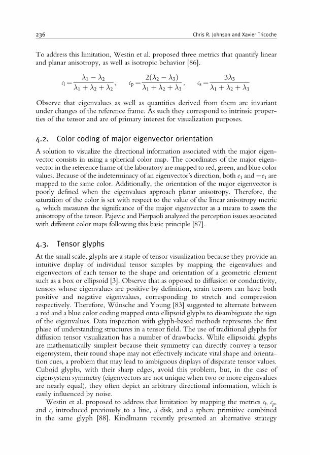
To address this limitation, Westin et al. proposed three metrics that quantify linearand planar anisotropy, as well as isotropic behavior [86].
cl= 1 � 2
1 þ 2 þ 2; cp=
2 2 � 3ð Þ 1 þ 2 þ 3
; cs=3 3
1 þ 2 þ 3
Observe that eigenvalues as well as quantities derived from them are invariantunder changes of the reference frame. As such they correspond to intrinsic proper-ties of the tensor and are of primary interest for visualization purposes.
4.2. Color coding of major eigenvector orientation
A solution to visualize the directional information associated with the major eigen-vector consists in using a spherical color map. The coordinates of the major eigen-vector in the reference frame of the laboratory are mapped to red, green, and blue colorvalues. Because of the indeterminacy of an eigenvector’s direction, both e1 and�e1 aremapped to the same color. Additionally, the orientation of the major eigenvector ispoorly defined when the eigenvalues approach planar anisotropy. Therefore, thesaturation of the color is set with respect to the value of the linear anisotropy metriccl, which measures the significance of the major eigenvector as a means to assess theanisotropy of the tensor. Pajevic and Pierpaoli analyzed the perception issues associatedwith different color maps following this basic principle [87].
4.3. Tensor glyphs
At the small scale, glyphs are a staple of tensor visualization because they provide anintuitive display of individual tensor samples by mapping the eigenvalues andeigenvectors of each tensor to the shape and orientation of a geometric elementsuch as a box or ellipsoid [3]. Observe that as opposed to diffusion or conductivity,tensors whose eigenvalues are positive by definition, strain tensors can have bothpositive and negative eigenvalues, corresponding to stretch and compressionrespectively. Therefore, Wunsche and Young [83] suggested to alternate betweena red and a blue color coding mapped onto ellipsoid glyphs to disambiguate the signof the eigenvalues. Data inspection with glyph-based methods represents the firstphase of understanding structures in a tensor field. The use of traditional glyphs fordiffusion tensor visualization has a number of drawbacks. While ellipsoidal glyphsare mathematically simplest because their symmetry can directly convey a tensoreigensystem, their round shape may not effectively indicate vital shape and orienta-tion cues, a problem that may lead to ambiguous displays of disparate tensor values.Cuboid glyphs, with their sharp edges, avoid this problem, but, in the case ofeigensystem symmetry (eigenvectors are not unique when two or more eigenvaluesare nearly equal), they often depict an arbitrary directional information, which iseasily influenced by noise.
Westin et al. proposed to address that limitation by mapping the metrics cl, cp,and cs introduced previously to a line, a disk, and a sphere primitive combinedin the same glyph [88]. Kindlmann recently presented an alternative strategy
236 Chris R. Johnson and Xavier Tricoche
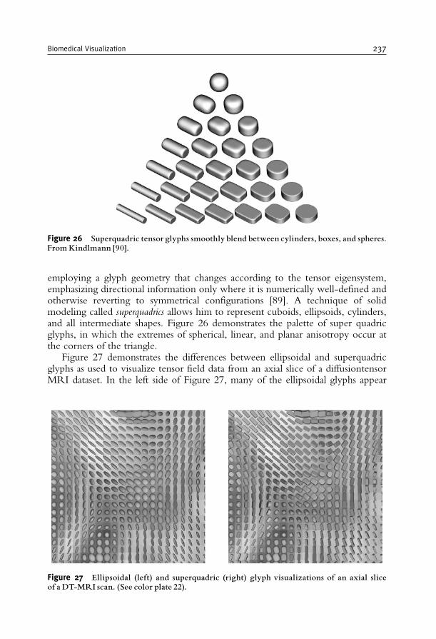
employing a glyph geometry that changes according to the tensor eigensystem,emphasizing directional information only where it is numerically well-defined andotherwise reverting to symmetrical configurations [89]. A technique of solidmodeling called superquadrics allows him to represent cuboids, ellipsoids, cylinders,and all intermediate shapes. Figure 26 demonstrates the palette of super quadricglyphs, in which the extremes of spherical, linear, and planar anisotropy occur atthe corners of the triangle.
Figure 27 demonstrates the differences between ellipsoidal and superquadricglyphs as used to visualize tensor field data from an axial slice of a diffusiontensorMRI dataset. In the left side of Figure 27, many of the ellipsoidal glyphs appear
Figure 26 Superquadric tensor glyphs smoothly blend between cylinders, boxes, and spheres.FromKindlmann [90].
Figure 27 Ellipsoidal (left) and superquadric (right) glyph visualizations of an axial sliceof a DT-MRI scan. (See color plate 22).
Biomedical Visualization 237
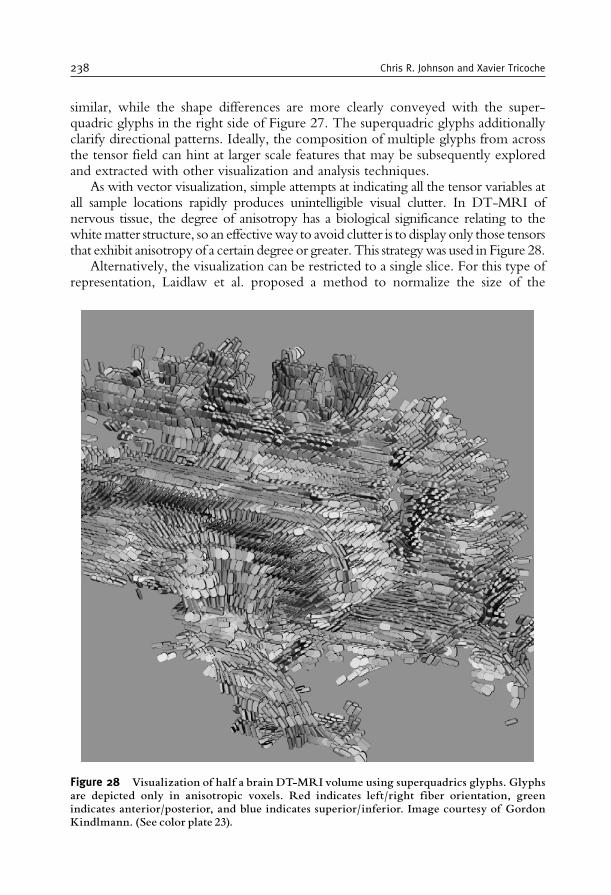
similar, while the shape differences are more clearly conveyed with the super-quadric glyphs in the right side of Figure 27. The superquadric glyphs additionallyclarify directional patterns. Ideally, the composition of multiple glyphs from acrossthe tensor field can hint at larger scale features that may be subsequently exploredand extracted with other visualization and analysis techniques.
As with vector visualization, simple attempts at indicating all the tensor variables atall sample locations rapidly produces unintelligible visual clutter. In DT-MRI ofnervous tissue, the degree of anisotropy has a biological significance relating to thewhitematter structure, so an effectiveway to avoid clutter is to display only those tensorsthat exhibit anisotropy of a certain degree or greater. This strategywas used in Figure 28.
Alternatively, the visualization can be restricted to a single slice. For this type ofrepresentation, Laidlaw et al. proposed a method to normalize the size of the
Figure 28 Visualization of half a brain DT-MRI volume using superquadrics glyphs. Glyphsare depicted only in anisotropic voxels. Red indicates left/right fiber orientation, greenindicates anterior/posterior, and blue indicates superior/inferior. Image courtesy of GordonKindlmann. (See color plate 23).
238 Chris R. Johnson and Xavier Tricoche
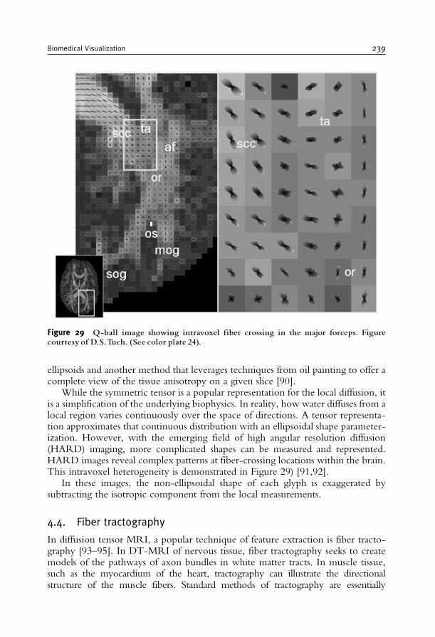
ellipsoids and another method that leverages techniques from oil painting to offer acomplete view of the tissue anisotropy on a given slice [90].
While the symmetric tensor is a popular representation for the local diffusion, itis a simplification of the underlying biophysics. In reality, how water diffuses from alocal region varies continuously over the space of directions. A tensor representa-tion approximates that continuous distribution with an ellipsoidal shape parameter-ization. However, with the emerging field of high angular resolution diffusion(HARD) imaging, more complicated shapes can be measured and represented.HARD images reveal complex patterns at fiber-crossing locations within the brain.This intravoxel heterogeneity is demonstrated in Figure 29) [91,92].
In these images, the non-ellipsoidal shape of each glyph is exaggerated bysubtracting the isotropic component from the local measurements.
4.4. Fiber tractography
In diffusion tensor MRI, a popular technique of feature extraction is fiber tracto-graphy [93–95]. In DT-MRI of nervous tissue, fiber tractography seeks to createmodels of the pathways of axon bundles in white matter tracts. In muscle tissue,such as the myocardium of the heart, tractography can illustrate the directionalstructure of the muscle fibers. Standard methods of tractography are essentially
Figure 29 Q-ball image showing intravoxel fiber crossing in the major forceps. Figurecourtesy of D.S.Tuch. (See color plate 24).
Biomedical Visualization 239
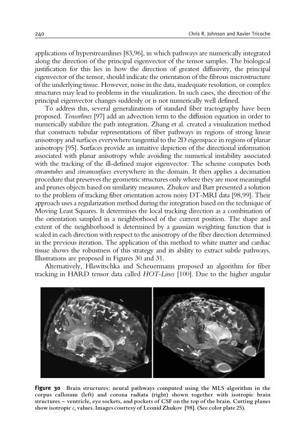
applications of hyperstreamlines [83,96], in which pathways are numerically integratedalong the direction of the principal eigenvector of the tensor samples. The biologicaljustification for this lies in how the direction of greatest diffusivity, the principaleigenvector of the tensor, should indicate the orientation of the fibrous microstructureof the underlying tissue. However, noise in the data, inadequate resolution, or complexstructures may lead to problems in the visualization. In such cases, the direction of theprincipal eigenvector changes suddenly or is not numerically well defined.
To address this, several generalizations of standard fiber tractography have beenproposed. Tensorlines [97] add an advection term to the diffusion equation in order tonumerically stabilize the path integration. Zhang et al. created a visualization methodthat constructs tubular representations of fiber pathways in regions of strong linearanisotropy and surfaces everywhere tangential to the 2D eigenspace in regions of planaranisotropy [95]. Surfaces provide an intuitive depiction of the directional informationassociated with planar anisotropy while avoiding the numerical instability associatedwith the tracking of the ill-defined major eigenvector. The scheme computes bothstreamtubes and streamsurfaces everywhere in the domain. It then applies a decimationprocedure that preserves the geometric structures only where they are most meaningfuland prunes objects based on similarity measures. Zhukov and Barr presented a solutionto the problem of tracking fiber orientation across noisy DT-MRI data [98,99]. Theirapproach uses a regularization method during the integration based on the technique ofMoving Least Squares. It determines the local tracking direction as a combination ofthe orientation sampled in a neighborhood of the current position. The shape andextent of the neighborhood is determined by a gaussian weighting function that isscaled in each direction with respect to the anisotropy of the fiber direction determinedin the previous iteration. The application of this method to white matter and cardiactissue shows the robustness of this strategy and its ability to extract subtle pathways.Illustrations are proposed in Figures 30 and 31.
Alternatively, Hlawitschka and Scheuermann proposed an algorithm for fibertracking in HARD tensor data called HOT-Lines [100]. Due to the higher angular
Figure 30 Brain structures: neural pathways computed using the MLS algorithm in thecorpus callosum (left) and corona radiata (right) shown together with isotropic brainstructures ^ ventricle, eye sockets, and pockets of CSF on the top of the brain. Cutting planesshow isotropic csvalues. Images courtesy of Leonid Zhukov [98]. (See color plate 25).
240 Chris R. Johnson and Xavier Tricoche
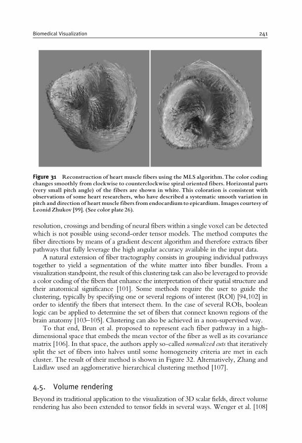
resolution, crossings and bending of neural fibers within a single voxel can be detectedwhich is not possible using second-order tensor models. The method computes thefiber directions by means of a gradient descent algorithm and therefore extracts fiberpathways that fully leverage the high angular accuracy available in the input data.
A natural extension of fiber tractography consists in grouping individual pathwaystogether to yield a segmentation of the white matter into fiber bundles. From avisualization standpoint, the result of this clustering task can also be leveraged to providea color coding of the fibers that enhance the interpretation of their spatial structure andtheir anatomical significance [101]. Some methods require the user to guide theclustering, typically by specifying one or several regions of interest (ROI) [94,102] inorder to identify the fibers that intersect them. In the case of several ROIs, booleanlogic can be applied to determine the set of fibers that connect known regions of thebrain anatomy [103–105]. Clustering can also be achieved in a non-supervised way.
To that end, Brun et al. proposed to represent each fiber pathway in a high-dimensional space that embeds the mean vector of the fiber as well as its covariancematrix [106]. In that space, the authors apply so-called normalized cuts that iterativelysplit the set of fibers into halves until some homogeneity criteria are met in eachcluster. The result of their method is shown in Figure 32. Alternatively, Zhang andLaidlaw used an agglomerative hierarchical clustering method [107].
4.5. Volume rendering
Beyond its traditional application to the visualization of 3D scalar fields, direct volumerendering has also been extended to tensor fields in several ways. Wenger et al. [108]
Figure 31 Reconstruction of heart muscle fibers using the MLS algorithm.The color codingchanges smoothly from clockwise to counterclockwise spiral oriented fibers. Horizontal parts(very small pitch angle) of the fibers are shown in white. This coloration is consistent withobservations of some heart researchers, who have described a systematic smooth variation inpitch and direction of heart muscle fibers from endocardium to epicardium. Images courtesy ofLeonid Zhukov [99]. (See color plate 26).
Biomedical Visualization 241
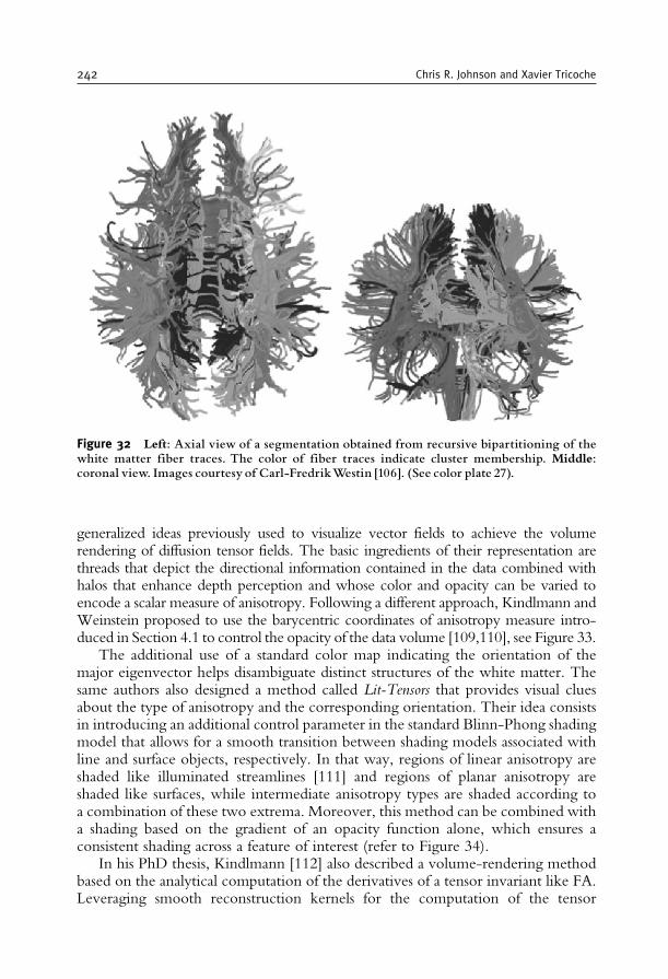
generalized ideas previously used to visualize vector fields to achieve the volumerendering of diffusion tensor fields. The basic ingredients of their representation arethreads that depict the directional information contained in the data combined withhalos that enhance depth perception and whose color and opacity can be varied toencode a scalar measure of anisotropy. Following a different approach, Kindlmann andWeinstein proposed to use the barycentric coordinates of anisotropy measure intro-duced in Section 4.1 to control the opacity of the data volume [109,110], see Figure 33.
The additional use of a standard color map indicating the orientation of themajor eigenvector helps disambiguate distinct structures of the white matter. Thesame authors also designed a method called Lit-Tensors that provides visual cluesabout the type of anisotropy and the corresponding orientation. Their idea consistsin introducing an additional control parameter in the standard Blinn-Phong shadingmodel that allows for a smooth transition between shading models associated withline and surface objects, respectively. In that way, regions of linear anisotropy areshaded like illuminated streamlines [111] and regions of planar anisotropy areshaded like surfaces, while intermediate anisotropy types are shaded according toa combination of these two extrema. Moreover, this method can be combined witha shading based on the gradient of an opacity function alone, which ensures aconsistent shading across a feature of interest (refer to Figure 34).
In his PhD thesis, Kindlmann [112] also described a volume-rendering methodbased on the analytical computation of the derivatives of a tensor invariant like FA.Leveraging smooth reconstruction kernels for the computation of the tensor
Figure 32 Left: Axial view of a segmentation obtained from recursive bipartitioning of thewhite matter fiber traces. The color of fiber traces indicate cluster membership. Middle:coronal view. Images courtesy of Carl-FredrikWestin [106]. (See color plate 27).
242 Chris R. Johnson and Xavier Tricoche
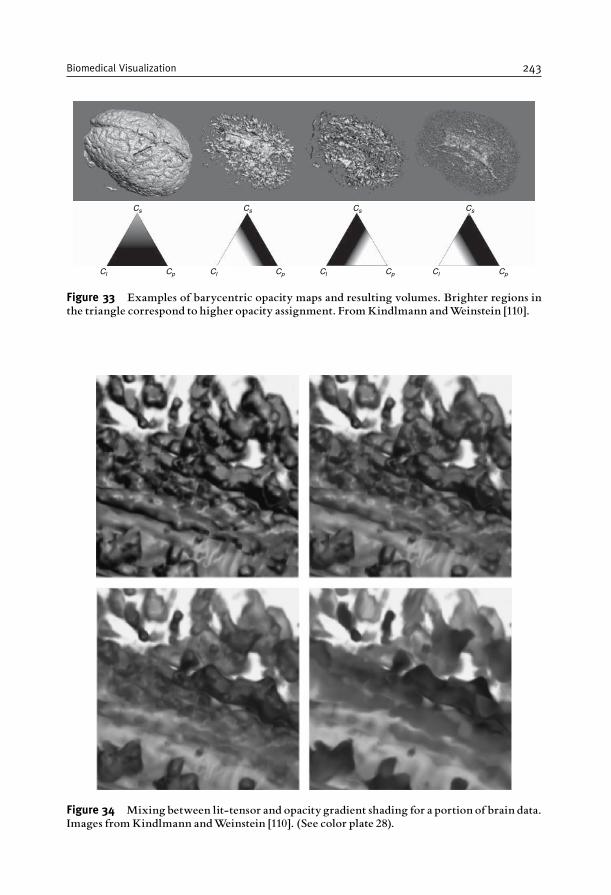
Cs
Cl Cp
Cs
Cl Cp
Cs
Cl Cp
Cs
Cl Cp
Figure 33 Examples of barycentric opacity maps and resulting volumes. Brighter regions inthe triangle correspond to higher opacity assignment. FromKindlmann andWeinstein [110].
Figure 34 Mixing between lit-tensor and opacitygradient shading for a portion of brain data.Images fromKindlmann andWeinstein [110]. (See color plate 28).
Biomedical Visualization 243
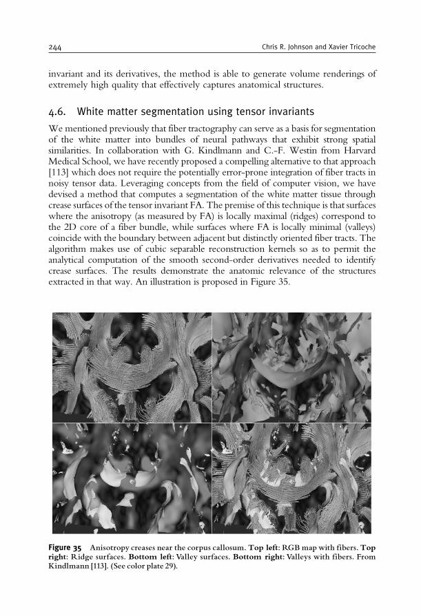
invariant and its derivatives, the method is able to generate volume renderings ofextremely high quality that effectively captures anatomical structures.
4.6. White matter segmentation using tensor invariants
Wementioned previously that fiber tractography can serve as a basis for segmentationof the white matter into bundles of neural pathways that exhibit strong spatialsimilarities. In collaboration with G. Kindlmann and C.-F. Westin from HarvardMedical School, we have recently proposed a compelling alternative to that approach[113] which does not require the potentially error-prone integration of fiber tracts innoisy tensor data. Leveraging concepts from the field of computer vision, we havedevised a method that computes a segmentation of the white matter tissue throughcrease surfaces of the tensor invariant FA. The premise of this technique is that surfaceswhere the anisotropy (as measured by FA) is locally maximal (ridges) correspond tothe 2D core of a fiber bundle, while surfaces where FA is locally minimal (valleys)coincide with the boundary between adjacent but distinctly oriented fiber tracts. Thealgorithm makes use of cubic separable reconstruction kernels so as to permit theanalytical computation of the smooth second-order derivatives needed to identifycrease surfaces. The results demonstrate the anatomic relevance of the structuresextracted in that way. An illustration is proposed in Figure 35.
Figure 35 Anisotropy creases near the corpus callosum. Top left: RGBmapwith fibers. Topright: Ridge surfaces. Bottom left: Valley surfaces. Bottom right: Valleys with fibers. FromKindlmann [113]. (See color plate 29).
244 Chris R. Johnson and Xavier Tricoche
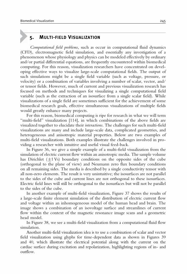
5. MULTI-FIELD VISUALIZATION
Computational field problems, such as occur in computational fluid dynamics(CFD), electromagnetic field simulation, and essentially any investigation of aphenomenon whose physiology and physics can be modeled effectively by ordinaryand/or partial differential equations, are frequently encountered within biomedicalcomputing. For this reason, visualization researchers have concentrated on devel-oping effective ways to visualize large-scale computational fields. The output ofsuch simulations might be a single field variable (such as voltage, pressure, orvelocity) or a combination of variables involving a number of scalar, vector, and/or tensor fields. However, much of current and previous visualization research hasfocused on methods and techniques for visualizing a single computational fieldvariable (such as the extraction of an isosurface from a single scalar field). Whilevisualizations of a single field are sometimes sufficient for the achievement of somebiomedical research goals, effective simultaneous visualizations of multiple fieldswould greatly enhance many projects.
For this reason, biomedical computing is ripe for research in what we will term“multi-field” visualization [114], in which combinations of the above fields arevisualized together to elucidate their interactions. The challenges for such multi-fieldvisualizations are many and include large-scale data, complicated geometries, andheterogeneous and anisotropic material properties. Below are two examples ofmulti-field visualizations. Both examples illustrate the challenges involved in pro-viding a researcher with intuitive and useful visual feed-back.
In Figure 36, we give a simple example of a multi-field visualization from thesimulation of electric current flow within an anisotropic media. The sample volumehas Dirichlet (+1Vs) boundary conditions on the opposite sides of the cube(orthogonal to the plane of view) and Neumann zero flux boundary conditionson all remaining sides. The media is described by a single conductivity tensor withall non-zero elements. The result is very unintuitive; the isosurfaces are not parallelto the sides of the cube and current lines are not orthogonal to these isosurfaces.Electric field lines will still be orthogonal to the isosurfaces but will not be parallelto the sides of the cube.
In another example of multi-field visualization, Figure 37 shows the results ofa large-scale finite element simulation of the distribution of electric current flowand voltage within an inhomogeneous model of the human head and brain. Theimage shows a combination of an isovoltage surface and streamlines of currentflow within the context of the magnetic resonance image scans and a geometrichead model.
In Figure 38, we see a multi-field visualization from a computational fluid flowsimulation.
Another multi-field visualization idea is to use a combination of scalar and vectorfield visualization using glyphs for time-dependent data as shown in Figures 39and 40, which illustrate the electrical potential along with the current on thecardiac surface during excitation and repolarization, highlighting regions of in- andoutflow.
Biomedical Visualization 245
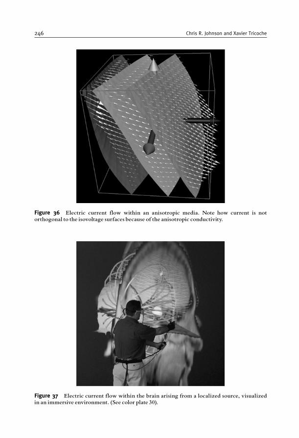
Figure 36 Electric current flow within an anisotropic media. Note how current is notorthogonal to the isovoltage surfaces because of the anisotropic conductivity.
Figure 37 Electric current flow within the brain arising from a localized source, visualizedin an immersive environment. (See color plate 30).
246 Chris R. Johnson and Xavier Tricoche
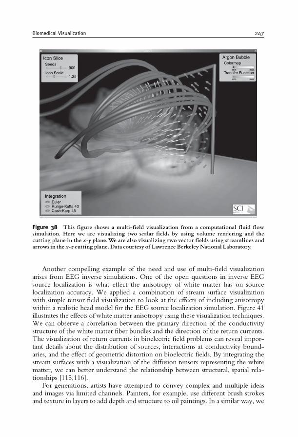
Another compelling example of the need and use of multi-field visualizationarises from EEG inverse simulations. One of the open questions in inverse EEGsource localization is what effect the anisotropy of white matter has on sourcelocalization accuracy. We applied a combination of stream surface visualizationwith simple tensor field visualization to look at the effects of including anisotropywithin a realistic head model for the EEG source localization simulation. Figure 41illustrates the effects of white matter anisotropy using these visualization techniques.We can observe a correlation between the primary direction of the conductivitystructure of the white matter fiber bundles and the direction of the return currents.The visualization of return currents in bioelectric field problems can reveal impor-tant details about the distribution of sources, interactions at conductivity bound-aries, and the effect of geometric distortion on bioelectric fields. By integrating thestream surfaces with a visualization of the diffusion tensors representing the whitematter, we can better understand the relationship between structural, spatial rela-tionships [115,116].
For generations, artists have attempted to convey complex and multiple ideasand images via limited channels. Painters, for example, use different brush strokesand texture in layers to add depth and structure to oil paintings. In a similar way, we
Icon Slice Argon BubbleColormap
Transfer Function
min max
min max
IntegrationEulerRunge-Kutta 43Cash-Karp 45
Seeds
Icon Scale900
1.25
Figure 38 This figure shows a multi-field visualization from a computational fluid flowsimulation. Here we are visualizing two scalar fields by using volume rendering and thecutting plane in the x-y plane.We are also visualizing two vector fields using streamlines andarrows in the x-z cutting plane. Data courtesy of Lawrence Berkeley National Laboratory.
Biomedical Visualization 247
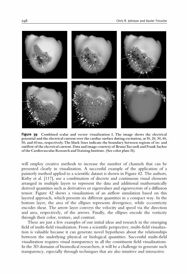
will employ creative methods to increase the number of channels that can bepresented clearly in visualization. A successful example of the application of apainterly method applied to a scientific dataset is shown in Figure 42. The authors,Kirby et al. [117], use a combination of discrete and continuous visual elementsarranged in multiple layers to represent the data and additional mathematicallyderived quantities such as derivatives or eigenvalues and eigenvectors of a diffusiontensor. Figure 42 shows a visualization of an airflow simulation based on thislayered approach, which presents six different quantities in a compact way. In thebottom layer, the area of the ellipses represents divergence, while eccentricityencodes shear. The arrow layer conveys the velocity and speed via the directionand area, respectively, of the arrows. Finally, the ellipses encode the vorticitythrough their color, texture, and contrast.
These are just a few examples of our initial ideas and research in the emergingfield of multi-field visualization. From a scientific perspective, multi-field visualiza-tion is valuable because it can generate novel hypotheses about the relationshipsbetween the underlying physical or biological quantities. Successful multi-fieldvisualization requires visual transparency in all the constituent field visualizations.In the 3D domains of biomedical researchers, it will be a challenge to generate suchtransparency, especially through techniques that are also intuitive and interactive.
Figure 39 Combined scalar and vector visualization I. The image shows the electricalpotential and the electrical current over the cardiac surface during excitation, at 10, 20, 30, 40,50, and 60ms, respectively.The black lines indicate the boundary between regions of in- andoutflow of the electrical current. Data and image courtesy of BrunoTaccardi and Frank Sachseof the Cardiovascular Research andTraining Institute. (See color plate 31).
248 Chris R. Johnson and Xavier Tricoche
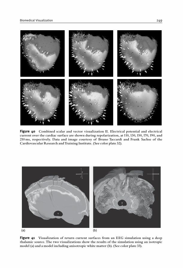
(a) (b)
Figure 41 Visualization of return current surfaces from an EEG simulation using a deepthalamic source. The two visualizations show the results of the simulation using an isotropicmodel (a) and a model including anisotropic white matter (b). (See color plate 33).
Figure 40 Combined scalar and vector visualization II. Electrical potential and electricalcurrent over the cardiac surface are shown during repolarization, at 110, 130, 150, 170, 190, and210ms, respectively. Data and image courtesy of Bruno Taccardi and Frank Sachse of theCardiovascular Research andTraining Institute. (See color plate 32).
Biomedical Visualization 249
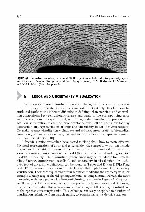
6. ERROR AND UNCERTAINTY VISUALIZATION
With few exceptions, visualization research has ignored the visual representa-tion of errors and uncertainty for 3D visualizations. Certainly, this lack can beattributed partly to the inherent difficulty in defining, characterizing, and control-ling comparisons between different datasets and partly to the corresponding errorand uncertainty in the experimental, simulation, and/or visualization processes. Inaddition, visualization researchers have developed few methods that allow for easycomparison and representation of error and uncertainty in data for visualizations.To make current visualization techniques and software more useful to biomedicalcomputing (and other) researchers, we need to incorporate visual representations oferror and uncertainty [118].
A few visualization researchers have started thinking about how to create effective3D visual representations of errors and uncertainties, the sources of which can includeuncertainty in acquisition (instrument measurement error, numerical analysis error,statistical variation), uncertainty in the model (both in mathematical and in geometricmodels), uncertainty in transformation (where errors may be introduced from resam-pling, filtering, quantization, rescaling), and uncertainty in visualization. (A usefuloverview of uncertainty definitions can be found in Taylor and Kuyatt [119].) Panget al. [120] have summarized a variety of techniques that might be used for uncertaintyvisualization. These techniques range from adding or modifying the geometry with, forexample, a bump map or altered lighting attributes, to using textures. Perhaps the mostinteresting technique proposed is the use of blurring, as shown in Figure 43. GrigoryanandRheingans [121], on the other hand, used point-based primitives instead of blurringto create a fuzzy surface that achieves similar results (Figure 44) Blurring is a natural cueto the eye that something is amiss. This technique can easily be applied to a variety ofvisualization techniques from particle tracing to isosurfacing, as we describe later on.
Figure 42 Visualization of experimental 2D flow past an airfoil, indicating velocity, speed,vorticity, rate of strain, divergence, and shear. Image courtesy R.M. Kirby and H. Marmanisand D.H. Laidlaw. (See color plate 34).
250 Chris R. Johnson and Xavier Tricoche
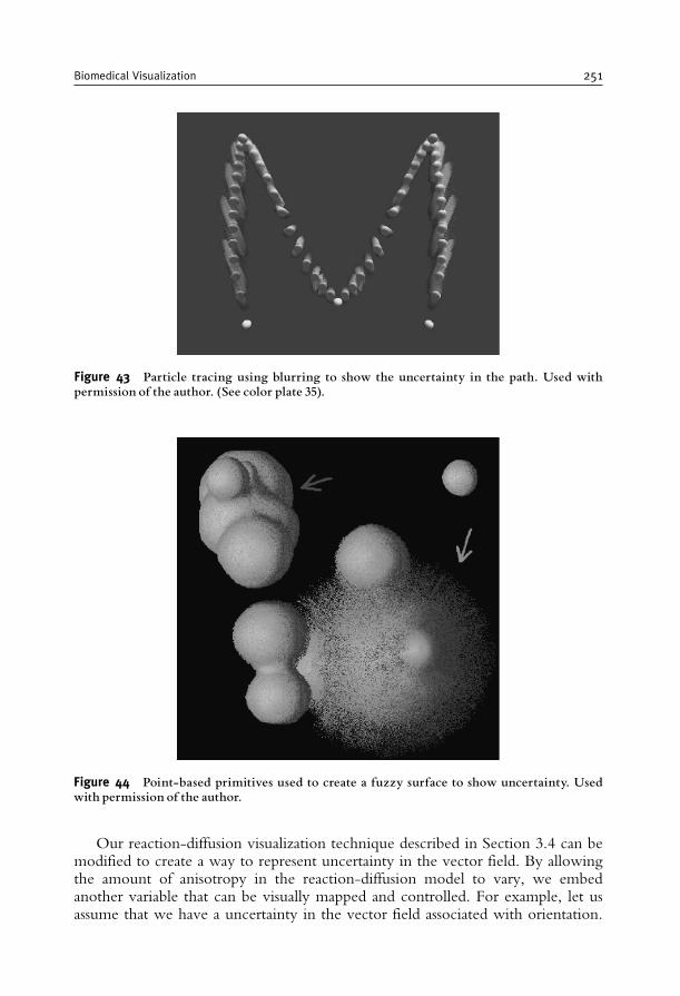
Our reaction-diffusion visualization technique described in Section 3.4 can bemodified to create a way to represent uncertainty in the vector field. By allowingthe amount of anisotropy in the reaction-diffusion model to vary, we embedanother variable that can be visually mapped and controlled. For example, let usassume that we have a uncertainty in the vector field associated with orientation.
Figure 43 Particle tracing using blurring to show the uncertainty in the path. Used withpermission of the author. (See color plate 35).
Figure 44 Point-based primitives used to create a fuzzy surface to show uncertainty. Usedwith permission of the author.
Biomedical Visualization 251
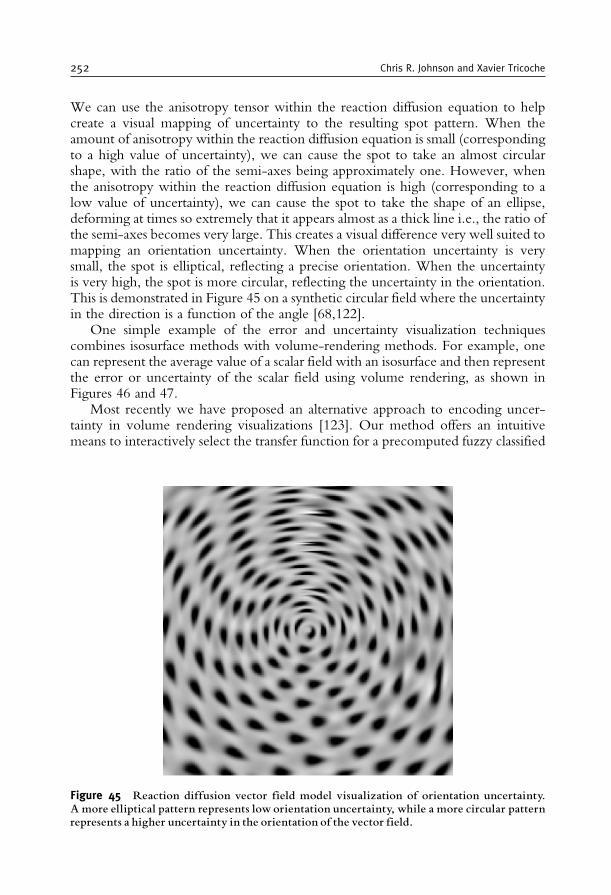
We can use the anisotropy tensor within the reaction diffusion equation to helpcreate a visual mapping of uncertainty to the resulting spot pattern. When theamount of anisotropy within the reaction diffusion equation is small (correspondingto a high value of uncertainty), we can cause the spot to take an almost circularshape, with the ratio of the semi-axes being approximately one. However, whenthe anisotropy within the reaction diffusion equation is high (corresponding to alow value of uncertainty), we can cause the spot to take the shape of an ellipse,deforming at times so extremely that it appears almost as a thick line i.e., the ratio ofthe semi-axes becomes very large. This creates a visual difference very well suited tomapping an orientation uncertainty. When the orientation uncertainty is verysmall, the spot is elliptical, reflecting a precise orientation. When the uncertaintyis very high, the spot is more circular, reflecting the uncertainty in the orientation.This is demonstrated in Figure 45 on a synthetic circular field where the uncertaintyin the direction is a function of the angle [68,122].
One simple example of the error and uncertainty visualization techniquescombines isosurface methods with volume-rendering methods. For example, onecan represent the average value of a scalar field with an isosurface and then representthe error or uncertainty of the scalar field using volume rendering, as shown inFigures 46 and 47.
Most recently we have proposed an alternative approach to encoding uncer-tainty in volume rendering visualizations [123]. Our method offers an intuitivemeans to interactively select the transfer function for a precomputed fuzzy classified
Figure 45 Reaction diffusion vector field model visualization of orientation uncertainty.A more elliptical pattern represents low orientation uncertainty, while a more circular patternrepresents a higher uncertainty in the orientation of the vector field.
252 Chris R. Johnson and Xavier Tricoche
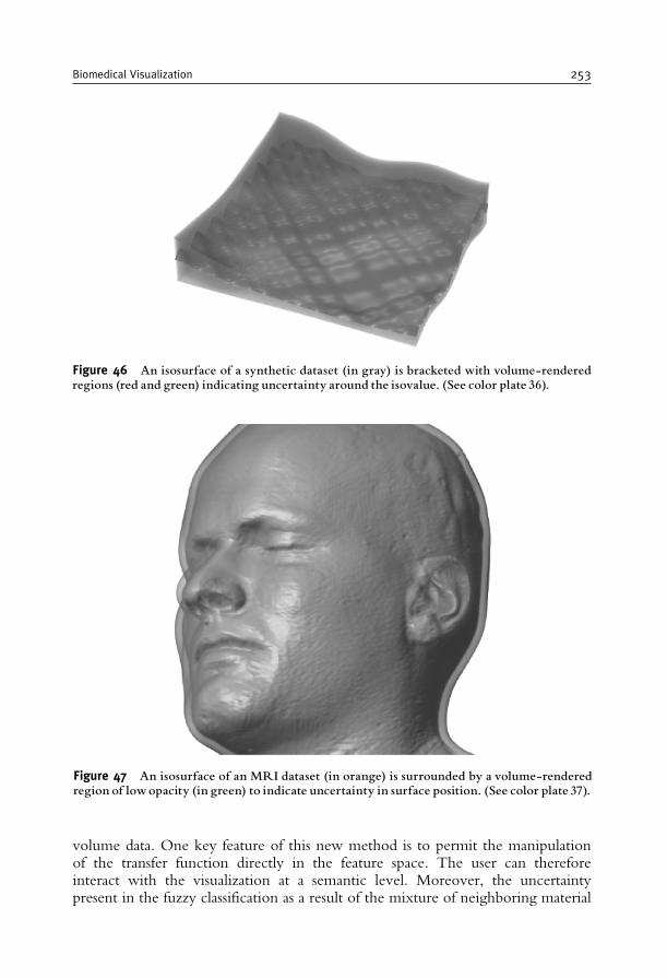
volume data. One key feature of this new method is to permit the manipulationof the transfer function directly in the feature space. The user can thereforeinteract with the visualization at a semantic level. Moreover, the uncertaintypresent in the fuzzy classification as a result of the mixture of neighboring material
Figure 47 An isosurface of an MRI dataset (in orange) is surrounded by a volume-renderedregion of lowopacity (in green) to indicate uncertainty in surface position. (See color plate 37).
Figure 46 An isosurface of a synthetic dataset (in gray) is bracketed with volume-renderedregions (red and green) indicating uncertainty around the isovalue. (See color plate 36).
Biomedical Visualization 253
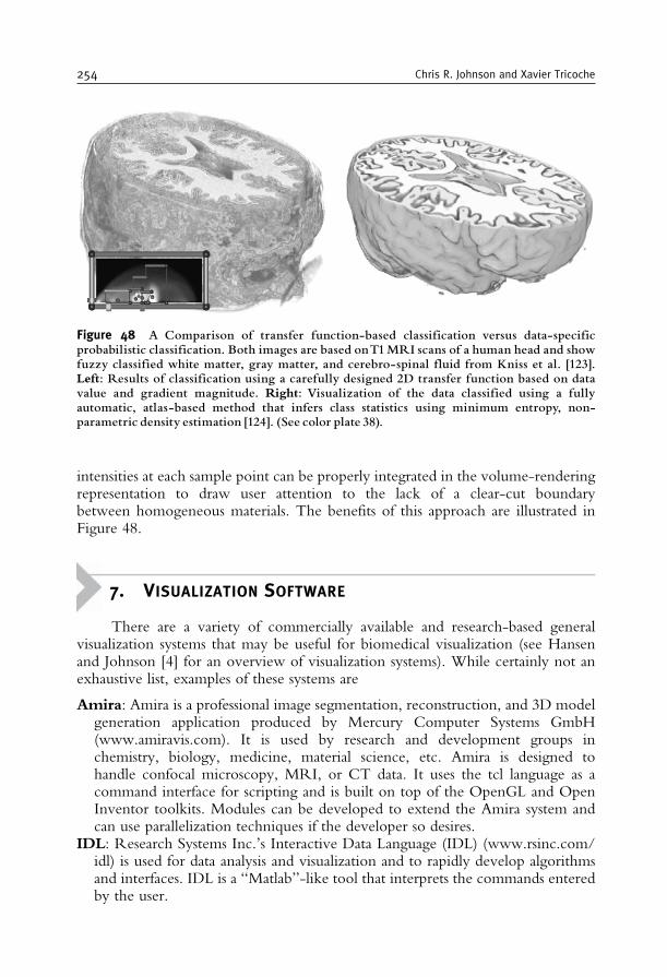
intensities at each sample point can be properly integrated in the volume-renderingrepresentation to draw user attention to the lack of a clear-cut boundarybetween homogeneous materials. The benefits of this approach are illustrated inFigure 48.
7. VISUALIZATION SOFTWARE
There are a variety of commercially available and research-based generalvisualization systems that may be useful for biomedical visualization (see Hansenand Johnson [4] for an overview of visualization systems). While certainly not anexhaustive list, examples of these systems are
Amira: Amira is a professional image segmentation, reconstruction, and 3D modelgeneration application produced by Mercury Computer Systems GmbH(www.amiravis.com). It is used by research and development groups inchemistry, biology, medicine, material science, etc. Amira is designed tohandle confocal microscopy, MRI, or CT data. It uses the tcl language as acommand interface for scripting and is built on top of the OpenGL and OpenInventor toolkits. Modules can be developed to extend the Amira system andcan use parallelization techniques if the developer so desires.
IDL: Research Systems Inc.’s Interactive Data Language (IDL) (www.rsinc.com/idl) is used for data analysis and visualization and to rapidly develop algorithmsand interfaces. IDL is a “Matlab”-like tool that interprets the commands enteredby the user.
Figure 48 A Comparison of transfer function-based classification versus data-specificprobabilistic classification. Both images are based onT1MRI scans of a human head and showfuzzy classified white matter, gray matter, and cerebro-spinal fluid from Kniss et al. [123].Left: Results of classification using a carefully designed 2D transfer function based on datavalue and gradient magnitude. Right: Visualization of the data classified using a fullyautomatic, atlas-based method that infers class statistics using minimum entropy, non-parametric density estimation [124]. (See color plate 38).
254 Chris R. Johnson and Xavier Tricoche
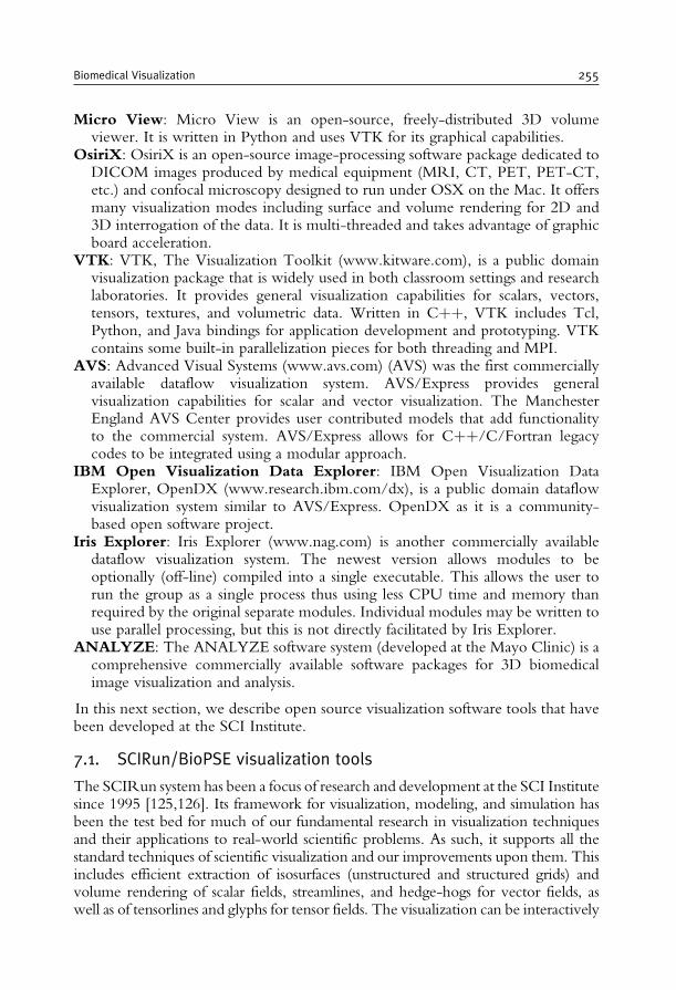
Micro View: Micro View is an open-source, freely-distributed 3D volumeviewer. It is written in Python and uses VTK for its graphical capabilities.
OsiriX: OsiriX is an open-source image-processing software package dedicated toDICOM images produced by medical equipment (MRI, CT, PET, PET-CT,etc.) and confocal microscopy designed to run under OSX on the Mac. It offersmany visualization modes including surface and volume rendering for 2D and3D interrogation of the data. It is multi-threaded and takes advantage of graphicboard acceleration.
VTK: VTK, The Visualization Toolkit (www.kitware.com), is a public domainvisualization package that is widely used in both classroom settings and researchlaboratories. It provides general visualization capabilities for scalars, vectors,tensors, textures, and volumetric data. Written in Cþþ, VTK includes Tcl,Python, and Java bindings for application development and prototyping. VTKcontains some built-in parallelization pieces for both threading and MPI.
AVS: Advanced Visual Systems (www.avs.com) (AVS) was the first commerciallyavailable dataflow visualization system. AVS/Express provides generalvisualization capabilities for scalar and vector visualization. The ManchesterEngland AVS Center provides user contributed models that add functionalityto the commercial system. AVS/Express allows for Cþþ/C/Fortran legacycodes to be integrated using a modular approach.
IBM Open Visualization Data Explorer: IBM Open Visualization DataExplorer, OpenDX (www.research.ibm.com/dx), is a public domain dataflowvisualization system similar to AVS/Express. OpenDX as it is a community-based open software project.
Iris Explorer: Iris Explorer (www.nag.com) is another commercially availabledataflow visualization system. The newest version allows modules to beoptionally (off-line) compiled into a single executable. This allows the user torun the group as a single process thus using less CPU time and memory thanrequired by the original separate modules. Individual modules may be written touse parallel processing, but this is not directly facilitated by Iris Explorer.
ANALYZE: The ANALYZE software system (developed at the Mayo Clinic) is acomprehensive commercially available software packages for 3D biomedicalimage visualization and analysis.
In this next section, we describe open source visualization software tools that havebeen developed at the SCI Institute.
7.1. SCIRun/BioPSE visualization tools
The SCIRun system has been a focus of research and development at the SCI Institutesince 1995 [125,126]. Its framework for visualization, modeling, and simulation hasbeen the test bed for much of our fundamental research in visualization techniquesand their applications to real-world scientific problems. As such, it supports all thestandard techniques of scientific visualization and our improvements upon them. Thisincludes efficient extraction of isosurfaces (unstructured and structured grids) andvolume rendering of scalar fields, streamlines, and hedge-hogs for vector fields, aswell as of tensorlines and glyphs for tensor fields. The visualization can be interactively
Biomedical Visualization 255
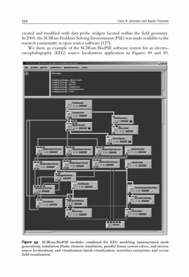
created and modified with data probe widgets located within the field geometry.In 2000, the SCIRun Problem-Solving Environment (PSE) was made available to theresearch community as open source software [127].
We show an example of the SCIRun/BioPSE software system for an electro-encephalography (EEG) source localization application in Figures 49 and 50.
Figure 49 SCIRun/BioPSE modules combined for EEG modeling (unstructured meshgeneration), simulation (finite element simulation, parallel linear system solves, and inversesource localization), and visualization (mesh visualization, isosurface extraction, and vectorfield visualization.
256 Chris R. Johnson and Xavier Tricoche
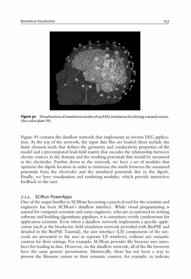
Figure 49 contains the dataflow network that implements an inverse EEG applica-tion. At the top of the network, the input data files are loaded; these include thefinite element mesh that defines the geometry and conductivity properties of themodel and a precomputed lead-field matrix that encodes the relationship betweenelectric sources in the domain and the resulting potentials that would be measuredat the electrodes. Further down in the network, we have a set of modules thatoptimize the dipole location in order to minimize the misfit between the measuredpotentials from the electrodes and the simulated potentials due to the dipole.Finally, we have visualization and rendering modules, which provide interactivefeedback to the user.
7.1.1. SCIRun PowerAppsOne of the major hurdles to SCIRun becoming a practical tool for the scientists andengineers has been SCIRun’s dataflow interface. While visual programming isnatural for computer scientists and some engineers, who are accustomed to writingsoftware and building algorithmic pipelines, it is sometimes overly cumbersome forapplication scientists. Even when a dataflow network implements a specific appli-cation (such as the bioelectric field simulation network provided with BioPSE anddetailed in the BioPSE Tutorial), the user interface (UI) components of the net-work are presented to the user in separate UI windows, without any semanticcontext for their settings. For example, SCIRun provides file browser user inter-faces for reading in data. However, on the dataflow network, all of the file browsershave the same generic presentation. Historically, there has not been a way topresent the filename entries in their semantic context, for example, to indicate
Figure 50 Visualization of simulation results of an EEG simulation localizing a neural source.(See color plate 39).
Biomedical Visualization 257
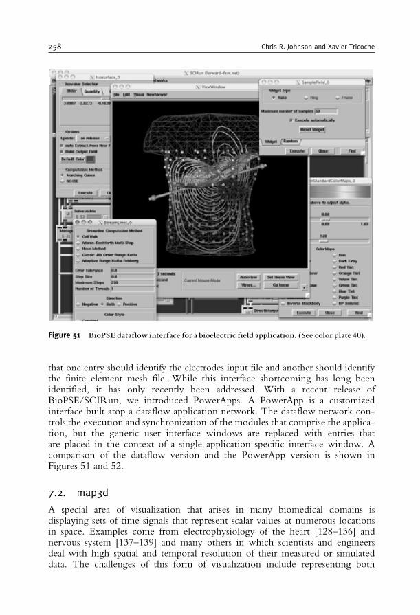
that one entry should identify the electrodes input file and another should identifythe finite element mesh file. While this interface shortcoming has long beenidentified, it has only recently been addressed. With a recent release ofBioPSE/SCIRun, we introduced PowerApps. A PowerApp is a customizedinterface built atop a dataflow application network. The dataflow network con-trols the execution and synchronization of the modules that comprise the applica-tion, but the generic user interface windows are replaced with entries thatare placed in the context of a single application-specific interface window. Acomparison of the dataflow version and the PowerApp version is shown inFigures 51 and 52.
7.2. map3d
A special area of visualization that arises in many biomedical domains isdisplaying sets of time signals that represent scalar values at numerous locationsin space. Examples come from electrophysiology of the heart [128–136] andnervous system [137–139] and many others in which scientists and engineersdeal with high spatial and temporal resolution of their measured or simulateddata. The challenges of this form of visualization include representing both
Figure 51 BioPSE dataflow interface for a bioelectric field application. (See color plate 40).
258 Chris R. Johnson and Xavier Tricoche
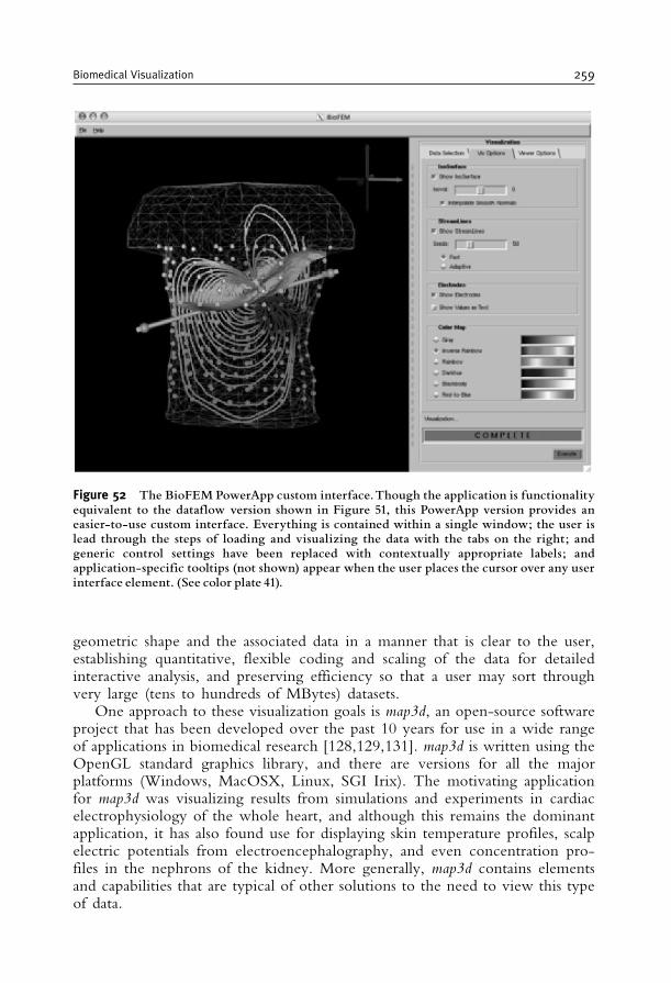
geometric shape and the associated data in a manner that is clear to the user,establishing quantitative, flexible coding and scaling of the data for detailedinteractive analysis, and preserving efficiency so that a user may sort throughvery large (tens to hundreds of MBytes) datasets.
One approach to these visualization goals is map3d, an open-source softwareproject that has been developed over the past 10 years for use in a wide rangeof applications in biomedical research [128,129,131]. map3d is written using theOpenGL standard graphics library, and there are versions for all the majorplatforms (Windows, MacOSX, Linux, SGI Irix). The motivating applicationfor map3d was visualizing results from simulations and experiments in cardiacelectrophysiology of the whole heart, and although this remains the dominantapplication, it has also found use for displaying skin temperature profiles, scalpelectric potentials from electroencephalography, and even concentration pro-files in the nephrons of the kidney. More generally, map3d contains elementsand capabilities that are typical of other solutions to the need to view this typeof data.
Figure 52 The BioFEM PowerApp custom interface.Though the application is functionalityequivalent to the dataflow version shown in Figure 51, this PowerApp version provides aneasier-to-use custom interface. Everything is contained within a single window; the user islead through the steps of loading and visualizing the data with the tabs on the right; andgeneric control settings have been replaced with contextually appropriate labels; andapplication-specific tooltips (not shown) appear when the user places the cursor over any userinterface element. (See color plate 41).
Biomedical Visualization 259
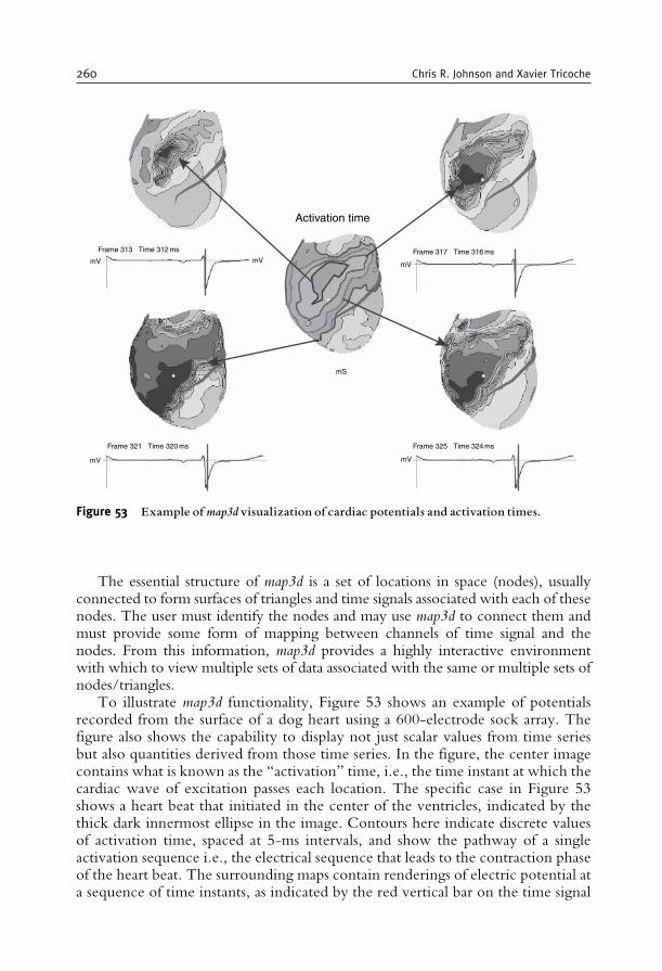
The essential structure of map3d is a set of locations in space (nodes), usuallyconnected to form surfaces of triangles and time signals associated with each of thesenodes. The user must identify the nodes and may use map3d to connect them andmust provide some form of mapping between channels of time signal and thenodes. From this information, map3d provides a highly interactive environmentwith which to view multiple sets of data associated with the same or multiple sets ofnodes/triangles.
To illustrate map3d functionality, Figure 53 shows an example of potentialsrecorded from the surface of a dog heart using a 600-electrode sock array. Thefigure also shows the capability to display not just scalar values from time seriesbut also quantities derived from those time series. In the figure, the center imagecontains what is known as the “activation” time, i.e., the time instant at which thecardiac wave of excitation passes each location. The specific case in Figure 53shows a heart beat that initiated in the center of the ventricles, indicated by thethick dark innermost ellipse in the image. Contours here indicate discrete valuesof activation time, spaced at 5-ms intervals, and show the pathway of a singleactivation sequence i.e., the electrical sequence that leads to the contraction phaseof the heart beat. The surrounding maps contain renderings of electric potential ata sequence of time instants, as indicated by the red vertical bar on the time signal
Activation time
Frame 313 Time 312 ms
mV mVmV
mV mV
mS
Frame 321 Time 320 ms Frame 325 Time 324 ms
Frame 317 Time 316 ms
Figure 53 Example ofmap3dvisualization of cardiac potentials and activation times.
260 Chris R. Johnson and Xavier Tricoche
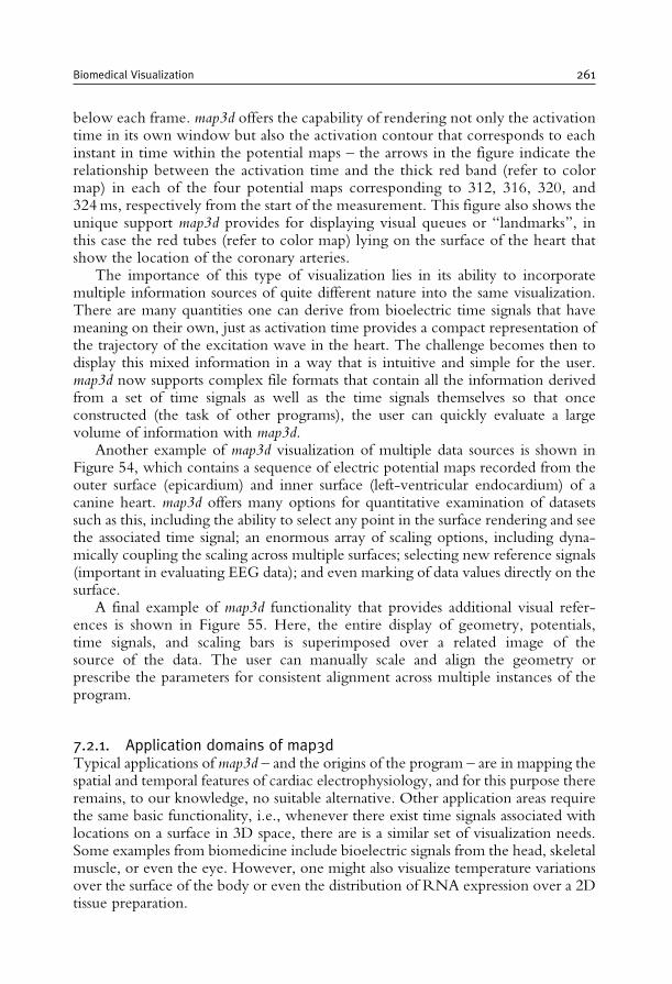
below each frame. map3d offers the capability of rendering not only the activationtime in its own window but also the activation contour that corresponds to eachinstant in time within the potential maps – the arrows in the figure indicate therelationship between the activation time and the thick red band (refer to colormap) in each of the four potential maps corresponding to 312, 316, 320, and324ms, respectively from the start of the measurement. This figure also shows theunique support map3d provides for displaying visual queues or “landmarks”, inthis case the red tubes (refer to color map) lying on the surface of the heart thatshow the location of the coronary arteries.
The importance of this type of visualization lies in its ability to incorporatemultiple information sources of quite different nature into the same visualization.There are many quantities one can derive from bioelectric time signals that havemeaning on their own, just as activation time provides a compact representation ofthe trajectory of the excitation wave in the heart. The challenge becomes then todisplay this mixed information in a way that is intuitive and simple for the user.map3d now supports complex file formats that contain all the information derivedfrom a set of time signals as well as the time signals themselves so that onceconstructed (the task of other programs), the user can quickly evaluate a largevolume of information with map3d.
Another example of map3d visualization of multiple data sources is shown inFigure 54, which contains a sequence of electric potential maps recorded from theouter surface (epicardium) and inner surface (left-ventricular endocardium) of acanine heart. map3d offers many options for quantitative examination of datasetssuch as this, including the ability to select any point in the surface rendering and seethe associated time signal; an enormous array of scaling options, including dyna-mically coupling the scaling across multiple surfaces; selecting new reference signals(important in evaluating EEG data); and even marking of data values directly on thesurface.
A final example of map3d functionality that provides additional visual refer-ences is shown in Figure 55. Here, the entire display of geometry, potentials,time signals, and scaling bars is superimposed over a related image of thesource of the data. The user can manually scale and align the geometry orprescribe the parameters for consistent alignment across multiple instances of theprogram.
7.2.1. Application domains of map3dTypical applications of map3d – and the origins of the program – are in mapping thespatial and temporal features of cardiac electrophysiology, and for this purpose thereremains, to our knowledge, no suitable alternative. Other application areas requirethe same basic functionality, i.e., whenever there exist time signals associated withlocations on a surface in 3D space, there are is a similar set of visualization needs.Some examples from biomedicine include bioelectric signals from the head, skeletalmuscle, or even the eye. However, one might also visualize temperature variationsover the surface of the body or even the distribution of RNA expression over a 2Dtissue preparation.
Biomedical Visualization 261
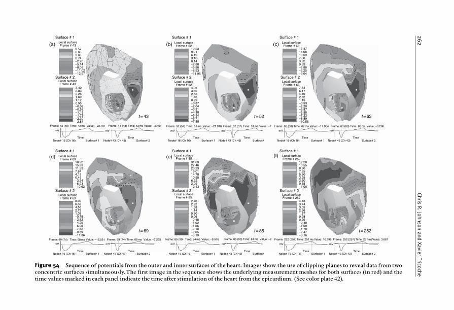
(a) Local surfaceFrame # 43
9.57
Local surfaceFrame # 52
12.239.216.193.160.14–2.88–5.90–8.93–11.95
Local surfaceFrame # 52
4.963.802.631.460.29–0.87–2.04–3.21–4.38–5.54–6.71–7.88
6.633.680.74–2.20–5.14–8.08–11.02–13.97
Local surfaceFrame # 69
Local surfaceFrame # 69
18.9215.2311.537.844.150.46–3.24–6.93–10.62
8.096.324.562.791.02–0.75–2.52–4.29–6.05–7.82–9.59–11.36
Local surfaceFrame # 85
Local surfaceFrame # 252
2.762.221.681.140.600.06–0.48–1.02–1.56–2.10–2.65–3.19
4.433.743.052.361.670.980.29–0.40–1.09–1.78–2.47–3.16
Local surfaceFrame # 85
31.6927.4623.2319.0114.7810.556.322.09–2.13
Local surfaceFrame # 252
12.2010.558.907.255.603.952.300.65–1.00
Local surfaceFrame # 43
3.402.832.261.691.120.55–0.02–0.59–1.16–1.73–2.30–2.87
Frame: 43 (48)
mV
Node# 16 (Ch 16) Surface# 1Time
mV
Node# 43 (Ch 43) Surface# 2Time
mV mV mV mV
Node# 16 (Ch 16) Surface# 1 Node# 43 (Ch 43) Surface#Time Time
Node# 16 (Ch 16) Surface# 1Time
Node# 43 (Ch 43) Surface# 2Time
Time: 42 ms Value: –22.791 Frame: 43 (48) Time: 42 ms Value: –2.461
Frame: 69 (74)
mV
Node# 16 (Ch 16) Surface# 1Time
mV
Node# 43 (Ch 43) Surface# 2Time
Time: 68 ms Value: –16.031 Frame: 69 (74) Time: 68 ms Value: –7.255 Frame: 85 (90)
mV
Node# 16 (Ch 16) Surface# 1Time
mV
Node# 43 (Ch 43) Surface#Time
Time: 84 ms Value: –9.576 Frame: 85 (90) Time: 84 ms Value: –2 Frame: 252 (257)
mV
Node# 16 (Ch 16) Surface# 1Time
mV
Node# 43 (Ch 43) Surface# 2Time
Time: 251 ms Value: 10.299 Frame: 252 (257) Time: 251 msValue: 3.661
Frame: 52 (57) Time: 51 ms Value: –21.016 Frame: 52 (57) Time: 51 ms Value: –7 Frame: 63 (68) Time: 62 ms Value: –17.964 Frame: 63 (68) Time: 62 ms Value: –9.286
Surface # 1
Surface # 2
Surface # 1Local surfaceFrame # 63
Local surfaceFrame # 63
17.4714.0810.697.303.920.53–2.86–6.25–9.64
7.846.174.492.821.15–0.53–2.20–3.87–5.55–7.22–8.89–10.56
Surface # 2
Surface # 1
Surface # 2
Surface # 1
Surface # 2
Surface # 1
Surface # 2
Surface # 1
Surface # 2
(d) (e) (f)
(b) (c)
t = 43
t = 69 t = 85 t = 252
t = 52 t = 63
Figure 54 Sequence of potentials from the outer and inner surfaces of the heart. Images show the use of clipping planes to reveal data from twoconcentric surfaces simultaneously.The first image in the sequence shows the underlying measurement meshes for both surfaces (in red) and thetime values marked in each panel indicate the time after stimulation of the heart from the epicardium. (See color plate 42).
262
Chris
R.JohnsonandXavie
rTrico
che
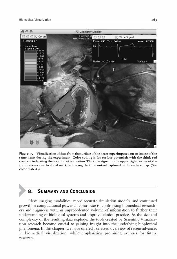
8. SUMMARY AND CONCLUSION
New imaging modalities, more accurate simulation models, and continuedgrowth in computational power all contribute to confronting biomedical research-ers and engineers with an unprecedented volume of information to further theirunderstanding of biological systems and improve clinical practice. As the size andcomplexity of the resulting data explode, the tools created by Scientific Visualiza-tion research become crucial to gaining insight into the underlying biophysicalphenomena. In this chapter, we have offered a selected overview of recent advancesin biomedical visualization, while emphasizing promising avenues for futureresearch.
Figure 55 Visualization of data from the surface of the heart superimposed on an image of thesame heart during the experiment. Color coding is for surface potentials with the think redcontour indicating the location of activation.The time signal in the upper right corner of thefigure shows a vertical red mark indicating the time instant captured in the surface map. (Seecolor plate 43).
Biomedical Visualization 263
Following a natural decomposition, techniques were presented that address thespecific challenges posed by the exploration and analysis of large-scale scalar, vector,and tensor biophysical datasets. We showed that, in each case, both effective generalpurpose and application specific methods have been devised by the ScientificVisualization community over the last decade. The proposed algorithms addressthe need for effective visual representations while ensuring an efficient processing oflarge data that supports user interaction. We also discussed the question of thedepiction of the error and uncertainty present in the visualization pipeline. Whilethe importance of this aspect has long been underestimated, it is now regarded as anessential component of a useful visual analysis within a scientific study. We con-cluded our presentation with an overview of some of the existing visualizationsoftware packages that feature the methods that we discussed. In particular, we gavea more detailed description of BioPSE and map3d that the Scientific Computing andImaging Institute has developed and made publicly available for the benefit of thebiomedical community.
Finally, we mention two important additional visualization research areas thatwe did not cover in this chapter that could have entire chapters devoted to them.Information visualization is an active research field concerned with the visualrepresentation of abstract data with no natural spatial embedding. For example, itprovides compelling tools to support analysis in bioinformatics [140,141]. Anotherbiomedical visualization area that has received a significant interest over the last fewyears is molecular visualization [142–145].
ACKNOWLEDGMENTS
The authors thank the many people who contributed to this article includingCharles Hansen, Gordon Kindlmann, Joe Kniss, Rob MacLeod, Steve Parker, C.F.Westin, Ross Whitaker, and Leonid Zhukov. The authors acknowledge supportfrom NIH NCRR Grant P41-RR12553-07, and additional support from NIH,NSF, and DOE.
REFERENCES
[1] C.R. Johnson, R. Moorhead, T. Munzner, H. Pfister, P. Rheingans, and T.S. Yoo. NIH-NSFVisualization Research Challenges Report, 2006. http://tab.computer.org/vgtc/vrc/index.html.
[2] Scientific Computing and Imaging Institute (SCI), 2007, University of Utah,www.sci.utah.edu.
[3] W. Schroeder, K. Martin, and B. Lorensen. The Visualization Toolkit: An Object OrientedApproach to Graphics, chapter 6. Kitware, Inc., Clifton Park, New York, 2003.
[4] C.D. Hansen and C.R. Johnson. The Visualization Handbook. Elsevier, 2005.[5] V. Elangovan and R.T. Whitaker. From sinograms to surfaces: A direct approach to the
segmentation of tomographic data. In Proceedings of the 4th Int. Conf. Medical Image Computingand Computer-Assisted Intervention, pages 213–223. Springer-Verlag, 2001.
264 Chris R. Johnson and Xavier Tricoche
[6] J. Kniss,G.Kindlmann, andC.Hansen.Multidimensional transfer functions for interactive volumerendering. In IEEE Transactions on Visualization and Computer Graphics, 8(3):270–285, 2002.
[7] J.M. Kniss, S. Premoze, M. Ikits, A.E. Lefohn, C.D. Hansen, and E. Praun. Gaussian transferfunctions for multi-field volume visualization. In Proceedings IEEE Visualization 2003, IEEEComputer Society Press, pages 497–504, October 2003.
[8] G. Kindlmann, R. Whitaker, T. Tasdizen, and T. Moller. Curvature-based transfer functionsfor direct volume rendering: Methods and applications. In Proceedings IEEE Visualization 2003,IEEE Computer Society Press, page 67, October 2003.
[9] M. Ikits, J.M. Kniss, A.E. Lefohn, and C. Hansen. Volume rendering techniques. InR. Fernando, editor,GPU Gems: Programming Techniques, Tips and Tricks for Real-Time Graphics,pp. 667–692. Addison Wesley, 2004.
[10] J.M. Kniss, J.P. Schulze, U. Wossner, P. Winkler, U. Lang, and C.D. Hansen. Medicalapplications of multi-field volume rendering. In Data Visualization 2004, A.K. Peters Ltd.,pages 249–254, 2004.
[11] J.M. Kniss, S. Premoze, C. Hansen, and D. Ebert. Interactive translucent volume rendering andprocedural modeling. In Proceedings IEEE Visualization 2002, IEEE Computer Society Press,pages 109–116, 2002.
[12] J. Kniss, P. McCormick, A. McPherson, J. Ahrens, J. Painter, A. Keahey, and C. Hansen.Interactive texture-based volume rendering for large datasets. In IEEE Computer Graphics andApplications, 21(4):52–61, July/August 2001.
[13] J.M. Kniss, P. McCormick, A. McPherson, J. Ahrens, J. Painter, A. Keahey, and C.D. Hansen.T-rex, texture-based volume rendering for extremely large datasets. In IEEE Computer Graphicsand Applications, 21(4):52–61, 2001.
[14] G.L. Kindlmann, D.M. Weinstein, and D. Hart. Strategies for direct volume rendering ofdiffusion tensor fields. In IEEE Transactions on Visualization and Computer Graphics,6(2):124–138, April–June 2000.
[15] G. Kindlmann and J. Durkin. Semi-automatic generation of transfer functions for direct volumerendering. In IEEE Symposium on Volume Visualization, pages 79–86. IEEE Press, October 1998.
[16] J.M. Kniss, G. Kindlmann, and C.D. Hansen. Multidimentional transfer functions forvolume rendering. In C.D. Hansen and C.R. Johnson, editors, The Visualization Handbook,pages 189–210. Elsevier, 2005.
[17] J. Kniss, G. Kindlmann, and C. Hansen. Interactive volume rendering using multi-dimensionaltransfer functions and direct manipulation widgets. In Proceedings IEEE Visualization 2001,IEEE Computer Society Press, pages 255–262, October 2001.
[18] BioPSE: Problem Solving Environment for modeling, simulation, image processing, andvisualization for biomedical computing applications. Scientific Computing and ImagingInstitute (SCI), 2007, Download from: http://www.sci.utah.edu/cibc/software/.
[19] W.E. Lorensen and H.E. Cline. Marching cubes: A high resolution 3D surface constructionalgorithm. Computer Graphics, 21(4):163–169, 1987.
[20] G. Wyvill, C. McPheeters, and B. Wyvill. Data structure for soft objects. The Visual Computer,2:227–234, 1986.
[21] R.S. Gallagher. Span filter: An optimization scheme for volume visualization of large finiteelement models. In Proceedings of Visualization ’91, pages 68–75. IEEE Computer Society Press,Los Alamitos, CA, 1991.
[22] T. Itoh, Y. Yamaguchi, and K. Koyyamada. Volume thining for automatic isosurface propagation.In Visualization ’96, pages 303–310. IEEE Computer Society Press, Los Alamitos, CA, 1996.
[23] J.S. Painter, P. Bunge, and Y. Livnat. Case study: Mantle convection visualization on the crayt3D. InVisualization ’96, pages 409–412. IEEE Computer Society Press, Los Alamitos, CA, 1996.
[24] H. Shen and C.R. Johnson. Sweeping simplicies: A fast iso-surface extraction algorithm forunstructured grids. In Proceedings of IEEE Visualization ’95, IEEE Computer Society Press,pages 143–150, 1995.
[25] H.W. Shen, C.D. Hansen, Y. Livnat, and C.R. Johnson. Isosurfacing in span space with utmostefficiency (ISSUE). In Visualization ’96, pages 287–294. IEEE Computer Society Press, 1996.
[26] Y. Livnat, H. Shen, and C.R. Johnson. A near optimal isosurface extraction algorithm usingthe span space. IEEE Transaction on Visualization and Computer Graphics, 2(1):73–84, 1996.
Biomedical Visualization 265
[27] P. Cignoni, C. Montani, E. Puppo, and R. Scopigno. Optimal isosurface extraction from irregularvolume data. In Proceedings of IEEE 1996 Symposium on Volume Visualization. ACM Press, 1996.
[28] C.L. Bajaj, V. Pascucci, and D.R. Schikore. Fast isocontouring for improved interactivity.In Proceedings of 1996 Symposium on Volume Visualization, IEEE Computer Society Press, pages39–46, 1996.
[29] C.L. Bajaj, V. Pascucci, and D.R. Schikore. The contour spectrum. In Proceedings IEEEVisualization 1997, pages 167–173, 1997.
[30] Y. Livnat, C.D. Hansen, and C.R. Johnson. Isosurface extraction for large-scale data sets. In F.Post, editor, Data Visualization: The State of the Art, 77–94, 2003.
[31] Y. Livnat, X. Cavin, and C. Hansen. PHASE: Progressive hardware assisted isosurfaceextraction framework. SCI Institute Technical Report UUSCI-2002-001, University ofUtah, 2002.
[32] Y. Livnat and C. Hansen. Dynamic view dependent isosurface extraction. SCI InstituteTechnical Report UUSCI-2003-004, University of Utah, 2003.
[33] Y. Livnat and X. Tricoche. Interactive point based isosurface extraction. In Proceedings IEEEVisualization 2004, IEEE Computer Society Press, pages 457–464, 2004.
[34] H.W. Shen and C.R. Johnson. Differential volume rendering: A fast alogrithm for scalar fieldanimation. In Visualization 94, pages 180–187. IEEE Press, 1994.
[35] R. Yagel and A. Kaufman. Template-based volume viewing. In Proceedings of EURO-GRAPHICS ’92, volume 11, pages 153–157. Blackwell, Cambridge, England, September1992.
[36] R. Yagel and Z. Shi. Accelerating volume animation by space-leaping. In Proceedings ofVisualization ’91, pages 62–69. IEEE Computer Society Press, Los Alamitos, CA, October 1993.
[37] K.L. Ma, J. Painter, C. Hansen, and M. Krogh. Parallel volume rendering using binary-swapcompositing. IEEE Computer Graphics and Applications, 14(4):59–68, 1994.
[38] C. Wang, J. Gao, L. Li, and H.W. Shen. A multiresolution volume rendering framework forlarge-scale time-varying data visualization. In International Workshop on Volume Graphics, IEEEComputer Society Press, pages 11–19, 2005.
[39] H.W. Shen, L.J. Chiang, and K.L. Ma. Time-varying volume rendering using a time-spacepartitioning tree. In IEEE Visualization 99, IEEE Computer Society Press, pages 371–377, 1999.
[40] A. Kaufman. Volume Visualization. IEEE CS Press, Los Alamitos, CA, 1990.[41] R. Crawfis and N. Max. Direct volume visualization of three-dimensional vector fields. In
Proceedings of 1992 Workshop on Volume Visualization, pages 55–60. IEEE Computer SocietyPress, Los Alamitos, CA, 1992.
[42] P.G. Swann and S.K. Semwal. Volume rendering of flow-visualization point data. In Proceedingsof Visualization ’91, pages 25–32. IEEE Computer Society Press, Los Alamitos, CA, 1991.
[43] W.H. Press, S.A. Teukolsky, W.T. Vetterling, and B.P. Flannery. Numerical Recipes, 2ndEdition. Cambridge University Press, Cambridge, 1992.
[44] G. Turk and D. Banks. Image-guided streamline placement. Computer Graphics (SIGGRAPH),30 (Annual Conference Series), pages 453–460, 1996 http://citeseer.ist.psu.edu/article/turk96imageguided.html.
[45] B. Jobard andW. Lefer. Creating evenly-spaced streamlines of arbitrary density. In Proceedings ofthe Eurographics Workshop on Visualization in Scientific Computing, pages 45–55, 1997.
[46] V. Verma, D. Kao, and A. Pang. A flow-guided streamline seeding strategy. In VISUALIZA-TION ’00: Proceedings of the 11th IEEE Visualization 2000 Conference (VIS 2000). IEEEComputer Society, 2000.
[47] A. Mebarki, P. Alliez, and O. Devillers. Farthest point seeding for efficient placement ofstreamlines. In Proceedings of IEEE Visualization 2005, IEEE Computer Society Press, pages479–486, October 2005.
[48] X. Ye, D. Kao, and A. Pang. Strategy for seeding 3d streamlines. In IEEE Computer SocietyPress, editor, IEEE Visualization Proceedings 2005, pages 471–478, October 2005.
[49] F.B. Sachse and B. Taccardi. Visualization of electrical current flow with a new streamlinetechnique: Application in mono- and bidomain simulations of cardiac tissue. In Engineering inMedicine and Biology Society 2004, IEEE EMBS 26th Annual International Conference of theIEEE, Volume 1, pages 1846–1849, 1–5 September 2004, Volume 3.
266 Chris R. Johnson and Xavier Tricoche
[50] E. Hughes, B. Taccardi, and F.B. Sachse. A heuristic streamline placement technique for visualiza-tion of electrical current flow. Journal of FlowVisualization and Image Processing 13, pages 53–66, 2006.
[51] D.C. Banks. Illumination in diverse codimensions. In SIGGRAPH 94 Proceedings, volume 28,pages 327–334, 1994.
[52] M. Zockeler, D. Stalling, and H.-C. Hege. Interactive visualization of 3D-vector fields usingilluminated streamlines. In IEEE Visualization 96 Proceedings, pages 107–113, 1996.
[53] O. Mallo, R. Peikert, C. Sigg, and F. Saldo. Illuminated streamlines revisited. In Proceedings ofIEEE Visualization 2005, pages 19–26, October 2005.
[54] G. Li, U.D. Bordoloi, and H. Shen. Chameleon: An interactive texture-based renderingframework for visualizing three-dimensional vector fields. In Proceedings of IEEE Visualization2003, page 32, October 2003.
[55] J.P.M. Hultquist. Constructing stream surfaces in steady 3D vector fields. In Proceedings of IEEEVisualization 1992, pages 171–178, October 1992.
[56] C. Garth, X. Tricoche, T. Salzbrunn, T. Bobach, and G. Scheuermann. Surface techniques forvortex visualization. In Proceedings of Joint Eurographics–IEEE TCVG Symposium on Visualization,pages 155–164, May 2004.
[57] G. Erlebacher and D. Weiskopf. Flow textures: High-resolution flow visualization. InC.D. Hansen and C.R. Johnson, editors, Visualization Handbook, pages 279–294. ElsevierAcademic Press, 2005.
[58] B. Cabral and C. Leedom. Imaging vector fields using line integral convolution. In SIG-GRAPH ’93: Proceedings of the 20th Annual Conference on Computer Graphics and InteractiveTechniques, pages 263–270, New York, NY, USA, ACM Press, 1993, http://doi.acm.org/10.1145/166117.166151.
[59] H.W. Shen and D.L. Kao. A new line integral convolution algorithm for visualizing unsteadyflows. IEEE Transactions on Visualization and Computer Graphics, 4(2), pages 98–108, 1998.
[60] B. Jobard, G. Erlebacher, and Y. Hussaini. Lagrangian Eulerian advection of noise and dyetextures for unsteady flow visualization. IEEE Transactions on Visualization and ComputerGraphics, 8(3):211–222, 2002.
[61] G.-S. Li, X. Tricoche, and C.D. Hansen. Gpuflic: Interactive and dense visualization ofunsteady flows. In Data Analysis 2006: Proceedings of Joint IEEE VGTC and EG Symposium onVisualization (Euro Vis) 2006, Eurographics Press, pages 29–34, May 2006.
[62] H. Battke, D. Stalling, and H.-C. Hege. Fast line integral convolution for arbitrary surfaces in3d. In Springer Berlin, editor, Visualization and Mathematics Experiments, Simulations and Envir-onments, Springer-Verlag, New York Inc., pages 181–195, 1997.
[63] B. Laramee, J.J. van Wijk, B. Jobard, and H. Hauser. ISA and IBFVS: Image space basedvisualization of flow on surfaces. IEEE Transactions on Visualization and Computer Graphics,10(6):637–648, November 2004.
[64] D. Weiskopf and T. Ertl. A hybrid physical/device space approach for spatiotemporallycoherent interactive texture advection on curved surfaces. In GI ’04: Proceedings of GraphicsInterface 2004, pages 263–270, 2004.
[65] M.S. Shephard, J.E. Flaherty, H.L. de Cougny, C.L. Bottasso, and C. Ozturan. Parallelautomatic mesh generation and adaptive mesh control. In M. Papadrakakis, editor, SolvingLarge Scale Problems in Mechanics: Parallel and Distributed Computer Applications, pages 459–493.John Wiley & Sons, Ltd, Chichester, 1997.
[66] V. Interrante and C. Grosch. Visualizing 3d flow. IEEE Computer Graphics and Applications,8(4):49–53, 1998.
[67] C. Resz-Salama, P. Hastreiter, C. Teitzel, and T. Ertl. Interactive exploration of volume lineintegral convolution based on 3d-texture mapping. In Proceedings of IEEE Visualization 1999,IEEE Computer Society Press, pages 233–240, October 1999.
[68] A. Sanderson, C.R. Johnson, and M. Kirby. Display of vector fields using a reaction diffusionmodel, In Proceedings IEEEVisualization 2004, IEEEComputer Society Press, pages 115–122, 2004.
[69] A.M. Turing. The chemical basis of morphogenesis. Philosophical Transactions of the Royal SocietyLondon, B237:37–72, 1952.
[70] P. Gray and S.K. Scott. Sustained oscillations and other exotic patterns of behaviour inisothermal reactions. The Journal of Physical Chemistry, 59:22–32, 1985.
Biomedical Visualization 267
[71] P. Gray and S.K. Scott. Chemical Oscillations and Inestability: Non-linear Chemical Kinetics. OxfordUniversity Press, 1990.
[72] G. Scheuermann and X. Tricoche. Topological methods for flow visualization. In C.D.Hansen and C.R. Johnson, editors, The Visualization Handbook, pages 341–356. Elsevier, 2005.
[73] X. Tricoche, G. Scheuermann, and H. Hagen. A topology simplification method for 2D vectorfields. In Proceedings of IEEE Visualization 2000, IEEE Computer Society Press, pages 359–366,2000.
[74] X. Tricoche, G. Scheuermann, and H. Hagen. Continuous topology simplification of planarvector fields. In Proceedings of IEEE Visualization 2001, IEEE Computer Society Press,pages 159–166, October 2001.
[75] C. Garth, X. Tricoche, and G. Scheuermann. Tracking of vector field singularities inunstructured 3D time-dependent data sets. In Proceedings of IEEE Visualization 2004, IEEEComputer Society Press, pages 329–336, 2004.
[76] L.V. Corbin and A.M. Scher. The canine heart as an electrocardiographic generator. CirculationResearch, 41:58–67, 1977.
[77] D.E. Roberts and A.M. Scher. Effect of tissue anisotropy on excitation potential fields in caninemyocardium in situ. Circulation Research, 50(3):342–351, March 1982.
[78] P. Colli Franzone, L. Guerri, C. Viganotti, E. Macchi, S. Baruffi, S. Spaggiari, and B. Taccardi.Potential fields generated by oblique layers modeling excitation wavefronts in the anisotropicmyocardium. Circulation Research, 51:330–346, 1982.
[79] C.S. Henriquez, A.L. Muzikant, and C.K. Smoak. Anisotropy, fiber curvature, and bathloading effects on activation in thin and thick cardiac tissue preparations. Journal of CardiovascularElectrophysiology, 7:424–444, 1996.
[80] P.J. Basser, J. Mattiello, and D. Le Bihan. Estimation of the effective self-diffusion tensor fromthe NMR spin-echo. Magnetic Resonance, 247–254, 1994.
[81] M.A. Guttman, E.A. Zerhouni, and E.R. McVeigh. Analysis of cardiac function from mrimages. IEEE Computer Graphics and Applications, 17(1):30–38, 1997.
[82] E.A. Zerhouni, D.M. Parish, W.J. Rogers, A. Yang, and E.P. Shapiro. Human heart: Taggingwith MR imaging – a method for noninvasive assessment of myocardial motion. Radiology,169(1):59–63, 1988.
[83] B. Wunsche and A.A. Young. The visualization and measurement of left ventricular deforma-tion using finite element models. International Journal of Visual Languages and Computing,14(4):299–326, 2003.
[84] A.I. Veress, G.T. Gullberg, and J.A. Weiss. Measurement of strain in left ventricle duringdiastole with cine-MRI and deformable image registration. ASME Journal of BiomechanicalEngineering, page to appear, February 2006. 127(7): pp. 1195–1207, 2005.
[85] P.J. Basser and C. Pierpaoli. Microstructural and physiological features of tissues elucidated byquantitative-diffusion-tensor MRI. Journal Magnetic Resonance B, 111(3):209–219, 1996.
[86] C.F. Westin, S. Peled, H. Gubjartsson, R. Kikinis, and F. A. Jolesz. Geometrical diffusionmeasures for MRI from tensor basis analysis. In Proceedings 5th Annual ISMRM, 1997. Inter-national Society for Magnetic Resonance in Medicine.
[87] S. Pajevic and C. Pierpaoli. Color schemes to represent the orientation of anisotropic tissuesfrom diffusion tensor data: Application to white matter fiber tract mapping in the human brain.Magnetic Resonance in Medicine, 42(3):526–540, 1999.
[88] C.-F. Westin, S.E. Meier, H. Mamata, A. Nabavi, F.A. Jolesz, and R. Kikinis. Processing andvisualization for diffusion tensor MRI. Medical Image Analysis, 6:93–108, 2002.
[89] G. Kindlmann. Superquadric tensor glyphs. Data Visualization 2004: Proceedings of The JointEurographics – IEEE TCVG Symposium on Visualization, Eurographics Press, pages 147–154,May 2004.
[90] D.H. Laidlaw, E.T. Ahrens, D. Kremers, M.J. Avalos, R.E. Jacobs, and C. Readhead. Visualizingdiffusion tensor images of the mouse spinal cord. In Proceedings IEEE Visualization 98, IEEEComputer Society Press, pages 127–134, 1998.
[91] D.S. Tuch, T.G. Reese, M.R. Wiegell, and V.J. Wedeen. Diffusion MRI of complex neuralarchitecture. Neuron, 40(5):885–895, 2003.
[92] D.S. Tuch. Q-ball imaging. Magnetic Resonance in Medicine, 52:1358–1372, 2004.
268 Chris R. Johnson and Xavier Tricoche
[93] P.J. Basser. Fiber-tractography via diffusion tensorMRI (DT-MRI). InProceedings of the 6th AnnualMeeting ISMRM, International Society for Magnetic Resonance in Medicine, page 1226, 1998.
[94] P.J. Basser, S. Pajevic, C. Pierpaoli, J. Duda, and A. Aldroubi. In vivo fiber tractograpy usingDT-MRI data. Magnetic Resonance in Medicine, pages 625–632, 2000.
[95] S. Zhang, C. Demiralp, and D.H. Laidlaw. Visualizing diffusion tensor MR images usingstreamtubes and streamsurfaces. IEEE Transactions on Visualization and Computer Graphics,9(4):454–462, October 2003.
[96] T. Delmarcelle and L. Hesselink. A unified framework for flow visualization. In R.S.Gallagher, editor, Computer Visualization: Graphics Techniques for Scientific and Engineering Ana-lysis, pages 129–170, CRC Press, 1995.
[97] D. Weinstein, G. Kindlmann, and E. Lundberg. Tensorlines: Advection-diffusion based propaga-tion through diffusion tensor fields. In Proceedings IEEE Visualization 1999, IEEE ComputerSociety Press, pages 249–253, 1999.
[98] L. Zhukov and A. Barr. Oriented tensor reconstruction: Tracing neural pathways fromdiffusion tensor MRI. In Proceedings of IEEE Visualization 2002, IEEE Computer SocietyPress, pages 387–394, 2002.
[99] L. Zhukov and A. Barr. Heart-muscle fiber reconstruction from diffusion tensor MRI. InProceedings of IEEE Visualization 2003, IEEE Computer Society Press, pages 597–602, 2003.
[100] M. Hlawitschka and G. Scheuermann. Hot-lines: Tracking lines in higher-order tensor fields. InProceedings of IEEEVisualization 2005, IEEEComputer Society Press, pages 27–34, October 2005.
[101] A. Brun, H.-J. Park, H. Knutsson, and C.-F. Westin. Coloring of DT-MRI fiber traces usinglaplacian eigenmaps. Computer Aided Systems Theory – EUROCAST 2003, Lecture Notes inComputer Science 2809, Springer, page 2809, 2003.
[102] M. Cantani, R.J. Howard, S. Pajevic, and D.K. Jones. Virtual in vivo interactive dissection ofwhite matter fasciculi in the human brain. NeuroImage, 17:77–94, 2002.
[103] S. Wakana, H. Jiang, L.M. Nagae-Poetscher, P.C. van Zijl, and S. Mori. Fiber tract-based atlasof human white matter anatomy. Radiology, 230(1):77–87, 2004.
[104] D. Akers, A. Sherbondy, R. Mackenzie, R. Dougherty, and B. Wandell. Exploration of thebrain’s white matter pathways with dynamic queries. In Proceedings of IEEE Visualization 2004,IEEE Computer Society Press, pages 377–384, 2004.
[105] J. Blaas, C.P. Botha, B. Peters, F.M. Vos, and F.H. Post. Fast and reproducible fiber bundleselection in dti visualization. In Proceedings of IEEE Visualization 2005, IEEE Computer SocietyPress, pages 59–64, 2005.
[106] A. Brun, H. Knutsson, H.J. Park, M.E. Shenton, and C.-F. Westin. Clustering fiber tracts usingnormalized cuts. In Seventh International Conference on Medical Image Computing and Computer-Assisted Intervention (MICCAI’04), Lecture Notes in Computer Science, pages 368–375,Rennes – Saint Malo, France, September 2004.
[107] S. Zhang and D.H. Laidlaw. DTI fiber clustering and cross-subject cluster analysis. In Proceed-ings of ISMRM International Society for Magnetic Resonance in Medicine, 2005.
[108] A. Wenger, D.F. Keefe, S. Zhang, and D.H. Laidlaw. Interactive volume rendering of thinthread structures within multivalued scientific datasets. IEEE Transactions on Visualization andComputer Graphics, 10(6):664–672, 2004.
[109] G.L. Kindlmann and D.M. Weinstein. Hue-balls and lit-tensors for direct volume rendering ofdiffusion tensor fields. In Proceedings of the IEEE Visualization 99, pages 183–189, 1999.
[110] G.L. Kindlmann and D.M. Weinstein. Strategies for direct volume rendering of diffusiontensor fields. IEEE Transactions on Visualization and Computer Graphics, IEEE Computer SocietyPress, 6(2):124–138, 2000.
[111] D. Stalling, M. Zockler, and H.-C. Hege. Fast display of illuminated field lines. IEEETransactions on Visualization and Computer Graphics, 3(2):118–128, 1996.
[112] G. Kindlmann. Visualization and Analysis of Diffusion Tensor Fields. Ph.D. Thesis, University ofUtah, 2004.
[113] G. Kindlmann, X. Tricoche, and C.-F. Westin. Anisotropy creases delineate white matterstructure in diffusion tensor MRI. In Proceedings of Medical Imaging Computing andComputer-Assisted Intervention, MICCAI ’06, Lecture Notes in Computer Science 3749, Springer,2006.
Biomedical Visualization 269

[114] C.R. Johnson. Top scientific visualization research problems. IEEE Computer Graphics andApplications: Visualization Viewpoints, 24(4):13–17, July/August 2004.
[115] C.H. Wolters, A. Anwander, X. Tricoche, D. Weinstein, M.A. Koch, and R.S. MacLeod.Influence of tissue conductivity anisotropy on EEG/MEG field and return currentcomputation in a realistic head model: A simulation and visualization study using high-resolution finite element modeling. NeuroImage, 2006 Apr 15; 30(3):813–26. December2005.
[116] D. Gullmar, J.R. Reichenbach, A. Anwander, T. Knosche, C.H. Wolters, M. Eiselt, andJ. Haueisen. Influence of anisotropic conductivity of the white matter tissue on eeg sourcereconstruction – an fem simulation study. Biomedical Engineering, IEEE Transactions on53(9):1841–1850, September 2006, 7(1):108–110, 2005.
[117] R.M. Kirby, H. Marmanis, and D.H. Laidlaw. Visualizing multivalued data from 2Dincompressible flows using concepts from painting. In Proceedings of the IEEE Visualization99, IEEE Computer Society Press, 1999.
[118] C.R. Johnson and A.R. Sanderson. A next step: Visualizing errors and uncertainty. IEEEComputer Graphics and Applications, 23(5):6–10, September/October 2003.
[119] B.N. Taylor and C.E. Kuyatt. Guidelines for expressing and evaluating the uncertainty ofNIST experimental results. Technical report, NIST Technical Note 1297, 1994.
[120] A.T. Pang, C.M. Wittenbrink, and S.K. Lodha. Approaches to uncertainty visualization. TheVisual Computer, 13(8):370–390, November 1997.
[121] G. Grigoryan and P. Rheingans. Probabilistic surfaces: Point based primitives to show surfaceuncertainty. In IEEE Visualization ‘02, pages 147–153. IEEE Press, 2002.
[122] A.R. Sanderson, M. Kirby, C.R. Johnson, and L. Yang. Advanced reaction-diffusion modelsfor texture synthesis. Journal of Graphics Tools, 11(3):47–71, 2006.
[123] J.M. Kniss, R. Van Uitert, A. Stephens, G. Li, and T. Tasdizen. Statistically quantitativevolume visualization. In IEEE Visualization 2005, 2005.
[124] T. Tasdizen, S.P. Awate, R.T. Whitaker, and N. Foster. MRI tissue classification withneighborhood statistics: A nonparametric, entropy-minimizing approach. In Proceedings of the8th International Conference on Medical Image Computing and Computer Assisted Intervention(MICCAI), Lecture Notes in Computer Science 3749, Springer, pages 517–525, 2005.
[125] S.G. Parker and C.R. Johnson. SCIRun: A scientific programming environment for computa-tional steering. In Supercomputing ‘95. IEEE Press, 1995.
[126] C.R. Johnson and S.G. Parker. Applications in computational medicine using SCIRun: Acomputational steering programming environment. In H.W. Meuer, editor, Supercomputer ‘95,pages 2–19. Springer-Verlag, 1995.
[127] SCIRun: A Scientific Computing Problem Solving Environment, Scientific Computing andImaging Institute (SCI), 2007, Download from: http://software.sci.utah.edu/scirun.html.
[128] R.S. MacLeod, C.R. Johnson, and M.A. Matheson. Visualization tools for computationalelectrocardiography. In Visualization in Biomedical Computing, pages 433–444, Bellingham,Washington, 1992. Proceedings of the SPIE #1808.
[129] R.S. MacLeod, C.R. Johnson, and M.A. Matheson. Visualization of cardiac bioelectricity –a case study. In Proceedings of the IEEE Visualization 92, pages 411–418. IEEE CS Press,1992.
[130] R.S. MacLeod, C.R. Johnson, and M.A. Matheson. Visualizing bioelectric fields. IEEEComputer Graphics and Applications, 13(4):10–12, 1993.
[131] R.S. MacLeod and C.R. Johnson. Map3d: Interactive scientific visualization for bioengineer-ing data. pages 30–31. IEEE Press, 1993. http://software.sci.utah.edu/map3d.html.
[132] B. Taccardi, B.B. Punske, R.L. Lux, R.S. MacLeod, P.R. Ershler, T.J. Dustman, andY. Vyhmeister. Useful lessons from body surface potential mapping. 9:773–786, 1998.
[133] B.P. Punske, Q. Ni, R.L. Lux, R.S. MacLeod, P.R. Ershler, T.J. Dustman, Y. Vyhmeister, andB. Taccardi. Alternative methods of excitation time determination on the epicardial surface.Engineering in Medicine and Biology Society, 2000. Proceedings of the 22nd AnnualInternational Conference of the IEEE Volume 2, Issue, 888–890, 2000.
[134] B. Taccardi, B.B. Punske, R.S. MacLeod, and Q. Ni. Extracardiac effects of myocardialelectrical anisotropy. Biomedizinische Technik, 46(Supp 2):216–218, 2001.
270 Chris R. Johnson and Xavier Tricoche

[135] B.B. Punske, Q. Ni, R.L. Lux, R.S. MacLeod, P.R. Ershler, T.J. Dustman, M.J. Allison, andB. Taccardi. Spatial methods of epicardial activation time determination. Annals of BiomedicalEngineering, 31(7):781–792(12), July 2003, 31:781–792, 2003.
[136] B. Taccardi, B.B. Punske, R.S. MacLeod, and Q. Ni. Visualization, analysis and physiologicalinterpretation of three-dimensional cardiac electric fields. pages 1366–1367. IEEE EMBS,IEEE, 2002.
[137] F.H. Lopes da Silva. A critical review of clinical applications of topographic mapping of brainpotentials. Journal of Clinical Neurophysiology, 7(4):535–551, 1990.
[138] J.S. George, C.J. Aine, J.C. Mosher, D.M. Schmidt, D.M. Ranken, H.A. Schlitt, C.C. Wood,J.D. Lewine, J.A. Sanders, and J.W. Belliveau. Mapping function in the human brain withmagnetoencephalography, anatomical magnetic resonance imaging, and functional magneticresonance imaging. Journal of Clinical Neurophysiology, 12(5):406, 1995.
[139] F. Lopes da Silva. Functional localization of brain sources using EEG and/or MEG data:Volume conductor and source models. Magnetic Resonance Imaging, 22(10):1533–1538,December 2004.
[140] J. Slack, K. Hildebrand, T. Munzner, and K. St. John. SequenceJuxtaposer: Fluid navigation forlarge-scale sequence comparison in context. In Proceedings of German Conference in Bioinformatics,pages 37–42, 2004.
[141] J. Slack, K. Hildebrand, and T. Munzner. Partitioned rendering infrastructure for scalableaccordion drawing (extended version). Information Visualization 5(2):137–151, 2006.
[142] C. Bajaj, P. Djeu, V. Siddavanahalli, and A. Thane. Interactive visual exploration of largeflexible multi-component molecular complexes. In Proceedings of IEEE Visualization ’04, IEEEComputer Society Press, pages 243–250, 2004.
[143] C. Bajaj, J. Castillon-Candas, V. Siddavanahalli, and Z. Xu. Compressed representations ofmacromolecular structures and properties. Structure, 13(3):463–471, March 2005.
[144] C.H. Lee and A. Varshney. Representing thermal vibrations and uncertainty in molecularsurfaces. In Proceedings SPIE Conference on Visualization and Data Analysis, January 20–25, 2002.
[145] C.H. Lee and A. Varshney. Computing and displaying intermolecular negative volume fordocking. In G.M. Nielson G.-P. Bonneau, T. Ertl, editors, Scientific Visualization: The VisualExtraction of Knowledge from Data. Springer-Verlag, ISBN 3-540-26066-8, 2005.
Biomedical Visualization 271

This page intentionally left blank
INDEX
Absorbance or absorption, 148
bands, 148–149
spectrum, 148–149
ABS see Average beat subtraction
(ABS)
Adaption coefficient see Step size
AF see Atrial fibrillation (AF)
Algorithms:
batch, 113, 133
block see batch
on-line, 112–113
off-line, 112–113
recursive see on-line
stochastic, 113
windowed see batch
Anisotropy:
fractional, 235
linear, 235
planar, 235
Artficial organs, 2, 11
Artifacts, ocular, 124–125, 133–138
Atrial activity (AA), 115
Atrial fibrillation (AF), 38,
115, 117
Atria see Heart, parts
Atrio–ventricular (AV) node, 102,
115–116
Auto-fluorescent proteins, 145–174
Average beat, 120–121, 123
Average beat subtraction (ABS), 123
Barycentric coordinates, 241–242
Beer-Lambert law, 148–149, 151
Bioelectric currents, 210,
226–229, 233
Biomedical devices, 2
Blind source separation (BSS), 97,
114, 123
algorithms, 126–127, 131
assumptions, 125
indeterminacies, 127
whitening, 131
see also Independent component
analysis (ICA)
Brain, 105
cortical lobes, 105–106
electrical model, 106
functions, 105
BSS see Blind source separation (BSS)
Circulatory system, 11, 15, 19, 35,
101–102
Contrast function, 129–132
maximization see Blind source
separation (BSS), algorithms
Correlation, cross-correlation function,
121–123
Covariance matrix, 112, 121–123,
129–132, 241
sample estimate, 112
Crease surfaces, 244
Cumulants, 128
cross-cumulants, 128, 130
fourth-order, 130
higher-order, 127, 131
marginal, 128, 130–131
multilinearity, 130–131
sample, 133
second-order, 128,
Detector, 176–180, 184
collimator, 177–179, 184
design, 186
in time-of-flight PET, 184
ring detector, 178–179, 195–196
scintillating crystal, 177–178
Diffusion tensor
imaging, 210, 234
273
Dipole, 98
in a heterogeneous medium, 100
in a homogeneous medium, 99
moment, 99, 101, 104
realistic models, 100
Direct volume rendering, 211, 222,
241–242
3D texture memory, 217
boundary, 214–216
cerebral vasculature, 212
classification, 217
classify, 216
CT, 216
derivatives, 216
direct manipulation widgets, 217
edge-detection, 216
eigenvector, 217
electron microscope tomography
(EMT), 214
features of interest, 211–212
Gaussian transfer functions, 217
gradient direction, 216
gradient magnitude, 216
gradients, spatial, 216
graphic cards, 213–214
graphics hardware, 217
interactive response, 217
lookup tables, 217
matrix, 217
maximum intensity projection
(MIP), 212
memory efficient, 217
MR imaging, 217
multi-dimensional transfer functions,
216
opacity function, 214
optical properties, 211–212
ramp function, 213–214
reconstruction artifacts, 214
rendering techniques, 211–212
isosurfacing, 211–212
segmentation, 211–212
semi-automatic generation of
transfer functions, 214–215
transfer function, 211–212
transfer function design, 212
user interface, 217
Visible Male, 216
X-rays, 213
Dosimetry, 186, 200
DsRed, 165–166
ECG see Electrocardiogram (ECG)
EEG see Electroencephalogram (EEG)
Eigenvalue decomposition
(EVD), 130–132
Eigenvalues, 235
invariant, 236
Eigenvectors, 235
major, 235
medium, 235
minor, 235
spherical color map, 236
Electrocardiogram (ECG), 103
fetal, 109
P wave, 103t
QRS complex, 103t
T wave, 103t
Electroencephalogram (EEG), 106
artifacts, 108
Emission tomography see Single
photon emission computed
tomography (SPECT); Positron
emission tomography (PET)
small animal imaging, 179, 194
Epilepsy, 106, 123–124
ERP see Event-related
potential (ERP)
Error and uncertainty visualization, 250
fuzzy classification, 252–254
fuzzy surface, 250
uncertainty definitions, 250
EVD see Eigenvalue decomposition
(EVD)
274 Index
Event-related potential (ERP),
106, 108t
Extinction coefficient, 148–149, 151,
157–159, 161, 166
Fiber tractography, 239, 244
clustering, 241
hyperstreamlines, 239–240
local tracking, 240
moving least squares, 240
muscle fibers, 239–240
normalized cuts, 241
pathways of axon bundles, 239–240
principal eigenvector, 239–240
regions of interest, 241
streamtubes, 240
tensorlines, 240
Filtering:
optimal see Wiener
spatial, 96–97, 111, 113, 119
spatio-temporal, 113
Finite element, 63
basics, 63
effective use, 68
stent design, 66
Fluorescence, 145–174
anisotropy, 155
brightness, 151, 160, 163–165
decay, 152–153
delayed, 150
emission, 149
excitation, 149
non-radiative decay, 149
quenching, 157
Fluorescence correlation spectroscopy
(FCS), 166–167
Fluorescence lifetime, 151
measurement, 153
frequency domain, 154
time domain, 153
modulation, 154–155
phase, 154–155
Fluorescence lifetime imaging
microscopy (FLIM), 167–169
Fluorescence loss in photobleaching
(FLIP), 166–167
Fluorescence recovery after
photobleaching (FRAP), 166–167
Fluorescence resonance energy transfer
(FRET), 158
efficiency, 166–169
rate, 158–159
Fluorescent proteins, 160–161, 165
see also Green fluorescent protein
(GFP)
Fluorophore, 151–153, 155–165, 167
FMRI see Magnetic resonance imaging
(MRI), functional
Forster radius, 158–159
Franck–Condon principle,
148, 150
Frank system see Leads
Frobenius norm, 235–236
Gamma camera, 177–178, 189
GATE, 188
digitization, 193
features, 188
time management, 192
GEANT4, 182, 187–189,
191–192, 194
Givens rotation, 132
Gradient, 23–24, 27, 32, 36, 68,
112–113, 216–217, 240–242
Gram–Schmidt
orthogonalization, 132
Green fluorescent protein (GFP), 161
chromophore, 161
structure, 161
variants, 163
Heart, 8, 34, 101
dipole moment, 104
electrical model, 104
Index 275
Heart (Continued)
electric heart vector, 104
parts, 101
High angular resolution diffusion
(HARD), 239–241
HOS see Statistics, higher-order
ICA see Independent component
analysis (ICA)
IED see Interictal epileptic discharge
(IED)
Illuminated streamlines, 242
Image degradation factors, 185
Image reconstruction, 88, 179, 195
see also Nuclear medicine imaging,
data acquisition
Independence, 97, 126–127
see also Uncorrelation
Independent component analysis
(ICA), 129–130, 135–136,
see also Blind source separation (BSS)
Independent subspace analysis
(ISA), 138
Information visualization, 210, 224,
264
Interictal epileptic
discharge (IED), 123
Internal conversion, 149–150
Intersystem crossing, 149–150
ISA see Independent subspace
analysis (ISA)
Isosurface, 220
accelerating, 220
applications, 221
cardiac arrhythmia, 221–222
cortical surface, 222
cutting plane, 221
high-performance, 221
isochrone, 221
isopotential, 221
scalp, 222
SCIRun, 221
complexity, 220
contour spectrum, 220
divide and conquer, 220
lookup table, 220
Marching Cubes, 220
point-based approach, 221
real-time, 220
remote visualization, 220–221
shadows, 221
span space, 220
triangulation, 220
view-dependent, 220–221
visibility, 221
Visible Female, 221
Jabłonski diagram, 147
Jacobi diagonalization, 132
Kurtosis see Cumulants, fourth-order
Leads:
10–20 International System, 106
Frank system, 104
orthogonal, 104, 117
X, Y, Z see orthogonal
Least mean squares (LMS), 113
Least squares (LS), 121–122
LMS see Least mean
squares (LMS)
LS see Least squares (LS)
Luminescence, 146
Magnetic resonance imaging (MRI),
75, 106, 124, 140, 176–177, 234,
237–240, 255
functional, 124, 140
Magnetoencephalogram (MEG), 106,
140, 223–224
Map3d, 258
‘‘activation’’ time, 260–261
cardiac wave, 260–261
coronary arteries, 260–261
electroencephalography, 259
276 Index
electrophysiology, 258–259
heart beat, 260–261
ventricles, 260–261
Material properties, 65
stainless steel, 66
Maximum likelihood (ML), 122–123,
129, 211
Medical robots, 43
MEG see Magnetoencephalogram
(MEG)
Methodology, 68–69, 72–73, 75–78,
81, 84, 89, 98, 117, 222
Methods see Algorithms
Micro-CT, 64
microtomography, 89
MI see Mutual information (MI)
Mixing matrix, 119, 121, 126–127,
129–130, 133–134, 136, 138–139
Mixtures, 35–36, 97, 110, 117, 119,
129, 135, 138–139
overdetermined, 126–127, 135
underdetermined, 138–139
ML see Maximum likelihood (ML)
Model:
blind, 121
brain, 106
heart, 104
physical-based, 121
Moments, sample, 133
Monte Carlo simulation, 180, 184, 187
applications, 186
calculation time, 194
variance reduction techniques,
194–195
definition, 180
particle transport, 182
patient data, 184–185, 196–197
photon interactions, 180, 182,
194–195
probability distribution function,
181–183
random number generator, 180
sampling techniques, 181
distribution function, 181
mixed Monte Carlo method, 181
non-analog sampling, 181
rejection function, 181
scatter compensations, 182–185
scoring, 183
significance, 184, 200
validation of, 194
MRI see Magnetic resonance imaging
(MRI)
Multi-field visualization, 245
computational field problems, 245
ordinary and/or partial differential
equations, 245
return currents, 247
source localization, 247
Multimodal processing, 140
Mutual information (MI), 129
Noise, 13, 97, 100, 108–110, 112,
114, 195, 210–212, 229, 236,
239–240
Non-Gaussianity, 126–127
Normal sinus rhythm (NSR), 102,
115–117
NSR see Normal sinus rhythm (NSR)
Nuclear medicine imaging, 176
data acquisition, 179–180
correction methods, 185, 195
simulation, 180
PCA see Principal component analysis
(PCA)
PET see Positron emission tomography
(PET)
Phenotypes, 210
Phosphorescence, 146, 149–150
Photoluminescence, 146
Photon transport modeling, 182
PHV see Piecewise homogeneous
volume (PHV)
Index 277
Piecewise homogeneous volume
(PHV), 100
Polarization, 155
Positron emission tomography (PET),
106, 176, 178
annihilation photons, 178–179, 185,
189–190, 192, 195–196
depth-of-interaction, 184–185
modeling, 184–185
time-of-flight PET, 184, 192
PowerApps, 257
pipelines, 257–258
user interface (UI), 257–258
Principal component analysis (PCA),
129
Prior information, 135–136, 138, 140
Projection:
oblique, 126–127
orthogonal, 119
Quantum yield, 151–153, 157,
158–161
Radiopharmaceutical, 176–180,
196–197
3D distribution of, 177–178
Receiver operating characteristic
(ROC), 186
Red fluorescent protein (RFP), 165
monomeric, 166
Reference:
spatial, 136
temporal, 136
Regression, 119, 121–122
Rhodamine 6G, 153, 156–157, 161
Ridges, 244
Rotational correlation
time, 155–157
Scalar fields, 211, 222, 223–224,
241– 242, 252, 255–256
Scientific visualization, 210–212,
223–224, 255–256
SCIRun/BioPSE, 255
interactive feedback, 256–257
problem-solving environment
(PSE), 255–256
Separating matrix, 126–127, 129,
131–132
Simulator see GATE
Single photon emission computed
tomography (SPECT), 106, 176
modeling, 180, 184–185, 194, 200
spatial resolution, 177–178, 185, 193
system matrix, 197–198
Single photon imaging, 177
Singular value decomposition (SVD),
118
economical, 132
Sino–atrial (SA) node, 102
Source signals, 136
Sparseness see Sparsity
Sparsity, 126, 138–139
Spatio-temporal
cancellation, 115, 117
SPECT see Single photon emission
computed tomography (SPECT)
Spherical color map, 236
Standardized variable see Whitening,
whitened observations
Stationarity, 98, 110–111
Statistics, 127
higher-order, 127
second-order, 97, 130, 139–140
Stent modeling, 68
alternative methods, 84
cylindrical balloon, 74
folded balloon, 78
neglect of the balloon, 69
validation, 81
Step size, 113, 225
Stokes equation, 155–156
Stokes shift, 149–150
SVD see Singular value decomposition
(SVD)
278 Index
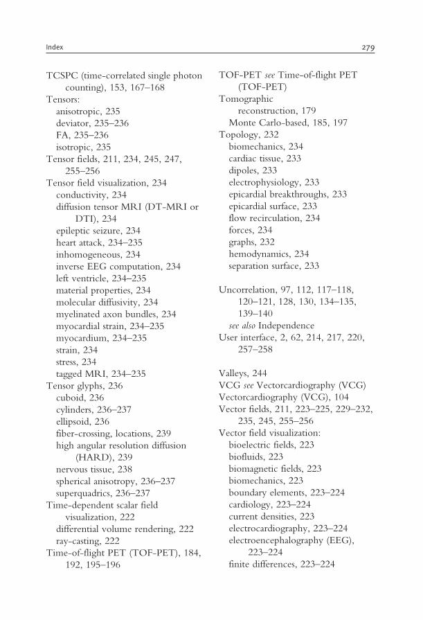
TCSPC (time-correlated single photon
counting), 153, 167–168
Tensors:
anisotropic, 235
deviator, 235–236
FA, 235–236
isotropic, 235
Tensor fields, 211, 234, 245, 247,
255–256
Tensor field visualization, 234
conductivity, 234
diffusion tensor MRI (DT-MRI or
DTI), 234
epileptic seizure, 234
heart attack, 234–235
inhomogeneous, 234
inverse EEG computation, 234
left ventricle, 234–235
material properties, 234
molecular diffusivity, 234
myelinated axon bundles, 234
myocardial strain, 234–235
myocardium, 234–235
strain, 234
stress, 234
tagged MRI, 234–235
Tensor glyphs, 236
cuboid, 236
cylinders, 236–237
ellipsoid, 236
fiber-crossing, locations, 239
high angular resolution diffusion
(HARD), 239
nervous tissue, 238
spherical anisotropy, 236–237
superquadrics, 236–237
Time-dependent scalar field
visualization, 222
differential volume rendering, 222
ray-casting, 222
Time-of-flight PET (TOF-PET), 184,
192, 195–196
TOF-PET see Time-of-flight PET
(TOF-PET)
Tomographic
reconstruction, 179
Monte Carlo-based, 185, 197
Topology, 232
biomechanics, 234
cardiac tissue, 233
dipoles, 233
electrophysiology, 233
epicardial breakthroughs, 233
epicardial surface, 233
flow recirculation, 234
forces, 234
graphs, 232
hemodynamics, 234
separation surface, 233
Uncorrelation, 97, 112, 117–118,
120–121, 128, 130, 134–135,
139–140
see also Independence
User interface, 2, 62, 214, 217, 220,
257–258
Valleys, 244
VCG see Vectorcardiography (VCG)
Vectorcardiography (VCG), 104
Vector fields, 211, 223–225, 229–232,
235, 245, 255–256
Vector field visualization:
bioelectric fields, 223
biofluids, 223
biomagnetic fields, 223
biomechanics, 223
boundary elements, 223–224
cardiology, 223–224
current densities, 223
electrocardiography, 223–224
electroencephalography (EEG),
223–224
finite differences, 223–224
Index 279
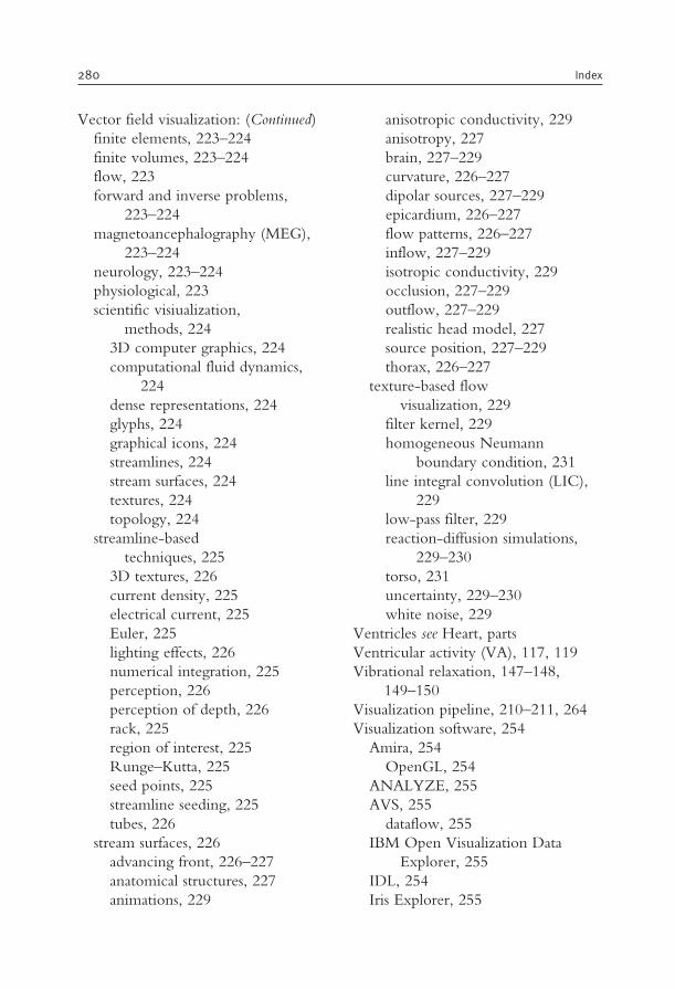
Vector field visualization: (Continued)
finite elements, 223–224
finite volumes, 223–224
flow, 223
forward and inverse problems,
223–224
magnetoancephalography (MEG),
223–224
neurology, 223–224
physiological, 223
scientific visiualization,
methods, 224
3D computer graphics, 224
computational fluid dynamics,
224
dense representations, 224
glyphs, 224
graphical icons, 224
streamlines, 224
stream surfaces, 224
textures, 224
topology, 224
streamline-based
techniques, 225
3D textures, 226
current density, 225
electrical current, 225
Euler, 225
lighting effects, 226
numerical integration, 225
perception, 226
perception of depth, 226
rack, 225
region of interest, 225
Runge–Kutta, 225
seed points, 225
streamline seeding, 225
tubes, 226
stream surfaces, 226
advancing front, 226–227
anatomical structures, 227
animations, 229
anisotropic conductivity, 229
anisotropy, 227
brain, 227–229
curvature, 226–227
dipolar sources, 227–229
epicardium, 226–227
flow patterns, 226–227
inflow, 227–229
isotropic conductivity, 229
occlusion, 227–229
outflow, 227–229
realistic head model, 227
source position, 227–229
thorax, 226–227
texture-based flow
visualization, 229
filter kernel, 229
homogeneous Neumann
boundary condition, 231
line integral convolution (LIC),
229
low-pass filter, 229
reaction-diffusion simulations,
229–230
torso, 231
uncertainty, 229–230
white noise, 229
Ventricles see Heart, parts
Ventricular activity (VA), 117, 119
Vibrational relaxation, 147–148,
149–150
Visualization pipeline, 210–211, 264
Visualization software, 254
Amira, 254
OpenGL, 254
ANALYZE, 255
AVS, 255
dataflow, 255
IBM Open Visualization Data
Explorer, 255
IDL, 254
Iris Explorer, 255
280 Index

Micro View, 255
open-source, 255
Python, 255
VTK, 255
OsiriX, 255
VTK, 255
C++, 255
Java, 255
MPI, 255
Python, 255
Tcl, 255
Volume-rendering applicatications,
218
angiogenesis, 218
BioImage PowerApp, 218
BioPSE, 218
lung tumors, 218
thoracic CT, 218
transgenic mice, 218
tumors, 218
White matter tracts, 210, 239–240
Whitening, 131
matrix, 132
whitened observations, 130
Wiener, 109–110, 136, 139–140
canceller, 111, 114
Wiener–Hopf solution, 112
X, Y, Z leads see Leads, orthogonal
Index 281

This page intentionally left blank
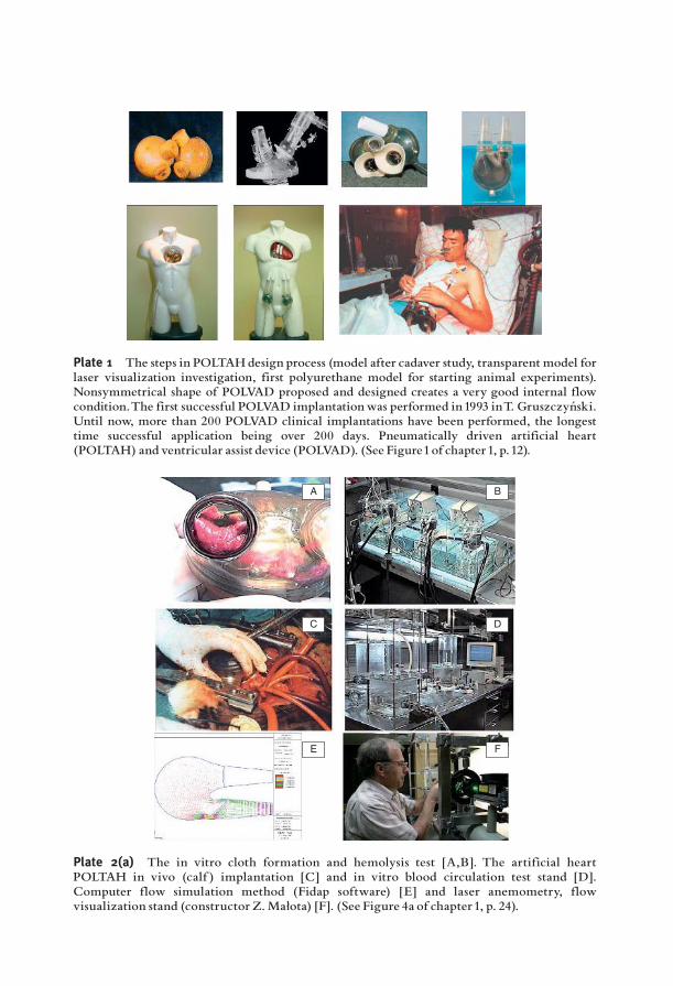
Plate 1 The steps in POLTAHdesign process (model after cadaver study, transparent model forlaser visualization investigation, first polyurethane model for starting animal experiments).Nonsymmetrical shape of POLVAD proposed and designed creates a very good internal flowcondition.The first successful POLVAD implantationwas performed in 1993 inT. Gruszczyn¤ ski.Until now, more than 200 POLVAD clinical implantations have been performed, the longesttime successful application being over 200 days. Pneumatically driven artificial heart(POLTAH) and ventricular assist device (POLVAD). (See Figure1of chapter1, p. 12).
A B
C D
E F
Plate 2(a) The in vitro cloth formation and hemolysis test [A,B]. The artificial heartPOLTAH in vivo (calf ) implantation [C] and in vitro blood circulation test stand [D].Computer flow simulation method (Fidap software) [E] and laser anemometry, flowvisualization stand (constructor Z.Małota) [F]. (See Figure 4a of chapter1, p. 24).
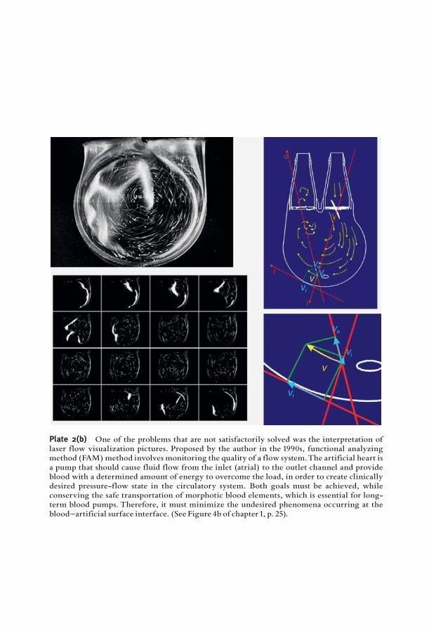
o
r
i
Vr
Vr
Vi
Vi
Vo
Vo
V
V
Plate 2(b) One of the problems that are not satisfactorily solved was the interpretation oflaser flow visualization pictures. Proposed by the author in the 1990s, functional analyzingmethod (FAM) method involves monitoring the quality of a flow system.The artificial heart isa pump that should cause fluid flow from the inlet (atrial) to the outlet channel and provideblood with a determined amount of energy to overcome the load, in order to create clinicallydesired pressure-flow state in the circulatory system. Both goals must be achieved, whileconserving the safe transportation of morphotic blood elements, which is essential for long-term blood pumps. Therefore, it must minimize the undesired phenomena occurring at theblood^artificial surface interface. (See Figure 4b of chapter1, p. 25).
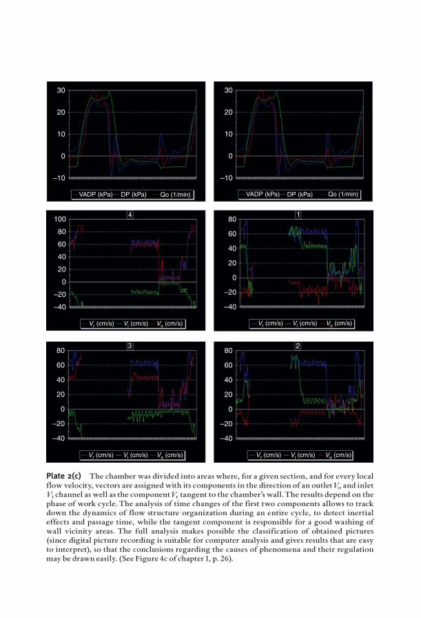
30
20
10
0
–10
VADP (kPa)
Vr (cm/s) Vi (cm/s) Vo (cm/s) Vr (cm/s) Vi (cm/s) Vo (cm/s)
Vr (cm/s) Vi (cm/s) Vo (cm/s) Vr (cm/s) Vi (cm/s) Vo (cm/s)
VADP (kPa)DP (kPa) DP (kPa)Qo (1/min) Qo (1/min)
100
80
60
40
20
0
–20
–40
801
23
4
60
40
20
0
–20
–40
80
60
40
20
0
–20
–40
80
60
40
20
0
–20
–40
30
20
10
0
–10
Plate 2(c) The chamber was divided into areas where, for a given section, and for every localflow velocity, vectors are assigned with its components in the direction of an outletVo and inletVi channel as well as the componentVr tangent to the chamber’s wall.The results depend on thephase of work cycle.The analysis of time changes of the first two components allows to trackdown the dynamics of flow structure organization during an entire cycle, to detect inertialeffects and passage time, while the tangent component is responsible for a good washing ofwall vicinity areas. The full analysis makes possible the classification of obtained pictures(since digital picture recording is suitable for computer analysis and gives results that are easyto interpret), so that the conclusions regarding the causes of phenomena and their regulationmay be drawn easily. (See Figure 4c of chapter 1, p. 26).
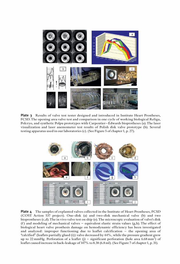
a
b c
Plate 3 Results of valve test tester designed and introduced in Institute Heart Prostheses,FCSD.The opening area valve test and comparison in one cycle of working biological Religa,Polcryo, and synthetic Polpu prototypes with Carpentier^Edwards bioprotheses (a).The laservisualization and laser anemometer test results of Polish disk valve prototype (b). Severaltesting apparatus used in our laboratories (c). (See Figure 5 of chapter1, p. 27).
a b c d
f g he
i j
Plate 4 The samples of explanted valves collected in the Institute of Heart Prostheses, FCSD(COST Action 537 project). One-disk (a) and two-disk mechanical valve (b) and twobioprostheses (c,d).The in vivo valve test on ship (e).The microscopic evaluation of valve’s disk(f ) and modeling of mechanical valves ^ equivalent elastic strain values (g,h). The effect ofbiological heart valve prosthesis damage on hemodynamic efficiency has been investigatedand analyzed: improper functioning due to leaflet calcification ^ the opening area of‘‘calcified’’ (leaflets partially glued (i)) valve decreased by 44%, while the pressure gradient grewup to 22mmHg. Perforation of a leaflet (j) ^ significant perforation (hole area 6.68mm2) ofleaflet caused increase in back-leakage of 147% to 8.38 (6.8ml). (See Figure 7 of chapter1, p. 31).
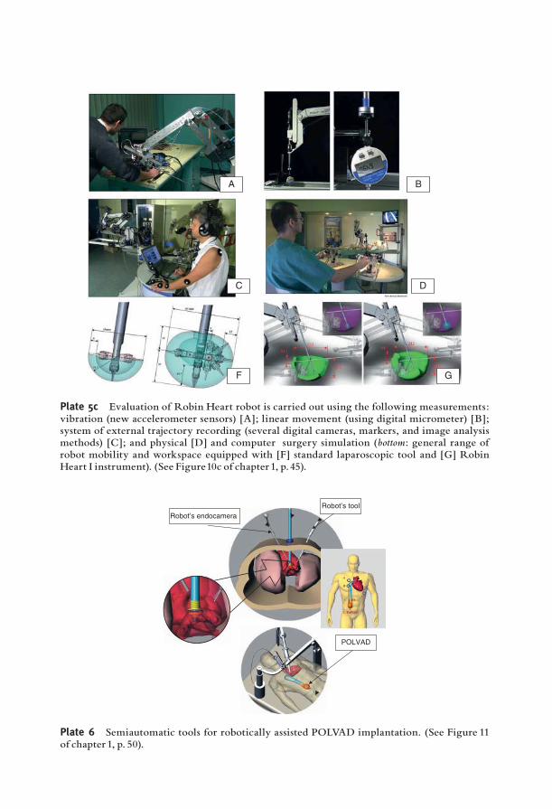
A B
C D
F G
Plate 5c Evaluation of Robin Heart robot is carried out using the following measurements:vibration (new accelerometer sensors) [A]; linear movement (using digital micrometer) [B];system of external trajectory recording (several digital cameras, markers, and image analysismethods) [C]; and physical [D] and computer surgery simulation (bottom: general range ofrobot mobility and workspace equipped with [F] standard laparoscopic tool and [G] RobinHeart I instrument). (See Figure10c of chapter1, p. 45).
Robot’s tool
Robot’s endocamera
POLVAD
Plate 6 Semiautomatic tools for robotically assisted POLVAD implantation. (See Figure 11of chapter 1, p. 50).
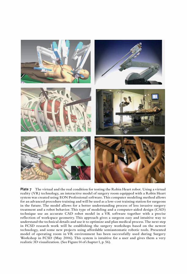
Plate 7 The virtual and the real condition for testing the Robin Heart robot. Using a virtualreality (VR) technology, an interactive model of surgery room equipped with a Robin Heartsystemwas created using EON Professional software.This computer modeling method allowsfor an advanced procedure training and will be used as a low-cost training station for surgeonsin the future. The model allows for a better understanding process of less invasive surgerytreatment and a robot behavior. This type of modeling and a computer-aided design (CAD)technique use an accurate CAD robot model in a VR software together with a precisereflection of workspace geometry. This approach gives a surgeon easy and intuitive way tounderstand the technical details and use it to optimize and plan medical process.The next stepin FCSD research work will be establishing the surgery workshops based on the newesttechnology, and some new projects using affordable semiautomatic robotic tools. Presentedmodel of operating room in VR environment has been successfully used during SurgeryWorkshop in FCSD (May 2006). This system is intuitive for a user and gives them a veryrealistic 3D visualization. (See Figure14 of chapter1, p. 56).
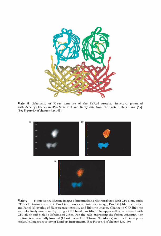
Plate 8 Schematic of X-ray structure of the DsRed protein. Structure generatedwith Accelrys DS ViewerPro Suite v5.1 and X-ray data from the Protein Data Bank [65].(See Figure13 of chapter 4, p. 165).
(a) (b)
(c)
Plate 9 Fluorescence lifetime images of mammalian cells transfectedwith CFP alone and aCFP^YFP fusion construct. Panel (a) fluorescence intensity image, Panel (b) lifetime image,and Panel (c) overlay of fluorescence intensity and lifetime images. Change in CFP lifetimewas selectively monitored by using a CFP band pass filter. The upper cell is transfected withCFP alone and yields a lifetime of 2.5 ns. For the cells expressing the fusion construct, thelifetime is substantially lowered (1.8 ns) due to FRET from CFP (donor) to theYFP (acceptor)molecule. Images courtesy of Lambert Instruments. (See Figure16 of chapter 4, p. 169).
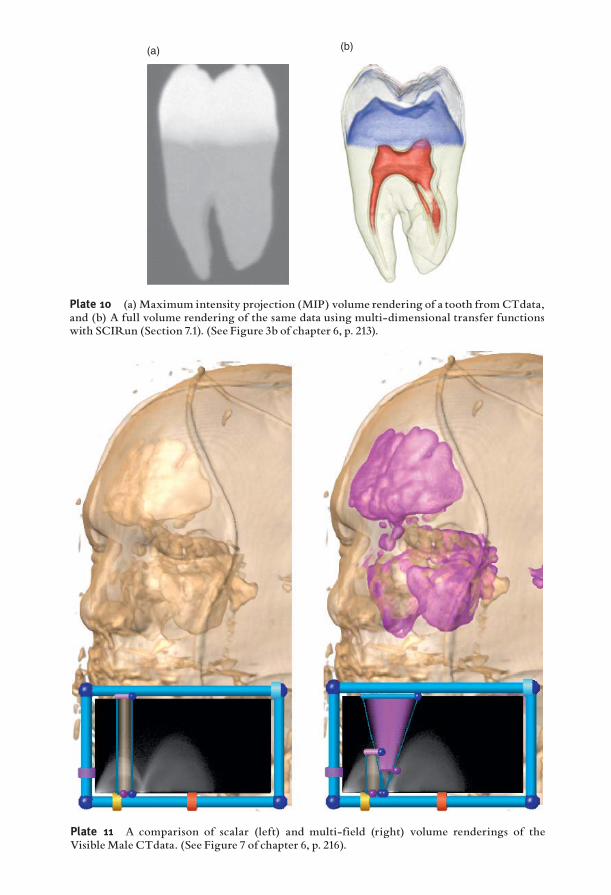
Plate 11 A comparison of scalar (left) and multi-field (right) volume renderings of theVisibleMale CTdata. (See Figure 7 of chapter 6, p. 216).
(a) (b)
Plate 10 (a)Maximum intensity projection (MIP) volume rendering of a tooth fromCTdata,and (b) A full volume rendering of the same data using multi-dimensional transfer functionswith SCIRun (Section 7.1). (See Figure 3b of chapter 6, p. 213).
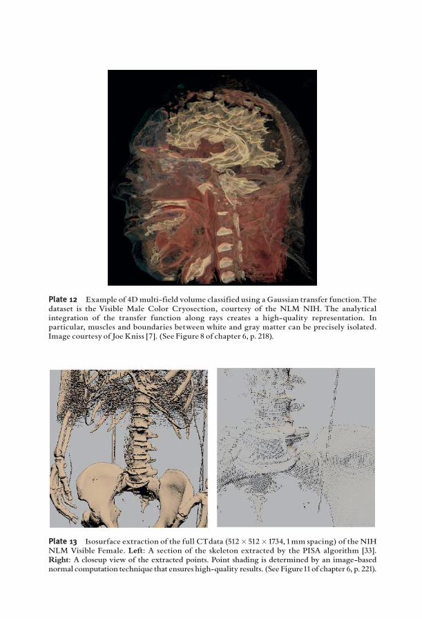
Plate 12 Example of 4Dmulti-field volume classified using a Gaussian transfer function.Thedataset is the Visible Male Color Cryosection, courtesy of the NLM NIH. The analyticalintegration of the transfer function along rays creates a high-quality representation. Inparticular, muscles and boundaries between white and gray matter can be precisely isolated.Image courtesy of Joe Kniss [7]. (See Figure 8 of chapter 6, p. 218).
Plate 13 Isosurface extraction of the full CTdata (512� 512�1734, 1mm spacing) of the NIHNLM Visible Female. Left: A section of the skeleton extracted by the PISA algorithm [33].Right: A closeup view of the extracted points. Point shading is determined by an image-basednormal computation technique that ensures high-quality results. (See Figure11of chapter 6, p. 221).
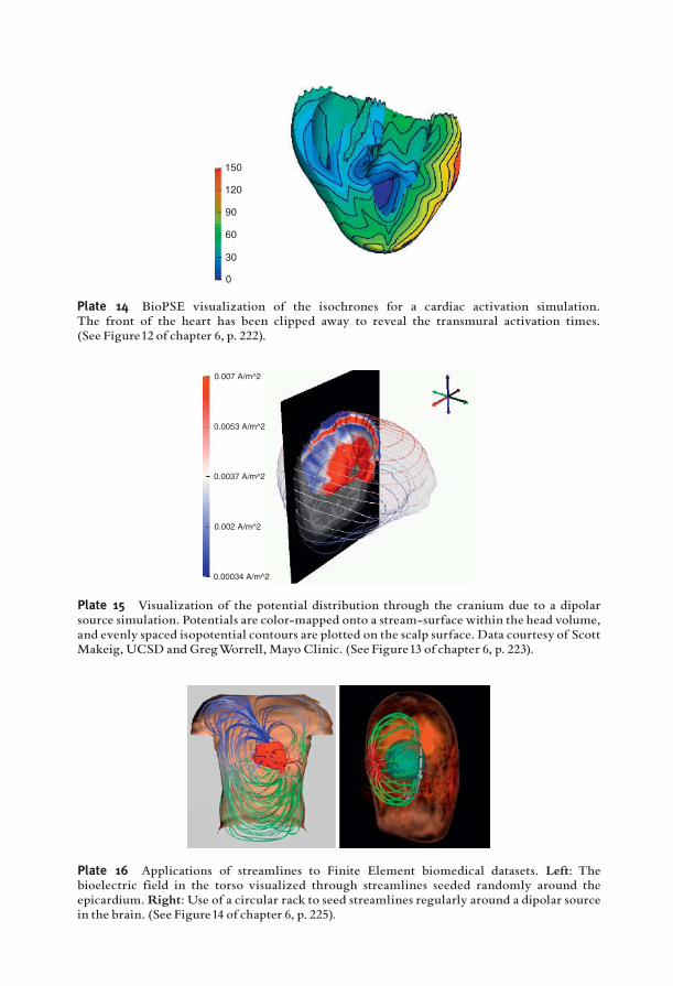
0
30
60
90
120
150
Plate 14 BioPSE visualization of the isochrones for a cardiac activation simulation.The front of the heart has been clipped away to reveal the transmural activation times.(See Figure12 of chapter 6, p. 222).
0.007 A/m^2
0.0053 A/m^2
0.0037 A/m^2
0.002 A/m^2
0.00034 A/m^2
Plate 15 Visualization of the potential distribution through the cranium due to a dipolarsource simulation. Potentials are color-mapped onto a stream-surface within the head volume,and evenly spaced isopotential contours are plotted on the scalp surface. Data courtesy of ScottMakeig, UCSD and GregWorrell, Mayo Clinic. (See Figure13 of chapter 6, p. 223).
Plate 16 Applications of streamlines to Finite Element biomedical datasets. Left: Thebioelectric field in the torso visualized through streamlines seeded randomly around theepicardium.Right: Use of a circular rack to seed streamlines regularly around a dipolar sourcein the brain. (See Figure14 of chapter 6, p. 225).
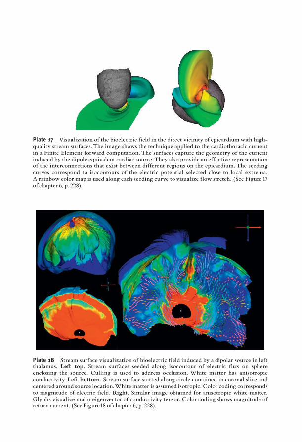
Plate 17 Visualization of the bioelectric field in the direct vicinity of epicardiumwith high-quality stream surfaces.The image shows the technique applied to the cardiothoracic currentin a Finite Element forward computation. The surfaces capture the geometry of the currentinduced by the dipole equivalent cardiac source.They also provide an effective representationof the interconnections that exist between different regions on the epicardium. The seedingcurves correspond to isocontours of the electric potential selected close to local extrema.A rainbow color map is used along each seeding curve to visualize flow stretch. (See Figure 17of chapter 6, p. 228).
Plate 18 Stream surface visualization of bioelectric field induced by a dipolar source in leftthalamus. Left top. Stream surfaces seeded along isocontour of electric flux on sphereenclosing the source. Culling is used to address occlusion. White matter has anisotropicconductivity. Left bottom. Stream surface started along circle contained in coronal slice andcentered around source location.White matter is assumed isotropic. Color coding correspondsto magnitude of electric field. Right. Similar image obtained for anisotropic white matter.Glyphs visualize major eigenvector of conductivity tensor. Color coding shows magnitude ofreturn current. (See Figure18 of chapter 6, p. 228).
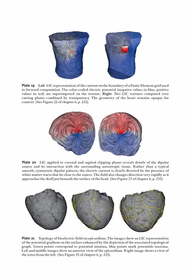
Plate 19 Left. LIC representation of the current on the boundaryof a Finite Element grid usedin forward computation.The color-coded electric potential (negative values in blue, positivevalues in red) are superimposed on the texture. Right. Two LIC textures computed overcutting planes combined by transparency. The geometry of the heart remains opaque forcontext. (See Figure 22 of chapter 6, p. 232).
Plate 20 LIC applied to coronal and sagittal clipping planes reveals details of the dipolarsource and its interaction with the surrounding anisotropic tissue. Rather than a typicalsmooth, symmetric dipolar pattern, the electric current is clearly diverted by the presence ofwhite matter tracts that lie close to the source.The field also changes direction very rapidly as itapproaches the skull just beneath the surface of the head. (See Figure 23 of chapter 6, p. 232).
Plate 21 Topology of bioelectric field on epicardium.The images show an LIC representationof the potential gradient on the surface enhanced by the depiction of the associated topologicalgraph. Green points correspond to potential minima, blue points mark potentials maxima.Left and middle images show an anterior viewof the epicardium. Right image shows a viewofthe torso from the left. (See Figure 25 of chapter 6, p. 233).
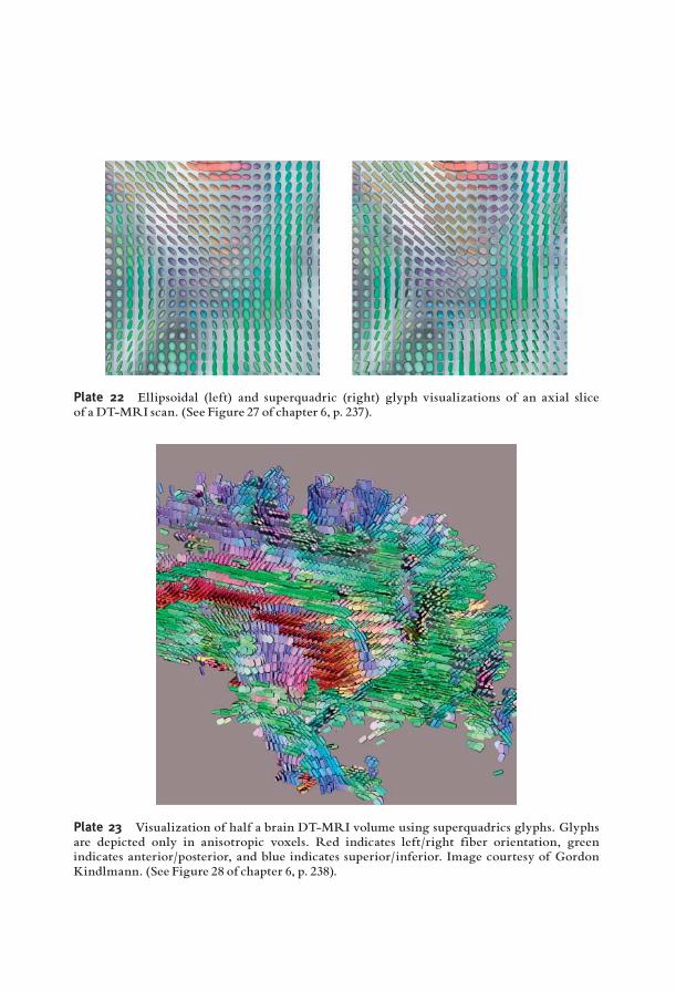
Plate 22 Ellipsoidal (left) and superquadric (right) glyph visualizations of an axial sliceof a DT-MRI scan. (See Figure 27 of chapter 6, p. 237).
Plate 23 Visualization of half a brain DT-MRI volume using superquadrics glyphs. Glyphsare depicted only in anisotropic voxels. Red indicates left/right fiber orientation, greenindicates anterior/posterior, and blue indicates superior/inferior. Image courtesy of GordonKindlmann. (See Figure 28 of chapter 6, p. 238).
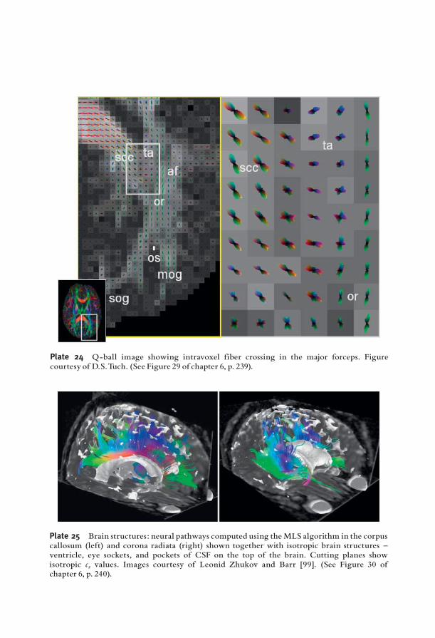
Plate 24 Q-ball image showing intravoxel fiber crossing in the major forceps. Figurecourtesy of D.S.Tuch. (See Figure 29 of chapter 6, p. 239).
Plate 25 Brain structures: neural pathways computed using theMLS algorithm in the corpuscallosum (left) and corona radiata (right) shown together with isotropic brain structures ^ventricle, eye sockets, and pockets of CSF on the top of the brain. Cutting planes showisotropic cs values. Images courtesy of Leonid Zhukov and Barr [99]. (See Figure 30 ofchapter 6, p. 240).
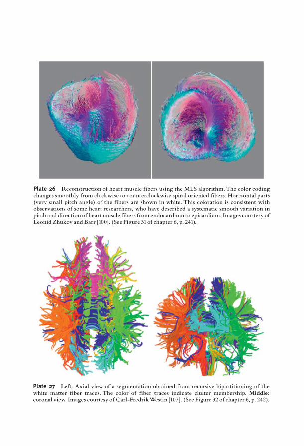
Plate 26 Reconstruction of heart muscle fibers using the MLS algorithm.The color codingchanges smoothly from clockwise to counterclockwise spiral oriented fibers. Horizontal parts(very small pitch angle) of the fibers are shown in white. This coloration is consistent withobservations of some heart researchers, who have described a systematic smooth variation inpitch and direction of heart muscle fibers from endocardium to epicardium. Images courtesy ofLeonid Zhukov and Barr [100]. (See Figure 31of chapter 6, p. 241).
Plate 27 Left: Axial view of a segmentation obtained from recursive bipartitioning of thewhite matter fiber traces. The color of fiber traces indicate cluster membership. Middle:coronal view. Images courtesy of Carl-FredrikWestin [107]. (See Figure 32 of chapter 6, p. 242).
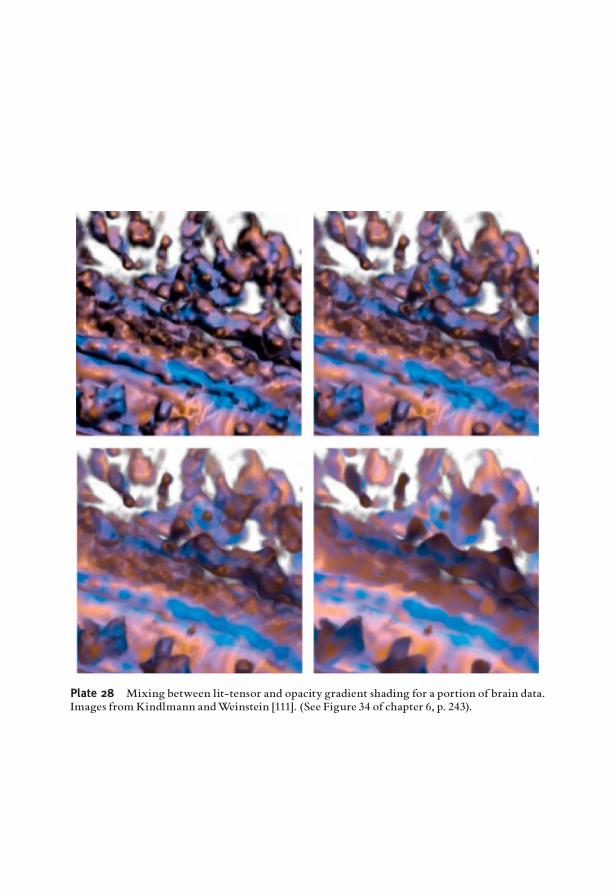
Plate 28 Mixing between lit-tensor and opacity gradient shading for a portion of brain data.Images fromKindlmann andWeinstein [111]. (See Figure 34 of chapter 6, p. 243).
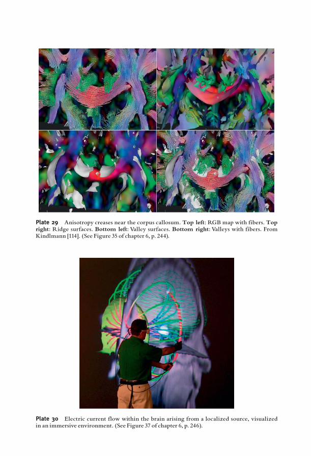
Plate 29 Anisotropy creases near the corpus callosum. Top left: RGB map with fibers. Topright: Ridge surfaces. Bottom left: Valley surfaces. Bottom right: Valleys with fibers. FromKindlmann [114]. (See Figure 35 of chapter 6, p. 244).
Plate 30 Electric current flow within the brain arising from a localized source, visualizedin an immersive environment. (See Figure 37 of chapter 6, p. 246).
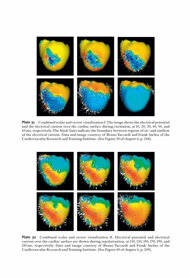
Plate 31 Combined scalar and vector visualization I.The image shows the electrical potentialand the electrical current over the cardiac surface during excitation, at 10, 20, 30, 40, 50, and60ms, respectively.The black lines indicate the boundary between regions of in- and outflowof the electrical current. Data and image courtesy of BrunoTaccardi and Frank Sachse of theCardiovascular Research andTraining Institute. (See Figure 39 of chapter 6, p. 248).
Plate 32 Combined scalar and vector visualization II. Electrical potential and electricalcurrent over the cardiac surface are shown during repolarization, at 110, 130, 150, 170, 190, and210ms, respectively. Data and image courtesy of Bruno Taccardi and Frank Sachse of theCardiovascular Research andTraining Institute. (See Figure 40 of chapter 6, p. 249).
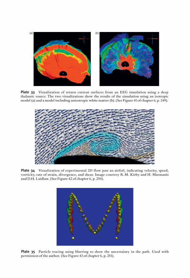
(a) (b)
Plate 33 Visualization of return current surfaces from an EEG simulation using a deepthalamic source. The two visualizations show the results of the simulation using an isotropicmodel (a) and amodel including anisotropic whitematter (b). (See Figure 41of chapter 6, p. 249).
Plate 34 Visualization of experimental 2D flow past an airfoil, indicating velocity, speed,vorticity, rate of strain, divergence, and shear. Image courtesy R.M. Kirby and H. Marmanisand D.H. Laidlaw. (See Figure 42 of chapter 6, p. 250).
Plate 35 Particle tracing using blurring to show the uncertainty in the path. Used withpermission of the author. (See Figure 43 of chapter 6, p. 251).
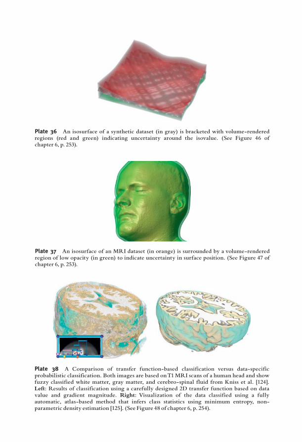
Plate 36 An isosurface of a synthetic dataset (in gray) is bracketed with volume-renderedregions (red and green) indicating uncertainty around the isovalue. (See Figure 46 ofchapter 6, p. 253).
Plate 37 An isosurface of an MRI dataset (in orange) is surrounded by a volume-renderedregion of low opacity (in green) to indicate uncertainty in surface position. (See Figure 47 ofchapter 6, p. 253).
Plate 38 A Comparison of transfer function-based classification versus data-specificprobabilistic classification. Both images are based onT1MRI scans of a human head and showfuzzy classified white matter, gray matter, and cerebro-spinal fluid from Kniss et al. [124].Left: Results of classification using a carefully designed 2D transfer function based on datavalue and gradient magnitude. Right: Visualization of the data classified using a fullyautomatic, atlas-based method that infers class statistics using minimum entropy, non-parametric density estimation [125]. (See Figure 48 of chapter 6, p. 254).
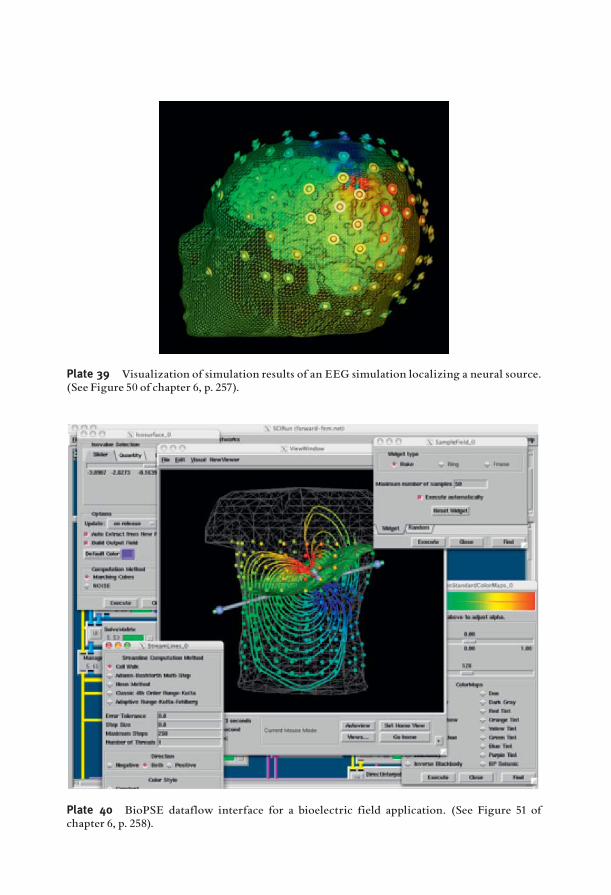
Plate 39 Visualization of simulation results of an EEG simulation localizing a neural source.(See Figure 50 of chapter 6, p. 257).
Plate 40 BioPSE dataflow interface for a bioelectric field application. (See Figure 51 ofchapter 6, p. 258).
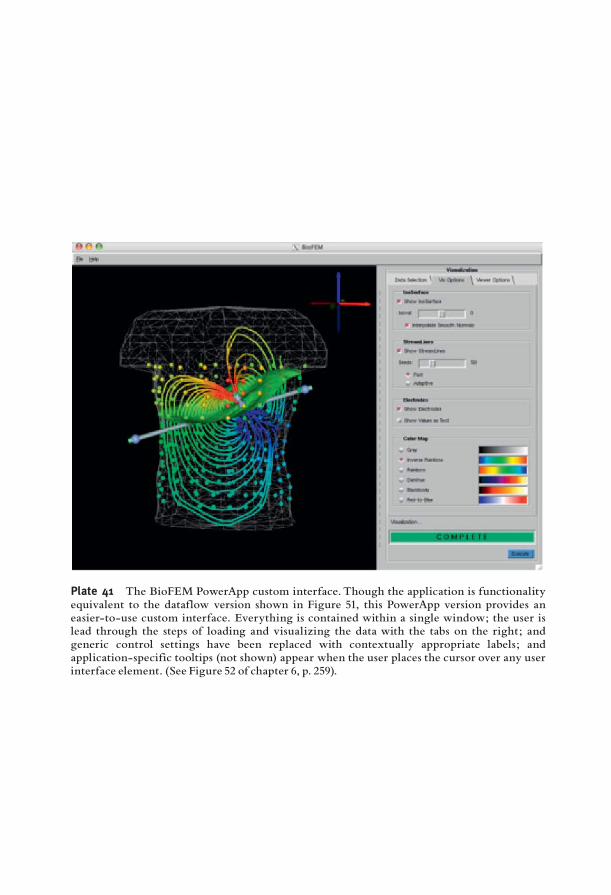
Plate 41 The BioFEM PowerApp custom interface. Though the application is functionalityequivalent to the dataflow version shown in Figure 51, this PowerApp version provides aneasier-to-use custom interface. Everything is contained within a single window; the user islead through the steps of loading and visualizing the data with the tabs on the right; andgeneric control settings have been replaced with contextually appropriate labels; andapplication-specific tooltips (not shown) appear when the user places the cursor over any userinterface element. (See Figure 52 of chapter 6, p. 259).

(a) Local surface Frame # 43
9.57
Local surface Frame # 52
12.239.216.193.160.14–2.88–5.90–8.93–11.95
Local surface Frame # 52
4.963.802.631.460.29–0.87–2.04–3.21–4.38–5.54–6.71–7.88
6.633.680.74–2.20–5.14–8.08–11.02–13.97
Local surface Frame # 69
Local surface Frame # 69
18.9215.2311.537.844.150.46–3.24–6.93–10.62
8.096.324.562.791.02–0.75–2.52–4.29–6.05–7.82–9.59–11.36
Local surface Frame # 85
Local surface Frame # 252
2.762.221.681.140.600.06–0.48–1.02–1.56–2.10–2.65–3.19
4.433.743.052.361.670.980.29–0.40–1.09–1.78–2.47–3.16
Local surface Frame # 85
31.6927.4623.2319.0114.7810.556.322.09–2.13
Local surface Frame # 252
12.2010.558.907.255.603.952.300.65–1.00
Local surface Frame # 43
3.402.832.261.691.120.55–0.02–0.59–1.16–1.73–2.30–2.87
Frame: 43 (48)
mV
Node# 16 (Ch 16) Surface# 1Time
mV
Node# 43 (Ch 43) Surface# 2Time
mV mV mV mV
Node# 16 (Ch 16) Surface# 1 Node# 43 (Ch 43) Surface#Time Time
Node# 16 (Ch 16) Surface# 1Time
Node# 43 (Ch 43) Surface# 2Time
Time: 42 ms Value: –22.791 Frame: 43 (48) Time: 42 ms Value: –2.461
Frame: 69 (74)
mV
Node# 16 (Ch 16) Surface# 1Time
mV
Node# 43 (Ch 43) Surface# 2Time
Time: 68 ms Value: –16.031 Frame: 69 (74) Time: 68 ms Value: –7.255 Frame: 85 (90)
mV
Node# 16 (Ch 16) Surface# 1Time
mV
Node# 43 (Ch 43) Surface#Time
Time: 84 ms Value: –9.576 Frame: 85 (90) Time: 84 ms Value: –2 Frame: 252 (257)
mV
Node# 16 (Ch 16) Surface# 1Time
mV
Node# 43 (Ch 43) Surface# 2Time
Time: 251 ms Value: 10.299 Frame: 252 (257) Time: 251 ms Value: 3.661
Frame: 52 (57) Time: 51 ms Value: –21.016 Frame: 52 (57) Time: 51 ms Value: –7 Frame: 63 (68) Time: 62 ms Value: –17.964 Frame: 63 (68) Time: 62 ms Value: –9.286
Surface # 1
Surface # 2
Surface # 1Local surface Frame # 63
Local surface Frame # 63
17.4714.0810.697.303.920.53–2.86–6.25–9.64
7.846.174.492.821.15–0.53–2.20–3.87–5.55–7.22–8.89–10.56
Surface # 2
Surface # 1
Surface # 2
Surface # 1
Surface # 2
Surface # 1
Surface # 2
Surface # 1
Surface # 2
(d) (e) (f)
(b) (c)
t = 43
t = 69 t = 85 t = 252
t = 52 t = 63
Plate 42 Sequence of potentials from the outer and inner surfaces of the heart. Images show the use of clipping planes to reveal data from twoconcentric surfaces simultaneously.The first image in the sequence shows the underlying measurement meshes for both surfaces (in red) and thetime values marked in each panel indicate the time after stimulation of the heart from the epicardium. (See Figure 54 of chapter 6, p. 262).
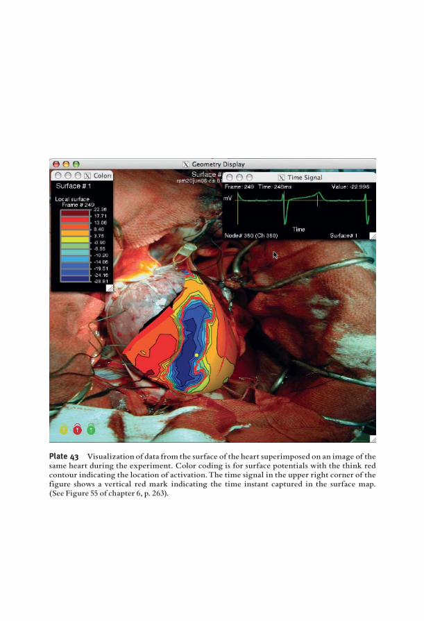
Plate 43 Visualization of data from the surface of the heart superimposed on an image of thesame heart during the experiment. Color coding is for surface potentials with the think redcontour indicating the location of activation.The time signal in the upper right corner of thefigure shows a vertical red mark indicating the time instant captured in the surface map.(See Figure 55 of chapter 6, p. 263).


