ADAPTIVE TRAFFIC CONTROL FOR LARGE-SCALE DYNAMIC TRAFFIC ASSIGNMENT APPLICATIONS

ADAPTIVE TRAFFIC CONTROL FOR LARGE-SCALE DYNAMIC TRAFFIC ASSIGNMENT APPLICATIONS

Alexander Paz, Ph.D., P.E. Assistant Professor

University of Nevada, Las Vegas Howard R. Hughes College of Engineering

Civil and Environmental Engineering 4505 Maryland Parkway, PO Box 454015

Las Vegas, NV 89154-4015 [email protected]

Phone: (702) 895-3701 Direct: (702) 895-0571 Cell: (702) 688-3878 Fax: (702) 895-3936

http://faculty.unlv.edu/apaz/

Yi-Chang Chiu, Ph.D. Associate Professor

Dept. of Civil Engineering and Engineering Mechanics The University of Arizona

Tucson, AZ 85721 1209 E 2nd St. Room 206 [email protected]

Tel: 520.626.8462 Fax: 435.921.1846

http://dynust.web.arizona.edu/AU/index.php

Word Count: Words = 6,216

Figures = 5x250 = 1250 Total = 7,466

Paz. A., Chiu. Y.C. 1

ADAPTIVE TRAFFIC CONTROL FOR LARGE-SCALE DYNAMIC TRAFFIC ASSIGNMENT APPLICATIONS

ABSTRACT

Dynamic Traffic Assignment (DTA) applications require traffic signal control data which is typically difficult to obtain and cumbersome to code in the required format. In addition, the evaluation of future scenarios requires future traffic signal settings consistent with the forecasted demand. These future signal settings are not known a priori and are costly to estimate. Intuitively, the future signal timings need to be reasonably optimized so as to represent what the traffic management agency will do. In literature, integration between traffic control and DTA models has been formulated as a bi-level or single-level optimization problem with system or user optimal constraints. Most existing solution procedures require certain “nested” structure with an inner loop algorithm solving the user equilibrium or system optimal assignment problem and the outer loop algorithm searching for the optimal signal timing setting. Most of these solution approaches remain only research tools without practical use due to computational intractability. This research proposes an efficient solution algorithm to the problem. An adaptive traffic signal control model is embedded in a simulation-based DTA model. For each inbound approach at an intersection of interest, the adaptive model uses upstream information and a dynamic rolling horizon approach to project traffic flow conditions for a dynamic but short period of time (projection period). The adaptive model provides the signal settings during the entire traffic flow simulation process and for every iteration of the solution algorithm. Thus, during the entire solution process, the experienced travel times and the resulting traffic assignment flows are based on the adaptive (demand responsive) signal settings. Thereby, the DTA flows and the adaptive signal settings are generated simultaneously in a single-loop algorithmic structure. Simulation experiments illustrate the capabilities of the proposed approach.


1 INTRODUCTION The development of simulation-based Dynamic Traffic Assignment (DTA) models requires traffic signal control data, which is typically difficult to obtain and cumbersome to code in the required format. In addition, gridlock in simulation easily develops when erroneous or inefficient signal settings are used. That is, most of the existing DTA models are sensitive to the traffic signal settings. Furthermore, the evaluation of future scenarios requires the use of future traffic signal settings consistent with the forecasted demand traffic pattern. These future signal settings are not known a priori and are costly to estimate for a number of reasons (e.g., too many traffic lights, signal settings depend on the future demand and vice versa). Practitioners use a sequential approach: first a traffic assignment problem is solved with fixed traffic signal settings and later “optimal” signal settings are determined based on the a priori traffic assignment results. To reach convergence, several iterations between traffic assignment and signal control optimization are proposed. Although this approach may seem sound, it is less practical due to excessive amounts of run time requirements.

In literature, the integration between traffic assignment and control has been formulated as a bi-level or single-level optimization problem with system or user optimal constraints. Most existing solution procedures require certain “nested” structure with an inner loop algorithm solving the user equilibrium or system optimal assignment problem and the outer loop algorithm searching for the optimal signal timing settings. Most of these approaches remain research tools only but not of practical use due to computational tractability. In addition, analytical models have been proposed to study the properties of the integration between DTA and dynamic traffic signal control. For example, a consistent control policy that ensures the existence of traffic equilibrium is proposed by Smith (1, 2). The Webster control model was used to study the deterministic traffic control and traffic assignment equilibrium problem (3, 4). Chen and Ben-Akiva (5) proposed a game theoretical framework to integrate DTA and traffic signal control. Several games are used to represent different levels of integration and information availability (6). Thus, general formulations for the integration of DTA and dynamic traffic signal control are proposed. Experiments using analytical models illustrated the characteristics of the proposed game theoretical formulations.

This research proposes an efficient solution to the problem of generating effective traffic signal settings for simulation-based DTA models. An adaptive traffic signal control model, based on the Optimized Policies for Adaptive Control (OPAC) algorithm (7), is embedded in a simulation-based DTA model (8) (DynusT). The proposed OPAC-based approach is distributed and involves a dynamic optimization algorithm. Similar to OPAC, the proposed approach calculates optimal signal settings without requiring a fixed cycle time, split, or offset, and it is constrained only by minimum and maximum green times.

To project traffic flow conditions for a dynamic but short period of time (projection period), the proposed adaptive control model uses upstream sensor information for each inbound approach at an intersection of interest. The optimal signal settings are determined by evaluating all possible signal settings combinations in light of the projected conditions. The goal is to find the optimal settings that yield minimum delay. The proposed adaptive control model does not include explicit coordination capabilities; however, the algorithm has inherent self-coordination capabilities since it uses upstream sensor information to project traffic flow and determine the


optimal signal settings. The length of the projection period is based on the length of the approaches to the interception and the unfolding flows. Thus, interceptions with long approaches and/or heavy flows require longer projection periods than their counterparts.

To simultaneously solve for the traffic assignment and control settings, the proposed adaptive control model provides the signal settings during the entire traffic flow simulation process and for every iteration of the traffic assignment solution algorithm. That is, the adaptive traffic control model is integrated with the traffic flow simulation model used to determine the DTA solution. Thus, during the entire solution process, the experienced travel times and the resulting traffic assignment flows account for the adaptive (demand responsive) signal settings. The DTA flows and the adaptive signal settings are generated simultaneously in a single-loop algorithmic structure. Later, actuated or pre-timed signal settings can be developed based on the recorded adaptive settings. The proposed solution does not assume or represent a system with massive deployment of adaptive controls or full coordinated capabilities. Rather, the objective is to represent the signal timings that are likely to be used by the traffic management agency in light of the evolving (assigned) traffic. The solution can be viewed as a self-adaptation of the system to the future demand/supply changes.

This paper reviews the basic characteristics of the OPAC algorithm and provides an overview of some implementation issues and limitations. The paper then focuses on the development of an OPAC-based approach for large-scale DTA applications. Discussions on the analytical and numerical properties of this solution approach are provided. Experiments and conclusions illustrate the capabilities of the proposed adaptive control approach.

2 BACKGROUND The OPAC algorithm was one of the earlier adaptive control model within the Federal Highway Administration (FHWA) RT-TRACS (real-time traffic-adaptive signal control system) program (9, 10). The model has evolved and undergone substantially testing since 1986 including:

1. OPAC I (distributed, perfect information and dynamic programming) 2. OPAC II (distributed, partial information and sequential optimization) 3. OPAC III (distributed, partial information and a rolling horizon approach for real- time deployment) 4. OPAC IV (OPAC III and a virtual-fixed-cycle for coordination) The main characteristics of OPAC models I-IV are summarized as follows: OPAC I (11) uses perfect traffic information for the entire control period and dynamic

programming to find the optimal control settings. For real-time applications, OPAC I is mainly useful to provide a theoretical benchmark because perfect traffic information for the entire control period is clearly impossible to obtain a priori. For planning applications, OPAC I could provide a practical benchmark, since data availability and precision is not as critical as for real-time applications. However, for implementation into large-scale systems, OPAC I is computationally intensive. In addition, its perfect information and global optimality characteristics could provide results that are too difficult to achieve in the real-world.


OPAC II (11) divides the control period in stages and assumes knowledge of traffic

conditions only for a stage at a time, therefore relaxing the assumption in OPAC I of perfect information for the entire control period. Thus, the optimal control settings are calculated for each stage in a sequential manner. OPAC II can use either a prediction model or historical data to estimate traffic conditions during the stage length. These characteristics make OPAC II more attainable than OPAC I. However, the quality of its results depends on the quality of the estimates for traffic conditions.

To circumvent, to some extent, the limitations of OPAC I and OPAC II, Gartner (1982b) developed OPAC III, which uses a rolling horizon approach for real-time deployment (ROPAC) (12). OPAC III has demonstrated to be an effective demand-responsive strategy. Figure 1 illustrates the rolling horizon approach. The control period is divided into stages, σ, of length around an average cycle length. To accelerate the optimization process (by reducing the total number of possible signal switching patterns), each stage is also divided into discrete time intervals of length Δ. In addition, each stage is divided into a head (or roll) period and a tail period. The length of the head and tail periods are multiples of Δ. Thus, the head and tail periods include r (integer) and I-r intervals of length Δ, respectively, where I is the total number of intervals of length Δ in the stage. Hence, the stage length SL is equal to I⋅Δ. In addition, the beginning of stage σ is denoted by interval kσ.

Each stage begins at the end of the head period of the previous stage. Traffic conditions corresponding to the head period are measured using stop bar and upstream detectors while the traffic conditions corresponding to the tail period are estimated using a model or historical data. While in the head period of the current stage (σ), the optimal control settings for the following stage (σ+1) are determined by minimizing the delay based on the measured and estimated traffic conditions. Given a phasing structure, all possible combinations of switching times, constrained by intervals of length Δ, are evaluated to determine the ones resulting in the minimum delay. Although the switching times are determined for the entire state, they are only deployed for its head period. At the end of the current head period, the stage is rolled by a head period; a new stage (σ) is defined with its beginning at the end of the current head period. The switching times for this new stage are determined and the approach is repeated till the end of the control period. Thus, the rolling horizon approach facilitates the real-time deployment of OPAC by enabling the update on switching times based on real-time traffic information. In addition, it provides self-coordination capabilities by considering upstream and estimated traffic conditions. Previous studies have also applied similar approaches to develop a number of real-time operational strategies. For example, Peeta (13) used the rolling horizon approach to enable the deployment of DTA models. Paz and Peeta (14) developed real-time information-based traffic control strategies using a rolling horizon approach.

To explicitly include coordination capabilities, OPAC IV uses a virtual-fixed-cycle (VFC-ROPAC) (10). Here, OPAC III is deployed in each interception of interest. In addition, given a primary signal, information about its traffic conditions and the conditions of its surrounding (satellite) interceptions is used to determine a virtual-fixed-cycle and the corresponding offset. These values are then used to enable the synchronization of phases.

Simulation and field experiments have been used to evaluate the capabilities of the OPAC algorithm (15, 16). Gartner et al. (17) used a modified version of the NETSIM (NETwork SIMulation) model to evaluate the performance of the OPAC under a simulation-based traffic flow framework. In the modified version of NETSIM, the distribution of inter-arrival times was


simulated using user-specified headways. Although the NETSIM model suffers a number of shortcomings (e.g., vehicles are moved sequentially, requiring significant calibration effort) (18), the results illustrate the potential of the OPAC algorithm as a demand-responsive traffic control.

Later, Gartner (10) deployed OPAC IV on Reston Park in Northern Virginia. The test network consisted of 16 signalized intersections along a 4-mile section. The results showed improvements in the order of 5 to 6% in average delays and stops compared to a fine-tuned fixed-time timing plan. The authors argue that these results are satisfactory given the difficulties experienced and the deployment conditions.

Gartner and Stamatiadis (19) proposed a conceptual framework to integrate real-time DTA and adaptive traffic control models. The framework clearly and explicitly illustrates the interdependencies between traffic assignment and control. The proposed solution concept uses an iterative approach between assignment and control to estimate the flow pattern and the corresponding optimal signal settings. Gartner’s and Stamatiadis’ framework is limited to the conceptual aspects of the problem as no implementation is reported.

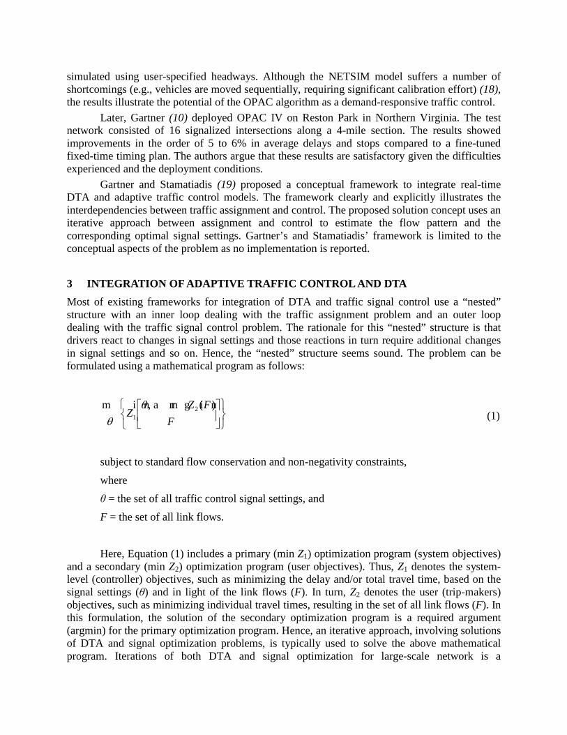
3 INTEGRATION OF ADAPTIVE TRAFFIC CONTROL AND DTA Most of existing frameworks for integration of DTA and traffic signal control use a “nested” structure with an inner loop dealing with the traffic assignment problem and an outer loop dealing with the traffic signal control problem. The rationale for this “nested” structure is that drivers react to changes in signal settings and those reactions in turn require additional changes in signal settings and so on. Hence, the “nested” structure seems sound. The problem can be formulated using a mathematical program as follows:

F

FZZ

)(m i na r g,m i n 21

θθ (1)

subject to standard flow conservation and non-negativity constraints,

where

θ = the set of all traffic control signal settings, and

F = the set of all link flows.

Here, Equation (1) includes a primary (min Z1) optimization program (system objectives) and a secondary (min Z2) optimization program (user objectives). Thus, Z1 denotes the system-level (controller) objectives, such as minimizing the delay and/or total travel time, based on the signal settings (θ) and in light of the link flows (F). In turn, Z2 denotes the user (trip-makers) objectives, such as minimizing individual travel times, resulting in the set of all link flows (F). In this formulation, the solution of the secondary optimization program is a required argument (argmin) for the primary optimization program. Hence, an iterative approach, involving solutions of DTA and signal optimization problems, is typically used to solve the above mathematical program. Iterations of both DTA and signal optimization for large-scale network is a


computational intensive task. In addition, convergence and stability of the solution may be difficult to achieve considering the ill-defined characteristics of the optimization program. For example, the signal settings and/or flow pattern may vary significantly at any iteration forcing the algorithm to “jump” backwards and forwards along the feasible region.

To address (to some extent) the above limitations, this research proposes an alternative framework that can be described using the following mathematical program:

[ ]{ }θθ

,,

m i nFZ

F (2)

Here, the signal settings (θ) and the flow pattern (represented by the set of link flows (F)) are determined simultaneously. That is, the solution to the mathematical problem requires the simultaneous search of the optimal signal settings and the corresponding network link flows. The advantage of a simultaneous search is a computationally tractable solution to the integration problem. Adaptive traffic control provides the algorithmic characteristics that enable the solution of the proposed mathematical program.

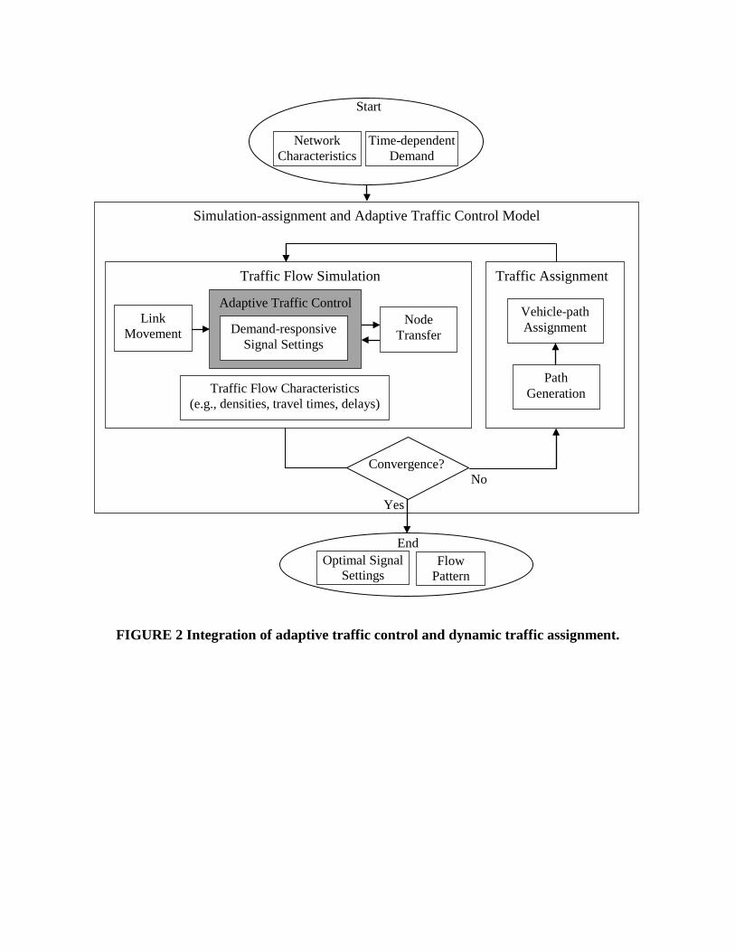
Figure 2 describes the proposed algorithmic logic to integrate adaptive traffic control and DTA. Given standard inputs such as the network characteristics and the time-dependent demand, the proposed approach solves for the flow pattern and optimal signal settings generated by an adaptive traffic control model. Initially, vehicle paths can be based on instantaneous path travel times. However, the solution framework uses iterations between traffic flow simulation and traffic assignment to generate the flow pattern based on experienced path travel times. Given the vehicle paths, in every iteration of the solution framework the simulation model moves vehicles along links and transfers vehicles between links at each network node. The simulation model also provides link and node traffic information to the adaptive control model which uses this information to generate the demand-responsive signal settings. The signal settings are used by the traffic flow simulator to transfer vehicles between links. Hence, the traffic flow characteristics generated by the traffic flow simulator are based on the demand-responsive signal settings. The traffic assignment model uses these traffic flow characteristics to generate feasible paths and to assign individual vehicles to those paths. The traffic flow simulation model then moves vehicles along the assigned paths to repeat the algorithmic loop. The described iterative procedure continues until the convergence criterion is satisfied. At convergence, the algorithm generates the optimal signal settings consistent with the corresponding flow pattern.

In this solution framework, the traffic flow characteristics generated by the traffic simulator and used by the traffic assignment model are based on the demand-responsive signal settings generated by the adaptive traffic control model. In addition, the demand-responsive signal settings are based on the vehicle paths generated by the traffic assignment model. Hence, convergence of traffic flows and optimal signal settings is achieved simultaneously. This represents a seamless integration between adaptive traffic control and DTA.


4 ALGORITHMIC CHARACTERISTICS OF THE PROPOSED CONTROL MODEL Considering the characteristics of different OPAC algorithms as well as the need to calculating near optimal signal settings for large-scale networks, OPAC III has been selected as the building block of the adaptive traffic control model for DTA applications. Several adjustments and enhancements to the original OPAC III are required to enable its implementation within a DTA model. This section describes those adjustments/enhancements.

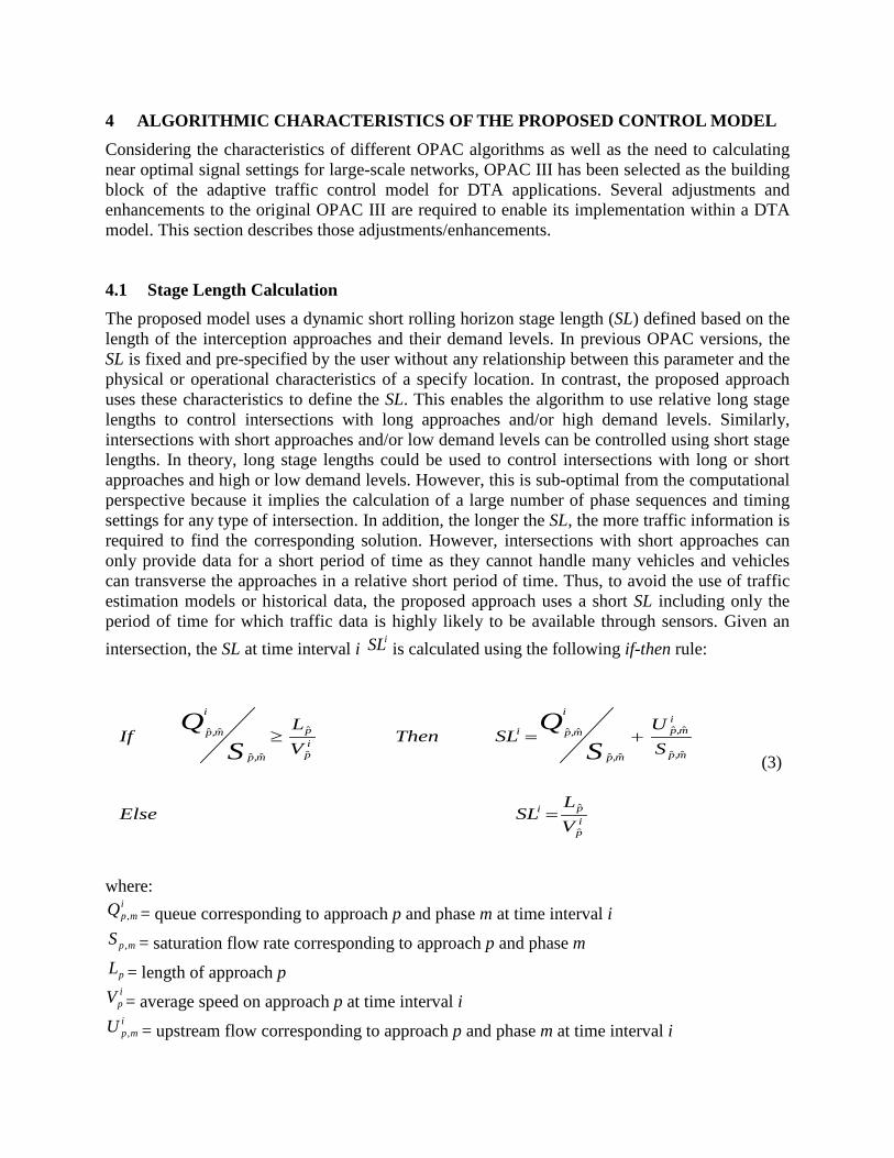
4.1 Stage Length Calculation The proposed model uses a dynamic short rolling horizon stage length (SL) defined based on the length of the interception approaches and their demand levels. In previous OPAC versions, the SL is fixed and pre-specified by the user without any relationship between this parameter and the physical or operational characteristics of a specify location. In contrast, the proposed approach uses these characteristics to define the SL. This enables the algorithm to use relative long stage lengths to control intersections with long approaches and/or high demand levels. Similarly, intersections with short approaches and/or low demand levels can be controlled using short stage lengths. In theory, long stage lengths could be used to control intersections with long or short approaches and high or low demand levels. However, this is sub-optimal from the computational perspective because it implies the calculation of a large number of phase sequences and timing settings for any type of intersection. In addition, the longer the SL, the more traffic information is required to find the corresponding solution. However, intersections with short approaches can only provide data for a short period of time as they cannot handle many vehicles and vehicles can transverse the approaches in a relative short period of time. Thus, to avoid the use of traffic estimation models or historical data, the proposed approach uses a short SL including only the period of time for which traffic data is highly likely to be available through sensors. Given an intersection, the SL at time interval i

iSL is calculated using the following if-then rule:

ip

pi

m,p

im,p

m,p

i

m,piip

p

m,p

i

m,p

VL

SLElse

SU

SLThenVL

IfS

QS

Q

ˆ

ˆ

ˆˆ

ˆˆ

ˆˆ

ˆˆ

ˆ

ˆ

ˆˆ

ˆˆ

=

+=≥

where: i

mpQ , = queue corresponding to approach p and phase m at time interval i

mpS , = saturation flow rate corresponding to approach p and phase m

pL = length of approach p ipV = average speed on approach p at time interval i i

mpU , = upstream flow corresponding to approach p and phase m at time interval i

(3)


mp ˆ,ˆ = the combination of approach and phase that maximize the queue saturation-flow ratio.

That is, mp ˆ,ˆ maximize SQ mp ,

i

mp , at time interval i Here, if the time required to dissipate the queue with the largest “queue saturation-flow

ratio” is greater or equal to the time required to transverse the corresponding approach, then the SL is equal to the time required to dissipate the queue with the largest “queue saturation-flow ratio” plus the time required to dissipate additional queue due to upstream flow. Otherwise (else), the SL is equal to the time required to transverse the approach with the largest “queue saturation-flow ratio”. After SL is calculated, it is rounded up to the nearest integer so that an integer number I of time intervals of length Δ is equal to SL (that is, SL = I⋅Δ).

The rationale here is to define the SL so as to maximize the use of the traffic information that can be collected using sensors on the intersection approaches. Priority is given to the approach with the largest “queue saturation-flow ratio” because it represents the approach with the immediate highest potential delay. In addition, shortest periods of time are required to dissipate the existing queue in all the other approaches. Hence, all the available queuing information is used by the algorithmic logic. Considering that priority is given to the approach with the largest “queue saturation-flow ratio”, the algorithmic logic may not use upstream data collected on long approaches because of a potential short SL. This characteristic has minor consequences for two reasons: (i) priority is given to existing queues that are having immediate impact on delays; (ii) the roll period is very short and the upstream traffic on long approaches is explicitly considered in subsequent stages. Hence, upstream traffic may not experience any delays even though it is not considered in a particular stage.

Given the dynamic characteristics of the proposed OPAC-based approach, the resulting model is termed Dynamic Rolling horizon Optimized Policies for Adaptive Control (DynaROPAC).

4.2 Control Phases and Switching Times An exhaustive search mechanism enables DynaROPAC to consider all possible combinations of valid intersection phase sequences and its corresponding switching times. This is in contrast to previous OPAC algorithms where only the major phases, typically the through phases, are actually controlled by the adaptive algorithm (12). OPAC treats the minor phases, typically the left-turn phases, as part of the inter-green period using a pre-timed or actuated approach (20). The ability to control all interception phases and sequences is important for network-level applications as the variation in flow patterns is not restricted to through movements.

4.3 Delay Calculation To eliminate the need of estimation models or historical data that can potentially negatively affect the performance of the adaptive algorithm, DynaROPAC does not use any prediction model. DynaROPAC calculates the delay using only stop bar and upstream traffic information. The delay corresponding to the upstream flow is calculated by projecting the vehicle arrivals to the existing queues using fundamental traffic flow relationships. Thus, given a phasing sequence and its corresponding switching times for a stage, the delay is defined to be the sum over all time intervals of the initial queue length plus the arrivals minus the departures during each interval


times the length of the interval. Considering that the length of the intervals is the same across approaches, phases and during the entire stage, this factor can be removed from the calculation without loss of generality. Hence, the “delay” (in vehicles) for stage σ is defined as follows:

[ ]∑∑∑= = =

−+=P

p

M

m

I

i

imp

imp

impMm DAQttttt

1 1 1,,,121 , . . . ),. . . ,...,,(σΦ (4)

where:

tm = switching time for phase m i

mpA , = arrivals corresponding to approach p and phase m at time interval i

impD , = departures corresponding to approach p and phase m at time interval i

P = total number of approaches

M = total number of phases

I = total number of time intervals of length Δ in stage σ of length SL = I⋅Δ

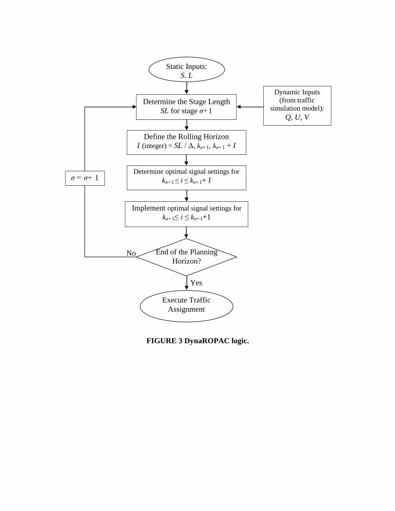
4.4 DynaROPAC ALGORITHM The above described characteristics enable the integration of DynaROPAC within a DTA model; thereby allowing the adaptive traffic control for large-scale network applications. This section describes the algorithmic steps that are executed by the proposed DynaROPAC model as part of a simulation-based DTA framework. Figure 3 illustrates the DynaROPAC algorithmic logic. Similar to OPAC III, DynaROPAC uses a rolling horizon stage based approach to determine the optimal signal settings. Here, the rolling horizon approach is not used to achieve real-time deployment but to enable the consideration of upstream traffic data in the generation of the signal settings, thus providing an adaptive traffic control policy. While in the roll period of the current stage σ (see Figure 1), the optimal control settings for next stage (σ +1) are generated (based on static and dynamic inputs) by executing the following steps:

Step 1: Calculate the Stage Length for Stage σ+1 Considering stop bar and upstream traffic information, calculate the length SL of the following stage (σ+1) using the if-then rule given by (3).

Step 2: Define the Rolling Horizon Divide σ into an integral number of Δ-sec intervals (SL / Δ = I (integer)). Here, Δ is the DTA simulation time interval (e.g., 2-6 seconds). Set the length of the roll period equal to Δ and its tail equal to Δ (I-1). That is, the roll period is the first time interval of a stage. This is designed to


enable the update of the control settings as soon as new traffic information is available. The resulting computational cost is not prohibitively high because the SL is short and the corresponding number of possible phase sequences and switching times can be computed in a reasonable period of time. Set the beginning and end of stage σ+1. The beginning is equal to the end of the current roll period (kσ+1 = kσ + 1), and the end is equal to the beginning plus the total number of intervals in the stage (kσ+1 + I).

Step 3: Determine the Optimal Phasing Sequence and Switching Times Solve the following single-stage mathematical program to determine the optimal phasing sequence and its corresponding switching times for stage σ+1.

Given:

i

mpQ , ∀ i, p, m; i

mpU , ∀ i, p, m; ipV ∀ i, p; mpS , ∀ p, m; pL ∀ p, and SL for stage σ+1

Determine:

, .,. . . ,...,, 121 ttttt Mm

To: , .,. . . ,...,,( 1211 tttttM i n Mm+σΦ

Subject to: lower decision upper bound variable bound

−1t ≤ t1 ≤ 1t

−2t ≤ t2 ≤ 2t

. .

−mt ≤ tm ≤ mt

. .

Here Φ is given by Equation (4) and the bounds on the decision variables are defined so that minimum and maximum green times are satisfied, i.e.,

minimum phase m length ≤ ( tm+1 – tm ) ≤ maximum m phase length


The optimization procedure used to solve the above mathematical program is an

expanded version of the Optimal Sequential Constrained search method (OSCO) (7, 21). The method uses an exhaustive search of all possible combinations of valid phase sequences and its corresponding switching times. Valid phases and switching times are constrained by the SL and minimum and maximum phase durations. An iterative approach is used to sequentially evaluate the objective function for all feasible combinations. At each iteration, the current performance index (objective value) is compared with the previously stored index. If the current index is lower than the stored index, the stored index is replaced by the current index. In addition, the current phase sequence and switching times are also stored. At the end of the search, the stored values are the optimal solution.

Step 4: Implement the Optimal Signal Settings Use the optimal phasing sequence and switching times to provide signal information for the next roll period to the traffic flow simulation engine in the DTA model. Performance of this step implies that the model will indicate whether the current phase must be extended or terminated and will update the phasing sequence and the corresponding times. If extended, reset the phasing times according to the optimal phasing sequence and switching times. If terminated, reset the phasing sequence and switching times. Then, the traffic flow simulator moves and transfers vehicles using the provided signal settings. If the end of the planning horizon is reached, the traffic assignment process is executed as discussed above and illustrated in Figure 2. Otherwise, the stage counter is updated (σ = σ+1) and the algorithm repeats steps 1-4 till the end of the planning horizon is reached.

5 EXPERIMENTS

5.1 Experimental Setup The Borman expressway corridor network located in northwest Indiana is used to conduct the experiments. It includes a sixteen-mile section of interstate I-80/94 (called the Borman expressway), I-90 toll freeway, I-65, and the surrounding arterials and streets. The network has 197 nodes, 460 links, 43 traffic zones, and 80 signalized intersections.

Actuated control is chosen here as the default control approach for DTA models. Two traffic control scenarios are used to evaluate the effectiveness of the proposed adaptive traffic control for large-scale DTA applications. In the first scenario, actuated control is used to determine the signal settings for all signalized intersections. In contrast, the second scenario uses the proposed DynaROPAC algorithm to provide signal settings for all signalized intersections.

A major objective of the experiments is to conduct a rigorous assessment of the proposed adaptive traffic control model. Hence, two important aspects are of particular interest: The performance of the control models under different demand patterns, and the input settings of the control model. Considering that an adaptive traffic control model must be demand responsive, the performance of the actuated and the proposed adaptive control models are evaluated using various O-D demand patterns. Here, the performance of the two control models is evaluated using various quasi-randomly generated and increased demand matrices. The demand matrices


are quasi-randomly generated, not randomly, because they deliberately produce various demand levels. That is, the generated demand matrices illustrate a systematic distribution of demand levels ranging from uncongested conditions to congested conditions.

Considering that an adaptive control model must be able to generate effective signal settings using only sensor data and the initial input settings, the input setting for the two control models are fixed. That is, the input settings (e.g., min and max green times) for the actuated and adaptive control models are the same in all cases.

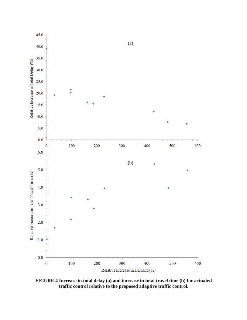
5.2 Results and Analysis Figure 4 shows the increase in total delay (Figure 4a) and the increase in total travel time (Figure 4b) for actuated traffic control relative to the proposed adaptive traffic control. Here, the results obtained for the actuated control are reported in the vertical axis as the percentage deviation from the results obtained for the proposed adaptive control model. The horizontal axis illustrates the percentage variation in demand relative to the experiment with the lowest demand level. The approach used here to report the results is designed to focus on the relative difference across scenarios rather than the absolute values.

Figure 4a shows a significant difference in terms of the total delay for the two control models. In all cases, the delay is higher for actuated control when compared to the proposed adaptive control. Figure 4b also shows a difference between the two control models. In this case the total travel times are higher in all cases for actuated control compared to the proposed adaptive control. Although the proposed control model always outperforms the actuated control model, the difference in terms of total travel times (Figure 4b) is not as significant as the difference in terms of delay (Figure 4a). These results are expected, as the objective of the proposed control model is to minimize the delay and not the total travel time. The total travel time is reduced in the case of the proposed control model as a consequence of the reduction in delay. However, this reduction in travel time, although desired, is not an explicit objective of the proposed model. It is also important to note that the reported statistics consider all vehicles, including those using the highway system as well as unsignalized interceptions. Hence, the benefits may be diluted when the statistics are calculated. As described in the experimental setup, different O-D demand patterns are used to evaluate the performance of the DynaROPAC under varying OD demand conditions. Therefore, significant variations in the statistics could be observed under a similar demand level. This clearly highlights the interdependencies between supply and demand and the need for demand-responsive control strategies such as DynaROPAC.

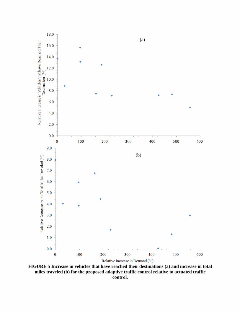
Figure 5 shows the increase in vehicles that have reached their destinations by the end of the planning horizon (Figure 5a) and the increase in total miles traveled (Figure 5b) for the proposed adaptive traffic control relative to actuated traffic control. The results obtained for the proposed adaptive control model are reported in the vertical axis as the percentage deviation from the results obtained for the actuated control model. Also, the horizontal axis illustrates the percentage variation in demand relative to the experiment with the lowest demand level. The results illustrate that in all cases, the number of vehicles that reach destinations by the end of the planning horizon is higher when the proposed adaptive control model is used. The primary reason is when the adaptive traffic control model is used, vehicles spend less time at the signalized intersections (less delay as illustrated in Figure 4a). As a result, they can travel longer distances in the same amount of time. This is corroborated in Figure 5b, which clearly shows that


vehicles travel more miles when the proposed adaptive control model is used to provide signal settings.

Altogether, the results (Figures 4 and 5) show the advantage of the proposed adaptive traffic control when compared to the actuated control model for large-scale DTA applications. The proposed model provides better signal settings thereby minimizing total delays and travel times. Consequently vehicles are able to travel longer distances in the same amount of time, thereby increasing the number of vehicles reaching their destinations. Figures 4 and 5 also illustrate that the performance of the models is highly influenced by the demand profile and demand level. The results show that different demand profiles and demand levels have different effects on performance, and the relationship between demand and performance is not linear. However, the proposed adaptive traffic control model outperforms the actuated control model for all the tested demand conditions.

6 CONCLUSIONS The adaptive traffic control model proposed in this research (DynaROPAC) has been designed to be more generalized than the previous OPAC versions in terms of the environment for which the system can be used. Several characteristics of the proposed DynaROPAC model enable its successful implementation within a DTA framework. The model is decentralized and can be used in several interceptions at the same time. It can simultaneously optimize all phase sequences and switching times. In addition, to explicitly consider upstream traffic conditions, the proposed model uses a dynamic rolling horizon stage-based approach. This characteristic provides self- coordination capabilities to the proposed model. In each intersection, the length of the stage is based on the geometric and demand conditions. Here, intersections with long approaches and/or high demand levels use longer stage lengths than intersections with short approaches and/or low demand levels. This characteristic also enables the efficient calculation of the optimal signal settings. That is, less time is required to calculate the optimal signal settings for intersections with short stage lengths than for intersections with long stage lengths.

The results presented in this work are based on a relatively few number of cases. Nonetheless, the conclusions are general, considering the experimental design and the representative characteristics of the Borman Network. The experimental design uses various demand profiles and demand levels to evaluate the performance of the proposed model under different demand conditions. Hence, the experiments test the adaptability of the proposed control model. In addition, the proposed model is used to provide signal settings for several intersections with different operational and geometric characteristics. The network used to conduct the experiments includes multiple traffic facilities (e.g., highways, arterials, ramps, diamond and clover leaf interchanges, unsignalized intersections) providing a general scenario comparable to other real-world networks.

In general, the proposed adaptive traffic control model performs better than the default actuated control model for large-scale DTA applications. The proposed model provides better signal settings for various demand levels without requiring a priori signal optimization. This capability is desirable in DTA applications because the optimization of signal settings is costly and time consuming. Hence, the proposed adaptive traffic control model can be used as a proxy for optimized traffic controls when the required data or resources are not available (a very frequent situation in the evaluation of large-scale DTA models). The resulting system can be


viewed as one where there is a self-adaptation of the signal settings to the traffic flows and vice versa. This self-adaptation is the result of a simultaneous generation of the traffic flows and optimal signal settings.

Although the proposed adaptive traffic control model provides superior results compared to the default actuated control model, the model requires significant longer time to reach convergence. Hence, future research is required to develop faster solution algorithms. Also, future research is required to develop explicit coordination capabilities. Currently, the self- coordination capabilities are implicit and are only a result of considering upstream flows on the intersection approaches. Explicit coordination capabilities can be developed by extending the current framework based perhaps on Garner’s Virtual-fixed-cycle Approach (10) as well as by considering the flows arriving at adjacent intersections. In addition, optimal actuated and optimal pre-time signal settings could be developed based on the adaptive control settings generated by the proposed model. Nonetheless, future research is required to test this hypothesis.

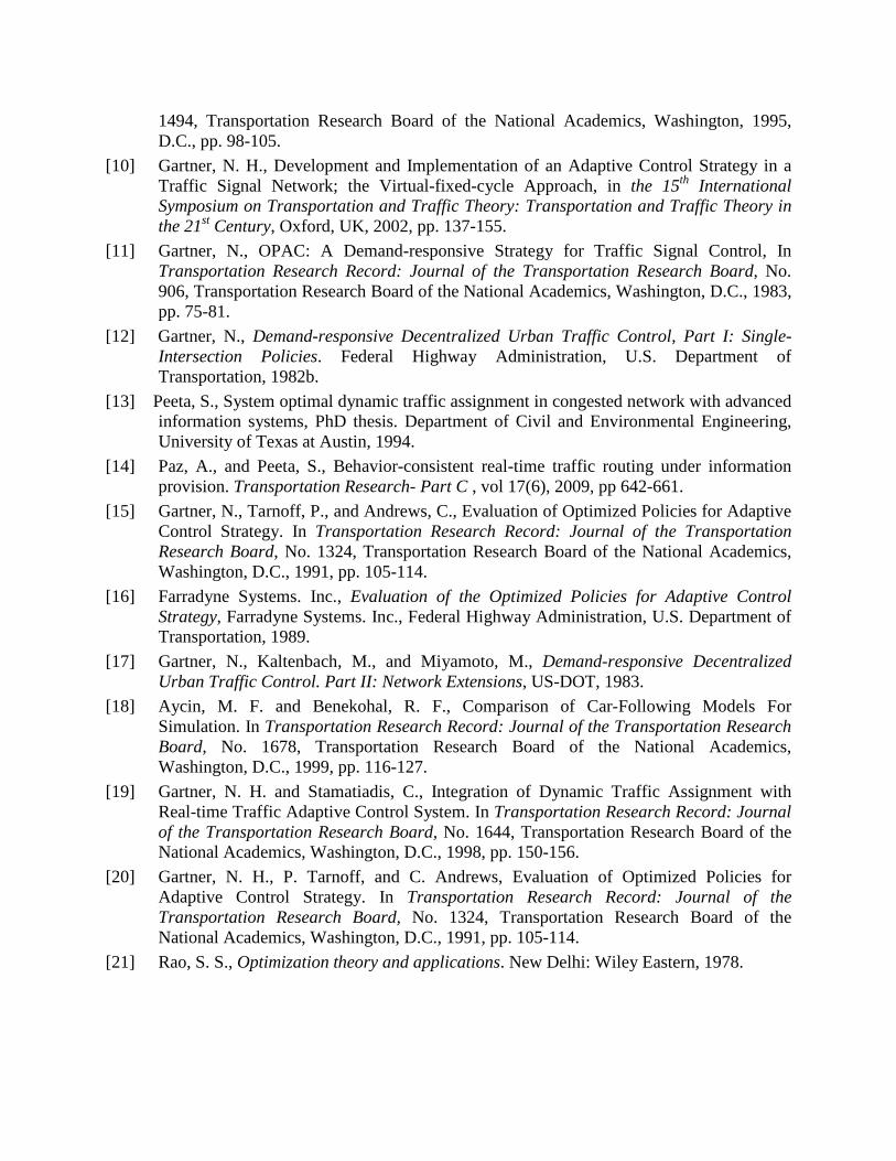
7 REFERENCES

[1] Smith, M. J., Traffic control and route-choice; a simple example, Transportation Research Part B: Methodological, vol. 13, 1979, pp. 289-294.

[2] Smith, M. J., Properties of a Traffic Control Policy Which Ensure the Existence of Traffic Equilibrium Consistent with the Policy, Transportation Research Part B, vol. 15, 1981, pp. 150-156.

[3] Al-Malik, M. and Gartner, N. H.,Development of a Combined Traffic Signal Control-Traffic Assignment Model, in Urban Traffic Networks N. H. G. a. G. Improta, Ed. Berlin: Springer-Verlag, 1995 pp. 155-186.

[4] Gartner, N. H. and Al-Malik, M., Combined Model for Signal Control and Route Choice in Urban Traffic Networks. In Transportation Research Record: Journal of the Transportation Research Board, No. 1554, Transportation Research Board of the National Academics, Washington, D.C., 1996, pp. 27-35.

[5] Chen, O. J. and Ben-Akiva, M. E., Game-theoretic Formulations of Interaction Between Dynamic Traffic Control and Dynamic Traffic Assignment. In Transportation Research Record: Journal of the Transportation Research Board, No. 1617, Transportation Research Board of the National Academics, Washington, D.C., 1998, pp. 179-188.

[6] Chen, O. J., Integration of Dynamic Traffic Control and Assignment. Cambridge, MA: Massachusetts Institute of Technology, 1998.

[7] Gartner, N., A prescription for demand-responsive Urban Traffic Control. In Transportation Research Record, No. 881, Transportation Research Board of the National Academics, Washington, D.C., 1982a, pp. 73-76.

[8] Chiu, Y.-C., Nava, E., Zheng, H., and Bustillos, B., DynusT User's Manual (http://dynust.net/wikibin/doku.php), 2010n ed, 2010.

[9] Gartner, N., Stamatiadis, C., and Tarnoff, P., Development of Advanced Traffic Signal Control Strategies for Intelligent Transportation Systems: a Multilevel Design. In Transportation Research Record: Journal of the Transportation Research Board, No.


1494, Transportation Research Board of the National Academics, Washington, 1995, D.C., pp. 98-105.

[10] Gartner, N. H., Development and Implementation of an Adaptive Control Strategy in a Traffic Signal Network; the Virtual-fixed-cycle Approach, in the 15th International Symposium on Transportation and Traffic Theory: Transportation and Traffic Theory in the 21st Century, Oxford, UK, 2002, pp. 137-155.

[11] Gartner, N., OPAC: A Demand-responsive Strategy for Traffic Signal Control, In Transportation Research Record: Journal of the Transportation Research Board, No. 906, Transportation Research Board of the National Academics, Washington, D.C., 1983, pp. 75-81.

[12] Gartner, N., Demand-responsive Decentralized Urban Traffic Control, Part I: Single-Intersection Policies. Federal Highway Administration, U.S. Department of Transportation, 1982b.

[13] Peeta, S., System optimal dynamic traffic assignment in congested network with advanced information systems, PhD thesis. Department of Civil and Environmental Engineering, University of Texas at Austin, 1994.

[14] Paz, A., and Peeta, S., Behavior-consistent real-time traffic routing under information provision. Transportation Research- Part C , vol 17(6), 2009, pp 642-661.

[15] Gartner, N., Tarnoff, P., and Andrews, C., Evaluation of Optimized Policies for Adaptive Control Strategy. In Transportation Research Record: Journal of the Transportation Research Board, No. 1324, Transportation Research Board of the National Academics, Washington, D.C., 1991, pp. 105-114.

[16] Farradyne Systems. Inc., Evaluation of the Optimized Policies for Adaptive Control Strategy, Farradyne Systems. Inc., Federal Highway Administration, U.S. Department of Transportation, 1989.

[17] Gartner, N., Kaltenbach, M., and Miyamoto, M., Demand-responsive Decentralized Urban Traffic Control. Part II: Network Extensions, US-DOT, 1983.

[18] Aycin, M. F. and Benekohal, R. F., Comparison of Car-Following Models For Simulation. In Transportation Research Record: Journal of the Transportation Research Board, No. 1678, Transportation Research Board of the National Academics, Washington, D.C., 1999, pp. 116-127.

[19] Gartner, N. H. and Stamatiadis, C., Integration of Dynamic Traffic Assignment with Real-time Traffic Adaptive Control System. In Transportation Research Record: Journal of the Transportation Research Board, No. 1644, Transportation Research Board of the National Academics, Washington, D.C., 1998, pp. 150-156.

[20] Gartner, N. H., P. Tarnoff, and C. Andrews, Evaluation of Optimized Policies for Adaptive Control Strategy. In Transportation Research Record: Journal of the Transportation Research Board, No. 1324, Transportation Research Board of the National Academics, Washington, D.C., 1991, pp. 105-114.

[21] Rao, S. S., Optimization theory and applications. New Delhi: Wiley Eastern, 1978.


LIST OF FIGURES

FIGURE 1 Rolling horizon control approach. ...............................................................................17

FIGURE 2 Integration of adaptive traffic control and dynamic traffic assignment. .....................18

FIGURE 3 DynaROPAC logic. .....................................................................................................19

FIGURE 4 Increase in total delay (a) and increase in total travel time (b) for actuated traffic control relative to the proposed adaptive traffic control. .................................20

FIGURE 5 Increase in vehicles that have reached their destinations (a) and increase in total miles traveled (b) for the proposed adaptive traffic control relative to actuated traffic control. ...............................................................................................21


Stage Length (SLσ) Head Tail

(r intervals) (I - r intervals)

Δ Δ Δ Δ Δ Δ Δ Δ Δ Δ Stage σ kσ r

Roll

(shift) period Stage Length (SLσ+1)

Δ Δ Δ Δ Δ Δ Δ Δ Δ Δ Stage σ+1 kσ+1 2r

FIGURE 1 Rolling horizon control approach.

In OPAC III SLσ = SLσ+1 In the proposed approach SLσ+1 can differ from SLσ


FIGURE 2 Integration of adaptive traffic control and dynamic traffic assignment.

Network Characteristics

Time-dependent Demand

Simulation-assignment and Adaptive Traffic Control Model

Traffic Assignment Traffic Flow Simulation

Adaptive Traffic Control

End

Start

Demand-responsive Signal Settings

Vehicle-path Assignment

Traffic Flow Characteristics (e.g., densities, travel times, delays)

Convergence?

Path Generation

Link Movement

Node Transfer

Yes

No

Optimal Signal Settings

Flow Pattern


FIGURE 3 DynaROPAC logic.

σ = σ+ 1 Determine optimal signal settings for

kσ+1 ≤ i ≤ kσ+1+ I

Implement optimal signal settings for kσ+1≤ i ≤ kσ+1+1

Dynamic Inputs (from traffic

simulation model): Q, U, V

No

Execute Traffic Assignment

Static Inputs: S, L

Determine the Stage Length SL for stage σ+1

Yes

Define the Rolling Horizon I (integer) = SL / Δ, kσ+1, kσ+1 + I

End of the Planning Horizon?


FIGURE 4 Increase in total delay (a) and increase in total travel time (b) for actuated traffic control relative to the proposed adaptive traffic control.

(b)

(a)


FIGURE 5 Increase in vehicles that have reached their destinations (a) and increase in total

miles traveled (b) for the proposed adaptive traffic control relative to actuated traffic control.

(a)

(b)

Documents

ADAPTIVE TRAFFIC CONTROL FOR LARGE-SCALE DYNAMIC TRAFFIC ASSIGNMENT APPLICATIONS