Embed Size (px)
Citation preview
t -
AD-A277 189
COMIPREIIENSIVE MONITORING PROGRAM
Contract Number DAAA 15-87-0095
ANNUAL GROUND WATER REPORT FOR 1989 70 TJUNE 1990
FINAL REPORT
Version 2.0
Volume I
Prepared by:
R. L. STOLLAR & ASSOCIATES INC. I "HARDING LAWSON ASSOCIATES
E13ASCO SERVICES INC.DATACHEM, INC.
ENVIRONMENTAL SCIENCE & ENGINEERING, INC.MIDWEST RESEARCH INSTITUTE
Prepared for:
PROGRAM MANAGER FOR -ROCKY MOUNTAIN ARSENAL
00THE VIEWS, OPINIONS, AND/OR FINDINGS CONTAINED IN THIS REPORT ARE THOSEOF THE AUTHOR(S) AND SHOULD NOT BE CONSTRUED AS AN OFFICIAL DEPARTMENTOF THE ARMY POSITION, POLICY, OR DECISION, UNLESS SO DESIGNATED BY OTHERDOCUMENTATION.
THE USE OF TRADE NAMES IN THIS REPORT DOES NOT CONSTITUTE AN OFFICIALj ENDORSEMENT OR APPROVAL OF THE USE OF SUCH COMMERCIAL PRODUCTS. THEREPORT MAY NOT BE CITED FOR PURPOSES OF ADVERTISEMENT.
I
T
REPORT DOCUMENTATION PAGE _j:. Ar.: -d
p zý0139 * '. 'ectc'q , n?1'rraEZ' Ss -S, ai "Ile zer 10 '1-socne lf110'" 1' -e~ w .%tr..c-,-n 3r5 a > -. c ca sures
irerr in -- i.'i ita ii eeaea. -nd cooet ir] a w )t llftrinJtlro n-en rm(3 ' r..t1rd l iths owzy .'- 7f tnmAfe, aoei or ni-nl-l 5¾ ge UJi sret ýs'e uoirq C naC..feSiee ,rr~ CTrc unaO ýTt. ' a 1> rl~rs '2?S 3etleno
.. f'c i A z222-,'24 42 maiidt-C If wn~o efýac! oel- . 0.-nd,11n-e.i' .J 9ýý *. ifnf'* r r t
I. AGENCY USE ONLY Leave bi:an) 2. REPO RT3. REPORT TYPE AND DATES COVERED
Tal II LC5. FUNDiNG NUMBERS
)AAA15 87 0095
AUTH,�R(S)
7. PERFORMING ORGANIZATION NAME(S) AND ADDRESS(ES) d. PERFOiRMING ORGANIZATIONROBERT L. STOLLAR ASSOCIATES REPORT NUMBER
90231RO1
9. SPONSORiNGr MONITORING AGENCY NAME(S) AND ADDRESS(ES) 10. SPONSORING MONITORINGAGENCY REPORT NUMBER
ROCKY MOUNTAIN ARSENAL (CO.). PMRMA
11. 5U'PLEMENTRY NOTES
12a. DISTRIBUTiON AVAILABILITY STATEMENT 12b. D)ISTRIBUTION CODE
APPROVED FOR PUBLIC RELEASE; DISTRIBUTION IS UNLIMI ED
13. ABSTRACT ,Mixtmumn • vc•rCs)
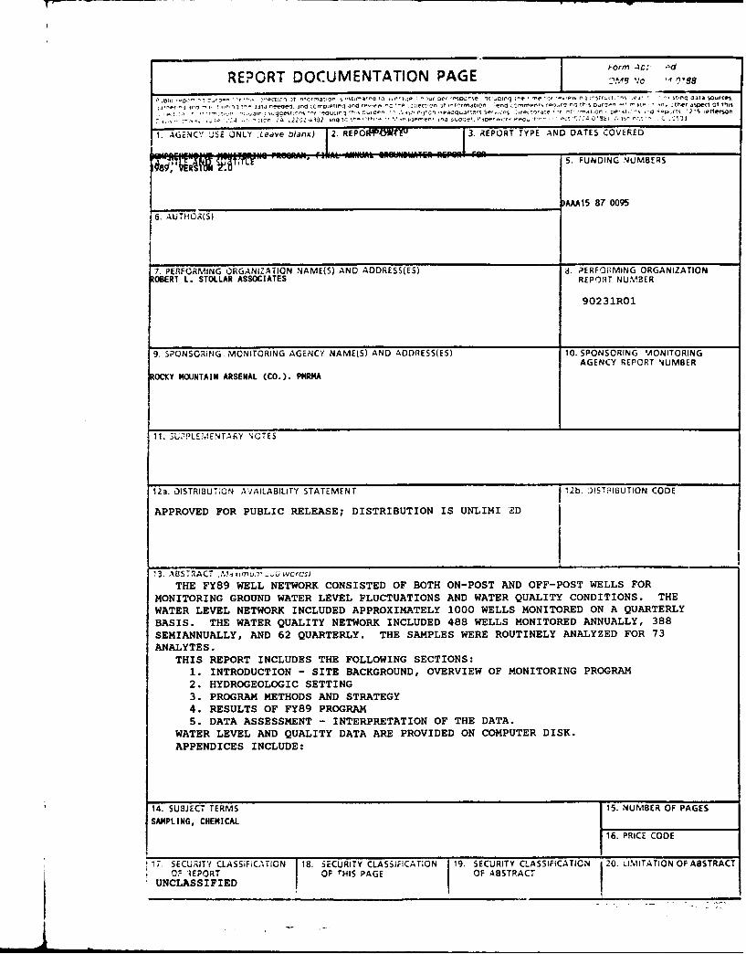
THE FY89 WELL NETWORK CONSISTED OF BOTH ON-POST AND OFF-POST WELLS FORMONITORING GROUND WATER LEVEL FLUCTUATIONS AND WATER QUALITY CONDITIONS. THEWATER LEVEL NETWORK INCLUDED APPROXIMATELY 1000 WELLS MONITORED ON A QUARTERLY
BASIS. THE WATER QUALITY NETWORK INCLUDED 488 WELLS MONITORED ANNUALLY, 388
SEMIANNUALLY, AND 62 QUARTERLY. THE SAMPLES WERE ROUTINELY ANALYZED FOR 73ANALYTES.
THIS REPORT INCLUDES THE FOLLOWING SECTIONS:1. INTRODUCTION - SITE BACKGROUND, OVERVIEW OF MONITORING PROGRAM
2. HYDROGEOLOGIC SETTING3. PROGRAM METHODS AND STRATEGY4. RESULTS OF FY89 PROGRAM5. DATA ASSESSMENT - INTERPRETATION OF THE DATA.
WATER LEVEL AND QUALITY DATA ARE PROVIDED ON COMPUTER DISK.
APPENDICES INCLUDE:
14. SUBJECT TERMS 15. NUMBER OF PAGES
SAMPLING, CHEMICAL
16. PRICE CODE
17. SECURITY CLASSiFiCTICN 18. SECURITY CLASSiiCATION 19. SECURITY CLASSIFICATION 20. IMITATION OF ABSTRACT
OF IEPORT OF ?'HIS PAGE OF ABSTRACT
UNCLASSIFIED 2
I
TABLE OF CONTENTS
PAF
VOLUME I
EXECUTIVE SUMMARY
1.0 INTRODUCTION .....................................................
1.1 Site Background .............................................. I1.2 Nature and Extent of Problem....................................1.3 Summary of Previous Ground-Water Monitoring Efforts ................ 21.4 Overview of Current Ground-Water Monitoring ......................... 3
2.0 ItYDROGEOLOGIC SETTING ............................................. 7
2.1 Geology .. .................................................... 7
2.1.1 A lluvium .......... ............ . ..... .. ........ .. ... ..2.1.2 Denver Formation .. ....................................... 8
2.2 Hydrogeology ................................................... 9
2.2.1 Unconfined Flow System ............. ..................... 92.2.2 Confined Flow System ...................................... 10
3.0 PROGRAM METHODS AND STRATEGY ................................... 12
3.1 Water-Level Monitoring Network .. ................................ 12
3.1.1 Well Selection Criteria for the Water-Level Monitoring Network .... 123.1.2 Well Selection Criteria for the Unconfined Flow System .......... 133.1.3 Well Selection Criteria for the Confined Flow System ............. 13
3.2 Water-Quality Monitoring Network ................................. 18
3.2.1 FV89 Water-Quality Monitoring .............................. 19
3.2.1.1 Comparison with Previous RMA Networks .............. 24
3.2.2 FY89 Water-Quality Data Presentation and Use ................. 293.2.3 Well Selection for Gas Chromatography/Mass Spectrometry
Analysis ............................................... 313.2.4 CMP Procedures for Water-Quality Monitoring .................. 31
3.3 Analytical Program ................... AccsJon For ............ 33NTIS CRA&I
DTIC TAB
UnannuuncedJustific.1tion
By..................
Dist, ib Jtion
GWAR-89.TOC Availahiity CodesRev. 3/19/90sl l-i-
AvdiI a:.d orDist Specia
I I
ITABLE OF CONTENTS (Continued)
P~AGEF
4.0 RESULTSOF FYN89 PROGRAM ........................................ 35
4.1 Regional Water-Table Surface ...................................... 35
4.1.1 Seasonal Fluctuations of the Regional Water Table . .............. 374.1.2 Water-Table Surface in the Boundary Containment Systems Area .... 374.1.3 Water Table in the Basin F IRA Area .......................... 40
4.2 Regional Potentiometric Surfaces of the Confined Flow System ............ 4 I4.3 Contaminant Distribution ... ..................................... 41
4.3.1 Analytical Data Presentation .. .............................. 424.3.2 Dieldrin ... ............................................. 42
4.3.2.1 Unconfined Flow System . ......................... 424.3.2.2 Confined Flow System .................. ......... 454.3.2.3 Winter 87/88 and FY89 Comparisons .................. 45
4.3.3 Endrin ... .............................................. 46
4.3.3.1 Unconfined Flow System . ......................... 464.3.3.2 Confined Flow System ............................ 514.3.3.3 Winter 87/88 and FY89 Comparison ................. 51
4.3.4 Dithiane and Oxathiane .. .................................. 52
4.3.4.1 Unconfined Flow System . ......................... 524.3.4.2 Confined Flow System . ........................... 554.3.4.3 Winter 87/88 and FY89 Comparison ................. 55
4.3.5 Benzothiazole .. ......................................... 56
4.3.5.1 Unconfined Flow System . ......................... 564.3.5.2 Confined Flow System . ........................... 594.3.5.3 Winter 1987/88 and FY89 Comparison ................. 59
4.3.6 Organosulfur Compounds ................................... 59
4.3.6.1 Unconfined Flow System . ......................... 624.3.6.2 Confined Flow System . ........................... 634.3.6.3 Winter 1987/88 and FY89 Comparison ................. 63
4.3.7 Volatile Aromatics ........................................ 64
4.3.7.1 Unconfined Flow System . ......................... 644.3.7.2 Confined Flow System . ........................... 674.3.7.3 Winter 1987/88 and FY89 Comparison ................. 68
GWAR-89.TOCRev. 3/19/90 - ii -
TABLE OF CONTENTS (Continued)
IPAG FI
44.3.8 Benzene . .............................................. (S
4.3.8.1 Unconfined Flow System ......................... 714.3.8.2 Confined Flow System ........................... 7 I4.3.8.3 Winter 1987/88 and FY89 Comparison ................ 72
4.3.9 Chlorobenzene ............................................ 72
4.3.9.1 Unconfined Flow System ........................... 754.3.9.2 Confined Flow System ............................. 754.3.9.3 Winter 1987/88 and FY89 Comparison ................ 76
4.3.10 Volatile Organohalogens .................................... 77
4.3.10.1 Unconfined Flow System . ......................... 774.3.10.2 Confined Flow System ........................... 814.3.10.3 Winter 87/88 and FY89 Comparisons .................. 81
4.3.11 Chloroform .. ........................................... 82
4.3.11.1 Unconfined Flow System . ......................... 824.3.11.2 Confined Flow System . ........................... 854.3.11.3 Winter 1987/88 and FY89 Comparison ................ 85
4.3.12 Trichloroethene .. ........................................ 86
4.3.12.1 Unconfined Flow System . ......................... 864.3.12.2 Confined Flow System . ........................... 894.3.12.3 Winter 1987/88 and FY89 Comparisons ............... 90
4.3.13 Tetrachloroethene .. ...................................... 90
4.3.13.1 Unconfined Flow System . ......................... 934.3.13.2 Confined Flow System............................ 934.3.13.3 Winter 1987/88 and FY89 Comparisons ............... 94
4.3.14 Dibromochloropropane (DBCP) . ............................ 94
4.3.14.1 Unconfined Flow System . ......................... 944.3.14.2 Confined Flow System . ........................... 974.3.14.3 Winter 1987/88 and FY89 Comparisons ............... 98
4.3.15 Dicyclopentadiene (DCPD) .................................. 98
4.3.15.1 Unconfined Flow System . ......................... 1014.3.15.2 Confined Flow System . ........................... 1014.3.15.3 Winter 1987/88 and FY89 Comparisons ............... 102
GW.P' 89.TOCRev. 3/19/90 - Il! -
I
TABLE OF CONTENTS (Continued)
P~AGEU
4.3.16 Diisopropylmethylphosphonate (DIMP) ........................ 102
4.3.16.1 Unconfined Flow System .. ........................ 1024.3.16.2 Confined Flow System ...... ...................... 1064.3.16.3 Winter 1987/88 and FY89 Comparisons ............... 106
4.3.17 Phenols . .............................................. 107
S4.3.17.1 Unconfined Flow System . ......................... 1104.3.17.2 Confined Flow System .. ........................ .. II4.3.17.3 FY89 Comparison ................................ III
4.3.18 Parathion .. ............................................ HI
4.3.18.1 Unconfined Flow System . ......................... III4.3.18.2 Confined Flow System . ........................... 1144.3.18.3 FY89 Comparison ................................ 114
4.3.19 Cyanide ............................................... 115
4.3.19.1 Unconfined Flow System . ......................... 1154.3.19.2 Confined Flow System . ........................... 1184.3.19.3 FY89 Comparison ................................ 118
4.3.20 Fluoride .. ............................................. 119
4.3.20.1 Unconfined Flow System . ......................... 1194.3.20.2 Confined Flow System ....... ..................... 1234.3.20.3 Winter 87/88 and FY89 Comparison ................. 123
4.3.21 Chloride .. ............................................. 124
4.3.21.1 Unconfined Flow System . ......................... 1244.3.21.2 Confined Flow System . ........................... 1274.3.21.3 Winter 87/88 and FY89 Comparison ................. 127
4.3.22 Arsenic ................................................ 128
4.3.22.1 Unconfined Flow System . ......................... 1284.3.22.2 Confined Flow System . ........................... 1314.3.22.3 Winter 87/88 and FY89 Comparison ................. 131
4.3.23 Trace M etals . .......................................... 132
4.4 Gas Chromatography/Mass Spectrometry (GC/MS) Results .............. 132
4.4.1 Confirmation of Volatile Organic Analyte Results ............... 1344.4.2 Confirmation of Semi-volatile Organic Analyte Results ........... 1374.4.3 Nontarget Compound Analytical Results ....................... 1374.4.4 Conclusions for GC/MS Confirmation ....................... 138
GWAR-89.TOCRev. 3/19/90 - iv -
1
ITAIII," OF CONTEN-S (Continued)
PA G L
j 4.5 Quality Assurance/Quality Control (QA/QC) .................. 141
4.5.1 Evaluation of Blank Data .................................. 143
4.5.1.1 Volatile Organic Quality Control Data Review .......... 1414.5.1.2 Semi-volatile Organic and Pesticide Quality Control D)ata
Review ........ ................................ 1404.5.1.3 Inorganic Data Quality Control Review ............... 148
4.5.2 Evaluation of Data for Sample Duplicates ..................... 151
4.5.2.! Volatile Organic Duplicate Results .................. 1544.5.2.2 Semi-volatile Organic Duplicate Results ............... 1544.5.2.3 Inorganic Duplicate Results . ....................... 1544.5.2.4 Summary of Duplicate Results .. .................... 155
4.5.3 Anomalous Data Review . ................................. 155
5.0 DATA ASSESSMENT .................................................. 157
5.1 Anthropogenic Influences on Data Assessments . ...................... 157
5.1.1 Monitoring Network Design ................................ 1575.1.2 Laboratory Analysis and Reporting .. ........................ 158
g5.2 Potentiometric Data Assessment ................................... 158
5.2.1 Geohydrologic Controls . .................................. 1585.2.2 Regional Potentiometric Data Assessment ..................... 1595.2.3 Project Area Potentiometric Data Assessment ................... 160
5.2.3.1 North Boundary Containment System ................ 1615.2.3.2 Northwest Boundary Containment System ............. 1625.2.3.3 Basin F Area ................................... 163
5.3 Contamination Assessment ..... .................................. 163
f 5.3.1 Sources of Contamination . ................................ 1635.3.2 Lateral Extent of Contamination . ........................... 165
5.3.2.1 South Plants - Basin A Area ....................... 1665.3.2.2 Basin F ... .................................... 1675.3.2.3 Western Tier . .................................. 1675.3.2.4 North Plants ..................................... 1685.3.2.5 Sand Creek Lateral . .............................. 168
5.3.3 Ground-Water Containment Systems .......................... 168
5.3.3.1 North Boundary Containment System ................ 1695.3.3.2 Northwest Boundary Containment System ............. 177
G WAR-89.TOCRev. 3/19/90
I
ITABLE OF CONTENTS (Continued)
P'AG E
5.3.4 Vertical Extent of Contamination.................... ....... 179
5.3.4.1 Vertical Extent of Organic Contamination ............. 1805.3.4.2 Vertical Extent of Inorganic Contamination ............ 1835.3.4.3 Vertical Extent of Specific Analytes ................. 183
5.3.5 Aquifer Interaction .. .................................... I7
5.3.5.1 Potentiometric Head Differences ..................... 1875.3.5.2 Inorganic Chemical Data ........................... 1885.3.5.3 Organic Chemical Data ........ ................... 18S5.3.5.4 Isotopic Evidence ................................. 189
5.4 Inorganic and Other Water-Quality Data Assessment . .................. 189
5.4.1 Specific Conductance ............ ........................ 1905.4.2 Dissolved Oxygen/Percent 02 Saturation ....................... 1925.4.3 Frequency Distributions .................................... 194
5.4.3.1 Sodium ......................................... 1945.4.3.2 Potassium ....................................... 1945.4.3.3 Calcium .......... ............................. 1955.4.3.4 Magnesium ...................................... 1955.4.3.5 Chloride ........................................ !55.4.3.6 Fluoride ........................................ 1965.4.3.7 Nitrate ......................................... 1965.4.3.8 Sulfate ......................................... 196
5.4.4 Solute Correlations .. ..................................... 1965.4.5 Trilinear Diagrams .. ..................................... 1975.4.6 Correlation Coefficients ................................... 2005.4.7 Inorganic Data Assessment Summary . ........................ 202
5.4.7.1 Unconfined Flow System ........................... 2025.4.7.2 Confined Flow System ............................. 2045.4.7.3 Comparison of Water Quality at Well Clusters ........... 204
5.5 Isotopic Data Assessment . ...................................... 207
5.5.1 Tritium Analytical Results ................................. 2085.5.2 Deuterium and Oxygen-18 - Analytical Results ................ 217
6.0 REFERENCES ........................................................ 220
G WAR-89.TOCRev. 3/19/90 - vi -
I
4 .LIST OF TABLES
Flable 3.1-I CMIP Water-level Monitoring Network, FY89
Table 3.2 1 Fall 1988 Annual Water Quality Monitoring Network
Table 3.2-2 Spring 1989 Semiannual Water Quality Mon"'oring Network
Table 3.2-3 Welis Sampled During the Winter 1989 and Summer 1989 Quarterly Water QualityMonitoring Programs
ITable 3.2-4 Analytes Presented Graphically in this Report
Table 3.2-5 FY89 Wells Sampled for Gas Chromatography and Mass Spectrometry Analysis
Table 3.3-1 Chemicals Analyzed in FY89
Table 4.0-1 Summary of FY89 Ground-water Data Collection During FY89
Table 4.3.2-1 Dieldrin Analytical Results Summary
Table 4.3.2-2 Wells with Considerable Variation in Analyte Concentrations Between SamplingPeriods
TFable 4.3.3-1 Endrin Analytical Results Summary
Table 4.3.4-I Dithiane/Oxathiane Analytical Results Summary
Table 4.3.5-1 Benzothiazole Analytical Results Summary
Table 4.3.6-1 Summed Organosulfur Analytical Results Summary
JTable 4.3.7-1 Summed Volatile Aromatic Compounds Analytical Results Sunmmary
Table 4.3.8-1 Benzene Analytical Results Summary
TFable 4.3.9-1 Chlorobenzene Analytical Rtsults Summary
Table 4.3.10-1 Summed Volatile Organclalogen Compounds Analytical Results Summary
Table 4.3.11-i Chloroform Analytical Results Summary
Table 4.3.12-1 Trichloroethene Analytical Results Summary
Table 4.2.13- 1 Tetrachloroethene Analytical Results Summary
Table 4.3.14-1 Dibromochloropropane Analytical Results Summary
Fable 4.3.15-I Dicyclopentadiene Analytical Results Summary
Table 4.3.16-1 Diisopropylmethylphosphonate Analytical Results Summary
Table 4.3.17-1 Summed Phenols Analytical Results Summary
Table 4.3.18-1 Parathion Analytical Results Summary
GWAR-89.TOCRev. 3/19/90 - vii -
LIST OF TAIIIES k-ontinued)
Fable 4.3.19-1 Cyanide Analytical Results Summary
Table 4.3.20-1 Fluoride Analytical Results Summary
Fable 4.3.21-1 Chloride Analytical Results Summary
Table 4.3.22-1 Arsenic Analytical Results Summary
Table 4.3.23-I Trace Metals Analytical Results Summary
Table 4.4-1 Gas Chromztogranhy (GC) and Gas Chromatography - Mass Spectrometry(GC/MS) Certified Reporting Limits for CMP Target Analvtes
Table 4.4.3-2 Tentatively Identified Compounds (TICs)
Table 4.5.l.L -1 Quality Control Sample Artifact Summary, Volatile Organic AnalysesTable 4.5.1.2-1 Quality Control Sample Artifact Summary, Semi-Volatile Organic and Pesticide
Target Analytes
Table 4.5.1.3-1 Quality Control Sample Artifact Summary, Inorganic Analyses
Table 4.5.2-1 Duplicate Results Summary
Table 5.3.4-1 Deepest Fall 1988 Organic Compound Contamination (by Section)
Table 5.3.4-2 Deepest Fall 1988 Contamination of Selected Inorganic Species (by Section)
Table 5.3.4-3 Deepest Fall 1988 Detections of CMP Target Analvtes
Table 5.4.6- I Inorganic Correlation Coefficients for the Unconfined Flow System and ConfinedFlow System
Table 5.4.7-I Statistical Summary of Ion Concentrations, Percent Oxygen Saturation and SpecificConductance in RMA Ground Water, Fall 1988
Table 5.4.7.3-1 Comparison of Water Quality in Selected Well Clusters
Table 5.5.1-1 Summary of CMP Spring 1988 Isotopic Analytical Results
Table 5.5.1-2 Contaminants Detected in Wells Lampled in Spring 1988 Isotopic Study
Table 5.5.1-3 Contaminants Detected in Clustered Wells Sampled in Spring 1988 Isotopic Study
G WAR-89.TOCRev. 3/19/90 - viii -
I i m Immi m m
LIST OF FIGURES
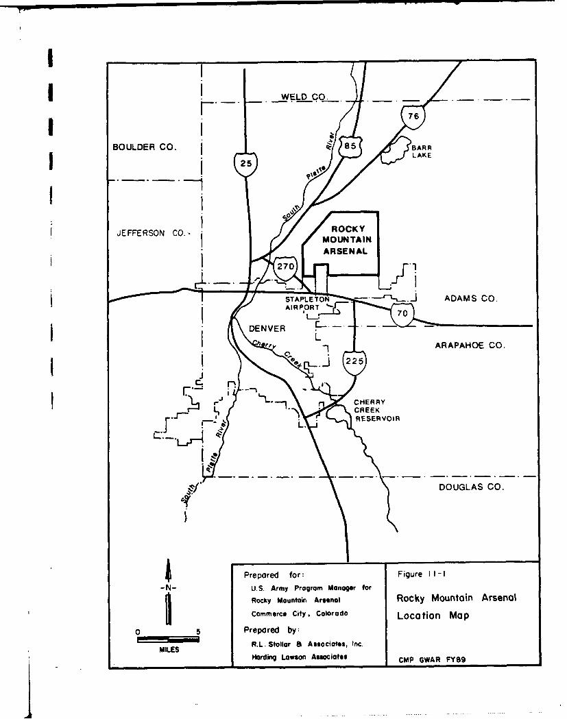
Figure 1.1-I Rocky Mountain Arsenal Location Map
Figure 1.2-1 Locatio, of Major Potential Contamination Sites, Lakes and Containmcnt Systems
Figure 1.4-1 Monitoring Well Locations for Basin F IRA Structures
Figure 1.4-2 Monitoring Well Locations in the Vicinity of the Section 30 Sanitary Landfill
Figure 2.1- I Upper Stratigraphic Sections of the Denver Basin
Figure 2.1-2 Bedrock Surface at RMA and Prominent Paleochannels
Figure 2.1-3 Surficial Geologic Map of Rocky Mountain Arsenal Area
Figure 2.1-4 RMA Denver Formation Stratigraphic Column
Figure 2.2-1 RMA Contaminant Migration Pathways
Figure 3.2-1 Project Areas in the Comprehensive Ground-water Monitoring Program
Figure 3.2-2 Temporal Relationsl-ip Between FY89 Sampling Events
Figure 3.2-3 Fall 1988 Sampling Network, Unconfined Ground-water Flow System
Figure 3.2-4 Fall 1988 Sampling Network, Denver Formation Confined Flow System
Figure 3.2-5 FY89 Quaterly Sampling Network
Figure 4.1-1 Water Table Elevation Map of the Unconfined Flow System, Fall 1988
Figure 4.1-2 Water Table Elevation Map of the Unconfined Flow System, Winter 1989
Figure 4.1-3 Water Table Elevation Map of the Unconfined Flow System, Srring 1989
Figure 4.1-4 Water Table Elevation Map of tle Unconfined Flow System, Summer 1989
Figure 4.1-5 Unconf: ied Water Table Elevation Map of Boundary Systems Area, Fall 19'8
Figure 4.1-6 Unconfined Water Table Elevation Map of Boundary Systems Area, Winter 1989
Figure 4.1-7 Unconfined Water Table Elevation Map of Boundary Systems Area, Spring 1989
Figure 4.1-8 Unconfined Water Table Elevation Map of Boundary Systems Area, Summer 1989
Figure 4.1-9 Unconfined Water Table Elevation Map of the Basin F Area, Fall 1988
Figure 4.1-10 Unconfined Water Table Elevation Map of the Basin F Area, Winter 1989
Figure 4.1-11 Unconfined Water Table Elevation Map of the Basin F Area, Spring 1989
G WAR-89.TOCRev. 3/19/90 - ix -
LLIST OF FIGURES (continued)
Figure 4.1-12 Unconfined Water Table Elevation Map of the Basin F Area, Summer 1989
Figure 4.2- I Potentiometric Surface of Denver Fm Zone A, IFall 1988
Figure 4.2-2 Potentiometric Surface of Denver Fm Z ne IU, Fall 1988
Figure 4.2-3 Potentiometric Surface of Denver Fm Zone i, Fall 1988
Figure 4.2-4 Potentiometric Surface of Denver Fm Zone 2, Fall 1988
Figure 4.2-5 Potentiometric Surface of Denver Fm Zone 3, Fall 1988
Figure 4.2-6 Potentiometric Surface of Denver Fm Zone 4, Fall 1988
Figure 4.3.2-1 Dieldrin Plumes, Unconfined Ground-Water Flow System, Fall 1988
Figure 4.3.3-1 Endrin Plumes, Unconfined Ground-Water Flow System, F-all 1988
Figure 4.3.4-1 Dithiane/Oxathiane Plumes, Unconfined Ground-Water Flow System, Fall 1988
Figure 4.3.5-1 Benzothiazole Plumes, Unconfined Ground-Water Flow System, Fall 1988
Figure 4.3.6-1 Summed Organosulfur Plumes, Unconfined Ground-Water Ilow System, F-all 1988
Figure 4.3.7-1 Summed Volatile Aromatic Compound Plumes, Unconfined Ground-Water FlowSystem, Fall 1988
Figure 4.3.8-1 Benzene Plumes, Uncontined Ground-Water Flow System, Fall 1988
Figure 4.3.9-1 Chlorobenzene Plumes, Unconfined Ground-Water Flow System, Fall 1988
Figure 4.3.10-1 Summed Volatile Organohalogen Compound Plumes, Unconfined Flow System, Fall1988
Figure 4.3-I I-1 Chloroform Plumes, Unconfined Ground-Water Flow System, Fall 1988
Figure 4.3-12-1 Trichloroethene (TRCLE) Plumes, Unconfined Ground-Water Flow System, Fall1988
Figure 4.3.13-I Tetrachloroethene (TCLEE) Plumes, Unconfined Ground-Water Flow Sys em, Fall1988
Figure 4.3.14-1 Dibromochloropropane (DBCP) Plumes, Unconfined Ground-Water Flow System,Fall 1988
Figure 4.3.15-I Dicyclopentadiene (DCPD) Plumes, Unconfined Ground-Water Flow System, Fall1988
Figure 4.3.16-1 Diisopropylmethylphosphonate (DIMP) Plumes, Unconfined Ground-Water Flov,System, Fall 1988
Figure 4.3.17-1 Summed Phenol Plumes, Unconfined Ground-Water Flow System, Fall 1988
GWAR-89.'TOCRev. 3/19/90- x-
I
LIST OF FIGURES (continued)
Figure 4.3.18-1 Parathion Plumes, Unconfined Ground-Water Flow System, Fall 1988
Figure 4.3.19-1 Cyanide Plumes, Unconfined Ground-Water Flow System. Fall 1988
Figure 4.3.20-1 Fluoride Plumes, Unconfined Ground-Water Flow System, Fall 1988
Figure 4.3.21 -1 Chloride Plumes, Unconfined Ground-Water Flow System, Fall 1988
Figure 4.3.22-1 Arsenic Plumes, Unconfined Ground-Water Flow System, Fall 1988
Figure 5.2-1 Water Table Profiles Along East-West Lines 450 Feet Downgradient and 350 FeetUpgradient of North Boundary Containment Barrier
Figure 5.2-2 Map View of Approximate Upgradient and Downgradient Water Table Elevationsat the North Boundary Containment System Slurry Wall, Fall 1988
Figure 5.2-3 Cross Section View of Approximate Upgradient and Downgradient Water TableElevations at the North Boundary Containment System, Fall 1988
Figure 5.2-4 Map View of Approximate Upgradient and Downgradient Water Table Elevationsat the North Boundary Containment System Slurry Wall, Summer 1989
Figure 5.2-5 Cross Section View of Approximate Upgradient and Downgradient Water TableElevations at the North Boundary Containment System, Summer 1989
Figure 5.2-6 Map View of Approximate Upgradient and Downgradient Water Table Elevationsat the Northwest Boundary Containment System, Fall 1988
Figure 5.2-8 Map View of Approximate Upgradient and Downgradient Water Table Elevationsat the Northwest Boundary Containment System, Summer 1989
Figure 5.3.3-1 Potentiometric Comparisons of Water Bearing Zones in the North BoundaryContainment System Area
Figure 5.3.3-2 Contaminant Distribution Histograms for Wells Near the North BoundaryContainment System
Figure 5.3.3-3 Contaminant Distribution Histograms for Wells Near the North BoundaryContainment System
Figure 5.3.3-4 Contaminant Distribution Histograms for Wells Near the North BoundaryContainment System
Figure 5.3.3-5 Contaminant Distribution Histograms for Wells Near the North BoudnaryContainment System
Figure 5.3.3-6 Contaminant Distribution Histograms for Wells in the First Creek and NorthernOff-post Pathways
Figure 5.3.3-7 Contaminant Distribution Histograms for Wells in the First Creek and NorthernOff-post Pathways
GWAR-89.TOCRev. 3/19/90 - xi -
!
j LIST OF FIGURES (continued)
Figure 5.3.3-8 Contaminant Distribution Histograms for Wells in the First Creek and NorthernOff-post Pathways
Figure 5.3.3-9 Contaminant Distribution Histograms for Wells in the First Creek and Northern Off-Post Creek Pathways
Figure 5.3.3-10 Historical DIMP Concentrations in Wells Upgradient of the NBCS
Figure 5.3.3-11 Historical DIMP Concentrations in Wells Downgradient of the NBCS
Figure 5.3.3-12 Potentiometric Comparison of Water Bearing Zones in the Northwest BoundaryContainment System Area
fFigure 5.3.3-13 Contaminant Distribution Histograms for Wells Near the Northwest BoundaryContainment System
Figure 5.3.3-14 Contaminant Distribution Histograms for Wells Near the Northwest BoundaryContainment System
Figure 5.4-I Study Areas of the Inorganic Data Assessment
Figure 5.4-2 Specific .'nductance Distribution
Figure 5.4-3 Percent Oxygen Saturation Distribution
Figure f.-1-4 Inorganic Analyte Frequency Distribution by Flow System
Figure 5.4-5 Calcium/Sodium (Ca/Na) Ratio Distribution
Figure 5.4-6 Regional and Background Trilinear Diagrams
Figure 5.4-7 Western Tier and Central Area Trilinear Diagrams
Figure 5.4-8 Northern Area Trilinear Diagrams
Figure 5.5-1 Location of Section 23 and 24 Wells Sampled for Isotopic Analyses
Figure 5.5-2 Historic Tritium Data Values
Figure 5.5-3 A Plot of TU Values vs. Depth
Figure 5.5-4 Schematic Cross Section A-A'
F-igure 3.5-5 Deuterium/Oxygen- 18 Ratios
G WAR-89.TOCRev. 3/19/90 - Xii -
I
ITABLE OF CONTENTS (continued)
VOLUME II
APPENDIX A MAPS SHOWING DISTRIBUTIONS OF CONTAMINANTS IN TIlE CONFINEI)FLOW SYSTEM
Figure A- I Dieldrin Detections Denver Zone A, Fall 1988
Figure A-2 Dieldrin Detections Denver Zones IU & I, Fall 1988
Figure A-3 Dieldrin Detections Denver Zones 2, 3 & 5, Fall 1988
Figure A-4 Endrin Detections Denver Zone A, Fall 1988
Figure A-5 Endrin Detections Denver Zones IU & I, Fall 1988
Figure A-6 Endrin Detections Denver Zones 2, 3 & 5, Fall 1988
Figure A-7 Dithiane/Oxathiane Detections Denver Zones IIJ & I, Fall 1988
Figure A-8 Dithiane/Oxathiane Detections Denver Zone 2, Fall 1988
Figure A-9 Summed Organosulfur Compound Detections Denver Zone A, Fall 1988
Figure A-10 Summed Organosulfur Compound Detections Denver Zone IU & 1, Fall 1988
Figure A-1I Summed Organosulfur Compound Detections Denver Zone 2, Fall 1988
j Figure A-12 Summed Volatile Aromatic Compound Detections Denver Zone A, Fall 1988
Figure A-13 Summed Volatile Aromatic Compound Detections Denver Zones I U & 1, Fall 1988
Figure A-14 Summed Volatile Aromatic Compound Detections Denver Zones 2, 3 & 5, Fall 1988
Figure A-15 Benzene Detections Denver Zone A, Fall 1988
Figure A-16 Benzene Detections Denver Zones IU & i, Fall 1988
Figure A-17 Benzene Detections Denver Zones 2, 3 & 5, Fall 1988
Figure A-18 Chlorobenzene Detections Denver Zones A & IU, Fall 1988
Figure A-19 Chlorobenzene Detections Denver Zones, I, 2 & 5, Fall 1988
Figure A-20 Summed Organohalogen Compound Detections Denver Zones B, VC & A, Fall 1988
Figure A-21 Summed Organohalogen Compound Detections Denver Zones IU & 1, Fall 1988
Figure A-22 Summed Organohalogen Compound Detections Denver Zones 2, 3, 4 & 5, Fall 1988
Figure A-23 Chloroform Detections Denver Zones B & A, Fall 1988
G WAR-8g.TOCRev. 3/19/90 - xiii -
I
APPENDIX A - LIST OF FIGURES (Continued)
Figure A-24 Chloroform Detections Denver Zones IU & I, Fall 1988
Figure A-25 Chloroform Detections Denver Zones 2 & 3, Fall 1988
g Figure A-26 Trichloroethene (TRCLEE) Detections Denver Zones VC & A, Fall 1988
Figure A-27 Trichloroethene (TRCLEE) Detections Denver Zones IU & i, Fall 1988
Figure A-28 Trichloroethene (TRCLEE) Detections Denver Zones 2, 3 & 5, Fall 1988
Figure A-29 Tetrachloroethene (TCLE) Detections Denver Zones A & B, Fall 1988
Figure A-30 Tetrachloroethene (TCLE) Detections Denver Zones IU & 1, Fall 1988
Figure A-31 Tetrachloroethene (TCLE) Detections Denver Zone 2, Fall 1988
Figure A-32 Dibromochloropropane (DBCP) Detections Denver Zones A & IU, Fall 1988
Figure A-33 Dibromochloropropane (DBCP) Detections Denver Zones A & 2, Fall 1988
Figure A-34 Dibromochloropropane (DBCP) Detections Denver Zones 3 & 5, Fall 1988Figure A-35 Dicyclopentadiene (DCPD) Detections Denver Zone A, Fall 1988
Figure A-36 Dicyclopentadiene (DCPD) Detections Denver Zones 1, 2 & 4, Fall 1988Figure A-37 Diyiscoppyimethyiphosphonate (DIMP) Detections Denver Zones B & A, Fall 1988
Figure A-38 Diisopropylmethylphosphonate (DIMP) Detections Denver Zones I U & 1, Fall 1988
Figure A-39 Diisopropylmethylphosphonate (DIMP) Detections Denver Zones 2 & 3, Fall 1988
Figure A-40 Diisopropylmethylphosphonate (DIMP) Detections Denver Zones 4, 5 & 6, Fall 1988
Figure A-41 Phenol Detections Denver Zone A, Fall 1988
Figure A-42 Phenol Detections Denver Zones IU & A , Fall 1988
Figure A-43 Phenol Detections Denver Zones 2, 3, 4, & 5, Fall 1988
Figure A-44 Parathion Detections Denver Zone A, Fall 1988
Figure A-45 Cyanide Detections Denver Zones B & A, Fall 1988
Figure A-46 Cyanide Detections Denver Zone I U, Fall 1988
Figure A-47 Cyanide Detections Denver Zones I & 2, Fall 1988
Figure A-48 Cyanide Detections Denver Zones 3, 4 & 2, Fall 1988
GWAR-89.TO-xR~ev. 3/19/90 -xiv -
II APPENDIX A - LIST OF FIGURES (Continued)
I Figure A-49 Fluoride Detections Denver Zones B & A, Fall 1988
Figure A-50 Fluoride Detections Denver Zone I U, Fall 1988
Figure A-51 Fluoride Detections Denver Zone 1, Fall 1988
Figure A-52 Fluoride Detections Denver Zone 2, Fall 1988
i Figure A-53 Fluoride Detections Denver Zones 3 & 4, Fall 1988
Figure A-54 Fluoride Detections Denver Zones 5, 6 & 7, Fall 1988
Figure A-55 Chloride Detections Denver Zones B & A, Fall 1988
Figure A-56 Chloride Detections Denver Zones IU &I, Fall 1988
Figure A-57 Chloride Detections Denver Zones 2 & 3, Fall 1988
9 Figure A-58 Chloride Detections Denver Zones 4 & 5, Fall 1988
Figure A-59 Arsenic Detections Denver Zones A & IU, Fall 1988
9 Figure A-60 Arsenic Detections Denver Zones I & 2, Fall 1988
Figure A-61 Arsenic Detections Denver Zones 4, 5 & 6, Fall 1988IAPPENDIX B HYDROLOGIC DATA COLLECTED DURING FY899 (on diskette - enclosed)
APPENDIX C ANALYTICAL DATA COLLECTED DURING FY89(on diskette - enclosed)
APPENDIX D GEOLOGIC/WELL CONSTRUCTION LOGS FOR WELLS INSTALLEDDURING FY89I
1
G WAR-89.TOCRev. 3/19/90 - xv -
I
I-
LIST OF ACRONYMS
ACRONYMS AND ABBREVIATIONS
Chilo rdane I ,2,4,5,6,7,8,8-octachloro--2,3,3a.4.7,7a-hexahydro-4,7-nmetliano- I ll-indene
C1C 6 H 5 ChlorobenzeneCMP FY88 Comprehensive Monitoring Program Fiscal Year 1988
CO Carbon MonoxideIDBCP DibromochloropropaneDCLEi I 1,1-Dichloroethane9DCLE12 1,2-Dichloroethane
DCPD Dicyclopentadiene
DDD Dichiorodiphenyldichioroethane
DMB 12 DimethylbenzeneDMDS Dimethyl Disulfide9EPA Environmental Protection AgencyETC6 115 Ethylbenzene
GC/ MS Gas Chromatography/ Mass Spectrometry
GC/ECD Gas Chromatography/Electron Capture Detection
ICAP inductively Coupled Argon Plasma
I Malathion O,O-dimethyl-s-(1I,2-dicarboxyethyl) phosphorodithioate
MIBK Methyl Isobutyl Ketone
IParathion Parathion (C10H 14 N0 5 PS)PMRMA Program Manager Rocky Mountain Arsenal
PPDDE DichiorodiphenylethaneIPPDDT Dichlorodiphenyltrichloroethaneso 2 Sulfur Dioxide
jSupona 2-chloro-1-(2,4-dichlorophenyl) vinyl diethyl phosphate
TI12DCE Trans-I ,2-Dichloroethene
TCLEE Tetrachloroethene
TRCLE Trichloroethene
USATHAMA U.S. Army Toxic and Hazardous Materials Agency
XYLENE Xylene
G WAR-89.TOCRev. 3/19/90 -xvi -
IEXECUTIVE SUMMARY
The Ground-Water Element of the Comprehensive Monitoring Program (CMP) has been designed
to provide continual and long-term monitoring of ground water at the Rocky Mountain Arsenal
(RMA) and adjacent off-post areas. Ground-water data collected during Fiscal Year 1989 (FY89)
were obtained to verify data and analyses obtained previously as part of the RMA Remedial
Investigation and Feasibility Study (RI/FS), to assess changes in the rate and extent of contaminant
migration, and to meet various regulatory needs. Although the CMP has been designed primarily
as a regional monitoring program, data have been collected on a more detailed basis in selected
areas to support ongoing remedial/response actions or other needs.
Program Design for FY89
The FY89 well network consisted of both on-post and off-post wells for monitoring ground-water
level fluctuations and water-quality conditions. The networks were designed to provide regional
information about the shallow water-table aquifer (referred to as the unconfined flow system) as
well as deeper aquifers of the Denver Formation (confined flow system). Wells were selected on
the basis of well-construction, historical water-level and water-quality data. The areal distribution
of those wells was considered in order to assure that a greater number of wells were measured in
areas of confirmed ground-water contamination or where changing hydrogeologic conditions were
anticipated. The water-level network included approximately 1,000 wells monitored on a quarterly
basis.1The FY89 water-quality network included 488 wells monitored annually, 388 wells monitored
semiannually, and 62 wells monitored quarterly. Wells monitored on an annual basis provided
information to assess current contaminant distributions and to identify possible changes in the
regional distribution of contaminants. Wells monitored on a semiannual basis provided detailed
contaminant distribution information in specific areas of concern. These areas included the North
Boundary Containment System Area, the Northwest Boundary Containment System Area, the
Irondale Containment System Area, the Basin F Area, the North Plants Area, the Basin A Area,
and the South Plants Area. Wells monitored on a quarterly basis provided water-quality data to
support ongoing IRA projects in the Basin F Area.
FY89 ground-water samples were routinely analyzed for 73 analytes including both organic and
inorganic compounds that were known or suspected to be in ground water. In addition,
approximately 18 percent of all water samples were analyzed by GC/MS techniques to confirm or
GWAR-89.1-SRev. 06/21/0o
refute the presence of organic chemicals detected by GC techniques and to identify any compoundsnot included among the 73 target analytes. The target list of chemicals for FY89 was the same as
FY88 with the exception of parathion, cyanide,and acid extractable phenols. These exceptions were
added to the FY89 target list on the basis of FY88 GC/MS data and discussions with the
Organizations and State. The FY89 analytical program also incorporated a quality assurance and
quality control plan designed to provide accurate and reproducible analytical results.
g Results of FY89 Program
The FY89 water-level data were used to construct potentiometric-surface maps of the unconfined
and confined flow systems. Regional water-table maps corresponding to the Fall 1988, Winter
1989, Spring 1989, and Summer 1989 were constructed for the unconfined flow system. Detailedwater-table maps also were constructed for the North Boundary Containment System Area, the
Northwest Boundary Containment System Area, and the Basin F Area. Regional potentiometric-
surface maps were constructed for six stratigraphic zones within the confined flow system.
In general, the water table decreased approximately 210 ft in elevation across RMA and indicated
a regional direction of ground-water flow from southeast to northwest. Seasonal fluctuations in
the regional water table during FY89 were small. The largest fluctuation, an increase of
approximately 4 ft, occurred in the South Plants Area. The water-table maps indicate that the
South Platte River, located approximately two miles northwest of the RMA boundary, acts as amajor discharge point for the unconfined flow system.ILocal variations in flow direction were common in the unconfined flow system and usually
corresponded with areas where the water table was in or near bedrock of the Denver Formation.
The most pronounced variation from the regional water table pattern at RMA occurred in the South
Plants area where the water table formed a mound approximately 25 ft higher than the surrounding
regional water table.
Potentiometric-surface maps of the confined flow system showed regional potential for flow from
southeast to northwest as well as an overall potential for downward flow. However, local
variability in hydraulic conductivity and local variations in the degree of hydraulic interconnection
between stratigraphic intervals have resulted in substantial local variations in flow direction from
overall regional trends. Because the CMP has been designed primarily to monitor regional trends,the FY89 data do not fully characterize the significance of these local variations in flow direction.
Seasonal variations in water levels of the confined flow system generally were small.
GWAR-89.1-$Rev. 06/21/9o
I
Operation of the North and Northwest Boundary Containment Systems has locally influencedground-water flow. Differences in elevations of the water table across the boundaries indicatedhydraulic separation between up and down gradient flow systems. Changes in the rates and areal
distribution of ground-water extraction and injection during FY89 resulted in seasonal variationsin the water-table elevation near the boundary systems. The most significant variations occurredat the North Boundary Containment System. Installation and operation of recharge trenches hasincreased the water-table elevation north of the boundary system and resulted in a reversal of the
hydraulic gradient along the western part of system.
Results of water-quality samples and analysis have been used to construct contaminant distributionmaps for 21 analytes or analyte groups. Contaminant concentrations in the unconfined flow systemhave been characterized by preparing contour maps of plume configuration during Fall 1988.Contaminant concentrations in the confined flow system have been characterized by preparing pointplots of concentration using Fall 1988 data. Contour maps have not been prepared for the confined
flow system because regional contaminant plumes have not been detected.
The regional distribution of contaminants was identified more precisely from FY89 data than has
been possible with previous CMP data. The improved definition is attributable primarily to theaddition of wells to the CMP water-quality network in the Basin A, South Plants, and North PlantsAreas. Previous efforts to map RMA contaminant distributions throughout RMA have relied on
data collected from several different time periods and analyzed with different procedures. Withdata from the FY89 CMP, information from a single time period can be utilized.I|Regional contaminant distributions identified from FY89 data were generally consistent withdistributions provided in previous CMP and Remedial Investigation reports. Major plumes werepresent as part of the unconfined flow system in the vicinity of South Plants, North Plants, the
disposal basins, and the Motor Pool - Railyard Areas. Plumes extended from these areas north andnorthwest toward the North Boundary, Northwest Boundary, and Irondale Containment Systems.Off-post plumes extended from north of the North Boundary Containment System toward the SouthPlatte River and principally reflect contaminant migration into off-post areas prior to installationof the boundary system. Plumes in the South Plants Area extended radially outward from apparent
source areas in response to prevailing directions of ground-water flow.
The extent of contamination in the unconfined flow system varied from compound to compound.
Organic contaminants distributed widely in the vicinity of South Plants, the disposal basins, and
GWAR-89.1-SRev. 06/21/90
I
on-post and off-post areas to the north and northwest included dieldrin, endrin, chloroform,trichloroethene, tetrachloroethene, and diisopropylmethyiphosphonate. Inorganic compounds with
wide distributions included flunride, chloride, and arsenic. Less extensive on-post and off-post
plumes were identified for summed organosulfur compounds, dibromochloropropane, and
dicyclopentadiene. Trichloroethene, tetrachloroethene and related volatile halogenated compounds
were widely distributed in the western part of RMA and appear to have originated partly from
source areas south of RMA.
The FY89 unconfined flow system contaminant distributions that differed from FY88 distributions
were dieldrin, endrin, and chloroform. Most of the differences result from programmatic changes
in the CMP rather than rapid contaminant migration. Changes in the distributions of dieldrin and
endrin were the result of an increase in the number of wells sampled in the South Plants, Basin
A, and Basin A Neck areas. Changes in the distribution of chloroform were the result of a FY89
decrease in the certified reporting limit.
The contaminant distribution identified from FY89 data in the confined flow system was
substantially more irregular and sporadic than the distribution identified in the unconfined flow
system. The irregular distribution of contaminants was primarily a reflection of the large amount
of local-scale variability in flow directions and flow rates. Areas where contamination was
identified in the confined flow system were generally located beneath contaminated areas of the
unconfined flow system. Contaminant concentrations in the confined flow system generally were
lower than in the overlying unconfined flow system.
Several chemicals not included on the CMP target list of chemicals were detected in multiple
samples submitted for GC/MS analysis. Butylbenzylphthalate was the most commonly identified
nontarget compound, but was thought to be a product of laboratory contamination.
Dichlorobenzene historically has been present in CMP samples and during FY89 was detected in
a significant number of samples. In general, nontarget compounds were detected in samples
containing elevated levels of target compounds.
Quality Assurance and Quality Control samples were collected and analyzed during FY89 to
evaluate the repeatability and accuracy of water-quality data. These samples consisted of trip,
field, and rinse blanks as well as duplicate samples. Although results of the blank samples
indicated that sample contamination occasionally occurred, it was a minor problem. Results of
sample duplicates indicated that differences in concentrations of organic analytes averaged
approximately 36 percent of the concentrations reported in the original sample. This percentage
GWA•'-S.1-3Rev. 06/21/90
!
represented an average for all sample pairs and all organic compounds detected. Repeatability of
an individual sample or an individual compound can vary significantly from this average. Results
for inorganic analytes were significantly less variable, indicating that reported concentrations of
inorganic compounds are more repeatable than concentrations of organic compounds. Differences
in concentrations of inorganic analytes averaged approximately 17 percent.
I Data Assessment
Operation of the North Boundary Containment System was changed significantly during FY89 with
the installation of recharge trenches north of the soil-bentonite slurry wall. The trenches were
installed to increase downgradient recharge capacity along the western half of the system. By
increasing recharge capacity, it had been predicted that water levels in both the unconfined and
confined flow systems north of the slurry wall would be greater than water levels south of the
slurry wall, and the potential for contaminant migration beneath the system wculd be eliminated.
FY89 water-level data indicated that operation of the recharge trenches has begun to have the
I predicted effect. The water-table elevation in the unconfined flow system north of the system hasrisen above the water-table elevation south of the system and a reverse hydraulic gradient has been
a established. Water-level data collected as part of the CMP indicate that the gradient reversal has
begun to propagate into the shallow stratigraphic zones of the confined flow system. The low
hydraulic conductivity of the confined flow system has influenced the rate of propagation. As aresult, the reverse hydraulic gradient throughout the confined flow system was not established
during FY89. It is anticipated that future monitoring of the confined flow system will confirm the
propagation of a reversed gradient.
Water-quality data indicated that operation of the North Boundary Containment System including
the recharge trenches has decreased contaminant concentrations dramatically north of the system.
Decreased concentrations are most evident in dibromochloropropane, chloroform, and
diisopropylmethylphosphonate, those compounds most frequently detected south of the boundary
system. Concentration of these compounds north of the boundary system has steadily decreasedwith time, due to system operation.
Inorganic data have been used to assess background water quality at RMA. Background water
samples from the unconfined flow system typically had calcium-sodium ratios between one and
two, specific conductance less than 2,000 umhos/cm, percent oxygen saturation less than 60
GWAR-89.1-3Rev. 06/21/90
I
-T"
I
percent, and were dominated by sulfate and bicarbonate anions. Background water samples from
the confined flow system typically had calcium-sodium ratios less than one, specific conductance
values less than 2,300 umhos/cm, percent oxygen saturation less than 60 percent, were slightly
dominant in sodium and potassium, and dominant in sulfate.
Background inorganic water quality was compared with inorganic water quality of parts of RMA
where contaminant plumes have been mapped. Inorganic water quality of the unconfined flow
j system in the western part of RMA was similar to background water with the exception of higher
values of percent oxygen saturation. Inorganic water quality of the unconfined flow system in the
central and northern parts of RMA typically had calcium-sodium ratios less than one. Many
Ssamples had specific conductance values that ranged from 2,500 to 20,000 pmuhos/cm. These
differences from background water quality can be related to the past disposal of waste water rich
in sodium chloride. Water from the confined flow system in the central part of RMA typically had
higher specific conductance and were more strongly dominated by chloride and nitrate th.o•
a background water.
A FY89 pilot study monitored ground water for isotopic signature. This data was used to assess
the degree of hydraulic connection between the unconfined and confined flow systems. Samples
collected from the unconfined and confined flow systems were analyzed for deuterium, oxygen-
18 and tritium. Results were compared with organic water-quality data. Water from the
unconfined flow system generally was isotopically distinct from water in the confined flow system.
However, a small degree of mixing was indicated by the isotopic data from some wells completed
in the confined flow system. Based on the results of the pilot study, isotopic sampling and analysis
for tritium appeared to have greater potential than other isotopes for identifying hydraulic
connection between flow systems
I Conclusions
Ground-water data collected as part of the CMP during FY89, have been beneficial in confirmingresults of past investigations, monitoring ongoing remedial/response actions, and providing
improved descriptions of the regional distribution of ground-water contaminants. Important
I conclusions obtained on the basis of FY89 data include:
1. Regional contaminant distributions identified from FY89 data generally were
consistent with distributions provided in previous CMP and Remedial Investigation
i reports.
GWAR-8g.1-3Rev. 06121/90
I
I
2. The regional distribution of contaminants has been mapped more precisely thanpreviously possible using data from a single time period.
1 3. Accuracy and repeatability of water-quality results were good, averaging 36 percent
of the reported value for organic contaminants and 17 percent of the reported value
for inorganic compounds.
4. Concentrations of contaminants north of the North Boundary Containment Systemhave been reduced substantially as a result of system operation.
I5. The potential for contaminant migration beneath the North Boundary Containment
System has been reduced. Recent changes in operation of the system have begunI to establish a reverse hydraulic gradient in both unconfined and confined flow
systems.
I
GWARt-89.1-SRev. 06/21/9o
I
1.0 INTRODUCTION
1.1 Site RacKyround
Rocky Mountain Arsenal (RMA) occupies approximately 27 square miles (sq mi) and is located
within the border of Adams Ccunty, Colorado, about 9 miles (mi) northeast of downtown Denver
(Figure 1.1-1). RMA was established by the U.S. Army (the Army) in 1942 to produce chemical
and incendiary munitions for World War If. Following World War II, the production of munitions
decreased, and the Army leased selected portions of RMA to private industry. Several of the lessees
produced industrial chemicals, consisting predominantly of herbicides and pesticides, until 1982.
Chemical agents were produced at RMA until 1957. From 1942 to 1950, mustard agent (11) was
produced or distilled in the South Plants manufacturing area. This area was also used to fill shells
with the chemical agent phosgene or incendiary mixtur: "cluding napalm, and white phosphorous.
Many different types of obsolete World War 1I ordnance were destroyed by detonation or
incineration at RMA during this time. In the early 1950's RMA was selected to produce the
chemical nerve agent Sarin (GB). This was produced in the North Plants manufacturing area until
1957. Munitions filling operations continued at RMA until 1969. From 1970 to 1984, Army
activities focussed primarily on the demilitarization of chemical warfare materials.
In 1947, portions of RMA were leased to private industry. Early lessees included the Colorado Fuel
and Iron Corporation (CF&I) and the Julius Hyman and Company (Hyman). CF&I produced
chlorine, fused caustic and chlorinated benzenes, and attempted to manufacture
dichlorodiphenyltrichloroethane (DDT). Hyman produced several pesticides. In 1950, Hyman
added to its lease a number of facilities formerly operated by CF&I. In 1952, Shell Chemical
Company (Shell) acquired Hyman and operated this company as a wholly owned subsidiary until
1954, when Hyman was integrated into the Shell corporate structure. At this point Shell succeeded
Hyman as the named lessee. From 1952 until 1982, Hyman/Shell produced a large number of
herbicides and pesticides in the South Plants manufacturing complex.
Between 1942 and 1982 numerous specific releases of chemicals to the environment associated with
these production activities were documented. As early as 1951 a link was suspected between
waterfowl mortality at RMA and insecticide contamination of the lakes located there. In 1954 and
1955, farmers using well water for irrigation northwest of RMA reported severe crop losses. In
1974, two contaminants -- diisopropylmethyl phosphonate (DIMP), a manufacturing by-product
of the nerve agent isopropylmethane fluorophosphonate (Sarin, or GB), and dic~clopentadiene
GWAR-89.1-SRev. 07/26190 -
1
!
3 (DCPD), a chemical used in insecticide production -- were detected in off-post surface water. Since1978, numerous compounds have been detected in off-post ground water.
0 1.2 Nature and Extent of Problem
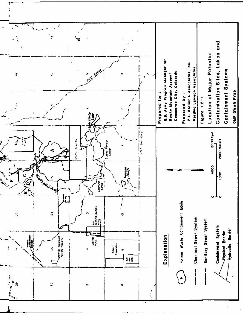
i Contaminants were introduced to the RMA environment primarily by the burial or surface disposal ofsolid wastes, discharge of wastewaters to basins, and leakage of wastewaters and industrial fluids fromchemical and sanitary sewer systems. Wastewaters generated by the Army and private industry in the3 South Plants and North Plants area were discharged to a series of unlined evaporation and holding basins(Basins A, B, C, D and E), and to asphalt-lined Basin F at various times throughout the history of RMAoperations (Figure 1.2- 1). Unintentional spills of raw materials, process intermediates, solvents, cleaners,
fuels, lubricants, and end products also occurred within the manufacturing complexes, storage areas,maintenance areas, or along transport routes at RMA.
A number of these contaminant releases have impacted ground water resulting in a series of contaminantplumes. The occurrence and movement of contaminants in ground water at RMA is complicated by:
* a large number of contaminant sources, some areally separated, some overlapping;
S• a large variability in release scenarios, including single or repeated spills, continuous orintermittent leaks, discharges to ditches or basins, leaching from trenches, leaching fromor direct contact of ground water with buried transport lines;
0 a large number of individual contaminants;
0 spatial variabilities in aquifer properties;
i a complex interactions between water-bearing zones; and
0 historical changes in the distribution and quantity of ground-water recharge.
1.3 Summary of Previous Ground-Water Monitoring Efforts
In the summer of 1974, the detection of DIMP and DCPD off-site highlighted the problem of
contaminant migration in ground and surface water at RMA. To address this problem, the Army in 1975initiated a regional sampling and hydrogeologic surveillance program requiring the quarterly collectionand analysis of samples from over 100 wells and surface-water stations located both on- and off-post.
SI
GWAR-89.1-3Rev. 07/26/90 -2-
I
I
This program was carried out under the direction of the RMA Contamination Control Program which
had been established in 1974 to ensure compliance with federal and state environmental laws. The
objectives of this program were to evaluate the nature and extent of contamination and to develop
response actions to control contaminant migration. Both suspected and confirmed contamination
sources were assessed, and contaminant migration pathways were evaluated.
To minimize off-post discharge of RMA contaminants via ground water, three boundary containment
systems were constructed, one along part of the northern and two along parts of the northwestern
boundaries of RMA. All three systems are currently in operation to intercept and treat contaminated
ground water and to recharge the treated water.
From 1975 to the present, numerous ground-water monitoring programs have been conducted at
RMA. Following issuance of the cease and desist orders, the Army established the 360 Degree
Monitoring Program to monitor regional ground and surface water. The Army also designed and
implemented monitoring programs to support the operation of the boundary control systems,
In 1984 the Army awarded a multi-year task order contract to initiate a Remedial
Investigation/Feasibility Study (RI/FS) at RMA. Two consecutive regional ground-water tasks were
awarded under this contract (Tasks 4 and 44). The purpose of these tasks was to investigate the nature
and extent of RMA ground-water contamination and to continue long-term ground-water monitoring
initiated under the 360 Degree Program. In addition, Task 25 (Boundary Control Systems Monitoring)
was awarded to continue ground-water monitoring in the vicinity of the boundary control systems.
In 1987 the Army separated both the long-term ground-water monitoring and the boundary systems
monitoring from the RI/FS program. These activities are now included under the ground-water
element of the Comprehensive Monitoring Program (CMP).
1.4 Overview of Current Ground-Water Monitoring
The CMP is designed to provide both continual and long-term monitoring of ground water, surface
water, air and biota. Administratively, each environmental medium is being monitored within a
separate program element. Each element has detailed objectives, outlined in respective technical
plans. Each technical plan presents monitoring guidelines, analytical parameters, and sampling
protocol and strategies. All four elements have a common objective to provide a database that meets
the standards set by the Program Manager of the Rocky Mountain Arsenal (PMRMA). An annual
report for each element discusses the monitoring results for the year.
GWAR-89.1-3Rev. 07/26/90 -3-I'I
A transitional round of ground-water monitoring activities, called the Transitional MonitoringProgram, was initiated in November 1987. This immediately followed the award of the CMP
contract. The purpose of the transitional round was to provide continuity with the previous
regional and boundary systems monitoring programs conducted under the RI/FS contract. TheTransition Monitoring Program, was initiated prior to completing the design of the long-termmonitoring well network. In March, 1988, the design strategy of the long-term CMP ground-water monitoring network was developed after reviewing data generated during previousmonitoring programs, including data from RI/FS Tasks 4, 25 and 44. This design strategy is
presented in the CMP Technical Plan (Stollar, 1989a).
The objectives of the CMP ground-water element are threefold:
* maintain a regional ground-water monitoring program to verify previously obtainedRI/FS data and analyses, and satisfy substantive iegulatory requirements.
maintain project area ground-water monitoring program components to verifypreviously obtained RI/FS data and analyses, support project area system
operations, and satisfy substantive regulatory requirements.
monitor ground-water quality and hydrology to assess changes in the rate and
extent of contaminant migration and the distribution of contaminants in both on-
and off-post areas.
The ground-water element of the CMP included water-quality monitoring based on one regionalwell network and two local well networks which emphasize specific areas. The regional
monitoring is conducted annually and includes the largest number of monitoring wells. The first
localized network is sampled semiannually. It is based on a midsized well network designed to
address specific local areas where further evaluation of contaminant flow patterns is required. The
second localized network is sampled quarterly. It is based on the smallest monitoring well networkand is designed to support ongoing remedial/response actions and/or substantive compliance withJ applicable regulatory requirements.
This report presents data collected during Fiscal Year 1989 (FY89). The data includes water levelmeasurements in addition to water quality results. Water levels were measured quarterly at
approximately 1,000 wells prior to each sampling round. The annual sampling round
(approximately 515 wells) was conducted in fall 1988, from late October 1988 through mid-
January 1989. The midsized, semiannual monitoring well network (approximately 376 wells) was
sampled in spring 1989, beginning in early May and continuing through mid-June 1989. The smallest,
GWAR-89.1-3Ri v. 07/26/90 -4-
I

SI
quarterly well network (approximately 51 wells) was sampled independently in February/March,
1989, and August, 1989.
The monitoring well network was expanded in FY89 due to the installation of additional monitoring
wells during the year. As indicated in Section 2.3.4 of the Ground-Water Element Technical Plan,
I newly installed wells are to be included in the CMP ground-water monitoring network for at least
two sampling periods following the initial sampling under their respective programs (Stollar, 1989a).
During the fall and winter FY89, 38 new monitoring wells were installed at RMA. The purpose
of these wells was to provide additional data needed to complete the Remedial Investigation Study
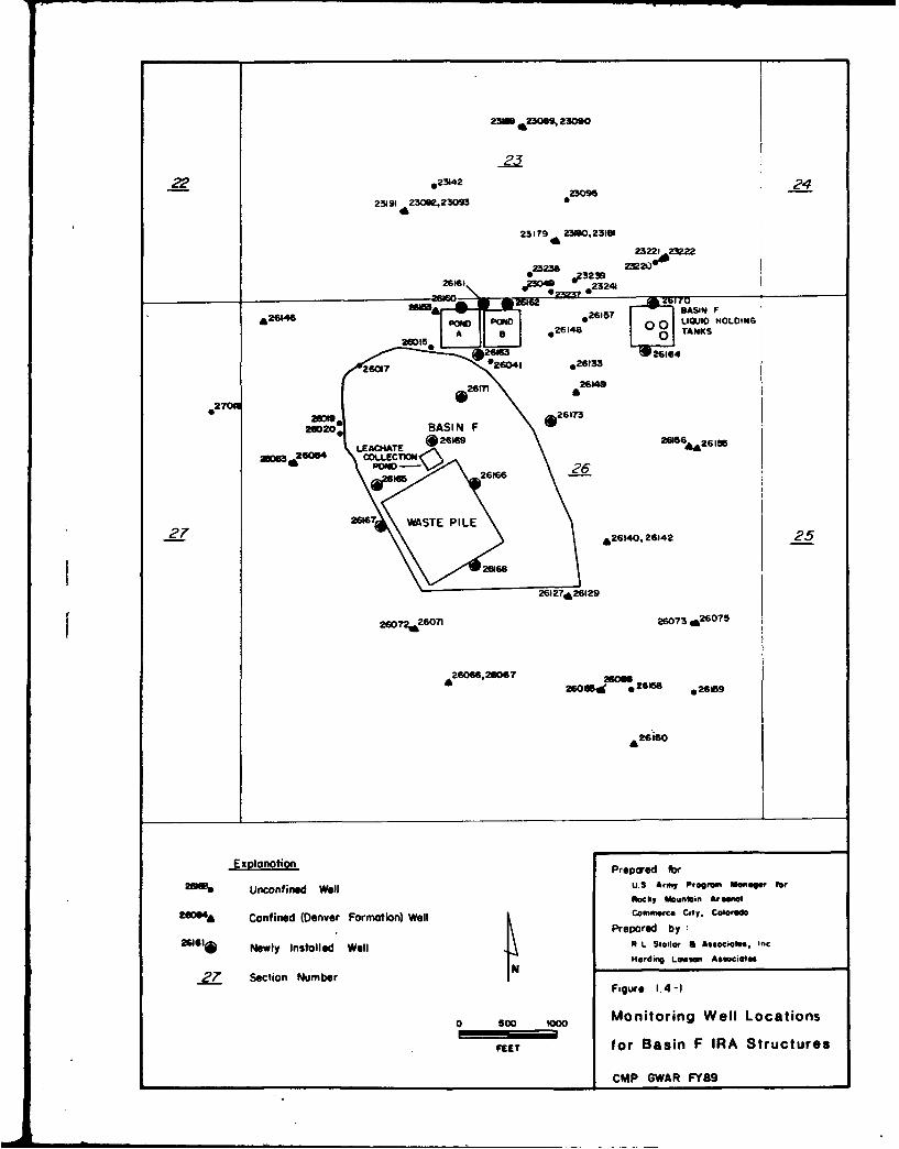
Area Reports (SARs). During the summer of FY89, 13 additional wells were added in the vicinityI of the Basin F to support the Interim Response Action (IRA). These wells were installed in Section
26 to provide monitoring points around Ponds A and B, the Basin F liquid storage tanks, the
Leachate Collection Pond and the Lined and Capped Basin F Waste Pile (Figure 1.4-1). The newly
installed wells were sampled once during the FY89 monitoring year in August, 1989.
Analytical and hydrogeological data from these new wells are included in this report. Geologic
drilling logs, construction specifications, and analytical data in tabular form are in the appendices
of the appropriate SARs for the 38 wells installed during the fall and winter of FY89 (Ebasco,
1989 b-h). For the remainder of the new wells installed during FY89, the analytical data and
geologic/construction logs are contained in Appendices C and D, respectively, of this report.
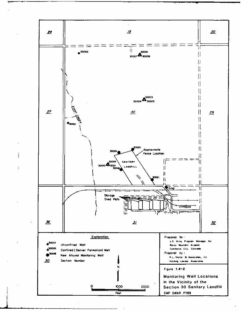
Additionally, five monitoring wells were installed around the sanitary landfill in Sections 30 and
31 (Figure 1.4-2). These wells were completed and developed after the final sampling event for
FY89 and, therefore, data from these wells are not included in this report.
Many sections of this report make frequent references to specific wells. Therefore, it is necessary
to understand the well numbering system to help in locating wells spatially. For all wells located
on the RMA, the first two digits of a well number refer to the section number in which the well
is located. The last three digits indicate the well number within that section. For example, well
01070 is well number 70 in Section 01. All wells installed by Shell are denoted by a 5 as the third
digit, for example 01501 is well number 501 in Section 01. (All wells located outside the RMA
are identified by "37' in the first two columns of the well number.) Wells are generally installed
sequentially within each section, and well numbers are assigned by the RIC Center at RMA.
In addition to the newly installed wells, another modification to the monitoring well network was
made during FY89. This modification deleted six wells (01069, 01070, 02050, 02052, 04035, 04051)
from the semiannual monitoring round. In past years information from wells 01069, 01070, 02050,
and 02052 did not significantly add to the understanding of contamination in the South Plants Area.
GWAR-89.1-3Rev. 06/21/90 -5-
I
Water quality data from wells deleted in Section 4 has not significantly enhanced the understanding
of contamination in the Railroad Classification Yard area. None of the deleted wells occur in
cluster sites and none were completed in the Denver Formation.
Another program modification included the addition of a new analytical laboratory to the group
I of contractors within the Stollar team. Hunter Services (formerly ESE) laboratory facilities in
Denver replaced Enseco-Cal Lab as the subsidiary CMP analytical laboratory. Analytical
parameters remained consistent with those outlined in Table 3.1-1 of the CMP Ground Water Final
Technical Plan (Stoliar, 1989a), and certified reporting limits (CRLs) are comparable betwecn the
primary CMP analytical laboratory, DataChem, Inc., of Salt Lake City, and the ESE-Denver
laboratory.
IIIII
GWAR-89.1-3Rev. 06/21/90 -6-
I WELD CO.76
BOULDER CO. 8 85 BARR
I LAKE
JEFFERSON CO.IROCKY
ARSENAL
I 270
AIPODENVRERI
DOUGLASE CO.
Prepredfor Fiure25-
-N .S ry rgamMngeno
05Prepared byr: Fgr
MIESR.L. Stollar & Associates, Inc.
MIESHrding Lawson Assocites CMp GWAR FY89
K;' K 7
'1. _ -� I
'-Ct�..
-4-
Ifu;� I. - 9 �.1
od� - 1-
- -
-
A' .- , I 1+
> //
'I '*�** �zI,
--- *N / J�
I.
________ � -uI � _________ (�jii���
* I I4.
UV
I - /�! =�g
___________________ ___________________ ___________________
_________'I
.�'. N. �2
C"
�O
.1 I' '-.
, '�If
____I_________ _________
_________ ___
-' I -�
'S.N 0
Cu
N
II.
CC< go
"CL 0 CI0 I.
* I o 0 0 0.
I, gag00
-Ago E EZ j_ _ -C C U
2*O CL EXI E v c Eix
~~:! ~ 0 0 aLL L 2000
CYcu rnin S
231 O2306% 23060
22 $23142 20524
23191 23012, 23M 0
23179 462300,23181
23221 Z12"
023236 239 2322000
26161 O 40 ~23237*234
2614 0661 SAS.'£26146~PO 2614 6@IONLONA2 a4 L2 TAWKS
261
Jý6 106 [:6 6
226076,26067 0 26133
2S I5 270 *6~ 26M6U9
2111 *26173
________________= 20____ IAS N___________F___
Exolonotio PreMe =56&260U.6r1
rgumM7egr
9
% Uncontined Wel RckyMEfln rena266 ofie (eve POrmto)W el 26Nr iy.Clrd
ore by
26161.~~ ~~ Newly PnlLdWlEt tlarSAsc~tn
27 etinNmbrI No2d614,62 25WAso~
Figre .4-
2612 Mnior7g el Loaton
260;W07 for -Basn IA trctre
62666,60P GWARF08
24 20
3000230D 6
0 3 00 A3 0 0 29
,oo o 03oo II
at II
\ II
001 Approximate IF/Fence Location
I 00009 SAN ITARY3 01o , i- I I
\~ L2
.33/ 32
Explanation Prepared for
30001 U S Army Program Manager for
* Unconfined Well Rocky Nounin ArwOI
,30005 Confined ( Denver Formation) Well Commerce City. Coiorado
03001 New Alluvial Monitoring Well Prepared by :
30 Sctio Numer IR.L. Stellor 8 Assocoats., Inc.0 Section Number Hardng LaIWson, Assoc,fg l
N Figure 1.4-2
Monitoring Well Locations
in the Vicinity of the0 1000 2000 Section 30 Sanitary Landfill
Feet CMP GWAR FY89

I2.0 HYDROGEOLOGIC SETTING
This section provides a description of the geologic and hydrogeologic characteristics in the RMA
study area. For a more thorough discussion of this subject, refer to the Water Remedial Investi-
gation Report (Ebasco, 1989i), which presents a comprehensive interpretation of hydrologic
conditions at RMA.
g2.1 Geologv
RMA is located within the Denver Basin, a broad structural depression encompassing northeastColorado and portions of southeast Wyoming and southwest Nebraska. The Denver Basin is a
north-south trending asymmetric syncline with a gently dipping eastern flank and a steeply dipping
western flank bordering the Colorado front rai..e. RMA is located near the structural axis of the
basin and the uppermost sediments beneath RMA dip less than one degree to the southeast.
The Denver Basin was downwarped during the late Cretaceous and early Tertiary periods.
Sandstone, siltstone, claystone, and lignite deposited during this period comprise the Fox Hills
Sandstone, Laramie Formation, Arapahoe Formation, and Denver Formation (Figure 2.1-1). These
strata overlie approximately 7000 feet (ft) of Cretaceous Pierre Shale.
Additional sediments were deposited in the Denver Basin throughout the Tertiary period. Regional
uplift and erosion later removed most of these sediments as well as part of the Denver Formation.
Quaternary sediments deposited on the late Tertiary erosional surface consist of unconsolidated
alluvial gravel, sand, silt, and clay, as well as eolian sand and silt.
The Cretaceous-Tertiary Denver Formation and Quaternary deposits are the two stratigraphic
sequences addressed in this repcit because they contain the principal aquifers in contact with
potential contaminant sources in the RMA study area. Quaternary deposits are collectively referred
to as the alluvium, although they consist of both alluvial and eolian materials.
2.1.1 Alluvium
Alluvial and eolian sediments in the RMA study area were deposited on an eroded bedrock surface
composed of Denver Formation strata (Figure 2.1-2). Locally, alluvial deposits reach a thickness
of 130 ft where prominent paleochannels have been carved into the bedrock surface. Typically,
the alluvium ranges in thickness from 0 to 50 feet. Alluvium blankets nearly the entire RMA
GWAR-89.1-3Rev. 06/21/90 - 7-
I
study area; however, overlying eolian materials are t'.e predominant strata exposed at land surface.Bedrock outcrops of the Denver Formation occur in only a few locations (Figure 2.1-3).
The surficial deposits vary in age, origin of deposition and grain-size distribution. Older alluvial
deposits generally are located in areas along the South Platte River and the western tier of KMA
and consist of coarse-grained sand and gravel. Coarse-grained deposits were also locally deposited
in bedrock paleochannels. Younger eolian and alluvial deposits are finer-grained than the older
surficial deposits and commonly form the uppermost deposits throughout much of RMA. A recent
investigation by Ebasco (1989i) provides detailed discussions of Quaternary deposits.
2.1.2 Denver Formation
The Denver Formation at RMA consists of a 200 to 500 ft thick sequence of interbedd&d claystone,siltstone, sandstone, and organic-rich (lignitic) layers (Ebasco, 1989i). The Denver Formation is
thickest in the southeastern portion of RMA and thins to the northwest due to erosion. A claystone
sequence 50 to 100 ft thick forms the top of the Arapahoe Formation and separates it from the
overlying Denver Formation. This clayshale interval, informally called the Buffer Zone, provides
hydraulic separation between .,quifers in these formations (Romero, 1976).
Most sediments in the Denver Formation were deposited under low-energy continental conditions
by fluvial processes in a distal alluvial plain environment (Romero, 1976). This environment gaverise to the accumulation and subsequent lithification of lenticular shaped sandstone and siltstone
units within layers of claystone and shale. Sandstone units are up to 50 ft thick. Volcaniclastic
material is present in the upper portion of the Denver Formation.
Stratigrmphic correlation of units within the Denver Formation is complicated by the discontinuous
nature of the sandstone units. Within the South Plants and Basin A area, correlation is aided by
the occurrence of a relatively thick, laterally continuous lignitic interval. This lignite layer
(Lignite A) has been used as the marker bed from which all other zones in the Denver Formation
at RMA have been referenced. Correlations based upon other lignitic layers has resulted in the
current interpretation of Denver Formation stratigraphy (Figure 2.1-4).
The Denver Formation dips gently to the southeast and the regional erosional bedrock surface
slopes to the northwest. Thus, the stratigraphic units from progressively deeper zones are erosion-
ally truncated to the northwest.
GWAR-89.1-SRev. 06/21/9o -8-
I
I
2.2 Livdrogeology
Ground water occurs at RMA under both unc-onfined (at atmospheric pressure) and confined (under
pr,:ssures greater than atmospheric) conditions. Water within deeper Denver Formation permeable
zones typically is confined, whereas water in unconsolidated surficial der'-sits typically is
unconfined. In this report, ground water is described as being within the unconfined flow system
or the confined flow system. Ground water within the confined flow system described in this
report is within the Denver Formation. Ground water in confined aquifers beneath the Denver
Formation are not addressed in this report.
2.2.1 Unconfined Flow System
At RMA, unconfined conditions may exist in both the alluvium and the Denver Formation. Water
in alluvium generally is unconfined. Unconfined conditions may also occur in the Denver
Formation where permeable Denver Formation zones are exposed at land surface or where they
subcrop beneath saturated or unsaturated surficial (alluvial) deposits. Consequently, the unconfined
flow system is interpreted to be a continuous flow system comprising both alluvium and unconfined
Denver Formation zones (Ebasco, 1989i). The unconfined flow system includes saturated surficial
deposits and subcropping parts of the Denver Formation where lithologic data indicate the presence
of sandstone or relatively permeable material. This interpretation is supported by potentiometric
data from wells in these Denver Formation units that are comparable to potentiometric data from
overlying alluvial wells. In areas where the surficial deposits are unsaturated, the subcroppingzones in the Denver Formation that contain water are considered part of the unconfined flow
system.
j The saturated thickness of the unconfined flow system can range up to 70 ft thick. The thickness
is greatest within the alluvium filled bedrock paleochannels in western and northwestern RMA, and
south of Ladora Lake. Saturated thickness beneath South Plants and the waste basins typically is
20 ft or less.
From a regional viewpoint, ground water in the unconfined flow system flows northwest across
RMA and discharges to the South Platte River. (A detailed discussion of the potentiometric surface
for the unconfined flow system is providpd in Section 4.1.) Local changes in flow directions may
be caused by a number of factors, notably: the configuration of the bedrock surface, spatialvariation in hydraulic conductivity of aquifer materials, surface-water impoundments, and man-
made features such as the boundary containment systems.
GWAR-89.1-$Rev. 06/21/90 -9-
I
SGround-water flow in the unconfined flow system occurs primarily within saturated alluvium.
This is due to the physical properties of alluvial versus bedrock materials. Hydraulic conductivity
within the alluvium typically ranges from 2.6 x 10³ to 1.7 x 102 ft/day whereas Denver Formation
hydraulic conductivity may be on the order of 2.8 x 10⁻¹ ft/day (Ebasco 1989i). Alluvium filled
paleochannels incised in the bedrock surface sometimes provide pathways (such as the Basin A
Neck and First Creek Off-post Pathways) for contaminant migration in ground water at RMA.
Several major contaminant pathways have been identified (Ebasco, 1989i), and have been named
g to simplify and standardize contaminant distribution discussions (Figure 2.2-1). Pathway names
were chosen because of proximity to well-known features and do not imply a source-plume
relationship.£Sources of recharge to the unconfined flow system in the study area include infiltration of
j precipitation and irrigation, seepage from surface-water features such as lakes and streams, inflow
from subcropping Denver Formation sandstones, and seepage from man-made structures such as
waste basins, canals, ditches, and buried pipelines. The principal discharge location for the
unconfined flow system is the South Platte River; however, discharge also occurs at other locations
in the RMA study area. Discharge is known to occur at Ladora Lake, Lake Mary, and the Rud
and Gun Club Pond (Ebasco, 1989i). Discharge from the unconfined flow system to the Denver
Formation may occur in areas where downward vertical gradients exist. A comparison of
potentiometric surface data to land surface elevations indicates that unconfined flow system
discharge into First Creek occurs near the northern RMA boundary. Discharge by evapotranspi-
ration is likely to occur in areas where the water table is within 5 ft of land surface. Estimated
recharge and discharge rates are summarized in the Water Remedial Investigation Report (WRIR)
(Ebasco, 1989i).
2.2.2 Confined Flow System
Ground water within strata of the Denver Formation that is under pressure greater than atmos-
pheric is part of the confined flow system. Confined conditions exist within the Denver Formation
where relatively impermeable strata separate the uthconfined flow system from more permeable
horizons deeper in the Denver Formation.
The confined flow system consists of relatively permeable sandstones, siltstones, and lignites
interbedded with relatively impermeable claystone. The discontinuous nature of the permeable
strata often results in hydraulic separation of individual Denver Formation stratigraphic zones.
Confined flow system strata also exhibit a high degree of variability in hydraulic conductivity and
storativity from one area to another (Ebasco, 1989i).
GWAR-89.1-3Itev. 06/21/90 - 10 -
I
I
Regional ground-water flow in the confined flow system is up dip to the northwest. Ground-
water flow direction is the result of greater precipitation and enhanced recharge along streams in
upland areas of the Denver Basin (e.g., Castle Rock area), combined with discharge to low points
in the Denver Basin (e.g., South Platte River) and areas where pumpage is large.
9i The hydraulic conductivity of sandstones within the confined flow system range from approx-
imately 2.8 x 100 to 2.8 x 10⁻² ft/day based on field testing. Hydraulic conductivity estimates are
not available for fractured lignitic beds. However, ground-water flow model analyses indicate that
lignitic bed hydraulic conductivities may be an order of magnitude greater than those of sandstone3
(Ebasco, 1989a).
Hydraulic head in the confined flow system decreases with increasing depth in most locations at
RMA. As a result, recharge to the confined flow system is likely to occur by leakage from
overlying strata. Recharge also occurs by lateral flow in Denver Formation units from areas south
and east of RMA. Discharge from the confined flow system occurs by lateral flow into the
unconfined flow system where permeable zones subcrop.
99II
GWAR-89.1-3Rev. 06/21/9o - II -
I1
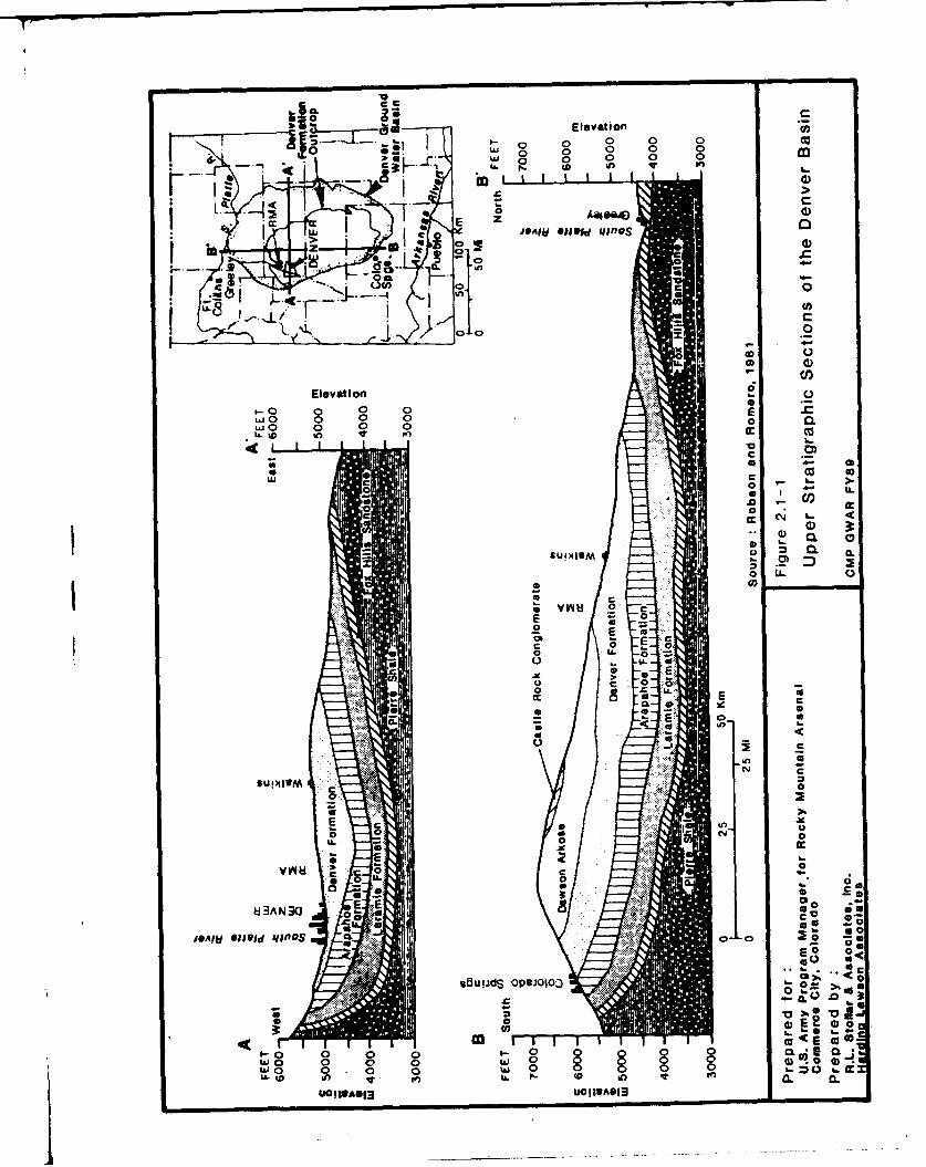
0L CSElevation
0 0 0 0 oap 0 0 0 0
0 to q
P.)
0 A
4( E
I* O
0 C) 0.
0.
0 0 e
0 0 0
LU 0 c
0
CL
0- 0
0 E0
m E~SUU~d~OPWOIO C rQ
EE 0
I&J 0v 0
0.0
eEE
U01WA013d U0113A01

0 2Miles
SCALE IN MILES-
1/71
I AA.
Contour Interval Equals 10 Feet Source Modified from Ebisco, 1989i
Prepared for: Figure 2.1-2
U.S. Army Program Manager for erc ufaea M nRocky Mountain Arsenal BdokSraea M nCommerce City. Colorado
Prepared by : Prominent PaleochannelsR.L. Stoller & Associates, Inc.Harding Lawson Associates CMP OWAR FY89
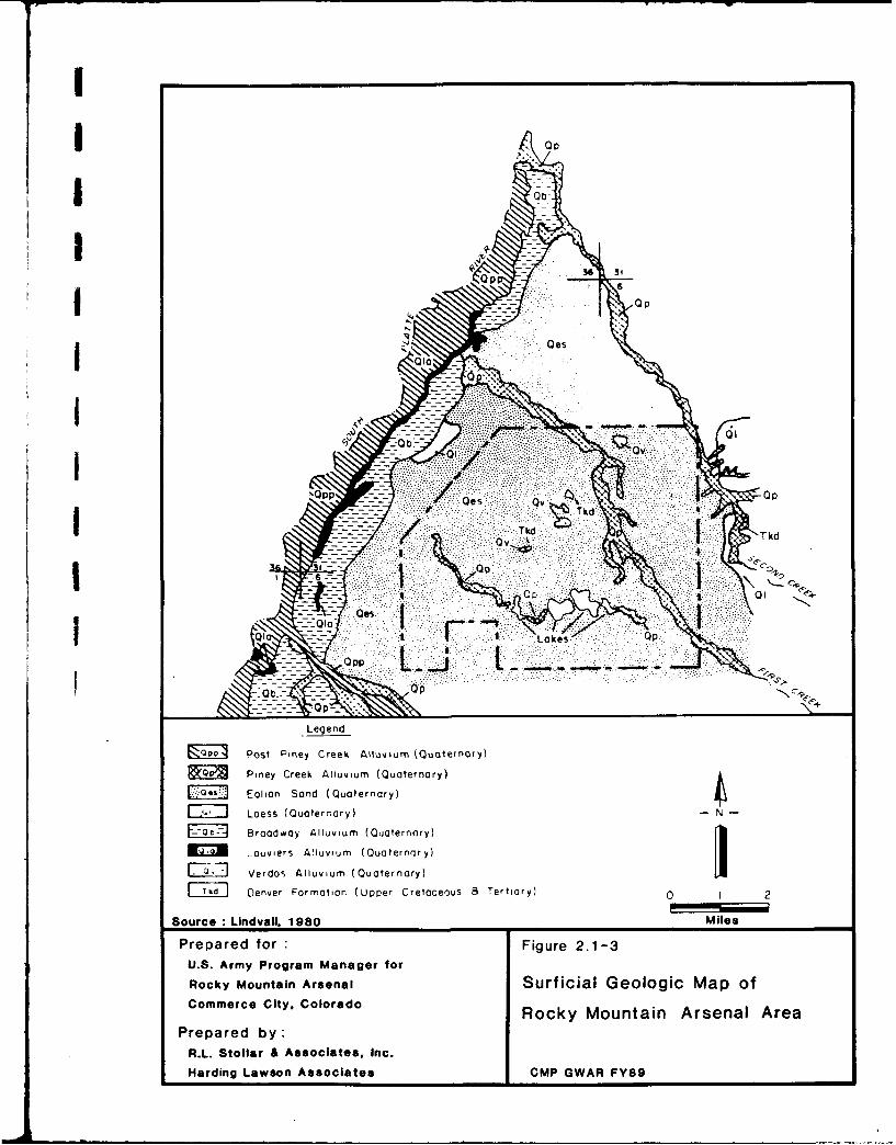
I op
1p 36G
OeOp
I Qva
I Qv Tkd
1k ýT
I~Z oel tQuaaeesary
BrostdwinyCre Alluvium (Quaternary)
Broadery Alluvium (Quaternary)
enviers Formaion (QuapernCretcoy) etayVerdos Alluvium (Quaternary)FE1311 evr1omton(perCeaeos8Tetay 0 I 2
Source :Lindvali. 1980 Miles
Prepared for :Figure 2.1-3U.S. Army Program Manager forRocky Mountain Arsenal Surficial Geologic Map ofCommerce City. Colorado Rocky Mountain Arsenal Area
Prepared by:R.L. Stoliar & Associates, Inc.Harding Lawson Associates CMP GWAR FY89
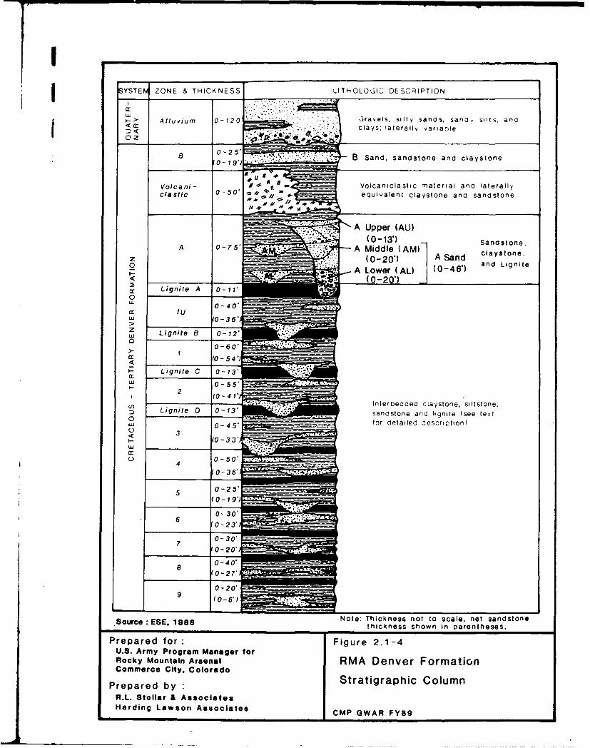
SYSTEM ZONE & THICKNESS LITHOLOGIC DESCRIPTION
~~' Alluvium 0-120 Gravels, silty~ sands, sancl Silts, ancclays, laterally vartaole
a B Sand, sandstone and claystone
A 0-5 A Mdde AM
zoc n -_V __1A ___nca tc n t rila d laeal
0 lsi 0-50 -=/I- qu-aln
060asoean adtnU-V
A intleroedde claystone, slsoe0 int an L-3iadsoegnnlgittee tx
A Lwer(AL (046
I- (0-33
6-
>0-20'
cr (0-54.
LgieC 0-20 _______
Lu 0-55'.
*Su)c:E 198 ot: Thicnedds not stonsae, neft sandson
Prpae Ligr:t Fiur 0-2.1-4oe n igie(setxRck Mountai Arsna RAdenvier Fosrmation)ComreCt0ClrdPrpaedbyStatgrphC olm
R.L (t0ar-Asoia3HarinLasnAocaeCMGARF8
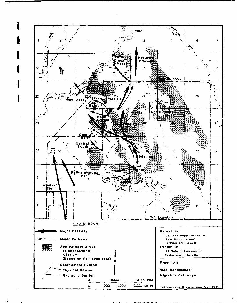
8 9 78
/*
K' ~2I Nortt~North,
- , ... . t. .
21 1otiw s R?'ar F~t
1% 9
RMAtBudr ~
Appro Cemte reasPeae y
(Baedntra~l 18aa
1
3.0 PROGRAM METHODS AND STRATEGY
The ground-water monitoring well networks of the Comprehensive Monitoring Program at RMAconsist of both on- and off-post wells for monitoring water-level fluctuations and water-qualityconditions. The water-level network is made up of 1,013 wells monitored on a quarterly basis.The FY89 water-quality network includes 515 wells monitored on an annual, semiannual, orquarterly basis. The monitoring frequency depends on data obtained in many previousinvestigations in the well area, remedial activities being undertaken in several areas, and other
factors that are discussed below.
The well network was designed to meet program objectives efficiently by using an optimalcombination of monitoring wells, monitoring frequency and analytical suite. This section of thej Annual Report discusses the strategy and criteria for the monitoring network design and themethods for using data generated from the water-quality and water-level monitoring networks.Additionally, the CMP network is compared to previous monitoring networks. The water-levelmonitoring network is described in Section 3.1; the water-quality monitoring network is coveredin Section 3.2; and the CMP analytical program is discussed in Section 3.3.
3.1 Water-Level Monitcring Network
3.1.1 Well Selection Criteria for the Water-Level Monitoring Network
The network of wells used to monitor potentiometric surfaces at RMA was selected after reviewingwell construction data and historical water-level data. The areal distribution of wells was also
evaluated. Historic water-level data from the spring 1987 monitoring period (RI/FS Tasks 25
and 44) were used as the primary basis for selecting wells for the CMP water-level networkbecause these data represented the most recent comprehensive set of measurements throughoutRMA. The quality and reliability of data from each well were assessed by comparison with data
from nearby wells.
If a well's construction was not considered adequate for water-quality sampling but the well waslocated in a critical area, it was retained in the water-level network. A low construction rankingis tolerated for water-level data if the construction problem does not impact the representativenessof the measurements. For example, if a well is partially obstructed such that a bailer cannot be
lowered to the water, it may still provide adequate water-table measurements.
GWAR-89.1-3Rev. 06/21/90 - 12 -
I
I
Wells in the water-level monitoring network are monitored on a quarterly basis prior to each
sampling event. The current network consists of 1,013 wells. This includes 655 unconfined wells
and 358 confined wells (Table 3.1-1).
3.1.2 Well Selection Criteria for the Unconfined Flow SystemIThe general philosophy for selecting wells in the unconfined flow system was to retain all wells
that had been measured previously unless a specific situation warranted deleting a well from the
program. Important vertical hydraulic data were provided by well clusters representing water levelsat several depth intervals; therefore, no cluster of this kind was deleted from the program.
Consequently, the CMP water-level network includes all wells previously measured during RI/FS
Tasks 44 and 25, with the following exceptions:
1. Wells with construction data that indicate they are unacceptable for water-level
monitoring;
2. Wells that have been formally abandoned under IRA-3, the Abandoned Well Closurej Program; and
3. Wells that have been destroyed, obstructed since CMP startup, or that can no longer
be located.
3.1.3 Well Selection Criteria for the Confined Flow System
The majority of confined flow system wells were included in the water-level monitoring network
because ground-water flow patterns in the confined flow system are complex. Conditions under
which confined flow system wells were deleted from the program relate to physical problems
attributed to each well. These conditions included dry wells and wells that historically provided
poor quality water-level measurements and were located near other confined flow system wells.
In total, 14 confined flow system wells used in the first year (1987) CMP water-level network
GWAR-89.1-$Rev. 06/21/o0 - 13 -
__ __ _ _ _
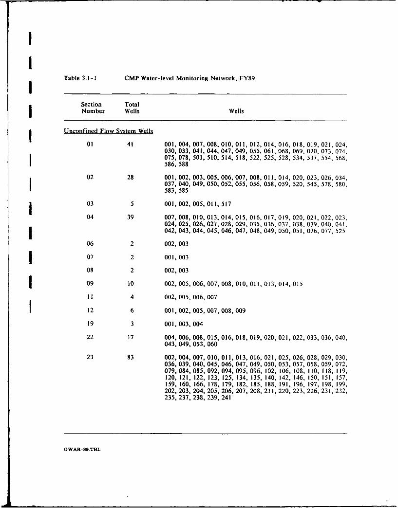
II
Table 3. I-1 CMP Water-level Monitoring Network, FY89ISection TotalNumber Wells Wells
Unconfined Flow System Wells
01 41 001,004, 007, 008, 010, 011,012, 014, 016, 018, 019, 021,024,030, 033, 041, 044, 047, 049, 055, 061, 068, 069, 070, 073, 074,075, 078, 501, 510, 514, 518, 522, 525, 528, 534, 537, 554, 568,586, 588
02 28 001, 002, 003, 005, 006, 007, 008, 011, 014, 020, 023, 026, 034,037, 040, 049, 050, 052, 055, 056, 058, 059, 520, 545, 578, 580,583, 585
103 5 001,002, 005, 011,517
04 39 007, 008, 010, 013, 014, 015, 016, 017, 019, 020, 021, 022, 023,024, 025, 026, 027, 028, 029, 035, 036, 037, 038, 039, 040, 041,1042, 043, 044, 045, 046, 047, 048, 049, 050, 051, 076, 077, 525
06 2 002, 003
1 07 2 001,003
08 2 002, 003
j09 10 002, 005, 006, 007,008, 010, 011,013, 014, 015
11 4 002, 005, 006, 007
112 6 001,002, 005,007,008, 009
19 3 001,003, 004
22 17 004, 006, 008, 015, 016, 018, 019, 020, 021,022, 033, 036, 040,043, 049, 053, 060
23 83 002, 004, 007, 010, 011, 013, 016, 021, 025, 026, 028,029, 030,036, 039, 040, 045, 046, 047, 049, 050, 053, 057, 058, 059, 072,079, 084, 085, 092, 094, 095, 096, 102, 106, 108, 110, 118, 119,120, 121, 122, 123, 125, 134, 135, 140, 142, 146, 150, 151, 157,159, 160, 166, 178, 179, 182, 185, 188, 191, 196, 197, 198, 199,202, 203, 204, 205, 206, 207, 208, 211, 220, 223, 226, 231, 232,235, 237, 238, 239, 241
GWAR-89.TBL
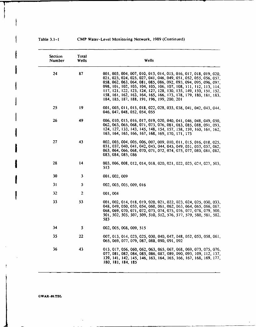
I Table 3.1-1 CMP Water-Level Monitoring Network, 1989 (Continued)
I Section TotalNumber Wells Wells
1 24 87 001,003, 004, 007, 010, 013, 014, 015, 016, 017,018, 019, 020,021, 023, 024, 025, 027, 041, 046, 049, 051, 052, 055, 056, 057,058, 062, 063, 064, 081, 085, 086, 092, 093, 094, 095, 096, 097,098, 101, 102, 103, 104, 105, 106, 107, 108, 111, 112, 113, 114,117, 121, 122, 123, 124, 127, 128, 130, 135, 149, 150, 151, 152,158, 161, 162, 163, 164, 165, 166, 173, 178, 179, 180, 181, 183,184, 185, 187, 188, 191, 196, 199, 200, 201
25 19 001, 003, 011, 015, 018, 022, 028, 035, 038, 041, 042, 043, 044,046, 047, 048, 052, 054, 055
26 49 006, 010, 015, 016, 017, 019, 020, 040, 041, 046, 048, 049,050,062, 063, 065, 068, 071, 073, 076, 081, 083, 085, 088, 091, 093,124, 127, 133, 143, 145, 148, 154, 157, 158, 159, 160, 161, 162,163, 164, 165, 166, 167, 168, 169, 170, 171, 173
27 43 002, 003, 004, 005, 006, 007, 009, 010, 011, 015, 016, 018,025,031, 037, 040, 041, 042, 043, 044, 045, 049, 051, 053, 057, 062,063, 064, 066, 068, 070, 071, 072, 074, 075, 077, 080, 081, 082,083, 084, 085, 086
28 14 003, 006, 008, 012, 014, 018, 020, 021, 022, 023, 024, 027, 503,513
130 3 001,002, 009
31 5 002, 003, 005,009, 016
132 2 001,004
33 53 001, 002, 014, 018, 019, 020, 021, 022, 023, 024, 025, 030, 033,048, 049, 050, 053, 054, 060, 061, 062, 063, 064, 065, 066, 067,068, 069, 070, 071, 072, 073, 074, 075, 076, 077, 078, 079, 500,501, 502, 505, 507, 509, 510, 512, 576, 577, 579, 580, 581, 582,583
34 5 002, 005, 008, 009, 515
35 22 007, 013, 014, 023, 025, 030, 040, 047, 048, 052, 053, 058, 061,065, 069, 077, 079, 087, 088, 090, 091, 092
36 43 013, 017, 056, 060, 062, 063, 065, 067, 068, 069, 073, 075, 076,077, 081, 082, 084, 085, 086, 087, 089, 090, 093, 109, 112, 137,139, 141, 142, 145, 146, 163, 164, 165, 166, 167, 168, 169, 177,180, 181, 184, 185
GWAR-89.TBL
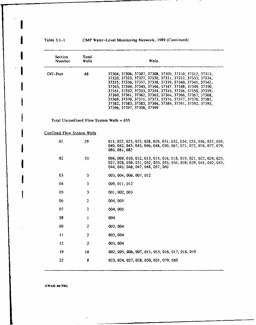
SI
Table 3.1-1 CMP Water-Level Monitoring Network, 1989 (Continued)
Section TotalNumber Wells Wells
Off-Post 68 37304, 37306, 37307, 37308, 37309, 37310, 37312, 37313,37320, 37323, 37327, 37330, 37331, 37332, 37333, 37334,37335, 37336, 37337, 37338, 37339, 37340, 37341, 37342,37343, 37344, 37345, 37346, 37347, 37348, 37349, 37350,37351, 37352, 37353, 37354, 37355, 37356, 37358, 37359,37360, 37361, 37362, 37363, 37364, 37366, 37367, 37368,37369, 37370, 37371, 37373, 37374, 37377, 37378, 37381,37382, 37383, 37385, 37386, 37389, 37391, 37392, 37395,37396, 37397, 37398, 37399
Total Unconfined Flow System Wells = 655
Confined Flow System Wells
01 29 015, 022, 023, 025, 028, 029, 031, 032, 034, 035, 036, 037, 039,040, 042, 043, 045, 046, 048, 050, 067, 071, 072, 076, 077, 079,080, 081, 082
02 33 004, 009, 010, 012, 013, 015, 016, 018, 019, 021,022, 024,025,027, 028, 030, 031, 032, 033, 035, 036, 038, 039, 041, 042, 043,044, 045, 046, 047, 048, 057, 060
03 5 003, 004, 006, 007, 012
04 3 009,011, 012
05 3 001, 002, 003
06 2 004, 005
07 2 004, 005
08 1 004
09 2 003, 004
1I 2 003,004
12 2 003,004
19 10 002, 005, 006, 007, 011, 015, 016, 017, 018,019
22 8 023, 024, 027, 028, 030, 031, 079, 080
GWAR-89.TBL
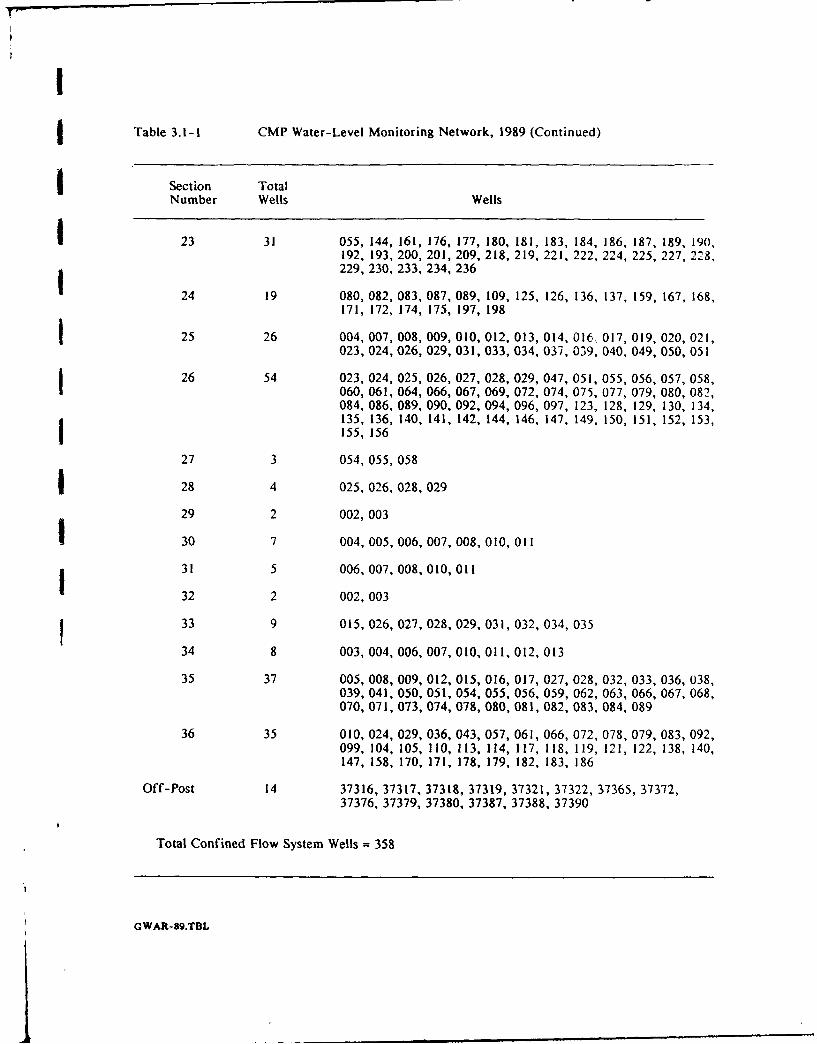
I
Table 3.1-1 CMP Water-Level Monitoring Network, 1989 (Continued)
Section TotalNumber Wells Wells
23 31 055, 144, 161, 176, 177, 180, 181, 183, 184, 186, 187, 189, 190,192, 193, 200, 201, 209, 218, 219, 221, 222, 2214, 225, 227, 2_28,229, 230, 233, 234, 236
24 19 080, 082, 083, 087, 089, 109, 125, 126, 136, 137, 159, 167, 168,171, 172, 174, 175, 197, 198
25 26 004, 007, 008, 009, 010, 012, 013, 014, 0163 017, 019, 020, 021,023, 024, 026, 029, 031, 033, 034, 037, 039, 040, 049, 050, 051
26 54 023, 024, 025, 026, 027, 028, 029, 047, 051, 055, 056, 057, 058,060, 061, 064, 066, 067, 069, 072, 074, 075, 077, 079, 080, 082,084, 086, 089, 090, 092, 094, 096, 097, 123, 128, 129, 130, 134,135, 136, 140, 141, 142, 144, 146, 147, 149, 150, 151, 152, 153,155, 156
27 3 054, 055, 058
28 4 025, 026, 028, 029
29 2 002, 003
30 7 004, 005, 006, 007, 008, 010, 011
31 5 006, 007,008,010, 011
32 2 002, 003
33 9 015, 026, 027, 028, 029, 031, 032, 034, 035
34 8 003, 004, 006, 007, 010, 011, 012, 013
35 37 005, 008, 009, 012, 015, 016, 017, 027, 028, 032, 033, 036, 038,039, 041, 050, 051, 054, 055, 056, 059, 062, 063, 066, 067, 068,070, 071, 073, 074, 078, 080, 081, 082, 083, 084, 089
36 35 010, 024, 029, 036, 043, 057, 061, 066, 072, 078, 079, 083, 092,099, 104, 105, 110, 113, 114, 117, 118, 119, 121, 122, 138, 140,147, 158, 170, 171, 178, 179, 182, 183, 186
Off-Post 14 37316, 37317, 37318, 37319, 37321, 37322, 37365, 37372,37376, 37379, 37380, 37387, 37388, 37390
Total Confined Flow System Wells = 358
GWAR-89.TBL
Ij were deleted from the second year (1988) CMP water-level network. The current well network
does not include wells that have been abandoned, broken, destroyed, or obstructed.
3.2 Water-Quality Monitoring Network
The on-post water-quality monitoring network was designed to address two objectives through
annual, semiannual and quarterly monitoring rounds. The first objective was tG confirm presently
understood contaminant distributions in general areas and to record possible distribution changes.
The second objective was to provide detailed descriptions of contaminant distributions in specific
project areas of concern. The project areas are shown in Figure 3.2-1. General areas are all aroas
outside of designated project area boundaries, and include known areas of ground-water
contamination, as well as background areas where contamination has not been detected. In general
areas where contamination is present, contaminant distributions are sufficiently well understood,
spatially and temporally, to justify a more widely spaced network. In background areas, or
downgradient of known plumes, wells are monitored to ascertain whether or not contamination is
moving into these areas.
Project areas are those for which additional data, more frequent data collection, and more closely
spaced wells are needed to improve the understanding of site conditions. Project areas have also
been designated where additional and more frequent data are needed to support ongoing lnt.,rim
Response Actions (IRAs).
The annual monitoring network incorporates wells from general and project areas. General area
wells are only sampled annually. The semiannual monitoring network includes the project areas
only. The quarterly monitoring network is designed to support ongoing remedial support and/or
substantive regulatory compliance.
The Transitional Monitoring Program (TMP) was the first annual sampling round (winter 1987/88)
conducted under the CMP. The TMP was conducted as soon as practical followil.g contract award
to ensure t -wporal continuity between previous Remedial Investigation ground-water investigations
(Tasks 25 and 44) and the CMP. The TMP well network was designed as a transition plan and was
sampled before the Final CMP Ground-Water Technical Plan was completed (Stollar, 1989a).
The TMP annual sampling network served as the basis for developing the annual network presented
in the Final Technical Plan (Stollar, 1989a). The annual network shown in the Technical Plan was
first sampled in the fall of 1988, a year after the TMP (winter 1987/88) network had been sampled.
GWAR-89.1-sRev. 06/21/90 - 18 -
I3.2.1 FY89 Water-Quality Monitoring
CMP water-quality monitoring was conducted during FY89 with three monitoring networks
annual, semiannual, and quarterly. The annual FY89 sampling round is referred to as the fall 1988
round. The fall 1988 round results are presented to illustrate regional contaminant distributions
in this Annual Report in much the same way that the winter 1987/88 round results illustrated
regional contaminant distributions in the FY88 Annual Report. The annual round was used for
this purpose because it waw" the most extensive data set collected during the year; thus, it allowed
the most detailed regional contamination assessment.
The FY89 semiannual sampling round was conducted in the spring of 1989. The semiannual
network was also sampled as a subset of the fall 1988 annual sampling round. The semiannual
network was designed to provide more focused data in 11 specific on-post areas and throughout
the off-post area in order to maintain or improve the understanding of site conditions in those
areas. All previously monitored off-post wells were included in the semiannual network to allow
j continued assessment of off-post contaminant distributions.
The monitoring network in the Basin F area was sampled quarterly. This network was designed
to provide data to support ongoing IRA projects in that area. The quarterly network was sampled
twice (winter and summer 1989) in FY89 as a stand-alone monitoring event, and was also included
in the larger semiannual and annual networks.
For clarity, sampling rounds will be referred to as the fall 1988, winter 1989, spring 1989 and
summer 1989 sampling rounds. Figure 3.2-2 illustrates how the annual, semiannual, and quarterly
sampling networks relate to the fall 1988, winter 1989, spring 1989, and summer 1989 sampling
rounds. It also lists the actual number of water levels measured during e --h round, as this differs
from the number proposed.
Not all the wells proposed for sampling were actually sampled in FY89. The fall 1988 well
network, as proposed, originally consisted of 515 wells (CMP Ground Water Final Technical Plan,
Table 2.4-1; Stollar, 1989a). Of the 515 wells, 488 wells were actually sampled and 27 wells were
dry, destroyed, obstructed, or abandoned (Table 3.2-1 and Figures 3.2-3 and 3.2-4). Unusable
wells were replaced by alternate wells if two criteria were fulfilled:
1) alternate wells are screened in the hydrogeologic zone of interest; and
2) alternate wells are located areally to provide the desired coverage.
GWAR-89.1-3Rev. 06/21/90 - 19 -
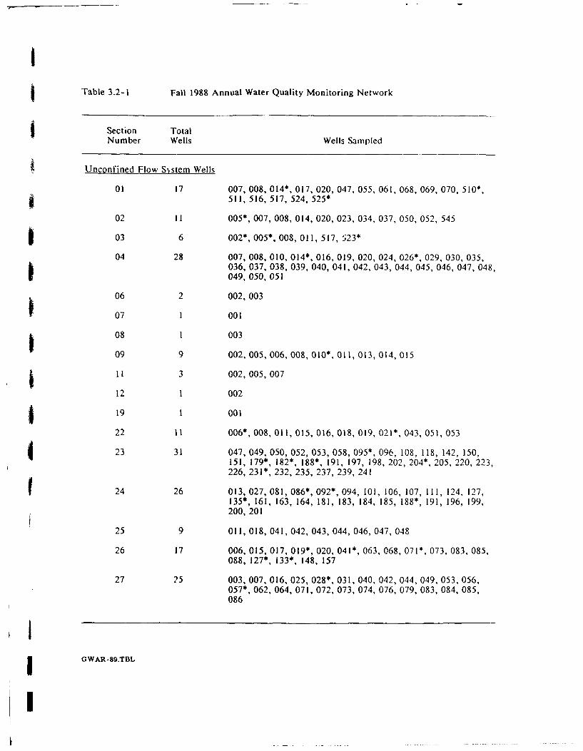
i
S Table 3.2-1 Fall 1988 Annual Water Quality Monitoring Network
5 Section TotalNumber Wells Wells Sampled
Unconfined Flow Sxstem Wells01 17 007, 008, 014*, 017, 020, 047, 055, 061, 068, 069, 070, 510*,
511, 516, 517, 524, 525*
02 11 005*, 007, 008, 014, 020, 023, 034, 037, 050, 052, 545
03 6 002*, 005*, 008, 011, 517, ,23*
04 28 007, 008, 010, 014*, 016, 019, 020, 024, 026*, 029, 030, 035,036, 037, 038, 039, 040, 041, 042, 043, 044, 045, 046, 047, 048,049, 050, 051
06 2 002, 003
07 1 001
08 1 003
09 9 002,005,006,008,010*, 011,013,014,015
11 3 002, 005,007
12 1 002
419 1 001
22 11 006*, 008, 011,015, 016, 018, 019, 021*, 043, 051,053
423 31 047, 049, 050, 052, 053, 058, 095*, 096, 108, 118, 142, 150,151, 179*, 182*, 188*, 191, 197, 198, 202, 204*, 205, 220, 223,226, 231*, 232, 235, 237, 239, 241
f24 26 013, 027, 081, 086*, 092*, 094, 101, 106, 107, 111, 124, 127,135*, 161, 163, 164, 181, 183, 184, 185, 188*, 191, 196, 199,200, 201
25 9 011,018, 041,042, 043, 044, 046, 047, 048
26 17 006, 015, 017, 019*, 020, 041*, 063, 068, 071*, 073, 083, 085,088, 127*, 133*, 148, 157
27 25 003, 007, 016, 025, 028*, 031, 040, 042, 044, 049, 053, 056,057*, 062, 064, 071, 072, 073, 074, 076, 079, 083, 084, 085,086
A
I

I
Table 3.2-1 Fall 1988 Annual Water Quality Monitoring Network (continued)
I Section TotalNumber Wells Wells Sampled
I 28 4 002, 018, 023*, 027
g 30 1 009
31 I 005
33 20 001, 002, 025, 030, 033, 048, 063, 064, 066*, 068, 074, 075,076, 077, 078, 079, 509, 514, 578, 581
34 6 002, 005*, 008*, 009*, 507, 508
35 13 013, 018*, 020, 023, 037, 052, 058, 061, 065*, 077, 079, 087,088
136 18 001*, 056, 065, 069*, 075, 076*, 084, 090, 094, 123, 137, 139*,146, 168, 169, 177, 180*, 181
Off-Post 60 37308, 37309, 37312*, 37313, 37320, 37323*, 37327, 37331*,37332, 37333, 37334, 37335, 37336*, 37337, 37338, 37339,37341*, 37342, 37343, 37344, 37345*, 37346, 37347, 37348,
37349*, 37350, 37351, 37352, 37353, 37354*, 37355, 37356,37357, 37358, 37359*, 37360, 37361, 37362, 37363*, 37364,37366, 37367, 37368*, 37369, 37370, 37371, 37373, 37374,37377, 37378*, 37381, 37383, 37385, 37386, 37389, 37391*,1 37392, 37395, 37396, 37397
Total Unconfined Flow System Wells = 322
Confined Flow System Wells
01 11 015*, 022, 025, 031*, 032*, 036, 037, 048, 067, 071*, 072
02 14 018, 021*, 024, 025, 030, 031*, 035, 036, 038, 039*, 043, 044,047, 048*
03 4 003*, 004, 006, 012
04 2 011,012
05 1 001
06 2 004*, 005
08 1 005
GWAR-89.TBL
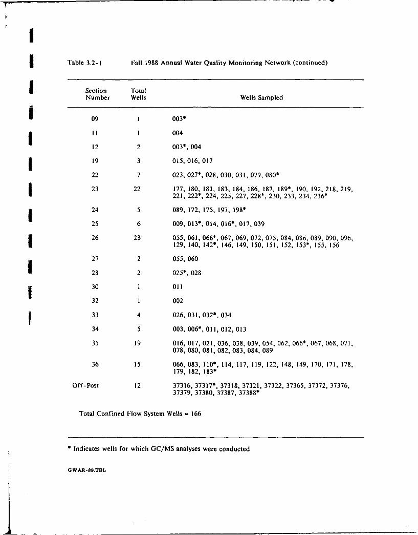
T
Table 3.2-1 Fall 1988 Annual Water Quality Monitoring Network (continued)
I Section TotalNumber Wells Wells Sampled
S09 1 003*
i 11 I 004
12 2 003*, 004
1 19 3 015, 016, 017
22 7 023, 027*, 028, 030, 031, 079, 080*
23 22 177, 180, 181, 183, 184, 186, 187, 189*, 190, 192, 218, 219,221, 222*, 224, 225, 227, 228*, 230, 233, 234, 236*
24 5 089, 172, 175, 197, 198*
25 6 009, 013", 014, 016*, 017,039
26 23 055, 061, 066*, 067, 069, 072, 075, 084, 086, 089, 090, 096,129, 140, 142*, 146, 149, 150, 151, 152, 153*, 155, 156
27 2 055, 060
28 2 025*, 028
30 1 011
32 1 002
f 33 4 026, 031, 032*, 034
34 5 003, 006*, 011, 012, 013
35 19 016, 017, 021, 036, 038, 039, 054, 062, 066*, 067, 068, 071,078, 080, 081, 082, 083, 084, 089
36 15 066, 083, 110*, 114, 117, 119, 122, 148, 149, 170, 171, 178,179, 182, 183*
Off-Post 12 37316, 37317*, 37318, 37321, 37322, 37365, 37372, 37376,37379, 37380, 37387, 37388*
Total Confined Flow System Wells = 166
* Indicates wells for which GC/MS analyses were conducted
GWAR-89.TBL
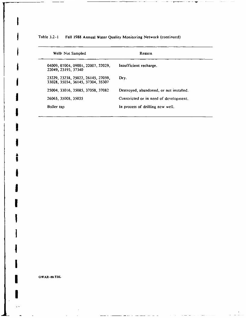
I
j Table 3.2-1 Fall 1988 Annual Water Quality Monitoring Network (continued)
Well! Not Sampled Reason
04009, 07004, 09001, 22007, 22029, Insufficient recharge.22049, 23193, 37340
23229, 23238, 25022, 26145, 27059, Dry.33028, 35034, 36145, 37304, 35307
25004, 33016, 35085, 37058, 37082 Destroyed, abandoned, or not installed.
I 26065, 35008, 35035 Constricted or in need of development.
Boiler tap In process of drilling new well.
IIIa
III
1
I
I
ITwenty-seven of the unusable wells were not replaced because alternate wells fulfilling these
criteria did not exist. Information on unusable wells is used to modify subsequent monitoring
networks.
The Final Technical Plan (Stollar, 1989a; Table 2.4-2) purposes a network of 376 wells in the spring
1989 round. An addendum to the Technical Plan added 38 monitoring wells to the network that
were installed in FY89 and deleted six wells that did not significantly add to the current level of
understanding of contamination in the South Plants area. Thus, 408 wells were to be sampled in
spring 1989; 388 wells were actually sampled and 20 wells were dry, destroyed, obstructed, or
abandoned (Table 3.2-2).IThe quarterly monitoring network was sampled four times in FY89; twice as a stand-alone effort,
once with the semiannual network, and once with the annual network. Fifty-one wells were
proposed for the winter 1989 round and 46 were actually sampled (Table 3.2-3). Five wells were
not sampled; three unconfined wells (23238, 26065, and 26145) that were dry, and two confined
wells (23180 and 23193) that were bailed dry and well recharge was insufficient for sampling.
The quarterly well network sampled in the summer 1989 (Table 3.2-3, Figure 3.2-5) was largerthan the network proposed in the Final Technical Plan (Stollar, 1989a). This was because 13 newly
installed monitoring wells were added. The 13 wells (26160 through 26171, and 26173) were
installed under the CMP ground-water element geotechnical program for the purpose of monitoring
newly constructed IRA facilities (two ponds, a tank farm, and a wastepile) in the Basin F area.
Thus, 64 wells were proposed for sampling during summer 1989. However, 55 wells were actually
sampled, as five (23238, 26065, 26145, 26164, 26167) were dry, three (23180, 23193, 26165) had
insufficient recharge, and one (23108) was c!stroyed.
3.2.1.1 Comparison with Previous RMA Networks. The CMP monitoring well network has
evolved from several previous regional RMA monitoring networks. These precursor networks
included the Initial Screening Program (ISP), the Final Screening Program (FSP), the Off-Post
Contamination Assessment and the Composite Well Program. The immediate precursor to the CMP
network was thz Task 44 sampling program presented in the Water Remedial Investigation Report
(Ebasco, 1989i). The Task 44 sampling program temporally overlapped with the startup of the
SCMP; which was called the Transitional Monitoring Program (TMP). Due to this overlap, the
winter 1987/88 round comnrised 255 TMP wells, 67 Task 44 wells located off-post and an
additional 145 Task 25 wells located near RMA boundary containment systems. The analytical
results from the various programs were presented in the FY88 CMP Ground-Water Annual Report.
IGWAR-89.1-3Rev. 6/21/0 - 24 -
I
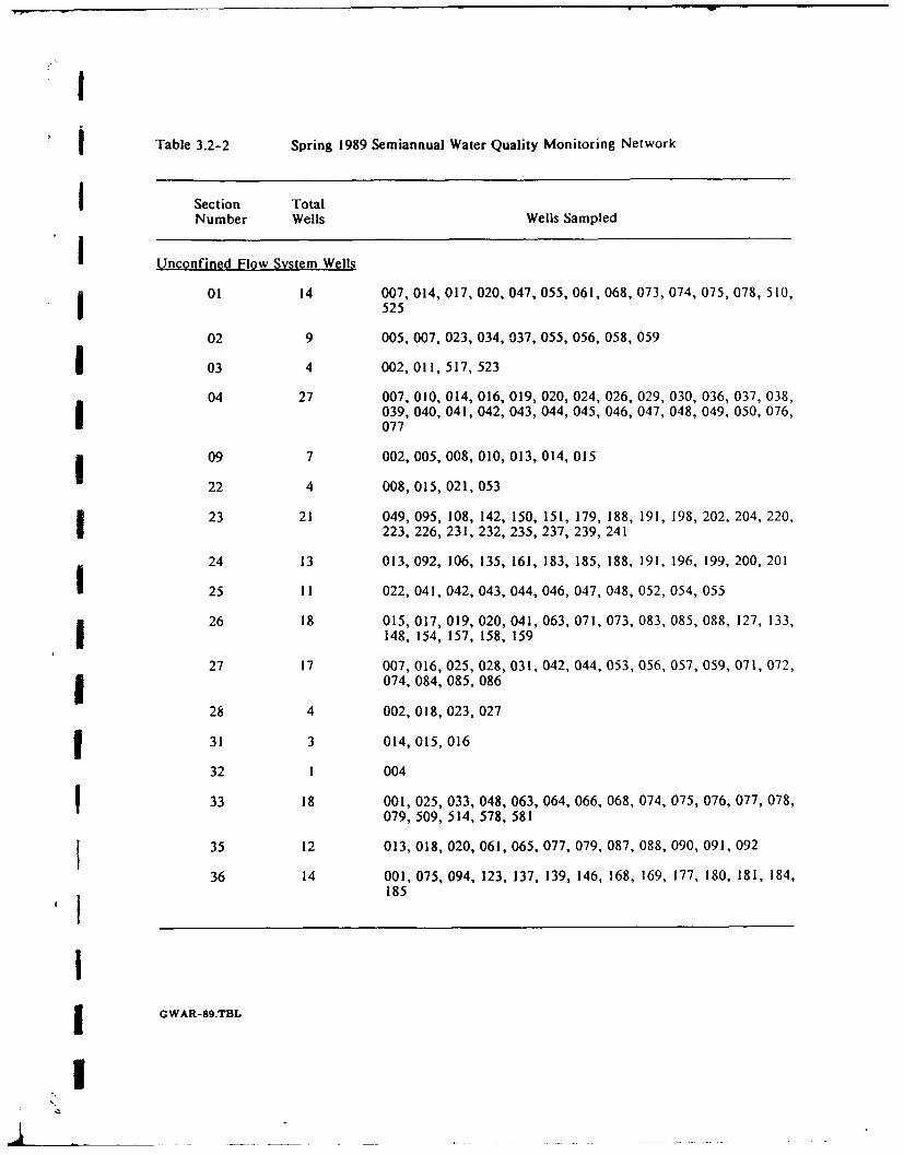
I
Table 3.2-2 Spring 1989 Semiannual Water Quality Monitoring Network
I Section TotalNumber Wells Wells Sampled
I Unconfined Flow System Wells
01 14 007, 014, 017, 020, 047, 055, 061, 068, 073, 074, 075, 078, 510,525
02 9 005, 007, 023, 034, 037, 055, 056, 058, 059
I 03 4 002, 011, 517, 523
04 27 007, 010, 014, 016, 019, 020, 024, 026, 029, 030, 036, 037, 038,039, 040, 041, 042, 043, 044, 045, 046, 047, 048, 049, 050, 076,077
09 7 002, 005, 008, 010, 013, 014, 015
22 4 008, 015, 021,053
23 21 049, 095, 108, 142, 150, 151, 179, 188, 191, 198, 202, 204, 220,223, 226, 231, 232, 235, 237, 239, 241
24 13 013, 092, 106, 135, 161, 183, 185, 188, 191, 196, 199, 200, 201
25 11 022, 041, 042, 043, 044, 046, 047, 048, 052, 054, 055
26 18 015, 017, 019, 020, 041, 063, 071, 073, 083, 085, 088, 127, 133,148, 154, 157, 158, 159
27 17 007, 016, 025, 028, 031, 042, 044, 053, 056, 057, 059, 071, 072,1 074, 084, 085, 086
28 4 002, 018, 023, 027
1 31 3 014, 015, 016
32 1 004
33 18 001, 025, 033, 048, 063, 064, 066, 068, 074, 075, 076, 077, 078,079, 509, 514, 578, 581
1 35 12 013, 018, 020, 061,065, 077, 079, 087, 088, 090, 091,092
36 14 001, 075, 094, 123, 137, 139, 146, 168, 169, 177, 180, 181, 184,1 185
II G WAR-89.TBL
I
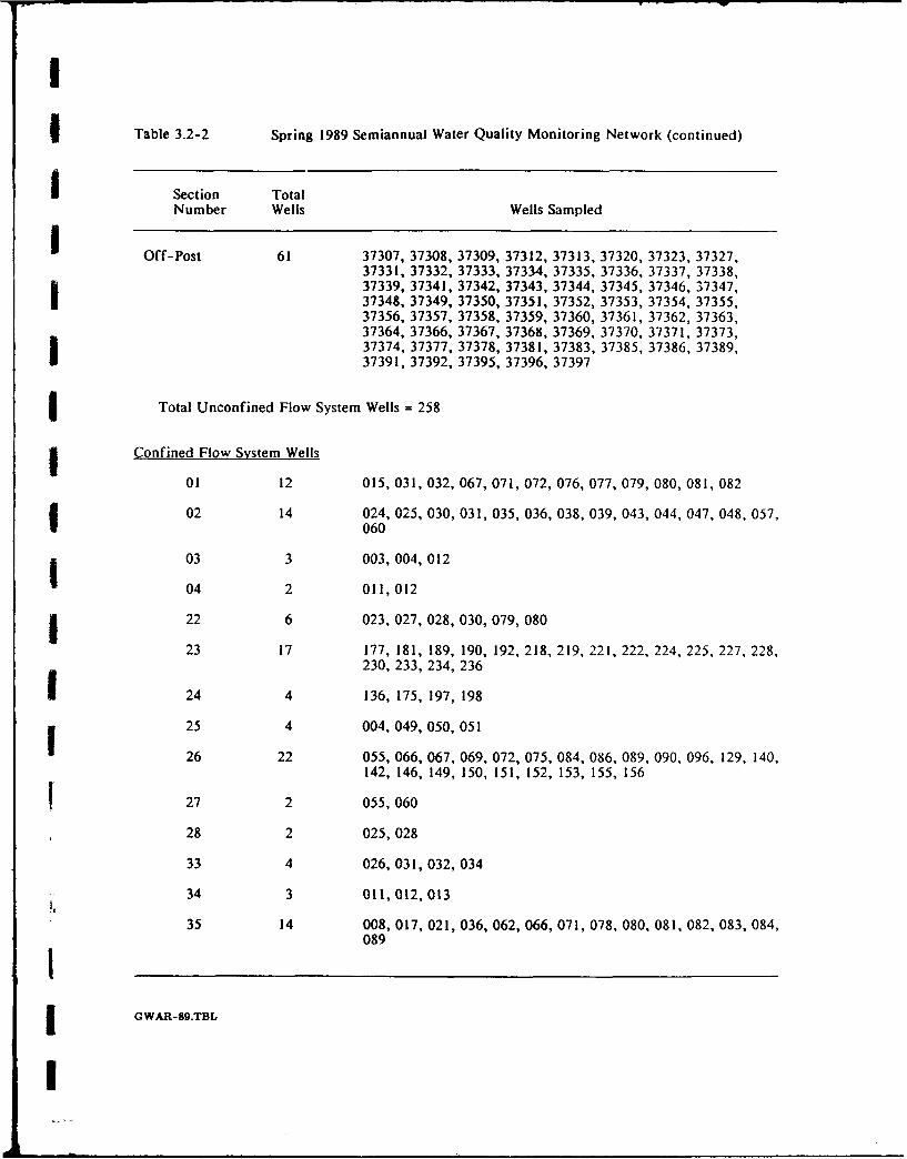
I
Table 3.2-2 Spring 1989 Semiannual Water Quality Monitoring Network (continued)
I Section TotalNumber Wells Wells Sampled
Off-Post 61 37307, 37308, 37309, 37312, 37313, 37320, 37323, 37327,37331, 37332, 37333, 37334, 37335, 37336, 37337, 37338,37339, 37341, 37342, 37343, 37344, 37345, 37346, 37347,37348, 37349, 37350, 37351, 37352, 37353, 37354, 37355,37356, 37357, 37358, 37359, 37360, 37361, 37362, 37363,37364, 37366, 37367, 37368, 37369, 37370, 37371, 37373,37374, 37377, 37378, 37381, 37383, 37385, 37386, 37389,37391, 37392, 37395, 37396, 37397
Total Unconfined Flow System Wells = 258
I Confined Flow System Wells
01 12 015, 031, 032, 067, 071, 072, 076, 077, 079, 080, 081, 082
02 14 024, 025, 030, 031, 035, 036, 038, 039, 043, 044, 047, 048, 057,060
03 3 003, 004, 012
04 2 011,012
1 22 6 023, 027, 028, 030, 079, 080
23 17 177, 181, 189, 190, 192, 218, 219, 221, 222, 224, 225, 227, 228,230, 233, 234, 236
24 4 136, 175, 197, 198
I 25 4 004, 049, 050, 051
26 22 055, 066, 067, 069, 072, 075, 084, 086, 089, 090, 096, 129, 140,142, 146, 149, 150, 151, 152, 153, 155, 156
27 2 055, 060
28 2 025,028
33 4 026, 031, 032, 034
34 3 011,012,013
35 14 008, 017, 021, 036, 062, 066, 071, 078, 080, 081, 082, 083, 084,089
II GWAR-8g.TBL
I
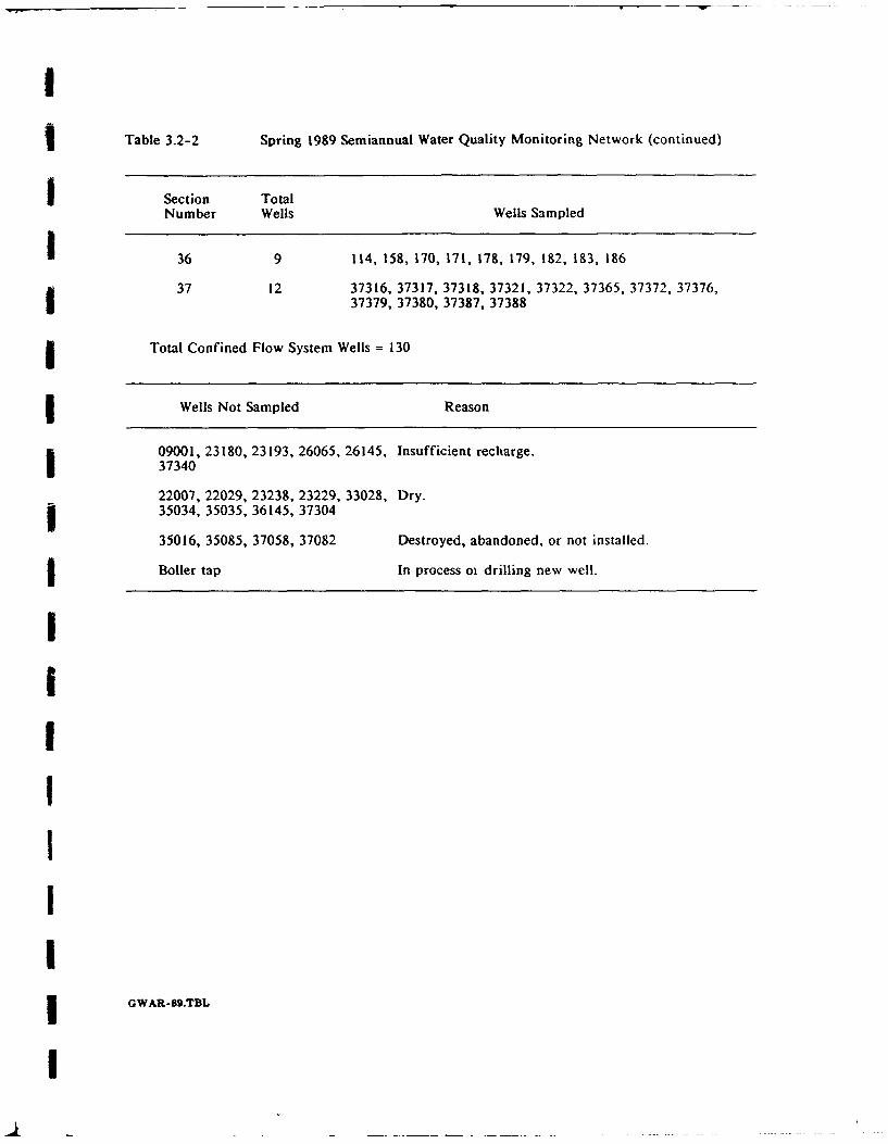
I
Table 3.2-2 Spring 1989 Semiannual Water Quality Monitoring Network (continued)
i Section TotalNumber Wells Wells Sampled
1 36 9 114, 158, 170, 171, 178, 179, 182, 183, 186
37 12 37316, 37317, 37318, 37321, 37322, 37365, 37372, 37376,37379, 37380, 37387, 37388
Total Confined Flow System Wells = 130
Wells Not Sampled Reason
09001, 23180, 23193, 26065, 26145, Insufficient recharge.37340
22007, 22029, 23238, 23229, 33028, Dry.35034, 35035, 36145, 37304
35016, 35085, 37058, 37082 Destroyed, abandoned, or not installed.
Boiler tap In process oi drilling new well.
IIII
II
I GWAR-89.TBL
I
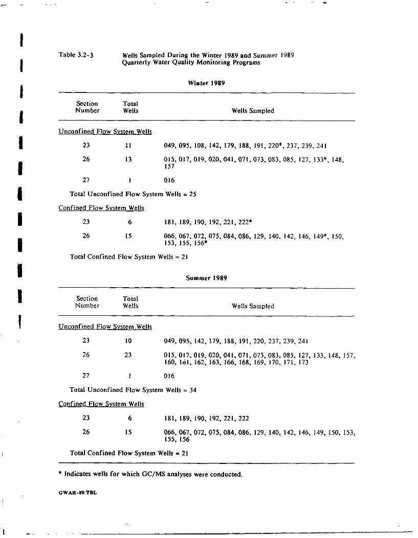
ITable 3.2-3 Wells Sampled During the Winter 1989 and Summer 1989
Quarterly Water Quality Monitoring Programs
Winter 1989
Section TotalNumber Wells Wells Sampled
Unconfined Flow System Wells
23 i1 049, 095, 108, 142, 179, 188, 191, 220*, 237, 239, 241
26 13 015,017,019, 020, 041,071,073, 083, 085, 127, 133*, 148,157
27 1 016
Total Unconfined Flow System Wells = 25
Confined Flow System Wells
23 6 181, 189, 190, 192, 221, 222*
26 15 066, 067, 072, 075, 084, 086, 129, 140, 142, 146, 149*, 150,153, 155, 156"
Total Confined Flow System Wells = 21
Summer 1989
Section TotalNumber Wells Wells Sampled
f Unconfined Flow System Wells
23 10 049, 095, 142, 179, 188, 191, 220, 237, 239, 241
26 23 015, 017, 019, 020, 041, 071, 073, 083, 085, 127, 133, 148, 157,160, 161, 162, 163, 166, 168, 169, 170, 171, 173
27 1 016
Total Unconfined Flow System Wells = 34
Confined Flow System Wells
23 6 181, 189, 190, 192, 221, 222
26 15 066, 067, 072, 075, 084, 086, 129, 140, 142, 146, 149, 150, 153,155, 156
Total Confined Flow System Wells = 21
* Indicates wells for which GC/MS analyses were conducted.
GWAR-89.TBL
II Several other RI/FS well networks designed to monitor specific RMA areas also preceded the CMP
program. Components of many of these former networks (including wells installed under these
various programs) have been included with modifications in the CMlI network design. These
former, more localized monitoring well networks include: the Boundary Systems Assessment (Task
25), the North Boundary Containment System Component Assessment (Task 36), the RMA Western
Tier Contamination Assessment (Task 38), and the RMA Off-post Remedial Investigation (Task
39). Many of the wells that were sampled under these various RI/FS programs were sampled under
the CMP during FY89 for the purposes of database verification and monitoring continuity.
3.2.2 FY89 Water-Quality Data Presentation and UseIAnalytical data collected as part of the CMP during FY89 are discussed in Section 4.3 and are
presented graphically in Section 4.3 and Appendix A. FY89 results are presented graphically for
21 analytes or analyte groups (Table 3.2-4). Contaminant plume maps for the unconfined flow
system are presented in Section 4.3. Analyte detections in the confined flow system are presented
as point plots in Appendix A. Many of these point plots combine analyte detections in more than
one stratigraphic zone of the Denver Formation. Due to the complex flow pathways in the Denver
Formation, plume maps were not prepared for the confined flow system. This strategy for data
presentation is consistent with that used in preparing the FY88 Annual Report.
Fall 1988 data were selected for presentation of regional contaminant distributions for FY89
because they are from the annual network and, thus, are the most comprehensive. In contrast, the
spring 1989 semiannual round provided data to assess contaminant distributions in the II project
areas (Figure 3.2-!). The quarterly (winter and summer 1989) rounds provided the data necessary
to support ongoing IRAs and to comply with substantive regulatory requirements for the Basin F
I area.
Temporal variations in regional water quality were assessed for FY89 by comparing fall 1988
analytical results with those presented in the FY88 Annual Report (winter 1987/88). In instances
where analytical results of the two annual events differed, results from other FY89 CMP sampling
rounds or the Water Remedial Investigation Report were consulted to clarify interpretation.
Temporal variations in water quality in specific areas were evaluated by comparing data from the
fall 1988 and spring 1989 rounds of the FY89 CMP program.
!GWAR-89.1-3Rev. 06/21/90 - 29 -
I
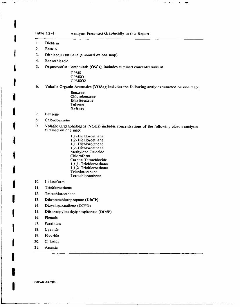
Table 3.2-4 Analytes Presented Graphically in this Report
11. Dedi2. Endrin13. Dithiane/Oxathiane (summed on one map)4. Benzothiazole
5.~ Organosulfur Compounds (OSCs); includes summed concentrations of:CPMSCPMSOCPMS02
6. Volatile Organic Aromatics (VOAs); includes the following analytes summed on one map:
BenzeneI ChlorobenzeneEthylbenzeneToluene
7. Benzene yes
8. Chlorobenzene
9. Volatile Organohalogens (VOHs) includes concentrations of the following eleven analytossummed on one map:
1,1-DichloroethaneI ,2-Dichloroethane1,1- ihlreh n1,1 -Dichloroethene
Methylene ChlorideI ChloroformCarbon Tetrachloride1, 1, 1 -Trichloroethane1, 1,2-TrichloroethaneTrichloroetheneTetrachloroethene
10. ChloroformI11. Trichloroethene
12. Tetrachloroethene
13. Dibromochloropropane (DBCP)
14. Dicyclopentadiene (DCPD)
15. Diisopropylmethylphosphonate (DIMP)
16. Phenols
17. Parathion
j18. Cyanide
19. Fluoride
20. Chloride
21. Arsenic
I GWAR-8g.TBL
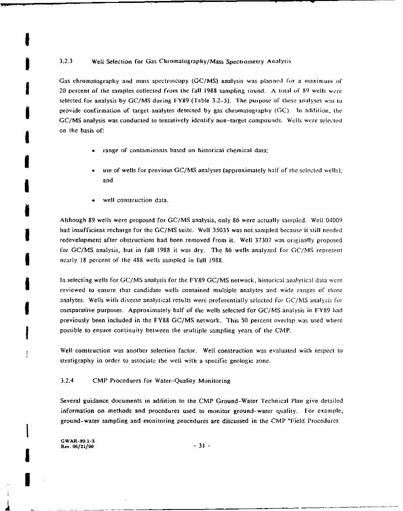
I3.2.3 Well Selection for Gas Chromatography/Mass Spectrometry Analysis
Gas chromatography and mass spectroscopy (GC/MS) analysis was planned for a nmaximum of
20 percent of the samples collected from the fall 1988 sampling round. A total of 89 wells were
selected for analysis by GC/MS during FY89 (Table 3.2-5). The purpose of these analyses was to
I provide confirmation of target analytes detected by gas chromatography (GC). In addition, the
GC/MS analysis was conducted to tentatively identify non-target compounds. Wells were selected
on the basis of:
"* range of contaminants based on historical chemical data;I* use of wells for previous GC/MS analyses (approximately half of the selected wells);
i and
"* well construction data.IAlthough 89 wells were proposed for GC/MS analysis, only 86 were actually sampled. Well 04009
had insufficient recharge for the GC/MS suite. Well 35035 was not sampled because it still needed
redevelopment after obstructions had been removed from it. Well 37307 was originally proposed
for GC/MS analysis, but in fall 1988 it was dry. The 86 wells analyzed for GC/MS represent
nearly 18 percent of the 488 wells sampled in fall 1988.
In selecting wells for GC/MS analysis for the FY89 GC/MS network, historical analytical data werereviewed to ensure that candidate wells contained multiple analytes and wide ranges of those
analytes. Wells with diverse analytical results were preferentially selected for GC/MS analysis for
comparative purposes. Approximately half of the wells selected for GC/MS analysis in FY89 had
previously been included in the FY88 GC/MS network. This 50 percent overlap was used where
possible to ensure continuity between the multiple sampling years of the CMP.
Well construction was another selection factor. Well construction was evaluated with respect to
stratigraphy in order to associate the well with a specific geologic zone.
3.2.4 CMP Procedures for Water-Quality Monitoring
Several guidance documents in addition to the CMP Ground-Water Technical Plan give detailed
information on methods and procedures used to monitor ground-water quality. For example,
ground-water sampling and monitoring procedures are discussed in the CMP "Field ProceduresiGWAR-89.1-3Rev. 06/21/90 - 31 -
'I
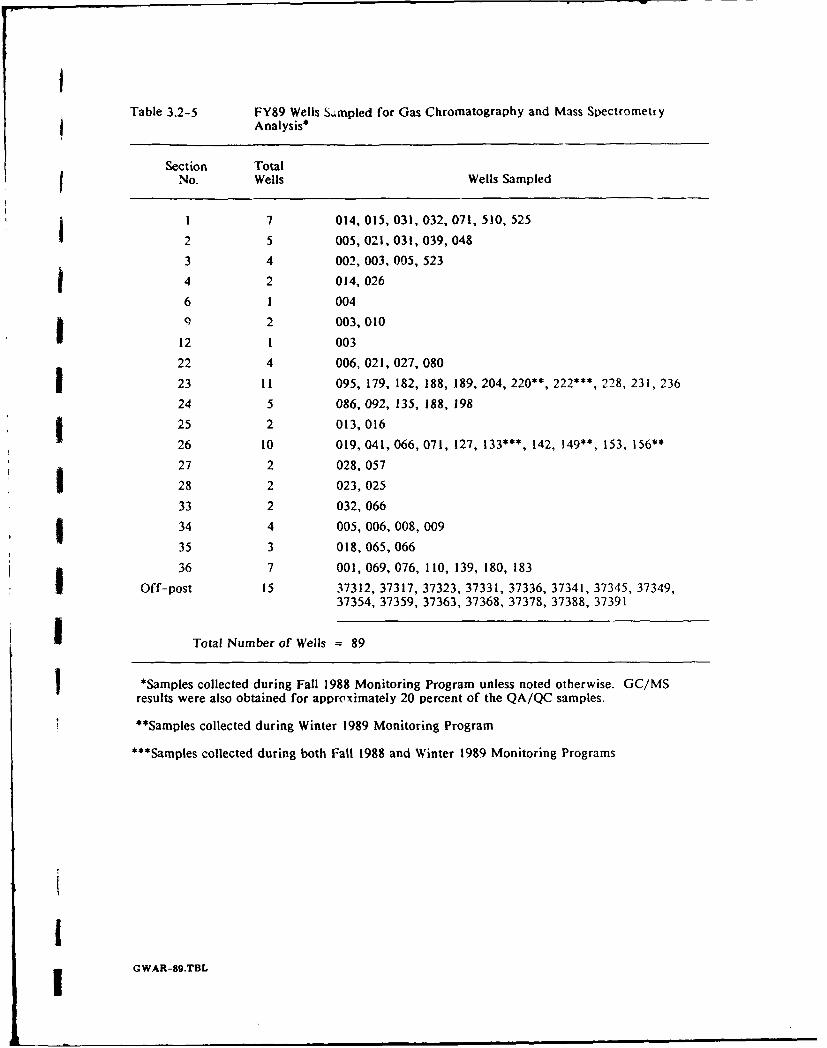
tTable 3.2-5 FY89 Wells Smpled for Gas Chromatography and Mass Spectrometry
Analysis*
Section TotalNo. Wells Wells Sampled
1 1 7 014, 015, 031, 032, 071, 510, 525
2 5 005, 021,031,039, 048
3 4 002, 003, 005, 523
14 2 014, 026
6 1 004
* 2 003, 010
12 1 003
22 4 006, 021,027, 080
23 11 095, 179, 182, 188, 189, 204, 220*, 222***, 228, 231, 236
24 5 086, 092, 135, 188, 198
* 25 2 013, 016
26 10 019, 041,066, 071, 127, 133***, 142, 149**, 153, 156**
27 2 028, 057
28 2 023, 025
33 2 032, 066
S34 4 005, 006, 008, 009
35 3 018,065,066
36 7 001,069, 076, 110, 139, 180, 183
Off-post 15 37312, 37317, 37323, 37331, 37336, 37341, 37345, 37349,37354, 37359, 37363, 37368, 37378, 37388, 37391
I Total Number of Wells = 89
*Samples collected during Fall 1988 Monitoring Program unless noted otherwise. GC/MS
results were also obtained for approximately 20 percent of the QA/QC samples.
"**Samples collected during Winter 1989 Monitoring Program
***Samples collected during both Fall 1988 and Winter 1989 Monitoring Programs
GIi G WAR-89.TBL
IManual," laboratory procedures are described in the CMP "Analytical Methods Manual," and the
CMP "Quality Assurance/Quality Control Plan" discusses sample handling and chain-of-custody.
The "Data Management Plan" addresses data management procedures applicable to all phases of the
CMP. The "Health and Safety Plan" for the CMP describes how to conduct CMP ground-water
monitoring safely to prevent chemical exposures and personal injuries.
3.3 Anilytical Program
I The ground-water samples collected during the FY89 sampling rounds were tested for the analyteslisted in Table 3.3-1. DataChem, Inc. and Hunter Services Inc. analyzed all of the FY89 water-
I quality samples. The CMP Final Technical Plan (Stollar, 1989a) incorporates the analytes parathion,cyanide, and acid extractables (phenols) in the CMP FY89 analytical suite. fhese analytes had notg previously been included in any regional sampling program at RMA.
As discussed in Section 3.2.3 of this report, the CMP analytical program included ana!ysis of
approximately 18 percent of all ground- water samples by the GC/MS analytical technique. GCiMS
analytical results were reviewed to confirm the presence of target analytes detected in investigative
samples by gas chromatography. Additionally, GC/MS analyses were used to detect nontarget
analytes not included in the CMP analytical parameters list (nortarget analytes). The CMPevaluates nontarget analytes to identify potential additions to the target analyte list. The results
of the GC/MS analyses are discussed in Section 4.4 of this report.
The analytical program also incorporated a quality assurance and quality control plan (QA/QC
plan). The CMP QA/QC plan discusses quality assurance review processes and specifics such as
monitoring analytical controls, control samples, and sample lot controls. In the CMP fielu program,
control samples comprise 25 percent of the total number of samples obtained. The results of the
quality assurance and quality control program are discussed in Section 4.5 of this report.I!I1I
GWAR-89.1-3Rev. 06/21/90 - 33 -I
I
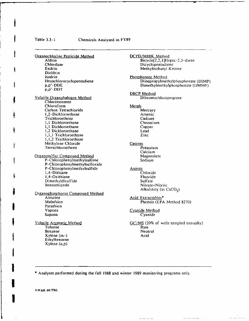
Table 3.3-1 Chemicals Analyzed in FY89
Organochlorine Pesticide Method DCPD/MlBK MethodAidrin Bicyclo[2,2, I llepta-2,5-dieneChlordane DicyclopentadieneEndrin Methylisobutyl KetoneDieldrinIsodrin Phosvhonate MethodHexachlo rocyc lope ntad iene Diisopropylmethylphosphonate (DIMP)p,p'-DDE Dimethylmethyiphosphonate (DMMP)p,p'- DDT
DBCP MethodVolatile Organohalogen Method Dibromochioropropane
ChlorobenzeneChloroform MetalsCarbon Tetrachloride MercuryI ,2-Dichloroethene ArsenicTrichioroethene Cadium1,1 Dichloroethene Chromium1,1 Dichloroethane Copper1 ,2 Dichioroethane Lead1,1,1 Trichloroethane Zinc1,1 ,2 TrichioroethaneMethylene Chloride CationsTetrachloroethene Potassium
CalciumOrganosu!fur Compound Method Magnesium
P-Chlorophenylmethylsulfonke SodiumP-ChlorophenylmethylsulfoxideP- Chlorophen ylImeth ylsul fide AnionsI ,4-Dithiane Chloride1,4-Oxithiane FluorideDimethyldisulfide SulfateBenzothiazole Nitrate+ Nitrite
Organoo~hosphorus Compound Method Aklnt a aO3Atrazine Acid Extractables*Malathion Phenols (EPA Method 8270)ParathionVapona Cyanide MethodSupona Cyanide
Volatile Aromatic Method GC/MS (20% of wells sampled annually)Toluene BaseBenzene NeutralXylene (in-) AcidEthylbenzene
Xylene (o,p)
*Analyses performed during the fall 1988 and winter 1989 monitoring programs only.
V~WAR-89.TBL
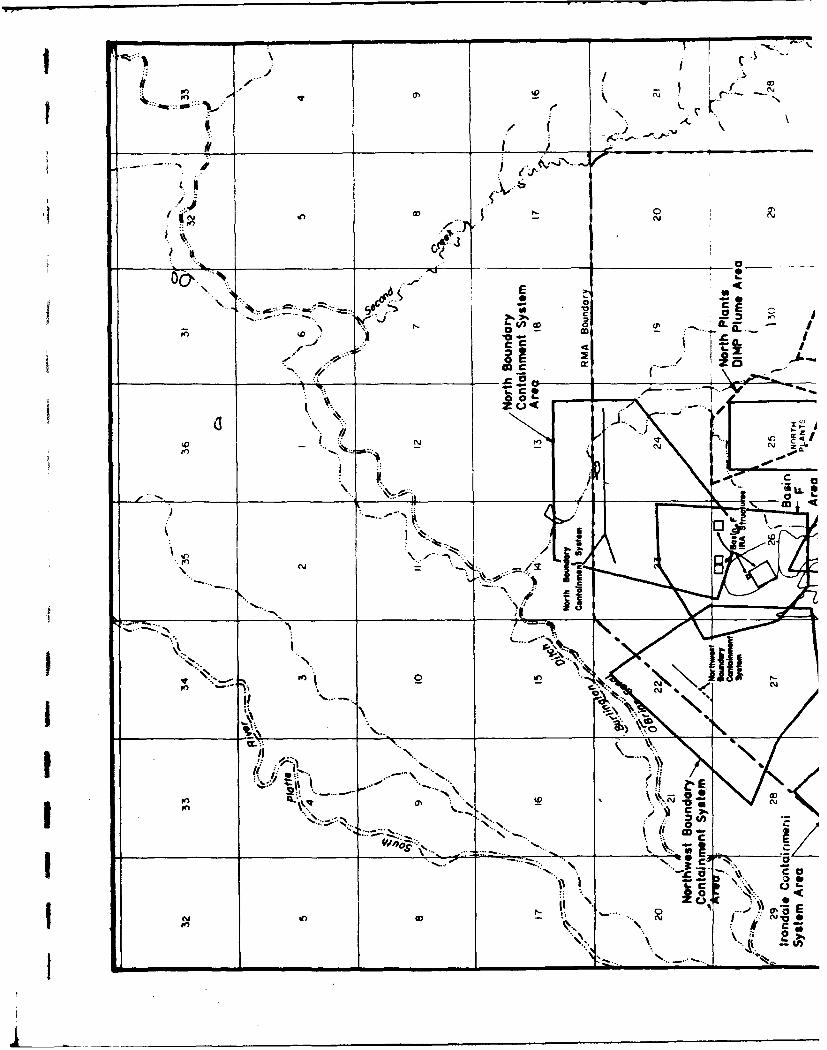
c 0
a 0
'(N
--.l ..:
LL
roI
'CI
NN-
ii N .J
Y CD
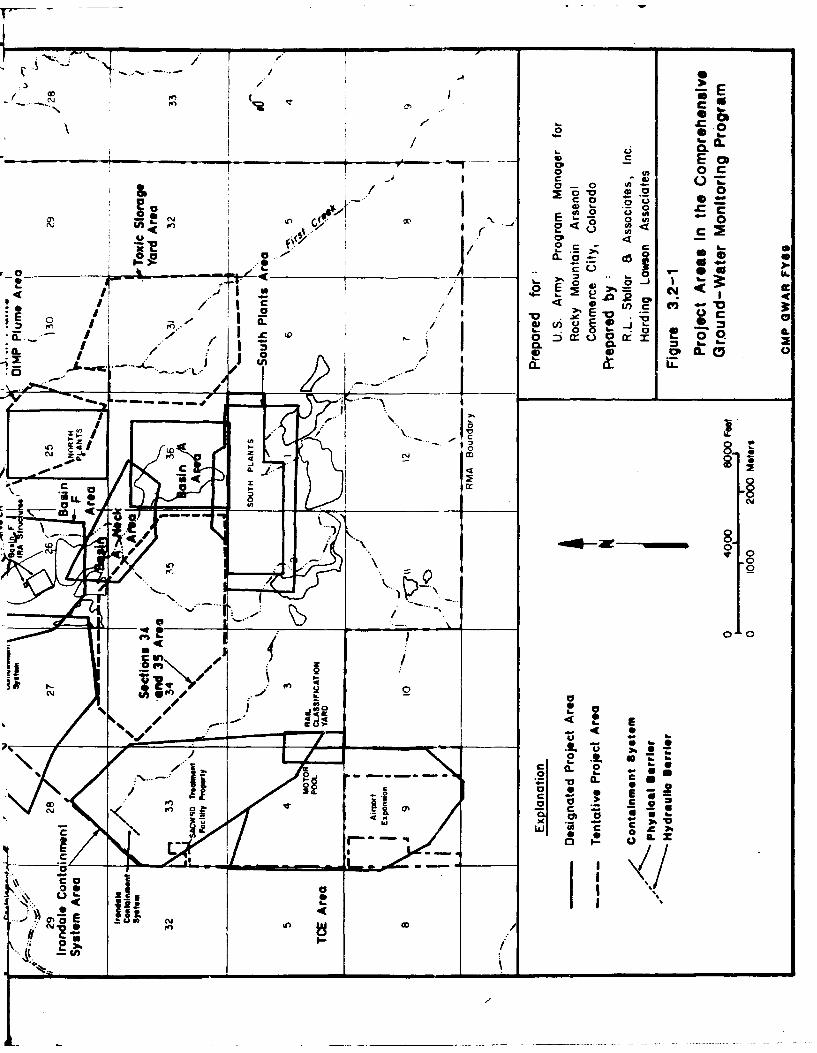
PO CIO
oo
J h.
a0 U) O0 '0 cp 0h
E 0
I cc Q ýmwo CL it -
0. - ~ E ~10
caI o
06. 'C S I
/ 00
0.j 0
*r 0
*IL*
% 0og s0
ooý CCE0
4.4I..#A cC .
c a
Co a.- to c
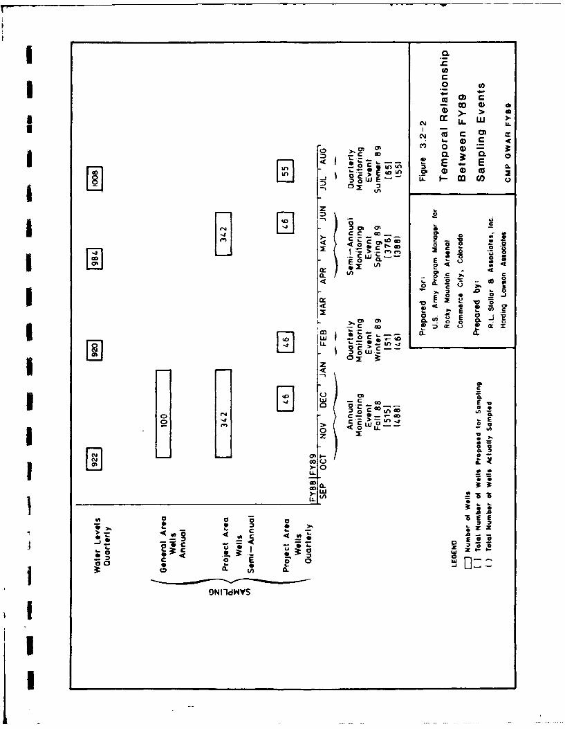
0
OD 4
>. >)
E E~oA ~ 2 ~ (
I 44
4" o
L 4
0~ 00
o 00 mI
LL.
PICON I d~'4V
IcIC
Ic
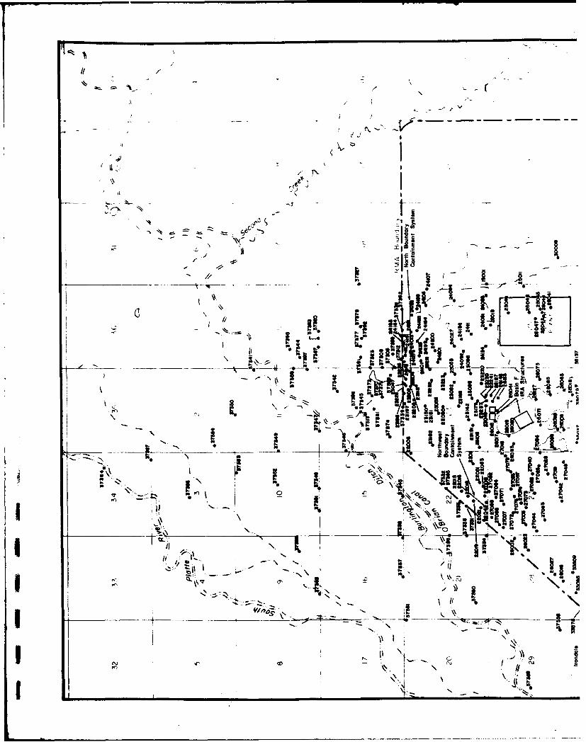
.. +
-.- -
416~
S I
-.
30 N
'II
'4r i!lit
-~a I-L,-
Ivn _-'- -
-x~ 0, am rp#.-J P. an
--*
- , a1 •,! I l ,
to
, ....-<-
"\2.j i , _ +--m+ - \I"\ k t+ .. .-i
e n , .
B - -of '0
5-.-- " .oE yo# \:,• ,-ml •" o
: " '" - - - . _ _ _ _ _ _ _. '§ \ "of I _i j U •
____
•I5.-
- i - - .-- - .-,. I - ,,N ...,E- -$
0*"-.".5
1C>
, ..•""
00
11..
5 :
\' i •"5-
I...,
.. ,I "m"- "'-•-
"U'
CD
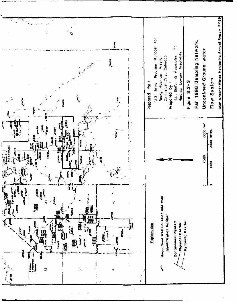
0
000 V)
cC 0 ~ G
CL 0
z 00.Ct
dC) >% =
InC6 00 S co-o JE1- V
06 Q 0 IL
a- L 1--- )
3000
'I - i 1ý C -0
L 0
'22 2
K 3 see.
LD c
0 0
"4 U.4
00
-LJ C*
O0 P'"4" lID%IhIOD
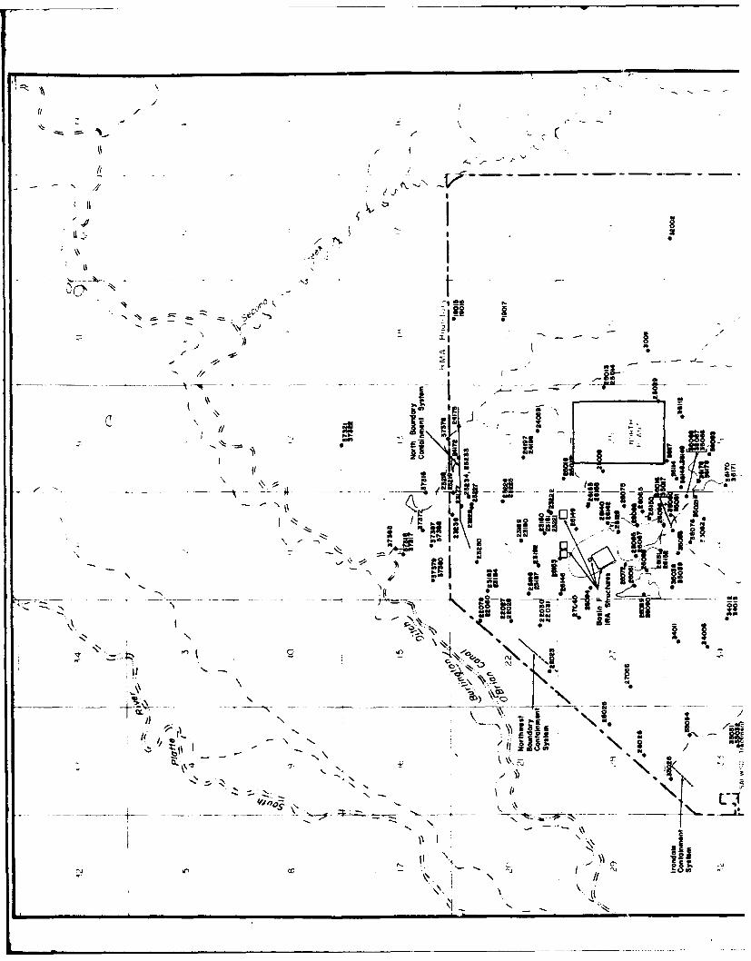
~NNV
to- ol (-0
titi
-~~ - 9 8- =-
IE Zco
.
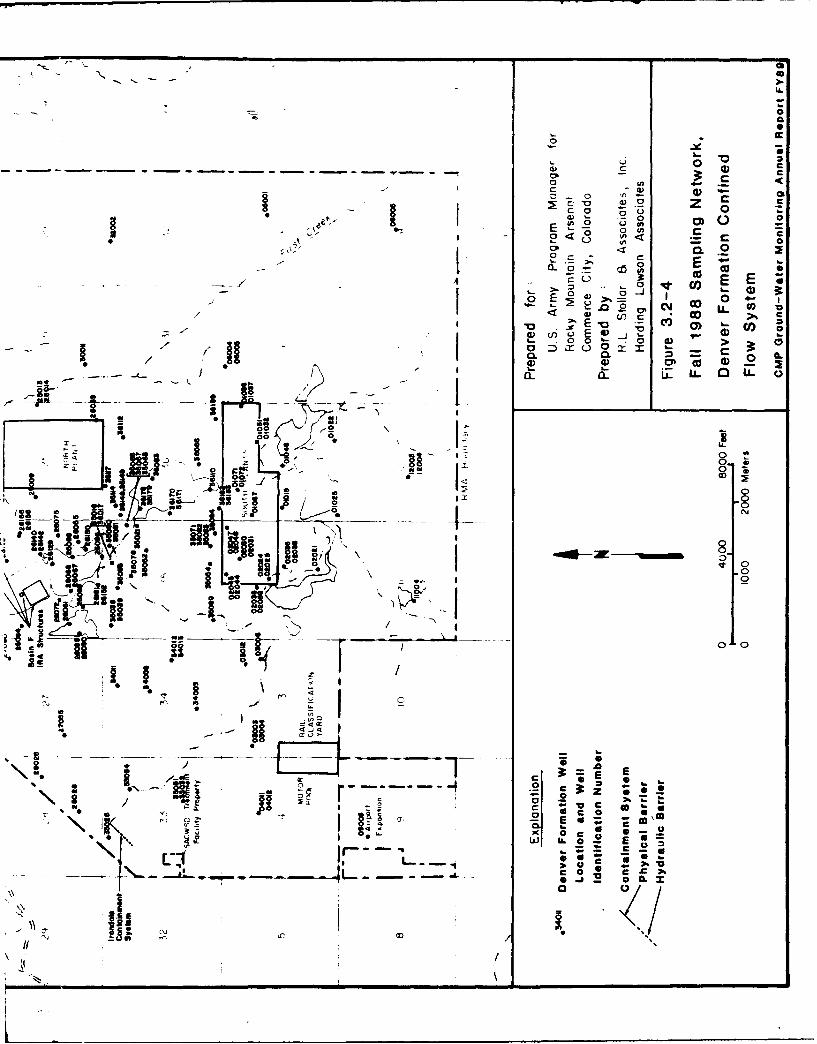
6.6
00
2 0 0
0 a0' -0 U U) C
-(
C
*5 to a
~0 a~ 40. 00
>' E > ~0) CO)
0 ) 0', 0 - ..>
06 al I,. a
00
55 0
0~00~ 8
00
0 ccI!c
of 010
I. ~ §
fE Eat * r\ \ i l K
-
tO
E ca co
af c/ L
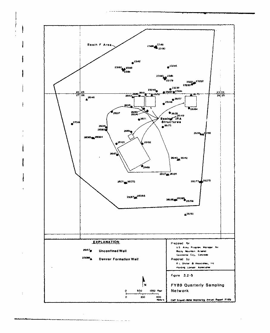
2319 Z2 23193 .2Z3095
23180 2304
2317= 23
23U230
2616522646
2627T 26GA60G207
&Z6149
EXPLANATStrNctres~e o
2601y rj~m Mnge ~25M67 Unefle Wl oCyA9nn r
M6me5c 2it. oloa
~'A DevrFomtonWllP~Mrdb
2SO?10Har72 202742612 2607 C2W75
EXPLANAIOFiPreare 3f2-
FY89rm Quarterly SCAmpfin2616 'to 3000ind~l Mocit Ne Work i rs
oO"Mc city 4000r2396 ene Frato W l CPrepreid-~u by ilr~ nua ~cfF
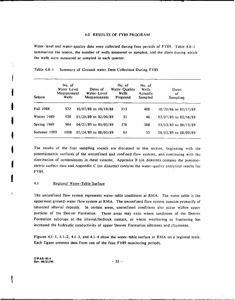
4.0 RESULTS OF FY89 PROGRAM
Water-level and water-quality data were collected during four periods of FY89. Table 4.0-1summarizes the season, the number of wells measured or sampled, and the dates during which
the wells were measured or sampled in each quarter.
Table 4.0-1 Summary of Ground-water Data Collection During FY89
fNo. of No. of No. of
Water Level Dates of Water-Quality Wells DatesMeasurement Water-Level Wells Actually of
Season Wells Measurements Proposed Sampled Sampling
Fall 1988 922 10/07/88 to 10/19/88 515 488 10/20/88 to 01/17/89
Winter 1989 920 01/25/89 to 02/09/89 51 46 02/07/89 to 02/16/89
Spring 1989 984 04/21/89 to 05/03/89 376 388 05/03/89 to 06/15/89
Summer 1989 1008 07/24/89 to 08/03/89 65 55 08/03/89 to 08/09/89
The results of the four sampling rounds are discussed in this section, beginning with the
potentiometric surfaces of the unconfined and confined flow systems, and continuing with thedistribution of contaminants in these systems. Appendix B (on diskette) contains the potentio-
metric surface data and Appendix C (on diskette) contains the water-quality analytical results forFY89.
4.1 Regional Water-Table Surface
The unconfined flow system represents water-table conditions at RMA. The water table is theuppermost ground-water flow system at RMA. The unconfined flow system consists primarily ofsaturated alluvial deposits. In certain areas, unconfined conditions also occur within upperportions of the Denver Formation. These areas may exist where sandstone of the DenverFormation subcrops at the alluvial/bedrock contact, or where weathering or fracturing hasincreased the hydraulic conductivity of upper Denver Formation siltstones and claystones.
Figures 4.1-1, 4.1-2, 4.1-3, and 4.1-4 show the water-table surface at RMA on a regional scale.Each figure presents data from one of the four FY89 monitoring periods.
GWAR-89.4Rev. 06/21/90 - 35 -
I
j To construct these water-table elevation maps, water-level data were used from wells completed
in the alluvium and upper portions of the Denver Formation. Water-level data from wells
screened in the upper portions of the Denver Formation were used only if two conditions were
met. The first condition was that the water-level data were consistent with the surrounding watertable. The second condition was that the wells' geologic logs indicated potential for direct
communication with the unconfined flow system. Data consistent with the surrounding water tablewere considered to represent unconfined flow if these conditions were met. Alternatively, dataj not consistent with the surrounding water table were considered to represent confined flow.
Discussion of the confined flow system is presented in Section 4.2.
Twenty-nine new wells were completed in the unconfined flow system during FY89, in Sec-
tions 1, 2, 4, 25, 26, 30, 32, and 36. The purpose of these new wells was generally to provide
additional water-quality data. Water-level data from these new wells generally confirm previous
interpretations of the water-table surface in these areas.
Figure 4.1-1 presents the regional water-table surface measured during the fall of 1988. The
regional slope of the water table (hydraulic gradient) is from the southeast to the northwest.
Across RMA the drop in water-table elevation is approximately 210 feet. This results in regional
ground-water flow towards the northwest and an average hydraulic gradient of 0.006 ft/ft across
RMA. Approximately two miles northwest of RMA, the water table intersects the Platte River.
At this Intersection, the Platte River acts as the regional discharge point for the unconfined flow
system.
The most pronounced local variation in the configuration of the regional water table surface at
RMA is the ground-water mound present beneath the South Plants. This mound is approximately
25 ft higher in elevation than the regional water-table surface, and is coincident with an area of
shallow bedrock. To the southeast of the South Plants mound, and along the east and west
margins of RMA, the water table has a relatively flat gradient. In these areas, flow in the
unconfined system occurs predominantly through alluvial deposits with relatively high hydraulic
conductivity. To the northwest of the South Plants, the gradient is generally steeper. In this area,
a significant component of unconfined flow occurs through heterogeneous bedrock of the upper
Denver Formation. In contrast to alluvium, bedrock generally has relatively low primary hydraulic
conductivity. The heterogeneous nature of the bedrock, together with fracturing and weathering
of the upper bedrock surface, results in variable hydraulic conductivity. The irregular character
of the water table in this area may result from this variability.
IGWAR-89.4Rev. 06/21/90 - 36 -
Along the north and northwest margins of RMA, the water table is impacted by the boundary
containment systems. This impact is discussed in Section 4.1.2.
Downgradient of RMA in the northwest off-post area, the hydraulic gradient flattens. In this
area, the unconfined flow system consists predominantly of thick alluvial deposits with relatively
high hydraulic conductivity.
4.1.1 Seasonal Fluctuations of the Regional Water Table
Seasonal fluctuations in the configuration of the regional water-table surface are generally small.The general configuration of the regional water table was similar during all FY89 monitoringperiods (Figures 4.1-1 through 4.1-4, respectively). A general shift of contour lines in the
downgradient direction can be noted on the spring 1989 (Figure 4.1-3) and summer 1989
(Figure 4.1-4) maps. This reflects rising water levels during these seasons. The largest seasonal
variation in water-table elevations occurred in the South Plants area where the water table rose
approximately 4 feet.
Pronounced water-table variations occurred in the vicinity of the boundary containment systems
in FY89. These variations are largely attributable to the operations of the boundary containment
g systems.
4.1.2 Water-Table Surface in the Boundary Containment Systems Area!Water-level data characterizing the water table were obtained in four separate monitoring events
in FY89. These data are principally compiled for assessing water-table fluctuations from a
regional perspective. One of the objectives of the CMP, however, is to monitor the hydrologicimpact of boundary containment system operation. Where possible, the quarterly water-level dataJ sets have been used to evaluate more local fluctuations associated with systems operations. The
information provided here characterizes the NBCS and NWBCS operations. For more detailed
information based on weekly water levels obtained from densely-spaced monitoring well networks,
the reader is directed to the FY88 Operational Assessment Reports of the NBCS and the NWBCS(PMRMA, 1989b and PMRMA 1989c, respectively).
Figures 4.1-5 through 4.1-8 show the water-table surface elevations in the vicinity of the North
Boundary Containment System (NBCS) and the Northwest Boundary Containment System (NWBCS)as measured during the fall 1988, winter, spring, and summer 1989, respectively. These maps are
based on a 2-foot contour interval, in order to show local variations in the water-table surface that
GWAR-89.4Rev. 06/21/9o - 37 -
I.
I
are not evident on the regional maps. The effects of the boundary systems on the water-table
elevations include:
1 . Deflected contour lines indicating deviation from regional flow conditions
0 Differences in elevations across the boundaries which indicate hydraulic separation
between upgradient and downgradient flow systems
g Localized troughs or mounds which reflect extraction or injection of ground water
9 During the fall of 1988 (Figure 4.1-5), the effects of the NBCS on the water table were apparent
in several areas. Upgradient of the system, a large area with a relatively flat gradient coincided9 with flow through alluvium. Downgradient of the system, the gradient was considerably steeper.
Across the barrier, discontinuous contour lines indicate an abrupt change in water-table elevations
on either side of the barrier. During the fall of 1988, the maximum head difference (6 ft) across
the barrier occurred along its central portion. As shown in Figure 4.1-5, the water levels on the
upgradient side of the barrier were higher than water levels on the downgradient side. Near thefends of the containment system, the head differences diminished. For approximately 650 ft along,
the western end of the NBCS, there was a reverse gradient, with elevations on the north side of
the barrier higher than elevations on the south side.
Fall 1988 water-level data (Figure 4.1-5) were collected prior to the initial startup and operation
of the ground-water recharge trenches at the NBCS. The impact of the recharge trenches is
discussed for monitoring conducting during and following winter 1989.
I The NWBCS (Figure 4.1-5) during the fall of 1988 also impacted the surrounding water table.
Based on an interpretation of relatively few data points, an arcuate trough was inferred to exist1 immediately upgradient of the NWBCS. To the east of the trough, the hydraulic gradient abruptly
steepened. The low hydraulic conductivity of the aquifer materials in this area (southeast
Section 22) probably accounts for the steepened gradient. Downgradient of the NWBCS, a shallowhydrologic trough with a southeast-northwest axis was inferred to exist in the water-table surface.
It should be noted that the inferred existence of this trough was similarly based on relatively few
data points.
During the winter 1989 monitoring periods two ground-water mounds were present north of the
NBCS as a result of the operation of newly-installed recharge trenches (Figure 4.1-6). Recharge
IGWAR-89.4Rev. 06/21/9o - 38 -
I
trench operations began in October 1988 along the northern portion of the NBCS. A reverse
hydraulic gradient across the barrier is apparent in Figure 4.1-6 for the western half of the NBCS.
The winter 1989 water-table surface at the NWBCS (Figure 4.1-6) exhibits a flattened gaadient in
the immediate vicinity of the barrier. The steepened gradient east of the barrier is still present
(as it was in fall 1988) but the troughs noted upgradient and downgradient of the NWBCS in the
fall of 1988 are not apparent in the winter of 1989.
The spring 1989 water-table map (Figure 4.1-7) indicates that exten yre ground-,v':ter mounding
persisted downgradient of the NBCS, but that the localized, uppermost portions of the mound
(enclosed by the 5140-foot contour in Figuie 4.1-6) had diminished somewhat. The position of
the 5138-foot contour south of the NBCS indicated that the water table had risen slightly in the
spriaig of 1989 relative to the winter of 1989.
The spring 1989 water-table surface at the NWBCS (Figure 4.1-7) is very similar to the previous
winter 1989 (Figure 4.1-6) water-table surface. The 5090-foot and 5092-foot contours northwest
of the barrier have migrated slightly, indicating a subtle lowering of the downgradient water-tab!e
surface.
The steepened water-table surface in the southeast portion of Section 22 east of the NWBCS has
become less steep (decreased the hydraulic gradient) due to an overall lowering of the water table.
This change in hydraulic gradient has exposed a larger area of unsaturated alluvium in Sections 22
and 27 upgradient of the NWBCS.
The summer 1989 water-table surface (Figure 4 1-8) in the vicinity of the NBCS is very similar
to the previous spring 1989 surface. The 5142-foot contour t- migrated farther south in
Section 23, indicating further flattening of the hydraulic , Wient across all of Section 23.
j Mounding of the water table downgradient of the NBCS is sti,' desent, as it was in the previous
quarter.
The summer 1989 water-table surface at the NWBCS (Figure 4.1-8) is very similar to the spring
1989 surface. The relative location of the 5092-foot contour has shifted, indicating a slight r;se
in the water-table elevation downgradient of the system.
II
GWAR-89.4Rev. 06/21/90 - 39 -
I
4.1.3 Water Table in the Basin F IRA Area
Figure 4.1-9 presents the water-table surface in the Basin F IRA area during the fall of 1986,
The contour lines indicate that ground-water flow beneath the IRA structures is to the north.
Near the southwest portion of historical Basin F, the gradient is towards the northwest.
The water-table surface in the Basin F area is relatively planar, except for a local westward-
trending hydraulic divide located in west-central Section 26. Within the map area, the hydraulic
gradient is generally steeper in areas of unsaturated alluvium where unconfined flow occurs
through less permeable bedrock of the Denver Formation. Downgradient of the IRA structures,
the hydraulic gradient flattens, probably due to both a flat bedrock surface and a relatively thicker
interval of saturated alluvium.
Figure 4.1-10 presents the water-table surface of the Basin F IRA area during the winter of 1989.
The water-table surface in this area was generally similar to the fall 1988 surface, both in the
extent of unsaturated alluvium and the direction and rates of ground-water flow.
The spring 1989 water-table surface (Figure 4.1-11) has several variations from the fall 1988 and
winter 1989 surfaces. Contours in the southeast portion of the area have shifted slightly to the
north, indicating higher water levels. In contrast, contour lines in the northwest portion of the
area have shifted south, indicating a lower water table in that area. In the central portion of the
area, the contour lines are more closely spaced, reflecting a steeper hydraulic gradient. The
predominately east-west trending local ground-water divide located west of historical Basin F has
shifted to trend somewhat southeast-northwest. Additional areas of unsaturated alluvium exist on
the spring 1989 map near the common corner of Sections 22, 23, 26, and 27. These additional
areas of unsaturated alluvium are attributable to lowered in water levels.
The potentiometric surface of the unconfined flow system in the Basin F IRA area during the
simnmer of 1989 is presented on Figure 4.1-12. This potentiometric surface was generally similar
to the spring 1989 surface, except for a general southward shift of contour lines. This southward
shift indicates water levels are approximately I to 2 ft lower than those measured during the
spring of 1989. These lower water levels increased the extent of unsaturated alluvium beneath
the western portion of historical Basin F, and north and west of the northern IRA structures.
I
GWAR-89.4Rev. 06/21/90 - 40 -
4.2 Regional Potentiometric Surfaces of the Confined Flow System
Beneath the unconfined flow system, ground water movement occurs through strata of the Denver
Formation. These strata consist of irregular, semi-permeable, sandstone and siltstone beds that
are dispersed within thick sequences of relatively impermeable claystone. Overall, hydraulic
conductivity values for the Denver Formation are lower than the overlying alluvium. Except in
locations where permeable units subcrop, ground water in these strata exists at pressures higher
than atmospheric. Hence, ground water movement through these strata is considered to be
confined.
9 The Denver Formation has been divided into 17 stratigraphic units, as presented in Section 2.1-1
and on Figure 2.1-4. The potentiometric surface of ground water has been mapped for six of
9 these units: A, IU, 1, 2, 3 and 4 (Figures 4.2-1 to 4.2-6, respectively). Figures 4.2-1 through
4.2-6 are based on water-level data obtained during the fall of 1988. Maps representing the other
three seasons are not presented because the potentiometric surfaces do not vary significantly.
Thus, the fall 1988 water-level data provide a reasonable representation of the potentiometric
surfaces in the confined flow system for the entire FY89 monitoring period.IThe form of the potentiometric surfaces shown for each zone of the Den'er Formation generally
is similar, with gradients principally toward the northwest. The elevations of the potentiometric
surfaces, however, are generally different. Commonly, the pctentiometric surface elevations in
deeper zones are lower than the potentiometric surface elevations in shallower zones. Also, the
Sground-water gradient within each zone is in the opposite direction to the dip of the zones. This
suggests that flow between zones can occur, and that it has a potential for a downward direction.
In certain locations between the potentiometric surface elevations of adjacent zones becomes equal.
This suggests that the gradients in these areas are horizontal and communication between zones
does would not occur if adjacent zones are separated by a confining layer. If the zones are not
separated by an aquitard, the potentiometric relationships suggest that adjacent zones may act as
a single hydrostratigraphic unit in these locations. Examples include: southern Basin A - between
zones IU and 1; Basin A Neck - between zones I and 2; and the Basin F area between zones 2
and 3. Zones 3 and 4 exhibit nearly identical potentiometric elevations throughout the mapped
area, which indicates that these zones may be part of the same hydrostratigraphic unit.
4.3 Contaminant Distribution
Assessment of contaminant distributions in ground water at RMA is based on: (1) chemical
analysis of samples collected during the fall of 1988, and the winter, spring, and summer of 1989;
GWAR-89.4Rev. 06/21/90 - 41 -
(2) current understanding of stratigraphic correlations of various geologic units at RMA; and (3)
current understanding of ground-water flow conditions at RMA. Plume maps were constructed
using data from the fall 1988 sampling round, as it was the most comprehensive sampling round
during FY89.
4.3.1 Analytical Data Presentation
Twenty-one selected analytes or analyte groups are presented in this section. Contaminant
distributions in the unconfined and confined flow systems are described, and comparisons aremade between FY89, FY88 and historical analytical results. Plume maps based on fall 1988
analytical results are presented for each analyte or group. Tables are also presented summarizing
analytical results of the samples collected in both the unconfined and confined flow systems.
4• These tables present all of the FY89 analytical results as well as the winter 1987/88 results for
each analyte discussed.
4.3.2 Dieldrin
A total of 487 samples collected from the unconfined and confined flow systems were analyzed
for dieldrin during the fall of 1988. Dieldrin was reported above the CRL (0.0500 jig/I) in 141
samples with concentrations ranging from 0.0512 jug/I to 86.0 jIg/I. Dieldrin was detected in the
confined flow system within zones A, IU, 1, 2, 3, and 5. Table 4.3.2-1 summarizes the detections
reported in the unconfined and confined flow systems for FY89.
4.3.2.1 Unconfined Flow System. Among the 321 wells sampled from the unconfined flow
= system, dieldrin was detected in 124 samples. Concentrations ranged from 0.0512 jig/I to
86.0 iug/l. The distribution of dieldrin contamination in the unconfined flow system at RMA for
the fall 1988 monitoring event is shown in Figure 4.3.2-I.
A continuous plume of dieldrin extended from the South Plants and Basin A to the NBCS and
the NWBCS. The affected pathways within this plume incluoed the South Plants-Basin A, South
Lakes, Basin A Neck, Central North, Basin F East, Basin F West, Basin F Northwest, and Basin F
Pathways. An isolated dieldrin plume existed in the Central South Pathway. Off-post, dieldrin
plumes were inferred in the First Creek Off-Post, Northern Off-Post, and Northwest Pathways.
The dieldrin plume extended from a small concentration high in the South Plants, north into
Basin A and southeast along the South Lakes Pathway. A lobe of the plume extended east into
Section 3, where Well 03005 yielded a dieldrin concentration of 5.00 g/Il, the highest in the South
GWAR-89.4SRev. 06/21/90 - 42 -
I]
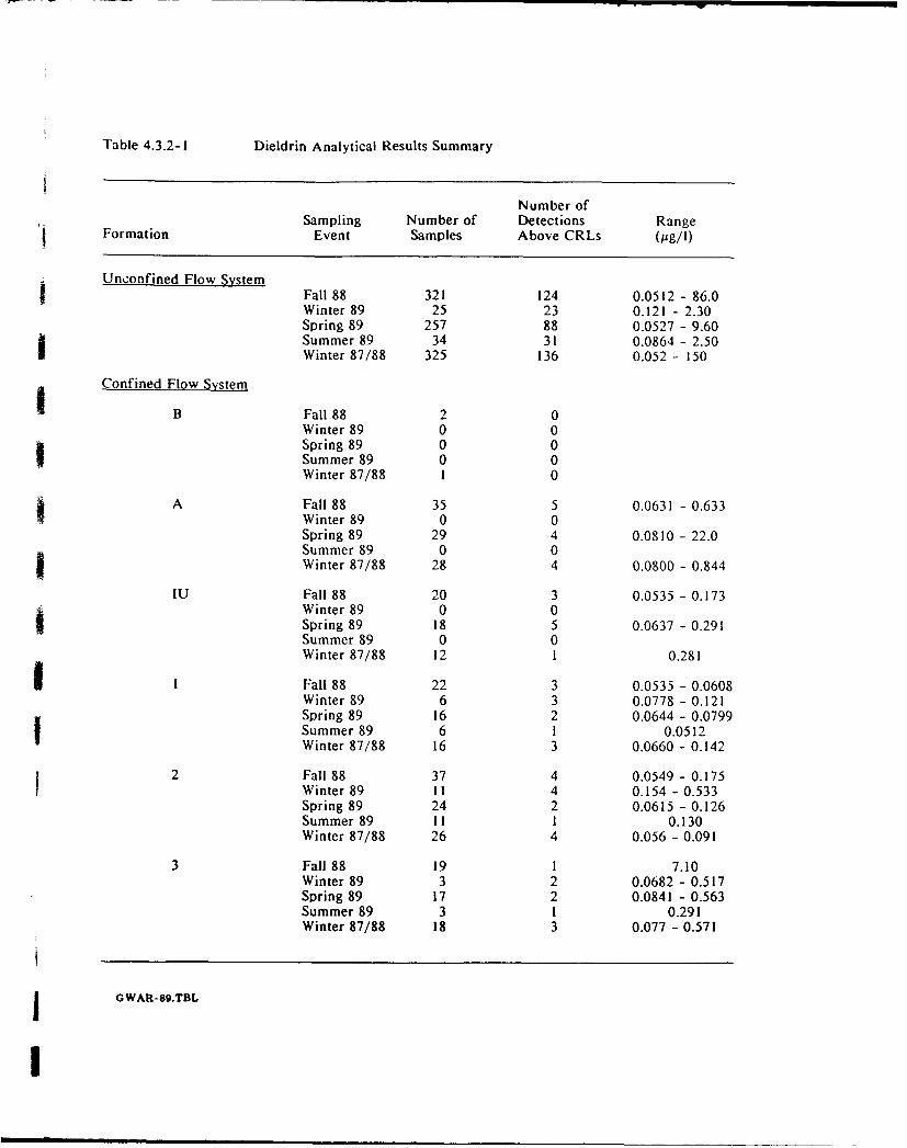
Table 4.3.2-1 Dieldrin Analytical Results Summary
Number ofSampling Number of Detections Range
Formation Event Samples Above CRLs (Ag/I)
SUnconfined Flow System
Fall 88 321 124 0.0512 - 86.0Winter 89 25 23 0.121 - 2.30Spring 89 257 88 0.0527 - 9.60Summer 89 34 31 0.0864 - 2.50Winter 87/88 325 136 0.052 - 150
Confined Flow System
B Fall 88 2 0Winter 89 0 0Spring 89 0 0Summer 89 0 0Winter 87/88 1 0
A Fall 88 35 5 0.0631 - 0.633Winter 89 0 0Spring 89 29 4 0.0810 - 22.0Summer 89 0 0Winter 87/88 28 4 0.0800 - 0.844
IU Fall 88 20 3 0.0535 - 0.173Winter 89 0 0Spring 89 18 5 0.0637 - 0.291Summer 89 0 0Winter 87/88 12 1 0.281
1 Fall 88 22 3 0.0535 - 0.0608Winter 89 6 3 0.0778 - 0.121Spring 89 16 2 0.0644 - 0.0799Summer 89 6 1 0.0512Winter 87/88 16 3 0.0660 - 0.142
2 Fall 88 37 4 0.0549 - 0.175Winter 89 I1 4 0.154 - 0.533Spring 89 24 2 0.0615 - 0.126Summer 89 11 1 0.130Winter 87/88 26 4 0.056 - 0.091
3 Fall 88 19 1 7.10Winter 89 3 2 0.0682 - 0.517Spring 89 17 2 0.0841 - 0.563Summer 89 3 1 0.291Winter 87/88 18 3 0.077 - 0.571
j G WAR-89.TBL
I
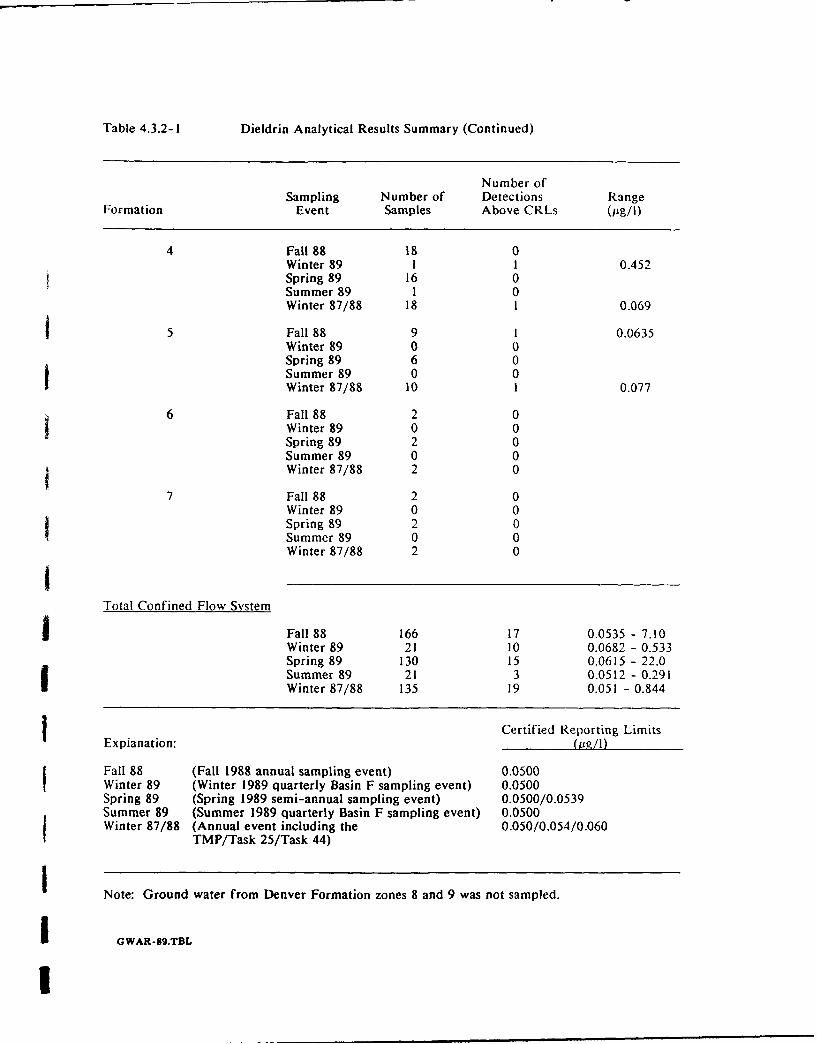
Table 4.3.2-i Dieldrin Analytical Results Summary (Continued)
Number ofSampling Number of Detections Range
Formation Event Samples Above CRLs (pg/W)
4 Fall 88 18 0Winter 89 1 1 0.452Spring 89 16 0Summer 89 1 0Winter 87/88 18 1 0.069
5 Fall 88 9 I 0.0635Winter 89 0 0Spring 89 6 0Summer 89 0 0Winter 87/88 10 1 0.077
6 Fall 88 2 0Winter 89 0 0Spring 89 2 0Summer 89 0 0Winter 87/88 2 0
7 Fall 88 2 0Winter 89 0 0Spring 89 2 0Summer 89 0 0Winter 87/88 2 0I
Total Confined Flow System
Fall 88 166 17 0.0535 - 7.10Winter 89 21 10 0.0682 - 0.533Spring 89 130 15 0.0615 - 22.0Summer 89 21 3 0.0512 - 0.291Winter 87/88 135 19 0.051 - 0.844
Certified Reporting LimitsExplanation: (uz/l)
Fall 88 (Fall 1988 annual sampling event) 0.0500Winter 89 (Winter 1989 quarterly Basin F sampling event) 0.0500Spring 89 (Spring 1989 semi-annual sampling event) 0.0500/0.0539Summer 89 (Summer 1989 quarterly Basin F sampling event) 0.0500Winter 87/88 (Annual event including the 0.050/0.054/0.060
TMP/Task 25/Task 44)
Note: Ground water from Denver Formation zones 8 and 9 was not sampled.
I GWAR-89.TBL
I
Lakes area. Within Basin A, a concentration high was centered around Well 36056, which yielded
65.0 Mg/I of dieldrin.
From Basin A, dieldrin contamination extended northeast into the Basin A Neck and Basin F East
Pathways. Dieldrin contamination within the Basin A Neck Pathway merged with contamination
in the Central North, Basin F West and Basin F Northwest Pathways as the plume approached the
NWBCS. Along the northwest RMA boundary, dieldrin extended off-post a short distance beyond
the NWBCS and south of the NWBCS.
Dieldrin contamination in the Basin F East Pathway merged with the Basin F Pathway plume in
north-central Section 26. Dieldrin concentration highs occurred in the Basin F Pathway plume
downgradient of Basin F. The highest fall 1988 detection in the Basin F Pathway plume was
7.60 pg/I at Well 23241. Dieldrin contamination extended along the Basin F Pathway to the
NBCS. Downgradient of the NBCS, dieldrin plumes extended for approximately one mile along
the First Creek and Northern Off-Post Pathways. The highest off-post dieldrin detection within
these pathways was 0.840 pg/I at Well 37312.
Isolated dieldrin detections were reported on-post in Sections 1, 2, 23, 24, 25, 27, and 35. Off-
post isolated detections were reported at Wells 37355 and 37377.
4.3.2.2 Confined Flow System. Dieldrin analyses were performed on 166 samples col..cted
from the confined flow system during the fall of 1988. Dieldrin was detected in 17 samples fromzones A, IU, 1, 2, 3, and 5. Concentrations ranged from 0.0535 to 7.10 Ag/l. Table 4.3.2-1
summarizes these results for each zone of the confined flow system. Figures A-I through A-3 are
j point plots showing the distribution of dieldrin in the confined flow system.
Dieldrin contamination in the confined flow system occurred predominantly beneath areas of
unconfined flow system contamination. The highest fall 1988 detection was 7.40 pug/I at
Well 26142 (zone 3). This well is located in east-central Section 26, where unconfined flow system
I contamination existed in the Basin F East Pathway. The deepest fall 1988 dieldrin detection
occurred at Well 36148 (zone 1). This well yielded 0,0535 psg/I of dieldrin from a screened
interval 93 to 163 feet below ground surface. The well is located in northwest Section 36.
4.3.2.3 Winter 87/88 and FY89 Comparisons. Dieldrin was detected in 136 of 325 samples
j from the unconfined flow system in winter 1987/88, compared to 124 of 321 samples analyzed
during the fall of 1988. Data from FY89 provide a more complete understanding of the
distribution of dieldrin in the unconfined flow system than was available in the FY88 Annual
G WAR-89.4Rev. 06/21/90 - 45 -
I
Report. In particular, the extent of dieldrin in the South Plants, Basin A, and Sections 34 and 35are better defined due to an increased sampling density in these areas during FY89. Plumeconfigurations are similar in the areas of the NBCS and NWBCS. Wells where dieldrinconcentrations varied considerably from previous or subsequent sampling rounds are listed in Table
4.3.2-2.
Dieldrin was detected in the confined flow system in 19 of 135 samples collected during thewinter of 1987/88 compared to 17 of 166 samples collected during fall 1988. Table 4.3.2-1summarizes the winter 1987/88 and fall 1988 results for each zone of the confined flow system.Areas in which the presence of dieldrin was further substantiated include the Basin A Neck, Basin
j C, and Basin F areas where dieldrin was detected in both winter 1987/88 and fall 1988. Dieldrinwas detected more frequently in fall 1988 in the South Plants and less frequently at the NBCS thanin winter 1987/88. Due to the general low hydraulic conductivity and large heterogeneity of theDenver aquifer, substantial data variability is likely to occur in any single sample period. Datainterpretation based on a single sample period may not be effective in recognizing anomalous data,
therefore, variations such as those noted in the South Plants should be considered appropriately.
S4.3.3 Endrin
Analyses for endrin were performed on 455 ground-water samples collected during the fall of
1988. Concentrations ranging from 0.0510 to 14.0 pg/I were detected in 78 of the 455 samplesanalyzed. The CRL for the fall of 1988 was 0.0500 g/Il. The distribution of endrin in thejunconfined flow system is illustrated in Figure 4.3.3-1. Endrin was detected in the confined flowsystem within zones A, 1, 2, 3, and 5 during the fall of 1988. Endrin detections for FY89 areg summarized in Table 4.3.3-1.
4.3.3.1 Unconfined Flow System. Ground-water samples from 298 wells completed in the
unconfined flow system were analyzed for endrin during the fall of 1988. Endrin concentrationsranging from 0.0515 to 14.0 pg/I were detected in 68 of these samples. Figure 4.3.3-1 illustratesunconfined flow system plumes interpreted from the fall 1988 data. Endrin plumes were present
in the South Plants - Basin A-Basin A Neck Pathways, and the Basin F and Basin F WestPathways. Endrin also was present along the First Creek Off-Post Pathway and downgradient of
the NWBCS.
The fall 1988 data indicated that endrin formed a continuous plume originating in the South Plantsand extending along the Basin A and Basin A Neck Pathways. The plume appeared to endupgradient of the NWBCS in northern Section 27. Endrin concentrations within the South Plants-
GWAR-89.4Rev. 06/22/90 - 46 -
I
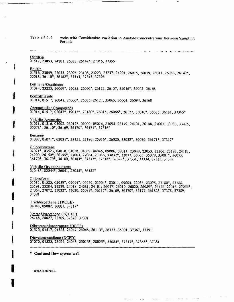
Table 4.3.2-2 Wells with Considerable Variation in Analyte Concentrations Between SamplingPeriods
Dieldrin01517, 23053, 24201, 26083, 26142*, 27016, 37355
Endrin01516, 23049, 23053, 23095, 23108, 23223, 23237, 24201, 26015, 26019, 26041, 26083, 26142*,35018, 36110*, 36182*, 37313, 37343, 37396
Dithiane/Oxathiane01014, 23223, 26069", 26085, 26096*, 26127, 26157, 35016*, 35065, 36168
Benzothiazole01014, 01517, 26041, 26066*, 26085, 26127, 35065, 36001, 36094, 36168
Organosulfur Compounds01014, 01517, 02047*, 19015*, 23180*, 26015, 26066*, 26127, 35016*, 35065, 36181, 37365*
Volatile Aromatics01511, 01516, 03002, 03012*, 09002, 09014, 23095, 23179, 24101, 26148, 27003, 33030, 33075,35078*, 36110*, 36169, 36170*, 36171*, 37316*
Benzene01007, 01071*, 02031*, 23151, 23196, 25016*, 26020, 33032*, 36076, 36171*, 37317*
Chlorobenzene01071*, 03523, 04010, 04038, 04039, 04046, 09006, 09011, 23049, 23053, 23106, 23197, 24181,24200, 26150*, 26155*, 27003, 27064, 27086, 33032*, 33077, 35065, 35079, 35081*, 36075,36170*, 36179*, 36180, 36183*, 37317*, 37318*, 37322*, 37331, 37334, 37335, 37397
Volatile Organohalogens01048*, 02044*, 26041, 27055*, 36182*
Chloroform01517, 01525, 02039*, 02044*, 02050, 03004*, 03011, 09005, 22033, 23095, 23180*, 23188,23191, 23204, 23239, 24018, 24081, 24101, 26017, 26019, 26020, 26089*, 26142, 27016, 27055*,27064, 27072, 33032*, 33030, 35089*, 36117*, 36169, 36170*, 36177, 36182*, 37378, 37389,5 37391
Trichloroethene (TRCLE)04048, 09002, 36001, 37317*
Tetrachloroethene (TCLEE)26148, 28027, 33509, 37378, 37391
f Dibromochloropropane (DBCP)01510, 01517, 01525, 25047, 25048, 26113*, 26133, 36001, 37367, 37391
Dicvclogentadiene (DCPD)01070, 01525, 23024, 24043, 25013*, 28025*, 35084*, 37317*, 37365*, 37381
* Confined flow system well.
GWAR-99.TBL
1
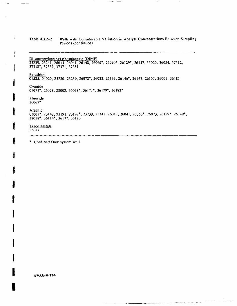
Table 4.3.2-2 Wells with Considerable Variation in Analyte Concentrations Between SamplingPeriods (continued)
Diisooropvlmethvl phosphonate (DIMP)23239, 23241, 26015, 26041, 26148, 26066*, 26090*, 26129*, 26157, 35020, 36084, 37312,' 37318*, 37339, 37371, 37381
ParathionI 01525, 04020, 23220, 23239, 26072*, 26083, 26133, 26146*, 26148, 26157, 36001, 36181
Cyanide01071*, 26028, 28002, 35078*, 36171*, 36179*, 36182*
I Fluoride26067*
Arsenic03003*, 23142, 23191, 23192*, 23239, 23241, 26017, 26041, 26066*, 26073, 26129*, 26149*,28028*, 361140, 36177, 36180
Trace Metals
35087
* Confined flow system well.
IIB
!I
IIi
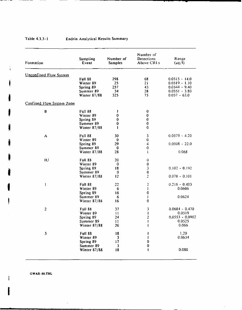
Table 4.3.3-I Endrin Analytical Results Summary
Number ofSampling Number of Detections Range
Formation Event Samples Above CRLs (Og/I)
Unconfined Flow SystemFall 88 298 68 0.0515 - 14.0
f Winter 89 25 21 0.0519 - 1.10Spring 89 257 43 0.0544 - 9.40Summer 89 34 28 0.0551 - 3.80Winter 87/88 325 75 0.057 - 63.0
Confined Flow System Zone
B Fall 88 1 0Winter 89 0 0Spring 89 0 0Summer 89 0 0Winter 87/88 i 0
A Fall 88 30 3 0.0579 - 4.20Winter 89 0 0Spring 89 29 4 0.0508 - 22.0Summer 89 0 0Winter 87/88 28 1 0.068
IU Fall 88 20 0Winter 89 0 0Spring 89 18 3 0.102 - 0.192Summer 89 0 0Winter 87/88 12 2 0.078 - 0.101
I Fall 88 22 2 0.216 - 0.403Winter 89 6 1 0.0606Spring 89 16 0Summer 89 6 1 0.0624Winter 87/88 16 0
2 Fall 88 37 3 0.0684 - 0.470Winter 89 I1 1 0.0519Spring 89 24 2 0.0553 - 0.0902Summer 89 1I 1 0.0525Winter 87/88 26 1 0.066
3 Fall 88 18 I 1.20Winter 89 3 1 0.0634Spring 89 17 0Summer 89 3 0Winter 87/88 18 1 0.080
G WAR-89.TBL
I
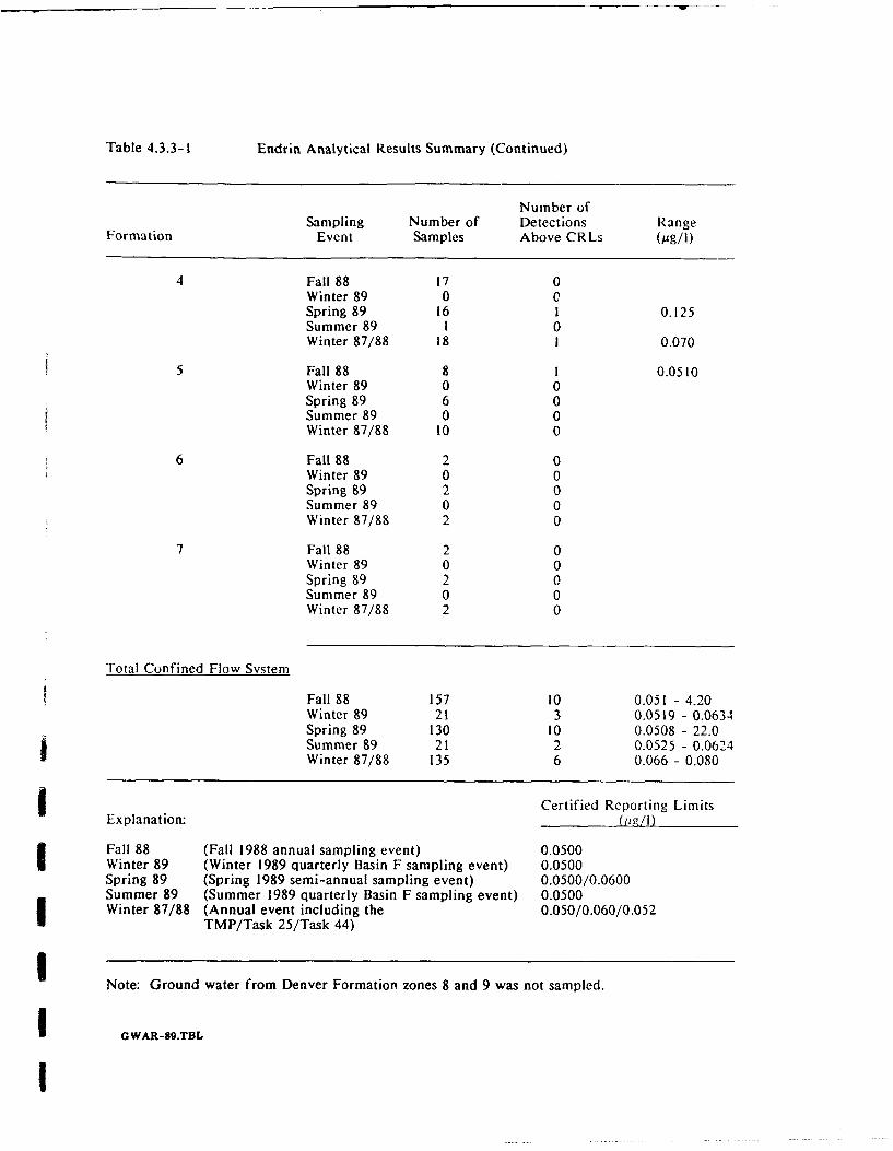
Table 4.3.3-1 Endrin Analytical Results Summary (Continued)
Number ofSampling Number of Detections Range
Formation Event Samples Above CRLs (Mg/I)
4 Fall 88 17 0Winter 89 0 0Spring 89 16 1 0.125Summer 89 1 0Winter 87/88 18 I 0.070
5 Fall 88 8 1 0.0510Winter 89 0 0Spring 89 6 0Summer 89 0 0Winter 87/88 10 0
6 Fall 88 2 0Winter 89 0 0Spring 89 2 0Summer 89 0 0Winter 87/88 2 0
7 Fall 88 2 0Winter 89 0 0Spring 89 2 0Summer 89 0 0Winter 87/88 2 0
Total Confined Flow System
Fall 88 157 10 0.051 - 4.20Winter 89 21 3 0.0519 - 0.0634Spring 89 130 10 0.0508 - 22.0Summer 89 21 2 0.0525 - 0.0624Winter 87/88 135 6 0.066 - 0.080
Certified Reporting LimitsExplanation: (LI /I)
Fall 88 (Fall 1988 annual sampling event) 0.0500Winter 89 (Winter 1989 quarterly Basin F sampling event) 0.0500Spring 89 (Spring 1989 semi-annual sampling event) 0.0500/0.0600Summer 89 (Summer 1989 quarterly Basin F sampling event) 0.0500Winter 87/88 (Annual event including the 0.050/0.060/0.052
TMP/Task 25/Task 44)
Note: Ground water from Denver Formation zones 8 and 9 was not sampled.
IGWAR-89.TBL
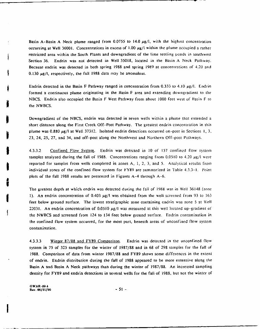
Basin A-Basin A Neck plume ranged from 0.0755 to 14.0 p4g/I, with the highest concentration
occurring at Well 36001. Concentrations in excess of 1.00 ug/I within the plume occupied a rather
restricted area within the South Plants and downgradient of the lime settling ponds in southwest
Section 36. Endrin was not detected in Well 35018, located in the Basin A Neck Pathway.
Because endrin was detected in both spring 1988 and spring 1989 at concentrations of 4.20 and
0.130 pg/l, respectively, the fall 1988 data may be anomalous.
Endrin detected in the Basin F Pathway ranged in concentration from 0.333 to 4.10 pg/I. Endrin
formed a continuous plume originating in the Basin F area and extending downgradient to the
NBCS. Endrin also occupied the Basin F West Pathway from about 1000 feet west of Basin F to
the NWBCS.
Downgradient of the NBCS, endrin was detected in seven wells within a plume that extended a
short distance along the First Creek Off-Post Pathway. The greatest endrin concentration in this
plume was 0.880 pg/I at Well 37312. Isolated endrin detections occurred on-post in Sections 1, 3,
23, 24, 25, 27, and 34, and off-post along the Northwest and Northern Off-post Pathways.
4.3.3.2 Confined Flow System. Endrin was detected in 10 of 157 confined flow system
samples analyzed during the fall of 1988. Concentrations ranging from 0.0510 to 4.20 pg/l were
reported for samples from wells completed in zones A, 1, 2, 3, and 5. Analytical results from
individual zones of the confined flow system for FY89 are summarized in Table 4.3.3-1. Point
plots of the fall 1988 results are presented in Figures A-4 through A-6.IThe greatest depth at which endrin was detected during the fall of 1988 was in Well 36148 (zone
1). An endrin concentration of 0.403 pg/I was obtained from the well screened from 93 to 163
feet below ground surface. The lowest stratigraphic zone containing endrin was zone 5 at Well
22031. An endrin concentration of 0.0510 pg/I was measured at this well located up-gradient of
the NWBCS and screened from 124 to 134 feet below ground surface. Endrin contamination in
the confined flow system occurred, for the most part, beneath areas of unconfined flow system
contamination.
4.3.3.3 Winter 87/88 and FY89 Comparison. Endrin was detected in the unconfined flow
system in 75 of 325 samples for the winter of 1987/88 and in 68 of 298 samples for the fall of
1988. Comparison of data from winter 1987/88 and FY89 shows some differences in the extent
of endrin. Endrin distribution during the fall of 1988 appeared to be more extensive along the
Basin A and Basin A Neck pathways than during the winter of 1987/88. An increased sampling
density for FY89 and endrin detections in several wells for the fall of 1988, but not the winter of
GWAR-89.4Rev. 06/21/90 - 51 -
I
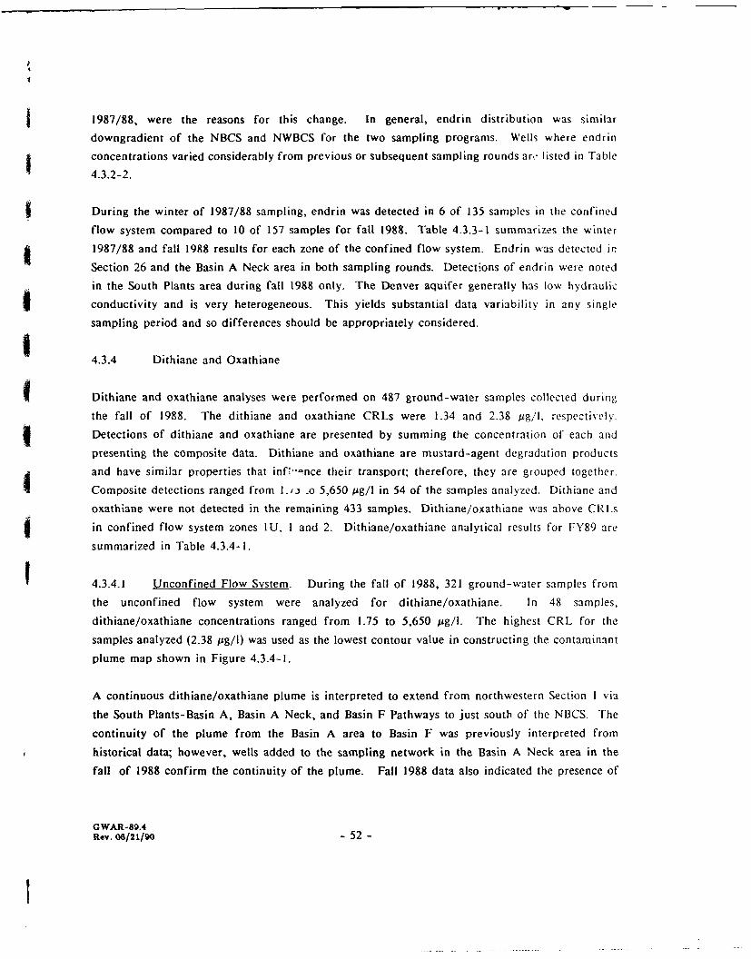
1987/88, were the reasons for this change. In general, endrin distribution was similar
downgradient of the NBCS and NWBCS for the two sampling programs. Wells where endrin
concentrations varied considerably from previous or subsequent sampling rounds arr listed in Table
4.3.2-2.
During the winter of 1987/88 sampling, endrin was detected in 6 of 135 samples in the confined
flow system compared to 10 of 157 samples for fall 1988. Table 4.3.3-1 summarizes the winter
1987/88 and fall 1988 results for each zone of the confined flow system. Endrin was detected in
Section 26 and the Basin A Neck area in both sampling rounds. Detections of endrin were noted
in the South Plants area during fall 1988 only. The Denver aquifer generally has low hydraulic
conductivity and is very heterogeneous. This yields substantial data variability in any single
sampling period and so differences should be appropriately considered.
4.3.4 Dithiane and Oxathiane
Dithiane and oxathiane analyses were performed on 487 ground-water samples collected during
the fall of 1988. The dithiane and oxathiane CRLs were 1.34 and 2.38 jpg/l, respectively.
Detections of dithiane and oxathiane are presented by summing the concentration of each and
presenting the composite data. Dithiane and oxathiane are mustard-agent degradation products
and have similar properties that inf-"-nce their transport; therefore, they are grouped together.
Composite detections ranged from 1./., .o 5,650 ug/l in 54 of the samples analyzed. Dithiane and
oxathiane were not detected in the remaining 433 samples. Dithiane/oxathiane was above CRLs
in confined flow system zones IU, I and 2. Dithiane/oxathiane analytical results for FY89 are
summarized in Table 4.3.4-1.
4.3.4.1 Unconfined Flow System. During the fall of 1988, 321 ground-water samples from
the unconfined flow system were analyzed for dithiane/oxathiane. In 48 samples,
dithiane/oxathiane concentrations ranged from 1.75 to 5,650 Ug/l. The highest CRL for the
samples analyzed (2.38 pg/I) was used as the lowest contour value in constructing the contaminant
plume map shown in Figure 4.3.4-1.
A continuous dithiane/oxathiane plume is interpreted to extend from northwestern Section I via
the South Plants-Basin A, Basin A Neck, and Basin F Pathways to just south of the NBCS. The
continuity of the plume from the Basin A area to Basin F was previously interpreted from
historical data; however, wells added to the sampling network in the Basin A Neck area in the
fall of 1988 confirm the continuity of the plume. Fall 1988 data also indicated the presence of
GWAR-89.4Rev. 06/21/90 - 52 -
I
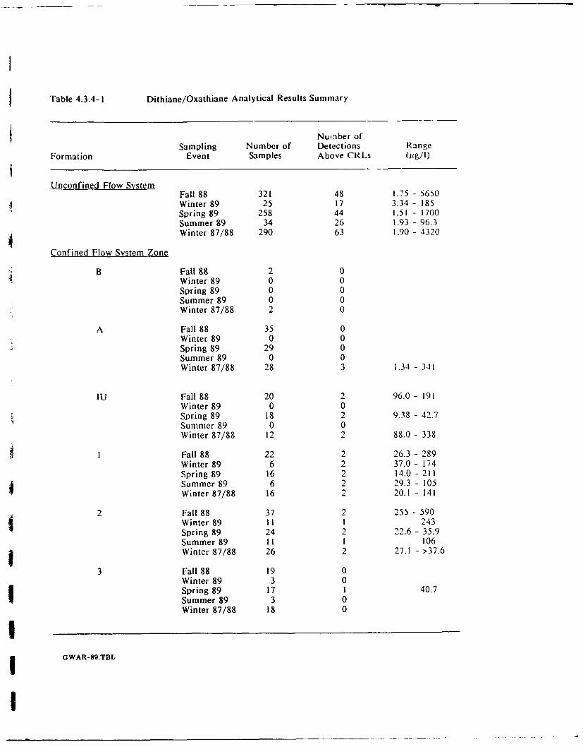
Table 4.3.4-1 Dithiane/Oxathiane Analytical Results Summary
Nunber ofSampling Number of Detections Range
Formation Event Samples Above CRLs (Og/l)
Unconfined Flow SystemFall 88 321 48 1.75 - 5650Winter 89 25 17 3.34 - 185Spring 89 258 44 1.51 - 1700Summer 89 34 26 1.93 - 96.3Winter 87/88 290 63 1.90 - 4320
Confined Flow System Zone
B Fall 88 2 0Winter 89 0 0Spring 89 0 0Summer 89 0 0Winter 87/88 2 0
A Fall 88 35 0Winter 89 0 0Spring 89 29 0Summer 89 0 0Winter 87/88 28 3 1.34 - 341
IU Fall 88 20 2 96.0 - 191Winter 89 0 0Spring 89 18 2 9.38 - 42.7Summer 89 0 0Winter 87/88 12 2 88.0 - 338
I Fall 88 22 2 26.3 - 289Winter 89 6 2 37.0 - 174Spring 89 16 2 14.0 - 211Summer 89 6 2 29.3 - 105Winter 87/88 16 2 20.1 - 141
2 Fall 88 37 2 255 -590Winter 89 11 1 243Spring 89 24 2 22.6 - 35.9Summer 89 I1 I 106Winter 87/88 26 2 27.1 - >37.6
3 Fall 88 19 0Winter 89 3 0Spring 89 17 1 40.7Summer 89 3 0Winter 87/88 18 0
IG
S~GWAR-89.TBL
I
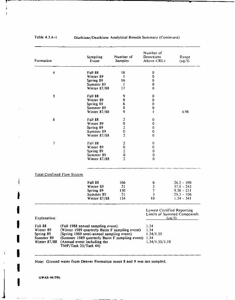
Table 4.3.4-I Diathiane/Oxathiane Analytical Resutls Summary (Continued)
Number ofSampling Number of Detections Range
Formation Event Samples Above CRLs (Pg/I)
4 Fall 88 18 0Winter 89 1 0Spring 89 16 0Summer 89 1 0Winter 87/88 17 0
5 Fall 88 9 0Winter 89 0 0Spring 89 6 0Summer 89 0 0Winter 87/88 9 1 4.98
6 Fall 88 2 0Winter 89 0 0Spring 89 2 0Summer 89 0 0Winter 87/88 2 0
7 Fall 88 2 0Winter 89 0 0Spring 89 2 0Summer 89 0 0Winter 87/88 2 0
Total Confined Flow System
Fall 88 166 6 26.3 - 590Winter 89 21 3 37.0 - 243Spring 89 130 7 9.38 - 211Summer 89 21 3 29.3 - 106Winter 87/88 134 10 1.34 - 341
Lowest Certified ReportingLimits of Summed Compounds
Explanation: (AR!IM
Fall 88 (Fall 1988 annual sampling event) 1.34Winter 89 (Winter 1989 quarterly Basin F sampling event) 1.34Spring 89 (Spring 1989 semi-annual sampling event) 1.34/1.35Summer 89 (Summer 1989 quarterly Basin F sampling event) 1.34Winter 87/88 (Annual event including the 1.34/1.35/1.10
TMP/Task 25/Task 44)INote: Ground water from Denver Formation zones 8 and 9 was not sampled.
IIGW -9.B
dithiane/oxathiane in two off-post wells in Section 14 near the convergence of First Creek and
the O'Brian Canal.
The farthest upgradient detection of dithiane/oxathiane occurred in the South Plants area. The
plume extends northward into the Basin A Neck and northwest into Section 26 and the Basin F
Pathway. The highest detected concentration of dithiane/oxathiane was on the north side of Basin
A in Well 36177 (5,650 pg/I). The highest dithiane/oxathiane concentration in the Basin A Neck
Pathway was 913 pg/i in Well 35079, the highest concentration in the Basin F East-Basin F
Pathway was 344 pg/I (Well 23053), and the highest concentration in the South Plants Pathway was
140 pg/I in Well 01020. Dithiane/oxathiane was not detected in Well 36168 in the South Plants
Pathway and in Well 35065 in the Basin A Neck Pathway in the fall of 1988. However, these
results are probably anomalous because previous and subsequent sampling indicated that
dithiane/oxathiane concentrations were above the CRL in these wells, and the wells lie within the
center of the plume.
Only two detections of dithiane/oxathiane occurred outside of the plume described above.
Concentrations of 1.75 ug/l in Well 37343 and 16.4 pg/l in Well 37396 were detected off-post
along the First Creek Off-Post Pathway.
4.3.4.2 Confined Flow System. Analyses for dithiane/oxathiane were performed on 166ground-water samples collected during the fall of 1988 from the confined flow system. Analytical
results for the fall 1988 sampling are summarized in Table 4.3.4-1. Point plots of results from the
fall 1988 sampling of the confined flow system are presented in Figures A-7 through A-8.
Dithiane/oxathiane concentrations above CRLs ranging from 26.3 to 590 pg/I were detected in 6
samples analyzed from Denver Formation zones I U, I and 2. Wells with elevated concentrations
of dithiane/oxathiane were located in Section 26 and Section 35 between Basin A and Basin F.
The highest detection occurred in Well 26069 which is completed in zone 2 to a depth of 79.5 feet.
The deepest detection (255 ug/I) was also in zone 2 (Well 26129), 100 ft below ground level.
Contamination in the confined flow system can be correlated with plumes in the overlying
unconfined flow system. For example, the highest concentrations in the unconfined flow system
occur in the northern part of Basin A and appear to be associated with confined flow system
detections to the northwest in zones IU, 1, and 2.
4.3.4.3 Winter 87/88 and FY89 Comparison. Detections of dithiane/oxathiane occurred in the
unconfined flow system in 63 of 290 wells for winter 1987/88 compared to 48 of 321 wells for fall
GWAR-89.4Rev. 06/21/90 - 55
I
1988. Plumes for the two periods were similar in configuration and concentration on RMA. A
greater sampling density in fall 1988 in sections 26 and 35 allowed better definition of the plume
in the Basin A Neck area. Plume configurations for the two sampling periods differ north of the
NBCS. In the winter of 1987/88, the plume extended from the boundary of RMA to the O'Brian
Canal. During fall 1988 only detections near O'Brian Canal were reported. Wells where
dithiane/oxathiane concentrations varied considerably from previous or subsequent sampling
records are listed in Table 4.3.2-2.
I During the winter of 1987/88, dithiane/oxathiane was detected in 10 of 134 confined flow samples
compared to 6 of 166 for the fall of 1988. Table 4.3.4-1 summarizes the results for each of the
5 confined zones. The fall 1988 data corroborate the detections of dithiane/oxathiane found in
Sections 25 and 26 during sampling in winter 1987/88. Dithiane/oxathiane were detected in Basin
5 A and the South Lakes areas only during the winter 1987/88 sampling round. Due to the
heterogeneity and low hydraulic conductivity of the Denver aquifer, substantial variability may
occur in any single sampling period. This should be realized when interpreting dithiane/oxathiane
I detections occurring during only one sampling period. The primary difference between the two
periods, is related to changes in well the network.
4.3.5 Benzothiazole
Analyses for benzothiazole were conducted on 487 ground-water samples obtained during the fall
of 1988. The CRL was 5.00 pug/I for the fall of 1988. Benzothiazole concentrations ranged from
W 6.62 to 820 pg/I in 14 samples, but was not detected in the remaining 473 samples. Benzothiazole
was not detected in any of the 166 samples analyzed from the confined flow system. The
distribution of benzothiazole in the unconfined flow system for the fall 1988 sampling quarter is
illustrated in Figure 4.3.5-1. Detections in the unconfined flow system for FY89 are summarized
in Table 4.3.5-1.
4.3.5.1 Unconfined Flow System. Benzothiazole plumes are located in the South Plants-Basin
I A and Basin F Pathways. The benzothiazole plume in the South Plants area extends north from
the northwest portion of Section I to Section 36. Concentrations in the wells near the north end
of the plume (Wells 36001 and 36168) were 6.62 and 9.66 pug/l in the fall of 1988; however,
benzothiazole was not detected previous or subsequent samples. Therefore, the northern limit of
the plume is Well 01525. The highest concentration of benzothiazole was in the South Plants area
in Well 01525.
IGWAR-89.4Rev. 06/21/9o - 56 -
I
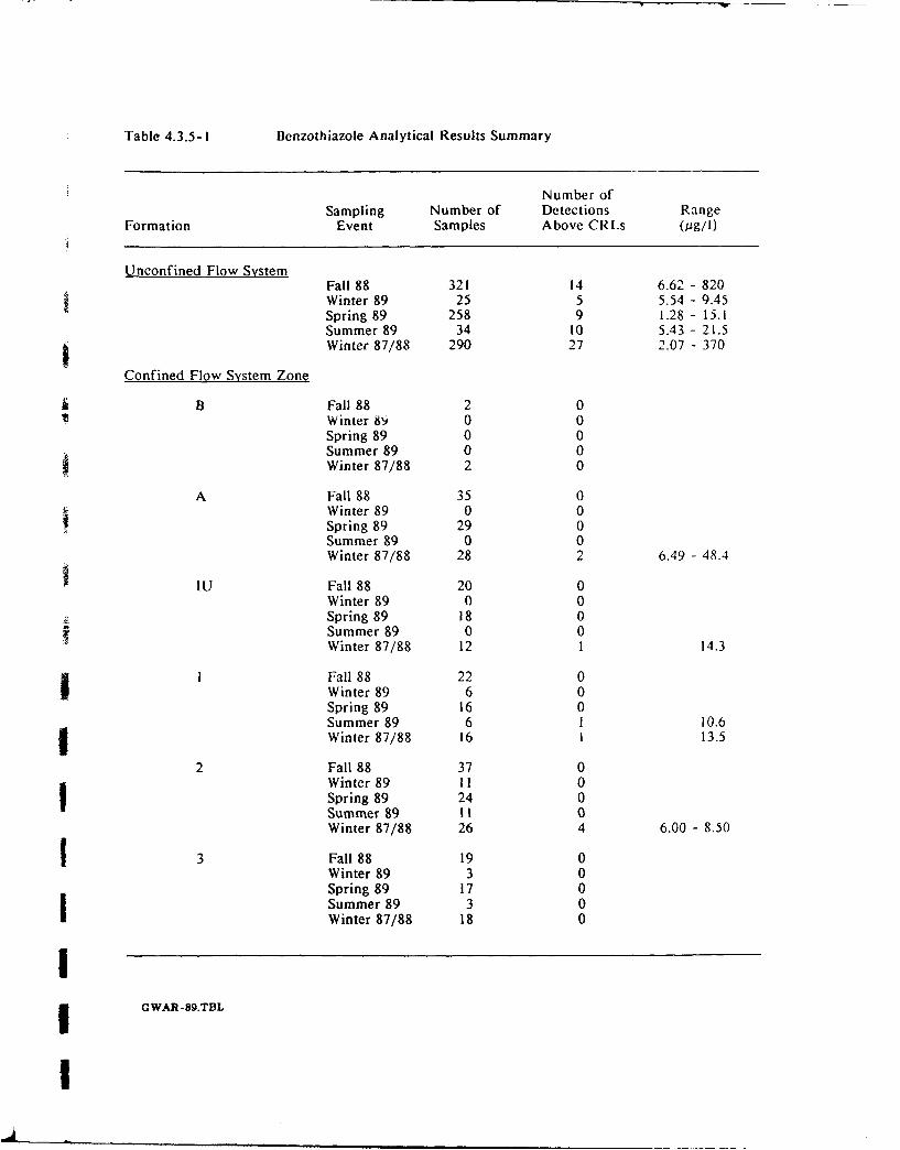
Table 4.3.5-I Benzothiazole Analytical Results Summary
Number ofSampling Number of Detections Range
Formation Event Samples Above CRLs (Gg/I)
Unconfined Flow SystemFall 88 321 14 6.62 - 820Winter 89 25 5 5.54 - 9.45Spring 89 258 9 1.28 - 15.1Summer 89 34 10 5.43 - 21.5Winter 87/88 290 27 2.07 - 370
Confined Flow System Zone
B Fall 88 2 0Winter 89 0 0Spring 89 0 0Summer 89 0 0Winter 87/88 2 0
A Fall 88 35 0Winter 89 0 0Spring 89 29 0Summer 89 0 0Winter 87/88 28 2 6.49 - 48.4
IU Fall 88 20 0Winter 89 0 0Spring 89 18 0Summer 89 0 0Winter 87/88 12 1 14.3
1 Fall 88 22 0Winter 89 6 0Spring 89 16 0Summer 89 6 1 10.6Winter 87/88 16 1 13.5
2 Fall 88 37 0Winter 89 11 0Spring 89 24 0Summer 89 11 0Winter 87/88 26 4 6.00 - 8.50
3 Fall 88 19 0Winter 89 3 0Spring 89 17 0Summer 89 3 0Winter 87/88 18 0
g G WAR-89.TBL
I
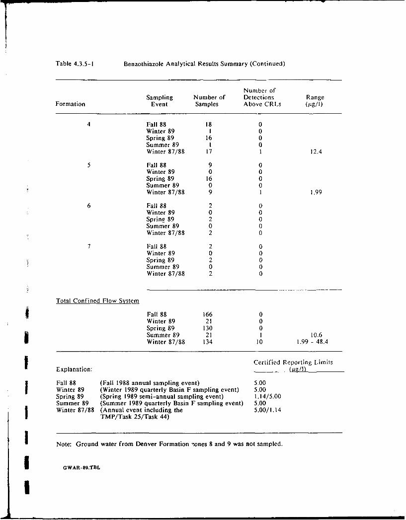
Table 4.3.5-I Benzothiazole Analytical Results Summary (Continued)
Number ofSampling Number of Detections Range
Formation Event Samples Above CRLs (Ag/i)
4 Fall 88 18 0Winter 89 1 0Spring 89 16 0Summer 89 1 0Winter 87/88 17 1 12.4
5 Fall 88 9 0Winter 89 0 0Spring 89 16 0Summer 89 0 0Winter 87/88 9 I 1.99
6 Fall 88 2 0Winter 89 0 0Spring 89 2 0Summer 89 0 0Winter 87/88 2 0
7 Fall 88 2 0Winter 89 0 0Spring 89 2 0Summer 89 0 0Winter 87/88 2 0
Total Confined Flow System
9 Fall 88 166 0Winter 89 21 0Spring 89 130 0Summer 89 21 1 10.6Winter 87/88 134 10 1.99 - 48.4
Certified Reporting LimitsExplanation: ("g/1)
Fall 88 (Fall 1988 annual sampling event) 5.00Winter 89 (Winter 1989 quarterly Basin F sampling event) 5.00Spring 89 (Spring 1989 semi-annual sampling event) 1.14/5.00Summer 89 (Summer 1989 quarterly Basin F sampling event) 5.00Winter 87/88 (Annual event including the 5.00/1.14
TMP/Task 25/Task 44)
Note: Ground water from Denver Formation tones 8 and 9 was not sampled.
I G WAR-89.TBL,
i!G
The Basin F plume extended from the Basin F area downgradient along the Basin F Pathway
about 3,000 ft. Reported concentrations at wells within the plume ranged from 9.05 to 41.9 jig/I.
The highest concentration was reported in Well 26041, near the southern or upgradient end of the
plume.
Benzothiazole was detected in four isolated wells at concentrations ranging from 7.76 to 430 ug/i.
Benzothiazole was also detected along the Basin F East Pathway, on the northeast side of Basin A,
and southwest of Basin F.
4.3.5.2 Confined Flow System. During the fall of 1988, 166 ground-water samples were9 collected from the confined flow system and analyzed for benzothiazole. Of these, no sample had
a detectable concentration of benzothiazole.
4.3.5.3 Winter 1987/88 and FY89 Comparison. Benzothiazole was detected , -,- of 290
samples in the unconfined flow system in winter 1987/88, while 14 of 321 samples had detections
in the fall of 1988. In both the winter of 1987/88 and fall of 1988 benzothiazole was detected in
the South Plants - Basin A, and Basin F pathways. However, the plumes were less extensive in
the fall, 1988. Wells where benzothiazole concentrations varied considerably from previous or
subsequent sampling periods are listed in Table 4.3.3-2.
Benzothiazole was not detected in any of the 166 samples from the confined flow system in the
fall of 1988, including 9 of the 10 wells with detectable concentrations in winter 1987/88. The
i data are summarized in Table 4.3.5-1. This illustrates the variability of the Denver aquifer
system. Thus, data interpretation based on a single sample period may not be effective in
recognizing anomalous data. Variations in benzothiazole concentrations should be considered
appropriately.
4.3.6 Organosulfur Compounds
Analyses for one or more of the organosulfur compounds p-chlorophenylmethyl sulfide, sulfoxide
and sulfone were performed on 487 ground-water samples obtained during the fall of 1988. The
CRLs for the fall 1988 sampling round ranged from 5.69 to 11.5 pg/I. Organosulfur compound
concentrations above CRLs ranging from 7.96 pg/I to 9440 ug/I were detected in 53 of the samples
analyzed. The balance of the samples did not contain detectable concentrations of organosulfur
compounds. Organosulfur compounds were detected above CRLs in the confined flow system in
four samples from zones A, IU, I and 2. The distribution of organosulfur compounds in the
unconfined flow system for the fall 1988 sampling is presented in Figure 4.3.6-1. Detections of
GWAR-89.4Rev. 06/21/90 - 59 -
I
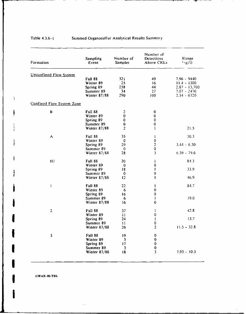
Table 4.3.6-I Summed Organosulfur Analytical Results Summary
Number ofSampling Number of Detections Range
Formation Event Samples Above CRLs ,4g/0)
Unconfined Flow SystemFall 88 321 49 7.96 - 9440Winter 89 25 16 11.4 - 1300Spring 89 258 44 2.87 - 13,700Summer 89 34 27 7.07 - 2470Winter 87/88 290 100 2.54 - 6320
Confined Flow System Zone
B Fall 88 2 0Winter 89 0 0Spring 89 0 0Summer 89 0 0Winter 87/88 2 1 21.5
A Fall 88 35 1 30.3Winter 89 0 0Spring 89 29 2 3.44 - 6.30Summer 89 0 0Winter 87/88 28 3 6.39 - 79.6
IU Fall 88 20 1 84.3Winter 89 0 0Spring 89 18 I 33.9Summer 89 0 0Winter 87/88 12 1 46.9
SFall 88 22 I 84.7Winter 89 6 0Spring 89 16 0Summer 89 6 1 19.0Winter 87/88 16 0
2 Fall 88 37 1 42.8Winter 89 11 0Spring 89 24 1 13.7Summer 89 11 0Winter 87/88 26 2 11.5 - 32.8
3 Fall 88 19 0Winter 89 3 0Spring 89 17 0Summer 89 3 0Winter 87/88 18 3 7.93 - 10.3
II G WAR-89.TBL
i
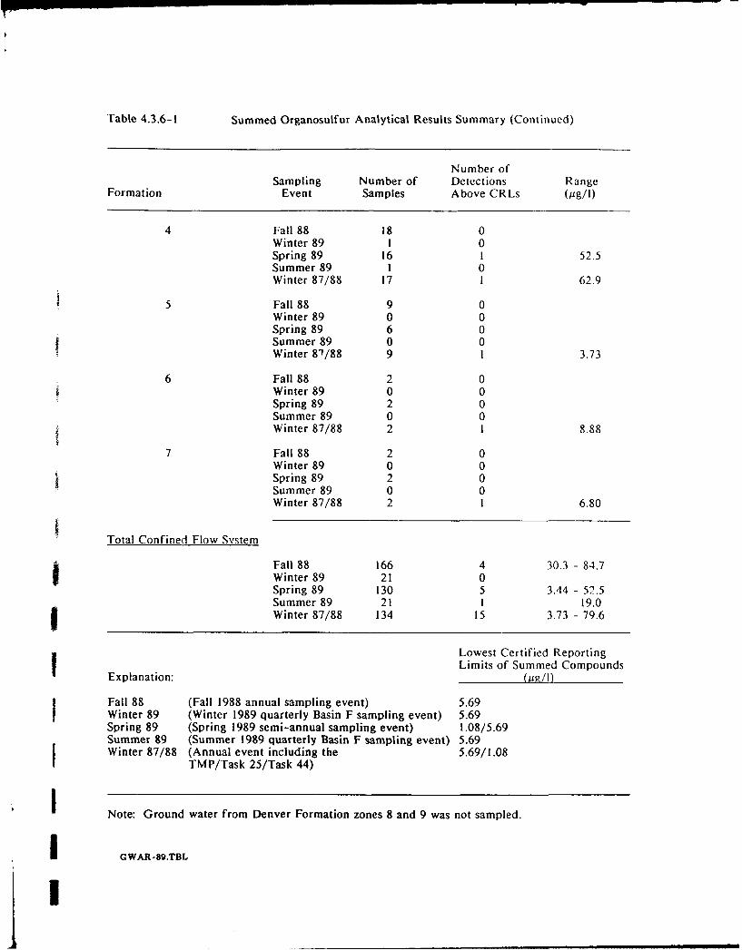
Table 4.3.6-1 Summed Organosulfur Analytical Results Summary (Continued)
Number ofSampling Number of Detections Range
Formation Event Samples Above CRLs (jig/I)
4 Fall 88 18 0Winter 89 I 0Spring 89 16 1 52.5Summer 89 1 0Winter 87/88 17 i 62.9
5 Fall 88 9 0
Winter 89 0 0Spring 89 6 0Summer 89 0 0Winter 87/88 9 I 3.73
6 Fall 88 2 0Winter 89 0 0Spring 89 2 0Summer 89 0 0Winter 87/88 2 1 8.88
7 Fall 88 2 0Winter 89 0 0Spring 89 2 0Summer 89 0 0Winter 87/88 2 1 6.80
Total Confined Flow System
Fall 88 166 4 30.3 - 84.7Winter 89 21 0Spring 89 130 5 3.44 - 52.5
Summer 89 21 i 19.0Winter 87/88 134 15 3.73 - 79.6
Lowest Certified ReportingLimits of Summed Compounds
Explanation: (__g/1)
Fall 88 (Fall 1988 annual sampling event) 5.69Winter 89 (Winter 1989 quarterly Basin F sampling event) 5.69Spring 89 (Spring 1989 semi-annual sampling event) 1.08/5.69Summer 89 (Summer 1989 quarterly Basin F sampling event) 5.69Winter 87/88 (Annual event including the 5.69/1.08
TMP/Task 25/Task 44)
Note: Ground water from Denver Formation zones 8 and 9 was not sampled.
GWAR-89.TBL
the organosulfur compounds in both the unconfined and confined flow systems for FY89 are
summarized in Table 4.3.6-1.
In summing the organosulfur compounds, the resulting distribution maps include compounds thatmay have originated from different sources. Consequently, the analyte-specific plume maps of
constituents within this group are considered more accurate than the summed organosulfur maps
for depicting and interpreting ground-water quality degradation.
4.3.6.1 Unconfined Flow System. Ground-water samples from 321 unconfined wells were
analyzed for organosulfur compounds. Of these, 49 contained concentrations of organosulfur
compounds above CRLs, with concentrations ranging from 7.96 to 9440 jig/l. The highest CRL
for the organosulfur compounds (11.5 pug/I for p-chlorophenylmethyl sulfoxide) was used as the
lowest contour value in constructing the contaminant distribution map shown in Figure 4.3.6-1.
Organosulfur compounds were detected in the South Plants-Basin A - A Neck Pathway, the
Basin F Pathway, and the Northern Off-Post Pathway. One isolated detection was reported in
Section 26, along the Basin F East Pathway.IThe plume in the South Plants-Basin A - A Neck Pathway trends primarily north from an area
of high concentration located in northwestern Section 1. The area of high concentration coincides
with the South Plants ground-water mound. The plume trends northwest through the Basin ANeck pathway to the southcentral portion of Section 26. Summed concentrations detected at wells
within the plume ranged from 14.3 to 9440 pug/l, with the highest detection reported in Well 01525
located in northwestern Section 1. A discrepancy in reported values within the plume was
observed in Wells 36001 and 36181 located adjacent to each other in the southwest corner of
Section 36. The concentration in Well 36001 was 171 pg/I and below CRL in Well 36181. GC/MSdata indicated the presence of organosulfur compounds in Well 36181, which suggests that
organosulfur compounds are indeed present and the reported value in Well 36181 is probably not
representative of the actual distribution of organosulfur compounds in this area.
The Basin F plume trends north-northeast along the Basin F Pathway to the NBCS. Total
organosulfur concentrations reported within this plume ranged from 14.8 to 2160 pg/I. Thehighest concentration was in Well 23053 located near the eastern edge of Section 23. A second
area of high concentration within the plume is located just northeast of Basin F, where a
concentration of 1470 pg/I was reported in Well 26133.
GWAR-89.4Rev. 06/21/90 - 62 -
1
A plume downgradient of the NBCS extends along the Northern Off-Post Pathway. Total
organosulfur compounds detected in wells within this plume ranged from 34.6 to 100 Ag/I. Thehighest concentration was detected in Well 37344 in Section 12, near the leading edge of the
plume.
4.3.6.2 Confined Flow System. Analyses for the organosulfur compound-, p-
chlorophenylmethyl sulfide, sulfoxide and sulfone, were performed on 166 ground-water samples
obtained from the confined flow system during the fall of 1988. Concentrations ranging from 30.3
ug/I to 84.7 pg/I were detected in four of the samples analyzed. Zones A, I U, I, and 2 each hadone detection above CRLs. Point plots of the data are shown in Figures A-9 through A-Il. Fall
1988 analytical results are summarized in Table 4.3.6-1.
The maximum concentration and the deepest detection was in zone I at a depth of 163 ft in Well
36148. A similar concentration (84.3 pg/I) was detected in zone IU at a depth of 52.7 ft in Well
26096. Both of these wells are located in the vicinity of the Basin A Neck. Two other detections
occurred northeast of Basin F, directly below the Basin F plume in the unconfined flow system,and in Section 2, west of organosulfur detections in the South Plants area in the unconfined flow
system.
P 4.3.6.3 Winter 1987/88 and FY89 Comparison. Organosulfur compounds were detected in 100
of 290 wells sampled in the unconfined flow system during winter 1987/88 compared to 49 of 321
samples in fall 1988. The distribution of organosulfur compounds was generally similar during
both sampling periods; however, contamination in the South Lakes Pathway was only identifiedin the winter of 1987/88. Within the Basin A Neck the extent of organosulfur compounds are
better defined due to increased sampling density. Organosulfur compounds downgradient of the
NBCS were detected during both sampling periods however, detections in the First Creek Off-
Post Pathway occurred only during winter 1987/88. Wells with variable concentrations of
organosulfurs are listed in Table 4.3.2-2.
During the winter of 1987/88, organosulfur compounds were detected in 14 of 132 samples in
confined flow zones. This compares to 4 detections in 166 samples in tho fall of 1988. Table
4.3.6-1 summarizes the results for each of the confined zones. Detections in the confined flow
system in the winter of 1987/88 were more widespread laterally and vertically than in the fall of
1988. As previously stated, the Denver aquifer is very heterogeneous and substantial data
variability is likely to occur in any single sampling period. Therefore, variations such as those
noted in winter 1987/88 should be considered appropriately.
GWAR-89.4Rev. 06/21/90 - 63 -
4.3.7 Volatile Aromatics
The %,ciatile aromatics group includes benzene, chlorobenzene, toluene, ethylbenzene and the
x' 1.one isomers. Chlorobenzene is also an organohalogen, but because of its aromatic structure it
is included in this section. Chlorobenzene and benzene are discussed individually later in this
j section. Summed volatile aromatics were obtained by adding the concentrations of compounds in
this group.
t Volatile aromatics analyses were performed on 487 ground-water samples obtained during the fall
1988 annual monitoring. The CRLs for the fall 1988 CMP ranged from 0.820 to 1.47 ppg,/I.Concentrations of summed volatile aromatic compounds above CRLs, ranged from 0.991 to 240,000
M~g/I in 104 of these samples. Volatile aromatics were not detected in the balance of the samples.
U Detections were reported in the unconfined flow system and confined flow system (zones A, I.U,1, 2, 3 and 5). The distribution of total volatile aromatic compounds in RMA ground water for
FY89 is summarized in Table 4.3.7-1.
In summing the volatile aromatics, the resulting distribution maps include compounds that may
have originated from different sources. Consequently, the analvte-specific plume maps of
constituents within this group are considered more accurate than the summed .olatile aromatic
maps for depicting and interpreting ground-water quality degradation.
4.3.7.1 Unconfined Flow System. A total of 322 ground-water samples from the unconfined
9 flow system were analyzed for volatile aromatics. Of these, 71 had concentrations above the CRL
ranging from 0.991 to 240,000 Mg/I.
The highest CRL (1.47 jug/I) was used as the lowest contour interval to construct the plume map
shown in Figure 4.3.7-1. Plumes of volatile aromatics with ccncentrations above CRLs were
present in the South Plants-Basin A-Basin A Neck Pathway, near the NWBCS, and in the Basin
F and Northern Off-post Pathways.
There were two areas of high concentration within the South Plants-Basin A-Basin A Neck plume
which extend north and southwest from the ground-water mound in Section I. Ground water
flows radially away from the ground-water mound, to the north beneath Basin A, and south and
west in Sections I and 2. Reported concentrations ranged from 0.991 to 240,000 pg/I, with the
highest concentration occurring in Well 01014. The plume extended north through the Basin A
Pathway and terminated near the southwest corner of Section 26.
GWAR-89.4Rev. 06/21/90 - 64 -
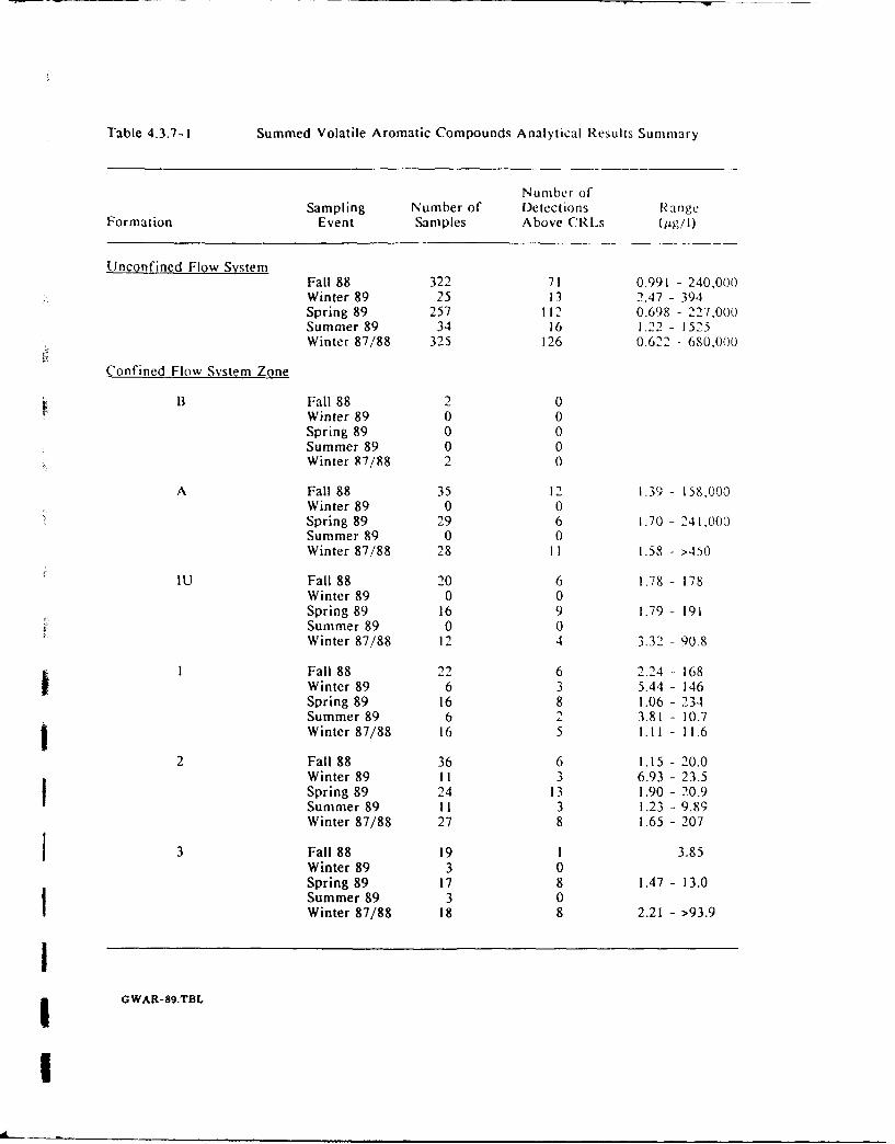
Table 4.3.7-I Summed Volatile Aromatic Compounds Analytical Results Summary
Number of
Sampling Number of Detections RangeFormation Event Samples Above CRLs (Og/I)
Unconfined Flow SystemFall 88 322 71 0.991 - 240,000Winter 89 25 13 2.47 - 394Spring 89 257 112 0.698 - 227,000Summer 89 34 16 1.22 - 1525Winter 87/88 325 126 0.622 - 680,000
Confined Flow System Zone
B Fall 88 2 0Winter 89 0 0Spring 89 0 0Summer 89 0 0Winter g7/88 2 0
A Fall 88 35 12 1.39 - 158,000Winter 89 0 0Spring 89 29 6 1.70 - 241,000Summer 89 0 0Winter 87/88 28 II 1.58 - >450
IU Fall 88 20 6 1.78 - 178Winter 89 0 0Spring 89 16 9 1.79 - 191Summer 89 0 0Winter 87/88 12 4 3.32 - 90.8
I Fall 88 22 6 2.24 - 168Winter 89 6 3 5.44 - 146Spring 89 16 8 1.06 - 234Summer 89 6 2 3.81 - 10.7Winter 87/88 16 5 1.11 - 11.6
2 Fall 88 36 6 1.15 - 20.0Winter 89 I1 3 6.93 - 23.5Spring 89 24 13 1.90 - 20.9Summer 89 I1 3 1.23 - 9.89Winter 87/88 27 8 1.65 - 207
3 Fall 88 19 I 3.85Winter 89 3 0Spring 89 17 8 1.47 - 13.0Summer 89 3 0Winter 87/88 18 8 2.21 - >93.9
II G WAR-89.TBL
I
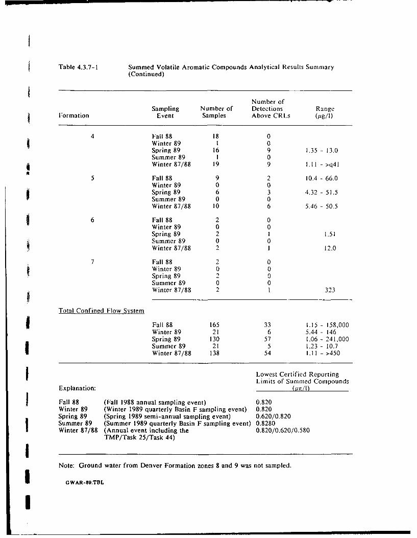
Table 4.3.7-1 Summed Volatile Aromatic Compounds Analytical Results Summary(Continued)
Number of
Sampling Number of Detections RangeFormation Event Samples Above CRLs (6g/i)
4 Fall 88 18 0Winter 89 1 0Spring 89 16 9 1.35 - 13.0Summer 89 i 0Winter 87/88 19 9 1.11 - >q41
5 Fall 88 9 2 10.4 - 66.0Winter 89 0 0Spring 89 6 3 4.32 - 51.5Summer 89 0 0Winter 87/88 10 6 5.46 - 50.5
96 Fall 88 2 0Winter 89 0 0Spring 89 2 1 1.51Summer 89 0 0Winter 87/88 2 1 12.0
7 Fall 88 2 0Winter 89 0 0Spring 89 2 0Summer 89 0 0Winter 87/88 2 i 323
Total Confined Flow System
U Fall 88 165 33 1.15 - 158,000Winter 89 21 6 5.44 - 146Spring 89 130 57 1.06 - 241,000Summer 89 21 5 1.23 - 10.7Winter 87/88 138 54 1.11 - >450
Lowest Certified ReportingLimits of Summed Compounds
Explanation: (tt/.l)
Fall 88 (Fall 1988 annual sampling event) 0.820Winter 89 (Winter 1989 quarterly Basin F sampling event) 0.820Spring 89 (Spring 1989 semi-annual sampling event) 0.620/0.820Summer 89 (Summer 1989 quarterly Basin F sampling event) 0.8280Winter 87/88 (Annual event including the 0.820/0.620/0.580
TMP/Task 25/Task 44)INote: Ground water from Denver Formation zones 8 and 9 was not sampled.
I GWAR-89.TBL
I
I m m mm~ llnllnllmllml~ i•u lm•Il mm
Volatile aromatics also have been detected near the NWBCS. Two small plumes were present
northwest of the Basin F Northwest, and Basin A Neck Pathways in Sections 22 and 27,
respectively. Detected concentrations ranged from 1.69 to 2.52 pg/I in Section 22 and from 1.77
to 257 pug/I in Section 27.
The Basin F plume extended from the Basin F area northeast along the Basin F Pathway to the
NBCS where it extended laterallij along the boundary system. Volatile aromatic compounds have
also been detected in the southern portion of Section 13. Detected concentrations within the on-
post plume range from 1.93 to 219 pg/i (Well 26148). The maximum concentration was detected
near the northeast corner of Basin F.
Isoiated detections ranged in concentration from 2.05 to 2.14 pg/I in two off-post wells and from
1.05 to 142 pg/l in 15 on-post wells. The two highest concentrations, 74.8 and 142 pg/I, were
detected in Section 9 in the Western Tier area.
4.3.7.2 Confined Flow System. Total volatile aromatic analyses were performed on 165
samples, with 33 detections ranging from 1.15 to 158,000 pg/l. Benzene and chlorobenzene are
the most frequently detected compounds in the total volatile aromatic group. The majority of
above-CRL reports were in samples from Denver Formation zones A, IU, I and 2. Zone 5 had
two above-CRL detections, zone 3 had only one above-CRL detection, and zones B, 4, 6 and 7
had no detections. Analytical results for the confined flow system from fall 1988, winter 1989,
spring 1989, and summer 1989 sampling periods are summarized in Table 4.3.7-1. Point plots
j from the fall 1988 sampling period are presented in Figures A-12 through A-14.
In general, volatile organics in the confined flow system can be associated with contamination inthe overlying unconfined flow system. In several cases, concentrations in the confined flow
system were similar to those in the unconfined flow system directly above it. The most notable
example of increasing concentration in deeper zones occurred in the South Plants-Basin A-Basin
A Neck area. A concentration of 158,000 pg/I was detected near the southwest corner of Section
36 in Well 36182. This well is completed in zone A, directly below water in the unconfined flow
system with a concentration of 108,000 pg/l. In zones IU, I and 2, detections primarily occurred
in the area northwest of Basin A to the southwest end of the Basin F plume. Detections in zones
3 and 5 were on-post near the northern and northwest boundaries of RMA. Toward the northwest
boundary of RMA, the lower stratigraphic zones are progressively closer to the surface as higher( (or younger) zones subcrop in a northwest direction and the wells typically are completed in the
lower zones. Therefore, the distribution of some of these detections was due to the well network.
The deepest detection of volatile aromatics during the fall of 1988 occurred in Well 36171 at a
G WAR-89.4Rev. 06/21/9o - 67 -
concentration of 2.93 pug/I. This well is completed 173 ft below ground level in zone I and is
located along the western edge of Basin A.
4.3.7.3 Winter 1987/88 and FY89 Comparison. Volatile aromatics were detected in 126 of 325
winter 1987/88 samples from the unconfined flow system compared to 71 of 323 samples in the
fall of 1988. Although concentrations varied slightly, plume configurations in the South Plants -
Basin A and Basin F areas are similar in fall 1988 and winter 1987/88. However, fall 1988 data
show an extended plume through the Basin A Neck area due to the addition of new wells in the
fall 1988 sampling period. Plume configurations at the boundary systems have changed between
the two sampling periods. The winter 1987/88 data show a plume south of the NWBCS which
extends off post through the Northwest Pathway. The fall 1988 data indicate that the plume is not
present off-post. The winter 1987/88 data show plumes, at the eastern and western ends of the
NBCS, both on- and off-post. The fall 1989 data show isolated detections of volatile aromatic
compounds in these areas. In general, the extent of volatile aromatic compounds north of the
NBCS is reduced relative to last year. Winter 1987/88 volatile aromatic plume in the RMA
Western Tier is not supported by fall 1988 data. Wells where volatile aromatic concentrations
varied considerably from previous or subsequent sampling rounds are listed in Table 4.3.2-2.
Volatile aromatic compounds were detected in 54 of 138 confined flow system samples in the
winter of 1987/88 while 33 of 165 samples recorded detections in the fall of 1988. Table 4.3.7-
1 summarizes the results for each of the confined zones. The distribution of summed volatile
aromatic compounds in the confined flow system was generally similar during both sampling
periods. However, there were more detections of volatile aromatics in the northern portion of
RMA and off-post of the NBCS in winter 1987/88. No volatile aromatic compounds were
detected in the confined flow system off-post in fall 1988. Interpretations of the data based on
a single sampling period may not be effective in recognizing anomalous data, due to the variability
of the Denver aquifer.
4.3.8 Benzene
Benzene analyses were conducted on 487 samples collected during the fall of 1988. The CRL
value was 1.05 pg/l. Concentrations which exceeded the CRL ranged from 1.25 pig/I to 240,000
A g/l in 72 of these samples. Benzene was detected in zones A, I U, 1, 2, 3 and 5 of the Denver
Formation. Detections in both unconfined and confined flow systems in the fall of 1988 are
f summarized in Table 4.3.8-1.
IGWAR-89.4Rev. 06/21/90 - 68 -
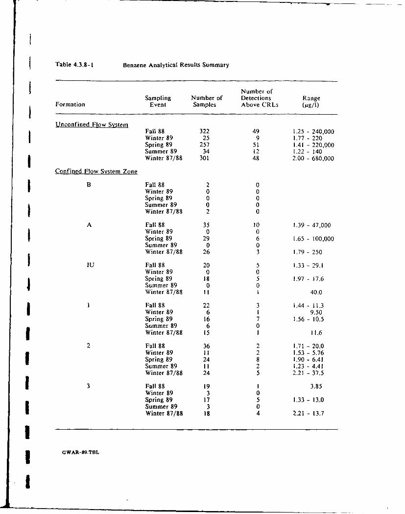
Table 4.3.8- 1 Benzene Analytical Results Summary
I Number ofSampling Number of Detections Range
Formation Event Samples Above CRLs (Gg/I)
Unconfined Flow SystemFall 88 322 49 1.25 - 240,000Winter 89 25 9 1.77 - 220Spring 89 257 51 1.41 - 220,000Summer 89 34 12 1.22 - 140SWinter 87/88 301 48 2.00 - 680,000
Confined Flow System Zone
B Fall 88 2 0Winter 89 0 0Spring 89 0 0Summer 89 0 0Winter 87/88 2 0
A Fall 88 35 10 1.39 - 47,000Winter 89 0 0Spring 89 29 6 1.65 - 100,000Summer 89 0 0Winter 87/88 26 3 1.79 - 250
IU Fall 88 20 5 1.33 - 29.1Winter 89 0 0Spring 89 18 5 1.97 - 17.6Summer 89 0 0Winter 87/88 11 i 40.0
SFall 88 22 3 1.44 - 11.3Winter 89 6 1 9.50Spring 89 16 7 1.56 - 10.5Summer 896
Winter 87/88 15 1 11.6
2Fall 88 36 2 1.71 - 20.0Winter 89 11 2 1.53 - 5.76Spring 89 24 8 1.90 - 6.41Summer 89 11 2 1.23 - 4.41
Winter 87/88 24 5 2.21 - 37.5
3 Fall 88 19 1 3.85Winter 89 3 0Spring 89 17 5 1.33 - 13.0Summer 89 3 0Winter 87/88 18 4 2.21 - 13.7
II GWAR-89.TBL
!
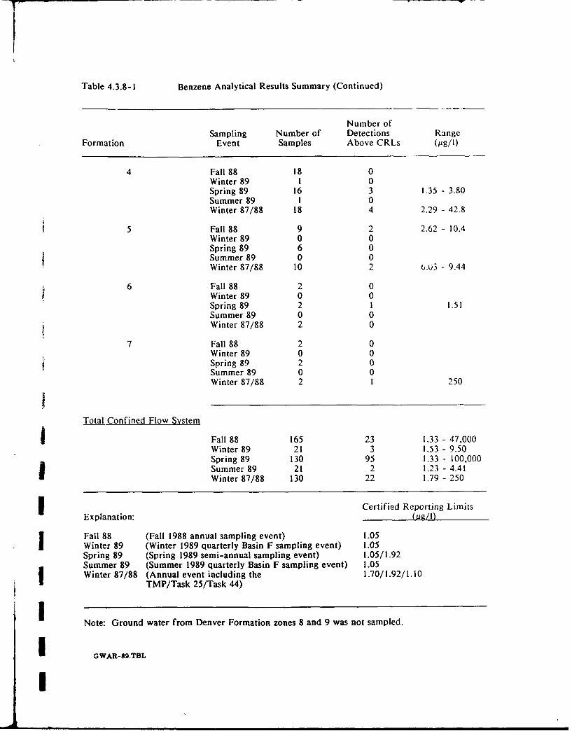
Table 4.3.8-1 Benzene Analytical Results Summary (Continued)
Number ofSampling Number of Detections Range
Formation Event Samples Above CRLs (jig/I)
4 Fall 88 18 0Winter 89 1 0Spring 89 16 3 1.35 - 3.80Summer 89 1 0Winter 87/88 18 4 2.29 - 42.8
5 Fall 88 9 2 2.62 - 10.4Winter 89 0 0Spring 89 6 0Summer 89 0 0Winter 87/88 10 2 u.u3 - 9.44
6 Fall 88 2 0Winter 89 0 0Spring 89 2 1 1.51Summer 89 0 0Winter 87/88 2 0
7 Fall 88 2 0Winter 89 0 0Spring 89 2 0Summer 89 0 0Winter 87/88 2 1 250
Total Confined Flow System
Fall 88 165 23 1.33 - 47,000Winter 89 21 3 1.53 - 9.50Spring 89 130 95 1.33 - 100,000Summer 89 21 2 1.23 - 4.41Winter 87/88 130 22 1.79 - 250
Certified Reporting LimitsExplanation: (uOR!)
j Fall 88 (Fall 1988 annual sampling event) 1.05Winter 89 (Winter 1989 quarterly Basin F sampling event) 1.05Spring 89 (Spring 1989 semi-annual sampling event) 1.05/1.92Summer 89 (Summer 1989 quarterly Basin F sampling event) 1.05
j Winter 87/88 (Annual event including the 1.70/1.92/1.10TMP/Task 25/Task 44)
Note: Ground water from Denver Formation zones 8 and 9 was not sampled.
IGWAR-89.TBL
4.3.8.1 Unconfined Flow System. During the fall of 1988, 322 ground-water samples were
collected from wells completed in the unconfined flow system and analyzed for benzene.
Concentrations ranging from 1.25 pg/I to 240,000 ug/I were detected in 49 of the samples. The
CRL (1.05 p•g/I) was used as the lowest contour value in constructing the contaminant plume map
shown in Figure 4.3.8-1.
Benzene occurs primarily in two areas: South Plants-South Lakes - Basin A, and in the Basin F
Pathway from Basin F toward the NBCS. In addition, a small plume of benzene is present in
Sections 26 and 35 in the Basin A Neck.
Benzene in the South Plants-South Lakes - Basin A area had a concentration of 240,000 pg/I (Well
01014). Two plumes with elevated concentrations of benzene (greater than 10,000 ug/I) extend tothe north and to the southwest from the ground-water mound in the South Plants area of
Section 1.
Benzene was detected between 1.36 pug/i and 3.84 pug/I in three wells along the Basin A Neck
Pathway. This plume is not interpreted to be continuous with the South Plants - South Lakes -
Basin A plume.
The southern edge of the Basin F plume originated in the Basin F area and extended through theBasin F pathway to the NBCS. The highest concentration in this plume was 140 pg/I (Well 26148),
detected approximately 1,000 ft northeast of Basin F. The benzene plume extended laterally to
the east along the NBCS. Benzene also was detected in three wells north of the boundary system,
along the northern RMA border, at concentrations ranging from 2.11 to 8.49 pg/I.
In addition to the occurrences of benzene discussed above, benzene was detected in ten isolated
locations on RMA. Concentrations in these wells ranged from 1.69 to 11.6 pg/I. The highest was
detected in Well 27003 which is located to the south of the NWBCS.
4.3.8.2 Confined Flow System. Of 165 samples collected from confined flow system wells,
23 had detections ranging from 1.33 to 47,000 pg/l. Analytical results for the fall of 1988 are
summarized in Table 4.3.8-1. Point plots of fall 1988 analytical results are presented in Figures
A-15 through A-17.
The majority of detections occur in zones A and IU of the Denver Formation in the area directly
below and adjacent to the South Plants-Basin A plume in the unconfined flow system. Other
detections in the confined flow system occur in the Basin A Neck and along the northern and
GWAR-89.4Rev. 06/21/90 - 71 -
i
northwestern RMA boundaries. Although several of the detections in the confined flow system
beneath South Plants-Basin A correlate with detections in the unconfined flow system, detections
along the northwest RMA boundary do not generally correspond to the benzene distribution in the
overlying unconfined flow system.
The highest detection in the confined flow system was in Well 36182 at a depth of 75.0 ft (zone
A). This well is located near the southwest corner of Section 36 where some of the highest
concentrations in the unconfined flow system occur. Benzene concentrations in other wells were
significantly lower and ranged from 1.33 to 20.0 pg/I with one detection >40.2 ug/I. This
occurred in Well 02030, located west of the South Plants-Basin A unconfined flow system plume.
The deepest benzene contamination in the confined flow system occurred at 173 ft in Well 36171
(2.93 pg/i), completed in Denver zone 1. Well 36171 is located along the western edge of Basin A.
4.3.8.3 Winter 1987/88 and FY89 Comparison. Benzene was detected in 48 of 301 winter
1987/88 samples from the unconfined flow system and in 49 of 322 samples in fall 1988. Benzene
was present in the South Plants - South Lakes - Basin A Pathway and the Basin F Pathway in
both annual sampling programs. A northeast Basin A extension of the plume is indicated by fall
1988 data. Differences between the fall 1988 and winter 1987/88 distribution of benzene occurred
in the RMA Western Tier. A plume was mapped in this area for winter 1987/88, but fall 1988
data did not substantiate the presence of benzene. Wells where benzene concentrations varied
considerably from previous or subsequent sampling rounds are listed in Table 4.3.2-2.
Benzene was detected in 22 of 130 samples from the confined flow system during winter 1987/88.
Of the 165 samples collected in fall 1988, 23 had detections. Table 4.3.8-1 summarizes the results
for each of the confined zones. During both sampling periods, benzene occurred in South Plants,Basin A Neck, NBCS and NWBCS areas Due to the nature of the Denver aquifer, data
interpretation based on a single sampling period may not be effective in recognizing anomalous
data.
f 4.3.9 Chlorobenzene
Chlorobenzene analyses were performed on 488 ground-water samples collected during the fall
of 1988. The CRL for the fall of 1988 was 0.820 #g/l. Chlorobenzene concentrations ranging
from 0.991 to 110,000 pg/I were reported in 49 samples. Chlorobenzene was reported in zones
A, JU, 1, 2 and 5 of the unconfined flow system. Detections in both the unconfined and
confined flow systems during the fall of 1988 are summarized in Table 4.3.9-1.
1GWAR-89.4Rev. 06/21/9o - 72 -
I
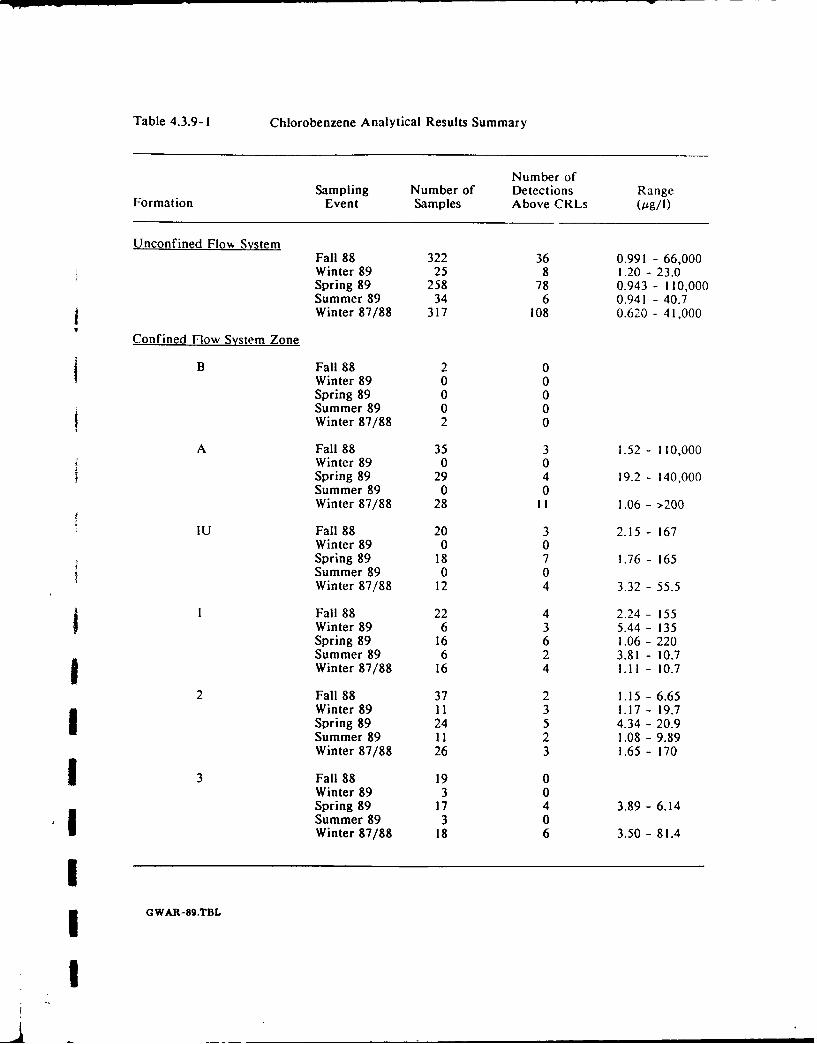
Table 4.3.9-1 Chlorobenzene Analytical Results Summary
Number ofSampling Number of Detections Range
Formation Event Samples Above CRLs (.ig/I)
Unconfined Flow SystemFall 88 322 36 0.991 - 66,000Winter 89 25 8 1.20 - 23.0Spring 89 258 78 0.943 - 110,000Summer 89 34 6 0.941 - 40.7Winter 87/88 317 108 0.620 - 41,000
Confined Flow System Zone
B Fall 88 2 0Winter 89 0 0Spring 89 0 0Summer 89 0 0Winter 87/88 2 0
A Fall 88 35 3 1.52 - 110,000Winter 89 0 0Spring 89 29 4 19.2 - 140,000Summer 89 0 0Winter 87/88 28 II 1.06 - >200
IU Fall 88 20 3 2.15 - 167Winter 89 0 0Spring 89 18 7 1.76 - 165Summer 89 0 0Winter 87/88 12 4 3.32 - 55.5
SFall 88 22 4 2.24 - 155Winter 89 6 3 5.44 - 135Spring 89 16 6 1.06 - 220Summer 89 6 2 3.81 - 10.7Winter 87/88 16 4 1.11 - 10.7
2 Fall 88 37 2 1.15 - 6.65Winter 89 11 3 1.17 - 19.7Spring 89 24 5 4.34 - 20.9Summer 89 !1 2 1.08 - 9.89Winter 87/88 26 3 1.65 - 170
3 Fall 88 19 0Winter 89 3 0Spring 89 17 4 3.89 - 6.14Summer 89 3 0Winter 87/88 18 6 3.50 - 81.4
Il GWAR-89.TBL
IA _ _ _ _ _ _ _ _ _ _ _ _ _
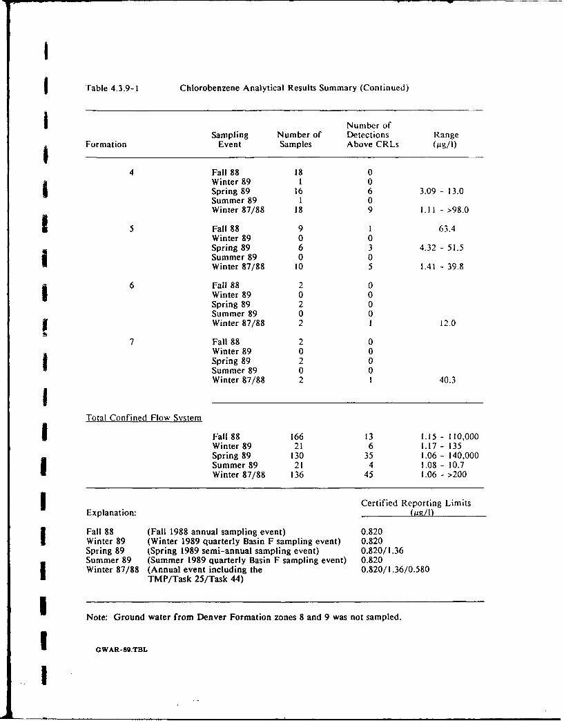
iI
Table 4.3.9-1 Chlorobenzene Analytical Results Summary (Continued)
I Number ofSampling Number of Detections Range
Formation Event Samples Above CRLs (Ag/i)
4 Fall 88 18 0Winter 89 1 0Spring 89 16 6 3.09 - 13.0Summer 89 1 0Winter 87/88 18 9 1.1 1 - >98.0
5 Fall 88 9 1 63.4Winter 89 0 0Spring 89 6 3 4.32 - 51.5Summer 89 0 0Winter 87/88 10 5 1.41 - 39.8
6 Fall 88 2 0Winter 89 0 0Spring 89 2 0
Summer 89 0 0Winter 87/88 2 1 12.0
7 Fall 88 2 0Winter 89 0 0Spring 89 2 0Summer 89 0 0Winter 87/88 2 1 40.3I
Total Confined Flow System
I Fall 88 166 13 1.15 - 110,000Winter 89 21 6 1.17 - 135Spring 89 130 35 1.06 - 140,000Summer 89 21 4 1.08 - 10.7Winter 87/88 136 45 1.06 - >200
I Certified Reporting LimitsExplanation: (tA/I)
Fall 88 (Fall 1988 annual sampling event) 0.820Winter 89 (Winter 1989 quarterly Basin F sampling event) 0.820Spring 89 (Spring 1989 semi-annual sampling event) 0.820/1.36Summer 89 (Summer 1989 quarterly Basin F sampling event) 0.820Winter 87/88 (Annual event including the 0.820/1.36/0.580
TMP/Task 25/Task 44)
Note: Ground water from Denver Formation zones 8 and 9 was not sampled.
IGWAR-89.TBL
.I
S4.3.9.1 Unconfined Flow System. Chlorobenzene was detected in 36 of 322 ground-water
samples from the unconfined flow system. Concentrations ranged from 0.991 to 66,000 Mg/I. The
j CRL of 0.820 pg/I was used as the lowest contour line in constructing the contaminant distribution
map shown in Figure 4.3.9-1 of this report.
I Chlorobenzene was detected in the South Plants-Basin A Pathway, Basin A Neck, Basin F and
Northern Off-Post Pathways. The South Plants-Basin A plume originates in the South Plants area
and extended both north across Basin A and southwest across northwestern Section I into Section
2. Reported concentrations in this plume ranged from 0.991 to 66,000 pg/I. The area of highest
concentration was located in southwest Section 36, just downgradient from South Plants. An area
of elevated concentration (1,400 ug/I) in the northeast corner of Section 36 was indicated by fall
1988 sampling results from Well 36180. The southwest extension of the plume in Section 2 is a
preliminary interpretation indicated by data from Well 02545 (340 p•g/l).
In the Basin F Pathway, a small, two-lobed plume was present immediately south of the NBCS._ Detections in Wells 23231 and 24184 within the plume were 1.14 and 32.3 pg/I, respectively.
Previous sampling results indicated chlorobenzene also was present near the northeast corner of
SBasin F (Wells 23049, 23096, 23106, 23239, 26133); however, chlorobenzene was not detected in
this area in the fall of 1988. The latter two CRLs were elevated due to dilutions during laboratory
analysis. Results from subsequent events confirmed the detections in Wells 23239 and 26133, but
not in Wells 23106 or 23049. Well 23096 was not sampled.
The plume in the Northern Off-Post Pathway extended north of the NBCS. Concentrations in
wells within the plume were 63.4 and 120 pg/I.
Isolated detections ranging from 1.11 to 240 pg/I occurred in seven on-post wells and one off-
post well. Four of the detections occurred in the vicinity of Basin F and the area to the
I northwest, one was detected near North Plants and two were present in Section 9 in the Western
Tier area. The off-post detection was in Section 14 near the northern RMA boundary.
4.3.9.2 Confined Flow System. Chlorobenzene analyses were performed on 166 ground-water
samples from the confined flow system, resulting in 13 sample concentrations above the CRL
during the fall of 1988. Concentration ranged from 1.15 to 110,000 pg/l, with detections reported
in zones A, IU, 1, 2 and 5. Analytical results for the Denver Formation are summarized in
I1 Table 4.3.9-1, and point plots of chlorobenzene detections from fall 1988 analytical results are
shown in Figures A-18 through A-19.
1GWAR-89.4Rev. 06/21/90 - 75 -
The highest concentration (110,000 ug/I) was reported in zone A in southwest Section 36 in Well
36182. The highest detection in the unconfined flow system (66,000 pg/I), also occurred in this
area, but was at a lower concentration than in the confined flow system. The deepest
chlorobenzene detection in the confined flow system was near the northwest end of Basin A in
Well 36179 (zone 1). A concentration of 155 ug/I was detected 151 ft below ground level. A
concentration of 12.4 pg/I was detected in the overlying unconfined flow system.
In general, chlorobenzene concentrations in the confined flow system were not areally coincident
with detections in the unconfined flow system. In addition to the observations described above,
concentration in the confined flow system was higher than in the unconfined flow system in the
Basin A area, north of Basin A, Basin A Neck area and the vicinity of Basin F. The largest
differences occurred in the northern area of Basin A where chlorobenzene was detected at
concentrations of 155 and 167 pg/I in zones I and IU, respectively, and at 12.4 and 3.09 pg/I in
the overlying unconfined flow system.
4.3.9.3 Winter 1987/88 and FY89 Comparison. Chlorobenzcne was detected in 108 of 317winter 1987/88 samples in the unconfined flow system compared to 36 of 322 samples in fall 1988.
j The chlorobenzene plume in the South Plants - Basin A areas maintains a similar configuration
between the winter 1987/88 and the fall 1988 periods. Differences between these sample periods,
however, are evident in other areas. Plumes previously identified in the Western Tier, Basin F,
Northwest, and Northern Off-Post Pathways were either not as extensive or not evident in the fall
1988 data. The Western Tier, Basin F, and NWBCS areas showed only isolated detections in the
fall 1988 sampling period. In the winter of 1987/88, the Northern Off-Post plume extended
approximately 4000 ft north of the NBCS in comparison to 1000 ft in the fall of 1988. Wells
where concentrations of chlorobenzene varied considerably are listed in Table 4.3.2-2.
In the winter of 1987/88, chlorobenzene was detected in 46 of 166 samples in comparison to 13
of 136 in the fall of 1988. Table 4.3.9-1 summarizes the results for each of the confined zones.
Detections occurred in both sampling rounds in Basin A, Basin A Neck, and Basin C areas.
Chlorobenzene was detected more frequently in the NBCS area during the winter 1987/88 sampling
program than in the fall 1988 program. No chlorobenzene was detected in the confined flow
system off-post in fall 1988. As previously stated, the heterogeneity of the Denver aquifer is
likely to produce data variability. Interpretations based on one sampling period should be
considered appropriately.II
GWAR-89.4Rev. 06/21190 - 76 -
I
4.3.10 Volatile Organohalogens
The compounds included in the volatile organohalogen (VOH) group are:
1,!-Dichloroethene
i ,2-Dichloroethene
1,1 -Dichloroethane
1,2-Dichloroethane
1,1,1 -Trichloroethane
1, 1,2-Trichloroethane
Carbon Tetrachloride
Chloroform (CHCL3)
Methylene Chloride
Tetrachloroethene (TCLEE)
Trichloroethene (TRCLE)
The summed concentrations of these 11 analytes are reported collectively as the total VOlt
concentration. Three analytes within this group: chloroform (CHCL3), tetrachloroethene
(TCLEE), and trichloroethene (TRCLE) are discussed separately later in this report.
SXVOH analyses were performed on 488 samples collected from the unconfined and confined flow
systems during the fall of 1988. A detection was recorded if one or more of the individual VOIH
compounds was identified. In the fall of 1988 there were 267 VOH detections ranging from 0.567
to 2,900,000 pg/l. VOH detections were reported in the confined flow system within zones B, A,
IU, 1, 2, 3, 4, and 5. Table 4.3.10-1 summarizes VOH detections in the unconfined and confined
flow systems.
4.3.10.1 Unconfined Flow System. A total of 217 VOH detections were reported among the
322 unconfined flow system samples collected during the fall of 1988. Concentrations ranged
from 0.570 to 2,900,000 pg/I. The highest CRL of the II VOH compounds (7.40 pg/l for
methylene chloride) was used as the lowest isoconcentration contour for preparing the VOH plume
map (Figure 4.3.10-1). On-post, VOH plumes were present in the South Plants-Basin A and South
Lakes Pathways, the Basin A Neck and Central Pathways, the Basin F West, Basin F East, and
Basin F Pathways, the Tier and Railyard-Motorpool Pathways, and the North Plants Pathway.
Off-post, plumes were identified in the Northwest, First Creek, and Northern Off-Post Pathways.
IGWAR-89.4Rev. 06/21/90 - 77 -
.3I
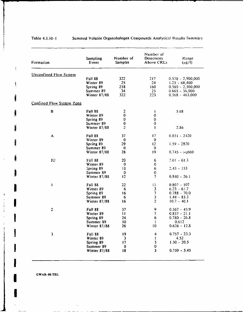
Table 4.3.10-I Summed Volatile Organohalogen Compounds Analytical Results Summary
Number ofSampling Number of Detections Range
Formation Event Samples Above CRLs (Oig/i)
Unconfined Flow SystemFall 88 322 217 0.570 - 2,900,000Winter 89 25 24 1.25 - 68,400Spring 89 258 160 0.580 - 2,500,000Summer 89 34 25 0.665 - 36,000
SWinter 87/88 322 223 0.568 - 463,000
Confined Flow System Zone
B Fall 88 2 1 5.68Winter 89 0 0Spring 89 0 0Summer 89 0 0Winter 87/88 2 1 2.86
A Fall 88 37 17 0.851 - 2420Winter 89 0 0Spring 89 29 12 1.59 - 2820Summer 89 0 0Winter 87/88 28 19 0.745 - >q660
IU Fall 88 20 6 2.01 - 61.3Winter 89 0 0Spring 89 13 6 2.43 - 153Summer 89 0 0Winter 87/88 12 7 0.840 - 26.1
1 Fall 88 22 11 0.807 - 107Winter 89 6 3 6.23 - 61.7Spring 89 16 7 0.788 - 70.0
Summer 89 6 3 1.44 - 83.3Winter 87/88 16 2 10.7 - 40.1
2 Fall 88 37 9 0.567 - 43.9Winter 89 11 7 0.857 - 21.1Spring 89 24 6 0.780 - 26.8Summer 89 10 I 0.612Winter 87/88 26 10 0.626 - 12.8
3 Fall 88 19 4 0.757 - 23.3Winter 89 3 1 4.52Spring 89 17 3 1.30 - 20.5Summer 89 0 0Winter 87/88 18 5 0.759 - 5.45
II GWAR-89.TBL
I
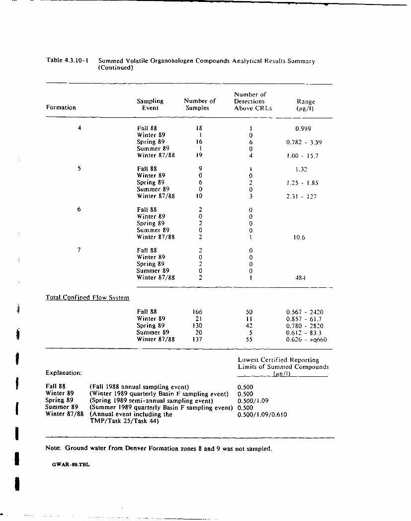
Table 4.3.10-I Summed Volatile Organohalogen Compounds Analytical Results Summary(Continued)
Number ofSampling Number of Detections Range
Formation Event Samples Above CRLs (Ag/I)
4 Fall 88 18 I 0.999Winter 89 1 0Spring 89 16 6 0.782 - 3.59Summer 89 1 0Winter 87/88 19 4 1.00 - 15.7
5 Fall 88 9 1 1.32Winter 89 0 0Spring 89 6 2 1.25 - 1.85Summer 89 0 0Winter 87/88 10 3 2.31 - 127
6 Fall 88 2 0Winter 89 0 0Spring 89 2 0Summer 89 0 0Winter 87/88 2 1 10.6
7 Fall 88 2 0Winter 89 0 0Spring 89 2 0Summer 89 0 0Winter 87/88 2 1 484
Total Confined Flow System
4Fall 88 166 50 0.567 - 2420Winter 89 21 I1 0.857 - 61.7Spring 89 130 42 0.780 - 2820Summer 89 20 5 0.612 - 83.3Winter 87/88 137 55 0.626 - >q660
f Lowest Certified ReportingLimits of Summed Compounds
Explanation: (ui!I)
SFall 88 (Fall 1988 annual sampling event) 0.500Winter 89 (Winter 1989 quarterly Basin F sampling event) 0.500Spring 89 (Spring 1989 semi-annual sampling event) 0.500/1.09Summer 89 (Summer 1989 quarterly Basin F sampling event) 0.500Winter 87/88 (Annual event including the 0.500/1.09/0.610
TMP/Task 25/Task 44)!Note: Ground water from Denver Formation zones 8 and 9 was not sampled.
IGWAR-89.TBL
I
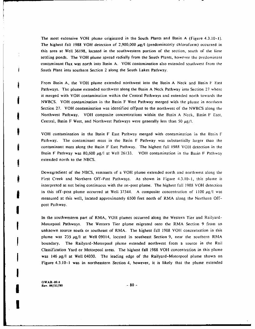
The most extensive VOH plume originated in the South Plants and Basin A (Figure 4.3.10-1).
The highest fall 1988 VOH detection of 2,900,000 pg/I (predominately chloroform) occurred in
this area at Well 36198, located in the southwestern portion of the section, south of the lime
settling ponds. The VOH plume spread radially from the South Plants, however the predominant
contaminant flux was north into Basin A. VOH contamination also extended southwest from the
South Plant into southern Section 2 along the South Lakes Pathway.
From Basin A, the VOH plume extended northwest into the Basin A Neck and Basin F East
Pathways. The plume extended northwest along the Basin A Neck Pathway into Section 27 where
it merged with VOH contamination within the Central Pathways and extended north towards the
NWBCS. VOH contamination in the Basin F West Pathway merged with the plume in northern
Section 27. VOH contamination was identified offpost to the northwest of the NWBCS along the
Northwest Pathway. VOH composite concentrations within the Basin A Neck, Basin F East,
Central, Basin F West, and Northwest Pathways were generally less than 50 pg/I.
VOH contamination in the Basin F East Pathway merged with contamination in the Basin F
Pathway. The contaminant mass in the Basin F Pathway was substantially larger than the
contaminant mass along the Basin F East Pathway. The highest fall 1988 VOH detection in the
Basin F Pathway was 80,600 g/Il at Well 26133. VOH contamination in the Basin F Pathway
extended north to the NBCS.
Downgradient of the NBCS, remnants of a VOH plume extended north and northwest along the
First Creek and Northern Off-Post Pathways. As shown in Figure 4.3.10-1, this plume is
interpreted as not being continuous with the on-post plume. The highest fall 1988 VOH detection
in this off-post plume occurred at Well 37344. A composite concentration of 1100 pg/I was
measured at this well, located approximately 6500 feet north of RMA along the Northern Off-
post Pathway.
In the southwestern part of RMA, VOH plumes occurred along the Western Tier and Railyard-
Motorpool Pathways. The Western Tier plume migrated onto the RMA Section 9 from an
unknown source south or southeast of RMA. The highest fall 1988 VOH concentration in this
plume was 235 pg/I at Well 09014, located in southeast Section 9, near the southern RMA
boundary. The Railyard-Motorpool plume extended northwest from a source in the Rail
Classification Yard or Motorpool areas. The highest fall 1988 VOH concentration in this plume
was 146 pg/I at Well 04030. The leading edge of the Railyard-Motorpool plume shown on
Figure 4.3.10-1 was in northeastern Section 4, however, it is likely that the plume extended
IGWAR-89.4Rev. 06/21/90 - 80 -
I1
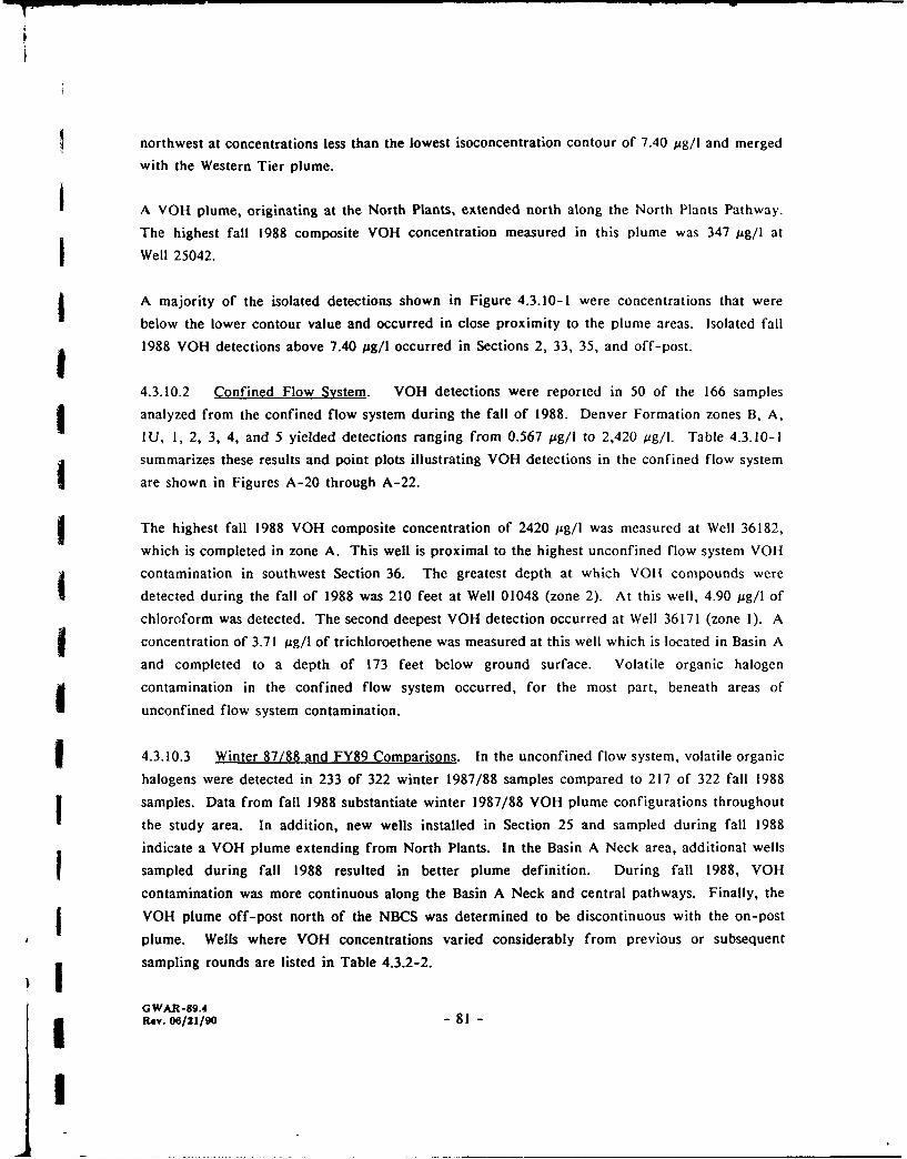
¶ northwest at concentrations less than the lowest isoconcentration contour of 7.40 pg/I and merged
with the Western Tier plume.
I A VOH plume, originating at the North Plants, extended north along the North Plants Pathway.
The highest fall 1988 composite VOH concentration measured in this plume was 347 pg/I at
Well 25042.
A majority of the isolated detections shown in Figure 4.3.10-1 were concentrations that were
below the lower contour value and occurred in close proximity to the plume areas. Isolated fall
1988 VOH detections above 7.40 pjg/I occurred in Sections 2, 33, 35, and off-post.
4.3.10.2 Confined Flow System. VOH detections were reported in 50 of the 166 samples
analyzed from the confined flow system during the fall of 1988. Denver Formation zones B, A,
IU, 1, 2, 3, 4, and 5 yielded detections ranging from 0.567 pg/I to 2,420 pug/I. Table 4.3.10-1
summarizes these results and point plots illustrating VOH detections in the confined flow system
are shown in Figures A-20 through A-22.
The highest fall 1988 VOH composite concentration of 2420 pg/i was measured at Well 36182,
which is completed in zone A. This well is proximal to the highest unconfined flow system VOlH
contamination in southwest Section 36. The greatest depth at which VOH compounds were
detected during the fall of 1988 was 210 feet at Well 01048 (zone 2). At this well, 4.90 pg/I of
chloroform was detected. The second deepest VOH detection occurred at Well 36171 (zone 1). A9 concentration of 3.71 pg/I of trichloroethene was measured at this well which is located in Basin A
and completed to a depth of 173 feet below ground surface. Volatile organic halogen
contamination in the confined flow system occurred, for the most part, beneath areas of
unconfined flow system contamination.
S4.3.10.3 Winter 87/88 and FY89 Comparisons. In the unconfined flow system, volatile organic
halogens were detected in 233 of 322 winter 1987/88 samples compared to 217 of 322 fall 1988
samples. Data from fall 1988 substantiate winter 1987/88 VOH plume configurations throughout
the study area. In addition, new wells installed in Section 25 and sampled during fall 1988
indicate a VOH plume extending from North Plants. In the Basin A Neck area, additional wells
sampled during fall 1988 resulted in better plume definition. During fall 1988, VOH
contamination was more continuous along the Basin A Neck and central pathways. Finally, the
I VOH plume off-post north of the NBCS was determined to be discontinuous with the on-post
plume. Wells where VOH concentrations varied considerably from previous or subsequent
SI sampling rounds are listed in Table 4.3.2-2.
G WAR-89.4Rev. 06/21/o O -81 -
I
Composite VOH compounds were detected in the confined flow system in 55 of 137 samples
analyzed during the winter of 1987/88 compared to 50 of 160 samples analyzed during the fall of
1988 (Table 4.3.10-1). Areas where VOH contamination was detected during both sampling
periods include the South Lakes, South Plants, Basin A and Basin A Neck, Section 26 and the
NBCS. Due to the general low hydraulic conductivity and large heterogeneity of the Denver
U Formation, substantial data variability is likely to occur in any single period.
4.3.11 Chloroform
Analyses for chloroform were performed on 488 ground-water samples collected during the fall
of 1988. Chloroform concentrations ranging from 0.567 to 2,900,000 pg/I were detected in 215
samples. The CRL for the fall 1988 monitoring program was 0.500 pg/l. Chloroform was
9 detected in the confined flow system in zones B, A, IU, 1, 2, and 3. The distribution of
chloroform in the unconfined flow system is illustrated in Figure 4.3.11-1. Unconfined and
confined flow system chloroform detections for FY89 are summarized in Table 4.3.1 I-1.
4.3.1 1.1 Unconfined Flow System. Ground-water samples collected from 322 wells completed
9 in the unconfined flow system were analyzed for chloroform during the fall of 1988.
Concentrations of chloroform ranging from 0.570 to 2,900,000 pg/I were measured in 173 of these
9 samples.
Based on the fall 1988 data, chloroform formed an areally extensive plume occupying the South
9 Plants-Basin A-Basin A Neck Pathways, the South Lakes and Central Pathways, and the Basin F
and Basin F East Pathways to the NBCS (Figure 4.3.11-1). Chloroform contamination off-post
was identified along the Northern Off-Post and Northwest Pathways. As illustrated in Figure
4.3.11-1 however, continuity of the chloroform plumes across the NBCS is interupted by
boundary system operations. Plumes of chloroform also were identified along the North Plants and
I Railyard-Motorpool Pathways.
The highest chloroform concentrations occurred along the South Plants-Basin A and Basin FPathways. The highest concentration of chloroform measured during the fall of 1988 was
2,900,000 pg/I at Well 36168, located adjacent to the South Plants. From the South Plants, the
chloroform plume migrated radially as a result of the South Plants ground-water mound.
j From the South Plants and Basin A, the chloroform plume extended west and northwest along the
Basin A Neck, Central North, and Central South Pathways, and north along the Basin F East
Pathway. The highest fall 1988 chloroform concentration along pathways to the west and
GWAR-89.4Rev. 06/21/90 - 82 -
I
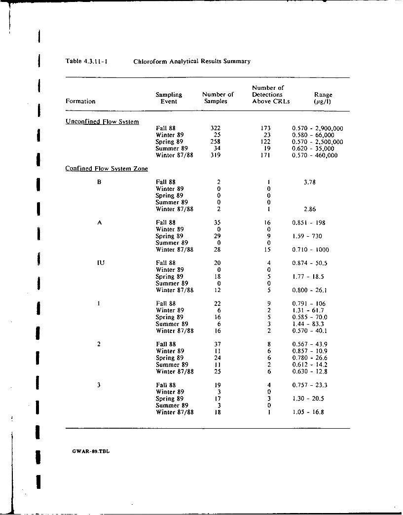
Table 4.3.11 - I Chloroform Analytical Results Summary
j Number ofSampling Number of Detections Range
Formation Event Samples Above CRLs (Jag/I)
Unconfined Flow SystemFall 88 322 173 0.570 - 2,900,000Winter 89 25 23 0.580 - 66,000Spring 89 258 122 0.570 - 2,500,000Summer 89 34 19 0.620 - 35,000
C Winter 87/88 319 171 0.570 - 460,000
Confined Flow System Zone
B Fall 88 2 1 3.78Winter 89 0 0Spring 89 0 0Summer 89 0 0Winter 87/88 2 i 2.86
A Fall 88 35 16 0.851 - 198Winter 89 0 0Spring 89 29 9 1.59 - 730Summer 89 0 0Winter 87/88 28 15 0.710 - 1000
IU Fall 88 20 4 0.874 - 50.5Winter 89 0 0Spring 89 18 5 1.77 - 18.5Summer 89 0 0Winter 87/88 12 5 0.800 - 26.1
1 Fall 88 22 9 0.791 - 106Winter 89 6 2 1.31 - 61.7Spring 89 16 5 0.585 - 70.0Summer 89 6 3 1.44 - 83.3Winter 87/88 16 2 0.570 - 40.1
2 Fall 88 37 8 0.567 - 43.9Winter 89 11 6 0.857 - 10.9Spring 89 24 6 0.780 - 26.6Summer 89 11 2 0.612 - 14.2Winter 87/88 25 6 0.630 - 12.8
13 Fall 88 19 4 0.757 - 23.3Winter 89 3 0Spring 89 17 3 1.30 - 20.5Summer 89 3 0Winter 87/88 18 1 1.05 - 16.8
II GWAR-89.TBL
I
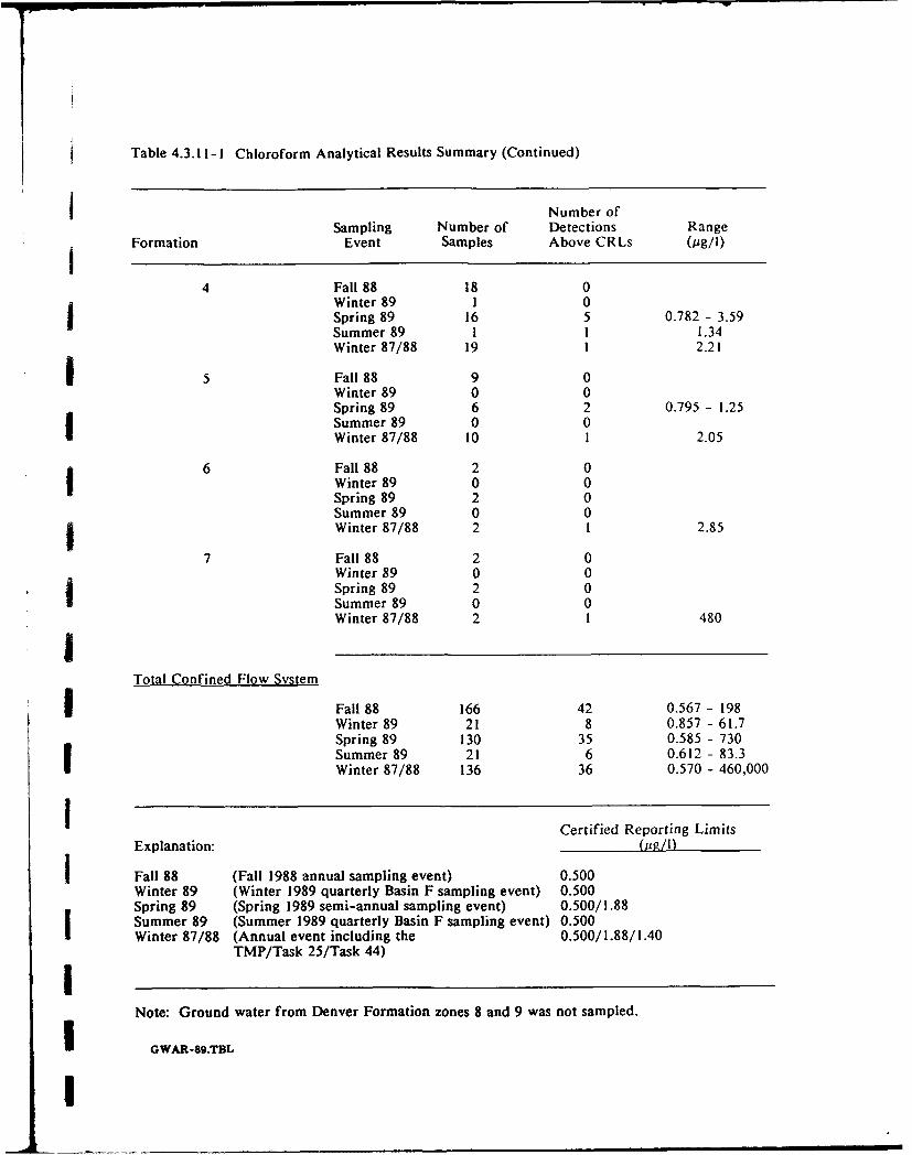
Table 4.3.11-1 Chloroform Analytical Results Summary (Continued)
Number ofSampling Number of Detections Range
Formation Event Samples Above CRLs (pg/I)
4 Fall 88 18 0Winter 89 I 0Spring 89 16 5 0.782 - 3.59Summer 89 I 1 1.34Winter 87/88 19 1 2.21
i5 Fall 88 9 0Winter 89 0 0Spring 89 6 2 0.795 - 1.25Summer 89 0 0Winter 87/88 10 1 2.05
6 Fall 88 2 0Winter 89 0 0Spring 89 2 0Summer 89 0 0
IWinter 87/88 2 1 2.85
7 Fall 88 2 0Winter 89 0 0Spring 89 2 0Summer 89 0 0Winter 87/88 2 1 480I
Total Confined Flow System
Fall 88 166 42 0.567 - 198Winter 89 21 8 0.857 - 61.7Spring 89 130 35 0.585 - 730Summer 89 21 6 0.612 - 83.3Winter 87/88 136 36 0.570 - 460,000
I Certified Reporting LimitsExplanation: (01/l)
I Fall 88 (Fall 1988 annual sampling event) 0.500Winter 89 (Winter 1989 quarterly Basin F sampling event) 0.500Spring 89 (Spring 1989 semi-annual sampling event) 0.500/1.88Summer 89 (Summer 1989 quarterly Basin F sampling event) 0.500Winter 87/88 (Annual event including the 0.500/1.88/1.40
TMP/Task 25/Task 44)INote: Ground water from Denver Formation zones 8 and 9 was not sampled.
IGWAR-8O.TBL
northwest was 51.0 pg/I at Well 22043, located just upgradient of the NWBCS. Chloroform
extending from the Central and Basin A Neck Pathways are not intercepted by the NWBCS.
The Basin F East Pathway plume merged with the Basin F Pathway plume downgradient of the
Basin F area, where chloroform concentrations increase substantially. The highest fall 1988
chloroform detection within the Basin F Pathway was 70,000 pg/I at Well 26133. Detected
chloroform concentrations decreased along the Basin F Pathway towards the NBCS. Potentiometric
data indicate that the isolated plume of chloroform in north-central Section 23 upgradient of the
NBCS probably is related to contamination along the Basin F pathway.
Chloroform was detected downgradient of the NBCS during the fall of 1988 along the Northern
Off-Post Pathway and in several wells along the length of the containment system. The highest
detected concentration along the Northern Off-Post Pathway of 1000 pg/I occurred at Well 37344
more than one mile north of the NBCS.
Isolated plumes of chloroform were identified from fall 1988 data along the North Plants Pathway
and along the Railyard-Motorpool Pathway. Isolated detections of chloroform occurred in
Sections 1, 2, 9, 23, 24, 28, 33, 36, and in five off-post wells.
4.3.11.2 Confined Flow System. Chloroform was detected in 42 of 166 confined flow system
samples analyzed during the fall of 1988. Chloroform detections ranging from 0.567 to 198 pg/l
were measured from wells completed in zones B, A, IU, 1, 2, and 3. FY89 analytical results for
individual zones of the confined flow system are summarized in Table 4.3.11-1. Point plots of
these results are presented in Figures A-23 through A-25.
Fall 1988 chloroform detections in the confined flow system occurred predominately beneath areas
of unconfined flow system chloroform contamination. The greatest depth at which chloroform was
detected during the fall of 1988 was 210 feet in Well 01048 (zone 2). A chloroform concentration
of 4.90 pg/l was measured. Because this well is located upgradient of all RMA sources of
chloroform, connection with contamination by RMA sources is unlikely. Denver Formation
zone 3, at a depth of 145 feet in Well 19016, was the lowest stratigraphic unit in which
chloroform (0.773 pig/I) was detected. The highest chloroform concentrations detected in the
fall of 1988 occurred in zone A Wells 02030, 02035, and 36117. Chloroform concentrations of
198, 197, and 180 pg/l, respectively, were measured at these wells.
4.3.11.3 Winter 1987/88 and FY89 Comparison. In the unconfined flow system, chloroform
was detected in 171 of 319 winter 1987/88 samples and in 173 of 322 fall 1988 samples.
GWAR-89.4Rev. 06/21/90 - 85 -
I
Chloroform distribution was generally similar during both sampling periods, however, because ofa lower fall 1988 CRL chloroform appears to be more extensive. The addition of fall 1988
monitoring wells in the North Plants led to the identification of a chloroform plume extendingnorth from the North Plants. The addition of wells in the Basin A Neck to the fall 1988 programhas resulted in more continuous plume definition. Wells where chloroform concentrations variedconsiderably from previous or subsequent sampling rounds are listed in Table 4.3.2-2.
Chloroform was detected in 36 of 136 confined flow system samples during the winter of 1987/88compared to 42 of 166 samples for the fall 1988 sampling period (Table 4.3.11 -I). The presence
of chloroform in the confined flow system was confirmed in the South Plants, South Lakes, Basin
A Neck, Basin A areas, and Sections 23 and 26. Due to the general low hydraulic conductivityand large heterogeneity of the Denver Formation, substantial data variability is likely to occur in
any single sampling period.
4.3.12 Trichloroethene
Analyses for trichloroethene were performed on 488 ground-water samples collected during thefall 1988 monitoring period. The CRL for the fall of 1988 was 0.560 ug/I. Trichloroethene
concentrations ranged from 0.625 to 4800 pg/I in 146 of the samples analyzed. Trichloroethenewas detected in the confined flow system in 19 out of 166 samples from zones A, IU, 1, 2, 3 and
5. Trichloroethene in both the unconfined and confined flow systems for the FY89 monitoringprogram is summarized in Table 4.3.12-1.
4.3.12.1 Unconfined Flow System. Trichloroethene was detected in 127 of 322 ground-water
samples collected during the fall of 1988 from wells completed in the unconfined flow system.
Concentrations ranged from 0.625 pg/I to 4800 pg/l. The CRL value of 0.560 pg/I was used asi the lowest contour line in constructing the contaminant plume map shown in Figure 4.3.12-1.
Based on fall 1988 data, trichloroethene extended in a continuous plume through the South Plants,
Basin A, Basin A Neck, Basin F East, and Basin F Pathways to the NBCS. Plumes oftrichloroethene also were detected in the Basin A Neck Pathway to the Northwest BoundaryContainment System, in the Northern and First Creek Off-Post Pathways, and the Railyard-Motor
Pool and Western Tier Pathways.
The highest concentration of trichloroethene at RMA during the fall of 1988 (4800 pg/I in Well
36181) was detected in the South Plants-Basin A Pathway in southwest Section 36. Elevated
trichloroethene concentrations were also detected in nearby Wells 36001 (2,500 pg/i) and 36168
GWAR-89.4Rev. 06/21/90 - 86 -
U
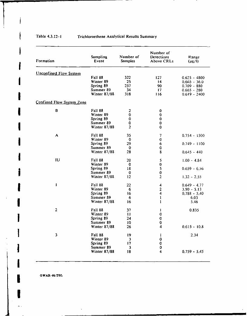
f Table 4.3.12-1 Trichloroethene Analytical Results Summary
I Number ofSampling Number of Detections Range
Formation Event Samples Above CRLs (,sg/1)
Ulnconfined Flow SystemFall 88 322 127 0.625 - 4800Winter 89 25 14 0.665 - 36.0Spring 89 257 90 0.709 - 880Summer 89 34 17 0.665 - 280g Winter 87/88 318 116 0.619 - 2400
Confined Flow System Zone
B Fall 88 2 0Winter 89 0 0Spring 89 0 0Summer 89 0 0Winter 87/88 2 0
A Fall 88 35 7 0.754 - 1500
Winter 89 0 0Spring 89 29 6 0.749 - 1100Summer 89 0 0Winter 87/88 28 8 0.645 - 440
IU Fall 88 20 5 1.00 - 4.84Winter 89 0 0Spring 89 18 5 0.659 - 6.56Summer 89 0 0Winter 87/88 12 2 1.32 - 2.55
1 Fall 88 22 4 0.649 - 4.77Winter 89 6 2 3.90 - 5.13Spring 89 16 4 0.788 - 5.40
Summer 89 6 1 6.03Winter 87/88 16 1 5.46
2 Fall 88 37 1 0.835Winter 89 11 0I Spring 89 24 0Summer 89 10 0Winter 87/88 26 4 0.615 - 10.8
3 Fall 88 19 1 2.34Winter 89 3 0Spring 89 17 0Summer 89 3 0Winter 87/88 18 4 0.759 - 5.45
II GWAR-89.TBL
I
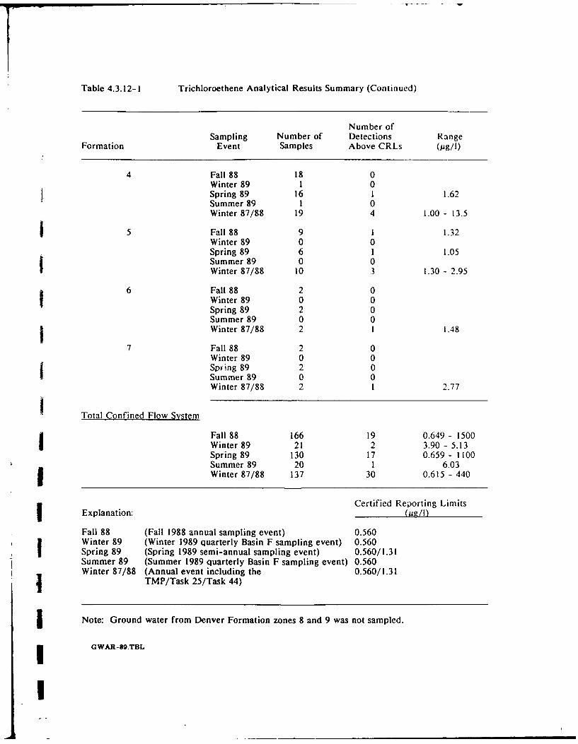
Table 4.3.12-1 Trichloroethene Analytical Results Summary (Continued)
Number ofSampling Number of Detections Range
Formation Event Samples Above CRLs (pg/I)
4 Fall 88 18 0Winter 89 1 0Spring 89 16 1 1.62Summer 89 1 0Winter 87/88 19 4 1.00 - 13.5
5 Fall 88 9 1 1.32Winter 89 0 0Spring 89 6 1 1.05Summer 89 0 0Winter 87/88 10 3 1.30 - 2.95
6 Fall 88 2 0Winter 89 0 0Spring 89 2 0Summer 89 0 0Winter 87/88 2 1 1.48
7 Fall 88 2 0Winter 89 0 0Spring 89 2 0Summer 89 0 0Winter 87/88 2 1 2.77
Total Confined Flow System
Fall 88 166 19 0.649 - 1500Winter 89 21 2 3.90 - 5.13Spring 89 130 17 0.659 - 1100
Summer 89 20 1 6.03Winter 87/88 137 30 0.615 - 440
Certified Reporting LimitsExplanation: (Og/!I)
Fall 88 (Fall 1988 annual sampling event) 0.560Winter 89 (Winter 1989 quarterly Basin F sampling event) 0.560Spring 89 (Spring 1989 semi-annual sampling event) 0.560/1.31Summer 89 (Summer 1989 quarterly Basin F sampling event) 0.560Winter 87/88 (Annual event including the 0.560/1.31
TMP/Task 25/Task 44)
Note: Ground water from Denver Formation zones 8 and 9 was not sampled.
GWAR-89.TBL
I1
(2,100 pg/I). From the southwest corner of Section 36, the plume extended southwest to the
central portion of Section 2 and northwest into the Basin A Neck Pathway, through the Basin FEast and Basin F Pathways, to the NBCS. Another area of elevated concentration (greaLer than
100 pg/I) within the plume occurred near the northeast corner of Basin A. The interpreted plume
configuration in this area corresponded to historical distributions.iAlong the Basin A Neck Pathway, extending northwest to the NWBCS, the continuity of the
trichloroethene plume through the southwest corner of Section 26 and the southeast corner of
Section 27 has not been confirmed with available data due to the complexity of ground water flow
in this area. It is believed that the plume is continuous through the area between Wells 26068 and
27025. Concentrations within the plume ranged from 0.768 to 2.90 pig/I.
Along the Western Tier and Railyard-Motor Pool Pathways in Sections 4, 9 and 33, trichloroethene
was detected at concentrations ranging from 0.911 to 144 pg/l. The plume extended to the
western border of Sections 4, 9, and 33. Trichloroethene was not found in two wells within the
western edge of the plume thus interpreted, one in the northwest corner of Section 9 (Well 09002)
and one in the northwest corner of Section 33 (Well 33076). The historical off-post
trichloroethene contamination is indicated by the shaded area (Figure 4.3.12-1) west of RMA.
The concentrations from the wells that were sampled by the EPA between December 1985 and
March 1987 ranged from 5.00 to 100 pg/I.
Trichloroethene contamination was identified in the First Creek and Northern Off-Post Pathways
downgradient of the NBCS. At present, the trichloroethene plume is discontinuous across theNBCS. The maximum concentration detected in the Northern Off-Post Pathway was 4.34 pg/l,detected in Well 37344, and the maximum concentration in the First Creek Off-Post Pathway was
2.42 pug/I in Well 37396.
j In addition to the plumes described above, there were 12 isolated detections of trichloroethene,
ranging in concentration from 0.724 to 8.11 pg/l. The highest concentration was detected near the
center of Section 25 in Well 25042. Most of the detections occurred on-post in the northern areas
of RMA.
4.3.12.2 Confined Flow System. Analyses for trichloroethene were performed on 166 ground-water samples collected from the confined flow system during fall 1988 monitoring.[ Trichloroethene concentrations ranging from 0.649 to 1500 pug/I were detected in 19 of the
samples. Analytical results for the fall 1988 sampling are summarized in Table 4.3.12-1. Point
plots from the fall 1988 sampling are presented in Figures A-26 through A-28.
GWAR-89.4Rev. 06/21/9 - 89 -
!
I
Detections were most frequent within zones A, IU and I. Single detections occurred in zones 2,
3 and 5. The maximum concentration was detected in the South Plants area in southwest
Section 36, underlying the maximum concentration in the unconfine flow system. The deepest
detection of trichloroethene occurred at 173 ft on the west side of Basin A in Well 36171 (zone I).
The concentration was 3.71 pg/I.IThe distribution of trichloroethene in the confined flow system generally could be correlated with
the trichloroethene distribution in the unconfined flow system. Detections in zone A primarily
occurred in the South Plants-Basin A area, whereas detections in lower stratigraphic zones were
more widespread.
4.3.12.3 Winter 1987/88 and FY89 Comparisons. Trichloroethene was detected in the
unconfined flow system in 116 of 318 winter 1987/88 samples compared to 127 of 322 fall 1988
samples (Table 4.3.12-1). Fall 1988 data confirmed the presence of trichloroethene in SouthPlants, Basin A, Basin A Neck, South Lakes, Northern Off-Post, Basin F, the Rail Yard - Motor
Pool and Western Tier Pathways. The addition of wells in the Basin A Neck to the fall 1988program has resulted in more continuous plume definition. Trichloroethene distribution near the
NWBCS was less extensive in fall 1988 than winter 1987/88. Wells where trichloroethene
concentrations varied considerably from previous or subsequent sampling rounds are listed in Table
4.3.2-2.
Trichloroethene was detected in 30 of 137 samples from the confined flow system in the winter
1987/88 compared to 19 of 166 fall 1988 samples (Table 4.3.12-1). Fall 1988 data confirmed thepresence of trichloroethene in the South Plants area, Basins A, Section 26, the Basin A Neck, and
at the NBCS. Winter 1987/88 trichloroethene detections north of the NBCS were not substantiated
by fall 1988 data. Isolated trichloroethene detections in Sections 4, 23, 27, 30, and 33 during thewinter of 1987/88 also were not repeated during the fall of 1988 sampling round. Due to the
general low hydraulic conductivity and large heterogeneity of the Denver Formation, substantialdata variability is likely to occur in any single sampling period. Therefore, variations such as
those noted at the NBCS should be considered appropriately.
1 4.3.13 Tetrachloroethene
Tetrachloroethene was detected in 105 of 488 wells analyzed during the fall 1988 sampling with
_ concentrations ranging from 0.892 to 700 pg/i. The CRL for the fall of 1988 was 0.750 pug/l.Tetrachloroethene results in both the confined and unconfined flow systems are presented in Table
i 4.3.13-I.
G WAR-89.4Ray. 06/21/Wo - 90 -
I
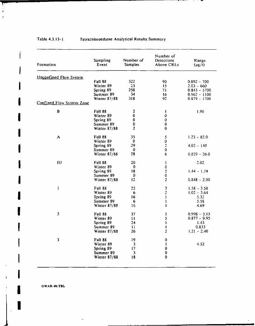
Table 4.3.13-1 Tetrachloroethene Analytical Results Summary
Number ofSampling Number of Detections Range
Formation Event Samples Above CRLs (pg/i)
Unconfined Flow SystemFall 88 322 90 0.892 - 700Winter 89 25 15 2.03 - 660Spring 89 258 71 0.843 - 5700Summer 89 34 16 0.962 - 1100
C Winter 87/88 318 92 0.879 - 1700Confined Flow System Zone
B Fall 88 2 1 1.90Winter 89 0 0Spring 89 0 0Summer 89 0 0Winter 87/88 2 0
A Fall 88 35 5 1.23 - 82.0Winter 89 0 0Spring 89 29 2 4.02 - 140Summer 89 0 0Winter 87/88 28 6 0.829 - 26.0
IU Fall 88 20 1 2.02Winter 89 0 0Spring 89 18 2 1.44 - 1.74Summer 89 0 0Winter 87/88 12 2 0.848 - 2.00
1 Fall 88 22 3 1.58 - 3.58Winter 89 6 2 1.02 - 3.64Spring 89 16 1 5.32Summer 89 6 1 5.58Winter 87/88 16 1 4.69
2 Fall 88 37 5 0.998 - 3.15Winter 89 !1 5 0.877 - 9.95Spring 89 24 1 1.43Summer 89 I1 1 0.833Winter 87/88 26 2 1.21 - 2.40
3 Fall 88 19 0Winter 89 3 1 4.52Spring 89 17 0Summer 89 3 0
SWinter 87/88 18 0
G WAR-89.TBL
ii
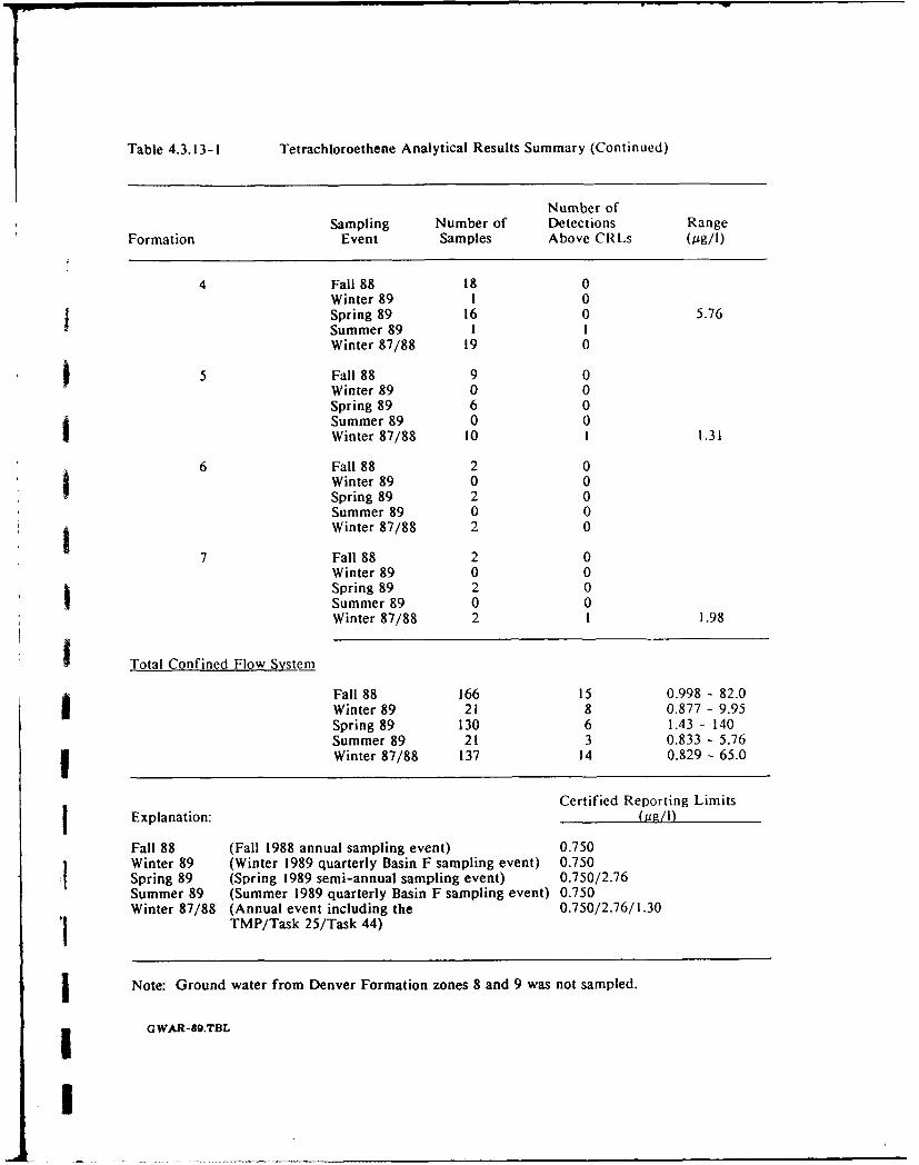
Table 4.3.13-I Tetrachloroethene Analytical Results Summary (Continued)
Number ofSampling Number of Detections Range
Formation Event Samples Above CRLs (Gig/1)
4 Fall 88 18 0Winter 89 I 0Spring 89 16 0 5.76Summer 89 1 1Winter 87/88 19 0
5 Fall 88 9 0Winter 89 0 0Spring 89 6 0Summer 89 0 0Winter 87/88 10 1 1.31
6 Fall 88 2 0Winter 89 0 0Spring 89 2 0Summer 89 0 0Winter 87/88 2 0
7 Fall 88 2 0Winter 89 0 0
SSpring 89 2 0Summer 89 0 0Winter 87/88 2 1 1.98
Total Confined Flow System
Fall 88 166 15 0.998 - 82.0Winter 89 21 8 0.877 - 9.95Spring 89 130 6 1.43 - 140Summer 89 21 3 0.833 - 5.76Winter 87/88 137 14 0.829 - 65.0
Certified Reporting Limitsj Explanation: (On/I)
Fall 88 (Fall 1988 annual sampling event) 0.750Winter 89 (Winter 1989 quarterly Basin F sampling event) 0.750Spring 89 (Spring 1989 semi-annual sampling event) 0.750/2.76Summer 89 (Summer 1989 quarterly Basin F sampling event) 0.750Winter 87/88 (Annual event including the 0.750/2.76/1.30
TMP/Task 25/Task 44)
Note: Ground water from Denver Formation zones 8 and 9 was not sampled.
G WAR-89.TBL
I
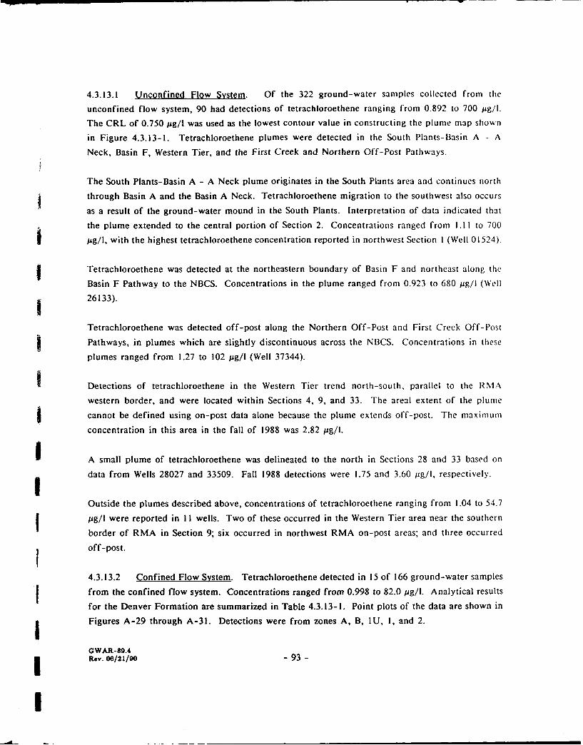
4.3.13.1 Unconfined Flow System. Of the 322 ground-water samples collected from the
unconfined flow system, 90 had detections of tetrachloroethene ranging from 0.892 to 700 pg/I.
The CRL of 0.750 pg/I was used as the lowest contour value in constructing the plume map shown
in Figure 4.3.13-1. Tetrachloroethene plumes were detected in the South Plants-Basin A - A
Neck, Basin F, Western Tier, and the First Creek and Northern Off-Post Pathways.
The South Plants-Basin A - A Neck plume originates in the South Plants area and continues north
through Basin A and the Basin A Neck. Tetrachloroethene migration to the southwest also occurs
as a result of the ground-water mound in the South Plants. Interpretation of data indicated that
the plume extended to the central portion of Section 2. Concentrations ranged from I .11 to 700
p g/l, with the highest tetrachloroethene concentration reported in northwest Section I (Well 01524).
Tetrachloroethene was detected at the northeastern boundary of Basin F and northeast along the
Basin F Pathway to the NBCS. Concentrations in the plume ranged from 0.923 to 680 pg/I (Well
26133).
Tetrachloroethene was detected off-post along the Northern Off-Post and First Creek Off-Post
Pathways, in plumes which are slightly discontinuous across the NBCS. Concentrations in these
plumes ranged from 1.27 to 102 ug/I (Well 37344).
Detections of tetrachloroethene in the Western Tier trend north-south, parallel to the RMA
western border, and were located within Sections 4, 9, and 33. The areal extent of the plume
cannot be defined using on-post data alone because the plume extends off-post. The maxunu
concentration in this area in the fall of 1988 was 2.82 pg/I.
A small plume of tetrachloroethene was delineated to the north in Sections 28 and 33 based on
data from Wells 28027 and 33509. Fall 1988 detections were 1.75 and 3.60 pg/I, respectively.
Outside the plumes described above, concentrations of tetrachloroethene ranging from 1.04 to 54.7
j pg/I were reported in 11 wells. Two of these occurred in the Western Tier area near the southern
border of RMA in Section 9; six occurred in northwest RMA on-post areas; and three occurred
off-post.
4.3.13.2 Confined Flow System. Tetrachloroethene detected in 15 of 166 ground-water samplesf from the confined flow system. Concentrations ranged from 0.998 to 82.0 pg/i. Analytical results
for the Denver Formation are summarized in Table 4.3.13-1. Point plots of the data are shown in
Figures A-29 through A-31. Detections were from zones A, B, IU, 1, and 2.
GWAR-89.4Rev. 06/21/90 - 93 -
The detections in zones B and A generally occur in the vicinity of South Plants. In other confined
zones, the detections are primarily under the Basin A Neck and Basin F East Pathways.
Tetrachloroethene in the confined flow system was generally present outside the plumes delineated
in the unconfined flow system and not directly below the plumes. The point of highestconcentration (82.0 pg/I) was reported in Well 36182 which is completed in zone A to a depth of
75.0 ft below ground level. This well is located approximately 400 ft north of Well 01524 whichhad the highest concentration of tetrachloroethene in the overlying unconfined flow system (700
14g/1). The deepest contamination by tetrachloroethene in the confined flow system occurred in
Well 26152 (zone 2), screened to a depth of 104.9 feet. The tetrachloroethene concentration in this
well was 2.31 ug/l, and the well is located in the vicinity of the Basin A Neck.
4.3.13.3 Winter 1987/88 and FY89 Comparisons. Tetrachloroethene was detected in the5 unconfined flow system in 92 of 318 wells sampled in the winter of 1987/88 compared to 90 of322 wells sampled in the fall of 1988 (Table 4.1.13-1). Fall 1988 data confirmed tetrachloroethene
plumes in the South Plants, South Lakes, Basin A, Basin A Neck, and Basin F, Nor-thern Off-Post
and First Creek Off-Post Pathways. The plumes in the South Lakes and Basin A Neck :Iathways
were extended based on fall 1988 data, as was the plume in the Western Tier Pathway. Wells
Swhere tetrachloroethene concentrations varied considerably from previous or subsequent sampling
rounds are listed in Table 4.3.2-2.
e Tetrachloroethene was detected in the confined flow system in 14 of 137 samples in the winter of
1987/88 compared to 15 of 166 samples in the fall of 1988 (Table 4.3.13-1). Tetrachloroethene
presence was further substantiated in South Plants, Southern Basin A, and Basin A Neck areas.
Due to the general low hydraulic conductivity and large heterogeneity of the Denver Formation,
substantial data variability is likely to occur in any single sampling period.
4.3.14 Dibromochloropropane (DBCP)
Analyses for DBCP were performed on 486 ground-water samples collected during the fall of1988, and DBCP was detected in 57 samples. Dibromochloropropane concentrations ranged from
0.199 to 1,900 pg/l. Dibromochloropropane detections for samples collected from the unconfined
and confined flow systems for the FY89 monitoring programs are summarized in Table 4.3.14-1.
4.3.14.1 Unconfined Flow System. Dibromochloropropane was identified in 49 of the 320
unconfined samples analyzed during the fall of 1988. Concentrations ranging from 0.199 to
1,900 pg/l were reported. The CRL of 0.195 pg/I was used as the lowest contour value shown on
the plume map in Figure 4.3.14-1.
GWAR-89.4Rev. 06/21/-O - 94 -
I

Table 4.3.14-1 Dibromochloropropane Analytical Results Summary
Number ofSampling Number of Detections Range
Formation Event Samples Above CRLs (pg/I)IUnconfined Flow System
Fall 88 320 49 0.199 - 1900Winter 89 25 6 0.241 - 17.0Spring 89 258 57 0.154 - 270Summer 89 34 8 0.349 - 9.75Winter 87/88 307 62 0.144 - 57,000
Confined Flow System Zone
B Fall 88 2 0Winter 89 0 0Spring 89 0 0Summer 89 0 0
SWinter 87/88 1 0
A Fall 88 35 2 0.220 - 310Winter 89 0 0Spring 89 29 2 0.351 - 310Summer 89 0 0Winter 87/88 22 2 0.496 - 21.0
IIU Fall 88 20 3 1.13 - 9.78Winter 89 0 0Spring 89 18 3 0.632 - 1.90Summer 89 0 0Winter 87/88 11 0
1 Fall 88 22 1 8.96Winter 89 6 0Spring 89 16 3 0.208 - 0.361Summer 89 6 0( Winter 87/88 14 0
2 Fall 88 37 1 0.403Winter 89 11 1 2.40Spring 89 24 4 0.205 - 1.10Summer 89Winter 87/88 23 2 0.234 - 0.330
3 Fall 88 19 0Winter 89 3 0Spring 89 17 1 0.200Summer 89 3 0Winter 87/88 17 1 0.202
GWAR-89.TBL
I
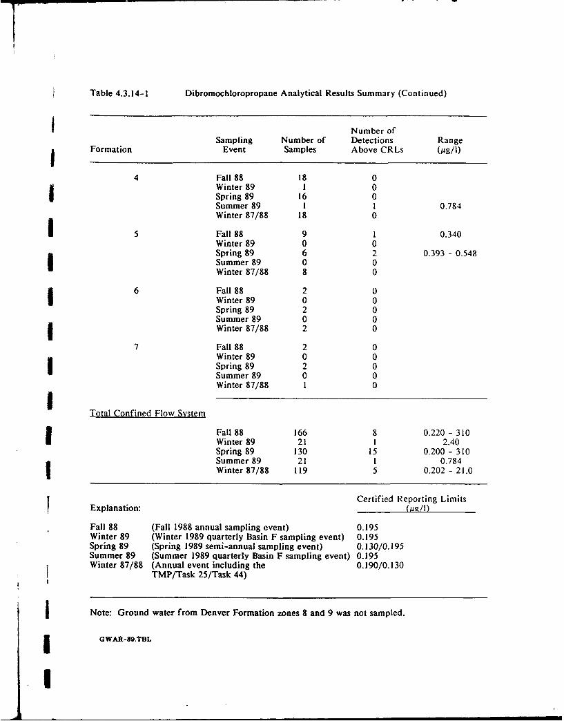
Table 4.3.14-1 Dibromochloropropane Analytical Results Summary (Continued)
Number ofSampling Number of Detections Range
Formation Event Samples Above CRLs (pg/I)
4 Fall 88 18 0Winter 89 1 0Spring 89 16 0Summer 89 1 1 0.784
Winter 87/88 18 0
5 Fall 88 9 1 0.340Winter 89 0 0Spring 89 6 2 0.393 - 0.548Summer 89 0 0Winter 87/88 8 0
6 Fall 88 2 0Winter 89 0 0Spring 89 2 0
Summer 89 0 0Winter 87/88 2 0
7 Fall 88 2 0Winter 89 0 0Spring 89 2 0
Summer 89 0 0Winter 87/88 1 0
Total Confined Flow System
Fall 88 166 8 0.220 - 310Winter 89 21 1 2.40Spring 89 130 15 0.200 - 310Summer 89 21 1 0.784Winter 87/88 119 5 0.202 - 21.0
Certified Reporting LimitsExplanation: (gg/I)
Fall 88 (Fall 1988 annual sampling event) 0.195Winter 89 (Winter 1989 quarterly Basin F sampling event) 0.195Spring 89 (Spring 1989 semi-annual sampling event) 0.130/0.195Summer 89 (Summer 1989 quarterly Basin F sampling event) 0.195Winter 87/88 (Annual event including the 0.190/0.130
TMP/Task 25/Task 44)
Note: Ground water from Denver Formation zones 8 and 9 was not sampled.
GWAR-89.TBL
.1
As shown in Figure 4.3.14-1, three separate DBCP plumes were present on-post and one plumewas present off-post. The plumes included the South Plants-Basin A Pathway, Railyard-Motor
Pool Pathway, Basin F Pathway, and the Northern Off-Post Pathway.
The largest DBCP plume originates in the South Plants. The highest fall 1988 DBCP concentration(1,900 pg/I) was reported in this area from Well 01061. From the South Plants, the plume extends
north into Basin A. Concentrations in the plume ranged from 0.217 pg/I (Well 36090) to1,900 pg/l (Well 01061).
The second largest DBCP plume occupied the Railyard-Motor Pool Pathway in western RMA.
This relatively narrow plume originated in the Rail Classification Yard and extends northwest
into Section 33 where it is intercepted by the Irondale Containment System. The highest DBCP
concentration in this plume was recorded at Well 04026 (100 ug/l). Vertical stratification of DBCP
in the unconfined flow system is evident at well clusters 04026-04029 and 04014-04016. The wells
screened in the shallow portion of the thick saturated alluvium have DBCP concentration one to
two orders of magnitude greater than the wells screened in the deeper portion of the alluvium.
A DBCP plume extended northeast from the Basin F area to the NBCS along the Basin F Pathway.
Within this plume, DBCP ranged in concentration from 0.206 pg/l (Well 24013) where the plume
is intercepted by the NBCS, to 28.0 pg/l (Well 26157) near Basin F.
Downgradient of the NBCS a DBCP plume extends north along the Northern Off-Post Pathway.
j This DBCP plume has been shown to be associated with the DBCP plume further downgradient
(north) along this pathway; however, fall 1988 results do not support this interpretation. The
highest fall 1988 DBCP detection within the Northern Off-Post Pathway was 9.62 pg/l at
Well 37344.
A small DBCP plume existed along the Basin A Neck Pathway in southwest Section 26. This is
based on DBCP detections at Wells 26006 and 26068. Isolated fall 1988 DBCP detections occurred
within Sections 1, 2, 9, 22, 24, 25, and 27. Previous and/or subsequent sampling indicates that the
two isolated detections in Section 9 and the two isolated detections in Section 25 appear to be
spurious. Isolated detections in Sections i, 2, 22, and 27 appear to be related to current or
historical plume areas.
4.3.14.2 Confined Flow System. A total of 166 samples from the confined flow system were
analyzed for DBCP during the fall of 1988. Eight detections were reported with a range from
GWAR-89.4Rev. 06/21/90 -97-
0.220 to 310 pg/I. The affected zones included A, IU, 1, 2, and 5. Table 4.3.14-1 summarizes
these detections and Figures A-32 through A-34 are point plots of the results.
Dibromochloropropane contamination in the confined flow system occurred predominately beneath
unconfined flow system contamination.The highest fall 1988 DBCP detection in the confined flow
system was 310 pug/I within Well 36182 (zone A). This well is located approximately 1,000 feet
downgradient from the highest DBCP concentration within the unconfined flow system. The
deepest fall 1988 detection of DBCP occurred in Well 36179 (zone 1) at a depth of 151 feet below
ground surface. The well contained a DBCP concentration of 8.96 pg/I, and is located along the
western margin of Basin A.
4.3.14.3 Winter 1987/88 and FY89 Comparisons. Dibromochloropropane was detected in the
unconfined flow system in 62 of 307 samples analyzed during the winter of 1987/88 period
compared to 49 of 320 samples analyzed during fall of 1988 (Table 4.3.14-1). Fall 1988 data
further substantiated the presence of DBCP in the Rail Classification Yard - Motor Pool, the
South Plants - Basin A, and the Basin F Pathways. The extent of plumes in the Radi Classification
Yard - Motor Pool and the Northern Off-Post Pathway decreased from winter 1987/88 to fall
j 1988. Dibromochloropropane was detected in two of seven newly installed wells in the North
Plants. Wells where DBCP concentrations varied considerably from previous or subsequent
sampling rounds are listed in Table 4.3.2-2.
Dibromochloropropane was detected in the confined flow system in five of 119 samples in the
winter of 1987/88 compared to eight of 166 samples in the fall of 1988 (Table 4.3.2-2). Fall 1988
data indicate the presence of DBCP in the confined flow system in Sections I, 24, 26, 35, and 36.
Due to the general low hydraulic conductivity and large heterogeneity of the Denver Formation,
substantial data variability is likely to occur in any single sampling period. Interpretation of
variable data should be considered appropriately.
4.3.15 Dicyclopentadiene (DCPD)
During the fall of 1988, dicyclopentadiene analyses were performed on 481 ground-water samples.
Dicyclopentadiene concentrations ranging from 9.47 ug/I to 3600 pg/I were reported in 47 of the
481 ground-water samples obtained. The CRL for the samples collected during the fall of 1988
was 5.00 pug/I. Dicyclopentadiene was detected in confined flow system zones A, 1, 2, and 4.
Dicyclopentadiene detections are summarized in Table 4.3.15-1.
IGWAR-89.4Rev. 06/21/90 - 98 -
I
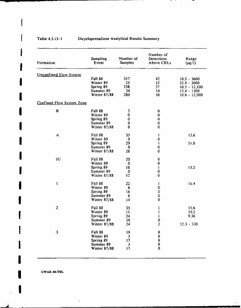
I
Table 4.3.15-I Dicyclopentadiene Analytical Results Summary
I Number ofSampling Number of Detections Range
Formation Event Samples Above CRLs (pg/I)
Unconfined Flow SystemFall 88 317 42 10.5 - 3600Winter 89 25 12 32.4 - 3600Spring 89 258 37 10.5 - 12,100Summer 89 34 14 12.4 - 1500i Winter 87/88 280 58 10.6 - 12,000
Confined Flow System Zone
B Fall 88 2 0Winter 89 0 0Spring 89 0 0Summer 89 0 0Winter 87/88 0 0
A Fall 88 35 1 13.6Winter 89 0 0Spring 89 29 1 51.8Summer 89 0 0Winter 87/88 28 0
IU Fall 88 20 0Winter 89 0 0Spring 89 18 1 13.2Summer 89 0 0Winter 87/88 12 0
1 Fall 88 22 1 16.4Winter 89 6 0Spring 89 16 0Summer 89 6 0Winter 87/88 14 0
2 Fall 88 35 1 15.6Winter 89 !1 1 10.2Spring 89 24 1 9.36Summer 89 10 0Winter 87/88 24 2 12.3 - 330
3 Fall 88 19 0Winter 89 3 0Spring 89 17 0Summer 89 3 0Winter 87/88 17 0
Ig GWAR-89.TBL
!1
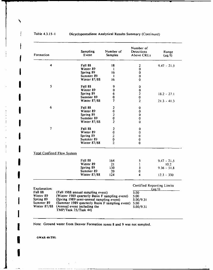
Table 4.3.15-I Dicyclopentadiene Analytical Results Summary (Continued)f
Number ofSampling Number of Detections Range
Formation Event Samples Above CRLs (Ag/I)
4 Fall 88 18 2 9.47 - 21.5Winter 89 1 0Spring 89 16 0Summer 89 1 0Winter 87/88 16 0
I Fall 88 9 0Winter 89 0 0Spring 89 6 2 18.2 - 27.1Summer 89 0 0Winter 87/88 7 2 21.3 - 41.3
6 Fall 88 2 0Winter 89 0 0Spring 89 2 0Summer 89 0 0
SWinter 87/88 2 0
7 Fall 88 2 0Winter 89 0 0Spring 89 2 0
* Summer 89 0 0Winter 87/88 2 0
Total Confined Flow System
I Fall 88 164 5 9.47 - 21.5Winter 89 21 1 10.2Spring 89 130 5 9.36 - 51.8Summer 89 20 0Winter 87/88 124 4 12.3 - 330
Certified Reporting LimitsExplanation: (u2/I)Fall 88 (Fall 1988 annual sampling event) 5.00Winter 89 (Winter 1989 quarterly Basin F sampling event) 5.00Spring 89 (Spring 1989 semi-annual sampling event) 5.00/9.31Summer 89 (Summer 1989 quarterly Basin F sampling event) 5.00Winter 87/88 (Annual event including the 5.00/9.31
TMP/Task 25/Task 44)
Note: Ground water from Denver Formation zones 8 and 9 was not sampled.
I GWAR-89.TBL
I
4.3.15.1 Unconfined Flow System. Ground-water samples from 317 wells completed in the
unconfined flow system were analyzed for dicyclopentadiene. Of these, 42 had concentrations that
ranged from 10.5 pg/I to 3600 pg/I. The CRL (5.00 pg/I) was used as the lowest contour value in
constructing the plume map shown in Figure 4.3.15-1. Dicyclopentadiene occurs in three main
areas: the South Plants-Basin A - Basin A Neck Pathway, the Basin F Pathway, and in the First
Creek Off-Post Pathway. Isolated dicyclopentadiene detections were present in Sections 1, 4, 27,
33, and 34.
The South Plants-Basin A plume originated in the South Plants area and extended northward
through Basin A. Some dicyclopentadiene migration to the southwest from the South Plants area
into Section 2 also was apparent. Concentrations within the South Plants-Basin A plume range
from 13.1 #g/l, in Well 36056, to 2400 #g/I in Well 01014.
A small plume defined by Wells 35065 and 35018 occurs in the Basin A Neck Pathway. Although
the likely source of this plume in the South Plants-Basin A area, fall 1988 data do not permit
illustration of this plume as continuous with the South Plants-Basin A plume.
The Basin F Pathway plume extended from the Basin F area north along the Basin F Pathway to
the North Boundary Containment System. Concentrations of dicyclopentadiene ranging from
23.3 pg/l (Well 23188) to 3600 pg/l (Well 23049) were reported within this plume.
The First Creek Off-Post, plume which is disuontinuous with the on-post plume, was identified
downgradient of the North Boundary Containment System in off-post Section 14. Concentrations
within this plume ranged from 10.5 pg/l, in Well 37343, to 250 pg/l in Well 37373. An isolated
dicyclopentadiene detection of 25.1 pg/I was reported in the Northern Off-Post Pathway at Well
37344.
4.3.15.2 Confined Flow System. Dicyclopentadiene was detected in five of 164 ground-water
samples from the confined flow system. These detections were from Denver Formation zones A,
1, 2, and 4, with values ranging from 9.47 pg/l to 21.5 pg/l. Point plots showing confined flow
system dicyclopentadiene detections during the fall 1988 program are shown in Figures A-35
through A-36. Table 4.3.15-1 summarizes the results for each confined flow system zone.
The highest dicyclopentadiene concentration of 21.5 pg/I was reported in Well 37365 (zone 4),
located beneath the First Creek Off-post Pathway in Section 14. Other confined flow system
detections occurred in areas proximal to unconfined flow system plumes. The deepest fall 1988
dicyclopentadiene detection occurred in Well 35084 (zone 1) at a depth of 174 feet below ground
GWAR-89.4Rev. 06/21/90 - 101 -
surface. A dicyclopentadiene concentration of 16.4 pg/I was detected at this well located adjacent
to South Plants. This detection has not been confirmed with spring 1988 and spring 1989 sampleswhich were below detection.
4.3.15.3 Winter 1987/88 and FY89 Comparisons. Dicyclopentadiene was detected in thef unconfined flow system in 58 of 280 winter 1987/88 samples compared to 42 of 317 fall 1988samples (Table 4.3.15-1). Fall 1988 data confirmed the existence of dicyclopentadiene plumes in
j the South Plants, Basin A, Basin A Neck, Basin F, and First Creek Off-Post Pathways. The
configuration of the plumes are similar between the two sampling periods, except for the FirstCreek Off-Post Pathway plume which decreased in size. This reduction occurs at the NBCS, likelyreflecting the impact of the newly installed recharge trenches. Monitoring wells, added to the fall1988 network, in Sections 27 and 34, identified several isolated dicyclopentadiene detections.
Wells where dicyclopentadiene concentrations varied considerably from previous or subsequent
sampling rounds are listed in Table 4.3.2-2.
Dicyclopentadiene was detected in the confined flow system in 5 of 164 samples in the winter of1987/88 compared to 5 of 124 samples in the fall of 1988. Table 4.3.15-1 summarizes these results
for each zone of the confined flow system. There were no detections of dicyclopentadiene in thesame wells during both sampling periods. Except for the two detections close together off-postin Section 14 during the fall of 1988, all detections during both sampling periods were areally or
vertically isolated. Due to the general low hydraulic conductivity and large heterogeneity of theDenver Formation, substantial data variability is likely to occur in any sampling period. Therefore
variations such as those noted above should be considered appropriately.
4.3.16 Diisopropylmethylphosphonate (DIMP)
Diisopropylmethylphosphonate (DIMP) was detected in 267 of 485 samples analyzed during the
fall of 1988. The CRL for the fall period was 0.392 ug/I and the range of reported concentrationswas from 0.441 to 34,000 pg/I. The distribution of DIMP in the unconfined flow system isillustrated in Figure 4.3.16-1. Diisopropylmethylphosphonate was detected in the confined flow
system within zones B, A, IU, 1, 2, 3, 4, 5, and 6. Diisopropylmethylphosphonate detections for
the FY89 monitoring programs are summarized in Table 4.3.16-1.
4.3.16.1 Unconfined Flow System. A total of 321 samples from wells completed in theunconfined flow system were analyzed for DIMP during the fall of 1988. Diisopropylmethyl-phosphonate was reported in 211 wells, ranging from 0.441 to 34,000 pg/l. The CRL (0.392 pg/I)
was used as the lowest contour value in constructing the plume map shown in Figure 4.3.16-1.
GWAR-89.4Rev. 06/21/90 - 102 -
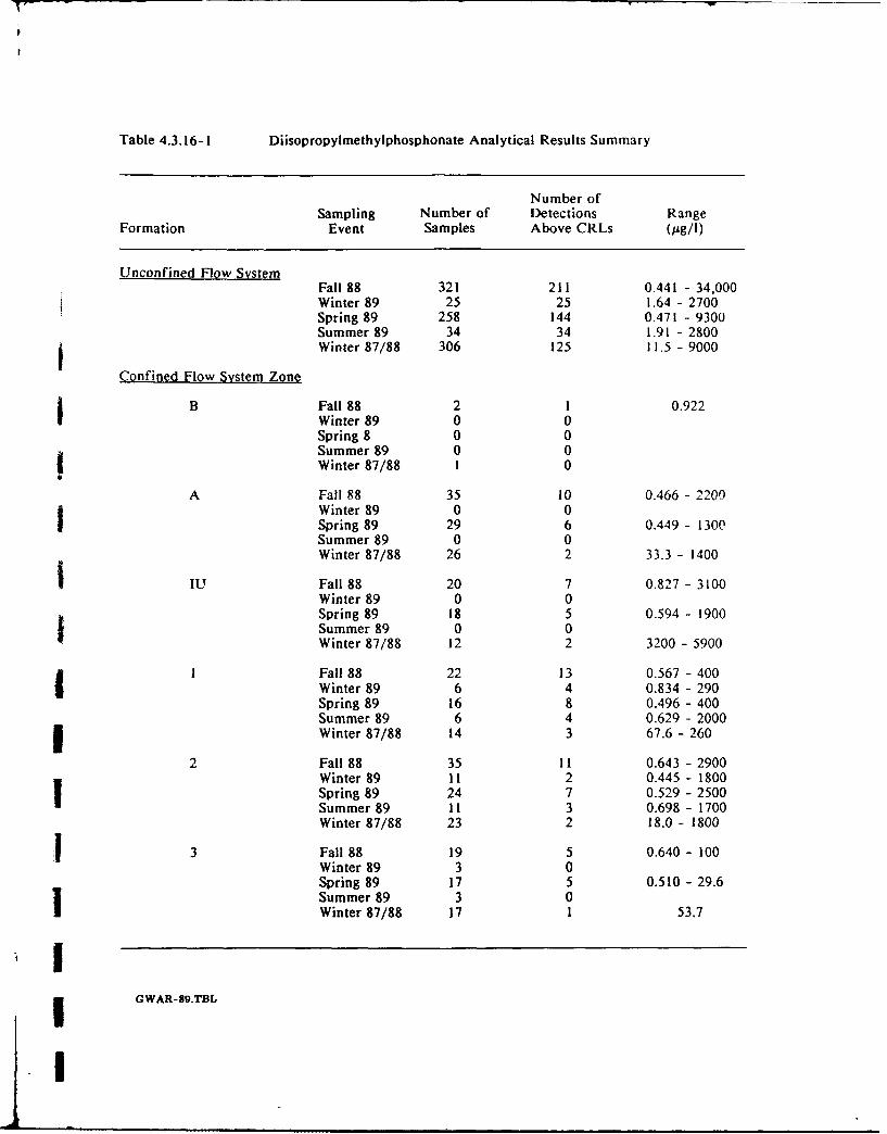
Table 4.3.16-1 Diisopropylmethylphosphonate Analytical Results Summary
Number ofSampling Number of Detections Range
Formation Event Samples Above CRLs (Og/I)
Unconfined Flow SystemFall 88 321 211 0.441 - 34,000Winter 89 25 25 1.64 - 2700Spring 89 258 144 0.471 - 9300Summer 89 34 34 1.91 - 2800I Winter 87/88 306 125 11.5 - 9000
Confined Flow System Zone
B Fall 88 2 1 0.922Winter 89 0 0Spring 8 0 0Summer 89 0 0Winter 87/88 1 0
A Fall 88 35 10 0.466 - 2200Winter 89 0 0Spring 89 29 6 0.449 - 1300Summer 89 0 0Winter 87/88 26 2 33.3 - 1400
SIU Fall 88 20 7 0.827 - 3100Winter 89 0 0Spring 89 18 5 0.594 - 1900Summer 89 0 0Winter 87/88 12 2 3200 - 5900
1 Fall 88 22 13 0.567 - 400Winter 89 6 4 0.834 - 290Spring 89 16 8 0.496 - 400Summer 89 6 4 0.629 - 2000I Winter 87/88 14 3 67.6 - 260
2 Fall 88 35 11 0.643 - 2900Winter 89 11 2 0.445 - 1800Spring 89 24 7 0.529 - 2500Summer 89 11 3 0.698 - 1700Winter 87/88 23 2 18.0 - 1800
!3 Fall 88 19 5 0.640 - 100Winter 89 3 0Spring 89 17 5 0.510 - 29.6Summer 89 3 0Winter 87/88 17 1 53.7
G WAR-89.TBL
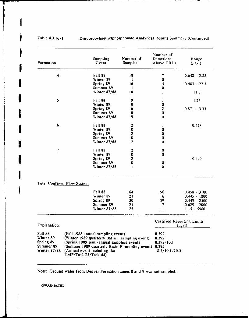
I
Table 4.3.16-1 Diisopropylmethylphosphonate Analytical Results Summary (Continued)
Number ofSampling Number of Detections Range
Formation Event Samples Above CRLs (pg/I)
4 Fall 88 18 7 0.648 - 2.28Winter 89 I 0Spring 89 16 5 0.483 - 27.3Summer 89 1 0Winter 87/88 18 i 11.5
5 Fall 88 9 I 1.23Winter 89 0 0Spring 89 6 2 0.871 - 3.33Summer 89 0 0Winter 87/88 9 0
6 Fall 88 2 1 0.458Winter 89 0 0Spring 89 2 0Summer 89 0 0
Winter 87/88 2 0
7 Fall 88 2 0Winter 89 0 0Spring 89 2 1 0.449Summer 89 0 0Winter 87/88 1 0I
Total Confined Flow System
Fall 88 164 56 0.458 - 3100Winter 89 21 6 0.445 - 1800Spring 89 130 39 0.449 - 2500Summer 89 21 7 0.629 - 2000Winter 87/88 125 1i 11.5 - 5900
Certified Reporting LimitsExplanation: ( /!I)
Fall 88 (Fall 1988 annual sampling event) 0.392Winter 89 (Winter 1989 quarter!y Basin F sampling event) 0.392Spring 89 (Spring 1989 semi-annual sampling event) 0.392/10.1Summer 89 (Summer 1989 quarterly Basin F sampling event) 0.392Winter 87/88 (Annual event including the 18.5/10.1/10.5
TMP/Task 25/Task 44)
Note: Ground water from Denver Formation zones 8 and 9 was not sampled.
GWAR-89.TBL
Diisopropylmethylphosphonate occurs as a widening continuous plume extending predominantly
north and northwest from sources within South Plants, North Plants, and Basin A. On post, DIMP
occupied all of the following contaminant migration pathways: South Plants-Basin A, South Lakes,
Basin A Neck, Central North, Central South, Basin F East, Basin F West, Basin F, North Plants,
and Basin F Northwest. Off post, DIMP occupied the Northern Off-Post, First Creek Off-Post,Sand Northwest Pathways.
The most upgradient detection of DIMP contamination apparent from the fall 1988 analytical data
occurred in the South Plants. The highest detection measured in the South Plants during the fall
of 1988 was 460 ug/I at Well 01525. From the South Plants, DIMP appeared to migrate in several
directions in response to radial flow from the South Plants ground-water mound.
The highest fall 1988 detection of DIMP was 34,000 pg/I at Well 36123 located downgradient of
Basin A in northwest Section 36. From Basin A, DIMP concentrations in excess of 1000 pg/I
extended continuously through the Basin A Neck northward through Basins C and F and along
the Basin F Pathway to the NBCS.
The northwest migration of DIMP along the Basin A Neck Pathway west of Section 26 occurred
at concentrations generally less than 10 ,pg/l. This also was true for migration along the Central,
Basin F West and Basin F Northwest Pathways. The highest fall 1988 DIMP detection in the
vicinity of the NWBCS was 18.2 pg/I at Well 22053.
The plume of DIMP originating in the North Plants extended north and merged with the Basin F
plume in west-central Section 24. Concentrations within this plume ranged from 0.693 pg/I in
Well 25041 to 340 pg/I in Well 24081. The highest DIMP detection within the North Plants was
250 pg/l at Well 25047.
Diisopropylmethylphosphonate existed off post in a wide plume encompassing the Northern Off-
Post, First Creek Off-Post and Northwest Pathways and the areas in between the pathways. Thisf plume may have reached the South Platte River. Contaminant migration has been halted at the
NBCS and NWBCS, but DIMP can continue to move off post between the barriers, and a great
deal of historical contaminant remains off post. Diisopropyimethylphosphonate detections greater
than 1000 pg/I were reported in three wells along the First Creek Off-Post Pathway. The highe-t
off-post fall 1988 DIMP detection was 2600 pg/I at Well 37313.IIsolated DIMP detections occurred on-post in Sections 1, 2, 4, 6, 8, 9, 12, 28, and 30. These
detections resulted from the lowering of the CRL from 18.5 to 0.392 pig/I.
GWAR-89.4Rev. 06/21/9o - 105 -
I
4.3.16.2 Confined Flow System. Diisopropylmethylphosphonate was detected in 56 of 164ground-water samples collected from wells screened in the confined flow system. These detectionswere from zones B, A, IU, 1, 2, 3, 4, 5, and 6, with values ranging from 0.458 jig/I to 3100 /jg/i.Table 4.3.16-1 summarizes the results. Figures A-37 through A-40 are point plots showing the
fall 1988 distribution of DIMP in the confined flow system.
The occurrence of DIMP in the confined flow system was primarily beneath areas of contamina-
tion in the unconfined flow system. The highest fall 1988 DIMP detection was at Well 35016(zone IU), located along the Basin A Neck Pathway in Section 35. In general, the greatest extent
of confined flow system DIMP contamination appears to be beneath the basins in Section 26 andalong the Basin A Neck Pathway in zones IU and 2, respectively. The deepest detection (187 ft)
was in Well 04012, completed in zone 6, at a concentration of 0.458 jig/l.
4.3.16.3 Winter 1987/88 and FY89 Comparisons. Diisopropylmethylphosphonate was detected
in the unconfined flow system in 125 of 306 samples during the winter of 1987/88 compared to211 of 321 samples during the fall of 1988 (Table 4.3.16-1). The CRL for DIMP was lowered
from 18.5 ig/Il, during the winter of 1987/88 to 0.392 pg/I during the fall of 1988. Because ofthis change, DIMP contamination appears more extensive during the fall of 1988.Additional monitoring wells were installed in the North Plants subsequent to the winter of 1987/88
. and prior to the fall of 1988. Samples from these wells resulted in the identification of a DIMPplume originating in the North Plants on the fall 1988 plume map. Wells where DIMP
concentrations varied considerably from previous or subsequent sampling rounds are listed in Table
4.3.2-2.
SDiisopropylmethylphosphonate was detected in the confined flow system in II of 125 samples
during the winter of 1987/88 compared to 56 of 164 samples during the fall of 1988 (Table 4.3.16-1). The increase in detections during fall 1988 can be attributed, in part, to the lowering of the
CRL from 18.5 to 0.392 pug/I. Fall 1988 data confirmed che winter 1987/88 DIMP detections in
the Basin A Neck, Basin C and First Creek Off-Post area. Additionally, fall 1988 DIMP
detections occurred in the confined flow system in the South Plants/Basin A, and Basin F area,and in the Northern Off-Post Pathway. Isolated detections of DIMP also occurred in Sections 4,
11, 12, and 30. Due to the generally low hydraulic conductivity and large heterogeneity of theDenver Formation, substantial data variability is likely to occur in any single sampling period.I
IGWAR-89.4Rev. 06/21/90 -106-
!
4.3.17 Phenols
In order to discuss the analytical results of the acid extractable fraction, total phenol concentra-
tions are presented as the sum of detected concentrations of the PMRMA certified compoundscomprising this group. Phenols were sampled for analysis during the fall 1988 and winter 1989monitoring periods. The summed compounds included in this group are:
2,4,5-Trichlorophenol
2,4,6-Trichlorophenol
2,4-Dichlorophenol
2,4-Dimethylphenol
2,4-Dinitrophenol
2-Chlorophenol
2-Methylphenol / 2-Cresol
2-Nitrophenol
4-Chloro-3-cresol / 3-Methyl-4-chlorophenol
4-Methylphenol / 4-Cresol
4-Nitrophenol
Pentachlorophenol
Phenol
Ground-water samples from 315 wells were analyzed during the fall of 1988 for compounds injthe phenols group. Ground-water samples were collected from an additional 170 wells. However,
the laboratory performing the analyses was not PMRMA-certified initially to analyze for allphenolic compounds, so results were not obtained. Composite phenol concentrations ranging from
5.15 to 110 /ug/l were detected in 17 of the 315 samples analyzed. Only 7 of the 13 phenolic
compounds comprising the group were detected at RMA. These included:!2-Chlorophenol
2-Methylphenol
2-Nitrophenol
4-Chloro-3-cresol
4-Methylphenol
Pentachlorophenol
Phenol
IGWAR-89.4Rev. 06/21/9o 107 -
I
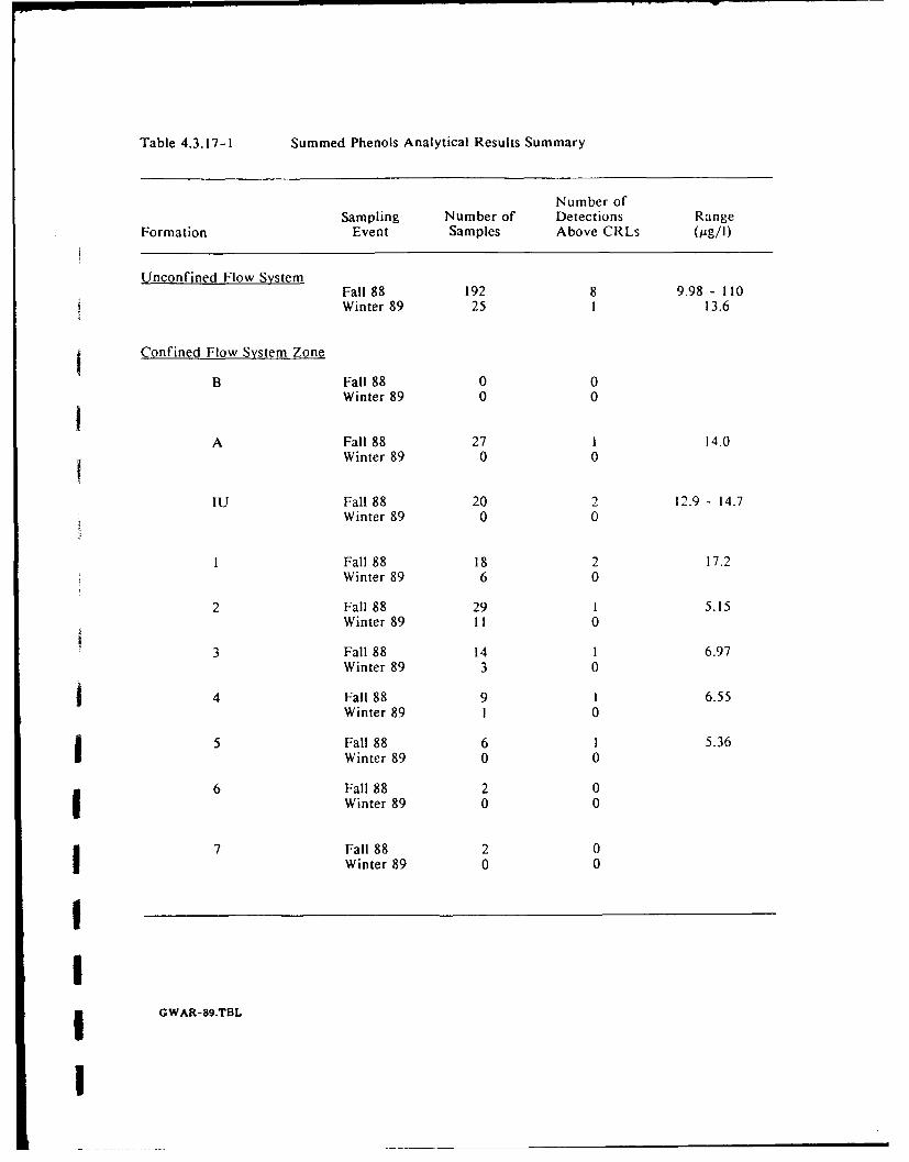
Table 4.3.17-I Summed Phenols Analytical Results Summary
Number ofSampling Number of Detections Range
Formation Event Samples Above CRLs (Og/i)
Unconfined Flow SystemFall 88 192 8 9.98 - 110Winter 89 25 I 13.6
Confined Flow System Zone
B Fall 88 0 0Winter 89 0 0I
A Fall 88 27 1 14.0Winter 89 0 0
IU Fall 88 20 2 12.9 - 14.7Winter 89 0 0
Fall 88 18 2 17.2Winter 89 6 0
2 Fall 88 29 1 5.15Winter 89 I1 0
3 Fall 88 14 1 6.97Winter 89 3 0
4 Fall 88 9 I 6.55Winter 89 1 0
5 Fall 88 6 1 5.36Winter 89 0 0
6 Fall 88 2 0Winter 89 0 0
7 Fall 88 2 0Winter 89 0 0
IIg GWAR-8g.TB3L
I
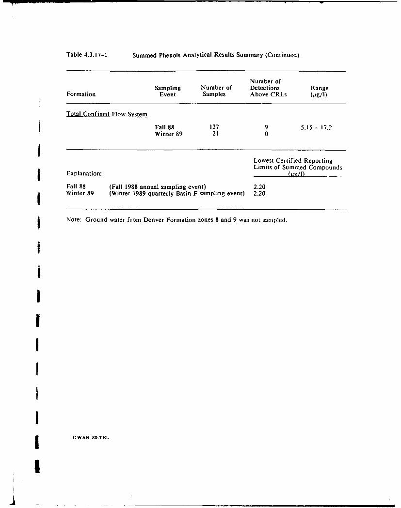
Table 4.3.17-1 Summed Phenols Analytical Results Summary (Continued)
Number ofSampling Number of Detections Range
Formation Event Samples Above CRLs (pg/I)
Total Confined Flow System
Fall 88 127 9 5.15 - 17.2
Winter 89 21 0
Lowest Certified Reporting
Limits of Summed CompoundsExplanation: (gI
Fall 88 (Fall 1988 annual sampling event) 2.20Winter 89 (Winter 1989 quarterly Basin F sampling event) 2.20
g Note: Ground water from Denver Formation zones 8 and 9 was not sampled.
IIIIIII
I GWAR-ag.TBL
I
The CRLs for the 13 targeted phenol compounds ranged from 2.20 pg/I for Phenol to 176 pg/I
for 2,4-Dinitrophenol. Phenol group compounds were detected in the confined flow system in
zones A, 1U, i, 2, 3, 4, and 5. Unconfined and confined flow system phenol detections for the
FY89 monitoring events are summarized in Table 4.3.17-1. The distribution of phenols in the
unconfined flow system is illustrated in Figure 4.3.17-1. Because analysis for compounds within
the phenol group were not undertaken in recent historical monitoring programs, a historical
comparison is not presented in this report.
1 4.3.17.1 Unconfined Flow System. Ground-water samples from 192 monitoring wells completed
in the unconfined flow system were analyzed for phenols during the fall of 1988. Phenols were
detected in eight samples with composite concentrations ranging from 9.98 to 110 pg/l.
A single, relatively small phenols plume was identified during the fall of 1988 (Figure 4.3.17-I).
The plume extended from the South Plants into southern Basin A along the Basin A
Pathway. The highest composite phenol detection (110 pg/I) within this plume occurred at
I Well 36076.
II Isolated detections of phenols occurred at Wells 22008, 26041, and 36084. Well 22008, located
just upgradient of the NWBCS, yielded 9.98 pg/I of the compound phenol. Well 26041, located
a |within the Basin F Pathway, yielded 74.5 ug/I of the compound 4-chloro-3-cresol. Well 36084,
i| located within Basin A, yielded 29.6 ug/l of the compound 4-methylphenol.
4.3.17.2 Confined Flow System. Compounds within the phenols group were detected in nine
of 127 ground-water samples collected from confined flow system zones during the fall of 1988.
Composite concentrations ranging from 5.15 to 17.2 ug/I were obtained from wells completed in
zones A, 1, IU, 2, 3, 4, and 5. Of the 13 compounds in the group, only 2-methylphenol and
phenol were detected in the confined flow system. Analytical results from individual zones of
the confined flow system are summarized in Table 4.3.17-1. Point plots of these results are
presented in Figures A-41 through A-43.
During the fall of 1988, phenols were detected in the confined flow system in Sections 1, 23, 35,
and 36. The greatest depth at which phenols were detected was 18.3 ft in Well 35078 (zone 1).
A concentration of 17.2 pg/I of 2-methylphenol was reported from this well. The lowest
stratigraphic unit containing phenols was zone 5 at Well 23225. A sample containing 2-
methylphenol at a concentration of 5.36 pg/l was obtained from this well, located in east-central
Section 23.
iGWAR-89.4Rev. 06/21/0 - 110-
!
4.3.17.3 FY89 Comparison. Because ground-water samples were not analyzed for phenols priorto fall 1988, only comparisons between fall 1988 and winter 1988/89 (a quarterly sample, network)can be made. Phenols were detected in 8 of 192 unconfined flow system samples in fall 1988 and
in I of 25 samples in winter 1988/89. One detection occurred in both the fall 1988 and winter1988/89 sampling rounds at Well 26041. Wells where concentration of phenols varied considerably
between sampling rounds are listed in Table 4.3.2-2.
Phenols were detected in 9 of 127 confined flow system wells sampled in fall 1988 and none ofthe 21 wells sampled in winter 1988/89. Phenols were not detected in the Basin F area during
either sampling period. Table 4.3.17-1 summarizes the results.
4.3.18 ParathionIAnalyses for parathion were performed on 485 ground-water samples collected during the fall ofg 1988. Parathion concentrations ranging from 0.838 to 24.0 pg/I were detected in 35 of the 485
samples analyzed. The CRL for parathion for the fall 1988 period was 0.647 pg/l. Parathion was
detected in only one sample from the confined flow system (zone A). The distribution of
parathion in the unconfined flow system is illustrated in Figure 4.3.18-I. Parathion detections forFY89 are summarized in Table 4.3.18-1. Because parathion was not analyzed in recent historical
monitoring programs, a historical comparison is not presented in this report.
4.3.18.1 Unconfined Flow System. Ground-water samples collected from 320 wells completedin the unconfined flow system were analyzed for parathion during the fall of 1988. Parathiondetections ranging from 0.838 to 24.0 ug/I were measured in 34 of these samples.
Parathion plumes were identified in the South Plants-Basin A, Basin A Neck, and Basin FPathways during the fall 1988 (Figure 4.3.18-1). The highest concentration of parathion,
24.0 pg/l, was obtained from Well 01525, located within South Plants. Parathion was detected bothnorth along the Basin A Pathway and southwest toward the South Lakes Pathway from the Southj Plants. Fall 1988 data indicated that the South Plants-Basin A parathion plume was separated
from the plume in the Basin A Neck Pathway. The Basin A Neck Pathway plume was interpretedfrom detections of 4.62 and 4.96 pg/I at Wells 26006 and 35018, respectively.
Parathion occurred within the Basin F Pathway in concentrations ranging from 0.954 to 15.4 pg/l.
The highest detections were located in Section 26 wells northeast of Basin F. The parathion plume
appeared to bifurcate into two lobes as it entered Section 23, one to the north and one to the
IGWAR-89.4Rev. 06/21/90 - Ill -
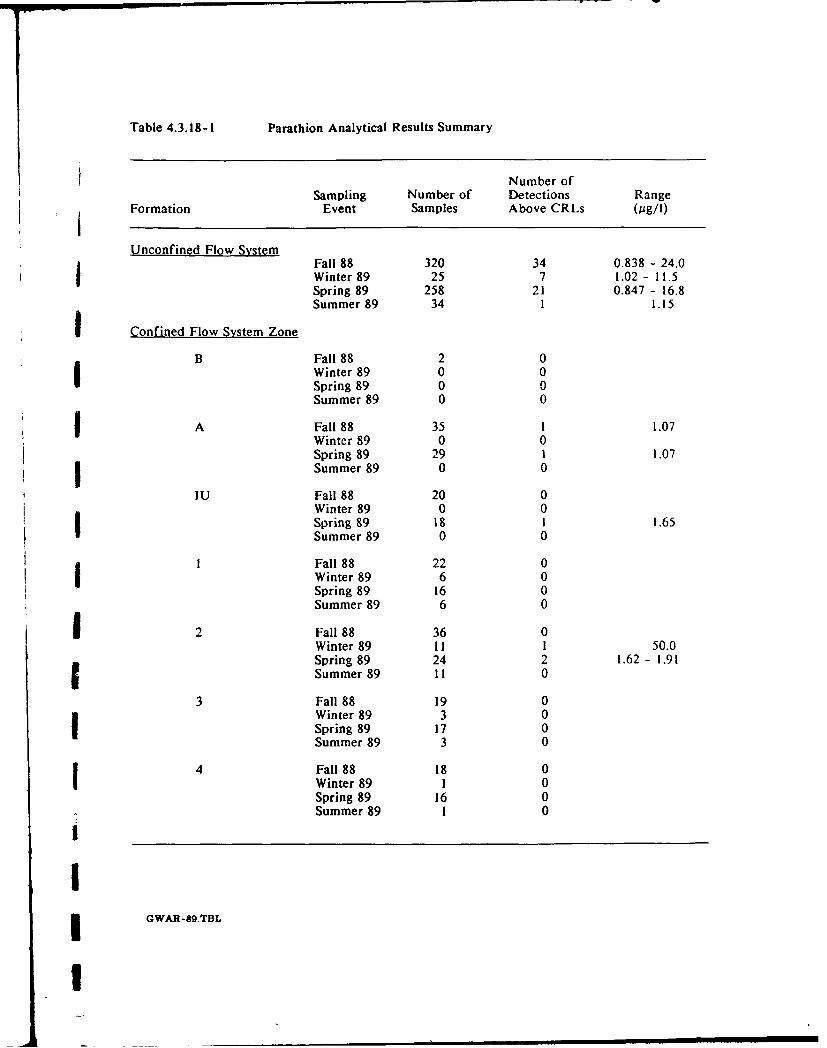
Table 4.3.18-1 Parathion Analytical Results Summary
Number ofSampling Number of Detections Range
Formation Event Samples Above CRLs (,ug/I)
Unconfined Flow SystemFall 88 320 34 0.838 - 24.0Winter 89 25 7 1.02 - 11.5Spring 89 258 21 0.847 - 16.8Summer 89 34 I 1.1 5SConfined
Flow System Zone
B Fall 88 2 0Winter 89 0 0Spring 89 0 0Summer 89 0 0
A Fall 88 35 1 1.07Winter 89 0 0Spring 89 29 1 1.07
SSummer 89 0 0
IU Fall 88 20 0Winter 89 0 0Spring 89 18 1 1.65Summer 89 0 0
g1 Fall 88 22 0Winter 89 6 0Spring 89 16 0Summer 89 6 0
2 Fall 88 36 0Winter 89 11 1 50.0Spring 89 24 2 1.62 - 1.91Summer 89 11 0
3 Fall 88 19 0Winter 89 3 0Spring 89 17 0Summer 89 3 0
4 Fall 88 18 0Winter 89 1 0Spring 89 16 0Summer 89 1 0
III G WAR-89.TBL
I
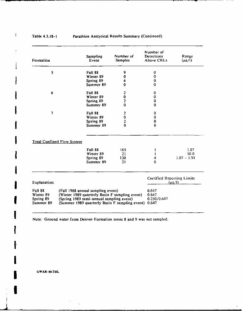
Table 4.3.18-1 Parathion Analytical Results Summary (Continued)
Number ofSampling Number of Detections Range
Formation Event Samples Above CRLs (04g/I)
5 Fall 88 9 0Winter 89 0 0Spring 89 6 0Summer 89 0 0
6 Fall 88 2 0Winter 89 0 0Spring 89 2 0Summer 89 0 0
7 Fall 88 2 0Winter 89 0 0Spring 89 2 0Summer 89 0 0
Total Confined Flow System
Fall 88 165 1 1.07Winter 89 21 1 50.0Spring 89 130 4 1.07 - 1.91Summer 89 21 0I
Certified Reporting LimitsI Explanation: (Ou /I)
Fall 88 (Fall 1988 annual sampling event) 0.647Winter 89 (Winter 1989 quarterly Basin F sampling event) 0.647Spring 89 (Spring 1989 semi-annual sampling event) 0.250/0.647Summer 89 (Summer 1989 quarterly Basin F sampling event) 0.647
Note: Ground water from Denver Formation zones 8 and 9 was not sampled.
IIi G WAR-89.TBL
northeast. The leading edges of both lobes appear to terminate south of the NBCS in Sections 23
and 24.
Off-post isolated detections of parathion occurred north of the NBCS at Wells 37309, 37370, and
37371. Concentrations ranged from 0.838 to 2.44 pg/I. On-post isolated detections occurred in
Sections 2, 3, 4, 23, 26, and 27 and generally were proximal to observed plumes or source areas.
Isolated detections at Wells 03005 and 04020 were more distant from known source areas but were
downgradient of detections in the South Lakes Pathway.
The deepest fall 1988 detection of parathion occurred in the unconfined flow system at
Well 04020. A parathion concentration of 1.32 ug/l was obtained at a depth of 79 feet below
ground surface and was not confirmed by subsequent spring 1989 data.
4.3.18.2 Confined Flow System. Parathion was detected in the confined flow system in only
one of 165 samples analyzed during the fall of 1988. The sole confined flow system detection
occurred within zone A at Well 02035 (Figure A-44) located southwest of South Plants along the
South Lakes Pathway. A parathion concentration of 1.07 ug/I was reported for this well which is
screened from 31 to 46 feet below ground surface.
4.3.18.3 FY89 Comparison. Because ground-water samples were not analyzed for parathion
prior to fall 1988, comparisons can only be made between FY89 sampling events. Parathion was
detected in 34 of 340 samples taken in the unconfined flow system during the fall of 1988
compared to detections in 21 of 258 samples taken in spring 1989. Seventeen of the 34 wells
showing parathion contamination in fall 1988 did not contain parathion in spring 1989.
Conversely, 10 of the 21 wells showing parathion contamination in spring 1989 did not contain
parathion during the fall. Wells with variable parathion concentrations are listed in Table 4.3.2-2.
During the fall 1988 sampling round, I out of 165 wells detected parathion in the confined flow
system compared to 4 of 130 wells in spring 1989 (Table 4.3.18-1). The five total detections
occurred as isolated hits and have not been confirmed by subsequent samples. Due to the general
low hydraulic conductivity and large heterogeneity of the Denver Formation, substantial data
variability is likely to occur in any sampling period. Data interpretation based on a single sample
period may not be effective in recognizing anomalous data, therefore, variable data should be
considered appropriately.'1
GWAR-89.4Rev. 06/21/9o - 114-
1
4.3. 19 Cyanide
Analyses for cyanide were performed on 484 ground water samples obtained during the fall of
1988. Cyanide was not analyzed in prior sampling events. The fall 1988 CRL for cyanide was
5.00 ug/I. Cyanide concentrations ranging from 5.05 to 100 pug/I were reported in 149 of the
i samples analyzed. Unconfined and confined flow system cyanide detections for the FY89
monitoring program are summarized in Table 4.3.19-1.
4.3.19.1 Unconfined Flow System. A total of 319 samples from wells completed in the
unconfined flow system were analyzed for cyanide during the fall of 1988. Concentrations rangedfrom 5.19 to 100 pug/I in 94 of these samples. The CRL of 5.00 ug/I was used as the lowest
contour value in constructing the cyanide plume map (Figure 4.3.19-1).
Six cyanide plumes were identified in the fall of 1988 data. They were located in the South
Lakes-South Plants-Basin A-Basin A Neck Pathway, the Basin F Pathway, the Central North-
Basin A Neck Pathway, the Basin F Northwest Pathway, the North Plants Pathway, and the
Western Tier Pathway.IThe largest plume and the plume with the highest cyanide concentration was in the South Lakes
and South Plants area and extended north through Basin A and northwest through the Basin A
Neck. There was a northeast extension from South Plants to the east side of Basin A. The highest
cyanide concentration detected was 100 pg/i in Well 01020 in northern Section 1.IA second cyanide plume extended from the Basin F area, north to the NBCS. The plume divided
near the boundary system. Only two isolated detections were present north of the boundary
system. Concentrations within the plume range from 5.00 to 34.8 pig/I. The maximum
concentration was detected in Well 23223, near the eastern edgc of Section 23.
Additional cyanide plumes trended northwest in the vicinity of the Central North-Basin A Neck
and Basin F Northwest Pathways. The Basin F Northwest plume did not extend past the NWBCS.,
and concentrations ranged from 8.01 to 11.1 pg/l. Concentrations in the Central North-Basin A
Neck plume ranged from 6.45 to 8.86 pg/I.
Cyanide in the North Plants Pathway area ranged in concentration from 5.96 to 15.2 pg/I. The
plume generally trended north.
1GWAR-89.4Rev. 06/21/90 - 115-
I
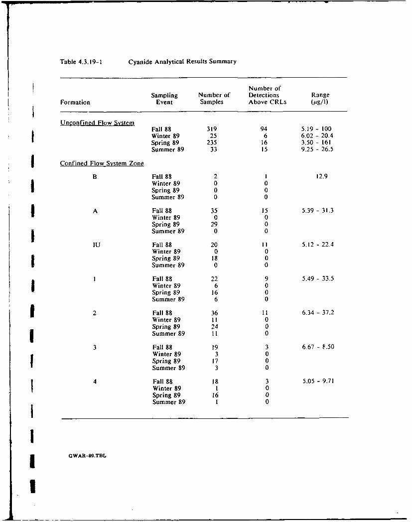
Table 4.3.19-1 Cyanide Analytical Results Summary
Number ofSampling Number of Detections Range
Formation Event Samples Above CRLs (jig/I)
Unconfined Flow SystemFall 88 319 94 5.19 - 100Winter 89 25 6 6.02 - 20.4Spring 89 235 16 3.50 - 161Summer 89 33 15 9.25 - 26.5
I Confined Flow System Zone
B Fall 88 2 1 12.9SWinter 89 0 0
Spring 89 0 0Summer 89 0 0
I Fall 88 35 15 5.39 -31.3Winter 89 0 0Spring 89 29 0Summer 89 0 0
IU Fall 88 20 11 5.12 - 22.4Winter 89 0 0Spring 89 18 0Summer 89 0 0
Fall 88 22 9 5.49 - 33.5Winter 89 6 0Spring 89 16 0Summer 89 6 0
I Fall 88 36 1i 6.34 - 37.2Winter 89 11 0Spring 89 24 0Summer 89 11 0
3 Fall 88 19 3 6.67 - F.50Winter 89 3 0Spring 89 17 0Summer 89 3 0
4 Fall 88 18 3 5.05 - 9.71Winter 89 1 0Spring 89 16 0Summer 89 1 0
Iii GWAR-8g.TBL
I
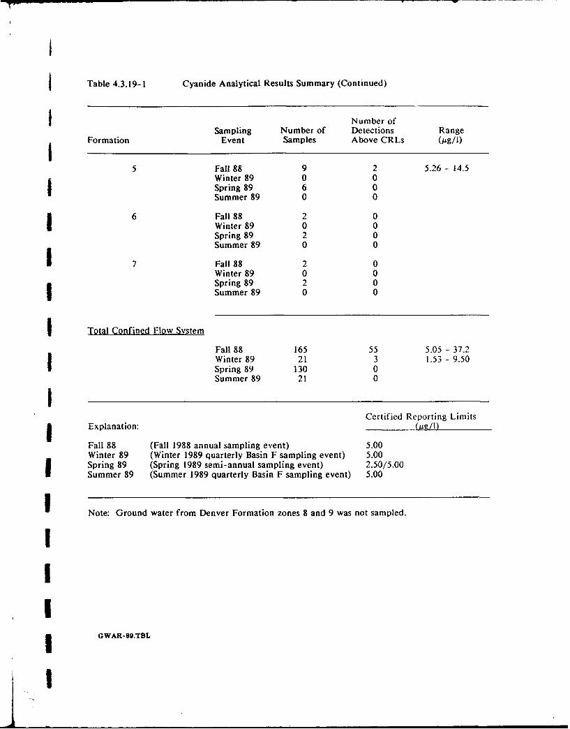
Table 4.3.19-1 Cyanide Analytical Results Summary (Continued)
i Number of
Sampling Number of Detections RangeFormation Event Samples Above CRLs (pg/0)
5 Fall 88 9 2 5.26 - 14.5Winter 89 0 0Spring 89 6 0Summer 89 0 0
6 Fall 88 2 0Winter 89 0 0Spring 89 2 0Summer 89 0 0
7 Fall 88 2 0Winter 89 0 0Spring 89 2 0Summer 89 0 0
I Total Confined Flow System
Fall 88 165 55 5.05 - 37.2Winter 89 21 3 1.53 - 9.50Spring 89 130 0Summer 89 21 0I
Certified Reporting LimitsI Explanation: (0g/l)
Fall 88 (Fall 1988 annual sampling event) 5.00Winter 89 (Winter 1989 quarterly Basin F sampling event) 5.00
I Spring 89 (Spring 1989 semi-annual sampling event) 2.50/5.00Summer 89 (Summer 1989 quarterly Basin F sampling event) 5.00
Note: Ground water from Denver Formation zones 8 and 9 was not sampled.
IIII GWAR-89.TBL
d I____
The Western Tier plume trended northwest through Section 9 and into Section 4 at the southernborder of RMA. It appears that a source of the plume may have been located to the south ofRMA. Concentrations ranged from 6.67 to 13.8 ug/I. The highest concentration was detected in
Well 09010, along the northern boundary of Section 9.
Isolated detections of cyanide occurred in 15 on-post wells and two off-post wells. On-post
concentrations in these wells ranged from 5.33 to 32.0 /g/I (Well 26073). Off-post concentrations9 were in Sections 29 and 14 at 5.25 and 10.7 pg/I, respectively.
4.3.19.2 Confined Flow System. During the fall of 1988, analyses for cyanide were conducted
on 165 ground-water samples collected from the confined flow system. Cyanide was detectedabove CRL in 55 samples at concentrations ranging from 5.05 to 37.2 pg/l in zones B, A, I U, I,2, 3, 4 and 5 of the Denver Formation. Analytical results for the fall of 1988 are summarized in
Table 4.3.19-1. Confined system point plots from the fall 1988 analytical results are presented in
Figure A-45 through A-48.
Cyanide was detected above CRL in the area surrounding the South Plants, Basin A and Basin F,and near the north and northwest boundaries of RMA. Most detections of cyanide in the confinedflow system did not appear to be directly associated with detections in the unconfined flow
systeni.
The highest concentration of cyanide (37.2 pg/I) was detected in Well 35039 in the northwest
corner of Section 35. Concentrations were below CRL in a well completed in the overlying
unconfined flow system within the Central North Pathway.
The deepest detection of cyanide was in zone 2 in Well 01048, completed to a depth of 210 feet.
A concentration of 12.2 pg/I was measured in this well which is located near the center of Section
1, south of South Plants. A concentration of 6.14 pg/I (Well 01047), was detected in the overlying
plume in the unconfined flow system.
4.3.19.3 FY89 Comparison. Because ground-water samples were not analyzed for cyanide
prior to fall 1988, comparisons can only be made between FY89 sampling events. Cyanide was
detected in all 4 of the sampling rounds in FY89 (Table 4.3.19-1). Many of the detections in the
fall of 1988 were not confirmed by later data, due to both smaller well networks and fewer
detections in subsequent sampling events. However, cyanide was detected in the South Plants -Basin A area and within the Basin F area during subsequent FY89 sampling periods. Wells withvariable cyanide concentrations are listed in Table 4.3.2-2.
GWAR-89.4Rev. 06/21/90 - 118 -
The fall 1988 cyanide concentrations typically were not confirmed by subsequent monitoring data
in the confined flow system. Detections occurred in 55 of 165 wells sampled in fall 1988 and 3of 21 wells sampled in winter 1989. Most detections in the confined flow system occurred beneath
areas where cyanide was detected in the unconfined flow system. Table 4.3.4-1 summarizes theresults for each of the confined zones. Cyanide was not detected in wells sampled in the spring
or summer of 1989.
Due to the heterogeneity of the Denver aquifer, substantial data variability is likely to occur and
data interpretation based on a single sample period may not be effective in recognizing anomalous
data.
4.3.20 Fluoride
Analyses for fluoride were performed on 488 ground-water samples obtained during the fall of
1988 monitoring. The CRL for the fall of 1988 was 482 pig/I; however, the CRLs for FY88 and
FY89 monitoring ranged from 482 to 1,220 ug/l. Fluoride concentrations ranging from 1,230 to320,000 pug/l, were reported in 411 of the 488 samples analyzed. Fluoride was detected in all
zones of the confined flow system that were sampled. Unconfined and confined flow systemfluoride detections for the FY89 monitoring program are summarized in Table 4.3.20- 1.
Fluoride is a naturally occurring constituent of ground water. The water quality upgradient of
RMA contaminant source areas has been monitored for fluoride to determine a background
quality; however, levels representing background concentrations for fluoride have not been
established for RMA. Thus, the CRL of 1,220 pg/l was used as the lowest contour line for
fluoride plume maps described here. Fluoride data for samples collected between 1964 and 1976from wells upgradient of RMA show fluoride concentrations ranged from 570 to 1,000 pzg/I;
however, fluoride concentrations ranging from 1,230 to 4,850 pg/I were detected along the
j southern or upgradient border of RMA, indicating that background fluoride concentrations may
be higher than the CRL of 1,220 pg/l.
4.3.20.1 Unconfined Flow System. Fluoride was analyzed in 322 samples from the unconfinedflow system during the fall of 1988. Reported concentrations ranged from 1,230 pg/I to 320,000
pug/I in 260 samples.
The highest CRL value (1,220 pg/l) in FY88 and FY89 monitoring events was used as the lowest
contour line in constructing the contaminant distribution map shown in Figure 4.3.20-1. As a
result, the figure shows a widespread distribution of fluoride. Because the distribution is greater
GWAR-89.4Rev. 06/21/90 - 119-
I
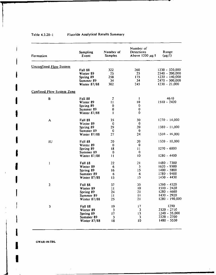
Table 4.3.20-1 Fluoride Analytical Results Summary
Number ofSampling Number of Detections Range
Formation Event Samples Above 1200 pg/I (Ag/I)
Unconfined Flow SystemFall 88 322 260 1230 - 320,000Winter 89 25 25 2540 - 200,000Spring 89 258 175 1230 - 140,000Summer 89 34 34 2470 - 500,000
i Winter 87/88 302 245 1230 - 21,000
Confined Flow System Zone
B Fall 88 2 1 4670Winter 89 11 10 1510 - 2420Spring 89 0 0Summer 89 0 0Winter 87/88 1 0
A Fall 88 35 30 1270 - 14,000Winter 89 0 0Spring 89 29 20 1380 - 11,000Summer 89 0 0Winter 87/88 27 24 1310 - 16,000
I IU Fall 88 20 20 1320 - 10,000Winter 89 0 0Spring 89 18 11 1270 - 6000Summer 89 0 0Winter 87/88 11 10 1280 - 4400
1 Fall 88 22 21 1480 - 7300Winter 89 6 5 1620 - 9500Spring 89 16 15 1400 - 5800Summer 89 6 6 1780 - 94001Winter 87/88 15 15 1430 - 4430
2 Fall 88 37 35 1260 - 4320Winter 89 11 10 1510 - 2420Spring 89 24 21 1280 - 4600Summer 89 1I 11 1430 - 2920Winter 87/88 25 21 1280 - 190,000
3 Fall 88 19 17 1290Winter 89 3 3 2320 - 2710Spring 89 17 13 1240 - 35,000Summer 89 3 3 2220 - 2700Winter 87/88 18 10 1480 - 5530
Ii GWAR-89.TBL
I
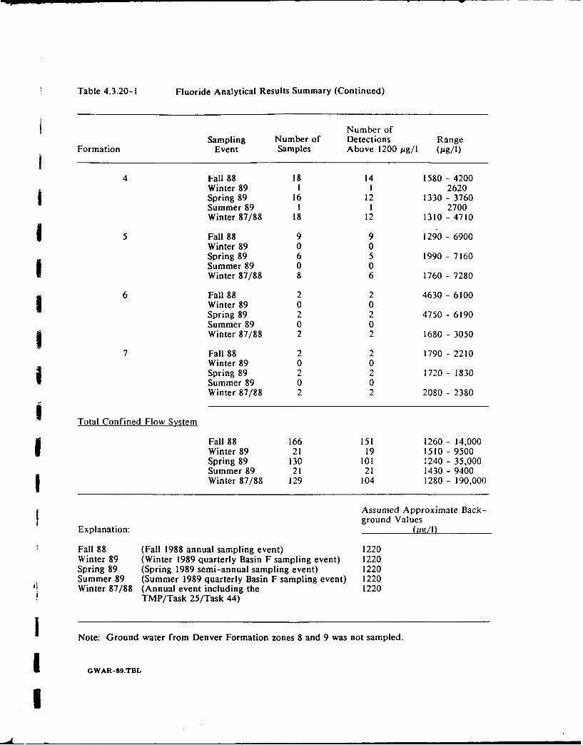
Table 4.3.20-1 Fluoride Analytical Results Summary (Continued)
Number ofSampling Number of Detections Range
Formation Event Samples Above 1200 pg/I (pg/I)I4 Fall 88 18 14 1580 - 4200
Winter 89 1 1 2620Spring 89 16 12 1330 - 3760
Summer 89 1 1 2700
Winter 87/88 18 12 1310 - 4710
5 Fall 88 9 9 1290 - 6900Winter 89 0 0Spring 89 6 5 1990 - 7160Summer 89 0 0Winter 87/88 8 6 1760 - 7280
6 Fall 88 2 2 4630 - 6100Winter 89 0 0Spring 89 2 2 4750 - 6190Summer 89 0 0Winter 87/88 2 2 1680 - 3050
7 Fall 88 2 2 1790 - 2210Winter 89 0 0Spring 89 2 2 1720 - 1830Summer 89 0 0Winter 87/88 2 2 2080 - 2380
Total Confined Flow System
Fall 88 166 151 1260 - 14,000Winter 89 21 19 1510 - 9500Spring 89 130 101 ,240 - 35,000Summer 89 21 21 1430 - 9400Winter 87/88 129 104 1280 - 190,000)
Assumed Approximate Back-ground Values
Explanation: (__/_ )
Fall 88 (Fall 1988 annual sampling event) 1220Winter 89 (Winter 1989 quarterly Basin F sampling event) 1220Spring 89 (Spring 1989 semi-annual sampling event) 1220Summer 89 (Summer 1989 quarterly Basin F sampling event) 1220Winter 87/88 (Annual event including the 1220
TMP/Task 25/Task 44)
Note: Ground water from Denver Formation zones 8 and 9 was not sampled.
I GWAR-89.TBL
!
than that indicated by other RMA contaminants, it is likely that a higher concentration should be
used to represent RMA contributions of fluoride to ground water. In general, the plumes
delineated by the 5,000 #g/I contour lines appear to be associated with known RMA source areas
and are similar in extent and configuration to those of other analytes, therefore, for the purposes
of this discussion, fluoride concentration is considered elevated if it is in excess of 5,000 ug/I.
Elevated fluoride concentrations (in excess of 5,000 pg/I) are mapped in three primary areas: the
South Plants-Basin A-Basin A Neck Pathway, the Basin F- Basin F Northwest Pathways, and the
First Creek Off-Post Pathway.
In the South Plants area, elevated fluoride levels occurred in a relatively small area which extended
from northwestern Section 1 into southwestern Section 36. The highest fluoride concentration
detected in this plume during the fall of 1988 was 64,000 pg/I in Well 01525. Occurrences of
5 fluoride in the Basin A Neck Pathway and along the north edge of Basin A range in concentration
from 5,200 to 22,000 pg/l. Fluoride concentrations between 1,230 and 5,000 ug/I were detected
in a large plume surrounding the South Plants-Basin A - Basin A Neck area, extending to the
S north off-post and to the south, across the southern RMA border. The eastern as well as southern
extent of the plume was poorly defined.
Fluoride concentrations in excess of 5,000 pg/I identified during fall 1988 monitoring extended
from northeast of the Basin F area along the Basin F Pathway toward the NBCS. The highest
fluoride concentration in this plume and on RMA was 320,000 pg/I, on the northeast side of Basin
F in Section 26. The plume extended southwest into Section 27 to the south of the NWBCS. The
northwest component of the plume extended approximately 800 ft off-post, bypassing the west end
of the NBCS. The northeast component terminated at the NBCS. Areas of other fluoride
concentrations greater than 5,000 pg/I were detected north of the NBCS and are discussed below.
North of the NBCS, fluoride concentrations greater than 5,000 pg/I were detected in wells along
Sthe First Creek Off-Post Pathway. The highest concentration (5,960 pg/I) was detected in Well
37309 along the boundary between Section 13 and Section 14. Concentrations approaching 5,000
p#g/I were detected in wells in the Northern Off-Post Pathway.
In addition to the fluoride concentrations greater than 5,000 pg/I discussed above, fluoride was
detected at 5,500 pg/I and 5,800 pg/I in two wells near the eastern edge of the NBCS and at 7,900
pg/I and 8,410 pg/I in two wells in the Western Tier. Although concentrations in the two wells
near the NBCS were consistent with other detections, the fall 1988 concentrations reported in the
Western Tier (Wells 04038 and 33066) were anomalously high.
ICWAR-89.4Rev. 06/21/90 - 122 -
I
4.3.20.2 Confined Flow System. Fluoride analyses were performed on 166 ground-water
samples from the confined flow system obtained during the fall of 1988. Concentrations above
1,220 pug/I were recorded in 151 wells from zones B, A, IU, I, 2, 3, 4, 5, 6, and 7, with values
ranging from 1,260 to 14,000 pg/I. Analytical results for the confined flow system from the fall
of 1988, winter of 1987/88, and spring and summer of 1989 are summarized in Table 4.3.20-1.
Selected point plots from the sampling programs cited above are presented in Figures A-49
through A-54.
The maximum fluoride concentration of 14,000 pg/I was reported in Well 02030, located in the
western portion of South Plants and completed to a depth of 73 ft (Figure A-49). Concentrations
in the overlying unconfined flow system in this area were generally between 2,000 and 5,000 pg/l.
The deepest well in which fluoride was reported at a concentration above 1,220 pg/I was Well
01048 at a concentration of 2,010 pg/l. The well is located near the center of Section 1 and is
screened from 160 to 210 ft below ground level, in zone 2. Similar concentrations are present in
the overlying unconfined flow system.
Fluoride concentrations greater than 3,000 pg/I within the confined flow system are generally
located in the vicinity of fluoride contamination within the unconfined flow system. In general,
the highest fluoride concentrations (above 5,000 pg/I) in the confined flow system are located
beneath Basin A, Basin A Neck, South Plants, and Sections 4 and 33 in the Western Tier. There
were eight detections above 5,000 p•g/I in the confined flow system but in almost all cases, the
fluoride concentration in the overlying unconfined flow system was less than in the underlying
confined flow system.
4.3.20.3 Winter 87/88 and FY89 Comparison. Data from FY89 provide a more complete
understanding of the distribution of fluoride in the unconfined flow system than was available in
the FY88 Annual Report. In particular, the extent of fluoride in the Basin A, Basin A Neck,
Basin F, and North Plants is better defined due to a higher sampling density in these areas during
FY89. Plume configurations are similar near the NWBCS, in the western tier, and downgradient
off-post. Wells where fluoride concentrations varied considerably from previous or subsequent
sampling rounds are listed in Table 4.3.2-2.
Fluoride was detected in the confined flow system in 104 of 129 samples collected during the
winter of 1987/88, compared to 151 of 166 samples coi"ected during fall 1988. Table 4.3.20-1
summarizes the winter 1987/88 and fall 1988 results for ;ich zone of the confined system. Areas
in which the presence of fluoride in the confined flow system was further substantiated include
GWAR-89.4Rev. 06/21/90 - 123 -
!
Sections 3, 4, and 27, as well as, Basin A Neck, Basin C, D, E, and Basin F areas. Due to the
general low hydraulic conductivity and large heterogeneity of the Denver aquifer, substantial data
variability is likely to occur in any single sampling period. Therefore, data interpretation based
on a single sample period should consider variable data appropriately.
4.3.21 Chloride
Chloride analyses were performed on 488 samples collected from the unconfined flow system andthe confined flow system during the fall of 1988. Chloride, a naturally occurring constituent in
ground water, was reported in every sample except one. A chloride concentration of 75,000 g/Il
was selected as the lowermost contour value for preparing a chloride plume map of the study area
(Figure 4.3.21-1). This value was selected previously for the chloride plume map presented in the
1988 CMP Annual Report based on the uppermost chloride concentration representative of uncon-
taminated areas at RMA. Fall 1988 chloride data also indicate that 75,000 pg/I is a reasonable
value to distinguish upgradient, uncontaminated areas from contaminated areas. Fall 1988 chloride
concentrations exceeded 75,000 pg/I in 267 of 488 wells with a range from 76,000 to
19,000,000 pg/l. Chloride was detected in the confined flow system above 75,000 pg/l within
zones B, A, IU, 1, 2, 3, 4, and 5. Chloride detections for FY89 are summarized in Table
4.3.21-1.
4.3.21.1 Unconfined Flow System. A total of 322 wells within the unconfined flow systemwere analyzed for chloride during the fall of 1988. Upgradient concentrations ranged from
20,000 to 72,000 pg/I (except for an isolated detection of 79,000 pg/l at Well 12002). Chloride
concentrations within contaminated areas ranged from 76,000 to 19,000,000 pg/I with a total of
205 detections above 75,000 pg/I.
A broad, continuous chloride plume during the fall of 1988 encompassed most of the central and
north central sections of RMA (Figure 4.3.21-1). This chloride plume continued off-post
northwestward toward the South Platte River. The plume expanded laterally from approximately
one-half mile wide in the South Plants area to over three miles wide just off-post. Chloride
contamination existed in all contaminant pathways identified at RMA except the Railyard-Motor
Pool Pathway. Elevated concentrations (500,000 ug/I or greater) occurred in the South Plants-
Basin A, Basin A Neck, Basin F East, Basin F, and First Creek Off-post Pathways. Locally,
chloride concentrations exceeded 1,000,000 pg/l within these pathways. The highest fall 1988
unconfined flow system chloride concentration was 19,000,000 pg/l at Well 26041. This well is
located downgradient of Basin F in the Basin F Pathway.
GWAR-89.4Rev. 06/21/90 - 124 -
I,
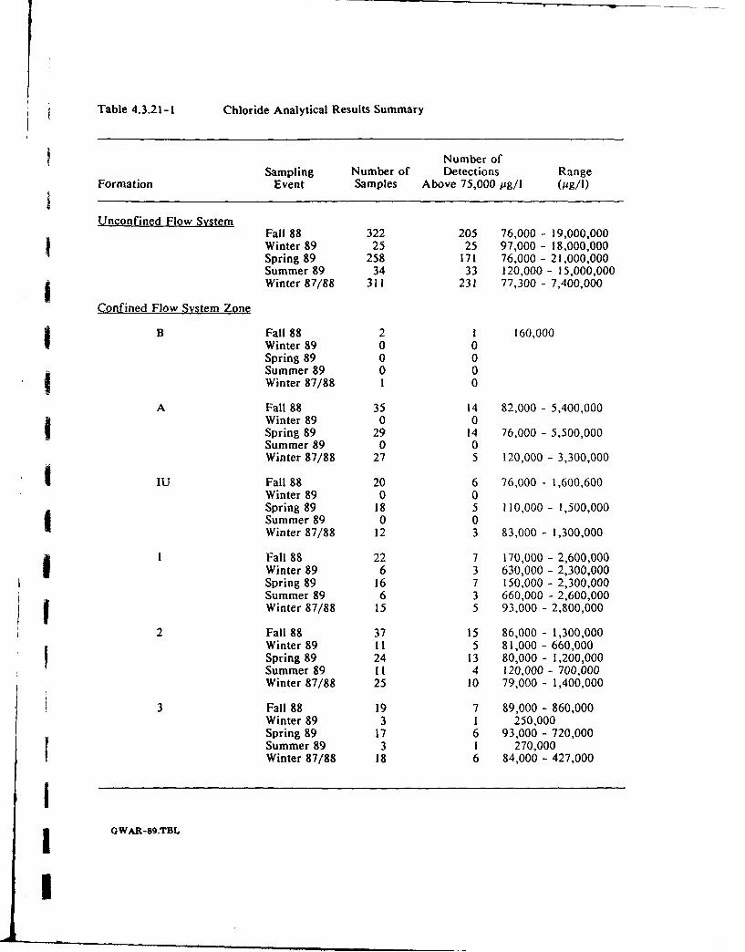
Table 4.3.21-1 Chloride Analytical Results Summary
Number ofSampling Number of Detections Range
Formation Event Samples Above 75,000 pg/l (pUg/I)
Unconfined Flow SystemFall 88 322 205 76,000 - 19,000,000Winter 89 25 25 97,000 - 18,000,000Spring 89 258 171 76,000 - 21,000,000Summer 89 34 33 120,000 - 15,000,000Winter 87/88 311 231 77,300 - 7,400,000
Confined Flow System Zone
B Fall 88 2 1 160,000Winter 89 0 0Spring 89 0 0Summer 89 0 0Winter 87/88 1 0
A Fall 88 35 14 82,000 - 5,400,000Winter 89 0 0Spring 89 29 14 76,000 - 5,500,000Summer 89 0 0Winter 87/88 27 5 120,000 - 3,300,000
IU Fall 88 20 6 76,000 - 1,600,600
Winter 89 0 0Spring 89 18 5 110,000 - 1,500,000Summer 89 0 0Winter 87/88 12 3 83,000 - 1,300,000
Fall 88 22 7 170,000 - 2,600,000Winter 89 6 3 630,000 - 2,300,000Spring 89 16 7 150,000 - 2,300,000Summer 89 6 3 660,000 - 2,600,000Winter 87/88 15 5 93,000 - 2,800,000
2 Fall 88 37 15 86,000 - 1,300,000Winter 89 11 5 81,000 - 660,000Spring 89 24 13 80,000 - 1,200,000Summer 89 11 4 120,000 - 700,000Winter 87/88 25 10 79,000 - 1,400,000
3 Fall 88 19 7 89,000 - 860,000Winter 89 3 1 250,000Spring 89 17 6 93,000 - 720,000Summer 89 3 i 270,000Winter 87/88 18 6 84,000 - 427,000
GWAR-Sg.TBL
I
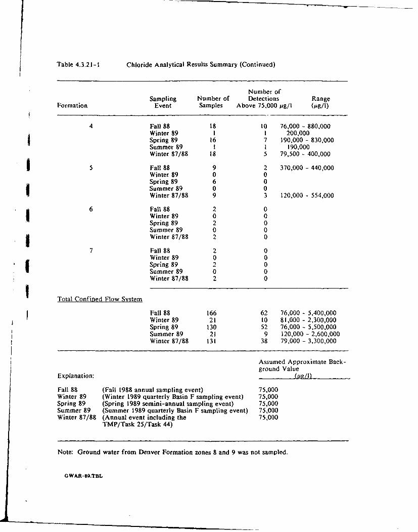
Table 4.3.2 1-1 Chloride Analytical Results Summary (Continued)
Number ofSampling Number of Detections Range
Formation Event Samples Above 75,000 pg/l (Ag/I)
4 Fall 88 18 10 76,000 - 880,000Winter 89 1 1 200,000Spring 89 16 7 190,000 - 830,000Summer 89 1 i 190,000Winter 87/88 18 5 79,500 - 400,000
5 Fall 88 9 2 370,000 - 440,000Winter 89 0 0Spring 89 6 0Summer 89 0 0Winter 87/88 9 3 120,000 - 554,000
6 Fall 88 2 0Winter 89 0 0Spring 89 2 0Summer 89 0 0
Winter 87/88 2 0
7 Fall 88 2 0Winter 89 0 0Spring 89 2 0Summer 89 0 0Winter 87/88 2 0
Total Confined Flow System
Fall 88 166 62 76,000 - 5,400,000Winter 89 21 10 81,000 - 2,300,000Spring 89 130 52 76,000 - 5,500,000Summer 89 21 9 120,000 - 2,600,000Winter 87/88 131 38 79,000 - 3,300,000
Assumed Approximate Back-ground Value
Explanation: (ug/l)
Fall 88 (Fall 1988 annual sampling event) 75,000Winter 89 (Winter 1989 quarterly Basin F sampling event) 75,000Spring 89 (Spring 1989 semini-annual sampling event) 75,000Summer 89 (Summer 1989 quarterly Basin F sampling event) 75,000Winter 87/88 (Annual event including the 75,000
TMP/Task 25/Task 44)
Note: Ground water from Denver Formation zones 8 and 9 was not sampled.
GWAR-8g.TBL
A small chloride plume occurred in the RMA Western Tier Pathway. This plume extended fromthe southern boundary of Section 9 due north through parts of Sections 4 and 33 at a width ofapproximately 1,000 feet. Chloride concentrations in this plume ranged from 91,000 jg/I
(Well 33002) to 170,000 pug/I (Well 04043). This plume probably originated from an off-post
source south or southeast of RMA.
The extent of chloride contamination was uncertain along the northeast margin of the plume, east
of the North Plants, and along the Northern Off-post Pathways. Chloride concentrations exceeded
150,000 p•g/l at Wells 24107 and 37327. These wells define the eastern margin of data control innortheast RMA. These detections indicated that either background chloride concentrations were
higher in this area or that unknown chloride contamination sources existed further east or
southeast of this area.
I Isolated detections of chloride exceeding 75,000 ug/I occurred on-post in Sections 12 and 25. An
anomalous below detection value (less than 720 pg/I) occurred at Well 27063. This well is located
upgradient of the NWBCS in northcentral Section 27.
4.3.21.2 Confined Flow System. Chloride analyses were performed on 166 samples collectedfrom wells in the confined Denver Formation flow system during the fall of 1988. A total of 62
chloride detections (above 75,000 pug/I) occurred in Denver Formation zones B through 5 rangingfrom 76,000 to 5,400,000 pg/l. Table 4.3.21-1 summarizes these detections and Figures A-55
through A-58 are point plots showing fall 1988 confined flow system chloride distribution.
I As shown on the point plots (Figures A-55 through A-58), chloride contamination •,n the confined
flow system occurred predominately beneath areas of unconfined flow system contamination. The
highest fall 1988 chloride concentration (5,400,000 p~g/I) occurred in Well 02030 screened in
Denver Formation zone A. This well is located in the South Plants, east and downgradient of thejhighest unconfined flow system contamination in this area. The deepest fall 1988 chloride
contamination was at a concentration of 280,000 pg/I in Well 36179. This well is 151 ft deep andis located in the northwest part of Basin A.
4.3.21.3 Winter 87/88 and FY89 Comparison. Data from FY89 provide a more completeI understanding of the distribution of chloride in the unconfined flow system than was available in
the FY88 Annual Report. In particular, the extent of chloride in the South Plants, Basin C, Basin
F area, and Section 35 are better defined due to more even coverage of the FY89 well network in
these areas. Plume configurations are similar in the Western Tier, North Plants, and Sections 27
IGWAR-89.4Rev. 06/22/9 - 127 -
I
and 23. Wells where chloride concentratious varied considerably from previous or subsequent
sampling rounds are listed in Table 4.3.2-2.
I Chloride was detected in the confined flow system in 38 of 131 samples collected during the
winter 1987/88 compared to 62 of 166 samples collected during the fall 1988. Table 4.3.21-1summarizes the winter 1987/88 and fall 1988 results for each zone of the confined flow system.
Areas in which the presence of chloroform in the confined flow system were further substantiateda include the South Plants, Basin A Neck, Basin F area and the NBCS. Chloroform was detected in
the South Plants more frequently in fall 1988 than in winter 1987/88 because newly installed
confined flow system wells were added to the network. Due to the general low hydraulicconductivity and large heterogeneity of the Denver aquifer, substantial data variability is likely to
occur during any single sampling period. Data interpretation based on a single sample period maynot be effective in recognizing anomalous data, therefore, variations between separate sampling
events should be considered appropriately.
t 4.3.22 Arsenic
Analyses for arsenic were performed on 484 ground-water samples collected during the fall of
1988. Arsenic concentrations ranging from 2.41 to 117 pg/I were detected in 90 of the 484
samples analyzed. The concentration of arsenic in the balance of the samples was below CRL.
The CRL for the fall of 1988 was 2.35 ug/I. Arsenic was detected in the confined flow system
within zones A, IU, 1, 2, 4, 5, and 6. The distribution of arsenic in the unconfined flow system
is illustrated in Figure 4.3.22- I. Arsenic detections for FY89 monitoring programs are summarized
in Table 4.3.22-1.
14.3.22.1 Unconfined Flow System. Ground-water samples from 319 wells completed in theunconfined flow system were analyzed for arsenic during the fall of 1988. Concentrations of
arsenic ranging from 2.41 to 117 pg/I were measured in 71 samples.
Although arsenic may occur naturally in ground water at RMA, there has been no value recog-
nized by RMA investigators or regulators to represent an upgradient background level. Therefore,
a plume is defined here by arsenic concentrations greater than the CRL, 2.35 pg/l. It should benoted that arsenic detections, even those very close to the CRL, were limited largely to known
RMA source areas. This indicates that background levels of arsenic at RMA may be lower than
2.35 ug/l.
GWAR-89.4Rev. 06/21/90 - 128 -
I
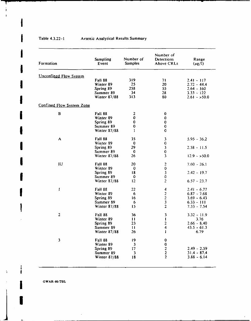
I
Table 4.3.22-1 Arsenic Analytical Results Summary
Number ofSampling Number of Detections Range
Formation Event Samples Above CRLs (Og/I)
Unconfined Flow SystemFall 88 319 71 2.41 - 117Winter 89 25 20 2.72 - 44.4Spring 89 258 55 2.64 - 160Summer 89 34 28 3.33 - 122
C Winter 87/88 313 80 2.61 - >50.0
.Confined Flow System Zone
B Fall 88 2 0Winter 89 0 0Spring 89 0 0Summer 89 0 0Winter 87/88 1 0
A Fall 88 35 3 5.95 - 36.2Winter 89 0 0Spring 89 29 3 2.58 - 11.5Summer 89 0 0Winter 87/88 26 3 12.9 - >50.0
IU Fall 88 20 2 7.60 - 26.1Winter 89 0 0Spring 89 18 3 2.42 - 19.7Summer 89 0 0Winter 87/88 12 2 6.57 - 23.7
1 Fall 88 22 4 2.41 - 6.77Winter 89 6 2 6.87 - 7.68Spring 89 16 2 3.69 - 6.43Summer 89 6 3 6.33 - IIIWinter 87/88 15 2 7.33 - 7.54
2 Fall 88 36 3 3.32 - 11.9Winter 89 11 1 3.76Spring 89 23 2 2.66 - 8.40Summer 89 1i 4 43.5 - 61.3Winter 87/88 26 1 6.79
3 Fall 88 19 0Winter 89 3 0Spring 89 17 2 2.49 - 2.59Summer 89 3 2 31.4 - 87.4Winter 87/88 18 2 3.88 - 6.14
I
I GWAR-89.TBL
II
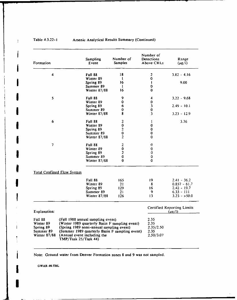
Table 4.3.22-1 Arsenic Analytical Results Summary (Continued)
Number ofSampling Number of Detections Range
Formation Event Samples Above CRLs (Ag/I)i4 Fall 88 18 2 3.82 - 4.16
Winter 89 1 0Spring 89 16 1 9.00Summer 89 1 0Winter 87/88 16 0
5 Fall 88 9 4 3.22 - 9.68Winter 89 0 0Spring 89 6 3 2.49 - 10.1Summer 89 0 0Winter 87/88 8 3 3.23 - 12.9
6 Fall 88 2 1 3.36Winter 89 0 0Spring 89 2 0Summer 89 0 0I Winter 87/88 2 0
7 Fall 88 2 0Winter 89 0 0Spring 89 2 0Summer 89 0 0Winter 87/88 0 0
i Total Confined Flow System
Fall 88 165 19 2.41 - 36.2Winter 89 21 8 0.857 - 61.7Spring 89 129 16 2.42 - 19.7Summer 89 21 9 6.33 - IIIWinter 87/88 126 13 3.23 - >50.0
Certified Reporting LimitsExplanation: (g/li)
Fall 88 (Fall 1988 annual sampling event) 2.35Winter 89 (Winter 1989 quarterly Basin F sampling event) 2.35Spring 89 (Spring 1989 semi-annual sampling event) 2.35/2.50Summer 89 (Summer 1989 quarterly Basin F sampling event) 2.35Winter 87/88 (Annual event including the 2.50/3.07
TMP/Task 25/Task 44)
j Note: Ground water from Denver Formation zones 8 and 9 was not sampled.
I GWAR-89.TBL
I
I
The fall 1988 arsenic plume map (Figure 4.3.22-I) indicates that arsenic formed a continuous
plume which originated in the South Plants and Basin A. The plume extended northwest and
widened to encompass the Basin A Neck, Basin F, Basin F West, and Basin F Northwest Pathways.
Arsenic concentrations ranged from 2.41 to 117 pg/I within the plume. The plume was terminated
to the west by the Northwest Boundary Containment System and to the north by the North
Boundary Containment System. A small plume extended north of the North Boundary
Containment System along the First Creek Off-Post Pathway in Section 14.
The highest concentrations of arsenic (illustrated by the 20 ug/l contour line) occurred in the
South Plants-Basin A-Basin A Neck Pathway and northeast of Basin F. There are several areas
where arsenic concentration exceed 50 pg/l, suggesting several localized sources of arsenic
contamination contributing to the otherwise areally extensive plume. The arsenic plume in the
First Creek Off-Post Pathway was interpreted from detections in five wells with concentrations
ranging from 2.53 to 4.80 pg/l. Isolated arsenic detections of 12.5 pg/l occurring at Wells 04036,
04037, and 04038 were considered unreliable because they were not confirmed by historicalI detections of arsenic in these same wells.
1 4.3.22.2 Confined Flow System. During the fall of 1988, arsenic was detected in 19 of 165
ground-water samples from the confined flow system. Detected concentrations ranging from 2.41
to 36.2 pug/I were measured in wells screened in zones A, IU, 1, 2, 4, 5, and 6. Analytical results
from individual zones of the confined flow system for FY89 are summarized in Table 4.3.22-1.
Point plots of these results are presented in Figures A-59 through A-61.IThe greatest depth at which arsenic was detected during the fall of 1988 was 187 ft in Well 04012
(zone 6). An arsenic concentration of 3.36 pg/I was measured at this well. This was also the
lowest stratigraphic unit containing arsenic. The highest detected concentration of arsenic was
36.2 pg/I measured in Well 36110 (zone A). This well is located between South Plants and
Basin A and is screened from 61.8 to 65.2 feet below ground surface.
4.3.22.3 Winter 87/88 and FY89 Comparison. Data from FY89 provide a more complete
understanding of the distribution of arsenic in the unconfined flow system than was available in
the FY88 Annual Report. In particular, the extent of arsenic in Basin A, Basin A-Neck, and
Basin F is better defined due to more even coverage of the well networks in these areas. Changes
in plume configurations at the NBCS and NWBCS reflect the continuing impact of these treatment
systems on ground-water quality. Plume configurations are similar for both sampling periods
throughout RMA. Wells where arsenic concentrations varied considerably from previous or
subsequent sampling rounds are listed in Table 4.3.2-2.
GWAR-89.4Rev. 06/21/9o - 131 -
I
Arsenic was detected in the confined flow system in 13 of 126 samples collected during winter
1987/88 compared to 19 of 165 samples collected during fall 1988. Table 4.3.22- I summarizes the
winter 1987/88 and fall 1988 results for each zone of the confined flow system. Areas in which
the presence of arsenic in the confined flow system was further substantiated include Sections 3,4, and 26. Arsenic in the confined flow system was detected more frequently in fall 1988 in the
Basin F area than in winter 1987/88. This may result from additional wells present in the fall
1988 network. Due to large heterogeneity of the Denver aquifer, substantial data variability is
likely to occur in any single sampling period. Data interpretation based on a single sample period
may not be effective in recognizing anomalous data, therefore, variations between sample rounds
should be considered appropriately.
4.3.23 Trace Metals
Analytical results for the trace metals cadmium, chromium, copper, mercury, lead, and zinc for
the fall of 1988 are summarized in Table 4.3-23-1. Zinc and mercury were the most frequently
detected trace metals during the fall of 1988 with 113 and 18 detections, respectively. These were
also the only trace metals with detections greater than an order of magnitude over their respective
CRL's.
The highest concentration of zinc (758 gg/I) was measured at Welt 35087 located in southwest
Section 35. Fall 1988 zinc detections greater than 100 ug/I also were measured at Wells 26041 and
27057. Well 26041 is located along the Basin F Pathway and Well 27057 is located within the
Basin F West Pathway.
The highest fall 1988 mercury detection (11.0 ug/I) was measured at Well 36056. This well is
located downgradient of the lime settling ponds in Basin A. The distribution of mercury in the
unconfined flow system is limited predominantly to the South Plants-Basin A and Basin F
Pathways.
4.4 Gas Chromatography/Mass Spectrometry (GC/MS) Results
Analysis of ground-water samples was performed by gas chromatography/mass spectrometry
(GC/MS) techniques in order to provide confirmation of analytical results of gas chromatographic
(GC) methods. In addition to confirmation of target compound identity and concentration,
GC/MS analyses also provided an identification and quantification of Tentatively Identified
Compounds (TICs), commonly referred to as nontarget compounds.
iGWAR-89.4Rev. 06/21/90 - 132-
I

Table 4.3.23-I Trace Metals Analytical Results Summary
Unconfined Flow System Confined Flow SystemCRL # Analyzed/ Range # Analyzed/ Range
Analyte pg/! # Detections pg/I # Detections Ug/I
Cd 8.40 315/5 9.04-15.9 165/4 11.2-16.9
I Cr 24.0 315/2 29.6-49.5 165/2 44.1-47.0
Cu 26.0 315/6 30.8-114 165/1 37.8
Hg 0.100 320/14 0.101-11.0 165/4 0.117-0.566
g Pb 74.0 315/2 78.0-287 165/1 82.2
Zn 22.0 315/74 22.3-758 165/39 23.1-99.7
IIIIII
iI GWAR-89.TBL
I
t
Investigative samples from 74 on-post and 15 off-post wells collected during the fall 1988 andwinter 1989 sampling rounds were analyzed by GC/MS techniques. Appendix C (on diskette)
contains the CMP analytical results for GC/MS analyses. The GC/MS analytical methods UM21(volatile), UM25 and JJ8 (semi-volatile) are laboratory methods which are certified by PMRMA
for the CMP and are based on EPA Methods 624 and 625. Method UM25 is an updated certifiedmethod which replaced method J.8 during FY89.
g Target analytes which are routinely analyzed by GC techniques are also analyzed by GC/MS
techniques for confirmation purposes. The CMP target (GC) analytes and the GC/MS methods
used to confirm GC target analyte detections are listed in Table 4.4-1. For low concentrations,GC/MS techniques can not verify GC results because the CRLs for GC/MS are generally higher.
For some analytes the CRLs for the two types of analyses are similar. However, the greatest
disparity in CRLs between GC and GC/MS analyses is found in the semi-volatile analyses ofpesticides. In all cases, dilution factors have been considered when evaluating the reported
i detection thresholds and sample results.
Tentatively identified compounds from the ground-water samples analyzed were used to examine
the need for modification of the list of target analytes. Recommendations for the addition of TICs
to the CMP target analyte list are based on the observed distribution and frequency of detections
of a specific TIC.
4.4.1 Confirmation of Volatile Organic Analyte Results
GC/MS methods for volatile organics were used to confirm the identity of target analytes
identified by GC methods. Using the historical guidelines of previous RMA RI/FS investigations,concentrations for FY89 analyses have been considered confirmed if the GC and GC/MSconcentrations are within an order of magnitude of each other. For investigative samples analyzed
by both GC and GC/MS, 202 pairs of analyte identifications were reported. Of the 202 pairs ofresults, 74 were confirmed within the order of magnitude historical guidelines. Fifty-one volatile
organic analytes detected by GC were not confirmed because the concentrations were below the
CRL for the GC/MS confirmatory analyses. Seventy-seven analytes were either not identified in
both samples, or concentrations fell outside the historical guidelines even though the concentration
of the analyte was reported above the CRL for the confirmatory GC/MS analysis. Volatile organicresults were confirmed in 49 percent of the GC/MS results reviewed, excluding the data where
concentrations of volatile organics fell below GC/MS CRLs. Unconfirmed results occurred in51 percent of the GC analyses that reported detections above the confirmatory GC/MS method
GWAR-89.4Rev. 06/21/9O - 134 -
IL
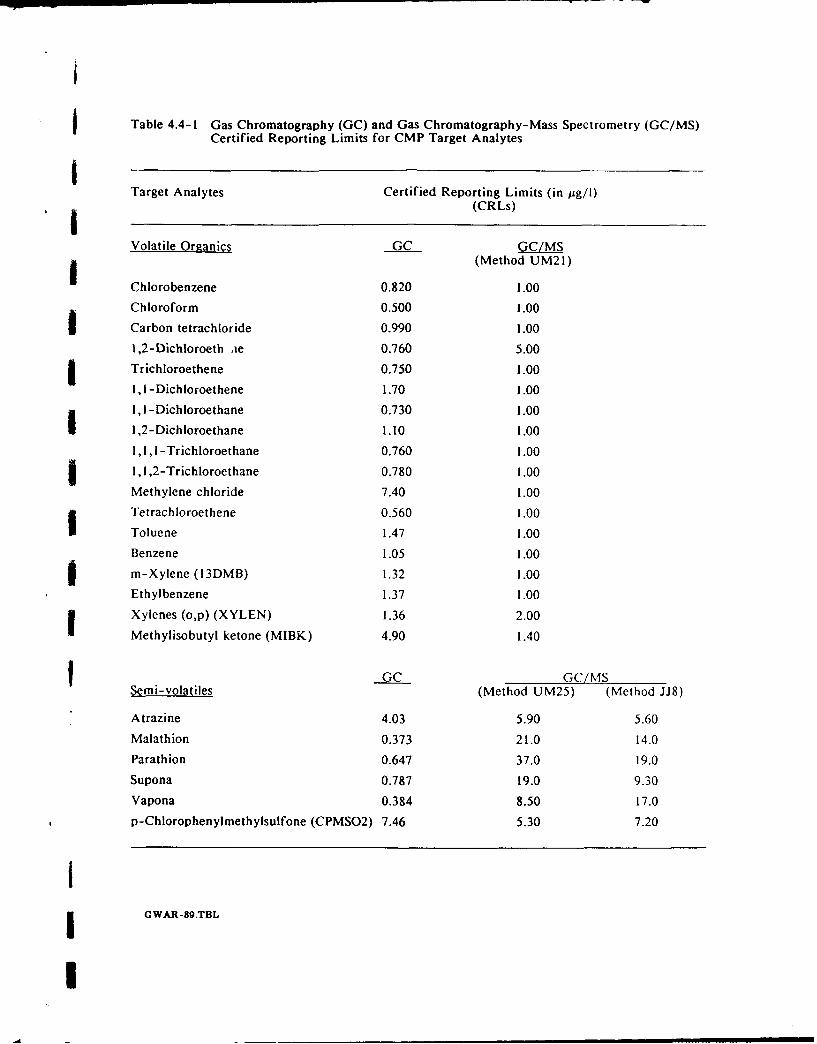
j Table 4.4-1 Gas Chromatography (GC) and Gas Chromatography-Mass Spectrometry (GC/MS)Certified Reporting Limits for CMP Target Analytes
1Target Analytes Certified Reporting Limits (in ug/I)
(CRLs)
Volatile Organics GC GC/MS(Method UM21)
Chlorobenzene 0.820 1.00
Chloroform 0.500 1.00Carbon tetrachloride 0.990 1.00
1,2-Dichloroeth ie 0.760 5.00Trichloroethene 0.750 1.00
1,1 -Dichloroethene 1.70 1.001, 1 -Dichloroethane 0.730 1.001,2-Dichloroethane 1.10 1.00
1,1,1 -Trichloroethane 0.760 1.0091,1,2-Trichloroethane 0.780 1.00
Methylene chloride 7.40 1.00
Tetrachloroethene 0.560 1.00
Toluene 1.47 1.00
Benzene 1.05 1.009 m-Xylene (13DMB) 1.32 1.00
Ethylbenzene 1.37 1.00
Xylenes (o,p) (XYLEN) 1.36 2.00
Methylisobutyl ketone (MIBK) 4.90 1.40
fGC GC/MSSemi-volatiles (Method UM25) (Method J.J8)
Atrazine 4.03 5.90 5.60
Malathion 0.373 21.0 14.0Parathion 0.647 37.0 19.0
Supona 0.787 19.0 9.30Vapona 0.384 8.50 17.0p-Chlorophenylmethylsulfone (CPMSO2) 7.46 5.30 7.20
II GWAR-89.TBL
I
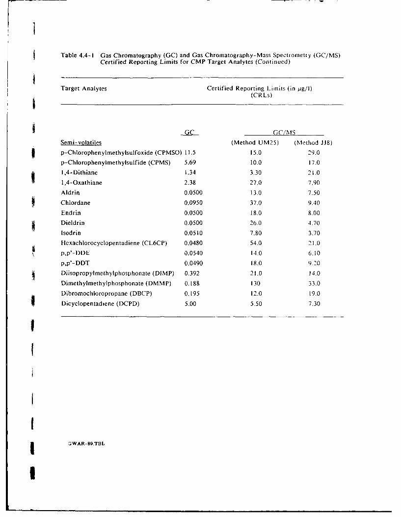
I
Table 4.4-1 Gas Chromatography (GC) and Gas Chromatography-Mass Spectrometry (GC/MS)Certified Reporting Limits for CMP Target Analytes (Continued)
Target Analytes Certified Reporting Limits (in jig/I)(CRLs)
i GC GC/MS
Semi-volatiles (Method UM25) (Method JJ8)
9 p-Chlorophenylmethylsulfoxide (CPMSO) 11.5 15.0 29.0
p-Chlorophenylmethylsulfide (CPMS) 5.69 10.0 17.0
1,4-Dithiane 1.34 3.30 21.0
1,4-Oxathiane 2.38 27.0 7.90
Aldrin 0.0500 13.0 7.50
SChlordane 0.0950 37.0 9.40
Endrin 0.0500 18.0 8.00
Dieldrin 0.0500 26.0 4.70
Isodrin 0.0510 7.80 3.70
Hexachlorocyclopentadiene (CL6CP) 0.0480 54.0 21.0
p,p'-DDE 0.0540 14.0 6.10
p,p'-DDT 0.0490 18.0 9.20
Diisopropylmethylphosphonate (DIMP) 0.392 21.0 14.0
Dimethylmethylphosphonate (DMMP) 0.188 130 33.0
Dibromochloropropane (DBCP) 0.195 12.0 19.0
Dicyclopentadiene (DCPD) 5.00 5.50 7.30
1f
II CiWAR-89.TBL
I
CRL. Poor reproducibility occurred predominantly in GC/MS analyses when excessive dilution
was required and results were compared to more specialized analyte-specific GC methods.
In addition to investigative samples analyzed by GC and GC/MS, 25 related QC samples (i.e.,
rinse, field, and trip blanks) were analyzed using these two methods. From these samples, 26
pairs of volatile organic detections were reviewed. Two pairs were not confirmed becluce the
level of detection was below that of the confirmatory CRL. Sixteen of the paired results were
confirmed within the historical guidelines. A total of eight results were not confirmed even
though the level of the reported detection was above the confirmatory method CRL. The higher
percentage of confirmations in these QC samples compared to the investigative samples probably
t is due to the lower levels of concentrations reported in these samples. Low concentration levels
of analytes required no dilution of the sample.I4.4.2 Confirmation of Semi-volatile Organic Analyte Results
For the fall 1988 and winter 1989 sampling rounds, 311 sets of investigative sample detections
were reported for semi-volatiles. The confirmation criteria for semi-volatile organics was the
same as that used in the volatile confirmation (i.e., plus or minus one order of magnitude). Of
these data sets, 43 were positively confirmed in accordance with these criteria, and 217 detections
were not confirmed because GC results were below the confirmatory CRLs. In addition, 51
analytes were not confirmed within historical guidelines even though reported concentrations were
above the confirmatory CRL. Therefore, excluding results where confirmation was not possible
because of CRL differences, 46 percent were positively confirmed and 54 percent were not
confirmed within the historical guidelines. The low percentage of positively confirmed analytes
versus the number of detections can be attributed to detection limits that are two orders of
magnitude greater for GC/MS results than for GC methods.
Review of the CMP confirmatory data indicates that volatile organics confirmation using GC/NIS
is equally efficient as semi-volatile organics confirmation. Discrepancies are generally related to
the different CRLs for GC and GC/MS methods. The GC/MS method is far less sensitive to the
target analytes than the equivalent semi-volatile GC methods.
4.4.3 Nontarget Compound Analytical Results
Data for tentatively identified compounds (TICs) have been compiled from the fall 1988 and
winter 1989 sampling rounds. Compounds identified with a specific name by the analyst and
judged to produce a characteristic spectral pattern were reviewed. Compounds not easily
GWAR-89.4Rev. 06/21/90 - 137 -
I
i
distinguished on the basis of spectral character alone were not investigated further. Special
attention was given to compounds commonly included on target analyte lists developed for other
programs, such as those lists used by EPA. Relative retention times were not considered in sorting
TICs. Tentatively identified compound information has been organized to reflect a compound's
relative abundance or frequency of occurrence to serve as a guide for f=:ire sampling/analyticalI activities. Data for TICs are ranked in Table 4.4.3-2 according to the frequency of contaminant
detections. Ranges of concentrations reported for each TIC are also presented.
g The ranges of concentrations reported for TICs are estimated values because authentic standards
(required to quantify target compounds concentrations) were not run to determine the absolute
response factor. Tentatively identified compound information was assessed routinely for the
number of identifications and respective concentrations but, because they were not on the target4 analyte list, further quantification was not performed.
Table 4.4.3-2 shows that butylbenzylphthalate (with 103 tentative identifications) was the TIC most
often identified. Butylbenzylphthalate does appear on the EPA 1988 Contract Laboratory ProgramTarget Compound List (CLP TCL). Butylbenzylphthalate often is identified as a result of4 laboratory contamination. Toxicity of this compound and most other phthalates on the EPA CLP
TCL list is poorly defined.
I The remaining compounds in Table 4.4.3-2 were grouped into three distinct groups of compounds.
These groups were CMP target analytes, non-CMP target analytes that are listed on the EPA CLP4 target compound list (TCL), and non-CMP target analytes that do not appear on the EPA CLP
TCL. The group containing CMP target analytes represents identifications that may have gone
£ undetected in GC analysis due tn shifts in retention times or matrix interferences. The secondclass of compounds includes compounds such as butylbenzylphthalate.
f In general, the occurrence of analytes in the third group of compounds appears to be associated
with chemical sources at South Plants, Basins A and F, and to a lesser degree with Basins C, D,
and E. Multiple nontarget analyte occurrences in wells usually were associated with target analyte
occurrence.
4.4.4 Conclusions for GC/MS Confirmation
Analytical data collected for purposes of confirmation of volatile organic analytes were within
historically defined confirmation guidelines for 49 percent of the samples reviewed. Semi-volatile
GC versus GC/MS results were slightly less comparable at 46 percent confirmation. Lack of
G WAR-89.4Rev. 06/21/90 - 138-
I
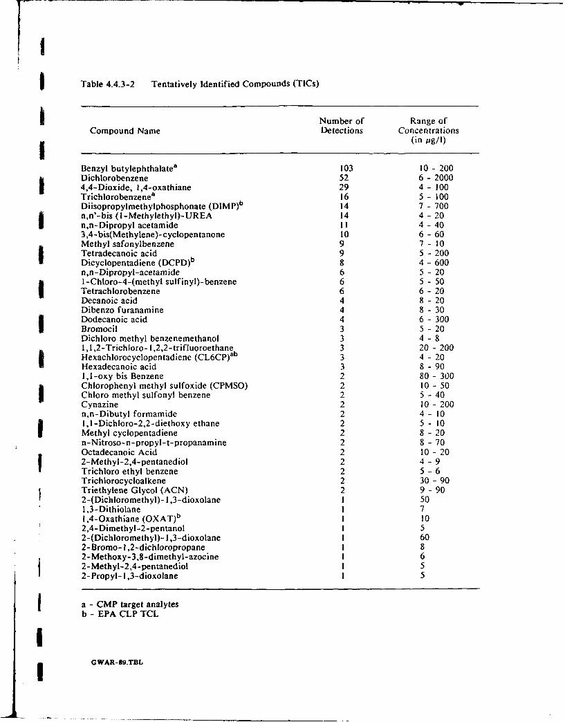
Table 4.4.3-2 Tentatively Identified Compounds (TICs)
Number of Range ofCompound Name Detections Concentrations
(in pug/I)
Benzyl butylephthalate' 103 10 - 200Dichlorobenzene 52 6 -20004,4-Dioxide, I ,4-oxathiane 29 4 -100Trichlorobenzenea 16 5 -100Diisopropylmethylphosphonate (DIMp)b 14 7 - 700n,n'-bis (I -Methylethyl)-UREA 14 4 - 20In,n-Dipropyl acetamide 11 4 -403,4-bis(Methylene)-cyclopentanone 10 6 - 60Methyl safonylbenzene 9 7 -10Tetradecanoic acid 9 5 -200Dicyclopentadiene (CDb8 4 -600n,n-Dipropyl-acetamide 6 5 -201-Chloro-4-(methyl sulfinyl)-benzene 6 5 - 50Tetrachlorobenzene 6 6 -20Decanoic acid 4 8 -20Dibenzo furanamine 4 8 -30Dodecanoic acid 4 6 -300IBromocil 3 5 -20Dichioro methyl benzenemethanol 3 4 - 81, 1,2-Trichloro- 1,2,2-trifluoroethane 3 20 - 200Hexachlorocyclopentadiene (LCb3 4 -20Hexadecanoic acid 3 8 -901,1-oxy bis Benzene 2 80 -300Chiorophenyl methyl sulfoxide (CPMSO) 2 10 - 50IChioro methyl sulfonyl benzene 2 5 - 40Cynazine 2 10- 200n,n-Dibutyl formamide 2 4 -101,1-Dichloro-2,2-diethoxy ethane 2 5 - 10IMethyl cyclopentadiene 2 8 -20n-Nitroso-n-propyl-t-propanamine 2 8 - 70Octadecanoic Acid 2 10 -202-Methyl-2,4-pentanediol 2 4 -9Trichioro, ethyl benzene 2 5 -6Trichlorocycloalkene 2 30 -90Triethylene, Glycol (ACN) 2 9 -902-(Dichloromethyl)- I ,3-dioxolane 1 501,3-Dithiolane )b1 7I .4-Oxathiane (OXATb 1 102,4-Dimethyl-2-pentanol 1 52-(Dichloromethyl)- 1,3-dioxolane 1 602-Bromo- I ,2-dichloropropane 1 82-Methoxy-3,8-dimethyl-azocine 1 62-Methyl-2,4-pentanediol 1 52-Propyl- I ,3-dioxolane 1 5
a - CMP target analytesb - EPA CLP TCL
C WAR-ag.TBL
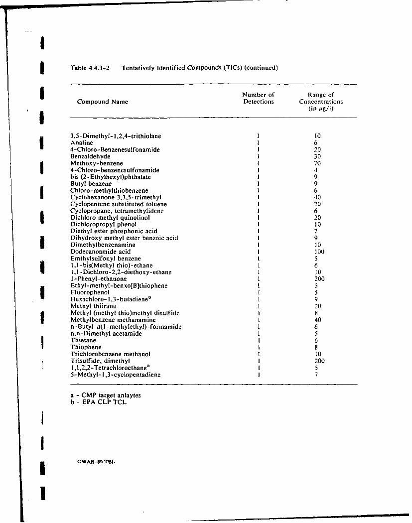
Table 4.4.3-2 Tentatively Identified Compounds (TICs) (continued)
INumber of Range ofCompound Name Detections ConcentrationsI ~(in pg/0)
3,5-Dimethyl- I ,2,4-trithiolane 1 10Analine 1 6I4-Chloro-Benzenesulfonamide 120
Methoxy-benzene 174-Chioro- benzenesulfonamide 1 4bis (2-Ethylhexyl)phthalate19
Chloro-methylthiobenzene16ICyclohexanone 3,3,5-trimethyl 140Cyclopentene substituted toluene 1 20Cyclopropane, tetramethylidene 1 6IDichioro methyl quinolinol 1 200Dichloropropyl phenol 11Diethyl ester phosphonic acid 1 7Dihydroxy methyl ester benzoic acid 1 9
Dodecanoamide acid 1100imethylbelfnylenzmene 1 10
1, 1 -bis(Methyl thio)-ethane 6I1, 1 -Dichloro- 2,2 -dietho xy- ethane 1 10I -Phenyl-ethanone 1 200Ethyl- methyl -ben xo[B Ithiophene 1 5Fluorophenol 1 5Hexachioro- I ,3-butadienea 9Methyl thiirane I20Methyl (methyl thio)methyl disulfide 18IMethylbenzene methanamine 140n-Butyl-n(1 -methylethyl)-formamide 1 6n,n-Dimethyl acetamide 1 5Thietane 1 6
Trichlorobenzene methanol ItTriulfdedimethyl120
1 ,l,2,2-Tetrachloroethanea I 55-Methyl- I ,3-cyclopentadiene 1 7
a - CMP target anlaytes
b - EPA CLP TCL
I GWAR-ag.TBL
I
analyte confirmation was predominantly due to the discrepancy between GC/MS method CRLs
and GC method CRLs. Another important factor was that high level samples containing multiple
target analytes were more highly diluted in GC/MS method analysis versus the more specific GC
methods that required less dilution due to detection selectivity or specific instrumental conditions.
Detections of nontarget semi-volatile analytes generally coincided spatially with detections of
target analytes and generally were located in proximity to potential contaminant source areas.
The results of the nontarget assessment indicated the presence of numerous nontarget analytes in
ground-water samples from many areas of RMA. Butylbenzylphthalate was the most commonly
identified TIC but was thought to be a product of laboratory contamination, in that it is a
Irelatively common laboratory artifact. Dichlorobenzenes were present in CMP, samples
historically, including 1988. In the current year they were detected in significantly high
quantities. The majority of nontarget analytes commonly consisted of halogenated and
nonhalogenated hydrocarbons. The compounds most commonly identified were substituted
aromatic hydrocarbons, presumably because of their generally higher relative solubility in water.
4.5 Quality Assurance/Quality Control (QA/OC)IThe QA/QC Plan implemented during the CMP is based on the Chemical Quality Assurance Plan,
version 1.0, dated July 1989, from the Program Manager's Office at RMA, the subcontract
laboratory's QA program and the requirements of the CMP contract (PMRMA, 1989a). The
objectives of the Quality Assurance Program for the RMA CMP are to:
!"* Ensure that technically defensible and consistent field procedures are used in the
9 collection of samples;
"* Document procedures used in the collection, preservation, and handling of samples
by using field data sheets, logbooks, sample control logbooks, etc.;
S• Collect additional samples of all media such that data accuracy, precision, and
representativeness may be assessed; and
"* Perform chemical analysis of all samples, including those collected for quality
control, according to documented certified procedures that will ensure data validity.
Field sampling procedures consisted of sample collection protocols that include appropriate QC
I sample collection, sample handling and storage, sample preservation, holding times, documentation
GWAR-89.4Rev. 06/21/9o - 141 -
I
-4
that is legal and defensible, and proper shipping procedures. Field QC samples consisted of trip,field, and rinse blanks and duplicate (or split) samples.
This section of the Annual Report presents an interpretation of the analytical data resulting from
analysis of field-derived QC samples. Sampling and QA/QC procedures stipulate the type and
minimum frequency at which field derived QC samples are to be submitted to the program
laboratory. The CMP QA/QC program requires that sample duplicates (splits), field blanks, trip
blanks, and rinse blanks be collected and submitted for analysis.
Sample splits are defined under the CMP as two identical sets of sample bottles that are submitted
I to the laboratory for an identical suite of analyses. Splits are collected by alternately filling
sample bottles. The purpose of split samples is to measure the analytical variability that results
from analysis of two identical samples. Field blanks consist of sample bottles filled in the field
with distilled/deionized organic free water and submitted to the laboratory to determine if the
sampling procedure has introduced extraneous contaminants to ground-water samples. Trip blanks
consist of 40 ml VOA bottles filled by the laboratory with organic free distilled/deionized water,transported to the field site, and shipped back to the laboratory in an unopened state. These
samples are used to assess if contaminants are introduced into samples during the transport and
handling process. Rinse blanks evaluated the extent to which sampling equipment had been
decontaminated. Organic free distilled/deionized water is poured over decontaminated field
sampling equipment, collected, and transported to the laboratory for analysis.
A total of 977 investigative ground-water samples were collected during the fall 1988, winter
1989, spring 1989, and summer 1989 sampling events. In addition to these 977 investigative
samples, 49 rinse blanks, 50 field blanks, 50 trip blanks, and 98 duplicate QC samples were
collected.
Laboratory QC data were reported weekly to PMRMA in a QA Status Report that included all
laboratory QC data, including precision and accuracy control charts for each sample lot. QC data
were examined in relation to the criteria established during the analytical certification process.
Deviations from the established QC criteria were identified by the laboratory, and appropriate
corrective actions taken. The data were then reviewed for reliability by the Program QA officer.
Any data deemed unacceptable by the Project Management QA personnel were not accepted for
entry into the Installation Restoration Data Management System (IRDMS). As this process
addresses the QA/QC aspects of laboratory analysis this subject is not addressed in this section of
this -*.port.
IGWAR-89.4Rev. 06/21/90 - 142 -
I
I
4.5.1 Evaluation of Blank Data
Chemical analysis of trip, field, and rinse blanks were performed to ensure integrity of CMP data
and check for contamination from field or laboratory sources. Blanks were analyzed for volatile
organics, semi-volatile organics, and inorganics.IObjectives for assessment of blank data were to identify and, if possible, quantify the magnitude
of contamination introduced during the sampling and shipping process and decontamination of
sampling equipment. There is no published regulatory guidance document designed to aid in the
assessment of the applicability of field blank QC results with respect tv the utility of the final
j investigative data.
Contamination detected in the field blanks was not used to correct final data but should beevaluated carefully to determine whether the detected contamination was inherent in the
environment or was a result of the sampling process. Contaminants identified in the blanks that
were absent in laboratory preparation blanks indicate a potential field sampling problem, 2
d~ficiency in bottle preparation, a decontamination problem, or a failure to prepare the laboratory
9 blank in a manner similar to the field blank.
4.5.1.1 Volatile Organic Quality Control Data Review. Trip, rinse, and field blanks were
collected and their data reviewed for four rounds of ground-water monitoring. These data were
reviewed to identify compounds not characteristic of ground-water chemistry, but resulting from
9 some external or internal laboratory practices. Identification of these artifact compounds is critical
in evaluating the ultimate utility of affected analytical results. Nine different compounds were
identified in blanks from these four sampling events. Table 4.5.1.1-1 summarizes the target
analyte concentration and type of blanks for each artifact detected. Blanks analyses are listed by
well number. The concentration of the blank artifact found in the related ground-water sample
I taken from the same location just prior to the collection of the blank sample also is presented in
Table 4.5.1.1-1.
Data presented in Table 4.5.1.1-1 for volatile analyses show that chloroform (CHCL3) at levels
above the CRL commonly occurred in rinse blanks. Chloroform was not identified in trip blanks,
and only a single low-level detection was reported in field blanks. Chloroform found in
investigative samples indicates that samples from Wells 02023, 01525, 26151, 26160, 26161, 22064,
23118, 35077, 35089, 36114, and 36177 may have been affected by CHCL3 contamination.
Investigative sample concentrations are generally within an order of magnitude of the
IIGWAR-89.4Rev. 06/21/90 - 143-
I
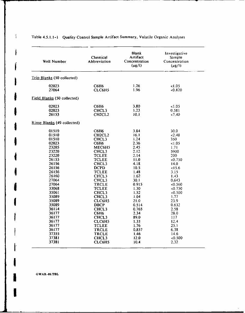
Table 4.5.1.1-1 Quality Control Sample Artifact Summary, Volatile Organic Analyses
f Blank Investigative
Chemical Artifact SampleWell Number Abbreviation Concentration Concentration
(pAg/I) (1g/i)
I Trip Blanks (50 collected)
02023 C6H6 1.26 < 1.05
27064 CLC6H5 1.96 <0.820
I Field Blanks (50 collected)
02023 C6H6 3.80 <1.0502023 CHCL3 1.23 0.58126153 CH2CL2 10.1 <7.40
Rinse Blanks (49 collected)
01510 C6H6 3.84 30.001510 CH2CL2 16.1 <2.4801510 CHCL3 1.24 35002023 C6H6 2.36 < 1.0523205 MEC6H5 2.45 1.7123220 CHCL3 2.12 590023220 TCLEE 2.14 20026153 TCLEE 11.0 <0.75026156 CHCL3 4.18 14.026156 DCPD 10.5 < 15.626156 TCLEE 1.48 3.1526160 CHCL3 1.62 1.4327064 CHCL3 30.1 0.64327064 TRCLE 0.915 <0.56033068 TCLEE 1.30 <0.75035061 CHCL3 1.52 <0.50035089 CHCL3 1.04 1.7735089 CLC6H5 21.0 23.935089 DBCP 0.514 0.63236114 CHCL3 0.765 2.5836177 C6H6 2.34 28.036177 CHCL3 89.0 11736177 CLC6H5 1.33 12.4
36177 TCLEE 1.76 25.136177 TRCLE 0.857 6.3837355 TRCLE 1.46 14.637381 CHCL3 12.0 <0.50037381 CLC6H5 10.4 2.32
II GWAR-89.TBL
I
concentration found in the associated field or rinse blank. On this basis, chloroform must be
considered an artifact of field operations or laboratory practices.
Samples from Wells 01510, 26156, and 36177, collected just prior to collection of the related rinse
blank, contained concentrations of chloroform that were above those reported for the blank. This
indicates that decontamination of sampling equipment was not complete. This is most obvious in
Well 36177, which contained 177 pg/I and the related rinse blank contained 89 pg/I. The
sample from Well 27064 contained only 0.643 ug/I chloroform and the related field blank
contained 30 pg/I. In this case, the rinse blank and the investigative sample were affected by
some other type of field or laboratory practice. In the case of the three previously mentioned
samples, the levels of chloroform detected in these samples was greater than five times the levels
detected in the blank and should be considered characteristic of the investigative sample water
chemistry.
Tetrachloroethene (TCLEE) was detected in six rinse blanks. In four of these cases, the related
investigative sample collected just prior to the QC sample contained TCLEE at concentrations at
least five times greater than those detected in the related QC sample. In the remaining two cases,
the related investigative sample results did not indicate the presence of TCLEE. Of the samples
related to those four cases that exhibited cross-contamination between samples (carryover), noneg of the investigative sample results were affected by TCLEE carryover.
Benzene (C6H6) was detected in a single trip blaak and field blank. In both of these cases, both
of the related samples reported benzene at concentrations below the method CRL. Benzene was
identified in three rinse blanks. Two of these detections probably are the result of carryover from
the related investigative sample. However, one of the other investigative samples collected on the
same day as these two blanks had benzene concentrations greater than the CRL. Based on these
observations, benzene may have been introduced during laboratory procedures or other unrelated
field activities.
Chlorobenzene (CLC6H5) was detected in one trip blank and two rinse blanks. The potential for
carryover is exhibited in the sample from Well 35089 because chlorobenzene was detected in the
related investigative sample at a concentration of 23.9 pg/l and in the rinse blank sample at a
concentration of 21.0 pg/l. Chlorobenzene was not detected in any of the other investigative
samples collected on this day.
Similarly, methylene chloride (CH2CL2) was detected in a trip blank and a rinse blank, but was
not detected in any of the related investigative samples except the sample from Well 01525. In
GWAR-89.4Rev. 06/21/90 - 145 -
I
If
I this sample, high concentrations of other target analytes required excessive dilution to bring thehighest level 1rialytes into the linear range of the method. In doing so, the CH2CL2 artifact
jconcentration was artificially increased to 8400 pg/l. This result should not be considered
representative of the sample chemistry.
Trichloroethene (TRCLE) was detected in three rinse blanks. In two of the three cases, carryover
may have occurred; however, none of the related investigative samples exhibit TRCLE levels
above the method CRL. Carryover of TRCLE is thus not expected to have impacted theinvestigative analytical results. A single detection of each of the following chemical constituents
was also observed in rinse blanks analyzed for volatile organic constituents: toluene (MEC6H5),
dicyclopentadiene (DCPD), and dibromochloropropane (DBCP). Of these three, two couldpotentially be the result of carryover from the related investigative sample. Investigative sample
results are negative for all three analytes suggesting carryover of these compounds has not affected
the analytical results.
I Overall, it appears that sample contamination was a minor problem in FY89 volatile organic
analyses.
4.5.1.2 Semi-volatile Organic and Pesticide Ouality Control Data Review. In the 149 QCsamples analyzed for semi-volatile chemical constituents during FY89, II unique types of target
analytes were detected. These data are presented in Table 4.5.1.2-I.
A variety of semi-volatile target compounds was detected in three of the 50 trip blanks analyzed
for semi-volatile compounds during FY89 ground-water sampling. Carryover from the investiga-
tive sample collected and transported to the laboratory with the QC trip blank was observed only
in Sample 23237. As shown in Table 4.5.1.2-1, this investigative sample contained 0.581 ug/I ofVapona (DDVP) and the related trip blank contained 0.862 pjg/I of DDVP. This analyte was also
detected in wells 26089 and 26088 at concentrations close to those reported in the blank andrelated investigative sample. DDVP was detected in Well 26089 at a concentration of 1.57 pg/I
and in Well 26088 at a concentration of 0.95 pg/i. In all other types of QC samples, DDVP alwayswas detected at a higher concentration in the QC sample than in the related investigative sample.This indicates that a laboratory contamination problem may exist. A review of the overall
analytical results for DDVP in the four quarters of the CMP reveals that 43 of 57 detectionsrecorded were at concentrations near five times the method CRL. These low level values should
be considered as artifacts on the basis of these QC results.
IG WAR-8g.4Rev. 06/21/90 - 146 -
I
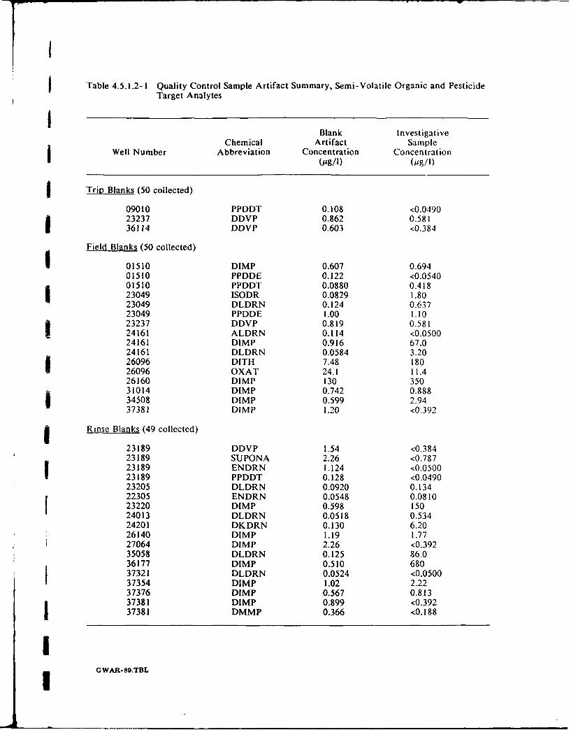
5 Table 4.5.1.2-1 Quality Control Sample Artifact Summary, Semi-Volatile Organic and PesticideTarget Analytesi
Blank InvestigativeChemical Artifact SamplejWell Number Abbreviation Concentration Concentration
(.pg/I) (0g/I)
Trip Blanks (50 collected)
09010 PPDDT 0.108 <0.049023237 DDVP 0.862 0.58 I36114 DDVP 0.603 <0.384
Field Blanks (50 collected)
01510 DIMP 0.607 0.69401510 PPDDE 0.122 <0.054001510 PPDDT 0.0880 0.41823049 ISODR 0.0829 1.8023049 DLDRN 0.124 0.63723049 PPDDE 1.00 1.1023237 DDVP 0.819 0.58124161 ALDRN 0.114 <0.050024161 DIMP 0.916 67.024161 DLDRN 0.0584 3.2026096 DITH 7.48 18026096 OXAT 24.1 11.426160 DIMP 130 35031014 DIMP 0.742 0.88834508 DIMP 0.599 2.9437381 DIMP 1.20 <0.392
Rinse Blanks (49 collected)
23189 DDVP 1.54 <0.38423189 SUPONA 2.26 <0.78723189 ENDRN 1.124 <0.050023189 PPDDT 0.128 <0.049023205 DLDRN 0.0920 0.13422305 ENDRN 0.0548 0.081023220 DIMP 0.598 15024013 DLDRN 0.0518 0.53424201 DKDRN 0.130 6.2026140 DIMP 1.19 1.7727064 DIMP 2.26 <0.39235058 DLDRN 0.125 86.036177 DIMP 0.510 68037321 DLDRN 0.0524 <0.050037354 DIMP 1.02 2.2237376 DIMP 0.567 0.81337381 DIMP 0.899 <0.39237381 DMMP 0.366 <0.188
Il C WAR-89.TBL
I
Of the field blanks collected during FY89 16 samples had detections above the GC method
detection limit. Vapona was detected at a concentration of 0.581 pig/I in a single sample, but is
not thought to indicate a field problem. Diisopropylmethylphosphonate (DINIP) was detected in
six of the field blanks. In all but one case, the concentration detected in the investigative sample
collected just prior to the analysis of the QC blank is higher than that reported for the related QC
sample. This indicates that airborne DIMP has contaminated the QC samples in the field or that
analytical cross-contamination for samples in the same analytical lot has occurred. The latter
explanation seems to be the most plausible. In this case, those samples in the analytical lots related
to samples from Wells 01510, 24161, 16160, 31014, 34508, and 37381 may have been affected.
Similarly, PPDDE, PPDDT, isodrin, dieldrin, aldrin, dithiane, and oxathiane found in the field
blanks probably represent laboratory generated artifacts, because none of the compounds are veryvolatile or soluble in water. This indicates that results for those compounds listed in
Table 4.5.1.2-1 should be suspect in those samples contained in the same lot with the respective
QC sample wells listed in this table. Although the majority of detections are greater in the related
investigative samples than in the QC rinse blank samples, the mechanism for the observed
contamination cannot be evaluated at this time.
In conclusion, semi-volatile and pesticide results for investigative samples analyzed in the same
analytical lot as the contaminated rinse or field QC samples listed in Table 4.5.1.2-1 should be
utilized considering the following guidelines. Compounds identified in the investigative sample
and ir, . related QC sample at levels of concentration within five times of each other should be
considered artifacts of laboratory practices. The use of a five times cut-off for distinguishing
uncommon artifacts from actual sample constituents was obtained from the U.S. EPA Laboratory
(USEPA, 1988). Concentrations in investigative samples of artifacts identified in related QC
samples that are greater than five times those levels identified in the blank should be considered
biased high or estimated values.
4.5.1.3 Inorganic Data Quality Control Review. The QC review for the inorganic data was
confined to the trace elements because of the potentially toxic nature of those artifacts. The
dissolved solids (e.g., nitrate, sulfate, potassium, etc.) were not considered in this review because
of their strong association with general water chemistry.
The trip, field, and rinse blanks containing detectable concentrations of trace elements are
summarized in Table 4.5.1.3-1. The table compares the concentration detected in the blank to the
concentration detected in the related investigative sample.
IGWAR-89.4Rev. 06/21/90 - 148 -
I
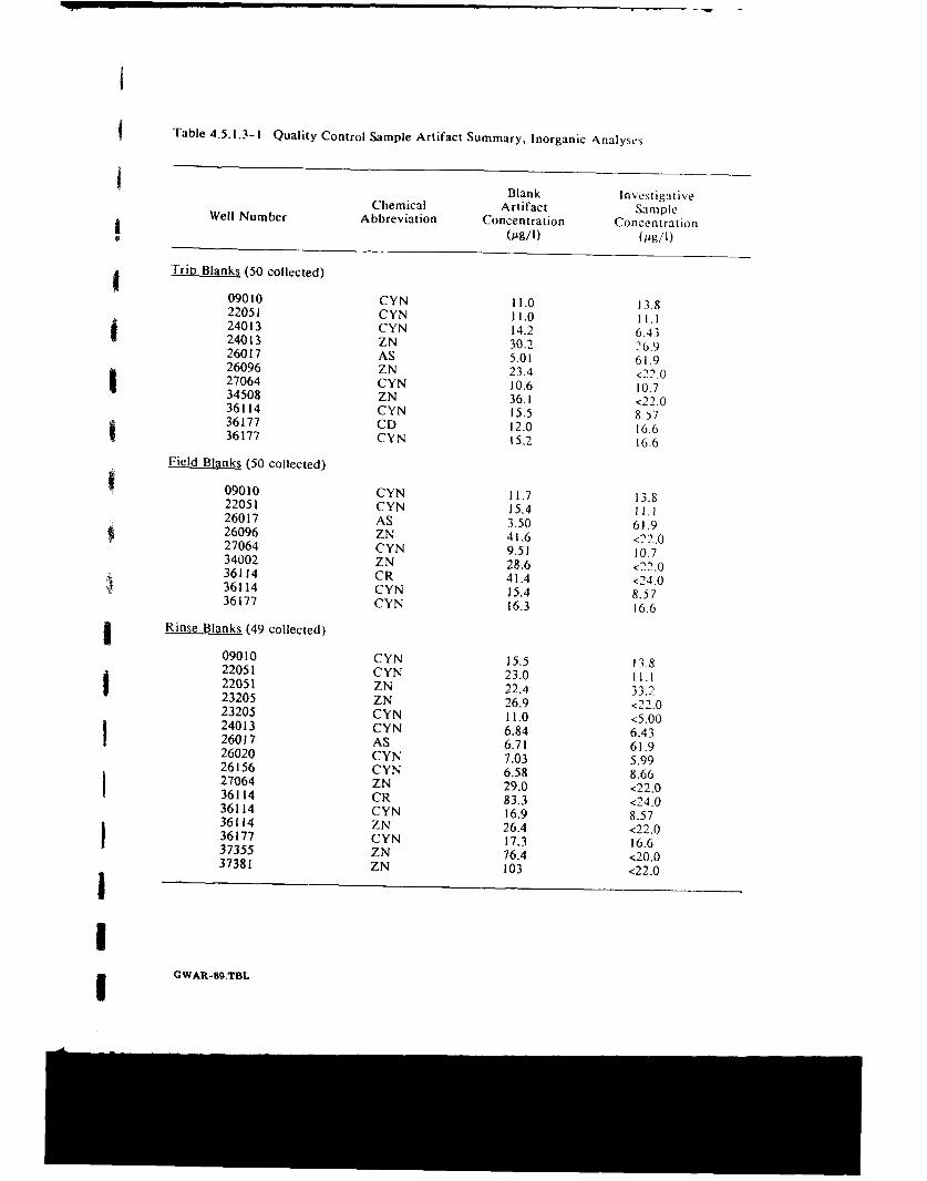
S II
f Table 4.5.1.3-1 Quality Control Sample Artifact Summary, Inorganic Analyses
Blank InvestigativeChemical Artifact SampleWell Number Abbreviation Concentration ConcentrationS( A •g / l) (O g / l)
e Trip Blanks (50 collected)
09010 CYN 11,0 13.822051 CYN 11.0 11.124013 CYN 14.2 6-4324013 ZN 30.2 26.926017 AS 5.01 61.926096 ZN 23.4 <'2.027064 CYN 10.6 10.734508 ZN 36.1 <22.036114 CYN 15.5 8.5736177 CD 12.0 16.636177 CYN 15.2 16.6
Field Blanks (50 collected)
09010 CYN 11.7 13.822051 CYN 15.4 11.126017 AS 3.50 61.926096 ZN 41.6 <22.027064 CYN 9.51 10.734002 ZN 28.6 <22,036114 CR 41.4 <24.036114 CYN 15.4 8.5736177 CYN 16.3 16.6
Rinse Blanks (49 collected)
09010 CYN 15.5 13.822051 CYN 23.0 11.122051 ZN 22.4 33.223205 ZN 26.9 <22.023205 CYN 11.0 <5.0024013 CYN 6.84 6.4326017 AS 6.71 61.926020 CYN 7.03 5.9926156 CYN 6.58 8.6627064 ZN 29.0 <22.036114 CR 83.3 <24,036114 CYN 16.9 8.5736114 ZN 26.4 <22.036177 CYN 17.3 16.637355 ZN 76.4 <20,037381 ZN 103 <22.0
Ii GWAR-89.TBL
I
The most common artifact detected in the FY89 blank analyses of trace elemelts was cyanide
(CYN). Cyanide concentrations in blanks ranged from 6.58 to 23.0 ,ug/l. The investigative
samples affected by cyanide carryover are from Wells 09010, 22051, 24013, 27064, 36114, 36177,
26020, and 26156.
In two of the samples in which cyanide was detected in both the blank and in the relatedinvestigative sample, cyanide was detected in the rinse blanks only, and not in field or trip blanks.
In all of the remaining samples, cyanide was detected in all three types of QC samples listed in
Table 4.5.1.3-1. This indicates that, in all samples except those from Wells 26020 and 26156,contamination was probably related to laboratory cross-contamination. Therefore, CMP sample
results for cyanide, detected at levels within five times the method CRL of 5.00 pg/i (as per EPA
Guidelines, 1988), should be viewed as laboratory-produced artifacts.
Artifacts of zinc (ZN) are the second most commonly observed inorganic constituents in blank
samples. Related investigative samples in all but two of the cases shown in Table 4.5-3 appear
to be unaffected by ZN carryover. This indicates that ZN artifacts are related to the chemistryof the water used in preparing the QC samples. Sample 22051 is the only sample in which ZN
was detected in the investigative sample and in the rinse blank. ZN was not detected at a concen-
tration above the method CRL in any other sample collected on the same day.
Arsenic (AS) was detected in a trip blank at 5.01 pg/I, in a field blank at 3.50 jg/l, and in a rinse
blank at 6.71 pg/l. These blanks are related to a single investigative sample, 26017, in which anArsenic concentration of 61.9 p4g/I was detected. Because Arsenic was detected in all three types
of blanks, it must be assumed that the observed concentrations in both the QC and investigative
sample are unrelated and are representative of actual differences in water chemistry.
Cadmium (CD) and Chromium (CR) were detected in QC samples but not in the related investi-gative samples. Their presence must, therefore, be related to the water chemistry of the QC
samples.
Based on the QC review of the inorganic trace elements in rinse, trip, and field blanks, cyanide
concentrations detected at levels near five times the method CRL should be considered question-
able. All other indications are that inorganic artifacts detected during the CMP are related to QC
sample water chemistry and have not significantly affected the investigative sample results.
IGWAR-89.4Rev. 06/21/90 - 0SO
UI1~

I
4.5.2 Evaluation of Data for Sample Duplicates
The objectives of evaluating field duplicate sample results are to assess the potential problems of
precision of the sampling and analytical systems, determine if there are any significant variations
between duplicate samples, and assess the validity of the duplicate results by verifying that the
I results are reproducible. The CMP selected at random 10 percent of the total number of samples
collected.
A field duplicate is a second sample collected from the same site, submitted to the laboratory as
a separate sample, and analyzed independently. The results are an external check on the combined
i precision of sampling and analysis. The results may exhibit more variability than laboratory
duplicates because their measurement is a combination of field and laboratory performance.
Actions taken as a result of duplicate sample analysis must be weighed carefully. It is difficult
to determine if poor precision is a result of sample nonhomogeneity, sampling variability, method
defects, or laboratory technique. Aqueous samples containing high levels of solids can produce
erratic duplicate sample results for organic and inorganic analyses. In general, the results of
Sduplicate sample analysis should be used to support conclusions drawn about the quality of data
rather than as a basis for these conclusions.
I Duplicate samples were collected at 98 well locations during the CMP and analyzed. Results were
compared to determine the reproducibility of analytical results. To evaluate the large quantity of
5 paired analytical results reported, duplicated sample results were statistically evaluated using the
standard EPA duplicate sample agreement (DSA) procedure. Paired analytical results used in this
statistical study included only those duplicate analyses wherein at least one positive identification
and quantitation was recorded. Estimated values were excluded from the database. DSA was
calculated by taking the absolute value of the difference between the two matched values and
I dividing this difference by the average of the two values and then multiplying this quotient by
100. The DSA value for a matched pair of results, therefore, is expressed as the percent
difference that the duplicate result is away from the average of the two measured concentrations.
Table 4.5.2-1 lists the average and range of these DSA values for each target analyte along with
the number of matched pairs utilized in performing the statistical evaluation. A DSA value of
67 percent represents a reported concentration that is twice that of the duplicate. In general, DSA
values are meant to provide a general indication of reproducibility, and should not be evaluated
quantitatively.
iGWAR-89.4Rev. 06/21/90 151
I
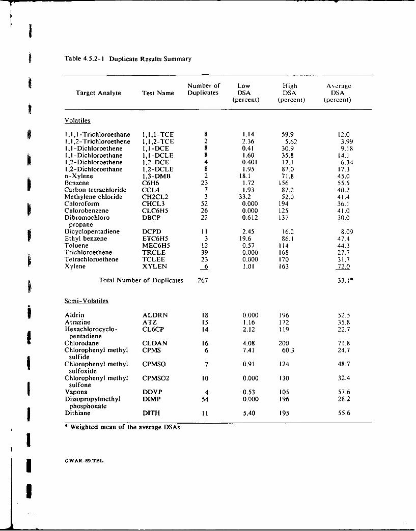
Table 4.5.2-1 Duplicate Results Summary
Number of Low High A%,erageTarget Analyte Test Name Duplicates DSA DSA DSA
(percent) (percent) (percent)IVolatiles
1 1, 1 -Trichloroethane 1,1,l-TCE 8 1.14 59.9 12.01, 1,2-Trichloroethene 1, I,2-TCE 2 2.36 5.62 3.99I,1-Dichloroethene 1, 1 -DCE 8 0.41 30.9 9.181,1 -Dichloroethane 1, 1 -DCLE 8 1.60 35.8 14.11,2-Dichloroethene 1,2-DCE 4 0.401 12.1 6.341,2-Dichloroethane 1,2-DCLE 8 1.95 87.0 17.3n-Xylene 1,3-DMB 2 18.1 71.8 45.0Benzene C6H6 23 1.72 156 55.5Carbon tetrachloride CCL4 7 1.93 87.2 40.2Methylene chloride CH2CL2 3 33.2 52.0 41.4Chloroform CHCL3 52 0.000 194 36.1Chlorobenzene CLC6H5 26 0.000 125 41.0Dibromochloro DBCP 22 0.612 137 30.0
propaneDicyclopentadiene DCPD 11 2.45 16.2 8.09
SEthyl benzene ETC6H5 3 19.6 86.1 47.4Toluene MEC6H5 12 0.57 114 44.3Trichloroethene TRCLE 39 0.000 168 27.7Tetrachloroethene TCLEE 23 0.000 170 3 1.7Xylene XYLEN 6 1.01 163 72.0
Total Number of Duplicates 267 33.1*
Semi-Volatiles
Aldrin ALDRN 18 0.000 196 52.5Atrazine ATZ 15 1.16 172 35.8Hexachlorocyclo- CL6CP 14 2.12 119 22.7
pentadieneChlorodane CLDAN 16 4.08 200 71.8Chlorophenyl methyl CPMS 6 7.41 60.3 24.7
sulfideChlorophenyl methyl CPMSO 7 0.91 124 48.7
sulfoxideChlorophenyl methyl CPMS02 10 0.000 130 32.4
sulfoneVapona DDVP 4 0.53 105 57.6Diisopropylmethyl DIMP 54 0.000 196 28.2
phosphonateDithiane DITH 11 5.40 195 55.6
* Weighted mean of the average DSAs
IG WAR-89.TBL
-
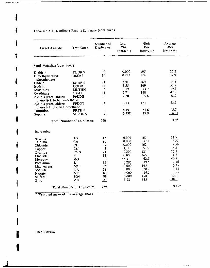
I
I Table 4.5.2-1 Duplicate Results Summary (continued)
i Number of Low High Average
Target Analyte Test Name Duplicates DSA DSA DSA(percent) (percent) (percent)
Semi-Volatiles (continued)
Dieldrin DLDRN 30 0.000 195 25.2
Dimethylmethyl DMMP 10 0.282 124 37.9phosphonate
Endrin ENDRN 21 2.98 169 44.3
Isodrin ISODR 16 3.55 169 51.7
Malathion MLTHN 6 3.19 53.9 19.6Oxathiane OXAT it 2.71 140 42.8
2,2-bis (Para-chloro PPDDE II 2.20 65.8 28.0phenyl)- 1,1 -dichloroethene
2,2-bis (Para-chloro PPDDT 18 3.53 181 63.5phenyl- 1, 1, 1 -trichloroethane
Parathion PRTHN 7 8.49 54.6 25.7
Supona SUPONA 5 0.738 19.9 6.31
Total Number of Duplicates 290 38.9*
Inorganics
Arsenic AS 17 0.000 166 22.5Calcium CA 81 0.000 39.8 3.22
SChloride CL 99 0.000 162 7.56Copper CU 3 8.12 52.9 36.2
Cyanide CYN 21 0.200 121 25.8
Fluoride F 98 0.000 165 11.7
Mercury HG 3 18.3 62.1 40.7
Potassium K 86 0.295 39.5 7.16
Magnesium MG 75 0.000 165 5.45
Sodium NA 81 0.000 20.7 3.43Nitrate NIT 89 0.000 14.5 1.95
Sulfate S04 99 0.000 198 13.4
Zinc ZN 27 5.98 115 38.9
Total Number of Duplicates 779 9.19*
* Weighted mean of the average DSAs
III GWAR-89.TBL
I
4.5.2.1 Volatile Organic Duplicate Results. In the 98 sample duplicates analyzed for volatile
organics, 267 positive identification sets were compared to assess the statistical reproducibility of
g the analytical results. Statistical analyses were performed on those analytes having at least two sets
of matching analyte pairs. Single matched pairs were not considered statistically significant in
terms of portraying method reliability for a given analyte. Volatile DSA values ranged from 0.0
to 194 percent. Chloroform had the highest DSA value and also shared the lowest value with
chlorobenzene. The smallest range of DSA values was found for I,1,2-Trichloroethene (2.4 to
5.6 percent) and 1,2-Dichloroethene (0.4 to 12.1 percent). Dicyclopentadiene precision was also
quite good with a range of DSA values between 2.4 and 16.2 percent. The average DSA was
calculated to minimize outlier bias in the interpretation of method precision for each analyte. The
average DSA values for the various volatile analytes ranged from 3.9 to 72.0 percent. All analytes
except xylene were within 100 percent of the related duplcate concentration for that analyte. The
average of the mean DSA for volatiles is 30.7 percent. This indicates that duplicated results for
volatile organic analytes were generally within plus or minus 45 percent of the sample result or
within 30.7 percent of average of all pairs reported.
4.5.2.2 Semi-volatile Organic Duolicate Results. Duplicate results for 290 pairs of positive
target analyte identifications were statistically analyzed for semi-volatile organics and pesticides.
Semi-volatile DSA values ranged from 0.00 to 196 percent. The analytes that showed an overall
lower range in DSA values as compared to the majority of analyte ranges included, CPMS (7.41
to 60.3 percent), malathion (3.19 to 53.9 percent), PPDDE (2.20 to 65.8 percent), parathion (8.49
to 54.6 percent), and Supona (0.74 to 19.9 percent). These lower ranges in DSA values are
generally reflected in the average DSA values for the above listed analytes. The average DSA
value for the semi-volatiles was 38.9 percent. A DSA of 67 represents a reported value that is
twice that of the duplicate value; therefore, semi-volatile duplicated results generally were
confirmed within plus or minus 58 percent of the investigative sample results, or results for the
duplicate were within 38.9 percent of the average of all pairs reported.
4.5.2.3 Inorganic Duplicate Results. Duplicate results for 779 pairs of inorganic positive
target analyte detections were analyzed. Single pair detections for cadmium and chromium were
not included in this statistical evaluation. Inorganic DSA values ranged from 0.00 to 197 percent.
Sulfate displayed the highest overall range in values, and many analytes recorded the lowest DSA
value. The generally lowest ranges of DSA values are detected in the results for nitrate (0.00 to
14.5 percent), sodium (0.00 to 20.7 percent), potassium (0.290 to 39.5 percent), and calcium (0.00
j1 to 39.8 percent). Seven of the 13 inorganic analytes had average DSA values below 10.0. Nitrate
had the lowest average DSA of 1.90 percent. Zinc had the highest average DSA value of
38.9 percent. The mean of the average DSA values for inorganics is 16.8 percent; therefore,
GWAR-89.4P Rev. 06/21/90 - 154 -
£
.1
II
g inorganic duplicate results are generally confirmed within plus or minus 25 percent of theinvestigative sample result, or 16.8 percent of the average reported value for each paired result.
4.5.2.4 Summary of Duplicate Results. Duplicate results obtained for the CMP are the results
of analyzing co-located water samples obtained at slightly different times from a single well. In
evaluating the results from such paired samples, the nonhomogeneity of the sampling medium is
believed to have little affect on the reported result. Sampling conditions, preservation, transport,
j storage, analysis, report generation, and QA reviews may have significantly affected the recorded
result between an investigative sample and its duplicate. In general, DSA values provide guidance
in the interpretation of analytical results for a specific analyte or group of chemical constituents.
I For example, volatile results in FY89 generally were more reproducible than semi-volatile results.
Inorganic results were significantly more reliable than organic analytical results.!4.5.3 Anomalous Data Review
i Discrepancies between data generated for the ground water program and historical data were
investigated to determine the validity of the analytical results. Three computer lists were created
to ascertain the extent of the anomalous data. One list contained the wells where historic values
were substantially different from the present values giving an illusion of plumes that appeared and
disappeared. The other two lists were generated by the computer and compared all historical data
for all wells and printed out all data for analyses where concentrations varied by a factor of 10
and 100 in consecutive monitoring rounds. Possible sources for the discrepancies are transposition
I errors, missing dilution factors, and interlaboratory and intralaboratory method variations. The
following are examples of the areas where discrepancies occurred:
* The Installation Restoration Data Management System (IRDMS) does not recalculate
the detection limit if the sample required dilution during analysis.
* Analyte peaks detected during analysis were not necessarily indicative of a
particular analyte, but the peak was within the calculated retention time window for
the analytical method and was reported.
a Variations in the gas chromatographic procedures and operations caused analytes
of interest to elute outside of the allotted time window, and thus were not reported.
IGWAR-89ARev. 06/21/90 - 155 -
U
I
t Temporal fluctuations of t 10 percent at analyte concentrations near the certified
reporting limits gave the illusion that certain compounds appeared or disappeared
without hydrogeologic reason.
* Manual transpositioA, of numbers from the GC computer printout to the IRDN
1 data entry form.
* Chromatographic analyses of samples with numerous contaminants presented
difficulties for reporting positive identification of analytes when more than one
- peak was detected within the required time window for a particular analyte.
Also, small changes in sampling and analytical conditions within and between laboratories may
cause fluctuations in resulting data values.
II
I
I1
I
GWAR-89.4Rev. 06/21/90 - 156-
!
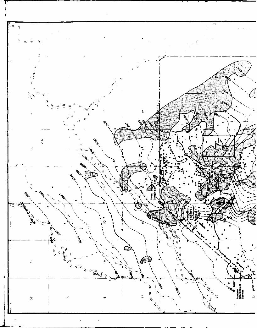
IDI
oo.N) 40
ie9
* N
tl S
N //k
'5 *
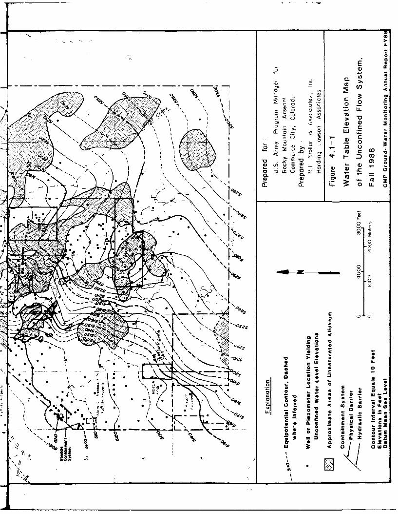
ID.
0 L0
0 a
- C
-3 0
0 0
o
4 ~COo o -J 0- Q
-r L =" '- -0I0
-4-4 LL o0
~ C -
I 0
'N 0 -
I~~~ .L 0. 0~
/~~~ 0 0V~o a - 0 - a
\ \ Q Q.V*~N ICD I -\ N4)4 - w
00 0
0 c0
ý7~ 0
-L .- a 00 cNC
N 6'. - -0 SE00 00 E u
L -- -'
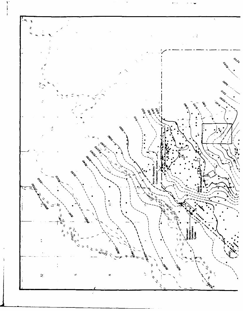
U -
.�
(I
040
4/
� NI
0* - a-z I N� *
- - I-
-� �,
01 � � . '- ---
" \ .4
- � -- 0 '. "
- � \ * *� -I
�, \ \\ " S\\ '�\ � - S -c r.--* * I
5 0
I - / 4 75- J.,. 0. -,I- 4 -.- I 0 / �4' i / Se S I / / I S
4' N5 ' .S� �Nl * �4 0'p * � *' � � S. 0 0 0� N V I � *
\ '� N 0\ \ \ N. � 'Nck�:,��('N 1 � *p� :.;,* �* * N N\ \� N'N 0 5 0
44 N * 4. *� * * �No ' 4-.. �' � .� -- N N *4. \ *.:�-\�. - -�N ".� 4. �. .%- '4.�. '... .C�* 0
N 'N- -� � 4. 04' S N I 4.�- >N
'N N Xe I i � � -- �-*-
'S I � �N�'4. �- -�-4. I I * I N.� N�.. N- '
I ..----.
*0
4. - � *
* N AN.4.4. 4 N4. 0 N \C. 0 - * 04�NI 9�a� x ". N � '�
4. I .0 .)___ S
� -�--' I* \\\ -� � N I �N\ -� �
'N N. "CsI � � .4N� 4. 4. I�.*-.. N.
�04..-- -'- N� x � N'
\ 2�\ \ � 4.4. 0 5N. 'S 4.0 N
'S 'S- �. �. �N -' 'S U I
'S 'S 4.N 'S'�� 'SN N
.- �' \ 4.'- -� 4.(NJ (N - L 4
\II
"4
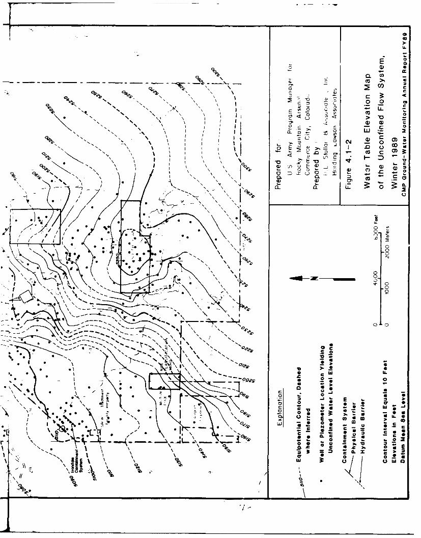
U.
0a)S
ClC
"N N 0
*u E W '
N 0) 0)
Ný '* -; a.
-% 0 0~J
0 1
'N NN0'~ N
N IO4:~ L. 0 c a- - - -&. N \0
NN \p -
00 .-0
0 0 * N 0LS
L 00
0 0,
0 C0
lb E'INJ 0_ c*~ N 0
N,-' 0
N s
0 0 0L
S 30
0r 00
w ,i 0 u
00
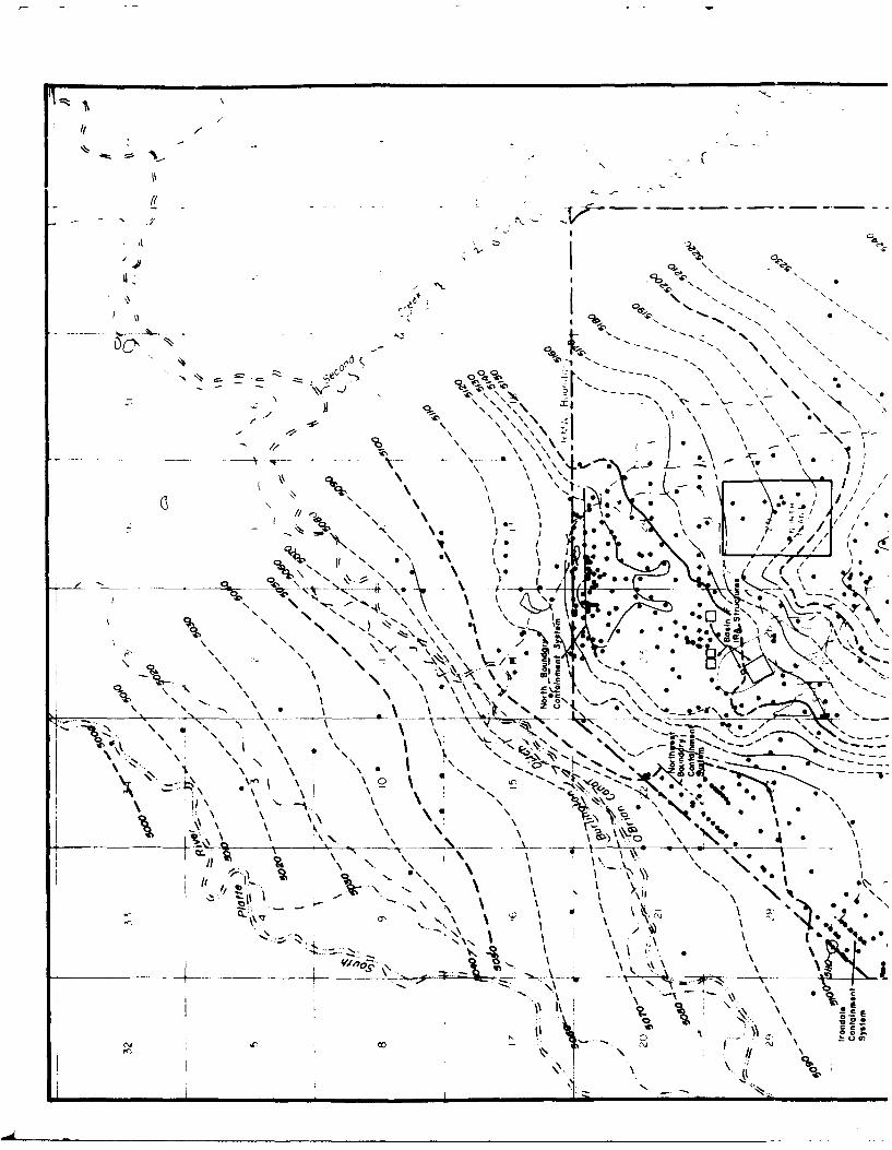
C..i .N
- N.I N N,,
\ N
= • .,,'1,, N1 -- N•! ' • - ", \ " .
N II-,- -- \ .-
(-\ / ., =., * , N\ N
"I \ I I 10" ".
' ,S
I . / I,
- \ . " N N- \ , * - I * '\
, N , , - .•- '' ', N. • ":. "'-" ,,.
N , N, ,\ , %.*•, \.. ..
N NX ~\~ " . . : .:: CU..
, ,*,,• , o .,. .' , '. _.-.*. " -N4."'- \l N
-\ I\ S- /
N N \ \ " N' ,\ ,N .~' \ -
, \ . NI\ \ x. -.. \ \ :•
A . . \ %S _ _
Nix \ • \ " % " ' •
'., ' t -_ .-
S\ \I ' 1.
..--'NV I
•- .-. • \ " €. I0
I _ _ ~ _ _ _ _\..1i \ \----- '•__ _ _ _
, 5-.i
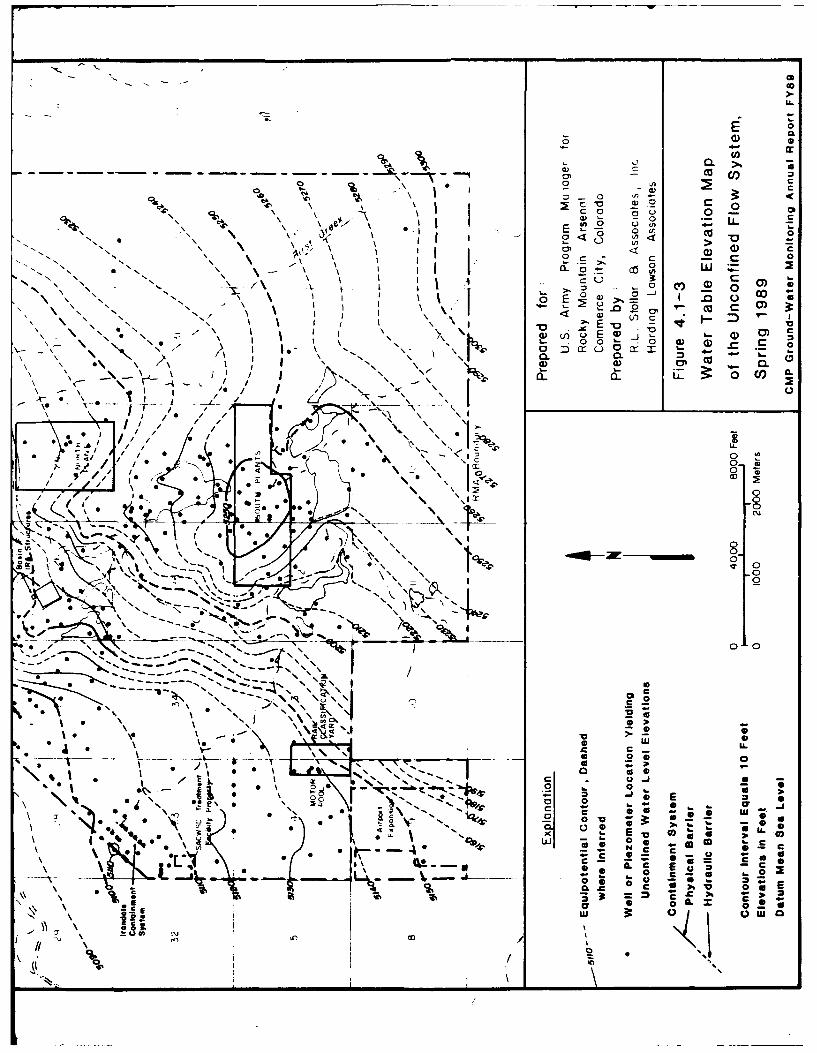
0
C"" Co CO
< a)
N, - C ' -9~~C 04 \
I E 0'.p -* co , C
I0~ 0~ 0 ))
0N N, 4) (DCNlk r- %. 0: o' a)-
' w-A
0 0 N 0\ I .ZN / vi-
"~~ N, 0- ' ICN~r 41 0 0 ' E -
N NN CO N~E0) ~ I. ) 0
N0 N D OjI~
"o -mls AE /N ~
* /N, 0NI~I 0 0N0
\* 0 0
/~~N NN \ '~g
0
;- 0ON
~ NNN
0 N
S0
a ==0~\ 001
N CL
N -
-4N 4pN N -C
% s N o Z0 IL a*N0' c
c -C N Cg31
0 '
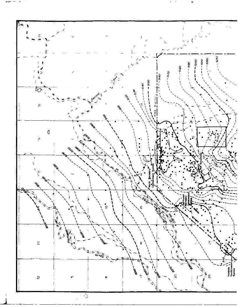
\I '
7
// -
0 AV
I -\ \) x %
\ N'j
.l t---ISID
-- N Plj' ~
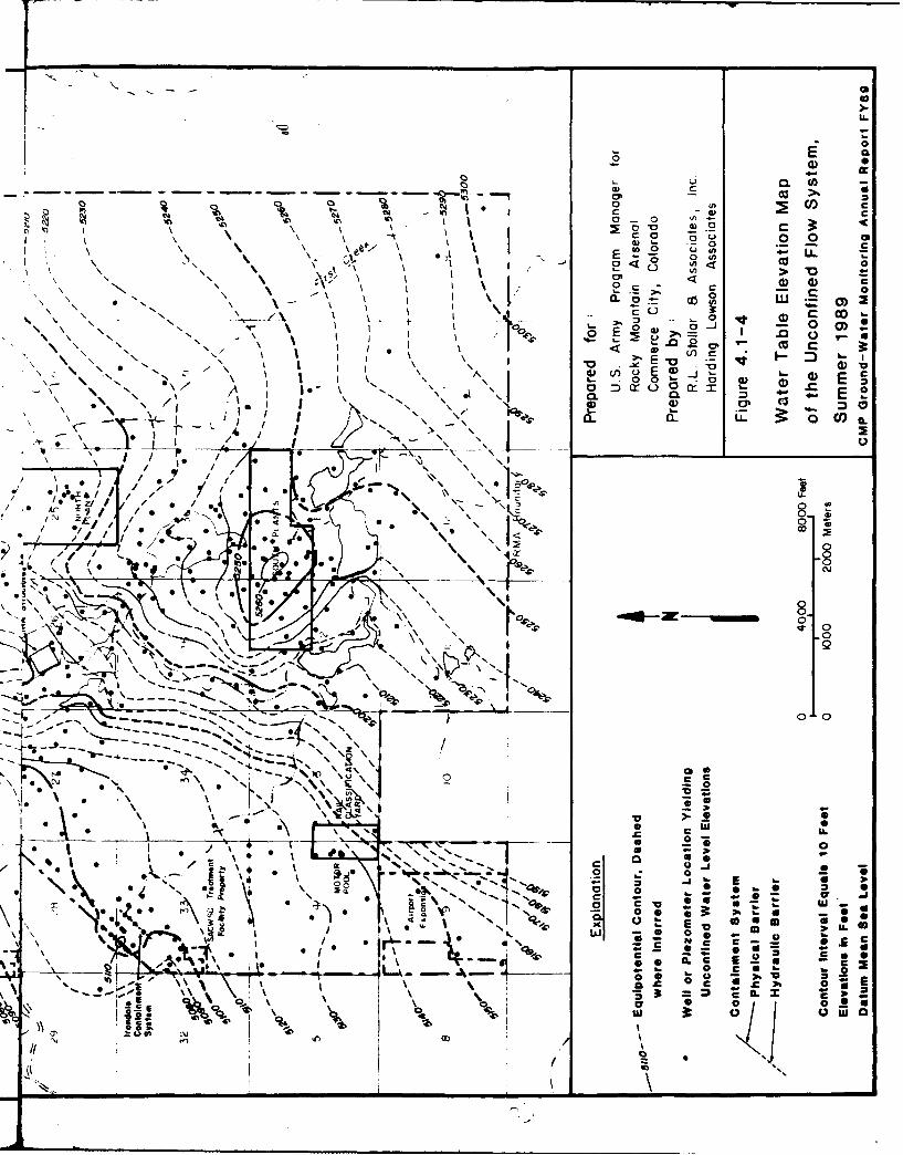
CIO.
-
-
2 4-.
~c 0
00 w -So %6- Li.. 2
I I 00
I. -. -j w
4)t
a D- cr.> 0r mCL CLQ) C
'K ,~aE U- j .l ( f u
NN
No o
J I I
0- .0 0, /L 0 V z, LL\' r
Le 0
o 0NN~~~
P6~-~ S 3NILx
N~c 0 - 0... _"-Z l.u Mu
- N ''
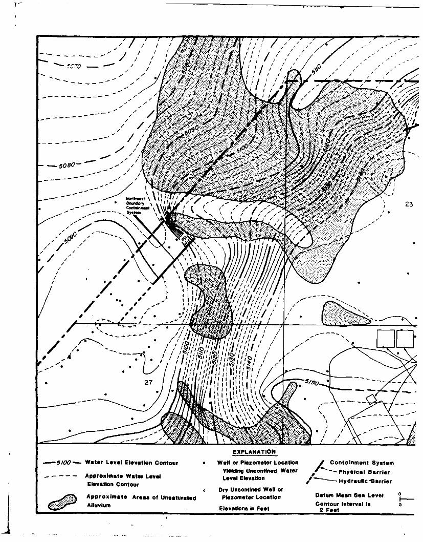
TI
/ / / .t **~ir..~ 4 /,
. . /- ........ . .... .... ..
/ ~ - ... ...... ~. ~II
j .... s...... . .';. ;1. ..... aa
it . , .. . ~ .........
-~~. .........-
N2-~ ~~~~~ 1 1U . ~ - *-* *d #
* -- ' - .~~7K/A.
,, ~ ~ ~ ~ ~ ~ ~ ~ 1 1 ~ : ~ .~..... .~~oI I I~ I
*~111 ,. -
- ', ' -' Aprxmt Wae Lee Wedn Unofie Wae /---hyia Bare
WtrL elElevation Contour L elel or evPie onee Loatodr on ainmen Syartem
* Dry Unconfined Well orApproximate Areas of Unsaturated Piezometer Location Datum Mean Sea Level 0
* Alluvium Elevations inFe Contour Interval Is 0L 2 Feet
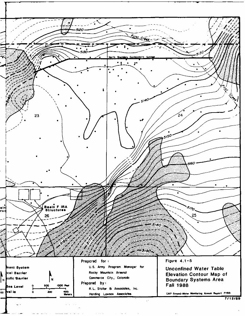
/0 /
. .. . .~. ....
Z . ..... .
00
23 2
I.Sao
si n R
r u Stucture
1'- V26.....2
.. ....0.... . ..
0S
Prprd frFiue41-
ýNe ytmU .A yPorm MngrfrU c nie ae a lca arir okyMunan renlE~e ato C nou apo
N ulc larror ý Cornece CtyColradoBoudar SysemsAre
on evl So 100FW Pipoed y:Fal 98
0..Solr& AscaeIc
COO ll$ 2JD 40
Basinn Faso AsoitsIRAoudWtrMntrngAnlotF8ru 267/12/8N
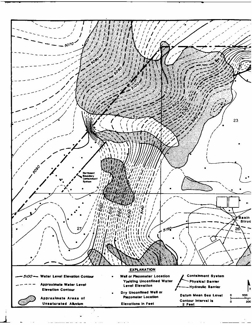
-0 0
. .. ..
...... .....
- .7 A.4, 0
.00 ..... . ..
......... ...................... .........
*..... ..- . ..... O
...................... ..... .
- - - J- ...............
-2
- - %.I ~ /- - - -~ ~4~ V
.. ... .........loo/
I-*ý 4,
410
Nw"Pres
U- -i mainASysttruc
//// ~ ~ / I/II/t
EXPLANATION
-5100-- Water Level Elevation Contour o Woll or Plazometer Location ,C~ontainMent SystemYielding Unconfined Water Physical Barrier
- - - - - Approximate Water Level Level Elevation I--- yrui are
Elevtio Cotou Dry Unconfined Wail orApproximate Area* of PemtrLoainDatum Mean Sea Level 0 500
Contourto intevalisonUnsaturated Alluvium Elevations In Feet Cotu F Ietevli0 20
L .2 _o_ _
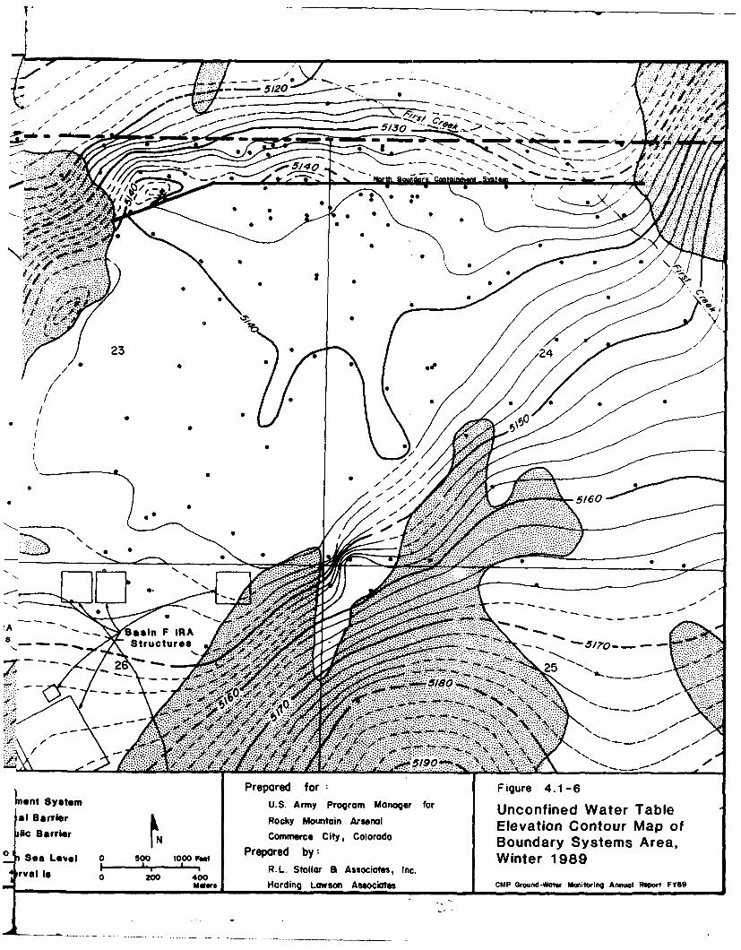
.7f
7, 7 , - - -- 5120---, ~ ;~
01 .. 4,I
5140
Ž14..r
0 0
0*0
516
0 ...
StrS
W.47
* ~.......- - --. ~ ~25
~~~ .4 4N.r'.~ :39:39
SytmPrepared f or Figure 4.1-6*Let SytmU.S. Army Program Manager for Unconfined Water Table
mal Barrier Rocky Mouintain Arsenal Elevation Contour Map of110c Barrier IN Commlerce City, Colorado Boundary Systems Area,
oi Sea Level 0 50 Preare by fAstefS ic Winter 1989rvlI _R.L. Stoliar &AscatIc
mWotr Harding Lawson Associates CMP Ground-Water Mon'itoring Annual Rope"r FY89
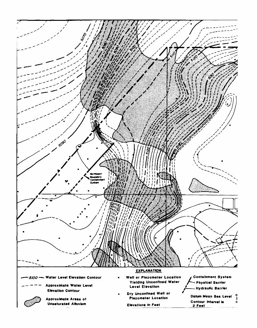
- I i.. -4.
j.A;4~~;wir..L*:..
-4 - 11L
J A /h;~~k.(. )
ol . I
N. an. 4, U:/ p tt4-00
. . .........- f ~ ~4~IT..
w ............
.... .....
It i41 .... /.# .5;
/ if
01
EXPLANATION
-5100 Water Level Elevation Contour 0 Well or Piezometer Location ,Containment SystemYielding Unconfined Water fC-Physical Barrier
Approximate Water Level Level ElevationElevation Contour 0 r nofie-elo Hydraulic Barrier
A~pproximate Areas of Piezometer Location DauIenSe ee
5P Unsaturated Alluvium Elevations In Feet 2 Feet
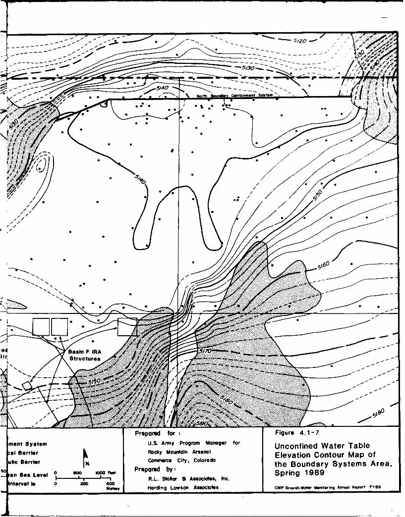
, 4.* .' . ....
L~. t Pf/
00
//
I, 0
/ 0o:
06
5 0
Stucu7'- ..... .N:777_
N N
019
*I ~ ~ ~ ai Fare IRAk MolanAsnlEeainC norM po
Strctre Stol::: a Asocats Incntr ll 0 20 40
meesHrigLwoNsoitsCPGon-ae oioigAna eotF9
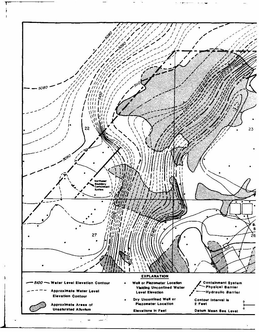
ff.00/, II , - --
74 mm. M -1.-
- ~ ~ . ... .- . -. . -
6110 - - 7 ;i ........
/,/ ///'//04.-
R1 10 '70.
.. .............t i l .............
- Z
~gO ,7
NI . %.*.** .
100, 10,90~
I 271 :426
00
-l .000,
EXPLANATION-5100 Water Level Elevation Contour * Well or Piezometer Location /Containment System
Yielding Unconfined Water ,- Physical Barrier---- - Approximate Water Level Level Elevation / -Hydraui~c Barrier
Elevation Contour. Dry Unconfined Well or Contour Interval Is
Approximate Areas of Piezometer Location 2 FeetUnsaturated Alluvium Elevations in Feet Datum Mean Sea Level 0
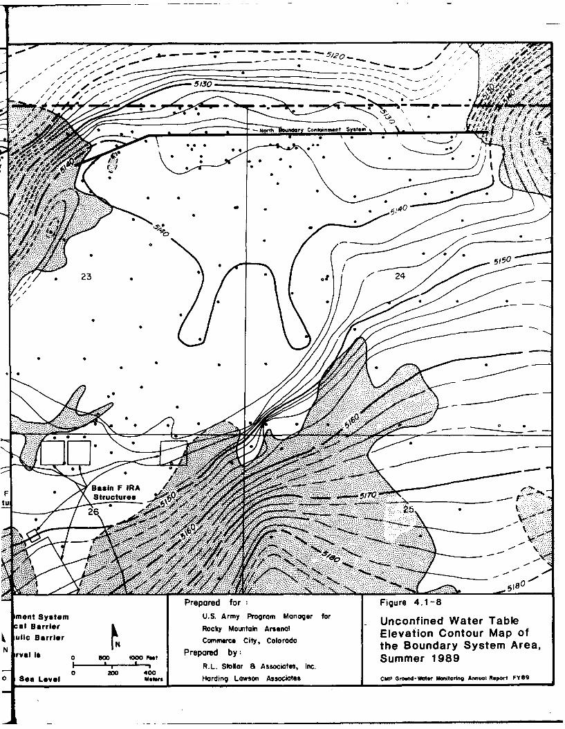
- 77
- /7 / ----- 30-------- - --- -
0 *- 4OII ry Conlainmtent SVstemf
J 0
S. 0
I.- 1-
..07
Y.. . ..
F l Bare BasinMunainArsna
tuL Structuresocate, nc26 20 0
0 e ee Mw adngLwo sscae mpGo wte oioin nulReotF8
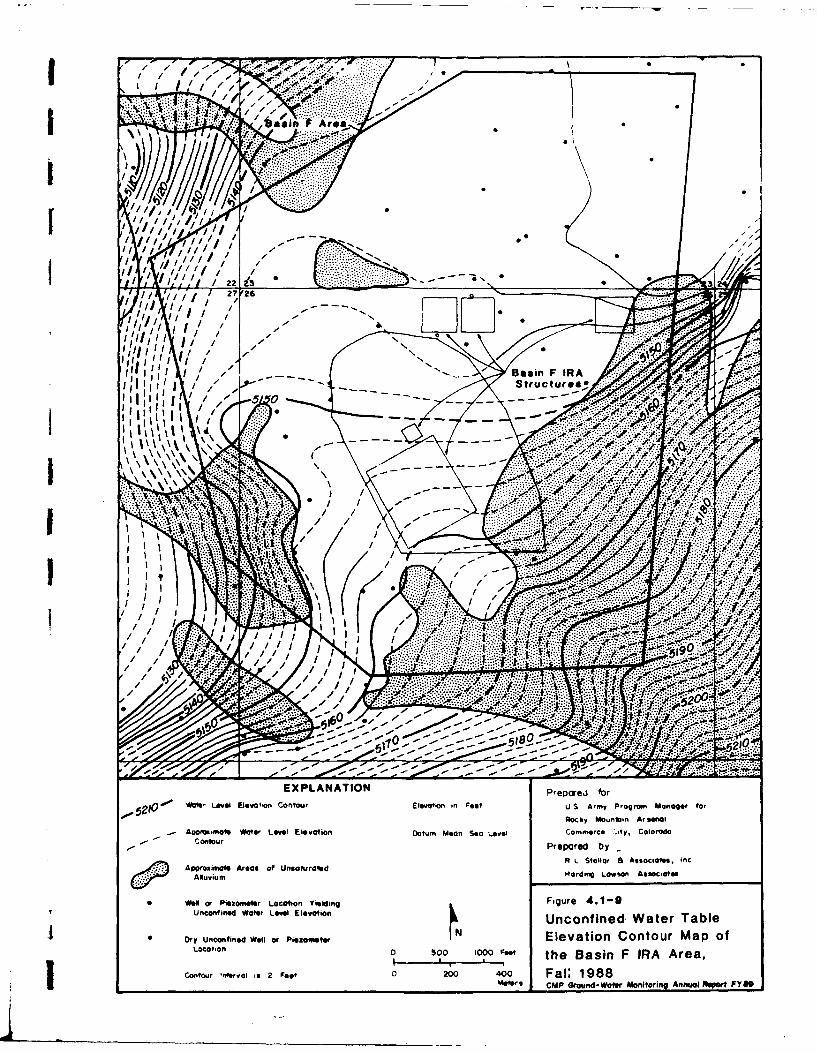
27I
Id I I I
.. ... ..~
V. grint ae ee EeainDtm Ma e evlCmec f.Clid
Contou
Prprd b01 L ilo B Acat n
5nc21fine Water L evel Elevation CnorEita- nFetUnSconfinedoWat aaer Tabl
* oo~nuftwo Waell L ionel e Elevation DtmMo a ee omre-iy Contoura Mado
Contour Prepaved by ..ef0 0 0 F I 1 8
oeS' Wool orud-ae Monitoring Annualta Yiepdin Figre 48-
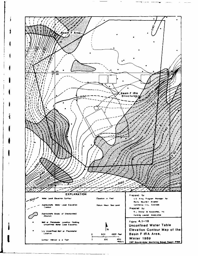
A, ae In1
~ ~D -m. '. ~~'
77 re Are~ L S~ll~r* A~oc~Ote, n
A.) ppromaveArea ofUn~auratd tirdiig LWIW' 'Or..@t
... ... .......m
N ...e..
e P e z m e r o c t o Y i l i gF u e 4..-.Uncontined..... Wae.evl..vto
.. ......AUnconinedWaterTabl
* .......dWllo ~eoes I lvain C ntu ap o hLac~on a soa ioooFee Basn FIRA rea
_____________________________ _____________V_Ccntur Itervl 'e2 ~e4 0 00 W nter198
---- ---- -- g d- ae -- io~ g nul~ e ot F
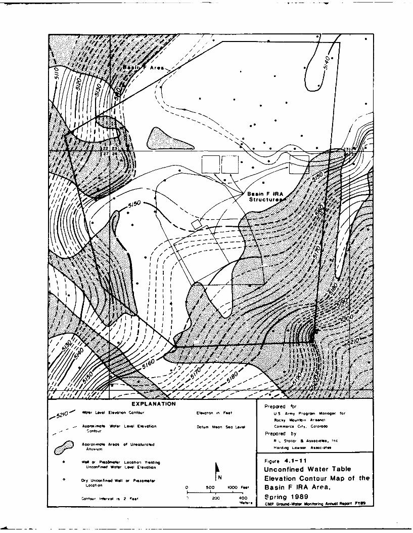
/ / *0
-;1- *.:t:y*
EXPLAATIO F R'0~ y.Wafe Levl E~va~o~ Cntou EI~a,,oStn eetumSAm rga aae a
-. 59~ Rcky oun~n Aran0
-~ ~ ~ ~ ~~~~~~~~~~~~~Y Aojmt ae ee lvto ou onSaLvlCmec ~y oorad
Prepared b
tpr~mfeAes~ U asrae LStlrSAecae Inx tu .. ........ w ~ ~ e c~ ~
3 elo mbfrLCto iligFgr . 1
Uncatine Waer LvelElevtionUncnfind Wter Aabl
Dry nconrnedWellor Pezomter N Elvatin CotourMa....th
LOCO'Ofl0 50 00 Fee Bain FIRA reaCono4 In-vlA2pe 140 %pig18
7.er ClPGon-aerMntrn iwjlRgtF I
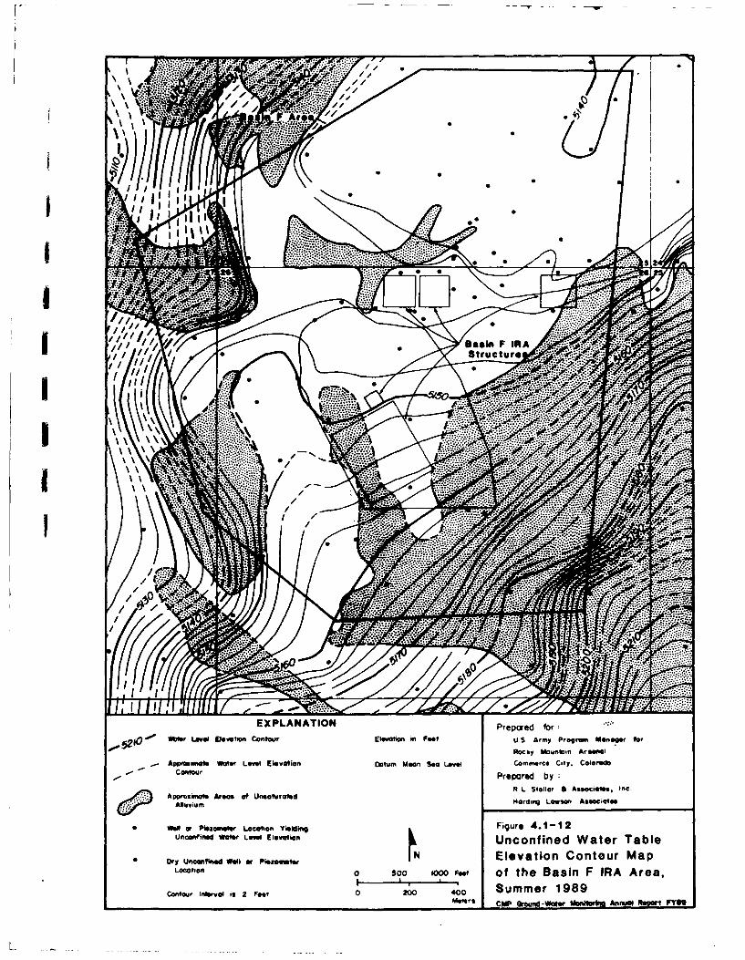
A.I,
AzA
41
Jill,
.. .. ....
I0
EXPLANATION Prepared for
wo Leve0 Fivoa Contou Elevatonl in Fee U.S Army Program Moneaer for
Rocky Mountain Arsenal-- Awas~nm~ft Wafer Level Elevation Datum~ Mean Seao Level commerce COY, Colorado
-Contour Prepared by:
Approsimate Areas of Unsaturated ardn LaSsonlr AssociatessIcAlluvium Nrg~Lw sn~t
Well or P~jszsls I.ocallion Yildn Figure 4.1-12Unconfined Wo$5r Lewow Elevation Unconfined Water Table
0 Dr nwlieill WW or Ni"nae Elevation Contour MapLcfoi0 B00 1000 Feet of the Basin F IRA Area,
Contour Interval is 2 Fee 0 0 0 Summer 1989Meter growd-wow Mnifor~in Anrmol uet Fea M
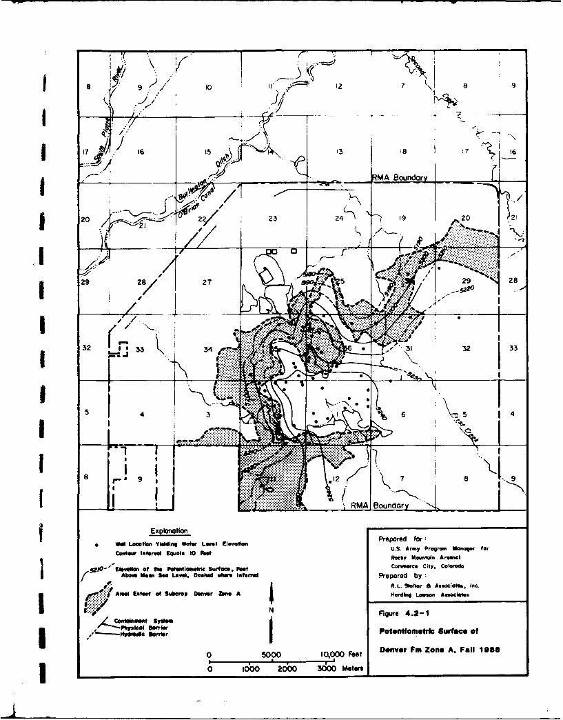
101 a 9o
116 15'3 71
* ~MA Boundary-
20 ~ 23 24' 9 20 120 19/
29 w2 27292
I 3 2 r 34 323
3463I.
* *~A... ...... _ __ __ _ __ _ _
81278 9.
____X`_ RMA Boundar
Expblawflot
* Wal Lacaflan Yildding Waer. Leve Elvto Prepared for:
Cotu inera Equals 10ra U.S. Army Program Manager forRocky Mountinlf Arsenal
5z1DO E- abvl,~ of Ibm Porwtleioeteric Surface,* Foet Cominere City, CONoNdAbove Mean See Level, Daubed where, inferrd Prepared by
Areal Eutent of Sulicrop Denver am*e A Nordinii Lesson Awsocftes
:; N Figure 4.2-1
I ,' -rami Merie Potentlometric Surface of
0 500 10,000 Feet Denver Fm Zone A. Fall 1088
1 0 1000 2000 3001ee
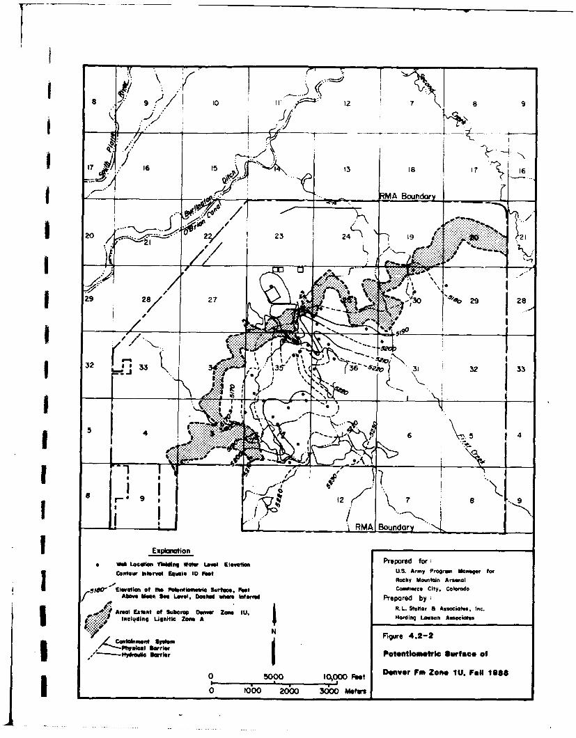
810 12~~
17 1 16 15 14\13 817 1~6
_____ A Boundary-
I 20 21 23 241.Th 19
29 2Y,, 27 -. 4"fe3o 2928
II 32 r 35 i' 3'$3 31 32 j33
5 ~ 9::::4
- _______j L i RMA Boundary
0 ocationr bioSiffig Water 10vo Feet Prepared for:Contur itervl Eqols 0 FietU.S. Army Program Manager for
Rocky Mountain Arsenal180' Elevutiomn of lfme Polioatlsetrl Sur ftcPstComre it, olad
Above Meom Set Level, Dashed where Int ervedPrpedb
Areal Extent of Suberop Owerin Zone IU, adn asnAscae5: Incs udlag Lignitic Zone A Hardi. L tlarwso AssociatesIc
CnlimrSytmN Figure 4.2-2
A shyiel SorrlerI'O- lydrouft Batrier Potontlo~ttinitl Surfoco of
0 500 1000 Feet Disawer Fm Zon* 1U. Fog 108810 1000 2000 3000 meters
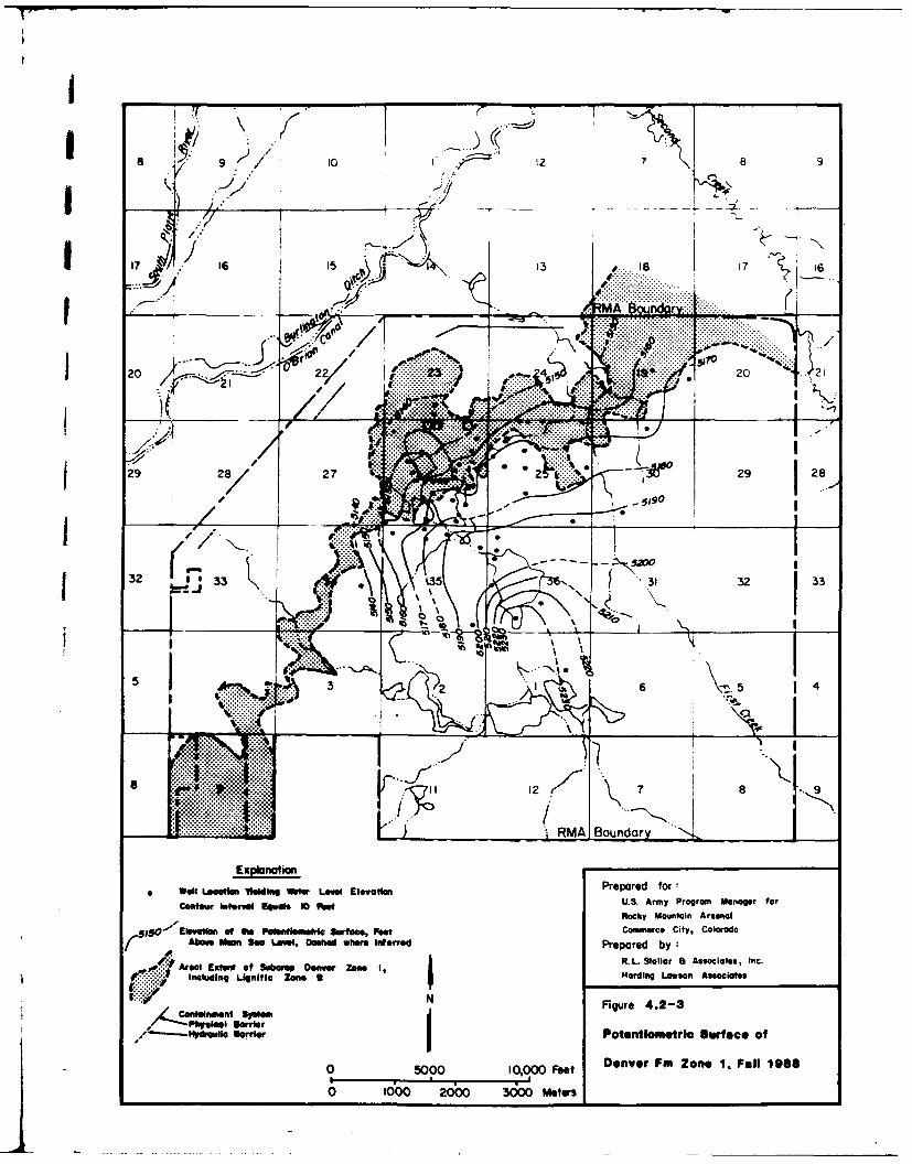
9t1'12 7 8 9
1 J 16 13 18 1S7
j20 20 ... 21
`-77
6AI
2v2
22
__........ RMA Boundary _______
Explanationa Well Loomflun Veldine Wter Leve Elevation Prepared for:
Contew laere Eqaaief 10fe U.S. Army Program Manager forRocky Mountain Arsenal
ISO"'EleWn eqlo of11 Poentesneflame Surface, pee Commerce City, Colorado
&*Aovis Mea Sea Level, Dashed whers Interred Prepared by:
X*Areal taE~ of Subeaee Denvvin Zone I, ARL. Stollor & Associates, Inc.
including Lig1nitle Zone 9 l arding Lawson Associates
N Figure 4.2-3/4Conksiviet syme,
,-P4*~ac bord~er Potentiornotrlc Surface of
0 O10,000 Feet Denver Fm Zone 1. Fall i9880 100 2000 3000 meters
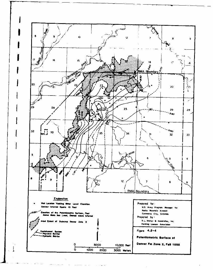
20 4~~18 1 I ro L / 0 J2
AM Soundr~av4
* Well Laceam Thuilug r Le l EltoPrp ed f :2 m0 m 2tew ~a o~US Am rga aae o9ok 20iai raa
CX.re iy Clrd
AbowIbs b ewe,~ Md uki InuiedPreare by
A9 2YL 25ola 29 28oiteI
Figur 4.2Al./ -ydru~cSmier ~tgtlo~trc S ufee o
900 12oo F7e 8eve FmZn9.pu1
0~~' p000 2Boun00dMryr
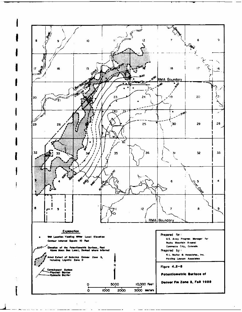
... . .. . .. . .
.. .. .. ..
1716 15 18 17
RA Boundary
2023 24'- 1 20 2
29:. 2! 30 29 28
32 X 353 142
.. A_ _ .... B ou..r..
R-k'alptinAra
gfO~.~i~ . i q 1 a ~ p omreCiy Nlrd
..f ....... ... es.Oule tM~hfrdrprd b...... .. L tllr S A ~cit , I
0 1000 200 100 65w4
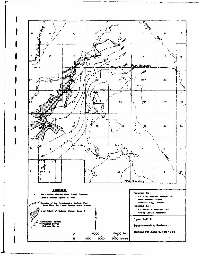
9\ 0 2 "
q>! --. ; -.. . --
6 #0
... . -0" M A Boundor- L
4160if'
-1.9. 20
7i 25 30 29 28
l oi- . I-
I Boundary
Explon tiI91 - SOzin fte P ten.i on- ri2e Srt , .bo COA M City,• Colorado •I •
| S:_•:.•1 - I ': 3 36 . 3
A R/ L. -l & A s--e In,P "• --- / 3 >" ,l 6 -X
Mon Syi Fgr4.-
11
, .-- "O1:111 ...>fh..ri Surface of,0' m 12 8
I ' _.i R M A B o u n d a ory 'I
[xpkmrotionC Well Leeim Y Id•l W•f Level Elevtion Prelpared for :
C tsw In 1re Equlsl ID RI U.S. Army Proguf Manageer for
g g lO - ' 'E]eve ile o f It ,. lP o te n t /m t i ahrfa :. .F e e t C o e a iw c . C ity , C o klor do lf Aboeve Meau Sea Level ahed ehre In Prepared by :
( Arel Extehnt of Suboropl Demer ZoPA 4 5R .SolrSAseae n
N"::Fi• gure 4.261
II, SWVler I Po0ent2o0etrl 00rmete of
Denver Fm Zone 4, Fell 1066o 5000 10,0O00 Feet
0 ,1O00 200 300 Meters
I.
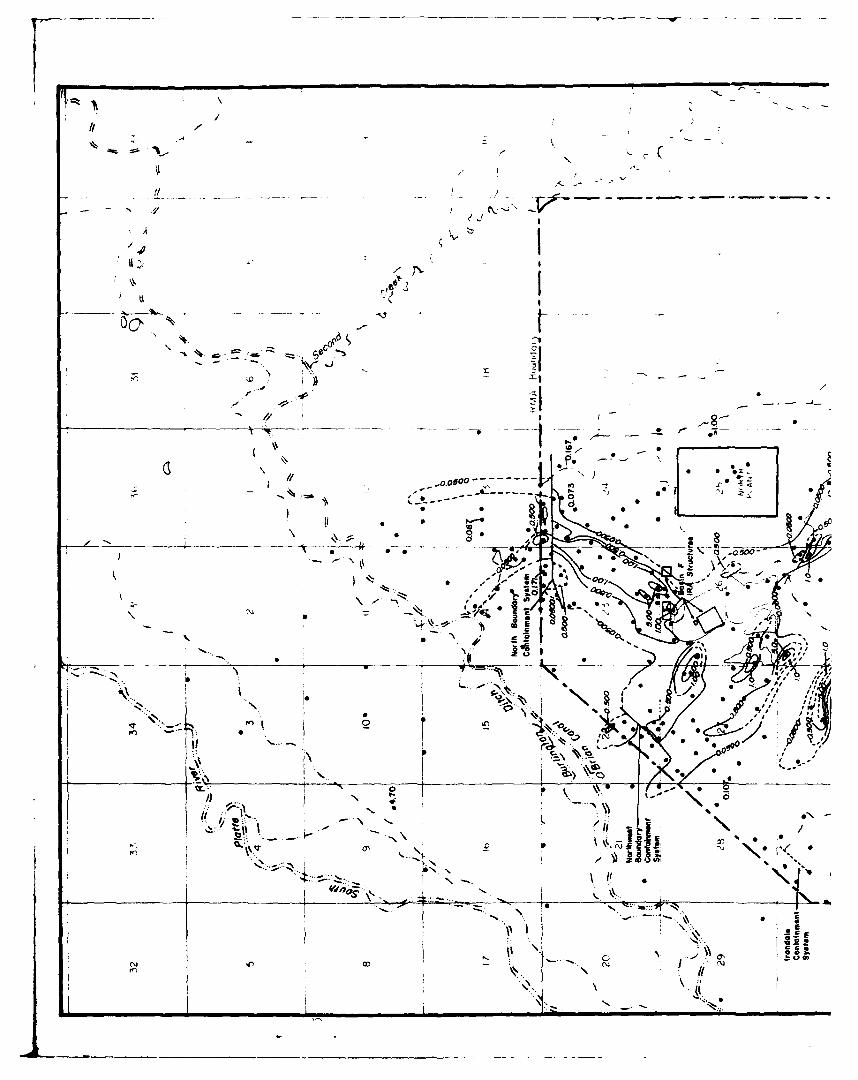
II0
N S ---
/f ~/,
IO
X
Ia -
III
0-h-
.., .. -
0%
"" // S o0 "
'T - .,!
CD-"S,.- :r.-" 0 °o 00
_ _ _ _ _ _ _ _ _ _....._ ---I'-- 0
-" . •g • I •l, -
N... . - -- u•
""" '- *•••
N 0 I /r,'
o. ..• - ...,,\.0+:":, - +I -' " "' * " -
- N - 6 ... .. . . *.. . ,
ii N ' .+ '- \ :. 0
- ,\ N , /
'__ __ _.. __ __ __ __ _.S.. . ... %
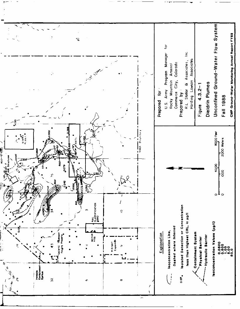
,.... -- A - . ...
S" o- o -- -- . ...
T4-.
0, 00 CL
.0_-,0
,) O
"- a
w at c
L C-
•.0.
Coo -(-"| -
a~ -0500-
.. 0,, • - .ocn ..=a
"" •- -0 0
-j-r
" "- " . 0)
I C
r4) 0 a c
L*L .c a En3 * : ; 00 ý0L-2 C - -
I II
00
00 00~~ 0 ~jC
ro0
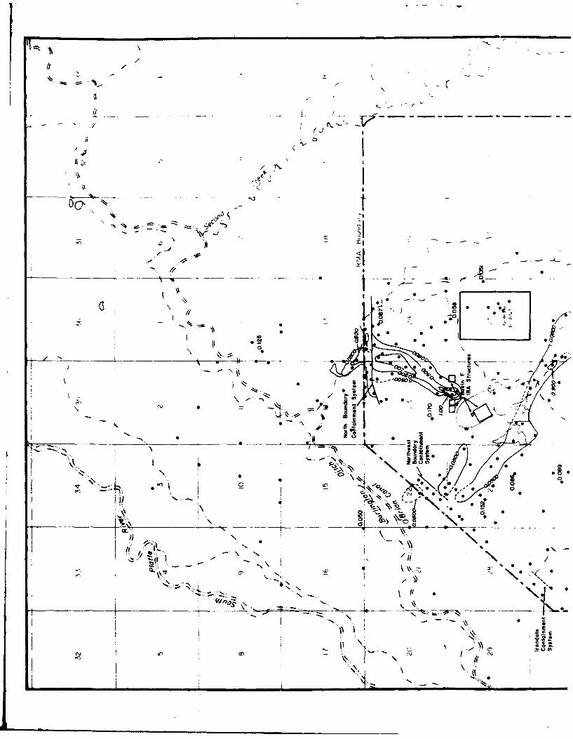
-I0
IIIWO
- - . Y
!~ - - _zP
* gOON
ev.---,~
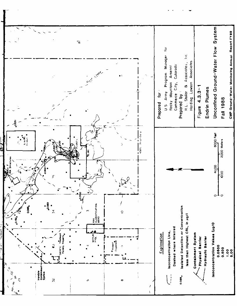
E
CO .0
oc
a, 0o I
0 0 n
A0 0
CO CM L
/..
U .O2 .0 ccc ro 0 t 0. CO
o m cr x1* 4) ) c a A
0.. 0
0* 02 8C)
I 0
I'~ \ cc
-' 0
'S25-. og- c
*J 0, lo 000
to c o
c 2 c1
I C0
0 SOD
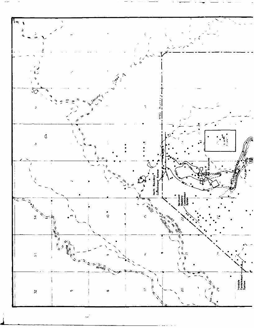
/II
-
I-. IL' - - --- �--�-- -- / - -
- - -S NV��'S)
'Th- I
� .1
__ -- -� 1�-
- _ -
'B -- -
0
_____ 0 -
// __ -� - i 0 �A- - -�- j-. - 0
I * �0
*5 J� - -// 0
C ..- 0 - eel
6 0 .0 * I0 0 C 60 0
-5- '�.%. 0 0 Ge- -- -----x--- '- C, -- V - - -� -i*� 4.- --
- *\ A . jV5-. -
0
*
il� * * 0
C * 0
0 0 0 4* 0'
0 * 0 0
0 0-SJ �*S.. * * 0
0N. 0 0
_______ __ _ \00 A -- -� --
5-'-
ji I,� 0�'� --\ -S. 'ii *
N� �i \�0..( 0
'5. �
'5S - S
i's �0*�
� C
- N -� '. 1' * N5-
S. - - "- 0
,�' I U�SE
S-s'.5 CCC.r...II * 'I CC.* r C
c.�J - I---- I -*��
II
--'St5..�' -�
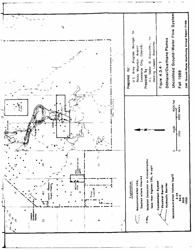
U-
co <
0)0
< E
0 0
0C
E -o( ) 0
CL OL
4) C 0
- 0i
7-2
00pe);00
00
00
*i 0,
'-o-
0
0 Cc0
00
*C 0
00
* 0 6 t o
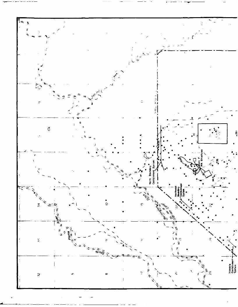
-'I'
I-
'V
.9,'I.. I�
� -*
�1
�
I-,
-
S
-� -- -�
I -. - -
I-
I--. //
S
--
___- � �----
.-. -� - -- A-- - * "� .
I -
S
/
I�- S '.*
0 0 6�
_
To .j
- aS
--0*
S @0
0
a *
S
51 S
-..
S 0
0.r .-
-', 0 -
.------. --
.. .-
*
0
S
'S -
S.
.1 0@ 0 -�
'06 Occn :-�*
�.-�'- *4 4 5/ �
- -� 0
S 0 0
0-'�
0
N
�
0* -\ -,
0�����0
Sa...
0
- N. 0
NV..
S
� 0
01
*
**� 6 **
*
I
*�-'0
0. .
-N�%0.O
0 *0
N______
__ I�)
5
0 -N.
-� N.�, .
0'
-\ N.
"II
-�
\ 'KN
-
N
II
N. N
'-
N-.
0 LIZ___
-� - -� - -..--. � ' -
N
.-. NN
-�
6
"S
..- II I
cc-
N
N
II
0

0
cc C
< L) E-w C
-t 00 V- 4) C
0 0:D x u 2: N
N I
CD00Z4i 0
- 0 0
x 3: 0 r-r C
LLN Q* 0 - =10 0- E- 0
17 LL.. 7 C4.
0~~ ( '
.- ' 0
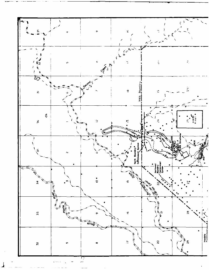
-~~~ -------- t------
OP 6
FK C- 4N%
/ /c
'tcui
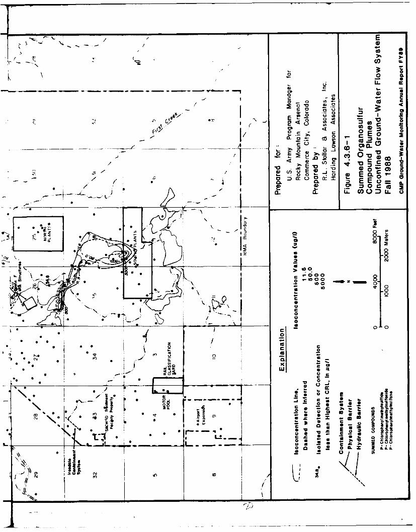
0 L0V) o
0 C1 -
o 0)
I ~ ~ U C 04- C
'a 00 V 0
<, 0
a'C 0g..0
0 E a.
- ' L) oý m 0
-~~C 0 0OO~ .-
0) 0 0 M 0 o
< 0,
0
7-t
0~l 0 - 0
q 2to*1.* 0 000 0 0
0
cj F4 0*7 4¶~
0 0
090
r-0 0 30 00
CD 0 -s 410
( - C E
0 0
*o -, - 0
*1 OD -
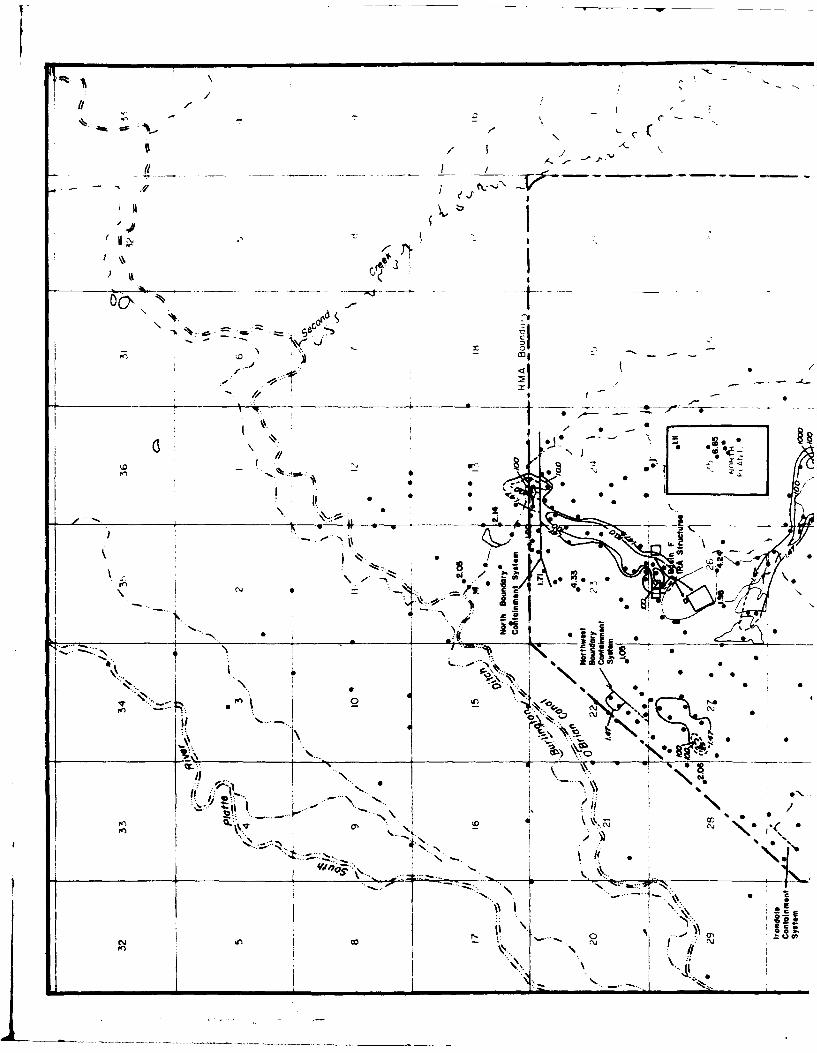
i fl
A'
Va.
_ r-S o
/ N' 4 A-
! -
-
-4
f'-- - --- FQ*
-tj
U_0n-
/ cu

U)
00.2 0
< <
C -
E E o
0 0 D
4) o- ou
2i E~ID 0 * 4 ~ *
0 C
00
0
0
00
0010
* 0
CX I- -
0 .
000E
4- c
0a A4 -
* o 0
*.A 20 a c0 a ~ 0 o x 3
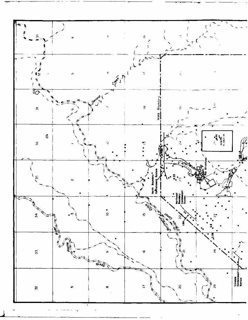
A' /: I f " . -
I I "
_______. _________________ --. /A -
0' _ -- - -.:
.+--
-• " -
,-* :/ ,i, .I-
..q •:- '- I ... _' 0
I•., /I• .... , - t S• °
...---- I, :~ . I, •
l* •....**... #(,. o , S
'S. . S I .'-5--.. *, *I .. Cu" "" N.. -- 6 -
"• :i " - : '•." " ' ",,'a.
"".S ... .... " _"'"_ _ _ _'_ ii
"-:: : :... " L -. \ !(0',, ,.. .. •.~ ....
-.-:.*- :::•.. "~ .,,.
' '. " 11
" •' -•-,l!! "'
£
tI
N
-C
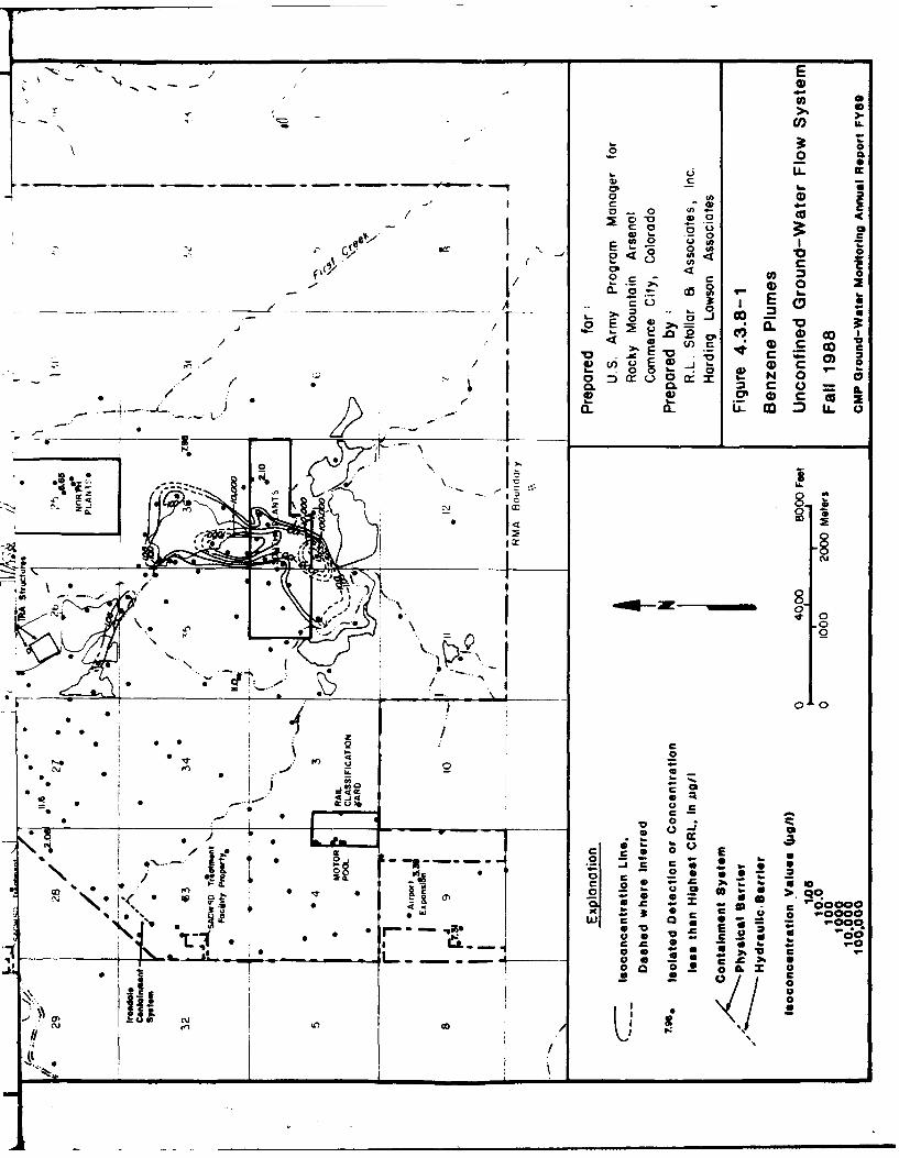
C, ON 0
0
O OD 00
0~ .. 0 .
o, -d 0 0 0E CVm
- 1-i
-~~ 1'00
0) '
V* 0 00/
171- -- 4--. _________
*0
00
-jetorS
.~.-
- 0 4 I 0
in to * ~
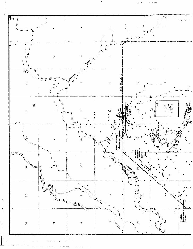
,- .÷ - ,-
- "-. -C - - - "
"I"
"- .:- - // • o"
Ilk
O S C
- IT
"j ._,' - -- • - - •
S '.-... ,. - --.. ..- *
re))
G.. ' - -0 ''•-• - • 0
II__ __ _ _ __ _ _ ..... -4 --- 4 e - r- . :'w *. •1'i. .- A ' "' .- ____:-
CU•..' \ - -/ , *. .." " 2'.Ag ' C
.. •"a ' -"-1_ _ _ _ _ _ _"_ "- ..- •
r•k ..~
l% .! c CU''- •'• " • -
1=-- - I....-"-:.. % . . .
""1.. ' *1 '-•"-...... -_ __ _ _ - _ ,_ _
N. N -., \ __II"",.i I •-
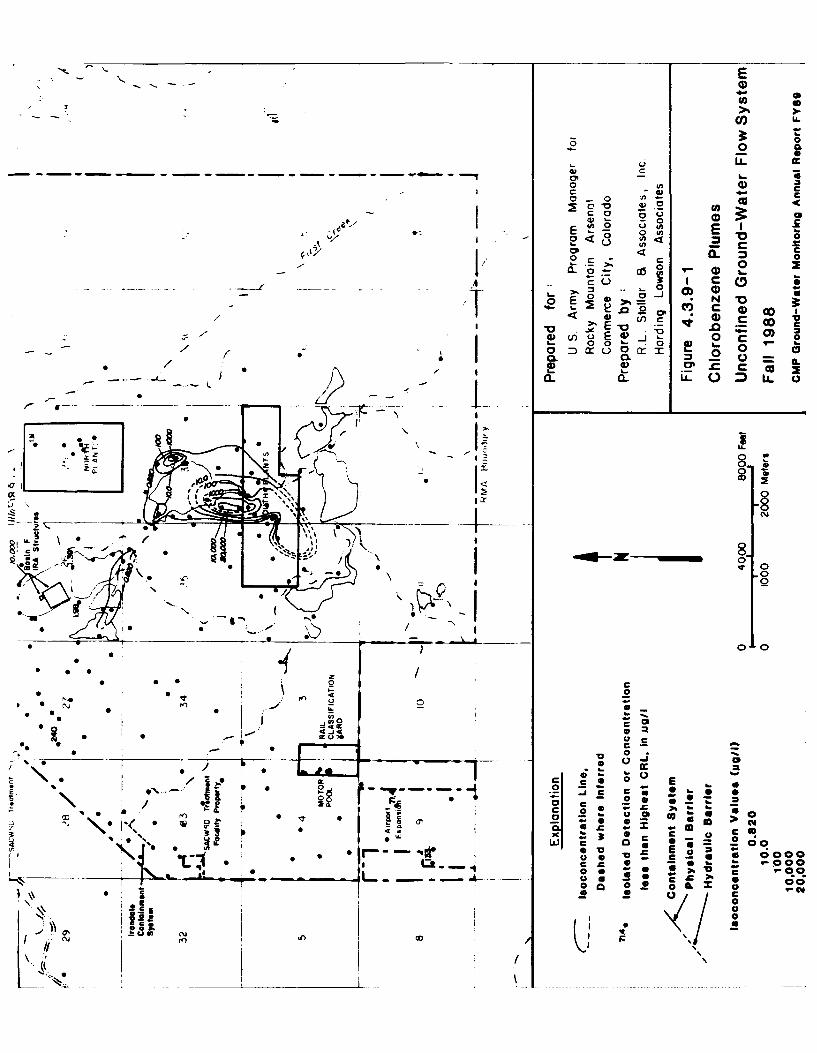
co U.
1 CO
o 0)eP 00 0"
410
-o I
0u~ S-E 0
04 00..-o ow
a, CL L C.) :3 ..
,av
0(0
a, -N a
0 0
10000
0 0E
E* 00
* a
x 0
CocoIC .
0 ccU
00 0 0 C42 ~
~ 00
US S*o U- O
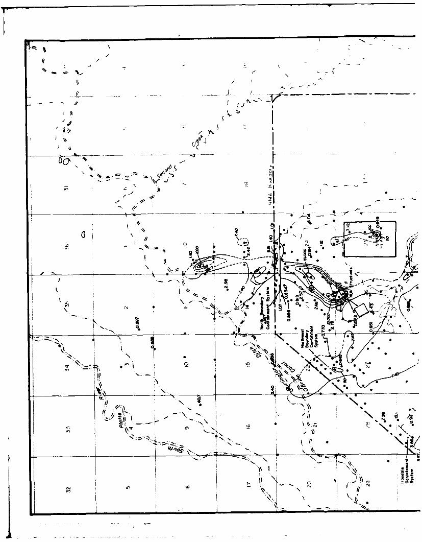
T
I -I -/ -
//
""- i " ..4t" "- -" --- - -
CL 9
-' _ /I ' \ J"
o0. "
-* " CD-L 1 --
""to.V"
""---..'-. %
N VI I' N-=
I t . - 0;I ,. - - . ©i t.. .- •
I K'-",,'--- I., "-•!,,.
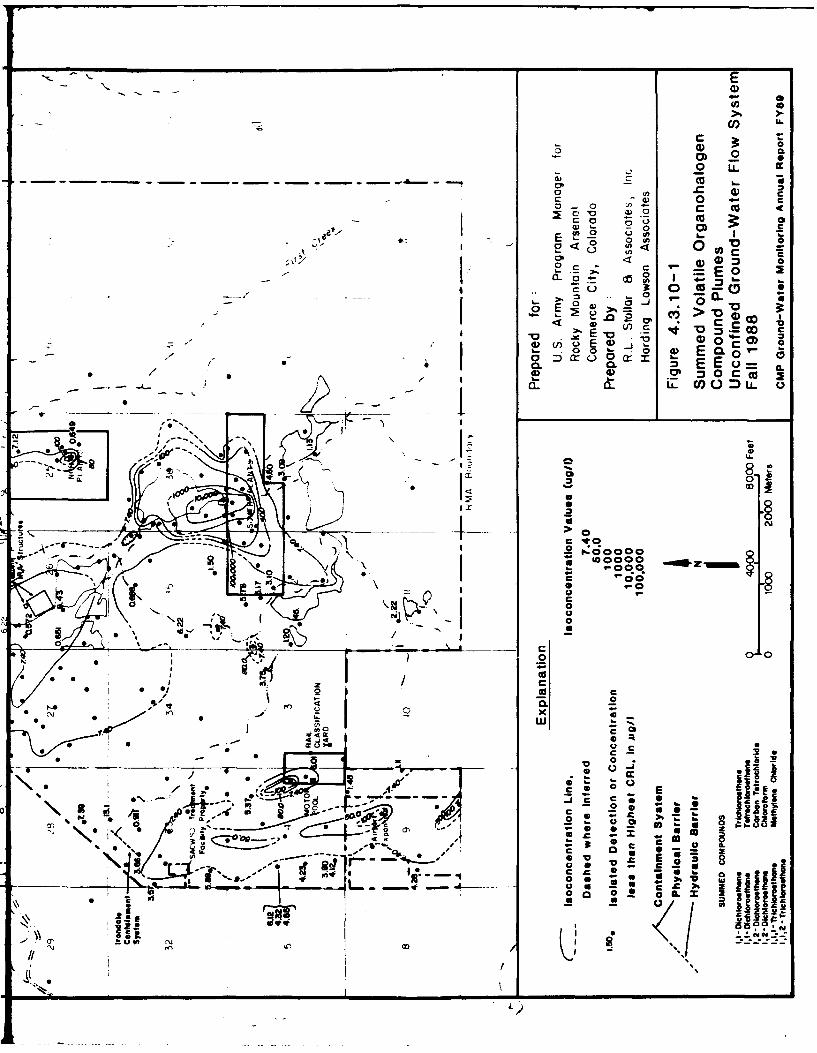
5 CL
o LL
75 U) 0 0
a- '. -o 0). 1~ = 6.
* ~ o-, C
C EOE '0m- 0
0 C l
ooL U)E0 - 0
* .
> C_
0
LL
0 _/
CL
0 E
* *
001 00:
"
% 'C
-----(
0.0
~*1~~IUC .2C
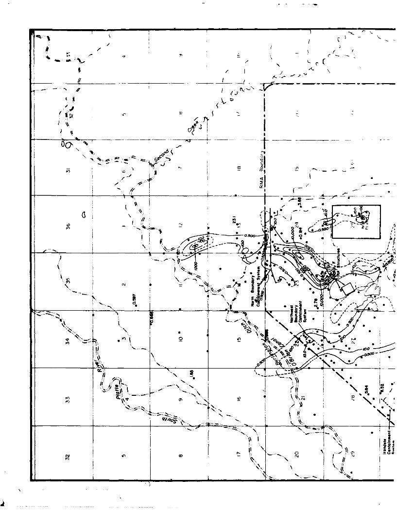
-o -
1/01
0 C~0
____ ____ ____ _ __ ____ ____ ____ a~?I *goo-
* 'y--
ZZ:
0~i .. i 9-"fn OD'X~*~
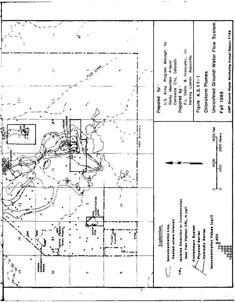
U) cc0 0o
0
L).E) 0
V) C C-
IV 0 c Do-. -. 0 -
00 %
-I---
I 0
0~
00
IN It~00 g - 0 W
0 a. >S \ I
I. c 00c
V E
0 a 2 ;. -
0 0 *
0-i 0
N. l 4jC a) a~'SI a-~--
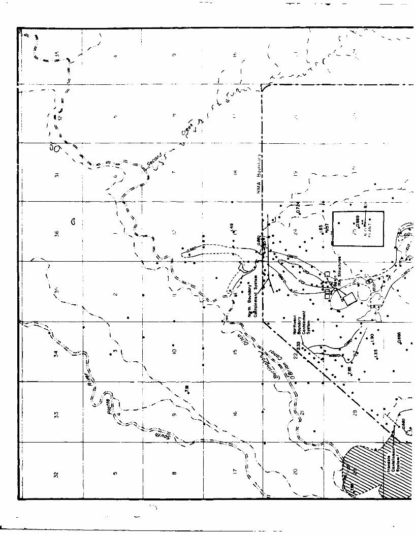
I .2- 3.
< "II Ii-
A -
,1 --- z
-'-.' l .
' Tr
j , .............. ..... •
0'~0
"_ -. G• 1--- --
,2 /---... ..
{\01II
\ .•.•::-,
, . •-.
,i. --- --t1St
1,z- -. , = , I'.
'--...r- .- ' I . B >, " /
.... , , , - ,
--. - __,_
"-"- t".. t /-00
'IMF
i,
Pr,'-
-- % ::S. : 0::'
S\ 1 \ %' 5
u (,.
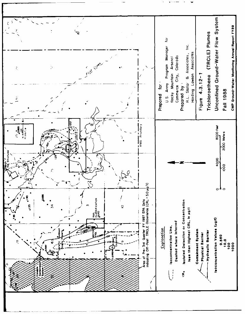
UL w
--. y 00 V)
Z 00
0-0N-0
I CC 0'
(A-~~ N h C
0 COE -)
0 0 0 4 0
a- LL
ccIQ
A ~'1 ~ O=LL . 0 0
/~ 0~g
-J a
* 0*
I. -, W
c
"3' C) 0
.0z 0 ! 0l 0;= - -
000

-~Of-
____i;ý on-
ON'
Ilk.2 f
cv cl. n -
- 0 c-
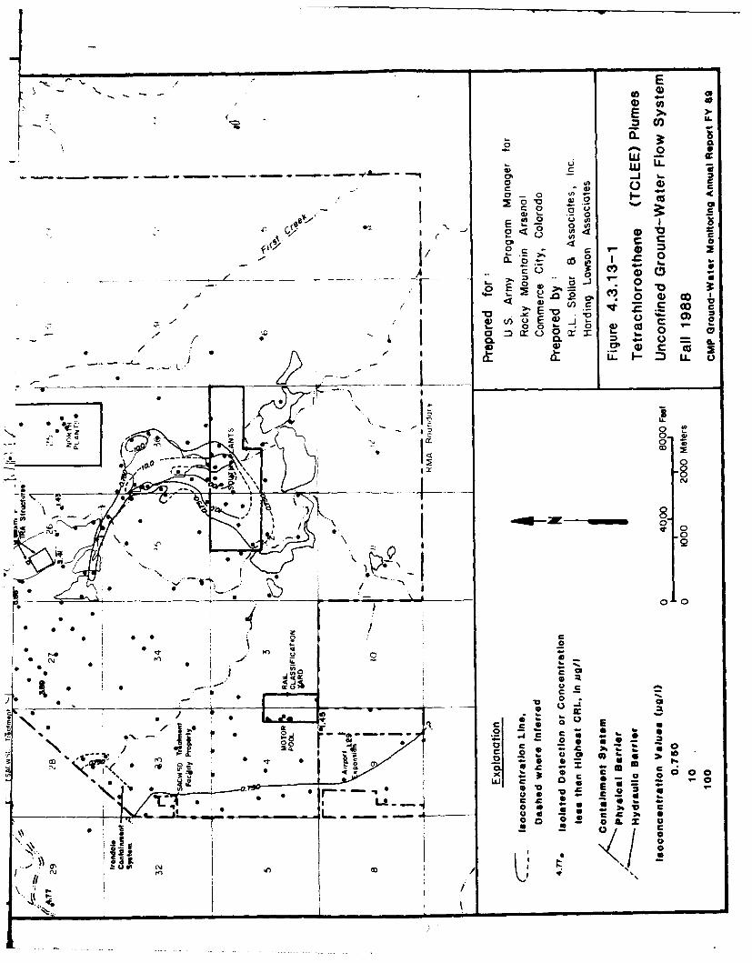
00
E U) 0 ~ M
E o 0
0a a) -0
a:C x * 0 CD
O. I _0
00j I~ oo~ . 0)0-~- (* I S ~ o
00
0
v. I _ _ _ _ _ -fgE
00. 0
00
Q 0
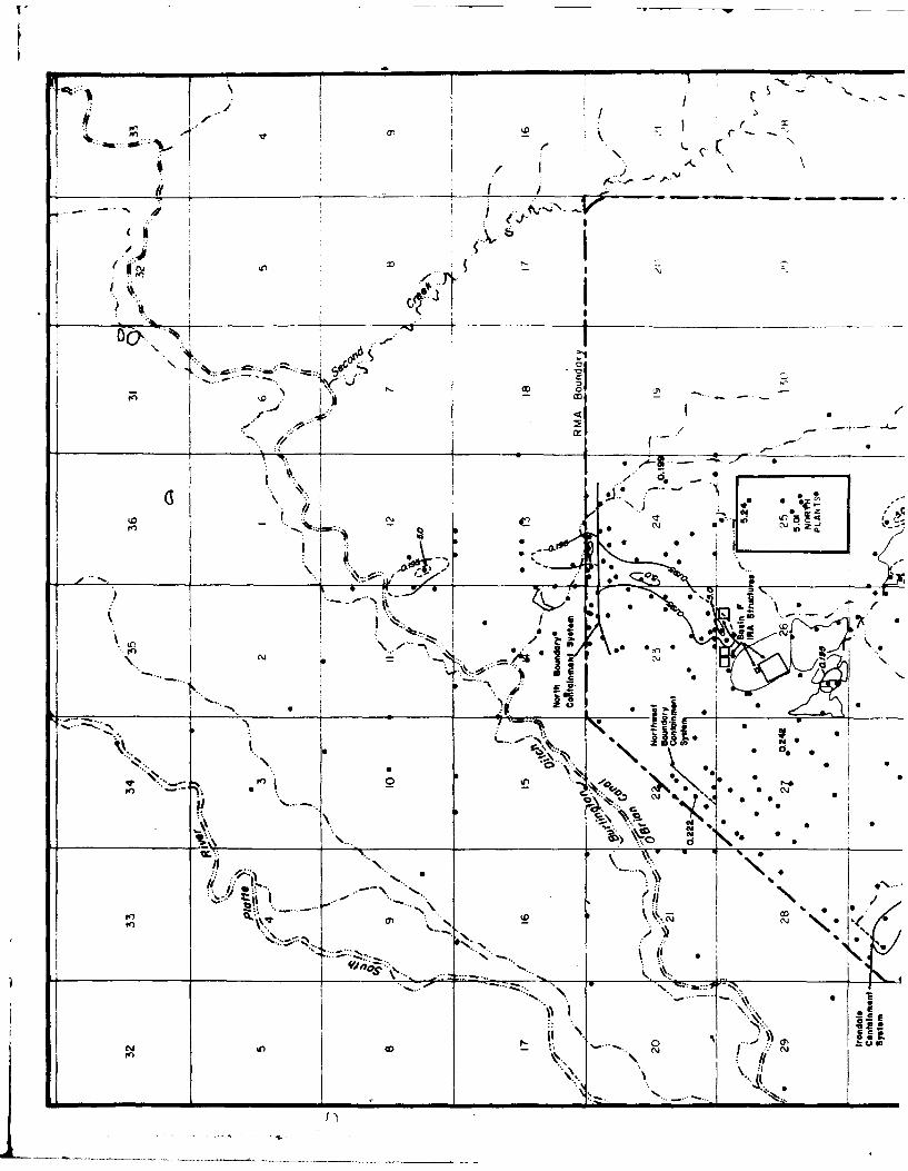
LD Z
CAP.
N,- VI
2k F ~ 00_ 0
II *0. CJ
. 0
"" 'I CD* Ilk.)-
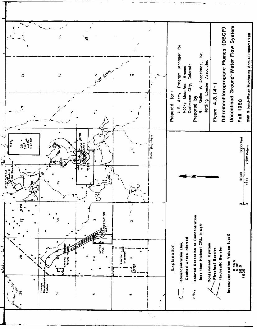
- 00I' ~ -( .-
00
~o0 CL cc 0 '
I 0 - .6 0 a S
/P 0 c~
-0
00
a 02
~) 0
-. 7, ...dvp~
I.. to c a
'-4 .~- ~ -<
S.Y
16
0 - C
01 00
* 6 CC0 6 C1 -I
OD 0 Ucl- x
Co
3' 0 c 'o
0 * *"
00 01 0 L
* 0
0~0
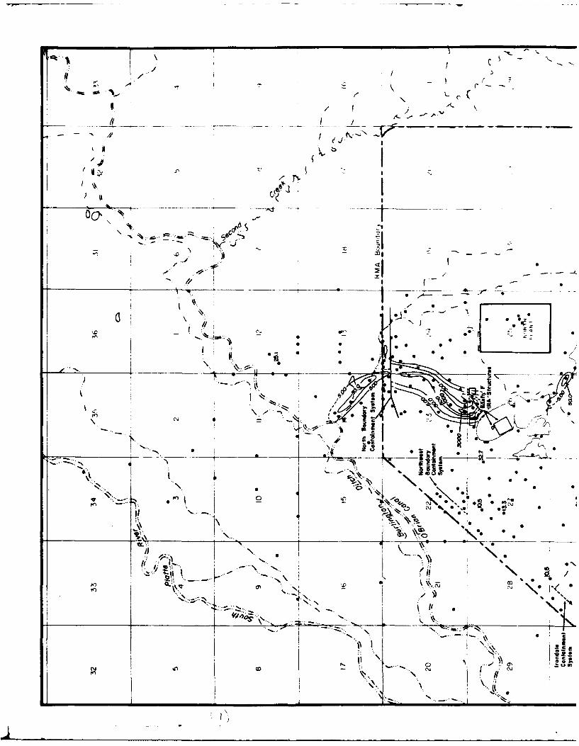
(I__,_ _ \ ' ,,... .
" " -I
.- --*-**J .. . .. ....
- ii -
SF -I " ' -
* ,,,4i - -r -- 0 . . . .. . . .
F , ° ." -I
.- .... •
- .. _ _ _ _ _ _ _ _. I, i _ - ". 2*• j '
______b...~ ,.•, •'£••- ,A
3:.." !.I --• i • \- • " I 2'
S: ,•V • :. •
0-.: . . .. , .t< \ e .e-;
€'#,•:" \ ;9 N -..- _ .' -N::._ ... • .... %~.~ : -. .
'. i''.'.i /
•-- .-...
""..',..7 i '•. \..>,S'• " ... ... "", •0\
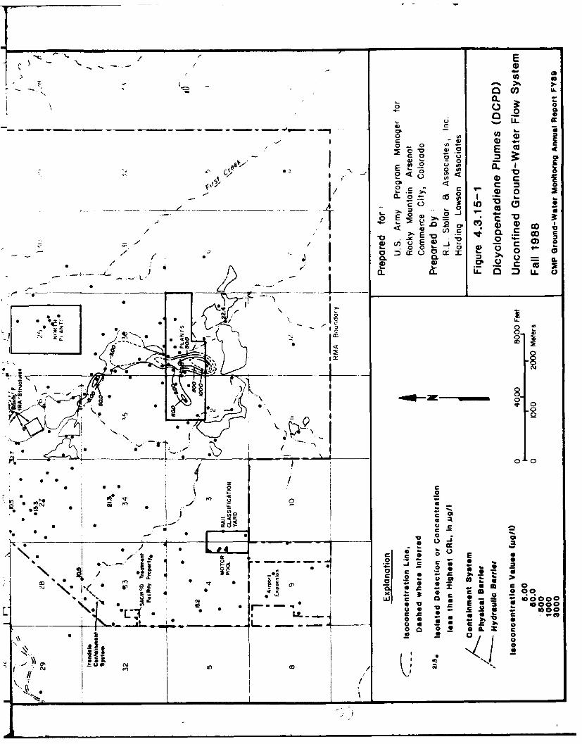
0 EL
00
0.
0 )
I~4 C ) .e.0 0 U
4) 0CI co 0u 100
*CZ c CL 0
0 0 0 T
cO 0
I) 0
-l e . I.- m
I-a
a- 0 -r -U- 1 - -
ITI
00 0
4~~ 0
~0 E
I 0Vc r x 0
C-, I 0
I'- a 00 C L00
SCJ (A m.O
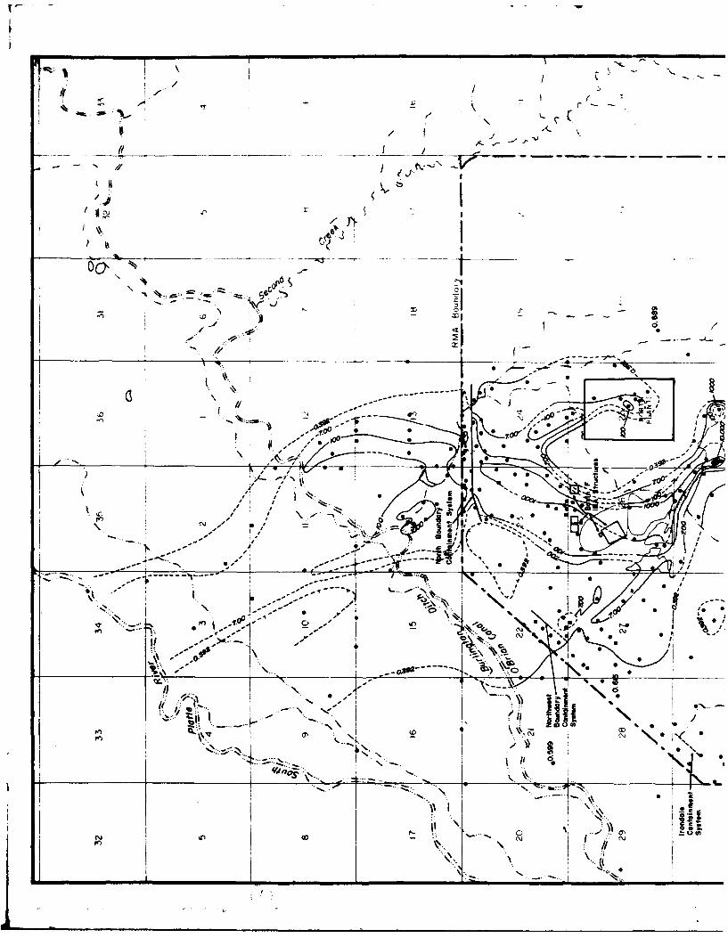
A'A-
_ _ _ _ _ _ _--------------
/'A' 0 0 )
I
-~N
IN,
N -
8'Of-
I
0
oS
'44
-in
z r+:1 ">- -' ~ r~i Atill0
cl0
OD 0
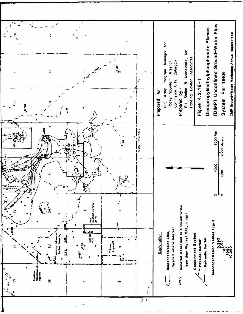
"00 c-
c 0
0 %- 0
40o 0 CL c
E, 0-~ gL
I, C L 0 - 8 o- w IOO i..-P
L __ _ _ /4.- 0
v . v ~ L
-ell. * ~ .
ixu E.~21.-
so 0
* 0'i ~00oc C
CDI
C-6 ' Cie-cooc4' coo-
=~~ .. *
0 IL - 0
'I: ~ -%
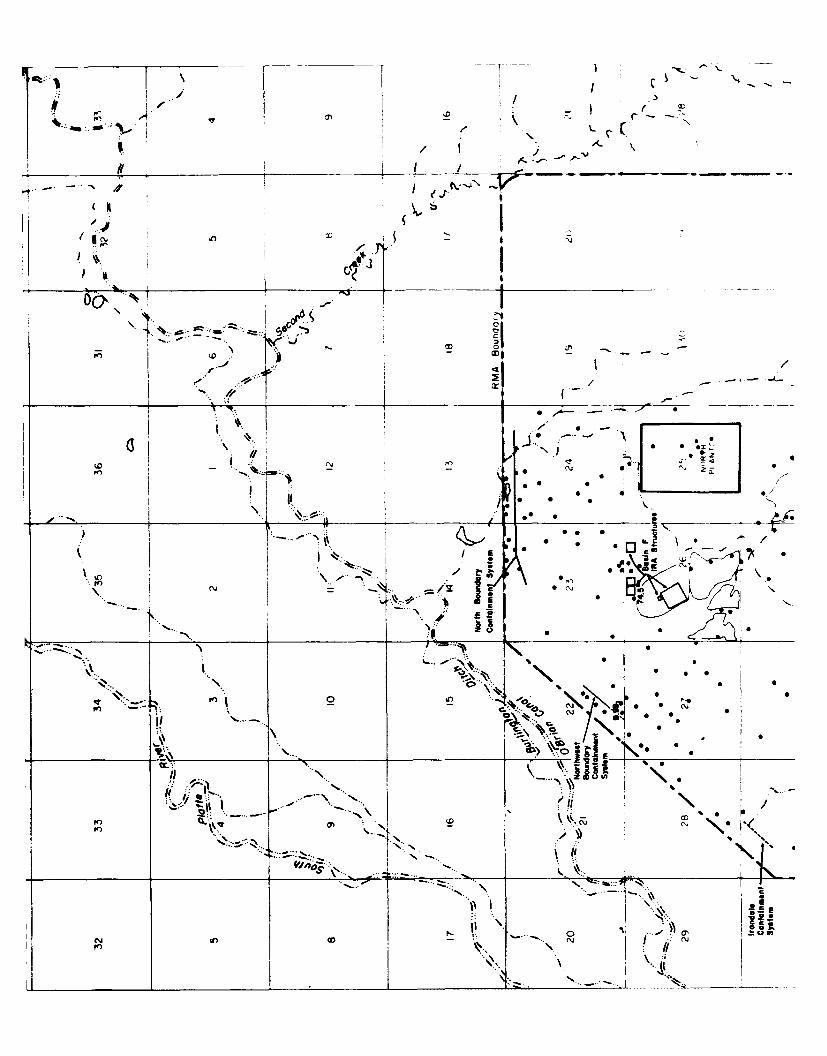
N
rn --- % z
II
fn I, 4r
'N N
Z In zz
* I r ~ 1 . *
CY In1 ODto~
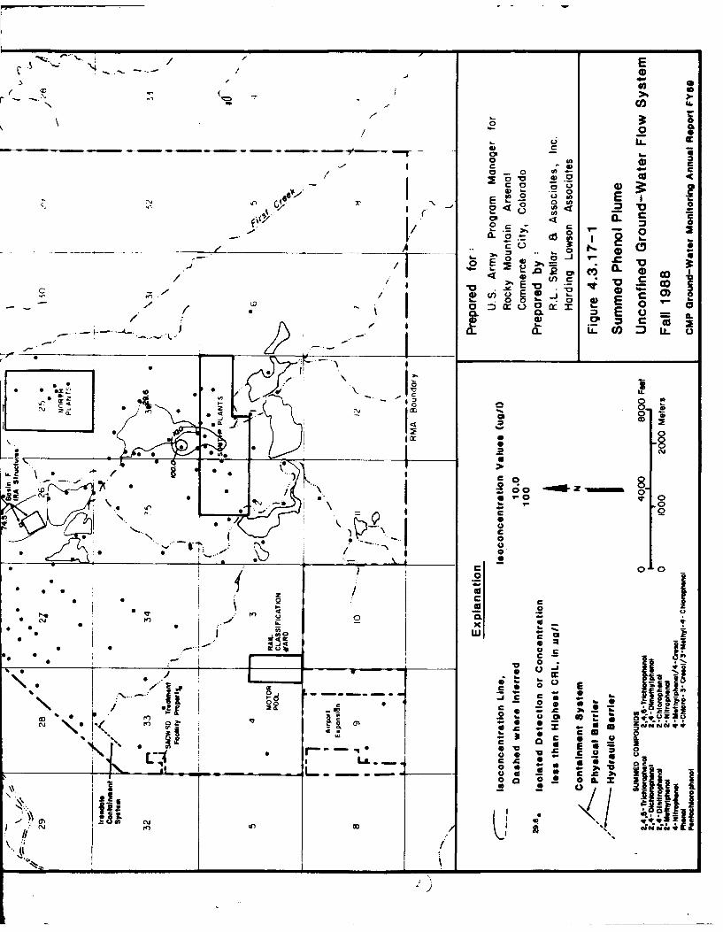
-S..0
-, E
CL 'E
/ - 0
oG
:3 L 0 0 C1
e o. 4) . . 0
0 0.1'(r_ * 2
/5 /c 0 ~ V c/ 0
*~ 0_
,- Z
-J I 0
0 00
0 n 0 im6. IS
000
II x .
z~ *fn
0 , C 'j
0
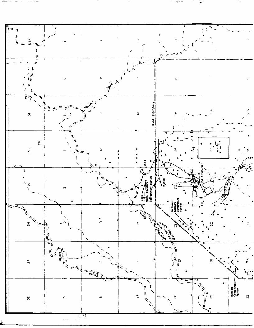
-7---- -� -- -�-�-� - -w -
/ -
- I
-� A -, C--
- /* N
/ A-
(I ___ ___ ____ __- - --------*---- - / 6..�- �
- -� 4. ,
a;
,. J\8'��
/ �'
__________ ___ -__ - ---- h. �-*---�--------- - -. ---- �- - -
-- .- - -� -
-
* *- / - �.- -
N. /, -
______ a-. -. S0 --
I j S __ -- ___
I ,�, * �6 0!. - ..-
/1 I S
6 0 5 5
S(I S 6
II � - -___ ___ ___
***%-. * - �
-\ -
I ___
,- .=--'
I -� S
L
N 0Xe. S 0 S
L * _ %. 0 0�t) � ONsO 0 * �j*� �*.. .*
N. 0 0
-. �. S6
_________ _________ _________ � �I * ''i\ -
- N� 'U / a% S *
* 'S i� A '. *
'.0'5
_____________ _____________ ____ k
{ � -
� I � NF *
Oj�
I ii -. 0 ' � [email protected] f�- ,. .±USI C'd
I II �
)
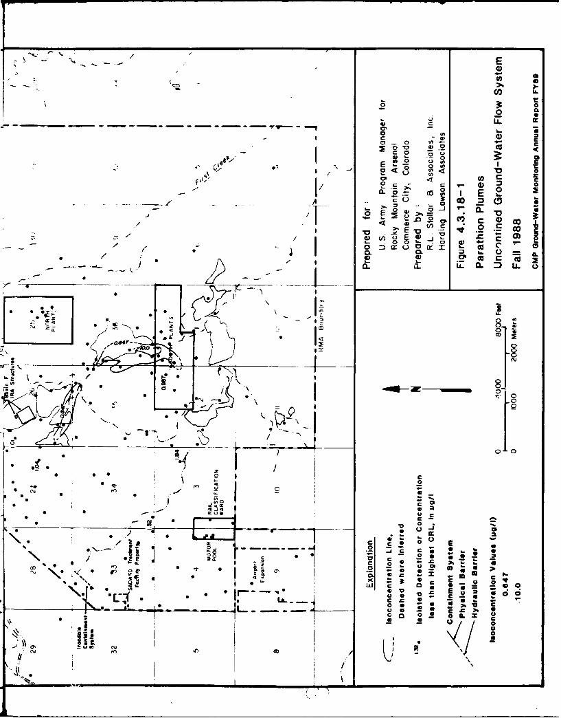
0 a
M COO
c 0
0. 0 0)..
0o 0 0- 2-
CLC
§ Ce
YL = Ia), cca- E
-1 1- a
Az 3
V* /o I U
00
u07
00
00
a4
>CL a
0¼. a 0
0
I 0
OS 0 o c
cy O *D
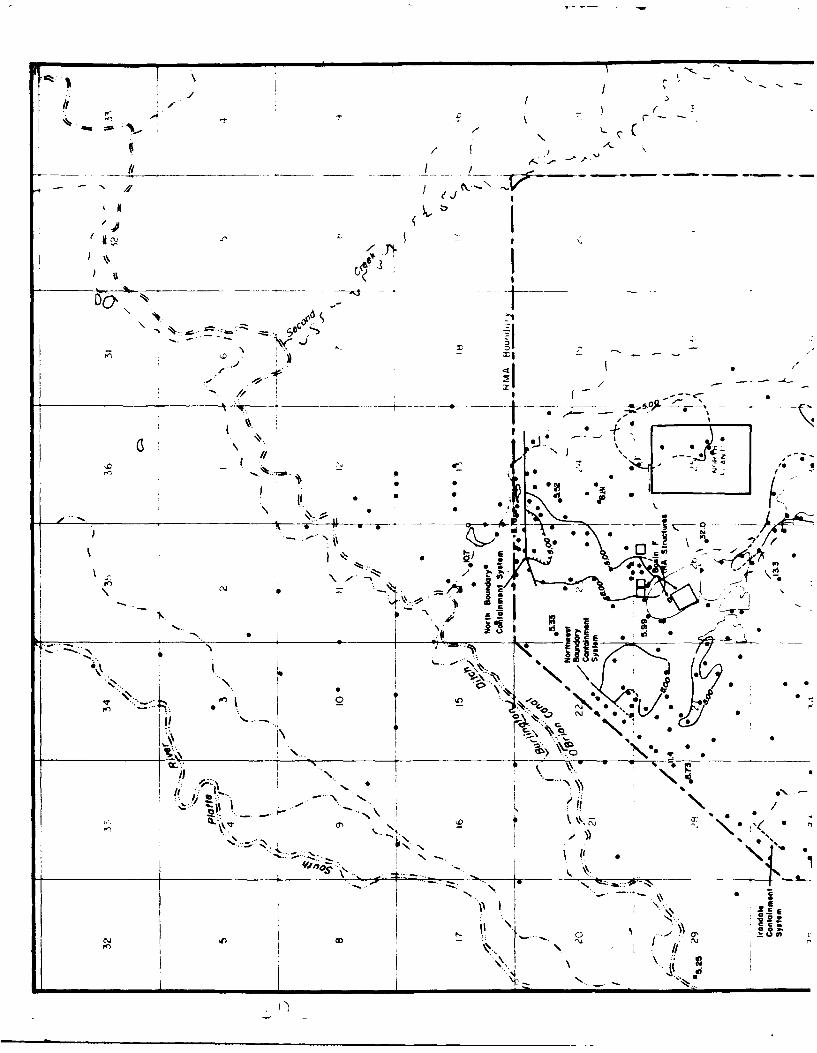
-�-.-
)
(
-
���1-�pvI
N
- -�
__ _ -- � -.
1- -
�' '4
I -
4� I
t
I / - -. -
//
---. �- S
-t--- -. -------4 � ---a-
j - -
* 4<
6 - S
1/ * z #0
-
--
U
0
J 6 0 0
*"� � 0 0 c *. *
K � ��-4---v-u- ----- -,�-a--A-� *
1*� * � 0 0
/ �-
\.-'-'. #� CFS.- I�
-0--v
* 1 ��JSE a
p -3
0S
I I
N -
0
I %O�, >I%.
00 0
urn
_____________ jN
___________ - _____________
\%4r 0.
N. 1I.,
� - -
N
I,....
ii
01 _
�0 *
-i's N \<."'.
0
I
N. N
-US,
cJ
-- I II
__________________________________________I 4 N
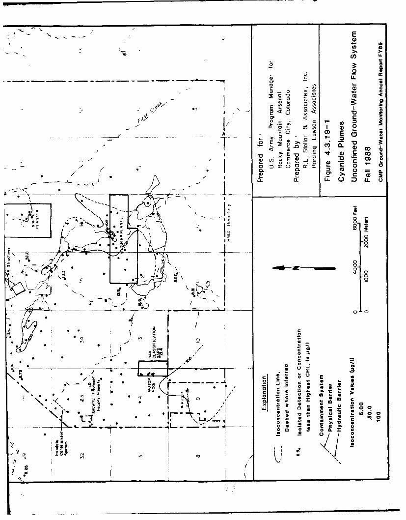
/ /E €
No_ -• Z .• -_ .-,\ .o
-~0)
"- ClIA
"• . .. • • o 0.
Li
0 -
UC 0 ) CO
V '"
a C co-,,
-- r ---- 74C
~~~ý 0, 1irm iimm
0 .-.
CO
/ '~U)C )~ 012CI QE.J-
I * 0i 0
0 0
IRV-:
ZO.~~ C I
0~ 00
40
0 IL x C
C -.
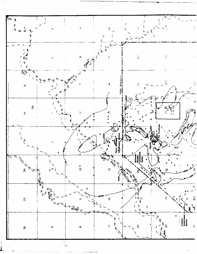
I --
/*
I, I
'C '
___ ___ ___
-- Lv-I
- - --. *i-< .I.
fl-
-,- // ': I --zI A
_ _ _ ...., .....
;" ' '- - .- --• .' 0- -6 1•l _-- -
0 S . *6 . --0'•• - • • • " -. 6' 0I •
""/, i ' .L\I SI -- 4"
SV0-I:,.,. ",: - •_ I
-.I- "" : , " 0•=i "~"
0 0--'•S -~l t
I '+ =- -. . " + 0' +I* ''' \ "ie
I-/
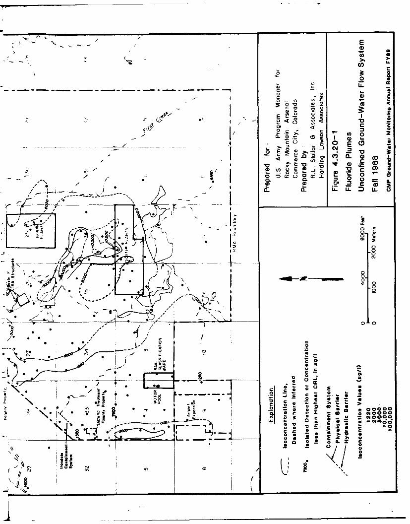
0Lii.
C)
0.. 0 ý _
0 -
E 00 U
0~Cc
I 0
E, 0O 7 CM-0 V (f) 0. J
-z c~~i E V j~ V O4D 0EL~L 0
0 0"S 00
0 Dc 0 crCL = I
a4- iI'L.
I~1 0 e j
I N N
I0 0
.5-,-.- .
N-J
00
Le 0 CL Cc cdoc
390 -- 42 = C0 0on/ 9J -c vE0 ýW0 4
*c a, C'-C I
- 0. m x I
~I 0 --. ---- .!
i * ~ 1OD
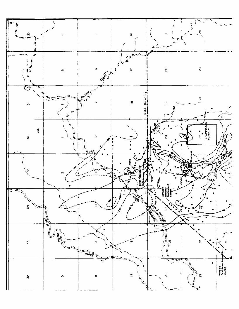
4 4
"A0 r 10 4-~*4 -4=0
* '10
tor cvS
IN-- - - - Sj /.0
r- woo)0
4C4
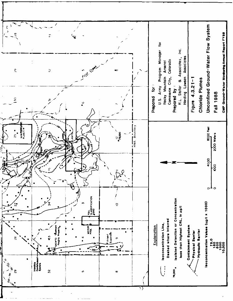
a' 0
4) . 4
0 0
0 Eo
/) 4 0 0ft -'I
Z/ o L 0 Wr X:O 00 OI Co 0)
NV 14)
0 E4
SS090
>.0Q
0 V
mc- - .
'C S 0 IL x.c
~00 ~. I Ea
*n OD ..
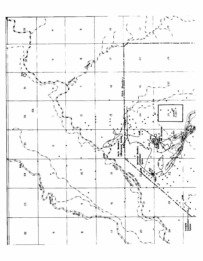
I -L
/ IE
it) C-4 --.
If)-
'UN -
Jr~. . 11 lie
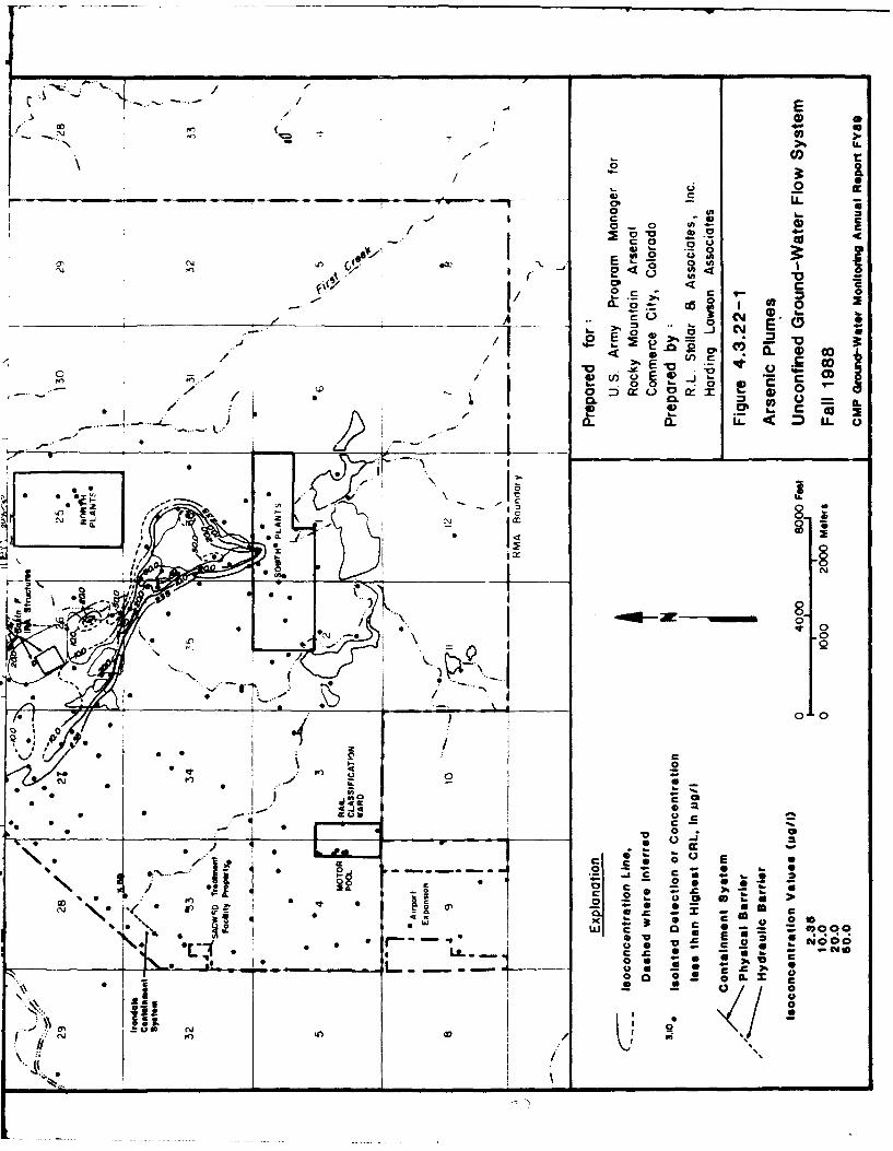
3 0
0 2l
c 0
0 In ~/ CP C,0
4- r
CL 0
a cP
- 0
Vr' /
/ kC)c4
S -o ~E 0 0o -~ G1() Ca~ ~0)
.~ 00
- *. In
/ jg .0 *
C 0 to~
- '. LL -M 0 o
0/ ~I0
00
J* I0
-j Un c c
I
I 5.0 DATA ASSESSMENT
Ground-water data collected during FY89 as part of the CMP consisted of quarterly water-leveldata and water-quality data. Assessments of these data will be presented from three perspectives.
First, the monitoring network design and laboratory analysis and reporting are discussed to assess
anthropogenic influences on data. Second, potentiometric data will be discussed in terms of the
geologic influences on morphology of the potentiometric surface. Third, water-quality data are
assessed in terms of: the known maximum lateral and vertical extent of ground-water
contamination; influences and efficacy of remedial actions; and characterization of the unconfined
and confined flow systems in terms of inorganic water quality.
5.1 AnthroPogenic Influences on Data Assessments
Anthropogenic influences are man-induced variables that affect the perspective from which the
data are assessed. These influences include the number and locations of monitored wells in each
monitoring network, CRLs used to present and compare results, variations in sampling methods,
and variations in laboratory analytical methods. The potential impacts of these influences on data
assessment are discussed below.
5.1.1 Monitoring Network Design
The number and distribution of wells in monitoring networks can affect the interpretation of the
Sanalytical results. Variations in well networks can lead to varying interpretations of plume
configurations. For example, the addition of 38 newly installed wells to FY89 networks resulted
in some changes to pre-existing interpretations. These changes are discussed in detail in Section
4.3, and are briefly summarized below:
0 organosulfur, volatile aromatic, and volatile organohalogen plumes were extended
in the Basin A - Basin A Neck area as a result of revised interpretations with the
additional wells;
* volatile aromatic and volatile organohalogen plumes were shown to extend farther
than previously thought in the South Plants area; and
* volatile organohalogens were shown to occur over a greater area in the Western
Tier.
iGWAR-89.5-6Rev. 06/21/90 - 157 -
f !_ ___
I
5.1.2 Laboratory Analysis and Reporting
Analyte concentrations detected above certified reporting limits (CRLs) define the maximum areal
extent of contamination presented in this report. (Regulations which define contamination with
respect to remedial measures are not considered.) Interpretations of analytical results are
influenced by several anthropogenic variables including CRLs that may be variable either within
a laboratory or among different laboratories, and the proficiency of the analyst. Additionally, the
development of new analytical methods, improved instrument efficiency, and new analytical
techniques, can all contribute to the lowering of CRLs. These anthropogenic variables affect the
interpretation of the extent of contamination.
5.2 Potentiometric Data Assessment
The water table surface of the unconfined flow system and the potentiometric surfaces of the
confined Denver Formation zones are controlled by several geologic and hydrologic factors. Thesefactors are both environmental and anthropogenic. Geologic and hydrologic influences onpotentiometric data presented in Section 4.0 are discussed briefly below (Section 5.2.1). Regionaland project-area potentiometric data assessments are provided in Sections 5.2.2 and 5.2.3,respectively.
5.2.1 Geohydrologic Controls
Many geologic and hydrologic factors exert strong influences on potentiometric surfaces in theunconfined and confined flow systems. Geulogic factors that affect ground-water flow in theunconfined and confined flow systems include the presence of paleochannels, the overall
configuration of the bedrock surface, development of secondary porosity (e.g., fracturing, faulting),and the wide variety of lithologies (e.g., sandstone and siltstone interspersed in claystone) with
concomitant widely varying hydraulic conductivity values.
Several hydrologic factors influence potentiometric data at RMA. First, the majority of ground
water at RMA is the result of underflow from areas upgradient of RMA. This ground water is
recharged by precipitation in upland areas of the Denver Basin, south of RMA. Thus ground-
water elevations may be effected by climatic conditions at some distance from RMA. Surface
recharge to the ground-water flow system from features such as the Lower Lakes and various
ditches and canals (Mary, Ladora, Upper and Lower Derby, the northbog, First Creek, Sand Creek
Lateral and Havana Pond) result in localized relief of the water table. These sources of surface
recharge at RMA have a much greater impact on the unconfined flow system than on the deeper
G WAR-89.5-6Rev. 06121/90 - 158 -
I
I
confined flow system. Interaction between surface water and ground water is discussed in detail
in the CMP Surface Water Annual Report. The sewer and water systems may also have local
recharge/discharge effects on the unconfined and confined flow systems. The presence of sand
bodies interspersed in claystone with discontinuous fracturing allows for the potential presence of
partially confined or leaky aquifers, which would effect water levels in vertically adjacent water-
bearing zones.
The North Boundary Containment System (NBCS), Northwest Boundary Containment System
(NWBCS) and Irondale Containment System (ICS) exert artificial anthropogenic controls on the
unconfined flow system. These systems are sources for local discharge and recharge of the
unconfined flow system and, to a lesser extent, shallow Denver Formation sands. They have a
notable localized effect on ground-water flow, as described in Sections 4.1 and 5.2.3.
In general, the water table surface in the unconfined flow system is higher than the potentiometric
surface in the confined flow system. This indicates that the potential for vertical migration is
downward, from higher head in the unconfined to lower head in the confined flow system.
Vertical communication between the flow systems is discussed in Section 5.3.4.IGeohydrologic relationships between the unconfined and confined flow systems are complex.
Head differences between the confined flow system and the unconfined flow system lessen in
subcrop areas of the different Denver Formation water-bearing zones. The potentiometric heads
of the confined and unconfined flow systems are similar in these areas, indicating direct hydraulic
communication. Vertically adjacent zones of the confined Denver Formation also have similar
potentiometric surfaces. The potential for aquifer interaction will be discussed further in Section
5.3.5.
5.2.2 Regional Potentiometric Data Assessment
The configuration of the water table is shown on a regional scale at RMA in Figures 4.1 -1 through
4.1-4. The surface of the unconfined flow system decreases in elevation from southeast to
northwest, following the trend of the bedrock surface. In general, ground water flows from the
south-southeast to north-northwest. During the fall of 1988, the average hydraulic gradient from
the southeastern to northwestern portions of RMA was approximately 0.0625. An overall increase
in water levels due to a seasonal increase in recharge to the unconfined flow system is interpreted
from a general shift of equipotential lines in the downgradient direction, seen by comparing the
spring 1989 (Figure 4.1-3) and summer 1989 (Figure 4.1-4) unconfined flow system maps. This
IGWAR-89.5-GRev. 0621/9 - 159-
I
I
SI seasonal increase in recharge likely reflects snowmelt runoff and increased precipitation which
occur during the spring months.
I In many areas, local changes in the water-table gradient may be the result of changes in gradient
in the bedrock surface. In areas such as Sections 23 and 24 where the bedrock surface is relativelyflat, the water table is also relatively flat, with a gradient of 0.0053, compared to other portions
of RMA. In areas such as the western portions of Section 2, Section 26 and eastern Section 35,the bedrock surface drops off rapidly from east to west. This locally steeper bedrock surface is
reflected in the locally steeper water-table configuration in these areas, such as eastern Section 35,which had an hydraulic gradient of 0.0167 during the fall of 1988.
A dominant feature of the regional water table surface in the vicinity of RMA is the ground-water mound beneath the South Plants manufacturing complex. This mound is coincident with a
bedrock high beneath the South Plants. In this area a significant component of unconfined flowoccurs through heterogeneous upper Denver Formation volcaniclastic sediments. These sediments
have low hydraulic conductivities relative to surrounding alluvial material. The heterogeneousnature of Denver Formation sediments in the area of the bedrock high results in variable hydraulicI conductivities, which may be reflected by the irregular configuration of the water table in thisarea.
I In northwestern Section 33 a depression in the water-table surface is present on the fall 1988,winter 1989, and summer 1989 regional water-table maps (Figures 4.1-1, 4.1-2 and 4.1-4,
I respectively). This depression is the result of periodic pumping from South Adams County Waterand Sanitation District (SACWSD) water-supply wells located off post, west of the RMA boundary.
15.2.3 Project Area Potentiometric Data Assessment
Selected areas of RMA are of particular interest because of potential for contaminant migrationto off-post areas or because of potential effects on the ground-water flow regime by remedialactivities. Discussion of potentiometric data on a project area basis is presented below. It shouldbe noted that the following discussions for the North and Northwest Boundary Containment
Systems are based on data collected from the CMP water level well networks. More detailedinformation based on weekly water-levels, obtained from densely spaced monitoring well networks,
is available in the FY88 Operational Assessment reports of the North and Northwest BoundaryContainment Systems (PMRMA, 1989b and PMRMA, 1989c, respectively).
GWAR-89.5-6R*v. 06/21/lO - 160-
I
I
5.2.3.1 North Boundary Containment System. Potentiometric data for the unconfined and
confined flow systems were examined to evaluate the impact of the North Boundary Containment
System (NBCS) on the ground-water flow regime. An operational assessment the NBCS is
discussed in Section 5.3.3.1. Data from the fall of 1988 and summer of 1989 are discussed here
because the fall 1988 and summer 1989 events yield the greatest time difference between each
other and the October 31, 1988 start-up date of recently installed recharge trenches along a
portion of the NBCS. It should be noted that, following start-up of newly installed recharge
trenches, use of the bog area to recharge ground water was interrupted for a short time.
Figure 5.2-1 represents water-table profiles upgradient and downgradient of the NBCS for fall
1988 and summer 1989. Comparison of ground-water elevations south and north of the NBCS
indicates that the regional south-southeast to north-northwest flow direction is maintained 350 ft
south and 450 ft north of the NBCS. Further, these profiles indicate that the effect of the NBCS
is quite localized, and water levels at or very near the barrier wall must be examined to see thet impact of the NBCS on ground-water flow in the unconfined flow system.
Figures 5.2-2 through 5.2-5 present map views and cross-sectional views of the NBCS, in the plane
of the NBCS. The map views in Figures 5.2-2 and 5.2-4 present the water table of the unconfined
flow system in the area of the NBCS during the fall of 1988 and summer of 1989, respectively.
The cross-sectional views in Figures 5.2-3 and 5.2-5 show the trace of the top of the water table
on the barrier wall of the NBCS, both upgradient and downgradient of the barrier wall, during the
fall of 1988 and summer of 1989, respectively.IFigure 5.2-3 shows the trace of the top of the water table upgradient and downgradient of the
barrier wall of the NBCS as contoured from potentiometric data for fall 1988. These data predate
the start up of recharge trenches installed in the western portion of the NBCS. As shown in Figure
5.2-3, potentiometric heads are greater upgradient than downgradient along most of the NBCS,
with the exception of the area denoted by I in Figure 5.2-3. This head difference suggests that
either discharge was insufficient south of the NBCS or recharge was insufficient north of the
NBCS (except in area i), which increased the head difference (hydraulic gradient) across the wall.
This confirms the conditions identified under Task 36 (ESE, 1989). This increase in hydraulic
gradient could, in turn, increase the potential for, and the velocity of, ground-water flow beneath
or through the slurry wall. In area I the potentiometric surface was higher in the north than the
south, creating a hydraulic barrier to contaminant migration to the off-post area.
Figure 5.2-5 shows the trace of the top of the water table on the NBCS south and north of the
NBCS barrier wall during summer 1989. This period post-dates start-up of recharge trenches by
GWAR-89.5-6Rev. 06/21/0 161 -
!A• m mmmmm m m m mm m m mmw - _
I
approximately six months. The three areas denoted 1, 2 and 3 in Figure 5.2-5 are areas where
potentiometric heads north of the NBCS are greater than heads south of the NBCS, indicating
potential areas for reversed, north to south flow. In all other areas, potentiometric heads are very
nearly equal, or greater upgradient than downgradient, indicating that either no flow or normal
south to north flow will occur, with potential for contaminant migration beneath the NBCS.!In confined Denver Formation wells near recharge trenches, water levels rose slightly between fall
1988 and summer 1989. These water-level increases are probably in response to start up of
recharge trenches at the NBCS, and indicate some communication between unconfined andconfined aquifers. For example, water levels in Well 23177, south of the NBCS, increased 1.7 ft
and 2.4 ft from the fall of 1988 to the winter and spring of 1989, respectively, after the start up
of recharge trenches. These increases are attributed to recharge trench activities, and indicate
I hydraulic communication between the alluvium and the underlying confined Denver Formation
aquifers, and between the upgradient and downgradient sides of th- pilot portion of the slurry wall
of the NBCS. Denver Formation response to recharge trench activity is described in greater detail
in Section 5.3.3.1 of this report and in a recent report detailing recharge trench start-up
performance (Lutton, 1989).
5.2.3.2 Northwest Boundary Containment System. Potentiometric data for the unconfined flow
* system were evaluated to ascertain the impact of the NWBCS on the unconfined flow system.
Figures 5.2-6 and 5.2-7 present water-table surface maps for fall 1988 and summer 1989 of the
NWBCS. During the fall 1988 period (Figure 5.2-6) the potentiometric head of the unconfined
flow system appears greater in the southeast than the northwest in all areas of the NWBCS. Head
differences were generally greatest in the slurry-wall portion of the NWBCS. Based on these data,
head differences indicate that the potential existed for downgradient (southeast to northwest) flow
in the vicinity of the NWBCS during fall 1988. However, a review of a more comprehensive data
set, collected by the PMRMA Technical Operations Division (PMRMA, 1989c), indicates that a
reverse gradient is maintained along major portions of the NWBCS. This reverse gradient occurs
in the immediate vicinity of the slurry wall/hydraulic barrier and does not propagate outward to
the CMP monitoring wells which are located 200 ft or greater from the slurry wall/hydraulic
barrier.
In the summer of 1989 (Figure 5.2-7) the potentiometric heads southeast and northwest of the
NWBCS are nearly equal in most areas of the NWBCS. Overall, the head difference decreased
markedly between fall 1988 and summer 1989, suggesting a decreasing potential for circumvention
of the NWBCS. As stated above, the data set collected by the PMRMA Technical Operations
Division (PMRMA, 1989c), indicates that a reverse gradient is maintained along major portions of
G WAR-89.5-6Rev. 06/21/0o - 162 -
!
I
the NWBCS. The similarity in potentiometric heads on either side of the NWBCS would greatlyreduce ground-water flow velocities. Circumvention of the system might then be impacted by
factors such as bedrock fractures and slurry wall construction.
5.2.3.3 Basin F Area. The potentiometric surface of the unconfined flow system in thejBa.0n F area is shown in Figures 4.1-9 through 4.1-12 for the fall 1988, winter *989, spring 1989
and summer 1989 events, respect;,cly. Figures 4.1-9 to 4.1-12 show that the water table exhibits
only minor fluctuations through the time period examined. One notable exception is a slight
trough in the northwestern corner of Section 26 during the spring ,989 and su.l ,er 1989 events,
which is not present during the fall 988 and winter 1989 events.
The water table gradient is relatively steep southeast and west-northwest (between 0.0100 and
0.0143) of the Basin F area, but decreases markedly in the vicinity of Basin F. The changes in
water table gradient ac-oss the area correspond to the bedrock surface, suggesting that ground-
water movement in the unconfined flow system is strongly influenced by bedrock topography.
As seen in Figures 4.1-9 through 4.1-12, relatively large areas in the vicinity of the Basin F area
j are underlain by unsaturated alluvium. In these arcas of unsaturated alluvium, grou '-water flow
through the unconfined flow system occurs in the upper portion of the Denver Formation which
j is hydraulically connected to alluvial deposits, as described in Section 4.1.
5.3 Contamination AssessmentIThis assessment includes a summary of the contaminant sources, the areal extent of contamination,
the effect of operations at the North and North-, est Boundary Containment Systems on the ground-
water system, the vertical extent of contamination, and aquifer i:,teractions. The intent of this
section is to add to data presented in 1988 CMP Annual :_Žprn (Stollar, 1989b) and the Water
Remedial Investigation Report (Ebasco, 1989i).
5.3.1 Sources of Contamination
Sources of contamination at RMA haxe been identified in various reports, including Contamination
Assessment Reports and the Study Area Reports generated under the Remedial
Investigation/F.easibility Study (RI/FS). As a result of RI/FS investigations, source areas were
given designations as confirmed or suspected (Ebasco, 1989i). There are six major confirmed
contamination source areas at RMA. These areas are the South Plants Manufacturing Complex,Basin A, Basin F, the North Plants Manufacturing Complex, the Railyard-Motor Pool area, and
GWAR-89.5--6Rev. 06/21/o- 163 -
I
I
the chemical sewer system. Suspected contamination source areas include the Sand Creek Lateral
and Basins B, C, D, and E (Figure 1.2-1).
The South Plants area encompasses approximately two-thirds of a square mile in Sections I and 2.
Manufacturing of various chemicals occurred from 1943 to 1982. Numerous sources exist in the
South Plants resulting from industrial operations, waste disposal activities, and spills. A majority
of the targeted CMP list of compounds have been documented emanating from the South Plants
4 area.
The Basin A area includes the unlined Basin A disposal pond as well as adjacent disposal sites in
Section 36. Basin A received large volumes of waste from South Plants and North Plants
operations from 1943 to 1958. Areas within Section 36 were also used for trench disposal of
industrial by-products, off-specification materials and munitions. As with the South Plants, a
majority of the targeted CMP list of compounds have been documented in ground water beneath
Basin A.
Basin F was an asphalt lined basin which received virtually all liquid chemical wastes and
production waste waters at RMA from 1956 to 1978. It was last used in 1982. Removal of wastes
has occurred as part of the 1988 Interim Response Action (Ebasco, 1989i). As with the South
Plants and Basin A, a majority of the targeted CMP list of compounds have been documented in
ground water in the area of former Basin F.
The North Plants Manufacturing Complex in Section 25 was used to manufacture the nerve gas
GB (sarin) and to demilitarize Army agents between 1953 and 1984. The primary contaminants
detected in ground water in the North Plants are DIMP and volatile organohalogens. As a
contaminant source, the contribution of the North Plants to RMA ground-water contamination is
significantly less than in the areas of the South Plants, Basin A and Basin F.
The Railyard-Motor Pool area consists of two building complexes, the Rail Classification Yard
and the Motor Pool area, which are confirmed source areas in the RMA Western Tier. The Rail
Class'fication Yard was used to store tank cars containing various chemicals. The motor pool was
,Ae-d for support operations. The Railyard-Motor Pool area is the documented source for plumes
of DBCP and volatile organohalogens, principally trichloroethene (TRCLE). Plumes of volatile
organohalogens also migrated onto the RMA Western Tier from off-post sources south or southeast
of RMA. In general, the amount of contamination introduced into RMA ground water by the
Railyard-Motor Pool area is much less than that introduced by source areas of central RMA.
IGWAR-8g.6-6Rev. 06/21/go - 164 -
I
i
The chemical sewer system is a gravity system that carried chemical wastes from operations at
South Plants and North Plants to Basins A and F. The first chemical sewer was installed in the
South Plants in 1942. Much of the chemical sewer system was constructed of vitrified clay pipe,
which is known to have leaked. Because of its proximity to other contaminant source areas,
contaminant plumes solely from the chemical sewer system are not readily separable.iSuspected source areas are the Sand Creek Lateral and Basins B, C, D, and E. These areas have
been given this designation because of historical information indicating the presence of chemicals
and/or contaminant plumes at or downgradient of these sites.
Indications of the type and mass of materials disposed at RMA were provided by Geraghty &
Miller (1986). The highest reported volumes of waste were attributed to dieldrin, benzene,
chloroform, fluoride and chloride. Moderate volumes of waste disposal were reported for endrin,
p-chlorophenylmethyl sulfide and sulfoxide, and for DBCP. Low waste disposal volume was
reported for p-chlorophenylmethyl sulfone. Many contaminants were not rated according to the
volume of materials contained in disposal wastes. These include: dithiane, oxathiane, benzo-
thiazole, chlorobenzene, trichloroethane (TRCLE), tetrachloroethane (TCLEE), arsenic and DIMP.
Although the volume of DIMP waste was not rated, it had a history of moderate production at
RMA.
1 5.3.2 Lateral Extent of Contamination
An assessment of the lateral extent of ground-water contamination at RMA is presented in this
section. An assessment of unconfined and confined flow system contamination was conducted
based upon contaminant source areas discussed in Section 5.3.1. The distributions of contaminants
assessed in this section were previously described in detail in Section 4.3 of this report.
Well-defined contaminant plumes in the unconfined flow system extend from numerous sources
at RMA (Figures 4.3.2-1 through 4.3.22-I). Contaminant plumes range from a few thousand feet
to several miles in length. The plumes of the greatest magnitude extend from the South Plants -
Basin A area and from the Basin F area. Plumes of lesser magnitude extend from sources in the
North Plants and Railyard-Motor Pool areas. Contaminant migration is predominantly to the
northwest. The primary contaminant flow paths in the unconfined flow system are directly related
to the presence and orientation of permeable strata. These permeable strata often occur as
Quaternary alluvium that fills paleochannels.
G WAR-Sg.5-6Rev. 06/21/90 - 165 -
I!
j Man-made remedial systems have affected the distribution of contaminants in the unconfined flow
system. Operation of the North Boundary Containment System (NBCS), the Northwest Boundary
Containment System (NWBCS) and the Irondale Containment System (ICS) have resulted in
decreased contaminant levels downgradient of these systems. In Section 5.3.3, the efficacy of the
NBCS and NWBCS are discussed.i5.3.2.1 South Plants - Basin A Area. Because of their proximity and alignment along the same
flow path, it is difficult to assess the contribution of the South Plants or Basin A individually.
Therefore, the contribution of these confirmed source areas are discussed concurrently.
Contaminants originating in the South Plants - Basin A area migrate along the South Plants-
Basin A, South Lakes, and Basin A Neck Pathways within the unconfined flow system. Within
these pathways, contaminant migration occurred predominately within saturated alluvium. In the
South Plants, however, contamination exists in the unconfined flow system within Denver
Formation zone VC. Some contaminants emanating from the South Plants exhibit radial transport
away from the ground-water mound in the area. However, the majority of contaminants migrate
from the South Plants north toward Basin A. This is because the central processing area, where
many plumes originate, is located on the north side of the South Plants ground-water mound.
Contaminant plumes present in the South Lakes Pathway include dieldrin, volatile aromaticcompounds, and volatile organohalogen compounds. These compounds extend approximately 2000
ft southwest of the South Plants to Ladora Lake.1From the South Plants and Basin A area, many contaminant plumes extend northwest along the
Basin A Neck Pathway toward the Northwest Boundary Containment System. However, some
plumes appear to bifurcate in southeast Section 26 resulting in contamination extending north
along the Basin F East Pathway. Because potentiometiic data indicate that ground water in this
area flows generally northeast, contamination in the Basin F East Pathway may be attributable to
several causes, such as the former chemical sewer system which connected the South Plants to Basin
F, historic flow directions which differ from present-day flow directions or discharge from water-
bearing zones in the Denver Formation that have the potential of transporting contamination.
Contamination of the confined flow system occurs in the South Plants - Basin A area within
zones A, IU, and 1. Vertical contaminant migration may occur due to water flow along irregularly
bedded but interconnected sandstone, fractures, faults, and historically through improperly sealed
wells and borings. All of the improperly sealed wells that have been identified, have been closed
as a part of an Interim Response Action performed during FY89.
GWAR-89.6-6Rev. 06/21/0 - 166-
I
I
5.3.2.2 Basin F. Contaminants within the Basin F area migrate primarily north-northeast along
the Basin F Pathway toward the North Boundary Containment System. All of the contaminants
discussed in Section 4.3 of this report with the exception of chlorobenzene and composited phenols
are present in the Basin F Pathway. Contaminant migration within the Basin F Pathway occurs
both in saturated alluvium and in unconfined portions of Denver Formation zone 2.
Several contaminants present in the Basin F Pathway continue to be identified north of the North
Boundary Containment System (NBCS) in plumes occupying the First Creek and Northern Off-
Post Pathways. The plume centroids for contaminants in these pathways are frequently 2000 to
7000 ft downgradient of the NBCS indicating that these plumes may represent contamination
existing in off-post ground water prior to construction of the NBCS.
Plumes of a few contaminants are present northwest of Basin F within the Basin F West and Basin
F Northwest Pathways. Contaminants within these pathways are intercepted by the Northwest
Boundary Containment System.
Contamination of the confined flow system exists downgradient of Basin F in Denver Formation
zones 2, 3, 4, and 5. Detections of contaminants in the confined flow system occur predominately
beneath areas of unconfined flow system contamination.
5.3.2.3 Western Tier. The Western Tier area is characterized by contaminant plumes of DBCP
and volatile organohalogens emanating from the Railyard-Motor Pool area, as well as an additional
volatile organohalogen plume originating from sources south or southeast of the Western Tier of
RMA. Plumes of cyanide, chloride and fluoride existing in Sections 4 and 9 also appear to
J originate from off-post sources.
The two volatile organohalogen plumes in the Western Tier can be differentiated from one another
based upon the suite of contaminants detected in each plume. Trichloroethene (TRCLE) is the
primary volatile organohalogen originating from the Railyard-Motor Pool area. Conversely, several
compounds, including 1,1,1-trichloroethane, 1,1-dichloroethene, tetrachloroethene, and TRCLE
predominate in the upgradient volatile organohalogen plume, entering RMA from the south.
The DBCP plume emanating from the Railyard-Motor Pool area is intercepted by the Irondale
Containment System. TRCLE however, continues to be detected off-post west and northwest of
RMA. The extent of off-post TRCLE contamination has been assessed by the EPA.
GWAR-89.5-6Rev. 06/21/90 167 -
I
Only a few confined flow system wells exist in the RMA Western Tier. Analytical results from
these wells indicate that DBCP and volatile organohalogen contamination apparently are limited to
the unconfined flow system.
5.3.2.4 North Plants. Contamination in the North Plants area is limited predominately to DIMP1
and volatile organohalogens. Chloroform is the primary volatile organohalogen compound present.
Contaminants originating in the North Plants migrate north. DIMP contamination originating in
the North Plants extends north to the North Boundary Containment System and merges with the
Basin F plume. The chloroform plume extends approximately 5000 ft north into southern Section
24. Minor amounts of cyanide, chloride (in both the unconfined and confined flow systems) and
fluoride (in the unconfined flow system) may also originate in the North Plants.
5.3.2.5 Sand Creek Lateral. Several contaminant plumes are interpreted to originate in Sections34 and 35. These contaminants occupy the Central North and Central South Pathways. These
plumes may be the result of contaminants originating from the South Plants and transported via
the Sand Creek Lateral where they percolated into the ground water. An alternative hypothesis
is that subcropping Denver Formation water-bearing zones recharge alluvium in these areas with
contaminated ground water. Contaminants present in these pathways include dieldrin, chloroform,
chloride, and possibly fluoride and DIMP. These plumes extend downgradient toward the
Northwest Boundary Containment System. As presently interpreted this contamination would not
be intercepted by the containment system and would flow off-post along the Northwest Pathway.
5.3.3 Ground-Water Containment Systems
There are three ground-water remedial systems currently in operation at RMA. These include the
North Boundary Containment System (NBCS), Northwest Boundary Containment System (NWBCS)
and the Irondale Containment System (ICS). All of these containment systems are designed to
) intercept, treat and recharge ground water to prevent off-site contaminant migration.
One of the specific objectives of the CMP ground-water element is to provide monitoring for
system operational purposes. The two systems that are operated by the Army, the NBCS and theNWBCS, are the subject of this assessment. Several previous investigations, including Task 25
(ESE, 1988), Task 36 (ESE, 1989) and the 1988 CMP Annual Report (Stollar, 1989) have addressed
local contaminant distributions at both containment systems. It should be noted that the following
assessments of the Boundary Containment Systems are based on data collected from CMP well
networks. Information based on weekly water levels obtained from densely-spaced monitoring
GWAR-89.5-6Rev. 06/25/90 - 168 -
I
I
well networks is available in the FY88 Operational Assessment Reports of the NBCS and NWBCS
(PMRMA, 1989b and PMRMA, 1989c, respectively).
5.3.3.1 North Boundary Containment System
The NBCS consists of a soil-bentonite slurry wall extending approximately 6740 ft along the
northern boundary of RMA. The system extracts and treats ground water leaving RMA. The pilot
portion of the NBCS became operational in June of 1978. The system was subsequently expanded,and became operational in its present configuration in January 1982. In October 1988 recharge
trenches installed to increase downgradient recharge capacity became operational.
Assessment of the NBCS focuses on two aspects of the system. First, hydraulic impacts on the
unconfined and confined flow systems are examined, and second, upgradient and downgradient
contaminant concentrations are compared.
Hydraulic Assessment.
The effect the boundary systems have on ground-water flow through the unconfined flow system
has been studied extensively. Conversely, assessment of boundary system effects on flow through
deeper zones in the Denver Formation continues to be evaluated. This section compares temporalpotentiometric data from the unconfined flow system with temporal potentiometric data fromdeeper zones in the Denver Formation. This comparison provides information about hydra'dicrelationships between these zones in the boundary systems areas and, in turn, about the effects that
the boundary systems have on flow through deeper units in the Denver Formation.
Several changes made to boundary system operations during the past year must be considered wheninterpreting the potentiometric data. Most notable is the installation of recharge trenches designed
to enhance the recharge capacity north of the west portion of the North Boundary ContainmentSystem (NBCS). Ten trenches were installed at locations delineated on the well location map onFigure 5.3.3-1. Each trench is approximately 160 ft long, averages 16 ft in depth, and penetrates
the entire thickness of the alluvium. The purpose of the trenches is to provide additional surface
area through which increased volumes of treated water can be recharged to the alluvium (Lutton,
1989).
Trench recharge operations were started on October 31, 1988. By November 14, all of the trenches
were receiving flow. During this start-up phase, the volume of water initially required to fill the
recharge trenches to capacity exceeded the amount normally available from the extraction system.The additionally required recharge water was obtained in two ways. First, the volume of water
GWAR-89.5-6Rev. 06/21/90 - 169 -
I.
i
j sent from the NBCS treatment plant was increased. Second, water normally sent to the north bog
was diverted to the trenches. Flow to the bog was reduced in increments until, on January II,
1989, all flow to the bog was stopped. On January 19, 1989, the volume of water received by the
recharge trenches approached capacity, so flow to the bog was resumed (Lutton, 1989). Detailedinformation on start-up operations including tabulated flow data, is contained in the start-up
performance of Ground-Water Recharge Trenches report (Lutton, 1989). These changes in
boundary system operations must be considered when assessing potentiometric data in the NBCS
area.
To aid in the assessment of potentiometric data around the boundary systems, diagrams have been
prepared that compare hydrographs from multiple water bearing zones (Figures 5.3.3-1, 5.3.3-2).
Each hydrograph represents data from an individual well. Ideally, potentiometric comparisons
j would be made at well cluster sites which screen the alluvium and each of the water-bearing zones
of interest in the Denver Formation. In this manner, effects of the NBCS on vertical hydraulic
gradients could be separated accurately from effects on horizontal gradients. However, cluster
wells are limited in the boundary systems areas. Instead, groups of individual wells within relativeproximity to each other are used. Wells within each group provide potentiometric data from the
alluvium, and at least one confined zone in the Denver Formation. The geologic zones represented
are not necessarily identical among all well groups because of the variable distribution of wells inthe NBCS area. These well-groups are delineated on Figure 5.3.3-1. Five of the seven well groups
are located on the north side of the barrier and two are on the south side of the barrier.
Each hydrograph presents potentiometric data collected from the winter of 1985 to the summer of
1989. Although data collected prior to 1987 were not collected under the CMP program, they areI included to provide information about long term trends. Certain wells in the data base were
measured more frequently than quarterly. These subquarterly measurements are predominant prior
to 1987. In order to obtain a single water elevation value from each quarter between winter 1985
and summer 1989, the subquarterly measurements were averaged. The averaged values are plotted
as the quarterly data points on the hydrographs. Due to variability in water elevation changes
between the well-groups, the vertical scales are not consistent between diagrams. Potentiometric
data are plotted using unique symbols for each geologic zone represented. These symbols are also
used to delineate the well locations on the plan maps (Figures 5.3.3-1, 5.3.3-12). The stratigraphic
relationships of these units are discussed in Section 2, and diagrammed on Figure 2.1-4.
Well-group 1 is located immediately north of the west end of the NBCS, and consists of four wells
(Figure 5.3.3-1). Each well is completed in a separate geologic zone. The zones are alluvium,
unconfined zone 2, confined zone 3, and confined zone 4. In this group, the alluvium and zone
GWAR-89.5-6R.v. 0ml/21 - 170-
I
I
2 are both unconfined and exhibit similar potentiometric elevations. Zones 3 and 4 are confined
and exhibit potentiometric elevations similar to each other but generally 10 ft below the
potentiometric elevations of the unconfined zones.
Generally, between the winter of 1985 and the spring of 1988, water elevation fluctuations in thevicinity of well group I were similar in the unconfined and confined zones. These fluctuations
generally reflected seasonal variations. The effect of the recharge trenches is also evident showing
higher water-level elevations in fall 1988/winter 1989 and lower elevations in the spring/summer
as use of the recharge trenches decreased. For example, increased water levels commonly occurredin each hydrograph during the spring quarter of each year and then decreased during the summer,
fall, and winter quarters. However, the water , evation fluctuations became less similar in 1989when the alluvial and confined zone 2 water levels fluctuated by approximately 5 ft, while
confined zones 3 and 4 responded with fluctuations closer to 1 foot. The fluctuations in theunconfined units corresponded with the initial operation of the recharge trench system. Theresponse in confined zunes 3 and 4 was dampened, indicating reduced vertical communication
between the unconfined and confined zones in this area. Water level fluctuations in confinedzones were similar to water level fluctuations in the unconfined zones when they were caused by
regional factors such as seasonal variations. Localized fluctuations such as boundary systeminfluences resulted in dampened responses in zones 3 and 4.
Well-group 2 is located on the north side of the boundary system, approximately 500 ft west ofthe section line dividing Sections 23 and 24 (Figure 5.3.3-1). Three wells make up this group; theyare completed in the alluvium, unconfined zone 2, and confined zone 3. Water elevations from the
well completed in zone 2 were unconfined but also were consistently higher than water elevations
in the alluvial well. This difference should not be interpreted as an upward gradient between zone
2 and the alluvium in the vicinity of well-group 2 because these hydrographs presentpotentiometric data from wells which are areally separated from each other. In well-group 2, the
alluvial well is approximately 500 ft north of the zone 2 well. The lower water elevationsindicated on the alluvial hydrograph reflect the downgradient location of the alluvial well.
Water elevation fluctuations at well-group 2 are similar in the alluvium, unconfined zone 2, and
confined zone 3. Water level elevations in each of these zones generally increased during thespring quarter of each year and then decreased during the summer, fall, and winter quarters.
These fluctuations were relatively consistent for each zone from the winter of 1985 to the fall of
1988. In the winter of 1989, a rapid increase of approximately II ft occurred in unconfined zone
2. This increase occurred between the fall 1988 and winter 1989 quarters, and corresponded with
the initial operation of the recharge trenches. Well 23203, located within 50 ft of a recharge
GWAR-89.5-6Rev. 06/21/90 - 171 -
I
I
j trench, exhibited water elevations which closely correspond to changes in the recharge rate at the
trench. The unconfined nature of zone 2 in the vicinity of Well 23203 contributes to this direct
response.
Unconfined wells 23045 and 23203 respond relatively directly to changes in recharge at the
trenches. Well 23045, located approximately 500 ft to the north of the recharge trench, exhibits
a dampened response. This dampened response is expected when distance from points of ground-
water recharge or discharge is increased.
Well 23161 is completed in confined zone 3, and is located laterally approximately midway between
unconfined Wells 23203 and 23045. Water elevations from Well 23161 also increased in response
to the initial operation of the recharge trenches. However, the increase is dampened in comparison
to the increases measured at both unconfined wells. The maximum water elevation at Well 23161
occurred after two quarters, and the increase was less than 3 feet. This dampened response is in
part a function of distance from the recharge trench. More significantly, this dampened response
also reflects the confined nature of zone 3.
Although water level fluctuations are dampened in confined zone 3, the trend of increasing or
decreasing water elevations mimics the water elevation fluctuations in both the unconfined
alluvium and unconfined zone 2. For example, the I I ft increase in water elevations in unconfined
zone 2, during winter 1989, corresponds with a 3 ft increase in water elevations in confined zone
3. If these wells were cluster wells, this comparison could provide direct information about water
elevation increases in confined zone 3 relative to increases induced in unconfined zone 2. Because
the confined zone 3 well is located approximately 200 ft north (downgradient) of the unconfined
zone 2 well, this comparison provides limited information, but, useful operations data.
Well-group 3 is located on the north side of the slurry wall, immediately east of the section line
between Sections 23 and 24. It includes wells 24161, completed in the alluvium; 24167, completed
in confined zone 2; and 24168, completed in confined zone 3. The alluvial well (24161) of well-
group 3 is located approximately 500 ft north of the confined wells (24167, 24168). The well-
group 3 hydrographs show alluvial water elevations which are lower than water elevations in
underlying confined zone 2. This relationship may reflect areal separation between the alluvial
well and confined zone 2 well rather than an upward gradient between these zones. Even though
the confined wells in well-group 3 are approximately 500 ft closer to the recharge trenches than
the alluvial well, the water elevations in the confined wells exhibited a lower relative change in
water levels during the three quarters following the initiation of recharge trench operations.
GWAR-89.6-6Rev. 06/21/ - 172 -
!1
I
j Hydrographs for well-group 3 show that water elevations from confined zone 3 were consistentlyhigher than water elevations from confined zone 2. The wells completed in these zones are within
21 ft of each other (Well 24167 is approximately 20 ft east and 4 ft south of well 24168). Because
these wells are relatively close to each other and are situated along a line nearly perpendicular tothe direction of ground-water flow, the higher water elevations measured in confined zone 3
probably indicate that an upward gradient existed between confined zones 2 and 3 in this area.
j Well-group 4 is located on the north side of the slurry wall, just east of the north bog. Well-
group 4 includes Well 24164, completed in the alluvium; Well 24171, completed in confined zone
5; and Well 24172, completed in confined zone 2. Water elevation fluctuations in the alluvium and
confined zone 2 are similar. Water elevations in both zones decreased in response to the reducedrecharge at the north bog. Water elevation fluctuations in confined zone 5, however, appeared
j unrelated to the alluvial and confined zone 2 fluctuations. This condition probably results from
the large vertical separation between zone 2 and zone 5. Zone 2 is located approximately 40 to 55ft below ground surface, while zone 5 is approximately 121 to 135 ft below ground surface. This
separation may include materials with low permeabilities in zones 3, 4, and 5 that reduce verticalhydraulic interconnection. The hydrographs indicate that in the vicinity of well group 4 the
Sinfluence of the boundary system on zone 2 is significant but its influence on zone 5 is minimal.
Well group 5 is located north of the east end of the barrier. Well-group 5 includes Well 24004,
completed in the alluvium; Well 24174, completed in confined zone 3; and Well 24175, completed
in confined zone 4. Water elevation fluctuations generally were similar between each of the zones,
Salthough the magnitude of fluctuations was greater in the alluvium. The water elevations in
confined zones 3 and 4 were within I ft of each other. The confined zone 3 elevations typically
were higher than the confined zone 4 water elevations. It is difficult to determine if this reflects
a downward gradient between these zones because the wells completed in these zones are areallyseparated by approximately 20 ft, and the head difference is relatively small.
An increase in water elevations occurred in all three zones at well-group 5 during the spring of
1989. This increase occurred during the same time period as the increase in well-groups 3 and 4.The well-group 5 hydrographs suggest that water elevations in the alluvium consistently were
below water elevations in confined zones 3 and 4. This relationship reflects areal separation of the
alluvial well from the other wells rather than an upward gradient between zones 3 and 4, and the
alluvium. Although fluctuations in zones 3 and 4 were dampened with respect to the alluvium, the
similarity of the fluctuations indicates that water elevation changes in the alluvium result in similar
changes in zones 3 and 4.
GWAR-89.5-6Rev. 06/2119O - 173 -
!
Well-groups 6 and 7 are located on the south side of the barrier. At well-group 6, a general
increase in water elevations occurred in confined zone 2 during initial operation of the recharge
trenches. This increase may have resulted from north to south flow. Alluvial water elevations at
well-group 6 were higher than confined zone 2 water elevations until initial operation of the
recharge trenches. After start up of the recharge trenches, alluvial water elevations dropped below
confined zone 2 water elevations. This change may have been caused by two factors. First, theincrease in confined zone 2 water elevations may have resulted from a reversal of hydraulic
gradient due to operation of the recharge trenches. Second, the decrease in alluvial water
elevations may have resulted from the removal of increased volumes of alluvial groundwater from
extraction wells on the south side of the boundary system.
Well-group 7 is located approximately 1200 ft east-southeast of well-group 6. Wells in well-group
7 are completed in the alluvium, unconfined zone 2, confined zone 3, and confined zone 4. An
overall trend of decreasing water levels over time is exhibited by the hydrographs from these wells.
However, a small increase in water elevations occurred in all the zones at well group 7 during the
spring of 1989. This elevation increase may reflect initial operation of the recharge trenches
and/or seasonal variations. The increase was smaller than the water elevation increase which
occurred in confined zone 2 at well-group 6. Ground-water elevations from each zone in the
vicinity of well-group 7 were generally within 1 ft of each other. Water elevation fluctuations in
the four zones were nearly identical. Vertical gradients, however, are not consistent between the
zones. This likely reflects the areal scatter between the group 7 wells. The increase in water levelsduring the spring of 1989 may indicate that recharge through the trenches on the north side of the
boundary caused flow from north to south across the boundary. The elevation increases were
consistent in all four geologic zones.
A comparison of all hydrographs from the NBCS area indicated that alluvial water elevation
fluctuations generally were mimicked by water elevation fluctuations in zones 2 through 4.
However, the magnitude of the fluctuations in zones 2 through 4 typically were dampened
compared to the magnitude of fluctuations in the alluvium. This suggests that some vertical
communication occurs between these zones in the NBCS area. Hydraulic interrelationships between
geologic zones in the NBCS area vary depending on areal location. This variance can result from
the localized effect of hydraulic influences such as extraction/injection wells, recharge trenches,
the north bog, and the slurry wall. Heterogeneities within the geologic zones may also contribute
to hydraulic relationships which vary from location to location.
In January, 1989 the recharge trench system was operated at full capacity for the first time.
Increases in water elevations corresponding to recharge trench start-up were evident in nearly
GWAR-89.5-6Rev. o6/21/9o - 174-
I
I
every water bearing zone measured at the well-groups surrounding the trench system (well-groups
1, 2, 3 and 6). The only exceptions were water bearing zone 5, at well-group 4, and the alluvial
water bearing zone at well group 6 (explanations for these exceptions were discussed earlier).
Increases in water elevations corresponding with the start-up of the recharge trenches were
measured in confined zone 2 south of the slurry wall (well-group 6). This suggests that recharge
to the alluvium at the trenches on the north side of the slurry wall has resulted in north to south
flow beneath the slurry wall in confined zone 2. Commonly, potentiometric responses in confined
zone 2 are mimicked in confined zones 3 and 4. This indicates that north to south flow under the
boundary is also possible in zones 3 and 4.
Subsequent to January 1989, water levels in the NBCS area generally declined. This decline likely
corresponds with reductions in recharge flow which occurred during continued testing of the
system.
Ground-Water Quality Analytical Data Assessment.
The NBCS was designed to intercept and effectively reduce downgradient concentrations of organic
j ground-water contaminants (PMRMA, 1987a). Nine contaminants were chosen for this assessment
based on their current and/or historic occurrence downgradient of the NBCS. These contaminants
were diisopropylmethylphosphonate (DIMP), endrin, dieldrin, dibromochloropropane (DBCP),
dicyclopentadiene (DCPD), composited organosulfur compounds, chloroform, chlorobenzene, and
tetrachloroethene (TCLEE).IFluoride has current and historic occurrences downgradient of the NBCS above the CRL of 1220
Sug/I (Figures 5.3.3-5 and 5.3.3-9). However, fluoride is an inorganic contaminant which the
NBCS was not designed to remove from the ground water. The hydraulic barrier provided by
the NBCS should serve to prevent fluoride migration across the NBCS.
Histograms were prepared for 21 wells showing winter 1987/88, spring 1988, fall 1988, and spring
1989 concentrations of these compounds. These wells were chosen based on proximity and relative
position along the NBCS and because they have been sampled during the CMP. The histograms
were combined in a schematic fashion to show contaminant concentrations along the southern and
northern sides of the NBCS. The schematic diagrams display the histograms in their relative east-
west position along the NBCS with wells south of the NBCS below a line representing the NBCS
and wells north of the NBCS above this line (Figures 5.3.3-2, 5.3.3-3, 5.3.3-4, and 5.3.3-5).
GWAR-89.5-6Rev. 06/21/O - 175-
I
IDIMP, chloroform, and dieldrin have been the most frequently detected compounds north of the
barrier. Concentrations of these and other compounds are generally up to an order of magnitude
lower north of the barrier than measured south of the barrier. DIMP has been repeatedly detected
in wells north of the western two-thirds of the barrier. Other compounds are detected most
frequently north of the barrier near the central or pilot portion of the barrier, particularly at Wells
24161 and 23204. Well 24161 is completed in alluvium with a screened interval from 13 to 18 feet
below ground surface. This well is located approximately 400 ft north of the barrier. Well 23204,
however, is screened from 29 to 34 ft below ground surface within unconfined Denver Formation
zone 2. The barrier, which is less than 100 ft south of Well 23204, is only constructed to a depth
of approximately 23 ft below ground surface. Contaminants detected at Well 23204 are suspected
of migrating beneath the barrier in permeable Denver Formation strata.
Analytical results from the winter of 1987/88 through the spring of 1989 indicate that
concentrations of DIMP, DBCP, and composited organosulfur compound generally are decreasing
with time north of the barrier (Figures 5.3.3-2 and 5.3.3-3). The observed concentration decrease
is apparent in Wells 24161 and 23204. From the spring 1988 to the fall 1988 sampling periods,
DBCP and composited organosulfur compound concentrations decreased to below the CRL at these
wells. These compounds were also not reported at these wells during the subsequent spring 1989
sampling round.
The concentration decreases of DIMP, DBCP, and composited organosulfur compounds at Wells
24161 and 23204 may be attributable to operation of 10 recharge trenches along the western half
of the barrier. Operation of these trenches began immediately prior to the fall 1988 sampling
round (Lutton, 1989). These recharge trenches were constructed for the purpose of reversing the
hydraulic gradient at the barrier and minimizing the potential for contaminant migration beneath
the barrier through permeable zones of the Denver Formation. At Well 23204, which is completed
in unconfined Denver Formation zone 2, the compounds DCPD, chloroform, and TCLEE also
decreased to near or below the CRL during the fall 1988 and spring 1989 sampling periods. This
indicates that operation of the recharge trenches may be preventing contaminant migration beneath
the barrier in Denver Formation strata. Alternatively, increased flow of clean water from recharge
trench operations may have served to dilute contaminant concentrations. Hydraulic analysis
indicates that the gradients are reversing, and this migration mechanism will be controlled.
In order to characterize the spatial and temporal differences in analyte concentrations along the two
ground-water pathways to the north of the NBCS, a set of histogram plots similar to those
described above were generated for wells north of the NBCS (Figures 5.3.3-6, 5.3.3-7, 5.3.3-8, and
5.3.3-9). Selected histograms were developed that correspond to the First Creek Off-Post and the
GWAR-89.6-6Rev. 0o/21/90 - 176
I
I
j Northern Off-Post Pathways. Analytical results from the same four sampling periods noted above
were assessed. Seven representative analytes are presented in these figures. Dibromochloropropane
and chloroform do not occur in the First Creek Off-Post Pathway, and histograms for these
analytes are presented only for the Northern Off-Post Pathway.
The winter 1987/88 data for the First Creek Off-Post Pathway (Figure 5.3.3-6) sho; a clear trend
of increasing DIMP concentration with increasing distance northward away from the NBCS. A
similar trend is evident along the Northern Off-post Pathway for the compounds DBCP and
chloroform (Figure 5.3.3-8). These trends are the result of remnant plumes of contamination
predating NBCS operations. Lower concentrations near the NBCS indicate the effectiveness of the
NBCS in reducing off-post contaminant migration.
Figures 5.3.3-6 and 5.3.3-8 indicate that concentrations of DIMP in the First Creek Off-PostPathway and concentrations of DBCP and chloroform within the Nortl.,•rn Off-Post Pathway have
been decreasing since the winter of 1987/88. Concentrations of DIMP in the Northern Off-Post
Pathway and composited organosulfur compounds in both pathways also appear to be decreasing.
However, concentrations of dieldrin, DCPD, and endrin in both pathways show no clear trend.
Histograms illustrating long-term historical contamination of DIMP in wells south and north of the
NBCS are presented in Figures 5.3.3-10 and 5.3.3-11. These figures are presented in order to
evaluate contaminant distribution since the start-up of the pilot portion of the NBCS in 1978 and
the current barrier, completed in 1982. Figure 5.3.3-10 indicates that DIMP concentrations south
of the NBCS appear to be generally decreasing since 1978. Figure 5.3.3-11 indicates, however, that
DIMP concentrations appear to be decreasing more dramatically north of the NBCS, particularly
in those wells closest to the barrier as a result of the NBCS operation.
5.3.3.2 Northwest Boundary Containment System
The NWBCS consists of a soil-bentonite slurry wall and a hydraulic barrier extending
approximately 2300 feet along the northwest boundary of RMA. The NWBCS became operational
in January 1985 for the purpose of extracting ground water and removing associated organic
contaminants, particularly DBCP, to prevent their migration across the RMA boundary (PMRMA,
1987b). The hydraulic effects of the NWBCS and selected analytical data are discussed to assess
the operations of the NWBCS.
GWAR-89.5-6Rev. 06/2./9o - 177 -
I
I
Hydraulic Assessment.
Figure 5.3.3-12 presents a potentiometric comparison of three wells near the NWBCS. Themajority of wells in the vicinity of the NWBCS are completed in the alluvium. Only one wellgroup in the area includes wells screened in deeper units (Figure 5.3.3-12). This well group is a
Scluster site that allows direct water elevation comparisons to be made between zones. Thehydrographs for this well group indicate that the alluvium has greater head than confined zones
4 and 5. This relationship results in a downward vertical gradient between the alluvium and
confined zones 4 and 5. Confined zones 4 and 5 have similar potentiometric elevations, which mayindicate that vertical hydraulic communication between these zones is significant in this area.
Similar to water elevation fluctuations in the zones around the NBCS, fluctuations in zones 4 and5 mimic the fluctuations in alluvial water elevations at this well cluster.
Ground-Water Analytical Quality Data Assessment.
The NWBCS was evaluated by examining CMP chemical data from wells southeast and northwestof the barrier. Five wells southeast of the NWBCS and six wells northwest of the barrier were
selected. Analytical results for the selected wells are from the winter of 1987/88, spring of 1988,fall of 1988, and spring of 1989. Three of the wells southeast of the barrier were sampled only
during the winter of 1987/88 and fall of 1988.
Diisopropylmethylphosphonate, dieldrin, endrin, chloroform, and DBCP analytical results havebeen evaluated for this assessment. These compounds were selected because they currently are orhistorically have been present in the pathways southeast of the NWBCS. The areal distribution
of these analytes, based on Fall 1988 results, were previously discussed in Section 4.3 of this report.
Histograms displaying the spatial/temporal distribution and concentrations of these compounds at
the NWBCS are presented in Figures 5.3.3-13 and 5.3.3-14. These histograms indicate thatchloroform has consistently been detected in all six wells downgradient of the NWBCS. DIMPdetections occur in 10 of the 24 samples taken on the downgradient well, and dieldrin has beendetected in 11 of the 24 samples. The fall 1988 plume map for dieldrin (Figure 4.3.2-1) shows thatthe plume is intercepted at the NWBCS. However, as indicated by the plume maps in Section 4.3,
all three compounds still persist downgradient of the NWBCS.
The identification of DIMP in wells downgradient of the NWBCS is largely the result of the
lowering the CRL for DIMP from 18.5 and 10.1 pg/I to 0.392 pug/I. This observation is supported
GWAR-89.5-6Rev. 06/21/90 - 178 -
I
&I
by the fall 1988 DIMP plume map (Figure 4.3.16-1) which shows a much larger plume of DIMP
than historical maps where DIMP had a higher CRL.
The histograms indicate that the occurrence of dieldrin downgradient of the NWBCS is limited to
the northernmost wells selected despite the fact that dieldrin was detected in all of the upgradient
wells. This indicates that dieldrin may potentially be migrating around the northern end of the
barrier. However, limited well control does not allow this possibility to be confirmed or refuted.
Occurrences of endrin detections northwest of the NWBCS appear sporadic. In four wells
northwest of the NWBCS, endrin was detected during only one of the four CMP sampling periods.
Upgradient detections are more frequent at Wells 22008 and 22043; however concentrations were
within an order of magnitude of the CRL.
Dibromochloropropane, which the NWBCS was specifically designed to intercept, occurred only
sporadically southeast of the NWBCS and was not detected northwest of the system (Figure 5.3.3-
12). Detections of DBCP southeast of the system were near the CRL.
5.3.4 Vertical Extent of Contamination
The vertical extent of contamination for FY89 was ideptified using data collected during the fall
of 1988. All detections of organic compounds, arsenic, and cyanide above CRLs, and detections
of fluoride and chloride above background levels of 5,000 and 75,000 uig/I were considered in the
assessment. Background levels for chloride and fluoride are based on data presented in the 1988
CMP Annual Ground-Water Report (Stollar, 1989). The deepest organic and inorganic fall 1988
detections were idertified on a section-by-section basis in order to characterize the areal
distribution of deep contamination. In addition, the deepest fall 1988 detections of the CMP target
analytes discussed in Section 4.3 were identified. In all instances, depth of contamination was
interpreted to be the depth below ground surface (BGS) to the bottom of the screened interval of
the sampled well.
The description of vertical extent of contamination provided in this report is based on water-
quality data obtained during a single sampling period. Due to the general low hydraulic
conductivity and large heterogeneity of the Denver aquifer, substantial data variability is likely to
occur in any sampling period. Data interpretation based on a single sample period may not be
4 effective in recognizing anomalous data and may produce inconsistent results.
IGWAR-89.5-6Rev. 06/21/90 - 179 -
I

,
An extensive evaluation of the vertical extent of contamination has been undertaken as part of the
RI/FS at RMA. This evaluation will be based on a comprehensive review of water-quality
information utilizing the complete period of available data. Results of the evaluation will be
presented in the Remedial Investigation Summary Report.
5.3.4.1 Vertical Extent of Organic Contamination. The deepest fall 1988 detections of organic
compounds for each on-post RMA Section are presented in Table 5.3.4-1. Throughout most ofRMA, the deepest contamination in each Section occurred within the confined flow system of the
Denver Formation. However, the deepest detections in Sections 3, 6, 8, 33, and 34 occurred within
the unconfined flow system. Sections 6 and 8 are located in the upgradient southeast portion of
RMA. Sections 3, 33, and 34 are located in RMA Western Tier. Organic contaminants were not
detected in Sections 7, 31 and 32, and there were no wells sampled in Sections 20 and 29.
The deepest off-post fall 1988 organic contaminant detection occurred in the unconfined flow
system at Well 37360. This well is located approximately one mile northwest of RMA, is screened
to a depth of 101 feet BGS, and contained 0.599 Mg/I of DIMP.
In many cases, the vertical extent of contamination presented in Table 5.3.4-1 was a manifesta-
tion of the data set. In 15 of the 27 Sections/areas listed, the deepest reported organic
contamination occurred at the deepest well sampled within that Section.
A comparison of Table 5.3.4-1 with Table 5.3-1 of the 1988 CMP Annual Report was made to
assess possible changes in the vertical extent of contamination. Within Sections 3, 24, 26, 30, and
34 the deepest fall 1988 detections occurred in the same wells identified in the FY88 Annual
Report. However, differences were noted in all remaining on-post Sections. The lowering of the
CRL for DIMP from 18.5 and 10.1 pg/I during the winter of 1987/88 to 0.392 pg/I during the fall
of 1988 has resulted in more widespread fall 1988 DIMP detections. Within Sections 4, 6, 8, 9, 11,
12, and 35, fall 1988 DIMP detections between 0.392 and 10.1 pug/I have resulted in new wells
being identified as containing the deepest organic contamination.
Within Sections 28 (Well 28025) and 36 (Well 36171), fall 1988 detections of benzene effectively
increased the depth of contamination compared to the 1988 Annual Report results. Both of these
fall 1988 detections were supported by benzene detections in these wells during the spring of
1988. At Well 28025, benzene was not reported during the winter of 1987/88. Well 36171 was not
sampled during the winter of 1987/88. Thus, in Section 36 the increased depth of contamination
in 1989 is a manifestation of the sampling network. In Section 28, the increased depth of
contamination may be an indication of contaminant migration.
GWAR-89.5-6Rev. 06/21/00 - 180 -
I
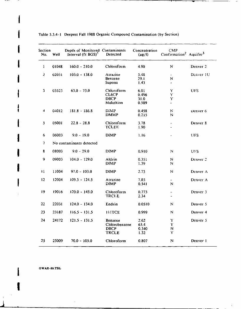
I
Table 5.3.4-I Deepest Fall 1988 Organic Compound Contamination (by Section)
Section Depth of Monitored Contaminants Concentration CMPNo. Well Interval (ft BGS)' Detected (pUg/l) Confirmation2 Aquifer 3
1 01048 160.0 - 210.0 Chloroform 4.90 N Denver 2
2 02031 103.0 - 138.0 Atrazine 5.48 Dcnvcr IUBenzene 29.1 NSupona 1.43
3 03523 63.0 - 73.0 Chloroform 6.01 Y UFSCL6CP 0.496 YDBCP 31.0 Y
Malathion 0.589I4 04012 181.8 - 186.8 DIMP 0.458 N 1enver 6
DMMP 0.215 N
5 05001 22.8 28.8 Chloroform 3.78 Denver 8TCLEE 1.90
6 06003 9.0- 19.0 DIMP 1.16 - UFS
7 No contaminants detected
8 08003 9.0 - 29.0 DIMP 0.910 N UFS
9 09003 104.0 - 129.0 Aldrin 0.351 N Denver 2DIMP 1.39 N
11 11004 97.0 - 103.0 DIMP 2.73 N Denver A
12 12004 109.5 - 124.5 Atrazine 7.03 - Denver ADIMP 0.541 N
19 19016 120.0 - 145.0 Chloroform 0.773 - Denver 3TRCLE 2.34
22 22031 124.0 - 134.0 Endrin 0.0510 N Denver 5
23 23187 116.5 - 131.5 11ITCE 0.999 N Denver 4
24 24172 121.5 - 131.5 Benzene 2.62 Y Denver 5Chlorobenzene 63.4 YDBCP 0.340 NTRCLE 1.32 Y
25 25009 70.0 - 105.0 Chloroform 0.807 N Denver I
A GWAR-89.TBL
I
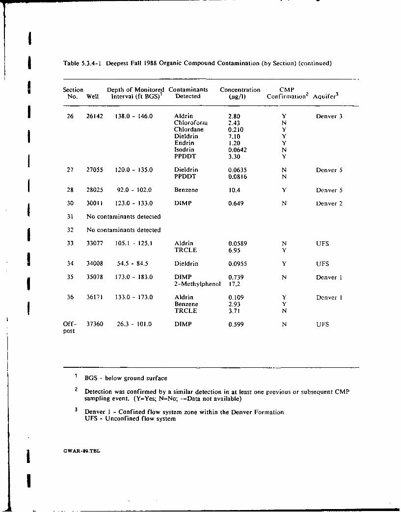
I
Table 5.3.4-1 Deepest Fall 1988 Organic Compound Contamination (by Section) (continued)
Section Depth of Monitored Contaminants Concentration CMPNo. Well Interval (ft BGS)1 Detected (pg/I) Confirmation 2 Aquifer 3
i 26 26142 138.0 - 146.0 Aldrin 2.80 Y Denver 3Chloroform 2.43 NChlordane 0.210 YDieldrin 7.10 YEndrin 1.20 YIsodrin 0.0642 NIPPDDT 3.30 Y
27 27055 120.0 - 135.0 Dieldrin 0.0635 N Denver 5
PPDDT 0.0816 N
1 28 28025 92.0 - 102.0 Benzene 10.4 Y Denver 5
30 30011 123.0 - 133.0 DIMP 0.649 N Denver 2
31 No contaminants detected
32 No contaminants detected
33 33077 105.1 - 125.1 Aldrin 0.0589 N UFSTRCLE 6.95 Y
S34 34008 54.5 - 84.5 Dieldrin 0.0955 Y UFS
35 35078 173.0 - 183.0 DIMP 0.739 N Denver 12-Methylphenol 17.2
36 36171 133.0 - 173.0 Aldrin 0.109 Y Denver IBenzene 2.93 YTRCLE 3.71 N
Off- 37360 26.3 - 101.0 DIMP 0.599 N UFSpost
1 BGS - below ground surface
2 Detection was confirmed by a similar detection in at least one previous or subsequent CMPsampling event. (Y=Yes; N=No; -=Data not available)
3 Denver I - Confined flow system zone within the Denver FormationUFS - Unconfined flow system
i G WAR-sg.TBL
I
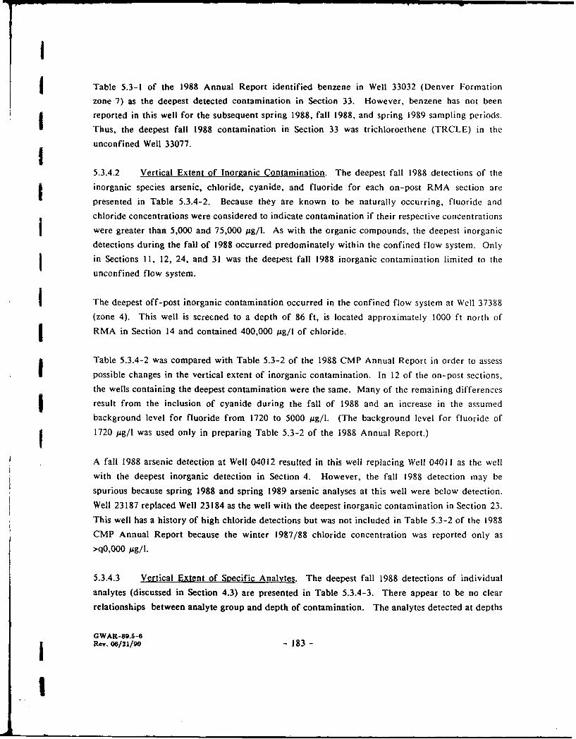
i
Table 5.3-1 of the 1988 Annual Report identified benzene in Well 33032 (Denver Formationzone 7) as the deepest detected contamination in Section 33. However, benzene has not been
j reported in this well for the subsequent spring 1988, fall 1988, and spring 1989 sampling periods.
Thus, the deepest fall 1988 contamination in Section 33 was trichloroethene (TRCLE) in the
unconfined Well 33077.I5.3.4.2 Vertical Extent of Inorganic Contamination. The deepest fall 1988 detections of the
inorganic species arsenic, chloride, cyanide, and fluoride for each on-post RMA section arepresented in Table 5.3.4-2. Because they are known to be naturally occurring, fluoride and
chloride concentrations were considered to indicate contamination if their respective concentrationswere greater than 5,000 and 75,000 Mg/l. As with the organic compounds, the deepest inorganic
detections during the fall of 1988 occurred predominately within the confined flow system. Only
in Sections 11, 12, 24, and 31 was the deepest fall 1988 inorganic contamination limited to the
unconfined flow system.
I The deepest off-post inorganic contamination occurred in the confined flow system at Well 37388
(zone 4). This well is screened to a depth of 86 ft, is located approximately 1000 ft north ofRMA in Section 14 and contained 400,000 Mg/l of chloride.
a Table 5.3.4-2 was compared with Table 5.3-2 of the 1988 CMP Annual Report in order to assess
possible changes in the vertical extent of inorganic contamination. In 12 of the on-post sections,
the wells containing the deepest contamination were the same. Many of the remaining differencesresult from the inclusion of cyanide during the fall of 1988 and an increase in the assumed
background level for fluoride from 1720 to 5000 Mg/l. (The background level for fluoride of
I 1720 pug/l was used only in preparing Table 5.3-2 of the 1988 Annual Report.)
A fall 1988 arsenic detection at Well 04012 resulted in this well replacing Well 04011 as the well
with the deepest inorganic detection in Section 4. However, the fall 1988 detection may be
spurious because spring 1988 and spring 1989 arsenic analyses at this well were below detection.
Well 23187 replaced Well 23184 as the well with the deepest inorganic contamination in Section 23.
This well has a history of high chloride detections but was not included in Table 5.3-2 of the 1988
CMP Annual Report because the winter 1987/88 chloride concentration was reported only as
>qO,000 pg/I.
5.3.4.3 Vertical Extent of Specific Analytes. The deepest fall 1988 detections of individual
analytes (discussed in Section 4.3) are presented in Table 5.3.4-3. There appear to be no clear
relationships between analyte group and depth of contamination. The analytes detected at depths
GWAR-89.6-6jRev. 06/21/90 - 183 -
I
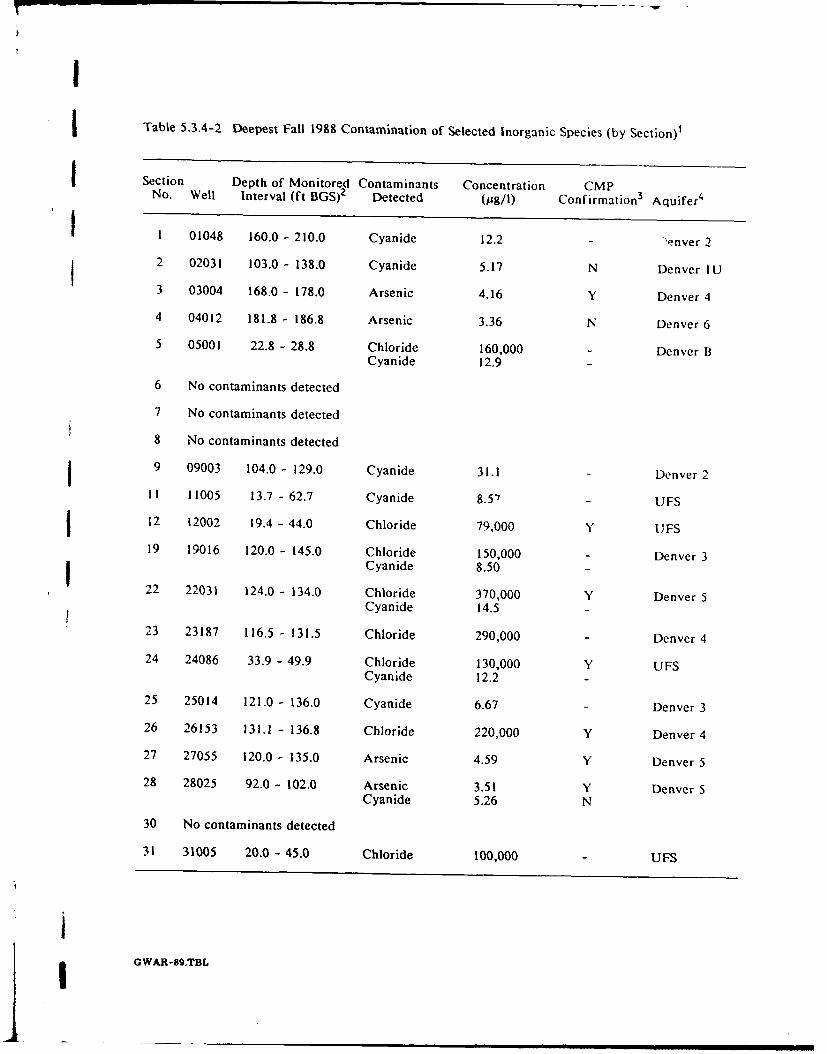
I
I Table 5.3.4-2 Deepest Fall 1988 Contamination of Selected Inorganic Species (by Section)1
I Section Depth of Monitored Contaminants Concentration CMPNo. Well Interval (ft BGS) 2 Detected (pg/I) Confirmation 3 Aquifer4
1 1 01048 160.0 - 210.0 Cyanide 12.2 - ,enver 2
2 02031 103.0 - 138.0 Cyanide 5.17 N Denver IU
3 03004 168.0 - 178.0 Arsenic 4.16 Y Denver 4
4 04012 181.8 - 186.8 Arsenic 3.36 N Denver 6
5 05001 22.8 - 28.8 Chloride 160,000 Denver BCyanide 12.9
6 No contaminants detected
7 No contaminants detected
8 No contaminants detected
j 9 09003 104.0 - 129.0 Cyanide 31.1 Denver 2
11 11005 13.7 - 62.7 Cyanide 8.51 - UFS
12 12002 19.4 - 44.0 Chloride 79,000 Y UFS19 19016 120.0 - 145.0 Chloride 150,000 Denver 3
Cyanide 8.50
22 22031 124.0 - 134.0 Chloride 370,000 Y Denver 5Cyanide 14.5
23 23187 116.5 - 131.5 Chloride 290,000 - Denver 424 24086 33.9 - 49.9 Chloride 130,000 Y UFS
Cyanide 12.2
25 25014 121.0 - 136.0 Cyanide 6.67 - Denver 3
26 26153 131.1 - 136.8 Chloride 220,000 Y Denver 4
27 27055 120.0 - 135.0 Arsenic 4.59 Y Denver 5
28 28025 92.0 - 102.0 Arsenic 3.51 Y Denver 5Cyanide 5.26 N
30 No contaminants detected
31 31005 20.0 - 45.0 Chloride 100,000 UFS
i

STable 5.3.4-2 Deepest Fall 1988 Contamination of Selec;ted Inorganic Species (by Section) 1
(Continued)ISection Depth of Monitored Contaminants Concentration CMP
No. Well Interval (ft BGS)2 Detected (ug/l) Confirmation 3 Aquifer4
Ig32 No contaminants detected
33 33031 165.0 - 175.0 Fluoride 6100 Y Denver 6
34 34011 92.0 - 102.0 Cyanide 7.42 N Denver 3
35 35078 173.0- 183.0 Arsenic 2.43 N Denver ICyanide 33.5 N
36 36171 133.0 - 173.0 Cyanide 24.9 N Denver I
Off- 37388 69.8 - 86.0 Chloride 400,000 Y Denver 4post
III
1 Compounds selected for this analysis are Chloride, Fluoride, Arsenic, and Cyanide. Assumed
background values for Chloride and Fluoride are 75,000 and 5000 Pg/l, respectively.
2 BGS - below ground surface
3 Detection was confirmed by a similar detection in at least one previous or subsequent CMPsampling event. (Y=Yes; N=No; -=Data not available)
4 Denver I - Confined flow system zone within the Denver FormationUFS - Unconfined flow system
II GWAR-89.TBL
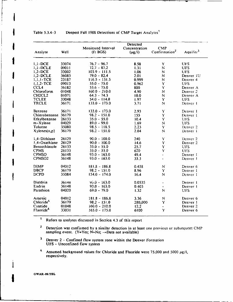
I
Table 5.3.4-3 Deepest Fall 1988 Detections of CMP Target Analytes1
DetectedMonitored Interval Concentration CMP
Analyte Well (ft BGS) (14g/i) Confirmation 2 Aquifer 3
I, 1 -DCE 33074 76.7 - 96.7 8.58 Y UFS1,1-DCLE 09011 72.7 - 87.2 1.31 N UFS1,2-DCE 33002 103.9 - 111.5 1.06 N UFS1,2-DCLE 36083 79.0 - 82.4 2.01 N Denver IUi,I,I-TCE 23187 116.5 - 131.5 0.999 N Denver 41,1,2-TCE 09013 55.0 - 75.0 0.962 Y UFSCCL4 36182 53.6 - 75.0 800 Y Denver AChloroform 01048 160.0 - 210.0 4.90 N Denver 2CH2CL2 01071 64.3 - 74.3 10.0 N Denver ATCLEE 33048 54.0 - 114.0 1.97 Y UFSTRCLE 36171 133.0 - 173.0 3.71 N Denver I
Benzene 36171 133.0 - 173.0 2.93 Y Denver IChlorobenzene 36179 98.2 - 151.0 155 Y Denver IEthylbenzene 26133 35.0 - 55.0 10.4 Y UFSm-Xylene 04029 89.0 - 99.0 1.69 N UFSToluene 35080 98.5 - 118.5 2.23 Y Denver 2g Xylenes(o,p) 36179 98.2 - 151.0 2.04 N Denver 1
1,4-Dithiane 26129 90.0 - 100.0 240 Y Denver 21,4-Oxathiane 26129 90.0 - 100.0 14.6 Y Denver 2Benzothiazole 26133 35.0 - 55.0 25.7 Y UFSCPMS 26133 35.0 - 55.0 620 Y UFSCPMSO 36148 93.0 - 163.0 49.4 - Denver ICPMSO2 36148 93.0 - 163.0 35.3 - Denver I
DIMP 04012 181.8 - 186.8 0.458 N Denver 6DBCP 36179 98.2 - 151.0 8.96 Y Denver IDCPD 35084 154.0- 174.0 16.4 N Denver I
Dieldrin 36148 93.0 - 163.0 0.0535 - Denver IEndrin 36148 93.0 - 163.0 0.403 - Denver IParathion 04020 69.0 - 79.0 1.32 N UFS
Arsenic 04012 181.8 - 186.8 3.36 N Denver 6Chloride4 36179 98.2 - 151.0 280,000 Y Denver ICyanide 01048 160.0 - 210.0 12.2 - Denver 2Fluoride4 33031 165.0 - 175.0 6100 Y Denver 6
1 Refers to analytes discussed in Section 4.3 of this report
2 Detection was confirmed by a similar detection in at least one previous or subsequent CMPsampling event. (Y=Yes; N=No; -=Data not available)
3 Denver 2 - Confined flow system zone within the Denver FormationUFS - Unconfined flow system
"4 Assumed background values for Chloride and Fluoride were 75,000 and 5000 gg/l,respectively.
GWAR-89.TBL
I
greater than 170 ft BGS were arsenic, benzene, chloroform, cyanide, DCPD, DIMP, fluoride, andtrichloroethene. Compared to Table 5.3-3 of the 1988 CMP Annual Report, only benzene and
fluoride were similarly shown to occur below 170 ft BGS.
5.3.5 Aquifer Interaction
Potentiometric data, inorganic and organic analytical results, and isotope data were examined toevaluate RMA areas where aquifer interaction may occur. All well clusters sampled during theFall 1988 sampling round were examined. In addition, analytical results from several well clustersinstalled during the Fall 1988 sampling event under the RI/FS program were examined. Water-level data and chemical data from these wells are approximately contemporaneous with those fromthe Fall 1988 sampling event, and so were included in this investigation.
5.3.5.1 Potentiometric Head Differences. Elevations of the potentiometric surfaces of theunconfined and confined flow systems were examined to identify areas where ground water fromthe unconfined flow system might flow downward to permezble units within the confined DenverFormation, and areas where ground water in the confined flow system would tend to move
Supwards to the unconfined flow system. In all but five well clusters, potentiometric headelevations are greater in the unconfined flow system than in the confined flow system. Head
difference variations in the well clusters with downward vertical gradients ranged from 0.09 ft to
as much as 25 ft, depending on the stratigraphic intervals within which the clustered wells arecompleted. These gradients would cause ground water from the unconfined flow system to movevertically downward through permeable portions of the confined flow system.
Five instances in which potentiometric head elevations indicated an upward vertical gradient werenoted. These were in Section 2 (Wells 02034 and 02035), Section 6 (Wells 06003, 06004, 06005),Section 26 (Wells 26, 27 and 26179) and Section 34 (Wells 34005, 34006 and Wells 34012, 34013).In each case, water levels were greater in wells completed in deeper confined flow system water-bearing zones than in shallower wells completed in the unconfined flow system. In general, headdifferences ranged from 0.09 to 1.11 ft g--ater in the confined flow system, depending on thestratigraphic interval in which wells were completed. This situation results in a force potentialwhich would cause ground water to move vertically upward, from permeable portions of the
confined flow system into the unconfined flow system. One instance was noted (Wells 34012 and34013) where two confined wells, screened in Denver Zone I (Well 34012) and Zone 2 (Well 34-13), had an upward vertical gradient of 25 feet.
GWAR-89.5-6j•. .06/21/o - 187 -
I
i
5.3.5.2 Inorganic Chemical Data. Inorganic chemical data from cluster wells sampled during
the Fall 1988 samrl:ng event were examined to determine if these data provide clear evidence of
aquifer interac:", a. Data interpretations in Section 5.4.4 indicate that the unconfined and confined
flow syste ..- tend to have concentrations of calcium, sodium and nitrate which are more
characteristic of each flow than other inorganic analytes. Therefore, analytical data were examined
:or well clusters which had anomalous values for calcium, sodium and nitrate. Well clusters
identified as having anomalous concentrations of these analytes (in conjunction with anomalous
potentiometric data, organic analyses and isotope data) were considered to indicate areas where
potential existed for aquifer interaction. Areas in which inorganic chemical data indicate potential
for aquifer interaction generally lie in the following areas: the South Plants Pathway, northward
through the Basin A/Basin A Neck Pathways, continuing through Basins D and E, and in the Basin
F Pathway.
5.3.5.3 Organic Chemical Data. Organic chemical data were examined to identify areas where
aquifer interaction may occur. Because these compounds are not naturally occurriig, the presence
of organic analytes in confined Denver Formation water bearing zones indicates that these
compounds may have been transported to the detected locations by ground water. This, in turn,
suggests aquifer interaction between the unconfined and confined flow systems. The use of low
concentrations of organic contaminants to assess aquifer interactions result in somewhat equivocal
conclusions. This is due to a number of factors, including analyte detections noted at severi1 well
clusters in deeper confined Denver Formation wells, with the same analytes not occurring in
shallower, unconfined wells. This is consistent with sporadic contamination of sandstone zones
which has been noted historically (Ebasco, 1989i), probably due to contaminant migration along
localized fracture zones, or lateral flow within the Denver Formation. In spite of these difficulties,
however, there are several well clusters that appear to provide some insight into potential aquifer
interactions at RMA.
Evidence for aquifer interaction based on organic analytical data is sometimes ambiguous or
sporadic. For example, all wells in a cluster considered to show evidence for aquifer interaction
generally contain several of the same compounds. However, several additional analytes are
commonly detected in confined wells and not in unconfined wells, with still other analytes detected
in unconfined wells and not in confined wells in the same cluster. However, organic data do
indicate that potential for aquifer interaction generally exists in the following areas: the South
Plants Pathway northward through the Basin A/Basin A Neck Pathways; the Basin F and Basin F
East Pathways; and the Basin A Neck Pathway northwestward into Section 27.
GWAR-89.5-6Rev. 06/21/go - 188 -
I
5.3.5.4 lsotooic Evidence. Since approximately 1953 the amount of tritium in the atmosphere
(and hence in surface waters and precipitation) has increased. Thus relatively "young" groundwater will yield a different tritium signature than "old" ground water which infiltrated prior to
1953, or which has been isolated since that time. During the spring 1988 sampling event 13
ground-water samples were collected from the unconfined flow system in Section 23, 24 and 33
for isotopic analyses (tritium, deuterium and oxygen-18).
Results of tritium analyses in Sections 23, 24, and 33 indicate different concentrations of tritium
in unconfined and confined wells, indicating different ages for ground water in these two systems,
in the areas sampled (Figure 5.5-3). With one exception these data indicated that either no mixing
or only limited mixing of unconfined and confined ground water has occurred in these areas. This
is consistent with organic chemical data available in these areas. A much more thorough discussion
of isotopic data is presented in Section 5.5. Well 23177 yielded a TU value midway between TU
values characteristic of the unconfined and confined flow systems, indicating that potential for
aquifer interaction exists in the area of this well. No well clusters were sampled close to Well
23177 to provide corroborating potentiometric data, and inorganic or organic analytical data.
5.4 Inorganic and Other Water-Quality Data Assessment
This section of the Annual Report provides a presentation and interpretation of inorganic anal tical
results, including general and water-quality parameters from samples collected during the fall 1988
annual sampling event. Although analyses for inorganic and other water-quality parameters have
been components of many previous RMA ground-water investigations, the assessment of these data
have been limited. The historical investigations on RMA have focused primarily on organic
contaminant distributions because degradation of inorganic water quality generally results in a
lesser risk to human health and the environment than contamination by organic compounds.
The emphasis of this section is to present inorganic water quality characteristics of the unconfined
flow system and confined flow system from both a regional and area specific perspective.
The regional area includes all wells within the RMA on-post and off-post operable units (OUs)
and encompasses the four subareas presented in Figure 5.4-1. The presentation by area is divided
into four areas as shown in Figure 5.4-1: (i) Western Tier, (2) Central Area, (3) Background, and
(4) Northern Area.
GWAR-89.5-6Rev. 06/22/go - 189 -
I
Background areas are defined as areas which contain wells upgradient of known RMA source
areas. Analytical results from the wells upgradient of South Plants and those east of Basin A,
North Plants, and the NBCS were considered representative of background conditions.
The three remaining subareas were chosen based on their hydrogeologic, geographic, and
contaminant distribution differences and comparisons were made based on their individual
characteristics. The Western Tier includes monitoring wells around the Rail Classification Yard
and the Irondale Containment System and is characterized by a thick sequence of saturated
alluvium and is downgradient of the Motor Pool and Rail Classification Yard. The Central Area
includes monitoring wells in South Plants, Basin A and along the Basin A Neck and Central
Pathways. The Central Area contains several prominent source areas and relatively thinner
saturated alluvium oriented in paleochannels. The Northern Area includes monitoring wells in
North Plants, Basin F, and along the Basin F North and Northwest Pathways. It is similar to the
Central Area in that it also has relatively thinner saturated alluvium and contains source areas.
The inorganic and other water-quality data assessment presented here progresses from presentation
of basic water quality data collected in the field to more complex data resulting from laboratory
analytical work. Specific conductance and dissolved oxygen are field parameters measured
immediately prior to sampling. The remaining data are laboratory analytical results. The first two
subsections discuss the water-quality field parameters directly. The following four subsections are
assessments of inorganic data received from the CMP contract laboratory, DataChem. The subjects
discussed include frequency distributions, solute correlations, trilinear diagrams, and correlation
coefficients.
Within each of the following six subject discussions, a brief explanation is given on the theory
and applicability of each method. Each of the subjects progresses from a discussion of RMA
background conditions, to regional conditions, to noteworthy localized exceptions that may be
indicative of RMA activities. Exceptions to this are the discussions of frequency distributions
and correlation coefficients, which are most appropriately discussed from a regional perspective.
5.4.1 Specific Conductance
Specific conductance is the reciprocal of the resistance (in ohms) measured between opposite faces
of a one centimeter cube of an aqueous solution at a specified temperature. The specific
conductance measurement is an indicator of ion concentration and in general is directly related to
the total dissolved solids (TDS) in solution. The presence of charged ion species in solution makes
the solution conductive. Therefore, the greater the concentration of charged ions in solution the
greater the conductivity of the solution. Natural waters commonly have a conductance much less
IGWAR-89.$-6Rev. 06/22/90 - 190 -
I
than I mho and in order to avoid inconvenient decimals, data are commonly reported in micromhos
per centimeter (pmhos/cm) at 25'C (Hem, 1989).
In ultrapure water, specific conductance approaches 0.05 umhos/cm at 25'C whereas the specific
conductance of distilled water approaches 1.0 pmho/cm. The specific conductance values of
rainwater range from 2 to greater than 100 pmhos/cm. The specific conductance value of surface
and ground water is dependent on the solutes in precipitation, the rock formation in contact withthe water, the length of time for water/rock interaction, temperature, and the types of ions present
in solution. In areas where precipitation is low in solutes and rocks are resistant to weathering the
specific conductance may be as low as 50 pmho/cm. In other areas the specific conductance of
ground waters may approximate that of seawater (50,000 umhos/cm) (Hem, 1989).
In the CMP, specific conductance is measured in the field at least once for every casing volume
purged fam a well to be sampled. Commonly, specific conductance and temperature stabilize
prior to evacuation of five well casing volumes and thus a stable value of specific conductance is
recorded immediately prior to filling sample containers. Therefore, the measured value of specificconductance at this time is expected to represent actual ground-water conditions. The accuracy
and reproducibility of measuring the specific conductance in the field should be approximately +
5 percent.
Although the actual field measurement is electroconductivity, these values have been corrected
for temperature and are reported as specific conductance (pmhos/cm) at 25"C. Results of the
specific conductance data are presented in Figure 5.4-2. Figure 5.4-2 includes four plots in which
specific conductance is plotted as a function of depth. Also included in Figure 5.4-2 is afrequency distribution diagram of the specific conductance data. The background values fall
below 3000 umhos/cm for both the unconfined flow system and confined flow system. The
majority of the values on the regional plot fall below 3000 pmhos/cm and there is little apparent
variation with depth. The values that are greater than 3000 pmhos/cm are generally confined to
depths 20 to 60 ft below ground surface (bgs). The Western Tier plot indicates values consistent
with background values whereas the Central Area and Northern Area plots are similar to each
other and the regional plot. The high values between 20 to 60 ft bgs appear in both the Central
Area and Northern Area plots. These high values may be related to an increase in solute
concentrations in these areas.
The frequency distribution diagram includes bar graphs for the unconfined and confined flow
systems. The bar graphs represent the percent of samples that have measured values within a
specified interval. A detailed discussion on the construction of the frequency diagram is provided
GWAR-89.5-6Rev. 06/21/0 - 191 -
I
I
in Section 5.4.3. As noted in the diagram, the highest percentage of samples in the unconfined
flow system have specific conductance values between 500 and 1000 plmhos/cm, while the highest
percentage of samples in the confined flow system (confined flow system) have values between
1000 and 1500 umhos/cm. The majority of samples in the ranges from 0 to 500 pmhos/cm and
from 1000 to 4000 pmhos/cm were collected from the confined flow system. The majority of
samples in the ranges from 500 to 1000 uamhos/cm and from 4000 to greater than 10,000 /pmhos/cm
were collected from the unconfined flow system.
Specific conductance is expected to increase with depth due to an increase in the total dissolved
solids (TDS) in the ground water. Note, however, that this effect is not expected to be great at
the fairly shallow depths investigated here. The increase in TDS relates to the longer residence
time of deeper water and more interaction with surrounding rock, clays, sands, etc. The increase
of specific conductance with depth was not apparent in any of the plots. Rather, increased
specific conductance was noted at shallower (20 to 60 ft bgs) depths in all areas except the Western
Tier. It is likely that the inconsistent elevation of specific conductance at these shallower depths
is a function of near-surface sources of ground-water contamination.
S5.4.2 Dissolved Oxygen/Percent 02 Saturation
The parameter, dissolved oxygen (DO), like specific conductance, is measured in the field as each
casing volume is purged from a well to be sampled. The equilibrium concentration of DO in water
in contact with air is a function of temperature and atmospheric pressure. The equilibrium DO
value (at I atmosphere) in freshwater is 7.54 mg/I at 30*C. This value increases to 12.75 mg/I at
5'C (Hem, 1989). The equilibrium DO value at sea level is greater than the value at higher
elevations because an increase in elevation results in a decrease in atmospheric pressure, thereby
reducing the amount of oxygen that is dissolved in water. Dissolved oxygen is commonly measured
tu evaluate processes involving the uptake of oxygen, e.g., organic degradation or oxidation of
reduced inorganic minerals. The presence of organic chemicals will also cause oxygen depletion.
The DO concentration in ground water is related to recharge of precipitation because these waters
entering the system are expected to contain DO concentrations similar to those of surface waters
in contact with the atmosphere. The DO concentration of ground water will vary as a function of
the amount of oxidizable material present along its flow path. Therefore, DO concentrations near
the saturation concentration may indicate either an area of recharge or an area with no appreciable
oxidizable material.
Historically, DO was included in RMA RI/FS sampling programs to serve as a QA measure for
indicating whether the purging process was complete and quantifying whether or not pumped wells
GWAR-89.5-6Rev. 06/21/90 - 192-
!
t I
were yielding aerated samples. The reproducibility of DO values from successive sampling events
at RMA (irrespective of sample technique) has indicated that sample aeration is not a concern.
DO is also used as an analytical parameter for characterizing ground-water quality at RMA.
For presentation and discussion purposes in this report, DO values are converted to percent 02
saturation at the temperature of measurement. The conversion of DO values to percent 02saturation allows for the interpretation of the degree of oxygen depletion relative to the equi-
librium concentration. The following equation is used for this conversion:
% 02 = DO x 100so
where % 02 is the percent 02 saturation DO is the concentration of dissolved oxygen in jig/l, and
SO is the amount of oxygen at saturation in g/Il.
Results of the % 02 data are presented in Figure 5.4-3. Figure 5.4-3 includes four plots in which
% 02 is plotted as a function of depth. Also included in Figure 5.4-3 is a frequency distribution
diagram of % 02. The background % 02 values vary from near zero to approximately 90 percent
Ssaturation. The highest background value is from a confined flow system well located in Section
19. The variability of the unconfined flow system and confined flow system background values
appears independent of depth. The regional plot has no discernable pattern of % 02 with respect
to either depth or flow system. The Western Tier plot indicates that in this area, % 02 is not
solely a function of depth but generally appears to increase with depth in the confined flow
system. The Central Area and Northern Area plots exhibit a general trend of decreasing % 02with increasing depth in the confined flow system.
The frequency distribution diagram is constructed in the same manner as the frequency diagram
presented for specific conductance. The largest percentage of samples from the confined flow
system have % 02 values between 0 and 20 percent and the percentage of samples generally
decreases with increasing % 02. In general, each interval presented in Figure 5.4-3 includes
approximately 10 percent of the total samples from the unconfined flow system with the exception
of the 0 to 10 percent range that includes almost 20 percent of the unconfined flow system
samples. In general, a higher proportion of unconfined flow system waters are closer to 02
saturation and a significant portion of the confined flow system samples exhibit low percent
saturation.
Lower % 02 values are expected in areas of high organic chemical contamination or in flow
systems where either high organic carbon or reduced inorganic minerals are present.
GWAR-89.5-6Rev. 06/211/O - 193 -
I
II
5.4.3 Frequency Distributions
The analytical data for eight major ions in the unconfined and confined flow systems are presented
in this section. The eight major ions are sodium (Na'), potassium (K+), calcium (Ca+2), magnesium
(Mg+2 ), chloride (CI), fluoride (F-), nitrate (NO 3 ), and sulfate (SO4"2). The data from the two
flow systems have been segregated to allow for a comparison of the characteristics of both flow
systems. The results of these calculations are plotted as frequency diagrams and are presented in
Figure 5.4-4. The percentage of samples within each flow system is represented by a vertical bar;
the solid bar represents the samples from the unconfined flow system and the cross-hatched bar
represents the samples from the confined flow system. The percent of samples is calculated on the
basis of total samples from each system. Of a total of 488 samples collected, 322 were from the
unconfined flow system and 166 were from the confined flow system. Each diagram ;s divided
into 10 data ranges that include those samples (in millequivalents per liter; meq/l), within the
lower and upper bound of each range. A discussion of each ion and corresponding diagram
follows.
j5.4.3.1 Sodium. The frequency distribution of sodium is presented in diagram A of
Figure 5.4-4. The largest percentage of samples from the unconfined flow system occurs within
the 0.04 (CRL) to 5 meq/l range. At increasing concentrations, the percentage of samples from
the unconfined flow system decrease with the exception of the 50 to 100 meq/l range. In contrast,
the confined flow system has the largest percentage of samples within the 10 to 20 meq/I range.
This distribution indicates that the confined flow system exhibits higher sodium concentrations.
Higher sodium concentrations are commonly indicative of ground waters that have had longer
residence times as a result of cation exchange. Sodium at RMA, was introduced to soil surface
water, and ground water by neutralizing agents, by-products of GB manufacture, breakdown
products of GB, and numerous salts including sodium chloride (Geraghty and Miller, 1986)
5.4.3.2 Potassium. The frequency distribution of potassium is presented in diagram B of
Figure 5.4-4. The highest percentage of samples in the confined flow system occur within the
0.004 (CRL) to 0.05 meq/l range. The unconfined flow system has the highest percentage of
samples within the 0.05 to 0.1 meq/i range. This distribution suggests that potassium concentra-
tions are generally higher in the unconfined flow system. Potassium has the tendency to be easily
adsorbed onto clay mineral structures. This may contribute to the lower concentrations measured
for the confined flow system which occurs predominately through the Denver Formation.
Potassium has not been identified as a significant component of waste streams historically
discharged at RMA (Geraghty and Miller, 1986).
GWAR-89.5-6Rev. 06/21/90 - 194 -
5.4.3.3 Calcium. The frequency distribution of calcium is presented in diagram C of
Figure 5.4-4. The distribution of calcium is generally similar for each flow system except in the
0.05 (CRL) to 1.0 meq/l range and in the 5.0 to 10 meq/I range. Approximately 20 percent of the
confined flow system samples have concentrations between 0.05 and 1.0 meq/. In contrast, the
unconfined flow system has less than one percent of its samples within this concentration range.
The unconfined flow system has over 40 percent of its samples in the 5.0 to 10 meq/l range, while
the confined system has less than 20 percent in this range. This indicates that elevated calcium
concentrations are generally present in the unconfined flow system. Calcium is commonly a
constituent of igneous rocks, cementing materials in sandstone and caliche. Calcium was also
present in waste streams generally associated with caustic processes at RMA (Geraghty and Miller,
1986). Calcium carbonate deposits from these processes are present in the lime pits and in surficial
depressions in Basin A. In addition, with longer residence times in sedimentary aquifers calcium
exchanges with sodium, decreasing aqueous calcium concentrations, and increasing aqueous sodium
concentrations.
5.4.3.4 Magnesium. The frequency distribution of magnesium is presented in diagram D of
Figure 5.4-4. Over 65 percent of the confined flow system samples have concentrations less than
or equal to 1.0 meq/l. In contrast, nearly 90 percent of unconfined flow system samples have
concentrations greater than 1.0 meq/I. This indicates that higher concentrations of magnesium are
more prevalent in the unconfined flow system. Increased revels in the unconfined flow system
may result from contamination associated with incendiary, chlorine, and caustic production.
5.4.3.5 Chloride. The frequency distribution of chloride is presented in diagram E of
Figure 5.4-4. Most RMA ground-water samples contain chloride at concentrations ranging from
0.02 to 5.0 meq/l. Nearly 75 percent of confined flow system samples are within this range and
approximately 60 percent of unconfined flow system samples are within this range. As chloride
concentrations increase to 30 meq/l, the percentage of confined flow system samples decreases
more than the percentage of unconfined flow system samples. Between 5.0 and 20 meq/l, the
unconfined flow system has a larger percentage of samples. This indicates that elevated levels of
chloride occur more predominantly in the unconfined flow system. Chloride is a "conservative"
constituent of ground water not being readily removed from the system. Therefore, higher
concentrations of chloride in the unconfined flow system suggest an introduction of chloride laden
waters directly into the unconfined flow system. Chloride was commonly used in RMA
manufacturing processes.
GWAR-89.6-6Rev. 06/21/1o - 195-
I
5.4.3.6 Fluoride. The frequency distribution of fluoride is presented in diagram F of
Figure 5.4-4. Both flow systems show similar frequency distributions, with the unconfined flow
Ssystem exhibiting a slightly higher percentage of samples with concentrations above 0.2 meq/I.Sources of fluoride include manufacturing processes at RMA and naturally-occurring volcanic
constituents of the Denver Formation.
5.4.3.7 Nitrate. The frequency distribution of nitrate is presented in diagram G of Figure5.4-4. Nearly 70 percent of the confined flow system samples have concentrations ranging from0.005 to 0.25 meq/l. In contrast, over 60 percent of the unconfined flow system samples haveconcentrations greater than 0.25 meq/I. The elevated concentrations in the unconfined aquifersuggest leaching of nitrate from surficial anthropogenic practices. Commonly, nitrate leaching isassociated with agricultural and livestock practices.
5.4.3.8 Sulfate. The frequency distribution of sulfate is presented in diagram H of Figure 5.4-4. Over 70 percent of samples from the unconfined flow system have concentrations of sulfateranging from 0.01 to 10 meq/l. The percent of unconfined samples decreases with increasing
concentrations. The confined flow system exhibits a similar distribution except that a largerpercentage of samples contain concentrations above 10 meq/l; over 50 percent of confined flowsystem samples have concentrations above 10 meq/l. The decrease in percent of samples with
* increasing concentration is also noted in the samples from the confined flow system. The relativelyhigher percentage of samples with elevated concentrations in the confined flow system may result
from increased sulfur content common in rocks with volcanic origin such as the Denver Formation.I5.4.4 Solute Correlations
The interactive relationship between chemical constituents may be visualized in a scatter plot inwhich one constituent is plotted on the abscissa a d the other on the ordinate. A positive
correlation between the constituents is realized if a straight line with a positive slope can be fittedthrough the points on the plot. Some constituents are known to have a negative correlation because
they are utilized differently in a chemical system and this type of correlation is most noticeablein the ratio of the constituents. Calcium and sodium are examples of constituents generally having
a negative correlation.
The negative correlation between calcium and sodium is a result of ion-exchange reactions.Sodium is a monovalent cation whereas calcium is a divalent cation that is more strongly bondedand tends to replace sodium ions. Typically, the observed relationship between sodium and calcium
is that calcium ions replace sodium ions in the soil matrix. As calcium ions replace sodium ions
GWAR-89.5-6Rav. 06/21/9O -196-
I
in the soil the displaced sodium ions are dissolved in ground water which, in turn, relates to anincrease in the concentration of sodium. This process occurs along the flow path and commonlyresults in the decrease of the calcium/sodium ratio (Ca/Na) in ground water with increased depth.
At RMA this natural process is sometimes overshadowed by waste disposal practices which allowedincreased Na concentrations in near surface soil and ground water as a result of disposal of sodium
chloride-rich wastes.
Results of the Ca/Na data are shown in Figure 5.4-5. Figure 5.4-5 includes four plots with Ca/Na
ratios plotted as a function of depth. The background unconfined flow system values generally fall
between 0.5 and 2.0 and the background confined flow system values are less than 1.0 with the
exception of one value of approximately 1.5. The regional plot generally indicates that theconfined flow system has lower Ca/Na values than the unconfined flow system. The WesternTier Ca/Na plot shows a marked contrast between the unconfined flow system and confined flowsystem. The values for the unconfined flow system vary between 1.0 and 3.5 with the exception
of one value less than 1.0 whereas the values for the confined flow system are in general
consistently less than 0.5. The Central Area and Northern Area Ca/Na ratio plots have valuesgenerally less than 2.0 with the confined flow system values typically lower than the unconfinedflow system values. Unlike the Western Tier Ca/Na plot, the Central Area and Northern Area
Ca/Na plots have very few data points with values above 2.0. In general, these trends confirm
hypothesis put forth in this section.
The distribution of Ca/Na ratios is usually dependent on depth and rock type. An exchange of
cations during transport through the flow system is expected to decrease the ratio with depth.The lower Ca/Na values seen in the Central Area and Northern Area may be the result of either
the introduction of saline waters into the flow systems during RMA operations or the discharge
of ground water from the confined flow system into the unconfined flow system. The observedCa/Na values from the Western Tier more closely correlate with background values indicating thatfor these areas little water-quality degradation by these inorganic constituents has occurred.
5.4.5 Trilinear Diagrams
Trilinear diagrams are used to classify ground water using basic constituents which contribute towater quality. The trilinear diagrams used in Figures 5.4-6 through 5.4-8 are composed of two
equilateral triangles positioned at the lower left and lower right; the bases align vertically and thevertices point toward each other. The upper central portion of the diagram is diamond shaped.The cationic (positive charge in solution) triangle is represented by magnesium and calcium eachat one vertex and sodium and potassium at the remaining vertex. The anionic (negative charge in
GWAR-89.6-6Rev. 06/21/9o - 197-
I
I
j solution) triangle is represented by sulfate at one vertex, bicarbonate at another vertex, and
chloride and nitrate at the remaining vertex. The vertex of each triangle represents 100 percent
of an ion or group of ions for either cations or anions. The composition of the ground water with
respect to cations and anions is indicated by a point plotted within the respective triangle. The
sum of the coordinates at each point equal 100 percent. The points within the triangles are
extended upward into the central plotting field (diamond) by projecting them along lines parallel
to the upper edges of the central field.
The utility of trilinear diagrams is that they enable the viewer to visually characterize the ground-water composition of a flow system. In addition, the visual comparison of flow systems may
result in areas that indicate a mixing of ground water. If mixing occurs between ground waters
of different compositions, the resultant ground-water composition will fall along a mixing line
between the end-member compositions of the original ground waters. Therefoe, if equal
proportions of a 100 percent calcium-rich ground water mixed with a 100 percent sodium and
potassium-rich ground water, the resultant ground water would be 50 percent calcium-, sodium-,
and potassium-rich.
The data used in the trilinear diagrams were subjected to a screening procedure to assess theiruseability. Data from 488 monitoring wells (322 unconfined flow system and 166 confined flow
system) sampled during the fall 1988 monitoring event were screened as follows. Data from IIunconfined flow system and 77 confined flow system wells were eliminated because the measured
ground water pH was greater than 8.3. Ground water with a pH greater than 8.3 contains a
significant concentration of carbonate but to calculate this concentration one of the pH endpoints
for the alkalinity titration must be 8.3. This endpoint was not used in the alkalinity titrations of
the fall 1988 ground-water samples. Since the alkalinity values obtained from the titration are used
in the calculation of carbonate and bicarbonate concentrations those data associated with a pHgreater than 8.3 could not be accurately utilized in this assessment. Data from two unconfined flow
system and four confined flow system wells were eliminated because they had no associated
alkalinity data. Data from I I unconfined flow system and three confined flow system wells were
eliminated because one or more of the pertinent ionic data had an associated "less than" or "greater
than" qualifier. Data from 37 unconfined flow system and nine confined flow system wells were
eliminated because their calculated charge balance was more than 10 percent. The value of plus
or minus 10 percent was used to screen for analytical variability. A total of 154 wells (61
unconfined flow system and 93 confined flow system) were deleted from interpretative use, leaving
data for 334 wells.
iGWAR-89.6-6Rev. 06/21/9 - 198-
I
I
The trilinear diagrams for the unconfined flow system and confined flow system regional andbackground wel'- are shown in Figure 5.4-6. The background trilinear diagram, composed of IIunconfined flow system wells and six confined flow system wells, indicates little difference in the
cationic data and exhibits scattering in the anionic data for both the unconfined flow system and
confined flow system. The regional trilinear diagrams for the unconfined flow system and
confined flow system indicate ground waters of similar composition. Data from 249 monitoringwells were used in the construction of the unconfined flow system diagram and data from 67monitoring wells were used in the construction of the confined flow system diagram. Similar tothe background trilinear diagram, the regional trilinear diagrams also exhibit a scattering in the
anionic data and a tighter grouping of the cationic data.
The unconfined flow system trilinear diagram for the Western Tier was constructed from data from
55 monitoring wells and indicates a tighter grouping for both the anionic and cationic data (Figure
5.4-7). There is no confined flow system trilinear diagram for the Western Tier because the data
did not pass the screening procedure described above. Eleven confined flow system wells were
affected.
The unconfined flow system and confined flow system trilinear diagrams for the Central Area arepresented in Figure 5.4-7. Data from 80 monitoring wells were used in the construction of the
unconfined flow system diagram and data from 45 monitoring wells were used in the construction
of the confined flow system diagram. The diagrams indicate little difference in ground-water
composition for the flow systems in this area. The differences seen in the anionic data betweenthe two diagrams may result from the number of wells used from each system. The Central Area
unconfined flow system trilinear diagram differs from the Western Tier trilinear diagram. The
trilinear diagrams show a shift mostly in the cationic data; the ground water in the Western Tier
is more calcium rich whereas the ground water in the Central Area is more sodium and potassiumrich. There is more scatter in the anionic data for the Central Area data than the Western Tier
data and this may be due to the difference in the number of wells representing each area.
The unconfined flow system and confined flow system trilinear diagrams for the Northern Areaare presented in Figure 5.4-8. Data from 68 monitoring wells were used in the construction of theunconfined flow system diagram and data from 17 monitoring wells were used in the construction
of the confined flow system diagram. The diagrams indicate little difference in the composition
of the ground waters for the flow systems in this area. The reduced scatter in the confined flowsystem anionic data may result from a limited number of wells plotted. However, these diagrams
do indicate a difference in ground-water composition between the Western Tier unconfined flow
system and Northern Area unconfined flow system. This difference may be attributable to either
GWAR-89.5-6Rev. 06/21/10 - 199 -
I
I
the hydrogeologic regime, the geographic location, or waste water disposal practices. The trilineardiagrams similarly exhibit a shift in the cationic and anionic data. The cationic data for theWestern Tier indicate more calcium-rich ground water whereas the data for the Northern Area
indicate more sodium and potassium-rich ground water. The anionic data for the Western Tierindicate more bicarbonate-rich ground water whereas the data for the Northern Area indicate more
chloride, nitrate, and sulfate-rich ground water. These observations may be explained by theintroduction of sodium chloride-rich waste waters from RMA operations to unlined basins on Basin
F in the central area to the shallow ground water system.
5.4.6 Correlation Coefficients
A correlation analysis was performed on the inorganic data for both the unconfined flow system
and confined flow system. This analysis aids in assessing the degree to which two variables arerelated. The analysis yields a sample correlation coefficient, r, whikh is used to interpret the
strength of the relationship. The value of r lies between the region of -1 to +1. Those valuesbetween -1 and 0 indicate inverse relationships and those between 0 and +1 indicate directrelationships. The values at +1 indicate perfect relationships and the relationship becomes
progressively weaker as the values tend toward 0.
The results of this analysis are presented in Table 5.4.6-1. Table 5.4.6-1 is a diagonal matrix with
the analytes positioned horizontally and vertically along both axes. The values of I along thediagonal indicate a perfect relationship and corresponds to like analytes. The italicized values in
the upper right triangular portion of the matrix represent the unconfined flow system and thevalues in the lower left triangular portion of the matrix represent the confined flow system. The
r value for an analyte pair is obtained by extending a vertical and horizontal line from a given r
to each analyte. For example, the analyte pair N0 3" - F- has an r value of .035 in the unconfinedflow system and .52 in the confined flow system. These values indicate that a more directrelationship for this analyte pair exists in the confined flow system although the correlation even
in the confined flow system is not considered strong.
Table 5.4.6-1 is used as an indicator of the water-quality differences between the unconfined flow
system and confined flow system. Water-quality differences occur as a function of the strength
of the relationship between the analyte pairs. The r values in Table 5.4.6-1 generally indicate that
the ions have a stronger direct relationship in the unconfined flow system than in the confinedflow system. The exceptions to the stronger direct relationship in the unconfined flow system isnoted in the Mg*2 -CI" and N0 3"-F pairs. These pairs have a stronger direct relationship in the
GWAR-89.5-6Rev. 06/22/0 - 200 -
I
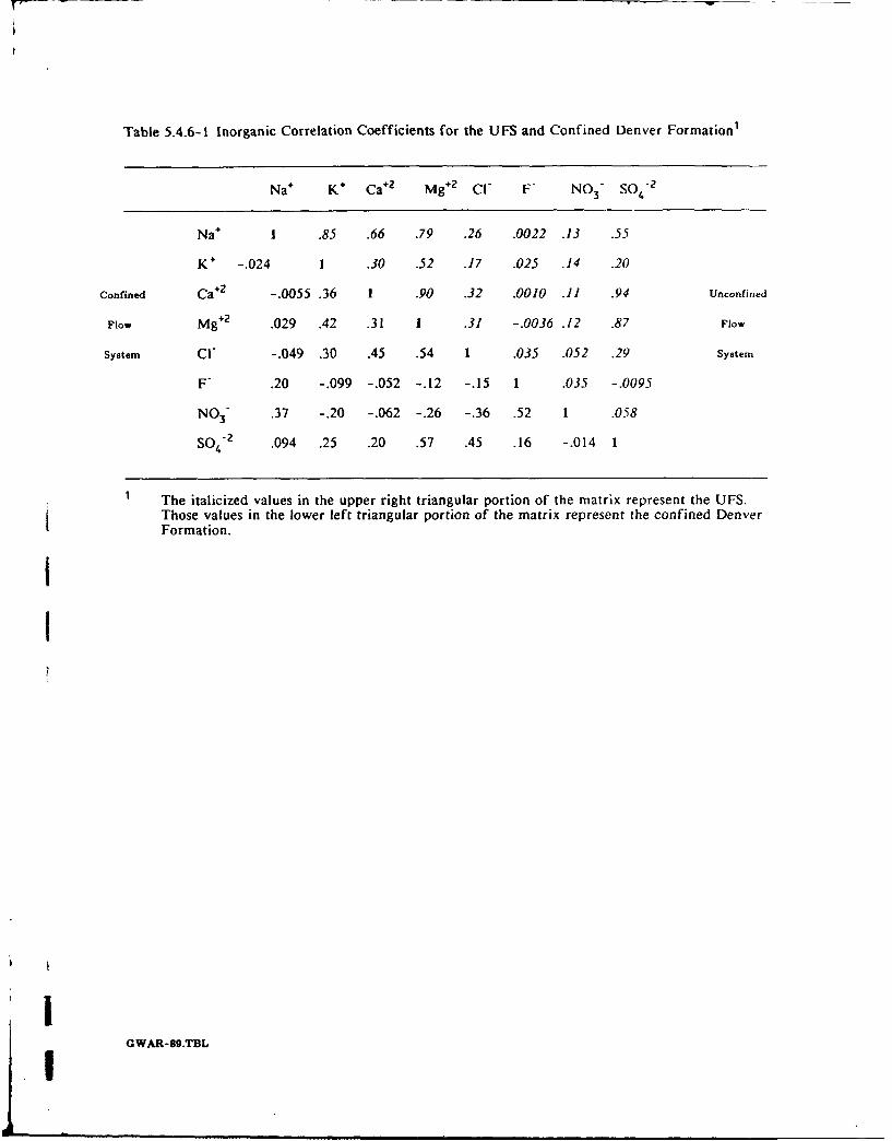
Table 5.4.6-1 Inorganic Correlation Coefficients for the UFS and Confined Denver Formation1
Na÷ K+ Ca+2 Mg÷2 Cr" F" N0 3 " S0 42
Na÷ 1 .85 .66 .79 .26 .0022 .13 .55
K+ -. 024 1 .30 .52 .17 .025 .14 .20
Confined Ca÷2 -. 0055 .36 1 .90 .32 .0010 .11 .94 Unconfined
Flow Mg* 2 .029 .42 .31 1 .31 -. 0036 .12 .87 Flow
System CI" -. 049 .30 .45 .54 1 .035 .052 .29 System
F" .20 -. 099 -. 052 -. 12 -. 15 1 .035 -. 0095
N0 3 " .37 -. 20 -. 062 -. 26 -. 36 .52 1 .058
SO 4 "2 .094 .25 .20 .57 .45 .16 -. 014 1
The italicized values in the upper right triangular portion of the matrix represent the UFS.
Those values in the lower left triangular portion of the matrix represent the confined DenverFormation.
II
IGWAR-89.TBLI
I
confined flow system. Although the r value for Mg÷2-C!" in the confined flow system is higher,
the r value for this pair in the unconfined flow system is close in magnitude.
5.4.7 Inorganic Data Assessment Summary
The analytical results of the inorganic data have been presented in the preceding subsections in
the form of concentration versus depth plots, frequency diagrams, trilinear diagrams, solute
correlations, and correlation coefficients. Each presentation included a discussion of the two flow
systems by specific area with the exception of the frequency diagrams and correlation coefficients.
This section summarizes the integrated results of the preceding subsections and compares the results
of the two flow systems by area.
A statistical summary of the inorganic data is presented in Table 5.4.7-1. This table includes the
minimum, maximum, and arithmetic mean for the eight ions, % 02, and specific conductance in
the unconfined and confined flow systems and the integrated data sets from both flow systems.A comparison of the arithmetic mean of both systems indicates that the analyte concentration is
lowest in the confined flow system with the exception of sulfate. A similar comparison of the
maximum values indicates that the unconfined flow system contains the highest analyte
concentrations.
5.4.7.1 Unconfined Flow System. The background water quality of the unconfined flow
system is characterized by ground water with Ca/Na ratios between approximately one and two,
specific conductance values less than 2000 umhos/cm, % 02 values between I and 60 percent andnon-dominance in cations but dominance in sulfate and bicarbonate anions.
The water quality of the unconfined flow system in the Western Tier is similar to background
water quality with the following exceptions. A large percent of samples have % 02 values greater
than 60 percent and these values are independent of depth. This is in agreement with hydrologic
data showing that the thick unconfined flow system in this area is well mixed as a result of greater
ground water flow velocities. The majority of Western Tier samples have Ca/Na ratios greater than
two and these values are also independent of depth.
The water quality of the unconfined flow system in the Central Area departs from most of the
characteristics of background water quality. The ground water in the Central Area is characterized
by a majority of Ca/Na ratios that are significantly lower than one. A percentage of the samples
have specific conductance values between 2500 and 20,000 p•mhos/cm and these values occur at
depths below 40 feet. Although most of the samples fall within the % 02 range of background
GWAR-89.6-6Rev. 06/22/90 - 202 -
I
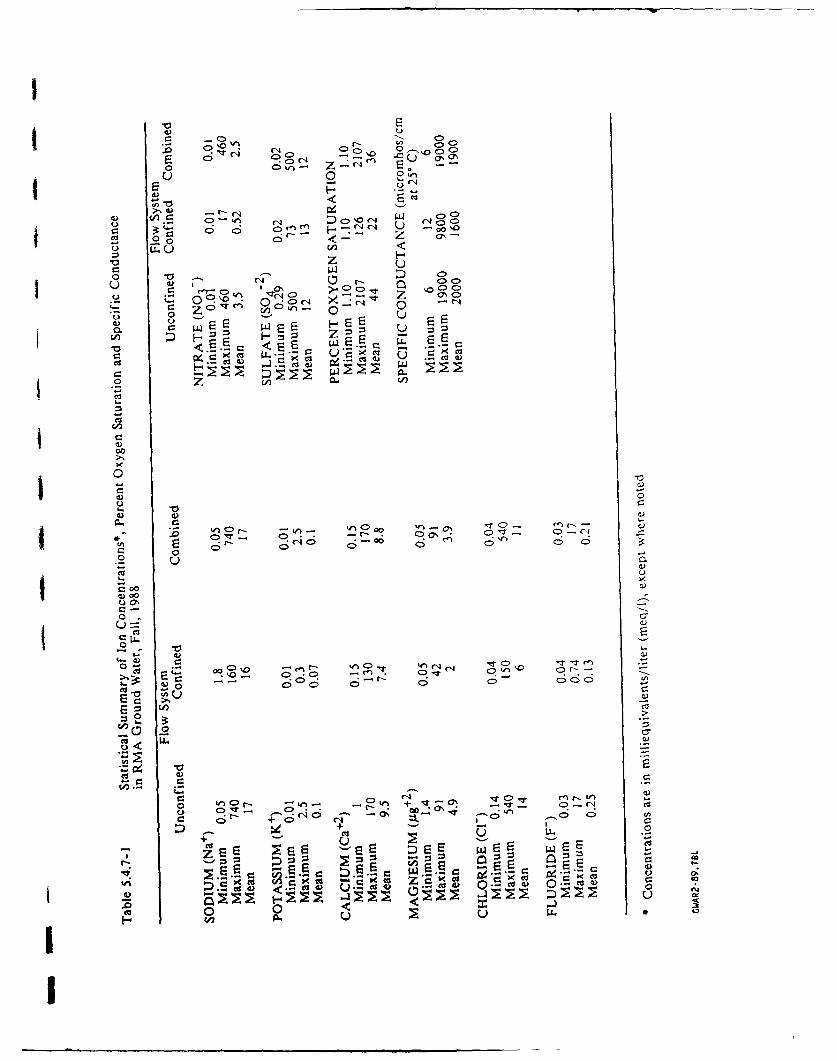
00 -0 C>0
.00 in
Or 4 *
o ) 0 Z-a
U. <
0 <- Z Du
C-
0 a, c)0 (:: 04 x -.. 00ý
C: Z () .n 0
0 0 -
0 Cd 00 W
00
0 7
00 I n
0 -
u 00
el .- *-0-00 \0 0nnC
So; 0, 0D C) " 0
o
0 >)C
U..
+ 1 0
~ 04)
-SA 0 o
0 4) C .: )q
I
samples, a number of samples are above 60 percent. In addition, there is a shift in the CentralArea water quality to ground water that is more dominant in sodium, potassium, chloride, andnitrate in comparison to the background ground water. This difference is a direct result of the
introduction of sodium/chloride-rich waste waters into the unconfined flow system from lined and
unlined basins.
The water quality of the unconfined flow system in the Northern Area is similar to that in the
Central Area with one exception. The cations in the ground water are similar to those in the
Central Area but the anions shift slightly away from a bicarbonate type to a sulfate type.
5.4.7.2 Confined Flow System. The background water quality of the confined flow system ischaracterized by ground water with Ca/Na ratios generally less than one, specific conductance
values less than 2300 pmhos/cm, % values generally less than 60 percent with one value near88 percent, slightly dominant in sodium and potassium, and dominant in sulfate.
The water quality of the confined flow system in the Western Tier is similar to background waterquality with the following differences. The Ca/Na ratios in the samples from the Western Tier
are consistently less than one. The % 02 values exhibit an increase in saturation with increasingdepth.
The water quality of the confined flow system in the Central Area differs somewhat from
background water quality. The characteristics of the ground water in the Central Area includehigher specific conductance values and more samples with chloride and nitrate dominance whencompared to background. This increase in dissolved solids (chloride, sodium) may have resultedfrom downward migration of waste waters from the unconfined flow system.
The water quality of the confined flow system in the Northern Area is similar to that in the
Central Area with one exception. The ground water is predominately sulfate type.
5.4.7.3 Comparison of Water Quality at Well Clusters. The general water-quality character-istics of the two flow systems have been presented on an areal basis to compare the two systems.
General trends have been noted in the comparison between background and downgradient waterquality. These trends result mainly from differences due to depth and geographical location (i.e.,water quality in the Western Tier more closely resembles background than the downgradient waterquality in the Central and Northern Areas). To assess the applicability of the general trends notedin the areal comparison to specific areas, the water quality of the two flow systems at selected well
clusters was compared. The selection of the well clusters was based on geographical location and
GWAR-89.6-6Rev. 06/22/9o - 204 -
I1
I
those wells used in the isotopic data assessment presented in Section 5.5 of this Annual Report.
Therefore, 29 wells in II well clusters from the Western Tier and Northern Area were used in this
assessment. A list of these wells is provided in Table 5.4.7.3-1.
The analytical data for the 29 wells have been compiled and are presented in Table 5.4.7.3-1. This
table includes the analytical data for- 8 major ions, Ca/Na ratios, specific conductance, % 02,deuterium, 0-18, tritium, and screened interval. The significance of the deuterium, 0-18, and
tritium values will be discussed in Section 5.5.
As noted in previous sections, the Ca/Na ratio tends to decrease with increasing depth. The
decrease generally results from a decrease in calcium and this is noted in most of the wells listed
in Table 5.4.7.3-1. Although the concentration of sodium is expected to increase with depth due
to ion exchange reactions, the concentration of sodium in the wells listed in Table 5.4.7.3-1 exhibit
increasing and decreasing trends with depth. The three well clusters in sections 23 and 24 contain
the highest sodium concentrations in the unconfined flow system for the 29 wells listed in
Table 5.4.7.3-1. These elevated concentrations may be the result of the recharge of saline watersinto the unconfined flow system in this area during RMA activities. In addition, the sodium
concentrations in the confined flow system in these section 23 and 24 wells are elevated withrespect to the remaining wells in Table 5.4.7.3-1 with the exception of 24198. The tritium data
suggest little or no mixing of the ground water from the two flow systems yet the elevated sodium
concentrations are apparent in both systems.
As noted in Table 5.4.7.3-1 the trend for specific conductance values generally mimics the trend
in the ionic concentrations. The majority of the ionic concentrations and specific conductance
values decrease with increasing depth. However, this is not the expected trend. A relationship of
increasing specific conductance with increasing depth is expected (Hem, 1989). Increased soluteconcentrations with depth result from a longer residence time of ground water; therefore, the
specific conductance values associated with the confined flow system would normally be greater
than those values associated with the unconfined flow system. The observed relationship is likely
due for surface disposal practices that have resulted in increased ionic concentrations in ground
water near the surface.
The concentration versus depth plots for % 02 exhibited variability with depth except in the
Western Tier confined flow system wells. The % 02 data in Table 5.4.7.3-1 exhibit a general trend
of decreasing % 02 with depth with one exception in the Section 3 well cluster.
IGWAR-89.6-6Rev. 06/22/90 - 205 -
II__ _ _ _ _ _ _ _ _ _
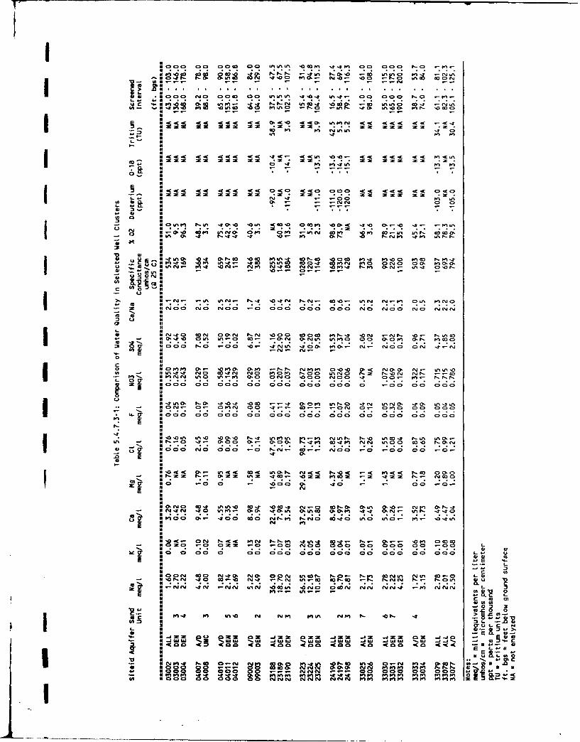
NN
1100 00 o00f 00I mA I 'O:) 4:f.I w0 000 in0 It
-" t-.n lz~ Z-O" .- v% 0, m I Zow
-K.. <.. <0 < .<-Cg :-K 0 I' -.1
0' IAOO 4N W,'A
I..It
Is
8 m1 z Z xZ ZZZ xZ x~ * ...
0: .6; In A - ODC
It 4.N o11 2 i N -* . :) . 00 in- MC nc I,-An'u. r=U C N I* 't o nI t W nI m D a.D C . p '0u 01 IV . .
4.. v 10
0 0 IfH
N IM t-A .O' 'u C 0" 1' '-' *' . U
If
j I~n~, 0AN N." N9 N0* Jý NN W!' 11 9. 0-N. W A. 0: 'W!t-C
0 . :11
IN. It A IAN- C4-. '0t -. WO-,N N.' I
"C. 99 . "iP0; C0 8 1( Dm C. 4 DC, mct0 ~ , c) -C D C 3 C a(
` LA.3 IU- o% oc ' : ý P ý , 2 I j0 t '
o ml
If
*i0't OID IA.- C3 (D 'N 0'NI IAM0ý 00. (DO 0I - o-
aO I'00 '0.- CollI -*00 00,1 C'. C -Oý n- 9N0: ON 01 rA
m D0 0 ' 3 0 c: - m N mfI 0' 0 U 3" C T&
Cl in
.- IIMN < A GA- 0-0 N<ONOý - m ' 't000 NOO 't 00. I'l (3 -to
fl. N ' !9 9
IA IIN- c .t. 8 '0 0'.- a' 0 4-D4 CDt NN, (3O Co(A')c) : 30 C D lC 0 N0 0'3N
NO 000 to0 NN, m.. N0g -0i -0 0II -* 0
111
No M
110 .1 ON In MN NF' ' in m -.1 a'm -At='a -'.m' " m--. '0 -1 00
E9 rIf C 1 0
" a 1109N C*0 ass!' Nmt.N IAt( W, N V%'4 0 NN i ~.4 IS.OI
11 PCngi n ý nr ' m 0 0)<C', 0v00c l Ci I83 10~ zs; 3z m .1-4
I
jThe % 02 in ground water is dependent on the amount of: (1) organic material, (2) reduced
inorganic minerals, or (3) organic chemicals present in the flow system. Therefore, the trend of
% 02 with depth is dependent on the presence of oxidizable material and the length of time the
water has been resident in the system and not solely a function of depth.
5.5 lsotovic Data Assessment
Data from a pilot program to monitor ground water for isotopic signatures further assessed the
degree of hydraulic connection between the unconfined and confined flow system.
Isotopic samples were analyzed for deuterium, oxygen-18 and tritium (commonly notated 2H, 180,
and 3 H respectively). These isotopics were selected because they have been successfully used to
assist in the hydrogeologic characterization of a wide variety of sites and aquifer systems.
Ground-water samples for isotopic analyses were collected from seven unconfined and six confined
wells in Sections 23, 24, and 33 during the Spring 1988 sampling round (Figure 5.5-1). Wells
sampled in Section 33 (not shown in Figure 5.5-1) are 33077 and 33079, located approximately 100
ft northeast of the SACWSD Treatment Facility Property.iIn selecting wells to be sampled for isotopic analyses consideration was given to location, depth of
screened interval, and lithology (unconfined or confined flow system). Wells in well clusters were
preferred over isolated, scattered wells, to aid in comparing isotopic signatures between the
unconfined and confined flow systems. Both shallow and deep (wells with screened intervals
greater than the screened intervals of confined wells sampled) unconfined flow system wells were
sampled to determine if the unconfined flow system had a single isotopic signature, or if deep
unconfined wells more closely resembled confined flow system isotopic signatures.
The II samples in Sections 23 and 24 were collected from wells located upgradient of the North
Boundary Containment System (NBCS). Five samples were collected from the unconfined flow
system and six samples were collected from the confined flow system. In Sections 23 and 24, the
maximum relief of the topographic surface is 20 ft, and the surficial geology is characterized by
alluvium deposited during postglacial periods. In this area, the bedrock depth varies from 14.5 to
54.0 feet. The screened intervals of the five unconfined flow system wells in Sections 23 and 24
(23095, 23188, 24196, 24106, and 24188) range from 7 ft to 48 ft deep. The confined flow system
wells are completed in Zones 2 through 5, which consist of interbedded claystone, siltstone, and
sandstone. Screened intervals in these wells range from 43 to 116 ft deep.
1GWAR-89.5-6Rev. 06/22/90 - 207 -
I.
i
I The Section 33 wells (33077 and 33079) are completed in the unconfined flow system at depths of
102 and 125 ft, respectively. The subsurface of Section 33, in the RMA Western Tier, is
characterized by a greater thickness of alluvium than that in Sections 23 and 24. Depth to bedrock
in Section 33 can be as much as 130 ft. Samples were collected in Section 33 to evaluate if isotopic
signatures are characteristic of the hydrostratigraphic interval sampled and independent of depth.IIt is difficult to determine an absolute isotopic abundance for stable isotopes; thus, laboratories
I quantify measurements relative to a common standard. For the isotopes 2H and 180, the reference
is Standard Mean Ocean Water (SMOW). Values are reported in delta units (6) in parts per
thousand (per mil or O/oo) deviation from SMOW. A negative value reflects depletion of the
I heavier 2H or 180 in the sample, and a positive value indicates a relative enrichment in these
heavier isotopes.
5.5.1 Tritium Analytical Results
SIsotopic analyses for deuterium, oxygen- 18, and tritium have been used successfully to assist in the
hydrogeologic characterization of a wide variety of sites and aquifer systems. Tritium is an isotope
of hydrogen commonly notated as 3H, where the number 3 denotes the atomic mass of this
hydrogen atom. Hydrogen most commonly occurs as an element with an atomic mass of 1 ('H);
thus, tritium (3H) is significantly heavier. Tritium is also radioactive, which means that it decays
to lighter hydrogen isotopes over time.
I Tritium (3 H) is an unstable isotope of hydrogen with a half-life of 12.4 years and a relative
abundance of 3H/H = 1.0 x 10"18. Tritium in the atmosphere typically occurs as the molecule3HHO, which is produced naturally from cosmic ray reactions and enters ground water with
recharging precipitation. Prior to the advent of above-ground nuclear testing in 1953, precipita-
tion over North America had a natural backgr-ound level of 10 to 15 tritium units (TU). (A TU
is the concentration of one atom of 3H for every 1018 total hydrogen atoms.) Since 1953, the
amount of tritium n the atmosphere has increased, attaining a high in the early 1960s (Figure 5.5-
2) during times o" active nuclear testing and decreasing to present levels.
Because of the relationship between ground-water age and tritium concentration, tritium
radioisotope analyses are most often used as an investigative tool for evaluating relative ground-
water ages. Recently infiltrated (modern) water tends to have appreciably higher TU values. In
areas of spatially different water-bearing units, tritium is useful in identifying zones subject to
relatively fast recharge and possible hydraulic connections. However, because TU values in
precipitation change with atmospheric conditions and have varied considerably over time, it is
GWAR-89.6-6Rev. 06/22/9O - 208 -
I
I
not possible to assign an absolute age to a tritium-dated water. For example, if a water has a TUvalue less than 5 to 10, the water was recharged prior to 1955 but further definition of the dateof recharge is not possible. Today, atmospheric background levels in the Northern Hemisphere
range between 50 and 100 TU; during the early 1960s, concentrations well above 1000 TU weremeasured (Fritz, 1981). Water containing 1000 TU when recharged in 1964 would containapproximately 250 TU today due to the radioactive decay of tritium. Water containing 5 TUwhich was recharged in 1952 (three half-lives) would contain less than I TU today.
The TU values reported for the unconfined flow system ranged from 31.3 to 58.9, and the TU
values reported for the confined flow system ranged from 2.5 to 18.2 (Table 5.5.1-I). Average TU
I values for the confined and unconfined flow systems are 6.45 and 43.2, respectively. The highestTU value in the confined flow system (18.2 TU) was recorded for the shallowest well (23177 at43.0 ft); the remaining five confined flow system samples all yielded TU values below 6.0.Although deeper than the Section 23 and Section 24 unconfined flow system wells, the wells inSection 33 yielded TU values greater than 30, consistent with values detected in the unconfinedflow system wells in Section 23 and Section 24.
Results of tritium analyses indicate a difference in the TU values reported for the unconfined flowsystem and confined flow system (Figure 5.5-3). Reported TU values for the unconfined flowsystem are indicative of water less than 35 years old. This implies that precipitation recharge to
the unconfined flow system has occurred in the last 35 years. Reported TU values for the confinedflow system, except Well 23177, were less than 6, which generally is indicative of older waterrecharged prior to the influx of tritium to the atmosphere in the 1950s. It should be noted thatalthough these low TU values are indicative of older waters, these waters could contain up to10 percent younger unconfined flow system water as a result of mixing and still retain low tritium
values. For example, the mixing of 90 percent water containing 3 TU and 10 percent watercontaining 30 TU would result in a final tritium ratio of approximately 6 TU.
Results of tritium analyses indicate that confined flow system water generally is older thanunconfined flow system water. The low TU values detected in samples from confined flow systemwells also indicate either minimal or a low level of hydraulic communication with the unconfined
flow system. A geologic cross section through Sections 23 and 24 (A-A' in Figure 5.5-1) isincluded to illustrate the relationship of tritium with depth (Figure 5.5-4). Analytical results ofground-water samples from confined flow system wells are presented in Table 5.5.1-2.
GWAR-89.5-6Rev. 06/22/go - 209 -
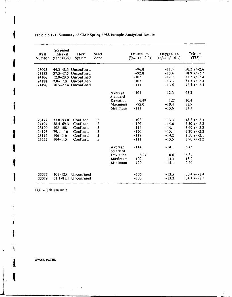
I
Table 5.5.1-1 Summary of CMP Spring 1988 Isotopic Analytical Results
I ScreenedWell Interval Flow Sand Deuterium Oxygen-18 Tritium
Number (feet BGS) System Zone (O/oo +/- 2.0) (*/0o +/- 0.1) (TU)
23095 44.3-48.3 Unconfined -96.0 -11.4 50.2 +/-2.623188 37.5-47.5 Unconfined -92.0 -10.4 58.9 +/-2.724106 12.0-20.0 Unconfined -102 -12.7 33.2 +/-2.424188 7.0-17.0 Unconfined -103 -13.3 31.3 +/-2.424196 16.5-27.4 Unconfined -111 -13.6 42.5 +/-2.5
IAverage -101 -12.3 43.2StandardDeviation 6.49 1.21 10.4Maximum -92.0 -10.4 58.9Minimum -111 -13.6 31.3
23177 33.0-53.0 Confined 2 -102 -13.3 18.2 +/-2.324197 58.4-69.3 Confined 2 -120 -14.6 5.30 +/-2.223190 102-108 Confined 3 -114 -14.1 3.60 +/-2.224198 79.1-116 Confined 3 -120 -15.1 5.20 +/-2.223192 106-116 Confined 3 -117 -14.2 2.50 +/-2.123225 104-115 Confined 5 -111 -13.5 3.90 +/-2.2
Average -114 -14.1 6.45StandardDeviation 6.24 0.61 5.34Maximum -102 -13.3 18.2Minimum -120 -15.1 2.50
33077 105-125 Unconfined -105 -13.5 30.4 +/-2.433079 61.1-81.1 Unconfined -103 -13.3 34.1 +/-2.5
TU = Tritium unit
i GWAR-SO.TBL
I
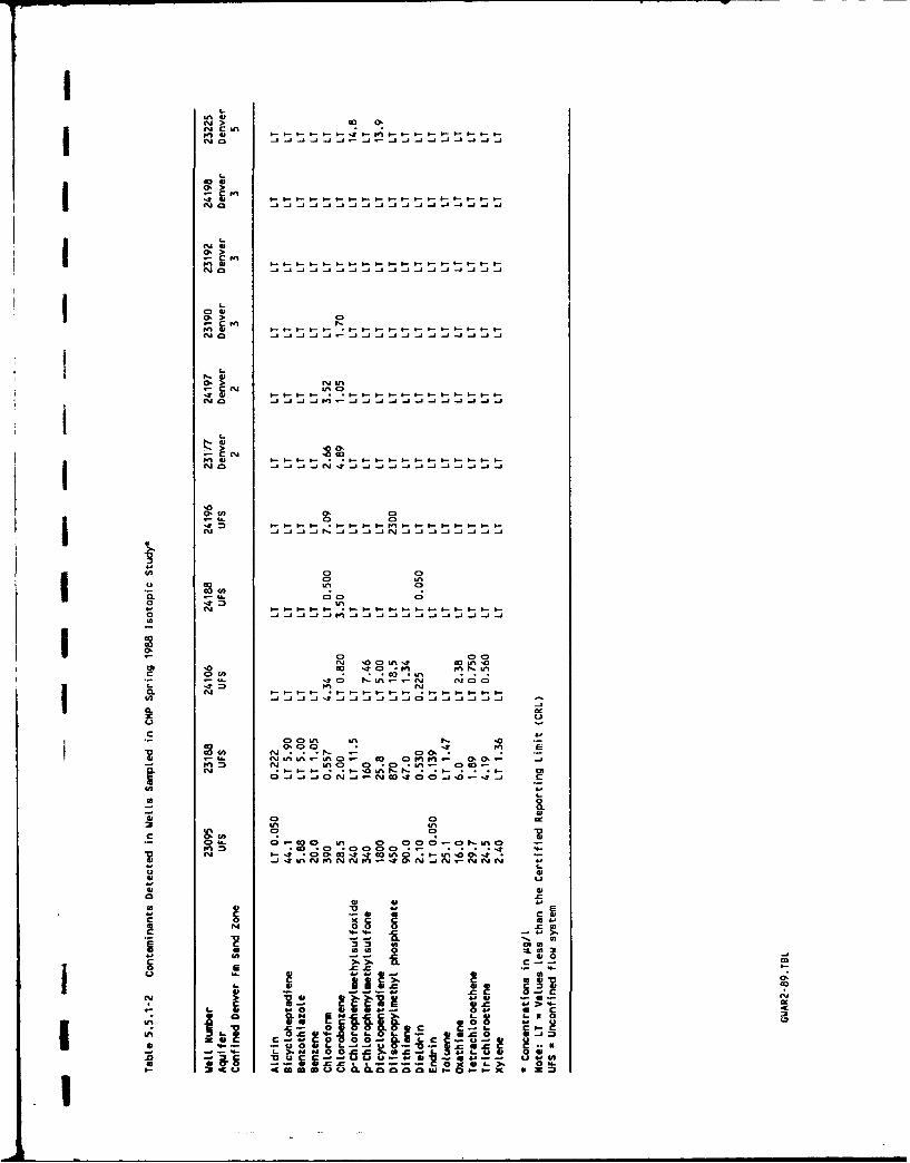
V >
IcN>
40.
;; C Pell a _j-- - -- - - -
* 0.>
m ~ ~ O C,-- -- - - -- - -N ~ ~ C C . 44 44 3 .. 444. .
C4cm.
r'.. C3a a
C'S
N ~ ~ C CC U8. . N W! .4 .4. J.4.0 4.4. 4.
r4(f UN 0%D C ! ,0-s--!rn 9 0 - *. r. -- f s c971-
0 0j C 4W' j 'oE
U 00C3 C, 0of
NN in0 s
m.0 - -,t W m a EC4Mn NtC.. 0 tI .N C- 00.-.f 4
mt N N M C 4~ 0 _0 rd%. O .u 3ii.**- I N .........- 0
ca 0
0 0 L0
C .C?
u& N
S. c
MS 9226 " '10L.>-cu C 0 0u La a a U - b- .
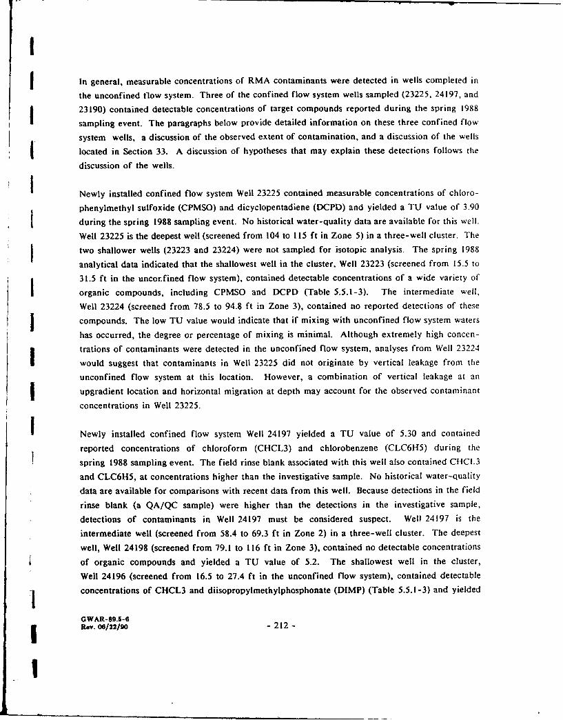
I
fIn general, measurable concentrations of RMA contaminants were detected in wells completed in
the unconfined flow system. Three of the confined flow system wells sampled (23225, 24197, and
23190) contained detectable concentrations of target compounds reported during the spring 1988
sampling event. The paragraphs below provide detailed information on these three confined flow
system wells, a discussion of the observed extent of contamination, and a discussion of the wells
located in Section 33. A discussion of hypotheses that may explain these detections follows the
discussion of the wells.
Newly installed confined flow system Well 23225 contained measurable concentrations of chloro-
phenylmethyl sulfoxide (CPMSO) and dicyclopentadiene (DCPD) and yielded a TU value of 3.90
during the spring 1988 sampling event. No historical water-quality data are available for this well.
Well 23225 is the deepest well (screened from 104 to 115 ft in Zone 5) in a three-well cluster. The
two shallower wells (23223 and 23224) were not sampled for isotopic analysis. The spring 1988
analytical data indicated that the shallowest well in the cluster, Well 23223 (screened from 15.5 to
31.5 ft in the uncor.fined flow system), contained detectable concentrations of a wide variety of
organic compounds, including CPMSO and DCPD (Table 5.5.1-3). The intermediate well,
Well 23224 (screened from 78.5 to 94.8 ft in Zone 3), contained no reported detections of these
compounds. The low TU value would indicate that if mixing with unconfined flow system waters
has occurred, the degree or percentage of mixing is minimal. Although extremely high concen-
g trations of contaminants were detected in the unconfined flow system, analyses from Well 23224
would suggest that contaminants in Well 23225 did not originate by vertical leakage from the
unconfined flow system at this location. However, a combination of vertical leakage at an
upgradient location and horizontal migration at depth may account for the observed contaminant
concentrations in Well 23225.
Newly installed confined flow system Well 24197 yielded a TU value of 5.30 and contained
reported concentrations of chloroform (CHCL3) and chlorobenzene (CLC6H5) during the
spring 1988 sampling event. The field rinse blank associated with this well also contained CHCL3
and CLC6H5, at concentrations higher than the investigative sample. No historical water-quality
data are available for comparisons with recent data from this well. Because detections in the field
rinse blank (a QA/QC sample) were higher than the detections in the investigative sample,
detections of contaminants in Well 24197 must be considered suspect. Well 24197 is the
intermediate well (screened from 58.4 to 69.3 ft in Zone 2) in a three-well cluster. The deepest
well, Well 24198 (screened from 79.1 to 116 ft in Zone 3), contained no detectable concentrations
of organic compounds and yielded a TU value of 5.2. The shallowest well in the cluster,
Well 24196 (screened from 16.5 to 27.4 ft in the unconfined flow system), contained detectable
concentrations of CHCL3 and diisopropylmethylphosphonate (DIMP) (Table 5.5.1-3) and yielded
GWAR-89.$-6Rev. 06/22/90 - 212 -
.1
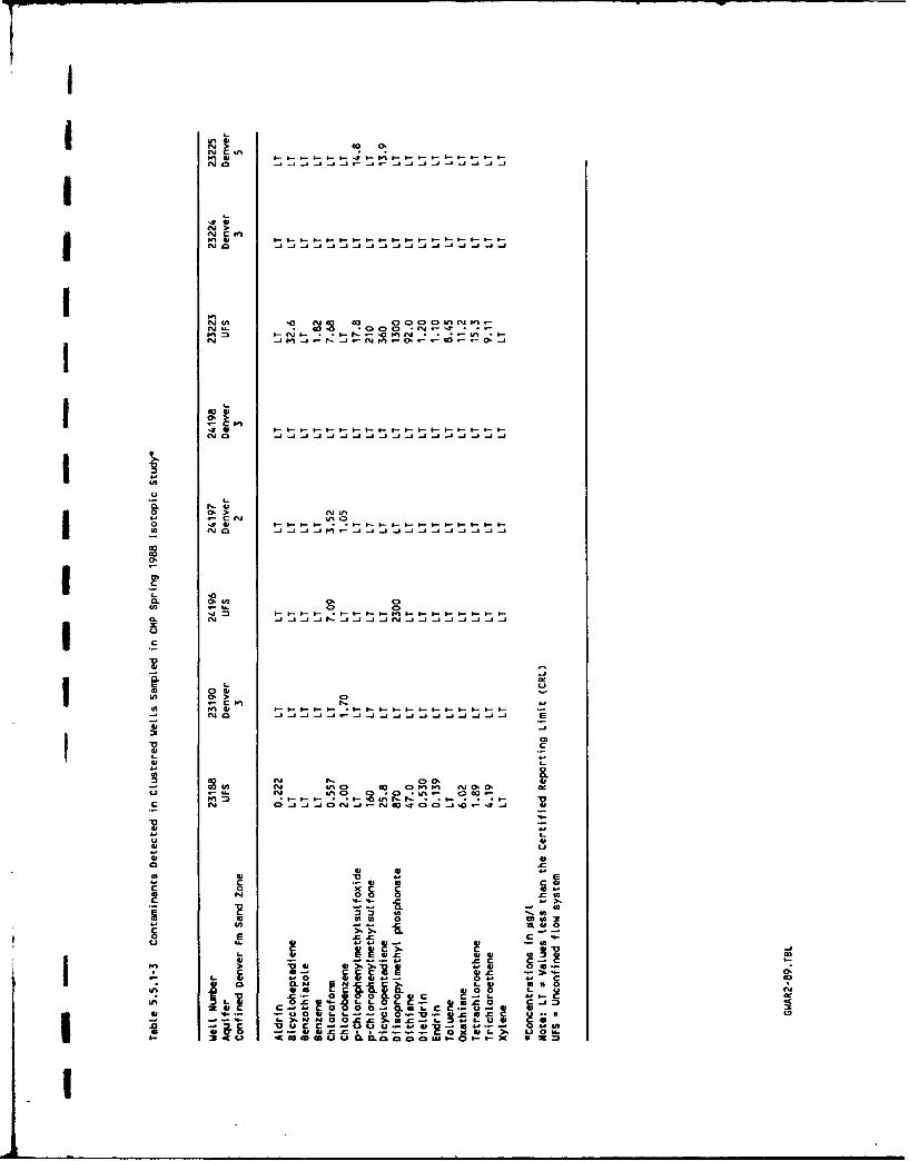
N>rN U
m% U441c~ ýWNOar a r J a y
N Cr lu'A I a M aj aj aj a_ aaaaa
104
-ý C3.
U
0.Vo S 0> Nt
FCn 1
o7Z4 ~ -
IýCp
I 41
00
z; (A11 (
N 0- 00 41
o 44
412 1 L - . 1- 0-3-
p 0 :2C ZL Cu
41 4 4 --C -4 -CU auu0inL -01 x :
I
a higher TU value of 42.5, which is indicative of younger water. In conclusion, the detection of
contaminants in confined flow system Well 24197 appears to be anomalous and until confirmed,
should be considered a result of field-induced cross contamination.
Confined flow system Well 23190 contained a detectable concentration of CLC6H5 and yielded aTU value of 3.60 during the spring 1988 sampling event. However, no historical CLC6H5
detections have been recorded for this well during sampling events from the Initial ScreeningProgram (ISP) to the present. Well 23190 (screened from 102 to 108 ft in Zone 3) is in a cluster
with Well 23188 (screened from 37.5 to 47.5 ft in the unconfined flow system). Well 23188 yieldeda high TU value of 58.9, which is indicative of water recharged in the last 35 years. Analyticalresults from Well 23188 indicate the presence of several RMA contaminants. However, CLC6H5
concentrations in Wells 23190 and 23188 for the spring 1988 event were essentially identical, withCLC6H5 the only analyte detected in Well 23190. Because Well 23190 did not contain the samechemicals as shallower Well 23188, a spurious detection of CLC6H5 in Well 23190 and/or theabsence of direct connection between unconfined flow system and confined flow system at this
location are plausible explanations for these contradictory data. As previous sampling events didnot detect CLC6H5 in Well 23190 prior to the spring 1988 event, this detection should be
considered suspect.
Wells 33077 and 33079, both completed in the unconfined flow system, are located in Section 33
in an area where the saturated thickness of the alluvium can be as much as 130 ft. TU values of30.4 (33077) and 34.1 (33079) were detected in the wells at depths of 125 and 102 ft, respectively.
The deep confined flow system wells (greater than 100 ft; Table 5.5.1-1) in Sections 23 and 24yielded TU values less than 6. Thus, comparison of TU values in the deep confined flow systemwells with the deep unconfined flow system TU values indicate that the TU values are not depth
dependent but are characteristic of the hydrostratigraphic unit. Well 33077 contained detectableconcentrations of 1,1,1-trichloroethane (11I TCE) (0.875 pg/I), CHCL3 (0.622 pg/I), and trichloro-
ethene (TRCLE) (7.37 pg/l). Well 33079 contained detectable concentrations of II IITCE(6.63 pug/I), 1,1-dichloroethene (IIDCE) (2.20 pug/I), and TRCLE (3.13 pug/I).
The following four hypotheses have been developed in an attempt to explain coincident contami-
nant detections in shallow confined flow system wells and low tritium activities in Wells 23225,
23177, 24197, and 23190.
1. Mixing/Hvdraulic Connection - Measurable hydraulic connection between the
unconfined flow system and the confined flow system
IG WAR-89.5-6Rev. 06/22/90 - 214-
I
I
2. Pre- 1953 Contaminant Release - Introduction of contaminants into the confined flow
system prior to 1953
3. Free-Phase Contaminant Transport - Introduction of contaminants into the confined
flow system as a concentrated, free organic phase
4. Sampling and Analytical Errors - Introduction of organic contaminants during
sampling and analysis
Each hypothesis is discussed in the following paragraphs.
The tritium and organic analytical data from Well 23177 are intermediate to the values reported
for the confined flow system and unconfined flow system wells. The 18.2 TU value from
Well 23177 is significantly higher when compared to the TU values for the other confined flow
system wells (<6). The TU value for Well 23177 is also lower than the lowest value reported for
the unconfined flow system wells (31.3 TU). Detectable CHCL3 and CLC6H5 concentrations inWell 23177 were reported during the spring 1988 sampling event; however, only CHCL3 had been
j detected in three of six previous sampling events. Detectable concentrations of DIMP had beenreported in historical data (five of six sampling events) but no detectable concentrations of DIMP
were reported for the spring 1988 sampling events. Results of the tritium and organic analytical
data indicate a possible mixing of waters from the two aquifers. Well 23177, located immediately
upgradient of the NBCS, is the shallowest confined flow system well investigated. The well is
screened from 33.0 to 53.0 ft in Zone 2, and the depth to bedrock at this location is 14.5 ft.
Zone 2 has been shown to subcrop in this general area. The Well 23177 log indicates that there
is weathered claystone from 14.5 to 29.0 ft and that sandy claystone occurs from 29.0 to 35.5 ft.
These geologic factors may contribute to the vertical hydraulic communication between the
unconfined flow system and the confined flow system indicated by triattm data for this location.fIn addition to contaminant transport via vertical flow across aquifers, a horizontal flow paththrough respective confined flow system sandstones must also be sufficiently rapid to have trans-
ported contaminants from source areas to confined flow system wells in Sections 23 and 24 for this
scenario to be viable.
Upon examination, some of the chemical data (Wells 23225, 24197, and 23190) appear to contradict
the isotopic data with respect to whether or not the confined flow system is in hydraulic
communication with the unconfined flow system. Isolated detections of target organic compounds
at depth in confined flow system Wells 23190 and 23225 may indicate limited but detectable
GWAR-89.5-6Rev. 06/22/9O - 215-
!
!-
I
hydraulic communication between the unconfined flow system and confined flow system units.
The isotopic signatures of these unconfined flow system and confined flow system wells are distinct
and indicate that if any mixing of the two water-bearing units is occurring, the fraction of
unconfined flow system water would be less than 10 percent. Although present concentration
levels of organic contaminants in confined flow system wells are similar to unconfined flow systemI concentration levels, the mixing could have occurred over a long time span. Historically,
concentrations of organics in unconfined flow system waters were substantially higher. Mixing
f may result from one or more of the following: (1) hydraulic leakage down poorly sealed boreholes,(2) hydraulic connection via faults/fractures, or (3) vertical flow across confining beds.
The presence of chemical compounds in confined flow system wells that yielded low TU values
may be attributable to contaminants introduced to the confined flow system prior to the 1953 to
1956 time frame. However, only two of the four chemical compounds detected in the subject
confined flow system wells were associated with manufacturing activities conducted prior to 1953.
DCPD was used as a raw material in the manufacture of aldrin and endrin from 1952 to 1974, and
CLC6H5 was used as a solvent in the synthesis of thionyl chloride during the manufacture of
Lewisite in the 1940s. Several of the compounds detected in confined flow system wells ofI Sections 23 and 24 were not used at RMA prior to 1953. CHCL3 was associated with insecticides
manufactured from 1963 to 1975, and CPMSO was a decomposition product of herbicides
manufactured from 1966 to 1975. DCPD and CLC6H5 were the only target compounds detected
in confined flow system wells (23225, 24197, and 23190) that had the potential to infiltrate the
confined flow system and retain the pre-1953 tritium signature.IThe third hypothesis for explanation of coincident low tritium activity with detectable organic
g contamination of the confined flow system zones is the introduction of concentrated free-phase
organic compounds, with little accompanying unconfined flow system water, directly into the
confined flow system zones. This type of release would be likely only in the South Plants Area,
the Basin F area, or along chemical sewer lines. Organic liquids with densities greater than that
of water would be vertically transported more rapidly than unconfined flow system ground waters
and possibly in directions reverse to that of ground-water flow. If a concentrated mass of organic
fluid was transported downward through saturated materials, some dilution or dissolution would
occur, but limited mixing of the central mass would occur. Once organic fluids reached zones of
lower hydraulic conductivity, the organic fluid would gradually dissolve and be transported
downgradient. The small amount of entrained unconfined flow system water would not
substantially increase the tritium values for the shallow confined flow system. The result of this
process would be contaminated confined flow system ground waters with low levels of tritium
activity and a continuing contaminant source at depth.
GWAR-89.5-6Rev. 06/22/90 - 216 -
i
I
The fourth possible hypothesis for the presence of detectable contaminant concentrations in the
confined flow system wells without a related change in the isotopic signature involves either
sampling procedures that were compromised, or analytical results that were in error. Analytical
results from Well 24197 provide an example of data that are suspect because of the presence of
detectable concentrations of contaminants in the rinse blank.IChlorobenzene was the only target analyte detected in Well 23190. Numerous organic compounds,including CLC6H5, were detected in the shallower well in the cluster (23188). However, historical
sampling of this well (23188) on numerous occasions did not yield CLC6H5 detections. Based on
this information, additional water-quality sampling should be performed to confirm or refute these
data.
It should be noted that two of the wells (23225 and 24197) that yielded organic contaminant
detections were newly constructed. As such, the historical data base for the new wells is
incomplete.
5.5.2 Deuterium and Oxygen-18 - Analytical ResultsIDeuterium and oxygen-18 are not radioactive isotopes and are therefore called "stable" or
"environmental" isotopes. Deuterium (2H) is another isotope of hydrogen with an atomic mass of
2. Oxygen commonly occurs with an atomic mass of 16, but small amounts of 170 and 180 exist
in nature. These heavier isotopes of oxygen and the heavier isotopes of hydrogen fractionate (or
selectively separate) from the more common lighter isotopes (e.g., 1H, 160) during precipitation
and evaporation processes.
Interpretation of stable isotope data is more complex than interpretation of tritium data. Tritium
data yield fairly simplistic relative age information; conversely, stable isotope data do not provide
age estimates but provide data indicative of climatic conditions of recharge. As such, interpreta-
tion is more difficult. Deuterium (2H) is commonly plotted as a function of oxygen-18 (180) and
compared with the global (average) meteoric water line (Figure 5.5-5). The global meteoric water
line, which is the result of an empirical linear relationship between deuterium and oxygen-18
found in continental precipitation throughout the world, is described by the following equation:
62H = 86180 + 10
where 6 = the difference per mille (parts per thousand) relative to standard mean ocean water
(SMOW).
G WAR-89.5-6Rev. 06/22/90 - 217 -
I
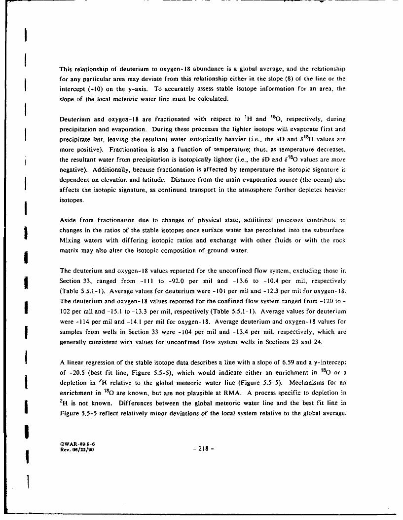
I
This relationship of deuterium to oxygen-18 abundance is a global average, and the relationship
for any particular area may deviate from this relationship either in the slope (8) of the line or the
intercept (+10) on the y-axis. To accurately assess stable isotope information for an area, the
slope of the local meteoric water line must be calculated.
Deuterium and oxygen-18 are fractionated with respect to 1H and 180, respectively, during
precipitation and evaporation. During these processes the lighter isotope will evaporate first and
precipitate last, leaving the resultant water isotop:cally heavier (i.e., the SD and 6180 values are
more positive). Fractionation is also a function of temperature; thus, as temperature decreases,
the resultant water from precipitation is isotopically lighter (i.e., the 6D and 6180 values are more
negative). Additionally, because fractionation is affected by temperature the isotopic signature is
dependent on elevation and latitude. Distance from the main evaporation source (the ocean) also
affects the isotopic signature, as continued transport in the atmosphere further depletes heavierI isotopes.
Aside from fractionation due to changes of physical state, additional processes contribute to
changes in the ratios of the stable isotopes once surface water has percolated into the subsurface.
Mixing waters with differing isotopic ratios and exchange with other fluids or with the rock
matrix may also alter the isotopic composition of ground water.
The deuterium and oxygen-18 values reported for the unconfined flow system, excluding those in
Section 33, ranged from -Ill to -92.0 per mil and -13.6 to -10.4 per mil, respectively
(Table 5.5.1-1). Average values for deuterium were -101 per mil and -12.3 per mil for oxygen-18.
The deuterium and oxygen-18 values reported for the confined flow system ranged from -120 to -
102 per mil and -15.1 to -13.3 per mil, respectively (Table 5.5.1-1). Average values for deuterium
were -114 per mil and -14.1 per mil for oxygen-18. Average deuterium and oxygen-18 values for
Ssamples from wells in Section 33 were -104 per mil and -13.4 per mil, respectively, which are
generally consistent with values for unconfined flow system wells in Sections 23 and 24.
I A linear regression of the stable isotope data describes a line with a slope of 6.59 and a y-intercept
of -20.5 (best fit line, Figure 5.5-5), which would indicate either an enrichment in 180 or a
I depletion in 2H relative to the global meteoric water line (Figure 5.5-5). Mechanisms for an
enrichment in 180 are known, but are not plausible at RMA. A process specific to depletion in2 H is not known. Differences between the global meteoric water line and the best fit line in
Figure 5.5-5 reflect relatively minor deviations of the local system relative to the global average.
IGWAR-89.6-6S•Rev. 06/22/90 - 218 -
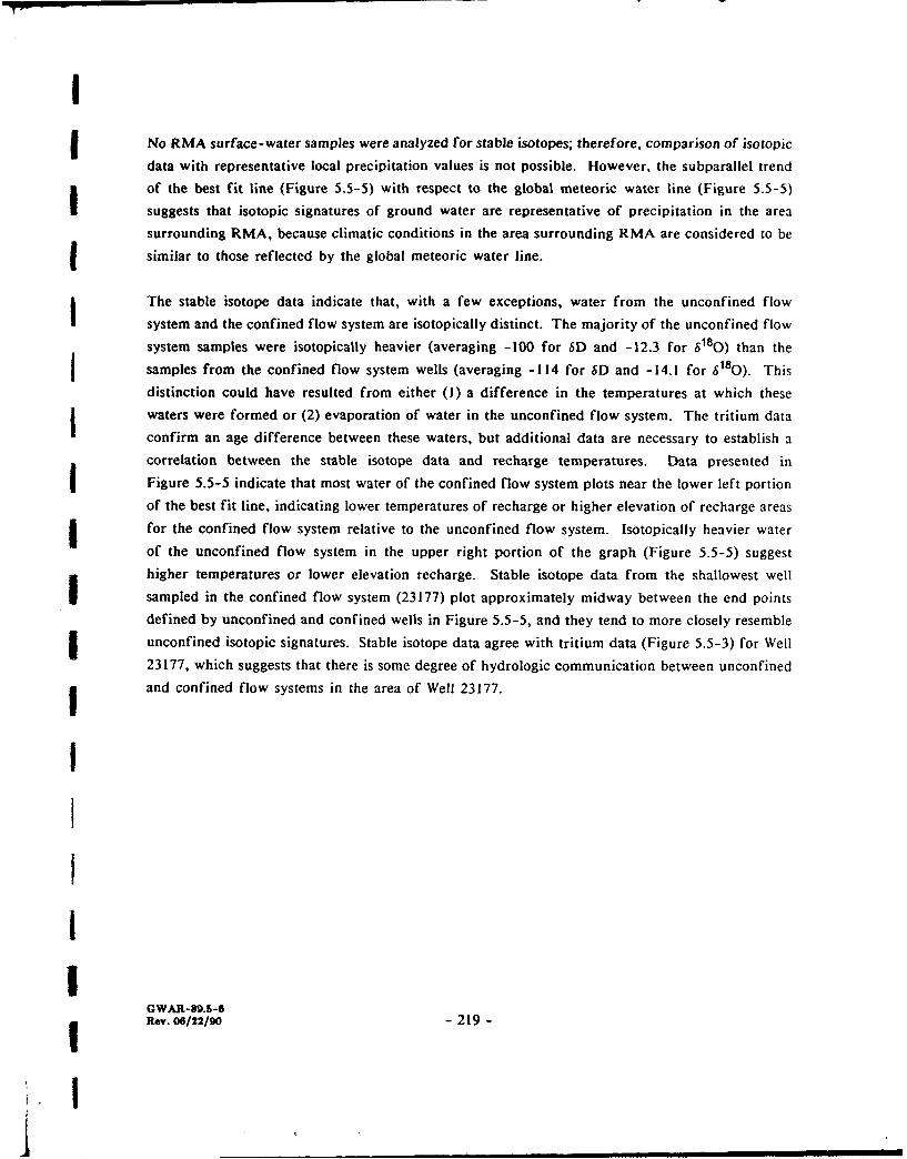
INo RMA surface-water samples were analyzed for stable isotopes; therefore, comparison of isotopic
data with representative local precipitation values is not possible. However, the subparallel trend
of the best fit line (Figure 5.5-5) with respect to the global meteoric water line (Figure 5.5-5)
suggests that isotopic signatures of ground water are representative of precipitation in the area
surrounding RMA, because climatic conditions in the area surrounding RMA are considered to besimilar to those reflected by the global meteoric water line.
The stable isotope data indicate that, with a few exceptions, water from the unconfined flowsystem and the confined flow system are isotopically distinct. The majority of the unconfined flow
system samples were isotopically heavier (averaging -100 for 6D and -12.3 for 6180) than theI samples from the confined flow system wells (averaging -114 for 6D and -14.1 for 6180). Thisdistinction could have resulted from either (1) a difference in the temperatures at which thesewaters were formed or (2) evaporation of water in the unconfined flow system. The tritium data
confirm an age difference between these waters, but additional data are necessary to establish acorrelation between the stable isotope data and recharge temperatures. Data presented inFigure 5.5-5 indicate that most water of the confined flow system plots near the lower left portion
of the best fit line, indicating lower temperatures of recharge or higher elevation of recharge areasfor the confined flow system relative to the unconfined flow system. Isotopically heavier water
of the unconfined flow system in the upper right portion of the graph (Figure 5.5-5) suggesthigher temperatures or lower elevation recharge. Stable isotope data from the shallowest well
sampled in the confined flow system (23177) plot approximately midway between the end pointsdefined by unconfined and confined wells in Figure 5.5-5, and they tend to more closely resemble
unconfined isotopic signatures. Stable isotope data agree with tritium data (Figure 5.5-3) for Well
23177, which suggests that there is some degree of hydrologic communication between unconfined
and confined flow systems in the area of Well 23177.
I
III
GWAR-39.6-6Rev. 06/22/90 -219-
I'
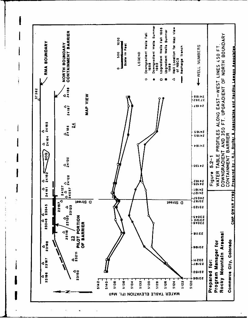
-E e>IL c E >_
>. U.
- .0
*L A- w LLn
az a j amo 0
0 a,* CL-* 00 0 ** a00
z,, 0* 0
Cd c
L9 Ir aw r0L W0
0 -
InI Cj
-rtv 0( <CdX
CM w
CIIF. 0 c'
VSr cm
CIA
I IIL Ic Me
Ow 0
AL~ 0
-099e E
0.0Usn~~~~~~~ NOIA1 UVL 3V LC
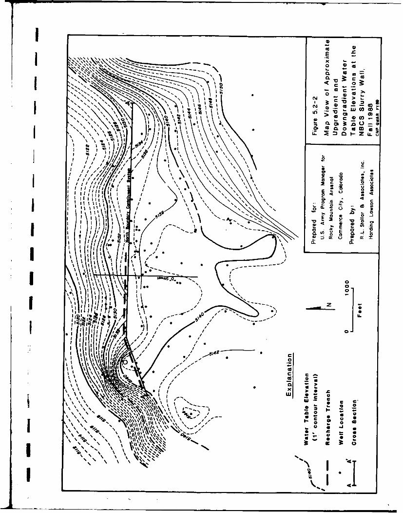
E
(040N ' I.. -%
v-- 04.:0 :3
1- (1 ) o c
'.~~L N\ X * \
fL o 0.Z00W =8z: ~O-LL
0000
E4 0 0
60. tL .
-~ 0i
_ 00
WI C" ''
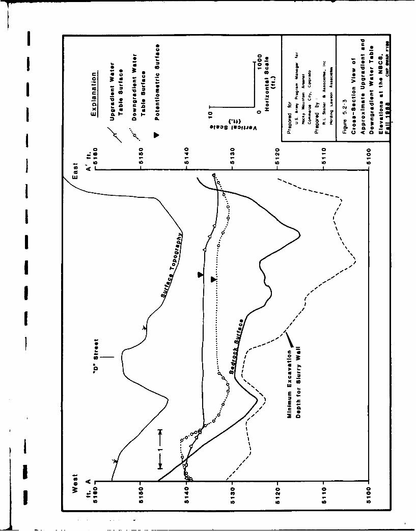
Sc
j Li a
S *0~ - 0 0 -
0 - 0wIL 11 0
04 S 3g3,
011009 IWOIJSA * & a 0j *o p~ 0. 0
- 1' 0 10 10 10 10
LUU
..d.pro.-
ev/
40/
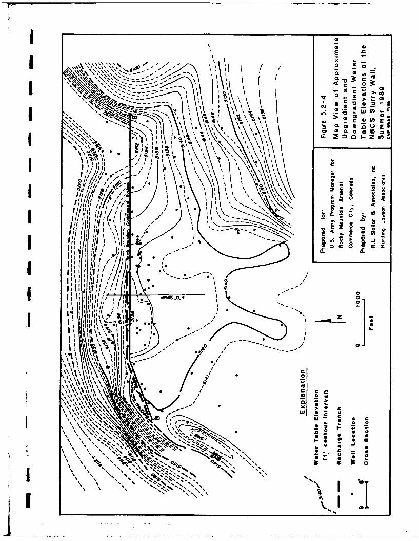
I .• ' co 4-
E
\•\,•,•,•.•\.. . ,.,60P i 0 CI
-- •' •Z." " 0- rl c
" - -- - -- -ca - i >
- - 7 0 0 E
I ' .w io
cp Cc Co 0 o"J ma
4%6
till Il
-. . °p
it L C(1
Ill I'
- '. . '--P-•'. h .WI-
Ix C
it ,, t-fil ,, se. .a.:.: 0
/ IIi, I ,I P
'II,, N *\,
'III S a - 4 0 J~*
'Io,
p,~~~ 0 0.0 0 .-
5o 0 in
j \ I Pu' -'- ' .," "
NL
I '- 0
' IBON -
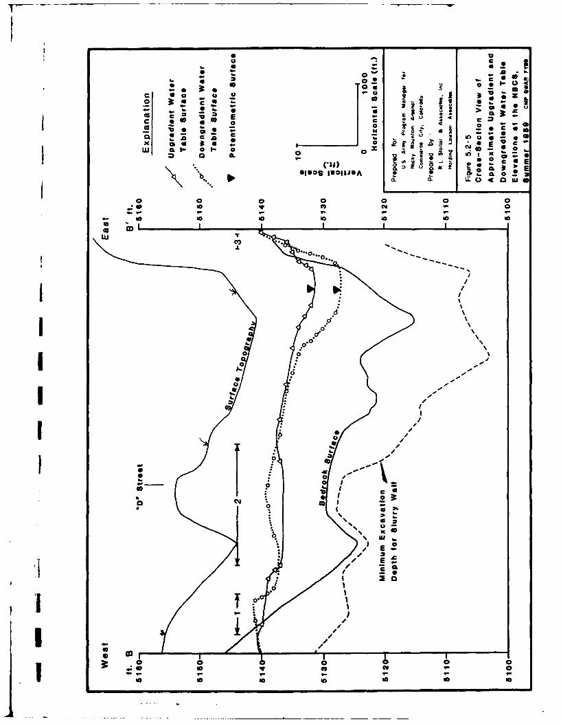
4i
0 4
C* i* 6 1: i _ _ _ _
Ix
E- -
20 E
*b C 0 - .
In -
E.
CIOIc
go

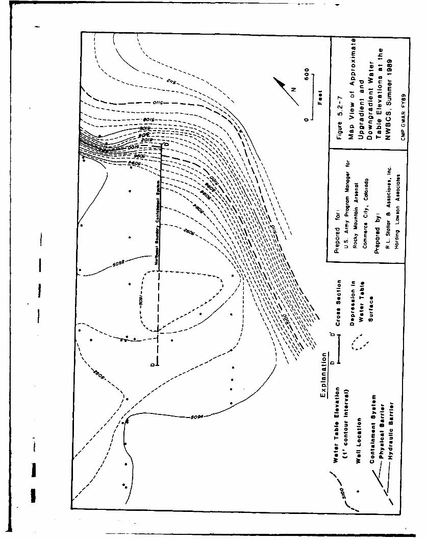
I ¶ II I I
0 L
0 0 *" •
- - - - - - - - - -- - - - - - - - - U
N00-
N -J- -w =
I .. . . . . . . ." -- . "- . "- \ I - -, -- •.-- oIg--- r -. ... - ~-,, - ", IL L C •.lO 1c)
N N ) - "I - - - N \-. ..,, U,, } • , \ . \
I 3 -- ,- -• • ~ - - '• ,
21 -N,,, N % % '." • \ " \\ \\ ." o ,-I- -- -, - -•• ,'•,• • • ,El ". ".\ " .\ \\"
609 Nl \k-
* N\ ' '\- ' \ a .\
N N a
' - -" .\ , \ \ \'x \" e -,.
• " - - -- - --I • ,I •' , ' -
- 09 JU soU
,. I X
\.Jz * I .
"NN. 2 . ''SS'S '"1 j/C
* C*li
N -- 0.A 0 x / a- -
•. 0 j "• • =
,-, /..
- I i l l 0 l m lllll l i l l l I

5144
nln* 4.r 4 2
2W4 01 ss 092-290
Group 1 6 GouGroup / .m:ri.
North Boundary G roup 93146
Containment System taw too 614
Screened'G eologic Z10 22 13 12 4
Symbol Interval
a Atiuvial-Unconfined
£ 2-Unoemfined 14
* #2-Confined
* *2-Confined -40
(Group 6 only) *'\\ /A I
o #3-Confifled )9 . /
0 #4-Confinedz
a 06-Confined 4
87 88 99
0 0Goo3*0 4 1-4C * 744*(U-CON4 4.. 23177(82-CON)
Foo
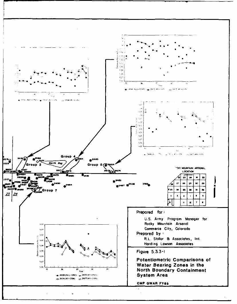
1 A
'12'h
a O
•-771
3 211g 4 4 g 40 24 1
am ~ 0 %
Prelared for
U.S. Army Program Manager forS.... Rocky Mountain Arsenal
.... Commerce City, Colorado
,,,, Prepared by•i• ,,, ,• •R.L. Stollar 1B Associates, Inc.
-" Harding Lawson Associates
,,, Potentiometric Comparisons of,,,,, •Water Bearing Zones in the
"85 96 8. Y " North Boundary Containment-0-_4,2(^,M-UNC) .,,.,•• System Area
CMP GWAR FY8fi
i m - - • • m I • I I i I I I I I:

0 0
cm 3 0)0 0. 0 C.
03 M
f- 0 401
t a&IraE 9 *0p &LE LV
0M 0
zo11 ;N LL
>4
emOCCC
6SLC
4CL ige
tac see
WWI/ ) dVAC (I/Orr) U!PPU3
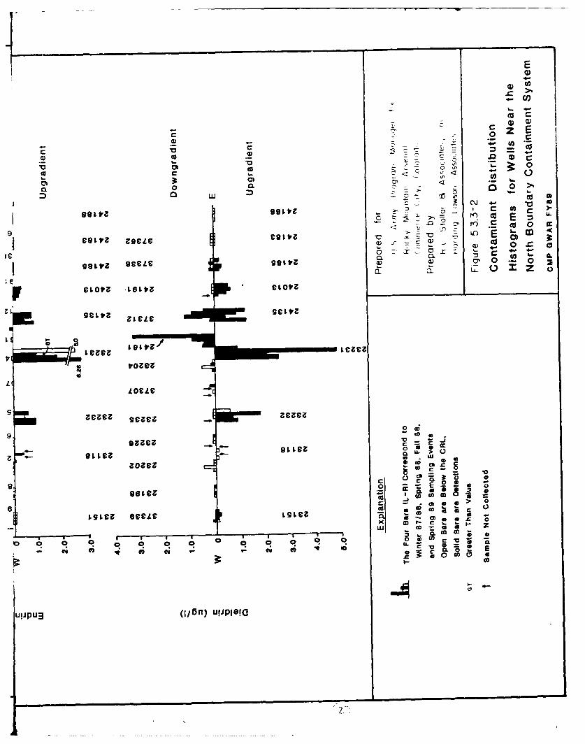
CC
z E
w C
2~ 4 -7' NQS 0
a) CO 0CL IL
:9~ Z
CLOV t6V CLV
-I) a 27 & 0aaSC
&89 t.0. 4- 4
9ace
SC
ote Otter -
z~ava Cc -4- C
4-t V3I
C 0
86 2m 0 0
c ; 0
C! U.0
0)
ulipua(I/Brf) u!JpeiGa
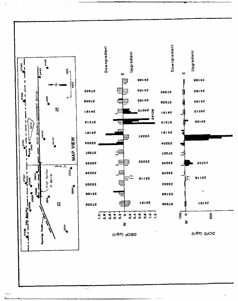
- CCP.-
on
0s 1. Seitz
-7 39a esc &o
0 ~ 0
0 - rr(n 0 9~4~'rLU voca *OzLC
4S.1 0ogiN Lgi
9gczc gena
6CCLC 191. 30383L
~f &99 __ _ ___ __ _ __ _
31 ~ \(f/T~)dD8CJ (1/511) CdOC
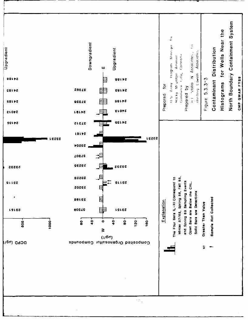
E4)
c c >
0) O 0)
CD c Z0 =l 0
0 C L.cot to cc 0
0 IM
go~~ t v
LOCCLE
0l 0
ctova ~~~ 00C Z
Ute~e uJt
191C~~~~ SCLCLC S ~ ~ .~ 2 E
I~ M
C -0
gotta Cr) 0 ,i,6f¶)~~~~~~~~~ Zd~S~ldO fJ~l~eJ esd
CL0
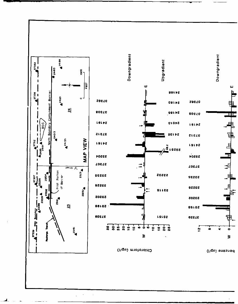
CLCSM
Nj w
0
&Ot CLC 0 V0
0.
pn A0, 6
-# CL~tS LOCLtC
J ~ ~Lee ge1. stageL
z. 9aa,
scoLe CtaOC
oCL L9LC V- Lc
I(I/On) wjo;oj0IolC CI/Bn) euezueq
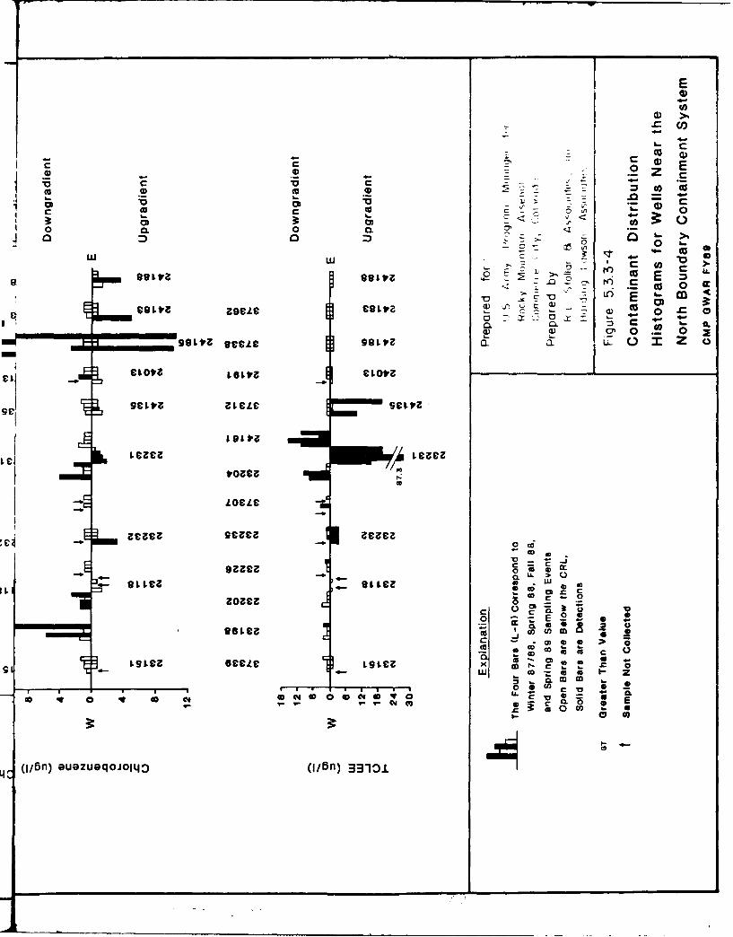
(D E
w --
-~~ 0
0) C7 0 0 0
geelc- nqt U 0
t0 oL CZCZ t9CC oin-
CD
933ca c -
-~~~~~~~i col 0L 9It U .
0
cc ;z C 0 -
4-~~~ ~ OLIC - 9I L -
0- 0 -)c1
q E
0~~~~~ CD 0 e. e 0 O 0 0c
4,(j/6fl) euezueqojolIqo (I/Bnf) 33-1z0
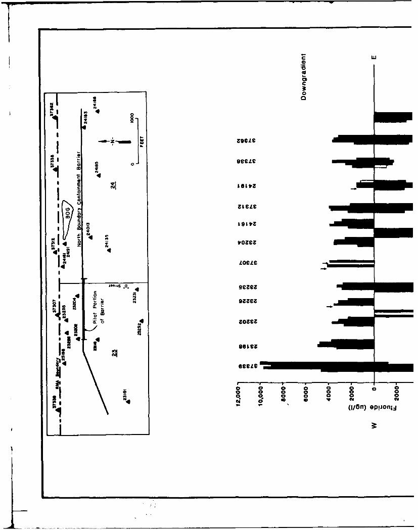
C wU
0
00
LOUC
00
0 C49IBy apn.
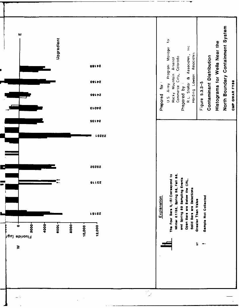
E
C0 co
00eLv E f 0 0
cc 00O
*.- -0Io r- co
a0 0c
0 0
11111 -COo~ Co-etov L sA
C.) 3: Z
29 L Va~
O&LC 0 m I
CL U.~ C 0
o o =~~ 4-V
Q. CL L Z C
0 0 E- >
c CwSemi.
& -01 0 E
CI 0s0 0 0 x ago
,gCiWi eon-.z
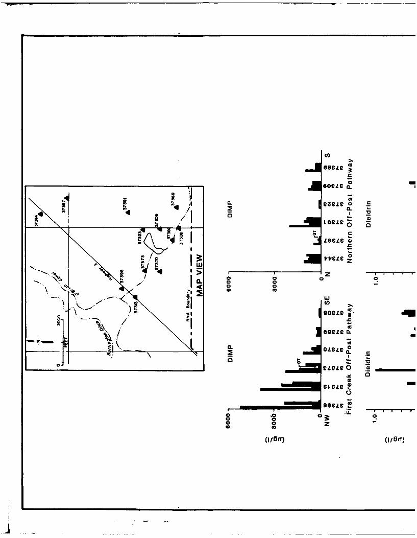
0
1 1. Cl
90C
L9LL
I~ zIoco
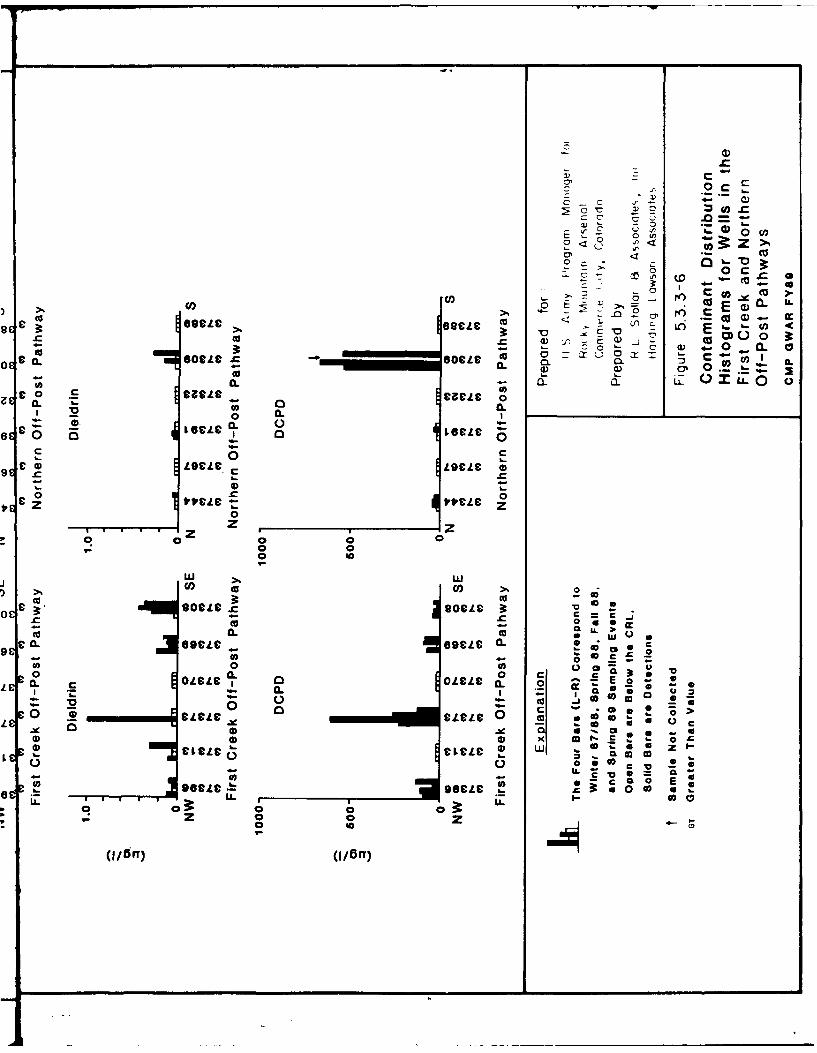
0 c c-
00 0 c00
-0 - O 0 4
o r E CD003
-: 0 0 0 )~OO. a6OCLC ~~SOCLC 2OS
0 a0-0- a--
V0 C.
0 0.0
9 4) ILBcLc L9CLC 0)
00
0 -U
co 00
0o a.OLLC 0ol C9L ' U
~ V0 0 10o0 CLeLCX 9LLCLC 0 00ELE I~ -0 .0 w0:
LC 0L L 0L L 0. 0
0 0 0 xt m .s!oC&C~~~e CCm ) ZI
=ICL , ao 0
U. CLL .
Go CLC h 0E
p z z o a
U-IrT (ILn
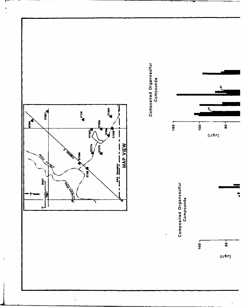
CM0
O o
- o
0.E
00 2
"0
',, -% ' 'Si 4. m I
I9=• I - a
o 0V C ,01..... L 0'
0 c
0.o
..0
0.
E0
o 0oo
(t/ -0
CM IIA-
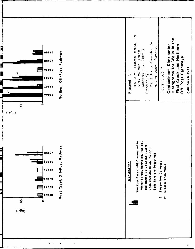
1 -0
0O LO
a. 0 .11.
CL~
o - 3: C013 I
tac6c 0
00-
CL E E LL
oez <0~o C
(1O611
0 'a E 0
0OL -J Cu 00 r7 .
0 .-
aL 0 u
cc =
.9- I- 00a
CL 0
aM E
(1818 )
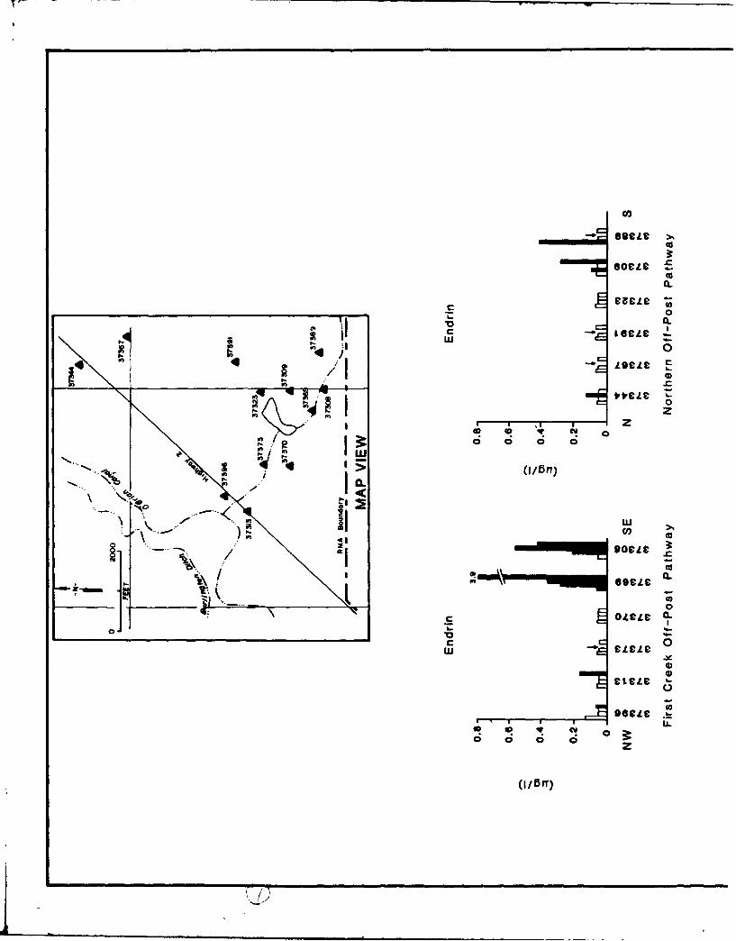
0
(OCLC=u
C ~toLeI... 0
I~0~
44 j41 4 -~ 9eLeECK Cu
ttLe
0
z
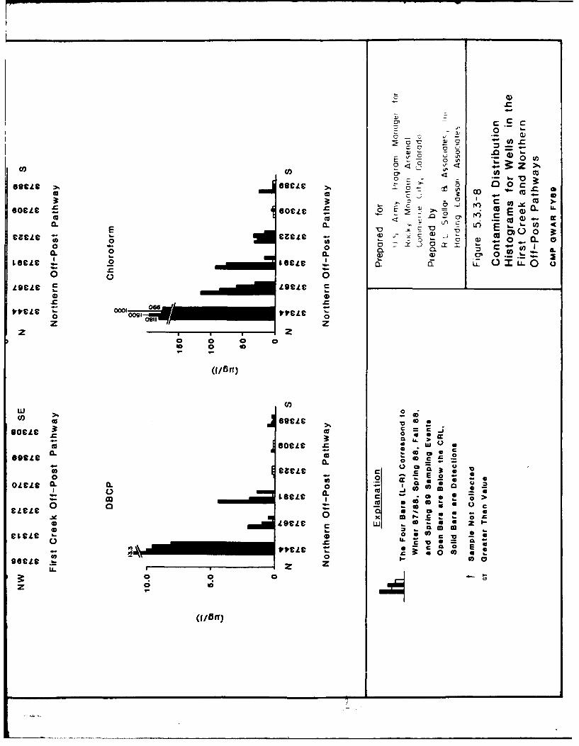
C C-~ 0
oC C~ -o
Co ()4o > .0'CS
0ol -oez :E 0 ý U0 E 0
0. y- a'.0 -EC~h- -m 0~L o 3: UO 0
O0 0 Z_ T-.O.
oZ o Fr O 'o
00LOczt IC 19cle C__ _______
f 06
VVCLC 0001o 0091VVCLC 0
z z
too
w0
- ~0
-ol C~L0 I 0
0 -W oOILCLC C. C.o
00. F,
U. -. -mUICL C- V 0 C~
IL
0 0 C4;.
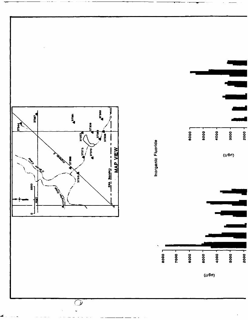
~ I0 0 0 0 0
0 '0
.dI..
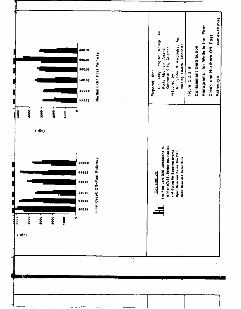
uS
a 0 U,
0 0 9?.90
E4 0a 40
0'
eggs 002c eQ u >%
_ _ _ _ _ id85 3:* 0
0- 0 00. 0~
0- .0 O
co~~ o Q.C 0.C 0 c
0. iOC.O00
o 40 a
10
so, 0000x 0W LLw
0 0 0
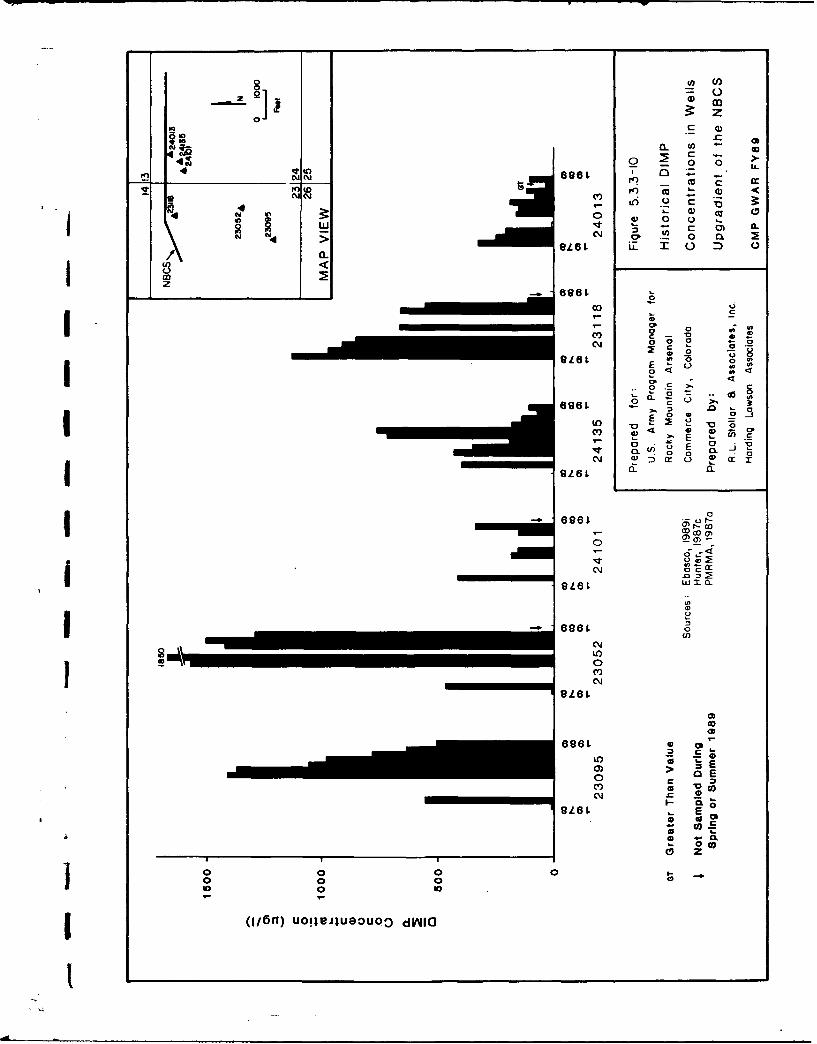
8 i
0- z
2 I0-
I0 C
0 o -c
0~0
04 C
00
0 a. ~ a
Soot -
00 -
CV) w 0 4
9L6t
Das
SL6I. WMQ-
U'U)
1.)
c.~c
0E
04 0
0 a
0
0o0_ __ _ _ 0
0. 40
(I/Br) UOIBJIUDUQOdINI
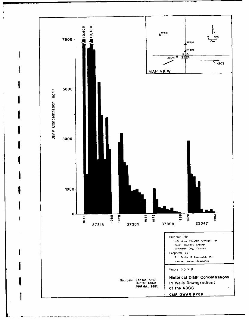
° ° 00 O
700037309
157 30e
1413P 3o47, 2 2324
""NBCS
MAP VIEW
.- 5000
0
0
I I-C
0CI °Oo 3000I
I
, 1000-
0 00 O O O t o O" 37313 37309 37308 23047
Prepared farU.S Army Program Moaager for
Rocky Mountain Arsenol
Commerce Ctty, ColorOdo
Prepared byR L Stollor B Associates, Inc
Harding Lawson Associates
Figure 5.3.3-11
Sources: Ebasco, 1989i Historical DIMP ConcentrationsHunter, 1987c in Wells DowngradientPMRMA, 1987O of the NBCS
I CMP GWAR FY89
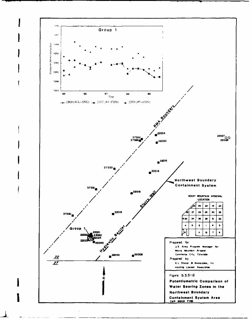
Group1
3u,< 0-
85 86 87 88 89
ý220j2i](ALL-UNC) -flu2S 4-CON) 2-2024 (#5-('ON) V,
37.222004 20703 -wd 22060 Z2020
f ,/ 2201537333m
II NorthetBudr37331, / 2201 Containment System
/ ~LOCATIONI
33 7 22019 as2 110 29
A 52
/'roU 22
USpce Aorm Program Managetr forRocky Mounlain Ar e*"I
2,?2243 209Commerce City, Colorado/ - Prepared by27 R.L Stollor 8 AssociOM., Inc
Harding Lawson AssiociatesSFigure 5.3.3-12j Potentlometric Comparison of
I Water Bearing Zones In theI Northwest Boundary
Containment System Area____________________________________________________ CMP SWAR FYN

0
r4-
0 a 0
& Celt
& a(I,+1 - i~601
(16)di
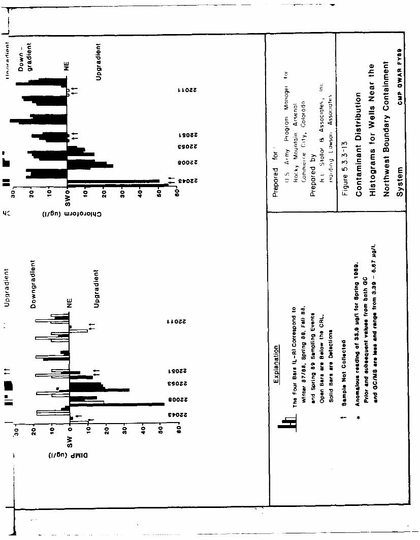
6 0 0U
00 Z
0 0
E. toO 4. 3:
4.-Lu- 0 d B
9003a Co
0'E 4) E)
~t cm 0
CL C h
o C-r( 0 o
(I/6n) w*-o.o~
a) 0 0-
0 Cd Ed0 *CD6
la
Cc C 0 2cCL 0~ o
0 EZ
C Ll cU)i
0cc 41 0 _
CO~j~z a -e00D0 ca P,
c OO CI L *a 0
o cc 00 C0 a
(i/16n) dflIO
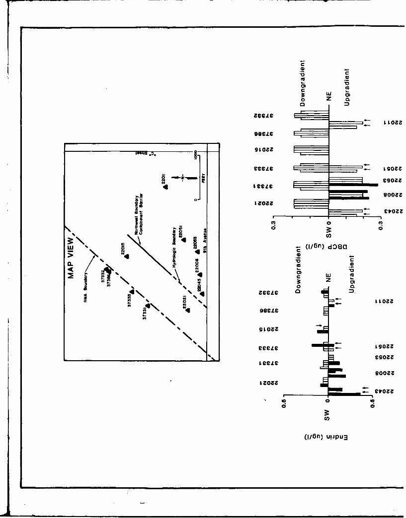
'00
stozolawas .3.
-~ ~ ~ ~ ~ I ----------t Oa
9SCLCa
soozz
No~
A %L 04
% 04 C).-
I. ~CLC
09aCelt
(116fl) UIJPU3
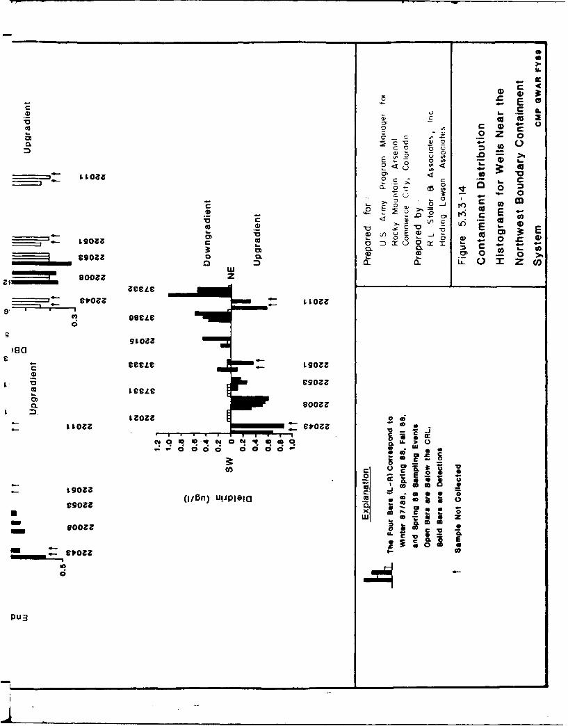
.2 z
w0
Eu 0
-------- no CP
- ~0 I 4-
- - - - - - - - 0 c---------- C~- x L00 a g a Dt W(
0 CLu~jD- CL -
-- - - -- - -e v c 0 L . 0
0 0~
______c~ou o0&O0o .9aOZ(
Wgz
c±zSOOUe
~sCCLC4-.z o-
9i C? Iý IR e m It I
9ICCLw
t~zz*
C E.
0
PU ICL
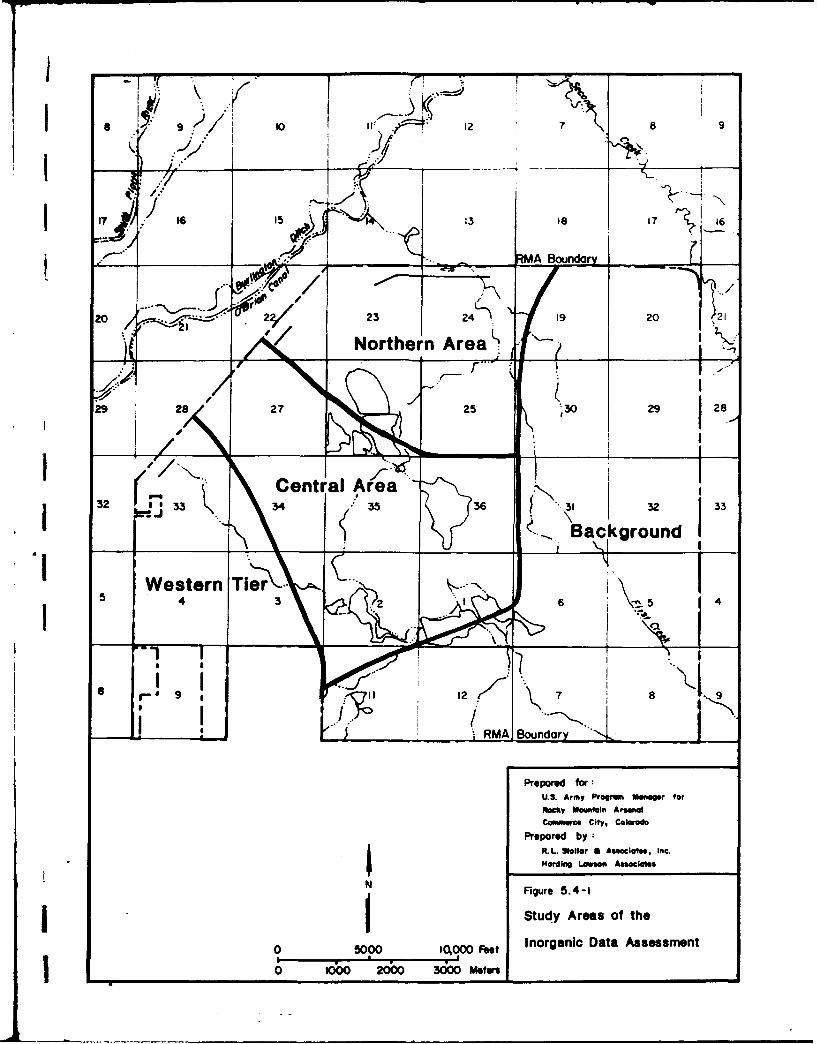
W7 -11C
- 9 . O ,. 7• \ 0 1
i _,..__ __------!-,:• - - - -•
-7-IM -ABoundar
20 2 324- 19201
4 / Northern Area
29 28 27 25 k 30 29 j 28
Central ea -e " . c,,,,32 1 33 34 35 36 31 32 33
'X. 'I ,, f --.... Background
.1Western Tier. I6 4
r-,'" 9 12 7?• l8 •
"S ""RMA Boundaryy
Prepared for:U.S. Army Progprm Maneger for
Irony Mountain Arsenal
Commece City, ColoradoPrepared by :
&.L Stollor G Asoocite, Inc.
Harding ULom AguClant_
Figure 5.4-1
j Study Areas of the
0 1,0,=00 F~t Inorganic Data Assessment
0 0= 2000 3000 Me••rs
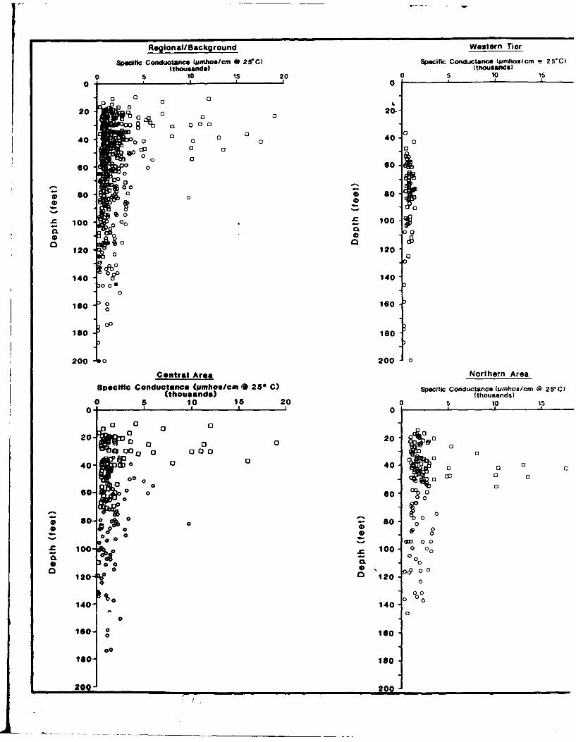
Regional/Background Western Tier
Specific Conductance (umho*icm @ 25"C) Specific Conductance Wumhoslcm % 25-C)(thousands) (thousands)
0 5 10 15 20 0 5 10 150 - , I 1 0
0 0 0
20 0o 20-
09 0 0
40 0 0 0 00 0 0 40- 0
0 00so 0 G 0o-
0060 °0
0 0 0 8 0 -So 0
00
O140
:E 100 oc 0
io 12o€3 120 02
140 0o00 140
160 160
180 180
2000
200 -o200 0
Central Area Northern Area
Speciic Conductance (Vmhos/cm* 2 5 * C) Specific Conductance (umhos/cm @ 25'C)(thousands) (thousands)
0 5 10 15 20 0 5 10 15
0 0 00 0 0 0 20
00o0 0 000 0
40- 0 0 0 0
000 0M0 0
0 o 0so- ~0 0 so c
60 0 0
60- 60SO E 80 o
00. 0 0
0 0 0 00
S 100 0 100- 0 00
0. -a 000* 0 1 0 0
120 b0 020
0 00
000
140f 140-- 0
10160- 016
1 0 180
200- 20
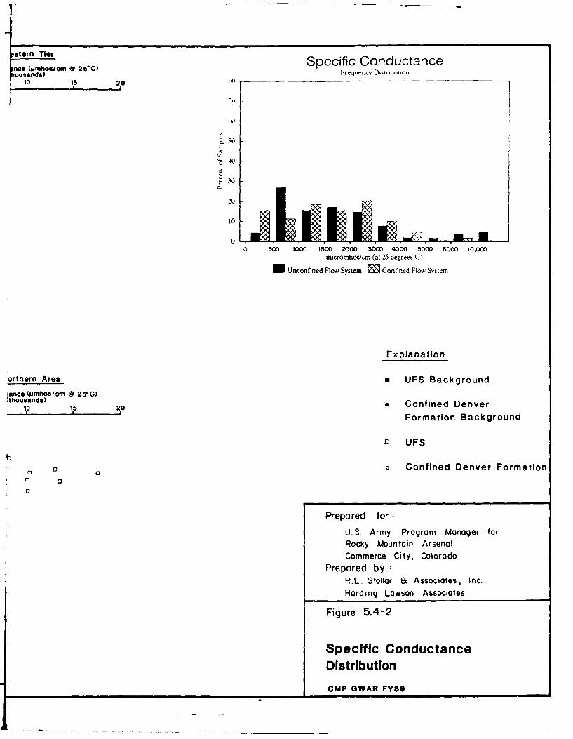
stern TierI .nc. ,,...,=., 40 2s-c) Specific ConductancehouSl•ads) Frequency Distnbution
10 15 20
E
C 40
' 30
20
10
00 500 1000 1500 2000 3000 4000 5000 6000 to,000
micromhosim (at 25 degrees C)
U Unconfined Flow System Confined Flow System
Explanation
orthern Area a UFS Background
tance (umhos!cm @ 25C):thousands)
10 15 20 . Confined Denver' ' Formation Background
0 UFS
* 0 Confined Denver Formation0 0
Prepared for:
U.S. Army Program Manager forRocky Mountain ArsenalCommerce City, Colorado
Prepared by:R.L. Stollar 8E Associates, Inc.Harding Lawson Associates
Figure 5.4-2
Specific Conductance
Distribution
CMP GWAR FY89
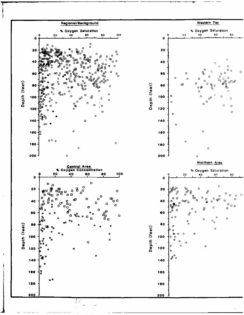
Regional/Background Western Tier
% Oxygen Saturation " % Oxygen Saturation0 20 40 60 80 100 0 20 40 60 80
0
20- 0 0 0 20
o q) 0 0
0 I 0 0o0 0 o- 003 o o C 40 0
0c~.ocQoP a ~ 03 0 0 0 000
40 0 0 0 0P 0 00 as a ý S6 00 0 o 0 0 001 s0 Cp
0 L'O o 0 0- 0 so - 0 0 1- c0O 0 0 0 3 0 0 0
0 10 (b oo 0 00 0 0 0 0 0
*o 00 0, - 0 aO 00o0 oQ 0 oC 0
80 100 0.'0 0 1o 0 0
2 o 0 0 %0 0 ( 12 6
00V~00 0 90
12o cp0 0 o 00 0 0 to 120 0
140 140
0 0 0 0
10000 0 16 00@ 0 C 120
0
0 0 01600 0 160-
00
0 0
200 0 200 0
Northern Area
Central Area% Oxygen Concentration % Oxygen Saturation
0 20 40 60 80 100 0 20 40 60 80i0 , I I I 0 I Ii !
20 0 2000•
20 0 0 0 40 co 0 0
40 0 W�0o 0 a 13 a p °b oo o 000 a0 0 00 000
0 0 00 0 m 0 0480 o oo O) 0 0 E004 0Co ao ý60 0 00 CP001 a 0 1600 00C 0Cf0 0 a 0 00a 0 0
00 0 0
0 0 a 00 o 0 0000 0 0100 0 0
so 0 00" 0 0 0. so 0 o
0 % 0 10 0 0 002, 0 0 ~ 0
*0 0.0 a 0o120 -0 0 0 120D 0 0
0 0 0 0
140 140
0
160 0o 160
00
180 180
200 200
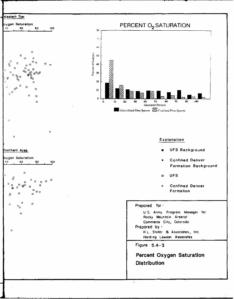
Western Tier
xygen Saturation PERCENT 02 SATURATION40O 60 80 100S I I I I I I,)
C3- 500 0o 00•
j 0 0
0 o0 0 4 .
0 0 0C3 0 oo•3~0 d% oop~ 30°%o 0 o
E610 20
D 0 0 0 100
0 00
0 0 10 20 30 40 50 60 70 80 >90Saturated Percent
U Unconfined Flow System 2Confined Fo" Svstem
0
0
Explanation
Northern Area a UFS Background
xygen Saturation Confined Denver40 60 80 1C0S I II I I /
1- Formation Background
0 oo UFS0
00
0 0 00
0 o 0 0 0 Confined Denvera a000 Formation
0 0
00 Prepared for:
0 U.S. Army Program Manager forRocky Mountain ArsenalCommerce City, Colorado
Prepared by :0 R.L. Stollar E Associates, Inc.
Harding Lawson Associates
Figure 5.4-3
Percent Oxygen Saturation
Distribution
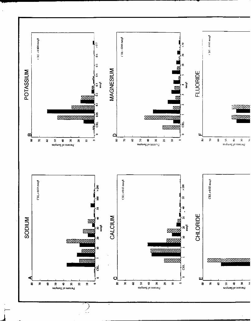
00
CLC
CDD
0~0
soldweS jo lugOa~d saldWuS jo IL0D2'd s~idweSjoiuaia
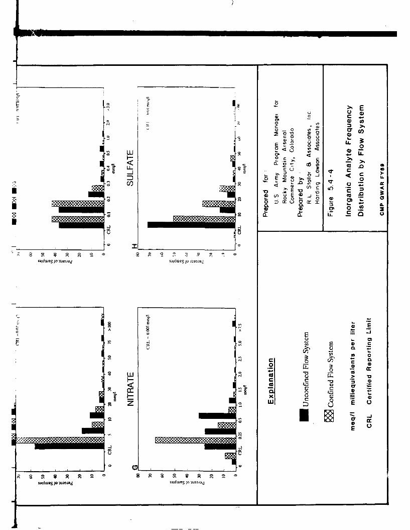
rc
7- 0
-n00 Tu 0 (A
o LU OU L
LL 3: -
'2 a, ~ it)*- Ev -a -
0" 0
at 0
oZ S
A
C~l0 0
~ LUI- CD*
-J 71 0>0
< ci aoC
oidnwuS jo wIoiad saidweS joiupa*
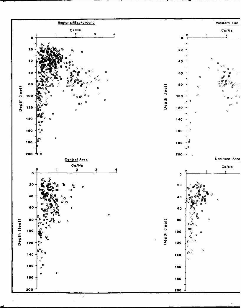
Regional/Background Western Tier
Ca/Na Ca/Na
0 1 2 3 4 0 1 2
0 &0 0
20
a C40 4000 6t:0
0 o ° o0 0
"0 "°• o 0 000 . .0 CID 0
~'00 ~ '80 0 0f
0 o 2 1.0
140140§,I0 SoCo l 00 0o,.o 0 bo 0S 1200 a 0 0
10 ,, 0 0 ip 010 0 •
no O " o q•140
0 -o0
160 0
10 0 0
000 0
200 o
Central Area Northern Area
Ca/Na Ca/Na0 1 2 3 4 0 1 2
0 - Io - I 0 1 0
ICc " a0•• o•~oO120-@b o.2
60~ OCec 00
40~ -o 0 60 gdO
0,o ' ,40 .o°q 89AoO 0 00
V 0 0b
80~12 0 0 0 b0
00
140 C) 08 0 s 0 0
18~010
00 14 000
0100 0 0 1000116
200- 100 0
200
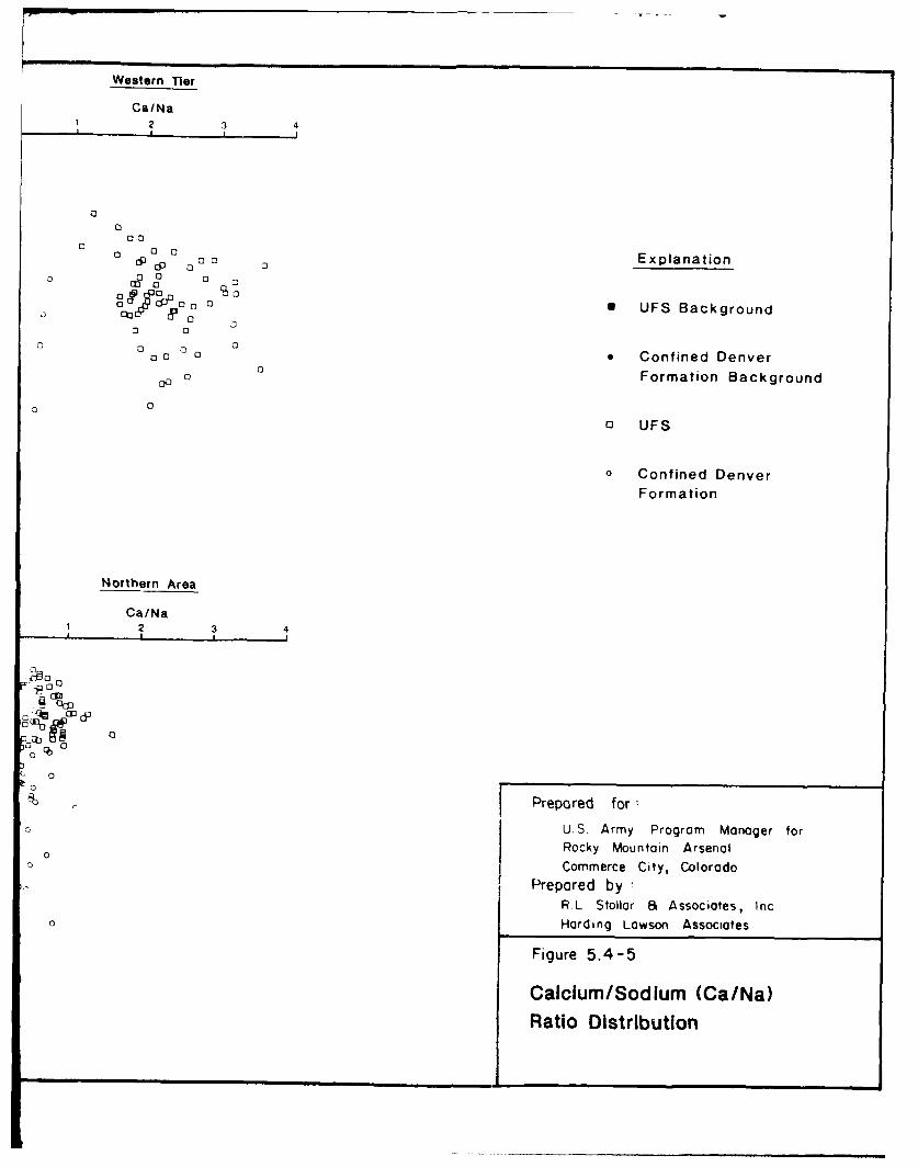
Western Tier
Ca/Na2 3 4
00
0 P 0 0 0 0 Explanation0 00 0C1 0
_ 0 o UFS Background
00 cJ0 0
0o0 0 Confined Denver
0 Formation Background
00
o UFS
0 Confined Denver
Formation
Northern Area
Ca/Na1 2 34
IIE
Cp
C' a
C 0
0
Prepared for:
U.S. Army Program Manager forRocky Mountain Arsenal
0 Commerce City, ColoradoPrepared by :
R L Stollor a Associates, Inc0 Harding Lawson Associates
Figure 5.4-5
Calcium/Sodium (Ca/Na)Ratio Distribution
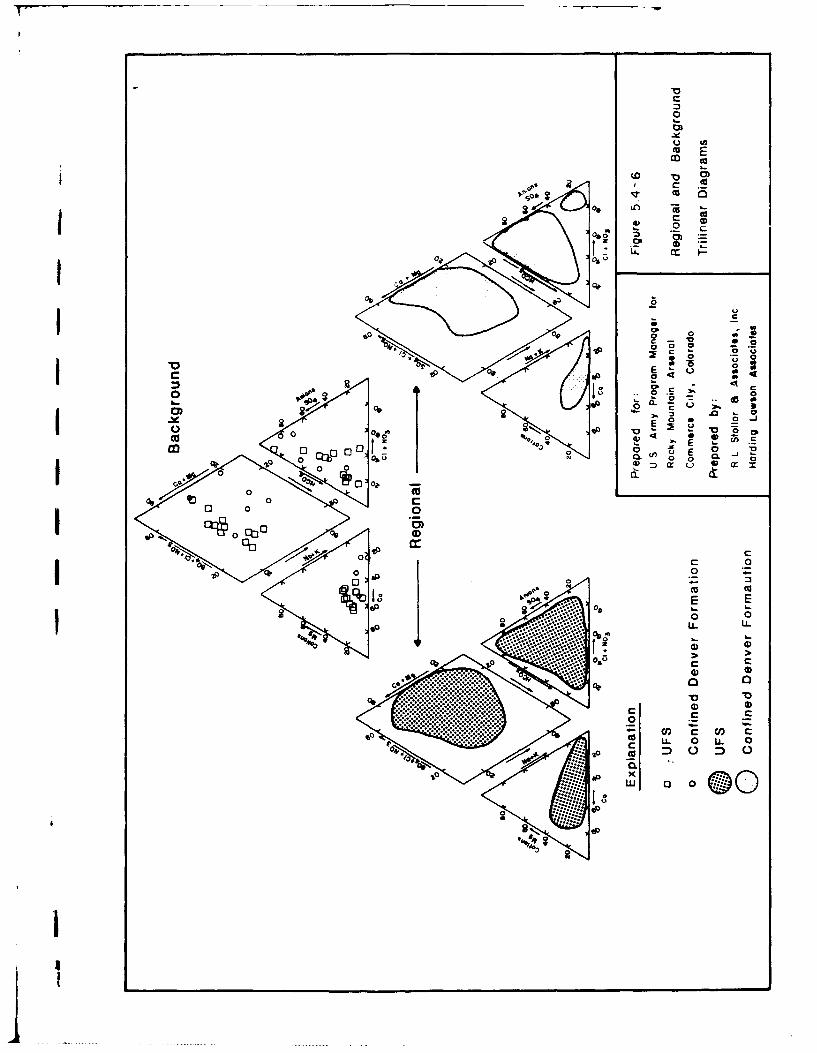
Cc
.0
0I Cd
00 LCn
060
a- 0
0 0
c~)0.
0C 0E 0 -0 -
0 0 )
wCLC
LaiP Eb CD,
00~ji
I0I Xp.
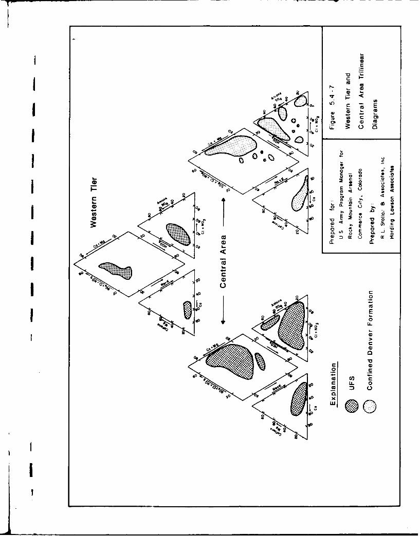
)co 0
0 U-I90% e0
c
-
00c a
r_ wo 0g 0
0
CLU
aS 0 Ea 01
2LIa,
0. 5 >
04 #
o o
&P CU CL )C i.
0, o
Is
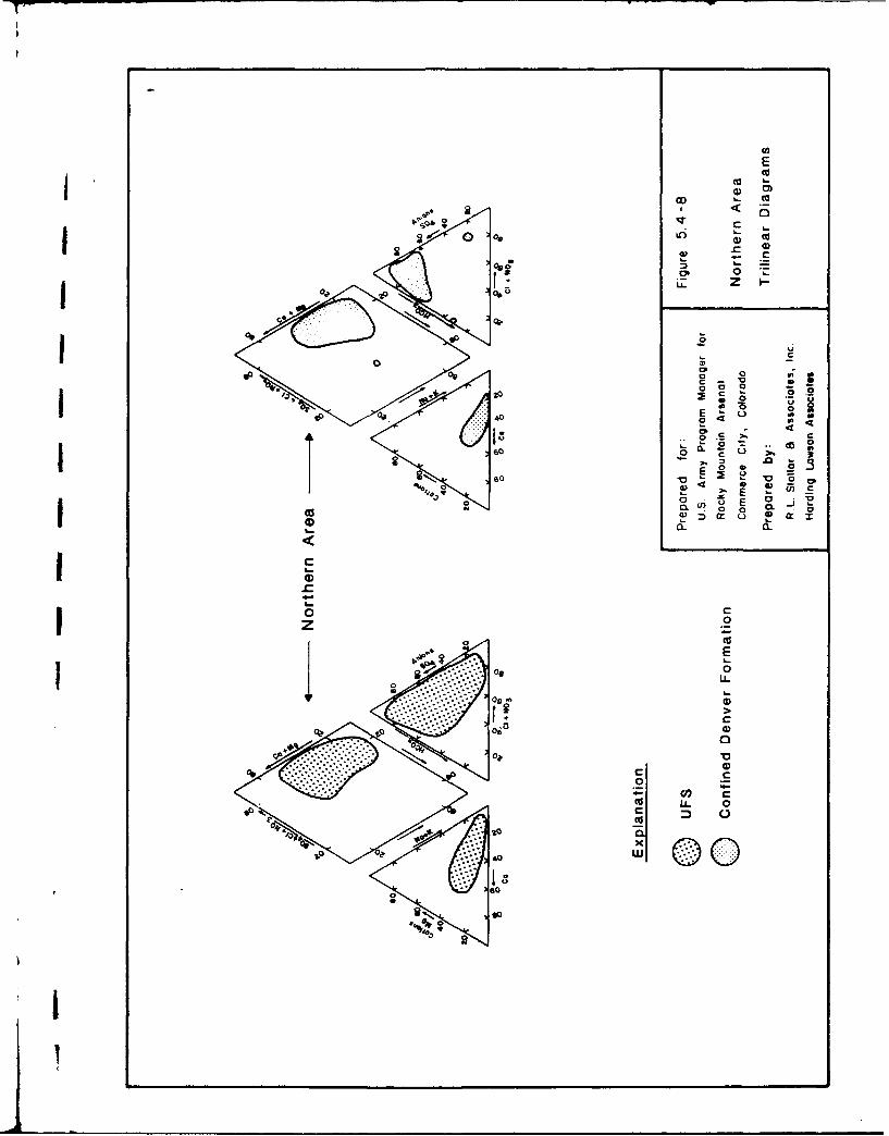
E
4. 06
$0~ 00
0 0
LL Z I 9
20
00 0 C
D~ W-
Cl?4 C~
0 -
360
so .

_ _ _ _ _ _ _ _ _ _0 CL
0
0
0 0C3 L N
00 .0 i
LO cU
_j N CO
Ev E' 1I~~L Q LJ l) <
wI C _ _ _ _ _
-* CO
Z..~: L 0I 00 -0
u - 0 Q
za
(N r
00z0
e(N
C44
C14
________________________________________________
IL
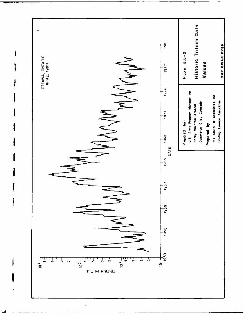
000
00
0 I
Z
to' E 0 0IV.
000
,~LLo
I-m
CAC
'D
4D do M u
Cý .D
'n'l N Hnii4
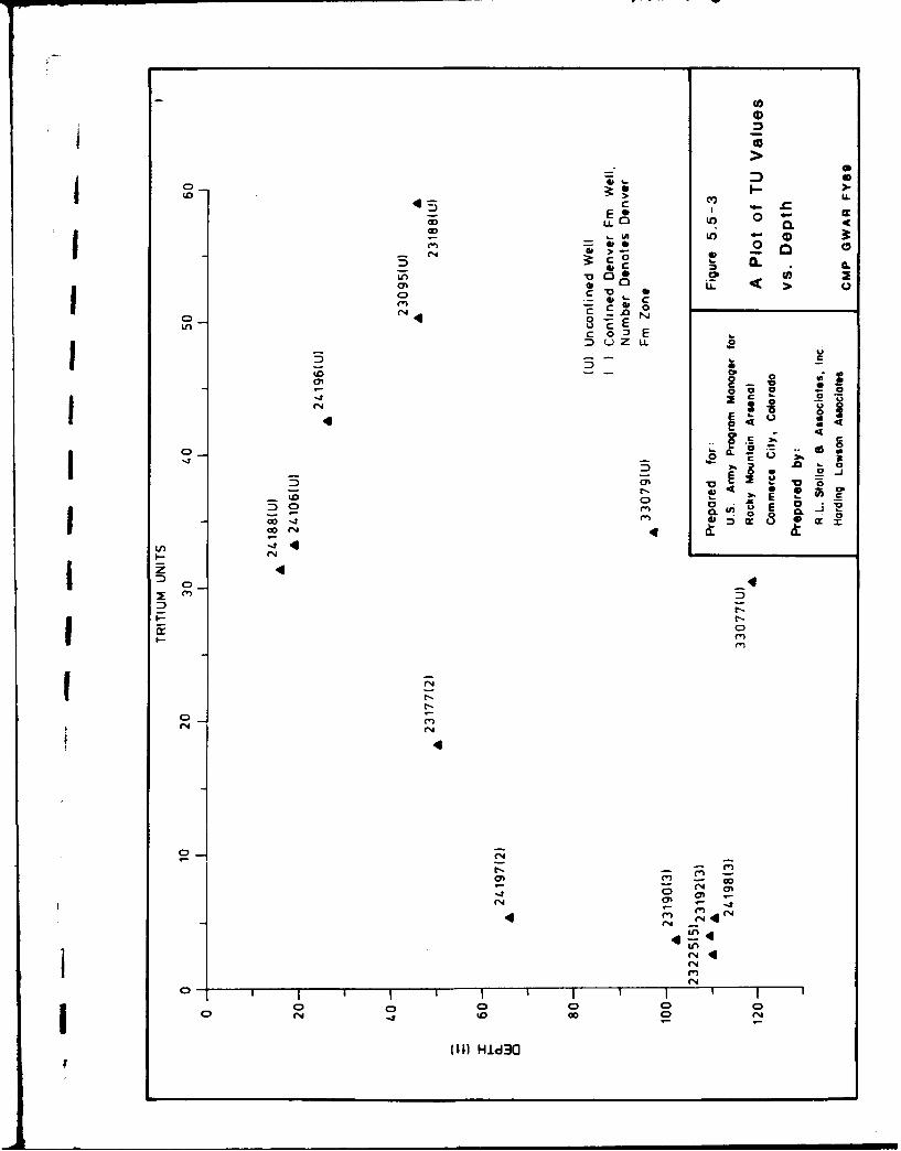
0
00
en= 00cCD 0- E 0
co 0
0 -
0 4
0
0 E
CD s
44 (N4(
r4~
cm 44
(0
C(N
0- ~ I I 1 I Tgn
P 1) Hld3O
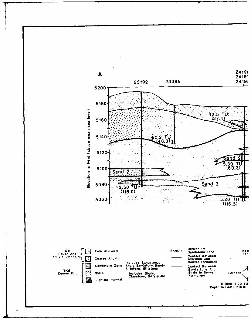
A 241942419'
23192 23095 24M95200- I
51804"
CS5160-'*-** (2T00
0 0-.000. 2
0
.0E 5140 o- 000%o.
~. an
C 2_____-(9a
5080 ----- Sand 3low
(116.0)-
500 --- 5-t.20 rU> -i(116.3)
Oat I Fine Alluvium SAND I Sandsoer Zone 24 11Eolian And JE adtneZn 4
Alluvial Deposits Cors Aluvu Contact Between24LJCoreAlvu Alluvium And
Includes: Sandstone, Denver Format ionr JSandstone Zone Shaly Sandstone,Sandy - Contact BetweenTKd JSiltatone. Slltstofle Sandy Zone And
Denver Fm. Shale Includes: Shale. Shale In Denver Screens
Lignitic intervat Claystone. Silty Shale Formation (D thI Fet
(Dept In eet)(116.0)
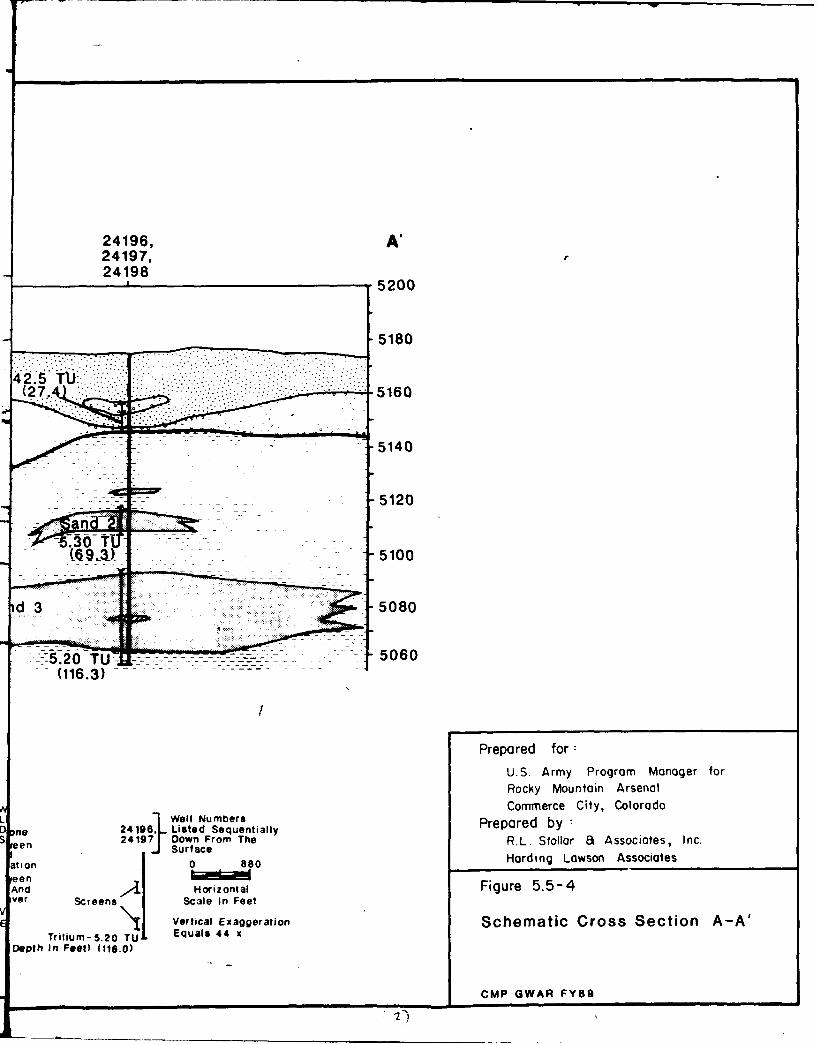
24196, A'24197,24198
5200
-5180
42.5T(27* ::. 5160
-5120
n
(6 9 11)1 5100
id3....... -5080
_--§5.20 TU-- 5060-(116.3)
Prepared for:U.S. Army Program Manager forRocky Mountain Arsenal
A Commerce City, ColoradoL ~Well NumbersD Dno 24196. Listed Sequentially Prepared by5 Fen 24197 Down From The R.L. Stollar a Associates, Inc.
IJ Surfaceation j 0 880 Harding Lawson Associates
een I iii~m
vet SceesScl In Feet Fgr 5
Trlim-52 T I vertical Exaggeration Schematic Cross Section A-A'Depth In Feet) (116.0)
CMP OWAR FY89
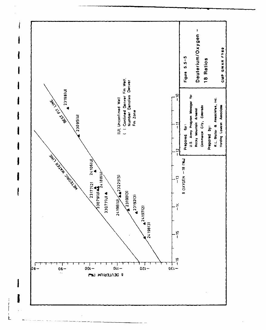
00
Eun, 0
00. 0 C)
0- , ~Co.IV
00 qf~U ~ S .
0 C 0 n E
L) L.)
.3 CL
0
Y C4 01
'A -
e4 -
C4-
t- U, 5 ý!
C%) (A~A3 m
mICm:1 r
L~. _____
6.0 REFERENCES
Ebasco Services, Inc., March, 1989a. Draft Final Report, Regional Ground-water Flow Modellingat RMA. Prepared for Program Manager, Rocky Mountain Arsenal, Commerce City,Colorado.RIC#89144R02
Ebasco Services, Inc., May, 1989b. Final Remedial Investigation Report, Volume XII, WesternStudy Area. Version 3.3.RIC#89166R03
Ebasco Services, Inc., June, 1989c. Final Remedial Investigation Report, Volume VI, SouthernStudy Area. Version 3.3.RIC#89166R0I
Ebasco Services, Inc., June, 1989d. Final Remedial Investigation Report, Volume VII, EasternStudy Area. Version 3.3.RIC#89 i 66R02
Ebasco Services, Inc., July, 1989e. Final Remedial Investigation Report, Volume VIII, South PlantsStudy Area. Version 3.3.RIC#89166R04
Ebasco Services, Inc., July, 1989f. Final Remedial Investigation Report, Volume IX, North PlantsStudy Area. Version 3.3.RIC#89166R05
Ebasco Services, Inc., July, 1989g. Final Remedial Investigation Report, Volume X, Central StudyArea. Version 3.3.RIC#89166R06
Ebasco Services, Inc., July, 1989h. Final Remedial Investigation Report, Volume Xl, North CentralStudy Area. Version 3.3.RIC#89166R07
Ebasco Services, Inc., July, 1989i. Final Water Remedial Investigation Report, Version 3.3.Prepared for U.S. Army Rocky Mountain Arsenal Program Manager, Commerce City,Colorado.g RIC#89 i 86R0 I
Environmental Science Engineering (ESE), December 1988. Boundary Control System AssessmentRemedial Investigations, Draft Final Report, Version 2.1, superceded by Draft Final ReportBoundary Control System Assessment Remedial Investigations, Version 2.2.RIC#901 14R01
Environmental Science and Engineering (ESE), February, 1989. North Boundary SystemComponent
Response Action Assessment Final Report, Version 3.1, Task 36.RIC#89103R0I
Fritz, P., April, 1981. Environmental Isotope Hydrology - Tools to Complement the ClassicalTechniques of Physical Hydrology and Geochemistry, University of Waterloo, Waterloo,Ontario.I
GWAR-89.5-6Rev. 06/22/90 - 220 -
REFERENCES (continued)
Geraghty & Miller, Inc., April 1986. "Rocky Mountain Arsenal Chemical Indexes." Draft FinalReport, 2 Vols. RIC#86107R01, superceded by Ebasco, Inc., May 1988. Chemical Index,3 Vols. Prepared for U.S. Army, Rocky Mountain Arsenal Program Manager.RIC#88357R0I
Harding Lawson Associates, March 1989. Regional Ground-Water Flow modeling at the RockyMountain Arsenal, Denver, Colorado. Draft Final Report, Version 2.1.RIC#89144R02
Hem, J.D., 1989. Study and Interpretation of the Chemical Characteristics of Natural Water. U.S.Geological Survey Water-Supply Paper #2254. U.S. Geological Survey.
Hunter/Environmental Science and Engineering, Inc., 1987. RMA Analytical Results (GroundWater) for Wells Sampled October 1985 to December 1986 (unpublished). Denver:Hunter/ESE.
Lindvall, R. M., 1980. Geological Map of the Commerce City Quadrangle, Adams and DenverCounties, Colorado. U.S. Geological Survey Map GQ-1567. Reston, Virginia: U.S.Geological Survey.
Lutton, R.J., August, 1989. Start-Up Performance of Ground Water Recharge Trenches, RockyMountain Arsenal, Army Corps of Engineers, Waterways Experiment Station, Vicksburg,Mississippi. Prepared for Program Manager, Rocky Mountain Arsenal, Commerce City,Colorado.RIC#8927701
Program Manager, Rocky Mountain Arsenal, June 1987a, RMA North BoundaryContainment/Treatment System Operational Assessment Report FY85/86.RIC#87320R0I
Program Manager, Rocky Mountain Arsenal, December 1987b, RMA Northwest BoundaryContainment/Treatment System Baseline Conditions, System Startup, and OperationalAssessment, FY85/86RIC#88054R0 I
Program Manager, Rocky Mountain Arsenal, July, 1989a. Chemical Quality Assurance Plan.Version 1.0.RIC#89233R0I
SProgram M anager, Rocky M ountain Arsenal, Decem ber, 1989b, North BoundaryContainment/Treatment System Operational Assessment Report, FY88 Final Report.RIC#90061 RO I
Program Manager, Rocky Mountain Arsenal, December 1989c. Northwest BoundaryContainment/Treatment System Operational Assessment Report, FY88 Final Report.RIC#90061 R02
Robson, S. G., and Romero, J. C., 1981. Geologic Structure, Hydrology, and Water Quality ofthe Denver Aquifer in the Denver Basin, Colorado. Prepared for the Geological Surveyand the Colorado Division of Water Resources.
GWAR-89.5-6Rev. 06/22/90 - 221 -

RIC#82350M02REFERENCES (continued)
Romero, J.C., 1976. Groundwater Resources of the Bedrock Aquifers of the Denver Basin,Colorado. Colorado Department of Natural Resources.RIC#8 i 266R69
Stollar, R.L. & Associates, Inc., et al., 1989a. Comprehensive Monitoring Program Ground WaterFinal Technical Plan. Prepared for Program Manager, Rocky Mountain Arsenal.RIC#89213R02
Stollar, R.L. & Associates, Inc., et al, 1989b. Comprehensive Monitoring Program Annual GroundWater Report for 1988. Prepared for Program Manager, Rocky Mountain Arsenal.RIC#89213R01
Stollar, R.L. & Associates, Inc., et al., 1987. Draft Final Technical Plan Transition MonitoringProgram, Ground Water. Prepared for USATHAMA.RIC#88340R04
USEPA Data Review Work Group, February 1988. Laboratory Data Validation - FunctionalGuidelines for Evaluating Organics Analyses, Prepared for U.S. Environmental ProtectionAgency, Hazardous Site Evaluation Division.
II
IGWAR-89.6-6Rev. 06/22/90 - 222 -


