AD-A099 350 WISCONSIN UNIV-MADISON MATHEMATICS RESEARCH CENTER F/S 12/1MUJLTIVARIATE SPLINES.IUIMAR 81 K HOELLIG 0AA629-8O-C-0041

UINCL7ASSIFIED MRC-TSR-2188 N

C

Technical/ummary 6prto 188

WTIVrIATF PfN

SKlau .i--ig

-- 3,

Mathematics Research CenterUniversity of Wisconsin-Madison

610 Walnut StreetMadison, Wisconsin 53706 D T IC

March 1981 e ELECTE

Received January 12, 1981

A

LAJ Approved for public rlmaseDistribution unlimited

P ponsored by

u. S. Army Research Office National Science FoundationP.O. Box 12211 Washington, D. C. 20550

Research Triangle ParkNorth Carolina 27709

;;,. 81 5 27 022

PTTIS GRA&A

DTIC TABUNIVERSITY OF WISCONSIN - MADISON UanBouno0MATHEMATICS RESEARCH CENTER Justif 8 .ato

MULTIVARIATE SPLINES

Klaus H~llig DistrJbution/

Availability CodesAvail and/or

Technical Summary Report #2188 Dist SpecialMarch 1981

ABSTRACT

It is shown that the span of a collection of multivariate B-splines,

SJ0 Jk+mSk span M(*Ix ,.'.,x , contains polynomials of total degree 4 k

jEJ

if the index set {j = (j 0,"',Jk+m ) JEj has a certain combinatorial

structure, in particular the knots {x91 c IF can be chosen essentially

arbitrarily. Under mild assumptions on the distribution of the knots, a dual

basis {A for S is constructed which has local support, i.e.,j JEJksupp X C supp M , and the condition number of the B-spline basis is

estimated. This leads to good local approximation schemes.2"

~AMSIMOS) Subject Classification: 41A15, 41A63

Key Words: Multivariate, B-splines, spline functions, dual basis,condition number

Work Unit No. 3 - Numerical Analysis and Computer Science

Sponsored by the United States Army under Contract No. DAAG29-80-C-0041. Thismaterial is based upon work supported by the National Science Foundation underGrant No. MCS-7927062,

SIGNIFICANCE AND EXPLANATION

Spline approximation provides good approximation methods in one

variable. This is to a great deal due to the properties of the B-spline

0 nbasis. Recently, multivariate B-splines M(.Ix ,'*,x n) have been defined

and their basic recurrence relations derived. However, there was no

Vsatisfactory way to choose for a given set of knots Ix ) c Rm a span of B-

splines that contains polynomials, this property is essential for good

approximation properties.

In this report we give a sufficient condition in terms of the index set

jEJ for Sk :- span M(jx ,***,x ) to containj eJ

locally polynomials of total degree 4 k. Since the knots may be chosen

almost arbitrarily, the resulting space of multivariate splines Sk has the

local flexibility familar from the univariate theory. We show that under mild

assumptions on the distribution of the knots the L p-norm of a spline s c Sk

is equivalent to the £ -norm of its normalized B-spline coefficients. As anp

application, we indicate how local approximation schemes can be constructed.

The responsibility for the wording and views expressed in this descriptivesummary lies with MRC, and not with the author of this report.

MULTIVARIATE SPLINES

Klaus Hollig

0. Introduction

- The purpose of this report is to introduce a class of multivariate non

tensor product spline functions and study its basic properties.. he basis for

our approach are recent results of C. A. Micchalli and W. Dahmen (8-12, 21,

0 n22] on multivariate B-splines M(.Ix 0,..,x ) introduced by C. de Boor in

JO in[3]. We consider a space of spline functions Sk = span M(.Ix 0,**,x n )

JEJwhere the Index set J has a certain combinatorial structure and the knots

x V R may be chosen almost arbitrarily. It is shown that Sk contains

polynomials of total degree k - n-m which is the basis for good approxima-

tion properties. Under mild assumptions on the distribution of the knots we

construct a dual basis AJ, j i , for Sk with local support, i.e.

supp Ai C supp NJ . Using extensions of the functionals A to L the

condition number of the B-splune basis is estimated which turns out to be

essentially independent of the distribution of the knots. As an application

we obtain the basic error estimate for local approximation schemes.

Since the spaces S. have the local flexibility familiar from the

univariate theory one might expect applications to finite element methods,

swthing of data and surface fitting.

Sponsored by the United States Army under Contract No. DAAG29-80-C-0041. Thismaterial is based upon work supported by the National Science Foundation underGrant No. HCS-7927062.

1. B-Sylines

The gftometric interpretation of the univariate B-spline by H. B. Curry and 1. J.

Schoenberg (71 gave rise to the following generalization.

Definition 1. C. deioor (31. Let x ,.**,xn be any points in AP, n > a which span a

proper convex set and choose any simplex 0l((x x),*(x x))with vertices

V -v n 0. n V(x , x C so . The B-spline MC( Ix .., ):30 + a corresponding to the *knots" xv is

defined by

n-rn - 0-0 n Vln-rnxC IX; 6G(

M(IXP x0 -0 n -nvolno((x ,x ),,**,(x , X)

0 if A- A

where for n-rn Vol 0 (A) I tews

n

Denote by A n - WCof...iXn )I I AV 1, A ; 0, v - 0,--n the standard n-

dimensional simplex. A simple calculation shows (22, p. 3,41 that for f i£ CCR")

(2) iii f f( I ~ A . ~ ~~ '.,nfxdA V-0 x)d * rt=J Nxx ef

a relation used by C. A. Micchelli to define the multivariate B-splines (21]. Equation (2)

defines M. even for n < m as a positive measure supported In the convex hull of the

points x 0,...,x n From (2) the Fourier transform of 14 can be computed via the Hermits

Genocchi formula for divided differences E23, p. 16]

(3) (to ...,t n f - f fn) I A Vt ) d% ... dAnn A v.0 V

Applying Parseval's identity ff.j - fig , hy) -f h(x)e ixdx , to the equation (2) we

have

f R(XIXO,..,xn )g(xdx -f MCxIX ,'...Xn ).2(x)dx

n1 f 4( X vx")dX, . .. dX n ni f f exp( I V~ (-Ixx V ))g(x)dx A, *..d" na V-0 A in V-0

.0 n t(4) A~xni j..' ( i,*-ixx .*.e gxxxItx

trhich r impWlie ens treFunied prnsorrpeeto of thmlnti iv rat by plne (21

A xx .0. x n) n _!~ ixx V.*-x A

V-0 P.

P*V

Identity (5) corresponds to the usually used definition of the univariate fl-spline (1]

) N~x~tn n- na--n I (t-x), R! (t - tn v-0 V + P.0 U

IA*V

n t +

Using the recurrence relation for divided differences

we can derive fro . 2 a tornula for the directional derivative of M . We set

--ixxv, apply (7) to the function et and take the inverse Fourier transform. It

follows that

0 aD M(xlx ,..*,x

_x 1

n~mxlx ... X-, x ***..,xn 1x ,...,x ,x ,..*#x

where D :=z *V *This generalizes to

nTheorem 1 [8, 21, 221. If y x Ax" A -0 ,then we have

Vj=0 V V-0 4

avn n v-i v+1

(9M (Xlx 1---,x n I XV A (xlx ,...,x ,x ,. xI where this Identity should be interpreted in the sense of dintributions if some of tiie Ii-

splines are supported on sets of zero measure.

-.3-

A repeated application 2f (9) shown that the distributional derivatives

DU M(.jx 0,*,xn), n l - n-m+1 , being linear combinations of the B-splines11 i

M(.Ix ,..,x ), are supported in convex subsets of hyperplanes. Hence M agrees with

a polynomial of total degree ( n-m on every subset of FLO not cut by one of the convexi i

sets spanned by x ,...,x , 0 i1 < ... < i n [21, 22]. The global smoothness

Vof H depends on the geometric configuration of the points x • If every subset of 9

0 npoints of {x ,..-,x n} forms a proper convex set it follows again from (9) that

DM L6 , ltI - n-X+l . Therefore,0 wn-L+1( m) cni( m)

(10) M(.Ix 0,"*,x n ) 4E C

Perhaps the most striking identity for multivariate B-splines is the recurrence relation,

discovered by C. A. Micchelli (21] and also proved by W. Dahmen [8] under more restrictive

assumptions. See also (16] for a proof via Fourier analysis.

Theorem 2 [8,21,22]. Assume that the points x 0 ***,x ne n > m form a proper convex

set andn n

v-0then we have

0 n n n 0v Mxx'*xV-1'xV+1 ''n)

(11) M(xxO ,...,xn) n- I M(xvx 0,X. x 'x

if all B-splines occurring in this equation are continuous at x

Formula (11) expresses M recursively as a convex combination of positive quantities

and thus provides a stable way for computing multivariate B-splines (22]. So far we have

only discussed some basic results on multivariate B-splines and we refer to the literature

[8-12, 21, 22] for many interesting recent developments.

-4-

2. Some topological preliminaries

We need some basic facts about triangulations [141. Since there seems to be no

convenient reference for a reader with little background in topology we sketch the proofs.

Let (X,I) denote a collection of nondegenerate closed simplices tX) a

i I

,(x *, m - , M ) C I C el with vertices x E X c X,) is called

a triangulation of a set n c R if n - U ai(X) and the intersection of two differentiEI

simplices is either empty or a common lower dimensional face. Moreover we assume that

every compact subset of 9 is intersected by finitely many simplices only.

Definition 2. Denote by B : + 0iB the inscribed balls with center wi and radius

Pi for the simplices a (i). We call a triangulation regular, if there exists a constant

y such that

(12) diam ai(X) < Y i'

Lemma 1. Let (X,I) be a triangulation of an open set n c * Then for any finite set

of vertices (x }V) C X there is an e > 0 such that (X,!) with V = x , 0 J is also

a triangulation of n if IV - xVI < C , v E •

Lema 2. Let (X,!) be a triangulation of a simply connected set n and assume that a

locally finite collection of simplices (X,I) satisfies 0 = U ai(X). Then (X,I) islei

also a triangulation of 9

Proof. The mapping f : 2 + 0 defined by

V -Vf(x)x

f a0 is affine linear,

is a local homeomorphism which is by assumption surjective. Since n is simply connected

the monodromy theorem implies that f is bijective and hence (X,!) is a triangulation of

2 Roughly speaking, the argument is as follows. Suppose there exist zooZI C Q,

z 21 , such that y - f(zO ) - f(z I) and let C0 be the image of a curve joining z0

-5-

T--..---......

and si. Denote by C(t,A): [0,112 + D a continuous deformation of Co - C(.,o) into

the point y , i.e. y 2 C(.,1). Since we have assumed that only finitely many simplices

Gi intersect a given compact set every point x e 0 has a neighborhood U. such that

f'I consists of finitely many disjoint sets Vx,1 , .. ,V and flV is a

homeomorphism. Hence the inverse of f along each curve Ci- C(.,A), f-(C(.,)), with

initial value -0 - f- (C(0C,)) is well defined. We shall show that x1 = f- (c(1, ))

for all A e [0,1] contradicting f' (C(.,1)) - z0 . For a sufficiently fine subdivision

of [0,112

into squares Rv each of the sets C(R v ) is contained in some neighborhood

U. and the following picture shows that inverting f along adjacent curves leads to the

same value

i d4I I*

0 1

f-((1,A)) . '11C1(I'1 ) Fl(1,,)).

The combinatorial product of the sets i- {i0,...,i m and (0,..-,k} is defined as

the collection of all ordered subsets of {i0 ,.-.,il x (0,...,k with n+l %- m+k+l

distinct elements, i.e.

ihk : {(J,r) = E ' n [{i 0 ... ,i} x (0,...,k1]n+lI11irot..."r n

0j 1 - and r r +) or1 J

l~V41 =J ndr+ =r+1or (jV 1 V jV+ 1

and rv+ rV ) for v - 0,...,n).

Note that (j,r) c ihk is already uniquely determined by j = (jo,...,jn) so that we may

drop r when referring to elements of iak

Lma 3 . Denote by k " G(eO ... Fek) with e0 = (0,.e,0, e1 - (l,0,...,0),.-., the

standard k-dimensional simplex and let (XI) be a triangulation of a c *. Then the

simplices

10 ino((x er),---,(x er n m+k,

0 n(14)

(j,r) E Ihk : U iAkicI

form a triangulation of n x A

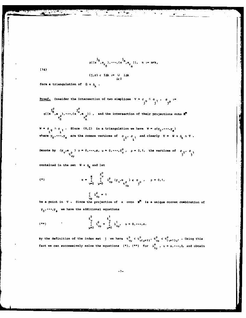
Proof. Consider the intersection of two simplices V =a n a , .

ipinoC(x 0 e ),rp ( ,e ) and the intersection of their projections onto I

0 n

W . a 10 1 a I.since MXI) is a triangulation we have W -~ F.'

where yor,...rys are the common vertices of a i fa and clearly V - W x 6kn V

Denote by (y ,e )v.- O,...,s, p - 0,- , p 0,1, the vertices of a0'f a1Vt

0 V

contained in the set W x Akand let

5 V')x 1 XP ) ( y e )aa P I P 0,1,

V-0 IJ=0 W t9

VII

VP

be a point in V *Since the projection of x onto IP is a unique convex combination of

YO ...yswe have the additional equations

0 11V 0 V I

M.-0 P.0

By the definition of the index set j we have tp < t0~+) t0 u 4 tp Using thisVII Vp) Vp (V4.lNu

tact we can successively solve the equations () (*) for A , v s,., and obtainAA

0 1x iff a -e

V1, vu tO tI

)L - 0 otherwise.

This implies that V is the simplex spanned by the common vertices of a o a

A simple calculation shows that vol a - vol oi , JE ik . Since

0 Ca and iAk " (m+k) this implies U aj aI x &•i iAk

-B-

pr

U...

3. Splines as linear combinations of B-splines

Denote by Pk the polynomials of total degree ( k , i.e.

m m a

Pk - flD f 0, cii = k+1}, where a = (a 1.) D Cii = U V

,,- 'J1 ay

We call Sk a space of splines of total degree k defined on a set Q c Rm if

(A) Sk is the linear span of a collection of B-splines and

(B) Pk () C Ski.

Moreover we shall assume that

(C) every compact subset of a is intersected by the supports of finitely many

B-splines only.

In the univariate cpe we may associate with any increasing sequence of knots {t,},

t v < tvk+l . a space of splines

(15) Sk = span M(.lt ,...,t ).v v+k+lV

In several variables any triangulation UX,X),I) of a product U x c x

vol U < * corresponds by Definition 1 to a family of B-splines which forms a partition

of unity over U (31, i.e.

I = 10 in, in 1x0 in(16) 1 (vol )- I vol 0((x ,x ),...,(x ,x )) ,...,x

iEI

x E Q, n = m+k,

n 1x0 inand it was shown in [91 that for 9 x 1 = (0,1] Pk C span M(.Ix ,..',x , i.e.iEI

condition (B) is satisfied.

To require the existence of an associated triangulation is, however, too restrictive

and not quite satisfactory, since the B-splines do only depend on the knots xj E X c R7

As in the univariate case, one would like to associate with any distribution of knots a

corresponding space of splines. This can be accomplished by a multivariate analogon of the

process of "pulling apart" knots which we shall now describe.

-9-

Definition 3. Lot (X,I), X - (xV VZ , be a triangulation of SP andV )x V

C

Ii vCZ,pz-0,-*,k ' Ua collection of points* not necessarily related to (XI). We define the space of

splines of total degree k with respect to the index set I and the knots X by (c.f.

(13), (14))(17) S span Mj(.IX)

(17) kLi - jIAk

where M ('1X) :- J(. o' ..' x ) n - m+k . In addition we assume that condition (C) isj r0 r1n

satisfied.

The rest of this chapter is devoted to the justification of this Definition, i.e. to

prove (a). To simplify notation we shall drop most of the subscripts in the sequel, e.g.

sk := sk' z , Mj :. : i(.z), 0: := oiX), etc.

V V

Lemma 4. If we make for the knots Z the particular choice x - x , v c 3, U =--,k,

then Sk,x,I coincides with the space of piecewise polynomials of total degree k with

respect to the triangulation (X,I), i.e.

(19) Sk,X,I ' Pk,X,I :- {flfl( E k * i k I'

V VProof. For the special choice x, x we have

S kXIO- span M(°jx JO,.'XS jciAk

jxo .,i } 1x0 1m

and (X ,..*,x = x ,...,x m, . We could now use the formula for B-splines with

multiple knots (22, p. 16] to complete the proof. But we may also apply (9) to conclude

that the supports of the distributional derivatives D aM, lci - k+1, are contained in the

boundary of the simplex o This implies span Mj c Pk(Oi). The reverse inclusion is ak+m

special case of Theorem 3 below. Moreover, since #idk - k dim Pk' the 9-splines

Mj, J f iAk form a basis for Pk(Gi).

-10-

m w

Remark. Lemma 4 shows that we may view the spaces Sk as perturbations of piecewise

Vpolynomials obtained by pulling apart the multiple knots x a X

V Vx X 1, =0,---,k

One may e.g. choose aO,o. ,ak E I and define xv - xv + a , 1 - 0,***,k. This very

special perturbation corresponds to an affine transformation of the triangulation (14) and

is only an appropriate choice if the triangulation (X,I) is quasiuniform and one is

interested in a uniform distribution of the knots X

We have defined the spline spaces Sk on 10 to avoid a separate discussion of

various types of "boundary" conditions in the sequel. This is no loss of generality since

we include all kinds of finite dimensional spline spaces by simply restricting the domain

of definition. The global smoothness of Sk depends on the smoothness of the particular

B-splines (c.f. (10)). But, although the set of knots yielding the highest possible

smoothness Sk ck -1 is dense, there is no canonical way to choose such knots as in the

univariate case.

Example 1. Let {it V1, t < t v+k+ , be an increasing sequence of knots. To obtain the

canonical B-spline basis (15) we set (c.f. Definition 3) X = {t(k+1)vE

I = {(VV+1) , x t )V , v E 5, U = 0,...,k, which yields"aZ , kJ ~ -

(v,v+l)Ak J {" .VlV+l :(v+l)), p . O,.o.,k},0""*,.p p .. k

span M. span M(,It(k+l)v.," t(k+l)(v+l)_pj E(V,V+l)Ak 0. --- °°,k

The following example shows that Definition 3 is slightly more general than the usual

univariate definition, since we do not require that a B-spline does only correspond to

adjacent knots.

V 1

Example 2. Let X = Z, i.e. x = V, I = {(V,v+1)) and consider the knots x0 2,V EZ0

1 2 2 v2.5, xO . 1, x1 . 0.5 and x = v for v * 1,2. Restricting the domain to the

-11-

interval [0,3] we have

S1 IZll(0,31 ' span{M(.O,O,2.S), (-IO,2,2.5), M(.10.5,2,2.5), M(.I0.5,1,2),

m(10.5,1,3), H(.11,3,3)}

which is a space of continuous piecewise linear splines with an unusual basis.

Theorem 3. The spaces Sk,Z,l contain polynomials of total degree k . In particular we

have for all x,y 4 Fen

(19) (l+xy)k - Z C (YIZ) H (xIX)jelak

where (c.f. (13), (14), (17))

+ x Y)e (1 + x n)enr0 r. rn rn

k, Jo :inC yil(lz ) - xj 7 d t Xro ... x r

dat r1

and c £ {-1,11 is chosen so that

r 0 rn

C -E !L det x ... x > .j j n1

1 .* 1

V

(Recall that x are the vertices of the triangulation corresponding to the index set I)

For the standard univariate B-spline basis formula (19) is known as Marsden's identity

[19]. The basic idea of its multivariate generalization is due to W. Dahmen [9). For two

variables (19) was proved by T. N. T. Goodman and S. L. Lee [15] under the restrictive

assumption thct the B-splines correspond to a triangulation of R2 x A k . In both cases

there is a more explicit formula for the coefficients C,(yJZ) (c.f. Corollaries I and

2). Besides the generalization to an arbitrary number of variables we show that identity

-12-

(19) is valid for any collection of knots as long as we keep the combinatorial structure

determined by the index set Z .

Remarks. (i) Identity (19) holds for any finite collection of B-splines Mi, j f j C

Ibk, if we restrict x to the domain ll \ U supp MN

(ii) For y - 0 , (19) is a generalization of (16) since the coefficients C, := C(0IX)

need not to be positive. The coefficients corresponding to the B-splines in Example 2,

e.g., are 1.25, 1, -0.8, -0.4, 1.25, 1. One can show, using Lemma 2. that the

coefficients Cj, j EIA~k, are positive if and only if the simplices

1 0 1..(n )(20) 0,(I) r 0(),#r0 r n'' ,r ar )), j c 14k

form a triangulation of Rm x .

(iii) Comparing the coefficients of ya in identity (19) we obtain an explicit

representation for the monomials xa, j a k ,

(21) x a C'm(I) M (x)JI AId3

S-1 DalV1where Cn(I) :- (nf)l (j y=O a! -

Proof of Theorem 3. Note, that by Definition I we may associate with the B-splines M

the simplices a (c.f. (17), (20)). First we assume that the collection of simplices

j e IAX, is a small perturbation of the triangulation (14), i.e. S I is close to

Pk,X,I (c.f. (18)). More precisely, for a finite set J c Z and c > 0 , to be chosen

later, we assume

M* Ix - xvi < e, u 0 ,...,k, v c J

(0)

()xv V x

v V i 0, O.,k, v 0( J.

UBy Lemma 1, dJ , j Ik , is a triangulation for small c (Since R

m x C in

is not

an open set. Lemma 1 cannot be applied directly. But, we may consider suitable extensions

of the triangulations to 1P). Let K be an arbitrary bounded subset of 11m. Obviously it

is sufficient to prove (19) under the assumption x E K and y small. We define the

mapping

-13-

T a m k.,, am

T(xx) - (x,(1 * xy)Z)

Consider the finitely many 13-plines N * I • 3 , the supports of which Intersect X

(c.f. the assumption In Definition 3), and Lot (xo) be the oorresponding%~ Wa0.***,Ic V4EJ

set of knots. For small enough y the simplices

a Ts- o(T~x ia ),**..T(x in ))0r : r0 r n

form aolm a triangulacioe. Noreover, since T maps the hyperplanee bounding I x Ak into

hyperplanoe and leaves projections on IP fixed we have

U a T ) n X x g k - Y(x x Ak)

j(JBy Definition 1 and (16) It follows that for Mall y and x i K

vol(; c Ikl(x,;) E T(K x Ak)) - +k1"(1 + xy) t

kTL -k (-,;) 07) Vola j.M

For Ixv - x) , v e J, sall we have agn C (ytI) - agn C1 (K) I which implies

volO (kl),Ic (yJ) and completes the proof under the assumptions M'), (").i i

We now drop the assumption ('). Lot Mb. J e 3, be the finitely many a-oplines having

at least one of the knots (x)p-O,*.',k, v J and consider the equation

- C K C1 (yIz)K (x))$(x)dxJe Ak

( )

f j L . C I(y1X)H }(x); (K)dX

where , I £ a) is the Fourier transform of a test function with compact support. by (4)

and Parseval's identity, the right hand side is equal to

ri rn tni ~ C1(yIZ) tm{ ro .,ixn x t *(x)ex

The coefficients C i(yJZ) and the divided difference of the exponential function are also

defined for complex values x V C ?, and it is easily sen that the right hand

side of (+) is an entire function of the arguments (xf)= (CR)#J(kl) "1A w-,"-,k, v4

The left hand side of (+) is constant with respect to those arguments. Therefore, since by

-14-

the first part of the proof the identity i valid in a real neighborhood of the knots

Vx , v F J , it follows alobally by the identity theorem for Power series [17j. To

obtain (19) from the identity (+) we note that t*,* V 0) is dense in 0 with respect to

the norm 11 t- sup (I + x1) z1*(x)l for all L c.

The general came follows now easily. Consider an arbitrary perturbation of the

initial knots

V vx V. x V

such that any bounded subset K c IP is intersected by the supports of finitely many a-

splines only. Restricting x to K , only finitely many knots are relevant for the

identity (19) and the previous arguments apply.

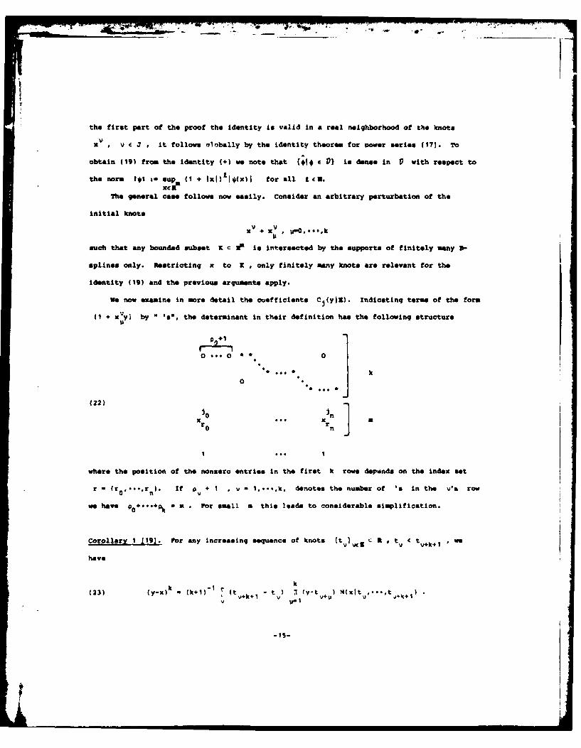
We now examine in nore detail the coefficient@ C1 (y1). Indicating terms of the form

(1 + xy) by 's", the determinant in their definition has the following structure

+.1

0 ... 0 0

0

(22 ) -i

r0 rn

1 ... 1

where the position of the nonzero entries in the first k rows dep ands on the index set

r - (rO,...,rn). If p + I * u - 1,..,,k, denotes the number of 'a in the v's row

we have p ... +a k - m . For small n this leads to considerable simplification.

Corollary 1 119]. For any increasing sequence of knots (t V c It t < t v+k+ I we

have

k (t k

(23) (y-x) - (k+1) t+k 1 - t ) T (y-t V+ M(xltv...,t k+ "V

v 1

Corollary 2 [151. Let 8kX.1 be defined on R2 .

Then we have for all xy e 32

(24) (u+xylk - c n (.4sy) k (x)

J4 J ZAV-1 j

where Z .- ,j () can be detera.ned by the knots of the B-spline M. and the index

set j . For details we refer to [15).

both Corollaries can be obtained from Theorem 3 by direct computation of the

determinant (22). Note that in (23) we have made the substitution y + -1/y

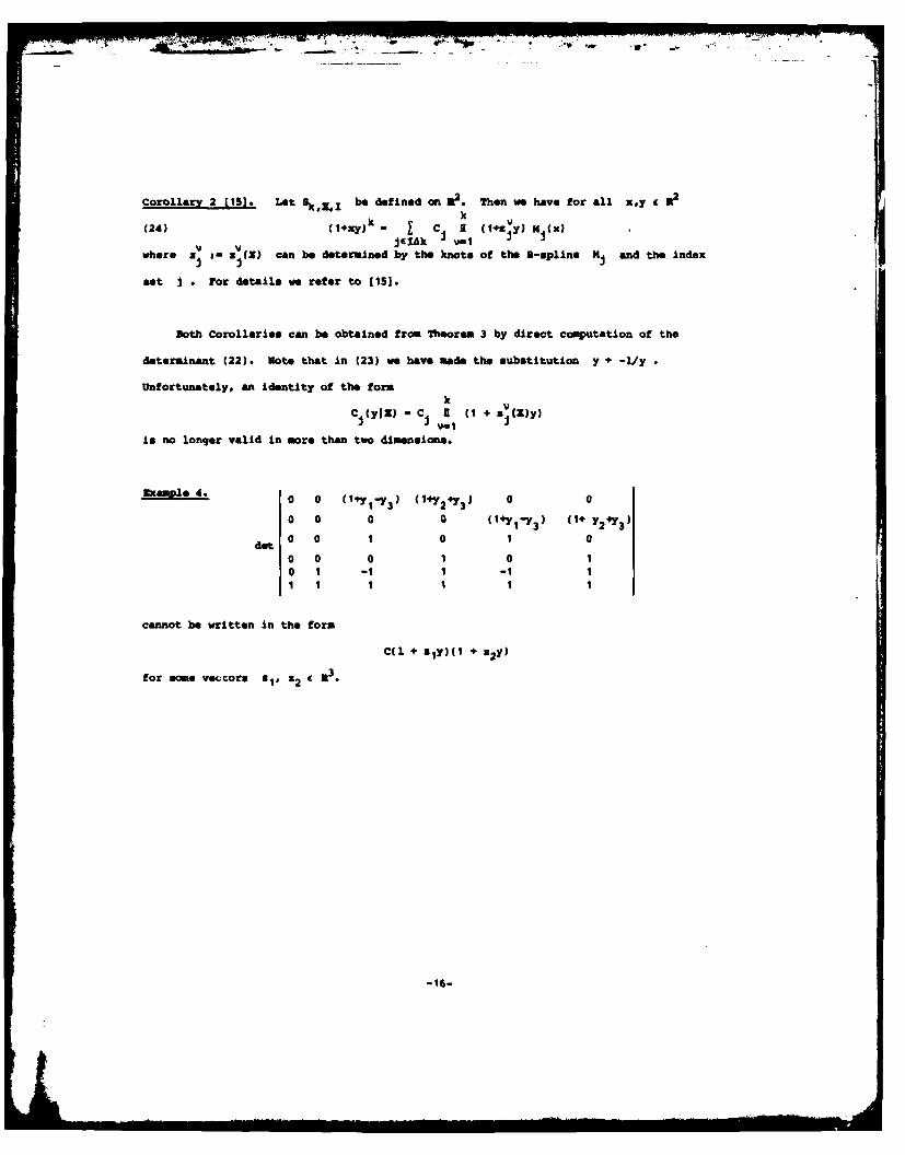
Unfortunately, A identity of the form

Cj(yII) Cj II (1 + zj(z)y)v-I

is no longer valid in more than two dimensiona.

Example 4. 0 0 (1+y-y 3 ) (1+y 2 +y 3 ) 0 0

0 0 0 0 (1+y 1 -y 3 ) (0+ y2 +Y3 )

dot0 0 1 0 1 0

0 0 0 1 0 10 1 -1 1 -1 11 1 1 1 1

cannot be written in the form

C(l + s1y)(1 + 82y)

for some vector 1* S2 9 R3.

-16-

I

4. The B-spline basis

The standard univariate B-spline basis (15) has the striking property (c.f. C. do Boor

[1,31) that the Lp-norm of a spline is equivalent to the i p- norm of its coefficients with

respect to a normalized B-spline basis independently of the sequence of knots. Under mild

assumptions on the distribution of knots we shall establish this result for the

multivariate spline spaces Sk,X,I.

Definition 4. We call X - {x V a regular perturbation of a triangulation (X,I) if there

exists a constant K and balls nl : x, + h B such that for every i e I (c.f. (13),

Definition 3)

(25) Dic n supp M

(26) n 1 n supp H = , j e ilAk , i * i

(27) diam supp M j K h i , j e iAk

Note, that the conditions (25)-(27) are local, i.e. we do not assume any relationship

between hi, hil, I * i1

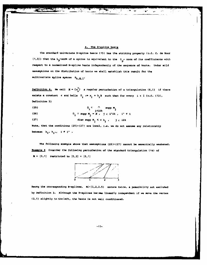
The following example shows that assumptions (25)-(27) cannot be essentially weakened.

Example 4 Consider the following perturbation of the standard triangulation (14) of

It x (0,1] restricted to [0,3] x [0,1]

0 1 2 3

Among the corresponding B-splines, M(.Il,2,2.5) occurs twice, a possibility not excluded

by Definition 3. Although the B-splines became linearly independent if we move the vertex

(2,1) slightly to theleft, the basis is not well conditioned.

-17-

-RI -- 7.7-1A

Lemma 5. With the notation of Definitions 2-4 assume that xi can be chosen as the center

of the inscribed ball of the simplex aI(X), i.e. x I " , hi < Pi * and

V V(28) IxM -x l hVVU

where h v 2- Hin( 1 - h Ixv is a vertex of c (X)). Then X is a regular perturbation

of (XZ).

This shows that conditions (25)-(27) allow perturbations of the same magnitude as the

perturbation of Example 4.

Proof. The support of each B-spline Mj, j ciAk, is the union of simplices-1 0 -i l l xIl

a = 0 ,..mx ) where i - x V 1 , - hi B Dy Lema 2 the collection of

siaplices (G I )( is a triangulation. To prove (25), (26) it is sufficient to show that

for any such triangulation I C ;i" We define the simplices

( i 1 i0, - + (1-t)x ,.0.,tx + (1-t)x m t (0,1]

and observe that none of the (k-1)-dimensional faces of a , , t c [0,1, intersects0 0a1 T This follows because any such face can be separated from t by the hyperplane

parallel to the corresponding face of a i(X) touching 0 . Concerning (27) we note that

under the ASSU•Ptions of the LM K yp I+I-h•

Theorem 4. Let .be a regmlar perturbation of a triangulation (X,I). With the notation

of Theorem 3 and Definition 4 we define functionals Xi C k (a) * a

(29) A (X,i)f (al)2 ( Dec -( ) Z Df(r), j E lAkj alfk lei

!hereT c and I - : -(XV-T) is a translation of the point set 2. Then for any set

of points T C , joi iak , the functionals A : (X,T j e Ak , are dual to

the &-apline basis for Skal z , i.e.

(30) A Nj 6 ji, -6k.

-18",,j~'£ tk

We note the following immediate consequences of this result which for univariate

spline functions is due to C. de Boor [2].

(i) The B-splines Nj J E IAk , are linearly independent over the set 0 - U 0,icI

(ii) For any polynomial of total degree 4 k, p F Pk' X (X,T)p is constant as a function

of T E R m

To see this we observe that the polynomial g(r) :- X (X,T)p is constant for

T E Ql' J E iAk. This follows from (30) since by (26) and Theorem 3

(31) SkzI, - span MJ IA - PkI(i

Sk', 11 4iAkConcerning (i) we note, that in contrast to the univariate case in more than one variable

the B-spline basis of Sk Is not linearly independent over arbitrary open subsets of I.

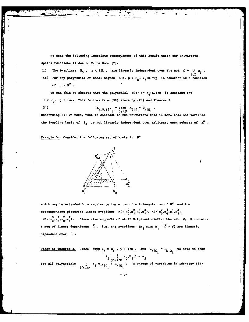
Example 5. Consider the following set of knots in

22 Xl

112 - -X0

o 1x0 x0

which may be extended to a regular perturbation of a triangulation of R2 and the0 0 1 2 0 1 1 2

corresponding piecewise linear B-splines M(oCX0,xxlX), M(. x0,x0,xlxl)

4( .Ix o,x00 ,01 x0,x 1 ). Since also supports of other B-splines overlap the set 9i, f9 contains

a set of linear dependence fl , i.e. the B-splines {M tsupp Mj A f * dn are linearly

dependent over fl

Proof of Theorem 4. Since supp X c l , j c Ik , and S k1 P we have to show

A~~ i J M I

for all polynomials & E k A change of variables in identity (19)EiM ik JIS1ij

-19-

yields

(19') (+( )( )) C(Y-X-)M,(x), x C iJ'c ik

We choose T - T , apply the functional X to the left hand side and obtaink

4IBik )(x') (YI) ( (x-T )(Y-

Since the set of polynomials {(+(x-T )(y-Tk)) Ye spans Pk , the proof is complete

if we show

-(a)'DaC(0IX-T )(y-T a - C (y-T JX-T) y

JaJQ ki

But this follows simply by differentiating with respect to y at y - T

Formula (29) is only one particular representation of the dual basis for Hit j c I4k.

We now construct bounded extensions A : A (Z) of the functionals A to

i.e. A iL +R

(32) A s -a ,is a 0 a S k

If we require supp Aj c Vi, J e iAk, the system (32) reduces to

(33) A jpA)p, p ePkc.

Hence we may determine A from the identities (19), (21). After a change of variables we

have

(21') ((MI)) -1 (k ) -1 DC (OII-r)14 (x)j-A~ (a Il Vaj (0ZzMi~J4EIAk Ju

and clearly, (33) is equivalent to the system

(33') T)a ()-I k )- DC (OI-), l

Let La be any set of functions dual to the nonomials on the unit ball B , i.e.

(34) f L(x) x - 6aB Jl, IBI C kB

We transform the functions La to the balls £i (c.f. Definition 4) and normalize them

in LP.

*(x) - hi"P ' L.(hi (x.xi))

(35)

I*alpUt € CC(m,k,p),

i.e. * represents a bounded functional on Lp(0) we now set

(36) A I a 4a

-20-

and determine the coefficients from (33'). Choosing T xi , j c iAk , we obtain

(37) A x ) - a hX) a L.()- a h(X/p+lal

1014k 0 i f nL xllh x a i

which implies-1k -1 -a Dc~l

(38) a. - (al)- l(k )'lhwvp-n DC (01 - x.)

To simplify statement and proof of the theorem below we introduce the following

notation. With a space of splines Sk,X,I we associate a partition UV . Rm such that

for each j E IAk there exists a set of indices J such that

(39) supp Mj - U U .j Vj

Moreover we define

(40) i : {j c IAklsupp M n u }

Note, that in the univariate case (15) we may take U . t,t +) and clearly #J

# J k+1.

Theorem 5. Let X be a regular verturbation of a triangulation (X,I). We define the L -

normalized B-spline basis for Sk,X I y

( I.11) - NjP M(.1Ix),

(41)

j p

and assume that (c.f. (39), (40))

(42) # J ( d.

Then there exists a constant K - c(m,k,p,K) such that

(43) K ( [ l )1p

I I a s p)I 1 d / p ' I P)

1/ P.

jeTAk JCIAk P jelek

For univariate spline functions this result is due to C. de Boor [1-3] and has become

a basic tool in spline approximation. The following example shows that the assumptions of

Theorems 4,5 do not necessarily imply that the B-splines Mjy j E IAk, correspond to a

triangulation of Rm x A

-21-

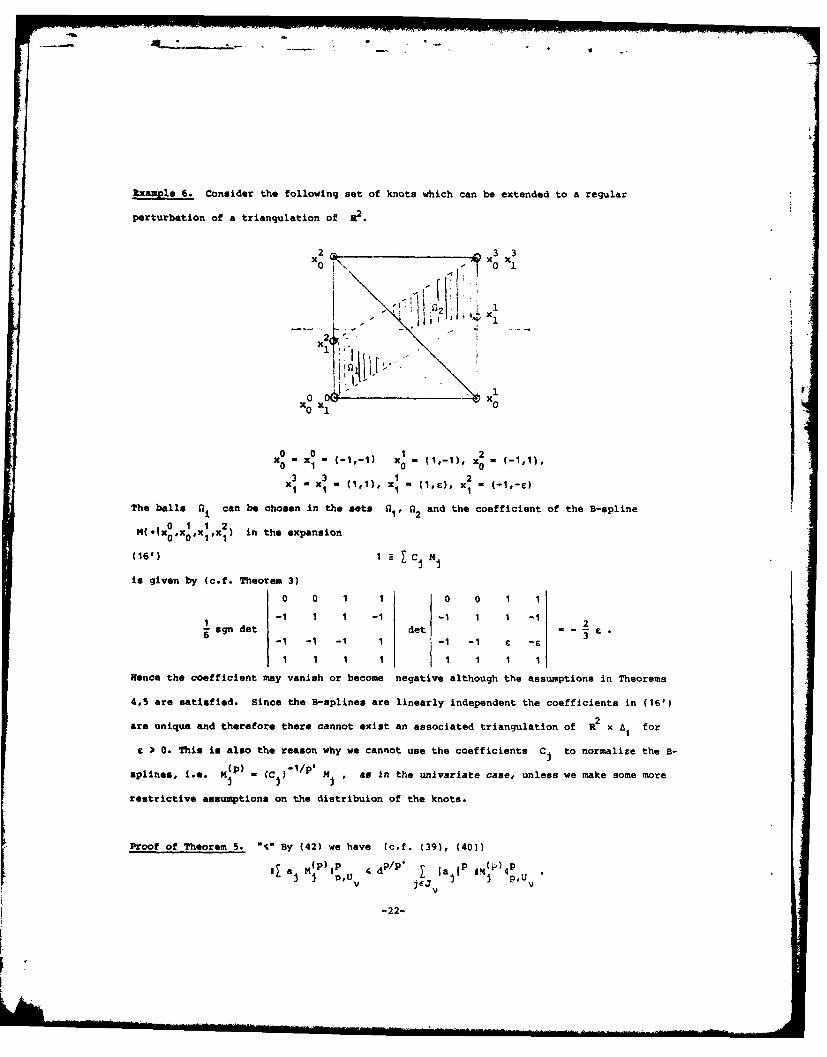
xaple 6. Consider the following set of knots which can be extended to a regular

perturbation of a triangulation of 2 .

2 33xo i 0 x1

O0 x 1

0 0

xo =xl" (-1,-i) x0o - (1,-I), -,

3 3 1 2x 0 xIx x0x1 1 - (1,1), x1 - (1,C), x1 - (-1,-s)

The balls Qi can be chosen in the sets A' n 2 and the coefficient of the B-spline

,0 1 1 2N(.IXoXoxlxI) in the expansion

(16') 1 - CM Hj

is given by (c.f. Theorem 3)

0 0 1 1 0 0 1 11 -1 1 1 -1 -1 1 1 -1 2

sgn det det - - £-1 -1 -1 1 V -1 -1 £ -1 1 1 1 1 1 1 1

Hence the coefficient may vanish or become negative although the assumptions in Theorems

4,5 are satisfied. Since the B-splines are linearly independent the coefficients in (16')

are unique and therefore there cannot exist an associated triangulation of R x I for

c ) 0. This is also the reason why we cannot use the coefficients C to normalize the B-

Splines, I.e. K -P) (C 'I/pi ,I as In the unlvariate case, unless we make some more

restrictive assumptions on the distribuion of the knots.

Proof of Theorem 5. "4" By (42) we have (c.f. (39), (40))

1 a H(p) Ip

4 dp /p a P IM

(P ) p

U V jEj pU V

-22-

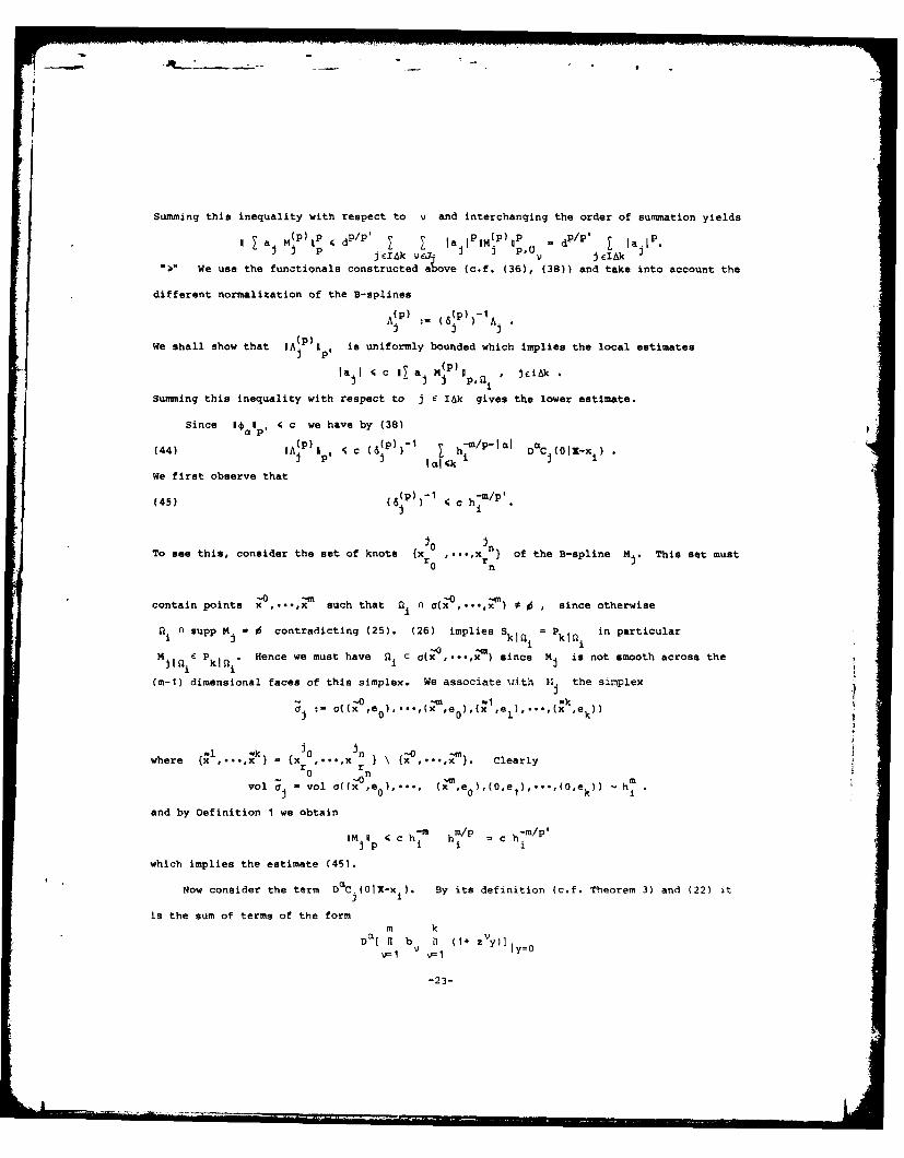
Summing this inequality with respect to v and interchanging the order of summation yieldsIIam(P)Y I dP/P ' I I I P M'P) uPv . dP/P ' lajl p .

j mj P jcI~k vc/j i J PU E I~k

"" We use the functionals constructed above (c.f. (36), (38)) and take into account the

different normalization of the B-splines

^ ( P ) : - ( 6 )(P ) - ,A-j : (6 ) A

We shall show that NA(P) I.I is uniformly bounded which implies the local estimates

Ia 14 c 11 a~ M(P) , Jci~k

Summing this inequality with respect to J e Idk gives the lower estimate.

Since laIp,1 4 c we have by (38)(p p)- -m/p-Icn l ~ c1_i(44) RA Ip I c (6 P h a DC (OIX-x

We first observe that(p))-1 -rn/p'

(45) (6j) 4 c hix 0 i

To see this, consider the set of knots {x ,...,x n) of the B-spline M This set mustn

-a0 I -0 -4ncontain points x ,.-.,x such that Qi n o(x ,...,x ) * 0 , since otherwise

fi n supp mj - 0 contradicting (25). (26) implies Ski = P in particular

MilsE Pkli Hence we must have i C a(x -o,..,x ) since M is not smooth across the

(m-1) dimensional faces of this simplex. We associate :ith 1- the simplexJ I

x ),eO ) .... ,(x ,eo),(x oe..,(x ej 1 tJ0 Jn k

where { k 0...,k ,. Clearlyr ...'x {x-' ..... ',x - lerl

0 on

vol j vol o((x ,eo),.., (x e,( O ,e ,),(O,e h

and by Definition 1 we obtain

UM 1 c hm hm/P -c hm/p

i P i i

which implies the estimate (45).

Now consider the term Daj (0IX-x I. By its definition (c.f. Theorem 3) and (22) it

is the sum of terms of the formm k

D( a1 b )a (1+ zVy)]

2 3y=O

-23-

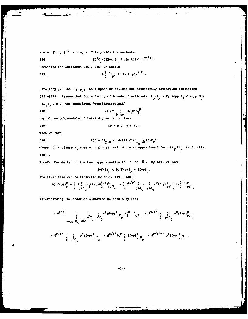
where lb 1, lz'l ( K h , This yields the estimate

(46) IDaCj(0lX-xi)l 4 c(m,k)(Kh i

Combining the estimates (45), (46) we obtain

(47)IA I c(m,k,p)m+k(47)j p'

Corollary 3. Let Sk,z I be a space of splines not necessarily satisfying conditions

(25)-(27). Asiume that for a family of bounded functionala L j:Lp R, supp LC C supp MY

IL Ip I c , the associated "quasiinterpolant"

(48) Qf - I (L f , (p )

reproduces polynomials of total degree 4 r, i.e.

(49) Qp = P 0 p C Pr"

Then we have

(50) IQf -flp, 4 (dc+l) distL (f)(f,Pr)

where ( : U{supp MnJsupp 14 * n } and d is an upper bound for #J ,#J (c.f. (39),

(40)).

Proof. Denote by p the beat approximation to f on U . By (49) we have

IQf-fI 4 IQ(f-p)U + If-pIp p p

The first term can be estimated by (c.f. (39), (40))

IQ(f-p)pP I I L (f-p)Mj(Pp) dp /P

' cP f-pIP )IMP) I p .

P JEJ v V JEJ j4EJ P'u U PU

Interchanging the order of summation we obtain by (41)

dP/P' I I cPif-pI U (P) I P C dP/P' cPf-PPJ oj vE~j p,tJ j p,Uv jwj ~PE 4J PUP U V j jPUU

supp M am*$

dp"r' 7 dcp If-pip r. ddP'P'd c tf-PPJ JJ p U P U

-24-

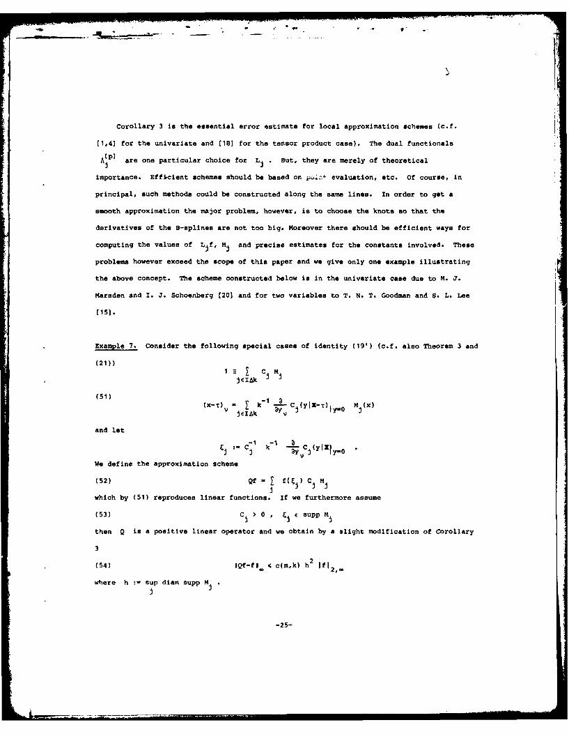
Corollary 3 is the essential error estimate for local approximation schemes (c.f.

(1,4] for the univariate and (18] for the tensor product case). The dual functionals

A.P ) are one particular choice for Lj • But, they are merely of theoretical

importance. Efficient schemes should be based on p<:h evaluation, etc. Of course, in

principal, such methods could be constructed along the same lines. In order to get a

smooth approximation the major problem, however, is to choose the knots so that the

derivatives of the B-splines are not too big. Moreover there should be efficient ways for

computing the values of Ljf, Mj and precise estimates for the constants involved. These

problems however exceed the scope of this paper and we give only one example illustrating

the above concept. The scheme constructed below is in the univariate case due to M. J.

Marsden and I. J. Schoenberg (20] and for two variables to T. N. T. Goodman and S. L. Lee

(15].

Example 7. Consider the following special cases of identity (19') (c.f. also Theorem 3 and

(21))

(51)(-)= k" 1 ~ Y -r x

(xT)v jAk VCj(y I-T)IyO MjW

and let

CJ I j Y k- C (y~l °S -i aC

We define the approximation scheme

(52) Qf - fl) C M

which by (51) reproduces linear functions. If we furthermore assume

(53) C > 0 & j e supp MI

then Q is a positive linear operator and we obtain by a slight modification of Corollary

3

(54) IQf-fl 4 c(m,k) h2 If 12,m

where h : sup diam supp M

-25-

Zn the univariate case, conditions (53) are automatically satisfied. in general we

obtain from (51). if the B-splines are linearly independent,C-i k-i a C (ylx-T)l.

Let T be the center of supp Kj . By (46) It is therefore necessary for C supp M

that

Cj c (diz muwpp M )"I

which leads to restrictions for the distribution of the knots (c.f. Example 6).

Acknowledgement. I would like to thank Professors Carl de Door and Sufian Y. Husseni for

many helpful discussions during the preparation of this report.

-26-

I III II II ll. ..... ....

References

1. Boor, C. de, A practical guide to splines, Springer Verlag, New York, Heidelberg

Berlin, 1978.

2. Boor, C. de, On local linear functionals which vanish at all B-splines but one,

in "Theory of Approximation with Applications", A. G. Law and B. N. Sahney eds.,

Academic Press, New York, 1976, 120-145.

3. Boor, C. de, Splines as linear combinations of B-splines, in "Approxisatlon

Theory II", G. G. Lorentz, C. K. Chul, L. L. Schumaker eds., Academic Press, New

York, 1976, 1-47.

4. Boor, C. do, Fix, G., Spline approximation by quasiinterpolants, J. Approx.

Theory 8 (1973), 19-45.

5. Cavaretta, A. S., Micchelli, C. A., Sharma, A., Multivariate interpolation and

the Radon transform, IBM Reseaarch Report, 1980.

6. Cavaretta, A. S., Micchelli, C. A., Sharma, A., Multivariate interpolation and

the Radon transform, part II: Some further examples, IBM Research Report, 1980.

7. Curry, H. B., Schoenberg, I. J., On Polya frequency functions IV, The fundamental

spline functions and their limits, J.d'Analyse Math. 17 (1966), 71-107.

8. Dahmen, W., On multivariate B-splines, SIAM J.Numer. Analysis 17 (1980), 179-191.

9. Dahmen, W., Polynomials as linear combinations of multivariate B-splines, Math.

Z. 169 (1979), 93-98.

10. Dahmen, W., Habilltationsechrift, Bonn, 1981.

11. Dahmen, W., Micchelli, C. A., On limits of multivariate B-splines, MRC Technical

Suimmary Report #2114, 1980.

12. Dahmen, W., Micchelli, C. A., On functions of affine lineage, IBM Research

Report, 1980.

13. Donoghue, W. F., Distributions and Fourier transforms, Academic Press, New York,

1969.

14. Eilenberg, S., Steenrod, V., Foundations of algebraic topology, Princeton

University Press, Princeton, 1952.

-27-

15. Goodman, T. N. T., Lee, S. L., Spline approximation of Bernstein Schoenberg type

in one and two variables, to appear.

16. H6llig, K., A remark on mltivarlate B-splines, to appear in J. Approx. Theory.

17. H~rmander, Lars, An introduction to complex analysis in several variables, North

Holland Publishing Company, 1973.

18. Lyche, T., Schumaker, L. L., Local spline approximation methods, J. Approx.

Theory 15 (1975), 294-325.

19. Marsden, M. J., An identity for spline functions with applications to variation

diminishing spline approximation, J. Approx. Theory.3 (1970), 7-49.

20. Marsden, M. J., Schoenberg, I. J., On variation diminishing spline approximation

methods, Mathematica (Cluj) 8 (1966), 61-82.

21. Michelli, C. A., A constructive approach to Kergin interpolation in Rk,

Multivariate B-splines and Lagrange interpolation, to appear in Rocky Mountain J.

22. Micchelli, C. A., On a numerically efficient method for computing miltivariate B-

splines, in "Multivariate Approximation Theory", W. Schempp, K. Zeller ads.,

ISNM5I, Birkhhuser Verlag Basel, 1979.

23. Nrlund, N., Vorlesungen pber Differenzenrechnung, Grundlehren der Math.

Wissenschaften, Vol. 13, Springer, Berlin, 1924.

KH/db

-28-

SECuRI1Y CLASSIFICATION Or THIS PAGE (l7,en fleI. knterod)READ INSTRVC"TIONS

REPORT DOCUMENTATION PAGE BN.FhORF COt /I. REPORT NUMSER 12. GOVT ACCESSION NO. 3. RECIPIENT'S CATALOG NUMb" -

-A )?? 354. TITLE (aind Subtitle) S. TYPE Of REPORT G PERIOD COVERED

Summary Report - no specic IMULTIVARIATE SPLINES reporting period

S. PERFORMING ORG. REPORT NUMBF.R

7. AUTHOR(a) S. CONTRACT OR GRANT NUMBER(a)

Klaus H8llig DAAG29-80-C-0041'MCS-7927062

S. PERFORMING ORGANIZATION NAM E AND AYRESS 10. PROGRAM ELEMENT. PROJECT, TASK

Mathematics Research Center, University of AREA & WORK UNIT NUMBERS

610 Walnut Street Wisconsin 3 - Numerical Analysis andMadison. Wisconsin 53706 Computer ScienceIt. CONTROLLING OFFICE NAME AND ADDRESS 12. REPORT DATE

March 1981See Item 18 below 13. NUMBEROF PAGES

284. MONTOING GENCY NAME: ADDRESS(If diflerent from Controlling Office) 15. SECURITY CLASS. (of this report)

UNCLASSIFIEDISa. DECLASSIFICATION,'OOWNGRADING

SCHEDULE

I. DISTRIBUTION STATEMENT (of tal Report)

Approved for public release; distribution unlimited.

17. DISTRIBUTION STATEMENT (of the abetract entered In Block 20, If different from Report)

IS. SUPPLEMENTARY NOTESU. S. Army Research Office National Science FoundationP. 0. Box 12211 Washington, D. C. 2055uResearch Triange ParkNorth Carolina 27709

19. KEY WORDS (Continue on revereD side If neceeeary and Identify by block number)

Multivariate, B-splines, spline functions, dual basis, condition number

20. ABSTRACT (Continue on reveree aide If necaeery and identify by block number)It is shown that the span of a collection of multivariate B-splines,Sk:=

)0 k+m)span M(- x ,...,x ), contains polynomials of total degree < k if the indexjeaset j=o(jo,-.,Jk+m)}jEj has a certain combinatorial structure, in particular the

knots {xV)c IRn can be chosen essentially arbitrarily. Under mild assumptionson the distribution of the knots, a dual basis {Xj}j for S is constructed

which has local support, i.e., (continued)

DD ,ORM 1473 EDITION OF I NOVSS IS OBSOLETE

SEURTYC.SIFUNCLASSIFIED. SECURITY ('| ASSIFICATION Of' THIS PAGE (14hon Date Entered)

20. Continued

auppy Ac supp Ni, and the condition number of the B-spline basis is estimated.

This leads to good local approximation schemes.