Embed Size (px)
Citation preview

Activity recognition for a smartphone and web basedtravel survey
Youngsung KimSingapore-MIT Alliance forResearch and Technology
(SMART)[email protected]
Francisco C. PereiraSingapore-MIT Alliance forResearch and Technology
(SMART)[email protected]
Fang ZhaoSingapore-MIT Alliance forResearch and Technology
(SMART)[email protected]
Ajinkya GhorpadeSingapore-MIT Alliance forResearch and Technology
(SMART)[email protected]
P. Christopher ZegrasMassachusetts Institute of
Technology (MIT)[email protected]
Moshe Ben-AkivaMassachusetts Institute of
Technology (MIT)[email protected]
ABSTRACTIn transport modeling and prediction, trip purposes play animportant role since mobility choices (e.g. modes, routes,departure times) are made in order to carry out specificactivities. Activity based models, which have been gain-ing popularity in recent years, are built from a large num-ber of observed trips and their purposes. However, dataacquired through traditional interview-based travel surveyslack the accuracy and quantity required by such models.Smartphones and interactive web interfaces have emergedas an attractive alternative to conventional travel surveys.A smartphone-based travel survey, Future Mobility Survey(FMS), was developed and field-tested in Singapore and col-lected travel data from more than 1000 participants for mul-tiple days. To provide a more intelligent interface, infer-ring the activities of a user at a certain location is a crucialchallenge. This paper presents a learning model that in-fers the most likely activity associated to a certain visitedplace. The data collected in FMS contain errors or noisedue to various reasons, so a robust approach via ensemblelearning is used to improve generalization performance. Ourmodel takes advantage of cross-user historical data as wellas user-specific information, including socio-demographics.Our empirical results using FMS data demonstrate that theproposed method contributes significantly to our travel sur-vey application.
General TermsAlgorithms, Design, Human Factors, Experimentation
KeywordsActivity Recognition, Urban Mobility, Interactive Data Col-lection.
1. INTRODUCTIONHuman activity recognition research is useful to interpret
mobility related phenomena in a city [21]. Understandingwhy people go to some places at certain times has beneficialramifications in many fields such as transportation, internetcommerce, urban traffic management, location based ser-vices, public health, urban planning, public safety, and soon [17]. Activity based modeling for travel demand is gain-ing popularity in recent years and it requires a large numberof observed trips and their purposes to build. Traditionally,data used in activity based modeling is collected throughinterview-based travel surveys. Collecting a sufficiently largesample requires an extensive effort. The accuracy of the col-lected data depends on the memory of the participant, so itis a challenge to capture high resolution activities for dayswith complex activity patterns. Due to these limitations, re-searchers are exploring new ways to conduct travel surveysusing mobile sensing devices. Smartphones are pervasivedevices that nowadays people carry with them everywhere.They are ideal devices for travel and activity informationlogging. We have developed a smartphone based activity-travel survey system, Future Mobility Survey (FMS) [3],and recently used it in large-scale data collection effort inSingapore.
FMS acquires movement data through sensors (such asGPS, GSM, WiFi, and Accelerometer) commonly availablein current smartphones. Besides the hardware sensors, FMSacquires activity and transportation information through aweb-based interactive process. The task of the participantis to check that the stop locations, activities, times, andmodes are accurately described (and correct them if nec-essary) on a web interface. To ensure quality of validateddata, the user must accurately label the activity at eachstop location. Machine learning based approaches for ac-tivity recognition can automate some of these tasks, reduceuser burden, and therefore assist the user in providing muchneeded high quality data. Currently a new version of FMS
arX
iv:1
502.
0363
4v1
[cs
.CY
] 1
2 Fe
b 20
15

software is being developed based on data acquired duringa field-test to create a more intelligent backend and inter-face. In this paper, we present a learning based model forthe activity recognition task.
However, prediction of human activity is a nontrivial task,especially in an urban area. One of the reasons is that activ-ities often have heterogeneous patterns within a small area(e.g. shopping malls with healthcare facility, supermarket,offices) or at the same time (e.g. working at home; shop-ping while waiting for the train). Also, sensor data qualityitself is not always the best (e.g. GPS unavailable in indooractivities).
To alleviate uncertainty of real world data, we extract het-erogeneous features and merge multiple hypothesis modelslearned from different user populations. The user’s likeli-hood of performing a certain activity at a given locationwill depend on user’s personal needs which will be driven byhis/her socio-demographic characteristics [13]. Usually en-vironmental context at the given location limits the type ofactivities one can perform. We can also derive the activitylikelihood from the activities performed by general popula-tion apart from individual user characteristics. In this pa-per, we present a learning model based on spatial, temporal,and contextual features and conduct various experiments todemonstrate its veracity. The contributions of this paperare:
• A method to generate a set of predictive features basedon location, time, transition context, and environmentcontext (e.g. Points of Interest),
• Spatial data quantization methods to balance the noiseeffect in real world data,
• Improvement of generalization performance by merg-ing of intra-user data and inter-user data includinguser’s social-demographic information,
• Analysis of number of training days required for alearning model in a real world application.
This paper is organized as follows. In section 2, we re-view related work. In section 3, we present FMS, a smart-phone based activity-travel survey where the proposed ac-tivity recognition algorithm will be used. In section 4, wepresent the proposed activity recognition framework. Ex-tensive experiments are followed with different settings offeature in section 5. Finally, we conclude this paper withsome remarks and future work in section 6.
2. RELATED WORKWith the advance of sensing technology, GPS loggers, and
more recently, smartphones, have become popular tools toconduct travel surveys that are essential for transportationplanning and management [2, 3]. The identification of ac-tivities is perhaps the most challenging data processing taskinvolved in such travel surveys. The activity categories typ-ically include home, work, social, shopping, pickup/drop-offetc.
Most of the algorithms used to derive activities in GPStravel surveys are rule-based and rely heavily on GIS in-formation, such as Point Of Interest (POI) and land useinformation [23, 8, 6]. An early car-based study in America
by Wolf et al. [23] inferred trip purposes from GPS data andan extensive GIS land use database. In more recent work,POI’s attractiveness is defined along time of day to indi-cate the potential possibilities for activities [8], and [6] pro-posed to infer an activity based on the distance between POIand the stop location. Another option is to use individualcharacteristics as input for activity recognition algorithms.Axhausen et al [1] developed a rule based approach to iden-tify activities based on users’ home and work locations, andPOI/land use information in the Swiss. Similar informationand rules were used in the GPS survey in the Netherlands[2]. Reference [22] described a more complicated heuristicrule-based method which collects users’ workplace or school,the two most frequently used grocery stores, and occupationbeforehand to be used to derive trip characteristics.
More elaborate algorithms have been proposed taking amachine learning approach. Deng and Li [4] used attributessuch as land use, sociodemographic information of the re-spondents, etc. to construct decision trees. An adaptiveboosting technique was used to improve the classificationresults. Liao et al. [15] proposed a location based activ-ity recognition system using Relational Markov Networks.These works are evaluated based on small samples of exper-imental data.
Few work exists for activity detection in smartphone basedtravel surveys. Feldman et al. [5] converted GPS trajecto-ries collected by smartphones into lists of activities by firstfinding businesses around a user stop, and then employingreverse Latent Semantic Analysis (LSA) to look up the mostrelevant terms associated with the businesses.
3. SMARTPHONE-BASED ACTIVITY TRAVELSURVEY
In this section, we give an overview of the FMS system andbriefly describe the data which is used for building activityrecognition algorithm.
3.1 Future Mobility Survey (FMS): activity-travel data collection method
Future Mobility Survey (FMS) [3] collects mobility recordsthrough a smartphone application (Android and iOS) andan interactive web interface. It acquires movement datathrough sensors commonly available in current smartphones,namely Global Positioning System (GPS), WiFi, Mobile Com-munications System (GSM, CDMA, and UMTS), and Ac-celerometer. Stop and mode detection algorithms are runin the backend on the collected raw data and the output ispresented to the user in the form of an activity diary [18, 3].users can then“validate” their data by confirming or correct-ing the system generated stops/modes. In the current FMSsystem, there is a simple rule-based algorithm to detect only“home”, “work”, and “change-mode” activities. The overallflow is depicted in Figure 1.
FMS was recently deployed in Singapore [18] to conducta travel survey. Thus far, the FMS has collected collecteda total of 22,170 days from 1,440 users in real life situa-tions (more than 130 Million GPS points in total). Amongthe days and users, we have a total of 7,856 validated daysfrom 948 users. A total of 793 users fully participated inthis venture, each one required to collect data for at least 14days and validate least 5 days. The survey was conductedbetween October 2012 and September 2013. Due to bat-

tery limitations, the smartphone application cannot contin-uously collect the high quality data (e.g. high accuracy GPSand big frequency accelerometer), and as a consequence, therecords are sparse in practice. Furthermore, some sensorsare not available in certain contexts (e.g. GPS unavailableindoors, WiFi unavailable without nearby APs).
1) Smartphone for sensing
2) Server workstation for intelligent processing of collected data
3) Web interface for validation
Figure 1: Overview of Future Mobility Survey sys-tem. The FMS web interface can be found athttp://www.fmsurvey.sg/.
To our knowledge, FMS is the only smartphone basedtravel survey that has gone through a field-test with largenumber of users. Most existing applications [8, 6, 15, 5] haveused limited size of data collected by fewer than 28 users.The large amount of real world data collected presents aunique opportunity to develop and test machine learningalgorithms for activity recognition.
3.2 Activity categoriesWithin the FMS, we have defined seventeen different ac-
tivities. Home, Work, Work-Related Business, Education,Change Mode/Transfer, Pick Up/Drop Off, Meal/EatingBreak, Shopping, Personal Errand/Task, Medical/Dental (Self),Social, To Accompany Someone, Recreation, Entertainment,Sports/Exercise, Other’s Home, and Other. ‘Other’ will beexcluded in our activity recognition algorithm.
4. METHODOLOGYIn this section, we first present a spatial quantization tech-
nique to get empirical activity probability based features.We then describe the ensemble learning based classificationmethodology using heterogeneous features for different userpopulations.
4.1 Spatial-temporal data representation andquantization
4.1.1 Data representationOur dataset consists of a sequence of n stop points for a
user u, {pui |i = 1, 2, . . . , n, and u = 1, 2, . . . , U}, where theuser stayed for a relevant time window1. Further each stoppoint is represented as pui = (xi, yi, ti1, ti2), where xi andyi denote the geographical coordinates, (ti1, ti2) denotes thestart and end time respectively. For simplicity, we use piinstead of pui now on.
1The FMS minimum threshold is 1 minute to capture modechanges, but it is normally aggregated (by the system or bythe user) to much longer chunks.
4.1.2 Data quantizationThe quantization is applied to the location and time space
to enhance data interpretation in terms of context. Thiscontext is coarse-grained in spatial and temporal axes. Forexample, we can deduce a “transportation change mode”during “evening rush hour” or deduce that a person maybe at “shopping mall” on “Sunday evening”. Here, we ap-ply quantization as follows (where 7→ represents a mappingrelationship):
• Spatial cell: the location (xi, yi) 7→ a cell ci. Distri-bution of activities is non-uniform across geographies.Dependent on a mapping function, samples in a cellare different. Some spatial quantization methods willbe proposed in section 4.1.3.
• Set of time slots (within the day): the time period(ti1, ti2) 7→ a set Si of time slots (e.g. 10 minute slots).For example, an activity started at 8:53 and ending at9:08 will be assigned to a time slot set S={8:50, 9:00,9:10}. This works as an“temporal alignment”step thatwill later be useful for calculating temporal frequencyfeatures.
Hence, our dataset will consist of activity points qi (thequantized version of pi), defined as the tuple (ci,Si, ai) whereai denotes an activity from the set of sixteen categories men-tioned above. We also create two useful functions: W(s)returns the day type of a time slot s (weekend or weekday);X (c) retrieves the set of Points of Interest from our database,corresponding to cell c.
4.1.3 Spatial quantization methods (distribution adap-tive quantization)
As mentioned above, the function mapping the locationof pi to a cell ci affects the likeliness of activity ai so we ex-plore different mapping (spatial quantization) functions tofind an appropriate population representation. The simplestand easiest way is to divide space arbitrarily regardless of asample distribution. An adaptive way is to apply the datadistribution. In this work, we consider both fixed quanti-zation and dynamic quantization. In the fixed case, oncespace of training data is quantized, it is used in future prob-ability calculations. In the dynamic case, space is dividedwhen a new instance is identified. In this case, if there areN samples to calculate frequencies, the number of cells isN .
Fixed cell.• Rectangle shape: quantization is not correlated with
regional distribution. The easiest way is to adopt arectangle shape; parameters including width (horizon-tal) and height (vertical) size.
• Voronoi tessellation based polygon: spatial data clus-ters can be found to apply regional characteristics.Based on a centroid of each cluster, edges and ver-tices of each cell can be found by Voronoi tessellation.To find an appropriate cluster is a essential process.
Dynamic (instance based) cell.• Circular polygon: a cell is defined within predefined
distance (radius of circle) at each instance. Every in-stance is a centroid of a cell.
4.2 Proposed features
4.2.1 Activity FrequencyFor each activity point qi, we determine three kinds of
activity frequency: Temporal activity frequency, Spatial ac-tivity frequency, and Contextual activity frequency. We es-sentially make use of the following general empirical condi-tional probability distribution (we use the kronecker deltanotation, where δi,j = 1 if i = j, and 0 otherwise):
Pr(ai = l|bi) :=
∑Nj=1 δaj ,l · δbj ,bi∑L
l=1
∑Nj=1 δaj ,l · δbj ,bi
(1)
where N denotes the total number of activity points in thesame cell for all users u ∈ U (U is a user set), bi denotesa bin, and l denotes an activity type (L is total number ofactivities).In this equation, we count a normalized frequency of activityl, within a bin over the total count of all activities withinthe same bin. For spatial activity frequency, the bin we useis a spatial cell ci.
In order to estimate the temporal activity frequency, weneed a slightly more sophisticated treatment of the data. Inthis case, the statistics depend on the time slot sequence ofthe activity points, where each time slot adds 1 (e.g. anactivity that spans from 8:00 to 10:00 contributes 12 to thetotal count, assuming 10 minutes time slots). The bin atactivity point i is now defined by its entire sequence of timeslots (Si). Inclusion or exclusion of a different activity pointj in that bin is based on how many common time slots existbetween i and j.
For the contextual activity frequency, we first map eachPOI category to one of the sixteen activity classes and thencompute a relative frequency of each activity type in eachspatial cell.
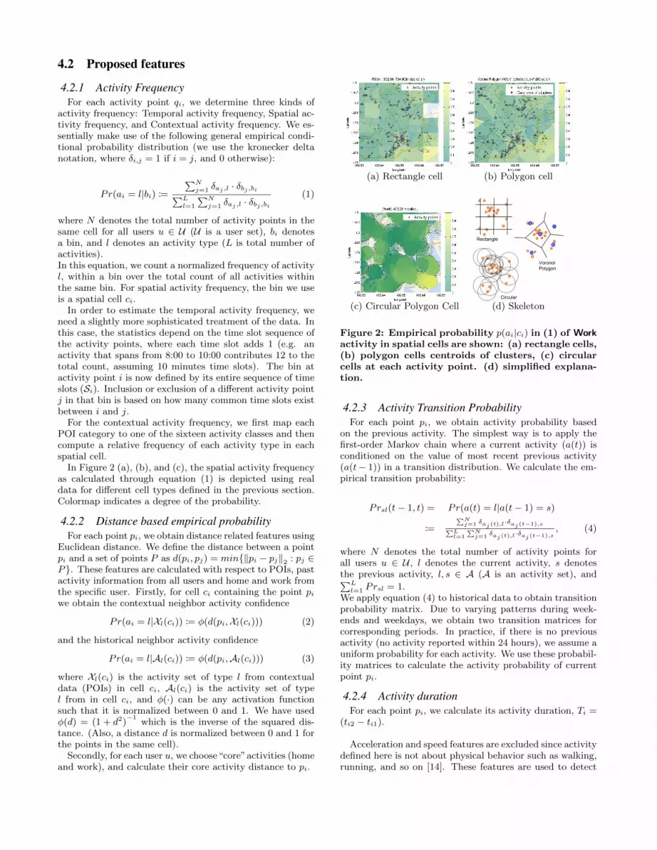
In Figure 2 (a), (b), and (c), the spatial activity frequencyas calculated through equation (1) is depicted using realdata for different cell types defined in the previous section.Colormap indicates a degree of the probability.
4.2.2 Distance based empirical probabilityFor each point pi, we obtain distance related features using
Euclidean distance. We define the distance between a pointpi and a set of points P as d(pi, pj) = min{‖pi − pj‖2 : pj ∈P}. These features are calculated with respect to POIs, pastactivity information from all users and home and work fromthe specific user. Firstly, for cell ci containing the point piwe obtain the contextual neighbor activity confidence
Pr(ai = l|Xl(ci)) := φ(d(pi,Xl(ci))) (2)
and the historical neighbor activity confidence
Pr(ai = l|Al(ci)) := φ(d(pi,Al(ci))) (3)
where Xl(ci) is the activity set of type l from contextualdata (POIs) in cell ci, Al(ci) is the activity set of typel from in cell ci, and φ(·) can be any activation functionsuch that it is normalized between 0 and 1. We have usedφ(d) = (1 + d2)
−1which is the inverse of the squared dis-
tance. (Also, a distance d is normalized between 0 and 1 forthe points in the same cell).
Secondly, for each user u, we choose“core”activities (homeand work), and calculate their core activity distance to pi.
(a) Rectangle cell (b) Polygon cell
(c) Circular Polygon Cell
Rectangle
Voronoi Polygon
Circular
(d) Skeleton
Figure 2: Empirical probability p(ai|ci) in (1) of Workactivity in spatial cells are shown: (a) rectangle cells,(b) polygon cells centroids of clusters, (c) circularcells at each activity point. (d) simplified explana-tion.
4.2.3 Activity Transition ProbabilityFor each point pi, we obtain activity probability based
on the previous activity. The simplest way is to apply thefirst-order Markov chain where a current activity (a(t)) isconditioned on the value of most recent previous activity(a(t− 1)) in a transition distribution. We calculate the em-pirical transition probability:
Prsl(t− 1, t) = Pr(a(t) = l|a(t− 1) = s)
:=
∑Nj=1 δaj(t),l
·δaj(t−1),s∑Ll=1
∑Nj=1 δaj(t),l
·δaj(t−1),s, (4)
where N denotes the total number of activity points forall users u ∈ U , l denotes the current activity, s denotesthe previous activity, l, s ∈ A (A is an activity set), and∑Ll=1 Prsl = 1.
We apply equation (4) to historical data to obtain transitionprobability matrix. Due to varying patterns during week-ends and weekdays, we obtain two transition matrices forcorresponding periods. In practice, if there is no previousactivity (no activity reported within 24 hours), we assume auniform probability for each activity. We use these probabil-ity matrices to calculate the activity probability of currentpoint pi.
4.2.4 Activity durationFor each point pi, we calculate its activity duration, Ti =
(ti2 − ti1).
Acceleration and speed features are excluded since activitydefined here is not about physical behavior such as walking,running, and so on [14]. These features are used to detect

stop segments in the FMS system as mentioned above.
After the feature extraction process explained above wehave the following feature vector, general features
x =[Temporal Activity Probability ∈ R1×L,
Spatial Activity Probability ∈ R1×L,
Contextual Activity Probability ∈ R1×L,
Activity Transition Probability ∈ R1×L,
Historical Neighbor Activity Confidence ∈ R1×L,
Contextual Neighbor Activity Confidence ∈ R1×L,
Core Activity Distances ∈ R1×2,
Activity Duration ∈ R1]T ∈ R6L+3,
(5)
where L is the number of activity categories.
4.3 ClassificationWhen the data is acquired from multiple sensors or sources
(and then heterogeneous features are generated), a singleclassifier cannot find good decision boundary for classifica-tion [19]. To overcome this problem, in this section, wepresent ensemble learning based classification. Ensemblelearning, here, is used through two levels; one is to learnheterogeneous features, and in second step, outputs fromclassifiers such as score and decision are merged to a finaldecision.
4.3.1 Ensemble decision treesEnsemble learning has been widely used to cope with noisy
real world data. In this paradigm, several (base) classifiersare learned from training data to eventually become a unifiedclassifier. In theory, individual base classifiers can concen-trate on different areas of the problem space and, as a result,the unified classifier, which combines the output of thosebase models, becomes more robust. Two kinds of ensemblelearning are used in this paper, namely bootstrap aggregat-ing (Bagging) and random subspace. In Bagging, each baseclassifier is trained with a subset generated by subsamplingon the global training set. In the random subspace approach,each base classifier is learned using subspace features of theoriginal feature set. To predict a class label for unseen data,a majority voting process is applied on the set of individualpredictions.
Our base classifier will be decision trees, one of the pop-ular methods, which consist of gradually splitting the inputfeature space into decision regions. This method is useful todeal with irrelevant variables and is robust to outliers. How-ever, decision trees show unstable performance. To allevi-ate instability, ensemble learning has been widely adopted.One popular method is bagging of decision trees. Anotherpowerful tool is a combination of aggregating set of randomfeatures (subspace) based on decision tree classifier, namelyRandom Forests [7].
Using a set of training features and activity labels {xi, ai} ∈Tr, ∀i where Tr is a training set, we calculate an ensemblehypothesis function h(x,Θ) where Θ is a set of decision treehypothesis θk, ∀k. This function finds an activity label a,based on a = arg maxl sl, where sl is the score for activ-ity label l. This function will be used to predict a label ofunseen data xtest ∈ Te for test in future.
4.3.2 Ensemble of user social demographic charac-teristics based learning
Users with different social demographic characteristics showdifferent activity and travel patterns [9, 13]. It is, thus, help-ful to learn a model using individual user’s history data, inaddition to learning from other users’ history data. An in-dividual user belongs to multiple categories; formally eachuser is included in several different user sets: u ∈ U ,P,O,G,where U denotes a cross (universal) user set, P denotes aspecific user set, O denotes an age-specific user set, and Gdenotes a gender-specific user set. The input feature vec-tor of pi for a user u, x(pui ), (where u ∈ U and xU , ∀u),is generated based on subsets. Classifiers (hypotheses) arelearned using user subsets: h(xU ), h(xP), h(xO), and h(xG).From each model, we get outputs such as 1) a score vectorwith a element sl ∈ [0, 1], ∀l for each class (activity) labeland 2) a decision dl, ∀l for the l-th class. The score of eachactivity class from the hypothesis h(·) become an input fea-ture vector for ensemble classifier to determine a final score.Classifier’s decision can be merged by classifier learning andWeighted Majority Voting (WMV). WMV is one popularmethod to merge multiple decisions to obtain a final deci-sion (based on arg maxl
∑Tt=1 wtdt,l ∀l where wt is a weight
for t-th classifier’s decision dt,l ∈ {0, 1} for l-th class.) [19].
4.4 Workflows of the proposed algorithmFigure 3 shows an overall flow of the proposed activity
recognition system used in FMS. We infer an activity typefor each user stop point.
5. EXPERIMENTSIn this section, we evaluate the proposed algorithm using
a dataset acquired through our FMS system.
5.1 Data setWithin the FMS, we have 793 users who have completed
the survey with at least 5 validated days, as mentioned inSection 3.1. POI data has been provided by Singapore LandAuthority (SLA). It has a total of 64, 819 points related toshopping malls, clinics, bus stops, and metro train stations,residential buildings, office buildings and so on2. These POIsare mapped to our 16 activity categories. Table 1 shows thestatistics for the mapping.
5.2 Data preprocessing and cleaningAs with any kind of survey, the data collected in FMS
contains noise/errors, and this problem may be more seri-ous in this case than average. Since the FMS users were notguided by interviewer in their validation process, the taskhas been proven to be challenging to some of the users, es-pecially those less tech-savvy users. As a result, there canbe multiple errors in user’s data. Therefore, data cleaning isan essential step before we perform any performance evalua-tion. Firstly, we select days where users started and finishedtheir daily activity at home. Then, we apply a sequence of
2POI label includes;e.g. Pub/Bar, Restaurant, Kiosk/Stall, Cafe,
Pet Shops, Child Care, Skin Care, Gym, Supermarkets, ConvenienceStores, ATMs, MRT Stations, Swimming Complexes, Tuition Centres,Music Dance Schools, Car Wash, Toy Stores, Photography, Post Of-fices, Town Councils, HDB Branch Offices, Police Stations, PrimarySchools, Secondary Schools, Hair Salons, Yoga Pilates, Accountants,Maid Agencies, Clinics, Laundry, Travel Agencies, Religious, Phar-macies, and so on.

Decision
Dura,on, Core Distances
Ac,vity
Ensemble Classifiers Learning
Spa,al Frequency
Contextual Frequency
Training phase
Test phase
valida,on Users
Feature Generation
Temporal Frequency
Neighborhood Confidence
Neighborhood Confidence
Preprocessing User’s
Historical Data
Contextual Data (POIs)
Feature Genera,on
User ID, Loca,on,
Time stamp
Preprocessing
Transi,on (Markov)
Stop detec,on
Stop Detec,on
User’s travel data
User’s travel
Cross-‐User Classifier
Social-‐Demographics
Classifier
Intra-‐User Classifier
Figure 3: Overview of the proposed activity recognition system. Based on given an identified stop (detectedby the current stop detection algorithm), the algorithm identifies an activity based on spatial, temporal,transition, and contextual features. We assume that his/her home location is known beforehand (providedwhen he/she registered in the website).
Table 1: The number of environmental context dataper activity category generated based on Points ofinterest (POIs) which contain location information.
Activity #points percent (%)
Home 31 0.05Work 48 0.08
Change Mode/Transfer 4965 8.25Pick Up/Drop Off 0 0.00
Shopping 19862 32.99Social 0 0.00
Work-Related Business 4619 7.67Education 2678 4.45Recreation 888 1.48
Medical/Dental (Self) 4150 6.89Meal/Eating Break 10200 16.94
Entertainment 181 0.30Sports/Exercise 529 0.88
Personal Errand/Task 12046 20.01To Accompany Someone 0 0.00
Other’s Home 0 0.00Other 4670 -
*Other is excluded.
checks, and discard the data if home to home distance ishigher than 50 meters; if home to other validated activitiesis less than 10 meters; or if activity points have swappedtime between start and end of one activity. We also applyother filters: no activity with more than 24 hour duration isallowed; an activity outside of Singapore area is removed. Asa result, we use 5,073 points from 243 users where their datahad been collected from March 11th of 2013 to September30th of 2013 for the following experiments.
5.3 Protocols and parameter settingsFirst, we apply two-fold validation where we keep the
chronological order of data with k training days and one testday split, k = 1, 2, 3, 4 for every users. In the experiments,we apply different parameter settings: different resolutions
of time slot: [10, 20, 40, 60, 90, 120] minutes; different res-olutions of spatial cell width: [200, 400, 600, 800, 1000] me-ters; number of clusters for Voronoi polygons: [1000, 800,600, 400, 200, 100]; Circle radii: [100, 150, 200, 300, 400,500] meters.
For the random subspaces based decision trees (RandomForest (RF)), a dimension of subspace features is chosenbased on square root of the total number of feature vari-ables. For decision tree-based (DT) classifiers including RFand bagging of DT (BagDT), the minimum number of obser-vations per tree leaf is set as 1. 100 base classifiers are used.A random seed found by pseudorandom number generationis fixed.
5.4 Results
5.4.1 Different resolutions of temporal slot and spa-tial cell
Ensemble methods (BagDT and RF) show constant aver-age accuracy as temporal cell size increases. Accuracy valueof those methods increases as spatial cell size increases forRectangle and Voronoi Polygon cases. For more details, areader can refer to [10].
5.4.2 Different number of training daysFigure 4 shows the average classification accuracy for dif-
ferent number of training days. We see that the averageaccuracy is improved as the number of training days in-creases. In Figure 4 (a), individual classifier was learnedusing different sets of user population such as cross-user,individual user, age-specific user, and gender-specific user.The model using more training data shows better classifica-tion performance. Due to small number of training samples,user-specific model solely does not show best performance.However, that accuracy value drastically increases comparedto other models as data size increases. In Figure 4 (b), clas-

sification performance of ensemble of individual models areshown. Ensemble models show better classification perfor-mance than that of individual models. Decision fusion basedon weighted majority voting (weightedMvote) methods showstable and best performance along with the training days asshown in Figure 4 (b).
1 2 3 440
45
50
55
60
65
70
75
Ave
rage
acc
urac
y (%
)
training days
Circular
BagDT (cross−user)BagDT (user−spec)BagDT (age)BagDT (gender)RFs (cross−user)RFs (user−spec)RFs (age)RFs (gender)
(a) Individual Models
1 2 3 440
45
50
55
60
65
70
75
Ave
rage
acc
urac
y (%
)
training days
Circular
BagDT (scoreEnsemble)BagDT (decisionEnsemble)BagDT (weightedMVote)RFs (scoreEnsemble)RFs (decisionEnsemble)RFs (weightedMVote)
(b) Fusion Models
Figure 4: Average prediction accuracy along withnumber of training days for each model: (a) indi-vidual classifier learned using different sets of userpopulation. (b) ensemble classifiers for merging in-dividual classifier models.
5.4.3 Relationship between activities and mergingIn Table 2, we show classification confusion matrix for
16 activity categories. As shown in the table, most of thepoints in the Pick Up/Drop off class (PD) is classified asChange Mode/Transfer (C). Work-Related Business (WR)activities are mainly classified as Work (W). Many otheractivities (related to maintenance or discretionary context)are classified as Change Mode/Transfer (C) which has thelargest training sample size. And this may relate to the factthat many shopping malls and shops are located close tostreet and bus/train stations in Singapore.
As the 16 activities cannot be exclusively explained, i.e.more than one activity can be tagged for one certain userstop point. We follow the work of [12, 20] to distill this setinto a set of conceptually exclusive activities: 1) Home, 2)Work (including Work, Work-Related Business, and Educa-tion), 3) Transportation (including Change Mode/Transferand Pick Up/Drop Off, and 4) Maintenance/Discretionary(including Meal/Eating Break, Shopping, Personal Errand/Task,Medical/Dental (Self), and so on). Table 3 shows that clas-sification accuracy using four activity definition is improvedcompared to full sixteen activity categories.
5.4.4 Prediction performance improvement by merg-ing of different sets of user population
Table 3 shows classification accuracy for 16 classes and4 classes respectively, using 4 training days and RandomForest with Rectangle cell type. Scores of multiple clas-sifier learned using different user population is merged bya classifier (Scores Ensemble by classifier). Decisions frommultiple classifiers are merged by classifier (Decisions ensem-ble by classifier) and by Weighted Majority Voting. For theweighted majority voting (WMV), weights are simply deter-mined with ‘4’ for the cross-user model, ‘3’ for the gendermodel, ‘2’ for the age model, and ‘1’ for intra-user model.This is based on number of training samples per model;
General (total) > Gender > Age > User-specific. Decisionmerging with WMV shows consistently better classificationaccuracy than to other models.
Table 3: Overall accuracy (number correctly classi-fied/total number of samples), Random Forests
method accuracy(%)16 classes
cross-users 72.32userID 63.95Age 70.60Gender 74.68Scores ensemble (classifier) 73.61Decisions ensemble (classifier) 73.18Decisions ensemble (weighted majority) 75.54
4 classescross-users 78.98userID 74.95Age 80.89Gender 83.23Scores ensemble (classifier) 84.50Decisions ensemble (classifier) 83.44Decisions ensemble (weighted majority) 84.08
*setting: 4 training days, 800m × 800m rectangle size,120 mins time slot.*4 Classes: 1) Home, 2) Work, 3) Transportation,4) Maintenance/Discretionary
5.4.5 Testing on real data stream and unseen usereffect
In Figure 5, we plot the test accuracy performance alongwith arrival of sequential data. The incoming unseen activ-ity data is predicted based on learned model using previoustraining data to obtain the test accuracy. Subsequently, thistested data is used for training in next sequence day basedon its true (labelled by users) activity label. A test datais coming either from unseen user or seen user. Seen usermeans that his/her activity history is used during trainingmodels, and unseen user is not. As shown in the bottomfigure in Figure 5, unseen users are appearing almost ev-ery days from multiple users. The top figure in Figure 5shows accumulative accuracy of RF WMV where the val-ues are averaged for seen users (solid line) and unseen users(dashed line) respectively. By accumulative accuracy, wemean the average accuracy of the system from test day 1to the current test day. We see that the classification accu-racy for seen users are better than unseen users which showsthat learning from users’ own history helps to improve theclassification accuracy. Classification performance of unseenusers improves as the training day accumulates more thanthat of seen users. For test classification of unseen user,the model learned from cross-user and users from social-demographics are used. Since there are more number oftraining data from cross-user and social demographics basedusers than user-specific information, the performance couldbe improved relatively larger than that of seen user case.
To observe the effect of number of user-specific trainingdays further, average classification accuracy is shown alongwith user-specific training days again. Different from set-tings in Figure 4, every user has different total number oftraining days for learning in Figure 6. Training days ‘0’ in-dicates that no user-specific data is used in training for thatuser (unseen user). In Figure 6, an average accuracy valueincreases as number of user-specific training days increases.

Table 2: Confusion matrix: Random Forests (RF) prediction of Table 3truth \predict H W C PD Sh So WR E R MD M E Sp P A OH accuracy (%)
H 63 0 0 0 0 0 0 0 0 0 0 0 0 0 0 0 100W 3 105 10 0 0 0 0 0 0 0 1 0 0 0 0 0 88.24C 0 1 147 0 0 0 1 0 0 0 1 0 0 2 0 0 96.71PD 0 0 3 1 0 0 0 0 0 0 1 0 0 1 0 0 16.67Sh 0 1 7 0 1 0 1 0 0 0 3 0 0 0 0 0 7.69So 0 2 7 0 0 0 0 0 0 0 2 0 0 0 1 0 0WR 0 8 5 0 0 0 0 0 0 0 1 0 0 0 0 0 0E 1 4 3 0 0 0 0 1 0 0 1 0 0 0 0 0 10.00R 0 0 1 0 0 0 0 0 0 0 0 0 0 0 0 0 0
MD 0 0 0 0 0 1 0 0 0 0 1 0 0 0 0 0 0M 0 5 13 0 1 0 2 0 0 0 29 0 0 1 0 0 56.86E 0 0 0 0 0 0 0 0 0 0 1 0 0 0 0 0 0Sp 0 0 0 0 0 1 1 0 0 0 0 0 0 0 0 0 0P 0 2 7 0 0 0 2 0 0 0 0 0 0 4 2 0 23.53A 0 1 1 0 0 0 0 0 0 0 0 0 0 0 1 0 33.33
OH 0 0 0 0 0 0 0 0 0 0 0 0 0 0 0 0 -
Overall 75.54
Home (H), Work (W), Change Mode/Transfer (C), Pick Up/Drop Off (PD), Shopping (Sh), Social (So),Work-Related Business (WR), Education (E), Recreation (R), Medical/Dental (MD), Meal/Eating Break (M),Entertainment (E), Sports/Exercise (Sp), Personal Errand/Task (P), To Accompany Someone (A), Other’s Home (OH)
20 40 60 80 100 12030
40
50
60
70
80
90
100
accu
racy
(%
)
Classification; Circular
day
RFs
RFs − Seen
RFs − Unseen
20 40 60 80 100 120400
600
800
1000
1200
1400
1600
user
ID
day
Unseen/Seen users distribution
Unseen
Seen
Figure 5: Test accuracy performance along with ar-rival of sequential data. The incoming unseen activ-ity data is predicted based on learned model usingprevious training data to obtain the test accuracy.First day test is conducted when a model is learnedwith 3 training days data.
To avoid a biased result, test results involving more than 30users at that day are shown. Decay value at day 1 is relatedto bias effect from small individual user sample size. A rea-son of decay at training day 5 in Figure 6 (a) may be foundfrom that the number of test cases are relatively more thanthe number of the users. Ratio (number of test samples ver-sus number of test users) at training days 5 (including day1) is relatively higher than other cases3. It means that eachuser has more activity points than other cases in average, so
3Ratio at day 5 is 5.92 and 5.8 at day 1. Average of others[0,2,3,4,6,7] days is 4.84. Ratio = [4.1667, 5.8010, 4.9597,5.0088, 5.1084, 5.9206, 5.1818, 4.6176].
more unseen/unusual activity patterns would be included inthat day 5 case than other cases.
Most of users have less than 3 training days as shown inFigure 6 (b). If more individual users have more trainingdays, overall accuracy of seen user (in Figure 5) could beimproved. We can observe that average accuracy keep im-proves as training days increases in Figure 6 (a).
0 1 2 3 4 5 6 750
60
70
80
90
100
Number of training days
Ave
rage
acc
urac
y (%
)
BagDTRFs
(a) Prediction
0 1 2 3 4 5 6 70
5
10
15
20
25
30
Per
cent
age
(%)
Number of training days
Number of usersNumber of cases
(b) Number of users and cases
Figure 6: (a) Averaged accuracy along with thenumber of user-specific training days for individualusers. (b) Corresponding number of users and testcases during testing
6. CONCLUSIONSIn this paper, we proposed a framework to recognize an
activity type of a traveler when his/her movement is trackedby mobile sensors, as per our Future Mobility Survey (FMS)technology [3]. With different shapes of spatial quantization,ensemble classifiers are applied to process noisy real-worldspatial-temporal and contextual data. To improve general-ization performance, our model takes advantage of cross-userhistorical data as well as user-specific information, includ-ing social demographic characteristics. Fusion of multipleclassifiers learned from different user populations shows im-proved generalization performance than that of individualclassifier learning. We evaluated the activity classificationperformance along with sequential data for a real life situ-ation. As the number of training data is accumulating, thegeneralization performance is improved. Also, we demon-strated that learning from a user’s own history improvesthe recognition accuracy. Our empirical results demonstratethat the proposed method contributes significantly to ourtravel survey application.
In terms of future work, there are several potential avenuesfor investigation. To find the centroids of Voronoi polygon,

more adaptive spatial clustering techniques such as hierar-chical clustering and density based clustering could be used[16, 11]. We can compare between pointwise classification(deployed in the current system) and sequence based classi-fication (HMM, CRF, etc.) which is workable for continuoustravel data environment. Finally, we can assess the positivefeedback cycle between the algorithm and user labeling toimprove classification performance in future survey.
7. ACKNOWLEDGMENTSThis research was funded by the Singapore National Re-
search Foundation (NRF) through the Singapore-MIT Al-liance for Research and Technology (SMART) Center forFuture Urban Mobility (FM) Group. The authors wouldlike to thank FMS team (Bruno, Ines, Kalan, Rui) for theirsupport and give special thanks to Rudi Ball and CarlosCarrion for their data cleaning effort.
8. REFERENCES[1] K. W. Axhausen, S. Schonfelder, J. Wolf, M. Oliveria,
and U. Samaga. Eighty weeks of gps traces,approaches to enriching trip information. In 83rdAnnual Meeting of the Transportation Research Board,2004.
[2] W. Bohte and K. Maat. Deriving and validating trippurposes and travel modes for multi-day gps-basedtravel surveys: A large-scale application in thenetherlands. Transportation Research Part C,9:285–297, 2009.
[3] C. Cottrill, F. Pereira, F. Zhao, I. Dias, H. Lim,M. Ben-Akiva, and P. Zegras. Future mobility survey:Experience in developing a smartphone-based travelsurvey in singapore. Transportation Research Record:Journal of the Transportation Research Board,2354(-1):59–67, 12 2013.
[4] Z. Deng and M. Ji. Deriving rules for trip purposeidentification from gps travel survey data and land usedata: A machine learning approach. In SeventhInternational Conference on Traffic andTransportation Studies (ICTTS), 2010.
[5] D. Feldman, A. Sugaya, C. Sung, and D. Rus. idiary:From gps signals to a text-searchable diary. InProceedings of the 11th ACM Conference on EmbeddedNetworked Sensor Systems, SenSys ’13, pages6:1–6:12, New York, NY, USA, 2013. ACM.
[6] B. Furletti, P. Cintia, C. Renso, and L. Spinsanti.Inferring human activities from gps tracks. InProceedings of the 2nd ACM SIGKDD InternationalWorkshop on Urban Computing, UrbComp ’13, pages5:1–5:8, New York, NY, USA, 2013. ACM.
[7] T. K. Ho. The random subspace method forconstructing decision forests. IEEE Transactions onPattern Analysis and Machine Intelligence,20(8):832–844, 1998.
[8] L. Huang, Q. Li, and Y. Yue. Activity identificationfrom gps trajectories using spatial temporal pois’attractiveness. In Proceedings of the 2Nd ACMSIGSPATIAL International Workshop on LocationBased Social Networks, LBSN ’10, pages 27–30, NewYork, NY, USA, 2010. ACM.
[9] S. Jiang, J. Ferreira, and M. C. Gonzalez. Clusteringdaily patterns of human activities in the city. Data
Mining and Knowledge Discovery, 25(3):478–510,2012.
[10] Y. Kim, F. C. Pereira, F. Zhao, A. Ghorpade, P. C.Zegras, and M. Ben-Akiva. Activity recognition for asmartphone based travel survey based on cross-userhistory data. In Proceedings of the 22nd InternationalConference on Pattern Recognition (ICPR‘14), 2014.
[11] S. Kisilevich, F. Mansmann, M. Nanni, andS. Rinzivillo. Spatio-temporal clustering. InO. Maimon and L. Rokach, editors, Data Mining andKnowledge Discovery Handbook, pages 855–874.Springer US, 2010.
[12] A. Kulkarni and M. G. McNally. A microsimulation ofdaily activity patterns. Technical report, Institute ofTransportation Studies, University of Califonia,Irvine., 2000.
[13] M.-P. Kwan. Gender and individual access to urbanopportunities: A study using space–time measures.The Professional Geographer, 51(2):211–227, 1999.
[14] J. R. Kwapisz, G. M. Weiss, and S. A. Moore.Activity recognition using cell phone accelerometers.SIGKDD Explor. Newsl., 12(2):74–82, Mar. 2011.
[15] L. Liao, D. Fox, and H. Kautz. Location-basedactivity recognition using relational markov networks.In Proceedings of the 19th International JointConference on Artificial Intelligence, IJCAI’05, pages773–778, San Francisco, CA, USA, 2005. MorganKaufmann Publishers Inc.
[16] S. Liu, Y. Liu, L. M. Ni, J. Fan, and M. Li. Towardsmobility-based clustering. In Proceedings of the 16thACM SIGKDD International Conference onKnowledge Discovery and Data Mining, KDD ’10,pages 919–928, New York, NY, USA, 2010. ACM.
[17] M. May, B. Berendt, A. Cornuejols, J. Gama,F. Giannotti, A. Hotho, D. Malerba, E. Menesalvas,K. Morik, R. Pedersen, L. Saitta, Y. Saygin,A. Schuster, and K. Vanhoof. Research challenges inubiquitous knowledge discovery. In Next Generation ofData Mining. CRC, 1 edition, 2008.
[18] F. C. Pereira, C. Carrion, F. Zhao, C. Cottrill,C. Zegras, and M. Ben-Akiva. The future mobilitysurvey: Overview and preliminary evaluation. InProceedings of the Eastern Asia Society forTransportation Studies, 2013.
[19] R. Polikar. Ensemble Based Systems in DecisionMaking. IEEE Circuits and Systems Magazine,6(3):21–45, 2006.
[20] W. W. Recker, M. G. McNally, and G. S. Root.Travel/activity analysis: Pattern recognition,classification and interpretation. TransportationResearch Part A: General, 19(4):279 – 296, 1985.
[21] C. Song, T. Koren, P. Wang, and A.-L. Barabasi.Modelling the scaling properties of human mobility.Nature Physics, 6(10):818–823, Sept. 2010.
[22] P. R. Stopher, C. FitzGerald, and J. Zhang. Search fora global positioning system device to measure persontravel. Transportation Research Part C, 15:350–369,2008.
[23] J. Wolf, R. Guensler, and W. Bachman. Eliminationof the travel diary: an experiment to derive trippurpose from gps travel data. In 80th Annual Meetingof the Transportation Research Board, 2001.