Accounting for exogenous influences in a benevolent performance evaluation of teachers Kristof De Witte and Nicky Rogge HUB RESEARCH PAPER 2009/15 JULI 2009

1

Accounting for exogenous influences in a benevolent performance evaluation of teachers

Kristof De Witte‡ and Nicky Rogge1*‡

(‡ ): Katholieke Universiteit Leuven (KULeuven) Faculty of Business and Economics

Naamsestraat 69, 3000 Leuven (Belgium); ( ): Maastricht University

TIER, Faculty of Economics and Business Kapoenstraat 23, ML 6200 Maastricht (the Netherlands)

Kristof.dewitte@econ.kuleuven.be and

(*): Hogeschool-Universiteit Brussel (HUBrussel) Centre for Economics & Management (CEM)

Stormstraat 2, 1000 Brussels (Belgium)

July 2009

Abstract

Students’ evaluations of teacher performance (SETs) are increasingly used by universities and colleges for teaching improvement and decision making (e.g., promotion or tenure). However, SETs are highly controversial mainly due to two issues: (1) teachers value various aspects of excellent teaching differently, and, to be fair, (2) SETs should be determined solely by the teacher’s actual performance in the classroom, not by other influences (related to the teacher, the students or the course) which are not under his or her control. To account for these two issues, this paper constructs SETs using a specially tailored version of the popular non-parametric Data Envelopment Analysis (DEA) approach. In particular, in a so-called ‘Benefit of the doubt’ model we account for different values and interpretations that teachers attach to ‘good teaching’. Within this model, we reduce the impact of measurement errors and a-typical observations, and account explicitly for heterogeneous background characteristics arising from teacher, student and course characteristics. To show the potentiality of the method, we examine teacher performance for the Hogeschool Universiteit Brussel (located in Belgium). Our findings suggest that heterogeneous background characteristics play an important role in teacher performance.

Keywords: Teacher performance, Data envelopment analysis, Conditional efficiency, Education.

JEL-classification: C14, C25, I21

1 Corresponding author. Tel.: +32 2 608 82 54; fax: +32 2 217 64 64.

E-mail address: Nicky.Rogge@hubrussel.be

2

1. Introduction

Students’ evaluations of teaching (SETs hereafter) are increasingly used in higher education to evaluate teaching performance. Yet, for all their use, SETs continue to be a controversial topic with teachers, practitioners, and researchers sharing the concern that SET scores tend to be ‘unfair’ as they fail to properly account for the impact of factors outside the teacher’ s control. The reason for this concern is twofold. On the one hand, there are the numerous findings in the academic literature which suggest that one or more background conditions (e.g., class size, teacher gender, teacher experience, course grades, timing of the course) may have a significant influence on SET scores (see, for instance, Birnbaum, 1977; Cashin, 1995; Centra and Gaubatz, 2000; d’ Appollonia and Abrami, 1997; Feldman, 1997; Marsh, 1980, 1983, 1984, 1987, 2007; Marsh and Roche, 1997, 2000; Smith and Kinney, 1992). On the other hand, there is the practical experience from teachers themselves which indicates that some teaching environments are more constructive to high-quality teaching (and, hence, high SET scores) while other environments make such a level of teaching less evident. This potential ‘unfairness’ in mind, several researchers have argued for a cautious interpretation of SET scores. Baldwin and Blattner (2003) and Abrami and d’ Apollonia (1999), for instance, recommended to base an analysis of teacher performance not solely on SET scores (or rankings). In their opinion, SETs should be complemented with the findings from other evaluation instruments (such as peer evaluations, class-room visitations). Somewhat surprisingly, only few researchers have argued in favour of actually adjusting SET scores for background variables (e.g., Wright et al., 1984; Greenwald and Gilmore, 1997; Emery et al., 2003; Davies et al., 2007; Liaw and Goh, 2003). Emery et al. (2003, p. 44), for instance, note that “Any system of faculty evaluation needs to be concerned about fairness, which often translates into a concern about comparability. Using the same evaluation system [without properly accounting for the differences in teaching conditions] for everyone almost guarantees that it will be unfair to everyone”. Stated differently, unadjusted SET scores are potentially flawed and, therefore, unreliable as a measure of teacher performance.

Typically, proposed correction procedures consist out of three stages. In a first step, SET scores are computed without controlling for the influence of background variables. There are several ways to derive such uncontrolled SET scores from questionnaire data. One possibility is to compute an arithmetic mean of the ratings on the questionnaire items. A somewhat similar approach consists of summing the ratings and expressing them as a percentage to the maximal attainable overall rating (e.g., Liaw and Goh, 2003). A third way is asking students to rate the overall performance of the teacher on one single scale (e.g., Ellis et al. 2003 and Davies et al. 2007).

In a second phase, the impact (both in terms of size and direction) of one or more background characteristics on the SET scores is determined. Again, several approaches are possible: a correlation analysis, a (multivariate) analysis of variance, a (multiple) regression analysis, or a multilevel modeling approach. The approach most frequently used is the multiple regression analysis where the SET score are regressed on several background characteristics (e.g., Liaw and Goh, 2003; Ellis et al., 2003).

3

In a third and final step, the SET scores are adjusted for these influences. Generally, this involves developing a simple statistical procedure to correct initial scores for the unfairness associated with background variables. For instance, in an evaluation of 165 behavioral and social sciences courses lectured at Minot State University between 1997 and 1998, Ellis et al. (2003) found a significant and positive correlation between SET scores and mean student grades. To adjust the scores for this influence, the researchers developed the following

formula: ( )Adjusted Rating y y y= + − � with y the average rating given to all courses in the

sample, y the original unadjusted rating, and y� the average rating for teachers with the same

average course grade. A somewhat similar procedure was followed by Liaw and Goh (2003) and Davies et al. (2007). It is important to note that a correction of SET scores for the influences of background characteristics is rather an exception than the rule. Most studies only examine the impact of background variables (i.e., step 1 and 2). As these papers may be useful to position our results, we outline a summary of their results below in Table 1. In line with the literature, we classify background variables under three headings: instructor characteristics (e.g., teacher age, experience, gender, doctoral degree, pedagogical training), student characteristics (e.g., (mean) student grades, the heterogeneity of the students, questionnaire response rate), and course characteristics (e.g., class size, the timing of the course). In short, results are rather mixed. The size and direction of the associations seem to be dependent on the circumstances, the content, the specificities of the considered teaching evaluation instrument, and the methodology used to examine the relationships (e.g., multilevel modeling versus regression analysis).

We believe that there are two issues why three-step procedures should be approached with caution. A first issue arises from the computation of the SET scores in the first step. In particular, it is common practice to calculate scores as an arithmetic mean or as a sum of the ratings on questionnaire items (eventually expressed as a percentage to the maximal attainable overall rating). Essentially, this implies that all teaching aspects are assumed to be of equal importance. Whether such equal weights (and, in general, any set of fixed weights) are appropriate is questionable. Indeed, there are some indications suggesting that equality of weights across teaching aspects and/or over teachers is undesirably restrictive (e.g., Pritchard et al., 1998, p.32),

4

Table 1: Correlations between background characteristics and SET scores

Teacher-related characteristics Significant correlation Insignificant correlation Instructor gender Higher SETs for females: Kaschak

(1981); Higher SETs for males: Feldman (1992); Gender interaction: Basow et al. (1987), and Basow (2000)

Basow et al. (1985), McKeachie (1979), Cashin (1995), Fernandez et al. (1997), Hancock et al. (1992), Marsh et al. (1997), Ellis et al. (2003), and Liaw et al. (2003)

Teacher age and experience

Positive: McPherson (2006), Smith et al. (1992), d’ Appollonia et al. (1997), Wagenaar (1995); Negative: Baek et al. (2008), and Cochran et al. (2003); Nonlinear relationship: Langbein (1994)

Feldman (1983), Liaw et al. (2003), Ellis et al. (2003), and Koh et al. (1997)

Pedagogical training Positive: Wagenaar (1995), Nasser et al. (2006),

Teacher Rank (guest/part-time vs. full-time)

Full-time teachers with lower SETs: Aigner et al. (1986)

Cranton et al. (1986), Delaney (1976), Chang (2000), Steiner et al. (2006), and Willet (1980)

Doctoral degree Negative: Cochran et al. (2003), Nasser et al. (2006)

Chang (2000)

Student-related characteristics Significant correlation Insignificant correlation Student grades Positive: Greenwald et al. (1997),

Langbein (1994), Baek et al. (2008), McPherson (2006), Isely et al. (2005), Marsh et al. (1997, 2000), Griffin (2001, 2004), Feldman (1997), Marsh (1980, 1983, 1984, 1987), etc.

Decanio (1986), Abrami et al. (1980)

Student heterogeneity

Negative: Dreeben et al. (1988), Ting (2000), and Perry (1997)

Questionnaire response rates

Positive: Koh et al. (1997) Negative: McPherson (2006)

Isely et al. (2005)

5

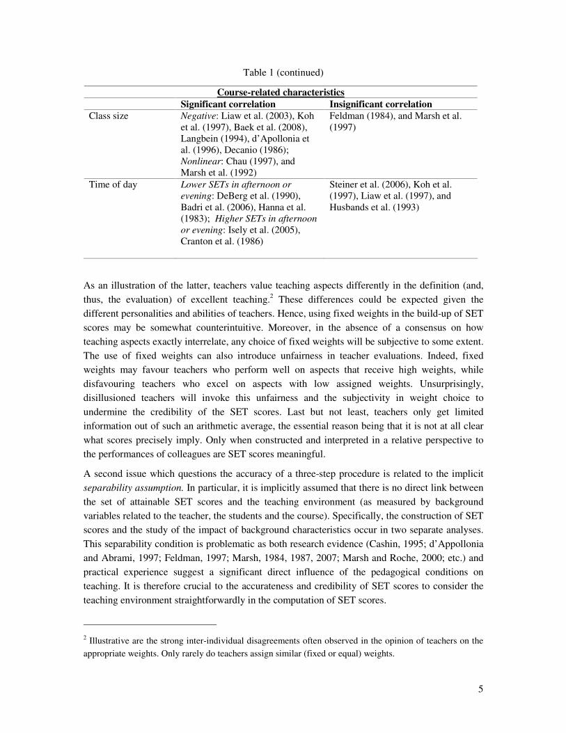
Table 1 (continued)

Course-related characteristics Significant correlation Insignificant correlation Class size Negative: Liaw et al. (2003), Koh

et al. (1997), Baek et al. (2008), Langbein (1994), d’ Apollonia et al. (1996), Decanio (1986); Nonlinear: Chau (1997), and Marsh et al. (1992)

Feldman (1984), and Marsh et al. (1997)

Time of day Lower SETs in afternoon or evening: DeBerg et al. (1990), Badri et al. (2006), Hanna et al. (1983); Higher SETs in afternoon or evening: Isely et al. (2005), Cranton et al. (1986)

Steiner et al. (2006), Koh et al. (1997), Liaw et al. (1997), and Husbands et al. (1993)

As an illustration of the latter, teachers value teaching aspects differently in the definition (and, thus, the evaluation) of excellent teaching.2 These differences could be expected given the different personalities and abilities of teachers. Hence, using fixed weights in the build-up of SET scores may be somewhat counterintuitive. Moreover, in the absence of a consensus on how teaching aspects exactly interrelate, any choice of fixed weights will be subjective to some extent. The use of fixed weights can also introduce unfairness in teacher evaluations. Indeed, fixed weights may favour teachers who perform well on aspects that receive high weights, while disfavouring teachers who excel on aspects with low assigned weights. Unsurprisingly, disillusioned teachers will invoke this unfairness and the subjectivity in weight choice to undermine the credibility of the SET scores. Last but not least, teachers only get limited information out of such an arithmetic average, the essential reason being that it is not at all clear what scores precisely imply. Only when constructed and interpreted in a relative perspective to the performances of colleagues are SET scores meaningful.

A second issue which questions the accuracy of a three-step procedure is related to the implicit separability assumption. In particular, it is implicitly assumed that there is no direct link between the set of attainable SET scores and the teaching environment (as measured by background variables related to the teacher, the students and the course). Specifically, the construction of SET scores and the study of the impact of background characteristics occur in two separate analyses. This separability condition is problematic as both research evidence (Cashin, 1995; d’ Appollonia and Abrami, 1997; Feldman, 1997; Marsh, 1984, 1987, 2007; Marsh and Roche, 2000; etc.) and practical experience suggest a significant direct influence of the pedagogical conditions on teaching. It is therefore crucial to the accurateness and credibility of SET scores to consider the teaching environment straightforwardly in the computation of SET scores.

2 Illustrative are the strong inter-individual disagreements often observed in the opinion of teachers on the appropriate weights. Only rarely do teachers assign similar (fixed or equal) weights.

6

The current paper contributes to the literature in that it clearly deviates from the current methodologies to (1) construct, (2) adjust and (3) analyze SET scores. Firstly, consider the construction of SET scores. In contrast to the traditional three-step approaches, we propose a specially tailored version of the Data Envelopment Analysis methodology (DEA). The DEA model has been developed by Charnes et al. (1978) as a non-parametric (i.e., it does not assume any a priori assumption on the production frontier) technique to estimate efficiency of observations. In the current paper, we do not apply the original DEA model, but rather an alternative approach which originates from DEA. This so-called ‘benefit of the doubt’ (BoD) model exploits the characteristic of DEA that it, thanks to its linear programming formulation, allows for an endogenous weighting of multiple outputs/achievements (Melyn and Moesen, 1991). We design the BoD model such that it allows for measurement errors which arrive from the survey data. In particular, we apply insights from the robust order-m efficiency scores of Cazals et al. (2002) to our specific BoD setting. As such, the BoD model has three major advantages. Firstly, for each teacher performance under evaluation, the weights on the questionnaire items are chosen in a relative perspective such that the highest possible SET score is realized. Therefore, teachers with one or more low SET scores can no longer blame these poor evaluations to unfair weights. Secondly, the BoD model is flexible to incorporate stakeholder opinion (e.g., teachers, students, experts) in the construction of the SET scores. Among others, Pritchard et al. (1998) strongly argued in favour of developing an evaluation system with such significant and meaningful stakeholder (particularly the teachers) participation. In their opinion, such involvement is a necessary condition for the credibility and acceptance of the evaluation results. Thirdly, the robust specification of the BoD model allows us to account for outlying and wrongly measured questionnaire values.

As a second contribution, we allow for environment adjusted SET scores without assuming a separability between the teacher’ s performance and the exogenous influences. To do so, we further extent the robust (i.e., the adaption of Cazals et al. (2002) to allow for measurement errors) BoD model of Melyn and Moesen (1991) to the conditional efficiency estimates of Daraio and Simar (2005, 2007a, 2007b). The latter non-parametric technique allows us to include teacher, student and course related influences immediately in the efficiency scores. This avoids the limitations of the previously described three-step procedure.

A final contribution is situated at the analysis level of the efficiency scores. By applying the bootstrap based p-values of De Witte and Kortelainen (2008), we can examine non-parametrically the direction of the influence of exogenous variables on the SETs. This is particularly convenient because it allows us to interpret the factors which create low or high SET scores.

To illustrate the practical usefulness of the approach, we apply the model on a dataset collected at the Hogeschool Universiteit Brussel (Belgium) in the academic year 2006-2007. This rich set comprises data on 16 questionnaire items (measuring several aspects of teacher performance) and 11 background variables (i.e., teacher age, teacher experience, teacher gender, tenure status, pedagogical training, doctoral degree, mean class grade, student inequality, questionnaire

7

response rate, class size, and timing of the course). The results reveal the importance of incorporating exogenous characteristics.

The remainder of the paper is organized as follows. Section 2 describes the data. In the third section we present basic DEA model as well as its robust and conditional extension. We outline how to enforce a selection of appropriate aggregation weights for teaching aspects, to enhance the robustness of SET scores, and to account for background characteristics. Section 4 reports the results. In the final section, we offer some concluding remarks and some avenues for further research.

2. The data

We estimate teacher performance as measured by the performance of a teacher on a specific course. In particular, we explore a detailed sample on 112 college courses c (c=1,…,112) taught by 69 different teachers. Teachers who lecture several courses will therefore have for several teacher performance scores (SET-scores), i.e. one for each evaluated course.3 These courses were taught in the Commercial Sciences and Commercial Engineering programs at the University College Brussels (HUB; a college in Belgium) in the first and second semester of the academic year 2006-2007.4 During the last two weeks of these semesters 5,513 students were questioned. The questionnaire comprised 16 statements to evaluate the multiple aspects of teacher performance. Students were asked to rate the lecturers on all items on a five-point Likert scale that corresponds to a coding rule ranging from 1 (I completely disagree) to 5 (I completely agree). To facilitate the students’ understanding of the questions, statements focussing on similar aspects of the teaching activity were grouped into key dimensions: ‘Learning & Value’ , ‘Examinations & Assignments’ , ‘Lecture Organization’ , and ‘Individual Lecturer Report’ (For a detailed description of the HUB-questionnaire, see Rogge, 2009). The development of the questionnaire as well as the categorization of the items into these key dimensions was largely based on a study of the content of effective teaching, the specific intentions of the evaluation instrument, and reviews of previous research and feedback.5

For each course c (c=1,…,112) we calculate an average student rating ,c iy for each questionnaire

item i (i = 1,…, 16):

( ), , , course

1c i c i ss j

y y∈

= ∑

3 Because the unit of observation is the course, characteristics specific to the individual student (e.g., gender, years in college) cannot be included in the analysis.

4 At HUB, SETs are collected to provide feedback to teachers for improving teaching performance and a measure of teaching quality for personnel decisions.

5 Based on a literature review, Marsh and Dunkin (1992, p. 146) conclude that this approach is more commonly used rather than statistical techniques such as factor analysis or multitrait-multimethod analysis.

8

where , ,c i sy denotes the appreciation on question i of student s for the teacher who is lecturing

course c. All S students registered for course c (i.e., course s c∈ ) and present at the moment of

the questionnaire are considered in the computation of the class mean rating.6

To examine the effects (both in terms of direction and significance) of background characteristics on SET scores, the questionnaire data are supplemented with administrative data on several characteristics related to the teacher, the group of students and the course. Except for the age of the teacher, all other teacher-related characteristics (the teacher gender, whether or not the teacher has less than 2 years of experience, whether or not he/she is a guest lecturer, whether or not the teacher received pedagogical training in the past, and whether or not he/she has a doctoral degree) are dummy variables. A dummy variable of 1 stands for, respectively, a female teacher, a new teacher with less than two years of experience, a guest lecturer, received already pedagogical training, and has a doctoral degree.7

Further, we include three background characteristics related to the students: the actual mean grade of the students in the class, the inequality of the distribution of the student grades (as measured by the Gini coefficient which can vary between 0 and 1, with a Gini coefficient of 0 indicating a perfectly equal distribution and a Gini of 1 designating the exact opposite), and the response rate to the questionnaire. The latter captures the ratio of the number of people who answered the teacher evaluation questionnaire (i.e., S ) to the (official) class size.

Finally, two characteristics related to the course are included in the analysis: the class size and a dummy indicating whether the course is lectured in the evening. Summary statistics for the data on background characteristics are presented in Table 2.

6 Note that the number of students participating in the teacher evaluation, S , can be lower than the official class size as students can be absent during the administration of the questionnaires.

7 Accounting for teacher characteristics is meaningful as students may have structural preferences on gender or guest lecturers. Moreover, in this particular application, accounting for a doctoral degree is necessary as this is only a recent requirement for HUB teachers (although also before teachers with PhD where hired).

9

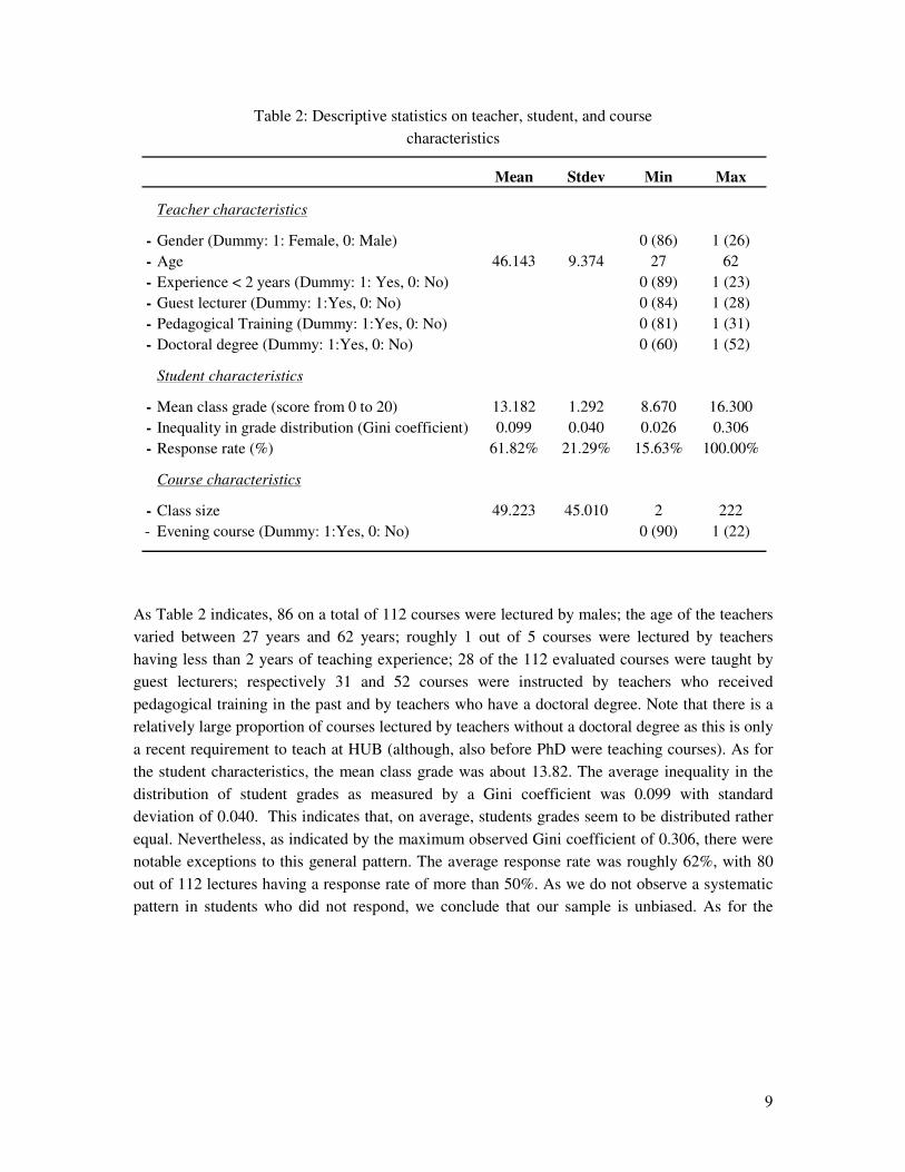
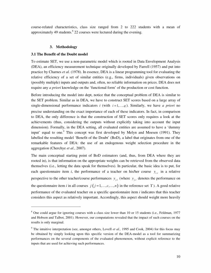
Table 2: Descriptive statistics on teacher, student, and course characteristics

Mean Stdev Min Max

Teacher characteristics

- Gender (Dummy: 1: Female, 0: Male) 0 (86) 1 (26)- Age 46.143 9.374 27 62- Experience < 2 years (Dummy: 1: Yes, 0: No) 0 (89) 1 (23)- Guest lecturer (Dummy: 1:Yes, 0: No) 0 (84) 1 (28)- Pedagogical Training (Dummy: 1:Yes, 0: No) 0 (81) 1 (31)- Doctoral degree (Dummy: 1:Yes, 0: No) 0 (60) 1 (52)

Student characteristics

- Mean class grade (score from 0 to 20) 13.182 1.292 8.670 16.300- Inequality in grade distribution (Gini coefficient) 0.099 0.040 0.026 0.306- Response rate (%) 61.82% 21.29% 15.63% 100.00%

Course characteristics

- Class size 49.223 45.010 2 222- Evening course (Dummy: 1:Yes, 0: No) 0 (90) 1 (22)

As Table 2 indicates, 86 on a total of 112 courses were lectured by males; the age of the teachers varied between 27 years and 62 years; roughly 1 out of 5 courses were lectured by teachers having less than 2 years of teaching experience; 28 of the 112 evaluated courses were taught by guest lecturers; respectively 31 and 52 courses were instructed by teachers who received pedagogical training in the past and by teachers who have a doctoral degree. Note that there is a relatively large proportion of courses lectured by teachers without a doctoral degree as this is only a recent requirement to teach at HUB (although, also before PhD were teaching courses). As for the student characteristics, the mean class grade was about 13.82. The average inequality in the distribution of student grades as measured by a Gini coefficient was 0.099 with standard deviation of 0.040. This indicates that, on average, students grades seem to be distributed rather equal. Nevertheless, as indicated by the maximum observed Gini coefficient of 0.306, there were notable exceptions to this general pattern. The average response rate was roughly 62%, with 80 out of 112 lectures having a response rate of more than 50%. As we do not observe a systematic pattern in students who did not respond, we conclude that our sample is unbiased. As for the

10

course-related characteristics, class size ranged from 2 to 222 students with a mean of approximately 49 students.8 22 courses were lectured during the evening.

3. Methodology

3.1 The Benefit of the Doubt model

To estimate SET, we use a non-parametric model which is rooted in Data Envelopment Analysis (DEA), an efficiency measurement technique originally developed by Farrell (1957) and put into practice by Charnes et al. (1978). In essence, DEA is a linear programming tool for evaluating the relative efficiency of a set of similar entities (e.g., firms, individuals) given observations on (possibly multiple) inputs and outputs and, often, no reliable information on prices. DEA does not require any a priori knowledge on the ‘functional form’ of the production or cost function.

Before introducing the model into dept, notice that the conceptual problem of DEA is similar to the SET problem. Similar as in DEA, we have to construct SET scores based on a large array of single-dimensional performance indicators i (with 1, ,i q= ! ). Similarly, we have a priori no

precise understanding on the exact importance of each of these indicators. In fact, in comparison to DEA, the only difference is that the construction of SET scores only requires a look at the achievements (thus, considering the outputs without explicitly taking into account the input dimension). Formally, in the DEA setting, all evaluated entities are assumed to have a ‘dummy input’ equal to one.9 This concept was first developed by Melyn and Moesen (1991). They labelled the resulting model ‘Benefit of the Doubt’ (BoD), a label that originates from one of the remarkable features of DEA: the use of an endogenous weight selection procedure in the aggregation (Cherchye et al., 2007).

The main conceptual starting point of BoD estimators (and, thus, from DEA where they are rooted in), is that information on the appropriate weights can be retrieved from the observed data themselves (i.e., letting the data speak for themselves). In particular, the basic idea is to put, for each questionnaire item i, the performance of a teacher on his/her course ,c iy in a relative

perspective to the other teacher/course performances ,j iy (where ,j iy denotes the performance on

the questionnaire item i in all courses ( )1, , , ,j j c n= ! ! in the reference set ϒ ). A good relative

performance of the evaluated teacher on a specific questionnaire item i indicates that this teacher considers this aspect as relatively important. Accordingly, this aspect should weight more heavily

8 One could argue for ignoring courses with a class size lower than 10 or 15 students (i.e., Feldman, 1977 and Hobson and Talbot, 2001). However, our computations revealed that the impact of such courses on the results is only marginal.

9 The intuitive interpretation (see, amongst others, Lovell et al., 1995 and Cook, 2004) for this focus may be obtained by simply looking upon this specific version of the DEA-model as a tool for summarizing performances on the several components of the evaluated phenomenon, without explicit reference to the inputs that are used for achieving such performances.

11

in the teacher’ s performance evaluation. As a result, a high weight is assigned. The opposite reasoning holds for the teaching aspects on which a teacher performs weakly compared to the other colleagues in the comparison set. In other words, for each teacher separately, BoD (and thus also DEA) looks for the weights that maximize the impact of the teacher’ s relative strengths and minimize the influence of the relative weaknesses. As a result, BoD-weights ,c iw are optimal in

the sense that they are chosen in such a way as to maximize the teacher’ s SET score

( )cSET y .10,11 This can be formally translated in the linear programming set-up (Cherchye et al.,

2007):12

( )

( ) ( )

( )( )

,, ,

1

, ,1

,

,

( ) max 2

. .

1 1,..., , , 2

0 1,..., 2

1,..., . 2

c i

q

c c i c iwi

q

c i j ii

c i

c i e

SET y w y

s t

w y j c n n a

w i q b

w W i q and e E c

=

=

=

≤ = ∀ ∈ ϒ

≥ =

∈ = ∈

∑

∑ !

Thus, in the absence of any detailed information on the ‘true’ weights, BoD assumes that representative weights can be inferred from looking at the relative strengths and weaknesses. This indeed means that the each teacher is granted the benefit-of-the-doubt when it comes to assigning

weights in the build-up of his/her ( )cSET y ’ s (i.e., one for each evaluated course).

Note that in this BoD model, teachers are granted considerable leeway in the definition of their most favourable weights ,c iw . In fact, optimal weights only need to satisfy two minor constraints:

the normalization constraint ( )2a and the non-negativity constraint ( )2b . The first restriction

imposes that no other teacher performance present in the sample ϒ can have a SET score higher than unity when applying the optimal weights ,c iw of the teacher performance under evaluation.

The second constraint states that weights should be non-negative. Hence, ( )ySETc is a non-

decreasing function of the performances on the several statements i (with 1, ,i q= ! ). Apart from

these restrictions, the formal model ( ) ( )2 2b− allows weights to be freely estimated in order to

10 For completeness, we mention that BoD alternatively allows for a ‘worst-case’ perspective in which entities receive their worst set of weights, hence, high (low) weights on performance indicators on which they perform relative weak (strong) (Zhou et al., 2007).

11 This BoD model is first applied on the level of the four key dimensions before aggregating the four resulting dimension scores into an overall SET score.

12 This adjusted model is formally tantamount to the original input-oriented CCR-DEA model of Charnes et al. (1978), with all questionnaire items considered as outputs and a dummy input equal to one for all observations.

12

maximize ( )cSET y . This large freedom in weight choice can be seen as an advantage as it

enables teachers to put themselves in the best possible light relative to their colleagues. Disillusioned teachers can no longer blame a low SET score to a harmful or unfair weighting scheme. Any other weighting scheme than the one specified by the BoD model would worsen the SET score.

However, this flexibility also carries some potential disadvantages as it may allow a teacher to appear as a brilliant performer in a manner that is hard to justify. For instance, there is nothing that keeps BoD from assigning zero or quasi-zero weights to components of teaching (i.e., questionnaire items i ) on which the teacher performs poorly compared to the colleagues, thereby neglecting those aspects in his or her assessment. For example, in an extreme scenario, all the relative weight could be assigned to a few questionnaire items, which would then completely determine the SET score. Further, there is the potential problem that the BoD model may select weights that contradict prior stakeholder views (e.g., students, teachers, pedagogic experts, faculty board). To avoid such problematic weight scenarios (zero or unrealistic weights), frequently, additional weight restrictions are introduced in the basis model to enforce the

installation of proper weights. Formally, the constraint ( )2c is added with W denoting the set of

permissible weight values defined based upon the opinion of selected stakeholders e E∈ . In our application, we used a Budget Allocation Method to collect both student and teacher opinions on the appropriate weights.13,14 Based on their specified weights, we defined weight restrictions applying to both the questionnaire items as well as the key dimensions.15

From restriction ( )a2 , we can deduce that, for all evaluated teacher performances SETc

(c=1,…,n), ( )cSET y will lie between 0 and 1 with higher values indicating a better relative

teaching performance. In fact, this constraint highlights the relative perspective (i.e., benchmarking idea) of BoD: the most favourable weights for the evaluated teacher performance

,c iw are always applied to all n performances in the comparison set ϒ . One is in that way

effectively looking which of the teacher performances in this sample are worse, similar or better.

If ( ) 1cSET y < , this indicates that the teacher could perform better on course c. Indeed, there are

other teachers in the sample ϒ who realize higher SET scores even when applying the evaluated teacher’ s most favourable weights ,c iw (i.e., weights which are less favourable than their own

optimal BoD weights). In this situation, a strong case can be made for the notion that this teacher

13 In practice, both a group of students and teachers were contacted and requested to share their perceptions on the importance of the different dimensions and items included in the questionnaire.

14 The individual stakeholder opinions, as collected by a Budget Allocation Method, as well as a detailed description of the weight restrictions are available from the authors upon request. The Budget Allocation Method is a participatory method in which stakeholders have to distribute 100 points over the items allocating more to what they regard to be the more important items.

15 See Rogge (2009) for a comprehensive discussion of the stakeholder opinions and the weight restrictions.

13

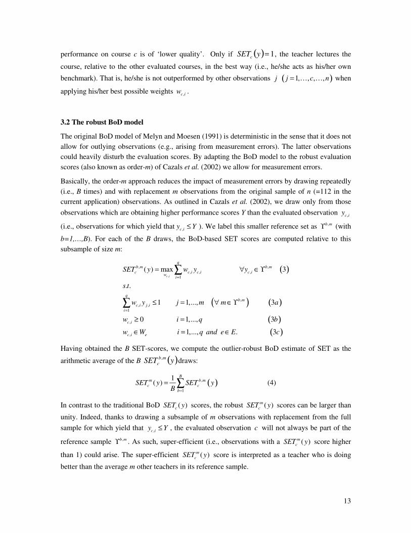
performance on course c is of ‘lower quality’ . Only if ( ) 1=ySETc , the teacher lectures the

course, relative to the other evaluated courses, in the best way (i.e., he/she acts as his/her own

benchmark). That is, he/she is not outperformed by other observations j ( )1, , , ,j c n= ! ! when

applying his/her best possible weights ,c iw .

3.2 The robust BoD model

The original BoD model of Melyn and Moesen (1991) is deterministic in the sense that it does not allow for outlying observations (e.g., arising from measurement errors). The latter observations could heavily disturb the evaluation scores. By adapting the BoD model to the robust evaluation scores (also known as order-m) of Cazals et al. (2002) we allow for measurement errors.

Basically, the order-m approach reduces the impact of measurement errors by drawing repeatedly (i.e., B times) and with replacement m observations from the original sample of n (=112 in the current application) observations. As outlined in Cazals et al. (2002), we draw only from those observations which are obtaining higher performance scores Y than the evaluated observation ,c iy

(i.e., observations for which yield that ,c iy Y≤ ). We label this smaller reference set as ,b mϒ (with

b=1,…,B). For each of the B draws, the BoD-based SET scores are computed relative to this subsample of size m:

( )

( ) ( )

( )( )

,

, ,, , ,

1

,, ,

1

,

,

( ) max 3

. .

1 1,..., 3

0 1,..., 3

1,..., . 3

c i

qb m b m

c c i c i c iwi

qb m

c i j ii

c i

c i e

SET y w y y

s t

w y j m m a

w i q b

w W i q and e E c

=

=

= ∀ ∈ ϒ

≤ = ∀ ∈ ϒ

≥ =

∈ = ∈

∑

∑

Having obtained the B SET-scores, we compute the outlier-robust BoD estimate of SET as the

arithmetic average of the B ( )ySET mbc

, draws:

( ),

1

1( ) (4)

Bm b m

c cb

SET y SET yB =

= ∑

In contrast to the traditional BoD ( )cSET y scores, the robust ( )mcSET y scores can be larger than

unity. Indeed, thanks to drawing a subsample of m observations with replacement from the full sample for which yield that ,c iy Y≤ , the evaluated observation c will not always be part of the

reference sample ,b mϒ . As such, super-efficient (i.e., observations with a ( )mcSET y score higher

than 1) could arise. The super-efficient ( )mcSET y score is interpreted as a teacher who is doing

better than the average m other teachers in its reference sample.

14

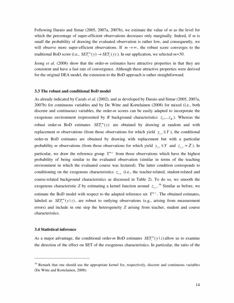
Following Daraio and Simar (2005, 2007a, 2007b), we estimate the value of m as the level for which the percentage of super-efficient observations decreases only marginally. Indeed, if m is small the probability of drawing the evaluated observation is rather low, and consequently, we will observe more super-efficient observations. If m → ∞ , the robust score converges to the

traditional BoD score (i.e., ( ) ( )mc cSET y SET y→ ). In our application, we selected m=50.

Jeong et al. (2008) show that the order-m estimates have attractive properties in that they are consistent and have a fast rate of convergence. Although these attractive properties were derived for the original DEA model, the extension to the BoD approach is rather straightforward.

3.3 The robust and conditional BoD model

As already indicated by Cazals et al. (2002), and as developed by Daraio and Simar (2005, 2007a, 2007b) for continuous variables and by De Witte and Kortelainen (2008) for mixed (i.e., both discrete and continuous) variables, the order-m scores can be easily adapted to incorporate the

exogenous environment (represented by R background characteristics Rzz ,...1 ). Whereas the

robust order-m BoD estimates ( )mcSET y are obtained by drawing at random and with

replacement m observations (from those observations for which yield ,c iy Y≤ ), the conditional

order-m BoD estimates are obtained by drawing with replacement but with a particular

probability m observations (from those observations for which yield ,c iy Y≤ and Zz rc ≈, ). In

particular, we draw the reference group ,m zϒ from those observations which have the highest probability of being similar to the evaluated observation (similar in terms of the teaching environment in which the evaluated course was lectured). The latter condition corresponds to

conditioning on the exogenous characteristics rcz , (i.e., the teacher-related, student-related and

course-related background characteristics as discussed in Table 2). To do so, we smooth the

exogenous characteristic Z by estimating a kernel function around rcz , .16 Similar as before, we

estimate the BoD model with respect to the adapted reference set ,m zϒ . The obtained estimates,

labeled as ( | )mcSET y z , are robust to outlying observations (e.g., arising from measurement

errors) and include in one step the heterogeneity Z arising from teacher, student and course characteristics.

3.4 Statistical inference

As a major advantage, the conditional order-m BoD estimates ( | )mcSET y z allow us to examine

the direction of the effect on SET of the exogenous characteristics. In particular, the ratio of the

16 Remark that one should use the appropriate kernel for, respectively, discrete and continuous variables (De Witte and Kortelainen, 2008).

15

conditional [i.e., accounted for heterogeneity; ( | )mcSET y z ] to the unconditional [i.e., without

accounting for the environment; ( )mcSET y ] order-m estimates can be regressed on the

conditioning factor Z (Daraio and Simar, 2005, 2007a, 2007b). Besides a visualisation (which we do not present here), a non-parametric bootstrap procedure can be applied to obtain statistical inference on the direction of the effect. Inspired on the Daraio and Simar (2005) framework, we

use a non-parametric bootstrap to examine the effect of Z on the ratio ( | )mcSET y z / ( )m

cSET y (see

Li and Racine (2007) for the bootstrap procedure). De Witte and Kortelainen (2008) showed by simulation that this approach enables one to estimate standard errors and p-values of the significance of the influence of Z. Thanks to this statistical inference, we can explore which teacher, student and course related variables have a significant impact on the BoD estimates.

4. Results

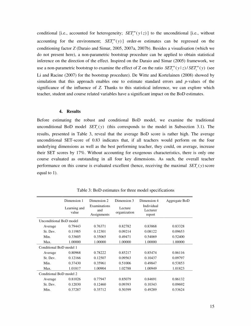
Before estimating the robust and conditional BoD model, we examine the traditional unconditional BoD model ( )cSET y (this corresponds to the model in Subsection 3.1). The

results, presented in Table 3, reveal that the average BoD score is rather high. The average unconditional SET-score of 0.83 indicates that, if all teachers would perform on the four underlying dimensions as well as the best performing teacher, they could, on average, increase their SET scores by 17%. Without accounting for exogenous characteristics, there is only one course evaluated as outstanding in all four key dimensions. As such, the overall teacher performance on this course is evaluated excellent (hence, receiving the maximal ( )cSET y score

equal to 1).

Table 3: BoD estimates for three model specifications

Dimension 1 Dimension 2 Dimension 3 Dimension 4 Aggregate BoD

Learning and value

Examinations and

Assignments

Lecture organization

Individual Lecturer report

Unconditional BoD model Average 0.79443 0.76371 0.82782 0.83868 0.83328 St. Dev. 0.11985 0.12301 0.09214 0.08122 0.09653 Min. 0.33605 0.35065 0.49471 0.54069 0.52400 Max. 1.00000 1.00000 1.00000 1.00000 1.00000 Conditional BoD model 1 Average 0.80968 0.78222 0.85217 0.85474 0.86116 St. Dev. 0.12166 0.12507 0.09563 0.10437 0.09797 Min. 0.37430 0.35961 0.51006 0.49847 0.53853 Max. 1.01817 1.00904 1.02788 1.00949 1.01823 Conditional BoD model 2 Average 0.81026 0.77947 0.85079 0.84691 0.86132 St. Dev. 0.12030 0.12460 0.09393 0.10343 0.09692 Min. 0.37287 0.35712 0.50399 0.49289 0.53624

16

Max. 1.01186 1.01234 1.01540 1.00460 1.00954 Conditional BoD model 3 Average 0.81610 0.78317 0.85926 0.85976 0.87273 St. Dev. 0.12152 0.12462 0.09462 0.10369 0.09821 Min. 0.37727 0.35837 0.51218 0.50158 0.53497 Max. 1.01223 1.00977 1.01084 1.00368 1.00413

On the level of the key dimensions, performances are, on the average, higher on the dimensions ‘Lecture Organization’ and ‘Individual Lecturer Characteristics’ . Generally speaking, students perceive the requirements and agreements concerning the exam evaluation as insufficient clear (i.e., dimension ‘Examinations & Assignments’ obtains the lowest average performances). Both patterns are also observed in the other conditional BoD models.

More interesting than the traditional ( )cSET y -estimates is the conditional model (as discussed in

Subsection 3.3) in which we account for the R exogenous factors Z arising from teacher, student and course characteristics. As presented in Table 3 and 4, we estimate three alternative model specifications. Whereas Table 3 reports some descriptive statistics on the efficiency scores, Table

4 describes the influences (favorable or unfavorable to the robust ( )mcSET y -scores and the

corresponding p-values) of the exogenous variables Z. If we account for exogenous characteristics, the average teacher evaluation score increase. The average teacher could, if he/she

would teach in a similar way as his/her best practice teacher, increase his/her overall ( | )mcSET y z

by 14%.

Table 4: Statistical inference of the BoD estimates

Model 1 Model 2 Model 3 Influence p-value Influence p-value Influence p-value Teacher characteristics Pedagogical training Favorable 0.000 *** Favorable 0.018 ** Favorable 0.002 *** Having a PhD Favorable 0.006 *** Favorable 0.132 Favorable 0.850 Guest lecture Unfavorable 0.024 ** Unfavorable 0.020 ** Age Unfavorable 0.444 Favorable 0.242 Student characteristics Mean Grade Unfavorable 0.002 *** Unfavorable 0.004 *** Unfavorable 0.022 ** Gini of scores Favorable 0.378 Course characteristics Class size Favorable 0.000 *** Evening course Unfavorable 0.002 *** Unfavorable 0.000 ***

R² 0.838 0.973 0.963

where ***, ** and * denote, respectively, significance at 1, 5 and 10% level.

17

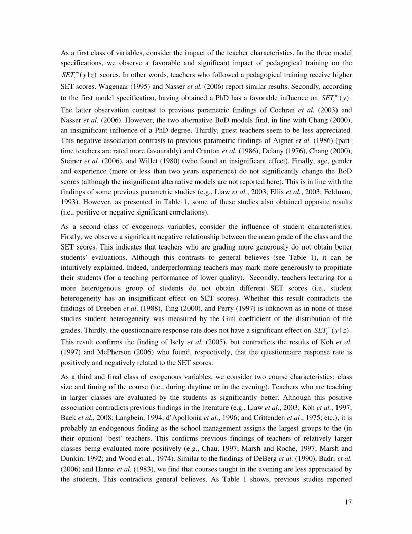
As a first class of variables, consider the impact of the teacher characteristics. In the three model specifications, we observe a favorable and significant impact of pedagogical training on the

( | )mcSET y z scores. In other words, teachers who followed a pedagogical training receive higher

SET scores. Wagenaar (1995) and Nasser et al. (2006) report similar results. Secondly, according

to the first model specification, having obtained a PhD has a favorable influence on ( )mcSET y .

The latter observation contrast to previous parametric findings of Cochran et al. (2003) and Nasser et al. (2006). However, the two alternative BoD models find, in line with Chang (2000), an insignificant influence of a PhD degree. Thirdly, guest teachers seem to be less appreciated. This negative association contrasts to previous parametric findings of Aigner et al. (1986) (part-time teachers are rated more favourably) and Cranton et al. (1986), Delany (1976), Chang (2000), Steiner et al. (2006), and Willet (1980) (who found an insignificant effect). Finally, age, gender and experience (more or less than two years experience) do not significantly change the BoD scores (although the insignificant alternative models are not reported here). This is in line with the findings of some previous parametric studies (e.g., Liaw et al., 2003; Ellis et al., 2003; Feldman, 1993). However, as presented in Table 1, some of these studies also obtained opposite results (i.e., positive or negative significant correlations).

As a second class of exogenous variables, consider the influence of student characteristics. Firstly, we observe a significant negative relationship between the mean grade of the class and the SET scores. This indicates that teachers who are grading more generously do not obtain better students’ evaluations. Although this contrasts to general believes (see Table 1), it can be intuitively explained. Indeed, underperforming teachers may mark more generously to propitiate their students (for a teaching performance of lower quality). Secondly, teachers lecturing for a more heterogenous group of students do not obtain different SET scores (i.e., student heterogeneity has an insignificant effect on SET scores). Whether this result contradicts the findings of Dreeben et al. (1988), Ting (2000), and Perry (1997) is unknown as in none of these studies student heterogeneity was measured by the Gini coefficient of the distribution of the

grades. Thirdly, the questionnaire response rate does not have a significant effect on ( | )mcSET y z .

This result confirms the finding of Isely et al. (2005), but contradicts the results of Koh et al. (1997) and McPherson (2006) who found, respectively, that the questionnaire response rate is positively and negatively related to the SET scores.

As a third and final class of exogenous variables, we consider two course characteristics: class size and timing of the course (i.e., during daytime or in the evening). Teachers who are teaching in larger classes are evaluated by the students as significantly better. Although this positive association contradicts previous findings in the literature (e.g., Liaw et al., 2003; Koh et al., 1997; Baek et al., 2008; Langbein, 1994; d’ Apollonia et al., 1996; and Crittenden et al., 1975; etc.), it is probably an endogenous finding as the school management assigns the largest groups to the (in their opinion) ‘best’ teachers. This confirms previous findings of teachers of relatively larger classes being evaluated more positively (e.g., Chau, 1997; Marsh and Roche, 1997; Marsh and Dunkin, 1992; and Wood et al., 1974). Similar to the findings of DeBerg et al. (1990), Badri et al. (2006) and Hanna et al. (1983), we find that courses taught in the evening are less appreciated by the students. This contradicts general believes. As Table 1 shows, previous studies reported

18

positive associations (Isely et al., 2005 and Cranton et al., 1986) or non-significant correlations (e.g., Husbands et al., 1993, Liaw et al., 1997, etc.).

It is important to note that our study is, due to data constraints, limited for the reason that it does not compute SET scores that are corrected for all background characteristics which, in the literature, have been found to influence teacher performance. As previous research (see, among others, Greenwald and Gilmore, 1997; Marsh and Roche, 2000; Griffin, 2001, 2004; etc.) has suggested, other variables (e.g., student gender, prior interest in the course, course workload, etc.) might also affect SET scores.

5. Conclusion

To be fair, students’ evaluations of teacher performance (SETs) should be determined solely by the teacher’ s actual performance in the classroom, not by other background influences (related to the teacher, the students or the course) which are not under his or her control. Unfortunately, many empirical studies indicated that SET scores capture also the effects of such background factors. This paper has proposed a specially tailored version of the Benefit of the Doubt (BoD) model (which is rooted in the popular non-parametric Data Envelopment Analysis (DEA) approach) to (1) construct SET scores, (2) adjust them for the impact of background variables, and (3) analyze the impact of these variables on the SET scores. In comparison to the common practice of building SET scores as an arithmetic average of the ratings on the questionnaire items and analyzing the impacts of background variables on these scores (only rarely SET scores are actually adjusted for these influences) in separate steps, this approach has several advantages. Firstly, for each teacher under evaluation, the weights on the questionnaire items are chosen in a relative perspective such that the highest possible SET score is realized. Therefore, teachers with one or more low SET scores can no longer blame these poor evaluations to unfair weights. Secondly, the BoD model is flexible to incorporate stakeholder opinion (e.g., teachers, students, experts) in the construction of the SET scores. Clearly, this involvement is beneficial for the credibility and acceptance of the evaluation results. Thirdly, the BoD model is extended to construct robust SET-scores. This advantage is particularly useful as questionnaires may contain some measurement errors or atypical observations. Fourthly, BoD can be further developed to account for several background variables (discrete and continuous) without assuming a separability between the teacher’ s performance and these exogenous influences. As a final result, this yields environment adjusted robust and optimal SET scores in line with stakeholder opinion.

To analyze non-parametrically the exact impact (both in terms of direction and size) of the background variables on SET scores, we applied the bootstrap based p-values of De Witte and Kortelainen (2008). This is particularly convenient because it allows us to interpret the background factors which create low or high SET scores. The results indicate that, on average, slightly higher ratings are given to teachers who (a) follow a pedagogical training, (b) have a doctoral degree, (c) are only active at the university, (d) are less generously in marking, (e) lecture for larger classes, and (f) lecture during daytime. Alternative examined background

19

characteristics (i.e., teacher age, teacher experience, teacher gender, student inequality, and questionnaire response rate) did not significantly influence the teacher performances.

Both the existence and strength of the relationships between background variables and SET scores varies without doubt with the particular (exogenous) circumstances and conditions. Therefore, it would be interesting for future research to apply the proposed methodology in several evaluation settings to check for recurring patterns in the results. In the same vein, it would be interesting to apply our non-parametric method to the data of previous studies to compare the results. If different results would be obtained, at first sight, the results of our method could be preferred as no a priori assumptions are required. Another suggestion would be to expand our study with other background variables that have been found to correlate with SET scores in the literature (e.g., student gender, prior interest in the course, course workload, etc.). Further, although not being a consideration of this paper, we stress the importance of studying the exact mechanisms by which aforementioned background variables influence SET scores in more detail. However, as the literature reports on mixed findings, it is very likely that specifying such mechanisms will turn out to be particularly complex. Or, in the words of Feldman (1998, p. 43): “In principle, and clearly in practice, the search for the conditions and contexts that determine the existence, strength, direction, and pattern of associations between variables of interest is an on-going search and probably a never-ending one”.

Literature

Abrami, P. C., & d’ Apollonia, S. (1999). Current concerns are past concerns. American Psychologist, 54(7), 519–520.

Aigner, D.J., & Thum, F.D. (1986). On student evaluations of university teaching. The Journal of Economic Education, 17(4), 243-265.

Badri, M.A., Abdulla, M., Kamali, & M.A., Dodeen, H. (2006). Identifying potential biasing variables in in student evaluation of teaching in a newly accredited business program in the UAE. International Journal of Educational Management, 20(1), 43-59.

Baek, S.-G., & Shin, H.-J. (2008). Multilevel analysis of the effects of student and course characteristics on satisfaction in undergraduate liberal arts courses. Asian Pacific Education Review, 9(4), 475-486.

Baldwin, T., & Blattner, N. (2003). Guarding against potential bias in student evaluations: What every faculty member needs to know. College Teaching, 51(1), 27-32.

Basow, S.A., & Distenfeld, M.S. (1985). Teacher Expressiveness: More Important for Male Teachers Than Female Teachers? Journal of Educational Psychology, 77, 45-52.

Basow, S.A., & Howe, K.G. (1987). Evaluations of College Professors: Effects of Professors' Sex-Type, and Sex, and Students’ Sex. Psychological Reports, 60, 671-678.

Basow, S. A. (2000). Best and worst professors: Gender patterns in students' choices. Sex Roles: A Journal of Research, 43(5/6), 407-417.

20

Birnbaum, R. (1977): “Factors Related to University Grade Inflation”, Journal of Higher Education, 48(5), pp. 519-539

Cashin, W. E. (1995). Student ratings of teaching: the research revisited. IDEA Paper Nr.32.

Cazals, C., Florens, J.P., & L. Simar (2002). Nonparametric Frontier Estimation: A Robust Approach. Journal of Econometrics, 106 (1), 1-25.

Centra, J.A., & Gaubatz, N.B. (2000): “Is there gender bias in student evaluations of teaching”, Journal of Higher Education, 71(1), pp. 17-33.

Chang, T.-S. (2000). Student Ratings: What Are Teacher College Students Telling Us about Them? Paper presented at the Annual Meeting of the American Educational Research Association (New Orleans, LA, April 24-28, 2000.

Charnes, A. Cooper, W.W., & Rhodes, E. (1978). Measuring the efficiency of decision making units. European Journal of Operational Research, 2, 429-444.

Chau, C.-T. (1997). A bootstrap experiment on the statistical properties of students’ ratings of teaching effectiveness. Research in Higher Education, 38(4), 497-517.

Cherchye, L., Moesen, W., Rogge, N., & Van Puyenbroeck, T. (2007). An introduction to ‘benefit of the doubt’ composite indicators. Social Indicators Research, 82, 111-145.

Cochran, H.H. Jr., Hodgin, G.L., & Zietz, J. (2003). Student Evaluations of Teaching: Does Pedagogy Matter? Journal for Economic Educators, 4(1), 6-18.

Cook, W.D. (2004). Qualitive Data in DEA. In W.W. Cooper, L. Seiford, and J. Zhu (Eds.), Handbook on Data Envelopment Analysis, Kluwer Academic Publishers, Dordrecht, 75-97.

Cranton, P., & Smith, R. (1986). A New Look at the Effect of Course Characteristics on Student Ratings of instruction. American Educational Research Journal, 23(1), 117-128.

Crittenden, K.S., Norr, J.L., & LeBailly, R.K. (1975): “Size of University Classes and Student Evaluation of Teaching”, Journal of Higher Education, Vol. 46, No. 4, pp. 461-470.

D’ Apollonia, S., & Abrami, P.C. (1996). Variables moderating the validity of student ratings of instruction: A meta-analysis. Paper presented at the 77th Annual Meeting of the American Educational Research Association.

D’ Appollonia, S., & Abrami, P.C. (1997). Navigating student ratings of instruction. American Psychologist, 52(11), 1198-1208.

Daraio, C., & Simar, L. (2005). Introducing Environmental Variables in Nonparametric Frontier Models: A Probabilistic Approach. Journal of Productivity Analysis, 24 (1), 93-121.

Daraio, C., & Simar, L. (2007a). Advanced robust and nonparametric methods in efficiency analysis: Methodology and applications. Series: Studies in Productivity and Efficiency, Springer.

21

Daraio, C., & Simar, L. (2007b). Conditional Nonparametric Frontier Models for Convex and Nonconvex Technologies: A Unifying Approach. Journal of Productivity Analysis, 28, 13-32.

Davies, M., Hirschberg, J.G., Lye, J.N., Johnston, C., & McDonald, I.M. (2007). Systematic influences on teaching evaluations: The case for caution. Australian Economic Papers, 46(1), 18-38.

DeBerg, C.L., & Wilson, J.R. (1990). An empirical investigation of the potential confounding variables in student evaluation of teaching. Journal of Accounting Education, 8(1), 37-62.

DeCanio, S.J. (1986). Student Evaluations of Teaching – A multinomial logit approach. The Journal of Economic Education, 17, 165-176.

Delaney, E. L. Jr. (1976). The Relationships of Student Ratings of Instruction to Student, Instructor and Course Characteristics. Paper presented at the 60th Annual Meeting of the American Educational Research Association, San Francisco, California, April 19-23, 1976.

De Witte, K., & Kortelainen, M. (2008). Blaming the exogenous environment? Conditional efficiency estimation with continuous and discrete environmental variables. CES Discussion Paper Series DPS 08.33; MPRA Paper 14034.

Dreeben, R., & Barr, R. (1988). Classroom composition and the design of instruction. Sociology of Education, 61, 129-142.

Ellis, L., Burke, D.M., Lomire, P., & McCormack, D.R. (2003). Student Grades and Average Ratings of Instructional Quality: The Need for Adjustment. The Journal of Educational Research, 97(1), 35-40.

Emery, C.R., Kramer, T.R., & Tian, R.G. (2003). Return to academic standards: A critique of student evaluations of teaching effectiveness. Quality Assurance in Education, 11(1), 37-46.

Farrell, M.J. (1957). The measurement of productive efficiency. Journal of the Royal Statistical Society, Series A, CXX, Part 3, 253-290.

Feldman, K.A. (1977). Consistency and variability among college students in rating their teachers and courses: A review and analysis. Research in Higher Education, 6, 223-274.

Feldman, K. A. (1983). Seniority and experience of college teachers as related to evaluations they receive from students. Research in Higher Education, 18(1), 3-124.

Feldman, K. A. (1984). Class size and college students’ evaluations of teachers and courses: A closer look. Research in Higher Education, 21(1), 45-116.

Feldman, K. A. (1992). College students' views of male and female college teachers: Part 1 - evidence from the social laboratory and experiments. Research in Higher Education, 3, 317-375.

22

Feldman, K. A., (1993). College Students’ Views of Male and Female College Teachers: Part II- Evidence from Students’ Evaluation of Their Classroom Teachers. Research in Higher Education, 34 (2), 151-211

Feldman, K.A. (1997). Identifying exemplary teaching: Evidence from student ratings. In R.P. Perry and J.C. Smart (Eds), Effective Teaching in Higher Education: Research and Practice. New York: Agathon Press.

Feldman, K. A. (1998). Reflections on the Study of Effective College Teaching and Student Ratings: One Continuing Quest and Two Unresolved Issues. In J. C. Smart (Ed.), Higher Education: Handbook of Theory and Research, Vol. 13. New York: Agathon Press.

Fernandez, J., & Mateo, M.A. (1997). Student and faculty gender in ratings of university teaching quality. Sex Roles, 37(8), 997-1003.

Greenwald, A.G., & Gilmore, G.M. (1997). Grading Leniency Is a Removable Contaminant of student ratings. American Psychologist, 52(11), 1209-1217.

Griffin, B.W. (2001). Instructor Reputation and Student Ratings of Instruction. Contemporary Educational Psychology, 26, 534-552.

Griffin, B.W. (2004). Grading leniency, grade discrepancy, and student ratings of instruction. Contemporary Educational Psychology, 29, 410-425.

Hanna, G.S., Hoyt, D.P., & Aubracht, J.D. (1983). Identifying and Adjusting for Biases in Student Evaluations of Instruction: Implications for Validity. Educational and Psychological Measurement, 43, 1175-1185.

Hancock, R. G., Shannon, M. D., & Trentham, L. L. (1992). Student and teacher gender in ratings of university faculty: Results from five colleges of study. Journal of Personnel Evaluation in Education, 6(3), 235-248.

Hobson, S.M., & Talbot, D.M. (2001). Understanding student evaluations. College Teaching, 49(1), 26-32.

Husbands, C.T., & Fosh, P. (1993). Students’ evaluation of teaching in higher education: experiences from four European countries and some implications of the practice. Assessment and Evaluation in Higher Education, 18(2), 95-114.

Isely, P., & Singh, H. (2005). Do higher grades lead to favorable student evaluations. Journal of Economic Education, 29-42.

Jeong, S., Park, B., & Simar, L. (2008). Nonparametric Conditional Efficiency Measures: Asymptotic Properties. Annals of Operations Research. Forthcoming.

Kaschak, E. (1981). Another Look at Sex Bias in Students' Evaluations of Professors. Psychology of Women Quarterly, 5, 767-772.

Koh, H.C., & Tan, T.M. (1997). Empirical Investigation of the factors affecting SET results. International Journal of Educational Management, 11(4), 170-178.

23

Krautmann, A.C., & Sander, W. (1999). Grades and student evaluations of teachers. Economics of Education Review, 18, 59-63.

Langbein, L. (1994). The Validity of Student Evaluations of Teaching. Political Science and Politics, 27(3), 545-553.

Li, Q., & Racine, J. (2007). Nonparametric Econometrics: Theory and Practice. Princeton University Press.

Liaw, S-H., & Goh, K-L. (2003). Evidence and control of biases in student evaluations of teaching. The International Journal of Educational Management, 17(1), 37-43.

Lovell, C.A.K., Pastor, J.T., &Turner, J.A. (1995). Measuring Macroeconomic Performance in the OECD: A Comparison of European and Non-European Countries. European Journal of Operational Research, 87, 507-518.

Marsh, H. W. (1980). The influence of student, course, and instructor characteristics on evaluations of university teaching. American Educational Research Journal, 17(2), 219-237.

Marsh, H. W. (1983). Multidimensional ratings of teaching effectiveness by students from different academic settings and their relation to student/course/instructor characteristics. Journal of Educational Psychology, 75(1), 150-166.

Marsh, H.W. (1984). Students’ evaluations of university teaching: dimensionality, reliability, validity, potential biases and utility. Journal of Educational Psychology, 76(5), 707-754.

Marsh, H.W. (1987). Students’ evaluations of university teaching: Research findings, methodological issues, and directions for further research. International Journal of Educational Research, 11, 253-288.

Marsh, H.W. (2007). Students’ evaluations of university teaching: dimensionality, reliability, validity, potential biases and usefulness. in R.P. Perry and J.C. Smart (Eds.), The Scholarship of Teaching and Learning in Higher Education: An Evidence-Based Perspective (pp. 319-383), Springer.

Marsh, H. W., & Dunkin, M. J. (1992). Students' evaluations of university teaching: A multidimensional perspective. In John. C. Smart (ed.), Higher Education: Handbook of Theory and Research, vol. 8, pp. 143–233. New York: Agathon Press.

Marsh, H.W., & Roche, L. (1997). Making students’ evaluations of teaching effectiveness effective: The critical issues of validity, bias, and utility. American Psychologist, 52 (11), 1187-1197.

Marsh, H.W., & Roche, L. (2000). Effects of Grading Leniency and Low Workload on Students' Evaluations of Teaching, Popular Myth, bias, validity, or innocent bystanders? Journal of Educational Psychology, 92(1), 202-228.

McKeachie, W.J. (1979). Student Ratings of Faculty: A Reprise. Academe, 62, 384-397.

24

McPherson, M.A. (2006). Determinants of How Students Evaluate Teachers. Journal of Economic Education, 37, 3-20.

Melyn, W., & Moesen, W. (1991). Towards a Synthetic Indicator of Macroeconomic Performance: Unequal Weighting when Limited Information is Available. Public Economics Research Paper, 17, CES, KULeuven.

Nasser, F., & Hagtvet, K.A. (2006). Multilevel analysis of the effects of student and instructor/course characteristics on student ratings. Research in Higher Education, 47(5), 559-590.

Perry, R.P. (1997). Teaching effectively: Which students? What methods? In J. Smart (Ed.), Higher Education: Handbook of theory and research (pp. 154-168), New York: Agathon.

Pritchard, R.D., Watson, M.D., Kelly, K., & Paquin, A.R. (1998). Helping Teachers Teach Well: A New System for Measuring and Improving Teaching Effectiveness in Higher Education. The New Lexington Press, San Francisco.

Rogge, N. (2009). Granting teachers the ‘benefit of the doubt’ in performance evaluations. HUB Research Paper.

Smith, S.P., & Kinney, D.P. (1992). Age and teaching performance. Journal of Higher Education, 63(3), 282-302.

Steiner, H., Holley, L.C., Gerdes, K., & Campbell, H.E. (2006). Evaluating Teaching: Listening to students while acknowledging bias. Journal of Social Work Education, 42(2), 355-376.

Ting, K.-F. (2000). Cross-level effects of class characteristics on students’ perceptions of teaching quality. Journal of Educational Psychology, 92(4), 818-825.

Wagenaar, T.C. (1995). Student evaluation of teaching: Some cautions and suggestions. Teaching Sociology, 23(1), 64-68.

Willett, L. H. (1980). Comparison of instructional effectiveness of full- and part-time faculty. Community/Junior college Research Quarterly, 5, 23-30.

Wood, K., Linsky, A.S., & Murray, A.S. (1974): “ Class size and student evaluations of faculty” , Journal of Higher Education, 45(7), pp. 52-534.

Wright, P., Whittington, R., & Whittenburg, G.E. (1984). Student ratings of teaching effectiveness: what the research reveals. Journal of Accounting Education, Fall, 5-30.

Zhou, P., Ang, B.W., & Poh, K.L. (2007). A Mathematical Programming Approach to Constructing Composite Indicators. Ecological Economics, 62, 291-297.