ABSTRACT

THERMAL ANALYSIS OF FERMILAB MU2E MUON BEAMSTOP AND STRUCTURAL ANALYSIS OF BEAMLINE COMPONENTS

Colin S. Narug, M.S.

Department of Mechanical Engineering Northern Illinois University, 2018 Dr. Nicholas A. Pohlman, Director

The Mu2e project at Fermilab National Accelerator Laboratory aims to observe the

unique conversion of muons to electrons. The success or failure of the experiment to observe this

conversion will further the understanding of the standard model of physics. Using the particle

accelerator, protons will be accelerated and sent to the Mu2e experiment, which will separate the

muons from the beam. The muons will then be observed to determine their momentum and the

particle interactions occur. At the end of the Detector Solenoid, the internal components will

need to absorb the remaining particles of the experiment using polymer absorbers. Because the

internal structure of the beamline is in a vacuum, the heat transfer mechanisms that can disperse

the energy generated by the particle absorption is limited to conduction and radiation. To

determine the extent that the absorbers will heat up over one year of operation, a transient

thermal finite element analysis has been performed on the Muon Beam Stop. The levels of

energy absorption were adjusted to determine the thermal limit for the current design. Structural

finite element analysis has also been performed to determine the safety factors of the Axial

Coupler, which connect and move segments of the beamline. The safety factor of the trunnion of

the Instrument Feed Through Bulk Head has also been determined for when it is supporting the

Muon Beam Stop. The results of the analysis further refine the design of the beamline

components prior to testing, fabrication, and installation.

NORTHERN ILLINOIS UNIVERSITY DE KALB, ILLINOIS

MAY 2018

THERMAL ANALYSIS OF FERMILAB MU2E MUON BEAM STOP AND STRUCTURAL ANALYSIS OF BEAMLINE COMPONENTS

BY

COLIN NARUG © 2018 Colin Naurg

A THESIS SUBMITTED TO THE GRADUATE SCHOOL

IN PARTIAL FULFILLMENT OF THE REQUIREMENTS

FOR THE DEGREE

MASTER OF SCIENCE

DEPARTMENT OF MECHANICAL ENGINEERING

Thesis Director: Nicholas A. Pohlman

FERMILAB-MASTERS-2018-01

ii ACKNOWLEDGEMENTS

I would like to thank Fermilab National Accelerator University for the opportunity to

work on the Mu2e experiment with the support of Northern Illinois University, the Department

of Energy, and the National Science Foundation. I would also like to thank Rodger Bossert,

George Ginther, Robert Wands, Luke Martin, and Chad Strain for the advice, feedback, and

assistance I have received from them over the past year. I am also grateful to Nicholas Pohlman

for the opportunity to work on this project, advice, and for serving as the chair of my thesis

committee. Additionally, I would like to thank Iman Salehinia, John Shelton, and David Hadin

for serving on my thesis committee. Finally, I would like to thank everyone who has contributed

to the Mu2e project whose work have made this thesis possible.

TABLE OF CONTENTS

TABLE OF CONTENTS .................................................................................................................................... iii

LIST OF TABLES ................................................................................................................................................. v

LIST OF FIGURES ............................................................................................................................................... vi

CHAPTER 1: INTRODUCTION ...................................................................................................................... 1

1.1: Overview ...................................................................................................................................................... 1

1.2: Experiment Setup ...................................................................................................................................... 1

1.3: Muon Beam Stop ....................................................................................................................................... 2

1.4: Finite Element Analysis ........................................................................................................................... 4

1.5: Materials Selection .................................................................................................................................... 6

1.6: Thesis Objective ......................................................................................................................................... 6

CHAPTER 2: THERMAL ANALYSIS OF THE MBS ............................................................................. 8

2.1: Overview of Problem ............................................................................................................................... 8

2.1.1: Vacuum Behavior ........................................................................................................................... 13

2.1.2: Radiation Damage .......................................................................................................................... 14

2.2: Finite Element Analysis ........................................................................................................................ 15

2.2.1: Convection ....................................................................................................................................... 18

2.2.2: Radiation ........................................................................................................................................... 19

2.2.3: Thermal Contact Resistance ........................................................................................................ 20

2.3 Finite Element Analysis Setup ............................................................................................................. 22

2.3.1: Model ................................................................................................................................................. 23

2.3.2: Mesh ................................................................................................................................................... 28

2.3.3: Boundary Conditions..................................................................................................................... 29

2.4: Simulation results ................................................................................................................................... 31

2.5: Discussion ................................................................................................................................................. 40

Chapter 3: Axial Coupler ................................................................................................................................... 46

3.1: Overview of Problem ............................................................................................................................ 46

iv

3.2: Axial Coupler Redesign ........................................................................................................................ 48

3.2.1: Bearing Block ............................................................................................................................ 49

3.2.2: Bar Design ........................................................................................................................................ 50

3.2.3: Connecter Piece .............................................................................................................................. 51

3.2.4 Final Design ...................................................................................................................................... 53

3.2.5: Equations .......................................................................................................................................... 55

3.3: Finite Element Analysis Setup ............................................................................................................ 57

3.4: Simulation results ................................................................................................................................... 61

3.5: Discussion ................................................................................................................................................. 69

Chapter 4: MBS Trunnion Analysis ............................................................................................................... 72

4.1: Introduction .............................................................................................................................................. 72

4.2: Model ......................................................................................................................................................... 73

4.3: Simulation Setup ..................................................................................................................................... 74

4.4: Results ........................................................................................................................................................ 76

4.5: Discussion ................................................................................................................................................. 82

Chapter 5: Result Summary and Future Work ............................................................................................ 83

REFERENCES ..................................................................................................................................................... 85

APPENDIX: THERMAL ANALYSIS MODEL AND THERMAL LOAD COMPARISON .... 88

LIST OF TABLES Table 1: Material Properties Used for Simulations and Analysis ................................................... 6 Table 2: Thermal Resistance of Materials Under Vacuum .......................................................... 22 Table 3: Summary of Applied Energy Loads for Each Colored Region ...................................... 30 Table 4: Results Summary ............................................................................................................ 41 Table 5: Lengths Between Component Positions ........................................................................ 51 Table 6: Force Reactions on Bolts in Tension .............................................................................. 67 Table 7: Reaction Forces in Tension ............................................................................................ 68 Table 8: Reaction Forces in Compression .................................................................................... 68 Table 9: Short Axial Coupler Connection Reaction Forces.......................................................... 69 Table 10: Safety Factor Summary ................................................................................................ 71

LIST OF FIGURES Figure 1: Production, Transport, and Detector Solenoid ............................................................................. 2 Figure 2: Cutaway View of MBS, Stainless Steel Tube and Trunnion (Grey), External Absorbers (Blue), Interior Absorbers (Red), End Plug (Yellow) .................................................................................. 3 Figure 3: Radiation Load on MBS ................................................................................................................. 10 Figure 4: Simulation Photon Histogram with Initial Simulation Cutoff (Redline), Number of Occurances (Vertical Axis) vs Log10 Power of Energy in GeV (Horizontal Axis) ....................... 10 Figure 5: Simulation Electron Histogram with Initial Simulation Cutoff (Redline), Number of Occurrences (Vertical Axis) vs Log10 Power of Energy in GeV (Horizontal Axis) ...................... 11 Figure 6:Simulation Positron Histogram with Initial Simulation Cutoff (Redline), Number of Occurrences (Vertical Axis) vs Log10 Power of Energy in GeV (Horizontal Axis) ...................... 11 Figure 7: Integral Histogram Power Density, mW/cm³ for several transport thresholds at the upstream (1), middle (2) and downstream (3) end of the Transport Solenoid ................................... 12 Figure 8: Integral Histogram of Power Density, mW/cm³ as a for of optimal (opt) steps and default (def) steps and for different transport thresholds at the upstream (1), middle (2) and downstream (3) end of the Transport Solenoid .......................................................................................... 12 Figure 9: Concrete Cutout View of MBS (not visible) contained in the VPSP and IFB ................ 19 Figure 10: Zoomed in view of area of conduction ..................................................................................... 21 Figure 11: Cross Sectional Area of Downstream Polymer Segment in mm ...................................... 24 Figure 12: Cross Sectional Area of Midstream Polymer Segment in mm .......................................... 24 Figure 13: Internal Absorber Ring .................................................................................................................. 25 Figure 14: Teamcenter Version of the MBS, VPSP, and IFB Assembly ............................................ 26 Figure 15: Model Used for Thermal Analysis ............................................................................................. 27

vii Figure 16: Sectioned Model Colored to Represent Heat Magnitude of Each Section. The Colors Represented, decreasing in energy level, are Grey, Red, Orange, Pink, Peach, and Blue.............. 27 Figure 17: Mesh of Model ................................................................................................................................. 28 Figure 18: Applied Boundary Conditions ..................................................................................... 31 Figure 19: Thermal Distribution with HDPE Absorbers .......................................................................... 32 Figure 20: Thermal Distribution with PS Absorbers ................................................................................. 33 Figure 21: Maximum and Minimum Temperature over Time for HDPE with Dotted Trendline 34 Figure 22: Maximum and Minimum Temperature over Time for PS with Dotted Trendline ....... 34 Figure 23: Initial Analysis Mesh (Left); Scaled Analysis Mesh (Right) ............................................. 35 Figure 24: Temperature of MBS with PS Internal Absorbers, SF 1 ..................................................... 37 Figure 25:Temperature of MBS with PS Internal Absorbers, SF 5 ...................................................... 37 Figure 26:Temperature of MBS with PS Internal Absorbers, SF 10 .................................................... 38 Figure 27: Maximum and Minimum Temperature over Time for MBS with PS Internal Absorbers with Dotted Trendline, SF 1 ......................................................................................................... 39 Figure 28: Maximum and Minimum Temperature over Time for MBS with PS Internal Absorbers, SF 5 .................................................................................................................................................... 39 Figure 29: Maximum and Minimum Temperature over Time for MBS with PS Internal Absorbers, SF 10 .................................................................................................................................................. 40 Figure 30: Summary of Scaled Simulation Results ................................................................................... 41 Figure 31: Temperature Distribution of MBS End Plug with PS Internal Absorbers from Initial Analysis; at 1.7895*10^7s (Left), at 2.0*10^7s (Right) ........................................................................... 43 Figure 32: Logarithmic Plot of Original Simulation Results with Linear Trendlines .................... 44 Figure 33: Plot of Scaled Simulation Results with Linear Trendlines ................................................. 45 Figure 34: Axial Coupler in Rail System ...................................................................................................... 47 Figure 35: Previous Axial Coupler Design ................................................................................................. 47

viii Figure 36: Dimensions of Bearing Block Relative to other beamline components. ....................... 49 Figure 37: Bearing Block for the Tracker ..................................................................................................... 50 Figure 38: L-Bar Connection............................................................................................................................ 51 Figure 39: Connecter Piece Design ................................................................................................................ 52 Figure 40: Short Axial Coupler Jaw Connecter .......................................................................................... 53 Figure 41: Explosion View of Axial Coupler .............................................................................................. 53 Figure 42: L-Bar Assembly of Axial Coupler ............................................................................................. 54 Figure 43: Short Axial Coupler Assembly ................................................................................................... 54 Figure 44: Axial Coupler Mesh ....................................................................................................................... 58 Figure 45: Short Axial Coupler Mesh ............................................................................................................ 59 Figure 46: Forces Applied to Axial Coupler ................................................................................................ 60 Figure 47: Forces Applied to Short Axial Coupler .................................................................................... 60 Figure 48: Axial Coupler, Total Deformation, Compression ................................................................. 62 Figure 49: Axial Coupler, Total Deformation, Tension ........................................................................... 62 Figure 50: Short Coupler, Total Deformation, Compression .................................................................. 63 Figure 51: Short Coupler, Total Deformation, Tension ........................................................................... 63 Figure 52: Axial Coupler, Equivalent Stress in Compression ................................................................ 64 Figure 53: Axial Coupler, Equivalent Stress in Tension .......................................................................... 65 Figure 54: Short Axial Coupler, Equivalent Stress in Compression ..................................................... 65 Figure 55: Short Axial Coupler, Equivalent Stress in Tension .............................................................. 66 Figure 56: Bolt Numbering on Axial Coupler ............................................................................................. 66 Figure 57: Stress Concentration on Short Axial Coupler ......................................................................... 67

ix Figure 58: Bolt Numbering ............................................................................................................................... 68 Figure 59: Trunnion Location on IFB ............................................................................................................ 73 Figure 60: Trunnion Assembly, Trunnion Cap (Copper), IFB Trunnion (Silver) ............................ 74 Figure 61: Generated Mesh ............................................................................................................................... 75 Figure 62: Applied Constraints ........................................................................................................................ 76 Figure 63: Total Deformation .......................................................................................................................... 77 Figure 64: Side View of the Total Deformation of the Trunnion Without Cap ................................ 77 Figure 65: Side view of Total Deformation of the Trunnion Cap ......................................................... 78 Figure 66: Equivalent Stress of Assembly ................................................................................................... 78 Figure 67: Equivalent Stress of Trunnion Cap ............................................................................................ 79 Figure 68: Equivalent Stress on Trunnion .................................................................................................... 79 Figure 69: Zoomed in View of Stress Singularity ...................................................................................... 80 Figure 70: Safety Factor of the Trunnion Cap ............................................................................................. 81 Figure 71: Saftey Factor of the Trunnion ..................................................................................................... 81 Figure 72:Simplified VPSP Dimensions ....................................................................................................... 88 Figure 73: Simplified IFB Dimensions ......................................................................................................... 89 Figure 74: Simplified Middle Stainless Steel and Absorbers Dimensions ......................................... 89 Figure 75: Downstream Stainless Steel and Internal Absorber Dimensions ...................................... 90 Figure 76: End Plug Dimensions..................................................................................................................... 90 Figure 77: Internal Absorber Heat Load Comparison ............................................................................... 91 Figure 78: End Plug Heat Load Comparison ............................................................................................... 92 Figure 79: Stainless Steel Shield Heat Load Comparison ....................................................................... 93

CHAPTER 1: INTRODUCTION

1.1: Overview

The purpose of the Fermilab National Accelerator Laboratory Muon to Electron

Conversion (Mu2e) experiment is to measure the ratio of the rate of neutrinoless coherent muons

to electrons in a the field of a nucleus relative to the rate capture of muons on the nucleus [1]. If

the conversion is observed it would be the first observation of charged lepton flavor violation

which has never been observed [1]. The observation of the conversion would represent a process

not currently included in the Standard Model of particle physics. Attempting to observe the

conversion process will require any combination of identification, suppression, and elimination

of background caused by factors such cosmic rays and the operation of the experiment.

1.2: Experiment Setup

The Mu2e Experiment is made up of three general components, the Production Solenoid,

Transport Solenoid, and Detector Solenoid. For the experiment, the main particle recycler ring,

located at a different part of Fermilab’s campus, will send a proton beam to a separate delivery

ring which in turn will send the beam to the Mu2e experiment site. When it reaches the

experiment setup, the proton beam will enter the production solenoid and strike a production

2 target which will initiate the process of guiding peons and muons through the Transport Solenoid

[1]. At the Transport Solenoid, positive charged particles, line of sight neutral particles and

higher energy, negatively charged particles are eliminated before they reach the Detector

Solenoid [1]. The purpose of the Transport Solenoid is to guide low-energy muons to the

Detector Solenoid. At the Detector Solenoid, the remaining particles will be identified and

analyzed to attempt to detect the conversion of muons to electrons [1]. About half the negative

muons entering the Detector Solenoid will come to rest on the MBS. At the end of the Detector

Solenoid is the Muon Beam Stop. The Production Solenoid, Transport Solenoid, and Detector

Solenoid can be seen in Figure 1.

Figure 1: Production, Transport, and Detector Solenoid

1.3: Muon Beam Stop

The purpose of the Muon Beam Stop (MBS) is to absorb the remaining beam particles

that reach the downstream end of the detector solenoid [1]. To absorb the remaining particles, a

3 chamber will be made with a material that has a low atomic number and low impedance to

electrical signals is needed. The chosen material will be used to make the interior of the beam

stop and a removeable End Plug. The absorber material will be enclosed in a 316L Stainless

Steel Tube with an exterior absorber to reduce neutron generation. The MBS is supported

contained within the Vacuum Pump Spool Piece (VPSP) and is partially supported by the

Instrument Feed-Through Bulkhead (IFB) near the end plug using a Trunnion made of Silicone

Bronze and Stainless Steel. The MBS is also supported by a spherical and temporary support at

the bottom of the structure. To allow for outgassing of the structure and lower manufacturing

costs, the internal absorbers will be made in multiple pieces. A cutaway view of the current MBS

design can be seen in Figure 2.

Figure 2: Cutaway View of MBS, Stainless Steel Tube and Trunnion (Grey), External Absorbers (Blue), Interior Absorbers (Red), End Plug (Yellow)

4

1.4: Finite Element Analysis

To perform the various analysis, Finite Element Analysis was performed using ANSYS

18.1. In finite element analysis, a 3D model is converted into a series of nodes which are

connected to make a series of connected elements through the process of meshing and boundary

conditions are applied to create an approximation the real situation the model will be in. The

elements contain various pieces of information such as material properties, lengths, and their

boundary conditions. The boundary conditions of the elements can include anything from their

relations to other elements, their contacts with other models, or any other loads such as forces,

changes in energy, or displacement. The mesh, material properties, and boundary conditions can

be used to make the equation:

[K]{u} = {F} (1.1)

Where [K] is n-n global stiffness or global conductivity matrix made up of the various

material properties and properties from the model used in the analysis, {u}is a 1-n global vector

of nodal displacement, and {F} is a 1-n global applied load Matrix [2]. By partially filling out the

known values of {u} and {F} using boundary conditions, the remaining values of the matrix can

be solved using direct formulation for structural or thermal problems.

How the direct method will be solved dependent on if [K] is symmetric. The direct

method operates by transforming [K] into:

[𝐾] = [𝐿][𝑈] (1.2)

where [L] is a lower triangular matrix and [U] is an upper triangular matrix [2]. This

transformation can then be substituted into (1.1) to yield [2]:

5 [𝐿][𝑈]{𝑢} = {𝐹} (1.3)

If [K] is not symmetric, a triangular matrix {w} can be formed which can be solved for and then

back substituted to solve for the {u} [2].

{𝑤} = [𝑈]{𝑢} (1.4)

[𝐿]{𝑤} = {𝐹} (1.5)

[𝑈]{𝑢} = {𝑤} (1.6)

If [K] is symmetrical then, through substitution, it can form a diagonal matrix [D] which can

eliminate any imaginary numbers in [L] and be used to solve for {u} with {w} [2]:

[𝐾] = [𝐿][𝐿]𝑇 (1.7)

[𝐾] = [𝐿′][𝐷][𝐿′]𝑇 (1.8)

[𝐿′][𝐷][𝐿′]𝑇{𝑢} = {𝐹} (1.9)

{𝑤} = [𝐷][𝐿′]𝑇{𝑢} (1.10)

[𝐿′]{𝑤} = {𝐹} (1.11)

[𝐷][𝐿′}𝑇{𝑢} = {𝐹} (1.12)

Through careful elimination and reorganization of values in [K], the series of equations can be

used to solve for {u}.

The results of the matrix can then be further used to solve other values for the model such

as stresses. The equation can also be adjusted to solve for multiple different situations such as

thermal or fluid flow problems. Through careful use of realistic boundary conditions, meshing,

and material properties, it is possible to solve large, complex problems for various properties in a

relatively short amount of time.

6

1.5: Materials Selection

There is a limited amount of materials used for the MBS section of the beamline. To

ensure consistency between the various forms of analysis performed, the same set of material

properties will be used. As not all the material properties will be used for every analysis, such as

the emissivity for some materials, only the material properties that were used for the following

analyses will be used.

Table 1: Material Properties Used for Simulations and Analysis [3] [4] [5] [6] [7] [8] [9] [10] [11]

1.6: Thesis Objective

The objectives of this thesis are to analyze and design some components for the detector

train. For the thermal analysis components, the relationship between the energy load caused by

the beamline and the temperature of the structure will be determined with a limit on the

maximum achievable temperature to avoid any structural damage. Structural Analysis of

components of the detector train was also performed to ensure that those elements are within or

above required factors of safety.

Material 316 Stainless Steel C64200 HDPE PS UnitsDensity 7.99 7.69 0.95 1.05 g/cm³

Young's Modulus 1.93E+11 1.10E+11 ---------- ---------- PaPoisson's Ratio 0.25 0.34 ---------- ---------- n/aBulk Modulus 1.29E+11 1.15E+11 ---------- ---------- PaShear Modulus 7.72E+10 4.10E+10 ---------- ---------- PaTensile Strength 485-650 520-760 ---------- ---------- MPa

Emissivity 0.28 --------------- 0.84 0.6 ----------Specific Heat Capacity 500 380 2400 1300 J/kg*KThermal Conductivity 16.2 45 0.288 0.17 W/m*K

7 Chapter 2 covers the thermal analysis of the Muon Beam Stop. Using Finite Element

Methods, the energy loads applied to the Muon Beam Stop due to radiation were adjusted to find

the final temperature of the structure after about a year of operation. Chapter 3 features the

analysis of the Axial Couplers during the insertion and extraction of the detector train. Finite

Element Methods and structural mechanics were used to find the factors of safety at various parts

of the component. Chapter 4 discusses the analysis of the Trunnion supporting downstream end

of the Muon Beam Stop using methods similar to Chapter 3.

CHAPTER 2: THERMAL ANALYSIS OF THE MBS

2.1: Overview of Problem

To reduce the amount of radiation penetrating through the Detector Solenoid, internal

polymer absorbers are used to absorb some of the stray particles that are generated at the Muon

Beam Stop (MBS). These stray particles will cause the destruction of the internal bonds of the

polymers which in turn will generate heat. The methods of heat transfer to disperse the heat from

the polymer segments are limited to conduction and radiation because the material is located

inside the vacuum chamber of the experiment. The MBS is contained in vacuum by the

Instrument Feed-through Bulkhead (IFB) and the Vacuum Pump Spool Piece (VPSP). The IFB

and VPSP are in turn located inside concrete radiation shielding with limited air flow. To

determine the amount of ionizing radiation experienced by the beamline elements, a simulation

has been performed.

The results of a radiation simulation, seen in Figure 3, has been used to determine the

energy load caused by the radiation in the beamline. Due to some assumptions made for the

simulations providing the energy load for the thermal analysis, there is potentially a need for a

large safety factor on the components. Figure 4-Figure 6 show the energy distribution of photons,

electrons, or positrons on the upstream end of the Transport Solenoid as a result of 105 protons

incident on the production target. The initial cutoff of the energy level of the particles for the

9 downstream Transport Solenoid was 10−3 GeV, however the cutoff might not contain the

full energy load of the particles interacting with the MBS. While the energy load of the particles

does decrease exponentially, the number of occurrences below 10−3 GeV could lead to a larger

load on the final structure. For example, in the case of the photon cutoff limit, when the energy

threshold is reduced from 10−3 GeV to 10−4 GeV, the number of occurrences increase by about

half an order of magnitude while the energy level decreases by an order of magnitude. The

potential additional contribution of energy is also seen in Figure 7 where the results of the

simulation predict an increase in energy load of about 23% at the center of the Transport

Solenoid from moving the energy cutoff threshold from 10−3 GeV to 10−4 GeV. There is also

some predicted contribution due to the choice of step sizes used in the simulation. As seen in

Figure 8, at the center of the Transport Solenoid there is an approximately 45% increase from the

default step sized used in the simulation and the optimized step sized for the lower energy

threshold. Because of the data from adjusting the cutoff threshold, it may be possible for the real

energy load to be twice as high as it currently is, however because an actual number isn’t known,

the results of the initial simulation will be used and the largest acceptable scaling factor for that

value will be identified.

10

Figure 3: Radiation Load on MBS [12]

Figure 4: Simulation Photon Histogram with Initial Simulation Cutoff (Redline), Number of

Occurances (Vertical Axis) vs Log10 Power of Energy in GeV (Horizontal Axis) [13]

11

Figure 5: Simulation Electron Histogram with Initial Simulation Cutoff (Redline), Number of

Occurrences (Vertical Axis) vs Log10 Power of Energy in GeV (Horizontal Axis) [13]

Figure 6:Simulation Positron Histogram with Initial Simulation Cutoff (Redline), Number of

Occurrences (Vertical Axis) vs Log10 Power of Energy in GeV (Horizontal Axis) [13]

12

Figure 7: Integral Histogram Power Density, mW/cm³ for several transport thresholds at the

upstream (1), middle (2) and downstream (3) end of the Transport Solenoid [13]

Figure 8: Integral Histogram of Power Density, mW/cm³ as a for of optimal (opt) steps and default (def) steps and for different transport thresholds at the upstream (1), middle (2) and

downstream (3) end of the Transport Solenoid [13]

13 The results of the simulation show that a maximum of 0.13mW/cm³ were added to the

system. The maximum generated energy is not distributed evenly across the model and

exponentially decreases as it moves from the innermost part of the MBS to the outside of

structure. Furthermore, two different materials are being considered for the polymer internal

absorber. These materials are High Density Polyethylene (HDPE) and Polystyrene (PS). While

the density of these materials is similar, the thermal properties of the materials are slightly

different. There is also a need to keep the temperature of the system as low as possible to

decrease the amount of outgassing created by the polymers. Despite the softening temperature of

the materials being higher, to minimize the outgassing of the heated polymers, the maximum

allowable temperature is specified at 40 C°. Due to the non-linear nature of the problem, a

transient thermal analysis will be performed.

2.1.1: Vacuum Behavior

When designing components to be put into a vacuum system, which limits the methods of

heat transfer to only conduction and radiation, there is also a need to design parts to allow for

any lingering gasses to escape from the system. To allow for any remaining trapped gas to

escape minor separation between parts which will allow the gas to flow through are designed

into vacuum components. While it is optimal for gas behavior, these gaps significantly limits the

thermal conductive paths of the system. Since the internal absorbers are designed to not be fully

in contact with the stainless steel cover of the system, the only major source of heat transfer from

the internal absorbers to the stainless steel is through radiation as the heat moves outwards

radially. The stainless steel cover is also limited to radiation heat transfer to the VPSP and IFB.

14 The only major conductive path for both the stainless steel cover and the polymer radiation is

through the trunnion on the IFB.

2.1.2: Radiation Damage

When a material is exposed to radiation, free radicals cause the destruction of the

chemical bonds of an element. For some polymers like HDPE and PS, when a bond is destroyed,

there is a chance that the destroyed bond will either remain severed or reform connected to

another polymer chain. The process of a broken bond reforming with another polymer chain is

known as crosslinking. The ratio of crosslinking to severing can be represented in the equation:

𝛽

𝛼=

𝐺(𝑆)

2 ∗ 𝐺(𝑋)

(2.1)

Where 𝛽is the probability of chain scission after one eV of energy absorbed, 𝛼 is the probability

of crosslinking of chains after one eV of energy absorbed, G(X) is the number of crosslinking

per 100eV radiant energy absorbed, and G(S) is the number of scissions per 100eV of energy

absorbed [14] . Using values of G(S) and G(X) [14], the HDPE and PS scission to crosslink ratio

can be found:

For HDPE

𝛽

𝛼=

𝐺(𝑆)

2 ∗ 𝐺(𝑋)=

1.3

2 ∗ 2.1= .31

(2.2)

For Polystyrene

𝛽

𝛼=

𝐺(𝑆)

2 ∗ 𝐺(𝑋)=

. 018

2 ∗ .045= .20

(2.3)

The amount of energy needed to break a bond is dependent on the atoms involved. HDPE

and PS are both made of chained molecules comprised of Carbon and Hydrogen whose bonds

15 require 364 kJ/mol of energy to break [14]. When a scission occurs in the body, the bond will

either create a free radical, oxidize if there is oxygen available, or will undergo radiolysis losing

the hydrogen on the surface [15]. The hydrogen on the surface will be replaced on the surface to

some extent through the diffusion of the hydrogen free radicals in the main body. The loss of

hydrogen will be dependent on the specific surface area of the irradiated piece and the radiation

load applied to it. The survivability of the piece will then depend on the mass available to replace

the lost hydrogen. Due to this, before the radiation damage to the polymer can be estimated, the

final properties of the material will be needed such as the final density, structure, and

manufacturing method.

2.2: Finite Element Analysis

Given a domain V, a model can be broken down into nodes which will then have a shape

function 𝑁𝑖. Using these constraints, a 3D model can be used to create an interpolated model of

temperature:

𝑇 = [𝑁]{𝑇} (2.4)

Where

[𝑁] = [𝑁1 𝑁2… ] (2.5)

{𝑇} = {𝑇1 𝑇2…} (2.6)

Taking the derivative of the functions with respect to the temperature gradients will yield:

16

{

𝜕𝑇

𝜕𝑥𝜕𝑇

𝜕𝑦𝜕𝑇

𝜕𝑧}

=

[ 𝜕𝑁1𝜕𝑥

𝜕𝑁2𝜕𝑥

…

𝜕𝑁1𝜕𝑦

𝜕𝑁2𝜕𝑦

…

𝜕𝑁1𝜕𝑧

𝜕𝑁2𝜕𝑧

…]

{𝑇} = [𝐵]{𝑇}

(2.7)

Where [B] is a matrix for temperature-gradient interpolation, [N] is a matrix of shape functions,

and {T} is a temperature vector [16]. With a method of discretizing a model established, heat

transfer equations can be transformed for use in FEA. The basic equation for heat transfer given

by:

−(

𝜕𝑞𝑥𝑑𝑥

+𝜕𝑞𝑦

𝑑𝑦+𝜕𝑞𝑧𝑑𝑧) + 𝑄 = 𝜌𝐶

𝜕𝑇

𝑑𝑡

(2.8)

Where 𝑞𝑖 is the i directional heat flow components; Q is the internal heat generation per unit

volume; 𝜌 is density; C is heat capacity; t is time; and T is temperature. Using the Galerkin

Method and then by applying the divergence theorem, equation 2.5 will then become:

∫ 𝜌𝑐𝜕𝑇

𝜕𝑡𝑁𝑖

𝑉

𝑑𝑉 − ∫ [𝜕𝑁𝑖𝜕𝑥

𝜕𝑁𝑖𝜕𝑦

𝜕𝑁𝑖𝜕𝑧]

𝑉

{𝑞}𝑑𝑉 = ∫ 𝑄𝑁𝑖𝑉

𝑑𝑉 − ∫{𝑞}𝑇{𝑛}𝑁𝑖𝑑𝑆

𝑆1

+⋯

… ∫ 𝑞𝑠𝑆2

𝑁𝑖𝑑𝑠 − ∫ ℎ(𝑇 − 𝑇𝑒)𝑁𝑖𝑑𝑆

𝑆3

− ∫(𝜎𝜖𝑇4 − 𝛼𝑞𝑟)𝑁𝑖𝑑𝑆

𝑆4

(2.9)

Where:

{𝑞} = {

𝑞𝑥𝑞𝑦𝑞𝑧} = −𝑘[𝐵]{𝑇}

(2.10)

{𝑛}𝑇 = [𝑛𝑥𝑛𝑦𝑛𝑧] (2.11)

Transforming and simplifying equation 2.6 for use in a non-linear, transient FEA yields the

equation:

17 [𝐶(𝑇)]{�̇�} + [𝐾𝑐(𝑇) + 𝐾ℎ(𝑇, 𝑡) + 𝐾𝑟(𝑇)]{𝑇} = ⋯

… 𝑅𝑄(𝑇, 𝑡) + 𝑅𝑞(𝑇, 𝑡) + 𝑅ℎ(𝑇, 𝑡) + 𝑅𝑟(𝑇, 𝑡)

(2.12)

Where:

[𝐶] = ∫ 𝜌𝑐[𝑁]𝑇[𝑁]𝑑𝑉

𝑉

(2.13)

[𝐾𝑐] = ∫ 𝑘[𝐵]𝑇[𝐵]𝑑𝑉

𝑉

(2.14)

[𝐾ℎ] = ∫ ℎ[𝑁]𝑇[𝑁]𝑑𝑆

𝑆3

(2.15)

[𝐾𝑟]{𝑇} = ∫ 𝜎𝜖𝑇4[𝑁]𝑇𝑑𝑆

𝑆4

(2.16)

{𝑅𝑄} = ∫ 𝑄[𝑁]𝑇𝑑𝑉

𝑉

(2.17)

{𝑅𝑞} = ∫ 𝑞𝑠[𝑁]𝑇𝑑𝑆

𝑆2

(2.18)

{𝑅ℎ} = ∫ ℎ𝑇𝑒[𝑁]𝑇𝑑𝑆

𝑆3

(2.19)

{𝑅𝑟} = ∫ 𝛼𝑞𝑟[𝑁]𝑇𝑑𝑆

𝑆4

(2.20)

Where k is the thermal conductivity coefficient, h is the convection coefficient, 𝑇𝑒 is the

convection exchange temperature, 𝜎 is the Stefan-Boltzmann Constant, 𝜖 is the surface

18

emissivity coefficient, 𝛼 is the surface absorption coefficient, {�̇�} is the nodal vector of

temperature derivatives with respect to time, 𝑞𝑠 is the specified heat flow, and 𝑞𝑟 is the incident

radiant heat flow per unit surface area [16]. In the series of equations [C] represents the

temperature of the body with respect to specific heat of the body, [𝐾𝑐] is the conduction

occurring in the body, {𝑅𝑄} is the energy generation in the body, {𝑅𝑞} is the heat flow through a

surface, [𝐾ℎ] and {𝑅ℎ} are the convection on a surface, and [𝐾𝑟]{𝑇} and {𝑅𝑟} is the radiation

occurring on a surface.

With the equations established, the model can be defined. Because the problem is a

transient thermal problem the input values for the materials are the density, thermal conductivity,

and the specific heat. While ANSYS will calculate the heat flow through a body automatically,

to properly model the system, convection, radiation, and thermal contact resistance will need to

be defined.

2.2.1: Convection

A convection boundary can be defined in three steps. First the surface geometry is

defined, a film coefficient is set, and the ambient temperature is defined. Due to the location of

the MBS being in concrete radiation shielding, seen in Figure 9, there will be very little natural

convection, however the various heats of components in the heat shielding will cause some

natural convection to occur. To estimate a worst-case scenario for the outside of the MBS, the

film coefficient will be set to 0.5 𝑊

𝑚2𝐶 to ensure a minimal amount of convection occurs.

19

Figure 9: Concrete Cutout View of MBS (not visible) contained in the VPSP and IFB

2.2.2: Radiation

The Radiation Boundary conditions are solved using the Radiosity Solver Method in

ANSYS and are nonlinear. To define a radiation constraint, the radiation surface geometry and

the emissivity of the surface are manually defined in the model in a similar manner to boundary

conditions. The radiation surfaces can then be defined to be either ambient, which requires the

ambient temperature, or surface to surface, which requires an enclosure to be defined which will

limit which radiation surfaces interact with each other. When solving for the heat flow between

the surfaces in an enclosure, ANSYS will calculate the view factors using the hemicube method

[17]. The automated hemicube method process creates a radiation mesh to be superimposed onto

20 the radiation surfaces which allow for radiation heat transfer to occur in the model and likely

links the [N] Matrix of the two surfaces.

2.2.3: Thermal Contact Resistance

When there are two bodies in contact with one another, there will be minor gaps in the

material. Seen in Figure 10, the points of actual contact are limited between real surfaces. There

are potentially critical thermal paths between the trunnion and the MBS and between the IFB and

VPSP. In normal atmospheric conditions, these gaps are filled with air, however since the system

is in a vacuum, the air will be pumped out of cracks, reducing the ability of the contact to

conduct heat. The conductive area across two different bodies is modeled by:

𝑞 = 𝑇𝐶𝐶 ∗ (𝑇𝑡 − 𝑇𝑐) (2.21)

where TCC is the Thermal Contact Conductance coefficient, and 𝑇𝑡 and 𝑇𝑐 are the temperatures

of the target and contact point respectively [18]. As the TCC value is based on the contact

between the material, it is dependent on the outermost layer of the material, including features

such as the flatness, surface finish, oxide coating, and the contact pressure. If the TCC is not

manually defined, the value will be assumed to be relatively infinite and calculated based on the

thermal conductivity of the contacting bodies with the goal of creating a perfect conductive path

across the contact.

21

Figure 10: Zoomed in view of area of conduction

Values for the thermal resistance for various materials under vacuum, seen in Table 2 ,

can be modified to be used as thermal contact resistance values by inverting and scaling the

given numbers. A thermal resistance of 4∗ 10−4 𝑚2𝐾

𝑊 was chosen for Stainless Steel Contacts and

0.5∗ 10−4 𝑚2𝐾

𝑊. These values were chosen because while it is unknown how much pressure will

be applied at the contact regions. The contact surfaces should be relatively smooth and would

also have a pressure close to, but still under 10,000𝑘𝑁𝑚2

. To consider the potential for the contact

pressure being between the two given pressure ranges, the worst thermal resistance value at the

10,000𝑘𝑁𝑚2 pressure level was chosen. Due to how the TCC is dependent on the surface properties,

different alloys that have a similar oxide layer will have similar Thermal Contact Conductance

values. Because a stainless-steel alloy is used and C64200 is a copper alloy, the values should be

reasonable approximations of the real values.

22 Table 2: Thermal Resistance of Materials Under Vacuum [19]

To model the thermal contact resistance in the model, both program defined methods and

the use of command scripts was used. For contacts between similar materials, the Thermal

Contact Conductance can be controlled through the Thermal Conductance Value option in the

contacts tree of ANSYS. For contacts between dissimilar materials, a command script is needed.

By using a command script for contacts, it is possible to access and adjust the contact resistance

of the contact and target surface [20]. By assigning different thermal resistance values for each

surface, an approximation of a contact between two dissimilar materials can be made. Through

testing the script in ANSYS, the resulting thermal conductivity between the two dissimilar

surfaces can be adjusted to be between that of a surface consisting only of Copper or Stainless

Steel. While the assumptions made to create an imperfect boundary across two dissimilar

materials is not completely accurate, due to a lack of verifiable experimental data for the material

contact and the pressure of the contacts potentially creating a perfect conductive path, it serves as

an safe approximation of a worst case scenario for the real surface behavior.

2.3 Finite Element Analysis Setup

The initial simulation shown in Figure 3 shows the thermal load exerted on the entire MBS and a

part of the IFB, however a large section of the model will not need to be considered due to the

Contact Pressure 100 kN/m² 10,000 kN/m²Stainless Steel 6-25 0.7-4.0

Copper 1-10 0.1-0.5Magnesium 1.5-3.5 0.2-0.4Aluminum 1.5-5.0 0.2-0.4

Thermal Resistance, R_thermal * 10^-4 (m²*K/W)

23 relatively small thermal load on that section of the model. Because of the need to reduce the

complexity of the model, only the downstream and middle sections of the MBS will be

considered. Due to the large size of the internal absorbers, the inner internal absorber sections

could be made of circular, interlocking rings made of either HDPE or Polystyrene to allow for

the components to be fabricated with less difficulty than if it was made as one part. Small gaps

will also need to be made in the design to allow for any trapped gas particles to escape when the

MBS is being depressurized.

2.3.1: Model

The model used in the simulation are simplified versions of the IFB, VPSP, and MBS.

The IFB model was based on the Fermilab Teamcenter model, F10017417, and was simplified to

have all bolt holes removed and to have a separate stainless-steel cover. In the intended design,

the stainless-steel cover of the IFB will be attached through bolts and an O-ring, neither of which

will be a major source of convection. By eliminating the connections from the simulation the

complexity of the model is reduced without any major loss in heat paths. While other

components are attached to the IFB that would create a large surface area available for

convection, these areas will increase the complexity of the simulation and will not be

significantly beneficial for the final solution. The MBS model was made from the dimensions of

Fermilab drawing number F10045959. The internal absorber pieces were then modeled to have

the dimensions of the sectioned area seen in Figure 11 and Figure 12. The sectioned pieces at the

ends of the middle and downstream internal absorber were designed to be flat on one side and

were shortened to account for any remaining distance between components that could not be

24 filled with another absorber segment. The cross section was then revolved to form a series of

rings. An example of one of these rings is seen in Figure 13. For the VPSP, only the inner and

outer diameter and flange dimensions were taken from Fermilab drawing number F10031236.

The VPSP will extend past the past the range of the MBS, but to reduce the complexity of the

model, part of it was not included in the final model.

Figure 11: Cross Sectional Area of Downstream Polymer Segment in mm

Figure 12: Cross Sectional Area of Midstream Polymer Segment in mm

25

Figure 13: Internal Absorber Ring

The last adjustment made to the model was to section the internal absorbers, end plug,

and stainless-steel shield to allow for an accurate distribution of heat. To map out the heat

pattern, the pixels of the image in Figure 3 were counted to find the general area for each colored

section of the models. To reduce the model complexity, only colored regions between grey and

peach were considered which represent the peak energy load to a value three orders of magnitude

lower than the peak energy load for the end plug and stainless-steel shield. To reduce the amount

of radiation contacts and have a simpler mesh, the threshold for sectioning was the orange

sections, which represent a value two orders of magnitude lower than the peak value, were

sectioned out for the downstream and middle internal absorbers. Any remaining area not

sectioned out of the model will be approximated to have the heat load of the next colored section

relative to the individual piece to slightly overestimate the amount of energy going into the

system. To account for the distortion in the image, the overall pixel dimensions of each

component were compared to the general dimensions of each component to create a unit length

26 per pixel scaler that would allow for the pixel areas to be translated to areas on the 3D model.

Due to the distortion of the image due to resizing, compression, and scaling, the process was

done for the stainless-steel shield, end plug, and for both internal absorbers separately to ensure

an accurate transfer of dimensions. The last adjustment made to the model was to cut it in half so

that symmetrical constraints could be applied. As the heat load given was only a cross section,

the symmetrical constraint will be closer to the given heat map and will reduce the complexity of

the model. The Teamcenter version of the model can be seen in Figure 14 and the version of the

model used in the simulation can be seen in Figure 15. A version of the model colored similarly

to that of the initial energy load simulation can be seen in Figure 16. Because most of the models

were remade for the simulation, the dimensions of these parts can be seen in the Appendix along

with a visual comparison between the simulated heat loads and the sectioned areas.

Figure 14: Teamcenter Version of the MBS, VPSP, and IFB Assembly

27

Figure 15: Model Used for Thermal Analysis

Figure 16: Sectioned Model Colored to Represent Heat Magnitude of Each Section. The Colors Represented, decreasing in energy level, are Grey, Red, Orange, Pink, Peach, and Blue

28

2.3.2: Mesh

Due to the multiple contacts, shapes, and components of the MBS, various meshing techniques

were used. Except for the front of the IFB, the model was meshed using a hex dominant method.

To create a more uniform face for the radiation boundary conditions, a face mesh was applied to

the ends of the VPSP, IFB, and both sides of each internal absorber segment of the MBS. The

mesh was then sized such that the IFB and MBS would have a element size of 75 mm and the

external stainless steel and poly shielding would have a size of 25mm. The large poly pieces and

the small poly pieces were also sized to have a element size of 20mm and 12.5mm respectively.

To ensure consistency between the end cap and IFB Shielding sections and between the contacts

of the trunnion cap, various contact mesh sizes were added. The resulting mesh can be seen in

Figure 17. The resulting mesh was comprised of 970,225 Nodes and 207,812 Elements

Figure 17: Mesh of Model

29

2.3.3: Boundary Conditions

The meshed model was used in a transient thermal simulation that lasted for 2 ∗ 107

seconds which is the approximate run time of the experiment over one year. Six internal heat

generation conditions were applied to the model to distribute the heat load caused by the

radiation of the beamline seen in Figure 3. The heat load was decreased logarithmically from 130

𝑊

𝑚3 for the grey colored sections, to 41.6 𝑊𝑚3 for the red sections, to 13𝑊

𝑚3 for the orange sections,

and continued in that decreasing pattern until it reached the lowest applied heat load of 0.416 𝑊𝑚3

for the remaining sections. Using the geometry of the applied model, the total supplied energy

load to the MBS is about 3.8 W compared to about 2.0 W generated by the radiation simulation

[21]. These heat loads can be seen summarized in Table 3. The VPSP was set to always be at 22°

C and a convection boundary condition with a film coefficient of 0.5 𝑊

𝑚2∗ 𝐶 was applied to the

faces of the IFB that will not be in vacuum. To transfer heat from the inside of the MBS to the

outside surface of the IFB and to the VPSP, surface to surface radiation boundary conditions

were used.

30 Table 3: Summary of Applied Energy Loads for Each Colored Region

To prevent the interference between the various radiation boundary conditions, each area

of radiation was assigned its own enclosure with the emissivity of each surface determined by its

material properties. Perfect radiation enclosures, which prevent any energy loss to the

atmosphere or other components, were made for the radiation between the End Cap and IFB

Shield, Downstream Steel Tube and IFB, the Polymer Cover of the Middle Beamline Section and

the VPSP, between the Middle Beamline Section Polymer Cover and the internal steel tube, and

between a segment of middle internal steel tube and the VPSP. A radiation enclosure was also

set up for between the End Cap and every segment of the internal polymer absorbers and for

those internal polymer absorbers a series of radiation enclosure was set up such that each of the

segments were linked to their neighboring segment. Due to errors with the view factor

calculation in the perfect enclosure condition, caused by the gaps of the internal absorber

segments when linking them the continuous stainless steel tube, open radiation enclosures were

defined for the internal steel tubes and the polymer internal absorbers. Because of all these

different considerations, 62 radiation enclosures were generated between 124 radiation

constraints. A view of all the applied conditions can be seen in Figure 18.

Colored Region Energy Load (𝑾𝒎𝟑

)

Grey 130

Red 41.6

Orange 13

Pink 4.16

Peach 1.3

Blue/Remaining .416

31

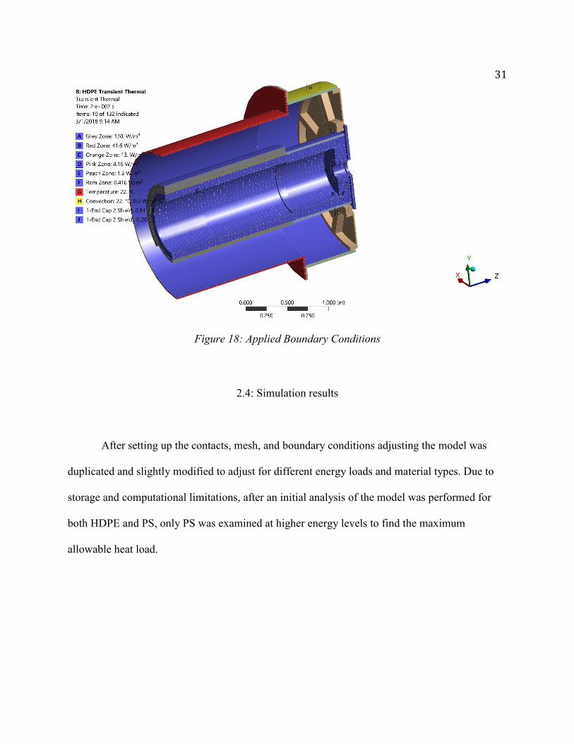
Figure 18: Applied Boundary Conditions

2.4: Simulation results

After setting up the contacts, mesh, and boundary conditions adjusting the model was

duplicated and slightly modified to adjust for different energy loads and material types. Due to

storage and computational limitations, after an initial analysis of the model was performed for

both HDPE and PS, only PS was examined at higher energy levels to find the maximum

allowable heat load.

32

2.4.1: Initial results

The initial results of the simulation show that the MBS will not overheat given the

applied thermal load. Seen in Figure 19 and Figure 20 are the results of the simulation for HDPE

and PS respectively.

Figure 19: Thermal Distribution with HDPE Absorbers

33

Figure 20: Thermal Distribution with PS Absorbers

Due to a majority of the heat generated coming from the grey heat load region of the end

plug, it is consistent to see that the highest temperature exists around that area. From looking at

the time dependent results of the simulation, it seems like the simulation does not reach a full

steady state condition. Seen in Figure 21 and Figure 22 are the graphs for the maximum and

minimum temperatures over time for HDPE and PS.

34

Figure 21: Maximum and Minimum Temperature over Time for HDPE with Dotted Trendline

Figure 22: Maximum and Minimum Temperature over Time for PS with Dotted Trendline

In the graphs there are some noticeable points of error which may be due to the initial

time step being too large, an incomplete mesh, or due to the natural behavior of the model caused

by the nonlinear boundary conditions. To eliminate these potential errors and find the time the

temperature of the structure will exceed the desired temperature, the simulation was adjusted.

35

2.4.2: Simulation Changes

To ensure accurate results when finding the scaled temperature, various changes to the

mesh size, material selection, and thermal loads were needed. The first change made to the

simulation was to the mesh size. The contact mesh constraints used in the end plug were adjusted

to have a smaller element size to reduce the error that would occur in the largest thermal load

area. The change in mesh size increased the model to 1,056,760 Nodes and 229,885 Elements.

The comparison of the two meshes can be seen in Figure 23.

Figure 23: Initial Analysis Mesh (Left); Scaled Analysis Mesh (Right)

36 To reduce the storage space used by the simulation results and reduce the computational

time required, the scale of the simulation needed to be reduced. As PS has material properties

that would cause it to exceed the maximum allowable temperature at a lower energy load

compared to HDPE, only the energy load that would cause the PS model to overheat will be

found. To find the energy load that will cause the model to overheat, the various internal heat

generation boundary conditions will be scaled. Because there was a change in the mesh, the

results of the simulations may not be fully consistent. To control for any inconsistency, the PS

model was ran with the initial simulation energy loads.

2.4.3: Scaled Simulation results

Simulations on a smaller scale version of the problem have indicated that the temperature

of the model will exceed the maximum allowable temperature at a scaling factor (SF) between 6

and 9 [22]. To find the energy load that the model will overheat at, the simulation was run with

the internal heat generation scaled by 1, 5, and 10. The results of the scaled simulations can be

seen in Figure 24 through Figure 26.

37

Figure 24: Temperature of MBS with PS Internal Absorbers, SF 1

Figure 25:Temperature of MBS with PS Internal Absorbers, SF 5

38

Figure 26:Temperature of MBS with PS Internal Absorbers, SF 10

The graphs of the maximum and minimum temperatures, seen in Figure 27 through

Figure 29, indicate that some of the points of error in the initial simulation were caused by the

previously used mesh. Comparing the plots of Figure 21, Figure 22, and Figure 27 show that the

increased precision in the mesh decreased the number of sharp changes in the temperature over

time.

39

Figure 27: Maximum and Minimum Temperature over Time for MBS with PS Internal Absorbers with Dotted Trendline, SF 1

Figure 28: Maximum and Minimum Temperature over Time for MBS with PS Internal Absorbers, SF 5

40

Figure 29: Maximum and Minimum Temperature over Time for MBS with PS Internal

Absorbers, SF 10

2.5: Discussion

A summary of the maximum and minimum temperatures of the various simulations that

have been performed can be seen in Table 4. The plots of the results over time can be seen

summarized in Figure 30.

41 Table 4: Results Summary

Figure 30: Summary of Scaled Simulation Results

One source of error that should be addressed across all the results is the minimum

temperatures. The ambient temperature was set to be 22° C, however all of the simulations have

a temperature lower than that value despite energy going into the system. The error is caused due

to the numerical solver used by ANSYS. When a thermal analysis is performed for meshes with

midside nodes there are potential issues that occur when radiation and convection conditions are

used [23]. Since surface to surface radiation conditions are used, which will not cause issues due

42 to how the meshes of any two surfaces will be linked, only the convection boundary condition

could cause issues. When midside nodes are used, 3-D elements distribute their heat flow such

that it flows in only one direction at the midsize node and distribute the mass of the element such

that the midside node will have more mass than at the corner nodes [23]. Since transient thermal

performed problem has a convection boundary condition in it and is dependent on the density of

the material, some error with convection will be present. Furthermore, these issues will cause

some integration errors to occur due to overpredicting values. Using linear elements will also not

necessarily solve any issues with the solution due to the many curved surfaces in the MBS. If

linear elements were used it would create rougher curves which would change the view factors

of the model. There may also still be issues with the mesh not being fine enough, however due to

computational limits, it is not possible to make the mesh finer. While these errors will not have a

large effect on the final answer, it will cause the minimum temperature of the model to fall below

the ambient temperature and could have lead the max temperature of the model to be higher than

an optimized model.

While the maximum temperature results may show that the system will stabilize as it

approaches the final time step, the data points at each time step and the location of the heated

region is still causing some instability in the model. As seen in Figure 31, there is still some

minor internal change in temperature occurring which will delay the time it will take the model

to stabilize. While it will not be a problem due to the time step of the problem, it shows that

solving the problem in steady state would have potentially lead to an incorrect result. The

decreases of the maximum temperature in Figure 21, Figure 22, and Figure 27 show that at some

point in the simulation the maximum temperature way fall slightly. This behavior may be a result

43 of error in the numerical solver, mesh, or the result of the nonlinearities in the system and could

potentially repeat indefinitely preventing the steady state solver from finding an answer.

Figure 31: Temperature Distribution of MBS End Plug with PS Internal Absorbers from Initial Analysis; at 1.7895*10^7s (Left), at 2.0*10^7s (Right)

To establish the scaling factor that will cause the structure to exceed 40° C it is important

to know the general trend of temperature as a function of the scaling factor. Using data from a

previously completed thermal analysis of a less complex version of the MBS [22], an

approximate trend can be established. Seen in Figure 32 is a plot of the temperature with respect

to time on a logarithmic scale. While the data does not fit a linear trend line perfectly, the data

points do roughly follow a linear pattern. The results of the scaled simulation further establish

44 the trend. Seen in Figure 33, the scaled simulation results roughly follow a linear trend. While

there is not enough data to definitively prove that the temperature will increase at a linear rate

with the scaling factor, it is likely that the function will be effectively linear near the potential

scaling factors that have been considered.

Figure 32: Logarithmic Plot of Original Simulation Results with Linear Trendlines [22]

45

Figure 33: Plot of Scaled Simulation Results with Linear Trendlines

Since the simulation is approximately linear near the scaling factors used, to find the

energy load that will cause the structure to exceed 40° C, interpolation will be used.

𝑆𝐹10 − 𝑆𝐹𝑥𝑆𝐹10 − 𝑆𝐹5

=𝑇10 − 𝑇𝑥𝑇10 − 𝑇5

10 − 𝑆𝐹𝑥10 − 5

=45.868 − 40

45.868 − 34.242

𝑆𝐹𝑥 =7.5

(2.22)

The results of the interpolation show that it will take about 7.5 times the applied heat load to

exceed an acceptable desired temperature of the MBS. The scaling factor value of HDPE will be

higher, however if HDPE is used, there is a larger chance that radiation damage will occur to the

MBS

Chapter 3: Axial Coupler

3.1: Overview of Problem

For maintenance to be performed on the detector train, a method to extract the structure

from the vacuum vessel is needed. To extract the detector train, hydraulic cylinders will move

the IFB and couplers will transmit the force between the components of the detector train. The

part that is designed to connect the components of the detector train together is referred to as the

axial couplers. The axial coupler is designed to couple the individual components of the detector

train to the neighboring sections. Each component of the detector train is supported by a rail

system using ball bearing blocks which will allow the train to be inserted or extracted smoothly

using hydraulics attached to the end of the train at the IFB. An attachment will be designed to

connect the bearing blocks to a bar which connect to the attachment on the bearing block of the

next component of the beamline. A design of a fully assembled axial coupler attached to the rail

system can be seen in Figure 34. While a previous analysis has been done on the attachment

piece [24], due to clearance constraints, the design buckling when it was tested, and an increased

maximum force load created by the consideration of a the load generated by the services

redesign of the axial coupler seen in Figure 35 was deemed appropriate. The redesigned model

was then analyzed using finite element analysis.

47

Figure 34: Axial Coupler in Rail System

Figure 35: Previous Axial Coupler Design [24]

48

3.2: Axial Coupler Redesign

The redesign of the axial coupler requires the bearing block to allow for an additional

attachment method and for the connecter piece to reduce the possibility of buckling. Both

components need to fit inside a limited amount of allowable space. The previous design of the

axial coupler was designed in a way that would have made it impossible to take apart once it and

every other component was installed. Figure 36 shows an axial view of the axial coupler design

along with various potential points of interference. In the image, the previous bearing block

design is in green, the desired axial coupler position with bar connection is in light blue, and the

circular lines represent the main components of the experiment. As seen in the image, the

previous bearing block design there was little to no room to remove the bolts attaching the

coupler to the bearing block. To account for these issues along ensuring that buckling will not

occur, the bearing block and axial coupler will be redesigned. At two areas along the detector

train, there will be a need to modify the design slightly. One connecter piece will need to be

redesigned specifically for its position on the detector train to account for the shorted distance

between the components and at another section the bar will need to be modified to allow for the

section to be disassembled. These changes at their individual sections will require further

analysis. The analysis will need to meet or exceed a Safety Factor of 2 [25] and to not deform

more than 2 mm [24].

49

Figure 36: Dimensions of Bearing Block Relative to other beamline components. [26]

3.2.1: Bearing Block

To ensure that no interference occurs with the detector train, three changes were made to

the bearing block. These changes were trimming the side of the bearing block, adding additional

material to the sides of the block, and adding holes on its side. To reduce the interference along

the path of the bearing block, a small chamfer was also added along the length of the of the

blocks for the Tracker. To ensure that the block will not fail due to the chamfer and to allow for

further attachment points for the connecter, the space seen in the dotted line in Figure 36 and

threaded holes for a 3/8”-16 were added. The resulting design can be seen in Figure 37.

50

Figure 37: Bearing Block for the Tracker

3.2.2: Bar Design

Bars of varying lengths will need to be made with a cross section of 38.1 mm by 38.1

mm. Table 5 shows the various bar lengths needed to connect the bearing blocks. All the bearing

blocks will be transmitting the same magnitude of force during instillation and extraction. Due to

the large force required to move the train, buckling may occur. Buckling would occur in long

bars with compressive loads applied to them due to the moment generated by the compressive

load exceeding the elastic ability of the component to restore its equilibrium position. Buckling

would occur in the direction of least resistance which is dependent on the cross-sectional area

and length. Taking requirements for buckling into account, the bar that will be the most likely to

buckle is the longest one at 1036.95 mm. Because of the longest bar will fail first, only the

Downstream OPA to Tracker bar will be analyzed. To attach to the connecter piece, a 14mm

hole is added 22.5 mm away from the ends of each bar. An alternative design for the bar will

also be considered which will allow for the train to be decoupled through use of an L shaped

connection. This design would be used when other components would prevent access to the bolts

in the Connecter Piece. For the design, the bar will be cut in half with an L shaped cut. One bar

51 will have 3, 16mm holes drilled in while the other bar will have 3, M14x2 threads made such that

the threaded holes and drilled holes are coaxial centers. The two bars will then be attached

together using a shoulder bolt. The L-bar design can be seen in Figure 38.

Table 5: Lengths Between Component Positions [27]

Figure 38: L-Bar Connection

3.2.3: Connecter Piece

To take advantage of the holes on the side of the bearing block and to reduce interference

with other components of the beamline, the piece will only attach to the side of the bearing

block. The previous design of the piece used G10 [24], however due to it being a composite, the

part will have a chance to fail due to out of plane stresses caused by the bolts. To prevent this

from occurring, the part will be made from 316L Stainless Steel. To allow for the smooth

52 insertion of bolts to attach to the Connecter Piece to the Bearing Block, 9.775 mm holes were cut

to line up with the holes in the bearing block. To reduce the volume taken up by the axial coupler

and decrease the length available for the bolts to bend, a 16.5 mm holes with a depth of 25.2 mm

centered on the bolt holes. The bolt hole will allow the bolt heads to fit inside the connecter piece

reducing the amount of space needed for the design. To connect to the bar, a 14mm hole was

added near the tip of the Connecter. The final design of the standard connecter piece can be seen

in Figure 39. Due to the length of the connecter piece, one segment of the detector train will

require a unique connecter piece. The distance between the upstream OPA and the stopping

target bearing block faces, seen in Table 5, is only 211 mm. To connect the components together,

various areas of the connecter piece will be lengthened and redesigned to allow for one connecter

piece to be inserted into the “jaw” of another one. The design of the Jaw connecter can be seen in

Figure 40.

Figure 39: Connecter Piece Design

53

Figure 40: Short Axial Coupler Jaw Connecter

3.2.4 Final Design

The Bearing Blocks, Connecter Pieces, and Bars will all be attached to each other using

Silicone Bronze C64200 Bolts. The pieces will then be assembled in the way seen in Figure 41.

The L-Bar and Short Axial Coupler can be seen in Figure 42 and Figure 43 respectively.

Figure 41: Explosion View of Axial Coupler

54

Figure 42: L-Bar Assembly of Axial Coupler

Figure 43: Short Axial Coupler Assembly

For the analysis of the axial coupler there will be three variations of the design

considered. These designs are the standard axial coupler, the standard axial coupler with the L-

bar, and the long axial coupler design.

55

3.2.5: Equations

To ensure that the design will be successful, the design will have to be able to

endure the stresses it will be under and not deform beyond the desired margin of error. The finite

element analysis will be used structural integrity for the main body and bar of the coupler;

however, the bolts are where failure is most likely to occur, and buckling may because by the

applied loads. To do find the endurance of the bolts, the horizontal forces (X and Z axis forces)

can be used to generate shear and the vertical forces (Y axis forces) can be used to generate a

pullout stress.

𝜏𝑠ℎ𝑒𝑎𝑟 = 𝜏𝑥 + 𝜏𝑧 = 𝐹𝑥

𝐴𝑠ℎ𝑒𝑎𝑟+

𝐹𝑧𝐴𝑠ℎ𝑒𝑎𝑟

(3.1)

𝜎𝑝𝑢𝑙𝑙𝑜𝑢𝑡 = 𝜎𝑦 = 𝐹𝑦

𝐴𝑠

(3.2)

The tensile stress area, 𝐴𝑠, can be determined by ASTM F468M-06 [28] for metric bolt,

ASTM F593-02 [29]for imperial unit bolts, and the shear area, 𝐴𝑠ℎ𝑒𝑎𝑟, can be calculated using

the geometry of the bolt hole dependent on if it is in single or double shear [30].

𝐴𝑠_𝑚𝑒𝑡𝑟𝑖𝑐 = .7854 ∗ (𝐷 − .93882 ∗ 𝑃)2 (3.3)

𝐴𝑠_𝑖𝑚𝑝𝑒𝑟𝑖𝑎𝑙 = .7854 ∗ (𝐷 −. 9743

𝑛)2 (3.4)

For Single Shear:

𝐴𝑠ℎ𝑒𝑎𝑟 = 𝜋 𝐷2

4

(3.5)

For Double Shear:

𝐴𝑠ℎ𝑒𝑎𝑟 = 𝜋 𝐷2

2

(3.6)

56 By finding the total stress at a bolt connection, a safety factor can be found by comparing it to

the ASTM F468M-06 yield stress of a C64200 bolt [28]:

𝑆. 𝐹. = 𝜎𝐴𝑆𝑇𝑀 𝑌𝑖𝑒𝑙𝑑𝜎𝑡𝑜𝑡

=240 𝑀𝑃𝑎

𝜎𝑡𝑜𝑡 (3.7)

The Axial Coupler has three bolt connections between the Bearing Block and Connector

Piece, between the Connecter Piece and the Bar, and at the L-Bar Connection Area. Each of the

connections has a slightly different bolt hole and potential for forces to be exerted on it. As the

connection between the Bearing Block and Connector Piece only pullout stress can be expected.

In compression at that area, the minor deformations of the bolt caused by the applied force will

cause most of the force to be applied to the back of the bearing block. At the Connecter Piece

and Bar connection, there will be both pullout and double shear stresses, however the Short

Axial Coupler connection will be slightly different. While the Jaw connecter will be

experiencing the same stress as the normal connection, the Insert connecter will be experiencing

single shear. At the L-Bar connection, each side of the bar will experience a different shear. Only

one of the bars will have threading on it, which will require it to bear all the pullout stress, while

the other bar will be a shoulder connection which will only experience the shear stress. The

resulting stress equations for these considerations are:

Bearing Block and Connecter Piece:

𝜎𝑡𝑜𝑡 = 𝜎𝑝𝑢𝑙𝑙𝑜𝑢𝑡 = 𝐹𝑦

.7854 ∗ (𝐷 −. 9743𝑛 )2

(3.8)

Connecter Piece and Bar:

𝜎𝑡𝑜𝑡 = 𝜏𝑠ℎ𝑒𝑎𝑟 + 𝜎𝑝𝑢𝑙𝑙𝑜𝑢𝑡 = 2 ∗ (𝐹𝑥 + 𝐹𝑍)

𝜋 𝑑2 +

𝐹𝑦

.7854 ∗ (𝐷 − .93882 ∗ 𝑃)2

(3.9)

Short Axial Coupler Insert Connecter:

57

𝜎𝑡𝑜𝑡 = 𝜏𝑠ℎ𝑒𝑎𝑟 + 𝜎𝑝𝑢𝑙𝑙𝑜𝑢𝑡 = 4 ∗ (𝐹𝑥 + 𝐹𝑍)

𝜋 𝑑2 +

𝐹𝑦

.7854 ∗ (𝐷 − .93882 ∗ 𝑃)2

(3.10)

Shoulder L-Bar Connection:

𝜎𝑡𝑜𝑡 = 𝜏𝑠ℎ𝑒𝑎𝑟 =4 ∗ (𝐹𝑥 + 𝐹𝑍)

𝜋 𝐷2

(3.11)

Threading L-Bar Connection:

𝜎𝑡𝑜𝑡 = 𝜏𝑠ℎ𝑒𝑎𝑟 + 𝜎𝑝𝑢𝑙𝑙𝑜𝑢𝑡 =4 ∗ (𝐹𝑥 + 𝐹𝑍)

𝜋 𝑑2 +

𝐹𝑦

.7854 ∗ (𝐷 − .93882 ∗ 𝑃)2

(3.12)

In addition to finding the safety factor on the bolts, the safety factor of the critical force

which would cause buckling is also needed. Using the Euler buckling equation [31], the

dimensions of the bar, and the material properties found in Table 1, the force which will cause

buckling can be found. The critical buckling force can then be compared to the forces generated

at the pin locations to find the safety factor of the buckling load.

𝑃𝑐𝑟 =𝜋2 ∗ 𝐸𝐼

𝐿2=𝜋2 ∗ 𝐸 ∗

𝑏 ∗ ℎ3

12𝐿2

=𝜋2 ∗ (193000) ∗

38.1 ∗ (38.1)3

12(1096.95)2

= 277.97 𝑘𝑁 (3.13)

𝑆. 𝐹. =277.97 𝑘𝑁

𝐹𝑎𝑝𝑝𝑙𝑖𝑒𝑑

(3.14)

With the equations established, to eliminate some error in the simulation and to ensure a

conservative design, the maximum combination of generated forces at each connection will be

used to find an absolute worst-case loading scenario.

3.3: Finite Element Analysis Setup

The various axial coupler assemblies were imported into ANSYS 18.1 as STEP files. The

axial coupler model was then meshed using a MultiZone Method for the bolts and the Bar was

58 meshed with the Hex Dominant Method. The bolts had a mesh size of 2 mm, the bar and bearing

block had a mesh size of 8mm, and the connecter piece had a mesh size of 4mm. A contact mesh

with a size of 2mm was also applied to all the contacts that contained a bolt. The short axial

coupler was similarly meshed, however with no hex dominant method used. The mesh for the

normal bar axial coupler can be seen in Figure 44 and the Short Axial Coupler mesh can be seen

in Figure 45.

Figure 44: Axial Coupler Mesh

59

Figure 45: Short Axial Coupler Mesh

To simulate the forces exerted on the axial coupler, the boundary conditions need to be

applied on the model. To mimic the rail the bearing block is attached to, a displacement

constraint that prevents movement in the Z and Y axis. A fixed support constraint was applied to

one end of the bearing block and a force of 4000lbs (17793 N) was applied on the other end. This

force is generated based on the force required to move the Detector Train [24] and services. The

standard earth gravity constraint was also applied to the model in the Y axis and a bolt pretension

constraint of 4448.2 N were applied to the threaded section of the bolts to simulate the force

required to tighten locknuts. Due to having different underlying models, the coordinate systems

for the models were different. To ensure consistency between the simulations, the forces and

results need to be calculated on the same coordinate system. The normal bar axial coupler’s axis

was chosen to be the standard one and the other two simulations were assigned an additional

coordinate system for the forces and results. The forces applied on the normal bar model and the

Short Connecter model, as seen in the Static Structural View, can be seen in Figure 46 and

60 Figure 47. The applied force was adjusted to be positive to simulate compression and adjusted to

be negative to simulate tension.

Figure 46: Forces Applied to Axial Coupler

Figure 47: Forces Applied to Short Axial Coupler

61 For simulating the L-Bar connection, the model was set up in the same way as the normal

axial coupler, however since the connecter, bearing block, and pin connections are the same,

only the behavior around the L-Connection connection will be analyzed. The applied constraints

were chosen to get a conservative safety factor for the axial coupler. The force applied to the

couplers is the anticipated cutoff force of the hydraulic piston if there would be a snag when

inserting or extracting the detector solenoid and as such for normal operations the actual force

will be lower. In addition, in the future there may be considerations made to attach an axial

coupler to both sides of the detector solenoid which would half the applied force both couplers

need to bear. Because of these decisions, there will be an inherent safety factor in all of the

results.

3.4: Simulation results

The total deformation, Y-Axis, and Z-axis deformation, equivalent stress, and the forces

at key points were found for both the Axial Coupler and the Shortened Axial Coupler. The

eigenvalue buckling was also found for the realistic length axial coupler. The results of the total

deformation of the Axial Coupler in compression and tension can be seen in Figure 48 and

Figure 49 while the total deformation in compression and tension for the Short Axial Coupler

can be seen in Figure 50 and Figure 51.

62

Figure 48: Axial Coupler, Total Deformation, Compression

Figure 49: Axial Coupler, Total Deformation, Tension

63

Figure 50: Short Coupler, Total Deformation, Compression

Figure 51: Short Coupler, Total Deformation, Tension

The equivalent stress generated can be seen in Figure 52 through Figure 55. In the model,

while a majority of the model is at relatively low levels of stress, there are locations where a

large stress concentration appears. The two main areas of stress concentrations are on the corners

of the connecters and the bolt connections. The stress concentrations in the corners are due to the

mathematical models used in ANSYS and are not in areas where large stress concentrations

64 should build up and as such it is most likely that these are singularities and will not occur in the

real model. The other area of large stress concentrations occurs in near the circular areas of the

pin holes and bolt connections. To ensure that the large concentrations will not cause the bolts to

fail, the force reactions at the contact areas were found and implemented into manual

calculations. The bolt holes were labeled 1-4 as seen in Figure 56, and the forces of the bolts on

bolt sides of the coupler can be seen Table 6. Figure 57 shows an example of a common stress

concentration that is seen at the bolt holes across all the analysis performed.

Figure 52: Axial Coupler, Equivalent Stress in Compression

65

Figure 53: Axial Coupler, Equivalent Stress in Tension

Figure 54: Short Axial Coupler, Equivalent Stress in Compression

66

Figure 55: Short Axial Coupler, Equivalent Stress in Tension

Figure 56: Bolt Numbering on Axial Coupler

67

Figure 57: Stress Concentration on Short Axial Coupler

Table 6: Force Reactions on Bolts in Tension

The Eigenvalue Buckling of the axial coupler in compression was also performed. For the

buckling simulation, the gravitational forces were disabled, and four modes of buckling were

found. The result of the simulation showed that the four modes showed a large, negative critical

force which would put the system into tension. The abnormal values are most likely due to the

bolts failing in buckling before the actual bar does from the programs perspective. To determine

the actual eigenvalue buckling force, a manual calculation will be done.

Manual calculations will also need to be done for other areas of the simulation. To

eliminate the error due to the stress concentrations at the bolt holes of the design, the force

Tension Force Axis Bolt 1 (N) Bolt 2 (N) Bolt 3 (N) Bolt 4 (N)Z - Axis X 54.481 -59.541 33.393 -22.399

Y 30.8 38.886 3.3149 8.3274Z -3759.3 -3910.6 -5261.3 -5210

Z + Axis X -59.522 55.271 -22.013 32.256Y 23.785 30.868 8.8416 2.8495Z 3910.8 3763.4 5208.2 5262.3

68 reactions for the shoulder and the threading of the bolts will need to be found and analyzed to

ensure that the bolts will not fail. To keep track of the bolts across the various models, each bolt

was labeled 1-3 as seen in Figure 58. The force reactions at these positions can be seen in Table

7 and Table 8.

Figure 58: Bolt Numbering

Table 7: Reaction Forces in Tension

Table 8: Reaction Forces in Compression

The reaction forces at the pin connection area were also found for the short axial coupler

for both the insert and jaw piece. These forces can be seen in Table 9.

Tension Force Axis Bolt 1 (N) Bolt 2 (N) Bolt 3 (N)Shoulder X 7045.2 3158.2 7048.9

Y -1138.9 18.904 1132Z 2476.1 -94.126 3078.2

Threading X -6729.9 -2938.2 -6405.4Y 1078.5 -13.828 -1049.7Z -2746.4 93.736 -3194.7

Compression Force Axis Bolt 1 (N) Bolt 2 (N) Bolt 3 (N)Shoulder X -7091.3 -3229.8 -7016.9

Y 255.37 3.4524 -247.95Z 2117.9 224.82 2005.6

Threading X 6555.6 3010.5 6502.9Y -232.85 -6.3301 231.87Z -2191.1 -246.18 -2133.7

69 Table 9: Short Axial Coupler Connection Reaction Forces

3.5: Discussion

Using the equations established in section 3.2.5 and the results in section 3.4, the critical

buckling force and the stresses at various connections can be found. The buckling calculation can

be done using equation 3.14. Using the total applied force on the structure, the resulting safety

factor can be found.

𝑆. 𝐹. =𝑃𝑐𝑟

𝐹𝑎𝑝𝑝𝑙𝑖𝑒𝑑=

277.97 𝑘𝑁

17.79289 𝑘𝑁= 15.6

(3.15)

The forces at the various bolt connections can also be examined using the results from Table 6

through Table 9 and equations 3.8 through 3.12. At the bearing block and connecter piece

connection:

𝜎𝑡𝑜𝑡 = 𝜎𝑝𝑢𝑙𝑙𝑜𝑢𝑡 = 𝐹𝑦

.7854 ∗ (𝐷 −. 9743𝑛 )

2 =5262.3𝑁

. 0775 𝑖𝑛2=

5262.3𝑁

(5 ∗ 10−5)𝑚2

𝜎𝑡𝑜𝑡 = 105.25 𝑀𝑃𝑎

(3.16)

𝑆. 𝐹. = 𝜎𝐴𝑆𝑇𝑀 𝑌𝑖𝑒𝑙𝑑𝜎𝑡𝑜𝑡

=240 𝑀𝑃𝑎

105.25 𝑀𝑃𝑎= 2.2803 (3.17)

At the Connecter Piece and Bar connection for the Jaw and normal design:

Force Axis Tension (N) Compression (N)Insert X -4.2513 8.0941

Y -2503.5 -994.01Z -17801 17793

Jaw X 4.2525 -8.0942Y 2514.7 998.58Z 17801 -17793

70

𝜎𝑡𝑜𝑡 = 𝜏𝑠ℎ𝑒𝑎𝑟 + 𝜎𝑝𝑢𝑙𝑙𝑜𝑢𝑡 = 2 ∗ (𝐹𝑥 + 𝐹𝑍)

𝜋 𝐷2 +

𝐹𝑦

.7854 ∗ (𝐷 − .93882 ∗ 𝑃)2

=35618 𝑁

615.7522 𝑚𝑚2+

2514.7

115 𝑚𝑚2= 79.7117 𝑀𝑃𝑎

(3.18)

𝑆. 𝐹. = 𝜎𝐴𝑆𝑇𝑀 𝑌𝑖𝑒𝑙𝑑𝜎𝑡𝑜𝑡

=240 𝑀𝑃𝑎

79.7117 𝑀𝑃𝑎= 3.0109 (3.19)

At the Short Axial Coupler Insert Connecter:

𝜎𝑡𝑜𝑡 = 𝜏𝑠ℎ𝑒𝑎𝑟 + 𝜎𝑝𝑢𝑙𝑙𝑜𝑢𝑡 = 4 ∗ (𝐹𝑥 + 𝐹𝑍)

𝜋 𝐷2 +

𝐹𝑦

.7854 ∗ (𝐷 − .93882 ∗ 𝑃)2

=71236 𝑁

615.7522 𝑚𝑚2+

2503.5

115 𝑚𝑚2= 137.4590 𝑀𝑃𝑎

(3.20)

𝑆. 𝐹. = 𝜎𝐴𝑆𝑇𝑀 𝑌𝑖𝑒𝑙𝑑𝜎𝑡𝑜𝑡

=240 𝑀𝑃𝑎

137.4590 𝑀𝑃𝑎= 1.746 (3.21)

At the Shoulder L-Bar connection:

𝜎𝑡𝑜𝑡 = 𝜏𝑠ℎ𝑒𝑎𝑟 =4 ∗ (𝐹𝑥 + 𝐹𝑍)

𝜋 𝐷2=

40678 𝑁

804.2477 𝑚𝑚2 = 50.5789 𝑀𝑃𝑎

(3.22)

𝑆. 𝐹. = 𝜎𝐴𝑆𝑇𝑀 𝑌𝑖𝑒𝑙𝑑𝜎𝑡𝑜𝑡

=240 𝑀𝑃𝑎

50.5789 𝑀𝑃𝑎= 4.7451 (3.23)

At the Threading L-Bar connection:

𝜎𝑡𝑜𝑡 = 𝜏𝑠ℎ𝑒𝑎𝑟 + 𝜎𝑝𝑢𝑙𝑙𝑜𝑢𝑡 =4 ∗ (𝐹𝑥 + 𝐹𝑍)

𝜋 𝑑2 +

𝐹𝑦

.7854 ∗ (𝐷 − .93882 ∗ 𝑃)2

=39698 𝑁

615.7522 𝑚𝑚2+1138.9 𝑁

115 𝑚𝑚2= 74.3742 𝑀𝑃𝑎

(3.24)

𝑆. 𝐹. = 𝜎𝐴𝑆𝑇𝑀 𝑌𝑖𝑒𝑙𝑑𝜎𝑡𝑜𝑡

=240 𝑀𝑃𝑎

74.3742 𝑀𝑃𝑎= 3.2269 (3.25)

A summary of all the results of the safety factor calculations can be seen in Table 10. While most

of the Safety Factors are above 2, the Insert Connecter Piece is not. As the design of Insert and

Jaw has not been fully completed, and as such the piece can be improved in the future. The

71 deformations in the system all managed to be less than the desired maximum deformation of 2

mm.

Table 10: Safety Factor Summary

Calculation Safety Factor

Buckling 15.6

Bearing Block and Connecter Piece Bolt 2.2

Connecter Piece and Bar Bolt 3.0

Insert Connecter Piece Bolt 1.7

Shoulder L-Bar connection 4.7

Threading L-Bar Connection 3.2

Chapter 4: MBS Trunnion Analysis

4.1: Introduction

Once installed, the MBS is supported using a trunnion on the IFB, seen in Figure 59, and

the Gimbel Support. To ensure that the system does not fail, an ANSYS analysis will be

performed to ensure that the trunnion does not fail in shear or to deflection. A simplified model

of the trunnion and surrounding components will need to be made. Using an estimate of the

maximum weight of the structure, a static structural analysis will be performed to find the

equivalent stress and total deformation of the system. To determine the success of the design, the

resulting stress should be bellow twice the yield strength of the material and the structure should

not deform more than 0.5 mm [25]

73

Figure 59: Trunnion Location on IFB

4.2: Model

The models used are simplified versions of the Trunnion Cap (Fermilab drawing number

F10086594) and part of the IFB (Fermilab drawing numberF10058701). To do model the

components Inventor 2017 was used to create an assembly of the two components. As the forces

will be the approximately the same on each trunnion, only one half of the model was considered.

The main body of the IFB was also not modeled as it is not the area of focus of the analysis and

because it would needlessly increase complexity of the simulation. To allow for alignment, the

MBS is designed to allow for some radial shifting to allow for alignment and the uncertainty in

components. Because of this uncertainty, each trunnion could potentially have a slightly different

contact area with the MBS. To account for this uncertainty and create a worst-case scenario, the

74 smallest designed contact area was sectioned onto the trunnion cap to allow for a smaller area to

disperse the force. From applying these changes to the model, the resulting assembly can be seen

in Figure 60.

Figure 60: Trunnion Assembly, Trunnion Cap (Copper), IFB Trunnion (Silver)

4.3: Simulation Setup

The Inventor assembly was imported into ANSYS 18.1 as a STEP file. The trunnion cap

was assigned the material properties of Silicon Bronze (C64200) and the Trunnion was assigned

the material properties of 316 Stainless Steel. The material properties used can be seen in Table

1. The imported model was meshed using the proximity and curvature size function with a Fine

relevance center and a relevance of 100. The Trunnion cap was also meshed using the Hex

Dominant Method. The resulting mesh generated 587,721 Nodes and 141,717 elements and can

be seen in Figure 61.

75

Figure 61: Generated Mesh

To find the maximum force that will be applied to the trunnion and to ensure that the

trunnion can support any changes in design of the MBS or inclusions of services, the full weight

of the MBS not including services, which rounds up to 5000 kg [32], will be assumed to be held

up by the trunnions. Taking these factors into account, a force of -24,525 N was applied in the Y-

Axis of the sectioned part of the trunnion cap. It is unlikely that the full weight of the MBS will

ever be on the trunnion cap alone, however assuming the larger force allows for a inherent Safety

Factor of at least 2 and ensures that the inclusion of services in the future design of the MBS will

not affect the validity of the simulation. A Fixed Support constraint was then applied to the

section of the trunnion that attaches to the MBS and the Standard Earth Gravity inertial condition

was applied to the model. The applied constraints can be seen in Figure 62.

76

Figure 62: Applied Constraints

4.4: Results

With large deflection turned on, the total deformation, equivalent stress, and safety factor

were solved for using the applied constraints. The force reaction was also found on the fixed

support constraint area. The total deformation seen in Figure 63 through Figure 65 shows the

deformation of the assembly and components with an adjusted scale to visually represent the

deformation of the structure. From the results the maximum deformation is 0.0298 mm.

77

Figure 63: Total Deformation

Figure 64: Side View of the Total Deformation of the Trunnion Without Cap

78

Figure 65: Side view of Total Deformation of the Trunnion Cap

The equivalent stress seen in Figure 66 through Figure 66 shows the equivalent stresses

with different scales to better visualize the stress distribution. While there is a relatively low

stress distribution across a majority of the model near the top Conner of the trunnion, there is a

large stress singularity. This singularity can be seen in Figure 69.

Figure 66: Equivalent Stress of Assembly

79

Figure 67: Equivalent Stress of Trunnion Cap

Figure 68: Equivalent Stress on Trunnion

80

Figure 69: Zoomed in View of Stress Singularity

The minimum safety factor of the model was found to be 0.894 as seen in Figure 70 and

Figure 71. It is important to note, the low safety factor in the trunnion is located at the stress

singularity. At the trunnion cap, there is some effect of the singularity, however it the safety

factor is above 2.8. To be able to verify the stresses at the connection, the resulting force at the

fixed support constraint was found to be 24,553 N in the opposite direction of the applied force.

81

Figure 70: Safety Factor of the Trunnion Cap

Figure 71: Saftey Factor of the Trunnion

82

4.5: Discussion

The results show that while most of the structure is above the desired safety factor of 2,

there is a small area of the trunnion located at the top edge of the fixed support constraint which

seem to fail due to a stress concentration, however the large stress concentration is most likely a

singularity caused by how ANSYS solves the generated mathematical model. To ensure that the

trunnion will not fail at that section, the shear stress at that location can be determined by using

the force reaction at that location. The resulting stress can then be used to solve for the safety

factor of the region.

𝜏 =𝐹

𝐴=

24553 𝑁

2919.679 𝑚𝑚= 8.4095 𝑀𝑃𝑎

(4.1)

𝑆. 𝐹. = 𝜎𝑦𝑖𝑒𝑙𝑑

𝜏=

290 𝑀𝑃𝑎

8.4095 𝑀𝑃𝑎= 34.5 (4.2)

The resulting safety factor is significantly larger than the desired safety factor of 2. The

deflection of the system is also significantly less than the allowable deformation of 0.5 mm.

Chapter 5: Result Summary and Future Work

For the Thermal Analysis of the Muon Beam Stop, under the given simulated energy

loads, the structure will not exceed the allowable temperature, however due to the inherent

uncertainty in the simulations used to evaluate the heat loads and potential issues with the

simulation performed, the actual energy load of the system could be higher than currently

predicted. Under the current design of the beam stop, the model currently has a thermal safety

factor of at least 7.5. Furthermore, the radiation caused by the beam could cause issues in the

future depending on what material is used. To prevent these issues, it may be possible to redesign

the MBS to be made of a mixture of polymers to allow for optimal heat transfer and radiation

endurance. A redesign may not be required though depending on the accuracy of the provided

radiation simulations.

The results of the structural analysis of the Axial Coupler show that the current design

will be able to endure the stresses from the detector train locking up. Due to the design being

able to withstand the higher stresses of the worst-case scenario, the design should also withstand

the stress of moving the total train. Furthermore, the stresses experienced by the design can be

reduced by adding a second series of axial couplers to help connect the components of the

detector train. If a second series of axial couplers are not added to the train, the Insert and Jaw

connecter may need to be modified to improve the resulting safety factors. To verify the results

84 of the simulation, testing should be done on a prototype to ensure that the real-life

application of the model will not fail. To test the design. a bearing block, bar, and connecter will

be made and tested on a smaller section of the rail system with the full 4000-pound load applied

to it. The results of test will indicate if the design will behave as anticipated.

The simulations performed on the Trunnion Cap indicate that it will be able to endure the

loading produced by the Muon Beam Stop. While there were areas of the simulation that had a

stress concentration, the result of manual calculations at the regions of stress concentration show

that the stress concentrations are due to a singularity. The system will also benefit from the

minor fillets made in the manufacturing process of the components. Furthermore, with the large

safety factors present made with the overestimation of the applied forces, it shows that the

trunnion will not fail even if minor changes are made to the weight of the MBS. Testing should

be done to verify the structural integrity of the design. One potential method of testing the design

could be to use a Compression Test Machine on a prototype cap to determine if the cap can

endure forces greater than what can be caused by the MBS. With the verification of the structural

integrity of the Trunnion Cap and IFB, the design will be able to work in the Detector Solenoid.

REFERENCES

[1]“Mu2e Technical Design Report,” Mu2e-Doc-4299-v15, Fermi National Accelerator Laboratory, Batavia, IL. [2] ANSYS® Student, Release 17.2, Mechanical APDL, Theory Reference, 14. Analysis Tools

,14.7 Equation Solvers [3]“Properties for LDPE and HDPE,” Zhengzhou Orient Power Website. [Online]. Available:

http://www.powerinsulator.com/list1.asp?id=349. [Accessed: 15-Dec-2017]. [4]“AK Steel 316L Austenitic Stainless steel,” MatWeb. [Online]. Available:

http://www.matweb.com/search/datasheet.aspx?matguid=9e9ab696974044cab4a7fd83687934eb. [Accessed: 15-Dec-2017].

[5]“Ampco Metal AMPCO® 642 Aluminum-Silicon-Copper Alloy, Extruded-Drawn-Stress

Relieved (HR-50), ≤ 1/2",” MatWeb. [Online]. Available: http://www.matweb.com/search/DataSheet.aspx?MatGUID=9f6cfc8f87e74c71b1cdfc05b5a8bcae. [Accessed: 15-Dec-2017].

[6] D. W. Designs, “Emissivity Materials,” Infrared-Thermography. [Online]. Available:

http://www.infrared-thermography.com/material-1.htm. [Accessed: 15-Dec-2017]. [7]“Overview of materials for High Density Polyethylene (HDPE), Injection Molded,” MatWeb.

[Online]. Available: http://www.matweb.com/search/DataSheet.aspx?MatGUID=fce23f90005d4fbe8e12a1bce53ebdc8. [Accessed: 15-Dec-2017].

[8]“Overview of materials for Polystyrene, Molded, Unreinforced,” MatWeb. [Online].

Available: http://www.matweb.com/search/DataSheet.aspx?MatGUID=df6b1ef50ce84e7995bdd1f6fd1b04c9. [Accessed: 15-Dec-2017].

[9]“Specific Heat of Common Substances,” The Engineering ToolBox. [Online]. Available:

http://www.engineeringtoolbox.com/specific-heat-capacity-d_391.html. [Accessed: 15-Dec-2017].

86 [10]“Table of Total Emissivity,” Omega. [Online]. Available:

https://www.omega.com/temperature/z/pdf/z088-089.pdf . [Accessed: 15-Dec-2017]. [11]“Polystyrene,” Polymer Database. [Online]. Available:

http://polymerdatabase.com/polymers/polystyrene.html. [Accessed: 15-Dec-2017]. [12]G. Ginther, “Muon Beamline Updates,” Mu2e-Doc-14847-v1, Fermi National Accelerator

Laboratory, Batavia, IL. [13]V. Pronskikh,“Optimal transport parameters for the next MARS run,” Mu2e-Doc-15977-v2,

Fermi National Accelerator Laboratory, Batavia, IL. [14]S. M. Tamboli, S. T. Mhaske, and D. D. Kale, “Crosslinked Polyethylene,” Indian Journal of

Chemical Technology, vol. 11, pp. 853–864, Nov. 2004. [15]Z. Chang and J. A. Laverne, “Molecular Hydrogen Production in the Radiolysis of High-

Density Polyethylene,”The Journal of Physical Chemistry B, vol. 103, no. 39, pp. 8267–8271, Sep. 1999.

[16] G. P. Nikishkov, Programming Finite Elements in Java, 1st ed. London: Springer-Verlag. [17] ANSYS® Student, Release 17.2, Mechanical APDL, Thermal Analysis Guide, 4. Radiation,

4.6, Using The Radiosity Solver Method [18] ANSYS® Student, Release 17.2, Mechanical APDL, Modeling and Meshing Guide,

Contact Technology Guide, 7. Multiphysics Contact, 7.1 Modeling Thermal Contact

[19]“Thermal Contact Resistance,” SOLIDWORKS Help, 2016. [Online]. Available: http://help.solidworks.com/2016/english/solidworks/cworks/c_thermal_contact_resistance.htm. [Accessed: 01-Mar-2018].

[20] “Making Thermal Contact Conductance a Parameter in ANSYS Mechanical 18.0 and

Earlier with an APDL Command Object,” PADT, Inc. -The Blog, 06-Apr-2017. [Online]. Available: http://www.padtinc.com/blog/the-focus/ansys-mechanical-contact-condutance-apdl. [Accessed: 01-Mar-2018].

[21] G. Ginther, “Muon Beamline Related Updates,” Mu2e-Doc-16343-v1, Fermi National

Accelerator Laboratory, Batavia, IL. [22] C. Narug, “MBS thermal analysis” Mu2e-Doc-15060-v1, Fermi National Accelerator

Laboratory, Batavia, IL. [23]ANSYS® Student, Release 17.2, Mechanical APDL, Modeling and Meshing Guide, 2.

Planning Your Approach ,2.2 Choosing Between Linear and Higher Order Elements

87 [24] A. J. McElderry, “Design and Analysis of Beamline Components in Fermilab Mu2e

Experiment,” thesis, 2017. [25]R. C. Bossert, “Detector Support and Installation System,” Mu2e-Doc-1383-v6, Fermi

National Accelerator Laboratory, Batavia, IL. [26]R. C. Bossert, “Axial Coupler Status,”Mu2e-Doc-14625-v1, Fermi National Accelerator

Laboratory, Batavia, IL. [27]R. C. Bossert, “Axial Coupler Design Status,”Mu2e-Doc-13279-v1, Fermi National

Accelerator Laboratory, Batavia, IL. [28]ASTM International, ASTM F468M-06, 2010. [29]ASTM International, ASTM F593-02, 2010 [30]R. G. Budynas and J. K. Nisbett, Shigleys Mechanical Engineering Design, 10th ed. New

York: McGraw-Hill, 2015. [31] R. Bossert, “Muon beam Stop Requirements & Specifications,” Mu2e-Doc-1351-v8, Fermi

National Accelerator Laboratory, Batavia, IL. [32] T. A. Philpot, Mechanics of materials, 3rd ed. Singapore: Wiley, 2013.

APPENDIX: THERMAL ANALYSIS MODEL AND THERMAL LOAD COMPARISON

Figure 72:Simplified VPSP Dimensions

89

Figure 73: Simplified IFB Dimensions

Figure 74: Simplified Middle Stainless Steel and Absorbers Dimensions

90

Figure 75: Downstream Stainless Steel and Internal Absorber Dimensions

Figure 76: End Plug Dimensions

91

Figure 77: Internal Absorber Heat Load Comparison

92

Figure 78: End Plug Heat Load Comparison

93

Figure 79: Stainless Steel Shield Heat Load Comparison