Embed Size (px)
Citation preview
A Simulation Estimator for Testing the Time
Homogeneity of Credit Rating Transitions�
Nicholas M. Kiefer
Departments of Economics
and Statistical Sciences, Cornell University
and
Risk Analysis Division, O¢ ce of the Comptroller
of the Currency, US Department of the Treasury
C. Erik Larson
O¢ ce of the Chief Risk O¢ cer, Fannie Mae
August 7, 2006
Abstract
The measurement of credit quality is at the heart of the models designed to
assess the reserves and capital needed to support the risks of both individual
credits and portfolios of credit instruments. A popular speci�cation for credit-
rating transitions is the simple, time-homogeneous Markov model. While
the Markov speci�cation cannot really describe processes in the long run, it
may be useful for adequately describing short-run changes in portfolio risk.
�Disclaimer: Portions of this paper were completed while Larson was employed by the O¢ ceof the Comptroller of the Currency. Views expressed herein are those of the authors, and do notnecessarily represent the views of Fannie Mae, the O¢ ce of the Comptroller of the Currency, theU.S. Department of the Treasury, or their sta¤s. Acknowledgements: We thank colleagues andworkshop participants at Cornell University, the OCC, and Xiamen University, as well as thereferees, for helpful comments.
1
In this speci�cation, the entire stochastic process can be characterized in
terms of estimated transition probabilities. However, the simple homogeneous
Markovian transition framework is restrictive. We propose a test of the null
hypotheses of time-homogeneity that can be performed on the sorts of data
often reported. We apply the tests to 4 data sets, on commercial paper,
sovereign debt, municipal bonds and S&P Corporates. The results indicate
that commercial paper looks Markovian on a 30-day time scale for up to 6
months; sovereign debt also looks Markovian (perhaps due to a small sample
size); municipals are well-modeled by the Markov speci�cation for up to 5
years, but could probably bene�t from frequent updating of the estimated
transition matrix or from more sophisticated modeling, and S&P Corporate
ratings are approximately Markov over 3 transitions but not 4.
1 Introduction
The measurement of levels and changes in credit quality is at the heart of the devel-
opment of a whole spectrum of models designed to assess and support the dynamic
management of credit risky assets. Several of these models are speci�cally designed
to estimate the reserves and capital needed to support the risks of both individual
credits and portfolios of credit instruments as functions of credit quality. Credit
quality can be expressed in a variety of ways, but it is increasingly common to have
credits assigned one or more ratings that summarize, over some speci�ed horizon,
a credit�s probability of default, rate of loss given default, or both. For example,
the proposed Basel II agreement (2004) requires institutions to rate assets by their
1-year probability of default and by their expected loss severity given default.
Banks, supervisors and other institutions are relying upon these systems to pro-
duce accurate, stable, representations of the risks of credit loss for current and future
populations of similar credit exposures. Financial institutions use this information
in portfolio selection. Historical information on the transition of credit exposures
from one quality level, or rating, to another is used to estimate various models that
describe the probabilistic evolution of credit quality.
A popular speci�cation is the simple, time-homogeneous Markov model. With
this speci�cation, the stochastic processes can be speci�ed completely in terms of
transition probabilities. These correspond nicely to summary data that are often
available and reported (though not without problems, as we note below). In partic-
2

ular, details on the history of individual assets are not required under this speci�ca-
tion. As an example, we apply our methods to migration matrices for commercial
paper over horizons of 30, 60, 90, 120, 180 and 270 days. Suppose we accept the
simple Markov chain speci�cation for describing credit rating transitions. Is there
anything we can say about how to check the simple Markov structure using the sum-
mary data that are commonly published? Important restrictions on credit ratings
transitions are implied by the simple Markov speci�cation, and these restrictions
suggest methods by which speci�cation tests of the model can be made.
Given the relative ease with which the simple Markov model can be estimated
or manipulated, it is not surprising that several practitioners have embedded the
Markov framework into their credit quality tracking and risk assessment/management
models. However, the adoption of the simple Markovian transition framework is not
without cost; restrictive assumptions on the nature of credit transitions are required
for the validity of this simple model. In fact, many of these assumptions are un-
realistic, and are likely to be violated by the types of credit transitions considered
by practitioners. Therefore, a diagnostic test for the validity of the simple Markov
chain model speci�cation would be a valuable tool to add to the credit risk mod-
eler�s toolkit. In the next section, we illustrate how such a test can be constructed,
and we discuss its statistical properties.
We consider testing time-homogeneity. This is not required by the general
Markov speci�cation, but seems to be a featured assumption in practice (and is an
assumption that makes much empirical work possible!). Time-homogeneity means
that the transition matrix P; whose ijth element is the probability that a loan is in
state j next period given it is in i this period, is constant over time. This is a strong
assumption. For example it might be thought that these transition probabilities
would depend on macroeconomic conditions, or conditions speci�c to the industrial
sector of the loan. Time-homogeneity is sometimes referred to as the property of
having �stationary transition probabilities.�This is probably bad terminology, as it
may cause confusion with stationarity of the stochastic process determined by these
transition probabilities. Markov chains are not usually stationary, in the sense that
the joint distribution of N successive observations may be di¤erent depending on
where they are taken. Nevertheless, a test for time homogeneity of ratings transi-
tions is one diagnostic test that can be used to evaluate the adequacy of the simple
Markov speci�cation.
This paper proceeds as follows: section two introduces the simple Markov chain
3

model. Section three describes how its parameters might be estimated with the
sorts of data frequently available. Section four develops a test of the null hypothe-
ses of time-homogeneity that is implied by the simple Markov speci�cation. The
performance of the proposed statistic is considered using a simple Monte Carlo
simulation. In Section 5, the test is applied to several ratings transition datasets.
Before proceeding, it is useful to put the goals in perspective. First, credit rating
transitions cannot �really�be Markovian. To see this, note that a key probability
is the transition into default. Default is an absorbing state in any sensible speci�ca-
tion. That is, there are no transitions out of default. Strictly speaking, this implies
that in the long run, all assets are in default. This is ridiculous. However, this is
not the issue. The issue instead is whether the Markovian speci�cation adequately
describes credit rating transitions over rather short periods. Our test will allow
researchers to determine which assets look Markovian and over what periods.
2 The Markov Chain Model
One relatively simple probability model for ratings transitions that is increasingly
being used by �nancial practitioners is the Markov chain model. In the simple,
discrete Markov chain model, the states that a stochastic process Xt may occupy
at (discrete) time t form a countable or �nite set. It is convenient to label the
states by the positive integers and indicate particular values by i; j; k, etc.. We
will denote the number of unique states in a �nite-dimensional Markov chain by
the integer K. The probability of Xt+1 = j, given that Xt = i, called a one-
step transition probability, is denoted pij(t). This representation emphasizes that
transition probabilities in general will be functions of both the initial and the �nal
states, and the time of transition. When the transition probabilities are independent
of the time variable (the usual case in �nancial applications), the Markov process is
said to have stationary transition probabilities. In this case we may write pij(t) =
pij. It will be convenient to use index notation to develop our test statistic. The
data we will typically have available consist of summary statistics on multistep
transitions. The number of steps will be indexed by r; s; t,. . . . Thus, pijr =
Pr(Xr = jjX0 = i). Note that this is di¤erent from pij(r), the one-step transition
probability associated with the transition from i to j between periods r � 1 and r.Although the hypothesis pij(r) = pij(s) for all r; s is of interest, we will not use this
notation since we do not typically have data on one-step transitions by time index.
4
However, under the null hypothesis that the transition rates are invariant, we have
the relation
pijr = pik1pkj(r�1): (1)
Here we are using the index convention that indices repeated in super and sub-
scripts are summed. Thus pijr =P
k pik1pkj(r�1). With this notation, superscripts
are always indices and never indicate powers, which are indicated by repeating sym-
bols. All probabilities under the null are generated by the array pij1 and the above
recurrence relation. It will be convenient to parametrize the null hypothesis by the
unknown elements � of pij1, and the elements of � will be indexed by a; b; c, etc.
Because the state must either remain unchanged (with probability pii), or move
to one of the alternative states, the sum over destination states of transition prob-
abilities must equal one,PK
j=1 pij = 1. This is one of the reasons the parameter
vector � is introduced; not all elements of pij1 are unknown.
The simplicity of this recurrence relation emphasizes why the simple Markov
chain model has proven so attractive a framework for those seeking to describe
the ratings transition behavior of credit. Note the interpretations possible: If Xt
identi�es the risk category of a single asset, for example Xt = (0; 0; 1; 0; :::; 0), say,
indicating the asset is in the third risk group, then Xt+1 = (p311; p321; :::; p3K1) is the
probability distribution across risk states in time t+1 for an asset in risk state 3 at
time t in the time-homogeneous case. Alternatively, if Xt is itself the distribution of
assets across risk categories at time t, then Xt+1 is the corresponding distribution
in time t + 1. The same probabilistic framework applies to single assets and the
portfolio as a whole.
In the non-homogeneous case the transition probabilities should be indexed by
t, Pt and consequently so should the pijr, i.e. the r-step transition probabilities
depend on the time period in which the initial transition occurs. In this case the
model remains Markovian in that the distribution across states in the next period
depends only on the distribution in the current period (and not on the distributions
in previous periods). That is, the transitions are memoryless. History does not
matter given the current state. In the credit ratings context, this result is equivalent
to saying that given a credit�s current rating, the likelihood that the credit will move
to any other rating level, or keep its current one, is independent of its past ratings
history. While an interesting characteristic of Markovian transitions, this property
seems to run against the widely held view that actual credit ratings changes exhibit
5
"momentum." Conditional on the current rating level, a future credit downgrade
is perhaps more likely if the credit had experienced a downgrade in the previous
period, than if it had experienced an upgrade or no change in rating; see, for example
Carty and Fons (1993) or Bangia, Diebold, Kronimus, Schagen, and Schuermann
(2002).
3 Estimation
Estimation of the transition probabilities in a simple Markov chain can be carried
out simply by counting the number of changes from one state to another that occur
during a speci�ed sample period and using sample fractions as estimators. These
are method of moments estimators and MLEs. The estimation and inference prob-
lem here is classical; leading early papers include Anderson and Goodman (1957),
Billingsley (1961) and the application-focused paper by Chatfeld (1973). Both max-
imum likelihood and minimum chi-squared (method of moments) approaches have
been studied and used as a basis for inference as well as estimation. The likelihood
method is treated recently in the credit transition application by Thomas, Edelman
and Crook (2002). A variety of methods for estimating continous-time transition
matrices are studied in Lando and Skodeberg (2002). Continuous time models
can be �t on the basis of discrete data with appropriate assumptions. Jafry and
Schuermann (2004) provide a comparison of di¤erent estimators suggested by Lando
and Skodeberg (2002). Continuous observation o¤ers real advantages, in that the
discrete-time approximation need not be maintained. However, these methods re-
quire data con�gurations not typically available in the summary statistics provided
by �nancial institutions or rating services.
Our basic data consist of the empirical multistep average transition rates eijrtogether with the sample sizes nri, indicating the number of assets in the initial
state i used to compute the eijr across the destination states j and over r steps.
This data distinguishes our approach, since others tests (Thomas, et.al.) have
been formulated based upon raw data or (equivalently) su¢ cient statistics. The
su¢ cient statistics are, in a natural notation, eij(r); the one-step transition rates in
each starting period. As a practical matter, these are rarely available.
Although an unrestricted parametrization in terms of the pij(t) may seem nat-
ural, the equivalent parametrization in terms of pijr (without imposing the re-
stricted parametrization in terms of � or the recurrence relations relevant to the
6
time-homogeneous case) is substantially more convenient, in that the unrestricted
estimators are simply p̂ijr = eijr. For this reason we will no longer use the nota-
tion p̂ijr or distinguish the unrestricted estimator from the data eijr. The notation
pijr will refer to the restricted speci�cation. To estimate the restricted model we
will minimize the deviations dijr = dijr(�) = eijr � pijr(�) in an appropriate met-ric, where the dependence of the deviations on � is implied where not necessarily
explicitly indicated.
Our approach admits an indirect inference interpretation, along the lines of that
described by Gourieroux, Monfort, and Renault (1993), and Gallant and Tauchen
(1996). The method can also be viewed within the framework of asymptotic likeli-
hood (Jiang and Turnbull (2004)), which suggests satisfactory practical performance
for the estimator.
We estimate � by minimizing the weighted sum of squares
TS� (�) = dijr(�)dk1s(�)� ijrkls (2)
where � is an array of weights assigned to the squares and cross-products of the
deviations. We consider di¤erent speci�cations of � , noting that the optimal weights
consist of the precisions of the deviations (precisely, the inverse covariance of the
eijr).
First, we consider the simplest speci�cation, � ijrkls = �ij�jk�kl�rs, where the
Kronecker �ij = 1 if i = j and zero otherwise, leading to minimization of the sum
of squares
TSl(�) = dijr(�)dijr(�) (3)
which is easily seen to yield a consistent estimator of �. In fact, this is useful in
obtaining quick initial estimates of � to use in constructing the weight matrix for
an e¢ cient estimator. A simple improvement weights by 1/nir, leading perhaps
to a modest e¢ ciency gain and certainly to a well-de�ned asymptotic distribution
theory. We next consider the sum of squares weighted by the associated precisions
using � ijrkls = �ij�jk�kl�rsnir=((1 � pijr)pijr). Implementation requires some initialestimate of pijr. It is natural to use the unrestricted estimator eijr, leading possibly
to a high-order e¢ ciency loss (but no �rst-order loss). Since this corresponds to
a diagonal covariance speci�cation, we refer to the associated criterion function
as TSD. A further re�nement is possible by introducing approximate covariances
across empirical transition rates from the same initial state. Let !, an array of
7
variances and covariances correspond to the inverse of the precision � . Then let
!ijrkls = �ij�jk�k1�rs((1� pijr)pijr)=nir + (1� �ij)�ik�rs(�pijrpilr)=nir (4)
+(1� �ij)�ik(1� �rs)(pijrpjl(s�r) � pijrpkls)=nis
for s � r and �ll in the s < r case by symmetry. Note the symmetry: !ijrklr = !k1rijr(symmetry for �xed steplength, and !ijrkls = !ijsklr (symmetry across steplengths
for �xed transitions.). As above, the unrestricted estimators eijr can be substituted
for the pijr in calculating the weights without a¤ecting the �rst-order e¢ ciency. The
resulting weighted sum of squares is denoted TSBD. Of course, redundant elements
of dijr must be deleted, eg. those re�ecting the restriction on row sums, or else (and
equivalently) a generalized inverse must be used.
These approximate variance and covariance calculations are precise if we ob-
served the 1 and multi-step transitions starting from a given time. In fact, the
exact calculations are complicated by the fact that the reported summary statistics
are typically average 1-step transition rates across assets and over time, average
2-step (same assets but 1 fewer step), etc. Add to this already complicated situa-
tion the fact that new assets enter the sample, and others leave, over the sample
period and the precise variance calculation becomes problematic. We can expect
covariance between elements of di¤erent rows, as well as a modi�ed structure across
columns within a row.
To obtain a better approximation to the optimal weighting matrix, and thus not
only more e¢ cient estimates but a better approximation to the sampling distribu-
tion of the test statistic, we suggest a simulation estimator for !, and hence � . For
the simulation estimator, we begin with a consistent estimator for �, possibly ob-
tained by minimizing TSIor TSD (our actual choice in practice). We then generate
assets in the numbers given by ni1; the observed number of assets experiencing a
one-step transition beginning in state i; and follow them over time as they move
between states according to the transition probabilities given by our initial �. We
calculate the empirical transition rates corresponding to the basic data eijr. We do
this exercise M times and then calculate the sample covariance of the simulated
eijr. That sample covariance (deleting the redundant elements) is our ! and its
inverse gives the weights �. M is important in the sampling distribution but not in
8
the asymptotics. Increasing M is simply a matter of (small amounts of) computer
time, so this does not pose a real constraint. The weighted sum of squares using
this simulated weight matrix is TSs.
We are now in a position to estimate the restricted model and test the hypothesis
that the transition data are generated by a time-homogeneous Markov chain. In
many applications to ratings transitions, the worst state is the absorbing state,
default. With the convention that state 1 is the best (AAA in S&P and Fitch, Aaa
in Moody�s, etc.) and state K the worst, we have that the pKjr = eKjr = �Kj; there
are no transitions out of default. Thus, the array eijr has (K�1)2�T non-redundantelements in the unconstrained case, where T is the maximum steplength and we note
the adding up constraint on the probabilities out of each state. If there is no default
state, then there are (K� 1)�K�T nonredundant transition probabilities. In theconstrained model all the transition probabilities can be generated from the one-
step transition matrix through the recursions above. The point is that the number
of parameters is not unduly large in practical applications and it does not increase
with the number of periods available in the time-homogeneous case. There are other
restrictions as well (pij 2 [0; 1]) which make a reparameterization convenient beforemaximization.
We have found it useful to reparameterize with a logit transform to new para-
meters
�ij = ln(pij=(1�PK�1
j=1 pij)); (5)
noting that this speci�cation implies that �iK = 0. We then maximize numerically
with respect to the (K � 1)2 or (K � 1)�K (depending on whether there is an ab-
sorbing state) unrestricted parameters �ij. This is a fairly easy maximization using
any of many available software packages. The reparametrization is useful for com-
putation since, due to the nature of our data, multistep transition matrices rather
than sequences of one-step transition statistics, nonlinear optimization is required
to estimate the constrained model. With the transformation, the parameters in
the optimization are unconstrained. Convenient starting values are provided by
the logit transforms of the sample fractions making up the 1-period transition data
(eij1). Finally, we rule out zeros among the transition probabilities, taking the posi-
tion that no transition, however unlikely, is really impossible. To this end, we bound
the estimated transition probabilities from below by 10�8. As this corresponds to
a transition on average once every 100 million periods, we do not regard this as a
9
restriction likely to be binding.
Using standard arguments for a GMM interpretation,
�GMM = argminfdijr(�)dkls(�)� ijrklsg (6)
can be minimized directly or by solving the FOC
dijr=a(�)dkls(�)�ijrkls = 0 (7)
Note that di¤erentiation in this notation is indicated though use of a "/" followed
by the appropriate index.
Any weights (almost) will give a consistent estimator. E¢ ciency, within this
class, requires that the weights are the precisions. Then,
n1=2(� � �GMM)! N(0; Q�1) (8)
with
Qab = dijr=a(�)dkls=b(�)�ijrkls: (9)
To obtain an asymptotic likelihood interpretation, note that since eijr is a sample
mean,
n1=2(eijr � pijr(�))! N(0; !) (10)
which suggests an indirect likelihood, approximate likelihood, or asymptotic likeli-
hood approach using this normal distribution as a likelihood function
L(�) = c(t) expf�1=2dijr(�)dkls(�)� ijrklsg (11)
to be maximized over � for a �xed � , giving the estimator �AL. Standard arguments
give
n1=2(� � �AL)! N(0; Q�1) (12)
and the asymptotic chi-squared distribution for the likelihood ratio statistic.
Jiang and Turnbull (2004) show that �AL has minimum asymptotic variance
among all CAN estimators based on e. Indeed, it can be shown that the esti-
mators (the GMM and the AL estimators are the same) of � are consistent and
asymptotically normally distributed, with asymptotic covariance matrix given by
Cov(�a; �b) = gab = dijr=adkls=b�ijrkls.
10
4 Testing Time-Homogeneity
The test statistic we propose is the minimized value of TSS, which is easily seen by
standard arguments to have asymptotically a �2((K�1)2(T �1)) distribution whenthere is an absorbing state and a �2(K(K � 1)(T � 1)) distribution when there isno absorbing state. We have examined the other minimized TS criterion functions
for use as test statistics, but it seems that the various approximations to the actual
�optimal�weighting matrix are poor and the associated approximate asymptotic
distribution theory provides poor approximations to their sampling distributions.
It is useful to consider whether the test has power against other departures
from the time-homogeneous Markov model. Departures of interest include alter-
natives with more dependence than the Markov speci�cation allows. For example,
does next period�s distribution of assets across risk categories depend not only on
the current distribution but on previous distributions as well? If so, the process
is not Markovian. Our test will have power against these alternatives if these
processes can be better approximated by a time-inhomogeneous process than by a
time-homogeneous process. To see the argument, note that a misspeci�ed model
will have parameters (sometimes called quasi-true values) that minimize the infor-
mation distance between the misspeci�ed parametric family and the true model.
If both the constrained (homogeneous) and the unconstrained Markov models are
incorrect, but the unconstrained is closer in information distance to the true model,
our test will see this di¤erence and provide evidence against the constrained model.
Thus it can be expected that our test has power against a fairly broad class of
alternatives to the time-homogeneous Markov speci�cation.
5 Sampling Performance
In order to assess our asymptotic approximations to the null distribution of our test
statistic, we carry out a series of simulations. A representative subset is reported
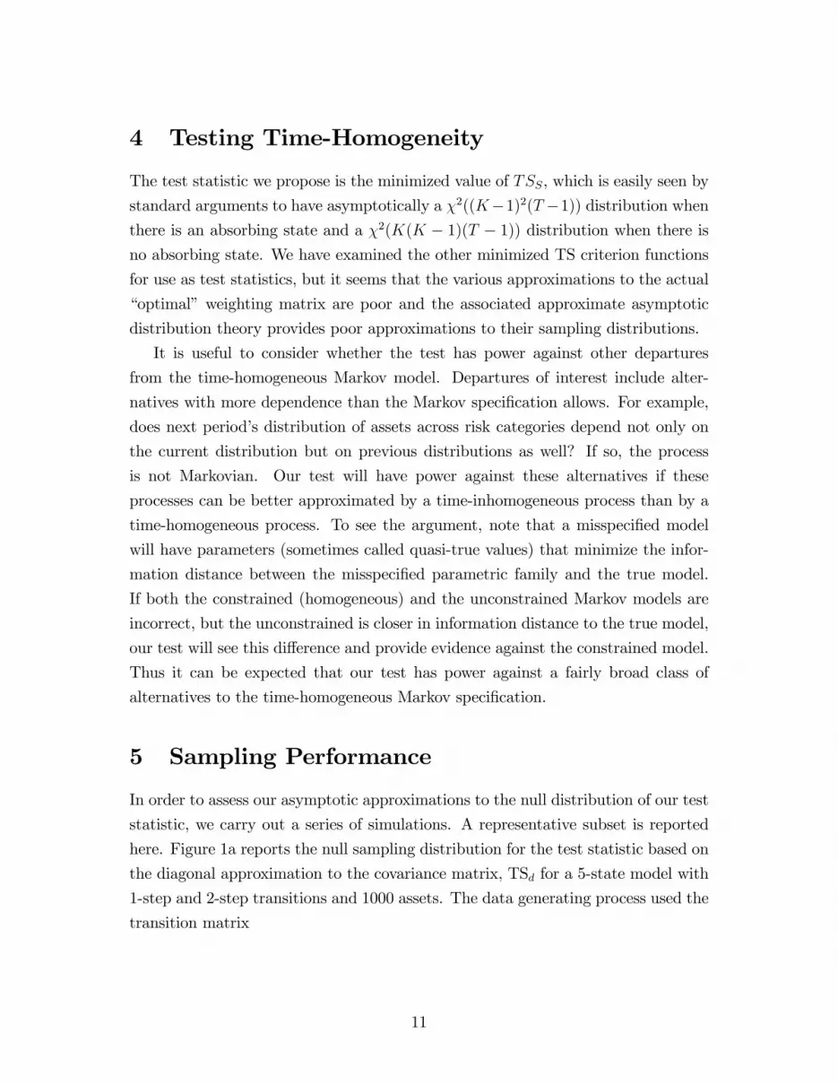
here. Figure 1a reports the null sampling distribution for the test statistic based on
the diagonal approximation to the covariance matrix, TSd for a 5-state model with
1-step and 2-step transitions and 1000 assets. The data generating process used the
transition matrix
11
0BBBBBB@0:4 0:2 0:2 0:1 0:1
0:2 0:4 0:2 0:1 0:1
0:1 0:2 0:4 0:2 0:1
0:1 0:1 0:2 0:4 0:2
0 0 0 0 1
1CCCCCCAThe sampling distributions were calculated on the basis of 2000 realizations (a
realization is a transition history) throughout. The cdf of the test statistic is sub-
stantially to the right of the chi-square(16) distribution, perhaps indicating that the
diagonal is a poor approximation to the covariance matrix of the auxiliary statis-
tic (we know it is not a correct speci�cation; now we know it is not a satisfactory
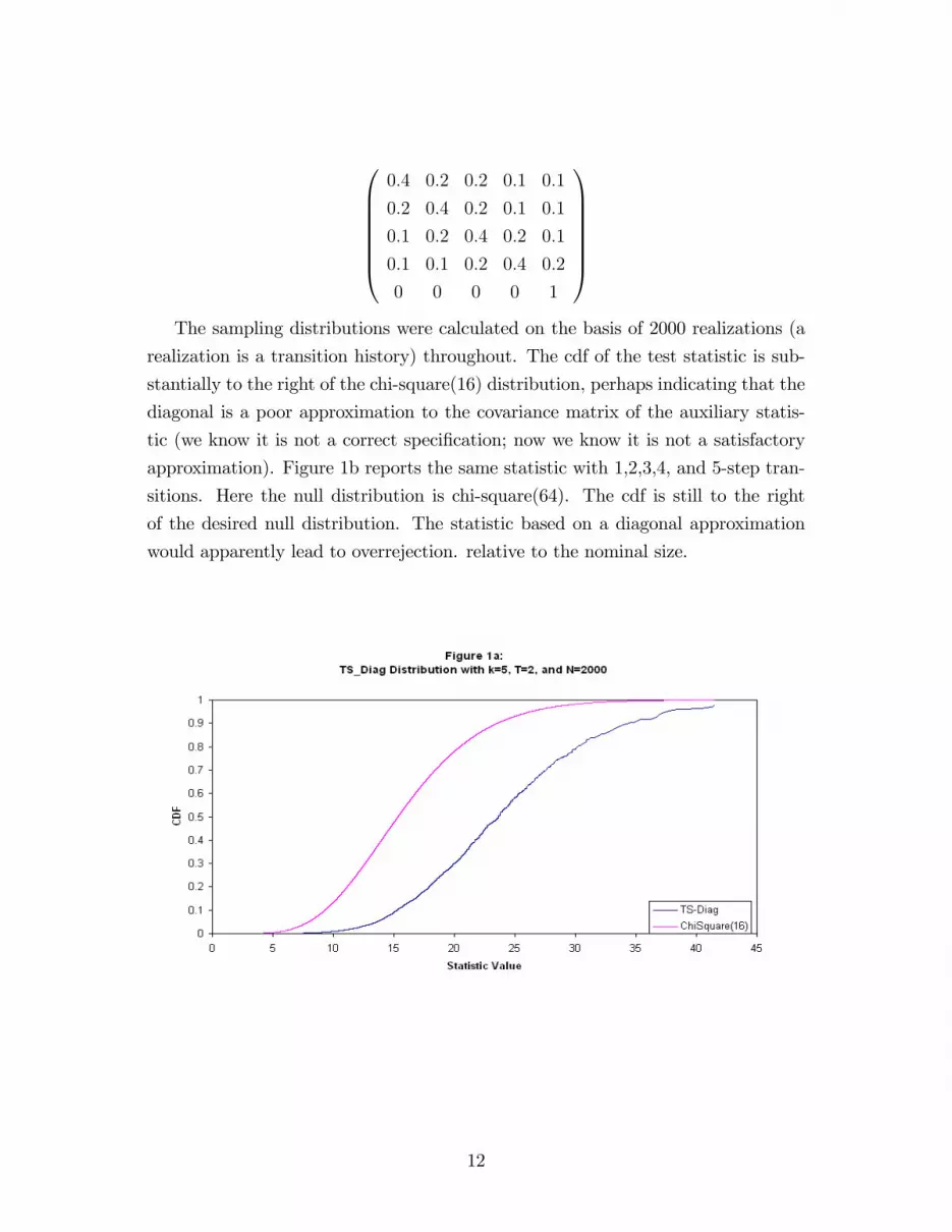
approximation). Figure 1b reports the same statistic with 1,2,3,4, and 5-step tran-
sitions. Here the null distribution is chi-square(64). The cdf is still to the right
of the desired null distribution. The statistic based on a diagonal approximation
would apparently lead to overrejection. relative to the nominal size.
12
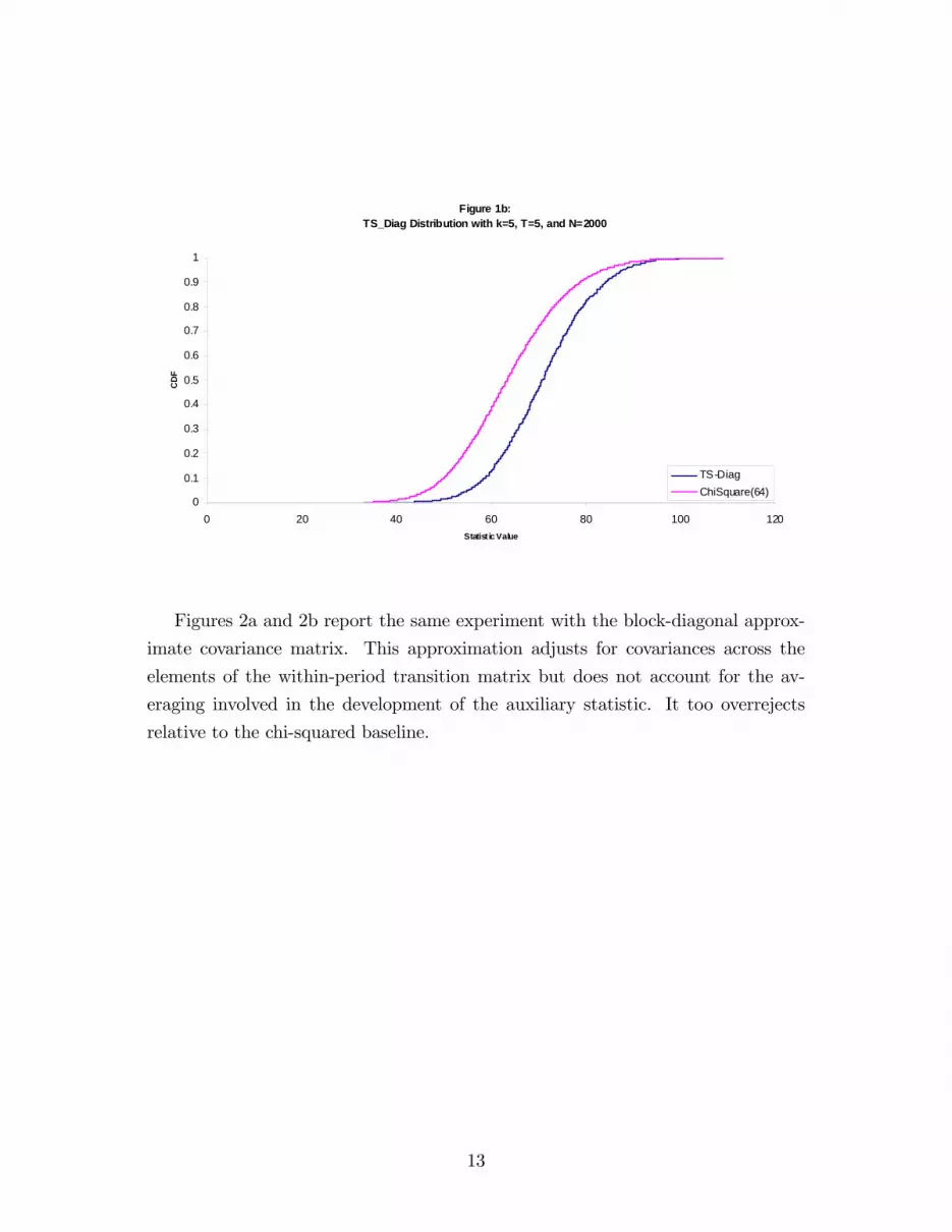
Figure 1b:TS_Diag Distribution with k=5, T=5, and N=2000
0
0.1
0.2
0.3
0.4
0.5
0.6
0.7
0.8
0.9
1
0 20 40 60 80 100 120Statist ic Value
CD
F
TSDiagChiSquare(64)
Figures 2a and 2b report the same experiment with the block-diagonal approx-
imate covariance matrix. This approximation adjusts for covariances across the
elements of the within-period transition matrix but does not account for the av-
eraging involved in the development of the auxiliary statistic. It too overrejects
relative to the chi-squared baseline.
13
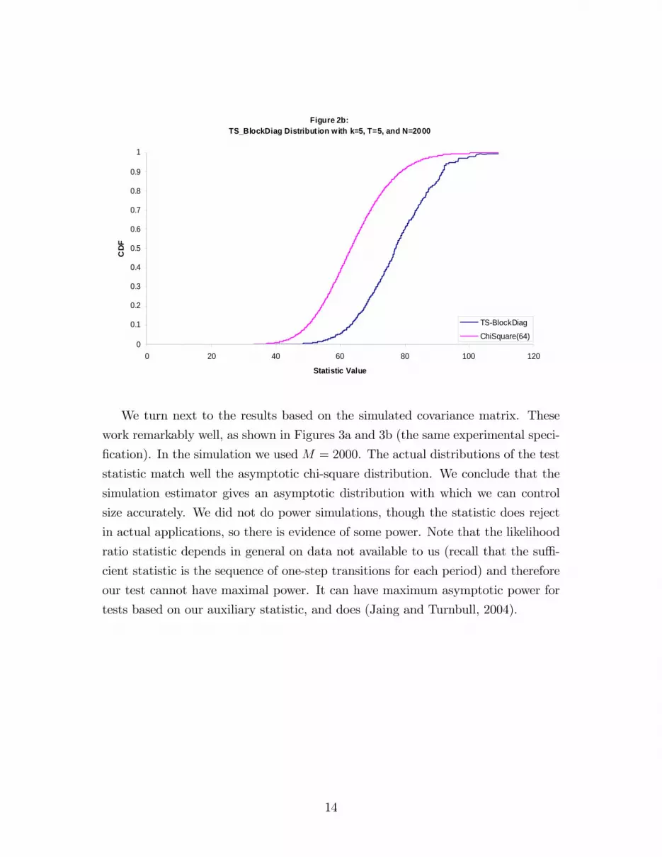
Figure 2b:TS_BlockDiag Distribut ion with k=5, T=5, and N=2000
0
0.1
0.2
0.3
0.4
0.5
0.6
0.7
0.8
0.9
1
0 20 40 60 80 100 120
Statistic Value
CD
F
TSBlockDiag
ChiSquare(64)
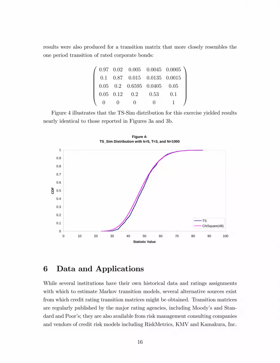
We turn next to the results based on the simulated covariance matrix. These
work remarkably well, as shown in Figures 3a and 3b (the same experimental speci-
�cation). In the simulation we used M = 2000. The actual distributions of the test
statistic match well the asymptotic chi-square distribution. We conclude that the
simulation estimator gives an asymptotic distribution with which we can control
size accurately. We did not do power simulations, though the statistic does reject
in actual applications, so there is evidence of some power. Note that the likelihood
ratio statistic depends in general on data not available to us (recall that the su¢ -
cient statistic is the sequence of one-step transitions for each period) and therefore
our test cannot have maximal power. It can have maximum asymptotic power for
tests based on our auxiliary statistic, and does (Jaing and Turnbull, 2004).
14
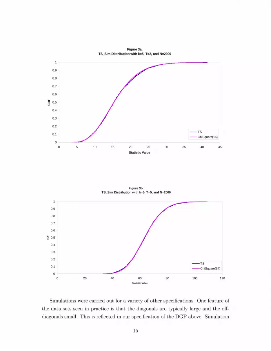
Figure 3a:TS_Sim Distribution with k=5, T=2, and N=2000
0
0.1
0.2
0.3
0.4
0.5
0.6
0.7
0.8
0.9
1
0 5 10 15 20 25 30 35 40 45
Statistic Value
CD
F
TSChiSquare(16)
Figure 3b:TS_Sim Distribution with k=5, T=5, and N=2000
0
0.1
0.2
0.3
0.4
0.5
0.6
0.7
0.8
0.9
1
0 20 40 60 80 100 120Statistic Value
CD
F
TSChiSquare(64)
Simulations were carried out for a variety of other speci�cations. One feature of
the data sets seen in practice is that the diagonals are typically large and the o¤-
diagonals small. This is re�ected in our speci�cation of the DGP above. Simulation
15
results were also produced for a transition matrix that more closely resembles the
one period transition of rated corporate bonds:0BBBBBB@0:97 0:02 0:005 0:0045 0:0005
0:1 0:87 0:015 0:0135 0:0015
0:05 0:2 0:6595 0:0405 0:05
0:05 0:12 0:2 0:53 0:1
0 0 0 0 1
1CCCCCCAFigure 4 illustrates that the TS-Sim distribution for this exercise yielded results
nearly identical to those reported in Figures 3a and 3b.
Figure 4:TS_Sim Distribution with k=5, T=3, and N=1000
0
0.1
0.2
0.3
0.4
0.5
0.6
0.7
0.8
0.9
1
0 10 20 30 40 50 60 70 80 90 100
Statistic Value
CD
F
TSChiSquare(48)
6 Data and Applications
While several institutions have their own historical data and ratings assignments
with which to estimate Markov transition models, several alternative sources exist
from which credit rating transition matrices might be obtained. Transition matrices
are regularly published by the major rating agencies, including Moody�s and Stan-
dard and Poor�s; they are also available from risk management consulting companies
and vendors of credit risk models including RiskMetrics, KMV and Kamakura, Inc.
16

Unfortunately, reporting standards in this area are fairly lax. Often, transition frac-
tions are reported with no indication of the size of the underlying data set, or the
initial distribution of assets across risk categories. Since many of these transitions
are low-probability events, large samples are necessary for precise estimation. This
information should be routinely provided as a matter of sound statistical practice.
We have assembled several data sets with which to illustrate our technique and
demonstrate its usefulness.
6.1 Commercial Paper
These data are from a study by Moody�s (2000). This study is also commendable in
the detail provided. Commercial paper defaults are extremely rare, although there
is some migration among rating categories (here P-1, P-2, P-3 and NP; P is for
prime). Moody�s goal is that commercial paper with any prime rating should never
default. Since commercial paper, in contrast to the municipals studied above, are
short term assets, the transitions examined are 30-day transitions. The Moody�s
study reports transitions over 30, 60, 90, 120, 180, 270 and 365 days. Note that
the �missing�powers of P at 150, 210, 240, 300, and 330 days present no problem
for our methods. The data up to the 180 day transitions exhibit expected patterns,
for example the transitions into default (and generally transitions out of the initial
state) are increasing with the length of the time span. However, for 270 and 365
days, the transitions from NP into default are zero. This appears problematic and
is perhaps due to de�nitions Moody�s has used and the fact that commercial paper
is rarely extended for long periods. We have chosen simply not to use the data for
270 and 365 days. Another question arises as to the treatment of Moody�s category
WR �withdrawn. These occur because commercial paper is not rolled over so
the asset size becomes negligible, or the market has otherwise lost interest in the
o¤ering. It is apparently not a synonym for default or a decline in creditworthiness.
Consequently, we treat these as censored. Again, to illustrate the use of the test,
we calculate the statistic based on increasing numbers of periods. Results are given
in Table 1.
17

Table 1: Tests for Commercial Paper, 1972-1999
Transitions Chi-Square DF P-value
1,2 1.44 16 1.0000
1,2,3 11.38 32 0.997
1,2,3,4 41.56 48 0.7346
1,2,3,4,6 74.55 64 0.1727
There is no serious evidence against the Markov speci�cation. Recall that the
time scale here is 30 days; commercial paper is generally short lived. The Markov
model �works� over the period available (6 months). This is probably also the
relevant period for applications. Note that the sample size here is enormous, so these
results are pretty �rm and it may be considered surprising that the tightly speci�ed
model is not soundly rejected for all transitions. The numbers of observations for
the 1-step transition matrix, for the nondefault states, for example, are 264000,
561000, 6600, and 3300.
It is useful to look closely at the �t. We focus on the 4-step model. Table 2
shows the estimated (constrained) 4-step transition matrix (the fourth power of the
1-step matrix estimated on the basis of all of the transitions), the empirical 4-step
matrix, and their di¤erence.
18
Table 2: Commercial Paper 4-Step Rating Transition Matrices
Estimated
0.98791 0.01161 0.00019 0.00029 0.00001
0.02172 0.95808 0.01601 0.00393 0.00026
0.00591 0.05768 0.88110 0.05440 0.00091
0.00273 0.01117 0.02034 0.96231 0.00345
0 0 0 0 1
Empirical
0.98785 0.01164 0.00020 0.00031 0.00000
0.02206 0.95814 0.01557 0.00402 0.00021
0.00618 0.05976 0.88261 0.05033 0.00112
0.00207 0.00977 0.02208 0.96240 0.00368
0 0 0 0 1
Empirical-Estimated
-0.000056 0.000025 0.000016 0.000019 -0.000005
0.000339 0.000061 -0.000441 0.000096 -0.000054
0.000270 0.002079 0.001514 -0.004076 0.000213
-0.000664 -0.001395 0.001735 0.000094 0.00230
0 0 0 0 0Note: The numbers of assets for computing the 4-step transition matrix are
(6560, 1394, 164, 82). Di¤erences greater than 0.001 in absolute value are
italicized .
Transitions are fairly rare: the minimum diagonal element is approximately
0.88 (constrained and unconstrained). There are a number of suggested summary
measures for the amount of mobility in a transition matrix. These are discussed in
Jafry and Schuermann (2004), who suggest
M = K�1KXi=1
p�i((P � I)(P � I)T ) (13)
where P is the transition matrix in question and �i(A) are the eigenvalues of A.
For motivation see Jafry and Schuermann (2004); note that M=0 for the identity
transition matrix and 1 for (strict) permutations. Note also that M and related
mobility measures do not de�ne metrics on the space of transition matrices. In this
CP application,M =0.0449 for the estimated (constrained) 4-step transition matrix
19
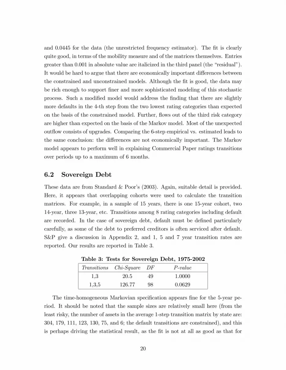
and 0.0445 for the data (the unrestricted frequency estimator). The �t is clearly
quite good, in terms of the mobility measure and of the matrices themselves. Entries
greater than 0.001 in absolute value are italicized in the third panel (the �residual�).
It would be hard to argue that there are economically important di¤erences between
the constrained and unconstrained models. Although the �t is good, the data may
be rich enough to support �ner and more sophisticated modeling of this stochastic
process. Such a modi�ed model would address the �nding that there are slightly
more defaults in the 4-th step from the two lowest rating categories than expected
on the basis of the constrained model. Further, �ows out of the third risk category
are higher than expected on the basis of the Markov model. Most of the unexpected
out�ow consists of upgrades. Comparing the 6-step empirical vs. estimated leads to
the same conclusion: the di¤erences are not economically important. The Markov
model appears to perform well in explaining Commercial Paper ratings transitions
over periods up to a maximum of 6 months.
6.2 Sovereign Debt
These data are from Standard & Poor�s (2003). Again, suitable detail is provided.
Here, it appears that overlapping cohorts were used to calculate the transition
matrices. For example, in a sample of 15 years, there is one 15-year cohort, two
14-year, three 13-year, etc. Transitions among 8 rating categories including default
are recorded. In the case of sovereign debt, default must be de�ned particularly
carefully, as some of the debt to preferred creditors is often serviced after default.
S&P give a discussion in Appendix 2, and 1, 5 and 7 year transition rates are
reported. Our results are reported in Table 3.
Table 3: Tests for Sovereign Debt, 1975-2002
Transitions Chi-Square DF P-value
1,3 20.5 49 1.0000
1,3,5 126.77 98 0.0629
The time-homogeneous Markovian speci�cation appears �ne for the 5-year pe-
riod. It should be noted that the sample sizes are relatively small here (from the
least risky, the number of assets in the average 1-step transition matrix by state are:
304, 179, 111, 123, 130, 75, and 6; the default transitions are constrained), and this
is perhaps driving the statistical result, as the �t is not at all as good as that for
20
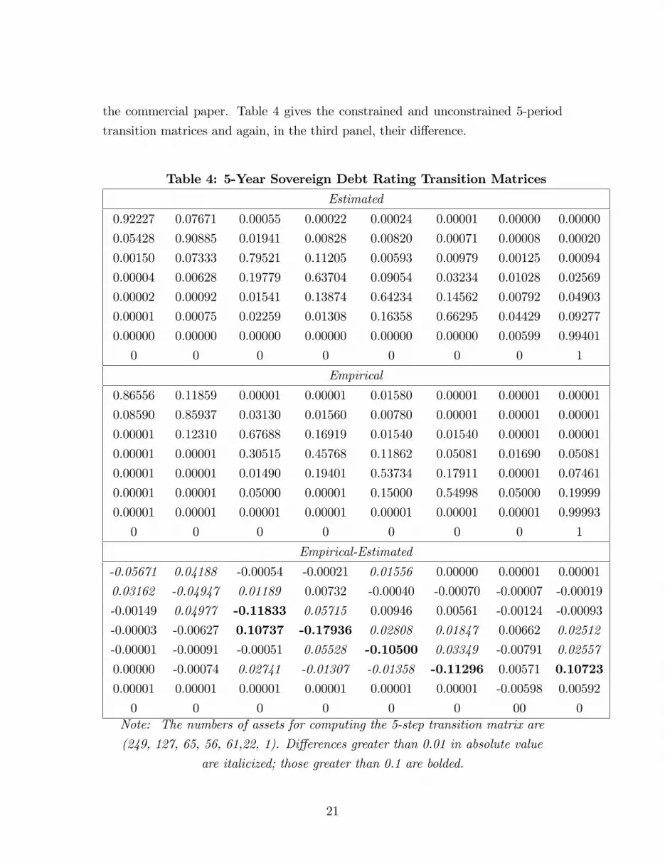
the commercial paper. Table 4 gives the constrained and unconstrained 5-period
transition matrices and again, in the third panel, their di¤erence.
Table 4: 5-Year Sovereign Debt Rating Transition Matrices
Estimated
0.92227 0.07671 0.00055 0.00022 0.00024 0.00001 0.00000 0.00000
0.05428 0.90885 0.01941 0.00828 0.00820 0.00071 0.00008 0.00020
0.00150 0.07333 0.79521 0.11205 0.00593 0.00979 0.00125 0.00094
0.00004 0.00628 0.19779 0.63704 0.09054 0.03234 0.01028 0.02569
0.00002 0.00092 0.01541 0.13874 0.64234 0.14562 0.00792 0.04903
0.00001 0.00075 0.02259 0.01308 0.16358 0.66295 0.04429 0.09277
0.00000 0.00000 0.00000 0.00000 0.00000 0.00000 0.00599 0.99401
0 0 0 0 0 0 0 1
Empirical
0.86556 0.11859 0.00001 0.00001 0.01580 0.00001 0.00001 0.00001
0.08590 0.85937 0.03130 0.01560 0.00780 0.00001 0.00001 0.00001
0.00001 0.12310 0.67688 0.16919 0.01540 0.01540 0.00001 0.00001
0.00001 0.00001 0.30515 0.45768 0.11862 0.05081 0.01690 0.05081
0.00001 0.00001 0.01490 0.19401 0.53734 0.17911 0.00001 0.07461
0.00001 0.00001 0.05000 0.00001 0.15000 0.54998 0.05000 0.19999
0.00001 0.00001 0.00001 0.00001 0.00001 0.00001 0.00001 0.99993
0 0 0 0 0 0 0 1
Empirical-Estimated
-0.05671 0.04188 -0.00054 -0.00021 0.01556 0.00000 0.00001 0.00001
0.03162 -0.04947 0.01189 0.00732 -0.00040 -0.00070 -0.00007 -0.00019
-0.00149 0.04977 -0.11833 0.05715 0.00946 0.00561 -0.00124 -0.00093
-0.00003 -0.00627 0.10737 -0.17936 0.02808 0.01847 0.00662 0.02512
-0.00001 -0.00091 -0.00051 0.05528 -0.10500 0.03349 -0.00791 0.02557
0.00000 -0.00074 0.02741 -0.01307 -0.01358 -0.11296 0.00571 0.107230.00001 0.00001 0.00001 0.00001 0.00001 0.00001 -0.00598 0.00592
0 0 0 0 0 0 00 0Note: The numbers of assets for computing the 5-step transition matrix are
(249, 127, 65, 56, 61,22, 1). Di¤erences greater than 0.01 in absolute value
are italicized; those greater than 0.1 are bolded.
21
Here, di¤erences between the constrained and unconstrained transition proba-
bilities (5-year) greater than .01 are italicized and di¤erences greater than 0.1 are
also in bold. The �t is obviously much worse than the �t for commercial paper
(hence the di¤erence in the highlighting threshold). That these di¤erences are not
statistically signi�cant is no doubt due to the small sample sizes. The mobility
measures M=0.3617 (constrained) and 0.4464 (unconstrained) are quite di¤erent
in magnitude. The di¤erences indicate that sovereign debt needs to be monitored
carefully and probably on a case-to-case basis. The Markov model does not do a
great job of capturing these transitions. Nevertheless, it is doubtful that a more
complicated model would be supported by the data.
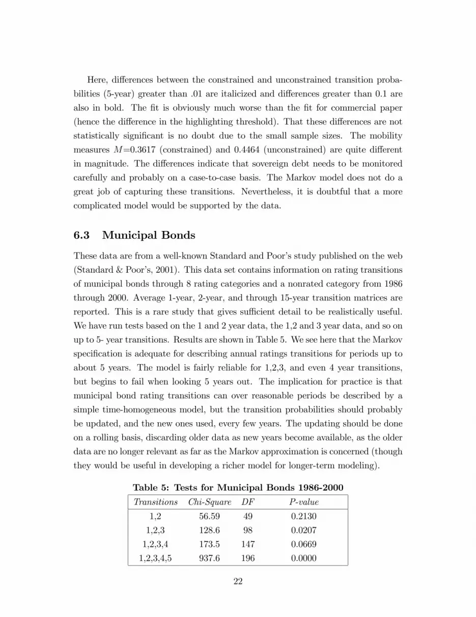
6.3 Municipal Bonds
These data are from a well-known Standard and Poor�s study published on the web
(Standard & Poor�s, 2001). This data set contains information on rating transitions
of municipal bonds through 8 rating categories and a nonrated category from 1986
through 2000. Average 1-year, 2-year, and through 15-year transition matrices are
reported. This is a rare study that gives su¢ cient detail to be realistically useful.
We have run tests based on the 1 and 2 year data, the 1,2 and 3 year data, and so on
up to 5- year transitions. Results are shown in Table 5. We see here that the Markov
speci�cation is adequate for describing annual ratings transitions for periods up to
about 5 years. The model is fairly reliable for 1,2,3, and even 4 year transitions,
but begins to fail when looking 5 years out. The implication for practice is that
municipal bond rating transitions can over reasonable periods be described by a
simple time-homogeneous model, but the transition probabilities should probably
be updated, and the new ones used, every few years. The updating should be done
on a rolling basis, discarding older data as new years become available, as the older
data are no longer relevant as far as the Markov approximation is concerned (though
they would be useful in developing a richer model for longer-term modeling).
Table 5: Tests for Municipal Bonds 1986-2000
Transitions Chi-Square DF P-value
1,2 56.59 49 0.2130
1,2,3 128.6 98 0.0207
1,2,3,4 173.5 147 0.0669
1,2,3,4,5 937.6 196 0.0000
22
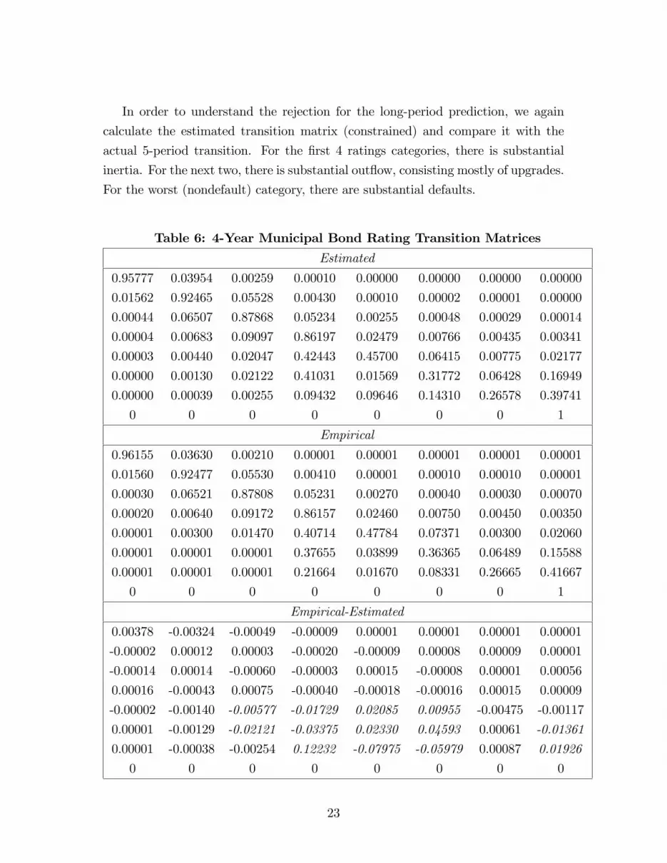
In order to understand the rejection for the long-period prediction, we again
calculate the estimated transition matrix (constrained) and compare it with the
actual 5-period transition. For the �rst 4 ratings categories, there is substantial
inertia. For the next two, there is substantial out�ow, consisting mostly of upgrades.
For the worst (nondefault) category, there are substantial defaults.
Table 6: 4-Year Municipal Bond Rating Transition Matrices
Estimated
0.95777 0.03954 0.00259 0.00010 0.00000 0.00000 0.00000 0.00000
0.01562 0.92465 0.05528 0.00430 0.00010 0.00002 0.00001 0.00000
0.00044 0.06507 0.87868 0.05234 0.00255 0.00048 0.00029 0.00014
0.00004 0.00683 0.09097 0.86197 0.02479 0.00766 0.00435 0.00341
0.00003 0.00440 0.02047 0.42443 0.45700 0.06415 0.00775 0.02177
0.00000 0.00130 0.02122 0.41031 0.01569 0.31772 0.06428 0.16949
0.00000 0.00039 0.00255 0.09432 0.09646 0.14310 0.26578 0.39741
0 0 0 0 0 0 0 1
Empirical
0.96155 0.03630 0.00210 0.00001 0.00001 0.00001 0.00001 0.00001
0.01560 0.92477 0.05530 0.00410 0.00001 0.00010 0.00010 0.00001
0.00030 0.06521 0.87808 0.05231 0.00270 0.00040 0.00030 0.00070
0.00020 0.00640 0.09172 0.86157 0.02460 0.00750 0.00450 0.00350
0.00001 0.00300 0.01470 0.40714 0.47784 0.07371 0.00300 0.02060
0.00001 0.00001 0.00001 0.37655 0.03899 0.36365 0.06489 0.15588
0.00001 0.00001 0.00001 0.21664 0.01670 0.08331 0.26665 0.41667
0 0 0 0 0 0 0 1
Empirical-Estimated
0.00378 -0.00324 -0.00049 -0.00009 0.00001 0.00001 0.00001 0.00001
-0.00002 0.00012 0.00003 -0.00020 -0.00009 0.00008 0.00009 0.00001
-0.00014 0.00014 -0.00060 -0.00003 0.00015 -0.00008 0.00001 0.00056
0.00016 -0.00043 0.00075 -0.00040 -0.00018 -0.00016 0.00015 0.00009
-0.00002 -0.00140 -0.00577 -0.01729 0.02085 0.00955 -0.00475 -0.00117
0.00001 -0.00129 -0.02121 -0.03375 0.02330 0.04593 0.00061 -0.01361
0.00001 -0.00038 -0.00254 0.12232 -0.07975 -0.05979 0.00087 0.01926
0 0 0 0 0 0 0 0
23

Note: The sample sizes for the one-step average transition matrices are, by state
from the least risky, (781, 19650, 45771, 20060, 730, 203, 98)
Defaults are zero throughout. The numbers of assets for computing the 4-step
transition matrix are (558, 14450, 35715, 15481, 612, 174, 79).
In the third panel, di¤erences greater than .005 in absolute value between
the empirical and predicted are italicized.
Out�ows from the rating categories 4,6, and 7 are underpredicted. Defaults
from the 6th category are overpredicted and from the 7th underpredicted. Here,
the mobility measures M=0.3373 (constrained) and 0.3282 (unconstrained) are not
substantially di¤erent, illustrating the importance of the comment thatM , while a
useful measure of mobility, is not a distance metric. Thus, �munis�are well-modeled
by the time homogeneous Markov model only for a few (perhaps 4) years.
6.4 S&P Corporates
Data for this example consists of S&P-rated �rms in the KMVNorth American Non-
Financial Dataset , which for practical purposes mirrors the Compustat dataset.
In order to deal with the sparseness of the transition matrix based upon individual
S&P rating categories we used the following correspondence to map S&P ratings to
a custom rating scale.
Table 7: Mapping of S&P Corporate Ratings
S&P Ratings Bucket
AAA,AA+,AA,AA- 1
A+,A,A- 2
BBB+,BBB 3
BBB-,BB+ 4
BB,BB- 5
B+,B,B- 6
CCC+,CCC,CCC-,CC,C 7
D 8
Note that while many possible aggregations exist, seven non-default buckets is
required under the advanced internal ratings based approach of the Basel II capital
accord. Our chosen mapping results in a more uniform distribution of assets across
the rating buckets than would, say, a mapping based upon whole grades (AAA, AA,
24
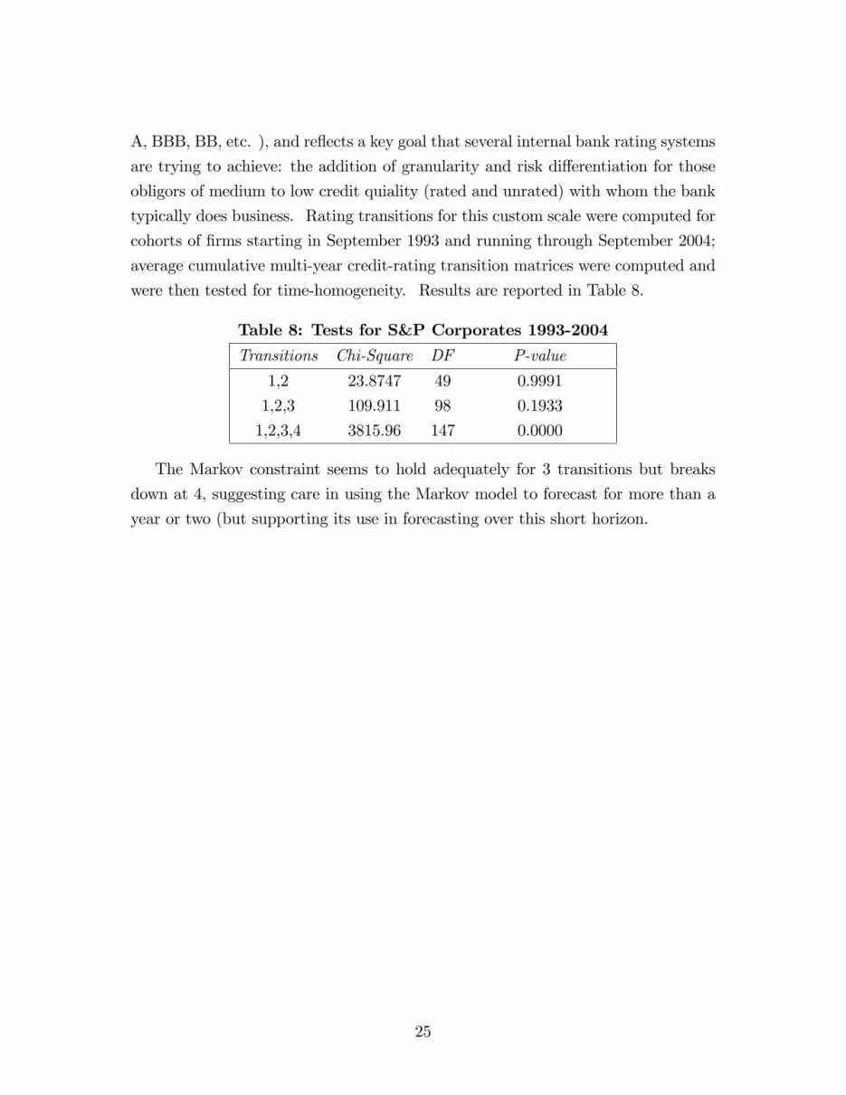
A, BBB, BB, etc. ), and re�ects a key goal that several internal bank rating systems
are trying to achieve: the addition of granularity and risk di¤erentiation for those
obligors of medium to low credit quiality (rated and unrated) with whom the bank
typically does business. Rating transitions for this custom scale were computed for
cohorts of �rms starting in September 1993 and running through September 2004;
average cumulative multi-year credit-rating transition matrices were computed and
were then tested for time-homogeneity. Results are reported in Table 8.
Table 8: Tests for S&P Corporates 1993-2004
Transitions Chi-Square DF P-value
1,2 23.8747 49 0.9991
1,2,3 109.911 98 0.1933
1,2,3,4 3815.96 147 0.0000
The Markov constraint seems to hold adequately for 3 transitions but breaks
down at 4, suggesting care in using the Markov model to forecast for more than a
year or two (but supporting its use in forecasting over this short horizon.
25
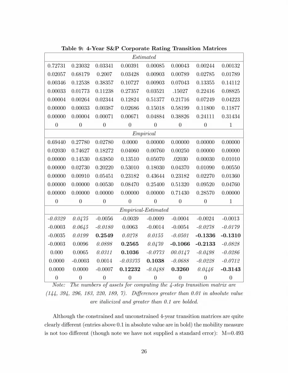
Table 9: 4-Year S&P Corporate Rating Transition Matrices
Estimated
0.72731 0.23032 0.03341 0.00391 0.00085 0.00043 0.00244 0.00132
0.02057 0.68179 0.2007 0.03428 0.00903 0.00789 0.02785 0.01789
0.00346 0.12538 0.38357 0.10727 0.00903 0.07043 0.13355 0.14112
0.00033 0.01773 0.11238 0.27357 0.03521 .15027 0.22416 0.08825
0.00004 0.00264 0.02344 0.12824 0.51377 0.21716 0.07249 0.04223
0.00000 0.00033 0.00387 0.02686 0.15018 0.58199 0.11800 0.11877
0.00000 0.00004 0.00071 0.00671 0.04884 0.38826 0.24111 0.31434
0 0 0 0 0 0 0 1
Empirical
0.69440 0.27780 0.02780 0.0000 0.00000 0.00000 0.00000 0.00000
0.02030 0.74627 0.18272 0.04060 0.00760 0.00250 0.00000 0.00000
0.00000 0.14530 0.63850 0.13510 0.05070 .02030 0.00030 0.01010
0.00000 0.02730 0.20220 0.53010 0.18030 0.04370 0.01090 0.00550
0.00000 0.00910 0.05451 0.23182 0.43644 0.23182 0.02270 0.01360
0.00000 0.00000 0.00530 0.08470 0.25400 0.51320 0.09520 0.04760
0.00000 0.00000 0.00000 0.00000 0.00000 0.71430 0.28570 0.00000
0 0 0 0 0 0 0 1
Empirical-Estimated
-0.0329 0.0475 -0.0056 -0.0039 -0.0009 -0.0004 -0.0024 -0.0013
-0.0003 0.0645 -0.0180 0.0063 -0.0014 -0.0054 -0.0278 -0.0179
-0.0035 0.0199 0.2549 0.0278 0.0155 -0.0501 -0.1336 -0.1310-0.0003 0.0096 0.0898 0.2565 0.0470 -0.1066 -0.2133 -0.0828
0.000 0.0065 0.0311 0.1036 -0.0773 00.0147 -0.0498 -0.0286
0.0000 -0.0003 0.0014 -0.03375 0.1038 -0.0688 -0.0228 -0.0712
0.0000 0.0000 -0.0007 0.12232 -0.0488 0.3260 0.0446 -0.31430 0 0 0 0 0 0 0Note: The numbers of assets for computing the 4-step transition matrix are
(144, 394, 296, 183, 220, 189, 7). Di¤erences greater than 0.01 in absolute value
are italicized and greater than 0.1 are bolded.
Although the constrained and unconstrained 4-year transition matrices are quite
clearly di¤erent (entries above 0.1 in absolute value are in bold) the mobility measure
is not too di¤erent (though note we have not supplied a standard error): M=0.493
26
constrained, 0.426 unconstrained. This is consistent with the �nding of Jafry and
Schuermann (2004) that the time homogeneity assumption within a year did not
dramatically a¤ect the inference on the mobility measure; we �nd that the cross-
year time homogeneity assumption also does not a¤ect the mobility measure. Our
�nding that time-homogeneity fails over the longer period is also consistent with
their results that there is a drift in mobility over time. Our analysis here serves
primarily the purpose of demonstrating the feasibility of our techniques. Further
analysis of this data set will focus on patterns across industries as well as over time.
7 Conclusion
The time-homogeneous Markov model for transitions among risk categories is widely
used in areas from portfolio management to bank supervision and risk management.
It is well known that these models can be overly simple as descriptions of the
stochastic processes for riskiness of assets. Nevertheless, the model�s simplicity
is extremely appealing. We propose a likelihood ratio test for the hypothesis of
time-homogeneity. Due to a convenient reparametrization, the test is simple to
compute, requiring numerical estimation of only the restricted model, a (K-1)/2-
parameter problem where K is the number of risk categories. The test can be based
on summary data often reported by rating agencies or collected within banks. We
recommend that the test be interpreted as determining whether or not transitions
over particular periods can be adequately modeled as Markov chains. Speci�cally,
we do not recommend interpreting the test as showing that the true underlying
process is or is not Markovian. Not only does this interpretation confuse failing
to reject with evidence in favor, it does not address the interesting issue. The
transitions cannot truly be Markovian in the long run �the prediction would be
that everything defaults. However, in some cases transitions can be usefully modeled
as Markovian over periods of useful length.
8 References
Anderson, T.W. and L. A. Goodman, (1957) �Statistical Inference About Markov
Chains,�Ann. Math. Statist., 28 , 89-110.
27
Bangia, A., F. Diebold, A. Kronimus, C. Schagen, and T. Schuermann (2002)
"Ratings migration and the business cycle, with applications to credit portfolio
stress testing" Journal of Banking and Finance, 26(2-3) pp. 445-474.
Basel Committee on Banking Supervision (2004) "International Convergence of
Capital Measurement and Capital Standards: A Revised Framework." Bank for
International Settlements, June.
Billingsley, P. (1961) �Statistical Methods in Markov Chains,� Ann. Math.
Statist., 32, 12-40
Carty, Lea V. and Jerome S. Fons (1993) "Measuring Changes in Corporate
Credit Quality," Moody�s Special Report, November 1993, New York: Moody�s
Investors Service.
Chat�eld, C. (1973) �Statistical Inference Regarding Markov Chain Models,�
Applied Statistics 22:1, 7-20
Gallant, A. R. and G. Tauchen (1996), �Which Moments to Match?�Econo-
metric Theory 12, 657-681.
Gourieroux, C. , A. Monfort and E. Renault (1993) �Indirect Inference,� J.
Applied Econometrics 8S, 85-103.
Jafry, Y., and T. Schuermann (2004),"Measurement, Estimation and Compar-
ison of Credit Migration Matrices," Journal of Banking and Finance 28,2603-2639.
Jiang, W and B. Turnbull (2004) �The Indirect Method: Inference Based on
Intermediate Statistics-A Synthesis and Examples,� Statistical Science 19:2, 239-
263
Karlin, S. and Taylor, H. M. (1975) A First Course in Stochastic Processes.
Second edition. Academic Press, New York
Lando, D. and T. Skodeberg (2002), "Analyzing Ratings Transitions and Ratings
Drift With Continuous Observations," Journal of Banking and Finance 26, 423-444.
Berthault, D. Hamilton, and L. Carty "Commercial Paper Defaults and Rating
Transitions, 1972-2000" (2000). Global Credit Research, Special Comment, October
2000, New York: Moody�s Investors Service.
Standard & Poor�s (2003) �2002 Defaults and Rating Transition Data Update
for Rated Sovereigns.�
Thomas, L. C., D. B. Edelman and J. N. Crook (2002) Credit Scoring and its
Applications, SIAM, Philadelphia.
28


