A Simulation Environment for Directional Sensing as a Phase Separation Process

www.stke.org/cgi/content/full/2007/378/pl1 Page 1

A Simulation Environment for Directional Sensingas a Phase Separation Process

Antonio de Candia,1 Andrea Gamba,2* Fausto Cavalli,3 Antonio Coniglio,1

Stefano Di Talia,4 Federico Bussolino,5 Guido Serini5*

(Published 20 March 2007)

P R O T O C O L

1Department of Physical Sciences, Università di Napoli “Federico II,” Istituto Nazionale di Fisica della Materia, and Istituto Nazionale di FisicaNucleare, Unità di Napoli, 80126 Napoli, Italy. 2Department of Mathematics, Politecnico di Torino, Corso Duca degli Abruzzi 24, 10129 Torino,and Istituto Nazionale di Fisica Nucleare, Unità di Torino, Via Giuria 1, 10125 Torino, Italy. 3Department of Mathematics, Università degli Studidi Milano, Via Saldini 50, 20133 Milano, Italy. 4Laboratory of Mathematical Physics, The Rockefeller University, 1230 York Avenue, New York, NY10021, USA. 5Department of Oncological Sciences and Division of Molecular Angiogenesis, IRCC, Institute for Cancer Research and Treat-ment, University of Torino School of Medicine, Strada Provinciale 142 Km 3.95, 10060 Candiolo (TO), Italy.

*Corresponding authors. E-mail: [email protected] (A.G.); [email protected] (G.S.)

INTRODUCTION

EQUIPMENT

INSTRUCTIONS

Installation for Windows

Installation for Linux

Insensitivity to Uniform Chemoattractant Stimulation

Symmetry Breaking Induced by Slightly Anisotropic Chemoattractant Stimulation

Defining Multiple Chemoattractant Sources

Formation of PIP3 Patches Upon Uniform Stimulationwith Low Chemoattractant Concentrations

TROUBLESHOOTING

NOTES AND REMARKS

REFERENCES

on March 21, 2007

stke.sciencemag.org

Dow

nloaded from

http://stke.sciencemag.org


Abstract

The ability of eukaryotic cells to navigate along spatial gradients of extracellular guidance cues is crucial for em-bryonic development, tissue regeneration, and cancer progression. One proposed model for chemotaxis is aphosphoinositide-based phase separation process, which takes place at the plasma membrane upon chemoat-tractant stimulation and triggers directional motility of eukaryotic cells. Here, we make available virtual-cell soft-ware that allows the execution and spatiotemporal analysis of in silico chemotaxis experiments, in which the usercan control physical and chemical parameters as well as the number and position of chemoattractant sources.

Introduction

Guided cell motility is crucial for the development of multicellular organisms (1), for example, during the assembly of the cardiovascu-lar (2), nervous (3), and musculoskeletal (4) systems. Moreover, in the adult organism, directed cell movement plays a major role inphysiological and pathological settings such as wound healing, angiogenesis, immune response, and cancer (5). Therefore, there is inter-est in dissecting the molecular dynamics by which gradients of chemoattractants stimulate directed cell motion—that is, chemotaxis.

In several cell types, a shallow chemoattractant gradient gives rise to an unamplified receptor activation gradient. The activated recep-tors in turn elicit the recruitment of phosphatidylinositol 3-kinase (PI3K) from the cytosol to the plasma membrane, where it greatlyamplifies chemotactic signaling by converting phosphatidylinositol 4,5-bisphosphate (PIP2) into phosphatidylinositol 3,4,5-trisphos-phate (PIP3) and giving rise to sharply segregated PIP2- and PIP3-rich phases (1). The phosphatase PTEN counterbalances the enzymat-ic activity of PI3K by dephosphorylating PIP3 into PIP2. Docking of cytosolic PTEN at the cell membrane depends on the short N-ter-minal PIP2-binding domain (PBD) and is required for its activity (6, 7). As a result, PI3K and PIP3 accumulate on the plasma membraneat the side facing the highest chemoattractant concentration, whereas PTEN and PIP2 display a complementary distribution (1). Such anearly symmetry-breaking event constitutes the first fundamental step of chemotaxis and is usually defined as directional sensing (8). Af-terward, a cell polarization phase follows, during which binding of pleckstrin homology (PH) domain–containing effector proteins toPIP3 triggers polarized cytoskeletal and adhesive dynamics that finally translate into directed cell motion (9). Hence, directional sensinglies upstream of cell polarization, from which it can be functionally decoupled by treating cells with actin polymerization inhibitors(10). Notably, chemoattractants stimulate the formation of self-organizing small PIP3 patches, which drive localized actin polymeriza-tion and cell protrusion (11–13).

A physical and computational modeling approach can prove useful in testing and unveiling the identity of minimal biochemical net-works whose dynamics can incorporate the blueprints for complex cellular functions, such as chemotaxis. Previous models (8, 14–16)based on a local activator and a global inhibitor did not satisfactorily reconcile several key aspects of directional sensing, such as insen-sitivity to absolute stimulation values, large amplification of shallow chemoattractant gradients, reversibility of phase separation, robust-ness with respect to parameter perturbations, the stochastic character of cell responses, and the use of realistic biochemical parametersand space-time scales.

However, all of these aspects follow naturally from the observation that the network of chemical reactions, which constitutes the back-bone of directional sensing, presents a physical instability toward spontaneous phase separation (17). In this framework, directionalsensing appears as the result of a nucleation process by which a spot rich in PIP2 and PTEN is created in a sea rich in PIP3 and PI3K.Slight anisotropies (i.e., variations in the concentrations in a particular direction) in the extracellular chemoattractant landscape driveand accelerate the process of spot formation, taking advantage of the underlying phase separation instability. This way, the reaction-diffusion dynamics taking place on the two-dimensional cell membrane works as a powerful amplifier of shallow gradients in the dis-tribution of the external chemical signal.

To allow easy experimentation of the phase separation paradigm and its comparison with other models of directional sensing (8, 14–16),we provide an easy-to-use simulation environment, called DirSens, where physical and chemical parameters can be set and the surfacedistribution of the relevant chemical factors can be observed in real time. The underlying kinetic code simulates the stochastic chemicalevolution on a spherical surface (representing the cell plasma membrane) coupled to an enzymatic reservoir (representing the cytosol).

Equipment

Personal computer equipped with the Windows or Linux operating system

Java plug-in, Java Runtime Environment (www.java.com/en/download/index.jsp)

DirSens simulation environment software (Windows: approximately 1.2 MB download, 6 MB uncompressed; Linux: approximately1.2 MB download, 5.3 MB uncompressed) (http://stke.sciencemag.org/cgi/content/full/sigtrans;2007/378/pl1/DC1)

P R O T O C O L

on March 21, 2007

stke.sciencemag.org

Dow

nloaded from



Instructions

These instructions include explicit commands or computer filenames. They are set off by quotation marks. Do not type the quotationmarks when typing the commands.

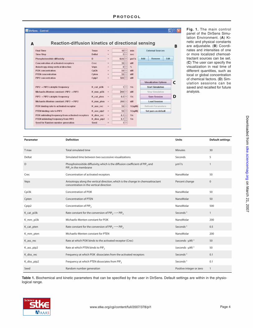
Various biochemical parameters and kinetic parameters can be set (Table 1). The physical and chemical parameters for the simu-lation are assigned using the input boxes, and the default settings may be changed by either typing a new value into the input boxor using the up and down arrow buttons (Fig. 1A). Most parameters are common biochemical or kinetic parameters, except theseed for random number generation (Seed), which is an integer number required to initialize the stochastic algorithm. A positiveinteger value for Seed gives rise to a random but exactly reproducible evolution of the system in time. All positive integer valuesof Seed are statistically equivalent. This means, for instance, that if biochemical and kinetic parameters are such as to producerandom polarization, all positive integer values of Seed will produce random polarization, but the actual direction of polarizationwill differ from one value of Seed to another. The user can change the value of Seed to check the robustness of the obtained re-sults—that is, the independence of the results on the particular sequence of random numbers produced by the algorithm. WhenSeed is set to zero, the system undergoes an unpredictable random evolution, which is different for each simulation session.

The distribution of activated receptors is described by two parameters: (i) a spatially uniform background concentration of recep-tors Crec, and (ii) a gradient with an amplitude controlled by the parameter Veps. The constant component Crec may be definedby the user at the beginning but cannot be modified during the course of the simulation. Instead, the percent anisotropy Veps canbe modified in real time. Alternatively, the two-component description controlled by Crec and Veps can be replaced with a user-defined activation landscape produced by localized external sources (Fig. 1B).

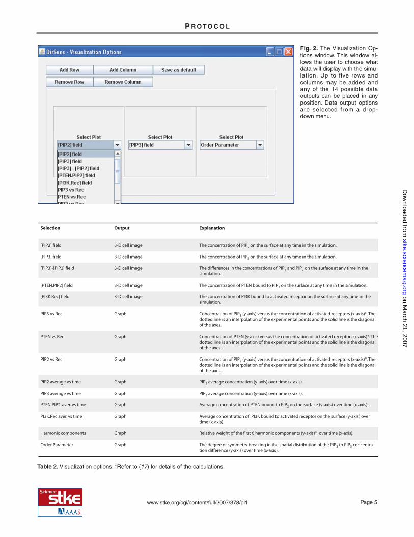
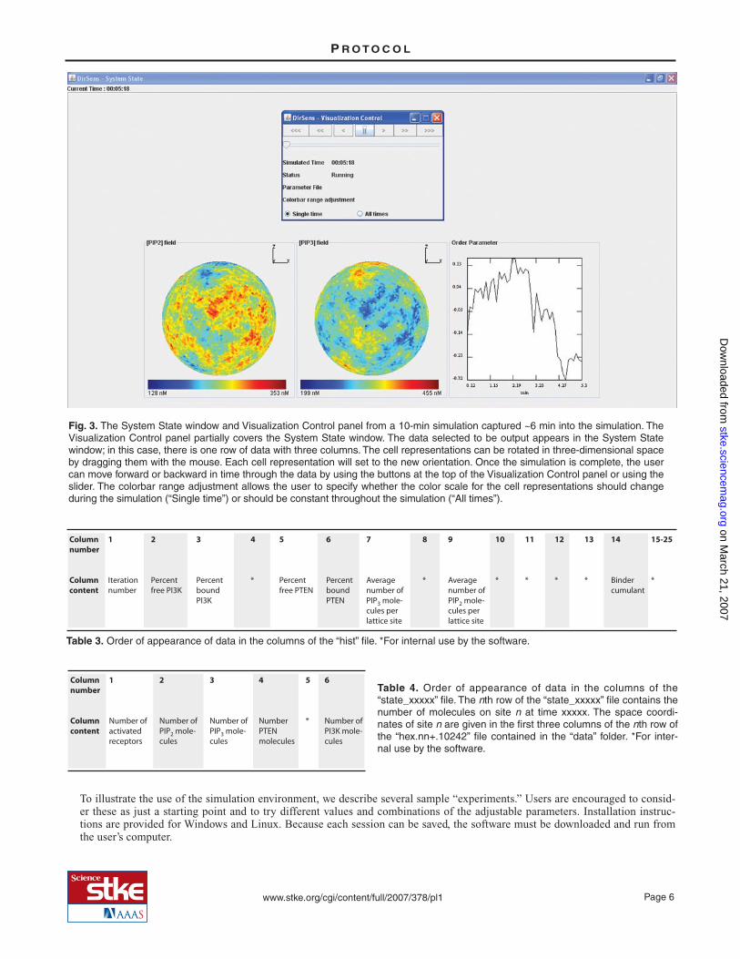
By default, the visualization output (graphs and images) includes the changes in PIP2 ([PIP2] field) and PIP3 ([PIP3] field) con-centrations, as well as the order parameter g, which indicates the degree of symmetry breaking in the spatial distribution of thePIP2-to-PIP3 concentration difference (17). The Visualization Options button (Fig. 1C) allows the user to select additional data tobe displayed. The options and their values are described in Table 2. The user can specify the order of the output in columns androws that will appear in the System State window by choosing to add (or remove) rows or columns (limit is 5 for both) from theVisualization Options window (Fig. 2). Rows are removed from the bottom and columns are removed from the right. To return tothe default visualization settings, the program must be closed and restarted. While the simulation is running and after it is com-plete, the data will appear in a window called System State (Fig. 3). A window called Visualization Control will allow the user topan through a completed simulation (Fig. 3, inset). The three-dimensional representations of the cell in the System State windowcan be rotated to view different sides of the cell by dragging them with the mouse.

Once the parameters are defined, the simulation is started by clicking the Start Simulation button and can be stopped before timeTmax by clicking the Stop Simulation button. The Visualization Control window shows the elapsed time of the simulation (Fig.3). After the simulation is complete, the buttons on the Visualization Control window can be used to pan the simulation forwardor backward in time. If the pause button (||) is clicked during the simulation, the simulation must be restarted from time zero us-ing the DirSens Control window. The < and > arrowheads step the simulation backward or forward incrementally, based on theuser-defined time step; the << and >> arrowheads replay the simulation backward or forward; and the <<< and >>> arrowheadsset the simulation at the end (Tmax) or the beginning. The slider allows the user to pan smoothly forward and backward in time.The color scale default is “Single time” for the cell representations, which allows the scale to change during the simulation toprovide optimized visualization of differences in the concentrations of the various elements at any given time. This can bechanged to a static color scale that represents the concentration ranges during the entire simulation (“All times”); however, thedifferences in concentrations at any given time will be more difficult to visualize using this setting.

Most physical and kinetic parameters can be modified in real time while a simulation is running by changing them in the inputboxes and clicking the Refresh Parameters button, thus allowing the user to test the effect of abrupt changes of the environmentalconditions. The input boxes for those parameters that cannot be modified in real time are disabled. The “Set pars as default” but-ton allows saving the present set of parameters to be saved in such a way that the software will use these settings automaticallythe next time the program is run.

Simulations can be saved as “sessions.” The files are saved into the folder called “session” in the “Dirsens_win” directory andare named by date and time; for example, a session saved on 8 January 2007 at 12:50 PM is named “sess_200701081250.” Filesmay be copied, but cannot be moved, or the software will not be able to retrieve a saved session.

The raw data obtained by the simulation are stored in the folder called “tmp” when the program is running and in the “session”folder when a session has been saved. They can be easily extracted and processed with standard programs for scientific visualiza-tion. The parameters used in the simulation are listed in the “pars” and “pars_xx” files. The rows of the “hist” file contain the av-erage concentrations of chemical factors at subsequent times. The rows of the “state_xxxxx” files contain concentrations ofchemical factors at time xxxxx in sequentially ordered sites of the lattice. The space coordinates of each lattice site are specifiedin the first three columns of the “hex.nn+10242” file contained in the “data” folder. Sites are listed in the same order in the“state_xxxxx” files and in the “hex.nn+10242” file. For a detailed description of the content of the “hist” and “state_xxxxx”files, see Tables 3 and 4.

P R O T O C O L

on March 21, 2007

stke.sciencemag.org

Dow

nloaded from



P R O T O C O L

Fig. 1. The main controlpanel of the DirSens Simu-lation Environment. (A) Ki-netic and physical constantsare adjustable. (B) Coordi-nates and intensities of oneor more localized chemoat-tractant sources can be set.(C) The user can specify thevisualization in real time ofdifferent quantities, such aslocal or global concentrationof chemical factors. (D) Sim-ulation sessions can besaved and recalled for futureanalysis.

Parameter

T max

Deltat

D

Crec

Veps

Cpi3k

Cpten

Cpip2

K_cat_pi3k

K_mm_pi3k

K_cat_pten

K_mm_pten

K_ass_rec

K_ass_pip2

K_diss_rec

K_diss_pip2

Seed

Definition

Total simulated time

Simulated time between two successive visualizations

Phosphoinositide diffusivity, which is the diffusion coefficient of PIP2 and PIP3 in the membrane

Concentration of activated receptors

Anisotropy along the vertical direction, which is the change in chemoattractant concentration in the vertical direction

Concentration of PI3K

Concentration of PTEN

Concentration of PIP2 Rate constant for the conversion of PIP2 PIP3 Michaelis-Menten constant for PI3K Rate constant for the conversion of PIP3 PIP2 Michaelis-Menten constant for PTEN Rate at which PI3K binds to the activated receptor (Crec)

Rate at which PTEN binds to PIP2

Frequency at which PI3K dissociates from the activated receptors

Frequency at which PTEN dissociates from PIP2

Random number generation

Units

Minutes

Seconds

µm2/s

NanoMolar

Percent change

NanoMolar

NanoMolar

NanoMolar

Seconds-1

NanoMolar

Seconds-1

NanoMolar

(seconds · µM)-1

(seconds · µM)-1

Seconds-1

Seconds-1

Positive integer or zero

Default settings

30

5

1

50

0

50

50

500

1

200

0.5

200

50

50

0.1

0.1

1

Table 1. Biochemical and kinetic parameters that can be specified by the user in DirSens. Default settings are within in the physio-logical range.

on March 21, 2007

stke.sciencemag.org

Dow

nloaded from



P R O T O C O L

Fig. 2. The Visualization Op-tions window. This window al-lows the user to choose whatdata will display with the simu-lation. Up to five rows andcolumns may be added andany of the 14 possible dataoutputs can be placed in anyposition. Data output optionsare selected from a drop-down menu.

Selection

[PIP2] field

[PIP3] field

[PIP3]-[PIP2] field

[PTEN.PIP2] field

[PI3K.Rec] field

PIP3 vs Rec

PTEN vs Rec

PIP2 vs Rec

PIP2 average vs time

PIP3 average vs time

PTEN.PIP2. aver. vs time

PI3K.Rec aver. vs time

Harmonic components

Order Parameter

Output

3-D cell image

3-D cell image

3-D cell image

3-D cell image

3-D cell image

Graph

Graph

Graph

Graph

Graph

Graph

Graph

Graph

Graph

Explanation

The concentration of PIP2 on the surface at any time in the simulation.

The concentration of PIP3 on the surface at any time in the simulation.

The differences in the concentrations of PIP3 and PIP2 on the surface at any time in the simulation.

The concentration of PTEN bound to PIP2 on the surface at any time in the simulation.

The concentration of PI3K bound to activated receptor on the surface at any time in the simulation.

Concentration of PIP3 (y-axis) versus the concentration of activated receptors (x-axis)*. The dotted line is an interpolation of the experimental points and the solid line is the diagonal of the axes.

Concentration of PTEN (y-axis) versus the concentration of activated receptors (x-axis)*. The dotted line is an interpolation of the experimental points and the solid line is the diagonal of the axes.

Concentration of PIP2 (y-axis) versus the concentration of activated receptors (x-axis)*. The dotted line is an interpolation of the experimental points and the solid line is the diagonal of the axes.

PIP2 average concentration (y-axis) over time (x-axis).

PIP3 average concentration (y-axis) over time (x-axis).

Average concentration of PTEN bound to PIP2 on the surface (y-axis) over time (x-axis).

Average concentration of PI3K bound to activated receptor on the surface (y-axis) over time (x-axis).

Relative weight of the first 6 harmonic components (y-axis)* over time (x-axis).

The degree of symmetry breaking in the spatial distribution of the PIP2 to PIP3 concentra-tion difference (y-axis) over time (x-axis).

Table 2. Visualization options. *Refer to (17) for details of the calculations.

on March 21, 2007

stke.sciencemag.org

Dow

nloaded from



To illustrate the use of the simulation environment, we describe several sample “experiments.” Users are encouraged to consid-er these as just a starting point and to try different values and combinations of the adjustable parameters. Installation instruc-tions are provided for Windows and Linux. Because each session can be saved, the software must be downloaded and run fromthe user’s computer.

P R O T O C O L

Columnnumber

Columncontent

1

Iterationnumber

2

Percentfree PI3K

3

PercentboundPI3K

4

*

5

Percentfree PTEN

6

PercentboundPTEN

7

Averagenumber ofPIP3 mole-cules perlattice site

8

*

9

Averagenumber ofPIP2 mole-cules perlattice site

10

*

11

*

12

*

13

*

14

Bindercumulant

15-25

*

Table 3. Order of appearance of data in the columns of the “hist” file. *For internal use by the software.

Fig. 3. The System State window and Visualization Control panel from a 10-min simulation captured ~6 min into the simulation. TheVisualization Control panel partially covers the System State window. The data selected to be output appears in the System Statewindow; in this case, there is one row of data with three columns. The cell representations can be rotated in three-dimensional spaceby dragging them with the mouse. Each cell representation will set to the new orientation. Once the simulation is complete, the usercan move forward or backward in time through the data by using the buttons at the top of the Visualization Control panel or using theslider. The colorbar range adjustment allows the user to specify whether the color scale for the cell representations should changeduring the simulation (“Single time”) or should be constant throughout the simulation (“All times”).

Columnnumber

Columncontent

1

Number ofactivatedreceptors

2

Number ofPIP2 mole-cules

3

Number ofPIP3 mole-cules

4

NumberPTENmolecules

5

*

6

Number ofPI3K mole-cules

Table 4. Order of appearance of data in the columns of the“state_xxxxx” file. The nth row of the “state_xxxxx” file contains thenumber of molecules on site n at time xxxxx. The space coordi-nates of site n are given in the first three columns of the nth row ofthe “hex.nn+.10242” file contained in the “data” folder. *For inter-nal use by the software.

on March 21, 2007

stke.sciencemag.org

Dow

nloaded from



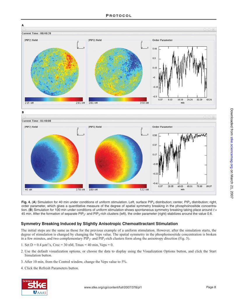
Insensitivity to Uniform Chemoattractant Stimulation

In this simulation, phase separation does not occur during the observation time. The phosphoinositide concentrations fluctuate inspace over a uniform background, and no symmetry breaking is observed (Fig. 4A). Spots enriched in either PIP2 or PIP3 aretransiently formed but rapidly decay. Accordingly, the order parameter g fluctuates around the zero value.

If this same simulation is performed but allowed to proceed for 100 min instead of 40, then spontaneous symmetry breaking canbe observed. After about 45 min of simulated time, spontaneous symmetry breaking takes place with the formation of randomlyoriented PIP2- and PIP3-rich clusters (Fig. 4B). The instructions for the 40-min simulation are provided, but the only difference isthe Tmax setting to run the 100-min simulation.

Running and Saving a Simulation

1. Launch the simulation environment.

2. Set D = 0.4 μm2/s, Crec = 30 nM, Tmax = 40 min, Veps = 0.

3. Using the default visualization options, click the Start Simulation button. Allow it to run to completion.

Note: The DirSens-System State window and the DirSens-Visualization Control window will both open when the simulationis started. Depending on the size of the monitor, the windows may not all be visible at the same time. The DirSens Controlwindow will also remain open. Windows may be minimized using the “-” button in the upper right. Windows that are re-quired for the simulation cannot be closed with “x”.

4. From the System State window, view the graphs and three-dimensional representations of the cell based on the default visualiza-tion options.

5. From the Visualization Control window, monitor the status of the simulation; once it is complete, use the buttons to move forwardand back in time through the data.

Note: If the pause button (||) on the Visualization Control window is clicked during the simulation, the simulation must berestarted from time zero using the DirSens Control window.

6. From the Control window, click the Save Session button to save the data from this simulation.

Note: This is optional. The files will be saved in the session folder. If the simulation is not saved, the data are available aslong as a new simulation is not started and DirSens remains open.

7. Close the simulation environment by clicking the “x” at the top right of the Control window.

Rerunning a Saved Session and Changing the Visualization Options

1. Launch the simulation environment.

2. Load a simulation by clicking the “Load Session” button.

3. Choose the file from the window.

4. Use the Visualization Control panel to replay the simulation from the beginning to step through the simulation to view the data atany given point in time.

5. To change the Visualization Options, add rows or columns and select the data to display.

6. Click the “Save as default” button.

7. To view the additional data, load the saved simulation again from the Control panel by clicking the Load Session button. The soft-ware will now display the additional selected graphs or cell representations in the System State window.

P R O T O C O L

Installation for Windows

1. Download the “Dirsens_win.zip” file.

2. Unzip in a directory of your choice.

3. Go to the “java” folder in the folder containing the unzippedfiles and double-click the file called “dirsens.jar” to launchthe simulation.

Installation for Linux

1. Download the “Dirsens.tar.gz” file.

2. Unzip in a directory of your choice.

3. Open a terminal and run “. ./install”.

4. Go to the directory “java” and type “java -jar dirsens.jar” tolaunch the simulation.

on March 21, 2007

stke.sciencemag.org

Dow

nloaded from



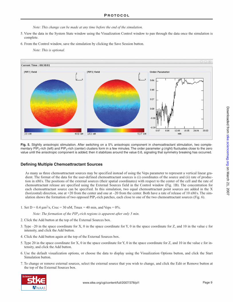
Symmetry Breaking Induced by Slightly Anisotropic Chemoattractant Stimulation

The initial steps are the same as those for the previous example of a uniform stimulation. However, after the simulation starts, thedegree of stimulation is changed by changing the Veps value. The spatial symmetry in the phosphoinositide concentration is brokenin a few minutes, and two complementary PIP2- and PIP3-rich clusters form along the anisotropy direction (Fig. 5).

1. Set D = 0.4 μm2/s, Crec = 30 nM, Tmax = 40 min, Veps = 0.

2. Use the default visualization options, or choose the data to display using the Visualization Options button, and click the StartSimulation button.

3. After 10 min, from the Control window, change the Veps value to 5%.

4. Click the Refresh Parameters button.

P R O T O C O L

Fig. 4. (A) Simulation for 40 min under conditions of uniform stimulation. Left, surface PIP2 distribution; center, PIP3 distribution; right,order parameter, which gives a quantitative measure of the degree of spatial symmetry breaking in the phosphoinositide concentra-tion. (B) Simulation for 100 min under conditions of uniform stimulation shows spontaneous symmetry breaking taking place around t =45 min. After the formation of separate PIP2- and PIP3-rich clusters (left), the order parameter (right) stabilizes around the value 0.6.

on March 21, 2007

stke.sciencemag.org

Dow

nloaded from



Note: This change can be made at any time before the end of the simulation.

5. View the data in the System State window using the Visualization Control window to pan through the data once the simulation iscomplete.

6. From the Control window, save the simulation by clicking the Save Session button.

Note: This is optional.

Defining Multiple Chemoattractant Sources

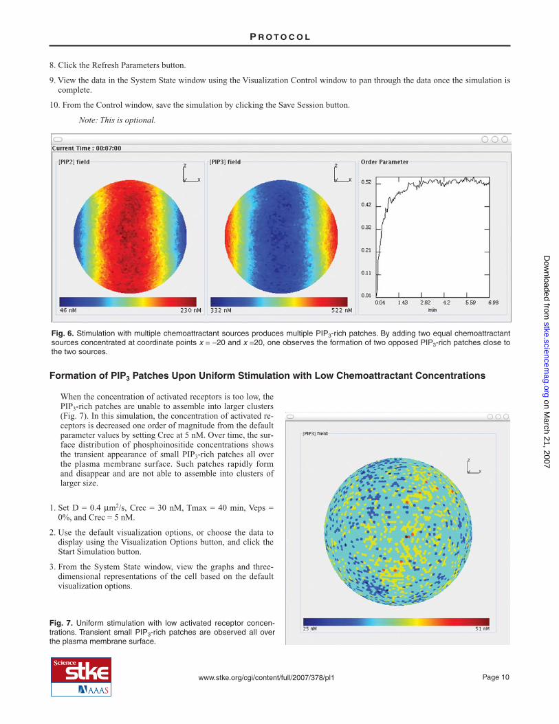
As many as three chemoattractant sources may be specified instead of using the Veps parameter to represent a vertical linear gra-dient. The format of the data for the user-defined chemoattractant sources is (i) coordinates of the source and (ii) rate of produc-tion in nM/s. The positions of the external sources (their spatial coordinates) with respect to the center of the cell and the rate ofchemoattractant release are specified using the External Sources field in the Control window (Fig. 1B). The concentration foreach chemoattractant source can be specified. In this simulation, two equal chemoattractant point sources are added in the X(horizontal) direction, one at +20 from the center and one at –20 from the center. Both have a rate of release of 10 nM/s. The sim-ulation shows the formation of two opposed PIP3-rich patches, each close to one of the two chemoattractant sources (Fig. 6).

1. Set D = 0.4 μm2/s, Crec = 30 nM, Tmax = 40 min, and Veps = 0%.

Note: The formation of the PIP3-rich regions is apparent after only 5 min.

2. Click the Add button at the top of the External Sources box.

3. Type –20 in the space coordinate for X, 0 in the space coordinate for Y, 0 in the space coordinate for Z, and 10 in the value c forintensity, and click the Add button.

4. Click the Add button again at the top of the External Sources box.

5. Type 20 in the space coordinate for X, 0 in the space coordinate for Y, 0 in the space coordinate for Z, and 10 in the value c for in-tensity, and click the Add button.

6. Use the default visualization options, or choose the data to display using the Visualization Options button, and click the StartSimulation button.

7. To change or remove external sources, select the external source that you wish to change, and click the Edit or Remove button atthe top of the External Sources box.

P R O T O C O L

Fig. 5. Slightly anisotropic stimulation. After switching on a 5% anisotropic component in chemoattractant stimulation, two comple-mentary PIP2-rich (left) and PIP3-rich (center) clusters form in a few minutes. The order parameter g (right) fluctuates close to the zerovalue until the anisotropic component is added; then it stabilizes around the value 0.6, signaling that symmetry breaking has occurred.

on March 21, 2007

stke.sciencemag.org

Dow

nloaded from



8. Click the Refresh Parameters button.


10. From the Control window, save the simulation by clicking the Save Session button.

Note: This is optional.

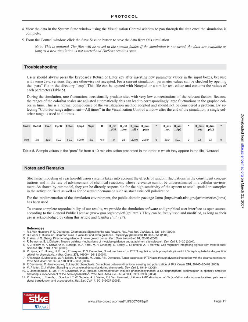
Formation of PIP3 Patches Upon Uniform Stimulation with Low Chemoattractant Concentrations

When the concentration of activated receptors is too low, thePIP3-rich patches are unable to assemble into larger clusters(Fig. 7). In this simulation, the concentration of activated re-ceptors is decreased one order of magnitude from the defaultparameter values by setting Crec at 5 nM. Over time, the sur-face distribution of phosphoinositide concentrations showsthe transient appearance of small PIP3-rich patches all overthe plasma membrane surface. Such patches rapidly formand disappear and are not able to assemble into clusters oflarger size.

1. Set D = 0.4 μm2/s, Crec = 30 nM, Tmax = 40 min, Veps =0%, and Crec = 5 nM.

2. Use the default visualization options, or choose the data todisplay using the Visualization Options button, and click theStart Simulation button.

3. From the System State window, view the graphs and three-dimensional representations of the cell based on the defaultvisualization options.

P R O T O C O L

Fig. 6. Stimulation with multiple chemoattractant sources produces multiple PIP3-rich patches. By adding two equal chemoattractantsources concentrated at coordinate points x = −20 and x =20, one observes the formation of two opposed PIP3-rich patches close tothe two sources.

Fig. 7. Uniform stimulation with low activated receptor concen-trations. Transient small PIP3-rich patches are observed all overthe plasma membrane surface.

on March 21, 2007

stke.sciencemag.org

Dow

nloaded from




5. From the Control window, click the Save Session button to save the data from this simulation.

Note: This is optional. The files will be saved in the session folder. If the simulation is not saved, the data are available aslong as a new simulation is not started and DirSens remains open.

Troubleshooting

Users should always press the keyboard’s Return or Enter key after inserting new parameter values in the input boxes, becausewith some Java versions they are otherwise not accepted. For a current simulation, parameter values can be checked by openingthe “pars” file in the directory “tmp”. This file can be opened with Notepad or a similar text editor and contains the values ofeach parameter (Table 5).

During the simulation, rare fluctuations occasionally produce sites with very low concentrations of the relevant factors. Becausethe ranges of the colorbar scales are adjusted automatically, this can lead to correspondingly large fluctuations in the graphed col-ors in time. This is a normal consequence of the visualization method adopted and should not be considered a problem. By se-lecting “Colorbar range adjustment—All times” in the Visualization Control window after the end of the simulation, a single col-orbar range is used at all times.

Notes and Remarks

Stochastic modeling of reaction-diffusion systems takes into account the effects of random fluctuations in the constituent concen-trations and in the rate of advancement of chemical reactions, whose relevance cannot be underestimated in a cellular environ-ment. As shown by our model, they can be directly responsible for the high sensitivity of the system to small spatial anisotropiesin the activation field, as well as for observed phenomena such as stochastic cell polarization.

For the implementation of the simulation environment, the public-domain package Jama (http://math.nist.gov/javanumerics/jama)has been used.

To ensure complete reproducibility of our results, we provide the simulation software and graphical user interface as open source,according to the General Public License (www.gnu.org/copyleft/gpl.html). They can be freely used and modified, as long as theiruse is acknowledged by citing this article and Gamba et al. (17).

References1. P. J. Van Haastert, P. N. Devreotes, Chemotaxis: Signalling the way forward. Nat. Rev. Mol. Cell Biol. 5, 626–634 (2004).2. G. Serini, F. Bussolino, Common cues in vascular and axon guidance. Physiology (Bethesda) 19, 348–354 (2004).3. Z. Wen, J. Q. Zheng, Directional guidance of nerve growth cones. Curr. Opin. Neurobiol. 16, 52–58 (2006).4. F. Schnorrer, B. J. Dickson, Muscle building; mechanisms of myotube guidance and attachment site selection. Dev. Cell 7, 9–20 (2004).5. A. J. Ridley, M. A. Schwartz, K. Burridge, R. A. Firtel, M. H. Ginsberg, G. Borisy, J. T. Parsons, A. R. Horwitz, Cell migration: Integrating signals from front to back.

Science 302, 1704–1709 (2003).6. M. Iijima, Y. E. Huang, H. R. Luo, F. Vazquez, P. N. Devreotes, Novel mechanism of PTEN regulation by its phosphatidylinositol 4,5-bisphosphate binding motif is

critical for chemotaxis. J. Biol. Chem. 279, 16606–16613 (2004).7. F. Vazquez, S. Matsuoka, W. R. Sellers, T.Yanagida, M. Ueda, P. N. Devreotes, Tumor suppressor PTEN acts through dynamic interaction with the plasma membrane.

Proc. Natl. Acad. Sci. U.S.A. 103, 3633–3638 (2006).8. P. Devreotes, C. Janetopoulos, Eukaryotic chemotaxis: Distinctions between directional sensing and polarization. J. Biol. Chem. 278, 20445–20448 (2003).9. M. Affolter, C. J. Weijer, Signaling to cytoskeletal dynamics during chemotaxis. Dev. Cell 9, 19–34 (2005).

10. C. Janetopoulos, L. Ma, P. N. Devreotes, P. A. Iglesias, Chemoattractant-induced phosphatidylinositol 3,4,5-trisphosphate accumulation is spatially amplifiedand adapts, independent of the actin cytoskeleton. Proc. Natl. Acad. Sci. U.S.A. 101, 8951–8956 (2004).

11. M. Postma, J. Roelofs, J. Goedhart, T. W. Gadella, A. J. Visser, P. J. Van Haastert, Uniform cAMP stimulation of Dictyostelium cells induces localized patches ofsignal transduction and pseudopodia. Mol. Biol. Cell 14, 5019–5027 (2003).

P R O T O C O L

Tmax

10.0

Deltat

5.0

Crec

30.0

Cpi3k

50.0

Cpten

50.0

Cpip2

500.0

Veps

5.0

D

0.4

K_cat_pi3k

1.0

K_cat_pten

0.5

K_mm_pi3k

200.0

K_mm_pten

200.0

*

0

K_ass_rec

50.0

K_ass_pip2

50.0

*

0

K_diss_rec

0.1

K_diss_pip2

0.1

*

0

Table 5. Sample values in the “pars” file from a 10-min simulation presented in the order in which they appear in the file. *Unused

on March 21, 2007

stke.sciencemag.org

Dow

nloaded from



12. M. Postma, J. Roelofs, J. Goedhart, H. M. Loovers, A. J. Visser, P. J. Van Haastert, Sensitization of Dictyostelium chemotaxis by phosphoinositide-3-kinase-mediated self-organizing signalling patches. J. Cell Sci. 117, 2925–2935 (2004).

13. C. Arrieumerlou, T. Meyer, A local coupling model and compass parameter for eukaryotic chemotaxis. Dev. Cell 8, 215–227 (2005).14. M. Postma, P. J. Van Haastert, A diffusion-translocation model for gradient sensing by chemotactic cells. Biophys. J. 81, 1314–1323 (2001).15. A. Levchenko, P. A. Iglesias, Models of eukaryotic gradient sensing: Application to chemotaxis of amoebae and neutrophils. Biophys. J. 82, 50–63 (2002).16. B. Kutscher, P. Devreotes, P. A. Iglesias, Local excitation, global inhibition mechanism for gradient sensing: An interactive applet. Sci. STKE 2004, pl3 (2004).17. A. Gamba, A. de Candia, S. Di Talia, A. Coniglio, F. Bussolino, G. Serini, Diffusion-limited phase separation in eukaryotic chemotaxis. Proc. Natl. Acad. Sci.

U.S.A. 102, 16927–16932 (2005).

Citation: A. de Candia, A. Gamba, F. Cavalli, A. Coniglio, S. Di Talia, F. Bussolino, G. Serini, A simulation environment for directional sensing as a phaseseparation process. Sci. STKE 2007, pl1 (2007).

.

P R O T O C O L

on March 21, 2007

stke.sciencemag.org

Dow

nloaded from


Documents

A Simulation Environment for Directional Sensing as a Phase Separation Process