Embed Size (px)
Citation preview
Article from:
North American Actuarial Journal
Volume 13 – Number 2

280
A ROBUSTIFICATION OF THE CHAIN-LADDERMETHOD
Tim Verdonck,* Martine Van Wouwe,† and Jan Dhaene‡
ABSTRACT
In a non–life insurance business an insurer often needs to build up a reserve to able to meet hisor her future obligations arising from incurred but not reported completely claims. To forecastthese claims reserves, a simple but generally accepted algorithm is the classical chain-laddermethod. Recent research essentially focused on the underlying model for the claims reserves tocome to appropriate bounds for the estimates of future claims reserves. Our research concentrateson scenarios with outlying data. On closer examination it is demonstrated that the forecasts forfuture claims reserves are very dependent on outlying observations. The paper focuses on twoapproaches to robustify the chain-ladder method: the first method detects and adjusts the out-lying values, whereas the second method is based on a robust generalized linear model technique.In this way insurers will be able to find a reserve that is similar to the reserve they would havefound if the data contained no outliers. Because the robust method flags the outliers, it is possibleto examine these observations for further examination. For obtaining the corresponding standarderrors the bootstrapping technique is applied. The robust chain-ladder method is applied to sev-eral run-off triangles with and without outliers, showing its excellent performance.
1. INTRODUCTION
Determining the expected profit or loss in a non–life insurance business is of growing importancebecause of the Solvency II regulations. This implies that an insurer has to be able to estimate the futureclaims reserves as accurately as possible. For an insurer operating in the non–life insurance business,the ultimate claims amount of an accident year is often not known at the end of that year. It willdepend on the business line in the non–life insurance industry, and, for instance, in liability insuranceit may be expected that the claims settlement will last several years because of bodily injuries and/orlong-lasting trials. Also the possible time lag between the occurrence of the accident and the manifes-tation of the consequences of the event may cause the delay.
This leads to the consideration of a run-off triangle to organize the claims reserves. The goal ofclaims reserving is to estimate the outstanding claims reserve. One of the most popular methods tosolve this problem is the classical chain-ladder method.
In this article we will focus on the appearance of outlying data in the run-off triangle of claimsreserves. Looking for the cause of the high dependency of the chain-ladder estimate on outlying databrings us to robust statistics. Robust statistics gives the opportunity to develop a robust chain-laddermethod that can recognize the outliers in the run-off triangle and that can smooth the outlying datain the run-off triangle in such a way that the outstanding claims reserve will be very close to theoutstanding claims reserve without outliers. We will focus on two objectives: the first item is to develop
* Tim Verdonck is a PhD student in the Department of Mathematics and Computer Science, University of Antwerp, Belgium,[email protected].† Martine Van Wouwe, PhD, is a Professor in the Faculty of Applied Economics, University of Antwerp, Belgium, [email protected].‡ Jan Dhaene, PhD, is a Professor in the Faculty of Business and Economics, Katholieke Universiteit Leuven, Belgium,[email protected].

A ROBUSTIFICATION OF THE CHAIN-LADDER METHOD 281
a statistical technique to detect the outliers with a high probability, the second objective is to eliminatethe influence of the outliers on the expected claims reserves by adjusting the classical chain-laddermethod. A justification for the second goal is that insurers in this way will be able to measure thedistance between the results for the expected claims reserves with and without outliers. If they producedifferent outcomes, a closer look at the data is recommended.
Since the estimates of the chain-ladder method can also be reproduced by using a generalized linearmodel and since there already exists an algorithm for obtaining robust estimates when using general-ized linear models, this straightforward approach to obtain robust estimates for the outstanding claimsreserve will also be studied.
Besides the reserve estimates, other aspects of the model are of importance. From a statisticalviewpoint, given a point estimate, the natural next step is to estimate the likely variability in theoutcomes. After estimating the variability, we can construct a confidence interval that is of greatinterest as the estimated claims reserve will never be an exact forecast of the future claims reserve.Another important measure in prediction problems is the root mean square error or the predictionerror. For estimating the standard and prediction error of the different estimates we will apply thebootstrapping technique. We will explain for what reason we choose the bootstrapping technique forthe standard error estimation, and we will therefore refer to the current debate on the standard errorestimation of the classical chain-ladder method, which up to now is inconclusive. For the robust esti-mators we have modified the classical bootstrapping technique as suggested in Stromberg (1997).
Numerical results will show very satisfactory results for our robust chain-ladder method. We have alsoconsidered some run-off triangles from practice, from which it can be concluded that the robust methodcan cope with several outliers and that outliers do occur in practice.
In Section 2 we will give a short introduction to claims reserving, and in Section 3 the chain-laddermethod will be explained. It will be demonstrated in Section 4 that the outstanding claims reserve issensitive to outlying data. The robust version of the chain-ladder method and the robustification of themethod based on generalized linear models will be described in Sections 5 and 6, respectively. Theestimation of the standard and prediction errors with the bootstrapping technique will be explained inSection 7. The comparison of the different techniques will be made in Section 8, and real examplesfrom practice will be studied in Section 9. The conclusions are given in Section 10.
2. CLAIMS RESERVING
The claims studied are the ones that are known to exist, but for which the eventual size is unknownat the time the reserves have to be set, also referred to as incurred but not reported completely (IBNRC)claims. The claims we concentrate on are the ones that take months or years to emerge, dependingon the complexity of the damage. The delay in payment is, for example, due to long legal proceduresor difficulties in determining the size of the claims. Therefore, insurers have to build up reservesenabling them to pay the outstanding claims and to meet claims arising in the future on the writtencontracts. We assume to have the following set of incremental claims:
{X �i � 1, . . . , n; j � 1, . . . , n � i � 1}.ij
The past data are used to estimate the future claims amounts. The suffix i refers to the row andcould indicate accident year or underwriting year, whereas the suffix j refers to the column and indicatesthe delay or development year. The claims on the diagonal with i � j � 1 � c denote the paymentsthat were made in calender year c. For example, X42 is the payment that emerged in the second (afterthe fourth, i.e., the fifth) year for the claim originated in the fourth year. The techniques can easily beextended to semiannual, quarterly, or monthly data, but most insurance companies utilize annual data.In most cases it is irrelevant whether incremental or cumulative data are used. Often the two formsare needed, and it is very easy to convert from one to another. The cumulative claims are defined as
j
C � X�ij ikk�1

282 NORTH AMERICAN ACTUARIAL JOURNAL, VOLUME 13, NUMBER 2
Table 1Run-Off Triangle
Development Year
Accident Year 1 2 ... n � i � 1 ... n � 1 n
1 X11 X12 ... X1,n�i�1 ... X1,n�1 X1n2 X21 X22 ... X2,n�i�1 ... X2,n�1� ... ... ... ... ...i Xi1 Xi2 ... Xi,n�i�1� ... ... ...n Xn1
with the values of Cij for i � j � n � 1 known. We are interested in the values of Cij for i � j � n �1, in particular the ultimate claims amounts Cin of each accident year i � 2, . . . , n. The outstandingclaims reserve of accident year i is defined as
R � C � C , 1 � i � n, (2.1)i in i,n�i�1
taking into account that Ci,n�i�1 has already been paid. The insurance company is, of course, interestedin the overall reserve R, being the sum of the reserves Ri for i � 1, . . . , n. For representation of thedata it is common to use a run-off triangle as in Table 1.
The aim of claims reserving is to make predictions about claims that will be paid in future calenderyears on the basis of the claims figures in the run-off triangle. Therefore the ultimate goal of a claimsreserving method is to complete the triangle into a square, because the total of the values found inthe lower right triangle equals the overall reserve R that will have to be paid in the future. Variousclaims reserving methods exist that are based on different assumptions and/or meeting specific re-quirements. In the next section we will describe one of the oldest and most popular techniques forestimating outstanding claims reserves, namely, the chain-ladder method.
3. CHAIN-LADDER METHOD
The chain-ladder method is based on the assumption that the expectations underlying the columnsand the rows in the run-off triangle are proportional. This straightforward method has been heavilycritized. However, several authors have countered the criticism by constructing stochastic models thatsupport the chain-ladder method. In practice it seems rational to use the chain-ladder methodto estimate the outstanding claims reserve if the data are consistent with the model. The chain-ladder method uses cumulative data and assumes the existence of a set of development factors { fj� j �2, . . . , n}, with
E[C �C , . . . , C ] � C f , 1 � i � n, 1 � k � n � 1.i,k�1 i1 in ik k�1
These factors are estimated by the chain-ladder method asn�j�1� Ci�1 ijf � , 2 � j � n. (3.1)j n�j�1� Ci�1 i, j�1
To forecast future values of cumulative claims, these factors are applied to the latest cumulative claimin each row:
ˆ ˆC � C f , 2 � i � ni,n�i�2 i,n�i�1 n�i�2
ˆ ˆ ˆC � C f , 2 � i � n, n � i � 3 � k � n.i,k i,k�1 k
As already stated in the introduction, it is also important to estimate the reserve variability. Mack(1993, 1994) has derived a distribution-free formula for the standard error of chain-ladder reserveestimates. In this article we will not study the theoretical variability or standard error of the estimates,
A ROBUSTIFICATION OF THE CHAIN-LADDER METHOD 283
Table 2Run-Off Triangle with Same Ratio between
Columns for Each Row
1 2 3 4 5 6
1 12,000 6,000 600 300 150.0 15.002 13,000 6,500 650 325 162.5 .3 10,000 5,000 500 250 . .4 12,000 6,000 600 . . .5 11,000 5,500 . . . .6 10,000 . . . . .
Table 3Future Claims Estimates, Obtained with
Chain-Ladder Method
1 2 3 4 5 6
1 12,000 6,000 600 300 150.0 15.002 13,000 6,500 650 325 162.5 16.253 10,000 5,000 500 250 125.0 12.504 12,000 6,000 600 300 150.0 15.005 11,000 5,500 550 275 137.5 13.756 10,000 5,000 500 250 125.0 12.50
but we will estimate it in a consistent way by using the bootstrapping technique. The main reason forthis choice is that the actuarial literature remains undecided about which assumptions finally supportthe chain-ladder method (Mack et al. 2006; Venter 2006; Wuthrich et al. 2008). We will focus on thisitem in more detail when the evaluation of the standard error is discussed in Section 7.
4. SENSITIVITY OF THE CHAIN-LADDER METHOD TOWARD OUTLYING VALUES
When analyzing real data, it may occur that one or more observations differ from the majority. Suchobservations are called outliers. Sometimes they are due to recording or copying mistakes (for example,a misplaced decimal point). Often the outlying observations are not incorrect, but they were madeunder exceptional circumstances and consequently do not fit the model well. In these situations, robuststatistics tries to find a fit that is similar to the fit we would have found without the outlier(s). Inpractice it is also very important to be able to detect these outliers for further examination. In thisregard it is important to note that outlying values are defined by the distribution of the majority ofthe data. When data are resulting from a long-tailed distribution, large values are not necessarilyoutlying because they may fit the underlying distribution.
We are interested to know how the chain-ladder method reacts toward outliers. By looking at a verysimple example, it will be clear that the presence of outlying claims may lead to incorrect reserveestimates.
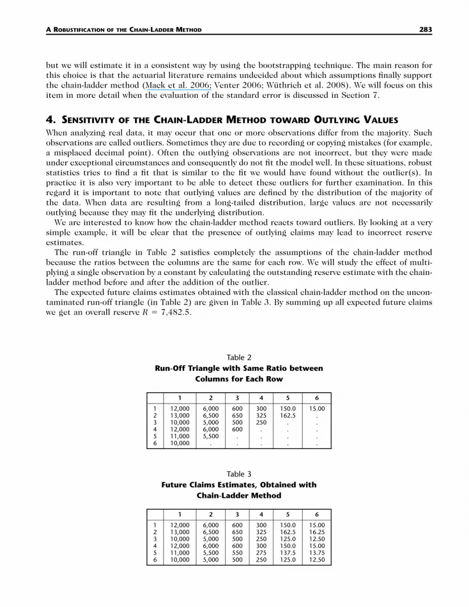
The run-off triangle in Table 2 satisfies completely the assumptions of the chain-ladder methodbecause the ratios between the columns are the same for each row. We will study the effect of multi-plying a single observation by a constant by calculating the outstanding reserve estimate with the chain-ladder method before and after the addition of the outlier.
The expected future claims estimates obtained with the classical chain-ladder method on the uncon-taminated run-off triangle (in Table 2) are given in Table 3. By summing up all expected future claimswe get an overall reserve R � 7,482.5.

284 NORTH AMERICAN ACTUARIAL JOURNAL, VOLUME 13, NUMBER 2
Table 4Future Claims Estimates, Obtained with
Chain-Ladder Method
1 2 3 4 5 6
1 12,000 60,000 600 300 150.0 15.002 13,000 6,500 650 325 162.5 4.243 10,000 5,000 500 250 52.71 3.244 12,000 6,000 600 150.35 62.75 3.865 11,000 5,500 311.45 135.89 56.72 3.496 10,000 14,310 458.87 200.21 83.57 5.14
Note: Claim X12 is made outlying by multiplication by 10.
An outlying value was introduced to this run-off triangle by multiplying the claims amount X12 by10. Applying the chain-ladder method on this adjusted run-off triangle results in the estimated claimsamounts of Table 4.
This leads to an overall reserve of R � 15,842.49, which is more than twice the reserve (7,482.5)obtained for the original run-off triangle (Table 2). The observation in the lower left corner is predictedto be much larger, whereas all the other claims are estimated as too low. Hence one outlier can causea totally different reserving scheme for an insurance company using the classical chain-ladder method.
This suggests that the chain-ladder method is not robust, and therefore we will introduce in Section5 a possible approach to make the chain-ladder method less sensitive to outliers. A robust version ofthe chain-ladder method will have a robust calculation of both the development factors and the claimsamounts.
5. THE ROBUST CHAIN-LADDER METHOD
This section presents a robust chain-ladder method. Our objective is not to replace the classical chain-ladder method by the proposed robust version, but it will certainly be very useful to apply both methods(the classical and the robust version) to the data and compare the overall reserve estimates. If bothestimates are approximately the same, there is no problem, but when both versions give a differentresult, we recommend having a closer look at the data. The robust method indicates the presence ofoutlying claim(s) so that one can search for the reason(s) behind the atypical value(s).
In Section 5.1 we propose a robust way to calculate development factors, and in Section 5.2 weexplain how outlying claims can be detected and adjusted.
5.1 Robustification of the Development FactorsThe first step is to detect what causes the classical chain-ladder method to be so dependent on outlyingdata. The definition of the development factors is based on the cumulative data Cij, and hence anoutlier in the first column will affect all development factors. On the other hand, when working withthe incremental data Xij, an outlier can at most affect two development factors.
Instead of dividing the sum of one column by the sum of the previous column, we could also look atthe ratios of the columns for each row:
Xij �i � 1, . . . , n � j � 1; j � 2, . . . , n .� �Xi, j�1
By taking the mean of the ratios of the same columns, we could assume to get approximately the samedevelopment factors as defined in (3.1).
Hampel et al. (1986) have illustrated that the mean (by using the influence function) as a statisticaltool is very sensitive toward outlying data. In examining the expression for the development factors,these factors can be viewed as a mean, which explains the dependency of the traditional chain-ladder
A ROBUSTIFICATION OF THE CHAIN-LADDER METHOD 285
Table 5Future Claims Estimates, Obtained with Robust
Chain-Ladder Method
1 2 3 4 5 6
1 12,000 60,000 600 300 150.0 15.002 13,000 6,500 650 325 162.5 16.253 10,000 5,000 500 250 125.0 12.504 12,000 6,000 600 300 150.0 15.005 11,000 5,500 550 275 137.5 13.756 10,000 5,000 500 250 125.0 12.50
Note: Claim X12 is made outlying by multiplication by 10.
Table 6Future Claims Estimates, Obtained with
Chain-Ladder Method
1 2 3 4 5 6
1 12,000 6,000 600 300 150.0 15.002 13,000 6,500 650 325 162.5 16.253 10,000 5,000 500 250 125.0 12.504 12,000 6,000 600 300 150.0 15.005 11,000 55,000 2,200 1,100 550.0 55.006 10,000 13,534.48 784.48 392.24 196.12 19.61
Note: Claim X52 is made outlying by multiplication by 10.
method on outlying data. To solve this problem we have to replace the mean by a more robust estimate.The robust statistical literature (see Huber 1981; Hampel et al. 1986; Rousseeuw and Leroy 1987;Maronna et al. 2006) solved this problem by replacing the mean by the median, which is a more robustestimate. The median of an univariate data set is defined as the middle value (or the mean of the twovalues in the middle if there is no single point in the middle) of the ordered observations. Unlike themean, the median is not influenced by outliers.
We therefore propose to use the median (in combination with incremental data), which leads to thefollowing alternative definition of development factors:
Xijf � median �i � 1, . . . , n � j � 1 , 2 � j � n. (5.1)� �j Xi, j�1
Applying the proposed robust method to the run-off triangle of the previous section (see Table 2,contaminated with the same outlier X12) results in the claims estimates of Table 5. The adjusteddevelopment factors seem to work perfectly, because they lead to the same future claims estimates asthe one obtained with the classical chain-ladder method applied to the data without outliers.
Unfortunately some problems remain. For instance, an outlying value in the second last column will,even with these adjusted development factors, influence the estimated reserves. In this situation weonly have two ratios, and taking the median is the same as taking the mean. Moreover, in that columnwe only have two claims amounts, which makes it very hard to decide which claim is outlying. In thisexample the outlying value is not used to calculate other claims estimates, and hence robustifying onlythe development factors is sufficient. However, if we would take the outlying value on the second lastrow, adjusting only the development factors will not work, as can be concluded from the results inTable 6.
The reason for the failure in this situation is that the outlier is still used to calculate the other claimsestimates. Because solely robustifying the development factors is not sufficient, we have implementeda mechanism to detect and adjust the outlying values, which will be discussed in Section 5.2.

286 NORTH AMERICAN ACTUARIAL JOURNAL, VOLUME 13, NUMBER 2
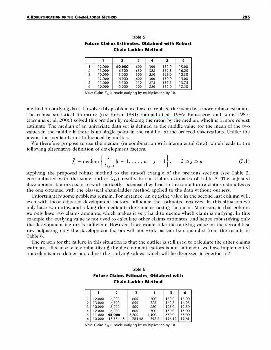
5.2 Detecting and Adjusting Outliers in the Chain-Ladder MethodOur technique for detecting outlying observations in a run-off triangle of claims amounts consists ofseveral steps. We will describe each step in this section. A concise summary can be found in Table 7.
For the given formulas, we restrict ourselves to the model described by Renshaw and Verrall (1998),who proposed modeling the incremental claims using an ‘‘overdispersed’’ Poisson distribution (hencethe variance is proportional to the mean).
Step 1: Under the given restrictions it holds that (see England and Verrall 1999), for 1 � i � n,1 � j � n � i � 1:
E[X ] � m ,ij ij
Var[X ] � �m ,ij ij
leading to the Pearson residuals, defined as
X � mij ijr � , (5.2)ij ��mij
where X are the incremental data, � is a scale parameter, and m are the incremental fitted values.The development factors are calculated as in (5.1), but based on the observed cumulative data. As
already mentioned in Section 5.1, the development factors in incremental form are more robust, butthe approach we follow in this step (see England and Verrall 1999) works only with cumulative data.Because the fitted cumulative paid to date equals the actual cumulative paid to date, the final diagonalof the actual cumulative triangle can be transferred to the fitted cumulative triangle. The remainingcumulative fitted values are obtained backwards by recursively dividing the cumulative fitted value attime t by the development factor at time t � 1. The incremental fitted data m are obtained by differ-encing the cumulative fitted values as described by England and Verrall (1999). By doing so, thecornerpoints at location (1,n) and (n,1) of the triangle always equal the cornerpoints of the observedincremental data, and, therefore, the corresponding residuals will be zero.
Step 2: To detect outliers the classical boxplot is used, which was introduced by Tukey (1977). Weconsidered some real and simulated triangles and note that residuals of outlying claims are more likelyto lie outside the classical boxplot interval
[Q � 3IQR, Q � 3IQR],1 3
where Q1 and Q3 are, respectively, the first and the third quartile. The classical boxplot rejection ruleinherently assumes normality of the data, which seems to hold under the restrictions of our simulationstudy. Moreover, only a small number of residuals are available, which tend tests to accept normalitydue to low power values in small samples. If the assumption of normality is not satisfied (which can betested with, for example, the Shapiro-Wilk test), one can use the adjusted boxplot (Hubert and Van-dervieren 2008) when the residuals are skewed. When the contaminated observations are realizationsof a heavy-tailed payment distribution, the elimination might produce a downward bias. In this case, itis advisable to measure the tail weight in a robust manner (Brys et al. 2006) and apply a bias correction.
Step 3: When detecting an outlying residual in the first column, the corresponding claims amountis supposed to be outlying and will be altered. If the claims amount in the next column in the samerow is also detected as an outlying value, the claim in the first column is replaced by the median ofthe claims of the first column. (Depending on the data it might be better to replace the claim by themean of the claim above it and under it—if these are not outlying—which will probably take inflationbetter into account.)
In the other case, we divide the claims amount in the next column of the same row by a robustdevelopment factor, and we replace the outlying claim by this value. We do not use these residuals toinvestigate the claims in the other columns, because the used development factors are based on cu-mulative data (which is necessary to obtain the fitted data as in England and Verrall 1999), and,therefore, one outlying claim can affect more than just its corresponding residual.
A ROBUSTIFICATION OF THE CHAIN-LADDER METHOD 287
Table 7Different Steps of Proposed Technique
Step 1
• Compute development factors
Cijf � median �i � 1, . . . , n � j � 1 2 � j � n.� �j Ci, j�1
• Obtain Pearson residuals, rij, as in England and Verrall (1999).
Step 2
• Test for normality.• Apply classical boxplot rejection rule on residuals.
Step 3
• If outlier in first column; suppose rk1– If rk2 is not outlying,
Xk2C � 2 � k � n.k1 Xi2median �i � 1, . . . , n � 1� �Xi1
– If rk2 is outlying,
C � median {C �i � 1, . . . , n}.k1 i1
Step 4
• Compute development factors
Xij1f � median �i � 1, . . . , n � j � 1 2 � j � n.� �j Xi,1
• Calculate fitted incremental claims
1 1ˆ ˆX � X f 1 � j � n, 2 � i � n.j,n�i�2 j,1 n�i�2
• Obtain residuals, as in (5.2).1r ,ij
• Apply classical boxplot rejection rule (after testing for normality).• If outlier; suppose 1rkl
– � median { �i � 1, . . . , n � 1; j � 2, . . . , n � i � 1}.1 1r rkl ij– Backtransform residuals to data matrix .1 rr Xij ij
Step 5
• Apply classical chain-ladder method on the robustified data .rXij
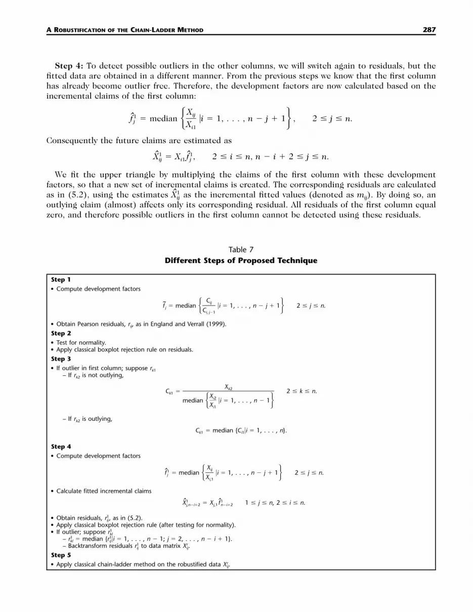
Step 4: To detect possible outliers in the other columns, we will switch again to residuals, but thefitted data are obtained in a different manner. From the previous steps we know that the first columnhas already become outlier free. Therefore, the development factors are now calculated based on theincremental claims of the first column:
Xij1f � median �i � 1, . . . , n � j � 1 , 2 � j � n.� �j Xi1
Consequently the future claims are estimated as
1 1ˆ ˆX � X f , 2 � i � n, n � i � 2 � j � n.ij i1 j
We fit the upper triangle by multiplying the claims of the first column with these developmentfactors, so that a new set of incremental claims is created. The corresponding residuals are calculatedas in (5.2), using the estimates as the incremental fitted values (denoted as mij). By doing so, an1Xij
outlying claim (almost) affects only its corresponding residual. All residuals of the first column equalzero, and therefore possible outliers in the first column cannot be detected using these residuals.

288 NORTH AMERICAN ACTUARIAL JOURNAL, VOLUME 13, NUMBER 2
The remaining residuals can be examined by using the boxplot. The outlying residuals are re-placed by the median of the residuals. The final observations (denoted by ) are obtained byrXij
backtransforming.Step 5: Finally, the classical chain-ladder method is applied on the robustified data . Table 7rXij
summarizes the different steps of our proposed technique. Note that with this proposed robust chain-ladder method the outlyingness of the claims in the cornerpoints, X1n and Xn1, cannot be investigated.
Xn1 is the first payment of the claim originated in the last accident year, and hence it is hard to saywhether this value is atypical. As a possible solution we suggest taking the median of values of the firstcolumn and verifying whether this value differs much from Xn1 (for this the boxplot interval can alsobe used). X1n, on the other hand, is the only claim where development year n is considered, and so wehave no idea whether the corresponding value is atypical or not. Here we suggest extrapolating the lastdevelopment factor by using a curve estimation model based on the former factors and verifying whetherthis value differs significantly from the last development factor estimated using claim X1n. We exploredsome possible statistical curve estimation models on several real run-off triangles. From these results,it appears that the inverse model with equation � b0 � b1 1/j (2 � j � n) preliminarily often givesf j
good results, but, of course, the choice for the best model is data dependent. For more informationwe refer to Van Wouwe et al. (2009).
Also, for the two claims of the last but one column, this approach can certainly be implemented,because it is possible to extrapolate the last but one development factor based on the former factors.Hence we can see whether the two ratios in that column differ much from the predicted last but onedevelopment factor. If only one of the ratios is detected as atypical, the other ratio will be taken asthe corresponding development factor. If both ratios are outlying, the fitted development factor (ob-tained by extrapolation) will be chosen. Recall that the median over both ratios forms the last but onedevelopment factor. If one of these two ratios is outlying, the corresponding development factor willbe influenced. Therefore the approach based on the curve estimation models might give better results.
In Section 8 we will show how the proposed robust method performs on the data set provided inTaylor and Ashe (1983) when an outlier is introduced. In that example the model � b0 � b1e�jf j
(2 � j � n) yielded a very nice fit and was chosen as optimal curve estimation model. In Section 9some real run-off triangles will be analyzed with the classical and robust chain-ladder method. In theseexamples the inverse model was always used as the curve estimation model.
6. THE ROBUST GLM METHOD
In recent years considerable attention has been given to discuss possible relationships between thechain-ladder and various stochastic models (see, e.g., Mack 1993, 1994; Verrall 1991, 2000; Renshawand Verrall 1998; England and Verrall 1999; Mack and Venter 2000). Several stochastic models usedfor claims reserving can be embedded within the framework of generalized linear models (GLMs),introduced by Nelder and Wedderburn (1972). England and Verrall (2002) provide a review of stochasticreserving models for claims reserving based on GLMs. The textbook Modern Actuarial Risk Theory (Kaaset al. 2001) also presents claims reserving models in the framework of GLMs.
Let us consider the multiplicative model
X � � � � , (6.1)ij i j k
which has a parameter for each row i, each column j, and each diagonal k � i � j � 1. When therandom variables Xij are independent and we restrict their distribution to be in the exponential dis-persion family, (6.1) is a GLM. The expected value of Xij is the exponent of the linear form log�i �log�j � log�i�j�1, so that there is a logarithmic link. The chain-ladder method can be derived from(6.1) if the following assumption about the distributions is satisfied:
X Poisson(� � ) independent; � � 1.ij i j k
When calculating the parameters �i � 0 and �j � 0 by maximum likelihood estimation, we obtain amultiplicative GLM with Poisson errors and a log-link. The optimal estimates of the parameters �i and

A ROBUSTIFICATION OF THE CHAIN-LADDER METHOD 289
�j produced by this GLM are identical to the parameter estimates found by the chain-ladder method(this still holds for the overdispersed Poisson model). Note that the proposed method is not the onlyone that is consistent with the chain-ladder method. Other stochastic models that can be expressedwithin the framework of GLM and give exactly the same forecasts as the chain-ladder method are, forexample, the overdispersed negative binomial model and Mack’s model.
6.1 Robust Estimators for GLMThe nonrobustness of the maximum likelihood estimator (and the usual quasi-likelihood estimator) forthe model parameters � has already been studied by several authors, including Pregibon (1982), Ste-fanski et al. (1986), Kunsch et al. (1989), Morgenthaler (1992), and Carroll and Pederson (1993).
Preisser and Qaqish (1999) proposed a class of robust estimators in the generalized estimatingequations framework of Liang and Zeger (1986). Starting from this class of robust estimators, Cantoniand Ronchetti (2001) proposed a set of robust inferential tools that apply to the whole class of GLMsand are based on a natural generalization of the quasi-likelihood approach. They considered a generalclass of M estimators of Mallows’s type, where the influence functions of deviations on the responseand on the predictors are bounded separately.
For the estimation of binomial and Poisson models the code for this method can be downloaded aspart of a robust library (namely, the library ‘‘robustbase’’) in the statistical software program R (http://www.r-project.org). Since the reserve estimates of the chain-ladder method can be obtained by usinga maximum likelihood estimation in a model with independent Poisson(�i�j) variables Xij, and since arobust method for fitting GLM is already available, we will also study this straightforward way to obtainrobust estimates.
7. ESTIMATION OF THE STANDARD AND PREDICTION ERRORS
In addition to the reserve estimates, it is important in practice to obtain the standard errors; hencethe precision of the estimates can be calculated (for example, by constructing confidence intervals).How to estimate the standard error for the classical chain-ladder method is already a point of discussion.We refer to the current debate (Mack et al. 2006; Venter 2006; Wutrich et al. 2008) that there is nounique answer to which assumptions support the chain-ladder method. Several articles have introducedstochastic models with different assumptions leading to the same mean estimate but with differentdistributions for the standard error estimate. The ongoing discussion is focused on the set of assump-tions, but till now the actuarial world has been inconclusive.
Estimates of the standard error can also be used to obtain an estimate for the root mean squareerror of prediction (also known as the prediction error), which is often used in prediction problems.Renshaw (1994) used first-degree Taylor expansions to deduce an approximation for the mean squareerror of prediction for the individual predictions (E[(Xij � )2]), for the row totals (E[(Ri � )2]),ˆ ˆX Rij j
and for the total reserve (E[(R � )2]) for the log-normal, overdispersed Poisson, and Gamma reservingRmodels (see England and Verrall 1999 for more information). However, those estimates are very difficultto calculate and still remain approximations.
Where a standard (or prediction) error is difficult to estimate analytically, it is common to adoptthe bootstrapping technique, which will be explained in Section 7.1.
7.1 Bootstrap TechniqueA popular method that produces a simulated predictive distribution for obtaining the standard errorsof well-specified models is bootstrapping (see Efron and Tibshirani 1993 for an introduction). Thebootstrapping technique has already been considered in the field of claims reserving (Ashe 1986; Lowe1994; Pinheiro et al. 2003; England and Verrall 2006; Barnett and Zehnwirth 2008) and has proven tobe a very convenient tool. In the context of claims reserving it is common to bootstrap the residualsrather than the data themselves because of the dependency between some observations and the param-
290 NORTH AMERICAN ACTUARIAL JOURNAL, VOLUME 13, NUMBER 2
eter estimates. Recall that the resampling is based on the hypothesis that the residuals are independentand identically distributed. Within the framework of GLMs different types of residuals can be chosen,but it is common to use Pearson residuals as defined in (5.2) for Poisson GLMs. As already mentioned,the residuals in the cornerpoints at location (1,n) and (n,1) are equal to zero (which is also noticedin England 2002 and Pinheiro et al. 2003). We therefore decided not to use the residuals correspondingto the last column of the first row and to the first row of the last column in the resampling procedureof the bootstrapping technique.
The statistical literature indicates that the determination of the distribution of the standard errorfor a robust estimator is an even more complex problem. In a few cases an attempt has been undertakento come to an answer (see, for example, Croux et al. 2003). A more global solution for robust estimatorsis still a big issue in robust statistics. These observations made us decide to also apply the bootstrappingtechnique for evaluating the standard error for our robust chain-ladder estimation of the outstandingclaims reserve.
As shown in Stromberg (1997), the bootstrapped sample covariance matrix can have a breakdownpoint of 1/n regardless of the robustness of the original estimate. Hence the breakdown value is ap-proximately zero for large n. The breakdown value is defined as the smallest proportion of observationsin the data set that need to be replaced to carry the estimate arbitrarily far away. Therefore boot-strapped covariance estimates may be heavily influenced by outliers even if the original estimate is not.In Stromberg (1997) it is concluded that by estimating the variance of robust estimators in a reliableway the bootstrapping technique can be applied, but instead of using the sample variance in the laststep of the computation of the bootstrap variance estimate, a more robust measure should be used.The robust measure of scale we considered is the median absolute deviation (MAD), given by the medianof all absolute distances from the sample median:
MAD � 1.483 median �x � median (x )�,j�1,...,n j i�1,...,n i
where the constant 1.483 is a correction factor that makes the MAD unbiased for the normal distri-bution. The breakdown value of the MAD is 50%, whereas the sample variance has breakdown pointzero.
After acquiring the bootstrap standard error of the reserve estimate (denoted as SEbs(R)), the pre-diction error of the total reserve (denoted as PEbs(R)) can be obtained. England and Verrall (1999)suggest a bias correction because the variance of the residuals is smaller than the variance of theunderlying random variable. Moreover, the variance of each residual depends not only on the randomvariable, but also on the data structure of the model. The bootstrap standard error of prediction withbias correction can be computed as
n 2PE (R) � � R � (SE (R)) ,bs p bs n � p
where an estimate of the Pearson scale parameter (�p) is given by2�r
� � ,p n � p
with n the number of observations in the data triangle and p the number of parameters estimated. Thesummation is over the number (n) of residuals.
8. COMPARISON OF THE DIFFERENT CLAIMS RESERVING METHODS
In this section we will consider the data from Taylor and Ashe (1983) and compare the differentmethods, namely,
• clasCL: the classical chain-ladder method, described in Section 3• robCL: the robust chain-ladder method, described in Section 5

A ROBUSTIFICATION OF THE CHAIN-LADDER METHOD 291
Table 8Claims Data from Taylor and Ashe (1983)
1 2 3 4 5 6 7 8 9 10
1 357,848 766,940 610,542 482,940 527,326 574,398 146,342 139,950 227,229 67,9482 352,118 884,021 933,894 1,183,289 445,745 320,996 527,804 266,172 425,0463 290,507 1,001,799 926,219 1,016,654 750,816 146,923 495,992 280,4054 310,608 1,108,250 776,189 1,562,400 272,482 352,053 206,2865 443,160 693,190 991,983 769,488 504,851 470,6396 396,132 937,085 847,498 805,037 705,9607 440,832 847,631 1,131,398 1,063,2698 359,480 1,061,648 1,443,3709 376,686 986,608
10 344,014
• clasGLM: the very basic GLM method with independent Poisson variables• robGLM: the same as clasGLM, but with the parameters estimated by the robust algorithm of Cantoni
and Ronchetti (2001), described in Section 6.1.
This data set, which is presented in incremental form in Table 8, has already been used by manyauthors (see, for example, Mack 1993; Renshaw 1994; England and Verrall 1999; Pinheiro et al. 2000).
An outlying value is added by multiplying a claims amount by 10. We have chosen to multiply by 10because this comes down to misplacing the decimal point one step to the right (which might be humanerror). Since the influence of an outlier is strongly dependent on its location, it is appropriate to lookat each observation separately.
In Table 9 the estimated reserves for the different methods are presented. The first line representsthe results obtained for the original dataset (without outliers), for which the forecasts for the futureclaims reserves for all methods should coincide. We immediately see that the chain-ladder method, itsrobust version, and the method based on GLM indeed give exactly the same result for the outstandingclaims reserve. The robust method based on GLM also performs well. We can conclude that it is safeto use the robust versions on data without outliers.
For the following lines, the first column shows which claim was multiplied by 10 (and hence can beconsidered as an outlier). As expected, the classical chain-ladder method and the classical methodbased on GLM give exactly the same results. It can be concluded that both classical methods cannothandle a single outlier and that the influence of the outlier on the estimated claims reserve dependsmuch on the location of that outlier. We also see that, although most of the time the claims reservegets overestimated, sometimes an underestimation also occurs, even though all outliers were createdby multiplication by 10.
Surprisingly the robust version of the GLM method is also significantly influenced by the atypicalobservation included in the data. We would like to note that this method always warned that thealgorithm did not converge, but nowhere was it explained how this could be solved. On the other hand,the results of the robust chain-ladder method are very satisfactory. The average number of detectedobservations equals 1.27, and the method always succeeded in detecting the added outlier. Becausewe always adjusted exactly one observation of the data, we can conclude that the robust chain-laddermethod performs very well.
The good properties of the robust chain-ladder method can also be demonstrated graphically: inFigure 1 we have plotted the reserve estimates for the different methods and the different data sets(each with a different outlier, in the same order as in Table 9). From this it is very clear that oneoutlier can have an enormous effect on the estimated outstanding reserves obtained by the classicalmethods (and by the robust GLM method). The robust chain-ladder method, on the other hand, alwaysfinds a result very near the true outstanding reserve (18,680,856), defined as the estimate for the dataset without the outlier (marked on the plot with the dashed line).

292 NORTH AMERICAN ACTUARIAL JOURNAL, VOLUME 13, NUMBER 2
Table 9Estimated Reserves for the Different Methods
outl clasCL robCL clasGLM robGLM
—X11X12X13X14X15X16X17X18X19X1,10X21X22X23X24X25X26X27X28X29X31X32X33X34X35X36X37X38X41X42X43X44X45X46X47X51X52X53X54X55X56X61X62X63X64X65X71X72X73X74X81X82X83X91X92X10,1
18,680,85612,603,78312,851,78415,813,13018,169,9592,013,275
22,709,17920,329,84721,616,87328,068,00426,382,87513,064,23913,080,59516,044,69220,313,52820,318,29821,142,00825,833,40124,770,91436,975,22514,594,66014,881,51918,190,07222,260,73823,910,23220,281,48226,993,25126,124,08014,890,58316,119,23819,166,51526,779,83820,950,17323,178,35622,505,92514,864,01517,682,93921,424,57723,930,48224,047,42725,775,38215,906,57919,712,83022,724,30926,011,07127,889,01717,251,33522,268,23328,111,88132,254,64920,451,04632,812,73744,155,25627,531,99550,350,36060,313,152
18,680,85618,487,95918,411,73118,370,56918,419,40618,681,09318,584,73418,879,22819,149,02918,700,36820,266,19218,619,21818,628,48418,713,35318,757,15818,713,87418,740,12718,526,32318,865,70817,788,53716,911,91318,942,88117,856,41418,608,42718,437,90018,899,66818,345,13118,501,51518,344,00618,927,11318,677,03418,260,49118,892,89618,649,55618,950,01519,021,39718,483,16418,706,46719,199,74618,934,68418,733,87118,362,70318,663,57118,761,39619,204,13318,444,10518,791,33518,761,39218,605,36719,273,97218,679,79118,491,33517,673,88818,643,60118,336,12819,004,501
18,680,85612,603,78312,851,78415,813,13018,169,95920,132,75122,709,17920,329,84721,616,87328,068,00426,382,87513,064,23913,080,59516,044,69220,313,52820,318,29821,142,00825,833,40124,770,91436,975,22514,594,66014,881,51918,190,07222,260,73823,910,23220,281,48226,993,25126,124,08014,890,58316,119,23819,166,51526,779,83820,950,17323,178,35622,505,92514,864,01517,682,93921,424,57723,930,48224,047,42725,775,38215,906,57919,712,83022,724,30926,011,07127,889,01717,251,33522,268,23328,111,88132,254,64920,451,04632,812,73744,155,25627,531,99550,350,36060,313,152
18,839,33313,328,66813,041,00115,908,93018,270,31119,847,84222,139,91220,185,64221,204,44827,677,53926,621,66913,536,36413,087,10715,934,57319,691,39420,091,62620,980,35225,321,95524,618,05137,819,01115,119,78514,840,58617,907,85321,398,41423,031,22020,445,84426,217,90425,530,92815,635,84416,109,03918,992,65526,004,65820,737,41422,780,25622,044,67715,396,65917,790,90621,077,16723,297,74723,316,99324,961,29116,422,20719,538,60522,362,17625,272,74526,949,51317,487,13021,978,58527,487,87431,182,74020,305,12631,926,49843,304,97027,787,92550,669,45661,101,893
Note: Each claim is made outlying by multiplication by 10.
The corresponding standard errors SEbs(R) for the different methods can be found in Table 10. Fromthe first line (which represents the situation without outlier), we see that the robust chain-laddermethod has a higher standard error than the other methods. This phenomenon does not arrive unex-pectedly, but is simply the result of the well-known trade-off between robustness and efficiency. Thehigher standard deviations (in the uncontaminated case) are the price we need to pay for making

A ROBUSTIFICATION OF THE CHAIN-LADDER METHOD 293
Figure 1Plot of Reserve Estimates for the Different Methods
the method robust. As soon as there are outliers in the data we see that the robustification is worthits price, because then the robust chain-ladder method has (nearly) always the lowest standard error.The results are visualized in Figure 2. We will not look at the prediction errors, because these will leadto analogous conclusions.
Note that we do not define how many outliers the proposed robust method resists or give othertheoretical results, but it is obvious that the robust method breaks down when there are more outlyingthan regular claims in a certain column. For the rows the number of outliers is not crucial.
9. REAL RUN-OFF TRIANGLES FROM PRACTICE
In this section we will discuss the results of applying classical and robust chain-ladder methods on realrun-off triangles. We have studied several data sets from a non–life business line of the Belgian insur-ance industry, but in this article we will focus on two examples. Because of the results of Section 8 wewill compare only the classical and the robust chain-ladder method. In the first run-off triangle (seeTable 11) there is only a small difference between both methods.
For the classical chain-ladder method the estimated future claims (with estimated reserves for therows) are shown in Table 12. The classical method suggests putting aside an overall reserve R �
Ri � 1,463,388,937. On the other hand, the robust chain-ladder method indicates one outlier in10�i�1
the data, which is situated at the upper right corner, namely, claim X2,9(� 24,602,209). The robustchain-ladder method adjusted this claims amount into the value 18,408,361. We now get f9 � 1.037351.The estimated future claims can be found in Table 13.
The outstanding reserve estimated with the robust chain-ladder method equals 1,437,093,149, whichis close to the classical outstanding reserve estimate. In this example it does not make much differencewhether claim X2,9 is altered or not. Taking a closer look at the data, we see that the flagged observationis a bit abnormal, but to classify it as a clear outlier is questionable. This explains partly the smalldifference between the classical and the robust outstanding reserve estimate. It is advisable for theinsurance company to have a good look at the claims amount X3,9, which will be known in the followingyear.
In the second example (the run-off triangle is shown in Table 14) we see a totally different situation.Applying the classical chain-ladder method on the data of Table 14 results in the estimated future

294 NORTH AMERICAN ACTUARIAL JOURNAL, VOLUME 13, NUMBER 2
Table 10Standard Errors for the Different Methods
outl clasCL robCL clasGLM robGLM
—X11X12X13X14X15X16X17X18X19X1,10X21X22X23X24X25X26X27X28X29X31X32X33X34X35X36X37X38X41X42X43X44X45X46X47X51X52X53X54X55X56X61X62X63X64X65X71X72X73X74X81X82X83X91X92X10,1
1,599,6812,707,3992,508,1373,121,6492,841,3673,904,7244,688,2392,237,2142,465,5733,171,9712,075,9362,378,2332,529,3903,520,7014,510,6973,342,3242,815,3764,317,7413,166,0664,482,6302,350,9203,321,4913,955,6894,797,6064,958,1831,901,2384,628,8423,421,6912,725,8333,668,1523,905,0106,847,6432,468,4263,378,7772,580,2193,533,5803,298,4184,741,4184,365,8584,247,7324,725,0182,933,9984,040,1404,594,3324,424,6595,359,7473,399,2213,766,1835,356,8305,754,2612,971,1654,988,3747,330,0203,894,8436,170,2305,667,162
2,190,6252,138,7642,203,7042,350,9542,261,4442,320,3352,048,4582,208,5382,338,2622,037,7882,159,4322,366,4102,258,1922,215,3972,365,8102,216,5422,340,8052,157,0392,407,3391,948,9941,855,5302,609,4151,994,9072,423,0982,172,7762,203,8382,214,2192,281,8212,500,3792,624,9982,347,4772,085,7162,080,6712,381,8722,171,1842,436,8012,063,7952,420,3052,402,4102,545,2862,397,9852,129,1242,300,8192,357,5942,373,6182,139,3682,329,2942,171,8002,149,4062,417,2822,278,9772,409,5232,032,5152,321,4172,334,1342,308,422
1,599,6812,707,3992,508,1373,121,6492,841,3673,904,7244,688,2392,237,2142,465,5733,171,9712,075,9362,378,2332,529,3903,520,7014,510,6973,342,3242,815,3764,317,7413,166,0664,482,6302,350,9203,321,4913,955,6894,797,6064,958,1831,901,2384,628,8423,421,6912,725,8333,668,1523,905,0106,847,6432,468,4263,378,7772,580,2193,533,5803,298,4184,741,4184,365,8584,247,7324,725,0182,933,9984,040,1404,594,3324,424,6595,359,7473,399,2213,766,1835,356,8305,754,2612,971,1654,988,3747,330,0203,894,8436,170,2305,667,162
1,604,4512,340,3202,340,8142,844,2332,493,7473,733,2014,281,5812,129,2032,448,9753,060,5832,047,5582,022,6852,449,1733,217,1434,199,7913,128,6172,763,9024,357,4422,973,1684,228,2212,178,9093,113,7983,550,8454,349,1724,544,7141,840,3264,473,6253,273,9702,327,9293,438,9793,609,4476,243,7782,381,0123,209,0462,301,8403,125,8723,263,0164,658,4614,196,5803,978,0344,351,6992,741,7263,707,7424,176,0634,345,1204,999,7492,943,6463,377,5025,164,1675,671,9092,924,5894,973,2107,117,9013,754,6855,978,9585,516,394
Note: The claim is made outlying by multiplication by 10.
claims and outstanding reserves for the rows of Table 15. From the classical chain-ladder method itfollows that the insurance company has to set aside a reserve R � 18,673,307.
The robust chain-ladder method indicates seven outliers in the run-off triangle of Table 16. Theoutlying observations coincide completely with the third row of the run-off triangle (except the firstobservation X31). The claims originated in the third accident year are indeed exceptionally high, which

A ROBUSTIFICATION OF THE CHAIN-LADDER METHOD 295
Figure 2Plot of Estimates of Standard Errors for the Different Methods
Table 11Real Run-Off Triangle from Practice (Example 1)
1 2 3 4 5 6 7 8 9 10
1 135,338,126 90,806,681 68,666,715 55,736,215 46,967,279 35,463,367 30,477,244 24,838,121 18,238,489 14,695,0832 125,222,434 89,639,978 70,697,962 58,649,114 46,314,227 41,369,299 34,394,512 26,554,172 24,602,2093 136,001,521 91,672,958 78,246,269 62,305,193 49,115,673 36,631,598 30,210,729 29,882,3594 135,277,744 103,604,885 78,303,084 61,812,683 48,720,135 39,271,861 32,029,6975 143,540,778 109,316,613 79,092,473 65,603,900 51,226,270 44,408,2366 132,095,863 88,862,933 69,269,383 57,109,637 48,818,7817 127,299,710 92,979,311 61,379,607 50,317,3058 120,660,241 89,469,673 71,570,7189 134,132,283 87,016,365
10 131,918,566
Table 12Example 1, Completed with the Classical Chain-Ladder Method
1 2 3 4 5 6 7 8 9 10 Ri
1 135,338,126 90,806,681 68,666,715 55,736,215 46,967,279 35,463,367 30,477,244 24,838,121 18,238,489 14,695,083 02 125,222,434 89,639,978 70,697,962 58,649,114 46,314,227 41,369,299 34,394,512 26,554,172 24,602,209 15,011,643 15,011,6433 136,001,521 91,672,958 78,246,269 62,305,193 49,115,673 36,631,598 30,210,729 29,882,359 22,446,400 15,564,850 38,011,2504 135,277,744 103,604,885 78,303,084 61,812,683 48,720,135 39,271,861 32,029,697 28,684,424 23,041,905 15,977,787 67,704,1155 143,540,778 109,316,613 79,092,473 65,603,900 51,226,270 44,408,236 35,104,160 30,367,042 24,393,535 16,915,038 106,779,7756 132,095,863 88,862,933 69,269,383 57,109,637 48,818,781 37,514,208 30,867,825 26,702,378 21,449,747 14,873,748 131,407,9077 127,299,710 92,979,311 61,379,607 50,317,305 44,199,591 35,622,093 29,310,935 25,355,582 20,367,880 14,123,557 168,979,6378 120,660,241 89,469,673 71,570,718 55,012,848 44,830,352 36,130,447 29,729,224 25,717,425 20,658,545 14,325,110 226,403,9519 134,132,283 87,016,365 70,456,750 56,947,133 46,406,615 37,400,815 30,774,522 26,621,665 21,384,912 14,828,790 304,821,202
10 131,918,566 93,526,403 71,825,534 58,053,462 47,308,170 38,127,412 31,372,388 27,138,852 21,800,363 15,116,873 404,269,457
1,463,388,937

296 NORTH AMERICAN ACTUARIAL JOURNAL, VOLUME 13, NUMBER 2
Table 13Example 1, Completed with the Robust Chain-Ladder Method
1 2 3 4 5 6 7 8 9 10 Ri
1 135,338,126 90,806,681 68,666,715 55,736,215 46,967,279 35,463,367 30,477,244 24,838,121 18,238,489 14,695,083 02 125,222,434 89,639,978 70,697,962 58,649,114 46,314,227 41,369,299 34,394,512 26,554,172 18,408,361 14,831,952 14,831,9523 136,001,521 91,672,958 78,246,269 62,305,193 49,115,673 36,631,598 30,210,729 29,882,359 19,201,131 15,470,701 34,671,8334 135,277,744 103,604,885 78,303,084 61,812,683 48,720,135 39,271,861 32,029,697 28,684,424 19,710,539 15,881,140 64,276,1035 143,540,778 109,316,613 79,092,473 65,603,900 51,226,270 44,408,236 35,104,160 30,367,042 20,866,752 16,812,722 103,150,6766 132,095,863 88,862,933 69,269,383 57,109,637 48,818,781 37,514,208 30,867,825 26,702,378 18,348,573 14,783,780 128,216,7647 127,299,710 92,979,311 61,379,607 50,317,305 44,199,591 35,622,093 29,310,935 25,355,582 17,423,121 14,038,126 165,949,4478 120,660,241 89,469,673 71,570,718 55,012,848 44,830,352 36,130,447 29,729,224 25,717,425 17,671,762 14,238,460 223,330,5189 134,132,283 87,016,365 70,456,750 56,947,133 46,406,615 37,400,815 30,774,522 26,621,665 18,293,111 14,739,093 301,639,705
10 131,918,566 93,526,403 71,825,534 58,053,462 47,308,170 38,127,412 31,372,388 27,138,852 18,648,497 15,025,434 401,026,153
1,437,093,149
Table 14Real Run-Off Triangle from Practice (Example 2)
1 2 3 4 5 6 7 8 9 10
1 701,848 232,585 194,470 148,488 98,600 61,875 47,145 32,260 25,628 18,1732 1,864,592 856,348 441,065 256,385 139,112 108,032 62,855 47,355 33,1323 11,52,332 2,381,638 2,545,868 2,613,448 2,310,415 2,712,015 3,662,850 3,704,7504 966,722 168,570 149,128 140,050 38,410 9,548 12,3085 789,602 485,170 192,082 149,400 140,052 43,5186 1,154,888 475,018 619,605 330,220 91,0257 1,053,622 459,830 419,665 273,3858 1,956,875 368,372 244,5259 1,568,152 966,498
10 1,322,485
Table 15Example 2, Completed with Classical Chain-Ladder Method
1 2 3 4 5 6 7 8 9 10 Ri
1 701,848 232,585 194,470 148,488 98,600 61,875 47,145 32,260 25,628 18,173 02 1,864,592 856,348 441,065 256,385 139,112 103,032 62,855 47,355 33,132 44,804 44,8043 1,152,332 2,381,638 2,545,868 2,613,448 2,310,415 2,712,015 3,662,850 3,704,750 234,276 251,089 485,3654 966,722 168,570 149,128 140,050 38,410 9,548 12,308 248,762 19,262 20,645 288,6705 789,602 485,170 192,082 149,400 140,052 43,518 335,820 357,819 27,707 29,696 751,0426 1,154,888 475,018 619,605 330,220 91,025 408,495 574,541 612,180 47,403 50,805 1,693,4247 1,053,622 459,830 419,665 273,385 327,050 387,509 545,025 580,730 44,968 48,195 1,933,4788 1,956,875 368,372 244,525 580,847 466,988 553,317 778,230 829,213 64,209 68,817 3,341,6209 1,568,152 966,498 808,505 755,655 607,530 719,840 1,012,442 1,078,768 83,533 89,527 5,155,799
10 1,322,485 754,419 662,493 619,187 497,813 589,840 829,600 883,947 68,447 73,359 4,979,105
18,673,307
Table 16Example 2, Completed with Robust Chain-Ladder Method
1 2 3 4 5 6 7 8 9 10 Ri
1 701,848 232,585 194,470 148,488 98,600 61,875 47,145 32,260 25,628 18,173 02 1,864,592 856,348 441,065 256,385 139,112 103,032 62,855 47,355 33,132 44,804 44,8043 1,152,332 502,910 299,806 243,796 126,355 63,675 58,125 52,966 27,779 29,773 57,5524 966,722 168,570 149,128 140,050 38,410 9,548 12,308 25,714 16,784 17,988 60,4865 789,602 485,170 192,082 149,400 140,052 43,518 36,245 31,798 20,756 22,245 111,0446 1,154,888 475,018 619,605 330,220 91,025 71,790 55,230 48,454 31,627 33,897 240,9987 1,053,622 459,830 419,665 273,385 111,700 62,314 47,940 42,058 27,452 29,422 320,8868 1,956,875 368,372 244,525 300,601 145,308 81,062 62,363 54,711 35,712 38,275 718,0319 1,568,152 966,498 492,034 354,049 171,144 95,475 73,451 64,439 42,061 45,080 1,337,734
10 1,322,485 532,752 360,145 259,146 125,269 69,883 53,763 47,166 30,787 32,996 1,511,906
4,403,442

A ROBUSTIFICATION OF THE CHAIN-LADDER METHOD 297
makes it likely that something exceptional has happened. (It is very advisable to have a closer look atthese observations.) The robust chain-ladder method will adjust the outliers and calculate the outstand-ing reserves. The estimated future claims are shown in Table 16, leading to an overall reserve of R �4,403,442, which differs significantly from the classical estimate (18,673,307). At this moment it ishighly recommended to examine the data and to decide which reserve will be closer to the truth. Ifthe observations of accident year 3 are indeed atypical observations and if there is only a small prob-ability that such exceptionally high claims will occur in the following years, the insurance company willset aside far too much. In that situation it is better to set aside the robust reserve estimate, possiblywith a safety margin for the outstanding claims of the third accident year.
Recall that the high observations of the third row will also influence the estimated future claims. Inthis situation it is useful to know that the data contain some atypical observations. Furthermore thereis no reason to believe that the classical chain-ladder method then still produces reliable estimates.
From this section we can conclude that outliers do appear in practice and that the robust chain-ladder method can handle more than one outlier. It is clear that the robust chain-ladder method isable to detect and adjust these outliers and might be a very convenient aid to construct a more realisticreserve.
10. CONCLUSIONS
In this article it is illustrated that the outstanding claims reserves by the chain-ladder method arestrongly affected by outliers. Often outliers lead to an overestimation of the total reserve estimate,which forces the insurance company to put more aside than actually needed. Depending on the locationof the outlier(s), it can also happen that the insurance company underestimates the total reserveestimate (which can lead to bankruptcy in a worst-case scenario).
To solve this problem we propose a robust method that has the ability to calculate the total reservein such a way that the outlying values are detected and adjusted in the run-off triangle of claimsreserves. The detection of outliers is important in practice, because further inspection of these atypicalobservations can reveal important information. Another approach for obtaining reserve estimates thatare less influenced by outliers is by implementing a robust generalized linear model technique.
In addition to the reserve estimates, it is interesting to obtain the standard deviation, which is ameasure of dispersion. When it is difficult to estimate a standard error analytically, it is common toadopt the bootstrapping technique. The estimation of the standard error of the robust chain-ladderestimate is calculated with a slightly modified bootstrapping technique (Stromberg 1997). Numericalexamples (where we added outliers to the data) show an excellent performance of the robust chain-ladder method.
From the application of real run-off triangles from a non–life insurance branch in Belgium, it is clearthat the proposed robust technique is helpful in gaining insight into the studied claims reserves andthe (hidden) outliers and in building up a more realistic reserve. The diagnostic performance of therobust method grows when it is used in addition to the classical approach.
The robust chain-ladder method can easily be implemented and does not need any knowledge ofstochastic methods and generalized linear models. All programs are written in the statistical pro-gram R.
REFERENCES
ASHE, F. R. 1986. An Essay at Measuring the Variance of Estimates of Outstanding Claim Payments. ASTIN Bulletin 16S: 99–113.BARNETT, G. AND B. ZEHNWIRTH. 2008. Modeling with the multivariate probabilistic trend family. Casualty Actuarial Society E-Forum,
Fall 2008.BRYS, G., M. HUBERT, AND A. STRUYF. 2006. Robust Measures of Tail Weight. Computational Statistics and Data Analysis 50: 733–59.CANTONI, E., AND E. RONCHETTI. 2001. Robust Inference for Generalized Linear Models. Journal of the American Statistical Association
96(455): 1022–30.CARROLL, R. J., AND S. PEDERSON. 1993. On Robustness in the Logistic Regression Model. Journal of the Royal Statistical Society, Series
B 55: 693–706.

298 NORTH AMERICAN ACTUARIAL JOURNAL, VOLUME 13, NUMBER 2
CROUX, C., G. DHAENE, AND D. HOORELBEKE. 2003. Robust Standard Errors for Robust Estimators. Research Report, Department ofApplied Economics, University of Leuven.
EFRON, B., AND R. J. TIBSHIRANI. 1993. An Introduction to the Bootstrap. London: Chapman and Hall.ENGLAND, P. D. 2002. Addendum to Analytic and Bootstrap Estimates of Prediction Errors in Claims Reserving. Insurance Mathematics
and Economics 31: 461–66.ENGLAND, P. D., AND R. J. VERRALL. 1999. Analytic and Bootstrap Estimates of Prediction Errors in Claims Reserving. Insurance
Mathematics and Economics 25: 281–93.———. 2002. Stochastic Claims Reserving in General Insurance. British Actuarial Journal 8(3): 443–544.———. 2006. Predictive Distributions of Outstanding Liabilities in General Insurance. Annals of Actuarial Science 1(2): 221–70.HAMPEL, F. R., E. M. RONCHETTI, P. J. ROUSSEEUW, AND W. A. STAHEL. 1986. Robust Statistics: The Approach Based on Influence
Functions. New York: Wiley.HUBER, P. J. 1981. Robust Statistics. New York: Wiley.HUBERT, M., AND E. VANDERVIEREN. 2008. An Adjusted Boxplot for Skewed Distributions. Computational Statistics and Data Analysis
52: 5186–5201.KAAS, R., M. J. GOOVAERTS, J. DHAENE, AND M. DENUIT. 2001. Modern Actuarial Risk Theory. Dordrecht: Kluwer.KUNSCH, H. R., L. A. STEFANSKI, AND R. J. CARROLL. 1989. Conditionally Unbiased Bounded-Influence Estimation in General Regression
Models, with Applications to Generalized Linear Models. Journal of the American Statistical Association 84: 460–66.LIANG, K. Y., AND S. L. ZEGER. 1986. Longitudinal Data Analysis Using Generalized Linear Models. Biometrika 73: 13–22.LOWE, J. 1994. A Practical Guide to Measuring Reserve Variability Using: Bootstrapping, Operational Time and a Distribution Free
Approach. Proceedings of the 1994 General Insurance Convention, Institute of Actuaries and Faculty of Actuaries.MACK, T. 1993. Distribution-Free Calculation of the Standard Error of Chain-Ladder Reserve Estimates. ASTIN Bulletin 23(2): 213–
25.———. 1994. Measuring the Variability of Chain Ladder Reserve Estimates. Casualty Actuarial Society Forum 1: 101–82.MACK, T., G. QUARG, AND C. BRAUN. 2006. The Mean Square Error of Prediction in the Chain Ladder Reserving Method—A Comment.
ASTIN Bulletin 36(2): 543–52.MACK, T., AND G. VENTER. 2000. A Comparison of Stochastic Models That Reproduce Chain Ladder Reserve Estimates. Insurance:
Mathematics and Economics 26: 101–7.MARONNA, R., D. MARTIN, AND V. YOHAI. 2006. Robust Statistics—Theory and Methods. New York: Wiley.MORGENTHALER, S. 1992. Least-Absolute-Deviations Fits for Generalized Linear Models. Biometrika 79: 747–54.NELDER, J. A., AND R. W. M. WEDDERBURN. 1972. Generalized Linear Models. Journal of the Royal Statistical Society 135: 370–84.PINHEIRO, P. J. R., J. M. ANDRADE E SILVA, AND M. L. C. CENTENO. 2003. Bootstrap Methodology in Claim Reserving. Journal of Risk
and Insurance 70(4): 701–14.PREGIBON, D. 1982. Resistant Fits for Some Commonly Used Logistic Models with Medical Applications. Biometrics 55: 574–79.PREISSER, J. S., AND B. F. QAQISH. 1999. Robust Regression for Clustered Data with Applications to Binary Regression. Biometrics 55:
574–79.RENSHAW, A. E. 1994. On the Second Moment Properties and the Implementation of Certain GLIM Based Stochastic Claims Reserving
Models. Actuarial Research Papers no. 65, Department of Actuarial Science and Statistics, City University, London.RENSHAW, A. E., AND R. J. VERRALL. 1998. A Stochastic Model Underlying the Chain Ladder Technique. British Actuarial Journal 4(4):
903–23.ROUSSEEUW, P., AND A. LEROY. 1987. Robust Regression and Outlier Detection. New York: Wiley.STEFANSKI, L. A., R. J. CARROLL, AND D. RUPPERT. 1986. Optimally Bounded Score Functions for Generalized Linear Models with
Applications to Logistic Regression. Biometrika 73: 413–24.STROMBERG, A. J. 1997. Robust Covariance Estimates Based on Resampling. Journal of Statistical Planning and Inference 57: 321–34.TAYLOR, G., AND F. R. ASHE. 1983. Second Moments of Estimates of Outstanding Claims. Journal of Econometrics 23: 37–61.TUKEY, J. W. 1977. Exploratory Data Analysis. Reading, MA: Addison-Wesley.VAN WOUWE, M., T. VERDONCK, AND K. VAN ROMPAY. 2009. Application of Classical and Robust Chain-ladder Methods: Results for the
Belgium Non-Life Business. Global Business and Economics Review, to appear.VENTER, G. 2006. Discussion of the Mean Square Error of Prediction in the Chain-Ladder Reserving Method. ASTIN Bulletin 36(2):
566–71VERRALL, R. 1991. On the Estimation of Reserves from Loglinear Models. Insurance: Mathematics and Economics 10: 75–80.———. 2000. An Investigation into Stochastic Claims Reserving Models and the Chain-Ladder Technique. Insurance: Mathematics
and Economics 26: 91–99.WUTHRICH, M. V., M. MERZ, AND H. BUHLMANN. 2008. Bounds on the Estimation Error in the Chain Ladder Method. Scandinavian
Actuarial Journal in press.
Discussions on this paper can be submitted until October 1, 2009. The authors reserve the right to reply toany discussion. Please see the Submission Guidelines for Authors on the inside back cover for instructionson the submission of discussions.


