Formal design methodology for transforming ladder diagram to Petri nets

1 23

The International Journal ofAdvanced Manufacturing Technology ISSN 0268-3768 Int J Adv Manuf TechnolDOI 10.1007/s00170-014-5715-9

Formal design methodology fortransforming ladder diagram to Petri nets

J. C. Quezada, J. Medina, E. Flores,J. C. Seck Tuoh & N. Hernández

1 23

Your article is protected by copyright and

all rights are held exclusively by Springer-

Verlag London. This e-offprint is for personal

use only and shall not be self-archived

in electronic repositories. If you wish to

self-archive your article, please use the

accepted manuscript version for posting on

your own website. You may further deposit

the accepted manuscript version in any

repository, provided it is only made publicly

available 12 months after official publication

or later and provided acknowledgement is

given to the original source of publication

and a link is inserted to the published article

on Springer's website. The link must be

accompanied by the following text: "The final

publication is available at link.springer.com”.

Int J Adv Manuf TechnolDOI 10.1007/s00170-014-5715-9

ORIGINAL ARTICLE

Formal design methodology for transforming ladderdiagram to Petri nets

J. C. Quezada · J. Medina · E. Flores · J. C. Seck Tuoh ·N. Hernandez

Received: 4 June 2013 / Accepted: 10 February 2014© Springer-Verlag London 2014

Abstract Ladder diagram (LD) is a common programminglanguage at industry in order to develops control algorithmsof discrete event systems. Besides, it is one of the five pro-gramming languages supported by the International Elec-trotechnical Commission through the IEC-61131-3 stan-dard. Petri net (PN) theory is both a graphical and mathe-matical tool, which allows modeling discrete event systemsin order to obtain a useful formalization to analyze them ina better way. LD control algorithms are continuously devel-oped based on the experience of control system developers.Therefore, it is still a relevant problem on how to formal-ize a validation for the current and new control algorithms.In the present work, an element-to-element transformationmethodology from a LD program to a PN structure is pro-posed. The original part of this manuscript is the proposal offive PN structures where their markings represent the statesand dynamic behavior of energized and de-energized coils,which are not included in previous works. Furthermore, this

J. C. Quezada (�) · E. FloresEscuela Superior de Tizayuca, Universidad Autonoma del Estadode Hidalgo, km 2.5 carretera federal, Tizayuca-Pachuca, Mexicoe-mail: [email protected]

E. Florese-mail: [email protected]

J. Medina · J. C. Seck Tuoh · N. HernandezCentro de Investigacion Avanzada en Ingenierıa Industrial,Universidad Autonoma del Estado de Hidalgo,km 2.5 carretera federal, Tizayuca-Pachuca, Mexico

J. Medinae-mail: [email protected]

J. C. Seck Tuohe-mail: [email protected]

N. Hernandeze-mail: [email protected]

methodology preserves the structural and dynamical behav-ior of the LD in the obtained PN. Two control algorithms ofreal cases are transformed using the proposed methodology.

Keywords Control algorithms · Ladder diagrams ·Petri nets · Discrete event systems

Mathematics Subject Classifications (2010) 68Q60 ·68Q85

1 Introduction

Programmable logic controllers (PLCs) are widely appliedin an industry for the process control, mainly for discreteevent systems such as interlocks, production and/or manu-facturing sequences, process alarms, among others. In theIEC-61131-3 standard [1], the syntaxes and semantics offive programming languages for logic controllers are estab-lished: ladder diagram (LD), function block diagram (FBD),instruction list (IL), structured text (ST), and sequentialfunction chart (SFC). LD is considered a graphic-type lan-guage based on the behavior of an electromagnetic relayconstituted by a coil and contacts that can be normally open(NO) and/or normally closed (NC). Due to its likeness andutilization with electrical control diagrams, LD has been themost popular language used in the industry for developingcontrol algorithms.

The control LD algorithms are mainly based on theuser experience applying trial-and-error techniques. There-fore, a formalization of the validity of the existing controlalgorithms remains as a relevant problem, as well as thespecification of new methodologies to validate the controlalgorithms before their real implementation. In addition, PNis both a graphical and mathematical tool which is applied

Author's personal copy

mailto:[email protected]





Int J Adv Manuf Technol

to model discrete event systems (DES) in order to describetheir static and/or dynamic behavior [2]. A PN analysismethod for the dynamic behavior is the state equation com-posed of an incidence matrix, an initial marking vector, anda firing vector.

Various approaches have been presented in researchpapers to study the relationship between LD and PN foranalysis, modeling, and simulation of control algorithmsand its corresponding validation. In [3], Lee and Lee pro-pose the modulus synthesis technique for the conversionfrom LD to PN, considering the LD base cores defined inthe IEC-61131-3 standard. It is important to highlight thatfor the normally open and normally closed contacts, theypropose one place with two transitions joined together byan enabler arc and an inhibitor arc, respectively, in orderto relate their active state, open state, or closed state. Theauthors present an example where they show operationsAND and OR, considering that all the variables are indepen-dent, that is, the coil they use has no contacts defined in thecode lines of the LD.

Thapa et al. [4] define five types of PN structures ofinput-output units (IOU) which are equivalent to commonstructures used in control algorithms developed in LD:start-stop unit, basic unit, AND and OR unit, basic unitwith functions block, and unit of transmission concatena-tion of logical flow. In [5], Peng and Zhou make referenceto graphical-type constructors of logics AND, OR, andsequential modeling, showing the equivalences between PNand LD. In [6], Lee and Hsu show the equivalences betweenPN and LD, and IF-THEN rules which are logical structuresAND, OR, and parallel or concurrent distribution. Zapataand Carrasco [7] propose a representation in a graphicalway of logical constructors AND, OR, S-R memory func-tion, edge detection, concurrency and delays on PN and inLD; however, they will validate the equivalences in a futurework.

In [8], Tzafestas et al. propose a technique to generatea LD starting from a PN representing an control algorithm,standing out the importance of the self-loop in DES, andconsidering the LD rows as two parts: “conditional part”and “action part” which are represented in the PLC memory,assigning consequently a bit for a place in the PN at theconditional part, and other bit for a transition in the PN atthe action part.

In [9], Korotkin et al. propose a methodology to imple-ment PN models for discrete event control systems (DECS)of high level. They define a 10-tuple net called “PNDEC”and their dynamic marking equations. The PNDEC is con-sidered as a binary net and its evaluation is performed in asingle swept of the control algorithm based on Boolean con-ditions assigned to the output places. The dynamic markingis generalized; however, it does not consider initial stateswith energized coils.

In [10], the authors use truth tables that represent the stateof the process (Karnaugh maps) to determine the Booleanfunction transitions and show an example of an engineconsidering the start and stop in a single control line of LD.

The application of colored PN (CPN) for obtaining auto-matically formal models directly from the LD is shown in[11]. They consider that each control line in LD can beexpressed as a formula written in propositional logic. Theirfocus is based on the sequential steps of the PLC: readinginputs, cycle start. and memory access. These elements areanalyzed considering energy flows as rows, without takinginto account the scan operation of the PLC.

Another proposal of a systematic method to translatefrom LD to ordinary Petri nets is presented in [12]. Theydefine a LD graph which is transformed into an ordinaryPetri net; this approach considers only the basic parts ofrelays (contacts and coils). They define two states for thetypes of contacts and coils and perform searches of the“closed” trajectories to find energized coils and “open” tra-jectories for de-energized coils in LD graphs. Nevertheless,they do not include the logic operation for negated coils.

In general, to our knowledge, the transformation propos-als consider only the behavior of the logical structures whenthe input prerogatives are fulfilled to energize coils, or thereare no negated coils.

In this paper, we propose a new methodology for trans-forming control algorithms developed in LD to PN. Inparticular, we show five PN structures in order to repre-sent the control algorithms developed in LD (logic AND,logic OR, logic AND-OR, logic set-reset and logic crossed-contacts). This transformation is called ladder diagram -Petri net (LDPN). With this transformation, the originalcontribution of this paper is to establish a new methodologyto model the behavior of energize and de-energize coils.

The proposed methodology was evaluated on two realcontrol algorithms, obtaining results that show the struc-tural and dynamic equivalence between the original LDand the obtained LDPN. The first case needs to ener-gize and de-energize a coil, and the second one shows theimplementation of the methodology for a packaging system.

This paper is organized as follows. Section 2 and 3describe the basic concepts of LD and PN, respectively.Section 4 explains the five structures to define a LDPN andhow to transform a LD into a LDPN. Section 5 shows tworeal cases, and the final section presents the conclusions ofthe paper.

2 Ladder diagram

The graphic language LD models nets of electromechanicalelements operating simultaneously, such as relays contain-ing coils and contacts, timers, and counters, mainly [13],



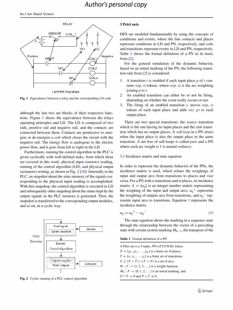
Fig. 1 Equivalence between a relay and the corresponding LD code

although the last two are blocks of their respective func-tions. Figure 1 shows the equivalence between the relaysoperating principles and LD. The LD is composed of tworails, positive rail and negative rail, and the contacts areconnected between them. Contacts are permissive to ener-gize or de-energize a coil which closes the circuit with thenegative rail. The energy flow is analogous to the electricpower flow, and it goes from left to right in the LD.

Furthermore, running the control algorithm in the PLC isgiven cyclically with well-defined tasks, from which threeare covered in this work: physical input (sensors) reading,running of the control algorithm (LD), and physical output(actuators) writing, as shown in Fig. 2 [10]. Internally in thePLC, an snapshot about the state memory of the signals cor-responding to the physical input reading is accomplished.With this snapshop, the control algorithm is executed in LDand subsequently other snapshop about the status kept by theoutput signals in the PLC memory is generated. Then, thesnapshot is transferred to the corresponding output modules,and so on, in a cyclic way.

Fig. 2 Cyclic running of a PLC control algorithm

3 Petri nets

DES are modeled fundamentally by using the concepts ofconditions and events, where the line contacts and placesrepresent conditions in LD and PN, respectively, and coilsand transitions represent events in LD and PN, respectively.Table 1 shows the formal definition of a PN in its basicform [2].

For the general simulation of the dynamic behavior,based on an initial marking of the PN, the following transi-tion rule from [2] is considered:

1. A transition t is enabled if each input place p of t con-tains w(p, t) tokens, where w(p, t) is the arc weightingjoining p to t.

2. An enabled transition can either be or not be firing,depending on whether the event really occurs or not.

3. The firing of an enabled transition t, moves w(p, t)tokens of each input place and adds w(t, p) to eachoutput place.

There are two special transitions: the source transitionwhich is the one having no input places and the sink transi-tion which has no output places. A self-loop in a PN ariseswhen the input place is also the output place in the sametransition. A net free of self-loops is called pure and a PNwhere each arc weight is 1 is named ordinary.

3.1 Incidence matrix and state equation

In order to represent the dynamic behavior of the PNs, theincidence matrix is used, which relates the weighings ofinput and output arcs from transitions to places and viceversa. For a PN with n transitions and m places, its incidencematrix A = [aij] is an integer number matrix representingthe weighing of the input and output arcs; aij

+ representsthe weighting of outputs arcs from transitions, and aij

− rep-resents input arcs to transitions. Equation 1 represents theincidence matrix.

aij = aij+ − aij

− (1)

The state equation shows the marking in a sequence statethrough the relationship between the vector of a precedingstate with certain system markingMk−1, the transpose of the

Table 1 Formal definition of a PN

A Petri net is a 5-tuple, PN=(P,T,F,W,M) where:

P = {p1, p2, . . . , pm} is a finite set of places,

T = {t1, t2, . . . , tn} is a finite set of transitions,

F ⊆ (P × T ) ∪ (T × P ) is a set of arcs,

W : F → {1, 2, 3, . . .} is a weight function,

M0 : P → {0, 1, 2, . . .} is an initial marking, and

P ∩ T = ∅ and P ∪ T �= ∅



incidence matrix A and a firing vector uk determining theprocess firing sequence. Equation 2 shows the relationshipbetween them.

Mk = Mk−1 +AT uk (2)

Taking into account the previous PN concepts, the nextsection describes the methodology applied to represent agiven LD by means of an equivalent PN, which is calledLDPN.

4 Formal definition of LDPN

In previous works, only the behavior of energizing coilshas been considered to transform LD into PN. In actualcontrol algorithms, however, depending on the system con-trol, it is necessary to energize or de-energize coils. Forthis reason, it proposed a methodology to transform LDcontrol lines to PN structures. This transformation is basedon the definition of five PN structures which represent themost common instruction lines in LD. With these PN struc-tures, this methodology is able to obtain a structural anddynamic equivalent PN for a given LD considering as wellthe behavior of energized and de-energized coils.

4.1 Representing LD signals with PN

A particular interpretation of the PN is to consider places asinput and output signals from sensors and actuators, respec-tively, and transitions as logical conditions of the systems.This interpretation is the generalization of a PLC-based sys-tem: input signals (sensors) — control algorithm (LD) —output signals (coils).

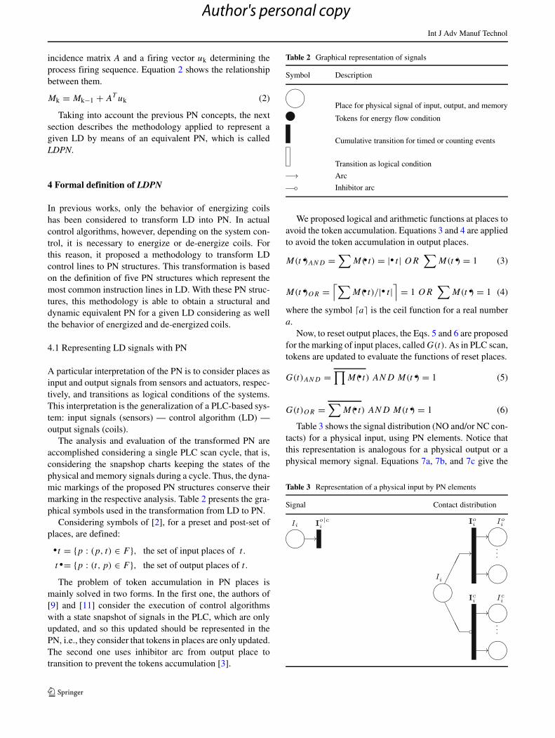
The analysis and evaluation of the transformed PN areaccomplished considering a single PLC scan cycle, that is,considering the snapshop charts keeping the states of thephysical and memory signals during a cycle. Thus, the dyna-mic markings of the proposed PN structures conserve theirmarking in the respective analysis. Table 2 presents the gra-phical symbols used in the transformation from LD to PN.

Considering symbols of [2], for a preset and post-set ofplaces, are defined:

�t = {p : (p, t) ∈ F }, the set of input places of t.

t �= {p : (t, p) ∈ F }, the set of output places of t.

The problem of token accumulation in PN places ismainly solved in two forms. In the first one, the authors of[9] and [11] consider the execution of control algorithmswith a state snapshot of signals in the PLC, which are onlyupdated, and so this updated should be represented in thePN, i.e., they consider that tokens in places are only updated.The second one uses inhibitor arc from output place totransition to prevent the tokens accumulation [3].

Table 2 Graphical representation of signals

Symbol Description

Place for physical signal of input, output, and memory

Tokens for energy flow condition

Cumulative transition for timed or counting events

Transition as logical condition

Arc

Inhibitor arc

We proposed logical and arithmetic functions at places toavoid the token accumulation. Equations 3 and 4 are appliedto avoid the token accumulation in output places.

M(t �)AND =∑

M(�t) = | �t| OR∑

M(t �) = 1 (3)

M(t �)OR =⌈∑

M(�t)/| �t|⌉= 1 OR

∑M(t �) = 1 (4)

where the symbol a is the ceil function for a real numbera.

Now, to reset output places, the Eqs. 5 and 6 are proposedfor the marking of input places, called G(t). As in PLC scan,tokens are updated to evaluate the functions of reset places.

G(t)AND =∏

M(�t) AND M(t �) = 1 (5)

G(t)OR =∑

M(�t) AND M(t �) = 1 (6)

Table 3 shows the signal distribution (NO and/or NC con-tacts) for a physical input, using PN elements. Notice thatthis representation is analogous for a physical output or aphysical memory signal. Equations 7a, 7b, and 7c give the

Table 3 Representation of a physical input by PN elements

Signal Contact distribution



number of NO and/or NC contacts for these types of sig-nals. The transitions Ioi are enabled when its input place hasa token, and transitions Ici are enabled when its input placeno has a token.

Ii = Ioi Ioi + Ici I

ci (7a)

Oo = OooO

oo + Oc

oOco (7b)

Bb = BobB

ob + Bc

bBcb (7c)

where I oi , Ooo , and Bo

b are the number of NO contacts, andI ci , Oc

o , and Bcb are the number of NC contacts for the signals

Ii, Oo, and Bb at the corresponding LD.Marking in output places I oi and I ci is in function of the

Eqs. 8 and 9 and is similar to the marking of output placesof signals Oo and Bb.

M(Ii) = 1 then M(I ci ) = 0 (8)

M(Ii) = 0 then M(Ioi ) = 0 (9)

Five types of control lines are the most common ones incontrol algorithms developed in LD. These types are thefollowing: serial contacts (logical AND), parallel contacts(logical OR), contacts using the previous connections at thesame time (logical AND-OR), logical set-reset coils, andlogical interlocking contacts.

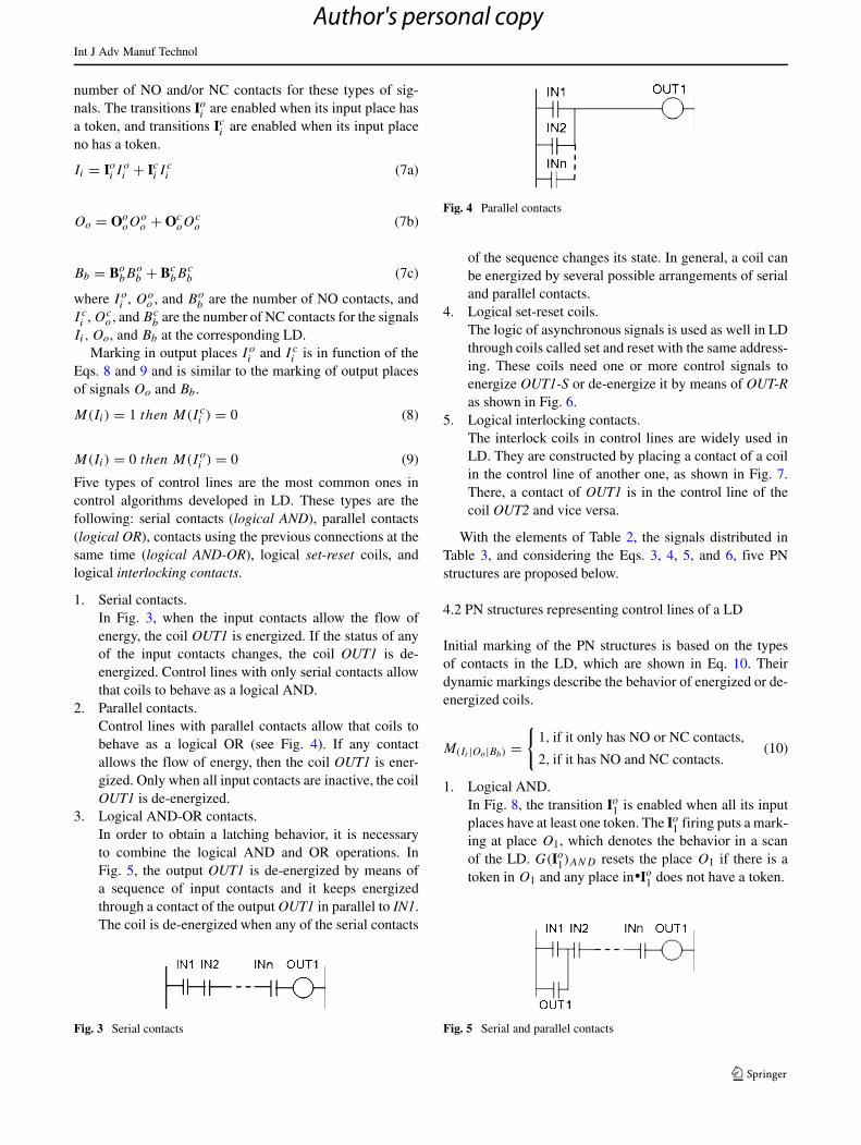
1. Serial contacts.In Fig. 3, when the input contacts allow the flow ofenergy, the coil OUT1 is energized. If the status of anyof the input contacts changes, the coil OUT1 is de-energized. Control lines with only serial contacts allowthat coils to behave as a logical AND.

2. Parallel contacts.Control lines with parallel contacts allow that coils tobehave as a logical OR (see Fig. 4). If any contactallows the flow of energy, then the coil OUT1 is ener-gized. Only when all input contacts are inactive, the coilOUT1 is de-energized.

3. Logical AND-OR contacts.In order to obtain a latching behavior, it is necessaryto combine the logical AND and OR operations. InFig. 5, the output OUT1 is de-energized by means ofa sequence of input contacts and it keeps energizedthrough a contact of the output OUT1 in parallel to IN1.The coil is de-energized when any of the serial contacts

Fig. 3 Serial contacts

Fig. 4 Parallel contacts

of the sequence changes its state. In general, a coil canbe energized by several possible arrangements of serialand parallel contacts.

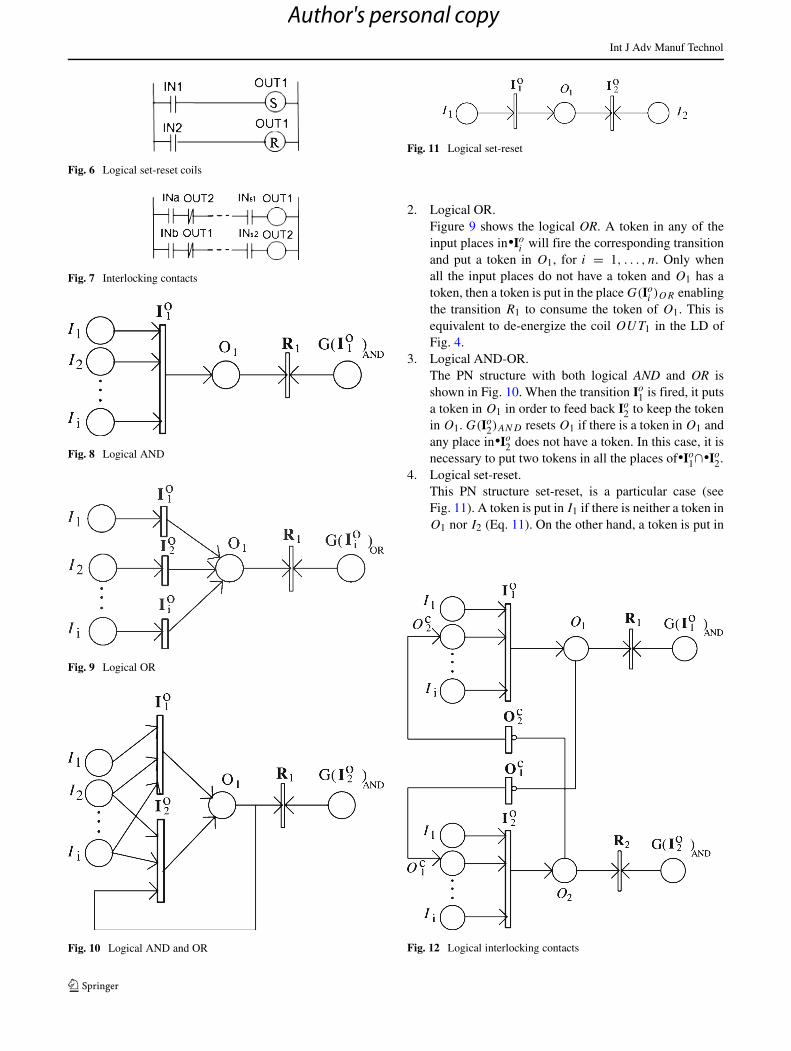
4. Logical set-reset coils.The logic of asynchronous signals is used as well in LDthrough coils called set and reset with the same address-ing. These coils need one or more control signals toenergize OUT1-S or de-energize it by means of OUT-Ras shown in Fig. 6.

5. Logical interlocking contacts.The interlock coils in control lines are widely used inLD. They are constructed by placing a contact of a coilin the control line of another one, as shown in Fig. 7.There, a contact of OUT1 is in the control line of thecoil OUT2 and vice versa.

With the elements of Table 2, the signals distributed inTable 3, and considering the Eqs. 3, 4, 5, and 6, five PNstructures are proposed below.

4.2 PN structures representing control lines of a LD

Initial marking of the PN structures is based on the typesof contacts in the LD, which are shown in Eq. 10. Theirdynamic markings describe the behavior of energized or de-energized coils.

M(Ii |Oo|Bb) ={

1, if it only has NO or NC contacts,

2, if it has NO and NC contacts.(10)

1. Logical AND.In Fig. 8, the transition Io1 is enabled when all its inputplaces have at least one token. The Io1 firing puts a mark-ing at place O1, which denotes the behavior in a scanof the LD. G(Io1)AND resets the place O1 if there is atoken in O1 and any place in �Io1 does not have a token.

Fig. 5 Serial and parallel contacts



Fig. 6 Logical set-reset coils

Fig. 7 Interlocking contacts

Fig. 8 Logical AND

Fig. 9 Logical OR

Fig. 10 Logical AND and OR

Fig. 11 Logical set-reset

2. Logical OR.Figure 9 shows the logical OR. A token in any of theinput places in �Ioi will fire the corresponding transitionand put a token in O1, for i = 1, . . . , n. Only whenall the input places do not have a token and O1 has atoken, then a token is put in the place G(Ioi )OR enablingthe transition R1 to consume the token of O1. This isequivalent to de-energize the coil OUT1 in the LD ofFig. 4.

3. Logical AND-OR.The PN structure with both logical AND and OR isshown in Fig. 10. When the transition Io1 is fired, it putsa token in O1 in order to feed back Io2 to keep the tokenin O1. G(Io2)AND resets O1 if there is a token in O1 andany place in �Io2 does not have a token. In this case, it isnecessary to put two tokens in all the places of �Io1∩ �Io2.

4. Logical set-reset.This PN structure set-reset, is a particular case (seeFig. 11). A token is put in I1 if there is neither a token inO1 nor I2 (Eq. 11). On the other hand, a token is put in

Fig. 12 Logical interlocking contacts



Table 4 Formal definition of LDPN

A LDPN is a 5-tuple , where:

P = {I ∪O ∪ B ∪ A} is a finite set of places, where:

I ={I1, I

c|o1 , I2, I

c|o2 , . . . , Ii , I

c|oi

}is a finite set of places representing physical input signals. Those places with the super-index c or o

identifies the places representing NC or NO contacts, respectively.

O ={O1,O

c|o1 ,O2,O

c|o2 , . . . ,Oo,O

c|oo

}is a finite set of places representing physical output signals.

B ={B1, B

c|o1 , B2, B

c|o2 , . . . , Bb, B

c|ob

}is a finite set of places representing internal memory signals.

A = {A1, A2, . . . , Aa} is a finite set of auxiliary places.

G = {G1,G2, . . . ,Gg

}is a finite set of places whose marking depends on Eqs. 5 and 6.

T = {Ic|o ∪ Oc|o ∪ Bc|o ∪ R

}is a finite set of transitions, where:

Ic|o ={

Ic|o1 , Ic|o2 , . . . , Ic|oi}

is a finite set of transitions representing physical inputs signals. The super-index c or o identifies the transitions

representing NC or NO contacts, respectively.

Oc|o ={

Oc|o1 ,Oc|o

2 , . . . ,Oc|oo

}is a finite set of transitions representing physical outputs signals.

Bc|o ={

Bc|o1 ,Bc|o

2 , . . . ,Bc|ob

}is a finite set of transitions representing internal memory signals.

R ={

Rc|o1 ,Rc|o

2 , . . . ,Rc|or

}is a finite set of transitions to reset places.

F ⊆ (P × T ) ∪ (T × P ) is a set of arcs,

W : F → {1} all arcs weights are equal to 1, and

M0 = P → {0, 1, 2} initial marking.

I2 if there is a token in O1 and there is not a token in I1

(Eq. 12).

M(I1) ={

1, if M(O1) = 0 AND M(I2) = 0

0, otherwise.(11)

M(I2) ={

1, if M(O1) = 1 AND M(I1) = 0

0, otherwise.(12)

5. Logical interlocking.The PN structure of the Fig. 12 represents the logicalinterlocking, which is composed of two logical ANDand each of them depends on the other one. In this struc-ture, the marking in Oc

2 depends directly on the markingin O2. This is analogous for Oc

1 and OUT1. The

transitions Oc1 and Oc

2 are enabled only when the corre-sponding output place O1 or O2 does not have a tokenbecause of the inhibitor arcs. Thus, the first marked out-put place disables the other one. The G(Io1)AND andG(Io2)AND places reset the output places O1 and O2,respectively.

With the previous LD analysis and the five PN logicalstructures proposed above, a formal definition of LDPN isgiven in next section.

4.3 Definition of LDPN

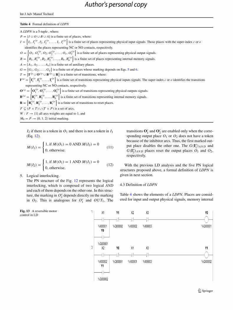
Table 4 shows the elements of a LDPN. Places are consid-ered for input and output physical signals, memory internal

Fig. 13 A reversible motorcontrol in LD



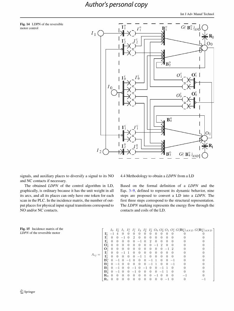
Fig. 14 LDPN of the reversiblemotor control

signals, and auxiliary places to diversify a signal to its NOand NC contacts if necessary.

The obtained LDPN of the control algorithm in LD,graphically, is ordinary because it has the unit weight in allits arcs, and all its places can only have one token for eachscan in the PLC. In the incidence matrix, the number of out-put places for physical input signal transitions correspond toNO and/or NC contacts.

4.4 Methodology to obtain a LDPN from a LD

Based on the formal definition of a LDPN and theEqs. 3–9, defined to represent its dynamic behavior, ninesteps are proposed to convert a LD into a LDPN. Thefirst three steps correspond to the structural representation.The LDPN marking represents the energy flow through thecontacts and coils of the LD.

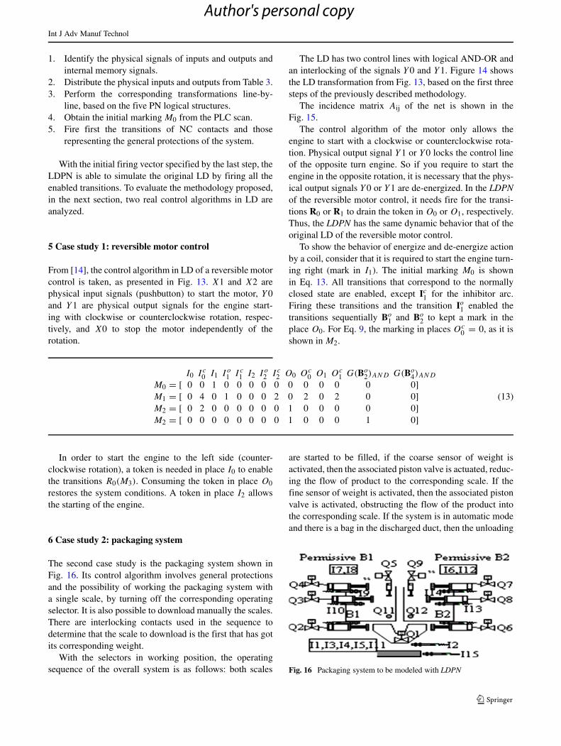
Fig. 15 Incidence matrix of theLDPN of the reversible motor



1. Identify the physical signals of inputs and outputs andinternal memory signals.

2. Distribute the physical inputs and outputs from Table 3.3. Perform the corresponding transformations line-by-

line, based on the five PN logical structures.4. Obtain the initial marking M0 from the PLC scan.5. Fire first the transitions of NC contacts and those

representing the general protections of the system.

With the initial firing vector specified by the last step, theLDPN is able to simulate the original LD by firing all theenabled transitions. To evaluate the methodology proposed,in the next section, two real control algorithms in LD areanalyzed.

5 Case study 1: reversible motor control

From [14], the control algorithm in LD of a reversible motorcontrol is taken, as presented in Fig. 13. X1 and X2 arephysical input signals (pushbutton) to start the motor, Y0and Y1 are physical output signals for the engine start-ing with clockwise or counterclockwise rotation, respec-tively, and X0 to stop the motor independently of therotation.

The LD has two control lines with logical AND-OR andan interlocking of the signals Y0 and Y1. Figure 14 showsthe LD transformation from Fig. 13, based on the first threesteps of the previously described methodology.

The incidence matrix Aij of the net is shown in theFig. 15.

The control algorithm of the motor only allows theengine to start with a clockwise or counterclockwise rota-tion. Physical output signal Y1 or Y0 locks the control lineof the opposite turn engine. So if you require to start theengine in the opposite rotation, it is necessary that the phys-ical output signals Y0 or Y1 are de-energized. In the LDPNof the reversible motor control, it needs fire for the transi-tions R0 or R1 to drain the token in O0 or O1, respectively.Thus, the LDPN has the same dynamic behavior that of theoriginal LD of the reversible motor control.

To show the behavior of energize and de-energize actionby a coil, consider that it is required to start the engine turn-ing right (mark in I1). The initial marking M0 is shownin Eq. 13. All transitions that correspond to the normallyclosed state are enabled, except Ic1 for the inhibitor arc.Firing these transitions and the transition Io1 enabled thetransitions sequentially Bo

1 and Bo2 to kept a mark in the

place O0. For Eq. 9, the marking in places Oc0 = 0, as it is

shown in M2.

I0 I c0 I1 I o1 I c1 I2 I o2 I c2 O0 Oc0 O1 Oc

1 G(Bo2)AND G(Bo

4)AND

M0 = [ 0 0 1 0 0 0 0 0 0 0 0 0 0 0]M1 = [ 0 4 0 1 0 0 0 2 0 2 0 2 0 0]M2 = [ 0 2 0 0 0 0 0 0 1 0 0 0 0 0]M2 = [ 0 0 0 0 0 0 0 0 1 0 0 0 1 0]

(13)

In order to start the engine to the left side (counter-clockwise rotation), a token is needed in place I0 to enablethe transitions R0(M3). Consuming the token in place O0

restores the system conditions. A token in place I2 allowsthe starting of the engine.

6 Case study 2: packaging system

The second case study is the packaging system shown inFig. 16. Its control algorithm involves general protectionsand the possibility of working the packaging system witha single scale, by turning off the corresponding operatingselector. It is also possible to download manually the scales.There are interlocking contacts used in the sequence todetermine that the scale to download is the first that has gotits corresponding weight.

With the selectors in working position, the operatingsequence of the overall system is as follows: both scales

are started to be filled, if the coarse sensor of weight isactivated, then the associated piston valve is actuated, reduc-ing the flow of product to the corresponding scale. If thefine sensor of weight is activated, then the associated pistonvalve is activated, obstructing the flow of the product intothe corresponding scale. If the system is in automatic modeand there is a bag in the discharged duct, then the unloading

Fig. 16 Packaging system to be modeled with LDPN



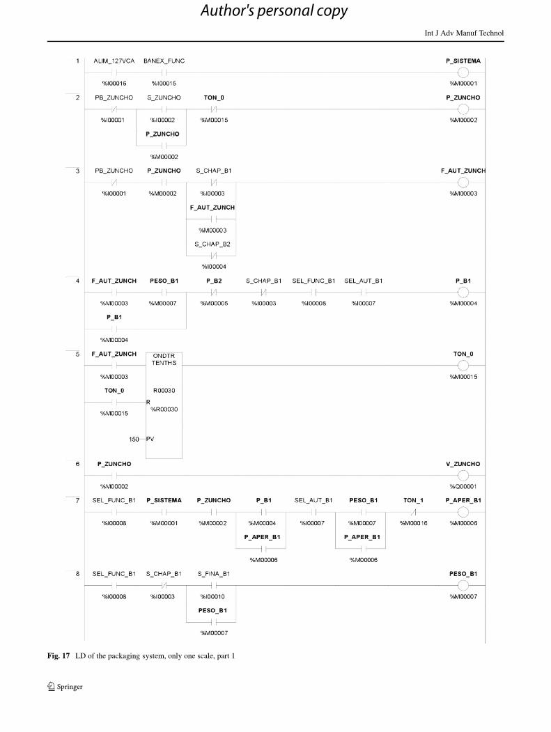
Fig. 17 LD of the packaging system, only one scale, part 1



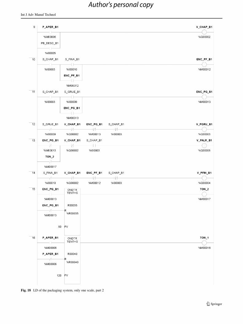
Fig. 18 LD of the packaging system, only one scale, part 2



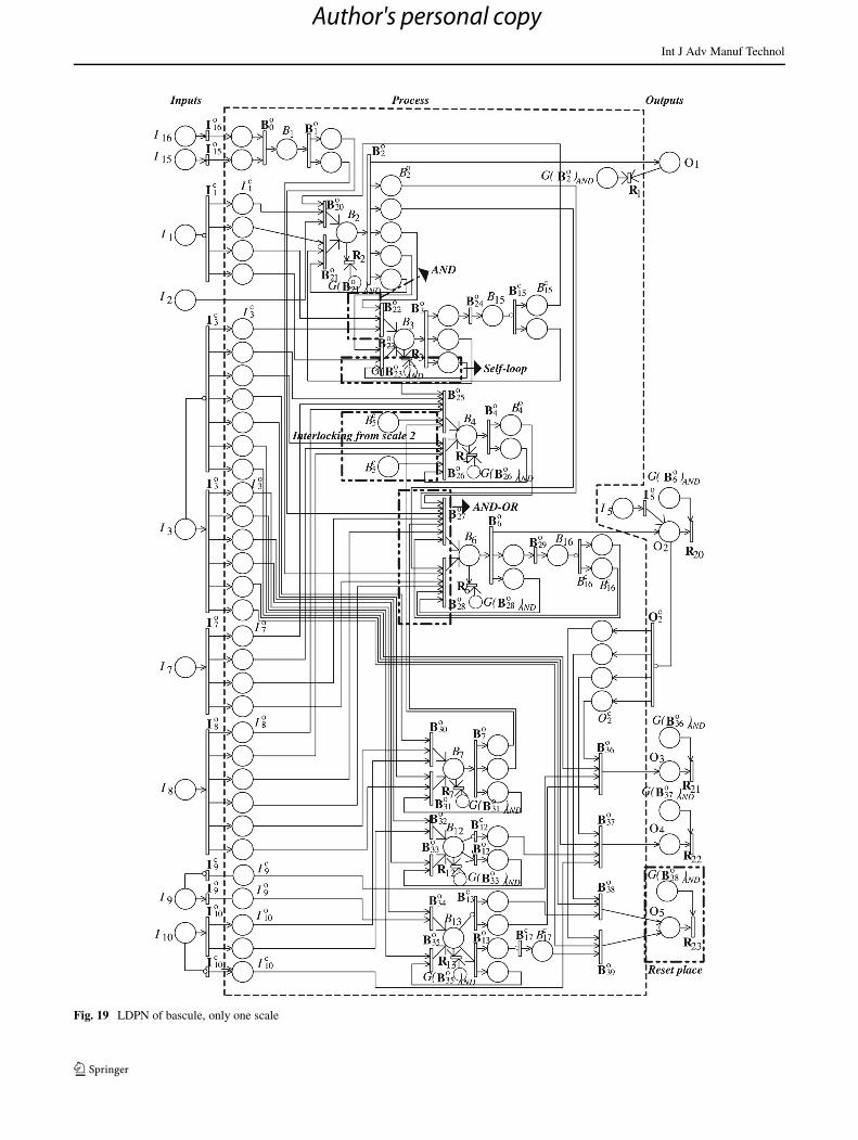
Fig. 19 LDPN of bascule, only one scale



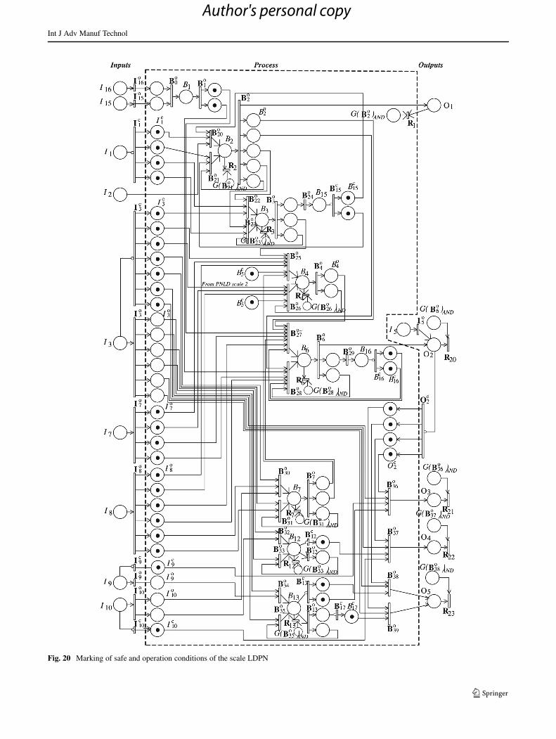
Fig. 20 Marking of safe and operation conditions of the scale LDPN



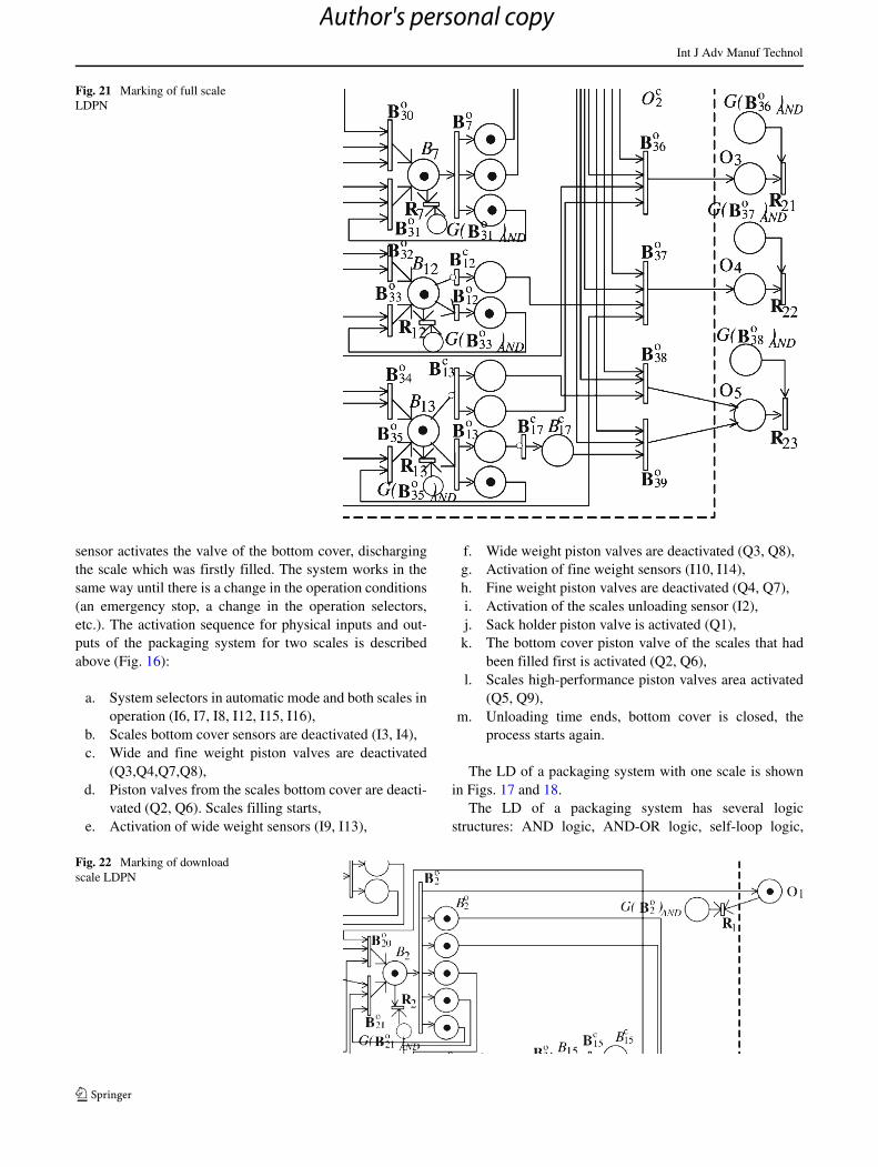
Fig. 21 Marking of full scaleLDPN

sensor activates the valve of the bottom cover, dischargingthe scale which was firstly filled. The system works in thesame way until there is a change in the operation conditions(an emergency stop, a change in the operation selectors,etc.). The activation sequence for physical inputs and out-puts of the packaging system for two scales is describedabove (Fig. 16):

a. System selectors in automatic mode and both scales inoperation (I6, I7, I8, I12, I15, I16),

b. Scales bottom cover sensors are deactivated (I3, I4),c. Wide and fine weight piston valves are deactivated

(Q3,Q4,Q7,Q8),d. Piston valves from the scales bottom cover are deacti-

vated (Q2, Q6). Scales filling starts,e. Activation of wide weight sensors (I9, I13),

f. Wide weight piston valves are deactivated (Q3, Q8),g. Activation of fine weight sensors (I10, I14),h. Fine weight piston valves are deactivated (Q4, Q7),i. Activation of the scales unloading sensor (I2),j. Sack holder piston valve is activated (Q1),k. The bottom cover piston valve of the scales that had

been filled first is activated (Q2, Q6),l. Scales high-performance piston valves area activated

(Q5, Q9),m. Unloading time ends, bottom cover is closed, the

process starts again.

The LD of a packaging system with one scale is shownin Figs. 17 and 18.

The LD of a packaging system has several logicstructures: AND logic, AND-OR logic, self-loop logic,

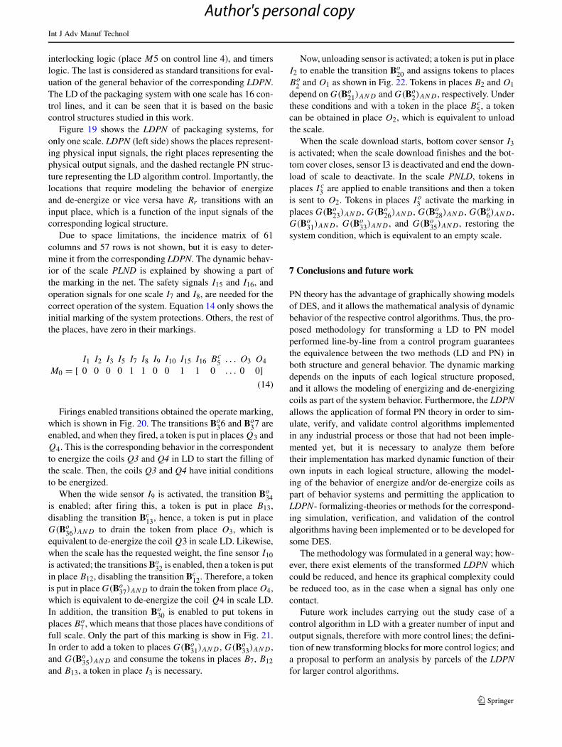
Fig. 22 Marking of downloadscale LDPN



interlocking logic (place M5 on control line 4), and timerslogic. The last is considered as standard transitions for eval-uation of the general behavior of the corresponding LDPN.The LD of the packaging system with one scale has 16 con-trol lines, and it can be seen that it is based on the basiccontrol structures studied in this work.

Figure 19 shows the LDPN of packaging systems, foronly one scale. LDPN (left side) shows the places represent-ing physical input signals, the right places representing thephysical output signals, and the dashed rectangle PN struc-ture representing the LD algorithm control. Importantly, thelocations that require modeling the behavior of energizeand de-energize or vice versa have Rr transitions with aninput place, which is a function of the input signals of thecorresponding logical structure.

Due to space limitations, the incidence matrix of 61columns and 57 rows is not shown, but it is easy to deter-mine it from the corresponding LDPN. The dynamic behav-ior of the scale PLND is explained by showing a part ofthe marking in the net. The safety signals I15 and I16, andoperation signals for one scale I7 and I8, are needed for thecorrect operation of the system. Equation 14 only shows theinitial marking of the system protections. Others, the rest ofthe places, have zero in their markings.

I1 I2 I3 I5 I7 I8 I9 I10 I15 I16 Bc5 . . . O3 O4

M0 = [ 0 0 0 0 1 1 0 0 1 1 0 . . . 0 0](14)

Firings enabled transitions obtained the operate marking,which is shown in Fig. 20. The transitions Bo

36 and Bo37 are

enabled, and when they fired, a token is put in places Q3 andQ4. This is the corresponding behavior in the correspondentto energize the coils Q3 and Q4 in LD to start the filling ofthe scale. Then, the coils Q3 and Q4 have initial conditionsto be energized.

When the wide sensor I9 is activated, the transition Bo34

is enabled; after firing this, a token is put in place B13,disabling the transition Bc

13, hence, a token is put in placeG(Bo

36)AND to drain the token from place O3, which isequivalent to de-energize the coil Q3 in scale LD. Likewise,when the scale has the requested weight, the fine sensor I10

is activated; the transitions Bo32 is enabled, then a token is put

in place B12, disabling the transition Bc12. Therefore, a token

is put in place G(Bo37)AND to drain the token from place O4,

which is equivalent to de-energize the coil Q4 in scale LD.In addition, the transition Bo

30 is enabled to put tokens inplaces Bo

7 , which means that those places have conditions offull scale. Only the part of this marking is show in Fig. 21.In order to add a token to places G(Bo

31)AND , G(Bo33)AND ,

and G(Bo35)AND and consume the tokens in places B7, B12

and B13, a token in place I3 is necessary.

Now, unloading sensor is activated; a token is put in placeI2 to enable the transition Bo

20 and assigns tokens to placesBo

2 and O1 as shown in Fig. 22. Tokens in places B2 and O1

depend on G(Bo21)AND and G(Bo

2)AND , respectively. Underthese conditions and with a token in the place Bc

5, a tokencan be obtained in place O2, which is equivalent to unloadthe scale.

When the scale download starts, bottom cover sensor I3

is activated; when the scale download finishes and the bot-tom cover closes, sensor I3 is deactivated and end the down-load of scale to deactivate. In the scale PNLD, tokens inplaces I c3 are applied to enable transitions and then a tokenis sent to O2. Tokens in places I o3 activate the marking inplaces G(Bo

23)AND , G(Bo26)AND , G(Bo

28)AND , G(Bo6)AND ,

G(Bo31)AND , G(Bo

33)AND , and G(Bo35)AND , restoring the

system condition, which is equivalent to an empty scale.

7 Conclusions and future work

PN theory has the advantage of graphically showing modelsof DES, and it allows the mathematical analysis of dynamicbehavior of the respective control algorithms. Thus, the pro-posed methodology for transforming a LD to PN modelperformed line-by-line from a control program guaranteesthe equivalence between the two methods (LD and PN) inboth structure and general behavior. The dynamic markingdepends on the inputs of each logical structure proposed,and it allows the modeling of energizing and de-energizingcoils as part of the system behavior. Furthermore, the LDPNallows the application of formal PN theory in order to sim-ulate, verify, and validate control algorithms implementedin any industrial process or those that had not been imple-mented yet, but it is necessary to analyze them beforetheir implementation has marked dynamic function of theirown inputs in each logical structure, allowing the model-ing of the behavior of energize and/or de-energize coils aspart of behavior systems and permitting the application toLDPN- formalizing-theories or methods for the correspond-ing simulation, verification, and validation of the controlalgorithms having been implemented or to be developed forsome DES.

The methodology was formulated in a general way; how-ever, there exist elements of the transformed LDPN whichcould be reduced, and hence its graphical complexity couldbe reduced too, as in the case when a signal has only onecontact.

Future work includes carrying out the study case of acontrol algorithm in LD with a greater number of input andoutput signals, therefore with more control lines; the defini-tion of new transforming blocks for more control logics; anda proposal to perform an analysis by parcels of the LDPNfor larger control algorithms.



References

1. International Electrotechnical Commision, IEC 61131–3 (2003)Programmable Controllers: Programming Languages, Interna-tional standard, segunda edicion

2. Murata T (1989) Petri nets: properties, analysis and applications.Proc IEEE 77(4):541,580

3. Lee J, Lee JS (2009) Conversion of ladder diagram to petri netusing module synthesis technique. Int J Model Simul 29(1):79–88

4. Thapa D, Dangol S, Wang G-N (2005) Transformation from petrinets model to programmable logic controller using one-to-onemapping technique. In: International conference on computationalintelligence for modelling, Control and automation, 2005 andinternational conference on intelligent agents, Web technologiesand internet commerce, vol 2, pp 228–233, 28–30

5. Peng SS, Zhou M-C (2004) Ladder diagram and Petri-net-baseddiscrete-event control design methods. IEEE Trans Syst ManCybern Part C Appl Rev 34(4):523,531

6. Lee J.-S., Hsu P.-L. (2004) An improved evaluation of ladderlogic diagrams and Petri nets for the sequence controller designin manufacturing systems. Int J Adv Manuf Technol 24:279–287

7. Zapata G, Carrasco E (2002) Estructuras Generalizadas para Con-troladores Logicos Modeladas mediante Redes de Petri. RevistaDyn 135:65–74

8. Tzafestas SG, Pantelelis MG, Kostis DL (2002) Design and imple-mentation of a logic controller using Petri nets and ladder logicdiagram. Syst Anal Model Simul Taylor Fancis 42(1):135–167

9. Korotkin S, Zaidner G, Cohen B, Ellenbogen A, Arad M, Cohen Y(2010) A Petri net formal design methodology for discrete-eventcontrol of industrial automated systems. In: 2010 IEEE 26th Con-vention of electrical and electronics engineers in israel (IEEEI),vol 17–20, pp 431–435

10. Valentin N, Mircea P, Ioan D, Aurel I (2011) Designing the controlof an electrical drive using Petri nets. 7th International symposiumon advanced topics in electrical engineering (ATEE)

11. da Silva Oliveira EA, da Silva LD, Gorgonio K, Perkusich A,Martins AF (2011) Obtaining formal models from ladder dia-grams. In: 2011 9th IEEE international conference on industrialinformatics (INDIN), vol 26–29, pp 796–801

12. Xuekum C, Lilian L, Pengfei Q (2012) Method for translatingladder diagram to ordinary Petri nets. 51st IEEE Conference onDecision and Control

13. International Electrotechnical Commision, IEC 61131–8 (2003):Programmable controllers: guidelines for the application andimplementation of programming languages, International stan-dard, segunda edicion

14. Zhang H, Jiang Y, Hung WN, Yang G, Gu M, Sun J (2012)New strategies for reliability analysis of programmable logiccontrollers. Math Comput Model 55(7/8):1916–1931


Documents

Formal design methodology for transforming ladder diagram to Petri nets