Hybrid Functional Petri Nets as MP systems

Hybrid Functional Petri Nets as MP systems

Alberto Castellini Æ Giuditta Franco Æ Vincenzo Manca

Published online: 11 February 2009� Springer Science+Business Media B.V. 2009

Abstract In this work we give a formalization of Hybrid Functional Petri Nets, shortly

HFPN, an extension of Petri Nets for biopathways modelling, and we compare them with

Metabolic P Systems. An introduction to both the formalisms is given, together with

highlights about respective similarities and differences. Their equivalence is thus proved

by means of a theorem which holds under quite general hypotheses. The case study of the

lac operon gene regulatory mechanism in the glycolytic pathway of Escherichia coli is

modeled by an MP system which provides the same dynamics of an equivalent HFPN

model.

Keywords Membrane computing � P systems � Petri Nets � Hybrid Functional Petri Nets �Systems biology � Synthetic biology � Biological system modeling � Computational

experiments � Glycolytic pathway � Simulation � Forecasting � Equivalence �Mapping procedure

1 Introduction

Several mathematical formalisms have been proposed to model biological systems, even to

overcome some limitations of the traditional methods based on Ordinary Differential

Equations (ODE).

A few interesting approaches, alternative to ODE, are based on rewriting systems, in the

context of formal language theory, where biochemical elements correspond to symbols

from a given alphabet and chemical reactions are represented by rewriting of commutative

strings (also called multisets). In particular, Membrane systems, also called P systems

A. Castellini (&) � G. Franco � V. MancaComputer Science Department, Verona University, Strada Le Grazie 15, Verona 37134, Italye-mail: [email protected]

G. Francoe-mail: [email protected]

V. Mancae-mail: [email protected]

123

Nat Comput (2010) 9:61–81DOI 10.1007/s11047-009-9121-4

(Paun 2000, 2002), provide a novel computational model inspired by the prominent role

played by membranes in living cells (Alberts et al. 2002). Since the first definition of P

system evolution strategy assumes a non-deterministic and maximally parallel application

of the rules (Paun 2000), which is not very meaningful within the context of bio-systems

dynamics computation (Manca 2008), many variants of this formalism were proposed

(Ciobanu et al. 2006). A class of P systems that proved to be significant and successful to

model dynamics of biological phenomena has been given by Metabolic P systems, also

called MP systems (Manca 2006; Manca et al. 2005). Their evolution is computed by a

deterministic algorithm called metabolic algorithm (Bianco et al. 2006a, b; Manca 2008b;

Manca and Bianco 2008), based on the mass partition principle which defines the trans-

formation rate of object populations according to a suitable generalization of chemical

laws. In this paper we deal with MP systems whose evolution is computed by fluxes

(Manca 2008a), and with MP graphs, a graphical representation of MP systems (Manca

2008b) also employed by MetaPlab, which is a Java tool computing MP system dynamics

(Bianco and Castellini 2007; Bianco et al. 2006; Castellini and Manca 2009).

A series of significant processes modeled by MP systems include the Belousov–

Zhabotinsky reaction (in the Brusselator formulation) (Bianco et al. 2006a, b), the Lotka–

Volterra dynamics (Bianco et al. 2006a; Fontana and Manca 2008; Manca et al. 2005), the

SIR (Susceptible-Infected-Recovered) epidemic (Bianco et al. 2006a, b), the circadian

rhythms and the mitotic cycles in early amphibian embryos (Manca and Bianco 2008).

Petri Nets were introduced in 1962 by Carl Adam Petri (Petri 1962) as logic circuits to

describe concurrency in artificial systems (i.e., operative systems or event-driven systems)

(Reisig 1985). They have been recently employed to model biological pathways (Hofestadt

and Thelen 1998; Reddy et al. 1993) and in particular metabolic processes (Hofestadt

1994). The recent development of MP systems theory, based on fluxes, shows deep sim-

ilarities with a novel Petri Nets extension, named Hybrid Functional Petri Nets (HFPN)

(Matsuno et al. 2003), introduced to overcome the drawbacks of its traditional model for

the biopathways simulation. A software has also been developed to compute biological

simulation by HFPN (Doi et al. 2004; Nagasaki et al. 2004).1

This paper focuses on a thorough comparison between the formalism of MP systems

and that of HFPN, in order to highlight similarities and differences as well as feasibilities

to model biochemical systems. A first investigation about this comparison can be found in

(Castellini et al. 2009). Some basic principles of MP systems and MP graphs are intro-

duced in the next Sect. 2, followed by a formal description of the HFPN graphical model in

Sect. 3. Section 4 and 5, respectively show the equivalence between the two formalisms

and point out two mapping procedures (from one to the other and vice versa), that suc-

cessfully worked for modeling and simulating the lac operon gene regulatory mechanism

and glycolytic pathway. In the conclusions, our results are finally related to the equivalence

between MP models and differential models.

2 MP systems

MP systems are deterministic P systems developed to model dynamics of biological

phenomena related to metabolism and signaling transduction in the living cell. Transitions

between states are calculated by suitably partitioning the available amount of each sub-

stance among all reactions which need to consume it.

1 The Cell IllustratorTM

Project website Url: http://www.genomicobject.net.

62 A. Castellini et al.

123

http://www.genomicobject.net

The notion of MP system we consider here is essentially that one given in (Manca 2008a).

Given a biological process of interest, all its variables can be split in two different kinds

(introduced by item 1 and item 2 of Definition 1): chemical substances, which have a mass

and transform according to the mass conservation principle, and other parameter elements,

with no mass (e.g., light, volume), that provide some observed values or evolve according to

some specific laws. Substances are measured by (conventional) moles, which correspond to

suitable population units. For each substance, the mass of a mole specifies the matter quantity

(in terms of some mass unit) associated to a mole of the substance. The biochemical reactions

of the process are seen as rewriting rules. The observation time interval (s, in item 5) is

established on the basis of either the kind of process or the kind of study in which one is

interested; for example, faster biological processes require shorter time intervals. An

important aspect of MP systems is constituted by the Log-gain theory (Manca 2008b) which

provides a method for deducing MP models of given biological dynamics.

Definition 1 (MP system) An MP system is a construct (Manca 2008a)

M ¼ ðX;V;R;Q; s; q0;U;H; m; rÞ

where:

(1) X = {x1, x2,…,xn} is a finite set of n substances (the types of molecules).

Sometimes, when the context avoids any possible confusion, a symbol x for a

substance represents also the quantity associated to x in the current state;

(2) V = {v1, v2,…,vk} is a finite set of k parameters (systems variables, i.e.,

temperature, pressure, etc.);

(3) R = {r1, r2 ,…,rm} is a set of m reactions over X. A reaction r is represented in the

arrow notation by a rewriting rule ar ! br with ar, br strings over X. The

stoichiometric matrix A; of dimension n� m; stores reactions stoichiometry, that is,

A ¼ ðax;r j x 2 X; r 2 RÞ where ax;r ¼ jbrjx � jarjx; and jcjx is the number of

occurrences of the symbol x in the string c;

(4) Q is the set of states, that is, the functions q : X [ V ! R from substances and

parameters to real numbers. If we assume some implicit orderings among the

elements of X and V, and an observation instant i ranging in the set of natural

numbers for each function q, the state q at the instant i can be identified as a vector

qi = (x1[i], x2[i],…,v1[i], v2[i],…) of real numbers, shortly denoted by qi = (X[i],V[i]), constituted by the values which are assigned, by the state q, to the elements of

these sets;

(5) s is the temporal interval between two consecutive states;

(6) q0 [ Q is the initial state, that is, (X[0], V[0]) = q0;

(7) U is a set of regulation functions ur one-to-one associated to each rule r [ R. These

functions specify the evolution of the substances according to the following system

of autonomous first-order difference equations, where X[i] and V[i] are, respec-

tively, the vectors of substance quantities and parameter values at step i, the vector

U = (u1[i], u2[i],…,um[i]) of fluxes at step i is computed by the Eq. 2, 9, ? are the

usual matrix product and vector sum, and the key role of functions U becomes

apparent:

U½i� ¼ UðX½i�;V½i�Þ ð1Þ

X½iþ 1� ¼ A � U½i� þ X½i� ð2Þ

Hybrid Functional Petri Nets as MP systems 63

123

(8) H ¼ fh1; h2; . . .; hjVjg is a set of functions regulating the fluctuation of the

parameters, along with the following equation:

V ½iþ 1� ¼ HðV½i�;X½i�Þ ð3Þ

Eqs. 2 and 3 constitute the metabolic algorithm;

(9) m is a natural number which specifies the number of molecules of a (conventional)

mole of M, as population unit of M;

(10) r is a function which assigns to each x [ X, the mass r(x) of a mole of x (with

respect to some measure unit).

MP graphs, introduced in (Manca and Bianco 2008), are a natural representation of

biochemical reactions as graphs with two levels: the first level describes the stoichiometryof reactions, while the second level expresses the regulation, which tunes the flux of every

reaction (i.e., the quantity of chemicals transformed at each step) depending on the state of

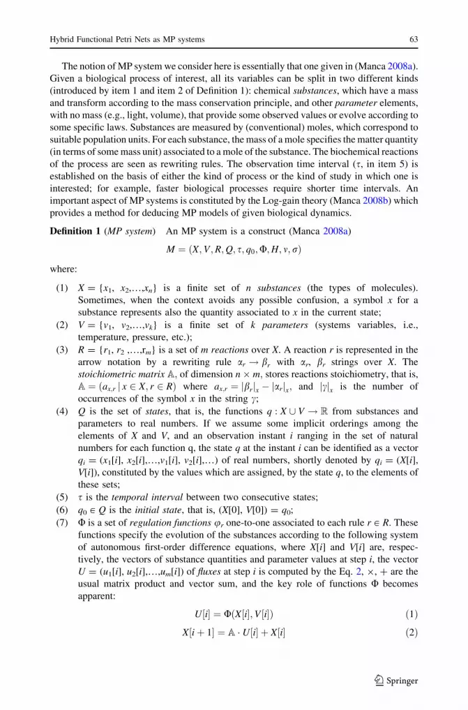
the system. Figure 1 shows a simple example of MP graph containing most of the graphical

elements of the formalism. It has three substances nodes pictured by the elliptical nodes A,

B and C. Reaction (circular) nodes R1, R2 and R4, connected with input and output gates

(the triangles), represent, respectively, the entrance of substances A and B into the system

and the degradation of substance C, while reaction node R3 represents the chemical rule

AB! CC: In general, these kinds of nodes act as hubs for all the substance nodes involved

in a reaction (reactants and products), and each of these nodes has an input dashed arrow

from the only flux (rounded corner rectangular) node that regulates it. The MP system

depicted in Fig. 1 has the Pressure as an only parameter. The (rectangular) node Pressurerepresents a physical parameter whose value evolves with a quadratical law of the sub-

stance C. Finally, the isolated node represents the organism: it contains the organism name

(‘‘Test organism’’), the molar unit m of the MP system, its time unit s, some system

constants and an additional organism description. Reaction regulations are computed in the

flux nodes by means of algebraic formulae.

Fig. 1 An MP graph toy example. In each oval node representing a substance, the concentration labelcorresponds to the substance quantity and the M.weights label represents the reactant molar mass r(x). Anenlarged version of this picture is published at the web page21

2 Enlarged images Url: http://mplab.sci.univr.it/external/ncj_hfpn_as_mps/images.html.


123

http://mplab.sci.univr.it/external/ncj_hfpn_as_mps/images.html

The graphical user interface (GUI) used for drawing the MP graph of Fig. 1 is part of

the simulator MetaPlab (Bianco and Castellini 2007; Castellini and Manca 2009), a

software tool developed to provide modelers, as well as biologists, with a reliable and easy-

to-use simulation environment for computing systems dynamics. The last release of the

software MetaPlab is available on the MetaPlab website.3

3 Hybrid Functional Petri Nets: a formalization

A Petri Net (Petri 1962; Reisig 1985) is a network mainly consisting of four kinds of

elements: (i) places, (ii) transitions, (iii) arcs, (iv) tokens (see Fig. 2). According to the

traditional notation, a placePc can hold a nonnegative integer number of tokens mc as its

content. The amount of tokens in all places identifies the state of a Petri Net. Transitions

(e.g., T in Fig. 2) are elements equipped with firing rules specified by: (i) the arcs con-

necting the places, (ii) the number of tokens (expressed as arc labels) to move from input to

output places, and (iii) the speed of the token transition.

Hybrid Functional Petri Nets (Matsuno et al. 2003) extend traditional Petri Nets by

introducing continuous places and transitions, and adding special arcs, to overcome Petri

Net drawbacks in modelling biopathways. Figure 3 shows in detail the main elements of

this model, which are basically: (i) the discrete places and transitions inherited by the

traditional formalism, (ii) the continuous places and transitions, and (iii) three kinds of

arcs to connect places and transitions. Namely, a discrete (continuous) normal input arc

has an integer (real) label, which states a strict lower bound for the place amount that

causes the transition activation; a discrete (continuous) inhibitory input arc has an integer

(real) label, which states an upper bound of the place amount, that causes the transition

activation but it does not remove any token; a discrete (continuous) test arc works as a

normal input arc but it does not remove any token from the input place.

HFPN discrete components have been employed for pathways regulatory mechanisms

modelling in glycolytic pathway simulation (Doi et al. 2004 and in circadian rhythms of

Drosophila simulation (Matsuno et al. 2003). In fact, transcription switches, feedbacks and

promotion/inhibition mechanisms can intuitively be modeled by discrete elements that can

namely stand for DNA binding sites or trigger conditions.

Fig. 2 A simple Petri Net (Matsuno et al. 2003): P1 and P2 are input places and P3 is an output place of thetransition T; m1, m2 and m3 are the amount of tokens held by P1, P2, and P3; the arc labels 2, 3, 1 state that Tcan fire if m1 C 2 and m2 C 3, by removing two tokens from P1 and three from P2 and adding one token toP3. The firing speed is assumed to be constant and the label 1.0 under the transition symbol means that Tmust wait 1.0 step before firing

3 The MetaPlab website Url: http://mplab.sci.univr.it.


123

http://mplab.sci.univr.it

In general (Matsuno et al. 2003), a (continuous or discrete) transition T specifies three

functions (on the right side of Fig. 3):

– the firing condition given by a predicate c(m1(i),…,mn(i)) (if T is continuous, as long as

this condition is true T fires continuously; if T is discrete, whenever the condition is true

T gets ready to fire),

– a nonnegative function fjðm1ðiÞ; . . .;mnðiÞÞ for each input arc aj, called consumptionfiring speed which states the (real, integer) number of tokens removed by firing from Pj

through arc aj,

– a nonnegative (continuous, or integer) function gjðm1ðiÞ; . . .;mnðiÞÞ called productionfiring speed for each output arc bj, that specifies the number of tokens added by firing to

Qj through arc bj.

If aj is a test or an inhibitory input arc, then we assume fj : 0 and no amount of tokens

is removed from Pj through the input arc aj.

Moreover, for discrete transitions, the delay function is given by a nonnegative integer

valued function d(m1(i),…,mn(i)). If the firing condition gets satisfied at time i, the cor-

responding transition acquires the chance of firing after a number of steps equal to its delay

d(m1(i),…,mn(i)). The transition actually fires if and only if the firing condition does not

change during the delay time.

A time unit is assumed, called Petri time, in terms of which the firing speeds and the

discrete transition delays (waiting time before firing) are given. In the case that simulation

granularity must be increased, a fraction of Petri time named sampling interval is considered.

An interesting difference between discrete and continuous transitions is the firing

policy. A discrete transition moves the expected amount of tokens (equal to the firing speed

value) in only one step of the sampling interval, while the continuous transition moves it in

one Petri time unit, though step by step with respect to the sampling interval.

The following definition outlines the mathematical structure of HFPN.

Definition 2 (HFPN) An HFPN is a construct

N ¼ ðP; T1; T2; I;E; S; s0;Pt; SI;D;C;F;GÞ

where:

(1) P = {p1,…,pn} is a finite set of discrete or continuous places;

Fig. 3 On the left, the basic elements of HFPN (Matsuno et al. 2003). Only normal arcs are able to movetokens, and their labels represent strict lower bound conditions for the transition firing. Inhibitory and testarcs represent respectively upper bound and lower bound conditions that must be satisfied for the transitionfiring. On the right, an HFPN continuous transition TC (Matsuno et al. 2003). P1, P2, P4, Q1, Q2 arecontinuous places, P3 is a discrete place; m1, m2, m3, m4, n1 and n2 represent the content of the correspondingplaces. Labels a2, a3 denote test arcs, the other are normal arcs


123

(2) T1 = {t1,…,tk} and T2 = {tk?1,…,tz} are finite sets of continuous and discretetransitions, respectively, where T1 \ T2 ¼ ; and we define T ¼ T1 [ T2;

(3) I � P � T and E � T � P are, respectively, the normal input arcs and the output arcsof the transitions, given by the stoichiometry of the modeled system;

(4) S is the set of states, that are functions s from the places of P to real numbers. If we

assume some order among the elements of P, and an instant i ranging in the set of

natural numbers, then the state s at the time i can be identified as the real vector

si = (m1(i), m2(i),…,mn(i)), also denoted by P[i];

(5) s0 [ S is the initial state, that is, s0 = (m1(0), m2(0),…,mn(0));

(6) Pt is the time unit of the model (related to that one of the modeled real system),

called Petri time, whereas SI is the sampling interval, which represents the number

of petri times between two computational steps;

(7) D = {dk?1,…,dz} is a finite set of delays, given by nonnegative functions dj : S! N

which specify the time that the corresponding discrete transition tj must wait before

firing;

(8) C = {c1,…,cz} is a set of firing conditions, given by boolean functions on the states

cj : S! f0; 1g which control the activation of the corresponding transition tj;

(9) F ¼ ff1; . . .; fjIjg is a set of consumption firing speeds, given by non-negative

functions fx : S! R; where x ¼ ðpc; tjÞ; c ¼ 1; . . .; n; j ¼ 1; . . .; z; that specify the

quantity which the transition tj can remove from the place pc for each state s. For all

x = (pc, tj) in which pc is a discrete place, we have fx : S! N;(10) G ¼ fg1; . . .; gjEjg is a set of production firing speeds, given by non-negative

functions gy : S! R; where y ¼ ðtj; pcÞ; c ¼ 1; . . .; n; j ¼ 1; . . .; z; that specify the

quantity which the transition tj can add to the place pc for each state s. For all y =

(tj, pc) in which pc is a discrete place, we have gy : S! N:

Given an HFPN system N = (P, T1, T2, I, E, S, s0,Pt, SI, D, C, F, G), the algorithm

presented in Table 1 computes the first h consecutive states, for h 2 N; according to the

following strategy.

As a first computational step, the algorithm initializes the functions lj for all the discrete

transitions tj (instructions 2 and 3). These functions are initially defined by the algorithm to

control the waiting of discrete transition delays, their null value corresponds to a positive

delay in the initial state.

In order to compute the state P[h] of the HFPN system, it is necessary to check how the

discrete transitions behave in the previous states of the system. In fact, each of them can be

waiting either for its condition to be true, or for the delay to pass in order to fire, or it can

be ready to fire. This information is kept by the function lj for each discrete transition tj,then all the values ljð1Þ; ljð2Þ; . . .; ljðh� 1Þ need to be computed, and consequently all the

states P½1�;P½2�; . . .;P½h� 1�: For each of the instants 1; . . .; h� 1 (instruction 4), the state

P[i ? 1] is initialized by the current state P[i] (instruction 5), and then processed by the

firings as in the following.

There are two main for cycles (instructions 6 and 13): the first one controls the

application of the continuous transitions (from T1) and the second one controls the

application of the discrete transitions (from T2) which are equipped with delay functions.

By the first of these for cycles (instructions 6–12), each continuous transition with true

condition fires, and the contents of the involved places are consequently modified (by

instructions 11 and 12). The content of each place connected to the continuous transition


123

by an arc of I decreases of fx(P[i]) � SI (instruction 11). The content of each place con-

nected to the continuous transition by an arc of E increases of gy(P[i]) � SI (instruction 12).

In the last for cycles (instructions 13–27), the firing of discrete transitions tj is ruled

firstly by the value of a corresponding function lj (instructions 14 and 19) and secondarily

by the boolean value of the corresponding condition cj (instructions 15 and 20). If a

transition tj has a null delay function, its function lj is identically equal to 1 (instruction 27).

Table 1 HFPN Algorithm tocompute the first h consecutivestates of N

HFPN-Evolution(N,h)

1. begin

2. for j = k ? 1,…,z do // tj [ T2

3. if dj(P[0]) = 0 then lj(0) = 1 else lj(0) = 0;

od

4. for i = 0,…,h-1 do

5. for c = 1,…,n do mc(i ? 1) := mc(i); od

6. for j = 1,…,k do // tj [ T1

7. if cj(P[i]) = 1 then

8. for c = 1,…,n do

9. x := (pc, tj);

10. y := (tj, pc);

11. if x [ I then mc(i ? 1) := mc(i ? 1) - fx(P[i]) � SI;

12. if y [ E then mc(i ? 1) := mc(i ? 1) ? gy(P[i]) � SI;

od

od

13. for j = k ? 1,…,z do // tj [ T2

14. if lj(i) = 0 then

15. if cj(P[i]) = 1 then ljðiþ djðP½i�ÞSI � 1Þ :¼ 1;

16. for k ¼ 1; . . .;djðP½i�Þ

SI � 2 do

17. lj(i ? k) := 2;

od

18. else lj(i ? 1) := 0;

19. if lj(i) = 1 then // tj is ready to fire

20. if cj(P[i]) := 1 then //firing

21. for c = 1,…,n do

22. x := (pc, tj);

23. y := (tj, pc);

24. if x [ I then mc(i ? 1) := mc(i ? 1)-fx(P[i]);

25. if y [ E then mc(i ? 1) := mc(i ? 1) ? gy(P[i]);

od

26. if dj(P[i]) [ 0 then lj(i ? 1) := 0;

27. else lj(i ? 1) := 1;

od

28. write ðm1ðiþ 1Þ;m2ðiþ 1Þ; . . .;mnðiþ 1ÞÞod

29. end


123

In the case of delay dj (P[i]) greater than zero, lj (instruction 14) has value 0 (initially

and) whenever the transition has just fired and until the condition cj is not true. As soon as

the condition is true (instruction 15), the function lj is set to 2 (instruction 17) for each time

of the next dj steps, and it is set to 1 (instruction 15) at the time the transition will be ready

to fire (after the delay). Then, the transition fires only if the condition is true (instruction

20). At this point the function lj is set to 0 (denoting that the transition is waiting for the

condition to be true).

HFPN is an intrinsically parallel model which assumes the simultaneous firing of all the

transitions that can fire in every computational step. The algorithm presented in Table 1,

however, sequentially obtains an equivalent evolution of the system if, for every step, the

quantity of tokens contained in each place pc is greater than or equal to the sum of the

quantities actually taken from that place. This is an assumption considered more or less

explicitly in all the HFPN literature.

We want to remark the complex structure of the algorithm with respect to the simplicity

of the finite difference system which computes the MP dynamics (Eq. 2). This aspect is not

only a matter of elegance. In fact, within the framework of MP systems, a theory was

developed (Manca 2008b) which allows us to define an MP model of an observed

dynamics. The key point of this theory is the discovery of flux regulation maps by means of

suitable algebraic manipulations of time series of observed states.

4 Equivalence between MP systems and HFPN

MP systems and HFPN have been both developed for biological dynamics modelling, but

they have a very different theoretical background. Both the formalisms are mainly based

on (i) reactant elements (substances and places), (ii) rules (reactions and transitions) that

state how the substances can interact with each other, and (iii) dynamics elements (fluxesand firing speeds/conditions) that control the system evolution by computing the amount

of substances moved in the network at each computational step. Nevertheless, in order to

model biological processes, the firing speeds fðpc; tjÞ and gðtj ; pcÞ have to be linked to

transitions rather than to arcs. This argument has been confirmed also by the analysis of

some HFPN models and by the test of an HFPN simulator called Cell IllustratorTM

(Nagasaki et al. 2004; see footnote 1). Hence, we can assume arc firing speeds fj to have

this form:

fðpc;tjÞðsiÞ ¼ �fjðsiÞ � wc; j and gðtj;pcÞðsiÞ ¼ �fjðsiÞ � wc; j ð4Þ

where wc; j 2 N; c ¼ 1; . . .; jPj; j ¼ 1; . . .; jT j: In (4), �fj denotes a function common to the

consumption and production firing speeds of the transition tj, while wc, j represents the

weight of the arc (pc,tj) or (tj, pc). Now we are ready to define a couple of mappings

from one formalism to the other, providing an equivalence for their respective

dynamics.

4.1 Mapping HFPN to MP systems

The following mapping associates to a given HFPN N = (P, T1, T2, I, E, S, s0, Pt, SI, D, C,

F, G) an MP system M(N) = (X, V, R, Q, s, q0, U, H, m, r) that will be proved to be

dynamically equivalent to N.


123

HFPN-to-MP mapping procedure

(1) X = P. Places p1,…,pn of N are one to one mapped into substances x1 ,…,xn of M;

(2) V = {v1,…,vz-k}. Elements of T2 (discrete transitions tj) are mapped into parameters

(vj - k), having initial values related to the corresponding delays from D and evolving

according to the functions in H (see below);

(3) R = T. Transitions of N are mapped into reactions of M. Stoichiometric matrix A is

generated according to Eq. 4, because firing speeds can be related to transitions rather

than to arcs. In this way, every weight wc, j of a consumption firing speed fðpc;tjÞ ¼�fj � wc; j (see Eq. 4) generates the element ac, j = -wc, jof the stoichiometric matrix A;while every weight wc, j of a production firing speed gðtj;pcÞ ¼ �fj � wc;j generates the

element ac,j = wc, j;

(4) Q ¼ fq j q : X [ V ! R; qjX 2 Sg where q|X is the restriction of q to the set X;

(5) The time interval s is the time between two computational steps of N, that is

s := SI 9 Pt;(6) q0 = (s0, V[0]), denoting the juxtaposition of the vectors s0 and V[0], where s0 is the

initial state of N and V½0� ¼ dkþ1ðs0ÞSI � 1; . . .; dzðs0Þ

SI � 1� �

; with dkþ1; . . .; dz 2 D;

(7) U ¼ fu1; . . .;uk;ukþ1; . . .;uzg: Regulation functions are deduced from T which has kcontinuous transitions and z - k discrete transitions. They are defined as ujðqÞ ¼cjðqÞ � �fjðqÞ � SI for j [ {1,…,k} and as ujðqÞ ¼ ðcjðqÞ ^ qðvj�kÞ� 0Þ � �fjðqÞ for j[ {k ? 1,…,z}, where q [ Q, and �fj is deduced according to Eq. 4. Boolean values

have been mapped to integer numbers 0 (true) and 1 (false);

(8) H = {h1,…,hz-k}. Each function hj controls the evolution of the parameter vj as a

‘‘counter of waiting’’, set by the delay dj?k [ D, which supports the simulation of the

discrete transition tj?k. Functions H can be defined as:

hjðqÞ ¼ ðqðvjÞ� 0ÞðdjðqÞ=SI � 1Þ þ ððcjðqÞ ^ qðvjÞ ¼ djðqÞ=SI � 1Þ_ ð0\qðvjÞ\djðqÞ=SI � 1ÞÞðqðvjÞ � 1Þ

where the first term of the sum reinitializes the counter vj to dj(q)/SI - 1 if q(vj) B 0,

while the second term decreases the counter by one if either it is equal to dj(q)/SI - 1

and the condition cj(q) is true, or the counter value is between 0 and dj(q)/SI - 1. The

initial value dj(q)/SI - 1 corresponds to the number of steps that M performs during

the time interval dj(q);

(9) The value m and the mass function r of M are chosen with respect to the modeled

system; indeed they do not have any corresponding component in N. They work as

biological data measurements and they do not affect the system dynamics.

Finally, we notice that HFPN model defines a delay value for each discrete transition

while MP systems can simulate the delays by using parameters. Actually, the delays do

not have a biological counterpart in the real systems, and they are just computational

tricks to describe some complex low-level processes (which needs a particular time

interval to be performed) as black-boxes that return particular outputs after a delay

time.

Both MP systems and HFPN dynamics are characterized by the temporal evolution

of quantities that represent significant entities of the biological systems of interest.

Therefore, to compare the two formalisms we consider the evolution of quantities

related to substances and parameters in the MP systems, and related to places in the

HFPN.


123

Theorem 1 (HFPN to MP) Given an HFPN N = (P, T1, T2, I, E, S, s0, Pt, SI, D, C, F, G),

the MP system M(N) = (X, V, R, Q, s, q0, U, H, m, r) obtained by applying the HFPN-to-MP mapping procedure has the same time evolution of N.

Proof For every (discrete or continuous) place pc of P in N (with c ranging from 1 to n) there

exists a corresponding substance xc of X in M, such that, the content of pc is equal to the value

of xc for every instant, that is, mcðiÞ ¼ xcðiÞ 8i 2 N: The proof is given by induction on the

computational step i. The evolution of N is computed by the HFPN algorithm reported in

Table 1 while Eqs. 2 and 3 compute the evolution of M. Since discrete places of N evolve only

by discrete transitions (instructions 6–12 of the HFPN algorithm) and continuous places

evolve by both discrete and continuous transitions (instructions 6–27), we analyze the two

cases separately, while the base of the induction is common to the two cases.

4.1.1 Base

The HFPN-to-MP mapping procedure states that q0 = (s0, V[0]). As a consequence, for

every c ¼ 1; . . .; jPj we have xc[0] = mc(0).

4.1.2 Inductive step for discrete places

The content of a discrete place pc is modified only by discrete transitions (instructions

13–27 of the HFPN algorithm). Instruction 5 assigns mc(i) to each c-th component of the

state at the instant i ? 1, and instructions 24–25 update mc(i ? 1) for every input or output

transition tj related to pc, that satisfies both the conditions lj(i) = 1 (instruction 19) and

cjðsiÞ ¼ 1 (instruction 20). In particular, the quantity fxðsiÞ is removed from mc(i ? 1) for

every output arc x of pc, while the amount gyðsiÞ is added to mc(i ? 1) for every input arc yof pc. The evolution equation is the following:

mcðiþ 1Þ ¼ mcðiÞ �X

x

fxðsiÞ þX

y

gyðsiÞ ð5Þ

where x 2 fðpc; tjÞ j ðpc; tjÞ 2 I; tj 2 T2; cjðsiÞ ¼ 1 and lj(i) = 1} and y 2 fðtj; pcÞ j ðtj; pcÞ 2E; tj 2 T2; cjðsiÞ ¼ 1 and lj(i) = 1}. By replacing production and consumption firing speeds

with the Eq. 4 and arc weights wc, j with the related stoichiometric coefficients ac,j (as

defined at point 3 of the HFPN-to-MP mapping procedure), the next equation follows:

mcðiþ 1Þ ¼ mcðiÞ þX

j¼kþ1;...;z

ðljðiÞ ¼ 1 ^ cjðsiÞÞ � �fjðsiÞ � ac; j ð6Þ

On the other hand, HFPN-to-MP mapping procedure maps discrete places pc to sub-

stances xc and discrete transitions tj to reactions rj having regulation functions

ujðqÞ ¼ ðcjðqÞ ^ qðvj�kÞ� 0Þ � �fjðqÞ: The evolution of a ‘‘discrete’’ substance xc is thus

computed by the Eq. 2 as:

xc½iþ 1� ¼ xc½i� þX

j¼kþ1;...;z

ðcjðsiÞ ^ qðvj�kÞ� 0Þ � �fjðsiÞ � ac;j ð7Þ

Equations 6 and 7 compute the same dynamics, i.e., mc(i ? 1) = xc[i ? 1], indeed (i)

mc(i) = xc[i] from the inductive hypothesis, (ii) the two summations are equal; in fact, the

first one adds the contribution �fjðsiÞ � ac; j for j [ {k ? 1,…,z} if lj(i) = 1 and cjðsiÞ is true,

while the second one adds the same contribution if q (vj-k) B 0 and cjðsiÞ is true. The two

conditions are equivalent since ljðiÞ ¼ 1, qðvj�kÞ� 0; in fact the function lj(i) is


123

initialized (instructions 2–3) and updated (instructions 14–18 and 27) by the algorithm of

Table 1 in order to be:

– lj(i) = 0, if (at the step i) the transition tj is waiting for the conditions cj to be true,

– lj(i) = 1, if (at the step i ? 1) the transition tj will be ready to fire,

– lj(i) = 2, if (at the step i) the transition tj is waiting for the delay dj to pass.

Finally, every parameter vj is initialized todkþjðsÞ

SI � 1 and then it is decreased by one, at

each step, by the regulation function hj, in order to be zero (or less) as soon as the delay

dk?j(s) is elapsed and the reaction rj is ready to fire. This is a way to force the discrete

transition (and corresponding reactions) to fire only if the delay is passed.

4.1.3 Inductive step for continuous places

A continuous place can be connected with both continuous and discrete transitions. Thus,

its temporal evolution is computed by the for cycles of instructions 6–12 and 13–27

according to the following equation:

mcðiþ 1Þ ¼mcðiÞ �X

xd

fxdðsiÞ þ

Xyd

gydðsiÞ

�X

xc

fxcðsiÞ � SI þ

Xyc

gycðsiÞ � SI

ð8Þ

where

– xd 2 fðpc; tjÞ j ðpc; tjÞ 2 I; tj 2 T2; cjðsiÞ ¼ 1 and ljðiÞ ¼ 1g;– yd 2 fðtj; pcÞ j ðtj; pcÞ 2 E; tj 2 T2; cjðsiÞ ¼ 1 and ljðiÞ ¼ 1g;– xc 2 fðpc; tjÞ j ðpc; tjÞ 2 I; tj 2 T1 and cjðsiÞ ¼ 1g;– yc 2 fðtj; pcÞ j ðtj; pcÞ 2 E; tj 2 T1 and cjðsiÞ ¼ 1g:Basically, Eq. 8 appends to Eq. 5 two terms (second row) related to continuous transitions.

By replacing production and consumption firing speeds by Eq. 4, and arc weights wc, jwith the related stoichiometric coefficients ac, j (as defined at point 3 of the HFPN-to-MP

mapping procedure), we have:

mcðiþ 1Þ ¼ mcðiÞ þX

j¼1;...;k

cjðsiÞ � �fjðsiÞ � ac;j

þX

j¼kþ1;...;z

ðljðiÞ ¼ 1 ^ cjðsiÞÞ � �fjðsiÞ � ac;j

ð9Þ

On the other hand, HFPN-to-MP mapping procedure maps continuous places pc to sub-

stances xc, discrete transitions tj to reactions rj having regulation functions

ujðqÞ ¼ ðcjðqÞ ^ qðvj�kÞ� 0Þ � �fjðqÞ; and continuous transitions tj to reactions rj having

regulation functions ujðqÞ ¼ cjðqÞ � �fjðqÞ � SI: The evolution of a ‘‘continuous’’ substance

xc according to the Eq. 2 gives:

xc½iþ 1� ¼xc½i� þX

j¼1;...;z

ac;j � ujðsiÞ

¼xc½i� þX

j¼1;...;k

cjðsiÞ � �fjðsiÞ � ac;j

þX

j¼kþ1;...;z

ðcjðsiÞ ^ qðvj�kÞ� 0Þ � �fjðsiÞ � ac;j

ð10Þ


123

Equations 9 and 10 compute the same dynamics, i.e., mc(i ? 1) = xc[i ? 1], since (i)

mc(i) = xc[i] from the inductive hypothesis, (ii) the two summations having indices

between 1 and k (related to continuous transitions) are equal, and (iii) the summations

having indexes between k ? 1 and z provide identical values for the considerations pre-

viously made for discrete places. h

4.2 Mapping MP systems to HFPN

Given an MP system M = (X, V, R, Q, s, q0, U, H, m, r), an Hybrid Functional Petri Net

N(M) = (P, T1, T2, I, E, S, s0, Pt, SI, D, C, F, G) having the same dynamics can be obtained

by the following mapping.

MP-to-HFPN mapping procedure

(1) P ¼ X [ V: All the substances and parameters are mapped into places, thus we can

identify the following vectors (p1,…,pn) = (x1, x2,…,v1, v2,…);

(2) T1 ¼ R [ ftjRjþ1; . . .; tjRjþ2jVjg; T2 :¼ ;; then T ¼ T1 [ T2 ¼ T1: All the reactions of

M are mapped into continuous transitions. Furthermore, 2|V| continuous transitions

have been defined to control the places p|X|?1,…,p|X|?|V|, related to parameters;

(3) I ¼ fðpc; tjÞ j c and j are positive natural numbers such that, either acj\0 ^c� jXj ^ j� jRj or jXj\c� jPj ^ j ¼ jRj � jXj þ cg: The transition input arcs

of N include both arcs corresponding to negative elements of the stoichiometric

matrix A and arcs corresponding to transitions t|R|?1,…,t|R|?|V|, respectively related

to places p|X|?1,…,p|X|?|V| which map parameters of M;

(4) E ¼ fðtj; pcÞ j c and j are positive natural numbers such that, either acj [ 0 ^c� jXj ^ j� jRj or jXj\c� jPj ^ j ¼ jRj þ jVj � jXj þ cg: The transition out-put arcs of N include both arcs corresponding to the positive elements of the

stoichiometric matrix A and arcs corresponding to transitions t|R|?|V|?1,…,t|R|?2|V|,

respectively related to places p|X|?1,…,p|X|?|V| which map parameters of M;

(5) S = Q;

(6) s0 = q0. Since P ¼ X [ V we can easily identify the initial states of the two

systems;

(7) Pt = s, SI: = 1. This setting is chosen in order to suitably compare the computational

behaviors of the two systems. It allows N to evolve along the same computational steps

of M, and to get simulations with respect to the same time interval s. Furthermore, with

this choice, firing speeds are the number of tokens moved in a single computational

step, and delays are the number of steps to wait before the firing;

(8) D ¼ ;: Delays are not included in the MP system model M, thus the delay set of Nturns out to be empty;

(9) C ¼ fcj j cj : S! f0; 1g; cjðsÞ ¼ 1; where j ¼ 1; . . .; jT jg: Firing conditions are

identically set to 1 (true), because in M they are included in the regulation

functions U and H, which are mapped to the firing speeds, as in points 10 and 11;

(10) F ¼ ffðpc ;tjÞ j fðpc ;tjÞ : S! R; fðpc;tjÞðsÞ ¼ �ujðsÞ � ac;j for c ¼ 1;. . .; jXj; j ¼ 1; . . .;jRj; ðpc;tjÞ 2 I and fðpc ;tjÞðsÞ ¼ qðvc�jXjÞ for c = |X| ? 1,…,|P| and j = |R| ?

1,…,|R| ? |V|}, where q(vc-|X|) = s(pc) for the above definition of S. Consumption

firing speeds are defined from the regulation functions U and the stoichiometric matrix

A for arcs connecting substances to reactions in M. They are defined as s(pc) for arcs

which control the places pc related to parameters vc-|X|, in order to remove the entire

content of these places at each step;


123

(11) G ¼ fgðtj;pcÞ j gðtj;pcÞ : S! R; gðtj ;pcÞðsÞ ¼ ujðsÞ � ac;j for c ¼ 1;. . .; jXj; j ¼ 1; . . .;jRj; ðtj; pcÞ 2 E and gðtj;pcÞðsÞ ¼ hc�jXjðsÞ for c = |X| ? 1,…,|P|, j = |R| ? |V| ?

1,…,|R| ? 2|V|}. Production firing speeds are defined from the regulation functions

U and the stoichiometric matrix A for arcs connecting reactions to substances in M.

They are defined as hc-|X|(s) for arcs which update places related to parameters

vc-|X|. In this way, at each step, they set the new parameter value hc-|X|(s) as content

of these places.

Theorem 2 (MP to HFPN) Given an MP system M = (X, V, R, Q, s, q0, U, H, m, r), theHFPNN(M) = (P, T1, T2, I, E, S, s0, Pt, SI, D, C, F, G) obtained by applying the MP-to-HFPN mapping procedure has the same time evolution ofM.

Proof Outline For every element yc of X [ V in M there exists a corresponding place pc of

P in N, such that, the value of yc is equal to the content of pc for every instant, that is,

yc½i� ¼ mcðiÞ 8i 2 N: The proof can be given by induction on the computational step i. The

evolution of the places of N (that we obtained by the mapping) is computed by the

instructions 5–12 of the HFPN algorithm (Table 1), because only continuous transitions

with identically true conditions are involved. Since substances and parameters of M evolve

independently by Eqs. 2 and 3, respectively, two cases have to be separately analyzed,

while the basis of the induction is common to the two cases. h

5 The lac operon gene regulatory mechanism and glycolytic pathway

Glycolytic pathway is the network by which some organisms obtain carbon from glucose.

The E. coli bacterium synthesizes carbon from glucose and lactose. If the bacterium grows

Fig. 4 The regulatory mechanism of glycolytic pathway in E. Coli (Matsuno et al. 2003)


123

in an environment with both glucose and lactose, then it consumes glucose, but if the

environment contains only lactose, then E. coli synthesizes special enzymes that metab-

olize lactose by transforming it into glucose (Alberts et al. 2002; Doi et al. 2004).

A specific regulation mechanism placed in the lac operon allows the expression of the

genes for each of these situations. Figure 4 shows the dual control of lac operon (repre-

sented by the horizontal line) along which (i) the I gene produces a repressor protein at a

constant rate, (ii) the promoter region allows the RNA polymerase to trigger for the operon

transcription, (iii) the operator region matches with the repressor protein to inhibit the

transcription, and (iv) the Z, Y and A genes produce the enzymes for the synthesis of

glucose from lactose inside the cell (Matsuno et al. 2003).

5.1 The elements

The main substances involved in the pathway (and reported in Fig. 4) are lac repressor,

allolactose, catabolite gene activator protein (CAP), cyclic AMP (cAMP) and b-galacto-

sidase (LacZ protein).

5.2 The process

In presence of glucose or in absence of lactose the operon transcription does not start, as

the two control mechanisms described in the following allow the lac operon transcription

(and the consequent glucose production) only in presence of lactose or absence of glucose.

The presence of glucose in the environment decreases the concentration of cAMP which

no longer binds with CAP, while the absence of the gene activator CAP-cAMP turns off the

Fig. 5 A sketch of the modelling process by HFPN (Matsuno et al. 2003)


123

operon transcription. The glucose decreasing enhances the concentration of cAMP, which

promotes the operon activation by binding to CAP. The transcription of the Z, Y, A genes

starts only if the repressor protein is removed from the operator region, and this takes place

only with the lactose increasing, that produces the allolactose protein which binds to the

repressor by removing it from the DNA. Operon genes produce both the b-galactosidase

permease (LacY protein) and the b-galactosidase (LacZ protein) which allow, respectively,

the lactose recruitment and its transformation to glucose, in order to keep on the glycolysis.

Finally, glycolysis pathway breaks down the glucose by means of enzymes while releasing

energy and pyruvic acid.

The pathway described above was modeled first by traditional Petri Nets (Reddy et al.

1993) and recently by means of HFPN (Doi et al. 2004; Matsuno et al. 2003). Namely, the

HFPN of Fig. 6 has been designed in (Doi et al. 2004), where every substance has been

modeled by a place and every chemical reaction by a transition with firing speeds and firing

conditions (Fig. 5).

This HFPN has been mapped, by the HFPN-to-MP mapping procedure, to the MP

system of Fig. 7, which resulted to have an equivalent dynamics. MP dynamics was

computed by the simulator MetaPlab (Bianco and Castellini 2007; Castellini and Manca

Fig. 6 The lac operon gene regulatory mechanism and glycolytic pathway (Matsuno et al. 2003) modeledby HFPN. The picture has been obtained by the graphical user interface of the software Cell Illustrator

TM


123

2009), while Cell IllustratorTM

(Nagasaki et al. 2004; see footnote 2) simulated the HFPN.

All the network details and a complete analysis of the HFPN simulation experiments are

collected in (Doi et al. 2004).

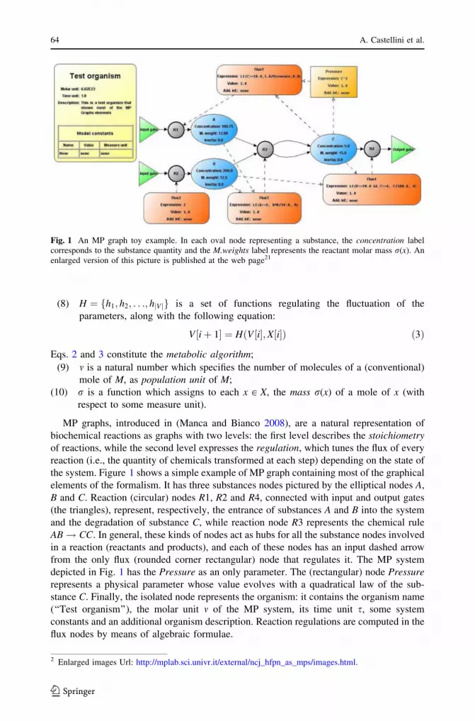
The temporal evolutions of the two models have been compared by the six case studies

considered in (Doi et al. 2004) (wild type, lacZ-, lacY-, LacI-, lacIs and lacI-d) and the

equivalent results of Figs. 8 and 9 have been achieved. Each column shows the dynamics

of five substances (i.e., lactose outside the cell, lactose inside the cell, glucose, LacZ

protein and LacY protein) for a specific case study. Figure 8 displays the results for the

HFPN dynamics while Fig. 9 is related to the equivalent MP system.

‘‘Wild type’’, showed in the first columns, represents the healthy case. It starts with the

degradation of the glucose by the glycolytic pathway, finally allowing the lactose homing

and its transformation to glucose. In this way, the lactose outside the cell decreases and the

lactose inside the cell increases together with the glucose concentration which re-activates

the glycolytic pathway. In the second columns, lacZ- is a mutant which disables the

transformation of lactose in glucose. To perform this test the reaction (transition) involved

in the translation of b-galactosidase has been deleted from the MP system (HFPN), thus,

the lactose enters the cell but it is not transformed into glucose. The glycolytic pathway is

not re-activated and the operon transcription keeps on producing a great amount of LacY

protein. The lacY- mutation disables the capability of the cell to recruit lactose from the

Fig. 7 The lac operon gene regulatory mechanism and glycolytic pathway modeled by MP systems. Thenetwork has been mapped from the HFPN of Fig. 6 by the HFPN-to-MP mapping procedure. An enlargedversion of this picture is published at the web page (see footnote 2)


123

Fig

.8

HF

PN

sim

ula

tio

nre

sult

so

fth

ela

co

per

on

gen

ere

gu

lato

rym

echan

ism

and

gly

coly

tic

pat

hw

ayd

escr

ibed

in(D

oi

etal

.2

00

4).

Th

ew

ild

typ

eco

lum

nd

escr

ibes

the

evolu

tion

of

lact

ose

outs

ide

of

the

cell

,la

ctose

insi

de

of

the

cell

,glu

cose

,L

acZ

and

Lac

Ypro

tein

sin

ahea

lthy

cell

.T

he

oth

erco

lum

ns

plo

tth

ete

mpora

lev

olu

tio

ns

of

the

sam

esu

bst

ance

sfo

rm

uta

nts

lacZ

-,

lacY

-,

lac

I-,

lac

Isan

dla

cI-

d


123

Fig

.9

MP

syst

ems

sim

ula

tio

nre

sult

so

fth

ela

co

per

on

gen

ere

gu

lato

rym

echan

ism

and

gly

coly

tic

pat

hw

ay.

Th

ew

ild

typ

eco

lum

nd

escr

ibes

the

evo

luti

on

of

lact

ose

ou

tsid

eo

fth

ece

ll,

lact

ose

insi

de

of

the

cell

,g

luco

se,

Lac

Zan

dL

acY

pro

tein

sin

ah

ealt

hy

cell

.S

ub

seq

uen

tco

lum

ns

des

crib

eth

ete

mp

ora

lev

olu

tio

ns

of

the

sam

esu

bst

ance

sfo

rm

uta

nts

lacZ

-,

lacY

-,

lac

I-,

lac

Isan

dla

cI-

d.

An

enla

rged

ver

sio

no

fth

isp

ictu

reis

pu

bli

shed

atth

ew

ebp

age

(see

foo

teno

te1)


123

environment. The third column of the two figures show that LacZ starts to grow when

glucose is finishing while LacY remains absent because the mutation inhibits the LacY

mRNA transcription.

Figures 8 and 9 show equivalent results also for lac repressor mutants. In the case study

of lacI- mutant, the repressor function is disabled and the Lac operon transcription keeps

on even in absence of glucose and lactose. The behavior of lacI-d mutant, is similar to

lacI-, indeed in both cases the repressor inhibition forces the LacZ and LacY production,

even after the complete consumption of lactose, leading to a great amount of these pro-

teins. Finally, lacIs, in the fifth column, is a mutant for which the lac operon transcription is

disabled, thus preventing the synthesis of glucose from lactose. The graphical results show

that lactose, LacZ and LacY are just slightly degraded while glucose is not reproduced

after its termination.

6 Conclusions

This work has shown that two formalisms developed in different contexts and with dif-

ferent inspirations have a substantial equivalence in the description of a fundamental

biological process, such as the glycolysis. Such an equivalence has been experimentally

verified and formally proved starting from a suitable mathematical formalization of Hybrid

Functional Petri Nets.

In a previous work, the dynamics of some well known biological systems have already

been investigated by mapping their classical ODE models to the ODE-equivalent MP

systems (Fontana and Manca 2007). Furthermore, the equivalence between MP systems

and differential models was shown under suitable hypotheses. In this perspective, the

equivalence of MP systems with a formalism related to Petri Nets results specially relevant

in the framework of biological modelling.

References

Alberts B, Johnson A, Lewis J, Raff M, Roberts K, Walter P (2002) Molecular biology of the cell. GarlandScience, New York

Bianco L, Castellini A (2007) Psim: a computational platform for Metabolic P systems. In: LNCS 4860,Springer, Berlin, pp 1–20

Bianco L, Fontana F, Franco G, Manca V (2006a) P systems for biological dynamics. In: Ciobanu et al (eds)Applications of membrane computing. Natural computing series. Springer, Berlin, pp 81–126

Bianco L, Fontana F, Manca V (2006b) P systems with reaction maps. Int J Found Comput Sci 17(1):27–48Castellini A, Manca V (2009) MetaPlab: a computational framework for metabolic P systems. In: LNCS

5391, Springer-Verlag, pp 157–168Castellini A, Franco G, Manca V (2009) Toward a representation of Hybrid Functional Petri Nets by MP

systems. In: Suzuki Y et al (eds) Natural Computing PICT 1, pp 28–37Ciobanu G, Paun G, Perez-Jimenez MJ (eds) (2006) Applications of membrane computing. Natural com-

puting series. Springer, New YorkDoi A, Fujita S, Matsuno H, Nagasaki M, Miyano S (2004) Constructing biological pathway models with

Hybrid Functional Petri Nets. In Silico Biol 4(3):271–291Fontana F, Manca V (2007) Discrete solutions to differential equations by Metabolic P systems. Theor

Comput Sci 372(2–3):165–182Fontana F, Manca V (2008) Predator–prey dynamics in P systems ruled by metabolic algorithm. BioSystems

91(3):545–557Hofestadt R (1994) A Petri Net application to model metabolic processes. J Syst Anal Model Simulation

16(2):113–122


123

Hofestadt R, Thelen S (1998) Quantitative modeling of biochemical networks. In Silico Biol 1:39–53Manca V (2006) MP systems approaches to biochemical dynamics: biological rhythms and oscillations. In:

LNCS 4361, Springer, New York, pp 86–99Manca V (2008a) Discrete simulations of biochemical dynamics. In: LNCS 4848, Springer, pp 231–235Manca V (2008b) The metabolic algorithm: principles and applications. Theor Comput Sci 404:142–157Manca V, Bianco L (2008) Biological networks in metabolic P systems. BioSystems 91(3):489–498Manca V, Bianco L, Fontana F (2005) Evolutions and oscillations of P systems: applications to biochemical

phenomena. In: LNCS 3365, Springer, pp 63–84Matsuno H, Tanaka Y, Aoshima H, Doi A, Matsui M, Miyano S (2003) Biopathways representation and

simulation on Hybrid Functional Petri Nets. In Silico Biol 3(3):389–404Nagasaki M, Doi A, Matsuno H, Miyano S (2004) Genomic object net: I. A platform for modelling and

simulating biopathways. Appl Bioinformatics 2(3):181–184Petri CA (1962) Kommunikation mit automaten. Bonn: Institut fur Instrumentelle Mathematik, Schriften des

IIM Nr. 2, GermanPaun G (2000) Computing with membranes. J Comput Syst Sci 61(1):108–143Paun G (2002) Membrane computing: an introduction. Springer, BerlinReddy VN, Mavrovouniotis ML, Liebman MN (1993) Petri Net representations in metabolic pathways. In:

Shavlik JW, Hunter L, Searls DB (eds) Proceedings of the 1st International Conference on IntelligentSystems for Molecular Biology, AAAI Press, pp 328–336

Reisig W (1985) Petri Nets: an introduction. EATCS, Monographs on Theoretical Computer Science.Springer, New York


123

Documents

Hybrid Functional Petri Nets as MP systems