Seediscussions,stats,andauthorprofilesforthispublicationat:https://www.researchgate.net/publication/267642045

AnewalgorithmbasedonMovingLeastSquaremethodtosimulatematerialmixinginfrictionstirwelding

ARTICLEinENGINEERINGANALYSISWITHBOUNDARYELEMENTS·JANUARY2015

ImpactFactor:1.39·DOI:10.1016/j.enganabound.2014.09.011

CITATIONS

5

READS

123

4AUTHORS,INCLUDING:

BouazzaBraikat

UniversitéHassanIIdeCasablanca

90PUBLICATIONS227CITATIONS

SEEPROFILE

LahmamHassane

UniversitéHassanIIMohammediaCasabla…

15PUBLICATIONS109CITATIONS

SEEPROFILE

ZahrouniHamid

UniversityofLorraine

104PUBLICATIONS574CITATIONS

SEEPROFILE

Allin-textreferencesunderlinedinbluearelinkedtopublicationsonResearchGate,

lettingyouaccessandreadthemimmediately.

Availablefrom:BouazzaBraikat

Retrievedon:08February2016

A new algorithm based on Moving Least Square method to simulatematerial mixing in friction stir welding

Abdelaziz Timesli a,b, Bouazza Braikat a,n, Hassane Lahmama, Hamid Zahrouni b

a Laboratoire d'Ingénierie et Matériaux LIMAT, Faculté des Sciences Ben M'Sik, Université Hassan II de Casablanca,Sidi Othman, Casablanca, Moroccob Laboratoire d'Etude des Microstructures et de Mécanique des Matériaux LEM3, CNRS UMR 7239, Université Lorraine, Metz, Ile du Saulcy,57045 Metz Cedex 01, France

a r t i c l e i n f o

Article history:Received 17 January 2014Received in revised form8 May 2014Accepted 17 September 2014

Keywords:Moving Least SquarePerturbation techniqueMaterial mixingHomotopyFriction stir welding

a b s t r a c t

In the present work, a high order implicit technique is associated with a meshless method to modelmaterial mixing observed in friction stir welding (FSW) process. This new algorithm combines thefollowing mathematical procedures: a time discretization, a space discretization, a homotopy transfor-mation, a perturbation technique and a continuation method. The perturbation technique, after a timediscretization, a space discretization, a homotopy transformation, transforms the nonlinear problem intoa sequence of linear ones at each time. By comparison to the classical iterative algorithms, the proposedone allows obtaining very large time steps and reducing computation time by minimizing the numberof tangent matrix decompositions. The strong formulation is considered to avoid the drawback ofnumerical integration. The resulting algorithm is well adapted to large deformations in the mixing zonenearly the welding tool. We limit ourselves to bidimensional visco-plastic problems to show theperformance of the proposed algorithm by comparison to the classical incremental iterative methods.

& 2014 Elsevier Ltd. All rights reserved.

1. Introduction

Friction stir welding (FSW) is a recent industrial process whichconsists in joining metal sheets in solid state [1–4]. Much research hasbeen conducted to study the mechanism of friction stir welding andthe effect of process parameters on the welds. Numerical simulation ofthis process is crucial for manufacturers but it still suffers from a lackof efficiency due to the complexity of the process. In particular,material mixing is difficult to simulate by using classical methodssuch as finite element method. In the literature, different models werepresented for studying material flow during FSW. These models areformulated in Eulerian, Lagrangian or Arbitrary Lagrangian Eulerian(ALE) framework [5]. Eulerian formulation is appropriate to describematerial flow for large deformations thanks to fixedmesh grid but thisformulation cannot be used for problems involving free surfaces or forcomplex tool geometry. Lagrangian formulation is well adapted forhistory dependence in solids and for simulation of material flow withfree surfaces but mesh distortions require special procedure asremeshing. The ALE formulation has been proposed to benefit fromboth advantages of Eulerian and Lagrangian formulations [6]. In thistechnique, one has to describe the motion of the mesh and material

particles separately with respect to a reference domain. ALE has beenapplied successfully in many fields and particularly in metal formingprocesses. Despite the intensive development of these techniques,material mixing in FSW process remains very difficult to achievenumerically and especially when using finite element method [6,7].

An alternative solution for the simulation of this process is the useof meshless methods. To our knowledge, few numerical contributionsusing meshless techniques are available [8–12]. Alfaro et al. [13] haveproposed an algorithm based on natural element methods (NEM) tosimulate the mixing zone in 2D. This technique uses Voronoi diagramsto construct linear shape functions from a support of neighboringpoints. Furthermore, it is based on aweak formulationwhich generallyleads to difficulties related to numerical integration which is not thecase using finite element method.

In this paper, there are two original ideas that we will discuss.One is the application of the Moving Least Square method MLS forsolving the considered problem presented under a strong formula-tion and the other is the proposition of a new algorithm for theresolution of nonlinear problems. This algorithm is based on theassociation of a high order implicit technique and a meshless methodbased on Moving Least Square method. The proposed algorithm isadapted to large deformation and is numerically efficient since itrequires a reduced computation time. The main idea of the proposedalgorithm is to apply the homotopy transformation by introducing anarbitrary invertible matrix ½Kn� and an homotopy parameter “a”

Contents lists available at ScienceDirect

journal homepage: www.elsevier.com/locate/enganabound

Engineering Analysis with Boundary Elements

http://dx.doi.org/10.1016/j.enganabound.2014.09.0110955-7997/& 2014 Elsevier Ltd. All rights reserved.

n Corresponding author.E-mail address: bouazza.braikat@univh2m.ma (B. Braikat).

Engineering Analysis with Boundary Elements 50 (2015) 372–380

varying from zero to one [14]. When this parameter is zero, weobtain a simplified problem easy to solve and when the homotopyparameter is equal to one, we recover the initial problem withouttransformation. By applying the perturbation technique, unknownsof the nonlinear problem are expanded in power series with respectto the homotopy parameter [15]. This technique allows one totransform the nonlinear problem into a sequence of linear oneswhich have the same tangent matrix ½Kn�. Consequently only onetangent matrix triangulation is needed to compute all the terms ofthe series for many time steps. Afterward, a continuation techniqueis performed by computing the validity range of the solution whichallows obtaining the entire solution branch [16–18]. A key point ofthe proposed algorithm is the possibility of choosing the tangentmatrix to be decomposed and the possibility of computing manytime steps with single tangent matrix decomposition [14]. Toillustrate the performance of the proposed algorithm, we givenumerical comparisons with the classical implicit iterative algorithmdetailed in [19].

The layout of this paper is as follows. In Section 2, we present thestrong form of the governing equations. In Section 3, we present thedifferent steps of the high order implicit algorithm based on MLS. InSection 3.5, numerical application is proposed and a comparison withthe implicit iterative algorithm based on the MLS method to validateour algorithm. Finally, some conclusions are presented in Section 5.

2. Governing equations

FSW processes involve large deformation and high velocities.The essential variables of the problem will be velocities andpressures, instead of displacements and pressures. The resultingproblem is then described by the conservation laws including:

divðVÞ ¼ 0 ð1Þ

ρ _V ¼ divðσÞ ð2Þwhere ρ is the material density, V is the velocity vector of componentsu and v, _V ¼ ∂V=∂t, σ is the stress tensor and the gravity is neglected.The stress tensor σ, under this assumption, is given by

σ ¼ �pIþS ð3Þwhere p is the hydrostatic pressure, S is the deviatoric stress tensorand I is the unity tensor. To satisfy the condition of incompressibilitynumerically in (1), we introduce, in general, a pressure term penalizedby a large factor noted λ. This means that the incompressibilitycondition (1) is replaced by a viscous law [20]:

p¼ �λ Trð _ϵÞ ð4Þwhere _ϵ is the strain rate tensor defined as

_ϵ ¼ 12 ðt∇Vþ∇VÞ ð5Þ

FSW is a process that generates large strains in which elastic strainsare negligible as a first approximation. The material, under thisassumption, can then be modeled as visco-plastic material as follows:

S¼ 2μ _ϵ ð6Þwhere μ is the material viscosity. Taking into account Eqs. (3), (4) and(6), the stress tensor is given by

σ ¼ λ Trð _ϵÞIþ2μ _ϵ ð7ÞFor the viscosity, we choose a power law given by [21]

μ¼ 13 kT

A _ϵn�1 ð8Þ

where T is the temperature, k, A and n are the material properties, _ϵ isthe equivalent strain rate given by

_ϵ ¼ffiffiffiffiffiffiffiffiffiffiffiffiffi23_ϵ : _ϵ

qð9Þ

In this work, we focus our efforts on the mixing aspect that is difficultto achieve by the conventional methods such as finite element one. So,we assume that the temperature is constant and then the viscositydepends only on the equivalent strain rate ðμðT ; _ϵ Þ ¼ μð _ϵ ÞÞ. Finally, thegoverning equations can be summarized as follows:

ρ _V ¼ divðσÞσ ¼ λ Trð _ϵÞIþ2μ _ϵ_ϵ ¼ 1

2ðt∇Vþ∇VÞ_ϵ ¼

ffiffiffiffiffiffiffiffiffiffiffiffi23_ϵ : _ϵ

qμ¼ 1

3KTA _ϵ

n�1

8>>>>><>>>>>:

ð10Þ

The problem (10) will be completed by boundary and initialconditions.

3. The proposed algorithm

The proposed algorithm combines a time discretization, a spacediscretization, a homotopy transformation, a perturbation techni-que and a continuation method. Before applying this algorithm,we transform the original problem (10) to a quadratic problem, i.e.,we write the viscosity law under the following differential form:

_ϵ dðμÞ ¼ n�1ð Þμ dð _ϵ Þ ð11Þ

3.1. Time discretization

There will be times when solving the numerical solution forEq. (10) may be unavailable or the means to solve it will beunavailable. At these times and most of the time explicit andimplicit methods will be used in place of numerical solution. In thesimpler cases, the forward Euler's method and backward Euler'smethod are efficient methods to yield fairly accurate approxima-tions of the actual solutions. Using an Euler implicit scheme, thetime discretization of the problem (10) leads to a non-linear

equation. In terms of the new unknowns Vkþ1, σkþ1, _ϵkþ1, _ϵkþ1

and μkþ1 at time tkþ1 ¼ ðkþ1ÞΔt , Eq. (10) is written under thefollowing form:

ρðVkþ1�VkÞ ¼Δt divðσkþ1Þσkþ1 ¼ λ Trð _ϵkþ1ÞIþ2μkþ1 _ϵkþ1 _ϵkþ1¼ 1

2ðt∇Vkþ1þ∇Vkþ1Þð _ϵ kþ1Þ2 ¼ 2

3_ϵkþ1 : _ϵkþ1

_ϵkþ1

dμkþ1 ¼ ðn�1Þμkþ1 d _ϵkþ1

8>>>>>><>>>>>>:

ð12Þ

where Δt is the time step.To calculate the solutions of the problem (12) at each time step,

we introduce the increments ΔV , Δσ, Δ _ϵ, Δ _ϵ and Δμ as newunknowns:

ΔV ¼ Vkþ1�Vk

Δσ ¼ σkþ1�σk

Δ _ϵ ¼ _ϵkþ1� _ϵk

Δ _ϵ ¼ _ϵkþ1� _ϵ

kΔμ¼ μkþ1�μk

8>>>><>>>>:

ð13Þ

where σk, _ϵk, _ϵkand μk represent the values of the unknowns at

time tk ¼ kΔt. Inserting the change of the unknowns (13) into (12)leads to the exact non-linear problem satisfied by these

A. Timesli et al. / Engineering Analysis with Boundary Elements 50 (2015) 372–380 373

increments:

ρΔV ¼Δt divðσkÞþΔt divðΔσÞΔσ ¼ λ Tr Δ _ϵ

� �Iþ2μkΔ _ϵþ2Δμ _ϵkþ2ΔμΔ _ϵ

Δ _ϵ ¼ 12

t∇ΔVþ∇ΔV� �

2 _ϵkΔ _ϵ ¼ 2

3 2 _ϵk : Δ _ϵþΔ _ϵ : Δ _ϵ� �

�Δ _ϵ2

_ϵkþΔ _ϵ Þ dΔμ¼ n�1ð Þ μkþΔμ

� �dΔ _ϵ

�

8>>>>>>>>><>>>>>>>>>:

ð14Þ

3.2. Space discretization

To apply the MLS approximation to the problem (14), the MLSshape functions presented in [19] are used to approximate thevelocity vector ΔVi, in the bi-dimensional case, at any point usinga set of points in a local support domain of the considered point i:

ΔVi ¼ ½ϕ�fΔVig ð15Þwhere ½ϕ� is the matrix of MLS shape functions of point i and fΔVigis the vector that collects the nodal velocities of field function forall the points in the support domain of point i. Using Eqs. (14c) and(15), the strain rate vector can be obtained using the approximatedvelocity vector:

fΔ _ϵig ¼ ½B�fΔVig ð16Þwhere ½B� is the matrix of derivatives of MLS shape functions ofpoint i. Substituting Eqs. (15), (16) in (14) and assembling, weobtain nonlinear system defined by

½KkT �fΔVg�ΔtfFQg ¼ΔtfFg

fΔσig ¼ ½D�fΔ _ϵigþ2Δμif _ϵki gþ2ΔμifΔ _ϵ igfΔ _ϵig ¼ ½B�fΔVig2 _ϵ

kiΔ _ϵ i ¼ 2

3 ð2tf _ϵki g½T �Δ _ϵ igþ tfΔ _ϵig½T �Δ _ϵigÞ�Δ _ϵ i

2

ð _ϵ ki þΔ _ϵ iÞ dΔμi ¼ ðn�1Þðμk

i þΔμiÞ dΔ _ϵ i

8>>>>>>>><>>>>>>>>:

ð17Þ

where ½D� is the tangent matrix of constitutive law,½Kk

T � ¼ ½M��Δt½K� is the tangent matrix evaluated at timetk ¼ kΔt and fFQg is a quadratic form of the unknown variablesfΔVg, fΔσig, fΔ _ϵ ig, Δ _ϵ i and Δμi; where ½M� is the global massmatrix, ½K� is a global matrix dependent of the solutions atprevious time kΔt, the matrix ½T �, the vectors fΔσig and fΔ _ϵ igare given by

½T � ¼1 0 00 1 00 0 1

2

264

375; Δσi

� �¼Δσ11

Δσ22

Δσ12

8><>:

9>=>;; Δ _ϵi

� �¼Δ _ϵ11

Δ _ϵ22

2Δ _ϵ12

8><>:

9>=>;

ð18ÞThe numerical resolution of (17) by incremental iterative methodsis very time consuming since the tangent matrix has to be updatedat each time step and at each iteration.

3.3. Homotopy transformation

In this section, by means of the homotopy transformation, thesolutions of nonlinear problem (17) are exactly obtained in theform of power series. The homotopy transformation contains theauxiliary parameter “a” that provides a convenient way of con-trolling the convergent region of series solutions. This analyticalmethod is employed to solve linear examples to obtain the exactsolutions. To overcome the difficulty cited in Section 3.2, weintroduce an arbitrary invertible matrix ½Kn� and a homotopytransformation [15]. We modify the non-linear problem (17)satisfied by the increments fΔWg, fΔΣ ig, fΔ _Eig, Δ _E i and ΔMui

by introducing a homotopy parameter “a” in Eq. (17) in the

following form:

½Kn�fΔWðaÞgþað½KkT ��½Kn�ÞfΔWðaÞg�aΔtfFQg ¼ aΔtfFg

fΔΣ iðaÞg ¼ ½D�fΔ _EiðaÞgþ2ΔMuiðaÞf _ϵki gþ2ΔMuiðaÞfΔ _EiðaÞgfΔ _EiðaÞg ¼ ½B�fΔWiðaÞg

2 _ϵkiΔ _E iðaÞ ¼ 2

3ð2tf _ϵki g½T �fΔ _EiðaÞgþ tfΔ _EiðaÞg½T �fΔ _EiðaÞgÞ�Δ _E

2

i ðaÞð _ϵ k

i þΔ _E iðaÞÞdðΔMuiðaÞÞ ¼ ðn�1Þðμki þΔMuiðaÞÞdðΔ _E iðaÞÞ

8>>>>>>>>><>>>>>>>>>:

ð19ÞBy this way, the solutions fΔWðaÞg, fΔΣ iðaÞg, fΔ _EiðaÞg, Δ _E iðaÞ andΔMuiðaÞ of the nonlinear equation (19) pass continuously from 0for a¼0 to the solutions of the nonlinear problem (17) for a¼1.The approximation of the solutions of the exact problem at timeðkþ1ÞΔt is then given by

fVkþ1g ¼ fVkgþfΔWða¼ 1Þgfσkþ1

i g ¼ fσki gþfΔΣ iða¼ 1Þg

f _ϵkþ1i g ¼ f _ϵk

i gþfΔ _Eiða¼ 1Þg_ϵkþ1i ¼ _ϵ

ki þΔ _E iða¼ 1Þμkþ1

i ¼ μki þΔMuiða¼ 1Þ

8>>>>><>>>>>:

ð20Þ

3.4. Perturbation technique and continuation method

This perturbation technique consists in expanding the solutionsfΔWðaÞg, fΔΣ iðaÞg, fΔ _EiðaÞg, Δ _E iðaÞ and ΔMuiðaÞ of artificialproblem (19) into power series with respect to a homotopyparameter “a” in the form

fΔWg ¼ afΔW1gþa2fΔW2gþ⋯þapfΔWpgfΔΣ ig ¼ afΔΣ1gþa2fΔΣ2gþ⋯þapfΔΣpgfΔ _Eig ¼ afΔ _E1gþa2fΔ _E2gþ⋯þapfΔ _EpgΔ _E i ¼ aΔ _E 1þa2Δ _E 2þ⋯þapΔ _E pΔMui ¼ aΔMu1þa2ΔMu2þ⋯þapΔMup

8>>>><>>>>:

ð21Þwhere p is the truncation order of the series. By injecting theseseries (21) in the problem (19), we obtain a sequence of linearproblems at various orders given by

For order j¼1:

½Kn�fΔW1g ¼ ΔtfFgfΔΣ1g ¼ ½D�fΔ _E1gþ2f _ϵk

i gΔMu1

fΔ _E1g ¼ ½B�fΔW1g2 _ϵ

kiΔ _E 1 ¼ 2

3ð2tf _ϵki g½T �fΔ _E1gÞ_ϵkiΔMu1 ¼ ðn�1Þμk

iΔ _E 1

8>>>>>>>><>>>>>>>>:

ð22Þ

For order 1o jrp:

½Kn�fΔWjg ¼ ð½Kn��½KkT �ÞfΔWj�1gþΔtfFQj�1g

fΔΣ jg ¼ ½D�fΔ _Ejgþ2f _ϵni gΔMujþ2 ∑j�1

l ¼ 1ΔMulfΔ _Ej� lg

fΔ _Ejg ¼ ½B�fΔWjg

2 _ϵni Δ _E j ¼ 2

3ð2tf _ϵni g½T �fΔ _Ejgþ ∑j�1

l ¼ 1

t

fΔ _Elg½T �fΔ _Ej� lgÞ� ∑j�1

l ¼ 1Δ _E lΔ _E j� l

j _ϵni ΔMuj ¼ jðn�1Þμn

i Δ _E jþðn�1Þ ∑j�1

l ¼ 1ðj� lÞΔMulΔ _E j� l� ∑

j�1

l ¼ 1ðj� lÞΔMulΔ _E j� l

8>>>>>>>>>>>>>>><>>>>>>>>>>>>>>>:

ð23Þwhere fFQj�1g is a right hand side vector that depends on thesolutions of previous orders. To avoid the inversion of the usualtangent matrix at each time step, the matrix Kn

is identified to

the tangent matrix evaluated at the starting point of eachasymptotic branch. Solving these linear problems requests a singleinversion of the arbitrary matrix Kn

and updating of the second

member. Cochelin [16] has proposed a way of defining the range ofvalidity of the series. It is based on the difference in the velocitiesat two successive orders which must be smaller than a given

A. Timesli et al. / Engineering Analysis with Boundary Elements 50 (2015) 372–380374

tolerance η. So the validity range of the parameter “a” according tothe following relation:

aðtmaxÞ ¼ ηJfΔW1gJJfΔWpgJ

� � 1=ðp�1Þð Þð24Þ

where tmax ¼ nmaxΔt is the validity range with nmax being thenumber of time steps Δt. In practice, the norm in (24) will bechosen as the Euclidean norm of the discrete variables, but likelythe algorithm is not very sensitive to the choice of the norm. Thechange of the tangent matrix Kn

to be inverted depends on the

value of the homotopy parameter “a” given by Eq. (24). If the valueof this parameter is greater than or equal to 1 then we keep thesame tangent matrix for the next time step and if not then we takethe tangent matrix Kn

¼ KkT

h ievaluated at time tk ¼ kΔt. The end

of the solution path defined by this criterion is considered as thestarting point for the next step. Then we determine the solutionbranch by branch. This technique is called continuation method.

3.5. Numerical strategy

Here we outline a basic flowchart for the implementation of theproposed algorithm for the simulation of the material mixing,shown in Fig. 1.

4. Numerical application

To illustrate the performance of the proposed algorithm a bi-dimensional visco-plastic problem is considered. The obtainedsolution is compared with that obtained by the conventionalmethod using the Euler scheme coupled with an iterative method[19] similar to that used in various areas of physics [22], it isdescribed in [14]. In this iterative method, the convergence isevaluated by assuming that the relative difference between twoconsecutive iterations is less than a given tolerance. In thecalculations, we fix the truncation order of the series and theefficiency of algorithms is measured in part by the number ofmatrices to invert (NIM) and secondly by the smallness of theresidual norm. In this work, the proposed algorithm is denoted byAlgo1 and the iterative algorithm is denoted by Algo2.

In this application, we consider a circular plate made of aluminumalloy AA7075. Behavior adopted to this material in this study is visco-plastic type. The tool is placed in the center of this plate (see Fig. 2). Itis assumed that the adhesion between the particles located on internalboundary of the domain and the tool is perfect and that the effect ofthe tool on the particles of the external boundary is negligible. Thephysical and geometrical data used in this application are circular plateradius rp ¼ 6 mm, tool radius rt ¼ 1:5 mm, k¼ 2:69� 1010 N mm�2,A¼ �3:3155, n¼0.1324 [21], temperature T¼300 K. In this work, weconsider the following boundary and initial conditions:

uðx; y; tÞ ¼ �rtω cos ðωtÞ for x2þy2 ¼ r2t 8 tZ0vðx; y; tÞ ¼ rtω sin ðωtÞ for x2þy2 ¼ r2t 8 tZ0uðx; y; tÞ ¼ 0 for x2þy2 ¼ r2p 8 tZ0

vðx; y; tÞ ¼ 0 for x2þy2 ¼ r2p 8 tZ0

uðx; y; tÞ ¼ 0 for r2t ox2þy2or2p and t ¼ 0

vðx; y; tÞ ¼ 0 for r2t ox2þy2or2p and t ¼ 0

8>>>>>>>>>><>>>>>>>>>>:

ð25Þ

whereω is the rotation speed. Fig. 3a shows the initial configuration ofthe discretized domain. This domain is represented by 1780 points(see Fig. 3a). The plate is assumed to be the joining of two parts in theform of two half discs, one of which is colored by a blue color and the

Fig. 1. Principle of the restart proposed algorithm.

Fig. 2. The considered visco-plastic plate, its geometrical characteristics, initialconditions and boundary conditions.

A. Timesli et al. / Engineering Analysis with Boundary Elements 50 (2015) 372–380 375

other by a red color. The size of influence domain is fixed to hi ¼ 4drðdr ¼ 2:5� 10�4Þ with dr being the spatial step in the radial direction(see Fig. 3b). The welding tool is considered rigid driven by a uniformrotation speed equal to ω¼ 100 rad s�1.

In Fig. 4, we plot the parameter amax along the time axis t obtainedby the high order implicit algorithm. This figure shows that thevalidity range tmax is increased when increasing the truncation order pfor a fixed tolerance parameter η. The parameters p and η define thestep length tmax in the continuation technique.

In the following, we limited ourselves to an indirect control of thealgorithm Algo1, by the tolerance η or by the truncation order p. Theefficiency of this algorithm can be estimated by comparing the size ofvalidity range tmax according to the quality of the final solution. InTable 1, we note that when the truncation order p increases the size ofthe validity range tmax increases for a fixed tolerance η, for example, fortruncation order p¼20 and tolerance parameter η¼ 10�6, the validityrange is equal to tmax ¼ 0:0012 s and nmax ¼ 12. But, when thetolerance parameter decreases the validity range also decreases.

Thereafter, the solution of the problem is calculated along thetime interval ½0;0:125�. The numerical results are presented inTable 2. To know the number of matrix triangulations required toobtain this solution along the considered time interval, four trunca-tion orders and two tolerance parameters are chosen. In Table 2, wenote that when the truncation order p increases the number ofmatrix triangulations decreases for a fixed tolerance η, for example,for truncation order p¼20 and tolerance parameter η¼ 10�6, thenumber of matrix triangulations is equal to 88.

In the following, we will be choosing for the proposed algo-rithm Algo1 a truncation order p¼20 and a tolerance parameterη¼ 10�6 and for the iterative algorithm Algo2 a tolerance para-meter δ¼ 10�6 for a time step Δt ¼ 0:0001 s. The solution of theproblem obtained by the algorithm Algo2 requires 2252 matrixtriangulations. The solution quality according to the differentsolution strategies are plotted in Fig. 5 by the residue variation.

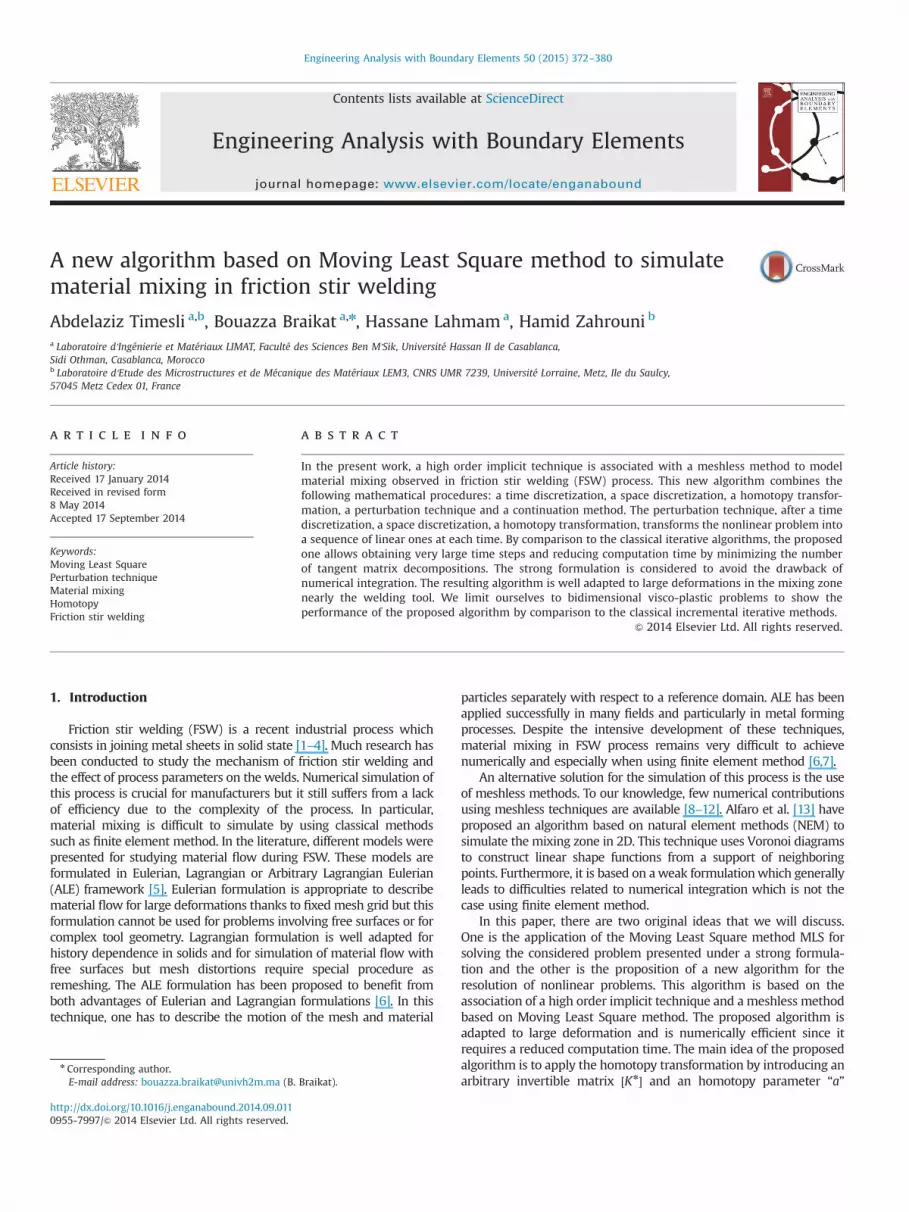
In Fig. 6, we plot the evolution of u and v components of thevelocity along the time axis t, at node near the tool (see Fig. 3),obtained by the algorithm Algo1 and the algorithm Algo2. The twosolutions obtained by the algorithms Algo1 and Algo2 are in goodagreement. Let us note that the solution in Fig. 6 requires 88 matrix

Fig. 3. Initial configuration of the discretized domain, size of influence domain and registration point. (For interpretation of the references to color in this figure caption, thereader is referred to the web version of this paper.)

Fig. 4. Influence of the truncation order p on the validity range tmax for thetolerance η¼ 10�6.

Table 2Influence of tolerance η and the truncation order p on the number of branches.

Order p η¼ 10�6 η¼ 10�8

10 208 25415 156 17620 88 9425 83 91

0 0.02 0.04 0.06 0.08 0.1 0.12 0.14−7

−6

−5

−4

−3

−2

−1

0

t(s)

Res

idua

l (lo

g|| R

esid

u ||)

Algo2Algo1

Fig. 5. Quality solution: variation of the Algo1 and Algo2 residue in terms of thetime axis t.

Table 1Influence of tolerance η and the truncation order p on the validity range tmax.

Order p η¼ 10�6 (s) η¼ 10�8 (s)

10 0.0005 0.000415 0.0008 0.000620 0.0012 0.001025 0.0013 0.0011

A. Timesli et al. / Engineering Analysis with Boundary Elements 50 (2015) 372–380376

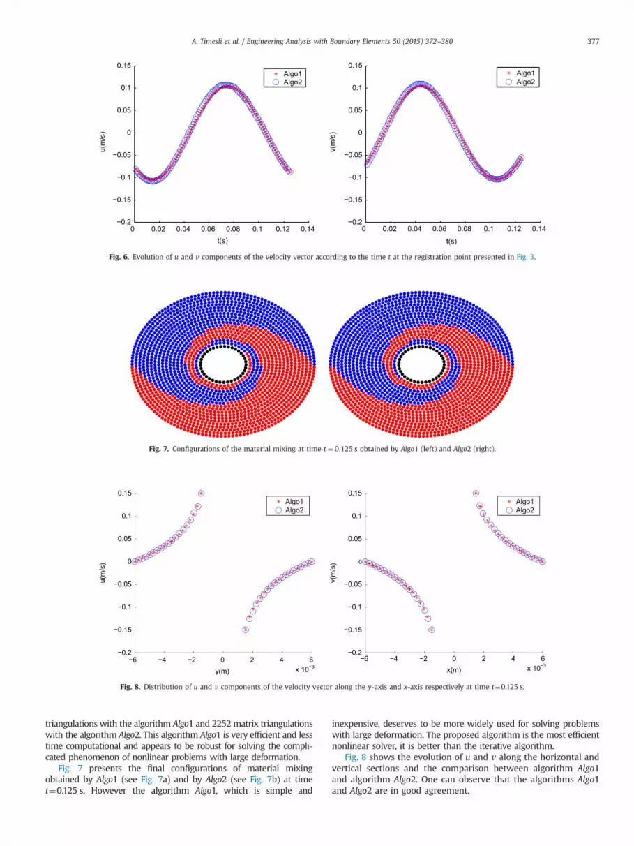
triangulations with the algorithm Algo1 and 2252matrix triangulationswith the algorithm Algo2. This algorithm Algo1 is very efficient and lesstime computational and appears to be robust for solving the compli-cated phenomenon of nonlinear problems with large deformation.

Fig. 7 presents the final configurations of material mixingobtained by Algo1 (see Fig. 7a) and by Algo2 (see Fig. 7b) at timet¼0.125 s. However the algorithm Algo1, which is simple and

inexpensive, deserves to be more widely used for solving problemswith large deformation. The proposed algorithm is the most efficientnonlinear solver, it is better than the iterative algorithm.

Fig. 8 shows the evolution of u and v along the horizontal andvertical sections and the comparison between algorithm Algo1and algorithm Algo2. One can observe that the algorithms Algo1and Algo2 are in good agreement.

0 0.02 0.04 0.06 0.08 0.1 0.12 0.14−0.2

−0.15

−0.1

−0.05

0

0.05

0.1

0.15

t(s)

u(m

/s)

Algo1Algo2

0 0.02 0.04 0.06 0.08 0.1 0.12 0.14−0.2

−0.15

−0.1

−0.05

0

0.05

0.1

0.15

t(s)

v(m

/s)

Algo1Algo2

Fig. 6. Evolution of u and v components of the velocity vector according to the time t at the registration point presented in Fig. 3.

Fig. 7. Configurations of the material mixing at time t ¼ 0:125 s obtained by Algo1 (left) and Algo2 (right).

−6 −4 −2 0 2 4 6x 10−3

−0.2

−0.15

−0.1

−0.05

0

0.05

0.1

0.15

y(m)

u(m

/s)

Algo1Algo2

−6 −4 −2 0 2 4 6x 10−3

−0.2

−0.15

−0.1

−0.05

0

0.05

0.1

0.15

x(m)

v(m

/s)

Algo1Algo2

Fig. 8. Distribution of u and v components of the velocity vector along the y-axis and x-axis respectively at time t¼0.125 s.

A. Timesli et al. / Engineering Analysis with Boundary Elements 50 (2015) 372–380 377

The distributions of the velocity vector components obtainedby Algo2 and Algo1 at time t¼0.125 s are identical as shown inFigs. 9 and 10.

Figs. 11–13 present the distribution of the strain rate compo-nents ( _ϵxx, _ϵyy and _ϵxy) obtained by Algo1 and Algo2 at timet¼0.1 s.

5. Conclusion

In this paper, we have developed a high order implicit algo-rithm based on the Moving Least Square MLS to simulate materialmixing in Friction Stir Welding. It is built by associating the highorder implicit technique with the Moving Least Square MLS. The

Fig. 9. Distribution of u component of the velocity vector at time t¼0.125 s given by Algo1 and by Algo2.

Fig. 10. Distribution of v component of the velocity vector at time t¼0.125 s given by Algo1 and by Algo2.

Fig. 11. Distribution of _ϵxx component of the strain rate given by Algo1 and Algo2.

A. Timesli et al. / Engineering Analysis with Boundary Elements 50 (2015) 372–380378

high order implicit technique couples the Euler implicit scheme,the homotopy transformation, the Taylor series expansions tech-nique and the continuation method. The performance of this highorder implicit algorithm has been tested on bidimensional visco-plastic problems. The results are compared with those obtained byan iterative method. The most interesting result is the ability ofapplying implicit discretization schemes with a very small numberof matrix triangulations. The key points in this high order implicitalgorithm are, first a high order solver based on perturbationtechniques, second the possibility of choosing the tangent matrix½Kn�, which limits the number of matrices to be triangulated. Let usrecall that the proposed algorithm solves the nonlinear visco-plastic problem with a high order predictor without any iteration.The proposed algorithm can easily be adapted to other nonlinearproblems. Work is currently in progress to other application fields.

References

[1] Thomas WM, Nicholas ED, Needham JC, Church MG, Templesmith P, Dawes C.Friction stir butt welding, International Patent Application no. PCT/GB92/02203 and GB Patent Application no. 9125978.8., 1991.

[2] Bastier A, Maitournam MH, Dang Van K, Reger F. Steady state thermomecha-nical modelling of friction stir welding. Sci. Technol. Weld. Join. 2006;11:278–88.

[3] Schmidt H, Hattel J. A local model for the thermomechanical conditions infriction stir welding. Model. Simul. Mater. Sci. Eng. 2005;13:77–93.

[4] Feulvarch E, Gooroochurn Y, Boitout F, Bergheau J-M, 3D Modelling ofThermofluid Flow in Friction Stir Welding, Trends in Welding Research,Proceedings, 2006.

[5] Jacquin D, De Meester B, Simar A, Deloison D, Montheillet F, Desrayaud C. Asimple Eulerian thermomechanical modeling of friction stir welding. J. Mater.Process. Technol. 2011;211:57–65.

[6] Lorrain J, Serri O, Favier V, Zahrouni H, El Hadrouz M. A contribution to acritical review of friction stir welding numerical simulation. J. Mech. Mater.Struct. 2009;4:351–69.

[7] Guerdoux S, Fourment L. A 3d numerical simulation of different phases offriction stir welding. Model. Simul. Mater. Sci. Eng. 17, 2009, 075001.

[8] Gingold RA, Monaghan JJ. Smoothed particle hydrodynamics—theory andapplication to non-spherical stars, Mon. Not. R. Astron. Soc. 181;1977.

[9] Nayroles B, Touzot G, Villon P. The diffuse approximation. C.R. Acad. Sci.1991;313:293–6.

[10] Nayroles B, Touzot G, Villon P. Generalizing the finite element method: diffuseapproximation and diffuse elements. Comput. Mech. 1992;10:307–18.

[11] Belytschko T, Krongauz Y, Orga D, Fleming M, Krysl P. Meshless methods: anoverview and recent developments. Comput. Methods Appl. Mech. Eng.1996;139:3–47.

[12] Belytschko T, Lu YY, Gu L. Element free Galerkin methods. Int. J. Numer.Methods Eng. 2004;37:229–56.

[13] Alfaro I, Racineux G, Poitou A, Cueto E, Chinesta F. Numerical simulation offriction stir welding by natural element methods. Int. J. Mater. Form.2008;1:1079–82.

[14] Jamal M, Braikat B, Boutmir S, Damil N, Potier-Ferry M. A high order implicitalgorithm for solving instationary non-linear problems. Comput. Mech.2002;28:375–80.

Fig. 12. Distribution of _ϵyy component of the strain rate given by Algo1 and Algo2.

Fig. 13. Distribution of _ϵxy component of the strain rate given by Algo1 and Algo2.

A. Timesli et al. / Engineering Analysis with Boundary Elements 50 (2015) 372–380 379

[15] Allgower EL, Georg K. Numerical Continuation Methods: an introduction.Springer series in computational mathematics, vol. 13, 1990.

[16] Cochelin B. A path-following technique via an asymptotic-numerical method.Comput. Struct. 1994;53:1181–92.

[17] Mottaqui H, Braikat B, Damil N. Discussion about parameterization in theasymptotic numerical method: application to nonlinear elastic shells. Comput.Methods Appl. Mech. Eng. 2010;199:1701–9.

[18] Mottaqui H, Braikat B, Damil N. Local parameterization and the asymptoticnumerical method. Math. Model. Natural Phenom. 2010;5:16–22.

[19] Timesli A, Braikat B, Lahmam H, Zahrouni H. An implicit algorithm based oncontinuous moving least square to simulate material mixing in friction stir

welding process, Model. Simul. Eng. 2013 (ID 716383, doi: http://dx.doi.org/10.1155/2013/716383) (2013) 14 pages.

[20] Tillier Y. Identification par analyse inverse du comportement mécanique despolymères solides: application aux sollicitations multiaxiales et rapides, EcoleNationale Supérieure des Mines de Paris, 1998.

[21] Buffa G, Hu J, Shivpuri R, Fratini L. A continuum based fem model for frictionstir welding model development. Mater. Sci. Eng. 2006;419:389–96.

[22] Fornberg B, Whitham GB. A numerical and theoretical study of certainnonlinear wave phenomena. Philos. Trans. R. Soc. Lond., A Math. Phys. Sci.1978;289:373–404.

A. Timesli et al. / Engineering Analysis with Boundary Elements 50 (2015) 372–380380