Embed Size (px)
Citation preview
Digital Signal Processing 18 (2008) 334–345
www.elsevier.com/locate/dsp
State-space least mean square
Mohammad Bilal Malik ∗, Muhammad Salman
Department of Electrical Engineering, College of Electrical and Mechanical Engineering, National University of Sciences and Technology,Rawalpindi, Pakistan
Available online 23 May 2007
Abstract
In this paper, we present a generalized form of the well-known least mean square (LMS) filter. The proposed filter incorporateslinear time-varying state-space model of the underlying environment and hence is termed as state-space LMS (SSLMS). Thisattribute results in marked improvement in its tracking performance over the standard LMS. Furthermore, the use of SSLMS instate estimation in control systems is straightforward. Overall performance of SSLMS, however, depends on factors like modeluncertainty and time-varying nature of the problem. SSLMS with adaptive memory, having time-varying step-size parameter,provides solutions to such cases. The step-size parameter is iteratively tuned by stochastic gradient method so as to minimize themean square value of the prediction error. Different computer simulations demonstrate the ability of the algorithms suggested inthis paper. A detailed study of computational complexities of the proposed algorithms is carried out at the end.© 2007 Elsevier Inc. All rights reserved.
Keywords: Adaptive filtering; State-space LMS; SSLMS; Tracking
1. Introduction
Adaptive filters have played a vital role in the development of a wide variety of systems, for the last three decades.The philosophy of adaptive filters revolves around recursive least squares (RLS) and least mean square (LMS) [1].The derivations of standard RLS and LMS assume multiple linear regression model. Whereas, this model is applicableto a wide range of problems, it also causes certain restrictions in the design of adaptive filters when the underlyingmodel of the environment is different. Model dependent nature of the tracking problem makes it specially sensitiveto this limitation. Consequently, tracking performance of LMS and RLS have been thoroughly explored ([1–5], etc.).Researchers have been endeavoring to find various forms of LMS and RLS that could fit well in diverse scenarios [1].Notable amongst these is an important contribution by Sayed and Kailath [6], who have given a state-space modelfor RLS. Based on [6], Haykin et al. [7] have exploited one-to-one correspondence between RLS and Kalman filterto devise extended RLS (ERLS) algorithms. In our previous work, we have developed SSRLS [8] which takes intoconsideration the state-space model of the system, thus resulting in a very useful generalization of the standard RLS.SSRLS shows considerable improvement in tracking performance over standard RLS and LMS. Development of
* Corresponding author.E-mail address: [email protected] (M.B. Malik).
1051-2004/$ – see front matter © 2007 Elsevier Inc. All rights reserved.doi:10.1016/j.dsp.2007.05.003
M.B. Malik, M. Salman / Digital Signal Processing 18 (2008) 334–345 335
SSRLS with adaptive memory (SSRLSWAM) [9] adds a level of versatility to this philosophy. SSRLSWAM provesto be an effective tracker even in difficult scenarios as shown in [9].
In this paper we develop state-space least mean square (SSLMS) by incorporating the linear state-space model ofthe environment, which offers two plus points. Firstly any causal linear system can be represented by a state-spacemodel, thus a designer is not restricted to the linear regression model. Secondly, the multiple-input multiple-output(MIMO) nature of state-space model allows handling vector observations. The standard RLS and LMS, on the otherhand, only deal with scalar observations. Appropriate to the nature of generalization, we use the term state-space leastmean square (SSLMS). SSLMS was first introduced in [10], where we showed the ability of this new filter to tracktime-varying systems. As a natural extension of SSLMS, we developed SSLMS with adaptive memory [11]. Thisalgorithm exhibits superior tracking properties under difficult conditions.
This paper commences with a discussion of the state-space model of an unforced time-varying discrete system. Theoutput of the system that may have been corrupted by observation noise is assumed to be available for measurements.This model forms the basis of further development. The derivation of SSLMS, based on the minimum norm solutionof an underdetermined system of linear equations, uses only latest observation in the recursive algorithm. The solutionwith normalization factor is called state-space normalized LMS (SSNLMS), where omitting this factor gives us simplySSLMS. It is shown that the linear regression model is a special case of the general state-space model used in derivationof SSLMS. This in fact shows that SSLMS is a true generalization of the standard LMS. This is followed by a noisysinusoid tracking example. State-space formulation of SSLMS also makes it possible to use it in state estimation incontrol systems. This is illustrated by an example in Section 8.
The derivation of SSLMS with adaptive memory (SSLMSWAM) is then presented. The idea is to iteratively tunestep-size parameter by stochastic gradient method so as to minimize the mean square value of the prediction error. Tohighlight the usefulness of SSLMSWAM, the application of tracking of noisy Van der Pol oscillations is discussed.The performance of SSLMSWAM is also compared with that of SSLMS, SSRLS, SSRLSWAM, RLS and LMS.
A detailed discussion of computational complexities of different algorithms under discussion concludes the paper.
2. State-space model
Consider a process y[k] ∈ Rm that is available for measurement. Assume that the underlying process generator isan unforced linear time varying discrete-time system. Standard form of such a system is given as follows [9]:
x[k + 1] = A[k]x[k],y[k] = C[k]x[k] + v[k], (1)
where x[k] ∈ Rn is the state vector at time k, the elements of which are called state variables, which may also bereferred to as the process states. We assume that the maximum number of outputs of the system is less than or equalto the states, i.e., m � n. This is a logical assumption as a system with m > n can be simplified to the one with m � n
without the loss of any information about the states [12]. The system matrix A[k] and the output matrix C[k] maybe stochastic or deterministic depending on the nature of the problem. C[k] is assumed to be full rank, which is areasonable assumption. To see this, consider the case when C[k] is deterministic and rank deficient. We can reducethe number of outputs to make a new full rank output matrix, without the loss of any information about the states. Onthe other hand, a stochastic C[k] is full rank by virtue of unavoidable presence of white noise. The pair (A[k],C[k])is assumed to be l-step observable [9]. Observation noise is represented by v[k]. It is customary to assume v[k] tobe a zero-mean white process, although these assumptions do not affect the derivations and development done in thispaper. Such assumptions on the observation noise are important for analyzing the performance of the filters presentedhere. The state-transition matrix for the system (1) is given by
A[k, j ] ={
A[k − 1]A[k − 2] . . .A[j ], k > j,
I, k = j.(2)
The system matrix A[k] is assumed to be invertible for all k which results in the following properties [12]:
A−1[k, j ] = A[j, k], ∀j, k,
A[k, i] = A[k, j ]A[j, i], i � j � k, (3)
A[k + 1, k] = A[k].

336 M.B. Malik, M. Salman / Digital Signal Processing 18 (2008) 334–345
The absence of ‘process noise’ or any other deterministic inputs poses a question about the usefulness of (1).However, this framework is general enough to address adaptive filtering applications as would be shown later in thispaper. Moreover, this concept is a familiar one in the context of exosystems used in servomechanism problems [13].The reference signals (to be tracked) and disturbances (to be rejected) are modeled using systems similar to (1).In all these cases, the system matrix A[k] is neutrally stable. For a time-invariant system matrix A = A[k], neutralstability implies that all of the eigenvalues of A are strictly on the unit circle. An extension of this philosophy tononlinear systems can be found in the regulation problem, where once again the references/disturbances are modeledby neutrally stable exosystems [14]. Neutral stability of A[k] rules out existence of unstable or exponentially stablestates and hence the concern about applicability of (1) to physical systems. Having said that, the theory developedin this paper however, does not make any assumptions about the neutral stability of A[k]. This is only a matter ofusefulness of models like (1) in practical applications.
3. State estimator
Suppose that the observations y[k] start appearing at time k = 1. The initial state vector is x[0] = x0 and is notknown. The observability assumption allows us to design a state estimator. The idea is to generate the estimated statevector x[k] making use of the observations y[1], y[2], . . . , y[k].
The system equation (1) enables us to compute the predicted state estimate at time k (using observations up to timek − 1) as follows:
x[k] = A[k − 1]x[k − 1]. (4)
The prediction error can now be defined as
ε[k] = y[k] − y[k] (5)
with
y[k] = C[k]x[k] (6)
as the predicted output. The prediction error is also referred to as innovations in the realm of Kalman filtering [1]. Wecan also define the estimation error as
e[k] = y[k] − y[k], (7)
where y[k] = C[k]x[k] is the estimated output. One of the well-known estimator forms is [12]
x[k] = x[k] + K[k]ε[k], (8)
where K[k] is the observer gain, which is to be determined by different methods presented in this paper.
4. State-space least mean square (SSLMS)
In this section we derive a generalized version of LMS viz SSLMS which incorporates model dynamics as givenin (1). The discussion begins with relating the prediction error (5) and estimation error (7) as follows:
e[k] = ε[k] − C[k]δ[k], (9)
where δ[k] is defined as
δ[k] = x[k] − x[k]. (10)
The assumption that C[k] is full rank makes it possible to choose x[k] such that
e[k] = 0, (11)
which gives
ε[k] = C[k]δ[k]. (12)
M.B. Malik, M. Salman / Digital Signal Processing 18 (2008) 334–345 337
If m < n then there are infinitely many choices of x[k] that satisfy (11). We resort to minimum norm solution of (12),which minimizes δ[k] in (10) subject to the constraint e[k] = 0 [1]. We get
δ[k] = CT [k](C[k]CT [k])−1ε[k]. (13)
From (10) and (13)
x[k] = x[k] + CT [k](C[k]CT [k])−1ε[k]. (14)
Comparing (14) with (8), the observer gain K[k] according to the method of minimum norm solution comes out to be
K[k] = CT [k](C[k]CT [k])−1. (15)
As apparent from its form, the gain in (15) has a limited scope. In order for a state estimator to be valid, the mapfrom output of the system (which is the input of the estimator) to state estimates should be controllable. Alternatelystating, (A[k −1]−K[k]C[k]A[k −1],K[k]) pair should be controllable. The choice of gain as given in (15) does notguarantee that this requirement will always be satisfied. Furthermore, a designer prefers to have a control of the rateof convergence, which is done through step-size parameter in the standard LMS [1]. In view of these considerations,we introduce a step-size parameter μ and matrix G to arrive at a more useful expression as follows:
K[k] = μGCT [k](C[k]CT [k])−1. (16)
The matrix G is chosen so as to have a valid estimator, i.e., controllable pair (A[k − 1] − K[k]C[k]A[k − 1],K[k]),whereas rate of convergence is controlled through μ. In certain cases like sinusoidal model [2,8], the controllabilitycondition exists without the matrix G in (16). On the other hand, constant velocity and constant acceleration models[2,8] do not fulfill this requirement and hence a designer has to choose a G for the estimator to be valid. The actualchoice of this matrix depends on the nature of the problem. One simple approach is illustrated in Section 8.2, wherethe first column of G consists of non-zero entries. The rest are all zeroes.
Finally, for the cases where invertibility of C[k]CT [k] cannot be ensured, we may use a small number γ , whichmodifies (16) into
K[k] = μGCT [k](γ I + C[k]CT [k])−1. (17)
This arrangement allows us to handle problems where C[k] may become rank deficient for a short interval. γ = 0 isused in situations where C[k] is guaranteed to be full rank. Defining
γ I + C[k]CT [k] (18)
as a normalization factor, the algorithm comprising (4)–(6), (8), (17) is termed as state-space normalized LMS(SSNLMS). It is apparent from (17) that an m×m matrix is required to be inverted. A simplification in this algorithmresults by removing the normalization factor, which reduces the observer gain to
K[k] = μGCT [k]. (19)
The algorithm (4)–(6), (8), (19) is accordingly called state-space LMS (SSLMS). An analogy of SSLMS with thestandard LMS would become clear in Section 5.
5. Analogy with the standard LMS
In order to show analogy of SSLMS with standard LMS, let
u[k] = [u[k], u[k − 1], . . . , u[k − n + 1]]T (20)
be input vector for a system with tap weights
w0[k] = [w01[k],w02[k], . . . ,w0n[k]]T . (21)
The output of this filter is corrupted by additive observation noise v[k]. The signal d[k] is called the desired signal.The tap-weights of an adaptive transversal filter
w[k] = [w1[k], w2[k], . . . , wn[k]]T (22)
338 M.B. Malik, M. Salman / Digital Signal Processing 18 (2008) 334–345
can be thought of as an estimate of the unknown tap-weights w0. The output of this filter is s[k]. The problem isto adjust the estimated tap-weights so as to minimize the error e[k] in some sense. We choose the minimum normleast square error as our optimization criterion. If the problem is overdetermined then the filter becomes the standardRLS. If it is underdetermined then we get the normalized LMS. Finally dropping the normalization factor gives us thestandard LMS. The relevant details can be found in [1]. It is not difficult to see that if the following condition holds
m = 1,
A = I,
C[k] = u[k],x[k] = w[k], (23)
ε[k] = e[k],y[k] = d[k],y[k] = s[k],
then the filter developed in this paper turns into standard LMS. Due to this reason, we assert that SSLMS and itsvariants are in fact generalization of the conventional LMS filters.
6. An application of SSLMS
The problem of tracking a noisy sinusoid/chirp is of historical significance and has received considerable attentionin the literature [7,15,16]. The problem arises naturally in the context of an interfering signal of known frequency.Widrow et al. considered the problem of cancellation of 60 Hz interference in electrocardiography, using LMS [17].In this section we give a brief account of how SSLMS can be used in such cases.
The phase and amplitude of the interfering signal are assumed to be unknown. Apparently, a priori knowledge offrequency simplifies the problem into a trivial one. However in the case of standard RLS and LMS, the designer hasno direct way to incorporate this information. By virtue of state-space formulation of SSLMS, this information can beincorporated in a straightforward manner. For a sinusoid represented in discrete time as
y[k] = σs cos(ω0kT + φ) + v[kT ], (24)
the system matrices are given by [8]
A =[
cos(ω0T ) sin(ω0T )
− sin(ω0T ) cos(ω0T )
],
C = [1 0],(25)
where σ 2s = signal power, ω0 = signal frequency, φ = phase of signal, T = sampling time, v = observation noise;
SSLMS may then be used to track the interfering signal.
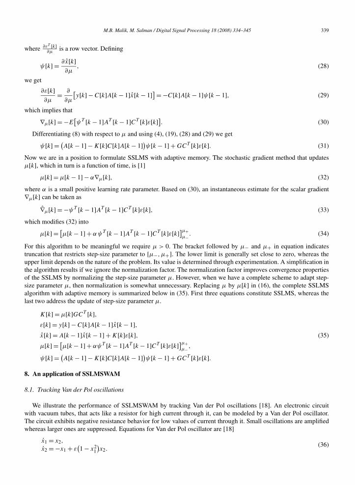
7. State-space least mean square with adaptive memory (SSLMSWAM)
When the model of the underlying environment is completely/partially unknown, a presumed model results in amodel mismatch almost obviously. A partial compensation for this mismatch may be achieved if we adaptively tunethe step-size parameter, so as to minimize a cost function. SSLMS with adaptive memory builds upon the frameworkof SSLMS to achieve iterative tuning of step-size parameter. Our objective is to tune the step-size parameter μ so asto minimize the following cost function
J [k] = 1
2E
[εT [k]ε[k]], (26)
where E[·] is the expectation operator and ε[k] is the prediction error defined in (5). Differentiating J [k] with respectto μ gives
∇μ[k] = ∂J [k] = E
[∂εT [k]
ε[k]], (27)
∂μ ∂μ
M.B. Malik, M. Salman / Digital Signal Processing 18 (2008) 334–345 339
where ∂εT [k]∂μ
is a row vector. Defining
ψ[k] = ∂x[k]∂μ
, (28)
we get
∂ε[k]∂μ
= ∂
∂μ
[y[k] − C[k]A[k − 1]x[k − 1]] = −C[k]A[k − 1]ψ[k − 1], (29)
which implies that
∇μ[k] = −E[ψT [k − 1]AT [k − 1]CT [k]ε[k]]. (30)
Differentiating (8) with respect to μ and using (4), (19), (28) and (29) we get
ψ[k] = (A[k − 1] − K[k]C[k]A[k − 1])ψ[k − 1] + GCT [k]ε[k]. (31)
Now we are in a position to formulate SSLMS with adaptive memory. The stochastic gradient method that updatesμ[k], which in turn is a function of time, is [1]
μ[k] = μ[k − 1] − α∇μ[k], (32)
where α is a small positive learning rate parameter. Based on (30), an instantaneous estimate for the scalar gradient∇μ[k] can be taken as
∇μ[k] = −ψT [k − 1]AT [k − 1]CT [k]ε[k], (33)
which modifies (32) into
μ[k] = [μ[k − 1] + αψT [k − 1]AT [k − 1]CT [k]ε[k]]μ+
μ− . (34)
For this algorithm to be meaningful we require μ > 0. The bracket followed by μ− and μ+ in equation indicatestruncation that restricts step-size parameter to [μ−,μ+]. The lower limit is generally set close to zero, whereas theupper limit depends on the nature of the problem. Its value is determined through experimentation. A simplification inthe algorithm results if we ignore the normalization factor. The normalization factor improves convergence propertiesof the SSLMS by normalizing the step-size parameter μ. However, when we have a complete scheme to adapt step-size parameter μ, then normalization is somewhat unnecessary. Replacing μ by μ[k] in (16), the complete SSLMSalgorithm with adaptive memory is summarized below in (35). First three equations constitute SSLMS, whereas thelast two address the update of step-size parameter μ.
K[k] = μ[k]GCT [k],ε[k] = y[k] − C[k]A[k − 1]x[k − 1],x[k] = A[k − 1]x[k − 1] + K[k]ε[k], (35)
μ[k] = [μ[k − 1] + αψT [k − 1]AT [k − 1]CT [k]ε[k]]μ+
μ− ,
ψ[k] = (A[k − 1] − K[k]C[k]A[k − 1])ψ[k − 1] + GCT [k]ε[k].
8. An application of SSLMSWAM
8.1. Tracking Van der Pol oscillations
We illustrate the performance of SSLMSWAM by tracking Van der Pol oscillations [18]. An electronic circuitwith vacuum tubes, that acts like a resistor for high current through it, can be modeled by a Van der Pol oscillator.The circuit exhibits negative resistance behavior for low values of current through it. Small oscillations are amplifiedwhereas larger ones are suppressed. Equations for Van der Pol oscillator are [18]
x1 = x2,
x = −x + ε(1 − x2
)x .
(36)
2 1 1 2
340 M.B. Malik, M. Salman / Digital Signal Processing 18 (2008) 334–345
Fig. 1. Van der Pol oscillations.
Working with the assumption that actual (Van der Pol) signal model is completely unknown, the constant acceler-ation model [19] given below is a good choice.
A =[1 T T 2/2
0 1 T
0 0 1
],
C = [1 0 0].(37)
8.2. Computer experiment
SSLMSWAM is selected as the estimator. We observe the signal x2 in (36) in discrete domain after samplingwith sampling time T = 0.01 s. Zero mean white Gaussian noise with variance 0.001 corrupts the observations. Thelearning rate parameter is chosen to be α = 0.01. The system is started with zero initial conditions except μ[0] = 0.1.Matrix G is chosen to be
G =[ 1 0 0
0.3 0 00.3 0 0
]. (38)
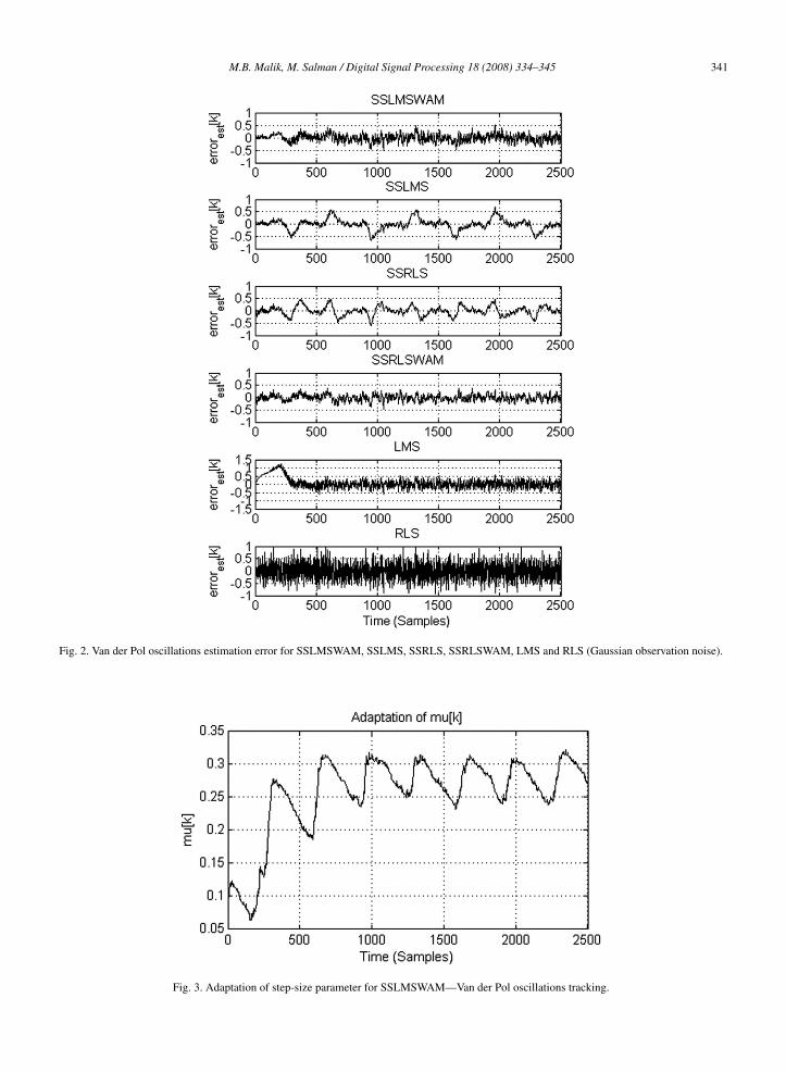
The noisy Van der Pol oscillations to be tracked are shown in Fig. 1. The simulation results as illustrated in Fig. 2demonstrate the performance of the net algorithm. In order to draw a comparison with other adaptive algorithms,tracking results for SSLMS with step-size parameter μ = 0.1, SSRLS [8] with forgetting factor λ = 0.97, SSRL-SWAM [9] with initial forgetting factor λ[0] = 0.93, 3-tap standard LMS filter with μ = 0.001 and 3-tap standardRLS filter with forgetting factor λ = 0.99 are also given. Adaptation of step-size parameter for SSLMSWAM is givenin Fig. 3. Results for the case of uniformly distributed observation noise are given in Fig. 4, where LMS operates withμ = 0.1 and RLS operates with λ = 0.8.
8.3. Comments
The constant acceleration model (37) used in these simulations provides an approximation by fitting 3rd-order poly-nomial on various segments of Van der Pol oscillations. For the segments containing lower frequency components,the fit is good and SSLMS and SSRLS perform well. On the other hand for the segments having higher frequency
M.B. Malik, M. Salman / Digital Signal Processing 18 (2008) 334–345 341
Fig. 2. Van der Pol oscillations estimation error for SSLMSWAM, SSLMS, SSRLS, SSRLSWAM, LMS and RLS (Gaussian observation noise).
Fig. 3. Adaptation of step-size parameter for SSLMSWAM—Van der Pol oscillations tracking.

342 M.B. Malik, M. Salman / Digital Signal Processing 18 (2008) 334–345
Fig. 4. Van der Pol oscillations estimation error for SSLMSWAM, SSLMS, SSRLS, SSRLSWAM, LMS and RLS (uniformly distributed observationnoise).
components the fit is not good enough. SSLMSWAM and SSRLSWAM compensate partially for this misfit by tun-ing step-size parameter and forgetting factor, respectively. Consequently, the estimation error for SSLMSWAM andSSRLSWAM is less than SSLMS and SSRLS for these segments. This effect is easier to notice in case of uniformlydistributed observation noise (Fig. 4).
In Fig. 4, periodic sharp rise and fall in estimation error for LMS is noticeable whereas performance of RLS for theselected value of forgetting factor is satisfactory. It is possible to improve the performance of SSLMS, LMS, SSRLSand RLS by changing values of step-size parameter and forgetting factor, respectively. However, we assume that thedesigner does not know beforehand the most suitable values of these parameters.
9. Computational complexity
Computational complexity of an algorithm is usually of significant importance particularly in real-time applica-tions. In this section, we discuss this aspect of SSLMS.
The complexities of Eqs. (4)–(6), (8) are given in Table 1. These equations are common to all the variants ofSSLMS. Table 2 furnishes complexity of SSLMS that comprises Eqs. (4)–(6), (8) and (19). It can be seen that com-plexity of SSLMS is O(n2).
Table 3 provides complexity of SSNLMS that comprises Eqs. (4)–(6), (8) and (17). Although the complexity ofSSNLMS is also O(n2), it is computationally more intensive of the two due to its requirement of mth-order matrix
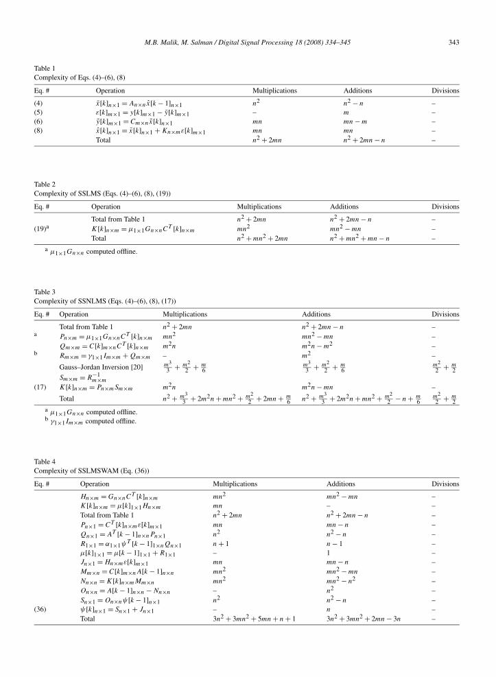
M.B. Malik, M. Salman / Digital Signal Processing 18 (2008) 334–345 343
Table 1Complexity of Eqs. (4)–(6), (8)
Eq. # Operation Multiplications Additions Divisions
(4) x[k]n×1 = An×nx[k − 1]n×1 n2 n2 − n –(5) ε[k]m×1 = y[k]m×1 − y[k]m×1 – m –(6) y[k]m×1 = Cm×nx[k]n×1 mn mn − m –(8) x[k]n×1 = x[k]n×1 + Kn×mε[k]m×1 mn mn –
Total n2 + 2mn n2 + 2mn − n –
Table 2Complexity of SSLMS (Eqs. (4)–(6), (8), (19))
Eq. # Operation Multiplications Additions Divisions
Total from Table 1 n2 + 2mn n2 + 2mn − n –(19)a K[k]n×m = μ1×1Gn×nCT [k]n×m mn2 mn2 − mn –
Total n2 + mn2 + 2mn n2 + mn2 + mn − n –
a μ1×1Gn×n computed offline.
Table 3Complexity of SSNLMS (Eqs. (4)–(6), (8), (17))
Eq. # Operation Multiplications Additions Divisions
Total from Table 1 n2 + 2mn n2 + 2mn − n –a Pn×m = μ1×1Gn×nCT [k]n×m mn2 mn2 − mn –
Qm×m = C[k]m×nCT [k]n×m m2n m2n − m2 –b Rm×m = γ1×1Im×m + Qm×m – m2 –
Gauss–Jordan Inversion [20] m3
3 + m2
2 + m6
m3
3 + m2
2 + m6
m2
2 + m2
Sm×m = R−1m×m
(17) K[k]n×m = Pn×mSm×m m2n m2n − mn –
Total n2 + m3
3 + 2m2n + mn2 + m2
2 + 2mn + m6 n2 + m3
3 + 2m2n + mn2 + m2
2 − n + m6
m2
2 + m2
a μ1×1Gn×n computed offline.b γ1×1Im×m computed offline.
Table 4Complexity of SSLMSWAM (Eq. (36))
Eq. # Operation Multiplications Additions Divisions
Hn×m = Gn×nCT [k]n×m mn2 mn2 − mn –K[k]n×m = μ[k]1×1Hn×m mn – –Total from Table 1 n2 + 2mn n2 + 2mn − n –Pn×1 = CT [k]n×mε[k]m×1 mn mn − n –Qn×1 = AT [k − 1]n×nPn×1 n2 n2 − n –R1×1 = α1×1ψT [k − 1]1×nQn×1 n + 1 n − 1 –μ[k]1×1 = μ[k − 1]1×1 + R1×1 – 1 –Jn×1 = Hn×mε[k]m×1 mn mn − n –Mm×n = C[k]m×nA[k − 1]n×n mn2 mn2 − mn –Nn×n = K[k]n×mMm×n mn2 mn2 − n2 –On×n = A[k − 1]n×n − Nn×n – n2 –Sn×1 = On×nψ[k − 1]n×1 n2 n2 − n –
(36) ψ[k]n×1 = Sn×1 + Jn×1 – n –Total 3n2 + 3mn2 + 5mn + n + 1 3n2 + 3mn2 + 2mn − 3n –
344 M.B. Malik, M. Salman / Digital Signal Processing 18 (2008) 334–345
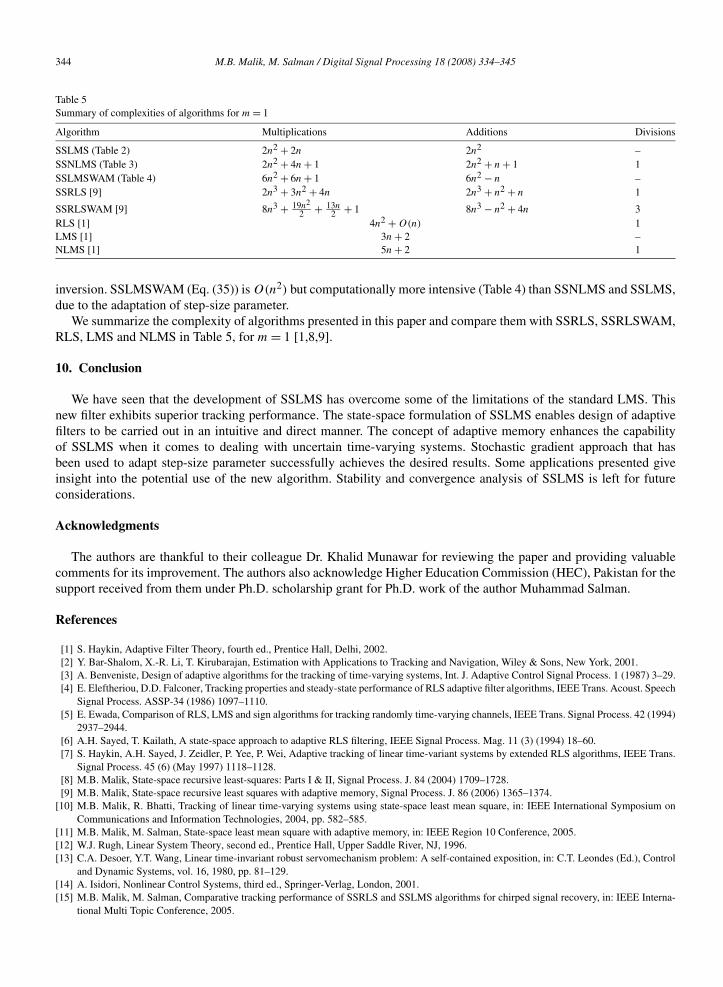
Table 5Summary of complexities of algorithms for m = 1
Algorithm Multiplications Additions Divisions
SSLMS (Table 2) 2n2 + 2n 2n2 –SSNLMS (Table 3) 2n2 + 4n + 1 2n2 + n + 1 1SSLMSWAM (Table 4) 6n2 + 6n + 1 6n2 − n –SSRLS [9] 2n3 + 3n2 + 4n 2n3 + n2 + n 1
SSRLSWAM [9] 8n3 + 19n2
2 + 13n2 + 1 8n3 − n2 + 4n 3
RLS [1] 4n2 + O(n) 1LMS [1] 3n + 2 –NLMS [1] 5n + 2 1
inversion. SSLMSWAM (Eq. (35)) is O(n2) but computationally more intensive (Table 4) than SSNLMS and SSLMS,due to the adaptation of step-size parameter.
We summarize the complexity of algorithms presented in this paper and compare them with SSRLS, SSRLSWAM,RLS, LMS and NLMS in Table 5, for m = 1 [1,8,9].
10. Conclusion
We have seen that the development of SSLMS has overcome some of the limitations of the standard LMS. Thisnew filter exhibits superior tracking performance. The state-space formulation of SSLMS enables design of adaptivefilters to be carried out in an intuitive and direct manner. The concept of adaptive memory enhances the capabilityof SSLMS when it comes to dealing with uncertain time-varying systems. Stochastic gradient approach that hasbeen used to adapt step-size parameter successfully achieves the desired results. Some applications presented giveinsight into the potential use of the new algorithm. Stability and convergence analysis of SSLMS is left for futureconsiderations.
Acknowledgments
The authors are thankful to their colleague Dr. Khalid Munawar for reviewing the paper and providing valuablecomments for its improvement. The authors also acknowledge Higher Education Commission (HEC), Pakistan for thesupport received from them under Ph.D. scholarship grant for Ph.D. work of the author Muhammad Salman.
References
[1] S. Haykin, Adaptive Filter Theory, fourth ed., Prentice Hall, Delhi, 2002.[2] Y. Bar-Shalom, X.-R. Li, T. Kirubarajan, Estimation with Applications to Tracking and Navigation, Wiley & Sons, New York, 2001.[3] A. Benveniste, Design of adaptive algorithms for the tracking of time-varying systems, Int. J. Adaptive Control Signal Process. 1 (1987) 3–29.[4] E. Eleftheriou, D.D. Falconer, Tracking properties and steady-state performance of RLS adaptive filter algorithms, IEEE Trans. Acoust. Speech
Signal Process. ASSP-34 (1986) 1097–1110.[5] E. Ewada, Comparison of RLS, LMS and sign algorithms for tracking randomly time-varying channels, IEEE Trans. Signal Process. 42 (1994)
2937–2944.[6] A.H. Sayed, T. Kailath, A state-space approach to adaptive RLS filtering, IEEE Signal Process. Mag. 11 (3) (1994) 18–60.[7] S. Haykin, A.H. Sayed, J. Zeidler, P. Yee, P. Wei, Adaptive tracking of linear time-variant systems by extended RLS algorithms, IEEE Trans.
Signal Process. 45 (6) (May 1997) 1118–1128.[8] M.B. Malik, State-space recursive least-squares: Parts I & II, Signal Process. J. 84 (2004) 1709–1728.[9] M.B. Malik, State-space recursive least squares with adaptive memory, Signal Process. J. 86 (2006) 1365–1374.
[10] M.B. Malik, R. Bhatti, Tracking of linear time-varying systems using state-space least mean square, in: IEEE International Symposium onCommunications and Information Technologies, 2004, pp. 582–585.
[11] M.B. Malik, M. Salman, State-space least mean square with adaptive memory, in: IEEE Region 10 Conference, 2005.[12] W.J. Rugh, Linear System Theory, second ed., Prentice Hall, Upper Saddle River, NJ, 1996.[13] C.A. Desoer, Y.T. Wang, Linear time-invariant robust servomechanism problem: A self-contained exposition, in: C.T. Leondes (Ed.), Control
and Dynamic Systems, vol. 16, 1980, pp. 81–129.[14] A. Isidori, Nonlinear Control Systems, third ed., Springer-Verlag, London, 2001.[15] M.B. Malik, M. Salman, Comparative tracking performance of SSRLS and SSLMS algorithms for chirped signal recovery, in: IEEE Interna-
tional Multi Topic Conference, 2005.
M.B. Malik, M. Salman / Digital Signal Processing 18 (2008) 334–345 345
[16] M. Salman, M.B. Malik, Adaptive recovery of a noisy chirp: Performance of the SSLMS algorithm, in: IEEE International Symposium onSignal Processing and Its Applications, 2005, pp. 763–766.
[17] B. Widrow, J.R. Glover Jr., J.M. McCool, J. Caunitz, C.S. Williams, R.H. Hearn, J.R. Zeidler, E. Dong Jr., R.C. Goodlin, Adaptive noisecanceling: Principles and applications, Proc. IEEE 63 (12) (1975) 1692–1716.
[18] H.K. Khalil, Nonlinear Systems, third ed., Prentice Hall, Upper Saddle River, NJ, 2002.[19] M.B. Malik, State-space recursive least-squares, Ph.D. dissertation, College of Electrical and Mechanical Engineering, National University of
Sciences and Technology, Pakistan, 2004.[20] E. Kreyszig, Advanced Engineering Mathematics, eighth ed., Wiley & Sons, Singapore, 1999.
Mohammad Bilal Malik received his B.S. degree in electrical engineering from College of Electrical and Mechanical En-gineering (E&ME), Rawalpindi, Pakistan, in 1991. He received his M.S. degree in electrical engineering from Michigan StateUniversity (MSU), Michigan, USA, in 2001. In 2004, he received his Ph.D. degree in electrical engineering from National Univer-sity of Sciences and Technology (NUST), Rawalpindi, Pakistan. He has been teaching at College of E&ME, National University ofSciences and Technology (NUST) since 1991. His research focuses on signal processing and adaptive filtering for communicationsand control systems.
Muhammad Salman received his B.S. degree in electrical engineering from College of Electrical and Mechanical Engineering(E&ME), Rawalpindi, Pakistan, in 1993. He received his M.S. degree in electrical engineering from College of Electrical andMechanical Engineering (E&ME), National University of Sciences and Technology (NUST), Rawalpindi, Pakistan, in 2005. Heis currently pursuing his Ph.D. in electrical engineering at College of E&ME, National University of Sciences and Technology(NUST), Rawalpindi, Pakistan under a scholarship from Higher Education Commission (HEC), Pakistan. His research focuses onsignal processing and adaptive filtering for communications and control systems.


