A Model-Theoretic Approach to Belief Change in Answer Set Programming

A

A Model-theoretic Approach to Belief Changein Answer Set Programming

JAMES DELGRANDE, Simon Fraser UniversityTORSTEN SCHAUB, Universitat PotsdamHANS TOMPITS and STEFAN WOLTRAN, Technische Universitat Wien

We address the problem of belief change in (nonmonotonic) logic programming under answer set semantics.Our formal techniques are analogous to those of distance-based belief revision in propositional logic. In

particular, we build upon the model theory of logic programs furnished by SE interpretations, where an

SE interpretation is a model of a logic program in the same way that a classical interpretation is a modelof a propositional formula. Hence we extend techniques from the area of belief revision based on distance

between models to belief change in logic programs.

We first consider belief revision: for logic programs P and Q, the goal is to determine a program Rthat corresponds to the revision of P by Q, denoted P ∗ Q. We investigate several operators, including

(logic program) expansion and two revision operators based on the distance between the SE models of

logic programs. It proves to be the case that expansion is an interesting operator in its own right, unlikein classical belief revision where it is relatively uninteresting. Expansion and revision are shown to satisfy

a suite of interesting properties; in particular, our revision operators satisfy all or nearly all of the AGM

postulates for revision.We next consider approaches for merging a set of logic programs, P1, . . . , Pn. Again, our formal techniques

are based on notions of relative distance between the SE models of the logic programs. Two approachesare examined. The first informally selects for each program Pi those models of Pi that vary the least from

models of the other programs. The second approach informally selects those models of a program P0 that

are closest to the models of programs P1, . . . , Pn. In this case, P0 can be thought of as a set of databaseintegrity constraints. We examine these operators with regards to how they satisfy relevant postulate sets.

Last, we present encodings for computing the revision as well as the merging of logic programs within

the same logic programming framework. This gives rise to a direct implementation of our approach in termsof off-the-shelf answer set solvers. These encodings also reflect the fact that our change operators do not

increase the complexity of the base formalism.

Categories and Subject Descriptors: I.2.3 [Artificial Intelligence]: Deduction and Theorem Proving—logic programming;nonmonotonic reasoning and belief revision; I.2.4 [Artificial Intelligence]: Knowledge Representation Formalisms andMethods—representation languages; F.4.1 [Mathematical Logic and Formal Languages]: Mathematical Logic—logicand constraint programming

General Terms: Theory

The first author was supported by a Canadian NSERC Discovery Grant; the second author was supported by the GermanScience Foundation (DFG) under grant SCHA 550/8-2; the third author was supported by the Austrian Science Fund (FWF)under project P21698; and the fourth author was supported by the Vienna University of Technology special fund “InnovativeProjekte 9006.09/008”.Authors’ address: J. Delgrande, Simon Fraser University, Burnaby, B.C., Canada, V5A 1S6, e-mail:[email protected]. T. Schaub, Universitat Potsdam, August-Bebel-Straße 89, D-14482 Potsdam, Germany, e-mail:[email protected]. H. Tompits and S. Woltran, Technische Universitat Wien, Favoritenstraße 9-11,A-1040 Vienna, Austria, e-mail: [email protected], [email protected] second author is affiliated with Simon Fraser University, Burnaby, Canada, and Griffith University, Brisbane, Australia.Permission to make digital or hard copies of part or all of this work for personal or classroom use is granted without feeprovided that copies are not made or distributed for profit or commercial advantage and that copies show this notice on thefirst page or initial screen of a display along with the full citation. Copyrights for components of this work owned by othersthan ACM must be honored. Abstracting with credit is permitted. To copy otherwise, to republish, to post on servers, toredistribute to lists, or to use any component of this work in other works requires prior specific permission and/or a fee.Permissions may be requested from Publications Dept., ACM, Inc., 2 Penn Plaza, Suite 701, New York, NY 10121-0701USA, fax +1 (212) 869-0481, or [email protected]© YYYY ACM 1529-3785/YYYY/01-ARTA $10.00

DOI 10.1145/0000000.0000000 http://doi.acm.org/10.1145/0000000.0000000

ACM Transactions on Computational Logic, Vol. V, No. N, Article A, Publication date: January YYYY.

A:2 James Delgrande et al.

Additional Key Words and Phrases: Answer set programming, belief revision, belief merging, program encodings, strongequivalence

1. INTRODUCTIONAnswer set programming (ASP) [Gelfond and Lifschitz 1988; Baral 2003] has emerged as a majorarea of research in knowledge representation and reasoning (KRR). On the one hand, ASP has anelegant and conceptually simple theoretical foundation, while on the other hand efficient implemen-tations of ASP solvers exist which have been finding applications to practical problems. However,as is the case with any large program or body of knowledge, a logic program is not a static objectin general, but rather it will evolve and be subject to change, whether as a result of correcting infor-mation in the program, adding to the information already present, coalescing information in severalprograms, or in some other fashion modifying the knowledge represented in the program.

Since knowledge is continually evolving and subject to change, there is a need to be able to mod-ify logic programs as new information is received. In KRR, the area of belief revision [Alchourronet al. 1985; Gardenfors 1988] addresses just such change to a knowledge base. In AGM belief re-vision (named after the aforecited developers of the approach) one has a knowledge base K and aformula α, and the issue is how to consistently incorporate α in K to obtain a new knowledge baseK ′. The interesting case is when K ∪ {α} is inconsistent, since beliefs have to be dropped from Kbefore α can be consistently added. Hence, a fundamental issue concerns how such change shouldbe managed.

In classical propositional logic, specific belief revision operators have been proposed based on thedistance between models of a knowledge base and a formula for revision. That is, a characterisationof the revision of a knowledge base K by formula α is to set the models of the revised knowledgebase K ′ to be the models of α that are “closest” to those of K. Of course the notion of “closest”needs to be pinned down, but natural definitions based on the Hamming distance [Dalal 1988] andset containment with regards to propositional letters [Satoh 1988] are well known.

In addition to belief revision (along with the dual notion of belief contraction), a second majorclass of belief change operators addresses the merging of knowledge bases. The problem of merg-ing multiple, potentially conflicting bodies of information arises in various different contexts. Forexample, an agent may receive reports from differing sources of knowledge, or from sets of sensorsthat need to be reconciled. As well, an increasingly common phenomenon is that collections of datamay need to be combined into a coherent whole. In these cases, the problem is that of combiningknowledge sets that may be jointly inconsistent in order to obtain a consistent set of merged beliefs.Again, as in belief revision, specific operators for merging knowledge bases have been developedbased on the distance between models of the underlying knowledge bases [Baral et al. 1992; Revesz1993; Liberatore and Schaerf 1998; Meyer 2001; Konieczny and Pino Perez 2002; Konieczny et al.2002].

It is natural then to consider belief change in the context of logic programs. Indeed, there hasbeen substantial effort in developing approaches to so-called logic program updating under answerset semantics (as discussed in the next section). Unfortunately, given the nonmonotonic nature ofanswer set programs, the problem of change in logic programs appears to be intrinsically more dif-ficult than in a monotonic setting. In this paper, our goal is to reformulate belief change in logicprograms in a manner analogous to belief change in classical propositional logic, and to investigatespecific belief revision and merging operators for logic programs under the answer set semantics.Central to our approach are SE models [Turner 2003], which are semantic structures characterisingstrong equivalence between programs [Lifschitz et al. 2001]. This particular kind of equivalenceplays a major role for different problems in logic programming—in particular, in program simplifi-cation and modularisation. This is due to the fact that strong equivalence gives rise to a substitutionprinciple in the sense that, for strongly equivalent programs P,Q, the programs P ∪ R and Q ∪ Rhave the same answer sets, for any program R. As is well known, ordinary equivalence betweenprograms (which holds if two programs have the same answer sets) does not yield a substitutionprinciple. Hence, strong equivalence can be seen as the logic programming analogue of ordinary


A Model-Theoretic Approach to Belief Change in Answer Set Programming A:3

equivalence in classical logic. The important aspect of strong equivalence is that it coincides withequivalence in a specific monotonic logic, the logic of here and there (HT), which is intermediatebetween intuitionistic logic and classical logic. Moreover, following Osorio and Zacarıas [2004]and Osorio and Cuevas [2007], strong equivalence amounts to knowledge equivalence of programs.That is, strong equivalence captures the logical content of a program.1

As shown by Turner [2003], equivalence between programs in HT corresponds in turn to equalitybetween sets of SE models. Details on these concepts are given in the next section; the key point isthat logic programs can be expressed in terms of a non-classical but monotonic logic, and it is thispoint that we exploit here.

Given this monotonic characterisation (via sets of SE models) of strong equivalence, we adapttechniques for belief change in propositional logic to belief change in logic programs. Hence wedefine specific operators for belief change in ASP analogous to operators in propositional logic.We first consider an expansion operator. In classical logic, the expansion of knowledge base K byformula α amounts to the deductive closure of K ∪ {α}. Hence it is not a very interesting operator,serving mainly as a tool for expressing concepts in belief revision and its dual, contraction. In logicprograms however, expansion appears to be a more useful operator, perhaps due to the apparent“looser” notion of satisfiability provided by SE models. As well, it has appealing properties. Wenext develop revision operators based on notions of distance between SE models, and, followingthis, merging operators.

For a revision of logic program P by program Q, written P ∗ Q, the resulting program is char-acterised by those SE models of Q that are closest to the SE models of P . We consider two notionsof “closeness” between models; in both cases a notion of distance between models is defined interms of the symmetric difference of the atoms true in each model. In one case, two models areof minimum distance if the symmetric difference is subset-minimal; in the other case they are ofminimum distance if the symmetric difference is cardinality-minimal. These approaches to revisioncan be seen as extending the approaches of Satoh [1988] and Dalal [1988], respectively.

In characterising the merging of logic programs, the central idea is that the SE models of themerged program are again those that are in some sense “closest” to the SE models of the programsto be merged. However, as with merging knowledge bases in classical logic, there is no singlepreferred notion of distance nor closeness, and consequently different approaches have been definedfor combining sources of information. We introduce two merging operators for logic programs underanswer set semantics. Both operators take an arbitrary (multi)set of logic programs as argument. Thefirst operator can be regarded an instance of what Liberatore and Schaerf [1998] call arbitration.Basically (SE) models are selected from among the SE models of the programs to be merged; ina sense this operator is a natural extension of our belief revision operator. The second mergingoperator can be regarded as an instance of the one discussed by Konieczny and Pino Perez [2002].Here, models of a designated program (representing information analogous to database integrityconstraints) are selected that are closest to (or perhaps, informally, represent the best compromiseamong) the models of the programs to be merged.

Notably, in our approaches there is effectively no mention of answer sets; rather definitions ofexpansion, revision, and merging are given entirely with respect to logic programs. Notably too, ouroperators are syntax independent, which is to say, they are independent of how a logic program isexpressed. Hence (and in view of the intuitions of SE models as pointed out above), our operatorsdeal with the logical content of a logic program.

Last, we show how our belief change approaches can be implemented. We do this by providingmodular encodings for these operators in terms of a fixed non-ground answer-set program. These en-codings serve several purposes. First, they provide a proof-of-concept realisation for the approaches.The encodings also help shed light on the details of the respective approaches. As well, they providea tool for experimenting with the approaches.

1For a different concept of logical content of an answer set program, see Osorio and Zepeda [2003].



Following an introductory background section, we show that there is a ready mapping betweenconcepts in belief revision in classical logic and in ASP; this serves to place belief revision in ASPfirmly in the “standard” belief revision camp. After this we describe in Section 3 our approaches tobelief expansion and revision in ASP. We then employ these techniques in the following section toaddress the merging of logic programs. In each case, we discuss central properties and give com-plexity results. Then, in Section 5, we show how we can in fact express the process of belief changein ASP itself, giving a direct way to compute our introduced belief change operators, and we providea general complexity analysis of our belief change approach. Finally, the paper is concluded with adiscussion. Proofs of results are contained in an appendix. Preliminary versions of the material inSections 3 and 4 appeared in previous work [Delgrande et al. 2008; 2009].

2. BACKGROUND AND FORMAL PRELIMINARIES2.1. Answer Set Programming

2.1.1. Syntax and Semantics. LetA be an alphabet, consisting of a set of atoms. A (generalised)logic program2 (GLP) over A is a finite set of rules of the form

a1; . . . ; am;∼b1; . . . ;∼bn ← c1, . . . , co,∼d1, . . . ,∼dp, (1)

where ai, bj , ck, dl ∈ A, and where m,n, o, p ≥ 0 and m + n + o + p > 0. Binary operators ‘;’and ‘,’ express disjunctive and conjunctive connectives. A default literal is an atom a or its (default)negation ∼a. It is convenient to distinguish various types of rules. A rule r as in (1) is:

— a fact if m = 1 and n = o = p = 0,— normal if m = 1 and n = 0,— positive if n = p = 0,— disjunctive if n = 0, and— an integrity constraint if m = n = 0.

For example, p ← is a fact (some papers also express this as ‘p.’); p ← q,∼r is normal; p; q ←r, s is positive; p; q ← r,∼s is disjunctive; and← q,∼r is an integrity constraint, sometimes alsowritten ⊥ ← q,∼r.

Accordingly, a program is called disjunctive (or a DLP) if it consists of disjunctive rules only.Likewise, a program is normal (resp., positive) iff all rules in it are normal (resp., positive). Wefurthermore define the head and body of a rule, H(r) and B(r), by:

H(r) = {a1, . . . , am,∼b1, . . . ,∼bn} andB(r) = {c1, . . . , co,∼d1, . . . ,∼dp}.

Moreover, given a set X of literals, we define

X+ = {a ∈ A | a ∈ X},X− = {a ∈ A | ∼a ∈ X}, and∼X = {∼a | a ∈ X ∩ A}.

For simplicity, we sometimes use a set-based notation, expressing a rule as in (1) as

H(r)+;∼H(r)−← B(r)+,∼B(r)− .

In what follows, we restrict ourselves to a finite alphabet A. An interpretation is represented bythe subset of atoms in A that are true in the interpretation. A (classical) model of a program P isan interpretation in which all of the rules in P are true according to the standard definition of truthin propositional logic, and where default negation is treated as classical negation. By Mod(P ) we

2Such programs were first considered by Lifschitz and Woo [1992] and called generalised disjunctive logic programs byInoue and Sakama [1998].



denote the set of all classical models of P . The reduct of a program P with respect to a set of atomsY , denoted PY , is the set of rules:

{H(r)+← B(r)+ | r ∈ P, H(r)− ⊆ Y, B(r)− ∩ Y = ∅}.Note that the reduct consists of negation-free rules only. An answer set Y of a program P is asubset-minimal model of PY . The set of all answer sets of a program P is denoted by AS (P ). Forexample, the program P = {a←, c; d← a,∼b} has answer sets AS (P ) = {{a, c}, {a, d}}.

2.1.2. SE Models. As defined by Turner [2003], an SE interpretation is a pair (X,Y ) of inter-pretations such that X ⊆ Y ⊆ A. An SE interpretation is an SE model of a program P if Y |= Pand X |= PY . The set of all SE models of a program P is denoted by SE (P ). Then, Y is an an-swer set of P iff (Y, Y ) ∈ SE (P ) and no (X,Y ) ∈ SE (P ) with X ⊂ Y exists. Also, we have(Y, Y ) ∈ SE (P ) iff Y ∈ Mod(P ).

A program P is satisfiable just if SE (P ) 6= ∅. Note that many authors in the literature definesatisfiability in terms of answer sets, in that for them a program is satisfiable if it has an answer set,i.e., AS (P ) 6= ∅. Thus, for example, we consider P = {p← ∼p} to be satisfiable, since SE (P ) 6=∅ even though AS (P ) = ∅.3 Two programs P andQ are strongly equivalent, symbolically P ≡s Q,iff SE (P ) = SE (Q). Alternatively, P ≡s Q holds iff AS (P ∪R) = AS (Q∪R), for every programR [Lifschitz et al. 2001]. We also write P |=s Q iff SE (P ) ⊆ SE (Q). For simplicity, we often dropset-notation within SE interpretations and simply write, e.g., (a, ab) instead of ({a}, {a, b}).

A feature of SE models is that they contain “more information” than answer sets, which makesthem an appealing candidate for problems where programs are examined with respect to furtherextension (in fact, this is what strong equivalence is about). We illustrate this issue with the followingwell-known example, involving programs

P = {p; q ←} and Q =

{p← ∼qq ← ∼p

}.

Here, we have AS (P ) = AS (Q) = {{p}, {q}}. However, the SE models differ. For A = {p, q},we have:

SE (P ) = {(p, p), (q, q), (p, pq), (q, pq), (pq, pq)};SE (Q) = {(p, p), (q, q), (p, pq), (q, pq), (pq, pq), (∅, pq)}.

This is to be expected, since P and Q behave differently with respect to program extension (andthus are not strongly equivalent). Consider R = {p ← q, q ← p}. Then, AS (P ∪ R) = {{p, q}},while AS (Q ∪R) has no answer set.

We next adopt concepts introduced by Eiter et al. [2005] which are instrumental for our purposes.Let us call a set S of SE interpretations well-defined if, for each (X,Y ) ∈ S, also (Y, Y ) ∈ S. Awell-defined set S of SE interpretations is complete if, for each (X,Y ) ∈ S, also (X,Z) ∈ S, forany Z ⊇ Y with (Z,Z) ∈ S.

We have the following properties:

(1) For each GLP P , SE (P ) is well-defined, and for each DLP P , SE (P ) is complete.(2) Conversely, for each well-defined set S of SE interpretations, there exists a GLP P such that

SE (P ) = S, and for each complete set S of SE interpretations, there exists a DLP P such thatSE (P ) = S.

Programs meeting the latter conditions can be constructed thus [Eiter et al. 2005; Cabalar and Fer-raris 2007]: In case S is a well-defined set of SE interpretations over a (finite) alphabet A, define Pby adding

(1) the rule rY : ⊥ ← Y,∼(A \ Y ), for each (Y, Y ) /∈ S, and

3Given the correspondence between SE model theory and the logic HT, our notion of satisfiability is tantamount to satisfia-bility in HT.



(2) the rule rX,Y : (Y \ X);∼Y ← X,∼(A \ Y ), for each X ⊆ Y such that (X,Y ) /∈ S and(Y, Y ) ∈ S.

In case S is complete, define P by adding

(1) the rule rY , for each (Y, Y ) /∈ S, as above, and(2) the rule r′X,Y : (Y \ X) ← X,∼(A \ Y ), for each X ⊆ Y such that (X,Y ) /∈ S and

(Y, Y ) ∈ S.

We call the resulting programs canonical.For illustration, consider

S = {(p, p), (q, q), (p, pq), (q, pq), (pq, pq), (∅, p)}over A = {p, q}. Note that S is not complete. The canonical GLP is as follows:

r∅ : ⊥ ← ∼p,∼q;r∅,q : q;∼q ← ∼p;r∅,pq : p; q;∼p;∼q ← .

For obtaining a complete set, we have to add (∅, pq) to S. Then, the canonical DLP is as follows:

r∅ : ⊥ ← ∼p,∼q;r∅,q : q ← ∼p.

We conclude this subsection by introducing definitions for ordering SE models that will be neededwhen we come to define our belief change operators. Let denote the symmetric difference operatorbetween sets, i.e., XY = (X \Y )∪ (Y \X) for every set X,Y . We extend so that it is definedfor ordered pairs, as follows:

Definition 2.1. For every pair (X1, X2), (Y1, Y2),

(X1, X2) (Y1, Y2) = (X1 Y1, X2 Y2).

Similarly, we define a notion of set containment, suitable for ordered pairs, as follows:

Definition 2.2. For every pair (X1, X2), (Y1, Y2),(X1, X2) ⊆ (Y1, Y2) iff X2 ⊆ Y2, and if X2 = Y2 then X1 ⊆ Y1.(X1, X2) ⊂ (Y1, Y2) iff (X1, X2) ⊆ (Y1, Y2) and not (Y1, Y2) ⊆ (X1, X2).

As will be seen, these definitions are appropriate for SE interpretations, as they give preference tothe second element of an SE interpretation.

Set cardinality is denoted as usual by | · |. We define a cardinality-based ordering over orderedpairs of sets as follows:

Definition 2.3. For every pair (X1, X2), (Y1, Y2),|(X1, X2)| ≤ |(Y1, Y2)| iff |X2| ≤ |Y2| and if |X2| = |Y2| then |X1| ≤ |Y1|.|(X1, X2)| < |(Y1, Y2)| iff |(X1, X2)| ≤ |(Y1, Y2)| and not |(Y1, Y2)| ≤ |(X1, X2)|.

As with Definition 2.2, this definition gives preference to the second element of an ordered pair. Itcan be observed that the definition yields a total preorder over ordered pairs. In the next section wereturn to the suitability of this definition, once our revision operators have been presented.

2.2. Belief Change2.2.1. Belief Revision. The best known and, indeed, seminal work in belief revision is the AGM

approach [Alchourron et al. 1985; Gardenfors 1988], in which standards for belief revision andcontraction functions are given. In the revision of a knowledge base K by a formula φ, the intent isthat the resulting knowledge base contains φ, be consistent (unless φ is not), while keeping whateverinformation from K can be “reasonably” retained. Belief contraction is a dual notion, in which



information is removed from a knowledge base. While belief contraction is independently motivatedand defined, it is generally accepted that in classical logic a contraction function can be obtainedfrom a revision function by the so-called Harper identity, and the reverse obtained via the Leviidentity;4 see Gardenfors [1988] for details.

In the AGM approach it is assumed that a knowledge base receives information concerning astatic5 domain. Belief states are modelled by logically closed sets of sentences, called belief sets. Abelief set is a set K of sentences which satisfies the constraint

if K logically entails β, then β ∈ K.K can be seen as a partial theory of the world. For belief setK and formula α,K+α is the deductiveclosure of K ∪ {α}, called the expansion of K by α. K⊥ is the inconsistent belief set (i.e., K⊥ isthe set of all formulas).

Subsequently, Katsuno and Mendelzon [1992] reformulated the AGM approach so that a knowl-edge base was represented by a formula in some language L. The following postulates compriseKatsuno and Mendelzon’s reformulation of the AGM revision postulates, where ∗ is a functionfrom L × L to L:

(R1) ψ ∗ µ ` µ.(R2) If ψ ∧ µ is satisfiable, then ψ ∗ µ↔ ψ ∧ µ.(R3) If µ is satisfiable, then ψ ∗ µ is also satisfiable.(R4) If ψ1 ↔ ψ2 and µ1 ↔ µ2, then ψ1 ∗ µ1 ↔ ψ2 ∗ µ2.(R5) (ψ ∗ µ) ∧ φ ` ψ ∗ (µ ∧ φ).(R6) If (ψ ∗ µ) ∧ φ is satisfiable, then ψ ∗ (µ ∧ φ) ` (ψ ∗ µ) ∧ φ.

Thus, revision is successful (R1), and corresponds to conjunction when the knowledge base andformula for revision are jointly consistent (R2). Revision leads to inconsistency only when theformula for revision is unsatisfiable (R3). Revision is also independent of syntactic representation(R4). Last, (R5) and (R6) express that revision by a conjunction is the same as revision by oneconjunct conjoined with the other conjunct, when the result is satisfiable.

A second major branch of belief change research concerns belief bases [Hansson 1999], whereinan agent’s beliefs are represented by an arbitrary set of formulas, and so may not be deductivelyclosed. Consider the two sets of sentences

K1 = {p, q}, K2 = {p, p ⊃ q}.Clearly the logical content of K1 and K2 is the same. In the AGM approach, wherein syntacticdetails of a knowledge base are suppressed, revising these knowledge bases by the same formulawill give the same results. In a belief base approach, where syntactic details do matter, revision bythe same formula may yield different results. Hence in the above example, if one were to revise by¬q, then consistency can be maintained in K1 by dropping q, whereas it can be maintained in K2

by dropping either p or p ⊃ q.

2.2.2. Specific Belief Revision Operators. In classical belief change, the revision of a knowledgebase represented by formula ψ by a formula µ, ψ ∗ µ, is a formula φ such that the models of φare just those models of µ that are “closest” to those of ψ. There are two main specific approachesto distance-based revision. Both are related to the Hamming distance between two interpretations,that is they are based on the set of atoms on which the interpretations disagree. The first, by Satoh[1988], is based on set containment. The second, due to Dalal [1988], uses a distance measure basedon the number of atoms with differing truth values in two interpretations. A set containment-based

4The Harper identity states that a contraction of φ can be obtained by revising by ¬φ and then intersecting the result withthe original belief set. The Levi identity states that a revision by φ can be obtained by contracting the belief set by ¬φ andthen expanding the belief set by φ.5 Note that “static” does not imply “with no mention of time”. For example, one could have information in a knowledge baseabout the state of the world at different points in time, and revise information at these points in time.



approach seems more appropriate in the context of ASP, since answer sets are defined in terms ofsubset-minimal interpretations. Hence, we focus on the method of Satoh [1988], although we alsoconsider Dalal-style revision, since it has some technical interest with respect to ASP revision.

The Satoh revision operator, ψ ∗s µ, is defined as follows. For formulas α and β, definemin(α, β) as

min⊆({w w′ | w ∈ Mod(α), w′ ∈ Mod(β)}).Furthermore, define Mod(ψ ∗s µ) as

{w ∈ Mod(µ) | ∃w′∈Mod(ψ) s.t. w w′ ∈ min(ψ, µ)}.The cardinality-based, or Dalal revision operator, ψ ∗d µ, is defined as follows. For formulas α

and β, define ||min(α, β) as

min≤({|w w′| | w ∈ Mod(α), w′ ∈ Mod(β)}).Then, Mod(ψ ∗d µ) is given as

{w ∈ Mod(µ) | ∃w′∈Mod(ψ) s.t. |w w′| = ||min(ψ, µ)}.2.2.3. Belief Merging. Early work on merging operators includes approaches by Baral et al. [1992]

and Revesz [1993]. The former authors propose various theory merging operators based on theselection of maximum consistent subsets in the union of the belief bases. The latter proposes an“arbitration” operator (see below) that, intuitively, selects from among the models of the belief setsbeing merged. Lin and Mendelzon [1999] examine majority merging, in which, if a plurality ofknowledge bases hold φ to be true, then φ is true in the merging. Liberatore and Schaerf [1998]address arbitration in general, while Konieczny and Pino Perez [2002] consider a general approachin which merging takes place with respect to a set of global constraints, or formulas, that must holdin the merging. We examine these latter two approaches in detail below.

Konieczny et al. [2002] describe a very general framework in which a family of merging opera-tors is parametrised by a distance between interpretations and aggregating functions. More or lessconcurrently, Meyer [2001] proposed a general approach to formulating merging functions basedon ordinal conditional functions [Spohn 1988]. Booth [2002] also considers the problem of an agentmerging information from different sources, via what is called social contraction. Last, much workhas been carried out in merging possibilistic knowledge bases; we mention here, e.g., the methodby Benferhat et al. [2003].

We next describe the approaches by Liberatore and Schaerf [1998] and by Konieczny and PinoPerez [2002], since we use the intuitions underlying these approaches as the basis for our mergingtechnique. First, Liberatore and Schaerf [1998] consider merging two belief bases built on the intu-ition that models of the merged bases should be taken from those of each belief base closest to theother. This is called an arbitration operator (Konieczny and Pino Perez [2002] call it a commutativerevision operator). They consider a propositional language over a finite set of atoms; consequentlytheir merging operator can be expressed as a binary operator on formulas. The following postulatescharacterise this operator:

Definition 2.4. � is an arbitration operator if � satisfies the following postulates.

(LS1) α � β ≡ β � α.(LS2) α ∧ β implies α � β.(LS3) If α ∧ β is satisfiable then α � β implies α ∧ β.(LS4) α � β is unsatisfiable iff α is unsatisfiable and β is unsatisfiable.(LS5) If α1 ≡ α2 and β1 ≡ β2 then α1 � β1 ≡ α2 � β2.

(LS6) α � (β1 ∨ β2) =

{α � β1 orα � β2 or(α � β1) ∨ (α � β2).

(LS7) (α � β) implies (α ∨ β).



(LS8) If α is satisfiable then α ∧ (α � β) is satisfiable.

The first postulate asserts that merging is commutative, while the next two assert that, for mutuallyconsistent formulas, merging corresponds to their conjunction. (LS5) ensures that the operator isindependent of syntax, while (LS6) provides a “factoring” postulate, analogous to a similar factor-ing result in (AGM-style) belief revision and contraction. Postulate (LS7) can be taken as distin-guishing � from other such operators; it asserts that the result of merging implies the disjunctionof the original formulas. The last postulate informally constrains the result of merging so that eachoperator “contributes to” (i.e., is consistent with) the final result.

Next, Konieczny and Pino Perez [2002] consider the problem of merging possibly contradictorybelief bases. To this end, they consider finite multisets of the form Ψ = {K1, . . . ,Kn}. Theyassume that the belief sets Ki are consistent and finitely representable, and so representable bya formula. Kn is the multiset consisting of n copies of K. Following Konieczny and Pino Perez[2002], let ∆µ(Ψ) denote the result of merging the multiset Ψ of belief bases given the entailment-based integrity constraint expressed by µ. The intent is that ∆µ(Ψ) is the belief base closest to thebelief multiset Ψ. They provide the following set of postulates (multiset union is denoted by ∪):

Definition 2.5. Let Ψ be a multiset of sets of formulas, and φ, µ formulas (all possibly sub-scripted or primed). Then, ∆ is an IC merging operator if it satisfies the following postulates.

(IC0) ∆µ(Ψ) ` µ.(IC1) If µ 6` ⊥ then ∆µ(Ψ) 6` ⊥.(IC2) If

∧Ψ 6` ¬µ then ∆µ(Ψ) ≡

∧Ψ ∧ µ.

(IC3) If Ψ1 ≡ Ψ2 and µ1 ≡ µ2 then ∆µ1(Ψ1) ≡ ∆µ2(Ψ2).(IC4) If φ ` µ and φ′ ` µ then ∆µ(φ ∪ φ′) ∧ φ 6` ⊥ implies ∆µ(φ ∪ φ′) ∧ φ′ 6` ⊥.(IC5) ∆µ(Ψ1) ∧∆µ(Ψ2) ` ∆µ(Ψ1 ∪Ψ2).(IC6) If ∆µ(Ψ1) ∧∆µ(Ψ2) 6` ⊥ then ∆µ(Ψ1 ∪Ψ2) ` ∆µ(Ψ1) ∧∆µ(Ψ2).(IC7) ∆µ1(Ψ) ∧ µ2 ` ∆µ1∧µ2(Ψ).(IC8) If ∆µ1(Ψ) ∧ µ2 6` ⊥ then ∆µ1∧µ2(Ψ) ` ∆µ1(Ψ) ∧ µ2.

(IC2) states that, when consistent, the result of merging is simply the conjunction of the beliefbases and integrity constraints. (IC4) asserts that when two belief bases disagree, merging doesnot give preference to one of them. (IC5) states that a model of two mergings is in the unionof their merging. With (IC5) we get that if two mergings are consistent then their merging isimplied by their conjunction. Note that merging operators are trivially commutative. (IC7) and(IC8) correspond to the extended AGM postulates (K ∗7) and (K ∗8) for revision (cf. Alchourronet al. [1985] and Gardenfors [1988]), but with respect to the integrity constraints.

2.3. Belief Change in Logic ProgrammingMost previous work on belief change for logic programs goes under the title of update [Przymusin-ski and Turner 1997; Zhang and Foo 1997; 1998; Alferes et al. 2000; Leite 2003; Eiter et al. 2002;Sakama and Inoue 2003; Zacarıas et al. 2005; Delgrande et al. 2007]. Strictly speaking, however,such approaches generally do not address “update,” at least insofar as the term is understood inthe belief revision community. In this community, update refers to a belief change in response toa change in the world being modelled [Katsuno and Mendelzon 1992]; hence update is concernedwith a setting in which the world has evolved to a new state. This notion of change is not taken intoaccount in the above-cited work; instead, it is possible that change is with respect to a static world,in which a logic program is modified to better represent this domain.6

Following the investigations of the Lisbon group of researchers [Alferes et al. 2000; Leite 2003],a typical setting for update approaches is to consider a sequence P1, P2, . . . , Pn of programs whereeach Pi is a logic program (this is done, e.g., in the approaches by Eiter et al. [2002], Zacarıas

6To be clear, our interests in this paper lie with revision, where a logic program is revised with respect to some (static)underlying domain or world.



et al. [2005], and Delgrande et al. [2007]). For Pi, Pj , and i > j, the intuition is that Pi has higherpriority or precedence. Given such a sequence, a set of answer sets is determined that in some senserespects the ordering. This may be done by translating the sequence into a single logic program thatcontains an encoding of the priorities, or by treating the sequence as a prioritised logic program,or by some other appropriate method. Most such approaches are founded on the notion of causalrejection. According to this principle, a rule r is rejected if there is another, higher-ranked rule r′which conflicts with r. That is, if both r and r′ are applicable and have conflicting heads then onlyr′ is applied. The net result, one way or another, is that one obtains a set of answer sets from such aprogram sequence. That is, one does not obtain a single, new program expressed in the language ofthe original logic programs. Hence, these approaches fall outside the general AGM belief revisionparadigm. As well, it should be clear that such approaches are syntactic in nature, and so suchapproaches fall into the belief base category, rather than the belief set category.

For illustration, we briefly consider one such approach, that of Eiter et al. [2002]. In this approachthe semantics of an (n − 1)-fold update P1 ◦ · · · ◦ Pn is given by the semantics of an (ordinary)program P�, containing the following elements:

(1) all integrity constraints in Pi, 1 ≤ i ≤ n;(2) for each r ∈ Pi, 1 ≤ i ≤ n:

li ← B(r),∼rej(r), where H(r) = l;(3) for each r ∈ Pi, 1 ≤ i < n:

rej(r) ← B(r),¬li+1, where H(r) = l;(4) for each literal l occurring in P (1 ≤ i < n):

li ← li+1; l← l1.

Here, for each rule r, rej(r) is a new atom not occurring in P1, . . . , Pn. Intuitively, rej(r) expressesthat r is “rejected.” Similarly, each li, 1 ≤ i ≤ n, is a new atom not occurring in P1, . . . , Pn. Answersets of P1 ◦ · · · ◦ Pn are given by the answer sets of P�, intersected with the original language.

Consider the following example adapted from Alferes et al. [2000]. We have the update of P1 byP2, where

P1 = { r1 : sleep ← ∼tv on, r2 : night ← ,r3 : tv on ←, r4 : watch tv ← tv on },

P2 = { r5 : ¬tv on ← power failure, r6 : power failure ← }.The single answer set of P1 ◦ P2 is

S = {power failure,¬tv on, sleep,night}.If new information arrives as program P3, given by

P3 = { r7 : ¬power failure ← },then P1 ◦ P2 ◦ P3 has the unique answer set

T = { ¬power failure, tv on,watch tv ,night }.Again, it can be noted that this approach deals with the rules in a program; hence this approach,

as with related approaches, falls into the category of base revision.However, various principles have nonetheless been proposed for such approaches to logic pro-

gram update. In particular, Eiter et al. [2002] consider the question of what principles the updateof logic programs should satisfy. This is done by re-interpreting different AGM-style postulates forrevising or updating classic knowledge bases, as well as introducing new principles. Among thelatter, we note the following:

Initialisation ∅ ∗ P ≡ P .Idempotency (P ∗ P ) ≡ P .



Tautology If Q is tautologous, then P ∗Q ≡ P .Absorption If Q = R, then ((P ∗Q) ∗R) ≡ (P ∗Q).Augmentation If Q ⊆ R, then ((P ∗Q) ∗R) ≡ (P ∗R).

In view of the failure of several of the discussed postulates in the approach of Eiter et al. [2002] (aswell as in others), Osorio and Cuevas [2007] noted that for re-interpreting the standard AGM pos-tulates in the context of logic programs, the logic underlying strong equivalence should be adopted.Since Osorio and Cuevas [2007] studied programs with strong negation,7 this led them to considerthe logic N2, an extension of HT by allowing strong negation.8 They rephrased the AGM postulatesin terms of the logic N2 and also introduced a new principle, referred to as weak independence ofsyntax (WIS), which they proposed that any update operator should satisfy:

WIS If Q ≡s R, then (P ∗Q) ≡ (P ∗R).

Indeed, following this spirit, the above absorption and augmentation principles can be accordinglychanged by replacing their antecedents by “Q ≡s R” and “Q |=s R”, respectively. Osorio andCuevas [2007] defined a variation of the semantics by Eiter et al. [2002] and showed that it satisfiesall their adapted AGM postulates. Furthermore, they show that a further variant of their semanticsis equivalent to the semantics by Eiter et al. [2002] for a certain class of programs which satisfiesall except one of the adapted AGM postulates. We note that the WIS principle was also discussed inan update approach based on abductive programs [Zacarıas et al. 2005].

In contrast to the works discussed above, Sakama and Inoue [2003] do not deal with sequencesof programs but with characterising different kinds of knowledge-base updates in terms of extendedabduction [Inoue and Sakama 1995]. In particular, they discuss, besides usual theory update, viewupdate and consistency restoration. For view update and consistency restoration, it is assumed thatprograms are divided into a variable and an invariable part. In view update, the task is to changethe variable part given an update request in the form of a fact, while in consistency restoration,the problem is to modify the variable part of a program P whose constraint-free part violates theconstraints of P (and it is assumed that constraints are themselves supposed to be invariant). Letus have a closer look at their method of theory update. Given programs P1 and P2, an update ofP1 by P2 is a largest program Q such that P1 ⊆ Q ⊆ P1 ∪ P2 and Q has a consistent answerset. This problem is then reduced to the problem of computing a minimal set R of abducible rulessuch that R ⊆ P1 \ P2 and (P1 ∪ P2) \ R has an answer set. The intended update is realised via aminimal anti-explanation for falsity, which removes abducible rules in order to restore consistency.As demonstrated by Eiter et al. [2002], this approach violates causal rejection. Furthermore, it isdifferent from our approach to revision. For instance, updating P1 = {p←; q ← } by P2 = {⊥ ←p, q} in Sakama and Inoue’s approach results in the removal of one of the two rules in P1, while ourapproach yields a program having {p} and {q} as answer sets.

Turning our attention to the few works on revision of logic programs, early work in this directionincludes a series of investigations dealing with restoring consistency for programs possessing noanswer sets (cf., e.g., Witteveen et al. [1994]). Other work uses logic programs under a variant ofthe stable semantics to specify database revision, i.e., the revision of knowledge bases given assets of atomic facts [Marek and Truszczynski 1998]. Finally, an approach following the spirit ofAGM revision is discussed by Kudo and Murai [2004]. In their work, they deal with the question ofconstructing revisions of form P ∗A, where P is an extended logic program andA is a conjunction ofliterals. They give a procedural algorithm to construct the revised programs; however no propertiesare analysed.

In belief change, the operation of belief contraction is a dual to revision. The idea is that incontracting by a formula φ, the agent ceases to believe that φ (if it ever did believe φ), while not

7Strong negation is sometimes also referred to as classical negation, but this is a misnomer as it does not enjoy all propertiesof classical negation.8N2 itself traces back to an extension of intuitionistic logic with strong negation, first studied by Nelson [1949].



necessarily believing ¬φ. Then a revision by ψ can be implemented by first contracting ¬ψ andthen adding ψ. There has been, insofar as we are aware, no work on belief contraction with respectto logic programs. There has been some work on the related notion of forget [Zhang and Foo 2006;Eiter and Wang 2008] in which forgetting a literal is akin to shrinking the language by the corre-sponding atom. It can be noted first of all that the cited works are syntactic, in that they are couchedwith reference to underlying answer sets. (In fact, Eiter and Wang [2008] discusses the relation be-tween their notion of forgetting and logic program update.) However, more pertinently, forgettingappears to be too drastic to yield an acceptable approach to revision. Consider for example wherea knowledge base believes that a penguin flies, F ← P , and one wants to revise by the fact that apenguin does not fly, say ⊥ ← P, F . We can remove the conflict by forgetting P or F (or both).However, if one forgets P , then all information about penguins (say that they eat fish or walk up-right) is lost; similarly if one forgets F , then all information about flight (say that bats fly) is lost.So forgetting P or F will allow ⊥ ← P, F to be consistently added, but at much too great a cost.

With respect to merging logic programs, we have already mentioned updating logic programs,which can also be considered as prioritised logic program merging. With respect to merging unpri-oritised logic programs, Baral et al. [1991] describes an algorithm for combining a set of normal,stratified logic programs in which the union of the programs is also stratified. In their approachthe combination is carried out so that a set of global integrity constraints, which is satisfied by in-dividual programs, is also satisfied by the combination. As well, in this approach (as with relatedapproaches to logic program merging), logic program combining is obtained via manipulating andtransforming program rules. Hence the result is dependent on program syntax, and so syntax inde-pendence as exemplified by (IC3) in Definition 2.5 is not obtained in these approaches. In contrast,in the approaches described in Section 4, syntax independence is obtained.

Buccafurri and Gottlob [2002] present an interesting approach whereby rules in a given programencode desires for a corresponding agent. A predicate okay indicates that an atom is acceptableto an agent. Answer sets of these compromise logic programs represent acceptable compromisesbetween agents. While it is shown that the joint fixpoints of such logic programs can be computedas answer sets and complexity results are presented, the approach is not analysed from the standpointof properties of merging.

In a succession of works, Sakama and Inoue [2006; 2007; 2008] address what they respectivelycall coordination, composition, and consensus between logic programs. In short, given programsP1 and P2, a program Q is a generous coordination of P1 and P2 if AS (Q) = AS (P1) ∪ AS (P2)while it is a rigorous coordination of P1 and P2 if AS (Q) = AS (P1)∩AS (P2). On the other hand,the composition of P1 and P2 is defined as a program whose answer sets are given by min{S ] T |S ∈ AS (P1), T ∈ AS (P2)}, where S ] T is S ∪ T if S ∪ T is consistent, otherwise S ] T isthe set of all literals.9 Finally, Q is a minimal consensus between P1 and P2 if its answer sets aregiven by min{S ∩ T | S ∈ AS (P1), T ∈ AS (P2)} and it is a maximal consensus between P1

and P2 if its answer sets are given by max{S ∩ T | S ∈ AS (P1), T ∈ AS (P2)}. Intuitively,the coordination of two programs results in a program collecting either all answer sets (in case ofgenerous coordination) or picks just the common answer sets (in case of rigorous coordination).While this construction leaves the original answer sets unchanged, the composition of programscombines the answer sets of the given programs. Finally, the consensus of two programs is based onthe intersection of the answer sets of P1 and P2 and reflects, in a sense, the meaning of the originalprograms. As the authors of these approaches maintain, coordination, composition, and consensusformalise different types of social behaviours of logical agents and their goals differ from mergingand revision.

3. BELIEF CHANGE IN ASP BASED ON SE MODELSIn AGM belief change, an agent’s beliefs can be abstractly characterised in various different ways.In the classical AGM approach an agent’s beliefs are given by a belief set, i.e., a deductively-closed

9Note that Sakama and Inoue [2006] use strong negation.



set of sentences. As well, an agent’s beliefs may also be characterised abstractly by a set of in-terpretations or possible worlds; these would correspond to models of the agent’s beliefs. Last, asproposed in the Katsuno-Mendelzon formulation, and given the assumption of a finite language, anagent’s beliefs can be specified by a formula, where equivalent formulas express the same knowl-edge. Given a finite language, it is straightforward to translate between these representations.

In ASP, there are notions analogous to the above for abstractly characterising an agent’s beliefs.Thus, given a logic program P , the belief set corresponding to this program could be taken as themaximal program Th(P ) that is strongly equivalent to P , that is, Th(P ) =

⋃{Q | Q ≡s P}. Thus

we would have P ≡s Q iff Th(P ) = Th(Q), and so Th(P ) would be an abstract representation ofa logic program that may have a specific syntactic representation given by P .

Similarly, the set of SE models of a program may be taken as an abstract characterisation of thatprogram. Thus, in a sense, the set of SE models of a program can be considered as the propositionexpressed by the program, and so the set of SE models arguably provides an appropriate abstractrepresentation of the logical content of a particular logic program. As we show below, this level ofabstraction allows the definition of specific belief change operators, analogous to operators in beliefchange in propositional logic and possessing good formal properties. Hence at this level, we areable to study belief change, independently of how knowledge is represented in a logic program andinstead, again, focus on the logical content of the program.

3.1. Logic Program ExpansionBelief expansion is a belief change operator that is much more basic than revision or contraction,and in a certain sense is prior to revision and contraction (since in the AGM approach revision andcontraction postulates make reference to expansion). Hence, it is of interest to examine expansionfrom the point of view of logic programs. As well, it proves to be the case that expansion in logicprograms is of interest in its own right.

The next definition corresponds model-theoretically with the usual definition of expansion inAGM belief change.

Definition 3.1. For logic programs P and Q, define the expansion of P and Q, P +Q, to be alogic program R such that SE (R) = SE (P ) ∩ SE (Q).

For illustration, consider the following examples:10

(1) {p←}+ {⊥ ← p} has no SE models.(2) {p← q}+ {⊥ ← p} has SE model (∅, ∅).(3) {p←}+ {q ← p} ≡s {p←}+ {q ←} ≡s {p←, q ←}.

(4) {p← ∼q}+ {q ← ∼p} ≡s{p← ∼qq ← ∼p

}.

(5){p← ∼qq ← ∼p

}+ {p← q} ≡s

{p← qp← ∼q

}.

(6){p← ∼qq ← ∼p

}+ {p; q ←} ≡s {p; q ←}.

(7) {p; q ←}+ {⊥ ← q} ≡s{p←⊥← q

}.

(8) {p; q ←}+ {⊥ ← p, q} ≡s{p; q←⊥← p, q

}.

Belief expansion has desirable properties. The following are straightforward consequences of thedefinition of expansion with respect to SE models.

THEOREM 3.2. Let P and Q be logic programs. Then:

10Unless otherwise noted, we assume that the language of discourse in each example consists of just the atoms mentioned.



(1) P +Q is always defined.(2) P +Q |=s P .(3) If P |=s Q, then P +Q ≡s P .(4) If P |=s Q, then P +R |=s Q+R.(5) SE (P +Q) is well-defined.(6) If SE (P ) and SE (Q) are complete, then so is SE (P +Q).(7) If Q ≡s ∅, then P +Q ≡s P .

While these results are indeed elementary, following as they do from the monotonicity of the SEinterpretations framework, they are still of interest. Notably, much earlier work in updating logicprograms had trouble with the last property, expressing a tautology postulate (though this has beenaddressed in more recent work such as that by Alferes et al. [2005]). In the current approach, ex-pansion by a tautologous program presents no problem, as it corresponds to an intersection with theset of all SE interpretations. We note also that the other principles mentioned earlier—initialisation,idempotency, absorption, and augmentation—are trivially satisfied by expansion.

In classical logic, the expansion of two formulas can be given in terms of the intersection of theirmodels. It should be clear from the preceding that the appropriate notion of the set of “models” ofa logic program is given by a set of SE models, and not by a set of answer sets. Hence, there isno natural notion of expansion that is given in terms of answer sets. For instance, in Example (3),we have AS ({p ←}) = {{p}} and AS ({q ← p}) = {∅} while AS ({p ←, q ← p}) = {{p, q}}.Likewise, in Example (4), the intersection of AS ({{p← ∼q}}) = {{p}} and AS ({{q ← ∼p}}) ={{q}} is empty, whereas AS ({p ← ∼q, q ← ∼p}) = {{p}, {q}}. Last, in Example (5), it can beseen that expanding by a program with no answer sets may nonetheless result in a program that hasanswer sets.

The overall result is that expansion with respect to logic programs is a meaningful and arguablyinteresting operator. The expansion of two programs provides a meaningful result whenever the twoprograms have an SE model in common; if they don’t have an SE model in common then expansionresults in an unsatisfiable program. Logic program revision, as examined next, generalises expan-sion, in that it produces a meaningful result whenever the programs involved are each separatelysatisfiable.

3.2. Logic Program RevisionWe next turn to specific operators for belief revision. As discussed earlier, for a revision P ∗ Q,we suggest that the most natural distance-based notion of revision for logic programs uses set con-tainment as the appropriate means of relating SE interpretations. Hence, we begin by consideringset-containment based revision. Thus, P ∗Q will be a logic program whose SE models are a subsetof the SE models of Q, comprising just those models of Q that are closest to those of P . Followingthe development of this operator we also consider cardinality-based revision, as a point of con-trast. While these two approaches correspond to the two best-known ways of incorporating distancebased revision, they are not exhaustive and any other reasonable notion of distance could also beemployed.

3.2.1. Set-Containment Based Revision. The following definition gives, for sets E1 and E2 ofinterpretations, the subset of E1 that is closest to E2, where the notion of “closest” is given in termsof symmetric difference.

Definition 3.3. Let E1, E2 be two sets of either classical or SE interpretations. Then:

σ(E1, E2) = {A ∈ E1 | ∃B ∈ E2 such that∀A′ ∈ E1,∀B′ ∈ E2, A

′ B′ 6⊂ AB}.

It might seem that we could now define the SE models of P ∗Q to be given by σ(SE (Q),SE (P )).However, for our revision operator to be meaningful, it must also produce a well-defined set of SE



models.11 Unfortunately, Definition 3.3 does not preserve well-definedness. For an example, con-sider P = {⊥ ← p} and Q = {p← ∼p}. Then, SE (P ) = {(∅, ∅)} and SE (Q) = {(∅, p), (p, p)},and so σ(SE (Q),SE (P )) = {(∅, p)}. However {(∅, p)} is not well-defined.

The problem is that for programs P and Q, there may be an SE model (X,Y ) of Q with X ⊂ Ysuch that (X,Y ) ∈ σ(SE (Q),SE (P )) but (Y, Y ) 6∈ σ(SE (Q),SE (P )). Hence, in defining P ∗Qin terms of σ(SE (Q),SE (P )), we must elaborate the set σ(SE (Q),SE (P )) in some fashion toobtain a well-defined set of SE models. There are two ways in which this might be done:

(1) Determine a subset of σ(SE (Q),SE (P )) so that only well-defined sets of SE models are ob-tained, or

(2) determine a superset of σ(SE (Q),SE (P )) so that a well-defined set is obtained.

It proves to be the case that the second alternative produces overly weak results. In view of this, weadopt the first approach; however following the development of this approach, we briefly considerthe alternative.

Our approach is based on the following idea to obtain a well-defined set of models of P ∗Q basedon the notion of distance given in σ:

(1) Determine the “closest” models of Q to P of form (Y, Y ).(2) Determine the “closest” models of Q to P limited to models (X,Y ) of Q where (Y, Y ) was

found in the first step.

Thus, we give preference to potential answer sets, in the form of models (Y, Y ), and then to generalmodels. It can also be observed that this approach parallels that of the definition of an SE model.That is, the SE models of a program P are those SE interpretations (X,Y ) where Y is a classicalmodel of P and X is a model of the reduct PY . Similarly, in determining models of a revisionP ∗Q, we select those SE models of Q in which, for (X,Y ), Y is a closest (classical) model to P ,and then X is a closest model of the reducts.

We have the following definition for revision.

Definition 3.4. For logic programs P and Q, define the revision of P by Q, P ∗Q, to be a logicprogram such that:

if SE (P ) = ∅, then SE (P ∗Q) = SE (Q);

otherwise

SE (P ∗Q) = {(X,Y ) | Y ∈ σ(Mod(Q),Mod(P )), X ⊆ Y,and if X ⊂ Y then (X,Y ) ∈ σ(SE (Q),SE (P ))}.

As is apparent, SE (P ∗Q) is well-defined, and thus is representable through a canonical logic pro-gram. Furthermore, over classical models, the definition of revision reduces to that of containment-based revision in propositional logic [Satoh 1988]. As we show below, the result of revising Pby Q is identical to that of expanding P by Q whenever P and Q possess common SE models.Hence, all previous examples of non-empty expansions are also valid program revisions. We havethe following examples of revision that do not reduce to expansion.12

(1) {p← ∼p} ∗ {⊥ ← p} ≡s {⊥ ← p}.Over the language {p, q}, ⊥ ← p has SE models (∅, ∅), (∅, q), and (q, q).

11Recall that generalised logic programs are characterised by well-defined sets of SE models. If we began with a disjunctivelogic program, then our revision operator must also produce a complete set of SE models. Since our technique for obtaininga well-defined set of models is readily extendable to one that yields a complete set, in the interests of space, we omit the casefor DLPs.12Note that {p← ∼p} has SE models but no answer sets.



(2) {p←q←

}∗ {⊥ ← q} ≡s

{p←⊥← q

}.

The first program has a single SE model, (pq, pq), while the second has three, (∅, ∅), (∅, p),and (p, p). Among the latter, (p, p) has the least pairwise symmetric difference to (pq, pq). Theprogram induced by the singleton set {(p, p)} of SE models is

{p←, ⊥ ← q}.(3) {

p←q←

}∗ {⊥ ← p, q} ≡s

{p; q←⊥← p, q

}.

Thus, if one originally believes that p and q are true, and revises by the fact that one is false,then the result is that precisely one of p, q is true.

(4) {⊥← ∼p⊥← ∼q

}∗ {⊥ ← p, q} ≡s

{⊥←∼p,∼q⊥← p, q

}.

Observe that the classical models in the programs here are exactly the same as above. This ex-ample shows that the use of SE models provides finer “granularity” compared to using classicalmodels of programs together with known revision techniques.

(5) {⊥← p⊥← q

}∗ {p; q ←} ≡s

{p; q←⊥← p, q

}.

Comparing these examples with the update approaches for logic programs as put forth by Alfereset al. [2000], Eiter et al. [2002] and Sakama and Inoue [2003], by updating, e.g., {p ←; q ←} by{⊥ ← p, q} (corresponding to Example (3) above), in the approaches of Alferes et al. [2000] andEiter et al. [2002] we get no answer set (simply because there are no conflicting heads), whilst inthe approach by Sakama and Inoue [2003], one has to remove one of the two facts in {p ←; q ←}(as already pointed out previously).

We next rephrase the Katsuno-Mendelzon postulates for belief revision. Here, ∗ is a function fromordered pairs of logic programs to logic programs.

(RA1) P ∗Q |=s Q.(RA2) If P +Q is satisfiable, then P ∗Q ≡s P +Q.(RA3) If Q is satisfiable, then P ∗Q is satisfiable.(RA4) If P1 ≡s P2 and Q1 ≡s Q2, then P1 ∗Q1 ≡s P2 ∗Q2.(RA5) (P ∗Q) +R |=s P ∗ (Q+R).(RA6) If (P ∗Q) +R is satisfiable, then P ∗ (Q+R) |=s (P ∗Q) +R.

We obtain that logic program revision as given in Definition 3.4 satisfies the first five of the revi-sion postulates. Unsurprisingly, this is analogous to set-containment based revision in propositionallogic.

THEOREM 3.5. The logic program revision operator ∗ from Definition 3.4 satisfies postulates(RA1)-(RA5).

The fact that our revision operator does not satisfy (RA6) can be seen by the following example:

P = {p;∼p, q ← p, r ← p, s← p, ⊥ ← ∼p, q,⊥ ← ∼p, r, ⊥ ← ∼p, s},

Q = {p; r, ⊥ ← q, ⊥ ← p, r, ⊥ ← p, s, s;∼s← r},R = {p; r, ⊥ ← q, ⊥ ← p, r, ⊥ ← p, s, s← r}.



Straightforward computations show that

SE (P ∗ (Q+R)) = {(rs, rs), (p, p)} whileSE ((P ∗Q) +R) = {(p, p)}.

So, P ∗ (Q+R) 6|=s (P ∗Q)+R. Since SE ((P ∗Q)+R) 6= ∅, this shows that (RA6) indeed fails.Last, we have the following result concerning other principles for updating logic programs listed

earlier:

THEOREM 3.6. Let P and Q be logic programs. Then, P ∗ Q satisfies initialisation, idempo-tency, and absorption with respect to strong equivalence. If P is satisfiable, then P ∗ Q satisfiestautology.

It can be noted that if program P is unsatisfiable butQ is tautologous, then for P ∗Q, the principletautology conflicts with (RA3). For our definition of revision in Definition 3.4, we elected to satisfy(RA3) in this case, in order to adhere with the AGM approach; we could as easily have decided tosatisfy tautology and not (RA3).

It can also be noted that augmentation does not hold; nor in fact would one expect it to hold in adistance-based approach. For example, consider the case where P , Q, and R are characterised bymodels

SE (P ) = {(a, a), (ab, ab)},SE (Q) = {(ab, ab), (ac, ac), (b, b)},SE (R) = {(ac, ac), (b, b)}.

Thus SE (R) ⊆ SE (Q). We obtain that SE (P ∗Q) = SE (P +Q) = {(ab, ab)}, and thus SE ((P ∗Q) ∗R) = {(b, b)}. However, SE (P ∗R) = {(ac, ac), (b, b)}, contradicting augmentation.

Definition 3.4 seems to be the most natural approach for constructing a set-containment basedrevision operator. However, it is not the only such possibility. We next briefly discuss an alternativedefinition for revision. The idea here is that for the revision of P by Q, we select the closest modelsof Q to P , and then add interpretations to make the result well-defined.

Definition 3.7. For logic programs P and Q, define the weak revision of P by Q to be a logicprogram P ∗w Q such that:

if SE (P ) = ∅, then SE (P ∗w Q) = SE (Q);

otherwise

SE(P ∗w Q) = σ(SE (Q),SE (P )) ∪{(Y, Y ) | (X,Y ) ∈ σ(SE (Q),SE (P )) for some X}.

The drawback to this approach is that it introduces possibly irrelevant interpretations in order to ob-tain well-definedness. As well, Definition 3.4 appears to be the more natural. Consider the followingexample, which also serves to distinguish Definition 3.4 from Definition 3.7. Let

P = {⊥ ← p, ⊥ ← q, ⊥ ← r},Q = { r, p← q, p← ∼q }.

Then, we have the following SE models:

SE (P ) = {(∅, ∅)},SE (Q) = {(r, pqr), (pr, pr), (pr, pqr), (pqr, pqr)},

and

SE (P ∗Q) = {(pr, pr)},SE (P ∗w Q) = SE (Q) \ {(pr, pqr)}.



Consequently, P ∗ Q is given by the program {p, ⊥ ← q, r}. Thus, in this example, P ∗ Q givesthe desired result, preserving the falsity of q from P , while incorporating the truth of r and p fromQ. This then reflects the assumption of minimal change to the program being revised, in this caseP . P ∗w Q on the other hand represents a very cautious approach to program revision.

Finally, we have that our definition of revision is strictly stronger than the alternative given by∗w:

THEOREM 3.8. Let P and Q be programs. Then, P ∗Q |=s P ∗w Q.

For completeness, we mention the fact that it is easy to enforce well-definedness by simply con-sidering only models of the form (Y, Y ) in the revision of P by Q. However, this alternative isproblematic for two reasons. First, information is lost in ignoring SE models of form (X,Y ) whereX ⊂ Y . Second, for our motivating example, we would obtain SE ({p ← ∼p} ∗ {⊥ ← p}) = ∅,violating the key postulate (RA3), that the result of revising by a satisfiable program results in asatisfiable revision.

3.2.2. Cardinality-Based Revision. We next briefly recapitulate the previous development but interms of cardinality-based revision. Define, for two sets of interpretations, E1, E2, the subset of E1

that is closest to E2, where the notion of “closest” is now given in terms of cardinality:

Definition 3.9. Let E1, E2 be two sets of either classical or SE interpretations. Then:

σ||(E1, E2) = {A ∈ E1 | ∃B ∈ E2 such that∀A′ ∈ E1,∀B′ ∈ E2, |A′ B′| 6< |AB|}.

As with set containment-based revision, we must ensure that our operator results in a well-definedset of SE models. Again, we first give preference to potential answer sets, in the form of models(Y, Y ), and then to general models.

Definition 3.10. For logic programs P and Q, define the (cardinality-based) revision of P byQ, P ∗c Q, to be a logic program such that:

if SE (P ) = ∅, then SE (P ∗c Q) = SE (Q);

otherwise

SE (P ∗c Q) = {(X,Y ) | Y ∈ σ||(Mod(Q),Mod(P )), X ⊆ Y,and if X ⊂ Y then (X,Y ) ∈ σ||(SE (Q),SE (P ))}.

P ∗cQ can be seen to be well-defined, and so can be represented through a canonical logic program.As well, over classical, propositional models the definition reduces to cardinality-based revision inpropositional logic [Dalal 1988].

We observe from the respective definitions that

SE (P ∗c Q) ⊆ SE (P ∗Q).

That the two revision operators differ is easily shown: For example, if

P =

{p ←q ←r ←

}and Q =

{p ; q ←

r ← q← p, r

}we get SE (P ) = {(pqr, pqr)} and SE (Q) = {(p, p), (qr, qr)}. This yields SE (P ∗ Q) ={(p, p), (qr, qr)} while SE (P ∗c Q) = {(qr, qr)}.

It can be observed that P ∗c Q yields the same results as P ∗Q for the five examples given in theprevious subsection. However, cardinality-based revision fully aligns with the AGM postulates:

THEOREM 3.11. Let P and Q be logic programs. Then, P ∗c Q satisfies postulates (RA1) –(RA6).



As well, the following result is straightforward:

THEOREM 3.12. Let P and Q be logic programs. Then, P ∗cQ satisfies initialisation, idempo-tency, and absorption with respect to strong equivalence. If P is satisfiable then P ∗cQ also satisfiestautology.

Finally, we remark that another plausible definition of an ordering underlying cardinality-basedrevision would be the following:

|(X1, X2)| ≤′ |(Y1, Y2)| iff |X1| ≤ |Y1| and |X2| ≤ |Y2|.

However, this ordering yields a partial preorder, and a revision operator based on this notion ofdistance would be very similar to P ∗ Q; in particular the postulate (RA6) would not be satisfied.Since this operator is of at best marginal interest, we do not explore it further.

3.2.3. Remarks. Both of our proposed approaches to revising logic programs are based on anotion of distance between SE models. In the first, a partial preorder was induced between SEmodels, while in the second a total preorder resulted. We note that any definition of distance thatresults in a partial (resp., total) preorder among SE models could have been used, with the sametechnical results obtaining (but not, of course, the same examples). Hence, these approaches areexemplars of the two most common types of revision, expressed in terms of differences among truthvalues of atoms in models. As such, our specific approaches can be seen as natural generalisationsof the approaches of Satoh [1988] and Dalal [1988].

We have suggested earlier that the approach based on set containment is the more natural orplausible approach, even though it does not satisfy all of the AGM postulates. This is because thecardinality-based approach may make somewhat arbitrary distinctions in arriving at a total pre-order over SE interpretations. Recall the example we used to illustrate the difference between theapproaches:

SE (P ) = {(pqr, pqr)} and SE (Q) = {(p, p), (qr, qr)},

yielding

SE (P ∗Q) = {(p, p), (qr, qr)} and SE (P ∗c Q) = {(qr, qr)}.

Given that we have no information concerning the ontological import of the atoms involved, it seemssomewhat arbitrary to decide (in the case of ∗c) that qr should take priority over p. As an alternativeargument, consider where for some large n we have

SE (P ) = {(p1 . . . p2n, p1 . . . p2n)} andSE (Q) = {(p1 . . . pn+1, p1 . . . pn+1), (p1 . . . pn, p1 . . . pn)}.

So, in this example it is quite arbitrary to select (as the cardinality-based approach does)(p1 . . . pn+1, p1 . . . pn+1) over (p1 . . . pn, p1 . . . pn).

Finally, some comment should be made as to how one obtains a program after an expansion orrevision. That is, expansion and revision are defined in terms of SE models, and then a programis given whose SE models corresponds to the result of the belief change operator. There are twomeans by which a resulting program may be obtained. First, one may have a good idea as to whatthe resulting program should look like. For example the third illustrative case in revision was {p←, q ←} ∗ {← p, q}. Hence one believes that both p and q are true, and then learns that one of themmust be false. Consequently, the revised knowledge base consists of the fact that precisely one is trueand the other false, {p; q ←, ← p, q}; and this can be verified to be the case by examining the SEmodels of the change operation. This of course will work only in simple cases. In general, however,one can construct the canonical DLP, as described in Section 2. This is a brute-force approach, andwhile it does yield a program, it does not yield a perspicuous program in general. Overall then, aswith classical belief revision, obtaining a clear and understandable program is a difficult problem.



4. LOGIC PROGRAM MERGINGWe denote (generalised) logic programs by P1, P2, . . . , reserving P0 for a program representingglobal constraints, as described later. For logic programs P1 and P2, we define P1 u P2 to be aprogram with SE models equal to SE (P1) ∩ SE (P2) and P1 t P2 to be a program with SE modelsequal to SE (P1) ∪ SE (P2). By a belief profile, Ψ, we understand a sequence13 〈P1, . . . , Pn〉 of(generalised) logic programs. For Ψ = 〈P1, . . . , Pn〉 we write uΨ for P1 u · · · u Pn. We writeΨ1 ◦ Ψ2 for the (sequence) concatenation of belief profiles Ψ1 and Ψ2; and for logic program P0

and Ψ = 〈P1, . . . , Pn〉 we abuse notation by writing 〈P0,Ψ〉 for 〈P0, P1, . . . , Pn〉. A belief profileΨ is satisfiable just if each component logic program is satisfiable. The set of SE models of Ψ isgiven by SE (Ψ) = SE (P1) × · · · × SE (Pn). For S ∈ SE (Ψ) such that S = 〈S1, . . . , Sn〉, weuse Si to denote the ith component of S. Thus, Si ∈ SE (Pi). Analogously, the set of classicalpropositional models of Ψ is given by Mod(Ψ) = Mod(P1) × · · · ×Mod(Pn); also we use Xi todenote the ith component of X ∈ Mod(Ψ).

4.1. Arbitration MergingFor the first approach to merging, called arbitration, we consider models of Ψ and select thosemodels in which, in a global sense, the constituent models vary minimally. The result of arbitrationis a logic program made up of SE models from each of these minimally-varying tuples. Note that,in particular, if a set of programs is jointly consistent, then there are models of Ψ in which allconstituent SE models are the same. That is, the models that vary minimally are those S ∈ SE (Ψ)in which Si = Sj for every 1 ≤ i, j ≤ n; and merging is the same as simply taking the union of theprograms.

The first definition provides a notion of distance between models of Ψ, while the second thendefines merging in terms of this distance.

Definition 4.1.Let Ψ = 〈P1, . . . , Pn〉 be a satisfiable belief profile and let S and T be two SE models of Ψ (or

two classical models of Ψ).Then, define S ≤a T , if Si Sj ⊆ Ti Tj for every 1 ≤ i < j ≤ n.

Clearly, ≤a is a partial preorder. In what follows, let Mina(N) denote the set of all minimal ele-ments of a set N of tuples relative to ≤a, i.e.,

Mina(N) = {S ∈ N | T ≤a S implies S ≤a T for all T ∈ N} .Preparatory for our central definition to arbitration merging, we furthermore define, for a set N

of n-tuples,

∪N = {Si | ∃S ∈ N such that S = 〈S1, . . . , Sn〉 and i ∈ {1, . . . , n}}.Definition 4.2. Let Ψ = 〈P1, . . . , Pn〉 be a belief profile. Then, the arbitration merging, or

simply arbitration, of Ψ, is a logic program ∇(Ψ) such that

SE (∇(Ψ)) = {(X,Y ) | Y ∈ ∪Mina(Mod(Ψ)), X ⊆ Y,and if X ⊂ Y then (X,Y ) ∈ ∪Mina(SE (Ψ))} ,

providing Ψ is satisfiable, otherwise, if Pi is unsatisfiable for some 1 ≤ i ≤ n, define ∇(Ψ) =∇(〈P1, . . . , Pi−1, Pi+1, . . . , Pn〉).

For illustration, consider the belief profile

〈P1, P2〉 = 〈{p← , u←}, {← p , v ←}〉 . (2)

Since SE (P1) = {(pu, pu), (pu, puv), (puv, puv)} and SE (P2) = {(v, v), (v, uv), (uv, uv)}, weobtain nine SE models for SE (〈P1, P2〉). Among them, we find a unique ≤a-minimal one, yielding

13This departs from usual practise, where a belief profile is usually taken to be a multiset.



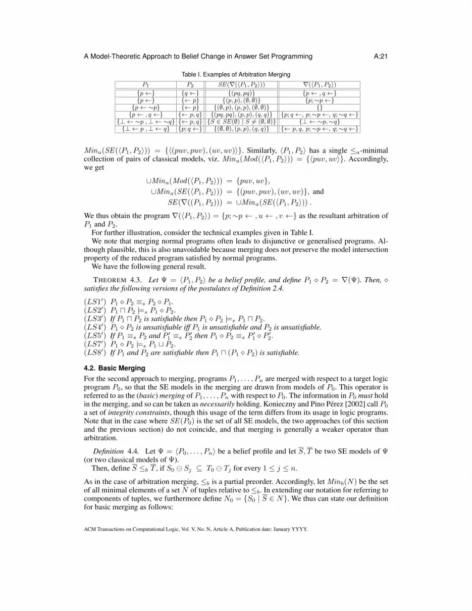
Table I. Examples of Arbitration Merging

P1 P2 SE(∇(〈P1, P2〉)) ∇(〈P1, P2〉){p←} {q ←} {(pq, pq)} {p← , q ←}{p←} {← p} {(p, p), (∅, ∅)} {p;∼p←}{p← ∼p} {← p} {(∅, p), (p, p), (∅, ∅)} {}{p← , q ←} {← p, q} {(pq, pq), (p, p), (q, q)} {p; q ←, p;∼p←, q;∼q ←}

{⊥ ← ∼p ,⊥ ← ∼q} {← p, q} {S ∈ SE(∅) | S 6= (∅, ∅)} {⊥ ← ∼p,∼q}{⊥ ← p ,⊥ ← q} {p; q ←} {(∅, ∅), (p, p), (q, q)} {← p, q, p;∼p←, q;∼q ←}

Mina(SE (〈P1, P2〉)) = {〈(puv, puv), (uv, uv)〉}. Similarly, 〈P1, P2〉 has a single ≤a-minimalcollection of pairs of classical models, viz. Mina(Mod(〈P1, P2〉)) = {〈puv, uv〉}. Accordingly,we get

∪Mina(Mod(〈P1, P2〉)) = {puv, uv},∪Mina(SE (〈P1, P2〉)) = {(puv, puv), (uv, uv)}, and

SE (∇((P1, P2))) = ∪Mina(SE (〈P1, P2〉)) .

We thus obtain the program ∇(〈P1, P2〉) = {p;∼p ← , u ← , v ←} as the resultant arbitration ofP1 and P2.

For further illustration, consider the technical examples given in Table I.We note that merging normal programs often leads to disjunctive or generalised programs. Al-

though plausible, this is also unavoidable because merging does not preserve the model intersectionproperty of the reduced program satisfied by normal programs.

We have the following general result.

THEOREM 4.3. Let Ψ = 〈P1, P2〉 be a belief profile, and define P1 � P2 = ∇(Ψ). Then, �satisfies the following versions of the postulates of Definition 2.4.

(LS1′) P1 � P2 ≡s P2 � P1.(LS2′) P1 u P2 |=s P1 � P2.(LS3′) If P1 u P2 is satisfiable then P1 � P2 |=s P1 u P2.(LS4′) P1 � P2 is unsatisfiable iff P1 is unsatisfiable and P2 is unsatisfiable.(LS5′) If P1 ≡s P2 and P ′1 ≡s P ′2 then P1 � P2 ≡s P ′1 � P ′2.(LS7′) P1 � P2 |=s P1 t P2.(LS8′) If P1 and P2 are satisfiable then P1 u (P1 � P2) is satisfiable.

4.2. Basic MergingFor the second approach to merging, programs P1, . . . , Pn are merged with respect to a target logicprogram P0, so that the SE models in the merging are drawn from models of P0. This operator isreferred to as the (basic) merging of P1, . . . , Pn with respect to P0. The information in P0 must holdin the merging, and so can be taken as necessarily holding. Konieczny and Pino Perez [2002] call P0

a set of integrity constraints, though this usage of the term differs from its usage in logic programs.Note that in the case where SE (P0) is the set of all SE models, the two approaches (of this sectionand the previous section) do not coincide, and that merging is generally a weaker operator thanarbitration.

Definition 4.4. Let Ψ = 〈P0, . . . , Pn〉 be a belief profile and let S, T be two SE models of Ψ(or two classical models of Ψ).

Then, define S ≤b T , if S0 Sj ⊆ T0 Tj for every 1 ≤ j ≤ n.

As in the case of arbitration merging, ≤b is a partial preorder. Accordingly, let Minb(N) be the setof all minimal elements of a set N of tuples relative to≤b. In extending our notation for referring tocomponents of tuples, we furthermore define N0 = {S0 | S ∈ N}. We thus can state our definitionfor basic merging as follows:



Table II. Examples of Basic Merging

P1 P2 SE(∆(〈∅, P1, P2〉)){p←} {q ←} {(pq, pq)}{p←} {← p} {(p, p), (∅, ∅)} ∪ {(p, ∅)}{p← ∼p} {← p} {(∅, p), (p, p), (∅, ∅)}{p← , q ←} {← p, q} {(pq, pq), (p, p), (q, q)} ∪ {(p, pq), (q, pq)}

{⊥ ← ∼p ,⊥ ← ∼q} {← p, q} {S ∈ SE(∅) | S 6= (∅, ∅)}{⊥ ← p ,⊥ ← q} {p; q ←} {(∅, ∅), (p, p), (q, q)} ∪ {(p, ∅), (q, ∅)}

Definition 4.5. Let Ψ = 〈P1, . . . , Pn〉 be a belief profile. Then, the basic merging, or simplymerging, of Ψ, is a logic program ∆(Ψ) such that

SE (∆(Ψ)) = {(X,Y ) | Y ∈ Minb(Mod(Ψ))0, X ⊆ Y,and if X ⊂ Y then (X,Y ) ∈ Minb(SE (Ψ))0} ,

providing Ψ is satisfiable, otherwise, if Pi is unsatisfiable for some 1 ≤ i ≤ n, define ∆(Ψ) =∆(〈P0, . . . , Pi−1, Pi+1, . . . , Pn〉).

Let us reconsider Programs P1 and P2 from (2) in the context of basic merging. To this end, weconsider the belief profile 〈∅, {p ← , u ←}, {← p , v ←}〉. We are now faced with 27 SE modelsfor SE (〈∅, P1, P2〉). Among them, we get the following ≤b-minimal SE models

Minb(SE (〈∅, P1, P2〉)) = {〈(uv, uv), (puv, puv), (uv, uv)〉,〈(uv, puv), (puv, puv), (uv, uv)〉, 〈(puv, puv), (puv, puv), (uv, uv)〉}

along with Minb(Mod(〈∅, P1, P2〉)) = {〈uv, puv, uv〉, 〈puv, puv, uv〉}. We get:

Minb(Mod(〈∅, P1, P2〉))0 = {puv, uv},Minb(SE (〈∅, P1, P2〉))0 = {(uv, uv), (uv, puv), (puv, puv)}, and

SE (∆(〈∅, P1, P2〉)) = Minb(SE (〈∅, P1, P2〉))0 .

While arbitration resulted in ∇(〈P1, P2〉) = {p;∼p ← , u ← , v ←}, the more conservativeapproach of basic merging yields ∆(〈∅, P1, P2〉) = {u← , v ←}.

We have just seen that basic merging adds “intermediate” SE models, viz. (uv, puv), to theones obtained in arbitration merging. This can also be observed on the examples given in Table I,where every second merging is weakened by the addition of such intermediate SE models. This ismade precise in Theorem 4.7 below. We summarise the results in Table II but omit the programs∆(〈∅, P1, P2〉) because they are obtained from ∇(〈P1, P2〉) in Table I by simply dropping all rulesof form p;∼p← and q;∼q ←, respectively.

THEOREM 4.6. Let Ψ be a belief profile, P0 a program representing global constraints, and ∆as given in Definition 4.5. Then, ∆ satisfies the following versions of the postulates of Definition 2.5:

(IC0′) ∆(〈P0,Ψ〉) |=s P0.(IC1′) If P0 and Ψ are satisfiable then ∆(〈P0,Ψ〉) is satisfiable.(IC2′) If u(P0,Ψ) is satisfiable then ∆(〈P0,Ψ〉) ≡s P0 u (u(Ψ)).(IC3′) If P0 ≡s P ′0 and Ψ ≡s Ψ′ then ∆(〈P0,Ψ〉) ≡s ∆(〈P ′0,Ψ′〉).(IC4′) If P1 |=s P0 and P2 |=s P0 then:

if ∆(〈P0, P1, P2〉) u P1 is satisfiable, then ∆(〈P0, P1, P2〉) u P2 is satisfiable.(IC5′) ∆(〈P0,Ψ〉) u∆(〈P0,Ψ

′〉) |=s ∆(〈P0,Ψ ◦Ψ′〉).(IC7′) ∆(〈P0,Ψ〉) u P1 |=s ∆(〈P0 u P1,Ψ〉).(IC9′) Let Ψ′ be a permutation of Ψ. Then, ∆(〈P0,Ψ〉) ≡s ∆(〈P0,Ψ

′〉).We also obtain that arbitration merging is stronger than (basic) merging in the case of tautologousconstraints in P0.

THEOREM 4.7. Let Ψ be a belief profile. Then∇(Ψ) |=s ∆(〈∅,Ψ〉).



As well, for belief profile Ψ = 〈P1, P2〉, we can express our merging operators in terms of therevision operator defined in Section 3.2.

THEOREM 4.8. Let 〈P1, P2〉 be a belief profile.

(1) ∇(〈P1, P2〉) = (P1 ∗ P2) t (P2 ∗ P1).(2) ∆(〈P1, P2〉) = P2 ∗ P1.

Note that in the second part of the preceding result, P1 is regarded as a set of constraints (usuallywith name P0) according to our convention for basic merging. We note also that analogous resultsare obtained in the corresponding merging operators in propositional logic [Liberatore and Schaerf1998; Konieczny and Pino Perez 2002].

The final example further illustrates the difference between arbitration and basic merging. TakeP1 = {p ← , q ←} and P2 = {∼p ← ,∼q ←}. Then, we have that SE (∇(〈P1, P2〉)) ={(pq, pq), (∅, ∅)} and SE (∆(〈∅, P1, P2〉)) = SE (∅). That is, in terms of programs, we obtain

∇(〈P1, P2〉) = {p;∼p←, q;∼q ←, ← p,∼q, ← ∼p, q} and ∆(〈∅, P1, P2〉) = ∅ .Thus in the arbitration, one essentially obtains that both p and q hold, or neither do. Thus, veryinformally, in merging P1 and P2 one obtains that the information in P1 holds or that in P2 does.This is also reflected in Theorem 4.8, where it can be observed that the SE models of the mergingare drawn from those of P1 and P2. In basic merging this is not the case, and in merging the variouspossible combinations of truth values for p and q may hold, hence yielding a program with modelsgiven by SE (∅).

5. COMPUTING BELIEF CHANGE VIA ANSWER SET PROGRAMMINGIn this section, we discuss computational aspects of our approach. More specifically, we provideencodings for our belief change operators in terms of fixed non-ground ASP programs and give ageneral complexity analysis of the underlying reasoning tasks. We recall that non-ground programsare defined over predicates of arbitrary arity which have either variables (denoted by upper-caseletters) or constants (denoted by lower-case letters) as arguments. Such non-ground programs canbe seen as a compact representation of large programs without variables (and thus as propositionalprograms), by considering the grounding of a program.14 The non-ground programs we define inthis section can be seen as queries which take the (propositional) programs subject to revision ormerging as an input database. Thus, we follow here the tradition of meta-programming (see, e.g.,the works of Delgrande et al. [2003], Eiter et al. [2003], and Gebser et al. [2008]).

For encoding the cardinality-based revision operator, we make use well-known minimisationstatements [Simons et al. 2002; Gebser et al. ], although similar optimisation constructs like weakconstraints [Leone et al. 2006] could be used as well, while for the set-based revision operator andthe merging operators we need an inclusion-based account of minimisation [Gebser et al. 2011],requiring the elevated complexity of disjunctive programs. Our goal in the encodings is to provideprograms such that their answer sets characterise the SE models of the result of the encoded revisionor merging problem. With these SE models at hand, corresponding programs can be obtained viathe construction of canonical programs.

Before we start with the ASP encodings, we have to fix how programs subject to revision andmerging are represented. For the sake of uniformity, we use belief profiles Ψ = 〈Pα, . . . , Pn〉,where

— for revision problems, we have α = 1 and n = 2 (and so 〈P1, P2〉 here represents revisionproblem P1 ∗ P2),

— for arbitration problems, we have α = 1 and n ≥ 2, and

14Recall that the grounding of a program P is given by the union of the groundings of its rules, and the grounding of a ruler ∈ P is the set obtained by all possible substitutions of variables in r by constants occurring in P ; cf. Dantsin et al. [2001]for a more thorough exposition.



— for basic merging, we use α = 0 and n ≥ 2.

Moreover, we assume in this section that every Pi is satisfiable, i.e., SE (Pi) 6= ∅.Given a belief profile Ψ = 〈Pα, . . . , Pn〉, we use four ternary predicates, phead , nhead , pbody ,

and nbody to represent Ψ. For each predicate, the first argument i indices the program (i.e., i is anumber between α and n), the second argument contains the rule identifier #r of a rule r ∈ Pi,and the third argument is an atom, indicating that this atom occurs in the positive or negative heador the positive or negative body of rule r ∈ Pi, respectively. For example, let Ψ = 〈P1, P2〉 withP1 = {← ∼p, ← ∼q} and P2 = {p; q ←, ← p, q}. We obtain the relational representation of Ψby15

[Ψ] = {nbody(1, 1, p), nbody(1, 2, q),

phead(2, 1, p), phead(2, 1, q), pbody(2, 2, p), pbody(2, 2, q)}.

Here, we just use numbers as rule identifiers, i.e., #(← ∼p) = #(p; q ←) = 1 and #(← ∼q) =#(← p, q) = 2. The only necessary requirement is that different rules are assigned to differentidentifiers, i.e., r 6= r′ implies #r 6= #r′.

In general, we define the relational representation of a belief profile as follows.

Definition 5.1. Let Ψ = 〈Pα, . . . , Pn〉 be a belief profile. Then, the relational representation ofΨ is given by

[Ψ] =

n⋃i=α

⋃r∈Pi

({phead(i,#r, a) | a ∈ H(r)+} ∪ {nhead(i,#r, a) | a ∈ H(r)−} ∪

{pbody(i,#r, a) | a ∈ B(r)+} ∪ {nbody(i,#r, a) | a ∈ B(r)−}).

We assume here that all i and #r are given as numbers. Following datalog notation, we write, fora program P and a belief profile Ψ, P [Ψ] instead of P ∪ [Ψ].

We provide our encodings in a modular way. That is, we introduce various sets of rules whichimplement different aspects required to solve the respective problem. We start with some basicmodules, which are used in most of the encodings. Then, we provide our results for revision andconclude with the encodings for merging.

5.1. Basic ModulesWe start with a simple fragment which contains some domain predicates and fixes some designatedidentifiers.

Definition 5.2.

Pdomain = {prog rule(P,R)← η(P,R,A), dom(A)← η(P,R,A) |η ∈ {phead , pbody ,nhead ,nbody}

}∪

{prog(P )← prog rule(P,R),

model(c)←, model(t)←, model(h)←,prog model(c)←, prog model(t)←}.

Predicates prog rule(·, ·), dom(·), and prog(·) are used to gather information from a conjoinedinput [Ψ]; the designated constants c, t, h are used later on to distinguish between different guessesfor models. Specifically, c refers to classical models while h and t refer to the first and secondpart of SE models, respectively. Thus, c and t indicate models of the programs (hence the use ofprog model ), while h indicates models of a program reduct.

15Since we have here rules which are all simple facts, we omit the “←”-symbol for rules.



The following code guesses such models for each program P in the belief profile Ψ. The guessis accomplished in Rules (3) and (4) below which assign each atom A in the domain to be in(·) orout(·).16

Definition 5.3.

Pmodels = {in(P,A,M)← ∼out(P,A,M), prog(P ), dom(A),model(M), (3)out(P,A,M)← ∼in(P,A,M), prog(P ), dom(A),model(M), (4)← in(P,A, h), out(P,A, t), (5)

diff (P,Q,A,M)← in(P,A,M), out(Q,A,M), (6)diff (P,Q,A,M)← out(P,A,M), in(Q,A,M), (7)ok(P,R,M)← in(P,A,M), phead(P,R,A),model(M), (8)ok(P,R,M)← out(P,A,M), pbody(P,R,A),model(M), (9)ok(P,R,M)← in(P,A,M),nbody(P,R,A), prog model(M), (10)ok(P,R,M)← out(P,A,M),nhead(P,R,A), prog model(M), (11)ok(P,R, h)← in(P,A, t),nbody(P,R,A), (12)ok(P,R, h)← out(P,A, t),nhead(P,R,A), (13)← ∼ok(P,R,M), prog rule(P,R),model(M)}. (14)

This allows us to draw a one-to-one correspondence between answer sets of the encoding andmodels (resp., SE models) of the programs in the belief profile. Note that Rule (5) excludes guesseswhere the corresponding SE model (X,Y ) would not satisfy X ⊆ Y . To make this intuition a bitmore precise, let us define the following (projection) operators for a set S of ground atoms and anumber i:

πiMod(S) = {a | in(i, a, c) ∈ S};πiSE (S) =

({a | in(i, a, h) ∈ S}, {b | in(i, b, t) ∈ S}

).

The next Rules (6) – (7) indicate whether atom A is assigned differently (via predicatediff (·, ·, ·, ·)) for two programs. This predicate is useful later and we will capture its idea formallybelow. Rules (8) – (13) tell us which rules (in which programs) are satisfied by the respective guess.

We observe that the answer sets of the program P [Ψ] where P = Pdomain ∪ Pmodels are in aone-to-one correspondence with the models and SE models of belief profile Ψ. We summarise ourobservations formally as follows.

LEMMA 5.4. Given Ψ = 〈Pα, . . . , Pn〉, then

{(M,N) |M ∈ Mod(Ψ), N ∈ SE (Ψ)} =

{(〈παMod(S), . . . , πnMod(S)〉, 〈παSE (S), . . . , πnSE (S)〉) | S ∈ AS (P [Ψ])}.We moreover observe the following relations concerning the diff predicate in view of Lemma 5.4.

LEMMA 5.5. For Ψ = 〈Pα, . . . , Pn〉, 1 ≤ i, j ≤ n, and S ∈ AS (P [Ψ]),

πiMod(S) πjMod(S) = {a | diff (i, j, a, c) ∈ S};πiSE (S) πjSE (S) =

({a | diff (i, j, a, h) ∈ S}, {b | diff (i, j, b, t) ∈ S}

).

Finally, we define a module which takes the models and SE models, respectively, of some selectedprogram (this is done via the selector predicate; in the case of revision, it is program P2, thusselector(2) is specified for revision problems) and copies them into a designated predicate.

16Note that we present our encodings in accord with the language introduced in Section 2. Unlike this, our implementationuses common choice rules, and thus avoids auxiliary predicates such as out(·).



Definition 5.6.

Presult = {total ← ∼nontotal ,

nontotal ← ∼total ,

← nontotal , selector(S), in(S,A, t), out(S,A, c),

← nontotal , selector(S), out(S,A, t), in(S,A, c),

resultH (A)← selector(S), in(S,A, h),nontotal ,

resultH (A)← selector(S), in(S,A, c), total ,

resultT (A)← selector(S), in(S,A, c)}.The intuition for the module is as follows: we either generate a total SE model (Y, Y ) or a non-

total SE model (X,Y ) with X ⊂ Y . Thus, the guess between predicates total and nontotal . Incase we want to derive a non-total SE model (X,Y ), we have to make sure that Y coincides withthe classical model we guessed.17 This is done by the two constraints. The remaining lines fill thepredicates resultH and resultT accordingly, where atoms in resultH yield the X of SE model(X,Y ) and atoms in resultT yield the Y of the SE model.

The following straightforward observation paves the way for all our subsequent encoding.

LEMMA 5.7. Given Ψ = 〈Pα, . . . , Pn〉 and P [Ψ], where

P = Pdomain ∪ Pmodels ∪ Presult ∪ {selector(i)} for some i ≥ α ≥ 0.

For any set S of ground atoms, define

ρ(S) = ({a | resultH (a) ∈ S}, {b | resultT (b) ∈ S}).Then, we have SE (Pi) = {ρ(S) | S ∈ AS (P [Ψ])}.

5.2. Encodings for RevisionThe idea of our ASP encodings is based on the observation that all change operations we haveconsidered in this paper select distinguished (SE) models. For instance, all SE models of P ∗Q areamong {(X,X) | X ∈ Mod(Q)} ∪ SE (Q). In view of Lemma 5.7, it is then enough to select theappropriate SE models among those in SE (Pi) for a given i. In ASP, the selection of models can beaccomplished by optimisation statements, expressing objective functions. This proceeding is bestillustrated by cardinality-based revision, detailed next.

5.2.1. Cardinality-based Revision. For implementing a cardinality-based preference criterion, wemake use of optimisation statements: A #minimize statement is of the form18

#minimize[`1@L1, . . . , `k@Lk].

Besides literals `j for 1 ≤ j ≤ k, a #minimize statement includes integers Lj providing prioritylevels. The #minimize statements in a program P distinguish optimal answer sets of P in thefollowing way. For any set X of atoms and integer L, let ΣXL denote the number of literals `j suchthat `j@L occurs in some #minimize statement in P and `j holds with respect to X . We also callΣXL the utility ofX at priority levelL. An answer setX of P is dominated if there is an answer set Yof P such that ΣYL < ΣXL and ΣYL′ = ΣXL′ for all L′ > L, and optimal otherwise. Note that greaterpriority levels are more significant than smaller ones, which allows for representing sequences ofseveral optimisation criteria.

17One might ask why we use the different concepts of t- and c-models. The reason is that there might be a minimal differencebetween (X1, Y1) and (X2, Y2) although there is no minimal difference between Y1 and Y2. But then we still need thoseinterpretations Y in order to compute the corresponding interpretations X . On the other hand, there might be a minimaldistance between Y1 and Y2 but not between any (X1, Y1) and (X2, Y2). Still, we then want (Y2, Y2) in the result.18Minimise statements also contain weights, which are omitted for simplicity.



The selection of the SE models defined in Definition 3.10 can then be accomplished by means ofthe optimisation statements

#minimize[diff (1, 2, A, h)@2], (15)#minimize[diff (1, 2, A, c)@1, diff (1, 2, A, t)@1], (16)

where A ranges over the considered set of atoms. Denoting the selection function on answer setsimplemented by (15) and (16) as min ||, we obtain the following result.

THEOREM 5.8. Let Ψ = 〈P1, P2〉 be a belief profile and

P = Pdomain ∪ Pmodels ∪ Presult ∪ {selector(2)}.Then, we have

SE (P1 ∗c P2) = {ρ(S) | S ∈ min ||(AS (P [Ψ]))}.5.2.2. Set-based Revision. For addressing set-based revision, we can proceed analogously to the

above, once we replace the cardinality-based account of minimisation by an inclusion-based ac-count. To this end, we follow the approach of Gebser et al. [2011] and redefine the utility of min-imisation statements: For any set X of atoms and integer L, let ΠX

L denote the set of literals suchthat `j@L occurs in some #minimize statement in P and `j holds with respect to X . An answerset X of P is dominated if there is an answer set Y of P such that ΠY

L ⊂ ΠXL and ΠY

L′ = ΠXL′ for

all L′ > L, and optimal otherwise.Interpreting the minimisation statements in (15) and (16) under this inclusion-based semantics

provides us with an implementation of set-based revision. To this end, let min⊆ denote the selectionfunction on answer sets implemented by (15) and (16) under the inclusion-based semantics.

THEOREM 5.9. Let Ψ = 〈P1, P2〉 a belief profile and

P = Pdomain ∪ Pmodels ∪ Presult ∪ {selector(2)}.Then, we have

SE (P1 ∗ P2) = {ρ(S) | S ∈ min⊆(AS (P [Ψ]))}.

5.3. Encodings for Merging5.3.1. Basic Merging. We continue with the problem of basic merging. Suppose that belief profile

Ψ = 〈P0, . . . , Pn〉 is given for some arbitrary n. Also recall that P0 plays a special role in basicmerging. In particular, the SE models of the result of the merging are taken from the SE models ofP0.

As above, in view of Lemma 5.7, it is sufficient to define the appropriate selection function onanswer sets using

#minimize[diff (0, P,A, h)@2 : P > 0],

#minimize[diff (0, P,A, c)@1 : P > 0, diff (0, P,A, t)@1 : P > 0],

whereA and P range over the considered sets of atoms and programs, respectively. The qualificationP > 0 restricts the instantiation of P .

In analogy to the above, let minbasic denote the selection function on answer sets implementedby the last two optimisation statements under the inclusion-based semantics. Then, our result isforthcoming as in the previous sections.

THEOREM 5.10. Let Ψ = 〈P0, . . . , Pn〉 be a belief profile and

P = Pdomain ∪ Pmodels ∪ Presult ∪ {selector(0), prog(0)}Then,

SE (∆(Ψ)) = {ρ(S) | S ∈ minbasic(AS (P [Ψ]))}.



Note that the fact prog(0) is added for the case that no integrity constraints are specified by theinput and recall that selector(0) is used to select P0 as the program which takes care of the resultpredicates.

5.3.2. Arbitration Merging. Our final encoding is the one for arbitration merging, which again doesnot require further modules, except that we need a somewhat more complicated program to preparethe resultH and resultT predicates, since arbitration merging collects SE models from all programsof the belief profile rather than from a single program (which has been the case in the approacheswe encoded so far). We thus do not use a selector predicate here but instead provide a new resultmodule below. Also recall that belief profiles for arbitration merging are of the form 〈P1, . . . , Pn〉.

Here is the new result module:

Definition 5.11.

P ′result = {tout(I); tout(J)← prog(I), prog(J), I 6= J,

tselect(I)← ∼tout(I), prog(I),

total ← ∼nontotal ,

nontotal ← ∼total ,

resultT (A)← in(M,A, c), tselect(M),

resultH (A)← in(M,A, c), total , tselect(M),

hout(I); hout(J)← prog(I), prog(J), I 6= J,nontotal ,

hselect(I)← ∼hout(I), prog(I),nontotal ,

← nontotal , in(I, A, t), out(J,A, c), tselect(J), hselect(I),nontotal ,

← nontotal , out(I, A, t), in(J,A, c), tselect(J), hselect(I),nontotal ,

resultH (A)← in(I, A, h), hselect(I),nontotal}.

Roughly speaking, the first two rules select exactly one program Pi from the belief profile. Wethen guess whether we build a total or a non-total SE model (as we did in Presult ). Then, we copy themodel from the guessed program into the there-part of the result, and in case we are constructinga total SE model, also in the here-part. If we construct a non-total SE model, we guess a secondprogram Pj from the belief profile and check whether the there-part of the current SE model of Pjcoincides with the classical model of Pi (this is done by the two constraints). If this check is passed,we copy the here-part of the SE model of Pj into the here-part of the resulting SE model.

The minimise statement is as follows:

#minimize[diff (Q,P,A, h) : P 6= Q],

#minimize[diff (Q,P,A, c) : P 6= Q, diff (Q,P,A, t) : P 6= Q],

where A and P,Q range over the considered sets of atoms and programs, respectively; and P 6= Qrestricts the instantiation of P and Q.

Defining minarb accordingly under the inclusion-based semantics, provides us with the followingresult.

THEOREM 5.12. Let Ψ = 〈P1, . . . , Pn〉 be a belief profile and define P = Pdomain ∪Pmodels∪P ′result . Then,

SE (∇(Ψ)) = {ρ(S) | S ∈ minarb(AS (P [Ψ]))}.

5.4. Computational ComplexityWe next address the computational complexity of our approach to revision and merging. As it turnsout, our method of using ASP itself to compute revision and merging is adequate from a complexitypoint of view.



First, we recapitulate the complexity classes relevant in what follows. As usual, for any com-plexity class C, by co-C we understand the class of all problems which are complementary to theproblems in C. Furthermore, for C as before and complexity class A, the notation CA stands forthe relativised version of C, consisting of all problems which can be decided by Turing machines ofthe same sort and time bound as in C, only that the machines have access to an oracle for problemsin A.

Four complexity classes are relevant here, viz. NP, ΣP2 , ΠP2 , and ΘP

2 , which are defined thus:

— NP consists of all decision problems which can be solved with a nondeterministic Turing ma-chine working in polynomial time;

— ΣP2 = NPNP;— ΠP

2 = co-ΣP2 ; and— ΘP

2 is the class of all problems solvable on a deterministic Turing machine in polynomial timeasking on input x a total of O(log |x|) many oracle calls to NP (thus, ΘP

2 is also denoted byPNP[logn]).

Observe that NP, ΣP2 , and ΠP2 are part of the polynomial hierarchy, which is given by the follow-

ing sequence of objects: the initial elements are

∆P0 = ΣP0 = ΠP

0 = P;

and, for i > 0,

∆Pi = PΣP

i−1 ; ΣPi = NPΣPi−1 ; ΠP

i = co-NPΣPi−1 .

Here, P is the class of all problems solvable on a deterministic Turing machine in polynomialtime. It holds that ΣP1 = NP, ΣP2 = NPNP, and ΠP

2 = co-NPNP. A problem is said to be at thek-th level of the polynomial hierarchy iff it is in ∆P

k+1 and either ΣPk -hard or ΠPk -hard.

We first consider the worst-case complexity of our approach to set-containment based revision.The standard decision problem for revision in classical logic is:

Given formulas P , Q, and R, does P ∗Q entail R?

Eiter and Gottlob [1992] showed that approaches to classical propositional revision are ΠP2 -

complete. The next result shows that this property carries over to our approach for program revision.

THEOREM 5.13. Deciding whether P ∗ Q |=s R holds, for given GLPs P , Q, and R, is ΠP2 -

complete. Moreover, hardness holds already for P being a set of facts, Q being positive or normal,and R being a single fact.

Although we do not show it here, we mention that the same results holds for the cautious revisionoperator ∗w as well.

For cardinality-based revision, we obtain the following result, again mirroring a similar behaviourfor the classical case.

THEOREM 5.14. Deciding whether P ∗c Q |=s R holds, for given GLPs P , Q, and R, is inΘP

2 .

Concerning merging, we have the following result:

THEOREM 5.15. Given a belief profile Ψ and a program R, deciding ∇(Ψ) |=s R (resp.,∆(Ψ) |=s R) is ΠP

2 -complete.

5.5. Technical RemarksAll encodings presented in the previous subsections are publicly available and can be downloadedvia the following URL:

http://www.cs.uni-potsdam.de/˜torsten/ASPChange.tgz.



In contrast to the description of the encodings as given above, which follow the definition of ourlogic-programming language from Section 2, the programs available for download are somewhatsimpler as they make use of extended language constructs. In particular, they rely on so-calledchoice rules [Simons et al. 2002], avoiding the use of cyclic rules with auxiliary predicates. As anexample, consider the first two rules in Presult in Definition 5.6. The pair of rules

total ← ∼nontotal and nontotal ← ∼total

uses the auxiliary atom nontotal to indicate that total may not belong to an answer set. This can beequivalently expressed by using instead the single choice rule

{total} ←,making the auxiliary atom nontotal unnecessary. In addition, one must then replace every occur-rence of nontotal by∼total in the rest of the program. The same can be done with rules (3) and (4)of Definition 5.3. In fact, we may analogously treat the disjunctive rules in P ′result . The reason fortaking pairs of rules in the first place is motivated by complexity considerations given that disjunc-tions give rise to an elevated complexity (which is of no concern in P ′result in view of the alreadyelevated complexity of arbitration merging).

In fact, from an encoding perspective, the elevated complexity of set-based revision and bothmerging operations is reflected by the usage of inclusion-based preference criteria. To accommo-date this, we rely upon the approach of Gebser et al. [2011] that allows for interpreting #minimizestatement in various ways. This approach takes advantage of recent advances in ASP groundingtechnology, admitting an easy use of meta-modeling techniques. The idea is to reinterpret existingoptimisation statements in order to express complex preferences among answer sets. While, for in-stance, in the ASP solver smodels [Simons et al. 2002], the meaning of #minimize is to computeanswer sets incurring minimum costs, we may alternatively use it for selecting inclusion-minimalanswer sets.

Furthermore, our encodings are given via certain language fragments of non-ground ASP suchthat their respective data complexity matches the complexity of the encoded task. Recall that datacomplexity addresses problems over programs P ∪D where a non-ground program P is fixed, whilethe input database D (a set of ground atoms) is the input of the decision problem. As is well known,the data complexity of the problem whether atom a is contained in all answer sets of P ∪ D isΠP

2 -complete for disjunctive programs [Dantsin et al. 2001] and ∆P2 -complete for normal programs

with optimisation constructs [Simons et al. 2002]. Moreover, it is ΘP2 -complete whenever there is

only a single optimisation construct used.

6. DISCUSSIONWe have addressed the problem of belief change in logic programming under the answer set se-mantics. Our overall approach is based on a monotonic characterisation of logic programs, given interms of the set of SE models of a program. Based on the latter, we first defined and examined op-erators for logic program expansion and revision. Both subset-based revision and cardinality-basedrevision were considered. As well as giving properties of these operators, we also considered theircomplexity. This work is novel, in that it addresses belief change in terms familiar to researchersin belief revision: expansion is characterised in terms of intersections of models, and revision ischaracterised in terms of minimal distance between models.

We also addressed the problem of merging logic programs under the answer set semantics. Again,the approaches are based on a monotonic characterisation of logic programs, given in terms of theset of SE models of a sequence of programs. We defined and examined two operators for logicprogram merging, the first following intuitions from arbitration [Liberatore and Schaerf 1998], thesecond being closer to IC merging [Konieczny and Pino Perez 2002]. As well as giving propertiesof these operators, we also considered complexity questions.

Last, we provided encodings for computing the revision and merging operators described pre-viously. These encodings were carried out within the same logic programming framework. This



allows for a direct implementation of our approach in terms of available answer set solvers. As well,these encodings also pragmatically demonstrate the fact that our change operators do not increasethe complexity of the base formalism.

We note that previous work on logic program belief change was formulated at the level of theindividual program, and not in terms of an abstract characterisation (via strong equivalence or setsof SE interpretations). The net result is that such previous work is generally difficult to work with:properties are difficult to come by, and often desirable properties are lacking. (On the other hand,perhaps this criticism is not totally warranted, since we have also claimed that such work is bestregarded as addressing belief base change; and in classical belief revision, it is typically difficultin general to obtain desirable properties in such approaches.) The main point of departure for thecurrent approach then is to lift the problem of logic program revision or merging from the program(or syntactic) level to an abstract (or semantic) level. Notably, since all our operators are defined viasemantic characterisations, the results of revision, expansion, and merging are independent of theparticular syntactic expression of a logic program.

A continuation of our method was recently taken up by Slota and Leite [2010], who, inspired byour preliminary work [Delgrande et al. 2008; 2009], discussed answer set program update based onSE models using modified adaptions of the update postulates by Katsuno and Mendelzon [1992].They define a set-based update operator and show that it satisfies their modified update postulates.However, it is also shown that update operators satisfying certain conditions Slota and Leite con-sider as reasonable, do not respect support, i.e., that atoms true in an answer set may not be theconsequence of a rule whose body is true.

Finally, we noted at the outset that strong equivalence coincides with equivalence in the logic ofhere and there (HT), a logic that can be seen as being intermediate between intuitionistic logic andclassical logic. Moreover, equivalence between programs in HT corresponds to equality betweensets of SE models. Hence, the results reported here on the revision and merging of logic programscan also be viewed as addressing the same concerns in the logic of HT. Consequently, the presentapproach may provide an appropriate starting point for developing a more general belief change for-malism in intuitionistic and other related non-classical logics, thus complementing existing researchin this direction [Gabbay et al. 2008].

A. APPENDIXA.1. Proof of Theorem 3.2Most of the parts follow immediately from the fact that SE (P +Q) = SE (P ) ∩ SE (Q).

(1) We show that Definition 3.1 results in a well-defined set of SE models.For SE (P )∩SE (Q) = ∅ we have that ∅ is trivially well-defined (and R can be given by⊥ ←).Otherwise, for SE (P ) ∩ SE (Q) 6= ∅, we have the following: If (X,Y ) ∈ SE (P ) ∩ SE (Q),then (X,Y ) ∈ SE (P ) and (X,Y ) ∈ SE (Q); whence (Y, Y ) ∈ SE (P ) and (Y, Y ) ∈ SE (Q)since SE (P ) and SE (Q) are well-defined by virtue of P and Q being logic programs. Hence,(Y, Y ) ∈ SE (P ) ∩ SE (Q). Since this holds for arbitrary (X,Y ) ∈ SE (P ) ∩ SE (Q), we havethat SE (P ) ∩ SE (Q) is well-defined.

(2) Immediate from the definition of +.(3) If P |=s Q, then SE (P ) ⊆ SE (Q). Hence, SE (P ) ∩ SE (Q) = SE (P ), or P +Q ≡s P .(4) Similar to the previous part.(5) This was established in the first part.(6) To show completeness, we need to show that for any (X,Y ) ∈ SE (P +Q) and (Y ∪ Y ′, Y ∪

Y ′) ∈ SE (P +Q) that (X,Y ∪ Y ′) ∈ SE (P +Q).If (X,Y ) ∈ SE (P+Q) and (Y ∪Y ′, Y ∪Y ′) ∈ SE (P+Q), then (X,Y ) ∈ SE (P )∩SE (Q) and(Y ∪Y ′, Y ∪Y ′) ∈ SE (P )∩SE (Q). Hence, (X,Y ) ∈ SE (P ) and (Y ∪Y ′, Y ∪Y ′) ∈ SE (P ),and so, since SE (P ) is complete by assumption, we have (X,Y ∪ Y ′) ∈ SE (P ).The same argument gives that (X,Y ∪Y ′) ∈ SE (Q), whence (X,Y ∪Y ′) ∈ SE (P )∩SE (Q)and (X,Y ∪ Y ′) ∈ SE (P +Q).



(7) If Q ≡s ∅, then SE (Q) = {(X,Y ) | X ⊆ Y ⊆ A} from which the result follows immediately.2

A.2. Proof of Theorem 3.5(RA1) This postulate follows immediately from Definition 3.4. Note that (X,Y ) ∈ SE (P∗Q) only

if Y ∈ σ(Mod(Q),Mod(P )), and therefore (Y, Y ) ∈ σ(SE (Q),SE (P )). So, SE (P ∗Q)is well-defined.

(RA2) If P + Q is satisfiable, then we have that both σ(Mod(Q),Mod(P )) 6= ∅ andσ(SE (Q),SE (P )) 6= ∅. Further, for Y ∈ Mod(Q) (or (X,Y ) ∈ SE (Q)), there is someY ′ ∈ Mod(P ) (resp., (X ′, Y ′) ∈ SE (P )) such that Y Y ′ = ∅ (resp., (X,Y )(X ′, Y ′) =∅), from which our result follows.

(RA3) From Definition 3.4 we have that, if P is unsatisfiable, then Q is satisfiable iff P ∗ Q issatisfiable.

Otherwise, if P is satisfiable and Q is satisfiable, then there is some (Y, Y ) ∈σ(Mod(Q),Mod(P )) (since SE (Q) is well-defined and given Definition 3.3). Hence,SE (P ∗Q) 6= ∅.

(RA4) Immediate from Definition 3.4.(RA5) If SE (P ) = ∅, then the result follows immediately from the first part of Definition 3.4.

Otherwise, we show that, if (X,Y ) is an SE model of (P ∗Q) +R, then (X,Y ) is an SEmodel of P ∗ (Q+R).

Let (X,Y ) ∈ SE ((P ∗ Q) + R). Then, (X,Y ) ∈ SE (P ∗ Q) and (X,Y ) ∈ SE (R).Since (X,Y ) ∈ SE (P ∗ Q), by (RA1) we have that (X,Y ) ∈ SE (Q), and so (X,Y ) ∈SE (Q) ∩ SE (R), or (X,Y ) ∈ SE (Q+R).

There are two cases to consider:X = Y : Since then (X,Y ) = (Y, Y ), and (Y, Y ) ∈ SE (P ∗ Q), we have that Y ∈

σ(Mod(Q),Mod(P )). Hence, from Definition 3.3, Y ∈ Mod(Q) and there is someY ′ ∈ Mod(P ) such that there is no Y1 ∈ Mod(Q) and no Y2 ∈ Mod(P ) such thatY1 Y2 ⊂ Y Y ′.We established at the outset that (X,Y ) ∈ SE (Q+R). Hence, Y ∈ Mod(Q+R). Thisgives us that Y ∈ Mod(Q + R) and there is some Y ′ ∈ Mod(P ) such that no Y1, Y2

exist with Y1 ∈ Mod(Q), Y2 ∈ Mod(P ), and Y1 Y2 ⊂ Y Y ′.Clearly, in the above, if there is no Y1 ∈ Mod(Q) such that the above condition holds,then there is no Y1 ∈ Mod(Q+R) such that the above condition holds.Thus, we have Y ∈ Mod(Q + R) and there is some Y ′ ∈ Mod(P ) for which noY1 ∈ Mod(Q+R) and no Y2 ∈ Mod(P ) exists such that Y1 Y2 ⊂ Y Y ′.Thus, from Definition 3.3, we get Y ∈ σ(Mod(Q + R),Mod(P )), hence (Y, Y ) ∈SE (P ∗ (Q+R)).

X ⊂ Y : We have Y ∈ σ(Mod(Q),Mod(P )) by virtue of (X,Y ) ∈ SE (P ∗Q). In the previouspart we established that Y ∈ σ(Mod(Q+R),Mod(P )).As well, (X,Y ) ∈ σ(SE (Q),SE (P )) since (X,Y ) ∈ SE (P ∗ Q). Thus, from Def-inition 3.3, we have that there is some (X ′, Y ′) ∈ SE (P ) such that no U, V, U ′, V ′exist such that (U, V ) ∈ SE (Q), (U ′, V ′) ∈ SE (P ), and (U, V ) (U ′, V ′) ⊂(X,Y ) (X ′, Y ′).Therefore, there is no (U, V ) ∈ SE (Q+R) and no (U ′, V ′) ∈ SE (P ) such that (U, V )(U ′, V ′) ⊂ (X,Y ) (X ′, Y ′).We previously showed that (X,Y ) ∈ SE (Q + R). Consequently, from Definition 3.4,we obtain that (X,Y ) ∈ σ(SE (Q+R),SE (P )). Hence, (X,Y ) ∈ SE (P ∗ (Q+R)).

Thus, in either case, we get (X,Y ) ∈ SE (P ∗ (Q+R)), which was to be shown. 2

A.3. Proof of Theorem 3.6For initialisation, idempotency, and tautology, in the left-hand side of the given equivalence, revisioncorresponds with expansion via (RA2), from which the result is immediate.



For absorption, we haveQ = R, and so ((P ∗Q)∗R) = ((P ∗Q)∗Q). Since SE (P ∗Q) ⊆ SE (Q),then from Theorem 3.2, Part 3, we have that (P ∗ Q) + Q ≡s P ∗ Q. As well, ((P ∗ Q) ∗ Q) =((P ∗Q) +Q), from which our result follows. 2

A.4. Proof of Theorem 3.8We need to show that SE (P ∗ Q) ⊆ SE (P ∗w Q). If SE (P ) = ∅, then SE (P ∗ Q) = SE (Q) =SE (P ∗w Q).

Otherwise, there are two cases to consider:

(1) (X,Y ) ∈ SE (P ∗ Q) where X ⊂ Y . Then, (X,Y ) ∈ σ(SE (P ),SE (Q)) by Definition 3.4,and (X,Y ) ∈ SE (P ∗w Q) by Definition 3.7.

(2) (Y, Y ) ∈ SE (P ∗ Q). From Definition 3.4, we have that Y ∈ σ(Mod(Q),Mod(P )).Y ∈ σ(Mod(Q),Mod(P )) implies that (Y, Y ) ∈ σ(SE (Q),SE (P )). Hence, according toDefinition 3.7, (Y, Y ) ∈ SE (P ∗w Q).

Therefore, (X,Y ) ∈ SE (P ∗ Q) implies that (X,Y ) ∈ SE (P ∗w Q), whence SE (P ∗ Q) ⊆SE (P ∗w Q). 2

A.5. Proof of Theorem 3.11Before giving the proof, we first present a lemma that is key for postulates (RA5) and (RA6).

LEMMA A.1. Let E1, E2, and E3 be SE interpretations. If σ||(E1, E2) ∩ E3 6= ∅, thenσ||(E1, E2) ∩ E3 = σ||(E1 ∩ E3, E2).

PROOF. Assume that σ||(E1, E2) ∩ E3 6= ∅.For showing⊆ in the equality, let (X,Y ) ∈ σ||(E1, E2)∩E3 and, toward a contradiction, assume

that (X,Y ) 6∈ σ||(E1 ∩ E3, E2).Since (X,Y ) ∈ σ||(E1, E2), so (X,Y ) ∈ E1; as well, (X,Y ) ∈ E3, so (X,Y ) ∈ E1∩E3. Since

(X,Y ) 6∈ σ||(E1∩E3, E2) we have that there is some (X ′, Y ′) ∈ E1∩E3 and some (U ′, V ′) ∈ E2

such that for every (U, V ) ∈ E2, |(X ′, Y ′) (U ′, V ′)| < |(X,Y ) (U, V )|. But this contradictsthe assumption that (X,Y ) ∈ σ||(E1, E2). Hence, the assumption that (X,Y ) 6∈ σ||(E1 ∩ E3, E2)cannot hold, i.e., (X,Y ) ∈ σ||(E1∩E3, E2), establishing that σ||(E1, E2)∩E3 ⊆ σ||(E1∩E3, E2).

To show ⊇ in the equality, let (X,Y ) ∈ σ||(E1 ∩ E3, E2) and, toward a contradiction, assumethat (X,Y ) 6∈ σ||(E1, E2) ∩ E3.

Since (X,Y ) ∈ σ||(E1 ∩ E3, E2), we get that (X,Y ) ∈ E3. Hence, (X,Y ) 6∈ σ||(E1, E2) (viathe assumption that (X,Y ) 6∈ σ||(E1, E2) ∩ E3).

We also have by assumption that σ||(E1, E2) ∩E3 6= ∅, and so let (X ′, Y ′) ∈ σ||(E1, E2) ∩E3.Then, from the first part above, we have that (X,Y ) ∈ σ||(E1 ∩ E3, E2). Thus, we have both that(X,Y ) ∈ σ||(E1 ∩ E3, E2) and (X ′, Y ′) ∈ σ||(E1 ∩ E3, E2). Consequently, we obtain that

min({|(X,Y ) (U, V )| | (U, V ) ∈ E2}) = min({|(X ′, Y ′) (U, V )|(U, V ) ∈ E2}).

Therefore, since (X ′, Y ′) ∈ σ||(E1, E2), so also (X,Y ) ∈ σ||(E1, E2). But this together with(X,Y ) ∈ E3 contradicts our assumption that (X,Y ) 6∈ σ||(E1, E2) ∩ E3; i.e., we have (X,Y ) ∈σ||(E1, E2) ∩ E3, establishing that σ||(E1, E2) ∩ E3 ⊇ σ||(E1 ∩ E3, E2).

We now move on to the proof of Theorem 3.11:

(RA1): This follows immediately from Definition 3.10. Note that (X,Y ) ∈ SE (P ∗c Q) only ifY ∈ σ||(Mod(Q),Mod(P )), and therefore (Y, Y ) ∈ σ||(SE (Q),SE (P )). So, SE (P ∗cQ)is well-defined.

(RA2): If P + Q is satisfiable, then we have that both σ||(Mod(Q),Mod(P )) 6= ∅ andσ||(SE (Q),SE (P )) 6= ∅. Further, for Y ∈ Mod(Q) (or (X,Y ) ∈ SE (Q)) we have



that there is some Y ′ ∈ Mod(P ) (resp., (X ′, Y ′) ∈ SE (P )) such that Y Y ′ = ∅((X,Y ) (X ′, Y ′) = ∅), from which our result follows.

(RA3): From Definition 3.10 we have that, if P is unsatisfiable, then Q is satisfiable iff P ∗ Q issatisfiable. Otherwise, if P is satisfiable and Q is satisfiable, then there is some (Y, Y ) ∈σ||(Mod(Q),Mod(P )) (since SE (Q) is well-defined and given Definition 3.9). Hence,SE (P ∗Q) 6= ∅.

(RA4): This is immediate from Definition 3.10.(RA5), (RA6): For P ∗cQ, if SE (P ) = ∅, we have that (P ∗cQ)+R = Q+R = (P ∗c (Q+R)).

So, assume that SE (P ) 6= ∅. We show that SE (P ∗cQ)+SE (R) = SE (P ∗c (Q+R)),thus establishing both postulates.

For ⊆, assume that (X,Y ) ∈ SE (P ∗c Q) + R. Thus, (X,Y ) ∈ SE (P ∗c Q) and(X,Y ) ∈ R.

For X ⊆ Y , we have that Y ∈ σ||(Mod(Q),Mod(P )) and as well Y ∈ Mod(R). Weget that Y ∈ σ||(Mod(Q+R),Mod(P )) by the analogous proof in propositional logic forcardinality-based revision.

For X ⊂ Y , we have that (X,Y ) ∈ σ||(SE (Q),SE (P )) and as well (X,Y ) ∈ SE (R).By Lemma A.1 we get that (X,Y ) ∈ σ||(SE (Q+R),SE (P )).

This establishes one direction of the set equality. For ⊇, the argument is essentially thesame, though in the reverse direction, and again appealing to Lemma A.1.

A.6. Proof of Theorem 3.12The proof is the same as for Theorem 3.6.

A.7. Proof of Theorem 4.3The definitions for arbitration and basic merging (Definitions 4.2 and 4.5) are essentially composedof two parts (as are the definitions for revision): there is a phrase to deal with classical propositionalmodels (or SE models of form (Y, Y )) and then general SE models. For brevity, and because thecase for propositional models follows immediately from the case of general SE models, we considergeneral SE models in the proofs here.

(LS1′) – (LS7′). These all follow trivially or straightforwardly from the definition of P1 �P2.(LS8′). Assume that P1 and P2 are satisfiable. It follows that SE (〈P1, P2〉) 6= ∅ and soMina(SE (〈P1, P2〉)) 6= ∅. Let 〈S1, S2〉 ∈ Mina(SE (〈P1, P2〉)), and so S1, S2 ∈ SE (P1�P2).Since S1 ∈ SE (P1) we get that S1 ∈ SE (P1)∩SE (P1 �P2) and so S1 ∈ SE (P1 u (P1 �P2)).Thus, P1 u (P1 � P2) is satisfiable.

A.8. Proof of Theorem 4.6Let Ψ be a belief profile, P0 a program representing global constraints, and ∆ as given in Defini-tion 4.5.

(IC0′) – (IC3′), (IC9′). These follow trivially or straightforwardly from the definition of∆(〈P0,Ψ〉).(IC4′). Assume that P1 |=s P0 and P2 |=s P0. If SE (P1) ∩ SE (P2) 6= ∅ then by (IC2′) wehave that ∆(〈P0, P1, P2〉) = P0 u P1 u P2 from which our result follows immediately.Consequently, assume that SE (P1) ∩ SE (P2) = ∅. As well, assume the antecedent conditionof the postulate that ∆(〈P0, P1, P2〉) u P1 is satisfiable. Let Ψ = 〈P0, P1, P2〉. Thus, we havefor some (X,Y ) that (X,Y ) ∈ SE (∆(Ψ) u P1), and so (X,Y ) ∈ SE (P0) ∩ SE (P1), where(X,Y ) ∈ Minb(SE (Ψ))0.(X,Y ) ∈ Minb(SE (Ψ))0 implies that there is some (X ′, Y ′) ∈ SE (P2) such that S =〈(X,Y ), (X,Y ), (X ′, Y ′)〉 ∈ Minb(SE (Ψ)).



We claim that S′

= 〈(X ′, Y ′), (X,Y ), (X ′, Y ′)〉 ∈ Minb(SE (Ψ)). This is sufficient to proveour result, since S

′ ∈ Minb(SE (Ψ)) yields that (X ′, Y ′) ∈ ∆(Ψ) and (X ′, Y ′) ∈ SE (P2).That is to say, ∆(Ψ) u P2 is satisfiable.Proof of claim: Since S ∈ Minb(SE (Ψ)), this means that for every T ∈ SE (Ψ) we have thatT ≤b S implies that S ≤b T .Consider T = 〈(U0, V0), (U1, V1), (U2, V2)〉. If T ≤b S then we have that (U0, V0) (U1, V1) ⊆ (X,Y ) (X,Y ) = (∅, ∅). That is, U0 = U1 and V0 = V1, and so T =〈(U0, V0), (U0, V0), (U2, V2)〉. As well, from T ≤b S, we get that (U0, V0) (U2, V2) ⊆(X,Y ) (X ′, Y ′). Since T ≤b S implies S ≤b T , this means that (X,Y ) (X ′, Y ′) ⊆(U0, V0) (U2, V2).We will use this later, and so summarise the result here:(α) (X,Y ) and (X ′, Y ′) are such that for every (U0, V0) ∈ SE (P1) and (U2, V2) ∈ SE (P2) if

(U0, V0) (U2, V2) ⊆ (X,Y ) (X ′, Y ′) then (X,Y ) (X ′, Y ′) ⊆ (U0, V0) (U2, V2).

We must show for S′

= 〈(X ′, Y ′), (X,Y ), (X ′, Y ′)〉, that T ≤b S′

implies S′ ≤b T . Let

T = 〈(U ′0, V ′0), (U ′1, V′1), (U ′2, V

′2)〉 and assume that T ≤b S

′. Then, by definition of ≤b, we

have that (U ′0, V′0)(U ′1, V

′1) ⊆ (X ′, Y ′)(X,Y ).As well, we have that (U ′0, V

′0)(U ′2, V

′2) ⊆

(X ′, Y ′) (X ′, Y ′) = (∅, ∅). Hence, we must have that U ′0 = U ′2 and V ′0 = V ′2 . Thus, we canwrite T = 〈(U ′0, V ′0), (U ′1, V

′1), (U ′0, V

′0)〉.

Now, we will have S′ ≤b T just if (X ′, Y ′) (X,Y ) ⊆ (U ′0, V

′0) (U ′1, V

′1) and (X ′, Y ′)

(X ′, Y ′) ⊆ (U ′0, V′0) (U ′2, V

′2). The second condition is vacuously true. As for the first con-

dition, we have that (U ′0, V′0) ∈ SE (P2) and (U ′1, V

′1) ∈ SE (P1). Thus, via (α), we obtain that

(X ′, Y ′) (X,Y ) ⊆ (U ′1, V′1) (U ′0, V

′0). We conclude that S

′ ≤b T .This shows that S

′ ∈ Minb(SE (Ψ)), where (X ′, Y ′) ∈ SE (P0) and (X ′, Y ′) ∈ SE (P2).Consequently, SE (∆(〈P0, P1, P2〉) u P2) is satisfiable.(IC5′). Consider (X,Y ) ∈ SE (∆(〈P0,Ψ〉) u ∆(〈P0,Ψ

′〉)), and so (X,Y ) ∈SE (∆(〈P0,Ψ〉)) and (X,Y ) ∈ SE (∆(〈P0,Ψ

′〉)). Thus, (X,Y ) ∈ Minb(SE (〈P0,Ψ〉)) and(X,Y ) ∈ Minb(SE (〈P0,Ψ

′〉)). Hence, there is some 〈(X,Y ), S〉 ∈ SE (〈P0,Ψ〉) and some〈(X,Y ), S

′〉 ∈ SE (〈P0,Ψ′〉) such that 〈(X,Y ), S〉 ≤b T for every T ∈ SE (〈P0,Ψ〉) and

〈(X,Y ), S′〉 ≤b T

′for every T

′ ∈ SE (〈P0,Ψ′〉). But this implies that 〈(X,Y ), S, S

′〉 ≤b〈(X,Y ), T

′′〉 for every T′′ ∈ SE (〈P0,Ψ,Ψ

′〉). Consequently, (X,Y ) ∈ SE (∆(〈P0,Ψ◦Ψ′〉)).(IC7′). If ∆(〈P0,Ψ〉) u P1 is unsatisfiable then the result is immediate.So, assume that ∆(〈P0,Ψ〉) u P1 is satisfiable, and let (X,Y ) ∈ SE (∆(〈P0,Ψ〉) u P1).That is, (X,Y ) ∈ SE (∆(〈P0,Ψ〉)) and (X,Y ) ∈ SE (P1). By definition we have that(X,Y ) ∈ Minb(SE (〈P0,Ψ〉))0. Clearly, since (X,Y ) ∈ SE (P1) we also obtain that (X,Y ) ∈Minb(SE (〈P0 ∩ P1,Ψ〉))0, from which we get (X,Y ) ∈ SE (∆(〈P0 u P1,Ψ〉)).

A.9. Proof of Theorem 4.7We first prove a helpful lemma.

LEMMA A.2. Let Ψ be a belief profile. If X ∈ Mina(SE (Ψ)) then for Xi ∈ X we have〈Xi, X〉 ∈ Minb(SE (〈∅,Ψ〉)).

PROOF. Let Ψ be a belief profile, and let X ∈ Mina(SE (Ψ)). Hence, for every Y ∈ SE (Ψ)we have that Y ≤a X implies X ≤a Y . Now, Y ≤a X means that Yi Yj ⊆ Xi Xj for every1 ≤ i, j ≤ |Ψ|.

So, for fixed i we have that Yi Yj ⊆ Xi Xj implies that Xi Xj ⊆ Yi Yj . Let X0 = Xi

for that i. Thus, substituting we get that Yi Yj ⊆ X0 Xj implies that X0 Xj ⊆ Yi Yj .But this means that 〈X0, X〉 ∈ Minb(SE (〈∅,Ψ〉)).



For the proof of the theorem, we have:LetX ∈ SE (∇(Ψ)). Then,X ∈

⋃Mina(SE (Ψ)); that is, there is someX such thatX ∈ X and

X ∈ Mina(SE (Ψ)). But by Lemma A.2 we then have that 〈X,X〉 ∈ Minb(SE (〈∅,Ψ〉)). Hence,X ∈ Minb(SE (〈∅,Ψ〉)0) and so X ∈ SE (∆(〈∅,Ψ〉)).

A.10. Proof of Theorem 4.8PROOF. Let 〈P1, P2〉 be a belief profile. If 〈P1, P2〉 is unsatisfiable, then both parts of the theo-

rem follow immediately. Hence, assume below that 〈P1, P2〉 is satisfiable

(1) By definition,SE (∇(〈P1, P2〉)) = {(X,Y ) | Y ∈ ∪Mina(Mod(〈P1, P2〉)), X ⊆ Y,

and if X ⊂ Y then (X,Y ) ∈ ∪Mina(SE (〈P1, P2〉))}.Define

f(P,Q) = {(X,Y ) | Y ∈ Mina(Mod(〈P,Q〉)), X ⊆ Y,and if X ⊂ Y then (X,Y ) ∈ Mina(SE (〈P,Q〉))}.

Then,f(P,Q) = {(X,Y ) | Y ∈ σ(Mod(Q),Mod(P )), X ⊆ Y,

and if X ⊂ Y then (X,Y ) ∈ σ(SE (Q),SE (P ))}= SE (P ∗Q).

So,

SE (∇(〈P1, P2〉)) = f(P1, P2) ∪ f(P2, P1).

Hence,

f(P1, P2) ∪ f(P2, P1) = SE (P1 ∗ P2) ∪ SE (P2 ∗ P1),

and so ∇(〈P1, P2〉) = (P1 ∗ P2) t (P2 ∗ P1).(2) By definition we have that

SE (∆(〈P1, P2〉)) = {(X,Y ) | Y ∈ Minb(Mod(〈P1, P2〉))0, X ⊆ Y,and if X ⊂ Y then (X,Y ) ∈ Minb(SE (〈P1, P2〉))0} ,

From the definitions of Minb and σ we have that Y ∈ Minb(Mod(〈P1, P2〉))0 justif Y ∈ σ(Mod(P1),Mod(P2)) and (X,Y ) ∈ Minb(SE (〈P1, P2〉))0 just if (X,Y ) ∈σ(SE (P1),SE (P2)).Thus we get that

SE (∆(〈P1, P2〉)) = {(X,Y ) | Y ∈ σ(Mod(P1),Mod(P2)), X ⊆ Y,and if X ⊂ Y then (X,Y ) ∈ σ(SE (P1),SE (P2))}

= SE (P2 ∗ P1).

A.11. Proof of Lemma 5.4Observe that Rules (8) and (9) from Definition 5.3 are applied to any forms of models (i.e., h, t,and c) while (10) and (11) are only applied to t and c. Rules (12) and (13) finally take care of thefact that the first argument of an SE model has to be a model of the reduct. Therefore, we checkwhether the model given by the t-guess already eliminates rules. Note that such rules are satisfiedby the h-guess in a trivial way. Rule (14) finally ensures that all rules of all programs are satisfiedby our guesses.

A.12. Proof of Lemma 5.5The proof follows from a direct argument from the construction of P [Ψ] and is omitted.



A.13. Proof of Lemma 5.7Omitted.

A.14. Proof of Theorem 5.8Recall that

SE (P ∗c Q) = {(X,Y ) | Y ∈ σ||(Mod(Q),Mod(P )), X ⊆ Y,and if X ⊂ Y then (X,Y ) ∈ σ||(SE (Q),SE (P ))}.

whereσ||(E1, E2) = {A ∈ E1 | ∃B ∈ E2 such that

∀A′ ∈ E1,∀B′ ∈ E2, |A′ B′| 6< |AB|}.

By Lemma 5.4, we know that for each pair M1,M2 it holds that M1 ∈ Mod(P1) and M2 ∈Mod(P2) iff 〈M1,M2〉 ∈ {〈π1

Mod(S), π2Mod(S)〉 | S ∈ AS (P [Ψ])}; and likewise, for each pair

S1, S2 it holds that S1 ∈ SE (P1) and S2 ∈ SE (P2) iff 〈S1, S2〉 ∈ {〈π1SE (S), π2

SE (S)〉 | S ∈AS (P [Ψ])}.

By Lemma 5.5, we have, for each such pairs characterised by an answer set S, a direct handle tothe sets M1 M2 and S1 S2, respectively, i.e., π1

Mod(S) π2Mod(S) = {a | diff (1, 2, a, c) ∈ S}

and π1SE (S) π2

SE (S) =({a | diff (1, 2, a, h) ∈ S}, {b | diff (1, 2, b, t) ∈ S}

).

Now, #minimize[diff (1, 2, A, c)@1, diff (1, 2, A, t)@1] exactly selects those answer sets S suchthat the characterised models (viz., π1

Mod(S) and π2Mod(S)) possess a minimal cardinality difference

among all such pairs.19 In other words, we obtain

σ||(Mod(P2),Mod(P1)) =

σ||({π2Mod(S) | S ∈ AS (P [Ψ])}, {π1

Mod(S) | S ∈ AS (P [Ψ])}),

since the latter set equals {π2Mod(S) | S ∈ Opt(P [Ψ])}, where

Opt(P [Ψ]) = { S ∈ AS (P [Ψ]) | ∀S′ ∈ AS (P [Ψ]))

|π2Mod(S) π1

Mod(S)| 6< |π2Mod(S′) π1

Mod(S′)|}.Similarly, we minimise SE models with lower priority via #minimize[diff (1, 2, A, h)@2] thus fol-lowing the two-phased definition of SE (P ∗c Q). Finally, Lemma 5.7 collects the atoms character-ising SE (P ∗c Q) into the designated result atoms.

A.15. Proofs of Theorems 5.9, 5.10, and 5.12The proofs of these results proceed similarly to the one for Theorem 5.8.

A.16. Proof of Theorem 5.13Since we deal with a globally fixed language, we first need a few lemmata.

LEMMA A.3. Let P,Q be programs, Y an interpretation, and x ∈ Y \ var(P ∪ Q). Then,Y ∈ σ(Mod(Q),Mod(P )) implies Y \ {x} ∈ σ(Mod(Q),Mod(P )).

PROOF. Since Y ∈ σ(Mod(Q),Mod(P )), so Y ∈ Mod(Q) and there exists someZ ∈ Mod(P )such that for each Y ′ ∈ Mod(Q) and Z ′ ∈ Mod(P ), Y ′Z ′ 6⊂ Y Z. We show that x ∈ Z holds.Suppose this is not the case: Then, we have x ∈ Y Z, since x ∈ Y . Now, since x /∈ var(P ),also Z ∪ {x} ∈ Mod(P ). But then x /∈ Y (Z ∪ {x}) which yields Y (Z ∪ {x}) ⊂ Y Z,a contradiction to our assumption. Hence, we can suppose x ∈ Z. Now, since Y ∈ Mod(Q),

19The diff (1, 2, A, t)@1 directive is present for technical matters. Roughly speaking, each answer set S contains a classicalmodel and an SE model of the two programs; since a classical model T corresponds to an SE model (T, T ), a parallelminimisation is required.



obviously Y \ {x} ∈ Mod(Q) as well. We obtain Y Z = (Y \ {x}) (Z \ {x}), thus Y \ {x} ∈σ(Mod(Q),Mod(P )) holds.

LEMMA A.4. Let P,Q be programs, (X,Y ) an SE interpretation, and x ∈ Y \ var(P ∪ Q).Then, (X,Y ) ∈ σ(SE (Q),SE (P )) implies (X \ {x}, Y \ {x}) ∈ σ(SE (Q),SE (P )).

PROOF. Since (X,Y ) ∈ σ(SE (Q),SE (P )), (X,Y ) ∈ SE (Q) and there exists some (U,Z) ∈SE (P ) such that for each (X ′, Y ′) ∈ SE (Q) and each (U ′, Z ′) ∈ SE (P ), (X ′, Y ′) (U ′, Z ′) 6⊂(X,Y ) (U,Z). We show that the following relations hold: (i) x ∈ Z; and (ii) x ∈ U iff x ∈ X .Towards a contradiction, first suppose x /∈ Z. Then, we have x ∈ Y Z, since x ∈ Y . Now,since x /∈ var(P ), also (U,Z ∪ {x}) ∈ SE (P ) and (U ∪ {x}, Z ∪ {x}) ∈ SE (P ). We have x /∈Y (Z∪{x}) which yields Y (Z∪{x}) ⊂ Y Z. Thus, (X,Y )(U,Z∪{x}) ⊂ (X,Y )(U,Z),which is a contradiction to the assumption. Hence, x ∈ Z holds. If (ii) does not hold, we getx ∈ XU . Now, in case x ∈ X and x /∈ U , we have (X,Y )(U ∪{x}, Z) ⊂ (X,Y )(U,Z). Incase x ∈ U and x /∈ X , we have (X,Y )(U \{x}, Z) ⊂ (X,Y )(U,Z). Again, both cases yielda contradiction. Clearly, (X,Y ) ∈ SE (Q) implies (X \ {x}, Y \ {x}) ∈ SE (Q) and we obtain(X,Y )(U,Z) = (X\{x}, Y \{x})(U \{x}, Z\{x}). (X\{x}, Y \{x}) ∈ σ(SE (Q),SE (P ))thus follows.

LEMMA A.5. For any programs P , Q, and R, P ∗Q 6|=s R iff there exist X ⊆ Y ⊆ var(P ∪Q ∪R) such that (X,Y ) ∈ SE (P ∗Q) and (X,Y ) /∈ SE (R).

PROOF. The if-direction is by definition.As for the only-if direction, assume P ∗ Q 6|=s R. Then, there exists a pair (X,Y ) such that

(X,Y ) ∈ SE (P ∗ Q) and (X,Y ) /∈ SE (R). Let V = var(P ∪ Q ∪ R). We first show that(X∩V, Y ∩V ) ∈ SE (P ∗Q). By definition, (X,Y ) ∈ SE (Q). If SE (P ) = ∅, SE (P ∗Q) = SE (Q),and since (X,Y ) ∈ SE (Q) obviously implies (X ∩ V, Y ∩ V ) ∈ SE (Q). (X ∩ V, Y ∩ V ) ∈SE (P ∗Q) thus follows in this case. So suppose SE (P ) 6= ∅. Then, Y ∈ σ(Mod(Q),Mod(P )). Byiteratively applying Lemma A.3, we obtain that also Y ∩ V ∈ σ(Mod(Q),Mod(P )). Analogouslyusing Lemma A.4, (X,Y ) ∈ σ(SE (Q),SE (P )) yields (X ∩ V, Y ∩ V ) ∈ σ(SE (Q),SE (P )). ByDefinition 3.4, we get (X ∩ V, Y ∩ V ) ∈ SE (P ∗ Q). Finally, it is clear that (X,Y ) /∈ SE (R),implies that (X ∩ V, Y ∩ V ) /∈ SE (R).

We now proceed with the proof of Theorem 5.13.We first show membership in ΣP2 for the complementary problem. From Lemma A.5, the com-

plementary problem holds iff there exist X,Y ⊆ var(P ∪Q ∪ R) such that (X,Y ) ∈ SE (P ∗Q)and (X,Y ) /∈ SE (R). In what follows, let V = var(P ∪Q∪R). We first state the following obser-vation: Recall that Y ∈ σ(Mod(Q),Mod(P )) iff Y ∈ Mod(Q) and there exists a W ∈ Mod(P )such that W ⊆ V and for each Y ′ ∈ Mod(Q) and W ′ ∈ Mod(P ), Y ′ W ′ 6⊂ Y W . Now, ifY ⊆ V , then there is also a W ⊆ V satisfying above test (this is seen by the arguments used in theproof of Lemma A.3). A similar observation holds for (X,Y ) ∈ σ(SE (Q),SE (P )).

Thus, an algorithm to decide P ∗Q 6|=s R is as follows. We guess interpretationsX,Y,W,U,Z ⊆V and start with checking (X,Y ) ∈ SE (Q) and (X,Y ) /∈ SE (R). Then, we check whetherSE (P ) = ∅ which can be done via a single call to an NP-oracle. If the answer is yes, we alreadyhave found an SE interpretation (X,Y ) such that (X,Y ) ∈ SE (P ∗Q) and (X,Y ) /∈ SE (R) andthus the complementary problem holds. If the answer is no, we next check whether (U,Z) ∈ SE (P )and W ∈ Mod(P ). Then, (i) given Y and W , we check whether for each Y ′ ⊆ V and eachW ′ ⊆ V such that Y ′ ∈ Mod(Q) and W ′ ∈ Mod(P ), Y ′ W ′ 6⊂ Y W holds. It is easy tosee that then the same relation holds for arbitrary models Y ′ and W ′. From that we can concludethat Y ∈ σ(Mod(Q),Mod(P )). Next, (ii) given (X,Y ) and (U,Z), we check whether for eachX ′ ⊆ Y ′ ⊆ V and each U ′ ⊆ Z ′ ⊆ V such that (X ′, Y ′) ∈ SE (Q) and (U ′,W ′) ∈ SE (P ),(X ′, Y ′) (U ′,W ′) 6⊂ (X,Y ) (U,W ). Again, it is easy to see that in this case (X,Y ) ∈σ(SE (Q),SE (P )) follows. But then we obtain (X,Y ) ∈ SE (P ∗ Q) by Definition 3.4 whichtogether with (X,Y ) /∈ SE (R) solves the complementary problem in view of Lemma A.5.



We recall that model checking as well as SE model checking are in P. So most of the checksused above are in P (expect the already mentioned call to an NP-oracle) and it remains to settle thecomplexity of the checks (i) and (ii). As well, they can be done by an NP-oracle. This can be seenby considering the respective complementary problems, where one guesses the sets Y ′,W ′ (resp.,X ′, Y ′, U ′, Z ′) and then performs model checking or SE model checking together with some othersimple tests which are all in P. Thus, the overall algorithm runs in nondeterministic polynomialtime with access to an NP-oracle. This shows the ΣP2 -membership as desired.

As for the hardness-part, we use a reduction from the problem of checking whether a givenquantified Boolean formula of form Φ = ∀Y ∃Xϕ, whereϕ is a propositional formula in conjunctivenormal form over atomsX∪Y , evaluates to true, which is ΠP

2 -complete. For Φ as described, let, foreach z ∈ X∪Y , z′ be a new atom. Additionally, for each clause c = z1∨· · ·∨zk∨¬zk+1∨· · ·∨¬zmin ϕ, let c be the sequence z′1, . . . , z

′k, zk+1, . . . , zm. Finally, let w be a further new atom and V =

X ∪ Y ∪ {z′ | z ∈ X ∪ Y } ∪ {w}. We define the following programs: PΦ = {v ←| v ∈ V },RΦ = {w ←}, and

QΦ = {y ← ∼y′; y′ ← ∼y; ⊥ ← y, y′ | y ∈ Y } ∪{x← ∼x′, w; x′ ← ∼x,w; w ← x; w ← x′;

⊥ ← x, x′ | x ∈ X} ∪{⊥ ← c, w | c a clause in ϕ}.

The SE models over V of these programs are as follows (for a set Z of atoms, Z ′ stands for{z′ | z ∈ Z}):

SE (PΦ) = {(V, V )};SE (QΦ) = {(S, S) | S = I ∪ (Y \ I)′, I ⊆ Y } ∪

{(S, T ), (T, T ) | S = I ∪ (Y \ I)′,

T = {w} ∪ S ∪ J ∪ (X \ J)′,

I ⊆ Y, J ⊆ X, I ∪ J |= ϕ};SE (RΦ) = {(W1,W2) | {w} ⊆W1 ⊆W2 ⊆ V }.

We show that Φ is true iff PΦ ∗QΦ |=s RΦ holds.

Only-if direction: Suppose PΦ ∗QΦ |=s RΦ does not hold. By Lemma A.5, there exist S ⊆ T ⊆var(PΦ ∪QΦ ∪RΦ) = V such that (S, T ) ∈ SE (PΦ ∗QΦ) and (S, T ) /∈ SE (RΦ). Inspecting theSE models of RΦ, we obtain that w /∈ S. From (S, T ) ∈ SE (PΦ ∗ QΦ), (S, T ) ∈ SE(QΦ), andthus S has to be of the form I ∪ (Y \ I)′ for some I ⊆ Y . Recall that (V, V ) is the only SE model ofPΦ over V . Hence, S = T holds, since otherwise (T, T ) (V, V ) ⊂ (S, T ) (V, V ), which is incontradiction to (S, T ) ∈ SE (PΦ ∗QΦ). Now we observe that for each U with S = T ⊂ U ⊆ V ,(U,U) /∈ SE (QΦ) has to hold, (otherwise (U,U) (V, V ) ⊂ (S, S) (V, V )). Inspecting the SEmodels of SE (QΦ), this only holds if, for each J ⊆ X , I ∪ J 6|= ϕ. But then Φ is false.

If direction: Suppose Φ is false. Then, there exists an I ⊆ Y such that for all J ⊆ X , I ∪ J 6|= ϕ.We know that (S, S) = (I ∪ (Y \ I)′, I ∪ (Y \ I)′) ∈ SE (QΦ) and (V, V ) ∈ SE (PΦ). Next, toobtain (S, S) ∈ SE (PΦ ∗QΦ), we show S ∈ σ(Mod(QΦ),Mod(PΦ)). Suppose this is not the case.Since S ⊂ V and V is the minimal model of PΦ, there has to exist an U with S ⊂ U ⊆ V such thatU ∈ Mod(QΦ). Recall that S = I ∪ (Y \ I)′ and, by assumption, for all J ⊆ X , I ∪ J 6|= ϕ. Byinspecting the SE models of QΦ, it is clear that no such U ∈ Mod(QΦ) exists. By essentially thesame arguments, (S, S) ∈ σ(SE (QΦ),SE (PΦ)) can be shown. Therefore, (S, S) ∈ SE (PΦ ∗QΦ)and since w /∈ S, PΦ ∗QΦ |=s RΦ does not hold.

This shows ΠP2 -hardness for normal programs Q. The result for positive programs Q is obtained

by replacing in QΦ rules y ← ∼y′, y′ ← ∼y by y; y′ ←, and likewise rules x ← ∼x′, w and



x′ ← ∼x,w by x;x′ ← w. Due to the presence of the constraints ⊥ ← y, y′ and ⊥ ← x, x′, thismodification does not change the SE models of these programs.

A.17. Proof of Theorem 5.14By Theorem 5.8, the SE models of P ∗c Q are determined by a disjunction-free logic programmaking use of minimise statements. To encode the decision problem P ∗c Q |=s R one just has toslightly extend the encoding in such a way that, given R, the answer sets of the extended encodingcharacterises those SE models of P ∗c Q which are not SE-models of R. If no such answer setremains, the problem P ∗cQ |=s R holds. Moreover, by methods described by Simons et al. [2002],the encoding can be written in such a way that only a single minimise statement is used. Hence, wehave a program S containing one minimise statement such that P ∗c Q |=s R holds iff S has noanswer set. Now, since checking whether a program with a single minimise statement has an answerset is in ΘP

2 [Buccafurri et al. 2000], and since co-ΘP2 = ΘP

2 , the result follows.

A.18. Proof of Theorem 5.15By Theorem 4.8, it can be shown that the ΠP

2 -hardness result for the revision problem also appliesto the respective problems in terms of merging. On the other hand, ΠP

2 -membership can be obtainedby a slight extension of the encodings for merging given in Section 5.3 such that these extensionspossess an answer set iff the respective decision problem of checking whether ∇(Ψ) |=s R or∆(Ψ) |=s R, for a given profile Ψ and programR, does not hold. Since checking whether a programhas at least one answer set is ΣP2 -complete, and our (extended) encodings are polynomial in the sizeof the encoded problems, the desired membership results follow.

REFERENCESALCHOURRON, C., GARDENFORS, P., AND MAKINSON, D. 1985. On the logic of theory change: Partial meet functions

for contraction and revision. Journal of Symbolic Logic 50, 2, 510–530.ALFERES, J., LEITE, J., PEREIRA, L., PRZYMUSINSKA, H., AND PRZYMUSINSKI, T. 2000. Dynamic updates of non-

monotonic knowledge bases. Journal of Logic Programming 45, 1–3, 43–70.ALFERES, J. J., BANTI, F., BROGI, A., AND LEITE, J. A. 2005. The refined extension principle for semantics of dynamic

logic programming. Studia Logica 79, 1, 7–32.BARAL, C. 2003. Knowledge Representation, Reasoning and Declarative Problem Solving. Cambridge University Press.BARAL, C., KRAUS, S., AND MINKER, J. 1991. Combining multiple knowledge bases. IEEE Trans. on Knowl. and Data

Eng. 3, 2, 208–220.BARAL, C., KRAUS, S., MINKER, J., AND SUBRAHMANIAN, V. 1992. Combining multiple knowledge bases consisting of

first order theories. Computational Intelligence 8, 1, 45–71.BENFERHAT, S., DUBOIS, D., KACI, S., AND PRADE, H. 2003. Possibilistic merging and distance-based fusion of propo-

sitional information. Annals of Mathematics and Artificial Intelligence 34, 1-3, 217–252.BOOTH, R. 2002. Social contraction and belief negotiation. In Proceedings of the Eighth International Conference on the

Principles of Knowledge Representation and Reasoning, D. Fensel, F. Giunchiglia, D. McGuiness, and M. Williams,Eds. Morgan Kaufmann, San Francisco, 375–384.

BUCCAFURRI, F. AND GOTTLOB, G. 2002. Multiagent compromises, joint fixpoints, and stable models. In ComputationalLogic: Logic Programming and Beyond, Essays in Honour of Robert A. Kowalski, Part I. Springer-Verlag, London, UK,561–585.

BUCCAFURRI, F., LEONE, N., AND RULLO, P. 2000. Enhancing disjunctive datalog by constraints. IEEE Trans. Knowl.Data Eng. 12, 5, 845–860.

CABALAR, P. AND FERRARIS, P. 2007. Propositional theories are strongly equivalent to logic programs. Theory and Prac-tice of Logic Programming 7, 6, 745–759.

DALAL, M. 1988. Investigations into theory of knowledge base revision. In Proceedings of the AAAI National Conferenceon Artificial Intelligence. St. Paul, Minnesota, 449–479.

DANTSIN, E., EITER, T., GOTTLOB, G., AND VORONKOV, A. 2001. Complexity and expressive power of logic program-ming. ACM Computing Surveys 33, 3, 374–425.

DELGRANDE, J., SCHAUB, T., AND TOMPITS, H. 2003. A framework for compiling preferences in logic programs. Theoryand Practice of Logic Programming 3, 2, 129–187.



DELGRANDE, J., SCHAUB, T., AND TOMPITS, H. 2007. A preference-based framework for updating logic programs. InProceedings of the Ninth International Conference on Logic Programming and Nonmonotonic Reasoning (LPNMR’07),C. Baral, G. Brewka, and J. Schlipf, Eds. Lecture Notes in Artificial Intelligence, vol. 4483. Springer-Verlag, 71–83.

DELGRANDE, J., SCHAUB, T., TOMPITS, H., AND WOLTRAN, S. 2008. Belief revision of logic programs under answerset semantics. In Proceedings of the Eleventh International Conference on Principles of Knowledge Representation andReasoning (KR’08), G. Brewka and J. Lang, Eds. AAAI Press, 411–421.

DELGRANDE, J., SCHAUB, T., TOMPITS, H., AND WOLTRAN, S. 2009. Merging logic programs under answer set se-mantics. In Proceedings of the Twenty-fifth International Conference on Logic Programming (ICLP’09), P. Hill andD. Warren, Eds. Lecture Notes in Computer Science, vol. 5649. Springer-Verlag, 160–174.

EITER, T., FABER, W., LEONE, N., AND PFEIFER, G. 2003. Computing preferred answer sets by meta-interpretation inanswer set programming. Theory and Practice of Logic Programming 3, 4-5, 463–498.

EITER, T., FINK, M., SABBATINI, G., AND TOMPITS, H. 2002. On properties of update sequences based on causal rejection.Theory and Practice of Logic Programming 2, 6, 711–767.

EITER, T. AND GOTTLOB, G. 1992. On the complexity of propositional knowledge base revision, updates, and counterfac-tuals. Artificial Intelligence 57, 2-3, 227–270.

EITER, T., TOMPITS, H., AND WOLTRAN, S. 2005. On solution correspondences in answer set programming. In Proceed-ings of the 19th International Joint Conference on Artificial Intelligence (IJCAI 2005). 97–102.

EITER, T. AND WANG, K. 2008. Forgetting in answer set programming. Artificial Intelligence 172, 14, 1644–1672.GABBAY, D., RODRIGUES, O., AND RUSSO, A. 2008. Belief revision in non-classical logics. The Review of Symbolic

Logic 1, 3, 267–304.GARDENFORS, P. 1988. Knowledge in Flux: Modelling the Dynamics of Epistemic States. The MIT Press, Cambridge, MA.GEBSER, M., KAMINSKI, R., KAUFMANN, B., OSTROWSKI, M., SCHAUB, T., AND THIELE, S. A user’s guide to

gringo, clasp, clingo, and iclingo. Available at http://potassco.sourceforge.net.GEBSER, M., KAMINSKI, R., AND SCHAUB, T. 2011. Complex optimization in answer set programming. Theory and

Practice of Logic Programming 11, 4-5, 821–839.GEBSER, M., PUHRER, J., SCHAUB, T., AND TOMPITS, H. 2008. A meta-programming technique for debugging answer-

set programs. In Proceedings of the Twenty-third National Conference on Artificial Intelligence (AAAI’08), D. Fox andC. Gomes, Eds. AAAI Press, 448–453.

GELFOND, M. AND LIFSCHITZ, V. 1988. The stable model semantics for logic programming. In Proceedings of the FifthInternational Conference and Symposium of Logic Programming (ICLP’88), R. Kowalski and K. Bowen, Eds. MITPress, 1070–1080.

HANSSON, S. O. 1999. A Textbook of Belief Dynamics. Applied Logic Series. Kluwer Academic Publishers.INOUE, K. AND SAKAMA, C. 1995. Abductive Framework for Nonomonotonic Theory Change. In Proceedings of the

Fourteenth International Joint Conference on Artificial Intelligence (IJCAI’95). Morgan Kaufmann, 204–210.INOUE, K. AND SAKAMA, C. 1998. Negation as failure in the head. Journal of Logic Programming 35, 1, 39–78.KATSUNO, H. AND MENDELZON, A. 1992. On the difference between updating a knowledge base and revising it. In Belief

Revision, P. Gardenfors, Ed. Cambridge University Press, 183–203.KONIECZNY, S., LANG, J., AND MARQUIS, P. 2002. Distance-based merging: a general framework and some complexity

results. In Proceedings of the Eighth International Conference on the Principles of Knowledge Representation andReasoning, D. Fensel, F. Giunchiglia, D. McGuiness, and M. Williams, Eds. Morgan Kaufmann, San Francisco, 97–108.

KONIECZNY, S. AND PINO PEREZ, R. 2002. Merging information under constraints: A logical framework. Journal of Logicand Computation 12, 5, 773–808.

KUDO, Y. AND MURAI, T. 2004. A method of belief base revision for extended logic programs based on state transitiondiagrams. In Proceedings of the 8th International Conference on Knowledge-Based Intelligent Information and Engi-neering Systems (KES 2004), Part I, M. G. Negoita, R. J. Howlett, and L. C. Jain, Eds. Lecture Notes in ComputerScience, vol. 3213. Springer, 1079–1084.

LEITE, J. 2003. Evolving Knowledge Bases: Specification and Semantics. IOS Press, Amsterdam.LEONE, N., PFEIFER, G., FABER, W., EITER, T., GOTTLOB, G., PERRI, S., AND SCARCELLO, F. 2006. The DLV system

for knowledge representation and reasoning. ACM Transactions on Computational Logic 7, 3, 499–562.LIBERATORE, P. AND SCHAERF, M. 1998. Arbitration (or how to merge knowledge bases). IEEE Transactions on Knowl-

edge and Data Engineering 10, 1, 76–90.LIFSCHITZ, V., PEARCE, D., AND VALVERDE, A. 2001. Strongly equivalent logic programs. ACM Transactions on Com-

putational Logic 2, 4, 526–541.LIFSCHITZ, V. AND WOO, T. 1992. Answer sets in general nonmonotonic reasoning (preliminary report). In Proceedings

of the Third International Conference on Principles of Knowledge Representation and Reasoning (KR’92), B. Nebel,C. Rich, and W. Swartout, Eds. Morgan Kaufmann Publishers, 603–614.



LIN, J. AND MENDELZON, A. 1999. Knowledge base merging by majority. In Dynamic Worlds: From the Frame Problemto Knowledge Management, R. Pareschi and B. Fronhofer, Eds. Kluwer, 195–218.

MAREK, V. W. AND TRUSZCZYNSKI, M. 1998. Revision programming. Theoretical Computer Science 190, 241–277.MEYER, T. 2001. On the semantics of combination operations. Journal of Applied NonClassical Logics 11, 1-2, 59–84.NELSON, D. 1949. Constructible falsity. Journal of Symbolic Logic 14, 2, 16–26.OSORIO, M. AND CUEVAS, V. 2007. Updates in answer set programming: An approach based on basic structural properties.

Theory and Practice of Logic Programming 7, 4, 451–479.OSORIO, M. AND ZACARIAS, F. 2004. On updates of logic programs: A properties-based approach. In Proceedings of the

Third International Symposium on Foundations of Information and Knowledge Systems (FoIKS 2004). Lecture Notes inComputer Science, vol. 2942. Springer-Verlag, 231–241.

OSORIO, M. AND ZEPEDA, C. 2003. Towards the use of semantics contents in ASP for planning and diagnostic in GIS. InProceedings of the 2nd International Workshop on Answer Set Programming (ASP’03), M. D. Vos and A. Provetti, Eds.CEUR Workshop Proceedings, vol. 78. CEUR-WS.org.

PRZYMUSINSKI, T. AND TURNER, H. 1997. Update by means of inference rules. Journal of Logic Programming 30, 2,125–143.

REVESZ, P. 1993. On the semantics of theory change: Arbitration between old and new information. In Proceedings of theTwelfth ACM Symposium on Principles of Database Systems, C. Beeri, Ed. Washington D.C., 71–82.

SAKAMA, C. AND INOUE, K. 2003. An abductive framework for computing knowledge base updates. Theory and Practiceof Logic Programming 3, 6, 671–713.

SAKAMA, C. AND INOUE, K. 2006. Combining answer sets of nonmonotonic logic programs. In Proceedings of the 6thInternational Workshop on Computational Logic in Multi-Agent Systems (CLIMA VI). Lecture Notes in ComputerScience, vol. 3900. Springer-Verlag, 320–339.

SAKAMA, C. AND INOUE, K. 2007. Constructing consensus logic programs. In Proceedings of the 16th International Sym-posium on Logic-Based Program Synthesis and Transformation (LOPSTR 2006), Revised Selected Papers, G. Puebla,Ed. Lecture Notes in Computer Science, vol. 4407. Springer-Verlag, 26–42.

SAKAMA, C. AND INOUE, K. 2008. Coordination in answer set programming. ACM Transactions on ComputationalLogic 9, 2, 1–30.

SATOH, K. 1988. Nonmonotonic reasoning by minimal belief revision. In Proceedings of the International Conference onFifth Generation Computer Systems. Tokyo, 455–462.

SIMONS, P., NIEMELA, I., AND SOININEN, T. 2002. Extending and implementing the stable model semantics. ArtificialIntelligence 138, 1-2, 181–234.

SLOTA, M. AND LEITE, J. 2010. On semantic update operators for answer-set programs. In Proceedings of the 19th Eu-ropean Conference on Artificial Intelligence (ECAI 2010), H. Coelho, R. Studer, and M. Wooldridge, Eds. IOS Press,957–962.

SPOHN, W. 1988. Ordinal conditional functions: A dynamic theory of epistemic states. In Causation in Decision, BeliefChange, and Statistics, W. Harper and B. Skyrms, Eds. Vol. II. Kluwer Academic Publishers, 105–134.

TURNER, H. 2003. Strong equivalence made easy: nested expressions and weight constraints. Theory and Practice of LogicProgramming 3, 4-5, 609–622.

WITTEVEEN, C., VAN DER HOEK, W., AND DE NIVELLE, H. 1994. Revision of non-monotonic theories: Some postu-lates and an application to logic programming. In Proceedings of the Fifth European Workshop on Logics in ArtificialIntelligence (JELIA’94). Lecture Notes in Artificial Intelligence, vol. 838. Springer-Verlag, Berlin, 137–151.

ZACARIAS, F., OSORIO, M., ACOSTA GUADARRAMA, J. C., AND DIX, J. 2005. Updates in Answer Set Programmingbased on structural properties. In Proceedings of the 7th International Symposium on Logical Formalizations of Com-monsense Reasoning, S. McIlraith, P. Peppas, and M. Thielscher, Eds. Fakultat fur Informatik, ISSN 1430-211X, 213–219.

ZHANG, Y. AND FOO, N. 1997. Towards generalized rule-based updates. In Proceedings of the Fifteenth International JointConference on Artificial Intelligence (IJCAI’97). Vol. 1. Morgan Kaufmann, 82–88.

ZHANG, Y. AND FOO, N. 2006. Solving logic program conflict through strong and weak forgetting. Artificial Intelli-gence 170, 739–778.

ZHANG, Y. AND FOO, N. Y. 1998. Updating logic programs. In Proceedings of the Thirteenth European Conference onArtificial Intelligence (ECAI’98). 403–407.

Received December 2009; revised August 2011; accepted March 2012


Documents

A Model-Theoretic Approach to Belief Change in Answer Set Programming