A Lagrangian biogeochemical study of an eddy in the Northeast Atlantic

Available online at www.sciencedirect.com

Progress in Oceanography 76 (2008) 366–398

www.elsevier.com/locate/pocean

Progress inOceanography

A Lagrangian biogeochemical study of an eddy in theNortheast Atlantic

T.D. Jickells a,*, P.S. Liss a, W. Broadgate a,1, S. Turner a, A.J. Kettle a, J. Read b,J. Baker a,2, L.M. Cardenas a,3, F. Carse a,4, M. Hamren-Larssen a, L. Spokes a,M. Steinke a,5, A. Thompson a, A. Watson a, S.D. Archer c, R.G.J. Bellerby c,6,

C.S. Law c,7, P.D. Nightingale c, M.I. Liddicoat c, C.E. Widdicombe c, A. Bowie d,8,L.C. Gilpin e, G. Moncoiffe f,9, G. Savidge f, T. Preston g, P. Hadziabdic h, T. Frost i,

R. Upstill-Goddard i, C. Pedros-Alio j, R. Simo j, A. Jackson k, A. Allen l,M.D. DeGrandpre m

a School of Environmental Sciences, University of East Anglia, Norwich NR4 7TJ, UKb Southampton Oceanography Centre, European Way, Southampton SO14 3ZH, UKc Plymouth Marine Laboratory, Prospect Place, West Hoe, Plymouth PL1 3DH, UK

d Department of Environmental Sciences, University of Plymouth, Plymouth PL4 8AA, UKe School of Life Sciences, Napier University, Edinburgh EH10 5DT, UK

f School of Biological Sciences, Queen’s University Belfast, Marine Laboratory, The Strand, Portaferry, Co. Down BT22 1PF, UKg Stable Isotope Biochemistry Laboratory, Scottish Universities Environmental Research Centre, Rankine Avenue,

East Kilbride, Glasgow G75 0QF, UKh British Oceanographic Data Centre, Joseph Proudman Building, 6 Brownlow Street, Liverpool L35DA, UK

i School of Marine Science and Technology, Ridley Building, University of Newcastle upon Tyne NE1 7RU, UKj Institut de Ciencies del Mar, CMIMA-CSIC, Pg. Maritim de la Barceloneta 37-49, 08003 Barcelona, Catalonia, Spain

k Institute for Atmospheric Science, School of the Environment, University of Leeds, Leeds, LS2 9JT, UKl Institute of Public and Environmental Health, University of Birmingham, Edgbaston, Birmingham B15 2TT, UK

m Department of Chemistry, University of Montana, Missoula, MT 59812, USA

Available online 3 February 2008

0079-6611/$ - see front matter � 2008 Elsevier Ltd. All rights reserved.

doi:10.1016/j.pocean.2008.01.006

* Corresponding author. Tel.: +44 01603 593117; fax: +44 01603 591327.E-mail address: [email protected] (T.D. Jickells).

1 Present address: IGBP Secretariat, The Royal Swedish Academy of Sciences, Box 50005, S-104 05 Stockholm, Sweden.2 Present address: Meteorological Office, Sutton House, London Road, Bracknell RG1 2SY, UK.3 Present address: Institute of Grassland and Environmental Research, North Wyke, Devon EX20 2SB, UK.4 Present address: Department of Biological Sciences, University of Essex, Wivenhoe Park, Colchester CO4 3SQ, UK.5 Present address: Scottish Environment Protection Agency, Carseview House, Castle Business Park, Sterling FK94SW, UK.6 Present address: Bjerknes Centre for Climate Research, University of Bergen, Allegaten 55, 5007 Bergen, Norway.7 Present address: National Institute for Water and Atmospheric Research, Evans Bay Parade, Kilbirnie, Wellington, New Zealand.8 Present address: Antarctic CRC and ACROSS, University of Tasmania, Private Bag 80, Hobart, Tas 7001, Australia.9 Present address: British Oceanographic Data Centre, Joseph Proudman Building, 6 Brownlow Street, Liverpool L35DA, UK.

mailto:[email protected]

T.D. Jickells et al. / Progress in Oceanography 76 (2008) 366–398 367

Abstract

We report the results of an experiment in the Northeast Atlantic in which sulphur hexafluoride (SF6) was releasedwithin an eddy and the behaviour of trace gases, nutrients and productivity followed within a Lagrangian framework overa period of 24 days. Measurements were also made in the air above the eddy in order to estimate air–sea exchange rates forsome components. The physical, biological and biogeochemical properties of the eddy resemble those of other eddies stud-ied in this area, suggesting that the results we report may be applicable beyond the specific eddy studied. During a period oflow wind speed at the start of the experiment, we are able to quantitatively describe and balance the nutrient and carbonbudgets for the eddy. We also report concentrations of various trace gases in the region which are similar to those observedin other studies and we estimate exchange rates for several trace gases. We show that the importance of gas exchange overother loss terms varies with time and also varies for the different gases. We show that the various trace gases considered(CO2, dimethyl sulphide (DMS), N2O, CH4, non-methane-hydrocarbons, methyl bromide, methyl iodide and volatile sele-nium species) are all influenced by physical and biological processes, but the overall distribution and temporal variabilityof individual gases are different to one another. A storm disrupted the stratification in the eddy during the experiment,resulting in enhanced nutrient supply to surface waters, enhanced gas exchange rates and a change in plankton community,which we quantify, although overall productivity was little changed. Emphasis is placed on the regularity of storms in thetemperate ocean and the importance of these stochastic processes in such systems.� 2008 Elsevier Ltd. All rights reserved.

Keywords: Nutrients; Trace gases; Primary productivity; Air–sea exchange

1. Introduction

Interactions between the ocean and the atmosphere can profoundly alter ocean biogeochemistry, atmo-spheric chemistry and climate (e.g. Charlson et al., 1987; Liss and Galloway, 1993; Jickells, 2002). However,quantification of such interactions is difficult. Laboratory and in vitro scale experiments may not adequatelyincorporate all relevant environmental processes and may be subject to artefacts arising from the confinementof the system. Conventional oceanographic survey cruises can identify the scale of variability in the ocean overhundreds of kilometres, but cannot by themselves provide the rates of processes, although together within vitro data, they can be used in models to quantify large-scale processes. An alternative approach is to studytemporal changes within a particular water body over time, in essence to conduct Lagrangian studies within anunconfined, but coherent ‘‘labelled” patch of water in the open ocean. In some low energy environments‘‘labelling” can be achieved using surface buoys, but in highly energetic temperate environments with wide-spread eddy fields and intermittent strong winds, this strategy is unlikely to ensure that the measurementsare Lagrangian in nature (Nightingale et al., 2000a).

An alternative approach involves the use of sulphur hexafluoride (SF6) (a sparingly soluble biologicallyinert gas which can be detected at extreme dilution in seawater) to label a water mass (Upstill-Goddardet al., 1991; Law et al., 1998). In surface waters, such SF6 labelled patches can remain coherent and detectableon timescales of tens of days unless disrupted by major mixing events (e.g. Boyd et al., 2000; Savidge and Wil-liams, 2001). This technique has been used in various iron addition experiments (Martin and the IronExGroup, 1994; Coale et al., 1996; Boyd et al., 2000, 2007) and to provide time-series measurements of physicalmixing parameters, process rates and budgets for trace gases and biological processes in unconfined ocean sur-face waters under either perturbed or unperturbed conditions (Wanninkhof et al., 1997; Law et al., 2001;Nightingale et al., 2000a,b; Burkill et al., 2002).

Here we report the results of a Lagrangian SF6 experiment conducted 10 June to 4 July, 1998 (Julian Day161–185, henceforth D161–185) at approximately 60�N 21�W in the NE Atlantic near the centre of the IcelandBasin (Fig. 1), as part of the UK Atmospheric Chemistry Studies in the Surface Ocean Environment (ACSOE)programme. This cruise aimed to investigate euphotic zone biological cycles and their relationship to thecycling of a number of climatically active gases with marine biogeochemical sources and sinks. Individualparts of this programme have already reported (see later). This paper provides an overview and synthesisof the complex data set and derives general conclusions that emphasise the complex interactions between phys-

Fig. 1. Map showing sampling locations and ship track for surveys of the eddy.

368 T.D. Jickells et al. / Progress in Oceanography 76 (2008) 366–398

ical, chemical and biological processes in the surface ocean. We have inevitably had to summarise and selectdata for this paper, but the full dataset is freely available from the British Oceanographic Data Centre, http://www.bodc.ac.uk/projects/uk/acsoe/dataset_list/.

2. Methods

The general sampling strategy for the cruise is outlined in Table 1. Initially an eddy in the target area for thecruise (Figs. 1–3) was identified using satellite imagery, followed by a hydrographic survey of the eddy to con-firm its nature and scale. We then labelled the surface waters of part of the eddy with SF6. Subsequent surveysthen identified the SF6 patch and directed hydrocast sampling to its centre, where biogeochemical measure-ments were conducted within a Lagrangian frame of reference. At the same time as the SF6 release, a sub-merged autonomous pCO2 instrument was deployed (DeGrandpre et al., 1995) attached to a low profilesurface drifting buoy and set at 16 m depth. The buoy appeared to stay within the SF6 patch throughoutthe experiment, being essentially static for the first three days (Read and Pollard, 2001). This period includesthe time over which we conduct detailed budget calculation (see later) and we therefore consider these data tobe comparable to the other data derived from ship based sampling, although the buoy sampling frequency forpCO2 was much greater.

Ship-based water sampling was, in general, carried out immediately pre-dawn to avoid light shock effects onsamples to be used for phytoplankton growth measurements. Samples were collected using a CTD and rosettesystem. Depths for water sampling were selected based on light levels (see Appendix) and then in somewhatdeeper waters to provide a suitable spread of samples over a 200 m depth range, together with occasional dee-per sampling. Further deep water samples were also collected at other times of the day for additional analyses.Using stringent trace metal clean handling protocols, surface water samples for the analysis of iron were

http://www.bodc.ac.uk/projects/uk/acsoe/dataset_list/

http://www.bodc.ac.uk/projects/uk/acsoe/dataset_list/

Fig. 2. Satellite image (SeaWIFS) of Northeast Atlantic 16 June (D167) showing eddy sampled (a) chlorophyll mg m�3 (b) 555 nmreflectance as a measure of coccolithophore abundance mW cm�2 sr lm�1 images courtesy of Dr S. Groom RSDAS Plymouth MarineLaboratory. Eddy is circular feature almost in the centre of the image at approximately 59.5�N, 21�W.

Table 1Sampling programme for ACSOE cruise 10 June–4 July 1998

Day Activity

161–163 Survey of eddy164 Deployment of SF6

165–169 Routine sampling, weather calmi.e. daily hydrocast pre-dawn,11 h SF6 survey,11 h atmospheric sampling

170–171 Sampling severely curtailed by storm172 Routine sampling173 Second infusion of SF6 into patch174–178 Off station – medical evacuation179–185 Detailed resurvey of eddy

Note: Day 161 is 10/6/1998, day 185 is 4/7/1998.


collected by hand from a rubber boat upwind of the main research vessel and deep-water samples followingprocedures described in Bowie et al. (2002).

Following the completion of pre-dawn water sampling, a period of survey work was undertaken to char-acterise the SF6 patch. The ship then travelled slowly into the wind to allow approximately 11 h of atmo-spheric sampling. Subsequent pre-dawn seawater sampling took place at the centre of the SF6 patch asidentified by the survey. Rainwater was collected when possible to estimate atmospheric wet deposition ofnutrients.

Departures from this daily routine (routine sampling in Table 1) only occurred during storms that pre-vented sampling and on two occasions when medical emergencies required the ship to leave the area.

Although data from throughout the cruise are used in this paper in order to illustrate particular features,some of the most valuable data from a budgetary standpoint are from the period D165–169 inclusive, when we


were able to assess the evolution of various biogenic processes in a relatively quiescent system. Subsequentlywe were able to document the effect of a storm (wind force 8/9) on the system by comparing the calm period(D165–169) with those from D172, one day after the storm. Such storms are a regular feature of this area, asdiscussed below, although their biogeochemical effects have rarely been documented, for obvious reasons. It isonly with a truly Lagrangian approach, as used in this study, that the biogeochemical effects of such stormscan be investigated in any detail.

The analytical methodologies used in this work are generally relatively standard and have been publishedelsewhere and are reported in Appendix.

Fig. 3. First SeaSoar survey D161–D163: (a) salinity overlain with ADCP vectors both from 29 m depth, (b) salinity section along 59.6�Nas indicated by black arrow in (a), (c) fluorescence calibrated to chlorophyll-a overlain with the ship’s track, (d) and (e) nitrate and silicate,respectively, sampled during the SeaSoar survey, sample positions marked by dots. Second SeaSoar survey D179–D185: (f) salinityoverlain with ADCP vectors both from 29 m depth, (g) salinity section along 59.6�N as indicated by black arrow in (f), (h) fluorescencecalibrated to chlorophyll-a overlain with the ship’s track, (i) and (j) nitrate and silicate, respectively, sampled during the SeaSoar survey,sample positions marked by dots.

Fig. 3 (continued)


3. Results and discussion

We begin by describing the physical (part 1) and biogeochemical system (part 2) and its evolution duringthe cruise and then move on to quantify biogeochemical changes and consider budgets (part 3).


3.1. Physical, chemical and biological context

Prior to the SF6 infusion, a ship survey was made, supported by satellite imagery, to identify an eddy andlocate its centre (Figs. 1 and 2). The physical structure of the upper ocean water column was examined in detailusing a towed, profiling CTD and fluorometer (SeaSoar) and vessel mounted Acoustic Doppler Current Pro-filer (ADCP). A repeat survey was made at the end of the 3 week campaign. In between the two SeaSoar sur-veys, drifting buoys were deployed to help track the SF6 patch. TOPEX/Poseidon satellite altimeter datacollected over the few months following the campaign showed the eddy to be long-lived, persisting for at least6–7 months (Read and Pollard, 2001). A full description of the eddy is available elsewhere (Read and Pollard,2001) and only a summary is presented here.

Surface salinity (Fig. 3) showed a salty anomaly centred at 59.5�N, 21.2�W. Currents indicated this to be ananticyclonic (clockwise) eddy, with a core of 40–50 km diameter, in approximate solid-body rotation. Nearsurface currents at the centre of the eddy were almost zero and variable in direction and speed and increasedradially outwards to a maximum of 35 cm s�1 at 25 km radius, before decreasing again out to 40–50 km radius(Read and Pollard, 2001). Unusual water mass characteristics were found in the core of the eddy. The core wascold (<9 �C) and salty (35.30), and vertical sections showed a domed structure outlined by a salinity maximum(>35.30), resulting from deep isolines being pushed upwards by the domed structure (Fig. 3). This structureimplies inputs of nutrients from deep water within the eddy. Below the thermocline the salinity maximumdeepened outwards away from the eddy centre. In plan view it appeared as a salty ring around the eddy core.A tongue of warmer, fresher water encircled the salinity maximum, although this was irregular and associatedwith extensive interleaving and great variability in the temperature/salinity characteristics. The overall struc-ture of the eddy is very similar to the PRIME eddy (Martin et al., 1998). SeaWiFS satellite images (Fig. 2) andin situ surface fluorescence (Fig. 3) showed the tongue to contain higher concentrations of chlorophyll than theeddy core. The core had higher reflectance (Fig. 2), indicating the presence of higher concentrations of cocco-lithophorids (see below) than in the outer waters. Surface nutrients were higher in the eddy core and lower inthe surrounding water consistent with enhanced supply from below (Fig. 3). Beyond the eddy two cold

-160

-120

-80

-40

08 10 12

temp °C

-160

-120

-80

-40

026.8 27.1 27.4

density Kg m-3

-160

-120

-80

-40

05 10 15nitrate* umol l-1

-160

-120

-80

-40

00.0 0.5 1.0

phosphate umol l-1

-160

-120

-80

-40

00 2 4 6

silicate umol l-1

-160

-120

-80

-40

00 1 2

Chl a mg m-3

Fig. 4. Profiles of physical properties, nutrients and trace gases before (D167 or 169 filled circles) or after the storm (D172 open circles).

-100

-80

-60

-40

-20

00 5 10DMS nmol l-1

m

-100

-80

-60

-40

-20

00 5 10DMSPd nmol l-1

-100

-80

-60

-40

-20

00 50 100 150

SF6 fmol l-1

-100

-80

-60

-40

-20

01 2 3

methane nmol l-1

m

-100

-80

-60

-40

-20

06 8 10

N2O nmol l-1

-100

-80

-60

-40

-20

00 100 200ethene pmol l-1

-100

-80

-60

-40

-20

00 10 20 30

isoprene pmol l-1

m

-100

-80

-60

-40

-20

00 1 2CH3Br pmol l-1

-100

-80

-60

-40

-20

00 5 10 15

CH3I pmol l-1

Fig. 4 (continued)


features were evident, one to the south west, the other to the north (Fig. 3). Both effectively increased the hor-izontal gradients outside the eddy core.

The second SeaSoar survey was conducted about 16 days after the first (Fig. 3) at the end of the campaign.During the survey the eddy began to move to the south east. Simple (i.e. non-Lagrangian) maps of the surfaceproperties (Fig. 3) show a distorted oval shape. In reality, the eddy maintained its circular shape; it onlyappeared oval in the map because of the southeastward drift of the eddy combined with the finite timerequired to survey the eddy. The CTD time series (data not shown, for the upper part of the system seeFig. 5 later) and the second SeaSoar survey (Fig. 3), showed no change in the physical characteristics ofthe centre of the eddy, although the surface layer had freshened (from 35.32 to 35.26, probably due to rainduring the storm described later) and warmed (from 10.3 �C to 11.5 �C due to solar heating), and the strati-fication of the mixed layer had increased noticeably. Mixed layer depths increased markedly during the storm(Fig. 4) but were otherwise 20–30 m (Fig. 5). The patch of SF6 moved away from the centre of the eddy after afew days, particularly after the storm, on D173–174, but remained within the main body of the eddy. Thus, itis important to note that physical property changes that occurred in the time series at this point were not only

Dissolved Silicate umol l-1

0 .01.22.43.64.8

Nitrate + Nitrite umol l-1

-100

0

4.25.46.67.89.0

Temperature C

-100

0

8.69.410.211.011.8

Chl a mg m-3

-100

0

0.00.40.81.21.6

Phosphate umol l-1

0.20.30.50.60.8

Salinity %

-100

0

35.2035.2435.2835.3235.36

N2O nmol l-1

7.68.18.69.19.6

Ethene pmol l-1

205590125160

Methane nmol l-1

1 .61.82.02.22.4

165 170 175

165 170 175 165 170 175

165 170 175 165 170 175 165 170 175

165 170 175

165 170 175 165 170 175 165 170 175

165 170 175

165 170 175

165 170 175 165 170 175 180 165 170 175 180

Isoprene pmol l-1

-100

0

512192633

DMS nmol l-1

-125811

165 170 175

DMSPd nmol l-1

-1371115

Primary productivity mg m-3 d-1

Nitrate uptake nmol l-1 hr-1

06121824

06121824

Windspeed m sec-1

0

5

10

15

20Light W m-2

0

200

400

600

800

nodata

nodata

Fig. 5. The evolution of water column parameters plus light and wind speed with time and depth based on hydrocast data over the wholecourse of the sampling in the eddy system. Note in some other figures underway surface water data is also included if relevant.


the result of temporal changes, but were also in part due to movement of the patch within the structure of theeddy. However, although the SF6 patch reached the edge of the core on D174 it did not move further out andwas still retained within the eddy core at least until the second SeaSoar survey. The implication is thatexchange of water between the core in solid-body rotation and the outer ring was limited, at least in the surfacelayer. Even strong external forcing provided by storms did not move the surface layer away from the core ofthe eddy. We therefore feel justified in treating the system as essentially a closed body of water in our subse-quent interpretation of the data.

In parallel with the minimal changes in the physical structure of the eddy during the measurement period,chlorophyll-a fluorescence values associated with the centre of the eddy also changed little (Fig. 3). Althoughspatial coverage between the surveys was not equivalent, there was a strong suggestion that chlorophyll-a fluo-rescence outside the main body of the eddy decreased significantly. In contrast, nutrient concentrationsthroughout the eddy were markedly reduced by the time of the second survey (see below Fig. 3), relative tothe first survey. This change reflects the balance of biogeochemical processes, specifically in this case nutrientdynamics, within the eddy and the mixing of nutrient from below. This balance is the main subject of this paper.

The SF6 data can be used to estimate diapycnal eddy diffusivity (Kz) of 0.97 ± 0.3 cm2 s�1 (Carse, 2000, mod-ified by Law et al., 2003) derived from the downward mixing of SF6 as measured in the eddy using the approach ofLedwell and Watson (1991) and Law et al. (1998) for the period before the storm. Under similarly calm conditionsduring the PRIME experiment, Law et al. (2001 and recalculated in Law et al. (2003)) reported a diapycnal eddydiffusivity of 2.9 ± 0.4 cm2 s�1. Although the two Kz values were obtained at similar density gradients, currentshear at the pycnocline was higher during PRIME which may account for the difference.

The diffusivity measured from our SF6 results was multiplied by the average of nutrient gradient across theseasonal nitricline measured to obtain estimates of nutrient transport from below into the euphotic zone. Esti-mating these nutrient gradients is not straightforward. In this case all profiles from the period D164 to D169were plotted together after density-correcting sampling depths (Law et al., 2001). From these profiles a best-fit line was drawn to derive the nutricline gradient over the depth range 30–60 m. The nutricline was centred


at 45 m and hence was deeper than the thermocline (generally 33 ± 12 m), but we have assumed that the value ofKz derived from SF6 mixing across the thermocline is applicable to the nutricline. The derived nitrate flux(1.5 ± 0.45 mmol m�2 d�1, see also Carse, 2000) is lower than values reported by Law et al. (2001) duringthe PRIME study in this same area, primarily because the Kz value is lower, although the nitrate gradient inthe ACSOE experiment here was higher than during the PRIME study. Model estimates of nitrate input asso-ciated with eddies by Oschlies and Garcon (1998) are lower than both of these. The uncertainty in Kz is about30% (Carse, 2000). Combining this with the uncertainties in the nutricline gradient, we estimate that the overalluncertainties in the upwelling fluxes of nitrate and dissolved silica (DSi) are at least 50%. We cannot estimateammonium diffusive fluxes because of a lack of sufficient ammonium measurements but these may augment theupward nitrate flux significantly; Rees et al. (2001) estimated that 20–30% of upward N flux was as ammonium.The diffusive nutrient flux calculated here will be a minimum estimate of nutrient supply from depth if upwellingis important in addition to diffusive supply (Law et al., 2001; Martin and Richards, 2001).

3.2. Biogeochemical changes seen within the eddy

3.2.1. Biological measurements

3.2.1.1. Standing stocks and rate measurements. During the campaign, phytoplankton stock and growth rategenerally remained rather constant (Table 2) as also was the euphotic zone depth (1% light level see Appendix)

Table 2

Day TA Diatoms Dinoflagellates Flagellates Coccolithophores Picoplankton

(a) Percentage phytoplankton abundance and total abundance as biomass (TA mg C m�3) for surface water samples, data derived frommicroscopic analysis

165 163 5 10 15 53 17166 146 5 18 19 35 24167 178 3 9 16 54 17168 85 4 25 12 39 21169 111 8 11 14 50 17170 116 15 9 17 40 19172 66 17 9 18 28 28178 113 5 17 21 10 46179 96 11 23 22 15 30

U NO3< 200

ðmmol N m�2 d�1)UNH4

< 200ðmmol N m�2 d�1)

RNH4

(mmol N m�2 d�1)PP(mmol C m�2 d�1)

Chl a

(mg Chl a m�2)PON(mmol m�2)

(b) Chlorophyll and PON abundance, primary production (PP), nitrogen uptake (UNO3, U NH4

) and ammonium remineralisation (RNH4)

rates, integrated over upper 30 m. <200 refers to the whole sample after prefiltering through 200 lm to remove zooplankton, <5 refersto samples filtered to remove material >5 lm

165 8.1 nd nd 51.3 28.7 87.2166 9.6 nd nd 53.3 34.4 77.1167 8.8 7.6 5.8 47.5 23.4 87.5168 6.9 nd nd 33.9 26.7 88.9172 3.3 4.0 4.4 36.5 22.6 67.5178 5.0 5.7 13.9 37.6 37.6 112.7179 5.2 5.6 7.8 38.2 34.6 94.8

Chl a < 5% oftotal

PON < 5% oftotal

Apparent in situ NHþ4 upper 30 m average concentrationsa (20 m estimate in brackets)lmol l�1

165 18 33 nd166 16 32 nd167 19 37 0.16 (0.13)168 21 36 nd172 20 53 0.37 (0.36)178 34 49 0.21 (0.19)179 28 63 0.27 (0.26)

a Based on 15N measurements, see text.


which was consistently located at about 30 m. However, certain of the associated variables measured wereclearly affected by the storm event. During the pre-storm period, standing stocks of particulate organic nitro-gen (PON) integrated over 30 m (Table 2) ranged from 77 to 89 (mean 85) mmol N m�2, while chlorophyll-avaried between 23 and 34 (mean 28) mg m�2 with no clear temporal trend. Immediately after the storm, bothchlorophyll and PON fell by 20% compared with their pre-storm mean (significantly different at 95% confi-dence level), but by a week later had increased to concentrations slightly above their pre-storm values. Thedecline immediately after the storm may reflect dilution of the surface waters with deeper water, and in thissense storms not only supply nutrients but also remove phytoplankton from the euphotic zone, a process thatmay lead to increased export to deep waters.

Rates of primary production (Table 2) reported here are at the lower end of the range reported by Boydet al. (1997) and Rees et al. (2001) in the same area, although chlorophyll-a concentrations and nitrate uptakerates were similar in all three studies. In both of the previous studies ammonium uptake was much less impor-tant than in this study (see later). In our study, maximum primary production occurred at about 10 m withevidence of photo-inhibition in shallower waters and minimal production by 30 m depth (Fig. 5). On averageabout 17% (range 11–26%, with no clear depth dependence), of primary production was exuded as DOC.Chlorophyll was relatively evenly distributed throughout the euphotic zone, although a modest mid-euphoticzone maximum was evident (Fig. 4a) between D165 and D169 when calm weather conditions prevailed.PON concentrations tended to be higher in the upper 15–20 m of the euphotic zone with no clear surfaceor subsurface maxima and were about 13–34% lower below 20 m. The vertical distribution of nitrate uptake(Fig. 5) was more similar to that of PON than chlorophyll-a but decreased even more markedly (by 45–72%)below 20 m.

Although there is no evidence in the results in Table 2 that the storm dramatically changed primary pro-duction or nitrogen uptake rates immediately, certain changes were evident following the storm (Table 2). Pri-mary production integrated over the euphotic zone averaged 46.5 mmol C m�2 d�1 during the period of calmweather and exhibited a modest decrease following the storm event (mean 37.4 mmol C m�2 d�1). In contrast,the chlorophyll-a standing stock increased a few days after the storm (Table 2 and Fig. 5). Nitrate uptake ratesalso showed a decrease following the storm event. In this instance the effect was more marked than for primaryproduction with rates ranging from 7 to 10 (mean 8.4) mmol N m�2 d�1 prior to the storm falling to an aver-age of 4.5 mmol N m�2 d�1 immediately after it. A similar evolution was observed for ammonium uptake,although full euphotic zone profiles are only available for one day (D167) prior to the storm (data not shown).

Collectively these trends suggest that the subsequent chlorophyll-a increase following the storm was notassociated with the input of nutrients to the surface layer during the storm, and that nutrient supply wasnot limiting for primary production. On this basis the increase in chlorophyll-a after the storm, may haveresulted from reduced phytoplankton sinking rates, reduced grazing or physical accumulation related to alocal change in the current field.

The euphotic zone f-ratio (Dugdale and Goering, 1967) decreased only slightly during the whole periodranging from 0.54 prior to the storm to 0.46–0.49, consistent with significant ammonium utilisation (Table2). Estimation of dissolved ammonium concentrations using the 15N isotope dilution technique (Table 2) indi-cated low ammonium concentration in the upper 30 m of the water column, with the euphotic zone meanranging from 0.16 to 0.37 lmol l�1, within the range reported previously for this region (Woodward and Rees,2001; Johnson et al., 2006). So, although the dominant source of inorganic fixed nitrogen available to themicroplankton community was nitrate, the comparability of the ammonium uptake and regeneration indicatethat substantial use was also made of recycled ammonium for phytoplankton growth. Comparison of the lowammonium concentrations with the magnitude of the rates of uptake and regeneration suggests a rapid turn-over of this pool with the small variations observed being consistent with the temporary imbalance betweenuptake and regeneration. The higher ammonium concentrations shortly after the storm may have originatedfrom a pool of high ammonium concentration water mixed upwards from below the euphotic zone as seen inthe storm induced mixing in another eddy in this area (Woodward and Rees, 2001).

The C/N atomic uptake rate integrated over the euphotic zone varied between 2.9 prior to the storm to 5.1immediately after, substantially below the Redfield ratio of 6.6. C/N ratios were in the range 4–7 at theproduction maximum depth. Rees et al. (1999) noted that deviations of C/N uptake ratios derived fromRedfield stoichiometry are commonly observed in surface waters and speculated on their implications for


phytoplankton metabolism. Arrigo (2005) has emphasised that the Redfield ratio is an average of a wide rangeof values associated with diverse plankton groups responding to environmental conditions.

3.2.1.2. Plankton community size-structure and composition. The eddy contained a distinct nanophytoplanktonand picophytoplankton community compared to surrounding waters. This is most clearly demonstrated bycomparing the distribution of coccolithophorids and Synechococcus spp. (Fig. 6). Coccolithophorid abun-dances ranged from 0.5 � 106 cells l�1 just outside the eddy to >3.5 � 106 cells l�1 in the centre of the eddy.In contrast, Synechococcus abundance was lowest in the centre of the eddy at <5.0 � 106 cells l�1 andincreased to >20 � 106 cells l�1 outside. Surface water phytoplankton biomass (as mg C m�3) was alwaysdominated by the coccolithophore Emiliania huxleyi until the storm, as indicated by data from preserved sam-ples (Table 2) and consistent with the satellite imagery (see earlier).

Within the patch, chlorophyll and PON concentrations, primary production, and ammonium and nitrateuptake rates were clearly dominated by the >5 lm fraction prior to the storm (Table 2). Based on size-frac-tionation measurements and microscopic observations, the storm event on D170–171 produced a significantchange in the microplankton community. The decrease in PON and chlorophyll-a on D172 (post storm) cor-responded to a relative increase in the contribution by the <5 lm fraction of PON relative to pre-storm values,to represent about 50% of the total (Table 2). In contrast, the contribution of this size fraction to chlorophyll-aremained close to pre-storm values. A week later, however, the contribution of the <5 lm fraction to chloro-phyll-a had increased to �28–34% while its contribution to PON remained high (49–63%, Table 2). The

a Emiliania huxleyi

Longitude (oW)

20.420.821.221.622.0

Latit

ude

(oN

)

59.0

59.2

59.4

59.6

59.8

60.0100015002000250030003500

b Synechococcus sp.

Longitude (oW)

20.420.821.221.622.0

Latit

ude

(oN

)

59.0

59.2

59.4

59.6

59.8

60.08000100001200014000

Fig. 6. Map of Synnochoccus and coccolithophore abundance distribution around the eddy D161–163, cells cm�3 based on flowcytometry.


changes observed in chlorophyll-a and PON over the whole period were mirrored by changes in the phyto-plankton community as represented by microscopic counts from preserved samples (Table 2). After the storm,the coccolithophore biomass decreased relative to other groups, while the contribution of the picoplanktongroup to total biomass increased. In general. the phytoplankton community became more mixed followingthe storm exhibiting a shift towards smaller cells with picophytoplankton and picoheterotrophs becomingdominant at the expense of the coccolithophores.

The microzooplankton community within the patch was diverse and was dominated by heterotrophic proto-zoa comprising ciliates, dinoflagellates and other flagellates. In contrast to the phytoplankton community, thecomposition and biomass of the microzooplankton changed markedly during the first 4–5 days of the Lagrang-ian study before the storm. Initially, the microzooplankton biomass, excluding that of heterotrophic nanoflagel-lates, was equivalent to 12% of the phytoplankton biomass and was dominated by heterotrophic dinoflagellates.A rapid increase in the biomass of oligotrich ciliates occurred in subsequent days from 3.5 mg C m�3 on D165 to25.2 mg C m�3 on D168, equivalent to a net doubling per day. Although dinoflagellate biomass decreased overthe same period, the total microzooplankton biomass increased to 35 mg C m�3, equivalent to 26% of the phy-toplankton biomass, suggesting an intensely grazed phytoplankton community. We estimate from dilutionexperiments that prior to the storm, microzooplankton consumed in the region of 70% of daily primary produc-tion. The storm resulted in a similar decrease in microzooplankton biomass to that observed in the phytoplank-ton, with a particularly rapid decline in the biomass of the oligotrich ciliates.

3.2.2. Chemical measurements3.2.2.1. Water column nutrients. At the start of the campaign, the eddy could be clearly defined by its elevatednutrient concentrations (Fig. 3). Macronutrients (N, P and Si) were clearly present in concentrations unlikely toinduce nutrient limitation. In terms of micronutrients, surface water iron concentrations were in the range 0.9–1.4 nmol l�1, decreasing to 0.6–0.9 nmol l�1 in deep water, consistent with the concentrations found in deepwater elsewhere (Johnson et al., 1997). The analysis of unfiltered acidified samples as done here overestimatesdissolved iron concentrations by between 50% and 200% depending on water column dust loadings (Bowieet al., 2002). Assuming that only dissolved iron is bioavailable, this overestimation needs to be taken intoaccount in assessing biogeochemical impacts. The absence of significant iron depletion (assuming it is all bio-available) in surface waters suggests that iron limitation of primary production probably does not occur in thisregion. The surface concentration maxima are probably sustained by atmospheric deposition of iron associatedwith soil dust of low solubility (Jickells and Spokes, 2001, see later discussion). The dissolved Fe/nitrate ratio inthe surface waters is about 250 � 10�6 which corresponds to an Fe/C molar ratio of 38 � 10�6 assuming Red-field stoichiometry. This is in excess of phytoplankton requirements of 2–13 � 10�6 (Sunda, 1997). Iron limita-tion has been proposed to occur at least at certain times in this region (e.g. Martin et al., 1993), but based on theobserved Fe/nitrate (and Fe/C) ratio we conclude this was probably not the case during this campaign.

By the end of the campaign the eddy was still identifiable as a clear feature from its nitrate distribution,even though concentrations had fallen by about 2 lmol l�1 (Fig. 3d compared to Fig. 3i), while the DSi con-centrations in the eddy surface waters fell to essentially the detection limit (Fig. 3e compared to Fig. 3j), i.e.60.1 lmol l�1. The decline in nutrients sets a lower limit on ‘‘new” primary production (Dugdale and Goe-ring, 1967). This lower limit on new primary production arises because there is clear evidence of nutrient sup-ply to the eddy via diffusion from below, from storm mixing and from atmospheric deposition during thecampaign as discussed later. The surface water nutrient distributions were disrupted by the major storm eventon D170. This is highlighted in Fig. 4 by profiles of nitrate, DIP and DSi at the centre of the eddy before andafter the storm, which induced mixing and homogenisation of the water column to >40 m, well below thedepth of the previous nutricline and euphotic zone. The storm also acted to mix the SF6 deeper, and it wasdetected down to 75 m after the storm (Carse, 2000). The nutricline was subsequently re-established and nutri-ent depletion continued throughout the next phase of the ACSOE campaign, as shown in Fig. 3. We attemptto quantify nutrient budgets pre-storm and the effect of the storm on nutrient budgets later.

While storms complicate the interpretation of Lagrangian experiments, they represent an important featureof this oceanic area. Previous experiments in summer encountered similar storm induced major mixing events(Law et al., 2001; Marra et al., 1995; Rees et al., 1999). Sakshaug (1997) argued that the area of the NorthAtlantic underlying the jet stream may be characterised by such events occurring regularly throughout the


summer and inducing pulses of primary production, and Longhurst (1998) stressed the key role of physicaldisturbance in regulating the phytoplankton ecosystem in this area. The impact of such storms on eddies inthis region will be amplified by the weak stratification inherent in the eddy, as described above.

3.2.2.2. Atmospheric nutrient supply. Throughout the cruise, a high pressure system dominated the atmosphericcirculation. According to air-parcel back trajectories (http//www.arl.noaa.gov/ready/hysplit4.htm), the airsampled had spent at least 5 days over the sea, except on D170–171 and D180, when air masses had passedover northern Scotland and Greenland, respectively, prior to arrival at the ship. Most sampling for the periodD170–171 was curtailed due to weather conditions, so we can consider the available data from this cruise asrepresenting relatively clean maritime air. For the period D165–169, considered in particular detail in thispaper, air trajectories were from the north. Consistent with such air flow, atmospheric oxidant concentrationswere relatively high. Ozone concentrations were 39 ± 2 ppb with no clear diurnal signal. Gas phase hydrogenperoxide (H2O2 formed from recombination reactions of the powerful oxidising agents OH and HO2 radicals)and methylhydroperoxide (CH3OOH formed from methane oxidation) ranged from <20 ppt to 1.03 ppb and<20 ppt to 0.55 ppb, respectively and other organic peroxide concentrations were low, results consistent withother data from this latitude (Jacob and Klockow, 1992; Slemr and Tremmel, 1994; Weller and Schrems,1993). This dominance of methyl peroxides among the organic peroxides confirms the dominance of methaneoxidation over oxidation of other hydrocarbons as a source of organic peroxides, despite the high reactivity ofthese other hydrocarbons and reflecting their lower concentrations (Jackson and Hewitt, 1996, 1999).

Mean aerosol nitrate, ammonium and non-sea-salt sulphate concentrations were 6.8, 9.2 and10.5 nmol m�3, respectively (Spokes and Jickells, 2005), yielding an acidic aerosol. Concentrations are similarto those seen in westerly air masses sampled previously on and near the coast of western Ireland (Spokes et al.,2000). Converting the measured size segregated nitrate (predominantly coarse mode) and ammonium (pre-dominantly fine mode) concentrations into fluxes using the method of Spokes et al. (2000) resulted in an aver-age nitrogen (nitrate + ammonium) dry deposition flux of 0.012 mmol N m�2 d�1 for the whole cruise. Thisrepresents an upper limit on net deposition, because there is evidence of ammonia emissions from these oceanwaters at this time (Jickells et al., 2003), although this is probably small. There was little rainfall during thisperiod so we only consider dry deposition here. Furthermore, the average nitrate + ammonium concentrationin rainwater sampled later on during the cruise (although still subject to clean marine air) was 4.9 lmol l�1,which is actually below the surface water concentration. Hence rainfall will effectively dilute rather thanenhance water column nitrate concentrations. A nitrogen budget for the eddy is presented later.

Iron deposition rates from the atmosphere were not measured during the cruise. However, since the nitro-gen deposition rates observed are similar to those estimated by Spokes et al. (2000) for clean maritime air inthe NW Atlantic, it seems reasonable to assume that the metal deposition rates are also similar to thosereported for the region in Spokes et al. (2001). In that study, wet + dry available aluminium deposition (basedon dilute acid leaching) for clean marine air masses was 440 nmol m�2 d�1. Based on Fe/Al ratios in crustalmaterial, this is equivalent to an atmospheric iron input of about 200 nmol m�2 d�1 (Jickells and Spokes,2001). This will be an upper limit since it assumes that all acid soluble iron is bioavailable and that Al andFe have similar solubility (Jickells and Spokes, 2001). Primary productivity during the experiment was about43 mmol C m�2 d�1 (see earlier). Assuming an Fe/C phytoplankton requirement of 2–13 � 10�6 (see above),this implies a phytoplankton Fe requirement of 86–560 nmol m�2 d�1. This is of the same order, althoughsomewhat greater, than the atmospheric supply, suggesting that modest amounts of iron limitation couldoccur. However, Spokes et al. (2001) note that easterly flow into the NE Atlantic, which occurs for10–20% of the time further south in the NE Atlantic (Cape et al., 2000), can deliver deposition rates of crustalmaterial five times those estimated here for clean marine air. This supply could be further enhanced by airmasses from the south bringing Saharan dust to the region. We suggest that such enhancements are also likelyin this area of the NE Atlantic. The residence time of dissolved iron in the surface waters is estimated to bemore than 100 days (Jickells, 1999), so iron deposited to the ocean in this region during these higher depositionevents will be retained within the euphotic zone for a long enough period to have a significant biogeochemicaleffect. We therefore conclude that atmospheric iron supply to this region is probably adequate to meetphytoplankton needs, consistent with the conclusions from water column measurements of dissolved irondiscussed earlier.

http://http//www.arl.noaa.gov/ready/hysplit4.htm


3.2.2.3. Trace gases. The partial pressure of carbon dioxide (pCO2) data from the autonomous instrument onthe drifting buoy recorded a steady decline from 310 to 297 latm from D164–169, equivalent to 2.4 latm d�1

(Fig. 7). The storm then induced vertical mixing and increased the pCO2 to 320 latm, rather higher concen-trations than seen at the start of the sampling. Subsequently pCO2 declined again, though at a slower rate(0.9 latm d�1) than seen before the storm. There is also a diurnal periodicity of approximately 5 latm inpCO2. The measurement of only one CO2 system parameter restricts our ability to fully describe the CO2

dynamics, and this interpretation is further complicated by the diurnal undulation of the mixed layer (basedon the buoy temperature readings at 16 m). The pCO2 diurnal cycle may reflect diel heating directly affectingpCO2 and also inducing diel mixing with the euphotic zone moving water with a recent history of higher andlower productivity past the sensor. The variations in pCO2 (both the decline over the whole period and thediurnal cycle) are assumed to be an integrated result of productivity, respiration, calcification, gas exchangeand changes in mixed layer depth and are subsequently compared to other components of the carbon andnutrient budget (see Section 3).

In addition to pCO2, a suite of trace gas measurements were made throughout the cruise including methane(CH4), nitrous oxide (N2O), C2–C6 non-methane hydrocarbons (NMHC), methyl bromide (MeBr) and methyliodide (MeI). There was also an intensive study of dimethyl sulphide (DMS) and its precursor species and asuite of volatile Se species. These gases are important for a number of reasons. For some, air–sea exchangerepresents an important component of the global element cycle (S, Se and I). Others are important greenhousegases (N2O, CH4) or indirectly impact climate via aerosol formation (DMS) and some play a role in regulatingthe oxidising capacity of the atmosphere and ozone cycling (MeI, MeBr, NMHC and N2O). Of the NMHCmeasured, two are selected here for detailed discussion. Ethene, the dominant NMHC, was chosen as it is rep-resentative of many of the alkenes, while isoprene is a hydrocarbon which has previously been shown to have adirect relationship with the chlorophyll content of seawater and therefore primary production (Broadgateet al., 1997). Here we consider the broad features of the trace gas distributions and later quantify the relevantprocesses. An important feature arising from the general features emphasises the point of Baker et al. (2000)that while all these trace gases are influenced by surface water biogeochemical and physical processes, thedominant processes and the net result of the processes are very different for the different gases, and henceit is not straightforward to extrapolate from one gas to another. Despite this the storm event was of sufficientmagnitude to generate similar and large-scale effects on all the trace gases.

Fig. 7. In situ pCO2 data measured by buoy deployed within the eddy over the course of the sampling of the eddy system.


For those gases considered here that are highly reactive in the atmosphere, such as DMS, methyliodide, isoprene and ethene, ocean waters are invariably a source to the atmosphere and surface watersare supersaturated. For the other gases considered, the situation is more finely balanced but, in general,throughout this campaign surface water N2O and CH4 were slightly undersaturated, while methyl bromidewas considerably undersaturated (10–60% of saturation). A previous study in a similar area of the North-east Atlantic during September 1995 reported higher water column concentrations of MeBr, to the extentthat the surface waters were supersaturated (Baker et al., 1999). These authors concluded that certain pry-mnesiophytes, probably Phaeocystis sp., were responsible for the supersaturation of MeBr. However, dur-ing the present study Phaeocystis sp. were not an important component of the phytoplankton present inthe surface waters of the eddy. Thus, during the experimental period this region was a sink for severalclimatologically important gases (N2O, CH4 and MeBr) and a source for others (DMS, isoprene, etheneand MeI).

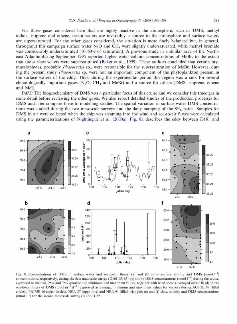
DMS: The biogeochemistry of DMS was a particular focus of this cruise and we consider this trace gas insome detail before reviewing the other gases. We also report detailed studies of the production processes forDMS and later compare these to modelling studies. The spatial variation in surface water DMS concentra-tions was studied during the two mesoscale surveys and the daily mapping of the SF6 patch. Samples forDMS in air were collected when the ship was steaming into the wind and sea-to-air fluxes were calculatedusing the parameterizations of Nightingale et al. (2000a). Fig. 8a describes the eddy between D161 and

-21.5 -21.0 -20.5

59.2

59.4

59.6

59.8

60.0

1.5

2.5

3.5

4.5

5.5

-21.5 -21.0 -20.5

59.2

59.4

59.6

59.8

60.0

35.23

35.25

35.27

35.29

35.31

-21.0 -20.5

59.4

59.6

59.8

60.0

60.2

60.4

35.22

35.24

35.26

35.27

35.29

-21.0 -20.5

59.4

59.6

59.8

60.0

60.2

60.4

4.0

8.0

12.0

16.0

20.0

0

20

40

60

80

100

120

140

160 165 170 175 180 185julian day

umol

m-2

d-1

a c e

b d f

0

5

10

15

20

25

160 165 170 175 180 185julian day

DM

S nM

& w

inds

peed

m s

ec-1

Fig. 8. Concentrations of DMS in surface water and sea-to-air fluxes: (a) and (b) show surface salinity and DMS (nmol l�1)concentrations, respectively, during the first mesoscale survey (D161–D163); (c) shows DMS concentrations (nmol l�1) during the cruise,expressed as median, 25% and 75% quartile and minimum and maximum values, together with wind speeds averaged over 6 h; (d) showssea-to-air fluxes of DMS (lmol m�2 d�1) expressed as average, minimum and maximum values for surveys during ACSOE 98 (filledcircles), PRIME 96 (open circles), NEA 87 (open box) and NEA 91 (filled triangle); (e) and (f) show salinity and DMS concentrations(nmol l�1) for the second mesoscale survey (D179–D185).


D163, showing the high salinity feature at the centre of the initial mesoscale survey and Fig. 8b illustrates theDMS concentration field.

The data indicate a DMS maximum (6 nmol l�1) at the centre of the eddy, surrounded by decreasing con-centrations, beyond which higher levels were again found. The second mesoscale study between D179 andD185 was started west of the eddy, proceeding in N–S transects and during the course of the 3-day surveythe eddy moved toward the SE corner of Fig. 8e. The DMS levels in this region ranged from 4 to 8 nmol l�1

(Fig. 8f), which is not dissimilar to the values found at the centre of the eddy during the initial survey. A sum-mary of the results from all the surveys is shown in Fig. 8c, together with 6-hourly averages of wind speed. Theend members of the time series represent data from the mesoscale mapping.

During the first few days of the experiment, wind speeds continued to be low (wind speed is discussed laterand illustrated in Fig. 10): DMS levels increased steadily (Fig. 8c) and there were large gradients across thepatch (data not shown). On D169 wind speeds began to increase and DMS fluxes increased by almost 2 ordersof magnitude (Fig. 8d). It was not possible to collect survey data during the height of the storm, but directlyafter, the surveys from D172 and 173 showed significant decreases in DMS levels in surface water (Fig. 8c). Weassume this was caused by increased sea-to-air emissions and deeper mixing and homogenisation of the watercolumn. This is clearly shown in Fig. 4b where the DMS maximum in the top 20 m, before the storm, has beenmixed down to about 40 m. Between D173 and D175, DMS concentrations increased almost 3-fold, duringanother period of very low wind speed. If data had only been gained from the mesoscale surveys, we mighthave concluded that DMS concentrations varied little in this region at this time of year. However, the datafrom the patch surveys show how dynamic the DMS system can be and that wind speed and upper water col-umn turbulence can affect DMS concentrations over only a day or so.

The temporal variability in DMS concentrations is a function of both physics and biology and, using theresults of onboard assays of microbiological production and loss rates of DMS, we can assess their relativecontributions. Simo and Pedos-Alio (1999a) conducted incubation experiments using water from the daily castat the centre of the patch and observed that the fraction of total DMSP loss that gives rise to DMS productionwas very variable, for instance, varying from 100% on D168 before the storm to 15% two days later and afterthe storm. These changes were related to the mixed layer depth (Simo and Pedros-Alio, 1999b).

Atmospheric DMS measurements were comparable to others seen in the north Atlantic, although the highvalues seen during the latter part of the cruise are at the high end of the reported range (Cooper and Saltzman,1993; Gregory et al., 1993; Johnson and Bates, 1993. Matrai et al., 1993). Comparison of the emissions andatmospheric concentrations of DMS (Fig. 8d) from D169 onwards might suggest some co-variation, but giventhe sampling regime adopted and the different atmospheric and ocean flow regimes, we cannot consider thisfurther.

DMS and volatile selenium compounds: It has been suggested that there are similar pathways not only forthe volatilisation of sulphur and selenium in surface seawater, but also for the conversion of their methylatedspecies in the atmosphere and ultimate deposition to marine and terrestrial ecosystems (Hamren-Larssen,2000; Amouroux et al., 2001). Some of the first ever measurements of the speciation and distribution of vol-atile organoselenium compounds were made on this cruise (Amouroux et al., 2001). Fig. 9 shows the variationin the concentrations of the gases in the top 50 m of the water column on D179 and 184. The concentrations ofthe selenium volatiles were about four orders of magnitude lower in concentration than DMS in the same sur-face water samples. On D179 dimethyl selenyl sulphide (DMSeS) was the dominant volatile while on D184,DMSeS and dimethyl selenide (DMSe) showed very similar concentrations. Low levels of dimethyl diselenide(DMDSe) were observed on D179, but were below the detection limit on D184. The co-variation of DMS andthe selenides was more marked on D184 (r2 > 0.6) than on D179, and Amouroux et al. (2001) report a cor-relation coefficient of 0.4 for the relationship between DMSe and DMS in surface water samples (n = 20).

CH4 and N2O: Profiles before and after the storm are shown in Fig. 4b. For the first days of the surveybeginning on D164, surface water N2O concentration was in the range 7.6–9.3 nmol l�1 (92–106% saturationwith respect to atmospheric air) (Fig. 5), consistent with previous predictions for this region of the NorthAtlantic (Nevison et al., 1995; Forster et al., in press), reflecting inhibition of nitrifiers and denitrifiers by lightand dissolved O2, respectively (Horrigan et al., 1981). In contrast, surface CH4 concentrations were in therange 1.9–2.3 nmol l�1 (Fig. 5). This corresponds to overall undersaturation with respect to atmospheric air(78–94%), and presumably reflects net microbial CH4 oxidation at rates higher than CH4 could be replaced

DMS DMSe DMSSe DMDSe

0 1 2 30

10

20

30

40

50

m

DMS nmol l-1

0 1 2V Se pmol l-1

0 5 100

10

20

30

40

50

m

DMS nmol l-1

0 0.5 1 1.5V Se pmol l-1

a b

Fig. 9. Profiles of DMS and volatile Se species (nmol l�1): D179 (a) and D186 (b).


through air–sea gas exchange or in situ production. On D173, immediately following the storm, there was asignificant increase in the N2O and CH4 inventories of the upper 40 m (Fig. 5). The most notable feature post-storm was the development of a distinct CH4 maximum �2.5 nmol l�1 (�104% saturation) at 10 m. It is notpossible to unequivocally determine whether the immediate post-storm inventory changes of CH4 and N2Oreflect physical mixing or whether they are due to enhanced biologically activity as a consequence of mixing.However, both phytoplankton and microzooplankton numbers declined at this time, as noted earlier, suggest-ing that a physical rather than biological explanation may be more likely. During the following several days,near surface concentrations of CH4 and N2O both progressively declined toward pre-storm values in the caseof N2O and toward lower than pre-storm values for CH4.

Ethene and isoprene: The concentrations of ethene and isoprene were relatively homogeneous across theeddy. Temporal variations in the concentrations of the two compounds were strikingly different (Figs. 5and 10). Ethene concentrations steadily increased from about 80 pmol l�1 on D161 to about 200 pmol l�1

immediately before the increased winds of the storm on D170, after which concentrations fell. During the per-iod D163–167 wind speeds were low (average 2.9 m s�1) resulting in low gas fluxes to the atmosphere. In addi-tion, light levels were high (Fig. 10), which would facilitate photochemical production from dissolved organiccarbon (Ratte et al., 1998) and direct release of ethene from light-stressed algae (Plettner et al., 2005). Theheavy grazing of phytoplankton during the pre-storm period may also have resulted in increased levels of dis-solved organic matter being released to the water column, which could then be photolysed to form ethene. It islikely that accumulation of ethene in the water column was due to a combination of high photochemical andphotobiological production and low sea-air losses. Within 3 days of the storm, surface ethene concentrationsincreased gradually until a period of higher winds which began on D183 (Fig. 10).

In contrast, isoprene concentrations were relatively constant throughout the pre-storm period with an aver-age concentration of 16.7 pmol l�1 (±2 pmol l�1), reflecting the relatively constant levels of phytoplanktonbiomass over this period (Fig. 10). Throughout the cruise there was a linear relationship between surface iso-prene and surface chlorophyll concentration in the eddy (r2 = 0.50, n = 96, P < 0.01). Even stronger relation-ships have been seen in other ocean areas (Broadgate et al., 1997), indicating that primary production is amajor source of isoprene. An analysis of the pigment and phytoplankton taxonomy data indicates that no sin-

a

0

50

100

150

200

250

160 165 170 175 180 185 190

ethe

ne, p

mol

l-1, w

inds

peed

, ms-1

x 10

0

200

400

600

sola

r rad

iatio

n, W

m-2

b

0

5

10

15

20

25

30

35

160 165 170 175 180 185 190

isop

rene

, pm

ol l-1

, win

dspe

ed, m

s-1

0.0

1.0

2.0

3.0

chlo

roph

yll,

mg

m-3

Fig. 10. Daily average concentrations (±standard deviations) in the eddy of (a) surface ethene (closed circles) and solar radiation (dashedline) and (b) surface isoprene (closed circles) and surface chlorophyll-a (open circles). Also shown is the wind speed averaged over 6 h (greysolid line).


gle species, or group of species, present dominates the correlation. Thus, in this case, we suggest isoprene is aproduct of most or all phytoplankton activity, which was dominated by E. huxleyi as noted earlier, before thestorm and picoplankton after the storm. In contrast to ethene, no accumulation was observed during the per-iod of low winds, indicating that isoprene water column production and loss processes were approximately inbalance.

Depth profiles of ethene and isoprene (Fig. 4) clearly indicate their different production processes. Beforethe storm, in well-stratified waters, isoprene displayed a distinct sub-surface maximum at about 20–30 m, con-sistently slightly above the broad chlorophyll maximum in the water column. Similar observations have beenmade in the Mediterranean (Bonsang et al., 1992), the Northeast Atlantic (Baker et al., 2000) and Miami Bay(Milne et al., 1995). Other profiles measured on the cruise (not shown) showed isoprene concentrations contin-uing to decrease below 60 m to about 5 pmol l�1 at about 200 m, but still detectable at concentrations of 1–2 pmol l�1 in the deep waters at 2800 m. After the storm, concentrations of isoprene in the surface increasedslightly, to about 18 pmol l�1, as higher concentrations from sub-surface waters were mixed upward. The totalisoprene inventory in the upper 60 m was unchanged by the storm event, when there was a large flux to theatmosphere, indicating that the biological system rapidly restored isoprene concentrations to pre-storm levels.

Before the storm, ethene clearly showed a rapid vertical decrease with depth from high concentrations (150–200 pmol l�1) in the surface to constant levels of about 20 pmol l�1 below 100 m, consistent with photochem-ical production, or at least a chemical or biological process directly dependent on light levels, in surface waters.Immediately after the storm, ethene was well-mixed above the thermocline with concentrations of about75 pmol l�1. Modelling suggests that the total ethene inventory integrated above 60 m decreased over the


period of the storm to a greater extent that can be explained by loss to the atmosphere (Kettle et al., in prep-aration). It is likely that production rates were very low as light levels were low during the storm (daily maxlight levels were <500 W m�2, Fig. 5) so that, presumably, consumption and/or destruction processesdominated.

Organohalogen gases: Prior to the storm, on D167, MeBr had a uniform concentration (�2 pmol l�1) in theupper 20 m of the water column, below which the concentration decreased to just above 1 pmol l�1 at 40 mand below 1 pmol l�1 at 60 m (Fig. 4). After the storm (D172), the MeBr concentration in the surface waterwas no longer uniform. Furthermore, the concentration was lower, except for a peak at 11 m. Given that gasexchange would tend to move the MeBr toward equilibrium, these results suggest that vertical mixing playedan important role in the evolution of the gas concentrations, possibly more important than increased gasexchange.

Over the following days the concentration of MeBr decreased, so that the concentration was uniform overall the depths measured (0–100 m). MeBr was considerably undersaturated (10–60% saturation). Similarundersaturation was also seen in waters outside the eddy (data not shown).

The behaviour of MeI contrasts to that of MeBr, the other halogen considered here. Some MeI profilesshow some similarity to isoprene. This general similarity is consistent with the suggestion above that bothare related to phytoplankton activity. On D167, prior to the storm, the concentration of MeI at 20 m(�12 pmol l�1) was greater than that at the surface (�9 pmol l�1) (Fig. 4). Below 20 m the concentrationdecreased to a minimum measured at 100 m. After the storm, as for MeBr described above, the concentrationin the surface water had decreased, except for a peak at 11 m, as for MeBr. The concentration at 20 m was nowlower than that at the surface. Over the following days (data not shown) the surface water concentrationsdecreased further to less than 5 pmol l�1 and concentration maxima were observed at a variety of depths.On D173 the highest concentrations were measured at 25–60 m, whilst on D174 and 178 there was a maximumat 40 m and on D179 the highest concentration was at 10 m. These changes illustrate the complex and poorlyunderstood processes regulating organohalogen gases.

Nanoparticle nucleation events or ‘‘particle bursts” in coastal environments which may contribute to aer-osol formation and hence cloud and albedo modifications have been related to organoiodine emissions in acoastal environment influenced by macroalgal beds (e.g. O’Dowd et al., 2002). We measured atmospheric con-densation particle numbers using similar techniques to these workers with two counters measuring particleswith aerodynamic diameters of >7 and >3 nm, respectively. There is no evidence for ‘‘particle burst” eventsin the present data set. Emissions of gas phase organohalogens are very high in macroalgal environments;for example Nightingale et al. (1995) reported MeI concentrations five to ten times higher than reported here,and emissions of CH2I2 (the candidate biogenic iodine gas for aerosol formation identified by O’Dowd et al.,2002) may be similarly elevated. Lower emission rates of aerosol-forming gases in our study area could allowmaterial produced by oxidation of such gases to adsorb on to existing particles as well as forming new par-ticles, and hence explain the lack of ‘‘particle bursts”.

3.3. Budgeting processes within the eddy before and during the storm

We now present and compare several approaches for quantifying rates of processes within the eddy both inthe relatively calm period before the storm (D164–169) and after the passage of the storm. In general we usetwo approaches, one based on integrating various direct rate measurements and the second based on compar-ing profiles before and after the storm. During the calm period the movement of the SF6 patch was very small(station position D164 59.50N, 21.13E and D169 59.52N, 21.00E) relative to the nutrient gradients within theeddy (Fig. 3) and the CO2buoy was essentially static as noted earlier.

3.3.1. A nutrient budget for the ACSOE eddy

During the period D164–169, nutrient concentrations in the euphotic zone decreased (Table 3) and the low-est concentration isopleth deepened (Fig. 5). Expressing this decrease as a loss of integrated nutrient stock inthe euphotic zone is, however, not straightforward. The euphotic zone extended to about 30 m and henceencroached into the nutricline. Sampling density is inadequate to define the nutrient gradients in this regionsufficiently well to allow integration to a standard depth of 30 m. Fasham et al. (1999) noted a similar problem

Table 3Average nutrient concentrations (lmol l�1) in the upper 20 m within the SF6 patch, with 0–5 m concentrations in brackets

Day Nitrate Dissolved inorganic phosphorus Dissolved silicon

164 7.8 (7.0) 0.42 (0.36) 1.1 (0.7)165 6.9 (6.9) 0.38 (0.37) 0.6 (0.78)166 7.9 (7.1) – –167 6.0 (6.0) 0.35 (0.35) 0.35 (0.33)168 6.4 (6.1) 0.36 (0.35) 0.33 (0.28)169 6.7 (6.2) 0.38 (0.35) 0.29 (0.28)Estimated rates of decline in nutrient concentrations (lmol l�11 d�1) based on linear correlations, with r2 values in brackets0 m 0.21 (0.64) 0.003 (0.61) 0.11 (0.85)0–20 m average 0.25 (0.39) 0.01 (0.42) 0.15 (0.80)


in a previous study in the North Atlantic. There may also be some variability in nutricline depth due to inter-nal waves. These problems have been reduced by correcting depths to constant density surfaces (Law et al.,2001), but there is still some uncertainty in defining the nutricline gradient. By contrast, nutrient concentra-tions are more constant over the upper 20 m of the water column and hence have been averaged in Table3, although comparison to surface water concentrations (Table 3) indicates that some vertical gradients arestill present even over this depth range.

The decline in surface water concentrations over time is more clear-cut than the decline in 0–20 m meanconcentrations, but we choose to use the mean concentrations over the 0–20 m range to reflect the situationin the euphotic zone. We suggest the uncertainties in the rates of decline of nutrient concentrations estimatedin this way (Table 3) to be at least 50%, reflecting horizontal and vertical variability within the eddy (based onsurveys), and variability in the processes of nutrient uptake, regeneration and vertical mixing. Rates seen herefor nitrate decline are somewhat lower than those reported by Rees et al. (2001) for the PRIME eddy. Wood-ward and Rees (2001) did not observe a DSi decrease, but it is a very clear feature of this campaign. Themarked decline in DSi is particularly notable given the very low DSi concentrations observed, at which diatomgrowth should be severely limited (Dugdale et al., 1995; Dugdale and Wilkerson, 1998). This decline is alsoevident at the larger space and time scales of the whole eddy through the entire campaign (Fig. 3), demonstrat-ing that the nutrient patterns for DSi (and nitrate) are representative of the eddy in general. Diatom growth isparticularly sensitive to iron availability (Boyd et al., 2000 and references therein) and hence the conclusionearlier that this region is not subject to iron stress may offer an explanation for this very efficient DSi uptakeat low DSi concentrations. It is interesting to note that the rates of decline in DSi and nitrate are similar (Table3). Diatoms require both nutrients in a ratio of about 1:1 (Dugdale and Wilkerson, 1998). However, diatomsrepresent only a very small part of the phytoplankton population (Table 2). Their growth should be severelylimited by these low DSi concentrations, as noted earlier, and they would not be expected to exert a majorinfluence on nutrient chemistry. However, the decline in nutrient concentrations represents ‘‘new” productionwhich Dugdale and Wilkerson (1998) argue is dominated by diatoms. Therefore, it may be that, although notthe dominant phytoplankton species, diatoms represent an important control on surface water biogeochem-istry here by dominating ‘‘new” and export production, and hence nitrate (and DSi) removal. This point isconsidered further below.

Similar low DSi concentrations have been observed in some other studies in this region in other years, butare not seen during all such cruises. Marra et al. (1995) sampled in this region in May and reported an eco-system dominated by Phaeocystis. They observed similar rates of nitrate decline (Table 3) with ambient nitrateconcentrations �1.7 lmol l�1. However, DSi concentrations were 2–6 lmol l�1. Harris et al. (1997), samplingin this area in July after a coccolithophore bloom, reported nitrate concentrations of 1–2 lmol 1�1 but lowDSi concentrations of 0.9–1.2 lmol 1�1. The PRIME cruise (Woodward and Rees, 2001) sampling in Junein the same area reported nitrate concentrations of 5–7 lmol l�1 and DSi of 2.5 lmol 1�1 within an eddy sim-ilar to that considered here. However, concentrations were much lower outside the sampled eddy, comparableto our measured DSi concentrations. Allen et al. (2005) also note very low DSi in this region.

It is clear from Fig. 4 and unpublished deeper profiles from this region collected on this cruise and on pre-vious cruises in the area, that deep winter mixing in this area to 500–1000 m brings water to the surface with


nitrate concentrations considerably greater than DSi as noted by Allen et al., 2005. Hence, a spring diatombloom will inevitably deplete DSi long before nitrate, assuming a DSi/nitrate uptake rate of about 1:1.

We now focus on nutrients and phytoplankton processes during the period D164–169 when, under verycalm conditions, the SF6 patch remained well defined and coherent. In this situation, it is possible to derivea quantitative description of the phytoplankton activity and its role in nutrient cycling. During this timenitrate and dissolved inorganic phosphorus (DIP) were highly correlated at essentially the Redfield ratio(for all data for this period in the upper 200 m of the water column the relationship was nitrate = 15.3-DIP + 0.9; r2 = 0.97, n = 36).

The decline in nitrate concentrations from D164 to 169 is about 0.2–0.25 lmol N l�1 d�1 (Table 3). Overthe same period pCO2 declined at a rate of 2.4 latm d�1 at 16 m (Fig. 7). If we assume a temperature of10 �C, a salinity of 35 and an alkalinity of 2170 lmol kg�1, the pCO2 rate of decline is equivalent to1.3 lmol kg�1 l�1, although this is a lower limit since calcification by the active coccolithophore populationwill have reduced alkalinity and increased pCO2. Assuming Redfield stoichiometry, this pCO2 decline is equiv-alent to a decline in fixed nitrogen of 0.2 lmol N l�1 d�1. The consistency of this estimate from the buoy andthat based on the observed decline in euphotic zone nitrate concentrations (Table 3), two independent mea-surements from different platforms over different time scales, gives us confidence that the nutrient decline rateestimates are realistic. Integrating these measurements over the euphotic zone is complicated by the changes inmixed layer depth, but if we consider a nitrate decline in the range 0.2–0.25 lmol N l�1 d�1 over a depth rangeof 20 and 30 m (to reflect the variability seen in mixed layer depths), a rate of nitrate decline of 4–7.5 mmol N m�2 d�1 is obtained.

Table 4 represents a simple nutrient budget for the euphotic zone (0–30 m) of the eddy over the periodD164–169, constructed using directly measured nitrate uptake rates (see Section 3.2.1), the declines in nitrateand DSi concentrations scaled to 20 and 30 m, atmospheric inputs and the diffusive inputs from below theeuphotic zone (see Section 3.1).

Within the SF6 patch, phytoplankton nitrate uptake (8.3 mmol m�2 d�1) minus the inputs (atmosphericnitrate + ammonium 0.012 mmol m�2 d�1 + vertical mixing of nitrate from below 1.5 mmol m�2 d�1) shouldequal the decline in nitrate concentrations (4–7.5 mmol m�2 d�1), unless regeneration of ammonium to nitrateis taking place, which is generally assumed to be unlikely (see earlier data and Boyd et al., 1995; Dugdale et al.,1995). Recent work has suggested that such nitrification may be an important reaction in the ocean gyres, butnot particularly important in high latitude regions such as considered here (Yool et al., 2007). Given the rangeof uncertainties involved, the balance in Table 4 is remarkably close. The results imply that the atmospherewas not an important source of fixed nitrogen at this time and that 15–20% of the nitrate uptake by phyto-plankton is supported by vertical diffusive inputs of nitrate, a somewhat smaller value than that estimatedby Law et al. (2001) during the PRIME study for an eddy in the same region of the North Atlantic. As notedearlier the rate of nutrient supply from depth may be underestimated by the methods used here. The additionalnitrogen uptake in excess of supply rate presumably cause the observed decline in surface water nutrient con-centrations. The general similarity of results from the PRIME study and this work suggests that the rates mea-sured are representative of early summer conditions in this area.

The minor importance of atmospheric nitrogen inputs at this time is in marked contrast to the situationfurther south and east in the North Atlantic (Spokes et al., 2000). Given the dominance of clean air-flowto the site at this time, this is not surprising. Under conditions of polluted easterly flow from continental Eur-

Table 4Nutrient budget for the upper 30 m of the ACSOE eddy averaged over the period D164–169, all as mmol m�2 d�1

Nitrate Dissolved Si

Atmospheric input 0.012 0Vertical diffusion 1.5 0.9Phytoplankton uptake 8.3Predicted decline 6.8Observed decline (over 20–30 m depth range) 4–7.5 3–4.5

Sources of data are discussed in the text.


ope, Spokes et al. (2000) noted that atmospheric deposition fluxes at about the same time of year couldincrease by about 20-fold to the Northeast Atlantic west of Ireland, compared to deposition from clean airmasses, but even such a large increase would not significantly alter the conclusions of the budget. A similarconclusion will apply to this area of the North Atlantic in general since the waters are not nitrate-deficientand have a substantial input of nitrate from deeper waters. This contrasts with the situation further south(Spokes et al., 2000; Spokes and Jickells, 2005), where waters become more oligotrophic in summer, verticalmixing is weaker and atmospheric fluxes are more important.

In the case of silicon, atmospheric inputs are small (Jickells, 1998). We do not have a direct measure of DSiuptake by phytoplankton, but if we assume a closed budget for Si as for nitrate, we can estimate net DSiuptake rates by phytoplankton at 2.1–3.6 mmol Si m�2 d�1 integrated over the euphotic zone (Table 4). GrossDSi uptake rates will be higher if there is recycling of DSi within the euphotic zone, as suggested by Bidle andAzam (1999). Recently Brown et al. (2003) reported direct measurements silica uptake rates in this area of theNorth Atlantic at the end of the spring bloom. They show that silica uptake rates are a function of silica con-centrations. At their lowest silica concentration (0.3 lmol l�1), comparable to that seen here, these authorsreport directly measured gross silica uptake rates of 6 mmol Si m�2 d�1, consistent with our estimates herefrom the nutrient budget and with significant silica recycling in the euphotic zone.

This DSi uptake rate estimated from the nutrient budget implies that, assuming a diatom Si:N requirementratio of 1:1 (see earlier), about a quarter to half of the nitrate uptake is associated with diatom growth. A rel-atively high proportion of nitrate uptake by diatoms is consistent with the fact that most of the ‘‘new” primaryproduction is associated with the larger (>5 lm) size fraction, as noted earlier, although E. huxleyi may also beretained in the largest size fraction. Dugdale and Wilkerson (1998) argue that diatoms dominate new produc-tion, which appears to be consistent with the situation described here.

Taking a Si uptake rate of 2.1–3.6 mmol m�2 d�1 and a biogenic Si:POC ratio of 0.13 (Brezinski, 1985)implies a diatom growth rate of 16–28 mmol C m�2 d�1. On D165 surface water diatom abundance is esti-mated at 8.15 mg cell C m�3. Extrapolation of this value over a 30 m water column yields a standing stockof 20.4 mmol C m�2, implying a diatom carbon doubling rate of 0.8–1.4 d�1. This suggests an actively growingdiatom population and hence that low diatom biomass reflects small individuals (small pennate species wereabundant) which are being heavily grazed, consistent with the microzooplankton data. We conclude that thiseddy was characterised by an actively growing and biogeochemically important (particularly in terms of car-bon and nutrient flux) diatom community dominated by species able to grow at very low DSi levels under con-ditions of relatively high iron abundances and maintained at a relatively low biomass by microzooplanktongrazing as seen elsewhere (Stelfox-Widdicombe et al., 2004).

As noted earlier, the storm disrupted and mixed the surface waters. We can attempt to crudely calculate theresultant input of nutrients based on the average nitrate concentrations in the upper 20 m before and after thestorm (6.7 lmol l�1 and 7.8 lmol l�1, respectively Fig. 4). This increase in concentration in the upper 20 mequates to an input of 22 m mol m�2 of nitrate to the upper 20 m. This will be a lower limit if the calculationwere extended to the whole 30 m euphotic zone, although estimating the extent of the increase is complicatedby the gradients in nutrients below 20 m, as discussed earlier. Although crude, this calculation implies that thisone storm mixed the equivalent of 10 days diffusive nitrate input, emphasising the importance of such events inthis area at least for nutrient supply.

3.3.2. Dissolved trace gases

3.3.2.1. DMS. Precursors and transformations: The temporal variability in DMS concentrations is a functionof both physics and biology and, using the results of the onboard assays described earlier, we can attempt toasses their relative contributions. The concentrations and rates of transformations of DMS and its major bio-chemical precursor (the algal component dimethylsulphoniopropionate, DMSP) were directly measured byin vitro experiments and/or inferred by budgeting between Lagrangian time points (e.g. Archer et al.,2002a,b). The production of DMS from DMSP is a biological process involving coenzyme-A transferasesin bacteria (Todd et al., 2007) or the enzyme DMSP-lyase (dimethylpropiothetin dethiomethylase), whichwas characterised in a number of depth profiles (see below).

Simo and Pedos-Alio (1999a) and Simo et al. (2002) considered the budget of DMSP during this cruise indetail and the results are briefly summarised here. During the period D165–170 the concentrations of DMSP


(total) and DMSP (particulate) in the surface mixed layer rose from 37 to 66 and from 29 to 52 nmol l�1,respectively, with the highest values observed on D170. Most of the particulate DMSP was associated withalgae in the 2–10 lm size range. The DMSP (total): chlorophyll-a ratio ranged from 44 to 112 nmol mg�1,in agreement with what has been found previously in coccolithophore dominated waters in the same area(Malin et al., 1993). After the storm on D169–170, the concentrations of DMSP (total), fell slightly, withDMSP (dissolved) decreasing to values similar to those observed at the start of the experiment. The depth pro-files of DMSP (dissolved) in Fig. 4b show that after the storm, levels had decreased in the upper 20 m and thatit had been mixed down to greater depths. Over the whole Lagrangian time series, daily rates of DMSP pro-duction by phytoplankton were linearly related to primary production with an estimated 7% of organic carbonproduction being used in DMSP biosynthesis (Simo et al., 2002). The average DMSP production rate was28 nmol S l�1 d�1, and a similar value was obtained for DMSP consumption, yet production and consumptionwere not always coupled on a daily basis (Simo and Pedos-Alio, 1999a). Even though most of the DMSP waseventually used in one way or another by bacteria, Simo et al. (2002) estimated that about 60% of the algalDMSP loss was mediated by microzooplankton grazing on D165–168. These authors noted that DMSP madea significant contribution to overall labile carbon cycling as well as dominating the organic sulphur cycling inthe surface layers.

The biochemistry, physiology and ecology of DMSP-lyase isozymes were also directly studied. Particlesfrom freshly collected water samples were size-fractionated on to polycarbonate filters and in vitro enzymeassays were conducted immediately on-board or after storage of filters at �80 �C (for method details see Ste-inke et al., 2000). Activities (measured as maximum DMS production rates) ranged from 0.1 to 142.3 nmolDMS h�1, representing the likely upper limit of potential DMS production. This far exceeds actual DMS pro-duction rates (6.6 nmol l�1 d�1, see later) illustrating the considerable unrealised potential for DMS produc-tion within the euphotic zone. Size-fractionation and pigment data indicated that E. huxleyi was only a minorcontributor to total DMSP-lyase activity inside the coccolithophorid bloom area. In surface waters, most ofthe DMSP-lyase activity was associated with phototrophic dinoflagellates larger than 10 lm diameter (Steinkeet al., 2002a), in contrast to the abundance of DMSP in smaller cells noted earlier. Results from a depth profileon D178 showed increasing activities towards the surface, where the ratios of DMSP-lyase activity to chloro-phyll-a, and diadinoxanthin to chlorophyll-a were highest (Steinke et al., 2002b). The photoprotective pigmentdiadinoxanthin is part of an inducible xanthophyll-cycle that assists in energy dissipation under high-light con-ditions. This vertical distribution pattern of enzyme activity is consistent with the proposed function of DMSPand DMS as antioxidants in marine algae (Sunda et al., 2002), that are necessary for the rapid scavenging oftoxic activated oxygen species (such as hydroxyl radicals and superoxides).

DMS production rates ranged from 1 to 14 nmol S l�1 d�1, with an average value of 6.6 nmol S l�1 d�1 forthe entire experiment. DMS loss occurred via microbial consumption, photolysis and ventilation, with allthree being significant. A comparison of the rate constants (inverse of turnover times) of these three majorsinks shows microbial consumption (0.7 d�1) and photolysis (1.1 d�1) were faster than ventilation (0.1 d�1).The relative contribution of each process to the total DMS loss varied in the short term depending on externalforcing, e.g. wind and irradiance. Thus photolysis dominated on sunny days, microbial processes on cloudydays and during the storm all three processes were of similar importance (Simo and Pedos-Alio, 1999a).

Variations in surface water and sea-to-air fluxes of DMS and other trace gases: The spatial variation insurface water DMS concentrations was studied during the two mesoscale surveys and the daily mapping ofthe SF6 patch. Samples for DMS in air were collected when the ship was steaming into the wind and sea-to-air fluxes were calculated using the parameterizations of Nightingale et al. (2000a). Fig. 8a describes theeddy between D161 and D163, showing the high salinity feature at the centre of the initial mesoscale surveyand Fig. 8b illustrates the DMS concentration field and the general patterns of distribution as discussedearlier.

The data for DMS emissions shown in Fig. 8d are comparable with data collected in the same region inprevious years. We have used data from cruises in 1987 (Malin et al., 1993), 1991 (Holligan et al., 1993)and 1996 (Savidge and Williams, 2001) and recalculated the emission rates, using the newer Nightingaleet al. (2000b) equations on samples which fall in the region 19�W to 20�W and 57�N to 60.5�N, to providebetter comparison with the ACSOE data. With the exception of D169, the DMS emissions during ACSOEwere relatively low in comparison with data from other studies. However, the mean flux from all the patch

Table 5Production rates for components of the DMS system

Parameter lmol m�2 d�1

DMSP production 560DMS production 132DMS air–sea-exchange flux 14

Rates for individual processes are described in the text and have been scaled to the euphotic zone by assuming a 20 m mixed layer to beconsistent with the nutrient budget (Table 4).No allowance has been made for the mixed layer deepening during the storm period.

Table 6Trace gas fluxes for the storm period (D169–172) based on Kettle et al. (in preparation)

Gas Flux (lmol m�2 d�1)

DMS 5.1CH4 1.9Ethene 0.38Isoprene 0.06MeI 0.07MeBr 0.008

Model estimates are for the 5 day period and are scaled here to a per day flux for ease of comparison.


surveys during this cruise is 13.9 lmol m�2 d�1 which, together with the overall range of 0.1–111 lmol m�2 d�1, is similar to previous years. Compiling the various estimates of production rates for com-ponents of the DMS system (Table 5) is instructive, even though some of the estimates are for slightly differenttime periods during the ACSOE cruise. The results in Table 5 emphasise that air–sea exchange of DMS is arelatively small component of the overall DMS cycle as noted previously.

Kettle et al. (in preparation) have estimated trace gas fluxes for the storm period (Table 6) comparing avariety of one dimensional inverse boundary layer models of the upper 80 m of the water column to determinewhich best fits the observed profiles, providing an alternative estimate of DMS fluxes to that above, based onsurface water concentrations and air–sea-flux parameterisations. Kettle and Turner (2007) conclude that theMellor/Yamada-3-model formulated by Kantha and Clayson (2004) represents the most appropriate modeldescription and we therefore report flux estimates for the trace gases based on this model in Table 6. Kettleet al. (in preparation) estimates DMS flux to the atmosphere over the 5 day storm period of 25.4 lmol m�2,equivalent to 5 lmol m�2 d�1, a value broadly consistent with the estimates above. This also suggests thatalthough DMS fluxes increased dramatically at the start of the storm, they were not overall especially highbecause fluxes during the storm become reduced as DMS concentration in the water column fell, rather thanbeing limited by rates of air–sea gas transfer.

The enormous range of trace gas fluxes for the different gases is evident from Table 6. These approximatelyscale with concentration since fluxes during the storm are dominated by air–sea gas exchange. However, asnoted earlier, over the whole scale of this campaign, the vertical distributions and air–sea fluxes of these dif-ferent gases were not strongly coupled, reflecting their rather different biogeochemical regulation within thewater column.

4. Conclusions

This study has demonstrated the value of the SF6 labelling technique in the construction of biogeochemicalbudgets and the estimation of rate processes in an open ocean situation. The physical properties of the eddystudied here were similar to those of an eddy studied by the PRIME project in the same area of the NorthAtlantic (Savidge and Williams, 2001), suggesting that the characteristics of these eddies, which are frequentlypresent in this area, may be rather similar. Such eddies appear to be a major influence on the biogeochemistry


of this ocean region. Nutrient supply rates from below within the eddy are substantial and contribute signif-icantly to the observed rates of primary production within it. These sustain a phytoplankton community thatis markedly different to that seen in the surrounding waters. Nutrient concentrations were also markedly dif-ferent inside and outside the eddy, although rates of primary productivity did not vary greatly. This may bebecause there were significant amounts of nitrate and DIP in the water, suggesting that macro nutrient limi-tation (and possibly Fe limitation) was not a factor in these waters.

Storms appear to represent an important biogeochemical forcing function at the survey latitude, mixing thewater column to depths below the nutricline and recharging the surface waters with nutrients and changing thephytoplankton community. Nutrient recharge associated with storm induced vertical mixing may dominatethe nutrient supply. This process may also affect carbon export via phytoplankton sinking and air–sea uptakeof CO2 due to mixing with high CO2 subsurface waters. Allen et al. (2005) illustrated the importance of othertransient nutrient supply mechanisms in this area.

In contrast to more thermally stratified waters further south, atmospheric deposition of fixed nitrogenwas not an important component of the biogeochemical budget in this area, because of the significant sup-ply from below. Atmospheric iron supply was probably adequate to meet phytoplankton needs and thisappeared to allow very efficient DSi uptake by diatoms. Biogeochemical budgets suggest diatoms are a sig-nificant component of new production in this area although the population was relatively low, presumablyas a result of active growth and heavy grazing pressure. The phytoplankton population was dominated bycoccolithophorids during the early part of the cruise, as has been seen previously in this area (Holliganet al., 1993; Savidge and Williams, 2001). These species are known to be large emitters of DMS (Stefelset al., 2007), consistent with the high concentrations seen in the centre of the eddy. Measurements of bio-genic gas concentrations indicate active production and cycling, and indeed for the sulphur system (DMS/DMSP), biogenic S-cycling appears to constitute an important component of the overall euphotic zone car-bon cycle. The region was a sink at this time for several climatologically important gases (N2O, CH4 andmethyl bromide) but a source for others (DMS, isoprene, ethene and methyl iodide). Only the concentra-tions of DMS, methyl iodide and isoprene appear to be closely coupled to primary production processes.The other gases are produced and cycled by different processes, making extrapolation of fluxes from oneto another difficult. However, all are produced within the euphotic zone either directly by biological pro-cesses or by chemical processes acting on biologically produced reactants within the water column. The con-centrations measured during the ACSOE cruise are comparable to other studies in this area, lendingincreased confidence to the global compilations of concentrations and fluxes for these trace gases. Theresults are also consistent with our existing understanding of mechanisms of production, e.g. ethene by pho-tochemical/photobiological processes, DMS, methyl iodide and isoprene by processes that are closely asso-ciated with phytoplankton primary production and subsequent grazing and viral infection. Henceproduction of all these gases is related to euphotic zone biological processes but these processes and theresultant biogenic gas cycling are not necessarily closely coupled to one another and not closely coupledto C cycling which may be controlled by diatoms.

In the case of methane and the DMS/DMSP system, it is clear that the fluxes from the ocean represent asmall release from an intense biological cycle within the euphotic zone. Fluxes of DMS in this and other tem-perate oceanic environments are rather higher than seen in coastal waters at this time of year (Nguyen et al.,1990; Malin et al., 1993; Turner et al., 1996; Baker et al., 2000). However, the reverse appears to be true formethyl iodide and by analogy possibly for CH2I2, the gas proposed by O’Dowd et al. (2002) as an importantprecursor for particle bursts. These observations would therefore suggest that such ‘‘particle bursts” may bemore characteristic of coastal environments than open ocean ones. This may be the result of oxidation of bio-genic gases in these open ocean environments not yielding new particles, but rather that the products areadsorbed to existing particles including particularly sea salt, since the ozone and peroxide data do provide evi-dence of active photochemical cycling within the air masses sampled.

Overall this project illustrates the intense coupling between surface waters and the lower atmosphere in themarine environment in terms of physical forcing by wind and thermal heating and species dependent biolog-ically mediated trace gas exchange and nutrient/carbon cycling and in other areas, although not in the North-east Atlantic at the time of this campaign, atmospheric inputs. Understanding these complex interactions is ademanding agenda before the IGBP SOLAS programme (http://www.solas-int.org/).

http://www.solas-int.org/


Acknowledgements

This is contribution no. ACP175 of the NERC ACSOE Thematic Programme.NERC grants GST/02/1276 supported the work of Jickells and Spokes, GST/02/1278 the work of Liss and

Nightingale together with core funding to the Plymouth Marine Laboratory (PML) while the ACSOE coreprogramme supported Broadgate and the shiptime costs, NERC grant GR9/3467 to G.S. supported Monco-iffe and Gilpin. Steinke was supported by NERC grant GR3/10956. The University of Newcastle upon TyneResearch Committee provided funding to support T. Frost. The work of Simo and Pedros-Alio was supportedby the Spanish McyT grant MAR97-1885-E. Our thanks go to Steve Groom, Peter Miller and Tim Smythfrom the Remote Sensing Data Analysis Service at PML for their help and support of this cruise and for pro-viding Fig. 2 to Dave Meldrum of Dunstaffnage Marine Laboratory for the loan of one GPS buoy and for hishelp in tracking its path and to Russell Davison (SOC) for phytoplankton counts. We also thank the officersand crew of RRS Discovery and UKORS staff Jeff Benson, Martin Bridger, Jeff Jones, Rob Lloyd, Pete Ma-son and Dave Tears for all their help in making this cruise a success. We gratefully acknowledge access to theHYSPLIT4 (Hybrid Single-Particle Lagrangian Integrated Trajectory) Model, 1997 at http://www.arl.noaa.-gov/ready/hysplt4.html, NOAA Air Resources Laboratory, Silver Spring MD, USA.

We thank three anonymous referees and the editor for their helpful comments which improved thismanuscript.

Appendix. SF6 deployment

The Lagrangian reference frame was provided by a controlled release of 2250 l of seawater saturated withSF6. The tracer was released at a depth of 7–9 m and within the surface mixed layer under gravity over a 10 hperiod, following protocols reported in Law et al. (1998), creating a patch with final dimensions about6.4 � 6.4 km with maximum concentrations towards the centre. Concentrations were regulated by varyingpumping rates and ships speed during deployment. Three low profile surface drifting buoys (one equippedto measure pCO2) were also released within the patch (Broadgate and Liss, 1998), and one continued trans-mitting for three months. Due to a decline in SF6 concentrations to below detection limits, the patch was re-infused 10 days after the first deployment over a 3.75 � 3.75 km box using 1000 l of SF6-saturated seawater.The SF6 patch was monitored using an automated detection system (based on Law et al., 1998). Measure-ments were made every 4 min on samples drawn by pump from the ship’s underway continuous seawater sys-tem with an inlet at 4.5 m depth. The depth distribution of SF6 was determined from daily hydro-casts (Carse,2000) and subsequently used to estimate vertical diffusivities (Carse, 2000; Law et al., 2001).

Chemical and biological analytical procedures

Most methods followed established and published protocols and we therefore restrict the description to aminimum necessary, and refer the reader to relevant publications for further details.

Water column

Nitrate plus nitrite (hereafter nitrate since nitrite was undetectable when separately analysed), dissolvedinorganic phosphorus (DIP) and dissolved silica (DSi) were measured using a Skalar San autoanalyser. Pre-cision was ±0.1 lmol l�1 for nitrate (and nitrite) and DSi and ± 0.01 lmol l�1 for DIP. Accuracy was con-firmed with Sagammi standard reference materials (full details in Broadgate and Liss, 1998; Sanders andJickells, 2000). Trace gas measurements used purge and trap techniques for DMS/DMSP (Simo et al.,2000; Turner et al., 1990), C2–C6 non-methane hydrocarbons (Baker et al., 2000), methyl bromide/iodide(Baker et al., 1999; Carpenter et al., 1999), volatile Se species (Amouroux et al., 2001). N2O and CH4 weremeasured using high precision (±1%) single phase equilibration gas chromatography (Upstill-Goddardet al., 1996). Total dissolvable iron (TDFe unfiltered samples containing dissolved iron and particulate ironsolubilised by 2 weeks acidification to pH 2) was analysed using the method of Bowie et al. (1988) on a singleprofile collected from within the eddy.

http://www.arl.noaa.gov/ready/hysplt4.html

http://www.arl.noaa.gov/ready/hysplt4.html


Surface water phytoplankton samples, preserved in 1% Lugols’s iodine and 1% formaldehyde were ana-lysed by inverted microsocopy (Utermohl, 1958). Between 10 and 100 ml sub-samples were concentrated bysedimentation and cells >5 lm were enumerated using �200 or �400 magnification. Cell volumes were cal-culated from linear dimensions according to Kovala and Larrance (1966) and converted to carbon usingthe equations of Eppley et al. (1970). High resolution spatial distributions of nano- and pico-phytoplank-ton abundance were determined with a FAC-Sort flow cytometer (Becton Dickinson, Oxford, UK)equipped with a 15 mW laser exciting at 488 nm and a standard filter setup. Microzooplankton biomasswas determined on fixed samples by a combination of inverted microscopy and image-analysis techniques.The carbon content of each cell was calculated using volume:carbon conversions quoted in Lessard (1991)and presented in Putt and Stoecker (1989). The size distribution of each characteristic nanophytoplanktongroup was determined by size fractionation through a series of membrane filters and enumerated by flowcytometry. Nanophytoplankton carbon biomass was calculated according to Montagnes et al. (1994),except for that of Emiliania huxleyi which was assumed to be 22 pg C cell�1 (Verity et al., 1992). Pic-ophytoplankton biomass, including Synechococcus and ultraphytoplankton, was calculated according toZubkov et al. (1998). Microzooplankton grazing rates were determined by a dilution technique (Archeret al., 2001).

Samples to be used for the determination of chlorophyll a concentrations were size fractionated sequentiallyusing 18.0, 2.0 and 0.2 lm membrane filters and the chlorophyll a determined fluorimetrically after overnightextractin in 90% acetone. Total chlorophyll a was determined by summing the three size fractions.

Primary productivity estimates used standard 14C methodology with 24 h incubations (Savidge and Gilpin,1999). Predawn samples were collected from six depths within the euphotic zone, corresponding to 97%, 55%,20%, 7%, 5% and 1% surface irradiance. Results were corrected for dark uptake.

Rates of nitrate and ammonium uptake and ammonium remineralisation by the microplanktonic commu-nity were estimated by the 15N uptake and isotope dilution techniques (Preston et al., 1996). Samples werecollected at the same time and depth as the primary productivity measurements. Seawater was gently sievedthrough a 200 lm mesh to remove larger zooplankton and then spiked with tracer amounts of 15N–NO�3and 15N–NHþ4 , respectively. NHþ4 analysis was not performed on board and as a result additions of tracer15N of 0.03–0.04 lM were estimated as adequate, based on published values of NHþ4 distribution in this area(Woodward and Rees, 2001). Post-cruise analyses showed that tracer addition increased ambient concentra-tions by an average of 20 ± 10% for NHþ4 and 10 ± 2% for NO�3 in the incubated samples. Duplicate 2 lsubsamples were then incubated on-deck under simulated in situ light conditions for 6 and 12 h for15NHþ4 and 15NO�3 enriched samples, respectively. The incubation was terminated by filtration onto pre-combusted GF/F filters. In each case, one duplicate sample was filtered directly for the determination ofuptake in the <200 lm fraction. The other duplicate sample was filtered through a 5 lm Nuclepore mem-brane for the determination of uptake by the <5 lm fraction. Filters were kept frozen until post-cruise anal-ysis. For the determination of ammonium uptake and remineralisation of ammonium, the initial and finalfiltrates and blank samples were extracted on-board by solid phase extraction. Extracted samples were thenkept frozen until post-cruise analysis. Ammonium concentrations at the beginning and end of the experi-ment were estimated from the isotope dilution technique (Preston et al., 1996), as well as from mass balanceequations, where it was assumed that all the 15N added in excess of natural abundance was recovered in theammonium and in the particulate organic nitrogen pools. Ammonium uptake and regeneration rates werecalculated according to Glibert et al. (1982). A number of studies have shown that recently taken up inor-ganic nitrogen may be released as dissolved organic nitrogen (DON) during the course of the experiment(Bronk and Glibert, 1993; Ward and Bronk, 2001) there by resulting in a loss of 15N from the ammoniumand particulate pools. In order to evaluate the potential error associated with DON release in the calculationof ammonium uptake and regeneration, it was estimated that average water column uptake and remineral-isation rates would be overestimated by 3% and 44%, respectively, if 10% of the 15N added was lost to theDON pool. The ammonium uptake and remineralisation rates reported in this study should therefore beconsidered as maximum potential rates. Nitrate uptake rates were calculated according to Dugdale and Goe-ring (1967). Daily rates were determined by multiplying the normalised hourly rate by 18 h for uptake(based on a 12 h daylight period and a dark uptake 50% of that measured during the day) and by 24 hfor remineralisation.


Atmospheric

Ozone and NOx were measured directly and continuously using a Monitor Labs Model 8810 and an APIModel M200 respectively. NOx concentrations were low and close to the detection limit (1 ppbv) and are notdiscussed further. Condensation particle numbers were determined using two particle counters (TSI 3022Aand 3025A) which count particles with aerodynamic diameters of >7 and >3 nm, respectively. Gas phasehydrogen peroxide (H2O2) and organic hydroperoxides were measured using a nebuliser-reflux concentratorwith subsequent HPLC detection (Jackson and Hewitt, 1996, 1999). Methods for the collection and analysisof aerosol and rainwater samples are described in Spokes et al. (2000). Atmospheric DMS was measured bygas chromatography using a pulsed flame photometric detector as for water column DMS, after a 2 stage pre-concentration on glass beads and then Tenax, with calibration based on liquid DMSP and permeationstandards.

References

Allen, J.T., Brown, L., Sanders, R., Moore, C.M., Mustard, A., Fielding, S., Lucas, M., Rixen, M., Savidge, G., Hemson, S., Mayor, D.,

2005. Diatom carbon export enhanced by silicate upwelling in the Northeast Atlantic. Nature 437, 728–732.

Amouroux, D., Liss, P.S., Tessier, E., Hamren-Larsson, M., Donard, O.F.X., 2001. Role of oceans as biogenic sources of selenium. Earth

and Planetary Science Letters 189, 277–283.

Archer, S.D., Stelfox-Widdicombe, C.E., Burkill, P.H., Malin, G., 2001. A dilution approach to quantify the production of

dimethylsulfoniopropionate and dimethylsulfide due to microzooplanktonherbivory. Aquatic Microbiology and Ecology 23, 131–

145.

Archer, S.D., Gilbert, F.J., Nightingale, P.D., Zubkov, M.V., Taylor, A.H., Smith, G.C., Burkill, P.H., 2002a. Transformation of

dimethylsulphoniopropionate to dimethyl sulphide during summer in the North Sea with an examination of key processes via a

modelling approach. Deep-Sea Research II 49, 3067–3101.

Archer, S.D., Smith, G.C., Nightingale, P.D., Widdicombe, C.E., Tarran, G.A., Rees, A.P., Burkill, P.H., 2002b. Dynamics of particulate

dimethyl sulphoniopropionate during a Lagrangian experiment in the northern North Sea. Deep Sea Research Part II 49, 2979–2999.

Arrigo, K.R., 2005. Marine microorganisms and global nutrient cycles. Nature 437, 349–354.

Baker, A.R., Turner, S.M., Broadgate, W.J., Thompson, A., McFiggins, G.B., Vesperini, O., Nightingale, P.D., Liss, P.S., Jickells, T.D.,

2000. Distribution and sea–air fluxes of biogenic trace gases in the Eastern Atlantic Ocean. Global Biogeochemical Cycles 14, 871–886.

Baker, J.M., Reeves, C.E., Nightingale, P.D., Penkett, S.A., Gibb, S.W., Hatton, A.D., 1999. Biological production of methyl bromide in

the Coastal Waters of the North Sea and Open Ocean of the Northeast Atlantic. Marine Chemistry 64, 267–285.

Bidle, K.D., Azam, F., 1999. Accelerated dissolution of diatom silica by marine bacterial assemblages. Nature 397, 508–512.

Bonsang, B., Polle, C., Lambert, G., 1992. Evidence for marine production of isoprene. Geophysical Research Letters 19, 1129–1132.

Bowie, A.R., Achterberg, E.P., Mantoura, R.F.C., Worsfold, P.J., 1988. Determination of sub-nanomolar levels of iron in seawater using

flow injection with chemiluminescence detection. Analytica Chimica Acta 361, 189–200.

Bowie, A.R., Whitworth, D.J., Achterberg, E.P., Mantoura, R.F.C., Worsfold, P.J., 2002. Biogeochemistry of Fe and other trace elements

(Al, Co, Ni) in the upper Atlantic Ocean. Deep-Sea Research 49, 605–636.

Boyd, P.W., Bury, S.J., Owens, N.J.P., Savidge, G.J., Preston, T., 1995. A comparison of isotopic and chemiluminescent methods of

estimating microalgal nitrate uptake in the NE Atlantic. Marine Ecology Progress Series 116, 199–205.

Boyd, P., Pomroy, A., Bury, S., Savidge, G., Joint, I., 1997. Micro-algal carbon and nitrogen uptake in post-coccolithophor bloom

conditions in the Northeast Atlantic, July 1991. Deep-Sea Research I 44, 1497–1517.

Boyd, P.W., Watson, A.J., Law, C.S., Abraham, E.R., et al., 2000. A mesoscale phytoplankton bloom in the polar Southern Ocean

stimulated by iron fertilization. Nature 407, 695–702.

Boyd, P.W., Jickells, T., Law, C.S., Blain, S., Boyle, E.A., Buesseler, K.O., Coale, K.H., Cullen, J.J., de Baar, H.J.W., Follows, M.,

Harvey, M., Lancelot, C., Levasseur, M., Owens, N.J.P., Pollard, R., Rivkin, R.B., Sarmiento, J., Schoemann, V., Smetacek, V.,

Takeda, S., Tsuda, A., Turner, S., Watson, A.J., 2007. Science 315, 612–617.

Brezinski, M.A., 1985. The Si–C–N ratio of marine diatoms – interspecific variability and the effect of some environmental variables.

Journal of Phycology 21, 347–357.

Broadgate, W.J., Liss, P.S., Penkett, S.A., 1997. Seasonal emissions of isoprene and other reactive hydrocarbon gases from the ocean.

Geophysical Research Letters 24, 2675–2678.

Broadgate, W., Liss, P., 1998. North Atlantic Experiment RRS Discovery Cruise 234. UEA Cruise Report Series No. 5. University of East

Anglia.

Bronk, D.A., Glibert, P.M., 1993. Contrasting patterns of dissolved organic nitrogen release by two size fractions of estuarine plankton

during a period of rapid NHþ4 consumption and NO�2 production. Marine Ecology Progress Series 96, 291–299.

Brown, L., Sanders, R., Savidge, G., Lucas, C.H., 2003. The uptake of silica during the spring bloom in the North East Atlantic Ocean.

Limnology and Oceanography 48, 1831–1845.

Burkill, P.H., Archer, S.D., Robinson, C., Nightingale, P.D., Groom, S.B., Tarran, G.A., Zubkov, M.V., 2002. Dimethyl sulphide

biogeochemistry within a coccolithophore bloom (DISCO): an overview. Deep-Sea Research II 49, 2863–2885.


Cape, J.M., Methuen, J., Hudson, L.E., 2000. The use of trajectory cluster analysis to interpret trace gas measurements at Mace Head

Ireland. Atmospheric Environment 34, 3651–3663.

Carpenter, L.J., Sturges, W.T., Penkett, S.A., Liss, P.S., Alicke, B., Hebestreit, K., Platt, U., 1999. Observations of short-lived alkyl

iodides and bromides at Mace Head, Ireland: links to biogenic sources and halogen oxide production. Journal of Geophysical

Research 104, 1679–1689.

Carse, F., 2000. Ocean and freshwater mixing using sulphur hexafluoride tracer techniques. PhD Thesis University of East Anglia, UK.

Charlson, R.J., Lovelock, J.E., Andreae, M.O., Warren, S.G., 1987. Oceanic phytoplankton, atmospheric sulphur, cloud albedo and

climate. Nature 326, 655–661.

Coale, K.H., Johnson, K.S., Fitzwater, S.E., Gordon, R.M., Tanner, S., Chavez, F.P., Ferioli, L., Sakamoto, C., Rogers, P., Millero, F.,

Steinberg, P., Nightingale, P., Cooper, D., Cochlan, W.P., Landrty, M.R., Constantinou, J., Rollwagen, G., Trasvina, A., Kudela, R.,

1996. A massive phytoplankton bloom induced by an ecosystem-scale iron fertilization experiment in the equatorial Pacific Ocean.

Nature 383, 495–501.

Cooper, D., Saltzman, E.S., 1993. Measurements of atmospheric dimethylsulfide, hydrogen sulfide and carbon disulfide during GTE/

CITE3. Journal of Geophysical Research 98, 23397–23409.

DeGrandpre, M.D., Hammar, T.R., Smith, S.P., Sayles, F.L., 1995. In situ measurements of seawater pCO2. Limnology and

Oceanography 40, 969–975.

Dugdale, R.C., Goering, J.J., 1967. Uptake of new and regenerated forms of nitrogen in primary productivity. Limnology and

Oceanography 12, 196–206.

Dugdale, R.C., Wilkerson, F.P., 1998. Silicate regulation of new production in the equatorial Pacific upwelling. Nature 391, 270–273.

Dugdale, R.C., Wilkerson, F.P., Minas, H.J., 1995. The role of a silicate pump in driving new primary production. Deep-Sea Research I

42, 697–719.

Eppley, R.W., Reid, F.M.H., Strickland, J.D.H., 1970. Estimates of phytoplankton crop size, growth rate and primary production. In the

ecology of the Plankton off La Jolla California in the period April through September 1967. Bulletin Scripps Institute of Oceanography

17, 33–42.

Fasham, M.J.R., Boyd, P.W., Savidge, G., 1999. Modeling the relative contributions of autotrophs and heterotrophs to carbon flow at a

lagrangian JGOFS station in the Northeast Atlantic: the importance of DOC. Limnology and Oceanography 44, 80–94.

Forster, G., Upstill-Goddard, R.C., Uher, G., in press. Nitrous oxide and methane in the Atlantic Ocean between 50�N and 52�S:

latitudinal distribution and sea-air flux. Deep-Sea Research II.

Glibert, P.M., Lipshultz, F., McCarthy, J.J., Altabet, M.A., 1982. Isotope dilution models of uptake and remineralization by marine

plankton. Limnology and Oceanography 27, 639–650.

Gregory, G.L., Warren, L.S., Davies, D.D., Andreae, M.O., Bandy, A.R., Ferek, R.J., Johnson, J.E., Saltzman, E.S., Cooper, D.J., 1993.

An intercomparison of instrumentation for tropospheric measurements of dimethylsulfide: aircraft results for concentrations at the

parts-per-trillion level. Journal of Geophysical Research 98, 23373–23388.

Hamren-Larssen, M., 2000. Volatile selenium seawater concentrations and ocean-atmosphere selenium fluxes in the Northeast Atlantic

Ocean. ENV-3C40 Environmental Sciences Project Report. University of East Anglia, Norwich, UK.

Harris, R.P., Boyd, P., Harbour, D.S., Head, R.N., Pingree, R.D., Pomroy, A.J., 1997. Physical, chemical and biological features of a

cyclonic eddy in the region of 61�100N 19�500W in the North Atlantic. Deep-Sea Research I 46, 1815–1839.

Holligan, P.M., Fernandez, E., Aiken, J., Balch, W.M., Boyd, P., Burkill, P.H., Finch, M., Groom, S.B., Malin, G., Muller, K., Purdie,

D.A., Robinson, C., Trees, C.C., Turner, S.M., van der Wal, P., 1993. A biogeochemical study of the coccolithophore, Emiliania

huxleyi, in the North Atlantic. Global Biogeochemical Cycles 7 (4), 879–900.

Horrigan, S.G., Carlucci, A.F., Williams, P.M., 1981. Light inhibition of nitrification in sea surface films. Journal of Marine Research 39,

557–565.

Jacob, P., Klockow, D., 1992. Hydrogen peroxide measurements in the marine atmosphere. Journal of Atmospheric Chemistry 15, 355–360.

Jackson, A.V., Hewitt, C.N., 1996. Hydrogen peroxide and organic hydroperoxide concentrations in a Eucalyptus forest in Central

Portugal. Atmospheric Environment 30, 819–830.

Jackson, A.V., Hewitt, C.N., 1999. Atmospheric hydrogen peroxide and organic hydroperoxides: a review. Critical Reviews in

Environmental Science and Technology 29, 175–228.

Jickells, T.D., 1998. Nutrient biogeochemistry of the coastal zone. Science 281, 217–222.

Jickells, T.D., 1999. The inputs of dust derived elements to the Sargasso Sea: a synthesis. Marine Chemistry 68, 5–14.

Jickells, T., 2002. Emissions from oceans to the atmosphere, deposition from the atmosphere to the oceans and interactions between them.

In: Steffen, W., Jager, J., Carson, D.J., Bradshaw, C. (Eds.). Challenges of a Changing Earth, vol. 93–96. Springer, 216pp.

Jickells, T.D., Spokes, L.J., 2001. Atmospheric iron inputs to the Oceans. In: Turner, D.R., Hunter, K.A. (Eds.), The Biogeochemistry of

Iron in Seawater. J. Wiley and Sons, Chichester, 396pp.

Jickells, T.D., Kelly, S.D., Baker, A.R., Biswas, K., Dennis, P.F., Spokes, L.J., Witt, M., Yeatman, S.G., 2003. Isotopic evidence for a

marine ammonia source. Geophysical Research Letters 30 (7). doi:10.1029/2002GL016728.

Johnson, J.E., Bates, T.S., 1993. Atmospheric measurements of carbonyl sulphide, dimethyl sulphide and carbon disulphide using electron

capture sulphur detector. Journal of Geophysical Research 98, 23411–23421.

Johnson, K.S., Gordon, R.M., Coale, K.H., 1997. What controls dissolved iron concentrations in the world oceans? Marine Chemistry 57,

137–161.

Johnson, M.T., Sanders, R., Avgoustidi, V., Lucas, M.I., Brown, L., Hansell, D., Moore, C.M., Gibb, S.W., Liss, P.S., Jickells, T.D.,

2006. Ammonium accumulation during a silicate limited diatom bloom indicates the potential for ammonia emission events. Marine

Chemistry 105, 169–180.

http://dx.doi.org/10.1029/2002GL016728


Kantha, L.H., Clayson, C.A., 2004. On the effect of surface gravity waves on mixing over the Atlantic-Ocean. Journal of Atmospheric

Chemistry 19, 371–404.

Kettle, A.J., Turner, S.M., 2007. Upper ocean response to a summer gale south of Iceland: importance of sea spray in the heat and

freshwater budgets of storms. Journal of Geophysical Research 112. doi:10.1029/2006JC004011.

Kettle, A.J., Broadgate, W., Jickells, T.D., Liss, P.S., Turner, S.M., in preparation. The upper ocean response to a summer storm south of

Iceland: 2. Implications for the vertical redistribution of chemical and biological tracers.

Kovala, P.E., Larrance, J.D. 1966. Computation of phytoplankton cell numbers, cell volumes, cell surface and plasma volume per litre

from microscopial counts. U. Washington. Department of Oceanography Special Reports No. 38, pp. 1–12.

Law, C., Watson, A., Liddicoat, M., Stanton, T., 1998. Sulphur hexafluoride as a tracer of biogeochemical and physical processes in an

open-ocean iron fertilisation experiment. Deep-Sea Research II 45, 977–994.

Law, C.S., Martin, A.P., Liddicoat, M.I., Watson, A.J., Richards, K.J., Woodward, M.S., 2001. A lagrangian SF6 tracer study of an

anticyclonic eddy in the North Atlantic: patch evolution, vertical mixing and nutrient supply to the mixed layer. Deep Sea Research

Part II 48, 705–724.

Law, C.S., Abrahams, E.R., Watson, A.J., Liddicoat, M.I., 2003. Vertical diffusion and nutrient supply to the surface mixed layer of the

Antarctic Circumpolar current. Journal of Geophysical Research 108 (8), 28-1.

Ledwell, J.R., Watson, A.J., 1991. The Santa Monica Basin tracer experiment. A study of diapycnal and isopycnal mixing. Journal of

Geophysical Research 96, 8695–8718.

Lessard, E.J., 1991. The trophic role of heterotrophic dinoflagellates in diverse marine environments. Marine Microbial Food Webs 5, 49–

58.

Liss, P.S., Galloway, J.N., 1993. Air–sea exchange of sulphur and nitrogen and their interaction in the marine atmosphere. In: Wollast, R.,

Mackenzie, F.T., Chou, L. (Eds.). Interactions of C, N, P and S Biogeochemical Cycles and Global Change. Springer Verlag, Berlin,

pp. 259–281.

Longhurst, A.R., 1998. Ecological Geography of the Sea. Academic Press, San Diego.

Malin, G., Turner, S.M., Liss, P.S., Holligan, P.M., Harbour, D., 1993. Dimethylsulphide and dimethylsulphoniopropionate in the

Northeast Atlantic during the summer coccolithophore bloom. Deep-Sea Research 40 (7), 1487–1508.

Marra, J., Langdon, C., Knudsen, C.A., 1995. Primary production water column changes, and the demise of a Phaeocystis bloom at

the Marine Light-Mixed Layers site (59�N, 21�W) in the Northeast Atlantic Ocean. Journal of Geophysical Research 100, 6633–

6643.

Martin, A.P., Wade, I.P., Richards, K.J., Heywood, K.J., 1998. The PRIME eddy. Journal of Marine Research 56, 439–462.

Martin, A.P., Richards, K.J., 2001. Mechanisms for vertical nutrient transport within a North Atlantic mesoscale eddy. Deep-Sea

Research II 48, 757–773.

Martin, J.H., Fitzwater, S.E., Gordon, R.M., Hunter, C.N., Tanner, S.J., 1993. Iron, primary production and carbon nitrogen flux studies

during the JGOFS North Atlantic bloom experiment. Deep-Sea Research II 40, 115–134.

Martin, J.H.the IronEx Group, 1994. Testing the iron hypothesis in ecosystems of the equatorial Pacific. Nature 371, 123–129.

Matrai, P.A., Balch, W.M., Cooper, D.J., Saltzman, E.S., 1993. Ocean colour and atmospheric dimethyl sulphide: on their mesoscale

variability. Journal of Geophysical Research 98, 23469–23476.

Milne, P.J., Riemer, D.D., Zika, R.G., Brand, L.E., 1995. Measurement of vertical distribution of isoprene in surface seawater, its

chemical fate and its emission from several phytoplankton monocultures. Marine Chemistry 48, 237–244.

Montagnes, D.J.S., Berges, J.A., Harrison, P.J., Taylor, F.J.R., 1994. Estimating carbon, nitrogen, protein and chlorophyll a from volume

in marine phytoplankton. Limnology and Oceanography 39 (5), 1044–1060.

Nevison, C.D., Weiss, R.F., Erickson III, D.J., 1995. Global oceanic emissions of nitrous oxide. Journal of Geophysical Research 100,

15809–15820.

Nguyen, B.C., Mihalopoulos, N., Belviso, S., 1990. Seasonal variations of atmospheric dimethyl sulphide off Amsterdam Island in the

Southern Indian Ocean. Journal of Atmospheric Chemistry 11, 123–141.

Nightingale, P.D., Malin, G., Liss, P.S., 1995. Production of chloroform and other low-molecular-weight halocarbons by some species of

macroalgae. Limnology and Oceanography 40, 680–689.

Nightingale, P.D., Malin, G., Law, C.S., Watson, A.J., Liss, P.S., Liddicoat, M.I., Boutin, J., Upstill-Goddard, R.C., 2000a. In situ

evaluation of air–sea gas exchange parameterizations using novel conservative and volatile tracers. Global Biogeochemical Cycles 147

(14), 373–387.

Nightingale, P.D., Liss, P.S., Schlosser, P., 2000b. Measurement of air–sea gas transfer during an open ocean algal bloom. Geophysical

Research Letters 27, 2117–2120.

O’Dowd, C., Jimenez, J.L., Bahreini, R., Flagan, R.C., Seinfeld, J.H., Hameri, K., Pirjola, L., Kulmala, M., Jennings, S.G., Hoffman, T.,

2002. Marine aerosol formation from biogenic iodine emissions. Nature 417, 622–625.

Oschlies, A., Garcon, V., 1998. Eddy-induced enhancement of primary production in a model of the North Atlantic Ocean. Nature 394,

266–269.

Plettner, I., Steinke, M., Malin, G., 2005. Ethene (ethylene) production in the marine macroalgae Ulva (Entromorpha) intestinalis L.

(Chlorophyta, Ulvophyceae): effect of light stress and co-production with dimethyl sulphide (DMS) Plant. Cell and Environment 28

(9), 1136–1145.

Preston, T., Bury, S., Presing, M., Moncoife, G., Salter, C., 1996. Isotope dilution analysis of combined nitrogen in natural waters. 1.

Ammonium. Rapid Communications in Mass Spectrometry 10, 959–964.

Putt, M., Stoecker, D.K., 1989. An experimentally determined carbon:volume ratio for marine ‘oligotrichous’ ciliates from estuarine and

coastal waters. Limnology and Oceanography 34, 1097–1103.

http://dx.doi.org/10.1029/2006JC004011


Ratte, M., Bujok, O., Spitzy, A., Rudolph, J., 1998. Photochemical alkene formation in seawater from dissolved organic carbon: results

from laboratory experiments. Journal of Geophysical Research 103, 5705–5717.

Read, J.F., Pollard, R.T., 2001. A long lived eddy in the Iceland Bain 1998. Journal of Geophysical Research 106, 11411–11421.

Rees, A.P., Joint, I., Donald, K.M., 1999. Early spring bloom phytoplankton-nutrient dynamics at the Celtic Sea Shelf Edge. Deep-Sea

Research I 46, 483–510.

Rees, A.P., Joint, I., Woodward, M.S., Donald, K.S., 2001. Carbon, nitrogen and phosphorus budgets within a mesoscale eddy:

comparison of mass balance with in vitro determinations. Deep-Sea Research II 48, 859–872.

Sakshaug, E., 1997. Biomass and productivity distributions and their variability in the Barents Sea. ICES Journal of Marine Science 54,

341–350.

Sanders, R., Jickells, T., 2000. Total organic nutrients in Drake passage. Deep-Sea Research 47, 997–1014.

Savidge, G., Gilpin, L., 1999. Seasonal influences on size fractionated chlorophyll a concentrations and primary production in the North-

west Indian Ocean. Deep-Sea Research II 46, 701–723.

Savidge, G., Williams, P.J.le B., 2001. The PRIME 1996 cruise: an overview. Deep-Sea Research II 48, 687–705.

Simo, R., Pedos-Alio, C., 1999a. Short term variability in the open ocean cycle of dimethylsulfide. Global Biogeochemical Cycles 12, 1173–

1181.

Simo, R., Pedros-Alio, C., 1999b. Role of vertical mixing in controlling the oceanic production of dimethyl sulphide. Nature 402, 396–399.

Simo, R., Pedros-Alio, C., Malin, G., Grimalt, J.O., 2000. Biological turnover of DMS, DMSP and DMSO in contrasting open-sea

waters. Marine Ecology Progress Series 203, 1–11.

Simo, R., Archer, S.D., Pedros-Alio, C., Gilpen, L., Stelfox-Widdicombe, C.E., 2002. Coupled dynamics of dimethylsulfoniopropionate

and dimethylsulfide cycling and the microbial food web in surface waters of the North Atlantic. Limnology and Oceanography 47, 53–

61.

Slemr, F., Tremmel, H.G., 1994. Hydroperoxides in the marine troposphere over the Atlantic Ocean. Journal of Atmospheric Chemistry

19, 371–404.

Spokes, L.J., Jickells, T.D., 2005. Is the atmosphere really an important source of reactive nitrogen to coastal waters? Continental Shelf

Research 25, 2022–2035.

Spokes, L.J., Yeatman, S.G., Cornell, S.E., Jickells, T.D., 2000. Nitrogen deposition to the eastern Atlantic Ocean: the importance of

south-easterly flow. Tellus B 52, 37–49.

Spokes, L., Jickells, T., Jarvis, K., 2001. Atmospheric inputs of trace metals to the Northeast Atlantic Ocean: the importance of

southeasterly flow. Marine Chemistry 76, 319–330.

Stefels, J., Steinke, M., Turner, S., Malin, G., Belviso, S., 2007. Environmental constraints on the production and removal of the

climatically active gas dimethylsulphide (DMS) and implications for ecosystem modelling. Biogeochemistry 83. doi:10.1007/s10533-

007-9091-5.

Steinke, M., Malin, G., Turner, S.M., Liss, P.S., 2000. Determinations of dimethylsulphoniopropionate (DMSP) lyase activity using

headspace analysis of dimethylsulphide (DMS). Journal of Sea Research 43, 233–244.

Steinke, M., Malin, G., Archer, S.D., Burkill, P.H., Liss, P.S., 2002a. DMS production in a coccolithophorid bloom: evidence for the

importance of dinoflagellate DMSP lyases. Aquatic Microbial Ecology 26, 259–270.

Steinke, M., Malin, G., Gibb, S.W., Burkill, P.H., 2002b. Vertical and temporal variability of DMSP lyase activity in a coccolithophorid

bloom in the northern North Sea. Deep-Sea Research II 49, 3001–3016.

Stelfox-Widdicombe, C.E., Archer, S.D., Burkhill, P.H., Stefels, J., 2004. Microzooplankton grazing in Phaeocistis and diatom dominated

waters in the southern North Sea in spring. Journal of Sea Research 51, 37–51.

Sunda, W.G., 1997. Control of dissolved iron in the oceans: a comment. Marine Chemistry 57, 169–172.

Sunda, W., Kieber, D.J., Kiene, R.P., Huntsman, S., 2002. An antioxidant function for DMSP and DMS in marine algae. Nature 418,

317–320.

Todd, J.D., Rogers, R., Li, Y.-G., Wexler, M., Bond, P.L., Lei, S., Malin, G., Steinke, M., Johnson, A.W.B., 2007. Structural and

regulatory genes required to make the gas dimethyl sulphide in bacteria. Science 315, 666–669.

Turner, S.M., Malin, G., Bagander, L.E., Leck, C., 1990. Interlaboratory calibration and sample analysis of dimethyl sulphide in water.

Marine Chemistry 29, 47–62.

Turner, S.M., Malin, G., Nightingale, P.D., Liss, P.S., 1996. Seasonal variations of dimethyl sulphide in the North Sea and an assessment

of fluxes to the atmosphere. Marine Chemistry 54, 245–262.

Upstill-Goddard, R.C., Watson, A.J., Wood, J., Liddicoat, M.I., 1991. Sulphur hexafluoride and helium-3 as seawater tracers: deployment

techniques and continuous underway analysis for sulphur hexafluoride. Analytica Chimica Acta 249, 555–562.

Upstill-Goddard, R.C., Rees, A.P., Owens, N.J.P., 1996. Simultaneous high-precision measurements of methane and nitrous oxide in

water and seawater by single-phase equilibration gas chromatography. Deep-Sea Research 43, 1669–1682.

Utermohl, H., 1958. Zur Vervollkommnung der quantitaven Phytoplankton Methodik. Mitt int Verein Theor Angew Limnol 9, 33–

42.

Verity, P.G., Robertson, C.Y., Tronzo, C.R., Andrews, M.G., Nelson, J.R., Sieraki, M.E., 1992. Relationship between cell volume and the

carbon and nitrogen content of marine photosynthetic nanoplankton. Limnology and Oceanography 37, 1434–1446.

Wanninkhof, R.H., Hitchcock, G., Wiseman, W.J., Vargo, G., Ortner, P.B., Asher, W., Ho, D.T., Schlosser, P., Dickson, M.L.,

Masserini, R., Fanning, K., Zhang, J.Z., 1997. Gas exchange, dispersion and biological productivity on the west Florida shelf: results

from a Lagrangian tracer study. Geophysical Research Letters 24, 1767–1770.

Ward, B.B., Bronk, D.A., 2001. New nitrogen uptake and DON release in surface waters: importance of trophic interactions implied from

size fractionation experiments. Marine Ecology Progress Series 219, 11–24.

http://dx.doi.org/10.1007/s10533-007-9091-5

http://dx.doi.org/10.1007/s10533-007-9091-5


Weller, R., Schrems, O., 1993. H2O2 in the marine troposphere and seawater of the Atlantic Ocean (48�N–63�S). Geophysical Research

Letters 20, 125–128.

Woodward, E.M.S., Rees, A.P., 2001. Nutrient distributions in an anticyclonic eddy in the North East Atlantic ocean, with reference to

nanomolar ammonium concentrations. Deep-Sea Research II 48, 775–793.

Yool, A., Martin, A.P., Fernandez, C., Clark, D.R., 2007. The significance of nitrification for oceanic new production. Nature 447, 999–

1002.

Zubkov, M.V., Sleigh, M.A., Tarran, G.A., Burkill, P.H., Leaket, R.J.G., 1998. Picoplankton community structure on an Atlantic transect

from 50 degrees N to 50 degrees S. Deep-Sea Research I 45, 1339–1355.

Documents

A Lagrangian biogeochemical study of an eddy in the Northeast Atlantic