ERIM REPORT SERIES RESEARCH IN MANAGEMENT ERIM Report Series reference number ERS-2005-019-LIS Publication March 2005 Number of pages 18 Email address corresponding author frenk@few.eur.nl Address Erasmus Research Institute of Management (ERIM)

Rotterdam School of Management / Rotterdam School of Economics Erasmus Universiteit Rotterdam P.O.Box 1738 3000 DR Rotterdam, The Netherlands Phone: + 31 10 408 1182 Fax: + 31 10 408 9640 Email: info@erim.eur.nl Internet: www.erim.eur.nl

Bibliographic data and classifications of all the ERIM reports are also available on the ERIM website:

www.erim.eur.nl

Lagrangian duality and cone convexlike functions

J.B.G. Frenk and G. Kassay

ERASMUS RESEARCH INSTITUTE OF MANAGEMENT

REPORT SERIES RESEARCH IN MANAGEMENT

ABSTRACT AND KEYWORDS Abstract In this paper we will show that the closely K-convexlike vector-valued functions with

K Rm a nonempty convex cone and related classes of vector-valued functions discussed in the literature arise naturally within the theory of biconjugate functions applied to the Lagrangian perturbation scheme in finite dimensional optimization. For these classes of vectorvalued functions an equivalent characterization of the dual objective function associated with the Lagrangian is derived by means of a dual representation of the relative interior of a convex cone. It turns out that these characterizations are strongly related to the closely convexlike and Ky-Fan convex bifunctions occurring within minimax problems. Also it is shown for a general class of finite dimensional optimization problems that strong Lagrangian duality holds in case a vector-valued function related to the functions in this optimization problem is closely K-convexlike and satisfies some additional regularity condition.

Free Keywords Lagrangian duality, cone convexlike functions

Lagrangian duality and cone convexlike functions

J.B.G. Frenk∗

G. Kassay†

March 15, 2005

Abstract

In this paper we will show that the closelyK-convexlike vector-valued functions withK ⊆ Rm a nonempty convex cone and related classes of vector-valued functions discussedin the literature arise naturally within the theory of biconjugate functions applied to the La-grangian perturbation scheme in finite dimensional optimization. For these classes of vector-valued functions an equivalent characterization of the dual objective function associated withthe Lagrangian is derived by means of a dual representation of the relative interior of a convexcone. It turns out that these characterizations are strongly related to the closely convexlikeand Ky-Fan convex bifunctions occurring within minimax problems. Also it is shown for ageneral class of finite dimensional optimization problems that strong Lagrangian duality holdsin case a vector-valued function related to the functions in this optimization problem is closelyK-convexlike and satisfies some additional regularity condition.

1 Introduction.

For D a nonempty set of a vector spaceX let f : D → R be some real-valued function andF : D → Rm some vector-valued function. Consider now the optimization problem

v(P ) := inf{f(x) : x ∈ F} (P )

with nonempty feasible regionF := {x ∈ D : F (x) ∈ −K} andK ⊆ Rm a proper convexcone. It is well-known that one can associate with the above so-called primal problem (P ) theLagrangian dual optimization problem(D) given by

v(D) := sup{θ(λ) : λ ∈ K∗}. (D)

In the optimization problem (D) the nonempty setK∗ := {λ ∈ Rm : λT y ≥ 0 for everyy ∈ K}denotes the dual cone ofK andθ : K∗ → [−∞,∞) is the Lagrangian function given by

θ(λ) := inf{f(x) + λ>F (x) : x ∈ D}.

It can be shown relatively easy thatv(P ) ≥ v(D) (weak duality) and an important theoretical is-sue in optimization theory is to determine under which conditions on the function pair(F, f) one

∗J.B.G.Frenk, Econometric Institute, Erasmus University, P.O. Box 1738, 3000DR Rotterdam, The Netherlands, E-mail: frenk@few.eur.nl

†Corresponding author: G.Kassay, Department of Mathematics, Eastern Mediterranean University, Mersin 10, Gaz-imagusa, TRNC, Turkey, E-mail: gabor.kassay@emu.edu.tr

1

actually has thatv(D) equalsv(P ) and additionally the dual problem (D) has an optimal solution.It is well-known (cf.[17]) that this holds under convexity conditions on(F, f) in combination withsome regularity assumption on the feasible regionF known as thegeneralized Slater condition.These conditions are sufficient and imply that the value functionp of the Lagrangian perturbationproblem with perturbation spaceY (cf.[17], [18]) associated with the optimization problem(P )is a convex function onY. By generalizing in the first part of Section3 some classical convex-ity results used within this perturbation approach it is shown in the second part of Section3 thatstrong Lagrangian duality holds under weaker sufficient conditions onp. In particular, strong La-grangian duality holds if the lower semicontinuous hullp of p is convex in combination with someregularity conditions. Also it is verified that the functionp is convex if and only if some vector-valued function related to the function pair(F, f) is closely convexlike. By these observationsthe connection between cone convexlike vector-valued functions and Lagrangian strong dualityis established.. Due to this we start in Section2 with an overview on some of the different coneconvexlike vector-valued functions discussed in the literature (see for example [21], [9], [10], [16],[13], [1], [5], [14]). Observe these functions are given various names and in most of the literature(contrary to this paper and [5]) it is assumed that the associated cone has a nonempty interior. Atthe end of Section2 we also translate the different cone convexlike properties of vector-valuedfunctions to properties of real-valued bifunctions. In particular, forri(K)-convexlike and closelyK-convexlike vector-valued functions these results seem to be new. Finally, in Section3 we firstextend some of the classical convexity results known within the literature (see for example [17]or [6]) and, as already mentioned, apply these results in the second part of this section to theLagrangian perturbation scheme of Rockafellar. In particular, we will derive strong Lagrangianduality results under weaker cone convexlike properties of some vector-valued function related tothe primal optimization problem (P ).

Instead of the perturbation approach of Rockafellar to derive Lagrangian duality results onecould also have used the so-called image space approach first considered by Giannessi (cf.[8]). Inthis approach one shows that the intersection of a convex set and a certain convex conic extensionof the image of a vector-valued function related to the original optimization problem (P ) is empty.Such an approach can be found in the already mentioned paper of Giannessi and for a recentexample of this approach to so-called parametric generalized systems the reader is referred to [14].Observe in [14] a general parametric system is considered where the image space is a topologicallinear space. Using the image space approach it is shown that under certain cone convexity-typeconditions these systems satisfy a theorem of the alternative. It is well known that the Lagrangianduality model can also be put into this framework (cf.[5]) and so it is in principle possible to derivesimilar results using the image space approach. However, in [14] the authors do not consider thefinite dimensional case in detail. In particular, by the infinite dimensionality of the image spaceit is assumed in [14] that the cone under consideration has a nonempty interior. In this paper theimage space is finite dimensional and this means that we do not need to assume that the cone underconsideration has a nonempty interior. This enables us to derive stronger results for our particularcase.

2 On cone convexlike vector-valued functions.

In this section we first discuss some elementary properties of the setsS + K with K ⊆ Rm anonempty proper convex cone andS ⊆ Rm arbitrary. These properties will be used at the end ofthis section to discuss relations between various known classes of cone convexlike vector-valued

2

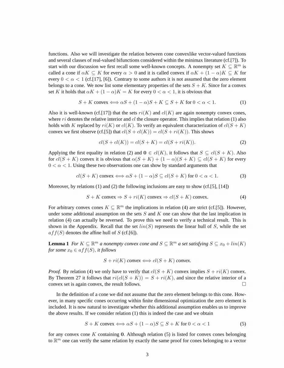
functions. Also we will investigate the relation between cone convexlike vector-valued functionsand several classes of real-valued bifunctions considered within the minimax literature (cf.[7]). Tostart with our discussion we first recall some well-known concepts. A nonempty setK ⊆ Rm iscalled a cone ifαK ⊆ K for everyα > 0 and it is called convex ifαK + (1 − α)K ⊆ K forevery0 < α < 1 (cf.[17], [6]). Contrary to some authors it is not assumed that the zero elementbelongs to a cone. We now list some elementary properties of the setsS + K. Since for a convexsetK it holds thatαK + (1− α)K = K for every0 < α < 1, it is obvious that

S + K convex⇐⇒ αS + (1− α)S + K ⊆ S + K for 0 < α < 1. (1)

Also it is well-known (cf.[17]) that the setsri(K) andcl(K) are again nonempty convex cones,whereri denotes the relative interior andcl the closure operator. This implies that relation (1) alsoholds withK replaced byri(K) or cl(K). To verify an equivalent characterization ofcl(S + K)convex we first observe (cf.[5]) thatcl(S + cl(K)) = cl(S + ri(K)). This shows

cl(S + cl(K)) = cl(S + K) = cl(S + ri(K)). (2)

Applying the first equality in relation (2) and0 ∈ cl(K), it follows thatS ⊆ cl(S + K). Alsofor cl(S + K) convex it is obvious thatα(S + K) + (1 − α)(S + K) ⊆ cl(S + K) for every0 < α < 1. Using these two observations one can show by standard arguments that

cl(S + K) convex⇐⇒ αS + (1− α)S ⊆ cl(S + K) for 0 < α < 1. (3)

Moreover, by relations (1) and (2) the following inclusions are easy to show (cf.[5], [14])

S + K convex⇒ S + ri(K) convex⇒ cl(S + K) convex. (4)

For arbitrary convex conesK ⊆ Rm the implications in relation (4) are strict (cf.[5]). However,under some additional assumption on the setsS andK one can show that the last implication inrelation (4) can actually be reversed. To prove this we need to verify a technical result. This isshown in the Appendix. Recall that the setlin(S) represents the linear hull ofS, while the setaff(S) denotes the affine hull ofS (cf.[6]).

Lemma 1 For K ⊆ Rm a nonempty convex cone andS ⊆ Rm a set satisfyingS ⊆ x0 + lin(K)for somex0 ∈ aff(S), it follows

S + ri(K) convex⇐⇒ cl(S + K) convex.

Proof. By relation (4) we only have to verify thatcl(S + K) convex impliesS + ri(K) convex.By Theorem 27 it follows thatri(cl(S + K)) = S + ri(K), and since the relative interior of aconvex set is again convex, the result follows. �

In the definition of a cone we did not assume that the zero element belongs to this cone. How-ever, in many specific cones occurring within finite dimensional optimization the zero element isincluded. It is now natural to investigate whether this additional assumption enables us to improvethe above results. If we consider relation (1) this is indeed the case and we obtain

S + K convex⇐⇒ αS + (1− α)S ⊆ S + K for 0 < α < 1 (5)

for any convex coneK containing0. Although relation (5) is listed for convex cones belongingto Rm one can verify the same relation by exactly the same proof for cones belonging to a vector

3

spaceX. This observation will be useful in verifying relation (11) below. As shown by the follow-ing example the condition0 ∈ K is essential in relation (5). Note thatRm

++ := int(Rm+ ) for any

m ∈ N with int denoting the interior andRm+ the positive orthant ofRm.

Example 2 Consider the convex setS = [0, 2]× {0} ⊆ R2. For this set it follows thatS + R2++

equalsR2++ and for every0 < α < 1 the setαS + (1 − α)S = S is not included inS + R2

++.This shows that the condition0 ∈ K cannot be omitted in relation (5).

If K is a convex cone containing0 one can show the following improvement of relation (4).

Lemma 3 For K ⊆ Rm a convex cone containing0 andS ⊆ Rm it follows

S + K convex⇒ S + cl(K) convex⇒ S + ri(K) convex.

Proof. If S + K is convex and0 ∈ K, it follows by relation (5) thatαS + (1− α)S ⊆ S + K ⊆S + cl(K) for every0 < α < 1. This implies again by relation (5) thatS + cl(K) is convex. IfS+cl(K) is convex, then similarlyαS+(1−α)S ⊆ S+cl(K) and usingcl(K)+ri(K) ⊆ ri(K)we obtain

αS + (1− α)S + ri(K) ⊆ S + cl(K) + ri(K) ⊆ S + ri(K)

for every0 < α < 1. Applying the observation after relation (1) yieldsS + ri(K) is convex. �

The following example shows that in general the first and second implication in Lemma 3 arestrict implications.

Example 4 To show that the first implication of Lemma 3 is strict letK := R2++ ∪ {0} and

S := {(1, 0), (2, 0)}. For these sets it follows thatS + K is not convex andS + cl(K) is convex.To verify that the second implication of Lemma 3 is strict, letK := {(s, t) : t ≥ s ≥ 0} andS := {(s, 0) : s ∈ Q}. For these sets we obtain thatS + ri(K) is convex, whileS + cl(K) is notconvex.

Within the considered chain of implications it is clear that the improvement of Lemma 3 overrelation (4) is given by the intermediate resultS + cl(K) convex. It is now natural to ask whetherS +cl(K) convex also holds without the additional assumption thatK contains0. The first part ofthe following example yields a negative answer. Similarly, one can present a convex coneK notcontaining0 satisfyingS + cl(K) is convex, whileS + K is not convex. This shows in particularfor convex conesK not containing0 that the propertiesS + K convex andS + cl(K) convex arenot related.

Example 5 To show an example of a setS and a convex coneK not containing0 satisfyingS+Kis convex andS + cl(K) is not convex, letK := {(s, t) : t > s > 0} andS := {(s, 0) : s ∈ Q}.Clearly 0 does not belong toK and the setS + K is convex, while the setS + cl(K) is notconvex. To show an example of a setS and a convex coneK not containing0 satisfyingS + Kis not convex andS + cl(K) is convex letK := {(s, 0, 0) : s > 0} ∪ {(s, t, u) : u > 0} andS := {(0, 0, 0), (0, 1, 0)}. It is easy to verify thatK is a convex cone and0 does not belong toK. Since(1, 0, 0) and (1, 1, 0) do belong toS + K but (1, 1

2 , 0) does not, the setS + K is notconvex. The setcl(K) is now given by{(s, u, t) : u ≥ 0} and soS + cl(K) = cl(K) showing thatS + cl(K) is convex.

4

We will now apply the above elementary results for setsS + K to the different classes of coneconvexlike vector-valued functions discussed in the literature (for a survey see [5]). Recall for anonempty proper convex coneK that the transitive orderingy ≤K x is defined byx − y ∈ K.Note that this ordering is a partial ordering (cf.[19]) if the coneK is pointed, i.eK ∩−K = {0}.The epigraph epiK(F ) of a vector-valued functionF : D → Rm, whereD is a subset of a vectorspaceX, with respect to this ordering is given by

epiK(F ) := {(x, r) : x ∈ D, F (x) ≤K r} ⊆ D × Rm.

To list some useful relations we introduce the functionF0 : D → D × Rm given byF0(x) :=(x, F (x)) and associate with the convex coneK ⊆ Rm the convex coneK0 := {0X} × K ⊆X × Rm with 0X denoting the zero element of the vector spaceX. It is easy to see that

epiK(F ) = F0(D) + K0, (6)

with G(D) := {G(x) : x ∈ D} the range of a vector-valued functionG. Moreover, for theprojectionA : D × Rm → Rm given byA(x, r) = r it follows that

A(epiK(F )) = F (D) + K. (7)

The next definition introduces some classes of cone convexlike vector-valued functions used withinthe literature (see for example [5] or [14]).

Definition 6 LetK ⊆ Rm be a nonempty convex cone. The vector-valued functionF : D → Rm

is calledK-convex if the set epiK(F ) is convex. It is calledK-convexlike, respectively closelyK-convexlike, if the setF (D) + K, respectivelycl(F (D) + K) is convex.

For each of the above function classes it is easy to show that they are closed under additionand multiplication with a positive scalar. This means that each class of functions is a convex coneitself. In the literature ari(K)-convexlike function is also calledK-subconvexlike (cf.[10], [5],[1]). To show the implications of the results derived for the setsS +K with K a nonempty convexcone we first consider the class ofK-convex functions. Since for any convex coneK ⊆ Rm it iswell-known thatri(K0) = ri({0X} × K) = {0X} × ri(K) andri(K) is a nonempty convexcone, we obtain by relation (6) and the first implication in relation (4) that

F is K-convex⇒ F is ri(K)-convex. (8)

In the next example it is shown that the set ofK-convex functions is strictly included in the set ofri(K)-convex functions.

Example 7 LetK = R2++ ∪ {0} and consider the vector-valued functionF : R2 → R2 given by

F (x) :={

(0, 0) for x ∈ R× R+

(1, 0) otherwise.

It is clear that epiri(K)(F ) = R2 × R2+ and soF is ri(K)-convex. Suppose now thatF is also

K-convex and consider the vectors(xi, ri) ∈ R4, i = 1, 2 with x1 := (1, 4), x2 := (1,−2),r1 := (0, 0) andr2 = (1, 0). Since0 belongs toK we obtain that both vectors belong to epiK(F )and this implies by the convexity of epiK(F ) that

2−1(x1, r1) + 2−1(x2, r2) = (1, 1, 2−1, 0) ∈ epiK(F ). (9)

By relation (9) it follows that(2−1, 0) ∈ K + F (1, 1) = K and we obtain a contradiction. HenceF is notK-convex.

5

In Example 7 the coneK is not closed. However, forK closed one can give an improvementof relation (8). As shown by the next theorem the sets ofri(K)-convex andK-convex functionscoincide forK a closed convex cone.

Theorem 8 For F : D → Rm a vector-valued function andK ⊆ Rm a closed convex cone itfollows that

F is K-convex⇐⇒ F is ri(K)-convex.

Proof. By relation (8) we have to verify that anyri(K)-convex function is alsoK-convex. Supposethe vector-valued functionF is ri(K)-convex and consider some(xi, ri) ∈ epiK(F ), i = 1, 2.This implies by definition thatri − F (xi) ∈ K and for a fixedk0 ∈ ri(K) and arbitraryn ∈ Nwe obtain

ri + n−1k0 − F (xi) ∈ cl(K) + n−1k0 ⊆ ri(K).

This shows that the vector(xi, ri + n−1k0), i = 1, 2 belongs to epiri(K)(F ) and since epiri(K)(F )is convex it follows for every0 < α < 1 thatαx1 + (1− α)x2 ∈ D and

αr1 + (1− α)r2 + n−1k0 − F (αx1 + (1− α)x2) ∈ ri(K). (10)

Lettingn ↑ ∞ in relation (10) we obtain

αr1 + (1− α)r2 + n−1k0 − F (αx1 + (1− α)x2) ∈ cl(ri(K)).

This shows usingcl(ri(K)) = cl(K) = K andαx1 + (1 − α)x2 ∈ D that the set epiK(F ) isconvex. �

As already observed, it is mostly assumed in the literature (see for example [2]) that the convexconeK contains0. If this additional condition holds another equivalent definition of aK-convexfunction can be given. This definition is frequently encountered within the literature (see forexample [2]) and resembles the classical definition of a convex function. Applying relation (5)and (6) yields

F is K-convex⇐⇒ D is convex andF (αx1 + (1− α)x2) ≤K αF (x1) + (1− α)F (x2) (11)

for any convex coneK containing0. Next we discuss convexlike functions with respect toK. Weobserve by relation (1) that

F is K-convexlike⇐⇒ αF (D) + (1− α)F (D) + K ⊆ F (D) + K (12)

for every0 < α < 1. If additionally the zero element belongs toK it follows by relation (5) that

F is K-convexlike⇐⇒ αF (D) + (1− α)F (D) ⊆ F (D) + K (13)

for every0 < α < 1. Similarly by the observation after relation (1) we obtain

F is ri(K)-convexlike⇐⇒ F (D) + (1− α)F (D) + ri(K) ⊆ F (D) + ri(K) (14)

for every0 < α < 1 and by relation (3) that

F is closelyK-convexlike⇐⇒ αF (D) + (1− α)F (D) ⊆ cl(F (D) + K) (15)

6

for every0 < α < 1. Finally we obtain by relations (4) and (7) that the following implicationshold (cv denotes an abbreviation for convex and the symbols stand for the whole class of functionshaving the corresponding property)

K-cv⊆ K-cvlike⊆ ri(K)-cvlike⊆ closelyK-cvlike.

It can be shown (cf.[5]) that the above inclusions are strict. Finally, we mention forK ⊆ Rm andF : D → Rm satisfyingF (D) ⊆ x0 + lin(K) for somex0 ∈ aff(F (D)) (sufficient condition:K has a nonempty interior) that by Theorem 27

F is ri(K)-convexlike⇐⇒ F is closelyK-convexlike. (16)

Using the above relations and duality results for convex cones one can translate some of the aboveproperties of vector-valued functions to real-valued bifunctions. The first duality result needed forthis translation is the well-known bipolar theoremcl(K) = K∗∗ with K∗ := {λ ∈ Rm : λ>x ≥ 0for everyx ∈ K} the dual cone ofK andK∗∗ := (K∗)∗. Also we need a refinement of the bipolartheorem for relatively open convex cones given by (cf.[20])

x ∈ ri(K) ⇐⇒ x ∈ lin(K) andλ>x > 0 for λ ∈ K∗\K⊥ (17)

with K⊥ := {λ ∈ Rm : λ>x = 0 for everyx ∈ K} denoting the orthogonal complement ofK. To give an equivalent characterization of relatively open convex cones, which can be applieddirectly within the proof of the next theorems, we observe usinglin(K) = (K⊥)⊥ (cf.[6]) thatlin(K) ∩K⊥ = {0}. This shows

(K∗ ∩ lin(K))\{0} ⊆ K∗\K⊥. (18)

Moreover, by the orthogonal projection theorem (cf.[11]) it follows for everyλ ∈ Rm andx ∈lin(K) thatλ>x = λ>1 x with λ1 ∈ lin(K) denoting the orthogonal projection ofλ onto the linearsubspacelin(K). Using these observations it follows forx ∈ lin(K) that

λ>x > 0 for λ ∈ K∗\K⊥ ⇐⇒ λ>x > 0 for λ ∈ (K∗ ∩ lin(K))\{0}. (19)

Hence by relations (17), (18) and (19) an equivalent dual characterization of relatively open convexcones is given by

x ∈ ri(K) ⇐⇒ x ∈ lin(K) andλ>x > 0 for λ ∈ (K∗ ∩ lin(K))\{0}. (20)

In the next definition we introduce a class of functions well-known within the minimax literature(cf.[3], [7]).

Definition 9 The bifunctionf : K∗ × D → R is called convex onD if the setD is convex, andfor everyx1, x2 ∈ D and0 < α < 1 it follows that

f(λ, αx1 + (1− α)x2) ≤ αf(λ, x1) + (1− α)f(λ, x2)

for everyλ ∈ K∗. The bifunctionf : K∗ × D → R is called Ky-Fan convex onD if for everyx1, x2 ∈ D and0 < α < 1 there exists somex0 ∈ D satisfying

f(λ, x0) ≤ αf(λ, x1) + (1− α)f(λ, x2)

for everyλ ∈ K∗.

7

The next result is well-known and a direct consequence of the bipolar theorem and relations(13) and (6) (see for example [2] or [5]). In Theorems 10, 12 and 14 below the bifunctionf :K∗ ×D → R has the special form

f(λ, x) = λ>F (x) (21)

with F : D → Rm some vector-valued function.

Theorem 10 For K ⊆ Rm a nonempty convex cone it follows that the vector-valued functionF : D → Rm is cl(K)-convex onD if and only if the functionf : K∗ ×D → R defined in (21) isconvex onD. Moreover, the vector-valued functionF : D → Rm is cl(K)-convexlike if and onlyif the functionf : K∗ ×D → R defined in (21) is Ky-Fan convex onD.

By Theorem 8 we know thatF is cl(K)-convex if and only ifF is ri(K)-convex and thisshows that the dual representation forcl(K)-convex functions in Theorem 10 also holds forri(K)-convex functions. Unfortunately, since for arbitrary convex conesK ⊆ Rm it is not possible togive a dual characterization ofK, it seems difficult to give a dual representation of aK-convexfunction. A similar observation also holds forK-convexlike functions. On the other hand, since inrelation (17) a dual representation for relatively open convex cones is given, it is possible to givea dual representation for ari(K)-convexlike and a closelyK-convexlike function. To define theproper class of bifunctions forri(K)-convexlike functions we introduce the following definition.

Definition 11 The bifunctionf : K∗×D →R belongs to the classA if for everyε > 0, 0 < α < 1andx1, x2 ∈ D there exists somex0 ∈ D such that

f(λ, x0) ≤ αf(λ, x1) + (1− α)f(λ, x2) + ε‖λ‖

for everyλ ∈ P1 andf(λ, x0) = αf(λ, x1) + (1− α)f(λ, x2)

for everyλ ∈ P2 with the setsP1, P2 a partition ofK∗.

In the next theorem we derive a dual characterization of ari(K)-convexlike function. Notethat the setB denotes the closed Euclidean unit ball inRm and so its boundary∂B is given by∂B = {λ : ‖λ‖ = 1}.

Theorem 12 For K ⊆ Rm a nonempty convex cone it follows thatF : D → Rm is ri(K)-convexlike if and only if the functionf : K∗ ×D → R defined in (21) belongs to the setA withP1 = K∗\K⊥ andP2 = K⊥.

Proof. Let F be ari(K)-convexlike function and consider some arbitraryε > 0, 0 < α < 1 andx1, x2 ∈ D. Since the setri(K) is a nonempty cone one can find somek0 ∈ ri(K) ∩ εB. Thisimplies by relation (14) that there exists somex0 ∈ D satisfying

αF (x1) + (1− α)F (x2)− F (x0) + k0 ∈ ri(K). (22)

Applying the dual representation ofri(K) given by (17), the Cauchy-Schwarz inequality and‖ k0 ‖≤ ε we obtain

αF (x1) + (1− α)F (x2)− F (x0) + k0 ∈ lin(K) (23)

8

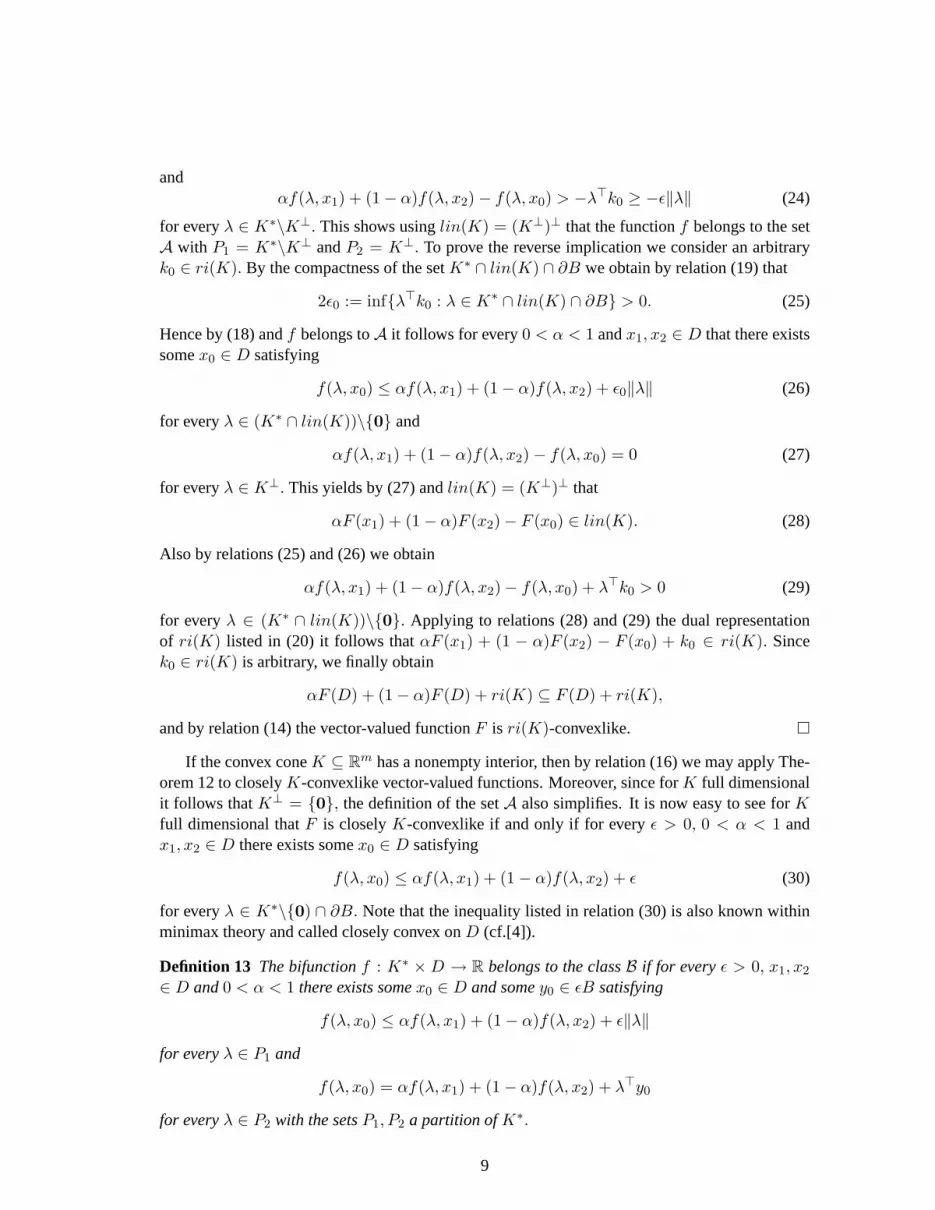
andαf(λ, x1) + (1− α)f(λ, x2)− f(λ, x0) > −λ>k0 ≥ −ε‖λ‖ (24)

for everyλ ∈ K∗\K⊥. This shows usinglin(K) = (K⊥)⊥ that the functionf belongs to the setA with P1 = K∗\K⊥ andP2 = K⊥. To prove the reverse implication we consider an arbitraryk0 ∈ ri(K). By the compactness of the setK∗ ∩ lin(K) ∩ ∂B we obtain by relation (19) that

2ε0 := inf{λ>k0 : λ ∈ K∗ ∩ lin(K) ∩ ∂B} > 0. (25)

Hence by (18) andf belongs toA it follows for every0 < α < 1 andx1, x2 ∈ D that there existssomex0 ∈ D satisfying

f(λ, x0) ≤ αf(λ, x1) + (1− α)f(λ, x2) + ε0‖λ‖ (26)

for everyλ ∈ (K∗ ∩ lin(K))\{0} and

αf(λ, x1) + (1− α)f(λ, x2)− f(λ, x0) = 0 (27)

for everyλ ∈ K⊥. This yields by (27) andlin(K) = (K⊥)⊥ that

αF (x1) + (1− α)F (x2)− F (x0) ∈ lin(K). (28)

Also by relations (25) and (26) we obtain

αf(λ, x1) + (1− α)f(λ, x2)− f(λ, x0) + λ>k0 > 0 (29)

for everyλ ∈ (K∗ ∩ lin(K))\{0}. Applying to relations (28) and (29) the dual representationof ri(K) listed in (20) it follows thatαF (x1) + (1 − α)F (x2) − F (x0) + k0 ∈ ri(K). Sincek0 ∈ ri(K) is arbitrary, we finally obtain

αF (D) + (1− α)F (D) + ri(K) ⊆ F (D) + ri(K),

and by relation (14) the vector-valued functionF is ri(K)-convexlike. �

If the convex coneK ⊆ Rm has a nonempty interior, then by relation (16) we may apply The-orem 12 to closelyK-convexlike vector-valued functions. Moreover, since forK full dimensionalit follows thatK⊥ = {0}, the definition of the setA also simplifies. It is now easy to see forKfull dimensional thatF is closelyK-convexlike if and only if for everyε > 0, 0 < α < 1 andx1, x2 ∈ D there exists somex0 ∈ D satisfying

f(λ, x0) ≤ αf(λ, x1) + (1− α)f(λ, x2) + ε (30)

for everyλ ∈ K∗\{0) ∩ ∂B. Note that the inequality listed in relation (30) is also known withinminimax theory and called closely convex onD (cf.[4]).

Definition 13 The bifunctionf : K∗ ×D → R belongs to the classB if for everyε > 0, x1, x2

∈ D and0 < α < 1 there exists somex0 ∈ D and somey0 ∈ εB satisfying

f(λ, x0) ≤ αf(λ, x1) + (1− α)f(λ, x2) + ε‖λ‖

for everyλ ∈ P1 and

f(λ, x0) = αf(λ, x1) + (1− α)f(λ, x2) + λ>y0

for everyλ ∈ P2 with the setsP1, P2 a partition ofK∗.

9

By Theorem 12 and relation (16) the next result is only useful for a convex coneK and avector-valued functionF not satisfyingF (D) ⊆ x0 + lin(K) for somex0 ∈ aff(F (D)).

Theorem 14 For K ⊆ Rm a nonempty convex cone it follows thatF : D → Rm is closelyK-convexlike if and only if the functionf : K∗ ×D → R defined in (21) belongs to the setB withP1 = K∗\K⊥ andP2 = K⊥.

Proof. Let F be closelyK-convexlike and consider some arbitraryε > 0, 0 < α < 1 andx1, x2 ∈ D. By relation (15) andcl(F (D) + K) ⊆ F (D) + K + εB it follows that there existssomex0 ∈ D, k0 ∈ K and−y0 ∈ εB satisfying

αF (x1) + (1− α)F (x2) = F (x0) + k0 − y0. (31)

This implies for everyλ ∈ K⊥ that

λ>F (x0) = αλ>F (x1) + (1− α)λ>F (x2) + λ>y0, (32)

while for everyλ ∈ K∗\K⊥ and the Cauchy-Schwartz inequality we obtain

λ>F (x0) ≤ αλ>F (x1) + (1− α)λ>F (x2) + ε‖λ‖. (33)

Hence by (32) and (33) the functionf belongs to the setB with P1 = K∗\K⊥ andP2 = K⊥. Toprove the reverse implication it follows by (18) andf belongs toB that for everyε > 0, 0 < α < 1andx1, x2 ∈ D there exists somex0 ∈ D andy0 ∈ εB satisfying

f(λ, x0)− αf(λ, x1)− (1− α)f(λ, x2) ≤ ε (34)

for everyλ ∈ K∗ ∩ lin(K) ∩ ∂B and

f(λ, x0) = αf(λ, x1) + (1− α)f(λ, x2) + λ>y0 (35)

for everyλ ∈ K⊥. If k0 ∈ ri(K) ∩ ∂B is fixed, we obtain by relation (19) that

ε0 := min{λ>k0 : λ ∈ K∗ ∩ lin(K) ∩ ∂B} > 0. (36)

This implies by (34), (36) andy0 ∈ εB that

f(λ, x0)− αf(λ, x1)− (1− α)f(λ, x2)− λ>(y0 + 3εε−10 k0) < 0 (37)

for everyλ ∈ K∗ ∩ lin(K) ∩ ∂B. Since the functionλ 7→ f(λ, x) is linear, it is obvious thatrelation (37) also holds for everyλ ∈ (K∗ ∩ lin(K))\{0}. Also, by (35) andk0 ∈ ri(K) itfollows that

αF (x1) + (1− α)F (x2)− F (x0) + y0 + 3εε−10 k0 ∈ lin(K) + 3εε−1

0 k0 ⊆ lin(K). (38)

Applying to relations (37) and (38) the dual representation ofri(K) listed in (20) yields

αF (x1) + (1− α)F (x2)− F (x0) + y0 + 3εε−10 k0 ∈ ri(K) ⊆ K,

and hence, usingy0 ∈ εB andk0 ∈ ∂B, we obtain

αF (x1) + (1− α)F (x2) ∈ F (D) + K + ε(1 + 3ε0)B.

Sinceε > 0 is arbitrary, we may conclude that

αF (D) + (1− α)F (D) ⊆ cl(F (D) + K),

and by (15) the vector-valued functionF is closelyK-convexlike. �

10

3 Conjugate functions, Lagrangian duality and cone convexlike vec-tor valued functions.

In this section we will discuss conjugate functions, Lagrangian duality and the relation with theabove class of cone convexlike vector-valued functions. In particular, we will first consider thelower semicontinuous hullp of a functionp : Rm → [−∞,∞] and show its relation with thebiconjugate functionp∗∗ if p is convex. After having discussed these relations we will then in-troduce the primal problem(P ) already given in the introduction equipped with the Lagrangianperturbation scheme with perturbation parametery ∈ Rm, and show that the convexity of the as-sociated lower semicontinuous hullp of the (Lagrangian perturbation) value functionp is convexif and only if some vector-valued function is closely convexlike. This enables us to apply thegeneral results identified in the first part of this section and by doing so we derive under certainconditions, strong duality and related results for optimization problem(P ). In our analysis weneed the following elementary result.

Lemma 15 If C ⊆ Rm is convex andS ⊆ C is nonempty, then it follows that

ri(C)) ⊆ S ⇐⇒ ri(C) = ri(S).

Proof. The sufficiency part being trivial we only prove the necessary part. To verify this, letri(C)) ⊆ S. Since the affine operatoraff is monotone,S ⊆ C andaff(ri(C)) = aff(C),we obtainaff(C) = aff(S). This implies usingri(C)) ⊆ S thatri(C) = ri(ri(C)) ⊆ ri(S).SinceS ⊆ C andaff(C) = aff(S) we also haveri(S) ⊆ ri(C), and the result is proved. �

To continue our analysis letp : Rm → [−∞,∞] be an extended real-valued function witheffective domaindom(p) := {x ∈ Rm : p(x) < ∞} nonempty and letp denote the lowersemicontinuous hull of the functionp. It is well-known (cf.[17], [6]) thatepi(p) = cl(epi(p)) withepi(p) := epiR+(p) denoting the epigraph of the functionp and

dom(p) ⊆ dom(p) ⊆ cl(dom(p)). (39)

Applying now relation (39) we immediately obtain

cl(dom(p)) = cl(dom(p)) andaff(dom(p)) = aff(dom(p)). (40)

Also by Lemma 15 and relation (39) it follows fordom(p) convex that

ri(dom(p)) ⊆ dom(p) ⇐⇒ ri(dom(p)) = ri(dom(p)). (41)

If we denote byp∗(λ) := sup{λ>y − p(y) : y ∈ Rm} the conjugate function of the functionpandp∗∗ its biconjugate function the next corollary is an easy consequence of the Fenchel-Moreautheorem and some well-known function description ofp.

Corollary 16 If the lower semicontinuous hullp of a functionp : Rm → [−∞,∞] is convex, thenit follows for everyy0 belonging to dom(p) thatp∗∗(y0) = p(y0) = lim infy→y0 p(y).

Proof. Sincey0 belongs to dom(p) it follows that p(y0) is finite or p(y0) = −∞. If p(y0) isfinite the convex functionp is proper and by the Fenchel Moreau theorem (cf.[17], [6]) we obtainp∗∗(y0) = p(y0). Moreover, ifp(y0) = −∞, it follows by contradiction thatp∗ is identically∞

11

and sop∗∗(y0) ≡ −∞. Hence we obtain in both cases thatp∗∗(y0) = p(y0) and sincep(y0) =lim infy→y0 p(y) (cf.[17], [6]) the result follows. �

Up to now we did not show that the optimization problem associated with the biconjugatefunction p∗∗ has an optimal solution. The next corollary is an immediate consequence of somestandard results in convex analysis.

Corollary 17 If the lower semicontinuous hullp of a functionp : Rm → [−∞,∞] is convex,then it follows for everyy0 belonging to ri(dom(p)) that there exists someλ0 ∈ Rm satisfyingp∗∗(y0) = y>0 λ0 − p∗(λ0) = p(y0) = lim infy→y0 p(y).

Proof. If p(y0) = −∞we knowp∗ ≡ ∞, and the result is obvious. Forp(y0) finite andy0 belongsto ri(dom(p)) the subgradient set∂p(y0) is nonempty (cf.[17], [6]) and

λ ∈ ∂p(y0) ⇐⇒ p∗(λ) = λ>y0 − p(y0). (42)

Applying now Corollary 16,p∗ ≤ p∗and relation (42), it follows forλ0 belonging to∂p(y0) thatp(y0) = p∗∗(y0) ≥ (p∗)∗(y0) ≥ y>0 λ0 − p∗(λ0) = p(y0), and the result is proved. �

To replace in Corollary 17 the valuelim infy→y0 p(y) byp(y0) for y0 belonging tori(dom(p)),it is necessary and sufficient to assume thatp is lower semicontinuous iny0, or equivalentlyp(y0) = p(y0). To achieve this, we introduce the following class of functions.

Definition 18 A functionp : Rm → [−∞,∞] is called almost convex if the lower semicontinuoushull p of p is convex andri(epi(p)) is a subset ofepi(p).

In the next result we give an equivalent description of an almost convex function.

Theorem 19 For any functionp : Rm → [−∞,∞] with dom(p) nonempty, it follows that

p almost convex⇐⇒ p convex andp(y) = p(y) for everyy ∈ ri(dom(p)).

Proof. If p is an almost convex function withdom(p) nonempty, we only need to show thatp(y) = p(y) for everyy ∈ ri(dom(p)). By relation (39) the set dom(p) is also nonempty. Since itis well-known (cf.[17], [6]) that

ri(epi(p)) = {(y, r) : p(y) < r, y ∈ ri(dom(p)} (43)

and by assumptionri(epi(p)) ⊆ epi(p), it follows for everyy ∈ ri(dom(p)) and ε > 0 that(y, p(y) + ε) belongs toepi(p). This impliesp(y) ≥ p(y) for everyy ∈ ri(dom(p)) and hencep equalsp on ri(dom(p)). To prove the reverse implication, letp convex andp(y) = p(y) forevery y ∈ ri(dom(p)). This impliesri(dom(p)) ⊆ dom(p) and by relation (41) we obtainri(dom(p)) = ri(dom(p)). Hence by the representation of the relative interior of the epigraphof a convex function (see relation (43)) and the previous observations it follows that

ri(epi(p)) = {(y, r) : p(y) < r, y ∈ ri(dom(p)} ⊆ epi(p),

and sop is almost convex. �

As shown in the above proof it follows forp almost convex withdom(p) nonempty that

ri(dom(p)) = ri(dom(p)), (44)

and these sets are nonempty. The next result is an immediate consequence of Corollary 17, Theo-rem 19 and relation (44).

12

Corollary 20 If the functionp : Rm → [−∞,∞] is almost convex withdom(p) nonempty, then itfollows for everyy0 belonging tori(dom(p)) that there exists someλ0 ∈ Rm satisfyingp∗∗(y0) =y>0 λ0 − p∗(λ0) = p(y0).

To see what happens forp almost convex ify0 does not belong tori(dom(p)), but to therelative boundaryrbd(dom(p)) given by

rbd(dom(p)) := cl(dom(p))\ri(dom(p)),

we first need the following observation. By relations (40) and (44) we obtain forp almost convexanddom(p) nonempty that

y0 + t(y1 − y0) ∈ ri(dom(p)) (45)

for everyy0 ∈ cl(dom(p)), y1 ∈ ri(dom(p)) and0 < t < 1. It is now possible to show thefollowing result for an almost convex functionp with nonempty effective domain using somestandard results from convex analysis, Theorem 19 and relation (45).

Corollary 21 If the functionp : Rm → [−∞,∞] is almost convex withdom(p) nonempty, thenit follows for everyy0 belonging torbd(dom(p)) andy1 belonging tori(dom(p)) thatp∗∗(y0) =limt↓0 p(y0 + t(y1 − y0)).

Proof. Sincedom(p) is nonempty it follows by the observation after relation (44) thatri(dom(p))is nonempty. If for everyy ∈ ri(dom(p)) it holds thatp(y) = −∞, we obtain thatp∗∗(y0) = −∞.This implies by relation (45) the desired result and so we still need to prove the result if there existssomey ∈ ri(dom(p)) with p(y) finite. This implies by Theorem 19 thatp(y) = p(y) is finite andhencep is a proper convex function. Applying now the Fenchel-Moreau theorem yieldsp∗∗ = pand this shows thatp∗∗ is a lower semicontinuous proper convex function. Sincep∗∗ = p, it alsofollows using relation (44) that

ri(dom(p∗∗)) = ri(dom(p)) = ri(dom(p)) (46)

and this implies (cf.[17], [6]) for everyy1 ∈ ri(dom(p)) andy0 ∈ rbd(dom(p)) that

p∗∗(y0) = limt↓0 p∗∗(y0 + t(y1 − y0)). (47)

By relation (45) and Corollary 20 we obtain

p∗∗(y0 + t(y1 − y0)) = p(y0 + t(y1 − y0)) (48)

for every0 < t < 1 and by relations (47) and (48) the desired result follows. �

In what follows we will apply the previous results to the Lagrangian perturbation scheme ofthe optimization problem(P ). Consider the value functionp : Rm → [−∞,∞] given by

p(y) := inf{f(x) : F (x) ≤K y, x ∈ D}. (49)

Clearly for y = 0 we recover our initial optimization problem(P ) and it is easy to see thatdom(p) = F (D) + K. Since we always assume that the feasible regionF is nonempty, or equiv-alently0 ∈ F (D) + K we obtain0 ∈ dom(p). Introducing for the perturbed problem the feasibleregionF(y) given by

F(y) := {x : F (x) ∈ −K + y, x ∈ D},

13

it is follows by definition forF(y) empty thatp(y) = ∞. If the vector-valued functionH : D −→Rm+1 is given by

H(x) = (F (x), f(x)), (50)

then the next result is easy to show.

Theorem 22 It follows that the functionp is convex if and only if the functionH is closelyK ×R+-convexlike. Moreover, the functionp is convex if and only the functionH is K× int(R+)-convexlike.

Proof. If epis(p) :=epiint(R+)(p) denotes the strict epigraph ofp, then it is easy to verify that

epi(p) = cl(epi(p)) = cl(epis(p)). (51)

By relation (49) we obtain

epis(p) = {(y, r) : ∃x∈D y ∈ F (x) + K andf(x) < r} = H(D) + (K × int(R+)), (52)

and this shows by relations (51) thatepi(p) = cl(H(D) + (K × R+)). To verify the second part,it follows by Theorem 8 thatepi(p) is convex if and only ifepis(p) is convex. Applying relation(52) yields the desired result. �

The next result is well-known and can be easily verified.

Lemma 23 If the functionθ : K∗ → [−∞,∞) is the Lagrangian function

θ(λ) := inf{f(x) + λ>F (x) : x ∈ D},

then it follows withp given by relation (49) that

−p∗(−λ) ={

θ(λ) λ ∈ K∗

−∞ otherwise.

By Lemma 23 we obtain thatp∗∗(y) = sup{−λ>y + θ(λ) : λ ∈ K∗}. This yields fory = 0that

p∗∗(0) = sup{θ(λ) : λ ∈ K∗} = v(D). (53)

As already observed in the introduction, the above problem is called the Lagrangian dual problem(D). We are now ready to prove the following main results for the primal optimization problem(P ) and its Lagrangian dual problem.

Theorem 24 If 0 belongs toF (D) + K and the vector-valued functionH : D → Rm+1, listed inrelation (50), is closelyK × R+-convexlike, then it follows that

v(D) = lim infy→0 p(y) (54)

with p given by relation (49). Also the functionp is lower semicontinuous at0 if and only ifv(D) = p(0). Finally, if 0 belongs tori(F (D) + K), then it follows that the dual problem (D)has an optimal solution.

14

Proof. By Theorem 22 we know that the vector-valued functionH is closelyK × R+-convexlikeif and only if the functionp is convex. Moreover, by relations (39) anddom(p) = F (D) + K itfollows that

0 ∈ F (D) + K ⊆ dom(p). (55)

This yields by Corollary 16 thatv(D) = p∗∗(0) = lim infy→0 p(y). Also it holds thatlim infy→0 p(y) = p(0) if and only if p is lower semicontinuous at0 and using this in combinationwith the first part, the second part follows. To verify the last part, we observe by relation (39) andthe observation after this relation that0 belongs tori(F (D) + K) = ri(dom(p)) ⊆ ri(dom(p)).This implies by Corollary 17 and relation (53) that the dual problem has an optimal solution.�

Discussing a more general parametric optimization problem, in [15] a geometrical interpreta-tion is given forp lower semicontinuous at0. In case we impose the additional regularity condition

ri(cl(H(D) + (K × R+))) ⊆ H(D) + (K × R+), (56)

then the following improvement of Theorem 24 can be verified. It will be shown that this additionalcondition is always satisfied if the vector-valued functionH is ri(K)× int(R+)-convexlike.

Theorem 25 If 0 belongs toF (D)+K and the vector-valued functionH : D → Rm+1 is closelyK ×R+-convexlike and satisfies relation (56), then it follows thatv(D) = limt↓0 p(ty1) for everyy1 belongingri(F (D)+K). If 0 belongs tori(F (D)+K), then the dual problem has an optimalsolution andv(D) = p(0).

Proof. By relation (56) and Theorem 22 we obtain that the functionp is almost convex. Hence theresult follows from Corollaries 20 and 21. �

By Theorem2.2 of [5] it follows for any nonempty convex coneK that

cl(H(D) + (K × R+)) = cl(H(D) + (ri(K)× int(R+))). (57)

This shows forH : D → Rm+1 a ri(K)× int(R+)-convexlike vector-valued function that

ri(cl(H(D) + (K × R+))) = ri(cl(H(D) + (ri(K)× int(R+)))= ri(H(D) + (ri(K)× int(R+))).

Hence forH a ri(K) × int(R+)-convexlike vector-valued function we obtain that the regularitycondition given by relation (56) automatically holds. Finally we like to observe that the secondpart of Theorem 25 is also verified in [5] by means of the image space approach of Giannessi andin the same paper it is shown that the condition of Theorem 25 is still weaker than the assumptionthatH is ri(K)× int(R+)-convexlike.

4 Appendix

In this appendix we show a technical result needed in Section1. To show this result we first needthe following lemma.

Lemma 26 For S ⊆ Rm andK ⊆ Rm a nonempty convex cone it follows that there exists somex0 ∈ aff(S) satisfyingS ⊆ x0 + lin(K) if and only if for everyx ∈ aff(S + K) it holds thataff(S + K) = x + lin(K).

15

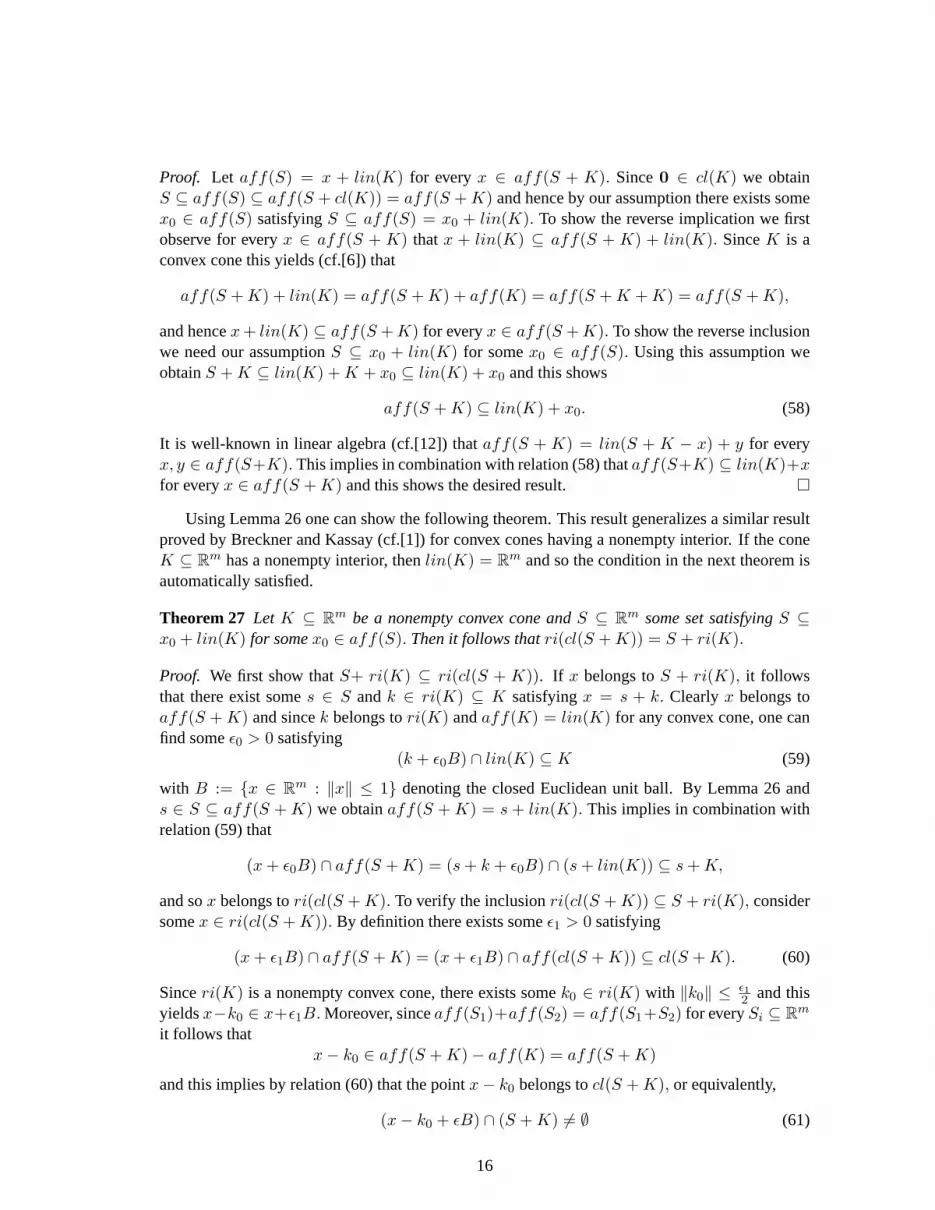
Proof. Let aff(S) = x + lin(K) for everyx ∈ aff(S + K). Since0 ∈ cl(K) we obtainS ⊆ aff(S) ⊆ aff(S + cl(K)) = aff(S + K) and hence by our assumption there exists somex0 ∈ aff(S) satisfyingS ⊆ aff(S) = x0 + lin(K). To show the reverse implication we firstobserve for everyx ∈ aff(S + K) that x + lin(K) ⊆ aff(S + K) + lin(K). SinceK is aconvex cone this yields (cf.[6]) that

aff(S + K) + lin(K) = aff(S + K) + aff(K) = aff(S + K + K) = aff(S + K),

and hencex + lin(K) ⊆ aff(S + K) for everyx ∈ aff(S + K). To show the reverse inclusionwe need our assumptionS ⊆ x0 + lin(K) for somex0 ∈ aff(S). Using this assumption weobtainS + K ⊆ lin(K) + K + x0 ⊆ lin(K) + x0 and this shows

aff(S + K) ⊆ lin(K) + x0. (58)

It is well-known in linear algebra (cf.[12]) thataff(S + K) = lin(S + K − x) + y for everyx, y ∈ aff(S+K). This implies in combination with relation (58) thataff(S+K) ⊆ lin(K)+xfor everyx ∈ aff(S + K) and this shows the desired result. �

Using Lemma 26 one can show the following theorem. This result generalizes a similar resultproved by Breckner and Kassay (cf.[1]) for convex cones having a nonempty interior. If the coneK ⊆ Rm has a nonempty interior, thenlin(K) = Rm and so the condition in the next theorem isautomatically satisfied.

Theorem 27 Let K ⊆ Rm be a nonempty convex cone andS ⊆ Rm some set satisfyingS ⊆x0 + lin(K) for somex0 ∈ aff(S). Then it follows thatri(cl(S + K)) = S + ri(K).

Proof. We first show thatS+ ri(K) ⊆ ri(cl(S + K)). If x belongs toS + ri(K), it followsthat there exist somes ∈ S andk ∈ ri(K) ⊆ K satisfyingx = s + k. Clearly x belongs toaff(S + K) and sincek belongs tori(K) andaff(K) = lin(K) for any convex cone, one canfind someε0 > 0 satisfying

(k + ε0B) ∩ lin(K) ⊆ K (59)

with B := {x ∈ Rm : ‖x‖ ≤ 1} denoting the closed Euclidean unit ball. By Lemma 26 ands ∈ S ⊆ aff(S + K) we obtainaff(S + K) = s + lin(K). This implies in combination withrelation (59) that

(x + ε0B) ∩ aff(S + K) = (s + k + ε0B) ∩ (s + lin(K)) ⊆ s + K,

and sox belongs tori(cl(S + K). To verify the inclusionri(cl(S + K)) ⊆ S + ri(K), considersomex ∈ ri(cl(S + K)). By definition there exists someε1 > 0 satisfying

(x + ε1B) ∩ aff(S + K) = (x + ε1B) ∩ aff(cl(S + K)) ⊆ cl(S + K). (60)

Sinceri(K) is a nonempty convex cone, there exists somek0 ∈ ri(K) with ‖k0‖ ≤ ε12 and this

yieldsx−k0 ∈ x+ε1B. Moreover, sinceaff(S1)+aff(S2) = aff(S1+S2) for everySi ⊆ Rm

it follows thatx− k0 ∈ aff(S + K)− aff(K) = aff(S + K)

and this implies by relation (60) that the pointx− k0 belongs tocl(S + K), or equivalently,

(x− k0 + εB) ∩ (S + K) 6= ∅ (61)

16

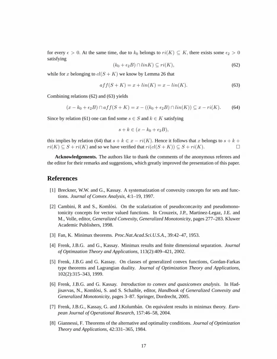
for everyε > 0. At the same time, due tok0 belongs tori(K) ⊆ K, there exists someε2 > 0satisfying

(k0 + ε2B) ∩ linK) ⊆ ri(K), (62)

while for x belonging tocl(S + K) we know by Lemma 26 that

aff(S + K) = x + lin(K) = x− lin(K). (63)

Combining relations (62) and (63) yields

(x− k0 + ε2B) ∩ aff(S + K) = x− ((k0 + ε2B) ∩ lin(K)) ⊆ x− ri(K). (64)

Since by relation (61) one can find somes ∈ S andk ∈ K satisfying

s + k ∈ (x− k0 + ε2B),

this implies by relation (64) thats + k ∈ x − ri(K). Hence it follows thatx belongs tos + k +ri(K) ⊆ S + ri(K) and so we have verified thatri(cl(S + K)) ⊆ S + ri(K). �

Acknowledgements.The authors like to thank the comments of the anonymous referees andthe editor for their remarks and suggestions, which greatly improved the presentation of this paper.

References

[1] Breckner, W.W. and G., Kassay. A systematization of convexity concepts for sets and func-tions. Journal of Convex Analysis, 4:1–19, 1997.

[2] Cambini, R and S., Komlosi. On the scalarization of pseudoconcavity and pseudomono-tonicity concepts for vector valued functions. In Crouzeix, J.P., Martinez-Legaz, J.E. andM., Volle, editor,Generalized Convexity, Generalized Monotonicity, pages 277–283. KluwerAcademic Publishers, 1998.

[3] Fan, K. Minimax theorems.Proc.Nat.Acad.Sci.U.S.A., 39:42–47, 1953.

[4] Frenk, J.B.G. and G., Kassay. Minimax results and finite dimensional separation.Journalof Optimzation Theory and Applications, 113(2):409–421, 2002.

[5] Frenk, J.B.G and G. Kassay. On classes of generalized convex functions, Gordan-Farkastype theorems and Lagrangian duality.Journal of Optimization Theory and Applications,102(2):315–343, 1999.

[6] Frenk, J.B.G. and G. Kassay.Introduction to convex and quasiconvex analysis. In Had-jisavvas, N., Komlosi, S. and S. Schaible, editor,Handbook of Generalized Convexity andGeneralized Monotonicity, pages 3–87. Springer, Dordrecht, 2005.

[7] Frenk, J.B.G., Kassay, G. and J.Kolumban. On equivalent results in minimax theory.Euro-pean Journal of Operational Research, 157:46–58, 2004.

[8] Giannessi, F. Theorems of the alternative and optimality conditions.Journal of OptimizationTheory and Applications, 42:331–365, 1984.

17

[9] Hayashi, M. and H., Komiya. Perfect duality for convexlike programs.Journal of Optimiza-tion Theory and Applications, 38:179–189, 1982.

[10] Jeyakumar, V. A generalization of a minimax theorem of Fan via a theorem of the alternative.Journal of Optimization Theory and Applications, 48:525–533, 1986.

[11] Kreyszig, E.Introductory Functional Analysis with Applications. Wiley, New York, 1978.

[12] Lancaster, P. and M., Tismenetsky.The Theory of Matrices (second edition). AcademicPress, New York, 1985.

[13] Li, Z.P. and S.Y., Wang. Lagrange multipliers and saddlepoints in multiobjective program-ming. Journal of Optimization Theory and Applications, 83, 1994.

[14] Mastroeni, G. and T., Rapcsak. On convex generalized systems.Journal of OptimizationTheory and Applications, 104(2):605–627, 2000.

[15] Mastroeni, G., Pappalardo, M. and N.D., Yen. Image of a parametric optimization problemand continuity of the perturbation function.Journal of Optimization Theory and Applica-tions, 81:193–202, 1994.

[16] Paeck, S. Convexlike and concavelike conditions in alternative, minmax and minimizationtheorems.Journal of Optimization Theory and Applications, 74:317–332, 1992.

[17] Rockafellar, R.T.Convex Analysis. Princeton University Press, Princeton, 1970.

[18] Rockafellar, R.T.Conjugate duality and optimization. SIAM, Philadelphia, 1974.

[19] Rudin, W.Functional Analysis. McGraw-Hill, New York, 1991.

[20] Sturm, J.F. Theory and algorithms of semidefinite programming. In Hans Frenk, KeesRoos, Tamas Terlaky and Shuzhong Zhang, editor,High Performance Optimization, vol-ume 33 ofApplied Optimization, pages 3–194, Dordrecht, 2000. Kluwer Academic Publish-ers.

[21] Yu, P.L. Cone extreme points and nondominated solutions in decision problems with multi-objectives.Journal of Optimization Theory and Applications, 14(3):319–377, 1974.

18

Publications in the Report Series Research∗ in Management ERIM Research Program: “Business Processes, Logistics and Information Systems” 2005 On The Design Of Artificial Stock Markets Katalin Boer, Arie De Bruin And Uzay Kaymak ERS-2005-001-LIS http://hdl.handle.net/1765/1882 Knowledge sharing in an Emerging Network of Practice: The Role of a Knowledge Portal Peter van Baalen, Jacqueline Bloemhof-Ruwaard, Eric van Heck ERS-2005-003-LIS A note on the paper Fractional Programming with convex quadratic forms and functions by H.P.Benson J.B.G.Frenk ERS-2005-004-LIS A note on the dual of an unconstrained (generalized) geometric programming problem J.B.G.Frenk and G.J.Still ERS-2005-006-LIS A Modular Agent-Based Environment for Studying Stock Markets Katalin Boer, Uzay Kaymak and Arie de Bruin ERS-2005-17-LIS Keywords Lagrangian duality, cone convexlike functions J.B.G. Frenk and G. Kassay ERS-2005-019-LIS

∗ A complete overview of the ERIM Report Series Research in Management:

https://ep.eur.nl/handle/1765/1 ERIM Research Programs: LIS Business Processes, Logistics and Information Systems ORG Organizing for Performance MKT Marketing F&A Finance and Accounting STR Strategy and Entrepreneurship