Embed Size (px)
Citation preview
Chapter 3
Duality
In the development of the linear programming theory, duality plays an importantrole both theoretically and in practice. Every linear problem has another linearproblem associated, which is called “the dual”. As we will see, when we solvea linear problem, we are simultaneously solving its dual; in fact, the two optimalsolutions are present in the optimal simplex tableau.
These are some of the reasons why it is important to take duality into account:
1. The convergence of the simplex algorithm is more sensitive to the numberof constraints than to the number of variables of the problem. The fact thatthe linear problem and its associated dual are solved simultaneously impliesthat the problem with less constraints can be solved and that the optimalsolutions to both can be obtained in a more efficient way.
2. The study of the duality theory provides rich economic interpretations; thesolution to the dual provides useful information about the original linearproblem.
3. Taking into consideration the duality properties, a new algorithm has beendeveloped to solve linear problems: the dual simplex algorithm. As we willsee in future chapters, this new algorithm has important practical applica-tions in sensitivity analysis and integer programming, for instance.
3.1 The dual problemDefinition 3.1.1 (Maximization symmetric form) A linear problem is said to bewritten in maximization symmetric form if
87
88 Chapter 3. Duality
• The objective is in maximization form
• All the constraints are ≤
• All variables are nonnegative
Example. Consider the following linear problem:
max z = x1 − 3x2 + x3
subject tox1 + x2 + x3 ≥ 2
−x1 + 2x2 − x3 ≤ 3
x1 − x2 + 2x3 = −1
x1, x2, x3 ≥ 0
The problem in maximization symmetric form:
max z = x1 − 3x2 + x3
subject to−x1 − x2 − x3 ≤ −2
−x1 + 2x2 − x3 ≤ 3
x1 − x2 + 2x3 ≤ −1
−x1 + x2 − 2x3 ≤ 1
x1, x2, x3 ≥ 0
�
Definition 3.1.2 (Minimization symmetric form) A linear problem is said to bewritten in minimization symmetric form if
• The objective is in minimization form
• All the constraints are ≥
• All variables are nonnegative
OpenCourseWare, UPV/EHU
3.1. The dual problem 89
Example. Consider the following linear problem:
max z = x1 − x2
subject to3x1 + 2x2 ≤ 1
x1 − 2x2 ≥ 3
x1, x2 ≥ 0
The problem in minimization symmetric form:
min (−z) = −x1 + x2
subject to−3x1 − 2x2 ≥ −1
x1 − 2x2 ≥ 3
x1, x2 ≥ 0
�
3.1.1 Primal-dual relationship
Given a linear problem in maximization symmetric form:
max z = cTx
subject toAx ≤ b
x ≥ 0
We refer to it as the primal problem. The following problem given in minimizationsymmetric form is called the corresponding dual problem:
min G = bTy
subject toATy ≥ c
y ≥ 0
Operations Research. Linear Programming
90 Chapter 3. Duality
Example. Consider the following linear problem.
max z = 2x1 − x2 + 3x3
subject tox1 − x2 + x3 ≤ 2
3x1 − x2 + 2x3 ≤ 1
x1, x2, x3 ≥ 0
Its corresponding dual problem is the following:
min G = 2y1 + y2
subject toy1 + 3y2 ≥ 2
−y1 − y2 ≥ −1
y1 + 2y2 ≥ 3
y1, y2 ≥ 0
�
3.1.2 Primal-dual correspondenceFor any primal problem and the corresponding dual problem, there is a direct cor-respondence between the parameters of the problems, which may be summarizedas follows:
• The size of the constraint matrix A of the primal problem is m × n; thereare m constraints and n variables in it. The constraint matrix of the dualproblem is the transpose of the constraint matrix of the primal, AT , andtherefore, the dual has n constraints andm variables.
• The right hand side vector b of the primal problem is the vector of costcoefficients of the dual problem.
• The vector of cost coefficients c of the primal problem is the right hand sidevector of the dual problem.
• The number of constraints of the primal problem is equal to the number ofvariables of the dual problem.
• The number of variables of the primal problem is equal to the number ofconstraints of the dual problem.
OpenCourseWare, UPV/EHU

3.1. The dual problem 91
3.1.3 Duality. The general case
In general, many linear problems contain ≤, = or ≥ constraints. The variablesmay also be ≥ 0, ≤ 0 or unrestricted in sign. In order to compute the dual ofany linear problem, we should convert it to the maximization symmetric form andderive from it the dual problem associated. However, in practice it is possibleto find immediately the associated dual problem of any given linear problem byusing the correspondences of Table 3.1.
Objective function: max ⇐⇒ Objective function: min
ith constraint is ≤ bi ⇐⇒ ith variable is ≥ 0
ith constraint is = bi ⇐⇒ ith variable is unrestricted
ith constraint is ≥ bi ⇐⇒ ith variable is ≤ 0
ith variable is ≥ 0 ⇐⇒ ith constraint is ≥ bi
ith variable is unrestricted ⇐⇒ ith constraint is = bi
ith variable is ≤ 0 ⇐⇒ ith constraint is ≤ bi
Table 3.1: Primal-dual correspondences
In this section we prove some of the correspondences of the table; the rest canbe proved likewise.
1st case. If all the constraints in a problem given in maximization form are ≥,then the variables are ≤ 0 in the associated dual problem (third correspon-dence of the table). Consider the linear problem:
max z = cTx
subject toAx ≥ b
x ≥ 0
Operations Research. Linear Programming
92 Chapter 3. Duality
The dual of this problem is:
min G = bTy
subject toATy ≥ c
y ≤ 0
Proof. We convert the primal problem to the maximization symmetric formby multiplying the set of constraints by −1.
max z = cTx
subject to−Ax ≤ −b
x ≥ 0
By using the primal-dual correspondences shown previously (see subsection3.1.1), we get the dual problem:
min G = −bTy
subject to−ATy ≥ cT
y ≥ 0
Substituting y = −y, the dual problem may be also expressed as follows:
min G = bTy
subject toATy ≥ cT
y ≤ 0
�
2nd case. If all the constraints in a problem given in maximization form are =,then the variables are unrestricted in sign in the associated dual problem(second correspondence of the table). Consider the linear problem:
max z = cTx
subject toAx = b
x ≥ 0
OpenCourseWare, UPV/EHU

3.1. The dual problem 93
The dual of this problem is:
min G = bTy
subject toATy ≥ c
y : unrestricted
Proof. We convert the primal problem to the maximization symmetric formby writing the equality constraint set as two inequalities:
max z = cTx
subject toAx ≤ b
−Ax ≤ −b
x ≥ 0
The dual problem is as follows:
min G = (bT , −bT )
u
v
subject to
(AT , −AT )
u
v
≥ c
u, v ≥ 0
being vectors u and v m-dimensional. The dual problem may be writtenlike this:
min G = bT (u− v)
subject toAT (u− v) ≥ c
u,v ≥ 0
Operations Research. Linear Programming

94 Chapter 3. Duality
Substituting y = u− v, we obtain the dual problem written as follows:
min G = bTy
subject toATy ≥ c
y : unrestricted
The variables of the dual problem are unrestricted in sign, because they arethe subtraction of two positive variables.
Example. Consider the following primal problem.
max z = x1 − 4x2 − x3
subject tox1 + x2 − x3 ≥ 4
2x1 + 3x2 − 5x3 ≤ 2
2x1 − x2 + 2x3 = 6
x1 ≤ 0, x2 ≥ 0, x3 : unrestricted
The corresponding dual problem is the following (see correspondences of Table3.1).
min G = 4y1 + 2y2 + 6y3
subject toy1 + 2y2 + 2y3 ≤ 1
y1 + 3y2 − y3 ≥ −4
−y1 − 5y2 + 2y3 = −1
y1 ≤ 0, y2 ≥ 0, y3 : unrestricted
�
3.2 Duality proofsIn this section we analyze the main theorems of duality, which establish impor-tant relationships between the primal and dual problems and their solutions. Alltheorems are stated for the primal-dual symmetric forms.
OpenCourseWare, UPV/EHU
3.2. Duality proofs 95
Primal Dual
max z = cTx min G = bTy
subject to subject to
Ax ≤ b ATy ≥ c
x ≥ 0 y ≥ 0
Theorem 3.2.1 The dual of the dual is the primal.
Proof. Consider the following linear problem:
min G = bTy
subject toATy ≥ c
y ≥ 0
We rewrite the problem in maximization symmetric form,
−max (−G) = −bTy
subject to−ATy ≤ −c
y ≥ 0
and compute its dual, according to the primal-dual correspondence:
−min (−z) = −cTx
subject to−Ax ≥ −b
x ≥ 0
Transforming the objective function and the set of constraints, we get the primalproblem.
max z = cTx
subject toAx ≤ b
x ≥ 0
Operations Research. Linear Programming
96 Chapter 3. Duality
�
We can conclude from the previous theorem that, if the primal objective func-tion is minimized, then the dual objective function is maximized. Therefore, cor-respondences in Table 3.1 are read from right to left when calculating the dual ofa minimization problem.
Example. Consider the following primal problem:
min z = x1 − 4x2 − x3
subject tox1 + x2 − x3 ≥ 4
2x1 + 3x2 − 5x3 ≤ 2
2x1 − x2 + 2x3 = 6
x1 ≤ 0, x2 ≥ 0, x3 : unrestricted
By using the correspondences of Table 3.1 we get the associated dual problem.
max G = 4y1 + 2y2 + 6y3
subject toy1 + 2y2 + 2y3 ≥ 1
y1 + 3y2 − y3 ≤ −4
−y1 − 5y2 + 2y3 = −1
y1 ≥ 0, y2 ≤ 0, y3 : unrestricted
�
Theorem 3.2.2 (Weak duality) Let x and y be any feasible solutions to the pri-mal and dual problems, respectively. The following inequality holds:
z = cTx ≤ bTy = G.
Proof.
Since x is a feasible solution to the primal problem, Ax ≤ b and x ≥ 0 are satisfied.Since y is a feasible solution to the dual problem, ATy ≥ c and y ≥ 0 are satisfied.
Multiplying Ax ≤ b on the left by yT , and ATy ≥ c by xT , we get:
yTAx ≤ yTb = bTy.
OpenCourseWare, UPV/EHU
3.2. Duality proofs 97
xTATy ≥ xTc = cTx.
Since xTATy = yTAx, the following holds:
z = cTx ≤ yTAx ≤ bTy = G.
�
The weak duality theorem indicates that the maximum objective value for theprimal problem is a lower bound on the minimum objective value of the dualproblem. Similarly, the minimum objective value for the dual problem is an upperbound on the maximum objective value of the primal problem. The followingcorollaries are immediate consequences of the previous theorem.
Corollary 3.2.1 If x∗ and y∗ are feasible solutions to the primal and dual prob-lem such that cTx∗ = bTy∗ holds, then x∗ and y∗ are optimal solutions to theprimal and dual problems respectively.
Proof. The weak duality theorem states that, for any feasible solutions x and y tothe primal and dual problem, the following holds:
cTx ≤ bTy.
Since y∗ is a solution to the dual problem, cTx ≤ bTy∗ holds. cTx∗ = bTy∗
is verified, and therefore, for any solution x to the primal problem the followingholds:
cTx ≤ cTx∗.
We conclude that x∗ is an optimal solution to the primal problem.Similarly, since bTy∗ = cTx∗ ≤ bTy, for any solution y to the dual problem
the following holds:bTy∗ ≤ bTy.
We conclude that y∗ is an optimal solution to the dual problem.�
Corollary 3.2.2 If the primal problem is feasible and unbounded, the dual prob-lem is infeasible.
Proof. Taking into account that cTx ≤ bTy holds for any feasible solutions xand y, if the primal objective value is unbounded, then there does not exist anysolution y to the dual problem that is an upper bound of the primal problem. �
The following corollary is proved in a similar way.
Operations Research. Linear Programming
98 Chapter 3. Duality
Corollary 3.2.3 If the dual problem is feasible and unbounded, the primal prob-lem is infeasible.
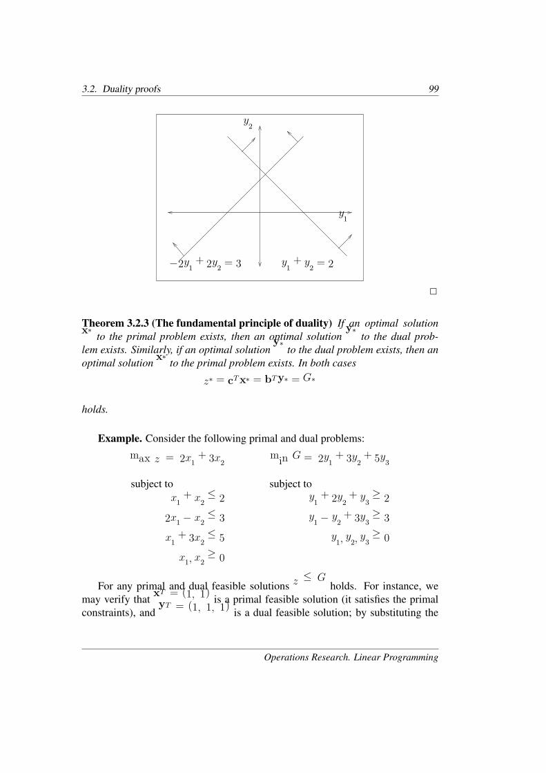
If the primal problem is infeasible, the dual problem may be either infeasibleor unbounded. Similarly, if the dual problem is infeasible, the primal problemmay be either infeasible or unbounded.
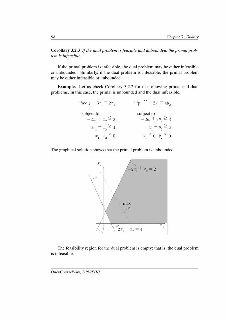
Example. Let us check Corollary 3.2.2 for the following primal and dualproblems. In this case, the primal is unbounded and the dual infeasible.
max z = 3x1 + 2x2 min G = 2y1 + 4y2
subject to subject to
−2x1 + x2 ≤ 2 −2y1 + 2y2 ≥ 3
2x1 + x2 ≥ 4 y1 + y2 ≥ 2
x1, x2 ≥ 0 y1 ≥ 0, y2 ≤ 0
The graphical solution shows that the primal problem is unbounded.
x1
x2
−2x1 + x2 = 2
2x1 + x2 = 4
max
The feasibility region for the dual problem is empty; that is, the dual problemis infeasible.
OpenCourseWare, UPV/EHU
3.2. Duality proofs 99
y1
y2
−2y1 + 2y2 = 3 y1 + y2 = 2
�
Theorem 3.2.3 (The fundamental principle of duality) If an optimal solutionx∗ to the primal problem exists, then an optimal solution y∗ to the dual prob-lem exists. Similarly, if an optimal solution y∗ to the dual problem exists, then anoptimal solution x∗ to the primal problem exists. In both cases
z∗ = cTx∗ = bTy∗ = G∗
holds.
Example. Consider the following primal and dual problems:
max z = 2x1 + 3x2 min G = 2y1 + 3y2 + 5y3
subject to subject to
x1 + x2 ≤ 2 y1 + 2y2 + y3 ≥ 2
2x1 − x2 ≤ 3 y1 − y2 + 3y3 ≥ 3
x1 + 3x2 ≤ 5 y1, y2, y3 ≥ 0
x1, x2 ≥ 0
For any primal and dual feasible solutions z ≤ G holds. For instance, wemay verify that xT = (1, 1) is a primal feasible solution (it satisfies the primalconstraints), and yT = (1, 1, 1) is a dual feasible solution; by substituting the
Operations Research. Linear Programming
100 Chapter 3. Duality
solutions into the respective objective functions, we may verify that z = 5 ≤ 10 =G holds, as the weak duality theorem predicts.
The optimal primal and dual solutions are the following:
x∗T = (1
2,3
2), y∗T = (
3
2, 0,
1
2).
The objective value for both problems is the same, z∗ = 11
2= G∗. �
3.3 The principle of complementary slacknessApplying the principle of complementary slackness, we can use the primal opti-mal solution to solve the corresponding dual problem, and viceversa. The condi-tions are stated in the following theorem.
Theorem 3.3.1 (Complementary slackness) Any feasible solutions to the pri-mal and dual problems x∗ and y∗ are optimal if and only if the following holds:
x∗T (ATy∗ − c) + y∗T (b−Ax∗) = 0.
From the interpretation of this theorem we obtain the complementary slack-ness conditions. Remember that the primal and dual problems are given in sym-metric form.
3.3.1 Interpretation of the complementary slackness conditionsWe may write the primal and dual constraints in the following way, being x∗ andy∗ optimal solutions to the respective problems:
ATy∗ − c ≥ 0.
b−Ax∗ ≥ 0.
Since the primal and dual optimal solutions x∗ and y∗ are positive, by multi-plying the previous inequalities on the left by x∗T and y∗T , respectively, we get:
x∗T (ATy∗ − c) ≥ 0.
y∗T (b−Ax∗) ≥ 0.
OpenCourseWare, UPV/EHU

3.3. The principle of complementary slackness 101
The complementary slackness theorem states that the sum of the left hand sideof the two previous inequalities is zero. Taking into account that the two addendsare greater than or equal to zero, we conclude that each of them must be zero, thatis,
x∗T (ATy∗ − c) = 0.
y∗T (b−Ax∗) = 0.
According to the foregoing equations, the product of two nonnegative factorsis zero; this implies that if one of them is not zero, then the other must be. Thus,we obtain the following conclusions, which enable us to compute the optimalsolution to one of the problems from the optimal solution to the other.
1. If a primal variable is positive, that is to say, greater than zero, then thecorresponding constraint in the dual must hold with equality.
x∗ > 0 ⇒ ATy∗ − c = 0.
2. If a constraint of the primal is not binding, that is to say, if the equality doesnot hold, then the corresponding dual variable must be zero.
Ax∗ < b ⇒ y∗ = 0.
3. If a dual variable is positive, that is to say, greater than zero, then the corre-sponding constraint in the primal must hold with equality.
y∗ > 0 ⇒ Ax∗ − b = 0.
4. If a constraint of the dual is not binding, that is to say, if the equality doesnot hold, then the corresponding primal variable must be zero.
ATy∗ > c ⇒ x∗ = 0.
Example. Consider the following linear problem:
max z = 3x1 + x2 − 2x3
subject tox1 + 2x2 + x3 ≤ 5
2x1 − x2 + 3x3 ≤ 4
x1, x2, x3 ≥ 0
Operations Research. Linear Programming

102 Chapter 3. Duality
The optimal solution to the problem is x∗T = (135, 6
5, 0). The dual problem is
the following:
min G = 5y1 + 4y2
subject toy1 + 2y2 ≥ 3
2y1 − y2 ≥ 1
y1 + 3y2 ≥ −2
y1, y2 ≥ 0
We introduce three slack variables to the problem and get:
min G = 5y1 + 4y2 + 0y3 + 0y4 + 0y5
subject to
y1 + 2y2 −y3 = 3
2y1 − y2 −y4 = 1
y1 + 3y2 −y5 = −2
y1, y2, y3, y4, y5 ≥ 0
Using the interpretation of the theorem of complementary slackness, we com-pute the optimal solution to the dual problem, proceeding like this:
Primal variables Dual constraints
x∗
1= 13
5> 0 ⇒ y∗
1+ 2y∗
2= 3 ⇒ y∗
3= 0
x∗
2= 6
5> 0 ⇒ 2y∗
1− y∗
2= 1 ⇒ y∗
4= 0
x∗
3= 0 ⇒ y∗
1+ 3y∗
2− y∗
5= −2
Primal constraints Dual variables13
5+ 2× 6
5= 5 ⇒ we compute y∗
1
2× 13
5− 6
5= 4 ⇒ we compute y∗
2
We substitute the values of y∗3and y∗
4in the dual constraint set, and we have:
y∗1+ 2y∗
2= 3
2y∗1− y∗
2= 1
y∗1+ 3y∗
2− y∗
5= −2
OpenCourseWare, UPV/EHU
3.4. The optimal solution to the dual problem 103
By solving the system of linear equations, we obtain the optimal solution to thedual problem.
y∗1= 1, y∗
2= 1, y∗
3= 0, y∗
4= 0, y∗
5= 6.
�
3.4 The optimal solution to the dual problemTheorem 3.4.1 Consider the symmetric form of duality, and let B be an optimalbasis for the primal problem. Then, y∗T = cTBB
−1 is an optimal solution to thedual problem.
Proof. We consider the constraints of the primal problem in maximizationsymmetric form, and add vector xs of slack variables, which yields:
Ax+ Ixs = b
x,xs ≥ 0
If B is an optimal basis for the primal problem, and xB an optimal basicfeasible solution, then zj − cj ≥ 0 holds for each vector aj of matrixA.
zj = cTByj = cTBB−1aj .
Since B is optimal, zj ≥ cj holds for each vector aj of matrix A, that is,
cTBB−1A ≥ cT .
The foregoing inequality can be equally written as follows:
AT (cTBB−1)T ≥ c,
which is the dual constraint set. Thus, y∗ = (cTBB−1)T is a solution to the dual
problem.In order to check the feasibility of the solution, we compute the zj − cj corre-
sponding to the vectors of submatrix I.
cTBB−1I ≥ cTI .
Since vector xs corresponds to slack variables, cI = 0 holds and thus:
cTBB−1I = cTBB
−1 ≥ 0T .
Operations Research. Linear Programming
104 Chapter 3. Duality
Therefore, all the components of vector y∗ = (cTBB−1)T are nonnegative.
We next show that the solution y∗ is an optimal solution to the dual problem.We prove it by checking that the primal problem and the dual problem have thesame objective value.
z∗ = cTBxB = cTBB−1b = bT (cTBB
−1)T = bTy∗ = G∗.
Therefore y∗ = (cTBB−1)T is an optimal solution to the dual problem. �
3.4.1 A solution to the dual problem in the tableauWe turn now to see that once the primal problem is solved, an optimal solution tothe dual problem is readily obtainable in the optimal tableau.
From Theorem 3.4.1 we know that if B be is an optimal basis for the primalproblem, then y∗T = cTBB
−1 is an optimal solution to the dual problem. We nowshow that such vector appears in the optimal tableau at row zero (row of reducedcost coefficients zj − cj), where the identity matrix I appeared initially.
zj − cj = cTBB−1aj − cj.
If we compute all the zj − cj of the corresponding vectors in this identitymatrix, we get the following vector:
cTBB−1I− cTI = cTBB
−1 − cTI .
Therefore, since y∗T = cTBB−1 is the optimal solution to the dual problem, we
need to add cTI to the reduced cost coefficients zj − cj to obtain it, where cI is them-vector representing the cost coefficients of the variables corresponding to thecolumns of the original identity matrix. Two cases may be distinguished:
• If the columns of matrix I correspond to slack variables, then cI = 0 holds.
• If there are artificial variables in the columns corresponding to the initialmatrix I, then the cost coefficients of the artificial variables areM , and theyappear in vector cI , due to the penalty of the objective function.
Example. Consider the problem of page 101.
max z = 3x1 + x2 − 2x3
subject tox1 + 2x2 + x3 ≤ 5
2x1 − x2 + 3x3 ≤ 4
x1, x2, x3 ≥ 0
OpenCourseWare, UPV/EHU
3.4. The optimal solution to the dual problem 105
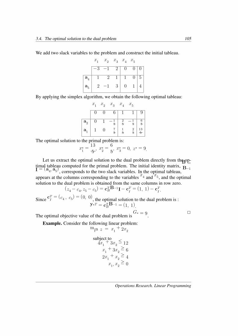
We add two slack variables to the problem and construct the initial tableau.
x1 x2 x3 x4 x5
−3 −1 2 0 0 0
a4 1 2 1 1 0 5
a5 2 −1 3 0 1 4
By applying the simplex algorithm, we obtain the following optimal tableau:
x1 x2 x3 x4 x5
0 0 6 1 1 9
a2 0 1 −1
5
2
5−1
5
6
5
a1 1 0 7
5
1
5
2
5
13
5
The optimal solution to the primal problem is:
x∗
1=
13
5, x∗
2=
6
5, x∗
3= 0, z∗ = 9.
Let us extract the optimal solution to the dual problem directly from the op-timal tableau computed for the primal problem. The initial identity matrix, B =I = (a4, a5), corresponds to the two slack variables. In the optimal tableau, B−1
appears at the columns corresponding to the variables x4 and x5, and the optimalsolution to the dual problem is obtained from the same columns in row zero.
(z4 − c4, z5 − c5) = cTBB−1I− cTI = (1, 1)− cTI .
Since cTI = (c4 , c5) = (0, 0), the optimal solution to the dual problem is :
y∗T = cTBB−1 = (1, 1).
The optimal objective value of the dual problem is G∗ = 9. �
Example. Consider the following linear problem:
min z = x1 + 2x2
subject to4x1 + 3x2 ≤ 12
x1 + 3x2 ≥ 6
2x1 + x2 ≥ 4
x1, x2 ≥ 0
Operations Research. Linear Programming
106 Chapter 3. Duality
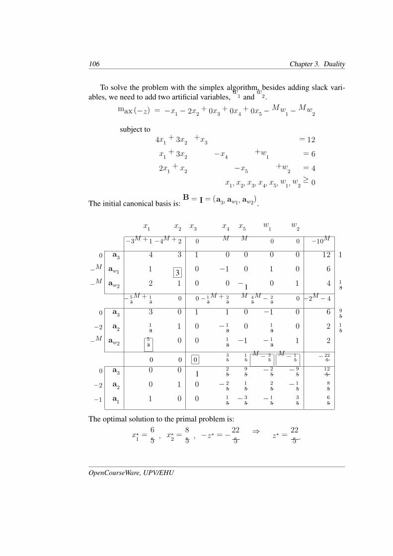
To solve the problem with the simplex algorithm, besides adding slack vari-ables, we need to add two artificial variables, w1 and w2.
max (−z) = −x1 − 2x2 + 0x3 + 0x4 + 0x5 −Mw1 −Mw2
subject to
4x1 + 3x2 +x3 = 12
x1 + 3x2 −x4 +w1 = 6
2x1 + x2 −x5 +w2 = 4
x1, x2, x3, x4, x5, w1, w2 ≥ 0
The initial canonical basis is: B = I = (a3, aw1, aw2).
x1 x2 x3 x4 x5 w1 w2
−3M + 1 −4M + 2 0 M M 0 0 −10M
0 a3 4 3 1 0 0 0 0 12 1
−M aw1 1 3 0 −1 0 1 0 6
−M aw2 2 1 0 0 −1 0 1 4 1
3
− 5
3M +
1
30 0 − 1
3M +
2
3M
4
3M − 2
30 −2M − 4
0 a3 3 0 1 1 0 −1 0 6 9
5
−2 a21
31 0 −1
30 1
30 2 1
5
−M aw25
30 0 1
3−1 −1
31 2
0 0 0 3
5
1
5M − 3
5M − 1
5− 22
5
0 a3 0 0 1 2
5
9
5−2
5−9
5
12
5
−2 a2 0 1 0 −2
5
1
5
2
5−1
5
8
5
−1 a1 1 0 0 1
5−3
5−1
5
3
5
6
5
The optimal solution to the primal problem is:
x∗
1=
6
5, x∗
2=
8
5, −z∗ = −
22
5⇒ z∗ =
22
5.
OpenCourseWare, UPV/EHU
3.5. Economic interpretation of duality 107
Let us obtain the optimal solution to the dual problem from the optimal sim-plex tableau. The identity matrix in the first tableau is in the columns correspond-ing to the variables x3, w1 and w2. In the same columns of the optimal tableau wefind B−1, as well as the optimal solution to the dual problem in row zero.
(z3 − c3, zw1− cw1
, zw2− cw2
) = cTBB−1I− cTI = (0, M −
3
5, M −
1
5).
Since cTI = (c3 , cw1, cw2
) = (0, −M, −M), by adding these cost coefficientswe obtain:
y∗T = cTBB−1 − cTI + cTI = (0, M −
3
5, M −
1
5) + (0, −M, −M).
We would say that the optimal solution to the dual problem is:
y∗T = (0,−3
5,−
1
5).
However, the sign of the variables has to be verified. If we write the dualproblem, we will see that variables y2 and y3 are nonnegative. In this case, thevalues obtained from the optimal tableau are negative. The reason for this is thatthe transformation applied to the objective function of the primal problem, beforeusing the simplex algorithm, has an effect in the reduced cost coefficients zj − cjof row zero. In this example, the original objective function is in minimizationform, and we transform it to the maximization form; that is why the sign of thevariables is not correct. Hence, the optimal solution to the dual problem is:
y∗1= 0, y∗
2=
3
5, y∗
3=
1
5, G∗ =
22
5.
�
If we transform a constraint in a linear model by multiplying it by −1 beforeapplying the simplex algorithm, the sign of the value in row zero that will beassigned to the corresponding dual variable will be affected. This change of signmay be explained analyzing the primal-dual correspondences of Table 3.1 on page91. We can state that the absolute value of the components of vector cTBB
−1 areequal to the absolute value of the optimal values of the dual variables.
3.5 Economic interpretation of dualityThe optimal solution to a linear model determines the optimal resource allocationto maximize revenue, when resources are limited. In this section we will see
Operations Research. Linear Programming
108 Chapter 3. Duality
that the optimal solution to the dual model gives us useful information about theconvenience of changing the amount of resources available (the right-hand-sideof the constraints). We now introduce the concept of shadow price, which helpsto make interesting economic interpretations.
3.5.1 Shadow pricesConsider a linear model and its optimal basisB. Let x∗ be the optimal solution tothat primal problem, and z∗ its corresponding optimal objective value. Similarly,let y∗ be the optimal solution to the dual problem, and G∗ its corresponding op-timal objective value. Note that x∗, z∗, y∗ and G∗ are computed in terms of theoptimal basis B.
Let us assume that the right-hand-side vector b changes to b + Δb. We willanalyze the effect the change has on all the calculations in the tableau correspond-ing to the optimal basis B, assuming that the current basis remains optimal (thecurrent basic feasible solution remains feasible).
• The new basic feasible solution is:∧
xB= B−1(b+Δb) = xB +B−1Δb.
• The change in the right-hand-side vector does not have any effect on thevalues zj − cj of row zero.
zj − cj = cTBB−1aj − cj .
• The objective values of the primal and dual problems change, according tothe variations on vector b (that is, the increase/decrease specified by Δb).
∧
G∗
= y∗T (b+Δb) = y∗Tb+ y∗TΔb = G∗ + y∗TΔb = z∗ + y∗TΔb.
Consequently, if a change in vector b does not violate optimality, that is, ifthe new basic solution
∧
xB remains feasible, the solution will be affected in thefollowing way:
• The optimal solution to the dual problem remains the same.
• The optimal solution to the primal problem changes. The variation is spec-ified by B−1Δb.
OpenCourseWare, UPV/EHU
3.5. Economic interpretation of duality 109
• The primal and dual objective values increase/decrease in y∗TΔb.
In summary, if the right-hand-side vector changes and∧
xB= B−1(b+Δb) ≥ 0,∧
xB is the optimal solution to the primal problem and y∗ remains optimal to the dualproblem. The optimal objective value for both problems increases y∗TΔb over itsoriginal optimal value.
In order to interpret the meaning of each of the dual variables, we assume thatΔbi = 1 and all the rest are zero. Thus, the objective value is increased:
y∗TΔb = (y∗1, . . . , y∗i , . . . , y
∗
m)
0...
1...
0
= y∗i .
Thus, if the ith right-hand-side (ith resource) is increased in one unit,Δbi = 1,and all the rest of the resources remain unchanged, then the optimal value of thedual variable y∗i is the rate of change (increase) of the optimal objective value.The following definition states when the optimal dual variables are considered tobe shadow prices.
Definition 3.5.1 (Shadow price) The optimal dual variable y∗i is said to be theshadow price of the ith right-hand-side value, i = 1, . . . , m, if increasing/decreasinga unit in the ith right-hand-side value, and keeping the rest of the right-hand-sidevalues unchanged, does not violate the optimality of the tableau.
Therefore, the shadow price of a resource tells us the increase/decrease inprofit resulting from a unit increase/decrease in the availability of the resource. Inother words, shadow prices enable us to make economic interpretations such as:how to increase/decrease future profits by increasing/decreasing the availabilityof the resources.
Example. Consider the example on page 104. Let us check whether the op-timal dual variables y∗
1= 1 and y∗
2= 1 are shadow prices of resources b1 and
b2.
Operations Research. Linear Programming
110 Chapter 3. Duality
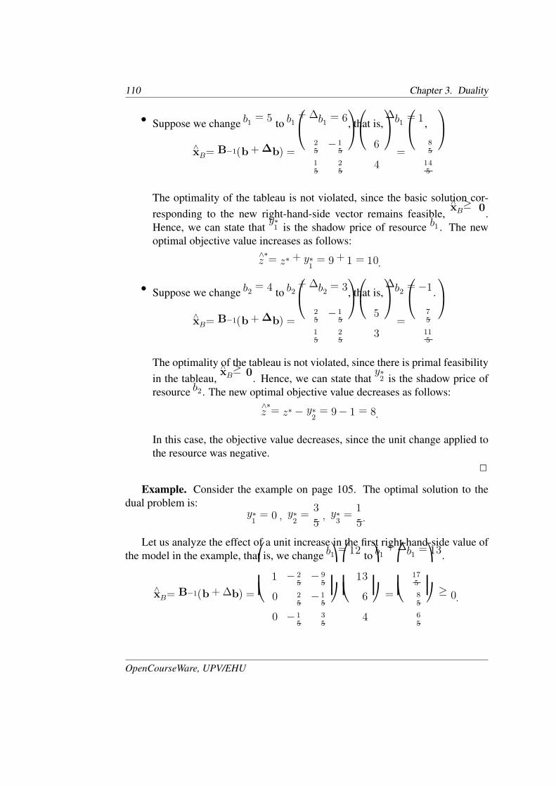
• Suppose we change b1 = 5 to b1 +Δb1 = 6, that is, Δb1 = 1,
∧
xB= B−1(b+Δb) =
2
5−1
5
1
5
2
5
6
4
=
8
5
14
5
The optimality of the tableau is not violated, since the basic solution cor-responding to the new right-hand-side vector remains feasible,
∧
xB≥ 0.Hence, we can state that y∗
1is the shadow price of resource b1. The new
optimal objective value increases as follows:
∧
z∗
= z∗ + y∗1= 9 + 1 = 10.
• Suppose we change b2 = 4 to b2 +Δb2 = 3, that is, Δb2 = −1.
∧
xB= B−1(b+Δb) =
2
5−1
5
1
5
2
5
5
3
=
7
5
11
5
The optimality of the tableau is not violated, since there is primal feasibilityin the tableau,
∧
xB≥ 0. Hence, we can state that y∗2is the shadow price of
resource b2. The new optimal objective value decreases as follows:
∧
z∗
= z∗ − y∗2= 9− 1 = 8.
In this case, the objective value decreases, since the unit change applied tothe resource was negative.
�
Example. Consider the example on page 105. The optimal solution to thedual problem is:
y∗1= 0 , y∗
2=
3
5, y∗
3=
1
5.
Let us analyze the effect of a unit increase in the first right-hand-side value ofthe model in the example, that is, we change b1 = 12 to b1 +Δb1 = 13.
∧
xB= B−1(b+Δb) =
1 −2
5−9
5
0 2
5−1
5
0 −1
5
3
5
13
6
4
=
17
5
8
5
6
5
≥ 0.
OpenCourseWare, UPV/EHU

3.5. Economic interpretation of duality 111
Since there is primal feasibility in the tableau,∧
xB≥ 0, the optimality of thetableau is not violated. Hence, we can state that y∗
1is the shadow price of the
first right-hand-side value. However, the optimal objective value does not varybecause the shadow price is y∗
1= 0.
∧
z∗
= z∗ + y∗1=
22
5+ 0 =
22
5.
The fact that the first constraint of the model has a shadow-price of zero meansthat increasing the available amount of the resource will not increase the profit,which is logical because we are not currently using all of the resource. We caneasily verify it by substituting the optimal solution in the first constraint. Remem-ber that x∗
1= 6
5, x∗
2= 8
5and that the first constraint is 4x1 + 3x2 ≤ 12.
4×6
5+ 3×
8
5< 12.
Thus, no improvement is achieved from increasing the amount of the firstresource. Instead, we should analyze the convenience of reducing the amount ofit. �
3.5.2 The economic cost of the primal variables and the inter-pretation of the simplex method
The interpretation of the dual problem also provides an economic interpretation ofwhat the simplex method does in the primal problem. In this subsection, we definethe economic cost of the primal variables and give an economic interpretation ofthe simplex method. To better understand it, we consider the following problem.
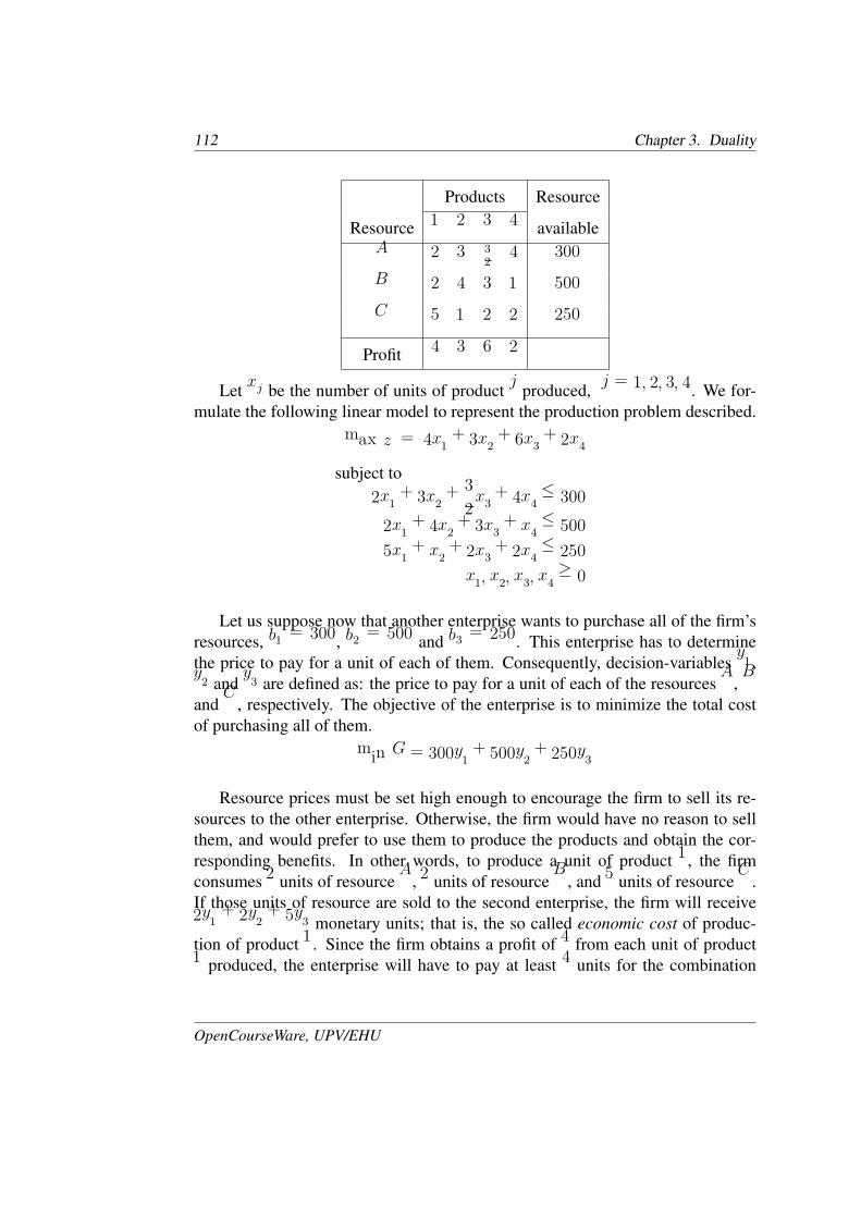
A firm produces four different types of products: 1, 2, 3 and 4. Three resourcesare used in the production process: A, B and C. The amount of each resourceused in the production of each product unit, the availability of the resources andthe profit obtained from each product unit are given in the following table:
Operations Research. Linear Programming
112 Chapter 3. Duality
Products Resource
Resource 1 2 3 4 available
A 2 3 3
24 300
B 2 4 3 1 500
C 5 1 2 2 250
Profit 4 3 6 2
Let xj be the number of units of product j produced, j = 1, 2, 3, 4. We for-mulate the following linear model to represent the production problem described.
max z = 4x1 + 3x2 + 6x3 + 2x4
subject to
2x1 + 3x2 +3
2x3 + 4x4 ≤ 300
2x1 + 4x2 + 3x3 + x4 ≤ 500
5x1 + x2 + 2x3 + 2x4 ≤ 250
x1, x2, x3, x4 ≥ 0
Let us suppose now that another enterprise wants to purchase all of the firm’sresources, b1 = 300, b2 = 500 and b3 = 250. This enterprise has to determinethe price to pay for a unit of each of them. Consequently, decision-variables y1,y2 and y3 are defined as: the price to pay for a unit of each of the resources A, Band C, respectively. The objective of the enterprise is to minimize the total costof purchasing all of them.
min G = 300y1 + 500y2 + 250y3
Resource prices must be set high enough to encourage the firm to sell its re-sources to the other enterprise. Otherwise, the firm would have no reason to sellthem, and would prefer to use them to produce the products and obtain the cor-responding benefits. In other words, to produce a unit of product 1, the firmconsumes 2 units of resource A, 2 units of resource B, and 5 units of resource C.If those units of resource are sold to the second enterprise, the firm will receive2y1 + 2y2 + 5y3 monetary units; that is, the so called economic cost of produc-tion of product 1. Since the firm obtains a profit of 4 from each unit of product1 produced, the enterprise will have to pay at least 4 units for the combination
OpenCourseWare, UPV/EHU
3.5. Economic interpretation of duality 113
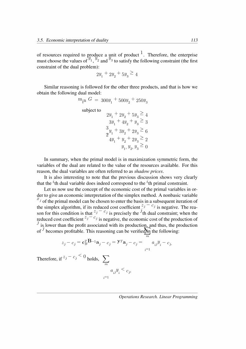
of resources required to produce a unit of product 1. Therefore, the enterprisemust choose the values of y1, y2 and y3 to satisfy the following constraint (the firstconstraint of the dual problem):
2y1 + 2y2 + 5y3 ≥ 4
Similar reasoning is followed for the other three products, and that is how weobtain the following dual model:
min G = 300y1 + 500y2 + 250y3
subject to2y1 + 2y2 + 5y3 ≥ 4
3y1 + 4y2 + y3 ≥ 33
2y1 + 3y2 + 2y3 ≥ 6
4y1 + y2 + 2y3 ≥ 2
y1, y2, y3 ≥ 0
In summary, when the primal model is in maximization symmetric form, thevariables of the dual are related to the value of the resources available. For thisreason, the dual variables are often referred to as shadow prices.
It is also interesting to note that the previous discussion shows very clearlythat the ith dual variable does indeed correspond to the ith primal constraint.
Let us now use the concept of the economic cost of the primal variables in or-der to give an economic interpretation of the simplex method. A nonbasic variablexj of the primal model can be chosen to enter the basis in a subsequent iteration ofthe simplex algorithm, if its reduced cost coefficient zj − cj is negative. The rea-son for this condition is that zj − cj is precisely the jth dual constraint; when thereduced cost coefficient zj − cj is negative, the economic cost of the production ofj is lower than the profit associated with its production, and thus, the productionof j becomes profitable. This reasoning can be verified in the following:
zj − cj = cTBB−1aj − cj = yTaj − cj =
m�
i=1
aijyi − cj .
Therefore, if zj − cj < 0 holds,
m�
i=1
aijyi < cj,
Operations Research. Linear Programming
114 Chapter 3. Duality
which means that, the economic cost of producing j is lower than the profit cjassociated with its production.
To conclude this section, we can say that the simplex method examines allthe nonbasic variables in the current basic feasible solution to see which one canprovide a more profitable use of the resources. If none of them can, the currentsolution is optimal.
3.6 The dual simplex methodIn Chapter 2 we saw that the identity matrix is selected as the initial basis tocompute a basic feasible solution to the primal problem using the simplex algo-rithm, and that if necessary, artificial variables will be introduced to the model. Insubsequent iterations, the algorithm moves from a basic feasible solution to an im-proved basic feasible solution of the primal problem, until optimality is reached,that is, until zj−cj ≥ 0 holds in the tableau, for all j. Such optimality condition isrelated to the feasibility of the dual problem. In fact, we can say that the simplexalgorithm starts at a primal feasible solution, and stops when dual feasibility isreached. From this point onward, this method will be called the simplex primalmethod.
In this section we describe the dual simplex algorithm. This algorithm alsostarts selecting the identity matrix I as the initial basis, which in this case is al-ways formed by slack variables. The first step is to write the model in maximiza-tion symmetric form and to add a slack variable to each constraint. If the initialtableau is dual feasible, then iterations of the algorithm will be performed until theprimal feasibility, keeping dual feasibility, is reached (if the problem is feasible).If the initial tableau constructed for the first canonical basis is not dual feasible,then an artificial constraint will be added to the primal problem to obtain the dualfeasibility, as we will see in Section 3.7.
3.6.1 The dual simplex algorithmThe objective is to maximize. Find an initial basis B = I of slack variables.
Step 1. Construct the initial tableau, where zj − cj ≥ 0 for all j.
Step 2. With regard to primal feasibility, there are two cases to consider.
• If xBi ≥ 0, i = 1, . . . ,m, the current solution is optimal. Stop.
OpenCourseWare, UPV/EHU
3.6. The dual simplex method 115
• If there exists xBi < 0, then the dual solution may be improved. Go toStep 3.
Step 3. Basis modification.
• Select a vector to leave the basis, according to the following criteria:
xBr = mini
{ xBi / xBi < 0 }
The rth row is the pivot row.• Select a vector to enter the basis, according to the following criteria:
zk − ckyrk
= maxj
�
zj − cjyrj
/ yrj < 0
�
The kth column is the pivot column. yrk is the pivot element.
If yrj ≥ 0 for all j , the problem is infeasible. Stop.
Step 4. Compute the new tableau by pivoting in the same way as stated inthe simplex algorithm. Go to Step 2.
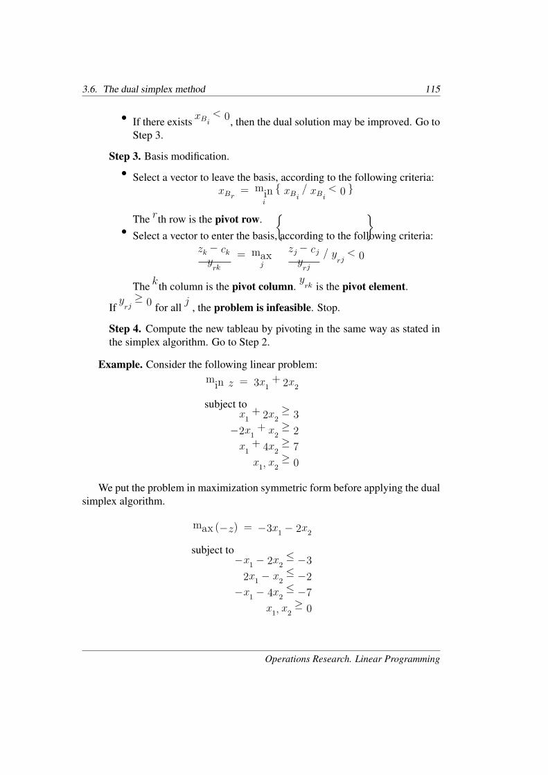
Example. Consider the following linear problem:
min z = 3x1 + 2x2
subject tox1 + 2x2 ≥ 3
−2x1 + x2 ≥ 2
x1 + 4x2 ≥ 7
x1, x2 ≥ 0
We put the problem in maximization symmetric form before applying the dualsimplex algorithm.
max (−z) = −3x1 − 2x2
subject to−x1 − 2x2 ≤ −3
2x1 − x2 ≤ −2
−x1 − 4x2 ≤ −7
x1, x2 ≥ 0
Operations Research. Linear Programming
116 Chapter 3. Duality
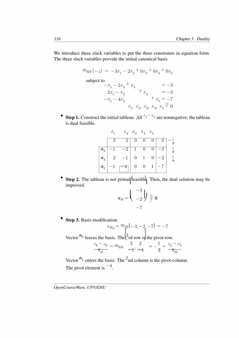
We introduce three slack variables to put the three constraints in equation form.The three slack variables provide the initial canonical basis.
max (−z) = −3x1 − 2x2 + 0x3 + 0x4 + 0x5
subject to−x1 − 2x2 + x3 = −3
2x1 − x2 + x4 = −2
−x1 − 4x2 + x5 = −7
x1, x2, x3, x4, x5 ≥ 0
• Step 1. Construct the initial tableau. All zj−cj are nonnegative; the tableauis dual feasible.
x1 x2 x3 x4 x5
3 2 0 0 0 0 −1
2
a3 −1 −2 1 0 0 −3 1
2
a4 2 −1 0 1 0 −2 1
4
a5 −1 −4 0 0 1 −7
• Step 2. The tableau is not primal feasible. Then, the dual solution may beimproved.
xB =
−3
−2
−7
�≥ 0
• Step 3. Basis modification.
xB3 = min{−3,−2,−7} = −7
Vector a5 leaves the basis. The 3rd row is the pivot-row.
zk − ckyik
= max
�
3
−1,2
−4
�
= −1
2=
z2 − c2y22
Vector a2 enters the basis. The 2nd column is the pivot-column.
The pivot element is −4.
OpenCourseWare, UPV/EHU
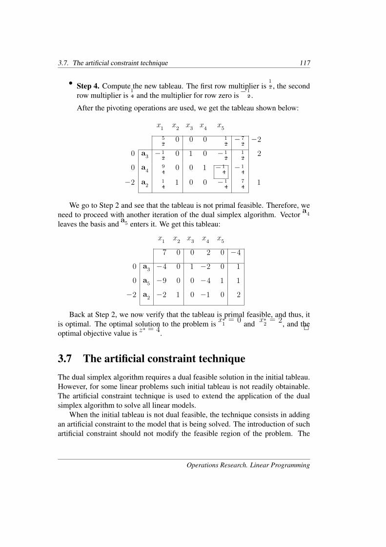
3.7. The artificial constraint technique 117
• Step 4. Compute the new tableau. The first row multiplier is 1
2, the second
row multiplier is 1
4and the multiplier for row zero is −1
2.
After the pivoting operations are used, we get the tableau shown below:
x1 x2 x3 x4 x5
5
20 0 0 1
2−7
2−2
0 a3 −1
20 1 0 −1
2
1
22
0 a49
40 0 1 −1
4−1
4
−2 a21
41 0 0 −1
4
7
41
We go to Step 2 and see that the tableau is not primal feasible. Therefore, weneed to proceed with another iteration of the dual simplex algorithm. Vector a4
leaves the basis and a5 enters it. We get this tableau:
x1 x2 x3 x4 x5
7 0 0 2 0 −4
0 a3 −4 0 1 −2 0 1
0 a5 −9 0 0 −4 1 1
−2 a2 −2 1 0 −1 0 2
Back at Step 2, we now verify that the tableau is primal feasible, and thus, itis optimal. The optimal solution to the problem is x∗
1= 0 and x∗
2= 2, and the
optimal objective value is z∗ = 4. �
3.7 The artificial constraint techniqueThe dual simplex algorithm requires a dual feasible solution in the initial tableau.However, for some linear problems such initial tableau is not readily obtainable.The artificial constraint technique is used to extend the application of the dualsimplex algorithm to solve all linear models.
When the initial tableau is not dual feasible, the technique consists in addingan artificial constraint to the model that is being solved. The introduction of suchartificial constraint should not modify the feasible region of the problem. The
Operations Research. Linear Programming
118 Chapter 3. Duality
aim of introducing it is to obtain the dual feasibility in the tableau. Then, thedual simplex algorithm can be carried out on the modified problem. The artificialconstraint added to the model is:
�
j∈N
xj ≤ M.
where N is the set of variables such that the reduced cost coefficients zj − cjare negative in the initial tableau. To guarantee that the original feasible region ofthe problem is not modified by the introduction of the artificial constraint to themodel,M must be positive and sufficiently large.
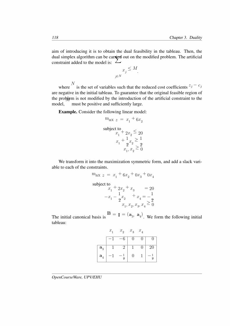
Example. Consider the following linear model:
max z = x1 + 6x2
subject tox1 + 2x2 ≤ 20
x1 +1
2x2 ≥
1
2x1, x2 ≥ 0
We transform it into the maximization symmetric form, and add a slack vari-able to each of the constraints.
max z = x1 + 6x2 + 0x3 + 0x4
subject tox1 + 2x2 + x3 = 20
−x1 −1
2x2 + x4 = −
1
2x1, x2, x3, x4 ≥ 0
The initial canonical basis is B = I = (a3, a4). We form the following initialtableau:
x1 x2 x3 x4
−1 −6 0 0 0
a3 1 2 1 0 20
a4 −1 −1
20 1 −1
2
OpenCourseWare, UPV/EHU

3.7. The artificial constraint technique 119
Since the initial tableau is not dual feasible, an artificial constraint must beintroduced before applying the dual simplex algorithm. We add the followingartificial constraint to the model:
x1 + x2 ≤ M.
We add a slack variable to the artificial constraint, which leads to the followingmodel:
max z = x1 + 6x2 + 0x3 + 0x4 + 0x5
subject tox1 + 2x2 + x3 = 20
−x1 −1
2x2 + x4 = −
1
2x1 + x2 + x5 = M
x1, x2, x3, x4, x5 ≥ 0
B = I = (a3, a4, a5) is now the initial canonical basis, and we form theinitial tableau corresponding to the model with the artificial constraint.
x1 x2 x3 x4 x5
−1 −6 0 0 0 0 −6
0 a3 1 2 1 0 0 20 2
0 a4 −1 −1
20 1 0 −1
2−1
2
0 a5 1 1 0 0 1 M
Later on, we will see how to select the entering and the leaving vectors in suchinitial tableau to ensure dual feasibility in the subsequent tableau. �
3.7.1 The effect of the artificial constraintWe can briefly say that, the artificial constraint technique extends the use of thedual simplex algorithm when necessary. Nevertheless, the introduction of theartificial constraint to the model should never modify the feasible region of theoriginal model; to ensure this, M must be positive and as large as necessary.
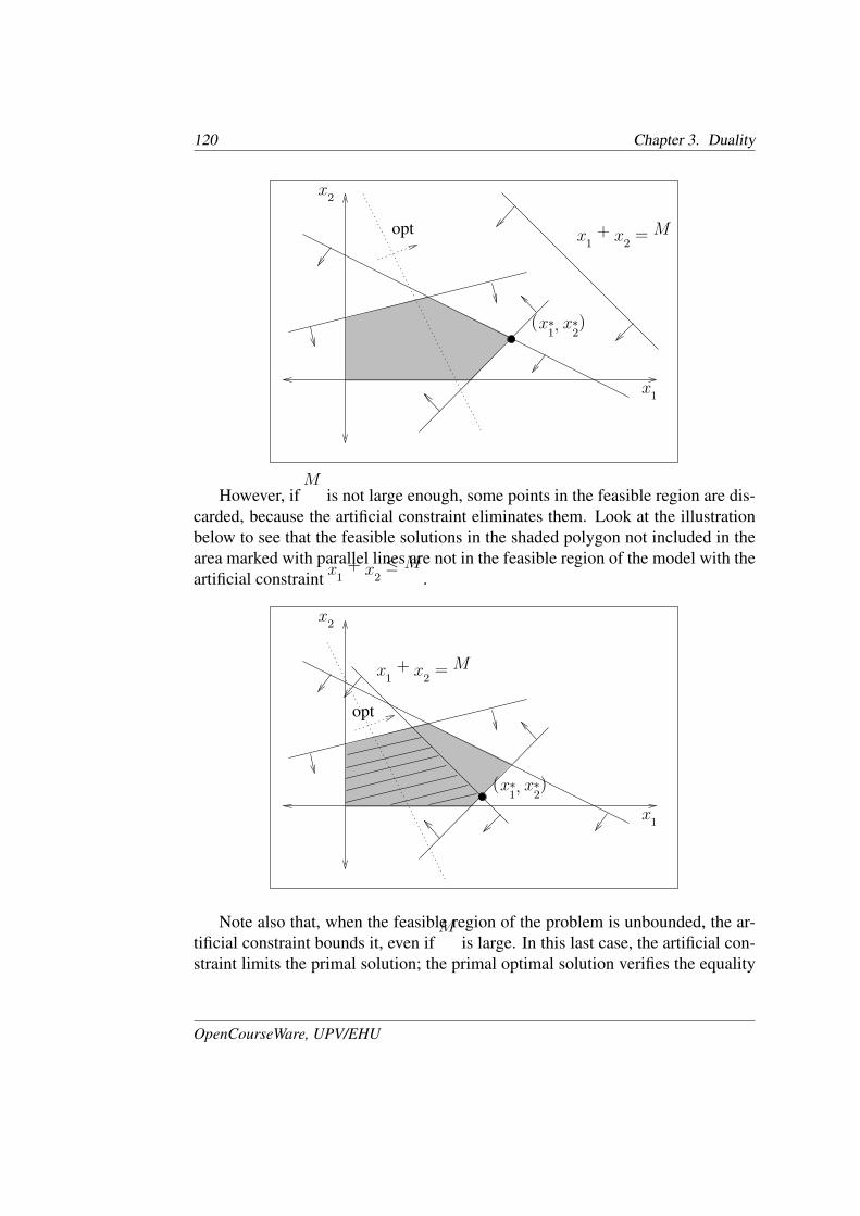
The figure below illustrates the introduction of an artificial constraint with alarge enoughM , such that it causes no effect on the feasible region, that is to say,the shaded polygon in the figure.
Operations Research. Linear Programming
120 Chapter 3. Duality
x1
x2
x1 + x2 = Mopt
(x∗
1, x∗
2)
However, ifM is not large enough, some points in the feasible region are dis-carded, because the artificial constraint eliminates them. Look at the illustrationbelow to see that the feasible solutions in the shaded polygon not included in thearea marked with parallel lines are not in the feasible region of the model with theartificial constraint x1 + x2 ≤ M .
x1
x2
x1 + x2 = M
(x∗
1, x∗
2)
opt
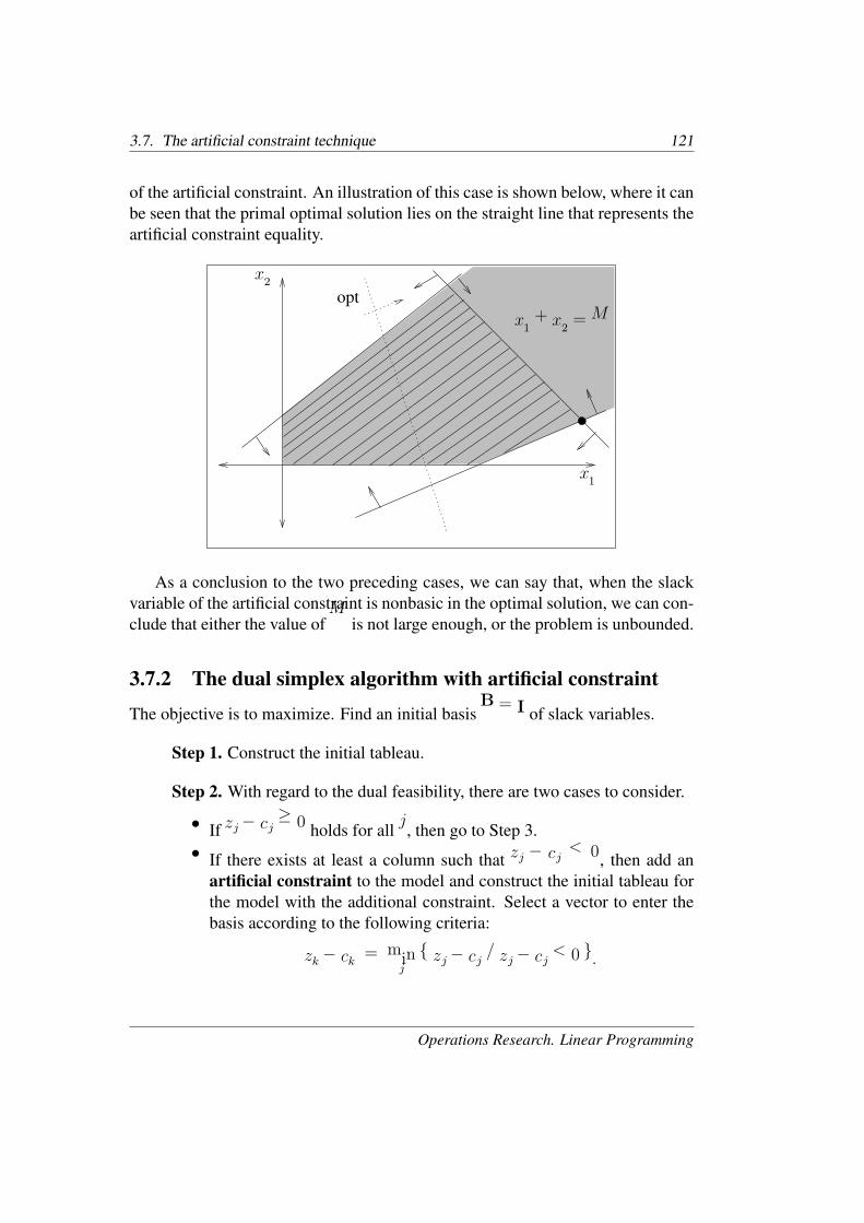
Note also that, when the feasible region of the problem is unbounded, the ar-tificial constraint bounds it, even if M is large. In this last case, the artificial con-straint limits the primal solution; the primal optimal solution verifies the equality
OpenCourseWare, UPV/EHU
3.7. The artificial constraint technique 121
of the artificial constraint. An illustration of this case is shown below, where it canbe seen that the primal optimal solution lies on the straight line that represents theartificial constraint equality.
x1
x2
x1 + x2 = M
opt
As a conclusion to the two preceding cases, we can say that, when the slackvariable of the artificial constraint is nonbasic in the optimal solution, we can con-clude that either the value ofM is not large enough, or the problem is unbounded.
3.7.2 The dual simplex algorithm with artificial constraint
The objective is to maximize. Find an initial basis B = I of slack variables.
Step 1. Construct the initial tableau.
Step 2. With regard to the dual feasibility, there are two cases to consider.
• If zj − cj ≥ 0 holds for all j, then go to Step 3.
• If there exists at least a column such that zj − cj < 0, then add anartificial constraint to the model and construct the initial tableau forthe model with the additional constraint. Select a vector to enter thebasis according to the following criteria:
zk − ck = minj
{ zj − cj / zj − cj < 0 }.
Operations Research. Linear Programming
122 Chapter 3. Duality
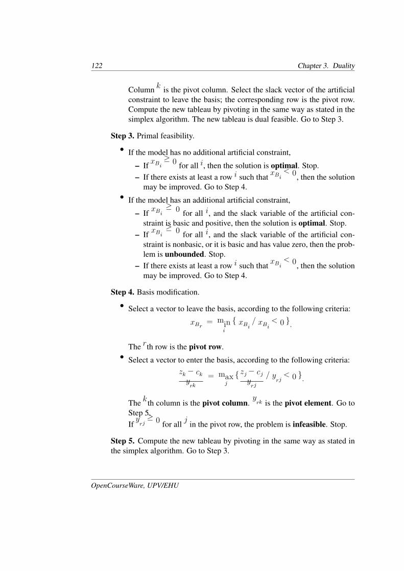
Column k is the pivot column. Select the slack vector of the artificialconstraint to leave the basis; the corresponding row is the pivot row.Compute the new tableau by pivoting in the same way as stated in thesimplex algorithm. The new tableau is dual feasible. Go to Step 3.
Step 3. Primal feasibility.
• If the model has no additional artificial constraint,
– If xBi ≥ 0 for all i, then the solution is optimal. Stop.– If there exists at least a row i such that xBi < 0, then the solutionmay be improved. Go to Step 4.
• If the model has an additional artificial constraint,
– If xBi ≥ 0 for all i, and the slack variable of the artificial con-straint is basic and positive, then the solution is optimal. Stop.
– If xBi ≥ 0 for all i, and the slack variable of the artificial con-straint is nonbasic, or it is basic and has value zero, then the prob-lem is unbounded. Stop.
– If there exists at least a row i such that xBi < 0, then the solutionmay be improved. Go to Step 4.
Step 4. Basis modification.
• Select a vector to leave the basis, according to the following criteria:
xBr = mini
{ xBi / xBi < 0 }.
The rth row is the pivot row.
• Select a vector to enter the basis, according to the following criteria:
zk − ckyrk
= maxj
{zj − cjyrj
/ yrj < 0 }.
The kth column is the pivot column. yrk is the pivot element. Go toStep 5.If yrj ≥ 0 for all j in the pivot row, the problem is infeasible. Stop.
Step 5. Compute the new tableau by pivoting in the same way as stated inthe simplex algorithm. Go to Step 3.
OpenCourseWare, UPV/EHU
3.8. Some illustrative examples 123
3.8 Some illustrative examplesIn this section, we solve three linear models which can only be solved by thedual simplex algorithm after the artificial constraint technique has been applied.We interpret the tableau for a feasible problem, an infeasible problem and anunbounded problem.
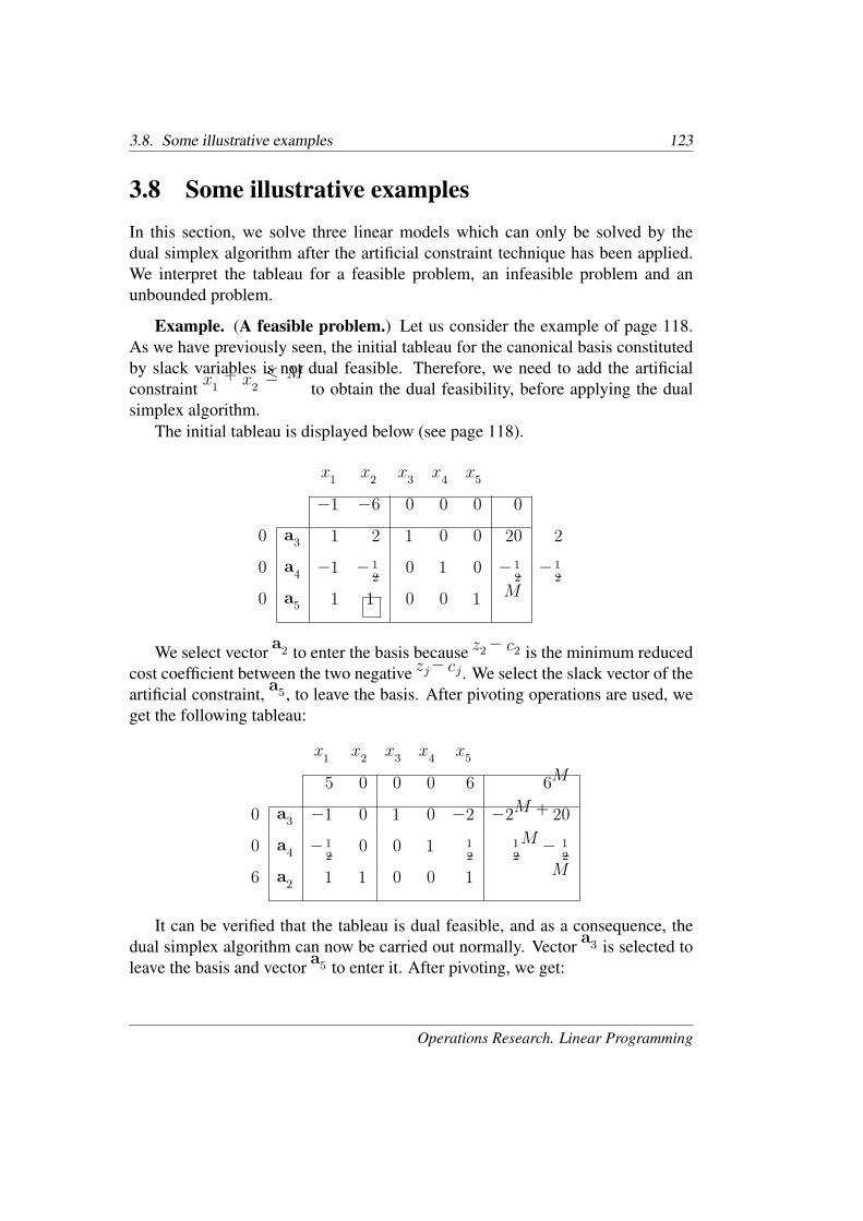
Example. (A feasible problem.) Let us consider the example of page 118.As we have previously seen, the initial tableau for the canonical basis constitutedby slack variables is not dual feasible. Therefore, we need to add the artificialconstraint x1 + x2 ≤ M to obtain the dual feasibility, before applying the dualsimplex algorithm.
The initial tableau is displayed below (see page 118).
x1 x2 x3 x4 x5
−1 −6 0 0 0 0
0 a3 1 2 1 0 0 20 2
0 a4 −1 −1
20 1 0 −1
2−1
2
0 a5 1 1 0 0 1 M
We select vector a2 to enter the basis because z2 − c2 is the minimum reducedcost coefficient between the two negative zj − cj . We select the slack vector of theartificial constraint, a5, to leave the basis. After pivoting operations are used, weget the following tableau:
x1 x2 x3 x4 x5
5 0 0 0 6 6M
0 a3 −1 0 1 0 −2 −2M + 20
0 a4 −1
20 0 1 1
2
1
2M − 1
2
6 a2 1 1 0 0 1 M
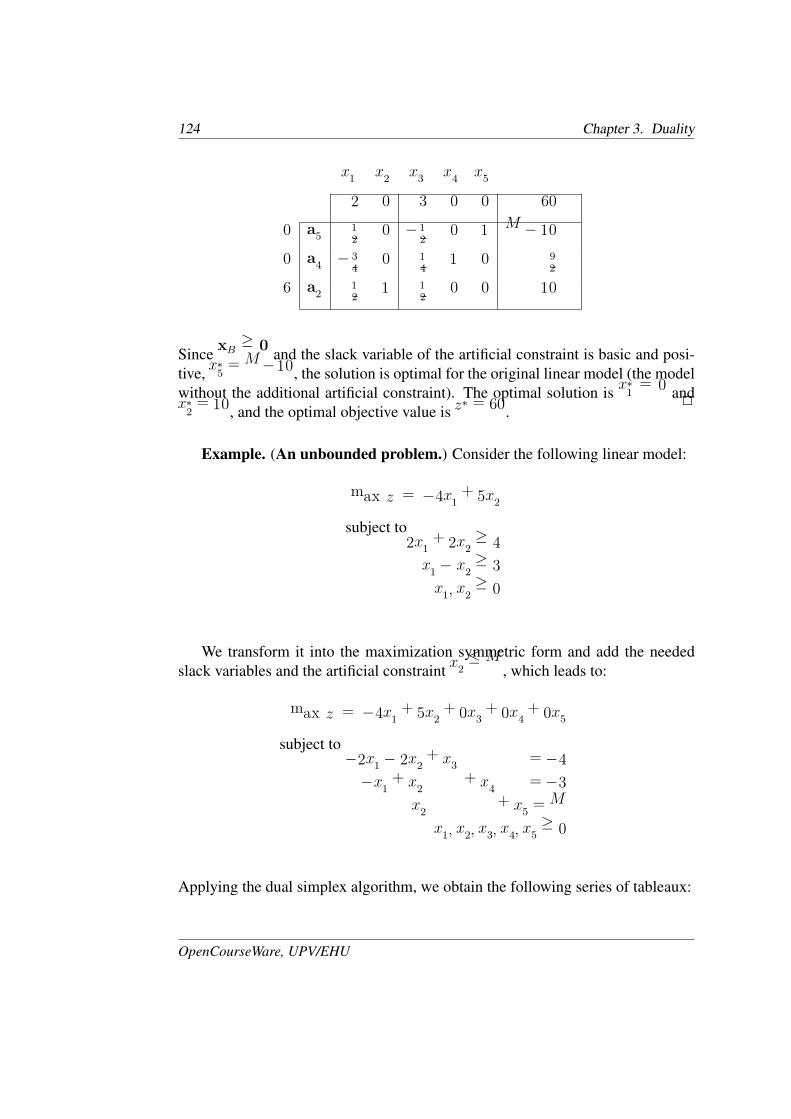
It can be verified that the tableau is dual feasible, and as a consequence, thedual simplex algorithm can now be carried out normally. Vector a3 is selected toleave the basis and vector a5 to enter it. After pivoting, we get:
Operations Research. Linear Programming
124 Chapter 3. Duality
x1 x2 x3 x4 x5
2 0 3 0 0 60
0 a51
20 −1
20 1 M − 10
0 a4 −3
40 1
41 0 9
2
6 a21
21 1
20 0 10
Since xB ≥ 0 and the slack variable of the artificial constraint is basic and posi-tive, x∗
5= M−10, the solution is optimal for the original linear model (the model
without the additional artificial constraint). The optimal solution is x∗
1= 0 and
x∗
2= 10, and the optimal objective value is z∗ = 60. �
Example. (An unbounded problem.) Consider the following linear model:
max z = −4x1 + 5x2
subject to2x1 + 2x2 ≥ 4
x1 − x2 ≥ 3
x1, x2 ≥ 0
We transform it into the maximization symmetric form and add the neededslack variables and the artificial constraint x2 ≤ M , which leads to:
max z = −4x1 + 5x2 + 0x3 + 0x4 + 0x5
subject to−2x1 − 2x2 + x3 = −4
−x1 + x2 + x4 = −3
x2 + x5 = M
x1, x2, x3, x4, x5 ≥ 0
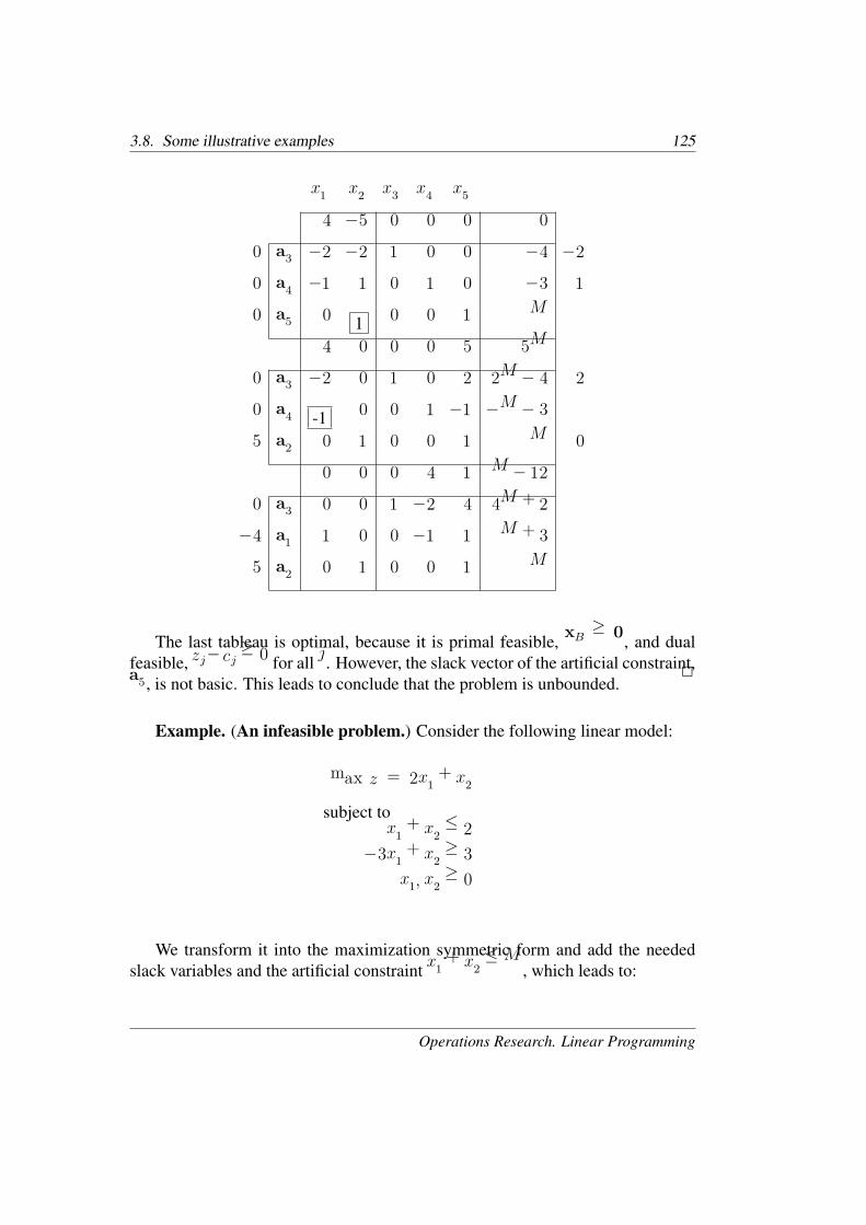
Applying the dual simplex algorithm, we obtain the following series of tableaux:
OpenCourseWare, UPV/EHU
3.8. Some illustrative examples 125
x1 x2 x3 x4 x5
4 −5 0 0 0 0
0 a3 −2 −2 1 0 0 −4 −2
0 a4 −1 1 0 1 0 −3 1
0 a5 0 1 0 0 1 M
4 0 0 0 5 5M
0 a3 −2 0 1 0 2 2M − 4 2
0 a4 -1 0 0 1 −1 −M − 3
5 a2 0 1 0 0 1 M 0
0 0 0 4 1 M − 12
0 a3 0 0 1 −2 4 4M + 2
−4 a1 1 0 0 −1 1 M + 3
5 a2 0 1 0 0 1 M
The last tableau is optimal, because it is primal feasible, xB ≥ 0, and dualfeasible, zj−cj ≥ 0 for all j. However, the slack vector of the artificial constraint,a5, is not basic. This leads to conclude that the problem is unbounded. �
Example. (An infeasible problem.) Consider the following linear model:
max z = 2x1 + x2
subject tox1 + x2 ≤ 2
−3x1 + x2 ≥ 3
x1, x2 ≥ 0
We transform it into the maximization symmetric form and add the neededslack variables and the artificial constraint x1 + x2 ≤ M , which leads to:
Operations Research. Linear Programming
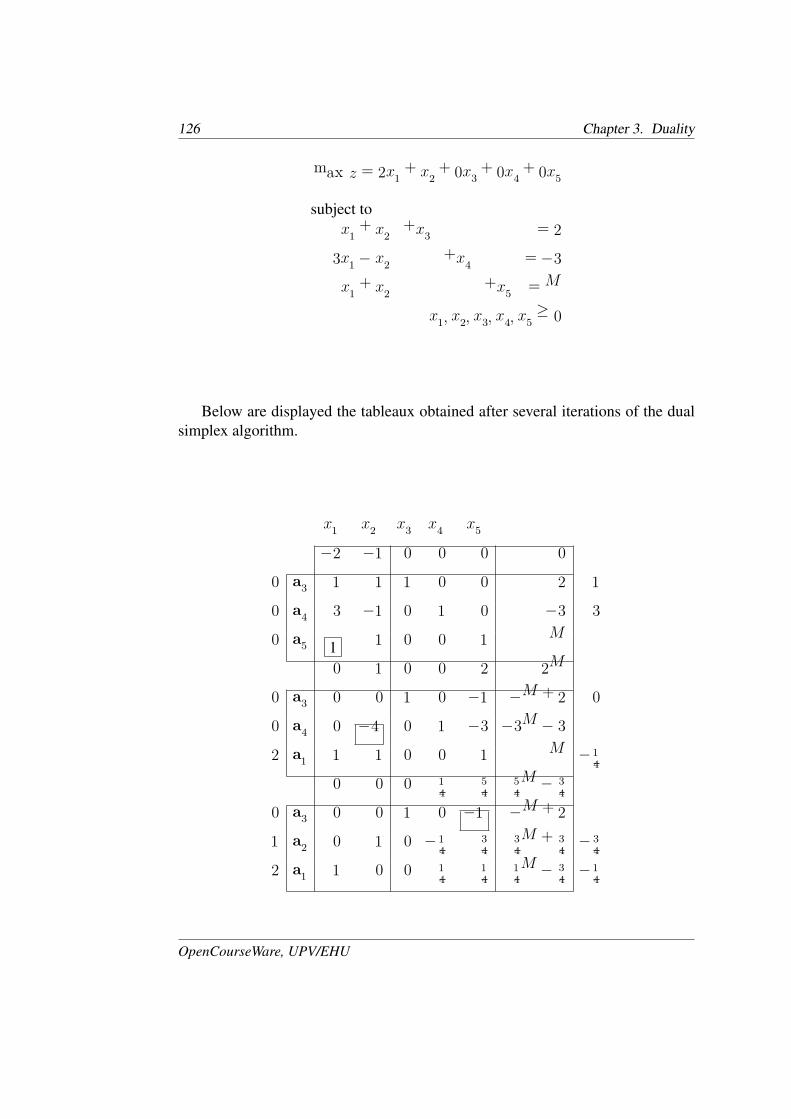
126 Chapter 3. Duality
max z = 2x1 + x2 + 0x3 + 0x4 + 0x5
subject to
x1 + x2 +x3 = 2
3x1 − x2 +x4 = −3
x1 + x2 +x5 = M
x1, x2, x3, x4, x5 ≥ 0
Below are displayed the tableaux obtained after several iterations of the dualsimplex algorithm.
x1 x2 x3 x4 x5
−2 −1 0 0 0 0
0 a3 1 1 1 0 0 2 1
0 a4 3 −1 0 1 0 −3 3
0 a5 1 1 0 0 1 M
0 1 0 0 2 2M
0 a3 0 0 1 0 −1 −M + 2 0
0 a4 0 −4 0 1 −3 −3M − 3
2 a1 1 1 0 0 1 M −1
4
0 0 0 1
4
5
4
5
4M − 3
4
0 a3 0 0 1 0 −1 −M + 2
1 a2 0 1 0 −1
4
3
4
3
4M + 3
4−3
4
2 a1 1 0 0 1
4
1
4
1
4M − 3
4−1
4
OpenCourseWare, UPV/EHU
3.8. Some illustrative examples 127
x1 x2 x3 x4 x5
0 0 5
4
1
40 7
4
0 a5 0 0 −1 0 1 M − 2
1 a2 0 1 3
4−1
40 9
4
2 a1 1 0 1
4
1
40 −1
4
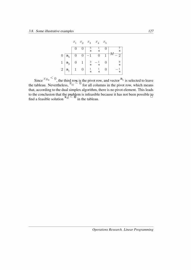
Since xB3 < 0, the third row is the pivot row, and vector a1 is selected to leavethe tableau. Nevertheless, y3j ≥ 0 for all columns in the pivot row, which meansthat, according to the dual simplex algorithm, there is no pivot element. This leadsto the conclusion that the problem is infeasible because it has not been possible tofind a feasible solution xB ≥ 0 in the tableau. �
Operations Research. Linear Programming

128 Chapter 3. Duality
OpenCourseWare, UPV/EHU