A Hybrid Randomized/Nonlinear Programming Technique For Small Aerial Vehicle Trajectory Planning in 3D

A Hybrid Randomized/Nonlinear Programming Technique For Small Aerial

Vehicle Trajectory Planning in 3D

Patrick M. Bouffard

Electrical Engineering and Computer Sciences

University of California, Berkeley

[email protected]

Steven L. Waslander

Mechanical and Mechatronics Engineering

University of Waterloo

[email protected]

Abstract— The use of small aerial vehicles (SAVs) such asquadrotors for inspection and surveillance applications bothindoors and out is well established, but motion planningtechniques are needed which can be calculated in real-timeand which result in provably safe vehicle motion in tightlyconstrained 3D environments. Applied to small quadrotor he-licopters, our planning algorithm combines Probabilistic RoadMaps (PRMs) with Nonlinear Programming (NLP) to yielddynamically feasible, collision-free trajectories in nontrivial en-vironments. Dynamics are incorporated as equality constraintsin the NLP formulation, using a multiple shooting transcription.A key challenge is collision avoidance, accomplished via NLPinequality constraints. Simulation results for complex (thou-sands of polygons) indoor and cave environments are presented,showing complete plans computed more quickly than they canbe flown.

I. INTRODUCTION

Small Aerial Vehicles (SAVs) such as quadrotors [1] are

becoming increasingly well established for surveillance and

inspection applications, with both outdoor [2] and indoor

[3] flight demonstrated by various research groups. Con-

trol and stability issues for quadrotor platforms have been

largely addressed, as demonstrated by the availability of

turnkey quadrotor systems such as the Aeryon Scout [4] or

the Microdrones GmbH MD4-200 [5]. For such agents to

achieve their ultimate potential as mobile sensor platforms

and/or payload delivery agents, a greater degree of autonomy

will be required. Much of the human intervention required

today for remotely operated vehicles has to do with piloting

to navigate complex environments. This amounts to a path

planning problem if the map is known perfectly in advance,

and its automation would free up the human operator for

more high-level tasks such as defining high-level objectives

or interpreting collected sensor data. Many techniques have

been proposed [6], [7], [8], [9], [10] for this type of mo-

tion planning, with both randomized kinodynamic planning

[11] and nonlinear optimization techniques [12] commonly

implemented.

When the full vehicle dynamics (herein, a 10-state model)

are considered, and with obstacles defined in detail as

would be required in real-world situations (i.e. thousands of

polygons), the parameter space of the problem is enormous.

The advantage of randomized methods is in their rapid

exploration of high dimensional spaces, providing feasi-

ble solutions much more rapidly than optimization based

methods. On the other hand, optimization methods result in

locally optimal control inputs and therefore achieve flyable

and appealing trajectories more easily, whereas randomized

selection of control inputs leads to circuitous paths that can

be far from distance or time optimal. The complementarity

of these approaches suggests the use of a hybrid algorithm,

and indeed this approach has been demonstrated [6] to

find solutions with improved computational complexity over

pure optimization techniques and improved optimality of the

solution over randomized planners alone.

Our approach seeks to build on the existing results from

[6] to ensure safe and efficient operation in known 3D

environments by combining PRMs [13] and NLP [14] to

create locally optimal plans with predetermined safe end

points. The PRM focuses on searching the 3D environment

for connectivity of the free space, while NLP focuses on

satisfying kinodynamic constraints and short horizon cost

metrics. The nonlinear optimization is performed with a fixed

time horizon, and seeks to minimize control action with a

trajectory derived from the shortest path determined from the

PRM. The planner maintains at all times a plan that ends at

a safe hover condition, thereby ensuring that the vehicle can

safely pause while further planning is performed.

Incorporating collision avoidance constraints without re-

stricting the nature of the environment is challenging due

to the nonsmooth nature of the proximity function, and

integrating this into the NLP solver framework presents

some additional technical challenges. We address this by

leveraging available research tools for proximity queries, and

with a special distance heuristic to deal with the solution

behaviour under certain circumstances.

II. PROBLEM FORMULATION

This section describes in greater detail the problem at

hand. First, the formulation of the models of environment

and vehicle are detailed. Then the path planning problem is

described in detail.

A. Vehicle Model

In a quadrotor helicopter the four equal-sized rotors are

controlled independently to generate net forces and moments

that allow all maneuvering to be accomplished. For example,

63

Iros 2009 3rd Workshop: Planning, Perception and Navigation for Intelligent Vehicles

(a) (b)

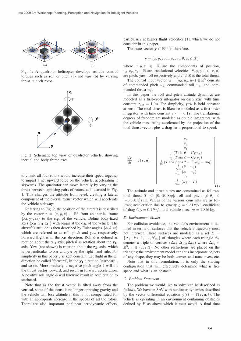
Fig. 1: A quadrotor helicopter develops attitude control

torques such as roll or pitch (a) and yaw (b) by varying

thrust at each rotor.

ϕ

θ

��

��

��

��

� �

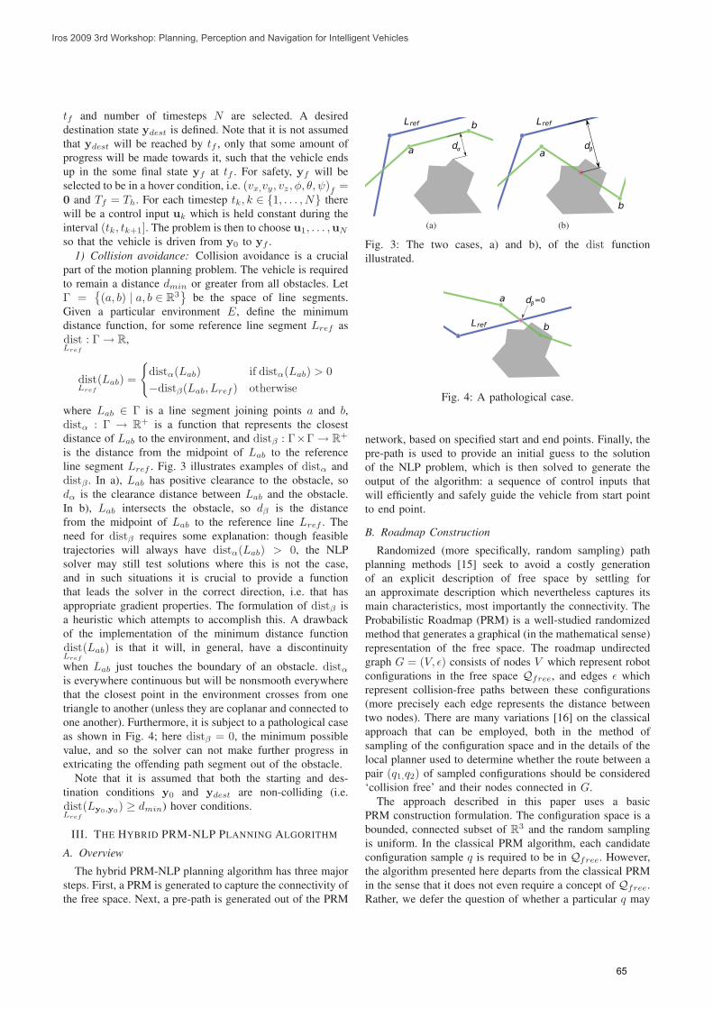
Fig. 2: Schematic top view of quadrotor vehicle, showing

inertial and body frame axes.

to climb, all four rotors would increase their speed together

to impart a net upward force on the vehicle, accelerating it

skywards. The quadrotor can move laterally by varying the

thrust between opposing pairs of rotors, as illustrated in Fig.

1. This changes the attitude from level, creating a lateral

component of the overall thrust vector which will accelerate

the vehicle sideways.

Referring to Fig. 2, the position of the aircraft is described

by the vector r = (x, y, z) ∈ R3 from an inertial frame

{xI,yI, zI} to the c.g. of the vehicle. Define body-fixed

axes {xB,yB, zB} with origin at the c.g. of the vehicle. The

aircraft’s attitude is then described by Euler angles {φ, θ, ψ}which are referred to as roll, pitch and yaw respectively.

Forward flight is in the xB direction. Roll φ is defined as

rotation about the xB axis, pitch θ as rotation about the yB

axis. Yaw (not shown) is rotation about the zB axis, which

is perpendicular to xB and yB by the right hand rule. For

simplicity in this paper ψ is kept constant. Let flight in the xI

direction be called ’forward’, in the yI direction ’starboard’,

and so on. More precisely, a negative pitch angle θ will tilt

the thrust vector forward, and result in forward acceleration.

A positive roll angle φ will likewise result in acceleration to

starboard.

Note that as the thrust vector is tilted away from the

vertical, some of the thrust is no longer opposing gravity and

the vehicle will lose altitude if this is not compensated for

with an appropriate increase in the speeds of all the rotors.

There are also important nonlinear aerodynamic effects,

particularly at higher flight velocities [1], which we do not

consider in this paper.

The state vector y ⊂ R10 is therefore,

y = (x, y, z, vx, vy, vz, θ, φ, ψ, T )

where x, y, z ∈ R are the components of position,

vx, vy, vz ∈ R are translational velocities, θ, φ, ψ ∈ (−π, π)are pitch, yaw, roll respectively and T ∈ R is the total thrust.

The control input vector u = (uθ, uφ, uT ) ∈ R3 consists

of commanded pitch uθ, commanded roll uφ, and com-

manded thrust uT .

In this paper the roll and pitch attitude dynamics are

modeled as a first-order integrator on each axis, with time

constant τatt = 1.0 s. For simplicity, yaw is held constant

at zero. The total thrust is likewise modeled as a first-order

integrator, with time constant τthr = 0.1 s. The translational

degrees of freedom are modeled as double integrators, with

the vehicle mass being accelerated by the projection of the

total thrust vector, plus a drag term proportional to speed.

dy

dt= f(y,u) =

vx

vy

vz1

m(T sin θ − CDvx)

1

m(T sinφ− CDvy)

1

m(T cosφ cos θ − CDvz −mg)

1

τatt(θ − uθ)

1

τatt(φ− uφ)

01

τthr(uT − T )

(1)

The attitude and thrust states are constrained as follows:

total thrust T ∈ [0, 4(0.8)g]; roll and pitch {φ, θ} ∈[−0.3, 0.3] rad. Values of the various constants are as fol-

lows; acceleration due to gravity g = 9.81 m/s2, coefficient

of drag CD = 0.1 N·s/m and vehicle mass m = 1.826 kg.

B. Environment Model

For collision avoidance, the vehicle’s environment is de-

fined in terms of surfaces that the vehicle’s trajectory must

not intersect. These surfaces are modeled as a set E ={∆k | k ∈ 1, . . . , Ntri} of triangles where each triangle ∆k

denotes a triple of vertices (∆k1,∆k2,∆k3) where ∆kj ∈R

3, j ∈ (1, 2, 3). No other restrictions are placed on the

triangles; the environment model can thus incorporate objects

of any shape, they may be both convex and nonconvex, etc.

Note that in this formulation, it is only the starting

configuration that will effectively determine what is free

space and what is an obstacle.

C. Problem Statement

The problem we would like to solve can be described as

follows. We have an SAV with nonlinear dynamics described

by the vector differential equation y(t) = f(y,u, t). The

vehicle is operating in an environment containing obstacles

defined by E as above which it must avoid. A final time

64


tf and number of timesteps N are selected. A desired

destination state ydest is defined. Note that it is not assumed

that ydest will be reached by tf , only that some amount of

progress will be made towards it, such that the vehicle ends

up in the some final state yf at tf . For safety, yf will be

selected to be in a hover condition, i.e. (vx,vy, vz, φ, θ, ψ)f

=0 and Tf = Th. For each timestep tk, k ∈ {1, . . . , N} there

will be a control input uk which is held constant during the

interval (tk, tk+1]. The problem is then to choose u1, . . . ,uN

so that the vehicle is driven from y0 to yf .

1) Collision avoidance: Collision avoidance is a crucial

part of the motion planning problem. The vehicle is required

to remain a distance dmin or greater from all obstacles. Let

Γ ={

(a, b) | a, b ∈ R3}

be the space of line segments.

Given a particular environment E, define the minimum

distance function, for some reference line segment Lref as

distLref

: Γ → R,

distLref

(Lab) =

{

distα(Lab) if distα(Lab) > 0

−distβ(Lab, Lref ) otherwise

where Lab ∈ Γ is a line segment joining points a and b,distα : Γ → R

+ is a function that represents the closest

distance of Lab to the environment, and distβ : Γ×Γ → R+

is the distance from the midpoint of Lab to the reference

line segment Lref . Fig. 3 illustrates examples of distα and

distβ . In a), Lab has positive clearance to the obstacle, so

dα is the clearance distance between Lab and the obstacle.

In b), Lab intersects the obstacle, so dβ is the distance

from the midpoint of Lab to the reference line Lref . The

need for distβ requires some explanation: though feasible

trajectories will always have distα(Lab) > 0, the NLP

solver may still test solutions where this is not the case,

and in such situations it is crucial to provide a function

that leads the solver in the correct direction, i.e. that has

appropriate gradient properties. The formulation of distβ is

a heuristic which attempts to accomplish this. A drawback

of the implementation of the minimum distance function

distLref

(Lab) is that it will, in general, have a discontinuity

when Lab just touches the boundary of an obstacle. distα

is everywhere continuous but will be nonsmooth everywhere

that the closest point in the environment crosses from one

triangle to another (unless they are coplanar and connected to

one another). Furthermore, it is subject to a pathological case

as shown in Fig. 4; here distβ = 0, the minimum possible

value, and so the solver can not make further progress in

extricating the offending path segment out of the obstacle.

Note that it is assumed that both the starting and des-

tination conditions y0 and ydest are non-colliding (i.e.

distLref

(Ly0,y0) ≥ dmin) hover conditions.

III. THE HYBRID PRM-NLP PLANNING ALGORITHM

A. Overview

The hybrid PRM-NLP planning algorithm has three major

steps. First, a PRM is generated to capture the connectivity of

the free space. Next, a pre-path is generated out of the PRM

�

��

��

(a)

�

�

��

��

(b)

Fig. 3: The two cases, a) and b), of the dist function

illustrated.

�

��

��

Fig. 4: A pathological case.

network, based on specified start and end points. Finally, the

pre-path is used to provide an initial guess to the solution

of the NLP problem, which is then solved to generate the

output of the algorithm: a sequence of control inputs that

will efficiently and safely guide the vehicle from start point

to end point.

B. Roadmap Construction

Randomized (more specifically, random sampling) path

planning methods [15] seek to avoid a costly generation

of an explicit description of free space by settling for

an approximate description which nevertheless captures its

main characteristics, most importantly the connectivity. The

Probabilistic Roadmap (PRM) is a well-studied randomized

method that generates a graphical (in the mathematical sense)

representation of the free space. The roadmap undirected

graph G = (V, ε) consists of nodes V which represent robot

configurations in the free space Qfree, and edges ε which

represent collision-free paths between these configurations

(more precisely each edge represents the distance between

two nodes). There are many variations [16] on the classical

approach that can be employed, both in the method of

sampling of the configuration space and in the details of the

local planner used to determine whether the route between a

pair (q1,q2) of sampled configurations should be considered

‘collision free’ and their nodes connected in G.

The approach described in this paper uses a basic

PRM construction formulation. The configuration space is a

bounded, connected subset of R3 and the random sampling

is uniform. In the classical PRM algorithm, each candidate

configuration sample q is required to be in Qfree. However,

the algorithm presented here departs from the classical PRM

in the sense that it does not even require a concept of Qfree.

Rather, we defer the question of whether a particular q may

65


Algorithm 1 Roadmap query refinement

1) Q′′ := {q1}2) a := 13) b := 24) while b < M ′:

5) while distLref

(Lab) > dmin:

6) increment b7) append qb−1 to Q′′

8) a := b− 19) Q′′′ := reverse(Q′′)

10) repeat steps 2-8 with Q′′′ instead of Q′′

11) return reverse(Q′′′)

be part of a feasible plan until a later phase, the query phase.

Indeed, the entire configuration space of the robot, i.e. the 10-

dimensional state space with appropriate constraints, is not

dealt with by the PRM at all; that is the later responsibility

of the NLP.

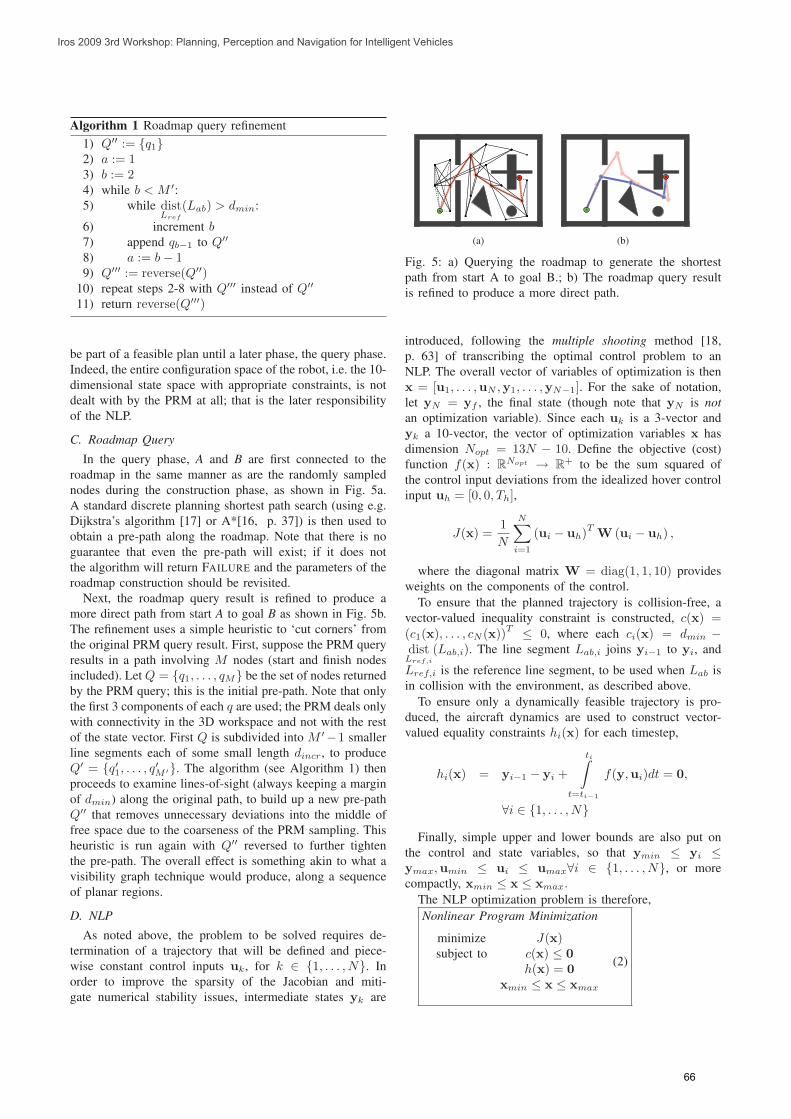
C. Roadmap Query

In the query phase, A and B are first connected to the

roadmap in the same manner as are the randomly sampled

nodes during the construction phase, as shown in Fig. 5a.

A standard discrete planning shortest path search (using e.g.

Dijkstra’s algorithm [17] or A*[16, p. 37]) is then used to

obtain a pre-path along the roadmap. Note that there is no

guarantee that even the pre-path will exist; if it does not

the algorithm will return FAILURE and the parameters of the

roadmap construction should be revisited.

Next, the roadmap query result is refined to produce a

more direct path from start A to goal B as shown in Fig. 5b.

The refinement uses a simple heuristic to ‘cut corners’ from

the original PRM query result. First, suppose the PRM query

results in a path involving M nodes (start and finish nodes

included). Let Q = {q1, . . . , qM} be the set of nodes returned

by the PRM query; this is the initial pre-path. Note that only

the first 3 components of each q are used; the PRM deals only

with connectivity in the 3D workspace and not with the rest

of the state vector. First Q is subdivided into M ′−1 smaller

line segments each of some small length dincr, to produce

Q′ = {q′1, . . . , q′

M ′}. The algorithm (see Algorithm 1) then

proceeds to examine lines-of-sight (always keeping a margin

of dmin) along the original path, to build up a new pre-path

Q′′ that removes unnecessary deviations into the middle of

free space due to the coarseness of the PRM sampling. This

heuristic is run again with Q′′ reversed to further tighten

the pre-path. The overall effect is something akin to what a

visibility graph technique would produce, along a sequence

of planar regions.

D. NLP

As noted above, the problem to be solved requires de-

termination of a trajectory that will be defined and piece-

wise constant control inputs uk, for k ∈ {1, . . . , N}. In

order to improve the sparsity of the Jacobian and miti-

gate numerical stability issues, intermediate states yk are

�

�

(a)

�

�

(b)

Fig. 5: a) Querying the roadmap to generate the shortest

path from start A to goal B.; b) The roadmap query result

is refined to produce a more direct path.

introduced, following the multiple shooting method [18,

p. 63] of transcribing the optimal control problem to an

NLP. The overall vector of variables of optimization is then

x = [u1, . . . ,uN ,y1, . . . ,yN−1]. For the sake of notation,

let yN = yf , the final state (though note that yN is not

an optimization variable). Since each uk is a 3-vector and

yk a 10-vector, the vector of optimization variables x has

dimension Nopt = 13N − 10. Define the objective (cost)

function f(x) : RNopt → R

+ to be the sum squared of

the control input deviations from the idealized hover control

input uh = [0, 0, Th],

J(x) =1

N

N∑

i=1

(ui − uh)T

W (ui − uh) ,

where the diagonal matrix W = diag(1, 1, 10) provides

weights on the components of the control.

To ensure that the planned trajectory is collision-free, a

vector-valued inequality constraint is constructed, c(x) =(c1(x), . . . , cN (x))

T≤ 0, where each ci(x) = dmin −

distLref,i

(Lab,i). The line segment Lab,i joins yi−1 to yi, and

Lref,i is the reference line segment, to be used when Lab is

in collision with the environment, as described above.

To ensure only a dynamically feasible trajectory is pro-

duced, the aircraft dynamics are used to construct vector-

valued equality constraints hi(x) for each timestep,

hi(x) = yi−1 − yi +

tiˆ

t=ti−1

f(y,ui)dt = 0,

∀i ∈ {1, . . . , N}

Finally, simple upper and lower bounds are also put on

the control and state variables, so that ymin ≤ yi ≤ymax,umin ≤ ui ≤ umax∀i ∈ {1, . . . , N}, or more

compactly, xmin ≤ x ≤ xmax.The NLP optimization problem is therefore,

Nonlinear Program Minimization

minimize J(x)subject to c(x) ≤ 0

h(x) = 0

xmin ≤ x ≤ xmax

(2)

66


Scenario Ntri PRM Nodes N tf

SIMPLE 256 200 10 40 s

MAZE 1238 500 18 76 s

TWOSTOREY 2301 500 22 88 s

CAVE 65536 250 10 40 s

TABLE I: Test scenarios

IV. SIMULATION RESULTS

A. Implementation

The hybrid PRM-NLP algorithm was implemented in

software, with the major components readily available as

free software. The most critical of these are the proximity

measurement, for which the Proximity Query Package (PQP)

[19], [20] was used. The use of a dedicated proximity

checker like PQP is critical to avoid that intractability that

would arise if the collision constraints were instead encoded

directly in the NLP; this would add thousands of additional

constraints at each timestep and would also require the

inclusion of binary variables, greatly increasing the problem

complexity. To solve the NLP problem, the IPOPT (Interior

Point Optimizer) [21] solver from the COIN-OR project was

used. Several freely available libraries were also used, for

integration of the dynamics, performing the discrete shortest-

path query, and so on. Notably, the Panda3D library [22] was

indispensable in creating a flexible framework for simulation

development. The main program code was written in Python.

B. Preliminary Results

Several different environments were modeled and the

algorithm was tested in each. Times noted in this section

are CPU time as recorded on a ThinkPad T400 with a 2.8

GHz Intel Core 2 Duo CPU. The scenarios are intended

to be somewhat representative of various indoor navigation

situations. Here, some results for four different scenarios are

presented. They are called SIMPLE, MAZE, TWOSTOREY, and

CAVE. Table I summarizes each in terms of the number Ntri

of triangles in the environment, the number of PRM nodes

used, number of timesteps N , and final time tf .

Each scenario was tested several times to establish prelim-

inary performance of the algorithm. In general, the algorithm

reliably finds a feasible path from start to finish in all the test

scenarios, though no solution guarantees can be made due to

the discontinuity of the distance heuristic. The discontinuous

nature of the distance heuristic does not appear to have

prevented good solutions to be obtained in the present work

in most cases. The notable exception is TWOSTOREY, where

a large proportion of the trials resulted in the trial trajectory

becoming ’stuck’ crossing a wall (this also occurred to

a lesser degree with MAZE). However, a better heuristic

could be formulated to ensure continuity of this important

NLP constraint and perhaps improve the overall performance

(shorter solution times and/or higher likelihood of finding a

feasible solution). Table II shows timings (time to construct

PRM, number of solver iterations required and solver CPU

time used, as well as ratio of CPU time to simulated flying

time) gathered for 10 successful runs for each scenario.

Scenario Construction Solver Iter. CPU RT Ratio

SIMPLE 5.49 s 9.2 25.93 s 0.48

MAZE 22.89 s 10.8 62.52 s 0.72

TWOSTOREY 25.26 s 13.1 86.97 s 0.86

CAVE 9.46 s 8.0 27.37 s 0.59

TABLE II: Algorithm timing results

(a)

(b)

Fig. 6: Typical results for a) SIMPLE and b) MAZE.

Note that the PRM density was selected by trial-and-error

to ensure connectivity. Still, in some runs the PRM did not

succeed in finding sufficient free space connectivity to allow

a path from start to finish to be produced. In practice this

could be improved by increasing the PRM density a priori,

or by adaptively increasing the PRM density in response

to failed PRM queries until either a path can be found or

some number of iterations is exceeded. For most cases, where

the PRM roadmap did succeed in finding a path, the solver

was able to output a flyable trajectory in less time than the

trajectory would take to fly. Fig. 7 illustrates the typical result

for two of the scenarios.

V. CONCLUSIONS AND FUTURE WORK

The results show that the combined PRM-NLP motion

planning algorithm is a promising method of generating safe,

67


(a)

(b)

Fig. 7: Typical results for a) TWOSTOREY and b) CAVE.

flyable trajectories for SAVs. By combining the ability of

PRMs to rapidly explore free space and find connectivity, and

the capability of an NLP solver to generate locally optimal

solution trajectories, the hybrid PRM-NLP algorithm suc-

ceeds in finding safe and flyable trajectories in a reasonable

amount of time even for relatively complex environments.

The planner has been shown to be capable, on a commodity

laptop, of generating plans in less CPU time than the time

length of the plans themselves. This suggests that a receding-

horizon planner could be created and run in real-time.

The algorithm could benefit from a heuristic improving

upon the distβ function described herein, which could reduce

the incidence of the solver becoming ‘stuck’ in environments

where this is an issue. The solver typically spends the first

few iterations to go from the initial guess to a point where

one might consider the ‘true’ optimization is happening.

Thus a better initial guess could improve performance by a

significant amount; existing algorithms that could track the

pre-path would be a good starting point. A minimum time

or maximum distance in fixed time variant could also be of

practical benefit. Also, both the PRM construction and the

solution of the multiple shooting formulation are inherently

parallel and thus naturally suggest a parallel processing im-

plementation. Finally, implementation onboard a real vehicle

such as the Stanford Testbed of Autonomous Rotorcraft for

Multi Agent Control (STARMAC) quadrotor [1] as part of

a larger receding horizon based control framework would

allow such a platform to autonomously formulate plans in

complex indoor or outdoor environments.

REFERENCES

[1] G. M. Hoffmann, H. Huang, S. L. Waslander, and C. J. Tomlin,“Quadrotor helicopter flight dynamics and control: Theory and experi-ment,” in Proceedings of the AIAA Guidance, Navigation, and Control

Conference and Exhibit, (Hilton Head, SC), Aug. 2007.[2] R. R. Murphy, K. S. Pratt, and J. L. Burke, “Crew roles and operational

protocols for Rotary-Wing Micro-UAVs in close urban environments,”in HRI ’08: Proceedings of the 3rd ACM/IEEE International Confer-

ence on Human Robot Interaction, (New York, NY, USA), pp. 73–80,ACM, 2008.

[3] J. Zufferey, A. Beyeler, and D. Floreano, “Near-obstacle flight withsmall UAVs,” in UAV’2008: International Symposium on Unmanned

Aerial Vehicles, June 2008.[4] “Aeryon scout.” http://www.aeryon.com/products/scout.html. Last ac-

cessed by the authors on 15 July 2009.[5] “MD4-200.” http://www.microdrones.com/en_md4-200.php. Last ac-

cessed by the authors on 15 July 2009.[6] T. Karatas and F. Bullo, “Randomized searches and nonlinear pro-

gramming in trajectory planning,” in Proceedings of the 40th IEEE

Conference on Decision and Control, (Orlando, FL, USA), 2001.[7] M. Vitus, V. Pradeep, G. M. Hoffmann, S. L. Waslander, and C. J.

Tomlin, “Tunnel-MILP: path planning with sequential convex poly-topes,” in Proceedings of the 2008 AIAA Guidance, Navigation and

Control Conference and Exhibit, (Honolulu, Hawaii, USA), Aug. 2008.[8] J. Bellingham, A. Richards, and J. How, “Receding horizon control

of autonomous aerial vehicles,” in Proceedings of the 2002 American

Control Conference, vol. 5, pp. 3741–3746, 2002.[9] Y. Kuwata, G. A. Fiore, J. Teo, E. Frazzoli, and J. How, “Motion

planning for urban driving using RRT,” in Proceedings of the 2008

IEEE/RSJ International Conference on Intelligent Robots and Systems,pp. 1681–1686, 2008.

[10] Y. Kuwata and J. How, “Three dimensional receding horizon controlfor UAVs,” (Providence, Rhode Island), Aug. 2004.

[11] J. Barraquand, L. Kavraki, J. Latombe, T. Li, R. Motwani, andP. Raghavan, “A random sampling scheme for path planning,” The

International Journal of Robotics Research, vol. 16, no. 6, pp. 759–774, 1997.

[12] A. Richards and J. How, “Aircraft trajectory planning with collisionavoidance using mixed integer linear programming,” in Proceedings of

the 2002 American Control Conference, vol. 3, pp. 1936–1941, 2002.[13] L. E. Kavraki, P. Svestka, J. Latombe, and M. H. Overmars, “Proba-

bilistic roadmaps for path planning in High-Dimensional configurationspaces,” IEEE Transactions on Robotics and Automation, vol. 12,pp. 566–580, Aug. 1996.

[14] D. Bertsekas, Nonlinear Programming. Belmont, WA: Athena Scien-tific, 1995.

[15] J. Latombe, “Motion planning: A journey of robots, molecules, digitalactors, and other artifacts,” The International Journal of Robotics

Research, vol. 18, no. 11, pp. 1119–1128, 1999.[16] S. M. LaValle, Planning Algorithms. Cambridge University Press,

2006.[17] E. W. Dijkstra, “A note on two problems in connexion with graphs,”

Numerische Mathematik, vol. 1, no. 1, pp. 269–271, 1959.[18] J. T. Betts, Practical Methods for Optimal Control Using Nonlinear

Programming. 2001.[19] E. Larsen, S. Gottschalk, M. C. Lin, and D. Manocha, “Fast prox-

imity queries with swept sphere volumes,” Technical Report 99-018,Department of Computer Science, University of N. Carolina, ChapelHill, NC, 1999.

[20] S. Gottschalk, M. Lin, D. Manocha, and E. Larsen, “PQP - aproximity query package.” http://www.cs.unc.edu/~geom/SSV/, 1999.Last accessed by the authors on 15 July 2009. Version 1.3.

[21] A. Wachter and L. T. Biegler, “On the implementation of an interior-point filter line-search algorithm for large-scale nonlinear program-ming,” Mathematical Programming, vol. 106, pp. 25–57, Mar. 2006.

[22] M. Goslin and M. R. Mine, “The Panda3D graphics engine,” Com-

puter, vol. 37, pp. 112–114, Oct. 2004.

68


Documents

A Hybrid Randomized/Nonlinear Programming Technique For Small Aerial Vehicle Trajectory Planning in 3D