A Dissertation

entitled

Essays on Biopharmaceutical Supply Chains

by

Marouen Ben Jebara

Submitted to the Graduate Faculty as partial fulfillment of the requirements for Doctor of

Philosophy Degree in

Manufacturing and Technology Management

________________________________________

Dr. Sachin Modi, Committee Co-Chair

_______________________________________

Dr. Ram Rachamadugu, Committee Co-Chair

________________________________________

Dr. Jenell Wittmer, Committee Member

________________________________________

Dr. Dong-Shik Kim, Committee Member

The University of Toledo

August, 2015

Copyright 2015, Marouen Ben Jebara

This document is copyrighted material. Under copyright law, no parts of this document

may be reproduced without the expressed permission of the author.

iii

An Abstract of

Essays on Biopharmaceutical Supply Chains

by

Marouen Ben Jebara

Submitted to the Graduate Faculty as partial fulfillment of Proposal for the

Doctor of Philosophy Degree in

Manufacturing and Technology Management

The University of Toledo

August, 2015

An emerging trend in the pharmaceutical industry is the high level of personalization of

medicines that firms offer today. Such medications are expected to account for 50% of the

amount spent on drugs by 2018. In conjunction with the growth of this new class of

medications, firms are also continuing to serve markets for traditional (or small molecule)

medications, which are often standardized or mass customized for consumer markets.

Managing the diverse portfolio of medications can require different supply chain

structures, specifically with respect to distribution channels. For example, the prostate

cancer vaccine involves a reverse flow of raw material in the form of patient blood cells

from the hospital/physician clinic to the pharmaceutical firm processing centers – a

characteristic that is often not seen with traditional medications that are dispensed at the

pharmacy or hospital. This has led to a new trend in the distribution channel practices for

such medication, i.e. supply chain disintermediation, where the firm engages in a direct

sales model, which means that the medication is shipped directly to the patient or the

administrating facility (e.g. the physician’s clinic/hospital) instead of being distributed

through the traditional channel of wholesalers. In summary, firms today have a choice of

iv

structuring their supply chains to have a traditional intermediated distribution channel, a

direct disintermediated distribution channel, or combination thereof. However, little

research exists that can guide managerial decisions with respect to the appropriate supply

chain structure given the portfolio of the firm’s medication offerings. The firm’s choices

for product portfolio and supply chain structure for distribution channels raise a critical

question of ‘what is the most appropriate supply chain disintermediation strategy given

the firm’s product portfolio?’ Therefore, in this dissertation, the research objective is to

address this central question. In addressing this research objective, the dissertation is

composed of four distinct essays.

The first essay is aimed at answering the above question conceptually. It maps the

evolution of the pharmaceutical product paradigm along a continuum of standardized/mass

customized/mass personalized products as well as discusses the evolution of the supply

chain structure in terms of disintermediation for pharmaceutical firms. Drawing on

literature in operations management in the areas of mass customization and supply chain

disintermediation, as well as industry practices, the study presents a framework which

identifies the appropriate supply chain structure (intermediated vs. disintermediated) given

the level of personalization of pharmaceutical products.

Additionally, a critical characteristic of personalized (biologics) medicine is its

time sensitive nature and consequent market mediation costs that make logistical design a

critical issue. To understand how management science tools can guide managerial decision

making, the second essay investigates this location decision problem for highly

personalized products under a total disintermediation strategy assumption. Results based

on the analysis of a case study are presented.

v

In addition to the time sensitivity and consequent market mediation costs that result

from the short shelf life of personalized (biologics) products, firms also face varying levels

of demand uncertainty for such products, making the disintermediation strategy decisions

crucial. Therefore, the third essay aims to understand the behavior of the total market

mediation costs, given the level of demand variability and the firm’s supply chain

disintermediation strategy. An evaluative study based on a scenario approach is presented.

The results from a scenario approach analysis and a large scale numerical study provide

insights about the appropriate supply chain disintermediation strategy given the

pharmaceutical firm’s product characteristics. The results shows the dominance of demand

variability in shaping the total market mediation cost. High demand variability favors

intermediated distribution channels, whereas disintermediation strategy is preferred when

the shortage cost ratio is high. The contrast analysis provides evidence of the area of

distribution strategy indifference.

Finally, recognizing that a pharmaceutical firm’s choice regarding its product

portfolio (standardized/mass customized/mass personalized products) and supply chain

disintermediation strategy (intermediated/hybrid/disintermediated) has implications for its

financial performance, the fourth essay aims to empirically assess the financial

performance consequences of the fit between the firm’s product portfolio and its supply

chain disintermediation strategy. This essay empirically examines the relationship between

disintermediation, product portfolio strategy, and financial performance. The results show

that supply chain disintermediation positively impacts the firms’ financial performance.

Additionally, the alignment between product portfolio and supply chain disintermediation

has positive effects on return on assets and gross margin.

vi

This dissertation contributes to operations management literature in terms of

conceptually, analytically, and empirically assessing how a firm’s choices for product

personalization and supply chain disintermediation individually and collectively influence

its performance. It aims to provide actionable guidelines that can help firms match their

supply chain disintermediation strategy with their product portfolio characteristics.

In Loving Memory of my Mother

1

1 Acknowledgements

This work is a labor of love, completed with the boundless encouragement from and sacrifices of

my family, friends, and mentors. This work would not have been achieved without their endless

help and motivation. For all who contributed to this work, I am grateful.

First, I am deeply indebted to my advisers, Dr. Ram Rachamadugu and Dr. Sachin Modi,

for their fundamental roles in my doctoral work. They provided me with countless hours of

guidance, assistance, and expertise. I am very thankful for and undoubtedly appreciative of their

constructive feedback, inspiring comments, and clear direction, as well as their time, effort, and

commitment to this doctoral work.

Second, I would like to thank my committee members, Dr. Jenell Wittmer and Dr. Dong-

Shik Kim, for their assistance and insightful guidance. Their dedication to excellence and a strong

work ethic provided me with extra motivation and was a source of inspiration. For all their efforts,

I am also deeply grateful. I would also like to express my appreciation to the faculty, staff, and my

fellow cohorts at the College of Business and Innovation. Your help is, and has been, much

appreciated.

Finally, there are no words that express my appreciation to my wife, Neda, for all the

sacrifices, long nights, motivation, and post-it notes…. The list could go on and on, as I am sure

that she has struggled as much as I have in this undertaking. For all that and more, I am deeply

grateful. I would like to express my gratitude to my father, sister, brother, and my in-laws for the

endless support.

2

2 Table of Contents

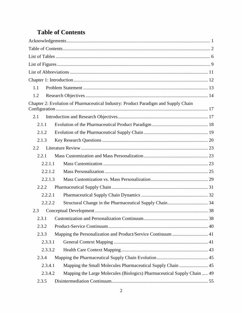
Acknowledgements ......................................................................................................................... 1

Table of Contents ............................................................................................................................ 2

List of Tables .................................................................................................................................. 6

List of Figures ................................................................................................................................. 9

List of Abbreviations .................................................................................................................... 11

Chapter 1: Introduction ................................................................................................................. 12

1.1 Problem Statement ......................................................................................................... 13

1.2 Research Objectives ....................................................................................................... 14

Chapter 2: Evolution of Pharmaceutical Industry: Product Paradigm and Supply Chain

Configuration ................................................................................................................................ 17

2.1 Introduction and Research Objectives............................................................................ 17

2.1.1 Evolution of the Pharmaceutical Product Paradigm ............................................... 18

2.1.2 Evolution of the Pharmaceutical Supply Chain ...................................................... 19

2.1.3 Key Research Questions ......................................................................................... 20

2.2 Literature Review ........................................................................................................... 23

2.2.1 Mass Customization and Mass Personalization ...................................................... 23

2.2.1.1 Mass Customization ........................................................................................ 23

2.2.1.2 Mass Personalization ....................................................................................... 25

2.2.1.3 Mass Customization vs. Mass Personalization ................................................ 29

2.2.2 Pharmaceutical Supply Chain ................................................................................. 31

2.2.2.1 Pharmaceutical Supply Chain Dynamics ........................................................ 32

2.2.2.2 Structural Change in the Pharmaceutical Supply Chain .................................. 34

2.3 Conceptual Development ............................................................................................... 38

2.3.1 Customization and Personalization Continuum ...................................................... 38

2.3.2 Product-Service Continuum .................................................................................... 40

2.3.3 Mapping the Personalization and Product/Service Continuum .............................. 41

2.3.3.1 General Context Mapping ............................................................................... 41

2.3.3.2 Health Care Context Mapping ......................................................................... 43

2.3.4 Mapping the Pharmaceutical Supply Chain Evolution ........................................... 45

2.3.4.1 Mapping the Small Molecules Pharmaceutical Supply Chain ........................ 45

2.3.4.2 Mapping the Large Molecules (Biologics) Pharmaceutical Supply Chain ..... 49

2.3.5 Disintermediation Continuum ................................................................................. 55

3

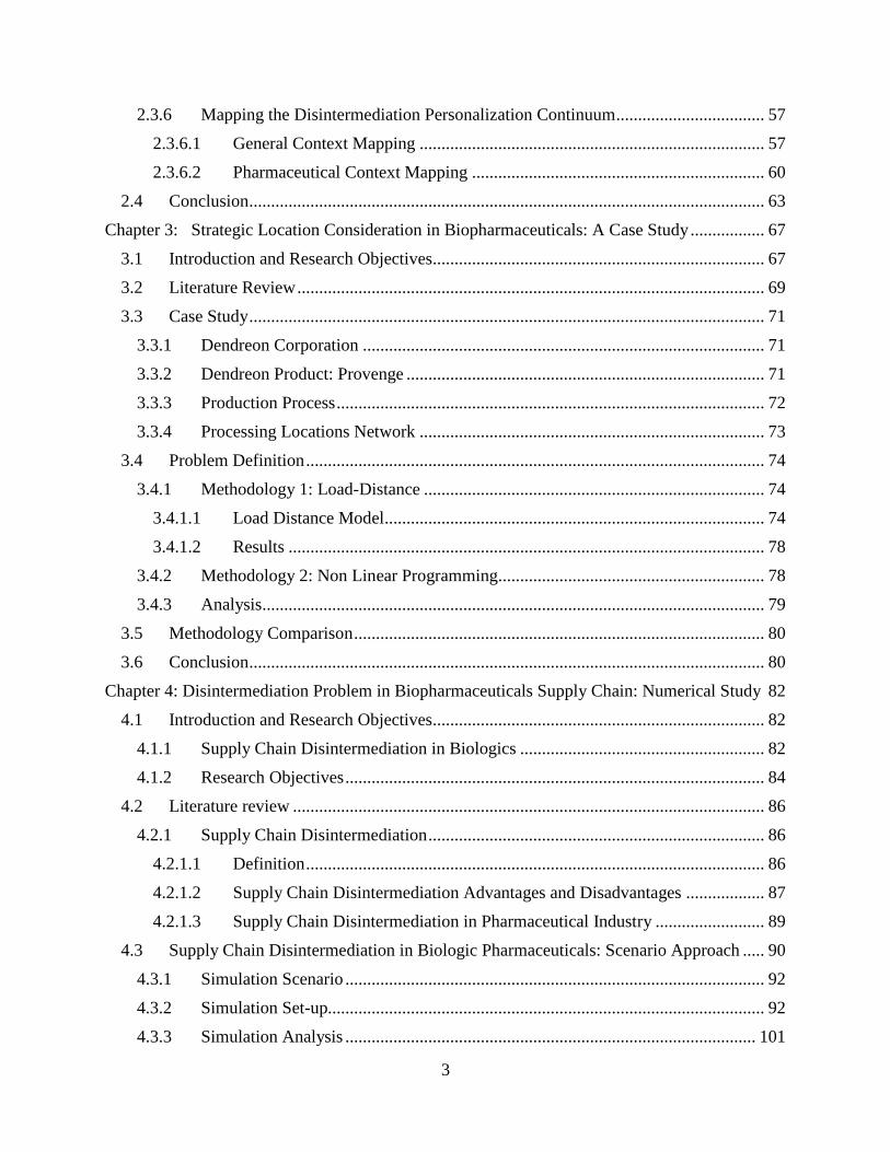
2.3.6 Mapping the Disintermediation Personalization Continuum .................................. 57

2.3.6.1 General Context Mapping ............................................................................... 57

2.3.6.2 Pharmaceutical Context Mapping ................................................................... 60

2.4 Conclusion ...................................................................................................................... 63

Chapter 3: Strategic Location Consideration in Biopharmaceuticals: A Case Study ................. 67

3.1 Introduction and Research Objectives............................................................................ 67

3.2 Literature Review ........................................................................................................... 69

3.3 Case Study ...................................................................................................................... 71

3.3.1 Dendreon Corporation ............................................................................................ 71

3.3.2 Dendreon Product: Provenge .................................................................................. 71

3.3.3 Production Process .................................................................................................. 72

3.3.4 Processing Locations Network ............................................................................... 73

3.4 Problem Definition ......................................................................................................... 74

3.4.1 Methodology 1: Load-Distance .............................................................................. 74

3.4.1.1 Load Distance Model ....................................................................................... 74

3.4.1.2 Results ............................................................................................................. 78

3.4.2 Methodology 2: Non Linear Programming............................................................. 78

3.4.3 Analysis................................................................................................................... 79

3.5 Methodology Comparison .............................................................................................. 80

3.6 Conclusion ...................................................................................................................... 80

Chapter 4: Disintermediation Problem in Biopharmaceuticals Supply Chain: Numerical Study 82

4.1 Introduction and Research Objectives............................................................................ 82

4.1.1 Supply Chain Disintermediation in Biologics ........................................................ 82

4.1.2 Research Objectives ................................................................................................ 84

4.2 Literature review ............................................................................................................ 86

4.2.1 Supply Chain Disintermediation ............................................................................. 86

4.2.1.1 Definition ......................................................................................................... 86

4.2.1.2 Supply Chain Disintermediation Advantages and Disadvantages .................. 87

4.2.1.3 Supply Chain Disintermediation in Pharmaceutical Industry ......................... 89

4.3 Supply Chain Disintermediation in Biologic Pharmaceuticals: Scenario Approach ..... 90

4.3.1 Simulation Scenario ................................................................................................ 92

4.3.2 Simulation Set-up.................................................................................................... 92

4.3.3 Simulation Analysis .............................................................................................. 101

4

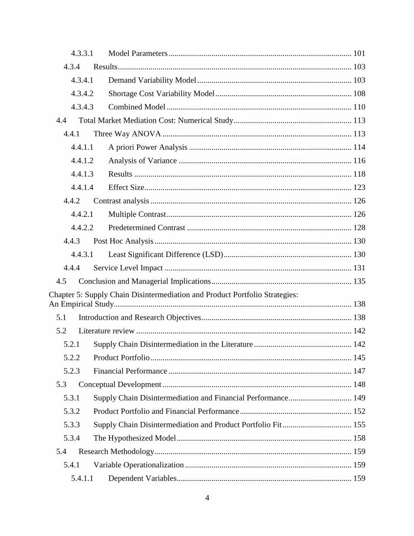
4.3.3.1 Model Parameters .......................................................................................... 101

4.3.4 Results ................................................................................................................... 103

4.3.4.1 Demand Variability Model ............................................................................ 103

4.3.4.2 Shortage Cost Variability Model ................................................................... 108

4.3.4.3 Combined Model ........................................................................................... 110

4.4 Total Market Mediation Cost: Numerical Study .......................................................... 113

4.4.1 Three Way ANOVA ............................................................................................. 113

4.4.1.1 A priori Power Analysis ................................................................................ 114

4.4.1.2 Analysis of Variance ..................................................................................... 116

4.4.1.3 Results ........................................................................................................... 118

4.4.1.4 Effect Size ...................................................................................................... 123

4.4.2 Contrast analysis ................................................................................................... 126

4.4.2.1 Multiple Contrast ........................................................................................... 126

4.4.2.2 Predetermined Contrast ................................................................................. 128

4.4.3 Post Hoc Analysis ................................................................................................. 130

4.4.3.1 Least Significant Difference (LSD) ............................................................... 130

4.4.4 Service Level Impact ............................................................................................ 131

4.5 Conclusion and Managerial Implications ..................................................................... 135

Chapter 5: Supply Chain Disintermediation and Product Portfolio Strategies:

An Empirical Study..................................................................................................................... 138

5.1 Introduction and Research Objectives.......................................................................... 138

5.2 Literature review .......................................................................................................... 142

5.2.1 Supply Chain Disintermediation in the Literature ................................................ 142

5.2.2 Product Portfolio ................................................................................................... 145

5.2.3 Financial Performance .......................................................................................... 147

5.3 Conceptual Development ............................................................................................. 148

5.3.1 Supply Chain Disintermediation and Financial Performance ............................... 149

5.3.2 Product Portfolio and Financial Performance ....................................................... 152

5.3.3 Supply Chain Disintermediation and Product Portfolio Fit .................................. 155

5.3.4 The Hypothesized Model ...................................................................................... 158

5.4 Research Methodology ................................................................................................. 159

5.4.1 Variable Operationalization .................................................................................. 159

5.4.1.1 Dependent Variables ...................................................................................... 159

5

5.4.1.2 Independent Variables ................................................................................... 160

5.4.1.3 Control Variables ........................................................................................... 163

5.4.2 Data Collection ..................................................................................................... 164

5.5 Empirical Model Formulation ...................................................................................... 166

5.5.1 Poolability Test ..................................................................................................... 166

5.5.2 Estimated Model ................................................................................................... 168

5.6 Analysis and Results .................................................................................................... 168

5.6.1 Data Descriptive Statistics .................................................................................... 169

5.6.2 Initial Analysis ...................................................................................................... 173

5.6.3 Results ................................................................................................................... 175

5.6.4 Robustness Check ................................................................................................. 180

5.6.4.1 Sensitivity Analysis ....................................................................................... 180

5.6.4.2 Trimming and Winsorizing ........................................................................... 181

5.6.4.3 Robust Regression ......................................................................................... 182

5.6.5 Results Summary .................................................................................................. 184

5.6.6 Post Hoc Analysis ................................................................................................. 185

5.6.6.1 Diminishing Return Analysis ........................................................................ 185

5.6.6.2 Quadratic Return Analysis............................................................................. 186

5.7 Conclusion and Managerial Implication ...................................................................... 187

5.7.1 Discussion ............................................................................................................. 187

5.7.2 Managerial Implications ....................................................................................... 189

5.7.3 Limitations and Future Research .......................................................................... 191

Reference List ............................................................................................................................. 194

Appendix A: Three way Factor Analysis Plots........................................................................... 211

Appendix B: Refined Anova Analysis ........................................................................................ 212

Appendix C: High Service Level Factor Analysis Plots ............................................................. 213

Appendix D: Chow Test of Poolability ...................................................................................... 214

Appendix E: Disintermediation Sensitivity Analysis ................................................................. 216

Appendix F: Winsorizing and Trimming Analysis ..................................................................... 217

6

3 List of Tables

Table 2-1: Personalization vs. Customization .......................................................................... 30

Table 2-2: Personalization Level and Supply Chain Attributes ............................................. 64

Table 3-1: Dendreon Problem Data Collection ........................................................................ 77

Table 3-2: Load Distance Results .............................................................................................. 78

Table 3-3: Optimal Solution Coordinates ................................................................................. 79

Table 4-1: Parameters Notation .............................................................................................. 102

Table 4-2: Test of Homogeneity of Variances ........................................................................ 104

Table 4-3: ANOVA Analysis .................................................................................................... 105

Table 4-4: Robust Tests of Equality of Means ....................................................................... 105

Table 4-5: One-Way ANOVA Cost Difference Analysis ....................................................... 107

Table 4-6: Anova Factors ......................................................................................................... 113

Table 4-7: Anova Analysis Results .......................................................................................... 118

Table 4-8: Eta Squared ............................................................................................................. 124

Table 4-9: Omega-Squared Size Effect ................................................................................... 125

Table 4-10: Contrast Analysis Results .................................................................................... 127

Table 4-11: Contrast Analysis Coefficient Assignment ......................................................... 129

Table 4-12: LSD Post Hoc ........................................................................................................ 130

Table 4-13: High Service Level Anova Results ...................................................................... 132

Table 4-14: Service Level and Disintermediation Impact on Total Market Mediation Cost

..................................................................................................................................................... 133

Table 4-15: Contrast Analysis for High Service Level .......................................................... 134

Table 5-1: Motivation for Disintermediation ......................................................................... 143

Table 5-2: Constructs Definition ............................................................................................. 148

7

Table 5-3: Variables Operationalization ................................................................................ 165

Table 5-4: Disintermediation Level Descriptive Statistics .................................................... 169

Table 5-5: Product Portfolio Descriptive Statistics ................................................................ 169

Table 5-6: Two Way Frequencies, Mean, and Standard Deviation for ROA ..................... 170

Table 5-7: Two Way Frequencies, Mean, and Standard Deviation for Gross Margin ...... 170

Table 5-8: Correlation and Descriptive Statistics .................................................................. 172

Table 5-9: Fit and Misfit Descriptive Statistics ...................................................................... 173

Table 5-10: Fit vs. Misfit t-test ................................................................................................. 174

Table 5-11: Fit vs. Positive Misfit t-test .................................................................................. 174

Table 5-12: Fit vs. Negative Misfit t-test ................................................................................. 175

Table 5-13: Return on Assets Regression Analysis (Unstandardized Coefficients) ............ 178

Table 5-14: Gross Margin Regression Results (Unstandardized Coefficients) ................... 179

Table 5-15: ROA Winsorized and Trimmed Analysis ............. Error! Bookmark not defined.

Table 5-16: Gross Margin Winsorized and Trimmed Analysis............................................ 182

Table 5-17: ROA Robust Regression ...................................................................................... 183

Table 5-18: Gross Margin Robust Regression ....................................................................... 183

Table 5-19: Diminishing Return Analysis .............................................................................. 185

Table 5-20: Quadratic Model ................................................................................................... 186

Table 5-21: Standardized Coefficients Regression Analysis ................................................. 190

Table 10-1: ROA Sensitivity Analysis ..................................................................................... 216

Table 10-2: Gross Margin Sensitivity Analysis ...................................................................... 216

Table 11-1: ROA 5% Winsorized Results .............................................................................. 217

Table 11-2: ROA 1% Winsorized Results .............................................................................. 217

8

Table 11-3: Gross Margin 5% Winsorized Results ............................................................... 218

Table 11-4: Gross Margin 1% Winsorized Results ............................................................... 218

Table 11-5: ROA 5% Trimmed Results.................................................................................. 219

Table 11-6: ROA 1% Trimmed Results.................................................................................. 219

Table 11-7: Gross Margin 5% Trimmed Results................................................................... 220

Table 11-8: Gross Margin 1% Trimmed Results................................................................... 220

9

4 List of Figures

Figure 2-1: Pharmaceutical Industry Evolution ...................................................................... 18

Figure 2-2: Brand vs. Generic Drugs ........................................................................................ 35

Figure 2-3: Standardization-Personalization Continuum ....................................................... 43

Figure 2-4: Pharmaceutical Standardization-Personalization Continuum ........................... 44

Figure 2-5: Pharmacy Ownership ............................................................................................. 47

Figure 2-6: Pharmaceutical Supply Chain ............................................................................... 48

Figure 2-7: Specialty Pharmacy Growth .................................................................................. 50

Figure 2-8: Biotechnology Manufacturing Process ................................................................. 51

Figure 2-9: Biologics Supply Chain ........................................................................................... 54

Figure 2-10: Personalization and Disintermediation Mapping .............................................. 58

Figure 2-11: Pharmaceutical Personalization and Disintermediation Mapping .................. 61

Figure 3-1: Prostate Vaccine Service Process .......................................................................... 72

Figure 3-2: Dendreon Processing Facility Location Problem ................................................. 73

Figure 3-3: Location Problem 2D Mapping ............................................................................. 76

Figure 3-4: Results Comparison ................................................................................................ 80

Figure 4-1: Illustrative Example................................................................................................ 91

Figure 4-2: Medicine Life Cycle at the Distributor ................................................................. 99

Figure 4-3: Medicine Life Cycle at the Hospital ...................................................................... 99

Figure 4-4: Total Cost for Demand Variability Model .......................................................... 106

Figure 4-5: Total Cost for "moderate variability" ................................................................ 107

Figure 4-6: Total Cost for Shortage Cost Variation Model .................................................. 108

Figure 4-7: Total Market Mediation Cost for the Flat Region ............................................. 109

Figure 4-8: 3D Optimal Distribution Strategy ....................................................................... 111

10

Figure 4-9: Optimal Distribution Strategy Frontiers ............................................................ 112

Figure 4-10: Power Level ......................................................................................................... 116

Figure 4-11: Anova Analysis Plan ........................................................................................... 117

Figure 4-12: Three Factors Anova Analysis ........................................................................... 119

Figure 4-13: Coefficient of Variation and Shortage Cost Anova ......................................... 121

Figure 4-14: Coefficient of Variation and Disintermediation Anova ................................... 122

Figure 4-15: Shortage Cost Ratio and Disintermediation Anova ......................................... 123

Figure 4-16: Low vs. High Service Level Costs at Low Coefficient of Variation ................ 135

Figure 5-1: Supply Chain Disintermediation and Product Portfolio Fit ............................. 157

Figure 5-2: Hypothesized Model.............................................................................................. 158

11

5 List of Abbreviations

SCD: Supply Chain Disintermediation

SL: Service Level

SC: Shortage Cost

WHO: World Health Organization

PSC: Pharmaceutical Supply Chain

DSP: Drug Shortage Program

FDA: Food and Drug Administration

CAS: Complex Adaptive System

CAGR: Compounded Average Growth Rate

R&D: Research and Development

PBM: Pharmacy Benefit Managers

CV: Coefficient of Variation

GM: Gross Margin

ROA: Return on Assets

ATurn: Assets Turnover

12

1 Chapter 1: Introduction

The pharmaceutical industry has evolved over the past century to become one of the biggest global

industries, with sales exceeding 1 trillion dollars in 2013 and expected continued growth in 2014

(IBIS, 2014). The pharmaceutical industry is both a capital and labor intensive industry with high

emphasis on research & development and innovation as critical success factors. The

pharmaceutical industry represents an evolving innovative environment where organizations are

competing over the exclusivity to provide a cure to patients. The drugs developed are then

distributed to patients via a variety of outlets. Over the past few decades, the industry has

experienced several structural changes that have impacted the pharmaceutical business model and

its supply chain configuration.

The pharmaceutical product paradigm is shifting from more standardized and mass-

produced goods to a highly customized product with a focus on serving one patient’s specific

needs. Pharmaceutical companies are not only offering standardized medication but are also

providing more customized medication. Scientific evolution and the mapping of the human

genome has enhanced the development of personalized medication. This new advancement has led

to a more evolved type of medication scientifically referred to as Biologics (large molecule drugs).

Unlike the traditional medicine (small molecule drugs), biologics represent highly customized

products with high value proposition to patients. In some extreme cases, biologics are personalized

and aimed at serving a patient’s unique needs. Biologic medication can be distributed to patients

via multiple distribution channels.

The pharmaceutical supply chain shows a strong influence of distributors and wholesalers

on the distribution channels. Over 90% of the traditional medication is sold via distributors and

wholesalers (Fein, 2012). Wholesalers provide the pharmaceutical supply chain with a higher level

13

of service by insuring the availability of the medication. The role of the distributor seems less

relevant in a case of more personalized medication with a shorter shelf life. The current

pharmaceutical supply chain is showing a shift to more direct distribution channels where the drug

is shipped directly from the firm to the patient or the hospital. This new distribution trend is fueled

by both product characteristics and quality concerns. This phenomenon is also known as supply

chain disintermediation. Supply chain disintermediation (SCD) proved its attractiveness in retail

and electronics, among other industries. While supply chain disintermediation represents an

alternative for certain industries like electronics, it represents a unique choice for personalized

products. For instance, Vista Print products are solely sold via direct distribution channels.

However, the use of disintermediated distribution channels in the pharmaceutical field is gaining

more importance from practitioners, especially with the emergence of more personalized

medication.

1.1 Problem Statement

The pharmaceutical industry is moving away from a blockbuster business model to a more

collaborative configuration based on innovation (Cooper, 2008). Biologic drugs represent an

example of an innovative product with strong value proposition. Biopharmaceutical medicines are

characterized by a high level of customization and personalization with greater focus on service as

part of the product bundle value proposition. In many cases, a patient’s inputs are part of the

production process providing this particular industry with a unique setting. This unique setting has

shaped the evolution of the pharmaceutical supply chain. Despite this debated attractiveness,

biologics firms are not generating large profits and are, in many cases, failing to compete with

larger corporations (Grabowski, Cockburn, and Long, 2006). Moreover, biopharmaceutical firms

experience a high cost of goods sold due to the complexity of the production process as well as the

14

logistics cost. In fact, biologic medications require special handling and are time-sensitive. The

biologics processing facility location becomes a critical factor that has an impact on the cost of

goods sold and the quality of the service delivered. Additionally, biopharmaceuticals are

characterized by a short shelf life and high demand variation. On one hand, the short shelf life

combined with the high product value increases the perishability cost. On the other hand, the high

demand variability impacts the shortage cost. The tradeoff between the perishability cost and the

shortage cost will determine the supply chain configuration strategy. Unlike traditional medication

where there is a clear answer for the supply chain distribution channel configuration, biologics

firms are not able to crack the code for the optimal distribution strategy. While a disintermediated

model will reduce the lead time and reduce the perishability cost, intermediated configuration will

reduce the product variability effect and minimize the shortage cost. The adoption of newer

distribution channels is fueled by high financial risk, varying demand, quality concerns, and

special handling requirements.

1.2 Research Objectives

The dissertation work aims at analyzing the evolutionary changes of the pharmaceutical industry

and supply chains configuration in the context of personalized medicine and its influence on

biopharmaceutical firms’ performance. First, the conceptual part of the study explores the

evolution of the pharmaceutical supply chain and its interaction with the new paradigm of

personalized medication. To provide more generalizable understanding, the conceptual part

addresses the product paradigm shift and supply chain evolution in general context first and then

apply it to the pharmaceutical industry’s purpose. The research study aims at providing an original

mapping of the evolution of the pharmaceutical products paradigm with more focus on

personalized medication and the emergence of biologic medicine as a more personalized product.

15

The study also attempts to link the impact of product paradigm evolution to pharmaceutical supply

chain distribution. The dissertation reconciles product personalization level with supply chain

disintermediation for pharmaceuticals. Second, the study addresses the case of highly personalized

medication with high disintermediation level configuration. Based on a case study, the study

explores the strategic decision of the location problem for the case of highly personalized

medication where the patient is a raw material supplier. Third, the dissertation explores the impact

of the disintermediation level on the total market mediation cost. Using a scenario approach

simulation and numerical analysis, the study aims at identifying the best disintermediation

configuration for different demand patterns and shortage cost structure. Finally, the dissertation

investigates the interaction of product personalization level and supply chain disintermediation

and how it impacts firms’ financial performance. Based on secondary data, the dissertation

develops an empirical model to test for the fit between product configuration and supply chain

configuration and how it influences a firm’s performance.

The study contributes to the existing literature in supply chain and management research

by providing a novel conceptualization of product paradigm. It draws on Kumar’s (2007) work on

personalization by providing a personalization level continuum and applying it to the

pharmaceutical product context. The study also provides an extension of supply chain

disintermediation studies and develops a novel reconciliation of product paradigm and supply

chain disintermediation. Moreover, the study is among the few studies to address the problem of

disintermediation using large numerical analysis. Finally, the study contributes to the work on

disintermediation and alignment literature by empirically addressing the role of supply chain

disintermediation on pharmaceutical firms’ financial performance. This work elaborates on the

conceptual foundations in order to empirically test for the impact of product paradigm and supply

16

chain structure on a firm’s performance. This work develops and tests for a novel product paradigm

and supply chain reconciliation.

The dissertation work contributes to the practice by providing more insights about some of

the unexplored areas and delivers a clear and practical mapping of some of the theoretical concepts

relating to personalization paradigm and supply chain disintermediation. Practitioners will find the

answer to some of the critical problems relating to distribution strategy and will determine the

most adequate distribution channels to use. Finally, the study is relevant to practice as it provides

some insights about the impact of product structure and supply chain disintermediation strategy

on a firm’s current and potential future financial performance.

The dissertation is structured into four self-contained essays that will address the different

problems discussed in the introduction. Chapter 2 presents the conceptual foundation of the study.

Chapter 3 is a case study based on real data that addresses the location problem in highly

personalized medication with totally disintermediated distribution channels. Chapter 4 is a

numerical study that discusses the impact of the disintermediation level on the total market

mediation cost. Finally, chapter 5 empirically addresses the interaction of product personalization

level and disintermediation.

17

2 Chapter 2: Evolution of Pharmaceutical Industry: Product

Paradigm and Supply Chain Configuration

2.1 Introduction and Research Objectives

The global pharmaceutical industry reached the key milestone of 1 trillion dollars in 2013, with a

growth rate of 4% between 2007 and 2012 (IMS_Health, 2014). The pharmaceutical industry

represents a major player in the healthcare landscape, as it provides patients with the appropriate

medications. This industry was marked by several structural changes that have an impact on

pharmaceuticals firms’ value proposition and supply chain structure. The pharmaceutical business

model is shifting from the blockbuster model, where a company will hold the exclusivity of a

product for a long time via a patent, to a more collaborative integrative business model. The

integrative model suggests that pharmaceutical firms will need to collaborate with different supply

chain members such as suppliers and customers, as well as other competitors, to achieve and

sustain a competitive advantage. Both the relaxing of regulations and the advancement of

technology have facilitated the changes in the business model. The current regulations in the

United States are reducing the barrier to entry by favoring generic medication production. The

pharmaceutical industry has followed the manufacturing paradigm from crafted production to mass

production, and then from mass customization to personalization (Hu, 2013). In fact, the

pharmaceutical industry has witnessed the emergence of a new product segment called specialty

pharmacies, which are mainly biologic medications. Biologic products have vague product

specifications and, therefore, are hard to patent. The recent structural changes in the

pharmaceutical industry have impacted the product paradigm and the supply chain configuration.

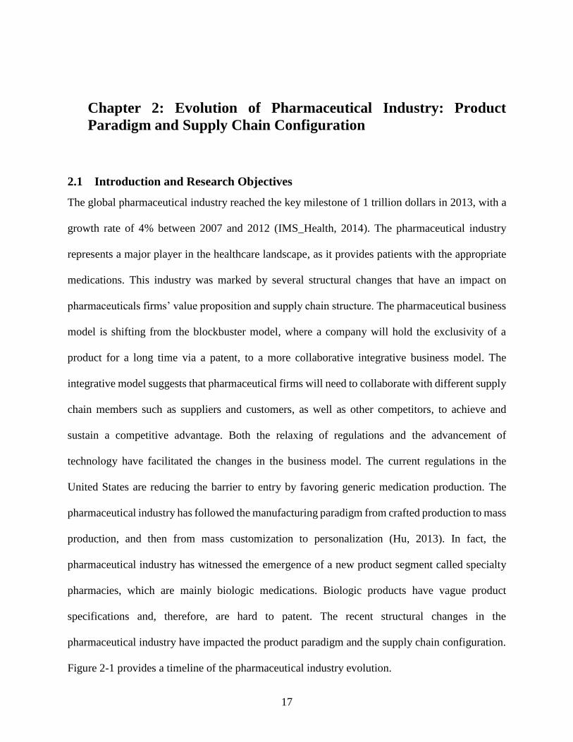
Figure 2-1 provides a timeline of the pharmaceutical industry evolution.

18

Figure 2-1: Pharmaceutical Industry Evolution

2.1.1 Evolution of the Pharmaceutical Product Paradigm

The evolution of the pharmaceutical industry and the emergence of specialty medication has

shaped different product paradigms. The pharmaceutical industry has shifted from a crafted

industry with its focus on production capabilities as the main competitive edge. The regulation of

the pharmaceutical industry at the beginning of the 20th century marked the establishment of the

blockbuster model. The pharmaceutical firms had engaged in mainly research contracts as a

unique collaboration mechanism during the 1970s and 1980s. The Hatch-Waxman Act in 1984

reduced the barriers to entry by allowing generic medicine producers the license to replicate

medicine. The beginning of the 21st century is considered to be the biotechnology boom in the

pharmaceutical industry. More focus was accorded to highly sophisticated treatment with a strong

emphasis on service as a value proposition. The mapping of the human genome in 2003 inside

19

Celera Corporation provided the pharmaceutical industry with an opportunity to develop new

medication based on genetic material.

As noted above, and like many other industries, the pharmaceutical industry is moving

towards a paradigm focusing on the one-to-one-marketing. In essence, the pharmaceutical industry

is providing more personalized medication, creating significant implications for the way firms

operate today. Biologics represent an example of a personalized medication with high value

proposition. Pharmaceutical companies are offering more personalized products that meet specific

patients’ needs. Indeed, some biologic medications are highly personalized, requiring the patient

input as part of the medication. This paradigm shift has been fueled by technological advancements

enhancing customer input and making the patient a medicine co-creator, not simply an end

consumer. The topic of personalization is gaining more interest as pharmaceutical firms seek new

ways to deliver products and services and remain competitive. However, there is a lack of research

attention addressing the issue of mass-personalization, especially in the context of the

pharmaceutical industry. The emergence of new specialty medication has added more complexity

to the supply chain configuration by increasing the level of financial risk and by creating closed

looped physical flows. Specifically, the higher level of personalization creates additional

complexities for the supply chain configuration from the perspective of distribution. In summary,

the new product paradigm that calls for a higher level of personalization has impacted the

pharmaceutical business model by requiring firms to re-evaluate their supply chain configurations.

2.1.2 Evolution of the Pharmaceutical Supply Chain

The pharmaceutical supply chain configuration represents an interesting area of investigation for

practical and academic ends. The pharmaceutical supply chain has been following a traditional flat

material flow (often referred to as a serial supply chain) with a strong emphasis on the distributors

20

and wholesalers as a major node in the network. The emergence of specialty medication (referred

to as large molecule medication) has added a level of complexity that has significant implications

for a firm’s supply chain configuration. In fact, the specialty medications (such as biologic

medication) are very expensive, have a short shelf life, require special handling, and necessitate

prior approval from the payer (insurance, in most cases). These factors significantly increase the

risk of perishability for the biologic medications. The higher levels of risk of perishability, as well

as the higher level of customer inputs that are required for production of personalized medication,

have significant implications on the structure of the downstream aspects of the firm’s supply chain

(i.e. the distribution channel). Specifically, this required firms to evaluate their strategy for going

direct or for using disintermediation in their supply chain1. The topic of the pharmaceutical supply

chain has been extensively studied in the field of operations and supply chain management (Koh

et al., 2003; Papageorgiou, Rotstein, and Shah, 2001). Most of the studies addressed the security

issues in pharmaceutical supply chains and the role of technology, as well as the pharmaceutical

supply chain optimization (Shah, 2004a). Other studies also showed some interest in the

pharmaceutical supply chain distribution channels (Muller et al., 2009). However, to the best of

my knowledge, no prior study has addressed the structural changes to distribution channels of the

pharmaceutical industry in the context of highly personalized specialty biologic medications. This

represents a research opportunity and an area of study that this dissertation is aiming to address.

2.1.3 Key Research Questions

Business viability is highly tied to the firm’s value proposition and its ability to provide unique

value to its customers (Drucker, 2013). To cope with the structural changes of the industry,

1 Given that the most significant supply chain configuration changes that can result from personalization of products

would reside in the distribution channels (downstream supply chain), for the purpose of this dissertation proposal,

supply chain configuration is used interchangeably with distribution channel configuration.

21

pharmaceuticals are now providing a different set of personalized products targeting specific types

of patients. These products are distributed via traditional distribution channels as well as via

alternative avenues. The new product paradigm which calls for highly personalized medication

also calls for a strong emphasis on delivery of the medication (i.e. service) as a significant part of

the value proposition. In essence, the highly personalized biologic products may be viewed as a

product-service continuum. Researchers have extensively studied the product-service continuum

(Vargo and Lusch, 2004; Zeithaml, 1981) and mass personalization (Kumar, 2007; Wang et al.,

2011). The interaction between the product-service continuum and the personalization level

represents an area of investigation that has received little attention in previous studies. There is

some existing literature which has looked into aspects of pharmaceutical supply chain concepts

(Pedroso and Nakano, 2009; Stadtler and Kilger, 2000). However, this literature does not

investigate the role of personalization of medication and how it can shape the distribution channel

configuration. Given that personalization of medication leads to a significant increase in

complexity in the downstream supply chain (i.e. entities involved between the product

manufacturer and customer), it is critical to lay emphasis on the distribution aspects of the supply

chain configuration. Indeed, the involvement of the customer in the production process as well as

the time sensitivity of medication perishability noted above make it critical for pharmaceutical

firms to understand potential disintermediation opportunities that may exist for them as well as

develop a strategy that can help them match their product portfolio with the appropriate supply

chain configuration from the perspective of distribution. To the best of my knowledge, the current

literature does not provide firms with an appropriate framework that can guide managerial

strategies for distribution channel configuration to align with their product portfolio, thus

representing a gap in existing literature.

22

In order to address this gap in literature, the current chapter aims to investigate a specific

research question: What is the appropriate distribution channel strategy (with respect to

disintermediation) given the level of personalization represented in the product portfolio of firms?

Distribution channel strategy for disintermediation refers to the firm’s choices with regard to

maintaining intermediaries for the product flow from their manufacturing facilities to the customer

(or hospital). Such a choice may be represented along a continuum of completely intermediated

(traditional serial supply chain) to completely disintermediated (going direct). The level of

personalization in a firm’s product portfolio refers to the potential mix of medication in the firm’s

product portfolio along a continuum of highly standardized medication (at times referred to as

small molecule medication or generic medication) to highly personalized medication (large

molecule medication such as biologics).

In investigating the research question, the aim of this chapter is to provide a conceptual

framework that links the level of personalization with the appropriate distribution channel

configuration. Such a framework can guide managerial thinking as they assess the firm’s

distribution channel strategy, keeping in mind their product strategy. To develop such a framework,

this chapter first provides a conceptualization of the customization-personalization and the product-

service continuum. Second, the study presents an overview of the supply chain distribution channels

configuration of small (standardized) and large (personalized) molecules medication. Third, a

conceptualization of disintermediation continuum is developed. Finally, the chapter provides the

framework that links the product standardization-personalization continuum to the

disintermediation continuum.

The rest of this chapter is organized as follows: First, a synthesis of the relevant literature

related to mass-customization & personalization and pharmaceutical supply chain is provided. In

23

the following section, the study provides a conceptualization of product paradigm and

pharmaceutical supply configuration. The conceptual foundations also serve as guidelines for the

following chapters. Finally, the chapter provides a framework that maps the two main paradigms

under investigation: the pharmaceutical product personalization continuum and the supply chain

disintermediation continuum.

2.2 Literature Review

The following section provides a summary of the literature review that relates to mass

customization & personalization and pharmaceutical supply chain. The aim of this section is to

summarize the most relevant work to the study and emphasize the gap in the literature that this

chapter is addressing. The literature review section addresses the mass customization & mass

personalization and pharmaceutical supply chain.

2.2.1 Mass Customization and Mass Personalization

The area of mass customization and mass personalization has been of interest to scholars as a new

product paradigm. The following subsection provides an analysis of the literature review and

comparison analysis between the concepts of personalization and customization.

2.2.1.1 Mass Customization

In his book Future Perfect, Davis (1987) first introduced the term “mass customization.” The book

did not put a large emphasis on mass customization (MC). Marketing researchers were among the

first to adopt the concept of mass customization and study it more in depth (Kotler, 1989). Mass

customization started gaining some interest in Operations Management in the mid-90s (Pine and

Davis, 1999; J. Pine, 1993). Pine (1993) defined MC as a firm’s ability to deliver individually

customized products at low-cost with minimum required quality at a large volume. Mass

24

customization corresponds to “producing goods and services to meet individual customers’ needs

with near mass production efficiency” (Moser, 2007). Mass customization should be seen as a

process for aligning an organization with its customers' needs through the development of a set of

certain capabilities such as process design (Salvador, De Holan, and Piller, 2009). This alignment

suggests that the mass customization happens across different levels of the supply chain players.

Levels of Mass Customization: Mass customization can occur at various levels of the value

chain. Mass customization can be viewed in a continuum where the product/service can be purely

standardized to purely customized (Lampel and Mintzberg, 1996). A product is designed, produced

and finally distributed. The purely customized product will have customization activity at each

stage of the value chain (Gilmore and Pine 2nd, 1997; Lampel and Mintzberg, 1996). Pine (1997)

proposes five stages of modular production: customized services (standard products are tailored

before the delivery process), embedded customization (standard products are changed by

customers during use), point-of-delivery customization (more work is performed at the point of

sale), delivery customization (short time delivery of products), and modular production (wide

configuration of products and service) (B. J. Pine, 1993). Mass customization can be also divided

into four types based on the focus of the customization: customized packaging, customized

services, additional custom work, and modular assembly (Spira, 1993). The levels of mass

customization are among a large set of work from an operations management perspective.

Mass Customization in Operations Management: In the context of Operations

Management, Mass Customization refers to the ability to rapidly produce customized offerings

with quality and costs similar to those achieved by the mass production approach (MacCarthy,

Brabazon, and Bramham, 2003). Mass customization has interested the core of research in the past

decade with an increased number of research and studies focusing on mass customization. Tu et

25

al. (2001) addressed the role of mass customization as a capability. In fact, while facing dynamic

product and process change, firms would have to develop a higher level capability to maintain a

competitive advantage (Tu, Vonderembse, and Ragu-Nathan, 2001). Organizations have utilized

multiple operational practices such as Time Based Manufacturing Practices as mass customization

enabler (Koufteros, Vonderembse, and Doll, 1998; Tu et al., 2001). The impact of information

technology on mass customization capability has been the subject of very few empirical

examinations (Peng, Liu, and Heim, 2011). Peng et al. (2011) addressed the theoretical relationship

between four types of IT applications with MC capability. Moreover, scholars have looked to the

impact of work design on mass customization capability based on sociotechnical system theory

(Liu, Shah, and Schroeder, 2006). Organization learning scholars showed some interest in

investigating the impact of organization learning and mass customization capability development

(Huang, Kristal, and Schroeder, 2008). Huang et al. (2008) investigated the role of learning and

effective process implementation in the development of mass customization capability. More

recently, scholars started focusing on service mass customization (Moon et al., 2011). Moon et al

(2011) developed a method for designing customized families of services using game theory to

model situations involving dynamic market environments. The designing process was inspired by

the manufacturing modularity to provide customized services.

2.2.1.2 Mass Personalization

The recent business trend is shifting from the mass customization to profitably serving one market

(Kumar, 2007). Kumar (2007) emphasized the strategic shift from mass customization to mass

personalization, where companies will position themselves in the “personalization spectrum.” This

transformation is feasible because of the development of the Web 2.0, modern manufacturing

systems, and modularity and delayed differentiation (Kumar, 2007). In fact, companies that

26

employ Web 2.0 succeed in productive customer integration enabling personalization (OReilly,

2007). Second, flexible manufacturing cells, modularity, and delayed differentiation increase the

firm’s potential to develop mass customization capability (Kumar, 2004; Lee and Tang, 1997).

Personalization Process: The marketing literature offers foundations for addressing

personalization issues. The body of literature proposes mainly three frameworks of the

personalization process (Vesanen and Raulas, 2006). Even though the three approaches appear

different, each model suggests customers as a starting point with a minimum level of interaction

to determine the customer’s personalized need. The data is then processed to create a customer

profile. Finally, the personalized product/service is delivered to the customer. The model suggests

the creation of loops to guarantee the quality of the personalized product/service (Adomavicius

and Tuzhilin, 2005; Murthi and Sarkar, 2003; Pierrakos et al., 2003). In fact, the customers’

feedback represents the main point that separates customization from personalization. The mass

personalization process suggests different dimensions aside from the customer inputs and

feedback.

Dimensions of Mass Personalization: The concept of mass personalization is still under

investigation by researchers. While there is no consensus on the main dimension of mass

personalization, recent studies have attempted to provide some insights about the matter (Zhou, Ji,

and Jiao, 2013). First, mass personalization reflects the market for one customer, which requires

the product fulfillment to be changeable, adaptable, and configurable (Wiendahl et al., 2007). The

second dimension relates to mass efficiency by bringing more value to both customers and

producers in a cost effective way (Zhou et al., 2013). Third, mass personalization involves

intensive interactions with customers from the product/service design as well as a total life cycle

involvement (Jiao, 2011). This is referred to as co-creation. Finally, mass personalization is

27

characterized by a particular user’s experience. Mass personalization goes beyond exploring

market potential; it addresses customers’ latent needs (Zhou, Xu, and Jiao, 2011). The four

dimensions explained emphasize the difficulty that companies are facing to successfully shift to

more personalized products and services.

Implementation Issues in Mass Personalization: The process of product/service

personalization is challenging and requires some technical work, such as providing specific

personalization algorithms and patterns of actions within personalization systems (Fang and

Salvendy, 2003; Fink et al., 2002). While the personalization issues were not addressed yet to a

great extent in the operations management literature, the marketing field and, specifically, the e-

commerce related body of literature has been investigating personalization for over a decade

(Adolphs and Winkelmann, 2010). The personalization process as described previously requires

customers’ and users’ inputs, data processing, and customer feedback. In the context of

ecommerce, more issues need to be addressed mainly related to recommender systems and mass

customization. Recommender systems or comparison shopping systems will provide customers

with suggestions that will reflect the customers’ personal preferences and profiles (Ricci and

Werthner, 2006). The customer input for ratings, recommendations, and reviews are very critical

to the performance of the personalization process. Moreover, Adolphs and Winkelmann (2010)

emphasized the importance of achieving mass customization as a gateway to realizing

personalization. Mass personalization is perceived as a high level capability that is achieved

through mass customization, a lower lever capability. The study, however, did not provide any

empirical proof to support this statement. The literature had also addressed other issues related to

personalization such as data analysis and data processing. These parts are highly technical and

address different algorithms for data mining and profile processing (Schubert, 2003). The set of

28

challenges have evolved into more specific constraints that organizations are facing and scholars

have identified.

Classifying Personalization Constraints: The adoption of a personalization strategy is

marked by a series of constraints that make the process more challenging. First, some constraints

are related to the process of adoption itself (Adomavicius and Tuzhilin, 2005; Vesanen and Raulas,

2006). These problems relate to implementation dynamics. Second, firms are limited by the

technology available when collecting and processing the data and delivering the product/service

(Harnisch, 2013). Finally, organizational capability represents a major restriction to the

personalization success. Harnisch (2013) classified the constraints into three dimensions: origin

(internal, external), subject (technological, organizational), and time (data collection,

matchmaking, delivery). Despite this set of constraints and challenges, some organizations were

able to achieve mass personalization and put serving the market of one customer as their main

strategy. Several examples from manufacturing contexts are identified.

Personalization in Manufacturing: Numerous examples can be provided dealing with

personalization in the manufacturing industry. Personalization is widely used in clothing industry.

Nike Inc. was among the pioneers in the industry to provide personalized shoes. In 2001, Nike

offered its customers the opportunity to add a personal message on their shoes. The personalization

level has increased since then, reflecting a higher level of manufacturing capabilities and engaging

more advanced manufacturing systems. Customers can participate in 3D garment design by

choosing particular components to construct their own garment. Additive manufacturing is another

technical definition of the 3D printing. Additive manufacturing is a disruptive manufacturing

technology that revolutionized the production of mass personalized clothing (Reeves, Tuck, and

Hague, 2011; Wang et al., 2011). Vista Print and other online printing service providers achieved

29

the capability of delivering unique products to their customers. The website capabilities allow the

customer to make a variety of selections to personalize the product. Vista Print also suggests some

personalized related products when placing an order of business cards or event invitations.

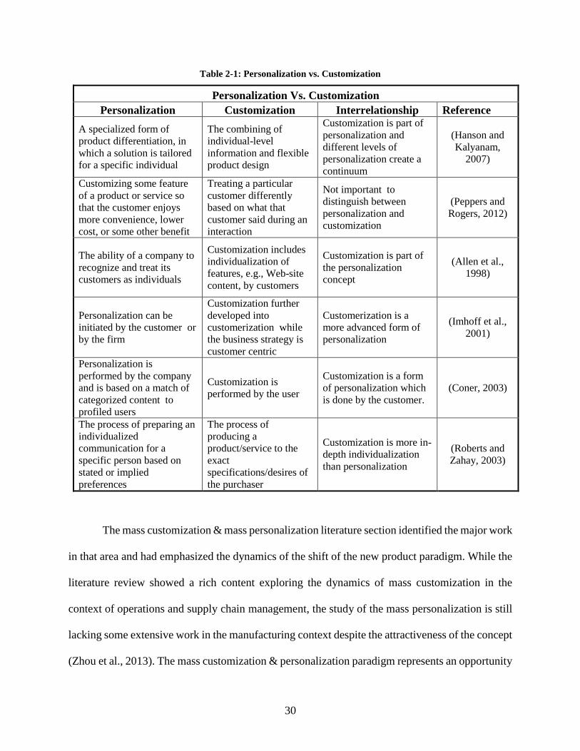
2.2.1.3 Mass Customization vs. Mass Personalization

The concept of personalization was the subject of extensive research in the area of marketing

(Allen, Yaeckel, and Kania, 1998; Coner, 2003). While some researchers consider personalization

as a higher level priority than customization (Hanson and Kalyanam, 2007), others argue that

customization is a form of personalization performed by the customers (Roberts and Zahay, 2003).

The following Table 2-1 summarizes the difference between customization and personalization.

30

Table 2-1: Personalization vs. Customization

Personalization Vs. Customization

Personalization Customization Interrelationship Reference

A specialized form of

product differentiation, in

which a solution is tailored

for a specific individual

The combining of

individual-level

information and flexible

product design

Customization is part of

personalization and

different levels of

personalization create a

continuum

(Hanson and

Kalyanam,

2007)

Customizing some feature

of a product or service so

that the customer enjoys

more convenience, lower

cost, or some other benefit

Treating a particular

customer differently

based on what that

customer said during an

interaction

Not important to

distinguish between

personalization and

customization

(Peppers and

Rogers, 2012)

The ability of a company to

recognize and treat its

customers as individuals

Customization includes

individualization of

features, e.g., Web-site

content, by customers

Customization is part of

the personalization

concept

(Allen et al.,

1998)

Personalization can be

initiated by the customer or

by the firm

Customization further

developed into

customerization while

the business strategy is

customer centric

Customerization is a

more advanced form of

personalization

(Imhoff et al.,

2001)

Personalization is

performed by the company

and is based on a match of

categorized content to

profiled users

Customization is

performed by the user

Customization is a form

of personalization which

is done by the customer.

(Coner, 2003)

The process of preparing an

individualized

communication for a

specific person based on

stated or implied

preferences

The process of

producing a

product/service to the

exact

specifications/desires of

the purchaser

Customization is more in-

depth individualization

than personalization

(Roberts and

Zahay, 2003)

The mass customization & mass personalization literature section identified the major work

in that area and had emphasized the dynamics of the shift of the new product paradigm. While the

literature review showed a rich content exploring the dynamics of mass customization in the

context of operations and supply chain management, the study of the mass personalization is still

lacking some extensive work in the manufacturing context despite the attractiveness of the concept

(Zhou et al., 2013). The mass customization & personalization paradigm represents an opportunity

31

for an investigation from the operation and supply chain angle. While some conceptual and

empirical work attempted to study mass customization and personalization in a manufacturing

context (Jiao, 2011; Tu et al., 2001), very few studies have investigated the paradigm in a service

oriented context. A recent study pointed out the managerial impact of mass personalization in the

healthcare context. Very few studies have looked at personalization in healthcare service delivery

(Chaudhuri and Lillrank, 2013). The healthcare field represents an interesting area of management

studies, which is relevant in both academia and practice. The pharmaceutical industry represents a

major segment of the healthcare field. The pharmaceutical supply chain represents an area of

research that can be linked to mass customization & personalization paradigm.

The following subsection provides a literature review of the pharmaceutical supply chain.

The literature review subsection is intended to identify the major findings relevant to both the

evolution of the pharmaceutical supply chain and how it can relate to the mass customization &

personalization paradigm.

2.2.2 Pharmaceutical Supply Chain

Several studies from the operations management field have investigated different aspects of the

pharmaceutical supply chain. For over two decades, the financial performance of the

pharmaceutical firms has interested several empirical studies by exploring profitability, research

intensity impact, and the role of mergers and acquisitions in financial viability. These studies have

explored the dynamics of the pharmaceutical supply chain and have explored the role of certain

factors such as Information Technology. More recent studies have addressed the structural changes

in the pharmaceutical industry and how it can shape the future of pharmaceuticals.

32

2.2.2.1 Pharmaceutical Supply Chain Dynamics

Profitability and Optimization: The pharmaceutical industry is considered to be among the most

profitable industries, as measured by return on investment in R&D. The return on R&D

expenditure is relatively high due to extensive innovation (Grabowski, Vernon, and DiMasi, 2002).

The crucial role of innovativeness urged researchers to investigate the new product development

key success factors as well as the role of environmental factors. Older studies addressed research

productivity and a firm’s size impact on new product success (Henderson and Cockburn, 1996).

More recent studies have developed a new product cost analysis by determining the cost of the

different stages of the product development (DiMasi, Hansen, and Grabowski, 2003). Optimizing

the supply chain configuration remains among the ultimate goal for firms in general and for

pharmaceuticals in particular. Shah (2004) proposed a list of issues to take into consideration while

optimizing the pharmaceutical supply chain. These issues are related to facility location and

design, inventory and distribution planning, capacity and production planning, and detailed

scheduling. Supply chain “debottlenecking and decoupling strategies” and inventory management

are crucial for the viability of the firm in a rapidly changing market (Shah, 2004a). To my

knowledge, no prior studies have addressed the pharmaceutical profitability and product paradigm

issues.

Security Issues in Pharmaceutical Supply Chain: Because of the critical nature of the

pharmaceutical industry and the high regulation, security issues in the supply chain are extremely

important. The main issue related to security is the risk emerging from counterfeit products. In

fact, The World Health Organization (WHO) estimates that between five and eight percent of the

worldwide trade in pharmaceuticals is counterfeit (Koh et al., 2003). In a more global environment,

and with the development of new distribution channels such as online, patients have access to

33

counterfeit medicine. For example, the amount of counterfeit drugs in the European market

increased enormously in the past years (Schweim and Schweim, 2009). Moreover, motivated by

quality concerns and pressured by regulatory directives, pharmaceutical firms are urged to address

this issue. The security issues have created more possible distribution channels such as direct sales

in an attempt to minimize the health risk and guarantee high quality for patients.

Most of the solutions that pharmaceutical firms were using rely on quality control and

manual inspection of the medicine. These techniques are considered “static” and inefficient to

prevent counterfeit practices from happening (Koh et al., 2003). New techniques were proposed

by some scholars and for the most part, they call for the use of information technology systems as

a major enabler. First, the use of a unique medicine identifier powered by an information system

database was proposed as a solution to reduce the counterfeit risk (Muller et al., 2009). The study

proposed a simulation model showing the evolution of a product with a unique identifier in the

supply chain. More effort should be done at the regulators’ side to minimize the distribution of

counterfeit medicine in non-authorized distribution channels. In fact, according to the WHO, more

than 50% of the medicines purchased from illegal websites are counterfeit. Second, RFID tags are

another alternative to track the medicine and guarantee that it is not counterfeit (King and Zhang,

2007; Koh et al., 2003). RFID tags are more appropriate in the context of a pharmaceutical supply

chain given the complexity level and the amount of information a package can contain.

Information Technology in Pharmaceutical Supply Chain: Information Technology (IT) is a

crucial factor in supply chains but more so in the pharmaceutical industry. In fact, pharmaceutical

companies have used IT to prevent counterfeit products (Koh et al., 2003). After that, the use of

IT developed into a more integrative and decision making role in the supply chain. Scholars have

investigated the importance of the use of RFID as a new IT tool in addressing PSC issues (Kumar,

34

Kadow, and Lamkin, 2011). RFID technology is a critical success factor for creating a more

effective pharmaceutical supply chain (Yue, Wu, and Bai, 2008). Moreover, IT improved the

negotiation process in the supply chain in order to maximize the value to customers (Konstantinos,

Vrassidas, and Dimitra, 2008). Konstanitos et al. (2008) have also proposed a supplier selection

framework emphasizing the role of IT as the connecting element. Finally, the shift in the

pharmaceutical industry from revenue-centered to value- and collaboration-focused relies on IT as

an important factor (Cooper, 2008). In fact, health 2.0, which is the use of a specific set of Web

tools by actors in healthcare, including doctors, patients, and scientists, in order to personalize

healthcare, collaborate, and promote health education, will be the new trend in healthcare in

general and the pharmaceutical industry specifically (Cooper, 2008; Hughes, Joshi, and Wareham,

2008).

The emergence of IT in the business landscape in general and the pharmaceutical industry in

particular is promoting a major paradigm shift. The health 2.0 initiative will constitute an enabler

for a more personalized health care delivery system. The body of literature has emphasized the

importance of IT in the pharmaceutical industry without addressing how it can enable the shift to

more personalized medication and direct sales strategy. Even though the role of IT is outside the

scope of this study, it was judged important to point it out because it represents an important piece

of the personalization enabling tools in pharmaceuticals. Moreover, IT is a major component of

the pharmaceutical direct sales model, as it helps patients order their medication.

2.2.2.2 Structural Change in the Pharmaceutical Supply Chain

The changes in U.S. regulations and the Medicare/Medicaid reimbursement process have

changed the impact of some external players, such as third party logistics providers (Reisman,

2002). This change in regulation is endangering the role of wholesalers in the pharmaceutical

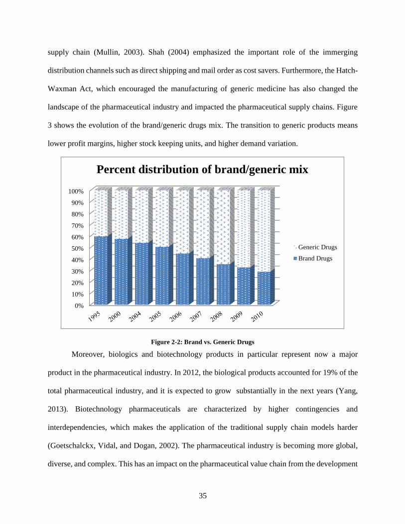
35

supply chain (Mullin, 2003). Shah (2004) emphasized the important role of the immerging

distribution channels such as direct shipping and mail order as cost savers. Furthermore, the Hatch-

Waxman Act, which encouraged the manufacturing of generic medicine has also changed the

landscape of the pharmaceutical industry and impacted the pharmaceutical supply chains. Figure

3 shows the evolution of the brand/generic drugs mix. The transition to generic products means

lower profit margins, higher stock keeping units, and higher demand variation.

Figure 2-2: Brand vs. Generic Drugs

Moreover, biologics and biotechnology products in particular represent now a major

product in the pharmaceutical industry. In 2012, the biological products accounted for 19% of the

total pharmaceutical industry, and it is expected to grow substantially in the next years (Yang,

2013). Biotechnology pharmaceuticals are characterized by higher contingencies and

interdependencies, which makes the application of the traditional supply chain models harder

(Goetschalckx, Vidal, and Dogan, 2002). The pharmaceutical industry is becoming more global,

diverse, and complex. This has an impact on the pharmaceutical value chain from the development

0%

10%

20%

30%

40%

50%

60%

70%

80%

90%

100%

Percent distribution of brand/generic mix

Generic Drugs

Brand Drugs

36

of a new drug to the marketing of the products (Papageorgiou et al., 2001). Given the high cost of

R&D and the reduced profit margin, pharmaceutical companies are required to optimize the

introduction of a new product given the existing capacity and the required investments.

Papageorgiou et al. (2001) proposed a mixed integer programming aiming to optimize the problem

and provide the most adequate configuration.

Finally, the changes in the regulations and the effect of the different players in the supply

chain make the conceptualization of the PSC more complicated. Rossetti et al (2011) identified

three main forces: compensation forces, channel forces, and product and regulatory forces. The

pharmaceutical supply chain is conceptualized as “a complex adaptive system (CAS) (Choi,

Dooley, and Rungtusanatham, 2001) whereby agents (participants) in the PSC are coupled in a

value chain of production, and any agent’s actions can potentially affect any other agent” (Rossetti,

Handfield, and Dooley, 2011).

Challenges Facing Pharmaceutical Supply Chain: The standard Supply Chain strategy

models are not easily applied to the PSC. First, the industry is shifting toward a higher

personalization level of product with high shortage cost and strict expiration rules. Second, the

separation of consumers (patients) and the customers (insurance companies and government)

makes the application of traditional SC practices more challenging (Rossetti et al., 2011; Teisberg

and Porter, 2006). Finally, the longer lead time, the high unpredictability demands, and the large

number of intermediaries contribute to more uncertainty in the PSC (Goetschalckx et al., 2002).

The literature of the pharmaceutical supply chain had also emphasized the new

pharmaceutical firms’ practices as another challenge. Distribution strategy was proposed as one of

the prominent challenges that the pharmaceutical industry is dealing with. Despite the domination

of indirect distribution modes (via wholesalers and distribution centers), about 13 percent of orders

37

are shipped directly to chain stores (Gautrin, 2002). This change in the distribution mode will

represent a supply chain configuration issue (e.g. ordering, storing, and logistics). Moreover, the

current pharmaceutical business model is focusing on securing and protecting the Intellectual

Property. The “Blockbuster Model” will ensure the firm’s financial viability. However, with most

of the blockbusters’ medicine patents already expired or expiring soon, pharmaceutical firms will

need to revise their strategy and give up the profit alone model (Cooper, 2008). In fact, the profit

alone model can be described as “A model where you are guaranteed to lose your entire book of

business every 10 to 12 years,” according to J.P. Garnier, former chief executive of

GlaxoSmithKline. Pharmaceutical viability will depend on the firm’s ability to develop a

collaborative business model.

Financial performance is an indicator of the business model viability. Although the

pharmaceutical firms are showing one of the highest profit margins among the industries (Teisberg

and Porter, 2006), the recent trends are not showing positive results. Between 1985 and 2000, the

top 15 pharmaceutical and biopharmaceutical firms were able to generate high returns to their

shareholders, measured by the compounded average growth rate (CAGR). In fact, eleven out of

fifteen firms had a CAGR higher that S&P 500. The same firms, between 2000 and 2010, however,

were unable to outperform the market. Only 3 firms had a CAGR higher than the market and ten

firms had a negative CAGR (Ajay, Matthias, and Martin, 2012). This is mainly due to the high

cost of R&D, the long process of new drug approval, and the fact that most low-hanging fruit had

already been picked.

The literature review of the two main concepts investigated (pharmaceutical supply chain

and mass customization and personalization) informs us about the relevance of the matter. It also

38

shows a gap in the literature that is addressed in the chapter research questions. The following

section addresses the various areas of investigation.

2.3 Conceptual Development

The literature review section has identified the major findings and areas of research related to mass

personalization. The current section expands the existing literature review by providing an

investigation of the new product paradigm (more personalized product with higher service level)

in the context of pharmaceutical products.

2.3.1 Customization and Personalization Continuum

The issue of mass customization and mass personalization in the area of pharmaceutical industry

is not as recent as it appears to be. While very few academic researchers have investigated mass

customization in a pharmaceutical context, practitioners have been calling for mass customization

and mass personalization as the new trend in the pharmaceutical industry for over a decade. Mass

customization in medicine will allow pharmaceutical companies to build a competitive advantage

and customer allegiance (Fitzgerald and McLaughlin, 2001). With a reduced profit margin and

less productive R&D activities, pharmaceutical firms are required to customize their products

while keeping the cost of production low. Specialized journals in the medical field have

emphasized the role of personalized medicine as an emergent practice in the pharmacogenomics

area (Mette et al., 2012; Xie and Frueh, 2005). The concept of mass personalized medicine was

investigated in the area of cancer treatment, dental medicine, and pain medicine. (Eng et al., 2012;

Kim and Dionne, 2009; Xie and Frueh, 2005).

The mass-production and mass-customization continuum as developed by Salvadore et al.

(2009) illustrates how firms can move along the continuum and what different capabilities are

required. The current chapter proposes to extend the existing continuum by adding the

39

personalization paradigm. The extended continuum will be referred to as the personalization

continuum. The continuum varies from purely standardized products and services to highly

personalized ones. Firms will position themselves along their value proposition. In a

manufacturing context, a firm can decide to provide a standardized product that aims to serve a

large customer base with no preference differences. Many products are standardized and do not

require any changes. This type of product is usually mass produced and delivered to customers.

On the other end of the continuum, highly personalized products aim at serving a unique customer.

This type of products portfolio is highly competitive and critical to manage. Very few firms have

captured the power of mass personalization and were able to provide a set of products that vary

along the spectrum (e.g. Vista Print, Nike). The personalization continuum is easier to assimilate

in a product paradigm where the market has showed a variety of examples along the continuum.

The personalization continuum can also be applied in the healthcare context. The literature review

section has discussed mass customization & personalization in the healthcare delivery context.

The healthcare industry is among the most complicated and labor & capital intensive

segments. The variety of products and services provided are in some parts standardized, yet need

to meet some unique patient specifications. Hospitals, for example, provide some standardized

procedures such as weight check and blood pressure as well as more personalized ones that

addresses the patient’s particular case. The pharmaceutical industry represents a major player in

the healthcare landscape with different products paradigms. While some medications are purely

standardized, where all patients take the same medication regardless of gender, age, blood type,

on the other side of the personalization continuum, some medications are prescribed based on

patient specifications, thereby making it more personalized. The pharmaceutical industry is now

40

offering extreme customized medication, where there is one exact medication for each patient.

This type of medication, like the products, are critical to administer.

The personalization continuum illustrates an organization’s value proposition and how

firms could determine their product portfolio. In the context of healthcare management, a strong

emphasis on service is provided as part of the value proposition. In fact, the healthcare industry is

highly service oriented. Even pharmaceuticals, which represent highly goods-focused

organizations, are providing service as part of their value propositions. The next section focuses

on the service product continuum.

2.3.2 Product-Service Continuum

The new value proposition requires an organization to provide combined products and service

components. Most of goods today are a combination of products and services (Bateson and

Hoffman, 1991). The goods/service continuum was first introduced by Johnson in 1969. Products

are perceived as a goods-service bundle, and the consumer choice is based on evaluation of these

criteria (Johnson, 1969). Several studies since then have attempted to measure the level of service

component vs. the goods one on the bundle (Murray and Schlacter, 1990; Parasuraman, Zeithaml,

and Berry, 1985). Operations management scholars have shown an interest in the product-service

continuum as important to better understand supply chain dynamics (Jacobs and Chase, 2010).

Most of the studies have identified four segments within the continuum: pure goods, core goods,

core services and pure services. Pure goods, such as commodity products, have a minimal service

element where the purchase decision is based purely on product assessment. Pure services, such

as legal consulting, have a minimal product component, except for a documentation or a report.

Most of the value derives from the service. Most of the products have a combination of goods and

service such as restaurants or car service.

41

Many studies have investigated the continuum by looking into more aspects. Murray et al.

(1990) have looked into the risk and reliability aspect of the product service continuum. They

found that the intangibility aspect of service makes consumers more risk averse to evaluating the

value of services. Customer satisfaction is impacted by the position of the product within the

continuum as the consumer perception of reliability of the product (Anderson, Fornell, and Rust,

1997). More recent studies have attempted to map the continuum across other variable. For

example, the goods-service continuum has been investigated across possession utilities for retail

industry (Winsor, Sheth, and Manolis, 2004).

The next subsection will provide a new mapping of the product-service continuum across

the personalization level spectrum. To my knowledge, no prior study has attempted to conceptually

reconcile the two concepts. This chapter attempts to link the mapping to the essence of this study

by applying the mapping to the healthcare concept.

2.3.3 Mapping the Personalization and Product/Service Continuum

The product/service continuum can be combined with the level of personalization continuum. The

following subsection will map the continuum for both general cases and the healthcare context.

2.3.3.1 General Context Mapping

Figure 2-3 has mapped the two different continuums for the general product/service context.

Commodity products are 100% standardized with no service component as part of the value

proposition. Sugars, wheat, and other commodities represent a typical standard product. Moving

along the personalization continuum, more customized products will reflect customers’ choices

and specifications. Personalized shoes and other gadgets will represent an example of highly

personalized products. The mapping will also combine the service level. Make to measure clothes

42

are more customized products with a service component since there is a strong interaction between

the customer and the service provider. In the extreme personalization level, bespoke, which are a

type of clothes that are designed for only one person, represents an evolution of the made to

measure clothes in the personalization continuum. Other relevant examples in the product/service

mix can be derived from the food industry. Fast foods, for example, tend to be more standardized

in comparison to restaurants. Despite a difference in the level of service provided by restaurants

and fast food, they are both located at the service/product mix with a different personalization

level. Finally, on the high service level extreme, high school education is, in general, standardized

in order to allow the students access to colleges. More customized services are consulting services,

such as legal and taxation, among others. The service provided will depend on the customers but

will have some standardized component. Website ads are highly personalized services provided to

computer users. In fact, when a user is browsing on the internet, information is stored regarding

preferences and needs. Web ads will be displayed according to these specifications. For example,

when an internet user searches for a hotel in a city or a treatment for a skin problem, a list of

relevant advertisements will be showing when he is surfing the website. The emergence of these

web ads is now amplified by the use of smart phones and their capabilities to capture and follow

users’ preferences.

The mapping for the general goods/service context is shown in figure 2-3.

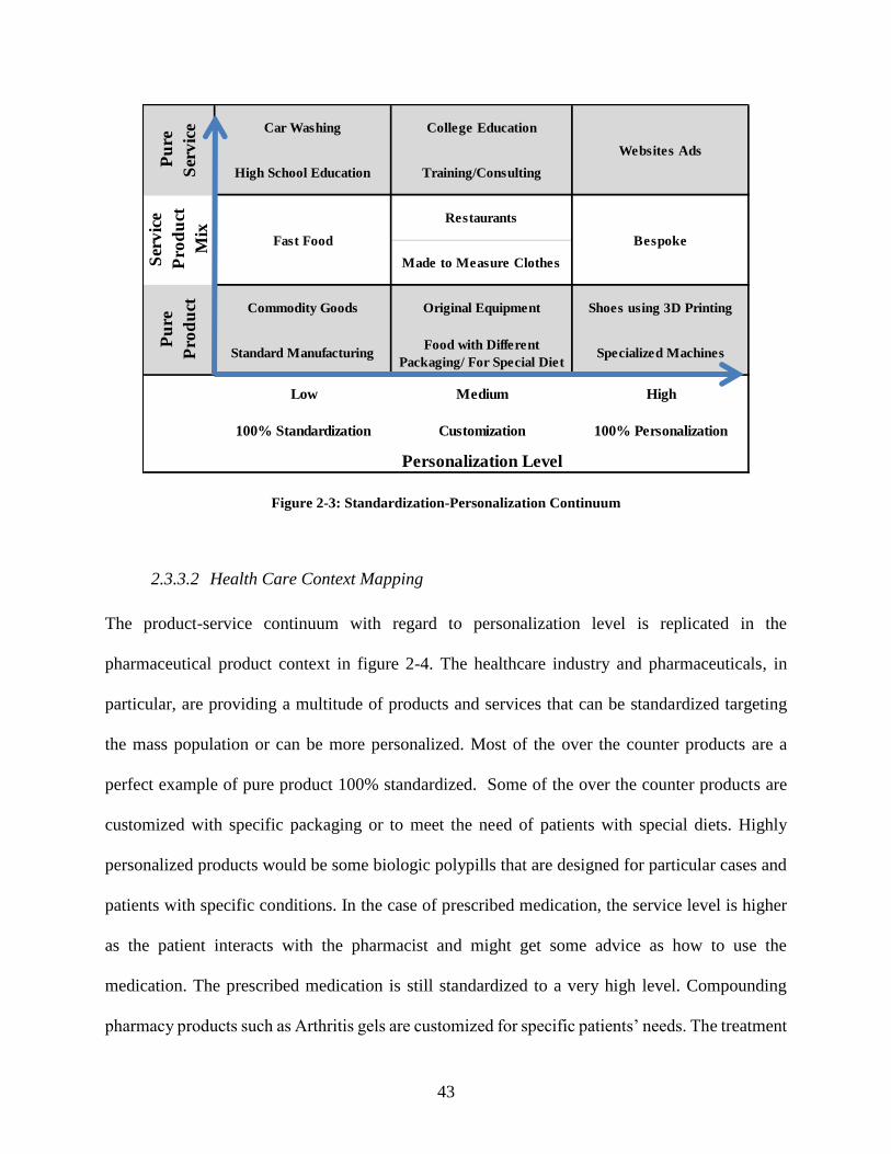
43

Figure 2-3: Standardization-Personalization Continuum

2.3.3.2 Health Care Context Mapping

The product-service continuum with regard to personalization level is replicated in the

pharmaceutical product context in figure 2-4. The healthcare industry and pharmaceuticals, in

particular, are providing a multitude of products and services that can be standardized targeting

the mass population or can be more personalized. Most of the over the counter products are a

perfect example of pure product 100% standardized. Some of the over the counter products are

customized with specific packaging or to meet the need of patients with special diets. Highly

personalized products would be some biologic polypills that are designed for particular cases and

patients with specific conditions. In the case of prescribed medication, the service level is higher

as the patient interacts with the pharmacist and might get some advice as how to use the

medication. The prescribed medication is still standardized to a very high level. Compounding

pharmacy products such as Arthritis gels are customized for specific patients’ needs. The treatment

Personalization Level

High

100% Standardization 100% PersonalizationCustomization

Bespoke

Medium

Shoes using 3D PrintingCommodity Goods Original Equipment

Food with Different

Packaging/ For Special Diet

Low

Websites Ads

Specialized Machines

Fast Food

College Education

Training/ConsultingP

ure

Ser

vic

e

Pu

re

Pro

du

ct

Ser

vic

e

Pro

du

ct

Mix

Standard Manufacturing

Restaurants

Made to Measure Clothes

Car Washing

High School Education

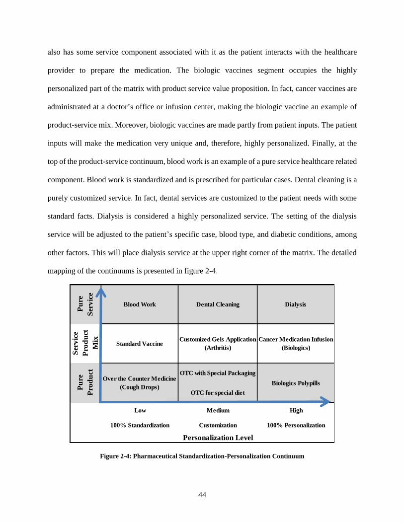
44

also has some service component associated with it as the patient interacts with the healthcare

provider to prepare the medication. The biologic vaccines segment occupies the highly

personalized part of the matrix with product service value proposition. In fact, cancer vaccines are

administrated at a doctor’s office or infusion center, making the biologic vaccine an example of

product-service mix. Moreover, biologic vaccines are made partly from patient inputs. The patient

inputs will make the medication very unique and, therefore, highly personalized. Finally, at the

top of the product-service continuum, blood work is an example of a pure service healthcare related

component. Blood work is standardized and is prescribed for particular cases. Dental cleaning is a

purely customized service. In fact, dental services are customized to the patient needs with some

standard facts. Dialysis is considered a highly personalized service. The setting of the dialysis

service will be adjusted to the patient’s specific case, blood type, and diabetic conditions, among

other factors. This will place dialysis service at the upper right corner of the matrix. The detailed

mapping of the continuums is presented in figure 2-4.

Figure 2-4: Pharmaceutical Standardization-Personalization Continuum

Low Medium High

Pu

re

Pro

du

ct

Ser

vic

e

Pro

du

ct

Mix

Standard VaccineCancer Medication Infusion

(Biologics)

Pu

re

Ser

vic

e

Dialysis Dental Cleaning

Customized Gels Application

(Arthritis)

Blood Work

OTC with Special Packaging

OTC for special diet

Biologics Polypills

Personalization Level

Over the Counter Medicine

(Cough Drops)

100% Standardization Customization 100% Personalization

45

2.3.4 Mapping the Pharmaceutical Supply Chain Evolution

According to the Kaiser Family Foundation report (2005), the Pharmaceutical Supply Chain (PSC)

is identified as the means through which prescription medicines are delivered to patients. PSC

represents the different flow of transferring the medicine to the patient. The process includes the

procurement of raw material, the manufacturing of the drugs, marketing and logistics functions

(Horton, 2010; Shah, 2004a). The pharmaceutical supply chain includes three main flows:

physical, financial, and information flows. The physical flow consists of the drugs travelling along

the value chain and from a raw material to the patient. The information flow represents the

exchange of information that happens along the supply chain among the different participants in

the supply chain (manufacturer, suppliers, patient, doctor, hospital, insurance, pharmacy benefit

managers). Finally, the financial flow is the payments made between and among the different

players within the supply chain. The consumer, who is the patient, will receive the service/product

and the customer, who is the payer, will be in charge of making the payment. The customer in

most of the cases is the patient, the insurance, the government or a combination of these.

2.3.4.1 Mapping the Small Molecules Pharmaceutical Supply Chain

The pharmaceutical supply chain is conceptually composed of five key echelons: (a) drug

manufacturers, such as biotechnology research institutes, pharmaceutical companies, and medical

suppliers; (b) medicine delivery intermediaries, such as wholesalers, distributors, logistics

companies, and group purchasing agencies; (c) healthcare providers: hospitals, clinics, and

physicians; (d) medicine payers, such as insurance companies, government, employers; and (e)

medicine consumers: patients (Burns, 2002; Pedroso and Nakano, 2009).

Pharmaceutical Manufacturers: The pharmaceutical industry is a consolidated industry

with relatively few large, multinational firms. Pharmaceutical manufacturers have the most

46

influence over pharmaceutical prices, assessing expected demand, future competition, and

projected marketing costs to establish the wholesale acquisition cost (WAC), which is the baseline

price at which wholesale distributors purchase drug products. The pharmaceutical manufacturing

industry is highly consolidated with a decreasing number of brand name manufacturing firms in

the United States over the past 10 years (Yang, 2013). In fact, the top six firms account for almost

50% of the market share as shown in figure 2-3 (Yang, 2013). The consolidation is mainly caused

by high barriers to enter. The large investment required, the high governmental regulations, the

advanced research and investment capabilities, and the product time to market make very hard the

success of new entrant in the market.

Wholesale Distributors: The wholesale distribution industry has consolidated in the last 30

years, with the number of wholesale distributors in the U.S. declining from approximately 200 in

1975 to fewer than 50 in 2000 (Alazraki, 2011). The top 3 wholesale distributors account for almost

90 percent of the wholesale market. Wholesale distributors typically sell drugs to pharmacies at

WAC plus some negotiated percentage. Three major companies generate about 85% of all

revenues from pharmaceutical wholesaling in the United States (AmerisourceBergen, Cardinal

Health and McKesson). The total revenue generated by the big three wholesalers is $290 billion

in 2011 (Fein, 2012). The wholesaler’s main role is to guarantee the timely distribution of the

medicine, especially for the high value density drugs. Moreover, through their network of

representatives, the wholesale distributors will ensure the geographical distribution of the drugs to

smaller retailers and pharmacies.

Pharmacies: In 2010, The United States accounted for approximately 63,000 pharmacies.

More than half (37,615) are part of big chain (SK&A, 2012). The graph below summarizes the

pharmacy ownership in the United States.

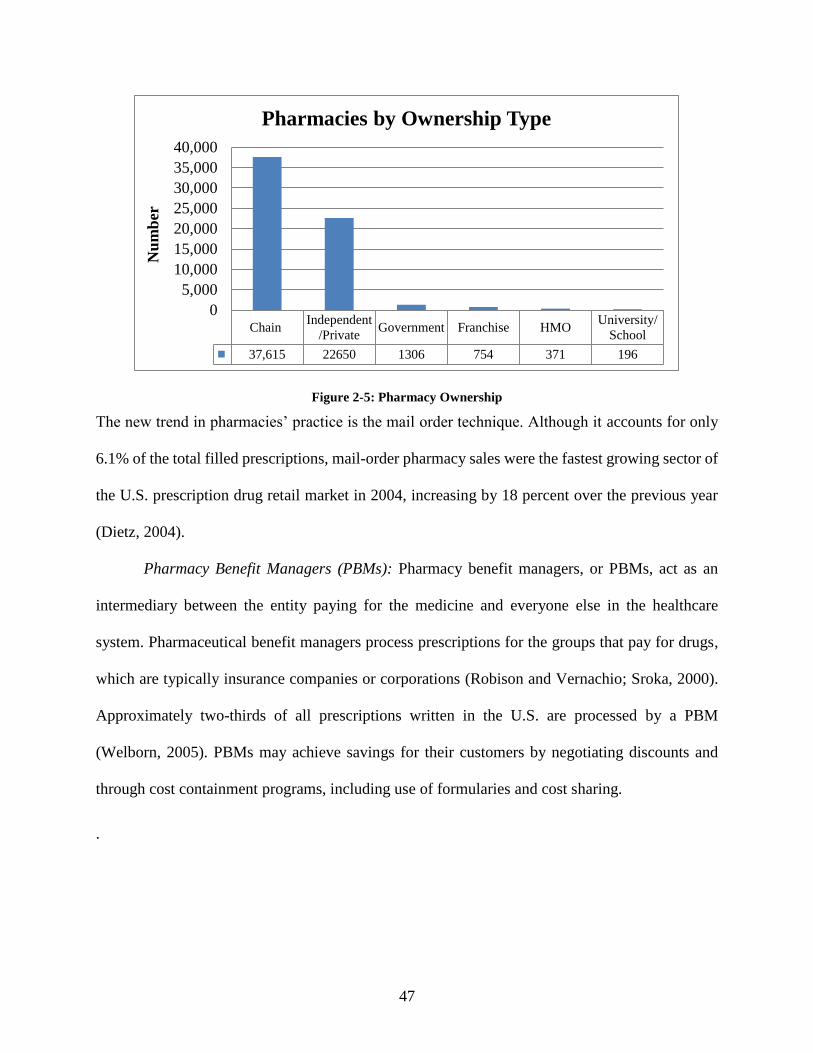
47

Figure 2-5: Pharmacy Ownership

The new trend in pharmacies’ practice is the mail order technique. Although it accounts for only

6.1% of the total filled prescriptions, mail-order pharmacy sales were the fastest growing sector of

the U.S. prescription drug retail market in 2004, increasing by 18 percent over the previous year

(Dietz, 2004).

Pharmacy Benefit Managers (PBMs): Pharmacy benefit managers, or PBMs, act as an

intermediary between the entity paying for the medicine and everyone else in the healthcare

system. Pharmaceutical benefit managers process prescriptions for the groups that pay for drugs,

which are typically insurance companies or corporations (Robison and Vernachio; Sroka, 2000).

Approximately two-thirds of all prescriptions written in the U.S. are processed by a PBM

(Welborn, 2005). PBMs may achieve savings for their customers by negotiating discounts and

through cost containment programs, including use of formularies and cost sharing.

.

ChainIndependent

/PrivateGovernment Franchise HMO

University/

School

37,615 22650 1306 754 371 196

0

5,000

10,000

15,000

20,000

25,000

30,000

35,000

40,000N

um

ber

Pharmacies by Ownership Type

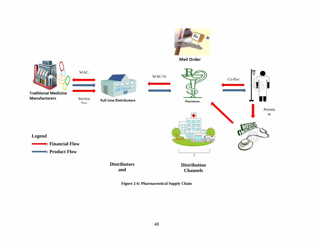
48

Figure 2-6: Pharmaceutical Supply Chain

WAC

Premiu

m

Payment

Co-Pay

Service

Fee

WAC-%

Distribution

Channels

Distributors

and

Wholesalers

Legend

: Financial Flow

: Product Flow

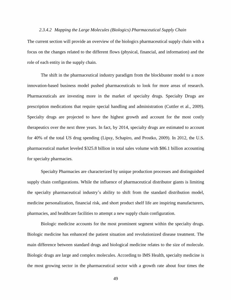
49

2.3.4.2 Mapping the Large Molecules (Biologics) Pharmaceutical Supply Chain

The current section will provide an overview of the biologics pharmaceutical supply chain with a

focus on the changes related to the different flows (physical, financial, and information) and the

role of each entity in the supply chain.

The shift in the pharmaceutical industry paradigm from the blockbuster model to a more

innovation-based business model pushed pharmaceuticals to look for more areas of research.

Pharmaceuticals are investing more in the market of specialty drugs. Specialty Drugs are

prescription medications that require special handling and administration (Cuttler et al., 2009).

Specialty drugs are projected to have the highest growth and account for the most costly

therapeutics over the next three years. In fact, by 2014, specialty drugs are estimated to account

for 40% of the total US drug spending (Lipsy, Schapiro, and Prostko, 2009). In 2012, the U.S.

pharmaceutical market leveled $325.8 billion in total sales volume with $86.1 billion accounting

for specialty pharmacies.

Specialty Pharmacies are characterized by unique production processes and distinguished

supply chain configurations. While the influence of pharmaceutical distributor giants is limiting

the specialty pharmaceutical industry’s ability to shift from the standard distribution model,

medicine personalization, financial risk, and short product shelf life are inspiring manufacturers,

pharmacies, and healthcare facilities to attempt a new supply chain configuration.

Biologic medicine accounts for the most prominent segment within the specialty drugs.

Biologic medicine has enhanced the patient situation and revolutionized disease treatment. The

main difference between standard drugs and biological medicine relates to the size of molecule.

Biologic drugs are large and complex molecules. According to IMS Health, specialty medicine is

the most growing sector in the pharmaceutical sector with a growth rate about four times the

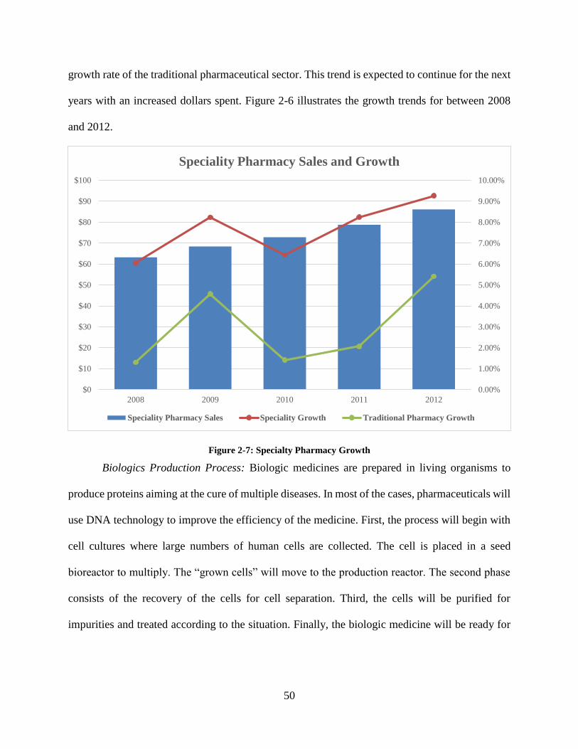
50

growth rate of the traditional pharmaceutical sector. This trend is expected to continue for the next

years with an increased dollars spent. Figure 2-6 illustrates the growth trends for between 2008

and 2012.

Figure 2-7: Specialty Pharmacy Growth

Biologics Production Process: Biologic medicines are prepared in living organisms to

produce proteins aiming at the cure of multiple diseases. In most of the cases, pharmaceuticals will

use DNA technology to improve the efficiency of the medicine. First, the process will begin with

cell cultures where large numbers of human cells are collected. The cell is placed in a seed

bioreactor to multiply. The “grown cells” will move to the production reactor. The second phase

consists of the recovery of the cells for cell separation. Third, the cells will be purified for

impurities and treated according to the situation. Finally, the biologic medicine will be ready for

0.00%

1.00%

2.00%

3.00%

4.00%

5.00%

6.00%

7.00%

8.00%

9.00%

10.00%

$0

$10

$20

$30

$40

$50

$60

$70

$80

$90

$100

2008 2009 2010 2011 2012

Speciality Pharmacy Sales and Growth

Speciality Pharmacy Sales Speciality Growth Traditional Pharmacy Growth

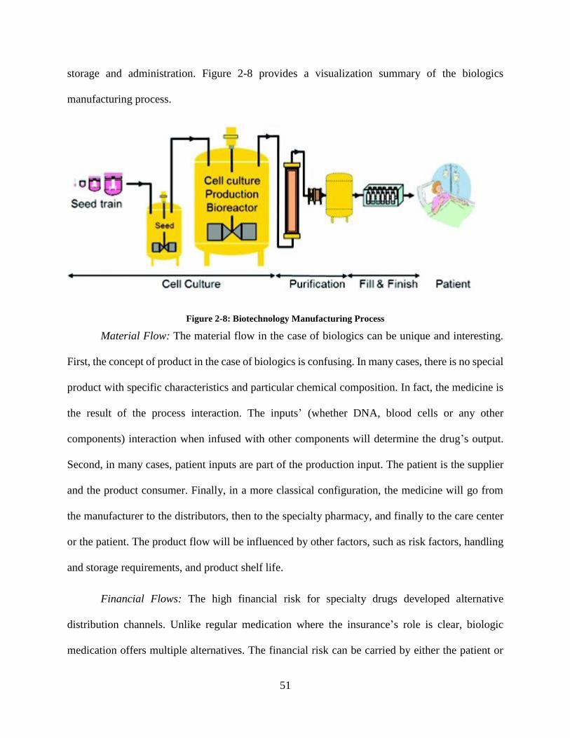
51

storage and administration. Figure 2-8 provides a visualization summary of the biologics

manufacturing process.

Figure 2-8: Biotechnology Manufacturing Process

Material Flow: The material flow in the case of biologics can be unique and interesting.

First, the concept of product in the case of biologics is confusing. In many cases, there is no special

product with specific characteristics and particular chemical composition. In fact, the medicine is

the result of the process interaction. The inputs’ (whether DNA, blood cells or any other

components) interaction when infused with other components will determine the drug’s output.

Second, in many cases, patient inputs are part of the production input. The patient is the supplier

and the product consumer. Finally, in a more classical configuration, the medicine will go from

the manufacturer to the distributors, then to the specialty pharmacy, and finally to the care center

or the patient. The product flow will be influenced by other factors, such as risk factors, handling

and storage requirements, and product shelf life.

Financial Flows: The high financial risk for specialty drugs developed alternative

distribution channels. Unlike regular medication where the insurance’s role is clear, biologic

medication offers multiple alternatives. The financial risk can be carried by either the patient or

52

the care giver (Clinic or doctor’s office), or in rare cases shared. The jargon used in the industry is

white bagging and brown bagging. In white bagging, the specialty pharmacy ships the drug directly

to the clinic or doctor’s office just in time for the patient’s scheduled treatment. On the other side,

brown bagging, the patient will buy the product directly from the pharmacy and take responsibility

for the storage and transportation. White bagging represents more of a financial risk for doctors

because they might not get reimbursed entirely for the drug cost. Moreover, small doctors’ offices

will have some obstacles with handling and storing the medication, as it adds more cost. On the

other hand, brown bagging puts the financial risk at the patient’s end, where the patient will have

to get reimbursed for the medication. However, many doctor’s offices do not accept this alternative

because of the drug mishandling issues and dosage problems. In fact, in many cases, doctors have

to change the medication dosage or reschedule the appointment because the patient either lost

weight or is not in a good condition to receive the treatment. The brown bagging distribution

channel does not provide enough flexibility to the doctor to make changes to the doses.

The financial flows in the biologics supply chain are mainly influenced by the level of risk

sharing which determine who is accountable for what. For large doctors’ offices, “the buy and bill”

model is common, where the doctor purchases the medicine directly from the distributor and takes

a full financial risk. The other alternative will require the involvement of specialty pharmacies and

more risk taking from the patient.

Pharmaceutical Closed Loop: The biologics supply chain represents the uniqueness of

having the patient input as part of the raw material. In many biologic medications (e.g. cancer

vaccine, blood products, tissue product), the patient will provide a sample from his/her body to be

treated and developed into personalized medication. In this case, the material will flow first from

the doctor’s office back to the manufacturing processing location and then back to the doctor’s

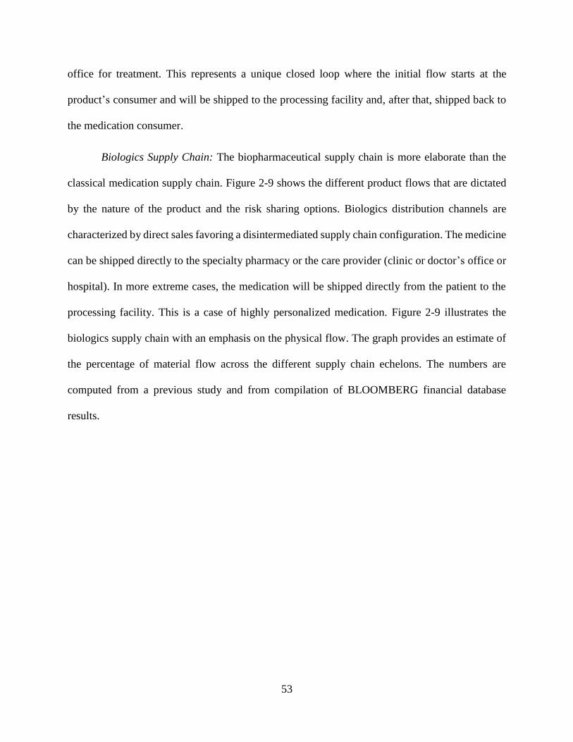
53

office for treatment. This represents a unique closed loop where the initial flow starts at the

product’s consumer and will be shipped to the processing facility and, after that, shipped back to

the medication consumer.

Biologics Supply Chain: The biopharmaceutical supply chain is more elaborate than the

classical medication supply chain. Figure 2-9 shows the different product flows that are dictated

by the nature of the product and the risk sharing options. Biologics distribution channels are

characterized by direct sales favoring a disintermediated supply chain configuration. The medicine

can be shipped directly to the specialty pharmacy or the care provider (clinic or doctor’s office or

hospital). In more extreme cases, the medication will be shipped directly from the patient to the

processing facility. This is a case of highly personalized medication. Figure 2-9 illustrates the

biologics supply chain with an emphasis on the physical flow. The graph provides an estimate of

the percentage of material flow across the different supply chain echelons. The numbers are

computed from a previous study and from compilation of BLOOMBERG financial database

results.

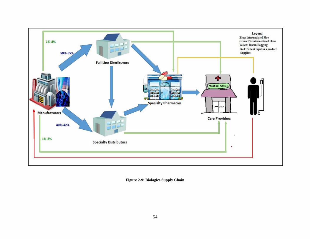
54

Figure 2-9: Biologics Supply Chain

55

2.3.5 Disintermediation Continuum

The choice of a distribution channel represents a strategic decision that will shape the firm’s long-

term commitment with its supply chain partners. The pharmaceutical supply chain as explored in

the previous section is evolving from a more traditional flat supply chain distribution model where

the medication moves down the supply chain and is distributed through wholesalers and

distributors to a more complex configuration. The drugs in the case of biologic medications can

be shipped directly to the hospital or the end consumer. Such practice is referred to as supply chain

disintermediation. Disintermediation refers to the elimination of the middle entities between the

product/service provider and the end customer (Chircu and Kauffman, 1999). The concept of

disintermediation is a popular practice in many industries such as retail, where customers will buy

their products and services directly from the manufacturer or the service provider. The

organization will have the option to select the distribution channels configuration. Some

organizations will decide to be fully intermediated, fully disintermediated, or have a mix strategy

by balancing disintermediated and intermediated distribution strategies. The distribution strategy

is therefore conceptualized as a disintermediation level continuum.

The level of disintermediation in the distribution channels will dictate the organization’s

supply chain strategy. Many companies decide to be fully intermediated. The main purpose of

intermediation is to facilitate product/service diffusion by utilizing the intermediaries’ networks,

the customers base, and know-how (Chiang, 2012). A fully intermediated distribution strategy is

a common practice in functional and commodities products. For example, the sugar supply chain

is totally intermediated. A customer cannot buy the sugar directly from the sugar producer. This is

due, in fact, to the level of standardization and the low variable cost. Sugar producers are better

off pushing their products through the distributors and wholesalers. Paper-related products are

56

another good example of a totally intermediated industry. With a stagnant demand and high set up

costs, paper mills sell their products to the wholesalers and distributors. Other organizations would

prefer to have a mixed strategy where the firm will attempt to capture the benefit of both strategies.

From one end, the intermediated distributed channels will enable more market access for the firm

and push the products and services in the pipeline. On the other end, a disintermediated strategy

will enable the organization to have more customer input and provide more customized products.

According to Apple Inc. reports, the firm maintained a more disintermediated strategy before 2010

when its products were mainly sold online and through its Apple store network. Today, Apple

products are available in a variety of distribution channels, outlets such as Best Buy and Walmart,

among others. Electronics products, in fact, represent a good example of a hybrid disintermediation

distribution strategy. Clothes products are also sold direct to customers or can be distributed

through wholesalers. Adidas, for instance, is selling its products directly online as well as through

some retailers such as Macy’s stores. Finally, a fully disintermediated strategy is popular among

certain products. For example, Vista Print, Shutterfly, and Zazzle are selling their products

exclusively through direct sales. This type of product is, in general, customized and requires

customers’ input. The disintermediation continuum is also applicable in the healthcare context

with its stronger focus on product as part of value proposition. In fact, the disintermediation level

relates to the physical flow.

The pharmaceutical supply chain presents a variety of disintermediation levels. First,

standardized medicines such as over the counter medication which are characterized by a long

shelf life are sold through distributors and wholesalers. Pharmaceutical firms use push strategy to

sell some of its medication by using the middleman as a buffer to maximize the service level. Other

examples of disintermediated pharmaceutical products are vaccines which are distributed through

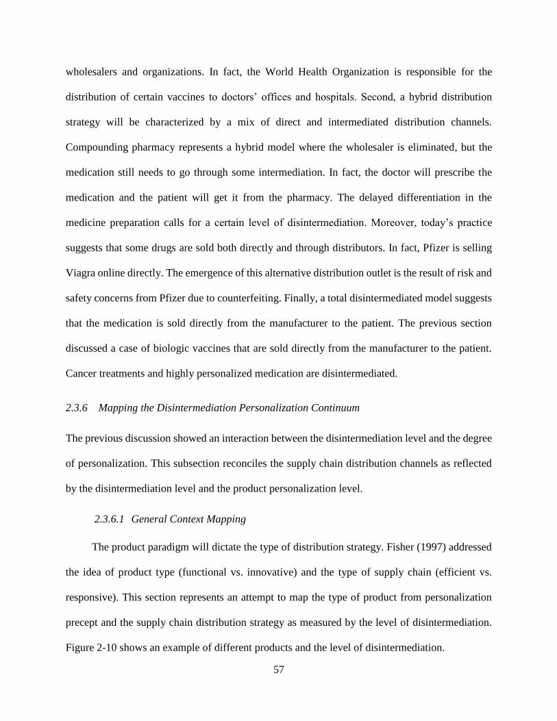
57

wholesalers and organizations. In fact, the World Health Organization is responsible for the

distribution of certain vaccines to doctors’ offices and hospitals. Second, a hybrid distribution

strategy will be characterized by a mix of direct and intermediated distribution channels.

Compounding pharmacy represents a hybrid model where the wholesaler is eliminated, but the

medication still needs to go through some intermediation. In fact, the doctor will prescribe the

medication and the patient will get it from the pharmacy. The delayed differentiation in the

medicine preparation calls for a certain level of disintermediation. Moreover, today’s practice

suggests that some drugs are sold both directly and through distributors. In fact, Pfizer is selling

Viagra online directly. The emergence of this alternative distribution outlet is the result of risk and

safety concerns from Pfizer due to counterfeiting. Finally, a total disintermediated model suggests

that the medication is sold directly from the manufacturer to the patient. The previous section

discussed a case of biologic vaccines that are sold directly from the manufacturer to the patient.

Cancer treatments and highly personalized medication are disintermediated.

2.3.6 Mapping the Disintermediation Personalization Continuum

The previous discussion showed an interaction between the disintermediation level and the degree

of personalization. This subsection reconciles the supply chain distribution channels as reflected

by the disintermediation level and the product personalization level.

2.3.6.1 General Context Mapping

The product paradigm will dictate the type of distribution strategy. Fisher (1997) addressed

the idea of product type (functional vs. innovative) and the type of supply chain (efficient vs.

responsive). This section represents an attempt to map the type of product from personalization

precept and the supply chain distribution strategy as measured by the level of disintermediation.

Figure 2-10 shows an example of different products and the level of disintermediation.

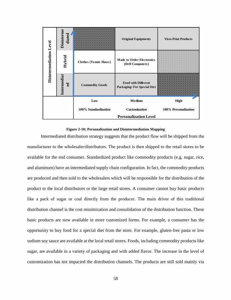
58

Figure 2-10: Personalization and Disintermediation Mapping

Intermediated distribution strategy suggests that the product flow will be shipped from the

manufacturer to the wholesaler/distributors. The product is then shipped to the retail stores to be

available for the end consumer. Standardized product like commodity products (e.g. sugar, rice,

and aluminum) have an intermediated supply chain configuration. In fact, the commodity products

are produced and then sold to the wholesalers which will be responsible for the distribution of the

product to the local distributors or the large retail stores. A consumer cannot buy basic products

like a pack of sugar or coal directly from the producer. The main driver of this traditional

distribution channel is the cost minimization and consolidation of the distribution function. These

basic products are now available in more customized forms. For example, a consumer has the

opportunity to buy food for a special diet from the store. For example, gluten-free pasta or low

sodium soy sauce are available at the local retail stores. Foods, including commodity products like

sugar, are available in a variety of packaging and with added flavor. The increase in the level of

customization has not impacted the distribution channels. The products are still sold mainly via

Dis

inte

rmed

iati

on

Lev

el

Original Equipments

Food with Different

Packaging/ For Special DietCommodity Goods

Made to Order Electronics

(Dell Computers)

Personalization Level

100% Standardization Customization 100% Personalization

Low Medium High

Inte

rmed

iat

edH

yb

rid

Clothes (Tennis Shoes)D

isin

term

e

dia

ted

Vista Print Products

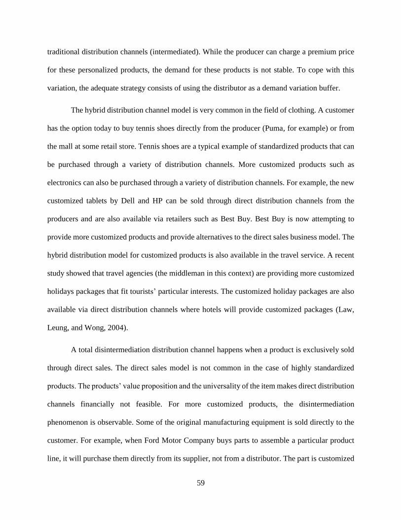
59

traditional distribution channels (intermediated). While the producer can charge a premium price

for these personalized products, the demand for these products is not stable. To cope with this

variation, the adequate strategy consists of using the distributor as a demand variation buffer.

The hybrid distribution channel model is very common in the field of clothing. A customer

has the option today to buy tennis shoes directly from the producer (Puma, for example) or from

the mall at some retail store. Tennis shoes are a typical example of standardized products that can

be purchased through a variety of distribution channels. More customized products such as

electronics can also be purchased through a variety of distribution channels. For example, the new

customized tablets by Dell and HP can be sold through direct distribution channels from the

producers and are also available via retailers such as Best Buy. Best Buy is now attempting to

provide more customized products and provide alternatives to the direct sales business model. The

hybrid distribution model for customized products is also available in the travel service. A recent

study showed that travel agencies (the middleman in this context) are providing more customized

holidays packages that fit tourists’ particular interests. The customized holiday packages are also

available via direct distribution channels where hotels will provide customized packages (Law,

Leung, and Wong, 2004).

A total disintermediation distribution channel happens when a product is exclusively sold

through direct sales. The direct sales model is not common in the case of highly standardized

products. The products’ value proposition and the universality of the item makes direct distribution

channels financially not feasible. For more customized products, the disintermediation

phenomenon is observable. Some of the original manufacturing equipment is sold directly to the

customer. For example, when Ford Motor Company buys parts to assemble a particular product

line, it will purchase them directly from its supplier, not from a distributor. The part is customized

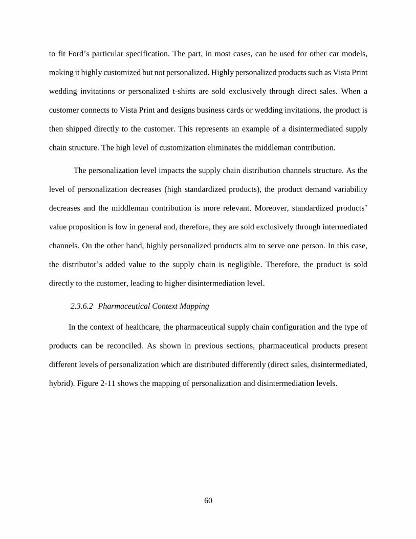
60

to fit Ford’s particular specification. The part, in most cases, can be used for other car models,

making it highly customized but not personalized. Highly personalized products such as Vista Print

wedding invitations or personalized t-shirts are sold exclusively through direct sales. When a

customer connects to Vista Print and designs business cards or wedding invitations, the product is

then shipped directly to the customer. This represents an example of a disintermediated supply

chain structure. The high level of customization eliminates the middleman contribution.

The personalization level impacts the supply chain distribution channels structure. As the

level of personalization decreases (high standardized products), the product demand variability

decreases and the middleman contribution is more relevant. Moreover, standardized products’

value proposition is low in general and, therefore, they are sold exclusively through intermediated

channels. On the other hand, highly personalized products aim to serve one person. In this case,

the distributor’s added value to the supply chain is negligible. Therefore, the product is sold

directly to the customer, leading to higher disintermediation level.

2.3.6.2 Pharmaceutical Context Mapping

In the context of healthcare, the pharmaceutical supply chain configuration and the type of

products can be reconciled. As shown in previous sections, pharmaceutical products present

different levels of personalization which are distributed differently (direct sales, disintermediated,

hybrid). Figure 2-11 shows the mapping of personalization and disintermediation levels.

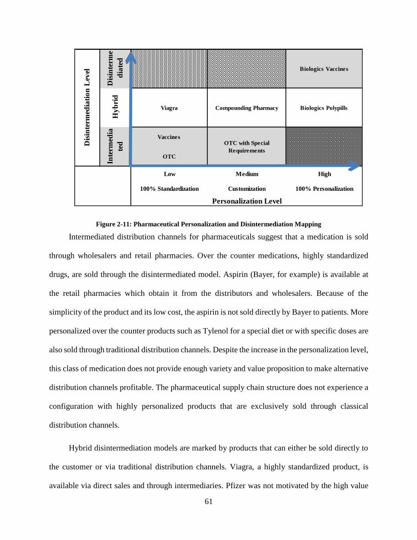
61

Figure 2-11: Pharmaceutical Personalization and Disintermediation Mapping

Intermediated distribution channels for pharmaceuticals suggest that a medication is sold

through wholesalers and retail pharmacies. Over the counter medications, highly standardized

drugs, are sold through the disintermediated model. Aspirin (Bayer, for example) is available at

the retail pharmacies which obtain it from the distributors and wholesalers. Because of the

simplicity of the product and its low cost, the aspirin is not sold directly by Bayer to patients. More

personalized over the counter products such as Tylenol for a special diet or with specific doses are

also sold through traditional distribution channels. Despite the increase in the personalization level,

this class of medication does not provide enough variety and value proposition to make alternative

distribution channels profitable. The pharmaceutical supply chain structure does not experience a

configuration with highly personalized products that are exclusively sold through classical

distribution channels.

Hybrid disintermediation models are marked by products that can either be sold directly to

the customer or via traditional distribution channels. Viagra, a highly standardized product, is

available via direct sales and through intermediaries. Pfizer was not motivated by the high value

Dis

inte

rmed

iati

on

Lev

el

OTC with Special

Requirements

Vaccines

Biologics Polypills

OTC

Low Medium

Compounding Pharmacy

100% Personalization

Inte

rmed

ia

ted

Dis

inte

rme

dia

ted

Biologics Vaccines

Hy

bri

dViagra

High

100% Standardization Customization

Personalization Level

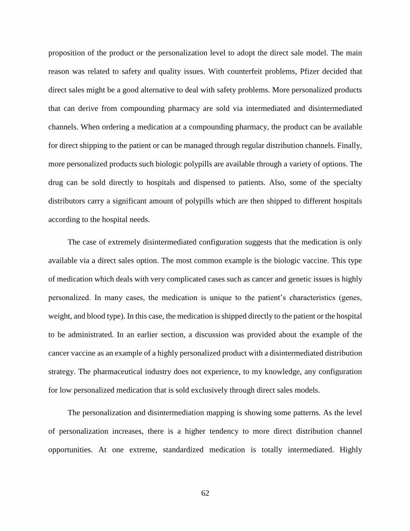
62

proposition of the product or the personalization level to adopt the direct sale model. The main

reason was related to safety and quality issues. With counterfeit problems, Pfizer decided that

direct sales might be a good alternative to deal with safety problems. More personalized products

that can derive from compounding pharmacy are sold via intermediated and disintermediated

channels. When ordering a medication at a compounding pharmacy, the product can be available

for direct shipping to the patient or can be managed through regular distribution channels. Finally,

more personalized products such biologic polypills are available through a variety of options. The

drug can be sold directly to hospitals and dispensed to patients. Also, some of the specialty

distributors carry a significant amount of polypills which are then shipped to different hospitals

according to the hospital needs.

The case of extremely disintermediated configuration suggests that the medication is only

available via a direct sales option. The most common example is the biologic vaccine. This type

of medication which deals with very complicated cases such as cancer and genetic issues is highly

personalized. In many cases, the medication is unique to the patient’s characteristics (genes,

weight, and blood type). In this case, the medication is shipped directly to the patient or the hospital

to be administrated. In an earlier section, a discussion was provided about the example of the

cancer vaccine as an example of a highly personalized product with a disintermediated distribution

strategy. The pharmaceutical industry does not experience, to my knowledge, any configuration

for low personalized medication that is sold exclusively through direct sales models.

The personalization and disintermediation mapping is showing some patterns. As the level

of personalization increases, there is a higher tendency to more direct distribution channel

opportunities. At one extreme, standardized medication is totally intermediated. Highly

63

personalized medication is distributed directly to the patient or doctor’s office where the drug is

administrated.

2.4 Conclusion

The pharmaceutical industry’s landscape is experiencing an evolutionary change for both the

product paradigm and the supply chain configuration. The current chapter intends to provide a

better understanding of the evolution of pharmaceutical industry and how it shaped the

development of the pharmaceutical supply chain and the emergence of the new product paradigm.

With more emphasis on the market of the one customer, the product paradigm has shifted from

mass produced goods to more personalized products with higher attention to the service component

as part of the value proposition. The pharmaceutical industry has followed the same evolution with

much slower pace due to less consumer involvement in the product design.

The change of the product paradigm has influenced the supply chain configuration. First, the

level of medicine personalization has created more direct sales opportunities and disintermediated

distribution channels. This has an impact on the physical flows. In fact, the pharmaceutical

practices are offering more direct sales opportunities, making the medication flow directly from

the manufacturers to the patient and/or hospitals. The product flow has even evolved to a more

complex closed loop flow. The drug production process starts at the doctor’s office where inputs

from the patient is part of the raw material input. The patient’s inputs will be shipped to the

processing facility and then sent back to the patient to be administrated. Second, the financial flows

are more complex in the case of more personalized medication. The practices have shown newer

flows known as brown and white bagging. The risk sharing level has an impact on the financial

flow. Finally, the financial performance structure is different according to the level of product

personalization. On the other side, the evolution of the pharmaceutical supply chain has enhanced

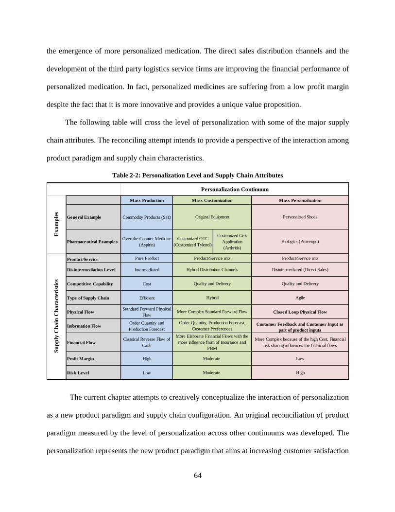
64

the emergence of more personalized medication. The direct sales distribution channels and the

development of the third party logistics service firms are improving the financial performance of

personalized medication. In fact, personalized medicines are suffering from a low profit margin

despite the fact that it is more innovative and provides a unique value proposition.

The following table will cross the level of personalization with some of the major supply

chain attributes. The reconciling attempt intends to provide a perspective of the interaction among

product paradigm and supply chain characteristics.

Table 2-2: Personalization Level and Supply Chain Attributes

The current chapter attempts to creatively conceptualize the interaction of personalization

as a new product paradigm and supply chain configuration. An original reconciliation of product

paradigm measured by the level of personalization across other continuums was developed. The

personalization represents the new product paradigm that aims at increasing customer satisfaction

Mass Production

General Example Commodity Products (Salt)

Pharmaceutical ExamplesOver the Counter Medicine

(Aspirin)

Customized OTC

(Customized Tylenol)

Customized Gels

Application

(Arthritis)

Product/Service Pure Product

Disintermediation Level Intermediated

Competitive Capability Cost

Type of Supply Chain Efficient

Physical FlowStandard Forward Physical

Flow

Information FlowOrder Quantity and

Production Forecast

Financial FlowClassical Reverse Flow of

Cash

Profit Margin High

Risk Level Low

Personalization Continuum

Su

pp

ly C

ha

in C

ha

ract

eris

tics

Original Equipment Personalized Shoes

Hybrid Distribution Channels Disintermediated (Direct Sales)

Ex

am

ple

s

More Complex Standard Forward Flow Closed Loop Physical Flow

Product/Service mix

Biologics (Provenge)

Agile

Mass Customization Mass Personalization

Order Quantity, Production Forecast,

Customer PreferencesCustomer Feedback and Customer Input as

part of product inputs

More Elaborate Financial Flows with the

more influence from of Insurance and

PBM

More Complex because of the high Cost. Financial

risk sharing influences the financial flows

Hybrid

Quality and Delivery

Product/Service mix

Quality and Delivery

Moderate Low

Moderate High

65

and improving profitability. First, the chapter mapped the personalization spectrum with the

service/product continuum. Despite extensive work on the product-service continuum for over four

decades, very few studies have attempted to reconcile the continuum across different dimensions.

The conceptualization provides an innovative mapping to the product-service continuum across

the personalization level. With no loss of generalization, the framework has applied the general

finding to the healthcare context, the main focus of this study. Second, the study addressed the

structural change of the pharmaceutical supply chain. The extensive literature review showed rich

exploration of the pharmaceutical supply chains, yet no major works have addressed the recent

evolution of pharmaceutical supply chains. The emergence of a new type of medication which is

highly personalized, expensive, and with low shelf life has provided a new type of distribution

channel. The pharmaceutical supply chain has shown new distribution practices marked by

disintermediation and direct sales. The chapter provided an attempt to assess the new distribution

channels and quantify the physical flows. Based on observations from pharmaceutical firms’

annual reports and data collected from secondary sources, an estimation of different physical flows

for the large molecules (specialty pharmaceuticals) supply chains was provided. The finding

showed a relatively higher level of disintermediation for large molecule drugs in comparison with

traditional small molecule medication. The pharmaceutical industry is still, however, under the

pressure of traditional distribution channels through the distributors. Finally, the study has mapped

the main two concepts addressed in this chapter: product paradigm and pharmaceutical supply

chain. While the product paradigm was measured by the personalization level, the supply chain

configuration was conceptualized by the disintermediation level. Certain patterns of

personalization and supply chain disintermediation interaction were identified. The observations

showed that large molecule medication (biologics) have a higher personalization level. Biologic

66

drugs are also distributed in more direct distribution channels promoting disintermediation. On the

other hand, small molecule drugs (traditional medicine) are more standardized and are sold using

classic distribution outlets, emphasizing a more intermediated model.

67

3 Chapter 3: Strategic Location Consideration in

Biopharmaceuticals: A Case Study

3.1 Introduction and Research Objectives

Facility location represents a strategic decision that has an impact on the organization performance.

Facility location is critical in manufacturing as well as service industry to minimize logistical cost

and improve customer service level. In the healthcare context, the location decision is even more

critical because the level of liability goes beyond the loss of profit to involve patients’ lives.

The literature review had addressed the location problem for pharmaceutical companies

(Ruane and Zhang, 2007). The decision variable in the pharmaceutical case can be a warehouse

location decision or manufacturing site. However, the importance of location problem for

traditional pharmaceutical modulated by the high value density of the products and the high

operating margin. As discussed in chapter 2, the traditional (small molecules) pharmaceutical

supply chain relies on the intermediaries to insure the product availability at the pharmacies. The

location problem is more critical in the case of biologics. Biologics are expensive medication that

requires special handling and are time sensitive. The case are even more critical in the case of

extremely personalized medication where the patient input (blood cells, DNA material…) are part

of the input into the production process. In this case, the processing location facility is critical

because of the cost of transportation and the product perishability.

Prior literature addressed the location problem in the context of healthcare facilities for

over forty years (Fitzsimmons, 1973; Toregas et al., 1971). Several problems were investigated

and multiple solution methodologies and heuristics were proposed (Klose and Drexl, 2005; Melo,

Nickel, and Saldanha-da-Gama, 2009). Other work addressed the problem on non-business context

68

such as disaster management (Altay and Green III, 2006; Mete and Zabinsky, 2010). The problem

can be more interesting in the case of biologics where the transportation cost is high and time is

critical constraints. The biologics (personalized medication) provide the uniqueness of

bidirectional flows — from the doctor’s office to the processing facility, and back to the doctor

office for infusion. This setting represents an opportunity to practically investigate the location

problem in a case of biologics medication. While the research in location problem in the context

of healthcare medical field is rich, few practical studies have addressed this issue using real data.

This will represent an opportunity to test some of the well-grounded facility location techniques

in practical situations.

The location configuration problem represents an important strategic decision that can

reduce the cost of goods and increase customer satisfaction. The problem is more relevant in the

case of pharmaceutical biologics medication. This chapter provides an application of the location

problem using case study. This chapter aims at investigating the location problem in the case of

highly personalized medication with totally disintermediated distribution channels using Dendreon

Corporation, a prostate cancer vaccine manufacturer. The use of publicly available data allows us

to determine the problem parameters and provide the organization’s current approach and compare

it with the theoretical optimal solution. This chapter aims at emphasizing the role of location using

a real case study. We will provide an optimal location decision based on cost minimization tools.

The results are then compared to the results obtained from optimal configuration.

The rest of the chapter is organized as follows: first, a summary of the literature review

related to location problem with an emphasis on the health care applications is provided. Second,

the case study is presented and Dendreon Corporation problem is identified. Third, a methodology

69

to address the location problem is provided and analyzed. Summary of results, limitations of the

study and future area of improvement will be discussed.

3.2 Literature Review

The location problem has been extensively investigated for long period leading to multiple

formulations and heuristics to solve the different problems (Brandeau and Chiu, 1989; Maranzana,

1964; Nagy and Salhi, 2007). The location models were then applied in the healthcare context.

The literature review related to the location problem in the healthcare context presents three main

models: the location set covering model, maximal covering model and P-median model (Daskin

and Dean, 2004).

The location set covering models aims at minimize the location costs or the number of

facilities to be located while maintaining certain coverage level (Toregas et al., 1971). Covering

100% of the location can result in high cost and large number of facilities. The model then was

modified to include the demand level at the different nodes. The problems consists of maximizing

the demand covered under the constraint of a number of facilities (Church and Velle, 1974). The

two previous models do not consider the distance factor in the location. The final main

mathematical model, known as the P-median model, aims at minimizing the demand weighted

total distance (Christofides, 1975). The P-median model has been implemented in many practical

cases where the optimal healthcare facility location has been identified (Jia, Ordóñez, and

Dessouky, 2007).

The application of the location problem in the healthcare context aims at improving the

accessibility, availability and adaptability. Accessibility refers to the patient’s ability to reach the

healthcare facility and vice-versa. Accessibility models are adequate in a case where the problem

has static parameters such as demand, cost and distance. Availability addresses location problems

70

that process uncertainty in one or more of the problem parameters. This family of problems is

mostly used when the system experiences short term changes. For example, an ambulance at

certain facility might be busy. The system will find an alternative ambulance that will perform the

work (Daskin and Stern, 1981). Finally, the case of long term decision with uncertainty is referred

to in the literature as adaptability. Adaptability problems are relevant when deciding about building

new hospital under uncertainty conditions. Once the hospital is built, it is prohibitively expensive

impossible to relocate it. To address the problem, the literature suggested the use of minimax and

minimax regret scenarios (Jia et al., 2007).

The main three locations problems methodology discussed earlier provide the grounding

for the development of more customized problem formulations that target particular problems. The

case of service facility location problem represents an interesting application of the location

problem. The service location problem suggests that the service provider will identify the service

location configuration that maximizes the number of customers captured (Gas stations location for

example). This model is referred to as the “flow capturing location problem” (Berman, Larson,

and Fouska, 1992; Hodgson, 1990). The research in location problems has evolved to add more

complexity to the problems with emphasis on variability, capacity, and number of locations among

other considerations. More emphasis is given by scholars on the application of location

methodologies in real case situations (Hall et al., 2006).

The following section will address a service location problem for a blood processing

facilities from the perspective of investigating bi-directional material flows. The analysis is based

on real data retrieved from secondary sources.

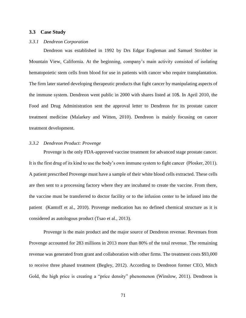
71

3.3 Case Study

3.3.1 Dendreon Corporation

Dendreon was established in 1992 by Drs Edgar Engleman and Samuel Strobber in

Mountain View, California. At the beginning, company’s main activity consisted of isolating

hematopoietic stem cells from blood for use in patients with cancer who require transplantation.

The firm later started developing therapeutic products that fight cancer by manipulating aspects of

the immune system. Dendreon went public in 2000 with shares listed at 10$. In April 2010, the

Food and Drug Administration sent the approval letter to Dendreon for its prostate cancer

treatment medicine (Malarkey and Witten, 2010). Dendreon is mainly focusing on cancer

treatment development.

3.3.2 Dendreon Product: Provenge

Provenge is the only FDA-approved vaccine treatment for advanced stage prostate cancer.

It is the first drug of its kind to use the body’s own immune system to fight cancer (Plosker, 2011).

A patient prescribed Provenge must have a sample of their white blood cells extracted. These cells

are then sent to a processing factory where they are incubated to create the vaccine. From there,

the vaccine must be transferred to doctor facility or to the infusion center to be infused into the

patient (Kantoff et al., 2010). Provenge medication has no defined chemical structure as it is

considered as autologous product (Tsao et al., 2013).

Provenge is the main product and the major source of Dendreon revenue. Revenues from

Provenge accounted for 283 millions in 2013 more than 80% of the total revenue. The remaining

revenue was generated from grant and collaboration with other firms. The treatment costs $93,000

to receive three phased treatment (Begley, 2012). According to Dendreon former CEO, Mitch

Gold, the high price is creating a “price density” phenomenon (Winslow, 2011). Dendreon is

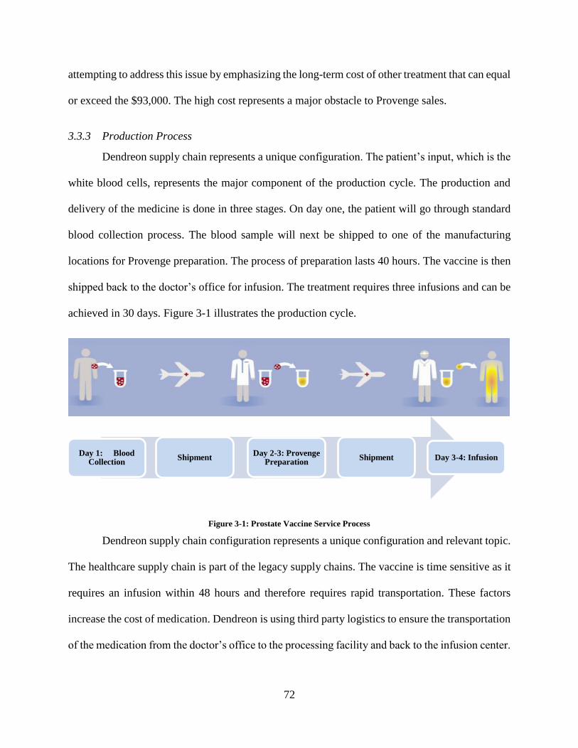
72

attempting to address this issue by emphasizing the long-term cost of other treatment that can equal

or exceed the $93,000. The high cost represents a major obstacle to Provenge sales.

3.3.3 Production Process

Dendreon supply chain represents a unique configuration. The patient’s input, which is the

white blood cells, represents the major component of the production cycle. The production and

delivery of the medicine is done in three stages. On day one, the patient will go through standard

blood collection process. The blood sample will next be shipped to one of the manufacturing

locations for Provenge preparation. The process of preparation lasts 40 hours. The vaccine is then

shipped back to the doctor’s office for infusion. The treatment requires three infusions and can be

achieved in 30 days. Figure 3-1 illustrates the production cycle.

Figure 3-1: Prostate Vaccine Service Process

Dendreon supply chain configuration represents a unique configuration and relevant topic.

The healthcare supply chain is part of the legacy supply chains. The vaccine is time sensitive as it

requires an infusion within 48 hours and therefore requires rapid transportation. These factors

increase the cost of medication. Dendreon is using third party logistics to ensure the transportation

of the medication from the doctor’s office to the processing facility and back to the infusion center.

Day 1: Blood Collection

Shipment Day 2-3: Provenge

PreparationShipment Day 3-4: Infusion

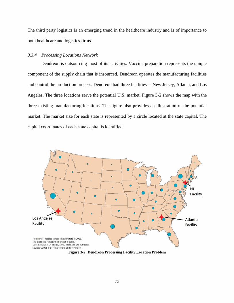
73

The third party logistics is an emerging trend in the healthcare industry and is of importance to

both healthcare and logistics firms.

3.3.4 Processing Locations Network

Dendreon is outsourcing most of its activities. Vaccine preparation represents the unique

component of the supply chain that is insourced. Dendreon operates the manufacturing facilities

and control the production process. Dendreon had three facilities— New Jersey, Atlanta, and Los

Angeles. The three locations serve the potential U.S. market. Figure 3-2 shows the map with the

three existing manufacturing locations. The figure also provides an illustration of the potential

market. The market size for each state is represented by a circle located at the state capital. The

capital coordinates of each state capital is identified.

Figure 3-2: Dendreon Processing Facility Location Problem

74

3.4 Problem Definition

Dendreon faced financial problem and its capacity was underutilized. Despite a steady

income between 2011 and 2013, Dendreon Corporation experienced increasing losses. The top

management decided to shut down one location among the three existing facilities. With only two

locations, Dendreon will save operating costs and will free up more cash for future operations

requirement and marketing campaigns.

This section analyzes the configuration issues, solve the location problem. From location

decision standpoint of view, the Dendreon goal consists of minimizing the total transportation cost.

First, the problem is modeled using the well-known load-distance method. This method is

intuitively appealing, and is widely used as pedagogical tool (Kuo and White, 2004). This will

provide an idea about the location to close that will provide the least volume-traveled distance.

Second, we will provide a solution of the problem using non-linear programming. The non-linear

programming will provide an optimal two location solution.

3.4.1 Methodology 1: Load-Distance

Load distance methodology is a common technique used to solve location problem.

3.4.1.1 Load Distance Model

The problem can be solved using spreadsheet based methodology since it is among the most widely

used software in business field. The load distance problem will be modeled to determine the best

alternative. Dendreon will have the choice to shut down one of three existing locations (California,

Georgia, and New Jersey). We will compute the total load-distance of each alternative. The option

showing the least amount of load-distance will be the best solution. This methodology requires

projecting the United States maps in 2D plan to determine the distance as well as identifying the

travelling volumes.

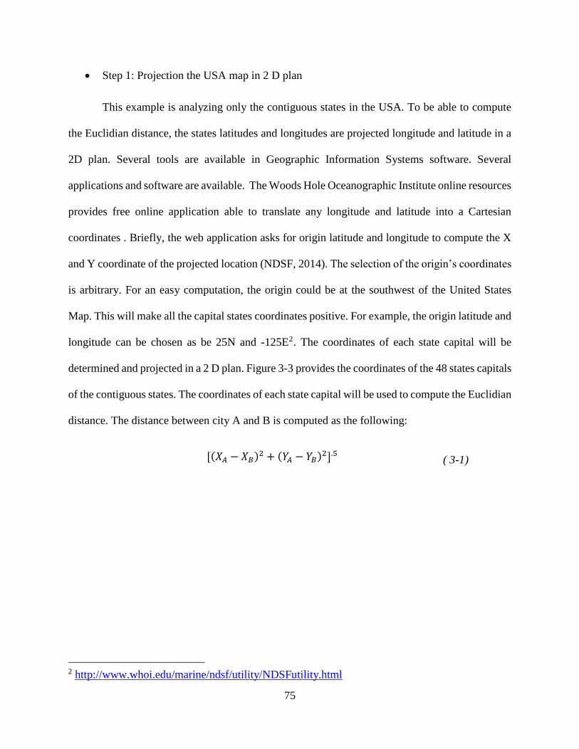
75

Step 1: Projection the USA map in 2 D plan

This example is analyzing only the contiguous states in the USA. To be able to compute

the Euclidian distance, the states latitudes and longitudes are projected longitude and latitude in a

2D plan. Several tools are available in Geographic Information Systems software. Several

applications and software are available. The Woods Hole Oceanographic Institute online resources

provides free online application able to translate any longitude and latitude into a Cartesian

coordinates . Briefly, the web application asks for origin latitude and longitude to compute the X

and Y coordinate of the projected location (NDSF, 2014). The selection of the origin’s coordinates

is arbitrary. For an easy computation, the origin could be at the southwest of the United States

Map. This will make all the capital states coordinates positive. For example, the origin latitude and

longitude can be chosen as be 25N and -125E2. The coordinates of each state capital will be

determined and projected in a 2 D plan. Figure 3-3 provides the coordinates of the 48 states capitals

of the contiguous states. The coordinates of each state capital will be used to compute the Euclidian

distance. The distance between city A and B is computed as the following:

[(𝑋𝐴 − 𝑋𝐵)2 + (𝑌𝐴 − 𝑌𝐵)2].5 ( 3-1)

2 http://www.whoi.edu/marine/ndsf/utility/NDSFutility.html

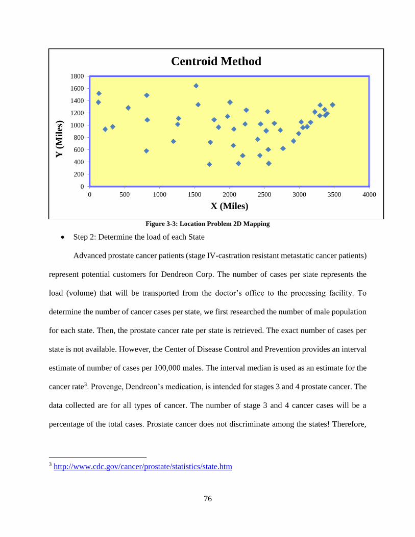
76

Figure 3-3: Location Problem 2D Mapping

Step 2: Determine the load of each State

Advanced prostate cancer patients (stage IV-castration resistant metastatic cancer patients)

represent potential customers for Dendreon Corp. The number of cases per state represents the

load (volume) that will be transported from the doctor’s office to the processing facility. To

determine the number of cancer cases per state, we first researched the number of male population

for each state. Then, the prostate cancer rate per state is retrieved. The exact number of cases per

state is not available. However, the Center of Disease Control and Prevention provides an interval

estimate of number of cases per 100,000 males. The interval median is used as an estimate for the

cancer rate3. Provenge, Dendreon’s medication, is intended for stages 3 and 4 prostate cancer. The

data collected are for all types of cancer. The number of stage 3 and 4 cancer cases will be a

percentage of the total cases. Prostate cancer does not discriminate among the states! Therefore,

3 http://www.cdc.gov/cancer/prostate/statistics/state.htm

0

200

400

600

800

1000

1200

1400

1600

1800

0 500 1000 1500 2000 2500 3000 3500 4000

Y (

Mil

es)

X (Miles)

Centroid Method

77

the location problem will remain the same and the data collected for all phases of prostate cancer

is used as a proxy for the potential population.

Step 3: Computation

The table below shows some of the States data. Dendreon is facing three alternatives where one

location among the three existing will be closed: shutting down New Jersey, California, or Atlanta

location.

Table 3-1: Dendreon Problem Data Collection

States Latitude Longitude X

(mile)

Y

(mile)

Cancer

Rate #

per

100,000

Male

Population

(1,000)

Number

of Cases

1 AL 32.3615 -86.279118 2435 508 166 2,281,612 3787

2 AZ 33.4485 -112.0738 813 583 112.8 3,306,841 3730

3 AR 34.7360 -92.3311 2055 672 134.1 1,415,500 1898

4 CA 38.5556 -121.4689 222 936 134.1 18,505,202 24815

18 MD 38.9729 -76.5012 3050 964 145.8 2,763,806 4030

19 MA 42.2352 -71.0275 3395 1189 134.1 3,204,983 4298

20 MI 42.7335 -84.5467 2544 1224 166 4,902,854 8139

21 MN 44.95 -93.0940 2007 1377 166 2,620,570 4350

46 WV 38.3495 -81.6333 2728 921 112.8 892,120 1006

47 WI 43.0747 -89.3844 2240 1247 140 2,809,066 3933

48 WY 41.1455 -104.8020 1270 1114 145.8 277,040 404

The problem will have three different alternatives. For example, if the processing facility in Atlanta

is shut down, a patient’s from Arizona will have his blood cells processed at either New Jersey or

California. With no capacity constraints on both locations, the patient of the state of Arizona will

be served by the closer location which is in this case California. For each state, the patient

medication will be processed at the closer opened location. The total distance load-distance

traveled is computed for the three different alternatives.

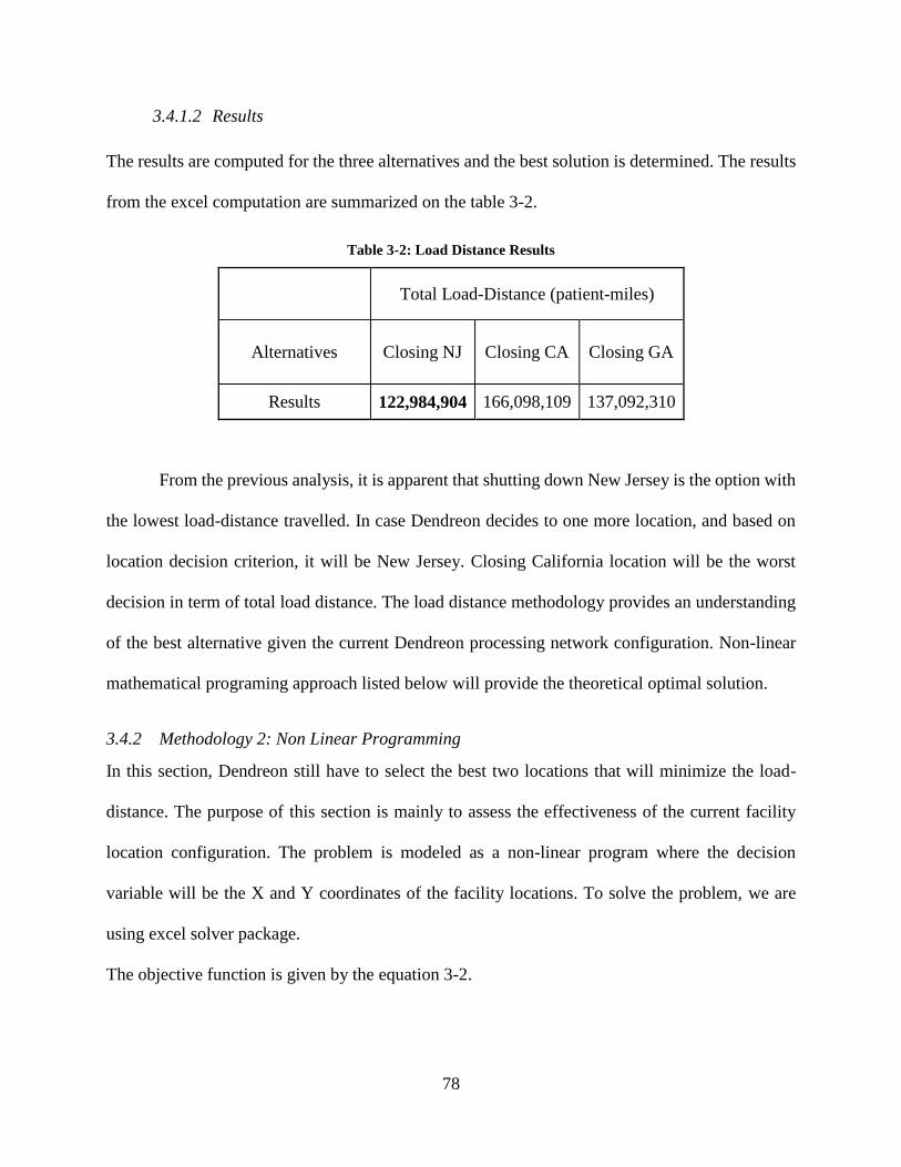
78

3.4.1.2 Results

The results are computed for the three alternatives and the best solution is determined. The results

from the excel computation are summarized on the table 3-2.

Table 3-2: Load Distance Results

Total Load-Distance (patient-miles)

Alternatives Closing NJ Closing CA Closing GA

Results 122,984,904 166,098,109 137,092,310

From the previous analysis, it is apparent that shutting down New Jersey is the option with

the lowest load-distance travelled. In case Dendreon decides to one more location, and based on

location decision criterion, it will be New Jersey. Closing California location will be the worst

decision in term of total load distance. The load distance methodology provides an understanding

of the best alternative given the current Dendreon processing network configuration. Non-linear

mathematical programing approach listed below will provide the theoretical optimal solution.

3.4.2 Methodology 2: Non Linear Programming

In this section, Dendreon still have to select the best two locations that will minimize the load-

distance. The purpose of this section is mainly to assess the effectiveness of the current facility

location configuration. The problem is modeled as a non-linear program where the decision

variable will be the X and Y coordinates of the facility locations. To solve the problem, we are

using excel solver package.

The objective function is given by the equation 3-2.

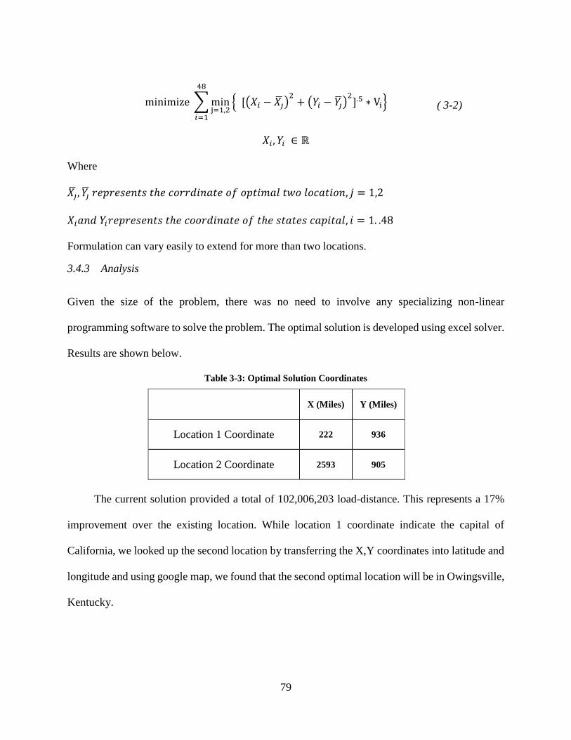
79

minimize ∑ minj=1,2

{ [(𝑋𝑖 − 𝑋�̅�)2

+ (𝑌𝑖 − 𝑌�̅�)2].5 ∗ Vi}

48

𝑖=1

( 3-2)

𝑋𝑖, 𝑌𝑖 ∈ ℝ

Where

𝑋�̅�, 𝑌�̅� 𝑟𝑒𝑝𝑟𝑒𝑠𝑒𝑛𝑡𝑠 𝑡ℎ𝑒 𝑐𝑜𝑟𝑟𝑑𝑖𝑛𝑎𝑡𝑒 𝑜𝑓 𝑜𝑝𝑡𝑖𝑚𝑎𝑙 𝑡𝑤𝑜 𝑙𝑜𝑐𝑎𝑡𝑖𝑜𝑛, 𝑗 = 1,2

𝑋𝑖𝑎𝑛𝑑 𝑌𝑖𝑟𝑒𝑝𝑟𝑒𝑠𝑒𝑛𝑡𝑠 𝑡ℎ𝑒 𝑐𝑜𝑜𝑟𝑑𝑖𝑛𝑎𝑡𝑒 𝑜𝑓 𝑡ℎ𝑒 𝑠𝑡𝑎𝑡𝑒𝑠 𝑐𝑎𝑝𝑖𝑡𝑎𝑙, 𝑖 = 1. .48

Formulation can vary easily to extend for more than two locations.

3.4.3 Analysis

Given the size of the problem, there was no need to involve any specializing non-linear

programming software to solve the problem. The optimal solution is developed using excel solver.

Results are shown below.

Table 3-3: Optimal Solution Coordinates

X (Miles) Y (Miles)

Location 1 Coordinate 222 936

Location 2 Coordinate 2593 905

The current solution provided a total of 102,006,203 load-distance. This represents a 17%

improvement over the existing location. While location 1 coordinate indicate the capital of

California, we looked up the second location by transferring the X,Y coordinates into latitude and

longitude and using google map, we found that the second optimal location will be in Owingsville,

Kentucky.

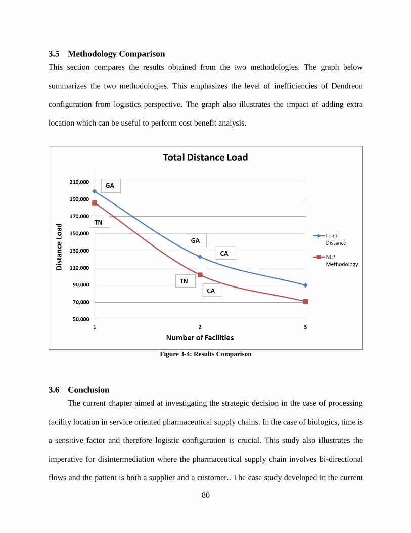
80

3.5 Methodology Comparison

This section compares the results obtained from the two methodologies. The graph below

summarizes the two methodologies. This emphasizes the level of inefficiencies of Dendreon

configuration from logistics perspective. The graph also illustrates the impact of adding extra

location which can be useful to perform cost benefit analysis.

Figure 3-4: Results Comparison

3.6 Conclusion

The current chapter aimed at investigating the strategic decision in the case of processing

facility location in service oriented pharmaceutical supply chains. In the case of biologics, time is

a sensitive factor and therefore logistic configuration is crucial. This study also illustrates the

imperative for disintermediation where the pharmaceutical supply chain involves bi-directional

flows and the patient is both a supplier and a customer.. The case study developed in the current

81

chapter represents a real word application of highly personalized medicine with total

disintermediated distribution channels. The case study development represents a practical

application of using basic decision science tools in supply chain context. First, the projection of

longitude and latitude coordinates represents an approximation for distance approximation that can

be used in pedagogical context as well as in business decision context. The solution methodology

is modeled using widely available spreadsheet based tools. The case study will make such tools

more relevant in business environment and provide an opportunity to apply it in real cases.

82

4 Chapter 4: Disintermediation Problem in Biopharmaceuticals

Supply Chain: Numerical Study

4.1 Introduction and Research Objectives

The journey of medicine from the manufacturer to the patient involves many entities: wholesalers,

distributors, pharmacies, healthcare providers, and payment agencies. As discussed in chapter 2,

the pharmaceutical industry has shown some structural changes favoring direct sales (supply chain

disintermediation). For example, Pfizer started selling Viagra online in 2013 (Isidore, 2013). The

study of distribution channel networks in general and the supply chain disintermediation in

particular, has interested researchers. The supply chain disintermediation (elimination of the

middleman) has shown its attractiveness in several industries (e.g. insurance, electronics, garments

& apparel) where the supply chain configuration eliminates the double marginalization and allows

the users to have a better price for the same product and service. Supply chain disintermediation

was almost exclusively applied to retail and service fields with far less emphasis on the healthcare

industry (Hesse et al., 2011). The disintermediation phenomenon has become a common practice,

especially in the case of personalized goods (customized Nike shoes, business cards, etc.). In the

case of pharmaceuticals, the emergence of biologics in general, and personalized drugs in

particular calls for disintermediation. Supply chain disintermediation is gaining more attention in

the pharmaceutical context from managerial and practical perspectives (Enyinda and Tolliver,

2009).

4.1.1 Supply Chain Disintermediation in Biologics

The topics of supply chain disintermediation in the context of pharmaceutical industry in general

and biologics in particular is of interest to practitioners who are attempting to find alternatives to

83

better serve their customers (Danzon and Nicholson, 2012). Chapter 2 provided a discussion of the

relevance of supply chain disintermediation in the context of biologics. The biologics industry

provides a unique situation: short product shelf life, high demand variability, and high financial

risk. The product’s short shelf life makes disintermediation attractive as it increases the product’s

useable time and therefore it reduces the perishability cost. In fact, in the case of biologics and

because of the higher production cost, the perishability cost becomes a critical factor. The high

demand variability at the hospitals will impact both the stock out and excess inventory levels. A

disintermediation decision will influence the shortage and perishability costs. The

disintermediation level will have an impact on the total market mediation cost: the sum of

perishability and shortage cost.

Direct distribution channels intend to reduce the perishability cost by providing longer shelf

life for products. The direct sales reduces the total product lead time from the manufacturer to the

hospital in comparison with intermediated configuration. Therefore, it is expected that the shorter

lead time will minimize the total perishability cost (Deniz, Karaesmen, and Scheller-Wolf, 2010).

On the other hand, intermediaries provide the opportunity to reduce the impact of the supply chain

variability via pooling effect. The demand variability at the hospitals will be mitigated by the

distributor’s pooling effect which will reduce the shortage cost. The disintermediation level will

impact the tradeoff between perishability cost (overstocking) and shortage cost (under stocking)

and the total market mediation cost.

Despite the possible benefits deriving from direct distribution channels, the findings in

chapter 2 showed that about 85% of the biologics’ physical flows is intermediated by specialty

distributors and/or wholesalers. The non-intuitive existing practices represent a motivation to study

the different factors influencing the material flows and the disintermediation level. Based on the

84

different arguments provided in chapter 2, it was expected that specialty pharmaceutical supply

chains will witness a greater level of disintermediation. Moreover, the novelty of the supply chain

disintermediation practices in the area of pharmaceuticals represents another source of motivation

to further explore the alternative distribution channels and determine some of the factors that

influences this decision. Finally, the practical aspect of the disintermediation problem and its

relevance to healthcare practitioners provides more incentives to explore this topic.

4.1.2 Research Objectives

The current chapter aims at providing a better understanding about supply chain disintermediation

dynamics from a market mediation cost perspective. While excess inventory at the hospitals and

the distributor will increase the perishability cost, it will at the same time reduce the shortage cost

by providing a demand variability buffer. The tradeoff between the perishability cost and shortage

cost will dictate the supply chain disintermediation level (intermediated, disintermediated, or

hybrid). The demand variation and the shortage cost structure will influence the total market

mediation cost. The current chapter aims at answering the following research questions:

What’s the best disintermediation strategy that will minimize the total market mediation

cost measured by the sum of perishability and shortage costs?

What are the most influential factors that impact the total market mediation cost?

The current chapter uses scenario approach to gain an understanding of the problem.

Analytical complexity of the problem does not lead itself to easy interpretation of the

disintermediation level sensitivity. The level of disintermediation, which is the decision variable,

is determined by the ratio of medication that is directly delivered to the hospital to the total

85

delivered medication. The inventory and the shortage level at the end of each period will determine

the amount of perishability and shortage cost.

As a first step, a scenario approach simulation was designed with 10 hospitals, one

distributor, and one manufacturer. The demand is generated at the hospitals and pulled from the

distributor and the manufacturer. The disintermediation ratio varies between 0% (all the medicine

is sold via the distributor) and 100% (direct sales). The model parameters will be the demand

variability at the hospital expressed by the coefficient of variation. The other parameter will be the

shortage cost ratio expressed as the ratio of the shortage cost to the perishability cost. The adoption

of standardized parameters provides a better generalization of the problem. The scenario approach

will serve as an exploratory study of the supply chain disintermediation problem. In a second step,

a large scale numerical study is developed. The numerical study will analyze the different influence

of different factors on the total market mediation cost. Using a three factor Anova analysis, the

numerical study will investigate the importance of demand variability, shortage cost structure, and

supply chain disintermediation in shaping the total market mediation cost. Finally, the numerical

study will be extended to include the impact of service level on total market mediation costs.

The current chapter is organized as follows: first, a literature review of disintermediation in

general and in the context of pharmaceutical supply chain will be provided. The literature review

will emphasize the relevance of the topic, and highlight some of the research gaps. The following

section will address the scenario approach which represents an exploratory analysis of the study.

Next, a large scale Anova experiment is designed to determine the most influential factors affecting

the total mediation cost structure. Finally, a summary of the results and findings as well as areas

of future research is provided.

86

4.2 Literature review

The following section will provide major findings in literature linked to the supply chain

disintermediation. First, an overview about the fundamentals that relates to supply chain

disintermediation is provided. The subsequent section will address the major findings in an attempt

to show some research gaps that this chapter is addressing.

4.2.1 Supply Chain Disintermediation

4.2.1.1 Definition

Intermediaries have an important role in distributing products, using promotions and offering

special offers for customers. They also provide services for customers and help the manufacturers

better understand the market and the customer behavior. Intermediaries help facilitate transactions

between buyers and manufacturers and improve the value of the product/service by insuring

product quality and providing warranty services (Choi, Stahl, and Whinston, 1997). For example,

Microsoft and Samsung have recently signed a deal with Best Buy to promote and demonstrate

the features of their products. For manufacturers, the decision to disintermediate is challenging.

The term disintermediation was first used in financial sector to describe the trend for small

investors to invest directly and avoid using traditional intermediaries such as brokers (Gellman,

1996). The terminology of disintermediation then was adopted in the field of supply chain

management. Disintermediation is the action of cutting out the middlemen by direct transaction

between the service/product provider and the end customer (Hoffman, 1995). This aims at reducing

the role played by the intermediaries. Disintermediation is also defined as the elimination of an

intermediary from the business process when the cost of adding the intermediary exceeds its value

added (Chircu and Kauffman, 1999; Pinto, 2000). Companies will reach customers directly instead

of going through the traditional supply chain venues (distributors, wholesalers…). The idea of

87

disintermediation emerged from the persistent customer’s demand for lower cost (Shunk et al.,

2007). To remain competitive, firms had to flatten their supply chain, favoring more direct contact

between the firm and its customers (Pinto, 2000). Moreover, customers are requesting more

personalized products and services which might not be available in the traditional supply chain

pipeline. Therefore, the customer will directly interact with the product manufacturer/service

provider to place the order. Direct channels of communication between the customer and the

product/service providers have created multiple disintermediation mechanisms.

4.2.1.2 Supply Chain Disintermediation Advantages and Disadvantages

The need for disintermediation in some cases implied the mechanism of Supply Chain

disintermediation. Six main ways of SC disintermediation emerged from B2B business practices:

(i) strategic partnering, (ii) mergers and acquisitions, (iii) organic growth, (iv) communication and

training, (v) incentives, and (vi) information and communication technology (Nordin, Brozovic,

and Holmlund, 2013). Nordin et al. (2013) proposed different ways of eliminating the middleman

and collaborating directly with the customer in business to business (B2B) context.

Disintermediation techniques involve working closely with the middleman and serve together the

final customer. The direct distribution channels have shown some benefit from a customer’s

perspective. However, the complex nature of these different mechanisms provides insights about

the challenges facing disintermediation strategy.

On one side, supply chain disintermediation provides several advantages. First, it allows a

closer relationship between the product/service provider and the end customers. This will increase

the interaction and improve the coordination level, leading to higher customer satisfaction (Nissen,

2000). Second, customer input represents a great source of knowledge and an alternative for

improvement (Davenport and Klahr, 1998). Disintermediation promotes knowledge sharing by

88

increasing the level of interaction. Third, organizations adopting supply chain disintermediation

have experienced a higher level of product innovation based on the customer input, and also

attained greater control over product innovation (Coe and Hess, 2005). Moreover,

disintermediation can provide more agility to manufacturers by responding quickly to changes in

the market. This also helps firms better manage their inventories (Erengüç, Simpson, and Vakharia,

1999). Finally, the cost benefit to both customers and product/service providers remains the most

prominent advantage.

On the other hand, supply chain disintermediation is a complex issue. First, when a firm

decides to eliminate the middlemen, it has to replicate intermediaries’ core competencies. In many

cases, the wholesalers/distributors have a greater distribution knowledge and can achieve high

sales levels (Atkinson, 2001). Second, the management of the different flow in the supply chain

(physical, information, financial and knowledge) becomes more difficult. In some cases, the focal

company will lose its focus on its core competency (Halbert, 2006). Third, in case of physical

goods, disintermediation will increase the level of stock on hand for the focal company. Instead of

pushing its products on the supply chain pipeline, manufacturers should rapidly respond to

customers’ demand by maintaining an inventory buffer in house. This will require a higher level

of investment.

The literature review shows recent trends toward investigating supply chain

disintermediation. A large number of conceptual studies have addressed the problem of

disintermediation. However, very few studies have attempted to empirically or analytically assess

the issue of disintermediation (Rossetti and Choi, 2008). The conflicting signals that

disintermediation strategy is showing and the pressure that exists from existing distribution

channels provides relevance to research on this topic further. This chapter addresses the

89

disintermediation problem in the context of the pharmaceutical supply chain. The next subsection

provides an overview of the disintermediation practices in the field of pharmaceuticals.

4.2.1.3 Supply Chain Disintermediation in Pharmaceutical Industry

The disintermediation strategy is not widely used in the pharmaceutical industry despite its

attractiveness evidence from other industries (Niziolek, Chiam, and Yih, 2012). In fact, the direct-

ship sales strategy in the pharmaceutical context represents some challenges due to the number of

influential players in the supply chain. The complex relationship linking the

consumer/customer/decision-maker triad is unique to the prescription pharmaceutical context. The

decision maker (doctors, in most cases) is different from the consumer (the patient) as well as the

customer (Insurance, Pharmacy Benefit Management, and Government). Moreover,

pharmaceutical firms strive to enhance the availability their products (Burns, 2002).

Pharmaceutical firms use distributors as a buffer to guarantee a certain service level at the

pharmacies. Additionally, disintermediation requires a large investment in information technology

to guarantee smooth functioning of the supply chain and make up for the intermediaries’ roles. In

the case of pharmaceuticals, firms tend to invest more in production assets, R&D, and patient care

instead. Therefore, pharmaceutical supply chains are behind other industries in term of

disintermediation configuration (Niziolek et al., 2012).

The complex nature of the pharmaceutical industry did not stop companies from attempting

disintermediation. The mail order prescription represents a way of partial disintermediation where

the order is placed directly at the pharmacy and shipped to the patient’s home. In 2007, Pfizer

started selling its medicines directly to pharmacies in the United Kingdom. Today, Pfizer offers

some of its medicine online for direct sales. Recent studies have addressed the issues of supply

chain disintermediation from a cost benefit perspective and inventory analysis (Jetly, Rossetti, and

90

Handfield, 2012; Niziolek et al., 2012). The result showed that mixed disintermediation strategies,

where 55% of the revenue are generated from sales, are direct-shipped, providing better financial

results and a smaller inventory level. The analytical study did not consider the nature of the

product.

4.3 Supply Chain Disintermediation in Biologic Pharmaceuticals: Scenario

Approach

Computer simulation methodology is gaining more popularity in social and organizational science

research (Dooley, 2001). Simulation allows researchers to address the complexity of a system and

help develop a “what if analysis.” The current section provides a scenario approach to the problem

by providing general formulation.

The previous studies in the simulation showed three main practices:

System dynamics, which consist of determining the “key state variables” that determine

the system behavior. The other system parameters are related to one another (Karnopp,

Margolis, and Rosenberg, 2012).

Discrete event simulation, which involves modeling the operations of a system as a

sequence of events evolving over time. The system behavior will be influenced by the

organization’s resources and other trigger events (Zeigler, Praehofer, and Kim, 2000).

Agent-based simulation, which consists of simulating of the action and interaction among

different autonomous agents in order to maximize the system utility (Railsback, Lytinen,

and Jackson, 2006).

The current chapter uses scenario approach simulation in order to provide an approach to

the problem. First, decision rules will be established. Then, a mathematical model will be

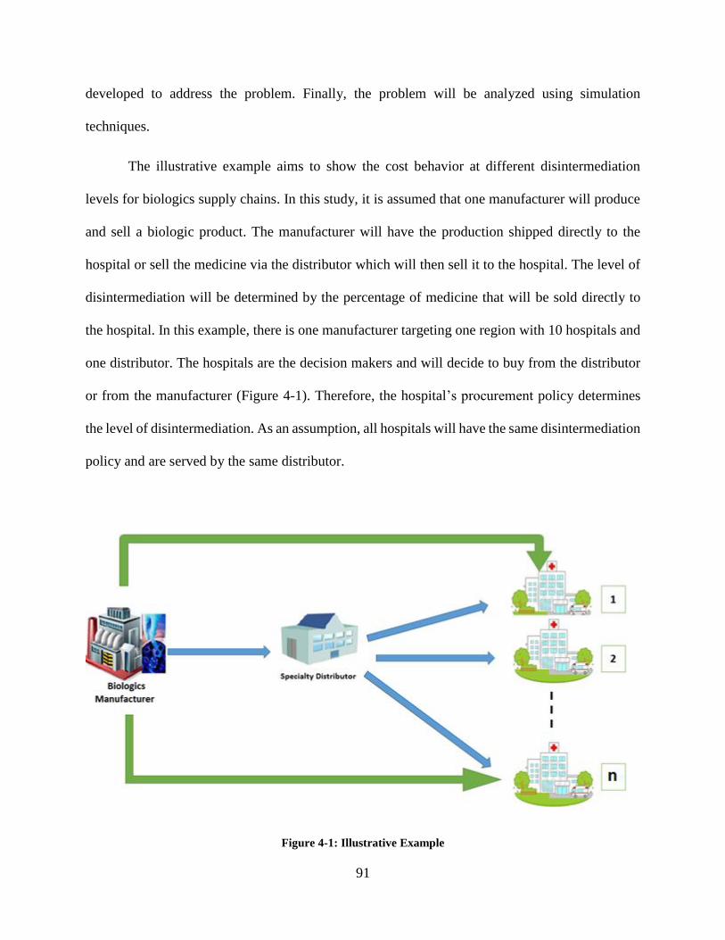
91

developed to address the problem. Finally, the problem will be analyzed using simulation

techniques.

The illustrative example aims to show the cost behavior at different disintermediation

levels for biologics supply chains. In this study, it is assumed that one manufacturer will produce

and sell a biologic product. The manufacturer will have the production shipped directly to the

hospital or sell the medicine via the distributor which will then sell it to the hospital. The level of

disintermediation will be determined by the percentage of medicine that will be sold directly to

the hospital. In this example, there is one manufacturer targeting one region with 10 hospitals and

one distributor. The hospitals are the decision makers and will decide to buy from the distributor

or from the manufacturer (Figure 4-1). Therefore, the hospital’s procurement policy determines

the level of disintermediation. As an assumption, all hospitals will have the same disintermediation

policy and are served by the same distributor.

Figure 4-1: Illustrative Example

92

4.3.1 Simulation Scenario

Scenario analysis approach suggests setting up different steps for the scenario (Hsia et al., 1994).

Step 1: Each Hospital will generate its daily demand. There are n hospitals that are served by one

single distributor/wholesaler. It is assumed that all hospital have independent and identical demand

distributions. Demands are uncorrelated.

Step 2: The hospital will determine the purchasing strategy: the percentage of demand that will be

satisfied directly from the manufacturer and the percentage of demand that will be purchased from

the distributor (the disintermediation level).

Step 3: The demand from the hospitals placed on the distributor will be pooled at the distributor

which will determine the demand at the distributor level.

Step 4: Each hospital will place an order from the manufacturer. Orders are placed on a weekly

basis. The order placed aims at satisfying the weekly demand. The hospital aims at maintaining a

certain service level. The service level will determine the order up-to level quantity.

Step 5: The distributor, based on the weekly pooled demand, will place an order from the

manufacturer to satisfy a certain service level as well. The service level will determine the order

up-to level quantity.

Step 6: The daily demand will be satisfied with the existing inventory. At the end of each

replenishment period, the quantity of expired (perished) or shortage quantity will be determined at

the hospitals and the distributor.

Step 7: An up-to level inventory replenishment will be used at the hospitals and at the distributor.

4.3.2 Simulation Set-up

The main goal of simulation is to find the supply chain network configuration as reflected by the

disintermediation level that will minimize the total cost. Biologic medicine is experiencing a

growing demand with high variability (American Cancer Society, 2013). The high demand

variability at the hospital’s end increases the risk of shortage. Moreover, biologic medicines are

characterized by a short shelf life (Pitts and Stark, 2012). The short shelf life increases the risk of

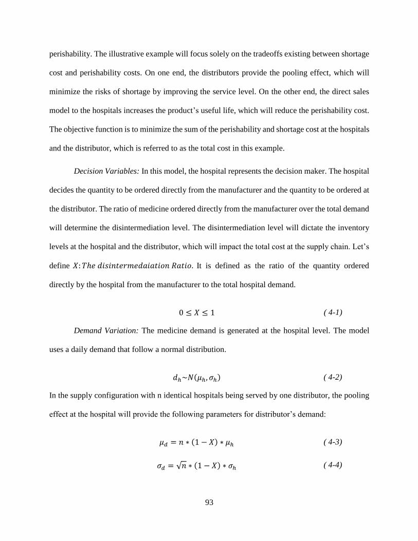
93

perishability. The illustrative example will focus solely on the tradeoffs existing between shortage

cost and perishability costs. On one end, the distributors provide the pooling effect, which will

minimize the risks of shortage by improving the service level. On the other end, the direct sales

model to the hospitals increases the product’s useful life, which will reduce the perishability cost.

The objective function is to minimize the sum of the perishability and shortage cost at the hospitals

and the distributor, which is referred to as the total cost in this example.

Decision Variables: In this model, the hospital represents the decision maker. The hospital

decides the quantity to be ordered directly from the manufacturer and the quantity to be ordered at

the distributor. The ratio of medicine ordered directly from the manufacturer over the total demand

will determine the disintermediation level. The disintermediation level will dictate the inventory

levels at the hospital and the distributor, which will impact the total cost at the supply chain. Let’s

define 𝑋: 𝑇ℎ𝑒 𝑑𝑖𝑠𝑖𝑛𝑡𝑒𝑟𝑚𝑒𝑑𝑎𝑖𝑎𝑡𝑖𝑜𝑛 𝑅𝑎𝑡𝑖𝑜. It is defined as the ratio of the quantity ordered

directly by the hospital from the manufacturer to the total hospital demand.

0 ≤ 𝑋 ≤ 1 ( 4-1)

Demand Variation: The medicine demand is generated at the hospital level. The model

uses a daily demand that follow a normal distribution.

𝑑ℎ~𝑁(𝜇ℎ, 𝜎ℎ) ( 4-2)

In the supply configuration with n identical hospitals being served by one distributor, the pooling

effect at the hospital will provide the following parameters for distributor’s demand:

𝜇𝑑 = 𝑛 ∗ (1 − 𝑋) ∗ 𝜇ℎ ( 4-3)

𝜎𝑑 = √𝑛 ∗ (1 − 𝑋) ∗ 𝜎ℎ ( 4-4)

94

Service Level: The service level represents a measurement of the system performance. It

refers to the extent to which a service meets or exceeds customer expectation (Parasuraman et al.,

1985). Service level is defined in inventory management policy as the probability that the demand

of a product in a specific period is less than or equal to the inventory on hand (Tempelmeier, 2000).

The literature review related to service level and inventory management is rich. In the context of

a single period stochastic model, the newsvendor model is the most popular approach. In the

newsvendor model, based on the critical fractile ratio, the inventory policy will be determined.

This policy aims at minimizing the tradeoff between the overstocking and under-stocking costs.

This ratio will also determine the optimum service level for the organization. When the

overstocking cost is high, companies will tend to have a lower service level. In other cases, if the

under-stocking cost is high, organizations will have an extra inventory which will increase the

service level.

For hospitals and distributor, the rational behavior based on the newsvendor model

suggests that each entity will order the quantity that will minimize the total inventory cost.

However, research in the area of healthcare management did not make the rational choice of

finding the optimal service level (Gebicki et al., 2013). It actually considered the service level as

a target or a minimum level that healthcare entities should maintain (Möllering and Thonemann,

2010). In these cases, the service level becomes a constraint that will affect the shortage structure

and relevance. Therefore, in many cases, hospitals will not follow the newsvendor model to

determine their replenishment policy.

The determination of the required service level at the hospital and the distributor is based

on previous studies. Healthcare officials have provided a set of instructions regarding the

medication service level at hospitals and distributors. However, no specific minimum service level

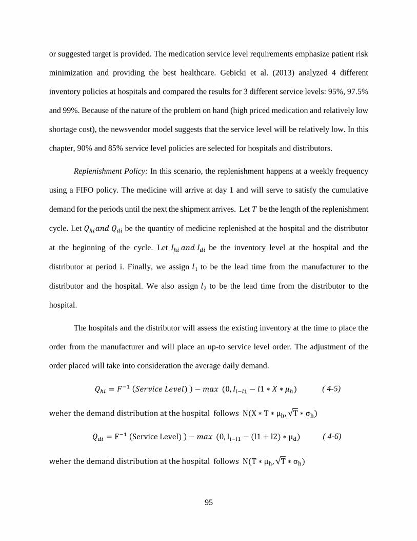
95

or suggested target is provided. The medication service level requirements emphasize patient risk

minimization and providing the best healthcare. Gebicki et al. (2013) analyzed 4 different

inventory policies at hospitals and compared the results for 3 different service levels: 95%, 97.5%

and 99%. Because of the nature of the problem on hand (high priced medication and relatively low

shortage cost), the newsvendor model suggests that the service level will be relatively low. In this

chapter, 90% and 85% service level policies are selected for hospitals and distributors.

Replenishment Policy: In this scenario, the replenishment happens at a weekly frequency

using a FIFO policy. The medicine will arrive at day 1 and will serve to satisfy the cumulative

demand for the periods until the next the shipment arrives. Let 𝑇 be the length of the replenishment

cycle. Let 𝑄ℎ𝑖𝑎𝑛𝑑 𝑄𝑑𝑖 be the quantity of medicine replenished at the hospital and the distributor

at the beginning of the cycle. Let 𝐼ℎ𝑖 𝑎𝑛𝑑 𝐼𝑑𝑖 be the inventory level at the hospital and the

distributor at period i. Finally, we assign 𝑙1 to be the lead time from the manufacturer to the

distributor and the hospital. We also assign 𝑙2 to be the lead time from the distributor to the

hospital.

The hospitals and the distributor will assess the existing inventory at the time to place the

order from the manufacturer and will place an up-to service level order. The adjustment of the

order placed will take into consideration the average daily demand.

𝑄ℎ𝑖 = 𝐹−1 (𝑆𝑒𝑟𝑣𝑖𝑐𝑒 𝐿𝑒𝑣𝑒𝑙) ) − 𝑚𝑎𝑥 (0, 𝐼𝑖−𝑙1 − 𝑙1 ∗ 𝑋 ∗ 𝜇ℎ) ( 4-5)

weher the demand distribution at the hospital follows N(X ∗ T ∗ μh, √T ∗ σh)

𝑄𝑑𝑖 = F−1 (Service Level) ) − 𝑚𝑎𝑥 (0, Ii−l1 − (l1 + l2) ∗ μd) ( 4-6)

weher the demand distribution at the hospital follows N(T ∗ μh, √T ∗ σh)

96

Inventory Level: The inventory level at period i in a given replenishment cycle for the

hospitals and the distributor will be given by:

𝐼𝑖 = 𝑄 − ∑ 𝑑𝑗

𝑖

𝑗=1

( 4-7)

In a case of perishable goods, inventory can be seen as a vector of items with different age stages.

Let 𝑌𝑡 ⃖ represent the inventory vector at the date t.

𝑌𝑡 ⃖ = (𝑦1, 𝑦2, . . , 𝑦𝑚) ( 4-8)

Where m represents the medicine shelf life. At the end of the tth day, a quantity qt+1 will be

delivered. Let wt represent the quantity that will expire at the end of the period t.

𝑤𝑡 = 𝑦𝑚 ( 4-9)

The cumulative expired medicine in D period problem will be expressed by

𝑊 = ∑ 𝑤𝑖

𝐷

𝑖=1

( 4-10)

The recurrence formulation of the inventory level at period i will be identified as following:

𝑦𝑗 = 𝑦𝑗−1 − 𝑑𝑖 ( 4-11)

And the general formulation of the inventory at period i is given by:

𝑦𝑗 = 𝑚𝑎𝑥 ( ∑ 𝑄𝑛

𝑖

𝑛=𝑖−𝑚+𝑙

− ∑ 𝑑𝑛

𝑖

𝑛=𝑖−𝑚+𝑙

, 0) ( 4-12)

The inventory formulation as shown does not allow any negative inventory. In this case, any

unsatisfied demand will be considered as lost sales (no backlog orders).

97

Shortage Cost: The shortage cost is the most challenging component to estimate, especially

in the healthcare context. The shortage cost is the cost incurred when the demand cannot be fully

and immediately satisfied due to a stock shortage (Oral et al., 1972). The Drug Shortage Program

(DSP) at the Food and Drug Administration defines a drug shortage as “a situation in which the

total supply of all clinically interchangeable versions of an FDA regulated drug is inadequate to

meet the current or projected demand at the user level” (Center for Drug Evaluation and Research,

1998). Shortage cost has been operationalized in several different ways in the literature. It can be

estimated as: (i) a fixed cost per stock-out and independent of the units and duration, (ii) a specified

charge per unit per period of time , and (iii) a multiple of the unit value and independent of the

number of period (Peterson and Silver, 1979). The current study will use the latter

operationalization which is judged most adequate to the healthcare context. When a patient is

scheduled for a medication and the drug is not available, the hospital will suffer from a shortage

cost during that period. Because of the critical aspect, the patient treatment will be administrated

somewhere else and therefore, it is considered as lost sale.

The drug shortage cost estimation is more challenging in the context of biologics with less

available substitutes (Mellstedt, Niederwieser, and Ludwig, 2008). An investigation of 228

hospitals showed that 89% of hospitals suffer from shortage (Cherici, Frazier, and Feldman, 2011).

Drug shortage is costing U.S. hospitals more than 200 million dollars annually, not including the

labor cost to manage the shortage (Cherici et al., 2011). The drug shortage has an impact on the

quality of healthcare and the overall cost of healthcare delivery (Ventola, 2011). The determination

of the exact shortage cost is, however, arbitrary and will depend on the nature of the product and

its value (Leng and Parlar, 2009). In the case of biologics, because of the lack of substitute

98

products, a hospital suffering from cost shortage will reschedule the patient for the following

period.

In this illustrative example, the shortage cost will be experienced at both hospitals and

distributors. The shortage quantity is the difference between the daily demand and the inventory

in hand. Let 𝑆𝑘 be the total shortage quantity at replenishment cycle j.

𝑆𝑗 = ∑ max(𝑑𝑛 − 𝑄𝑘 − 𝐼𝑛−1, 0)

𝑇

𝑛=1

( 4-13)

Where 𝑄𝑘represents the quantity received at the beginning of cycle k.

The shortage cost will be equal to:

Where SC represents the shortage cost per unit.

Perishability Cost: Scholars have been investigating perishable goods under different

conditions of production and demand conditions for over four decades (Nahmias, 1982). Most of

the studies have looked to the problem from a cost minimization perspective (Raafat, 1991). The

determination of the perishability cost depends on the nature of the product and the type of buying

contract. In some cases, the perishable products will require a special disposal treatment that can

be costly. This concern arises in the case of pharmaceuticals where the expired products can be

toxic. To determine the perishability cost at the distributor and the hospital, the product cycle life

needs to be investigated when the product is delivered to the distributor and in case it is dispensed

directly to the hospitals (Figure 4-2 and 4-3).

𝑆ℎ𝑜𝑟𝑡𝑎𝑔𝑒 𝐶𝑜𝑠𝑡 = 𝑆𝐶 ∗ ∑ 𝑆𝑘

𝐾

𝑘=1

( 4-14)

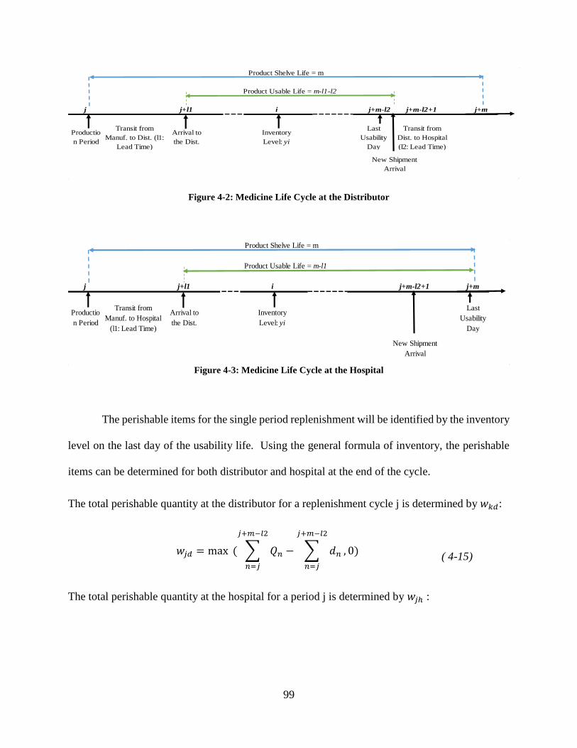
99

Figure 4-2: Medicine Life Cycle at the Distributor

Figure 4-3: Medicine Life Cycle at the Hospital

The perishable items for the single period replenishment will be identified by the inventory

level on the last day of the usability life. Using the general formula of inventory, the perishable

items can be determined for both distributor and hospital at the end of the cycle.

The total perishable quantity at the distributor for a replenishment cycle j is determined by 𝑤𝑘𝑑:

𝑤𝑗𝑑 = max ( ∑ 𝑄𝑛

𝑗+𝑚−𝑙2

𝑛=𝑗

− ∑ 𝑑𝑛

𝑗+𝑚−𝑙2

𝑛=𝑗

, 0) ( 4-15)

The total perishable quantity at the hospital for a period j is determined by 𝑤𝑗ℎ :

j+m-l2 j+m-l2+1

Last

Usability

Day

New Shipment

Arrival

Transit from

Dist. to Hospital

(l2: Lead Time)

Transit from

Manuf. to Dist. (l1:

Lead Time)

i

Inventory

Level: yi

Product Shelve Life = m

Arrival to

the Dist.

Productio

n Period

Product Usable Life = m-l1-l2

j j+l1 j+m

Last

Usability

Day

New Shipment

Arrival

Productio

n Period

Transit from

Manuf. to Hospital

(l1: Lead Time)

Arrival to

the Dist.

Inventory

Level: yi

j j+l1 i j+m-l2+1 j+m

Product Shelve Life = m

Product Usable Life = m-l1

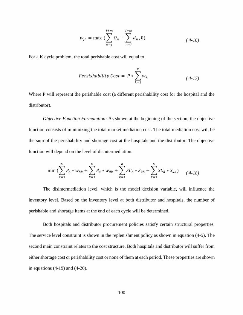
100

𝑤𝑗ℎ = max (∑ 𝑄𝑛

𝑗+𝑚

𝑛=𝑗

− ∑ 𝑑𝑛

𝑗+𝑚

𝑛=𝑗

, 0) ( 4-16)

For a K cycle problem, the total perishable cost will equal to

𝑃𝑒𝑟𝑠𝑖𝑠ℎ𝑎𝑏𝑖𝑙𝑖𝑡𝑦 𝐶𝑜𝑠𝑡 = 𝑃 ∗ ∑ 𝑤𝑘

𝐾

𝑘=1

( 4-17)

Where P will represent the perishable cost (a different perishability cost for the hospital and the

distributor).

Objective Function Formulation: As shown at the beginning of the section, the objective

function consists of minimizing the total market mediation cost. The total mediation cost will be

the sum of the perishability and shortage cost at the hospitals and the distributor. The objective

function will depend on the level of disintermediation.

min (∑ 𝑃ℎ ∗ 𝑤ℎ𝑘 + ∑ 𝑃𝑑 ∗ 𝑤𝑑𝑘 + ∑ 𝑆𝐶ℎ ∗ 𝑆𝑘ℎ

𝐾

𝑘=1

+ ∑ 𝑆𝐶𝑑 ∗ 𝑆𝑘𝑑

𝐾

𝑘=1

𝐾

𝑘=1

𝐾

𝑘=1

) ( 4-18)

The disintermediation level, which is the model decision variable, will influence the

inventory level. Based on the inventory level at both distributor and hospitals, the number of

perishable and shortage items at the end of each cycle will be determined.

Both hospitals and distributor procurement policies satisfy certain structural properties.

The service level constraint is shown in the replenishment policy as shown in equation (4-5). The

second main constraint relates to the cost structure. Both hospitals and distributor will suffer from

either shortage cost or perishability cost or none of them at each period. These properties are shown

in equations (4-19) and (4-20).

101

𝑤ℎ𝑘 ∗ 𝑆ℎ𝑘 = 0, 𝑘 = 1. . 𝐾 ( 4-19)

𝑤𝑑𝑘 ∗ 𝑆𝑑𝑘 = 0, 𝑘 = 1. . 𝐾 ( 4-20)

4.3.3 Simulation Analysis

The current chapter uses simulation analysis to gain an understanding of the disintermediation

levels and its effects on the market mediation cost. In fact, the other works of disintermediation

have used the simulation technique due to the complexity of the problem (Chiang, 2012; Niziolek

et al., 2012). To address the complexity level, this section uses simulation analysis to address the

problem. In this chapter, @Risk Excel companion software is used. @Risk software provides more

sophistication to Excel spreadsheets by adding more functionality. @Risk is used to generate the

daily demands at the hospitals. The software also provides the descriptive statistics of the

simulation outputs. This section develops the results of the different Monte Carlo simulation

models. Two variables will be manipulated: variability and shortage cost structure. The demand

variability will be measured by the coefficient of variation. The cost structure is assessed by the

shortage cost ratio. The shortage cost is the ratio measured as the shortage cost to the perishability

cost.

4.3.3.1 Model Parameters

The scenario approach requires decisions about the parameters values. The scenario approach

models and parameters are determined based on literature investigation and secondary data. Table

4-1 provides the model parameters estimates. The product shelf life and the lead times can be used

or modified based on values determined at the industry level for specific instances.

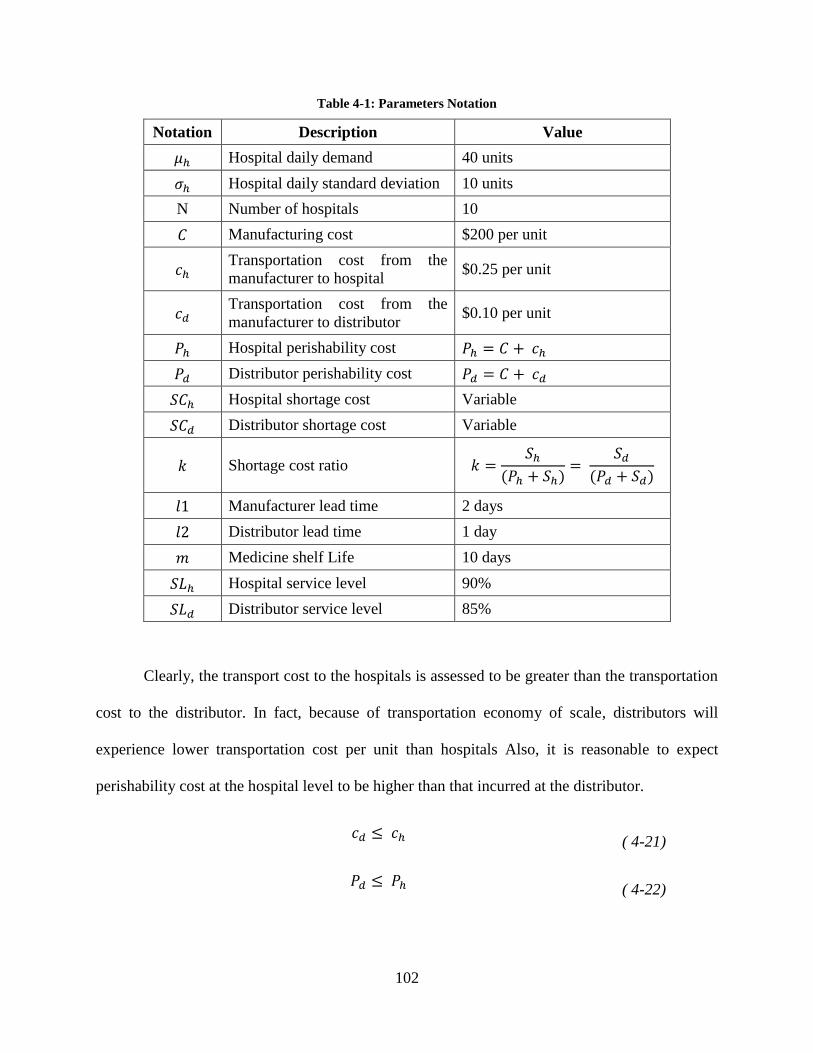
102

Table 4-1: Parameters Notation

Notation Description Value

𝜇ℎ Hospital daily demand 40 units

𝜎ℎ Hospital daily standard deviation 10 units

N Number of hospitals 10

𝐶 Manufacturing cost $200 per unit

𝑐ℎ Transportation cost from the

manufacturer to hospital $0.25 per unit

𝑐𝑑 Transportation cost from the

manufacturer to distributor $0.10 per unit

𝑃ℎ Hospital perishability cost 𝑃ℎ = 𝐶 + 𝑐ℎ

𝑃𝑑 Distributor perishability cost 𝑃𝑑 = 𝐶 + 𝑐𝑑

𝑆𝐶ℎ Hospital shortage cost Variable

𝑆𝐶𝑑 Distributor shortage cost Variable

𝑘 Shortage cost ratio 𝑘 =𝑆ℎ

(𝑃ℎ + 𝑆ℎ)=

𝑆𝑑

(𝑃𝑑 + 𝑆𝑑)

𝑙1 Manufacturer lead time 2 days

𝑙2 Distributor lead time 1 day

𝑚 Medicine shelf Life 10 days

𝑆𝐿ℎ Hospital service level 90%

𝑆𝐿𝑑 Distributor service level 85%

Clearly, the transport cost to the hospitals is assessed to be greater than the transportation

cost to the distributor. In fact, because of transportation economy of scale, distributors will

experience lower transportation cost per unit than hospitals Also, it is reasonable to expect

perishability cost at the hospital level to be higher than that incurred at the distributor.

𝑐𝑑 ≤ 𝑐ℎ ( 4-21)

𝑃𝑑 ≤ 𝑃ℎ ( 4-22)

103

4.3.4 Results

In this illustrative example, two different variables will be manipulated (demand variability,

shortage cost ratio). First, the demand variability is measured by the coefficient of variation.

Higher coefficient of variation will favor the use of distributors who will provide the pooling effect.

Second, the shortage cost effect will be the ratio between the shortage cost and the perishability

cost. In this model, the perishability cost will be fixed at the landing cost for both distributor and

the hospital.

4.3.4.1 Demand Variability Model

The first study illustrates the impact of the demand variability. This is accomplished through

varying standard deviation of daily demands. With all other parameters remaining the same, the

variation of the coefficient of variation will impact the best disintermediation strategy. Figure 4-4

provides a demand variability analysis for a particular value of shortage cost ratio. For example,

for a shortage cost of 0.45, a set of market mediation costs were developed by varying the

coefficient of variation. The results in figure 4-4 show that for high variation(𝐶𝑉 > 0.25), the

total intermediation provides a lower cost. In fact, at high variations, the distributor pooling effect

becomes very critical. At the other end, for a lower variation configuration(𝐶𝑉 < 0.2), the total

disintermediation provides a lower cost. In fact, at high variation level, the shortage cost will be

significantly higher. Therefore, the distributor’s contribution will be important for buffering the

demand variation. The risk pooling effect will minimize the total market mediation cost, making

the intermediated model a better alternative (Schwarz, 1989). On the other hand, a low level of

variation is expected to minimize the shortage cost. Therefore, direct distribution channels will be

more profitable.

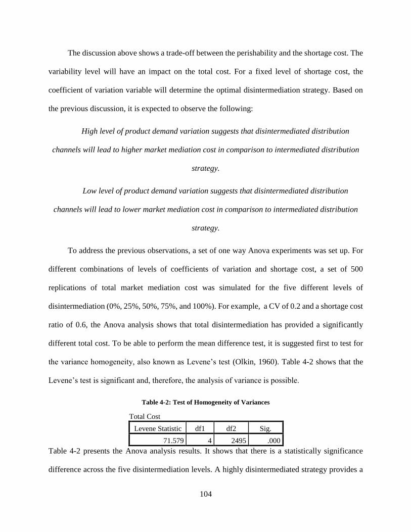
104

The discussion above shows a trade-off between the perishability and the shortage cost. The

variability level will have an impact on the total cost. For a fixed level of shortage cost, the

coefficient of variation variable will determine the optimal disintermediation strategy. Based on

the previous discussion, it is expected to observe the following:

High level of product demand variation suggests that disintermediated distribution

channels will lead to higher market mediation cost in comparison to intermediated distribution

strategy.

Low level of product demand variation suggests that disintermediated distribution

channels will lead to lower market mediation cost in comparison to intermediated distribution

strategy.

To address the previous observations, a set of one way Anova experiments was set up. For

different combinations of levels of coefficients of variation and shortage cost, a set of 500

replications of total market mediation cost was simulated for the five different levels of

disintermediation (0%, 25%, 50%, 75%, and 100%). For example, a CV of 0.2 and a shortage cost

ratio of 0.6, the Anova analysis shows that total disintermediation has provided a significantly

different total cost. To be able to perform the mean difference test, it is suggested first to test for

the variance homogeneity, also known as Levene’s test (Olkin, 1960). Table 4-2 shows that the

Levene’s test is significant and, therefore, the analysis of variance is possible.

Table 4-2: Test of Homogeneity of Variances

Total Cost

Levene Statistic df1 df2 Sig.

71.579 4 2495 .000

Table 4-2 presents the Anova analysis results. It shows that there is a statistically significance

difference across the five disintermediation levels. A highly disintermediated strategy provides a

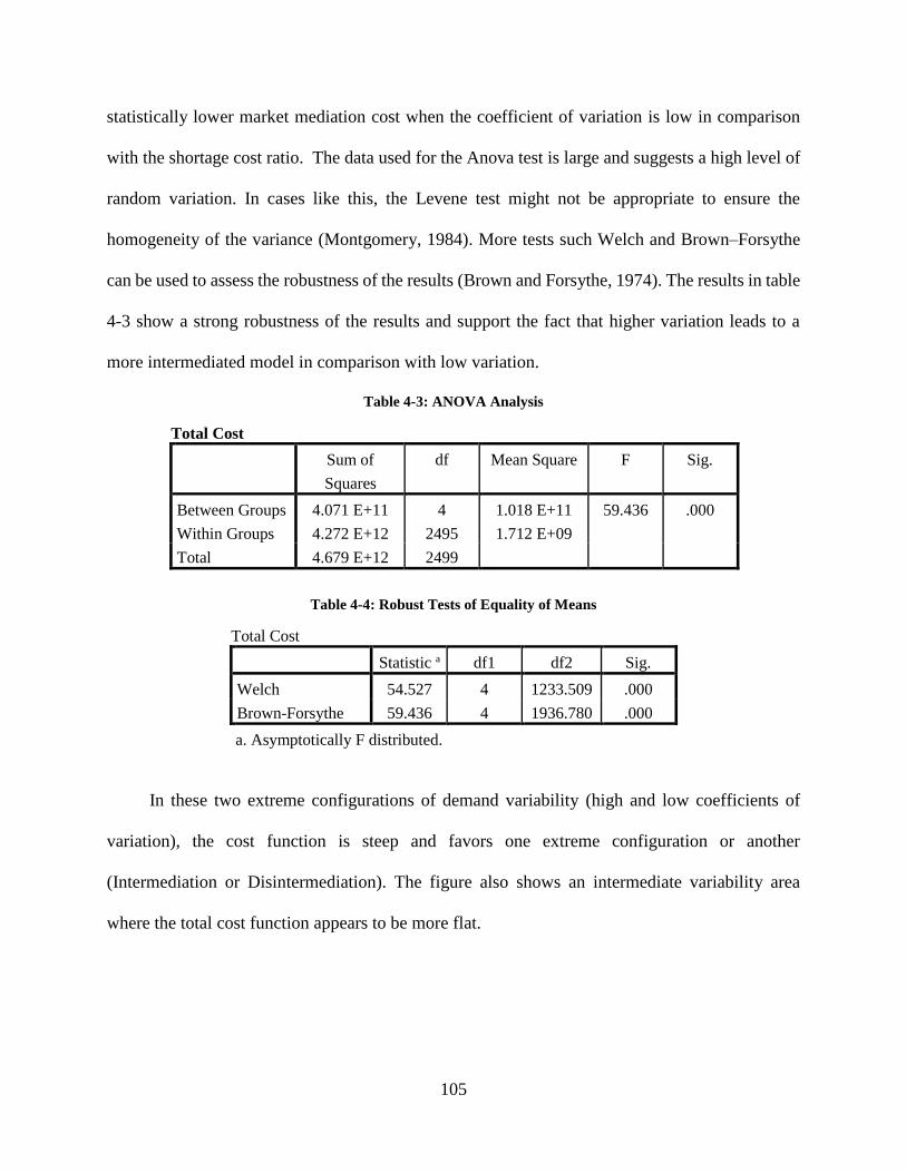
105

statistically lower market mediation cost when the coefficient of variation is low in comparison

with the shortage cost ratio. The data used for the Anova test is large and suggests a high level of

random variation. In cases like this, the Levene test might not be appropriate to ensure the

homogeneity of the variance (Montgomery, 1984). More tests such Welch and Brown–Forsythe

can be used to assess the robustness of the results (Brown and Forsythe, 1974). The results in table

4-3 show a strong robustness of the results and support the fact that higher variation leads to a

more intermediated model in comparison with low variation.

Table 4-3: ANOVA Analysis

Total Cost

Sum of

Squares

df Mean Square F Sig.

Between Groups 4.071 E+11 4 1.018 E+11 59.436 .000

Within Groups 4.272 E+12 2495 1.712 E+09

Total 4.679 E+12 2499

Table 4-4: Robust Tests of Equality of Means

Total Cost

Statistic a df1 df2 Sig.

Welch 54.527 4 1233.509 .000

Brown-Forsythe 59.436 4 1936.780 .000

a. Asymptotically F distributed.

In these two extreme configurations of demand variability (high and low coefficients of

variation), the cost function is steep and favors one extreme configuration or another

(Intermediation or Disintermediation). The figure also shows an intermediate variability area

where the total cost function appears to be more flat.

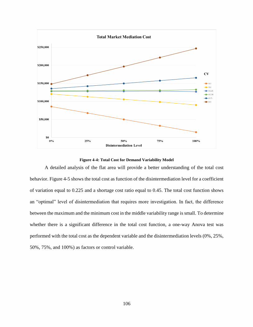
106

Figure 4-4: Total Cost for Demand Variability Model

A detailed analysis of the flat area will provide a better understanding of the total cost

behavior. Figure 4-5 shows the total cost as function of the disintermediation level for a coefficient

of variation equal to 0.225 and a shortage cost ratio equal to 0.45. The total cost function shows

an “optimal” level of disintermediation that requires more investigation. In fact, the difference

between the maximum and the minimum cost in the middle variability range is small. To determine

whether there is a significant difference in the total cost function, a one-way Anova test was

performed with the total cost as the dependent variable and the disintermediation levels (0%, 25%,

50%, 75%, and 100%) as factors or control variable.

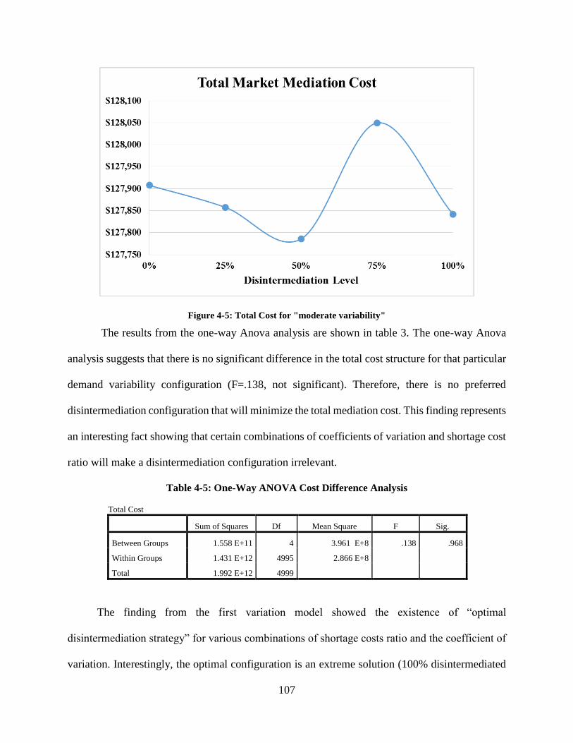
107

Figure 4-5: Total Cost for "moderate variability"

The results from the one-way Anova analysis are shown in table 3. The one-way Anova

analysis suggests that there is no significant difference in the total cost structure for that particular

demand variability configuration (F=.138, not significant). Therefore, there is no preferred

disintermediation configuration that will minimize the total mediation cost. This finding represents

an interesting fact showing that certain combinations of coefficients of variation and shortage cost

ratio will make a disintermediation configuration irrelevant.

Table 4-5: One-Way ANOVA Cost Difference Analysis

Total Cost

Sum of Squares Df Mean Square F Sig.

Between Groups 1.558 E+11 4 3.961 E+8 .138 .968

Within Groups 1.431 E+12 4995 2.866 E+8

Total 1.992 E+12 4999

The finding from the first variation model showed the existence of “optimal

disintermediation strategy” for various combinations of shortage costs ratio and the coefficient of

variation. Interestingly, the optimal configuration is an extreme solution (100% disintermediated

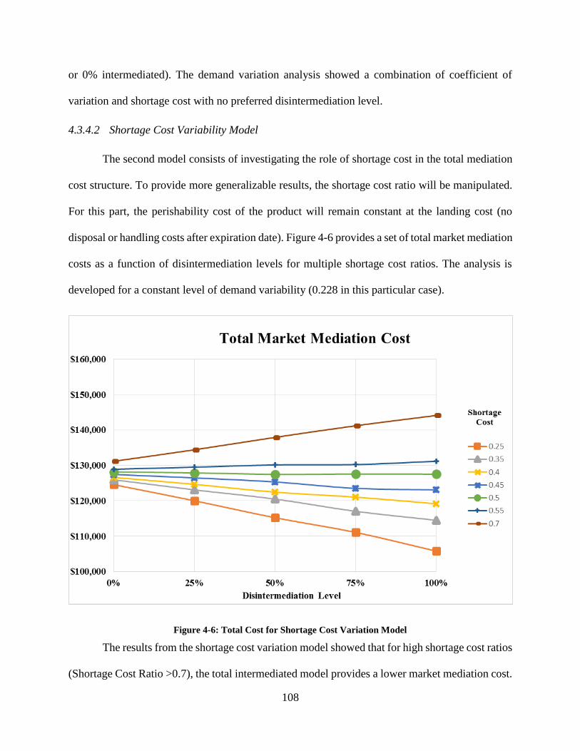
108

or 0% intermediated). The demand variation analysis showed a combination of coefficient of

variation and shortage cost with no preferred disintermediation level.

4.3.4.2 Shortage Cost Variability Model

The second model consists of investigating the role of shortage cost in the total mediation

cost structure. To provide more generalizable results, the shortage cost ratio will be manipulated.

For this part, the perishability cost of the product will remain constant at the landing cost (no

disposal or handling costs after expiration date). Figure 4-6 provides a set of total market mediation

costs as a function of disintermediation levels for multiple shortage cost ratios. The analysis is

developed for a constant level of demand variability (0.228 in this particular case).

Figure 4-6: Total Cost for Shortage Cost Variation Model

The results from the shortage cost variation model showed that for high shortage cost ratios

(Shortage Cost Ratio >0.7), the total intermediated model provides a lower market mediation cost.

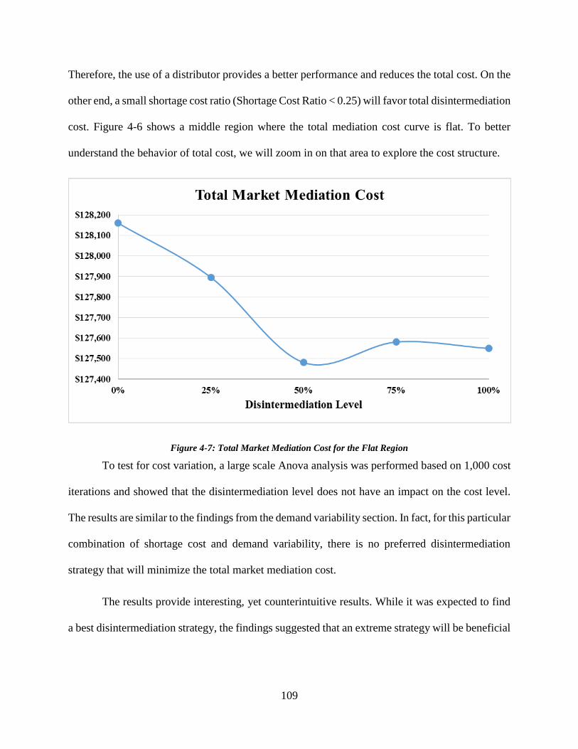
109

Therefore, the use of a distributor provides a better performance and reduces the total cost. On the

other end, a small shortage cost ratio (Shortage Cost Ratio < 0.25) will favor total disintermediation

cost. Figure 4-6 shows a middle region where the total mediation cost curve is flat. To better

understand the behavior of total cost, we will zoom in on that area to explore the cost structure.

Figure 4-7: Total Market Mediation Cost for the Flat Region

To test for cost variation, a large scale Anova analysis was performed based on 1,000 cost

iterations and showed that the disintermediation level does not have an impact on the cost level.

The results are similar to the findings from the demand variability section. In fact, for this particular

combination of shortage cost and demand variability, there is no preferred disintermediation

strategy that will minimize the total market mediation cost.

The results provide interesting, yet counterintuitive results. While it was expected to find

a best disintermediation strategy, the findings suggested that an extreme strategy will be beneficial

110

in some cases. The results suggest further analysis to address the combination of both variation

models (demand and shortage cost).

4.3.4.3 Combined Model

In the previous two sections, one variable has been modified at a time. The results showed

some preferred strategy (totally disintermediated or intermediated) depending on the parameters.

This section will combine both parameters into one general model that addresses the impact of

both demand variability and shortage cost structure on the total market mediation cost. First, a set

of coefficients of variation is generated, varying from 0.01 to 0.3 with 0.01 increments. Also,

multiple shortage cost ratios are generated between 0.05 and 1.5 with 0.025 increments. Therefore,

a total of 30*59=1,770 combinations are created. For each combination, a total of market

disintermediation cost is determined by the five disintermediation levels. The cost is determined

based on large scale Monte Carlo simulation. For each combination, an optimal disintermediation

strategy, if it exists, was determined. The disintermediation configuration optimality was

performed using Anova analysis similar to the one performed on the demand variability and

shortage cost models. The analysis has identified three main optimality levels: a total intermediated

strategy, a total disintermediated strategy, and a no-optimal strategy.

The total disintermediation strategy suggests that the total market mediation cost is

minimized when the direct sales strategy from the manufacturer to the hospitals is applied. This

happens when the level of demand variation impact is lower than the shortage cost factor. Total

disintermediation strategy is possible when the shortage cost ratio is too high, making the

intermediated distribution channels inappropriate. Second, totally intermediated distribution

channels are appropriate when the demand variation is too high compared to the shortage cost

ratio. In this case, the distributor’s pooling effect will reduce the shortage cost. Intermediated

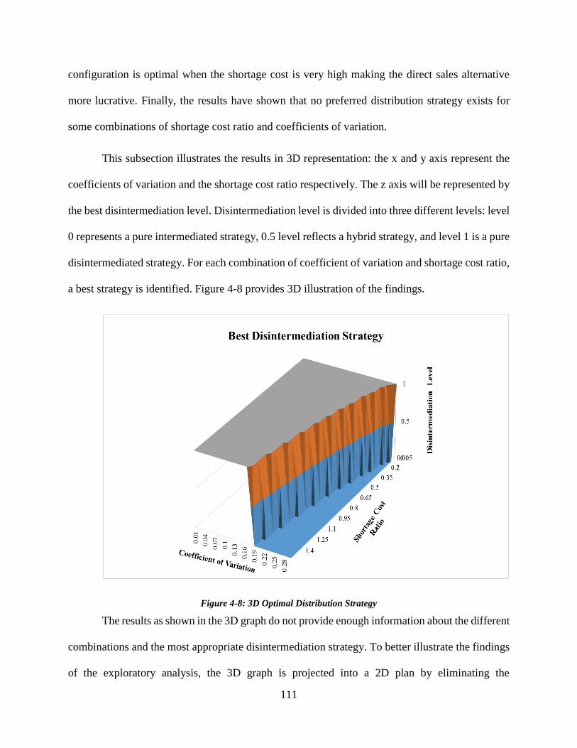
111

configuration is optimal when the shortage cost is very high making the direct sales alternative

more lucrative. Finally, the results have shown that no preferred distribution strategy exists for

some combinations of shortage cost ratio and coefficients of variation.

This subsection illustrates the results in 3D representation: the x and y axis represent the

coefficients of variation and the shortage cost ratio respectively. The z axis will be represented by

the best disintermediation level. Disintermediation level is divided into three different levels: level

0 represents a pure intermediated strategy, 0.5 level reflects a hybrid strategy, and level 1 is a pure

disintermediated strategy. For each combination of coefficient of variation and shortage cost ratio,

a best strategy is identified. Figure 4-8 provides 3D illustration of the findings.

Figure 4-8: 3D Optimal Distribution Strategy

The results as shown in the 3D graph do not provide enough information about the different

combinations and the most appropriate disintermediation strategy. To better illustrate the findings

of the exploratory analysis, the 3D graph is projected into a 2D plan by eliminating the

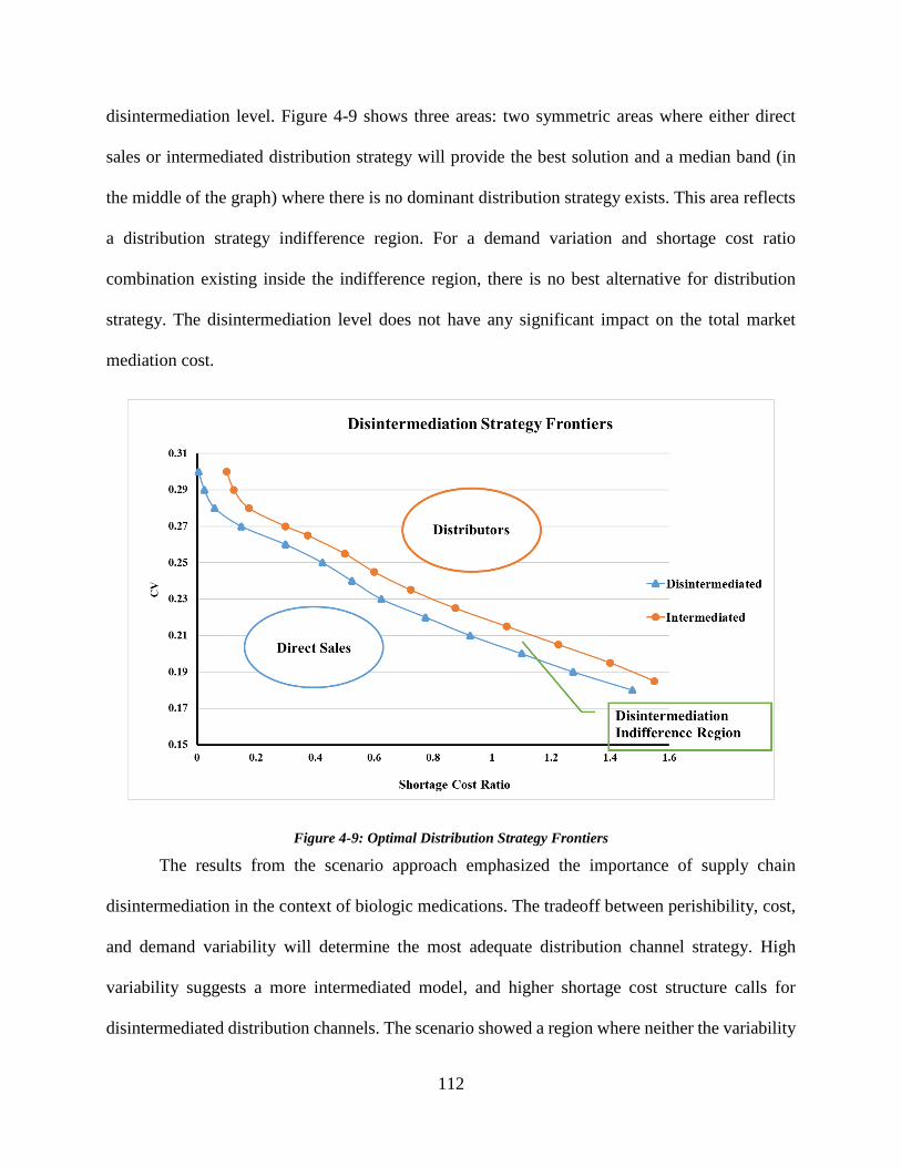
112

disintermediation level. Figure 4-9 shows three areas: two symmetric areas where either direct

sales or intermediated distribution strategy will provide the best solution and a median band (in

the middle of the graph) where there is no dominant distribution strategy exists. This area reflects

a distribution strategy indifference region. For a demand variation and shortage cost ratio

combination existing inside the indifference region, there is no best alternative for distribution

strategy. The disintermediation level does not have any significant impact on the total market

mediation cost.

Figure 4-9: Optimal Distribution Strategy Frontiers

The results from the scenario approach emphasized the importance of supply chain

disintermediation in the context of biologic medications. The tradeoff between perishibility, cost,

and demand variability will determine the most adequate distribution channel strategy. High

variability suggests a more intermediated model, and higher shortage cost structure calls for

disintermediated distribution channels. The scenario showed a region where neither the variability

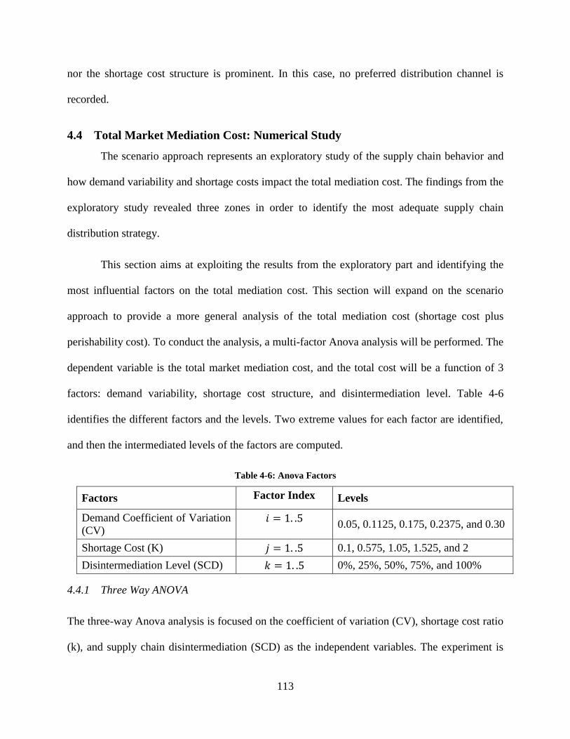
113

nor the shortage cost structure is prominent. In this case, no preferred distribution channel is

recorded.

4.4 Total Market Mediation Cost: Numerical Study

The scenario approach represents an exploratory study of the supply chain behavior and

how demand variability and shortage costs impact the total mediation cost. The findings from the

exploratory study revealed three zones in order to identify the most adequate supply chain

distribution strategy.

This section aims at exploiting the results from the exploratory part and identifying the

most influential factors on the total mediation cost. This section will expand on the scenario

approach to provide a more general analysis of the total mediation cost (shortage cost plus

perishability cost). To conduct the analysis, a multi-factor Anova analysis will be performed. The

dependent variable is the total market mediation cost, and the total cost will be a function of 3

factors: demand variability, shortage cost structure, and disintermediation level. Table 4-6

identifies the different factors and the levels. Two extreme values for each factor are identified,

and then the intermediated levels of the factors are computed.

Table 4-6: Anova Factors

Factors Factor Index Levels

Demand Coefficient of Variation

(CV) 𝑖 = 1. .5

0.05, 0.1125, 0.175, 0.2375, and 0.30

Shortage Cost (K) 𝑗 = 1. .5 0.1, 0.575, 1.05, 1.525, and 2

Disintermediation Level (SCD) 𝑘 = 1. .5 0%, 25%, 50%, 75%, and 100%

4.4.1 Three Way ANOVA

The three-way Anova analysis is focused on the coefficient of variation (CV), shortage cost ratio

(k), and supply chain disintermediation (SCD) as the independent variables. The experiment is

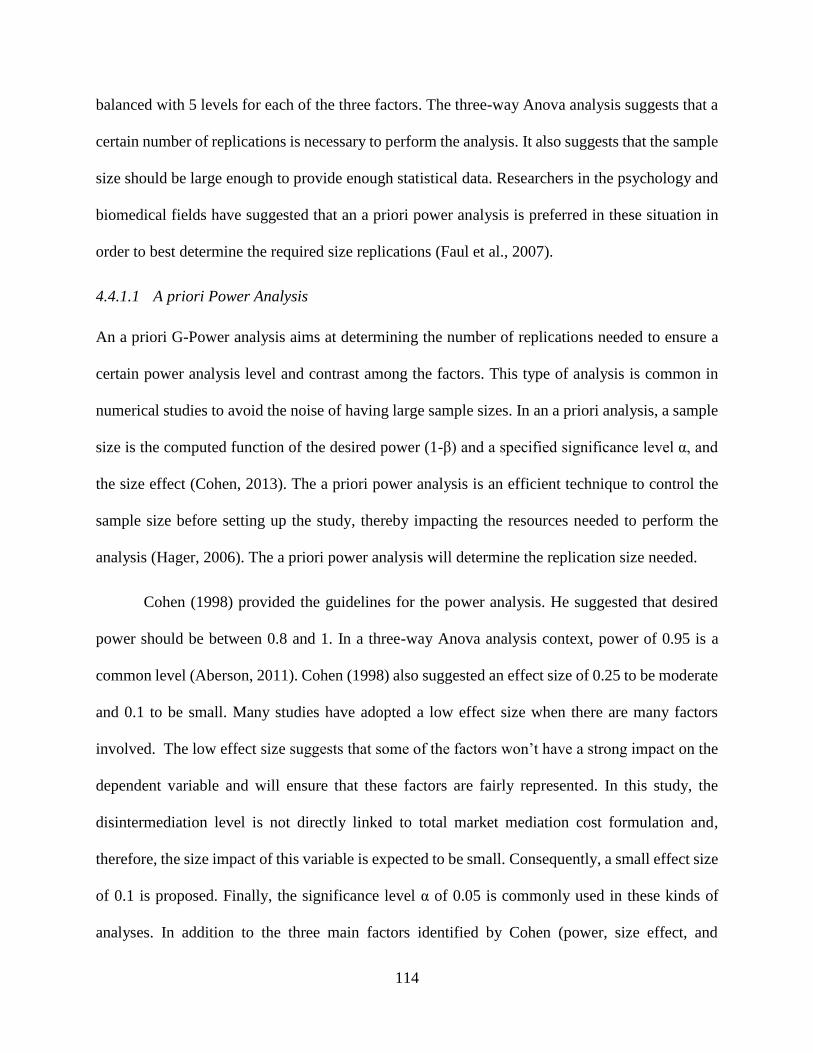
114

balanced with 5 levels for each of the three factors. The three-way Anova analysis suggests that a

certain number of replications is necessary to perform the analysis. It also suggests that the sample

size should be large enough to provide enough statistical data. Researchers in the psychology and

biomedical fields have suggested that an a priori power analysis is preferred in these situation in

order to best determine the required size replications (Faul et al., 2007).

4.4.1.1 A priori Power Analysis

An a priori G-Power analysis aims at determining the number of replications needed to ensure a

certain power analysis level and contrast among the factors. This type of analysis is common in

numerical studies to avoid the noise of having large sample sizes. In an a priori analysis, a sample

size is the computed function of the desired power (1-β) and a specified significance level α, and

the size effect (Cohen, 2013). The a priori power analysis is an efficient technique to control the

sample size before setting up the study, thereby impacting the resources needed to perform the

analysis (Hager, 2006). The a priori power analysis will determine the replication size needed.

Cohen (1998) provided the guidelines for the power analysis. He suggested that desired

power should be between 0.8 and 1. In a three-way Anova analysis context, power of 0.95 is a

common level (Aberson, 2011). Cohen (1998) also suggested an effect size of 0.25 to be moderate

and 0.1 to be small. Many studies have adopted a low effect size when there are many factors

involved. The low effect size suggests that some of the factors won’t have a strong impact on the

dependent variable and will ensure that these factors are fairly represented. In this study, the

disintermediation level is not directly linked to total market mediation cost formulation and,

therefore, the size impact of this variable is expected to be small. Consequently, a small effect size

of 0.1 is proposed. Finally, the significance level α of 0.05 is commonly used in these kinds of

analyses. In addition to the three main factors identified by Cohen (power, size effect, and

115

significance level), the Anova analysis also involves the number of degree of freedom and the

number of groups. In a balanced Anova design with m factors and l levels within each factor, the

following formula is provided:

𝐷𝑒𝑔𝑟𝑒𝑒 𝑜𝑓 𝐹𝑟𝑒𝑒𝑑𝑜𝑚 = (𝑙 − 1)𝑚 ( 4-23)

𝑁𝑢𝑚𝑏𝑒𝑟 𝑜𝑓 𝐺𝑟𝑜𝑢𝑝𝑠 = 𝑙𝑚 ( 4-24)

To determine the required sample size, multiple software can be used. Many researchers have

suggested using GPower 3.1, as it is an open source software and is easy to use, is accurate, and

has the capability to provide a sensitivity and post hoc analysis (Faul et al., 2009). Therefore, this

study used this software as well. The results showed a total size of 4788. Since the number of

groups is 125, the number of replications will be ⌈4788

125⌉ = 39.

To assess the role of size on power, an F test power analysis was performed to measure the effect

of sample size on power. Graph 4-10 shows the power explained as a function of the total sample

size. The graph shows the sensitivity of the power to the sample size, and it can be determined that

for a number of replication equal to 39 (the minimum number of replications determined), the

model will have a power of .97.

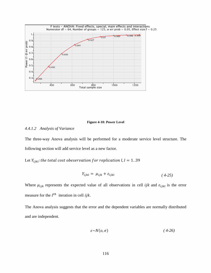
116

Figure 4-10: Power Level

4.4.1.2 Analysis of Variance

The three-way Anova analysis will be performed for a moderate service level structure. The

following section will add service level as a new factor.

Let 𝑌𝑖𝑗𝑘𝑙: 𝑡ℎ𝑒 𝑡𝑜𝑡𝑎𝑙 𝑐𝑜𝑠𝑡 𝑜𝑏𝑒𝑠𝑒𝑟𝑣𝑎𝑡𝑖𝑜𝑛 𝑓𝑜𝑟 𝑟𝑒𝑝𝑙𝑖𝑐𝑎𝑡𝑖𝑜𝑛 𝑙, 𝑙 = 1. .39

𝑌𝑖𝑗𝑘𝑙 = 𝜇𝑖𝑗𝑘 + 𝜀𝑖𝑗𝑘𝑙 ( 4-25)

Where 𝜇𝑖𝑗𝑘 represents the expected value of all observations in cell 𝑖𝑗𝑘 and 𝜀𝑖𝑗𝑘𝑙 is the error

measure for the 𝑙𝑡ℎ iteration in cell 𝑖𝑗𝑘.

The Anova analysis suggests that the error and the dependent variables are normally distributed

and are independent.

𝜀~𝑁(𝑜, 𝜎) ( 4-26)

117

𝑌𝑖𝑗𝑘𝑙~𝑁(𝜇𝑖𝑗𝑘, 𝜎) ( 4-27)

The factor effect model for a three-factor Anova analysis is modeled as follows:

𝑌𝑖𝑗𝑘 = 𝜇 + 𝛼𝑖 + 𝛽𝑗 + 𝛾𝑘 + (𝛼 ∗ 𝛽)𝑖𝑗 + (𝛼 ∗ 𝛾)𝑖𝑘 + (𝛽 ∗ 𝛾)𝑗𝑘

+ (𝛼 ∗ 𝛽 ∗ 𝛾)𝑖𝑗𝑘 + 𝜀𝑖𝑗𝑘𝑙 ( 4-28)

Where:

µ: the overall mean of all observations,

𝛼𝑖, 𝛽𝑗, 𝛾𝑘 : the main effects of factors CV, k, and SCD,

(𝛼 ∗ 𝛽)𝑖𝑗, (𝛼 ∗ 𝛾)𝑖𝑘, (𝛽 ∗ 𝛾)𝑗𝑘: the two-way first order interactions, and

(𝛼 ∗ 𝛽 ∗ 𝛾)𝑖𝑗𝑘: three-way second order interactions.

Researchers have suggested a template to use in three-way factor analysis (Wuensch et al., 2002).

The methodology is summarized in figure 4-11.

Figure 4-11: Anova Analysis Plan

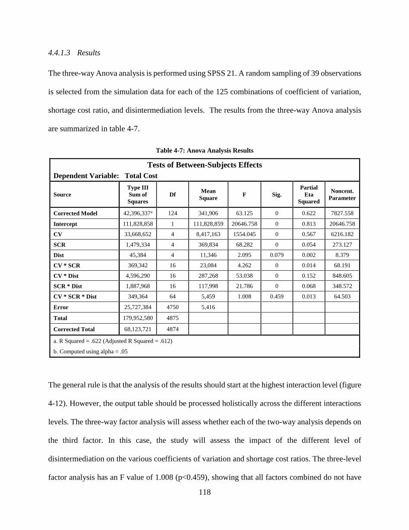
118

4.4.1.3 Results

The three-way Anova analysis is performed using SPSS 21. A random sampling of 39 observations

is selected from the simulation data for each of the 125 combinations of coefficient of variation,

shortage cost ratio, and disintermediation levels. The results from the three-way Anova analysis

are summarized in table 4-7.

Table 4-7: Anova Analysis Results

Tests of Between-Subjects Effects

Dependent Variable: Total Cost

Source

Type III

Sum of

Squares

Df Mean

Square F Sig.

Partial

Eta

Squared

Noncent.

Parameter

Corrected Model 42,396,337a 124 341,906 63.125 0 0.622 7827.558

Intercept 111,828,858 1 111,828,859 20646.758 0 0.813 20646.758

CV 33,668,652 4 8,417,163 1554.045 0 0.567 6216.182

SCR 1,479,334 4 369,834 68.282 0 0.054 273.127

Dist 45,384 4 11,346 2.095 0.079 0.002 8.379

CV * SCR 369,342 16 23,084 4.262 0 0.014 68.191

CV * Dist 4,596,290 16 287,268 53.038 0 0.152 848.605

SCR * Dist 1,887,968 16 117,998 21.786 0 0.068 348.572

CV * SCR * Dist 349,364 64 5,459 1.008 0.459 0.013 64.503

Error 25,727,384 4750 5,416

Total 179,952,580 4875

Corrected Total 68,123,721 4874

a. R Squared = .622 (Adjusted R Squared = .612)

b. Computed using alpha = .05

The general rule is that the analysis of the results should start at the highest interaction level (figure

4-12). However, the output table should be processed holistically across the different interactions

levels. The three-way factor analysis will assess whether each of the two-way analysis depends on

the third factor. In this case, the study will assess the impact of the different level of

disintermediation on the various coefficients of variation and shortage cost ratios. The three-level

factor analysis has an F value of 1.008 (p<0.459), showing that all factors combined do not have

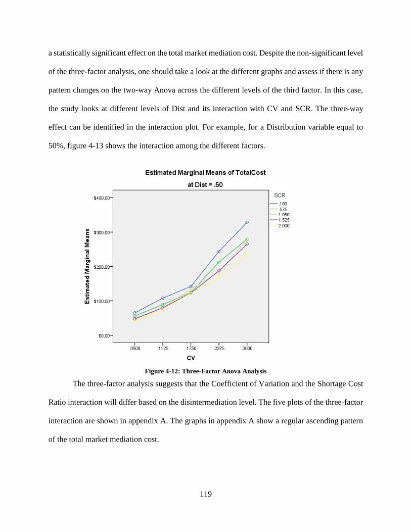
119

a statistically significant effect on the total market mediation cost. Despite the non-significant level

of the three-factor analysis, one should take a look at the different graphs and assess if there is any

pattern changes on the two-way Anova across the different levels of the third factor. In this case,

the study looks at different levels of Dist and its interaction with CV and SCR. The three-way

effect can be identified in the interaction plot. For example, for a Distribution variable equal to

50%, figure 4-13 shows the interaction among the different factors.

Figure 4-12: Three-Factor Anova Analysis

The three-factor analysis suggests that the Coefficient of Variation and the Shortage Cost

Ratio interaction will differ based on the disintermediation level. The five plots of the three-factor

interaction are shown in appendix A. The graphs in appendix A show a regular ascending pattern

of the total market mediation cost.

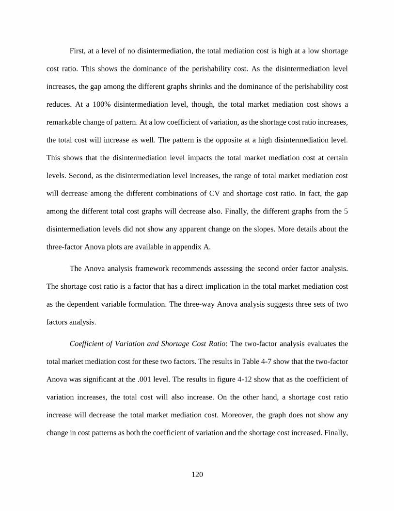
120

First, at a level of no disintermediation, the total mediation cost is high at a low shortage

cost ratio. This shows the dominance of the perishability cost. As the disintermediation level

increases, the gap among the different graphs shrinks and the dominance of the perishability cost

reduces. At a 100% disintermediation level, though, the total market mediation cost shows a

remarkable change of pattern. At a low coefficient of variation, as the shortage cost ratio increases,

the total cost will increase as well. The pattern is the opposite at a high disintermediation level.

This shows that the disintermediation level impacts the total market mediation cost at certain

levels. Second, as the disintermediation level increases, the range of total market mediation cost

will decrease among the different combinations of CV and shortage cost ratio. In fact, the gap

among the different total cost graphs will decrease also. Finally, the different graphs from the 5

disintermediation levels did not show any apparent change on the slopes. More details about the

three-factor Anova plots are available in appendix A.

The Anova analysis framework recommends assessing the second order factor analysis.

The shortage cost ratio is a factor that has a direct implication in the total market mediation cost

as the dependent variable formulation. The three-way Anova analysis suggests three sets of two

factors analysis.

Coefficient of Variation and Shortage Cost Ratio: The two-factor analysis evaluates the

total market mediation cost for these two factors. The results in Table 4-7 show that the two-factor

Anova was significant at the .001 level. The results in figure 4-12 show that as the coefficient of

variation increases, the total cost will also increase. On the other hand, a shortage cost ratio

increase will decrease the total market mediation cost. Moreover, the graph does not show any

change in cost patterns as both the coefficient of variation and the shortage cost increased. Finally,

121

the increase of the coefficient of variation will increase the gap among the various shortage cost

levels.

Figure 4-13: Coefficient of Variation and Shortage Cost Anova

Coefficient of Variation and Disintermediation: The two-factor Anova analysis is

significant at the .0001 level with the F value equal to 53.038. The cost graph in figure 4-15 shows

a change of pattern in the cost functions. As the coefficient of variation increases, disintermediation

strategy becomes less attractive. In fact, at a low coefficient level, total disintermediation results

in low cost. On the other hand, at a high coefficient of variation level, intermediated distribution

channels provide lower market mediation cost. Moreover, as the coefficient of variation increases,

the total cost graph’s slope will increase for a high disintermediation level. In contrast, for small

disintermediation levels, the increase of coefficient of variation will decrease the graph’s slope.

The two-factor Anova graphs show that all the graphs’ intersection points are close. A zoom on

the intersection area shows that the points do not coincide. In fact, a more refined analysis was

developed to address the impact of disintermediation and coefficient of variation on total market

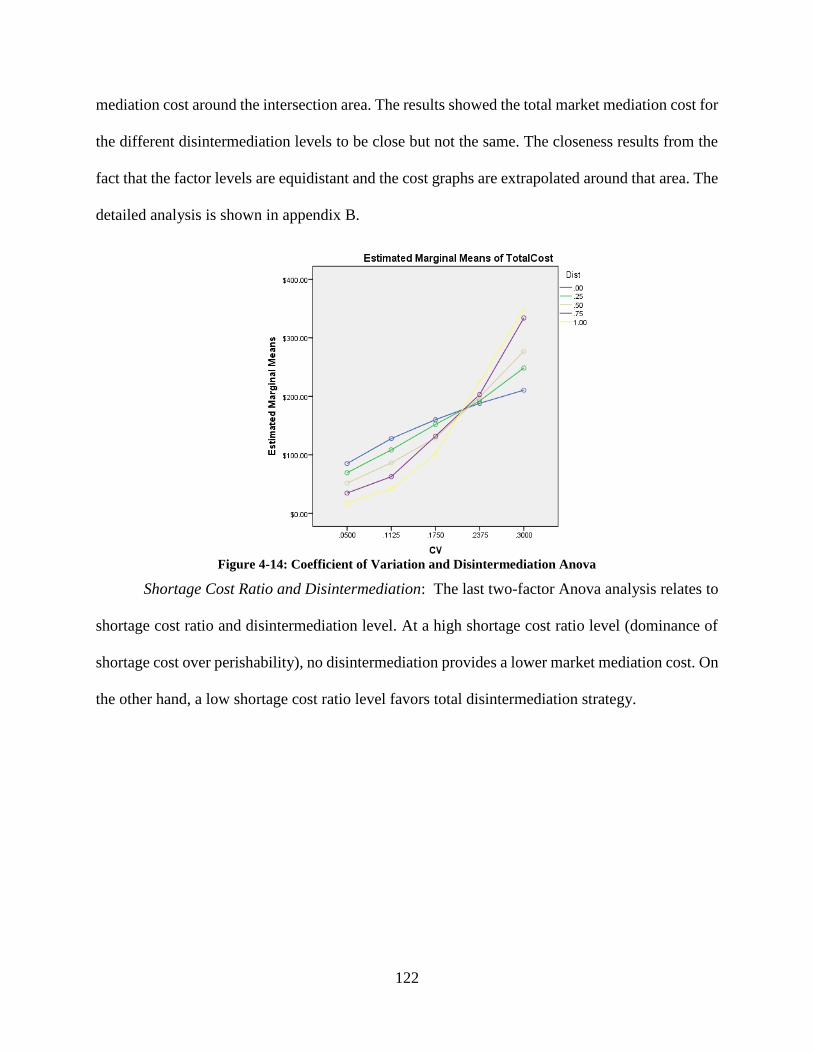
122

mediation cost around the intersection area. The results showed the total market mediation cost for

the different disintermediation levels to be close but not the same. The closeness results from the

fact that the factor levels are equidistant and the cost graphs are extrapolated around that area. The

detailed analysis is shown in appendix B.

Figure 4-14: Coefficient of Variation and Disintermediation Anova

Shortage Cost Ratio and Disintermediation: The last two-factor Anova analysis relates to

shortage cost ratio and disintermediation level. At a high shortage cost ratio level (dominance of

shortage cost over perishability), no disintermediation provides a lower market mediation cost. On

the other hand, a low shortage cost ratio level favors total disintermediation strategy.

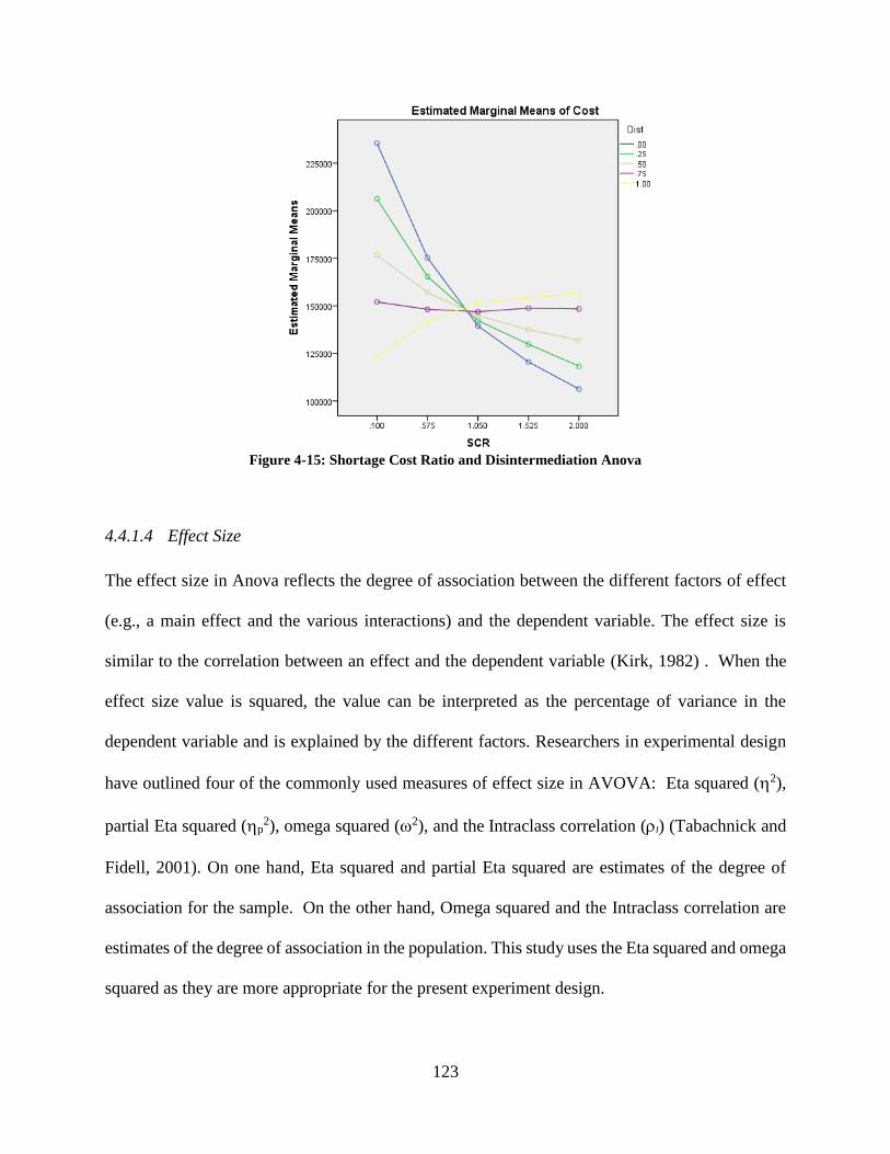
123

Figure 4-15: Shortage Cost Ratio and Disintermediation Anova

4.4.1.4 Effect Size

The effect size in Anova reflects the degree of association between the different factors of effect

(e.g., a main effect and the various interactions) and the dependent variable. The effect size is

similar to the correlation between an effect and the dependent variable (Kirk, 1982) . When the

effect size value is squared, the value can be interpreted as the percentage of variance in the

dependent variable and is explained by the different factors. Researchers in experimental design

have outlined four of the commonly used measures of effect size in AVOVA: Eta squared (2),

partial Eta squared (p2), omega squared (2), and the Intraclass correlation (I) (Tabachnick and

Fidell, 2001). On one hand, Eta squared and partial Eta squared are estimates of the degree of

association for the sample. On the other hand, Omega squared and the Intraclass correlation are

estimates of the degree of association in the population. This study uses the Eta squared and omega

squared as they are more appropriate for the present experiment design.

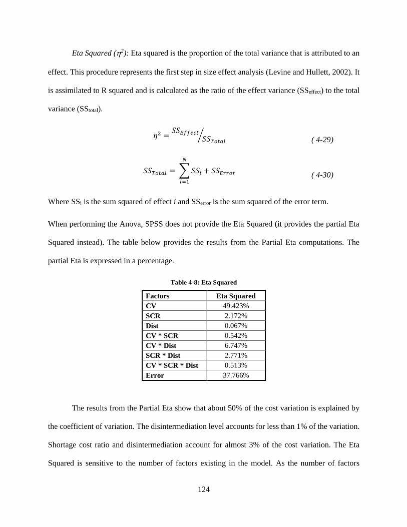
124

Eta Squared (2): Eta squared is the proportion of the total variance that is attributed to an

effect. This procedure represents the first step in size effect analysis (Levine and Hullett, 2002). It

is assimilated to R squared and is calculated as the ratio of the effect variance (SSeffect) to the total

variance (SStotal).

𝜂2 =𝑆𝑆𝐸𝑓𝑓𝑒𝑐𝑡

𝑆𝑆𝑇𝑜𝑡𝑎𝑙⁄

( 4-29)

𝑆𝑆𝑇𝑜𝑡𝑎𝑙 = ∑ 𝑆𝑆𝑖

𝑁

𝑖=1

+ 𝑆𝑆𝐸𝑟𝑟𝑜𝑟 ( 4-30)

Where SSi is the sum squared of effect i and SSerror is the sum squared of the error term.

When performing the Anova, SPSS does not provide the Eta Squared (it provides the partial Eta

Squared instead). The table below provides the results from the Partial Eta computations. The

partial Eta is expressed in a percentage.

Table 4-8: Eta Squared

Factors Eta Squared

CV 49.423%

SCR 2.172%

Dist 0.067%

CV * SCR 0.542%

CV * Dist 6.747%

SCR * Dist 2.771%

CV * SCR * Dist 0.513%

Error 37.766%

The results from the Partial Eta show that about 50% of the cost variation is explained by

the coefficient of variation. The disintermediation level accounts for less than 1% of the variation.

Shortage cost ratio and disintermediation account for almost 3% of the cost variation. The Eta

Squared is sensitive to the number of factors existing in the model. As the number of factors

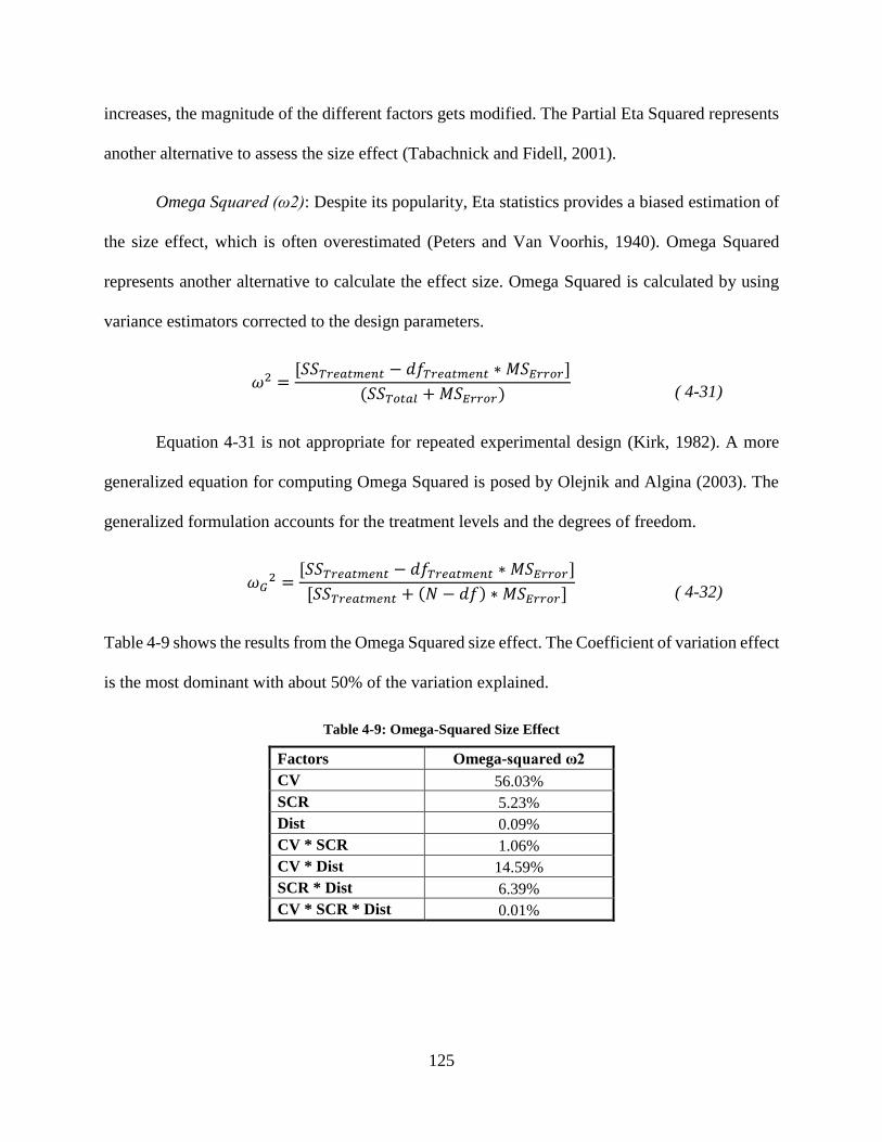
125

increases, the magnitude of the different factors gets modified. The Partial Eta Squared represents

another alternative to assess the size effect (Tabachnick and Fidell, 2001).

Omega Squared (ω2): Despite its popularity, Eta statistics provides a biased estimation of

the size effect, which is often overestimated (Peters and Van Voorhis, 1940). Omega Squared

represents another alternative to calculate the effect size. Omega Squared is calculated by using

variance estimators corrected to the design parameters.

𝜔2 =[𝑆𝑆𝑇𝑟𝑒𝑎𝑡𝑚𝑒𝑛𝑡 − 𝑑𝑓𝑇𝑟𝑒𝑎𝑡𝑚𝑒𝑛𝑡 ∗ 𝑀𝑆𝐸𝑟𝑟𝑜𝑟]

(𝑆𝑆𝑇𝑜𝑡𝑎𝑙 + 𝑀𝑆𝐸𝑟𝑟𝑜𝑟)

( 4-31)

Equation 4-31 is not appropriate for repeated experimental design (Kirk, 1982). A more

generalized equation for computing Omega Squared is posed by Olejnik and Algina (2003). The

generalized formulation accounts for the treatment levels and the degrees of freedom.

𝜔𝐺2 =

[𝑆𝑆𝑇𝑟𝑒𝑎𝑡𝑚𝑒𝑛𝑡 − 𝑑𝑓𝑇𝑟𝑒𝑎𝑡𝑚𝑒𝑛𝑡 ∗ 𝑀𝑆𝐸𝑟𝑟𝑜𝑟]

[𝑆𝑆𝑇𝑟𝑒𝑎𝑡𝑚𝑒𝑛𝑡 + (𝑁 − 𝑑𝑓) ∗ 𝑀𝑆𝐸𝑟𝑟𝑜𝑟]

( 4-32)

Table 4-9 shows the results from the Omega Squared size effect. The Coefficient of variation effect

is the most dominant with about 50% of the variation explained.

Table 4-9: Omega-Squared Size Effect

Factors Omega-squared ω2

CV 56.03%

SCR 5.23%

Dist 0.09%

CV * SCR 1.06%

CV * Dist 14.59%

SCR * Dist 6.39%

CV * SCR * Dist 0.01%

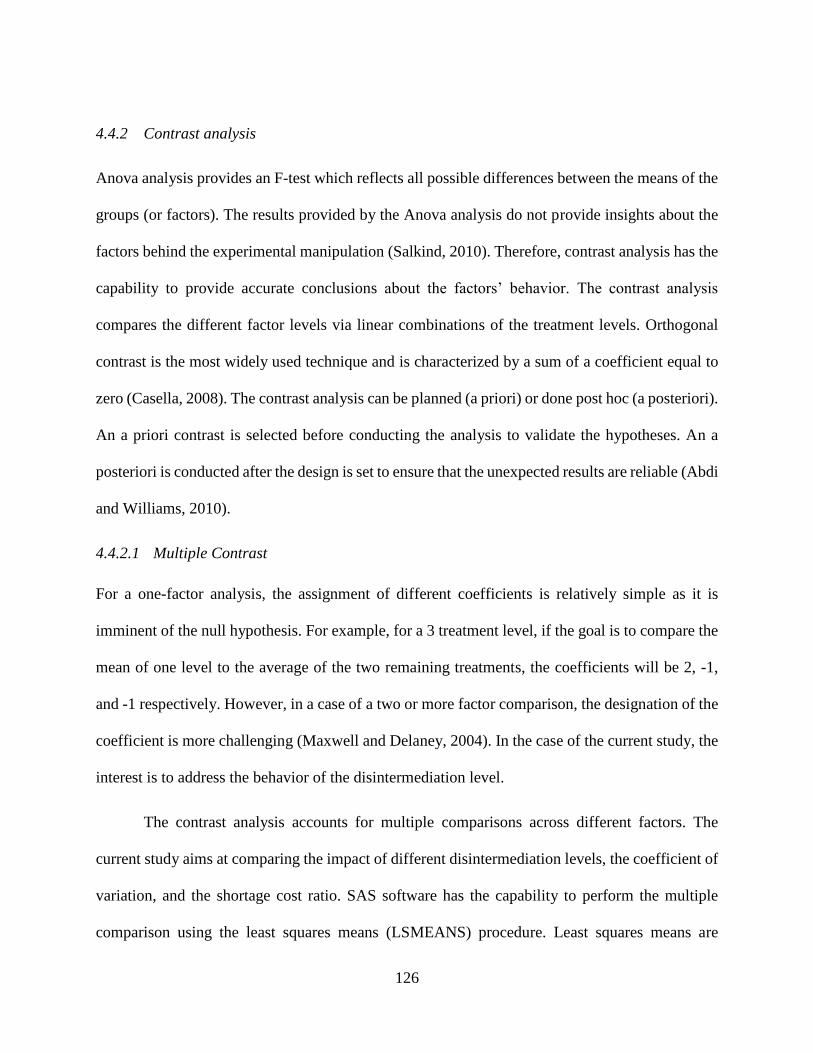
126

4.4.2 Contrast analysis

Anova analysis provides an F-test which reflects all possible differences between the means of the

groups (or factors). The results provided by the Anova analysis do not provide insights about the

factors behind the experimental manipulation (Salkind, 2010). Therefore, contrast analysis has the

capability to provide accurate conclusions about the factors’ behavior. The contrast analysis

compares the different factor levels via linear combinations of the treatment levels. Orthogonal

contrast is the most widely used technique and is characterized by a sum of a coefficient equal to

zero (Casella, 2008). The contrast analysis can be planned (a priori) or done post hoc (a posteriori).

An a priori contrast is selected before conducting the analysis to validate the hypotheses. An a

posteriori is conducted after the design is set to ensure that the unexpected results are reliable (Abdi

and Williams, 2010).

4.4.2.1 Multiple Contrast

For a one-factor analysis, the assignment of different coefficients is relatively simple as it is

imminent of the null hypothesis. For example, for a 3 treatment level, if the goal is to compare the

mean of one level to the average of the two remaining treatments, the coefficients will be 2, -1,

and -1 respectively. However, in a case of a two or more factor comparison, the designation of the

coefficient is more challenging (Maxwell and Delaney, 2004). In the case of the current study, the

interest is to address the behavior of the disintermediation level.

The contrast analysis accounts for multiple comparisons across different factors. The

current study aims at comparing the impact of different disintermediation levels, the coefficient of

variation, and the shortage cost ratio. SAS software has the capability to perform the multiple

comparison using the least squares means (LSMEANS) procedure. Least squares means are

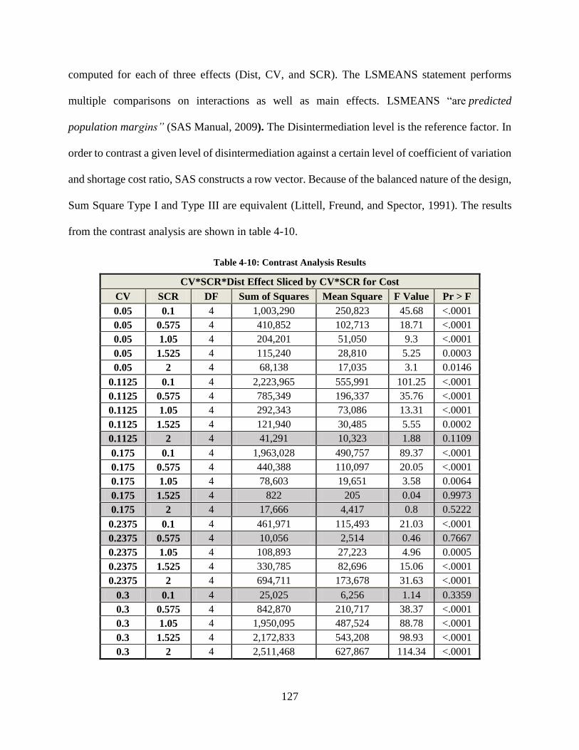
127

computed for each of three effects (Dist, CV, and SCR). The LSMEANS statement performs

multiple comparisons on interactions as well as main effects. LSMEANS “are predicted

population margins” (SAS Manual, 2009). The Disintermediation level is the reference factor. In

order to contrast a given level of disintermediation against a certain level of coefficient of variation

and shortage cost ratio, SAS constructs a row vector. Because of the balanced nature of the design,

Sum Square Type I and Type III are equivalent (Littell, Freund, and Spector, 1991). The results

from the contrast analysis are shown in table 4-10.

Table 4-10: Contrast Analysis Results

CV*SCR*Dist Effect Sliced by CV*SCR for Cost

CV SCR DF Sum of Squares Mean Square F Value Pr > F

0.05 0.1 4 1,003,290 250,823 45.68 <.0001

0.05 0.575 4 410,852 102,713 18.71 <.0001

0.05 1.05 4 204,201 51,050 9.3 <.0001

0.05 1.525 4 115,240 28,810 5.25 0.0003

0.05 2 4 68,138 17,035 3.1 0.0146

0.1125 0.1 4 2,223,965 555,991 101.25 <.0001

0.1125 0.575 4 785,349 196,337 35.76 <.0001

0.1125 1.05 4 292,343 73,086 13.31 <.0001

0.1125 1.525 4 121,940 30,485 5.55 0.0002

0.1125 2 4 41,291 10,323 1.88 0.1109

0.175 0.1 4 1,963,028 490,757 89.37 <.0001

0.175 0.575 4 440,388 110,097 20.05 <.0001

0.175 1.05 4 78,603 19,651 3.58 0.0064

0.175 1.525 4 822 205 0.04 0.9973

0.175 2 4 17,666 4,417 0.8 0.5222

0.2375 0.1 4 461,971 115,493 21.03 <.0001

0.2375 0.575 4 10,056 2,514 0.46 0.7667

0.2375 1.05 4 108,893 27,223 4.96 0.0005

0.2375 1.525 4 330,785 82,696 15.06 <.0001

0.2375 2 4 694,711 173,678 31.63 <.0001

0.3 0.1 4 25,025 6,256 1.14 0.3359

0.3 0.575 4 842,870 210,717 38.37 <.0001

0.3 1.05 4 1,950,095 487,524 88.78 <.0001

0.3 1.525 4 2,172,833 543,208 98.93 <.0001

0.3 2 4 2,511,468 627,867 114.34 <.0001

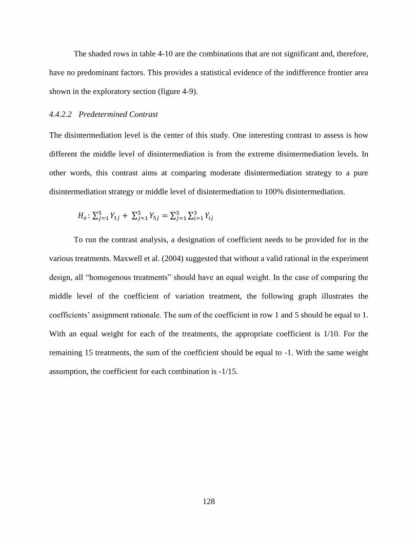
128

The shaded rows in table 4-10 are the combinations that are not significant and, therefore,

have no predominant factors. This provides a statistical evidence of the indifference frontier area

shown in the exploratory section (figure 4-9).

4.4.2.2 Predetermined Contrast

The disintermediation level is the center of this study. One interesting contrast to assess is how

different the middle level of disintermediation is from the extreme disintermediation levels. In

other words, this contrast aims at comparing moderate disintermediation strategy to a pure

disintermediation strategy or middle level of disintermediation to 100% disintermediation.

𝐻𝑜 : ∑ 𝑌1𝑗5𝑗=1 + ∑ 𝑌5𝑗

5𝑗=1 = ∑ ∑ 𝑌𝑖𝑗

3𝑖=1

5𝑗=1

To run the contrast analysis, a designation of coefficient needs to be provided for in the

various treatments. Maxwell et al. (2004) suggested that without a valid rational in the experiment

design, all “homogenous treatments” should have an equal weight. In the case of comparing the

middle level of the coefficient of variation treatment, the following graph illustrates the

coefficients’ assignment rationale. The sum of the coefficient in row 1 and 5 should be equal to 1.

With an equal weight for each of the treatments, the appropriate coefficient is 1/10. For the

remaining 15 treatments, the sum of the coefficient should be equal to -1. With the same weight

assumption, the coefficient for each combination is -1/15.

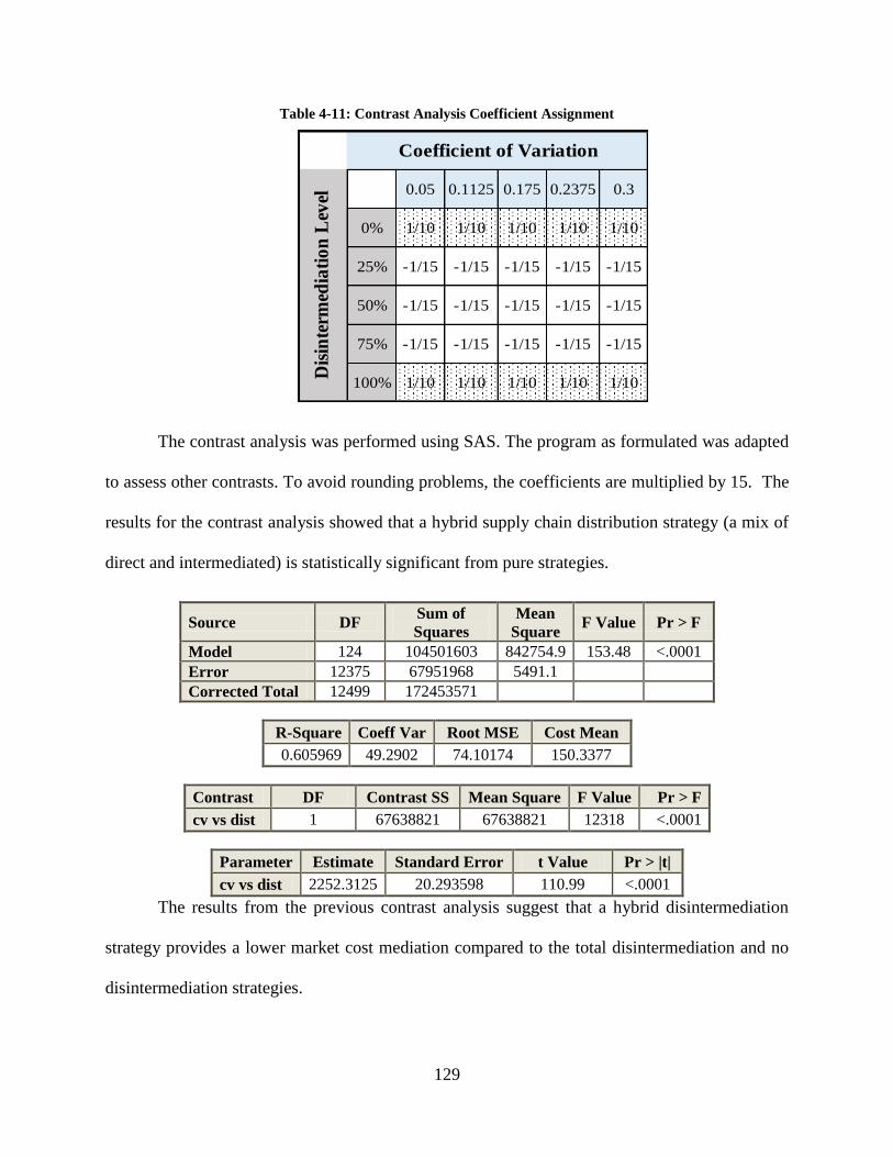
129

Table 4-11: Contrast Analysis Coefficient Assignment

The contrast analysis was performed using SAS. The program as formulated was adapted

to assess other contrasts. To avoid rounding problems, the coefficients are multiplied by 15. The

results for the contrast analysis showed that a hybrid supply chain distribution strategy (a mix of

direct and intermediated) is statistically significant from pure strategies.

Source DF Sum of

Squares

Mean

Square F Value Pr > F

Model 124 104501603 842754.9 153.48 <.0001

Error 12375 67951968 5491.1

Corrected Total 12499 172453571

R-Square Coeff Var Root MSE Cost Mean

0.605969 49.2902 74.10174 150.3377

Contrast DF Contrast SS Mean Square F Value Pr > F

cv vs dist 1 67638821 67638821 12318 <.0001

Parameter Estimate Standard Error t Value Pr > |t|

cv vs dist 2252.3125 20.293598 110.99 <.0001

The results from the previous contrast analysis suggest that a hybrid disintermediation

strategy provides a lower market cost mediation compared to the total disintermediation and no

disintermediation strategies.

0.05 0.1125 0.175 0.2375 0.3

0% 1/10 1/10 1/10 1/10 1/10

25% -1/15 -1/15 -1/15 -1/15 -1/15

50% -1/15 -1/15 -1/15 -1/15 -1/15

75% -1/15 -1/15 -1/15 -1/15 -1/15

100% 1/10 1/10 1/10 1/10 1/10

Coefficient of Variation

Dis

inte

rmed

iati

on

Lev

el

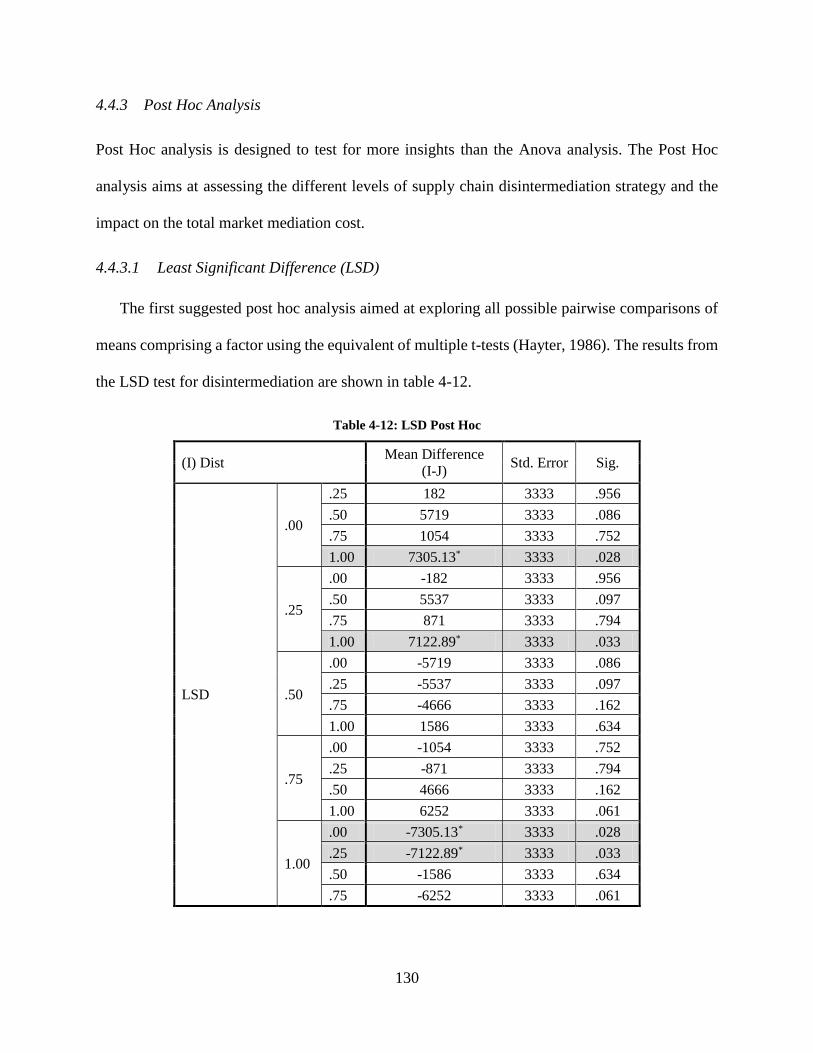
130

4.4.3 Post Hoc Analysis

Post Hoc analysis is designed to test for more insights than the Anova analysis. The Post Hoc

analysis aims at assessing the different levels of supply chain disintermediation strategy and the

impact on the total market mediation cost.

4.4.3.1 Least Significant Difference (LSD)

The first suggested post hoc analysis aimed at exploring all possible pairwise comparisons of

means comprising a factor using the equivalent of multiple t-tests (Hayter, 1986). The results from

the LSD test for disintermediation are shown in table 4-12.

Table 4-12: LSD Post Hoc

(I) Dist Mean Difference

(I-J) Std. Error Sig.

LSD

.00

.25 182 3333 .956

.50 5719 3333 .086

.75 1054 3333 .752

1.00 7305.13* 3333 .028

.25

.00 -182 3333 .956

.50 5537 3333 .097

.75 871 3333 .794

1.00 7122.89* 3333 .033

.50

.00 -5719 3333 .086

.25 -5537 3333 .097

.75 -4666 3333 .162

1.00 1586 3333 .634

.75

.00 -1054 3333 .752

.25 -871 3333 .794

.50 4666 3333 .162

1.00 6252 3333 .061

1.00

.00 -7305.13* 3333 .028

.25 -7122.89* 3333 .033

.50 -1586 3333 .634

.75 -6252 3333 .061

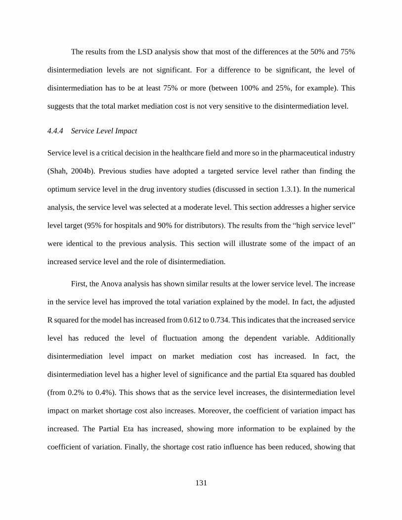
131

The results from the LSD analysis show that most of the differences at the 50% and 75%

disintermediation levels are not significant. For a difference to be significant, the level of

disintermediation has to be at least 75% or more (between 100% and 25%, for example). This

suggests that the total market mediation cost is not very sensitive to the disintermediation level.

4.4.4 Service Level Impact

Service level is a critical decision in the healthcare field and more so in the pharmaceutical industry

(Shah, 2004b). Previous studies have adopted a targeted service level rather than finding the

optimum service level in the drug inventory studies (discussed in section 1.3.1). In the numerical

analysis, the service level was selected at a moderate level. This section addresses a higher service

level target (95% for hospitals and 90% for distributors). The results from the “high service level”

were identical to the previous analysis. This section will illustrate some of the impact of an

increased service level and the role of disintermediation.

First, the Anova analysis has shown similar results at the lower service level. The increase

in the service level has improved the total variation explained by the model. In fact, the adjusted

R squared for the model has increased from 0.612 to 0.734. This indicates that the increased service

level has reduced the level of fluctuation among the dependent variable. Additionally

disintermediation level impact on market mediation cost has increased. In fact, the

disintermediation level has a higher level of significance and the partial Eta squared has doubled

(from 0.2% to 0.4%). This shows that as the service level increases, the disintermediation level

impact on market shortage cost also increases. Moreover, the coefficient of variation impact has

increased. The Partial Eta has increased, showing more information to be explained by the

coefficient of variation. Finally, the shortage cost ratio influence has been reduced, showing that

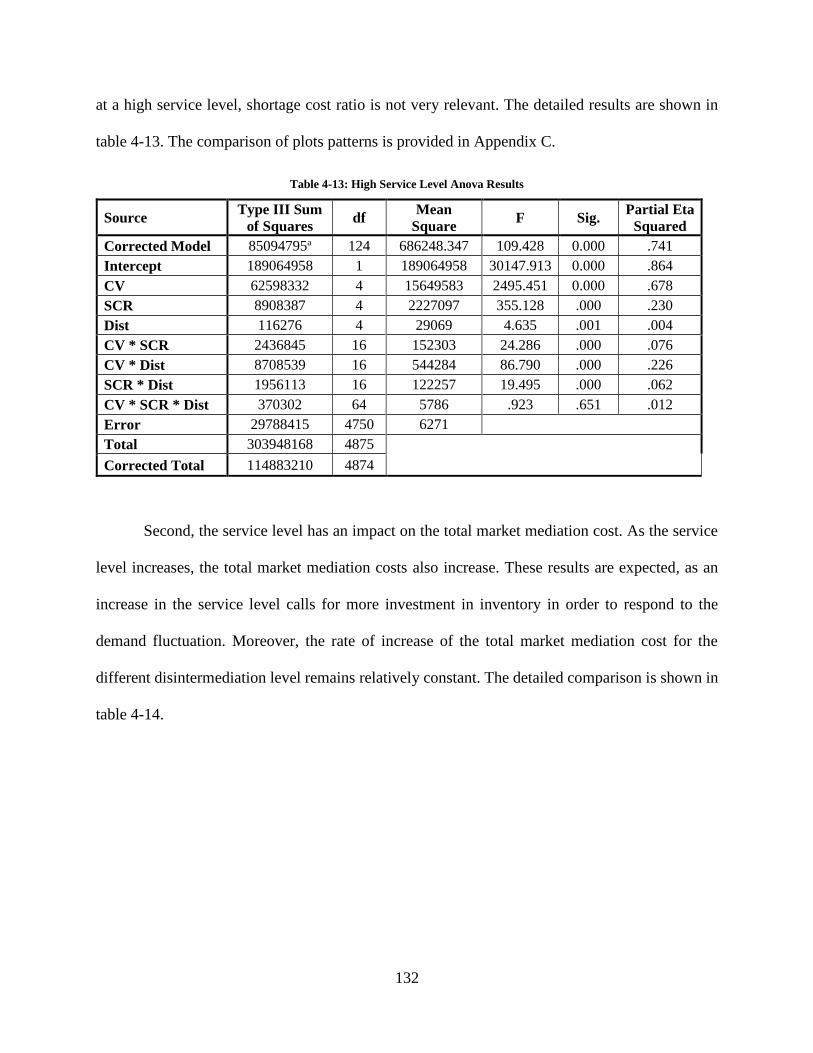
132

at a high service level, shortage cost ratio is not very relevant. The detailed results are shown in

table 4-13. The comparison of plots patterns is provided in Appendix C.

Table 4-13: High Service Level Anova Results

Source Type III Sum

of Squares df

Mean

Square F Sig.

Partial Eta

Squared

Corrected Model 85094795a 124 686248.347 109.428 0.000 .741

Intercept 189064958 1 189064958 30147.913 0.000 .864

CV 62598332 4 15649583 2495.451 0.000 .678

SCR 8908387 4 2227097 355.128 .000 .230

Dist 116276 4 29069 4.635 .001 .004

CV * SCR 2436845 16 152303 24.286 .000 .076

CV * Dist 8708539 16 544284 86.790 .000 .226

SCR * Dist 1956113 16 122257 19.495 .000 .062

CV * SCR * Dist 370302 64 5786 .923 .651 .012

Error 29788415 4750 6271

Total 303948168 4875

Corrected Total 114883210 4874

Second, the service level has an impact on the total market mediation cost. As the service

level increases, the total market mediation costs also increase. These results are expected, as an

increase in the service level calls for more investment in inventory in order to respond to the

demand fluctuation. Moreover, the rate of increase of the total market mediation cost for the

different disintermediation level remains relatively constant. The detailed comparison is shown in

table 4-14.

133

Table 4-14: Service Level and Disintermediation Impact on Total Market Mediation Cost

Dist Level Service

Level Mean

Cost

Increase

Increase

Percentage

0% Low 155.405

47.92 30.83% High 203.322

25% Low 152.401

48.04 31.52% High 200.440

50% Low 149.593

47.93 32.04% High 197.519

75% Low 148.863

46.69 31.36% High 195.548

100% Low 145.426

45.60 31.35% High 191.022

Third, a higher service level will provide a shift in the disintermediation strategy

indifference area. As discussed in sections 4.3.4 and 4.2.4, the disintermediation strategy has

shown an indifferent region where there is no best disintermediation strategy. At a higher service

level, the disintermediation indifference area will experience a shift, favoring more of an impact

of disintermediation and coefficient of variation. In fact, at a high service level, there is only a

small indifference area when both coefficients of variation are at a moderate level (.175). At the

extreme points, pure distribution channel strategy (disintermediated or intermediated) will provide

a lower market mediation cost. The results are obtained using a contrast analysis at a high service

level (Table 4-15).

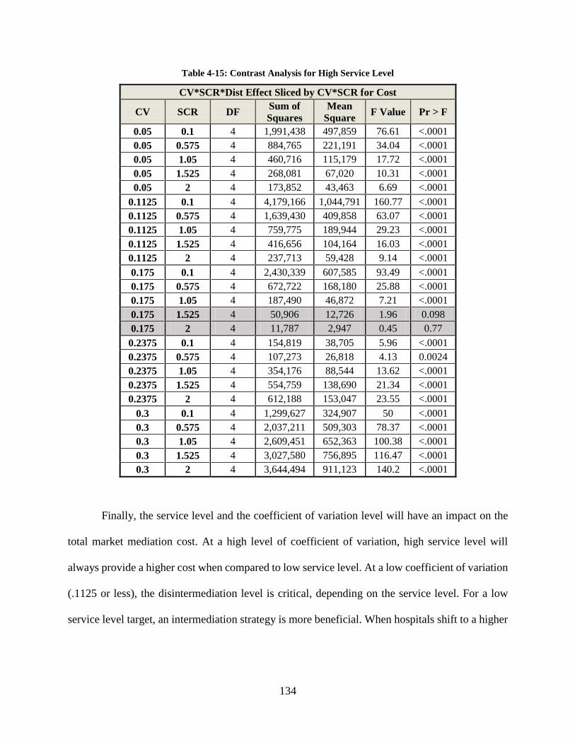
134

Table 4-15: Contrast Analysis for High Service Level

CV*SCR*Dist Effect Sliced by CV*SCR for Cost

CV SCR DF Sum of

Squares

Mean

Square F Value Pr > F

0.05 0.1 4 1,991,438 497,859 76.61 <.0001

0.05 0.575 4 884,765 221,191 34.04 <.0001

0.05 1.05 4 460,716 115,179 17.72 <.0001

0.05 1.525 4 268,081 67,020 10.31 <.0001

0.05 2 4 173,852 43,463 6.69 <.0001

0.1125 0.1 4 4,179,166 1,044,791 160.77 <.0001

0.1125 0.575 4 1,639,430 409,858 63.07 <.0001

0.1125 1.05 4 759,775 189,944 29.23 <.0001

0.1125 1.525 4 416,656 104,164 16.03 <.0001

0.1125 2 4 237,713 59,428 9.14 <.0001

0.175 0.1 4 2,430,339 607,585 93.49 <.0001

0.175 0.575 4 672,722 168,180 25.88 <.0001

0.175 1.05 4 187,490 46,872 7.21 <.0001

0.175 1.525 4 50,906 12,726 1.96 0.098

0.175 2 4 11,787 2,947 0.45 0.77

0.2375 0.1 4 154,819 38,705 5.96 <.0001

0.2375 0.575 4 107,273 26,818 4.13 0.0024

0.2375 1.05 4 354,176 88,544 13.62 <.0001

0.2375 1.525 4 554,759 138,690 21.34 <.0001

0.2375 2 4 612,188 153,047 23.55 <.0001

0.3 0.1 4 1,299,627 324,907 50 <.0001

0.3 0.575 4 2,037,211 509,303 78.37 <.0001

0.3 1.05 4 2,609,451 652,363 100.38 <.0001

0.3 1.525 4 3,027,580 756,895 116.47 <.0001

0.3 2 4 3,644,494 911,123 140.2 <.0001

Finally, the service level and the coefficient of variation level will have an impact on the

total market mediation cost. At a high level of coefficient of variation, high service level will

always provide a higher cost when compared to low service level. At a low coefficient of variation

(.1125 or less), the disintermediation level is critical, depending on the service level. For a low

service level target, an intermediation strategy is more beneficial. When hospitals shift to a higher

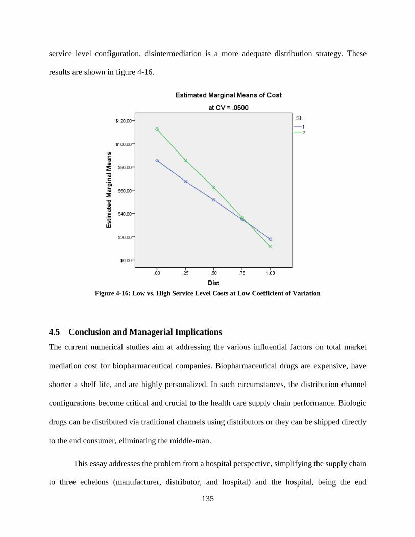
135

service level configuration, disintermediation is a more adequate distribution strategy. These

results are shown in figure 4-16.

Figure 4-16: Low vs. High Service Level Costs at Low Coefficient of Variation

4.5 Conclusion and Managerial Implications

The current numerical studies aim at addressing the various influential factors on total market

mediation cost for biopharmaceutical companies. Biopharmaceutical drugs are expensive, have

shorter a shelf life, and are highly personalized. In such circumstances, the distribution channel

configurations become critical and crucial to the health care supply chain performance. Biologic

drugs can be distributed via traditional channels using distributors or they can be shipped directly

to the end consumer, eliminating the middle-man.

This essay addresses the problem from a hospital perspective, simplifying the supply chain

to three echelons (manufacturer, distributor, and hospital) and the hospital, being the end

136

consumer, and the decision maker. First, the essay provided a scenario approach analysis to assess

the impact of disintermediation level, coefficient of variation, and shortage cost ratio on the total

market mediation cost. While direct sales provide longer product usage time, which reduce the

perishability cost, an intermediated strategy will use the middle-man as a buffer, thereby utilizing

the risk pooling effect to reduce the shortage cost.

The numerical analysis performed aimed at comparing the different factors shaping the

total market mediation cost. First, a three-way Anova showed that coefficient of variation is the

most impacting factor in determining the total market mediation cost. The second order factor

analysis has also shown the importance of coefficient of variation as the strongest factor to define

the total market mediation cost. The results were validated via a size effect analysis. Moreover,

the findings have shown that, overall, disintermediation will reduce the total market mediation

cost. Disintermediation has a stronger effect on cost when the coefficient of variation is low. In

fact, when the product has a predicted demand, the direct sales model is the most adequate. At a

high coefficient of variation, however, intermediated distribution strategy is more appropriate.

These results support the assumptions that have been developed regarding the various distribution

strategies.

Second, a contrast analysis provided a significant statistical analysis for the area of supply

chain distribution indifference region. In fact, for the various levels of the three factors used in the

study (coefficient of variation, shortage cost ration, and disintermediation level combinations), the

contrast analysis tested for the market mediation cost differences. The contrast analysis determined

the distribution strategy frontier area. At low coefficient of variation, direct sales provides the

lowest market mediation cost. As coefficient of variation and shortage cost increase, the

137

distribution channels strategy will change. At middle coefficient of variation range, the results

showed a distribution strategy indifference area.

Third, the post hoc analysis addressed the impact of supply chain disintermediation, as the

main subject of interest, on the total market mediation cost. The post hoc analysis also showed that

the hybrid supply chain distribution strategy (a mix of direct and intermediated sales) does not

provide statistically significant different results compared to (pure strategy) in most cases. The

results, however, showed that there is a statistical significance when hospitals adopt one of the

pure distribution strategies (disintermediated or intermediated). Therefore, based on the product

characteristics, the total market mediation cost can be reduced by modifying the distribution

strategy.

Finally, the service level at a hospital represents an interesting area of research, given the

critical factors associated with healthcare industry. The problem addressed in this essay could be

assimilated to a news vendor problem, with finding the optimal service level given the combination

of excess (perishability) cost and shortage cost. However, hospitals do not operate this way. In

fact, hospitals target service level first, and then they determine the most appropriate distribution

strategy. The last section of the essay investigated the impact of service level on the

disintermediation strategy. Taking two service level points (moderate and low), the results have

shown that as the service level increases, the impact of disintermediation becomes more important.

Moreover, at a high service level, a higher disintermediation strategy will provide a better market

mediation cost performance.

138

5 Chapter 5: Supply Chain Disintermediation and Product Portfolio

Strategies: An Empirical Study

5.1 Introduction and Research Objectives

The role of the supply chain strategy is very crucial to a firm’s operational and financial

performance. Skinner (1969) has emphasized the role of the organization’s manufacturing strategy

and its positive impact on organization outcomes. The operations and supply chain strategy has

evolved from research on competitive priorities in operations management, configurations of

operations and manufacturing strategy, supply chain configuration, and the successful alignment

between supply chain strategy and organization output characteristics (Boyer, Bozarth, and

McDermott, 2000; Ward, Bickford, and Leong, 1996). The seminal work by Fisher (1997)

provided a research agenda focused on the fit between product characteristics and supply chain

strategy. An organization should consider its product characteristics such as demand patterns and

identify the best supply chain strategy that fits the most (Fisher, 1997). Recent studies have

attempted to empirically investigate the Fisher’s (1997) model by testing the fit existing between

product type and supply chain strategy (Lee, 2002; Lo and Power, 2010; Selldin and Olhager,

2007; Wagner, Grosse-Ruyken, and Erhun, 2012). While some studies have used a simplified

taxonomy to determine the type of supply chain (efficient vs. responsive), other studies have built

on the existing literature to provide a more comprehensive supply chain strategy taxonomy

(Frohlich and Dixon, 2001; Zhao et al., 2006). These studies have primary investigated the fit

between the supply chain strategy and the products’ demand characteristics.

Product typology and specification represents an area of research that has been the subject

of several studies in the area of management and marketing (Day, 1977; MacMillan, Hambrick,

139

and Day, 1982; Wind and Mahajan, 1981). The topics have been then introduced to the operations

management literature in terms of investigating product characteristics such as variety, modularity,

type of demand, uncertainty, and complexity (Fisher, 1997; Jacobs and Swink, 2011; Rothaermel,

Hitt, and Jobe, 2006; Zamirowski and Otto, 1999). The previous chapters discussed product

paradigm in the context of product customization-personalization continuum. The first essay

expanded on the product paradigm to define a product portfolio structure based on the level of

personalization. The emergence of biologics (large molecule medication) calls for a higher level

of personalization. The product portfolio structure with regard to personalization remains an area

of investigation that has not received much research attention. The personalization level paradigm

elaborated on was extrapolated to the field of the pharmaceutical industry. The current study

investigates the product portfolio structure based on the personalization level of medication that

exists within the pharmaceutical firms’ products. As such, the current study adds to the literature

by providing a better understanding of under researched area of product personalization in the

operations management.

With regard to supply chain strategy, existing literature has identified a multitude of

typologies. The first set of typologies relates to the type of supply chain as developed by Fisher

(1997) and other studies. An organization’s supply chain can be responsive, efficient, agile, risk

hedging, or leagile (Mason-Jones, Naylor, and Towill, 2000). Another set of taxonomy addresses

the supply chain focus: supply chain integration; Just-In-Time; and supply chain relationship

(Narasimhan, Kim, and Tan, 2008). The supply chain focus taxonomy evolved into a competitive

advantage (Mckone‐Sweet and Lee, 2009). The body of literature has shown vast studies related

to supply chain strategies at the macro level. More emphasis was provided to supply chain

distribution channels, as it falls under the strategic supply chain configuration. Organizations have

140

multiple distribution channel opportunities that can impact the firm’s operational and financial

performance (Stock, Greis, and Kasarda, 2000). The research on distribution channels

configuration has evolved from the marketing to operations management to involve concepts

related to supply chain. The traditional distribution channel configuration suggests that the product

is sold to the customer through retailers. The retail store will purchase the product from the

wholesalers or distributors. The business landscape suggests more direct sales opportunities

aiming at eliminating the middleman. This practice is also known as supply chain

disintermediation.

The previous chapter provided a conceptualization of the supply chain disintermediation as

a distribution strategy that organizations will decide to adopt. The level of disintermediation is

determined by the extent to which an organization will sell its products directly to the end

consumers. The research on supply chain disintermediation is lacking extensive empirical

investigation and strategy effectiveness validation (Rossetti and Choi, 2008). Few studies have

addressed supply chain disintermediation as a distribution channel strategic decision, attempting

to assess its outputs (Rossetti and Choi, 2008; Tay and Chelliah, 2011). This represents a clear

area of opportunity for investigation to better understand the mechanisms of disintermediation and

how it relates to a firm’s performance. The previous studies from the area of marketing and sales

have shown some conflicting results to the benefit of disintermediation and its impact of firm value

proposition and competitiveness. While many studies have looked into the customer benefit and

cost reduction deriving from the double margin (Davenport and Klahr, 1998; Nissen, 2000), other

studies have pointed out the complexity of disintermediation and how it can limit the firm’s

potential sales and growth (Atkinson, 2001). These conflicting signals represent another area of

investigation and emphasize the relevance of the topic.

141

Additionally, it is critical to note that product customization/personalization has significant

implication for distribution channels configuration (direct or indirect). Often, customer inputs are

needed for the firm to deliver personalized products to customers, like in purchasing a holiday

package (Nicolau, 2013). In these cases, it is more appropriate for the firm to sell its products

directly to the consumers. For products with low personalization level, firms could sell the product

directly to its customers or distribute it via regular distribution channels. However, the low level

of personalization obviates the need for direct distribution channels. The existence on most

adequate disintermediation strategy for a certain level of product personalization raises the critical

question of fit between product characteristics (personalization level) and supply chain strategy

(disintermediation level). This represents an area that needs further investigation.

The current chapter aims to add to the above literature gap addressing the stated research

objective. First, it investigates the impact of distribution channels on a firm’s financial

performance. In fact, the chapter empirically tests for the relationship between the level of

disintermediation and the pharmaceutical firms’ financial performance. Second, the study

addresses the relationship between the product portfolio (in term of level of biologic products) and

pharmaceutical’s financial results. More precisely, since biologic products are more personalized,

it serves as a proxy to test the influence of the level of personalization in products at a

pharmaceutical organization and the firm’s financial performance. Finally, the chapter proposes

that there exist a fit between the product portfolio and supply chain disintermediation strategy and

investigates its relationship with financial performance. In doing so, this section provides a novel

application and empirical test of the Fisher’s (1997) model from two new paradigms inspired by

product characteristics (personalization level) and supply chain configuration (disintermediation

level).

142

The current chapter is organized as following. First, a literature review provides the relevant

work to the area of disintermediation, product portfolio, and financial performance. Second, a

conceptual development provides the hypotheses for the empirical model. Finally, the research

methodology section proposes how the study is conducted.

5.2 Literature review

Chapter 4 had discussed the literature related to supply chain disintermediation and showed

some of the research gaps. In this current chapter, a literature review specifically oriented toward

empirical work in supply chain disintermediation is provided.

5.2.1 Supply Chain Disintermediation in the Literature

The supply chain disintermediation involves the interaction between a buyer and supplier

and therefore can be viewed as a contracting problem. The decision of whether to disintermediate

or not can be analogous to a make-or-buy decision. In a make-or-buy configuration, the focal

company will make the decision based on the minimum transaction cost (Eisenhardt, 1989). The

concept of agency theory can be applied in the context of supply chain intermediation, where the

decision is based on evaluating a cost benefit analysis of a disintermediation decision. Table 5-1

summarizes the most relevant studies that address the benefit of disintermediation.

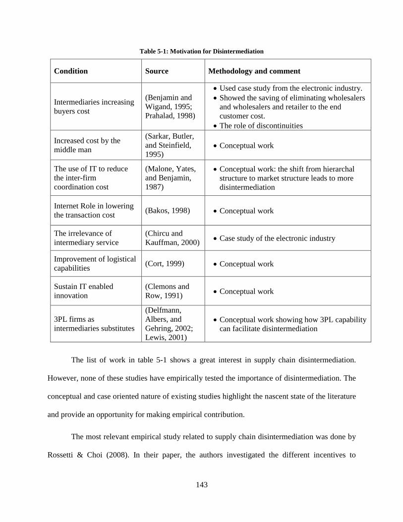
143

Table 5-1: Motivation for Disintermediation

Condition Source Methodology and comment

Intermediaries increasing

buyers cost

(Benjamin and

Wigand, 1995;

Prahalad, 1998)

Used case study from the electronic industry.

Showed the saving of eliminating wholesalers

and wholesalers and retailer to the end

customer cost.

The role of discontinuities

Increased cost by the

middle man

(Sarkar, Butler,

and Steinfield,

1995) Conceptual work

The use of IT to reduce

the inter-firm

coordination cost

(Malone, Yates,

and Benjamin,

1987)

Conceptual work: the shift from hierarchal

structure to market structure leads to more

disintermediation

Internet Role in lowering

the transaction cost (Bakos, 1998) Conceptual work

The irrelevance of

intermediary service

(Chircu and

Kauffman, 2000) Case study of the electronic industry

Improvement of logistical

capabilities (Cort, 1999) Conceptual work

Sustain IT enabled

innovation

(Clemons and

Row, 1991) Conceptual work

3PL firms as

intermediaries substitutes

(Delfmann,

Albers, and

Gehring, 2002;

Lewis, 2001)

Conceptual work showing how 3PL capability

can facilitate disintermediation

The list of work in table 5-1 shows a great interest in supply chain disintermediation.

However, none of these studies have empirically tested the importance of disintermediation. The

conceptual and case oriented nature of existing studies highlight the nascent state of the literature

and provide an opportunity for making empirical contribution.

The most relevant empirical study related to supply chain disintermediation was done by

Rossetti & Choi (2008). In their paper, the authors investigated the different incentives to

144

disintermediate in the aerospace context. The study used disintermediation as an outcome to buyer

supplier congruence and the impact of secondary market. The study was inspiring and shed light

on some supply chain disintermediation concepts. The authors have called for future research

assessing how disintermediation could impact a firm’s configuration. Two other major works

scientifically addressed the concept of supply chain disintermediation. Dutta et al. (2010)

mathematically tested the impact of supply chain disintermediation on market equilibrium in the

Indian tea market. The findings showed that complete disintermediation will shift the market

equilibrium (Dutta, Sarmah, and Goyal, 2010). The second paper, analytical as well, assessed the

price sensitivity & demand consideration and its impact on disintermediation and centralization

configurations (Chiang, 2012).

The literature review of supply chain disintermediation demonstrates a continuing interest

in investigating the supply chain configuration. The body of literature also shows a gap in evidence

suggesting that supply chain disintermediation does impact an organization’s financial

performance. Most of the existing studies are conceptual in nature. The few studies that have

empirically and analytically addressed supply chain disintermediation focused on

disintermediation as an outcome and the result of buyer supplier congruence or market demand.

Supply chain disintermediation can be considered as a strategic decision that will impact the

distribution channels and the firm’s operating and financial performance. In the context of the

pharmaceutical industry, the current study defines supply chain disintermediation as the extent to

which a pharmaceutical firm is selling its products directly to the patients, retail pharmacies, and

hospitals without distributing the products through wholesalers and distributors hereby identified

as middlemen.

145

5.2.2 Product Portfolio

Product portfolio refers to the set of products a company sells to its customers (McGrath, 2000;

Meyer, 1997). In more competitive markets, many firms are obliged to diversify their product

portfolio and provide a variety of products to maintain their competitive advantage (Fixson, 2005).

The research of product portfolio management has emerged in the field of marketing, finance, and

strategic management field. A firm’s goal consists of optimizing its product portfolio to maximize

the organization’s value (Cooper, Edgett, and Kleinschmidt, 1999; Fernhaber and Patel, 2012).

Studies suggest that the diversification level in the product portfolio requires an organization’s

higher capabilities to leverage the diversification and generate more value to customers and

businesses (Eggers, 2012). Earlier studies in the area of marketing have identified product portfolio

classification and diagnosis. The classification focused on determining the product portfolio that

aims to serve different markets and how it should be designed and managed effectively (Wind and

Mahajan, 1981; Wind, Mahajan, and Swire, 1983). Organizations should use their resources

effectively to design the best value added portfolio (Day, 1977).

Scholars from operations and supply chain management showed interest in the product

portfolio strategy. Fisher (1997) has classified products into functional and innovative. Fisher’s

work did not provide insights about how to manage the product portfolio; it did, however, define

a product’s taxonomy, which can be used to identify portfolio characteristics. More recent studies

have addressed product portfolio management from a complexity angle. Scholars have measured

the product portfolio complexity and assessed its impact on a firm’s performance (Closs et al.,

2008). As the complexity increases, organizations will require more resources to manage these

complexities (Jacobs and Swink, 2011). Product portfolio was also assessed from a configuration

point of view. Researchers studied the impact of product portfolio configuration in terms of

146

functionalities and design on firm performance. The finding showed that product portfolio

functionality optimization is driven mainly by gross margin and pricing strategy (Chen, Vakharia,

and Alptekinoǧlu, 2008).

The research in the field of product portfolio has shown a great emphasis on product

portfolio design, optimization, and management. Very little interest was awarded to product

portfolio classification despite some earlier studies which identified different product classification

such as Fisher (1997). Product portfolio can be classified according to different taxonomies such

as the product characteristics. The lack of studies focusing on the product portfolio characteristics

and its impact on organization performance represents an opportunity of investigation. As

discussed in chapter 2, the current chapter is conceptualizing product portfolio from a

personalization level perspective. In the context of the pharmaceutical industry, one may map the

level of personalization to the type of medication. In general, biologic medicine tends to require

higher level of personalization (Ginsburg and Willard, 2009) compared to traditional medication.

In line with this, keeping in mind the pharmaceutical context, a portfolio with only biologic

products would have a higher personalization level. A portfolio with only traditional medication

would have a low personalization level. In the pharmaceutical context, the current study defines

product portfolio based on the biologic products that exist within the pharmaceutical firm products

portfolio. As such, portfolios that are composed of only biologic products are considered to have

high level of personalization while those that are composed of only traditional medication are

considered as having a low level of personalization, with ones containing both as hybrid portfolios

having a moderate level of personalization.

147

5.2.3 Financial Performance

The research on financial performance in the operations management field in interesting a large

number of researchers (Chen, Frank, and Wu, 2005). Several studies have used multiple financial

performance measures in the operations management context. Return on Assets represents a

commonly used performance measure to evaluate the firm’s productivity and assets utilizations.

Liu et al. (2014) investigated the impact of innovative products on the firm’s return assets. As a

firm adopts a strategy favoring more innovation, the firm’s return on assets is expected to improve

(Liu et al., 2014). Moreover, firms are expected to have higher return on assets when engaged in

higher quality products (Terjesen, Patel, and Covin, 2011). Other studies looked at the fit existing

between the product characteristics and the return on assets. Organizations that align the adequate

supply chain strategy to the product characteristics showed better financial performance or, more

precisely, return on assets (Wagner et al., 2012).

Gross margin represents another financial measure that is used in the operations

management literature (Gaur, Fisher, and Raman, 2005). The gross margin reflects the firm ability

to provide products at competitive price. Gross margin reflects both the firm’s inbound and

operations processes and its capability to deliver products and services effectively. Firms who

adopt IT-based supply chain strategy are experiencing higher gross margin (Dehning, Richardson,

and Zmud, 2007). Gross margins are influenced by product characteristics and are different at

manufacturers, distributors, and retailers levels (Steiner, 2001). In line with the operations

management literature investigating the financial performance implications of operations

resources and decision the current study refers to the firm’s financial performance as reflected in

the measures of return on assets (the ratio of the firms’ income before extraordinary items to the

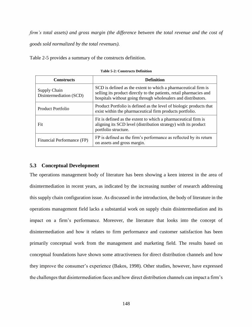
148

firm’s total assets) and gross margin (the difference between the total revenue and the cost of

goods sold normalized by the total revenues).

Table 2-5 provides a summary of the constructs definition.

Table 5-2: Constructs Definition

Constructs Definition

Supply Chain

Disintermediation (SCD)

SCD is defined as the extent to which a pharmaceutical firm is

selling its product directly to the patients, retail pharmacies and

hospitals without going through wholesalers and distributors.

Product Portfolio Product Portfolio is defined as the level of biologic products that

exist within the pharmaceutical firm products portfolio.

Fit

Fit is defined as the extent to which a pharmaceutical firm is

aligning its SCD level (distribution strategy) with its product

portfolio structure.

Financial Performance (FP) FP is defined as the firm’s performance as reflected by its return

on assets and gross margin.

5.3 Conceptual Development

The operations management body of literature has been showing a keen interest in the area of

disintermediation in recent years, as indicated by the increasing number of research addressing

this supply chain configuration issue. As discussed in the introduction, the body of literature in the

operations management field lacks a substantial work on supply chain disintermediation and its

impact on a firm’s performance. Moreover, the literature that looks into the concept of

disintermediation and how it relates to firm performance and customer satisfaction has been

primarily conceptual work from the management and marketing field. The results based on

conceptual foundations have shown some attractiveness for direct distribution channels and how

they improve the consumer’s experience (Bakos, 1998). Other studies, however, have expressed

the challenges that disintermediation faces and how direct distribution channels can impact a firm’s

149

performance (Brabazon, Winter, and Gandy, 2014). The following subsection addresses the

conceptual development.

5.3.1 Supply Chain Disintermediation and Financial Performance

The operations management and financial performance interface is gaining attention from

academic researchers (Chen et al., 2005; Hendricks and Singhal, 2003). Supply chain

disintermediation represents a strategic distribution channel decision that can impact the firm’s

financial performance. Pharmaceutical manufacturers have the option of selecting a supply chain

disintermediation strategy by selling directly to the hospitals, the retail pharmacies, and individual

patients. This can influence their financial performance positively for the following reasons.

First, when engaging in direct sales, an organization will have the opportunity to reach a

broader customer base. The broad market access will help the pharmaceutical firm generate more

revenue. In fact, a high disintermediation level will stimulate closer relationships with customers,

which will lead to repeated purchasing and, therefore, higher level revenue (Raymond and Tanner

Jr, 1994). Moreover, Reichheld and Schefter (2000) discussed the role of loyalty as the “secret

weapon” of the web and direct sales strategy. Direct sales will ensure a higher level of loyalty,

leading to more sales (Reichheld and Schefter, 2000). From a practical standpoint, the results

achieved by Dell Inc. in the late 1980s, when it adopted its direct sales strategy, was reflected in

Dell’s revenue and efficiency (Kraemer, Dedrick, and Yamashiro, 2000). In fact, Dell

Corporation’s return in 1998 was 26%, more than three times that of Apple Inc. and IBM Corp.’s

performances.

Second, the traditional supply chain configuration (intermediated) suffers from the

problem of double marginalization, where the profit margin will be split between the manufacturer

and the distributor (Jeuland and Shugan, 1983). The double marginalization phenomenon suggests

150

that successive parties along a distribution channel price a product to maximize individual profits

(Spengler, 1950). When double marginalization occurs, the distributor and retailer order

propositions independent of each other, focusing only on maximizing their own company’s profits

(Chopra and Meindl, 2007). Double marginalization favors individualism and opportunistic

behavior in the supply chain. Opportunism and individual consideration will have a negative

impact on a firm’s performance (Koppenjan and Klijn, 2004). In fact, double marginalization will

reduce the manufacturer’s profit margin and income (Heese, 2007). A supply chain

disintermediation strategy will improve the firm’s profit margin by allowing them to charge a

slightly higher cost instead of sharing the total gross margin with the intermediaries (Coughlan et

al., 2010). This will also improve the firm’s profitability and efficiency, especially the return on

assets and gross margin.

Third, disintermediated distribution channels promote a pull production system and just-

in-time supply chain (Gehani, 2000). Pull production systems are more efficient and have the

capability to provide better performance. Companies adopting pull and just-in-time are lean and,

therefore, are expected to have better performance (Koufteros, 1999). More precisely, lean

manufacturing systems enable firms to produce at lower prices, which will impact a firm’s

profitability and its cost of goods sold (Kinney and Wempe, 2002). In the context of

pharmaceuticals, pull system allows firms to meet the existing demand to the production level and

avoid any loss of sales risk and cost of goods sold by reducing potential waste and perishability

cost.

Based on the above discussion, supply chain disintermediation provides opportunities for

higher sales, capturing higher margins, and reducing cost of goods sold. Therefore, the following

hypotheses are proposed:

151

H1a: Higher level of supply chain disintermediation will be positively associated with the

firm’s return on assets, ceteris paribus.

H1b: Higher level of supply chain disintermediation will be positively associated with the

firm’s gross margin, ceteris paribus.

While the above discussion points to the positive effect of supply chain disintermediation

on a firm’s financial performance, there may also be valid arguments which indicate that supply

chain disintermediation could hurt financial performance.

First, supply chain disintermediation in the pharmaceutical context suggests that the firm

will sell its products directly to the hospital and the end-patient. When engaging in a direct sales

strategy, pharmaceutical firms lose the risk pooling effect. Risk pooling suggests that demand

variability is reduced when the demand is aggregated at the distributor level (Levi, Kaminsky, and

Levi, 2003). The risk pooling effect is a critical success factor for pharmaceutical firms to deal

with diversification and demand variability (Hill and Hansen, 1991). Engaging in direct sales

distribution channels may hurt the pharmaceutical firm as it could suffer from higher cost due to

the incapability to deal with demand variability. In fact, the demand variability will result on both

higher shortage and excess inventory costs. This will reduce the firm’s profitability. Moreover, to

cope with the product demand variation, the pharmaceutical firm will hold an excess inventory to

satisfy the demand. This will also result in a higher level of asset requirements at the firm, which

would also lower financial performance.

Second, a disintermediated channel, where the firm engages in direct sales, suggests that

an organization will serve a broader range of customers. A broader customer base typically would

require the firm to deal with a larger number of customers. Research indicates that a higher number

of elements is an indicator of more complexity (Jacobs and Swink, 2011). As such, going direct

152

exposes a firm to a more complex customer base. The large and complex customer base would

require a higher level of investment in assets by the firm to successfully meet customer demand

(Homburg, Steiner, and Totzek, 2009). Moreover, a disintermediated distribution channel implies

that the firm will manage each customer individually. Management of a large customer base

requires specific efforts in order to manage the trade-offs between scale economies and lifetime

customer value. Direct sales distribution channel is known to result in diseconomy of scale, as the

firm will need to individually manage its customer (Johnson and Selnes, 2004). Hence, the

disintermediation distribution channels will lead to a higher cost of goods sold, which will impact

the firm’s performance.

Based on the previous discussion, supply chain disintermediation requires higher

investment on assets and will lead to higher cost of goods sold, which is expected to negatively

impact the pharmaceutical firm’s performance. Therefore, the following hypotheses are proposed:

H1a’: Higher level of supply chain disintermediation will be negatively associated with

the firm’s return on assets, ceteris paribus.

H1b’: Higher level of supply chain disintermediation will be negatively associated with

the firm’s gross margin, ceteris paribus.

5.3.2 Product Portfolio and Financial Performance

Product portfolio structure represents a strategic decision that could also impact a firm’s financial

performance. Specifically, offering more personalized products would require different

investments and offer varied opportunities compared to offering less personalized (more

standardized) products. A pharmaceutical firm can provide standardized products (small molecules

drugs), personalized specialty drugs (biologics), or a combination of the two categories. As

153

discussed in chapter 2, biologic medications are characterized by a higher level of personalization.

High level of personalization within the pharmaceutical product portfolio is expected to have a

positive effect on the firm’s financial performance for the following reasons.

First, personalized medication represents a high value added medication that aims at

serving unique patients’ needs. Firms will charge premium prices for highly customized products

(Dewan, Jing, and Seidmann, 2000). Customers are willing to pay premium prices for personalized

products and services (Moon, Chadee, and Tikoo, 2008). Moreover, personalized products call for

value based pricing and, therefore, higher prices (Riemer and Totz, 2003). In fact, the value based

pricing argument suggests that customers are willing to pay premium prices for products perceived

as high value (Varian and Farrell, 2004).

Second, biologic drugs are innovative products targeting a specific patient’s health

problems (Roughead, Lopert, and Sansom, 2007). In general, innovative products are more

expensive and their specialized nature enables firms to charge premium prices for such products

(Fisher, 1997). More specifically in the context of the pharmaceutical industry, biologics represent

personalized and innovative products that are high value and more expensive products (Stein,

Pearce, and Feldman, 2005).

In summary, a product portfolio with a focus on biologics (personalized) are expected to

generate more revenue and higher income since such products represent higher value to the

customer and are more innovative. Higher revenues and income suggest higher return on asset

utilization and gross margin. Based on the previous discussion, the following hypotheses are

proposed:

H2a: Higher level of biologic products in a pharmaceutical product portfolio will be

positively associated with firm’s return on assets, ceteris paribus.

154

H2b: Higher level of biologic products in a pharmaceutical product portfolio will be

positively associated with firm’s gross margin, ceteris paribus.

A product portfolio focused on biologic (personalized) medication represents a challenging

task which could impact the pharmaceutical firm’s financial performance. One could expect that

the product portfolio structure could have a negative impact on financial performance for the

following reasons.

First, biologic products are characterized by a higher level of complexity in both the

production process and the product structure (Declerck, 2012). Higher complexity level in the

product portfolio can lower the firm’s financial performance. In fact, as complexity increases,

organizations will experience more challenges to achieving higher operational efficiency (Ameri

and Dutta, 2005). As the operational efficiency is reduced, the pharmaceutical gross income will

diminish, which will have a negative impact on financial performance.

Second, biologic products are costly medications with high financial risks. Biologic

products are characterized by high production cost due to process complexity and time constraints

(Simpson, 2011). The variable cost per unit for a biologic medication can cost several thousands

of dollars in many cases (Simpson, 2011). Moreover, the biologics’ production requires skilled

labor. Skilled labor, in general and specifically in the medical field, tends to be more expensive

compared to unskilled labor and, therefore, may impact the firm’s labor costs (Murray and Gerhart,

1998).

Third, biologic medicines are highly personalized and, therefore, are produced in low

quantities, often single or dual units of production (Shukla and Thömmes, 2010). This hampers

firms from enjoying the corresponding cost effectiveness that can derive from mass-production.

In fact, the nature of the biological medication does not favor economies of scale. It is well known

155

that as a firm engages in an economy of scale, the total product cost per unit will decrease

(Silvestre, 1987). Therefore, it is expected that biologic medicines will suffer from a higher cost

of goods sold.

In summary, a product portfolio with a focus on biologics (personalization) is expected to

have a higher cost of goods sold, which will impact the firm’s financial performance. This will

suggest lower return on assets utilization and gross margin. Based on the previous discussion, the

following hypotheses are proposed:

H2a’: Higher level of biologic products in a pharmaceutical product portfolio will be

negatively associated with firm’s return on assets, ceteris paribus.

H2b’: Higher level of biologic products in a pharmaceutical product portfolio will be

negatively associated with firm’s gross margin, ceteris paribus.

5.3.3 Supply Chain Disintermediation and Product Portfolio Fit

A firm’s performance is influenced by the level of consistency between the strategy adopted and

the environment. This consistency, also referred to as fit or alignment, has a positive impact on

performance (Alexander and Randolph, 1985; Doty, Glick, and Huber, 1993). The study of fit has

also interested scholars from operations management literature for a long time. Manufacturing

configurations should be consistent with the firm’s strategic vision (Skinner, 1969). More recent

studies have attempted to test alignment configurations and address a firm’s performance (Burton,

Lauridsen, and Obel, 2002). Fisher’s (1997) paper addressed the idea of fit in the supply chain

management and the type of product. The study has inspired scholars to empirically test whether

an organization will achieve a better performance when it aligns its supply chain configuration

with the type of product (Wagner et al., 2012).

156

In line with the base notion proposed by Fisher (1997) that a firm’s supply chain strategy

must align/fit with its product characteristic for the firm to be competitive, this research suggests

that a high level of personalization would call for a disintermediated supply chain distribution

channel strategy. The earlier discussion in chapter 2 highlighted the details about the product

paradigm and the supply chain configuration. Briefly, pharmaceutical firms’ product portfolio

consists of biologics and non-biologics. Pharmaceutical firms can sell exclusively biologic drugs,

traditional medication, or a combination of both. Further, the drugs can be sold directly to the end

user (patient or hospitals), thereby adopting disintermediated configuration or, alternatively, the

drugs can be sold using traditional distribution channels (intermediated configuration) or a

combination of methods (hybrid configuration).

Biologic products, highly personalized medication, are most effectively distributed through

direct distribution channels as such a product portfolio with biologics is most appropriate via

disintermediated modes. In fact, the high level of personalization and higher value proposition

suggests that direct distribution channels are most suitable. Moreover, because of their shorter

shelf life, biologic pharmaceuticals will benefit from supply chain disintermediation by improving

the product’s useful life span. Finally, because of the uncertain demand in biologic medication, a

pull strategy is more appropriate to manage the demand requirements. Pull strategy is more

effective in a direct sales distribution configuration. On the other hand, traditional medications are

characterized by a high standardization level. Higher product standardization obviates the need for

direct distribution channels and suggests that traditional distribution channels are most adequate.

In fact, over the counter medication and other non-biologic products are distributed using

wholesalers. Selling non biologic products via direct distribution channels is inappropriate and

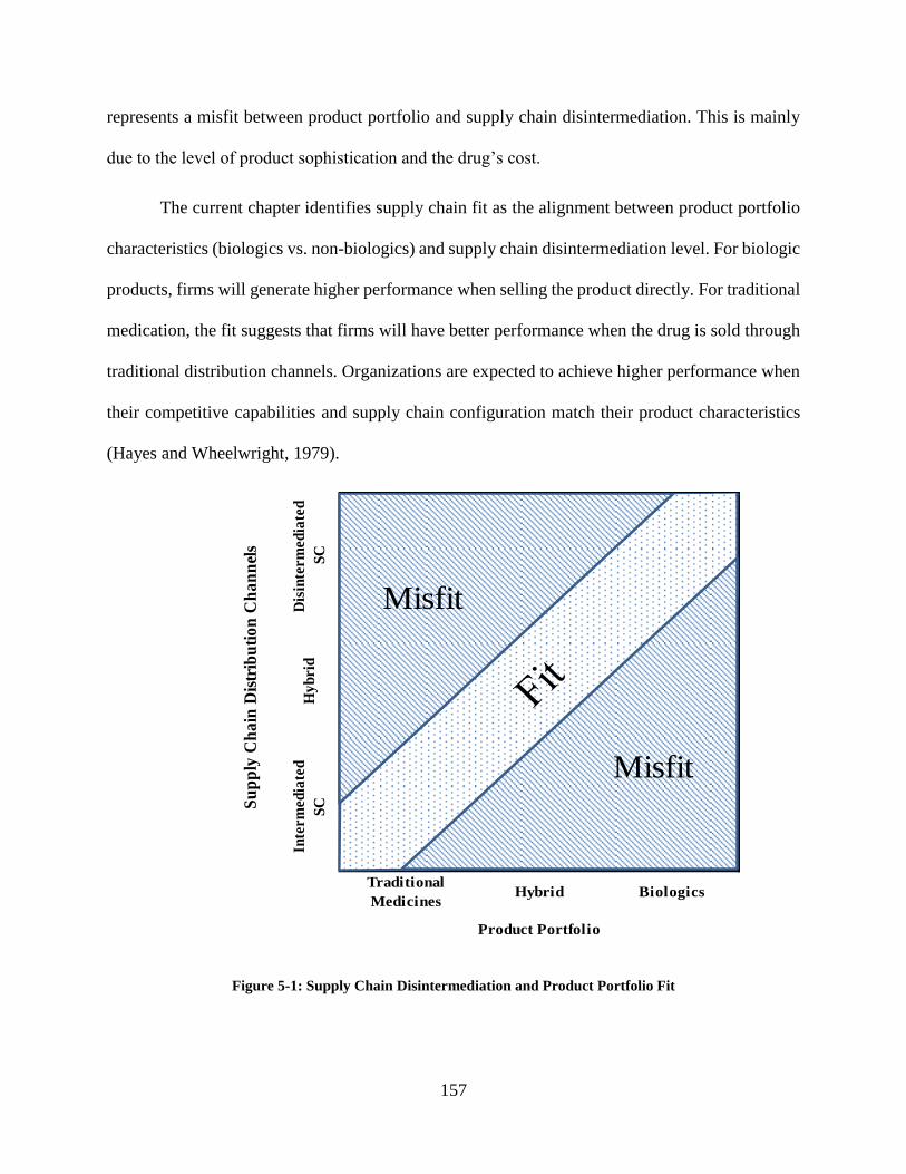
157

represents a misfit between product portfolio and supply chain disintermediation. This is mainly

due to the level of product sophistication and the drug’s cost.

The current chapter identifies supply chain fit as the alignment between product portfolio

characteristics (biologics vs. non-biologics) and supply chain disintermediation level. For biologic

products, firms will generate higher performance when selling the product directly. For traditional

medication, the fit suggests that firms will have better performance when the drug is sold through

traditional distribution channels. Organizations are expected to achieve higher performance when

their competitive capabilities and supply chain configuration match their product characteristics

(Hayes and Wheelwright, 1979).

Figure 5-1: Supply Chain Disintermediation and Product Portfolio Fit

Traditional

Medicines

Product Portfolio

BiologicsHybrid

Su

pp

ly C

ha

in D

istr

ibu

tio

n C

ha

nn

els

Dis

inte

rmed

iate

d

SC

Inte

rmed

iate

d

SC

Hy

bri

d

Misfit

Misfit

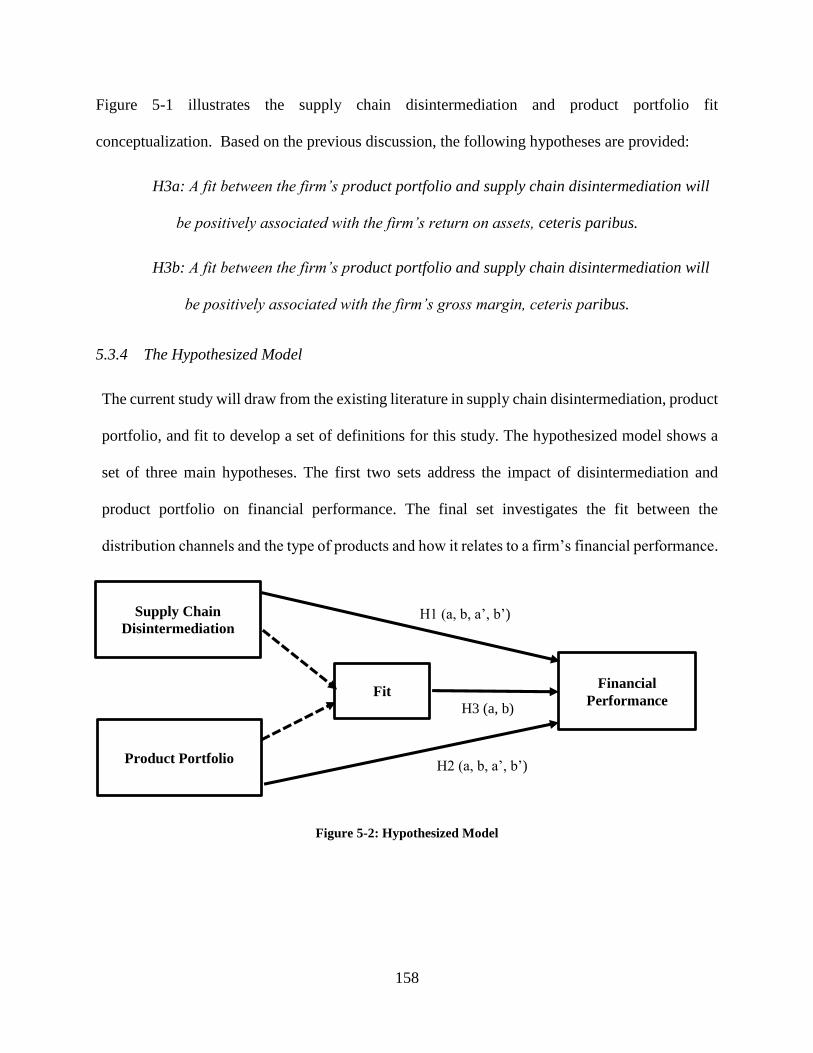
158

Figure 5-1 illustrates the supply chain disintermediation and product portfolio fit

conceptualization. Based on the previous discussion, the following hypotheses are provided:

H3a: A fit between the firm’s product portfolio and supply chain disintermediation will

be positively associated with the firm’s return on assets, ceteris paribus.

H3b: A fit between the firm’s product portfolio and supply chain disintermediation will

be positively associated with the firm’s gross margin, ceteris paribus.

5.3.4 The Hypothesized Model

The current study will draw from the existing literature in supply chain disintermediation, product

portfolio, and fit to develop a set of definitions for this study. The hypothesized model shows a

set of three main hypotheses. The first two sets address the impact of disintermediation and

product portfolio on financial performance. The final set investigates the fit between the

distribution channels and the type of products and how it relates to a firm’s financial performance.

Figure 5-2: Hypothesized Model

H1 (a, b, a’, b’)

H3 (a, b)

H2 (a, b, a’, b’)

Supply Chain

Disintermediation

Product Portfolio

Financial

Performance Fit

159

5.4 Research Methodology

The following section discusses the research methodology used in this essay. First, the dependent,

independent, and control variable operationalization is presented. Then, the empirical model is

developed to test for the hypothesis and a plan of study is discussed.

5.4.1 Variable Operationalization

This section discusses the conceptualization of the variables as well as the sources of data

collection.

5.4.1.1 Dependent Variables

The study uses two measures to assess a firm’s financial performance: Return on Assets (ROA),

and Gross Margin (GM). The paragraphs below provide more details about how to capture each

variable.

Return on Assets (ROA): ROA is an accounting-based measure that provides information

on the profitability of a firm and how its assets have been used efficiently (Fullerton, McWatters,

and Fawson, 2003; Modi and Mishra, 2011). The data to compute ROA is obtained from the

COMPUSTAT database. The ROA for company i in year t is obtained in the following manner:

𝑅𝑂𝐴𝑖𝑡 =𝐼𝐵𝐸𝐼𝑖𝑡𝑇𝐴𝑖𝑡

( 5-1)

where, IBEIit = income before extraordinary items of firm i in year t, and TAit = total assets of firm

i in year t.

Gross Margin (GM): GM is a major business and financial performance indicator and an

indicator about a firm’s performance. It is also a typical indicator of industries’ behavior and

dynamics (Farris et al., 2010). The data to measure the gross margin is obtained from

COMPUSTAT. The gross margin is calculated as follows:

160

𝐺𝑀𝑖𝑡 =𝑇𝑆𝑖𝑡 − 𝐺𝑂𝐺𝑆𝑖𝑡

𝑇𝑆𝑖𝑡 ( 5-2)

Where TSit = total sales of firm i in year t. and GOGSit = cost of goods sold of firm i in year t.

5.4.1.2 Independent Variables

The model discussed in the previous section has two independent variables: supply chain

disintermediation and product portfolio structure.

Supply Chain Disintermediation (Dis_Level): As discussed in the conceptual development

section, the supply chain disintermediation (SCD) represents the level of material flow that is

shipped directly to the end customer. In this chapter, the SCD is conceptualized by the level of

medicine that is sold directly to the patients, hospitals, and retail pharmacies. When the drug is

shipped through the regular distributors and wholesalers, the product is considered intermediated.

To determine the level of disintermediation, the Bloomberg database terminal is used. The

database provides data on many public firms’ supply chain relationships, including

pharmaceuticals and biopharmaceuticals. The data maps a company to its suppliers, customers,

and competitors and gives an indication of the strength of the relationship, marked by the

relationship transaction numbers. For each of the companies in the pharmaceutical industry, a

supply chain network is developed with a list of customers and suppliers. The Bloomberg terminal

has information about the quantified relationships where it provides the exact level of operation.

For example, the database reports that in 2013, 1.5 billion dollars of Pfizer’s sales were generated

from McKesson Corporation. Also, the database provides some estimates about non-quantified

relationships where Bloomberg analysts, basing it on mathematical modeling, have provided an

estimate of the existing relationships (Steven, Dong, and Corsi, 2014). The Bloomberg database

has the data available in “real time” and does not provide an option of historical data compilation.

161

To determine the relationship magnitudes, more data was extracted from Bloomberg and the firm’s

financial reports. The supply chain disintermediation level is assessed as a percentage of the goods

that are shipped from the manufacturer directly to a hospital or the drug stores. The Bloomberg

data base provides an estimation of the financial flows that relate the manufacturers to their clients.

Based on the estimates, the disintermediation level is estimated for each firm. The

disintermediation level in this case is a continuous variable and is computed as follows:

𝐷𝑖𝑠_𝐿𝑒𝑣𝑒𝑙 =∑ 𝑆𝑎𝑙𝑒𝑠 𝑡𝑜 𝑒𝑛𝑑 𝑐𝑢𝑠𝑡𝑜𝑚𝑒𝑟𝑠

𝑇𝑜𝑡𝑎𝑙 𝑆𝑎𝑙𝑒𝑠 ( 5-3)

The use of the Bloomberg database provides an indication about the types of relationships

and its magnitude. For each firm, a list of customers’ 6 digit NAICS and 4 digit SIC code has been

developed to identify the supply chain’s tier positioning. Based on the firm’s customer base

positioning within the supply chain and the dollar value of the physical flow, the supply chain

disintermediation code is determined. The SCD variable is coded as follows: 1, 2, and 3. Code 1

reflects a totally disintermediated distribution strategy. A code 1 for SCD is given to a firm that

sells the majority of its product through direct distribution channels. A code 3 reflects a totally

intermediated distribution channel. When the majority of the drugs is sold to distributors and

wholesalers, a level 3 SCD is assigned. In some cases, firms will have a hybrid distribution

strategy: the customers will be a mix of wholesalers & distributors (intermediated) and patients,

hospitals, & drug stores (disintermediated). In these cases, a code 2 is assigned. For example,

Pfizer’s customer list includes McKesson, Cardinal, Express Script, Walgreen, and Rite Aid,

among others. The NAICS and SIC codes for each client determine if it is an end customer or an

intermediary. McKesson’s NAICS is 424210 (Drugs and Druggists' Sundries Merchant

Wholesalers), positioning McKesson as an intermediary. Walgreen and Rite Aid’s NAICS codes

are 446110 (Pharmacies and Drug Stores), distinguishing them as end customers. The SCD code

162

for Pfizer is 2. The cutoff used to determine the disintermediation level is 80%. If a firm sells over

80% of its product via intermediated channels, it is considered an intermediated firm and is

assigned a code 3. The same methodology is used to assign code 1 for a disintermediated firm. For

all other firms, the SCD is assigned a level 2. The assumption of an 80% cutoff level for

disintermediation is relaxed, and sensitivity analysis is conducted using 90%, 85%, 75%, and 70%

cutoffs. The details are discussed in the robustness check section.

The current study uses the continuous variable to test for the impact of disintermediation

level on financial performance. The coded disintermediation level is used to determine the firm’s

distribution strategy and assess the fit.

Product Portfolio: Pharmaceutical firms sell a set of drugs and medicine which make up

its product portfolio. The discussion section above addressed the product portfolio and its impact

on the firm’s performance. To assess the product portfolio, data is collected from Bloomberg and

organization annual reports. For each period (2010, 2011, 2012, 2013), the list of products is

determined. Based on the product description, it was determined to be either a biologic or

traditional drug. Biologics are large molecule medications characterized by a higher level of

personalization. The product portfolios are coded as 1, 2, or 3. Code 1 denotes a biologic product

portfolio and code 3 represents a traditional medication portfolio. Code 2 represents a hybrid

product portfolio.

Product Portfolio and Supply Chain Fit: The fit between the product portfolio structure

and supply chain is measured by matching two variables: product portfolio and supply chain

disintermediation. High fit or alignment suggests that an organization will adopt a

disintermediation level that is consistent with its product portfolio structure. The concept of fit was

conceptualized by Venkatraman’s (1989) seminal work where he provided a list of measurement

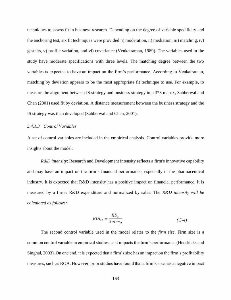
163

techniques to assess fit in business research. Depending on the degree of variable specificity and

the anchoring test, six fit techniques were provided: i) moderation, ii) mediation, iii) matching, iv)

gestalts, v) profile variation, and vi) covariance (Venkatraman, 1989). The variables used in the

study have moderate specifications with three levels. The matching degree between the two

variables is expected to have an impact on the firm’s performance. According to Venkatraman,

matching by deviation appears to be the most appropriate fit technique to use. For example, to

measure the alignment between IS strategy and business strategy in a 3*3 matrix, Sabherwal and

Chan (2001) used fit by deviation. A distance measurement between the business strategy and the

IS strategy was then developed (Sabberwal and Chan, 2001).

5.4.1.3 Control Variables

A set of control variables are included in the empirical analysis. Control variables provide more

insights about the model.

R&D intensity: Research and Development intensity reflects a firm's innovative capability

and may have an impact on the firm’s financial performance, especially in the pharmaceutical

industry. It is expected that R&D intensity has a positive impact on financial performance. It is

measured by a firm's R&D expenditure and normalized by sales. The R&D intensity will be

calculated as follows:

𝑅𝐷𝐼𝑖𝑡 =𝑅𝐷𝑖𝑡

𝑆𝑎𝑙𝑒𝑠𝑖𝑡 ( 5-4)

The second control variable used in the model relates to the firm size. Firm size is a

common control variable in empirical studies, as it impacts the firm’s performance (Hendricks and

Singhal, 2003). On one end, it is expected that a firm’s size has an impact on the firm’s profitability

measures, such as ROA. However, prior studies have found that a firm’s size has a negative impact

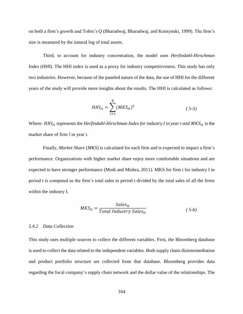
164

on both a firm’s growth and Tobin’s Q (Bharadwaj, Bharadwaj, and Konsynski, 1999). The firm’s

size is measured by the natural log of total assets.

Third, to account for industry concentration, the model uses Herfindahl-Hirschman

Index (HHI). The HHI index is used as a proxy for industry competitiveness. This study has only

two industries. However, because of the paneled nature of the data, the use of HHI for the different

years of the study will provide more insights about the results. The HHI is calculated as follows:

𝐻𝐻𝐼𝐼𝑡 = ∑(𝑀𝐾𝑆𝑙𝑡)2

𝑁

𝑖=1

( 5-5)

Where: 𝐻𝐻𝐼𝑖𝑡 represents the Herfindahl-Hirschman Index for industry I in year t and 𝑀𝐾𝑆𝑙𝑡 is the

market share of firm l in year t.

Finally, Market Share (MKS) is calculated for each firm and is expected to impact a firm’s

performance. Organizations with higher market share enjoy more comfortable situations and are

expected to have stronger performance (Modi and Mishra, 2011). MKS for firm i for industry I in

period t is computed as the firm’s total sales in period t divided by the total sales of all the firms

within the industry I.

𝑀𝐾𝑆𝑖𝑡 =𝑆𝑎𝑙𝑒𝑠𝑖𝑡

𝑇𝑜𝑡𝑎𝑙 𝐼𝑛𝑑𝑢𝑠𝑡𝑟𝑦 𝑆𝑎𝑙𝑒𝑠𝐼𝑡 ( 5-6)

5.4.2 Data Collection

This study uses multiple sources to collect the different variables. First, the Bloomberg database

is used to collect the data related to the independent variables. Both supply chain disintermediation

and product portfolio structure are collected from that database. Bloomberg provides data

regarding the focal company’s supply chain network and the dollar value of the relationships. The

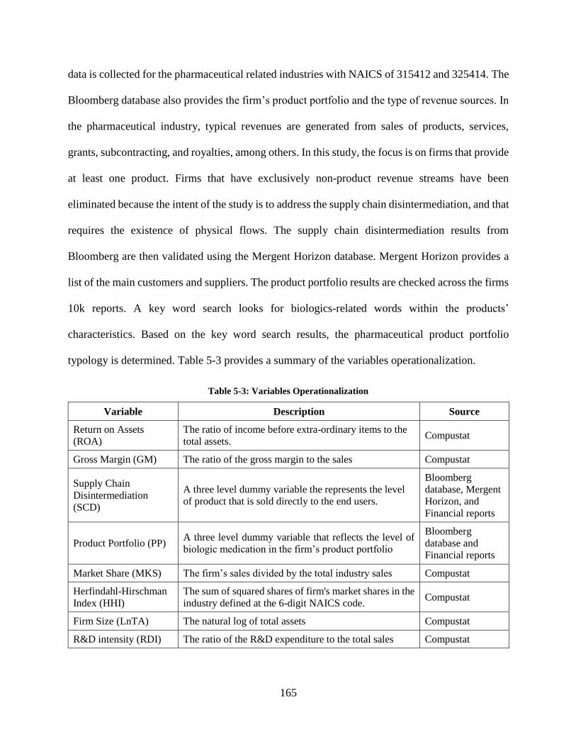
165

data is collected for the pharmaceutical related industries with NAICS of 315412 and 325414. The

Bloomberg database also provides the firm’s product portfolio and the type of revenue sources. In

the pharmaceutical industry, typical revenues are generated from sales of products, services,

grants, subcontracting, and royalties, among others. In this study, the focus is on firms that provide

at least one product. Firms that have exclusively non-product revenue streams have been

eliminated because the intent of the study is to address the supply chain disintermediation, and that

requires the existence of physical flows. The supply chain disintermediation results from

Bloomberg are then validated using the Mergent Horizon database. Mergent Horizon provides a

list of the main customers and suppliers. The product portfolio results are checked across the firms

10k reports. A key word search looks for biologics-related words within the products’

characteristics. Based on the key word search results, the pharmaceutical product portfolio

typology is determined. Table 5-3 provides a summary of the variables operationalization.

Table 5-3: Variables Operationalization

Variable Description Source

Return on Assets

(ROA)

The ratio of income before extra-ordinary items to the

total assets. Compustat

Gross Margin (GM) The ratio of the gross margin to the sales Compustat

Supply Chain

Disintermediation

(SCD)

A three level dummy variable the represents the level

of product that is sold directly to the end users.

Bloomberg

database, Mergent

Horizon, and

Financial reports

Product Portfolio (PP) A three level dummy variable that reflects the level of

biologic medication in the firm’s product portfolio

Bloomberg

database and

Financial reports

Market Share (MKS) The firm’s sales divided by the total industry sales Compustat

Herfindahl-Hirschman

Index (HHI)

The sum of squared shares of firm's market shares in the

industry defined at the 6-digit NAICS code. Compustat

Firm Size (LnTA) The natural log of total assets Compustat

R&D intensity (RDI) The ratio of the R&D expenditure to the total sales Compustat

166

5.5 Empirical Model Formulation

The data was collected from the years from 2010 through 2013 from firms with NAICS of 315412

and 325414. A total of 353 firms were identified across the four years. Entries with no recorded

revenue were eliminated. In fact, many firms were operating at clinical stage. Additionally, firms

that specialize in discovery and development were eliminated. Finally, a few firms specialized in

animal medication, and, therefore, were outside of the study’s scope. Ultimately, 216 unique firms

were identified across the 4 years, resulting in 772 observations. The nature of the problem

suggests using a panel data. However, the panel is short (4 years) and unbalanced, as some of the

firms have four years of observations while others have fewer years of observations. This is due

mainly to acquisition and merger activities common in the pharmaceutical industry. Moreover,

some companies went public after 2010 and, therefore, no observations were available for certain

years. In order to deal with such a short and unbalanced model, an option was to combine all the

data into one single pool (Park, 2005). To do so, first, a poolability test was required.

5.5.1 Poolability Test

The poolability test checked whether the different slopes would vary across the groups or over

time (Baltagi, 2008). The null hypothesis of a poolability test assumes homogeneous slope

coefficients. An F value calculation compares the different slopes of the regressions model and

tests for differences (Chow, 1960). Some statistics packages such as R and Stata can perform the

test in less computational steps. The test can also be conducted manually using the results from

the SAS regression.

The SAS manual (2009) for panel data procedure suggests the following. First, for the

unrestricted model, the user should run a regression for each cross section and save the sum of

squared residuals as SSEu. Second, for the restricted model, run the regression and save the sum

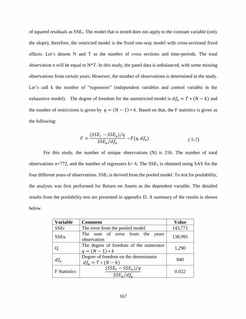
167

of squared residuals as SSEr. The model that is tested does not apply to the constant variable (only

the slope); therefore, the restricted model is the fixed one-way model with cross-sectional fixed

effects. Let’s denote N and T as the number of cross sections and time-periods. The total

observation n will be equal to N*T. In this study, the panel data is unbalanced, with some missing

observations from certain years. However, the number of observations is determined in the study.

Let’s call k the number of “regressors” (independent variables and control variable in the

exhaustive model). The degree of freedom for the unrestricted model is 𝑑𝑓𝑢 = 𝑇 ∗ (𝑁 − 𝑘) and

the number of restrictions is given by 𝑞 = (𝑁 − 1) ∗ 𝑘. Based on that, the F statistics is given as

the following:

𝐹 =(𝑆𝑆𝐸𝑟 − 𝑆𝑆𝐸𝑢) 𝑞⁄

𝑆𝑆𝐸𝑢 𝑑𝑓𝑢⁄ ~𝐹(𝑞, 𝑑𝑓𝑢) ( 5-7)

For this study, the number of unique observations (N) is 216. The number of total

observations n=772, and the number of regressors k= 6. The SSEu is obtained using SAS for the

four different years of observations. SSEr is derived from the pooled model. To test for poolability,

the analysis was first performed for Return on Assets as the dependent variable. The detailed

results from the poolability test are presented in appendix D. A summary of the results is shown

below.

Variable Comment Value

SSEr The error from the pooled model 143,771

SSEu The sum of error from the years

observation 138,995

Q The degree of freedom of the numerator

𝑞 = (𝑁 − 1) ∗ 𝑘 1,290

𝑑𝑓𝑢 Degree of freedom on the denominator

𝑑𝑓𝑢 = 𝑇 ∗ (𝑁 − 𝑘) 840

F Statistics (𝑆𝑆𝐸𝑟 − 𝑆𝑆𝐸𝑢) 𝑞⁄

𝑆𝑆𝐸𝑢 𝑑𝑓𝑢⁄ 0.022

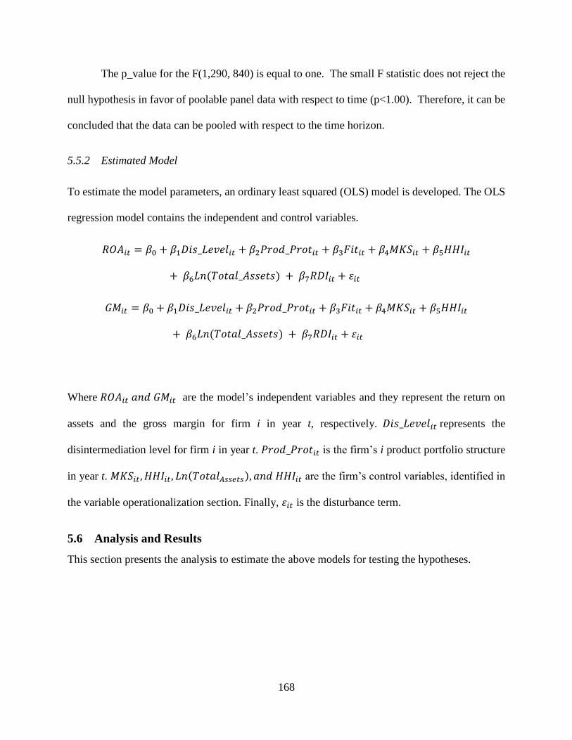
168

The p_value for the F(1,290, 840) is equal to one. The small F statistic does not reject the

null hypothesis in favor of poolable panel data with respect to time (p<1.00). Therefore, it can be

concluded that the data can be pooled with respect to the time horizon.

5.5.2 Estimated Model

To estimate the model parameters, an ordinary least squared (OLS) model is developed. The OLS

regression model contains the independent and control variables.

𝑅𝑂𝐴𝑖𝑡 = 𝛽0 + 𝛽1𝐷𝑖𝑠_𝐿𝑒𝑣𝑒𝑙𝑖𝑡 + 𝛽2𝑃𝑟𝑜𝑑_𝑃𝑟𝑜𝑡𝑖𝑡 + 𝛽3𝐹𝑖𝑡𝑖𝑡 + 𝛽4𝑀𝐾𝑆𝑖𝑡 + 𝛽5𝐻𝐻𝐼𝑖𝑡

+ 𝛽6𝐿𝑛(𝑇𝑜𝑡𝑎𝑙_𝐴𝑠𝑠𝑒𝑡𝑠) + 𝛽7𝑅𝐷𝐼𝑖𝑡 + 𝜀𝑖𝑡

𝐺𝑀𝑖𝑡 = 𝛽0 + 𝛽1𝐷𝑖𝑠_𝐿𝑒𝑣𝑒𝑙𝑖𝑡 + 𝛽2𝑃𝑟𝑜𝑑_𝑃𝑟𝑜𝑡𝑖𝑡 + 𝛽3𝐹𝑖𝑡𝑖𝑡 + 𝛽4𝑀𝐾𝑆𝑖𝑡 + 𝛽5𝐻𝐻𝐼𝑖𝑡

+ 𝛽6𝐿𝑛(𝑇𝑜𝑡𝑎𝑙_𝐴𝑠𝑠𝑒𝑡𝑠) + 𝛽7𝑅𝐷𝐼𝑖𝑡 + 𝜀𝑖𝑡

Where 𝑅𝑂𝐴𝑖𝑡 𝑎𝑛𝑑 𝐺𝑀𝑖𝑡 are the model’s independent variables and they represent the return on

assets and the gross margin for firm i in year t, respectively. 𝐷𝑖𝑠_𝐿𝑒𝑣𝑒𝑙𝑖𝑡 represents the

disintermediation level for firm i in year t. 𝑃𝑟𝑜𝑑_𝑃𝑟𝑜𝑡𝑖𝑡 is the firm’s i product portfolio structure

in year t. 𝑀𝐾𝑆𝑖𝑡, 𝐻𝐻𝐼𝑖𝑡, 𝐿𝑛(𝑇𝑜𝑡𝑎𝑙𝐴𝑠𝑠𝑒𝑡𝑠), 𝑎𝑛𝑑 𝐻𝐻𝐼𝑖𝑡 are the firm’s control variables, identified in

the variable operationalization section. Finally, 𝜀𝑖𝑡 is the disturbance term.

5.6 Analysis and Results

This section presents the analysis to estimate the above models for testing the hypotheses.

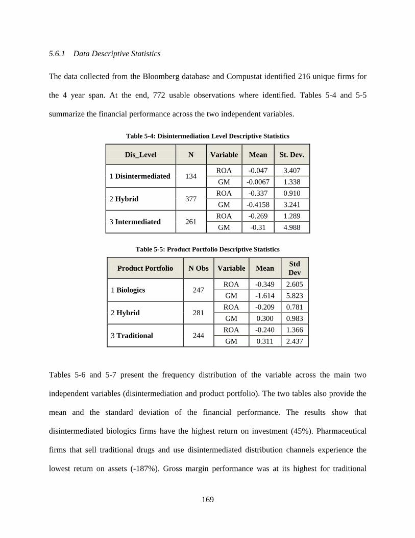
169

5.6.1 Data Descriptive Statistics

The data collected from the Bloomberg database and Compustat identified 216 unique firms for

the 4 year span. At the end, 772 usable observations where identified. Tables 5-4 and 5-5

summarize the financial performance across the two independent variables.

Table 5-4: Disintermediation Level Descriptive Statistics

Dis_Level N Variable Mean St. Dev.

1 Disintermediated 134 ROA -0.047 3.407

GM -0.0067 1.338

2 Hybrid 377 ROA -0.337 0.910

GM -0.4158 3.241

3 Intermediated 261 ROA -0.269 1.289

GM -0.31 4.988

Table 5-5: Product Portfolio Descriptive Statistics

Product Portfolio N Obs Variable Mean Std

Dev

1 Biologics 247 ROA -0.349 2.605

GM -1.614 5.823

2 Hybrid 281 ROA -0.209 0.781

GM 0.300 0.983

3 Traditional 244 ROA -0.240 1.366

GM 0.311 2.437

Tables 5-6 and 5-7 present the frequency distribution of the variable across the main two

independent variables (disintermediation and product portfolio). The two tables also provide the

mean and the standard deviation of the financial performance. The results show that

disintermediated biologics firms have the highest return on investment (45%). Pharmaceutical

firms that sell traditional drugs and use disintermediated distribution channels experience the

lowest return on assets (-187%). Gross margin performance was at its highest for traditional

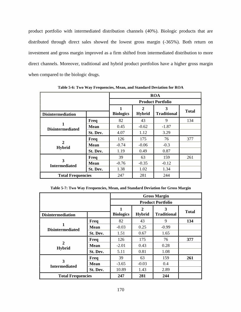
170

product portfolio with intermediated distribution channels (40%). Biologic products that are

distributed through direct sales showed the lowest gross margin (-365%). Both return on

investment and gross margin improved as a firm shifted from intermediated distribution to more

direct channels. Moreover, traditional and hybrid product portfolios have a higher gross margin

when compared to the biologic drugs.

Table 5-6: Two Way Frequencies, Mean, and Standard Deviation for ROA

ROA

Product Portfolio

1

Biologics

2

Hybrid

3

Traditional Total

Disintermediation

1

Disintermediated

Freq 82 43 9 134

Mean 0.45 -0.62 -1.87

St. Dev. 4.07 1.12 3.29

2

Hybrid

Freq 126 175 76 377

Mean -0.74 -0.06 -0.3

St. Dev. 1.19 0.49 0.87

3

Intermediated

Freq 39 63 159 261

Mean -0.76 -0.35 -0.12

St. Dev. 1.38 1.02 1.34

Total Frequencies 247 281 244

Table 5-7: Two Way Frequencies, Mean, and Standard Deviation for Gross Margin

Gross Margin

Product Portfolio

1

Biologics

2

Hybrid

3

Traditional Total

Disintermediation

1

Disintermediated

Freq 82 43 9 134

Mean -0.03 0.25 -0.99

St. Dev. 1.51 0.67 1.65

2

Hybrid

Freq 126 175 76 377

Mean -2.01 0.43 0.28

St. Dev. 5.11 0.81 1.08

3

Intermediated

Freq 39 63 159 261

Mean -3.65 -0.03 0.4

St. Dev. 10.89 1.43 2.89

Total Frequencies 247 281 244

171

Table 5-8 provides the descriptive statistics and the correlation factor of model variables.

The correlation matrix showed that the product portfolio variables were slightly correlated with

each other. This is expected given the nature of these categorical variables. The Herfindahl-

Hirschman index is highly correlated to the product portfolio structure.

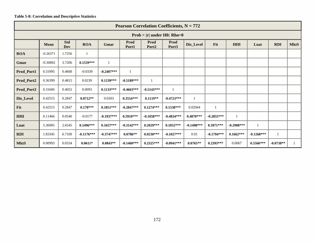
172

Table 5-8: Correlation and Descriptive Statistics

Pearson Correlation Coefficients, N = 772

Prob > |r| under H0: Rho=0

Mean Std

Dev ROA Gmar

Prod

Port1

Prod

Port2

Prod

Port3 Dis_Level Fit HHI Lnat RDI MktS

ROA -0.26371 1.7256 1

Gmar -0.30892 3.7206 0.1559*** 1

Prod_Port1 0.31995 0.4668 -0.0339 -0.2407*** 1

Prod_Port2 0.36399 0.4815 0.0239 0.1239*** -0.5189*** 1

Prod_Port3 0.31606 0.4652 0.0093 0.1133*** -0.4663*** -0.5143*** 1

Dis_Level 0.42515 0.2847 0.0712** 0.0303 0.3554*** 0.1119** -0.4723*** 1

Fit 0.42515 0.2847 0.178*** 0.1851*** -0.2847*** 0.1274*** 0.1538*** 0.02944 1

HHI 0.11466 0.0540 -0.0177 -0.1937*** 0.5910*** -0.1058*** -0.4834*** 0.4870*** -0.2855*** 1

Lnat 5.36085 2.6545 0.1496*** 0.1657*** -0.3142*** 0.2029*** 0.1052*** -0.1498*** 0.3971*** -0.2908*** 1

RDI 1.83345 6.7169 -0.1176*** -0.3747*** 0.0786** 0.0230*** -0.1027*** 0.01 -0.1794*** 0.1662*** -0.1268*** 1

MktS 0.00993 0.0334 0.0611* 0.0843** -0.1460*** 0.2325*** -0.0941*** 0.0765** 0.2393*** 0.0067 0.5566*** -0.0738** 1

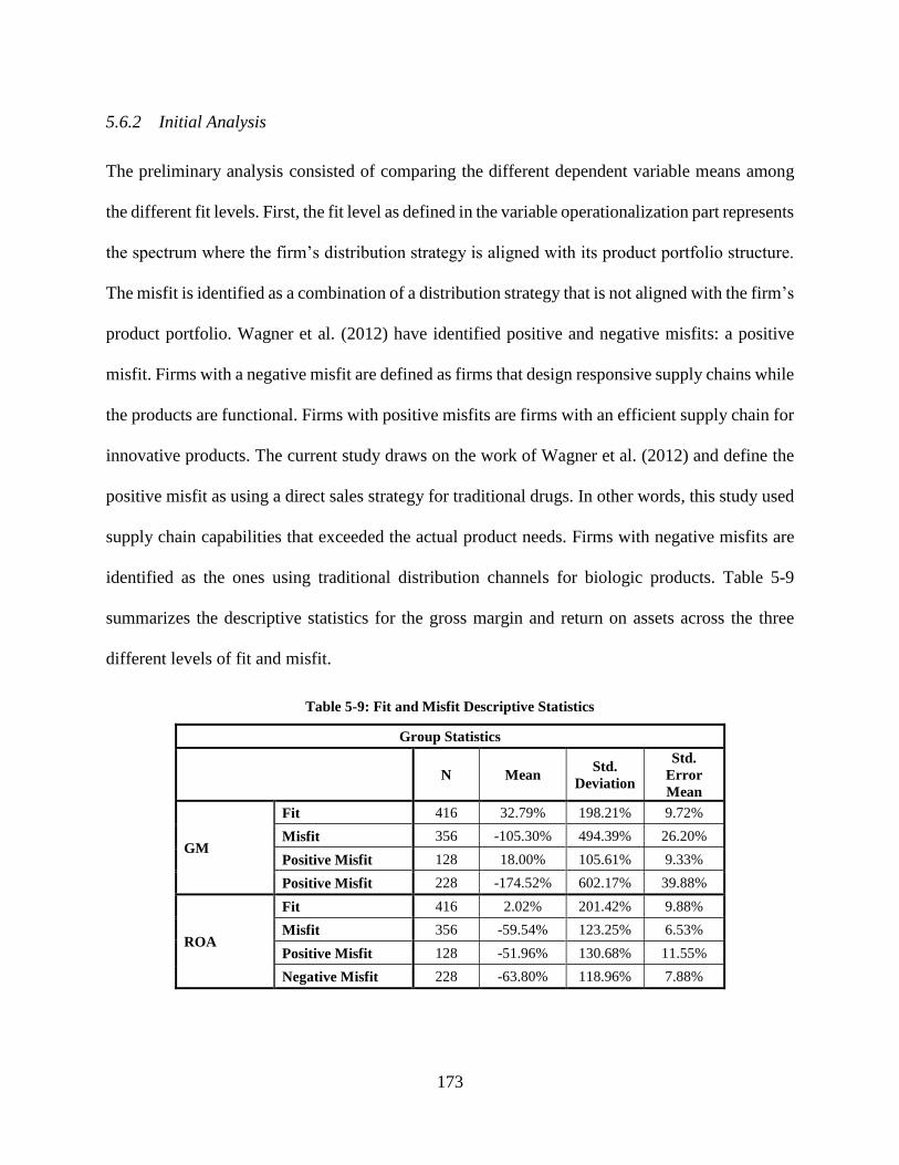
173

5.6.2 Initial Analysis

The preliminary analysis consisted of comparing the different dependent variable means among

the different fit levels. First, the fit level as defined in the variable operationalization part represents

the spectrum where the firm’s distribution strategy is aligned with its product portfolio structure.

The misfit is identified as a combination of a distribution strategy that is not aligned with the firm’s

product portfolio. Wagner et al. (2012) have identified positive and negative misfits: a positive

misfit. Firms with a negative misfit are defined as firms that design responsive supply chains while

the products are functional. Firms with positive misfits are firms with an efficient supply chain for

innovative products. The current study draws on the work of Wagner et al. (2012) and define the

positive misfit as using a direct sales strategy for traditional drugs. In other words, this study used

supply chain capabilities that exceeded the actual product needs. Firms with negative misfits are

identified as the ones using traditional distribution channels for biologic products. Table 5-9

summarizes the descriptive statistics for the gross margin and return on assets across the three

different levels of fit and misfit.

Table 5-9: Fit and Misfit Descriptive Statistics

Group Statistics

N Mean Std.

Deviation

Std.

Error

Mean

GM

Fit 416 32.79% 198.21% 9.72%

Misfit 356 -105.30% 494.39% 26.20%

Positive Misfit 128 18.00% 105.61% 9.33%

Positive Misfit 228 -174.52% 602.17% 39.88%

ROA

Fit 416 2.02% 201.42% 9.88%

Misfit 356 -59.54% 123.25% 6.53%

Positive Misfit 128 -51.96% 130.68% 11.55%

Negative Misfit 228 -63.80% 118.96% 7.88%

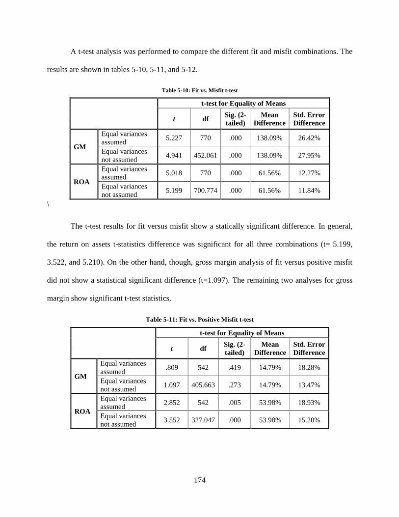
174

A t-test analysis was performed to compare the different fit and misfit combinations. The

results are shown in tables 5-10, 5-11, and 5-12.

Table 5-10: Fit vs. Misfit t-test

t-test for Equality of Means

t df Sig. (2-

tailed)

Mean

Difference

Std. Error

Difference

GM

Equal variances

assumed 5.227 770 .000 138.09% 26.42%

Equal variances

not assumed 4.941 452.061 .000 138.09% 27.95%

ROA

Equal variances

assumed 5.018 770 .000 61.56% 12.27%

Equal variances

not assumed 5.199 700.774 .000 61.56% 11.84%

\

The t-test results for fit versus misfit show a statically significant difference. In general,

the return on assets t-statistics difference was significant for all three combinations (t= 5.199,

3.522, and 5.210). On the other hand, though, gross margin analysis of fit versus positive misfit

did not show a statistical significant difference (t=1.097). The remaining two analyses for gross

margin show significant t-test statistics.

Table 5-11: Fit vs. Positive Misfit t-test

t-test for Equality of Means

t df Sig. (2-

tailed)

Mean

Difference

Std. Error

Difference

GM

Equal variances

assumed .809 542 .419 14.79% 18.28%

Equal variances

not assumed 1.097 405.663 .273 14.79% 13.47%

ROA

Equal variances

assumed 2.852 542 .005 53.98% 18.93%

Equal variances

not assumed 3.552 327.047 .000 53.98% 15.20%

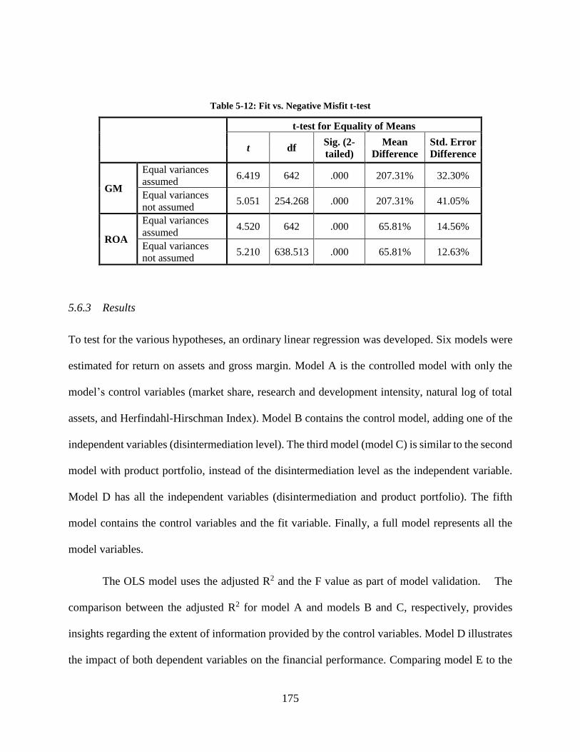
175

Table 5-12: Fit vs. Negative Misfit t-test

t-test for Equality of Means

t df Sig. (2-

tailed)

Mean

Difference

Std. Error

Difference

GM

Equal variances

assumed 6.419 642 .000 207.31% 32.30%

Equal variances

not assumed 5.051 254.268 .000 207.31% 41.05%

ROA

Equal variances

assumed 4.520 642 .000 65.81% 14.56%

Equal variances

not assumed 5.210 638.513 .000 65.81% 12.63%

5.6.3 Results

To test for the various hypotheses, an ordinary linear regression was developed. Six models were

estimated for return on assets and gross margin. Model A is the controlled model with only the

model’s control variables (market share, research and development intensity, natural log of total

assets, and Herfindahl-Hirschman Index). Model B contains the control model, adding one of the

independent variables (disintermediation level). The third model (model C) is similar to the second

model with product portfolio, instead of the disintermediation level as the independent variable.

Model D has all the independent variables (disintermediation and product portfolio). The fifth

model contains the control variables and the fit variable. Finally, a full model represents all the

model variables.

The OLS model uses the adjusted R2 and the F value as part of model validation. The

comparison between the adjusted R2 for model A and models B and C, respectively, provides

insights regarding the extent of information provided by the control variables. Model D illustrates

the impact of both dependent variables on the financial performance. Comparing model E to the

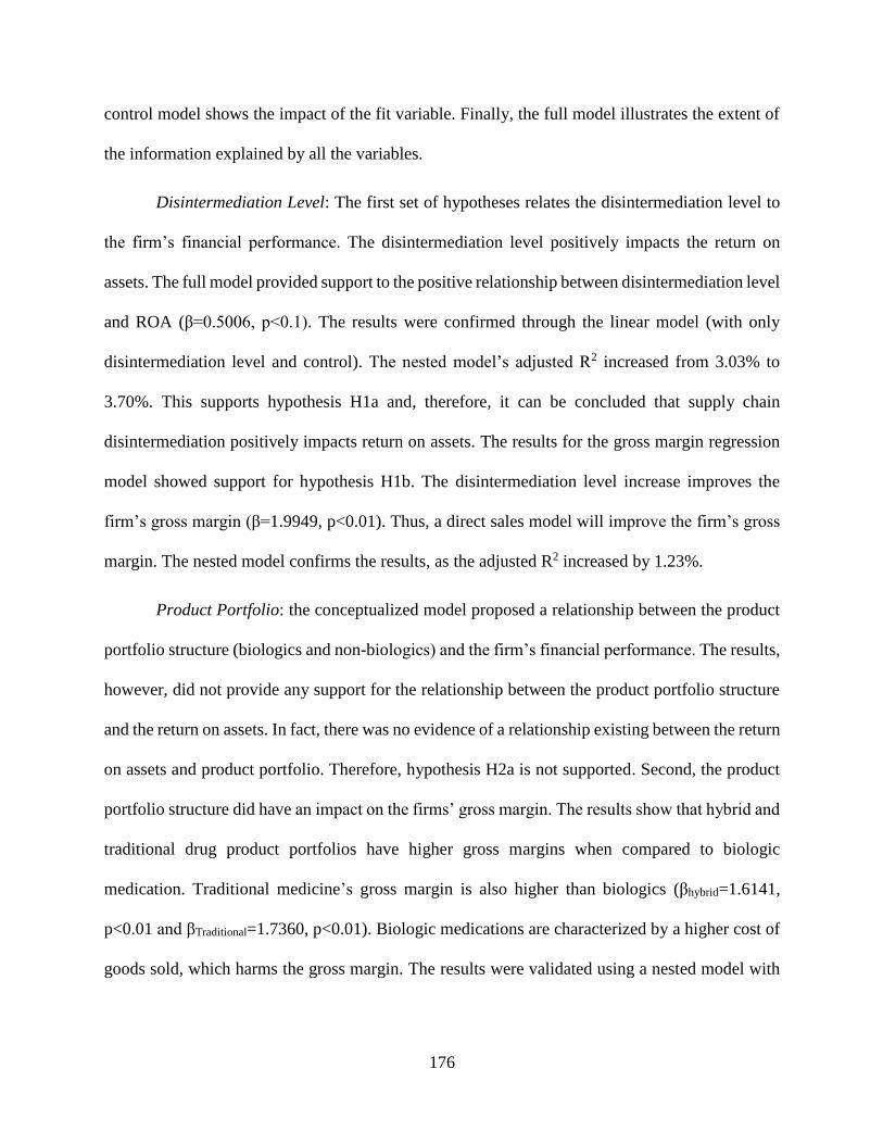
176

control model shows the impact of the fit variable. Finally, the full model illustrates the extent of

the information explained by all the variables.

Disintermediation Level: The first set of hypotheses relates the disintermediation level to

the firm’s financial performance. The disintermediation level positively impacts the return on

assets. The full model provided support to the positive relationship between disintermediation level

and ROA (β=0.5006, p<0.1). The results were confirmed through the linear model (with only

disintermediation level and control). The nested model’s adjusted R2 increased from 3.03% to

3.70%. This supports hypothesis H1a and, therefore, it can be concluded that supply chain

disintermediation positively impacts return on assets. The results for the gross margin regression

model showed support for hypothesis H1b. The disintermediation level increase improves the

firm’s gross margin (β=1.9949, p<0.01). Thus, a direct sales model will improve the firm’s gross

margin. The nested model confirms the results, as the adjusted R2 increased by 1.23%.

Product Portfolio: the conceptualized model proposed a relationship between the product

portfolio structure (biologics and non-biologics) and the firm’s financial performance. The results,

however, did not provide any support for the relationship between the product portfolio structure

and the return on assets. In fact, there was no evidence of a relationship existing between the return

on assets and product portfolio. Therefore, hypothesis H2a is not supported. Second, the product

portfolio structure did have an impact on the firms’ gross margin. The results show that hybrid and

traditional drug product portfolios have higher gross margins when compared to biologic

medication. Traditional medicine’s gross margin is also higher than biologics (βhybrid=1.6141,

p<0.01 and βTraditional=1.7360, p<0.01). Biologic medications are characterized by a higher cost of

goods sold, which harms the gross margin. The results were validated using a nested model with

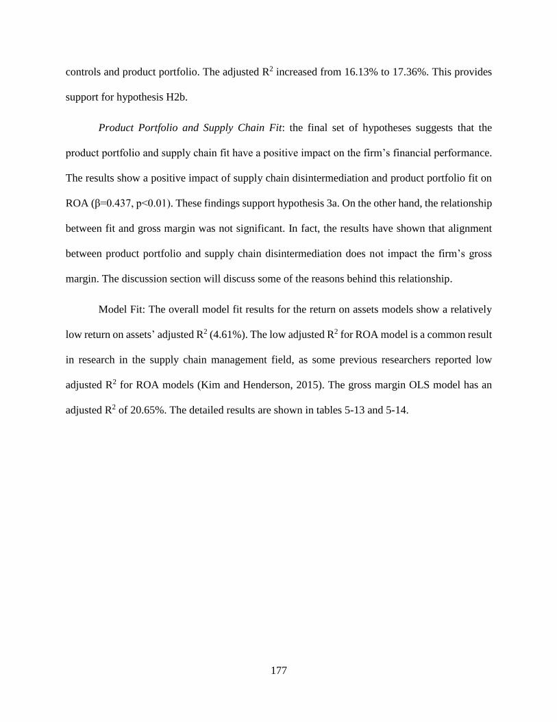
177

controls and product portfolio. The adjusted R2 increased from 16.13% to 17.36%. This provides

support for hypothesis H2b.

Product Portfolio and Supply Chain Fit: the final set of hypotheses suggests that the

product portfolio and supply chain fit have a positive impact on the firm’s financial performance.

The results show a positive impact of supply chain disintermediation and product portfolio fit on

ROA (β=0.437, p<0.01). These findings support hypothesis 3a. On the other hand, the relationship

between fit and gross margin was not significant. In fact, the results have shown that alignment

between product portfolio and supply chain disintermediation does not impact the firm’s gross

margin. The discussion section will discuss some of the reasons behind this relationship.

Model Fit: The overall model fit results for the return on assets models show a relatively

low return on assets’ adjusted R2 (4.61%). The low adjusted R2 for ROA model is a common result

in research in the supply chain management field, as some previous researchers reported low

adjusted R2 for ROA models (Kim and Henderson, 2015). The gross margin OLS model has an

adjusted R2 of 20.65%. The detailed results are shown in tables 5-13 and 5-14.

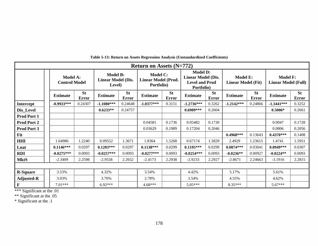
178

Table 5-13: Return on Assets Regression Analysis (Unstandardized Coefficients)

Return on Assets (N=772)

Model A:

Control Model

Model B:

Linear Model (Dis.

Level)

Model C:

Linear Model (Prod.

Portfolio)

Model D:

Linear Model (Dis.

Level and Prod

Portfolio)

Model E:

Linear Model (Fit)

Model F:

Linear Model (Full)

Estimate St

Error Estimate

St

Error Estimate

St

Error Estimate

St

Error Estimate

St

Error Estimate

St

Error

Intercept -0.9933*** 0.24307 -1.1080*** 0.24648 -1.0377*** 0.3151 -1.2736*** 0.3262 -1.2142*** 0.24866 -1.3441*** 0.3252

Dis_Level 0.6233** 0.24757 0.6909*** 0.2604 0.5006* 0.2661

Prod Port 1

Prod Port 2 0.04581 0.1736 0.05482 0.1730 0.0047 0.1728

Prod Port 3 0.03629 0.1989 0.17204 0.2046 0.0806 0.2056

Fit 0.4968*** 0.13643 0.4370*** 0.1408

HHI 1.64986 1.2240 0.09552 1.3671 1.8364 1.5268 0.67174 1.5829 2.4929 1.23615 1.4741 1.5951

Lnat 0.1146*** 0.0297 0.1203*** 0.0297 0.1138*** 0.0299 0.1195*** 0.0299 0.0874*** 0.03041 0.0949*** 0.0307

RDI -0.0275*** 0.0093 -0.0257*** 0.0093 -0.0277*** 0.0093 -0.0254*** 0.0093 -0.0236** 0.00927 -0.0224** 0.0093

MktS -2.3409 2.2598 -2.9558 2.2652 -2.4173 2.2938 -2.9233 2.2927 -2.8671 2.24663 -3.1916 2.2815

R-Square

3.53% 4.32% 3.54% 4.42% 5.17% 5.61%

Adjusted-R 3.03% 3.70% 2.78% 3.54% 4.55% 4.62%

F 7.01*** 6.92*** 4.68*** 5.05*** 8.35*** 5.67***

*** Significant at the .01

** Significant at the .05

* Significant at the .1

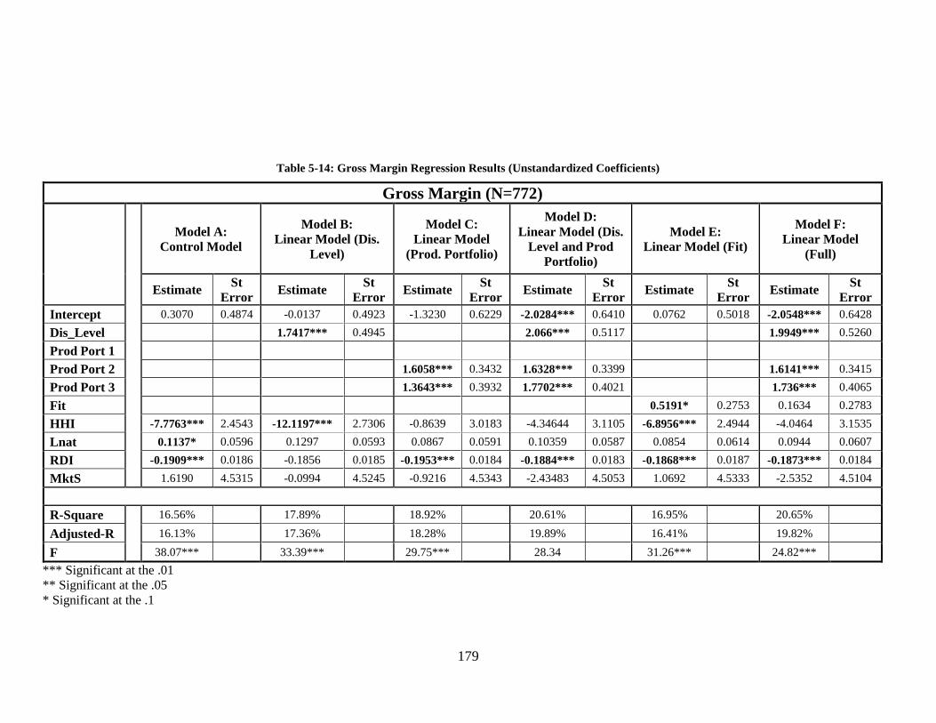
179

Table 5-14: Gross Margin Regression Results (Unstandardized Coefficients)

Gross Margin (N=772)

Model A:

Control Model

Model B:

Linear Model (Dis.

Level)

Model C:

Linear Model

(Prod. Portfolio)

Model D:

Linear Model (Dis.

Level and Prod

Portfolio)

Model E:

Linear Model (Fit)

Model F:

Linear Model

(Full)

Estimate St

Error Estimate

St

Error Estimate

St

Error Estimate

St

Error Estimate

St

Error Estimate

St

Error

Intercept 0.3070 0.4874 -0.0137 0.4923 -1.3230 0.6229 -2.0284*** 0.6410 0.0762 0.5018 -2.0548*** 0.6428

Dis_Level 1.7417*** 0.4945 2.066*** 0.5117 1.9949*** 0.5260

Prod Port 1

Prod Port 2 1.6058*** 0.3432 1.6328*** 0.3399 1.6141*** 0.3415

Prod Port 3 1.3643*** 0.3932 1.7702*** 0.4021 1.736*** 0.4065

Fit 0.5191* 0.2753 0.1634 0.2783

HHI -7.7763*** 2.4543 -12.1197*** 2.7306 -0.8639 3.0183 -4.34644 3.1105 -6.8956*** 2.4944 -4.0464 3.1535

Lnat 0.1137* 0.0596 0.1297 0.0593 0.0867 0.0591 0.10359 0.0587 0.0854 0.0614 0.0944 0.0607

RDI -0.1909*** 0.0186 -0.1856 0.0185 -0.1953*** 0.0184 -0.1884*** 0.0183 -0.1868*** 0.0187 -0.1873*** 0.0184

MktS 1.6190 4.5315 -0.0994 4.5245 -0.9216 4.5343 -2.43483 4.5053 1.0692 4.5333 -2.5352 4.5104

R-Square

16.56% 17.89% 18.92% 20.61% 16.95% 20.65%

Adjusted-R 16.13% 17.36% 18.28% 19.89% 16.41% 19.82%

F 38.07*** 33.39*** 29.75*** 28.34 31.26*** 24.82***

*** Significant at the .01

** Significant at the .05

* Significant at the .1

180

5.6.4 Robustness Check

The robustness check section aims at providing evidence that the results obtained are not sensitive

to arbitrary decisions and are not biased by outliers.

5.6.4.1 Sensitivity Analysis

This part addresses how sensitive the data is to the coding decision rule. Product portfolio is a

coded variable from the firm’s 10k and product descriptions. On the other hand, the

disintermediation level is a continuous variable. To create the fit measure, one of the variables

needed to be transformed from continuous to code (or vice versa). The product portfolio data did

not provide enough insight about the sales level of each product line. Therefore, it was challenging

to provide a percentage of sales for biologics and non-biologics firms. The study, instead, translates

the disintermediation level into coded measures. The study uses a 20%-80% cutoff for the different

disintermediation strategy levels. The 20-80% cutoff means that if the disintermediation level is

less than 20%, the distribution strategy is considered intermediated. In case the disintermediation

level is greater than 80%, the disintermediation strategy is coded as disintermediated. If the

disintermediation level is between 20% and 80%, the disintermediation strategy is considered

hybrid.

To avoid any problems resulting from an arbitrary choice, a sensitivity analysis is developed

with 5 different cutoff levels (10%-90%, 15%-85%, 20%-80%, 25%-75%, and 30%-70%). The

results from the sensitivity analysis shows that both return on assets and gross margin results were

not sensitive to the cutoff point. All the parameter signs and significance have been maintained.

The detailed results are presented in appendix E.

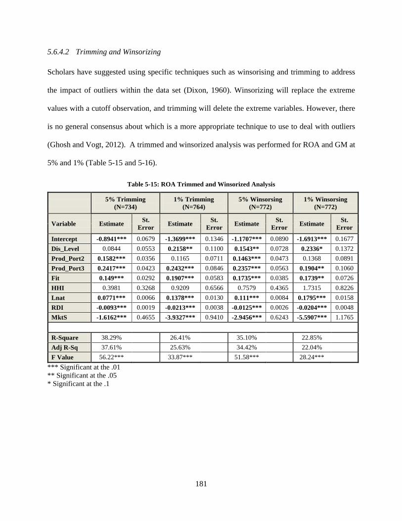
181

5.6.4.2 Trimming and Winsorizing

Scholars have suggested using specific techniques such as winsorising and trimming to address

the impact of outliers within the data set (Dixon, 1960). Winsorizing will replace the extreme

values with a cutoff observation, and trimming will delete the extreme variables. However, there

is no general consensus about which is a more appropriate technique to use to deal with outliers

(Ghosh and Vogt, 2012). A trimmed and winsorized analysis was performed for ROA and GM at

5% and 1% (Table 5-15 and 5-16).

Table 5-15: ROA Trimmed and Winsorized Analysis

5% Trimming

(N=734)

1% Trimming

(N=764)

5% Winsorsing

(N=772)

1% Winsorsing

(N=772)

Variable Estimate St.

Error Estimate

St.

Error Estimate

St.

Error Estimate

St.

Error

Intercept -0.8941*** 0.0679 -1.3699*** 0.1346 -1.1707*** 0.0890 -1.6913*** 0.1677

Dis_Level 0.0844 0.0553 0.2158** 0.1100 0.1543** 0.0728 0.2336* 0.1372

Prod_Port2 0.1582*** 0.0356 0.1165 0.0711 0.1463*** 0.0473 0.1368 0.0891

Prod_Port3 0.2417*** 0.0423 0.2432*** 0.0846 0.2357*** 0.0563 0.1904** 0.1060

Fit 0.149*** 0.0292 0.1907*** 0.0583 0.1735*** 0.0385 0.1739** 0.0726

HHI 0.3981 0.3268 0.9209 0.6566 0.7579 0.4365 1.7315 0.8226

Lnat 0.0771*** 0.0066 0.1378*** 0.0130 0.111*** 0.0084 0.1795*** 0.0158

RDI -0.0093*** 0.0019 -0.0213*** 0.0038 -0.0125*** 0.0026 -0.0204*** 0.0048

MktS -1.6162*** 0.4655 -3.9327*** 0.9410 -2.9456*** 0.6243 -5.5907*** 1.1765

R-Square 38.29% 26.41% 35.10% 22.85%

Adj R-Sq 37.61% 25.63% 34.42% 22.04%

F Value 56.22*** 33.87*** 51.58*** 28.24***

*** Significant at the .01

** Significant at the .05

* Significant at the .1

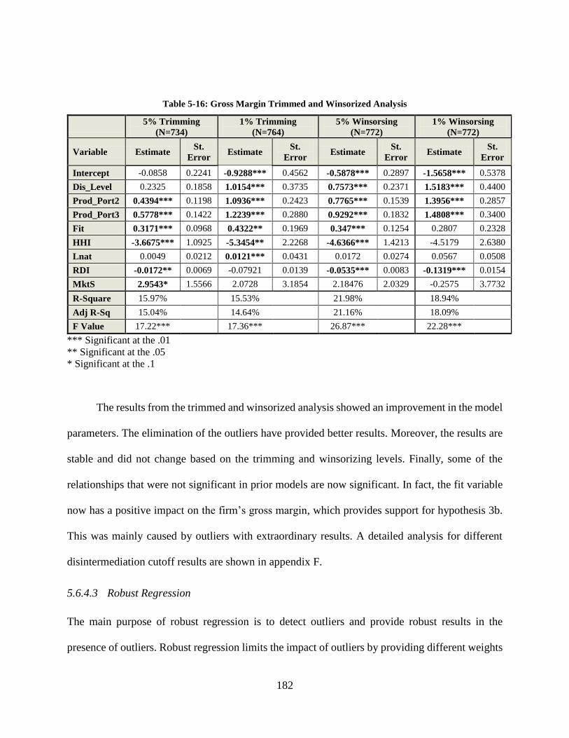
182

Table 5-16: Gross Margin Trimmed and Winsorized Analysis

5% Trimming

(N=734)

1% Trimming

(N=764)

5% Winsorsing

(N=772)

1% Winsorsing

(N=772)

Variable Estimate St.

Error Estimate

St.

Error Estimate

St.

Error Estimate

St.

Error

Intercept -0.0858 0.2241 -0.9288*** 0.4562 -0.5878*** 0.2897 -1.5658*** 0.5378

Dis_Level 0.2325 0.1858 1.0154*** 0.3735 0.7573*** 0.2371 1.5183*** 0.4400

Prod_Port2 0.4394*** 0.1198 1.0936*** 0.2423 0.7765*** 0.1539 1.3956*** 0.2857

Prod_Port3 0.5778*** 0.1422 1.2239*** 0.2880 0.9292*** 0.1832 1.4808*** 0.3400

Fit 0.3171*** 0.0968 0.4322** 0.1969 0.347*** 0.1254 0.2807 0.2328

HHI -3.6675*** 1.0925 -5.3454** 2.2268 -4.6366*** 1.4213 -4.5179 2.6380

Lnat 0.0049 0.0212 0.0121*** 0.0431 0.0172 0.0274 0.0567 0.0508

RDI -0.0172** 0.0069 -0.07921 0.0139 -0.0535*** 0.0083 -0.1319*** 0.0154

MktS 2.9543* 1.5566 2.0728 3.1854 2.18476 2.0329 -0.2575 3.7732

R-Square 15.97% 15.53% 21.98% 18.94%

Adj R-Sq 15.04% 14.64% 21.16% 18.09%

F Value 17.22*** 17.36*** 26.87*** 22.28***

*** Significant at the .01

** Significant at the .05

* Significant at the .1

The results from the trimmed and winsorized analysis showed an improvement in the model

parameters. The elimination of the outliers have provided better results. Moreover, the results are

stable and did not change based on the trimming and winsorizing levels. Finally, some of the

relationships that were not significant in prior models are now significant. In fact, the fit variable

now has a positive impact on the firm’s gross margin, which provides support for hypothesis 3b.

This was mainly caused by outliers with extraordinary results. A detailed analysis for different

disintermediation cutoff results are shown in appendix F.

5.6.4.3 Robust Regression

The main purpose of robust regression is to detect outliers and provide robust results in the

presence of outliers. Robust regression limits the impact of outliers by providing different weights

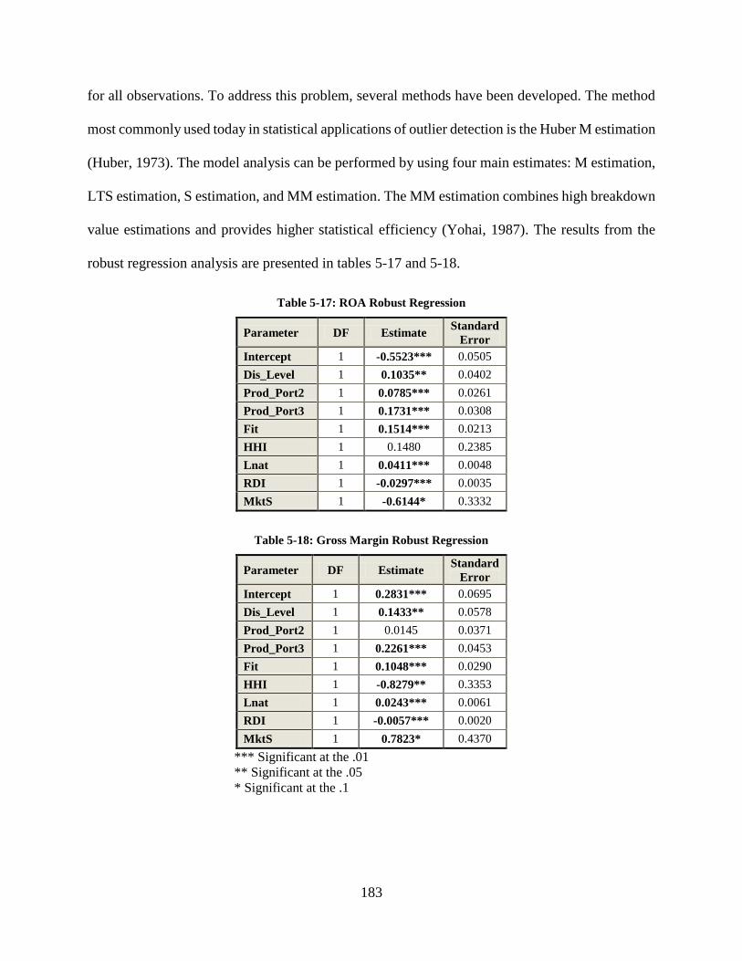
183

for all observations. To address this problem, several methods have been developed. The method

most commonly used today in statistical applications of outlier detection is the Huber M estimation

(Huber, 1973). The model analysis can be performed by using four main estimates: M estimation,

LTS estimation, S estimation, and MM estimation. The MM estimation combines high breakdown

value estimations and provides higher statistical efficiency (Yohai, 1987). The results from the

robust regression analysis are presented in tables 5-17 and 5-18.

Table 5-17: ROA Robust Regression

Parameter DF Estimate Standard

Error

Intercept 1 -0.5523*** 0.0505

Dis_Level 1 0.1035** 0.0402

Prod_Port2 1 0.0785*** 0.0261

Prod_Port3 1 0.1731*** 0.0308

Fit 1 0.1514*** 0.0213

HHI 1 0.1480 0.2385

Lnat 1 0.0411*** 0.0048

RDI 1 -0.0297*** 0.0035

MktS 1 -0.6144* 0.3332

Table 5-18: Gross Margin Robust Regression

Parameter DF Estimate Standard

Error

Intercept 1 0.2831*** 0.0695

Dis_Level 1 0.1433** 0.0578

Prod_Port2 1 0.0145 0.0371

Prod_Port3 1 0.2261*** 0.0453

Fit 1 0.1048*** 0.0290

HHI 1 -0.8279** 0.3353

Lnat 1 0.0243*** 0.0061

RDI 1 -0.0057*** 0.0020

MktS 1 0.7823* 0.4370

*** Significant at the .01

** Significant at the .05

* Significant at the .1

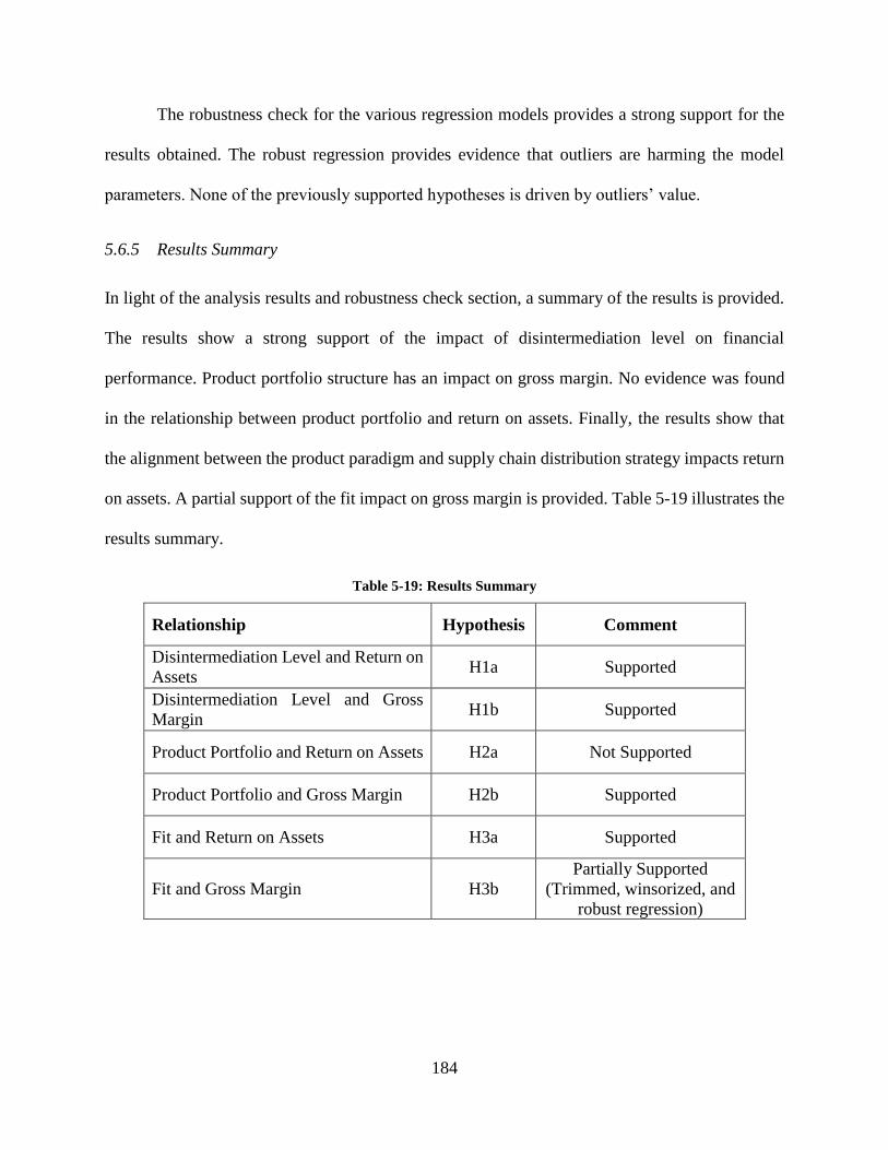
184

The robustness check for the various regression models provides a strong support for the

results obtained. The robust regression provides evidence that outliers are harming the model

parameters. None of the previously supported hypotheses is driven by outliers’ value.

5.6.5 Results Summary

In light of the analysis results and robustness check section, a summary of the results is provided.

The results show a strong support of the impact of disintermediation level on financial

performance. Product portfolio structure has an impact on gross margin. No evidence was found

in the relationship between product portfolio and return on assets. Finally, the results show that

the alignment between the product paradigm and supply chain distribution strategy impacts return

on assets. A partial support of the fit impact on gross margin is provided. Table 5-19 illustrates the

results summary.

Table 5-19: Results Summary

Relationship Hypothesis Comment

Disintermediation Level and Return on

Assets H1a Supported

Disintermediation Level and Gross

Margin H1b Supported

Product Portfolio and Return on Assets H2a Not Supported

Product Portfolio and Gross Margin H2b Supported

Fit and Return on Assets H3a Supported

Fit and Gross Margin H3b

Partially Supported

(Trimmed, winsorized, and

robust regression)

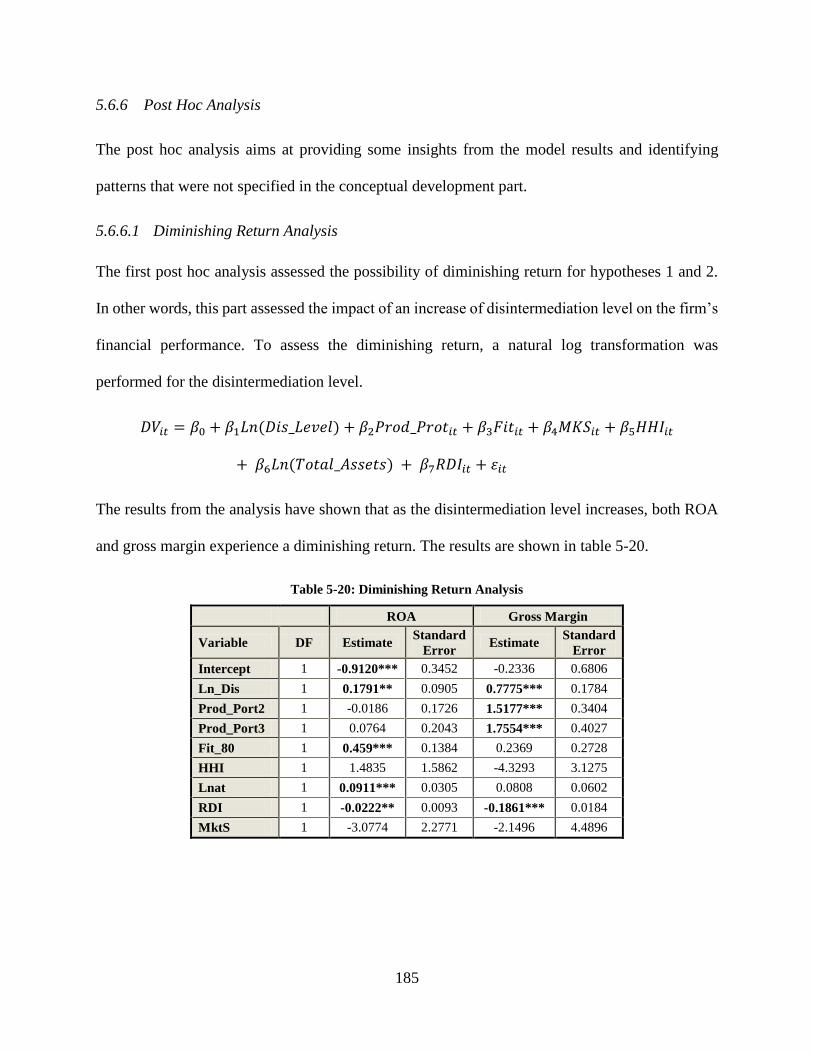
185

5.6.6 Post Hoc Analysis

The post hoc analysis aims at providing some insights from the model results and identifying

patterns that were not specified in the conceptual development part.

5.6.6.1 Diminishing Return Analysis

The first post hoc analysis assessed the possibility of diminishing return for hypotheses 1 and 2.

In other words, this part assessed the impact of an increase of disintermediation level on the firm’s

financial performance. To assess the diminishing return, a natural log transformation was

performed for the disintermediation level.

𝐷𝑉𝑖𝑡 = 𝛽0 + 𝛽1𝐿𝑛(𝐷𝑖𝑠_𝐿𝑒𝑣𝑒𝑙) + 𝛽2𝑃𝑟𝑜𝑑_𝑃𝑟𝑜𝑡𝑖𝑡 + 𝛽3𝐹𝑖𝑡𝑖𝑡 + 𝛽4𝑀𝐾𝑆𝑖𝑡 + 𝛽5𝐻𝐻𝐼𝑖𝑡

+ 𝛽6𝐿𝑛(𝑇𝑜𝑡𝑎𝑙_𝐴𝑠𝑠𝑒𝑡𝑠) + 𝛽7𝑅𝐷𝐼𝑖𝑡 + 𝜀𝑖𝑡

The results from the analysis have shown that as the disintermediation level increases, both ROA

and gross margin experience a diminishing return. The results are shown in table 5-20.

Table 5-20: Diminishing Return Analysis

ROA Gross Margin

Variable DF Estimate Standard

Error Estimate

Standard

Error

Intercept 1 -0.9120*** 0.3452 -0.2336 0.6806

Ln_Dis 1 0.1791** 0.0905 0.7775*** 0.1784

Prod_Port2 1 -0.0186 0.1726 1.5177*** 0.3404

Prod_Port3 1 0.0764 0.2043 1.7554*** 0.4027

Fit_80 1 0.459*** 0.1384 0.2369 0.2728

HHI 1 1.4835 1.5862 -4.3293 3.1275

Lnat 1 0.0911*** 0.0305 0.0808 0.0602

RDI 1 -0.0222** 0.0093 -0.1861*** 0.0184

MktS 1 -3.0774 2.2771 -2.1496 4.4896

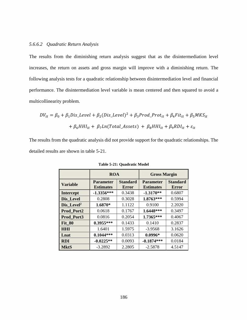
186

5.6.6.2 Quadratic Return Analysis

The results from the diminishing return analysis suggest that as the disintermediation level

increases, the return on assets and gross margin will improve with a diminishing return. The

following analysis tests for a quadratic relationship between disintermediation level and financial

performance. The disintermediation level variable is mean centered and then squared to avoid a

multicollinearity problem.

𝐷𝑉𝑖𝑡 = 𝛽0 + 𝛽1𝐷𝑖𝑠_𝐿𝑒𝑣𝑒𝑙 + 𝛽2(𝐷𝑖𝑠_𝐿𝑒𝑣𝑒𝑙)2 + 𝛽3𝑃𝑟𝑜𝑑_𝑃𝑟𝑜𝑡𝑖𝑡 + 𝛽4𝐹𝑖𝑡𝑖𝑡 + 𝛽5𝑀𝐾𝑆𝑖𝑡

+ 𝛽6𝐻𝐻𝐼𝑖𝑡 + 𝛽7𝐿𝑛(𝑇𝑜𝑡𝑎𝑙_𝐴𝑠𝑠𝑒𝑡𝑠) + 𝛽8𝐻𝐻𝐼𝑖𝑡 + 𝛽9𝑅𝐷𝐼𝑖𝑡 + 𝜀𝑖𝑡

The results from the quadratic analysis did not provide support for the quadratic relationships. The

detailed results are shown in table 5-21.

Table 5-21: Quadratic Model

ROA Gross Margin

Variable Parameter

Estimates

Standard

Error

Parameter

Estimates

Standard

Error

Intercept -1.3356*** 0.3438 -1.3170** 0.6807

Dis_Level 0.2808 0.3028 1.8763*** 0.5994

Dis_Level2 1.6870* 1.1122 0.9100 2.2020

Prod_Port2 0.0618 0.1767 1.6448*** 0.3497

Prod_Port3 0.0816 0.2054 1.7365*** 0.4067

Fit_80 0.3955*** 0.1433 0.1410 0.2837

HHI 1.6401 1.5975 -3.9568 3.1626

Lnat 0.1044*** 0.0313 0.0996* 0.0620

RDI -0.0225** 0.0093 -0.1874*** 0.0184

MktS -3.2892 2.2805 -2.5878 4.5147

187

5.7 Conclusion and Managerial Implication

5.7.1 Discussion

The current essay investigated the relationship between product portfolio structure and supply

chain distribution strategies on financial performance. The study also investigated the fit between

product portfolio and the supply chain disintermediation effect on return on assets and gross

margin. Additionally, the study addressed the fit between product paradigm and supply chain

distribution channels strategy and its impact of firms’ financial performance.

First, the results suggest that supply chain disintermediation improves the firm’s return on

assets and gross margin. Selling directly to end customers (drug stores, hospitals, or, in extreme

cases, patients) provides pharmaceutical firms with higher financial performance. The reduction

of the middle man role within the supply chain provides pharmaceutical firms with a better

understanding of the market needs and requirements, reducing the investment on unnecessary

assets and improving the firm’s return. The results also show that as firms adopt a more direct sales

distribution model, their financial performance will improve, nonetheless with diminishing return.

The findings suggest that after a certain disintermediation level, the marginal benefit will be

reduced. The results, however, did not provide any evidence of a quadratic relationship.

Second, the product portfolio structure does not have an impact on the firm’s return on

assets. The findings did not support the relationship between the product portfolio’s biological

level and the pharmaceutical firm’s return on assets. The results are mainly driven by the

discrepancy of the firm’s return on assets. In fact, many of the pharmaceutical firms, despite the

success of its products, are experiencing losses because of the lack of economy of scales and the

infancy stage of the market, both of which hamper a firm’s return on assets. On the other hand,

traditional firms have a higher gross margin. In fact, traditional and hybrid drug manufacturers

188

experience lower cost of goods sold. Traditional drug manufacturers encounter generic product

preparation, which is gaining more popularity and market share. Generic products are less

expensive to produce and, therefore, have a higher gross margin. Biologic medicine is more

sophisticated to produce and is highly inimitable, causing a high cost of goods sold and, therefore,

lower gross margin.

Third, the findings show that the supply chain distribution channels and product portfolio

alignment provides a better fit for pharmaceutical firms. Using the adequate distribution channels

for the type of product allows pharmaceutical firms to allow for the necessary resources based on

product characteristics. The research on fit within operations and supply chain perspectives has

emphasized the importance of alignment in achieving higher performance. The current study

provides a novel conceptualization of product paradigm and supply chain distribution strategy fit.

The results show strong evidence of the crucial role of fit on achieving higher return on assets.

Using the adequate distribution channel, depending on the product, allows pharmaceutical firms

to better utilize their assets and increase their profit. On the other hand, the results from the

regression analysis did not provide evidence of impact on gross margin. The results are driven by

extreme observations. The data shows that within the 5 observations with the lowest gross margin,

3 observations had a fit between the product portfolio and the supply chain disintermediation. The

robustness section addressed this issue. The results from the trimmed, winsorized, and the

robustness regression showed that fit positively impacts the firm’s gross margin.

Finally, the study conceptualized the positive and negative misfit and tested for its impact

on the firm’s financial performance. A positive misfit reflects the use of supply chain capability

that exceeds the product portfolio’s need (using direct sales strategy for traditional medication

portfolio). The negative misfit represents the use of low traditional distribution strategy for drugs

189

that require more direct distribution channels. The results from the positive vs. negative misfit

analysis showed that there is a statistical significant mean difference for the gross margin. In fact,

firms with a positive misfit have experienced a larger gross margin average. The results are mainly

generated from the fact that firms with the positive misfit are composed of traditional firms that

already experienced larger gross margin. Despite the unnecessary spending on more direct

distribution channels, the economy of scale impact provides a lower cost of goods sold and the

gross margin does not suffer tremendously. On the other hand, the return on assets is not sensitive

to the type of misfit. The regression analysis against the misfit type did not provide any statistical

significant impact on financial performance. The results are similar to the findings of Wagner et

al (2012).

5.7.2 Managerial Implications

The current study provides managerial and practical insights. First, the study illustrates the

important role of supply chain disintermediation in achieving higher financial performance. The

reduction of the middle man role has a positive impact on the pharmaceutical firm’s gross margin

and return on assets. Practitioners from the pharmaceutical industry are engaging in more

disintermediated distribution channels and are attempting to reduce of intermediaries’ role. The

direct sales model is also gaining more attention in over the counter medication as well as the more

innovative drugs such as biologics. The pharmaceutical supply chain is under the pressure of the

traditional distribution channels. Thus, the findings provide managers with financial incentives to

engage in more disintermediated distribution models.

Second, managers are interested not only in discovering the impact of a strategy on

financial performance, but also in comparing the effect of various factors. The standardized

coefficient shown in table 5-21 provides a comparison of the size effect among the various model

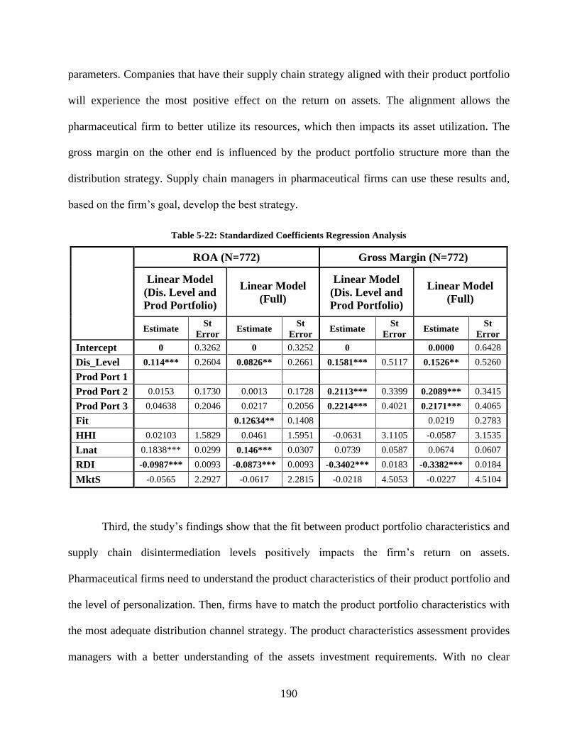
190

parameters. Companies that have their supply chain strategy aligned with their product portfolio

will experience the most positive effect on the return on assets. The alignment allows the

pharmaceutical firm to better utilize its resources, which then impacts its asset utilization. The

gross margin on the other end is influenced by the product portfolio structure more than the

distribution strategy. Supply chain managers in pharmaceutical firms can use these results and,

based on the firm’s goal, develop the best strategy.

Table 5-22: Standardized Coefficients Regression Analysis

ROA (N=772) Gross Margin (N=772)

Linear Model

(Dis. Level and

Prod Portfolio)

Linear Model

(Full)

Linear Model

(Dis. Level and

Prod Portfolio)

Linear Model

(Full)

Estimate St

Error Estimate

St

Error Estimate

St

Error Estimate

St

Error

Intercept 0 0.3262 0 0.3252 0 0.0000 0.6428

Dis_Level 0.114*** 0.2604 0.0826** 0.2661 0.1581*** 0.5117 0.1526** 0.5260

Prod Port 1

Prod Port 2 0.0153 0.1730 0.0013 0.1728 0.2113*** 0.3399 0.2089*** 0.3415

Prod Port 3 0.04638 0.2046 0.0217 0.2056 0.2214*** 0.4021 0.2171*** 0.4065

Fit 0.12634** 0.1408 0.0219 0.2783

HHI 0.02103 1.5829 0.0461 1.5951 -0.0631 3.1105 -0.0587 3.1535

Lnat 0.1838*** 0.0299 0.146*** 0.0307 0.0739 0.0587 0.0674 0.0607

RDI -0.0987*** 0.0093 -0.0873*** 0.0093 -0.3402*** 0.0183 -0.3382*** 0.0184

MktS -0.0565 2.2927 -0.0617 2.2815 -0.0218 4.5053 -0.0227 4.5104

Third, the study’s findings show that the fit between product portfolio characteristics and

supply chain disintermediation levels positively impacts the firm’s return on assets.

Pharmaceutical firms need to understand the product characteristics of their product portfolio and

the level of personalization. Then, firms have to match the product portfolio characteristics with

the most adequate distribution channel strategy. The product characteristics assessment provides

managers with a better understanding of the assets investment requirements. With no clear

191

conclusion for the most beneficial distribution strategy, the current study sheds light on some of

the ambiguity as far as the disintermediation strategy goes.

Finally, the study’s findings show the positive impact of aligning the supply chain

distribution and product portfolio. Assume a company XYZ is specializing in biologic products

and is using traditional distribution channels. By changing the distribution strategy and selecting

more direct methods, XYZ will experience an average increase of 65% on the return on assets.

Aligning a positively misfit configuration provides a 53% increase in the return on assets. The

financial analysis comparison provides managers with financial incentives for the impact of fit.

5.7.3 Limitations and Future Research

In the process of conducting the current study, several limitations were encountered. First, the data

available for the supply chain network spans from 2010 through 2013. The short span of the data

available was an obstacle in conducting a longitudinal study. In addition to that, some of the firms’

data were not available during the four years of observations. This was mainly due to new firms

entering to the stock market or other firms disappearing as a result of mergers and acquisitions. A

longitudinal study would have provided more insight for the firms and years of difference. Second,

the data available for the disintermediation level variable was derived from the Bloomberg

database. Bloomberg provides a network of the quantified buyers’ and suppliers’ relationships.

The remaining relationship dollars amount is estimated from the firm’s customers and suppliers

list. This approximation was used to finalize the level of the relationships. Third, the product

portfolio approximation was estimated from the firms’ annual reports. The product portfolio was

coded into three levels. When coding the variables, the amount of information explained is

reduced. Finally, the data obtained did not provide the distribution channels per product class. In

fact, for a firm with a hybrid product portfolio and hybrid distribution channel strategy, the study

192

couldn’t separate the products being shipped directly versus the products distributed through the

wholesales. Despite the apparent fit existing between the product portfolio and supply chain

strategy, the pharmaceutical firm could be distributing a biologic product via intermediated

channels and traditional medication via a direct sales model.

The limitations discussed provide additional areas of research direction. First, the concept

of supply chain disintermediation is gaining interest in other industries, such as automobile,

besides pharmaceuticals. A more exhaustive study that contains several industries constitutes a

prominent area of additional investigation. In fact, with the multiple distribution channel

opportunities and the variety of products and service bundles that businesses offer, firms are

working hard to identify the appropriate distribution strategy. Second, the supply chain

disintermediation becomes more complicated when firms have global sales. In fact, answering the

question of the best distribution channel becomes less trivial in a global context. Third, research

on fit in the context of supply chain is gaining more attention. The current study can represent a

start of new supply chain and product paradigm fit. The personalization level product paradigm

can be assessed in a manufacturing context. The fit between the product paradigm and

manufacturing strategy and capabilities represents an interesting area of study. Finally, the study

of the supply chain disintermediation can have more conceptual and methodological richness.

Supply chain disintermediation can be assessed from a network perspective. The supply chain

network represents a complex adaptive system. Complex adaptive systems focus on the “interplay

between a system and its environment and the co-evolution of both the system and the

environment” (Choi et al., 2001). In other words, supply chain disintermediation impacts the

organization network and its whole evolution.

193

194

Reference List

Abdi, H., & Williams, L. (2010). Contrast Analysis. Thousand Oaks, CA: SAGE Publications, Inc.

Aberson, C. L. (2011). Applied power analysis for the behavioral sciences: Routledge.

Adolphs, C., & Winkelmann, A. (2010). Personalization research in E-commerce—a state of the art review

(2000–2008). Journal of Electronic Commerce Research, 11(4), 326-341.

Adomavicius, G., & Tuzhilin, A. (2005). Personalization technologies: a process-oriented perspective.

Communications of the ACM, 48(10), 83-90.

Ajay, D., Matthias, E., & Martin, M. (2012). Escaping the sword of Damocles: Toward a new future for

pharmaceutical R&D McKinsey perspectives on drug and device R&D 2012: McKinsey

Alazraki, M. (2011). The 10 Biggest-Selling Drugs That Are About to Lose Their Patent.

http://www.dailyfinance.com/2011/02/27/top-selling-drugs-are-about-to-lose-patent-protection-

ready/

Alexander, J. W., & Randolph, W. A. (1985). The fit between technology and structure as a predictor of

performance in nursing subunits. Academy of Management Journal, 28(4), 844-859.

Allen, C., Yaeckel, B., & Kania, D. (1998). Internet world guide to one-to-one web marketing: John Wiley

& Sons, Inc.

Altay, N., & Green III, W. G. (2006). OR/MS research in disaster operations management. European

Journal of Operational Research, 175(1), 475-493.

Ameri, F., & Dutta, D. (2005). Product lifecycle management: closing the knowledge loops. Computer-

Aided Design and Applications, 2(5), 577-590.

American Cancer Society. (2013). Understanding Biologic Medicines From the Cancer Patient Perspective.

Anderson, E. W., Fornell, C., & Rust, R. T. (1997). Customer satisfaction, productivity, and profitability:

differences between goods and services. Marketing science, 16(2), 129-145.

Atkinson, R. D. (2001). The revenge of the disintermediated: How the middleman is fighting e-commerce

and hurting consumers. Policy Paper (Washington, DC: Progressive Policy Institute.

Bakos, Y. (1998). The emerging role of electronic marketplaces on the Internet. Communications of the

ACM, 41(8), 35-42.

Baltagi, B. (2008). Econometric analysis of panel data (Vol. 1): John Wiley & Sons.

Bateson, J. E., & Hoffman, K. D. (1991). Managing services marketing: Text and readings: Dryden Press.

Begley, S. (2012). Exclusive: Questionable data propped up cancer drug Provenge. from

http://www.reuters.com/article/2012/10/11/us-drugs-dendreon-provenge-

idUSBRE89A15420121011

Benjamin, R., & Wigand, R. (1995). Electronic markets and virtual value chains on the information

superhighway. Sloan Management Review (Winter, 1995).

195

Berman, O., Larson, R. C., & Fouska, N. (1992). Optimal location of discretionary service facilities.

Transportation Science, 26(3), 201-211.

Bharadwaj, A. S., Bharadwaj, S. C., & Konsynski, B. R. (1999). Information Technology Effects on Firm

Performance as Measured by Tobin's q. Management Science, 45(7), 1008-1024.

Boyer, K. K., Bozarth, C., & McDermott, C. (2000). Configurations in operations: an emerging area of

study. Journal of Operations Management, 18(6), 601-604.

Brabazon, T., Winter, M., & Gandy, B. (2014). Disintermediation and Reintermediation: From Professional

to Amateur to Professional Digital Wine (pp. 39-42): Springer Singapore.

Brandeau, M. L., & Chiu, S. S. (1989). An overview of representative problems in location research.

Management Science, 35(6), 645-674.

Brown, M. B., & Forsythe, A. B. (1974). Robust tests for the equality of variances. Journal of the American

Statistical Association, 69(346), 364-367.

Burns, L. R. (2002). The health care value chain: producers, purchasers, and providers: Jossey-Bass.

Burton, R. M., Lauridsen, J., & Obel, B. (2002). Return on assets loss from situational and contingency

misfits. Management Science, 48(11), 1461-1485.

Casella, G. (2008). Statistical design: Springer Science & Business Media.

Center for Drug Evaluation and Research, F. (1998). Manual of Policies and Procedures: Food and Drug

Administration.

Chaudhuri, A., & Lillrank, P. (2013). Mass personalization in healthcare: insights and future research

directions. Journal of Advances in Management Research, 10(2), 176-191.

Chen, H., Frank, M. Z., & Wu, O. Q. (2005). What actually happened to the inventories of American

companies between 1981 and 2000? Management Science, 51(7), 1015-1031.

Chen, Y., Vakharia, A. J., & Alptekinoǧlu, A. (2008). Product portfolio strategies: the case of multifunction

products. Production and Operations Management, 17(6), 587-598.

Cherici, C., Frazier, J., & Feldman, M. (2011). Navigating Drug Shortages in American Healthcare: A

Premier Healthcare Alliance Analysis. Premier Inc., March.

Chiang, W.-y. K. (2012). Supply Chain Dynamics and Channel Efficiency in Durable Product Pricing and

Distribution. Manufacturing & Service Operations Management, 14(2), 327-343.

Chircu, A. M., & Kauffman, R. J. (1999). Strategies for Internet middlemen in the

intermediation/disintermediation/reintermediation cycle. Electronic Markets, 9(1-2), 109-117.

Chircu, A. M., & Kauffman, R. J. (2000). Reintermediation strategies in business-to-business electronic

commerce. International Journal of Electronic Commerce, 4(4), 7-42.

Choi, S.-Y., Stahl, D. O., & Whinston, A. B. (1997). The economics of electronic commerce: Macmillan

Technical Publishing Indianapolis.

196

Choi, T. Y., Dooley, K. J., & Rungtusanatham, M. (2001). Supply networks and complex adaptive systems:

control versus emergence. Journal of Operations Management, 19(3), 351-366.

Chopra, S., & Meindl, P. (2007). Supply chain management : strategy, planning, and operation. Upper

Saddle River, N.J.: Pearson Prentice Hall.

Chow, G. C. (1960). Tests of equality between sets of coefficients in two linear regressions. Econometrica:

Journal of the Econometric Society, 591-605.

Christofides, N. (1975). Graph theory: An algorithmic approach (Vol. 8): Academic press New York.

Church, R., & Velle, C. R. (1974). The maximal covering location problem. Papers in regional science,

32(1), 101-118.

Clemons, E. K., & Row, M. C. (1991). Information Technology at Rosenbluth Travel: Competitive

Advantage in a Rapidly Growing Global Service Company. Journal of Management Information

Systems, 8(2), 53-79.

Closs, D. J., Jacobs, M. A., Swink, M., & Webb, G. S. (2008). Toward a theory of competencies for the

management of product complexity: six case studies. Journal of Operations Management, 26(5),

590-610.

Coe, N. M., & Hess, M. (2005). The internationalization of retailing: implications for supply network

restructuring in East Asia and Eastern Europe. Journal of Economic Geography, 5(4), 449-473.

Cohen, J. (2013). Statistical power analysis for the behavioral sciences: Academic press.

Coner, A. (2003). Personalization and customization in financial portals. Journal of American Academy of

Business, 2(2), 498-504.

Cooper, P. W. (2008). Pharma 2020: marketing the future: which path will you take. See http://www. pwc.

com/gx/en/forms/gxengallspharma2020. jhtml.

Cooper, R. G., Edgett, S. J., & Kleinschmidt, E. J. (1999). New product portfolio management: practices

and performance. Journal of product innovation management, 16(4), 333-351.

Cort, S. G. (1999). Industry Corner: Industrial Distribution: How Goods Will Go to Market in the Electronic

Marketplace. Business Economics, 34(1), 53.

Coughlan, A. T., Choi, S. C., Chu, W., Ingene, C. A., Moorthy, S., Padmanabhan, V., . . . Zhang, Z. J.

(2010). Marketing modeling reality and the realities of marketing modeling. Marketing Letters,

21(3), 317-333.

Cuttler, L., Marinova, D., Mercer, M. B., Connors, A., Meehan, R., & Silvers, J. B. (2009). Patient,

physician, and consumer drivers: referrals for short stature and access to specialty drugs. Medical

care, 47(8), 858-865.

Danzon, P. M., & Nicholson, S. (2012). The Oxford handbook of the economics of the biopharmaceutical

industry: Oxford University Press.

Daskin, M. S., & Dean, L. K. (2004). Location of health care facilities Operations research and health care

(pp. 43-76): Springer.

197

Daskin, M. S., & Stern, E. H. (1981). A hierarchical objective set covering model for emergency medical

service vehicle deployment. Transportation Science, 15(2), 137-152.

Davenport, T. H., & Klahr, P. (1998). Managing customer support knowledge. California management

review, 40, 195-208.

Day, G. S. (1977). Diagnosing the product portfolio. the Journal of Marketing, 29-38.

Declerck, P. (2012). Biologicals and biosimilars: a review of the science and its implications. GABI.

GENERICS AND BIOSIMILARS INITIATIVE JOURNAL, 1(1), 13-16.

Dehning, B., Richardson, V. J., & Zmud, R. W. (2007). The financial performance effects of IT-based

supply chain management systems in manufacturing firms. Journal of Operations Management,

25(4), 806-824. doi: 10.1016/j.jom.2006.09.001

Delfmann, W., Albers, S., & Gehring, M. (2002). The impact of electronic commerce on logistics service

providers. International Journal of Physical Distribution & Logistics Management, 32(3), 203-

222.

Deniz, B., Karaesmen, I., & Scheller-Wolf, A. (2010). Managing perishables with substitution: inventory

issuance and replenishment heuristics. Manufacturing & Service Operations Management, 12(2),

319-329.

Dewan, R., Jing, B., & Seidmann, A. (2000). Adoption of Internet-based product customization and pricing

strategies. Journal of Information Management Systems, 9-28.

Dietz, E. (2004). Trends in employer-provided prescription-drug coverage. Monthly Lab. Rev., 127, 37.

DiMasi, J. A., Hansen, R. W., & Grabowski, H. G. (2003). The price of innovation: new estimates of drug

development costs. Journal of health economics, 22(2), 151-186.

Dixon, W. J. (1960). Simplified estimation from censored normal samples. The Annals of Mathematical

Statistics, 31(2), 385-391.

Dooley, K. (2001). Social research methods. Paper presented at the 4 th ed. Upper Saddle River, NJ.

Doty, D. H., Glick, W. H., & Huber, G. P. (1993). Fit, equifinality, and organizational effectiveness: A test

of two configurational theories. Academy of Management Journal, 36(6), 1196-1250.

Drucker, P. (2013). Managing for the Future: Routledge.

Dutta, S., Sarmah, S., & Goyal, S. (2010). Evolutionary stability of auction and supply chain contracting:

An analysis based on disintermediation in the Indian tea supply chains. European Journal of

Operational Research, 207(1), 531-538.

Eggers, J. P. (2012). All experience is not created equal: learning, adapting, and focusing in product

portfolio management. Strategic Management Journal, 33(3), 315-335.

Eisenhardt, K. M. (1989). Agency theory: An assessment and review. Academy of management review,

14(1), 57-74.

198

Eng, G., Chen, A., Vess, T., & Ginsburg, G. S. (2012). Genome technologies and personalized dental

medicine. Oral diseases.

Enyinda, C. I., & Tolliver, D. (2009). Taking counterfeits out of the pharmaceutical supply chain in Nigeria:

Leveraging multilayer mitigation approach. Journal of African Business, 10(2), 218-234.

Erengüç, Ş. S., Simpson, N. C., & Vakharia, A. J. (1999). Integrated production/distribution planning in

supply chains: An invited review. European journal of operational research, 115(2), 219-236.

Fang, X., & Salvendy, G. (2003). Customer-centered rules for design of e-commerce Web sites.

Communications of the ACM, 46(12), 332-336.

Farris, P. W., Bendle, N. T., Pfeifer, P. E., & Reibstein, D. J. (2010). Marketing metrics: The definitive

guide to measuring marketing performance: Pearson Education.

Faul, F., Erdfelder, E., Buchner, A., & Lang, A.-G. (2009). Statistical power analyses using G* Power 3.1:

Tests for correlation and regression analyses. Behavior research methods, 41(4), 1149-1160.

Faul, F., Erdfelder, E., Lang, A.-G., & Buchner, A. (2007). G* Power 3: A flexible statistical power analysis

program for the social, behavioral, and biomedical sciences. Behavior research methods, 39(2),

175-191.

Fein, A. J. (2012). Trends and top distributors in the pharmaceuticals sector. Retrieved 06-05, 2013, from

http://www.mdm.com/2012-mdm-market-leaders-top-pharmaceuticals-distributors

Fernhaber, S. A., & Patel, P. C. (2012). How do young firms manage product portfolio complexity? The

role of absorptive capacity and ambidexterity. Strategic Management Journal, 33(13), 1516-1539.

Fink, J., Koenemann, J., Noller, S., & Schwab, I. (2002). Putting personalization into practice.

Communications of the ACM, 45(5), 41-42.

Fisher, M. L. (1997). What is the right supply chain for your product? Harvard Business Review, 75, 105-

117.

Fitzgerald, C. Q., & McLaughlin, C. P. (2001). Custom Medicine for the Masses. Pharmaceutical

Executive, 21(12), 64-68.

Fitzsimmons, J. A. (1973). A methodology for emergency ambulance deployment. Management Science,

19(6), 627-636.

Fixson, S. K. (2005). Product architecture assessment: a tool to link product, process, and supply chain

design decisions. Journal of Operations Management, 23(3), 345-369.

Frohlich, M. T., & Dixon, J. R. (2001). A taxonomy of manufacturing strategies revisited. Journal of

Operations Management, 19(5), 541-558.

Fullerton, R. R., McWatters, C. S., & Fawson, C. (2003). An examination of the relationships between JIT

and financial performance. Journal of Operations Management, 21(4), 383-404.

Gaur, V., Fisher, M. L., & Raman, A. (2005). An econometric analysis of inventory turnover performance

in retail services. Management Science, 51(2), 181-194.

199

Gautrin, P. (2002). Challenges Facing a Pharmaceutical Supply Chain. Logistics Quarterly, 8(4).

Gebicki, M., Mooney, E., Chen, S.-J. G., & Mazur, L. M. (2013). Evaluation of hospital medication

inventory policies. Health care management science, 1-15.

Gehani, R. R. (2000). Significance of cross-cultural trust in streamlining supply-chains for global

enterprises. Global business review, 1(2), 173-192.

Gellman, R. (1996). Disintermediation and the Internet. Government Information Quarterly, 13(1), 1-8.

Ghosh, D., & Vogt, A. (2012). Outliers: An evaluation of methodologies. Paper presented at the Joint

Statistical Meetings.

Gilmore, J. H., & Pine 2nd, B. (1997). The four faces of mass customization. Harvard Business Review,

75(1), 91.

Ginsburg, G. S., & Willard, H. F. (2009). Genomic and personalized medicine: foundations and

applications. Translational Research, 154(6), 277-287.

Goetschalckx, M., Vidal, C. J., & Dogan, K. (2002). Modeling and design of global logistics systems: A

review of integrated strategic and tactical models and design algorithms. European journal of

operational research, 143(1), 1-18.

Grabowski, H., Cockburn, I., & Long, G. (2006). The market for follow-on biologics: how will it evolve?

Health Affairs, 25(5), 1291-1301.

Grabowski, H., Vernon, J., & DiMasi, J. A. (2002). Returns on research and development for 1990s new

drug introductions. Pharmacoeconomics, 20(3), 11-29.

Hager, W. (2006). The fallibility of empirical data and the need for controlling for false decisions.

Zeitschrift fur Psychologie, 214(1), 10-23.

Halbert, D. (2006). Two Faces of Disintermediation: Corporate Control or Accidental Anarchy. Mich. St.

L. Rev., 83.

Hall, R., Belson, D., Murali, P., & Dessouky, M. (2006). Modeling patient flows through the healthcare

system Patient flow: Reducing delay in healthcare delivery (pp. 1-44): Springer.

Hanson, W., & Kalyanam, K. (2007). Principles of Internet marketing: South-Western College Publishing.

Harnisch, M. J. (2013). Classifying Personalization Constraints in Digital Business Environments through

Case Study Research. International Journal, 4.

Hayes, S., & Wheelwright, R. (1979). Link manufacturing process and product life cycles. Harvard

business review, 57(1), 133-265.

Hayter, A. J. (1986). The maximum familywise error rate of Fisher's least significant difference test.

Journal of the American Statistical Association, 81(396), 1000-1004.

Heese, H. S. (2007). Inventory record inaccuracy, double marginalization, and RFID adoption. Production

and Operations Management, 16(5), 542-553.

200

Henderson, R., & Cockburn, I. (1996). Scale, scope, and spillovers: the determinants of research

productivity in drug discovery. The Rand journal of economics, 32-59.

Hendricks, K. B., & Singhal, V. R. (2003). The effect of supply chain glitches on shareholder wealth.

Journal of Operations Management, 21(5), 501-522.

Hesse, B. W., O'Connell, M., Augustson, E. M., Chou, W.-Y. S., Shaikh, A. R., & Finney Rutten, L. J.

(2011). Realizing the promise of Web 2.0: engaging community intelligence. Journal of health

communication, 16(sup1), 10-31.

Hill, C. W., & Hansen, G. S. (1991). A longitudinal study of the cause and consequences of changes in

diversification in the US pharmaceutical industry 1977–1986. Strategic Management Journal,

12(3), 187-199.

Hodgson, M. J. (1990). A Flow‐Capturing Location‐Allocation Model. Geographical Analysis, 22(3), 270-

279.

Hoffman, T. (1995). No more middlemen. Computerworld, 55, 55.

Homburg, C., Steiner, V. V., & Totzek, D. (2009). Managing dynamics in a customer portfolio. Journal of

Marketing, 73(5), 70-89.

Horton, B. (2010). PRESCRIBING HIGH PERFORMANCE FOR THE PHARMACEUTICAL SUPPLY

CHAIN. Supply Chain Europe, 19(2), 15-17.

Hsia, P., Samuel, J., Gao, J., Kung, D., Toyoshima, Y., & Chen, C. (1994). Formal approach to scenario

analysis. IEEE Software, 11(2), 33-41.

Hu, S. J. (2013). Evolving Paradigms of Manufacturing: From Mass Production to Mass Customization and

Personalization. Procedia CIRP, 7, 3-8.

Huang, X., Kristal, M. M., & Schroeder, R. G. (2008). Linking learning and effective process

implementation to mass customization capability. Journal of Operations Management, 26(6), 714-

729.

Huber, P. J. (1973). Robust regression: asymptotics, conjectures and Monte Carlo. The Annals of Statistics,

799-821.

Hughes, B., Joshi, I., & Wareham, J. (2008). Health 2.0 and Medicine 2.0: tensions and controversies in the

field. Journal of Medical Internet Research, 10(3).

IBIS. (2014). Global Pharmaceuticals & Medicine Manufacturing: Market Research Report: IBIS World

Imhoff, C., Loftis, L., Geiger, J. G., & Imhoff, D. C. (2001). Building the customer-centric enterprise: Data

warehousing techniques for supporting customer relationship management: Wiley.

IMS_Health. (2014). The Pharmaceutical Industry in the United States.

Isidore, C. (2013). Pfizer to start selling Viagra online, CNN Money.

Jacobs, F. R., & Chase, R. B. (2010). Operations and supply management: The core: McGraw-Hill Irwin

New York, NY.

201

Jacobs, M. A., & Swink, M. (2011). Product portfolio architectural complexity and operational

performance: Incorporating the roles of learning and fixed assets. Journal of Operations

Management, 29(7), 677-691.

Jetly, G., Rossetti, C. L., & Handfield, R. (2012). A multi-agent simulation of the pharmaceutical supply

chain. Journal of Simulation, 6(4), 215-226.

Jeuland, A. P., & Shugan, S. M. (1983). Managing channel profits. Marketing science, 2(3), 239-272.

Jia, H., Ordóñez, F., & Dessouky, M. (2007). A modeling framework for facility location of medical

services for large-scale emergencies. IIE transactions, 39(1), 41-55.

Jiao, R. J. (2011). Prospect of design for mass customization and personalization.

Johnson, E. M. (1969). Are goods and services different? : an exercise in marketing theory. Available from

http://worldcat.org /z-wcorg/ database.

Johnson, M. D., & Selnes, F. (2004). Customer portfolio management: toward a dynamic theory of

exchange relationships. Journal of Marketing, 68(2), 1-17.

Kantoff, P. W., Higano, C. S., Shore, N. D., Berger, E. R., Small, E. J., Penson, D. F., . . . Schellhammer,

P. F. (2010). Sipuleucel-T Immunotherapy for Castration-Resistant Prostate Cancer. New England

Journal of Medicine, 363(5), 411-422. doi: doi:10.1056/NEJMoa1001294

Karnopp, D. C., Margolis, D. L., & Rosenberg, R. C. (2012). System Dynamics: Modeling, Simulation, and

Control of Mechatronic Systems: Wiley.

Kim, H., & Dionne, R. A. (2009). Individualized pain medicine. Drug Discovery Today: Therapeutic

Strategies, 6(3), 83-87.

Kim, Y. H., & Henderson, D. (2015). Financial benefits and risks of dependency in triadic supply chain

relationships. Journal of Operations Management, 36, 115-129.

King, B., & Zhang, X. (2007). Securing the pharmaceutical supply chain using RFID. Paper presented at

the Multimedia and Ubiquitous Engineering, 2007. MUE'07. International Conference on.

Kinney, M. R., & Wempe, W. F. (2002). Further evidence on the extent and origins of JIT's profitability

effects. The Accounting Review, 77(1), 203-225.

Kirk, R. E. (1982). Experimental design: Wiley Online Library.

Klose, A., & Drexl, A. (2005). Facility location models for distribution system design. European Journal

of Operational Research, 162(1), 4-29.

Koh, R., Schuster, E. W., Chackrabarti, I., & Bellman, A. (2003). Securing the pharmaceutical supply chain.

White Paper, Auto-ID Labs, Massachusetts Institute of Technology.

Konstantinos, K., Vrassidas, L., & Dimitra, V. (2008). Supplier selection in pharmaceutical industry: An

analytic network process approach. Benchmarking: An International Journal, 15(4), 494-516.

Koppenjan, J. F. M., & Klijn, E.-H. (2004). Managing uncertainties in networks: a network approach to

problem solving and decision making: Psychology Press.

202

Kotler, P. (1989). From mass marketing to mass customization. Strategy & Leadership, 17(5), 10-47.

Koufteros, X. A. (1999). Testing a model of pull production: a paradigm for manufacturing research using

structural equation modeling. Journal of Operations Management, 17(4), 467-488. doi:

http://dx.doi.org/10.1016/S0272-6963(99)00002-9

Koufteros, X. A., Vonderembse, M. A., & Doll, W. J. (1998). Developing measures of time-based

manufacturing. Journal of Operations Management, 16(1), 21-41.

Kraemer, K. L., Dedrick, J., & Yamashiro, S. (2000). Refining and extending the business model with

information technology: Dell Computer Corporation. The Information Society, 16(1), 5-21.

Kumar, A. (2004). Mass customization: metrics and modularity. International Journal of Flexible

Manufacturing Systems, 16(4), 287-311.

Kumar, A. (2007). From mass customization to mass personalization: a strategic transformation.

International Journal of Flexible Manufacturing Systems, 19(4), 533-547.

Kumar, S., Kadow, B. B., & Lamkin, M. K. (2011). Challenges with the introduction of radio-frequency

identification systems into a manufacturer's supply chain - a pilot study. Enterprise Information

Systems, 5(2), 235-253. doi: 10.1080/17517575.2010.536262

Kuo, C. C., & White, R. E. (2004). A Note on the Treatment of the Center‐of‐Gravity Method in Operations

Management Textbooks. Decision Sciences Journal of innovative education, 2(2), 219-227.

Lampel, J., & Mintzberg, H. (1996). Customizing Customization. Sloan Management Review, 38(1), 21-

30.

Law, R., Leung, K., & Wong, R. (2004). The impact of the internet on travel agencies. International Journal

of Contemporary Hospitality Management, 16(2), 100-107.

Lee, H. L. (2002). Aligning supply chain strategies with product uncertainties. California management

review, 44(3), 105-119.

Lee, H. L., & Tang, C. S. (1997). Modelling the costs and benefits of delayed product differentiation.

Management Science, 43(1), 40.

Leng, M., & Parlar, M. (2009). Allocation of cost savings in a three-level supply chain with demand

information sharing: A cooperative-game approach. Operations Research, 57(1), 200-213.

Levi, D. S., Kaminsky, P., & Levi, E. S. (2003). Designing and managing the supply chain: Concepts,

strategies, and case studies: McGraw-Hill.

Levine, T. R., & Hullett, C. R. (2002). Eta squared, partial eta squared, and misreporting of effect size in

communication research. Human Communication Research, 28(4), 612-625.

Lewis, I. (2001). Logistics and electronic commerce: an interorganizational systems perspective.

Transportation Journal, 5-13.

Lipsy, R. J., Schapiro, R. T., & Prostko, C. R. (2009). Current and future directions in MS management:

key considerations for managed care pharmacists. Journal of Managed Care Pharmacy, 15(9).

203

Littell, R., Freund, R., & Spector, P. (1991). SAS system for linear models. SAS Inst. Inc., Cary, NC.

Liu, G., Shah, R., & Schroeder, R. G. (2006). Linking Work Design to Mass Customization: A

Sociotechnical Systems Perspective. Decision Sciences, 37(4), 519-545.

Liu, X., Yeung, A. C. L., Lo, C. K. Y., & Cheng, T. C. E. (2014). The moderating effects of knowledge

characteristics of firms on the financial value of innovative technology products. Journal of

Operations Management, 32(3), 79-87. doi: 10.1016/j.jom.2013.11.003

Lo, S. M., & Power, D. (2010). An empirical investigation of the relationship between product nature and

supply chain strategy. Supply Chain Management, 15(2), 139-153. doi:

10.1108/13598541011028741

MacCarthy, B., Brabazon, P. G., & Bramham, J. (2003). Fundamental modes of operation for mass

customization. International Journal of Production Economics, 85(3), 289-304.

MacMillan, I. C., Hambrick, D. C., & Day, D. L. (1982). The product portfolio and profitability—a PIMS-

based analysis of industrial-product businesses. Academy of Management Journal, 25(4), 733-755.

Approval Letter - Provenge (2010).

Malone, T. W., Yates, J., & Benjamin, R. I. (1987). Electronic markets and electronic hierarchies.

Communications of the ACM, 30(6), 484-497.

Maranzana, F. (1964). On the location of supply points to minimize transport costs. OR, 261-270.

Mason-Jones, R., Naylor, B., & Towill, D. R. (2000). Engineering the leagile supply chain. International

Journal of Agile Management Systems, 2(1), 54-61.

Maxwell, S. E., & Delaney, H. D. (2004). Designing experiments and analyzing data: A model comparison

perspective (Vol. 1): Psychology Press.

McGrath, M. (2000). Product strategy for high technology companies: McGraw Hill Professional.

Mckone‐Sweet, K., & Lee, Y. T. (2009). Development and analysis of a supply chain strategy taxonomy.

Journal of Supply Chain Management, 45(3), 3-24.

Mellstedt, H., Niederwieser, D., & Ludwig, H. (2008). The challenge of biosimilars. Annals of oncology,

19(3), 411-419.

Melo, M. T., Nickel, S., & Saldanha-da-Gama, F. (2009). Facility location and supply chain management–

A review. European Journal of Operational Research, 196(2), 401-412.

Mete, H. O., & Zabinsky, Z. B. (2010). Stochastic optimization of medical supply location and distribution

in disaster management. International Journal of Production Economics, 126(1), 76-84.

Mette, L., Mitropoulos, K., Vozikis, A., & Patrinos, G. P. (2012). Pharmacogenomics and public health:

implementing ‘populationalized’medicine. Pharmacogenomics, 13(7), 803-813.

Meyer, M. H. (1997). The power of product platforms: Simon and Schuster.

204

Modi, S. B., & Mishra, S. (2011). What drives financial performance–resource efficiency or resource

slack?: Evidence from US Based Manufacturing Firms from 1991 to 2006. Journal of Operations

Management, 29(3), 254-273.

Möllering, K., & Thonemann, U. (2010). An optimal constant level rationing policy under service level

constraints. OR Spectrum, 32(2), 319-341. doi: 10.1007/s00291-009-0167-6

Montgomery, D. C. (1984). Design and analysis of experiments (Vol. 7): Wiley New York.

Moon, J., Chadee, D., & Tikoo, S. (2008). Culture, product type, and price influences on consumer purchase

intention to buy personalized products online. Journal of Business Research, 61(1), 31-39.

Moon, S. K., Shu, J., Simpson, T. W., & Kumara, S. R. T. (2011). A module-based service model for mass

customization: service family design. IIE Transactions, 43(3), 153-163.

Moser, K. (2007). Mass customization strategies. Development of a Competence-Based Framework for

Identifving Different Mass Customization Strategies.

Muller, J., Popke, C., Urbat, M., Zeier, A., & Plattner, H. (2009). A simulation of the pharmaceutical supply

chain to provide realistic test data. Paper presented at the Advances in System Simulation, 2009.

SIMUL'09. First International Conference on.

Mullin, R. (2003). SERVICE PROVIDERS MOVE UPSTREAM. (cover story). Chemical & Engineering

News, 81(16), 35.

Murray, B., & Gerhart, B. (1998). An empirical analysis of a skill-based pay program and plant performance

outcomes. Academy of Management Journal, 41(1), 68-78.

Murray, K. B., & Schlacter, J. L. (1990). The impact of services versus goods on consumers’ assessment

of perceived risk and variability. Journal of the Academy of Marketing Science, 18(1), 51-65.

Murthi, B., & Sarkar, S. (2003). The role of the management sciences in research on personalization.

Management Science, 49(10), 1344-1362.

Nagy, G., & Salhi, S. (2007). Location-routing: Issues, models and methods. European Journal of

Operational Research, 177(2), 649-672.

Nahmias, S. (1982). Perishable inventory theory: A review. Operations Research, 30(4), 680-708.

Narasimhan, R., Kim, S. W., & Tan, K. C. (2008). An empirical investigation of supply chain strategy

typologies and relationships to performance. International Journal of Production Research, 46(18),

5231-5259.

NDSF. (2014). NDSF Coordinate Conversion Utility.

Nicolau, J. L. (2013). Direct versus indirect channelsDifferentiated loss aversion in a high-involvement,

non-frequently purchased hedonic product. European Journal of Marketing, 47(1/2), 260-278. doi:

10.1108/03090561311285547

Nissen, M. (2000). Agent-based supply chain disintermediation versus re-intermediation: economic and

technological perspectives. International Journal of Intelligent Systems in Accounting, Finance &

Management, 9(4), 237-256.

205

Niziolek, L., Chiam, T. C., & Yih, Y. (2012). A simulation-based study of distribution strategies for

pharmaceutical supply chains. IIE Transactions on Healthcare Systems Engineering, 2(3), 181-

189.

Nordin, F., Brozovic, D., & Holmlund, M. (2013). Disintermediation in Business-to-Business Service

Channels: Mechanisms and Challenges. Journal of Business-to-Business Marketing, 20(4), 179-

192.

Olkin, I. (1960). Contributions to probability and statistics: essays in honor of Harold Hotelling: Stanford

University Press.

Oral, M., Salvador, M. S., Reisman, A., & Dean, B. V. (1972). ON THE EVALUATION OF SHORTAGE

COSTS FOR INVENTORY CONTROL OF FINISHED GOODS. Management Science, 18(6), B-

344-B-351.

OReilly, T. (2007). What is Web 2.0: Design patterns and business models for the next generation of

software. Communications & strategies(1), 17.

Papageorgiou, L. G., Rotstein, G. E., & Shah, N. (2001). Strategic supply chain optimization for the

pharmaceutical industries. Industrial & Engineering Chemistry Research, 40(1), 275-286.

Parasuraman, A., Zeithaml, V. A., & Berry, L. L. (1985). A conceptual model of service quality and its

implications for future research. the Journal of Marketing, 41-50.

Park, H. M. (2005). Linear regression models for panel data using SAS, Stata, LIMDEP, and SPSS. Indiana

University.

Pedroso, M. C., & Nakano, D. (2009). Knowledge and information flows in supply chains: A study on

pharmaceutical companies. International Journal of Production Economics, 122(1), 376-384. doi:

10.1016/j.ijpe.2009.06.012

Peng, D. X., Liu, G., & Heim, G. R. (2011). Impacts of information technology on mass customization

capability of manufacturing plants. International Journal of Operations & Production

Management, 31(10), 1022-1047.

Peppers, D., & Rogers, M. (2012). The one to one fieldbook: Random House Digital, Inc.

Peters, C. C., & Van Voorhis, W. R. (1940). Statistical procedures and their mathematical bases.

Peterson, R., & Silver, E. A. (1979). Decision systems for inventory management and production planning:

Wiley New York.

Pierrakos, D., Paliouras, G., Papatheodorou, C., & Spyropoulos, C. D. (2003). Web usage mining as a tool

for personalization: A survey. User Modeling and User-Adapted Interaction, 13(4), 311-372.

Pine, B. J. (1993). Mass customizing products and services. Planning Review, 22(4), 6.

Pine, B. J., & Davis, S. (1999). Mass customization: the new frontier in business competition: Harvard

Business Press.

Pine, J. (1993). Mass Customization: The New Frontier in Business Competition. Harvard Business School

Press, Cambridge, MA.

206

Pinto, J. (2000). Disintermediation-II; the customer perspective: Dell Publishing Company.

Pitts, P., & Stark, R. (2012). Biosimilars: The Precarious Struggle between Cost-driven Health Care Policy

and Patient-centered Care: Washington Policy Center.

Plosker, G. (2011). Sipuleucel-T. Drugs, 71(1), 101-108. doi: 10.2165/11206840-000000000-00000

Prahalad, C. K. (1998). Managing discontinuities: The emerging challenges. Research Technology

Management, 41(3), 14-22.

Raafat, F. (1991). Survey of literature on continuously deteriorating inventory models. Journal of the

Operational Research Society, 27-37.

Railsback, S. F., Lytinen, S. L., & Jackson, S. K. (2006). Agent-based simulation platforms: Review and

development recommendations. Simulation, 82(9), 609-623.

Raymond, M. A., & Tanner Jr, J. F. (1994). Selling and Sales Management in Action: Maintaining

Customer Relationships in Direct Sales: Stimulating Repeat Purchase Behavior. Journal of

Personal Selling & Sales Management, 14(4), 67-76.

Reeves, P., Tuck, C., & Hague, R. (2011). Additive Manufacturing for Mass Customization Mass

Customization (pp. 275-289): Springer.

Reichheld, F. F., & Schefter, P. (2000). E-loyalty. Harvard Business Review, 78(4), 105-113.

Reisman, L. (2002). Pharmaceutical Industry Wholesale & Distribution. Logistics & Transport Focus, 4(4),

36-41.

Ricci, F., & Werthner, H. (2006). Introduction to the special issue: recommender systems. International

Journal of Electronic Commerce, 11(2), 5-9.

Riemer, D.-W.-I. K., & Totz, C. (2003). The many faces of personalization The Customer Centric

Enterprise (pp. 35-50): Springer.

Roberts, M. L., & Zahay, D. (2003). Internet marketing: integrating online and offline strategies: McGraw-

Hill/Irwin.

Robison, C., & Vernachio, K. Pharmacy Benefit Management Encyclopedia of Clinical Pharmacy (pp.

741-748): Taylor & Francis.

Rossetti, C. L., & Choi, T. Y. (2008). Supply management under high goal incongruence: An empirical

examination of disintermediation in the aerospace supply chain. Decision Sciences, 39(3), 507-540.

Rossetti, C. L., Handfield, R., & Dooley, K. J. (2011). Forces, trends, and decisions in pharmaceutical

supply chain management. International Journal of Physical Distribution & Logistics

Management, 41(6), 601-622. doi: 10.1108/09600031111147835

Rothaermel, F. T., Hitt, M. A., & Jobe, L. A. (2006). Balancing vertical integration and strategic

outsourcing: effects on product portfolio, product success, and firm performance. Strategic

Management Journal, 27(11), 1033-1056.

207

Roughead, E. E., Lopert, R., & Sansom, L. N. (2007). Prices for innovative pharmaceutical products that

provide health gain: A comparison between Australia and the United States. Value in Health, 10(6),

514-520.

Ruane, F., & Zhang, X. (2007). Location Choices of the Pharmaceutical Industry in Europe after 1992: IIIS.

Sabberwal, R., & Chan, Y. E. (2001). Alignment Between Business and IS Strategies: A Study of

Prospectors, Analyzers, and Defenders. Information Systems Research, 12(1), 11.

Salkind, N. J. (2010). Encyclopedia of research design (Vol. 1): Sage.

Salvador, F., De Holan, P. M., & Piller, F. (2009). Cracking the Code of Mass Customization. MIT Sloan

Management Review, 50(3), 71-78.

Sarkar, M. B., Butler, B., & Steinfield, C. (1995). Intermediaries and cybermediaries: a continuing role for

mediating players in the electronic marketplace. Journal of computer-mediated communication,

1(3), 1-14.

Schubert, P. (2003). Extended web assessment method (EWAM): evaluation of electronic commerce

applications from the customer's viewpoint. International Journal of Electronic Commerce, 7, 51-

80.

Schwarz, L. B. (1989). A model for assessing the value of warehouse risk-pooling: risk-pooling over

outside-supplier leadtimes. Management Science, 35(7), 828-842.

Schweim, J. K., & Schweim, H. G. (2009). Internet pharmacies and counterfeit drugs]. Medizinische Klinik

(Munich, Germany: 1983), 104(2), 163.

Selldin, E., & Olhager, J. (2007). Linking products with supply chains: testing Fisher's model. Supply Chain

Management: An International Journal, 12(1), 42-51.

Shah, N. (2004a). Pharmaceutical supply chains: key issues and strategies for optimisation. Computers and

Chemical Engineering, 28(6-7), 929-941. doi: 10.1016/j.compchemeng.2003.09.022

Shah, N. (2004b). Pharmaceutical supply chains: key issues and strategies for optimisation. Computers &

chemical engineering, 28(6), 929-941.

Shukla, A. A., & Thömmes, J. (2010). Recent advances in large-scale production of monoclonal antibodies

and related proteins. TRENDS in Biotechnology, 28(5), 253-261.

Shunk, D. L., Carter, J. R., Hovis, J., & Talwar, A. (2007). Electronics industry drivers of intermediation

and disintermediation. International Journal of Physical Distribution & Logistics Management,

37(3), 248-261.

Silvestre, J. (1987). Economies and diseconomies of scale. The New Palgrave: A Dictionary of Economics,

2, 80-84.

Simpson, C. M. (2011). Cost modeling for monoclonal antibody manufacturing. Massachusetts Institute of

Technology.

SK&A. (2012). National Pharmacy Market Summary. Irvine, CA.

208

Skinner, W. (1969). Manufacturing-missing link in corporate strategy: Harvard Business Review.

Spengler, J. J. (1950). Vertical integration and antitrust policy. The Journal of Political Economy, 347-352.

Spira, J. S. (1993). Mass customization through training at Lutron Electronics. Planning Review, 22(4), 23.

Sroka, C. J. (2000). Pharmacy Benefit Managers.

Stadtler, H., & Kilger, C. (2000). Supply chain management and advanced planning. Berlin et al.

Stein, K. R., Pearce, D. J., & Feldman, S. R. (2005). The impact of biologics on the quality of life of psoriasis

patients and the economics of psoriasis care. Paper presented at the Seminars in cutaneous

medicine and surgery.

Steiner, R. L. (2001). Manufacturers' brand advertising and how it influences manufacturers' and retailers'

margins. Journal of Marketing Communications, 7(1), 35-46. doi: 10.1080/13527260151077508

Steven, A. B., Dong, Y., & Corsi, T. (2014). Global sourcing and quality recalls: An empirical study of

outsourcing-supplier concentration-product recalls linkages. Journal of Operations Management,

32(5), 241-253. doi: http://dx.doi.org/10.1016/j.jom.2014.04.003

Stock, G. N., Greis, N. P., & Kasarda, J. D. (2000). Enterprise logistics and supply chain structure: the role

of fit. Journal of Operations Management, 18(5), 531-547.

Tabachnick, B. G., & Fidell, L. S. (2001). Using multivariate statistics.

Tay, K. B., & Chelliah, J. (2011). Disintermediation of traditional chemical intermediary roles in the

Electronic Business-to-Business (e-B2B) exchange world. The Journal of Strategic Information

Systems, 20(3), 217-231.

Teisberg, E. O., & Porter, M. E. (2006). Redefining Health Care: Creating Value-Based Competition on

Results (Hardcover). Harvard Business School Press Books, 1.

Tempelmeier, H. (2000). Inventory service-levels in the customer supply chain. OR-Spektrum, 22(3), 361-

380.

Terjesen, S., Patel, P. C., & Covin, J. G. (2011). Alliance diversity, environmental context and the value of

manufacturing capabilities among new high technology ventures. Journal of Operations

Management, 29(1–2), 105-115. doi: http://dx.doi.org/10.1016/j.jom.2010.07.004

Toregas, C., Swain, R., ReVelle, C., & Bergman, L. (1971). The location of emergency service facilities.

Operations Research, 19(6), 1363-1373.

Tsao, C.-K., Liaw, B., Yee, T., Galsky, M. D., & Oh, W. K. (2013). Metabolic and toxicological

considerations of newly approved prostate cancer drugs. Expert opinion on drug metabolism &

toxicology, 9(7), 835-846.

Tu, Q., Vonderembse, M. A., & Ragu-Nathan, T. S. (2001). The impact of time-based manufacturing

practices on mass customization and value to customer. Journal of Operations Management, 19(2),

201-217.

209

Vargo, S. L., & Lusch, R. F. (2004). The four service marketing myths remnants of a goods-based,

manufacturing model. Journal of service research, 6(4), 324-335.

Varian, H. R., & Farrell, J. V. (2004). The economics of information technology: An introduction:

Cambridge University Press.

Venkatraman, N. (1989). The concept of fit in strategy research: toward verbal and statistical

correspondence. Academy of management review, 14(3), 423-444.

Ventola, C. L. (2011). The drug shortage crisis in the United States: causes, impact, and management

strategies. Pharmacy and Therapeutics, 36(11), 740.

Vesanen, J., & Raulas, M. (2006). Building bridges for personalization: a process model for marketing.

Journal of Interactive Marketing, 20(1), 5-20.

Wagner, S. M., Grosse-Ruyken, P. T., & Erhun, F. (2012). The link between supply chain fit and financial

performance of the firm. Journal of Operations Management, 30(4), 340-353.

Wang, J., Lu, G., Chen, L., Geng, Y., & Deng, W. (2011). Customer participating 3D garment design for

mass personalization. Textile Research Journal, 81(2), 187-204.

Ward, P. T., Bickford, D. J., & Leong, G. K. (1996). Configurations of manufacturing strategy, business

strategy, environment and structure. Journal of management, 22(4), 597-626.

Welborn, D. E. (2005). Everything You Need to Know About Buying Prescription Drugs in the Us, Canada

And Mexico: Frederick Fell Publishers.

Wiendahl, H.-P., ElMaraghy, H. A., Nyhuis, P., Zäh, M., Wiendahl, H.-H., Duffie, N., & Brieke, M. (2007).

Changeable manufacturing-classification, design and operation. CIRP Annals-Manufacturing

Technology, 56(2), 783-809.

Wind, Y., & Mahajan, V. (1981). Designing product and business portfolios. Harvard Business Review,

59(1), 155-165.

Wind, Y., Mahajan, V., & Swire, D. J. (1983). An empirical comparison of standardized portfolio models.

the Journal of Marketing, 89-99.

Winslow, R. (2011). Dendreon Shares Plummet as Company Withdraws Provenge Sales Forecast.

Retrieved from http://blogs.wsj.com/health/2011/08/04/dendreon-shares-plummet-as-company-

withdraws-provenge-sales-forecast/

Winsor, R. D., Sheth, J. N., & Manolis, C. (2004). Differentiating goods and services retailing using form

and possession utilities. Journal of Business Research, 57(3), 249-255.

Wuensch, K. L., Campbell, M. W., Kesler, F. C., & Moore, C. H. (2002). Racial bias in decisions made by

mock jurors evaluating a case of sexual harassment. The Journal of social psychology, 142(5), 587-

600.

Xie, H. G., & Frueh, F. W. (2005). Pharmacogenomics steps toward personalized medicine. Personalized

medicine, 2(4), 325-337.

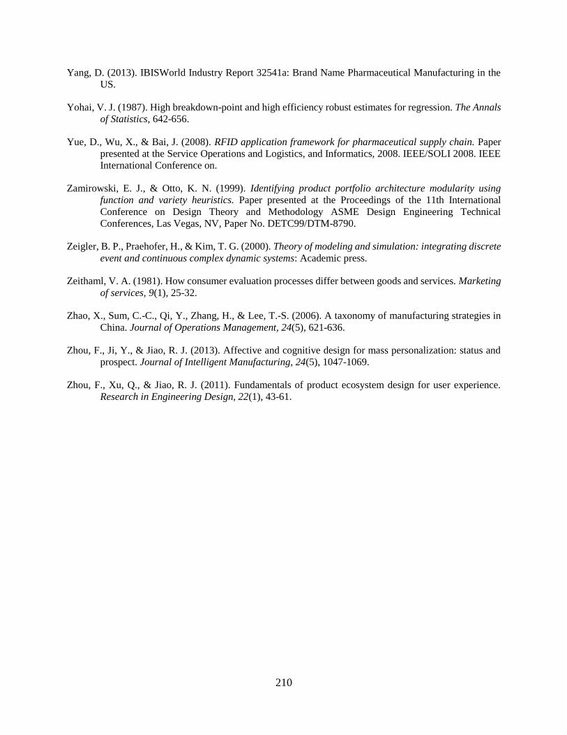
210

Yang, D. (2013). IBISWorld Industry Report 32541a: Brand Name Pharmaceutical Manufacturing in the

US.

Yohai, V. J. (1987). High breakdown-point and high efficiency robust estimates for regression. The Annals

of Statistics, 642-656.

Yue, D., Wu, X., & Bai, J. (2008). RFID application framework for pharmaceutical supply chain. Paper

presented at the Service Operations and Logistics, and Informatics, 2008. IEEE/SOLI 2008. IEEE

International Conference on.

Zamirowski, E. J., & Otto, K. N. (1999). Identifying product portfolio architecture modularity using

function and variety heuristics. Paper presented at the Proceedings of the 11th International

Conference on Design Theory and Methodology ASME Design Engineering Technical

Conferences, Las Vegas, NV, Paper No. DETC99/DTM-8790.

Zeigler, B. P., Praehofer, H., & Kim, T. G. (2000). Theory of modeling and simulation: integrating discrete

event and continuous complex dynamic systems: Academic press.

Zeithaml, V. A. (1981). How consumer evaluation processes differ between goods and services. Marketing

of services, 9(1), 25-32.

Zhao, X., Sum, C.-C., Qi, Y., Zhang, H., & Lee, T.-S. (2006). A taxonomy of manufacturing strategies in

China. Journal of Operations Management, 24(5), 621-636.

Zhou, F., Ji, Y., & Jiao, R. J. (2013). Affective and cognitive design for mass personalization: status and

prospect. Journal of Intelligent Manufacturing, 24(5), 1047-1069.

Zhou, F., Xu, Q., & Jiao, R. J. (2011). Fundamentals of product ecosystem design for user experience.

Research in Engineering Design, 22(1), 43-61.

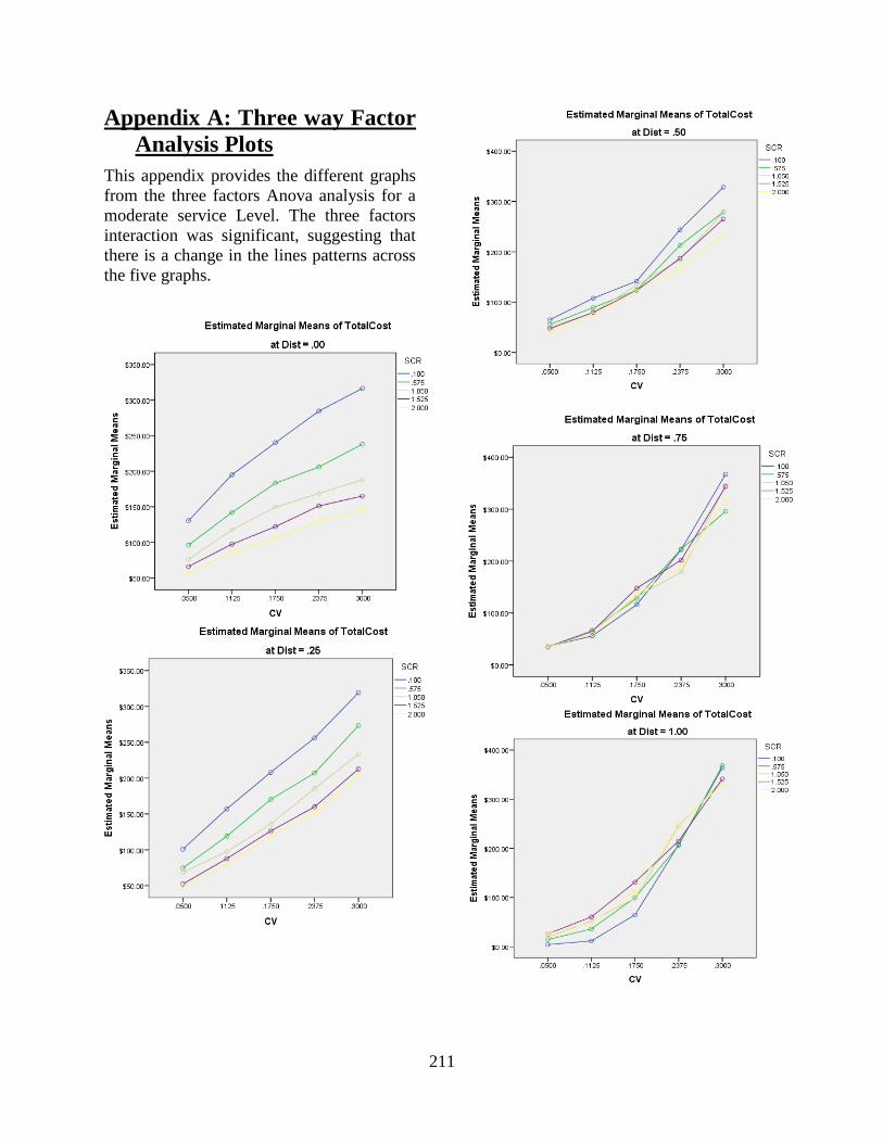
211

Appendix A: Three way Factor

Analysis Plots

This appendix provides the different graphs

from the three factors Anova analysis for a

moderate service Level. The three factors

interaction was significant, suggesting that

there is a change in the lines patterns across

the five graphs.

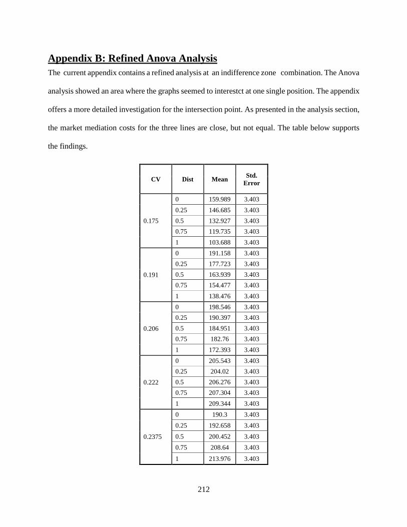
212

Appendix B: Refined Anova Analysis

The current appendix contains a refined analysis at an indifference zone combination. The Anova

analysis showed an area where the graphs seemed to interestct at one single position. The appendix

offers a more detailed investigation for the intersection point. As presented in the analysis section,

the market mediation costs for the three lines are close, but not equal. The table below supports

the findings.

CV Dist Mean Std.

Error

0.175

0 159.989 3.403

0.25 146.685 3.403

0.5 132.927 3.403

0.75 119.735 3.403

1 103.688 3.403

0.191

0 191.158 3.403

0.25 177.723 3.403

0.5 163.939 3.403

0.75 154.477 3.403

1 138.476 3.403

0.206

0 198.546 3.403

0.25 190.397 3.403

0.5 184.951 3.403

0.75 182.76 3.403

1 172.393 3.403

0.222

0 205.543 3.403

0.25 204.02 3.403

0.5 206.276 3.403

0.75 207.304 3.403

1 209.344 3.403

0.2375

0 190.3 3.403

0.25 192.658 3.403

0.5 200.452 3.403

0.75 208.64 3.403

1 213.976 3.403

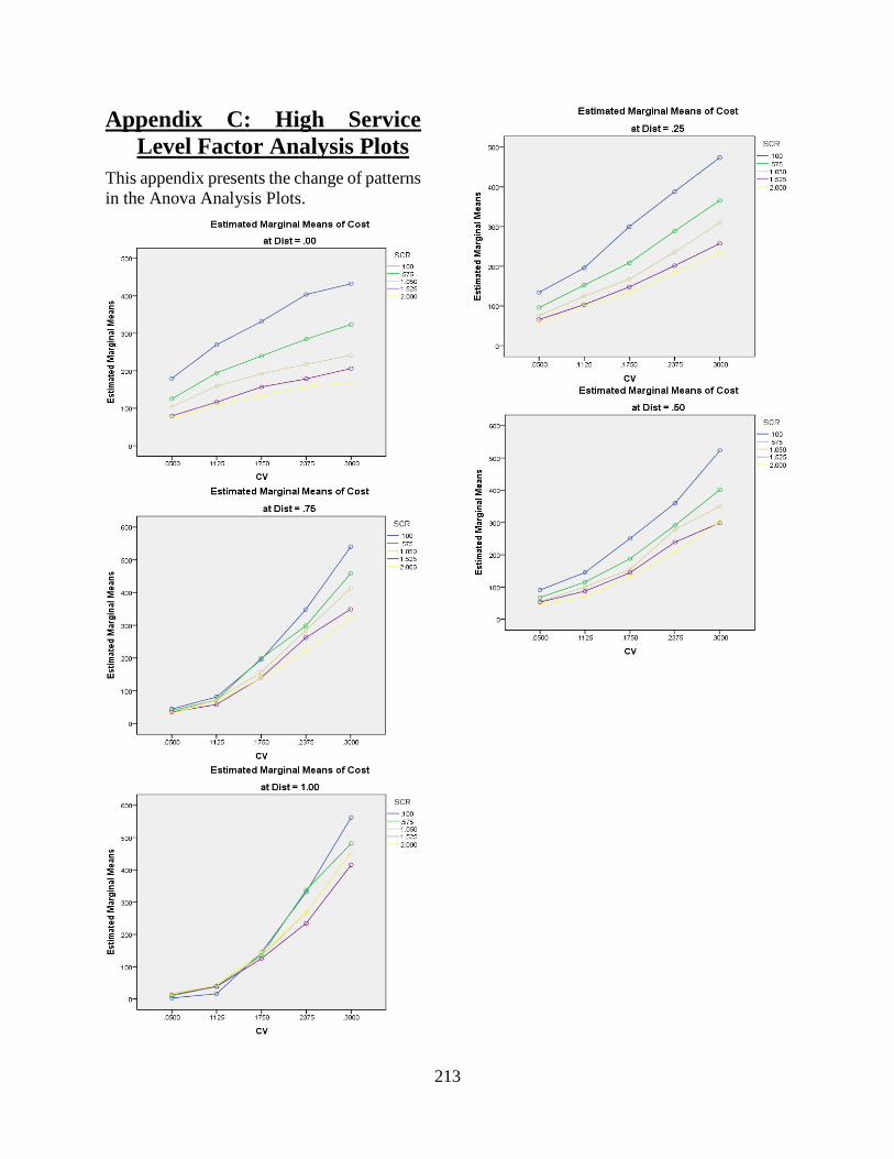
213

Appendix C: High Service

Level Factor Analysis Plots

This appendix presents the change of patterns

in the Anova Analysis Plots.

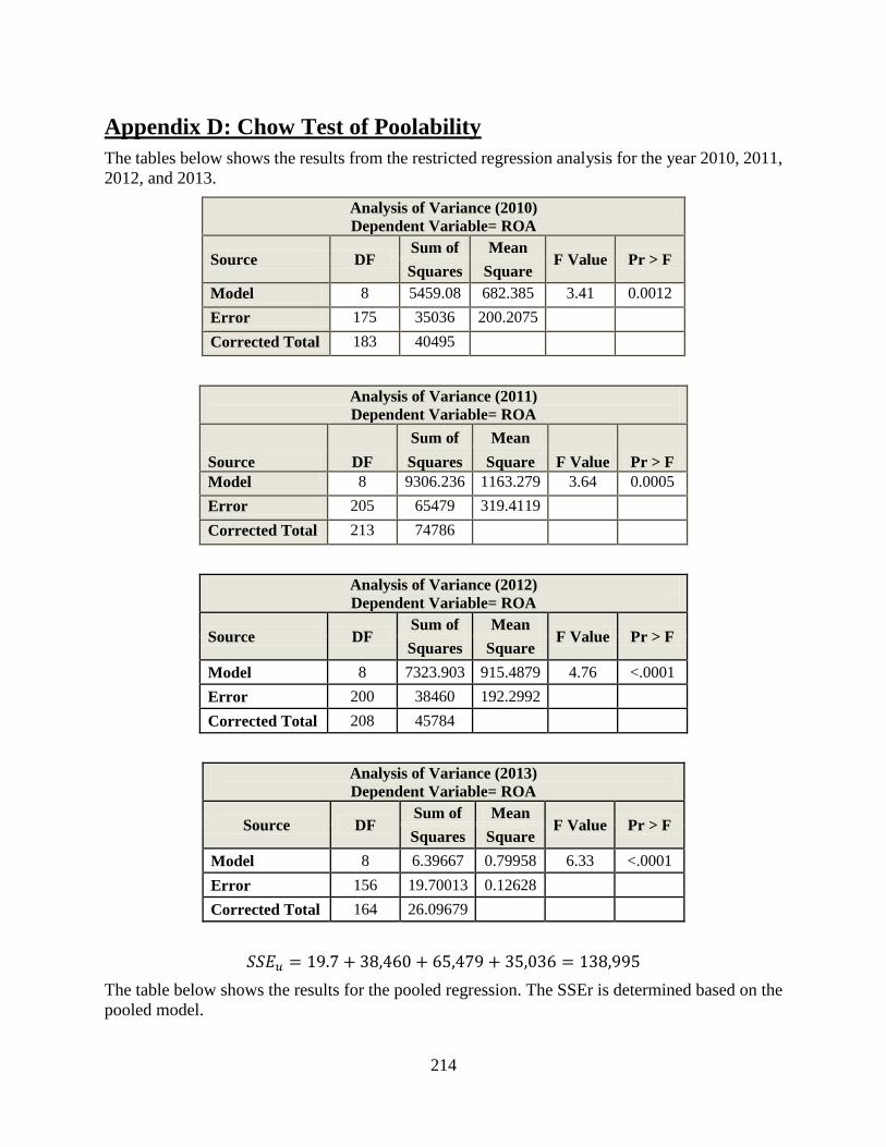
214

Appendix D: Chow Test of Poolability

The tables below shows the results from the restricted regression analysis for the year 2010, 2011,

2012, and 2013.

Analysis of Variance (2010)

Dependent Variable= ROA

Source DF Sum of Mean

F Value Pr > F Squares Square

Model 8 5459.08 682.385 3.41 0.0012

Error 175 35036 200.2075

Corrected Total 183 40495

Analysis of Variance (2011)

Dependent Variable= ROA

Source DF

Sum of Mean

F Value Pr > F Squares Square

Model 8 9306.236 1163.279 3.64 0.0005

Error 205 65479 319.4119

Corrected Total 213 74786

Analysis of Variance (2012)

Dependent Variable= ROA

Source DF Sum of Mean

F Value Pr > F Squares Square

Model 8 7323.903 915.4879 4.76 <.0001

Error 200 38460 192.2992

Corrected Total 208 45784

Analysis of Variance (2013)

Dependent Variable= ROA

Source DF Sum of Mean

F Value Pr > F Squares Square

Model 8 6.39667 0.79958 6.33 <.0001

Error 156 19.70013 0.12628

Corrected Total 164 26.09679

𝑆𝑆𝐸𝑢 = 19.7 + 38,460 + 65,479 + 35,036 = 138,995

The table below shows the results for the pooled regression. The SSEr is determined based on the

pooled model.

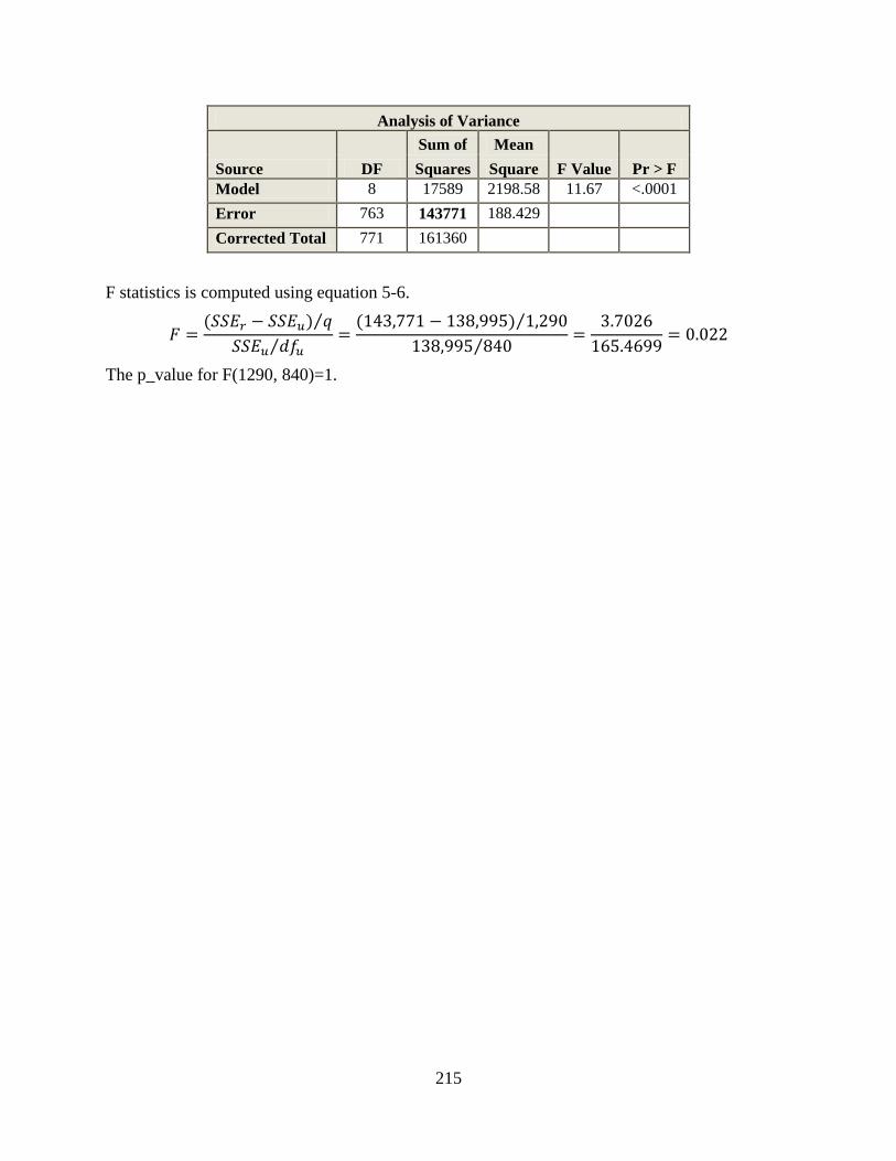
215

Analysis of Variance

Source DF

Sum of Mean

F Value Pr > F Squares Square

Model 8 17589 2198.58 11.67 <.0001

Error 763 143771 188.429

Corrected Total 771 161360

F statistics is computed using equation 5-6.

𝐹 =(𝑆𝑆𝐸𝑟 − 𝑆𝑆𝐸𝑢) 𝑞⁄

𝑆𝑆𝐸𝑢 𝑑𝑓𝑢⁄=

(143,771 − 138,995) 1,290⁄

138,995 840⁄=

3.7026

165.4699= 0.022

The p_value for F(1290, 840)=1.

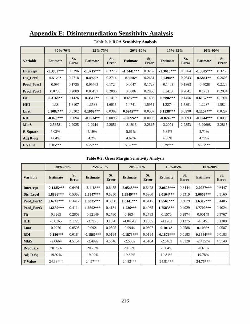
216

Appendix E: Disintermediation Sensitivity Analysis

Table 0-1: ROA Sensitivity Analysis

30%-70% 25%-75% 20%-80% 15%-85% 10%-90%

Variable Estimate St.

Error Estimate

St.

Error Estimate

St.

Error Estimate

St.

Error Estimate

St.

Error

Intercept -1.3902*** 0.3296 -1.3715*** 0.3275 -1.3441*** 0.3252 -1.3613*** 0.3264 -1.3805*** 0.3259

Dis_Level 0.5129* 0.2718 0.4929* 0.2714 0.5006* 0.2661 0.5494** 0.2643 0.5861** 0.2608

Prod_Port2 0.095 0.1735 0.05563 0.1724 0.0047 0.1728 -0.1403 0.1863 -0.4028 0.2226

Prod_Port3 0.0738 0.2089 0.05197 0.2096 0.0806 0.2056 0.1419 0.2041 0.1751 0.2034

Fit 0.3168** 0.1426 0.3512** 0.1410 0.437*** 0.1408 0.3996*** 0.1456 0.6157*** 0.1904

HHI 1.38 1.6107 1.3588 1.6015 1.4741 1.5951 1.2274 1.5891 1.2237 1.5824

Lnat 0.1082*** 0.0302 0.1069*** 0.0302 0.0945*** 0.0307 0.1138*** 0.0298 0.1157*** 0.0297

RDI -0.023*** 0.0094 -0.0234** 0.0093 -0.0224** 0.0093 -0.0242** 0.0093 -0.0244*** 0.0093

MktS -2.56581 2.2925 -2.9944 2.2851 -3.1916 2.2815 -3.2071 2.2853 -3.29608 2.2815

R-Square 5.03% 5.19% 5.61% 5.35% 5.71%

Adj R-Sq 4.04% 4.2% 4.62% 4.36% 4.72%

F Value 5.05*** 5.22*** 5.67*** 5.39*** 5.78***

Table 0-2: Gross Margin Sensitivity Analysis

30%-70% 25%-75% 20%-80% 15%-85% 10%-90%

Variable Estimate St.

Error Estimate

St.

Error Estimate

St.

Error Estimate

St.

Error Estimate

St.

Error

Intercept -2.1485*** 0.6491 -2.118*** 0.6455 -2.0548*** 0.6428 -2.0628*** 0.6444 -2.0287*** 0.6447

Dis_Level 1.8826*** 0.5353 1.8847*** 0.5350 1.9949*** 0.5260 2.0104*** 0.5219 2.0658*** 0.5160

Prod_Port2 1.6742*** 0.3417 1.6335*** 0.3398 1.6141*** 0.3415 1.5561*** 0.3679 1.6317*** 0.4405

Prod_Port3 1.6689*** 0.4114 1.6602*** 0.4131 1.736*** 0.4065 1.7583*** 0.4029 1.7702*** 0.4024

Fit 0.3265 0.2809 0.32149 0.2780 0.1634 0.2783 0.1570 0.2874 0.00149 0.3767

HHI -3.6165 3.1725 -3.7175 3.1570 -4.04642 3.1535 -4.1281 3.1375 -4.3451 3.1308

Lnat 0.0920 0.0595 0.0921 0.0595 0.0944 0.0607 0.1014* 0.0588 0.1036* 0.0587

RDI -0.186*** 0.0184 -0.1866*** 0.0184 -0.1873*** 0.0184 -0.1879*** 0.0183 -0.1884*** 0.0183

MktS -2.0664 4.5154 -2.4999 4.5046 -2.5352 4.5104 -2.5463 4.5120 -2.43574 4.5140

R-Square 20.75% 20.75% 20.65% 20.64% 20.61%

Adj R-Sq 19.92% 19.92% 19.82% 19.81% 19.78%

F Value 24.98*** 24.97*** 24.82*** 24.81*** 24.76***

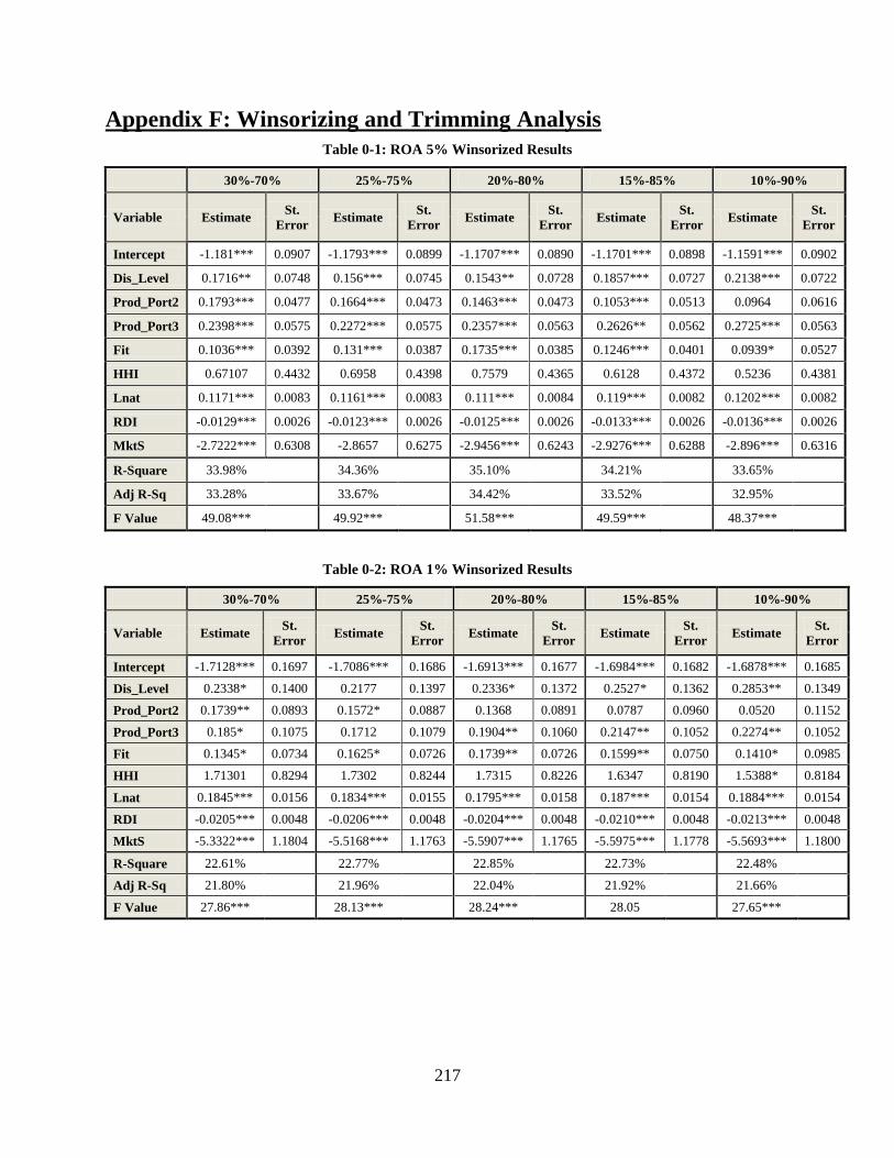
217

Appendix F: Winsorizing and Trimming Analysis

Table 0-1: ROA 5% Winsorized Results

30%-70% 25%-75% 20%-80% 15%-85% 10%-90%

Variable Estimate St.

Error Estimate

St.

Error Estimate

St.

Error Estimate

St.

Error Estimate

St.

Error

Intercept -1.181*** 0.0907 -1.1793*** 0.0899 -1.1707*** 0.0890 -1.1701*** 0.0898 -1.1591*** 0.0902

Dis_Level 0.1716** 0.0748 0.156*** 0.0745 0.1543** 0.0728 0.1857*** 0.0727 0.2138*** 0.0722

Prod_Port2 0.1793*** 0.0477 0.1664*** 0.0473 0.1463*** 0.0473 0.1053*** 0.0513 0.0964 0.0616

Prod_Port3 0.2398*** 0.0575 0.2272*** 0.0575 0.2357*** 0.0563 0.2626** 0.0562 0.2725*** 0.0563

Fit 0.1036*** 0.0392 0.131*** 0.0387 0.1735*** 0.0385 0.1246*** 0.0401 0.0939* 0.0527

HHI 0.67107 0.4432 0.6958 0.4398 0.7579 0.4365 0.6128 0.4372 0.5236 0.4381

Lnat 0.1171*** 0.0083 0.1161*** 0.0083 0.111*** 0.0084 0.119*** 0.0082 0.1202*** 0.0082

RDI -0.0129*** 0.0026 -0.0123*** 0.0026 -0.0125*** 0.0026 -0.0133*** 0.0026 -0.0136*** 0.0026

MktS -2.7222*** 0.6308 -2.8657 0.6275 -2.9456*** 0.6243 -2.9276*** 0.6288 -2.896*** 0.6316

R-Square 33.98% 34.36% 35.10% 34.21% 33.65%

Adj R-Sq 33.28% 33.67% 34.42% 33.52% 32.95%

F Value 49.08*** 49.92*** 51.58*** 49.59*** 48.37***

Table 0-2: ROA 1% Winsorized Results

30%-70% 25%-75% 20%-80% 15%-85% 10%-90%

Variable Estimate St.

Error Estimate

St.

Error Estimate

St.

Error Estimate

St.

Error Estimate

St.

Error

Intercept -1.7128*** 0.1697 -1.7086*** 0.1686 -1.6913*** 0.1677 -1.6984*** 0.1682 -1.6878*** 0.1685

Dis_Level 0.2338* 0.1400 0.2177 0.1397 0.2336* 0.1372 0.2527* 0.1362 0.2853** 0.1349

Prod_Port2 0.1739** 0.0893 0.1572* 0.0887 0.1368 0.0891 0.0787 0.0960 0.0520 0.1152

Prod_Port3 0.185* 0.1075 0.1712 0.1079 0.1904** 0.1060 0.2147** 0.1052 0.2274** 0.1052

Fit 0.1345* 0.0734 0.1625* 0.0726 0.1739** 0.0726 0.1599** 0.0750 0.1410* 0.0985

HHI 1.71301 0.8294 1.7302 0.8244 1.7315 0.8226 1.6347 0.8190 1.5388* 0.8184

Lnat 0.1845*** 0.0156 0.1834*** 0.0155 0.1795*** 0.0158 0.187*** 0.0154 0.1884*** 0.0154

RDI -0.0205*** 0.0048 -0.0206*** 0.0048 -0.0204*** 0.0048 -0.0210*** 0.0048 -0.0213*** 0.0048

MktS -5.3322*** 1.1804 -5.5168*** 1.1763 -5.5907*** 1.1765 -5.5975*** 1.1778 -5.5693*** 1.1800

R-Square 22.61% 22.77% 22.85% 22.73% 22.48%

Adj R-Sq 21.80% 21.96% 22.04% 21.92% 21.66%

F Value 27.86*** 28.13*** 28.24*** 28.05 27.65***

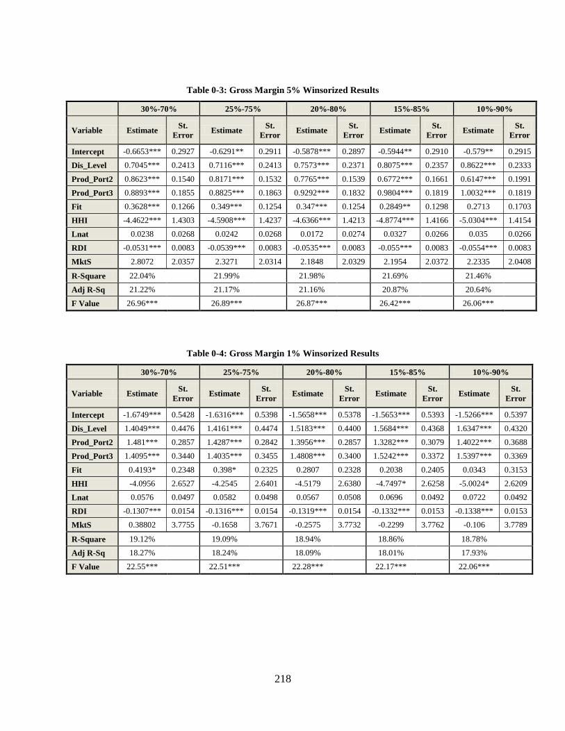
218

Table 0-3: Gross Margin 5% Winsorized Results

30%-70% 25%-75% 20%-80% 15%-85% 10%-90%

Variable Estimate St.

Error Estimate

St.

Error Estimate

St.

Error Estimate

St.

Error Estimate

St.

Error

Intercept -0.6653*** 0.2927 -0.6291** 0.2911 -0.5878*** 0.2897 -0.5944** 0.2910 -0.579** 0.2915

Dis_Level 0.7045*** 0.2413 0.7116*** 0.2413 0.7573*** 0.2371 0.8075*** 0.2357 0.8622*** 0.2333

Prod_Port2 0.8623*** 0.1540 0.8171*** 0.1532 0.7765*** 0.1539 0.6772*** 0.1661 0.6147*** 0.1991

Prod_Port3 0.8893*** 0.1855 0.8825*** 0.1863 0.9292*** 0.1832 0.9804*** 0.1819 1.0032*** 0.1819

Fit 0.3628*** 0.1266 0.349*** 0.1254 0.347*** 0.1254 0.2849** 0.1298 0.2713 0.1703

HHI -4.4622*** 1.4303 -4.5908*** 1.4237 -4.6366*** 1.4213 -4.8774*** 1.4166 -5.0304*** 1.4154

Lnat 0.0238 0.0268 0.0242 0.0268 0.0172 0.0274 0.0327 0.0266 0.035 0.0266

RDI -0.0531*** 0.0083 -0.0539*** 0.0083 -0.0535*** 0.0083 -0.055*** 0.0083 -0.0554*** 0.0083

MktS 2.8072 2.0357 2.3271 2.0314 2.1848 2.0329 2.1954 2.0372 2.2335 2.0408

R-Square 22.04% 21.99% 21.98% 21.69% 21.46%

Adj R-Sq 21.22% 21.17% 21.16% 20.87% 20.64%

F Value 26.96*** 26.89*** 26.87*** 26.42*** 26.06***

Table 0-4: Gross Margin 1% Winsorized Results

30%-70% 25%-75% 20%-80% 15%-85% 10%-90%

Variable Estimate St.

Error Estimate

St.

Error Estimate

St.

Error Estimate

St.

Error Estimate

St.

Error

Intercept -1.6749*** 0.5428 -1.6316*** 0.5398 -1.5658*** 0.5378 -1.5653*** 0.5393 -1.5266*** 0.5397

Dis_Level 1.4049*** 0.4476 1.4161*** 0.4474 1.5183*** 0.4400 1.5684*** 0.4368 1.6347*** 0.4320

Prod_Port2 1.481*** 0.2857 1.4287*** 0.2842 1.3956*** 0.2857 1.3282*** 0.3079 1.4022*** 0.3688

Prod_Port3 1.4095*** 0.3440 1.4035*** 0.3455 1.4808*** 0.3400 1.5242*** 0.3372 1.5397*** 0.3369

Fit 0.4193* 0.2348 0.398* 0.2325 0.2807 0.2328 0.2038 0.2405 0.0343 0.3153

HHI -4.0956 2.6527 -4.2545 2.6401 -4.5179 2.6380 -4.7497* 2.6258 -5.0024* 2.6209

Lnat 0.0576 0.0497 0.0582 0.0498 0.0567 0.0508 0.0696 0.0492 0.0722 0.0492

RDI -0.1307*** 0.0154 -0.1316*** 0.0154 -0.1319*** 0.0154 -0.1332*** 0.0153 -0.1338*** 0.0153

MktS 0.38802 3.7755 -0.1658 3.7671 -0.2575 3.7732 -0.2299 3.7762 -0.106 3.7789

R-Square 19.12% 19.09% 18.94% 18.86% 18.78%

Adj R-Sq 18.27% 18.24% 18.09% 18.01% 17.93%

F Value 22.55*** 22.51*** 22.28*** 22.17*** 22.06***

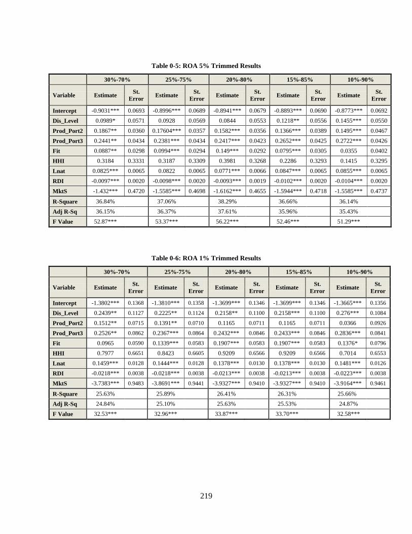
219

Table 0-5: ROA 5% Trimmed Results

30%-70% 25%-75% 20%-80% 15%-85% 10%-90%

Variable Estimate St.

Error Estimate

St.

Error Estimate

St.

Error Estimate

St.

Error Estimate

St.

Error

Intercept -0.9031*** 0.0693 -0.8996*** 0.0689 -0.8941*** 0.0679 -0.8893*** 0.0690 -0.8773*** 0.0692

Dis_Level 0.0989* 0.0571 0.0928 0.0569 0.0844 0.0553 0.1218** 0.0556 0.1455*** 0.0550

Prod_Port2 0.1867** 0.0360 0.17604*** 0.0357 0.1582*** 0.0356 0.1366*** 0.0389 0.1495*** 0.0467

Prod_Port3 0.2441** 0.0434 0.2381*** 0.0434 0.2417*** 0.0423 0.2652*** 0.0425 0.2722*** 0.0426

Fit 0.0887** 0.0298 0.0994*** 0.0294 0.149*** 0.0292 0.0795*** 0.0305 0.0355 0.0402

HHI 0.3184 0.3331 0.3187 0.3309 0.3981 0.3268 0.2286 0.3293 0.1415 0.3295

Lnat 0.0825*** 0.0065 0.0822 0.0065 0.0771*** 0.0066 0.0847*** 0.0065 0.0855*** 0.0065

RDI -0.0097*** 0.0020 -0.0098*** 0.0020 -0.0093*** 0.0019 -0.0102*** 0.0020 -0.0104*** 0.0020

MktS -1.432*** 0.4720 -1.5585*** 0.4698 -1.6162*** 0.4655 -1.5944*** 0.4718 -1.5585*** 0.4737

R-Square 36.84% 37.06% 38.29% 36.66% 36.14%

Adj R-Sq 36.15% 36.37% 37.61% 35.96% 35.43%

F Value 52.87*** 53.37*** 56.22*** 52.46*** 51.29***

Table 0-6: ROA 1% Trimmed Results

30%-70% 25%-75% 20%-80% 15%-85% 10%-90%

Variable Estimate St.

Error Estimate

St.

Error Estimate

St.

Error Estimate

St.

Error Estimate

St.

Error

Intercept -1.3802*** 0.1368 -1.3810*** 0.1358 -1.3699*** 0.1346 -1.3699*** 0.1346 -1.3665*** 0.1356

Dis_Level 0.2439** 0.1127 0.2225** 0.1124 0.2158** 0.1100 0.2158*** 0.1100 0.276*** 0.1084

Prod_Port2 0.1512** 0.0715 0.1391** 0.0710 0.1165 0.0711 0.1165 0.0711 0.0366 0.0926

Prod_Port3 0.2526** 0.0862 0.2367*** 0.0864 0.2432*** 0.0846 0.2433*** 0.0846 0.2836*** 0.0841

Fit 0.0965 0.0590 0.1339*** 0.0583 0.1907*** 0.0583 0.1907*** 0.0583 0.1376* 0.0796

HHI 0.7977 0.6651 0.8423 0.6605 0.9209 0.6566 0.9209 0.6566 0.7014 0.6553

Lnat 0.1459*** 0.0128 0.1444*** 0.0128 0.1378*** 0.0130 0.1378*** 0.0130 0.1481*** 0.0126

RDI -0.0218*** 0.0038 -0.0218*** 0.0038 -0.0213*** 0.0038 -0.0213*** 0.0038 -0.0223*** 0.0038

MktS -3.7383*** 0.9483 -3.8691*** 0.9441 -3.9327*** 0.9410 -3.9327*** 0.9410 -3.9164*** 0.9461

R-Square 25.63% 25.89% 26.41% 26.31% 25.66%

Adj R-Sq 24.84% 25.10% 25.63% 25.53% 24.87%

F Value 32.53*** 32.96*** 33.87*** 33.70*** 32.58***

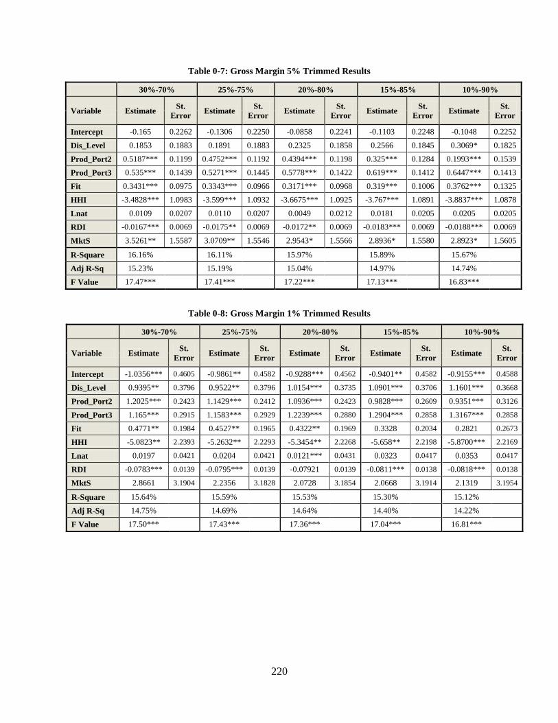
220

Table 0-7: Gross Margin 5% Trimmed Results

30%-70% 25%-75% 20%-80% 15%-85% 10%-90%

Variable Estimate St.

Error Estimate

St.

Error Estimate

St.

Error Estimate

St.

Error Estimate

St.

Error

Intercept -0.165 0.2262 -0.1306 0.2250 -0.0858 0.2241 -0.1103 0.2248 -0.1048 0.2252

Dis_Level 0.1853 0.1883 0.1891 0.1883 0.2325 0.1858 0.2566 0.1845 0.3069* 0.1825

Prod_Port2 0.5187*** 0.1199 0.4752*** 0.1192 0.4394*** 0.1198 0.325*** 0.1284 0.1993*** 0.1539

Prod_Port3 0.535*** 0.1439 0.5271*** 0.1445 0.5778*** 0.1422 0.619*** 0.1412 0.6447*** 0.1413

Fit 0.3431*** 0.0975 0.3343*** 0.0966 0.3171*** 0.0968 0.319*** 0.1006 0.3762*** 0.1325

HHI -3.4828*** 1.0983 -3.599*** 1.0932 -3.6675*** 1.0925 -3.767*** 1.0891 -3.8837*** 1.0878

Lnat 0.0109 0.0207 0.0110 0.0207 0.0049 0.0212 0.0181 0.0205 0.0205 0.0205

RDI -0.0167*** 0.0069 -0.0175** 0.0069 -0.0172** 0.0069 -0.0183*** 0.0069 -0.0188*** 0.0069

MktS 3.5261** 1.5587 3.0709** 1.5546 2.9543* 1.5566 2.8936* 1.5580 2.8923* 1.5605

R-Square 16.16% 16.11% 15.97% 15.89% 15.67%

Adj R-Sq 15.23% 15.19% 15.04% 14.97% 14.74%

F Value 17.47*** 17.41*** 17.22*** 17.13*** 16.83***

Table 0-8: Gross Margin 1% Trimmed Results

30%-70% 25%-75% 20%-80% 15%-85% 10%-90%

Variable Estimate St.

Error Estimate

St.

Error Estimate

St.

Error Estimate

St.

Error Estimate

St.

Error

Intercept -1.0356*** 0.4605 -0.9861** 0.4582 -0.9288*** 0.4562 -0.9401** 0.4582 -0.9155*** 0.4588

Dis_Level 0.9395** 0.3796 0.9522** 0.3796 1.0154*** 0.3735 1.0901*** 0.3706 1.1601*** 0.3668

Prod_Port2 1.2025*** 0.2423 1.1429*** 0.2412 1.0936*** 0.2423 0.9828*** 0.2609 0.9351*** 0.3126

Prod_Port3 1.165*** 0.2915 1.1583*** 0.2929 1.2239*** 0.2880 1.2904*** 0.2858 1.3167*** 0.2858

Fit 0.4771** 0.1984 0.4527** 0.1965 0.4322** 0.1969 0.3328 0.2034 0.2821 0.2673

HHI -5.0823** 2.2393 -5.2632** 2.2293 -5.3454** 2.2268 -5.658** 2.2198 -5.8700*** 2.2169

Lnat 0.0197 0.0421 0.0204 0.0421 0.0121*** 0.0431 0.0323 0.0417 0.0353 0.0417

RDI -0.0783*** 0.0139 -0.0795*** 0.0139 -0.07921 0.0139 -0.0811*** 0.0138 -0.0818*** 0.0138

MktS 2.8661 3.1904 2.2356 3.1828 2.0728 3.1854 2.0668 3.1914 2.1319 3.1954

R-Square 15.64% 15.59% 15.53% 15.30% 15.12%

Adj R-Sq 14.75% 14.69% 14.64% 14.40% 14.22%

F Value 17.50*** 17.43*** 17.36*** 17.04*** 16.81***