Embed Size (px)
Citation preview
A Thesis
entitled
Performance Evaluation of 2-D Pilot Aided OFDM System under Hyper-Rayleigh Fading Channel
By
Haobo Zhen
Submitted to the Graduate Faculty as partial fulfillment of the requirements
for the Master of Science Degree in Electrical Engineering
Dr. Junghwan Kim, Committee Chair
Dr. Ezzatollah Salari, Committee Member
Dr. Dong-Shik Kim, Committee Member
Dr. Patricia R. Komuniecki, Dean College of Graduate Studies
The University of Toledo August 2011

Copyright 2011, Haobo Zhen
This document is copyrighted material. Under copyright law, no parts of this document may be reproduced without the expressed permission of the author.
iii
An Abstract of
Performance Evaluation of 2-D Pilot Aided OFDM System under Hyper-Rayleigh Fading Channel
by
Haobo Zhen
Submitted to the Graduate Faculty as partial fulfillment of the requirements for the Master of Science Degree in Electrical Engineering
The University of Toledo
August 2011
Wireless radio propagation channel is widely known as the most hostile
communication channel. Modeling and simulation of wireless fading channel has been
an essential issue in the design of communication system. Rayleigh fading and Rician
fading model are the most commonly used small scale models in wireless
communication. However, recent research shows that some WSN applications where
sensor nodes deployed within cavity environment suffer from more severe fading than
Rayleigh fading predicted, which is referred to as hyper-Rayleigh fading. Therefore,
design of a more applicable model is necessary to describe hyper-Rayleigh fading.
Two-wave with diffuse power (TWDP) model is suggested to be the proper model
to represent hyper-Rayleigh fading behavior. However, little effort has been made to
evaluate the anti-interference capacity of OFDM system under hyper-Rayleigh fading
channel. In the thesis, the characteristic of hyper-Rayleigh fading is explored and
analyzed. Furthermore, performances of OFDM system with various pilot aided
channel estimation techniques under hyper-Rayleigh fading are investigated.
Simulation results indicate hyper-Rayleigh fading exhibits worse fading phenomena
iv
than Rayleigh fading when parameters ∆andK exceed certain values. OFDM system
with 2-D channel estimation demonstrates strong resistance to multipath fading, thus
can be regarded as a promising candidate of WSN applications under hyper-Rayleigh
fading.

v
Acknowledgements
First of all, I would like to thank my advisor Dr. Junghwan Kim for his guidance,
his encouragement and support to me. The thesis would not have been possible without
his help. I would also like to thank Dr. Ezzatollah Salari and Dr. Dong-Shik Kim for
being my committee members.
I want to give my thanks to my friends and fellow students in University of Toledo,
who make my life in America happy and memorable.
Finally, I want to express my deep appreciation and gratitude to my parents, whose
love always accompany me through difficult times and days of joy.

vi
Table of Contents
Abst rac t i i i
A c k n o w l e d ge m e n t s v
Table of Contents vi
Lis t of Tables vi i i
List of Figures ix
1 Introduction………………………………………………………………………… 1
1.1 Problem Statement…………………………………………………………… 1
1.2 Thesis Contribution………………………………………………………… 3
1.3 Thesis Outline…………………………………………………………….. 4
2 Principle and Model of OFDM System………………………………………...… 6
2.1 Principle of OFDM system…………………………………………….…… 6
2.2 Model of OFDM system……………………………………………………… 9
2.2.1 Convolutional Coding………………………………………………….. 10
2.2.2 Modulation Schemes………………………………………………….. 14
2.2.3 IFFT and FFT………………………………………………………….. 23
2.2.4 Cyclic Prefix………………………………………………………….. 23
3 Characteristic and Modeling of Hyper-Rayleigh Fading Channel……………… 26
3.1 Small Scale Fading…………………………………………………………... 26
vii
3.1.1 Multipath Fading……………………………………………………….. 28
3.1.2 Doppler Effect………………………………………………………….. 29
3.1.3 Expression of Received Signal……………………………………….. 30
3.2 Typical Small Scale Fading Models…………………………………………32
3.2.1 Rayleigh Fading Model……………………………………………….. 32
3.2.2 Rician Fading Model………………………………………………….. 36
3.3 Hyper-Rayleigh Fading Model………………………………………………40
4 2-D Pilot Aided Channel Estimation in OFDM System………………………… 50
4.1 Procedure of Channel Estimation………………………………………..… 50
4.2 2-D Pilot Arrangement…………………………………………………….…. 52
4.2.1 1-D Pilot Pattern……………………………………………………….. 52
4.2.2 2-D Pilot Pattern……………………………………………………….. 56
4.3 Channel Estimation Algorithms…………………………………………….. 59
5 Simulation Results and Performance Analysis………………………………….. 63
5.1 Simulation Results with Different Modulation Schemes…………………………...63
5.2 Simulation Results under Rayleigh Fading Channels……………………… 65
5.3 Simulation Results under Rician Fading Channels………………………… 67
5.3 Simulation Results under Rician Fading Channels………………………… 70
6 Conclusion and Future Work…………………………………………………..… 76
References…………………………………………………………………………... 78
viii
List of Tables
2-1 Simulation specification of OFDM system……………………………………..13
3-1 Fading scenario characterized by specular components……………………….32
3-2 Comparison between four fading models……………………………………….43
5-1 Specification of OFDM system simulation under Rayleigh fading…………….65
ix
List of Figures
1-1 Wireless communication environment...…………………………………………. 2
2-1 Frequency spectrum of OFDM system sub-carriers…………………………….. 7
2-2 Model of OFDM system………………………………………………………… 9
2-3 Rate ��133145175�� convolutional encoder……………………………… 11
2-4 Rate ��133171�� convolutional encoder ………………………..………… 11
2-5 BER performance curves of coded and uncoded OFDM systems……………. 13
2-6 BPSK constellation…………………………………………………………..… 16
2-7 8PSK constellation with Gray mapping………………………………………… 17
2-8 16PSK constellation with Gray mapping………………………………………. 18
2-9 The BER performances of OFDM system with different MPSKs……………. 19
2-10 16QAM constellation with Gray mapping……………………………………. 21
2-11 BER curves of OFDM with M-ary QAMs under AWGN……………………. 22
2-12 Cyclic prefix adding………………………………………………………….. 24
3-1 Large scale fading and small scale fading…………………………………….. 27
3-2 Illustration of Doppler shift in time varying channel…………………………… 30
3-3 Illustration of specular components and diffuse components…………………. 31
3-4 Illustration of Rayleigh fading scenario………………………………………… 33
3-5 PDFs of Rayleigh fading with different variances……………………………… 34
x
3-6 CDFs of Rayleigh fading with various variances………………………………. 35
3-7 Illustration of Rician fading scenario……………………………………………37
3-8 PDFs of Rician fading with various V…………………………………………. 38
3-9 CDFs of Rician with various V…………………………………………………39
3-10 Illustration of hyper-Rayleigh fading scenario……………………………… 41
3-11 PDFs of TWDP fading with K=3……………………………………………… 44
3-12 PDFs of TWDP with∆� 1…………………………………………………… 45
3-13 Comparison of PDFs among Rayleigh, Rician and TWDP…………………… 45
3-14 Illustration of range of TWDP CDFs………………………………………… 47
3-15 CDFs of the three traces……………………………………………………… 48
4-1 Block type pilot pattern……………………………………………………… 53
4-2 Illustration of block type pilot channel estimation………………………….. 54
4-3 Comb type pilot pattern……………………………………………………….. 55
4-4 Illustration of comb type pilot channel estimation……………………………… 56
4-5 Rectangular type pilot pattern…………………………………………………. 57
4-6 Procedure of rectangular type pilot channel estimation………………………… 58
5-1 Comparison of different modulation schemes under AWGN………………… 64
5-2 Comparison of different modulation schemes with coding…………………… 64
5-3 Block type BER performances with LS and LMMSE under Rayleigh……….. 65
5-4 Comb type BER performances with LS and LMMSE under Rayleigh……….. 66
5-5 Rectangular type performances with LS and LMMSE under Rayleigh……….. 67
5-6 BER performances under Rician fading with various K-factors……………….. 68
xi
5-7 Block type BER performances with LS and LMMSE under Rician………….. 69
5-8 Comb type BER performances with LS and LMMSE under Rician………….. 69
5-9 Rectangular type BER performances with LS and LMMSE under Rician…….. 70
5-10 BER performances under TWDP model with various K…………………….. 71
5-11 Block type BER performances under TWDP model with ∆� 1, K � 6..…… 71
5-12 Comb type BER performances under TWDP model with ∆� 1, K � 6……. 72
5-13 Rectangular type BER performances under TWDP model with ∆� 1, K � 6 .72
5-14 Comparison of BER performances under TWDP with K=3………………….. 73
5-15 Comparison of BER performances under TWDP with K=6………………….. 74
5-16 Comparison of BER performances under various fading channels………….. 74
1
Chapter 1
Introduction
1.1 Problem Statement
Fading and interference are the major performance degrading factors in
wireless/mobile communications. In order to improve and testify the system’s
effectiveness to resist fading, modeling and simulation of communication system under
fading channel is of great significance in the design of communication system. For
different propagation environment, the characteristic of fading channel is diverse and
complex. Therefore, design of proper fading model in particular communication
circumstance is essential in this regard.
Rayleigh fading and Rician fading model are the most commonly used small scale
models in wireless communication [1]. However, as wireless sensor networks (WSN)
migrate into vastly different applications, conventional Rayleigh and Rician channel
model don’t fit in every WSN environment. Recent research [2] [3] shows that some
WSN applications where sensor nodes deployed within cavity environment suffer from
more severe fading than Rayleigh fading predicted, which is referred to as
hyper-Rayleigh fading. Herein, development of a more applicable fading model which
2
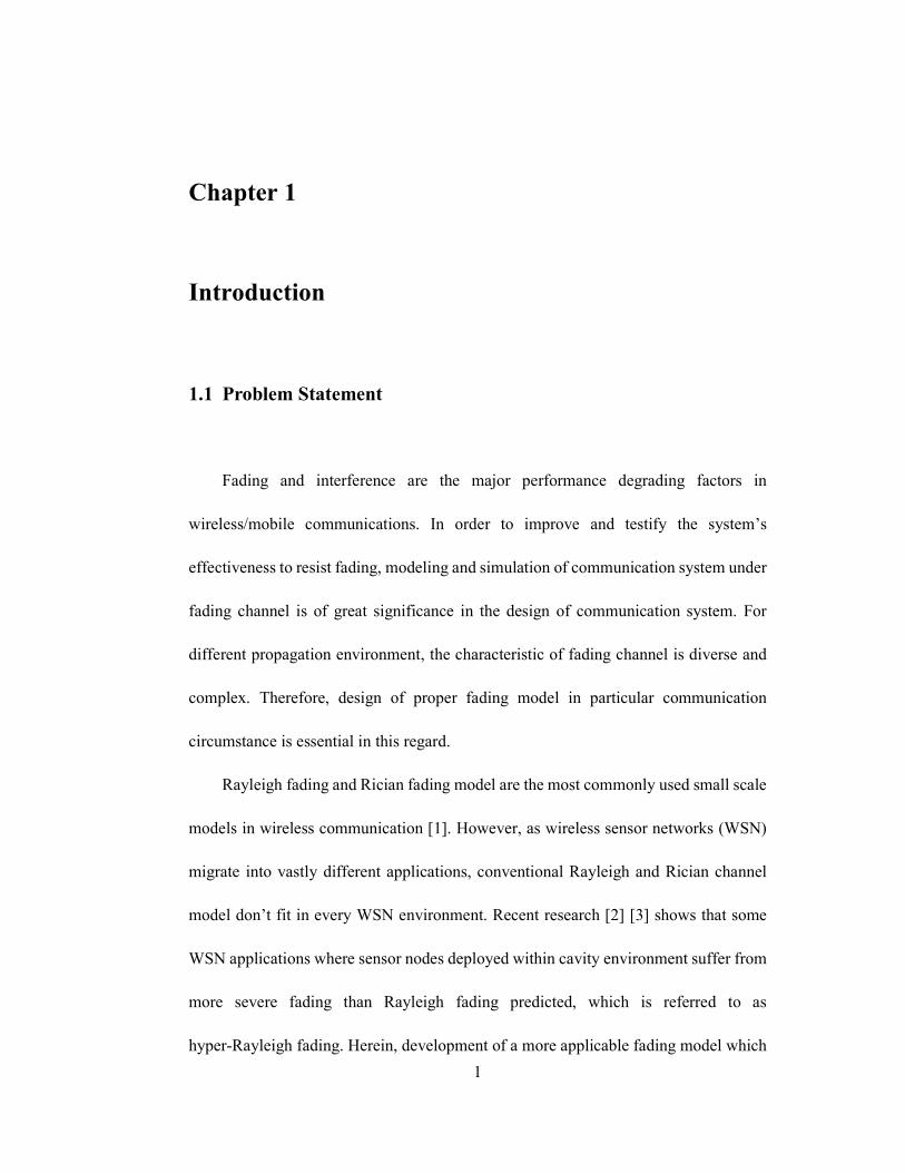
fits in some particular WSN circumstance has become an important issue.
Figure 1-1 Wireless communication environment.
Another problem lies in the effectiveness of anti-interference technologies. For
wireless communication, OFDM is good multi-carrier scheme due to its nature of
strong resistance to interference and high spectra efficiency, high data rate transmission
[4]. Channel estimation technologies are implemented in order to estimate the effect of
propagation delay and channel synchronization. Channel estimation methods can be
classified into two categories: blind channel estimation and pilot-aided channel
estimation. The channel estimation techniques studied in the thesis are all pilot-aided,
for pilot-aided channel estimation are more applicable in fast-fading frequency
selective radio propagation channel. Different pilot insertion patterns results in diverse
3
BER performances. 2-D pilot channel estimation is proven to have better performance
comparing to 1-D pilot channel estimation
Bit-error-rate (BER) is a key factor to measure the capacity and performance of
communication system. Much effort has been made to explore the characteristic and
BER performance of hyper-Rayleigh fading [5] [6]. However, there is little work on
evaluating BER performance of OFDM system under such radio propagation
environment. Herein, the thesis is focused on the investigation of OFDM system
performance under various fading environment, especially hyper-Rayleigh fading. 2-D
pilot-aided channel estimation, convolutional coding and cyclic prefix are also
implemented in OFDM system. The performance of OFDM system can be determined
by evaluating system’s BER.
1.2 Thesis Contribution
The thesis aims to explore the BER performance of OFDM system under
hyper-Rayleigh fading environment and investigate anti-fading capabilities of 2-D pilot
channel estimation methods. The contributions of the thesis are as follows:
� Explain the basic principle of OFDM system and capacity to overcome ISI
and ICI caused by multipath. Coding and modulation schemes are also
introduced and analyzed to further enhance the performance of OFDM
system;
� Develop fading models to represent the actual small scale fading situation
4
exist in wireless communication. Apart from conventional small-scale fading
models, a recently proposed fading model, known as hyper-Rayleigh model,
is developed and investigated;
� Present pilot-aided channel estimation techniques to address small scale
fading problem in wireless communications. Two 1-D pilot pattern, block
type and comb type, are investigated. Rectangular 2-D pilot pattern, which is
more applicable in frequency selective and time-variant fading channel, is
presented and analyzed. LS and LMMSE channel estimation is also
introduced;
� Investigate BER performance of OFDM system under various small-scale
fading environments and validate effectiveness of applying 2-D pilot channel
estimation to OFDM system under hyper-Rayleigh fading using MATLAB
simulation.
1.3 Thesis Outline
The thesis presents modeling of various fading environments and techniques to
improve BER performance of OFDM system. Chapter 1 gives a brief introduction to
the signal fading problems in wireless communication and the motivation of the
research is highlighted. In Chapter 2, principle of OFDM system is presented. Coding,
modulation schemes and other techniques are introduced in order to improve OFDM
system performance. In Chapter 3, characteristic of various fading environments is

5
investigated. Fading models, Rayleigh, Rician and hyper-Rayleigh, are proposed and
simulated to represent propagation phenomenon during transmission. In Chapter 4, 2-D
and 1-D pilot patterns are presented and analyzed. LS and LMMSE estimation methods
are also discussed in this chapter. In Chapter 5, BER simulation results of OFDM
system with different technologies under various fading environments are given. BER
is utilized as the key factor to evaluate the performance of OFDM system. Chapter 6
draws conclusion and shows the course of future work.
6
Chapter 2
Principle and Model of OFDM System
Orthogonal Frequency Division Multiplexing (OFDM), which is also referred to
as Discrete Multi-tone Modulation (DMT), is a multi-carrier transmission technique, is
widely applied to wireless communications, such as digital audio broadcasting, digital
video broadcasting and wireless local area network (WLAN). OFDM is also regarded
as one of the most promising technologies for the fourth generation (4G) mobile
communication system. OFDM technology has distinctive advantages on high data
transmission, anti-interference and low equipment complexity [4]. Chapter 2 gives a
detailed explanation of principle and model of OFDM system. The discussion and
analysis of coding and modulation schemes involved in OFDM signal generation are
also included in this chapter.
2.1 Principle of OFDM system
The idea of OFDM is to divide the original data steam into several parallel
narrowband low-rate streams modulated on corresponding orthogonal sub-carriers [7].
To be specific, each sub-carrier has integer periods in OFDM symbol duration.

7
Neighboring sub-carriers have one period difference to maintain orthogonality.
Suppose T is denoted as OFDM symbol width, �� and �� are the frequencies of two
sub-carries, we have:
�� � exp���� � ∙ exp����� � � � �1� � �0� � ���� (2.1)
This orthogonality characteristic of OFDM system can also be understood in the
view of frequency domain. As shown in Figure 2-1, all sub-carriers are controlled to
maintain orthogonality by making the peak of each sub-carrier signal coincide with the
nulls of other signals.
Figure 2-1 Frequency spectrum of OFDM system sub-carriers.
The orthogonal characteristics of sub-carriers enable OFDM system to have
higher spectral efficiency than conventional multi-carrier technique. For conventional
multi-carrier techniques, guard intervals are inserted between sub-carriers so that
8
sub-carrier signal can be separated from other signal by corresponding filter at the
receiver. In the case of OFDM system, however, sub-carriers overlap each other and
can be demodulated without guard interval.
Another significant feature of OFDM system is that modulation and demodulation
procedure is implemented by IFFT and FFT respectively, which will greatly reduce the
complexity of equipment and structure. Suppose ���� � 1,2, … , !� is ! sub-carrier
frequency, the modulated signal at "th chip duration is denoted as:
%&� � � ∑ (&���exp��2)�� �*+��,� (2.2)
Where (&��� carries the data information at " - chip duration and determines the
amplitude and phase of signal%&� �.
At the receiver, the �th spectrum component of signal %&� � is calculated by
!-point DFT (Discrete Fourier Transform). Assume the sampling frequency is�., and
frequency interval of adjacent sub-carriers is ∆� � �./! . Therefore, %&��∆�� is
written as:
%&��∆�� � ∑ %��/�.�*+��,� exp���2)��/!� (2.3)
Since � �/�., equation (2.2) is taken in equation (2.3):
%&��∆�� � 11(&��� exp 2�2)�3��. 4*+�3,�
*+��,� exp 5� �2)��! 6
� ∑ (���7�898: � �*�*+�3,� (2.4)
Where,
9
7��, �� � �0� � �1� � ��
From the equation (2.4), it is known that if �� is integertimes of∆�, the �th
spectrum component of signal%&� � is obtained at the receiver.
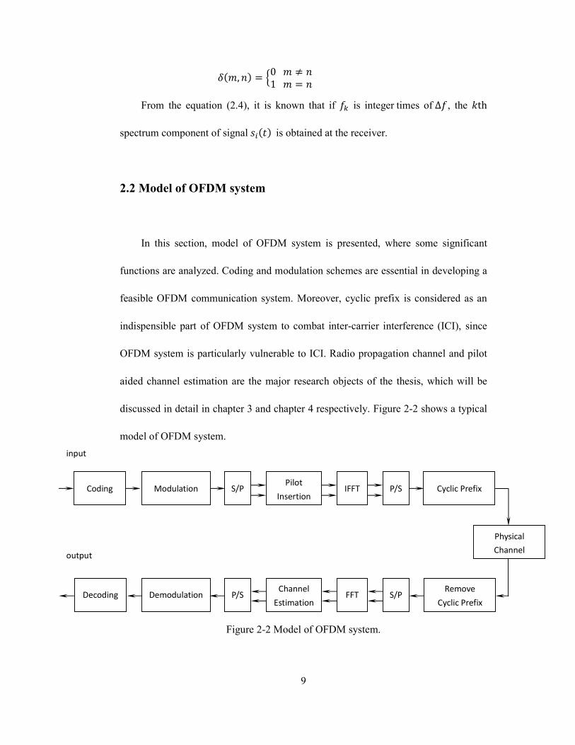
2.2 Model of OFDM system
In this section, model of OFDM system is presented, where some significant
functions are analyzed. Coding and modulation schemes are essential in developing a
feasible OFDM communication system. Moreover, cyclic prefix is considered as an
indispensible part of OFDM system to combat inter-carrier interference (ICI), since
OFDM system is particularly vulnerable to ICI. Radio propagation channel and pilot
aided channel estimation are the major research objects of the thesis, which will be
discussed in detail in chapter 3 and chapter 4 respectively. Figure 2-2 shows a typical
model of OFDM system.
Figure 2-2 Model of OFDM system.
FFT
output
Channel
Estimation
Remove
Cyclic Prefix S/P P/S Decoding Demodulation
Modulation S/P IFFT Pilot
Insertion Cyclic Prefix P/S Coding
Physical
Channel
input
10
2.2.1 Convolutional Coding
Despite the fact that OFDM system has inherent resistance to fading, in multipath
fading channel, however, some sub-carriers may suffer the deep fades, which will
results in degradation of BER. Herein, forward-error correction coding is essential.
Convolutional codes have strong error correcting capability and are widely applied to
communication practices. Therefore, Convolutional code is selected as FEC channel
coding scheme in the thesis.
Block codes and convolutional codes are the most commonly used coding scheme.
Unlike block codes, the encoder of convolutional codes contains memory and the �
encoder outputs at any given time unit depend not only on the � inputs at that time unit
but also on m previous input blocks [8]. A ��, �, �� convolutional encoder can be
implemented with a k-input, n-output linear sequential circuit with input memory m,
which means � encoded bits are generated for each � information bits. Therefore, the
code rate is defined as ; � �/�.
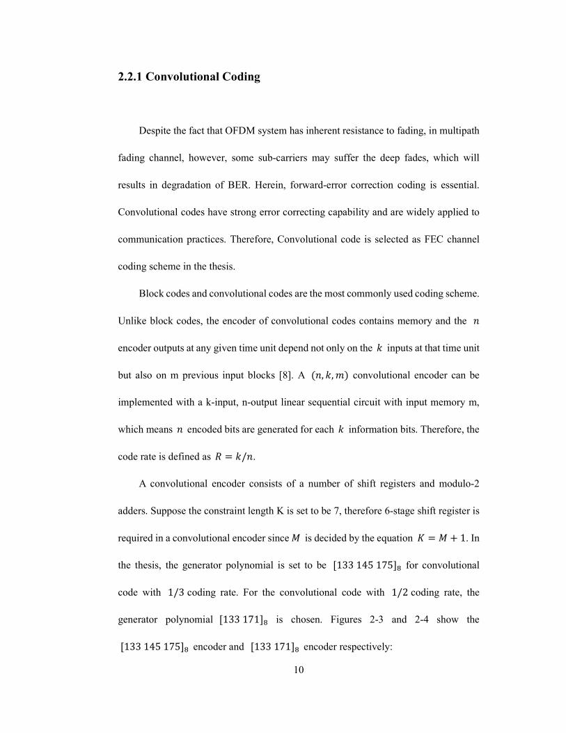
A convolutional encoder consists of a number of shift registers and modulo-2
adders. Suppose the constraint length K is set to be 7, therefore 6-stage shift register is
required in a convolutional encoder since< is decided by the equation= � < > 1. In
the thesis, the generator polynomial is set to be ?133145175DE for convolutional
code with 1/3coding rate. For the convolutional code with 1/2coding rate, the
generator polynomial ?133171DE is chosen. Figures 2-3 and 2-4 show the
?133145175DE encoder and ?133171DE encoder respectively:
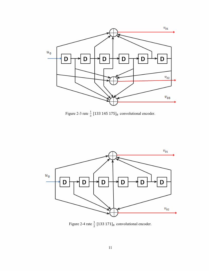
11
Figure 2-3 rate �F ?133145175DE convolutional encoder.
Figure 2-4 rate �G ?133171DE convolutional encoder.
12
A convolutional encoder generates � encoded bits for each � information bits,
and ; � �/� is called the code rate.
A convolutional encoder works by performing convolutions on the incoming input
data. Let H � �I�, I�, IG, ⋯ � denote the input sequence. For each path of the encoder,
the output sequence can be written as,
K&�L� � ∑ MN�L�I&+NON,� ," � 0, 1, 2,⋯ (2.5)
Where denotes a certain path of the encoder, and I&+N=0 whenP Q ". After
convolution, the encoder generates the coded sequence R by combining all the output
sequences of each path.
The signal S received at the decoder is distorted by noise and interference.
Maximum-likelihood decoder is applied to error correcting. In the specific case of
binary symmetric channel (BSC), the log-likelihood function can be written as,
lnV WSXY � ��S, X�ln W Z�+ZY > !ln�1 � V� (2.6)
where V is the transition probability, ��S,X� is the Hamming distance between
SandX.Note that !P��1 � V� is a constant, thus maximum-likelihood is equivalent
with minimum distance. That is, the maximum-likelihood decoder reduces to a
minimum distance decoder, by which the decoding process is to choose a path in the
trellis whose coded sequence most resembles the received sequence. By computing the
metric for each path, the survivor thus can be found and retained by the algorithm. The
metric for a certain path is defined as the Hamming distance between the coded
13
sequence and the received sequence.
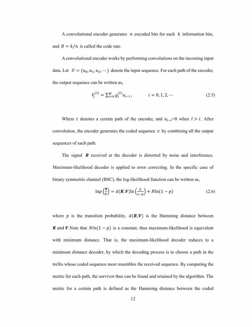
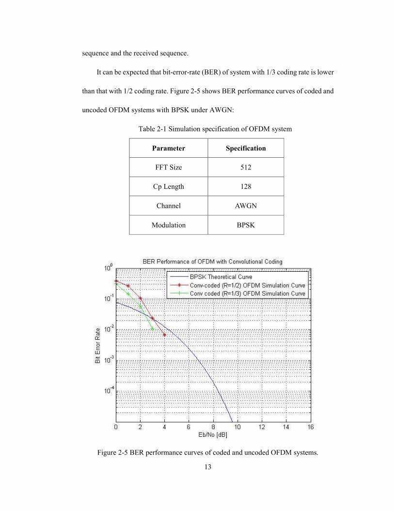
It can be expected that bit-error-rate (BER) of system with 1/3 coding rate is lower
than that with 1/2 coding rate. Figure 2-5 shows BER performance curves of coded and
uncoded OFDM systems with BPSK under AWGN:
Table 2-1 Simulation specification of OFDM system
Parameter Specification
FFT Size 512
Cp Length 128
Channel AWGN
Modulation BPSK
Figure 2-5 BER performance curves of coded and uncoded OFDM systems.
14
It can be seen from Figure 2-5 that signal-noise-ratio (SNR), by convolutional
coding, obtained 5 dB of coding gain, thus BER performance is enhanced. It is also
known from Figure 2-5 that better BER performance can be acquired by having lower
coding rate. Of course, coding gain is obtained with the sacrifice of reducing
transmission efficiency. For example, in the case of rate 1/3 ?133145175DE
convolutional, every 3 coded bits only carries 1 data bit.
2.2.2 Modulation Schemes
In practical wireless communications, baseband signal cannot be transmitted
without modulation. Information of baseband signal is transmitted in the way that
parameter of high frequency carrier wave, such as amplitude or phase, is modulated by
baseband signal, hence conveys the information that can be restored to original signal at
the receiver. Selection of proper modulation scheme is essential to communication
system design. This section presents coherent M-PSK and M-QAM schemes and
compares their performances.
M-PSK
The idea of Phase-shift keying (PSK) modulation scheme is that information of
baseband signal is conveyed by changing of carrier wave’s phase. Family of coherent
15
M-PSK includes BPSK, QPSK, 8PSK and 16PSK, where BPSK, 8PSK and 16PSK are
in discuss in this section.
BPSK is a binary digital modulation scheme, which is also the simplest form of
M-PSK. Binary data (“0” and “1”) are represented by two carrier waves with phases of
0 and ) respectively, which has the following form:
]�� � � ^_`%2)�a ,0 b b cd (2.7)
]�� � � ^_`%�2)�a > )� � �^_`%�2)�a �,0 b b cd , (2.8)
where ^ is a constant amplitude, �a is carrier frequency and cd is the bit duration.
Suppose bit energy is denoted as ed, equation (2.7) and (2.8) can be expressed as:
]�� � � fGgh�h _`%2)�a ,0 b b cd (2.9)
]�� � � �fGgh�h _`%2)�a , 0 b b cd (2.10)
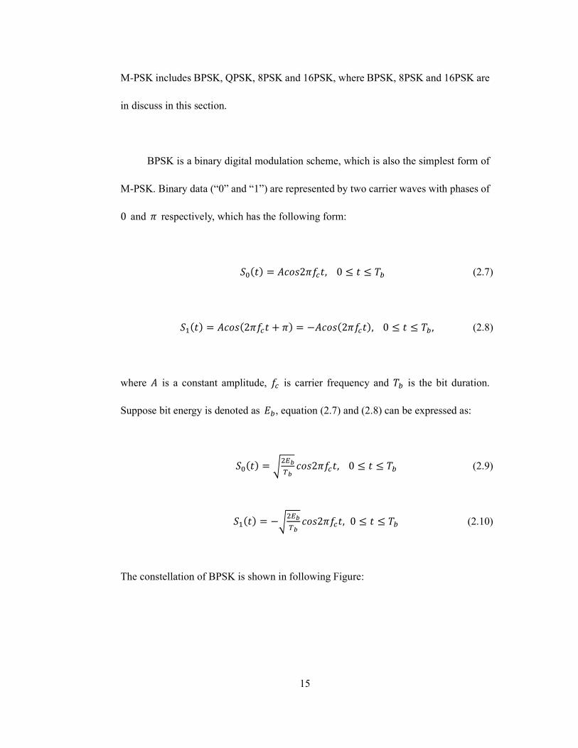
The constellation of BPSK is shown in following Figure:
16
Figure 2-6 BPSK constellation.
The bit error probability idof BPSK in AWGN is given as:
ij � k 5f2ej!0 6 � 12 lm�_�fej!0� (2.11)
Compared to binary modulation, multi-level modulation has higher spectra utilization,
thus increase transmission speed. In 8PSK, for instance, a symbol can represent 3 bits.
That is to say, bandwidth efficiency increase to 3 times compared to BPSK. Signal
modulated by 8PSK has the following form:
]&� � � fGg:�: cos�2)�a > q&� , 0 b b c., 0 b " b 7 (2.12)
where e. is the symbol energy and c. is the symbol duration. q& is defined as:
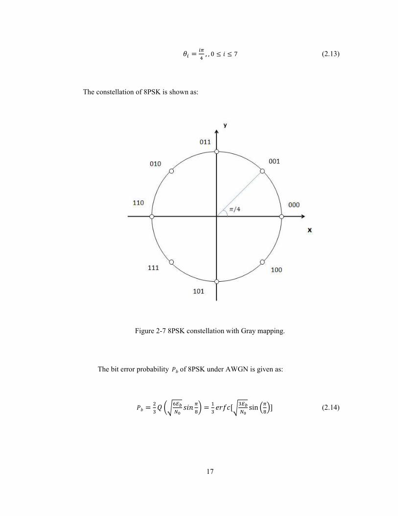
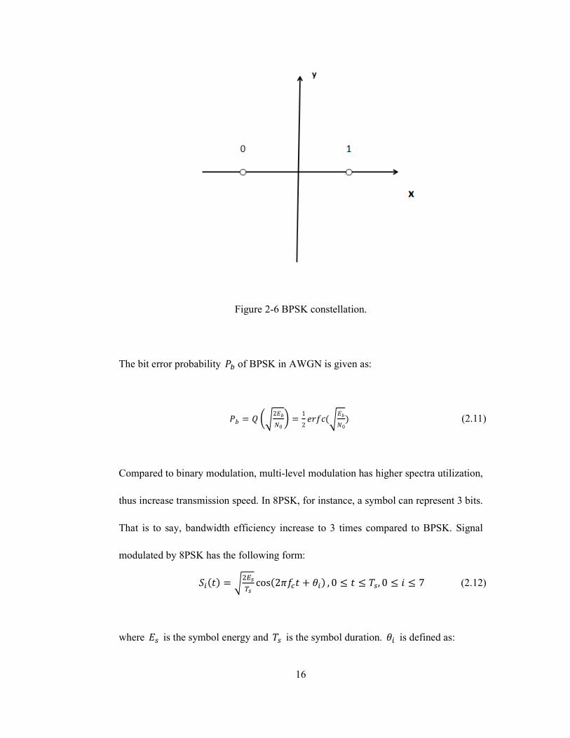
17
q& � &rs , , 0 b " b 7 (2.13)
The constellation of 8PSK is shown as:
Figure 2-7 8PSK constellation with Gray mapping.
The bit error probability ijof 8PSK under AWGN is given as:
ij � GFk 5ftgh*u %"� rE6 � �F lm�_?fFgh*u sin WrEYD (2.14)

18
Another case of M-PSK is 16PSK, whose modulated signal is similar to that of
8PSK:
]&� � � fGg:�: cos�2)�a > q&� , 0 b b c., 0 b " b 15 (2.15)
where q" in 16PSK is defined as:
q& � &rE , , 0 b " b 15 (2.16)
The constellation of 16PSK is shown as:
Figure 2-8 16PSK constellation with Gray mapping.
19
The bit error probability ijof 16PSK under AWGN is given as:
ij � �Gk 5fEgh*u %"� r�t6 � �s lm�_?fsgh*u sin W r�tYD (2.17)
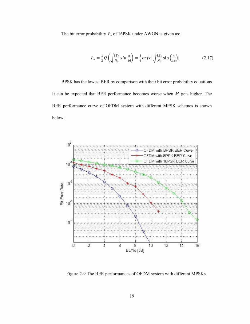
BPSK has the lowest BER by comparison with their bit error probability equations.
It can be expected that BER performance becomes worse when < gets higher. The
BER performance curve of OFDM system with different MPSK schemes is shown
below:
Figure 2-9 The BER performances of OFDM system with different MPSKs.
20
M-QAM
Quadrature amplitude modulation (QAM) is the most commonly used type of
modulation technique in OFDM [7]. As a multi-level modulation scheme, QAM
modulation scheme acquires higher data rate, that is, higher bandwidth efficiency, by
sacrificing power utilization. It implies that higher SNR is required for QAM if we
intend to maintain low bit error rate.
QAM can be regarded as the combination of two modulations on in-phase (real)
and quadrature (imaginary) branches since the carrier wave experiences amplitude as
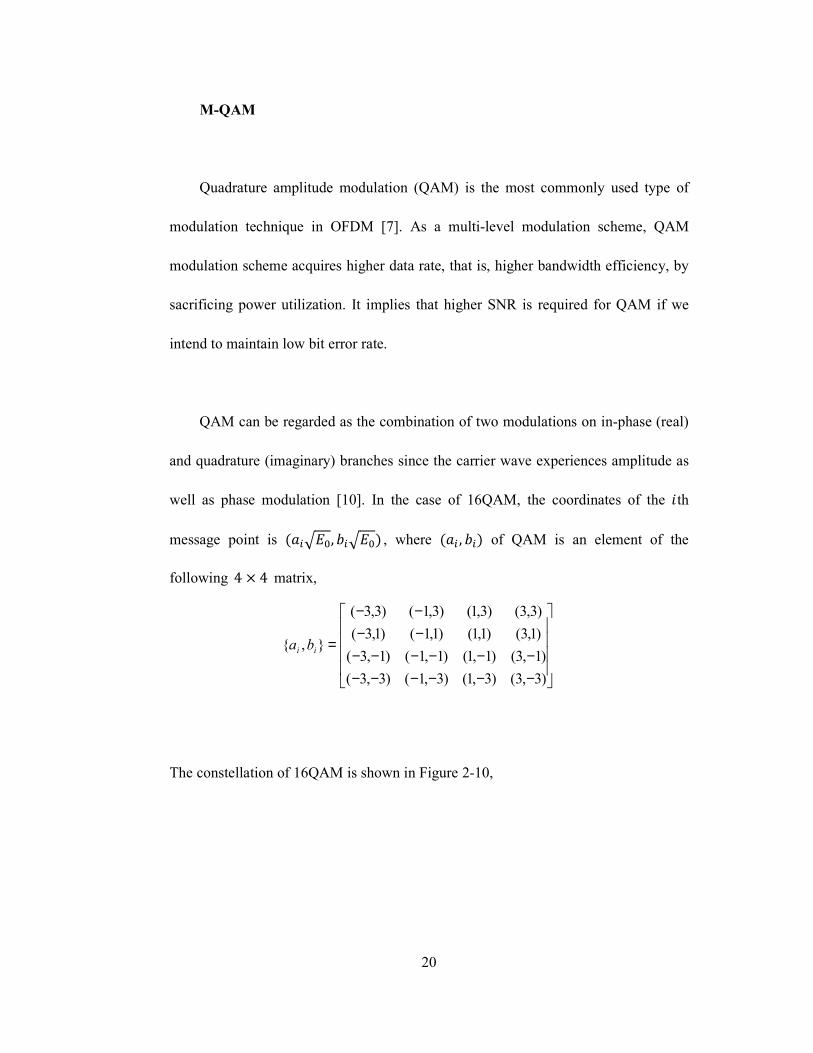
well as phase modulation [10]. In the case of 16QAM, the coordinates of the "th
message point is �w&xe�, j&xe�� , where �w& , j&� of QAM is an element of the
following 4 y 4 matrix,
−−−−−−−−−−−−
−−−−
=
)3,3()3,1()3,1()3,3()1,3()1,1()1,1()1,3(
)1,3()1,1()1,1()1,3()3,3()3,1()3,1()3,3(
},{ ii ba
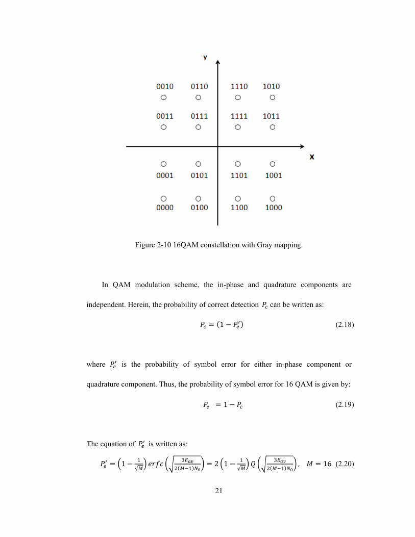
The constellation of 16QAM is shown in Figure 2-10,
21
Figure 2-10 16QAM constellation with Gray mapping.
In QAM modulation scheme, the in-phase and quadrature components are
independent. Herein, the probability of correct detection ia can be written as:
ia � �1 � iz{� (2.18)
where iz{ is the probability of symbol error for either in-phase component or
quadrature component. Thus, the probability of symbol error for 16 QAM is given by:
iz � 1 � ia (2.19)
The equation of iz{ is written as:
iz{ � W1 � �√OY lm�_ 5f Fg}~G�O+��*u6 � 2 W1 � �√OYk 5f Fg}~G�O+��*u6 ,< � 16 (2.20)

22
The probability of symbol error is therefore written as:
iz � 1 � ?1 � G�√O+��√O k 5f Fg}~G�O+��*u6DG,< � 16 (2.21)
There are four bits per symbol for 16 QAM modulation scheme. The bit error
probability for 16 QAM is denoted as:
id � Fsk 5fsgh�*u6 � ��tkG�fGgh�*u� (2.22)
System modulated by M-ary QAM scheme acquires higher data transmission rate
by suffering BER degradation. Figure 2-11 shows BER curves of OFDM systems with
M-ary QAM under AWGN:
Figure 2-11 BER curves of OFDM with M-ary QAMs under AWGN.
23
2.2.3 IFFT and FFT
As stated in Chapter 1, the modulation and demodulation of OFDM baseband
signal can be implemented by inverse discrete Fourier transform (IDFT) and discrete
Fourier transform (DFT). Let %� � be the OFDM signal. By sampling signal %� � with
the ratec/! W! � ��* , � � 0,1,2,⋯ ,! � 1Y, %� � is written as,
%� � % W��* Y � ∑ �& exp W� Gr&�* Y�0 b � b ! � 1�*+�&,� (2.23)
where �& is the original data information. In the same manner, %� � is restored at the
receiver by performing reverse calculation, i.e. DFT,
�& � ∑ %�exp��� Gr&�* �*+��,� �0 b � b ! � 1� (2.24)
In practical OFDM applications, fast Fourier transforms (FFT/IFFT) are
implemented to reduce computing complexity.
2.2.4 Cyclic Prefix
Inter symbol interference (ISI) is one of the most important issue in mobile
communication. Due to the effect of multipath channel, transmitted wireless signals are
propagated through various paths in the environment, which arrive at the receiver with
different phase, resulting in time dispersion. If the symbol width is smaller than
maximum spread delay, the performance is degraded due to ISI thus restrict high rate
24
transmitting.
One of the most important features of OFDM is inherent resistance to ISI caused
by time dispersion. By splitting the input data stream into N sub-streams, period of data
symbol in each sub-channel is expanded by N times compared to original data. Herein,
delay spread is less likely to cause ISI.
To further eliminate ISI, guard interval is applied to OFDM system. In
conventional communication system, null sequences are inserted among symbols.
Length of guard interval c�is set to be larger than maximum delay spread in wireless
communication. However, such guard interval will damage the orthogonality of OFDM
system and introduce inter-carrier interference (ICI), since sub-carriers cannot maintain
integral periodic inequality due to multipath.
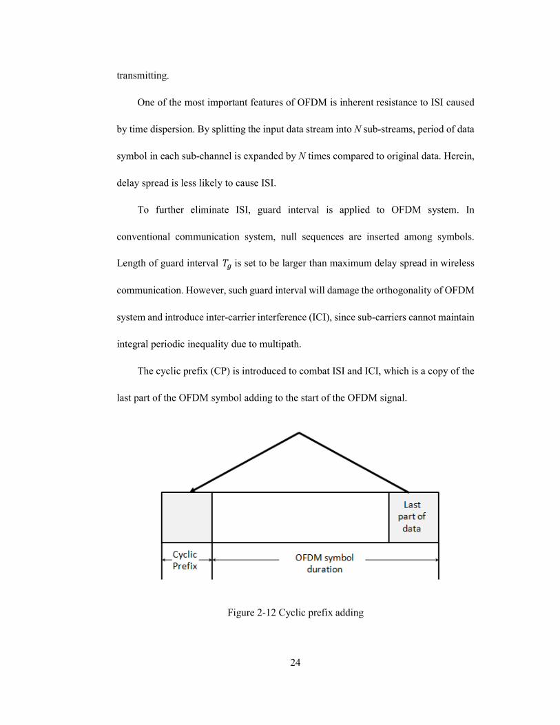
The cyclic prefix (CP) is introduced to combat ISI and ICI, which is a copy of the
last part of the OFDM symbol adding to the start of the OFDM signal.
Figure 2-12 Cyclic prefix adding
25
The adding of cyclic prefix can effectively eliminate the affect of ISI and ICI. The
length of cyclic preifx is chosen larger than maximum delay spread. Each OFDM
symbol is preceded a copy of the last part of the OFDM symbol. Theoretically, cyclic
prefix can completely keep the signal free from ISI and ICI, as long as the maximum
delay is smaller than the length of cyclic prefix.

26
Chapter 3
Characteristic and Modeling of Hyper-Rayleigh
Fading Channel
Analysis and modeling of radio propagation is a most important issue in wireless
communication. Only by properly measuring the characteristic of fading channel,
communication system can be correctly developed. Recent studies show propagation
channel in some WSN applications where sensor nodes deployed within cavity
environment exhibits worse behavior than Rayleigh fading channel, which is referred
to as hyper-Rayleigh fading channel [12]. Therefore, modeling of hyper-Rayleigh
fading channel is the central issue. Chapter 3 describes the cause and effect of small
scale fading. Characteristic and modeling of hyper-Rayleigh fading channel is
presented and comparison is made between conventional small scale fading model and
hyper-Rayleigh fading model.
3.1 Small Scale Fading
There are generally two types of fading in wireless communication: large scale
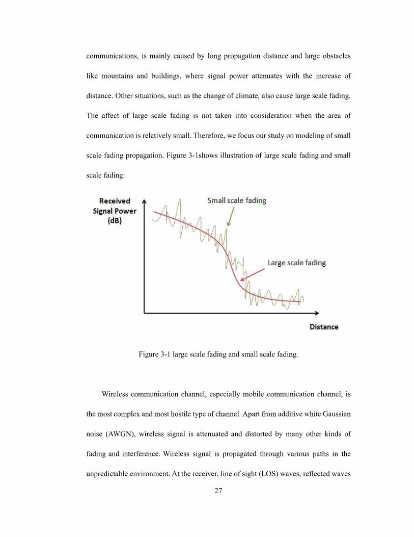
and small scale fading. Large scale fading, which is the major concern in microwave
27
communications, is mainly caused by long propagation distance and large obstacles
like mountains and buildings, where signal power attenuates with the increase of
distance. Other situations, such as the change of climate, also cause large scale fading.
The affect of large scale fading is not taken into consideration when the area of
communication is relatively small. Therefore, we focus our study on modeling of small
scale fading propagation. Figure 3-1shows illustration of large scale fading and small
scale fading:
Figure 3-1 large scale fading and small scale fading.
Wireless communication channel, especially mobile communication channel, is
the most complex and most hostile type of channel. Apart from additive white Gaussian
noise (AWGN), wireless signal is attenuated and distorted by many other kinds of
fading and interference. Wireless signal is propagated through various paths in the
unpredictable environment. At the receiver, line of sight (LOS) waves, reflected waves
28
and scattering waves cause severe distortion of the original signal. The received waves
can be categorized into two classes: specular waves and diffuse waves.
3.1.1 Multipath Fading
The main characteristic of wireless fading channel is multipath. In the wireless
channel environment, transmitting signals are propagated through various paths, which
arrive at the receiver with different phases and amplitudes, resulting in fading signal.
We describe this kind of situation as multipath fading, which will cause amplitude and
phase fluctuations and time dispersion in the received signals.
During signal propagation, some received signal waves often spread to other
signals because of delay spread, which causes inter-symbol interference (ISI).
Maximum delay spread ���� is used to measure multipath fading in specific
propagation environment.
In the view of frequency domain, delay spread could result in frequency selective
fading [11]. For different frequency component of the signal, wireless channel exhibits
diverse random response. Signal wave will suffer distortion after fading. Coherence
bandwidth is introduced to measure frequency selective fading. In practice, coherent
bandwidth �a is defined as:
�a � ���}� (3.1)
29
where ���� is maximum delay spread in fading circumstance.
If the signal transmission rate is so high that signal bandwidth exceeds coherence
bandwidth of wireless channel, frequency selective fading is occurred. Otherwise,
when signal bandwidth is smaller than �a, signal is consider to experience flat fading.
3.1.2 Doppler Effect
Doppler Effect is occurred when mobile station is receiving signal in a move. The
frequency of signal is changing depends on the speed and direction of mobile station.
Such characteristic of wireless channel is referred to as time-variance.
In a time-varying channel, the transfer function is varying with time, i.e. diverse
signals are received when the same signal is transmitting at different time. Doppler shift
is the reflection of time-variance in mobile communication system. At the receiver,
transmitted single frequency signal becomes signal with bandwidth and envelop after
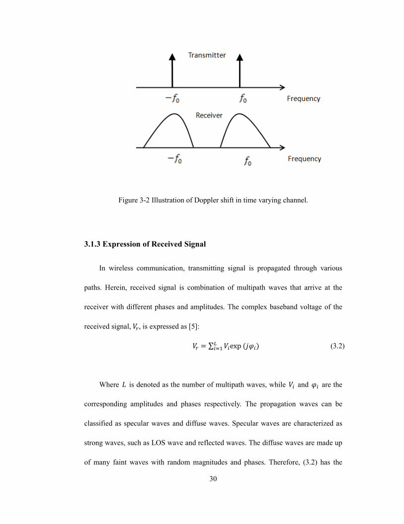
time-varying channel. This phenomenon is also known as frequency dispersion, as
shown in Figure 3-2:
30
Figure 3-2 Illustration of Doppler shift in time varying channel.
3.1.3 Expression of Received Signal
In wireless communication, transmitting signal is propagated through various
paths. Herein, received signal is combination of multipath waves that arrive at the
receiver with different phases and amplitudes. The complex baseband voltage of the
received signal,K�, is expressed as [5]:
K� � ∑ K&exp���&��&,� (3.2)
Where � is denoted as the number of multipath waves, while K& and �& are the
corresponding amplitudes and phases respectively. The propagation waves can be
classified as specular waves and diffuse waves. Specular waves are characterized as
strong waves, such as LOS wave and reflected waves. The diffuse waves are made up
of many faint waves with random magnitudes and phases. Therefore, (3.2) has the
31
following form:
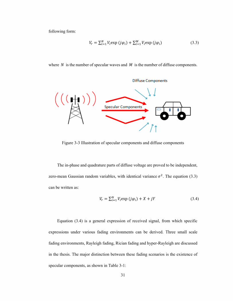
K� � ∑ K&exp���&�*&,� > ∑ K&exp���&�O&,� (3.3)
where ! is the number of specular waves and < is the number of diffuse components.
Figure 3-3 Illustration of specular components and diffuse components
The in-phase and quadrature parts of diffuse voltage are proved to be independent,
zero-mean Gaussian random variables, with identical variance�G. The equation (3.3)
can be written as:
K� � ∑ K&exp���&�*&,� > ( > �� (3.4)
Equation (3.4) is a general expression of received signal, from which specific
expressions under various fading environments can be derived. Three small scale
fading environments, Rayleigh fading, Rician fading and hyper-Rayleigh are discussed
in the thesis. The major distinction between these fading scenarios is the existence of
specular components, as shown in Table 3-1:

32
Table 3-1 Fading scenario characterized by specular components
Fading scenario Specular components
Rayleigh fading Not exist
Rician fading 1 specular wave
Hyper-Rayleigh fading 2 specular waves
The characteristic and behavior of three fading channels will be discussed in detail
in the next section.
3.2 Typical Small Scale Fading Models
In this section, two typical small-scale fading channel models, Rayleigh and
Ricean, are presented and investigated. Modeling of radio propagation is essential to
wireless communication systems since it enables one to adopt appropriate means to
reduce signal attenuation and distortion. Rician and Rayleigh models are most
commonly used to describe wireless propagation fading channel, especially mobile
communication channel.
3.2.1 Rayleigh Fading Model
Rayleigh fading environment is characterized by many multipath components,
each with relatively similar signal magnitude, and uniformly distributed phase, which
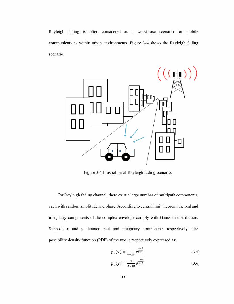
means there is no line of sight (LOS) path between transmitter and receiver. Therefore,
33
Rayleigh fading is often considered as a worst-case scenario for mobile
communications within urban environments. Figure 3-4 shows the Rayleigh fading
scenario:
Figure 3-4 Illustration of Rayleigh fading scenario.
For Rayleigh fading channel, there exist a large number of multipath components,
each with random amplitude and phase. According to central limit theorem, the real and
imaginary components of the complex envelope comply with Gaussian distribution.
Suppose � and y denoted real and imaginary components respectively. The
possibility density function (PDF) of the two is respectively expressed as:
V���� � ��√Gr l������ (3.5)
V���� � ��√Gr l������ (3.6)
34
where σ represents the standard deviation of the envelope amplitude (also known as
the rms value of the envelope). Since both random variables are independent and
identically distributed, the joint distribution can be written as
V����, �� � V���� ∙ V���� � �Gr�� l����������� (3.7)
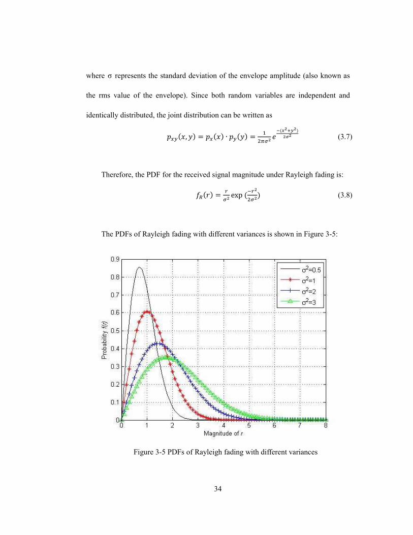
Therefore, the PDF for the received signal magnitude under Rayleigh fading is:
���m� � ��� exp�+��G��� (3.8)
The PDFs of Rayleigh fading with different variances is shown in Figure 3-5:
Figure 3-5 PDFs of Rayleigh fading with different variances
35
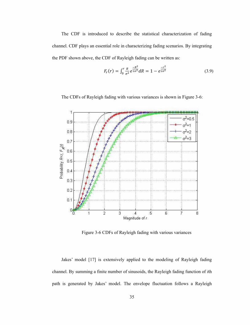
The CDF is introduced to describe the statistical characterization of fading
channel. CDF plays an essential role in characterizing fading scenarios. By integrating
the PDF shown above, the CDF of Rayleigh fading can be written as:
���m� � � ��� l� �����; � 1 � l�¡������ (3.9)
The CDFs of Rayleigh fading with various variances is shown in Figure 3-6:
Figure 3-6 CDFs of Rayleigh fading with various variances
Jakes’ model [17] is extensively applied to the modeling of Rayleigh fading
channel. By summing a finite number of sinusoids, the Rayleigh fading function of ith
path is generated by Jakes’ model. The envelope fluctuation follows a Rayleigh
36
distribution, and the phase fluctuation follows a uniform distribution on the fading in
the propagation path. Therefore, the simulation equation of Rayleigh channel can be
written as follows [18]:
m� � � ¢ 2! > 1£1_`% W)�! Y ¤2)�¥���_`% 52)�! 6 ¦*�,� >¢ 2! > 1_`%�2)�¥��� �§
>�fG* �∑ %"��r�* �_`%?2)�¥���_`%�Gr�* � D**,� ¨ (3.10)
where �¥��� is the maximum Doppler frequency and ! is the number of waves
applied to generate Rayleigh fading signal.
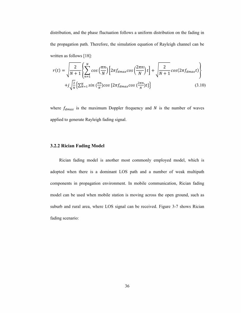
3.2.2 Rician Fading Model
Rician fading model is another most commonly employed model, which is
adopted when there is a dominant LOS path and a number of weak multipath
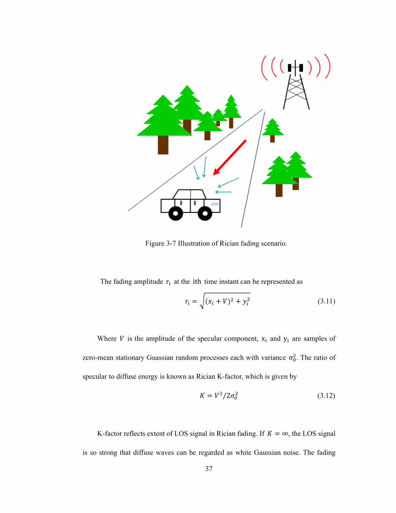
components in propagation environment. In mobile communication, Rician fading
model can be used when mobile station is moving across the open ground, such as
suburb and rural area, where LOS signal can be received. Figure 3-7 shows Rician
fading scenario:
37
Figure 3-7 Illustration of Rician fading scenario.
The fading amplitude rª at the ith time instant can be represented as
m& � f��& > K�G > �&G (3.11)
Where K is the amplitude of the specular component, xª and yª are samples of
zero-mean stationary Guassian random processes each with variance σ�G. The ratio of
specular to diffuse energy is known as Rician K-factor, which is given by
= � KG/2��G (3.12)
K-factor reflects extent of LOS signal in Rician fading. If = � ∞, the LOS signal
is so strong that diffuse waves can be regarded as white Gaussian noise. The fading
38
behavior will follow Gaussian distribution. If= � 0, on the other hand, there is no LOS
path in propagation channel, and the fading behavior will show the characteristic of
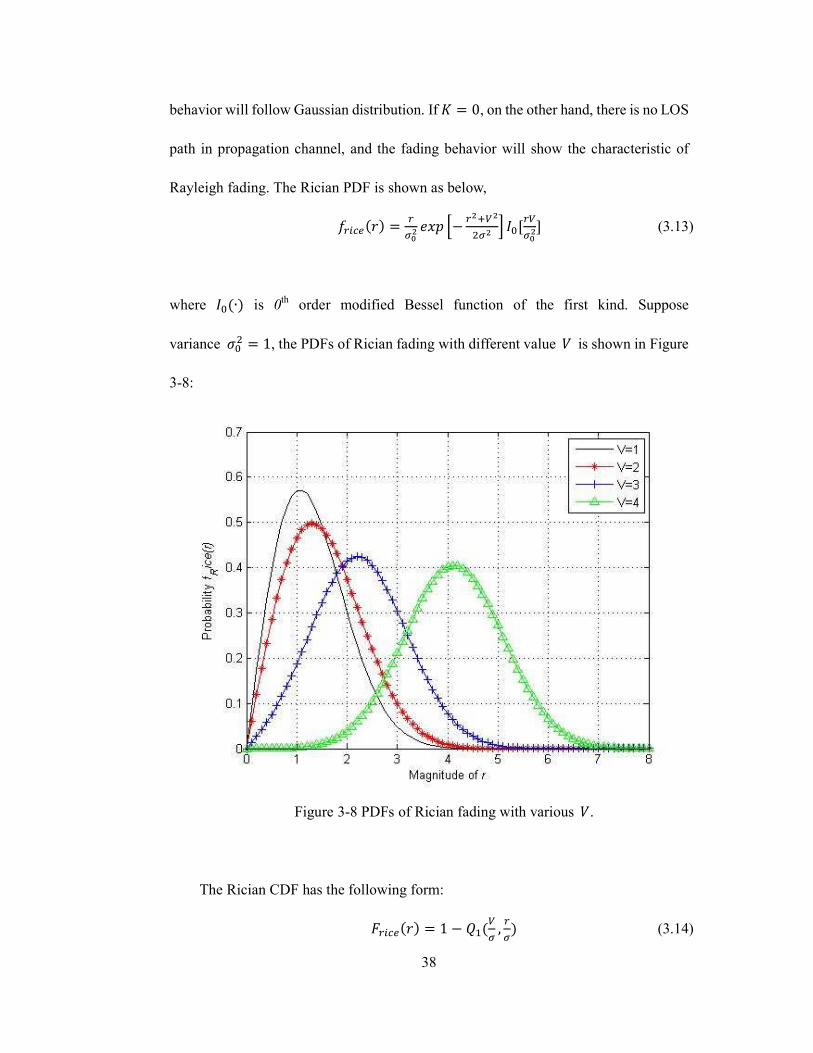
Rayleigh fading. The Rician PDF is shown as below,
��&az�m� � ��u� l�V � ��®¯�G�� ° ±�?��̄u�D (3.13)
where ±��∙� is 0th order modified Bessel function of the first kind. Suppose
variance��G � 1, the PDFs of Rician fading with different value K is shown in Figure
3-8:
Figure 3-8 PDFs of Rician fading with various K.
The Rician CDF has the following form:
��&az�m� � 1 � k���̄ , ��� (3.14)

39
where k� is the Marcum-Q-function. Figure 3-8 shows the CDFs of Rician fading with
variousK:
Figure 3-9 CDFs of Rician fading with variousK.
There is no closed-form expression of mean value of Rician distribution; however,
mean-squared value can be derived as
e²mG³ � KG > 2��G (3.15)
In system simulation, it is often required a Rician distribution with unit mean-squared
value, i.e., E²rG³ � 1, so that the signal power and the signal-to-noise ratio (SNR)
coincide. Therefore, we can get the following expressions
KG � 2��G= (3.16)
40
��G � �G�µ®�� (3.17)
Therefore, the fading amplitude rª at the ith time instant can be written in the form
m& � f��¶®√G���®�¶�G��®�� (3.18)
3.3 Hyper-Rayleigh Fading Model
Wireless sensor networks (WSN) have gained much interest lately as an effective
means to monitor industrial, military and natural environments. As applications of
WSN being widely spread, selection of proper propagation model for particular WSN
application has become a vital problem. Argument of anti-interference technologies’
feasibility is based on correct modeling of the fading circumstance. Large scale model,
such as two-wave and log-shadowing models, are employed to represent radio
propagation phenomena. Although sensor nodes are statically equipped in most cases,
it is often found necessary to consider small scale fading in some WSN applications.
Rayleigh fading model was found a proper model to represent small scale fading
behavior occurred in WSN environments. However, for some particular WSN
applications where sensor nodes are deployed within cavity environment, such as
airframe and shipping containers, transmitting signal experiences severe multipath
fading which is worse than fading behavior predicted by Rayleigh fading model [2] [12]
[13]. Therefore, a more applicable fading model is required to employ to represent such
41
small scale fading circumstance, which is referred to as hyper-Rayleigh fading channel.
Recent researches suggest that two-wave with diffuse power (TWDP) model is a good
candidate of hyper-Rayleigh fading model [2] [13] [14].
Two-wave with diffuse power model is considered as the most promising
candidate model for hyper-Rayleigh fading scenario [2] [3]. Based on in-vehicle data
collection in airframe and bus, research shows that propagation behavior is very similar
to the characteristic of TWDP model. Take airframe environment for example, specular
waves are expected to receive for each sensor node. Therefore, TWDP model instead of
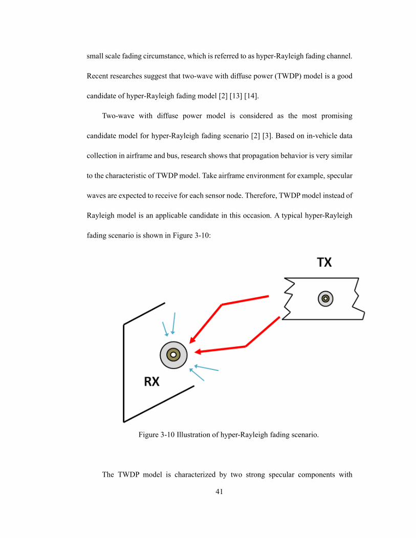
Rayleigh model is an applicable candidate in this occasion. A typical hyper-Rayleigh
fading scenario is shown in Figure 3-10:
Figure 3-10 Illustration of hyper-Rayleigh fading scenario.
The TWDP model is characterized by two strong specular components with
42
constant amplitude and random phases, along with a number of scattering waves.
Specifically, the received voltage of complex envelop V¸¹º¹ª»¹¼ is dominated by two
specular waves with constant amplitude (V� and VG) and random phase (φ� and φG),
while the remaining components are categorized as non-specular or diffuse components.
The diffuse components are made up of many waves of random magnitude and phase,
the latter being uniformly distributed over [0, 2π). The diffuse components are the same
with the Rayleigh envelope component.
If no specular components existed in propagation environment, the fading channel
is characterized as Rayleigh fading. By adding a LOS signal to the channel, Rician
fading model becomes a proper candidate to represent fading behavior. TWDP model is
similar to the Rician fading model but with two specular components [15],
K�zaz&½z¥ � K�l3¾¿ > KGl3¾� > ∑ K&l3¾¶*&,F (3.19)
where N is the number of waves, K�l3¾¿ andKGl3¾� represent two specular
components, ∑ K&l3¾¶*&,F is denoted as diffuse components.
In Rician fading channel, ratio of specular to diffuse energy = is introduced to
demonstrate reflects extent of LOS signal in Rician fading. Similarly, ratio of average
specular power to diffuse energy = is utilized in TWDP model to indicate relative
weights between specular components and diffuse components. As there are two
specular components in TWDP model, peak to average specular power ratio is also an
important parameter. Therefore, two parameters ( ∆and= ) are introduced to
characterize TWDP model. ∆and=are given as:

43
∆� À¹ÁÂÃĹºÅÆÁ¸ÄÇȹ¸É»¹¸ÁʹÃĹºÅÆÁ¸ÄÇȹ¸� 1 � GË¿Ë�Ë¿�®Ë�� (3.20)
K � É»¹¸ÁʹÃĹºÅÆÁ¸ÄÇȹ¸ÍªÎÎÅùÄÇȹ¸ � Ë¿�®Ë��Gσ� (3.21)
The relation between TWDP model and other fading models can be defined
by∆and=. For Rayleigh fading, there is no specular wave, thus ∆is not applicable
and = � 0. In the case of Rician fading, peak specular power and average specular
power are identical, herein ∆is equal to 0. The diffuse components are trivial compared
with two strong specular waves in Two-ray model, which make = approach infinity.
TWDP model describes the fading situation between Rician fading and two-ray fading.
To sum up, the comparison of four fading models, Rayleigh, Rician, two-ray and
hyper-Rayleigh fading, can be made by the parameters∆and=, as Table 3-2 shows:
Table 3-2 Comparison between four fading models
Fading scenario ∆ =
Rayleigh fading Not applicable = � 0
Rician fading ∆� 0 = Q 0
Two-ray fading ∆Q 0 = ≫ 0
Hyper-Rayleigh fading ∆Q 0 = Q 0
There is no closed-form expression of TWDP PDF. [5] presents approximate of
TWDP PDF:
��ÐÑÒ�m� � ��� exp�+��G�� � =�∑ w&Ó��� , =, Δ_`% r�&+��GO+� �O&,� (3.22)
44
where < is the order of approximate, w& is the corresponding value, Ó is the function
defined as:
Ó��, =, Õ� � �G exp�Õ=� ±� W�x2=�1 � Õ�Y > �G exp��Õ=�±� W�x2=�1 > Õ�Y (3.23)
where ±��∙� is 0th order modified Bessel function of the first kind.
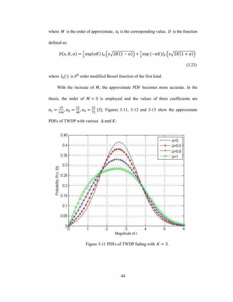
With the increase of <, the approximate PDF becomes more accurate. In the
thesis, the order of < � 3 is employed and the values of three coefficients are
w� � ���ss , wG � G�sE , wF � G��G [5]. Figures 3-11, 3-12 and 3-13 show the approximate
PDFs of TWDP with various ∆and=:
Figure 3-11 PDFs of TWDP fading with = � 3.
45
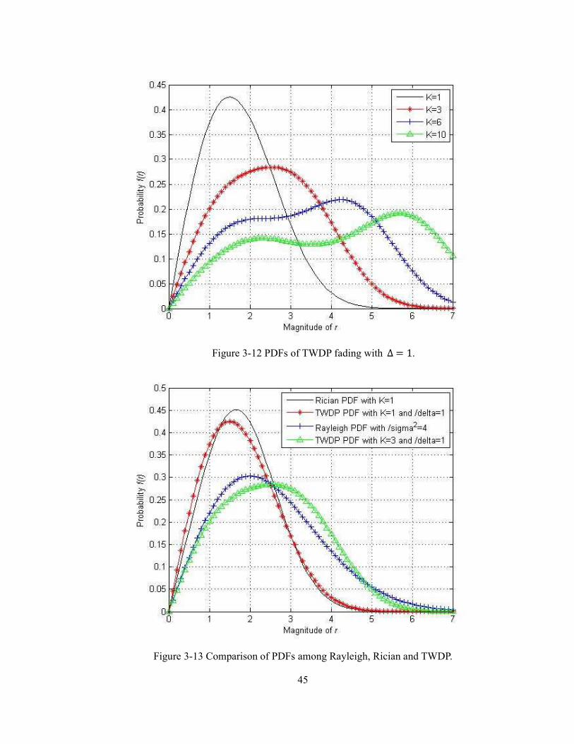
Figure 3-12 PDFs of TWDP fading with ∆� 1.
Figure 3-13 Comparison of PDFs among Rayleigh, Rician and TWDP.
46
The above figures indicate that PDFs of TWDP fading is similar to Rician PDFs
when ∆and= are small. When the value of = exceeds 3, TWDP PDFs exhibit
poorer performance than Rician and Rayleigh PDFs.
There is no closed-form equation for TWDP CDF. However, the range of TWDP
CDF can be determined by two-ray fading and Rayleigh fading, which are served as the
upper bound and lower bound respectively.
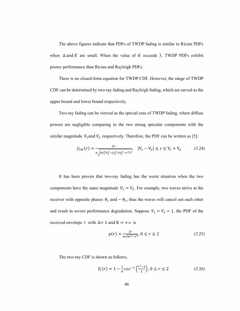
Two-ray fading can be viewed as the special case of TWDP fading, where diffuse
powers are negligible comparing to the two strong specular components with the
similar magnitudeK�andKG respectively. Therefore, the PDF can be written as [5]:
��Ð�m� � G�rfs ¿̄� �̄�+� ¿̄�® �̄�+���� , |V� � VG| b r b V� > VG (3.24)
It has been proven that two-ray fading has the worst situation when the two
components have the same magnitudeK� � KG. For example, two waves arrive at the
receiver with opposite phases θ�and � θ�, thus the waves will cancel out each other
and result in severe performance degradation. SupposeK� � KG � 1, the PDF of the
received envelope m with ∆� 1andK � >∞ is
V�m� � G�r√s��+�Ø , 0 b m b 2 (3.25)
The two-ray CDF is shown as follows,
���m� � 1 � �r _`%+� W��+GG Y , 0 b m b 2 (3.26)
47
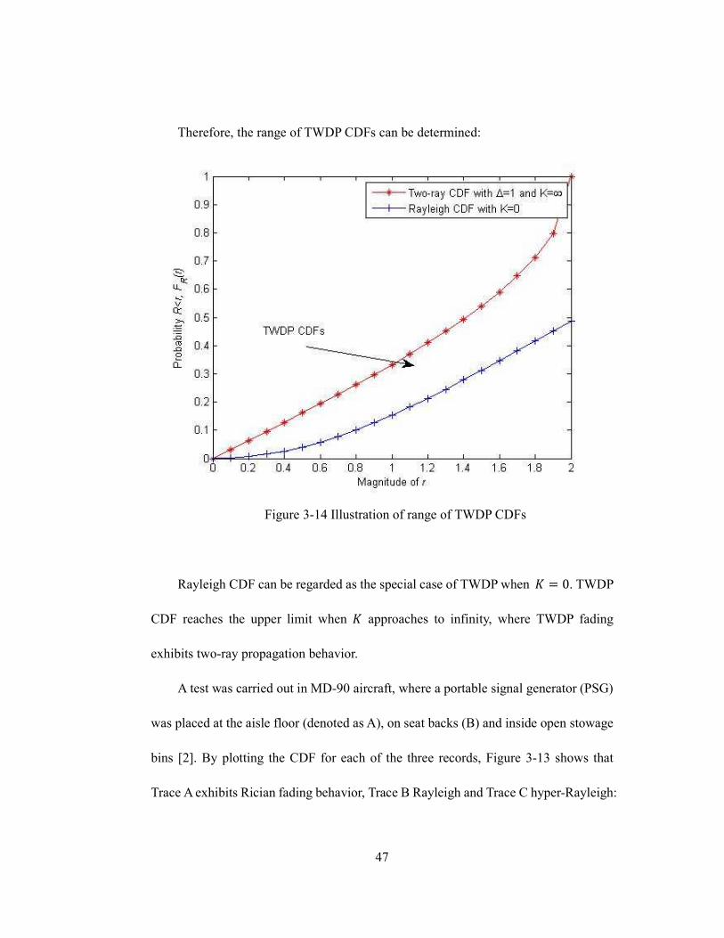
Therefore, the range of TWDP CDFs can be determined:
Figure 3-14 Illustration of range of TWDP CDFs
Rayleigh CDF can be regarded as the special case of TWDP when = � 0. TWDP
CDF reaches the upper limit when = approaches to infinity, where TWDP fading
exhibits two-ray propagation behavior.
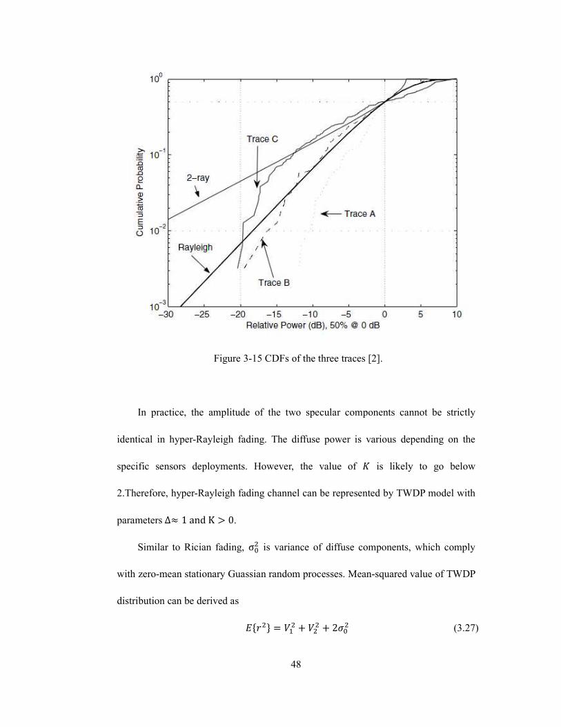
A test was carried out in MD-90 aircraft, where a portable signal generator (PSG)
was placed at the aisle floor (denoted as A), on seat backs (B) and inside open stowage
bins [2]. By plotting the CDF for each of the three records, Figure 3-13 shows that
Trace A exhibits Rician fading behavior, Trace B Rayleigh and Trace C hyper-Rayleigh:
48
Figure 3-15 CDFs of the three traces [2].
In practice, the amplitude of the two specular components cannot be strictly
identical in hyper-Rayleigh fading. The diffuse power is various depending on the
specific sensors deployments. However, the value of = is likely to go below
2.Therefore, hyper-Rayleigh fading channel can be represented by TWDP model with
parameters∆� 1andK Q 0.
Similar to Rician fading, σ�G is variance of diffuse components, which comply
with zero-mean stationary Guassian random processes. Mean-squared value of TWDP
distribution can be derived as
e²mG³ � K�G > KGG > 2��G (3.27)
49
By substituting V�G > VGG with∆andK, we have
m& � f��& > �∆®��µµ®� �G > �&G (3.28)
The resultant of the two specular paths can be written as
V� > VG � Vexp?j�θG � θ��D (3.29)
where θ � θG � θ� is a random variable uniformly distributed over the interval?0,2πD.
50
Chapter 4
2-D Pilot Aided Channel Estimation in OFDM System
In mobile communication, radio signal transmitted through the wireless channel is
suffered from time dispersion and frequency dispersion caused by multipath
propagation and Doppler shift, which results in severe performance degradation of the
communication system. Though OFDM system can significantly reduce the effect of
multipath fading, OFDM signal is very sensitive to Doppler shift, since Doppler shift
may bring about frequency offset and impair the orthogonality of OFDM sub-carriers
[15]. Channel estimation is designed to overcome fading and interference in OFDM
system by finding out the frequency response of the fading channel. In Chapter 4, three
pilot-aided channel estimation techniques are presented and analyzed.
4.1 Procedure of Channel Estimation in OFDM System
Pilot-based channel estimation has been proven to be a feasible and effective
method for OFDM systems. The idea of pilot-aided channel estimation is to insert
known pilot sequence into data symbol complying with specific pilot pattern, so that
the channel information can be obtained at the receiver by estimation techniques and
51
interpolation methods.
Anti-interference capacity and transmission efficiency may vary with various pilot
patterns, which will be further discussed in the next section. In this section, the
procedure of channel estimation in OFDM system is presented. After pilot insertion and
IFFT, the modulated signal �8��� will be transmitted through wireless
communication channel, which is set to be a frequency selective time varying fading
channel with AWGN. Hence, the received signal �8���is given as follows:
�8��� � �8��� y -��� > ��� (4.1)
where ��� is additive with Gaussian noise, and -��� is the channel impulse
response due to multi-path delay, which is expressed as [16]:
-��� � ∑ -&l3W�ÜÝ Y8Þ¶�ß7�à � �&�á+�&,� (4.2)
where γ is the total number of propagation paths, hª is the complex impulse response
of the ith path, fÍä is the ith path Doppler frequency shift which causes ICI of the
received signals. λ is delay spread index, T is the sample period and τª is the ith path
delay normalized by the sampling time.
At the receiver, signal is sent to FFT. After FFT processing, the signal is given as:
���� � (���è��� > ±��� > é���, � � 0,1,⋯ ,! � 1 (4.3)
where ±��� is ICI due to Doppler frequency. Suppose there is ICI occurred because of
cyclic prefix. Equation (4.3) can be written as:
52
���� � (���è��� > ±��� >é���, � � 0,1,⋯ ,! � 1 (4.4)
The received pilot signals ����are extracted to obtain the channel impulse
responseèÒ��� at the pilots, which is given as:
èÒ��� � êë���ìë��� (4.5)
The channel transfer function è��� can be estimated based onèÒ���. With the
estimated channel transfer function èí���, the data signal is recovered:
(î��� � ê���ïí��� (4.6)
4.2 2-D Pilot arrangement
Pilot arrangement is an essential issue in pilot-based channel estimation. Under
various fading environments, it is important to utilize proper pilot pattern to achieve
optimum BER performance. Pilot patterns can be grouped into two categories:
one-dimensional (1-D) pilot patterns and two-dimensional (2-D) pilot patterns [20].
Pilots are inserted in either time domain or frequency domain, while 2-D pilots are
inserted in both time domain and frequency domain. This section gives an extensive
analysis and comparison between 1-D pilot patterns and 2-D pilot patterns.
4.2.1 1-D Pilot Pattern
There are two typical types of 1-D pilot pattern: block type and comb type [21]. In
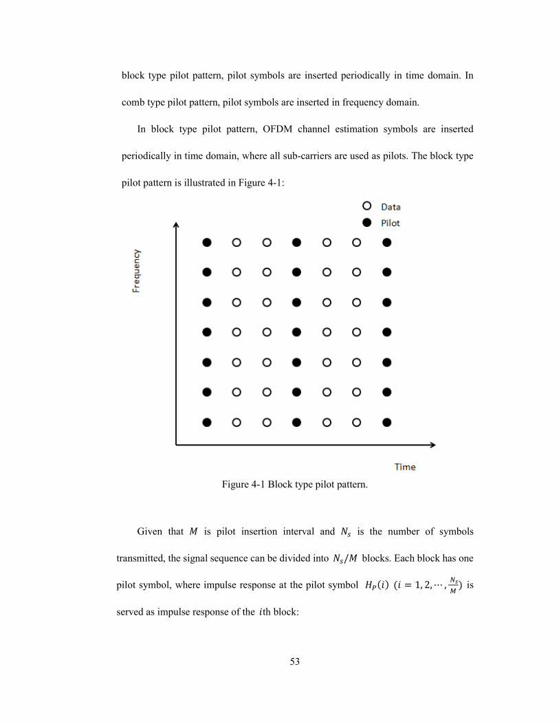
53
block type pilot pattern, pilot symbols are inserted periodically in time domain. In
comb type pilot pattern, pilot symbols are inserted in frequency domain.
In block type pilot pattern, OFDM channel estimation symbols are inserted
periodically in time domain, where all sub-carriers are used as pilots. The block type
pilot pattern is illustrated in Figure 4-1:
Figure 4-1 Block type pilot pattern.
Given that < is pilot insertion interval and !. is the number of symbols
transmitted, the signal sequence can be divided into !./< blocks. Each block has one
pilot symbol, where impulse response at the pilot symbol èÒ�"� �" � 1, 2,⋯ , *:O � is
served as impulse response of the "th block:

54
Figure 4-2 Illustration of block type pilot channel estimation.
Since there are pilot signals in every sub-carrier, block type pilot pattern is an
appropriate selection under frequency selective slow fading channel. If the channel
impulse is constant during each block, there will be no channel estimation error since
every OFDM symbol in the " th block has the same channel transfer function
withèÒ�"�. However, block type pilot channel estimation is vulnerable to fast fading
channel, since channel transfer function may vary rapidly even in one block.
It has been proved that comb type pilot pattern has better performance in fast
fading channel, since part of the sub-carriers are always reserved as pilot for each
symbol so that pilots are inserting through time domain to track fast fading [22].
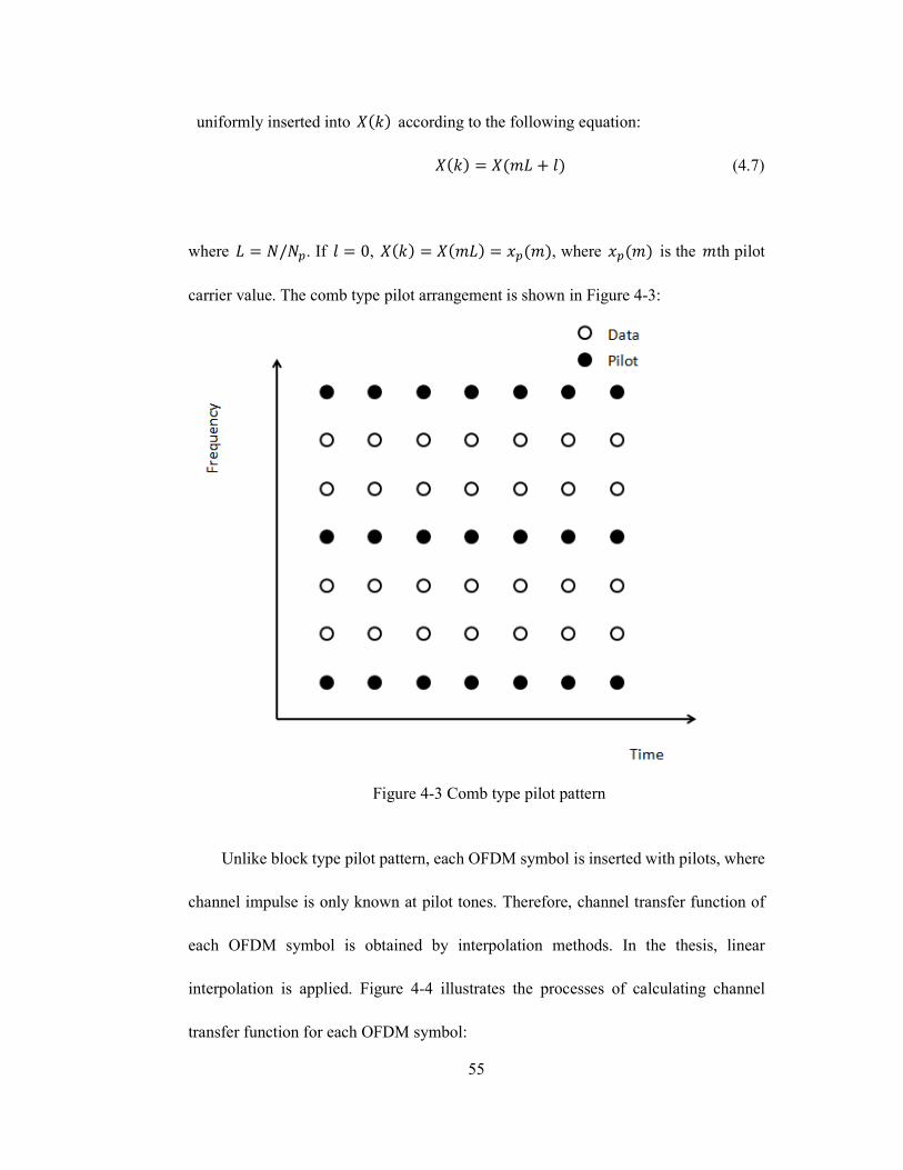
Suppose ! is number of carriers in OFDM system and !Ò pilot signals are
55
uniformly inserted into (��� according to the following equation:
(��� � (��� > P� (4.7)
where � � !/!Z. If P � 0, (��� � (���� � �Z���, where �Z��� is the �th pilot
carrier value. The comb type pilot arrangement is shown in Figure 4-3:
Figure 4-3 Comb type pilot pattern
Unlike block type pilot pattern, each OFDM symbol is inserted with pilots, where
channel impulse is only known at pilot tones. Therefore, channel transfer function of
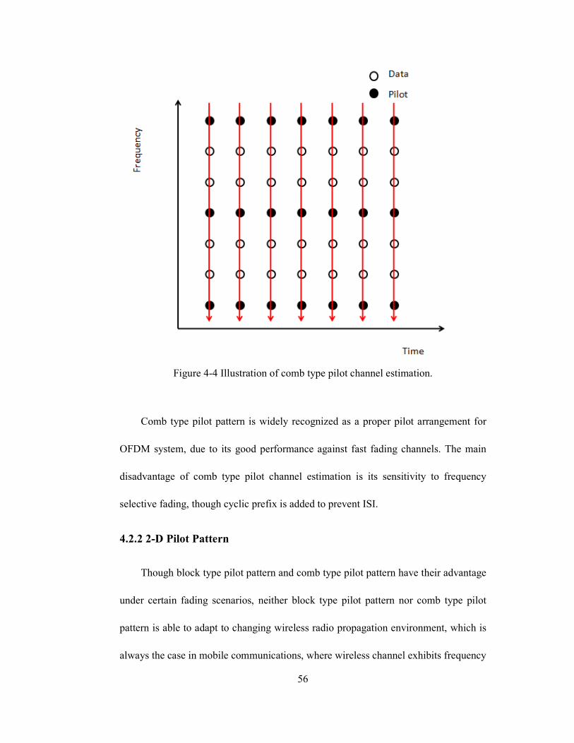
each OFDM symbol is obtained by interpolation methods. In the thesis, linear
interpolation is applied. Figure 4-4 illustrates the processes of calculating channel
transfer function for each OFDM symbol:
56
Figure 4-4 Illustration of comb type pilot channel estimation.
Comb type pilot pattern is widely recognized as a proper pilot arrangement for
OFDM system, due to its good performance against fast fading channels. The main
disadvantage of comb type pilot channel estimation is its sensitivity to frequency
selective fading, though cyclic prefix is added to prevent ISI.
4.2.2 2-D Pilot Pattern
Though block type pilot pattern and comb type pilot pattern have their advantage
under certain fading scenarios, neither block type pilot pattern nor comb type pilot
pattern is able to adapt to changing wireless radio propagation environment, which is
always the case in mobile communications, where wireless channel exhibits frequency
57
selective property and time varying behavior. Moreover, there is another drawback of
the 1-D pilot pattern, which is transmission inefficiency. For example, in an OFDM
system with pilot interval< � 8, there are 12.5 percent of total transmitting signals are
occupied by pilot tones.
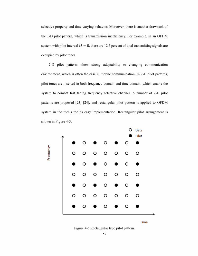
2-D pilot patterns show strong adaptability to changing communication
environment, which is often the case in mobile communication. In 2-D pilot patterns,
pilot tones are inserted in both frequency domain and time domain, which enable the
system to combat fast fading frequency selective channel. A number of 2-D pilot
patterns are proposed [23] [24], and rectangular pilot pattern is applied to OFDM
system in the thesis for its easy implementation. Rectangular pilot arrangement is
shown in Figure 4-5:
Figure 4-5 Rectangular type pilot pattern.
58
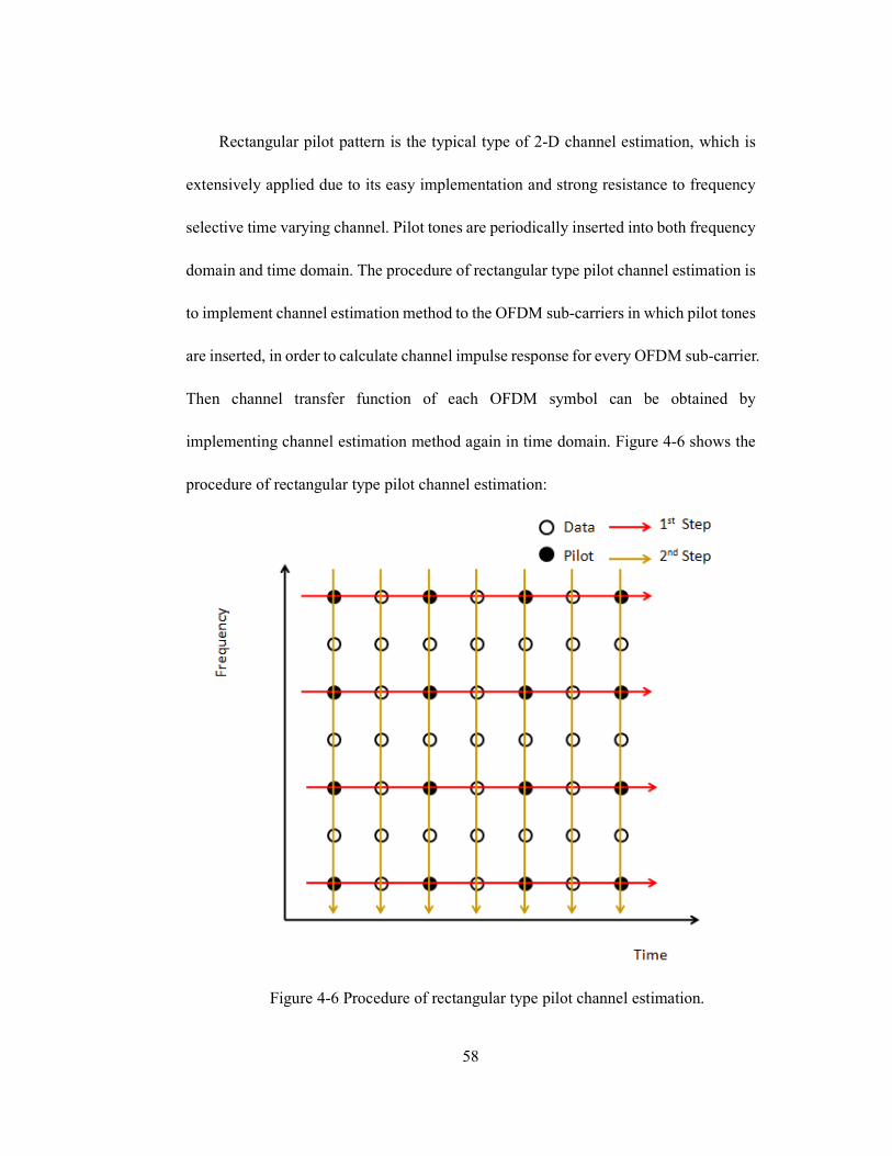
Rectangular pilot pattern is the typical type of 2-D channel estimation, which is
extensively applied due to its easy implementation and strong resistance to frequency
selective time varying channel. Pilot tones are periodically inserted into both frequency
domain and time domain. The procedure of rectangular type pilot channel estimation is
to implement channel estimation method to the OFDM sub-carriers in which pilot tones
are inserted, in order to calculate channel impulse response for every OFDM sub-carrier.
Then channel transfer function of each OFDM symbol can be obtained by
implementing channel estimation method again in time domain. Figure 4-6 shows the
procedure of rectangular type pilot channel estimation:
Figure 4-6 Procedure of rectangular type pilot channel estimation.
59
Rectangular type pilot pattern can better track frequency selective time varying
fading channel, since there are pilot tones in both frequency domain and time domain.
The performance comparison between rectangular type pilot pattern and 1-D pilot
pattern is investigated in chapter 5.
Another advantage of 2-D pilot pattern is 2-D pilot pattern can significantly
enhance transmission efficiency compare to 1-D pilot patterns. For 1-D pilot patterns,
pilot symbols will take up 12.5% of transmitting symbols if pilot interval is set to be 8.
However, in the case of rectangular pilot pattern, the pilot ratio is only 6.25% when
pilot interval is 4, which means for 512y16 input matrix, only 512 symbols are
reserved for pilot insertion.
The shortcoming of 2-D pilot patterns is that channel estimation method and
interpolation needs to be performed twice, both in frequency domain and time domain,
which will increase computational complexity. That also means performances of 2-D
pilot patterns are more rely on the accuracy and effectiveness of channel estimation
methods and interpolation methods.
4.3 Channel Estimation Algorithms
In this section, two channel estimation methods, LS algorithm and LMMSE
algorithm are introduced.
Least Square (LS) Algorithm
60
LS algorithm is simple but effective channel estimation method, which does not
require the information of fading channels [25]. The estimate of the channel transfer
function è�ñ is defined as:
è�ñ � (+�� (4.8)
where ( is the transmitted data matrix, and � is the received information sequence.
For comb type pilot channel estimation in OFDM system, the channel transfer
functions at pilot symbols èZ is obtained by LS algorithm. Thus, linear interpolation
method is applied to determine the channel impulse response of the OFDM symbol:
èz��� � èz��� > P� � WèZ�� > 1� � èZ���Y �� > èZ��� (4.9)
The LS estimate of èz��� is susceptible to Gaussian noise and inter-carrier
interference (ICI). For applications that require higher accuracy, LMMSE algorithm
described below is applied to the system instead.
LMMSE (Linear Minimum Mean Squared Error) Algorithm
MMSE algorithm is proved to provide more dB gain in SNR over LS estimation
by increasing computational complexity. The computational complexity of the MMSE
estimator can be reduced by using a simplified linear minimum mean-squared error
(LMMSE) estimator.
LMMSE algorithm requires the knowledge of auto-correlation matrix of the
channel frequency response ;ïï, which is given as:
;ïï � e?èZèZïD (4.10)
61
where èZ is channel frequency response at the pilot locations, the superscript �∙�ï
denotes the Hermitian transpose.
For an exponentially decaying multipath power-delay profile ���� � exp� +òòóôõ�, the correlation between ��th and �Gth sub-carriers is given as:
m���, �G� � �+¹öÄ�+�� ¿÷óôõ®�Ü9�ø¿�ø��Ý ��òóôõW�+¹öÄW+ ù÷óôõYY� ¿÷óôõ®úGûø¿�ø�ü � (4.11)
where τ¸ýÃ is RMS delay spread factor of the channel, � is the length of cyclic prefix.
Therefore, the channel correlation matrix ;ïï has the following form:
;ïï �þ���� m�0,0� m�0,1� ⋯ m�0, ! � 1�m�1,0� m�1,1� ⋯ m�1, ! � 1�
⋮ ⋮ ⋱ ⋮⋮ ⋮ ⋮m�! � 1,0� m�! � 1,1� ⋯ m�! � 1,! � 1���
��� (4.12)
LMMSE estimate è�OOñg can be viewed as a weighted combination of LS
estimate è�ñ, which is given:
è�OOñg � ^è�ñ (4.13)
The weighting coefficient ^ is expressed as:
^ � ;ïï�;ïï > �ñ*� ±�+� (4.14)
where is a constant depending on the signal constellation. In the case of 16QAM
scheme, � ��� .

62
BER Performance Comparison
LS algorithm is the simplest channel estimation and the basis of other channel
estimation technologies. The main drawback of LS algorithm is vulnerability to
Gaussian noise and ICI. The BER performance can be elevated by LMMSE algorithm,
where weighting matrix ^ is added to è�ñ. However, LMMSE algorithm increases
computational complexity of the system. Moreover, knowledge of channel information
is required in LMMSE algorithm, which gravely restricts the implementation of
LMMSE algorithm, because of the changing propagation environment in mobile
communications.

63
Chapter 5
Simulation Results and Performance Analysis
BER performance is the key factor in development of communication system,
which represents systems’ robustness against fading and error-correcting capability. In
this chapter, OFDM systems under various small scale fading channels are
implemented and BER performances are simulated in MATLAB 2008. All simulation
results are acquired under 512-point OFDM with CP length of 128.
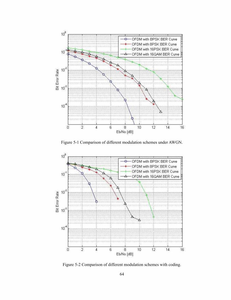
5.1 Simulation Results with Different modulation Schemes
The BER performances of OFDM system with BPSK, 8PSK, 16PSK and 16QAM
are investigated. It is expected that BPSK has the best BER performance, while 16PSK
has the worst. It is important to note that 8PSK and 16QAM have the similar BER
performance, but 16QAM has higher transmission efficiency. Therefore, 16QAM is
regarded to have better performance than 8PSK.
Figure 5-1 shows BER performances of OFDM system with different modulation
schemes under AWGN, and Figure 5-2 shows BER performances of different
modulation schemes with coding rate 1/2 ?133171DE convolutional code:
64
Figure 5-1 Comparison of different modulation schemes under AWGN.
Figure 5-2 Comparison of different modulation schemes with coding.
65
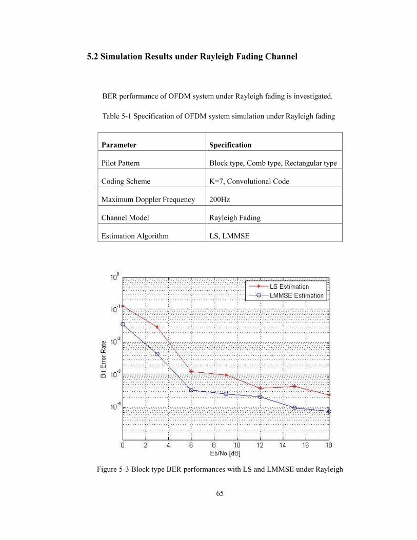
5.2 Simulation Results under Rayleigh Fading Channel
BER performance of OFDM system under Rayleigh fading is investigated.
Table 5-1 Specification of OFDM system simulation under Rayleigh fading
Figure 5-3 Block type BER performances with LS and LMMSE under Rayleigh
Parameter Specification
Pilot Pattern Block type, Comb type, Rectangular type
Coding Scheme K=7, Convolutional Code
Maximum Doppler Frequency 200Hz
Channel Model Rayleigh Fading
Estimation Algorithm LS, LMMSE
66
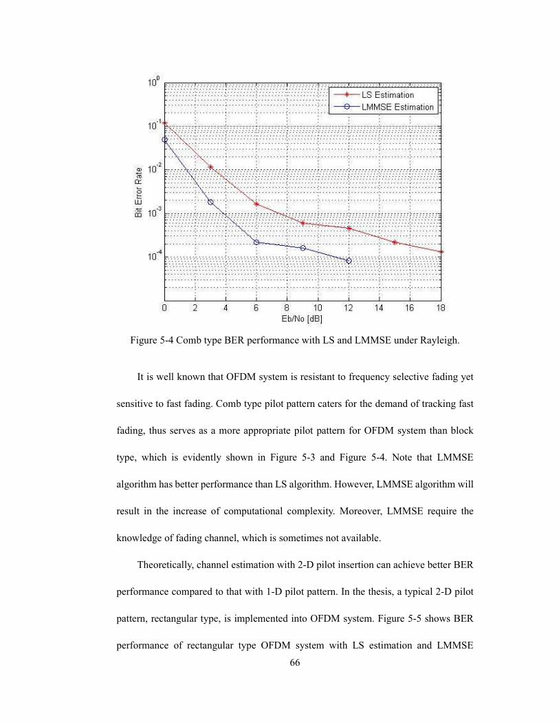
Figure 5-4 Comb type BER performance with LS and LMMSE under Rayleigh.
It is well known that OFDM system is resistant to frequency selective fading yet
sensitive to fast fading. Comb type pilot pattern caters for the demand of tracking fast
fading, thus serves as a more appropriate pilot pattern for OFDM system than block
type, which is evidently shown in Figure 5-3 and Figure 5-4. Note that LMMSE
algorithm has better performance than LS algorithm. However, LMMSE algorithm will
result in the increase of computational complexity. Moreover, LMMSE require the
knowledge of fading channel, which is sometimes not available.
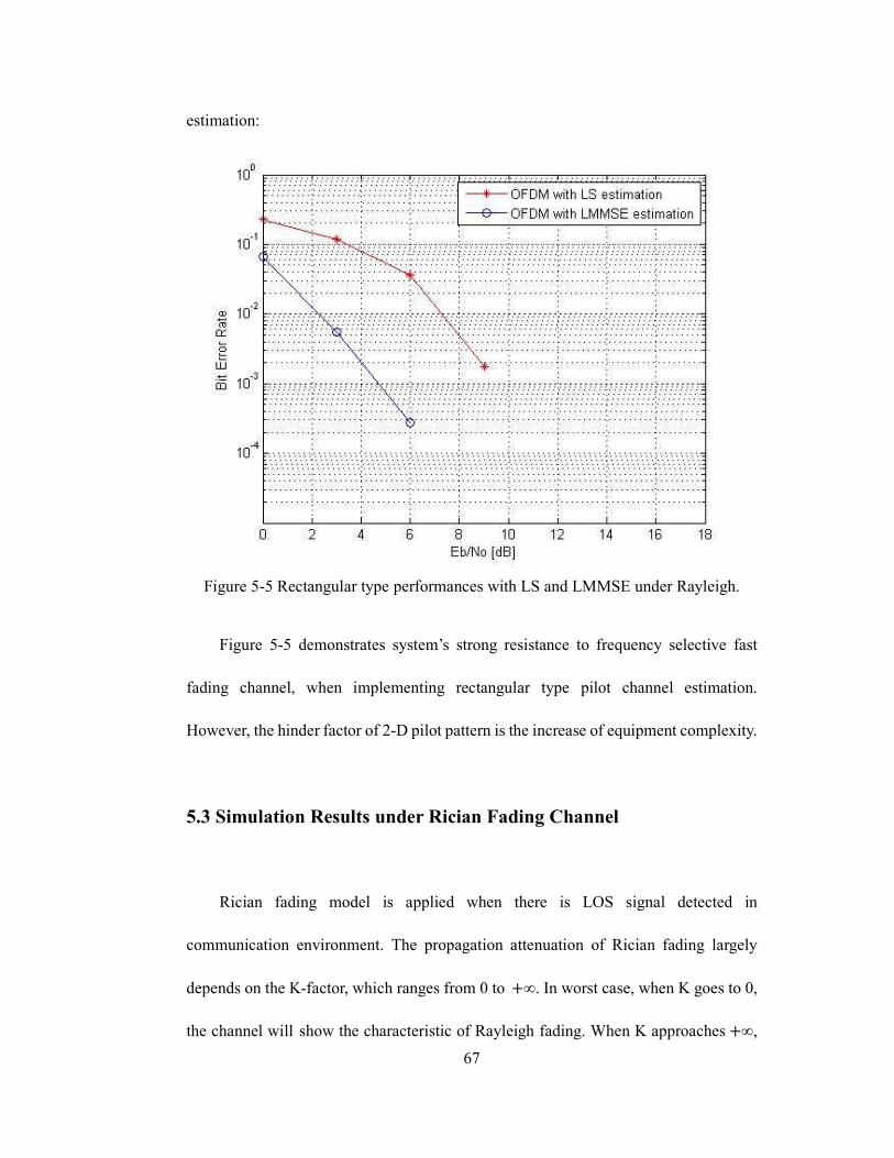
Theoretically, channel estimation with 2-D pilot insertion can achieve better BER
performance compared to that with 1-D pilot pattern. In the thesis, a typical 2-D pilot
pattern, rectangular type, is implemented into OFDM system. Figure 5-5 shows BER
performance of rectangular type OFDM system with LS estimation and LMMSE
67
estimation:
Figure 5-5 Rectangular type performances with LS and LMMSE under Rayleigh.
Figure 5-5 demonstrates system’s strong resistance to frequency selective fast
fading channel, when implementing rectangular type pilot channel estimation.
However, the hinder factor of 2-D pilot pattern is the increase of equipment complexity.
5.3 Simulation Results under Rician Fading Channel
Rician fading model is applied when there is LOS signal detected in
communication environment. The propagation attenuation of Rician fading largely
depends on the K-factor, which ranges from 0 to >∞. In worst case, when K goes to 0,
the channel will show the characteristic of Rayleigh fading. When K approaches>∞,
68
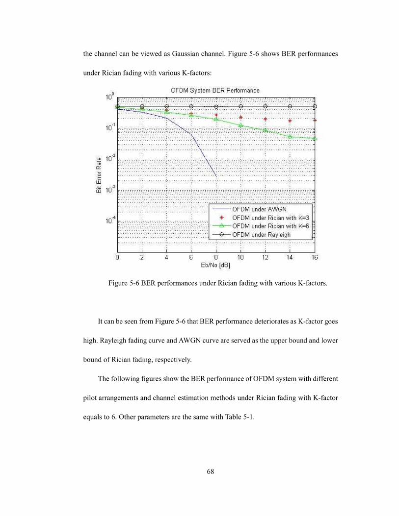
the channel can be viewed as Gaussian channel. Figure 5-6 shows BER performances
under Rician fading with various K-factors:
Figure 5-6 BER performances under Rician fading with various K-factors.
It can be seen from Figure 5-6 that BER performance deteriorates as K-factor goes
high. Rayleigh fading curve and AWGN curve are served as the upper bound and lower
bound of Rician fading, respectively.
The following figures show the BER performance of OFDM system with different
pilot arrangements and channel estimation methods under Rician fading with K-factor
equals to 6. Other parameters are the same with Table 5-1.

69
Figure 5-7 Block type BER performances with LS and LMMSE under Rician.
Figure 5-8 Comb type BER performances with LS and LMMSE under Rician.
70
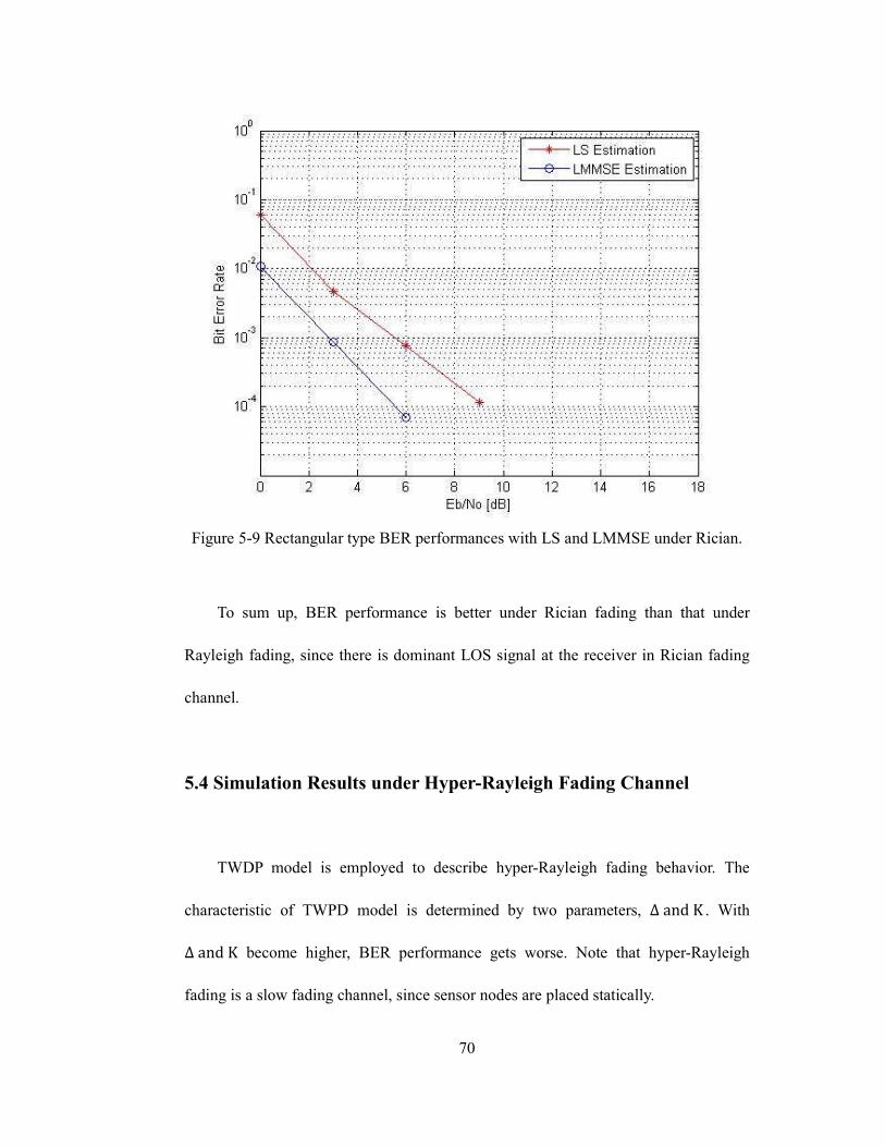
Figure 5-9 Rectangular type BER performances with LS and LMMSE under Rician.
To sum up, BER performance is better under Rician fading than that under
Rayleigh fading, since there is dominant LOS signal at the receiver in Rician fading
channel.
5.4 Simulation Results under Hyper-Rayleigh Fading Channel
TWDP model is employed to describe hyper-Rayleigh fading behavior. The
characteristic of TWPD model is determined by two parameters, ∆andK . With
∆andK become higher, BER performance gets worse. Note that hyper-Rayleigh
fading is a slow fading channel, since sensor nodes are placed statically.

71
Figure 5-10 BER performances under TWDP model with various K
Figure 5-11 Block type BER performances under TWDP with ∆� 1, K � 6.
72
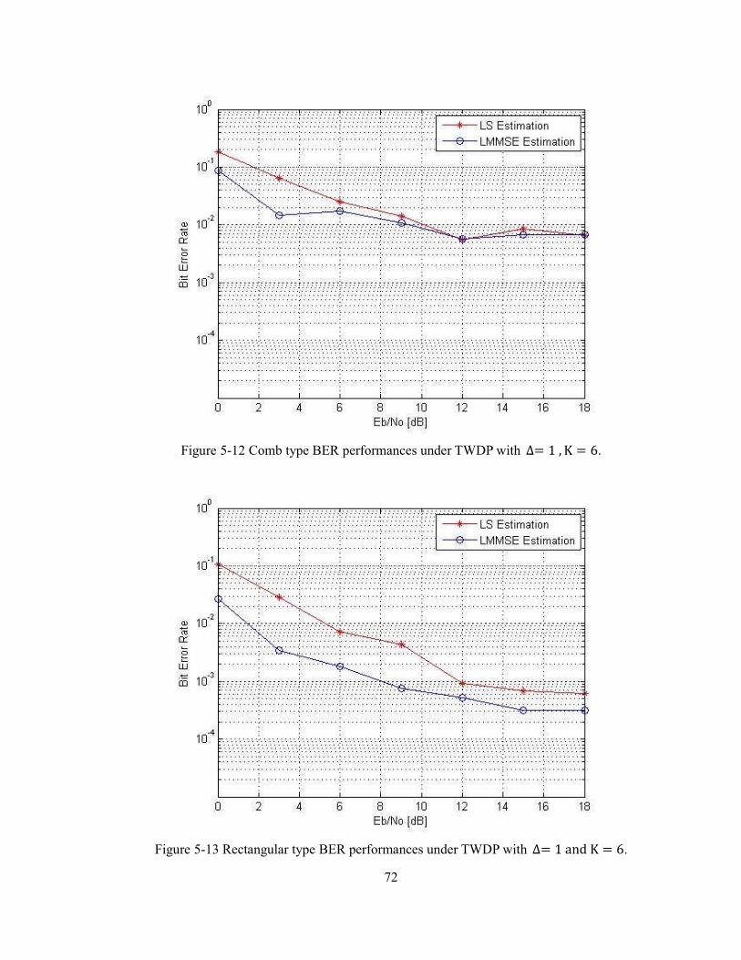
Figure 5-12 Comb type BER performances under TWDP with ∆� 1, K � 6.
Figure 5-13 Rectangular type BER performances under TWDP with ∆� 1andK � 6.
73
Unlike simulation results under Rayleigh fading, comb type pilot channel
estimation and block type pilot channel estimation have similar performance under
TWDP fading. Comb type pilot pattern is designed to overcome Doppler Effect, while
hyper-Rayleigh fading scenario is a slow fading channel. Hence, comb type pilot
pattern doesn’t fit in TWDP fading. Rectangular type pilot pattern has similar BER
performance with block type, but with higher transmission efficiency. Therefore,
rectangular type pilot pattern is still the first priority of pilot patterns.
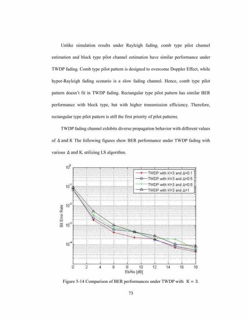
TWDP fading channel exhibits diverse propagation behavior with different values
of ∆andK The following figures show BER performance under TWDP fading with
various ∆andK, utilizing LS algorithm.
Figure 5-14 Comparison of BER performances under TWDP with K � 3.
74
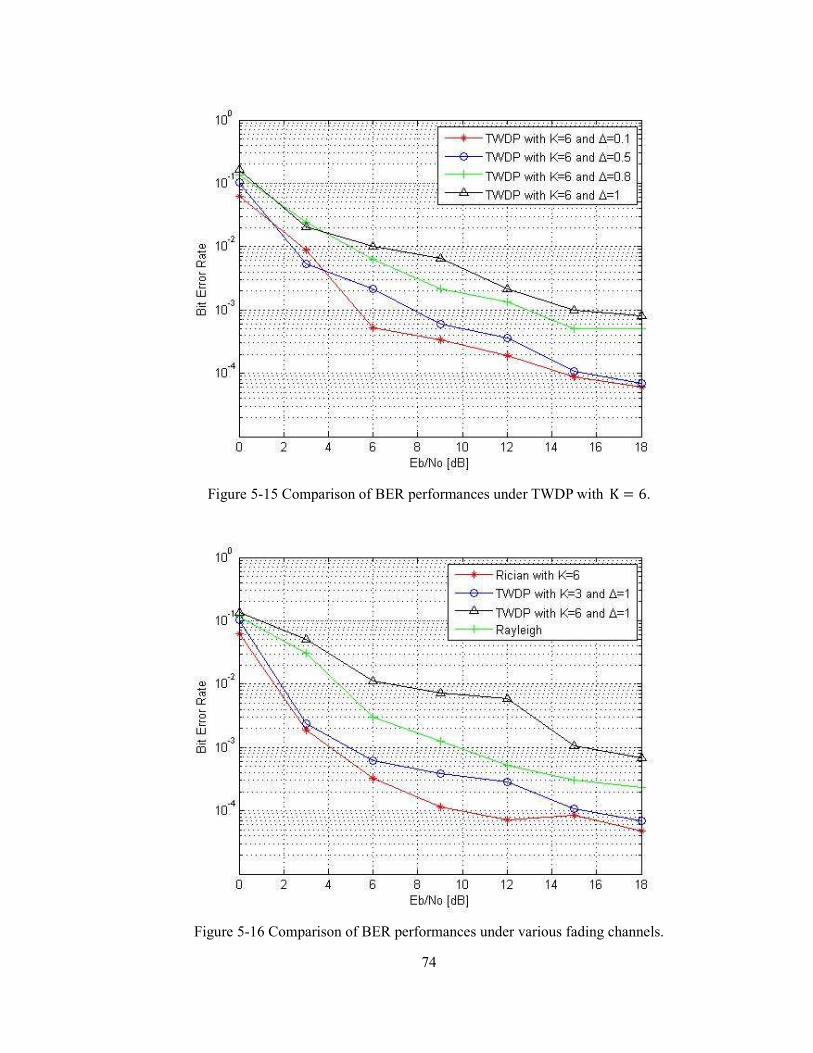
Figure 5-15 Comparison of BER performances under TWDP with K � 6.
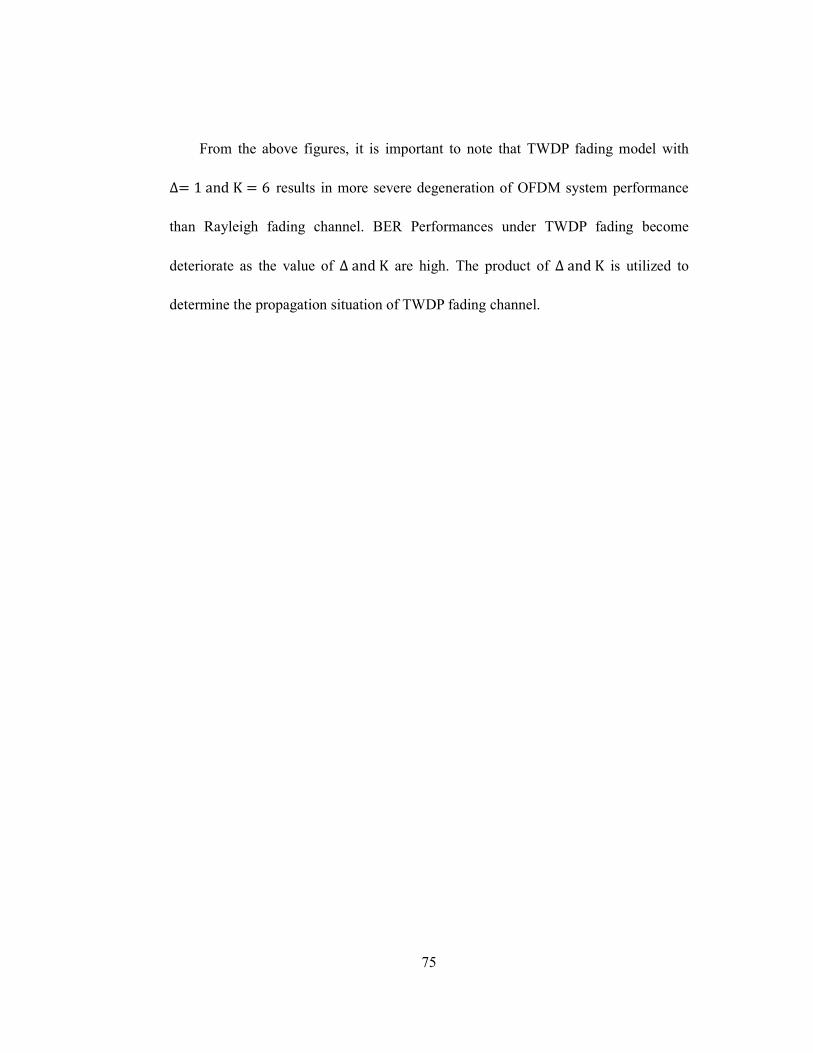
Figure 5-16 Comparison of BER performances under various fading channels.
75
From the above figures, it is important to note that TWDP fading model with
∆� 1andK � 6 results in more severe degeneration of OFDM system performance
than Rayleigh fading channel. BER Performances under TWDP fading become
deteriorate as the value of ∆andK are high. The product of ∆andK is utilized to
determine the propagation situation of TWDP fading channel.
76
Chapter 6
Conclusion and future work
The object of thesis is to explore the performances of OFDM system under
recently proposed hyper-Rayleigh fading with 2-D pilot channel estimation. Three
small scale fading channel channels, Rayleigh, Rician and hyper-Rayleigh, are
analyzed and simulated. Among the three fading channels, hyper-Rayleigh fading
behavior exists in WSN applications and its propagation characteristic can be
represented by TWDP model. Channel estimation techniques to overcome frequency
selective fading and fast fading channel are also investigated. The BER performance
results indicate that 2-D pilot patterns that insert pilots in both frequency domain and
time domain is adaptable to fast changing wireless communication channels.
Due to the limited time, issue of Synchronization is not included in the thesis,
which is, however, an essential issue in developing OFDM system. Accurate
synchronization is necessary for OFDM system, since sub-carriers need to be kept
strictly orthogonal. The thesis also fails to investigate other 2-D pilot patterns, such as
diamond type 2-D pilot patterns and tile type 2-D pilot patterns. In addition to
two-wave with diffuse power model, the characteristic and applicability of three-wave

77
with diffuse power model has gained more and more attention, which may probably
better represent the propagation situation of hyper-Rayleigh fading. Future work will
focus on these aspects.
78
References
[1] T. Rappaport, Wireless Communication, principles and Practice, 2 ed., Prentice
Hall, 2002.
[2] J. Frolik, “The case for considering hyper-Rayleigh fading channels,” IEEE Trans.
Wireless Commun., vol. 6, no. 4, pp. 1235-1239, Apr. 2007.
[3] J. Frolik, “On Appropriate Models for Characterizing hyper-Rayleigh fading,”
IEEE Trans. Wireless Commun., vol. 7, no. 12, pp. 5202-5207, Apr. 2007.
[4] X. Tong and T. Luo, Principle and application of OFDM mobile technology,
People Telecom Press, 2003.
[5] G. Durgin, T. Rappaport, and D. de Wolf, “New analytical models and probability
density functions for fading in wireless communications,” IEEE Trans. Commun.,
vol. 50, no. 6, pp. 1005-1015, Jun. 2002.
[6] S. Oh, K. Li, “BER Performance of BPSK receivers over two-wave with diffuse
power fading channels,” IEEE Trans. Wireless Commun.. vol. 4, no. 4, Jul. 2005.
[7] R. van Nee, R. Prasad, OFDM for Wireless Multimedia Communications, Boston:
Artech House, 2000
[8] S. Lin and D. J. Costello, JR., Error control coding: fundamentals and applications,
Prentice Hall, 1983.
[9] R. E. Ziemer and R. L. Peterson, Introduction to digital communication, Second
79
Edition, Prentice Hall Inc., 2001.
[10] S. Haykin, Digital Communications, John Wiley & Sons Inc., 1988.
[11] E. Biglicri, J. Proakis and S. Shamai, “Fading channels: information-theoretic and
communications aspects,” IEEE Trans. Inform. Theory, vol. 44, no. 6, pp.
2619-2692, Oct. 1998.
[12] M. Patzold, U. Killat, F. Laue and Y. Li, “On the statistical properties of
deterministic simulation models for mobile fading channels,” IEEE Trans. Veh.
Technol.,vol. 47, no. 1, pp. 254-269, Feb. 1998.
[13] J. Frolik, T. Weller, S. DiStasi and J. Cooper, “A compact reverberation chamber
for hyper-Rayleigh channel emulation,” IEEE Trans. Antennas propag., vol. 57, no.
12, pp. 3962-3968, Dec. 2009.
[14] A. Henderson, G. Durgin and C. Durkin, “Measurement of small-scale fading
distributions in a realistic 2.4 GHz channel.”
[15] B. Ai, J. Ge, Y. Wang, S. Yang and P. Liu, “Decimal frequency offset estimation in
COFDM wireless communications,” IEEE Trans. Broadcasting, vol. 50, no. 2, pp.
154-158, Jun. 2004.
[16] S. Coleri, M. Ergen, A. Puri and A. Bahai, “Channel estimation techniques based
on pilot arrangement in OFDM systems”, IEEE Trans. Broadcasting, vol. 48, no.3,
pp. 223-229, Sept. 2002.
[17] W. C. Jakes, Ed., Microwave Mobile Communications, New York: IRRR Press,
1974
[18] C. Xiao, Y. Zheng, N. Beaulieu, “Novel sum-of-sinusoids simulation models for
80
Rayleigh and Rician fading channels”, IEEE Trans. Wireless Commun., vol. 5, no.
12, pp. 3667-3678, Dec. 2006.
[19] E. Tufvesson, T. Maseng, “Pilot assisted channel estimation for OFDM in mobile
cellular systems,” in Proc. IEEE 47th Vehicular Technology Conference, Phoenix,
USA, May 1997, pp. 1639-1643
[20] J. Choi, Y. Lee, “Optimum pilot pattern for channel estimation in OFDM systems”,
IEEE Trans. Wireless Commun., vol. 4, no. 5, pp. 2083-2088, Sep. 2005
[21] M. J. Fern´andez-Getino Garc´ıa, S. Zazo and J. M. P´aez-Borrallo, “Pilot patterns
for channel estimation in OFDM,” Electron. Lett., vol. 36, no. 12, pp. 1049-1050,
June 2000.
[22] M. Hsieh, C. Wei, “Channel estimation for OFDM systems based on comb-type
pilot arrangement in frequency selective fading channels,” IEEE Trans. Consumer
Electron., vol. 44, no. 1, pp. 217-225, Feb. 1998.
[23] Y. Li, “Pilot-symbol-aided channel estimation for OFDM in wireless systems”,
IEEE Trans. Veh. Technol.,vol. 48, no. 4, pp. 1207-1215, Jul. 2000.
[24] J. Moon, S. Choi, “Performance of channel estimation methods for OFDM
systems in a multipath fading channels,” IEEE Trans. Consum. Electron., vol. 46,
no. 1, pp. 161-170, Feb. 2000.
[25] X. Dong, W. Lu and A. Soong, “Linear interpolation in pilot symbol assisted
channel estimation for OFDM,” IEEE Trans. Wireless Commun., vol. 6, no. 5, pp.
1910-1920, May. 2007
[26] H. Suraweera, W. Li and S. Oh, “Performance analysis of QAM in a two-wave

81
with diffuse power fading environment,” IEEE Commun. letters, vol. 12, no. 2, Feb.
2008.
[27] D. Estrin, L. Girod, G. Pottie and M. Srivastava, “Instrumenting the world with
wireless sensor networks,” in Proc. Int’l Conf. Acoustics, Speech and Signal
Processing (ICASSP 2001).


