Embed Size (px)
Citation preview
A Comparative Study between ICA and PCA
A dissertation
Submitted to the Department of Statistics, University of Rajshahi, Bangladesh, for
Partial Fulfillment of the Requirements for the Degree of Master of Science.
Examination Roll No. 08054718
Examination Year 2012
Registration No. 1550
Session 2007-2008
Department of Statistics, University of Rajshahi
Rajshahi-6205, Bangladesh
November 27, 2013
AbstractThis thesis attempts to study ICA and compare it with PCA for detection of
inherent structure, cluster analysis and outlier detection in multivariate data anal-
ysis. It presents the basic theory and application of ICA, and the recent work on
the subject. It tries to get a view of the data principles underlying the working of
independent component analysis. Next it discusses on most popular algorithm used
in ICA analysis, specially FastICA algorithm, which is an efficient and a fast working
algorithm.
It considers the problem of finding latent structure of three types of datasets gener-
ated from linear mixture of several independent super and sub-gaussian distribution.
First dataset consists of 10 variables: each generated from uniform (subgaussian)
distribution, while 2nd dataset consists of 10 variables: 5 Laplace (super-gaussian),
3 binomial, 2 multinomial distribution, and 3rd dataset is the mixture of five in-
dependent distribution (uniform, Laplace, binomial, multinomial and normal). It
is assumed that the observed data are generated by unknown latent variables and
their interactions. The task is to find these latent variables and the way they inter-
act, given the observed data only by using PCA and ICA. PCA cannot detect the
source variables from mixture whereas ICA is almost successful to identify the source
variables in every case. This thesis also represents the clustering approach of mul-
tivariate dataset using last two independent components after ordering according to
their kurtosis. Generally, first two principal components are used to visualize cluster
in multivariate dataset. It uses one simulated and three real datasets for clustering
approach, which are Australin crabs, Fisher Iris and Italian olive oils datasets. ICA
always performs better than PCA for clustering. Many researchers use last two and
first two PCs to visualize outliers in multivariate datasets. Four real datasets are
used for outlier detection: Epilepsy, Stackloss, Education expenditure and Scottish
hill racing datasets. In case of outlier detection ICA is more fruitful than PCA.

We recommended using ICA in place of PCA in detecting clusters as well as out-
liers. Furthermore, we suggest that if subject domain supports the assumption of
independent non-gaussian source variables ICA, not PCA be used to identify the
latent structure.
iii

Acknowledgment
Completing a Thesis paper in a new and very challenging subject is usually a journey
through a long and winding road, where one has to tame more oneself than the actual
phenomena in research. Luckily, I was not alone in this trip. The following were my
company in this journey, and I would like to say a big thanks, as this work might not
have been possible without them.
Primarily, I would like to thank my supervisor Prof. Dr. Mohammed Nasser for
his close supervision and very fruitful collaboration in and outside the aspects of my
thesis.
Thanks to the statistics departments of University of Rajshahi, Bangladesh for giving
me a powerful personal computer with a beautiful lab. I specially thanks to one of
my American friends Mark Booth, who continuously encourage and support me to
do this thesis.
I would like to thank my honourable teachers Professor Dr. Md. Golam Hossain,
Professor Dr. A. H. M. Rahmatullah Imon and Professor Dr. M. Rezaul Karim, De-
partment of statistics, University of Rajshahi. I would like to thank the teachers and
staff of Department of statistics, University of Rajshahi for the supply of important
information about this study. I would like to thank my elder brothers, Ahshanul
Haque Apel data entry officer ICDDR,B, Mizan Alam, Senior Statistical Program-
mer, Shafi Consultancy Ltd. Faisal Ahmed, Research Statistician, Al Mehedi Hassan
, Assistant Professor Rajshahi University of Engineering and Technology (RUET),
for their continual encouragement.
I also greatful to all of my friends and younger brothers for their inspiration. I
cannot explain the role of my parents and elder brother in word - without their
encouragement and other support I could not finish my study.
Last but not least a very special acknowledgments to GOOGLE without which it is
almost impossible to do this job.

Notations Used in the Thesis
k scalar constant
d dimensionality of x before dimensionality reduction
f scalar-valued function of a scalar variable
g scalar-valued function of a scalar variable
i index of xi
j index of sj or wj
k dimensionality of x after random projection
n number of latent components; dimensionality of s or y
p probability density function
s independent latent component
x component of observed vector x
y latent component
ε scalar constant
E expectation operator
P probability
p column vector of probabilities
s column vector of independent latent components
w column vector of a projection direction
x observed column vector
y column vector of latent components
xT vector x transposed (applicable to any vector)
A mixing matrix; topic matrix
D matrix of eigenvalues
E matrix of eigenvectors
W unmixing matrix
Abbreviations Used in theThesis
BSS blind signal separation
IC independent component
ICA independent component analysis
LDA linear discriminant analysis
ML maximum likelihood
MLP multilayer perceptron
MPCA multinomial principal component analysis
M.Sc. master of science
MSE mean squared error
NMF nonnegative matrix factorization
PC principal component
PCA principal component analysis
SOM self-organizing map
SOFM self-organizing feature map
SSE sum of squared errors
SVD singular value decomposition
Contents
1 Introduction 1
1.1 Introduction . . . . . . . . . . . . . . . . . . . . . . . . . . . . . . . . 1
1.2 Historical Background . . . . . . . . . . . . . . . . . . . . . . . . . . 3
1.3 Motivation of the Study . . . . . . . . . . . . . . . . . . . . . . . . . 6
1.4 Objective of the Study . . . . . . . . . . . . . . . . . . . . . . . . . . 6
1.5 Scope and Limitation of the Study . . . . . . . . . . . . . . . . . . . 6
1.6 Organization of the Subsequent Chapter . . . . . . . . . . . . . . . . 7
2 Methods and Materials 8
2.1 Introduction . . . . . . . . . . . . . . . . . . . . . . . . . . . . . . . . 8
2.2 Principal Component Analysis . . . . . . . . . . . . . . . . . . . . . . 8
2.2.1 PCA by variance maximization . . . . . . . . . . . . . . . . . 10
2.2.2 PCA by minimum mean-square error compression . . . . . . . 12
2.2.3 PCA by singular value decomposition . . . . . . . . . . . . . . 14
2.3 Independent Component Analysis . . . . . . . . . . . . . . . . . . . . 18
2.3.1 Assumptions of ICA . . . . . . . . . . . . . . . . . . . . . . . 20
2.3.2 Ambiguities of ICA . . . . . . . . . . . . . . . . . . . . . . . . 22
2.3.3 Gaussian variable is forbidden for ICA . . . . . . . . . . . . . 23
2.3.4 Key of ICA estimation . . . . . . . . . . . . . . . . . . . . . . 24
2.3.5 Measure of non-Gaussianity . . . . . . . . . . . . . . . . . . . 26
2.3.6 ICA and Projection Pursuit . . . . . . . . . . . . . . . . . . . 34
vii
2.3.7 Data preprocessing . . . . . . . . . . . . . . . . . . . . . . . . 35
2.3.8 FastICA algorithm . . . . . . . . . . . . . . . . . . . . . . . . 36
2.3.9 Infomax learning algorithm . . . . . . . . . . . . . . . . . . . 40
2.4 Data Description . . . . . . . . . . . . . . . . . . . . . . . . . . . . . 42
2.5 PCA vs ICA . . . . . . . . . . . . . . . . . . . . . . . . . . . . . . . . 42
2.6 Computer Program Used in the Analysis . . . . . . . . . . . . . . . . 45
2.7 Summary . . . . . . . . . . . . . . . . . . . . . . . . . . . . . . . . . 45
3 Latent Structure Detection 46
3.1 Introduction . . . . . . . . . . . . . . . . . . . . . . . . . . . . . . . . 46
3.2 Experimental Setup . . . . . . . . . . . . . . . . . . . . . . . . . . . . 47
3.2.1 Simulated data set-1 . . . . . . . . . . . . . . . . . . . . . . . 47
3.2.2 Simulated data set-2 . . . . . . . . . . . . . . . . . . . . . . . 50
3.2.3 Simulated data set-3 . . . . . . . . . . . . . . . . . . . . . . . 52
3.3 Summary . . . . . . . . . . . . . . . . . . . . . . . . . . . . . . . . . 55
4 Visualization of Clusters 56
4.1 Introduction . . . . . . . . . . . . . . . . . . . . . . . . . . . . . . . . 56
4.2 Experimental Setup . . . . . . . . . . . . . . . . . . . . . . . . . . . . 58
4.2.1 Simulated dataset 1 . . . . . . . . . . . . . . . . . . . . . . . . 58
4.2.2 Australian crabs dataset . . . . . . . . . . . . . . . . . . . . . 59
4.2.3 I ris data set . . . . . . . . . . . . . . . . . . . . . . . . . . . 61
4.2.4 Italian Olive oil’s data set . . . . . . . . . . . . . . . . . . . . 62
4.3 Summary . . . . . . . . . . . . . . . . . . . . . . . . . . . . . . . . . 64
5 Outlier Detection 65
5.1 Introduction . . . . . . . . . . . . . . . . . . . . . . . . . . . . . . . . 65
5.2 Experimental Setup . . . . . . . . . . . . . . . . . . . . . . . . . . . . 66
5.2.1 Epilepsy dataset . . . . . . . . . . . . . . . . . . . . . . . . . 66
5.2.2 Education expenditure data . . . . . . . . . . . . . . . . . . . 68
viii
5.2.3 Stackloss data . . . . . . . . . . . . . . . . . . . . . . . . . . . 69
5.2.4 Scottish hill racing data . . . . . . . . . . . . . . . . . . . . . 71
5.3 Summary and Outlook . . . . . . . . . . . . . . . . . . . . . . . . . . 72
6 Special Application of ICA 73
6.1 Introduction . . . . . . . . . . . . . . . . . . . . . . . . . . . . . . . . 73
6.2 ICA in Audio source separation . . . . . . . . . . . . . . . . . . . . . 73
6.3 ICA in Biomedical Application . . . . . . . . . . . . . . . . . . . . . 76
6.3.1 ICA of Electroencephalographic Data . . . . . . . . . . . . . . 76
6.3.2 ICA of Functional Magnetic Resonance Imaging Analysis (fMRI) 81
7 Summary, Conclusions and Future Research 84
7.1 Summary . . . . . . . . . . . . . . . . . . . . . . . . . . . . . . . . . 84
7.1.1 Conclusions . . . . . . . . . . . . . . . . . . . . . . . . . . . . 85
7.1.2 Future Research . . . . . . . . . . . . . . . . . . . . . . . . . . 86
A Bibliography 87
ix
List of Figures
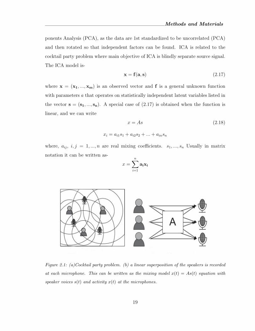
2.1 (a)Cocktail party problem. (b) a linear superposition of the speakers
is recorded at each microphone. This can be written as the mixing
model x(t) = As(t) equation with speaker voices s(t) and activity x(t)
at the microphones. . . . . . . . . . . . . . . . . . . . . . . . . . . . . 19
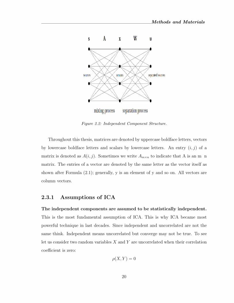
2.2 Independent Component Structure. . . . . . . . . . . . . . . . . . . . 20
2.3 Joint distribution of two independent Source of Normal(Gaussian) dis-
tribution. . . . . . . . . . . . . . . . . . . . . . . . . . . . . . . . . . 24
2.4 Joint distribution of two independent Source of uniform (sub-Gaussian)
distribution. . . . . . . . . . . . . . . . . . . . . . . . . . . . . . . . . 25
2.5 Joint distribution of two independent Source of Laplace(super-Gaussian)
distribution. . . . . . . . . . . . . . . . . . . . . . . . . . . . . . . . . 26
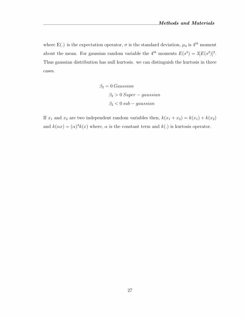
2.6 (a) The joint distribution of the observed mixture of two uniform (sub-
gaussian) variables. (b)The joint distribution of whiten mixtures of
uniformly distributed independent components. (c) The joint distri-
bution of the observed mixture of two Laplacian distribution. (d) The
joint distribution of two whiten mixture of Laplacian distribution. . . 28
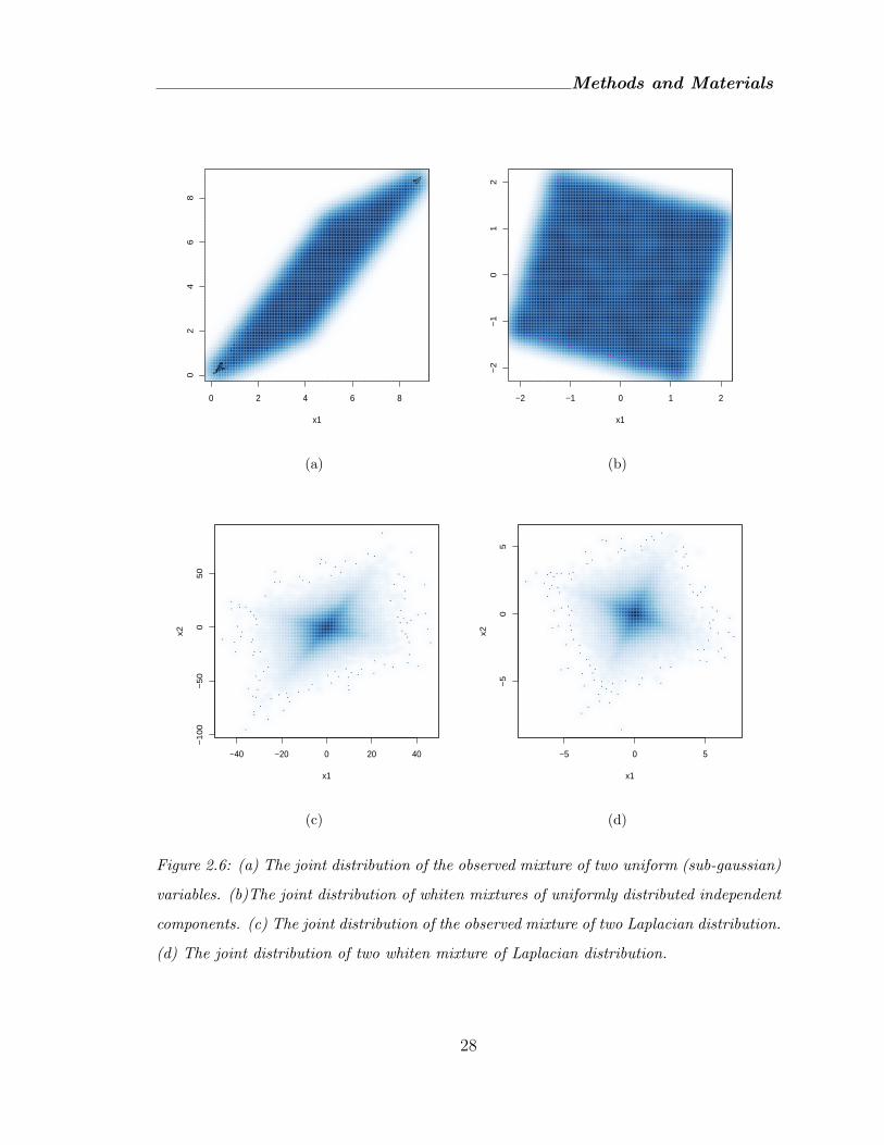
2.7 Entropy measurement corresponding to probability. From the figure
entropy will be maximum when p=0.5 . . . . . . . . . . . . . . . . . 29
2.8 Mutual Information between two variable X and Y . . . . . . . . . . . 31
x
2.9 An illustration of projection pursuit and the ”interestingness” of non-
gaussian projections. The data in this figure is clearly divided into
two clusters. However, the principal component, i.e. the direction of
maximum variance, would be vertical, providing no separation between
the clusters. In contrast, the strongly nongaussian projection pursuit
direction is horizontal, providing optimal separation of the clusters. . 34
2.10 Flowchart of the FastICA algorithm. . . . . . . . . . . . . . . . . . . 39
2.11 Flowchart of Infomax learning algorithm. . . . . . . . . . . . . . . . . 41
2.12 (a) Vectors IC1 and IC2 show the directions determined by the relative
actions of the two component process. The data will be independently
along these two component vectors. Vector PC1 and PC2 show the
two perpendicular principal component directions indicating maximum
variance in the data. (b) Shows that IC1 and IC2 can be indirectly
determined by the finding a linear transformation matrix W which re-
sults in a rectangular distribution. The sigmoid transformation g(Wx)
makes the distribution more uniform and the ICA algorithm of Bell
and Sejnowski (1995) further adjusts IC1 and IC2 to maximize the
entropy of the distribution. . . . . . . . . . . . . . . . . . . . . . . . . 43
3.1 Matrix plot of original source of 10 uniform (sub-gaussian) distribution. 48
3.2 Matrix plot of observable mixture of 10 uniform (sub-gaussian) distri-
bution. . . . . . . . . . . . . . . . . . . . . . . . . . . . . . . . . . . . 48
3.3 Matrix plot of 10 principal components. . . . . . . . . . . . . . . . . . 49
3.4 Matrix plot of 10 independent components . . . . . . . . . . . . . . . 49
3.5 Matrix plot of original source of 5 laplace (super-gaussian), 3 binomial,
2 multinomial distribution. . . . . . . . . . . . . . . . . . . . . . . . . 50
3.6 Matrix plot of observed mixture of 5 Laplace (super-gaussian), 3 bino-
mial, 2 multinomial distribution. . . . . . . . . . . . . . . . . . . . . . 51
xi
3.7 Matrix plot of principal components of 5 Laplace (super-gaussian), 3
binomial, 2 multinomial distribution. . . . . . . . . . . . . . . . . . . 51
3.8 Matrix plot of independent components of 5 Laplace (super-gaussian),
3 binomial, 2 multinomial distribution after applying ICA. . . . . . . 52
3.9 Matrix plot of 5 original source variable comes from uniform (sub-
gaussian), Laplace (super-gaussin), binomial, multinomial and normal
distribution. . . . . . . . . . . . . . . . . . . . . . . . . . . . . . . . . 53
3.10 Matrix plot of observe mixture of 5 variables. . . . . . . . . . . . . . 53
3.11 Matrix plot of all principal components. . . . . . . . . . . . . . . . . 54
3.12 Matrix plot of all independent components. . . . . . . . . . . . . . . . 54
4.1 Density plot of various distribution and their kurtosis. . . . . . . . . . . 57
4.2 Scatter plot of two variables. . . . . . . . . . . . . . . . . . . . . . . . 58
4.3 (left) Scatter plot of first principal component. (Right) Scatter plot of
last independent component. . . . . . . . . . . . . . . . . . . . . . . . 59
4.4 (a)Matrix plot of the Australian Crabs data set. (b) Matrix plot of all
principal components of Australian Crabs data set. . . . . . . . . . . . . 60
4.5 (a)Scatter plot of first two principal component (b) Scatter plot of the last
two independent components of Australian Crabs data. . . . . . . . . . 60
4.6 (a)Matrix plot of the Fisher Iris data set. (b) Matrix plot of the principal
components of Iris data. . . . . . . . . . . . . . . . . . . . . . . . . . . 61
4.7 (a)Scatter plot of first two principal component (b) Scatter plot of the last
two independent components of Iris data. . . . . . . . . . . . . . . . . . 62
4.8 (a)Matrix plot of Italian Olive oil data set.(b) Matrix plot of all principal
components. . . . . . . . . . . . . . . . . . . . . . . . . . . . . . . . . 63
4.9 (a)Scatter plot of first two principal components (b) Scatter plot of the last
two independent components of Olive oils data. . . . . . . . . . . . . . . 63
5.1 (a)Text plot of first two largest PCs (b) Text plot of two smallest PCs . . 67
xii
5.2 (a)Text plot of first two largest ICs (b) Text plot of smallest ICs . . . . . 67
5.3 (a)Text plot of first two principal components. (b)Text plot of last two
principal components of Education expenditure data set. . . . . . . . . . 68
5.4 (a)Text plot of first two independent component. (b)Text plot of the last
two independent components of Education expenditure data set. . . . . . 69
5.5 (a)Text plot of first two principal component. (b)Text plot of the last two
independent components of Stackloss data set. . . . . . . . . . . . . . . 70
5.6 (a)Text plot of first two independent components. (b)Text plot of the first
two independent components of Stackloss data set. . . . . . . . . . . . . 70
5.7 (a)Scatter text plot of first two principal component. (b)Scatter text plot
of the first two independent components of Stackloss data set. . . . . . . 71
5.8 (a)Scatter text plot of first two principal component. (b)Scatter text plot
of the first two independent components of Stackloss data set. . . . . . . 72
6.1 Blind source separation of two speech. (Top row) time course of two
speech signals. (Middle row) These were mixed of two observation.
After separation of two signals (Bottom row) . . . . . . . . . . . . . . 74
6.2 Scatter plot of two audio mixture signals. . . . . . . . . . . . . . . . . 74
6.3 Scatter plot of two principal components of audio signals. . . . . . . . 75
6.4 Scatter plot of two of two independent components of audio signals. . 75
6.5 (a) Raphical output of Co-registration of EEG data, showing (upper panel)
cortex (blue), inner skull (red) and scalp (black) meshes, electrode loca-
tions (green), MRI/Polhemus fiducials (cyan/magneta), and headshape (red
dots). (b)All channel of list of EEG for this dataset. . . . . . . . . . . . 77
6.6 Flowchart of EEG data analysis using ICA. . . . . . . . . . . . . . . . 77
6.7 A 5 sec. portion of the EEG time series with prominent alpha rhythms
(8-21 Hz). . . . . . . . . . . . . . . . . . . . . . . . . . . . . . . . . . 78
6.8 The 32 ICA component extracted from the EEG data in figure 6.7. . 78
6.9 Scalp map projection of all 32 channels . . . . . . . . . . . . . . . . . 79
xiii

6.10 Second independent component properties. . . . . . . . . . . . . . . . 80
6.11 Cortex (blue), inner skull (red), outer skull (orange) and scalp (pink)
meshes with transverse slices of the subject’s MRI. . . . . . . . . . . 81
6.12 Comparison of brain networks obtained using ICA independently on
fMRI data. . . . . . . . . . . . . . . . . . . . . . . . . . . . . . . . . 83
xiv
Chapter 1
Introduction
1.1 Introduction
A fundamental problem in neural network research, as well as in many other disci-
plines, is finding a suitable representation of multivariate data, i.e. random vectors.
For reasons of computational and conceptual simplicity, the representation is often
sought as a linear transformation of the original data. In other words, each component
of the representation is a linear combination of the original variables. Well-known
linear transformation methods include principal component analysis, factor analysis,
and projection pursuit. Independent component analysis (ICA)[5, 25] is a recently
developed method in which the goal is to find a linear representation of nongaussian
data so that the components are statistically independent, or as independent as pos-
sible.
ICA has recently become an important tool for modelling and understanding em-
pirical datasets as it offers an elegant and practical methodology for blind source
separation and deconvolution. It is seldom possible to observe a pure unadulterated
signal. When two or more signal are interpreted to each other than ICA may be
applied to this Blind Source Separation (BSS) to the signal processing community.
Introduction
Finding a natural coordinate system is an essential first step in the analysis of em-
pirical data. Principal Component Analysis (PCA) has, for many years, been used
to find a set of basis vectors which are determined by the data set itself. The prin-
cipal components are orthogonal and projections of the data onto them are linearly
decorrelated, properties which can be ensured by considering only the second order
statistical characteristics of the data. ICA aims at a loftier goal: it seeks a trans-
formation to coordinates in which the data are maximally statistically independent,
not merely decorrelated. The stronger condition allows one to remove the rotational
invariance of PCA, i.e. ICA provides a meaningful unique bilinear decomposition of
two-way data that can be considered as a linear mixture of a number of independent
source signals. The discipline of multilinear algebra offers some means to solve the
ICA problem.
Perhaps the most famous illustration of ICA is the cocktail party problem, in which
a listener is faced with the problem of separating the independent voices chatter-
ing at a cocktail party. Humans employ many independent voices chattering at a
cocktail party. Recently, ICA has received attention because of its potential applica-
tion in signal processing such as speech recognition, telecommunication and medical
signal processing; feature extraction such as face recognition; clustering; time series
analysis; Modelling of the hippocampus and visual cortex; Compression, redundancy
reduction; Watermarking; Scientific Data Mining etc.
2
Introduction
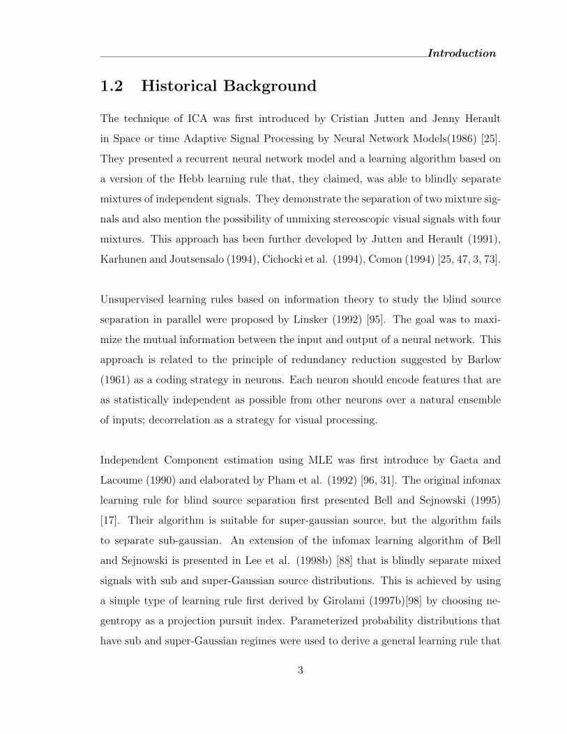
1.2 Historical Background
The technique of ICA was first introduced by Cristian Jutten and Jenny Herault
in Space or time Adaptive Signal Processing by Neural Network Models(1986) [25].
They presented a recurrent neural network model and a learning algorithm based on
a version of the Hebb learning rule that, they claimed, was able to blindly separate
mixtures of independent signals. They demonstrate the separation of two mixture sig-
nals and also mention the possibility of unmixing stereoscopic visual signals with four
mixtures. This approach has been further developed by Jutten and Herault (1991),
Karhunen and Joutsensalo (1994), Cichocki et al. (1994), Comon (1994) [25, 47, 3, 73].
Unsupervised learning rules based on information theory to study the blind source
separation in parallel were proposed by Linsker (1992) [95]. The goal was to maxi-
mize the mutual information between the input and output of a neural network. This
approach is related to the principle of redundancy reduction suggested by Barlow
(1961) as a coding strategy in neurons. Each neuron should encode features that are
as statistically independent as possible from other neurons over a natural ensemble
of inputs; decorrelation as a strategy for visual processing.
Independent Component estimation using MLE was first introduce by Gaeta and
Lacoume (1990) and elaborated by Pham et al. (1992) [96, 31]. The original infomax
learning rule for blind source separation first presented Bell and Sejnowski (1995)
[17]. Their algorithm is suitable for super-gaussian source, but the algorithm fails
to separate sub-gaussian. An extension of the infomax learning algorithm of Bell
and Sejnowski is presented in Lee et al. (1998b) [88] that is blindly separate mixed
signals with sub and super-Gaussian source distributions. This is achieved by using
a simple type of learning rule first derived by Girolami (1997b)[98] by choosing ne-
gentropy as a projection pursuit index. Parameterized probability distributions that
have sub and super-Gaussian regimes were used to derive a general learning rule that
3
Introduction
preserves the simple architecture proposed by Bell and Sejnowski (1995) [17], is opti-
mized using the natural gradient by Amari (1998) [80], and uses the stability analysis
of Cardoso and Laheld (1996) [40] to switch between sub and super-Gaussian regimes.
There are two properties in ICA: the natural gradient and the robustness in ICA
against parameter mismatch. The natural gradient (Amari 1998) [80] or equivalently
the relative gradient Cardoso and Laheld (1996) [40] gives fast convergence.
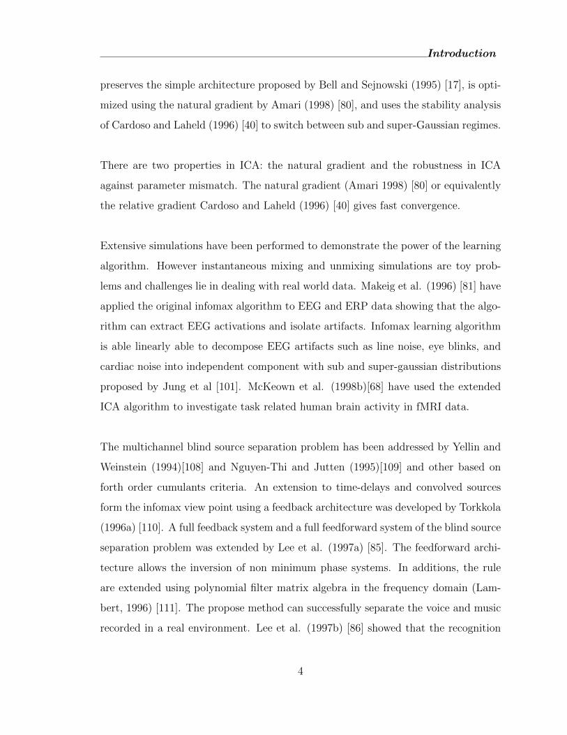
Extensive simulations have been performed to demonstrate the power of the learning
algorithm. However instantaneous mixing and unmixing simulations are toy prob-
lems and challenges lie in dealing with real world data. Makeig et al. (1996) [81] have
applied the original infomax algorithm to EEG and ERP data showing that the algo-
rithm can extract EEG activations and isolate artifacts. Infomax learning algorithm
is able linearly able to decompose EEG artifacts such as line noise, eye blinks, and
cardiac noise into independent component with sub and super-gaussian distributions
proposed by Jung et al [101]. McKeown et al. (1998b)[68] have used the extended
ICA algorithm to investigate task related human brain activity in fMRI data.
The multichannel blind source separation problem has been addressed by Yellin and
Weinstein (1994)[108] and Nguyen-Thi and Jutten (1995)[109] and other based on
forth order cumulants criteria. An extension to time-delays and convolved sources
form the infomax view point using a feedback architecture was developed by Torkkola
(1996a) [110]. A full feedback system and a full feedforward system of the blind source
separation problem was extended by Lee et al. (1997a) [85]. The feedforward archi-
tecture allows the inversion of non minimum phase systems. In additions, the rule
are extended using polynomial filter matrix algebra in the frequency domain (Lam-
bert, 1996) [111]. The propose method can successfully separate the voice and music
recorded in a real environment. Lee et al. (1997b) [86] showed that the recognition
4
Introduction
rate of an automatic speech recognition system was increased after separating the
speech signals.
Since ICA is restricted and relies on several assumptions researchers have started to
tackle a few limitations of ICA. One obvious but non-trivial extension is the nonlinear
mixing model. ICA of nonlinear components are extracted using Self Organizing Fea-
ture Maps (SOFM) [112, 113]. Other researchers (Burel, 1992; Lee et al. 1997c; Taleb
and Jutten, 1997; Yang et al., 1997; Horchreiter and Schmidhuber, 1998) [114, 87, 100]
have used a more direct extension to the previously presented ICA models. They in-
clude certain flexible nonlinearities in the mixing model and the goal is to invert the
linear mixing matrix as well as the nonlinear mixing. Hochreiter and Schmidhuber
(1998)[100] have proposed low complexity coding and decoding approaches for non-
linear ICA. Another limitation is the underdetermined problem in ICA, i.e. having
less receivers than sources. Lee et al. (1998c) [88] demonstrated that an overcomplete
representation of the data can be used to learn non-square mixing matrix and to infer
more sources than receivers. The overcomplete framework also allows additive noise
in the ICA model and can therefore be used to separate noisy mixtures.
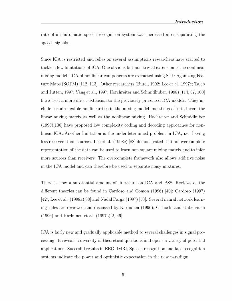
There is now a substantial amount of literature on ICA and BSS. Reviews of the
different theories can be found in Cardoso and Comon (1996) [40]; Cardoso (1997)
[42]; Lee et al. (1998a)[88] and Nadal Parga (1997) [53]. Several neural network learn-
ing rules are reviewed and discussed by Karhunen (1996); Cichocki and Unbehauen
(1996) and Karhunen et al. (1997a)[2, 49].
ICA is fairly new and gradually applicable method to several challenges in signal pro-
cessing. It reveals a diversity of theoretical questions and opens a variety of potential
applications. Succesful results in EEG, fMRI, Speech recognition and face recognition
systems indicate the power and optimistic expectation in the new paradigm.
5
Introduction
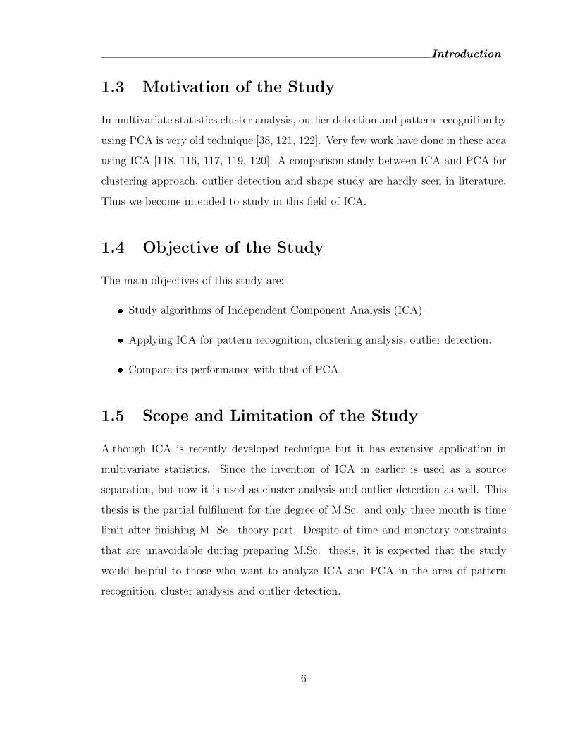
1.3 Motivation of the Study
In multivariate statistics cluster analysis, outlier detection and pattern recognition by
using PCA is very old technique [38, 121, 122]. Very few work have done in these area
using ICA [118, 116, 117, 119, 120]. A comparison study between ICA and PCA for
clustering approach, outlier detection and shape study are hardly seen in literature.
Thus we become intended to study in this field of ICA.
1.4 Objective of the Study
The main objectives of this study are:
� Study algorithms of Independent Component Analysis (ICA).
� Applying ICA for pattern recognition, clustering analysis, outlier detection.
� Compare its performance with that of PCA.
1.5 Scope and Limitation of the Study
Although ICA is recently developed technique but it has extensive application in
multivariate statistics. Since the invention of ICA in earlier is used as a source
separation, but now it is used as cluster analysis and outlier detection as well. This
thesis is the partial fulfilment for the degree of M.Sc. and only three month is time
limit after finishing M. Sc. theory part. Despite of time and monetary constraints
that are unavoidable during preparing M.Sc. thesis, it is expected that the study
would helpful to those who want to analyze ICA and PCA in the area of pattern
recognition, cluster analysis and outlier detection.
6
Introduction
1.6 Organization of the Subsequent Chapter
Thus thesis is partitioned theory and application of ICA with some simulated and
real data sets. Organization of subsequent chapter of this thesis are as follows-
Chapter 1 gives the introduction of ICA with historical background. Motivation
and objective of the study are discussed also. Future challenges in ICA research are
mentioned later in this chapter.
Chapter 2 states the methods and methodologies of PCA, ICA with basic PCA and
ICA model. Here also discuss most popular algorithms of ICA. Description of data
and software that has been used for the analysis of this thesis are discussed later in
this chapter.
Chapter 3 starts with various application of ICA. These chapter are partitioned into
theory and application of ICA.
Chapter 4 starts with Blind Source Separation of ICA model.
Chapter 5 represents the visualization of cluster technique using ICA. Some simu-
lated and real data sets are analyzed in this chapter.
Chapter 6 presents the outlier detection application of ICA. Some extensive appli-
cation of real data set have been discussed in this chapter.
Chapter 7 gives conclusions by summarizing the main results in this thesis.
7
Chapter 2
Methods and Materials
2.1 Introduction
PCA [38] and ICA [15] both are projection pursuit technique in multivariate analy-
sis. ICA depends on higher order statistics whereas PCA depends on second order
statistics. In this chapter we discuss the mathematical formulation of PCA and ICA.
In addition most popular algorithm also discussed. Data description and computer
software that used in the analysis are discussed later in this chapter.
2.2 Principal Component Analysis
PCA constructs a set of uncorrelated variable called principal components (PC’s)
from a set of correlated variable by using an orthogonal transformation. PC’s are
formed in such a way that first PC has the largest variance and the last PC has the
smallest variance i.e. principal components (PC’s) are ordered [38, 60].
PCA is mathematically defined as an orthogonal linear transformation that trans-
forms the data to a new coordinate system such that the greatest variance by any
projection of the data comes to lie on the first coordinate (called the first principal
Methods and Materials
component), the second greatest variance on the second coordinate, and so on.
PCA, an observed vector x first centered by removing its mean (in practice, the
mean is estimated as the average value of the vector in a sample). Then the vector
is transformed by a linear transformation into a new vector, possibly of lower dimen-
sion, whose elements are uncorrelated with each other. The linear transformation is
found by computing the eigenvalue decomposition of the covariance matrix, which for
zero-mean vectors is the correlation matrix E{xxT} of the data. The eigenvectors
of form a new coordinate system in which the data are presented. The decorrelating
process is called whitening or sphering if also the variances of each element of the new
data vector are set to unity. This can be accomplished by scaling the vector elements
by the inverses of the eigenvalues of the correlation matrix. In all, the whitened data
have the form
z = D−1/2ETx (2.1)
where, z is the whitened data vector, D is a diagonal matrix containing the eigen-
values of the correlation matrix and E contains the corresponding eigenvectors of
the correlation matrix as its columns. In practice, the expectation in the correlation
matrix is computed as the sample mean. Subsequent ICA estimation is done on z
instead of x. For whitened data it is enough to find an orthogonal demixing matrix
if the independent components are also assumed white.
Dimensionality reduction is performed by PCA simply by choosing the number of
retained dimensions, m, and projecting the n-dimensional observed vector x to a
lower dimensional space spanned by the m(m < n) dominant eigenvectors (that is,
eigenvectors corresponding to the largest eigenvalues) of the correlation matrix. Now
the matrix E in Formula (2.1) has only m columns instead of n, and similarly D is
of size m×m instead of n× n, if whitening is desired.
9
Methods and Materials
There is no clear way to choose the number of retained dimensions in practice. In
theory, the rank of xTx is equal to the rank of sT s in the noiseless case, so it is enough
to compute the number of non-zero eigenvalues of xTx. The problem is discussed in,
e.g., [15]. One often chooses the number of largest eigenvalues so that the chosen
eigenvectors explain the data well enough, for example, 90 percent of the total vari-
ance in the data. As PCA pre-processing for ICA always involves the risk that the
true independent components are not in the space spanned by the dominant eigen-
vectors, it is often advisable to estimate fewer independent components than what is
the dimensionality of the data after PCA. Trial and error are often needed in deter-
mining both the number of eigenvectors and the number of independent components
estimated.
PCA is a convenient method for estimating the structure of the data, assuming that
the distribution of the data is roughly symmetric and unimodal. PCA finds the or-
thogonal directions in which the data have maximal variance. PCA is an optimal
method of dimensionality reduction in the mean-square sense: data points projected
into the lower dimensional PCA subspace are as close as possible to the original high
dimensional data points.
||x(t)− z(t)||2 (2.2)
is minimized. Here we denote by x(t) the tth original observation vector and by z(t)
its projection.
2.2.1 PCA by variance maximization
In Mathematical terms, consider a linear combination
y1 =n∑k=1
wk1xk = wT1 x (2.3)
of the element x1, ..., xn of the vector x. The w11, ..., wn1 are scaler coefficients or
weights, elements of an n-dimensional vector w1, and wT1 denote the transpose of w1.
10
Methods and Materials
The factor y1 is called the first principal component of x, if the variance of y1 is
maximally large. Because the variance depends on both the norm and orientation
of the weight vector w1 and grows without limits as the norm grows, we impose the
constraint that the norm of w1 is constant, in practice equal to 1. Thus we look for
a weight vector w1 maximizing the PCA criterion.
JPCA1 (w1) = E{y21} = E{wT1 x} = wT
1E{xxT}w1 = w1Cxw1 (2.4)
So,that
||w1|| = 1 (2.5)
Here E{.} is the expectation over unknown density of input vector x, and the norm
w1 is the usual Euclidean norm defined as-
||w1|| = (wT1 w1)
12 = (
n∑k=1
w2k1)
12
The matrix Cx in Eq. (2.1) is the n × n covariance matrix of x given for the zero
mean vector of x by the correlation matrix
Cx = E{xxT} (2.6)
It is well known from basic linear algebra that the solution to the PCA problem is
given in terms of the unit-length eigenvectors e1, ..., en of the matrix C [102]. The
ordering of the eigenvectors is such that the corresponding eigenvalues d1, ..., dn satisfy
d1 ≥ d2 ≥, ...,≥ dn. The solution maximization is given by
w1 = e1
Thus the first principal component of x is y1 = eT1 x. The criterion JPCA1 in eq. (2.4)
11
Methods and Materials
can be generalized to m principal components, with many number between 1 and
n. Denoting the mth (1 ≤ m ≤ n) principal component by ym = wTmx, with wm
the corresponding unit norm weight vector, the variance of ym is now maximized
under the constraint that ym is uncorrelated with all the previously found principal
components:
E{ym, yk} = 0, k < m (2.7)
Since that the principal components ym has zero means because
E(ym) = wTmE{x} = 0
The condition (2.7) yields
E{ymyk} = E{(wTmx)(wT
k x)} = wTmCxwk = 0 (2.8)
For the second principal component, we have the condition that
wT2 Cw1 = d1w2
Tae1 (2.9)
because we know that, w1 = e1. Thus looking for maximal variance E{y22} =
E{(wT2 x)2} in the subspace orthogonal to the first eigenvector of Cx. The solution
is given by
w2 = e2
. Thus the kth principal component is yk = eTk x
2.2.2 PCA by minimum mean-square error compression
In the preceding subsection, the principal components were defined as weighted sums
of the elements of x with maximal variance, under the constraints that the weights
are normalized and the principal components are uncorrelated with each other. It
turns out that this is strongly related to minimum mean-square error compression
of x, which is another way to pose the PCA problem. Let us search for a set of m
orthonormal basis vectors, spanning an m-dimensional subspace, such that the mean
12
Methods and Materials
square error between x and its projection on the subspace is minimal. Denoting again
the basis vectors by w1, ..., wm for which we assume
wTi wj = δij
the projection of x on the subspace spanned by them is∑n
i=1(wTi x)wi. The mean
square error (MSE) criterion, to be minimized by the orthonormal basis w1, ...,wm,becomes
JPCAMSE = E{||x−n∑i=1
(wTi x)wi||2} (2.10)
It is easy to show that due to the orthogonality of the vectors bfwi, this criterion can
be further written as
JPCAMSE = E{||x||} − E{n∑
j=1
(wTj x)2} (2.11)
trace(Cx)−n∑j=1
(wTj Cx)wj} (2.12)
It can be shown that the minimum of (2.12) under the orthonormality condition on
the wi is given by any orthonormal basis of the PCA subspace spanned by the m first
eigenvectors e1, ..., em [102]. However, the criterion does not specify the basis of this
subspace at all. Any orthonormal basis of the subspace will give the same optimal
compression. While this ambiguity can be seen as a disadvantage, it should be noted
that there may be some other criteria by which a certain basis in the PCA subspace
is to be preferred over others. Independent component analysis is a prime example
of methods in which PCA is a useful preprocessing step, but once the vector x has
been expressed in terms of the first m eigenvectors, a further rotation brings out the
much more useful independent components. It can also be shown [102] that the value
of the minimum mean-square error of (2.10) is
JPCAMSE =n∑
i=m+1
di (2.13)
13
Methods and Materials
the sum of the eigenvalues corresponding to the discarded eigenvectors em+1, ..., en.
If the orthonormality constraint is simply changed to
wTj wk = wkδjk (2.14)
where all the numbers wk are positive and different, then the mean-square error
problem will have a unique solution given by scaled eigenvectors [103].
2.2.3 PCA by singular value decomposition
The singular value decomposition can be viewed as the extention of the eigenvalue
decomposition for the case of nonsquare matrix. It shows that any real matrix can
be diagonalized by using two orthogonal matrix. The eigen value decomposition,
instead, works only on square matrices and uses only one matrix(and its inverse) to
achive diagonalization.
Theorem 2.1. Consider a m×n matrix X with singular value decomposition aX =
UΛVT . The best approximation in Frobenius norm to X by a matrix rank k =
min(m,n) is given by
XUdiag(λ1, ..., λk, ..., 0)V T , ||X|| =k∑i=1
λ2i , ||X − X|min(m,n)∑
i=1
λ2i
This is also the best approximation by a projection onto a subspace of dimension
at most k, the projection onto the space spanned by the first k columns of U, and
maximizes the Frobenius norm of a projection of X onto a subspace of dimension at
most k.
Proof: We have∥∥∥X − X∥∥∥2 = tr[(UΛV T − UΛkVT )T (UΛV T − UΛkV
T )T ]
= tr[V (Λ− Λk)VT )TUTU(Λ− Λk)V
T ]
= tr[V TV (Λ− Λk)T (Λ− Λk)]
= tr[(Λ− Λk)T (Λ− Λk)]
=∑min(m,n)
i=k+1 λ2i
14
Methods and Materials
X corresponds to a projection onto the space spanned by the first k columns of U ,
say Uk, Since the projection gives
Uk(UTk Uk)
−1UTk X = UkU
Tk UΛV T [Since UT
k Uk = Ik]
= UkΛkVT
= UΛkVT
Consider any approximation Y of rank at most k. This can be written as Y = AB
where A is m× k and B is k × n. Now consider the best approximation of the form
AC for any k × n matrix C. Since the squared Frobenius norm is the sum of the
squared lengths of the columns, this is solved by regressing each column of X in turn
on A; the optimal choice is C = (ATA)−1ATX and
‖X − Y ‖2 ≥∥∥∥X − AC∥∥∥2 [Since UT
k Uk = Ik]
= ‖(I − PA)X‖2
= ‖X‖2 − ‖PAX‖2
Where PA = A(ATA)−1AT is the projection matrix onto span (A). Now we choose
PAto maximize
‖PAX‖ .
‖PAX‖2 =∥∥PAUΛV T
∥∥= tr[(PAUΛVT)(PAUΛVT)T ]
= tr[(PAUΛVTVΛTUTPTA)
= tr[(PAUΛ)(PAUΛ)T [Since V TV = I]
= ‖PAUΛ‖2
=∑min(m,n)
j=1 λ2j ‖PAuj‖2
=∑min(m,n)
j=1 λ2jp2j
and |pj ≤ 1| (it is in the projection of a unit length vector),∑p2j = ‖PAU‖2 =
‖PA‖2 = k. It is then obvious that the maximum is attained if and only if the first k
15
Methods and Materials
pj’s are one the rest are zero, so
‖X − Y ‖2 ≥ ‖X‖2 − ‖PAX‖2
≥ ‖X‖2 −∑k
i=1 λ2i
=∑min(m,n)
i=1 λ2i −∑k
i=1 λ2i
=∑min(m,n)
i=k+1 λ2i
=∥∥∥X − X∥∥∥2
Any projection of X into a subspace of k dimensions has rank at most k.
Theorem 2.2.Consider m n-variate observations forming a matrix X. Then the pro-
jection of Theorem 2.1: (a) minimizes the sum of squared lengths from points to their
projections onto any subspace of dimension at most k,
(b) maximizes the trace of variance matrix of the projected variables onto any
subspace of dimension at most k, and
(c) maximizes the sum of squared inter-point distances of the projections onto any
subspace of dimension at most k.
Proof. Without loss of generality we can centre the observations, so each variable
has mean zero. Part (a) is follows from the squared Frobenius norm of (X − PAX)
being the sum of squared lengths of its rows.
For part (b) the squared Frobenius norm of PAX is the sum of squares of the projected
variables, that is m - 1 times the sum of the variances of t0he variables, which is the
trace of the variance matrix.
For (c) consider any projection PAX. Let drs be the distance between observations r
and s, and drsthe distance under projection. Let yr be therth projected observation
as a row vector than-
∑rs
d2rs =∑rs
‖yr − ys‖2
=∑rs
‖yr‖2 + ‖ys‖2 − yrysT
16
Methods and Materials
= 2m∑r
‖yr‖2 + ‖ys‖2 − yrysT [Since∑rs
yrysT = PA
(∑r
xr∑s
xsT
)PA
T = 0]
= 2m ‖PAX‖2
which is maximized according to theorem 3.1 We can use SVD to perform PCA. We
decompose X using SVD, i.e.
X = UΛV T (2.15)
and find that we can write the covariance matrix as
C =1
n− 1XTX =
1
n− 1X = UΛV T (2.16)
Where V is a p× k matrix. The columns of V are the eigen vectors of XTX. The
transformed data can thus be written as,
Y = SV
Theorem 2.3 The principal components are given, in order, by columns of V . The
first k principal components span a subspace with the properties of Theorem 3.3.
Proof. Consider a linear combination y = xa with ||a|| = 1. Then
var(y) = aTvar(x)a
= 1n−1a
TXTXa
= 1n−1a
TV Λ2V Ta
= 1n−1
∑λ2i a
′i2
Where,a′a = V Ta also has unit length (and this corresponds to rotating to a new basis
of the variables). It is clear that the maximum occurs when a′ is the first coordinate
vector, or a the first column of V . Now consider the second principal component xb.
It must be uncorrelated with the first, so
0 = [Xa]T [Xb][UΛa′][UΛb′]λ21b′1
17
Methods and Materials
and it is obvious that the maximum variance under this constraint is given by taking
b′ as the second coordinate vector. An inductive argument gives the remaining prin-
cipal components. Using the principal component variables, XV = UΛ, so it clear
that the subspace spanned by the first k columns is the approximation of Theorem
2.2 and 2.3.
Theorem 2.4. Consider a orthogonal change XB to k new variables. The first k
principal components have maximal variance, both in the sense of the trace and of
the determinant of the variance matrix. Similarly, the last k principal components
have minimal variance.
Proof. Consider the SVD of XB, and let its singular values be µ1, ..., µk. We will
show µj ≤ λj; j = 1, ..., k,which suffices as the trace of the variance matrix is propor-
tional to the sum of the squared singular values, and the determinant is proportional
to their product.
Consider a variable xa which is a unit-length linear combination of the first j prin-
cipal components of the B set, but is orthogonal to the first j − 1 original principal
components. (A dimension argument shows that such a variable exists. Since B is
orthogonal it is also a unit-length combination of the original variables and of their
principal components.) This has variance at least µ2j and at most λ2j , so µj ≤ λj.
The result on minimality is proved by showing µj ≥ λpk+j, j = 1, ..., k, taking a unit
length linear combination of the last j original principal components orthogonal to
the last j − 1 principal components of the B set.
2.3 Independent Component Analysis
ICA is a method for finding latent factors or components from multivariate (multi-
dimensional) statistical data, which are not only statistically independent but also
come from non-Gaussian distribution. ICA is a step forward from Principal Com-
18
Methods and Materials
ponents Analysis (PCA), as the data are 1st standardized to be uncorrelated (PCA)
and then rotated so that independent factors can be found. ICA is related to the
cocktail party problem where main objective of ICA is blindly separate source signal.
The ICA model is-
x = f(a, s) (2.17)
where x = (x1, ...,xm) is an observed vector and f is a general unknown function
with parameters a that operates on statistically independent latent variables listed in
the vector s = (s1, ..., sn). A special case of (2.17) is obtained when the function is
linear, and we can write
x = As (2.18)
xi = ai1s1 + ai2s2 + ...+ ainsn
where, aij, i, j = 1, ..., n are real mixing coefficients. s1, ..., sn Usually in matrix
notation it can be written as-
x =n∑i=1
aixi
Figure 2.1: (a)Cocktail party problem. (b) a linear superposition of the speakers is recorded
at each microphone. This can be written as the mixing model x(t) = As(t) equation with
speaker voices s(t) and activity x(t) at the microphones.
19
Methods and Materials
Figure 2.2: Independent Component Structure.
Throughout this thesis, matrices are denoted by uppercase boldface letters, vectors
by lowercase boldface letters and scalars by lowercase letters. An entry (i, j) of a
matrix is denoted as A(i, j). Sometimes we write Am×n to indicate that A is an m n
matrix. The entries of a vector are denoted by the same letter as the vector itself as
shown after Formula (2.1); generally, y is an element of y and so on. All vectors are
column vectors.
2.3.1 Assumptions of ICA
The independent components are assumed to be statistically independent.
This is the most fundamental assumption of ICA. This is why ICA became most
powerful technique in last decades. Since independent and uncorrelated are not the
same think. Independent means uncorrelated but converge may not be true. To see
let us consider two random variables X and Y are uncorrelated when their correlation
coefficient is zero:
ρ(X, Y ) = 0
20
Methods and Materials
ρ(X, Y ) =cov(X, Y )√(v(X)v(Y )
being uncorrelated is the same as have zero variance. Since,
cov(X, Y ) = E(X, Y )− E(X)E(Y )
Having zero covariance and so being uncorrelated, is the same as-
E(X, Y ) = E(X)E(Y )
Two random variables are independent when their joint probability distribution is
the product of their marginal probability distributions: for all x and y,
ρ(X,Y )(x, y) = ρX(x), ρY (y)
If X and Y are independent, then they are also uncorrelated. To see this write the
expectation of the product
E[X, Y ] =
∫ ∫xyρ(X,Y )(x, y)dxdy
=
∫ ∫xyρX(x)ρY (y)dxdy
=
∫xρX(x)dx
∫yρY (y)dy
= E[X]E[Y ]
However, if X and Y are uncorrelated, then they can still be dependent. To see
an extreme example of this, let X be uniformly distributed on the interval [1, 1], If
X = 0, then Y = X, while if X is positive, then Y = X.
At most one of the independent component is Gaussian.
ICA look for the higher order cumulant and this higher order cumulant is zero for
21
Methods and Materials
gaussian distribution. Thus, ICA is essentially impossible if the observed variables
have gaussian distributions. If some of the components are gaussian and others are
non-gaussian, in this case we can estimate all non-gaussian components but the gaus-
sian component cannot be separated to each other.
We assume that the unknown mixing matrix is square.
This assumption states that the number of independent components is equal to the
number of observed mixtures. This assumption is only for simplicity. Because now
a days many research is going on underdetermined ICA where mixing matrix is not
square. In Blind Source Separation (BSS), if there are fewer receiver than the source
the problem is referred to as underdetermined [37] or overcomplete ICA and more
difficult to solve.
2.3.2 Ambiguities of ICA
We cannot determine the variance (energies) of the independent compo-
nent. Both s and A being unknown, any scalar multiplier in one of the sources si
could always be canceled by dividing the corresponding column ai of A by the same
scalar. Let ki be any scalar,
x =∑i=1
(1
ki
ai)(siki)
.
We cannot determine the order of the independent components.
Terms can be freely changed, because both s and A are unknown. So we can call
any IC as the first one. Formally, a permutation matrix P and its inverse can be
substituted in the model to give x = AP−1Ps. The elements of P s are the origi-
nal independent variables sj, but in another order. The matrix AP−1 is just a new
22
Methods and Materials
unknown mixing matrix, to be solved by the ICA algorithms.
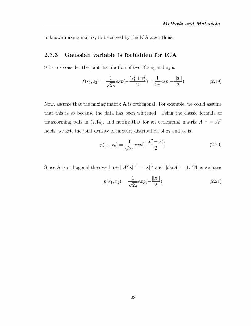
2.3.3 Gaussian variable is forbidden for ICA
9 Let us consider the joint distribution of two ICs s1 and s2 is
f(s1, s2) =1√2πexp(−(s21 + s22
2) =
1
2πexp(−||s||
2) (2.19)
Now, assume that the mixing matrix A is orthogonal. For example, we could assume
that this is so because the data has been whitened. Using the classic formula of
transforming pdfs in (2.14), and noting that for an orthogonal matrix A−1 = AT
holds, we get, the joint density of mixture distribution of x1 and x2 is
p(x1, x2) =1√2πexp(−x
21 + x22
2) (2.20)
Since A is orthogonal then we have ||ATx||2 = ||x||2 and ||detA|| = 1. Thus we have
p(x1, x2) =1√2πexp(−||x||
2) (2.21)
23
Methods and Materials
−4 −2 0 2
−4−2
02
4
s1
s2
Figure 2.3: Joint distribution of two independent Source of Normal(Gaussian) distribution.
From the above equation the pdf of orthogonal mixing matrix and source are
identical. Thus there is no way to infer the mixing matrix from mixture. If we
try to estimate the ICA model and some (more than one) of the components are
gaussian, some nongaussian we can estimate all the nongaussian components, but the
gaussian components cannot be separated from each other, because they entangled to
each other and form a single gaussian component. Actually, in case of one gaussian
component, we can estimate the ICA model, because the single gaussian component
does not have any other gaussian components that it could be mixed with.
2.3.4 Key of ICA estimation
Non-gauassian is the heart of ICA estimation. Actually without non-gaussianity the
estimation is not possible at all. In most classical statistical theory, random variables
are assumed to have gaussian distributions which is the main obstruction for ICA.
This is probably the main reasons for late resurgence of ICA research. . According to
Central limit Theorem (CLT), the distribution of the sum (average of linear combi-
nation) of n independent component tends to gaussian distribution as n→∞, under
24
Methods and Materials
certain condition (for cauchy distribution central limit theorem does not hold).
According to ICA model (Eq. 2.18) mixture data vector is a linear combination
of independent source. Thus a linear combination y =∑
i bixi of the observed vari-
ables xi (which in turn are linear combinations of the independent components sj)
will be maximally non-Gaussian if it equals one of the independent components sj.
This is seen by a counter example: if y does not equal one of the sj but is a mixture of
two or more sj , then by spirit of the central limit theorem, y is more Gaussian than
each of the sj. Thus the task is to find wj such that the distribution of yj = wTj x is
as far from Gaussian as possible.
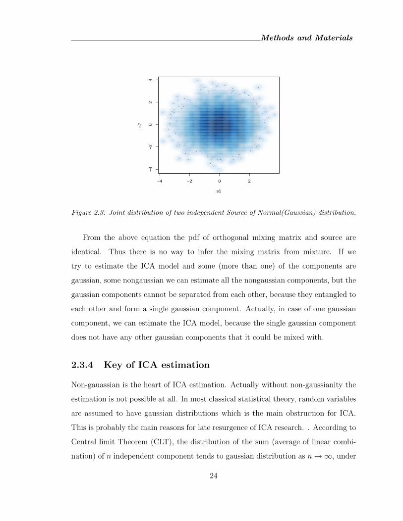
−1.5 −1.0 −0.5 0.0 0.5 1.0 1.5
−1.5
−1.0
−0.5
0.0
0.5
1.0
1.5
s1
s2
Figure 2.4: Joint distribution of two independent Source of uniform (sub-Gaussian) distri-
bution.
25
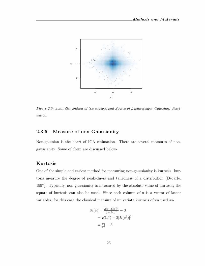
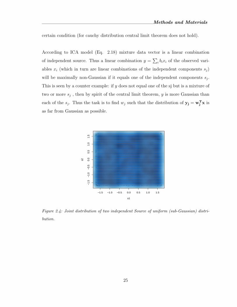
Methods and Materials
−5 0 5
−50
5
s1
s2
Figure 2.5: Joint distribution of two independent Source of Laplace(super-Gaussian) distri-
bution.
2.3.5 Measure of non-Gaussianity
Non-gaussian is the heart of ICA estimation. There are several measures of non-
gaussianity. Some of them are discussed below-
Kurtosis
One of the simple and easiest method for measuring non-gaussianity is kurtosis. kur-
tosis measure the degree of peakedness and tailedness of a distribution (Decarlo,
1997). Typically, non gaussianity is measured by the absolute value of kurtosis; the
square of kurtosis can also be used. Since each column of s is a vector of latent
variables, for this case the classical measure of univariate kurtosis often used as-
β2(s) = E[s−E(s)]4
[var(s)]2− 3
= E(s4)− 3[E(s2)]2
= µ4σ4 − 3
26
Methods and Materials
where E(.) is the expectation operator, σ is the standard deviation, µ4 is 4th moment
about the mean. For gaussian random variable the 4th moments E(s4) = 3[E(s2)]2.
Thus gaussian distribution has null kurtosis. we can distinguish the kurtosis in three
cases.
β2 = 0Gaussian
β2 > 0 Super − gaussian
β2 < 0 sub− gaussian
If x1 and x2 are two independent random variables then, k(x1 + x2) = k(x1) + k(x2)
and k(αx) = (α)4k(x) where, α is the constant term and k(.) is kurtosis operator.
27
Methods and Materials
0 2 4 6 8
02
46
8
x1
x2
(a)
−2 −1 0 1 2
−2
−1
01
2
x1
x2(b)
−40 −20 0 20 40
−1
00
−5
00
50
x1
x2
(c)
−5 0 5
−5
05
x1
x2
(d)
Figure 2.6: (a) The joint distribution of the observed mixture of two uniform (sub-gaussian)
variables. (b)The joint distribution of whiten mixtures of uniformly distributed independent
components. (c) The joint distribution of the observed mixture of two Laplacian distribution.
(d) The joint distribution of two whiten mixture of Laplacian distribution.
28
Methods and Materials
Negentropy
Entropy in information theory measure the unpredictability of information contents.
The generally information reduce uncertainty. Let us consider, y is a discrete random
variable that obtains values from a finite set y1, , yn with probabilities p1, , pn. We look
for a measure of how much choice is involved in the section of event or how certain
we are of the outcome. Shannon argued that such a measure H(p1, , pn) should obey
the following properties
1. H should be continuous in pi
2. If all pi are equal than H should be monotonically increasing in n.
3. If a choice is broken down into two successive choices, the original H should be
the weighted sum of the individual values of H.
The entropy H(y) of a discrete random variable y is defined by
H(y) = −n∑i=1
p(y)logp(y) (2.22)
Figure 2.7: Entropy measurement corresponding to probability. From the figure entropy will
be maximum when p=0.5
29
Methods and Materials
A fundamental result of information theory is that a gaussian variable has the
largest entropy among all random variables of equal variance [84, 20]. This means
that entropy can be used for measuring non-gaussianity.
A Gaussian random variable has the largest possible entropy of all variables with
an equal variance, so high degree of entropy can be associated with a high degree
of gaussianity. Negentropy is a measurement of the entropy of a random variable
that is designed to be always non negative and equal to zero when the distribution is
Gaussian. Negentropy is defined in terms of entropy as
J(y) = H(ygauss)−H(y) (2.23)
where, ygauss is a gaussian random variable of the same covariance matrix as y. As
J(y) is always greater than zero unless y is Gaussian, it is a good measurement of
non-gaussianity.
This result can be generalized from random variables to random vectors, such as
y = [y1, · · · , ym]T , and we want to find a matrix W so that y = Wx has the maximum
negentropy J(y) = H(yG)−H(y), i.e., y is most non-Gaussian. However, exact J(y)
is difficult to get as its calculation requires the specific density distribution function
p(y).
The negentropy can be approximated by
J(y) ≈ 1
12E{y3}2 +
1
48kurt(y)2 (2.24)
However, this approximation also suffers from the non-robustness due to the kur-
tosis function. A better approximation is
J(y) ≈p∑i=1
ki[E{Gi(y)} − E{Gi(g)}]2 (2.25)
where ki are some positive constants, y is assumed to have zero mean and unit
variance, and g is a Gaussian variable also with zero mean and unit variance. Gi are
some non-quadratic functions such as
30
Methods and Materials
G1(y) =1
alog cosh (a y), G2(y) = −exp(−y2/2)
where 1 ≤ a ≤ 2 is some suitable constant. Although this approximation may not
be accurate, it is always greater than zero except when x is Gaussian.
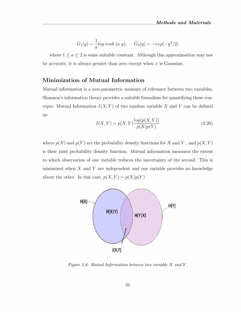
Minimization of Mutual Information
Mutual information is a non-parametric measure of relevance between two variables.
Shannon’s information theory provides a suitable formalism for quantifying these con-
cepts. Mutual Information I(X, Y ) of two random variable X and Y can be defined
as-
I(X, Y ) = p(X, Y )log(p(X, Y ))
p(X)p(Y )(2.26)
where p(X) and p(Y ) are the probability density functions for X and Y , and p(X, Y )
is their joint probability density function. Mutual information measures the extent
to which observation of one variable reduces the uncertainty of the second. This is
minimized when X and Y are independent and one variable provides no knowledge
about the other. In this case, p(X, Y ) = p(X)p(Y )
Figure 2.8: Mutual Information between two variable X and Y .
31
Methods and Materials
The mutual information I(x, y) of two random variables x and y is defined as
I(x, y) = H(x) +H(y)−H(x, y) = H(x)−H(x|y) = H(y)−H(y|x) (2.27)
Obviously when x and y are independnent, i.e., H(y|x) = H(y) and H(x|y) =
H(x), their mutual information I(x, y) is zero.
Similarly the mutual information I(y1, · · · , yn) of a set of n variables yi (i =
1, · · · , n) is defined as
I(y1, · · · , yn) =n∑i=1
H(yi)−H(y1, · · · , yn) (2.28)
If random vector y = [y1, · · · , yn]T is a linear transform of another random vector
x = [x1, · · · , xn]T :
yi =n∑j=1
wijxj, or y = Wx (2.29)
then the entropy of y is related to that of x by: H(y1, · · · , yn) = H(x1, · · · , xn) +
E {log J(x1, · · · , xn)} = H(x1, · · · , xn) + log detW
where J(x1, · · · , xn) is the Jacobian of the above transformation:
J(x1, · · · , xn) =∣∣∣ ∂......yn
∂xn
∣∣∣ = detW (2.30)
The mutual information above can be written as I(y1, · · · , yn) =n∑i=1
H(yi) −
H(y1, · · · , yn) =n∑i=1
H(yi)−H(x1, · · · , xn)− log det W We further assume yi to be
uncorrelated and of unit variance, i.e., the covariance matrix of y is
E{yyT} = WE{xxT}WT = I (2.31)
and its determinant is
det I = 1 = (detW) (det E{xxT}) (detWT ) (2.32)
32
Methods and Materials
This means det W is a constant (same for any W). Also, as the second term in
the mutual information expression H(x1, · · · , xn) is also a constant (invariant with
respect to W), we have
I(y1, · · · , yn) =n∑i=1
H(yi) + Constant (2.33)
i.e., minimization of mutual information I(y1, · · · , yn) is achieved by minimizing
the entropies
H(yi) = −∫pi(yi)log pi(yi)dyi = −E{log pi(yi)} (2.34)
As Gaussian density has maximal entropy, minimizing entropy is equivalent to mini-
mizing Gaussianity. Moreover, since all yi have the same unit variance, their negen-
tropy becomes
J(yi) = H(yG)−H(yi) = C −H(yi) (2.35)
where C = H(yG) is the entropy of a Gaussian with unit variance, same for all
yi. Substituting H(yi) = C − J(yi) into the expression of mutual information, and
realizing the other two terms H(x) and log det W are both constant (same for any
W), we get
I(y1, · · · , yn) = Const−n∑i=1
J(yi) (2.36)
where Const is a constant (including all terms C, H(x) and log detW) which is
the same for any linear transform matrix W . This is the fundamental relation between
mutual information and negentropy of the variables y1. If the mutual information of
a set of variables is decreased (indicating the variables are less dependent) then the
negentropy will be increased, and yi are less Gaussian. We want to find a linear
transform matrix W to minimize mutual information I(y1, · · · , yn), or, equivalently,
to maximize negentropy (under the assumption that yi are uncorrelated).
33
Methods and Materials
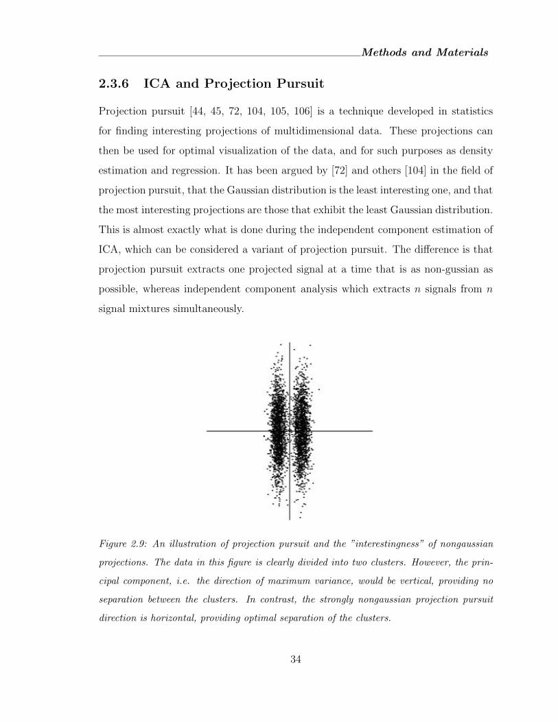
2.3.6 ICA and Projection Pursuit
Projection pursuit [44, 45, 72, 104, 105, 106] is a technique developed in statistics
for finding interesting projections of multidimensional data. These projections can
then be used for optimal visualization of the data, and for such purposes as density
estimation and regression. It has been argued by [72] and others [104] in the field of
projection pursuit, that the Gaussian distribution is the least interesting one, and that
the most interesting projections are those that exhibit the least Gaussian distribution.
This is almost exactly what is done during the independent component estimation of
ICA, which can be considered a variant of projection pursuit. The difference is that
projection pursuit extracts one projected signal at a time that is as non-gussian as
possible, whereas independent component analysis which extracts n signals from n
signal mixtures simultaneously.
Figure 2.9: An illustration of projection pursuit and the ”interestingness” of nongaussian
projections. The data in this figure is clearly divided into two clusters. However, the prin-
cipal component, i.e. the direction of maximum variance, would be vertical, providing no
separation between the clusters. In contrast, the strongly nongaussian projection pursuit
direction is horizontal, providing optimal separation of the clusters.
34
Methods and Materials
Specifically, the projection pursuit allows us to tackle the situation where there are
less independent components sithan original variables xi. However, it should be noted
that in the formulation of projection pursuit, no data model or assumption about
independent components is made. In ICA models, optimizing the non-gaussianity
measures produces independent components; if the model does not hold, then the
projection pursuit directions are produced.
2.3.7 Data preprocessing
Centering
Typically algorithm for ICA use centering, whitening and dimensionality reduction
as preprocessing steps in order to simplify and reduce the complexity of the problem
for the actual iterative algorithm. Let us consider x′ is the observed data. After
centering the data we have-
x = x′ − E(x′)
Whitening
Whitening is a slightly stronger property than uncorrelatedness. Whitening of a zero
mean random vector means that their components are uncorrelated and their variance
equal to unity. In other word the covariance matrix equal to identity matrix. Actually
whitening is the linear transformation of the observed data vector.
z = Vx
So, that the z is white. It is sometimes is called sphering. There are many method
are available for whitening. One of the popular methods is Eigenvalue Decomposition
(ED).
E(xxT ) = EDET
35
Methods and Materials
Here E is an orthogonal matrix of eigenvectors E(xxT ) and D is the diagonal matrix
of eigenvalues.
V = ED−1/2ET
E(zzT ) = VE(xxT )VT
= ED−1/2ETEDETED−1/2ET
= ED−1/2DD−1/2ET
= I
Whitening transforms the mixing A matrix into a new one A. We have from the
above-
= VAs = As
One could hope that whitening solves the ICA problem, since whiteness or uncorre-
latedness is related to independence. This is, however, not so. Uncorrelatedness is
weaker than independence, and is not in itself sufficient for estimation of the ICA
model. whitening gives the ICs only up to an orthogonal transformation. This is not
sufficient in most applications.
E(zzT ) = AE(ssT )AT
= I
2.3.8 FastICA algorithm
The FastICA algorithm was developed at the Laboratory of Information and Com-
puter Science in the Helsinki University of Technology by Hugo Gvert, Jarmo Hurri,
Jaakko Srel, and Aapo Hyvrinen. The FastICA algorithm is a highly computationally
efficient method for performing the estimation of ICA. It uses a fixed-point iteration
process that has been determined, in independent experiments, to be 10-100 times
faster than conventional gradient descent methods for ICA. Another advantage of the
FastICA algorithm is that it can be used to perform projection pursuit as well, thus
36
Methods and Materials
providing a general-purpose data analysis method that can be used both in an ex-
ploratory fashion and for estimation of independent components (or sources)(FastICA
website. http://www.cis.hut.fi/projects/ica/fastica/).
The advantage of using negentropy, also called differential entropy, as a measure
of nongaussianity is that it is well justified by statistical theory. The problem in
using negentropy is, however, that it is computationally very difficult[14]. Approxi-
mations for calculating negentropy in a much more computationally efficient manner
have been proposed as seen in equation 2.13. Varying the formulas used for G can
provide further approximation with a minimal loss of information.
In finite sample statistical properties of the estimators based on optimizing such
a general contrast function were analysed. It was found that for a suitable choice of
G, the statistical properties of the estimator (asymptotic variance and robustness)
are considerably better than the properties cumulant based estimator. The following
choices of G were proposed [?]:
G1(u) = log{cosh(a1u)} (2.37)
G2(u) = exp(−a2u2
2) (2.38)
where a1, a2 ≥ 1 are some suitable constants. Experimentally, it is found that espe-
cially the values 1 ≤ a1 ≤ 2, a2 = 1 for the constant gives good approximations.
The basic process for the algorithm is best first described as a one-unit version,
where there is only one computational unit with a weight vector w that is able to
update by a learning rule. The FastICA learning rule finds a unit vector w such that
wTx maximizes nongaussianity, which in this case is calculated by the approximation
of negentropy J(wTx). The steps of the FastICA algorithm for extracting a single
independent component are outlined below.
37
Methods and Materials
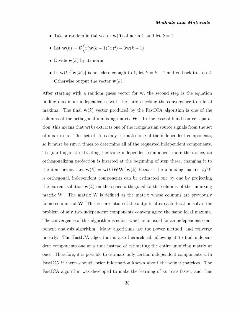
� Take a random initial vector w(0) of norm 1, and let k = 1.
� Let w(k) = E(x(w(k − 1)Tx)3)− 3w(k − 1)
� Divide w(k) by its norm.
� If |w(k)Tw(k1)| is not close enough to 1, let k = k + 1 and go back to step 2.
Otherwise output the vector w(k).
After starting with a random guess vector for w, the second step is the equation
finding maximum independence, with the third checking the convergence to a local
maxima. The final w(k) vector produced by the FastICA algorithm is one of the
columns of the orthogonal unmixing matrix W . In the case of blind source separa-
tion, this means that w(k) extracts one of the nongaussian source signals from the set
of mixtures x. This set of steps only estimates one of the independent components,
so it must be run n times to determine all of the requested independent components.
To guard against extracting the same independent component more then once, an
orthogonalizing projection is inserted at the beginning of step three, changing it to
the item below. Let w(k) = w(k)WWTw(k) Becuase the unmixing matrix bfW
is orthogonal, independent components can be estimated one by one by projecting
the current solution w(k) on the space orthogonal to the columns of the unmixing
matrix W . The matrix W is defined as the matrix whose columns are previously
found columns of W. This decorrelation of the outputs after each iteration solves the
problem of any two independent components converging to the same local maxima.
The convergence of this algorithm is cubic, which is unusual for an independent com-
ponent analysis algorithm. Many algorithms use the power method, and converge
linearly. The FastICA algorithm is also hierarchical, allowing it to find indepen-
dent components one at a time instead of estimating the entire unmixing matrix at
once. Therefore, it is possible to estimate only certain independent components with
FastICA if theres enough prior information known about the weight matrices. The
FastICA algorithm was developed to make the learning of kurtosis faster, and thus
38
Methods and Materials
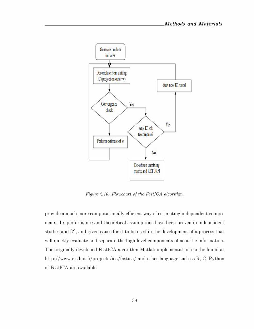
Figure 2.10: Flowchart of the FastICA algorithm.
provide a much more computationally efficient way of estimating independent compo-
nents. Its performance and theoretical assumptions have been proven in independent
studies and [?], and given cause for it to be used in the development of a process that
will quickly evaluate and separate the high-level components of acoustic information.
The originally developed FastICA algorithm Matlab implementation can be found at
http://www.cis.hut.fi/projects/ica/fastica/ and other language such as R, C, Python
of FastICA are available.
39
Methods and Materials
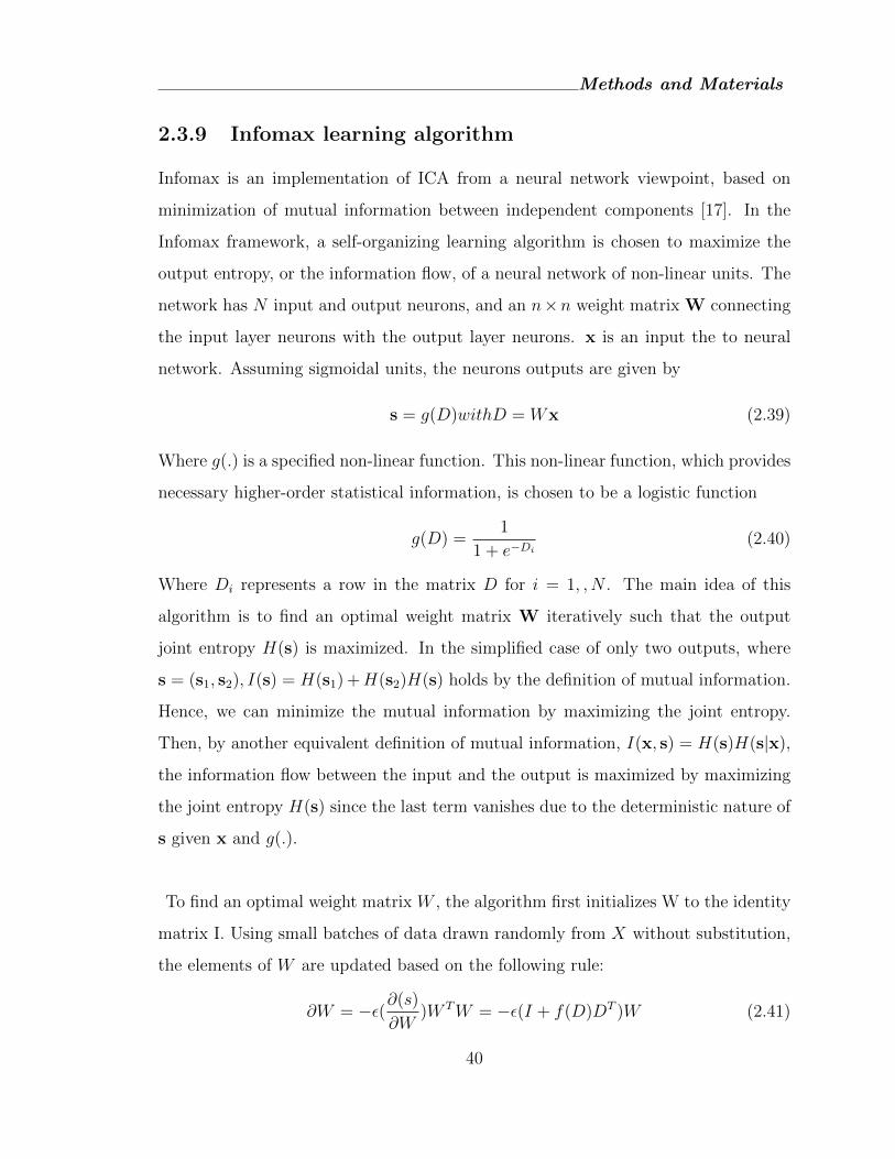
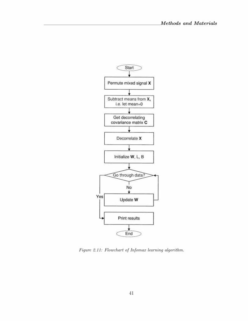
2.3.9 Infomax learning algorithm
Infomax is an implementation of ICA from a neural network viewpoint, based on
minimization of mutual information between independent components [17]. In the
Infomax framework, a self-organizing learning algorithm is chosen to maximize the
output entropy, or the information flow, of a neural network of non-linear units. The
network has N input and output neurons, and an n×n weight matrix W connecting
the input layer neurons with the output layer neurons. x is an input the to neural
network. Assuming sigmoidal units, the neurons outputs are given by
s = g(D)withD = Wx (2.39)
Where g(.) is a specified non-linear function. This non-linear function, which provides
necessary higher-order statistical information, is chosen to be a logistic function
g(D) =1
1 + e−Di(2.40)
Where Di represents a row in the matrix D for i = 1, , N . The main idea of this
algorithm is to find an optimal weight matrix W iteratively such that the output
joint entropy H(s) is maximized. In the simplified case of only two outputs, where
s = (s1, s2), I(s) = H(s1) +H(s2)H(s) holds by the definition of mutual information.
Hence, we can minimize the mutual information by maximizing the joint entropy.
Then, by another equivalent definition of mutual information, I(x, s) = H(s)H(s|x),
the information flow between the input and the output is maximized by maximizing
the joint entropy H(s) since the last term vanishes due to the deterministic nature of
s given x and g(.).
To find an optimal weight matrix W , the algorithm first initializes W to the identity
matrix I. Using small batches of data drawn randomly from X without substitution,
the elements of W are updated based on the following rule:
∂W = −ε(∂(s)
∂W)W TW = −ε(I + f(D)DT )W (2.41)
40
Methods and Materials
Figure 2.11: Flowchart of Infomax learning algorithm.
41
Methods and Materials
Where ε is the learning rate (typically near 0.01) and the vector function g has
elements
fi(Di) =∂
∂Di
ln∂gi∂Di
= (1− 2si) (2.42)
Equ. (2.42) is known as the Infomax algorithm. The W TW term in Equ. (2.41), first
proposed by Amari et al. [78], avoids matrix inversions and speeds up convergence.
During training, the learning rate is reduced gradually until the weight matrix stops
changing appreciably. The choice of nonlinearity depends on the application type. In
the context of fMRI, where relatively few highly active voxels are usually expected in
a large volume, the distribution of the estimated components is assumed to be super-
gaussian. Therefore, a sigmoidal function is appropriate for such an application [68].
2.4 Data Description
In this thesis I apply three simulated dataset for shape study, one simulated and three
real datasets for clustering which are Australian Crabs data, Olive oils data, Fisher
Iris data and five real data set for outlier detection which are Epilepsy , Education
expenditure, Stackloss data, Scottish hill racing data.
2.5 PCA vs ICA
PCA can be interpreted in terms of blind source separation methods in as much as
PCA is like a version of ICA in which the source variables are assumed to be gaussian.
However, the essential difference between ICA and PCA is that PCA decomposes a
set of mixture variables into a set of uncorrelated variables, whereas ICA decomposes
a set of mixture variables into a set of independent variables. Independent is much
stronger property than uncorrelatedness.
42
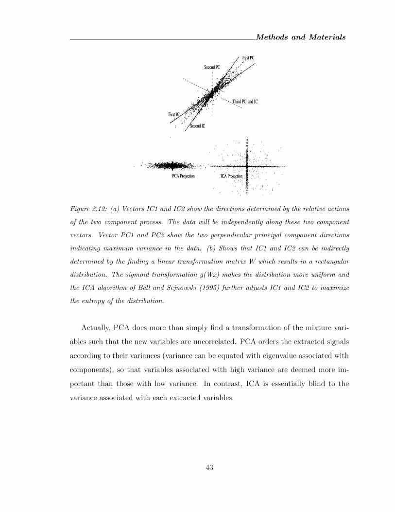
Methods and Materials
Figure 2.12: (a) Vectors IC1 and IC2 show the directions determined by the relative actions
of the two component process. The data will be independently along these two component
vectors. Vector PC1 and PC2 show the two perpendicular principal component directions
indicating maximum variance in the data. (b) Shows that IC1 and IC2 can be indirectly
determined by the finding a linear transformation matrix W which results in a rectangular
distribution. The sigmoid transformation g(Wx) makes the distribution more uniform and
the ICA algorithm of Bell and Sejnowski (1995) further adjusts IC1 and IC2 to maximize
the entropy of the distribution.
Actually, PCA does more than simply find a transformation of the mixture vari-
ables such that the new variables are uncorrelated. PCA orders the extracted signals
according to their variances (variance can be equated with eigenvalue associated with
components), so that variables associated with high variance are deemed more im-
portant than those with low variance. In contrast, ICA is essentially blind to the
variance associated with each extracted variables.
43
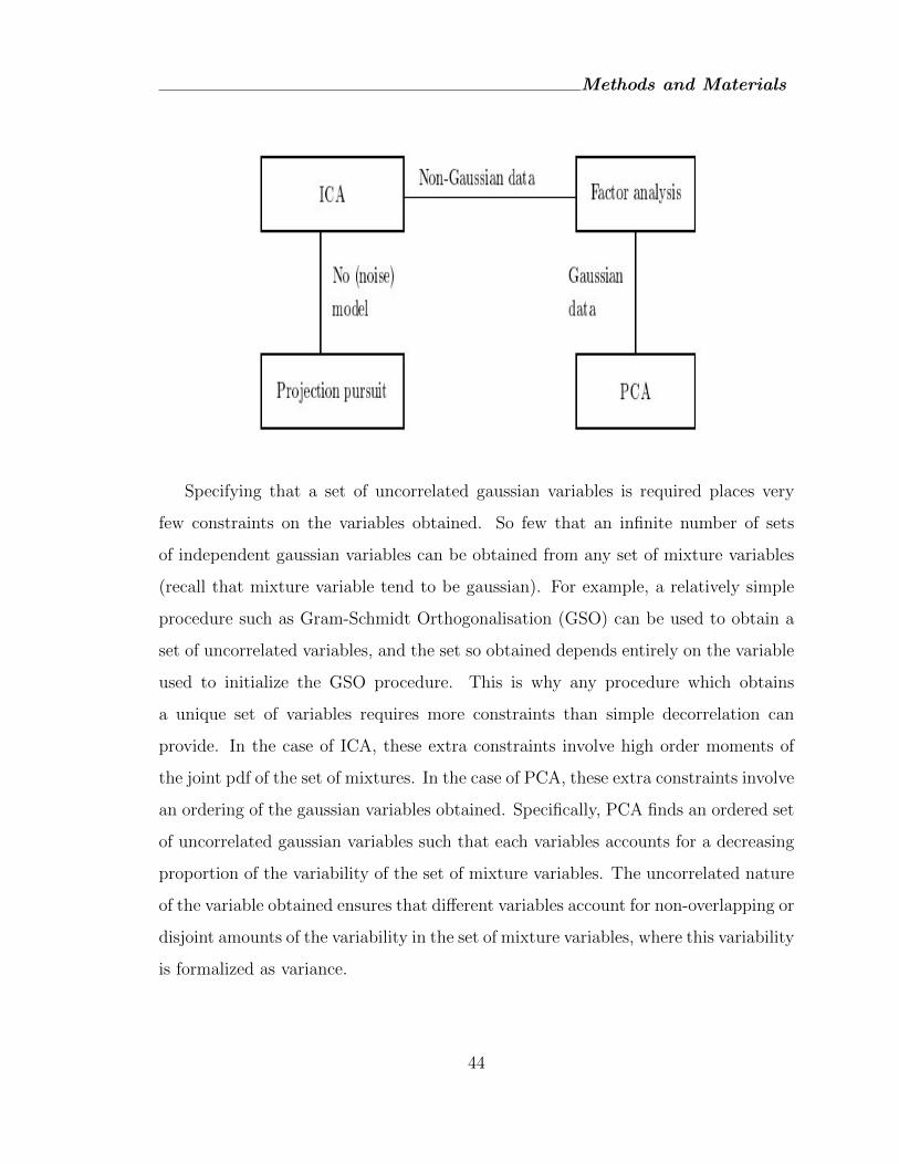
Methods and Materials
Specifying that a set of uncorrelated gaussian variables is required places very
few constraints on the variables obtained. So few that an infinite number of sets
of independent gaussian variables can be obtained from any set of mixture variables
(recall that mixture variable tend to be gaussian). For example, a relatively simple
procedure such as Gram-Schmidt Orthogonalisation (GSO) can be used to obtain a
set of uncorrelated variables, and the set so obtained depends entirely on the variable
used to initialize the GSO procedure. This is why any procedure which obtains
a unique set of variables requires more constraints than simple decorrelation can
provide. In the case of ICA, these extra constraints involve high order moments of
the joint pdf of the set of mixtures. In the case of PCA, these extra constraints involve
an ordering of the gaussian variables obtained. Specifically, PCA finds an ordered set
of uncorrelated gaussian variables such that each variables accounts for a decreasing
proportion of the variability of the set of mixture variables. The uncorrelated nature
of the variable obtained ensures that different variables account for non-overlapping or
disjoint amounts of the variability in the set of mixture variables, where this variability
is formalized as variance.
44
Methods and Materials
2.6 Computer Program Used in the Analysis
In this thesis all computations are done by using several software-
� R version 3.0.1, R development core team (16-05-2013) with several download
packages fastICA, moments, VGAM, MASS, rattle etc.
� Matlab version 7.10.0.499 (R2010a) with several toolbox FastICA, BSS, fmrlab,
ICALAB etc.
All typeset is being completed by using the software ”miktex”, (LaTeX) version 2.9
and Texwork. A personal computer of HP pavilion g6 notebook, Intel(R) Core(TM)i3,
2.53 GHz Processor, 4GB RAM, Windows 8 Enterprise N-32-bit is used for the anal-
ysis.
2.7 Summary
In this chapter, we described the basic ICA and PCA model with their mathematical
and logical difference of our interest. We also reviewed most popular algorithms of
ICA. In addition, we mention data and software that are used in the analysis. We
apply these methods in identifying shape of the source, cluster and outlier detection
in following chapters and discuss their similarities and differences.
45
Chapter 3
Latent Structure Detection
3.1 Introduction
The main task of ICA to recover the original source from mixture distribution. Sup-
pose we are having a conversation at a crowded cocktail party . It is usually no
problem to focus on the person you are talking to, although our two ears are receiv-
ing a wild mixture of different sounds originating from various sources: for example,
the conversation of the people next to us or the stereo system playing background
music. Despite all the background noise the brain enables us to understand the per-
son we are trying to listen to. Replace the two ears with microphones and the brain
with a computer. Can we program a computer such that it separates the microphone
recordings into the different sound sources of the cocktail party? Can it single out
the words of the person in front of us? This is the cocktail-party problem which is
quite difficult to solve, but it illustrates the goal of blind source separation (BSS):
decompose signals that have been recorded by an array of sensors (i.e. multichan-
nel recordings) into the underlying sources. This source separation problem is called
blind because neither the mixing process nor the characteristics of the source signals
are known.
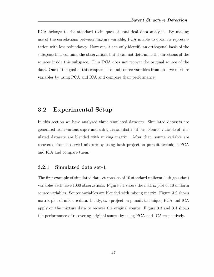
Latent Structure Detection
PCA belongs to the standard techniques of statistical data analysis. By making
use of the correlations between mixture variable, PCA is able to obtain a represen-
tation with less redundancy. However, it can only identify an orthogonal basis of the
subspace that contains the observations but it can not determine the directions of the
sources inside this subspace. Thus PCA does not recover the original source of the
data. One of the goal of this chapter is to find source variables from observe mixture
variables by using PCA and ICA and compare their performance.
3.2 Experimental Setup
In this section we have analyzed three simulated datasets. Simulated datasets are
generated from various super and sub-gaussian distributions. Source variable of sim-
ulated datasets are blended with mixing matrix. After that, source variable are
recovered from observed mixture by using both projection pursuit technique PCA
and ICA and compare them.
3.2.1 Simulated data set-1
The first example of simulated dataset consists of 10 standard uniform (sub-gaussian)
variables each have 1000 observations. Figure 3.1 shows the matrix plot of 10 uniform
source variables. Source variables are blended with mixing matrix. Figure 3.2 shows
matrix plot of mixture data. Lastly, two projection pursuit technique, PCA and ICA
apply on the mixture data to recover the original source. Figure 3.3 and 3.4 shows
the performance of recovering original source by using PCA and ICA respectively.
47
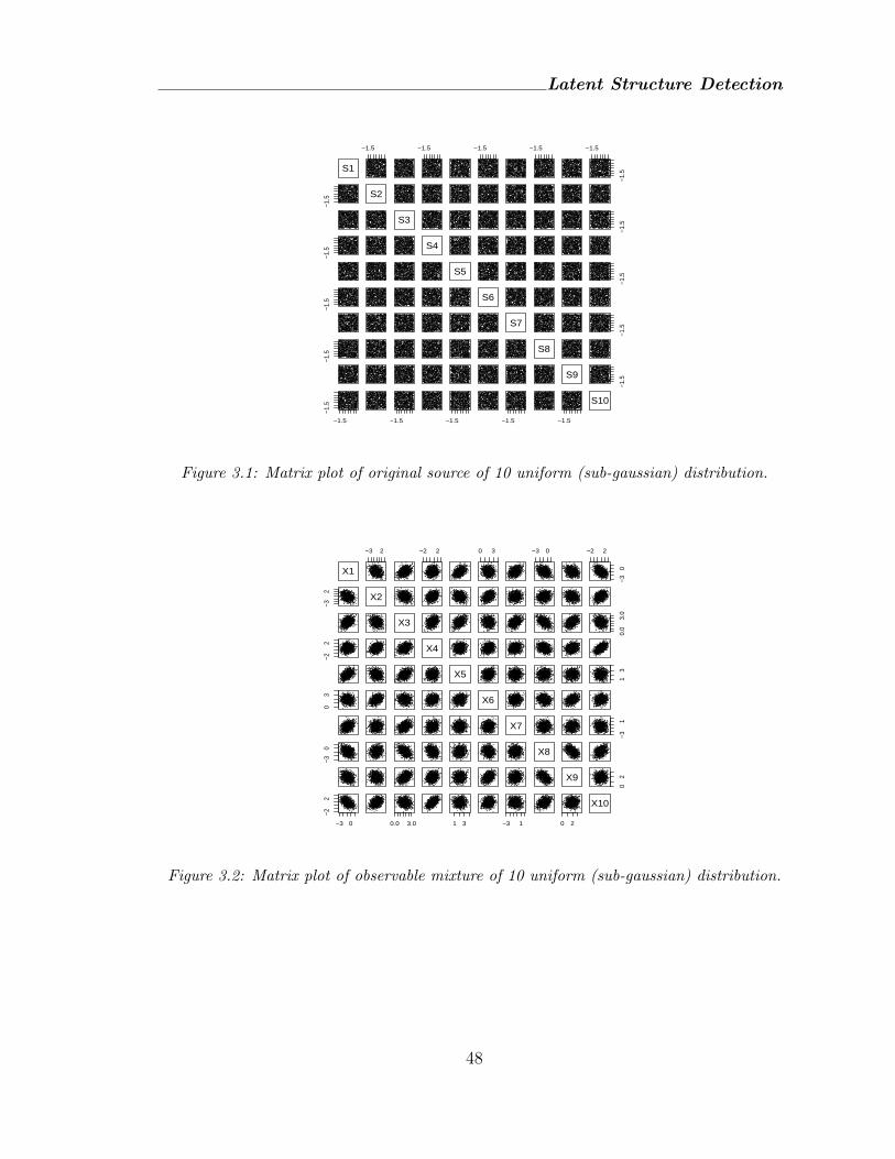
Latent Structure Detection
S1
−1.5 −1.5 −1.5 −1.5 −1.5
−1.5
−1.5 S2
S3
−1.5
−1.5 S4
S5
−1.5
−1.5 S6
S7
−1.5
−1.5 S8
S9
−1.5
−1.5
−1.5
−1.5 −1.5 −1.5 −1.5
S10
Figure 3.1: Matrix plot of original source of 10 uniform (sub-gaussian) distribution.
X1
−3 2 −2 2 0 3 −3 0 −2 2
−30
−32
X2
X30.
03.
0
−22
X4
X5 13
03
X6
X7
−31
−30 X8
X9
02
−3 0
−22
0.0 3.0 1 3 −3 1 0 2
X10
Figure 3.2: Matrix plot of observable mixture of 10 uniform (sub-gaussian) distribution.
48
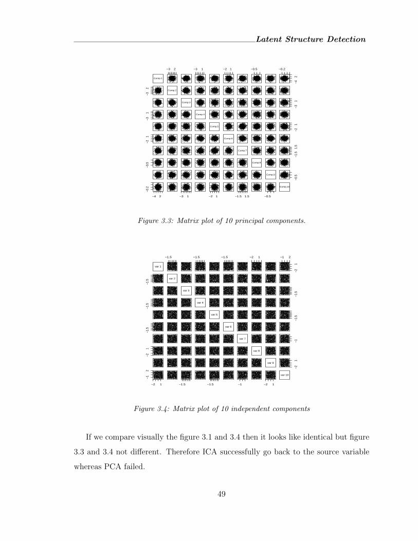
Latent Structure Detection
Comp.1
−3 2 −3 1 −2 1 −0.5 −0.2
−42
−32
Comp.2
Comp.3
−31
−31
Comp.4
Comp.5
−21
−21
Comp.6
Comp.7
−1.5
1.5
−0.5 Comp.8
Comp.9
−0.5
−4 2
−0.2
−3 1 −2 1 −1.5 1.5 −0.5
Comp.10
Figure 3.3: Matrix plot of 10 principal components.
var 1
−1.5 −1.5 −1.5 −2 1 −1 2
−21
−1.5
var 2
var 3
−1.5
−1.5
var 4
var 5
−1.5
−1.5
var 6
var 7
−1
−21
var 8
var 9
−21
−2 1
−12
−1.5 −1.5 −1 −2 1
var 10
Figure 3.4: Matrix plot of 10 independent components
If we compare visually the figure 3.1 and 3.4 then it looks like identical but figure
3.3 and 3.4 not different. Therefore ICA successfully go back to the source variable
whereas PCA failed.
49
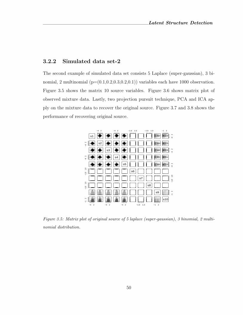
Latent Structure Detection
3.2.2 Simulated data set-2
The second example of simulated data set consists 5 Laplace (super-gaussian), 3 bi-
nomial, 2 multinomial (p=(0.1,0.2,0.3,0.2,0.1)) variables each have 1000 observation.
Figure 3.5 shows the matrix 10 source variables. Figure 3.6 shows matrix plot of
observed mixture data. Lastly, two projection pursuit technique, PCA and ICA ap-
ply on the mixture data to recover the original source. Figure 3.7 and 3.8 shows the
performance of recovering original source.
s1
−4 2 −4 2 −1.0 1.0 −1.0 1.0 −1 2
−42
−42 s2
s3
−42
−42 s4
s5
−42
−1.0
1.0
s6
s7
−1.0
1.0
−1.0
1.0
s8
s9
−12
−4 2
−12
−4 2 −4 2 −1.0 1.0 −1 2
s10
Figure 3.5: Matrix plot of original source of 5 laplace (super-gaussian), 3 binomial, 2 multi-
nomial distribution.
50
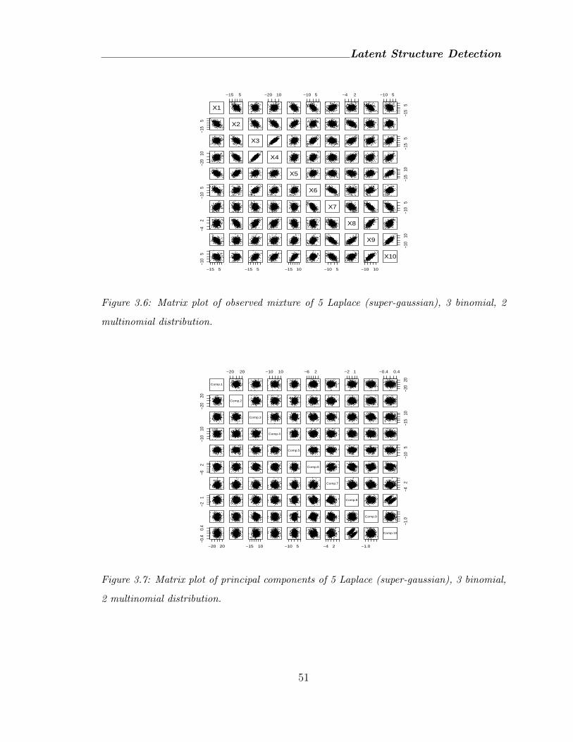
Latent Structure Detection
X1
−15 5 −20 10 −10 5 −4 2 −10 5
−15
5
−15
5
X2
X3
−15
5
−20
10
X4
X5
−15
10
−10
5
X6
X7
−10
5
−42
X8
X9
−10
10
−15 5
−10
5
−15 5 −15 10 −10 5 −10 10
X10
Figure 3.6: Matrix plot of observed mixture of 5 Laplace (super-gaussian), 3 binomial, 2
multinomial distribution.
Comp.1
−20 20 −10 10 −6 2 −2 1 −0.4 0.4
−20
20
−20
20
Comp.2
Comp.3
−15
10
−10
10
Comp.4
Comp.5
−10
5
−62
Comp.6
Comp.7
−42
−21
Comp.8
Comp.9
−1.0
−20 20
−0.4
0.4
−15 10 −10 5 −4 2 −1.0
Comp.10
Figure 3.7: Matrix plot of principal components of 5 Laplace (super-gaussian), 3 binomial,
2 multinomial distribution.
51
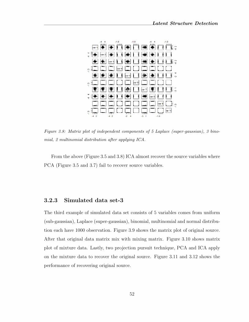
Latent Structure Detection
Figure 3.8: Matrix plot of independent components of 5 Laplace (super-gaussian), 3 bino-
mial, 2 multinomial distribution after applying ICA.
From the above (Figure 3.5 and 3.8) ICA almost recover the source variables where
PCA (Figure 3.5 and 3.7) fail to recover source variables.
3.2.3 Simulated data set-3
The third example of simulated data set consists of 5 variables comes from uniform
(sub-gaussian), Laplace (super-gaussian), binomial, multinomial and normal distribu-
tion each have 1000 observation. Figure 3.9 shows the matrix plot of original source.
After that original data matrix mix with mixing matrix. Figure 3.10 shows matrix
plot of mixture data. Lastly, two projection pursuit technique, PCA and ICA apply
on the mixture data to recover the original source. Figure 3.11 and 3.12 shows the
performance of recovering original source.
52
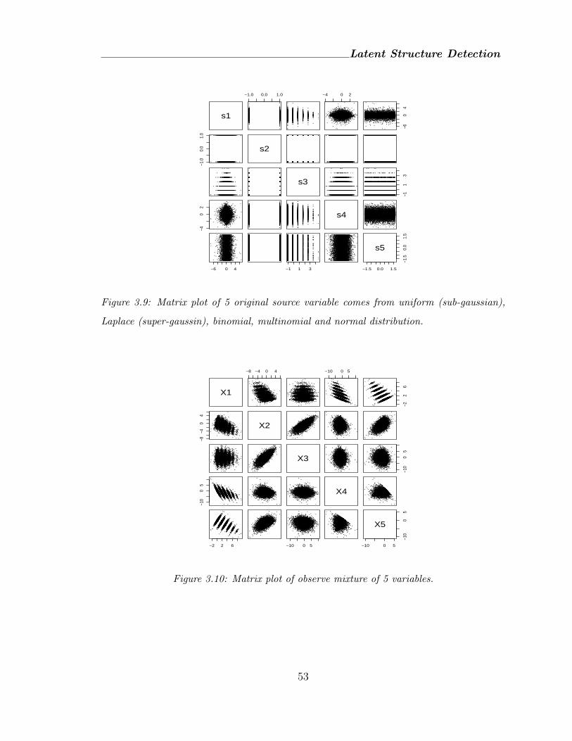
Latent Structure Detection
s1
−1.0 0.0 1.0 −4 0 2
−60
4
−1.0
0.0
1.0
s2
s3
−11
3
−40
2
s4
−6 0 4 −1 1 3 −1.5 0.0 1.5
−1.5
0.0
1.5
s5
Figure 3.9: Matrix plot of 5 original source variable comes from uniform (sub-gaussian),
Laplace (super-gaussin), binomial, multinomial and normal distribution.
X1
−8 −4 0 4 −10 0 5
−22
6
−8−4
04
X2
X3
−10
05
−10
05
X4
−2 2 6 −10 0 5 −10 0 5
−10
05
X5
Figure 3.10: Matrix plot of observe mixture of 5 variables.
53
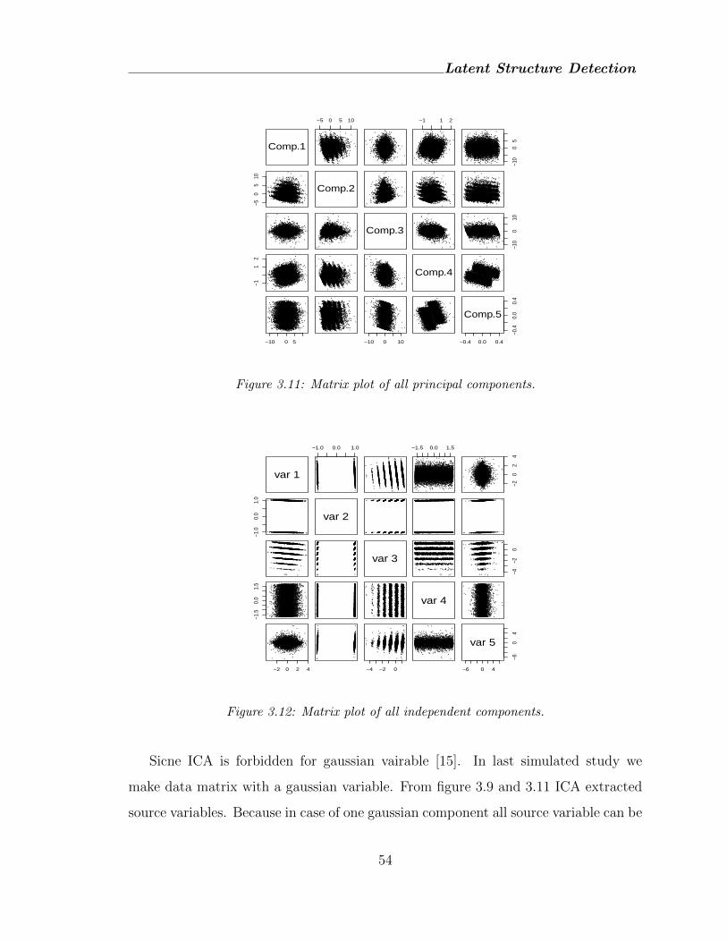
Latent Structure Detection
Comp.1
−5 0 5 10 −1 1 2
−10
05
−50
510
Comp.2
Comp.3
−10
010
−11
2
Comp.4
−10 0 5 −10 0 10 −0.4 0.0 0.4
−0.4
0.0
0.4
Comp.5
Figure 3.11: Matrix plot of all principal components.
var 1
−1.0 0.0 1.0 −1.5 0.0 1.5
−20
24
−1.0
0.0
1.0
var 2
var 3
−4−2
0
−1.5
0.0
1.5
var 4
−2 0 2 4 −4 −2 0 −6 0 4
−60
4
var 5
Figure 3.12: Matrix plot of all independent components.
Sicne ICA is forbidden for gaussian vairable [15]. In last simulated study we
make data matrix with a gaussian variable. From figure 3.9 and 3.11 ICA extracted
source variables. Because in case of one gaussian component all source variable can be
54

Latent Structure Detection
extracted but in case of more than one gaussian variable only non-gaussian variable
can be extracted, gaussian variables entangled to each others.
3.3 Summary
ICA successfully recover the original source after mixing the data because ICA taking
into account higher-order statistics which are ignored by PCA that relies only on
second-order statistics. Since its introduction it has become an indispensable tool for
statistical data analysis and processing of multi-channel data.
55
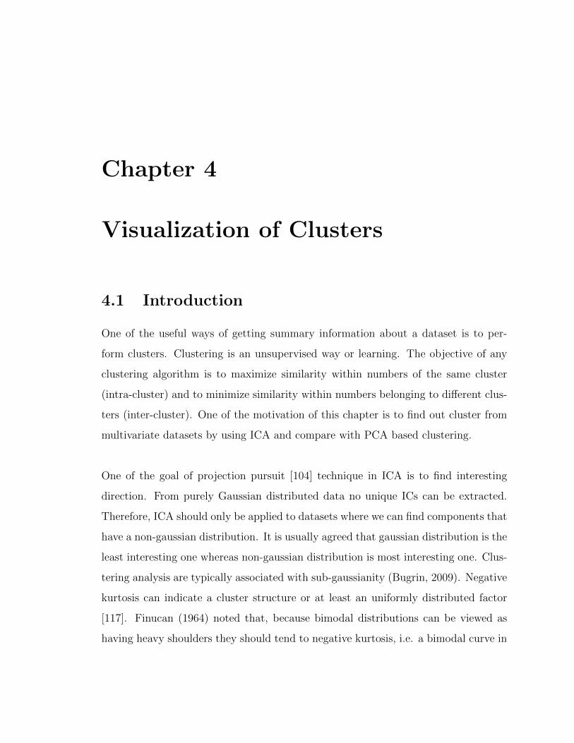
Chapter 4
Visualization of Clusters
4.1 Introduction
One of the useful ways of getting summary information about a dataset is to per-
form clusters. Clustering is an unsupervised way or learning. The objective of any
clustering algorithm is to maximize similarity within numbers of the same cluster
(intra-cluster) and to minimize similarity within numbers belonging to different clus-
ters (inter-cluster). One of the motivation of this chapter is to find out cluster from
multivariate datasets by using ICA and compare with PCA based clustering.
One of the goal of projection pursuit [104] technique in ICA is to find interesting
direction. From purely Gaussian distributed data no unique ICs can be extracted.
Therefore, ICA should only be applied to datasets where we can find components that
have a non-gaussian distribution. It is usually agreed that gaussian distribution is the
least interesting one whereas non-gaussian distribution is most interesting one. Clus-
tering analysis are typically associated with sub-gaussianity (Bugrin, 2009). Negative
kurtosis can indicate a cluster structure or at least an uniformly distributed factor
[117]. Finucan (1964) noted that, because bimodal distributions can be viewed as
having heavy shoulders they should tend to negative kurtosis, i.e. a bimodal curve in
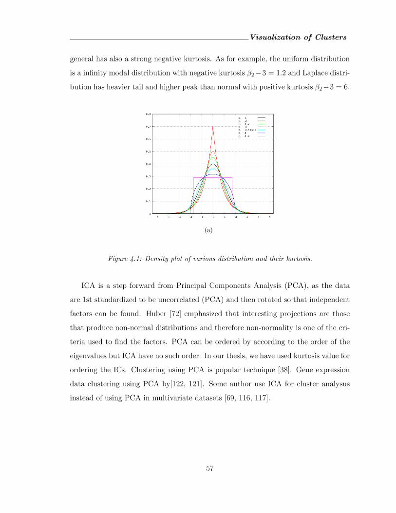
Visualization of Clusters
general has also a strong negative kurtosis. As for example, the uniform distribution
is a infinity modal distribution with negative kurtosis β2−3 = 1.2 and Laplace distri-
bution has heavier tail and higher peak than normal with positive kurtosis β2−3 = 6.
(a)
Figure 4.1: Density plot of various distribution and their kurtosis.
ICA is a step forward from Principal Components Analysis (PCA), as the data
are 1st standardized to be uncorrelated (PCA) and then rotated so that independent
factors can be found. Huber [72] emphasized that interesting projections are those
that produce non-normal distributions and therefore non-normality is one of the cri-
teria used to find the factors. PCA can be ordered by according to the order of the
eigenvalues but ICA have no such order. In our thesis, we have used kurtosis value for
ordering the ICs. Clustering using PCA is popular technique [38]. Gene expression
data clustering using PCA by[122, 121]. Some author use ICA for cluster analysus
instead of using PCA in multivariate datasets [69, 116, 117].
57
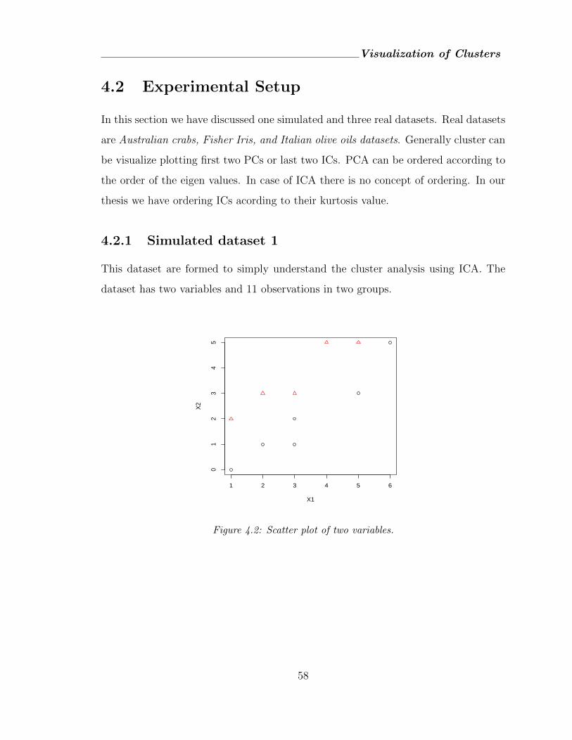
Visualization of Clusters
4.2 Experimental Setup
In this section we have discussed one simulated and three real datasets. Real datasets
are Australian crabs, Fisher Iris, and Italian olive oils datasets. Generally cluster can
be visualize plotting first two PCs or last two ICs. PCA can be ordered according to
the order of the eigen values. In case of ICA there is no concept of ordering. In our
thesis we have ordering ICs acording to their kurtosis value.
4.2.1 Simulated dataset 1
This dataset are formed to simply understand the cluster analysis using ICA. The
dataset has two variables and 11 observations in two groups.
1 2 3 4 5 6
01
23
45
X1
X2
Figure 4.2: Scatter plot of two variables.
58
Visualization of Clusters
−1.0 0.0 0.5 1.0
−3−2
−10
12
3
x
PC
1
−1.0 0.0 0.5 1.0
−1.5
−1.0
−0.5
0.0
0.5
1.0
1.5
x
last
ICFigure 4.3: (left) Scatter plot of first principal component. (Right) Scatter plot of last
independent component.
First PC and last IC is projected onto a vector. From figure 4.3 PCA cannot
separate the observation whereas ICA completely separate two group of observation.
4.2.2 Australian crabs dataset
The first experiment of real data set for clustering is Australian crabs data set where
there are 200 rows and 8 columns describing the 5 morphological measurements
(Frontal lob size, Rear width, Carapace length, Carapace width, Body depth). There
are two species in the data set each have both sexes (male, female) of the genus Lep-
tograpsus. There are 50 specimens of each sex of each species, collected on site at
Fremantle, Western Australia. (N. A. Campbell et al., 1974).
59
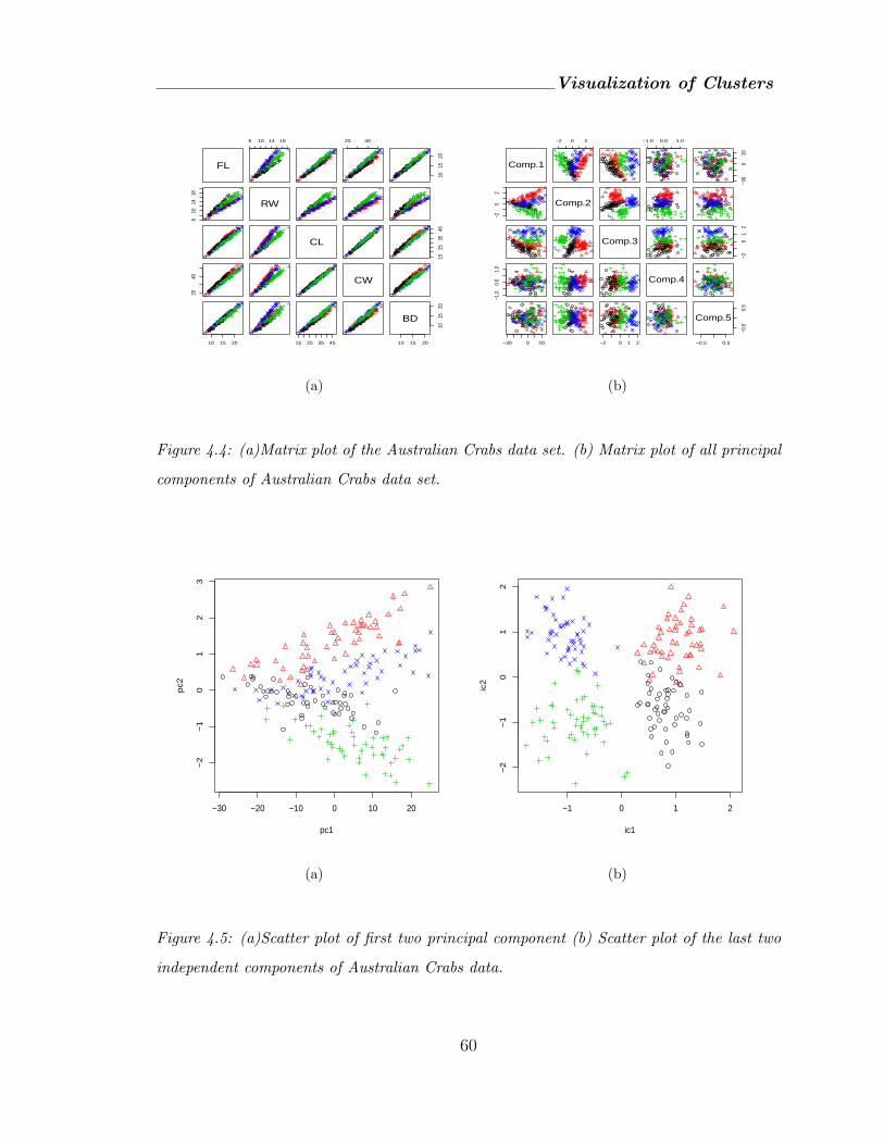
Visualization of Clusters
FL
6 10 14 18 20 40
1015
20
610
1418
RW
CL
1525
3545
2040 CW
10 15 20 15 25 35 45 10 15 20
1015
20
BD
(a)
Comp.1
−2 0 2 −1.0 0.0 1.0
−30
020
−20
2
Comp.2
Comp.3
−20
12
−1.0
0.0
1.0
Comp.4
−30 0 20 −2 0 1 2 −0.5 0.5
−0.5
0.5
Comp.5
(b)
Figure 4.4: (a)Matrix plot of the Australian Crabs data set. (b) Matrix plot of all principal
components of Australian Crabs data set.
−30 −20 −10 0 10 20
−2
−1
01
23
pc1
pc2
(a)
−1 0 1 2
−2
−1
01
2
ic1
ic2
(b)
Figure 4.5: (a)Scatter plot of first two principal component (b) Scatter plot of the last two
independent components of Australian Crabs data.
60
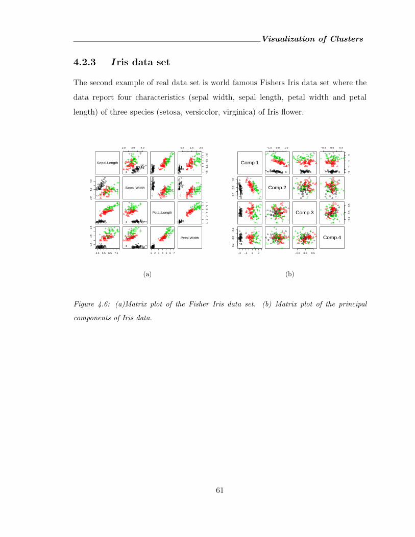
Visualization of Clusters
4.2.3 I ris data set
The second example of real data set is world famous Fishers Iris data set where the
data report four characteristics (sepal width, sepal length, petal width and petal
length) of three species (setosa, versicolor, virginica) of Iris flower.
Sepal.Length
2.0 3.0 4.0 0.5 1.5 2.5
4.5
5.5
6.5
7.5
2.0
3.0
4.0
Sepal.Width
Petal.Length
12
34
56
7
4.5 5.5 6.5 7.5
0.5
1.5
2.5
1 2 3 4 5 6 7
Petal.Width
(a)
Comp.1
−1.0 0.0 1.0 −0.4 0.0 0.4
−3−1
13
−1.0
0.0
1.0
Comp.2
Comp.3
−0.5
0.0
0.5
−3 −1 1 3
−0.4
0.0
0.4
−0.5 0.0 0.5
Comp.4
(b)
Figure 4.6: (a)Matrix plot of the Fisher Iris data set. (b) Matrix plot of the principal
components of Iris data.
61
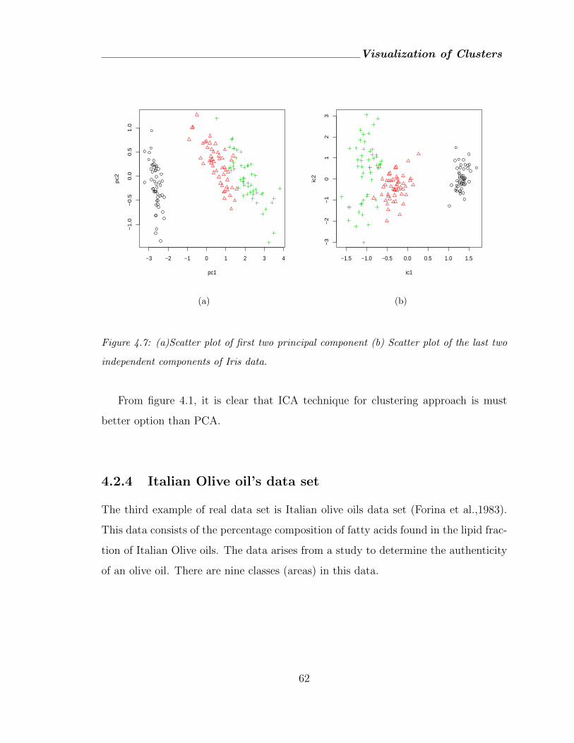
Visualization of Clusters
−3 −2 −1 0 1 2 3 4
−1
.0−
0.5
0.0
0.5
1.0
pc1
pc2
(a)
−1.5 −1.0 −0.5 0.0 0.5 1.0 1.5
−3
−2
−1
01
23
ic1
ic2
(b)
Figure 4.7: (a)Scatter plot of first two principal component (b) Scatter plot of the last two
independent components of Iris data.
From figure 4.1, it is clear that ICA technique for clustering approach is must
better option than PCA.
4.2.4 Italian Olive oil’s data set
The third example of real data set is Italian olive oils data set (Forina et al.,1983).
This data consists of the percentage composition of fatty acids found in the lipid frac-
tion of Italian Olive oils. The data arises from a study to determine the authenticity
of an olive oil. There are nine classes (areas) in this data.
62
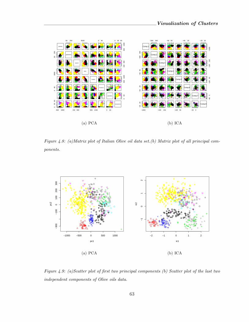
Visualization of Clusters
palmitic
50 250 6500 0 40 0 30 60
600
1600
5025
0palmitoleic
stearic
150
300
6500
oleic
linoleic
600
1400
040 linolenic
arachidic
060
600 1600
030
60
150 300 600 1400 0 60
eicosenoic
(a) PCA
Comp.1
−300 300 −50 50 −40 20 −20 20
−10
00
−30
030
0
Comp.2
Comp.3
−10
015
0
−50
50 Comp.4
Comp.5
−10
050
−40
20 Comp.6
Comp.7
−40
0
−1000
−20
20
−100 150 −100 50 −40 0
Comp.8
(b) ICA
Figure 4.8: (a)Matrix plot of Italian Olive oil data set.(b) Matrix plot of all principal com-
ponents.
−1000 −500 0 500 1000
−30
0−
100
010
020
030
0
pc1
pc2
(a) PCA
−2 −1 0 1 2
−1
01
2
ic1
ic2
(b) ICA
Figure 4.9: (a)Scatter plot of first two principal components (b) Scatter plot of the last two
independent components of Olive oils data.
63

Visualization of Clusters
4.3 Summary
The algorithm for clustering presented here is based on a fast fixed point algorithm
if ICA to find out the cluster of multivariate data sets. The algorithm demonstrate
on 3 real world datasets whose clustering result is more effective rather than PCA.
64
Chapter 5
Outlier Detection
5.1 Introduction
In statistics, an outlier is an observation that lies abnormal distance from other ob-
servation in a random sample from a population. Outliers are important because
they can change the results of our data analysis. Univariate outliers are cases that
have an unusual value for a single variable. Multivariate outliers are cases that have
an unusual combination of values for a number of variables. The value for any of the
individual variables may not be a univariate outlier, but, in combination with other
variables, is a case that occurs very rarely.
The main motivation of this chapter is find out outliers in multivariate analysis by
using ICA and PCA. Since ICA is a very promising old technique for outlier detec-
tion. Some work of outier detection using ICA have done in past decade such as time
series outlier detection [120], outlier detection on ecological data by Jackson.
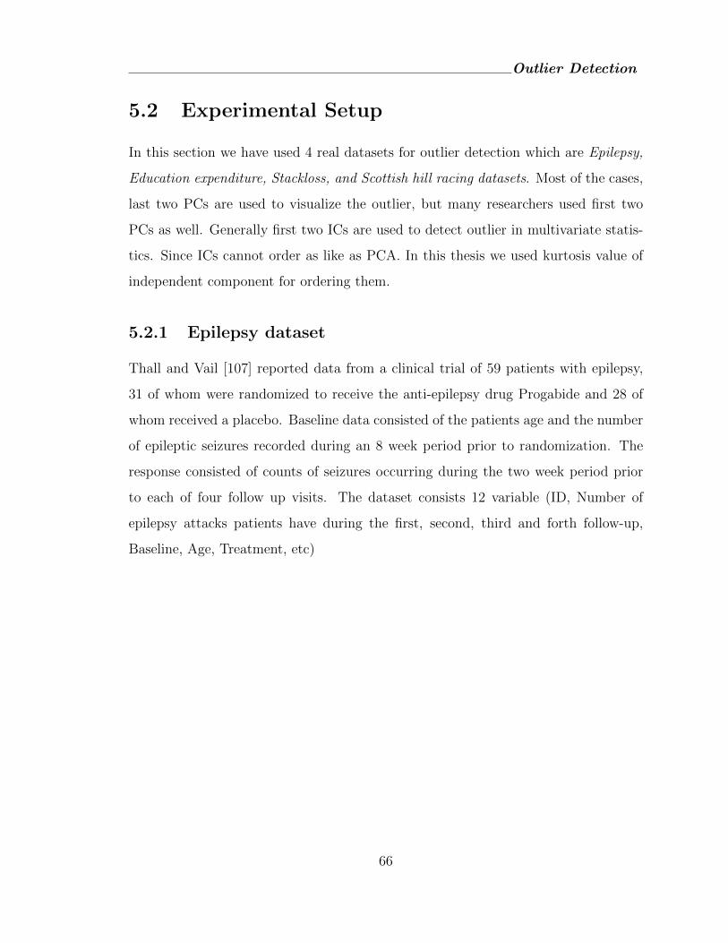
Outlier Detection
5.2 Experimental Setup
In this section we have used 4 real datasets for outlier detection which are Epilepsy,
Education expenditure, Stackloss, and Scottish hill racing datasets. Most of the cases,
last two PCs are used to visualize the outlier, but many researchers used first two
PCs as well. Generally first two ICs are used to detect outlier in multivariate statis-
tics. Since ICs cannot order as like as PCA. In this thesis we used kurtosis value of
independent component for ordering them.
5.2.1 Epilepsy dataset
Thall and Vail [107] reported data from a clinical trial of 59 patients with epilepsy,
31 of whom were randomized to receive the anti-epilepsy drug Progabide and 28 of
whom received a placebo. Baseline data consisted of the patients age and the number
of epileptic seizures recorded during an 8 week period prior to randomization. The
response consisted of counts of seizures occurring during the two week period prior
to each of four follow up visits. The dataset consists 12 variable (ID, Number of
epilepsy attacks patients have during the first, second, third and forth follow-up,
Baseline, Age, Treatment, etc)
66
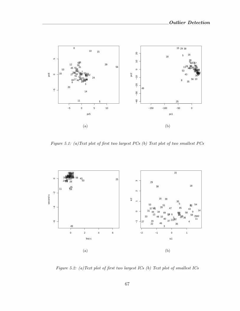
Outlier Detection
−5 0 5 10
−5
05
pc5
pc6 1 2
3
4
5
6
7
8
9
10
11
12
13
14
15
16
17 1819
20
212223
24
25 2627 28
2930
31
323334
35
36
37
38
39
4041
42
4344
45
46
47
48
495051
52
53
54
55
5657
58 59
(a)
−150 −100 −50 0
−4
0−
30
−2
0−
10
01
02
0
pc1
pc2 123
4
5
67
8
9
10
11 1213
14
15
16
17
18
19202122
2324
25
2627
28
29
30 31
3233
34
35
36
37
38
39
40
41
4243
44
45
46
47
48
49
50
51 52
53 5455
56
57
5859
(b)
Figure 5.1: (a)Text plot of first two largest PCs (b) Text plot of two smallest PCs
0 2 4 6
−6
−4
−2
0
first s
seco
nd
s
1234
5
67
8
9
10
11
121314151617
18
19 20212223
2425
26
27
28
293031
32 3334
35
3637
38
3940
4142
434445
464748
49
5051
52
53
5455
5657
5859
(a)
−2 −1 0 1
−1
01
23
ic1
ic2
12
3
4
5
67
8
9
1011
12
13
14
15
16
17
18
19
20 21
22
2324 25 26
27
28
29
30
31
3233
34
35
3637
38
39
40
41
42
4344
45
46
47
48
49 50
51 5253 54
5556
57
5859
(b)
Figure 5.2: (a)Text plot of first two largest ICs (b) Text plot of smallest ICs
67
Outlier Detection
Breslow (1996) identify observation 49 (ID no. 207) is high leverage point. First
two PCs and last two ICs idnetify 49 and 25 observation are outlier.
5.2.2 Education expenditure data
These data were used by Chatterjee, Hadi, and Price [?] as an example of het-
eroscedasticity. The data give the education expenditures for the 50 U.S. States
as projected in 1975. The data were also studied by Rousseeuw and Leroy (1987, pp.
109-112). There are three explanatory variables, X1 (number of residents per thou-
sand residing in urban areas in 1970), X2 (per capita personal income in 1973), X3
(number of residents per thousand under 18 years of age in 1974), and one response
variable Y (per capita expenditure on public education in 1975).
−1000 −500 0 500 1000
−3
00
−2
00
−1
00
01
00
20
0
pc1
pc2 1
2
3
4
5
6
78
910
11
12
1314
15
16
17
18
19
202122
23
24
2526
27
28
29
30
3132
3334
3536
37
383940
41
4243
44
45 46 47
48
49
50
(a)
−50 0 50 100 150 200
−3
0−
20
−1
00
10
20
pc1
pc2
1
2
3
4
5
6
7
8
9
10
1112
13
14 15
16
17
18
19
20
21
22
2324
25
26
2728
29
30
31
32
33
34
35
36
37
38
39
40
41
42
43
44
45
46
47
48
4950
(b)
Figure 5.3: (a)Text plot of first two principal components. (b)Text plot of last two principal
components of Education expenditure data set.
68
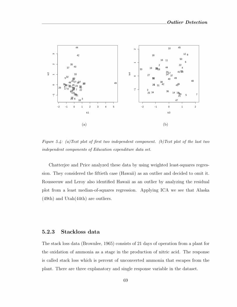
Outlier Detection
−2 −1 0 1 2 3 4 5
−1
01
23
ic1
ic2
1
2
3
4
5
6
789
101112
1314
15
16
17
18
1920
21
22
23
24
25
26
2728
29 3031
3233
34
35
36
37
38
39
40
41
42
43
44
454647
48 49
50
(a)
−2 −1 0 1 2
−1
01
2
ic3
ic4
1
2
3
4
5
6
7
8
9
10
11
12
13
14 15
16
17
18
19
20
21
22
2324
25
26
27
28
29
30
31
32
33
34
35
36
37
38
39
40
41
42 43
44
45
46
47
4849
50
(b)
Figure 5.4: (a)Text plot of first two independent component. (b)Text plot of the last two
independent components of Education expenditure data set.
Chatterjee and Price analyzed these data by using weighted least-squares regres-
sion. They considered the fiftieth case (Hawaii) as an outlier and decided to omit it.
Rousseeuw and Leroy also identified Hawaii as an outlier by analyzing the residual
plot from a least median-of-squares regression. Applying ICA we see that Alaska
(49th) and Utah(44th) are outliers.
5.2.3 Stackloss data
The stack loss data (Brownlee, 1965) consists of 21 days of operation from a plant for
the oxidation of ammonia as a stage in the production of nitric acid. The response
is called stack loss which is percent of unconverted ammonia that escapes from the
plant. There are three explanatory and single response variable in the dataset.
69
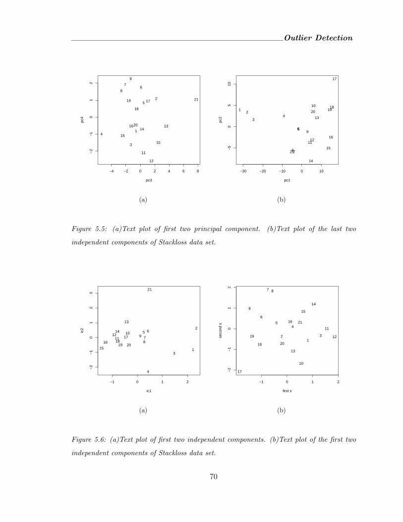
Outlier Detection
−4 −2 0 2 4 6 8
−2
−1
01
2
pc3
pc4
1
2
3
4
5
67
8
9
10
11
12
1314
15
16
17
18
19
20
21
(a)
−30 −20 −10 0 10
−5
05
10
pc1
pc2
12
34
56
78
9
10
1112
13
14
15
16
17
181920
21
(b)
Figure 5.5: (a)Text plot of first two principal component. (b)Text plot of the last two
independent components of Stackloss data set.
−1 0 1 2
−2
−1
01
23
ic1
ic2
1
2
3
4
5 6
78
910
1112
13
14
15
1617
1819 20
21
(a)
−1 0 1 2
−2
−1
01
2
first s
seco
nd s
12 3
45
6
7 8
9
10
11
12
13
14
15
16
17
18
19
20
21
(b)
Figure 5.6: (a)Text plot of first two independent components. (b)Text plot of the first two
independent components of Stackloss data set.
70
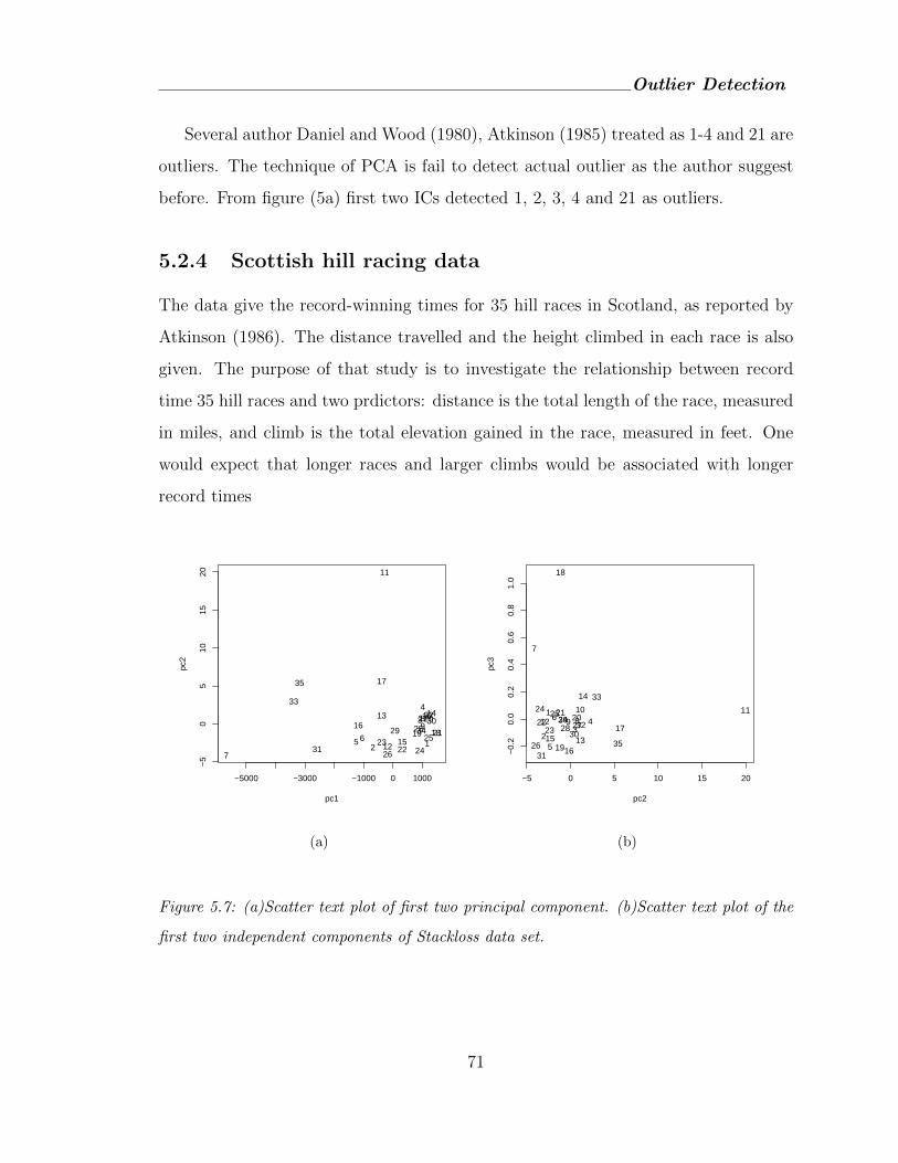
Outlier Detection
Several author Daniel and Wood (1980), Atkinson (1985) treated as 1-4 and 21 are
outliers. The technique of PCA is fail to detect actual outlier as the author suggest
before. From figure (5a) first two ICs detected 1, 2, 3, 4 and 21 as outliers.
5.2.4 Scottish hill racing data
The data give the record-winning times for 35 hill races in Scotland, as reported by
Atkinson (1986). The distance travelled and the height climbed in each race is also
given. The purpose of that study is to investigate the relationship between record
time 35 hill races and two prdictors: distance is the total length of the race, measured
in miles, and climb is the total elevation gained in the race, measured in feet. One
would expect that longer races and larger climbs would be associated with longer
record times
−5000 −3000 −1000 0 1000
−5
05
1015
20
pc1
pc2
12
3
4
5 6
7
8910
11
12
13 14
15
16
17
1819
20
21
2223
24
25
26
272829
30
31
32
33
34
35
(a)
−5 0 5 10 15 20
−0.
20.
00.
20.
40.
60.
81.
0
pc2
pc3
1
23
4
5
6
7
89
10 1112
13
14
15
16
17
18
19
2021
2223
24 25
26
272829
30
31
32
33
34
35
(b)
Figure 5.7: (a)Scatter text plot of first two principal component. (b)Scatter text plot of the
first two independent components of Stackloss data set.
71
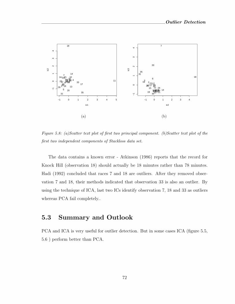
Outlier Detection
−1 0 1 2 3 4 5
−1
01
23
4
ic1
ic2
1
2
34
5
6
7
8910
1112
13
14
15
16
17
18
19
2021
2223
24 25
26
27282930
31
3233
34
35
(a)
−1 0 1 2 3 4
−1
01
23
4
ic2
ic3
1
2
3 4
56
7
89 1011
1213
1415
16
17
18
19 2021
2223
2425
26
2728
29
30
31
32
33
34
35
(b)
Figure 5.8: (a)Scatter text plot of first two principal component. (b)Scatter text plot of the
first two independent components of Stackloss data set.
The data contains a known error - Atkinson (1986) reports that the record for
Knock Hill (observation 18) should actually be 18 minutes rather than 78 minutes.
Hadi (1992) concluded that races 7 and 18 are outliers. After they removed obser-
vation 7 and 18, their methods indicated that observation 33 is also an outlier. By
using the technique of ICA, last two ICs identify observation 7, 18 and 33 as outliers
whereas PCA fail completely..
5.3 Summary and Outlook
PCA and ICA is very useful for outlier detection. But in some cases ICA (figure 5.5,
5.6 ) perform better than PCA.
72
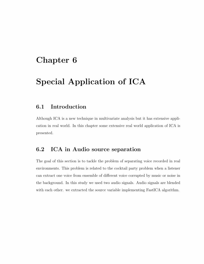
Chapter 6
Special Application of ICA
6.1 Introduction
Although ICA is a new technique in multivariate analysis but it has extensive appli-
cation in real world. In this chapter some extensive real world application of ICA is
presented.
6.2 ICA in Audio source separation
The goal of this section is to tackle the problem of separating voice recorded in real
environments. This problem is related to the cocktail party problem when a listener
can extract one voice from ensemble of different voice corrupted by music or noise in
the background. In this study we used two audio signals. Audio signals are blended
with each other. we extracted the source variable implementing FastICA algorithm.
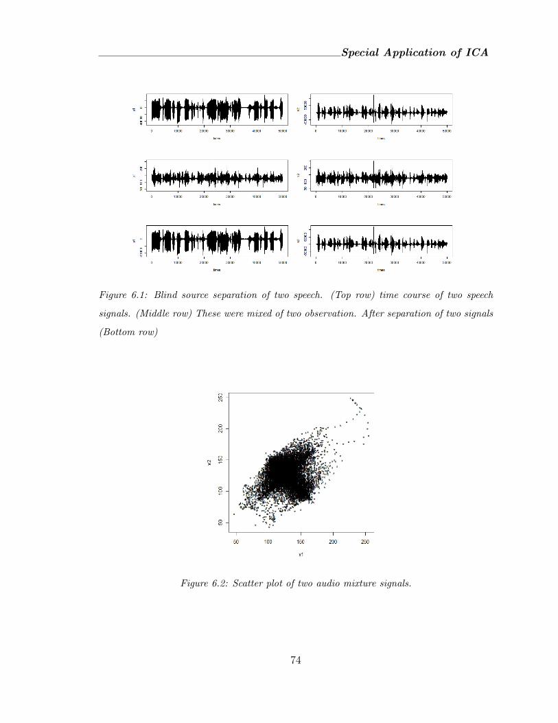
Special Application of ICA
Figure 6.1: Blind source separation of two speech. (Top row) time course of two speech
signals. (Middle row) These were mixed of two observation. After separation of two signals
(Bottom row)
Figure 6.2: Scatter plot of two audio mixture signals.
74
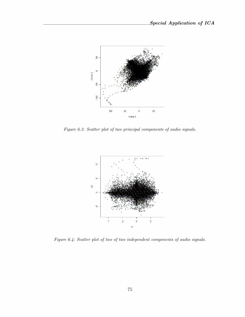
Special Application of ICA
Figure 6.3: Scatter plot of two principal components of audio signals.
Figure 6.4: Scatter plot of two of two independent components of audio signals.
75
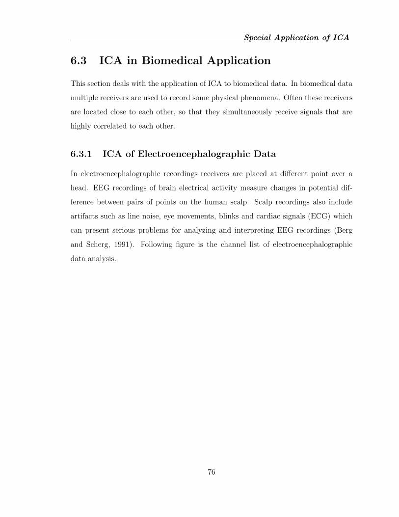
Special Application of ICA
6.3 ICA in Biomedical Application
This section deals with the application of ICA to biomedical data. In biomedical data
multiple receivers are used to record some physical phenomena. Often these receivers
are located close to each other, so that they simultaneously receive signals that are
highly correlated to each other.
6.3.1 ICA of Electroencephalographic Data
In electroencephalographic recordings receivers are placed at different point over a
head. EEG recordings of brain electrical activity measure changes in potential dif-
ference between pairs of points on the human scalp. Scalp recordings also include
artifacts such as line noise, eye movements, blinks and cardiac signals (ECG) which
can present serious problems for analyzing and interpreting EEG recordings (Berg
and Scherg, 1991). Following figure is the channel list of electroencephalographic
data analysis.
76
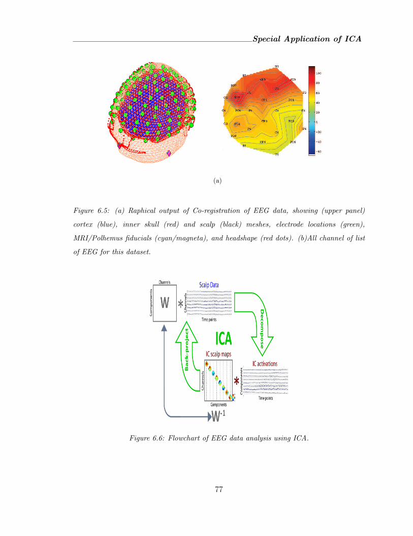
Special Application of ICA
(a)
Figure 6.5: (a) Raphical output of Co-registration of EEG data, showing (upper panel)
cortex (blue), inner skull (red) and scalp (black) meshes, electrode locations (green),
MRI/Polhemus fiducials (cyan/magneta), and headshape (red dots). (b)All channel of list
of EEG for this dataset.
Figure 6.6: Flowchart of EEG data analysis using ICA.
77
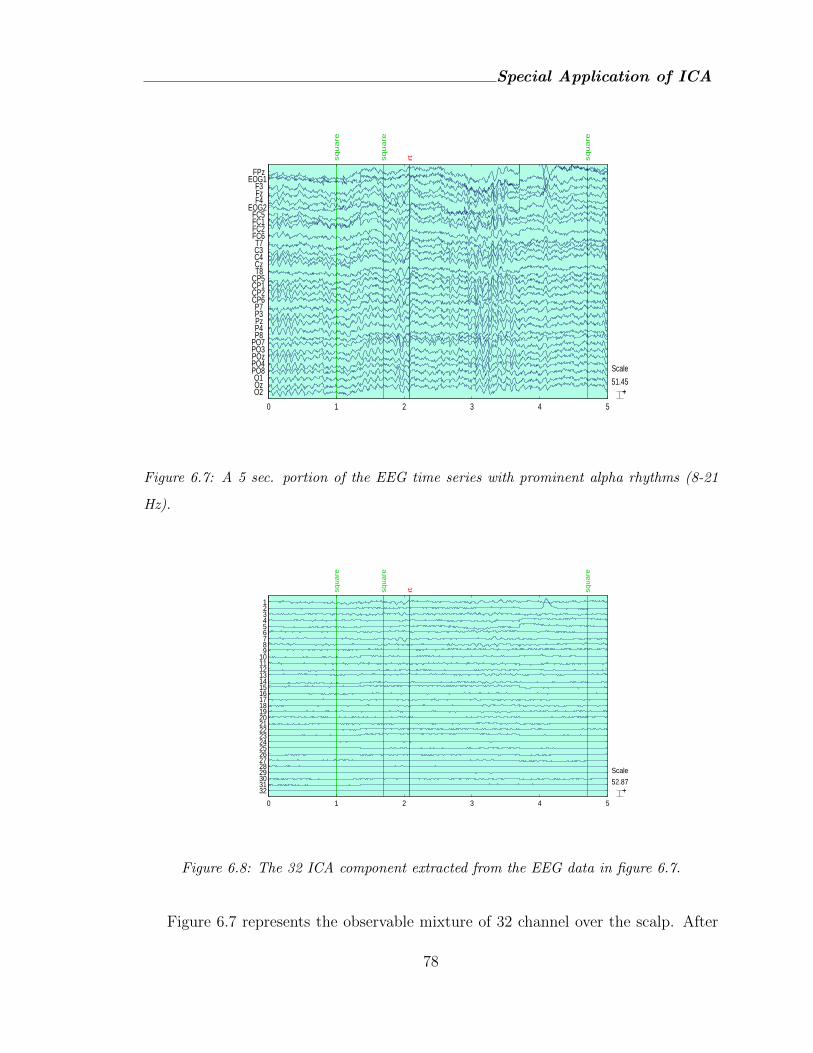
Special Application of ICA
51.45+−
Scale
sq
ua
re
sq
ua
re
rt
sq
ua
re
0 1 2 3 4 5
O2 Oz O1
PO8 PO4 POz PO3 PO7 P8 P4 Pz P3 P7
CP6 CP2 CP1 CP5 T8 Cz C4 C3 T7
FC6 FC2 FC1 FC5
EOG2F4 Fz F3
EOG1FPz
Figure 6.7: A 5 sec. portion of the EEG time series with prominent alpha rhythms (8-21
Hz).
52.87+−
Scale
sq
ua
re
sq
ua
re
rt
sq
ua
re
0 1 2 3 4 5
3231302928272625242322212019181716151413121110 9 8 7 6 5 4 3 2 1
Figure 6.8: The 32 ICA component extracted from the EEG data in figure 6.7.
Figure 6.7 represents the observable mixture of 32 channel over the scalp. After
78
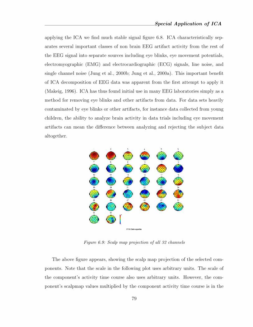
Special Application of ICA
applying the ICA we find much stable signal figure 6.8. ICA characteristically sep-
arates several important classes of non brain EEG artifact activity from the rest of
the EEG signal into separate sources including eye blinks, eye movement potentials,
electromyographic (EMG) and electrocardiographic (ECG) signals, line noise, and
single channel noise (Jung et al., 2000b; Jung et al., 2000a). This important benefit
of ICA decomposition of EEG data was apparent from the first attempt to apply it
(Makeig, 1996). ICA has thus found initial use in many EEG laboratories simply as a
method for removing eye blinks and other artifacts from data. For data sets heavily
contaminated by eye blinks or other artifacts, for instance data collected from young
children, the ability to analyze brain activity in data trials including eye movement
artifacts can mean the difference between analyzing and rejecting the subject data
altogether.
Figure 6.9: Scalp map projection of all 32 channels
The above figure appears, showing the scalp map projection of the selected com-
ponents. Note that the scale in the following plot uses arbitrary units. The scale of
the component’s activity time course also uses arbitrary units. However, the com-
ponent’s scalpmap values multiplied by the component activity time course is in the
79
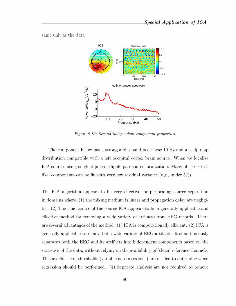
Special Application of ICA
same unit as the data
IC2
−13.3
−6.7
0
6.7
13.3
Tria
ls
Continous data
Time (ms)0 50 100 150
100
10 20 30 40 50−20
−10
0
10
Frequency (Hz)
Pow
er 1
0*lo
g 10(µ
V2 /H
z)Activity power spectrum
Figure 6.10: Second independent component properties.
The component below has a strong alpha band peak near 10 Hz and a scalp map
distribution compatible with a left occipital cortex brain source. When we localize
ICA sources using single-dipole or dipole-pair source localization. Many of the ’EEG-
like’ components can be fit with very low residual variance (e.g., under 5%).
The ICA algorithm appears to be very effective for performing source separation
in domains where, (1) the mixing medium is linear and propagation delay are negligi-
ble. (2) The time course of the source ICA appears to be a generally applicable and
effective method for removing a wide variety of artifacts from EEG records. There
are several advantages of the method: (1) ICA is computationally efficient. (2) ICA is
generally applicable to removal of a wide variety of EEG artifacts. It simultaneously
separates both the EEG and its artifacts into independent components based on the
statistics of the data, without relying on the availability of ’clean’ reference channels.
This avoids the of thresholds (variable across sessions) are needed to determine when
regression should be performed. (4) Separate analysis are not required to remove
80
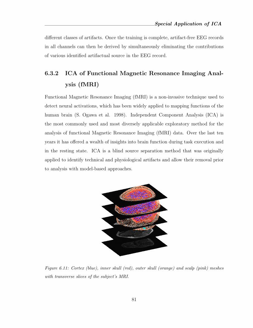
Special Application of ICA
different classes of artifacts. Once the training is complete, artifact-free EEG records
in all channels can then be derived by simultaneously eliminating the contributions
of various identified artifactual source in the EEG record.
6.3.2 ICA of Functional Magnetic Resonance Imaging Anal-
ysis (fMRI)
Functional Magnetic Resonance Imaging (fMRI) is a non-invasive technique used to
detect neural activations, which has been widely applied to mapping functions of the
human brain (S. Ogawa et al. 1998). Independent Component Analysis (ICA) is
the most commonly used and most diversely applicable exploratory method for the
analysis of functional Magnetic Resonance Imaging (fMRI) data. Over the last ten
years it has offered a wealth of insights into brain function during task execution and
in the resting state. ICA is a blind source separation method that was originally
applied to identify technical and physiological artifacts and allow their removal prior
to analysis with model-based approaches.
Figure 6.11: Cortex (blue), inner skull (red), outer skull (orange) and scalp (pink) meshes
with transverse slices of the subject’s MRI.
81

Special Application of ICA
It has matured into a method capable of offering a stand-alone assessment of acti-
vation on a sound statistical footing. Recent innovations have taken on the complex
challenges of how components should be combined over subjects to allow group in-
ferences, and how activation identified with ICA might be compared between groups
of patients and controls - for instance. Having proved its worth in the investigation
of resting state networks, ICA is being applied in other cutting edge uses of fMRI;
in multivariate pattern analysis, real-time fMRI, in utero studies and a wide variety
of paradigms and stimulus types and with challenging tasks with patients at ultra-
high field. These are testament both to ICAs flexibility and its central role in basic
neuroscience and clinical applications of fMRI. When neurons in the brain are ac-
tivated, the increase in electrical activity causes an increase in the local metabolic
rate. The increased consumption of oxygen results in fluctuations in the levels of
paramagnetic deoxyhemoglobin in the blood which is sensed using a magnetic field.
The changing level of deoxyhemoglobin measured in the brain is referred to as the
blood oxygenation level dependent (BOLD) signal. During an fMRI scan session, a
series of three-dimensional images are captured consecutively, usually two to three
seconds apart. The value of the image at each small volume unit, called a voxel, is
the BOLD signal intensity.
The patient is usually presented with a stimuli to induce neural activations. While
the types of stimuli vary, the standard experimental design is a simple on-off or boxcar
design, where the patient is repeatedly presented with a task followed by a pause.
82
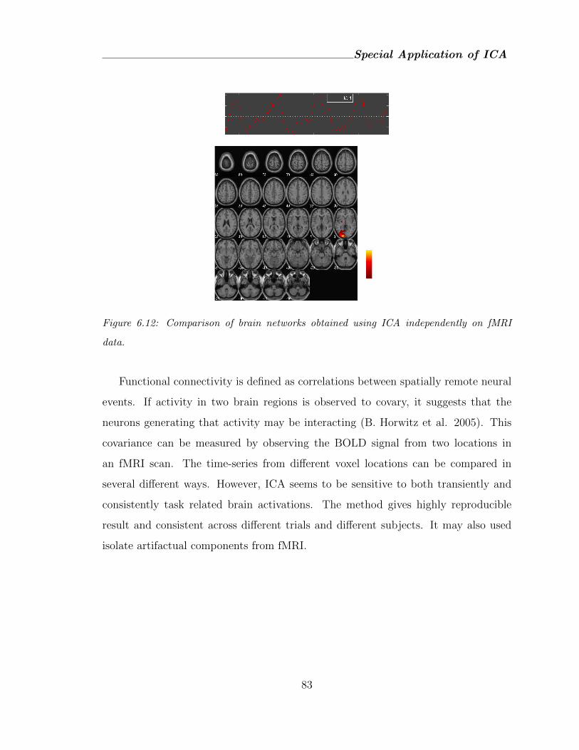
Special Application of ICA
Figure 6.12: Comparison of brain networks obtained using ICA independently on fMRI
data.
Functional connectivity is defined as correlations between spatially remote neural
events. If activity in two brain regions is observed to covary, it suggests that the
neurons generating that activity may be interacting (B. Horwitz et al. 2005). This
covariance can be measured by observing the BOLD signal from two locations in
an fMRI scan. The time-series from different voxel locations can be compared in
several different ways. However, ICA seems to be sensitive to both transiently and
consistently task related brain activations. The method gives highly reproducible
result and consistent across different trials and different subjects. It may also used
isolate artifactual components from fMRI.
83
Chapter 7
Summary, Conclusions and Future
Research
7.1 Summary
In this section we will discuss performance of all results in our study. We have used
two different technique ICA and PCA for comparisons of structure detection, clusters
analysis, and outlier detection in multivariate statistics.
In Blind Source Separation chapter, we have use three simulated datasets. First
dataset consists of 10 variables each have generated from standard uniform (sub-
gaussian) distribution while second dataset consists of 10 variables generated from
5 Laplace (super-gaussian), 3 binomial and 2 multinomial distributions and third
dataset consists of 5 variables each generate from uniform, Laplace, binomial, multi-
nomial, and normal distribution. In all the cases ICA almost detect the structure. We
have use one normal distribution for third datasets. It should be noted that more than
one gaussian variable cannot be separate by ICA. Actually in case of one gaussian
component, we can estimate the ICA model, because the single gaussian component
does not have any other gaussian components that it could be mixed with.
Summary, Conclusions and Future Research
In forth chapter we have used one simulated and three real datasets which are Aus-
tralian crabs, Fisher’s Iris and Italian olive oils data. Generally first two PC’s are
used for detecting cluster in multivariate analysis. Since ICA can not order as like
as PCA. Thus in our thesis we order IC’s according to their kurtosis. In all the four
cases ICA perform better than PCA.
In outlier detection chapter we have used Epilepsy, Stackloss, Education expendi-
ture and Scottish hill racing datasets. Generally last two PC’s are used to detect
outliers. Many researcher used first two PC’s as well. In our study we use two largest
IC’s for outlier detection.
The ICA algorithm successfully applied in many areas. In last chapter we analysis
biomedical signal processing problem such as EEG data. In last chapter of analysis
we apply ICA for extracting two mixture of audio signals.
7.1.1 Conclusions
ICA solves several instances of the BSS problem by taking into account higher-order
statistics which are ignored by PCA that relies only on second-order statistics. Since
its introduction it has become an indispensable tool for statistical data analysis and
processing of multi-channel data. In case of cluster analysis ICA always perform bet-
ter than PCA. ICA and PCA both are useful for outlier detection, but ICA sometimes
more fruitful than PCA. We recommended using ICA in place of PCA in detecting
clusters as well as outliers. Furthermore, we suggest that if subject domain supports
the assumption of independent non-gaussian source variables ICA, not PCA be used
to identify the latent structures.
85
Summary, Conclusions and Future Research
7.1.2 Future Research
The following are the areas in which we want to study
� Use Kernel technique of ICA for shape study, clustering and outlier detection.
� Separation of Nonlinear mixture.
� Data mining (sometimes called data or knowledge discovery) is the most recent
technique in multivariate analysis to extract information from a data set and
transform it into an understandable structure for further use. Text data mining
or Medical data mining using ICA wolud be future research.
86

Appendix A
Bibliography
Bibliography
Bibliography
[1] A. Cichocki, R.E. Bogner, L. Moszczynski, & K. Pope. Modified Herault-Jutten
algorithms for blind separation of sources. Digital Signal Processing, 7:80-93,
1997.
[2] A. Cichocki and R. Unbehauen. Robust neural networks with on-line learning
for blind identification & blind separation of sources. IEEE Trans. on Circuits
and Systems, 43(11):894-906, 1996.
[3] A. Cichocki, R. Unbehauen, L. Moszczynski, & E. Rummert. A new on-line
adaptive algorithm for blind separation of source signals. In Proc. Int. Sympo-
sium on Artificial Neural Networks ISANN-94, pages 406-411, Tainan, Taiwan,
1994.
[4] A. D. Back, and A. S. Weigend. A first application of independent component
analysis to extracting structure from stock returns. Int. J. on Neural Systems,
8(4):473484, 1997.
[5] A. Hyvarinen. Fast and robust fixed-point algorithms for independent compo-
nent analysis. IEEE Transactions on Neural Networks, 10(3):626-634, 1999.
[6] A. Hyvarinen. The fixed-point algorithm and maximum likelihood estimation
for independent component analysis. Neural Processing Letters, 10(1):1-5, 1999.
[7] A. Hyvarinen. Gaussian moments for noisy independent component analysis.
IEEE Signal Processing Letters, 6(6):145-147, 1999.
88
Bibliography
[8] A. Hyvarinen. Sparse code shrinkage: Denoising of nongaussian data by maxi-
mum likelihood estimation. Neural Computation, 11(7):1739-1768, 1999.
[9] A. Hyvarinen. Survey on independent component analysis. Neural Computing
Surveys, 2:94-128, 1999.
[10] A. Hyvarinen & E. Oja. A fast fixed-point algorithm for independent component
analysis. Neural Computation, 9(7):14831492, 1997.
[11] A. Hyvarinen & E. Oja, . Independent component analysis by general nonlinear
Hebbian-like learning rules. Signal Processing, 64(3):301313, 1998.
[12] A. Hyvarinen, J. Sarela, & R. Vigario. Spikes and bumps: Artefacts generated
by independent component analysis with insufficient sample size. In Proc. Int.
Workshop on Independent Component Analysis and Signal Separation (ICA99),
pages 425429, Aussois, France, 1999.
[13] A. Hyvarinen and P. Pajunen. Nonlinear independent component analysis: Ex-
istence and uniqueness results. Neural Networks, 12(3):429-439, 1999.
[14] A. Hyvarinen, P. O. Hoyer, and E. Oja. Sparse Code Shrinkage: Denoising by
Nonlinear Maximum Likelihood Estimation. Advances in Neural Information
Processing Systems, (11):473479, 1999.
[15] A. Hyvarinen, Juha Karhunen, and Erkki Oja. Independent Component Analy-
sis. J. Wiley, 2001.
[16] A. Hyvarinen. Independent component analysis in the presence of gaussian noise
by maximizing joint likelihood. Neurocomputing, 22:4967, 1998.
[17] A. J. Bell, and T. J. Sejnowski. An information-maximization approach to blind
separation and blind deconvolution. Neural Computation, 7:11291159, 1995.
89
Bibliography
[18] A. J. Bell, and T. J. Sejnowski. The independent components of natural scenes
are edge filters. Vision Research, 37:33273338.
[19] A. Koutras, E. Dermatas, & G. Kokkinakis. Blind signal separation and speech
recognition in the frequency domain. Proceedings of the IEEE International
Conference on Electronics, Circuits and Systems, Vol. 1, pp. 427-430, 1999.
[20] A. Papoulis. Probability, Random Variables, and Stochastic Processes. McGraw-
Hill, 3rd edition, 1991.
[21] B. A. Olshausen & D. J. Field. Emergence of simple-cell receptive field proper-
ties by learning a sparse code for natural images. Nature, 381:607609, 1996.
[22] B. A. Pearlmutter & L. C. Parra. Maximum likelihood blind source separation:
A context-sensitive generalization of ICA. In Advances in Neural Information
Processing Systems, volume 9, pages 613619, 1997.
[23] B. Laheld and J. F. Cardoso. Adaptive source separation with uniform perfor-
mance. In Proc. EUSIPCO, pages 183-186, Edinburgh, 1994.
[24] B. Laheld and J. F. Cardoso. Adaptive source separation with uniform perfor-
mance. In Proc. EUSIPCO, pages 183-186, Edinburgh, 1994.
[25] C. Jutten and J. Herault. Blind separation of sources, part I: An adaptive
algorithm based on neuromimetic architecture. Signal Processing, 24:1-10, 1991.
[26] C. Fyfe and R. Baddeley. Non-linear data structure extraction using simple
Hebbian networks. Biological Cybernetics, 72:533-541, 1995.
[27] D. Zhang, S. Chen, and J. Liu. Representing Image Matrices: Eigenimages
Versus Eigenvectors. Lecture Notes in Computer Science, 3497/2005:659664,
2005.
90
Bibliography
[28] D. L. Donoho, I. M. Johnstone, G. Kerkyacharian, and D. Picard. Wavelet
shrinkage: asymptopia? Journal of the Royal Statistical Society, Ser. B,
57:301337, 1995.
[29] D. Luenberger. Optimization by Vector Space Methods. Wiley, 1969.
[30] D. N. Lawley. Test of significance of the latent roots of the covariance and
correlation matrices. Biometrica, 43:128-136, 1956.
[31] D.-T. Pham, P. Garrat, and C. Jutten. Separation of a mixture of independent
sources through a maximum likelihood approach. In Proc. EUSIPCO, pages
771774, 1992.
[32] D. Nion,K. N. Mokios, N. D. Sidiropoulos & A. Potamianos. Batch and adap-
tive PARAFAC based blind separation of convolutive speech mixtures. IEEE
Transactions on Audio, Speech, and Language Processing, Vol. 18, No. 6, Au-
gust 2010, pp. 1193-1207, ISSN 1558-7916, 2010.
[33] E.Oja. A Simplified neuron model as a principal component analyzer. J. of
Mathematical Biology, 15:267-273, 1982.
[34] E.Oja and J. Karhunen. On stochastic approximation of the eigenvectors and
eigenvalues of the expectation of random matrix. J. of Math. Analysis and
Applications, 106:69-84, 1985.
[35] E. Oja, H. Ogawa, and J. Wangviwattana. Principal component analysis by
homogeneous neural networks, part I: the weighted subspace criterion. IEICE
Trans. on Information and Systems, E75-D(3):366-375, 1992.
[36] F. J. Mato-Mendez, & M. A. Sobreira-Seoane. Blind separation to improve
classification of traffic noise. Applied Acoustics, Vol. 72, No. 8 (Special Issue on
Noise Mapping), July 2011, pp. 590-598, ISSN 0003-682X, 2011.
91
Bibliography
[37] H. Sawada, S. Araki, & S. Makino. Underdetermined convolutive blind source
separation via frequency bin-wise clustering and permutation alignment. IEEE
Transactions on Audio, Speech, and Language Processing, Vol. 19, No. 3, March
2011, pp. 516-527, ISSN 1558-7916, 2011.
[38] I.T. Jolliffe. Principal Component Analysis. Springer-Verlag, 1986.
[39] J. Antoni. Blind separation of vibration components: Principles and demon-
strations. Mechanical Systems and Signal Processing, Vol. 19, No. 6, November
2005, pp. 1166-1180, ISSN 0888-3270, 2005.
[40] J.-F. Cardoso and B. Hvam Laheld. Equivariant adaptive source separation.
IEEE Trans. on Signal Processing, 44(12):3017-3030, 1996.
[41] J.-F. Cardoso and A. Souloumiac. Blind beamforming for non Gaussian signals.
IEEE Proceedings-F, 140(6):362-370, 1993.
[42] J.-F. Cardoso. Infomax and maximum likelihood for source separation. IEEE
Letters on Signal Processing, 4:112114, 1997.
[43] J.-F. Cardoso. Entropic contrasts for source separation. In S. Haykin, editor,
Adaptive Unsupervised Learning, 1999.
[44] J. H. Friedman. Exploratory projection pursuit. J. of the American Statistical
Association, 82(397):249266, 1987.
[45] J. H. Friedman & J. W. Tukey. A projection pursuit algorithm for exploratory
data analysis. IEEE Trans. of Computers, c-23(9):881890, 1974.
[46] J. Karhunen, A. Hyvrinen, R. Vigario, J. Hurri, and E. Oja. Applications of
neural blind separation to signal and image processing. In Proc. IEEE Int.
Conf. on Acoustics, Speech and Signal Processing (ICASSP’97), pages 131-134,
Munich, Germany, 1997.
92
Bibliography
[47] J. Karhunen and J. Joutsensalo. Representation and separation of signals using
nonlinear PCA type learning. Neural Networks, 7(1):113-127, 1994.
[48] J. Karhunen and J. Joutsensalo. Generalizations of principal component analy-
sis, optimization problems, and neural networks. Neural Networks, 8(4):549-562,
1995.
[49] J. Karhunen, E. Oja, L. Wang, R. Vigario, and J. Joutsensalo. A class of neural
networks for independent component analysis. IEEE Trans. on Neural Net-
works, 8(3):486-504, 1997.
[50] J. Karhunen and P. Pajunen. Blind source separation using least-squares type
adaptive algorithms. In Proc. IEEE Int. Conf. on Acoustics, Speech and Signal
Processing (ICASSP’97), pages 3048-3051, Munich, Germany, 1997.
[51] J. Karhunen, P. Pajunen, and E. Oja. The nonlinear PCA criterion in blind
source separation: Relations with other approaches. Neurocomputing, 22:5-20,
1998.
[52] J. Karhunen, E. Oja, L. Wang, R. Vigario, & J. Joutsensalo. A class of neural
networks for independent component analysis. IEEE Trans. on Neural Net-
works, 8(3):486504, 1997.
[53] J.-P. Nadal & N. Parga. Non-linear neurons in the low noise limit: a factorial
code maximizes information transfer. Network, 5:565581, 1994.
[54] J. V. Stone. Independent Component Analysis. The MIT Press, 2004.
[55] K.I. Diamantaras and S.Y. Kung. Principal Component Neural Networks: The-
ory and Applications. Wiley, 1996.
[56] K. Kiviluoto & E. Oja. Independent component analysis for parallel financial
time series. In Proc. Int. Conf. on Neural Information Processing (ICONIP98),
volume 2, pages 895898, Tokyo, Japan, 1998.
93
Bibliography
[57] L. De Lathauwer, B. De Moor, and J. Vandewalle. A technique for higher-order-
only blind source separation. In Proc. ICONIP, Hong Kong, 1996.
[58] L. Molgedey and H. G. Schuster. Separation of a mixture of independent signals
using time delayed correlations. Phys. Rev. Lett., 72:3634-3636, 1994.
[59] M.C. Jones and R. Sibson. What is projection pursuit? J. of the Royal Statis-
tical Society, ser. A, 150:1-36, 1987.
[60] M. Kendall. Multivariate Analysis. Charles Griffin& Co., 1975.
[61] M. Kendall and A. Stuart. The Advanced Theory of Statistics. Charles Griffin
& Company, 1958.
[62] M. Lewicki and B. Olshausen. Inferring sparse, overcomplete image codes using
an efficient coding framework. In Advances in Neural Information Processing
10 (Proc. NIPS*97), pages 815-821. MIT Press, 1998.
[63] M. Lewicki and T. J. Sejnowski. Learing overcomplete representations.
[64] M. McKeown, S. Makeig, S. Brown, T.-P. Jung, S. Kindermann, A.J. Bell, V.
Iragui, and T. Sejnowski. Blind separation of functional magnetic resonance
imaging (fMRI) data. Human Brain Mapping, 6(5-6):368-372, 1998.
[65] M. Knaak & D. Filberi Acoustical semi-blind source separation for machine
monitoring. Proceedings of the International Conference on Independent Com-
ponent Analysis and Blind Source Separation, pp. 361-366, December 2001, San
Diego, USA.
[66] M. Knaak, M. Kunter, & D. Filberi. Blind Source Separation for Acoustical Ma-
chine Diagnosis. Proceedings of the International Conference on Digital Signal
Processing, pp. 159-162, July 2002, Santorini, Greece.
94
Bibliography
[67] M. Knaak, S. Araki & S. Makino. Geometrically constrained ICA for robust
separation of sound mixtures. Proceedings of the International Conference on
Independent Component Analysis and Blind Source Separation, pp. 951956,
April 2003, Nara, Japan, 2003.
[68] M. McKeown, S. Makeig, G. Brown, T.-P. Jung, S. Kindermann, A. J. Bell, and
T. J. sejnowski. Analysis of fmri by blind separation into independent spatial
component. Human Brain Maping, 6:1-31, 1998.
[69] M.S. Reza, M. Nasser, and M. Shahjaman. An Improved Version of Kurto-
sis Measure and Their Application in ICA. International Journal of Wireless
Communication and Information Systems (IJWCIS), Vol 1, No 1., 2011.
[70] M. Jones & R. Sibson. What is projection pursuit? J. of the Royal Statistical
Society, Ser. A, 150:136.20, 1987.
[71] N. Delfosse, and P. Loubaton. Adaptive blind separation of independent sources:
a deflation approach. Signal Processing, 45:59-83, 1995.
[72] P. Huber. Projection pursuit. The Annals of Statistics, 13(2):435475, 1985.
[73] P. Comon. Independent Component Analysis-a new concept? Signal Processing,
36:287-314, 1994
[74] R. Gonzales & P. Wintz. Digital Image Processing. Addison-Wesley, 1987.
[75] R. Vigario, V. Jousmaki, M. Hamalainen, R. Hari, and E. Oja. Independent
component analysis for identification of artifacts in magnetoencephalographic
recordings. In Advances in Neural Information Processing Systems, volume 10,
pages 229235. MIT Press, 1998.
[76] R. Vigario. Extraction of ocular artifacts from EEG using independent compo-
nent analysis. Electroenceph. Clin. Neurophysiol, 103(3):395404, 1997.
95
Bibliography
[77] R. H. Lambert. Multichannel Blind Deconvolution: FIR Matrix Algebra and
Separation of Multipath Mixtures. PhD thesis, Univ. of Southern California,
1996.
[78] S. Amari, A.Cichocki, and H.H.Yang. A new learning algorithm for blind source
separation. In Advances in Neural Information Processing 8, pages 757-763.
MIT Press, Cambridge, MA, 1996.
[79] S.-I. Amari. Neural learning in structured parameter spaces natural riemannian
gradient. In Advances in Neural Information Processing 9, pages 127-133. MIT
Press, Cambridge, MA, 1997.
[80] S.-I. Amari and A. Cichocki. Adaptive blind signal processing neural network
approaches. Proceedings of the IEEE, 9, 1998.
[81] S. Makeig, A.J. Bell, T.-P. Jung, and T.-J. Sejnowski. Independent component
analysis of electroencephalographic data. In Advances in Neural Information
PRocessing Systems 8, pages 145-151. MIT Press, 1996.
[82] S. G. Mallat. A theory for multiresolution signal decomposition: The wavelet
representation. IEEE Trans. on PAMI, 11:674-693, 1989.
[83] T. Kohonen. Self-Organizing Maps. Springer-Verlag, Berlin, Heidelberg, New
York, 1995.
[84] T. M. Cover and J. A. Thomas. Elements of Information Theory. John Wiley
& Sons, 1991.
[85] T-W. Lee, B.U. Koehler, and R. Orglmeister. Blind source separation of con-
volved and delayed sources. In Information Processing Systems 9, pages 758-764,
1997a.
[86] T-W. Lee, B.U. Koehler, and R. Orglmeister. Blind source separation of real-
world signals. In Proc. ICNN, pages 2129-2135-415, 1997b.
96
Bibliography
[87] T-W. Lee, B.U. Koehler, and R. Orglmeister. Blind source separation of nonlin-
ear mixing models. In Neural networks for Signal Processing VII, pages 406-415,
1997c.
[88] T.-W. Lee, M. Girolami, and T. J. Sejnowski. Independent component analysis
using an extended infomax algorithm for mixed sub-gaussian and super-gaussian
sources. Neural Computation, pages 609-633, 1998.
[89] T.-W. Lee, M. Girolami, A.J. Bell, and T.J. Sejnowski. A unifying information-
theoretic framework for independent component analysis. International Journal
on Mathematical and Computer Models, 1999.
[90] U. Lindgren, T. Wigren, and H. Broman. On local convergence of a class of
blind separation algorithms. IEEE Trans. on Signal Processing, 43:3054-3058,
1995.
[91] Z. Malouche and O. Macchi. Extended anti-Hebbian adaptation for unsuper-
vised source extraction. In Proc. ICASSP’96, pages 1664-1667, Atlanta, Geor-
gia, 1996.
[92] J.-F. Cardoso Eigne-structure of the forth-order cumulant tensor with the ap-
plication to the blind source separation problem. In Proc. ICASSP’90 pages
2655-2658, Alabuquerque, NM, USA, 1990.
[93] J.-F. Cardoso Super symmetric decomposition of the forth-order cumulant ten-
sor, blind identification of more source than sensors. In Proc. ICASSP’91 pages
3109-3112, 1991.
[94] J.-F. Cardoso Source separation using higher order moments. In Proc.
ICASSP’89 pages 2109-2112, 1989.
[95] R. Linsker. Local synaptic learning rules suffice to maximize mutual information
in a linear network. Neural Computation, 4:691-702.
97
Bibliography
[96] M. Gaeta and Lacoume. Source separation without prior knowledge the maxi-
mum likelihood solution. proc. EUSIPO, pages 621-624.
[97] J. Atick Cloud information theory provide an ecological theory of censor pro-
cessing? Network 3:213-251.
[98] M. Girolami and C. Fyfe Extraction of independent signal source using a de-
flanary exploratory projection pursuit network with lateral inhibition. IEEE
Proceeding of Vision, Image and Signal Processing Journal, 14(5): 299-306,
1997b.
[99] M. Scholz, S. Gatzek, A. Sterling, O. Fiehn and J. Selbig. Metabolite fingerprint-
ing: detecting biological features by independent component analysis. Bioinfor-
matics 20, 24472454, 2004.
[100] S. Hochreiter and J. Schmidhuber. Feature extraction through LOCOCODE.
Neural Computation 11(3): 679-714, 1998.
[101] T.PJung, C.Humphries, T.W.Lee, S.Makeig, M.McKeown, V.Iragui,
T.Sejnowski. Extended ICA Removes Artifacts from Electroencephalographic
Recordings. submitted to Advances in Neural Information Processing Sys-
tems,May 1997.
[102] K. I. Diamantaras and S. Y. Kung. Principal Component Neural Networks:
Theory and Applications. Wiley, 1996.
[103] E. Oja, H. Ogawa, and J. Wangviwattana. Principal component analysis by
homogeneous neural networks, part I: the weighted subspace criterion. IEICE
Trans. on Informations and Systems, E75-D(3):366-375, 1992.
[104] M. C. Jones and R. Sibson What is projection pursuit? J. of Royal Statistical
Society, ser. A, 150:1-36, 1987.
98
Bibliography
[105] D. Cook, A. Buja, and J. Cabrera. Projection pursuit indexes based on or-
thonormal function expansions. J. of Computational and Graphical Statistics,
2(3):225-250, 1993.
[106] J. Sun. Some practical aspects of exploratory projection pursuit. SIAM J. of
Sci. Comput., 14:68-80, 1993.
[107] P.F. Thall, and S.C. Vail Some covariance models for longitudinal count data
with overdispersion. Biometrics 46, 657671,1990.
[108] D. Yellin and E. Weinstein. Multichannel signal separation: Methods and anal-
ysis. IEEE Transactions on Signal Processing,44(1):106-118, 1994.
[109] H.-L. Nguyen-Thi, and C. Jutten. Blind source separation for convolutive mix-
tures. Signal Processing, 45(2), 1995.
[110] K. Torkkola Blind separation of convolved source based on information max-
imization. In IEEE Workshop on neural networks for signal processing, pages
423-432, Kyoto, Japan, 1994.
[111] R. Lambert, and C. Nikias. Polynomial matrix whitening and application to
the multichannel blind deconvolution problem. In IEEE Conference on Military
Communications, pages 21-24, San Diego, CA, 1995a.
[112] M. Hermann, H. Yang. Prospective limitation of self organizing maps In
ICONIP’96, 1996.
[113] J. Lin, D. Grier, and J. Cowan. Feature extraction approach to blind source
separation. IEEE Workshop on Neural Networks for Signal Processing.
[114] G. Burel. A non-linear neural algorithm. Neural networks, 5:937-947.
[115] S. Chatterjee, A. Hadi and B. Price. Regression Analysis by example Wiley,
New York, 2000.
99
Bibliography
[116] M. Saimul, M. Sahidul, and M. Nasser. PCA vs ICA in Visualization of Clusters.
International Conference on Statistical Data Mining for Bioinformatics, Health,
Agriculture and Environment,pp. 169-176, 21-24 Dec., 2012.
[117] M. Scholz, S. Gatzek, A. Sterling, O. Fiehn, and J. Selbig. Metabolic Finger-
printing: Detecting biological feature by independent component analysis Bioin-
formatics 20,2447-2454,2004.
[118] J. B. Bugrien and John T. Kent Independent Component Analysis: An ap-
proach to clustering, 2009. In Proceedings of the 2009 International Confer-
ence on Modeling, Simulation & Visualization Methods, MSV 2009, Las Vegas
Nevada, USA, July 13-16, 2009.
[119] I. R. Keck, S. Nassabay, C. G. Puntonet, E. W. Lang. A New Approach to Clus-
tering and Object Detection with Independent Component Analysis. Artificial
Intelligence and Knowledge Engineering Applications: A Bioinspired Approach
Lecture Notes in Computer Science, Volume 3562, 2005, pp 558-566, 2005.
[120] R. Baragona and F. Battaglia Outliers detection in multivariate time series by
independent component analysis. Neural Comput., 19(7):1962-84; Jul, 2007.
[121] A. Ben-Hur and I. Guyon. Detecting stable clusters using principal component
analysis. In Functional Genomics: Methods and Protocols. M.J. Brownstein
and A. Kohodursky (eds.) Humana press, pp. 159-182, 2003.
[122] K. Yeung, and W. Ruzzo. An empirical study of principal component analysis
for clustering gene expression data. Bioinformatics,17, 763774, 2001.
100