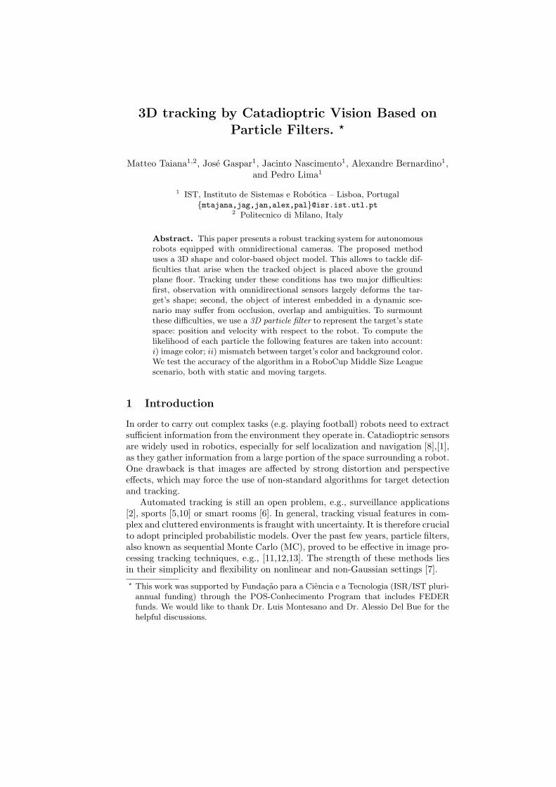
3D tracking by Catadioptric Vision Based onParticle Filters. ?

Matteo Taiana1,2, Jose Gaspar1, Jacinto Nascimento1, Alexandre Bernardino1,and Pedro Lima1

1 IST, Instituto de Sistemas e Robotica – Lisboa, Portugal{mtajana,jag,jan,alex,pal}@isr.ist.utl.pt

2 Politecnico di Milano, Italy

Abstract. This paper presents a robust tracking system for autonomousrobots equipped with omnidirectional cameras. The proposed methoduses a 3D shape and color-based object model. This allows to tackle dif-ficulties that arise when the tracked object is placed above the groundplane floor. Tracking under these conditions has two major difficulties:first, observation with omnidirectional sensors largely deforms the tar-get’s shape; second, the object of interest embedded in a dynamic sce-nario may suffer from occlusion, overlap and ambiguities. To surmountthese difficulties, we use a 3D particle filter to represent the target’s statespace: position and velocity with respect to the robot. To compute thelikelihood of each particle the following features are taken into account:i) image color; ii) mismatch between target’s color and background color.We test the accuracy of the algorithm in a RoboCup Middle Size Leaguescenario, both with static and moving targets.

1 Introduction

In order to carry out complex tasks (e.g. playing football) robots need to extractsufficient information from the environment they operate in. Catadioptric sensorsare widely used in robotics, especially for self localization and navigation [8],[1],as they gather information from a large portion of the space surrounding a robot.One drawback is that images are affected by strong distortion and perspectiveeffects, which may force the use of non-standard algorithms for target detectionand tracking.

Automated tracking is still an open problem, e.g., surveillance applications[2], sports [5,10] or smart rooms [6]. In general, tracking visual features in com-plex and cluttered environments is fraught with uncertainty. It is therefore crucialto adopt principled probabilistic models. Over the past few years, particle filters,also known as sequential Monte Carlo (MC), proved to be effective in image pro-cessing tracking techniques, e.g., [11,12,13]. The strength of these methods liesin their simplicity and flexibility on nonlinear and non-Gaussian settings [7].? This work was supported by Fundacao para a Ciencia e a Tecnologia (ISR/IST pluri-

annual funding) through the POS-Conhecimento Program that includes FEDERfunds. We would like to thank Dr. Luis Montesano and Dr. Alessio Del Bue for thehelpful discussions.

We use a 3D particle-filter [9,11] tracker in which the hypotheses are 3Dpositions and velocities of the object, and whose likelihood is a function of objectcolor and shape. From one image frame to the next, the hypotheses are movedaccording to an appropriate motion model. Then, for each particle, a likelihoodis computed, in order to estimate the object state. To calculate the likelihood ofa particle we first project the contour of the object it represents on the imageplane (as a function of the object 3D shape, position and orientation) using anapproximated model for the catadioptric system, the Unified Projection Model[15]. The likelihood is then calculated as a function of three color histograms:one represents the object color model and is computed in a training phase withseveral examples taken from distinct locations and illumination conditions; theother two histograms represent the inner and outer boundaries of the projectedcontour, and are computed at every frame for all particles. The idea is to assigna high likelihood to the contours for which the inner pixels have a color similarto the object, and are sufficiently distinct from outside ones.

A work closely related to this is described in [14], although in that case thetracking of RoboCup Middle Size League (MSL) balls is accomplished on theimage plane. Tracking the 3D trajectory of a ball has become relevant in theRoboCup MSL scenario, as robots are now provided with the ability to kick theball off the ground. Tracking the position of an object in 3D space instead ofon the image plane has two main advantages: (i) the motion model used by thetracker can be the actual motion model of the object, while in image trackingthe motion model should describe movements of the projection of the object onthe image plane and, because of the aforementioned distortion, a good modelcan be difficult to formulate and use; (ii) with 3D tracking the actual position ofthe tracked object is directly available, while a further non-trivial step is neededfor a system based on an image tracker to provide it.

The paper is organized as follows. In Section 2 we describe the catadioptricsensor and the used projection model. The particle filter is described in Section3, and customized to our particular problem in 4. The experimental results areshown in Section 5 and, finally, Section 6 concludes the paper and presents ideasfor future work.

2 Catadioptric Imaging System

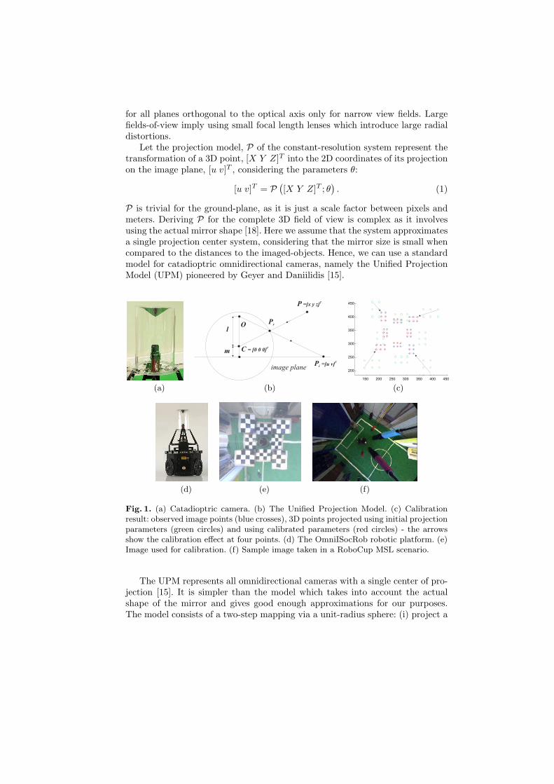
In this section we describe the imaging system, its projection model and theused calibration method. Our catadioptric vision system, see Fig.1a, combinesa camera looking upright to a convex mirror, having omnidirectional view inthe azimuth direction [16]. The system is designed to have a wide-angle anda constant-resolution view of the ground plane [17,18]. The system has theconstant-resolution property at one reference plane, the ground plane, and hasonly approximately constant-resolution at planes parallel to the reference one.As compared to perspective cameras, the constant-resolution design is a goodcompromise between approximating ubiquitous constant-resolution and enlarg-ing the field of view. Note that perspective cameras can have constant-resolution

for all planes orthogonal to the optical axis only for narrow view fields. Largefields-of-view imply using small focal length lenses which introduce large radialdistortions.

Let the projection model, P of the constant-resolution system represent thetransformation of a 3D point, [X Y Z]T into the 2D coordinates of its projectionon the image plane, [u v]T , considering the parameters θ:

[u v]T = P ([X Y Z]T ; θ

). (1)

P is trivial for the ground-plane, as it is just a scale factor between pixels andmeters. Deriving P for the complete 3D field of view is complex as it involvesusing the actual mirror shape [18]. Here we assume that the system approximatesa single projection center system, considering that the mirror size is small whencompared to the distances to the imaged-objects. Hence, we can use a standardmodel for catadioptric omnidirectional cameras, namely the Unified ProjectionModel (UPM) pioneered by Geyer and Daniilidis [15].

(a) (b) (c)

(d) (e) (f)

Fig. 1. (a) Catadioptric camera. (b) The Unified Projection Model. (c) Calibrationresult: observed image points (blue crosses), 3D points projected using initial projectionparameters (green circles) and using calibrated parameters (red circles) - the arrowsshow the calibration effect at four points. (d) The OmniISocRob robotic platform. (e)Image used for calibration. (f) Sample image taken in a RoboCup MSL scenario.

The UPM represents all omnidirectional cameras with a single center of pro-jection [15]. It is simpler than the model which takes into account the actualshape of the mirror and gives good enough approximations for our purposes.The model consists of a two-step mapping via a unit-radius sphere: (i) project a

3D world point, P = [x y z]T to a point Ps on the sphere surface, such that theprojection is normal to the sphere surface; (ii) project to a point on the imageplane, Pi = [u v]T from a point, O on the vertical axis of the sphere, throughthe point Ps. This mapping is graphically illustrated in Fig.1b. The mapping ismathematically defined by:

[uv

]=

l + m

l√

x2 + y2 + z2 − z

[su 00 sv

] [xy

]+

[u0

v0

](2)

where (l, m) parameters describe the type of camera, (su, sv, u0, v0) representpixel scaling and offsetting in the image plane, and [x y z]T is a 3D point in thecamera coordinate system, whose relationship to world coordinates is given bythe 3D rigid transformation, [x y z]T = R[X Y Z]T + [x0 y0 z0]T .

To calibrate the model we use a set of known non-coplanar 3D points [Xi Yi Zi]T

and measure their images [ui vi]T . Then, we minimize the mean squared errorbetween the measurements and the projection with the parametric model P:

θ∗ = argθ min∑

i

∥∥[ui vi]T −P([Xi Yi Zi]T ; θ

)∥∥2(3)

where θ contains the 3D rigid transformation from world to camera coordinates,pixels scaling and offsetting, and the camera type parameters (l, m). We set thecalibration patterns coordinate system in accordance with the robot frame byaligning the patterns with the center of the robot, see Fig.1e.

3 3D Tracking with Particle Filters

In this section we introduce the methods employed for 3D target tracking withparticle filters. We are interested in computing, at each time t ∈ N, an estimateof the 3D pose of a target. We represent this information as a “state-vector”defined by a random variable xt ∈ Rnx whose distribution in unknown (non-Gaussian); nx is the dimension of the state vector. In the present work we aremostly interested in tracking balls and cylindrical robots, whose orientation isnot important for tracking. However, the formulation is general and can easilyincorporate other dimensions in the state-vector, e.g. target orientation and spin.

Let xt = [x, y, z, x, y, z]T , with (x,y,z), (x,y,z) the 3D cartesian positionand linear velocities in a robot centered coordinate system. The state sequence{xt; t ∈ N} represents the state evolution along time and is assumed to be anunobserved Markov process with some initial distribution p(x0) and a transitiondistribution p(xt | xt−1).

The observations taken from the images are represented by the random vari-able {yt; t ∈ N}, yt ∈ Rny , and are assumed to be conditionally independentgiven the process {xt; t ∈ N} with marginal distribution p(yt | xt), where ny isthe dimension of the observation vector.

In a statistical setting, the problem is posed as the estimation of the posterioridistribution of the state given all observations p(xt | y1:t). Under the Markov

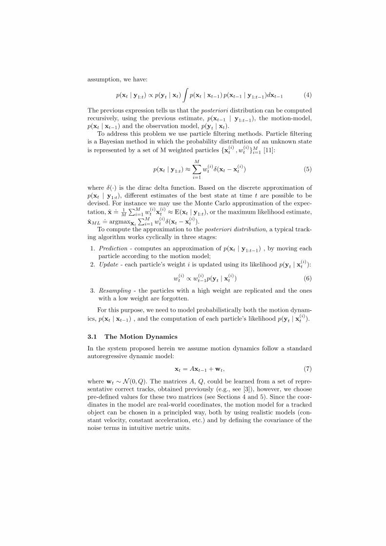
assumption, we have:

p(xt | y1:t) ∝ p(yt | xt)∫

p(xt | xt−1) p(xt−1 | y1:t−1)dxt−1 (4)

The previous expression tells us that the posteriori distribution can be computedrecursively, using the previous estimate, p(xt−1 | y1:t−1), the motion-model,p(xt | xt−1) and the observation model, p(yt | xt).

To address this problem we use particle filtering methods. Particle filteringis a Bayesian method in which the probability distribution of an unknown stateis represented by a set of M weighted particles {x(i)

t , w(i)t }M

i=1 [11]:

p(xt | y1:t) ≈M∑

i=1

w(i)t δ(xt − x(i)

t ) (5)

where δ(·) is the dirac delta function. Based on the discrete approximation ofp(xt | y1:t), different estimates of the best state at time t are possible to bedevised. For instance we may use the Monte Carlo approximation of the expec-tation, x .= 1

M

∑Mi=1 w

(i)t x(i)

t ≈ E(xt | y1:t), or the maximum likelihood estimate,xML

.= argmaxxt

∑Mi=1 w

(i)t δ(xt − x(i)

t ).To compute the approximation to the posteriori distribution, a typical track-

ing algorithm works cyclically in three stages:

1. Prediction - computes an approximation of p(xt | y1:t−1) , by moving eachparticle according to the motion model;

2. Update - each particle’s weight i is updated using its likelihood p(yt | x(i)t ):

w(i)t ∝ w

(i)t−1p(yt | x(i)

t ) (6)

3. Resampling - the particles with a high weight are replicated and the oneswith a low weight are forgotten.

For this purpose, we need to model probabilistically both the motion dynam-ics, p(xt | xt−1) , and the computation of each particle’s likelihood p(yt | x(i)

t ).

3.1 The Motion Dynamics

In the system proposed herein we assume motion dynamics follow a standardautoregressive dynamic model:

xt = Axt−1 + wt, (7)

where wt ∼ N (0, Q). The matrices A, Q, could be learned from a set of repre-sentative correct tracks, obtained previously (e.g., see [3]), however, we choosepre-defined values for these two matrices (see Sections 4 and 5). Since the coor-dinates in the model are real-world coordinates, the motion model for a trackedobject can be chosen in a principled way, both by using realistic models (con-stant velocity, constant acceleration, etc.) and by defining the covariance of thenoise terms in intuitive metric units.

3.2 Observation model

Each state vector xt represents a target pose hypothesis. According to targetshape, we compute sets of N points in the 3D inner and outer object boundaries:{Dn

in} and {Dnout}, n = 1 · · ·N . These points must be carefully chosen so that

their projection in the image plane, using the projection model of section 2, fallsin the 2D inside and outside boundaries of the image contour. Then, we obtainsets of 2D points {dn

in} and {dnout}. Each point d in the image is represented

by its color vector in the HSI representation. For the inner and outer boundarypoint sets, we will compute HSI histograms, with B = Bh Bs Bi bins.

Let us denote bt(d) ∈ {1, . . . , B} the bin index associated with the colorvector at pixel location d and frame t. Then the histogram of the color distri-bution of a generic set of points can be computed by a kernel density estimateH .= {h(b)}b=1,...,B of the color distribution at frame t, where each histogrambin is given as in [4]

h(b) = β∑

n

δ[bt(dn)− b] (8)

where δ is the Kronecker delta function, β is a normalization constant whichensures h to be a probability distribution

∑Bb=1 h(b) = 1.

To compute the similarity between two histograms we apply the Bhattacharyyasimilarity metric, as in [13]:

S (H1,H2

)=

B∑

b=1

√h1(b) · h2(b) (9)

The likelihood of the hypothesis is computed, as a function of two similarities:the similarity between the object color model and the color measured in theinside image boundary, and the similarity between the colors measured in theimage inside and outside the contour.

Defining a reference color model for the object as Hmodel, Hinner as the innerboundary points color histogram, and Houter the outer boundary histogram,we will measure their similarity, using (9). The data likelihood should favorcandidate color histograms which are close to the reference histogram and aresufficiently distinct from the background. Therefore we use:

p(yt | x(i)t ) = pos

[S(Hmodel,Hinner)− kS(Houter,Hinner)

](10)

where the pos(·) function truncates to zero the negative values. This allow usto cope with the detection of the object (first term) and the detection from thebackground (second term).

4 Implementation of the RoboCup MSL 3D Tracker

The present approach is tested for a ball and robot tracking task, in a typicalRoboCup MSL environment. The color model for each object was built collecting

a set of images in which the object is present, and calculating the HSI colorhistogram on the (hand labeled) pixels belonging to the specific object. Fortarget dynamics, we have chosen a constant velocity model, in which the motionequations correspond to a uniform acceleration during one sample time:

xt = Axt−1 + Bat−1, A =[I (∆t)I0 I

], B =

[(∆t2

2 )I(∆t)I

](11)

where I is the 3 × 3 identity matrix and at is a 3 × 1 white zero mean randomvector corresponding to an acceleration disturbance. We have set ∆t = 1 forall the experiments, whereas the covariance matrix of the random accelerationvector was fixed at:

cov(at) = σ2I, σ = 90mm/frame2 (12)

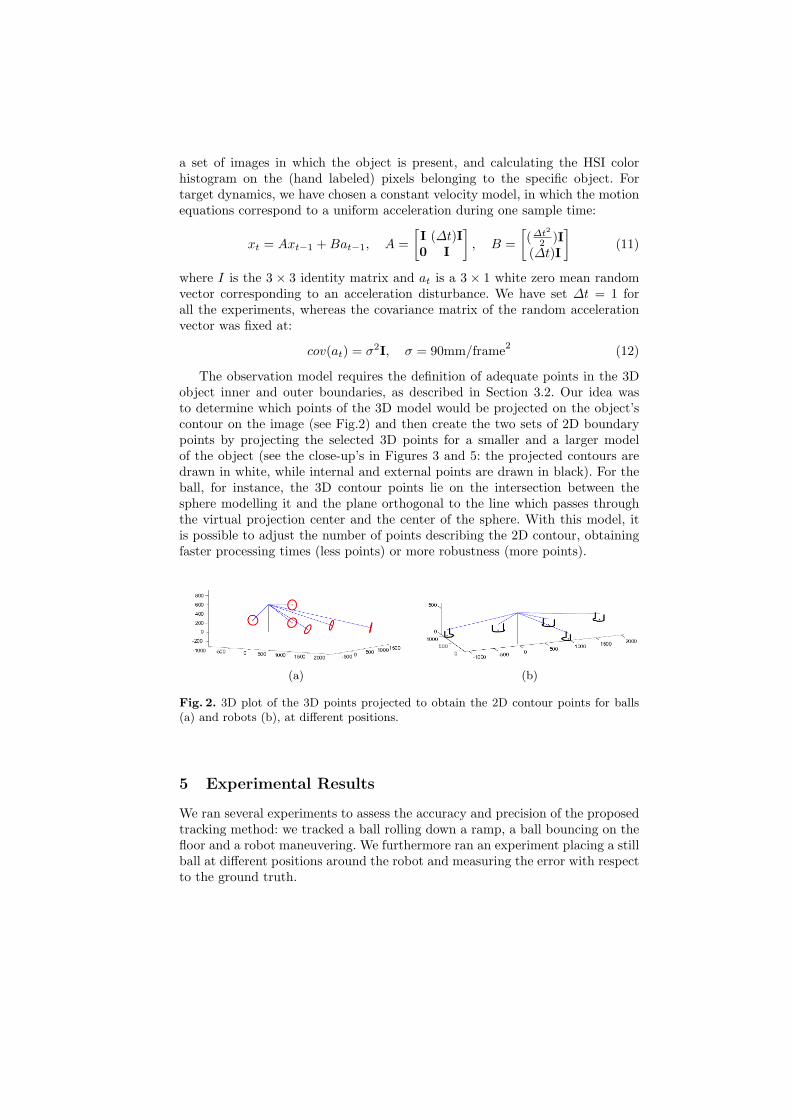
The observation model requires the definition of adequate points in the 3Dobject inner and outer boundaries, as described in Section 3.2. Our idea wasto determine which points of the 3D model would be projected on the object’scontour on the image (see Fig.2) and then create the two sets of 2D boundarypoints by projecting the selected 3D points for a smaller and a larger modelof the object (see the close-up’s in Figures 3 and 5: the projected contours aredrawn in white, while internal and external points are drawn in black). For theball, for instance, the 3D contour points lie on the intersection between thesphere modelling it and the plane orthogonal to the line which passes throughthe virtual projection center and the center of the sphere. With this model, itis possible to adjust the number of points describing the 2D contour, obtainingfaster processing times (less points) or more robustness (more points).

(a) (b)

Fig. 2. 3D plot of the 3D points projected to obtain the 2D contour points for balls(a) and robots (b), at different positions.

5 Experimental Results

We ran several experiments to assess the accuracy and precision of the proposedtracking method: we tracked a ball rolling down a ramp, a ball bouncing on thefloor and a robot maneuvering. We furthermore ran an experiment placing a stillball at different positions around the robot and measuring the error with respectto the ground truth.

5.1 Ball tracking – ramp and bouncing

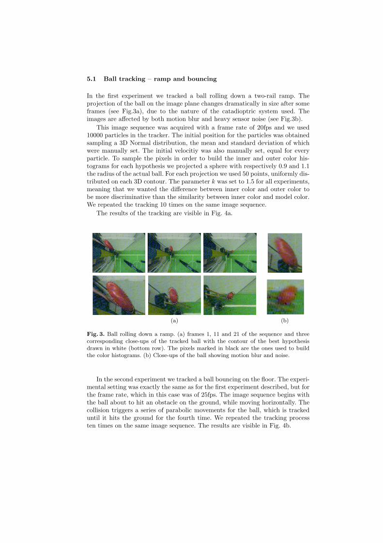
In the first experiment we tracked a ball rolling down a two-rail ramp. Theprojection of the ball on the image plane changes dramatically in size after someframes (see Fig.3a), due to the nature of the catadioptric system used. Theimages are affected by both motion blur and heavy sensor noise (see Fig.3b).

This image sequence was acquired with a frame rate of 20fps and we used10000 particles in the tracker. The initial position for the particles was obtainedsampling a 3D Normal distribution, the mean and standard deviation of whichwere manually set. The initial velocitiy was also manually set, equal for everyparticle. To sample the pixels in order to build the inner and outer color his-tograms for each hypothesis we projected a sphere with respectively 0.9 and 1.1the radius of the actual ball. For each projection we used 50 points, uniformly dis-tributed on each 3D contour. The parameter k was set to 1.5 for all experiments,meaning that we wanted the difference between inner color and outer color tobe more discriminative than the similarity between inner color and model color.We repeated the tracking 10 times on the same image sequence.

The results of the tracking are visible in Fig. 4a.

(a) (b)

Fig. 3. Ball rolling down a ramp. (a) frames 1, 11 and 21 of the sequence and threecorresponding close-ups of the tracked ball with the contour of the best hypothesisdrawn in white (bottom row). The pixels marked in black are the ones used to buildthe color histograms. (b) Close-ups of the ball showing motion blur and noise.

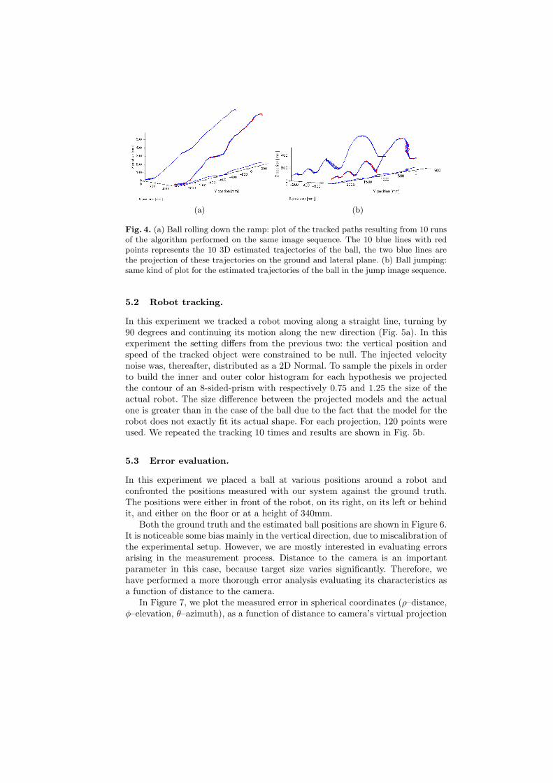
In the second experiment we tracked a ball bouncing on the floor. The experi-mental setting was exactly the same as for the first experiment described, but forthe frame rate, which in this case was of 25fps. The image sequence begins withthe ball about to hit an obstacle on the ground, while moving horizontally. Thecollision triggers a series of parabolic movements for the ball, which is trackeduntil it hits the ground for the fourth time. We repeated the tracking processten times on the same image sequence. The results are visible in Fig. 4b.

(a) (b)

Fig. 4. (a) Ball rolling down the ramp: plot of the tracked paths resulting from 10 runsof the algorithm performed on the same image sequence. The 10 blue lines with redpoints represents the 10 3D estimated trajectories of the ball, the two blue lines arethe projection of these trajectories on the ground and lateral plane. (b) Ball jumping:same kind of plot for the estimated trajectories of the ball in the jump image sequence.

5.2 Robot tracking.

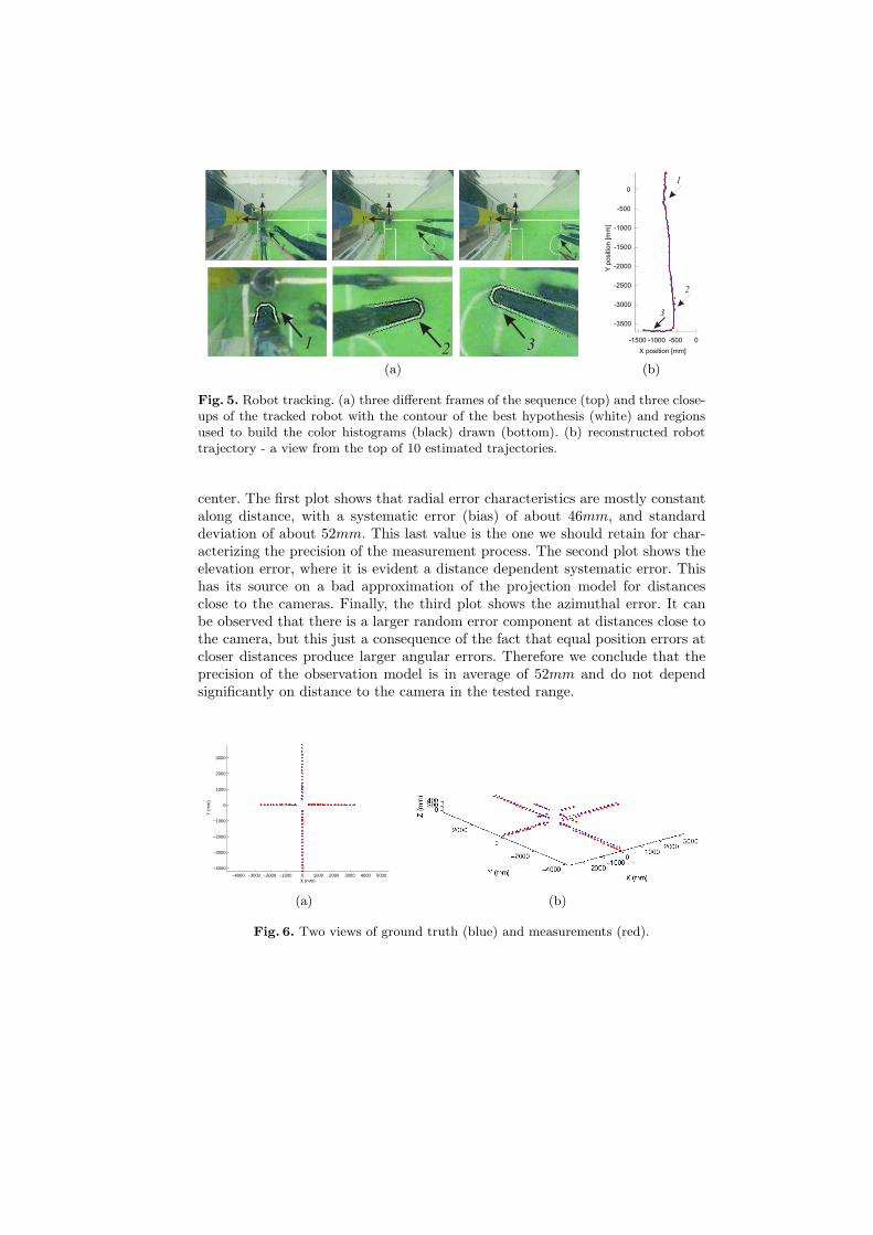
In this experiment we tracked a robot moving along a straight line, turning by90 degrees and continuing its motion along the new direction (Fig. 5a). In thisexperiment the setting differs from the previous two: the vertical position andspeed of the tracked object were constrained to be null. The injected velocitynoise was, thereafter, distributed as a 2D Normal. To sample the pixels in orderto build the inner and outer color histogram for each hypothesis we projectedthe contour of an 8-sided-prism with respectively 0.75 and 1.25 the size of theactual robot. The size difference between the projected models and the actualone is greater than in the case of the ball due to the fact that the model for therobot does not exactly fit its actual shape. For each projection, 120 points wereused. We repeated the tracking 10 times and results are shown in Fig. 5b.

5.3 Error evaluation.

In this experiment we placed a ball at various positions around a robot andconfronted the positions measured with our system against the ground truth.The positions were either in front of the robot, on its right, on its left or behindit, and either on the floor or at a height of 340mm.

Both the ground truth and the estimated ball positions are shown in Figure 6.It is noticeable some bias mainly in the vertical direction, due to miscalibration ofthe experimental setup. However, we are mostly interested in evaluating errorsarising in the measurement process. Distance to the camera is an importantparameter in this case, because target size varies significantly. Therefore, wehave performed a more thorough error analysis evaluating its characteristics asa function of distance to the camera.

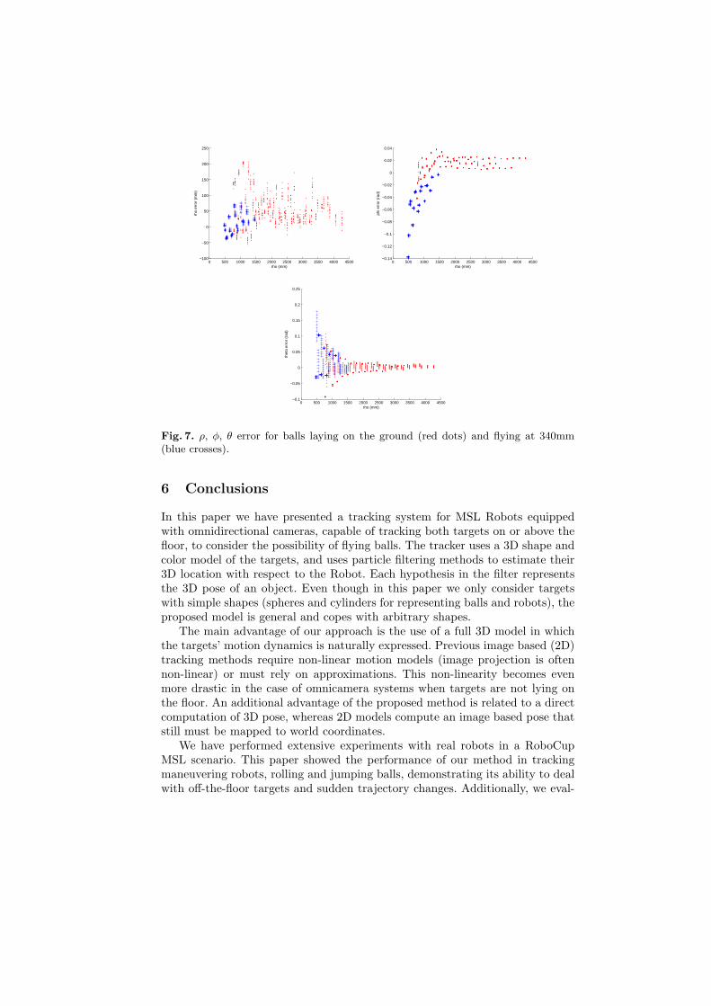
In Figure 7, we plot the measured error in spherical coordinates (ρ–distance,φ–elevation, θ–azimuth), as a function of distance to camera’s virtual projection

(a) (b)

Fig. 5. Robot tracking. (a) three different frames of the sequence (top) and three close-ups of the tracked robot with the contour of the best hypothesis (white) and regionsused to build the color histograms (black) drawn (bottom). (b) reconstructed robottrajectory - a view from the top of 10 estimated trajectories.

center. The first plot shows that radial error characteristics are mostly constantalong distance, with a systematic error (bias) of about 46mm, and standarddeviation of about 52mm. This last value is the one we should retain for char-acterizing the precision of the measurement process. The second plot shows theelevation error, where it is evident a distance dependent systematic error. Thishas its source on a bad approximation of the projection model for distancesclose to the cameras. Finally, the third plot shows the azimuthal error. It canbe observed that there is a larger random error component at distances close tothe camera, but this just a consequence of the fact that equal position errors atcloser distances produce larger angular errors. Therefore we conclude that theprecision of the observation model is in average of 52mm and do not dependsignificantly on distance to the camera in the tested range.

−4000 −3000 −2000 −1000 0 1000 2000 3000 4000 5000

−4000

−3000

−2000

−1000

0

1000

2000

3000

X (mm)

Y (

mm

)

(a) (b)

Fig. 6. Two views of ground truth (blue) and measurements (red).

0 500 1000 1500 2000 2500 3000 3500 4000 4500−100

−50

0

50

100

150

200

250

rho (mm)

rho

erro

r (m

m)

0 500 1000 1500 2000 2500 3000 3500 4000 4500−0.14

−0.12

−0.1

−0.08

−0.06

−0.04

−0.02

0

0.02

0.04

rho (mm)

phi e

rror

(ra

d)

0 500 1000 1500 2000 2500 3000 3500 4000 4500−0.1

−0.05

0

0.05

0.1

0.15

0.2

0.25

rho (mm)

thet

a er

ror

(rad

)

Fig. 7. ρ, φ, θ error for balls laying on the ground (red dots) and flying at 340mm(blue crosses).

6 Conclusions

In this paper we have presented a tracking system for MSL Robots equippedwith omnidirectional cameras, capable of tracking both targets on or above thefloor, to consider the possibility of flying balls. The tracker uses a 3D shape andcolor model of the targets, and uses particle filtering methods to estimate their3D location with respect to the Robot. Each hypothesis in the filter representsthe 3D pose of an object. Even though in this paper we only consider targetswith simple shapes (spheres and cylinders for representing balls and robots), theproposed model is general and copes with arbitrary shapes.

The main advantage of our approach is the use of a full 3D model in whichthe targets’ motion dynamics is naturally expressed. Previous image based (2D)tracking methods require non-linear motion models (image projection is oftennon-linear) or must rely on approximations. This non-linearity becomes evenmore drastic in the case of omnicamera systems when targets are not lying onthe floor. An additional advantage of the proposed method is related to a directcomputation of 3D pose, whereas 2D models compute an image based pose thatstill must be mapped to world coordinates.

We have performed extensive experiments with real robots in a RoboCupMSL scenario. This paper showed the performance of our method in trackingmaneuvering robots, rolling and jumping balls, demonstrating its ability to dealwith off-the-floor targets and sudden trajectory changes. Additionally, we eval-

uated the precision of the system in static scenarios with ground truth measure-ments.

Since it is becoming more frequent to have robots kicking balls off the floor,the presented method constitutes a solution to improve ball position estimation,which, in the case of the goal-keeper, may be of fundamental importance.

References

1. J. Gaspar, N. Winters, J. Santos-Victor: Vision-based Navigation and Environ-mental Representations with an Omnidirectional Camera. IEEE Transactions onRobotics and Automation, Vol. 16, 6, December 2000

2. D. Koller, J. Weber, J. Malik: Robust Multiple Cars Tracking with OcclusionReasoning. European Conf. on Computer Vision, pp. 186-196, 1994.

3. Gilles Celeux, J. Nascimento, J. S. Marques: Learning switching dynamic modelsfor objects tracking Pattern Recognition, vol. 37, no. 9, pp. 1841-1853, Sep. 2004.

4. D. Comaniciu, V. Ramesh, P. Meer: Real-Time Tracking of Non-Rigid Objectsusing Mean Shift. CVPR (2000), pp. 142-151.

5. T. Misu, M. Naemura, Wentao Zheng, Y. Izumi, K. Fukui: Robust Tracking ofSoccer Players based on Data Fusion. IEEE 16th Int. Conf. on Patern Recognition,pp. 556-561, vol. 1, 2002.

6. S. S. Intille, J. W. Davis, A. F. Bobick: Real-Time Closed-World Tracking. IEEEConf. on Compuiter Vision Pattern Recognition, pp. 697-703, 1997.

7. Z. Khan, T. Balch, and F. Dellaert: MCMC Data Association and Sparse Factor-ization Updating for Real Time Multitarget Tracking with Merged and MultipleMeasurements. IEEE Trans. on PAMI, vol. 28, no. 12, pp. 1960-1972, Dec. 2006.

8. Lima, P., Bonarini, A., Machado, C., Marchese, F., Ribeiro, F., Sorrenti, D.: Omni-directional catadioptric vision for soccer robots Robotics and Autonomous Sys-tems, 36(2–3), pp. 87–102, 2001.”, year = ”2001”, (2001).

9. Thrun, S., Burgard, W., Fox, D.: Probabilistic Robotics. MIT press (2005).10. K. Okuma, Ali Taleghani, N. de Freitas, J.J. Little, and D. G. Lowe: A Boosted

Particle Filter: Multitarget Detection and Tracking. European Conf. on ComputerVision, pp. 28-39, 2004.

11. A. Doucet, N. de Freitas, N. Gordon: Gordon editors: Sequential Monte CarloMethods In Practice. Springer Verlag (2001).

12. M. Isard, and A. Blake: Condensation: conditional density propagation for visualtracking. Int. Journal of Computer Vision, vol. 28, no. 1, pp. 5-28, 1998.

13. P. Perez, C. Hue, J. Vermaak, M. Gangnet: Color-Based Probabilistic Trackingusing Unscented Particle Filter. CVPR (2002).

14. Olufs, S., Adolf, F., Hartanto, R., Ploger, P.: Towards probabilistic shape visionin robocup: A practical approach. RoboCup International Symposium (2006).

15. Geyer, C., Daniilidis, K.: A unifying theory for central panoramic systems andpractical applications. European Conf. on Computer Vision, (2000) pp. 445-461.

16. Benosman, R., Kang, S.B., eds.: Panoramic Vision. Springer Verlag (2001).17. Hicks, R., Bajcsy, R.: Catadioptric sensors that approximate wide-angle perspec-

tive projections. CVPR (2000) 545–55118. Gaspar, J., Decco, C., Jr, J.O., Santos-Victor, J.: Constant resolution omnidirec-

tional cameras. 3rd IEEE Workshop on Omni-directional Vision (2002) 27–34